ORIGINAL PAPER

Finite Element and Reliability Analyses for Slope Stabilityof Subansiri Lower Hydroelectric Project: A Case Study

Ganesh W. Rathod • K. Seshagiri Rao

Received: 21 September 2010 / Accepted: 10 October 2011 / Published online: 26 October 2011

� Springer Science+Business Media B.V. 2011

Abstract The partly constructed and excavated

power house slopes of Subansiri Lower Hydroelectric

Project experienced extensive collapses through com-

plex mode of failure. A detailed study is attempted in

this paper to understand the reasons for the failure and

assess the stability of the existing constructed slopes

using limit equilibrium and FEM solutions and also to

propose modified design for rebuilding the slopes. To

take into account the uncertainty associated with the

rockmass and soil properties, probability and reliabil-

ity analyses have also been carried out. Based on the

field observations and stability analyses of the natural

and cut slopes, suitable support systems such as slope

flattening with various angles, weldmesh, shotcrete,

rockbolts and drainage holes have been considered to

meet the stability requirements. In this study, it is

demonstrated that the probabilistic approach when

used in conjunction with deterministic approach helps

in providing a rational solution for quantification of

stability in the estimation of risk associated with the

power house slope construction.

Keywords Hydroelectric project � Earthquakes �Seismic slope stability � FEM � Reliability

1 Introduction

In geotechnical engineering analysis and design,

various sources of uncertainties are encountered and

well recognized. The sources of uncertainties can be

model uncertainty, model parameter uncertainties and

data uncertainties. Slope stability analyses are con-

ventionally assessed using Limit Equilibrium Method

(LEM) and lately the Finite Element Method (FEM)

have been found to be suitable in performing stability

calculations. Although the LEM does not consider the

stress–strain relation of soil, it can provide an estimate

of the factor of safety of a slope without the knowledge

of the initial conditions, hence it is favoured by many

engineers. The LEM is well known to be a statically

indeterminate problem and assumptions on the distri-

butions of internal forces are required for the solution

of the factor of safety. The variational approach to

determine the factor of safety proposed by Baker and

Garber (1978) does not require the assumption on the

internal force distribution but is tedious to use even for

a single failure surface. Besides the LEM, limit

analysis has also been used for simple problems, but

their application in complicated real problems is still

limited, so this method is seldom adopted for routine

analysis and design. Both the LEM and limit analysis

G. W. Rathod (&) � K. S. Rao

Department of Civil Engineering, Indian Institute

of Technology Delhi, Hauz Khas,

New Delhi 110016, India

e-mail: ganesh.rathod@yahoo.co.in

K. S. Rao

e-mail: raoks@civil.iitd.ac.in

123

Geotech Geol Eng (2012) 30:233–252

DOI 10.1007/s10706-011-9465-2

methods require trial failure surfaces and optimization

analysis to locate the critical failure surface. Griffiths

and Lane (1999) highlighted that the FEM provides a

more powerful alternative to traditional LEM in

assessing stability in their study of unreinforced slopes

and embankments. Cheng (2003) provided detailed

discussions on various methods for locating the

critical failure surface.

In this paper, results are presented for a compara-

tive study that has been made between the FEM using

strength reduction technique and LEM using probabi-

listic approach for slope stability of Subansiri Lower

Hydroelectric Project. Relevant sources of uncertain-

ties involved in slope stability analysis are modelled

and analyzed.

2 The Project

The River Subansiri originates in the south of the Po

Rom peak (Mount Pororu, 5,059 m high). Po Rom

peak is 30 km from the Tsangpo and near 5 km from

Tarlung Chu (a tributary of Tsangpo). Subansiri is

called Lokong Chu (Tsari Chu) at its source. River

Subansiri is the major tributary of River Brahmaputra.

It contributes 10% of the flow of the River Brah-

maputra. Drainage area up to its confluence of River

Brahmaputra is 37,000 km2 of which 10,000 km2 lies

in Assam and 19,199 km2 in Arunachal Pradesh States

of India. Its length up to the confluence of River

Brahmaputra is 520 km. Location of the project site is

shown in Fig. 1.

The 2,000 MW Lower Subansiri hydel project is on

the Assam-Arunachal Pradesh border is the first large

project to be taken up in the Subansiri basin. Subansiri

Lower Hydroelectric Power Project is located in

Dhemaji and Lower Subansiri districts in the states

of Assam and Arunachal Pradesh. The project site falls

in the very active seismic belt of Himalayas (Zone V

as per BIS 1893:2002) as shown Fig. 1. The left bank

of the dam is in the state of Assam and right bank of

dam, power house (PH) and head race tunnels (HRT’s)

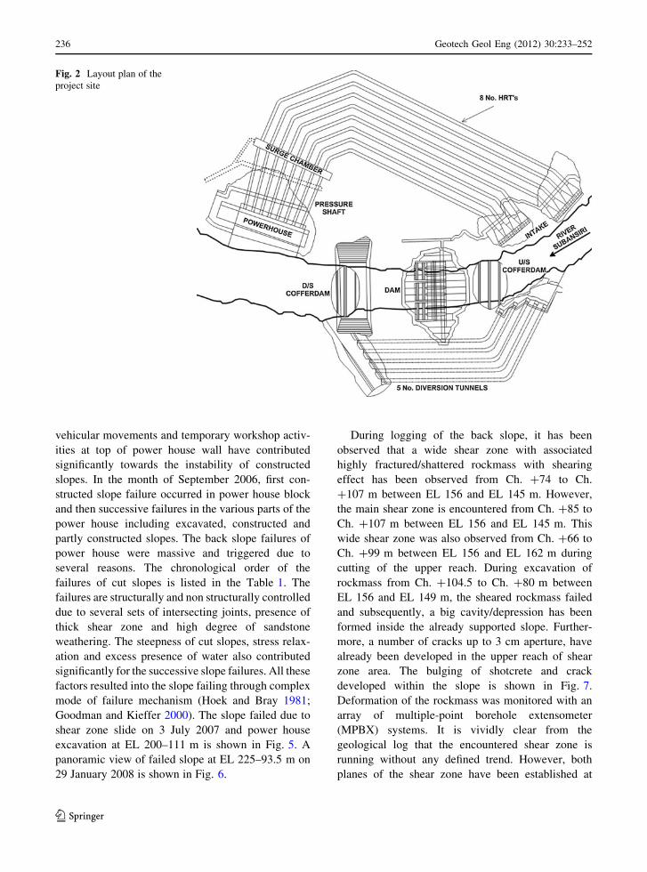
are in the state of Arunachal Pradesh. The layout plan

of the project site is shown in Fig. 2 and it is to harness

hydro potential of lower reaches of river Subansiri.

The project envisages generating 2,000 MW

(8 9 250 MW) of power utilizing 100 m of maximum

gross head through a 133 m high concrete gravity

dam. The typical section of the constructed slope is

shown in Fig. 3 and a full view of power house slope is

shown in Fig. 4. The specific technical features of the

project are as follows:

• A Concrete Gravity Dam 116 m high from river

bed level.

• Head Race Tunnel—8 Nos., 9.5 m diameter, Horse

shoe shaped having a length from 630 to 1,145 m.

• Pressure Shaft—8 Nos., Horse shoe/circular shaped

varying dia. of 9.5–7.0 m and length 192–215 m.

• Surface power house to accommodate 8 units of

Francis turbines of 250 MW capacity each.

• Tail race channel, 206 m 9 35 m (W 9 L).

The objective of the present work is to carry out

back analysis as well as to present the analysis of the

various slope sections (constructed, excavated and

proposed) at different locations of the hydroelectric

project. Deterministic, probabilistic and finite element

analyses were performed to assess the stability of

slope sections for static and pseudo-static loading

conditions and to suggest the support system for

reconstructing the slopes.

3 Geology of the Area

The power house area comprises of fine to medium

grained grey coloured sandstone of middle Shivalik

formation. Occurrence of quartzite pebbles, coal

patches and concretion of boulders and pebbles is

also a significant property of the rock of this locality

(Rao 2008). In this area, moderate to highly sheared

and fractured rockmass is present, which is the

continuation of the major slide plane in this area.

The fresh sandstone is massive and compact but

occasionally it is weathered to different degrees.

Along with several sets of joint planes clay fillings and

rock penetrative weathering also observed along the

discontinuity planes.

Several sets of major and minor joints and fractures

are present in the rockmass. Four sets of joints of

average orientation of N120�–165� and dip amount of

65�–80� (S1), N235�–260�/55�–75� (S2), N310�–350�/

50�–80� (S3), and N10�–80�/50�–85� (S4) are pre-

dominant. The joint planes are tight to partially open

of 2–4 mm with occasional clay and carbonaceous

filling. The persistence of these joint planes is 4–5 m

and the spacing between them is about 50–100 cm.

Apart from these joints, a major thick shear zone is

234 Geotech Geol Eng (2012) 30:233–252

123

also encountered at different elevations of the slope.

The rockmass in the shear zone area can be classified

as poor to very poor rockmass. The rockmass in the

shear zone is represented by a highly crushed, soft,

sandy and clayey gouge material. The shear zone

material is soft, sheared and very low strength

material, having low cohesion with damp to wet

ground condition as observed at the site. Both planes

of the shear zone are rough planar, slickensided and

filled with clay. The soft material, steep slopes, high

water precipitation, several sets of prominent joint sets

and presence of major shear zone culminated into a

complex geological setting at the power house area.

4 Observed Failures and Reasons

In August 2006, some cracks were observed at few

locations on the constructed slopes of the power house,

which was alarming to the whole project. So, a keen

monitoring programme was initiated to observe the

load in rock anchors, displacements and pore pressure

by installing load cells, multiple extensometers, incli-

nometers and piezometers. The monitoring pro-

gramme of slope is outside the scope of this paper

and hence not discussed in detail. In the month of

August 2006, the slopes were charged with water

precipitation and in addition the dynamic loads due to

III III

III

III

III

III

III

III

II

II

II

II

IV

IV

IV

IV

IV

V

V

V

V

VV

V

DELHI

SRINAGAR

LUCKNOW

ALLAHABAD

AHMEDABAD

NAGPUR

MUMBAI

PANJI

THIRUVANANTHPURAM

CALICUT

CHENNAI

PUDUCHERRY

LAKSHADWEEP

NELLORE

VIJAYWADA

RAIPUR

BHOPAL

JAIPUR

HYDERABAD

BANGALOREMANGALORE

JODHPUR

VADODARA

MACHLIPATNAM

CHANDIGARH

DEHRADUN

JAMMU120 120 240 360 480 KM

MAP OF INDIASHOWING

SEISMIC ZONES OF INDIA

LEGENDZONE II

ZONE III

ZONE IV

ZONE V

LOWERSUBANSIRI

UPPERSUBANSIRI

PAPUMPARE

ITANAGAR

EASTKAMENG

WESTKAMENG

TAWANG

KURUNGKUMEY

WESTSIANG

UPPERSIANG

EASTSIANG

DIBANG VALLEY

LOWERDIBANGVALLEY LOHIT

CHANGLANG

TIRAP

NAGALAND

ASSAM

PROJECT SITE

Fig. 1 Location of Subansiri project site and seismic zonation map of India (Modified from BIS 1893:2002)

Geotech Geol Eng (2012) 30:233–252 235

123

vehicular movements and temporary workshop activ-

ities at top of power house wall have contributed

significantly towards the instability of constructed

slopes. In the month of September 2006, first con-

structed slope failure occurred in power house block

and then successive failures in the various parts of the

power house including excavated, constructed and

partly constructed slopes. The back slope failures of

power house were massive and triggered due to

several reasons. The chronological order of the

failures of cut slopes is listed in the Table 1. The

failures are structurally and non structurally controlled

due to several sets of intersecting joints, presence of

thick shear zone and high degree of sandstone

weathering. The steepness of cut slopes, stress relax-

ation and excess presence of water also contributed

significantly for the successive slope failures. All these

factors resulted into the slope failing through complex

mode of failure mechanism (Hoek and Bray 1981;

Goodman and Kieffer 2000). The slope failed due to

shear zone slide on 3 July 2007 and power house

excavation at EL 200–111 m is shown in Fig. 5. A

panoramic view of failed slope at EL 225–93.5 m on

29 January 2008 is shown in Fig. 6.

During logging of the back slope, it has been

observed that a wide shear zone with associated

highly fractured/shattered rockmass with shearing

effect has been observed from Ch. ?74 to Ch.

?107 m between EL 156 and EL 145 m. However,

the main shear zone is encountered from Ch. ?85 to

Ch. ?107 m between EL 156 and EL 145 m. This

wide shear zone was also observed from Ch. ?66 to

Ch. ?99 m between EL 156 and EL 162 m during

cutting of the upper reach. During excavation of

rockmass from Ch. ?104.5 to Ch. ?80 m between

EL 156 and EL 149 m, the sheared rockmass failed

and subsequently, a big cavity/depression has been

formed inside the already supported slope. Further-

more, a number of cracks up to 3 cm aperture, have

already been developed in the upper reach of shear

zone area. The bulging of shotcrete and crack

developed within the slope is shown in Fig. 7.

Deformation of the rockmass was monitored with an

array of multiple-point borehole extensometer

(MPBX) systems. It is vividly clear from the

geological log that the encountered shear zone is

running without any defined trend. However, both

planes of the shear zone have been established at

Fig. 2 Layout plan of the

project site

236 Geotech Geol Eng (2012) 30:233–252

123

site. The upstream plane of the shear zone dips at

angle of 50� with dip direction N140� while

downstream plane dips slightly steeper at an angle

of 65� with dip direction N030�. The cut slope is

occupied by highly fractured/shattered rock zone

with shearing effect from Ch. ?75 to Ch. ?81 m,

having an attitude of N015�/85�. The rockmass in

between these two adverse zones of about 5 m

lengths is represented by moderately jointed sand-

stone, having high frequency of S2 joint sets.

5 Assessment of Slope Stability

Limit Equilibrium (LE) alongwith reliability analysis

as well as Finite Element Method (FEM) have been

used for the analyses. Slide (LE) and Phase2 (FEM)

software programs (RocScience Manual 2002) were

used in the study. To take into account the heteroge-

neity of the rockmass and soil, probability and

reliability analyses have also been carried out. These

analyses take care of the fluctuations of the material

properties in the field (Ramly et al. 2002; Low 2003).

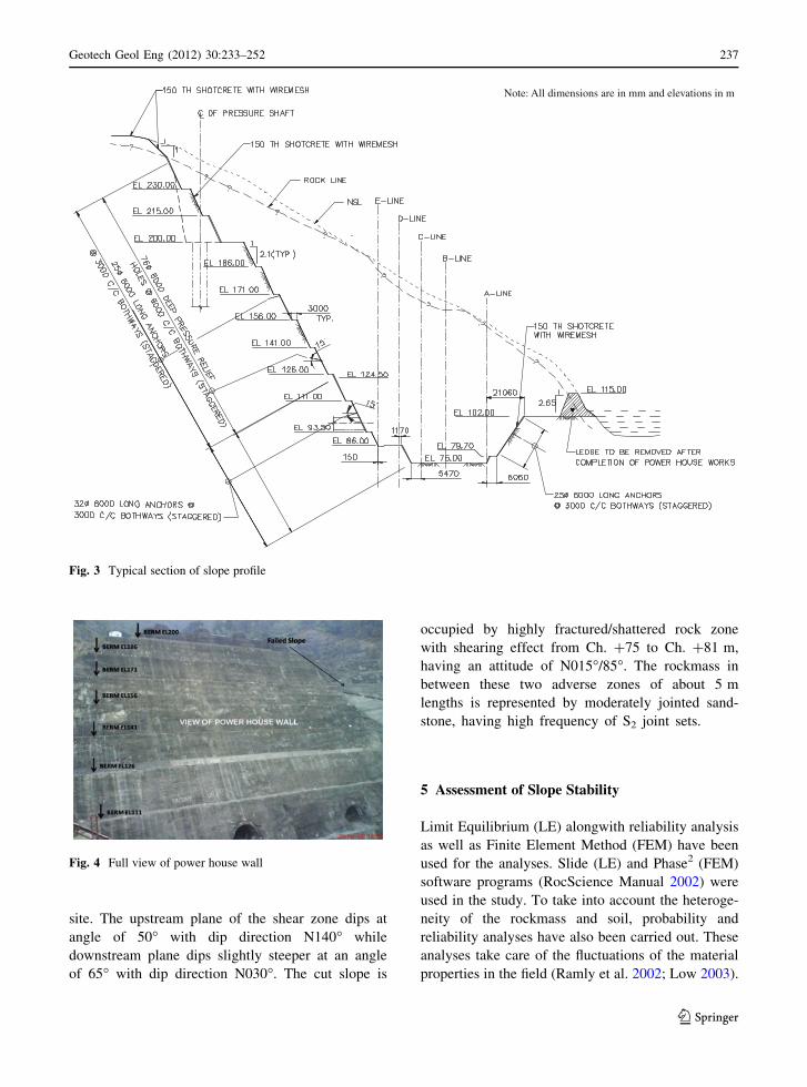
Note: All dimensions are in mm and elevations in m

Fig. 3 Typical section of slope profile

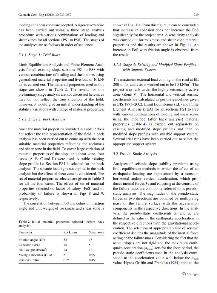
Fig. 4 Full view of power house wall

Geotech Geol Eng (2012) 30:233–252 237

123

5.1 Plan for the Analysis

A systematic study has been carried out to check the

effect of seismic and external (live) loading, presence of

shear zones and the fluctuation of material properties

within the rockmass and shear zones. A total of 8

sections of slopes at each power shaft (PS1 to PS8) were

selected for the analysis. Various combinations of

Table 1 Chronological order of the failures of cut slopes

Sr. no. Date Event

1 29.08.06 Cracks on shotcrete PH berm (EL 186 m, Ch. -35 m)

2 20.09.06 Slope failure in PH block (Ch. ?74 to 107 m, 156–145 m)

3 17.01.07 Cracks in PH region

4 02.05.07 Cracks in cut slope of PH region

5 11.05.07 Shear zone in cut slope of PH region

6 20.06.07 Cracks on shotcrete PH berm at intake approach road

7 24.06.07 Slide in PH back slope (Ch. ?75 to ?100 m, EL 156–145 m)

8 03.07.07 Slide in shear zone of PH slope (Ch. ?30 to ?100 m, EL 200–111 m)

9 03.09.07 Slide in the hill side cut slope at EL 126–111 m

10 12.09.07 Widening of cracks in cut slope of PH

11 27.10.07 Slide of cut slope berm at EL 86–76 m (Ch. ?36.6 to ?22 m)

12 02.01.08 Cracks in the shotcrete hill side cut slope of PH (EL 111–126 m)

13 06.01.08 Shear zone in cut slope of PH

14 25.01.08 Slide in cut slope berm at EL 112–126 m near end bay (Upstream side) Ch. ?140 to 165 m

15 29.01.08 Shear failure near shear zone in PH (Ch. -50 to ?40 m, EL 225–93.5 m)

16 11.02.08 Widening of cracks in cut slope of PH near tower crane area (EL 126–111 m)

17 11.02.08 New cracks on slopes of PH at EL 86–93.5 m (Ch. -100 to -90 m) and at EL 93.5–111 m (Ch. -110 to -65 m)

Fig. 5 A view of failed slope and power house excavation at

EL 200–111 m

Fig. 6 Panoramic view of failed slope at EL 225–93.5 m

Fig. 7 Bulging of Shotcrete and crack developed at EL 126 m

238 Geotech Geol Eng (2012) 30:233–252

123

loading and shear zones are adopted. A rigorous exercise

has been carried out using a three stage analysis

procedure with various combinations of loading and

shear zones for all sections (PS1 to PS8). The stages of

the analyses are as follows in order of sequence.

5.1.1 Stage 1: Trial Runs

Limit Equilibrium Analysis and Finite Element Anal-

ysis for all existing slope sections PS1 to PS8 with

various combinations of loading and shear zones using

generalized material properties and live load of 10 kN/

m2 is carried out. The material properties used in this

stage are shown in Table 2. The results for this

preliminary stage analysis are not discussed herein; as

they do not reflect the true situation of the field,

however, it would give an initial understanding of the

stability variations with change of material properties.

5.1.2 Stage 2: Back Analysis

Since the material properties provided in Table 2 does

not reflect the true representation of the field, a back

analysis has been carried out to come up with the best

suitable material properties reflecting the rockmass

and shear zone in the field. To cover large variation of

material properties of the slope and shear zone, four

cases (A, B, C and D) were used. A stable existing

slope profile i.e. Section PS1 is selected for the back

analysis. The seismic loading is not applied in the back

analysis but the effect of shear zone is considered. The

set of material properties selected are given in Table 3

for all the four cases. The effect of set of material

properties selected on factor of safety (FoS) and its

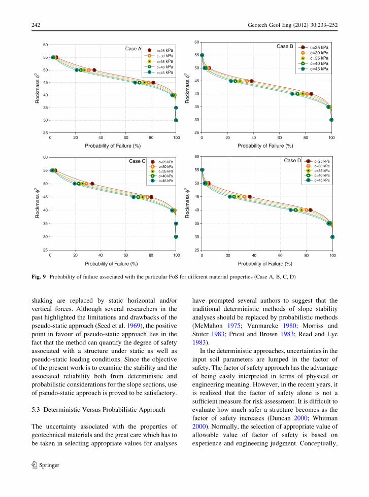
probability of failure is shown in Figs. 8 and 9,

respectively.

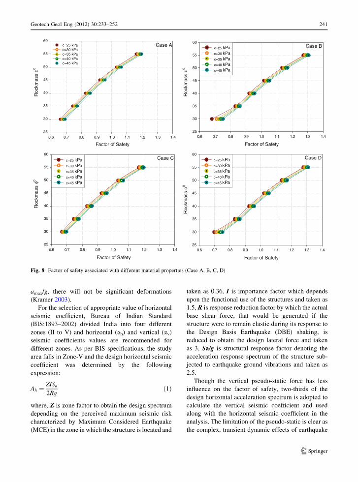
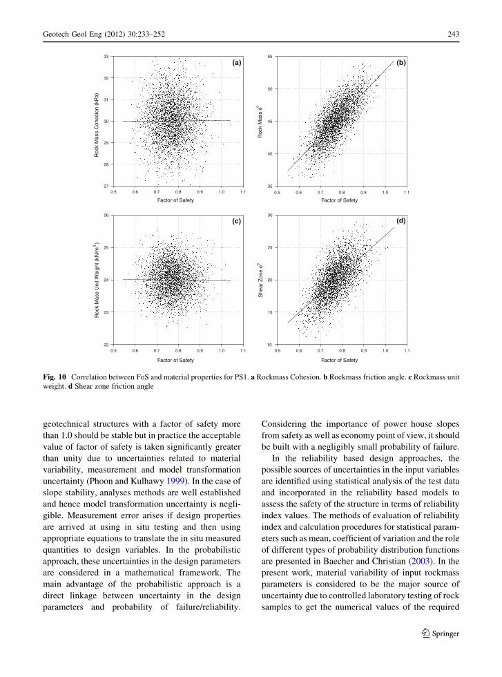
The correlation between FoS and cohesion, friction

angle and unit weight of rockmass and shear zone is

shown in Fig. 10. From this figure, it can be concluded

that increase in cohesion does not increase the FoS

significantly for the project area. A sensitivity analysis

was carried out for rockmass and shear zone material

properties and the results are shown in Fig. 11. An

increase in FoS with friction angle is observed from

the results.

5.1.3 Stage 3: Existing and Modified Slope Profiles

with Support System

The maximum external load coming on the road at EL

200 m for analysis is worked out to be 10 kN/m2. The

project area falls under the highly seismically active

zone (Zone V). The horizontal and vertical seismic

coefficients are calculated as per the guidelines given

in BIS:1893–2002. Limit Equilibrium (LE) and Finite

Element Analysis (FEA) for all sections PS1 to PS8

with various combinations of loading and shear zones

using the modified (after back analysis) material

properties (Table 4) is carried out separately on

existing and modified slope profiles and then on

modified slope profiles with suitable support system.

Several trial runs have been carried out to select the

appropriate support system.

5.2 Pseudo-Static Analysis

Analyses of seismic slope stability problems using

limit equilibrium methods in which the effect of an

earthquake loading are represented by a constant

horizontal and/or vertical acceleration, which pro-

duces inertial forces Fh and Fv acting at the centroid of

the failure mass are commonly referred to as pseudo-

static analyses. The magnitudes of the pseudo-static

forces in two directions are obtained by multiplying

mass of the failure surface with the acceleration

components in the respective directions. In the anal-

ysis, the pseudo-static coefficients ah and av are

defined as the ratio of the earthquake acceleration in

the respective directions with the gravitational accel-

eration. The selection of appropriate value of seismic

coefficient decides the magnitude of the inertial force

acting on the failure mass. Considering the fact that the

actual slopes are not rigid and the maximum earth-

quake acceleration (amax) acts for the short period, the

pseudo-static coefficients used in the analysis corre-

spond to the acceleration value well below the amax

value. Hynes-Griffin and Franklin (1984) applied the

Table 2 Initial material properties selected (before back

analysis)

Parameter Rockmass Shear zone

Friction angle (�) 32 15

Cohesion (kPa) 25 5

Unit weight (kN/m3) 24 18

Young’s modulus (GPa) 5 0.05

Poisson’s ratio 0.25 0.45

Geotech Geol Eng (2012) 30:233–252 239

123

Newmark sliding block analysis to over 350 acceler-

ograms and studied the correlation between pseudo-

static factor of safety and calculated deformation

based on sliding block analysis. It was concluded that

when the pseudo-static factor of safety is more than

unity and horizontal earthquake coefficient, ah = 0.5

Table 3 Set of material properties selected for back analysis

Angle of internal friction

for rockmass

Various combinations of c, Ø values for the back analysis

Case-A Case-B

Material properties for shear

zone c = 5 kPa, Ø = 15�Material properties for shear

zone c = 5 kPa, Ø = 20�

Cohesion values for rockmass (kPa) Cohesion values for rockmass (kPa)

25 30 35 40 45 25 30 35 40 45

30� 0.664 0.673 0.679 0.686 0.694 0.679 0.71 0.725 0.739 0.752a

100 100 100 100 100 100 100 100 100 100b

35� 0.742 0.752 0.76 0.768 0.776 0.831 0.84 0.848 0.854 0.861

100 100 100 100 100 98.5 98.8 98.5 97.8 97.5

40� 0.828 0.836 0.844 0.852 0.86 0.921 0.929 0.939 0.947 0.955

99 98.7 98.4 97.6 96.9 84.4 81.2 77.9 73.8 69.8

45� 0.922 0.93 0.94 0.948 0.956 1.018 1.028 1.036 1.044 1.052

81.9 78.4 75 70.9 67.5 38.6 34.9 29.6 26.1 22.6

50� 1.03 1.037 1.045 1.053 1.063 1.134 1.143 1.151 1.159 1.169

35.1 30.9 27.1 24.4 21.2 5.9 4.9 3.6 3.2 2.2

55� 1.162 1.17 1.179 1.187 1.195 1.273 1.282 1.29 1.298 1.306

5 3.7 3.4 2.4 2.2 0.4 0.3 0.3 0.3 0.3

Angle of internal friction

for rockmass

Various combinations of c, Ø values for the back analysis

Case-C Case-D

Material properties for shear

zone c = 10 kPa, Ø = 15�Material properties for shear

zone c = 10 kPa, Ø = 20�

Cohesion values for rockmass (kPa) Cohesion values for rockmass (kPa)

25 30 35 40 45 25 30 35 40 45

30� 0.668 0.676 0.683 0.691 0.697 0.697 0.71 0.726 0.739 0.752

100 100 100 100 100 100 100 100 100 100

35� 0.745 0.755 0.763 0.771 0.779 0.831 0.843 0.851 0.858 0.864

100 100 100 100 100 98.5 98.7 98.5 97.8 97

40� 0.831 0.839 0.847 0.856 0.864 0.924 0.934 0.942 0.95 0.958

98.8 98.6 97.9 97.1 96.7 83.2 80.1 76.2 71.8 68

45� 0.926 0.934 0.943 0.951 0.959 1.023 1.031 1.039 1.047 1.055

80.4 77.5 73.6 69.9 66.3 36.8 32.6 28.2 24.8 21.4

50� 1.033 1.041 1.049 1.057 1.067 1.138 1.146 1.154 1.162 1.172

33.4 28.8 25.9 22.8 19.5 5.3 4.2 3.4 2.9 2.2

55� 1.166 1.174 1.182 1.191 1.199 1.277 1.285 1.293 1.302 1.31

4.3 1.174 3.1 2.2 1.9 0.4 0.3 0.3 0.3 0.3

a Factor of safetyb Probability of failure (Italicized)

240 Geotech Geol Eng (2012) 30:233–252

123

amax/g, there will not be significant deformations

(Kramer 2003).

For the selection of appropriate value of horizontal

seismic coefficient, Bureau of Indian Standard

(BIS:1893–2002) divided India into four different

zones (II to V) and horizontal (ah) and vertical (av)

seismic coefficients values are recommended for

different zones. As per BIS specifications, the study

area falls in Zone-V and the design horizontal seismic

coefficient was determined by the following

expression:

Ah ¼ZISa

2Rgð1Þ

where, Z is zone factor to obtain the design spectrum

depending on the perceived maximum seismic risk

characterized by Maximum Considered Earthquake

(MCE) in the zone in which the structure is located and

taken as 0.36, I is importance factor which depends

upon the functional use of the structures and taken as

1.5, R is response reduction factor by which the actual

base shear force, that would be generated if the

structure were to remain elastic during its response to

the Design Basis Earthquake (DBE) shaking, is

reduced to obtain the design lateral force and taken

as 3, Sa/g is structural response factor denoting the

acceleration response spectrum of the structure sub-

jected to earthquake ground vibrations and taken as

2.5.

Though the vertical pseudo-static force has less

influence on the factor of safety, two-thirds of the

design horizontal acceleration spectrum is adopted to

calculate the vertical seismic coefficient and used

along with the horizontal seismic coefficient in the

analysis. The limitation of the pseudo-static is clear as

the complex, transient dynamic effects of earthquake

Case A

Factor of Safety

0.6 0.7 0.8 0.9 1.0 1.1 1.2 1.3 1.425

30

35

40

45

50

55

60c=25 kPac=30 kPac=35 kPac=40 kPac=45 kPa

Case B

Factor of Safety

25

30

35

40

45

50

55

60

c=25 kPac=30 kPac=35 kPac=40 kPac=45 kPa

Case C

Factor of Safety

25

30

35

40

45

50

55

60

c=25 kPac=30 kPac=35 kPac=40 kPac=45 kPa

Case D

Factor of Safety

0.6 0.7 0.8 0.9 1.0 1.1 1.2 1.3 1.4

0.6 0.7 0.8 0.9 1.0 1.1 1.2 1.3 1.4 0.6 0.7 0.8 0.9 1.0 1.1 1.2 1.3 1.4

Roc

kmas

s φ0

Roc

kmas

s φ0

Roc

kmas

s φ0

Roc

kmas

s φ0

25

30

35

40

45

50

55

60

c=25 kPac=30 kPac=35 kPac=40 kPac=45 kPa

Fig. 8 Factor of safety associated with different material properties (Case A, B, C, D)

Geotech Geol Eng (2012) 30:233–252 241

123

shaking are replaced by static horizontal and/or

vertical forces. Although several researchers in the

past highlighted the limitations and drawbacks of the

pseudo-static approach (Seed et al. 1969), the positive

point in favour of pseudo-static approach lies in the

fact that the method can quantify the degree of safety

associated with a structure under static as well as

pseudo-static loading conditions. Since the objective

of the present work is to examine the stability and the

associated reliability both from deterministic and

probabilistic considerations for the slope sections, use

of pseudo-static approach is proved to be satisfactory.

5.3 Deterministic Versus Probabilistic Approach

The uncertainty associated with the properties of

geotechnical materials and the great care which has to

be taken in selecting appropriate values for analyses

have prompted several authors to suggest that the

traditional deterministic methods of slope stability

analyses should be replaced by probabilistic methods

(McMahon 1975; Vanmarcke 1980; Morriss and

Stoter 1983; Priest and Brown 1983; Read and Lye

1983).

In the deterministic approaches, uncertainties in the

input soil parameters are lumped in the factor of

safety. The factor of safety approach has the advantage

of being easily interpreted in terms of physical or

engineering meaning. However, in the recent years, it

is realized that the factor of safety alone is not a

sufficient measure for risk assessment. It is difficult to

evaluate how much safer a structure becomes as the

factor of safety increases (Duncan 2000; Whitman

2000). Normally, the selection of appropriate value of

allowable value of factor of safety is based on

experience and engineering judgment. Conceptually,

Case A

Probability of Failure (%)

25

30

35

40

45

50

55

60c=25 kPac=30 kPac=35 kPac=40 kPac=45 kPa

Case B

Probability of Failure (%)

25

30

35

40

45

50

55

60c=25 kPac=30 kPac=35 kPac=40 kPac=45 kPa

Case C

Probability of Failure (%)

25

30

35

40

45

50

55

60c=25 kPac=30 kPac=35 kPac=40 kPac=45 kPa

Case D

Probability of Failure (%)

0 20 40 60 80 100 0 20 40 60 80 100

0 20 40 60 80 100 0 20 40 60 80 100

Roc

kmas

s φ0

Roc

kmas

s φ0

Roc

kmas

s φ0

Roc

kmas

s φ0

25

30

35

40

45

50

55

60c=25 kPac=30 kPac=35 kPac=40 kPac=45 kPa

Fig. 9 Probability of failure associated with the particular FoS for different material properties (Case A, B, C, D)

242 Geotech Geol Eng (2012) 30:233–252

123

geotechnical structures with a factor of safety more

than 1.0 should be stable but in practice the acceptable

value of factor of safety is taken significantly greater

than unity due to uncertainties related to material

variability, measurement and model transformation

uncertainty (Phoon and Kulhawy 1999). In the case of

slope stability, analyses methods are well established

and hence model transformation uncertainty is negli-

gible. Measurement error arises if design properties

are arrived at using in situ testing and then using

appropriate equations to translate the in situ measured

quantities to design variables. In the probabilistic

approach, these uncertainties in the design parameters

are considered in a mathematical framework. The

main advantage of the probabilistic approach is a

direct linkage between uncertainty in the design

parameters and probability of failure/reliability.

Considering the importance of power house slopes

from safety as well as economy point of view, it should

be built with a negligibly small probability of failure.

In the reliability based design approaches, the

possible sources of uncertainties in the input variables

are identified using statistical analysis of the test data

and incorporated in the reliability based models to

assess the safety of the structure in terms of reliability

index values. The methods of evaluation of reliability

index and calculation procedures for statistical param-

eters such as mean, coefficient of variation and the role

of different types of probability distribution functions

are presented in Baecher and Christian (2003). In the

present work, material variability of input rockmass

parameters is considered to be the major source of

uncertainty due to controlled laboratory testing of rock

samples to get the numerical values of the required

Factor of Safety

Roc

k M

ass

Coh

esio

n (k

Pa)

27

28

29

30

31

32

33

Factor of Safety

0.5 0.6 0.7 0.8 0.9 1.0 1.1

Roc

k M

ass

φ0

35

40

45

50

55

Factor of Safety

Roc

k M

ass

Uni

t Wei

ght (

kN/m

3)

22

23

24

25

26

Factor of Safety

She

ar Z

one

φ0

10

15

20

25

30

)b()a(

(c) (d)

0.5 0.6 0.7 0.8 0.9 1.0 1.1

0.5 0.6 0.7 0.8 0.9 1.0 1.10.5 0.6 0.7 0.8 0.9 1.0 1.1

Fig. 10 Correlation between FoS and material properties for PS1. a Rockmass Cohesion. b Rockmass friction angle. c Rockmass unit

weight. d Shear zone friction angle

Geotech Geol Eng (2012) 30:233–252 243

123

input soil parameters for stability assessment and

absence of model transformation uncertainty as indi-

cated earlier. Literature indicates that material param-

eters follow normal or lognormal distributions for

input random variables (USACE 1997). In order to

define the probabilistic assessment of the performance

of the structure in terms of reliability index (b), the

value of reliability index (b) is calculated from the

equations given below.

bLN ¼lFS � 1

rFSFor normally distributed FoS½ � ð2Þ

bLN ¼ln

lFSffiffiffiffiffiffiffiffiffiffiffi

1þV2ð Þp� �

ffiffiffiffiffiffiffiffiffiffiffiffiffiffiffiffiffiffiffiffiffi

ln 1þV2ð Þp For Log normally distributed FoS½ �

ð3Þ

Where, lFS and rFS is the mean and standard deviation

of factor of safety obtained from N number of Monte

Carlo simulations. V is the coefficient of variation

defined as rFS / lFS. The input random rockmass

properties are taken as cohesion (c), friction angle (/)

and bulk density (c) and numerical values of these

input soil parameters are obtained from the execution

authorities of the construction projects. For the

probabilistic analysis, reported values of input rock-

mass parameters are taken as mean values for different

slope sections as indicated in Table 4.

5.4 Finite Element Analysis

The Shear Strength Reduction (SSR) technique (Daw-

son et al. 1999; Griffiths and Lane 1999; Hammah et al.

2004) enables the FEM to calculate factors of safety for

slopes. The advantage of a finite element approach in the

analysis of slope stability problems over limit equilib-

rium methods is that no assumption needs to be made in

advance about the shape or location of the failure

surface, slice side forces and their directions. The

method can be applied with complex slope configura-

tions and soil deposits in two or three dimensions to

model virtually all types of mechanisms. General soil

material models that include Mohr–Coulomb and

numerous others can be employed. The equilibrium

stresses, strains and the associated shear strengths in the

soil mass can be computed very accurately. The critical

failure mechanism developed can be extremely general

and need not be simple circular or logarithmic spiral

arcs. This method can give information about the

deformations at working stress levels and is able to

monitor progressive failure including overall shear

failure (Griffiths and Lane 1999).

There are three major aspects which influences the

slope stability analysis. The first is about the material

properties of the slope model. The second is the

influence of calculating factor of safety to slope

stability and the third aspect is the definition of the

slope failure.

5.4.1 Model Material Properties

This work applied only for two-dimensional plain-

strain problem. The Mohr–Coulomb constitutive model

used to describe the rockmass material properties. The

Mohr–Coulomb criterion relates the shear strength of

the material to the cohesion, normal stress and angle

of internal friction of the material. The failure surface of

the Mohr–Coulomb model can be presented as:

fs ¼I1

3sin /þ

ffiffiffiffiffi

J2

pcos H� 1

3sin H sin /

� �

� c cos /

ð4Þ

Percent of Range (mean = 50%)

0 20 40 60 80 100

Fact

or o

f Saf

ety

0.6

0.7

0.8

0.9

1.0

Rock Mass Cohesion (kPa)Rock Mass φ0

Rock Mass Unit Weight (kN/m3)Shear Zone Cohesion (kPa)Shear Zone φ0

Shear Zone Unit Weight (kN/m3)

Fig. 11 Sensitivity plot for rockmass and shear zone material

Table 4 Material properties adopted after back analysis

Parameter Rockmass Shear zone

Friction angle (�) 45 20

Cohesion (kPa) 30 5

Unit weight (kN/m3) 24 18

Young’s modulus (GPa) 5 0.05

Poisson’s ratio 0.25 0.45

244 Geotech Geol Eng (2012) 30:233–252

123

where / is the angle of internal friction, c is cohesion

and

I1 ¼ ðr1 þ r2 þ r3Þ ¼ 3rm ð5Þ

J2 ¼1

2S2

x þ S2y þ S2

z

� �

þ s2xy þ s2

yz þ s2zx

� �

ð6Þ

H ¼ 1

3sin�1 3

ffiffiffi

3p

J3

2J1=22

" #

ð7Þ

where, J3 ¼ SxSySzþ 2sxysyzszx� Sxs2yz� Sys2

xz� Szs2xy

and Sx ¼ rx�rm;Sy ¼ ry�rm;Sz ¼ rz�rm

For Mohr–Coulomb material model, six material

properties are required. These properties are the

friction angle /, cohesion c, dilation angle w, Young’s

modulus E, Poisson’s ratio m and unit weight of soil/

rock c.

Dilation angle, w affects directly the volume

change during soil yielding. If w = /, the plasticity

flow rule is known as ‘‘associated’’, and if w = /, the

plasticity flow rule is considered as ‘‘no-associated’’.

Slope stability analysis is relatively unconfined, thus

the choice of dilation angle is less important. Griffiths

and Lane (1999) have shown that the w = 0 enables

the model to give reliable factors of safety and a

reasonable indication of the location and shape of the

potential failure surfaces. The change in the volume

during the failure is not considered in this study and

therefore, the dilation angle is taken as 0. Therefore,

only three parameters (friction angle, cohesion and

unit weight of material) of the model material are

considered in the modelling of slope failure.

5.4.2 Factor of Safety (FoS) and Strength Reduction

Factor (SRF)

For slopes, the FoS is traditionally defined as the ratio

of the actual shear strength to the minimum shear

strength required to prevent failure. As Duncan (1996)

points out, FoS is the factor by which the shear

strength must be divided to bring the slope to the verge

of failure. An obvious way of computing FoS with a

finite element or a finite difference program is simply

to reduce the shear strength until collapse occurs. This

technique was used as early as 1975 by Zienkiewicz

et al. (1975) and has since been applied by Naylor

(1981); Matsui and San (1992); Ugai and Leschinsky

(1995); Dawson et al. (1999); Griffiths and Lane

(1999); Lechman and Griffiths (2000).

Slope fails because of its material shear strength on

the sliding surface is insufficient to resist the actual

shear stresses. Factor of safety is a value that is used to

examine the stability state of slopes. For FoS values

greater than 1 means the slope is stable, while values

lower than 1 means slope is instable. In accordance to

the shear failure, the factor of safety against slope

failure is simply calculated as:

FoS ¼ ssf

ð8Þ

where s is the shear strength of the slope material,

which is calculated through Mohr–Coulomb criterion

as:

s ¼ cþ rn tan / ð9Þ

and sf is the shear stress on the sliding surface. It can be

calculated as:

sf ¼ cf þ rn tan /f ð10Þ

where the factored shear strength parameters cf and /f

are:

cf ¼c

SRFð11Þ

/f ¼ tan�1 tan /SRF

� �

ð12Þ

where, SRF is strength reduction factor. This method

has been referred to as the ‘shear strength reduction

method’. To achieve the correct SRF, it is essential to

trace the value of FoS that will just cause the slope to

fail.

5.4.3 Slope Collapse

Non-convergence within a user-specified number of

iteration in finite element program is taken as a

suitable indicator of slope failure. This actually means

that no stress distribution can be achieved to satisfy

both the Mohr–Coulomb criterion and global equilib-

rium. Slope failure and numerical non-convergence

take place at the same time and are joined by an

increase in the displacements. Usually, value of the

maximum nodal displacement just after slope failure

has a big jump compared to the one before failure.

Gravity load is applied to the model and the

strength reduction factor (SRF) gradually increased

affecting Eqs. (11) and (12) until convergence could

Geotech Geol Eng (2012) 30:233–252 245

123

not be achieved. Six nodded triangular elements are

used to discretize the slope geometry. Maximum

number of iteration and tolerance value are considered

to have effect on analysis. Two values of maximum

number of iteration are considered, i.e. 500 and 1,000.

Results from both these cases were very close. For

tolerance value, couple of values was assumed and the

tolerance of 0.005 is chosen as an indicator. In this

study, the procedure used to determine the strength

reduction factor is:

SRFn ¼ SRFn�1 �SRFn�2 � SRFn�1j j

2ð13Þ

Equation (13) determines whether to increase or

decrease the value of SRF in the next FoS.

6 Results and Discussion

6.1 Number of Simulation Cycles for Monte Carlo

Analysis

The number of simulation cycles influences the

accuracy in the estimation of reliability index values.

An exercise has been carried out to select the number of

simulations required for sufficient accuracy. The

analysis is carried out several times for incrementally

large number of simulations beyond the negligible

change in the value of coefficient of variation (CoV) of

estimated mean of the factor of safety and to check the

variations in the calculated value of reliability index.

The effect of number of simulation on standard

deviation (SD) and coefficient of variation of estimated

mean of the factor of safety is shown in Fig. 12 and it

can be observed that after 20,000 simulations, the value

of CoV and SD attains almost a constant value and

therefore, it can be stated that a further increase in

the number of simulation cycles does not affect the

accuracy of the results significantly. Hence, in the

present study, 30,000 simulations have been used.

6.2 Deterministic and Probabilistic Analyses

For the present study, commercially available soft-

ware SLIDE (2002) was used. It has options for the

deterministic and probabilistic, static as well as

pseudo-static analysis of the plain strain models of

geotechnical structures such as slopes and embank-

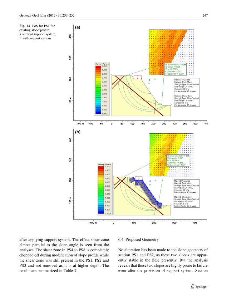
ments. Typical results of the analysis of the PS1

section considering all external, seismic loading and

presence of shear zone without and with support

system are shown in Fig. 13a, b, respectively. The

factor of safety and reliability index values are quite

low. Similar results were also obtained for other

sections. But the slope sections PS4 to PS8 were very

marginally safe. The results of the analysis of all the

eight slope profile sections without and with support

system are summarized in Tables 5 and 6, respec-

tively. An increase in FoS values was observed due to

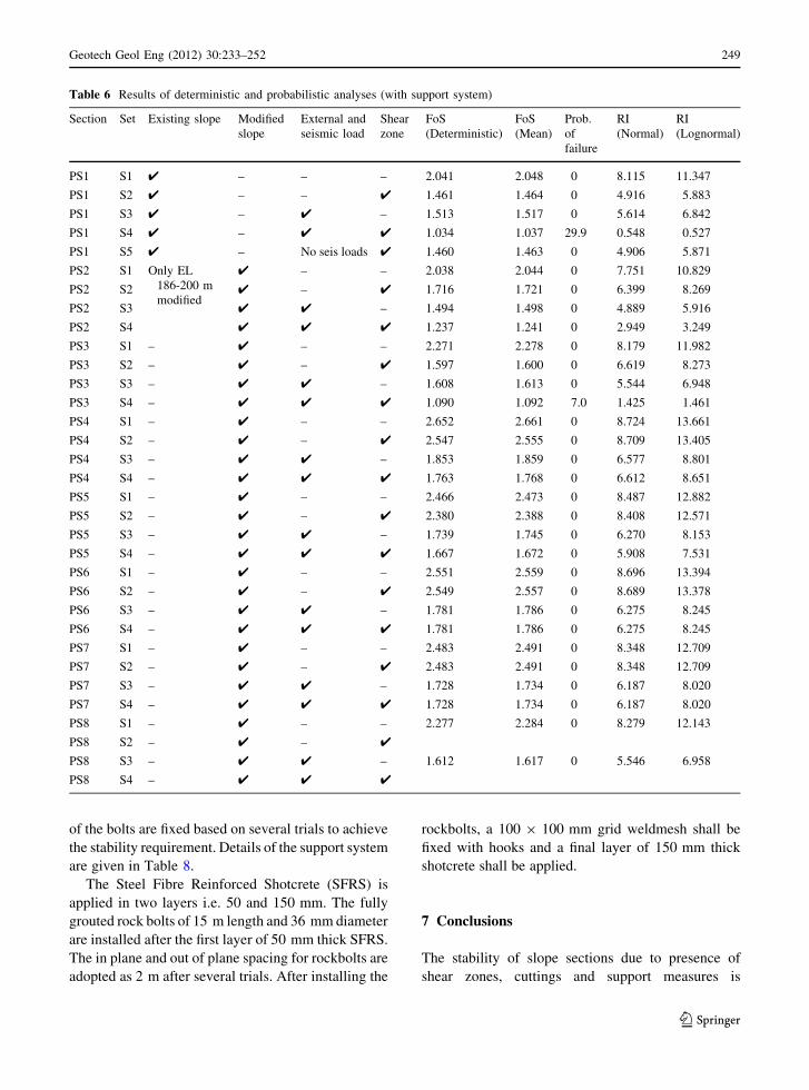
application of support system but the probability of

failure was still there for PS1 and PS3 sections as

shown in Table 6. It may be noted that the determin-

istic and mean factor of safety indicated in figures are

defined separately. The former is related to the

deterministic approach (limit equilibrium approach),

while the latter is the average of all the values of factor

of safety obtained from the number of Monte Carlo

simulations.

6.3 Shear Strength Reduction Technique (FEM)

Commercially available software Phase2 (2002) was

used for the analysis. The analyses were carried out for

all slope sections considering all shear zones, seismic

and external loadings combinations. Typical results

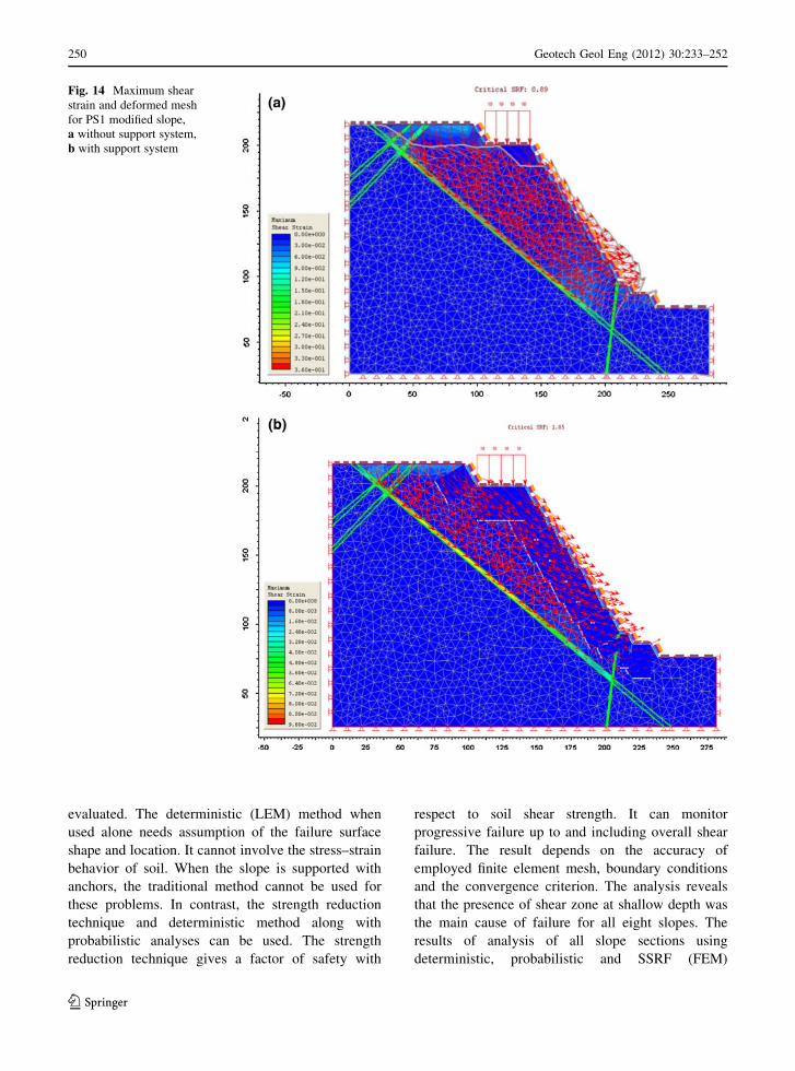
for PS1 are shown in Fig. 14. The SRF values less than

1 are observed for slope sections PS1, PS2 and PS3

without support systems. After the application of

support system the SRF values increased marginally.

Whereas SRF value of around 1 is observed for other

slope sections and an increase in stability is observed

No. of Simulations0 20000 40000 60000 80000 100000 120000

Coe

ff. o

f Var

iatio

n &

Std

. Dev

iatio

n

0.060

0.065

0.070

0.075

0.080

0.085

0.090

0.095CoVSD

Fig. 12 Variation of SD and CoV with number of simulation

cycles

246 Geotech Geol Eng (2012) 30:233–252

123

after applying support system. The effect shear zone

almost parallel to the slope angle is seen from the

analyses. The shear zone in PS4 to PS8 is completely

chopped off during modification of slope profile while

the shear zone was still present in the PS1, PS2 and

PS3 and not removed as it is at higher depth. The

results are summarized in Table 7.

6.4 Proposed Geometry

No alteration has been made to the slope geometry of

section PS1 and PS2, as these two slopes are appar-

ently stable in the field presently. But the analysis

reveals that these two slopes are highly prone to failure

even after the provision of support system. Section

Fig. 13 FoS for PS1 for

existing slope profile,

a without support system,

b with support system

Geotech Geol Eng (2012) 30:233–252 247

123

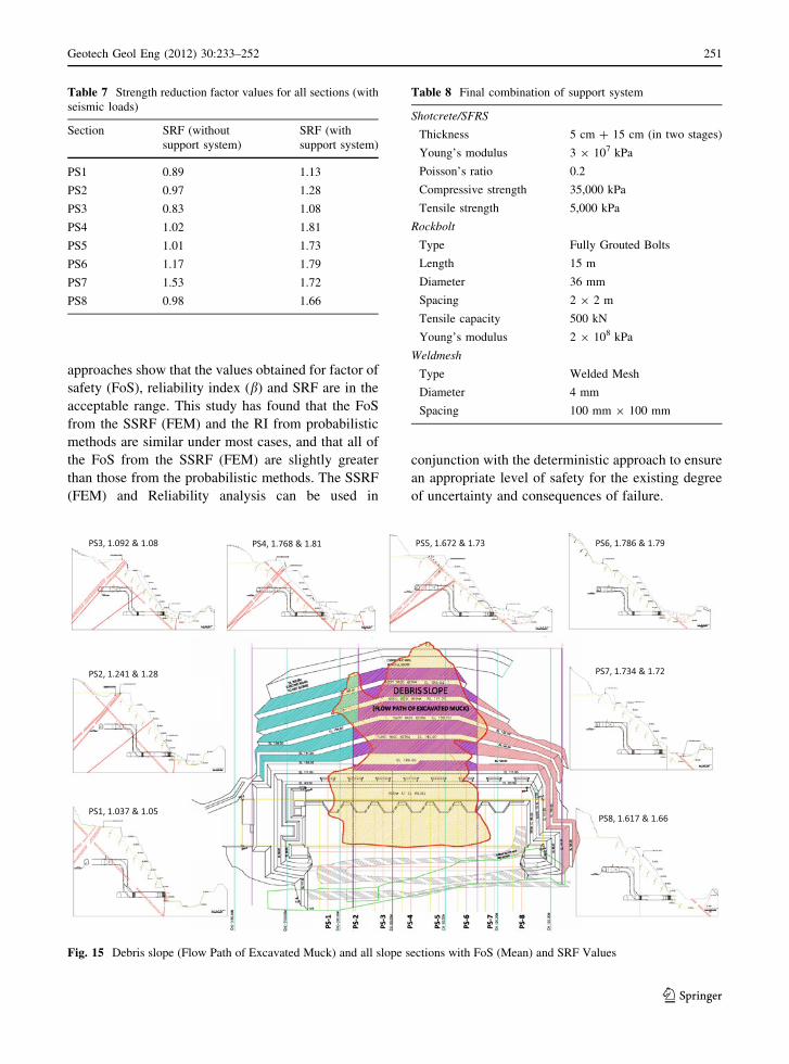
PS3 is made flat at an angle of 52�. At this slope angle,

the shear zone is at a minimum and maximum depth of

23–32 m from the modified geometry. The shear zone

present in this section made the slope unstable. All the

slopes were constructed on average slope angle of 64�.

PS4 and PS5 have shear zone at very shallow depth

and failed due to the slippage along the shear zone. So,

these two slopes have been made flatten (45�–50� and/

or combination of both) to remove the shear zone. The

details of all failed and modified slope sections are

given in Fig. 15. Slopes at sections PS4 to PS8 are also

made flat to meet the stability requirement, but not due

the shallow depth of shear zones.

6.5 Support System

Grouted rockbolts, shotcrete and weldmesh are con-

sidered for the support system. The length and spacing

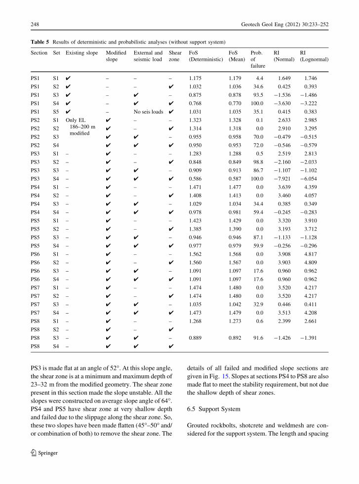
Table 5 Results of deterministic and probabilistic analyses (without support system)

Section Set Existing slope Modified

slope

External and

seismic load

Shear

zone

FoS

(Deterministic)

FoS

(Mean)

Prob.

of

failure

RI

(Normal)

RI

(Lognormal)

PS1 S1 4 – – – 1.175 1.179 4.4 1.649 1.746

PS1 S2 4 – – 4 1.032 1.036 34.6 0.425 0.393

PS1 S3 4 – 4 – 0.875 0.878 93.5 -1.536 -1.486

PS1 S4 4 – 4 4 0.768 0.770 100.0 -3.630 -3.222

PS1 S5 4 – No seis loads 4 1.031 1.035 35.1 0.415 0.383

PS2 S1 Only EL

186–200 m

modified

4 – – 1.323 1.328 0.1 2.633 2.985

PS2 S2 4 – 4 1.314 1.318 0.0 2.910 3.295

PS2 S3 4 4 – 0.955 0.958 70.0 -0.479 -0.515

PS2 S4 4 4 4 0.950 0.953 72.0 -0.546 -0.579

PS3 S1 – 4 – – 1.283 1.288 0.5 2.519 2.813

PS3 S2 – 4 – 4 0.848 0.849 98.8 -2.160 -2.033

PS3 S3 – 4 4 – 0.909 0.913 86.7 -1.107 -1.102

PS3 S4 – 4 4 4 0.586 0.587 100.0 -7.921 -6.054

PS4 S1 – 4 – – 1.471 1.477 0.0 3.639 4.359

PS4 S2 – 4 – 4 1.408 1.413 0.0 3.460 4.057

PS4 S3 – 4 4 – 1.029 1.034 34.4 0.385 0.349

PS4 S4 – 4 4 4 0.978 0.981 59.4 -0.245 -0.283

PS5 S1 – 4 – – 1.423 1.429 0.0 3.320 3.910

PS5 S2 – 4 – 4 1.385 1.390 0.0 3.193 3.712

PS5 S3 – 4 4 – 0.946 0.946 87.1 -1.133 -1.128

PS5 S4 – 4 4 4 0.977 0.979 59.9 -0.256 -0.296

PS6 S1 – 4 – – 1.562 1.568 0.0 3.908 4.817

PS6 S2 – 4 – 4 1.560 1.567 0.0 3.903 4.809

PS6 S3 – 4 4 – 1.091 1.097 17.6 0.960 0.962

PS6 S4 – 4 4 4 1.091 1.097 17.6 0.960 0.962

PS7 S1 – 4 – – 1.474 1.480 0.0 3.520 4.217

PS7 S2 – 4 – 4 1.474 1.480 0.0 3.520 4.217

PS7 S3 – 4 4 – 1.035 1.042 32.9 0.446 0.411

PS7 S4 – 4 4 4 1.473 1.479 0.0 3.513 4.208

PS8 S1 – 4 – – 1.268 1.273 0.6 2.399 2.661

PS8 S2 – 4 – 4

PS8 S3 – 4 4 – 0.889 0.892 91.6 -1.426 -1.391

PS8 S4 – 4 4 4

248 Geotech Geol Eng (2012) 30:233–252

123

of the bolts are fixed based on several trials to achieve

the stability requirement. Details of the support system

are given in Table 8.

The Steel Fibre Reinforced Shotcrete (SFRS) is

applied in two layers i.e. 50 and 150 mm. The fully

grouted rock bolts of 15 m length and 36 mm diameter

are installed after the first layer of 50 mm thick SFRS.

The in plane and out of plane spacing for rockbolts are

adopted as 2 m after several trials. After installing the

rockbolts, a 100 9 100 mm grid weldmesh shall be

fixed with hooks and a final layer of 150 mm thick

shotcrete shall be applied.

7 Conclusions

The stability of slope sections due to presence of

shear zones, cuttings and support measures is

Table 6 Results of deterministic and probabilistic analyses (with support system)

Section Set Existing slope Modified

slope

External and

seismic load

Shear

zone

FoS

(Deterministic)

FoS

(Mean)

Prob.

of

failure

RI

(Normal)

RI

(Lognormal)

PS1 S1 4 – – – 2.041 2.048 0 8.115 11.347

PS1 S2 4 – – 4 1.461 1.464 0 4.916 5.883

PS1 S3 4 – 4 – 1.513 1.517 0 5.614 6.842

PS1 S4 4 – 4 4 1.034 1.037 29.9 0.548 0.527

PS1 S5 4 – No seis loads 4 1.460 1.463 0 4.906 5.871

PS2 S1 Only EL

186-200 m

modified

4 – – 2.038 2.044 0 7.751 10.829

PS2 S2 4 – 4 1.716 1.721 0 6.399 8.269

PS2 S3 4 4 – 1.494 1.498 0 4.889 5.916

PS2 S4 4 4 4 1.237 1.241 0 2.949 3.249

PS3 S1 – 4 – – 2.271 2.278 0 8.179 11.982

PS3 S2 – 4 – 4 1.597 1.600 0 6.619 8.273

PS3 S3 – 4 4 – 1.608 1.613 0 5.544 6.948

PS3 S4 – 4 4 4 1.090 1.092 7.0 1.425 1.461

PS4 S1 – 4 – – 2.652 2.661 0 8.724 13.661

PS4 S2 – 4 – 4 2.547 2.555 0 8.709 13.405

PS4 S3 – 4 4 – 1.853 1.859 0 6.577 8.801

PS4 S4 – 4 4 4 1.763 1.768 0 6.612 8.651

PS5 S1 – 4 – – 2.466 2.473 0 8.487 12.882

PS5 S2 – 4 – 4 2.380 2.388 0 8.408 12.571

PS5 S3 – 4 4 – 1.739 1.745 0 6.270 8.153

PS5 S4 – 4 4 4 1.667 1.672 0 5.908 7.531

PS6 S1 – 4 – – 2.551 2.559 0 8.696 13.394

PS6 S2 – 4 – 4 2.549 2.557 0 8.689 13.378

PS6 S3 – 4 4 – 1.781 1.786 0 6.275 8.245

PS6 S4 – 4 4 4 1.781 1.786 0 6.275 8.245

PS7 S1 – 4 – – 2.483 2.491 0 8.348 12.709

PS7 S2 – 4 – 4 2.483 2.491 0 8.348 12.709

PS7 S3 – 4 4 – 1.728 1.734 0 6.187 8.020

PS7 S4 – 4 4 4 1.728 1.734 0 6.187 8.020

PS8 S1 – 4 – – 2.277 2.284 0 8.279 12.143

PS8 S2 – 4 – 4

PS8 S3 – 4 4 – 1.612 1.617 0 5.546 6.958

PS8 S4 – 4 4 4

Geotech Geol Eng (2012) 30:233–252 249

123

evaluated. The deterministic (LEM) method when

used alone needs assumption of the failure surface

shape and location. It cannot involve the stress–strain

behavior of soil. When the slope is supported with

anchors, the traditional method cannot be used for

these problems. In contrast, the strength reduction

technique and deterministic method along with

probabilistic analyses can be used. The strength

reduction technique gives a factor of safety with

respect to soil shear strength. It can monitor

progressive failure up to and including overall shear

failure. The result depends on the accuracy of

employed finite element mesh, boundary conditions

and the convergence criterion. The analysis reveals

that the presence of shear zone at shallow depth was

the main cause of failure for all eight slopes. The

results of analysis of all slope sections using

deterministic, probabilistic and SSRF (FEM)

Fig. 14 Maximum shear

strain and deformed mesh

for PS1 modified slope,

a without support system,

b with support system

250 Geotech Geol Eng (2012) 30:233–252

123

approaches show that the values obtained for factor of

safety (FoS), reliability index (b) and SRF are in the

acceptable range. This study has found that the FoS

from the SSRF (FEM) and the RI from probabilistic

methods are similar under most cases, and that all of

the FoS from the SSRF (FEM) are slightly greater

than those from the probabilistic methods. The SSRF

(FEM) and Reliability analysis can be used in

conjunction with the deterministic approach to ensure

an appropriate level of safety for the existing degree

of uncertainty and consequences of failure.

Table 7 Strength reduction factor values for all sections (with

seismic loads)

Section SRF (without

support system)

SRF (with

support system)

PS1 0.89 1.13

PS2 0.97 1.28

PS3 0.83 1.08

PS4 1.02 1.81

PS5 1.01 1.73

PS6 1.17 1.79

PS7 1.53 1.72

PS8 0.98 1.66

Fig. 15 Debris slope (Flow Path of Excavated Muck) and all slope sections with FoS (Mean) and SRF Values

Table 8 Final combination of support system

Shotcrete/SFRS

Thickness 5 cm ? 15 cm (in two stages)

Young’s modulus 3 9 107 kPa

Poisson’s ratio 0.2

Compressive strength 35,000 kPa

Tensile strength 5,000 kPa

Rockbolt

Type Fully Grouted Bolts

Length 15 m

Diameter 36 mm

Spacing 2 9 2 m

Tensile capacity 500 kN

Young’s modulus 2 9 108 kPa

Weldmesh

Type Welded Mesh

Diameter 4 mm

Spacing 100 mm 9 100 mm

Geotech Geol Eng (2012) 30:233–252 251

123

Acknowledgments

The authors acknowledge the help received from the

officials of M/S Larsen and Toubro Ltd., India and

NHPC Ltd., India during the field visits of the project.

References

Baecher GB, Christian JT (2003) Reliability and statistics in

geotechnical engineering. Wiley, New York

Baker R, Garber M (1978) Theoretical analysis of the stability of

slopes. Geotechnique 28(4):395–411

BIS:1893–2002. Part 1: 2002 Bureau of Indian Standards, cri-

teria for earthquake resistant design of structures, General

Provisions and Buildings

Cheng YM (2003) Locations of critical failure surface and some

further studies on slope stability analysis. Comput Geotech

30:255–267

Dawson EM, Roth WH, Drescher A (1999) Slope stability analysis

by strength reduction. Geotechnique 49(6):835–840

Duncan JM (1996) State of the art: limit equilibrium and finite-

element analysis of slopes. J Geotech Geoenviron Eng

ASCE 122(7):577–596

Duncan JM (2000) Factors of safety and reliability in geotech-

nical engineering. J Geotech Geoenviron Eng ASCE

126(4):307–316

Goodman RE, Kieffer DS (2000) Behaviour of rock in slopes.

J Geotech Geoenviron Eng ASCE 126(8):675–684

Griffiths DV, Lane PA (1999) Slope stability analysis by finite

elements. Geotechnique 49(3):387–403

Hammah RE, Curran JH, Yacoub TE, Corkum B (2004) Sta-

bility analysis of rock slopes using the finite element

method. In: Proceedings of the ISRM regional symposium

EUROCK 2004 and the 53rd Geomechanics Colloquy,

Salzburg, Austria

Hoek E, Bray J (1981) Rock slope engineering. The Institution

of Mining and Metallurgy, London

Hynes-Griffin ME, Franklin AG (1984) Rationalizing the seis-

mic coefficient method. Miscellaneous paper GL-84-13.

US Army Corps of Engineers Waterways Experiment

Station, Vicksburg

Kramer SL (2003) Geotechnical earthquake engineering. Pear-

son Education

Lechman JB, Griffiths DV (2000) Analysis of the progression of

failure of earth slopes by finite elements, Slope stability 2000.

In: Proceedings of sessions of Geo-Denver 2000, ASCE

Geotechnical Special Publication no. 101, pp 250–265

Low BK (2003) Practical probabilistic slope stability analysis.

In: Proceedings, soil and rock America 2003, 12th pan-

american conference on soil mechanics and geotechnical

engineering and 39th US rock mechanics symposium.

MIT, Cambridge, June 22–26, 2003, Verlag Gluckauf

GmbH Essen, vol 2, pp 2777–2784

Matsui T, San KC (1992) Finite element slope stability analysis by

shear strength reduction technique. Soils Found 32(1):59–70

McMahon BK (1975) Probability of failure and expected vol-

ume of failure in high rock slopes. In: Proceedings of 2nd

Australia-New Zealand conference on geomechanics,

Brisbane, pp 308–313

Morriss P, Stoter HJ (1983) Open-cut slope design using prob-

abilistic methods. In: Proceedings of 5th congress ISRM.,

Melbourne 1, Rotterdam, Balkema, pp C107–C113

Naylor DJ (1981) Finite elements and slope stability. In: Numerical

methods in geomechanics, proceedings of the NATO

advanced study institutes series, Lisbon, Portugal, pp 229–244

Phoon KK, Kulhawy FH (1999) Characterization of geotech-

nical variability. Can Geotech J 36:612–624

Priest SD, Brown ET (1983) Probabilistic stability analysis of

variable rock slopes. Inst Min Metall Trans (Sect. A) 92:1–12

Ramly H, Morgenstern NR, Cruden DM (2002) Probabilistic

slope stability analysis for practice. Can Geotech J

39:665–683

Rao KS (2008) Slope stability assessment and support measures

for Subansiri Lower Hydroelectric project, Technical

Report. Indian Institute of Technology Delhi, India

Read JRL, Lye GN (1983) Pit slope design methods, Bougain-

ville Copper Limited open cut. In: Proceedings of 5th

congress ISRM., Melbourne, Rotterdam, Balkema, pp

C93–C98

RocScience (2002) RocScience manual version 5. Rocscience

Inc., Canada

Seed HB, Lee KL, Idriss IM (1969) Analysis of Sheffield Dam

failure. J Soil Mech Found Div ASCE 95(SM6):1453–1490

Ugai K, Leschinsky D (1995) Three dimensional limit equilib-

rium and finite element analyses: a comparison of results.

Soils Found 29(4):1–7

USACE (1997) Risk-based analysis in geotechnical engineering

for support of planning studies, engineering and design. US

Army Corps of Engineers, Department of Army, Wash-

ington DC, 20314-100

Vanmarcke EH (1980) Probalistic analysis of earth slopes. Eng

Geol 16:29–50

Whitman RV (2000) Organizing and evaluating uncertainty in

geotechnical engineering. J Geotechn Geoenviron Eng

ASCE 126(7):583–593

Zienkiewicz OC, Humpheson C, Lewis RW (1975) Associated

and nonassociated viscoplasticity in soil mechanics. Geo-

technique 25(4):671–689

252 Geotech Geol Eng (2012) 30:233–252

123