Electronic copy available at: http://ssrn.com/abstract=1882564

Working Paper No. 200726900-02 School of Engineering – Universidad de los Andes

Bogotá D.C., Colombia. Wednesday, July 20, 2011

1

THE STRATEGIC COST OF HYDROELECTRIC RESOURCES1

Juan M. Alzate

2∗, Rafael Bautista3∗∗, Angela I. Cadena4

∗ Department of Electric and Electronic Engineering – School of Engineering. Universidad de los Andes.

∗

∗∗ Business School, Universidad de los Andes. Bogotá D.C., Colombia.

ABSTRACT Abstract: In liberalized hydro-dominated power supply systems, the way managers use the knowledge they have about water levels in order to make production decisions impacts both their market power potential and the market outcomes. Assuming that the corresponding risk can be priced, we develop a dynamic hydro-dominated oligopolistic modeling framework to discuss the strategic cost of hydroelectric resources, in the context of the short-term marginal opportunity cost of storable electricity. As our contribution over previous approaches we construct a criterion embodying in a single number the strategic cost of hydropower production decisions. This criterion is built through the use of an indifference (risk-neutral) argument regarding the expected profits associated to a particular production strategy. Our result enables us to define regulatory policies to mitigate the market power potential of oligopolistic hydro-dominated producers, and to define socially optimum water allocation policies. We use data from the Colombian power market to run an informal check of the plausibility of our findings. JEL: D24, D43, Q40. Key words: strategy and decisions, hydroelectric costs, oligopoly, dynamic model.

1. INTRODUCTION In all integrated markets for electricity production there are easily identified oligopolies. In particular, hydro dominated oligopolies have a high market power, though this fact does not imply that they are able to eliminate altogether some of the more basic uncertainties, for instance those related to unexpected hydrologic events, or the ones related to final actual delivery prices and quantities resulting from a daily auction. The basic strategy of the agents in such markets is built on two principles that more or less dictate day-to-day decisions: to manage reservoirs so that the producer minimizes the chance of undersupply, and to maximize short-term operational results given the previous constraint. For the purpose of this paper, following a ‘strategy’ means to consistently act according to a set of rules of thumb – call it policy – for production and bidding that any particular agent believes best reflects their stated medium- and long-term goals. In what follows it will be shown that if these are the two main strategic guidelines, then agents in a hydro dominated market should act assuming that water is costly, even if that cost is not realized as an immediate disbursement. In what follows, we assume that if the market for electricity is seen as a repeated game, then eventually all agents will fit into a very small set of strategies, which may vary somewhat, depending on size and technological portfolio. We assume that the agents in a given oligopoly and in a specific market 1 Accepted for a parallel session talk at the “Economics of Energy Markets” conference, held on June 15-16, 2011, organized by the IDEI, Toulouse School of Economics. 2 The author acknowledges the economic support from the grant No. 417/2007 afforded by COLCIENCIAS (The Colombian Science Council) to support national doctoral studies. Helpful and insightful comments from Alvaro Castro (XM) are also acknowledged. Email: alzate.jm@gmail.com. 3 Contact author (SSRN ID #95723), email: rbautist@uniandes.edu.co, rbautista_mena@yahoo.com. 4 Email: acadena@uniandes.edu.co.

Electronic copy available at: http://ssrn.com/abstract=1882564

Working Paper No. 200726900-02 School of Engineering – Universidad de los Andes

Bogotá D.C., Colombia. Wednesday, July 20, 2011

2

environment are, first, hydro dominated, and second, all pursue goals similar to those already stated above. Therefore, we expect that, in the aggregate, the pattern of use of water under different scenarios will show a degree of cogency that we take to be fully rational. To complete the description of the environment for the choice of strategy, it is important to mention a particular consequence of the process of deregulation that has spread worldwide. Deregulation of the mixed hydro and thermal power markets substituted the concept of short-term marginal opportunity costs of water for the earlier of variable cost of producing hydroelectricity. Just about all authors on the subject have the intuition that knowledge about water that will be missing later because of present overuse, and vice versa, should somehow constrain the present production decision, as it would an immediate cash disbursement. This fits the description of the typical opportunity cost commonly used in financial asset pricing theory. Our attempt to construct an explicit expression for such marginal short-term opportunity cost springs from the strategic behavior of hydropower producing agents, in the aggregate. The essence of the argument is that, due to concerns about the immediate future of water supply, members of an oligopoly who bid prices and quantities on a daily basis will often place their bids under different price expectations than if there were no such concerns. In our model, this difference translates into alternative cumulative conditional probability distributions for the realized prices. Clearly, from the previous discussion, the model may not be static. Decisions made today have to allow for what will be decided tomorrow. This interrelatedness is also a logical consequence of the existence of a long-term plan. In general, a multi-period model would seem as the natural setting for any strategy-related argument; we choose a minimalistic two-period model that leads to an iteration formula for the sought strategic cost formula. Our contribution differs from previous work in the attempt we make to explicitly construct a criterion embodying in a single number the strategic cost of hydropower production decisions. This criterion relies upon an indifference (and risk-neutral) argument regarding the expected profits associated to a particular production strategy. The plausibility of this construction is then assessed using data from the Colombian power market as a workbench on which to test our results. The resulting expression involves market and weather expectations, and absorbs all agents’ best responses through the careful definition of conditional cumulative distributions for two scenarios of water availability, which we take as those actually given by market conditions. This enables us to discuss some conceptual features of the rationale behind electricity markets. After the worldwide liberalization trend, the risk born by producers in hydro-dominated power supply systems is directly affected by the time-variable cost of using the storable hydroelectric resources. Once this strategic cost is made explicit, it sheds some new light on the way managers use the knowledge they have about present and future water levels, in order to make production decisions that impact their market power potential and the market outcomes. To achieve this goal, we develop a dynamic hydro-dominated oligopolistic modeling framework to discuss the economic rationale of power systems by way of the strategic cost of hydroelectric resources. That is, within the context of the short-term marginal opportunity cost of storable electricity. Beyond devising an explicit formula, an important part of our results is to provide a “proof of existence” by construction. We believe we provide that proof in section 5, were we apply the model in section 4 to data from the Colombian power market. These results readily reproduce the common intuition that in hydro-dominated markets, the strategic cost of the hydroelectric resources takes high (positive) values during dry hydrological seasons, and turns to low (and even negative) values during wet periods.

Working Paper No. 200726900-02 School of Engineering – Universidad de los Andes

Bogotá D.C., Colombia. Wednesday, July 20, 2011

3

In Section 2, we present a brief literature review on the subject. Then, the proposed model is described in Section 3. In Section 4 we derive an explicit expression for the strategic cost of hydroelectric resources in competitive power markets following an indifference argument. In Section 5 we show evidence that supports the existence of the priced opportunity cost using market data from the Colombian power market. In Section 6 we draw some conclusions and propose some ideas regarding further work.

2. OVERVIEW AND RELATED WORK Much of the rationale of oligopolistic power producers is driven by price risk exposition and by changes in the slope of the residual load they serve (Hansen, 2009). These two overarching causes are nevertheless composed of more specific ones. In the case of hydro-dominated power systems, it is important to clarify how managers use the knowledge they have about water levels in order to make production decisions. We assume that this is an important contributor to price risk in the system. There may be several channels through which this problem can be approached. In this paper we argue that in a price-bid structure the opportunity cost of the hydroelectric resources is also priced in. This cost depends on the market power potential and on local market architecture customizations. To our knowledge, previous work on the economics of deregulated hydro-thermal power supply systems has not dealt with the specific computation of the strategic cost of hydroelectric resources. Decades ago, the industry focused mainly in estimating water costs, but since then the main object of concern has evolved, following changes in regulation (Pereira, 1989; Wolfgang et al., 2009). By the 1950's, hydro-thermal systems grew complex and the integrated/centralized state owned model –worldwide adopted– was facing a resource allocation problem: To maximize the expected income subject to uncertainties, e.g. water inflows, electricity demands, transmission constraints, among others. There were trade-offs between hydro and thermal generation costs to be optimized in short-term planning horizons and in this pure resource management problem investment costs played no relevant role. Hence, water and electricity shadow prices as well as reservoir and turbine efficiency rates became the object of attention. In the late 1980's water allocation strategies were further enhanced exploiting computational developments. The initial emphasis in shadow prices yielded to interest in marginal hydroelectricity production costs from Stochastic Dual Dynamic Programming formulations. Nowadays, Brazil follows a centrally operated model using an improved SDDP formulation and there is a Scandinavian reciprocal model,5

Technological changes in the early 1990’s quickened the liberalization pace within the industry. The capital intensity of the industry led to concentrated markets, which motivated market power assessments by the regulators, especially in hydro-dominated systems, where the problem has been further exacerbated. Producers engaged in setting up bidding strategies in pool-based markets, while market regulators sough to create competitive environments.

though it is not used for scheduling purposes.

Afterwards, the technological differences became a deep concern, due to issues of their complementarities as well as the reliability of power supply systems without a centralized coordination. The situation got worse with the emergence of intermittent renewable resources hard to forecast. In fact, the coordination of these new resources will become a harder task to undertake if expected technological changes like “smart” electric devices become part of the market environment, and participate significantly in the system of distributed generation. 5 It is a power-market model, the EMPS1 (EFI’s Multi-area Power-market Simulator).

Working Paper No. 200726900-02 School of Engineering – Universidad de los Andes

Bogotá D.C., Colombia. Wednesday, July 20, 2011

4

Two decades after the liberalization trend started, the relative benefits of competition and coordination in power supply systems are still questioned. Due to market architectures that are unbundled and competitive, the concept of integrated water cost is being replaced by one of short-term marginal cost (Ambec & Doucet, 2003; Wolfgang, 2009).Water costs are benchmarked to the price of the fuels powering its thermal competitors as shadow prices; the short-term water opportunity costs incorporate this information, as well as the uncertainty of demand and water inflows, into the price-bid structure and the shape of the load individually served by producers6

The precise and proper estimation of water opportunity costs in deregulated markets would favor the achievement of efficient market prices, competitive strategies and water management policies as well. Nevertheless, most of the contributions regarding the economics of hydro-thermal and hydro-dominated power markets are not framed within this context

(Hansen, 2009). Therefore, the cost of water is no longer viewed as a variable production cost, declared to a centrally managed system, but rather as a cost of the strategic resource to be internally assessed.

7

Crampes and Moreaux developed a simplified dynamic model where hydro and thermal resources compete (Crampes & Moraux, 2001). Their formulation describes in analytical and geometrical ways optimal resource allocation policies and market price levels under alternative market architecture assumptions. The economic rationality of the model is supported on the shadow prices of the scarce resource (water balance constraint). In fact, the authors state the value of water arises from its scarcity as compared to the needs in successive time periods.

and usually lack an analytical and explicit interpretation of the strategic cost of the hydroelectric resources.

The approaches developed afterwards successfully overcame the static nature of the models describing the economics of hydropower markets and incorporated the intrinsic dynamism of the hydro technologies into the modeling framework. These contributions still lacked the means to explicitly model the water opportunity costs in deregulated markets; however, most of them point out the relevance of this concept. Ambec and Doucet developed a dynamic model to quantify the impact on welfare before and after the introduction of competition (Ambec & Doucet, 2003). Their formulation falls short of describing the strategic value of water, but they underscore its close interrelationship with the power market architecture. As they explain, welfare losses induced by biased water management policies may be counteracted by institutional settings. Moreover, they propose that the suitability of particular schemes depends upon the topology of the system. Førsund (2006) follows an approach close to that developed by Crampes and Moreaux (2001). The author assesses the market power potential of hydro-dominated monopolists supported on demand functions perfectly known by the producer and engages in deriving outcomes after considering different alternatives e.g. inter-regional trade, reservoir constraints, and a competitive thermal fringe. As it is stated by Førsund, the relevant variable to measure the existence of market power from hydropower producers is the opportunity cost of water; however, it is only highlighted as an important though not directly observable variable. The author associates the water value with the shadow price of a resource 6 As it is also explained in Hansen (2009), the demand faced by a firm with market power does not depend solely on consumer demand, but also on the supply of its competitors which further depends on production technologies and other constraints such as bottlenecks in the transmission network. 7 The idea of a water market parallel to the power market to properly price the resource in hydro-dominated systems have been suggested as a remedy (Ambec & Doucet, 2003). However, it remains an unpopular idea in a very reluctant institutional environment.

Working Paper No. 200726900-02 School of Engineering – Universidad de los Andes

Bogotá D.C., Colombia. Wednesday, July 20, 2011

5

constraint as it is done in (Crampes & Moraux, 2001). However, the strategic value of water is not explicitly summarized in a single variable. Hansen discusses how the costs structure of the marginal supply, as well as inflow uncertainties, influence the behavior of firms with market power (Hansen, 2009). This article presents an approach to how the qualitative and quantitative features of market power in hydro-dominated markets depend on the characteristics of the residual demand faced by individual firms. However, there is no explicit construction of a valuation formula for the cost of using the water, although the paper assumes that use of the resource may have significant, short-term consequences. Garcia, Campos-Nañez, & Reitzes (2005) (see also Garcia, Reitzes, & Stacchetti, 2001) came close to the idea of incorporating what they call the “strategic value” of water into price-bidding strategies of an infinite-horizon oligopoly model. They built upon an indifference pricing approach where the producer is indifferent between producing power with his water resources and holding onto those resources for the future. Their findings, despite symmetrical assumptions, characterize a Markov Perfect Equilibrium and give valuable insights for regulatory policy in hydro-dominated systems. They rely on a still general (stream of payoffs) functional form to describe the strategic value of water, which depends upon the states of own and competing water reservoirs after following a particular strategy.

3. THE MODEL We propose a three-date, two-period model. At the beginning of the first period (𝜏 = 1) the agents learn what the state of nature (the weather) will be during the period. This knowledge, together with the present state of the reservoir, plus any other ancillary information related to their own private financial state and about competitors, is enough for the oligopoly to choose its bid for the period. The future state of nature (time period 𝜏 + 1) is nevertheless uncertain, with inflows within typical, seasonally adjusted ranges that follow a known probability distribution. This distribution is common knowledge. Since all agents in this market have access to the same data, the processing of conditional sets of historic weather registries yields a distribution about which al agents may construct a common belief. This procedure avoids in part some of the more troubling assumptions made in the rational expectations frame, where common beliefs are supposed to arise from more contextual, less material knowledge. Consider an oligopolistic hydro dominated player that can exert a significant degree of market power. By “market power” we understand the ability of the hydro producer to effect the distribution of the final sale price. Besides, its production decision elicits enough correlation between its quantity bids and the final price that, for the period of the play, he may assume an approximate inverse demand function to hold. The producer owns a water reservoir with maximum storage capacity 𝛿̅, which is currently holding an amount of freely producible amount of hydroelectricity 𝛿𝜏 ≤ 𝛿̅. By convention, this is the amount of energy equivalent to the water level in the reservoir at the beginning of time interval 𝜏. Uncertain water inflows (𝑎𝜏) follow a cumulative distribution function 𝐹𝜏[𝑎𝜏]. This is in general a distribution over a continuous variable which, as mentioned earlier, varies in shape with the season.8

8 The time period sub index may be over specific; a season contains a sequence of dates.

This cumulative distribution in general includes a finite probability mass at 𝑎𝜏 = 0. Since at time 𝜏 there is often some critical value of 𝑎𝜏 on which the next period production decision will depend, it is useful in practice to recur to a coarse grained representation. Figure 2.A (in Appendix A) provides an example of a two-scenario plot of 𝐹𝜏[𝑎𝜏] for the ‘rain or no-rain’ partition. That figure shows a plot of the estimated

Working Paper No. 200726900-02 School of Engineering – Universidad de los Andes

Bogotá D.C., Colombia. Wednesday, July 20, 2011

6

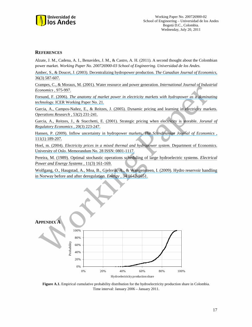
no-rain probability 𝜃𝜏, typical of the Colombian hydrologic cycle, as it varies over time from January 2006 until January 2011. The state variable 𝛿𝜏 is the main criterion used by agents to decide on the degree of significance of the random inflow 𝑎𝜏. In other words, the hydro production decision for period 𝜏 is related to perceptions about next period state 𝛿𝜏+1. Such perceptions are most easily summarized through the use of a dichotomy of sets of future states with associated cumulative distributions 𝐺𝜏𝐻 and 𝐺𝜏𝐿. These distributions are defined over the set of all possible values of the net operating income; therefore, some overlap of their corresponding supports is to be expected. Nevertheless, it will be assumed that agents’ decision processes are such that any overlap represents a negligible probability mass of either distribution, so that they are basically exclusive. The former represents expectations with states in which future prices are most likely going to be high, but quite possibly they will come associated with low volumes of hydro production. The 𝐺𝜏𝐿 distribution represents an alternative set of states. These distributions are the best rational beliefs that agents in the electric market may choose from, given the information set available to all. Last, there is the matter of when does any given agent know which distribution to choose. The criterion to choose one over the other will be some critical value of 𝛿𝜏+1, recognized by all through long experience to be the trigger point to change bidding strategies. For instance, an expected range of values of 𝛿𝜏+1 higher than the commonly accepted critical value induces all agents to assume a bidding strategy whose outcome is best represented by 𝐺𝜏𝐿. We postpone until section 5 the discussion of an implementation of this criterion. During the time interval 𝜏 there may also be spillovers 𝑠𝜏, that can be calculated from the balance equation

𝑠𝜏 = 𝑚𝑎𝑥{0,𝛿𝜏 + 𝑎𝜏 − 𝛿̅} (1) In practice, spillovers are unusual, and in the context of this paper they are not of much regulatory concern. Hydroelectricity production is mainly constrained either by the maximum turbine output capacity 𝛽, or by the amount of usable water 𝛿𝜏. The actual production of hydropower will take place at the end of interval 𝜏. The amount produced is given by

𝑞𝜏ℎ = 𝑤𝜏 ⋅ 𝑚𝑖𝑛{𝛿𝜏,𝛽} (2) Where 𝑤𝜏 ∈ [0,1] corresponds to the manager’s production decision at 𝜏. Therefore, the water/energy balance at the beginning of interval 𝜏 + 1 will be,

𝛿𝜏+1 = 𝛿𝜏 + 𝑎𝜏 − 𝑠𝜏 − 𝑞𝜏ℎ (3) A significant portion of the power supply comes from an oligopoly of large producers, who hold a portfolio of hydro (ℎ) and thermal (𝑡) power generation assets. In this model the oligopoly is assumed to be hydro-dominated. There may be also other fringe competitors, of comparatively smaller scale and diversified power production assets. It is assumed that there is a wholesale day-ahead spot market where producers individually bid their resources to meet an inelastic system load. The oligopoly has as its goal to bid an average residual amount of electric energy, taken to be equal to 𝐷 for all periods. The oligopoly produces an amount 𝑞𝜏ℎ of hydroelectricity, which, if viewed from traditional approaches to the problem, has no direct associated production costs. In this work the consequences of assuming the existence of a subjectively assessed strategic cost of opportunity 𝜈𝜏ℎ are explored. This cost accounts for the value of the forgone opportunity of using the storable resource once released, and may be affected by market customizations (in this case a pool-based spot market), by the expectations about inflow realizations, competitors’ behavior, and the market power exerted after following any particular production decision 𝑞𝜏ℎ.

Working Paper No. 200726900-02 School of Engineering – Universidad de los Andes

Bogotá D.C., Colombia. Wednesday, July 20, 2011

7

The oligopoly may also produce an amount

𝑞𝜏𝑡 ≤ 𝑚𝑖𝑛{𝛼,𝐷 − 𝑞𝜏ℎ} (4) of thermal electricity with corresponding variable production cost 𝜈𝜏𝑡 . Assuming that producers enter into fuel supply forward contracts, this cost is taken to be certain, though not necessarily constant, in the short run.9

With these definitions, the hydro-dominance of the oligopoly means that 𝛽 > 𝛼. For the remainder of this paper the relationship

Parameter 𝛼 is the maximum thermal electricity production given the installed capacity. In what follows it will be assumed that costs and toil of turning on and off make it unprofitable to operate the thermoelectric plant unless constraint (4) is binding.

𝐷 ≤ 𝛼 + 𝛽 (5) is assumed to hold. This condition is useful, since equations (2) and (4) might give the appearance that thermoelectricity production is marginal, once the choice has been made about how much water to draw. The combination of hydro-dominance and some overcapacity allows for the alternative decision process just as well.

Any deficit in supply is given by 𝑚𝑎𝑥{0,𝐷 − 𝑞𝜏ℎ − 𝑞𝜏𝑡}. This, as well as any production overhang, has to be bought or sold at spot prices. Note that, since we assume that any deficit is bought and sold at the same spot price, there is no net financial effect from this operation. The design of a strategy starts with the oligopolistic producer bidding its resources at the beginning of time interval 𝜏 expecting a market realization price 𝑝𝜏∗. Nevertheless, upon delivery, the actual market outcome 𝑝𝜏 may be somewhat different. His oligopoly market power resides in the fact that he can narrow the spread of the 𝑝𝜏 distribution about his expected price, which may be estimated from some privately specified procedure. The final spot price is known once the uniform-price auction is cleared, at the end of each period.10

The (risk-neutral) utility of the particular strategy will be the two-period total income associated to a fully speculative (𝜈𝜏ℎ = 0) strategy 𝑤𝜏. Except where otherwise specified, we shall limit ourselves to the case when 𝛿𝜏 ≥ 𝛽. Under those conditions, the total expected income for the two periods may be written as follows:

Once the price is known, delivery is assumed to be immediate.

Π(𝑤𝜏) = Π𝜏 + Π𝜏+1 = [𝑤𝜏𝛽𝑝𝜏 + 𝑞𝜏𝑡(𝑝𝜏 − 𝑣𝜏𝑡)] + 𝐸𝜏[𝑄𝜏+1𝑝𝜏+1−𝑣𝜏+1𝑡 𝑞𝜏+1𝑡 ] (6) In this model, any profits come only from the electricity traded in the spot market. 𝑄𝜏+1 denotes the total power produced, and 𝐸𝜏[∙] stands for the expectation operator over future income, once uncertainty about future inflow has been taken into consideration. For the first period, the final delivery price is taken as given, and it may play a role in the construction of expectations for the next. For the sake of simplicity, no bilateral contract market is considered. In practice, the share of total power production that goes to contracts is stable over a period of a few years, and therefore it is reasonable to take this component approximately as a fixed background. The discount rate for all cash flows is set at zero, because the time scale for the kind of uncertainty under consideration is in the order of few days. The power producers are assumed to be short-term utility maximizers, therefore the set of optimal strategies excludes cases with zero total power production for any single period. 9 It might of course be exposed to uncertainties different from the rain and no-rain scenarios, such as fluctuations in the international price of crude oil. 10 As it is common in auctions, these prices are directly affected by the bidding strategy followed by the oligopolistic power producers, their choice of technological production share and their near term expectations.

Working Paper No. 200726900-02 School of Engineering – Universidad de los Andes

Bogotá D.C., Colombia. Wednesday, July 20, 2011

8

It is worth noting that total first period production 𝑄𝜏 is not necessarily equal to 𝐷. In particular, the underlying rationale for any decision of rather producing less than the target demand is because the hydro producer expects that, by doing so, market power will bring a higher revenue during the second period that will more than compensate for the revenue lost in the initial move.11

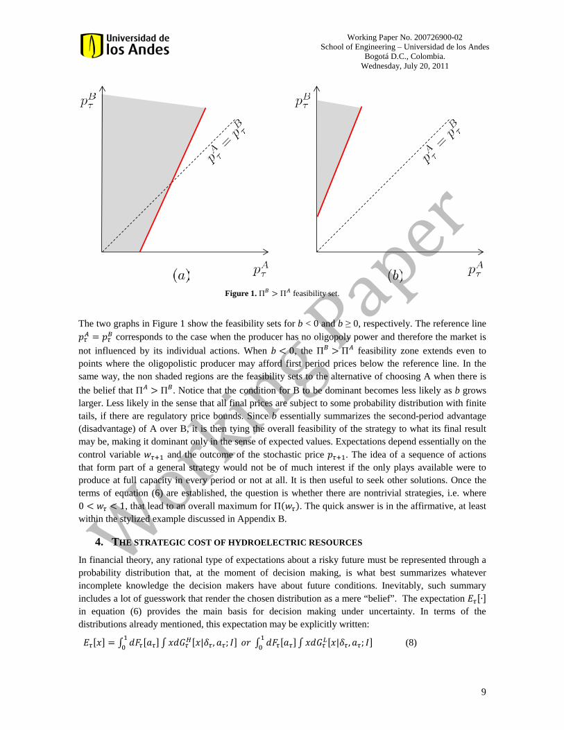
If the oligopoly adopts a particular production strategy in period 𝜏, to be followed by a second, coordinated move at 𝜏 + 1, then it must be expected that the distribution of price at the latter date is going to be effected by the chosen strategy. What sort of conditions should be met by the preferred strategy? A simple approach might be to consider two reference strategies, A and B, that correspond to the extremes 𝑤𝜏𝐴 = 1 and 𝑤𝜏𝐵 = 0, respectively. Given that the state of nature in period 𝜏 + 1 is still unknown, strategy A may be deemed a fully speculative one. On the other hand, B could be characterized as too conservative. In either case, the first move does not fully condition the decisions to be made for the second. Nevertheless, if the decision is A, then the hydro turbine is fully at work, and in the case of no oversupply 𝑞𝜏𝑡𝐴 = 𝐷 − 𝛽. If B is the choice, then the producer will limit himself to maximize his revenue given the choice, therefore 𝑞𝜏𝑡𝐵 = 𝛼.

By choosing B the producer believes that the next period will be dry. It also believes that his decision brings about present revenue sufficiently high to sustain a deferment of part of his hydro production until the next period. B will turn out to be dominant as long as Π𝐵 ≥ Π𝐴. The application of this condition to (6) yields the inequality:

𝛼𝑝𝜏𝐵 ≥ 𝐷𝑝𝜏𝐴 + (𝛼 + 𝛽 − 𝐷)𝑣𝑡 + Π𝜏+1𝐴 − Π𝜏+1

𝐵 (7) Inequality (7) corresponds to a linear constraint of the form 𝑝𝜏𝐵 ≥ 𝑚 ⋅ 𝑝𝜏𝐴 + 𝑏, which is shown in Figure 1. The shaded area demarks the Π𝐵 > Π𝐴 feasibility set. Depending on the market architecture, the depicted plane may be bounded by price caps.12

From (7) it can be seen that the slope 𝑚 is greater than 1, and will be defined by the target offer to thermal power production ratio. On the other hand, the intercept 𝑏 may take either positive or negative values, pending on the net income difference between strategies A and B at 𝜏 + 1.

11 Hansen (2009) offers a particular rationale for this belief. 12 At the other end, the origin in these graphs is not (0, 0). Instead, the origin in both graphs is set at the minimum price at which the producer is willing to place a bid, regardless of strategy.

Working Paper No. 200726900-02 School of Engineering – Universidad de los Andes

Bogotá D.C., Colombia. Wednesday, July 20, 2011

9

Figure 1. Π𝐵 > Π𝐴 feasibility set.

The two graphs in Figure 1 show the feasibility sets for b < 0 and b ≥ 0, respectively. The reference line 𝑝𝜏𝐴 = 𝑝𝜏𝐵 corresponds to the case when the producer has no oligopoly power and therefore the market is not influenced by its individual actions. When 𝑏 < 0, the Π𝐵 > Π𝐴 feasibility zone extends even to points where the oligopolistic producer may afford first period prices below the reference line. In the same way, the non shaded regions are the feasibility sets to the alternative of choosing A when there is the belief that Π𝐴 > Π𝐵. Notice that the condition for B to be dominant becomes less likely as b grows larger. Less likely in the sense that all final prices are subject to some probability distribution with finite tails, if there are regulatory price bounds. Since b essentially summarizes the second-period advantage (disadvantage) of A over B, it is then tying the overall feasibility of the strategy to what its final result may be, making it dominant only in the sense of expected values. Expectations depend essentially on the control variable 𝑤𝜏+1 and the outcome of the stochastic price 𝑝𝜏+1. The idea of a sequence of actions that form part of a general strategy would not be of much interest if the only plays available were to produce at full capacity in every period or not at all. It is then useful to seek other solutions. Once the terms of equation (6) are established, the question is whether there are nontrivial strategies, i.e. where 0 < 𝑤𝜏 < 1, that lead to an overall maximum for Π(𝑤𝜏). The quick answer is in the affirmative, at least within the stylized example discussed in Appendix B.

4. THE STRATEGIC COST OF HYDROELECTRIC RESOURCES In financial theory, any rational type of expectations about a risky future must be represented through a probability distribution that, at the moment of decision making, is what best summarizes whatever incomplete knowledge the decision makers have about future conditions. Inevitably, such summary includes a lot of guesswork that render the chosen distribution as a mere “belief”. The expectation 𝐸𝜏[∙] in equation (6) provides the main basis for decision making under uncertainty. In terms of the distributions already mentioned, this expectation may be explicitly written:

𝐸𝜏[𝑥] = ∫ 𝑑𝐹𝜏[𝑎𝜏]10 ∫ 𝑥𝑑𝐺𝜏𝐻[𝑥|𝛿𝜏, 𝑎𝜏; 𝐼] 𝑜𝑟 ∫ 𝑑𝐹𝜏[𝑎𝜏]1

0 ∫ 𝑥𝑑𝐺𝜏𝐿[𝑥|𝛿𝜏,𝑎𝜏; 𝐼] (8)

Working Paper No. 200726900-02 School of Engineering – Universidad de los Andes

Bogotá D.C., Colombia. Wednesday, July 20, 2011

10

As stated earlier, the choice depends on the most likely range of values that the information at 𝜏 yields about the future state 𝛿𝜏+1; whether it is going to be below or above a certain critical value, respectively. The set 𝐼 contains all other relevant information. Up to this point, an obvious mix of two or more possible interpretations of expressions (8) has been left standing. In one of them, expectations are a mere extension of the past, defined in terms of the cumulative experience from past events, up to some plausible back-time window. In this case the distributions shown in (8) are the result of organizing past data into convenient histograms, which will act as proxy for the concepts they represent. This approach may be further elaborated, for instance by giving rules about how the window is to be chosen. The rule could be a simple statement, something like “take the average of last week’s prices”, or it may specify which past events qualify to form part of the average, even if they are not from the immediate past, or for that matter are not even contiguous points. Regardless of the defined rule, this procedure implicitly recognizes that the past actions of the producers were rational. A second understanding of (8) may be through forward looking distributions, which come from some theoretically ideal general formula, parameterized according to beliefs held at the moment of the decision. In practice, this procedure may be complex to implement, due to the considerable analytical groundwork that would require. A third approach to the understanding of (8) is a special case of the second: the best belief about tomorrow’s price is the price realized today. This is particularly useful when expectations have a very short horizon, say one or two days ahead and there are no impending forecasts about sudden changes in the magnitude of the expected water inflows. It may be complemented with the use of averages over some short window over the past few days of the variables of interest. We proceed next to derive a simplified expression for the strategic cost of the hydroelectric resources 𝜈𝜏ℎ, in the way an oligopolistic hydro-dominated power producer could perceive it. To achieve this end, we rely upon an indifference argument. That is, a risk-neutral approach for an oligopolistic power producer with expected utility expressed in terms of the expected income minus an internally assigned cost. This is the short-term certainty equivalent cost of the hydroelectric resources.

Let’s consider now a decision 𝑤𝜏 ∈ (0,1). To determine 𝜈𝜏ℎ, we equate the profit of the decision 𝑤𝜏 when no hydroelectric production costs are considered, as it was previously defined in (6), to the expected operating income derived in the case when 𝜈𝜏ℎ > 0. Let Π𝜏

𝐿(𝑤𝜏) be the expected operational income in the former case. This expectation is to be taken over the distribution of incomes in a world where there are no opportunity costs to the use of water, and it is evaluated using the operator 𝐸𝜏𝐿[⋅] from expression (8). Let Π𝜏

𝐻(𝑤𝜏) be the expected income, corresponding to the same production decision 𝑤𝜏, but assuming that there is an implied cost 𝜈𝜏ℎ to the resource. This expectation is represented by the operator 𝐸𝜏𝐻[⋅]. The assumption here is that the resulting distribution of final prices, when agents act as if there were no strategic costs to the use water, is not in general the same as the one that results from some or all agents acting as if the use of the resource implied such cost. Notice that for the latter to be the case it is not necessary that the agents are themselves aware of their actions as being driven by this explicitly valued cost. These expected utilities are then computed over the two different distribution functions. For instance, if the oligopoly makes production decisions as if there were no implied costs in the use of the hydroelectric resource, it follows that:

Π𝜏𝐿(𝑤𝜏) = (𝑤𝜏𝛽 + 𝛼)𝑝𝜏 − 𝛼𝑣𝜏𝑡 + 𝐸𝜏𝐿[𝑄𝜏+1𝑝𝜏+1]− 𝐸𝜏𝐿[𝑞𝜏+1𝑡 ]𝜈𝜏+1𝑡 (9)

Working Paper No. 200726900-02 School of Engineering – Universidad de los Andes

Bogotá D.C., Colombia. Wednesday, July 20, 2011

11

where 𝑄𝜏+1 = 𝑞𝜏+1ℎ + 𝑞𝜏+1𝑡 . The value given in (9) serves as the basis to define a certainty equivalent. This statement is to be understood in the following sense: under the “business as usual” assumption of zero cost of water, agents’ responses are adjusted – given all they know about other agents plus their own private information – so that the overall result is a known lottery (distribution) 𝐺𝜏𝐿. The introduction of a cost to the use of water exposes all players to a different lottery 𝐺𝜏𝐻 . Since this cost would presumably arise from purely strategic behavior, agents will not be willing to assign a price to it larger than that which will produce the same utility as the certainty equivalent.

The implied cost of the hydroelectric resources is then defined to be the value 𝜈𝜏ℎ that makes the oligopoly indifferent between the two expectations:

Π𝜏𝐿(𝑤𝜏) = Π𝜏

𝐻(𝑤𝜏) (10) From (6) – (10) it follows that 𝜈𝜏ℎ satisfies the following recurrence formula:

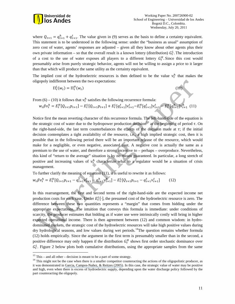
𝑤𝜏𝛽𝜈𝜏ℎ = 𝐸𝜏𝐻[𝑄𝜏+1𝑝𝜏+1]− 𝐸𝜏𝐿[𝑄𝜏+1𝑝𝜏+1] + 𝐸𝜏𝐿[𝑞𝜏+1𝑡 ]𝜈𝜏+1𝑡 −𝐸𝜏𝐻[𝑞𝜏+1𝑡 ]𝜈𝜏+1𝑡 − 𝐸𝜏𝐻[𝑞𝜏+1ℎ ]𝜈𝜏+1ℎ (11) Notice first the mean reverting character of this recurrence formula. The left-hand-side of the equation is the strategic cost of water due to the hydropower production decision13

To further clarify the meaning of equation (11), it is useful to rewrite it as follows:

at the beginning of period 𝜏. On the right-hand-side, the last term counterbalances the effects of the decision made at 𝜏; if the initial decision contemplates a tight availability of the resource, i.e., a high implied strategic cost, then it is possible that in the following period there will be an important release of the resource, which would make for a negligible, or even negative, associated cost. A negative cost is actually the same as a premium to the use of water, and therefore a strong incentive to – perhaps – overproduce. Nevertheless, this kind of “return to the average” situation is by no means guaranteed. In particular, a long stretch of positive and increasing values of 𝜈𝜏ℎ characterize what to a regulator would be a situation of crisis management.

𝑤𝜏𝛽𝜈𝜏ℎ = 𝐸𝜏𝐻[𝑄𝜏+1𝑝𝜏+1 − 𝑞𝜏+1𝑡 𝜈𝜏+1𝑡 − 𝑞𝜏+1ℎ 𝜈𝜏+1ℎ ]− 𝐸𝜏𝐿[𝑄𝜏+1𝑝𝜏+1 − 𝑞𝜏+1𝑡 𝜈𝜏+1𝑡 ] (12) In this rearrangement, the first and second terms of the right-hand-side are the expected income net production costs for each case. Under 𝐸𝜏𝐿[⋅], the presumed cost of the hydroelectric resource is zero. The difference between these two quantities represents a “margin” that comes from bidding under the appropriate expectations. The intuition that conveys this formula is immediate: under conditions of scarcity, the producer estimates that bidding as if water use were intrinsically costly will bring in higher expected operational income. There is then agreement between (12) and common wisdom: in hydro-dominated markets, the strategic cost of the hydroelectric resources will take high positive values during dry hydrological seasons, and low values during wet periods.14

13 This – and all other – decision is meant to be a part of some strategy.

The question remains whether formula (12) holds empirically. Since the argument in the first term is presumably smaller than in the second, a positive difference may only happen if the distribution 𝐺𝜏𝐻 shows first order stochastic dominance over 𝐺𝜏𝐿. Figure 2 below plots both cumulative distributions, using the appropriate samples from the same

14 This might not be the case when there is a smaller competitor counteracting the actions of the oligopolistic producer, as it was demonstrated in Garcia, Campos-Nañez, & Reitzes (2005). In this case, the strategic value of water may be positive and high, even when there is excess of hydroelectric supply, depending upon the water discharge policy followed by the part counteracting the oligopoly.

Working Paper No. 200726900-02 School of Engineering – Universidad de los Andes

Bogotá D.C., Colombia. Wednesday, July 20, 2011

12

time interval, from January 2006 to January 2011. The points that support 𝐺𝜏𝐿 where chosen under the condition that system water levels were above 80% of full system capacity, while those that belong to 𝐺𝜏𝐻 were chosen under the condition that the water level be between 65% and 75% of system capacity. The top of this range is important, because it is the level at which regulatory authorities frequently start issuing warnings about a possible condition of scarcity.

Figure 2. Comparative empirical plots for the cumulative distributions 𝐺𝜏𝐿 and 𝐺𝜏𝐻. The latter shows obvious first order stochastic dominance when the independent variable is realized price.

The difference between the two distributions is equivalent to our main argument that under different expectations about the future availability of water market agents will bid in a different manner. The influence on (11) of the storage-flow formulas given by equations (1) through (4) is not at first glance obvious. Nevertheless, straightforward applications of (11) in idealized situations show that if the producer has considerable water regulation capacity15

The degree of uncertainty in the weather forecast will impact the perceived value of the resource today. Taking clues from this general intuition, in the next section we proceed to check what the recurrence relation (11) can tell, using data from the Colombian power market.

, reservoir levels are not too relevant for his strategic valuation of the hydroelectric resource. This is because, if capacity is really large and the reservoir is nearly full, it might take many periods of no rain before the cost of water is of any importance. On the other hand, a run-of-the-river producer will be immediately affected by the water inflows and the reservoir levels after following a specific production strategy.

5. EVIDENCE FROM THE COLOMBIAN POWER MARKET In this section, we use the historic data from the Colombian power market as a laboratory to show the relevance the concept embodied by equation (11). Using this equation, we develop a time series

0

0,2

0,4

0,6

0,8

1

0 50 100 150 200 250 300 350

Prob

abili

ty

Price (in COP/kwh)

Comparative plot cumulative distributions GH vs. GL

GH

GL

Working Paper No. 200726900-02 School of Engineering – Universidad de los Andes

Bogotá D.C., Colombia. Wednesday, July 20, 2011

13

following a backwards induction approach. The necessary factors are estimated from past known time series for prices, thermal costs and volumes.16

Before 1995, the electricity in Colombia was supplied following a vertically integrated architecture. A centralized state-owned enterprise minimized variable costs of production declared by power producers. The economic inefficiencies of that scheme opened the door to the deregulation trend then sweeping the international power markets.

In aggregate terms, daily demand is typically in the range 0.13 to 0.17 Twh, and hydro system capacity normally stands in the range of 13 to 15 Twh. Depending on the particular weather and demand circumstances, hydro electricity provides from 50% up to 90% of total demand.

17

From its origin, a neutral regulatory policy regarding the technological preferences of the system has driven the capacity expansion of the national interconnected system; however, the large hydrologic resources within the national territory have favored hydro-dominated power generation. This particular feature has exposed the power supply system to abnormally dry events like the ENSO.

This reform was aimed at overcoming the following market inefficiencies: (i) the inaccurate power generation costs declared by power producers (mostly hydro); (ii) two major national blackouts in 1983 and between 1992 and 1993, due to inefficient water management policies from the central coordinator; (iii) the public finance constraints threatening the capacity headroom of the overall system. This centralized scheme was transformed into an unbundled/decentralized architecture, and the injection of private capital was allowed across most levels of the supply chain. The reform set a competitive market environment for wholesale power producers, which was further extended to power retailers. Power transmission and distribution remain regulated as natural monopolies, given their network economies.

18 This hydro-dominated feature of the technological park, combined with the capital structure of the power generation business, lead to an oligopolistic market structure in Colombia. Recent estimations of the Herfindahl-Hirschman Index19

15 We refer to the water regulation capacity of a hydroelectricity power producer as the ability to shift water from one time period to another. It depends on both its water storage capacity and its turbine output capacity. Henceforth it will be associated to the ratio 𝛿 𝛽� .

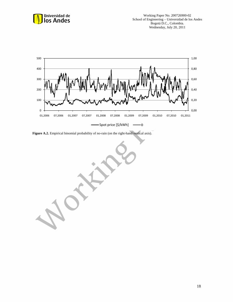
calculated as the market share of the (monthly) aggregated power generation in Colombia, show the index usually takes values between 1500 and 1600. However, it may oscillate between 1200 during extreme dry events and 1800 during abnormally wet seasons. This is evidence of not only a concentrated power generation market, but also an increased market power potential whenever there is excess of hydroelectricity supply. Additional evidence of the assumption of oligopolistic behavior by the hydro-dominated power generators in the Colombian market is provided in Figure A.3 (Appendix A). The daily load profile in Colombia is mainly driven by the residential sector; it presents its peak profile between the hours 18 and 20. The electricity demand during this time period tends to be relatively inelastic in the short-term, compared to off-peak periods. The upper graph in Figure A.3 sketches the median, lower and upper quartiles for the variable. Below this graph, the hydroelectric production profile for two anonymous generators A and B are plotted in the middle and lower graphs. These power plants belong to different owners holding significant shares of the installed capacity. Even when producer B holds about half the installed power capacity of producer A, its water

16 All the data for this section, and throughout the paper, are publicly available from the “NEON” database at www.xm.com.co. 17 See (Alzate, Cadena, Benavides, & Castro, 2011) for further details. 18 ENSO is the acronym for El Niño-Southern Oscillation. 19 It is a widely accepted indicator of market concentration taking into account the relative size and distribution of companies in a market. See http://www.justice.gov/atr/public/testimony/hhi.htm

Working Paper No. 200726900-02 School of Engineering – Universidad de los Andes

Bogotá D.C., Colombia. Wednesday, July 20, 2011

14

regulation capacity ratio is greater than that of producer A. As it can be observed in Figure A.3, producer B tends to shift the storable hydroelectric resources according to his strategic water valuation from relatively inelastic demand periods to relatively elastic ones. On the contrary, given its technological features, it is not profitable for the run-of-the-river producer A to follow the same strategy. To estimate the strategic cost of hydroelectric resources, we begin at a point where the hydrology guarantees an excess of hydroelectric supply. We then proceed to take this point as the reference level, i.e. 𝜈ℎ = 0. The chosen point lies within the severest time interval of the most recent La Niña event, in December 2010.20

In expression (11) we use the actual hydroelectric production of the aggregated market as a proxy for 𝑤𝜏𝛽. The expectation 𝐸𝜏𝐻[𝑄𝜏+1𝑝𝜏+1] comes from the revenue actually realized by the aggregated market. That is, under the assumption that hydroelectric power producers in Colombia behave as an oligopoly that effectively perceive a strategic cost for the storable resource.

Then, the series {𝑣𝜏ℎ} is estimated by backward iteration of the terms in (11) with their corresponding proxies.

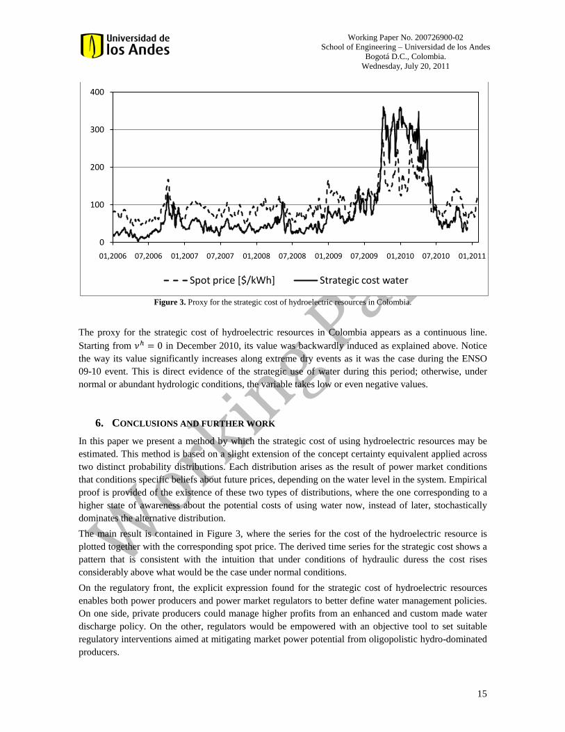
The proxy used for 𝐸𝜏𝐿[𝑄𝜏+1𝑝𝜏+1] is harder to estimate. We use the average revenue in the last event when it was perceived excess of hydroelectric supply by producers. The decision as to when to declare an “excess” of hydro power supply is somewhat arbitrary, but inspection of the empirical cumulative probability distribution of the hydroelectric production share indicates this threshold should be at about 80% of the system load (see Figure A.1 in Appendix A). Similar approaches were followed to derive the proxies for the terms 𝐸𝜏𝐻[𝑞𝜏+1𝑡 ] and 𝐸𝜏𝐿[𝑞𝜏+1𝑡 ]. In the first case, it is used the production associated to the thermoelectric production after the actions actually followed by the aggregated market. In the other case, the inspection of the empirical probability distribution of the thermal production share suggests the thermoelectric threshold should be about 20%. The result of the procedure just described is presented in Figure 3.21 It displays the evolution of electricity spot prices in Colombia (dashed line) and the impact the last ENSO event22

20 The calibration issue raised by this choice is not a serious problem, since this model does not seek to forecast, but rather to provide early diagnostics.

had on them.

21 The trajectories sketched in Figure 2 correspond to weekly moving average values in order to avoid unnecessary noise. 22 Due in part to the ENSO event, frequent regulatory interventions had some impact on the market signals throughout this time interval. See (Alzate, Cadena, Benavides, & Castro, 2011) for further details.

Working Paper No. 200726900-02 School of Engineering – Universidad de los Andes

Bogotá D.C., Colombia. Wednesday, July 20, 2011

15

Figure 3. Proxy for the strategic cost of hydroelectric resources in Colombia.

The proxy for the strategic cost of hydroelectric resources in Colombia appears as a continuous line. Starting from 𝜈ℎ = 0 in December 2010, its value was backwardly induced as explained above. Notice the way its value significantly increases along extreme dry events as it was the case during the ENSO 09-10 event. This is direct evidence of the strategic use of water during this period; otherwise, under normal or abundant hydrologic conditions, the variable takes low or even negative values.

6. CONCLUSIONS AND FURTHER WORK In this paper we present a method by which the strategic cost of using hydroelectric resources may be estimated. This method is based on a slight extension of the concept certainty equivalent applied across two distinct probability distributions. Each distribution arises as the result of power market conditions that conditions specific beliefs about future prices, depending on the water level in the system. Empirical proof is provided of the existence of these two types of distributions, where the one corresponding to a higher state of awareness about the potential costs of using water now, instead of later, stochastically dominates the alternative distribution. The main result is contained in Figure 3, where the series for the cost of the hydroelectric resource is plotted together with the corresponding spot price. The derived time series for the strategic cost shows a pattern that is consistent with the intuition that under conditions of hydraulic duress the cost rises considerably above what would be the case under normal conditions. On the regulatory front, the explicit expression found for the strategic cost of hydroelectric resources enables both power producers and power market regulators to better define water management policies. On one side, private producers could manage higher profits from an enhanced and custom made water discharge policy. On the other, regulators would be empowered with an objective tool to set suitable regulatory interventions aimed at mitigating market power potential from oligopolistic hydro-dominated producers.

0

100

200

300

400

01,2006 07,2006 01,2007 07,2007 01,2008 07,2008 01,2009 07,2009 01,2010 07,2010 01,2011

Spot price [$/kWh] Strategic cost water

Working Paper No. 200726900-02 School of Engineering – Universidad de los Andes

Bogotá D.C., Colombia. Wednesday, July 20, 2011

16

Our findings indicate oligopolistic producers tend to further exacerbate market outcomes bidding spikier prices according to the hydrologic scenarios when the price risk exposition is low, and contrarily, muffling either positive or negative market spikes whenever this risk exposition is significant. On the other hand, our findings indicate oligopolistic power producers tend to shift the storable hydroelectric resources according to its strategic water valuation from relatively inelastic demand periods to relatively elastic ones. The data from the Colombian power market was successfully used as a test bed to evidence both outcomes. Hence, and from a regulatory perspective aimed to control the market power potential from hydro-dominated oligopolistic power producers, the following can be suggested. First, bounds to the electricity served through bilateral contracts must be introduced. This measure will seek to avoid biased price bids and thus misleading market signals. This would also promote auto-regulatory behavior. Second, considering the current technological trend of positioning the demand side as an active market participant, the elasticity of the load individually served by oligopolistic producers might be affected using demand response programs (e.g. disconnecting consumers). This would set incentives for the producers to behave competitively. These interventions may improve the allocation of hydroelectric resources through time and would harmonize positively with the pro-competitive technological changes currently taking place (e.g. smart grids) to further exploit the advantages of market places. They would also prevent from going back to the centrally administrated institutional settings with a unique public firm allocating the resource. Our work might be further developed in different directions. For instance, the expression for the strategic cost of hydroelectric resources is suited for dynamic programming applications. Moreover, the impact associated to inflow and demand uncertainty might be further studied writing the expression (11) in terms that more explicitly include the water reservoir balance equations and the water regulation capacity of the plants. In this paper, these two aspects do not show in the application of (11) made in section 5, due to the fact that our approach follows the general outline of the “representative agent” model, and we use point estimates and short-term moving averages to construct Figure 2. Finally, the strategic cost of hydroelectric resources is dynamic and involves multiple time scales like that of the hydrologic seasons, the time resolution of the market where electricity is traded as well as that of the elasticity of load to be served. This value is thus affected by the time resolution and by its transition throughout overlapping time scales. This could be the object of further research.

How sensitive is 𝜈ℎ to the various producer parameters? This is perhaps one of the most interesting questions that may be addressed from a regulatory point of view. The answer to this question allows for an assessment based on technological fundamentals of the implied non-financial costs of opportunity that affect a hydro dominated producer’s decisions.

ACKNOWLEDGEMENTS We wish to thank helpful comments made by Professor J. P. Amigues from the Toulouse School of Economics on an earlier version of this paper.

Working Paper No. 200726900-02 School of Engineering – Universidad de los Andes

Bogotá D.C., Colombia. Wednesday, July 20, 2011

17

REFERENCES Alzate, J. M., Cadena, A. I., Benavides, J. M., & Castro, A. H. (2011). A second thought about the Colombian power market. Working Paper No. 200726900-03 School of Engineering. Universidad de los Andes. Ambec, S., & Doucet, J. (2003). Decentralizing hydropower production. The Canadian Journal of Economics, 36(3) 587-607. Crampes, C., & Moraux, M. (2001). Water resource and power generation. International Journal of Industrial Economics , 975-997. Forsund, F. (2006). The anatomy of market power in electricity markets with hydropower as a dominating technology. ICER Working Paper No. 21. Garcia, A., Campos-Nañez, E., & Reitzes, J. (2005). Dynamic pricing and learning in electricity markets. Operations Research , 53(2) 231-241. Garcia, A., Reitzes, J., & Stacchetti, E. (2001). Strategic pricing when electricity is storable. Jorunal of Regulatory Economics , 20(3) 223-247. Hansen, P. (2009). Inflow uncertainty in hydropower markets. The Scandinavian Journal of Economics , 111(1) 189-207. Hoel, m. (2004). Electricity prices in a mixed thermal and hydropower system. Department of Economics. University of Oslo. Memorandum No. 28 ISSN: 0801-1117.

Pereira, M. (1989). Optimal stochastic operations scheduling of large hydroelectric systems. Electrical Power and Energy Systems , 11(3) 161-169. Wolfgang, O., Haugstad, A., Moa, B., Gjelsvik, A., & Wangensteen, I. (2009). Hydro reservoir handling in Norway before and after deregulation. Energy , 34 1642-1651.

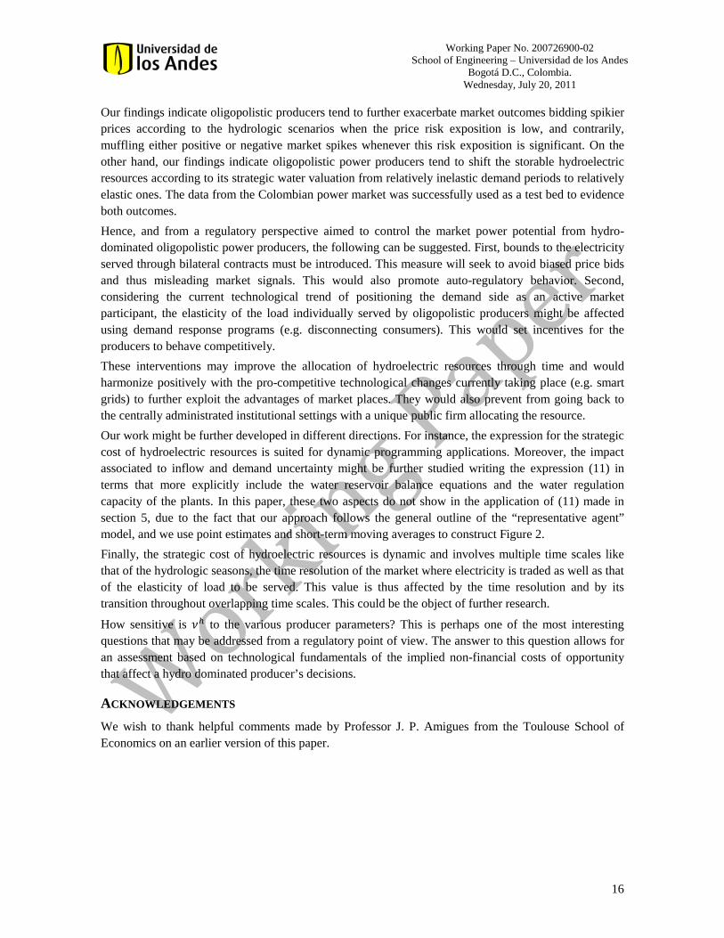
APPENDIX A

Figure A.1. Empirical cumulative probability distribution for the hydroelectricity production share in Colombia.

Time interval: January 2006 – January 2011.

0%

20%

40%

60%

80%

100%

0% 20% 40% 60% 80% 100%

Prob

abili

ty

Hydroelectricity production share

Working Paper No. 200726900-02 School of Engineering – Universidad de los Andes

Bogotá D.C., Colombia. Wednesday, July 20, 2011

18

Figure A.2. Empirical binomial probability of no-rain (on the right-hand vertical axis).

0,00

0,20

0,40

0,60

0,80

1,00

0

100

200

300

400

500

01,2006 07,2006 01,2007 07,2007 01,2008 07,2008 01,2009 07,2009 01,2010 07,2010 01,2011

Spot price [$/kWh] θ

Working Paper No. 200726900-02 School of Engineering – Universidad de los Andes

Bogotá D.C., Colombia. Wednesday, July 20, 2011

19

Figure A.3. Evidence of hydro-dominated oligopolistic behavior within the Colombian power market.

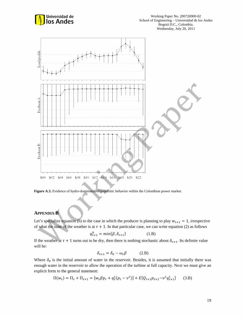
APPENDIX B Let’s specialize equation (6) to the case in which the producer is planning to play 𝑤𝜏+1 = 1, irrespective of what the state of the weather is at 𝜏 + 1. In that particular case, we can write equation (2) as follows

𝑞𝜏+1ℎ = 𝑚𝑖𝑛{𝛽, 𝛿𝜏+1} (1.B) If the weather at 𝜏 + 1 turns out to be dry, then there is nothing stochastic about 𝛿𝜏+1. Its definite value will be:

𝛿𝜏+1 = 𝛿0 − 𝜔𝜏𝛽 (2.B) Where 𝛿0 is the initial amount of water in the reservoir. Besides, it is assumed that initially there was enough water in the reservoir to allow the operation of the turbine at full capacity. Next we must give an explicit form to the general statement:

Π(𝑤𝜏) = Π𝜏 + Π𝜏+1 = [𝑤𝜏𝛽𝑝𝜏 + 𝑞𝜏𝑡(𝑝𝜏 − 𝑣𝑡)] + 𝐸[𝑄𝜏+1𝑝𝜏+1−𝑣𝑡𝑞𝜏+1𝑡 ] (3.B)

Working Paper No. 200726900-02 School of Engineering – Universidad de los Andes

Bogotá D.C., Colombia. Wednesday, July 20, 2011

20

The aim of this example is to calculate an optimal value for 𝜔𝜏 that is nontrivial, for some chosen set of reasonable values for all producer specific parameters and form representative (of the local market) set of inverse demand functions. For the present purpose let’s decompose expectations in the following manner:

𝐸[𝑥] ≡ 𝜃𝐸[𝑥] + (1− 𝜃)𝐸[𝑥] (4.B)

The first term on the right-hand-side is the product of the objective probability of no-rain for the next time period, multiplied times the expectations operator, conditional on no-rain for the next period realized prices. A parallel interpretation applies to the second term. The application of definition (4.B) to equation (3.B) above requires an explicit expression for each term on the right-hand-side. The appropriate expansions are as follows:

𝐸[𝑄𝜏+1𝑝𝜏+1−𝑣𝜏+1𝑡 𝑞𝜏+1𝑡 ] = 𝑞𝜏+1ℎ 𝐸[𝑝𝜏+1] + 𝑚𝑖𝑛�𝛼,𝐷 − 𝑞𝜏+1ℎ �𝐸[𝑚𝑎𝑥{𝑝𝜏+1 − 𝑣𝜏+1𝑡 , 0}] (5.B1)

And

𝐸[𝑄𝜏+1𝑝𝜏+1−𝑣𝜏+1𝑡 𝑞𝜏+1𝑡 ] = 𝛽𝐸[𝑝𝜏+1] + (𝐷 − 𝛽)𝐸[𝑚𝑎𝑥{𝑝𝜏+1 − 𝑣𝜏+1𝑡 , 0}] (5.B2)

Notice that under the no-rain expectation, the amount of hydro energy produced is generally more cautiously decided than in the alternative scenario. In the case of equation (5.B2) there is the assumption that under the state “rain” for the second period there will be more than enough water, and therefore the turbine could operate at full capacity, according to equation (1.B). This fact should be enough to make the result of (5.B2) to be much less dependent on the production decision made in period 𝜏. Therefore, it is more fruitful to concentrate on the effects of expression (5.B1).

We make here the approximation that most of the support of 𝐸[∙] is well above 𝑣𝜏+1𝑡 . Within this approximation, we get:

𝐸[𝑚𝑎𝑥{𝑝𝜏+1 − 𝑣𝑡, 0}] ≈ 𝐸[𝑝𝜏+1] − 𝑣𝜏+1𝑡 (7.B) The fact that the oligopoly has both enough information and market power in period 𝜏 translates into its having the best estimate for the inverse demand functions of both 𝑝𝜏 and 𝐸[𝑝𝜏+1]. This last assumption, together with the set of equations displayed above, allows for a numerical exploration of the issue whether there are interior solutions for the maximum of Π(𝑤𝜏). As a showcase example, we use the following set of typical data: 𝐷 = 1.0; 𝛽 = 0.7; 𝛼 = 0.4; 𝛿0 = 0.9; 𝜃 = 0.5. Notice that all demand and production parameters are normalized by the size of demand. For the inverse demand functions, we choose the following model, which replicates roughly the general behavior of the response of prices to supply by a large hydro generator.

𝑝𝜏 = 400(2+𝛿𝜏) ; 𝐸[𝑝𝜏+1] = 400

(2+𝛿𝜏+1)

If the numerical values are taken in local monetary units, these functions mimic the typical range of prices in any particular day for hour 18 in the Colombian electricity market. And finally, a typical thermal cost for all periods is 𝑣𝑡 = 80.

Working Paper No. 200726900-02 School of Engineering – Universidad de los Andes

Bogotá D.C., Colombia. Wednesday, July 20, 2011

21

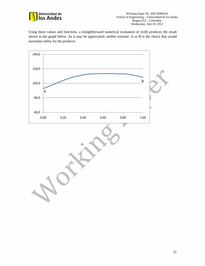
Using these values and functions, a straightforward numerical evaluation of (4.B) produces the result shown in the graph below. As it may be appreciated, neither extreme: A or B is the choice that would maximize utility for the producer.

60,0

80,0

100,0

120,0

140,0

0,00 0,20 0,40 0,60 0,80 1,00

A

B