FINAL TECHNICAL REPORT - HNEI

1

FINAL TECHNICAL

REPORT

Hawaii Energy and Environmental

Technologies Initiative

Office of Naval Research

Grant Award Number N00014-11-1-0391

For the period January 1, 2011 to September 30, 2016

September 2016

2

Table of Contents

EXECUTIVE SUMMARY ...................................................................................................................3

Task 1. FUEL CELL SYSTEMS ..........................................................................................................8

1.1 Fuel Cell Testing and Evaluation ..................................................................................... 8 1.2 Novel Fuel Cells ................................................................................................................. 54

Task 2. TECHNOLOGY FOR SYNTHETIC FUELS PRODUCTION ............................................57

2.1 Plasma Arc Processing ....................................................................................................... 58 2.2 Thermocatalytic Conversion of Synthesis Gas into Liquid Fuels ...................................... 78

2.3 Novel Solvent Based Extraction of Bio-oils and Protein from Biomass ........................... 78 2.4 Biochemical Conversion of Biomass Syngas into Liquid Fuels ........................................ 80 2.5 Biocontamination of Fuels ................................................................................................. 92

2.6 Biofuel Corrosion ............................................................................................................... 96 2.7 Waste Management Using the Flash-Carbonization

TM Process ....................................... 109

Task 3. METHANE HYDRATES ...................................................................................................110

Task 4. OCEAN ENERGY ...............................................................................................................156

4.1 Ocean Thermal Energy Conversion (OTEC) ................................................................... 156

4.2 Sea Water Air Conditioning (SWAC) .............................................................................. 157

Task 5. STORAGE TECHNOLOGY ...............................................................................................159

5.1 Distributed Storage Systems Testing ............................................................................... 160

5.2 Grid Scale Storage Systems Testing ................................................................................ 173

Task 6. PHOTOVOLTAICS EVALUATION ..................................................................................182

Task 7. HYDROGEN SYSTEMS ....................................................................................................209

7.1 Demonstration Hydrogen Fueling Technology at Marine Corps Base Hawaii ................ 209

7.2 Island of Hawaii Integrated Hydrogen Systems ............................................................... 230 7.3 Hawaii Military Biofuels Crop Assessment ..................................................................... 234 7.4 Alternative Hydrogen Production Assessment for Hawaii .............................................. 235

Task 8. ENERGY-NEUTRAL ENERGY TEST PLATFORMS .....................................................296

8.1 Off-Grid/Energy-Neutral Test Platform ........................................................................... 297 8.2 Platform Monitoring and Performance Analysis .............................................................. 306

8.3 Advanced Database Research, Development and Testing (RD&T) ................................ 309

8.4 Energy-Efficient End-Use Technologies: Desiccant Dehumidification ...................... 312

Task 9. ALGAL PRODUCTION STUDIES ....................................................................................317

3

Final Technical Report

Hawaii Energy and Environmental Technologies Initiative

Grant Award Number N00014-11-1-0391

January 1, 2011 to September 30, 2016

EXECUTIVE SUMMARY

This report summarizes work conducted under Grant Award Number N00014-11-1-0391, the

Hawaii Energy and Environmental Technologies Initiative 2010 (HEET10), funded by the Office

of Naval Research (ONR) to the Hawaii Natural Energy Institute (HNEI) of the University of

Hawaii at Manoa (UH). The overall objective of HEET10 effort was to use Hawaii as a model

for development, testing, and integration of distributed energy systems for the Pacific Region.

HEET10 included efforts to meet critical technology needs of the Navy associated with fuel cell

testing and evaluation, synthetic fuels processing and production to accelerate the use of liquid

biofuels for Navy needs, the extraction and stability of seabed methane hydrates, and alternative

energy systems. Testing and evaluation of alternative energy systems includes work on Ocean

Thermal Energy Conversion (OTEC), grid-scale battery energy storage, support for hydrogen

fuel operations at the Marine Corps Base Hawaii and on the Island of Hawaii, building energy

efficiency test platforms, and end-use high value energy efficiency technologies.

Tasks are summarized below, with all technical reports as well as publications produced through

these efforts available on HNEI’s website at http://www.hnei.hawaii.edu/node/346.

Under Task 1, subtask 1.1, new diagnostic capabilities for fuel cell testing and evaluation were

added and the evaluation of stacks for UUV and UAV applications continued. The use of

pressure swing adsorption technology to remove airborne contaminants was investigated as a

replacement for incumbent air filters. Rapid, ex situ catalyst and membrane materials screening

capabilities were implemented to isolate contaminant impacts on fuel cell performance. Gas

analysis capabilities were upgraded with the commissioning of a gas chromatograph/mass

spectrograph to identify contaminant decomposition reactions within a fuel cell. A prototype

tracer system was acquired to quantify product liquid water, assess the extent of flow field

channel blockages by the intrusion of flexible gas diffusion media, and determine the existence

of flow bypass and uneven flow distribution lowering cell efficiency. The potential of voltage

noise measurements to identify, in real time, specific failure modes was explored. An adaptable

reactant gas recirculation system representative of real system operating conditions was built to

study water and contaminant accumulation processes. A commercial automotive fuel cell stack

design was adapted for operation in an oxygen-fed UUV. The effect of duty cycling on the

durability of a commercial stack for a UAV application was determined by comparing load

following (fuel cell system) and constant load (fuel cell/battery hybrid system) cases. HNEI also

conducted testing of NRL’s variable current battery discharge method intended to improve the

specific energy of a lithium-ion battery pack.

Under subtask 1.2, Novel Fuel Cells, thin films suitable for biofuel cell electrodes were

fabricated from unique materials comprised of modified chitosan polymer. Results showed that

films of controlled thickness could be reproducibly produced using the technique of spread-

coating, and that chemical modification of the chitosan biopolymer with hydrophobic chemical

http://www.hnei.hawaii.edu/node/346

4

groups could extend the range over which a linear response between film thickness and

deposition rate could be achieved. These results were deemed important as having the ability to

understand how the introduction of hydrophobic modification - a technique shown to introduce

solution-based micelle structure and micellar aggregates that support enzyme immobilization -

affects film thickness and morphology of spread coated thin films will aid the long term

development and deployment of chitosan-based biofuel cell electrodes.

Task 2, Technology for Synthetic Fuels Production sought to identify and address issues related

to liquid biofuel variability caused by primary feedstock sources, conversion methods, storage

methods, or the presence of contaminants.

Subtask 2.1 focused on plasma reforming of renewable biogas to produce hydrogen rich streams that

can be upgraded for fuel cell applications. Additionally hydrogen sulfide contamination was

characterized. For this investigation, a non-thermal plasma reactor was modified and parametric

tests, factorial tests, and response surface methodology was conducted sequentially to identify

optimum reactor operating conditions to minimize specific energy requirements.

The thermocatalytic production of hydrocarbons from synthesis gas was examined in subtask

2.2, with emphasis on catalyst evaluation. The effects of pore size on ruthenium-silica catalyst

performance were investigated for Fischer–Tropsch synthesis, and the catalysts were

characterized. The addition of small amounts of zirconium and manganese improved catalytic

activity and stability for Fischer–Tropsch synthesis. Results were published and are available on

HNEI’s website.

Under subtask 2.3, novel solvents to extract bio-oils and proteins from biomass were

investigated. The three objectives were to quantify a 1-step extraction of phorbol esters from oil

seeds using a hydrophilic co-solvent system, determine the extent to which the phorbol esters can

be recovered from the co-solvent, and determine the extent to which the extracted biomass is

toxin-free and suitable as an animal feed.

The objective of subtask 2.4 was to investigate biochemical pathways for conversion of synthesis

gas into liquid fuel molecules (gasoline and diesel fuels). Unique microbial species were used to

convert syngas to a mid-stage product. Fuel costs could be reduced by reusing the hydrolysates

of cell debris, however current biodiesel production through microbial carbon dioxide fixation

was found to be economically infeasible.

Subtasks 2.5 and 2.6 were focused on fit-for-purpose testing of biofuels to determine their

susceptibility to biocontamination and propensity for creating biocorrosion, respectively. In

subtask 2.5, biocontamination of fuels, two isolates from a petroleum-contaminated sample were

used to study the biodegradation of sulfur containing hydrocarbon inherently present in all diesel

fuels. Glycerol was found to stimulate both rhamnolipid production and dibenzothiophene

degradation, and optimal molar ratios were determined. Under subtask 2.6, the influence of

fungi on the corrosion of 1018 steel was investigated. The influence of the fungi Paecilomyces

saturatus on the corrosion of 1018 steel was investigated in B100, B20, and ULSD fuel-water

mixtures for a three-month exposure. The 1018 steel coupons remained in the passive state (due

to the presence of the air-formed oxide film) in the B100 and B20 fuel-water mixtures; whereas,

the 1018 steel coupons corroded actively in the ULSD fuel-water mixture. The presence of

5

biodiesel appeared to have a beneficial effect on corrosion even in the presence of the fungi.

Corrosion rates decreased as the biodiesel content in the fuel-water mixtures increased. For all

cases where the steel actively corroded, the thick layer of iron corrosion product was identified

as lepidocrocite.

Subtask 2.7 explored using the Flash-CarbonizationTM

process to covert waste streams into

carbon products. Fundamental measurements of carbon yield as a function of conversion

technology and process parameters were determined using corncob as a model fuel. Elevated

pressure secured the highest fixed-carbon yields. Findings show that secondary reactions

involving vapor-phase species are at least as influential as primary reactions in the formation of

charcoal. Size reduction handling of biomass, significantly reduces the fixed-carbon yield, with

whole corncob carbonized at elevated pressure producing the highest yield of charcoal. By

comparison, fluidized-bed and transport reactors cannot realize high yields of charcoal from

biomass. Results have been published in a journal paper and are available on HNEI’s website.

Task 3 work on methane hydrates focused on methane hydrate stability and related

environmental issues; hydrogen fuel storage in binary hydrates; and promoting international

research collaborations. Fundamental laboratory studies were performed on hydrate formation

and dissociation in porous media and determining the effects of transition metal salts on hydrate

behavior. Hydrates that form in relatively fine sands were found to melt at lower temperatures

than hydrates that occur in larger void spaces. Most of the transition metal salts tested in the

present study inhibited methane hydrate formation at high concentrations, but none to the extent

of sodium chloride except for ferric chloride. As a continuation of our studies of the

microbiology of methane and other hydrocarbons in seafloor sediments and the oceanic water

column, a novel gas-tight bioreactor was designed and fabricated. The purpose of this bioreactor

was to increase target microorganism density to levels required to investigate microbial methane

cycling. During HEET 10, an investigation also was initiated to explore the use of gas hydrates

as a storage medium for hydrogen fuel for propulsion applications, and laboratory facilities and

protocols were designed, fabricated, and tested. Finally, to foster international collaborative

R&D on methane hydrates, HNEI supported and helped to organize the 8th

and 9th

International

Workshops on Methane Hydrate R&D.

Task 4, ocean energy focused on continued development of OTEC heat exchanger technology

(subtask 4.1), and analysis and testing to support development of lower cost Sea Water Air

Conditioning (subtask 4.2). HNEI subcontracted Makai Ocean Engineering to provide heat

transfer performance; and corrosion and biofouling testing of heat exchangers for use in OTEC

power plants. Makai completed the design, fabrication, installation, and performance testing of

the Lockheed Martin Graphite Foam heat exchanger. However it did not have the anticipated

improvement in performance compared to the plain shell and tube design. The Lockheed Martin

Enhanced Tube heat exchanger was also designed, fabricated, installed, and performance tested,

and showed a significant improvement in performance verses the plain tube heat exchanger.

Additionally, three years of corrosion testing was concluded on hollow extrusion samples.

Subtask 4.2 characterized environmental conditions within the receiving waters of a Seawater

Air Conditioning (SWAC) system. This included discharge plume analysis conducted by Makai

6

Ocean Engineering as well as procurement of three wave buoys to support future time series

water quality analysis in support of SWAC development.

Task 5 involved laboratory and field efforts to investigate battery energy storage. Under subtask

5.1 Lithium-ion batteries were evaluated to minimize battery cell degradation at the cell and

small-pack level for grid energy storage applications. Key performance metrics of alternative

Lithium-ion cell chemistries were explored including cycle life, useable energy and power,

power energy density, and power efficiencies. It was found that batteries with titanate negative

electrodes have better capacity retention than batteries using graphite. Titanate based batteries

were investigated further and their durability against mild overcharge was established. It was

shown that, upon overcharge, these cells are prone to some gassing and that it could limit their

performance if the gas remained trapped in-between electrodes. This effort allowed the

invention of a new patent-pending methodology for online state of health tracking that could be

applicable to large Battery Energy Storage (BESS) systems. In order to be able to test the larger

cells used in the grid-scale BESS, HNEI established a new battery testing laboratory within the

Hawaii Sustainable Energy Research Facility and expanded existing software tools to visualize

characteristics of cell chemistry performance and degradation.

Under subtask 5.2, research continued on three grid-connected battery energy storage systems

intended to assess range of ancillary services under different grid operational conditions on three

islands. Research efforts for the Hawaii Island grid primarily focused on regulating grid

frequency using an Altairnano 1MW, 250kWh battery system procured and installed under

HEET09. HEET10 findings illustrated how local battery storage support of the 10MW Hawi

wind farm can cause grid-wide issues. However, it was found that battery cycling can be greatly

reduced to extend lifetime while still providing a significant portion of the grid-wide benefit. A

second Altairnano 1MW, 250kWh BESS was procured, installed on Oahu, and tested to

simultaneously provide power smoothing as well as voltage regulation within an electric

substation serving large industrial loads. A third BESS was installed on Molokai, an Altairnano

2MW, 397kWh system, and facility acceptance testing completed. Testing and evaluation of the

BESS located on Oahu and Molokai will be conducted under future APRISES awards.

Under Task 6, grid-connected PV systems on Oahu and Maui were evaluated. Continuing

previous ONR-funded work, performance and durability of different PV and inverter

technologies under differing environmental conditions were characterized. The PV systems

under test represent grid-connected, residential and small-scale commercial systems. This work

has created a framework of knowledge on PV test platform design, installation, testing,

instrumentation and data analysis methodologies. Accomplishments under HEET10 include

development of new test protocols and data collection methodologies,; installation of a carport-

based PV test platform in South Maui, advancement of data analysis tools, including an

innovative dissociation of the DC performance ratio into current and voltage performance, and

detailed analysis of the first month of performance data from the Maui site and a year of data

from UH Manoa. Data collection and analysis from both sites will continue under future

APRISES awards.

Task 7 focused on four main areas of hydrogen development: fueling support and analysis for the

Navy/Marine Corps demonstration fuel cell vehicle project on Oahu; fueling support for the

7

forthcoming operation of demonstration fuel cell buses at Hawaii Volcanoes National Park on

Hawaii Island with a hydrogen dispensing system; assessment of the capacity for production of

hydrogen and biomass from agriculture in Hawaii, and; assessment of alternative pathways to

meet the projected growth in demand for hydrogen in Hawaii, mainly gasification of municipal

solid waste and importation of natural gas in small-scale container vessels.

Under subtask 7.1 HNEI supplied hydrogen in support of the Navy/Marine Corps demonstration

of General Motors Equinox fuel cell electric vehicles, first using hydrogen imported from the

mainland and then via operation of a dual pressure 350/700 bar fast fill hydrogen fueling station

at the Marine Corps Base Hawaii. This subtask also included analysis of the station’s technical

performance.

In anticipation of the future deployment of two hydrogen fuel cell shuttle buses at Hawaii

Volcanoes National Park, a high air contaminant environment, subtask 7.2 supported

development of a hydrogen dispensing system on the Island of Hawaii. The buses will be used

to test a novel (patent pending) air filtration system developed by HNEI to protect the shuttle bus

fuel cell power systems from airborne contaminants. In future operations, hydrogen will be

delivered from the Natural Energy Laboratory Hawaii Authority located on the west side of the

island using hydrogen transport trailers. Additionally under this subtask, a hydrogen dispenser

boost pump system was developed and tested to reduce hydrogen transport costs.

Subtask 7.3 explored production of hydrogen fuel from agriculture in Hawaii as an alternative to

importing oil. Pacific Biodiesel Technologies was contracted to conduct an operations sensitive

assessment of the capacity for the local production of fuels and biomass to assess the potential

for DOD operations and/or hydrogen production. The project site was transitioned from Oahu to

Hawaii Island in order to support the Navy and US Department of Agriculture goal of

establishing a biofuels commercialization program. The project emphasized broad assessments

of the potential agricultural crop production, products and co-products, and process technologies

available to produce advanced biofuels on Hawaii Island.

Subtask 7.4 assessed alternative pathways to meet the projected growth in demand for hydrogen

in Hawaii, primarily gasification of municipal solid waste and importation of natural gas in

small-scale container vessels. Technology and economic issues were addressed and

recommendations put forth for development of hydrogen infrastructure with capacity to meet

potential targeted demand to produce hydrogen for fuel cell vehicles.

Task 8 included four topics relating to energy efficiency in buildings. Under subtask 8.1 two

second-generation energy-neutral test platforms were designed and installed by Project Frog of

San Francisco on the UH Manoa campus. Construction was completed and the University began

to use the platforms as functioning classrooms in August 2016. Under subtask 8.2 two Project

Frog platforms installed at the Kawaikini New Century Public Charter School on Kauai were

monitored. Actual performance was compared to the predictive models developed during the

design phase. Under subtask 8.3, MKThink was contracted to develop a data management

platform to improve the acquisition, management and analysis of structured and unstructured

data in order to improve decisions related to sustainable energy solutions. Subtask 8.4 focused

on an evaluation of available desiccant dehumidification technologies and their potential

8

applications to improve thermal comfort in tropical and subtropical environments. As part of

this assessment, energy-saving air-management processes were evaluated considering technical

and economic aspects pertinent to retrofits and new building development in Hawaii. .

Task 9, Algal Production Studies focused on improving the economics of mixotrophic growth

systems through exploration of four areas: Environmental Controls, Organic Acids Feeding

Strategies, Lipid Accumulation Strategies, and Strain Sourcing and Selection. HNEI

subcontracted this effort to Hawaii BioEnergy to source indigenous microalgae and test in

laboratory and outdoor open cultures.

Task 1. FUEL CELL SYSTEMS

Under Task 1.1 of Fuel Cell Systems, HNEI conducted testing and evaluation of single cells to

examine the impact and mitigation of airborne contaminants; on performance, mitigation

measures; evaluated the performance of fuel cell stacks in support of Naval Research Laboratory

(NRL) development of UUV and UAV systems; and conducted testing of NRL’s variable current

battery discharge method intended to improve the specific energy of a lithium-ion battery pack.

Under Task 1.2, HNEI continued development of novel fuel cells focusing on thin films for

biofuel cell electrodes fabricated from modified chitosan polymer. Hydrophobic modification to

introduce solution-based micelle structure and micellar aggregates that support enzyme

immobilization was analyzed for the effect on film thickness and morphology.

1.1 Fuel Cell Testing and Evaluation

Work performed under previous ONR awards focused on the understanding, performance, and

durability of fuel cell systems subject to harsh environments, and issues associated with UUV

and UAV fuel cell systems. Work under HEET10 focused on the development of new fuel cell

diagnostics for improved understanding of contamination processes in single fuel cells, fuel cell

stacks and for fuel cell system level issues.

Ex-situ catalyst and membrane material diagnostics were developed because data are easier and

faster to obtain than in situ data due to the absence of temperature, concentration, current

distribution and other gradients created by reactant consumption and product formation along the

flow fields. Gas analysis capabilities were upgraded with the addition of a gas

chromatograph/mass spectrograph allowing for the identification of contaminant reaction

intermediates and products essential to formulate degradation mechanisms. Product water may

lead to flooding, preventing reactants from reaching the catalyst surface, or physical damage due

to an increase in volume during the liquid to solid phase transition. It was deemed important to

acquire the capability to measure the amount of liquid water during cell operation. A tracer based

system sensitive to volume changes was selected for this task due to its relatively low cost in

comparison to neutron imaging. Damage prevention to fuel cells necessitate the identification of

9

failure modes in real time. While most methods require additional components that increase

system cost and volume measurement of voltage noise is relatively simple and requires only

adaptation of an existing cell voltage monitoring unit, and the addition of a digital signal

processor. Voltage signals were analyzed with the wavelet transform which is more suitable than

other transforms such as the Fourier transform for real time analysis. Additionally, efforts

concentrated on the distinction between several failure modes. Reactant streams are often

recirculated to maximize reactant utilization and energy efficiency or is necessary because

venting is not possible (for air independent operation such as UUVs). Fuels are also not vented

due to safety risks. Reactants such as hydrogen and oxygen are not pure and fuel cells produce

water. The accumulation of such species dilutes the reactant streams decreasing energy

efficiency and are not fully understood especially for newly proposed modes of operation jointly

developed at NRL and HNEI.

Air filters are normally used in fuel cell applications to remove particulates and gaseous

contaminants. However, filters have a limited life and must be replaced during maintenance.

Rapid pressure swing adsorption technology offers an alternative that has an intrinsic

regeneration capability that may decrease the air filtering system cost.

Fuel cell manufacturers focusing on defense applications are generally relatively small and their

products may not necessarily offer the desired level of reliability. Therefore, a fuel cell stack

developed over many years by an automotive manufacturer and expected to be more reliable was

selected for integration into a UUV system. The impact of duty cycling on the durability of a

commercial UAV fuel cell stack was also determined because fuel cell degradation rates are

dependent on load history.

The hardware-in-the-loop system and previously developed custom designed multi-channel

impedance spectrometry tool was used to investigate the advantage of a variable current battery

discharge protocol proposed by NRL on the specific energy of a 4-cell Li-ion battery pack.

Each of these areas of work is described in more detail below.

Ex situ fuel cell testing capabilities

Understanding degradation in operating fuel cells is complex since numerous processes occur

simultaneously: ion, electron, reactant and product transport, oxygen reduction, hydrogen

oxidation, side reactions, and others. Ex situ tests offer complementary information under well

controlled conditions that facilitate the understanding of fuel cell processes and ultimately the

development of more durable fuel cells and mitigation strategies for contamination. Building on

HNEI testing facilities including hardware in the loop (HiL) test station for dynamic tests, and

segmented fuel cell for the acquisition of current/cell voltage distributions, capabilities pertaining

to three different ex situ diagnostics were acquired and used under HEET10. Focus was given to

the catalyst (rotating ring/disc electrode) and membrane (conductivity cell) materials which are

responsible for most of the cell voltage losses. In addition, gas stream analysis was also

improved (gas chromatograph/mass spectrograph) for the identification of intermediates and

products created by contaminants within a fuel cell. These capabilities are illustrated in Figure

10

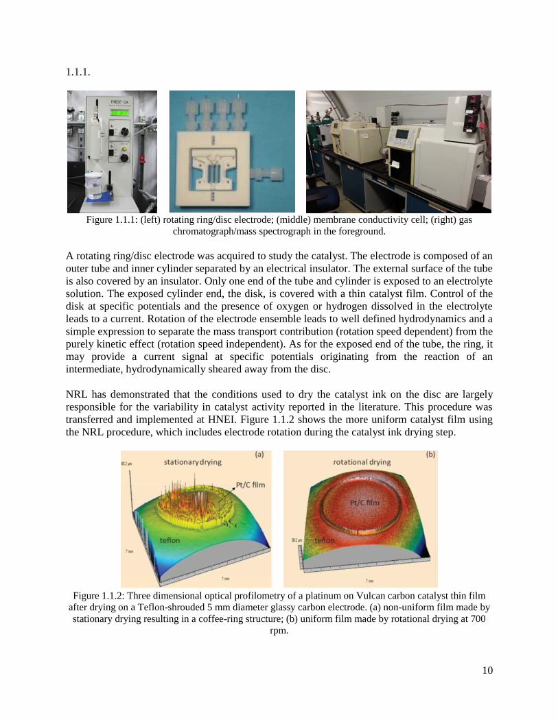
1.1.1.

Figure 1.1.1: (left) rotating ring/disc electrode; (middle) membrane conductivity cell; (right) gas

chromatograph/mass spectrograph in the foreground.

A rotating ring/disc electrode was acquired to study the catalyst. The electrode is composed of an

outer tube and inner cylinder separated by an electrical insulator. The external surface of the tube

is also covered by an insulator. Only one end of the tube and cylinder is exposed to an electrolyte

solution. The exposed cylinder end, the disk, is covered with a thin catalyst film. Control of the

disk at specific potentials and the presence of oxygen or hydrogen dissolved in the electrolyte

leads to a current. Rotation of the electrode ensemble leads to well defined hydrodynamics and a

simple expression to separate the mass transport contribution (rotation speed dependent) from the

purely kinetic effect (rotation speed independent). As for the exposed end of the tube, the ring, it

may provide a current signal at specific potentials originating from the reaction of an

intermediate, hydrodynamically sheared away from the disc.

NRL has demonstrated that the conditions used to dry the catalyst ink on the disc are largely

responsible for the variability in catalyst activity reported in the literature. This procedure was

transferred and implemented at HNEI. Figure 1.1.2 shows the more uniform catalyst film using

the NRL procedure, which includes electrode rotation during the catalyst ink drying step.

Figure 1.1.2: Three dimensional optical profilometry of a platinum on Vulcan carbon catalyst thin film

after drying on a Teflon-shrouded 5 mm diameter glassy carbon electrode. (a) non-uniform film made by

stationary drying resulting in a coffee-ring structure; (b) uniform film made by rotational drying at 700

rpm.

11

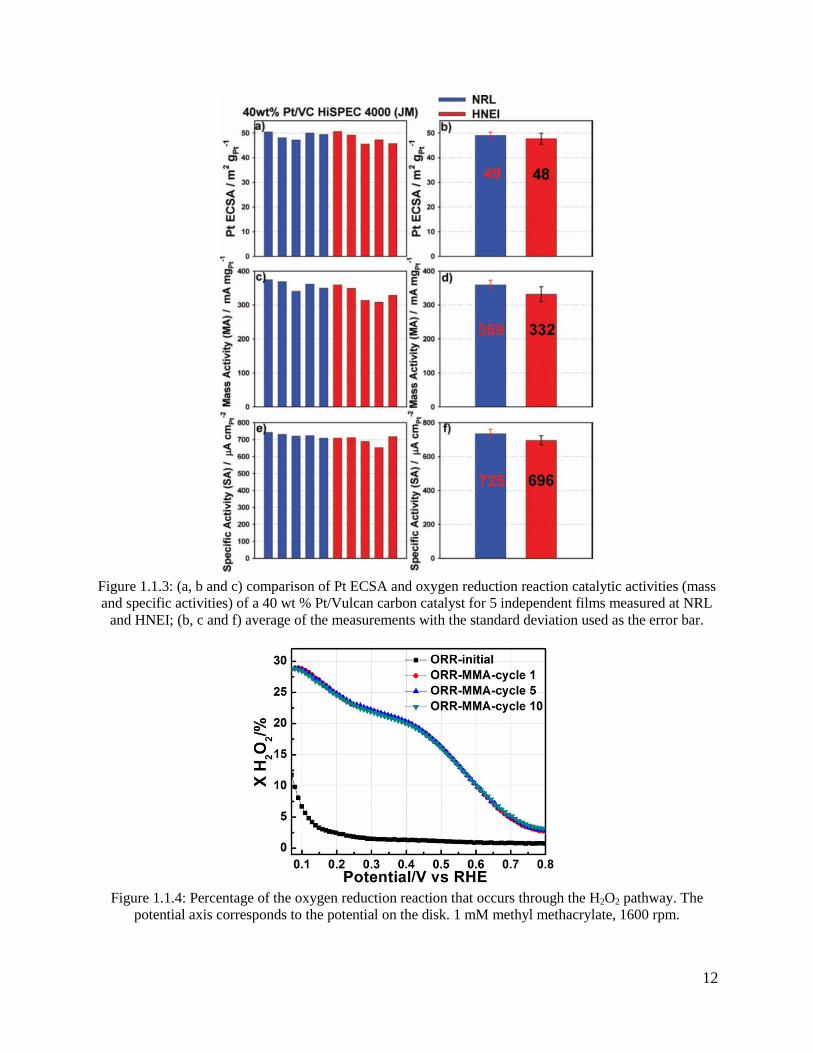
Catalyst films were tested at both NRL and HNEI sites for comparison and method validation.

Select results are illustrated in Figure 1.1.3 which shows on the left (Figures 1.1.3 a, c and e)

catalyst parameters (electrochemical surface area or ECSA, mass activity, specific activity) for

five NRL and five HNEI samples. Average values are shown on the right (Figures 1.1.3 b, d and

f). Results were deemed reproducible. More details are provided in the Papers and Presentations

Resulting from these Efforts section (items 1, 10, 11, 14 and 16).

The rotating ring/disc electrode was subsequently used to characterize the impact of several air

contaminants on the oxygen reduction reaction kinetics; acetonitrile, acetylene, methyl

methacrylate, naphthalene, and propene. These contaminants were selected because they were

expected to react within a fuel cell, were the most concentrated in air, have different organic

groups and their effects were not documented.1 Specifically, the yield of the hydrogen peroxide

production reaction, a side reaction of the oxygen reduction reaction, was examined by

monitoring the ring current at a potential sufficient to oxidize this intermediate. For each case, a

significant increase in peroxide production was observed (Figure 1.1.4). This was attributed to

the decrease in catalyst sites due to contaminant adsorption which forces oxygen adsorption in an

end-on configuration (adsorption on a single Pt site) rather than on a bridge configuration

(adsorption on two contiguous Pt sites). The oxygen end-on adsorbate leads to the formation of

hydrogen peroxide rather than water. This finding has an important durability ramification

because hydrogen peroxide attacks the membrane and therefore fuel cell life can be accelerated if

subjected to contaminants for a long period of time.2

12

Figure 1.1.3: (a, b and c) comparison of Pt ECSA and oxygen reduction reaction catalytic activities (mass

and specific activities) of a 40 wt % Pt/Vulcan carbon catalyst for 5 independent films measured at NRL

and HNEI; (b, c and f) average of the measurements with the standard deviation used as the error bar.

Figure 1.1.4: Percentage of the oxygen reduction reaction that occurs through the H2O2 pathway. The

potential axis corresponds to the potential on the disk. 1 mM methyl methacrylate, 1600 rpm.

13

Additional details are provided in the Papers and Presentations Resulting from these Efforts

below, (items 2-5 and 15).

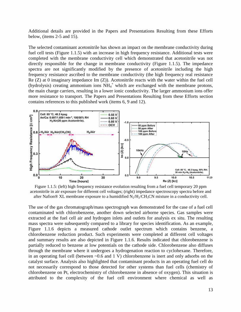
The selected contaminant acetonitrile has shown an impact on the membrane conductivity during

fuel cell tests (Figure 1.1.5) with an increase in high frequency resistance. Additional tests were

completed with the membrane conductivity cell which demonstrated that acetonitrile was not

directly responsible for the change in membrane conductivity (Figure 1.1.5). The impedance

spectra are not significantly modified by the presence of acetonitrile including the high

frequency resistance ascribed to the membrane conductivity (the high frequency real resistance

Re (Z) at 0 imaginary impedance Im (Z)). Acetonitrile reacts with the water within the fuel cell

(hydrolysis) creating ammonium ions NH4+ which are exchanged with the membrane protons,

the main charge carriers, resulting in a lower ionic conductivity. The larger ammonium ions offer

more resistance to transport. The Papers and Presentations Resulting from these Efforts section

contains references to this published work (items 6, 9 and 12).

Figure 1.1.5: (left) high frequency resistance evolution resulting from a fuel cell temporary 20 ppm

acetonitrile in air exposure for different cell voltages; (right) impedance spectroscopy spectra before and

after Nafion® XL membrane exposure to a humidified N2/H2/CH3CN mixture in a conductivity cell.

The use of the gas chromatograph/mass spectrograph was demonstrated for the case of a fuel cell

contaminated with chlorobenzene, another down selected airborne species. Gas samples were

extracted at the fuel cell air and hydrogen inlets and outlets for analysis ex situ. The resulting

mass spectra were subsequently compared to a library for species identification. As an example,

Figure 1.1.6 depicts a measured cathode outlet spectrum which contains benzene, a

chlorobenzene reduction product. Such experiments were completed at different cell voltages

and summary results are also depicted in Figure 1.1.6. Results indicated that chlorobenzene is

partially reduced to benzene at low potentials on the cathode side. Chlorobenzene also diffuses

through the membrane where it undergoes a hydrogenation reaction to cyclohexane. Therefore,

in an operating fuel cell (between ~0.6 and 1 V) chlorobenzene is inert and only adsorbs on the

catalyst surface. Analysis also highlighted that contaminant products in an operating fuel cell do

not necessarily correspond to those detected for other systems than fuel cells (chemistry of

chlorobenzene on Pt, electrochemistry of chlorobenzene in absence of oxygen). This situation is

attributed to the complexity of the fuel cell environment where chemical as well as

14

electrochemical reactions can take place, and the simultaneous presence of oxygen, hydrogen

(diffusing through the membrane from the anode side) and water. This work was published

(items 7 and 13 in the Papers and Presentations Resulting from these Efforts section).

Figure 1.1.6: (left) identification of the detected species at the cathode outlet with the mass spectrograph

(Exp) by matching results with the species library (Lib); (right) chlorobenzene reaction products during

fuel cell poisoning at different voltages. Cell IR voltage means the ohmic resistance corrected cell

voltage, which is closer to the cathode potential than the measured cell voltage. Ca: cathode compartment;

An: anode compartment.

This brief summary of some of the results obtained by studying fuel cell contamination with the

recently acquired capabilities indicate that contamination mechanisms are complex (species are

contaminant, potential and operating conditions dependent) and impact many parameters

(catalyst surface area, oxygen reduction mechanism including its side reaction, membrane

conductivity). Therefore, it was deemed easier to prevent contamination rather than minimizing

its impacts in situ by establishing tolerance limits (contaminant concentration leading to a

significant cell voltage loss) and developing strategies to limit fuel cell exposure to contaminants

(simultaneous use of filter systems, air quality sensors and shift in fuel cell to battery power).

Also and in spite of the contamination mechanisms complexity, in view of the large number of

contaminants that have not yet been tested, the development of simple and predictive capabilities

for fuel cell voltage losses was considered valuable.3

In situ fuel cell testing capabilities: water transport

The effective management of water transport within fuel cells is critical to optimize their

performance and avoid either flooding or membrane dehydration conditions. This consideration

is particularly relevant to air independent fuel cell operation (includes UUVs) which may be

designed with oxygen or enriched oxygen reactant streams that limit options for water removal

by entrainment and/or evaporation. Under HEET10, HNEI contracted with COANDA Research

and Development (COANDA) to design and build a residence time distribution (RTD) apparatus

15

which will be used in subsequent ONR awards (APRISES) to study water blockages within

single cell PEMFCs and small scale fuel cell stacks. The original goals of the research were: i)

study how water blockages within fuel cells affect their performance, ii) improve fuel cell

performance by developing operating strategies and fuel cell hardware component designs that

optimize water transport, and iii) assess how effective liquid water is in removing contaminants

from the fuel cell. Recent work from our laboratory in a supporting Department of Energy

project has shown that liquid water is not an effective medium for removing most of the common

airborne contaminants from a fuel cell under real-world operating conditions.4 Thus, future

research using the RTD will focus primarily on original goals i) and ii). This section contains: an

overview of the RTD system designed and built by COANDA during this period, a brief

summary of the relevance and benefits of using RTD to improve fuel cell performance, and a

general conceptualization describing how RTD will be applied to the study of fuel cells.

RTD system overview

The RTD system was developed by COANDA to study the residence time of gases within a

single fuel cell or a short fuel cell stack. The information provided by the RTD is useful as a

design diagnostic for fuel cell hardware components such as gas flow fields and gas diffusion

media because it provides information on how the residence time of the gases within the reactor

compares to the residence time profile of an ideal chemical reactor. The ideal reactor model

serves as the design benchmark. Other characteristic RTD responses provide diagnostic

information that identifies flow design problems in the fuel cell such as dead zones or flow

channeling. The RTD response data can also be used to develop a fuel cell performance model

that describes the effects of water blockages on performance when combined with mathematical

models for gas mixing within the fuel cell and information on the reaction rate.

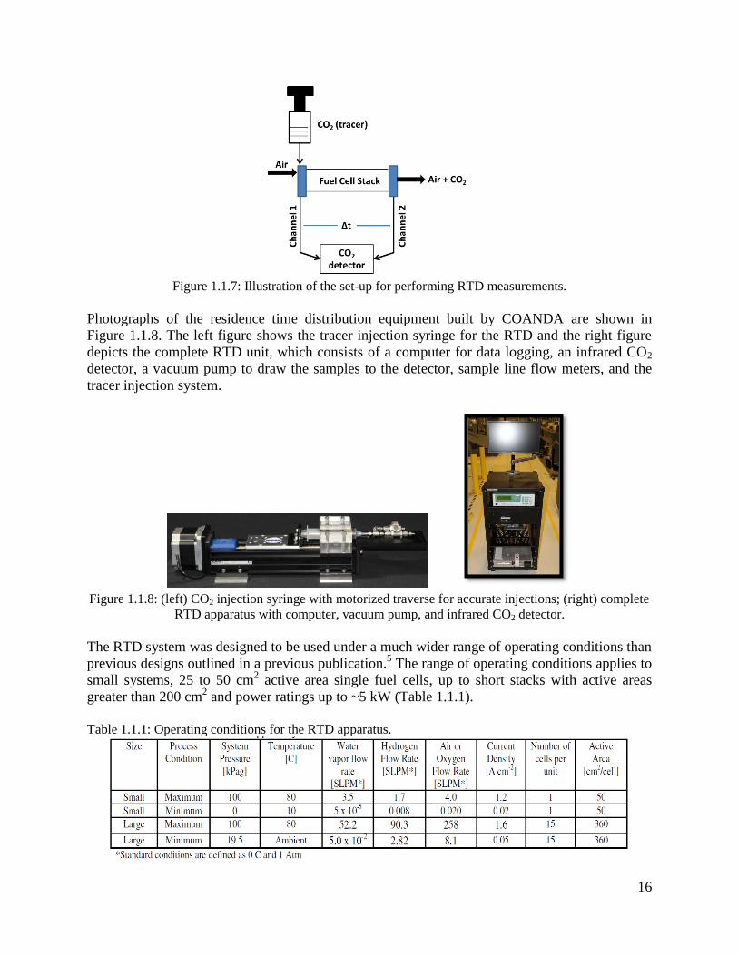
An illustration of the set-up developed for performing RTD measurements is shown in Figure

1.1.7 for a fuel cell stack. RTD measurements were performed by supplying an inert tracer into

the inlet stream of the fuel cell using a syringe attached to a motorized traverse. Tracer

measurements are taken through sample streams at the inlet and outlet of the stack or single cell.

The tracer used in the RTD design was carbon dioxide (CO2), because it is inert within a fuel cell

and it can be injected into the reactant stream at percentage level concentrations without

poisoning the catalyst that is used in fuel cells to facilitate the electrochemical reactions. Carbon

dioxide is also easily detected. A vacuum pump (not shown) was used to draw the gas samples

through the sample lines at the inlet and outlet. The use of the pump minimizes the transport time

of the tracer in the sample stream to the detector ensuring the measured residence time of the

gases between the inlet and outlet is accurate. The pump also enables the RTD to be used under a

much wider range of operating conditions than previous designs. The sample streams were sent

to an infrared CO2 detection device, which determines the CO2 concentration within the fuel cell

at that point in time. The shape and timing of the response at the outlet provides qualitative and

quantitative information on the residence time of gases within the system that can be used to

assist in developing a performance model for the fuel cell.

16

Figure 1.1.7: Illustration of the set-up for performing RTD measurements.

Photographs of the residence time distribution equipment built by COANDA are shown in

Figure 1.1.8. The left figure shows the tracer injection syringe for the RTD and the right figure

depicts the complete RTD unit, which consists of a computer for data logging, an infrared CO2

detector, a vacuum pump to draw the samples to the detector, sample line flow meters, and the

tracer injection system.

Figure 1.1.8: (left) CO2 injection syringe with motorized traverse for accurate injections; (right) complete

RTD apparatus with computer, vacuum pump, and infrared CO2 detector.

The RTD system was designed to be used under a much wider range of operating conditions than

previous designs outlined in a previous publication.5 The range of operating conditions applies to

small systems, 25 to 50 cm2 active area single fuel cells, up to short stacks with active areas

greater than 200 cm2 and power ratings up to ~5 kW (Table 1.1.1).

Table 1.1.1: Operating conditions for the RTD apparatus.

17

The RTD apparatus was designed and built during HEET10. However, HNEI identified several

issues with the performance of the unit that were resolved. Two of the issues were identified as

the most significant: the unit could not be accurately calibrated to determine the CO2

concentrations, and ; data streams for the CO2 measurements had several repeated values

resulting in inlet and outlet CO2 peaks that were stepped and incorrect in shape. HNEI worked

with COANDA to resolve these issues. The CO2 calibration was related to the calibration

process for the infrared CO2 detector which was originally developed for gas streams near

ambient pressure. The use of a vacuum pump results in a much lower total pressure in the

detector. COANDA has developed a correction and validated its performance. The repeated data

issue was due to a mismatch between the timing of the computer clock that was recording the

data being sent from the CO2 detector and the timing of the clock for the CO2 detector. Future

work under other ONR awards (APRISES) will focus on testing the unit to ensure that the CO2

concentration measurements are accurate and applying the RTD to improve water management

in fuel cells.

Relevance of RTD analysis for fuel cells

The management of water within PEMFCs and stacks is a critical factor in maximizing their

performance. The presence of solid ice crystals or liquid water droplets in the gas flow field

channels or the pores of the gas diffusion media, decreases fuel cell performance by inhibiting

the transport of reactant gases to the catalyst. A greater understanding of the processes leading to

these blockages is required so that PEMFCs can be operated at conditions (flow rates, pressures,

temperatures, etc.) that mitigate the potential for their occurrence. Additionally fuel cell

hardware components (gas flow fields, gas diffusion media) can be designed to enable optimal

water management within the stack.

Various experimental measurement techniques have been used to study water transport and

liquid water formation within fuel cells.5 Most of the methods previously used have trade-offs

between their benefits and disadvantages which include system cost, complexity, spatial

resolution, and the presence of artifacts introduced during the measurement process. Thus, a

simple and low cost method for characterizing the presence of water blockages in fuel cells is

needed that adequately addresses the challenges of real-time measurement within an operating

fuel cell.

The most developed technology, neutron imaging, has a greater geometric resolution and is

minimally invasive but is vastly more expensive requiring a nuclear reactor with high neutron

flux and has a limited time resolution.6 In comparison, RTD analysis is a simpler and lower cost

method. RTD is widely used in the field of chemical engineering.7 RTD measurements have

been demonstrated for use in fuel cell applications. The merits of several apparatus designs for

measuring the RTD of gases in fuel cells were evaluated and a specific type of design was

recommended.5 This design was employed to show it could detect water blockages in fuel cell

gas flow fields and measure liquid water content in gas diffusions media.8

RTD measurement methods for fuel cells

In this section, the general features of RTD measurements are discussed. Subsequently, these

18

concepts are specifically described for fuel cell applications.

The RTD tracer is the inert species that allows the measurement of the residence time of the

gases within the fuel cell. The tracer is generally supplied to the stack in two ways: either as an

injection pulse or as a step. An example of an injection pulse is shown in Figure 1.1.9 and a

negative step is also given in the same figure. Pulsed injections are first discussed followed by

negative step injections.

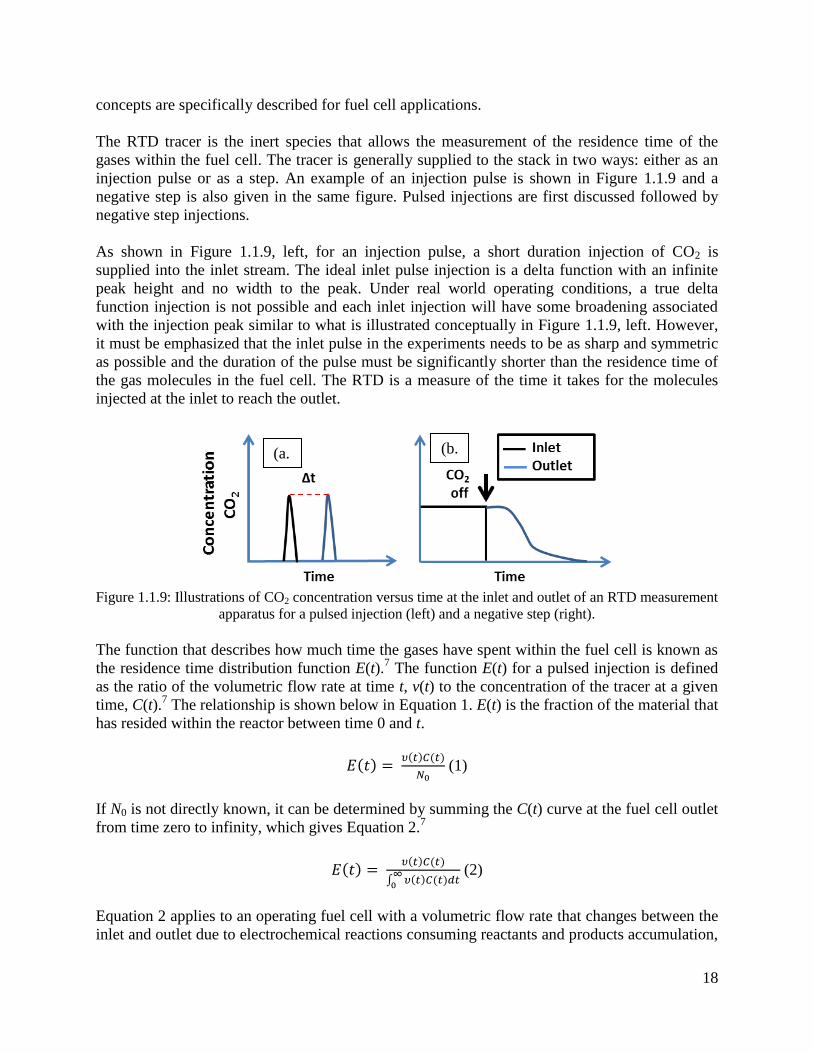
As shown in Figure 1.1.9, left, for an injection pulse, a short duration injection of CO2 is

supplied into the inlet stream. The ideal inlet pulse injection is a delta function with an infinite

peak height and no width to the peak. Under real world operating conditions, a true delta

function injection is not possible and each inlet injection will have some broadening associated

with the injection peak similar to what is illustrated conceptually in Figure 1.1.9, left. However,

it must be emphasized that the inlet pulse in the experiments needs to be as sharp and symmetric

as possible and the duration of the pulse must be significantly shorter than the residence time of

the gas molecules in the fuel cell. The RTD is a measure of the time it takes for the molecules

injected at the inlet to reach the outlet.

Figure 1.1.9: Illustrations of CO2 concentration versus time at the inlet and outlet of an RTD measurement

apparatus for a pulsed injection (left) and a negative step (right).

The function that describes how much time the gases have spent within the fuel cell is known as

the residence time distribution function E(t).7 The function E(t) for a pulsed injection is defined

as the ratio of the volumetric flow rate at time t, v(t) to the concentration of the tracer at a given

time, C(t).7 The relationship is shown below in Equation 1. E(t) is the fraction of the material that

has resided within the reactor between time 0 and t.

𝐸(𝑡) = 𝜐(𝑡)𝐶(𝑡)

𝑁0 (1)

If N0 is not directly known, it can be determined by summing the C(t) curve at the fuel cell outlet

from time zero to infinity, which gives Equation 2.7

𝐸(𝑡) = 𝜐(𝑡)𝐶(𝑡)

∫ 𝜐(𝑡)∞

0𝐶(𝑡)𝑑𝑡

(2)

Equation 2 applies to an operating fuel cell with a volumetric flow rate that changes between the

inlet and outlet due to electrochemical reactions consuming reactants and products accumulation,

(a.

)

(b.

)

19

and the transport of material across the proton exchange membrane when current is produced.

However, if the stack is not under load, then the volumetric flow rate in the fuel cell anode and

cathode compartments is essentially constant aside from negligible gas permeation across the

membrane. For a non-operating fuel cell, Equation 2 then becomes equation 3.7

𝐸(𝑡) = 𝐶(𝑡)

∫ 𝐶(𝑡)𝑑𝑡∞

0

(3)

For the case of a fuel cell, the gas flow is often modeled as a plug flow reactor. This implies that

the velocity front of the gases down the flow field channel is uniform and the flow regime is

turbulent. An idealized pulsed injection and E(t) response is shown in Figure 1.1.10 versus theta

(). Theta is the ratio of the actual residence time of the gas in the reactor to the time it would

take to process one reactor volume of gas. For an ideal plug flow reactor (PFR), E(t) is unity

(infinite height and 0 width). In an operating fuel cell however, the assumption of a turbulent

flow does not always hold because the flow in channels is often laminar. The RTD will thus

provide useful information for a range of operating conditions (gas flow rates, stream relative

humidity, etc.) as to whether or not the fuel cell should be modeled as a PFR type reactor or if it

is better suited to be modeled as a non-ideal PFR due to laminar characteristics of the gas

velocity profile.

Figure 1.1.10: Injection and E(t) for an ideal plug flow reactor.

Two other types of RTD responses that may commonly occur within fuel cells include: gas

dispersion down the flow path (Figure 1.1.11) and water blockages resulting in a dead zone with

channeling (Figure 1.1.12). The data in Figure 1.1.11 is for a pulsed injection and was taken

using the RTD unit built by COANDA with gas flowing down a tube. Data show the detector

response at the inlet and outlet versus time. The outlet peak is broader and the peak height is

decreased in comparison to the inlet injection. The reason for the change in the peak shape is the

progressive impact of axial diffusion as the gas flows down the tube, which results in some of the

gas exiting the tube sooner and later. Similar results may be observed in fuel cells especially at

low flow rates because the gas resides for a longer period within the fuel cell allowing axial

diffusion to have a larger impact.

20

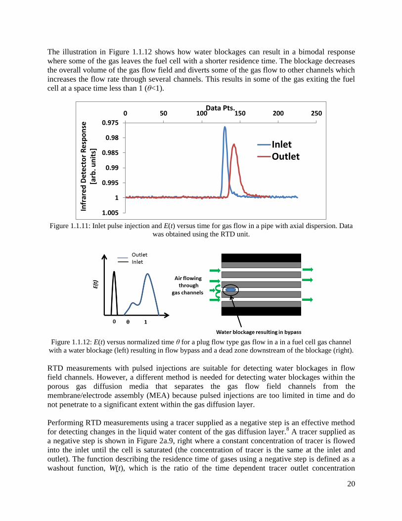
The illustration in Figure 1.1.12 shows how water blockages can result in a bimodal response

where some of the gas leaves the fuel cell with a shorter residence time. The blockage decreases

the overall volume of the gas flow field and diverts some of the gas flow to other channels which

increases the flow rate through several channels. This results in some of the gas exiting the fuel

cell at a space time less than 1 (θ<1).

Figure 1.1.11: Inlet pulse injection and E(t) versus time for gas flow in a pipe with axial dispersion. Data

was obtained using the RTD unit.

Figure 1.1.12: E(t) versus normalized time θ for a plug flow type gas flow in a in a fuel cell gas channel

with a water blockage (left) resulting in flow bypass and a dead zone downstream of the blockage (right).

RTD measurements with pulsed injections are suitable for detecting water blockages in flow

field channels. However, a different method is needed for detecting water blockages within the

porous gas diffusion media that separates the gas flow field channels from the

membrane/electrode assembly (MEA) because pulsed injections are too limited in time and do

not penetrate to a significant extent within the gas diffusion layer.

Performing RTD measurements using a tracer supplied as a negative step is an effective method

for detecting changes in the liquid water content of the gas diffusion layer.8 A tracer supplied as

a negative step is shown in Figure 2a.9, right where a constant concentration of tracer is flowed

into the inlet until the cell is saturated (the concentration of tracer is the same at the inlet and

outlet). The function describing the residence time of gases using a negative step is defined as a

washout function, W(t), which is the ratio of the time dependent tracer outlet concentration

0.975

0.98

0.985

0.99

0.995

1

1.005

0 50 100 150 200 250

Infr

ared

Det

ecto

r R

esp

on

se

[arb

. un

its]

Data Pts.

InletOutlet

21

Cout(t) to the steady state concentration measured at the outlet, C0, as shown in Equation 4.9

𝑊(𝑡) = 𝐶𝑜𝑢𝑡(𝑡)/𝐶0 (4)

For the washout function, when t<0, Cin=Cout=C0, and when t=∞, Cout(t)=0. The quantity W(t)

represents the fraction of molecules leaving the system that experienced a residence time > t.9 It

was shown that in a non-operating fuel cell, as the liquid water content within the gas diffusion

layer was increased, the residence time of the gas decreased because the hydraulic volume of the

fuel cell was decreased by the liquid water. Similar results were obtained when the fuel cell was

operated with the residence time decreasing with current density when the amount of water in the

system was higher.8 However, for large current densities, the opposite trend was observed and

was attributed to an easier liquid water removal process.

Three additional uses for RTD that can assist in improving performance for fuel cells are: i)

studying single phase gas flow distribution within flow field channels, ii) optimizing the

compressive force across the gas diffusion layer, and iii) studying reactant crossover at different

operating conditions [2]. Reactant flow distribution within gas channels is an important element

of modeling fuel cell performance. Flow channeling was observed in a fuel cell flow field plate

without the presence of blockages such as liquid water drops,8 which emphasizes the importance

of channel design to achieve a uniform reactant distribution over the active surface area and cell

voltage. The RTD also provides a method for determining the optimal compressive force of the

gas flow field plates across the gas diffusion media used within the fuel cell. The optimal

compressive force is large enough in magnitude to decrease the contact resistance between the

electrical components while maintaining the integrity of the gas diffusion media pore structure,

which serves to transport the reactants and products to and from the catalyst, respectively. Thus,

contact resistance is minimized without adversely affecting the rate of reactant gas transport to

the catalyst or inhibiting water transport in the pores of the diffusion media. A decrease in the

pore volume due to over compression would cause a decrease in the residence time of the gases

within the fuel cell. The RTD can be used to determine the optimal compressive force for the gas

flow field plates by comparing fuel cell performance data at different compressive forces with

changes to the RTD due to modifications in the pore structure of the gas diffusion media. This

consideration is especially important for flexible gas diffusion media that can intrude in the flow

fields and that are favored for continuous MEA manufacturing processes to reduce cost. Gas

crossover is also an important consideration during fuel cell operation (such as the undesirable

nitrogen accumulation in a fuel recirculation loop) that can be estimated using the RTD by

injecting CO2 in the cathode inlet and comparing the measured CO2 concentration at the outlet of

the anode. Although CO2 has a different permeability through the membrane/electrode assembly

than nitrogen or oxygen, it can be used to understand the in situ effects of variable operating

conditions. Generally, gas crossover is measured when a fuel cell is not operating and therefore

measured values are not necessarily relevant. For instance, gas crossover is dependent on the

membrane water content.10

Cell operation modifies the membrane water content in part by water

production at the cathode and electroosmotic drag transferring water from the anode to the

cathode.

To summarize, RTD measurements with pulsed tracer injections can be used to study water

blockages within the gas flow field of the fuel cell. Negative step tracer experiments can be used

22

to assess how the residence time of gases changes for different water content within the gas

diffusion media. Other important types of measurements that assist in fuel cell modeling and gas

transport were also described. These measurements will be performed during future ONR awards

(APRISES) with the RTD apparatus for single fuel cells and small scale stacks under different

operating conditions to obtain characteristic RTDs for different gas flow field designs and gas

diffusion media with different hydrological properties and porosities.

Future work will focus on first validating the full performance of the RTD unit. Fuel cell

characterization under a range of operating conditions will subsequently be considered to gain a

better understanding of liquid water accumulation dynamics in flow field channels and gas

diffusion electrodes.

Fast cycling pressure swing adsorption systems for the removal of reactant stream

contaminants

Conclusions from the ex-situ fuel cell testing suggest that the prevention of fuel cell exposure to

contaminants was a worthwhile activity. Traditionally, filters have been added to the fuel cell air

intake system to limit exposure to contaminants and particulates. Air filters are advantageously

passive and an established technology. However, air filters need maintenance or replacement to

maintain their function because adsorbents eventually become saturated with contaminant

species. The potential of pressure swing adsorption was explored Under HEET10 as an active

component alternative for air filters that do not need replacement.

Figure 1.1.13: A conceptual representation of a pressure swing adsorption system for nitrogen

enrichment.

Figure 1.1.13 illustrates the sequential steps of a pressure swing adsorption system. The example

pertains to nitrogen enrichment. The left tank is filled with an adsorbent that preferentially

adsorbs oxygen. The incoming air is pressurized to maximize the amount of oxygen adsorbed. At

the outlet, the gas stream is enriched in nitrogen having been depleted of oxygen. This step is

carried out until the adsorbent is nearly saturated with oxygen. In the right tank, the pressure is

https://www.google.com/url?sa=i&rct=j&q=&esrc=s&source=images&cd=&cad=rja&uact=8&ved=0ahUKEwiNlPG0_oLPAhWDKWMKHTzfDZ4QjRwIBw&url=http://www.iatt.co.uk/pressure-swing-adsorption-nitrogen-generators.asp&psig=AFQjCNGNGAxYp_0Rz-IaVjSUeB6w_vCRQQ&ust=1473533342312771

23

released which desorbs most of the oxygen and re-initialize the adsorbent for a new adsorption

cycle. The control system initiates a new cycle by switching the inlet and outlet valves. The left

tank desorbs the oxygen whereas the right tanks adsorbs oxygen. The process is discontinuous.

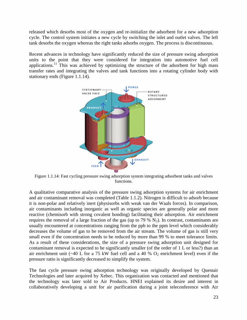
Recent advances in technology have significantly reduced the size of pressure swing adsorption

units to the point that they were considered for integration into automotive fuel cell

applications.11

This was achieved by optimizing the structure of the adsorbent for high mass

transfer rates and integrating the valves and tank functions into a rotating cylinder body with

stationary ends (Figure 1.1.14).

Figure 1.1.14: Fast cycling pressure swing adsorption system integrating adsorbent tanks and valves

functions.

A qualitative comparative analysis of the pressure swing adsorption systems for air enrichment

and air contaminant removal was completed (Table 1.1.2). Nitrogen is difficult to adsorb because

it is non-polar and relatively inert (physisorbs with weak van der Waals forces). In comparison,

air contaminants including inorganic as well as organic species are generally polar and more

reactive (chemisorb with strong covalent bonding) facilitating their adsorption. Air enrichment

requires the removal of a large fraction of the gas (up to 79 % N2). In contrast, contaminants are

usually encountered at concentrations ranging from the ppb to the ppm level which considerably

decreases the volume of gas to be removed from the air stream. The volume of gas is still very

small even if the concentration needs to be reduced by more than 99 % to meet tolerance limits.

As a result of these considerations, the size of a pressure swing adsorption unit designed for

contaminant removal is expected to be significantly smaller (of the order of 1 L or less?) than an

air enrichment unit (~40 L for a 75 kW fuel cell and a 40 % O2 enrichment level) even if the

pressure ratio is significantly decreased to simplify the system.

The fast cycle pressure swing adsorption technology was originally developed by Questair

Technologies and later acquired by Xebec. This organization was contacted and mentioned that

the technology was later sold to Air Products. HNEI explained its desire and interest in

collaboratively developing a unit for air purification during a joint teleconference with Air

24

Products representatives. However, repeated follow up attempts were ignored. Therefore, the

project was abandoned.

Table 1.1.2: Comparative analysis of 2 pressure swing adsorption applications for fuel cells.

Air enrichment Contaminant removal

Ease of species removal N2 is relatively difficult to

adsorb

Airborne contaminants of

relevance are either

inorganic (NOx, SOx, NH3)

or organic and relatively

easier to adsorb

Volume of material to be

removed

79 % of the dry air stream ppm levels or lower

creating an opportunity to

reduce the size and pressure

ratio for system

simplification

Fraction of material that

needs to be removed

At least 50 % of the N2 to

have a significant

performance impact on fuel

cell operation

Contaminant dependent

Tolerance levels leading to

a specific fuel cell

performance loss were

determined for several

contaminants

Cost - Lower in relation to air

enrichment in view of its

much smaller envisaged

size and power demand

Automotive fuel cell stack for autonomous Navy applications

New energy sources for UUVs continue to be of Navy interest. Current and future UUV missions

will require endurance on the order of days and months, where existing high energy density

batteries are insufficient and thus solutions beyond battery-only technology are a necessity. In

2011, the Office of Naval Research (ONR) held an industry day, focusing on a strategic priority

to develop a reliable Large Displacement Unmanned Undersea Vehicle (LDUUV) with the

following key program goals12

:

Improve current UUV energy density by 5 to 10 times,

Allow for autonomous operation in the littorals,

Have an open architecture,

And allow for over the horizon operation.

The resulting energy system would be capable of missions of up to 70 days using air independent

propulsion. Several organizations have been funded as part of the program and continue along

the development pathway set forth in 2011 with, as a central theme, hydrogen/oxygen fuel cells

previously developed for NASA applications as the core energy conversion device.13

As of

February 2016, the LDUUV development continues to be a high priority in the Navy’s

Innovative Prototype program.1416

25

In parallel with the outsourced programs, the NRL had already started an in-house program to

adapt a new, highly proven automotive fuel cell for integration into the LDUUV.17

The concept

behind this project was to avoid reliability issues with “boutique” fuel cells developed for niche

applications and instead utilize a well-proven system. If any issues with the selected automotive

fuel cell system vendor occur down the road, other automotive fuel cell vendors could be utilized

as well. Honda, Toyota, Daimler/Ford, GM, all have proven performance track records in fuel

cell research, development, and operation. An American based manufacturer’s automotive fuel

cell system with a 93 kW maximum power output and over 1.8 million cumulative road miles

was selected for the initial technology evaluation and integration.

The main research challenge was to operate an air-breathing fuel cell in an enclosed

environment. NRL began development of an air-recirculation system where the entire FC system

is placed inside a pressure vessel and the oxygen/nitrogen concentration inside the vessel

atmosphere is controlled. The nitrogen content is continually recirculated through the fuel cell,

while oxygen, stored on-board in another subsection, is supplied into the vessel to balance

consumption and maintain the O2/N2 concentration ratio near 21 %. In this manner, only bulk

oxygen and hydrogen need to be stored on-board the LDUUV, while maintaining the air-based

fuel cell system operation. Changes to the manufacturer’s fuel cell system controller and

standard operation were not anticipated.

Under HEET10 and in support of NRL’s Hydranox UUV program, the manufacturer provided

two 5 kW short stacks to HNEI and made available technical support to both HNEI and NRL to

develop stack testing protocols simulating actual system operation and evaluate the fuel cell

stack performance variability in the alternative environment of the pressure vessel with simulated

air. The variability in the oxygen concentration due to the O2 injection controller response, as

well as possible increases in the temperature and relative humidity of the atmosphere inside the

pressure vessel were measured at HNEI because the manufacturer did not have the required

testing capabilities. Any condition found detrimental to performance/efficiency could then be

accounted for in the design of the pressure vessel atmospheric control unit. Additional

diagnostics were added to determine the fate of the water generated when operating in these

alternate conditions to aid in the sizing of balance of plant components external to the fuel cell

system within the energy section such as a condenser and/or product water expulsion pumps.

Pure oxygen tests were also performed to establish efficiency gains and provide data for

comparison with other future energy packages. Pure O2 testing was only performed with the 5

kW short stack at HNEI because test stations were qualified for such operation. The

manufacturer indicated the air supply components of the actual 93 kW system were not designed

for oxygen service.

All tests were completed under a strict non-disclosure agreement between the automotive

manufacturer, NRL, and HNEI with data directly provided to NRL by HNEI. Data was

disseminated to NRL through monthly reports, meeting presentations, and compact discs mailed

to NRL. For more information and specific project details, contact Karen Swider-Lyons

[email protected] or the substitute Head, Alternative Energy Section, Chemistry

Division.

mailto:[email protected]

26

Development of a multi-configuration anode gas/water management test bed

In response to needs of ONR’s UAV and UUV programs, conducted testing to better understand

the performance and durability under expected vehicle operating conditions and in particular,

reactant recirculation used to maximize reactant utilization. Under conditions typical of UUVs

(using ‘pure’ reactants) and UAVs (using combination of ‘pure’ reactants and outside air), the

presence of contaminants in oxygen or hydrogen will favor their accumulation in the recycling

loop. Furthermore, the use of a recirculation strategy favors the accumulation of liquid water and

creates an opportunity to mitigate the presence of the contaminants by dissolution into water

drops with subsequent entrainment toward the stack outlet. A laboratory scale (< 1 kW)

recirculation test bed was developed for use with existing test stands, i.e. single cell, segmented

cell, and stack test stands at HNEI’s Hawaii Sustainable Energy Research Facility (HiSERF), to

facilitate further fundamental understandings of reactant recirculation processes. The system

layout was chosen to allow for multiple modes of operation with relative ease of switching

between modes for automating comparative studies and data production for model validation.18

The initial system was designed to look at fuel/hydrogen recirculation on the anode side of the

fuel cell, while allowing future recirculation studies of both oxidant and fuel. The following

modes of anode gas management (AGM) were incorporated into the initial test bed build:

Single pass venting of anode hydrogen at the outlet

o Humidified or dry gas flow control

o Back pressure control with optional pressure control locations

Dead end operation

o Dry hydrogen at the inlet

o Optional periodic purge

o Optional constant bleed

Pump based (controllable) pure recirculation

o Dry hydrogen at the inlet

o Optional periodic purge

o Optional constant bleed

These modes were based upon previous modeling work18

evaluating various operating schemes

for high hydrogen utilization. At the request of NRL’s UAV group, ballast based, pressure driven

hydrogen recirculation19

capabilities were also added. The overall layout of the system, .i.e.

wiring, sensors, controller, piping, was designed to be modular allowing for easy

interchangeability of components to accommodate future modifications.

Components sufficient for operation of 100 cm2 single cells were chosen as an initial design

point of the anode gas management test bed to facilitate the incorporation of other specialized

diagnostic tools already available, namely the segmented cell and RTD tracer system. The

system is capable of pressures up to 30 psig, temperatures up to 80 °C, operation up to a

stoichiometry of 4 for hydrogen flows, and a maximum current density of 2.5 A cm2

. Sample

port connections are integrated for connecting HiSERF’s gas chromatograph, gas

chromatograph/mass spectrograph, mass spectrograph and RTD systems. Several technical

hurdles were encountered during the design process, including:

27

Balancing measurement requirements, instrument performance, and instrument cost

trade-offs

Measurement stability was enhanced by selecting a recirculation pump that minimizes

pulsation, has a predictable/controllable flow rate, and has materials compatible with the

required temperature and pressure ranges

In-line instrumentation were incorporated to provide inlet and outlet concentration

measurements of H2, H2O, and N2, either directly or indirectly under hot, and pressurized

conditions

Recirculation flow rate measurement under varying gas concentrations requires low

pressure drop, heated flow meters with the ability to correct for gas composition

Heat tracing of components without affecting measurements

Dealing with component inherent leakage, e.g. diffusion of nitrogen from air through

elastomer seals is sufficient to influence results of recirculation studies

The first version (v1) of the as-built system is shown in Figure 1.1.15. Components were

arranged on an aluminum rack, with the controller and power electronics in a separate enclosure.

Nine heater zones were required and a separate control box was constructed for this purpose.

The entire rack rests on a movable cart for ease of transport from station to station. Two

corrugated, flexible stainless steel lines are used to connect to the anode inlet and outlet of the

test article in the station. The data acquisition system is based on the National Instruments

compact data acquisition modular controller with signal conditioning units installed to

accommodate the various sensors, pumps, valves, etc. Connection to the control PC is by USB

cable and is controlled by in-house Labview software. A schematic of the system is shown in

Figure 1.1.16, and the accompanying list of major components is provided in Table 1.1.3.

Figure 1.1.15: Anode gas recirculation test bed with heater controller (top/middle), process piping and

instrumentation mounted within an aluminum rack.

28

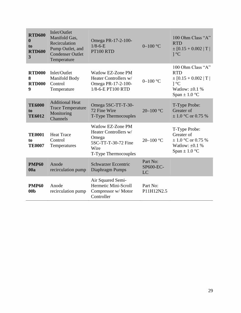
Table 1.1.3: Recirculation test bed measurement and control equipment of v1 system.

ID Description Type Range Accuracy

DEW60

00

DEW60

01

Inlet/Outlet

Manifold Dew

Point

Vaisala HMT 337 Dew

Point* Transmitter w/

HUMICAP 180RC RH

Sensor

20 to 100

Cdp

Sensor Calibration:

±0.6 Cdp @ 10 to

10 °C

±0.4 Cdp @ 10 to

21.5 °C

DEWC

AL

Dew Point

Calibration

Reference

Michell Optidew

Chilled Mirror Dew

Point Transmitter, Hi-

Temp Option

40 to 90 Cdp ±0.2 Cdp

FM6000

Hydrogen Supply

Dry Gas Inlet

Flow Rate

Brooks 5850s MFM/C 0.12 - 12

SLPM**

±0.7 % Flow Rate

+ 0.2 % F.S.

FM6001

Mixed Gas

Recirculation

Flow Rate, N2

Calibrated

MKS G50A Metal

Sealed Thermal MFM

0.05 5

SLPM

(N2

Calibrated)

±1 % F.R. for 20 to

100 % F.S.

±0.2 % F.S. for 0 to

20 % F.S.

FMCA

L

Dry Piston Gas

Flow Master

Meter

BIOS ML-800-10

ML-800-44

0.0050.5

SLPM

5 – 50 SLPM

± 0.15 %

Standardized Flow

H2C600

0

H2C600

1

Inlet/Outlet

Manifold

Hydrogen

Concentration

Applied Sensor HPS-

100

Hydrogen Sensors

0 – 100 % H2

±2 % H2 in N2

Background

w/ 0.5 %

Resolution

H2C600

2

Inlet/Outlet

Manifold

Hydrogen

Concentration

H2Scan Hy-Optima 730

Hydrogen Process

Monitor

0.5 – 100 %

H2 at 1 ATM

by volume

± 0.3 % for 0.5 to

10 % H2

± 1.0 % for 10 to

100 % H2 at 1

ATM

PT6000

PT6001

Inlet/Outlet

Manifold Absolute

Pressure

Wika C-10 Absolute

Pressure Transmitter

101.325 –

689.75 kPa,a

< ±0.5 % F.S. or

±3.44 kPa

PT6002

Recirculation

Return Line

Pressure,

Downstream of

Pump

Wika C-10 Gage

Pressure Transmitter

0 – 689.75

kPa,g

< ±0.5 % F.S. or

±3.44 kPa

DPT600

0

DPT600

1

Anode and

Recirculation

Pump Differential

Pressure

Druck PTX 2165-8971

Differential Pressure

Transmitter

0 – 70 kPa,d < ±0.1 % F.S. or

±0.07 kPa

29

RTD600

0

to

RTD600

3

Inlet/Outlet

Manifold Gas,

Recirculation

Pump Outlet, and

Condenser Outlet

Temperature

Omega PR-17-2-100-

1/8-6-E

PT100 RTD 0100 °C

100 Ohm Class “A”

RTD

± [0.15 + 0.002 | T |

] °C

RTD000

8

RTD000

9

Inlet/Outlet

Manifold Body

Control

Temperature

Watlow EZ-Zone PM

Heater Controllers w/

Omega PR-17-2-100-

1/8-6-E PT100 RTD

0100 °C

100 Ohm Class “A”

RTD

± [0.15 + 0.002 | T |

] °C

Watlow: ±0.1 %

Span ± 1.0 °C

TE6000

to

TE6012

Additional Heat

Trace Temperature

Monitoring

Channels

Omega 5SC-TT-T-30-

72 Fine Wire

T-Type Thermocouples 20100 °C

T-Type Probe:

Greater of

± 1.0 °C or 0.75 %

TE0001

to

TE0007

Heat Trace

Control

Temperatures

Watlow EZ-Zone PM

Heater Controllers w/

Omega

5SC-TT-T-30-72 Fine

Wire

T-Type Thermocouples

20100 °C

T-Type Probe:

Greater of

± 1.0 °C or 0.75 %

Watlow: ±0.1 %

Span ± 1.0 °C

PMP60

00a

Anode

recirculation pump

Schwarzer Eccentric

Diaphragm Pumps

Part No:

SP600-EC-

LC

PMP60

00b

Anode

recirculation pump

Air Squared Semi-

Hermetic Mini-Scroll

Compressor w/ Motor

Controller

Part No:

P11H12N2.5

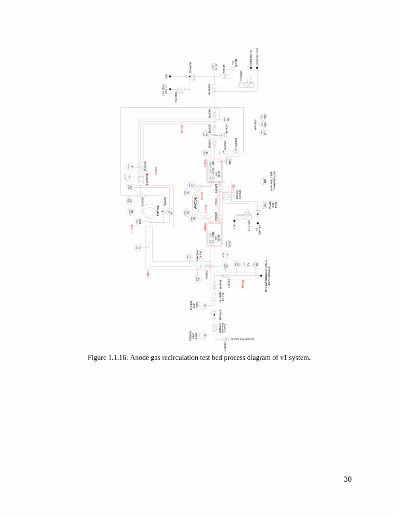
30

Figure 1.1.16: Anode gas recirculation test bed process diagram of v1 system.

AN

OD

E

dP

T

S

DE

W

PT

RT

DH

2C

DE

W

PT

RT

D

MF

C C

ON

TR

OL

LE

D G

AS

IN

[HE

AT

TR

AC

ED

]

H2 SUPPLY GAS IN

PG

PG

BV

60

00

FM

60

00

CA

LIB

RA

TE

D

@ 8

0 P

SIG

PG

60

00

0-1

00

PS

IG

PG

60

01

0-3

0

PS

IG

PR

V6

00

0B

V6

00

1

BV

60

02B

V6

00

3

CH

V6

00

1

0.1

PS

I

CO

OL

AN

T IN

CO

OL

AN

T O

UT

BV

60

04

BV

60

05

BV

60

07

BV

60

06

BP

V6

00

0

VT

E

RT

D

FM

60

01

NV

60

00

SV

60

00

PM

P6

00

0

PC

V1

10

0

GC

SE

P6

00

0

60

00

60

00

60

01

60

01

60

00

60

01

NA

FIO

N

DR

YE

R

60

02

RT

D

60

02

dP

T

60

01

RT

D

00

08

c

RT

D

00

09c

CO

NT

RO

L

GA

S IN

CH

V6

00

0

0.1

PS

IF

V1

10

0

FC

V5

00

0

TO

DR

AIN

HE

X6

00

0

60

03

BV

60

08

TE

TE

TC

TE T

E

TC

TE

HT

R0

1

HT

R0

8H

TR

09

HT

R0

2

HT

R0

3

HT

R0

4

HT

R0

5

HT

R0

6

HT

R0

7

00

01

00

05

TC

00

04

TC

00

07

TE

60

01

60

02

60

03

60

10

60

08

60

12

TE

60

09

TE

60

11

H2

C

60

00

H2C

60

01

TC

00

06

NV

60

01

BV

60

09

TC

00

02

TE

60

06

TE

60

07

TE

60

05

TC

00

03

PV

60

00

PG

VT

A

PG

70

0

0-1

5

PS

IG

N2

SU

PP

LY

FC

V7

00

0

HT

R1

0

HT

R1

1

FI

FI

UN

US

ED

60

00

TE

60

04

PT

60

02

GA

S A

NA

LY

ZE

R

TR

AN

SF

ER

LIN

E

31

Figure 1.1.17 provides an example of data recorded with the test bed. In this experiment, a 50

cm2 active area fuel cell was held at a constant current of 1 A cm

2 while feeding pressure

regulated dry hydrogen into the anode and recirculating it without venting. This configuration

enabled a precise monitoring of the decrease in cell voltage as the buildup of nitrogen diffusing

from the cathode into the anode compartment increased with time until a steady state was

reached. At the end of 140 h, the anode outlet was greater than 80 % nitrogen leading to a 5 %

loss in voltage efficiency. Future tests under other ONR awards (APRISES) will incorporate

contaminants such as carbon monoxide and utilize the gas analysis capabilities at HiSERF to

analyze carbon monoxide to carbon dioxide conversion and the subsequent impact on cell

efficiency.

Figure 1.1.17: Example data recorded with v1 system. The cell voltage decay due to nitrogen

accumulation was monitored. Single cell fuel cell operated at 1 A cm-2

. Anode recirculation without

venting.

Fuel cell UAV long term hardware in the loop performance tests

Under HEET10, two Ion Tiger stacks were tested using two different load profiles to determine

if they would meet the target design life of 300 h without significant performance degradation.

The commercial 36 cells PEMFC stacks were purchased from the vendor who designed and

supplied them to NRL for the Ion Tiger UAV.

The stacks were operated with a UAV load following (LF) profile (dynamic) and a constant

hybrid load (HL) corresponding to the average load of the dynamic profile. Figure 1.1.18

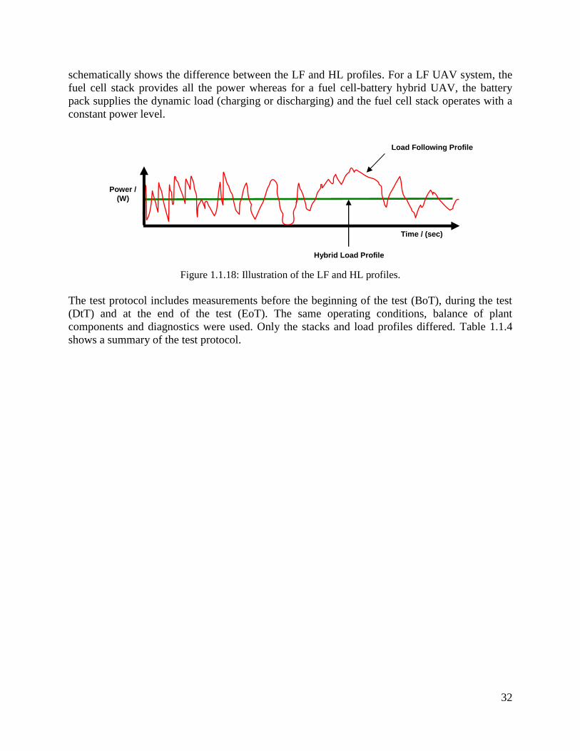
32

schematically shows the difference between the LF and HL profiles. For a LF UAV system, the

fuel cell stack provides all the power whereas for a fuel cell-battery hybrid UAV, the battery

pack supplies the dynamic load (charging or discharging) and the fuel cell stack operates with a

constant power level.

Figure 1.1.18: Illustration of the LF and HL profiles.

The test protocol includes measurements before the beginning of the test (BoT), during the test

(DtT) and at the end of the test (EoT). The same operating conditions, balance of plant

components and diagnostics were used. Only the stacks and load profiles differed. Table 1.1.4

shows a summary of the test protocol.

Time / (sec)

Load Following Profile

Hybrid Load Profile

Power /

(W)

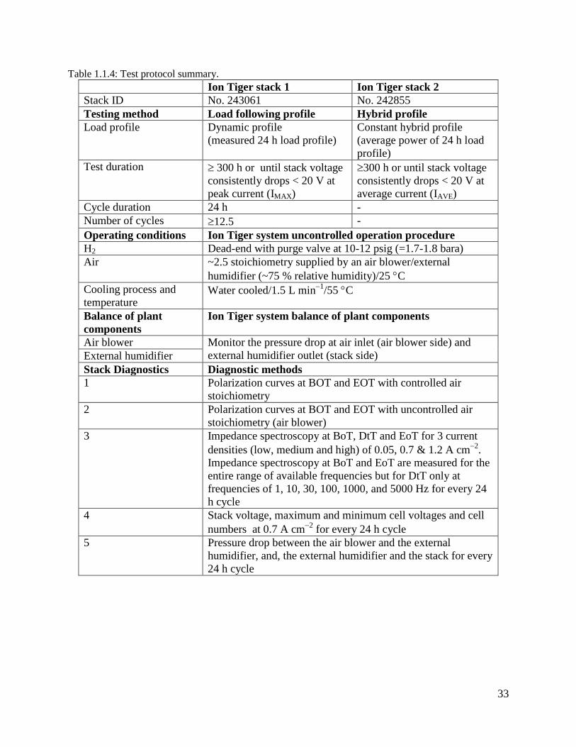
33

Table 1.1.4: Test protocol summary.

Ion Tiger stack 1 Ion Tiger stack 2

Stack ID No. 243061 No. 242855

Testing method Load following profile Hybrid profile

Load profile

Dynamic profile

(measured 24 h load profile)

Constant hybrid profile

(average power of 24 h load

profile)

Test duration 300 h or until stack voltage

consistently drops < 20 V at

peak current (IMAX)

300 h or until stack voltage

consistently drops < 20 V at

average current (IAVE)

Cycle duration 24 h -

Number of cycles 12.5 -

Operating conditions Ion Tiger system uncontrolled operation procedure

H2 Dead-end with purge valve at 10-12 psig (=1.7-1.8 bara)

Air ~2.5 stoichiometry supplied by an air blower/external

humidifier (~75 % relative humidity)/25 C

Cooling process and

temperature Water cooled/1.5 L min

1/55 C

Balance of plant

components

Ion Tiger system balance of plant components

Air blower Monitor the pressure drop at air inlet (air blower side) and

external humidifier outlet (stack side) External humidifier

Stack Diagnostics Diagnostic methods

1 Polarization curves at BOT and EOT with controlled air

stoichiometry

2 Polarization curves at BOT and EOT with uncontrolled air

stoichiometry (air blower)

3 Impedance spectroscopy at BoT, DtT and EoT for 3 current

densities (low, medium and high) of 0.05, 0.7 & 1.2 A cm2

.

Impedance spectroscopy at BoT and EoT are measured for the

entire range of available frequencies but for DtT only at

frequencies of 1, 10, 30, 100, 1000, and 5000 Hz for every 24

h cycle

4 Stack voltage, maximum and minimum cell voltages and cell

numbers at 0.7 A cm2

for every 24 h cycle

5 Pressure drop between the air blower and the external

humidifier, and, the external humidifier and the stack for every

24 h cycle

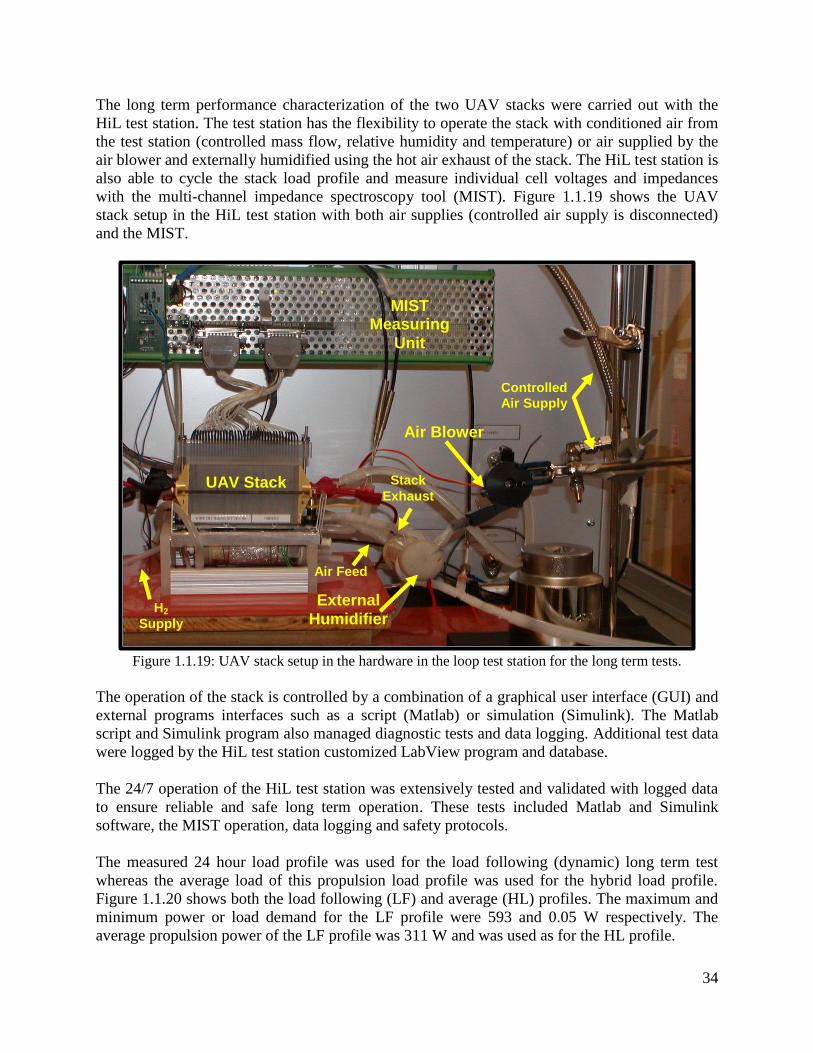
34

The long term performance characterization of the two UAV stacks were carried out with the

HiL test station. The test station has the flexibility to operate the stack with conditioned air from

the test station (controlled mass flow, relative humidity and temperature) or air supplied by the

air blower and externally humidified using the hot air exhaust of the stack. The HiL test station is

also able to cycle the stack load profile and measure individual cell voltages and impedances

with the multi-channel impedance spectroscopy tool (MIST). Figure 1.1.19 shows the UAV

stack setup in the HiL test station with both air supplies (controlled air supply is disconnected)

and the MIST.

Figure 1.1.19: UAV stack setup in the hardware in the loop test station for the long term tests.

The operation of the stack is controlled by a combination of a graphical user interface (GUI) and

external programs interfaces such as a script (Matlab) or simulation (Simulink). The Matlab

script and Simulink program also managed diagnostic tests and data logging. Additional test data

were logged by the HiL test station customized LabView program and database.

The 24/7 operation of the HiL test station was extensively tested and validated with logged data

to ensure reliable and safe long term operation. These tests included Matlab and Simulink

software, the MIST operation, data logging and safety protocols.

The measured 24 hour load profile was used for the load following (dynamic) long term test

whereas the average load of this propulsion load profile was used for the hybrid load profile.

Figure 1.1.20 shows both the load following (LF) and average (HL) profiles. The maximum and

minimum power or load demand for the LF profile were 593 and 0.05 W respectively. The

average propulsion power of the LF profile was 311 W and was used as for the HL profile.

MIST Measuring

Unit

Air Blower

External

Humidifier

UAV Stack

Controlled

Air Supply

H2

Supply

Stack

Exhaust

Air Feed

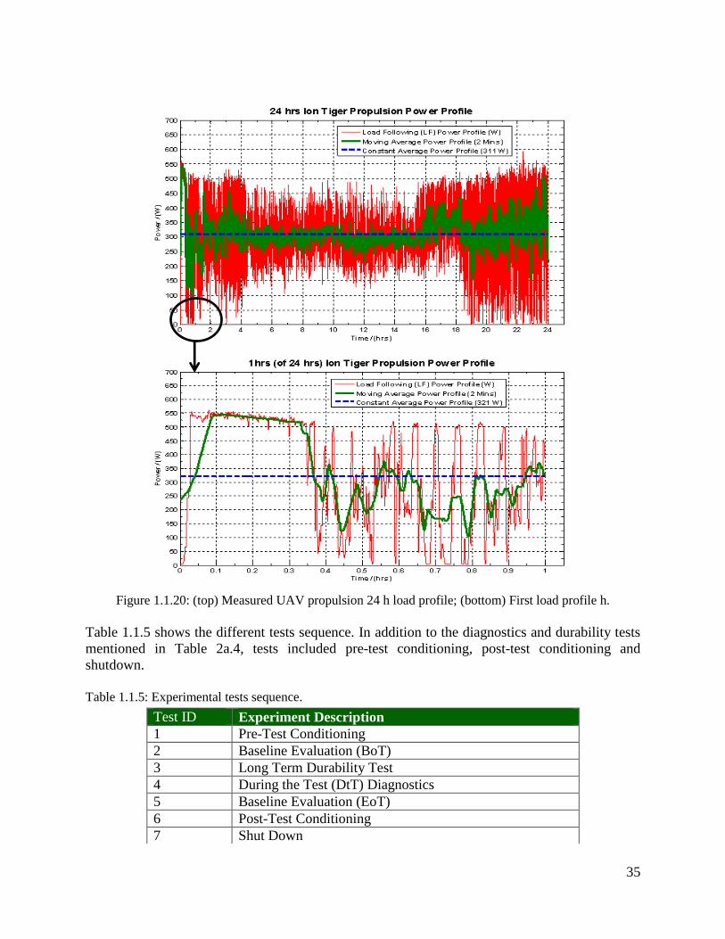
35

Figure 1.1.20: (top) Measured UAV propulsion 24 h load profile; (bottom) First load profile h.

Table 1.1.5 shows the different tests sequence. In addition to the diagnostics and durability tests

mentioned in Table 2a.4, tests included pre-test conditioning, post-test conditioning and

shutdown.

Table 1.1.5: Experimental tests sequence.

Test ID Experiment Description

1 Pre-Test Conditioning

2 Baseline Evaluation (BoT)

3 Long Term Durability Test

4 During the Test (DtT) Diagnostics

5 Baseline Evaluation (EoT)

6 Post-Test Conditioning

7 Shut Down

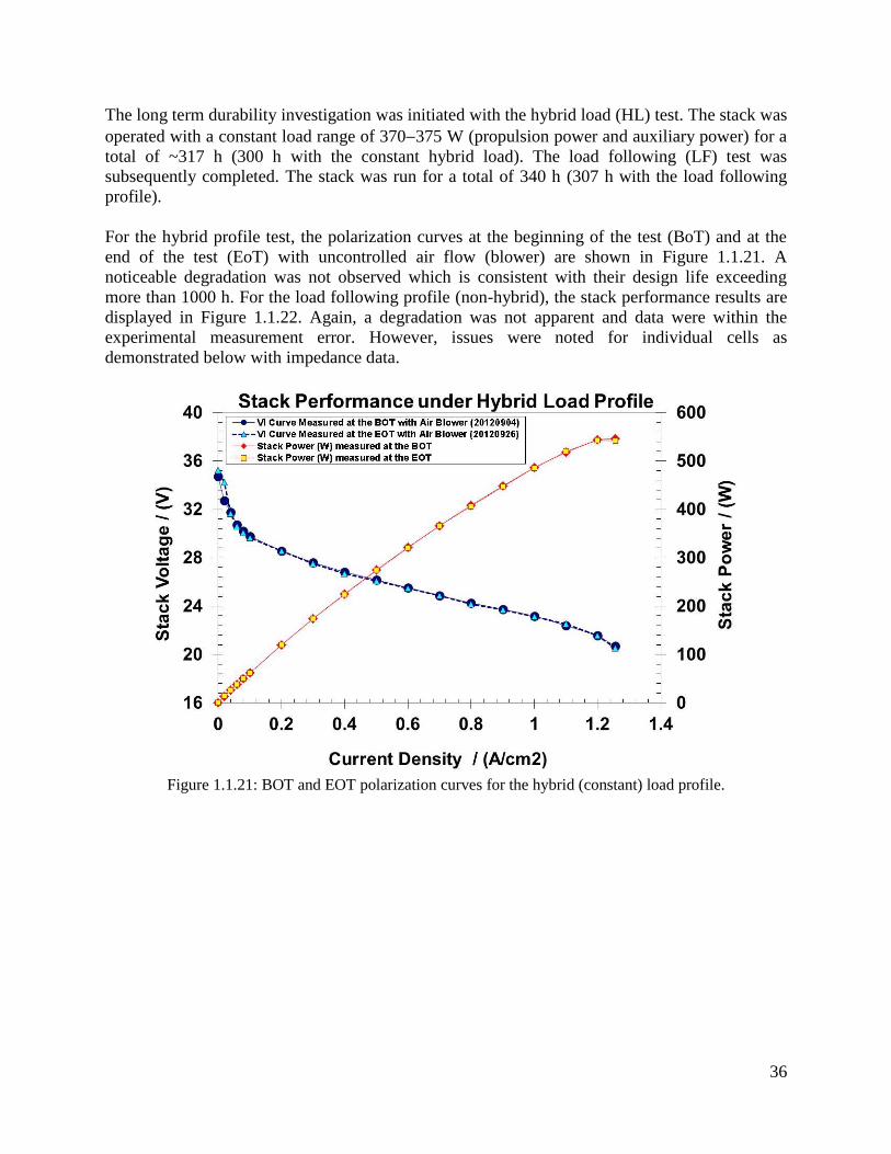
36

The long term durability investigation was initiated with the hybrid load (HL) test. The stack was

operated with a constant load range of 370375 W (propulsion power and auxiliary power) for a

total of ~317 h (300 h with the constant hybrid load). The load following (LF) test was

subsequently completed. The stack was run for a total of 340 h (307 h with the load following

profile).

For the hybrid profile test, the polarization curves at the beginning of the test (BoT) and at the

end of the test (EoT) with uncontrolled air flow (blower) are shown in Figure 1.1.21. A

noticeable degradation was not observed which is consistent with their design life exceeding

more than 1000 h. For the load following profile (non-hybrid), the stack performance results are

displayed in Figure 1.1.22. Again, a degradation was not apparent and data were within the

experimental measurement error. However, issues were noted for individual cells as

demonstrated below with impedance data.

Figure 1.1.21: BOT and EOT polarization curves for the hybrid (constant) load profile.

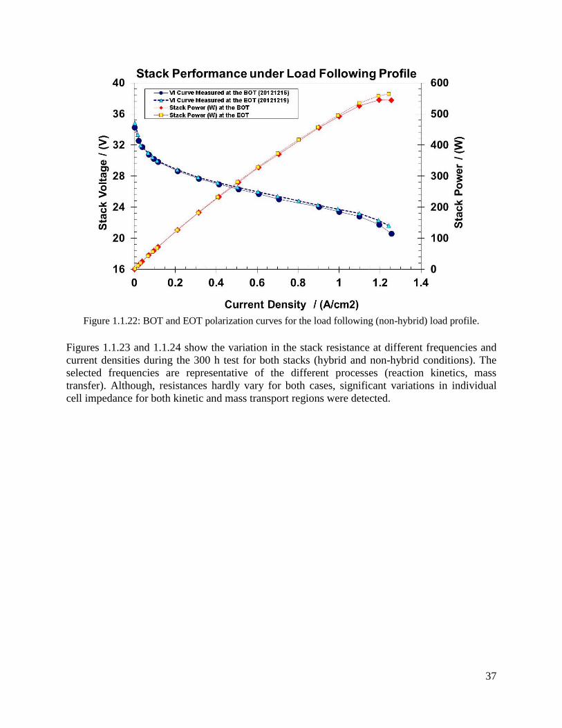
37

Figure 1.1.22: BOT and EOT polarization curves for the load following (non-hybrid) load profile.

Figures 1.1.23 and 1.1.24 show the variation in the stack resistance at different frequencies and

current densities during the 300 h test for both stacks (hybrid and non-hybrid conditions). The

selected frequencies are representative of the different processes (reaction kinetics, mass

transfer). Although, resistances hardly vary for both cases, significant variations in individual

cell impedance for both kinetic and mass transport regions were detected.

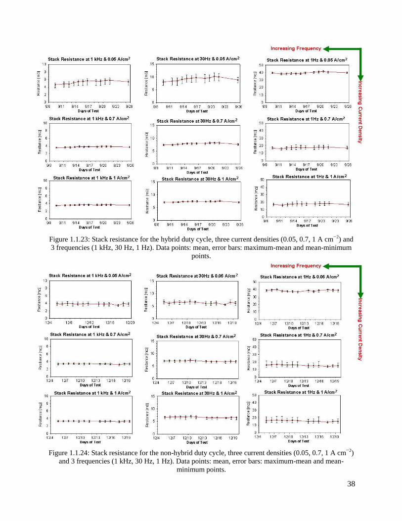
38

Figure 1.1.23: Stack resistance for the hybrid duty cycle, three current densities (0.05, 0.7, 1 A cm2

) and

3 frequencies (1 kHz, 30 Hz, 1 Hz). Data points: mean, error bars: maximum-mean and mean-minimum

points.

Figure 1.1.24: Stack resistance for the non-hybrid duty cycle, three current densities (0.05, 0.7, 1 A cm2

)

and 3 frequencies (1 kHz, 30 Hz, 1 Hz). Data points: mean, error bars: maximum-mean and mean-

minimum points.

39

Figure 1.1.25 shows a comparison between hybrid and non-hybrid electrochemical impedance

spectra (EIS) with only the 36 cell average values displayed for simplicity and for a 1 A current

(0.05 A cm2

) representative of oxygen reaction kinetics. Results show an increase in kinetic

resistance for the non-hybrid dynamic load profile (right) whereas for the hybrid load profile the

stack demonstrate significantly less performance degradation by catalyst deactivation (left).

Figure 1.1.25: BOT and EOT EIS results at 0.05 A cm2

for the hybrid (left) and non-hybrid (right) load

profile.

An effect in the mass transport region was also observed at high current densities (1 A cm2

) for

the non-hybrid stack operated with the air blower and external humidifier (uncontrolled air

supply). Figure 1.1.26 shows 36 cells EIS for the load following stack. The spread in the

individual impedance spectra for the 36 cells observed in the mass transport region (low

frequency loop) is indicative of the air supply method impact. The spread in cell impedance is

smaller at EOT (right). Presumably, the air blower performance improved during the test and led

to a more uniform air flow distribution in the stack. The kinetic (Figure 1.1.25) and mass transfer

(Figure 1.1.26) resistance changes (~5 mohm) are minor creating a voltage loss that is too small

to affect the polarization curves (Figures 1.1.21 and 1.1.22).

Increase in kinetic

resistance

Non-Hybrid Stack No. 243061 Hybrid Stack No. 242855

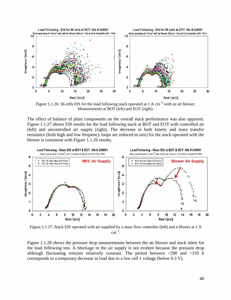
40

MFC Air Supply Blower Air Supply

Figure 1.1.26: 36 cells EIS for the load following stack operated at 1 A cm2

with an air blower.

Measurements at BOT (left) and EOT (right).

The effect of balance of plant components on the overall stack performance was also apparent.

Figure 1.1.27 shows EIS results for the load following stack at BOT and EOT with controlled air

(left) and uncontrolled air supply (right). The decrease in both kinetic and mass transfer

resistance (both high and low frequency loops are reduced in size) for the stack operated with the

blower is consistent with Figure 1.1.26 results.

Figure 1.1.27: Stack EIS operated with air supplied by a mass flow controller (left) and a blower at 1 A

cm2

.

Figure 1.1.28 shows the pressure drop measurements between the air blower and stack inlets for

the load following test. A blockage in the air supply is not evident because the pressure drop

although fluctuating remains relatively constant. The period between ~290 and ~310 h

corresponds to a temporary decrease in load due to a low cell 1 voltage (below 0.3 V).

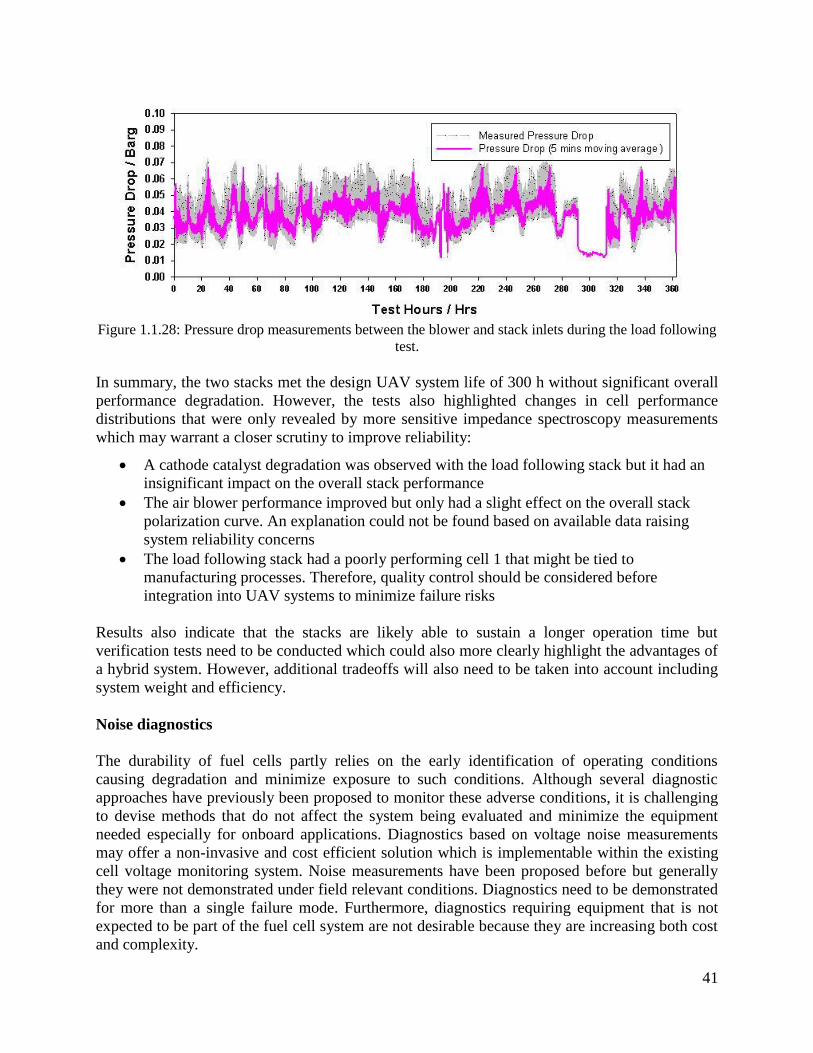
41

Figure 1.1.28: Pressure drop measurements between the blower and stack inlets during the load following

test.

In summary, the two stacks met the design UAV system life of 300 h without significant overall

performance degradation. However, the tests also highlighted changes in cell performance

distributions that were only revealed by more sensitive impedance spectroscopy measurements

which may warrant a closer scrutiny to improve reliability:

A cathode catalyst degradation was observed with the load following stack but it had an

insignificant impact on the overall stack performance

The air blower performance improved but only had a slight effect on the overall stack

polarization curve. An explanation could not be found based on available data raising

system reliability concerns

The load following stack had a poorly performing cell 1 that might be tied to

manufacturing processes. Therefore, quality control should be considered before

integration into UAV systems to minimize failure risks

Results also indicate that the stacks are likely able to sustain a longer operation time but

verification tests need to be conducted which could also more clearly highlight the advantages of

a hybrid system. However, additional tradeoffs will also need to be taken into account including

system weight and efficiency.

Noise diagnostics

The durability of fuel cells partly relies on the early identification of operating conditions

causing degradation and minimize exposure to such conditions. Although several diagnostic

approaches have previously been proposed to monitor these adverse conditions, it is challenging

to devise methods that do not affect the system being evaluated and minimize the equipment

needed especially for onboard applications. Diagnostics based on voltage noise measurements

may offer a non-invasive and cost efficient solution which is implementable within the existing

cell voltage monitoring system. Noise measurements have been proposed before but generally

they were not demonstrated under field relevant conditions. Diagnostics need to be demonstrated

for more than a single failure mode. Furthermore, diagnostics requiring equipment that is not

expected to be part of the fuel cell system are not desirable because they are increasing both cost

and complexity.

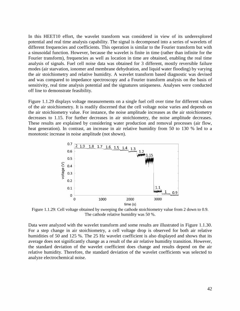
42

In this HEET10 effort, the wavelet transform was considered in view of its underexplored

potential and real time analysis capability. The signal is decomposed into a series of wavelets of

different frequencies and coefficients. This operation is similar to the Fourier transform but with

a sinusoidal function. However, because the wavelet is finite in time (rather than infinite for the

Fourier transform), frequencies as well as location in time are obtained, enabling the real time

analysis of signals. Fuel cell noise data was obtained for 3 different, mostly reversible failure

modes (air starvation, ionomer and membrane dehydration, and liquid water flooding) by varying

the air stoichiometry and relative humidity. A wavelet transform based diagnostic was devised

and was compared to impedance spectroscopy and a Fourier transform analysis on the basis of

sensitivity, real time analysis potential and the signatures uniqueness. Analyses were conducted

off line to demonstrate feasibility.

Figure 1.1.29 displays voltage measurements on a single fuel cell over time for different values

of the air stoichiometry. It is readily discerned that the cell voltage noise varies and depends on

the air stoichiometry value. For instance, the noise amplitude increases as the air stoichiometry

decreases to 1.15. For further decreases in air stoichiometry, the noise amplitude decreases.

These results are explained by considering water production and removal processes (air flow,

heat generation). In contrast, an increase in air relative humidity from 50 to 130 % led to a

monotonic increase in noise amplitude (not shown).

Figure 1.1.29: Cell voltage obtained by sweeping the cathode stoichiometry value from 2 down to 0.9.

The cathode relative humidity was 50 %.

Data were analyzed with the wavelet transform and some results are illustrated in Figure 1.1.30.

For a step change in air stoichiometry, a cell voltage drop is observed for both air relative

humidities of 50 and 125 %. The 25 Hz wavelet coefficient is also displayed and shows that its

average does not significantly change as a result of the air relative humidity transition. However,

the standard deviation of the wavelet coefficient does change and results depend on the air

relative humidity. Therefore, the standard deviation of the wavelet coefficients was selected to

analyze electrochemical noise.

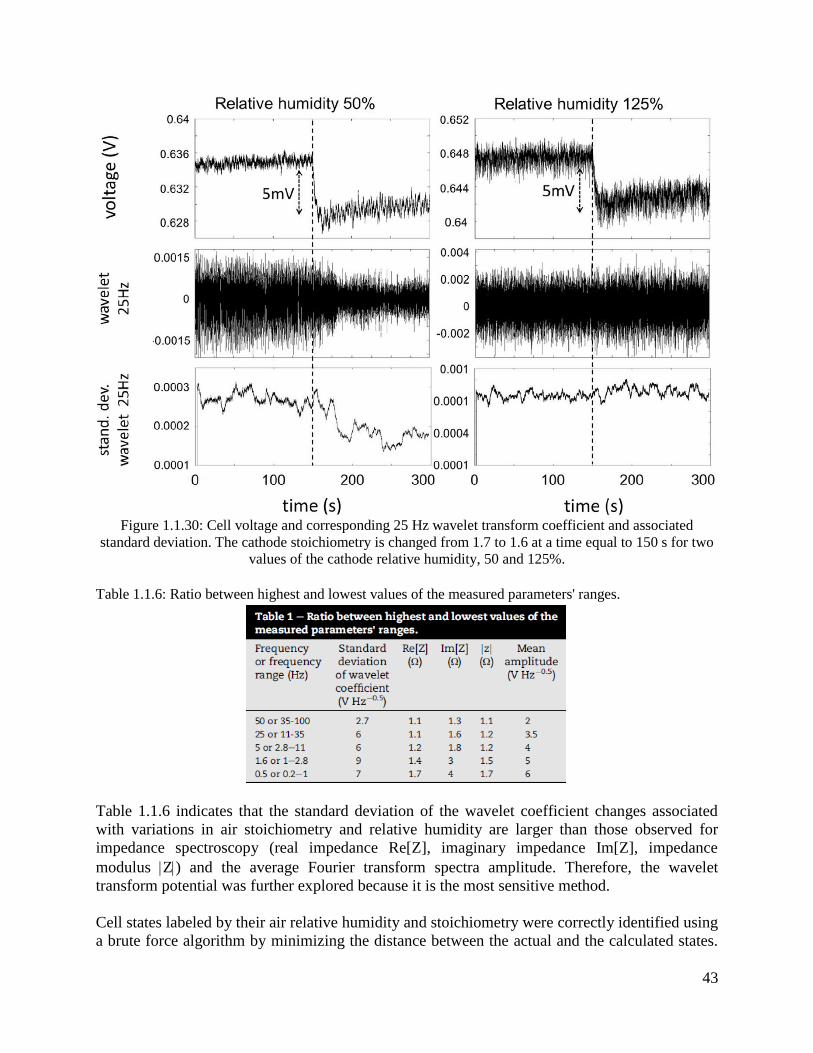
43

Figure 1.1.30: Cell voltage and corresponding 25 Hz wavelet transform coefficient and associated

standard deviation. The cathode stoichiometry is changed from 1.7 to 1.6 at a time equal to 150 s for two

values of the cathode relative humidity, 50 and 125%.

Table 1.1.6: Ratio between highest and lowest values of the measured parameters' ranges.

Table 1.1.6 indicates that the standard deviation of the wavelet coefficient changes associated

with variations in air stoichiometry and relative humidity are larger than those observed for

impedance spectroscopy (real impedance Re[Z], imaginary impedance Im[Z], impedance

modulus Z) and the average Fourier transform spectra amplitude. Therefore, the wavelet

transform potential was further explored because it is the most sensitive method.

Cell states labeled by their air relative humidity and stoichiometry were correctly identified using

a brute force algorithm by minimizing the distance between the actual and the calculated states.

44

Independent and uniformly distributed random variations were added to experimental wavelet

coefficients' standard deviations to define the calculated states. Additional information is

available in the published paper (item 8 in the Papers and Presentations Resulting from these

Efforts section). Future work under other ONR funding (APRISES) will include the

demonstration of a larger number of failure modes (2 different contaminants injected in the air

stream) and implementation of the wavelet transform method in real time.

Alternative cell evaluation

Under HEET10, the HNEI fuel cell MIST was adapted to characterize the effects of non-linear

discharge of a 4-cell, high power Li-ion battery pack in support of NRL battery research project

to minimize efficiency losses. This project is novel and the results give a unique perspective into

the cell to cell performance distribution of a battery pack in comparison to single cell

measurements which are generally employed to characterize batteries.

A sinusoidal (non-linear) discharge current was compared to a constant discharge current. Two

four-cell packs comprised of high power Li-ion batteries (A123 Li-Ion ANR26650) were used

for this study. Each cell has a capacity of 2.3 Ah and a nominal voltage of 3.3 V. The study was

carried out with the HiL test stand and the MIST. Discharge rates of 5C (11.5 A) and 10C (23 A)

were used. The sinusoidal discharge rate frequency varied from 1 Hz to 5 kHz. Impedance

Spectra were also acquired with fully charged and discharged states.

The initial measurement concept considered the MIST coupled with a voltage divider to match

the high battery cell voltage of 3.6 V, for both impedance measurements and non-linear battery

discharge. However, this method did not bring about satisfactory results especially for high

frequencies. Many different approaches were subsequently evaluated including a Solartron

impedance analyzer with AC coupled amplifiers with or without a voltage divider, the MIST, AC

coupled amplifiers and an offset correction, etc. However, each of these solutions had limitations

such as a complex setup, high noise levels or questionable results. A custom solution was

developed using modular one-channel signal treatment (MOST) circuit boards. The MOST

measurement system has 5 AC coupled channels and 5 DC coupled channels. The MIST

software was adapted to work with the MOST system and, capture and analyze data.

Different perturbation sources were also evaluated including an audio power amplifier operated

as a controlled voltage supply which delivered the best results for the impedance measurements.

For the non-linear discharge, different load units were equally evaluated for varied current and

frequency ranges. A smaller electronic load unit (60 V, 120 A) gave better results up to 5 kHz.

However, this solution was not ideal for higher currents (10C) due to the load unit power limit

(600 W) and higher frequencies (>5 kHz) as sinusoidal wave distortions were present due to an

increased current rise time at very low currents (<1 A).

Battery charging was conducted at 1C (2.3 A) up to 14.6 V with a power supply operated with a

constant current until the set point could no longer be maintained. Subsequently, battery charging

was carried out with a constant voltage mode until the current dropped to a zero value.

In a first series of tests completed with the first 4-cell battery pack, measurement systems were

45

verified, data are reported but results are not discussed in detail (Figures 1.1.31, 1.1.32, 1.1.33,

1.1.34, and 1.1.35, Tables 1.1.7 and 1.1.8) but highlight the capabilities that were developed for

this project. After the battery pack was fully charged, it was held at 14 V and excited with a 5

mV perturbation using frequencies spanning a 0.5 Hz to 10 kHz range (20 frequencies per

decade). For the discharged state measurements, the battery pack was non-linearly discharged

with a 1C rate and a 1 Hz frequency and then held at 10 V and again perturbed with a 5 mV

signal (0.5 Hz to 10 kHz, 20 frequencies per decade). Figures 1.1.31 and 1.1.32 show resulting

impedance spectra for the fully charged and discharged states respectively. Figures also show

cell resistances at 1 kHz. Measured 1 kHz cell resistances (6.67.7 m) are close to the

manufacturing data sheet (A123 System 26650) value of 8 m.

Figure 1.1.31: Impedance spectra of a charged 4-cell high power Li-ion battery pack.

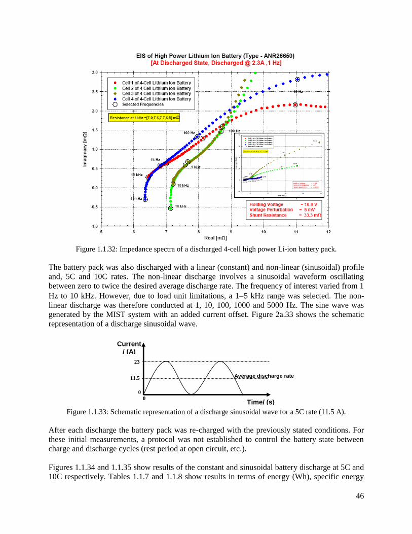
46

Figure 1.1.32: Impedance spectra of a discharged 4-cell high power Li-ion battery pack.

The battery pack was also discharged with a linear (constant) and non-linear (sinusoidal) profile

and, 5C and 10C rates. The non-linear discharge involves a sinusoidal waveform oscillating

between zero to twice the desired average discharge rate. The frequency of interest varied from 1

Hz to 10 kHz. However, due to load unit limitations, a 15 kHz range was selected. The non-

linear discharge was therefore conducted at 1, 10, 100, 1000 and 5000 Hz. The sine wave was

generated by the MIST system with an added current offset. Figure 2a.33 shows the schematic

representation of a discharge sinusoidal wave.

Figure 1.1.33: Schematic representation of a discharge sinusoidal wave for a 5C rate (11.5 A).

After each discharge the battery pack was re-charged with the previously stated conditions. For

these initial measurements, a protocol was not established to control the battery state between

charge and discharge cycles (rest period at open circuit, etc.).

Figures 1.1.34 and 1.1.35 show results of the constant and sinusoidal battery discharge at 5C and

10C respectively. Tables 1.1.7 and 1.1.8 show results in terms of energy (Wh), specific energy

Time/ (s)

Current / (A)

11.5

0

23

0

Average discharge rate

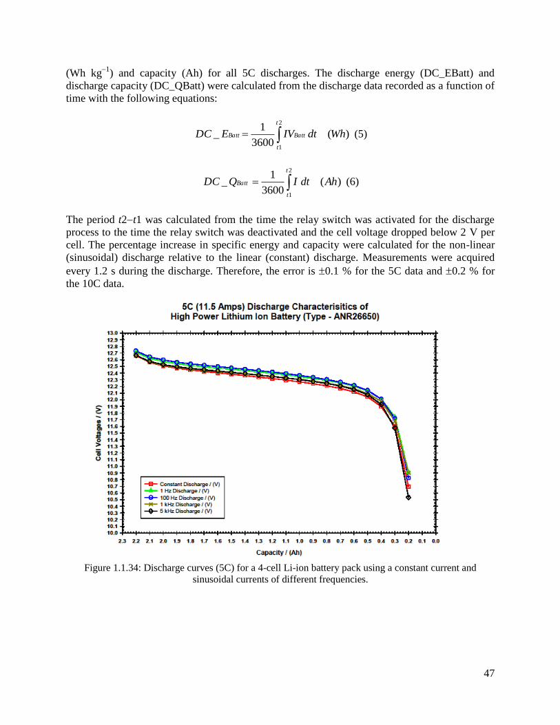
47

(Wh kg1

) and capacity (Ah) for all 5C discharges. The discharge energy (DC_EBatt) and

discharge capacity (DC_QBatt) were calculated from the discharge data recorded as a function of

time with the following equations:

)(3600

1_

2

1

WhdtIVEDC

t

t

BattBatt (5)

)(3600

1_

2

1

AhdtIQDC

t

t

Batt (6)

The period t2t1 was calculated from the time the relay switch was activated for the discharge

process to the time the relay switch was deactivated and the cell voltage dropped below 2 V per

cell. The percentage increase in specific energy and capacity were calculated for the non-linear

(sinusoidal) discharge relative to the linear (constant) discharge. Measurements were acquired

every 1.2 s during the discharge. Therefore, the error is 0.1 % for the 5C data and 0.2 % for

the 10C data.

Figure 1.1.34: Discharge curves (5C) for a 4-cell Li-ion battery pack using a constant current and

sinusoidal currents of different frequencies.

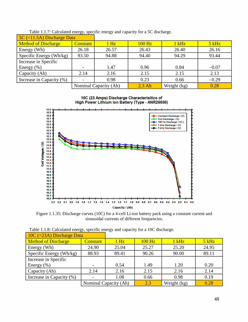
48

Table 1.1.7: Calculated energy, specific energy and capacity for a 5C discharge.

5C (=11.5A) Discharge Data

Method of Discharge Constant 1 Hz 100 Hz 1 kHz 5 kHz

Energy (Wh) 26.18 26.57 26.43 26.40 26.16

Specific Energy (Wh/kg) 93.50 94.88 94.40 94.29 93.44

Increase in Specific

Energy (%) - 1.47 0.96 0.84 0.07

Capacity (Ah) 2.14 2.16 2.15 2.15 2.13

Increase in Capacity (%) - 0.98 0.23 0.66 0.29

Nominal Capacity (Ah) 2.3 Ah Weight (kg) 0.28

Figure 1.1.35: Discharge curves (10C) for a 4-cell Li-ion battery pack using a constant current and

sinusoidal currents of different frequencies.


10C (=23A) Discharge Data

Method of Discharge Constant 1 Hz 100 Hz 1 kHz 5 kHz

Energy (Wh) 24.90 25.04 25.27 25.20 24.95

Specific Energy (Wh/kg) 88.93 89.41 90.26 90.00 89.11

Increase in Specific

Energy (%) - 0.54 1.49 1.20 0.20

Capacity (Ah) 2.14 2.16 2.15 2.16 2.14

Increase in Capacity (%) - 1.08 0.66 0.98 0.19

Nominal Capacity (Ah) 2.3 Weight (kg) 0.28

49

For the second 4-cell battery pack, a protocol was established to control the battery state between

the charge and discharge steps. The battery pack was charged with a 1C rate up to 14.6 V under

constant current (until the current could no longer be maintained) and constant voltage (until the

current dropped to 0) mode. The battery pack was allowed to rest until the voltage reached a

constant open circuit voltage (OCV) after the discharge cycle. This rest period was

approximately 12 h long. After the battery pack was charged it was also allowed to rest for a

short period (35 min) before it was discharged. The second battery pack was previously used

for a UAV hybrid power system study and therefore it had sustained a number of

charge/discharge cycles. The following testing protocol was followed for the non-linear battery

discharge:

1. Battery charged at 1C rate up to 14.6 V under constant current and constant voltage mode

until the charging current was zero (1-2 h)

2. Battery was discharged linearly at 10C rate with a constant current

3. Battery was allowed to rest until a constant OCV was reached (1-2 h)

4. Same as step 1.

5. Battery was discharged non-linearly at 10C rate and 1 kHz

6. Same as step 3.

7. Same as step 1.

8. Same as step 2.

9. Impedance spectroscopy measurements were conducted with a discharged state. The

battery was allowed to rest until it reached a constant OCV of 12.2 V. The battery was

held at 12.2 V during impedance spectroscopy measurements.

10. Same as step 3.

11. Same as step 1.

12. Impedance spectroscopy measurements were conducted with a charged state. The battery

was allowed to rest until it reached a constant OCV of 14 V. The battery was held at 14 V

during impedance spectroscopy measurements.

Figures 1.1.36 and 1.1.37 show impedance spectra for the second battery pack in a charged and

discharged state respectively.

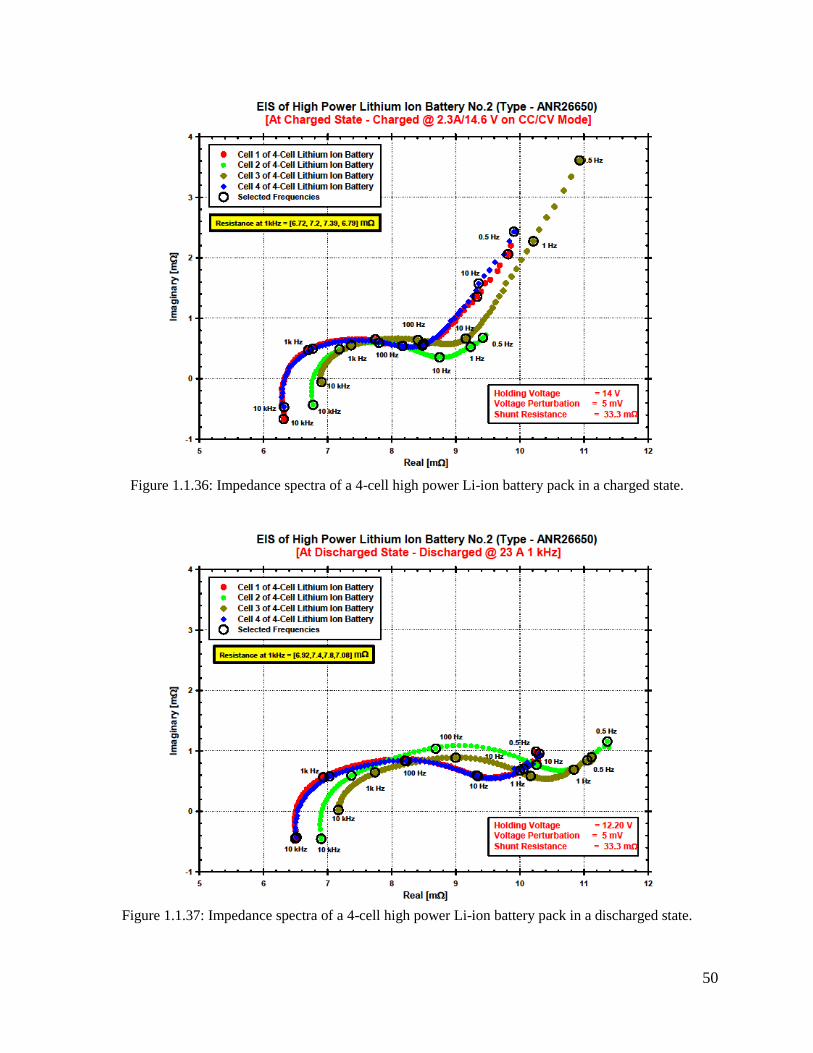
50

Figure 1.1.36: Impedance spectra of a 4-cell high power Li-ion battery pack in a charged state.

Figure 1.1.37: Impedance spectra of a 4-cell high power Li-ion battery pack in a discharged state.

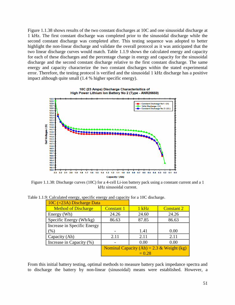
51

Figure 1.1.38 shows results of the two constant discharges at 10C and one sinusoidal discharge at

1 kHz. The first constant discharge was completed prior to the sinusoidal discharge while the

second constant discharge was completed after. This testing sequence was adopted to better

highlight the non-linear discharge and validate the overall protocol as it was anticipated that the

two linear discharge curves would match. Table 1.1.9 shows the calculated energy and capacity

for each of these discharges and the percentage change in energy and capacity for the sinusoidal

discharge and the second constant discharge relative to the first constant discharge. The same

energy and capacity characterize the two constant discharges within the stated experimental

error. Therefore, the testing protocol is verified and the sinusoidal 1 kHz discharge has a positive

impact although quite small (1.4 % higher specific energy).

Figure 1.1.38: Discharge curves (10C) for a 4-cell Li-ion battery pack using a constant current and a 1

kHz sinusoidal current.


10C (=23A) Discharge Data

Method of Discharge Constant 1 1 kHz Constant 2

Energy (Wh) 24.26 24.60 24.26

Specific Energy (Wh/kg) 86.63 87.85 86.63

Increase in Specific Energy

(%) - 1.41 0.00

Capacity (Ah) 2.11 2.11 2.11

Increase in Capacity (%) - 0.00 0.00

Nominal Capacity (Ah) = 2.3 & Weight (kg)

= 0.28

From this initial battery testing, optimal methods to measure battery pack impedance spectra and

to discharge the battery by non-linear (sinusoidal) means were established. However, a

52

significant improvement in performance was not observed for this specific high power lithium

ion battery with a non-linear discharge profile.

A more detailed investigation would be required to ascertain any significant impact of the non-

linear discharge method and could include other battery chemistries, improved charging and

discharging protocols, discharges at much higher currents and frequencies (>5 kHz) or lower

frequencies (<1 kHz) and other discharge or charge profiles (square or pulse waves, etc.). Higher

current and frequency discharge profiles could not be used due to testing equipment limitations

(amplifier, load unit, power supply, data acquisition system). Therefore, research would benefit

from upgraded battery testing equipment.

References

1. J. St-Pierre, Y. Zhai, M. S. Angelo, J. Electrochem. Soc., 161 (2014) F280.

2. D. A. Schiraldi, J. Macromol. Sci. C, 46 (2006) 315.

3. J. St-Pierre, Y. Zhai, J. Ge, J. Electrochem. Soc., 163 (2016) F247.

4. J. St-Pierre, B. Wetton, Y. Zhai, J. Ge, J. Electrochem. Soc., 161 (2014) E3357.

5. J. Diep, D. Kiel, J. St-Pierre, A. Wong, Chem. Eng. Sci., 62 (2007) 846.

6. J. St-Pierre, J. Electrochem. Soc., 154 (2007) B724.

7. H. S. Fogler, Elements of Chemical Reaction Engineering, 4th

edition, Prentice Hall (2006).

8. J. St-Pierre, A. Wong, J. Diep, D. Kiel, J. Power Sources, 164 (2007) 196.

9. E. B. Nauman, Chemical Reactor Design, Optimization, and Scaleup, John Wiley & Sons

(2008).

10. K. Broka, P. Ekdunge, J. Appl. Electrochem., 27 (1997) 117.

11. J. St-Pierre, D. P. Wilkinson, AIChE J., 47 (2001) 1482.

12. Large Displacement Unmanned Undersea Vehicle Innovative Naval Prototype Industry Day,

Office of Naval Research Presentation, March 11, 2011

(http://auvac.org/uploads/publication_pdf/734_LDUUV%20INP%20Industry%20Day_poste

d%20version.pdf).

13. ONR Undersea Energy and Propulsion Program Review: Quad Charts, Arlington, VA, April

15-17, 2015.

14. Statement of Rear Admiral Matthew L. Klunder, United States Navy Chief of Naval Research

before the Intelligence, Emerging Threats, and Capabilities Subcommittee of the House

Armed Services Committee on the Fiscal Year 2015 Budget Request, March 26, 2014,

http://www.acq.osd.mil/chieftechnologist/publications/docs/FY2015_TestimonyONR_Klund

erUSNM_20140326.pdf

15. Statement of Rear Admiral Mathias W. Winter, United States Navy Chief of Naval Research


Armed Services Committee on the Fiscal Year 2016 Budget Request, March 26, 2015,

http://www.onr.navy.mil/~/media/Files/About-ONR/FY16-Science-Technology-Budget-

Request.ashx

16. Statement of Rear Admiral Mathias W. Winter, United States Navy Chief of Naval Research

http://auvac.org/uploads/publication_pdf/734_LDUUV%20INP%20Industry%20Day_posted%20version.pdf

http://auvac.org/uploads/publication_pdf/734_LDUUV%20INP%20Industry%20Day_posted%20version.pdf

http://www.acq.osd.mil/chieftechnologist/publications/docs/FY2015_TestimonyONR_KlunderUSNM_20140326.pdf

http://www.acq.osd.mil/chieftechnologist/publications/docs/FY2015_TestimonyONR_KlunderUSNM_20140326.pdf

http://www.onr.navy.mil/~/media/Files/About-ONR/FY16-Science-Technology-Budget-Request.ashx

http://www.onr.navy.mil/~/media/Files/About-ONR/FY16-Science-Technology-Budget-Request.ashx

53


Armed Services Committee on the Fiscal Year 2017 Budget Request, February 24, 2015,

http://defenseinnovationmarketplace.mil/resources/HHRG-114-AS26-Wstate-WinterM-

20160224.pdf

17. K. Swider-Lyons, Integration Briefing; Hydra UUV Program: Adaption of an Automotive

Hydrogen Fuel Cell to Large Diameter Unmanned Undersea Vehicles, NRL/NSWC-

Carderock/GM/University of Hawaii, June 7, 2011.

18. K. Promislow, J. St- Pierre, B. Wetton, J. Power Sources, 196 (2011) 10050.

19. J. P. Owejan, J. C. Fagley, S. G. Goebel, United States Patent 7,960,062, June 14, 2011.

Papers and Presentations Resulting from these Efforts

Journals 1. Y. Garsany, J. Ge, J. St-Pierre, R. Rocheleau, K. E. Swider-Lyons, ‘Analytical Procedure for

Accurate Comparison of Rotating Disk Electrode Results for the Oxygen Reduction Activity of

Pt/C’, J. Electrochem. Soc., 161 (2014) F628-F640.

2. J. Ge, J. St-Pierre, Y. Zhai, ‘PEMFC Cathode Catalyst Contamination Evaluation with a

RRDE - Propene and Naphthalene’, Electrochim. Acta, 138 (2014) 437-446.


RRDE - Acetonitrile’, Electrochim. Acta, 134 (2014) 272-280.


RRDE - Acetylene’, Electrochim. Acta, 133 (2014) 65-72.


RRDE – Methyl Methacrylate’, Int. J. Hydrogen Energy, 39 (2014) 18351-18361.

6. Y. Zhai, J. Ge, J. St-Pierre, ‘The Ionic Conductivity and Catalyst Activity Effects of

Acetonitrile on Proton Exchange Membrane Fuel Cells’, Electrochem. Commun., 66 (2016) 49-

52.

7. Y. Zhai, O. Baturina, D. Ramaker, E. Farquhar, J. St-Pierre, K. Swider-Lyons, ‘Chlorobenzene

Poisoning and Recovery of Platinum-Based Cathodes in Proton Exchange Membrane Fuel

Cells’, J. Phys. Chem. C, 119 (2015) 20328-20338.

8. M. A. Rubio, K. Bethune, A. Urquia, J. St-Pierre, ‘Proton Exchange Membrane Fuel Cell

Failure Mode Early Diagnosis with Wavelet Analysis of Electrochemical Noise’, Int. J.

Hydrogen Energy, 41 (2016) 14991-15001.

Conference Proceedings 9. Y. Zhai, J. St-Pierre, J. Ge, ‘PEMFC Cathode Contamination Evaluation with Membrane

Conductivity Cell, CA, CP, CV, EIS, GC/MS and ISE - Acetonitrile’, Electrochem. Soc. Trans.,

64 (3) (2014) 805-816.

http://defenseinnovationmarketplace.mil/resources/HHRG-114-AS26-Wstate-WinterM-20160224.pdf

http://defenseinnovationmarketplace.mil/resources/HHRG-114-AS26-Wstate-WinterM-20160224.pdf

54

10. Y. Garsany, J. Ge, J. St-Pierre, R. Rocheleau, K. E. Swider-Lyons, ‘ORR Measurement

Reproducibility Using a RRDE’, Electrochem. Soc. Trans., 58 (1) (2013) 1233-1241.

11. Y. Garsany, J. Ge, J. St-Pierre, R. Rocheleau, K. E. Swider-Lyons, ‘Standardizing Thin-Film

Rotating Disk Electrode Measurements of the Oxygen Reduction Activity of Pt/C’, Electrochem.

Soc. Trans., 58 (1) (2013) 3-14.

Conference Presentations

12. Y. Zhai, J. St-Pierre, J. Ge, ‘PEMFC Cathode Contamination Evaluation with Membrane

Conductivity Cell, CA, CV and GC/MS - Acetonitrile’, in Meeting Abstracts, Electrochemical

Society volume 2014-2, The Electrochemical Society, Pennington, NJ, 2014, abstract 1271.

13. Y. Zhai, O. Baturina, D. E. Ramaker, J. St-Pierre, K. E. Swider-Lyons, ‘Contamination and

Recovery of PEMFC Cathodes with Organohalides: Chlorobenzene and Bromomethane’, in

Meeting Abstracts, Electrochemical Society volume 2014-2, The Electrochemical Society,

Pennington, NJ, 2014, abstract 1268.

14. J. Ge, Y. Garsany, Y. Zhai, J. St-Pierre, K. Swider-Lyons, ‘ORR Measurements

Reproducibility Using a RRDE’, in Meeting Abstracts, Electrochemical Society volume 2013-2,

The Electrochemical Society, Pennington, NJ, 2013, abstract 1498.

15. J. Ge, Y. Zhai, J. St-Pierre, ‘An RRDE Evaluation of the C2H2 Effect on the ORR’, in

Meeting Abstracts, Electrochemical Society volume 2013-2, The Electrochemical Society,

Pennington, NJ, 2013, abstract 1302.

16. Y. Garsany, J. Ge, J. St-Pierre, R. Rocheleau, K. Swider-Lyons, ‘Standardizing Thin-Film

Rotating Disk Electrode Measurements of the Oxygen Reduction Activity of Pt/C’, in Meeting

Abstracts, Electrochemical Society volume 2013-2, The Electrochemical Society, Pennington,

NJ, 2013, abstract 1238.

1.2 Novel Fuel Cells

Under subtask 1.2, HNEI conducted research to advance enzymatic biofuel cell technology

through quantitative, in-situ characterizations of immobilized enzyme to enhance fundamental

understanding of the underlying mechanism in biocatalysis. In this project, we continued to

investigate the ability to control pore structure within thin chitosan films through chemical

modification of the chitosan polymer backbone. To pursue this objective we hydrophobically

modified chitosan polymer with specific alkyl side chains (e.g., butyl, decyl) and then caste these

solutions into micron thin films using a spread coating technique. After air drying pore size of

the resulting films was characterized using established physical (high resolution microscopy) and

chemical (gas absorption) methodologies. Pore size was correlated to the method of chemical

modification (e.g., butyl, decyl etc.).

55

Chitosan biopolymer has gained attention in the research community, in part because of its

ability to be blended with other biomaterials and/or molded into highly porous matrices, creating

great potential as a biomaterial for enzyme immobilization, drug delivery, and gene delivery.

This work reports on the correlation between final thickness of spread-spread coated chitosan

polymer films and deposition rate. More, the impact of solution based micelle structure (gained

through the introduction of hydrophobic modification of chitosan polymer) on final film

thickness and morphology is also discussed. These results represent new knowledge on how the

introduction of hydrophobic modification, a technique shown to introduce solution-based micelle

structure and micellar aggregates that support enzyme immobilization, impacts final film

thickness and morphology of spread coated films and will aid the development and deployment

of chitosan-based biofuel cell electrodes.

The thickness of spread-coated films made from both deacetylated and butyl-modified chitosan

were correlated to deposition rate and solution micellar structure. Results demonstrated how, to

a certain degree, differences in the underlying micellar structure could impact the final film

thickness. At intermediate deposition rates, the thickness of chitosan films was predictable and

well controlled. Furthermore, it was shown that hydrophobic modification of the chitosan

extended the range of deposition rates (from 5-16 cm/hr to 6-30 cm/hr) which allowed for a

linear relationship between film thickness and deposition rate. Hydrophobic modification were

also extended the range of thickness achieved from 0.06-0.10 μm to 0.04-0.14 μm. These

features were accredited to the domination of intramolecular forces at lower concentrations of

hydrophobically modified chitosan solutions as opposed to equal concentration of the

deacetylated chitosan solutions, as supported by the viscosity and fluorescence experiments.

Although both deacetylated and butyl-modified chitosan solutions were found to have inter- and

intramolecular interactions, as well as hydrophobic domains able to incorporate fluorophores,

deacetylated chitosan was much more interconnected via intermolecular interactions at higher

concentrations.

56

Figure 1.2.1: Schematic of film deposition with inlayed microscope image from thickness measurement

of air-dried film (top left). Deacetylated or butyl-modified chitosan solutions were pipetted on the obtuse

side of the intersection of the two glass slides held at an angle of 30 ± 1°. A meniscus forms under the

leading slide as it pushes against the solution droplet and across the lower glass substrate at a constant

velocity, leaving a thin layer of solution behind. Films formed as the solution was air-dried.

Figure 1.2.2. Typical image of “cut” spread coated films using Keyence imaging microscope and

associated imaging software. The left hand image is a top down image of film surface while the right

hand image is the surface morphology mapped out in terms of relative surface film height. The inset to

the right hand image is a not-to-scale rendering of the shape of the surgical blade used to cut the film.

Region’s 2 and 3 represent film surface on either side of the cut while region 1 represents the region

where the film was cut. The sharp peak between region 3 and 1 represents the leading edge of polymer

material that was displaced by the blade’s cut into the film. The downward slope in region 1 mimics the

slope of the surgical blade while the sudden upturn to region 2 represents the back edge of the surgical

blade. The circular inset indicates a region that was found to possess, across all films analyzed, a

characteristic mark that was found to represent where the blade cut into the glass slide, yielding a

consistent relative reference to the surface of the slide and the bottom of the film.

2

1

3

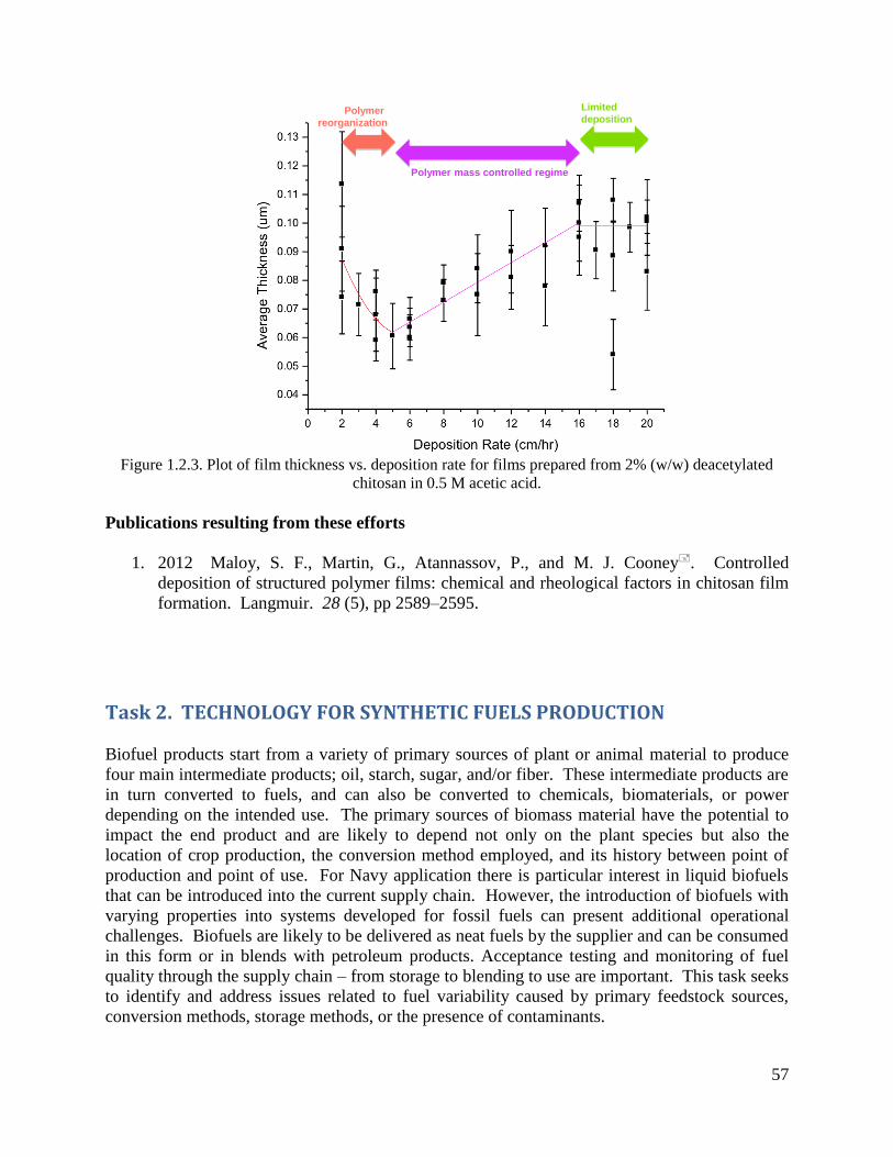
57

Polymer

reorganization

Polymer mass controlled regime

Limited

deposition

Figure 1.2.3. Plot of film thickness vs. deposition rate for films prepared from 2% (w/w) deacetylated

chitosan in 0.5 M acetic acid.

Publications resulting from these efforts

1. 2012 Maloy, S. F., Martin, G., Atannassov, P., and M. J. Cooney. Controlled

deposition of structured polymer films: chemical and rheological factors in chitosan film

formation. Langmuir. 28 (5), pp 2589–2595.

Task 2. TECHNOLOGY FOR SYNTHETIC FUELS PRODUCTION

Biofuel products start from a variety of primary sources of plant or animal material to produce

four main intermediate products; oil, starch, sugar, and/or fiber. These intermediate products are

in turn converted to fuels, and can also be converted to chemicals, biomaterials, or power

depending on the intended use. The primary sources of biomass material have the potential to

impact the end product and are likely to depend not only on the plant species but also the

location of crop production, the conversion method employed, and its history between point of

production and point of use. For Navy application there is particular interest in liquid biofuels

that can be introduced into the current supply chain. However, the introduction of biofuels with

varying properties into systems developed for fossil fuels can present additional operational

challenges. Biofuels are likely to be delivered as neat fuels by the supplier and can be consumed

in this form or in blends with petroleum products. Acceptance testing and monitoring of fuel

quality through the supply chain – from storage to blending to use are important. This task seeks

to identify and address issues related to fuel variability caused by primary feedstock sources,

conversion methods, storage methods, or the presence of contaminants.

58

Task 2.1 focuses on plasma reforming of renewable biogas to produce hydrogen rich streams that

can be upgraded for fuel cell applications. Task 2.2 investigates the thermocatalytic production

of hydrocarbons from synthesis gas with emphasis on catalyst evaluation. Results from the use

of novel solvents to extract bio-oils and proteins from biomass resources are reported in Task

2.3. Biochemical pathways for conversion of synthesis gas into liquid fuel molecules are

investigated in Task 2.4. Tasks 2.5 and 2.6 are focused on fit-for-purpose testing of biofuels to

determine their susceptibility to biocontamination and propensity for creating biocorrosion,

respectively. Finally Task 2.7 explores using waste products to produce carbon products.

Details of the results of each task are provided below.

2.1 Plasma Arc Processing

Biogas was reformed into a hydrogen rich gas stream and to characterize the fate of H2S present as a

contaminant. For this investigation, a non-thermal plasma reactor was modified and experiments

designed and performed. Parametric tests, factorial tests, and response surface methodology was

conducted sequentially to identify optimum reactor operating conditions to minimize specific energy

requirements (kJ/mol H2).

Background

Accessible, environmentally friendly, sustainable, secure sources of energy that can meet projected

energy requirements are needed [1]. Hydrogen is expected to play a larger role in the future energy

portfolio [2]. Among different sources and methods of hydrogen production, plasma assisted

reforming of hydrocarbons shows promising results [3-9]. This paper explores reforming of

simulated biogas, a ~50:50 mixture of methane (a renewable hydrocarbon) and carbon dioxide, in a

non-thermal gliding arc plasma reactor stabilized in a reverse vortex flow (RVF).

Organic wastes and biomass under anaerobic conditions found in landfills and digesters can be

microbially decomposed into biogas containing forty to sixty percent methane with the balance

being largely carbon dioxide. Less than two percent of the biogas is typically nitrogen, oxygen and

other trace volatile organic compounds (VOCs) [10]. Because methane is 20 to 25 times more potent

a greenhouse gas (GHG) than carbon dioxide (CO2), decomposing municipal solid waste can be a

serious climate change contributor. The EPA predicts global biogas emissions will grow by 13%

between 2010 and 2030 [11]. In 2010, the United States reported emissions of 130 Tg equivalent of

CO2 from municipal solid waste methane production [11]. Reforming of biogas at landfills can

convert methane, serving to reduce GHG emissions, while producing renewable hydrogen onsite for

fuel cell applications.

Sulfate reducing microorganisms produce hydrogen sulfide (H2S), a colorless and flammable gas,

under anaerobic conditions in landfills. H2S contamination poses threats to both humans and

materials. From the standpoint of facilities and maintenance, H2S can corrode metal components in

pipelines, sensors, engines, etc., and poison catalysts in fuel cell applications [12]. Undesirable

elements such as sulfur occupy catalyst active sites and reduce the overall performance of the fuel

cell [14]. For proton exchange membrane (PEM) fuel cell road vehicles, the International

Organization for Standardization (ISO) dictates a limit of 0.004 μmol total sulfur compounds (as

59

H2S) per mole of hydrogen (H2) at the dispenser nozzle [15]. The tolerance of molten carbonate fuel

cells (MCFCs) was reported to be less than 0.5 ppm [16]. Thus, practical use of biogas as hydrogen

feedstock depends on economical removal of H2S to meet these limits. Converting H2S into easily

removed sulfur forms may enhance removal between the reformer and the fuel cell.

Reforming seeks to maximize H2 production while minimizing carbon monoxide production. Partial

oxidization (POX), auto-thermal reforming, and steam reforming are three primary industrial fuel

reforming techniques [31]. Equations (1) and (2) describe general hydrocarbon reforming and ideal

methane steam reforming, respectively. The latter is endothermic and typically occupies a large

system footprint, experiences thermal lag, and requires expensive catalysts.

4222224 eCHdHOcHyCOxCOmOOnHCH (1)

)/165(42 2224 molkJHHCOOHCH (2)

POX (equation (3) below) and auto-thermal reforming are both exothermic, utilizing part of the fuel

stream to propagate the reaction.

)/36(25.0 224 molkJHHCOOCH (3)

Auto-thermal reforming, a combination of steam reforming and POX [32], requires specific reactant

ratios and high temperatures. It is prone to coking, catalyst deactivation [33], and slowly responds

to system changes making it unsuitable for mobile applications [5, 34].

Since the 1990’s, plasma reforming technologies have been employed to reform diesel, renewable

diesel [35, 36], methane [4, 8, 35, 37], ethanol [35], isooctane [8, 35, 37], gasoline [38] and gasoline

95 [39]. Advantages of plasma reformers include reduced system cost, catalyst deterioration (if

required), footprint, and response time, and the ability to reform heavy hydrocarbons [5, 31, 40-42].

Plasma reformers can also be configured to operate at near ambient temperatures [31, 41]. Electrode

erosion at high pressures and electricity requirements are identified as disadvantages [5].

The transition from gas to plasma takes place when electrons gain enough energy to be released

from atoms leading to high electrical conductivity [43, 44]. The high energy electrons, Te = 1 eV

(about 11,000 K) [45], provide the activation energy for reforming reactions via direct electron

impact. Plasma generally falls into one of two categories - thermal or non-thermal. In thermal

plasma, gas molecules and electrons exist in thermal equilibrium, requiring from 1 kW to over 50

MW [38, 46] and creating temperatures ranging from 5,000 to 10,000 °K. At these high

temperatures the electrodes must be cooled to reduce thermal erosion [38].

The gas molecules and electrons in non-thermal plasma are not in thermal equilibrium. The gas

molecules can exist at near-ambient temperature, while the electrons are excited at 10,000 to

100,000 °K (1–10 eV) [43]. In this way the electrons deliver energy for reaction initiation and

enhancement. Non-thermal plasma reformers require electrical energy on the order of hundreds of

Watts, have low electrode erosion, avoid the need for a cooling system, occupy a small footprint,

and have low weight [38]. For similar hydrogen yields, non-thermal plasma reformers require less

energy input, when compared to their thermal counterparts [6].

60

Gliding arc, glow discharge, corona discharge, silent discharge, dielectric barrier discharge,

microwave discharge, and radio frequency discharge are types of non-thermal plasma categorized by

their plasma generation mechanism, design pressure, and electrode geometry [47]. Corona discharge

[37], microwave discharge [48], dielectric barrier discharge [49], and gliding arc [3, 7, 49-51] show

the most promise for reforming hydrocarbons.

The Petitpas et al. review of non-thermal reforming technologies found that most operate via POX

mechanisms [4, 8, 9, 35, 37, 39]. The POX based reformers operate at ~75% efficiency [8, 37],

while auto-thermal and steam reforming reformers operate around 63% [35]. Efficiency is defined

as the lower heating value of the product divided by the electrical energy input to the plasma and the

lower heating value of the fuel.

The stabilization of gliding arc plasma within a reverse vortex flow has shown encouraging results

[3, 52]. Gas injection tangentially at one end of a cylindrical reaction chamber that exits tangentially

from the opposite end produces a forward vortex [53]. Alternatively, tangential injection and an

axial exit from the same end of the cylindrical reaction chamber produces a reverse vortex [3]. The

reverse vortex increases the residence time of the reactant within the plasma arc, has 25% higher

efficiency than the forward vortex [54], and produces a more uniform gas treatment than

conventional gliding arcs [54]. Gases swirling along the reactor wall produce near-perfect thermal

insulation, and the gliding of the arc reduces thermal erosion and eliminates the necessity to

fabricate the reaction chamber from materials with high-temperature tolerance [54].

Various non-thermal plasma systems have been studied for disassociation of H2S, including

dielectric barrier discharge, rotating glow, pulsed corona discharge, microwave discharge, gliding

arc discharge, and radio frequency discharge [17-22]. In all studies pure hydrogen sulfide was

diluted to produce a gas mixture containing 10-50% hydrogen sulfide. The high dielectric strength

of H2S, 2.9 times higher than air, requires increased breakdown voltage. Early stage technology for

H2S disassociation to form H2 required roughly 500 eV/ H2 molecule [23, 24]. Nunnally et al. [25]

enhanced the flat gliding arc geometry with the gliding arc in tornado (GAT) and greatly reduced

energy requirements to 1.2 eV/ H2 molecule. The decrease in energy requirements stems from

increased gas contact with the plasma in a GAT system. These results were produced at atmospheric

pressure, a pure H2S gas flow rate of 14 slpm, specific energy input of 0.31 eV per H2S molecule

(~240 W), and 25% H2S conversion to H2. Using the same GAT system, 2.8 slpm O2 was added to

the 14 slpm H2S flow, achieving a specific energy value of 1.0 eV/ H2 molecule produced [26].

The Claus process is a conventional method for recovering elemental S from H2S. In this process,

H2S is converted to elemental sulfur (S) and water (H2O) via a two step reaction (reactions (4) and

(5)) (Fridman et al., 1998)

OHSOOSH 2222 5.1 (thermal step) (4) OHSSHSO 222 232 (catalytic and thermal step) (5)

Direct decomposition of H2S into H2 and S, shown in Equation (6) can also extract S from H2S.

molkJGmolkJHSHSH r 3.334.202

1222 (6)

61

Positive changes in enthalpy and Gibbs free energy across Equation (5) indicate an endothermic and

non-spontaneous reaction. For example, only 12% conversion of H2S occurs at 1000 °C and 1

atmosphere pressure, while below 550 °C less than 1% conversion takes place [19]. Recent

thermodynamic calculations at 1250 °K by Nunnally et al. indicate that an energy input of 4 eV per

H2 molecule (386 kJ/mol H2) results in less than 20% H2S conversion [25].

Thermal decomposition methods; catalytic and non-catalytic, thermomechanical cycles,

photochemical methods, electrolysis, electrochemical methods, and plasma methods have been

investigated for direct decomposition of H2S into H2 and S. Although all methods were successful in

decomposing H2S, not all were economically viable. For example, electrochemical processes require

chemical oxidants and have high electrical energy requirements [27]. An in-depth review by

Luinstra concluded that the relatively low energy requirement of thermal and plasma methods make

them promising compared to electrochemical and photochemical methods [28, 29]. Only the

reaction (4) appears favored for contaminant levels of H2S (~100 ppmv) in biogas from landfills

undergoing plasma reforming.

Materials and Methods

Figure 2.1.1: Schematic diagram of the non-thermal plasma test bed.

62

This section describes testbed modifications, system parameters, parametric tests, and factorial

experiment design utilized in system optimization. A reverse vortex flow gliding arc non-thermal

plasma reformer test bed previously explored under previous funding, methane [3] and liquid fuel

reforming [36]. Figure 2.1.1 shows the methane reforming testbed used for biogas and sulfur

management.

Testbed modifications

Reactant delivery, reformer, reformate conditioning, and analysis modifications were made (under

prior funding), before conducting experiments with simulated biogas containing 0 to 45 ppm of H2S.

Sulfur inert materials were used for all wetted surfaces exposed to fuel and reformate. Reformate

conditioning and analysis systems were modified to include the capability to collect and analyze

gaseous, liquid, and sulfur species.

A Kin-Tek 491 (KIN-TEK Laboratories, Inc., La Marque, TX USA) permeation tube device was

used to meter synthetic biogas (50%-50% methane-carbon dioxide) containing 0 to 45 ppm of H2S

into the reformer via the tangential-inlet zirconia plate. Polytetrafluoroethylene (PTFE) tubing was

used between the Kin-Tek and the reformer. A 3 mm PTFE line bypassed the reformer to allow

calibration of gas analysis equipment directly from the Kin-Tek 491. Stainless steel Swagelok

fittings treated with SilcoNert® (SilcoTek, Bellefonte, PA USA) were used to make all connections.

The non-conducting zirconia (AmZirOx 86, Astro Met Zirconium Oxide, Cincinnati, OH) plate with

the embedded lead wire and inconel washer were retained from liquid fuel reforming work [36].

The inconel washer served as the lower electrode and formed the axial exit of the reactor. The

ultrasonic nozzle end plate at the top of the reactor used for liquid fuels was replaced with a solid

Macor (Corning Inc., Corning, NY) plate with an upper electrode access port. Electrode materials

were treated with SilcoNert®.

Changes to the reformate conditioning and analysis section alleviated sulfur poisoning and sulfur

losses due to adsorption. All stainless steel gas transport tubing was treated with SilcoNert®. The

online analyzers, meters, and the Horiba gas sampler were all sulfur incompatible and were only

used as a bypass for transitioning states when sulfur was absent from the system.

The main conditioning and analysis for sulfur containing reformate passed through two glass

impingers in series. The first contained 100 ml of IPA (A416 2-Propanol Certified ACS Plus, Fisher

Scientific, Hanover Park, IL) and the second was empty, both were immersed in an ice water bath.

A 6 mm diameter, 53 cm long PTFE sleeve lined the first impinger from the base of the 3 way valve

at the outlet of the reformer to the bottom of the impinger inlet tube. This sleeve collected any

precipitated solids that plated onto the tubing and was removed for examination after each test.

Exiting the impinger train, the reformate passed through a coalescing filter to capture remaining

liquids and a mass flow meter (Omega, Model FMA1820A-ST-N2-EPR) to measure dry gas flow

rate. A pump (Model R271-FT-EA-1, Air Dimensions, Deerfield Beach, FL) pulled a slip stream of

the reformate through the sample loops of two gas chromatographs (GC) in series and the remainder

vented into a fume hood.

63

A GC (Shimadzu, Model 2014, Colombia, MD) equipped with a sulfur chemiluminescence detector

(SCD) (Sievers-355) and a 60 m long capillary column (RestekTM Model Rtx®-1) with a 0.53 mm

internal diameter, 7 μm stationary phase was used to quantify sulfur species. A second GC

(Shimadzu, Model 14A, Columbia, MD) equipped with a thermal conductivity detector (TCD) and a

1.52 m × 3 mm Carboxen™ 1000 column (SUPELCO, Bellafonte, PA) quantified permanent gas

species, N2, CO, CO2, H2, and CH4 in accordance with ASTM Standard D1946-90 – Standard

Practice for Analysis of Reformed Gas by Gas Chromatography. Each set of reformer test

conditions were maintained for 40 minutes with sampling occurring at 10 minute intervals on both

GCs.

Liquid samples collected from the impingers were analyzed for sulfur containing species with a dual

Dionex ICS-1100 ion chromatograph (Thermo Fisher Scientific Inc, Waltham, Massachusetts, USA)

with a conductivity detector. Anion analysis took place with a Dionex Ion Pac AS14A (4 mm x 250

mm) column, utilizing 8 mM Na2CO3 and 1 mM NaHCO3 eluent at 1.0 mL/min with an AERS 500

suppressor at 43mA. Anions were calibrated against Dionex 7 Anion-II. Cation analysis took place

with a Dionex Ion Pac CS12A (4 mm x 250 mm) column, utilizing 20 mM methanesulfonic acid

eluent at 1.0 mL/min with a CERS 500 suppressor at 59 mA. Cations were calibrated against

Dionex 6 Cation-II. The pH was measured with an Accumet® Research AR25 Dual Channel

pH/Ion Meter (Thermo Fisher Scientific Inc, Waltham, Massachusetts, USA).

A Mettler-Toledo analytical balance (model ME204E, Mettler-Toledo, Columbus, Ohio) was used

to weigh the PTFE liner before adding Swagelok hardware to the tube for connection to the system,

post-test after hardware removal, and after 3 weeks of desiccation at 20 – 30 % relative humidity.

The mass gain of the tube resulted from solids collecting on the tube walls during tests. The tube

was then halved lengthwise and sectioned into 10 pieces, the dimensions and masses of each section

was recorded. The sample was removed from the tubing with a PTFE spatula and placed on a

polished aluminum stub.

A Hitachi S-4800 field emission scanning electron microscope (SEM) produced images of the

sample on the stub at 25,000x magnification, at an acceleration voltage of 15 kV, and gun current of

20 µA. Energy dispersive spectrometer (EDS) spectra acquired with an Oxford INCA PentaFet-x3

Si(Li) EDS allowed for qualitative identification of solid species present in the sample.

System variables

The following section outlines both the dependent and independent system variables.

Reactor chamber – independent variable: to remain fixed

This variable affected the residence time of reactants within the reactor. The nonthermal plasma

reactor used in these tests had a fixed geometry (42 mm ID, 100 mm length, 0.138 L total volume).

Post reaction chamber– independent variable: to remain fixed

The post reaction chamber had an inner diameter of 42 mm, a length of 76 mm and a total volume of

0.105 L.

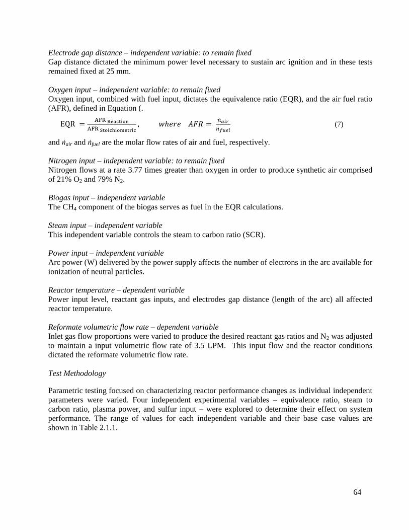
64

Electrode gap distance – independent variable: to remain fixed

Gap distance dictated the minimum power level necessary to sustain arc ignition and in these tests

remained fixed at 25 mm.

Oxygen input – independent variable: to remain fixed

Oxygen input, combined with fuel input, dictates the equivalence ratio (EQR), and the air fuel ratio

(AFR), defined in Equation (.

EQR =AFR Reaction

AFR Stoichiometric, 𝑤ℎ𝑒𝑟𝑒 𝐴𝐹𝑅 =

�̇�𝑎𝑖𝑟

�̇�𝑓𝑢𝑒𝑙 (7)

and ṅair and ṅfuel are the molar flow rates of air and fuel, respectively.

Nitrogen input – independent variable: to remain fixed

Nitrogen flows at a rate 3.77 times greater than oxygen in order to produce synthetic air comprised

of 21% O2 and 79% N2.

Biogas input – independent variable

The CH4 component of the biogas serves as fuel in the EQR calculations.

Steam input – independent variable

This independent variable controls the steam to carbon ratio (SCR).

Power input – independent variable

Arc power (W) delivered by the power supply affects the number of electrons in the arc available for

ionization of neutral particles.

Reactor temperature – dependent variable

Power input level, reactant gas inputs, and electrodes gap distance (length of the arc) all affected

reactor temperature.

Reformate volumetric flow rate – dependent variable

Inlet gas flow proportions were varied to produce the desired reactant gas ratios and N2 was adjusted

to maintain a input volumetric flow rate of 3.5 LPM. This input flow and the reactor conditions

dictated the reformate volumetric flow rate.

Test Methodology

Parametric testing focused on characterizing reactor performance changes as individual independent

parameters were varied. Four independent experimental variables – equivalence ratio, steam to

carbon ratio, plasma power, and sulfur input – were explored to determine their effect on system

performance. The range of values for each independent variable and their base case values are

shown in Table 2.1.1.

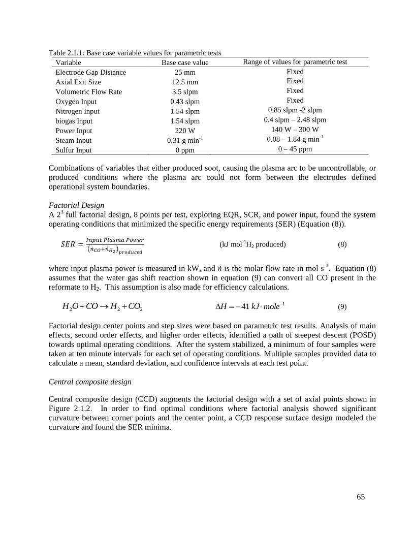
65

Table 2.1.1: Base case variable values for parametric tests

Variable Base case value Range of values for parametric test

Electrode Gap Distance 25 mm Fixed

Axial Exit Size 12.5 mm Fixed

Volumetric Flow Rate 3.5 slpm Fixed

Oxygen Input 0.43 slpm Fixed

Nitrogen Input 1.54 slpm 0.85 slpm -2 slpm

biogas Input 1.54 slpm 0.4 slpm – 2.48 slpm

Power Input 220 W 140 W – 300 W

Steam Input 0.31 g min-1 0.08 – 1.84 g min

-1

Sulfur Input 0 ppm 0 – 45 ppm

Combinations of variables that either produced soot, causing the plasma arc to be uncontrollable, or

produced conditions where the plasma arc could not form between the electrodes defined

operational system boundaries.

Factorial Design

A 23 full factorial design, 8 points per test, exploring EQR, SCR, and power input, found the system

operating conditions that minimized the specific energy requirements (SER) (Equation (8)).

𝑆𝐸𝑅 =𝐼𝑛𝑝𝑢𝑡 𝑃𝑙𝑎𝑠𝑚𝑎 𝑃𝑜𝑤𝑒𝑟

(�̇�𝐶𝑂+�̇�𝐻2)𝑝𝑟𝑜𝑑𝑢𝑐𝑒𝑑

(kJ mol-1

H2 produced) (8)

where input plasma power is measured in kW, and ṅ is the molar flow rate in mol s-1

. Equation (8)

assumes that the water gas shift reaction shown in equation (9) can convert all CO present in the

reformate to H2. This assumption is also made for efficiency calculations.

222 COHCOOH 141 molekJH (9)

Factorial design center points and step sizes were based on parametric test results. Analysis of main

effects, second order effects, and higher order effects, identified a path of steepest descent (POSD)

towards optimal operating conditions. After the system stabilized, a minimum of four samples were

taken at ten minute intervals for each set of operating conditions. Multiple samples provided data to

calculate a mean, standard deviation, and confidence intervals at each test point.

Central composite design

Central composite design (CCD) augments the factorial design with a set of axial points shown in

Figure 2.1.2. In order to find optimal conditions where factorial analysis showed significant

curvature between corner points and the center point, a CCD response surface design modeled the

curvature and found the SER minima.

66

Figure 2.1.2: Central composite design schematic showing the axial points in red, and the cube points in blue,

for k = 3, where k is the number of factors.

Data Reduction

The following equations define standardized performance indicators for plasma reformers proposed

by Petipas et al. and derived from the primary experimental test data [34].

Equation (10) defines hydrogen yield as the ratio of hydrogen atoms as molecular hydrogen in the

reformate gas to the hydrogen atoms in the input fuel.

%1002 FuelFeedinAtomsHydrogen

reformateinHinAtomsHydrogenYieldHydrogen (10)

Equation (11) defines hydrogen selectivity as the ratio of hydrogen atoms present in the reformate as

diatomic hydrogen (H2) to the total number of H atoms present in the dry reformate. Again it is

assumed that all CO present in reformate can be converted to hydrogen by the water gas shift

reaction (Equation (9)).

%100)(2

Pr

4

2 ConvertedCHofMoles

oducedHMolesySelectivitHydrogen (11)

Efficiency is defined as the ratio of chemical enthalpy of the H2 present in the reformate to the total

power input to the reactor - including the input plasma power and the enthalpy of the injected fuel

flow. As seen in Equation (12) ṁ and LHV, are mass flow rate and lower heating values of

identified species, respectively.

inputFuelfuel

producedCOHH

mLHVPowerPlasma

mmLHVEfficiency

gas

*

)(*22

(12)

Equation (13) defines methane conversion as the reactor’s ability to convert methane into other

species.

fuelinCH

reformateinCHfuelinCH

m

mmconversionMethane

)(

)()(

4

44

(13)

Results and Discussion

In this section the results of parametric tests, factorial tests, and response surface tests are

summarized and discussed.

67

Parametric test

This section discusses the parametric test results. The effects of four independent variables, EQR,

SCR, power input, and H2S input are investigated.

System performance metrics as a function of equivalence ratio are shown in Figure 2.1.3. Methane

conversion decreases approximately 40% as EQR decreases from a high of 0.7 to 0.1. Decreasing

EQR results from holding the air flow rate to the reactor constant while increasing the fuel flow rate,

producing a more fuel rich input mixture. Efficiency and H2 yield increase 10 to 15 % (absolute) as

the EQR decreases. Over the same range selectivity increases roughly 30% (absolute). The

decreasing EQR also produced exponentially decreasing SER values from 1017 kJ mol-1

of H2,

toward an asymptotic value of 285 kJ mol-1

of H2 produced. Thus the higher the biogas input to the

system the better the reformer performed as measured by SER. All indicators of system performance

are comparable with the same reactor operated on pure methane [3].

Figure 2.1.3: Equivalence ratio (EQR) parametric test results for biogas with no H2S input. Error bars indicate

95% confidence interval. Error bars that are not visible are equal or smaller in size to the data point symbol.

The effect of steam to carbon ratio was investigated while keeping EQR, power and inlet dry gas

flowrate constant at 0.14, 220 W, and 3.5 lpm, respectively. Figure 2.1.4 indicates that across a

SCR range from 0 (POX conditions) to 3.0, the H2 yield increases from 22% to 27.5%, while

efficiency decreases almost 4% from 26.8% to 22.7%. CH4 conversion also showed an 8% reduction

from 64% to 56%. Increasing SCR resulted in an increase in SER from 290 to 345 kJ mol-1

H2. H2

selectivity increased linearly across the SCR range, from 34 to 49% indicating that the decrease in

methane conversion did not result in decreased H2 productivity. With the exception of hydrogen

yield and selectivity, system performance parameters show similar trends to those measured for pure

methane reforming [3]. The increasing SCR for biogas tests increased hydrogen yield and

selectivity whereas similar tests on methane [3] found that selectivity remained constant and

200

300

400

500

600

700

800

900

1000

1100

0

10

20

30

40

50

60

70

80

90

100

0.00 0.10 0.20 0.30 0.40 0.50 0.60 0.70 0.80

SER

(kJ

mo

l-1 o

f H

2 )

Perc

enta

ge

%

Equivalence Ratio

CH4 Conversion

H2 Yield

Selectivity

Efficiency

SER

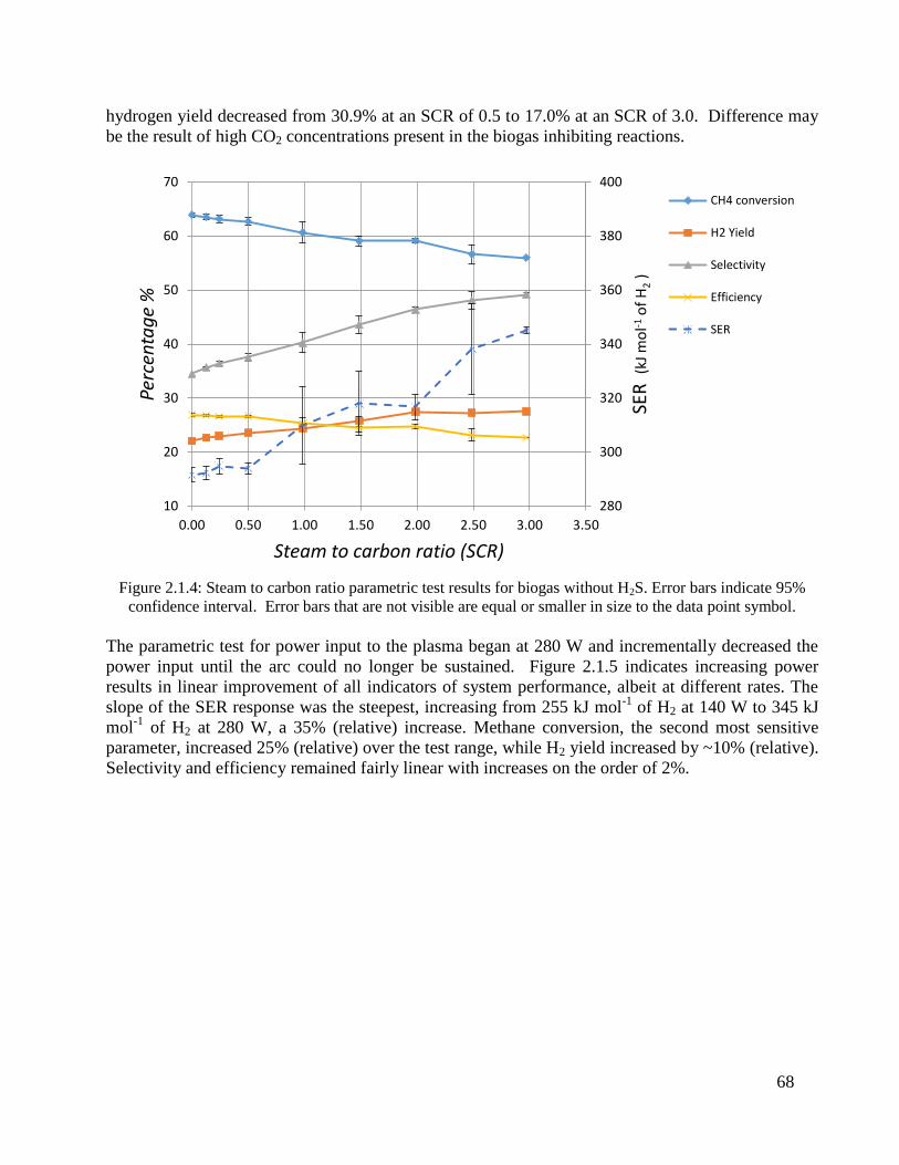
68

hydrogen yield decreased from 30.9% at an SCR of 0.5 to 17.0% at an SCR of 3.0. Difference may

be the result of high CO2 concentrations present in the biogas inhibiting reactions.

Figure 2.1.4: Steam to carbon ratio parametric test results for biogas without H2S. Error bars indicate 95%

confidence interval. Error bars that are not visible are equal or smaller in size to the data point symbol.

The parametric test for power input to the plasma began at 280 W and incrementally decreased the

power input until the arc could no longer be sustained. Figure 2.1.5 indicates increasing power

results in linear improvement of all indicators of system performance, albeit at different rates. The

slope of the SER response was the steepest, increasing from 255 kJ mol-1

of H2 at 140 W to 345 kJ

mol-1

of H2 at 280 W, a 35% (relative) increase. Methane conversion, the second most sensitive

parameter, increased 25% (relative) over the test range, while H2 yield increased by ~10% (relative).

Selectivity and efficiency remained fairly linear with increases on the order of 2%.

280

300

320

340

360

380

400

10

20

30

40

50

60

70

0.00 0.50 1.00 1.50 2.00 2.50 3.00 3.50

SER

(kJ

mo

l-1 o

f H

2 )

Perc

enta

ge

%

Steam to carbon ratio (SCR)

CH4 conversion

H2 Yield

Selectivity

Efficiency

SER

69

Figure 2.1.5: Power input parametric test for biogas without H2S. Error bars indicate 95% confidence interval.

Error bars that are not visible are equal or smaller in size to the data point symbol.

Figure 2.1.5 shows the H2S input parametric test increasing H2S content in the bio-gas feed from 5.3

to 45.4 ppm, which corresponded to 2.3 to 19.9 ppm H2S in the bulk inlet gas stream. Over this

range H2S reformate concentrations increased from 0.047 to 0.171 ppm, while SO2 increased

linearly from 0.47 to .82 ppm. This corresponded to removing 88% of the sulfur species at 5 ppm to

94.8% removal at 45 ppm. The remaining sulfur compounds in the gas stream exponentially

decreased approaching an asymptote around 5%. However, these measurements must be viewed

qualitatively as all H2S concentrations were below the SCD’s lower detectable limit (LDL) of 0.21

ppm, and the majority of the SO2 was detectable but under the 0.70 ppm lower quantitative limit

(LQL).

250

270

290

310

330

350

370

390

10

20

30

40

50

60

70

150 170 190 210 230 250 270 290

SER

(kJ

mo

l-1 o

f H

2 )

%

Power (W)

Conversion

H2 Yield

Selectivity

Efficiency

SER

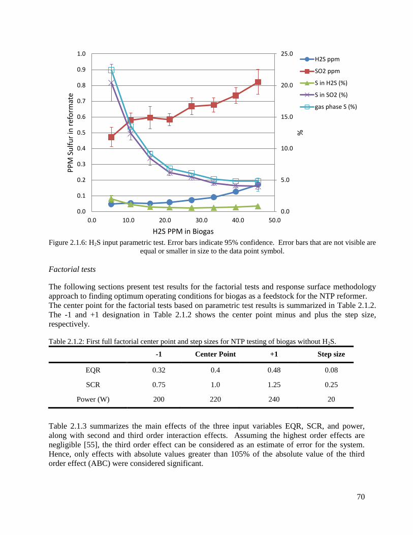
70

Figure 2.1.6: H2S input parametric test. Error bars indicate 95% confidence. Error bars that are not visible are

equal or smaller in size to the data point symbol.

Factorial tests

The following sections present test results for the factorial tests and response surface methodology

approach to finding optimum operating conditions for biogas as a feedstock for the NTP reformer.

The center point for the factorial tests based on parametric test results is summarized in Table 2.1.2.

The -1 and +1 designation in Table 2.1.2 shows the center point minus and plus the step size,

respectively.

Table 2.1.2: First full factorial center point and step sizes for NTP testing of biogas without H2S.

-1 Center Point +1 Step size

EQR 0.32 0.4 0.48 0.08

SCR 0.75 1.0 1.25 0.25

Power (W) 200 220 240 20

Table 2.1.3 summarizes the main effects of the three input variables EQR, SCR, and power,

along with second and third order interaction effects. Assuming the highest order effects are

negligible [55], the third order effect can be considered as an estimate of error for the system.

Hence, only effects with absolute values greater than 105% of the absolute value of the third

order effect (ABC) were considered significant.

0.0

5.0

10.0

15.0

20.0

25.0

0.0

0.1

0.2

0.3

0.4

0.5

0.6

0.7

0.8

0.9

1.0

0.0 10.0 20.0 30.0 40.0 50.0

%

PP

M S

ulf

ur

in r

efo

rmat

e

H2S PPM in Biogas

H2S ppm

SO2 ppm

S in H2S (%)

S in SO2 (%)

gas phase S (%)

71

Table 2.1.3: Effect summary for the first factorial test on biogas without H2S. Values represent the change in

the performance value resulting from increasing the independent variables from the -1 to the +1 values shown

in Table 2.1.2.

Responses

Methane

Conversion,

change (%)

Hydrogen

Yield,

change

(%)

Hydrogen

Selectivit

y,

change

(%)

Efficiency

,

change

(%)

SER,

change

(kJ/mol

H2)

1st O

rder

Eff

ects

A (EQ Ratio) 11.9† -4.5

† -10.5

† -3.5

† 103.0

†

B (SC Ratio) 4.5† -0.4 -2.3 -1.7 23.3

C (Power) 7.2† 1.3

† -0.9 -0.1 42.0

†

2nd O

rder

Eff

ects

AB 4.6† -0.3 -2.3 -0.7 11.1

AC 6.9† -1.0 -3.9

† 0.2 2.0

BC -6.3† 0.0 2.6 -1.2 9.0

3rd

ABC -3.8 1.0 2.7 2.9 -32.9

†indicates significant effect, |effect|> |(1.05*ABC)|

First order effects indicate that increasing the EQR has significant negative effects on all

performance parameters except methane conversion. Increasing the EQR has positive effects on

methane conversion as conditions approach stoichiometric AFR and complete oxidation. Increasing

the SCR has a slight positive effect on methane conversion but does not produce significant effects

in any of the other performance indicators. Increasing power increases methane conversion and

hydrogen yield but negatively impacts SER performance and has no effects on other performance

indicators.

Second order effect indicate that increasing EQR and SCR in tandem produces an additional 5%

methane conversion. Increasing EQR and power in tandem resulted in an additional ~7% increase in

methane conversion but an additional 4% reduction in H2 selectivity. Increasing power and SCR at

the same time provided an additional ~6% decrease in methane conversion.

Although the factorial results showed SCR effects to be insignificant, decreasing steam input lessens

steam generation energy costs and was included in the path of steepest descent (POSD) analysis.

Before running the POSD tests, low-steam reactor stability was tested and verified. The POSD was

characterized by decreasing all three variables until reaching system limits (arc extinction).

Based on the POSD results, center point and step sizes for the second factorial test are summarized

in Table 2.1.4. This factorial test analyzes the response surface around the new center point to see if

there is a further possible reduction in the value SER.

72

Table 2.1.4: Redesigned second full factorial center point and step sizes

-1 Center Point +1 Step size

EQ Ratio 0.12 0.16 0.2 0.04

SC Ratio 0.2 0.3 0.3 0.1

Power(W) 150 160 170 10

Table 2.1.5 summarizes the results for the second factorial test. The results indicate the effects of all

three factors are significant, and suggest decreasing all three factors for the next path of steepest

descent. ANOVA analysis however, shows a curvature P-value of 0.01 (less than 0.05) indicating

significant curvature [56] between corner points and the center point. This indicates that the reactor

is at near optimal conditions. Therefore, a response surface design was performed to model the

response curvature.

Table 2.1.5: Effect summary for the second factorial test on biogas without H2S

Responses

Methane

Conversion,

change (%)

Hydrogen

Yield,

change (%)

Hydrogen

Selectivity,

change (%)

Efficiency,

change (%)

SER,

change

(kJ/mol H2)

A (EQ Ratio) 13.9† 2.3

† -7.9

† 3.3

† 11.7

†

B (SC Ratio) -1.5† 0.4

† 1.9

† -0.6

† 4.6

†

C (Power) 3.0† 1.2

† -0.4 1.1

† 12.2

†

AB -0.5† 0.3 0.6 -0.2 -0.2

AC 0.1 -0.1 -0.1 -0.1 -0.2

BC -0.1 0.1 0.3 -0.1 -0.3†

ABC 0.4 -0.2 -0.8 0.2 -0.2

†indicated significant effect, |effect|> |(1.05*ABC)|

A central composite design (CCD) added six axial points to the last factorial test, and resulted in a

quadratic surface model for SER response. The global minima on this surface identified operating

conditions producing a minimum SER value.

The optimum operating point required 160 W of plasma power, due to occasional arc instability at

150 W. Optimal conditions were defined by an EQR of 0.11, an SCR of 0.14, and 160 W of arc

power. This is equivalent to inputs of 0.25 slpm O2, 0.95 slpm N2, 2.30 slpm of biogas, and 0.13 g

min-1

steam input. This results in an SER of 184.18 kJ/mol H2 (1.91 eV/H2 molecule), which is

significantly below 3.37 eV/ H2 molecule for conventional steam reforming of methane. At this

point CH4 conversion was 49%, H2 yield was 23%, H2 selectivity was 48%, and efficiency was 25%.

The optimal condition reported applies to this specific NTP reactor and their applicability at larger

scales should be investigated.

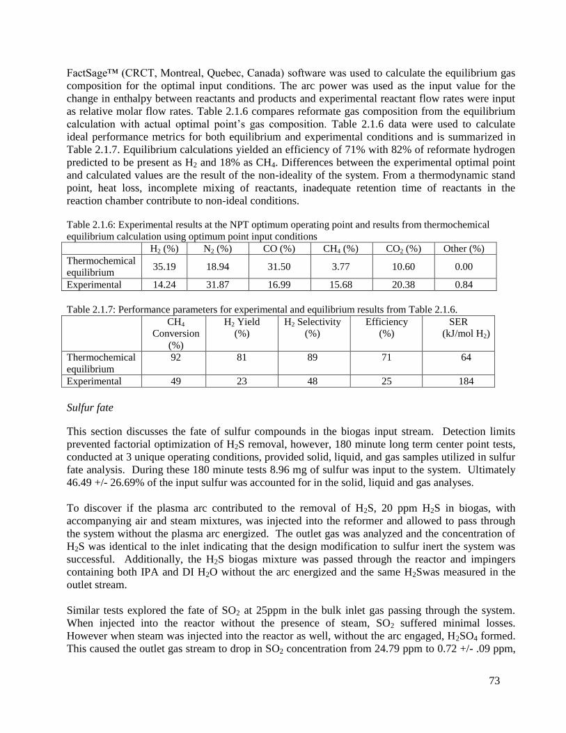
73

FactSage™ (CRCT, Montreal, Quebec, Canada) software was used to calculate the equilibrium gas

composition for the optimal input conditions. The arc power was used as the input value for the

change in enthalpy between reactants and products and experimental reactant flow rates were input

as relative molar flow rates. Table 2.1.6 compares reformate gas composition from the equilibrium

calculation with actual optimal point’s gas composition. Table 2.1.6 data were used to calculate

ideal performance metrics for both equilibrium and experimental conditions and is summarized in

Table 2.1.7. Equilibrium calculations yielded an efficiency of 71% with 82% of reformate hydrogen

predicted to be present as H2 and 18% as CH4. Differences between the experimental optimal point

and calculated values are the result of the non-ideality of the system. From a thermodynamic stand

point, heat loss, incomplete mixing of reactants, inadequate retention time of reactants in the

reaction chamber contribute to non-ideal conditions.

Table 2.1.6: Experimental results at the NPT optimum operating point and results from thermochemical

equilibrium calculation using optimum point input conditions

H2 (%) N2 (%) CO (%) CH4 (%) CO2 (%) Other (%)

Thermochemical

equilibrium 35.19 18.94 31.50 3.77 10.60 0.00

Experimental 14.24 31.87 16.99 15.68 20.38 0.84

Table 2.1.7: Performance parameters for experimental and equilibrium results from Table 2.1.6.

CH4

Conversion

(%)

H2 Yield

(%)

H2 Selectivity

(%)

Efficiency

(%)

SER

(kJ/mol H2)

Thermochemical

equilibrium

92 81 89 71 64

Experimental 49 23 48 25 184

Sulfur fate

This section discusses the fate of sulfur compounds in the biogas input stream. Detection limits

prevented factorial optimization of H2S removal, however, 180 minute long term center point tests,

conducted at 3 unique operating conditions, provided solid, liquid, and gas samples utilized in sulfur

fate analysis. During these 180 minute tests 8.96 mg of sulfur was input to the system. Ultimately

46.49 +/- 26.69% of the input sulfur was accounted for in the solid, liquid and gas analyses.

To discover if the plasma arc contributed to the removal of H2S, 20 ppm H2S in biogas, with

accompanying air and steam mixtures, was injected into the reformer and allowed to pass through

the system without the plasma arc energized. The outlet gas was analyzed and the concentration of

H2S was identical to the inlet indicating that the design modification to sulfur inert the system was

successful. Additionally, the H2S biogas mixture was passed through the reactor and impingers

containing both IPA and DI H2O without the arc energized and the same H2Swas measured in the

outlet stream.

Similar tests explored the fate of SO2 at 25ppm in the bulk inlet gas passing through the system.

When injected into the reactor without the presence of steam, SO2 suffered minimal losses.

However when steam was injected into the reactor as well, without the arc engaged, H2SO4 formed.

This caused the outlet gas stream to drop in SO2 concentration from 24.79 ppm to 0.72 +/- .09 ppm,

74

and the liquid recovered from the first impinger ultimately contained 59.9 ppm of sulfate. These

results confirm that if the NPT reactor converts H2S to SO2, that it can be removed with minimal

effort.

H2S was metered into the system at 21.25 ppm in the biogas and 9.35 ppm in the bulk reactant

stream. The plasma reforming removed the majority of H2S, leaving 0.069 ± 0.026 ppm on average

in the reformate – less than the LDL of 0.21 ppm. However due to the partial oxidation of some H2S

into SO2 via the reaction in equation (3), SO2 was found in detectable, but not quantifiable amounts.

Ultimately 5.7 ± 0.4% of the initial sulfur appeared to remain in the gas stream.

Partial oxidation of a portion of the H2S stream resulted in the production of SO2. The SO2 in turn

reacted with steam present in the reformer to form H2SO4, sulfuric acid. The first impinger in the

impinger train, initially filled with 100 ml of IPA, captured both condensed steam and sulfuric acid.

After 180 minutes of operation the impingers on average contained 249.6 ± 29.5 ml of solution.

Impinger solution had a pH value of 3.8 as measured by the AR25 Dual Channel pH/Ion meter. The

Dionex ICS-1100 Ion Chromatograph detected on average 17.6 ± 14.0 ppm sulfate ions. This

corresponded to 3.4 ± 2.2 mg of sulfur, or 38.2 ± 24.8% of the input sulfur.

Figure 2.1.7: SEM imaging of solid particles recovered from the PTFE impinger liner. Image A - Solids and

rods. Image B - Plates and rods. Image C - recovered solid particles in place on SEM target.

Images A and B in Figure 2.1.7 show the solid particles insitu on thePTFE liner, while image C

shows the solid particles scraped from the liner onto the targeting stub. The solid formations, rods,

plates, and spheres, in images A and B were crushed when scraped onto the targeting stub. Image C

has a ‘gummy’ or ‘slimy’ appearance, likely due to a light hydrocarbon oil.

Unfortunately, the solids would decay and ‘wander’ when exposed to the electron beam. This

impeded the image quality and the identification of species present in the solids. As detected by

EDS, on average solid composition was primarily oxygen (81.3 ± 3.3%), carbon (15.6 ± 3.0%), and

sulfur (2.8 ± 0.8%). Some particles detected contained 19.5% sulfur by mass, however, the large

majority of particles contained only ≤5%. Solids, containing 2.6 ± 1.5% of the input sulfur, was the

smallest percentage of sulfur detected in any form.

Conclusion

An experimental investigation was conducted to reform biogas into a hydrogen rich gas stream and

characterize the fate of H2S present as a contaminant. For this purpose, a non-thermal plasma reactor

was modified and experiments designed and performed. Parametric tests, factorial tests, and

75

response surface methodology conducted sequentially identified the best reactor operating

conditions that minimized specific energy requirements (kJ/mol H2).

Optimal operating conditions of EQR=0.11, SCR=0.14, and 160 W of arc input power resulted in a

minimized SER of 184 kJ/mol H2 for the reactor running on simulated biogas (50% methane, 50%

carbon dioxide). At these conditions, the reformate gas composition was 14.2% H2, 31.9% N2, 17.0% CO, 3.8% CH4, and 10.6% CO2, resulting in methane conversion of 48.8%, a hydrogen yield

of 23.4%, hydrogen selectivity = 47.8%, and an efficiency of 25.3%.

Approximately 5.7% of the sulfur input to the system as 21 ppm H2S in the biogas was measured in

the dry outlet reformate stream. The remainder of the sulfur was reformed into SO2 that was

captured as H2SO4 in the impingers or recovered as a solid of unknown molecular structure on PTFE

tubing surfaces between the reformer and the impingers.

Future research should identify optimal conditions for biogas reforming at higher input flowrates as

an approach to a more industrialized scale and explore the optimizing operating conditions for sulfur

removal and fate of sulfur species.

References

1. Mueller-Langer, F., et al., Techno-economic assessment of hydrogen production processes for

the hydrogen economy for the short and medium term. International Journal of Hydrogen

Energy, 2007. 32(16): p. 3797-3810.

2. Kothari, R., D. Buddhi, and R. Sawhney, Comparison of environmental and economic aspects

of various hydrogen production methods. Renewable and Sustainable Energy Reviews, 2008.

12(2): p. 553-563.

3. Piavis, W. and S. Turn, An experimental investigation of reverse vortex flow plasma reforming

of methane. International Journal of Hydrogen Energy, 2012. 37(22): p. 17078-17092.

4. Ahmar, E.E., et al., Hydrogen enrichment of a methane–air mixture by atmospheric pressure

plasma for vehicle applications. Chemical Engineering Journal, 2006. 116(1): p. 13-18.

5. Bromberg, L., et al., Plasma catalytic reforming of methane. International Journal of Hydrogen

Energy, 1999. 24(12): p. 1131-1137.

6. Bromberg, L., et al., Hydrogen manufacturing using low current, non-thermal plasma boosted

fuel converters. 2000: Plasma Science and Fusion Center, Massachusetts Institute of

Technology.

7. Iskenderova, K., et al. Methane conversion into syn-gas in gliding arc discharge. in 15th

International symposium on plasma chemistry, Orleans. 2001.

8. Kalra, C.S., A.F. Gutsol, and A.A. Fridman, Gliding arc discharges as a source of

intermediate plasma for methane partial oxidation. Plasma Science, IEEE Transactions on,

2005. 33(1): p. 32-41.

9. Ouni, F., A. Khacef, and J. Cormier. Methane steam reforming with oxygen in a sliding

discharge reactor. in 17th International symposium on plasma chemistry, Toronto. 2005.

10. Tchobanoglous, G., H. Theisen, and S.A. Vigil, Integrated solid waste management :

engineering principles and management issues. McGraw-Hill series in water resources and

environmental engineering. 1993, New York: McGraw-Hill. xxi, 978 p.

11. (EPA), U.S.E.P.A., Global Mitigation of Non-CO2 Greenhouse Gases: 2010-2030. 2013. p.

Section III.

76

12. Cheekatamarla, P.K. and A.M. Lane, Catalytic autothermal reforming of diesel fuel for

hydrogen generation in fuel cells: I. Activity tests and sulfur poisoning. Journal of Power

Sources, 2005. 152: p. 256-263.

13. Larminie, J., A. Dicks, and M.S. McDonald, Fuel cell systems explained. Vol. 2. 2003: Wiley

New York.

14. Mohtadi, R., et al., Effects of hydrogen sulfide on the performance of a PEMFC.

Electrochemical and Solid-State Letters, 2003. 6(12): p. A272-A274.

15. Brown, L.F., A comparative study of fuels for on-board hydrogen production for fuel-cell-

powered automobiles. International Journal of Hydrogen Energy, 2001. 26(4): p. 381-397.

16. Monteleone, G., et al., Deep H 2 S removal from biogas for molten carbonate fuel cell

(MCFC) systems. Chemical engineering journal, 2011. 173(2): p. 407-414.

17. Czernichowski, A., Gliding arc: applications to engineering and environment control. Pure

and Applied Chemistry, 1994. 66(6): p. 1301-1310.

18. Traus, I. and H. Suhr, Hydrogen sulfide dissociation in ozonizer discharges and operation of

ozonizers at elevated temperatures. Plasma chemistry and plasma processing, 1992. 12(3): p.

275-285.

19. Zhao, G.-B., et al., Production of hydrogen and sulfur from hydrogen sulfide in a nonthermal-

plasma pulsed corona discharge reactor. Chemical Engineering Science, 2007. 62(8): p. 2216-

2227.

20. Nicholas, J.E., C.A. Amodio, and M.J. Baker, Kinetics and mechanism of the decomposition of

H 2 S, CH 3 SH and (CH 3) 2 S in a radio-frequency pulse discharge. Journal of the Chemical

Society, Faraday Transactions 1: Physical Chemistry in Condensed Phases, 1979. 75: p. 1868-

1875.

21. Harkness, J.B., R.D. Doctor, and E.J. Daniels, Plasma-chemical conversion of hydrogen

sulfide into hydrogen and sulfur. 1993, Argonne National Lab., IL (United States).

22. Krasheninnikov, E., et al., Dissociation of hydrogen sulfide in an RF discharge. Soviet

Physics-Technical Physics, 1986. 31(6): p. 645-648.

23. Dalaine, V., et al., H2S destruction in 50 Hz and 25 kHz gliding arc reactors. Journal of

applied physics, 1998. 84(3): p. 1215-1221.

24. Dalaine, V., J. Cormier, and P. Lefaucheux, A gliding discharge applied to H2S destruction.

Journal of applied physics, 1998. 83(5): p. 2435-2441.

25. Nunnally, T., et al., Dissociation of H 2 S in non-equilibrium gliding arc “tornado” discharge.

international journal of hydrogen energy, 2009. 34(18): p. 7618-7625.

26. Nunnally, T., et al., Plasma dissociation of H 2 S with O 2 addition. international journal of

hydrogen energy, 2014. 39(24): p. 12480-12489.

27. Kalina, D. and E. Maas, Indirect hydrogen sulfide conversion—I. An acidic electrochemical

process. International Journal of Hydrogen Energy, 1985. 10(3): p. 157-162.

28. Luinstra, E., Hydrogen from H2S: technologies and economics. 1995: Sulfotech Research.

29. Cox, B.G., P.F. Clarke, and B.B. Pruden, Economics of thermal dissociation of H 2 S to

produce hydrogen. International journal of hydrogen energy, 1998. 23(7): p. 531-544.

30. Kaloidas, V. and N. Papayannakos, Hydrogen production from the decomposition of hydrogen

sulphide. Equilibrium studies on the system H 2 S/H 2/S i,(i= 1,…, 8) in the gas phase.

International journal of hydrogen energy, 1987. 12(6): p. 403-409.

31. Holladay, J.D., et al., An overview of hydrogen production technologies. Catalysis Today,

2009. 139(4): p. 244-260.

77

32. Li, Y., et al., Thermodynamic analysis of autothermal steam and CO 2 reforming of methane.

International Journal of Hydrogen Energy, 2008. 33(10): p. 2507-2514.

33. Czernichowski, A., GlidArc assisted preparation of the synthesis gas from natural and waste

hydrocarbons gases. Oil & Gas Science and Technology, 2001. 56(2): p. 181-198.

34. Petitpas, G., et al., A comparative study of non-thermal plasma assisted reforming

technologies. International Journal of Hydrogen Energy, 2007. 32(14): p. 2848-2867.

35. Bromberg, L., et al., Onboard plasmatron hydrogen production for improved vehicles. 2006:

Plasma Science and Fusion Center, Massachusetts Institute of Technology.

36. Piavis, W., S. Turn, and S.A. Mousavi, Non-thermal gliding-arc plasma reforming of

dodecane and hydroprocessed renewable diesel. International Journal of Hydrogen Energy,

2015. 40(39): p. 13295-13305.

37. Sobacchi, M., et al., Experimental assessment of a combined plasma/catalytic system for

hydrogen production via partial oxidation of hydrocarbon fuels. International Journal of

Hydrogen Energy, 2002. 27(6): p. 635-642.

38. Paulmier, T. and L. Fulcheri, Use of non-thermal plasma for hydrocarbon reforming.

Chemical engineering journal, 2005. 106(1): p. 59-71.

39. Czernichowski, A., M. Czernichowski, and P. Czernichowski. GlidArc-assisted reforming of

various carbonaceous feedstock into synthesis gas. Detailed study of Propane reforming. in

14-th Annual US Hydrogen Meeting. 2003.

40. O'Brien, C.J., et al. Hydrogen production via plasma reformers. in Energy Conversion

Engineering Conference, 1996. IECEC 96., Proceedings of the 31st Intersociety. 1996. IEEE.

41. Biniwale, R.B., A. Mizuno, and M. Ichikawa, Hydrogen production by reforming of iso-octane

using spray-pulsed injection and effect of non-thermal plasma. Applied Catalysis A: General,

2004. 276(1): p. 169-177.

42. Czernichowski, A., P. Czernichowski, and K. Wesolowska. Plasma-catalytical partial

oxidation of various carbonaceous feeds into synthesis gas. in ASME 2004 2nd International

Conference on Fuel Cell Science, Engineering and Technology. 2004. American Society of

Mechanical Engineers.

43. Petitpas, G., et al., A comparative study of non-thermal plasma assisted reforming

technologies. International Journal of Hydrogen Energy, 2007. 32(14): p. 2848-2867.

44. Fridman, A., Plasma chemistry. 2008: Cambridge University Press.

45. Fridman, A., et al., Gliding arc gas discharge. Progress in Energy and Combustion Science,

1999. 25(2): p. 211-231.

46. Fridman, A., et al., Gliding arc gas discharge. Progress in Energy and Combustion Science,

1998. 25(2): p. 211-231.

47. Fridman, A., A. Chirokov, and A. Gutsol, Non-thermal atmospheric pressure discharges.

Journal of Physics D: Applied Physics, 2005. 38(2): p. R1.

48. Sekiguchi, H. and Y. Mori, Steam plasma reforming using microwave discharge. Thin Solid

Films, 2003. 435(1): p. 44-48.

49. Rusu, I. and J.-M. Cormier, On a possible mechanism of the methane steam reforming in a

gliding arc reactor. Chemical Engineering Journal, 2003. 91(1): p. 23-31.

50. Bromberg, L., et al., Emissions reductions using hydrogen from plasmatron fuel converters.

International Journal of Hydrogen Energy, 2001. 26(10): p. 1115-1121.

51. Lesueur, H., A. Czernichowski, and J. Chapelle, Electrically assisted partial oxidation of

methane. International journal of hydrogen energy, 1994. 19(2): p. 139-144.

78

52. Guofeng, X. and D. Xinwei, Optimization geometries of a vortex gliding-arc reactor for

partial oxidation of methane. Energy, 2012. 47(1): p. 333-339.

53. Liu, J.-L., et al., Simulated biogas oxidative reforming in AC-pulsed gliding arc discharge.

Chemical Engineering Journal, 2016. 285: p. 243-251.

54. Kalra, C.S., et al., Gliding arc in tornado using a reverse vortex flow. Review of Scientific

Instruments, 2005. 76(2): p. 025110.

55. Box, G.E., Statistics for experimenterers, an introduction to design, data analysis and model

building, George EP Box, William G. Hunter, J. Stuart Hunter. 1978.

56. Box, G.E., W.G. Hunter, and J.S. Hunter, Statistics for experimenters. 1978.

2.2 Thermocatalytic Conversion of Synthesis Gas into Liquid Fuels

The effects of pore size on Ru/SiO2 catalyst performance were investigated for Fischer–Tropsch

synthesis under the conditions of 503 K, 20 bar and 1800 h–1

. Ru/SiO2 with 10 nm pore size

catalyst showed higher catalytic activity than Ru/SiO2 catalysts with 3, 6 and 30 nm pore sizes.

The 10 nm pore size, Ru/SiO2 catalyst exhibited uniform pore diameter, an increased surface

concentration of active Ru metals, and the increased dispersion of Ru on the surface compared to

the other pore diameters. Deactivation was clearly observed for all Ru/SiO2 catalysts during the

reaction. The addition of small amounts of Zr and Mn (1:30, Zr or Mn:Si) improved catalytic

activity and stability for Fischer–Tropsch synthesis. The deactivation rate of Ru/Zr/Q10 was

about 21% at 51 h time on stream and this rate was much lower than Ru/Q10 (57%).

Ru/Mn/Q10 showed higher catalytic activity than Ru/Q10 and Ru/Zr/Q10, and its deactivation

rate was much lower ~9% after 51 h time on stream. The catalysts were characterized by BET,

BJH, XRD, TPR, H2 and CO adsorption and TEM. The small amount of Mn added to the

Ru/SiO2 catalyst increased the concentration of active Ru metals and enhanced their dispersion

on the support surface.

Complete details of this study were presented in the publication:

Nurunnabi, M. and S.Q. Turn. 2015. Pore size effects on Ru/SiO2 catalysts with Mn and Zr

promoters for Fischer-Tropsch synthesis. Fuel Processing Technology. 130. pp 155-164.

Complete details can be found at:

http://www.sciencedirect.com/science/article/pii/S0378382014004196?np=y

or

http://dx.doi.org/10.1016/j.fuproc.2014.10.004

2.3 Novel Solvent Based Extraction of Bio-oils and Protein from Biomass

The overall objective of this task was to: 1) Quantify the degree to which a 1-step extraction

using a hydrophilic co-solvent system (comprised of an ionic liquid and an polar covalent

molecule) extracts phorbol esters from oil seeds; 2) Determine the extent to which the phorbol

http://www.sciencedirect.com/science/article/pii/S0378382014004196?np=y

http://dx.doi.org/10.1016/j.fuproc.2014.10.004

79

esters can be recovered from the co-solvent and 3) Determine the extent to which the extracted

biomass is toxin-free and suitable as an animal feed.

Two methods to determine the absolute amount of phorbol esters in the untreated jatropha kernel

(i.e. control) were evaluated: solvent extraction into methanol or dichloromethane. The

measurement of phorbol esters in untreated jatropha kernel using methanol method recovered

6.3 mg phorbol esters (PE) per gram of kernel, a value that is consistent with published results

reporting phorbol esters quantities as high as 6.5 mg per gram of kernel. The use of

dichloromethane, by contrast, produced only 3.8 mg PE per gram kernel. Given these results the

methanol method was used as the co-solvent. Table 2.3.1 presents the extraction yields of

phorbol esters for two ionic liquid based mixed with varying concentration of methanol co-

solvent. The highest yield of extracted phorbol esters was achieved in pure methanol with only a

slight decrease observed as the [C2mim][MeSO4] concentration was increased, generally resting

at a plateau until the [C2mim][MeSO4] concentration became dominant.

Protein analysis was performed to investigate the effect of the co-solvent extraction process on

the nutritive value of the biomass. Although proteins were found to extract into the middle co-

solvent phase (Table 2.3.2) their amounts were minimal at or just below 1.0 mg per ml of co-

solvent. These values are consistent with those reported in literature on protein solubility in pure

ionic liquids or in ionic liquid based aqueous two phase systems which are normally below 1 mg

per ml ionic liquid. Even though these reports suggested extraction efficiencies as high as 90%,

it should be noted that these reports also used samples that contained protein at starting

concentrations as low as 1 mg per ml of solvent. As the jatropha biomass source in this study

was rich in protein (32 wt% relative to the whole kernel), the low yields of solubilized protein

actually reflect a low solubility of protein in the polar co-solvent. Our results also demonstrated

that the bulk of protein remained with the biomass even after washing with water. The low

solubility of protein in solution was also confirmed by the Kjeldahl nitrogen analysis of the

bottom biomass phase which revealed that the majority of protein remained with the biomass,

Table 2.3.2. We believe that the high protein content in the de-lipified and de-toxified jatropha

biomass, even after water washes, further enhances the utility of the co-solvent system as a one-

step extraction process for jatropha biomass.

While it was initially surprising that the medium polarity of the co-solvent and amphiphilic

nature of the ionic liquid would have better facilitated the extraction and solubilization of greater

amounts of protein, whose outer shells are also amphiphilic, the limited extraction of protein

into the co-solvent is attributed to several factors. First, there is likely a lack of strong hydrogen

bonding between the co-solvent and proteins as the ionic liquids and methanol are themselves

strongly associated through hydrogen bonding and other electrostatic interactions. The pH and

temperature of the co-solvent could also be at values that induce protein denaturation, conditions

that would inhibit solubilization. Finally, if the proteins are initially stored in a phase associated

with the solid biomass, the conditions described above would suggest good reasons why the

proteins do not solubilize into the co-solvent. In addition to achieving effective co-extraction of

phorbol esters, the low phorbol esters - high protein content of the de-lipified biomass also

possessed high potential as an animal feed.

80

Table 2.3.1: Phorbol esters content in [C2mim][MeSO4]-MeOH co-solvent after extraction of jatropha

biomass.

IL concentration

(wt % in co-solvent)

Extraction yield (mg PE/ g kernel)

[C2mim][MeSO4] [C2mim][Ac]

0 6.3 6.3

10 5.8 3.5

20 5.7 3.9

25 4.1 3.5

30 4.5 2.9

45 4.5 3.7

50 5.4 3.6

60 5.3 3.5

70 2.9 3.3

90 0.8 2.9

Table 2.3.2: Protein yields from analyses of components of co-solvent extraction

Kjeldahl protein (wt %) Bradford protein (wt %) Protein concentration

(mg/ml)

Untreated BBP1 BBP

2 Co-solvent

1 Co-solvent

2 Co-solvent

1 Co-solvent

2

32 68 66 1.3 1.8 0.792 1.108

1[C2mim][MeSO4]-MeOH

2[C2mim][Ac]-MeOH

BBP denotes bottom biomass phase.

The weight % protein in untreated samples is expressed relative to the untreated biomass whilst the

weight % protein in BBP is expressed relative to the dry weight of the BBP phase.

Complete details of this study were presented in the publication:

2013 Godwin Severa, Kumar, G., Troung,, M., Young, G., and Michael J. Cooney, Ionic

liquid co-solvent assisted extraction of phorbol esters from jatropha biomass. Separation and

Purification Technology. 116:265-270.

2.4 Biochemical Conversion of Biomass Syngas into Liquid Fuels

In previous work, a hydrogen-oxidizing bacterium was used to produce polyhydroxybutyrate

(PHB) from syngas [1]. The autotrophic microorganism fixes CO2 as the carbon source by using

H2 as the sole reducing regent and energy source. PHB is a bacterial energy storage material and

accumulated in the microbial cells as intracellular granules (Figure 2.4.1). Depending on the

nutrients, the PHB content of the cell mass ranges from 30 wt% to 70 wt%. PHB can be

recovered by thermal hydrolysis of the cell mass and trans-esterified with methanol to form a

mixture of methyl esters (biodiesel). The hydrolysates of cell debris including proteins,

however, is discarded as a waste. This subtask aims to accomplish two things: (1) maximize the

process productivity by reusing the hydrolysates of cell debris in microbial cultivation, and (2)

conduct an economic analysis of biodiesel produced through microbial CO2 fixation. The techno

81

economic analysis was conducted with a computer simulation based on the best performance and

data reported in the literature.

Figure 2.4.1: Polyhydroxybutyrate (PHB, white granules) in Ralstonia eutropha. The scale depicted (bar

on lower right) is 0.5µm.

Cell debris utilization

The residual cell mass, after PHB being removed, was subjected to ultimate analysis. Table 2.4.1

gives the elemental compositions of the residual cell mass of the hydrogen-oxidizing bacterium

(R. eutropha) and polyhydroxybutyrate (PHB). Based on the composition, the experimental

formula of cell debris is CH1.69O0.46N 0.25 (FW 24.55). It indicates that nitrogen, accounting for

14 wt% of the residual cell mass, is an essential nutrient for microbial growth and CO2 fixation.

In contrast, the experimental formula of PHB is CH1.5O0.5 (FW 21.5) and its synthesis does not

need nitrogen as a nutrient.

Table 2.4.1: Elemental composition of residual cell mass and PHB of R. eutropha (ash free, dry base).

Residual cell mas Polyhydroxybutyrate (PHB)

C (wt) H (wt%) O (wt%) N (wt%) C (wt%) H (wt%) O (wt%)

49.0 6.9 30.1 14.0 55.8 6.9 37.2

Figure 2.4.2a: Autotrophic growth of R. eutropha

at different initial nitrogen (N) concentrations of

cell debris.

Figure 2.4.2b: The final dry cell mass (DCM)

concentration and PHB content at different

initial concentrations of cell debris nitrogen.

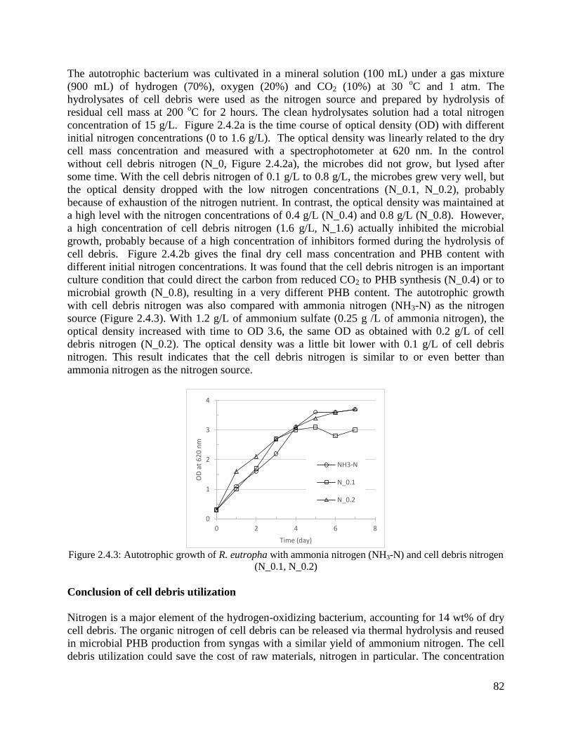
82

The autotrophic bacterium was cultivated in a mineral solution (100 mL) under a gas mixture

(900 mL) of hydrogen (70%), oxygen (20%) and CO2 (10%) at 30 oC and 1 atm. The

hydrolysates of cell debris were used as the nitrogen source and prepared by hydrolysis of

residual cell mass at 200 oC for 2 hours. The clean hydrolysates solution had a total nitrogen

concentration of 15 g/L. Figure 2.4.2a is the time course of optical density (OD) with different

initial nitrogen concentrations (0 to 1.6 g/L). The optical density was linearly related to the dry

cell mass concentration and measured with a spectrophotometer at 620 nm. In the control

without cell debris nitrogen (N_0, Figure 2.4.2a), the microbes did not grow, but lysed after

some time. With the cell debris nitrogen of 0.1 g/L to 0.8 g/L, the microbes grew very well, but

the optical density dropped with the low nitrogen concentrations (N_0.1, N_0.2), probably

because of exhaustion of the nitrogen nutrient. In contrast, the optical density was maintained at

a high level with the nitrogen concentrations of 0.4 g/L (N_0.4) and 0.8 g/L (N_0.8). However,

a high concentration of cell debris nitrogen (1.6 g/L, N_1.6) actually inhibited the microbial

growth, probably because of a high concentration of inhibitors formed during the hydrolysis of

cell debris. Figure 2.4.2b gives the final dry cell mass concentration and PHB content with

different initial nitrogen concentrations. It was found that the cell debris nitrogen is an important

culture condition that could direct the carbon from reduced CO2 to PHB synthesis (N_0.4) or to

microbial growth (N_0.8), resulting in a very different PHB content. The autotrophic growth

with cell debris nitrogen was also compared with ammonia nitrogen (NH3-N) as the nitrogen

source (Figure 2.4.3). With 1.2 g/L of ammonium sulfate (0.25 g /L of ammonia nitrogen), the

optical density increased with time to OD 3.6, the same OD as obtained with 0.2 g/L of cell

debris nitrogen (N_0.2). The optical density was a little bit lower with 0.1 g/L of cell debris

nitrogen. This result indicates that the cell debris nitrogen is similar to or even better than

ammonia nitrogen as the nitrogen source.

Figure 2.4.3: Autotrophic growth of R. eutropha with ammonia nitrogen (NH3-N) and cell debris nitrogen

(N_0.1, N_0.2)

Conclusion of cell debris utilization

Nitrogen is a major element of the hydrogen-oxidizing bacterium, accounting for 14 wt% of dry

cell debris. The organic nitrogen of cell debris can be released via thermal hydrolysis and reused

in microbial PHB production from syngas with a similar yield of ammonium nitrogen. The cell

debris utilization could save the cost of raw materials, nitrogen in particular. The concentration

0

1

2

3

4

0 2 4 6 8

OD

at

62

0 n

m

Time (day)

NH3-N

N_0.1

N_0.2

83

of cell debris nitrogen should be controlled to avoid the possible inhibition of cell debris

hydrolysates and optimize the production of PHB for fuels.

Economic analysis of biodiesel production through microbial CO2 fixation

Biodiesel is a renewable liquid fuel currently produced from plant oil and animal fat. The lipids

or triglycerides are esterified with methanol to form a mixture of fatty acids methyl esters

(FAMEs). The process yields about 100 kg of FAMEs and 10 kg glycerol from 100 kg lipids and

10 kg methanol. Research has been focused on microalgal lipids and methanolysis.

Nannochloropsis is a promising marine microalga for lipids production because it can be

cultivated in seawater on non-arable land, accumulating a high content of lipids (30-60 wt%) [2].

The microalga fixes carbon dioxide (CO2) as the carbon source via photosynthesis. Both artificial

and natural lights can be used as the energy source. Specifically, under nutrient starvation such

as nitrogen deficiency, the species is able to produce neutral triglycerides. In the downstream

processing, neutral lipids are the favorable substances for biodiesel production.

Biomass characterization

Nannochloropsis is a unicellular microalga of spherical or slightly ovoid cells (2-5 µm in

diameter). Nannochloropsis salina is a representative producer of algal oil [3]. The biomass of N.

salina, after oven drying, contains water moisture (7.7 wt%), volatile matter (78.0 wt%) and ash

(13.8 wt%) determined with a thermogravimetric analysis (Figure 2.4.4) [4]. The lipids in algal

biomass are volatilized at 280 oC followed by other organic components at 371

oC. The lipids

can be extracted from the algal biomass by using a mixture of chloroform and methanol (1:2

v/v). The composition of the fatty acids are summarized in Table 2.4.2. The saturated fatty acids,

primarily C16:0, account for 39 wt%, and the monounsaturated fatty acids, primarily C18:1 and

C16:1, account for 46 wt%. The polyunsaturated fatty acids, primarily C18, is less than 10 wt%.

The elemental composition of N. salina biomass is determined with ultimate analysis and shown

in Table 2.4.3. The empirical formula of biomass is CH1.74O0.55N0.03S0.007 (FW 23.18), or

CH1.74O0.55N0.03 (FW 22.96) without loss of mass balance generality. Compared to the nitrogen

content (6.73 wt%) of Chlorella, a representative green microalga, the nitrogen content of

Nannochloropsis is relatively low (1.6 wt%) because of the high contents of lipids and

carbohydrates (Table 2.4.4).

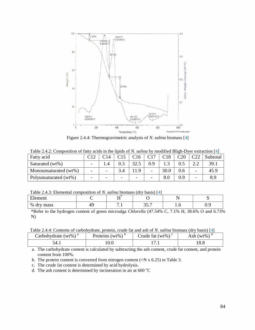
84

Figure 2.4.4: Thermogravimetric analysis of N. salina biomass [4]

Table 2.4.2: Composition of fatty acids in the lipids of N. salina by modified Bligh-Dyer extraction [4]

Fatty acid C12 C14 C15 C16 C17 C18 C20 C22 Subtotal

Saturated (wt%) - 1.4 0.3 32.5 0.9 1.3 0.5 2.2 39.1

Monounsaturated (wt%) - - 3.4 11.9 - 30.0 0.6 - 45.9

Polyunsaturated (wt%) - - - - - 8.0 0.9 - 8.9

Table 2.4.3: Elemental composition of N. salina biomass (dry basis) [4]

Element C H* O N S

% dry mass 49 7.1 35.7 1.6 0.9

*Refer to the hydrogen content of green microalga Chlorella (47.54% C, 7.1% H, 38.6% O and 6.73%

N)

Table 2.4.4: Contents of carbohydrate, protein, crude fat and ash of N. salina biomass (dry basis) [4]

Carbohydrate (wt%) a Proteins (wt%)

b Crude fat (wt%)

c Ash (wt%)

d

54.1 10.0 17.1 18.8

a. The carbohydrate content is calculated by subtracting the ash content, crude fat content, and protein

content from 100%.

b. The protein content is converted from nitrogen content (=N x 6.25) in Table 3.

c. The crude fat content is determined by acid hydrolysis.

d. The ash content is determined by incineration in air at 600 oC

85

Microalgal growth and lipids formation

Autotrophic growth of Nannochloropsis is affected by many environmental factors, including

CO2 concentration, irradiance, temperature, pH, nutrients, salinity, fluid mixing, mechanical

share stress and so on [3]. Nannochloropsis exhibits a high specific growth rate (2.5 day-1

) in an

indoor culture under optimal conditions: 25 oC, pH 7.5-8, 25% salinity, sufficient nutrients and

continuous irradiance of 58 w m-2

. However, the algal cells in an open pond are exposed to

variations of environmental conditions, particularly the irradiance and temperature as shown in

Figure 2.4.5a. The autotrophic growth of N. salina slows down significantly as shown in Figure

2.4.5b. The specific growth rate (µ) declines gradually from 0.38 day-1

on Day one, to 0.20 day-1

on Day 2, and 0.12 day-1

on Day 5. The average growth rate in the first two days under the

nutrient sufficient conditions is about 0.34 day-1

.

Compared with the commercial microalgal cultures in open ponds under extreme conditions (pH,

salinity, etc.), Nannochloropsis prefers mild conditions and hence faces competition from

wildtype microorganisms in an open pond. A photobioreactor is a closed system that can control

the growth of wildtype microalgae and the predators. Figure 2.4.6 shows the outdoor growth and

lipid production of a Nannochloropsis sp. in a flat photobioreactor with a total working volume

of 110 L (2.5 m2 x 0.045 m deep) [2]. The air-flow rate is maintained at 0.3 L per liter of liquid

per min (0.3 vvm) and CO2 is injected during the daylight hours at 3% of air to maintain pH in a

range of 7.5 to 8.0. Both gas streams are sterilized with microfiltration (1 µm). Cold water is

sprayed on the reactor to prevent the culture temperature to exceed 30 oC. During the night, the

temperature is not controlled, but equilibrate to ambient. Under an average global solar radiation

of 16 MJ m-2 day-1 in one week (Figure 2.4.6), the algal culture (40% vol) is daily replaced by a

fresh medium solution (nutrient sufficient or deprived). Specifically, in a medium of sufficient

nutrients (N, P, etc.), the biomass productivity is kept at 0.36 g L-1 day-1 (a dry cell mass

concentration of 0.36 g L-1) with a lipid content of 32.3 wt%. The lipid productivity is 117 mg

L-1 day-1. When the culture (40% vol) is replaced daily with a fresh medium without nitrogen,

the NO3-N is deprived gradually, and the biomass productivity declined slowly in the first 3 days

Figure 2.4.5b: Dry cell mass concentration (B)

increases with time in the open pond [3].

Figure 2.4.5a: Variation in temperature (T) and

irradiance (I) in an open pond (24.3 m x 2.44 m x

0.2 m)[3].

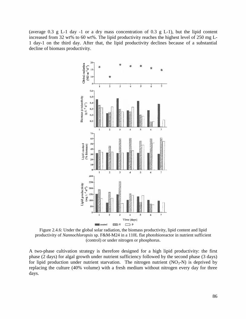
86

(average 0.3 g L-1 day -1 or a dry mass concentration of 0.3 g L-1), but the lipid content

increased from 32 wt% to 60 wt%. The lipid productivity reaches the highest level of 250 mg L-

1 day-1 on the third day. After that, the lipid productivity declines because of a substantial

decline of biomass productivity.

Figure 2.4.6: Under the global solar radiation, the biomass productivity, lipid content and lipid

productivity of Nannochloropsis sp. F&M-M24 in a 110L flat photobioreactor in nutrient sufficient

(control) or under nitrogen or phosphorus.

A two-phase cultivation strategy is therefore designed for a high lipid productivity: the first

phase (2 days) for algal growth under nutrient sufficiency followed by the second phase (3 days)

for lipid production under nutrient starvation. The nitrogen nutrient (NO3-N) is deprived by

replacing the culture (40% volume) with a fresh medium without nitrogen every day for three

days.

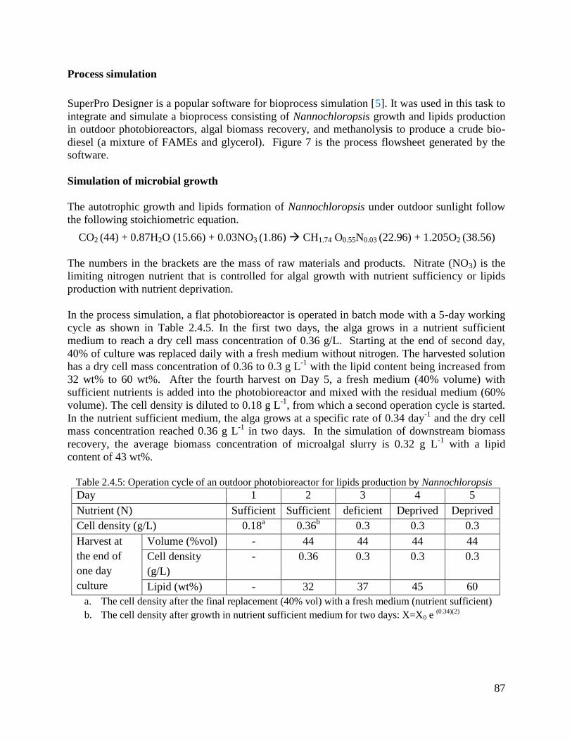
87

Process simulation

SuperPro Designer is a popular software for bioprocess simulation [5]. It was used in this task to

integrate and simulate a bioprocess consisting of Nannochloropsis growth and lipids production

in outdoor photobioreactors, algal biomass recovery, and methanolysis to produce a crude bio-

diesel (a mixture of FAMEs and glycerol). Figure 7 is the process flowsheet generated by the

software.

Simulation of microbial growth

The autotrophic growth and lipids formation of Nannochloropsis under outdoor sunlight follow

the following stoichiometric equation.

CO2 (44) + 0.87H2O (15.66) + 0.03NO3 (1.86) CH1.74 O0.55N0.03 (22.96) + 1.205O2 (38.56)

The numbers in the brackets are the mass of raw materials and products. Nitrate (NO3) is the

limiting nitrogen nutrient that is controlled for algal growth with nutrient sufficiency or lipids

production with nutrient deprivation.

In the process simulation, a flat photobioreactor is operated in batch mode with a 5-day working

cycle as shown in Table 2.4.5. In the first two days, the alga grows in a nutrient sufficient

medium to reach a dry cell mass concentration of 0.36 g/L. Starting at the end of second day,

40% of culture was replaced daily with a fresh medium without nitrogen. The harvested solution

has a dry cell mass concentration of 0.36 to 0.3 g L-1

with the lipid content being increased from

32 wt% to 60 wt%. After the fourth harvest on Day 5, a fresh medium (40% volume) with

sufficient nutrients is added into the photobioreactor and mixed with the residual medium (60%

volume). The cell density is diluted to 0.18 g L-1

, from which a second operation cycle is started.

In the nutrient sufficient medium, the alga grows at a specific rate of 0.34 day-1

and the dry cell

mass concentration reached 0.36 g L-1

in two days. In the simulation of downstream biomass

recovery, the average biomass concentration of microalgal slurry is 0.32 g L-1

with a lipid

content of 43 wt%.

Table 2.4.5: Operation cycle of an outdoor photobioreactor for lipids production by Nannochloropsis

Day 1 2 3 4 5

Nutrient (N) Sufficient Sufficient deficient Deprived Deprived

Cell density (g/L) 0.18a 0.36

b 0.3 0.3 0.3

Harvest at

the end of

one day

culture

Volume (%vol) - 44 44 44 44

Cell density

(g/L)

- 0.36 0.3 0.3 0.3

Lipid (wt%) - 32 37 45 60

a. The cell density after the final replacement (40% vol) with a fresh medium (nutrient sufficient)

b. The cell density after growth in nutrient sufficient medium for two days: X=X0 e (0.34)(2)

88

Figure 2.4.7: Process flowsheet of SuperPro Designer for crude biodiesel production (1 kg FAMEs per

batch).

Simulation of concentrating biomass

Because of the very dilute concentration of algal biomass (0.32 g/L) of the medium solution, the

first step in downstream processing is to increase the cell mass concentration by flocculation,

sedimentation and centrifugation. The seawater, after treatment, is re-used in the process [6].

Flocculation is the coalescence of finely divided suspended solids into larger loosely packed

conglomerates that settle out of suspension. Titrating seawater with NaOH to a concentration of

4 mM caused the pH to increase rapidly to pH 10.6. A fine white precipitate formed independent

of algal cells. Addition of polyelectrolyte (0.05% LT-25, CIBA Specialty Chemicals) promotes

formation of large flocs that quickly settle down. For example, an algal culture of 130 L is

flocculated by adding NaOH to 8 mM and polyelectrolyte (0.5 mg L-1

), the algal recovery

efficiency is 89% and the liquid volume is reduced by 95% vol [7]. In the downstream process

starting with a biomass concentration of 0.32 g dry mass L-1

, the flocculation operation can

reduce the liquid volume by 95%. The dry cell mass concentration is correspondingly increased

to 6.1 g L-1

, which is further concentrated by using continuous centrifugation to a dry mass

concentration of 200 g L-1

. By using a dead end filtration, a wet cake of algal biomass

containing 40 wt% dry mass is obtained. The cake is dried at 105 oC to give a biomass solid of

10% moisture suitable for direct methanolysis without solvent extraction [8].

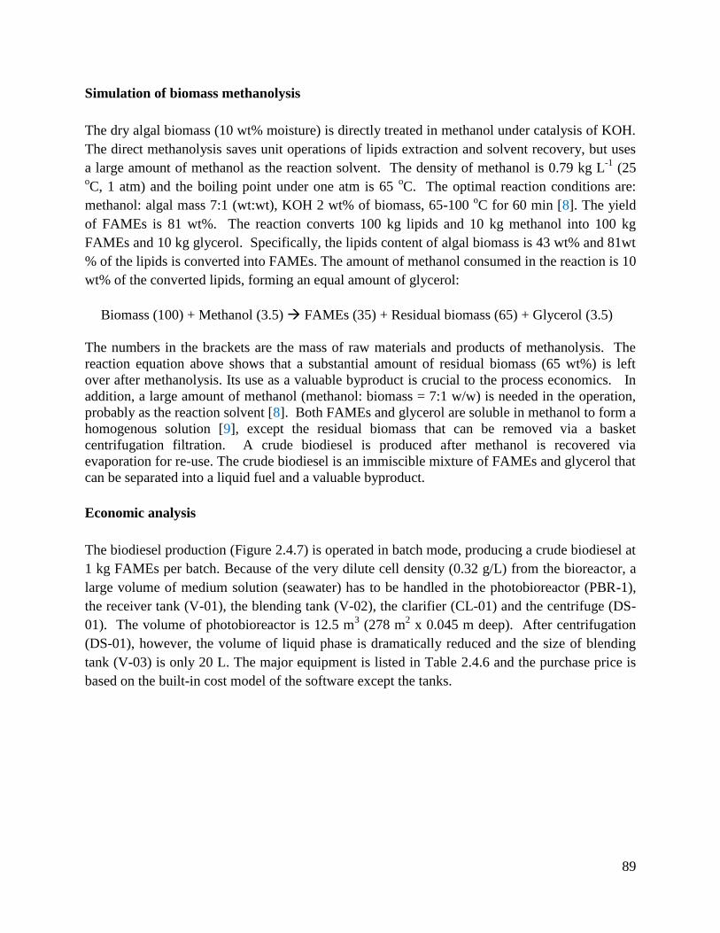
89

Simulation of biomass methanolysis

The dry algal biomass (10 wt% moisture) is directly treated in methanol under catalysis of KOH.

The direct methanolysis saves unit operations of lipids extraction and solvent recovery, but uses

a large amount of methanol as the reaction solvent. The density of methanol is 0.79 kg L-1

(25 oC, 1 atm) and the boiling point under one atm is 65

oC. The optimal reaction conditions are:

methanol: algal mass 7:1 (wt:wt), KOH 2 wt% of biomass, 65-100 oC for 60 min [8]. The yield

of FAMEs is 81 wt%. The reaction converts 100 kg lipids and 10 kg methanol into 100 kg

FAMEs and 10 kg glycerol. Specifically, the lipids content of algal biomass is 43 wt% and 81wt

% of the lipids is converted into FAMEs. The amount of methanol consumed in the reaction is 10

wt% of the converted lipids, forming an equal amount of glycerol:

Biomass (100) + Methanol (3.5) FAMEs (35) + Residual biomass (65) + Glycerol (3.5)

The numbers in the brackets are the mass of raw materials and products of methanolysis. The

reaction equation above shows that a substantial amount of residual biomass (65 wt%) is left

over after methanolysis. Its use as a valuable byproduct is crucial to the process economics. In

addition, a large amount of methanol (methanol: biomass = 7:1 w/w) is needed in the operation,

probably as the reaction solvent [8]. Both FAMEs and glycerol are soluble in methanol to form a

homogenous solution [9], except the residual biomass that can be removed via a basket

centrifugation filtration. A crude biodiesel is produced after methanol is recovered via

evaporation for re-use. The crude biodiesel is an immiscible mixture of FAMEs and glycerol that

can be separated into a liquid fuel and a valuable byproduct.

Economic analysis

The biodiesel production (Figure 2.4.7) is operated in batch mode, producing a crude biodiesel at

1 kg FAMEs per batch. Because of the very dilute cell density (0.32 g/L) from the bioreactor, a

large volume of medium solution (seawater) has to be handled in the photobioreactor (PBR-1),

the receiver tank (V-01), the blending tank (V-02), the clarifier (CL-01) and the centrifuge (DS-

01). The volume of photobioreactor is 12.5 m3 (278 m

2 x 0.045 m deep). After centrifugation

(DS-01), however, the volume of liquid phase is dramatically reduced and the size of blending

tank (V-03) is only 20 L. The major equipment is listed in Table 2.4.6 and the purchase price is

based on the built-in cost model of the software except the tanks.

90

Table 2.4.6: Equipment summary (2016 prices).

Name Type Capacity Material Cost ($/Unit)

PBR-1 Flat photobioreactor 12.5 m3 SS316, polyethylene 288,000

DS-01 Disk-stack centrifuge 1,174 m2 SS316 137,000

V-01 Receiver tank 11.6 m3 SS316 100,000

V-02 Blending tank 11.7 m3 SS 316 100,000

V-03 Blending tank 20 L SS 316 5,000

CL-01 Clarifier 0.33 m2 Concrete 6,000

R-01 Stirred reactor 40 L SS316 100,000

PFF-01 Plate & Frame filter 0.02 m2 SS316 31,000

BCFBD-

01

Basket centrifuge 0.04 m2 SS316 16,000

TDR-01 Tray dryer 0.2 m2 SS316 81,000

TFE-01 Thin film evaporator 0.04 m2 SS316 116,000

Total 980,000

Table 2.4.7: Overall process parameters.

Operating time (hours/year) 7917

Batch operation time (hours) 128

Number of batches per year (#/year) 62

Output of FAMEs per batch (kg/batch) 1

Output of FAMEs per year (kg/year) 62

Table 2.4.7 gives the overall process operation parameters. One batch operation takes 128 hours

(5.3 days) because of the microbial growth and lipids formation (5 days per batch). The number

of batches per year is 62, and the annual output of FAMEs or biodiesel is 62 kg. Figure 2.4.8

shows the usage of major equipment in two sequential batches. Obviously, the bottleneck of the

whole process is the microbial culture in the photobioreactor (PBR-1), because it is fully

occupied. The second possible bottleneck is the treatment and storage of the used mineral

solution or seawater in the receiver tank (V-01). Both units have a large capacity for seawater

handling. Other units, however, are idle in most of the time during a batch operation. A process

efficiency enhancement may improve the usage of the idle equipment in order to improve

process economics.

Figure 2.4.8: Equipment occupation in two sequential batch operations.

16 32 48 64 80 96 112 128 144 160 176 192 208 224 240 256 272 288h

1 2 3 4 5 6 7 8 9 10 11 12 13day

V-01

TFE-01

BCFBD-01

R-01

TDR-01

PFF-01

V-03

DS-01

CL-01

V-02

PBR-1

Mai

n E

qu

ipm

ent

& C

IP S

kid

s

Legend

B# 1

B# 2

91

The costs of raw materials are summarized in Table 2.4.8, excluding the costs of seawater and

carbon dioxide. The material cost of biodiesel is $10.3/kg FAMEs. It is interesting to note that

the methanol cost accounts for 71%, because of a significant loss of methanol in the recovery of

residual algal biomass (P-10). The loss of methanol can be reduced by using an operation unit for

biomass drying and methanol condensation. Sodium hydroxide and sulfuric acid are the second

and third major material costs, respectively. The base and acid are primarily used in pH

adjustment of the medium solution for flocculation of microalgal cells. Although the pH is

adjusted between 7 and 11, the large volume of seawater consumes a significant amount of base

and acid. If methanol is completely recovered, the material cost of FAMEs could be reduced to

$2.97/kg FAMEs. Table 2.4.9 is the executive summary of process economic evaluation.

Table 2.4.8: Material cost

a

Material name Unit cost

($/kg)

Amount

(kg/year)

Cost

($/year)

Percentage

(%)

Sodium Nitrate 0.4 19 7.76 1.21

Sulfuric acid 0.3 274 82.06 12.81

Filter aid 0.3 2 0.70 0.11

Methanol 0.3 1521 456.26 71.24

Sodium

Hydroxide

0.4 229 91.72 14.32

PolyE 5.0 0.39 1.94 0.3

Total 640.43 100

a. The costs of medium solution (seawater) and carbon dioxide are not included

Table 2.4.9: Executive summary (2016 price).

Total capital investment 1,007,000 $

Operating cost a 1,000 $/year

Revenue b 620 $/year

Unit product cost 10.3 $/kg FAMEs

Return on investment 0.78%

Payback time 128 years

a. Materials plus utilities

b. The revenue of biodiesel at $10/kg FAMEs

Conclusion of economic analysis

Based on a simplified economic model and rates, the process economic analysis indicates that

the current biodiesel production through microbial CO2 fixation is not economically feasible.

Three critical factors are identified for research and improvement: (a) a low dry cell mass

concentration from the bioreactors, (b) the methanol loss in direct methanolysis of the dry

biomass, and (c) the value (credit) of the residual biomass. If the cell mass concentration can be

increased from the current level of 0.3 g/L to 20-30 g/L, the volume of medium solution and

therefor the equipment size can be dramatically reduced. Some unit operations such as

92

flocculation for concentrating a dilute cell solution may be avoided, which could save the cost of

chemicals in pH control, capital investment, utilities, and labors. In addition, the residual cell

debris should be removed before methanolysis. This will not only reduce the methanol loss in the

unit operations of esterification and residual biomass recovery, but also generate a hydrolysates

solution of cell debris for reuse on site. The value of the residual biomass is crucial to the process

economics. This task has confirmed that the cell debris can be reused as the microbial nutrients

to save the material cost.

References

1. J. Yu, A. Dow, S. Pingali (2013). The energy efficiency of carbon dioxide fixation by a

hydrogen-oxidizing bacterium, Int J Hydrogen Energ 38:8683-8690.

2. L. Rodolfi, G.C. Zittelli, N. Bassi, G. Padovani, N. Biondi, G. Bonini, M.R. Tredici (2008).

Microalgae for oil: strain selection, induction of lipid synthesis and outdoor mass cultivation

in a low-cost photobioreactor. Biotech Bioeng 102(1):100112.

3. P.E. Gharagozloo, J. L. Drewry, A.M. Collins, T.A. Dempster, C.Y. Choi, S.C. James

(2014). Analysis and modeling of Nannochloropsis growth in lab, greenhouse, and raceway

experiments, J Appl Phycol 26:2303-2314.

4. Z. Bi, B.B. He (2013). Characterization of microalgae for the purpose of biofuel production.

Trans ASABE 56(4):1529-1539.

5. SuperPro Designer® User’s guide, Intelligen, Inc. Scotch Plains, NJ 07076,

http://www.intelligen.com.

6. L. Rodolfi, G.C. Zittelli, L. Barsanti, G. Rosati, M.R. Tredici (2003). Growth medium

recycling in Nannochloropsis sp. mass cultivation, Biomol Eng 20:243-248.

7. R.M. Knuckey, M.R. Brown, R. Robert, D.M.F. Frampton (2006). Production of microalgal

concentrates by flocculation and their assessment as aquaculture feeds, Aquacult Eng 35:300-

313.

8. P.D. Patil, V.G. Gude, A. Mannarswamy, P. Cooke, N. Nirmalakhandan, P. Lammers, S.

Deng (2012). Comparison of direct transesterification of algal biomass under superctitical

methanol and microwave irradiation conditions, Fuel 97:822-831.

9. S. Doungsri, T. Sookkumnerd (20110. Solubility curves of FAME+methanl+glycerol. TIChE

International Conference, November 10-11, Thailand.

2.5 Biocontamination of Fuels

From a petroleum-contaminated sample, two isolates have been used to study the biodegradation

of sulfur containing compounds. Arthrobacter sp. P1-1 and Burkholderia sp. C3 have been

utilized to investigate the biodegradation of dibenzothiophene (DBT), a thermodynamically

stable, sulfur containing poly aromatic hydrocarbon (PAH) compound that is inherently present

in all diesel fuels (Li et al. 2012).

http://www.intelligen.com/

93

Glycerol is the main byproduct that is formed during the fatty acid transesterification process for

the production of biodiesel. In use, biodiesel is often blended with petroleum diesel fuels. During

the blending process, a glycerol carbon source and DBT becomes bioavailable. Metabolic

enhancement using different nutrient sources such as glycerol can increase linked biochemical

pathways. Co-metabolic studies for the simultaneous utilization of both compounds are expected

to offer knowledge and information about sulfur metabolism and for this study also a fuel pre-

treatment protocol.

Approach

For FY 2010 our focus has shifted from the previously used Arthrobacter sp. P1-1 to

Burkholderia sp. C3, which was found to have higher PAH degradation rates (Seo et al. 2007).

Burkholderia sp. was also determined to contain dioxygenase genes that have a role in degrading

PAHs such as DBT (Seo et al. 2007, Tittabutr et al. 2011).

Results

During this study glycerol was found to stimulate both rhamnolipid production and DBT

degradation. Increased rhamnolipid biosynthesis and secretion facilitated the degradation of

DBT. Rhamnolipid could be involved in cell transport and may increase the biodegradation of

hydrophobic chemicals (Bai et al. 1997).

Glycerol readily enters into -oxidation and FAS II lipid pathways, affecting the production of

rhamnolipids (Abdel-Mawgoud et al. 2014, Gutierrez et al. 2013). It was determined that

optimal glycerol to DBT molar ratios increased DBT biodegradation rate constants up to 18-fold

and enhanced DBT cometabolism by 25-30% after 24hrs relative to controls containing only

DBT (Table 2.5.1). At day 7, DBT was completely biodegraded using the 100:1 glycerol to DBT

molar ratio used for cultivation (Figure 2.5.1). Increased degradation rates were associated with

nearly tripled amounts of RL secreted (Figure 2.5.2A). The presence of RLs affects DBT

biodegradation at early stages of incubation which is supported by the surface tension decrease at

day 1 (Figure 2.5.2B) and the RL secretion levels quantified using an orcinol assay.

The determination of the biological impact that the secretion of rhamnolipids has on the rate of

DBT degradation provides additional insight into how we might better understand sulfate uptake

metabolisms. A rhamnolipid is a glycolipid biosurfactant, produced by two anabolic pathways

(Perfumo et al. 2006, Nie et al. 2010). Due to its amphipathic chemistry, biosurfactants interact

with PAHs in solution and at water-particle and water-oil interfaces. Those interactions alter the

physicochemical properties of PAHs, making them more soluble and bioavailable (Makkar and

Rockne 2003). The production of both biosurfactants and hydrocarbon degradative enzymes

have been previously observed in bacteria (Xia et al. 2014). The dual functions of RL production

and PAH degradation may confer to the microorganism an evolutional adaptation to survive in

environmental conditions where hydrophobic chemicals are scarce. Further work under other

funding will investigate the effects of biosurfactant inhibition, and will identify the relevance of

rhlABC genes. These genes are sulfur mediated and involved with biosurfactant production

(Ismall et al. 2014).

94

Tab

le 2

.5.1

G

lyce

rol

conce

ntr

atio

n d

epen

den

t en

han

cem

ent

of

dib

enzo

thio

phen

e (D

BT

) bio

deg

rad

atio

n r

ate

con

stan

t an

d D

BT

hal

f

life

. E

xponen

tial

dec

ay e

quat

ion

C=

Coe-k

t was

use

d f

or

fitt

ing “

N”

dat

a p

oin

ts w

her

e k i

s th

e ra

te c

onst

ant

and t

is

tim

e in

day

s.

* R

elat

ive

to r

ate

const

ant

of

0.5

mM

DB

T.

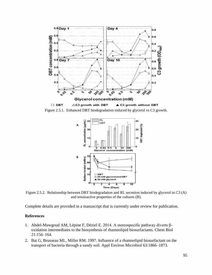
95

Figure 2.5.1. Enhanced DBT biodegradation induced by glycerol vs C3 growth.

Figure 2.5.2. Relationship between DBT biodegradation and RL secretion induced by glycerol in C3 (A)

and tensioactive properties of the cultures (B).

Complete details are provided in a manuscript that is currently under review for publication.

References

1. Abdel-Mawgoud AM, Lépine F, Déziel E. 2014. A stereospecific pathway diverts β-

oxidation intermediates to the biosynthesis of rhamnolipid biosurfactants. Chem Biol

21:156–164.

2. Bai G, Brusseau ML, Miller RM. 1997. Influence of a rhamnolipid biosurfactant on the

transport of bacteria through a sandy soil. Appl Environ Microbiol 63:1866–1873.

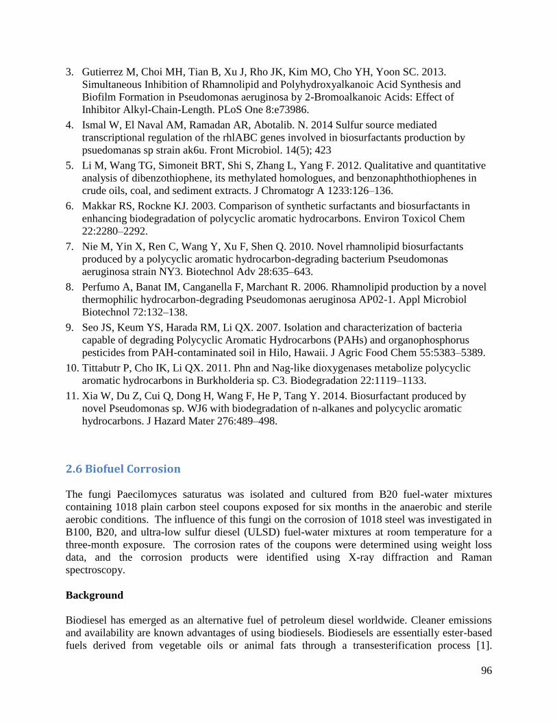
96

3. Gutierrez M, Choi MH, Tian B, Xu J, Rho JK, Kim MO, Cho YH, Yoon SC. 2013.

Simultaneous Inhibition of Rhamnolipid and Polyhydroxyalkanoic Acid Synthesis and

Biofilm Formation in Pseudomonas aeruginosa by 2-Bromoalkanoic Acids: Effect of

Inhibitor Alkyl-Chain-Length. PLoS One 8:e73986.

4. Ismal W, El Naval AM, Ramadan AR, Abotalib. N. 2014 Sulfur source mediated

transcriptional regulation of the rhlABC genes involved in biosurfactants production by

psuedomanas sp strain ak6u. Front Microbiol. 14(5); 423

5. Li M, Wang TG, Simoneit BRT, Shi S, Zhang L, Yang F. 2012. Qualitative and quantitative

analysis of dibenzothiophene, its methylated homologues, and benzonaphthothiophenes in

crude oils, coal, and sediment extracts. J Chromatogr A 1233:126–136.

6. Makkar RS, Rockne KJ. 2003. Comparison of synthetic surfactants and biosurfactants in

enhancing biodegradation of polycyclic aromatic hydrocarbons. Environ Toxicol Chem

22:2280–2292.

7. Nie M, Yin X, Ren C, Wang Y, Xu F, Shen Q. 2010. Novel rhamnolipid biosurfactants

produced by a polycyclic aromatic hydrocarbon-degrading bacterium Pseudomonas

aeruginosa strain NY3. Biotechnol Adv 28:635–643.

8. Perfumo A, Banat IM, Canganella F, Marchant R. 2006. Rhamnolipid production by a novel

thermophilic hydrocarbon-degrading Pseudomonas aeruginosa AP02-1. Appl Microbiol

Biotechnol 72:132–138.

9. Seo JS, Keum YS, Harada RM, Li QX. 2007. Isolation and characterization of bacteria

capable of degrading Polycyclic Aromatic Hydrocarbons (PAHs) and organophosphorus

pesticides from PAH-contaminated soil in Hilo, Hawaii. J Agric Food Chem 55:5383–5389.

10. Tittabutr P, Cho IK, Li QX. 2011. Phn and Nag-like dioxygenases metabolize polycyclic

aromatic hydrocarbons in Burkholderia sp. C3. Biodegradation 22:1119–1133.

11. Xia W, Du Z, Cui Q, Dong H, Wang F, He P, Tang Y. 2014. Biosurfactant produced by

novel Pseudomonas sp. WJ6 with biodegradation of n-alkanes and polycyclic aromatic

hydrocarbons. J Hazard Mater 276:489–498.

2.6 Biofuel Corrosion

The fungi Paecilomyces saturatus was isolated and cultured from B20 fuel-water mixtures

containing 1018 plain carbon steel coupons exposed for six months in the anaerobic and sterile

aerobic conditions. The influence of this fungi on the corrosion of 1018 steel was investigated in

B100, B20, and ultra-low sulfur diesel (ULSD) fuel-water mixtures at room temperature for a

three-month exposure. The corrosion rates of the coupons were determined using weight loss

data, and the corrosion products were identified using X-ray diffraction and Raman

spectroscopy.

Background

Biodiesel has emerged as an alternative fuel of petroleum diesel worldwide. Cleaner emissions

and availability are known advantages of using biodiesels. Biodiesels are essentially ester-based

fuels derived from vegetable oils or animal fats through a transesterification process [1].

97

Biodiesels can be used in its pure form (B100) or blended with petroleum diesel as another

source of renewable energy. Biodiesel, in comparison to petroleum diesel, has the advantage of

being biodegradable and non-toxic, having higher flash point, and causing reduced emissions.

However, the major cons of biodiesel include its oxidative instability, poorer low-temperature

properties, slightly lower power and torque generation, and higher fuel consumption [2].

The organic nature of biodiesels makes it a prime target for microbial contamination.

Microorganisms are able to survive in these fuels whenever there is the presence of water.

Microorganisms generally flourish in the water phase, but feed on fuel at the water-fuel phase

boundary [3]. Contamination of fuel by microorganisms can cause biofouling. Whenever

biofouling occurs, an extracellular polymeric substance (EPS) is formed at the fuel-water phase.

This is more commonly known as the biofilm. The term biofilm refers to the development of

microbial communities on submerged surfaces in aqueous environments [4]. Thus, a microbial

consortium is formed and corrosion is often accelerated due to the variety of microorganisms

present.

The development of the biofilm is facilitated by the production of EPS macromolecules such as

proteins, polysaccharides, nucleic acids and lipids [5]. Growth of the biofilm is considered to be

the result of complex processes involving the transport of organic and inorganic molecules and

microbial cells to the surface, adsorption of molecules to the surface, and initial attachment of

microbial cells followed by their irreversible adhesion facilitated by production of EPS, often

referred to as the glycocalyx or slime [6]. It has also been documented that degradation of metal

surfaces occurs when the contact between microbial cells, or products of their metabolism such

as EPS, and the surface is established [7]. The EPS plays an important role in attachment to

metal surfaces. It also has the ability to complex with metal ions [7]. This is important because

some bacteria require metal ions to grow [7]. Also, the availability and type of ions are likely to

have an effect on the colonization of a metal surface [7].

A number of studies have also been conducted to assess biodiesel compatibility with different

materials. In one study, petroleum diesel, a soybean-derived biodiesel, and a sunflower-derived

biodiesel were tested for material compatibility against structural carbon steel (ASTM A36) and

high density polyethylene (HDPE) [8]. The soybean-derived biodiesel was found to be more

compatible with carbon steel than the petroleum diesel and sunflower biodiesel. By using Fourier

transform infrared spectroscopy (FTIR), ageing was shown to take place only in the biodiesels

which had very little effect on the degradation of the carbon steel and HDPE. The petroleum

diesel, which did not age, was the most aggressive towards the steel and HDPE. Another study

[9] on the corrosion rates of a piston metal and piston liner metal immersed in biodiesel

originating from various seed oils (Pongamia glabra, Salvadora oleoides, Madhuca Indica, and

Jatropha curcas) revealed that the biodiesel comprised of Salvadora oil was the most aggressive

leading to the corrosion rate for the piston metal and piston liner metal of 0.1236 and 0.1329

mm/year or mpy, respectively. Interestingly, petroleum diesel showed low corrosivity and was

tied with biodiesel comprised of Pongamia and Madhuca oil as having the lowest corrosion rates

for piston metal and piston liner metal of 0.0058 and 0.0065 mpy, respectively. The higher

corrosivity of the biodiesel comprised of Salvadora oil was attributed to the higher percentage of

sulphur content.

98

The corrosive effects of biodiesel derived from rice husk was studied [10] on aluminum, mild

steel (Q235A), brass (H62), and austenite stainless steel (SS321, 1Cr18Ni9Ti). Three bio-oil-

diesel emulsions were used which were 100% biodiesel, 30% biodiesel, and 10% biodiesel. The

most significant weight loss was observed for mild steel, followed by aluminum, while brass

exhibited only slight weight loss. The 100% biodiesel fuel was the most corrosive followed by

the emulsions with 30% biodiesel and 10% biodiesel. Haseeb et al [11] investigated the

corrosion behavior of copper and bronze in diesel and palm biodiesel. Static immersions of test

coupons were conducted at two different temperatures, room temperature (25 - 30°C) and 60°C.

Copper was shown to have higher corrosion rates in comparison to leaded bronze. Fazal et al

[12] performed an investigation on the corrosion behavior of copper (99.99% pure), aluminum

(99% pure), and stainless steel (316) in diesel and palm biodiesel. The results revealed that

copper had the highest corrosion rate of 0.586 mpy followed by aluminum with 0.202 mpy and

stainless steel having the lowest at 0.015 mpy. Furthermore, Fazal et al [13] studied the

degradation mechanism of different automotive materials such as copper, brass, aluminum, and

cast iron by characterizing the corrosion products. The corrosion rates were found to be the

following for copper, brass, aluminum, and cast iron, 0.393, 0.210, 0.173, and 0.112 mpy,

respectively, for palm biodiesel. In the case of diesel, the rates were the following for copper,

brass, aluminum, and cast iron, 0.158, 0.120, 0.084, and 0.774 mpy, respectively. Thus, it was

shown that palm biodiesel was more corrosive than diesel (for non-ferrous metals), and that

copper exhibited the most severe corrosion. Similarly, Hu et al [14] also conducted a study on

the corrosion rates for copper, mild carbon steel, aluminum, and stainless steel exposed to

biodiesel derived from rapeseed oil and methanol along with diesel fuel and concluded that the

corrosive effects of biodiesel are more severe on copper and carbon steel compared to that of

aluminum and stainless steel, and that the corrosion mechanism of biodiesel on metals should be

mostly attributed to chemical corrosion.

Biodiesel has a higher affinity for moisture and water-retaining capacity in comparison to

petroleum diesel [15]. The hygroscopic fatty acid methyl ester (FAME) compounds are the

primary reason for biodiesel being much more hydrophilic than diesel. Although the maximum

water content allowed by ASTM standard D6751 is 500 mg·kg-1

, water contamination often

occurs in storage, where temperature and humidity greatly affect the amount of excess water

absorbed within the surrounding environment. Water contamination within biodiesel also poses a

serious problem as it harbors and facilitates the growth of microorganisms which could then lead

to the corrosion of metals, and the formation of sludge and slime, thereby constricting fuel filters

and fuel lines. [3, 15]. Water at high temperatures has also been shown to hydrolyze esters as

well as triglycerides and produce different types of fatty acids which are more corrosive [11].

The water absorbance of biodiesel and biodiesel-diesel fuel blends were studied by evaluating

the temperature and blend ratio parameters [15]. The water absorption capacity of 100%

biodiesel and diesel oil rapidly decrease if the temperature drops. At a temperature of 293.15 and

323.15 K, 100% biodiesel absorbed 15 and 10 times more water, respectively, than diesel.

Fregolente et al [15] ultimately concluded that the soluble water content of biodiesel, diesel, and

blends depends strongly on the temperature and blend ratio. Also it was found that under a

relative humidity of 79% and 66%, there was an increase of 51% and 23%, respectively, of water

content for 100% biodiesel and an increase of only 8% and 7% respectively, of water content for

99

diesel samples. The addition of biodiesel in diesel increases the water holding capacity of the

blend.

Microbiologically influenced corrosion (MIC), wherein the coupling of microorganisms to

corrosion, usually gives the adverse effect of accelerated corrosion. MIC has posed to be a

serious problem in biodiesel usage, storage, and transportation. Aktas et al [16] exposed

biodiesel to anaerobic microorganisms from fresh water and marine environments with differing

histories of exposure to hydrocarbons, biodiesel, and oxygen. Two common features of the

anaerobic inocula were that they could reduce sulfate or produce methane, and metabolized

biodiesel. In another study, experiments were designed to evaluate the nature and extent of

microbial contamination and the potential for MIC in alternative fuels (i.e., biodiesel, ULSD, and

their blends) [17]. ULSD, L100, B100, B20, and B5 were the selected fuels. Microorganisms

were identified via denaturing gradient gel electrophoresis (DGGE) and by 16S rRNA for

bacteria and 28S rRNA for fungi. Corrosion experiments were conducted with represent fuel

tank alloys (i.e., carbon steel UNS C10200, stainless steel UNS S30403, and aluminum alloy

UNS A95052). Lee et al [17] found that for each fuel-water combination, microorganism species

diversity generally decreased over the six months. Stainless steel exhibited no visual signs of

corrosion. Visual and microscopic analyses revealed an absence of corrosion on C1020 in the

presence of biodiesel, even in the lowest concentration. Lee et al [17] hypothesized that biodiesel

has a passivating effect on C1020. In the case of aluminum, pitting was visually observed in all

AA5052 fuel-water exposures. Overall, Lee et al [17] concluded that C1020 exhibited general

active corrosion in ULSD and L100, and passive behavior in B100 and biodiesel/ULSD blends.

SS304L remained passive in all exposures; whereas, AA5052 was found to be susceptible to

subsurface pitting in the water and fuel layers in addition to the fuel-water interface.

Experimental

Material selection

Plain carbon 1018 steel was chosen based on its similar chemical compositions to that of ASTM

A36 steel and API Spec 5L X60, which are often used for fuel tank storage and pipelines,

respectively.

The 1018 steel coupons were machined to the following dimensions: 2.25” × 1” × 0.125”. A

Telesis BenchMark 320 marking system was used to pin stamp the coupons for identification.

The coupons were then acetone washed and weighed to obtain an initial mass. To prevent

oxidation of the steel, the coupons were kept in a dry box (< 1% relative humidity) prior to

performing experiments.

Microorganism selection

The fungi Paecilomyces saturatus was successfully isolated and cultured from water-biofuel

(unfiltered B20) mixtures containing 1018 plain carbon steel coupons exposed for six months in

the anaerobic and sterile aerobic (air filtered through a 0.22 µm filter) conditions.

100

Fuel selection

The types of fuel that were chosen for this study were 100% biodiesel (B100), 20% biodiesel

(B20), and ultra-low sulfur diesel (ULSD). These fuels were obtained from local petrol filling

stations (i.e., 76 and Aloha Petroleum gas stations). To isolate and study the corrosive effects of

the fungi, Paecilomyces saturatus, the fuels were sterilized prior to being inoculated with the

fungi. Sterility of the B100, B20, and ULSD fuels were achieved via vacuum filter sterilization

by a 0.22 µm Millipore membrane filter.

Sample exposure

100 µL of the fungi, Paecilomyces saturatus, suspended in a nutrient rich broth (tryptic soy

broth) was added to the three different types of fuels. Ultrapure water (18.2 MΩ•cm) was also

added to the fuels to facilitate a suitable environment for the fungi. This fuel-water mixture (40

mL fuel, 40 mL water) was stored in 100 mL glass Pyrex media bottles. The 1018 steel coupon

samples were placed in the fuel-water mixtures at an angle of 45° with respect to the horizon.

Triplicates of each fuel-water mixture and 1018 steel coupons were exposed outdoors under

sterile aerobic environmental condition. UV exposure from the sun and rain water contamination

was kept to a minimum by encasing samples in boxes under a protective alcove. Figure 2.6.1

depicts the exposure setup. An additional triplicate setup of each fuel-water mixture without the

added 100 µL of Paecilomyces saturatus, served as the experimental control.

Figure 2.6.1: Fuel-water mixture depicting sterile aerobic environmental setup. Sterile aerobic cap also

depicted.

The gray cap simulates a “sterile” aerobic environment. The gray cap is fitted with a 0.22 µm

filter at the top to allow only air to be exchanged into and out of the bottle. Contamination from

the outside environment was not able to enter the bottle.

An exposure time of 3 months was chosen for this experiment.

0.22 µm filter

101

Sample Retrieval and Characterization

The coupons were retrieved after immersion for 3 months. All coupons immersed in B100 and

B20 fuel-water mixtures were lightly acetone washed to remove oil residue prior to digital

imaging. The coupons immersed in ULSD fuel-water mixtures did not have to be acetone

washed as very little oil residue remained upon retrieval of coupons. Digital imaging of the

exposed coupons was conducted using a Nikon D700 DSLR camera equipped with AF Micro-

NIKKOR 60mm f/2.8D.

The corrosion products formed on carbon steel coupons were characterized using a combination

of Raman spectroscopy and X-ray diffraction (XRD) [18, 19]. A Nicolet Almega XR dispersive

Raman Spectrometer (Thermo Scientific Corp.) equipped with multiple Olympus objectives and

a Peltier-cold charge-coupled device (CCD) detector was used for Raman spectroscopic analysis.

An objective with magnification of 50× with an estimated spatial resolution of 1.6 μm was used.

The instrument was operated with a laser source of an infrared diode laser with 780 nm

wavelength excitation. The estimated resolution was in the range of 8.4 – 10.2 cm-1

and the

accumulation time was 120 seconds. A Rigaku MiniFlexTM II benchtop XRD system equipped

with a Cu (Kα) radiation was used for XRD measurements. XRD spectra were obtained directly

on the corroded steel surfaces. The scans were conducted in the range of 3 – 90° (2θ) and with a

scan rate of 1° (2θ)/min.

After the corrosion product characterization, the steel coupons were cleaned with an acid wash

following ISO 8407. The cleaned coupons were dried in a dry box (1% RH) for at least one

hour, weighed and compared to their respective initial mass values to obtain the total mass loss.

The penetration rate in mpy was then calculated based on the total mass loss results according to

Eq. 1:

1

tA

mRatenPenetratio (1)

where Δm is the change in mass in grams, A the area of the sample in mm2, t the time in years,

and ρ the density of the 1018 steel in g/mm3.

Results

Corrosion product morphology

Photographs of the 1018 steel coupons after 3-month immersion in the sterile aerobic B100 fuel-

water (Figure 2.6.2), B20 fuel-water (Figure 2.6.3), and ULSD fuel-water (Figure 2.6.4) mixtures

contrast the fungi-inoculated and control (not inoculated) conditions. For the B100 and B20 fuel-

water mixtures (Figures 2.6.2 and 2.6.3), the samples from fungi-inoculated environments

showed significant amounts of corrosion products (orange color) that formed in the water layer.

The control samples, however, showed virtually no corrosion product over the entire surface, and

appeared to have passivated. Therefore, it is apparent that the fungi Paecilomyces saturatus plays

a significant role on the corrosivity of B100 and B20 fuel-water mixtures towards 1018 steel

coupons. Since the microorganisms generally reside in the water layer up to the fuel-water

interface, the presence of Paecilomyces saturatus was most likely the cause for the accelerated

corrosion of steel immersed in the fungi-inoculated environments.

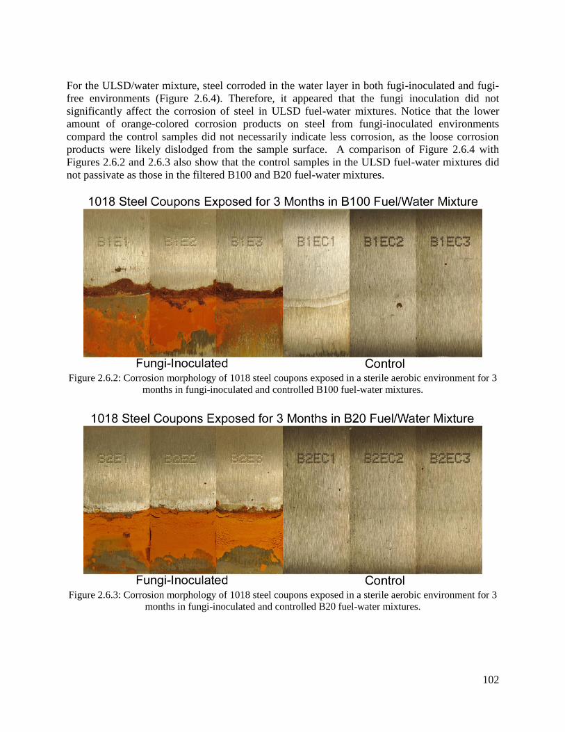
102

For the ULSD/water mixture, steel corroded in the water layer in both fugi-inoculated and fugi-

free environments (Figure 2.6.4). Therefore, it appeared that the fungi inoculation did not

significantly affect the corrosion of steel in ULSD fuel-water mixtures. Notice that the lower

amount of orange-colored corrosion products on steel from fungi-inoculated environments

compard the control samples did not necessarily indicate less corrosion, as the loose corrosion

products were likely dislodged from the sample surface. A comparison of Figure 2.6.4 with

Figures 2.6.2 and 2.6.3 also show that the control samples in the ULSD fuel-water mixtures did

not passivate as those in the filtered B100 and B20 fuel-water mixtures.

Figure 2.6.2: Corrosion morphology of 1018 steel coupons exposed in a sterile aerobic environment for 3

months in fungi-inoculated and controlled B100 fuel-water mixtures.


months in fungi-inoculated and controlled B20 fuel-water mixtures.

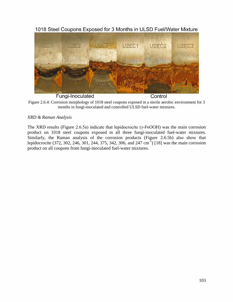
103


months in fungi-inoculated and controlled ULSD fuel-water mixtures.

XRD & Raman Analysis

The XRD results (Figure 2.6.5a) indicate that lepidocrocite (γ-FeOOH) was the main corrosion

product on 1018 steel coupons exposed in all three fungi-inoculated fuel-water mixtures.

Similarly, the Raman analysis of the corrosion products (Figure 2.6.5b) also show that

lepidocrocite (372, 302, 246, 301, 244, 375, 342, 306, and 247 cm-1

) [18] was the main corrosion

product on all coupons from fungi-inoculated fuel-water mixtures.

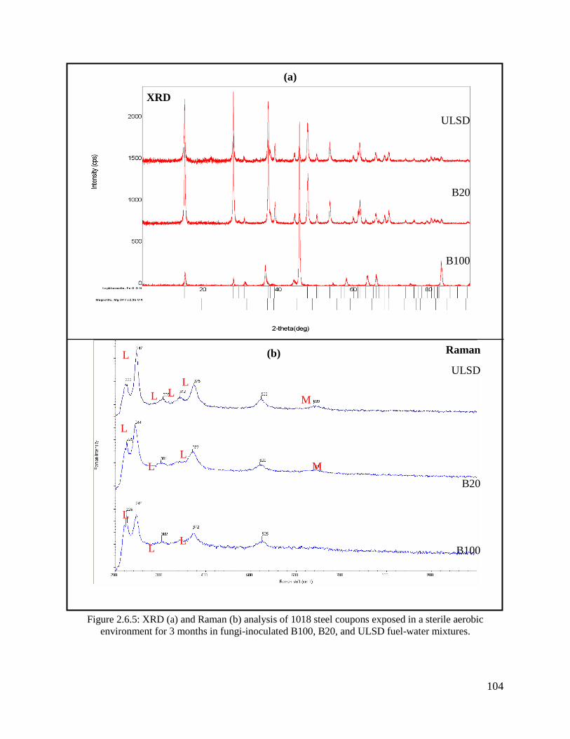
104

Figure 2.6.5: XRD (a) and Raman (b) analysis of 1018 steel coupons exposed in a sterile aerobic

environment for 3 months in fungi-inoculated B100, B20, and ULSD fuel-water mixtures.

L

L

L

L

L

L

L L

B100

B20

ULSD

B100

B20

ULSD

XRD

Raman

M

M

L

L

(b)

(a)

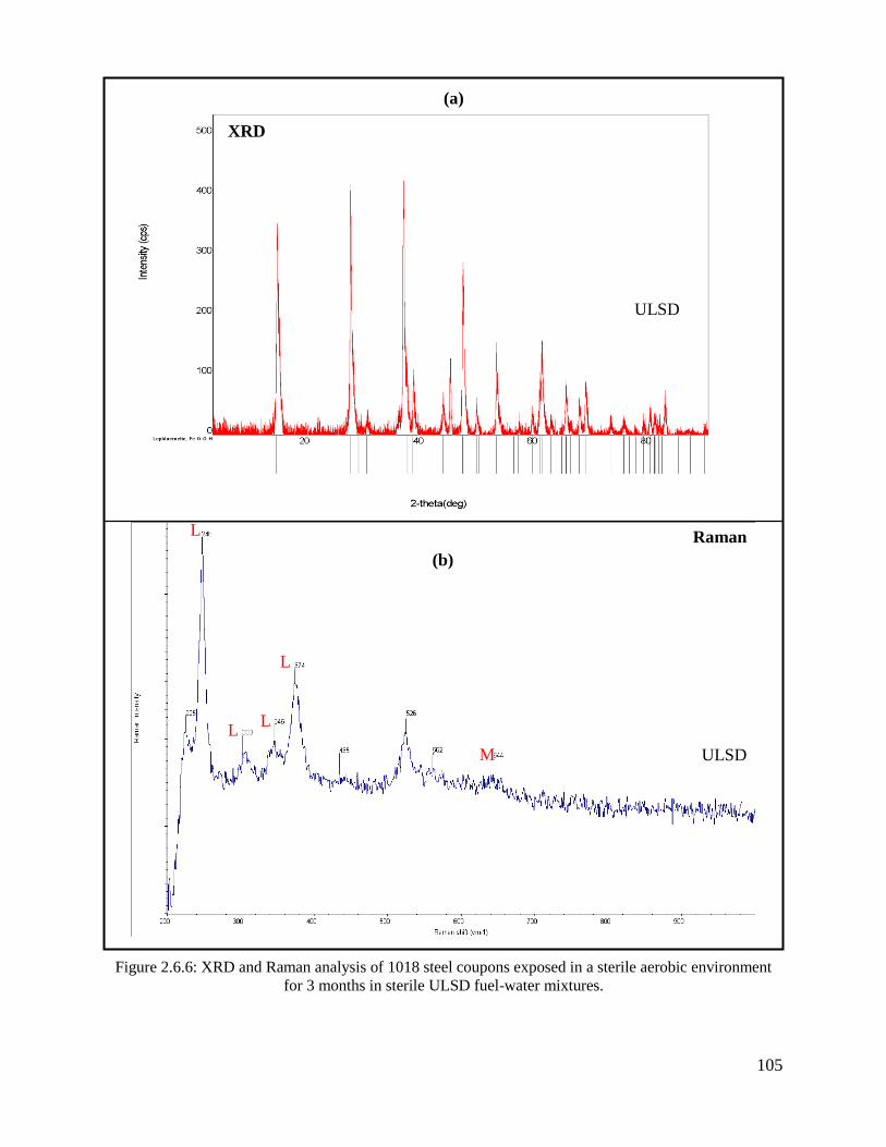
105

Figure 2.6.6: XRD and Raman analysis of 1018 steel coupons exposed in a sterile aerobic environment

for 3 months in sterile ULSD fuel-water mixtures.

XRD

Raman L

ULSD

ULSD

L L

L

M

(b)

(a)

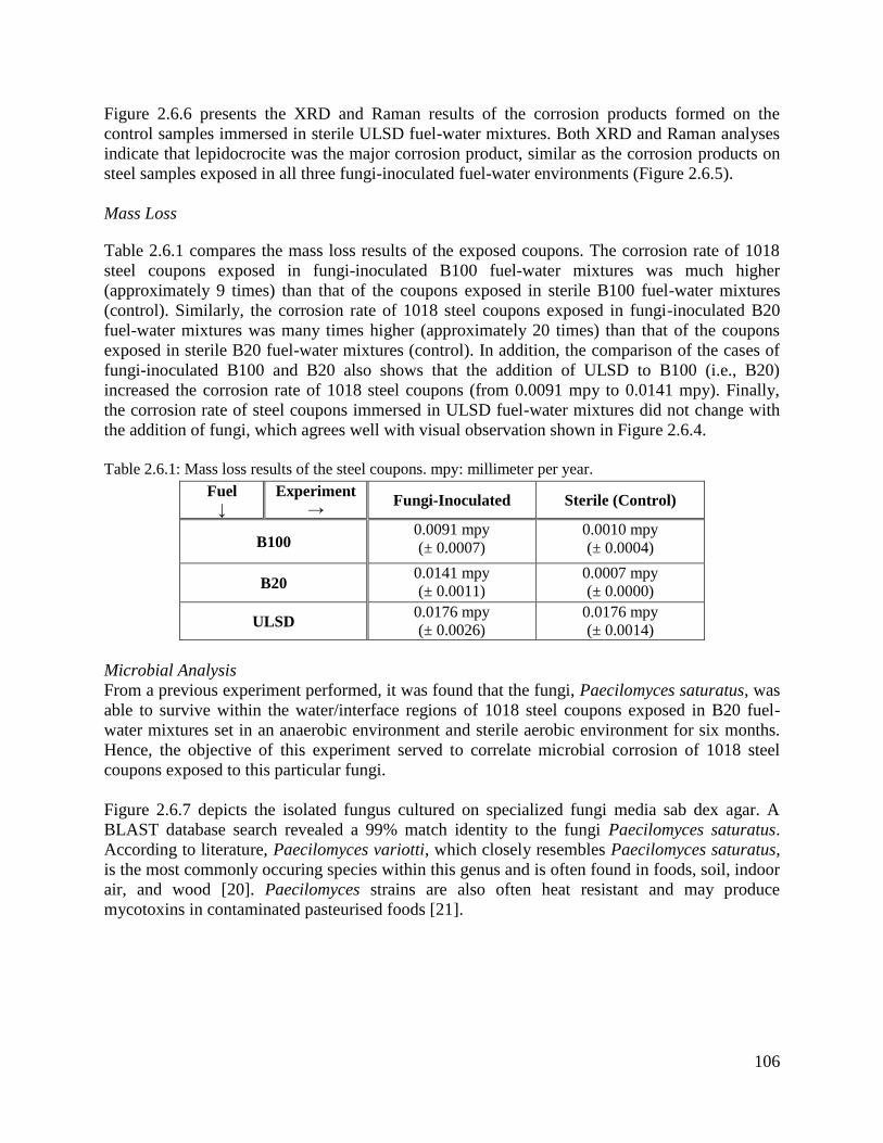
106

Figure 2.6.6 presents the XRD and Raman results of the corrosion products formed on the

control samples immersed in sterile ULSD fuel-water mixtures. Both XRD and Raman analyses

indicate that lepidocrocite was the major corrosion product, similar as the corrosion products on

steel samples exposed in all three fungi-inoculated fuel-water environments (Figure 2.6.5).

Mass Loss

Table 2.6.1 compares the mass loss results of the exposed coupons. The corrosion rate of 1018

steel coupons exposed in fungi-inoculated B100 fuel-water mixtures was much higher

(approximately 9 times) than that of the coupons exposed in sterile B100 fuel-water mixtures

(control). Similarly, the corrosion rate of 1018 steel coupons exposed in fungi-inoculated B20

fuel-water mixtures was many times higher (approximately 20 times) than that of the coupons

exposed in sterile B20 fuel-water mixtures (control). In addition, the comparison of the cases of

fungi-inoculated B100 and B20 also shows that the addition of ULSD to B100 (i.e., B20)

increased the corrosion rate of 1018 steel coupons (from 0.0091 mpy to 0.0141 mpy). Finally,

the corrosion rate of steel coupons immersed in ULSD fuel-water mixtures did not change with

the addition of fungi, which agrees well with visual observation shown in Figure 2.6.4.

Table 2.6.1: Mass loss results of the steel coupons. mpy: millimeter per year.

Fuel

↓

Experiment

→ Fungi-Inoculated Sterile (Control)

B100 0.0091 mpy

(± 0.0007)

0.0010 mpy

(± 0.0004)

B20 0.0141 mpy

(± 0.0011)

0.0007 mpy

(± 0.0000)

ULSD 0.0176 mpy

(± 0.0026)

0.0176 mpy

(± 0.0014)

Microbial Analysis

From a previous experiment performed, it was found that the fungi, Paecilomyces saturatus, was

able to survive within the water/interface regions of 1018 steel coupons exposed in B20 fuel-

water mixtures set in an anaerobic environment and sterile aerobic environment for six months.

Hence, the objective of this experiment served to correlate microbial corrosion of 1018 steel

coupons exposed to this particular fungi.

Figure 2.6.7 depicts the isolated fungus cultured on specialized fungi media sab dex agar. A

BLAST database search revealed a 99% match identity to the fungi Paecilomyces saturatus.

According to literature, Paecilomyces variotti, which closely resembles Paecilomyces saturatus,

is the most commonly occuring species within this genus and is often found in foods, soil, indoor

air, and wood [20]. Paecilomyces strains are also often heat resistant and may produce

mycotoxins in contaminated pasteurised foods [21].

107

Figure 2.6.7: Fungi culture, 18S rRNA sequencing yields a 99% match to the fungi Paecilomyces

saturatus.

Discussion

The 1018 steel coupons actively corroded in the inoculated (with the fungi Paecilomyces

saturatus) B100 (0.0091 mpy) and B20 (0.0141 mpy) fuel-water mixtures but passivated in the

non-inoculated B100 (0.0010 mpy) and B20 (0.0007 mpy) fuel-water mixtures. The 1018 steel

can remain in the passive state when immersed in ultrapure water if its air-formed oxide film is

not breached. When the air-formed oxide film is breached, corrosion initiates at the breach and

then propagates over the surface. If the water contains ions such as chlorides, the 1018 steel

does not remain in the passive state and actively corrodes. Hence, the presence of the fungi

Paecilomyces saturatus prevented the 1018 steel from remaining in the passive state, increasing

corrosion activity. In the ULSD, the 1018 steel actively corroded at the same rate (0.0176 mpy)

in both the inoculated and non-inoculated ULSD-water mixtures. The results indicate that the

filtered B100 biodiesel in its pure form or blended form (i.e., B20) does not induce corrosion of

the 1018 steel in fuel-water mixtures. However, in the presence of fungi Paecilomyces

saturatus, the B100 and B20 fuel-water mixtures lead to breakdown of the air-formed passive

film on 1018 steel resulting in active corrosion. The ULSD-water mixtures also lead to

breakdown of the air-formed passive film on 1018 steel whether or not the fungi Paecilomyces

saturatus was present. The presence of the biodiesel appeared to have a beneficial effect on

corrosion even in the presence of the fungi Paecilomyces saturatus, as corrosion rates decreased

as the biofuel content in the fuel-water mixtures increased: ULSD (0.0176 mpy) > B20 (0.0141

mpy) > B100 (0.0091 mpy). For all cases where the steel actively corroded, the thick layer of

iron corrosion product lepidocrocite was detected using XRD or Raman spectroscopy.

108

Conclusions

In the absence of microorganisms, sterile-aerobic B100 and B20 fuel-water mixtures were much

less corrosive towards 1018 steel compared to ULSD fuel-water mixtures. In three-month

exposures, the 1018 steel coupons remained in the passive state (due to the presence of the air-

formed oxide film) in the B100 and B20 fuel-water mixtures; whereas, the 1018 steel coupons

corroded actively in the ULSD fuel-water mixture. When the sterile-aerobic B100 and B20 fuel-

water mixtures, however, were inoculation with the fungi Paecilomyces saturatus (previously

isolated from B20-water fuel mixtures) the 1018 steel coupons did not remain in the passive state

and corroded actively. The inoculation of the ULSD-water mixtures appeared to have no effect,

since the 1018 steel coupons corroded actively and at the same rate as in the non-inoculated case.

The presence of the biodiesel appeared to have a beneficial effect on corrosion even in the

presence of the fungi Paecilomyces saturatus. Corrosion rates decreased as the biodiesel content

in the fuel-water mixtures increased: ULSD (0.0176 mpy) > B20 (0.0141 mpy) > B100 (0.0091

mpy). For all cases where the steel actively corroded, the thick layer of iron corrosion product

was identified as lepidocrocite using XRD or Raman spectroscopy.

References

1. P. McCarthy, M.G. Rasul, S. Moazzem, analysis and comparison of performance and

emissions of an internal combustion engine fuelled with petroleum diesel and different bio-

diesels, Fuel, 90 (2011) 2147-2157.

2. A.S.M.A. Haseeb, M.A. Fazal, M.I. Jahirul, H.H. Masjuki, compatibility of automotive

materials in biodiesel: a review, Fuel, 90 (2011) 922-931.

3. B. Klofutar, J. Golob, microorganisms in diesel and in biodiesel fuels, Acta Chimica

Slovenica, 54 (2007) 744-748.

4. W.G. Characklis, K.C. Marshall, biofilms, in, Wiley, 1990, pp. 796.

5. I.B. Beech, J. Sunner, biocorrosion: towards understanding interactions between biofilms and

metals, Current Opinion in Biotechnology, 15 (2004) 181-186.

6. J.W. Costerton, G.G. Geesey, K.-J. Cheng, how bacteria stick, Scientific American, 238

(1978) 86-95.

7. I.B. Beech, corrosion of technical materials in the presence of biofilms-current understanding

and state-of-the art methods of study, International Biodeterioration & Biodegradation, 53

(2004) 177-183.

8. M.M. Maru, M.M. Lucchese, C. Legnani, W.G. Quirino, A. Balbo, I.B. Aranha, L.T. Costa,

C. Vilani, L.A.d. Sena, J.C. Damasceno, T.d.S. Cruz, L.R. Lidizio, R.F. Silva, A. Jorio, C.A.

Achete, biodiesel compatibility with carbon steel and HDPE parts, Fuel Processing

Technology, 90 (2009) 1175-1182.

9. S. Kaul, R.C. Saxena, A. Kumar, M.S. Negi, A.K. Bhatnagar, H.B. Goyal, A.K. Gupta,

corrosion behavior of biodiesel from seed oils of indian origin on diesel engine parts, Fuel

Processing Technology, 88 (2007) 303-307.

10. L. Qiang, Z. Jian, Z. Xifeng, corrosion properties of bio-oil and its emulsions with diesel,

Chinese Science Bulletin, 53 (2008) 3726-3734.

109

11. A.S.M.A. Haseeb, H.H. Masjuki, L.J. Ann, M.A. Fazal, corrosion characteristics of copper

and leaded bronze in palm biodiesel, Fuel Processing Technology, 91 (2010) 329-334.

12. M.A. Fazal, A.S.M.A. Haseeb, H.H. Masjuki, comparative corrosive characteristics of

petroleum diesel and palm biodiesel for automotive materials, Fuel Processing Technology,

91 (2010) 1308-1315.

13. M.A. Fazal, A.S.M.A. Haseeb, H.H. Masjuki, degradation of automotive materials in palm

biodiesel, Energy, 40 (2012) 76-83.

14. E. Hu, Y. Xu, X. Hu, L. Pan, S. Jiang, corrosion behaviors of metals in biodiesel from

rapeseed oil and methanol, 37, (2012) 371-378.

15. P.B.L. Fregolente, L.V. Fregolente, M.R.W. Maciel, water content in biodiesel, diesel, and

biodiesel–diesel blends, Journal of Chemical and Engineering Data, (2012).

16. D.F. Aktas, J.S. Lee, B.J. Little, R.I. Ray, I.A. Davidova, C.N. Lyles, J.M. Suflita, anaerobic

metabolism of biodiesel and its impact on metal corrosion, Energy Fuels, 24 (2010) 2924-

2928.

17. J.S. Lee, R.I. Ray, B.J. Little, an assessment of alternative diesel fuels: microbiological

contamination and corrosion under storage conditions, Biofouling: The Journal of

Bioadhesion and Biofilm Research, 26 (2010) 623-635.

18. S. Li, L.H. Hihara, in situ raman spectroscopic study of NaCl particle-induced marine

atmospheric corrosion of carbon steel, Journal of The Electrochemical Society, 159 (2012)

C1-C8.

19. S. Li, J. Kealoha, L.H. Hihara, Corrosion of Low-Carbon Steel in Seawater/Biodiesel

Mixtures – a Study Related to the Corrosion of Fuel Tanks in Ships, in: Corrosion 2015,

NACE International, 2015.

20. J. Houbraken, P.E. Verweij, A.J.M.M. Rijis, A.M. Borman, R.A. Samson, identification of

Paecilomyces variotii in clinical samples and settings, Journal of Clinical Microbiology, 48

(2010) 2754-2761.

21. R.A. Samson, J. Houbraken, J. Varga, J.C. Frisvad, polyphasic taxonomy of the heat resistant

ascomycete genus Byssochlamys and its Paecilomyces anamorphs, Persoonia, 22 (2009) 14-

27.

2.7 Waste Management Using the Flash-CarbonizationTM Process

Past efforts under this HEET task studied the Flash CarbonizationTM

process applied to various

waste products and the characterization and use of the resulting biocarbons for downstream

applications including carbon fuel cells. The present study continued this work and reports on

fundamental measurements of carbon yield as a function of conversion technology and process

parameters using corn cobs as a model fuel.

Elevated pressure secures the highest fixed-carbon yields of charcoal from corncob. Operating at

a pressure of 0.8 MPa, a flash-carbonization reactor realizes fixed-carbon yields that range from

70 to 85% of the theoretical thermochemical equilibrium value from Waimanalo corncob. The

fixed-carbon yield is reduced to a range from 68 to 75% of the theoretical value when whole

110

Waimanalo corncobs are carbonized under nitrogen at atmospheric pressure in an electrically

heated muffle furnace. The lowest fixed-carbon yields are obtained by the standard proximate

analysis procedure for biomass feedstocks; this yield falls in a range from 49 to 54% of the

theoretical value. A round-robin study of corncob charcoal and fixed-carbon yields involving

three different thermogravimetric analyzers (TGAs) revealed the impact of vapor-phase reactions

on the formation of charcoal. Deep crucibles that limit the egress of volatiles from the pyrolyzing

solid greatly enhance charcoal and fixed-carbon yields. Likewise, capped crucibles with pinholes

increase the charcoal and fixed-carbon yields compared to values obtained from open crucibles.

Large corncob particles offer much higher yields than small particles. These findings show that

secondary reactions involving vapor-phase species (or nascent vapor-phase species) are at least

as influential as primary reactions in the formation of charcoal.

Our results offer considerable guidance to industry for its development of efficient biomass

carbonization technologies. Size reduction handling of biomass (e.g., tub grinders and chippers),

which can be a necessity in the field, significantly reduces the fixed-carbon yield of charcoal.

Fluidized-bed and transport reactors, which require small particles and minimize the interaction

of pyrolytic volatiles with solid charcoal, cannot realize high yields of charcoal from biomass.

When a high yield of corncob charcoal is desired, whole corncobs should be carbonized at

elevated pressure. Under these circumstances, carbonization is both efficient and quick.

Complete details of this subtask are presented in the publication:

Wang, L., M. Trninic, O. Skreiberg, M. Gronli, R. Considine, and M.J. Antal, Jr. 2011, Is

elevated pressure required to achieve a high fixed-carbon yield of charcoal from biomass?

Part 1: Round-robin results for three different corncob materials. Energy & Fuels. 25, pp.

3251-3265.

The full manuscript is available at:

http://pubs.acs.org/doi/abs/10.1021/ef400041h

or

http://dx.doi.org/10.1021/ef200450h

Task 3. METHANE HYDRATES

Methane hydrates are crystalline compounds consisting of polyhedral cavities formed from

networks of hydrogen-bonded water molecules, in which methane molecules reside. Methane

hydrates in ocean sediments constitute an enormous energy reservoir that is estimated to exceed

the energy content of all known coal, oil, and conventional natural gas resources. Located on

continental margins throughout the world, methane hydrates offer unique opportunities as an

onsite source of fuel for various marine applications and are believed to play a major role in

seafloor stability and global climate.

The HEET Methane Hydrates activities comprised four subtasks: Hydrate Energy, Environmental

Impacts of Methane Release from Seafloor Hydrates, Hydrate Engineering Applications, and

http://pubs.acs.org/doi/abs/10.1021/ef400041h

http://dx.doi.org/10.1021/ef200450h

111

International Collaborative R&D.

Objectives

National R&D programs on methane hydrates were initiated in Japan and India in the mid-

1990’s with the goal of commercial gas production within a 20 year time horizon. The U.S.

established its own program in May 2000. The Methane Hydrate Research and Development

Act of 2000 (Public Law 106-193) included seven technical areas of focus: (1) identification,

exploration, assessment, and development of methane hydrate as a source of energy; (2)

technology development for efficient and environmentally sound recovery of methane from

hydrates; (3) transport and storage of methane produced from methane hydrates; (4) education

and training related to methane hydrate resource R&D; (5) assessment and mitigation of

environmental impacts of natural and purposeful hydrate degassing; (6) development of

technologies to reduce the risks of drilling through methane hydrates; and (7) support of

exploratory drilling projects. The objectives of the Methane Hydrates Task of the HEET

initiative, which was initiated in 2001, reflect most of the priorities of P.L. 106-193, but

emphasize those areas of particular relevance to the Office of Naval Research (ONR) and which

are consistent to the overall goals of HEET. Specifically, the development of hydrates and

related sources of seafloor methane as logistical fuels for Naval applications and related marine

environmental issues, have been the principal areas of interest; exploratory drilling projects and

seafloor stability/safety have received limited attention. Work also has been initiated to explore

engineering applications of hydrates such as desalination and hydrogen storage. Task objectives

were devised to leverage fully hydrate R&D expertise and infrastructure that had been developed

at HNEI during previous research programs on CO2 ocean sequestration and deep oil spills.

During the present reporting period, the goals of the HEET Methane Hydrates Task were:

Pursue development of methods to recover methane gas from hydrates.

Investigate environmental impacts of methane hydrates on the marine environment.

Explore engineering applications of hydrates.

In cooperation with NRL and ONR Global, promote international collaborative research

on methane hydrates.

Specific technical initiatives that were pursued to attain the above goals included:

Conduct laboratory experiments on hydrate destabilization using chemical inhibitors.

Investigate hydrate stability in porous media.

Investigate the mechanisms of microbial methane metabolism in ocean sediment.

Initiate experiments to assess the feasibility of hydrate storage of hydrogen fuel.

Organize the 8th

International Workshop of Methane Hydrate R&D.

Scope of Work and Approach

Pursuant to the goals and technical objectives identified in the preceding section, work on the

Methane Hydrates Task during the present reporting period focused on four primary areas which

are described below.

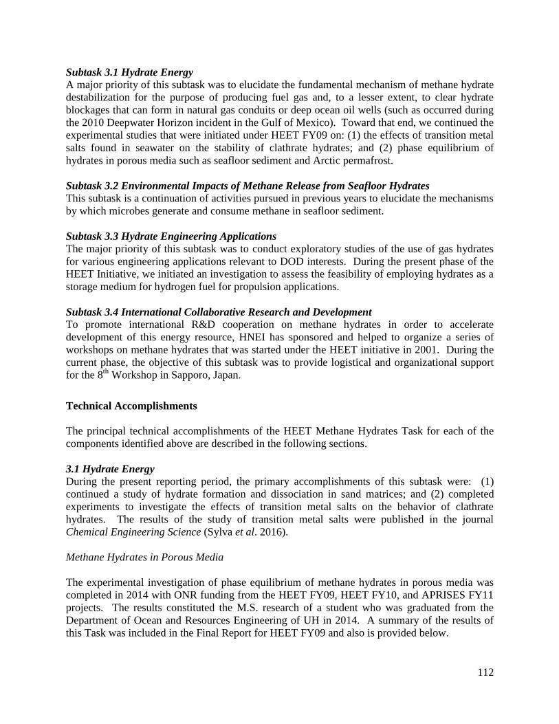
112

Subtask 3.1 Hydrate Energy

A major priority of this subtask was to elucidate the fundamental mechanism of methane hydrate

destabilization for the purpose of producing fuel gas and, to a lesser extent, to clear hydrate

blockages that can form in natural gas conduits or deep ocean oil wells (such as occurred during

the 2010 Deepwater Horizon incident in the Gulf of Mexico). Toward that end, we continued the

experimental studies that were initiated under HEET FY09 on: (1) the effects of transition metal

salts found in seawater on the stability of clathrate hydrates; and (2) phase equilibrium of

hydrates in porous media such as seafloor sediment and Arctic permafrost.

Subtask 3.2 Environmental Impacts of Methane Release from Seafloor Hydrates This subtask is a continuation of activities pursued in previous years to elucidate the mechanisms

by which microbes generate and consume methane in seafloor sediment.

Subtask 3.3 Hydrate Engineering Applications The major priority of this subtask was to conduct exploratory studies of the use of gas hydrates

for various engineering applications relevant to DOD interests. During the present phase of the

HEET Initiative, we initiated an investigation to assess the feasibility of employing hydrates as a

storage medium for hydrogen fuel for propulsion applications.

Subtask 3.4 International Collaborative Research and Development To promote international R&D cooperation on methane hydrates in order to accelerate

development of this energy resource, HNEI has sponsored and helped to organize a series of

workshops on methane hydrates that was started under the HEET initiative in 2001. During the

current phase, the objective of this subtask was to provide logistical and organizational support

for the 8th

Workshop in Sapporo, Japan.

Technical Accomplishments

The principal technical accomplishments of the HEET Methane Hydrates Task for each of the

components identified above are described in the following sections.

3.1 Hydrate Energy

During the present reporting period, the primary accomplishments of this subtask were: (1)

continued a study of hydrate formation and dissociation in sand matrices; and (2) completed

experiments to investigate the effects of transition metal salts on the behavior of clathrate

hydrates. The results of the study of transition metal salts were published in the journal

Chemical Engineering Science (Sylva et al. 2016).

Methane Hydrates in Porous Media

The experimental investigation of phase equilibrium of methane hydrates in porous media was

completed in 2014 with ONR funding from the HEET FY09, HEET FY10, and APRISES FY11

projects. The results constituted the M.S. research of a student who was graduated from the

Department of Ocean and Resources Engineering of UH in 2014. A summary of the results of

this Task was included in the Final Report for HEET FY09 and also is provided below.

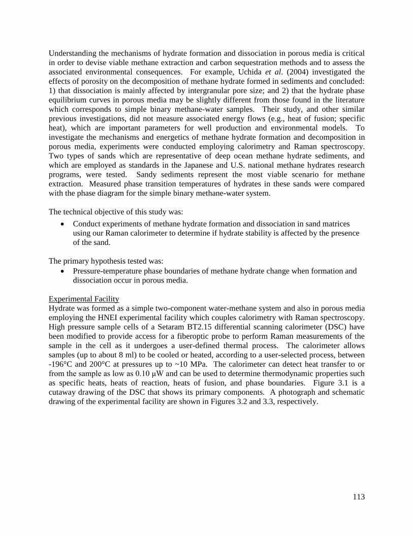
113

Understanding the mechanisms of hydrate formation and dissociation in porous media is critical

in order to devise viable methane extraction and carbon sequestration methods and to assess the

associated environmental consequences. For example, Uchida et al. (2004) investigated the

effects of porosity on the decomposition of methane hydrate formed in sediments and concluded:

1) that dissociation is mainly affected by intergranular pore size; and 2) that the hydrate phase

equilibrium curves in porous media may be slightly different from those found in the literature

which corresponds to simple binary methane-water samples. Their study, and other similar

previous investigations, did not measure associated energy flows (e.g., heat of fusion; specific

heat), which are important parameters for well production and environmental models. To

investigate the mechanisms and energetics of methane hydrate formation and decomposition in

porous media, experiments were conducted employing calorimetry and Raman spectroscopy.

Two types of sands which are representative of deep ocean methane hydrate sediments, and

which are employed as standards in the Japanese and U.S. national methane hydrates research

programs, were tested. Sandy sediments represent the most viable scenario for methane

extraction. Measured phase transition temperatures of hydrates in these sands were compared

with the phase diagram for the simple binary methane-water system.

The technical objective of this study was:

Conduct experiments of methane hydrate formation and dissociation in sand matrices

using our Raman calorimeter to determine if hydrate stability is affected by the presence

of the sand.

The primary hypothesis tested was:

Pressure-temperature phase boundaries of methane hydrate change when formation and

dissociation occur in porous media.

Experimental Facility

Hydrate was formed as a simple two-component water-methane system and also in porous media

employing the HNEI experimental facility which couples calorimetry with Raman spectroscopy.

High pressure sample cells of a Setaram BT2.15 differential scanning calorimeter (DSC) have

been modified to provide access for a fiberoptic probe to perform Raman measurements of the

sample in the cell as it undergoes a user-defined thermal process. The calorimeter allows

samples (up to about 8 ml) to be cooled or heated, according to a user-selected process, between

-196°C and 200°C at pressures up to ~10 MPa. The calorimeter can detect heat transfer to or

from the sample as low as 0.10 μW and can be used to determine thermodynamic properties such

as specific heats, heats of reaction, heats of fusion, and phase boundaries. Figure 3.1 is a

cutaway drawing of the DSC that shows its primary components. A photograph and schematic

drawing of the experimental facility are shown in Figures 3.2 and 3.3, respectively.

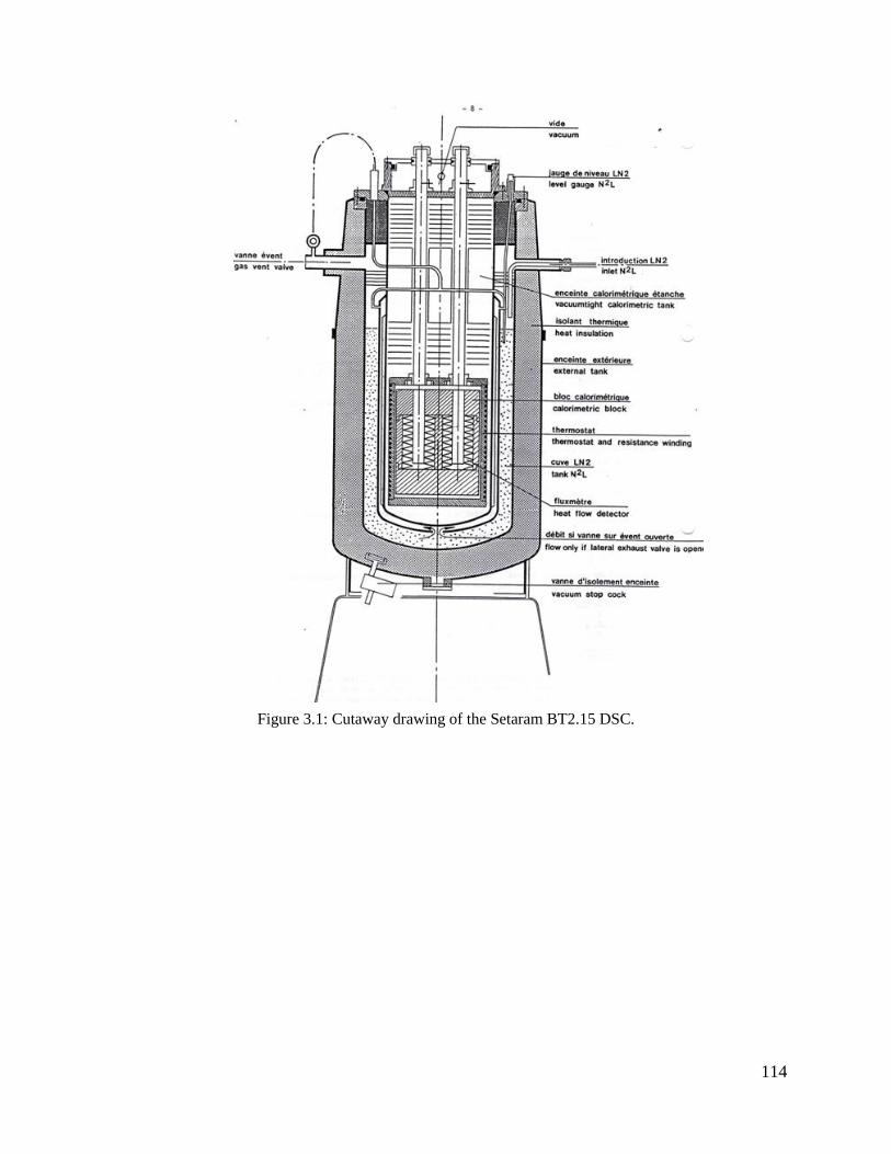
114

Figure 3.1: Cutaway drawing of the Setaram BT2.15 DSC.

115

Figure 3.2: Photograph of the experimental facility.

Figure 3.3: Schematic diagram of the experimental facility.

Calorimeter

Liquid Nitrogen

Spectrogragh

& CCD

Optical Iris Laser

PhotodiodeGas Inlet

& Outlet

Pressure

Transducer

Nitrogen Methane

Vacuum

Buffer Tank

Exhaust

Beam Splitter

Notch Filter

Computer

Gas bottles

Calorimeter

Liquid

Nitrogen

Raman

Spectrometers

Computer

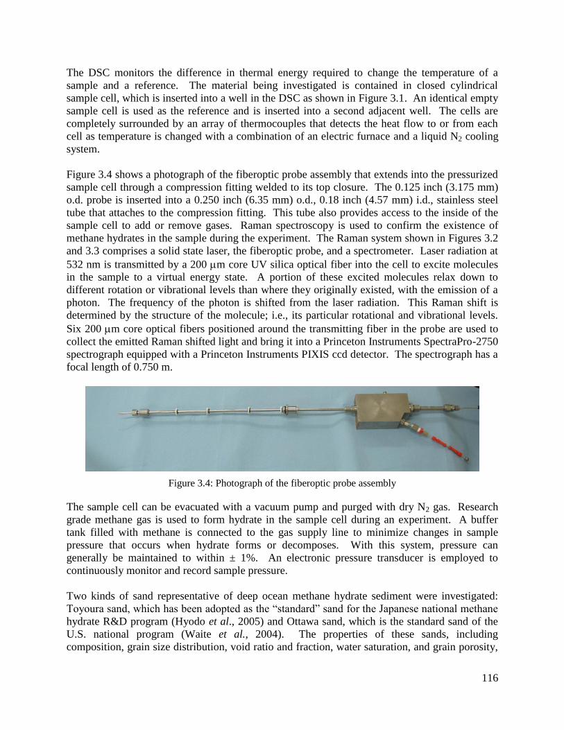
116

The DSC monitors the difference in thermal energy required to change the temperature of a

sample and a reference. The material being investigated is contained in closed cylindrical

sample cell, which is inserted into a well in the DSC as shown in Figure 3.1. An identical empty

sample cell is used as the reference and is inserted into a second adjacent well. The cells are

completely surrounded by an array of thermocouples that detects the heat flow to or from each

cell as temperature is changed with a combination of an electric furnace and a liquid N2 cooling

system.

Figure 3.4 shows a photograph of the fiberoptic probe assembly that extends into the pressurized

sample cell through a compression fitting welded to its top closure. The 0.125 inch (3.175 mm)

o.d. probe is inserted into a 0.250 inch (6.35 mm) o.d., 0.18 inch (4.57 mm) i.d., stainless steel

tube that attaches to the compression fitting. This tube also provides access to the inside of the

sample cell to add or remove gases. Raman spectroscopy is used to confirm the existence of

methane hydrates in the sample during the experiment. The Raman system shown in Figures 3.2

and 3.3 comprises a solid state laser, the fiberoptic probe, and a spectrometer. Laser radiation at

532 nm is transmitted by a 200 m core UV silica optical fiber into the cell to excite molecules

in the sample to a virtual energy state. A portion of these excited molecules relax down to

different rotation or vibrational levels than where they originally existed, with the emission of a

photon. The frequency of the photon is shifted from the laser radiation. This Raman shift is

determined by the structure of the molecule; i.e., its particular rotational and vibrational levels.

Six 200 m core optical fibers positioned around the transmitting fiber in the probe are used to

collect the emitted Raman shifted light and bring it into a Princeton Instruments SpectraPro-2750

spectrograph equipped with a Princeton Instruments PIXIS ccd detector. The spectrograph has a

focal length of 0.750 m.

Figure 3.4: Photograph of the fiberoptic probe assembly

The sample cell can be evacuated with a vacuum pump and purged with dry N2 gas. Research

grade methane gas is used to form hydrate in the sample cell during an experiment. A buffer

tank filled with methane is connected to the gas supply line to minimize changes in sample

pressure that occurs when hydrate forms or decomposes. With this system, pressure can

generally be maintained to within ± 1%. An electronic pressure transducer is employed to

continuously monitor and record sample pressure.

Two kinds of sand representative of deep ocean methane hydrate sediment were investigated:

Toyoura sand, which has been adopted as the “standard” sand for the Japanese national methane

hydrate R&D program (Hyodo et al., 2005) and Ottawa sand, which is the standard sand of the

U.S. national program (Waite et al., 2004). The properties of these sands, including

composition, grain size distribution, void ratio and fraction, water saturation, and grain porosity,

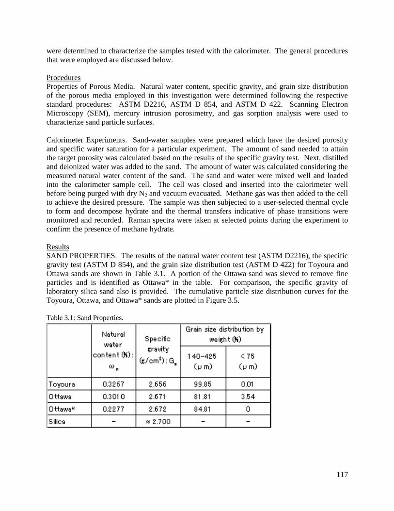
117

were determined to characterize the samples tested with the calorimeter. The general procedures

that were employed are discussed below.

Procedures

Properties of Porous Media. Natural water content, specific gravity, and grain size distribution

of the porous media employed in this investigation were determined following the respective

standard procedures: ASTM D2216, ASTM D 854, and ASTM D 422. Scanning Electron

Microscopy (SEM), mercury intrusion porosimetry, and gas sorption analysis were used to

characterize sand particle surfaces.

Calorimeter Experiments. Sand-water samples were prepared which have the desired porosity

and specific water saturation for a particular experiment. The amount of sand needed to attain

the target porosity was calculated based on the results of the specific gravity test. Next, distilled

and deionized water was added to the sand. The amount of water was calculated considering the

measured natural water content of the sand. The sand and water were mixed well and loaded

into the calorimeter sample cell. The cell was closed and inserted into the calorimeter well

before being purged with dry N2 and vacuum evacuated. Methane gas was then added to the cell

to achieve the desired pressure. The sample was then subjected to a user-selected thermal cycle

to form and decompose hydrate and the thermal transfers indicative of phase transitions were

monitored and recorded. Raman spectra were taken at selected points during the experiment to

confirm the presence of methane hydrate.

Results

SAND PROPERTIES. The results of the natural water content test (ASTM D2216), the specific

gravity test (ASTM D 854), and the grain size distribution test (ASTM D 422) for Toyoura and

Ottawa sands are shown in Table 3.1. A portion of the Ottawa sand was sieved to remove fine

particles and is identified as Ottawa* in the table. For comparison, the specific gravity of

laboratory silica sand also is provided. The cumulative particle size distribution curves for the

Toyoura, Ottawa, and Ottawa* sands are plotted in Figure 3.5.

Table 3.1: Sand Properties.

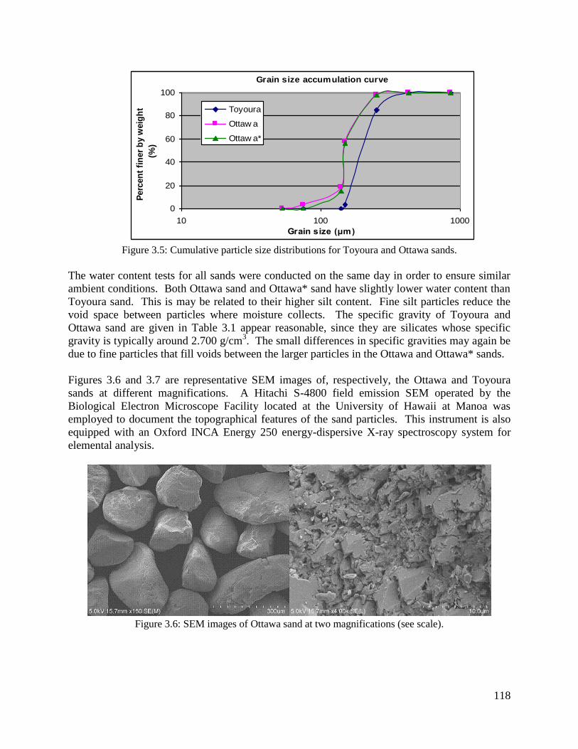
118

Figure 3.5: Cumulative particle size distributions for Toyoura and Ottawa sands.

The water content tests for all sands were conducted on the same day in order to ensure similar

ambient conditions. Both Ottawa sand and Ottawa* sand have slightly lower water content than

Toyoura sand. This is may be related to their higher silt content. Fine silt particles reduce the

void space between particles where moisture collects. The specific gravity of Toyoura and

Ottawa sand are given in Table 3.1 appear reasonable, since they are silicates whose specific

gravity is typically around 2.700 g/cm3. The small differences in specific gravities may again be

due to fine particles that fill voids between the larger particles in the Ottawa and Ottawa* sands.

Figures 3.6 and 3.7 are representative SEM images of, respectively, the Ottawa and Toyoura

sands at different magnifications. A Hitachi S-4800 field emission SEM operated by the

Biological Electron Microscope Facility located at the University of Hawaii at Manoa was

employed to document the topographical features of the sand particles. This instrument is also

equipped with an Oxford INCA Energy 250 energy-dispersive X-ray spectroscopy system for

elemental analysis.

Figure 3.6: SEM images of Ottawa sand at two magnifications (see scale).

Grain size accumulation curve

0

20

40

60

80

100

10 100 1000

Grain size (μm)

Perc

en

t fi

ner

by w

eig

ht

(%)

Toyoura

Ottaw a

Ottaw a*

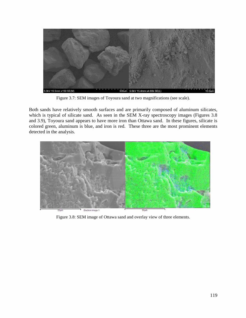
119

Figure 3.7: SEM images of Toyoura sand at two magnifications (see scale).

Both sands have relatively smooth surfaces and are primarily composed of aluminum silicates,

which is typical of silicate sand. As seen in the SEM X-ray spectroscopy images (Figures 3.8

and 3.9), Toyoura sand appears to have more iron than Ottawa sand. In these figures, silicate is

colored green, aluminum is blue, and iron is red. These three are the most prominent elements

detected in the analysis.

Figure 3.8: SEM image of Ottawa sand and overlay view of three elements.

120

Figure 3.9: SEM image of Toyoura sand and overlay view of three elements.

In order to determine void fraction and grain porosity, Particle Technology Labs (Downers

Grove, IL) performed mercury intrusion porosimetry on replicate aliquots of the sand. The

primary results of these analyses are summarized in Table 3.2. These data only consider surface

pores < 6 m. Additional information on sand grain porosity was obtained with a gas adsorption

instrument (Micromeritics TriStar 3000). Those data are summarized in Table 3.3.

Table 3.2: Mercury intrusion porosimetry results for Toyoura and Ottawa sands

Sample

Total

Intrusion

Volume

[cm3/g]

Total Pore

Area

[m2/g]

Volume

Median Pore

Diameter

[m]

Bulk

Density

[g/cm3]

Apparent

Density

[g/cm3]

Percent

Porosity

nint[%]

Toyoura #1 0.0082 0.38 0.32 1.41 1.43 1.15 Toyoura #2 0.0060 0.11 0.51 1.47 1.49 0.88 Ottawa #1 0.0032 0.25 1.60 1.49 1.49 0.47 Ottawa #2 0.0005 0.003 0.88 1.56 1.56 0.07

Table 3.3: Gas sorption analysis of Toyoura and Ottawa sands.

The results of the mercury intrusion porosimetry and gas sorption analyses of the two sands

indicate that they have very low grain porosity. The mercury porosimetry data exhibit

significant variations between samples of the same sand because of the extremely low measured

intrusion volumes that result from the low porosity of the material. The gas sorption data

indicate that the specific surface area of the Toyoura sand is larger than that of Ottawa sand;

however, both of the sands have very low specific surface areas, indicating that they are

essentially non-porous.

CALORIMETRY. A series of calorimetry experiments were performed at different pressures

between about 450 psig (3.2 MPa) and 1100 psig (7.7 MPa), which correspond to ocean depths

121

between approximately 300 m and 750 m. The primary outcome of these experiments was the

measured phase change temperatures for the hydrate at these pressures.

Figures 3.10 and 3.11 are representative thermograms from a calorimetry experiment using

Ottawa sand. The pressure was set at P = 1000 psi (7.00 MPa) and held constant (±1%)

throughout the test. Figure 3.10 shows the portion of the process where temperature is slowly

reduced over a period of about 5 hours from 23°C (room temperature in the lab) to 1°C. The

blue line in the figure is heat flow to or from the sample (mW) as a function of time, the red line

is sample temperature (°C), and the purple line is the temperature of the furnace (°C) that is used

to supply or remove heat. Heat flow is positive when energy is transferred from the sample cell

towards the reference cell, indicating an exothermic process, and negative during an endothermic

process. The steep positive peak in the heat flow curve seen in Figure 3.10 occurs as a result of

hydrate formation. Note that sample temperature is above the ice point.

Figure 3.11 shows the portion of the process where sample temperature is very slowly raised

from 1°C to 12°C over 16 hours. The large negative (endothermic) heat flow peak that begins at

around the 12 hour mark is due to dissociation of the hydrate in the sand. The heat flow peaks in

the thermograms at temperatures above the freezing point of water provided substantial evidence

of hydrate formation and dissociation.

Figure 3.10: Calorimetry thermogram of methane hydrate formation in Ottawa sand.

Formation

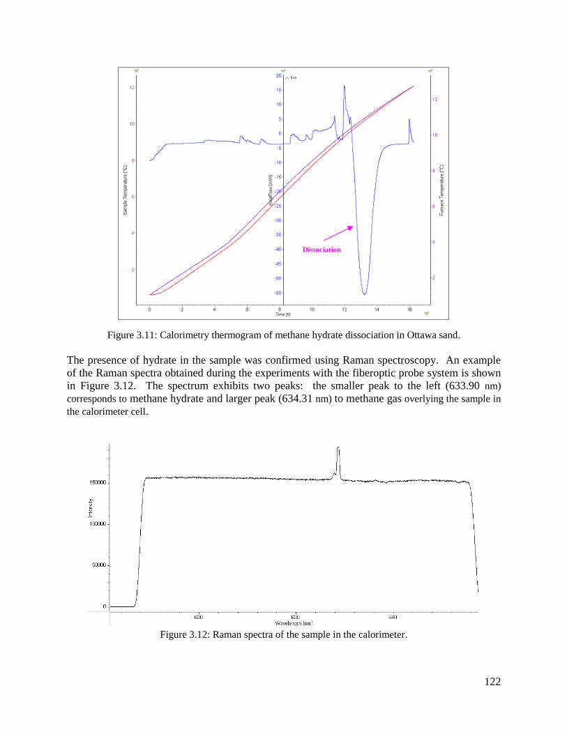
122

Figure 3.11: Calorimetry thermogram of methane hydrate dissociation in Ottawa sand.

The presence of hydrate in the sample was confirmed using Raman spectroscopy. An example

of the Raman spectra obtained during the experiments with the fiberoptic probe system is shown

in Figure 3.12. The spectrum exhibits two peaks: the smaller peak to the left (633.90 nm)

corresponds to methane hydrate and larger peak (634.31 nm) to methane gas overlying the sample in

the calorimeter cell.

Figure 3.12: Raman spectra of the sample in the calorimeter.

Dissociation

123

Hydrate formation is a crystallization process and therefore involves nucleation and growth.

Sub-cooling frequently is observed and phase transition data can exhibit significant scatter.

Dissociation, on the other hand, is less sensitive to random experimental factors, so the phase

transition temperatures were determined from the hydrate decomposition data. The process that

was employed to identify melting point temperatures from the calorimetry thermograms is

described below by reference to Figure 3.13:

i. Extend the baselines of heat flow before and after the hydrate dissociation peak since the

temperature ramping rate is constant.

ii. Calculate the average value of the heat flow at the two points of intersection of the curve

with these baselines, shown in the figure as green dots, and find the time that corresponds

to this average value.

iii. Determine the sample temperature at the time identified in step ii.

Figure 3.13: Determination of the hydrate dissociation temperature.

Table 3.4 summarizes the calorimeter experiments that were performed in this investigation.

Figure 3.14 presents the results for the Ottawa and sieved Ottawa* sands. The solid line is the

phase boundary for bulk hydrate (no porous media). Although there is significant scatter in the

data, measured dissociation temperatures were consistently lower than the values for bulk

hydrate at the same pressure. Differences typically fell between 1 and 2°C.

124

Table 3.4: Measured dissociation temperatures for different sands and pressures.

Figure 3.14: Measured dissociation temperatures for Ottawa sand.

From a different perspective, at a given temperature, the data suggest that methane hydrate in

sand dissociates at pressures 15 to 200 psi lower than expected, which is greater than the

uncertainty in the pressure data. Figure 3.14 also includes a trend line calculated from all the

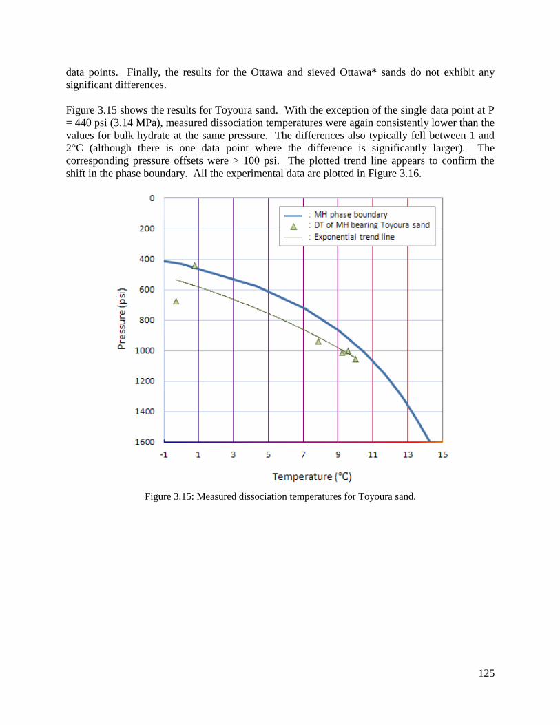
125

data points. Finally, the results for the Ottawa and sieved Ottawa* sands do not exhibit any

significant differences.

Figure 3.15 shows the results for Toyoura sand. With the exception of the single data point at P

= 440 psi (3.14 MPa), measured dissociation temperatures were again consistently lower than the

values for bulk hydrate at the same pressure. The differences also typically fell between 1 and

2°C (although there is one data point where the difference is significantly larger). The

corresponding pressure offsets were > 100 psi. The plotted trend line appears to confirm the

shift in the phase boundary. All the experimental data are plotted in Figure 3.16.

Figure 3.15: Measured dissociation temperatures for Toyoura sand.

126

Figure 3.16: Measured dissociation temperatures for all experiments.

Strategies to recover methane from marine hydrate deposits by thermal stimulation or

depressurization, estimates of the volume of the hydrate stability zone in marine sediments to

assess reservoir inventories, and assessments of the sensitivity to these reservoirs to changes in

deep water temperature typically employ the phase diagram for simple methane-water systems.

The results of Uchida et al. (2004) and the present investigation suggest this may not be

appropriate since methane hydrates appear to form and dissociate at lower temperatures in sand

than bulk hydrate.

Conclusions

Calorimetric experiments were performed to test the hypothesis that the pressure-temperature

phase boundaries of methane hydrate change when formation and dissociation occur in porous

media. Two “standard” sands selected by the national methane hydrate R&D programs in Japan

and the U.S. were employed in these experiments. The data suggest that a small shift in the

phase boundary of hydrates might occur in porous media. The measured change is of the order

of scatter in the experimental data but is consistent. For both sands, and over a range of

pressures relevant to deep ocean sediments, the phase boundary for a simple water-methane

binary system tends to overpredict hydrate melting temperature.

Lower melting temperatures imply that natural hydrate deposits in seafloor sediment are more

vulnerable to purposeful or inadvertent increases in temperature. While this can be advantageous

for certain methane recovery strategies, it raises concerns about outgassing and seafloor stability

in a warming climate. Additional experiments appear to be warranted to confirm this

127

phenomenon for a broader range of porous media properties and to more definitively quantify the

shift in the phase boundary and to understand the underlying mechanism.

Reagent Destabilization of Methane Hydrates

The mechanism underlying the influence of salts on hydrate stability has not been clearly

identified and warrants additional study, insofar as this has relevance to a host of engineering and

scientific issues including the development of new reagents for flow assurance in natural gas

pipelines and the formation and dissociation of hydrates in the seafloor and in permafrost.

Toward this end, we conducted experiments to explore the dissociation behavior of methane

hydrates in the presence of transition metal salts, which are present in seawater and sediment.

Information about this study was included in the HEET FY09 Final Report. These experiments

were completed during the present project period and the results have been published recently in

the archival literature (Sylva et al., 2016). A summary of that paper is provided below.

Formation of clathrate hydrates can be prevented using thermodynamic inhibitors such as

alcohols and salts. These inhibitors shift the equilibrium between the three phases, hydrate (H),

liquid water (Lw), and guest molecular vapor (V) to lower temperature or higher pressure (Sloan

& Koh, 2008). It has been posited that dissolved inhibitors tie up water molecules needed for

hydrate formation via hydrogen bonding, as in the case of alcohols and glycols (Nihous et al.

2009), or via Coulombic forces, as in the case of salt ions (Sloan & Koh 2008).

Alcohols are frequently employed by the oil industry to avoid hydrate blockages in natural gas

pipelines since the potential for undesirable side reactions (such as corrosion) is low relative to

salts; however, amounts needed may reach 50 wt% (aq), leading to high costs and disposal

problems (Kelland, 1994; Dholabhai et al., 1997). In addition to alcohols and salts, other

inhibitors include kinetic inhibitors, like polyvinyl caprolactam (PVCap) or polyvinylpyrrolidone

(PVP) and ionic liquids, e.g., dialkylimidazolium halide compounds, which have been studied

more recently (Sloan et al., 1996; Xiao & Adidharma, 2009). Kinetic inhibitors are quite

effective in delaying the crystallization of gas hydrates (Sloan et al., 1996), whereas ionic liquids

exhibit both thermodynamic and kinetic inhibition features (Xiao & Adidharma, 2009).

Studies have been conducted to investigate the roles played by cations and anions in the

inhibition of hydrate formation (Lu et al., 2001; Sabil et al., 2010). Lu et al. (2001) compared

the effects of salts with different cations and anions on hydrate phase equilibria of CO2, CH4, and

C3H8 hydrates. In particular, they compared CH3CO2Na versus CH3CO2H at different

concentrations and found that the stability of CO2 hydrate was affected by the concentration of

CH3CO2- and CH3CO2H but not Na

+. In addition, it was observed that there was a larger shift in

the equilibrium temperature of methane hydrate with MgSO4 versus MgCl2, but not a very large

difference between NaCl versus KCl and CaCl2. They concluded that the anion has a greater

influence on hydrate stability than the cation, and posited that difference was due to interactions

between liquid water molecules and ions.

In electrolyte solutions, hydrate formation may be hindered by disruption of the ambient water

network that is driven by hydrogen bonding. Lu et al. (2001) argued that, based on studies

performed by Mizuno et al. (1997) on hydrogen bonds in aqueous solution of halogenated

128

alcohols, anions exert a greater influence on hydrogen bonding of water molecules than cations

and are, therefore, more important in inhibiting hydrate crystallization.

Sabil et al. (2010) compared the effects of salts with different cations and anions on hydrate

phase equilibria of mixed CO2/THF hydrates using a Cailletet apparatus. Their observations did

not support the assertion by Lu et al (2001) that anions are more important than cations in

suppressing hydrate formation. They found that the inhibiting effect increased in the following

order: NaF < KBr < NaCl < NaBr < CaCl2 < MgCl2, and concluded that the inhibition of the

hydrate increased with the charge of the cation, and the radius of the anion. They proposed that

this trend was the result of the strength of the ion-hydrogen bonds which either disrupts or

reinforces the ambient water networks. The authors noted that the electrolyte concentrations that

were investigated (0.5 and 1 mol%) were relatively low and that higher concentrations might

yield different results.

It is important to understand the mechanism underlying the influence of salts on hydrate stability

since methane recovery and transport from marine hydrates or conventional reservoirs can take

place in an ocean environment that contains these types of salts. According to Barnes (1954),

and more recently, Millero et al. (2008), the top five ions present in seawater with the highest

molality (moles/kg of solvent) are Cl-, Na

+, Mg

2+, SO4

2-, and Ca

2+. Transition metals, such as

iron, manganese, copper, cobalt and nickel, are also commonly found in seawater at trace

concentrations. The source and biogeochemical processes related to these elements are still not

well understood (Aparicio-Gonzalez et al. 2012).

Other studies of the effects of metals on methane hydrate formation have been conducted,

although these studies focused on the elemental forms of the metal. Yang et al. (2012) examined

the effect of aluminum foam along with sodium dodecyl sulfate on methane hydrate formation.

They concluded that aluminum foam accelerated formation of methane hydrate by promoting

hydrate nucleation and enhancing heat transfer. Unlike salts, elemental aluminum does not

dissolve in the water phase.

In the present investigation, a Differential Scanning Calorimeter (DSC) was employed to

determine the effects of some transition metal salts and other salts on the behavior of methane

hydrate decomposition. Specifically, a DSC was employed to determine the onset temperature

for methane hydrate decomposition in the presence of ferric chloride hexahydrate,

[FeCl2(H2O)4]Cl∙2H2O (Lind 1967), anhydrous ferric chloride, FeCl3, MnSO4, FeSO4, CuSO4,

and AgNO3 and to compare the inhibiting properties of these transition metal salts with NaCl and

CaCl2, two well-known salt inhibitors. These transition metals salts were chosen because they

are soluble in water and each transition metal represents metals with varying charges (+1, +2,

+3), which are commonly found in the ocean. We attempted to determine whether the inhibiting

properties of these salts on methane hydrates follow the trends observed by Sabil et al. (2010).

Decomposition temperature was studied rather than formation temperature since the formation of

non-stoichiometric gas hydrates may be influenced by a host of factors such as nucleation,

diffusion, and history, which can result in various levels of subcooling when using the DSC

(Sloan & Koh 2008). This complicates identifying a formation temperature. If, however, care is

taken to form pure phases of hydrates with fixed compositions, then decomposition processes

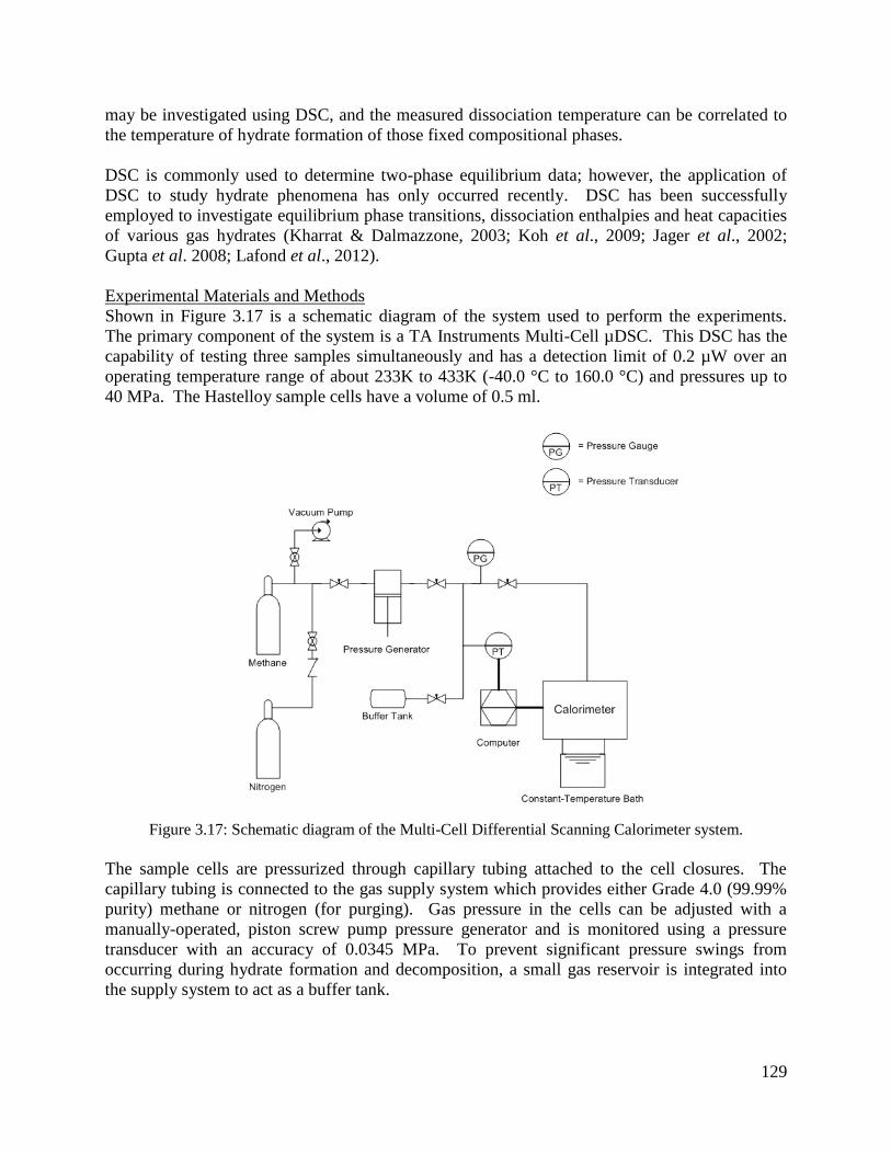
129

may be investigated using DSC, and the measured dissociation temperature can be correlated to

the temperature of hydrate formation of those fixed compositional phases.

DSC is commonly used to determine two-phase equilibrium data; however, the application of

DSC to study hydrate phenomena has only occurred recently. DSC has been successfully

employed to investigate equilibrium phase transitions, dissociation enthalpies and heat capacities

of various gas hydrates (Kharrat & Dalmazzone, 2003; Koh et al., 2009; Jager et al., 2002;

Gupta et al. 2008; Lafond et al., 2012).

Experimental Materials and Methods

Shown in Figure 3.17 is a schematic diagram of the system used to perform the experiments.

The primary component of the system is a TA Instruments Multi-Cell µDSC. This DSC has the

capability of testing three samples simultaneously and has a detection limit of 0.2 µW over an

operating temperature range of about 233K to 433K (-40.0 °C to 160.0 °C) and pressures up to

40 MPa. The Hastelloy sample cells have a volume of 0.5 ml.

Figure 3.17: Schematic diagram of the Multi-Cell Differential Scanning Calorimeter system.

The sample cells are pressurized through capillary tubing attached to the cell closures. The

capillary tubing is connected to the gas supply system which provides either Grade 4.0 (99.99%

purity) methane or nitrogen (for purging). Gas pressure in the cells can be adjusted with a

manually-operated, piston screw pump pressure generator and is monitored using a pressure

transducer with an accuracy of 0.0345 MPa. To prevent significant pressure swings from

occurring during hydrate formation and decomposition, a small gas reservoir is integrated into

the supply system to act as a buffer tank.

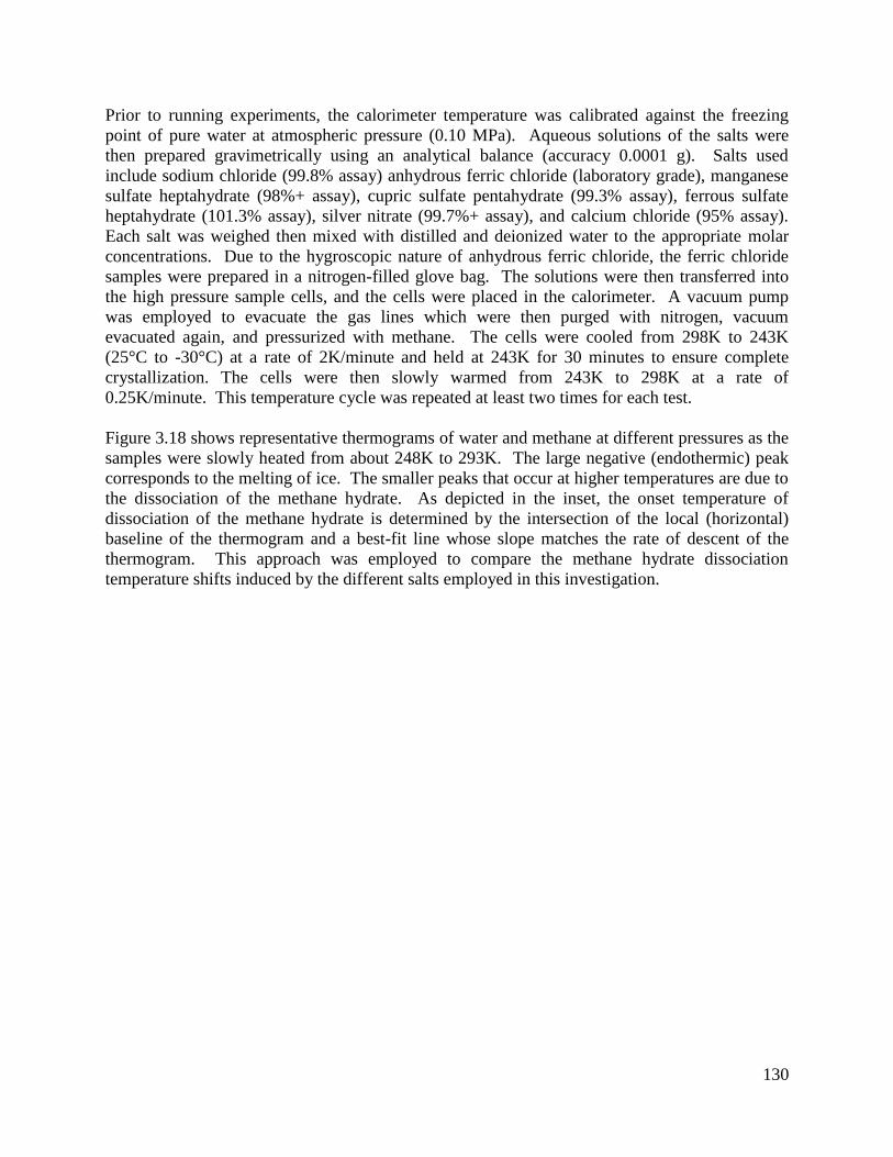
130

Prior to running experiments, the calorimeter temperature was calibrated against the freezing

point of pure water at atmospheric pressure (0.10 MPa). Aqueous solutions of the salts were

then prepared gravimetrically using an analytical balance (accuracy 0.0001 g). Salts used

include sodium chloride (99.8% assay) anhydrous ferric chloride (laboratory grade), manganese

sulfate heptahydrate (98%+ assay), cupric sulfate pentahydrate (99.3% assay), ferrous sulfate

heptahydrate (101.3% assay), silver nitrate (99.7%+ assay), and calcium chloride (95% assay).

Each salt was weighed then mixed with distilled and deionized water to the appropriate molar

concentrations. Due to the hygroscopic nature of anhydrous ferric chloride, the ferric chloride

samples were prepared in a nitrogen-filled glove bag. The solutions were then transferred into

the high pressure sample cells, and the cells were placed in the calorimeter. A vacuum pump

was employed to evacuate the gas lines which were then purged with nitrogen, vacuum

evacuated again, and pressurized with methane. The cells were cooled from 298K to 243K

(25°C to -30°C) at a rate of 2K/minute and held at 243K for 30 minutes to ensure complete

crystallization. The cells were then slowly warmed from 243K to 298K at a rate of

0.25K/minute. This temperature cycle was repeated at least two times for each test.

Figure 3.18 shows representative thermograms of water and methane at different pressures as the

samples were slowly heated from about 248K to 293K. The large negative (endothermic) peak

corresponds to the melting of ice. The smaller peaks that occur at higher temperatures are due to

the dissociation of the methane hydrate. As depicted in the inset, the onset temperature of

dissociation of the methane hydrate is determined by the intersection of the local (horizontal)

baseline of the thermogram and a best-fit line whose slope matches the rate of descent of the

thermogram. This approach was employed to compare the methane hydrate dissociation

temperature shifts induced by the different salts employed in this investigation.

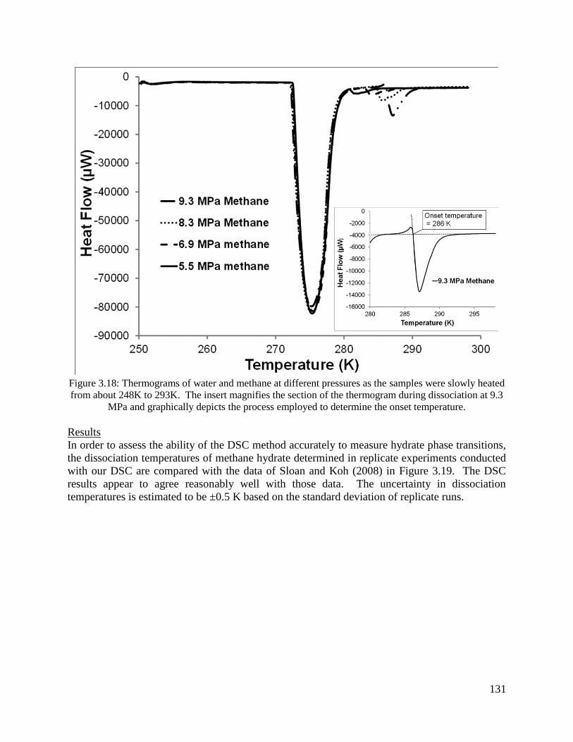
131

Figure 3.18: Thermograms of water and methane at different pressures as the samples were slowly heated

from about 248K to 293K. The insert magnifies the section of the thermogram during dissociation at 9.3

MPa and graphically depicts the process employed to determine the onset temperature.

Results

In order to assess the ability of the DSC method accurately to measure hydrate phase transitions,

the dissociation temperatures of methane hydrate determined in replicate experiments conducted

with our DSC are compared with the data of Sloan and Koh (2008) in Figure 3.19. The DSC

results appear to agree reasonably well with those data. The uncertainty in dissociation

temperatures is estimated to be ±0.5 K based on the standard deviation of replicate runs.

132

Figure 3.19: Dissociation temperatures of methane hydrate. Estimated error in measured dissociation

temperatures, based on replicates, is ±0.5K.

Table 3.4 summarizes the measured onset temperatures of methane hydrate dissociation at 5.51,

6.89, 8.27, and 9.65 MPa for solutions containing different concentrations of the inhibitors

examined in this study. The NaCl results are shown in Figure 3.20, along with the published

data from Roo et al. (1983). Here again, a reasonable degree of agreement is observed for 3.94

mol% NaCl.

2

3

4

5

6

7

8

9

10

274 276 278 280 282 284 286

Pre

ssu

re (

MP

a)

Temp (K)

Present study

Sloan Koh 2008

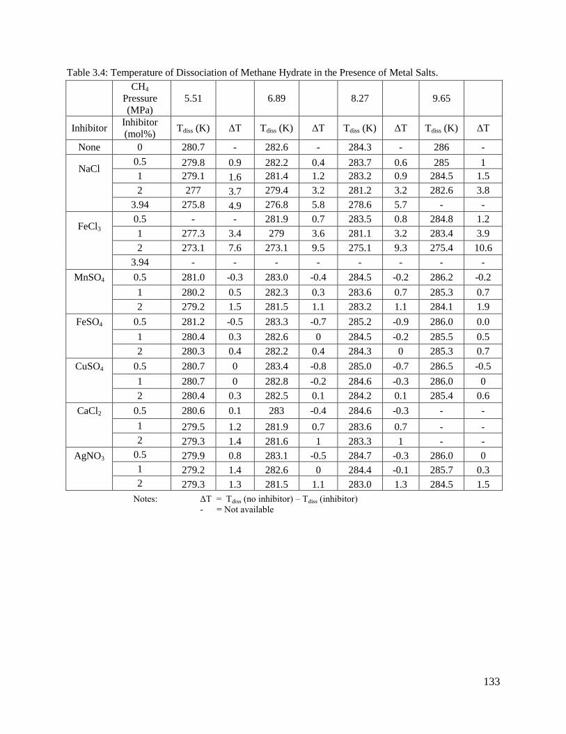
133

Table 3.4: Temperature of Dissociation of Methane Hydrate in the Presence of Metal Salts.

CH4

Pressure

(MPa)

5.51 6.89 8.27 9.65

Inhibitor Inhibitor

(mol%) Tdiss (K) ΔT Tdiss (K) ΔT Tdiss (K) ΔT Tdiss (K) ΔT

None 0 280.7 - 282.6 - 284.3 - 286 -

NaCl 0.5 279.8 0.9 282.2 0.4 283.7 0.6 285 1

1 279.1 1.6 281.4 1.2 283.2 0.9 284.5 1.5

2 277 3.7 279.4 3.2 281.2 3.2 282.6 3.8

3.94 275.8 4.9 276.8 5.8 278.6 5.7 - -

FeCl3 0.5 - - 281.9 0.7 283.5 0.8 284.8 1.2

1 277.3 3.4 279 3.6 281.1 3.2 283.4 3.9

2 273.1 7.6 273.1 9.5 275.1 9.3 275.4 10.6

3.94 - - - - - - - -

MnSO4 0.5 281.0 -0.3 283.0 -0.4 284.5 -0.2 286.2 -0.2

1 280.2 0.5 282.3 0.3 283.6 0.7 285.3 0.7

2 279.2 1.5 281.5 1.1 283.2 1.1 284.1 1.9

FeSO4 0.5 281.2 -0.5 283.3 -0.7 285.2 -0.9 286.0 0.0

1 280.4 0.3 282.6 0 284.5 -0.2 285.5 0.5

2 280.3 0.4 282.2 0.4 284.3 0 285.3 0.7

CuSO4 0.5 280.7 0 283.4 -0.8 285.0 -0.7 286.5 -0.5

1 280.7 0 282.8 -0.2 284.6 -0.3 286.0 0

2 280.4 0.3 282.5 0.1 284.2 0.1 285.4 0.6

CaCl2 0.5 280.6 0.1 283 -0.4 284.6 -0.3 - -

1 279.5 1.2 281.9 0.7 283.6 0.7 - -

2 279.3 1.4 281.6 1 283.3 1 - -

AgNO3 0.5 279.9 0.8 283.1 -0.5 284.7 -0.3 286.0 0

1 279.2 1.4 282.6 0 284.4 -0.1 285.7 0.3

2 279.3 1.3 281.5 1.1 283.0 1.3 284.5 1.5

Notes: ΔT = Tdiss (no inhibitor) – Tdiss (inhibitor)

- = Not available

134

Figure 3.20: DSC temperature and pressure data for the dissociation of methane hydrate in the presence of

sodium chloride (NaCl). Representative error bars are included for the 3.94 mole% NaCl data for

comparison with the earlier work by de Roo et al. (1983).

Figure 3.21 compares shifts in the methane hydrate P-T phase boundary arising from the

presence of sodium chloride and ferric chloride salt. The data indicate that, at a given pressure

and inhibitor concentration, dissociation of methane hydrate occurs at lower temperatures for

ferric chloride compared to sodium chloride. This effect increases with increasing

concentrations. Dissociation onset temperatures were measured for concentrations ranging from

0.5 mol% to 3.94 mol% of inhibitor. No hydrate was detected at 3.94 mol% FeCl3, but hydrate

formation does occur in the presence of 3.94 mol% NaCl. Scatter in the dissociation temperature

data for FeCl3 was observed to increase significantly between the 1 mol% and 2 mol% cases, as

the apparent hydrate suppression limit was approached.

2

4

6

8

10

12

14

270 272 274 276 278 280 282 284 286 288

Pre

ssu

re (

MP

a)

Temp (K)

No inhibitor

1 mol % NaCl

2 mol% NaCl

3.94 mol% NaCl

3.94 mol% NaCl (de Roo et al 1983)


135

Figure 3.21: DSC temperature and pressure data for the dissociation of methane hydrate in the presence of

sodium chloride (NaCl) and ferric chloride (FeCl3). The curve is from de Roos et al. (1983). Estimated

uncertainty of the measured dissociation temperatures is ±0.5K.

The effect of other metal salts investigated in this study (FeSO4, MnSO4, CuSO4, and AgNO3.)

on methane hydrate stability is shown in Figure 3.22. That figure also includes data for NaCl,

FeCl3, and CaCl2. The concentrations of the salts was 2 mol%. With the exception of FeCl3,

none of the tested salts were able to induce a reduction of the hydrate dissociation temperature to

the extent demonstrated by NaCl.

2

4

6

8

10

12

14

270 272 274 276 278 280 282 284 286

Pre

ssu

re (

MP

a)

Temp (K)

No inhibitor

0.5 mol% NaCl

1 mol % NaCl

2 mol% NaCl

3.94 mol% NaCl

0.5 mol% FeCl3

1 mol% FeCl3

2 mol% FeCl3


136

Figure 3.22: DSC temperature and pressure data for methane hydrate in the presence of 2 mole% NaCl,

CaCl2, FeCl3, MnSO4, FeSO4, CuSO4, and AgNO3. Solid line is the phase boundary for methane hydrate

with no inhibitor. Estimated uncertainty of the measured dissociation temperatures is ±0.5K.

Discussion and Conclusions

Most of the transition metal salts investigated in the present study inhibited methane hydrate

formation at high concentrations but none to the extent of sodium chloride except for ferric

chloride. FeSO4 and CuSO4 at concentrations up to 2 mol% were observed to have minimal

impact on hydrate stability. At lower concentrations (0.5 mol %), some of the salts (FeCl3,

FeSO4, and MnSO4), appeared to promote hydrate formation, i.e., dissociation temperature

increased slightly as indicated by negative ΔT in Table 3.4. This effect has not been observed

with other chloride salts, but has been observed with other water soluble compounds such as

alcohols (Abay & Svartaas, 2010).

The present results appear to confirm Sabil et al.’s (2010) assertion that the inhibitor effect

increases with increasing charge on the cation. The chloride salt of the higher charged Fe3+

exhibits greater inhibition of methane hydrate formation in comparison to Na+; but the iron salt

of the larger polyatomic anion, sulfate, exhibits less inhibition than the ferric chloride salt. One

possible explanation for the behavior observed in this and previous studies is that, when salts

dissolve, the ions interact with the dipoles of the water molecules. The stronger interaction

between water with salt ions (versus hydrate guest molecules) interferes with the organization of

the water lattice around the clathrate hydrate guest molecule, and thus inhibits hydrate formation.

4

5

6

7

8

9

10

270 272 274 276 278 280 282 284 286 288

Pre

ssu

re (

MP

a)

Temp (K)

No inhibitor

2 mole % NaCl

2 mol% CaCl2

2 mole % FeCl3

2 mol% MnSO4

2 mol% FeSO4

2 mol% CuSO4

2 mol% AgNO3

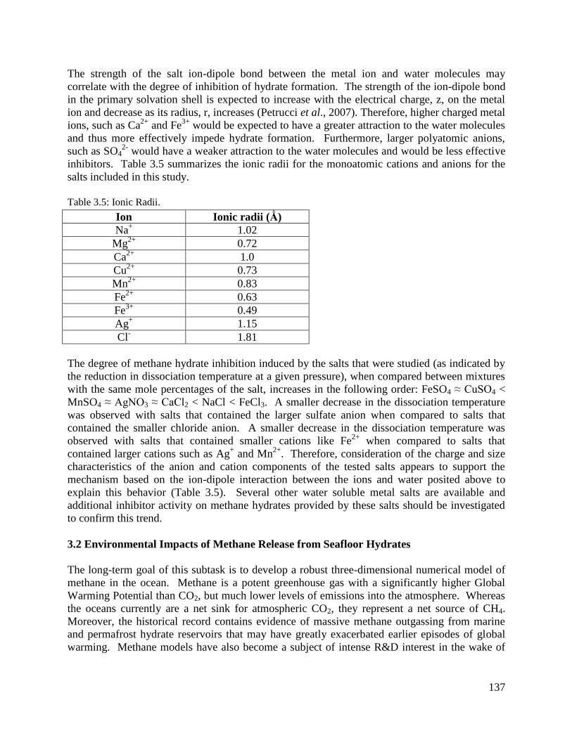
137

The strength of the salt ion-dipole bond between the metal ion and water molecules may

correlate with the degree of inhibition of hydrate formation. The strength of the ion-dipole bond

in the primary solvation shell is expected to increase with the electrical charge, z, on the metal

ion and decrease as its radius, r, increases (Petrucci et al., 2007). Therefore, higher charged metal

ions, such as Ca2+

and Fe3+

would be expected to have a greater attraction to the water molecules

and thus more effectively impede hydrate formation. Furthermore, larger polyatomic anions,

such as SO42-

would have a weaker attraction to the water molecules and would be less effective

inhibitors. Table 3.5 summarizes the ionic radii for the monoatomic cations and anions for the

salts included in this study.

Table 3.5: Ionic Radii.

Ion Ionic radii (Ǻ)

Na+ 1.02

Mg2+

0.72

Ca2+

1.0

Cu2+

0.73

Mn2+

0.83

Fe2+

0.63

Fe3+

0.49

Ag+ 1.15

Cl- 1.81

The degree of methane hydrate inhibition induced by the salts that were studied (as indicated by

the reduction in dissociation temperature at a given pressure), when compared between mixtures

with the same mole percentages of the salt, increases in the following order: FeSO4 ≈ CuSO4 <

MnSO4 ≈ AgNO3 ≈ CaCl2 < NaCl < FeCl3. A smaller decrease in the dissociation temperature

was observed with salts that contained the larger sulfate anion when compared to salts that

contained the smaller chloride anion. A smaller decrease in the dissociation temperature was

observed with salts that contained smaller cations like Fe2+

when compared to salts that

contained larger cations such as Ag+ and Mn

2+. Therefore, consideration of the charge and size

characteristics of the anion and cation components of the tested salts appears to support the

mechanism based on the ion-dipole interaction between the ions and water posited above to

explain this behavior (Table 3.5). Several other water soluble metal salts are available and

additional inhibitor activity on methane hydrates provided by these salts should be investigated

to confirm this trend.

3.2 Environmental Impacts of Methane Release from Seafloor Hydrates

The long-term goal of this subtask is to develop a robust three-dimensional numerical model of

methane in the ocean. Methane is a potent greenhouse gas with a significantly higher Global

Warming Potential than CO2, but much lower levels of emissions into the atmosphere. Whereas

the oceans currently are a net sink for atmospheric CO2, they represent a net source of CH4.

Moreover, the historical record contains evidence of massive methane outgassing from marine

and permafrost hydrate reservoirs that may have greatly exacerbated earlier episodes of global

warming. Methane models have also become a subject of intense R&D interest in the wake of

138

the 2010 Macondo Prospect oil spill in the Gulf of Mexico which released an estimated 2.5 x 108

standard m3 of natural gas from the broken wellhead at a depth of about 1,500 m.

The target model will need to consider the production, oxidation, and transport of CH4 and will

require an understanding of processes that affect the exchange of methane between the

atmosphere, ocean, and seafloor sediment. During the present reporting period, work focused on

laboratory experimental investigations of the role of microbes in methane production and

consumption.

Methane Microbiology

Investigation of methane cycling in sediments and the water column is ongoing. The sediment

work has focused on understanding biological formation and the anaerobic oxidation of methane.

Anaerobic oxidation of methane (AOM) occurs through an undefined process and is potentially

the largest sink for methane in sediments. Biological AOM is thought to be mediated by a

consortium of micro-organisms composed of sulfate reducing bacteria and methanogenic

Archaea. Geochemical data suggests that the majority of methane produced in sediments is

oxidized anaerobically within a narrow depth range called the sulfate methane interface (SMI).

The sediment depth of the SMI is influenced by the rates of methane flux. Stronger methane flux

results in shallower SMIs, and the possibility of methane releases into the water column. In

terrestrial environments, biological methane oxidation typically occurs as an obligate aerobic

process mediated by methanotrophic bacteria. This suggests that a methane sink could also exist

at the sediment-water interface in the ocean where there is dissolved oxygen. In consideration of

this, we expanded our research scope during the present reporting period to investigate aerobic as

well as anaerobic methane oxidation at this interface, as well as the associated prokaryotic

methanotrophic populations.

Molecular analyses is typically used to characterize microbial assemblages in sediments and are

often employed in combination with geochemical analysis to describe methane levels and fluxes

(Tavormina et al. 2008, Yoshioka et al. 2010). Our investigations have used similar techniques

and have provided evidence for the presence of assemblage microorganisms. Cultivation of

Archaea and Bacteria from these methane-rich environments have been problematic. Slow

metabolism and small populations relative to other microorganisms make isolation difficult in

spite of significant enrichment of the gas headspace in incubation vessels.

DNA extraction and PCR processing of sediment and porewater samples collected during

previous oceanographic research cruises was attempted multiple times, but results suffered from

poor reproducibility. Microscopy has helped to provide an explanation for this problem.

Sediment particles were examined using Transmission Electron Microscopy (TEM). As can be

seen in Figure 3.23, TEM indicates the presence of numerous nanometer to micrometer sized

particles found in the sediment-water suspensions. These small particles in the collected samples

result in very high surface areas where DNA can be readily adsorbed. This significantly

complicates the DNA extraction methods that we have been employing to characterize the

microbial assemblages.

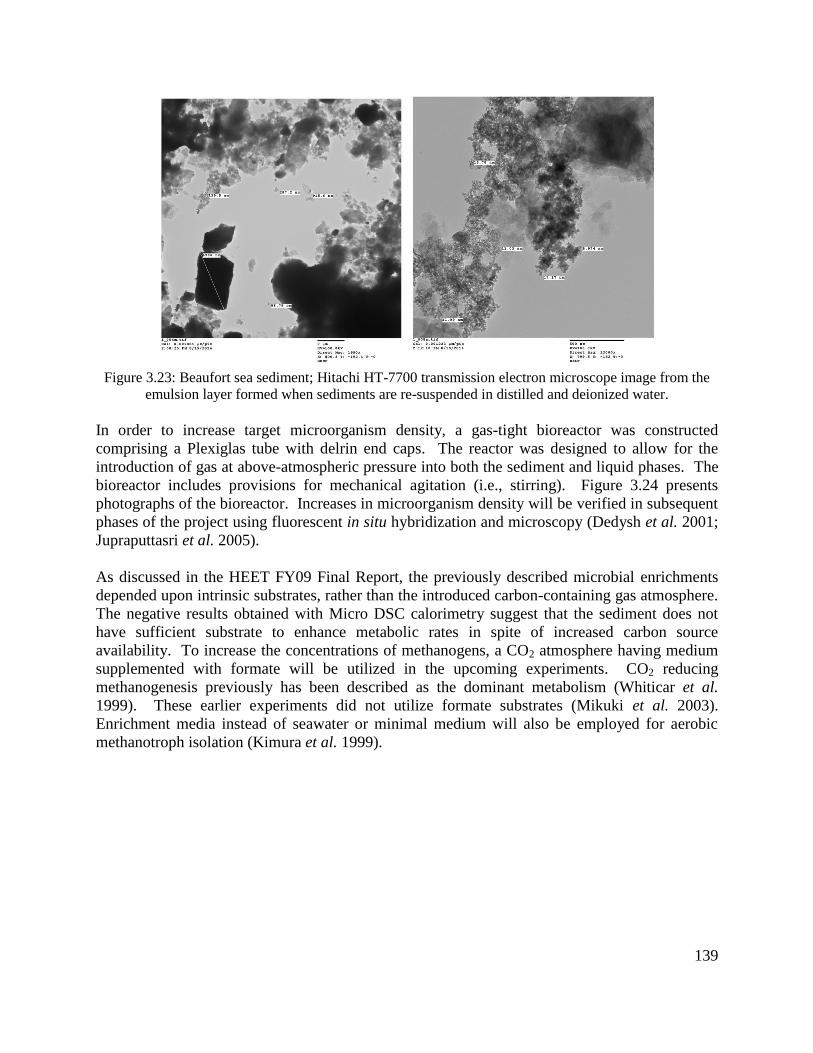
139

Figure 3.23: Beaufort sea sediment; Hitachi HT-7700 transmission electron microscope image from the

emulsion layer formed when sediments are re-suspended in distilled and deionized water.

In order to increase target microorganism density, a gas-tight bioreactor was constructed

comprising a Plexiglas tube with delrin end caps. The reactor was designed to allow for the

introduction of gas at above-atmospheric pressure into both the sediment and liquid phases. The

bioreactor includes provisions for mechanical agitation (i.e., stirring). Figure 3.24 presents

photographs of the bioreactor. Increases in microorganism density will be verified in subsequent

phases of the project using fluorescent in situ hybridization and microscopy (Dedysh et al. 2001;

Jupraputtasri et al. 2005).

As discussed in the HEET FY09 Final Report, the previously described microbial enrichments

depended upon intrinsic substrates, rather than the introduced carbon-containing gas atmosphere.

The negative results obtained with Micro DSC calorimetry suggest that the sediment does not

have sufficient substrate to enhance metabolic rates in spite of increased carbon source

availability. To increase the concentrations of methanogens, a CO2 atmosphere having medium

supplemented with formate will be utilized in the upcoming experiments. CO2 reducing

methanogenesis previously has been described as the dominant metabolism (Whiticar et al.

1999). These earlier experiments did not utilize formate substrates (Mikuki et al. 2003).

Enrichment media instead of seawater or minimal medium will also be employed for aerobic

methanotroph isolation (Kimura et al. 1999).

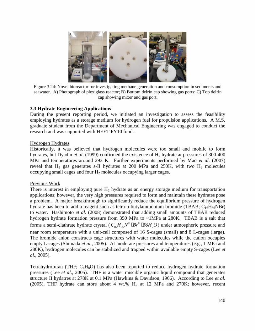
140

Figure 3.24: Novel bioreactor for investigating methane generation and consumption in sediments and

seawater. A) Photograph of plexiglass reactor; B) Bottom delrin cap showing gas ports; C) Top delrin

cap showing mixer and gas port.

3.3 Hydrate Engineering Applications

During the present reporting period, we initiated an investigation to assess the feasibility

employing hydrates as a storage medium for hydrogen fuel for propulsion applications. A M.S.

graduate student from the Department of Mechanical Engineering was engaged to conduct the

research and was supported with HEET FY10 funds.

Hydrogen Hydrates

Historically, it was believed that hydrogen molecules were too small and mobile to form

hydrates, but Dyadin et al. (1999) confirmed the existence of H2 hydrate at pressures of 300-400

MPa and temperatures around 293 K. Further experiments performed by Mao et al. (2007)

reveal that H2 gas generates s-II hydrates at 200 MPa and 250K, with two H2 molecules

occupying small cages and four H2 molecules occupying larger cages.

Previous Work

There is interest in employing pure H2 hydrate as an energy storage medium for transportation

applications; however, the very high pressures required to form and maintain these hydrates pose

a problem. A major breakthrough to significantly reduce the equilibrium pressure of hydrogen

hydrate has been to add a reagent such as tetra-n-butylammonium bromide (TBAB; C16H36NBr)

to water. Hashimoto et al. (2008) demonstrated that adding small amounts of TBAB reduced

hydrogen hydrate formation pressure from 350 MPa to ~1MPa at 280K. TBAB is a salt that

forms a semi-clathrate hydrate crystal ( ) under atmospheric pressure and

near room temperature with a unit-cell composed of 16 S-cages (small) and 8 L-cages (large).

The bromide anion constructs cage structures with water molecules while the cation occupies

empty L-cages (Shimada et al., 2005). At moderate pressures and temperatures (e.g., 1 MPa and

280K), hydrogen molecules can be stabilized and trapped within available empty S-cages (Lee et

al., 2005).

Tetrahydrofuran (THF; C4H8O) has also been reported to reduce hydrogen hydrate formation

pressures (Lee et al., 2005). THF is a water miscible organic liquid compound that generates

structure II hydatres at 278K at 0.1 MPa (Hawkins & Davidson, 1966). According to Lee et al.

(2005), THF hydrate can store about 4 wt.% H2 at 12 MPa and 270K; however, recent

C16H36N+ ×Br- ×38H2O

141

experiments by Ogata et al. (2008) suggest that, at similar conditions, stoichiometric THF

hydrate can store only 0.26 wt.% H2.

Motivation

Hydrogen can be produced domestically from natural gas, reducing our dependence on imported

fossil fuels. Employing hydrogen hydrate as an energy carrier has attracted interest due to

several advantages (Florusse, 2004). For example, unlike methane, pure hydrogen burns clean,

producing no greenhouse gas carbon emissions, making this a favorable clean alternative fuel. In

addition, PEM fuel cells, which are major candidates for transportation applications, use H2.

The primary advantage of H2 storage in hydrates is that, unlike metal hydrides, which must

undergo a chemical reaction (often having slow kinetics and requiring heating up to 473K) to

release hydrogen fuel, hydrates undergo a rapid phase transformation (i.e., melting), making

them ideal for onboard use in fuel cell vehicles and other specialized applications.

The greatest uncertainty related to onboard hydrogen hydrate storage for transportation

applications is energy density. Currently, the U.S. Department of Energy has set a 2015 target of

5.5 wt. % hydrogen storage in hydrates (Mao et al., 2007). Theoretical studies performed to date

by Willow and Xantheas (2012) suggest that hydrates may be able to store up to 5.3 wt. %

hydrogen; however, no experimental data exist to validate these results.

Since binary hydrates, such as those employing TBAB and THF, can store H2 at considerably

lower pressure than pure H2 hydrate, their use in transportation applications appears to warrant

investigation. Previous studies of the hydrogen storage capacity of binaryH2 hydrates have

produced conflicting results. The present study was undertaken to accurately quantify this

important parameter.

Technical Objectives

The overall goal of the present investigation is to explore the feasibility of employing binary

hydrates as a medium for H2 storage. Candidate protocols to form binary hydrogen hydrates with

the potential for high H2 storage capacity (at relatively low formation pressure and high

formations temperatures) will be identified via a series of exploratory experiments that employ a

Differential Scanning Calorimeter (DSC) and Raman spectroscopy system. Since H2 wt.%

probably cannot be accurately determined in small-scale DSC tests, these formation protocols

will need to be scaled up to produce samples large enough to measure the hydrogen content (gm

H2/gm hydrate) of the selected binary hydrates.

The primary hypothesis that will be tested is: binary hydrates can store H2 gas at acceptable

energy densities at moderate pressures and temperatures for transportation applications.

Facilities

Funding provided by the HEET FY10 grant was used to develop the laboratory facilities and

protocols employed in this investigation. This is the principal product of the present reporting

period. Experiment results will be included in the reports of the subsequent phases of this

program.

142

Calorimeter System

A TA Instruments Multi-Cell Differential Scanning Calorimeter (MCDSC) was employed to

identify candidate protocols to form binary hydrogen hydrates at moderate temperatures and

pressures. A photograph of the MCDSC facility is shown in Figure 3.25 followed by a

schematic diagram of the system in Figure 3.26.

Figure 2. 1 MCDSC setup.

Fig

ure

3.2

5:

Photo

gra

ph o

f th

e M

CD

SC

fac

ilit

y.

143

Figure 2. 2 Schematic drawing of the calorimeter setup.

Fig

ure

3.2

6:

Sch

emat

ic d

raw

ing o

f th

e ca

lori

met

er f

acil

ity

.

144

Figure 3.27 shows a cross-sectional view of the DSC that includes the major components. Built

into the DSC are four thermo-electric-device (TED) detectors (G) which are mounted to a shared

heat sink (A) and controlled by a resistance temperature detector (RTD) sensor (B) or scanned by

the Scan TED (C). A 1 kΩ platinum RTD (F) monitors the DSC temperature. Precise

temperature control over the range of 233K-423K is achieved using a combination of an electric

heater and a cascade of Peltier coolers (D) along with a circulating water bath which serves as a

hot side reference for the cooler. The 17.2 mm o.d. x 16.6 mm tall cylindrical sample cells

(ampoules) have an internal volume of 0.5 mL and are made of Hastelloy, which provide

excellent resistance to corrosion. Maximum operating pressure is 41.5 MPa (6000 psig). Figure

3.28 is a photograph of a sample cell showing the top closure that is fitted with a tube that allows

the addition or removal of different gases.

Figure 3.27: Cutaway of the MCDCS showing major components.

145

Figure 3.28: Photograph of the MCDSC high pressure sample cell and closure.

The TA Instruments MCDSC is equipped with three sample cells and one reference cell,

allowing the user to perform multiple tests simultaneously. The MCDSC can detect heat flows

down to about 0.2 W. Table 3.6 summarizes the instrument’s performance specifications

provided by the manufacturer.

Table 3.6: MCDSC Specifications.

Figure 3.29 shows the components used to pressurize the MCDSC samples. Research Grade 4.8

(99.998% purity) N2 and ultra-high purity grade 5.0 (99.999% purity) H2 were employed in the

experiments. N2 was used to purge the system of oxidizing gas before addition of the

combustible H2. Dry N2 gas also is constantly circulated within the calorimeter to prevent

condensation from occurring when operating at temperatures below the dew point of the ambient

air. H2 was used to form the gas hydrates. Since the commercial gas cylinder pressure was

13.79 MPa, a manual pressure generator from High Pressure Equipment Company was utilized

to increase the pressure of the sample above this value. The pressure generator has a stroke

capacity of 60 cm3 per stroke and a maximum working pressure of 34 MPa. A 100 cm

3 buffer

tank (i.e., high pressure stainless steel gas reservoir) was used to minimize pressure swings in the

sample cell during the experiment due to the consumption of gas during hydrate formation or

small leakage from valves and connections. System pressure is monitored with both a bourdon

tube pressure gauge and an electronic pressure transducer (Omega Engineering model PX309).

(See Note)

146

The pressure transducer had an operating range of 0 to 13.79 MPa and an accuracy of 2% full-

scale.

Figure 3.29: Photograph of the MCDSC gas supply subsystem.

Raman Spectroscopy System

Raman spectroscopy was employed to verify hydrogen hydrate formation. A schematic diagram

of the system is provided in Figure 3.30. Primary components include a solid-state laser, notch

filter, spectrograph, and charged couple device (CCD) detector. Fused silica optical fibers

epoxyed into stainless steel tube are used to transmit laser radiation into, and Raman shifted

radiation out of a high pressure sample cell with an internal volume of 12 ml and a maximum

pressure rating of 1500 psig (10.4 MPa). During these experiments, binary hydrogen hydrates

are formed in the pressurized sample cell which is immersed in a chilled constant temperature

liquid bath (rather than a DSC) consisting of a solution of water and ethylene glycol. Figure 3.31

shows the fiberoptic probe and gas supply lines connected to the sample cell. This is the same

apparatus shown earlier in Figure 3.4.

147

Figure 3.30: Schematic diagram of the Raman spectroscopy system.

Figure 3.31: Photograph of the fiberoptic probe and gas lines connected to the high pressure cell used to

form binary hydrogen hydrates.

148

For these experiments, the hydrate sample in the cell is irradiated by a single-frequency diode-

pumped solid-state laser (ALPHALAS GmbH Model MONOLAS-532-100-SM) with maximum

continuous (cw) power output of 100 mW at a wavelength of 532 nm. The laser light is

transmitted into the sample cell with an optical fiber probe. Energy is transferred to the

molecules through inelastic collisions. Raman shifted radiation is collected by the probe

composed of seven 200 m core UV silica fibers encased in epoxy within a 3.18 mm (0.125 in.)

o.d. stainless steel tube (Figure 3.32). The probe passes through a compression fitting installed

in the sample cell closure to prevent gas leakage. The center fiber, labeled (a), is used to bring in

light from the laser, while the six surrounding fibers, denoted as (b), collect scattered light and

transmit it to the spectrometer. The probe diameter was too small to include focusing optical

components at the ends of the fibers, so the laser radiation exiting the transmitting fiber diverges

in a cone of light determined by the difference in the refractive indices of the fiber core and

cladding (i.e., the acceptance cone). Similarly, the field of view of the collection fibers is

defined by the overlap of the acceptance cones of the ring of six fibers.

Figure 3.32: Cross-sectional view of the fiber optic probe. Light from the laser is transmitted into the

sample cell by fiber (a), the surrounding six fibers (b) collect scattered light.

Prior to entering the spectrograph, collected light from the sample cell passes through a

collimating lens, notch filter and focusing lens as shown in Figure 3.33. Since most of the light

collected by the probe is reflected laser radiation, the notch filter removes radiation at 532±0.6

nm and allows Raman shifted light to pass into the spectrograph.

Figure 3.33: Notch filter assembly.

149

A focusing lens directs the Raman shifted light onto a narrow slit at the entrance to the

spectrograph. The present experiments employ a Princeton Instruments SpectraPro-2750 with a

focal length of 0.750 m. A collimating mirror within the spectrograph directs light entering the

instrument through the adjustable inlet slit onto a diffraction grating. Gratings of 300, 1200 and

1800 nm are available. The grating has a series of equally-spaced grooves bladed into its surface

which disperse photons, according to their wavenumbers, onto on focusing mirror directed

toward a charged couple device (CCD) detector. This detector is composed of an array of light-

sensitive capacitors that digitalize light intensities. The Princeton Instruments PIXIS 2K (Model

number 7533-0001) camera detector employs a 2048 x 512 pixel imaging array. By employing

an array of pixels, a relatively wide spectral range can be captured simultaneously, unlike a

single element photomultiplier which samples small intervals of a spectrum sequentially as the

diffraction grating is rotated. The output of the camera is stored and displayed on computer.

Scale-up Facility

The calorimeter and Raman facilities examine small samples of hydate, typically of the order of

a few cm3 or less. Quantitative measurements of H2 content by analysis of gas collected after

decomposing the hydrate are difficult to perform accurately with such small quantities.

Consequently, a scale-up hydrate synthesis facility, shown in Figure 3.34, was constructed for

this purpose. The facility has a maximum working pressure of 17 MPa. The operating

temperature range is 243K to 298K.

150

H2

N2

Wat

er

Res

ervo

ir

Han

d

Pu

mp

Bla

dd

er

Acc

um

ula

tor

Vac

uu

m

Pu

mp

Pre

ssu

re

Gau

ge

P

Pre

ssu

re

Tran

sdu

cer

Free

zer

encl

osu

re

Gas

Co

ole

d

Cyl

ind

er

Pre

ssu

re

Gau

ge

P

Pre

ssu

re

Tran

sdu

cer

T

Rel

ief

Val

ve

Free

zer

encl

osu

re

Ther

mis

tor

P

Pre

ssu

re

Tran

sdu

cer

3 w

ay

valv

eC

om

pu

ter

Gas

Co

llect

or

Bac

k P

ress

ure

R

egu

lato

r

Ven

t

Hyd

rate

R

eact

or

Exh

aust

(To

th

e ro

of)

Fig

ure

3.3

4:

Sch

emat

ic d

iagra

m o

f th

e hydra

te s

ynth

esis

sca

le u

p f

acil

ity

.

151

Hydrate samples are formed in a HiP tubular series reactor (Model TOC-20) inside a laboratory

freezer shown in Figure 3.35. The stainless steel tubular reactor has an internal volume of 0.5L

and maximum working pressure of 34 MPa. A 51 cm long PTFE stainless pipe with and i.d. of

0.4 cm is inserted into the reactor to isolate the hydrate samples from the reactor walls. Pressure

is monitored with Omega Engineering pressure transducers (PT) (model PX309) teed into lines

connected to both the upper and lower closures of the reactor. Gas temperature is monitored

with a thermistor (Omega Engineering Model TJ36-44004) inserted into the gas line emerging

from the lower closure. Pressurized gases used to purge the system or to form the hydrate are

precooled inside two 300 cm3 buffer tanks (i.e., stainless steel sample cylinders) located behind

the reactor in Figure 3.35. Precooling minimizes changes in temperature of the sample during

the experiment. Gas flow into the reactor is controlled using the panel shown on the right hand

side of the photograph.

Figure 3.35: Photograph of the tubular reactor system used to synthesize binary hydrogen hydrate.

It was necessary to increase the pressure of the purge N2 gas and H2 gas used to form the hydrate

above levels in the supply tanks (commercial gas cylinders). A bladder accumulator was

employed for this purpose. Outside the freezer, bottled N2 or H2 gas flows into the shell of a 1

gallon accumulator purchased from Accumulators Inc. Water is pumped manually from a

reservoir into an elastomer bladder contained inside the metal accumulator shell. As the bladder

152

expands, it compresses the surrounding gas in the shell, increasing its pressure. Pressurized gas

exits from the bottom of the accumulator and fills the buffer tanks inside the freezer.

After hydrate is formed in the sample chamber and before it is decomposed to collect the

released gas, the head space in the chamber and the gas lines are purged with N2 to eliminate as

much of the H2 gas as possible, since residual H2 complicates the determination of the hydrogen

content of the hydrate. Care is exercised to minimize variations in the sample pressure (by

means of a back pressure regulator) and temperature (by using precooled gas from the buffer

tank) during the purge. After the lines and headspace are cleared of H2, the system is brought to

room temperature to allow the hydrate to fully dissociate. Flow exits the top of the sample

chamber and passes through a 3-way valve that directs the gas either to collection chambers or a

vent as shown in Figure 3.36. There are two collection ports; one to take 50 cm3 samples and

another to collect 3.8L samples. Gas samples collected during the purge and after hydrate

decomposition are analyzed with the Shimadzu 14A gas chromatograph (GC). The present tests

employed helium as a carrier to transport the sample gas through the GC separation column. A

thermal conductivity detector (TCD) was used to identify gas species in the eluted sample.

Figure 3.36: Photograph of the sample gas collection setup used to determine H2 content of binary

hydrates.

The experimental facilities described above have been operated successfully. Results of the

experiments will be provided in future reports.

3.4 International Collaborative Research and Development

The 8th

International Workshop on Methane Hydrate R&D was held in Sapporo, Japan on 28

May-1 June 2012. This series of meetings was initiated as part of HEET and HNEI has served

on the organizing committee and as a sponsor for all of the past workshops. The 8th

Workshop

was attended by 101 scientists, engineers, and other stakeholder from 16 countries. The

153

workshop comprised three overview lectures (two keynote speeches and the banquet talk), 13

national reports, six breakout sessions and 50 individual research presentations consisting of 15

oral and 35 poster presentations.

Publications Resulting from Efforts

During the present reporting period, R&D conducted as part of the HEET FY10 Methane

Hydrates Task has produced two journal publication:

1. Coffin, R.B., Smith J.P., Plummer R.E., Yoza B.A., Millholland L.C., and Montgomery M.T.

2014. The contribution of vertical methane flux to shallow sediment carbon pools across the

Porangahau Ridge, New Zealand. Energies 7(8) doi: 10.3390/en7085332.

2. Sylva, T.Y., Kinoshita, C.K., and Masutani. S.M. 2016. Inhibiting effects of transition metal

salts on methane hydrate stability. Chem. Eng. Sci. 155 doi: 10.1016/j.ces.2016.06.028.

References

1. Abay, H.K. and Svartaas, T.M. 2010. Effect of ultralow concentration of methanol on

methane hydrate formation. Energ. Fuels 24: 752-757.

2. Aparicio-Gonzalez, A., Duarte, C.M., and Tovar-Sanchez, A. 2012. Trace metals in deep

ocean waters: a review. J. Marine Syst. 100-101: 26-33.

3. Barnes, H. 1954. Some tables for the ionic composition of sea water. J. Exp. Biol. 31: 582-

588.

4. Dedysh S.N., Derakshani M., and Liesack W. 2001. Detection and enumeration of

methanotrophs in acidic sphagnum peat by 16srRNA Fluorecence in situ hybridization

including the use of newly developed oligonucleotide probes for Methylocella palustris.

Appl. Environ. Microbiol. 67(10): 4850-4857.

5. de Roo, J.L., Peters, C.J., Lichtenthaler, R.N., and Diepen, G.A.M. 1986. Occurrence of

methane hydrate in saturated and unsaturated solutions of sodium chloride and water in

dependence of temperature and pressure, AIChE J. 29(4): 651-657.

6. Dholabhai, P.D., Parent, J.S., and Bishnoi, P.R. 1997. Equilibrium conditions for hydrate

formation from binary mixtures of methane and carbon dioxide in the presence of

electrolytes, methanol and ethylene glycol. Fluid Phase Equilib. 141: 235-246.

7. Dyadin, Y.A., Larionov, É.G., Aladko, E.Y., Manakov, A.Y., Zhurko, F.V., Mikina,

T.V., Komarov, V.Y., and Grachev, E.V. 1999. Clathrate formation in water-noble gas

(hydrogen) systems at high pressure. J. Struct. Chem. 40(5). 790-795.

doi:10.1007/BF02903454.

8. Fan, S., L. Yang, X. Lang, Y. Wang, and D. Xie. 2012. Kinetics and thermal analysis of

methane hydrate formation in aluminum foam. Chem. Eng. Sci. 82: 185-193.

9. Florusse, L.J., Peters, C.J., Schoonman, J., Hester, K.C., Koh, C.A., and Dec, S.F. 2004.

Stable low-pressure hydrogen clusters stored in a binary clathrate. Science 306: 469-471.

154

10. Gupta, A., Lachance, J., Sloan Jr., E.D., and Koh, C.A. 2008. Measurement of methane

hydrate heat of dissociation using high pressure differential scanning calorimetry. Chem.

Eng. Sci. 63: 5848-5853.

11. Hashimoto, S., Sugahara, T., Moritoki, M., Sato, H., and Ohgaki, K. 2008. Thermodynamic

stability of H2+tetra-n-butyl ammonium bromide mixed gas hydrate in nonstoichiometric

aqueous solutions. Chem. Eng. Sci. 63:1092-1097.

12. Hawkins, R.E. and Davidson, D.W. 1966. Dielectric relaxation in the clathrate hydrate of

some cyclic ethers. J. Phys. Chem. 70: 1889-1984.

13. Hyodo, M., Nakata, Y., Yoshimoto, N., and Ebinuma, T. 2005. Basic research on the

mechanical behavior of methane hydrate-sediments mixture. Soils Found. 45(1): 75-85.

14. Jager, M.D., Peters, C.J., and Sloan, E.D., Jr. 2002. Experimental determination of methane

hydrate stability in methanol and electrolyte solutions. Fluid Phase Equilib. 193: 17–28.

15. Jupraputtasri W., Boonapatcharoen N., Cheevadhanarak S., Chaiprasert P., Tanticharoen M.,

Techkarnjanaruk S. 2005. Use of an alternative Archaea specific probe for methanogen

detection. J. Microbiol. Meth. 61: 95-104.

16. Kelland, K., 1994. Natural gas hydrates: Energy for the future. Marine Pollut. Bull. 29: 307–

311.

17. Kharrat, M. and Dalmazzone, D., 2003. Experimental determination of stability conditions of

methane hydrate in aqueious calcium chloride solutions using high pressure differential

scanning calorimetry. J. Chem. Thermodyn. 35: 1489-1505.

18. Kimura T., Sugahara I., Takikami F., Hanai C., and Matsumoto N. 1999. Isolation and

characterization of two marine methanotrophs from coastal sediments. Fisheries Sci. 65(4):

558-562.

19. Lafond, P.G., Olcott, K.A., Sloan, E.D., Koh, C.A., Sum, A.K. 2012. Measurements of

methane hydrate equilibrium in systems inhibited with NaCl and methanol. J. Chem.

Thermodyn. 48: 1-6.

20. Lee, H., Lee, J.W., Kim, D.Y., Park, J., Seo, Y.T., and Zeng, H. 2005. Tuning clathrate

hydrates for hydrogen storage. Nature 434: 743-746.

21. Lind, M.D. 1967. Crystal structure of ferric chloride hexahydrate. J. Chem. Phys. 47: 990-

993.

22. Lu, H., Matsumoto, R., Tsuji, Y., and Oda, H., 2001. Anion plays a more important role than

cation in affecting gas hydrate stability in electrolyte solution? – a recognition from

experimental results. Fluid Phase Equilib. 178: 228-232.

23. Mao, W.L., Koh, C.A., and Sloan, E.D. Jr. 2007. Phys. Today 60(42).

24. Michaelides, A. and Morgenstern, K., 2007. Ice nanoclusters at hydrophobic metal surfaces,

Nat. Mater. 6: 597-601.

25. Mikuki J.A., Liu Y., Delwiche M., Colwell F.S., and Boone D.R. 2003. Isolation of a

methanogen from deep marine sediments that contain methane hydrates and description of

Methanoculleus submarinus sp. nov. Appl. Environ. Microbiol. 69(6): 3311-3316.

26. Millero, F.J., Feistel, R., Wright, D.G., and McDougall, T.J. 2008. The Composition of

Standard Seawater and the Definition of the Reference-Composition Salinity Scale, Deep-

Sea Res. Pt. I 55: 50-72.

155

27. Mizuno, K., Mabuchi, K., Miyagawa, T., Matsuda, Kita, S., Kaida, M., and Shindo, Y., 1997.

IR study of hydrogen bonds in halogen-alcohol-water mixtures, J. Phys. Chem. A, 101(7),

1366-1369.

28. Nihous, G.C., C.K. Kinoshita, and S.M. Masutani. 2009. A determination of the activity of

water-alcohol mixtures using mobile order thermodynamics. Chem. Eng. Sci. 64(11): 2767-

2771.

29. Ogata, K., Hashimoto, S., Sugahara, T., Moritoki, M., Sato, H., and Ohgaki, K. 2008. Storage

capcity of hydrogen in tetrahydrofuran hydrate. Chem. Eng. Sci. 63: 5714-5718.

30. Petrucci, R. H., F.G. Herring, J.D. Madura, and C. Bissonnette. 2007. General Chemistry:

Principles and Modern Applications. Upper Saddle River, NJ: Prentice Hall.

31. Sabil, K.M., Roman, V.R., Witkamp, G-J., and Peters, C.J., 2010. Experimental observations

on the competing effect of tetrahydrofuran and an electrolyte and the strength of hydrate

inhibition among metal halides in mixed CO2 hydrate equilibria, J. Chem. Thermodyn. 42:

400-408.

32. Shimada, W., Shiro, M., Kondo, H., Takeya, S., Oyama, H., Ebinuma, T., and Narita, H.

2005. Tetra-n-butylammonium bromide-water. Acta Crystollogr. C C61: o65-o66.

33. Sloan, E.D., Koh, C.A., 2008. Clathrate hydrates of natural gases, 3rd

edition, Taylor &

Francis, CRC Press, Boca Raton, Fl.

34. Sloan, E.D., Lederhos, J.P., Long, J.P., Sum, A., and Christiansen, R.L. 1996. Effective

kinetic inhibitors for natural gas hydrate. Chem. Eng. Sci. 51: 1221-1229.

35. Sylva, T.Y., Kinoshita, C.K., and Masutani. S.M. 2016. Inhibiting effects of transition metal

salts on methane hydrate stability. Chem. Eng. Sci. 155 doi: 10.1016/j.ces.2016.06.028.

36. Tavormina P.L., Ussler W., and Orphan V.J. 2008. Planktonic and sediment associated

aerobic methanotrophs in two seep systems along the North American margin. Appl.

Environ. Microbiol. 74(13): 3985-3995.

37. Uchida, T., S. Takeya, Chuvilin, E.M., Ohmura, R., Nagao, J., Yakushev, V.S., Istomin,

V.A., Minagawa, H., Ebinuma, T., and Narita, H. 2004. Decomposition of methane hydrates

in sand, sandstone, clays, and glass beads, J. Geophys. Res., 109, B05206.

38. Waite, W.F., Winters, W.J., and Mason, D.H. 2004. Methane hydrate formation in partially

water-saturated Ottawa sand. Am. Mineral. 89(8-9): 1202-1207.

39. Whiticar M.J. 1999. Carbon and hydrogen isotope systematics of bacterial formation and

oxidation of methane. Chem. Geol. 161: 291–314.

40. Willow, S.Y. Xanheas, S.S. 2012. Enhancement of hydrogen storage capacity in hydrate

lattices. Chem. Phys. Lett. 525-526: 13-18.

41. Yoshioka H., Maruyama A., Nakamura T., Higashi Y., Fuse H., Sakata S., and Bartlett D.H.

2010. Activities and distribution of methanogenic and methane oxidizing microbes in marine

sediments from the Cascadia Margin. Geobiology 8(3): 223-233.

156

Task 4. OCEAN ENERGY

Efforts under Task 4, included continued development and testing of cost effective heat

exchangers for Ocean Thermal Energy Conversion by Makai Ocean Engineering; and analysis

and testing to support development of lower cost Sea Water Air Conditioning. The latter

included discharge plume analysis conducted by Makai Ocean Engineering as well as

procurement of three wave buoys to support future time series water quality analysis in support

of SWAC.

4.1 Ocean Thermal Energy Conversion (OTEC)

The overall objective of this project is to test, evaluate and develop an Ocean Thermal Energy

Conversion (OTEC) heat exchanger. HNEI has subcontracted with Makai Ocean Engineering

(MOE) to conduct testing at the OTEC test facility at the Hawaii Natural Energy Laboratory of

Hawaii Authority (NELHA). The long term goal of this facility is to provide heat transfer

performance; and corrosion and biofouling testing of heat exchangers for use in OTEC power

plants. As one of the most expensive components in an OTEC plant, proper heat exchanger

selection is crucial to the economic viability of OTEC. Heat exchanger development must

balance size, cost, and performance. To meet this goal, the OTEC Heat Exchanger (HX) Testing

Program is divided into three areas: HX Performance Testing, HX Design Development, and

Corrosion Testing. This report summarizes the activities conducted by MOE between October

2011 and February 2013. For detailed information, please refer to the online report available at

http://www.hnei.hawaii.edu/node/346, titled “Ocean Thermal Energy Conversion (OTEC) Heat

Exchanger Test and Evaluation”.

During this reporting period, Makai completed the design, fabrication, installation, and

performance testing of the Lockheed Martin Graphite Foam HX. The Graphite Foam HX

utilizes graphite foam sandwiched between multi-hollow extrusions. Cold seawater flows

through rectangular channels in the multi-hollow extrusion to condense ammonia on the shell

side of the HX. The 113 extrusions were fabricated from Al 6063. The graphite foam tiles are

epoxied between the multi hollow extrusions to provide additional heat transfer area in order to

improve the performance of the heat exchanger. The extrusions are friction stir welded into the

tubesheet. Friction stir welding allows for a full strength joint while avoiding a corrosion-prone

heat affected zone. Results showed that the HX did not have the anticipated improvement in

performance compared to the plain shell and tube HX.

The Lockheed Martin Enhanced Tube HX was also designed, fabricated, installed, and

performance tested. This HX consists of 283 enhanced tubes fabricated from Al 6063, and

friction stir welded into the tubesheet. Testing confirmed that this Enhanced Tube Condenser

has a significant improvement in performance verses the plain tube heat exchanger.

The performance testing procedure at the facility was streamlined and the ammonia pressure

control resolution was enhanced by adding a second (smaller) control valve in parallel with the

existing control valve.

http://www.hnei.hawaii.edu/node/346

157

Three years of corrosion testing was concluded on hollow extrusion samples. Pitting

performance of the hollow extrusion coupons was quantified using a profilometer system.

Results indicated that friction stir welded zones exhibit the same or better pitting performance

compared to the base metal. The roller expanded portion of a tube installed into a tube sheet has

worse pitting performance then the base metal. Initial testing of nitric acid as an in-situ

treatment for pit mitigation was completed. Results show that nitric acid doesn’t significantly

improve pitting performance when used as a periodic in-situ treatment. Initial testing of Siloxel,

a non-toxic replacement for chromate conversion coatings was also completed. It was shown

that Siloxel coating do not offer complete protection from pitting. Two additional in-situ

treatments were selected for future testing based on results from the nitric acid testing. Initial

test results suggest that the general corrosion rates of steel are low enough to make it a viable

condenser material.

4.2 Sea Water Air Conditioning (SWAC)

Plume Model

Under contract to HNEI, Makai Ocean Engineering developed a three-dimensional numerical

model of Sea Water Air Conditioning (SWAC) discharge plumes as the focus of this task. The

model simulates the momentum and buoyancy dominated discharges within a dynamic and

realistic ocean environment, using a dynamically coupled near field jet-plume and far-field

regional ocean circulation model. Makai used the model to simulate the trajectory, shape, and

dilution of the nutrient rich SWAC return seawater for several generic site conditions as well as

for a site-specific location on the south shore of Oahu. The results show that the cold, dense

SWAC discharge dilutes to near ambient temperatures and densities within meters of the

discharge, limiting the extent of any down the slope sinking of the dense nutrient rich plumes.

Rather than sinking, the plumes remain “bottom trapped” and are mainly advected along the

seafloor within a neutral density layer. As the plumes are advected downstream, they remain

bottom trapped, and no discernible or measurable plumes are observed in the upper water

column and surface waters.

The Makai plume model is based on the U.S. Environmental Protection Agency source code,

Environmental Fluid Dynamics Code (EFDC). The EFDC plume model was used to successfully

resolve the complex, time varying, and three-dimensional properties of a SWAC discharge. The

site–specific model was nested within a regional ocean model, and simulated using two-weeks of

data from March 2013. The resulting model output was used to plot the instantaneous plume

concentration as a function of space and time, demonstrating the three-dimensional structure and

temporal and spatial variability of the discharge plumes. The results show the site-specific plume

remaining within the bottom layers of the water column with negligible mixing towards the

surface, displaying a variety of horizontal dispersion patterns based on the direction and patterns

of the ambient circulation, and advecting along isobaths rather than across isobaths – behaviors

consistent with a bottom-trapped plume.

158

The results highlight the importance of capturing realistic bathymetry, dynamic ocean

circulation, and the turbulence of the surrounding ocean and near-field plumes. Visualizations of

the instantaneous plume properties, as well as a statistical analysis, show the ability to effectively

transfer the numerical model to meaningful presentations that will be critical for regulatory

authorities and SWAC stakeholders. These capabilities will be especially useful for presenting

SWAC discharges that may not fit within the mold of existing regulations; such as a deeper

discharge below the photic zone, where naturally occurring concentrations exceed the imposed

water quality thresholds.

For detailed information, please refer to the report online, entitled “Sea Water Air Conditioning

Plume Model: A Three-Dimensional Numerical Model for Sea Water Air Conditioning

Discharge”.

Time-series analysis for SWAC

The University of Hawaii maintains an ongoing moored and ship-based sampling program, as

well as a high-resolution ocean modeling system, focused on characterizing the environmental

conditions within the receiving waters of a seawater air conditioning system (SWAC) being

developed off the south shore of Oahu. This environmental monitoring of potential impacts from

SWAC operation, as well as environmental conditions that could impact the construction and

operation of a district cooling facility, are principally supported through the ongoing APRISES

12 and APRISES 13 funding.

Under the current program (HEET 10), the University augmented the existing mooring and ship-

based sampling program with two moored wave/current buoys within the sampling/model

domain on the south shore of Oahu (Barber’s Point, Pearl Harbor). These two buoys, with an

additional third buoy provided to ensure continuous data coverage as the in-water assets are

rotated for maintenance, will provide real-time measurement of surface wave height, wave

period, wave direction, sea surface temperature, and surface currents (Pearl Harbor only).

Accomplishments under HEET10 included:

Three buoys purchased, fabricated, and delivered from Datawell BV.

Three acoustic releases purchased and delivered from Teledyne (for mooring recovery).

Location determination for Pearl Harbor buoy, in consultation with US Navy Pacific

Fleet and Pearl Harbor Pilots Association, completed.

Permit request prepared for submission to USACE and USCG for Pearl Harbor buoy.

Data ingest pathway established with Coastal Data Information Program (CDIP) for data

management.

Continuation of long-term SWAC time-series, through shipboard surveys, staff support,

and provision of consumable supplies, to complement effort supported by APRISES 12

and APRISES 13 funding.

Wave buoys pending deployment at Barber’s Point and Pearl Harbor within coming

months to support ongoing APRISES 12 and APRISES 13 efforts.

159

Future impacts from activities supported through HEET10:

Wave buoy data provide real-time data for model assimilation—to both constrain the

surface boundary conditions and to validate the model output.

Wave buoy data augment data collected by ship and moored systems, allowing for a

better characterization of wave driven vertical mixing in the subsurface effluent plume as

forced by wind and swell.

Larger impacts of the data collected include

o real-time consumption of wave and current data by the US Coast Guard to inform

coastal SAROPS vector generation,

o use of the data to inform safe harbor operations by Pearl Harbor pilots as they

exit/enter the narrow Pearl Harbor channel (i.e. USS Port Royal grounding),

o use of the data by professional mariners in Honolulu Harbor, Pearl Harbor, and

Kalaeloa Harbor to ensure safe harbor approach and channel movement.

Task 5. STORAGE TECHNOLOGY

Research conducted under HEET10 included continued testing to evaluate the effectiveness of

three grid-connected Battery Energy Storage Systems (BESS) for ancillary services under

different operational conditions on three islands. With relatively short response times to grid

disturbances, BESS can help mitigate issues related to the high penetration of intermittent

renewable energy resources on isolated electrical grids. Additionally, a battery test laboratory

was established in the Hawaii Sustainable Energy Research Facility (HISERF) to characterize

battery cell degradation.

Under the current award, research efforts for the Hawaii Island grid primarily focused on

continued evaluation of the BESS for frequency regulation. The Big Island BESS was procured

under previous ONR funding (Award N00014-10-1-0310). The new work illustrated how local

BESS support (power smoothing from the 10MW Hawi wind farm) can cause grid-wide issues.

The current work also demonstrated that the use of expanded deadband in the BESS control

algorithm greatly reduced cycling, with an expected extension of lifetime, while still providing a

significant portion of the grid-wide benefit.

The second Altairnano 1MW, 250kWh BESS was procured and installed on Oahu to

simultaneously provide power smoothing and voltage regulation within an electric substation

serving large industrial loads. Under the current funding, commissioning was completed and

operation of the control algorithms demonstrated. Detailed testing and evaluation of this BESS

will continue other ongoing ONR funding (Award N00014-12-1-0496).

160

A third BESS, an Altairnano 2MW, 397kWh system also procured under Award N00014-10-1-

0310 was installed, commissioned and accepted for testing on the island of Molokai.

In addition to the testing and evaluation of the BESS’s, HNEI conducted testing at the cell and

small-pack level utilizing existing facilities from HNEI’s Electrochemical Power Systems

Laboratory. The research team investigated alternative cell chemistries to the standard LiCoO2

positive electrode and graphite negative electrode. Key performance metrics such as cycle life,

useable energy and power, power energy density, and power efficiencies were investigated.

In order to be able to test the larger cells used in the grid-scale BESS, HNEI also set up a new

battery testing laboratory within the HiSERF and expanded existing software tools to visualize

characteristics of cell chemistry performance and degradation. The knowledge gathered from

these efforts led to the invention of a new patent-pending methodology for online state of health

tracking that could be applicable to large BESS systems.

5.1 Distributed Storage Systems Testing

Emerging technology testing

Emerging lithium-ion battery technologies offer potentially lowered cost, improved safety, cycle

life and performance, but information regarding the degradation pace of these battery systems is

scarce The emerging technology testing conducted under this project was closely coordinated

with a similar program funded by the US Department of Energy (DOE). Specifically, testing was

conducted to compare the long-term performance of four different cells with different negative

electrode materials: one lithium titanate oxide (LTO) based cell from Altairnano (tested under

ONR funding), and three graphite based cells from SAFT America (tested under DOE funding).

Details of the test results are available on HNEI’s website [1]. This section provides a summary

of the results.

Table 5.1.1 summarizes the cells tested throughout the course of both projects. Looking at the

negative electrode, the selected cells contain 2 different materials: graphite and LTO. Graphite is

by far the most commonly used negative electrode material for Li-ion batteries today. It offers a

combination of a large specific capacity and a low intercalation potential. This makes graphite

the better performing viable negative electrode for energy density considerations. The drawback

of the low intercalation potential of lithium-ions into graphite however is that the cell is

operating below the electrolyte’s thermodynamic stability window. As a result, we typically

observe the formation of passivation layers which gradually induce power fade and capacity fade

of the cells. In comparison, LTO has a higher intercalation potential which lies within the

electrolyte’s stability window. This higher intercalation potential makes LTO based cells almost

immune to passivation layers at the expense of a significantly lower nominal cell voltage (e.g.

2.2V in Table 5.1.1).

The ALT nLTO (for ‘nano’-scale particles) chemistry was the one selected for installation in the

COASTAL2 (installed on Oah’u) and COASTAL3 BESS (installed on Moloka’i) supervised by

161

HNEI. It is therefore of interest to compare its performance to the other high quality batteries

provided by SAFT America.

Table 5.1.1: Specifications and characteristics of the four commercial cell types tested in this work.

Cell Model Vendor Format Chemistry

Rated

Capacity

(Ah)

Nominal

Voltage (V)

Specific

Energy

(Wh/kg)

Specific

Power

(kW/kg)

Funding

Source

VL12V Saft America Cylindrical PE: NCA

NE: Graphite 14 3.65 80 6.6 DOE

VL52E Saft America Cylindrical PE: NCA

NE: Graphite 52 3.6 185 0.2 DOE

VL10VFe Saft America Cylindrical PE: LFP

NE: Graphite 10 3.3 55 5 DOE

ALT nLTO Altairnano

(ALT) Pouch

PE: NMC

NE: LTO 13 2.2 74 1.6 ONR

Note:

NMC –– Positive electrode (or PE) materials with a nominal composition of Li(NiXMnYCoZ)O2.

LTO –– Negative electrode (or NE) materials with a nominal composition of Li4Ti5O12.

NCA –– Positive electrode materials with a nominal composition of Li(NiXCoYAlZ)O2.

LFP –– Positive electrode materials with a nominal composition of LiFePO4.

The evaluation process consisted of two steps. First, an initial conditioning and characterization

test (ICCT) is performed on all the available cells. This test aims at characterizing the

manufacturing quality of the cell and the reproducibility of its performance. Second, a cycle life

test is performed, aimed at shedding light on the durability of the batteries.

Because large scale battery energy storage systems typically consist of thousands of cells, cell-

to-cell variations can be detrimental to the overall performance of the battery system. Selecting

cells with small variations is therefore essential and the HNEI ICCT was designed to provide

three metrics that are representative of the cells overall quality: the maximum capacity, the

ability of the cells to provide capacity at large currents and the cells’ resistance [2]. The

maximum capacity is addressed via a proxy, the capacity ration that is the capacity (Ah) obtained

for each one percent of the state of charge (SOC). The cell’s ability to deliver stored capacity

when the discharge rate increases is addressed by another proxy, the rate capability that is

calculated as the ratio of capacity obtained at two different currents, one relatively low and one

relatively high. More details on the methodology can be found in [2].

A summary of the main parameters associated with cell performance variability is presented in

Table 5.1.2. The ALT nLTO cells showed larger deviation in variability of rate capability than

the SAFT cells, but it insignificant since below 1%. Such variability might be induced by the

different form factors, unpressurized large prismatic cell for the ALT nLTO cell versus

cylindrical cells for the SAFT batteries. In terms of capacity ration, the ALT nLTO and the

SAFT VL52E high-energy cell designs provide the highest consistency. Finally looking at

resistance variations, the variations in SAFT VL10VFe are much higher than the observed

variations in the ALT nLTO cells. Overall, the cell-to-cell variations of the ALT nLTO cells as

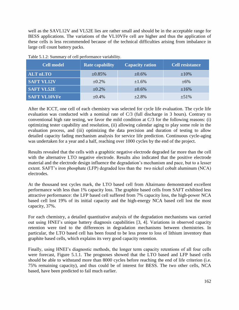
162

well as the SAVL12V and VL52E lies are rather small and should be in the acceptable range for

BESS applications. The variations of the VL10VFe cell are higher and thus the application of

these cells is less recommended because of the technical difficulties arising from imbalance in

large cell count battery packs.

Table 5.1.2: Summary of cell performance variability.

Cell model Rate capability Capacity ration Cell resistance

ALT nLTO ±0.85% ±0.6% ±10%

SAFT VL12V ±0.2% ±1.6% ±6%

SAFT VL52E ±0.2% ±0.6% ±16%

SAFT VL10VFe ±0.4% ±2.8% ±51%

After the ICCT, one cell of each chemistry was selected for cycle life evaluation. The cycle life

evaluation was conducted with a nominal rate of C/3 (full discharge in 3 hours). Contrary to

conventional high rate testing, we favor the mild condition at C/3 for the following reasons: (i)

optimizing tester capability and resolution, (ii) allowing calendar aging to play some role in the

evaluation process, and (iii) optimizing the data precision and duration of testing to allow

detailed capacity fading mechanism analysis for service life prediction. Continuous cycle-aging

was undertaken for a year and a half, reaching over 1000 cycles by the end of the project.

Results revealed that the cells with a graphitic negative electrode degraded far more than the cell

with the alternative LTO negative electrode. Results also indicated that the positive electrode

material and the electrode design influence the degradation’s mechanism and pace, but to a lesser

extent. SAFT’s iron phosphate (LFP) degraded less than the two nickel cobalt aluminum (NCA)

electrodes.

At the thousand test cycles mark, the LTO based cell from Altairnano demonstrated excellent

performance with less than 1% capacity loss. The graphite based cells from SAFT exhibited less

attractive performance: the LFP based cell suffered from 7% capacity loss, the high-power NCA

based cell lost 19% of its initial capacity and the high-energy NCA based cell lost the most

capacity, 37%.

For each chemistry, a detailed quantitative analysis of the degradation mechanisms was carried

out using HNEI’s unique battery diagnosis capabilities [3, 4]. Variations in observed capacity

retention were tied to the differences in degradation mechanisms between chemistries. In

particular, the LTO based cell has been found to be less prone to loss of lithium inventory than

graphite based cells, which explains its very good capacity retention.

Finally, using HNEI’s diagnostic methods, the longer term capacity retentions of all four cells

were forecast, Figure 5.1.1. The prognoses showed that the LTO based and LFP based cells

should be able to withstand more than 8000 cycles before reaching the end of life criterion (i.e.

75% remaining capacity), and thus could be of interest for BESS. The two other cells, NCA

based, have been predicted to fail much earlier.

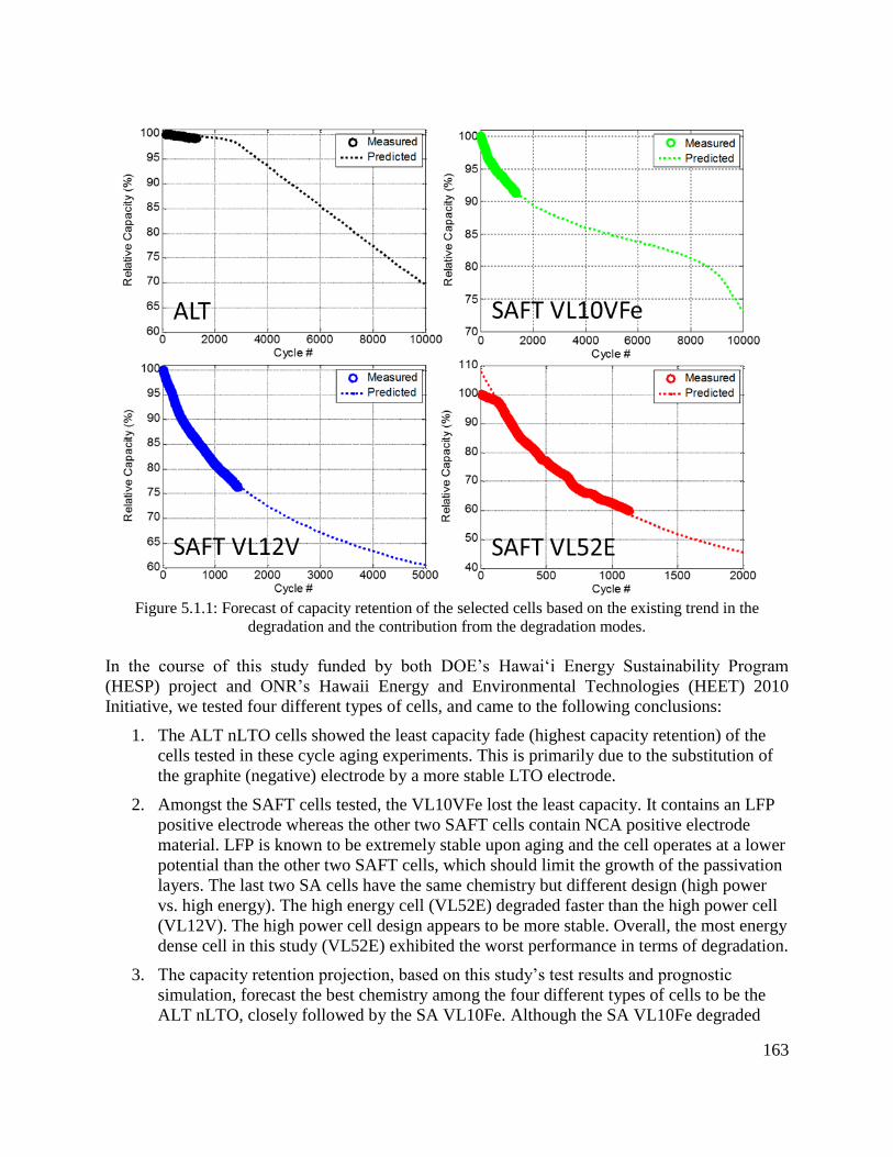
163

Figure 5.1.1: Forecast of capacity retention of the selected cells based on the existing trend in the

degradation and the contribution from the degradation modes.

In the course of this study funded by both DOE’s Hawai‘i Energy Sustainability Program

(HESP) project and ONR’s Hawaii Energy and Environmental Technologies (HEET) 2010

Initiative, we tested four different types of cells, and came to the following conclusions:

1. The ALT nLTO cells showed the least capacity fade (highest capacity retention) of the

cells tested in these cycle aging experiments. This is primarily due to the substitution of

the graphite (negative) electrode by a more stable LTO electrode.

2. Amongst the SAFT cells tested, the VL10VFe lost the least capacity. It contains an LFP

positive electrode whereas the other two SAFT cells contain NCA positive electrode

material. LFP is known to be extremely stable upon aging and the cell operates at a lower

potential than the other two SAFT cells, which should limit the growth of the passivation

layers. The last two SA cells have the same chemistry but different design (high power

vs. high energy). The high energy cell (VL52E) degraded faster than the high power cell

(VL12V). The high power cell design appears to be more stable. Overall, the most energy

dense cell in this study (VL52E) exhibited the worst performance in terms of degradation.

3. The capacity retention projection, based on this study’s test results and prognostic

simulation, forecast the best chemistry among the four different types of cells to be the

ALT nLTO, closely followed by the SA VL10Fe. Although the SA VL10Fe degraded

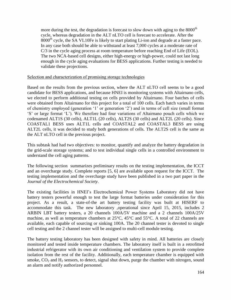
164

more during the test, the degradation is forecast to slow down with aging to the 8000th

cycle, whereas degradation in the ALT nLTO cell is forecast to accelerate. After the

8000th

cycle, the SA VL10Fe is likely to start plating Li-ion and degrade at a faster pace.

In any case both should be able to withstand at least 7,000 cycles at a moderate rate of

C/3 in the cycle aging process at room temperature before reaching End of Life (EOL).

The two NCA-based cell designs, either high-energy or high-power, could not last long

enough in the cycle aging evaluations for BESS applications. Further testing is needed to

validate these projections.

Selection and characterization of promising storage technologies

Based on the results from the previous section, where the ALT nLTO cell seems to be a good

candidate for BESS applications, and because HNEI is monitoring systems with Altairnano cells,

we elected to perform additional testing on cells provided by Altairnano. Four batches of cells

were obtained from Altairnano for this project for a total of 100 cells. Each batch varies in terms

of chemistry employed (generation ‘1’ or generation ‘2’) and in terms of cell size (small format

‘S’ or large format ‘L’). We therefore had four variations of Altairnano pouch cells which we

codenamed ALT1S (30 cells), ALT1L (20 cells), ALT2S (30 cells) and ALT2L (20 cells). Since

COASTAL1 BESS uses ALT1L cells and COASTAL2 and COASTAL3 BESS are using

ALT2L cells, it was decided to study both generations of cells. The ALT2S cell is the same as

the ALT nLTO cell in the previous project.

This subtask had had two objectives: to monitor, quantify and analyze the battery degradation in

the grid-scale storage systems; and to test individual single cells in a controlled environment to

understand the cell aging patterns.

The following section summarizes preliminary results on the testing implementation, the ICCT

and an overcharge study. Complete reports [5, 6] are available upon request for the ICCT. The

testing implementation and the overcharge study have been published in a two part paper in the

Journal of the Electrochemical Society.

The existing facilities in HNEI’s Electrochemical Power Systems Laboratory did not have

battery testers powerful enough to test the large format batteries under consideration for this

project. As a result, a state-of-the art battery testing facility was built at HISERF to

accommodate this task. The new laboratory ,operational since April 15, 2015, includes 2

ARBIN LBT battery testers, a 20 channels 100A/5V machine and a 2 channels 100A/25V

machine, as well as temperature chambers at 25°C, 45°C and 55°C. A total of 22 channels are

available, each capable of sourcing or sinking 100A. The 20 channel tester is devoted to single

cell testing and the 2 channel tester will be assigned to multi-cell module testing.

The battery testing laboratory has been designed with safety in mind. All batteries are closely

monitored and tested inside temperature chambers. The laboratory itself is built in a retrofitted

industrial refrigerator with its own air conditioning and ventilation system to provide complete

isolation from the rest of the facility. Additionally, each temperature chamber is equipped with

smoke, CO2 and H2 sensors, to detect, signal shut down, purge the chamber with nitrogen, sound

an alarm and notify authorized personnel.

165

Figure 5.1.2: (Left) Entrance to the battery laboratory, a self-contained converted refrigerator unit.

(Center) 20-channel Arbin battery tester and climate chamber by its side. (Right) large format Altairnano

cells in the climate chamber.

We started by performing the ICCT on the initial batch of 100 cells. The 100 cells provided to us

by Altairnano have been manufactured a few years ago and no information about the storage

conditions were available. As a result, there was reasonable doubt with regards to the uniformity

of the different batches of cells.

However the analysis showcased that the majority of the cells remained consistent (Table 5.1.3).

The rate capability variations are all below 0.5%, the capacity ratio variations are all below 1.5%

and the resistance variations are all below 6%. Analysis showed that 13 cells out of the 100 do

not match the performance of the others. The cell to cell variation of the ALT2S can be

compared to the cell-to-cell variation observed in our previous study (Table 5.1.2) for the similar

ALT nLTO cells and the values are similar. Since the size of the batches were different, (6 cells

for the first study and 30 for this study), it is unclear if the small observed differences are a result

of a statistical distribution of differences between batches. In any case, the variation is smaller

for this second study which is more important, since we will be testing multiple cells undergoing

different degradation patterns.

166

Table 5.1.3: Summary of cell performance variability.

Cell model Rate capability Capacity ration Cell resistance

ALT1S ±0.30% ±1.4% ±2%

ALT1L ±0.20% ±0.5% ±3%

ALT2S ±0.42% ±0.5% ±4%

ALT2L ±0.50% ±0.9% ±6%

In the next step of our work, we gathered high quality OCV vs. SOC data and individual

electrode electrochemical behavior from the laboratory testing to analyze existing and upcoming

COASTAL1 data. We will use every off line periods as well as tri-annual tests to estimate the

BESS single cells’ SOC distribution and SOH using the HNEI suite of models built from

laboratory testing results.[7, 8] The goal was to separate the contribution of the imbalance from

the contribution of single cells degradation in the BESS performance degradation. The same

study was undertaken for COASTAL2 and COASTAL3 BESS as soon as they began operation.

The cell degradation as a function of different aging conditions was investigated, including

calendar aging and cycle aging. The calendar aging study focus was placed on the effect of

temperature and state of charge. The cycling aging study focus was on understanding the

degradation introduced by the BESS field usage throughout the first 3 years of testing. This

knowledge will be used to test single cells under nominal and harsher conditions under ONR

APRISES funding. This approach is summarized in 3 and comprises 3 distinct steps: usage

analysis, laboratory test and HNEI custom analysis. In the first step, we will use one year worth

of collected real-world BESS data to quantify the average usage of the system and define

representative metrics, such as pulse intensity, SOC swings and temperature. In the second step,

we will generate a design of experiment that should allow us to test the impact of each of the

selected metrics on the cell degradation. In the last step, we are planning to use HNEI’s unique

battery degradation analysis capabilities such as incremental capacity analysis, cell emulation

and pack modeling to analyze cell degradation and diagnose the impact of the selected metrics

individually. This experiment is ongoing under ONR APRISES funding and results will be

reported at a later time.

167

Figure 5.1.3: Schematic approach to cycle aging experiment.

Aside from the aforementioned ongoing testing, we used the cells remaining from the previous

HESP/ONR project to perform an overcharge study [9, 10]. The battery pack used in BESS

applications is usually comprised of hundreds of cells in series to reach a practical voltage of 900

V or more. Typically, the same charging or discharging current flows through a string at all times

which means that all cells in series typically charge or discharge at the same pace. A problem

arises when one or more cells in the series that have less capacity than the others may get

overcharged. In this study, we investigated the abuse tolerance of a lithium-ion cell under an

overcharge scenario.

To investigate the overcharge behavior of lithium ion batteries for high power applications is of

great interest for safety and abuse tolerance. The ability to absorb rapid recharge to mitigate

intermittency of solar and wind power generation, high rate charging is a feature critical to the

success of LIB in BESS applications. An informative study of this ability to abuse tolerance is

necessary. In many multi-cell configurations, the cell management and balance is critical to the

reliability of the battery system performance. Overcharging may often be encountered in battery

pack operation, especially due to power quality fluctuations in real-life situations and cell

imbalance in a pack. Thus, understanding the impact of overcharging abuse is a useful exercise

to know how much the impact could occur in a quantitative manner, which is the first step

toward better battery management and control.

In the literature, overcharge-related studies often emphasize thermal impacts on cell behavior

(due to heat generation), as this phenomenon constitutes a serious safety hazard (e.g. to trigger

thermal runaway), and it is critical to diminish such a hazard. In those studies, postmortem

analyses are often used to disassemble cells in order to examine the evidence of overcharging in

the investigation. But such qualitative evidence does not aid battery design and management or

168

help engineers to alleviate concerns on reliability and safety issues. In this context, assessing the

resilience of a Li-ion cell exposed to mild abuse conditions (e.g. overcharge, overvoltage,

overheating) and its ability to maintain cycling under back-to-normal operating conditions was

assessed.

Here, we report a study on an overcharge event imposed on an ALT2S cell and a subsequent

investigation of the impacts on cell degradation in cycle aging. The analysis is conducted using

electrochemical inference techniques developed in our laboratory [3, 4], which is different from

the conventional postmortem analyses, and where no cell disassembly is required. This battery

diagnosis method is entirely based on simple current-voltage measurements. Diagnosis of the

cell is performed on two targeted cells, one cycled under a routine C/3 cycle aging protocol

while the other experienced an overcharge event under the same cycle aging protocol. Results

exhibit the contrast in the aging behavior, particularly capacity fade, before and after the

overcharging event, and fading through additional cycle aging after the event.

Both cells were subjected to C/3, [1.8 – 2.8] V cycle schedule for more than 100 cycles to

validate the minimal cell variability in the aging and degradation process. The overcharge event

was imposed on the overcharged cell as follows. After the routine C/3 discharge to 1.8 V, the

cell was recharged at C/4 to 3.6 V to create the intended overcharge event. The cutoff at 3.6 V

was chosen based on the indication that 3.7 V is a voltage limit as a safety precaution, according

to the manufacturer’s guide. The capacity fade induced by the overcharge was on the order of

13% and the overcharging event also led to additional 12% capacity fade in the subsequent 1000

cycle aging (Figure 5.1.4). The side plots show incremental capacity response (described below).

Figure 5.1.4: Center plot: Capacity retention as a function of cycle number on the baseline cell (gray line)

and the overcharged (O/C) cell (black line). Insets: schematic representation of the proposed gas

evolution inside the cell during, after and long after overcharge. The blue tint represents the presence of

liquid electrolyte, a cloud represents gas bubbles.

Side plots: Incremental capacity response at different color coded SOH levels, corresponding to the

colored dots on the center plot. Black line represents the fresh cell, blue represents the overcharged cell,

green represent the aged cell under normal conditions and red represents the aged cell after overcharge.

169

Aiming for further understanding of the capacity fading mechanism and to enable prognosis, we

conducted detailed analyses using an in-house incremental capacity technique. Detailed

descriptions of this technique are reported in Refs [3, 4, 11, 12]. The starting hypothesis for our

technique is that although the cell is degrading, the electrochemical behavior of each individual

electrode is not changing. The capacity loss is then induced by either a change in the balance

between the two electrodes (a loss of active material on either side) or a change in the amount of

lithium ions that could go back and forth between the electrodes. Any change in electrode

balance and/or lithium content will modify the voltage response of the battery. Studying the

changes in the voltage curve upon aging will then provide an insight on the degradation pattern

of any cell. Additionally, these variations can be simulated using our in-house model, ‘alawa,

[13] and compared to the experimental values for accurate quantification and prognosis. As the

variations can be minute, they are better analyzed by looking at a derivative of the voltage curve:

dQ/dV. This technique is known as incremental capacity analysis (ICA). The changes associated

with the overcharge event are presented on the side plots in Figure 5.1.4, showing the

incremental capacity response at various SOH points.

Figure 5.1.5 presents the comparison of the experimental data and the simulations. Using this

technique we were able to quantify that the overcharge induced 5% loss of lithium inventory and

13.5% loss of active material on each of the electrodes. The subsequent capacity loss during the

1000 cycles after the overcharge was attributed to 8% loss of active material on each electrode.

Figure 5.1.5: (a) Comparison of experimental (markers) and emulated (line) IC curves of a pristine LTO ||

NMC cell at a C/25 discharge rate. (b) IC (dQ/dV) experimental (markers) and emulated (lines) curves of

the overcharged (O/C) cell (in blue) and after 700 cycles (in red).

The unique capability of the ‘alawa emulation toolbox made it possible to quantify such detail

without the need of postmortem analysis. This is the first time a quantitative comparative study

was conducted with large format cells. The unique cell chemistry using LTO anode and NMC

cathode also provided an opportunity to study the capacity fade mechanism and the gassing

effect without much interference from lithium plating to understand the level of impact from the

charge and overcharge events in a quantitative manner.

170

Our results showed some visual indication of gassing (swollen pouch cell) as well as inferred

indication of electrolyte decomposition at the interface between electrolyte and LTO. This

prompted us to push the analysis further and to investigate the internal structure of the

overcharged cell to try to assess the spatial distribution of gas inside the cell and understand how

it affected the cell’s capacity. In order to do so, we subjected a pristine cell to computed

tomography (CT) scanning before and after an overcharge event. Before the overcharge, the cell

offered a uniform white halo under CT scan imaging in both the Y-Z (Figure 5.1.6 (a)) and X-Y

(Figure 5.1.6 (c)) planes. The halo is formed because the resolution is the CT scan (300µm) is

not high enough to separate the layers of electrode (100 µm). The scans did not exhibit any

visible gas bubble within the electrode stack. This was expected because, when not abused, these

cells present a tightly packed appearance, indicative of an absence of gaseous by-product. After

the overcharge, a large volume of gas is visible in the region between the top of the stack and the

soft bag (Figure 5.1.6 (b)), with a white curved line visible, which corresponds to the edge of the

top wall of the soft bag. Furthermore, a dark stripe, located at mid-depth, shows the presence of

a number of moderate-size gas bubbles is can be seen in the CT scan, in the X-Y plane.

The CT scan analysis showcased two areas where gases seemed to accumulate: at the top and at

mid-depth of the cell. So long as a sufficient volume of liquid electrolyte remained in the cell to

wet the entirety of the electrodes, we do not expect the gas trapped at the top of the cell between

the electrode stack and the soft bag to cause any capacity fade. On the contrary, we believe that

the gas bubbles evidenced by voids at mid-depth in the electrode stack mechanically separated

viable portions of the positive and negative electrode from each other, disabling the ionic

conduction pathway in the process. This ionic conduction pathway blockage would provide the

basis for explaining the occurrence of loss of active material at both electrodes.

Figure 5.1.6: Computed tomography (CT) scans of a pouch cell: before overcharge (a) in the Y-Z plane

and (c) in the X-Y plane; after the overcharge (b) in the Y-Z plane and (d) in the X-Y plane. Matter

shown in white, void in black.

171

In this study, we showed how a LTO || NMC pouch cell having sustained an overcharge had

been losing capacity through the generation and entrapment of gas bubbles within the electrode

stack. First, the degradation was diagnosed operando without the need for post-mortem analysis.

Second, using a dQ/dV analysis, we identified the transient reductive conditions which, in the

context of a LTO-based cell, resulted in substantial electrolyte decomposition. Third, we used a

CT scanner to image the internal structure of a cell before and after overcharge and obtained

evidence of the presence of gas bubbles trapped within the electrode stack. The physical

separation of both electrodes created by these gas bubbles appeared large enough to disrupt the

ionic conduction pathway, therefore disabling portions of otherwise perfectly viable electrodes.

This was later demonstrated by administrating a massage to the overcharged cell in an effort to

displace the trapped gas bubbles outside of the electrode stack. The massage helped reconnect 14

of the 25% of the lost active materials and helped restore nearly 60% of the capacity lost to the

overcharge and its aftermath.

The insets in Figure 5.1.4 portray this mechanism. Ultimately, this study illustrates the durability

of this LTO || NMC cell design against overcharge. It also showcases the detrimental effect of

electrolyte-reduction-induced gassing with LTO electrodes allowed to discharge below 1 V and

explains the mechanism through which the overcharge drove the capacity to fade. More details

on this study were published in the Journal of the Electrochemical Society [9, 10].

Apparatus & Method for Estimating the State of Health of a Battery via updating the OCV and

SOC relationship

Through the course of this project we invented a new method to dynamically adjust the

OCV/SOC curves while the batteries are aging. This could potentially allow to significant

improvement of the BESS SOH and SOC monitoring. SOC determination in battery packs

involves two steps, calibration and tracking. The calibration step is performed by recording the

rest voltage of battery packs and comparing it to a reference OCV/SOC lookup table. The

tracking step is performed by counting the coulombs exchanged since the last calibration and

converting them to SOC via the capacity ration. Whereas it is well established that they are

changing with aging, the reference lookup table and the capacity ration are typically not updated

because there is no accurate method to do so without a long downtime. This implies no SOH

tracking and leads to more and more SOC tracking errors with time. Our invention could solve

this issue by providing a simple way to recalibrate the look-up table and the capacity ration

without the need for any significant downtime. The method is also does not require the need for

any additional sensors nor complex testing protocols.

A provisional patent was filled in February 2016 and some validation work is ongoing under

other ONR funding.

172

Papers and Presentations resulting from these efforts

Internal Reports

Characterizing Emerging Cell Chemistries for Battery Energy Storage Systems, DOE

HESP report

Altairnano Single Cell Battery Testing, Initial Conditioning Characterization Test and

other preliminary testing, Internal report, available on demand

Altairnano Single Cell Battery Testing, Test plan, Internal report, available on demand

Publications

A. Devie, M. Dubarry, B.Y. Liaw, J. Electrochem. Soc., 162(6) (2015) A1033-A1040.

A. Devie, M. Dubarry, H.P. Wu, T.H. Wu, B.Y. Liaw, J. Electrochem. Soc., In

press(2017).

Patents

Apparatus & Method for Estimating the State of Health of a Battery via updating the

OCV and SOC relationship, provisional patent filed on 16/02/29.

Conference Presentations

Overcharge Study in Li4Ti5O12 Based Lithium-Ion Pouch Cell, M. Dubarry, A. Devie,

and B. Y. Liaw, International Battery Association (IBA 2016), Nantes, France, March

2016 (Invited lecture).

Laboratory testing of LTO based cells for BESS applications, M. Dubarry, and A. Devie,

International Battery Association (IBA 2016), Nantes, France, March 2016 (Poster).

Intrinsic degradation variability in commercial lithium-ion batteries, A. Devie, M.

Dubarry, P. Cabanel and B.Y. Liaw, 228th Meeting of the Electrochemical Society,

Phoenix, AZ, USA, October 2015.

Two-point state-of-charge determination in lithium-ion battery packs, M. Dubarry, A.

Devie, and B. Y. Liaw, International Battery Association (IBA 2015), Waikoloa, HI,

USA, January 2015 (Invited lecture).

Energy density: from half cells to full cell, A. Devie, M. Dubarry and B.Y. Liaw,

International Battery Association (IBA 2015), Waikoloa, HI, USA, January 2015 (Invited

Lecture).

References

1. H.N.E. Institute, Characterizing Emerging Cell Chemistries for Battery Energy Storage

Systems, 2016,

2. M. Dubarry, N. Vuillaume, B.Y. Liaw, Int J Energ Res, 34(2) (2010) 216-231.

3. M. Dubarry, C. Truchot, B.Y. Liaw, J. Power Sources, 219(2012) 204-216.

173

4. M. Dubarry, A. Devie, B.Y. Liaw, Journal of Energy and Power Sources, 1(5) (2014) 242-

249.

5. M. Dubarry, A. Devie, Altairnano Single Cell Battery Testing, Initial Conditioning

Characterization Test and other preliminary testing, 2016,

6. M. Dubarry, A. Devie, Altairnano Single Cell Battery Testing, Test plan, 2016,

7. M. Dubarry, C. Truchot, A. Devie, B.Y. Liaw, J. Electrochem. Soc., 162(6) (2015) A877-

A884.

8. M. Dubarry, A. Devie, B.Y. Liaw, J. Power Sources, 321(2016) 36-46.

9. A. Devie, M. Dubarry, B.Y. Liaw, J. Electrochem. Soc., 162(6) (2015) A1033-A1040.

10. A. Devie, M. Dubarry, H.P. Wu, T.H. Wu, B.Y. Liaw, J. Electrochem. Soc., In press(2017).

11. M. Dubarry, V. Svoboda, R. Hwu, B.Y. Liaw, Electrochem. Solid-State Lett., 9(10) (2006)

A454-A457.

12. M. Dubarry, B.Y. Liaw, J. Power Sources, 194(1) (2009) 541-549.

13. Alawa central, https://www.soest.hawaii.edu/HNEI/alawa/, last accessed: June 2016

5.2 Grid Scale Storage Systems Testing

HNEI continued its testing and evaluation of grid-tied battery energy storage systems under this

award. To date, three grid-scale Battery Energy Storage Systems (BESS) have been procured and

commissioned. The Big Island BESS has operated for over three years, in both a wind

smoothing and frequency regulation mode. The three BESS operating on three different islands

will ultimately provide unique ancillary services, and help determine the roles BESS can play on

isolated electrical grids under significant penetration from variable renewable energy resources.

The integration of large amounts of variable renewable power, such as photovoltaic (PV) and

wind into a power system, can lead to increased generation reserves and costs, lower power

quality and reliability, or in extreme cases, can cause blackouts if not implemented properly.

Rapid changes in power generation or consumption have a greater effect on small, isolated grid

systems. Because the response times of BESS are relatively short, they can provide services to

address some issues related to renewable integration and provide a mitigation strategy to address

some of these issues. The research conducted by HNEI not only investigates the effectiveness of

different ancillary services under different operational conditions, but also determines how to

minimize battery cell degradation through experimentation (see Subtask 5.1).

This report discusses the development efforts and accomplishments under this award.

Hawaii Island BESS

The Hawaii Island BESS has been in operation since December, 2012. Over that time it has

cycled more than 3.3 GWh. The objective of research and analytical efforts under this award

were to determine how to best support the grid on Hawaii Island while minimizing battery

degradation.

https://www.soest.hawaii.edu/HNEI/alawa/

174

As discussed in the HEET 09 final technical report (Award N00014-10-1-0310), this system can

provide one of two ancillary services at any given time: wind smoothing or grid frequency

response. The system is almost always set to frequency response because it was learned that

wind smoothing very often countered the needs of the e grid system. i.e. the BESS may inject

energy into the system to counter loss of power from the wind farm at time that the system

requires less energy to balance frequency. While running in frequency response mode, it was

learned that there are settings that serve grid needs while minimizing cycling. In HEET10 in one

case, the grid frequency appeared to become marginally stable when some highly periodic wind

gusts were encountered. It was learned that we could achieve 2/3 of the grid benefit (reduction of

grid frequency variability) while cycling only 1/3 of the energy throughput found in our initial

algorithm settings. Details about these results will be discussed in forthcoming papers.

HNEI’s planned data collection for grid interaction with this BESS has been completed under

HEET 10. However, there is further interest in long term battery cell degradation. Hawaiian

Electric Light Company (HELCO) has agreed to continue operation of the BESS and to provide

operational data to HNEI for further analysis.

Oahu BESS

Under HEET 10, a second 1MW, 250kWh BESS was procured and installed at the Hawaiian

Electric Company (HECO) substation at Campbell Industrial park on the island of Oahu. Unlike

the first BESS, which primarily regulated grid frequency, this BESS will be simultaneously

providing power smoothing as well as voltage regulation within an electric substation serving

large industrial loads. The industrial park served by the circuit served by this substation includes

a high penetration of large PV systems, which can disrupt voltage and power quality when

clouds suddenly occlude the solar panels.

Like the Hawaii Island BESS, the project team for the Oahu BESS consisted of both public and

private partners. Table 5.2.1 lists the key partners involved in the project.

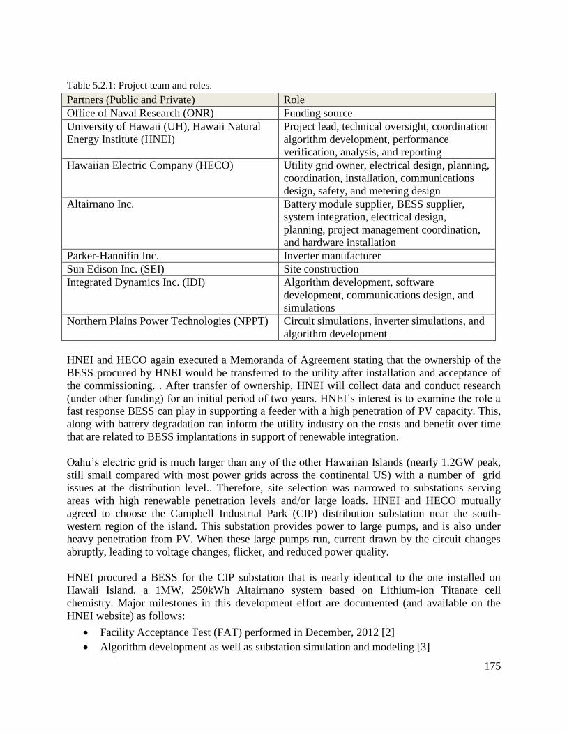
175

Table 5.2.1: Project team and roles.

Partners (Public and Private) Role

Office of Naval Research (ONR) Funding source

University of Hawaii (UH), Hawaii Natural

Energy Institute (HNEI)

Project lead, technical oversight, coordination

algorithm development, performance

verification, analysis, and reporting

Hawaiian Electric Company (HECO) Utility grid owner, electrical design, planning,

coordination, installation, communications

design, safety, and metering design

Altairnano Inc. Battery module supplier, BESS supplier,

system integration, electrical design,

planning, project management coordination,

and hardware installation

Parker-Hannifin Inc. Inverter manufacturer

Sun Edison Inc. (SEI) Site construction

Integrated Dynamics Inc. (IDI) Algorithm development, software

development, communications design, and

simulations

Northern Plains Power Technologies (NPPT) Circuit simulations, inverter simulations, and

algorithm development

HNEI and HECO again executed a Memoranda of Agreement stating that the ownership of the

BESS procured by HNEI would be transferred to the utility after installation and acceptance of

the commissioning. . After transfer of ownership, HNEI will collect data and conduct research

(under other funding) for an initial period of two years. HNEI’s interest is to examine the role a

fast response BESS can play in supporting a feeder with a high penetration of PV capacity. This,

along with battery degradation can inform the utility industry on the costs and benefit over time

that are related to BESS implantations in support of renewable integration.

Oahu’s electric grid is much larger than any of the other Hawaiian Islands (nearly 1.2GW peak,

still small compared with most power grids across the continental US) with a number of grid

issues at the distribution level.. Therefore, site selection was narrowed to substations serving

areas with high renewable penetration levels and/or large loads. HNEI and HECO mutually

agreed to choose the Campbell Industrial Park (CIP) distribution substation near the south-

western region of the island. This substation provides power to large pumps, and is also under

heavy penetration from PV. When these large pumps run, current drawn by the circuit changes

abruptly, leading to voltage changes, flicker, and reduced power quality.

HNEI procured a BESS for the CIP substation that is nearly identical to the one installed on

Hawaii Island. a 1MW, 250kWh Altairnano system based on Lithium-ion Titanate cell

chemistry. Major milestones in this development effort are documented (and available on the

HNEI website) as follows:

Facility Acceptance Test (FAT) performed in December, 2012 [2]

Algorithm development as well as substation simulation and modeling [3]

176

Laboratory Acceptance Test Plan [4]

Laboratory Acceptance Test Results [5]

Site preparation (including planning, communications, construction, and electrical work)

Shipping, logistics and installation

Site Acceptance Test (SAT) performed in August, 2016 [6]

Algorithm Acceptance Test Plan [7]

Algorithm Acceptance Test Results [8]

The SAT was conducted on 8/2/2016. Figure 5.2.1 shows the test in progress as a HECO lead

engineer coordinates with HECO System Operators (foreground) and an Altairnano engineer

discusses readings with Altairnano system experts (background). The tests were successful as the

system did meet hardware performance specifications.

Figure 5.2.1: Hawaiian Electric Company (HECO)/Campbell Industrial Park (CIP) Site Acceptance Test.

The HECO/CIP BESS is the most heavily metered of the three HEET systems. Figure 5.2.2

shows a one-line diagram indicating the locations of 6 of the meters. Some meters are used for

real-time control, while others are used for post-processing (data analysis) or for HECO

monitoring. In the figure, meters M1 and M5 measure essentially the same thing: the low side of

the output of the inverter. M5 is used by the inverter for control purposes. M1 is only used in

post processing. M2 is the power realized by the BESS on the circuit. This is used for post

processing. M3 is the power at the substation, which is used in post processing. M4 is the power

consumption of the circuit. This is used for both post processing and real-time control. M6 is

used in post processing. This meter measures the power consumption of the BESS itself.

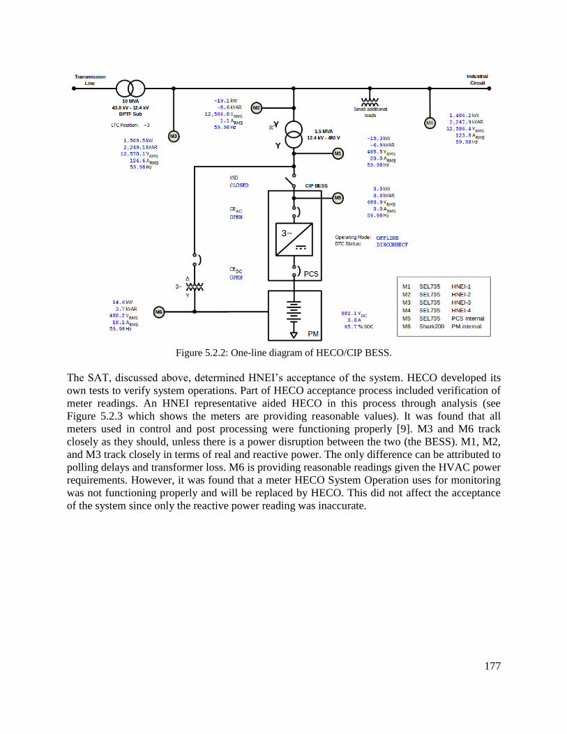
177

Figure 5.2.2: One-line diagram of HECO/CIP BESS.

The SAT, discussed above, determined HNEI’s acceptance of the system. HECO developed its

own tests to verify system operations. Part of HECO acceptance process included verification of

meter readings. An HNEI representative aided HECO in this process through analysis (see

Figure 5.2.3 which shows the meters are providing reasonable values). It was found that all

meters used in control and post processing were functioning properly [9]. M3 and M6 track

closely as they should, unless there is a power disruption between the two (the BESS). M1, M2,

and M3 track closely in terms of real and reactive power. The only difference can be attributed to

polling delays and transformer loss. M6 is providing reasonable readings given the HVAC power

requirements. However, it was found that a meter HECO System Operation uses for monitoring

was not functioning properly and will be replaced by HECO. This did not affect the acceptance

of the system since only the reactive power reading was inaccurate.

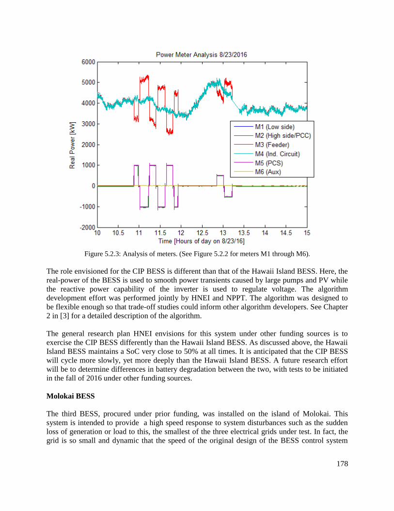
178

Figure 5.2.3: Analysis of meters. (See Figure 5.2.2 for meters M1 through M6).

The role envisioned for the CIP BESS is different than that of the Hawaii Island BESS. Here, the

real-power of the BESS is used to smooth power transients caused by large pumps and PV while

the reactive power capability of the inverter is used to regulate voltage. The algorithm

development effort was performed jointly by HNEI and NPPT. The algorithm was designed to

be flexible enough so that trade-off studies could inform other algorithm developers. See Chapter

2 in [3] for a detailed description of the algorithm.

The general research plan HNEI envisions for this system under other funding sources is to

exercise the CIP BESS differently than the Hawaii Island BESS. As discussed above, the Hawaii

Island BESS maintains a SoC very close to 50% at all times. It is anticipated that the CIP BESS

will cycle more slowly, yet more deeply than the Hawaii Island BESS. A future research effort

will be to determine differences in battery degradation between the two, with tests to be initiated

in the fall of 2016 under other funding sources.

Molokai BESS

The third BESS, procured under prior funding, was installed on the island of Molokai. This

system is intended to provide a high speed response to system disturbances such as the sudden

loss of generation or load to this, the smallest of the three electrical grids under test. In fact, the

grid is so small and dynamic that the speed of the original design of the BESS control system

179

was not sufficient to serve its intended purpose. Research and development of an improved

control and communications architecture has been started and is currently on-going.

Of the three BESS installations, the Molokai site provided the most challenges. The inertia (in

essence, a resistance to change) of the Molokai grid is low enough that relatively small

imbalances between power generation and consumption can cause chain reactions, leading to

island-wide blackouts. Technologies proposed to serve such a grid must be carefully vetted so

that latent responses to these imbalances (manifested as grid frequency deviations) do not

exacerbate the situation. Even a 200ms delay between a loss of generation (or load) and

realization of a real power correction, can cause the entire grid to become classically unstable

and can cause island-wide blackouts (that is, a latent correction is worse than no correction at

all).

The project partners and their roles are shown in Table 5.2.2.

Table 5.2.2: Project team and roles.

Partners (Public and Private) Role

Office of Naval Research (ONR) Funding source

University of Hawaii (UH), Hawaii Natural

Energy Institute (HNEI)

Project lead, technical oversight,

coordination, planning, performance

verification, analysis, and reporting

Maui Electric Company (MECO) Utility grid owner, electrical design, planning,

coordination, installation, communications

design, safety, and metering design

Altairnano Inc. Battery module supplier, BESS supplier,

system integration, electrical design,

planning, project management coordination,

and hardware installation

Parker-Hannifin Inc. Inverter manufacturer

Sun Edison Inc. (SEI) Site construction

Integrated Dynamics Inc. (IDI) Algorithm development, control system

infrastructure redesign, software

development, communications design, and

simulations

Northern Plains Power Technologies (NPPT) Grid simulations, inverter simulations, and

algorithm development

Of the approximately 5MW load, on Molokai over 2MW is serviced by PV during the daytime.

It was determined that an Altairnano 2MW, 397kWh BESS would be more suitable for this grid

than the 1MW, 250kWh systems used on the other two islands.

Although Factory Acceptance was completed and deemed acceptable, HNEI and its partners

discovered that the existing control and communications technology was insufficient for

application on Molokai because of the low grid inertia. HNEI is currently preparing additional

contract partnerships to address this problem during future awards.

180

The following was completed during this current award:

Algorithm (controller) design [10]

Simulation of BESS and grid [11]

Exploratory research and documentation on the latency issue (attempt to reduce

correction to 50ms or less) [12]

Site preparation (including planning, communications, construction, and electrical work)

Shipping, logistics, and installation

SAT Results [13]

For the Molokai grid, the SAT had to be more carefully designed and executed since, as

mentioned, a sudden excess generation of 2MW on a 5MW grid would cause island-wide

blackouts. For this reason, HNEI issued a memorandum [14] to the project team proposing a

stepped approach: several small power increments were to be used to demonstrate both the

power and energy performance of the BESS. When the tests were conducted, it was found that

500kW steps could be taken instead of the 100kW steps originally proposed. This simplified the

test process. Power data from all active diesel generators as well as the BESS is shown in Figure

5.2.4: Generation data from the Site Acceptance Test (SAT).

Figure 5.2.4: Generation data from the Site Acceptance Test (SAT).

An expansion of the power steps, as well as grid frequency is shown in Figure 5.2.5. While the

BESS was close to 0kW (offline), 500kW incremental steps were taken. As the power was

increased (away from the 0kW reference), 250kW incremental steps were taken. The 500kW

steps caused 0.55 Hz frequency events, while the 250kW steps caused 0.33 Hz frequency events.

These events were not large enough to cause grid-wide problems.

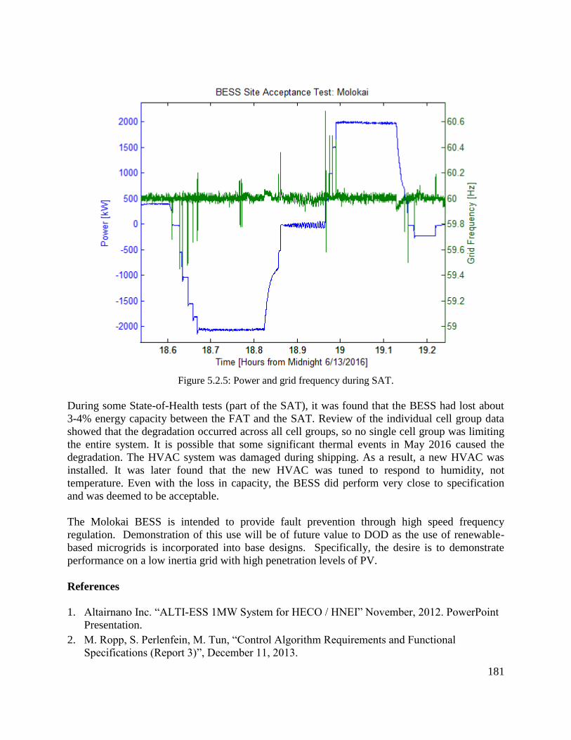
181

Figure 5.2.5: Power and grid frequency during SAT.

During some State-of-Health tests (part of the SAT), it was found that the BESS had lost about

3-4% energy capacity between the FAT and the SAT. Review of the individual cell group data

showed that the degradation occurred across all cell groups, so no single cell group was limiting

the entire system. It is possible that some significant thermal events in May 2016 caused the

degradation. The HVAC system was damaged during shipping. As a result, a new HVAC was

installed. It was later found that the new HVAC was tuned to respond to humidity, not

temperature. Even with the loss in capacity, the BESS did perform very close to specification

and was deemed to be acceptable.

The Molokai BESS is intended to provide fault prevention through high speed frequency

regulation. Demonstration of this use will be of future value to DOD as the use of renewable-

based microgrids is incorporated into base designs. Specifically, the desire is to demonstrate

performance on a low inertia grid with high penetration levels of PV.

References

1. Altairnano Inc. “ALTI-ESS 1MW System for HECO / HNEI” November, 2012. PowerPoint

Presentation.

2. M. Ropp, S. Perlenfein, M. Tun, “Control Algorithm Requirements and Functional

Specifications (Report 3)”, December 11, 2013.

182

3. K. Musser, “HECO Lab Acceptance Test Plan”, October 31, 2014.

4. K. Musser, “HECO Lab Acceptance Test Results Report”, November 17, 2014

5. Altairnano Inc., “Site Acceptance Test Project HECO 1.0MW ALTI-ESS”, August 11, 2016

6. K. Musser (2016), “HECO CIP – Control Algorithm Site Acceptance Test Plan”, May 3,

2016

7. HECO/CIP Algorithm Acceptance Test Results, September 9, 2016

8. M. Tun, “HECO BESS Metering Analysis”, August 26, 2016

9. NPPT report, “Report on a proposed controller for a frequency-stabilizing battery inverter

system for the Molokai power system”, January 23, 2015

10. NPPT report, “Behavior of a proposed battery-inverter system on Molokai during faults”,

May 06, 2015.

11. K. Musser, A. Mitchell, “MECO – Moloka i ʻ Algorithm Investigative Project Report”,

January 20, 2016.

12. Altairnano Inc., “Site Acceptance Test Project MECO 2.0MW ALTI-ESS”, June 23, 2016.

13. M. Tun, “Coastal III SAT – Proposed Power Test Design”, May 4, 2016.

Task 6. PHOTOVOLTAICS EVALUATION

Solar photovoltaic (PV) performance is dependent on cell materials, module design, inverter

technology and integration, and environment (solar radiation, temperature, cloud shadowing,

etc.). The intent of this project, which is a continuation of previous ONR-funded work in this

area, is to characterize performance and durability of different PV and inverter technologies

under differing environmental conditions. Data has been gathered on PV system performance

and environmental factors at a variety of installations around Hawaii using several

manufacturers’ products and system architectures. The PV systems under test represent grid-

connected, residential and small-scale commercial systems.

The project leverages work completed under US Department of Energy (US DOE) funding (DE-

FC26-06NT42847 and DE-EE0003507) that included the installation of three PV test platforms

located on Hawaii Island, Maui and Oahu, the development of a first-generation data acquisition

system (DAS), and critical data management and analysis tools. Results of these efforts were

reported in [1] for PV test platforms and test protocols and in [2] for the data management and

analysis tools, as well as analysis of two years of data. Under ONR HEET09 [3], two additional

test locations were completed on Oahu and Kauai, hosting grid-connected PV systems on Hawaii

Project Frog classrooms, and two-year performance results were analyzed for the Oahu site. Test

locations were developed to host new combinations of PV systems and a new DAS was designed

to streamline long-term monitoring of grid-connected PV systems. This work has created a

framework of knowledge on PV test platform design, installation, testing, instrumentation and

data analysis methodologies.

Accomplishments under ONR HEET10 funds fall in the following four categories:

183

1. Development of test protocols and data collection methodologies for new test

instrumentation.

2. Installation of a carport-based PV test platform in South Maui.

3. Advancement of data analysis tools, including an innovative dissociation of DC

performance ratio (PR) into current and voltage performance.

4. Detailed analysis of a month of performance data from the Maui site and a year of

data from UH Manoa.

Acronyms used herein are listed in a summary table at the end of this section.

6.1 Development of test protocols and data collection methodologies

Based on earlier research, a variety of new instrumentation and test equipment was deemed

necessary for inclusion in the new test platform on Maui. This included new sensors for

measuring incident solar radiation (a spectroradiometer and pyranometer), an IV tracer, an AC

power meter, and a switching mechanism that allows measurement of open circuit voltage and

short circuit current. These instruments were initially installed at the UH Manoa campus test site

– on the roof of Holmes Hall – to develop test protocols and refine data management tools

necessary to collect the datasets and transfer them to the data server. This site was originally

developed as part of a program called the Green Holmes Hall Initiative, and will thus be referred

to as GHHI. In the process of these developments, approximately one year of environmental

conditions and performance data were collected for the two grid-connected PV systems at GHHI.

IV curves were collected for both PV technologies. Analysis of these data will be presented in

Section 6.4.

New sensors: Spectroradiometer, Diffuse/Global pyranometer

To enhance the level of data available on incident solar radiation, a critical element in

understanding PV performance, a spectroradiometer and a masked pyranometer were installed.

These devices measure the light spectrum and irradiance distribution between direct and diffuse

light. An EKO MS-700 spectroradiometer and a Delta-T SPN1 Sunshine pyranometer were

selected for their ability to operate in remote areas and in the plane of the PV modules. Both

sensors were installed at GHHI and integrated into the DAS (Figure 6.1). The sensors were

tested for software and hardware stability. The spectroradiometer uses a shutter, resulting in a

full reading taking from 0.5 up to 10 seconds, depending on the overall irradiance. It then uses

serial communication to send data to the on-site DAS controller. To ensure a constant sampling

rate and to minimize risk of overwriting data, the spectroradiometer was programmed to take

readings every 15 seconds. The global/diffuse pyranometer produces analog signals for both the

global and diffuse irradiance. These signals are converted to digital, collected at 40Hz and

averaged to 1Hz by the controller.

184

Figure 6.1: Global/diffuse pyranometer on the left and spectroradiometer on the right installed at the

Green Holmes Hall Initiative test site (GHHI).

IV Tracer

We utilize an IV tracer to collect complete performance characteristics (IV curves) of individual

PV modules, which in turn allows the quantification of that performance in the absence of

system losses (such as those due to operation of PV modules with inverters and optimizers or due

to combining PV modules in strings (mismatch loss)). An IV tracer with multiple inputs, the

Daystar Multi-tracer, was selected and installed at GHHI (Figure 6.2) to test its operation in a

semi-protected outdoor environment. A structure was built that suspends the IV tracer load bank

and control unit beneath the existing solar array. This was done to protect the top of the unit

from sun and rain while at the same time ensuring that the unit would not damage the roof. A

more permanent outdoor cabinet was used for the eventual test location in Maui (Figure 6.2 -

right). Programmed Cron jobs were developed to automate the transfer of data files from the IV

tracer to the HNEI data server via secure VPN.

Figure 6.2: IV tracer installed on the rooftop of GHHI (left) and at the Maui test site in a weather-tight

outdoor cabinet (right).

185

AC power meter

An AC power meter was used to compare the AC performance of the grid-connected PV systems

and evaluate the efficiency and reliability of the inverters and optimizers. The Electro Industries

MP200 AC Power meter was selected to measure inverter output. The meter is designed to

measure eight 3-phase systems, and each phase can be individually monitored for a total of 24

single-phase systems. It was configured to monitor the output of eleven PV systems operating at

the Maui test platform, gathering information (AC active and reactive power, voltage and

current) on ten single-phase inverters and one 3-phase microinverter system. DAS software and

data management tools were developed to collect these AC measurements and transfer the data

to the UH server.

Switching: DAS ability to measure ISC and VOC

DC measurement boxes were developed to measure PV system or module performance in

normal operation (i.e., connected to the grid). These boxes are designed to collect one-second

DC voltage, DC current, voltage-to-ground, back-of-the-module temperature, and an auxiliary

DC voltage selected to allow connection of analog sensors such as pyranometers. Essential

parameters for evaluating optical and thermal performance of modules are short-circuit current

(Isc) and open-circuit voltage (Voc). Although these are routinely monitored by the IV tracer,

additional instrumentation was developed and integrated with the DAS to measure these

parameters without the need for an IV tracer, to reduce hardware costs for future test platforms.

At fixed intervals, switches disconnect the PV module from the microinverter, measure VOC and

ISC, and reconnect, within approximately 15 milliseconds. This feature was tested and validated

at the UH Manoa test site on two polycrystalline PV modules operating with Enphase

microinverters.

6.2 Installation of the Maui Test Platform

Planning for a PV test bed located at the Maui Economic Development Board (MEDB) has been

underway for several years. Issues related to the approval for interconnection of this system by

the local utility have caused substantial delays, but the permit for installation was issued on

November 17, 2015. Planning and design considerations for this test platform were presented in

the HEET09 report [3]. The installation of the PV systems began in January 2016, and was

completed by HNU Energy under subcontract to MEDB. Under HEET10, HNEI personnel

installed the DAS and provided guidance to the PV installer. The PV system, including modules,

inverters, DAS and IV tracer was commissioned on February 4, 2016.

Test platform description

The test platform is located on a carport at the MEDB in Kihei, South Maui (Figure 6.3). The

platform consists of 15 grid-connected PV systems rated to up to 2kW each, selected to provide

side-by-side comparison of 10 PV module brands/types and 3 system architectures – string

inverters, string inverter with optimizers, and microinverters. The full carport-based test

platform consists of 108 modules and 10 inverters, comprising a total power of 22 kW. The

carport roof is at an angle of 20o, facing 197

oN azimuth – slightly west of due south. The

latitude, longitude and altitude of the test site are 20.7oN, 156.4

oW and 60 meters, respectively.

186

Figure 6.3: HNEI PV test platform commissioned in February 2016 in South Maui.

Table 6.1 provides the description of the PV systems, including PV manufacturer, model

number, maximum power and efficiency at standard test conditions (STC), the number and

technology of the PV modules, and the auxiliaries (inverters and optimizers) used with each.

The last column in the table indicates the acronym used for each PV system in the analysis

section, with the first 2 letters indicating the PV module technology and the last letter the system

architecture (M: microinverter, S: String, O: string with optimizers).

One module of each brand/type is tested individually with the IV tracer. Performance results for

those modules are reported with the first 2 letters of the acronym indicating the PV module

technology and the last letter denoting the IV tracer, (I).

Table 6.1: PV systems in operation at the Maui PV test platform, South Maui.

PV Panels Rated

Power

[W]

𝛈

[%] PV Technology # of

PV Auxiliaries Acronym

ET Solar ET-P660250BB 250 15.4 Polycrystalline 2 Enphase M215-60-2LL-S22/S23 (2) ETM

First Solar FS-377 (2//9) 77.5 10.8 Cadmium

telluride (CdTe) 18 Sunny Boy SMA-2000HF (1) FSS

Kyocera KD245GX-LFB 245 14.6 Polycrystalline 2 Enphase M215-60-2LL-S22/S23 (2) KYM

LG LG255S1C-G3 MONO 255 15.5 Monocrystalline 2 Enphase M215-60-2LL-S22/S23 (2) LGM

Panasonic VBHN240SA06 240 19.0

Monocrystalline,

n-type with

heterojunction

intrinsic thin layer

(HIT)

8 ABB MICRO-0.25-I-OUTD-US-208 (8) PAM

8 Sunny Boy SMA-2000HF (1) PAS

Solar Frontier SF170-S

(2//4) 170 13.8 Copper indium

gallium selenide

(CIGS) 8 Sunny Boy SMA-2000HF (1) SFS

Solarworld SW260 POLY 260 15.5 Polycrystalline 8 Enphase M215-60-2LL-S22/S23 (8) SWM

187

8 SolarEdge SE3000A-US (1), SE optimizer

(8) SWO

8 Sunny Boy SMA-2000HF (1) SWS

Stion STO-145W (2//5) 145 13.3 CIGS 10 Sunny Boy SMA-2000HF (1) STS

Sunpower SPR-245NE-

WHT-D 240 19.7 Monocrystalline,

n-type, rear

contact

8 ABB MICRO-0.25-I-OUTD-US-208 (8) SPM

8 Sunny Boy SMA-2000HF (1) SPO

8 Sunny Boy SMA-2000HF (1), TIGO opt (4) SPS

Sunpreme G&B 300 L (2) 300 18.2 Bifacial Hybrid

Cell Technology 2 ABB MICRO-0.3-I-OUTD-US-208 (2) SUM

A sequence of photographs of the test platform, taken during installation, is shown in Figure 6.4.

These include (a) the string inverters, AC monitoring, internet connection hardware and HNEI

DAS controller, (b) the IV tracer cabinet with conduits to carry DC cabling to the PV modules

tested individually, located southeast of the carport, (c) the weather station and solar sensors and,

(d) the DC measurement boxes located below the PV modules on the underside of the carport.

a) b)

c) d)

Figure 6.4: The Maui PV test platform during installation, including string inverters, HNEI AC

instrumentation, internet connection hardware and DAS controller (a), the IV tracer (b), the weather

station and solar sensors (c) and the DC measurement boxes located below the PV modules (d).

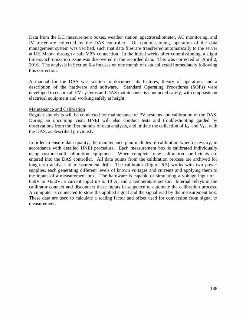
188

Data from the DC measurement boxes, weather station, spectroradiometer, AC monitoring, and

IV tracer are collected by the DAS controller. On commissioning, operation of the data

management system was verified, such that data files are transferred automatically to the server

at UH Manoa through a safe VPN connection. In the initial weeks after commissioning, a slight

time-synchronization issue was discovered in the recorded data. This was corrected on April 2,

2016. The analysis in Section 6.4 focuses on one month of data collected immediately following

this correction.

A manual for the DAS was written to document its features, theory of operation, and a

description of the hardware and software. Standard Operating Procedures (SOPs) were

developed to ensure all PV systems and DAS maintenance is conducted safely, with emphasis on

electrical equipment and working safely at height.

Maintenance and Calibration

Regular site visits will be conducted for maintenance of PV systems and calibration of the DAS.

During an upcoming visit, HNEI will also conduct tests and troubleshooting guided by

observations from the first months of data analysis, and initiate the collection of ISC and VOC with

the DAS, as described previously.

In order to ensure data quality, the maintenance plan includes re-calibration when necessary, in

accordance with detailed HNEI procedure. Each measurement box is calibrated individually

using custom-built calibration equipment. When complete, new calibration coefficients are

entered into the DAS controller. All data points from the calibration process are archived for

long-term analysis of measurement drift. The calibrator (Figure 6.5) works with two power

supplies, each generating different levels of known voltages and currents and applying them to

the inputs of a measurement box. The hardware is capable of simulating a voltage input of -

650V to +650V, a current input up to 10 A, and a temperature sensor. Internal relays in the

calibrator connect and disconnect these inputs in sequence to automate the calibration process.

A computer is connected to store the applied signal and the signal read by the measurement box.

These data are used to calculate a scaling factor and offset used for conversion from signal to

measurement.

189

a) b)

Figure 6.5: The custom built calibrator, with a) front view showing connection plate, digital multimeter

and two power supplies, and b) its portable cabinet to facilitate use at multiple locations.

An early maintenance issue discovered after system commissioning was an apparent problem

with one of the PV modules. The Solar Frontier module connected to the IV tracer showed signs

of operating issues. This module will be inspected and replaced, if necessary.

A second issue that will be investigated in the near future is the power factor (PF) measured on

PV systems using single-phase inverters (10 systems – from SMA, SolarEdge and ABB). These

systems have a PF of 0.86, while the 3-phase microinverter system (Enphase) has a PF close to 1,

as expected by datasheet specifications. Tests will be conducted to individually operate each

single-phase PV system, in order to evaluate whether the low PF is related to the interaction of

multiple PV systems on the same electrical panel.

Shading analysis

The Maui Brewing Company, located on the property immediately south of the PV test platform,

is planning to install a large PV system in their parking lot. The proposed PV system consists of

five carports, two of which will cause some degree of shading on the HNEI test platform. Based

on preliminary assessment of development plans and topography (the brewery site is

approximately 8 feet higher than the MEDB site), the new carports will partially shade the test

platform during the months of October through March. This would not only affect power

production of the test system, but also add unfortunate complexity to future data analysis.

Shading analysis was done with Sketchup, a freeware 3D visualization tool. CAD models of

relevant structures were built and placed in the locations indicated in the brewery carport plan.

The view of the two proposed carports expected to shade the test platform is shown in Figure

6.6. Although HNEI is not aware of current laws that would preclude construction of these

carports in the specified locations, HNEI and MEDB are working with Maui Brewing in hopes of

minimizing this impact.

https://docs.google.com/document/d/1xg1V1OUpxii4csx-KULJLR0PmtP3YNuUkN3sc0M68V4/edit?usp=sharing

190

Figure 6.6: Initial shading analysis in Maui Brewery’s planned PV installation.

6.3 Advancement of Data Analysis Methodology

Innovative approaches to PV performance data analysis were developed to enhance the value of

the data collected at the Maui and GHHI sites, and others around the state. Two of these are

discussed here as they relate to the results presented in Section 6.4. First, data are binned

according to angle of incidence (AOI), allowing for direct comparison of results from different

locations. Second, an important aspect of the HNEI approach to performance analysis is to

separate the DC performance ratio (PR), typically used in the literature, into current and voltage

performance, primarily to isolate optical from thermal performance. This methodology is

discussed here, and, will be described in detail in an upcoming journal article.

Matlab tools were developed to extract data from files on the UH server to develop a database of

parameters of interest. NetCDF [4] format, which supports the creation, access, and sharing of

array-oriented scientific data, was utilized for this database. From the raw data, parameters of

interest were developed, such as DC power of each module, string and system calculated from

current and voltage measurements, AC power produced by each PV system evaluated from

selected per-phase power measurements, and direct beam (DB) irradiance (difference between

global (G) and diffuse (DF) irradiance). Information related to sun position (calculated as in [5])

is also added to the database, including the angle-of-incidence (AOI) (the angle between the

normal to the PV modules and the sun direction), the air mass (AM) (the thickness of the

atmosphere crossed by the sun’s rays), and the top-of-the-atmosphere irradiance estimated in the

plane-of-array (XTRPOA), which leads to the clearness index (CI) using equation (1). Data

collected by the spectroradiometer is analyzed and the solar spectrum characterized using the

average photon energy (APE) index, calculated as in equation (2), by dividing the integrated

incident spectral irradiance by the integrated photon flux density [6].

(1) 𝐶𝐼 =𝐺

𝑋𝑇𝑅𝑃𝑂𝐴, (2) 𝐴𝑃𝐸 =

∫ 𝐺(𝜆)𝑑𝜆𝑏

𝑎

𝑞 ∫ 𝛷(𝜆)𝑑𝜆𝑏

𝑎

,

191

CI is the clearness index; G is the global irradiance collected in the plane-of-array (POA),

measured by the thermopile pyranometer [Wm-2

]; XTRPOA is the top-of-the-atmosphere

irradiance estimated in the POA [Wm-2

]; APE is the average photon energy [eV]; is the

wavelength of the light [nm]; 𝐺(𝜆) is the incident spectral irradiance for a specific wavelength

[Wm-2

nm-1

]; q is the electronic charge [=1.6e-19

C]; 𝛷(𝜆) is the incident spectral photon flux

density for a specific wavelength [m-2

s-1

nm-1

]; a, b, are the upper and lower wavelength limits of

the measured spectrum relative to the spectroradiometer wavelength sensitivity [nm].

Diurnal and daily analysis

A useful means to examine diurnal changes in PV performance is to average the results by angle

of incidence (AOI). For each recorded day, data were analyzed as follows:

1. Full day averages – including only data with AOI<70o to limit error due to directional

response of the solar sensors. These data are used as the daily average values of various

performance parameters. Monthly and yearly values are calculated using these daily values.

2. Binned by AOI – to examine the variation of the diurnal cycle, data are binned by AOI from

0o to 70

o using 10

o bins (except for the first interval from 0

o to 5

o, then every 10

o from 5

o to 75

o).

Results were calculated dissociating mornings from afternoons, using as midday the time when

sun direction is closest to normal to the PV surface. These bins correspond to periods of time

that vary from 20 to 40 minutes depending on AOI and time of the year.

AOI is a useful binning parameter because it allows analysis of PV loss due to reflection [7] and

because it allows a characterization of performance that is independent of PV module orientation

and location. The top-of-the-atmosphere solar resource (XTRPOA), used in the calculation of CI

(equation 1), increases with decreasing AOI (higher sun angle) and is constant at fixed AOI over

the course of the year. The CI per AOI, as a function of global irradiance G, collected at GHHI

in 2015, is shown in Figure 6.7. Morning values are shown in cool colors and afternoon in warm

colors. The daily averages are represented with black crosses. G is generally increasing with

decreasing AOI. At fixed AOI, CI increases when G increases, which is also generally true in

the daily averages. The analysis per AOI allows the addition of a dimension (CI) to the plots

presented in the next section, in which various parameters are plotted as a function of G. As will

be shown below, there is high correlation between CI and spectral energy. Further, plotting per

AOI provides a helpful visualization of operating conditions, such as potential operating issues

related to the inverter.

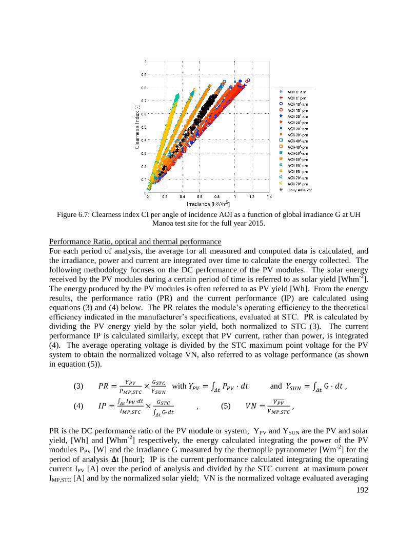
192

Figure 6.7: Clearness index CI per angle of incidence AOI as a function of global irradiance G at UH

Manoa test site for the full year 2015.

Performance Ratio, optical and thermal performance For each period of analysis, the average for all measured and computed data is calculated, and

the irradiance, power and current are integrated over time to calculate the energy collected. The

following methodology focuses on the DC performance of the PV modules. The solar energy

received by the PV modules during a certain period of time is referred to as solar yield [Whm-2

].

The energy produced by the PV modules is often referred to as PV yield [Wh]. From the energy

results, the performance ratio (PR) and the current performance (IP) are calculated using

equations (3) and (4) below. The PR relates the module’s operating efficiency to the theoretical

efficiency indicated in the manufacturer’s specifications, evaluated at STC. PR is calculated by

dividing the PV energy yield by the solar yield, both normalized to STC (3). The current

performance IP is calculated similarly, except that PV current, rather than power, is integrated

(4). The average operating voltage is divided by the STC maximum point voltage for the PV

system to obtain the normalized voltage VN, also referred to as voltage performance (as shown

in equation (5)).

(3) 𝑃𝑅 =𝑌𝑃𝑉

𝑃𝑀𝑃,𝑆𝑇𝐶×

𝐺𝑆𝑇𝐶

𝑌𝑆𝑈𝑁 with 𝑌𝑃𝑉 = ∫ 𝑃𝑃𝑉 ⋅ 𝑑𝑡

𝛥𝑡 and 𝑌𝑆𝑈𝑁 = ∫ G ⋅ 𝑑𝑡

𝛥𝑡 ,

(4) 𝐼𝑃 =∫ 𝐼𝑃𝑉⋅𝑑𝑡𝛥𝑡

𝐼𝑀𝑃,𝑆𝑇𝐶×

𝐺𝑆𝑇𝐶

∫ G⋅𝑑𝑡𝛥𝑡

, (5) 𝑉𝑁 =𝑉𝑃𝑉̅̅ ̅̅ ̅̅

𝑉𝑀𝑃,𝑆𝑇𝐶 ,

PR is the DC performance ratio of the PV module or system; YPV and YSUN are the PV and solar

yield, [Wh] and [Whm-2

] respectively, the energy calculated integrating the power of the PV

modules PPV [W] and the irradiance G measured by the thermopile pyranometer [Wm-2

] for the

period of analysis 𝚫t [hour]; IP is the current performance calculated integrating the operating

current IPV [A] over the period of analysis and divided by the STC current at maximum power

IMP,STC [A] and by the normalized solar yield; VN is the normalized voltage evaluated averaging

193

the operating voltage VPV [V] over the period of analysis normalized by the STC maximum

power voltage VMP,STC [V].

For PV modules tested individually with the IV tracer, additional electrical characteristics, VOC

and ISC, are monitored. This information will soon also be available for PV modules operating

with microinverters, due to the previously discussed switching capabilities of the DAS. As with

the calculation of current performance (IP) and normalized voltage (VN) at the maximum power

point, IPSC and VNOC are calculated as follows:

(6) 𝐼𝑃𝑆𝐶 =∫ 𝐼𝑆𝐶⋅𝑑𝑡𝛥𝑡

𝐼𝑆𝐶,𝑆𝑇𝐶×

𝐺𝑆𝑇𝐶

∫ G⋅𝑑𝑡𝛥𝑡

(7) 𝑉𝑁𝑂𝐶 =𝑉𝑂𝐶̅̅ ̅̅ ̅̅

𝑉𝑂𝐶,𝑆𝑇𝐶

where IPSC is the short-circuit current performance calculated integrating the short-circuit current

ISC [A] over the period of analysis t [hour] and divided by the STC short-circuit current ISC,STC

[A] and by the normalized solar yield; VNOC is the normalized VOC calculated averaging the

open-circuit voltage VOC [V] normalized by the STC open-circuit voltage VOC,STC [V].

For all of these performance parameters, the specifications indicated in the manufacturer's

datasheet were used for normalization. This means that the analysis results include the

normalization error due to slight differences between the actual performance of each PV module

and the specifications from the datasheet. Each PV module has a unique performance that is

determined during the manufacturing process and is evaluated by the manufacturers. The STC

flash test results (FTR) of each individual PV module are usually available upon request. The

FTR were collected for each PV module in test at MEDB, averaged per PV system, and

compared to the datasheet specifications, leading to a normalization error estimated at ±4%.

Unfortunately, one PV manufacturer did not share the FTR and another has no results on the ISC

and VOC. Thus, to provide information on all tested PV systems and modules, the performance

results normalized by FTR (which limits the impact of normalization error) are not presented in

the analysis contained in Section 6.4.

In our approach, the DC performance ratio (PR) was split into current performance (IP) and

normalized voltage (VN). The difference between PR and the product of IP and VN was

estimated to be below 1% for all periods of analysis. This small difference is a result of the

small variation of the voltage in comparison to the current during the periods of analysis, even

when considered on a daily basis. The IP is highly correlated to the IPSC as shown in the

following section. The IPSC provides the average values of ISC that characterize the optical

performance of the PV modules, which is sensitive to the intensity, incident angle and spectral

content of the irradiance, temperature, soiling and shading [8, 9]. In the analysis that follows,

results from the PV systems and modules tested in Maui and Oahu are presented in terms of DC

performance, including PR, VN, IP and its correlation with IPSC, as these parameters relate to PV

module brand/type and operating conditions. This approach allows improved understanding

relative to earlier methods by isolating optical from thermal performance.

194

6.4 PV System Performance Analysis

The instrumentation and analysis techniques discussed in preceding sections were used to

characterize the diurnal and day-to-day variation of the environmental conditions and resulting

DC performance of the PV systems. The DC performance of grid-connected PV systems is

affected by the performance of the PV modules and by system losses related to combining PV

modules into strings (mismatch loss), and potential operating issues with the inverters or

optimizers. A diagnostic approach was taken to calculate system losses by comparing the

performance of grid-connected systems to unconnected modules, tested individually with the IV

tracer. Results are presented below for the PV test platform in Maui, as well as for a one-year

dataset from UH Manoa. These results form the basis of a journal article now in preparation, as

well as a recently completed UH Master’s thesis [10].

Performance Analysis from Maui Test Site

Results presented here are for the month of April 2016 (including 25 days beginning after

correction of a data time sync issue). The analysis focuses initially on the diurnal variation of PV

performance, followed by monthly averages, detailing PR, VN, IP and its relationship to IPsc, to

examine performance differences between PV technologies in varying operating conditions. The

impact of system loss, especially loss due to operating issues in which microinverters limit

maximum module power output at high irradiance, is examined.

Diurnal performance variation

The DC performance of the Cadmium Telluride (CdTe) PV system, as an example representative

of the results obtained for all PV modules and systems at the test site, without the issue of

inverter saturation, is shown in Figure 6.8. PR, IP and VN are plotted versus G. In addition, VN

is plotted as a function of AT. The graphs indicate the performance calculated per day, per AOI,

differentiating morning (cool colors) and afternoon (warm colors) performance. Daily

performance (black crosses) shows the variability among analyzed days during the period (April

2016).

DC PR of the CdTe PV system, as a function of G, is shown in Figure 6.8a. G is generally

increasing with decreasing AOI, as seen previously in Figure 6.7, which also showed that at

fixed AOI, CI increases with increasing G. The PR values are highly distributed, ranging

between 83% and 107%. The PR is lower in the mornings than in the afternoons, especially for

AOI above 55o. The daily average PR is distributed between 94% and 101%. Performance

numbers above 100% are possible, since PR is computed according to values specified by the

manufacturer at STC. In addition to normalization error, actual environmental conditions differ

from STC.

IP, binned by AOI, as a function of G, is shown in Figure 6.8b. IP is lower in the morning than

in the afternoon. At fixed high AOI, IP tends to decrease with increasing G or CI. Daily IP

values vary within a small range between 102 and 105%. IP behavior is very similar to that of

PR, binned by AOI. IP varies by more than 25% during the day, and is largely responsible for

lower PR in the mornings than the afternoons.

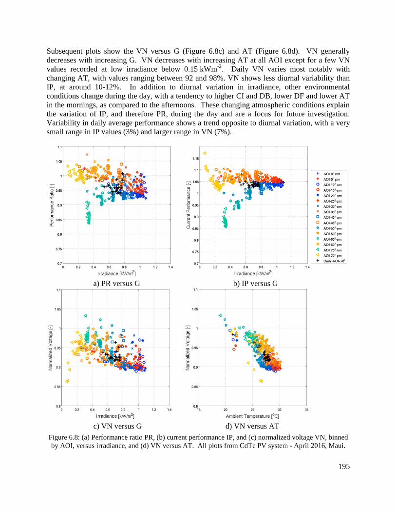
195

Subsequent plots show the VN versus G (Figure 6.8c) and AT (Figure 6.8d). VN generally

decreases with increasing G. VN decreases with increasing AT at all AOI except for a few VN

values recorded at low irradiance below 0.15 kWm-2

. Daily VN varies most notably with

changing AT, with values ranging between 92 and 98%. VN shows less diurnal variability than

IP, at around 10-12%. In addition to diurnal variation in irradiance, other environmental

conditions change during the day, with a tendency to higher CI and DB, lower DF and lower AT

in the mornings, as compared to the afternoons. These changing atmospheric conditions explain

the variation of IP, and therefore PR, during the day and are a focus for future investigation.

Variability in daily average performance shows a trend opposite to diurnal variation, with a very

small range in IP values (3%) and larger range in VN (7%).

a) PR versus G b) IP versus G

c) VN versus G d) VN versus AT

Figure 6.8: (a) Performance ratio PR, (b) current performance IP, and (c) normalized voltage VN, binned

by AOI, versus irradiance, and (d) VN versus AT. All plots from CdTe PV system - April 2016, Maui.

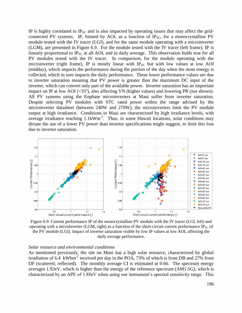
196

IP is highly correlated to IPSC and is also impacted by operating issues that may affect the grid-

connected PV systems. IP, binned by AOI, as a function of IPSC, for a monocrystalline PV

module tested with the IV tracer (LGI), and for the same module operating with a microinverter

(LGM), are presented in Figure 6.9. For the module tested with the IV tracer (left frame), IP is

linearly proportional to IPSC at all AOI, and in daily average. This observation holds true for all

PV modules tested with the IV tracer. In comparison, for the module operating with the

microinverter (right frame), IP is mostly linear with IPSC but with low values at low AOI

(midday), which impacts the performance during the portion of the day when the most energy is

collected, which in turn impacts the daily performance. These lower performance values are due

to inverter saturation meaning that PV power is greater than the maximum DC input of the

inverter, which can convert only part of the available power. Inverter saturation has an important

impact on IP at low AOI (<35º), also affecting VN (higher values) and lowering PR (not shown).

All PV systems using the Enphase microinverters at Maui suffer from inverter saturation.

Despite selecting PV modules with STC rated power within the range advised by the

microinverter datasheet (between 240W and 270W), the microinverters limit the PV module

output at high irradiance. Conditions in Maui are characterized by high irradiance levels, with

average irradiance reaching 1.1kWm-2

. Thus, in some Hawaii locations, solar conditions may

dictate the use of a lower PV power than inverter specifications might suggest, to limit this loss

due to inverter saturation.

Figure 6.9: Current performance IP of the monocrystalline PV module with the IV tracer (LGI, left) and

operating with a microinverter (LGM, right) as a function of the short-circuit current performance IPSC of

the PV module (LGI). Impact of inverter saturation visible by low IP values at low AOI, affecting the

daily average performance.

Solar resource and environmental conditions

As mentioned previously, the site on Maui has a high solar resource, characterized by global

irradiation of 6.4 kWhm-2

received per day in the POA, 73% of which is from DB and 27% from

DF (scattered, reflected). The monthly average CI is estimated at 0.66. The spectrum energy

averages 1.92eV, which is higher than the energy of the reference spectrum (AM1.5G), which is

characterized by an APE of 1.88eV when using our instrument’s spectral sensitivity range. This

197

means that the solar spectrum at the site is rich in low wavelengths compared to the reference

spectrum. Daytime AT averaged 27oC in April 2016, varying between 25

oC and 29

oC, with one

cooler day at 21oC.

Comparison of PV technologies and test conditions

Monthly averages of DC performance obtained at MEDB during April 2016, on all instrumented

PV systems, including the results of the modules tested with the IV tracer, are presented here.

These results emphasize DC performance of individual modules, since only one module in each

PV system that employs a microinverter or optimizer is instrumented. For the string inverter

systems, the results reflect the performance of the strings of PV modules. To ensure that

sampling time was not impacting the results, datasets synchronized with IV tracer measurements,

with a sampling time of 3 minutes, were selected for analysis. The impact of sampling time is

minor on the daily average results, with the difference estimated to be below 0.8% when

comparing results using a 1-second dataset versus a 3-minute dataset.

Monthly PR, IP and VN, calculated using datasheet specifications for normalization, are

presented in Figure 6.10. PR is plotted on the x-axis, with IP and VN on the y-axis. The best

performing PV systems are thus located on the right side of the graph. The data collected by the

IV tracer are in blue squares for VN and red diamonds for IP, while green circles and yellow

triangles correspond to performance of the PV modules in grid-connected operation. PV system

acronyms are as defined previously in Table 2. PR ranges between 86% and 97%, depending on

PV modules and test conditions. The best performing grid-connected system/module is the SFS

CIGS system, with a PR of 97%, while the second tested CIGS system, STS, is one of the poorer

performers, with a PR of 87%. The second best performer is the CdTe FSS system, with a PR of

96%. Following that system are the HIT PAM/PAS systems, with PR between 91% and 92%

and the Sunpower modules, with PR between 89% and 90%. Systems with PR below 88.5%

include the polycrystalline (ETM, KYM and SW), the CIGS STS, the monocrystalline LGM and

the bifacial monocrystalline SUM. IP is estimated at 90% for the CIGS system STS and 104%

for the CdTe. For all other PV systems, IP is between 95% and 101%. VN is lowest, at 88%, for

the polycrystalline from SW, increasing to above 96% for the 2 tested CIGS systems. The

remaining systems show VN between 89% and 94%.

The performance of the PV modules tested with the IV tracer (blue squares and red diamonds) is

generally higher by ~1%, as compared to the grid-connected systems. The CIGS module FS

exhibited operating issues, which decrease the performance by up to 4% in PR, as compared to

the grid-connected PV system. This module will be inspected and likely replaced in the near

future. The CdTe PV module is the best performer with a PR at 97%, followed by the HIT at

92.5%. The rest of the PV modules have a PR between 89% and 90% except for the CIGS STI

at 88% and the polycrystalline SWI at 87%. The PV systems tested with the Enphase

microinverters (ETM, KYM, LGM and SWM) exhibit the highest IP difference between test

conditions, with differences from 0.9% to 2.9% in IP, affecting the PR by up to 2.2%. These

results suggest low impact of test conditions on DC performance of the PV modules operating at

MEDB and limited impact of system loss (around 1%), which increases slightly in the case of

inverter saturation to ~2% in the monthly average.

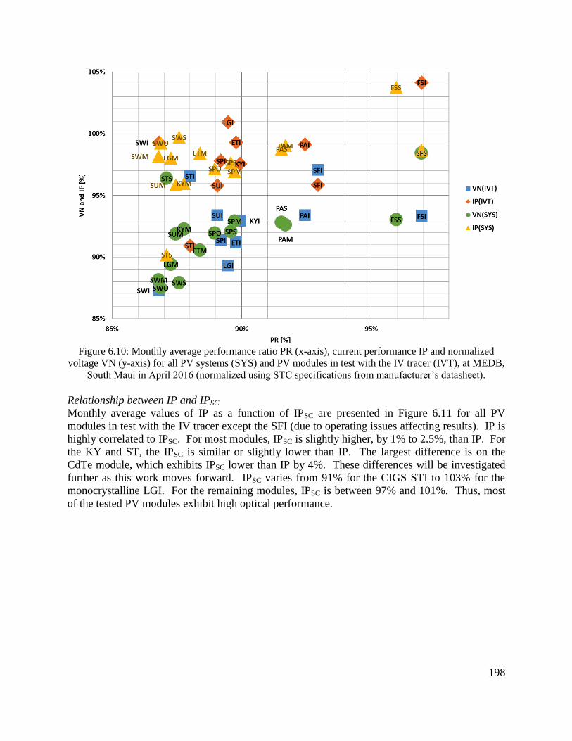
198

Figure 6.10: Monthly average performance ratio PR (x-axis), current performance IP and normalized

voltage VN (y-axis) for all PV systems (SYS) and PV modules in test with the IV tracer (IVT), at MEDB,

South Maui in April 2016 (normalized using STC specifications from manufacturer’s datasheet).

Relationship between IP and IPSC

Monthly average values of IP as a function of IPSC are presented in Figure 6.11 for all PV

modules in test with the IV tracer except the SFI (due to operating issues affecting results). IP is

highly correlated to IPSC. For most modules, IPSC is slightly higher, by 1% to 2.5%, than IP. For

the KY and ST, the IPSC is similar or slightly lower than IP. The largest difference is on the

CdTe module, which exhibits IPSC lower than IP by 4%. These differences will be investigated

further as this work moves forward. IPSC varies from 91% for the CIGS STI to 103% for the

monocrystalline LGI. For the remaining modules, IPSC is between 97% and 101%. Thus, most

of the tested PV modules exhibit high optical performance.

199

Figure 6.11: Monthly average current performance IP as a function of short-circuit current performance

IPSC for all PV modules tested with the IV tracer at MEDB, South Maui in April 2016 (normalized using

STC specifications from manufacturer’s datasheet).

Performance Analysis from UH Manoa/GHHI Test Site - 2015

The method of analysis described above was used to analyze 1 year of data collected at the PV

test site located on the campus of UH Manoa. Two PV technologies are installed at this location

– micromorph tandem thin film and polycrystalline, as detailed in Table 6.2, which includes the

PV manufacturer, model number, maximum power and efficiency at STC, number and

technology of the modules, and associated string inverters.

Table 6.2: Description of the PV arrays operating at GHHI in Oahu.

PV Modules Rated Power [W] 𝛈 [%] # of PV PV Technology Auxiliaries

Kyocera KD205 (2//13) 250 13.8 26 Polycrystalline Sunny Boy SMA-5000US (1)

Mitsubishi Heavy Industries MT130 (6//4) 130 8.5 24 Micromorph Sunny Boy SMA-3000US (1)

In the analysis below, the diurnal and day-to-day variation of environmental conditions is

described and correlation between atmospheric parameters established. The DC performance of

the PV systems and individual modules (tested with the IV tracer) is examined to establish the

primary factors affecting performance, to characterize the optical and thermal performance of the

PV technologies, to estimate the performance distribution of the PV modules at this site, and to

determine the impact of mismatch loss. Finally, the impact of degradation, at this 4-year old site,

on the performance of the PV systems is assessed using 2011 to 2013 datasets. Part of the work

presented here formed the core of a recently completed HNEI Master’s thesis [10].

IV curves were collected every minute in 2015 on the GHHI modules. The IV tracer, which was

selected for testing at the final location in Maui, can test a maximum of 4 micromorph and 2

polycrystalline PV modules at any given time. At GHHI, two sets of PV modules were tested

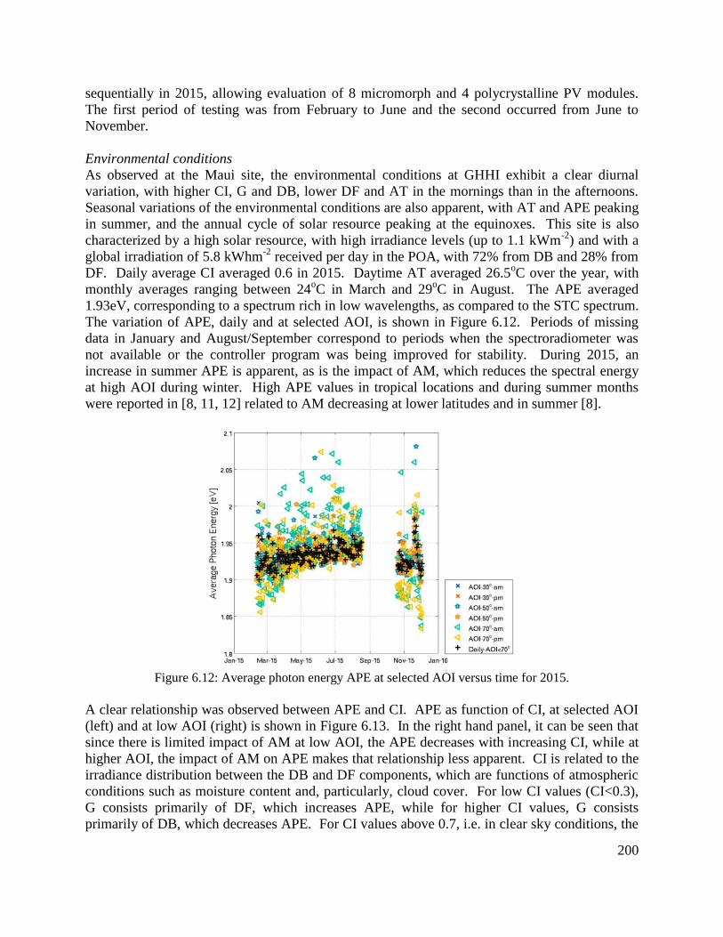
200

sequentially in 2015, allowing evaluation of 8 micromorph and 4 polycrystalline PV modules.

The first period of testing was from February to June and the second occurred from June to

November.

Environmental conditions

As observed at the Maui site, the environmental conditions at GHHI exhibit a clear diurnal

variation, with higher CI, G and DB, lower DF and AT in the mornings than in the afternoons.

Seasonal variations of the environmental conditions are also apparent, with AT and APE peaking

in summer, and the annual cycle of solar resource peaking at the equinoxes. This site is also

characterized by a high solar resource, with high irradiance levels (up to 1.1 kWm-2

) and with a

global irradiation of 5.8 kWhm-2

received per day in the POA, with 72% from DB and 28% from

DF. Daily average CI averaged 0.6 in 2015. Daytime AT averaged 26.5oC over the year, with

monthly averages ranging between 24oC in March and 29

oC in August. The APE averaged

1.93eV, corresponding to a spectrum rich in low wavelengths, as compared to the STC spectrum.

The variation of APE, daily and at selected AOI, is shown in Figure 6.12. Periods of missing

data in January and August/September correspond to periods when the spectroradiometer was

not available or the controller program was being improved for stability. During 2015, an

increase in summer APE is apparent, as is the impact of AM, which reduces the spectral energy

at high AOI during winter. High APE values in tropical locations and during summer months

were reported in [8, 11, 12] related to AM decreasing at lower latitudes and in summer [8].

Figure 6.12: Average photon energy APE at selected AOI versus time for 2015.

A clear relationship was observed between APE and CI. APE as function of CI, at selected AOI

(left) and at low AOI (right) is shown in Figure 6.13. In the right hand panel, it can be seen that

since there is limited impact of AM at low AOI, the APE decreases with increasing CI, while at

higher AOI, the impact of AM on APE makes that relationship less apparent. CI is related to the

irradiance distribution between the DB and DF components, which are functions of atmospheric

conditions such as moisture content and, particularly, cloud cover. For low CI values (CI<0.3),

G consists primarily of DF, which increases APE, while for higher CI values, G consists

primarily of DB, which decreases APE. For CI values above 0.7, i.e. in clear sky conditions, the

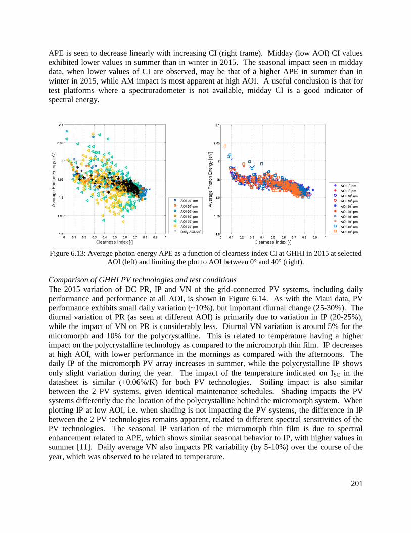
201

APE is seen to decrease linearly with increasing CI (right frame). Midday (low AOI) CI values

exhibited lower values in summer than in winter in 2015. The seasonal impact seen in midday

data, when lower values of CI are observed, may be that of a higher APE in summer than in

winter in 2015, while AM impact is most apparent at high AOI. A useful conclusion is that for

test platforms where a spectroradometer is not available, midday CI is a good indicator of

spectral energy.

Figure 6.13: Average photon energy APE as a function of clearness index CI at GHHI in 2015 at selected

AOI (left) and limiting the plot to AOI between 0° and 40° (right). Comparison of GHHI PV technologies and test conditions

The 2015 variation of DC PR, IP and VN of the grid-connected PV systems, including daily

performance and performance at all AOI, is shown in Figure 6.14. As with the Maui data, PV

performance exhibits small daily variation (~10%), but important diurnal change (25-30%). The

diurnal variation of PR (as seen at different AOI) is primarily due to variation in IP (20-25%),

while the impact of VN on PR is considerably less. Diurnal VN variation is around 5% for the

micromorph and 10% for the polycrystalline. This is related to temperature having a higher

impact on the polycrystalline technology as compared to the micromorph thin film. IP decreases

at high AOI, with lower performance in the mornings as compared with the afternoons. The

daily IP of the micromorph PV array increases in summer, while the polycrystalline IP shows

only slight variation during the year. The impact of the temperature indicated on ISC in the

datasheet is similar (+0.06%/K) for both PV technologies. Soiling impact is also similar

between the 2 PV systems, given identical maintenance schedules. Shading impacts the PV

systems differently due the location of the polycrystalline behind the micromorph system. When

plotting IP at low AOI, i.e. when shading is not impacting the PV systems, the difference in IP

between the 2 PV technologies remains apparent, related to different spectral sensitivities of the

PV technologies. The seasonal IP variation of the micromorph thin film is due to spectral

enhancement related to APE, which shows similar seasonal behavior to IP, with higher values in

summer [11]. Daily average VN also impacts PR variability (by 5-10%) over the course of the

year, which was observed to be related to temperature.

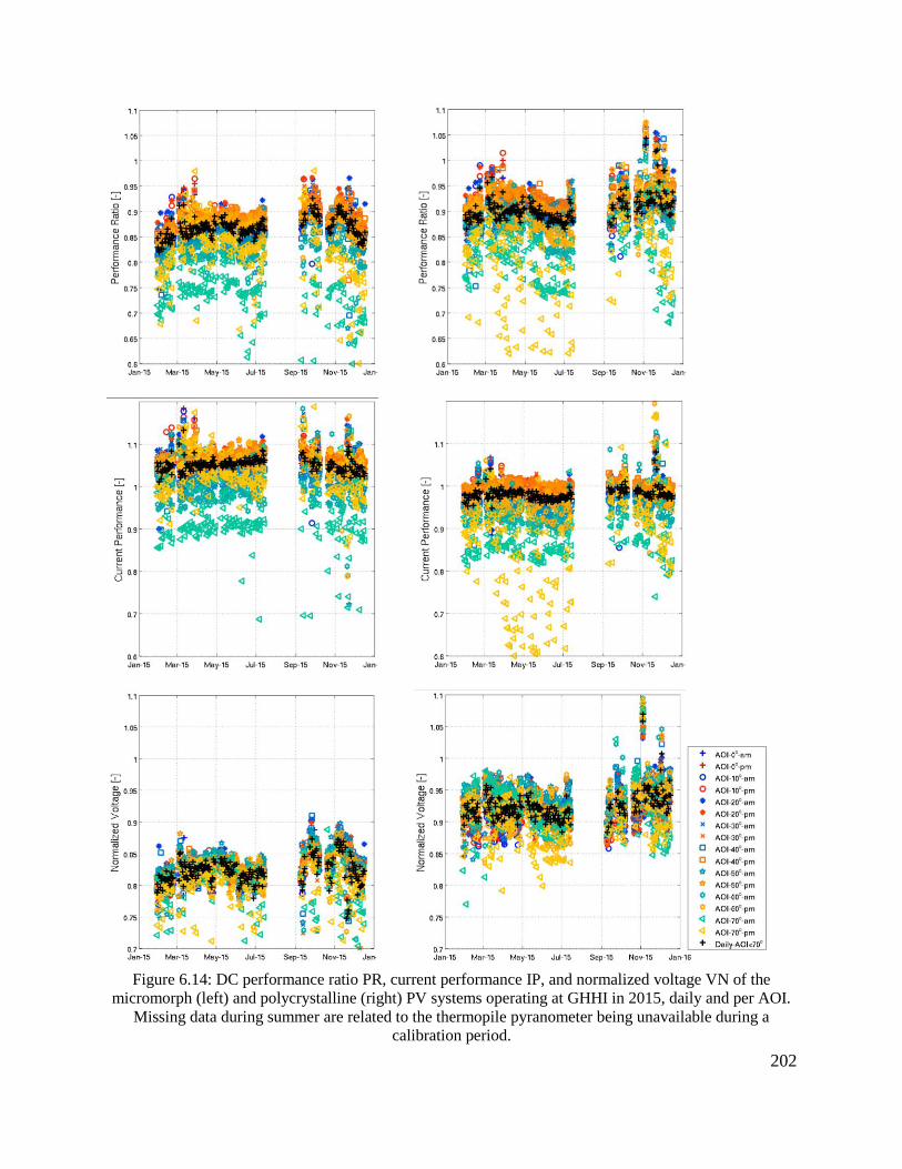
202

Figure 6.14: DC performance ratio PR, current performance IP, and normalized voltage VN of the

micromorph (left) and polycrystalline (right) PV systems operating at GHHI in 2015, daily and per AOI.

Missing data during summer are related to the thermopile pyranometer being unavailable during a

calibration period.

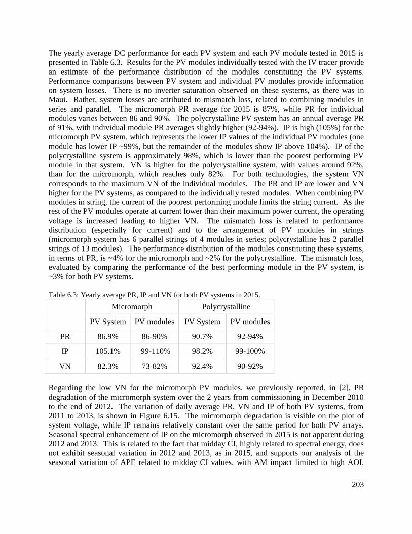
203

The yearly average DC performance for each PV system and each PV module tested in 2015 is

presented in Table 6.3. Results for the PV modules individually tested with the IV tracer provide

an estimate of the performance distribution of the modules constituting the PV systems.

Performance comparisons between PV system and individual PV modules provide information

on system losses. There is no inverter saturation observed on these systems, as there was in

Maui. Rather, system losses are attributed to mismatch loss, related to combining modules in

series and parallel. The micromorph PR average for 2015 is 87%, while PR for individual

modules varies between 86 and 90%. The polycrystalline PV system has an annual average PR

of 91%, with individual module PR averages slightly higher (92-94%). IP is high (105%) for the

micromorph PV system, which represents the lower IP values of the individual PV modules (one

module has lower IP ~99%, but the remainder of the modules show IP above 104%). IP of the

polycrystalline system is approximately 98%, which is lower than the poorest performing PV

module in that system. VN is higher for the polycrystalline system, with values around 92%,

than for the micromorph, which reaches only 82%. For both technologies, the system VN

corresponds to the maximum VN of the individual modules. The PR and IP are lower and VN

higher for the PV systems, as compared to the individually tested modules. When combining PV

modules in string, the current of the poorest performing module limits the string current. As the

rest of the PV modules operate at current lower than their maximum power current, the operating

voltage is increased leading to higher VN. The mismatch loss is related to performance

distribution (especially for current) and to the arrangement of PV modules in strings

(micromorph system has 6 parallel strings of 4 modules in series; polycrystalline has 2 parallel

strings of 13 modules). The performance distribution of the modules constituting these systems,

in terms of PR, is ~4% for the micromorph and ~2% for the polycrystalline. The mismatch loss,

evaluated by comparing the performance of the best performing module in the PV system, is

~3% for both PV systems.

Table 6.3: Yearly average PR, IP and VN for both PV systems in 2015.

Micromorph Polycrystalline

PV System PV modules PV System PV modules

PR 86.9% 86-90% 90.7% 92-94%

IP 105.1% 99-110% 98.2% 99-100%

VN 82.3% 73-82% 92.4% 90-92%

Regarding the low VN for the micromorph PV modules, we previously reported, in [2], PR

degradation of the micromorph system over the 2 years from commissioning in December 2010

to the end of 2012. The variation of daily average PR, VN and IP of both PV systems, from

2011 to 2013, is shown in Figure 6.15. The micromorph degradation is visible on the plot of

system voltage, while IP remains relatively constant over the same period for both PV arrays.

Seasonal spectral enhancement of IP on the micromorph observed in 2015 is not apparent during

2012 and 2013. This is related to the fact that midday CI, highly related to spectral energy, does

not exhibit seasonal variation in 2012 and 2013, as in 2015, and supports our analysis of the

seasonal variation of APE related to midday CI values, with AM impact limited to high AOI.

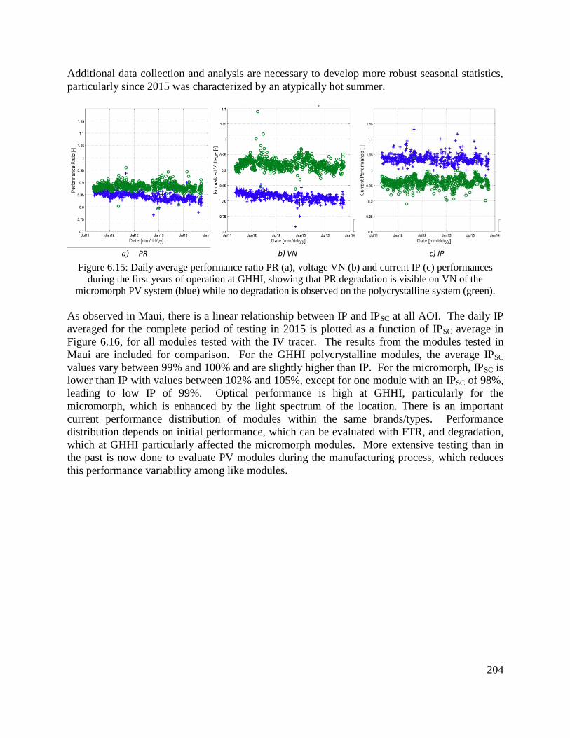
204

Additional data collection and analysis are necessary to develop more robust seasonal statistics,

particularly since 2015 was characterized by an atypically hot summer.

a) PR b) VN c) IP

Figure 6.15: Daily average performance ratio PR (a), voltage VN (b) and current IP (c) performances

during the first years of operation at GHHI, showing that PR degradation is visible on VN of the

micromorph PV system (blue) while no degradation is observed on the polycrystalline system (green).

As observed in Maui, there is a linear relationship between IP and IPSC at all AOI. The daily IP

averaged for the complete period of testing in 2015 is plotted as a function of IPSC average in

Figure 6.16, for all modules tested with the IV tracer. The results from the modules tested in

Maui are included for comparison. For the GHHI polycrystalline modules, the average IPSC

values vary between 99% and 100% and are slightly higher than IP. For the micromorph, IPSC is

lower than IP with values between 102% and 105%, except for one module with an IPSC of 98%,

leading to low IP of 99%. Optical performance is high at GHHI, particularly for the

micromorph, which is enhanced by the light spectrum of the location. There is an important

current performance distribution of modules within the same brands/types. Performance

distribution depends on initial performance, which can be evaluated with FTR, and degradation,

which at GHHI particularly affected the micromorph modules. More extensive testing than in

the past is now done to evaluate PV modules during the manufacturing process, which reduces

this performance variability among like modules.

205

Figure 6.16: Daily average current performance IP as a function of the short-circuit current performance

IPSC of the micromorph and polycrystalline PV modules tested with the IV tracer at GHHI in 2015 and for

the PV modules tested at Maui/MEDB in April 2016.

When comparing the performance results at GHHI to those from Maui, the Kyocera

polycrystalline modules have similar PR, IP and VN. The micromorph PV system has high IP

(105%), similar to the CdTe technology, and a VN lower than all other tested PV modules due

the 2-year long degradation (micromorph VN was 87-88% at commissioning in 2010). The

correlation between IP and IPSC is similar for the micromorph and the CdTe tested at MEDB,

with IPSC significantly lower than IP, while for most PV modules, IPSC is similar to or slightly

lower than IP. More investigation is needed to understand the correlation between IP and IPSC

among various PV technologies. The micromorph PV modules exhibit high IP (up to 110%) and

IPSC (up to 105%) values, and are sensitive to the seasonal variation of the spectral energy in

2015. The micromorph technology is enhanced by the location’s light spectrum, which is rich in

low wavelengths.

6.5 Conclusions

Important milestones were achieved in our understanding of the performance of grid-connected

PV systems operating in Hawaii. DC performance is affected by varying environmental

conditions, PV technology, and variations among like modules introduced in the manufacturing

process. DC performance of PV systems is also affected by system losses related to combining

PV modules into strings (mismatch loss) and due to the potential operating issues with the

inverters and optimizers. Test protocols and analysis tools were developed to streamline data

collection and better characterize module performance, and to identify and quantify the impact of

system architectures and losses. Methodologies and instrumentation were developed at the UH

campus site (GHHI), for incorporation into a new test site located on the island of Maui.

206

After considerable planning and permitting delays, the Maui test platform was commissioned in

February 2016, instrumented with the new HNEI DAS and providing side-by-side operation of

15 PV systems testing 10 PV module brands/types and 3 system architectures. PV technologies

in test include mono and polycrystalline, bifacial, high efficient and thin films (CdTe, CIGS and

micromorph). The test platform also has the capability to collect data on individual modules

through the use of an IV tracer that can record complete performance characteristics (IV curves)

in the absence of system losses. System losses can then be quantified by comparing this isolated

module performance with performance in grid-connected operation.

Newly developed analysis methodologies have enhanced our understanding of the diurnal and

day-to-day variation of DC performance and allowed us to identify the most important

environmental parameters and operating conditions. Specifically, we dissociate PR, typically

used to characterize PV performance, into current performance, which is highly correlated to

short-circuit current and characterizes optical performance, and voltage performance, which is

primarily related to thermal conditions. Current and voltage performance are also affected by

system losses and module degradation. Current performance was seen to be most sensitive to

inverter saturation (with corresponding impact on PR), while voltage performance proves to be a

good indicator of performance degradation. This innovative approach is useful for identifying

spectral enhancement (current) as well as temperature impact and degradation (voltage) on the

long-term performance of the PV systems or modules. Further, by analyzing performance at

varying incident angles, we are able to assess the diurnal variation of system performance, to

diagnose special operating conditions and issues (shading, reflection and inverter saturation), and

to compare performance of PV systems in different locations/orientations.

Experimental results were analyzed for a month (April 2016) at the new Maui site and for a year

(2015) at the UH Manoa site. Both locations are characterized by high daily average irradiation

(~ 6 kWhm-2

). An important finding that is related to high irradiance is that, despite

specifications from manufacturers, inverter saturation is likely at high sun angles in these tropical

locations. This suggests that lower PV power than would normally be advised may be

appropriate in such locations – for a given inverter. Also, the light spectrum in both locations is

rich in low wavelengths, as expected by the latitude. This is favorable to PV technologies that

are spectrally enhanced by low wavelengths, such as the micromorph tested on Oahu.

Daily average DC performance ratio of grid-connected systems was found to be between 86%

and 97%. The impact of DC system losses was below 3% at both locations, which is within the

range of normalization error (±4%). PV system performance variability is thus primarily related

to the selected PV modules. Optical performance of the tested PV modules varies by 14%, with

most modules performing between 95 and 101%, except one low performer (91% - CIGS) and

two high performers (104-105% - amorphous and CdTe). Thermal performance varies between

modules by 15% with most modules performing between 87 and 94%, with higher performance

(96-98%) for the two CIGS modules and degraded performance for the 4-year old micromorph

system (83%). While the standard crystalline modules exhibit similar performance, the two

tested CIGS modules exhibited a large difference of 10%.

207

Performance analysis of grid-connected PV systems operating in Hawaii will be continued, with

emphasis on the data now being collected at the fully instrumented Maui test platform, and at

other sites in Hawaii. Operating issues such as inverter saturation will be further diagnosed,

along with the impact of soiling and shading. The AC performance of the PV systems will be

analyzed to provide information on the efficiency and reliability of the inverters and optimizers.

The data collected by the IV tracer will serve be used to determine the impact of environmental

conditions and angle of incidence on short-circuit current, open-circuit voltage, and their

correlation with the maximum operating point. These efforts will ultimately lead to the

development of a performance modeling approach, suited to Hawaii and other locations, that will

allow the prediction of diurnal, monthly, seasonal, and long-term variation of PV module and

system performance.

Acronyms

Symbol Name Unit

AC Alternative current

AM Air mass -

AOI Angle-of-incidence o

APE Average photon energy eV

CdTe Cadmium telluride

CI Clearness index -

CIGS Copper indium gallium selenide

DAS Data acquisition system

DB Direct beam Wm-2

DC Direct current

DF Diffuse irradiance Wm-2

Spectral photon flux density m-2

s-1

nm-1

FTR Flash test result

G Global irradiance Wm-2

GHHI Green Holmes Hall Initiative

GSTC Irradiance at STC Wm-2

HIT Heterojunction intrinsic thin layer

IMP,STC Maximum power point current at STC A

IP Current performance -

IPV Operating PV current A

ISC Short-circuit current A

Wavelength nm

PF Power factor -

POA Plane of array

PMP,STC Maximum power at STC W

PPV Operating PV power W

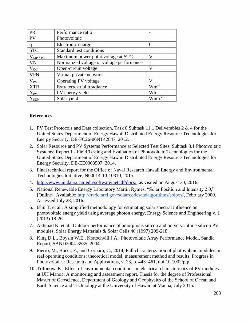
208

PR Performance ratio -

PV Photovoltaic

q Electronic charge C

STC Standard test conditions

VMP,STC Maximum power point voltage at STC V

VN Normalized voltage or voltage performance -

VOC Open-circuit voltage V

VPN Virtual private network

VPV Operating PV voltage V

XTR Extraterrestrial irradiance Wm-2

YPV PV energy yield Wh

YSUN Solar yield Whm-2

References

1. PV Test Protocols and Data collection, Task 8 Subtask 11.1 Deliverables 2 & 4 for the

United States Department of Energy Hawaii Distributed Energy Resource Technologies for

Energy Security, DE-FC26-06NT42847, 2012.

2. Solar Resource and PV Systems Performance at Selected Test Sites, Subtask 3.1 Photovoltaic

Systems: Report 1 - Field Testing and Evaluation of Photovoltaic Technologies for the

United States Department of Energy Hawaii Distributed Energy Resource Technologies for

Energy Security, DE-EE0003507, 2014.

3. Final technical report for the Office of Naval Research Hawaii Energy and Environmental

Technologies Initiative, N00014-10-10310, 2015.

4. http://www.unidata.ucar.edu/software/netcdf/docs/, as visited on August 30, 2016.

5. National Renewable Energy Laboratory Martin Rymes, “Solar Position and Intensity 2.0,”

[Online]. Available: http://rredc.nrel.gov/solar/codesandalgorithms/solpos/, February 2000.

Accessed July 28, 2016.

6. Ishii T. et al., A simplified methodology for estimating solar spectral influence on

photovoltaic energy yield using average photon energy, Energy Science and Engineering v. 1

(2013) 18-26.

7. Akhmad K. et al., Outdoor performance of amorphous silicon and polycrystalline silicon PV

modules, Solar Energy Materials & Solar Cells 46 (1997) 209-218.

8. King D.L., Boysin W.E., Kratochvill J.A., Photovoltaic Array Performance Model, Sandia

Report, SAND2004-3535, 2004.

9. Pierro, M., Bucci, F., and Cornaro, C., 2014, Full characterization of photovoltaic modules in

real operating conditions: theoretical model, measurement method and results, Progress in

Photovoltaics: Research and Applications, v. 23, p. 443–461, doi:10.1002/pip.

10. Trifonova K., Effect of environmental conditions on electrical characteristics of PV modules

at UH Manoa: A monitoring and assessment report, Thesis for the degree of Professional

Master of Geoscience, Department of Geology and Geophysics of the School of Ocean and

Earth Science and Technology at the University of Hawaii at Manoa, July 2016.

http://www.unidata.ucar.edu/software/netcdf/docs/

http://rredc.nrel.gov/solar/codesandalgorithms/solpos/

209

11. Minemoto T. et al., Effect of irradiance distribution on the outdoor performance of

amorphous Si//thin-film crystalline Si stacked photovoltaic modules, Solar Energy Materials

& Solar Cells 91 (2005) 120-122.

12. Gottschalg R., Infield D.G., Kearney M.J., Experimental study of variations of the solar

spectrum of relevance to thin film solar cells, Solar Energy Materials & Solar Cells 79 (2003)

527-537.

Task 7. HYDROGEN SYSTEMS

HNEI has developed and implemented hydrogen projects on Oahu and Hawaii Island with

collaborative funding from ONR, US DOE, and the State of Hawaii. HEET10 projects focus on

four main areas: modification of a hydrogen fueling station on Oahu to a dual pressure 350/700

bar “fast fill” station; design and installation of a hydrogen dispensing station on Hawaii Island;

production of hydrogen fuel from agriculture in Hawaii, and; assessment of alternative pathways

to meet the projected growth in demand for hydrogen in Hawaii, namely gasification of

municipal solid waste (MSW), and importation of natural gas in small-scale container vessels.

7.1 Demonstration Hydrogen Fueling Technology at Marine Corps Base Hawaii

The US Navy/Marine Corps conducted technical evaluations and gained valuable experience in

the operation of fuel cell electric vehicles (FCEVs) using a fleet of 5 General Motors (GM)

Equinox FCEVs deployed by ONR for potential use in operational systems as well as non-

tactical commercial fleet vehicle operations. The Marine Corps Base Hawaii (MCBH) hydrogen

fueling station used to support the demonstration program was provided by funding from the US

Department of Energy and the State of Hawaii who contributed an existing 350 bar fueling

station, and by the Office of Naval Research (ONR) that converted the station to provide a dual

pressure 350/700 bar fast fill capability using HEET 9 funding. The HEET 10 grant supported

the operation of the Equinox fuel cell electric vehicles by initially supplying hydrogen imported

from the mainland, supporting the O&M tasks associated with operating the hydrogen fueling

station after it became operational in November 2014, and analysis of the station’s technical

performance.

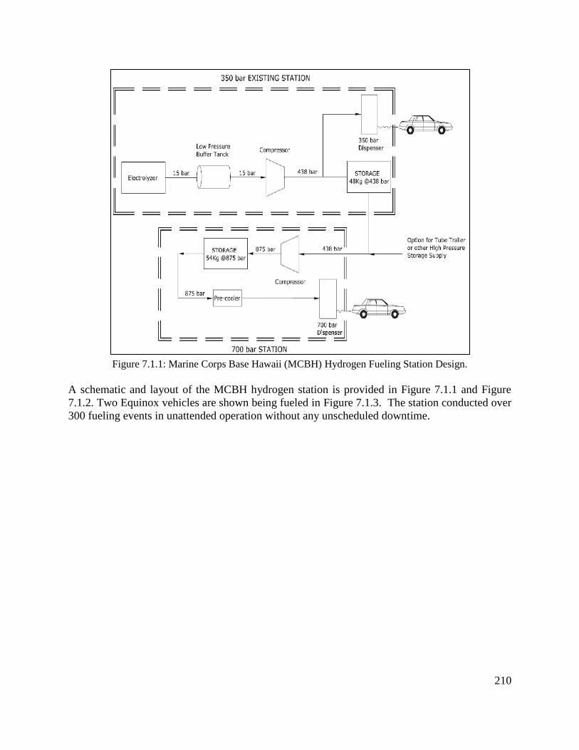
210

Figure 7.1.1: Marine Corps Base Hawaii (MCBH) Hydrogen Fueling Station Design.

A schematic and layout of the MCBH hydrogen station is provided in Figure 7.1.1 and Figure

7.1.2. Two Equinox vehicles are shown being fueled in Figure 7.1.3. The station conducted over

300 fueling events in unattended operation without any unscheduled downtime.

211

Figure 7.1.2: MCBH Hydrogen Fueling Station Layout.

Figure 7.1.3: MCBH Hydrogen Fueling Station

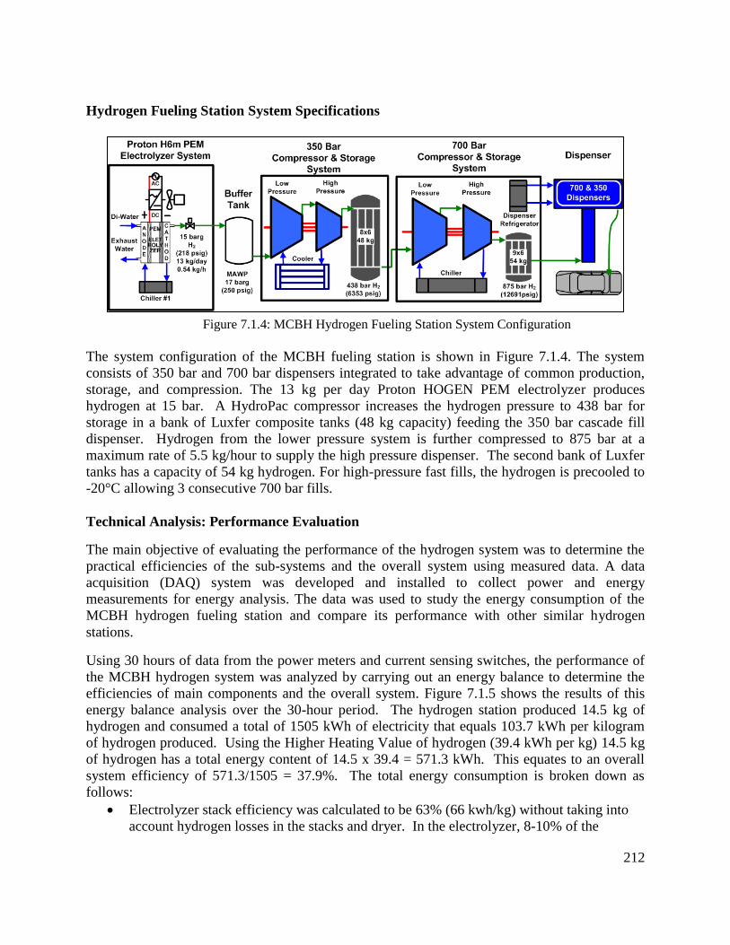
212

Hydrogen Fueling Station System Specifications

Figure 7.1.4: MCBH Hydrogen Fueling Station System Configuration

The system configuration of the MCBH fueling station is shown in Figure 7.1.4. The system

consists of 350 bar and 700 bar dispensers integrated to take advantage of common production,

storage, and compression. The 13 kg per day Proton HOGEN PEM electrolyzer produces

hydrogen at 15 bar. A HydroPac compressor increases the hydrogen pressure to 438 bar for

storage in a bank of Luxfer composite tanks (48 kg capacity) feeding the 350 bar cascade fill

dispenser. Hydrogen from the lower pressure system is further compressed to 875 bar at a

maximum rate of 5.5 kg/hour to supply the high pressure dispenser. The second bank of Luxfer

tanks has a capacity of 54 kg hydrogen. For high-pressure fast fills, the hydrogen is precooled to

-20°C allowing 3 consecutive 700 bar fills.

Technical Analysis: Performance Evaluation

The main objective of evaluating the performance of the hydrogen system was to determine the

practical efficiencies of the sub-systems and the overall system using measured data. A data

acquisition (DAQ) system was developed and installed to collect power and energy

measurements for energy analysis. The data was used to study the energy consumption of the

MCBH hydrogen fueling station and compare its performance with other similar hydrogen

stations.

Using 30 hours of data from the power meters and current sensing switches, the performance of

the MCBH hydrogen system was analyzed by carrying out an energy balance to determine the

efficiencies of main components and the overall system. Figure 7.1.5 shows the results of this

energy balance analysis over the 30-hour period. The hydrogen station produced 14.5 kg of

hydrogen and consumed a total of 1505 kWh of electricity that equals 103.7 kWh per kilogram

of hydrogen produced. Using the Higher Heating Value of hydrogen (39.4 kWh per kg) 14.5 kg

of hydrogen has a total energy content of 14.5 x 39.4 = 571.3 kWh. This equates to an overall

system efficiency of 571.3/1505 = 37.9%. The total energy consumption is broken down as

follows:

Electrolyzer stack efficiency was calculated to be 63% (66 kwh/kg) without taking into

account hydrogen losses in the stacks and dryer. In the electrolyzer, 8-10% of the

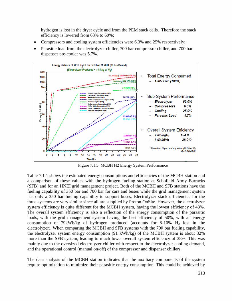
213

hydrogen is lost in the dryer cycle and from the PEM stack cells. Therefore the stack

efficiency is lowered from 63% to 60%;

Compressors and cooling system efficiencies were 6.3% and 25% respectively;

Parasitic load from the electrolyzer chiller, 700 bar compressor chiller, and 700 bar

dispenser pre-cooler was 5.7%.

Figure 7.1.5: MCBH H2 Energy System Performance

Table 7.1.1 shows the estimated energy consumptions and efficiencies of the MCBH station and

a comparison of these values with the hydrogen fueling station at Schofield Army Barracks

(SFB) and for an HNEI grid management project. Both of the MCBH and SFB stations have the

fueling capability of 350 bar and 700 bar for cars and buses while the grid management system

has only a 350 bar fueling capability to support buses. Electrolyzer stack efficiencies for the

three systems are very similar since all are supplied by Proton OnSite. However, the electrolyzer

system efficiency is quite different for the MCBH system, having the lowest efficiency of 43%.

The overall system efficiency is also a reflection of the energy consumption of the parasitic

loads, with the grid management system having the best efficiency of 50%, with an energy

consumption of 79kWh/kg of hydrogen produced (accounts for 8-10% H2 lost in the

electrolyzer). When comparing the MCBH and SFB systems with the 700 bar fueling capability,

the electrolyzer system energy consumption (91 kWh/kg) of the MCBH system is about 32%

more than the SFB system, leading to much lower overall system efficiency of 38%. This was

mainly due to the oversized electrolyzer chiller with respect to the electrolyzer cooling demand,

and the operational control (manual on/off) of the compressor and dispenser chillers.

The data analysis of the MCBH station indicates that the auxiliary components of the system

require optimization to minimize their parasitic energy consumption. This could be achieved by

214

implementing an automatic control system for the electrolyzer, compressor and dispenser chillers

and/or downsizing the chiller.

Table 7.1.1: Energy consumption and efficiencies of three hydrogen fueling systems

(Note: Accounts for 8-10% H2 lost in the electrolyzer stack).

System Maintenance

During the 2014 to 2016 operational period, extensive maintenance of the fueling station’s main

and auxiliary components was required. The main factors were infrequent use of the main

components after the Equinox operations were completed in August 2015, corrosion problems as

a result of the tropical high humidity salt air environment, and the frequent power outages at the

MCBH that have led to failure of computers and other equipment. The following maintenance

was required over this period:

1. Electrolyzer system

a. Regular water filter change

The original deionized (DI) water feed system for the electrolyzer consisted of 2 particle

filters and a resin bed. Since the resin bed ion exchanger gets exhausted very quickly and

no regeneration system was installed, an ELGA PURELAB Option S7/15 water purifier

with reverse osmosis and ion exchanger was installed during initial commissioning.

However, the filter bank was retained to filter out sediments and increase the lifetime of

the ELGA filter elements. These filter cartridges are replaced periodically to prevent

clogging and reduction of the water flow rate.

b. ELGA Feed Water Purifier

A broken fitting was replaced and all filter elements (pre-filter, osmosis unit and deionizer)

were changed. Water quality was checked regularly with a handheld meter rated for ultra-

pure feed water (WTW 3310 plus sensor LR325/01 for 0,011µS/cm to 200µS/cm)

c. Electrolyzer Chiller

Units GM H2ES MCB H2ES SFB H2ES

kg/day 65 12 65

Bar 350 350 & 700 350 & 700

24 hrs. Data 30 hrs. Data 12 hrs. Data

kWh/kg 67 66 65

kWh/kg 71 91 69

kWh/kg 79 104 90

% 59 60 60

% 56 43 57

% 50 38 44

Based on HHV of H 2 (39.4 kWh/kg)

Energy Consumption

Efficiencies

Electrolyzer Stack

System Overall

System Overall

System Fuelling Configurations

Electrolyzer System

H2 Fuelling Systems

System Production Capacity

Electrolyzer Stack

Electrolyzer System

215

One electrolyzer chiller fan motor was replaced twice. While the first motor was

completely corroded, the bearings of the second motor were worn out due to an unbalanced

propeller. Apparently a balancing weight had fallen off and caused damage to the bearings

and the motor mount. The mount was weld-repaired and the motor and the fan were

replaced. The concentration of ethylene glycol was lowered from ~50% to 10% in order to

reduce the load on the pumps. Ethylene glycol has ~10% higher density than water and is

primarily used for corrosion protection rather than low temperature protection.

d. Electrolyzer coolant cycle

Two repairs were performed on the electrolyzer cooling system. The DI water pump was

leaking because of a crack in the front pump shield (Figure 7.1.6 left). A clamp was

installed (Figure 7.1.8 right) which allows for tensioning the cracked parts. It was then

sealed with marine epoxy to provide a significant improvement, reducing the leak to an

occasional droplet that evaporates.

Another leak occurred at the heat exchanger, likely within the sheet metal pack as shown in

Figure 7.1.7. The unit was removed and pressure tested with Nitrogen to pinpoint the

location of the leak and also to confirm that there was no leak to the secondary side. The

heat exchanger has been vacuum-sealed with industrial radiator sealant on the outside

improving the situation. However, the heat exchanger and the DI pump will eventually

need to be replaced. Finally, the cable of the coolant proportional valve was corroded-off at

the connector; hence, a new connector has been crimped on.

Figure 7.1.6: Cracked Coolant Pump (left) and Repaired Housing (right)

216

Figure 7.1.7: Heat Exchanger Coolant Leak Heat

e. Power supply repairs

Six of the nine Pioneer Magnetic power supplies were repaired. This work had been

previously conducted for a different electrolyzer, so a test bed, spare parts stock and a

certain understanding of the schematics was previously established. A common failure of

the power supplies is due to the failure of high-power Metal-Oxide-Semiconductor Field-

Effect-Transistors (MOSFETs), caused by internal arcing due to a manufacturer’s defect.

As can be seen in Error! Reference source not found.7.1.8, the milled path, which was

made for increasing the electric strength, is bordered by a copper trace that caused an

electrical arc and damaged components. Other common problems were drifting values of a

resistant divider, which triggers an internal short upon overvoltage and blows the fuse in

order to protect the unit. However, as the values drift, especially at increased ambient

temperature, the short and blown fuse occurs at nominal voltage. Every repair was

followed by a validation test, startup/shutdown oscillogram and current/voltage calibration.

Calibration and performance data were recorded and a repair date/time sticker was placed

on the unit.

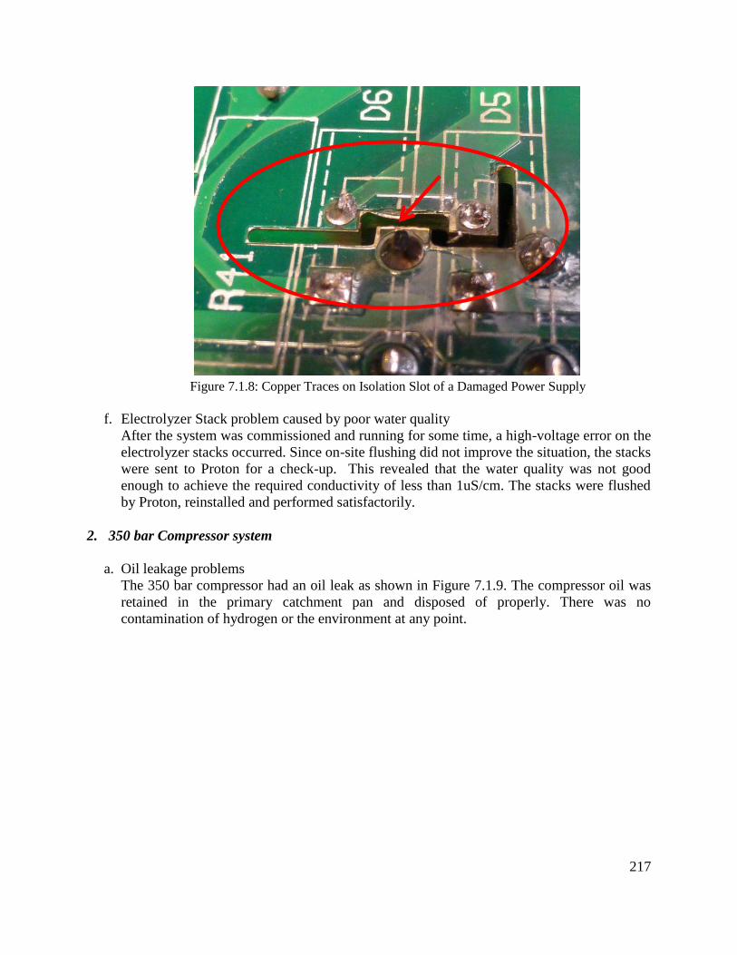
217

Figure 7.1.8: Copper Traces on Isolation Slot of a Damaged Power Supply

f. Electrolyzer Stack problem caused by poor water quality

After the system was commissioned and running for some time, a high-voltage error on the

electrolyzer stacks occurred. Since on-site flushing did not improve the situation, the stacks

were sent to Proton for a check-up. This revealed that the water quality was not good

enough to achieve the required conductivity of less than 1uS/cm. The stacks were flushed

by Proton, reinstalled and performed satisfactorily.

2. 350 bar Compressor system

a. Oil leakage problems

The 350 bar compressor had an oil leak as shown in Figure 7.1.9. The compressor oil was

retained in the primary catchment pan and disposed of properly. There was no

contamination of hydrogen or the environment at any point.

218

Figure 7.1.9: 350 bar Compressor Oil Leak

b. Compressor seal changes

Powertech was contracted to change the seals on the 350 bar compressor. Figure 7.1.10

shows the work in progress when both the oil and the hydrogen gaskets for both

compressor stages were changed.

Figure 7.1.10: Repair of 350 bar Compressor in Progress

c. Hydrogen leak in 350 bar system

Even after the service, there was a leak in the 350 bar system, noticeable by a pressure drop

of ~1.8 bar/day at 215 bar, which is roughly 0.12 kg/day of hydrogen. This leak seems to

come from the compressor’s check valve allowing high pressure H2 reversing through the

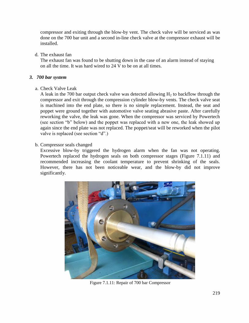
219

compressor and exiting through the blow-by vent. The check valve will be serviced as was

done on the 700 bar unit and a second in-line check valve at the compressor exhaust will be

installed.

d. The exhaust fan

The exhaust fan was found to be shutting down in the case of an alarm instead of staying

on all the time. It was hard wired to 24 V to be on at all times.

3. 700 bar system

a. Check Valve Leak

A leak in the 700 bar output check valve was detected allowing H2 to backflow through the

compressor and exit through the compression cylinder blow-by vents. The check valve seat

is machined into the end plate, so there is no simple replacement. Instead, the seat and

poppet were ground together with automotive valve seating abrasive paste. After carefully

reworking the valve, the leak was gone. When the compressor was serviced by Powertech

(see section “b” below) and the poppet was replaced with a new one, the leak showed up

again since the end plate was not replaced. The poppet/seat will be reworked when the pilot

valve is replaced (see section “d”.)

b. Compressor seals changed

Excessive blow-by triggered the hydrogen alarm when the fan was not operating.

Powertech replaced the hydrogen seals on both compressor stages (Figure 7.1.11) and

recommended increasing the coolant temperature to prevent shrinking of the seals.

However, there has not been noticeable wear, and the blow-by did not improve

significantly.

Figure 7.1.11: Repair of 700 bar Compressor

220

c. Hydrogen blow-by exhaust

As mentioned above, blow-by was not reduced with new gaskets. Powertech

recommended increasing the coolant inlet temperature by a few degrees in order to reduce

the shrinking of the seals, but the hydrogen concentration at the breathing vent was still too

high and would have triggered a gas alarm if the temperature controlled fan is not running.

Hence, the blow-by was piped to a vent stack, as shown in Figure 7.1.12. Both breathing

holes were connected by PVC tubes and routed to a newly erected vent stack. The piping

features a water trap and a T-element, suitable for accommodating a hydrogen sensor to

detect defective seals that would cause a rapid increase in H2 concentration.

Figure 7.1.12: Hydrogen Blow-by Vent on 700 bar Compressor

d. Pilot Instrument Air Valve

The compressor is controlled via two air-operated pilot valves, which switch a large

directional valve that allows the high-pressure oil to move the piston to either the right or

left. The directional valve caused problems at the very beginning of operations as it

occasionally became stuck at compressor start-up, probably due to build-up of oil residue

and mild corrosion. However after several hours of run time the start-up problems stopped.

As a new issue, the small piston of the air-operated valve started to leak. Figure 7.1.13

shows the defective air-operated pilot valve. The figure also shows water spills from

excessive humidity in the instrument air. This was caused by a defective purge valve in the

instrument air compressor (see section “Miscellaneous” for details).

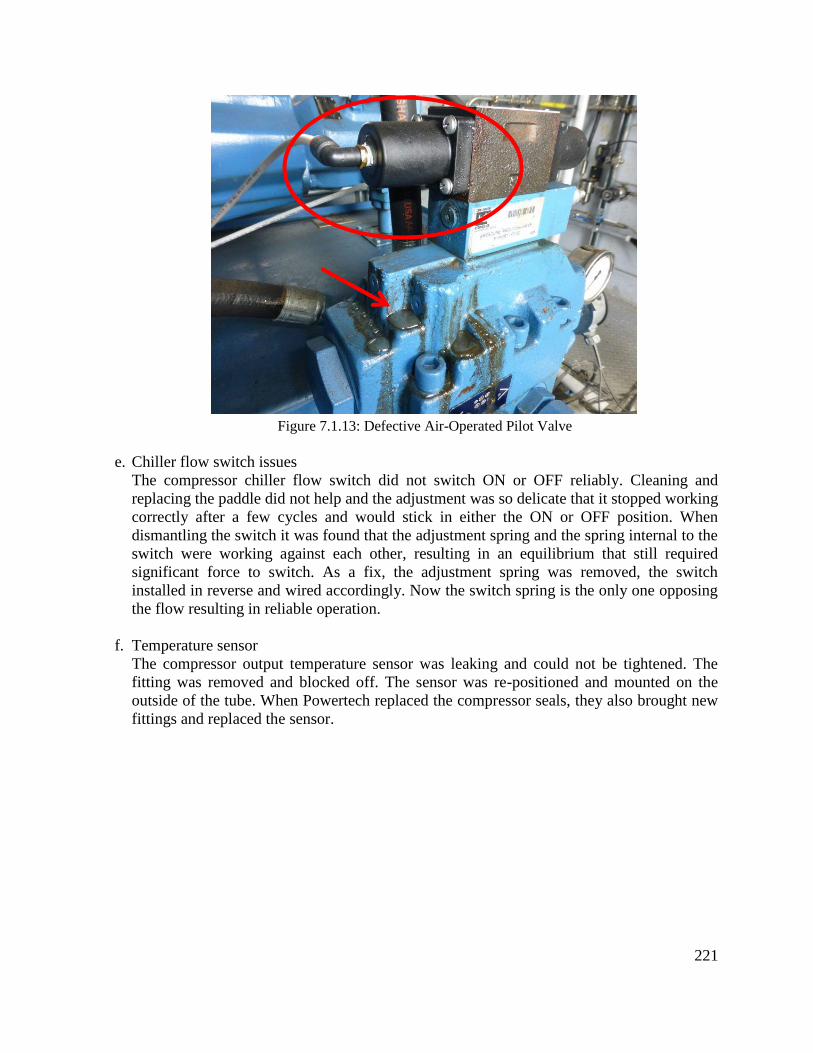
221

Figure 7.1.13: Defective Air-Operated Pilot Valve

e. Chiller flow switch issues

The compressor chiller flow switch did not switch ON or OFF reliably. Cleaning and

replacing the paddle did not help and the adjustment was so delicate that it stopped working

correctly after a few cycles and would stick in either the ON or OFF position. When

dismantling the switch it was found that the adjustment spring and the spring internal to the

switch were working against each other, resulting in an equilibrium that still required

significant force to switch. As a fix, the adjustment spring was removed, the switch

installed in reverse and wired accordingly. Now the switch spring is the only one opposing

the flow resulting in reliable operation.

f. Temperature sensor

The compressor output temperature sensor was leaking and could not be tightened. The

fitting was removed and blocked off. The sensor was re-positioned and mounted on the

outside of the tube. When Powertech replaced the compressor seals, they also brought new

fittings and replaced the sensor.

222

4. Dispenser

a. Pre-cooler circulation pump

The dispenser chiller circulation system was leaking from the start of operations.

Powertech tracked the leak to the circulation pump. During a service, all pump seals were

replaced, however, it is not confirmed that the leak is gone. The problem may be due to the

fact that the pump is not specified for low temperatures (water pump), so operating at -

30°C may be problematic. Detecting the leak of the clear heat transfer fluid mixed with

water condensation is very difficult; previously only a decrease of the level in the reservoir

indicated the problem. Adding a dye to spot any leaking heat transfer fluid has been

recommended to Powertech.

b. 350 bar dispenser

The 350 bar dispenser was only designed for filling buses and did not work for filling 350

bar small vehicles, like fork lifts, because it did not include a flow controller. This problem

was resolved by implementing an extra dispensing controller (see section “System

Upgrades” for details)

c. Dispenser touch screen degradation

The dispenser screen has become discolored and difficult to operate especially in wet

environmental conditions; after heavy rain, e.g., the touch screen is not responsive. Since

the dispenser can also be operated from the main control screen, no immediate repair been

scheduled. Powertech has identified a new model of screen that performs better. The

screen will be replaced.

5. 350 bar and 700 bar storage tanks

a. Cover from elements – putting a tarp screen

Noticeable bleaching of the type-3 cylinders in both storage areas required installation of

shading. A gas permeable, mesh-like tarp was installed as a cover over the open storage

areas preventing heating and UV exposure.

b. Gas Sensor Replacement

The gas sensor in the 350 bar storage was defective causing false alarms and was replaced.

Since electronic and electrochemical cells are paired, both were exchanged.

6. Fire and gas alarm

a. Gas panel

The gas panel caused initial problems because the pins of the PCB terminal blocks were cut

flush with the printed circuit board and hence the solder joints were bad and the terminal

block could simply be pulled out as shown in Figure 7.1.14. All pads in question have been

carefully re-soldered and tested.

223

Figure 7.1.14: Gas Panel Printed Circuit Board

b. Fire alarm system

The fire alarm system had loose connections, which caused smoke detector warnings.

c. Fire alarm incorrect time slot

The daily round call report to the central fire dispatch is not working because the time slot

the fire alarm box overlays with another unit. Phoenix Fire is being contracted to fix this

problem.

d. Emergency Shutdown Device (ESD) and fire alarm wiring

The fire alarm panel was originally not wired into the station’s ESD loop. The flame

detector was part of the ESD, but this unit was not wired to the fire panel. As a fix, the

main controller, which receives a separate signal from the flame detector, signaled through

an output relay to the fire panel. Additionally, a relay was placed into the ESD loop that

shuts the station down if the fire panel is triggered. However, since the ESD resets all

outputs, there was only a short, unreliable pulse sent out in case of flame detection as the

flame detector wired to PLC causes the relay to turn on, but the flame detector wired to the

ESD causes the relay to turn off. This problem will be resolved by changing the wiring.

7. Miscellaneous

a. Ground fault

A solid ground short was discovered on wire YDI10315, which is the signal from the

dispenser’s tilt switch. It caused the high potential of the entire 24V supply to be connected

to ground. This was not immediately noticed as the entire controller is electrically isolated

and a single point grounding pulled the 24V high potential to ground but did not create any

consecutive problems. Using a negatively grounded appliance, however, tripped a fuse and

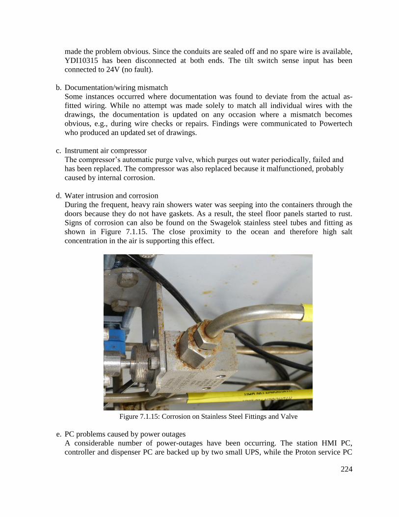
224

made the problem obvious. Since the conduits are sealed off and no spare wire is available,

YDI10315 has been disconnected at both ends. The tilt switch sense input has been

connected to 24V (no fault).

b. Documentation/wiring mismatch

Some instances occurred where documentation was found to deviate from the actual as-

fitted wiring. While no attempt was made solely to match all individual wires with the

drawings, the documentation is updated on any occasion where a mismatch becomes

obvious, e.g., during wire checks or repairs. Findings were communicated to Powertech

who produced an updated set of drawings.

c. Instrument air compressor

The compressor’s automatic purge valve, which purges out water periodically, failed and

has been replaced. The compressor was also replaced because it malfunctioned, probably

caused by internal corrosion.

d. Water intrusion and corrosion

During the frequent, heavy rain showers water was seeping into the containers through the

doors because they do not have gaskets. As a result, the steel floor panels started to rust.

Signs of corrosion can also be found on the Swagelok stainless steel tubes and fitting as

shown in Figure 7.1.15. The close proximity to the ocean and therefore high salt

concentration in the air is supporting this effect.

Figure 7.1.15: Corrosion on Stainless Steel Fittings and Valve

e. PC problems caused by power outages

A considerable number of power-outages have been occurring. The station HMI PC,

controller and dispenser PC are backed up by two small UPS, while the Proton service PC

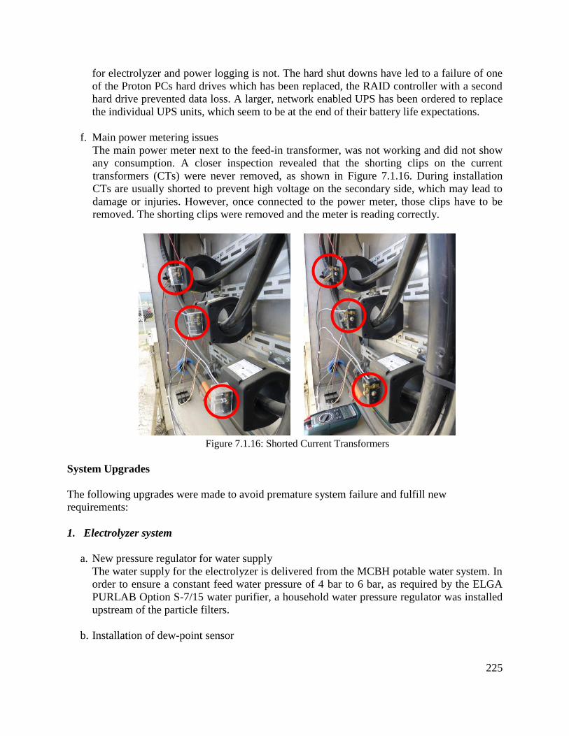
225

for electrolyzer and power logging is not. The hard shut downs have led to a failure of one

of the Proton PCs hard drives which has been replaced, the RAID controller with a second

hard drive prevented data loss. A larger, network enabled UPS has been ordered to replace

the individual UPS units, which seem to be at the end of their battery life expectations.

f. Main power metering issues

The main power meter next to the feed-in transformer, was not working and did not show

any consumption. A closer inspection revealed that the shorting clips on the current

transformers (CTs) were never removed, as shown in Figure 7.1.16. During installation

CTs are usually shorted to prevent high voltage on the secondary side, which may lead to

damage or injuries. However, once connected to the power meter, those clips have to be

removed. The shorting clips were removed and the meter is reading correctly.

Figure 7.1.16: Shorted Current Transformers

System Upgrades

The following upgrades were made to avoid premature system failure and fulfill new

requirements:

1. Electrolyzer system

a. New pressure regulator for water supply

The water supply for the electrolyzer is delivered from the MCBH potable water system. In

order to ensure a constant feed water pressure of 4 bar to 6 bar, as required by the ELGA

PURLAB Option S-7/15 water purifier, a household water pressure regulator was installed

upstream of the particle filters.

b. Installation of dew-point sensor

226

As a valuable feature, and required by Toyota, a hydrogen dew point sensor has been

installed in the hydrogen product line after the desiccant dryer as shown in Figure 7.1.17.

To run cables from the electrical side to the gas side, spare pins of an existing multi-contact

connector were used. Two cables with two shielded pairs each (8 wires total) were added

for supply and signal of the sensor and also to prepare for an automatic venting system, if

needed. The integrated vent is piped-in before the dryer and sensor, so when venting

humidity cannot be measured. The proposed valve would vent shortly before the product

gas outlet so it can be measured and the venting stopped as soon as the dew point is

sufficiently low. Extra terminal blocks were installed in the electrical side and the signal

routed to the electrical room inside the alarm box to the read-out unit (see Figure 7.1.18).

Finally, a signal was tapped-off and connected to the power monitoring system (see next

section) to include gas humidity in the power log. The logic for venting can also be

integrated into the monitoring PLC.

Figure 7.1.17: Hydrogen Dew Point Sensor

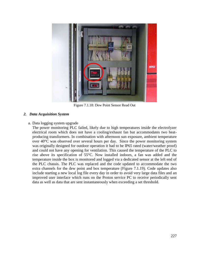
227

Figure 7.1.18: Dew Point Sensor Read Out

2. Data Acquisition System

a. Data logging system upgrade

The power monitoring PLC failed, likely due to high temperatures inside the electrolyzer

electrical room which does not have a cooling/exhaust fan but accommodates two heat-

producing transformers. In combination with afternoon sun exposure, ambient temperature

over 40°C was observed over several hours per day. Since the power monitoring system

was originally designed for outdoor operation it had to be IP65 rated (water/weather proof)

and could not have any opening for ventilation. This caused the temperature of the PLC to

rise above its specification of 55°C. Now installed indoors, a fan was added and the

temperature inside the box is monitored and logged via a dedicated sensor at the left end of

the PLC chassis. The PLC was replaced and the code updated to accommodate the two

extra channels for the dew point and box temperature (Figure 7.1.19). Code updates also

include starting a new local log file every day in order to avoid very large data files and an

improved user interface which runs on the Proton service PC to receive periodically sent

data as well as data that are sent instantaneously when exceeding a set threshold.

228

Figure 7.1.19: Upgraded Power Monitor System

3. Dispenser

a. A new 350 bar filling algorithm for smaller vehicles was developed, installed and tested.

The 350 bar dispenser was originally designed for buses and does not feature a flow

controller. However, since only small vehicles, like forklifts, are currently being filled at

MCBH, a solution was found to fill them reliably based on tank pressure, storage pressure

and flow rate without modification of the P&ID while maintaining all safety requirements.

A secondary PLC was installed to control the main and dispense valves of high and low

bank cylinders, and the nozzle valve. Pressure and flow analogue sensor signals were fed

into the controller as well as start-fill and emergency stop digital signals. An advanced

control strategy was developed to allow filling any size vehicle in a short time without the

risk of over pressurizing, utilizing only existing components (valves) and signals (pressure

and flow sensor).

Findings

Environmental Conditions: The close proximity to the ocean with the hot and humid salt

air environment took a toll on components. Even high quality 316 stainless steel showed

signs of corrosion after a year of exposure. Design issues, like missing gaskets on doors,

painted steel floor plates, no cover for the dispenser touch screen, etc., also aided in the

deterioration of system components.

Low Utilization: The station experienced low utilization after the GM Equinox testing

program was completed in August 2015. Since then the station has been operated to

support hydrogen forklifts. Periodic operation of chillers, pumps and compressors is

conducted in order to maintain functionality. The project is planning to support the

operation of Toyota Mirai fuel cell cars in early 2017.

229

The station demonstrated well-controlled, repeatable, 4 minute high-pressure fast fills

(over 300 between Nov 2014 and August 2015).

This project also provided significant insight into the challenges required to deploy and operate

hydrogen fueling infrastructure including:

Hydrogen safety issues;

Hydrogen station design;

Hydrogen codes & standards;

Working with the Authority Having Jurisdiction to obtain the necessary approvals to

install and operate the systems;

Developing a Project Hydrogen Safety Plan;

Working with the PNNL Hydrogen Safety Panel;

Developing operating and maintenance manuals;

First Responder training and obtaining buy-in from the local fire departments;

Equipment technical performance and reliability issues including providing feedback to

equipment suppliers on the performance of their equipment;

Equipment warranties and after sales support issues;

Costs involved in producing and dispensing hydrogen including operating and

maintenance costs that are substantial;

Training people to maintain and operate the systems;

Developing legal agreements working with the legal profession who are unfamiliar with

hydrogen;

Addressing the concerns of host site owners;

Collecting data and analyzing technical performance.

Publications and Presentations

Rocheleau R., Ewan, M., “Hawaii’s Hydrogen Programs”, f-cell Hydrogen Conference,

Stuttgart Germany, September 2011.

Ewan, M., “Supporting a Hawaii Hydrogen Economy”, US DOE Webinar, 29 July 2014.

Virji. M., Randolf, G., Polson, C., Ewan, M., “Water-to-Water Analysis of Hydrogen

Energy System for Hydrogen Fueling Stations in Hawaii”, Fuel Cell Seminar & Energy

Exposition 2014, Los Angeles, CA, 10-13 November, 2014.

Briefings

Ewan M., “Hawaii Hydrogen Programs”, Briefing to Toyota Corporate, Honolulu, March

2012.

Acknowledgements

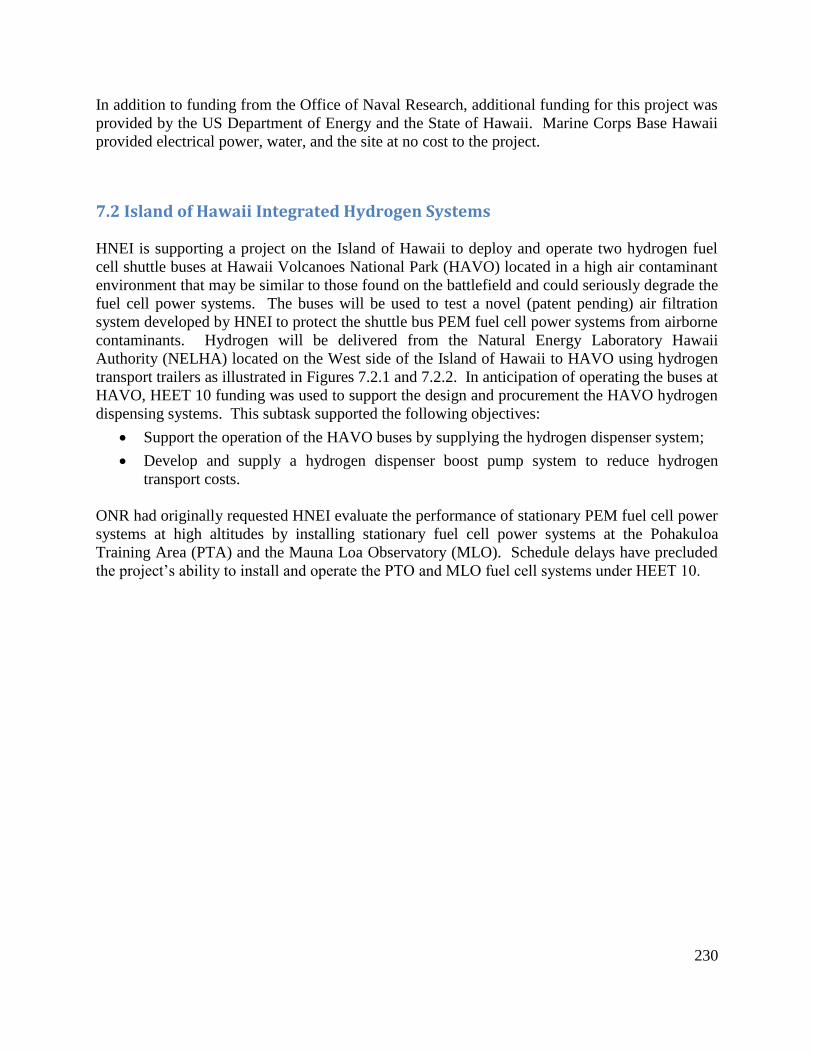
230

In addition to funding from the Office of Naval Research, additional funding for this project was

provided by the US Department of Energy and the State of Hawaii. Marine Corps Base Hawaii

provided electrical power, water, and the site at no cost to the project.

7.2 Island of Hawaii Integrated Hydrogen Systems

HNEI is supporting a project on the Island of Hawaii to deploy and operate two hydrogen fuel

cell shuttle buses at Hawaii Volcanoes National Park (HAVO) located in a high air contaminant

environment that may be similar to those found on the battlefield and could seriously degrade the

fuel cell power systems. The buses will be used to test a novel (patent pending) air filtration

system developed by HNEI to protect the shuttle bus PEM fuel cell power systems from airborne

contaminants. Hydrogen will be delivered from the Natural Energy Laboratory Hawaii

Authority (NELHA) located on the West side of the Island of Hawaii to HAVO using hydrogen

transport trailers as illustrated in Figures 7.2.1 and 7.2.2. In anticipation of operating the buses at

HAVO, HEET 10 funding was used to support the design and procurement the HAVO hydrogen

dispensing systems. This subtask supported the following objectives:

Support the operation of the HAVO buses by supplying the hydrogen dispenser system;

Develop and supply a hydrogen dispenser boost pump system to reduce hydrogen

transport costs.

ONR had originally requested HNEI evaluate the performance of stationary PEM fuel cell power

systems at high altitudes by installing stationary fuel cell power systems at the Pohakuloa

Training Area (PTA) and the Mauna Loa Observatory (MLO). Schedule delays have precluded

the project’s ability to install and operate the PTO and MLO fuel cell systems under HEET 10.

231

Figure 7.2.1: Hydrogen Delivery Concept

Figure 7.2.2: Hydrogen Transport Trailer

HAVO Hydrogen Dispensing System

HNEI designed the 350 bar HAVO hydrogen dispensing station illustrated in Figure 7.2.3. The

main components are comprised of “Drag & Drop” hydrogen transport trailers that are hauled by

truck from NELHA to HAVO. The trailers are connected to a fueling dispenser via a fueling

post that acts as an interface between the trailer and the dispenser. Each trailer is filled with 105

kilograms of hydrogen at a pressure of 450 bar. A full trailer is transported to the site from

NELHA and an empty trailer is picked up and returned to NELHA to be refilled. The station

employs a cascade fill process that leverages the energy expended to fill the trailer with 450 bar

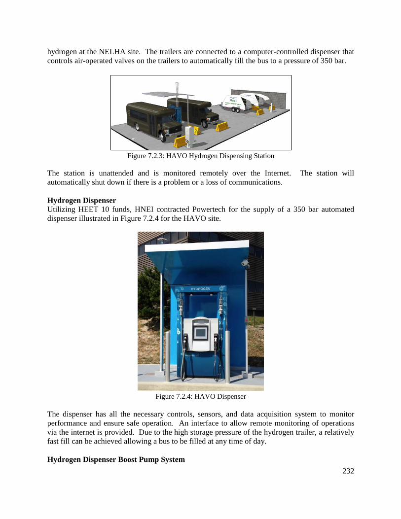
232

hydrogen at the NELHA site. The trailers are connected to a computer-controlled dispenser that

controls air-operated valves on the trailers to automatically fill the bus to a pressure of 350 bar.

Figure 7.2.3: HAVO Hydrogen Dispensing Station

The station is unattended and is monitored remotely over the Internet. The station will

automatically shut down if there is a problem or a loss of communications.

Hydrogen Dispenser

Utilizing HEET 10 funds, HNEI contracted Powertech for the supply of a 350 bar automated

dispenser illustrated in Figure 7.2.4 for the HAVO site.

Figure 7.2.4: HAVO Dispenser

The dispenser has all the necessary controls, sensors, and data acquisition system to monitor

performance and ensure safe operation. An interface to allow remote monitoring of operations

via the internet is provided. Due to the high storage pressure of the hydrogen trailer, a relatively

fast fill can be achieved allowing a bus to be filled at any time of day.

Hydrogen Dispenser Boost Pump System

233

Utilizing HEET 10 funds, HNEI contracted Powertech for the design and supply of a hydrogen

boost pump system that is integrated into the HAVO hydrogen dispenser.

The round trip distance to supply hydrogen from NELHA to HAVO is 300 miles. This incurs a

considerable transportation cost. It was calculated that using the cascade fill methodology, the

trailer would be 61.5% full when unable to complete a fill to >95% SOC (state of charge) at

which time it needs to be returned to NELHA for refilling. In order to extract more hydrogen

from the trailer, it was decided to add a boost pump system to the HAVO dispensing system. A

booster pump system was designed with the following capabilities and features:

Capable of compressing from low-pressure storage banks to high-pressure storage banks

in the tube trailer. This increases the number of cascade fills that can be performed per

trailer.

Compressing directly to the vehicle tank via the dispenser if unable to perform a cascade

fill.

Doubling the number of fills per trailer that can be completed to 95% SOC compared to

the original design (based on simulations using a bus with a 10 kg hydrogen tank of 5,000

psi normal operating pressure).

Simulations were conducted to determine the performance of the booster pump upgrade. The

results of these simulations were:

8 fills to >95% SOC can be completed per trailer

o Approximately 4 fills to >95% SOC can be completed without the booster pump

upgrade

Fills #1 to #4 are “fast” cascade fills. Fill #5 is a slower cascade fill.

The final 3 fills (#6 to #8) will require direct compression into the bus via the dispenser

after a “mini cascade” fill.

o These fills will be slower (ranging from 1 to 6 hours).

The compressor will take an average of 9 hours and a maximum of 15 hours between fills

to restore storage to its maximum fueling power (cascade fill).

The trailer will be approximately 23.5% full after 8 fills.

A 9th fill can be completed with direct compression and a “mini cascade” fill to 93%

SOC over an extended period of time

o The trailer will be approximately 10.3% full after this final fill

Assumptions

Vehicles (buses) maximum tank size is 10 kg of hydrogen at 5,000 psi and 15˚C as

provided;

Vehicles arrive with 0 kg of hydrogen in the tank and are filled to at least 9.5 kg

(95%<SOC<100%). Only applicable in fills #1 to #8;

Adequate recovery time is provided between each fill;

Hydrogen supply (tube trailer) arrives on-site with a minimum of 6,000 psi hydrogen at

234

15˚C (99.74 kg hydrogen);

Compressor (booster pump) outlet pressure of 6,000 psi at 15˚C (maximum outlet

pressure); and

Compressor runs continuously at the flow-rate specified by the manufacturer.

The dispenser and boost pump systems have been completed and are ready for installation at the

HAVO site.

Publications / Presentations

1. Ewan M., Rocheleau, R., Oral presentation at US DOE Annual Merit Review, “Hydrogen

Energy Systems as a Grid Management Tool”, Washington, DC, June 9, 2016.

2. Ewan M., Oral presentation at US DOE Sustainable Transportation Summit, “H2@Scale

Stakeholder Panel Session”, Washington, DC, July 12, 2016.

7.3 Hawaii Military Biofuels Crop Assessment

Under Subtask 7.3 Pacific Biodiesel Technologies (PBT) was contracted to conduct an

operations sensitive assessment of the capacity for the local production of fuels and biomass to

assess the potential for DOD operations and/or hydrogen production. The project, originally

intended to assess the potential for hydrogen production on Oahu was transitioned to Hawaii

Island to leverage ongoing work by PBT.

The project included broad assessments of the potential agricultural crop production, products

and co-products, and process technologies available to produce advanced biofuels on Hawaii

Island. The core objective was to determine how best to create an agricultural based feedstock

development approach that could provide advanced biofuels in order to meet the Department of

Navy needs which include:

Pricing at or near parity with petroleum equivalents

Predictable pricing, stable across a full year budget

Pricing not based on commodity market values of the feedstock

Feedstock with a chemical composition allowing economical conversion to useful fuels

Overall economic value that incentivizes famers to invest in the system

Pacific Biodiesel Technologies assisted by Rivertop Solutions and the University of Hawaii at

Hilo conducted analysis and crop testing in 11 specific areas:

1. Crop Regional Land Identification

2. Potential Fuel and Co-Product Options from Biomass

3. Jatropha Farm Optimization Plan

4. Economic Assessment Outline and Baseline Report

235

5. Economics Assessment

6. Survey of Hawaii Island Biofuels Lands

7. Supply Chain Plan

8. Bioenergy Farm Analysis

9. Field Testing

10. Land Selection and Site Identification

11. Jatropha Farm Optimization

Results of the project indicate that there appears to be an economically viable path to the

production of oilseed crops on Hawaii Island. Sunflower may be one of the rotational crops in

this production. Although much progress has been made recently, biomass-to-energy

technologies at the small scale needed for this project are not commercially available.. More

study is needed on cultivars and value-added co-product development. Additional work is also

need to understand the various microclimates and soil nutrient requirements for each crop.

Details of this effort are described in the “Hawaii Military Biofuels Crop Assessment” report

available on HNEI’s website.

7.4 Alternative Hydrogen Production Assessment for Hawaii

There are currently several demonstration projects on the island of Oahu requiring high purity

hydrogen for fuel cell vehicle use. Current demand is being met by electrolysis powered by high

cost electricity. The Gas Company is working with a number of partners to assess its ability to

supply high purity hydrogen for the expected increase in demand using its reformed hydrogen

production process. However, the Gas Company technology uses petroleum as the primary base

of production. This task assessed two alternative pathways to meet the projected growth in

demand for hydrogen: gasification of municipal solid waste (MSW) and importation of natural

gas in small-scale container vessels. Technology and economic issues were addressed and

recommendations put forth for development of hydrogen infrastructure with capacity to meet

potential targeted demand.

Hydrogen Purity and Quantity Requirements

In this section details are provided regarding the purity of hydrogen required for different types

of fuel cells. In addition, an estimate of the hydrogen production capacity required to displace

1% of the gasoline usage in Hawaii (as of 2014) is presented.

The details and specifications regarding the purity of hydrogen that is required for different fuel

cells are presented in Tables 7.4.1 and 7.4.2. This information was reproduced from the Society

of Automotive Engineers (SAE) Hydrogen Fuel Quality for Fuel Cell Vehicles Standard J2719.1

Table 7.4.1: Hydrogen fuel quality specifications - from Society of Automotive Engineering (SAE)

Hydrogen Fuel Quality for Fuel Cell Vehicles Standard J27191

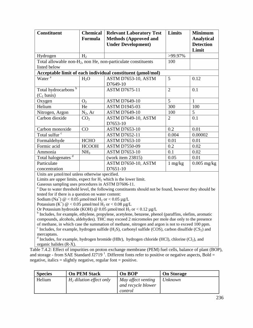
236

Constituent Chemical

Formula

Relevant Laboratory Test

Methods (Approved and

Under Development)

Limits Minimum

Analytical

Detection

Limit

Hydrogen H2 >99.97%

Total allowable non-H2, non He, non-particulate constituents

listed below

100

Acceptable limit of each individual constituent (µmol/mol)

Water a H2O ASTM D7653-10, ASTM

D7649-10

5 0.12

Total hydrocarbons b

(C1 basis)

ASTM D7675-11 2 0.1

Oxygen O2 ASTM D7649-10 5 1

Helium He ASTM D1945-03 300 100

Nitrogen, Argon N2, Ar ASTM D7649-10 100 5

Carbon dioxide CO2 ASTM D7649-10, ASTM

D7653-10

2 0.1

Carbon monoxide CO ASTM D7653-10 0.2 0.01

Total sulfur c ASTM D7652-11 0.004 0.00002

Formaldehyde HCHO ASTM D7653-10 0.01 0.01

Formic acid HCOOH ASTM D7550-09 0.2 0.02

Ammonia NH3 ASTM D7653-10 0.1 0.02

Total halogenates d (work item 23815) 0.05 0.01

Particulate

concentration

ASTM D7650-10, ASTM

D7651-10

1 mg/kg 0.005 mg/kg

Units are µmol/mol unless otherwise specified.

Limits are upper limits, expect for H2 which is the lower limit.

Gaseous sampling uses procedures in ASTM D7606-11. a Due to water threshold level, the following constituents should not be found, however they should be

tested for if there is a question on water content:

Sodium (Na+) @ < 0.05 µmol/mol H2 or < 0.05 µg/L

Potassium (K+) @ < 0.05 µmol/mol H2 or < 0.08 µg/L

Or Potassium hydroxide (KOH) @ 0.05 µmol/mol H2 or < 0.12 µg/L b Includes, for example, ethylene, propylene, acetylene, benzene, phenol (paraffins, olefins, aromatic

compounds, alcohols, aldehydes). THC may exceed 2 micromoles per mole due only to the presence

of methane, in which case the summation of methane, nitrogen and argon is not to exceed 100 ppm. c Includes, for example, hydrogen sulfide (H2S), carbonyl sulfide (COS), carbon disulfide (CS2) and

mercaptans. d Includes, for example, hydrogen bromide (HBr), hydrogen chloride (HCl), chlorine (Cl2), and

organic halides (R-X).

Table 7.4.2: Effect of impurities on proton exchange membrane (PEM) fuel cells, balance of plant (BOP),

and storage - from SAE Standard J2719 1. Different fonts refer to positive or negative aspects, Bold =

negative, italics = slightly negative, regular font = positive.

Species On PEM Stack On BOP On Storage

Helium H2 dilution effect only May affect venting

and recycle blower

control

Unknown

237

Inert Gases

(N2, Ar, etc.)

H2 dilution effect only May affect venting

and recycle blower

control

Unknown - Believed to

affect MeH cycle life

Hydrocarbons Aromatics, acids,

aldehydes, etc. degrade

performance

Unknown Unknown - Believed to

affect MeH cycle life

Oxygen Tolerant to > 500 ppm May form ice Exothermic reactions-

Believed to affect MeH

cycle life

Carbon

Monoxide Reacts with catalyst,

degrades performance

No effect expected Believed to affect MeH

cycle life

Carbon

Dioxide

Tolerant to < 100 ppm,

limited CO back

shifting

May affect venting

and recycle blower

control


cycle life

Formaldehyde Reacts with catalyst,


Unknown Unknown

Formic Acid Reacts with catalyst,


Unknown Unknown

Sulfur

compounds Reacts with catalyst,


Unknown Believed to affect MeH

cycle life

Ammonia Degrades membrane

ionomer conductivity

Unknown Unknown

Water Tolerant to > 500 ppm May form ice, ice

adversely affects

control

components

Exothermic reactions-


cycle life

Sodium Degrades membrane


May adversely

affect control

components

Unknown

Potassium Degrades membrane


May adversely

affect control

components

Unknown

Halogenated

Compounds Reacts with catalyst,


Unknown Unknown

Particulates May degrade membrane Adversely affects

control

components

Unknown

The combined amount of gasoline and diesel transportation fuels consumed in the state of

Hawaii in 2007 was 757 million gallons comprising 469 million gallons of gasoline and 288

million gallons of diesel.2, 3

The consumption in 2008 was slightly lower but of a similar

magnitude, i.e. 450 million gallons of gasoline were consumed for transportation.2, 3

The most

recent data available at the time of writing was for 2014 when 449 million gallons of gasoline

were used for transportation in the State of Hawaii.3

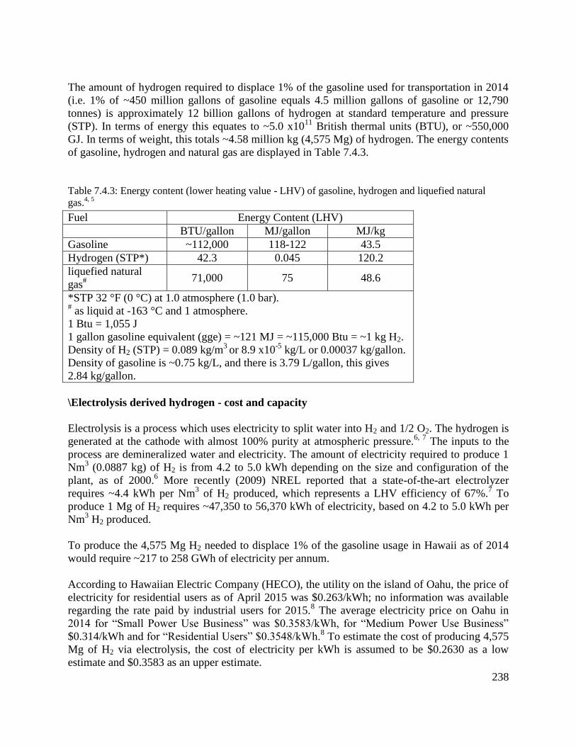
238

The amount of hydrogen required to displace 1% of the gasoline used for transportation in 2014

(i.e. 1% of ~450 million gallons of gasoline equals 4.5 million gallons of gasoline or 12,790

tonnes) is approximately 12 billion gallons of hydrogen at standard temperature and pressure

(STP). In terms of energy this equates to ~5.0 x1011

British thermal units (BTU), or ~550,000

GJ. In terms of weight, this totals ~4.58 million kg (4,575 Mg) of hydrogen. The energy contents

of gasoline, hydrogen and natural gas are displayed in Table 7.4.3.

Table 7.4.3: Energy content (lower heating value - LHV) of gasoline, hydrogen and liquefied natural

gas.4, 5

Fuel Energy Content (LHV)

BTU/gallon MJ/gallon MJ/kg

Gasoline ~112,000 118-122 43.5

Hydrogen (STP*) 42.3 0.045 120.2

liquefied natural

gas#

71,000 75 48.6

*STP 32 °F (0 °C) at 1.0 atmosphere (1.0 bar). # as liquid at -163 °C and 1 atmosphere.

1 Btu = 1,055 J

1 gallon gasoline equivalent (gge) = ~121 MJ = ~115,000 Btu = ~1 kg H2.

Density of H2 (STP) = 0.089 kg/m3

or 8.9 x10-5

kg/L or 0.00037 kg/gallon.

Density of gasoline is ~0.75 kg/L, and there is 3.79 L/gallon, this gives

2.84 kg/gallon.

\Electrolysis derived hydrogen - cost and capacity

Electrolysis is a process which uses electricity to split water into H2 and 1/2 O2. The hydrogen is

generated at the cathode with almost 100% purity at atmospheric pressure.6, 7

The inputs to the

process are demineralized water and electricity. The amount of electricity required to produce 1

Nm3 (0.0887 kg) of H2 is from 4.2 to 5.0 kWh depending on the size and configuration of the

plant, as of 2000.6 More recently (2009) NREL reported that a state-of-the-art electrolyzer

requires ~4.4 kWh per Nm3 of H2 produced, which represents a LHV efficiency of 67%.

7 To

produce 1 Mg of H2 requires ~47,350 to 56,370 kWh of electricity, based on 4.2 to 5.0 kWh per

Nm3 H2 produced.

To produce the 4,575 Mg H2 needed to displace 1% of the gasoline usage in Hawaii as of 2014

would require ~217 to 258 GWh of electricity per annum.

According to Hawaiian Electric Company (HECO), the utility on the island of Oahu, the price of

electricity for residential users as of April 2015 was $0.263/kWh; no information was available

regarding the rate paid by industrial users for 2015.8 The average electricity price on Oahu in

2014 for “Small Power Use Business” was $0.3583/kWh, for “Medium Power Use Business”

$0.314/kWh and for “Residential Users” $0.3548/kWh.8 To estimate the cost of producing 4,575

Mg of H2 via electrolysis, the cost of electricity per kWh is assumed to be $0.2630 as a low

estimate and $0.3583 as an upper estimate.

239

On the above basis, to produce 217 GWh of electricity will cost between $57.0 million and $77.6

million. To produce 258 GWh will cost from $67.8 million and $92.4 million.

To produce 4,575 tonnes of H2 per annum requires an electrolysis plant with a capacity of ~6,000

Nm3/h (533 kg/h) assuming it operates for 8,600 hours per annum. At this scale the cost of

investment for an electrolysis plant is greater than 150% of a steam reforming plant using

naphtha (or natural gas) as feedstock.6

At a scale of 4,000 Nm3/h (355 kg/h) of H2, the production cost per Nm

3 H2 using electrolysis is

~$0.50 (based on an electricity cost of $0.08/kWh), using prices from 2000.6 Whereas the cost

from steam reforming of natural gas is ~$0.10 per Nm3 H2 produced, assuming the NG costs

$0.12 per Nm3 (if naphtha is used instead of NG the price will be similar but slightly higher).

6

Electrolysis is clearly much more expensive than steam reforming at this scale of hydrogen

production even when the electricity is assumed to cost $0.08 per kWh (whereas the actual cost

on Oahu is at least $0.26). The cost differential between electrolysis and steam reforming

remains similar to that outlined above as capacity increases.

More recently (2009), NREL reported the cost of small scale H2 production (i.e. at the filling

station, capacity up to 1,500 kg/day) to be $0.46 per Nm3 H2 assuming an electricity price of

$0.053/kWh.7 For a larger centralized facility (capacity of 50,000 kg/day) the cost is $0.27 per

Nm3 H2, assuming a renewable-based electricity (wind) cost of $0.045/kWh.

7 It is stated in the

NREL report:7 "For electrolysis to be priced competitively for hydrogen production, it must be

produced in areas having low-priced electricity for the industrial sector. The U.S. average price

is $0.0639/kWh."

The annualized production cost of H2 at a scale of 2,000 Nm3/h (178 kg/h) when using

electrolysis is ~$7.5 million per annum assuming an electricity cost of $0.08 per kWh.6 If steam

reforming of natural gas is used, the annualized production cost is ~$1.9 million per annum,

assuming NG costs $0.12 per Nm3.6 The cost of steam reforming of naphtha is similar to that of

natural gas. The cost differential between electrolysis and steam reforming remains similar to

that outlined above as capacity increases.

It has been estimated that for every Nm3 of H2 produced by electrolysis 2.6 kg of CO2 are

emitted assuming the electricity is produced using natural gas at high efficiency.6 Electricity on

Oahu is produced primarily from low sulfur fuel oil at lower efficiency than from a state-of-the-

art power station, hence CO2 emissions will be greater than 2.6 kg per Nm3 H2. For context, the

CO2 emissions from steam reforming of naphtha (or natural gas) for hydrogen production is ~0.8

kg CO2 per Nm3 H2 produced.

6

From the cost information outlined above it is clear that electrolysis is an expensive option for

producing hydrogen and leads to significantly greater CO2 emissions than steam reforming.

However, if the electricity is produced renewably (i.e. solar, wind, biomass or geothermal) the

CO2 emission will be reduced.

240

One possible scenario is to use surplus renewable electricity to run the electrolysis plant, i.e.

from geothermal, wind, biomass or solar, when demand is low. This would mean the plant would

only operate when there is excess electricity being generated during periods of reduced demand.

It is unclear what the cost implications are for this strategy, as it is possible that the cost of the

electricity per kWh would be less than for typically industrial users (assuming an agreement can

be made with the generators). However, on the down side an electrolysis plant requires

significant capital investment, roughly 150% greater than for a steam-reforming plant, and

hydrogen production costs can be up to 5 times greater than steam-reforming of naphtha or

natural gas. Therefore, it is unlikely to be economically feasible to operate such an expensive

facility on a part time bases. Plants of this scale often have to operate continuously throughout

the year, achieving ~8,600 hours of on-line operation time per year to make a positive return on

investment. Unanticipated shut downs can result in significant financial losses. Therefore, unless

there is political support for such a scheme with credits or support provided to the facility to

cover these losses, possibly in the form of carbon credits for reduced green house gas emissions,

it is hard to see how the facility could make a return on the considerable investment.

Petroleum naphtha derived hydrogen - cost and capacity

A conventional method for producing hydrogen is via steam reforming of petroleum naphtha.

This process has been used industrially since the early 1900's and is practiced commercially in

Hawaii up to the present day, therefore the details of the process will not be described herein.

Refer to references authored by Stolle6 and Rostrup-Nielsen

9 for information on the process.

The price paid for naphtha (delivered to Kauai) was ~$80 per barrel in 2015, and ~$120 per bbl

in 2013-2014.10

One barrel of naphtha has a volume of ~0.159 Nm3 with a mass of 105.7 kg

(density of petroleum naphtha is ~665 kg/m3). Therefore, the cost of naphtha ranges from ~$757

to $1,135 per Mg.

The amount of naphtha required to produce 1 Nm3 of H2 (0.0887 kg) via steam reforming is

~0.40 kg; or 0.222 kg of H2 are produced per kg of naphtha.6

The amount of hydrogen that is required to displace 1% of the gasoline usage in Hawaii as of

2014 is ~4,575 Mg per annum. To produce 4,575 Mg of hydrogen via steam reforming requires

~20,621 Mg of naphtha. Based on the costs outlined above for naphtha imported to Kauai, this

would cost ~$15.6 million to ~$23.4 million for the feedstock alone.

The production cost per Nm3 of H2 produced via naphtha steam reforming, and the annualized

production cost were provided in the previous sub-section and are summarized in Table 7.4.4. In

addition, the CAPEX investment for an electrolysis plant is greater than 150% of a steam

reforming plant using naphtha (or natural gas) as feedstock.6

Table 7.4.4: Production costs and CO2 emissions for hydrogen produced via electrolysis or steam

reforming of natural gas (or naphtha).

Process

Production

cost per Nm3

H2

Annualized

production cost

CO2 emissions

per Nm3 H2

Reference

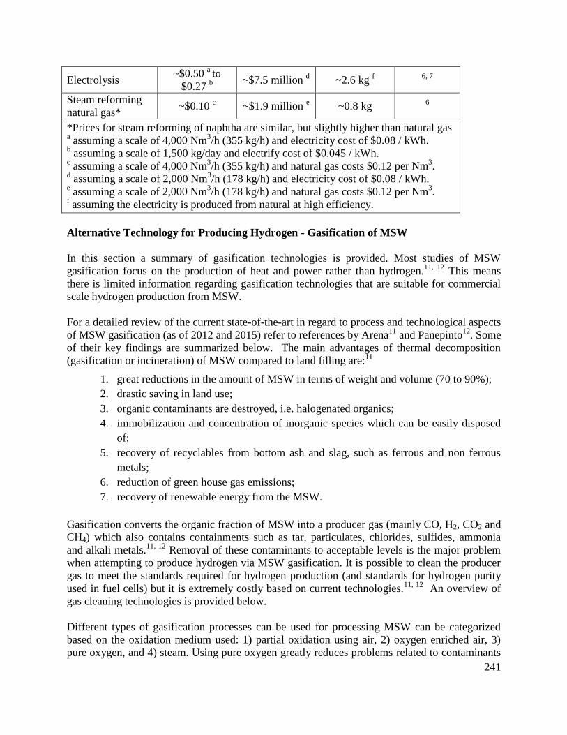
241

Electrolysis ~$0.50

a to

$0.27 b

~$7.5 million d ~2.6 kg

f

6, 7

Steam reforming

natural gas* ~$0.10

c ~$1.9 million

e ~0.8 kg

6

*Prices for steam reforming of naphtha are similar, but slightly higher than natural gas a assuming a scale of 4,000 Nm

3/h (355 kg/h) and electricity cost of $0.08 / kWh.

b assuming a scale of 1,500 kg/day and electrify cost of $0.045 / kWh.

c assuming a scale of 4,000 Nm

3/h (355 kg/h) and natural gas costs $0.12 per Nm

3.

d assuming a scale of 2,000 Nm

3/h (178 kg/h) and electricity cost of $0.08 / kWh.

e assuming a scale of 2,000 Nm

3/h (178 kg/h) and natural gas costs $0.12 per Nm

3.

f assuming the electricity is produced from natural at high efficiency.

Alternative Technology for Producing Hydrogen - Gasification of MSW

In this section a summary of gasification technologies is provided. Most studies of MSW

gasification focus on the production of heat and power rather than hydrogen.11, 12

This means

there is limited information regarding gasification technologies that are suitable for commercial

scale hydrogen production from MSW.

For a detailed review of the current state-of-the-art in regard to process and technological aspects

of MSW gasification (as of 2012 and 2015) refer to references by Arena11

and Panepinto12

. Some

of their key findings are summarized below. The main advantages of thermal decomposition

(gasification or incineration) of MSW compared to land filling are:11

1. great reductions in the amount of MSW in terms of weight and volume (70 to 90%);

2. drastic saving in land use;

3. organic contaminants are destroyed, i.e. halogenated organics;

4. immobilization and concentration of inorganic species which can be easily disposed

of;

5. recovery of recyclables from bottom ash and slag, such as ferrous and non ferrous

metals;

6. reduction of green house gas emissions;

7. recovery of renewable energy from the MSW.

Gasification converts the organic fraction of MSW into a producer gas (mainly CO, H2, CO2 and

CH4) which also contains containments such as tar, particulates, chlorides, sulfides, ammonia

and alkali metals.11, 12

Removal of these contaminants to acceptable levels is the major problem

when attempting to produce hydrogen via MSW gasification. It is possible to clean the producer

gas to meet the standards required for hydrogen production (and standards for hydrogen purity

used in fuel cells) but it is extremely costly based on current technologies.11, 12

An overview of

gas cleaning technologies is provided below.

Different types of gasification processes can be used for processing MSW can be categorized

based on the oxidation medium used: 1) partial oxidation using air, 2) oxygen enriched air, 3)

pure oxygen, and 4) steam. Using pure oxygen greatly reduces problems related to contaminants

242

in the producer gas but on the other hand it is very expensive and appears to only be feasible for

large scale facilities (> 100 Gg per annum).11

Steam gasification shows the greatest promise due

to low construction and operating costs, medium levels of contaminants in the producer gas and

relatively high yields of hydrogen and carbon monoxide.11

In addition to the oxidizing medium, there are a number of different reactor designs used for the

gasification of MSW including: fixed bed designs (down or up draft), fluidized or circulating

bed, entrained flow, rotary kiln or plasma reactors. The main type of gasification process that has

been investigated for generating hydrogen from MSW are direct steam gasification (no catalyst)

and catalytic steam gasification using fixed- or fluidized-bed designs. Plasma gasification is an

emerging technology that provides superior conversion of the MSW into producer gas which is

less affected by changes in the MSW composition. However, it has low energy efficiency and is

relatively expensive compared to other designs. In general, plasma gasification is only

considered to be feasible for large scale processes (> 100 Gg per annum) and where landfill

tipping fees are high.11

One of the main factors in the successful operation of a MSW gasification facility is controlling

the chemical and physical properties of the MSW feedstock. The main properties to consider are

heating value, elemental composition, ash content and composition, volatiles content, moisture

content, particle size, bulk density and contaminants (S, Cl, N, alkali metals and heavy metals).11

This is why many gasification plants that work with MSW pre-process the waste to control these

properties or use refuse-derived fuel with specific properties.11

The main benefits and drawbacks

of MSW gasification compared to combustion (incineration) are listed in Table 7.4.5.

243

Table 7.4.5: Schematic analysis of main potential advantages of solid waste gasification with respect to

solid waste combustion. Reproduced from reference 11

.

Potential advantage/benefits of

gasification vs combustion

Related drawbacks/issues that hinder the

benefit of gasification

Fuel syngas from gasification is easier

to handle, meter, control and burn than

solid MSW

Syngas is toxic and potentially explosive, its

presence raises major security concerns and

requires reliable control equipment

Plants tend to be more complex and more

difficult to operate and maintain since feedstock

is converted in two steps (gasification + syngas

combustion/ conversion)

Gasification plants can be designed for

a small-medium scale (<100 Gg/y) at

which the direct combustion plants

appear too expensive

At the smallest scale of waste treatment plants,

efficiency of internally-fired systems is low

(especially if gas turbine-based) so that the heat

configuration becomes an un-escapable choice

The reducing environment of the

gasifier: (i) improves the quality of

solid residues, particularly metals; (ii)

strongly reduces the generation of some

pollutants (dioxins, furans and NOX)

The actual production of pollutants depends on

how syngas is processed downstream of the

gasifier: if syngas is eventually oxidized,

dioxins, furans and NOX potentially may still be

an issue

Syngas can be used, after proper

treatment, in highly efficient internally-

fired cycles (gas turbines and combined

cycles, Otto engines)

The required syngas conditioning and cleaning is

today costly

The consumptions and losses of gasification and

syngas clean-up imply that the overall energy

conversion efficiency is close to that of

combustion plants

Syngas could be used, after proper

treatment, to generate high-quality fuels

(diesel fuel, gasoline or hydrogen) or

chemicals

The required syngas treatment is very costly, so

that synthesizing quality fuels or chemicals could

entail prohibitive costs

As of 2007 there were 85 commercial gasification facilities operating in Japan which process on

average 200 tonnes/day of waste, the largest plants process up to 720 tonnes/day.12

Norway,

Canada, Germany, Britain and Iceland also have a few commercial plants in operation.11, 12

Table

7.4.6 provides a summary of waste to energy (WtE) gasification plants and companies that have

commercially proven technology 11

; although it should be noted that all these plants produce heat

and/or power. No reports could be found for continuously commercially operating gasification

plants that produce hydrogen from MSW.

244

Table 7.4.6: Selected companies of WtE gasification-based plants, that offer a commercially proven

process. Reproduced from reference 11

.

Company Gasification

process A

Type of

solid waste B

No. of

WtE

gasifiers

Range of

capacity k

tonnes/annum

AlterNRG (Canada),

Westinghouse Plasma

Corp., Hitachi Metals

(Japan)

A-PG-HT-VS-PWG MSW, RDF,

ASR, TDF 2 (+1) 8–90

Ebara TIFG (Japan) A-AG-ICFB-LT-

(BA + VS)-HEG

MSW, ASR,

MPW, IW 12 30–135

Ebara Co. and Ube

Industries Ltd (Japan)

P-OG-ICFB-(LT +

HT)-VS-NH3

production

MPW 3 10–60

Energos (Norway/UK) A-AG-MG-BA-HEG MSW, RDF 8 (+6) 10–80

Hitachi Zosen (Japan) A-AG-BFB-LT-(BA

+ VS)-HEG MSW, RDF 9 10–100

JFE (Japan); (Kawasaki

Steel and NKK)

A-(EAG)-DD-HT-

VS-PWG

MSW, RDF,

IR, IW, EW 10 30–110

JFE (Japan);

Thermoselect

(Switzerland)

A-(OXG)-DD-HT-

VS-PWG MSW, RDF 7 30–200

Kobelco (Japan) A-AG-BFB-LT-(BA

+ VS)-HEG MSW 12 (+1) 20–170

Mitsui (Japan) A-AG-RK-HT-VS-

HEG MSW, ASR 7 (+2) 60–150

Nippon Steel

Engineering (Japan)

A-EAG-DD-HT-VS-

HEG

MSW, IR,

IW 32 (+5) 30–230

Plasco Energy Group

(Canada) A-PG-HT-VS-PWG MSW, RDF 2 5–35

Takuma (Japan) A-AG-RK-HT-VS-

HEG MSW, ASR 2 40–100

Values in parenthesis refer to plants that are under construction. A Atmospheric gasifiers (A), Pressurized gasifiers (P), Air gasifiers (AG), Oxygen enriched-air

gasifiers (EAG), Oxygen gasifiers (OG), Steam gasifiers (SG), Plasma gasifiers (PG), Up-draft

(UD), Down-draft (DD), Bubbling fluidized bed (BFB), Circulating fluidized bed (CFB), Internally

circulating fluidized bed (ICFB), Entrained flow gasifiers (EF), Rotary kiln gasifiers (RK), Moving

grate gasifiers (MG), Plasma gasifiers (PG), Low-temperature gasifiers typically below 900 °C

(LT), High-temperature gasifiers (typically above 1200 °C) (HT), Dry bottom ash gasifiers (BA),

Vitrified slag gasifiers (VS), Heat gasifiers (dirty syngas is post-combusted in a recovery boiler

with heat/electricity production via steam turbine cycle) (HEG), Power gasifiers (syngas is first

cooled and cleaned and clean syngas is then burned in an internal combustion engine or a gas

turbine) (PWG) B ASR = auto shredded residue; EW = excavated wastes; IR = incineration residues; IW = industrial

waste; MPW = mixed plastic waste; MSW = municipal solid waste; RDF = refuse-derived fuel;

TDF = tire-derived fuel.

245

The most promising route for the production of hydrogen from MSW is steam gasification in the

presence of a catalyst. The type of gasifier most suited to this type of process are fluidized bed

designs, especially for large scale operations. Compared to other types of gasifier design, the

construction and operating cost of fluidized beds are moderate and small-scale to large-scale

plants are feasible.11

Maintenance costs are also relatively low. Another option when working at

small to medium scale is fixed bed reactors (up or down draft) due to their low construction and

operating costs, however they are less energy efficient than fluidized bed designs.

One of the main issues related to gasification or incineration of MSW is environmental

performance concerns (i.e. release of toxic or harmful materials to the environment). Technical

reports from 2009 found that thermochemical (or biochemical) MSW processes can be

performed with no greater risk to the environment or human health than common industrial

processes.13, 14

Emissions from MSW gasification can be controlled by different strategies which

are dependent on the plant configuration and the properties of the MSW feedstock. Tables 7.4.7

and 7.4.8 provide examples of certified emissions from MSW gasification facilities as well as

acceptable amount of emissions from EC and Japanese standards.11, 12

Gas cleaning technologies

are discussed below.

Table 7.4.7: Some certified emissions from waste gasification plants. Reproduced from reference

11.

Company Nippon

Steel

JFE/

Thermosel

ect

Ebara

TwinRe

c

Mitsui

R21 Energos

Plasco

En. EC

standard

/

Japanese

standard

Location Japan Japan Japan Japan Norway Canada

Gasifier

Type A

DD-

EAG-

HT

DD-OG-

HT

ICFB-

AG

(LT +

HT)

RK-

AG-LT

MG-

AG-LT PG-HT

MSW

Capacity 200 t/d 300 t/d 420 t/d 400 t/d 100 t/d 110 t/d

Power

production

2.3

MWe 8 MWe

5.5

MWe

8.7

MWe

10.2

MWe -

Emissions, mg/Nm3

(at 11% O2)

Particulate 10.1 <3.4 <1 <0.71 0.24 9.1 10/11

HCl <8.9 8.3 <2 39.9 3.61 2.2 10/90

NOX 22.3 - 29 59.1 42 107 200/229

SOX <15.6 - <2.9 18.5 19.8 19 50/161

Hg - - <0.005 - 0.0026 0.0001 0.03/-

Dioxins/fu

rans 0.032 0.018

0.00005

1 0.0032 0.0008 0.006 0.1/0.1

A Acronyms from Table 4.2.

246

Table 7.4.8: Air emissions from MSW gasification / pyrolysis processes. Reproduced from reference 12

.

Values are reported for dry gaseous effluent at 0 °C, 1 atm., 11 % O2.

Company AlterNRG Compact

Power Enerwaste TechTrade

Tpf

Basse

Sambre

D. Lgs

133/2005

BAT ¤

Process

Type Units PL P + G G P P + G - -

Flue Gas Nm3/t

1,400-

2,400 - - 6,495

5,600

(lhv

12.5

MJ/kg)

- -

Dust

mg/N

m3

<3 1.4 - 0.3-1.8 2.8 10 1-5

HCl 22-39 0.96 0-6.5 5.5-6.4 9.3 10 1-8

HF - 0.12 - - 0.12 1 <1

SO2 <1-2 0.74 16.6-25.4 5.4 11.1 50 1-40

NO2 62-68 21 58.7-

199.2* 179.5 327

# 200

40-

100

CO <29 3.9 30.9-40.5 5.7 7.4 50 5-30

Hg - - - 0.007-

0.012

0.0001

3 0.05

<0.0

5

Cd + Ti - 0.006 - 0.0006 0.0011 0.05 0.00

5-0.5

PCDD /

PCDF

µg/N

m3

<0.0007 <0.003 - 0.0013 0.06 0.1 0.01-

0.1 ¤

BAT, best available technology.

LHV, lower heating value. G, gasification. P, pyrolysis. PL, plasma gasification.

- unknown.

* without de-NOx. # now 200 without de-NOx.

PCDD / PCDF, polychlorinated dibenzo-p-dioxins and polychlorinated dibenzofurans

In summary of the findings from the 2012 and 2015 review articles11, 12

, gasification is a

technically viable option for the treatment of MSW when operating in cogeneration mode (for

heat and power) and is able to meet existing emissions limits. Gasification can also be considered

as a competitive technology to incineration. However, when looking at the energy efficiency of

the two processes, incineration appears to be more efficient than syngas recovery. It is possible

that gasification can compete with, or outperform incineration in terms of energy efficiency

when it is operated at large scale (>100 k tonnes/annum) with co-firing of the syngas or through

the use of combined cycle gas turbines.

Gasification still faces some technical issues which are related mainly to the inhomogeneity and

variability of the MSW feedstock and relative lack of plants operating at commercial scale. At

present there are less than 100 commercial plants worldwide with continuous operation

experience. These issues are a bigger problem when considering MSW gasification for the

production of hydrogen as, to our knowledge, there are currently no commercial plants operating

247

continuously. The main issues that remain to be fully overcome are improved and cheaper gas

cleaning technologies that are able to meet the specifications for high purity hydrogen

production. In particular, there is very limited experience with pyrolysis-gasification or plasma-

gasification processes regarding performance, economics and reliability.12

Another important factor is the economics of MSW gasification as they tend to have higher

operating and capital costs than conventional combustion based processes (approx. 10% higher).

However, there is evidence from the last few years that gasification plants that are smaller than

~120 Gg/y are cost competitive with combustion plants.11

Small gasification units also offer

greater flexibility than incineration plants due to their modular design.

Regarding emissions, in general all the gasification technologies studied can meet air emission

limits, and syngas combustion can grant lower emissions of heavy metals, polychlorinated

dibenzo-p-dioxins and polychlorinated dibenzofurans, NOx, and particulates than incineration

when using gas engines equipped with the best available technology.12

A more detailed account

of gas cleaning technologies is provided in the section below.

Hawaii and Guam energy improvement technology demonstration project 15

The most recent study published on the gasification of MSW at demonstration scale is from

2014. This was a joint project between the National Renewable Energy Laboratory (NREL) and

the U.S. Navy. A promising waste-to-energy (WtE) technology was selected for demonstration at

the Hickam Commissary, Joint Base Pearl Harbor-Hickam (JBPHH), Hawaii. The WtE

technology used in the study is called 'high-energy densification waste-to-energy conversion'

(HEDWEC). HEDWEC technology is the result of significant U.S. Army investment in the

development of WtE technology for forward operating bases. The design is based on an existing

biomass gasification technology called BioMax that was developed by Community Power

Corporation (CPC). The BioMax design has over 10,000 hours of successful operating time

using biomass feedstocks. The HEDWEC gasifier is designed to produce heat and power from

MSW. A brief summary of the findings from the study are presented below.

The demonstration project was designed to include baseline performance testing at CPC,

commissioning at JBPHH, and a field demonstration period at JBPHH, including controlled

testing, operational testing, and stress testing. MSW with a composition representative of that

produced at the Hickam commissary was used in the tests.

The initial factory tests at CPC revealed unexpectedly low power generation and required greater

operating labor than anticipated. This meant the HEDWEC was unable to pass the factory

acceptance testing.15

248

The main issues were:

1) Incompatibility of the feedstock processing system with the selected feedstock.

2) An oversized shredder and briquetter created high parasitic load while inadequately

preparing the feedstock in a manner suitable for the gasifier.

3) Briquettes feeding was more difficult than expected and the gasifier did not produce the

volume of fuel expected.

4) It was difficult to control the sulfur content of the producer gas leading to pressure

differentials, this caused operating problem with the dual engine system.

These issues resulted in a drastic reduction in the system performance. The 70 kW engine gen-set

was unable to service the parasitic load and an additional 6 kW of electrical was required from

the host’s electrical system, e.g. the system required an external auxiliary power supply. In

addition, the HEDWEC system required consistent and skilled operator attention resulting in

more operating labor than anticipated.

Due to the inability of the HEDWEC reactor to create a net surplus of power and the increased

labor costs to operate the unit, the project was deemed economically unviable. Upon completion

of factory acceptance testing, it was decided not to proceed with commissioning at the Hickam

Commissary. Despite the failure of this project a number of valuable lessons were learnt. The

most important of these, in the context of the present report, is: "From a general perspective,

gasification systems must go through extensive testing using representative feedstocks to validate

performance prior to field demonstration. Prior performance using different feedstocks is not a

reliable indicator of system performance." 15

Another important issue raised in the study was described as: "Significant issues were found in

relation to small-scale WtE gasification technologies (defined as less than 10 tonnes per day).15

NREL could not find any other small-scale WtE gasification systems in the United States that use

a true waste material as feedstock for a commercial application."

In summary, many of the problems encountered were in relation to feedstock preparation and the

need to produce a more homogeneous feedstock.15

This is less of a problem for larger systems

because the fluctuations are less significant at higher feeding volumes. However, NREL is not

aware of any gasification WtE systems that operate commercially with raw MSW at any scale

within the United States. Larger scale technologies still require further validation. The estimated

construction cost of a large scale MSW gasification plant is over $6 per watt, meaning costs run

into the tens of millions of dollars for a demonstration unit.15

MSW gasification for hydrogen production

An NREL report from 2002 provides a review of biomass and waste gasification technologies for

the production of hydrogen.16

The most comprehensive study was performed at Lawrence

Livermore National Laboratory (LLNL) between 1994 and 1997 and included plans to test the

process at a Texaco pilot plant facility and to model the process at larger scale. However, no

experimental results have been published from the complete process. The most recent and

249

detailed account of the LLNL study was provided in a manuscript published in 1998 by Wallman

et al. 17

.

In summary of the LLNL and Texaco study 17

, conversion of MSW was carried out using a two-

step process. The first step uses pyrolysis which generates an intermediate product that contains

~90% of the primary feed in a form suitable for the second step. The second step uses Texaco's

high temperature, high pressure oxygen blown gasifier to produce a synthesis gas (CO and H2).

The pilot plant operated at 1 ton per day (tpd). For the purposes of modeling the process a small

commercial scale reactor was assumed (100 tpd, ~4,000 kg/h). For MSW, the total thermal

conversion efficiency is predicted to be 40-50%, while fossil-fuel feedstocks (plastics, scrap

tires) results in efficiencies of 60-70%. The production cost of hydrogen is ~$15/GJ for MSW

with a tipping fee of $50/ton, which drops to ~$6/GJ for MSW with high plastic contents

assuming this material has a tipping fee of $100/ton. It is unclear how accurate these production

cost estimates are, or whether these costs have decreased or increased since they were made in

1998 due to inflation and improvements in technology.

One of the key findings is that increasing amounts of plastics and scrap tires in the MSW greatly

increases thermal efficiency and H2 yield.17

It was also found that gasification of the MSW

derived slurry (from the first stage) is below the optimal heating value for the Texaco

gasification process, hence more oxygen was required which increased cost. From the results of

that study it was concluded that hydrogen production costs from MSW using a large commercial

scale oxygen blown gasifier (2,500 tpd) is comparable to that for coal derived hydrogen. If the

MSW contains greater amounts of plastics (or waste motor oil, etc.) which increase the heating

value of the slurry, the cost can be lowered to a point where it is competitive with hydrogen

produced via natural gas reforming.17

In the following paragraphs a brief review of studies that were published after the LLNL study

was completed (i.e. since 2002) to assess recent advances in the production of hydrogen via

MSW gasification. All of these studies were performed at small scale (i.e. bench-scale

reactor).18-21

Most of the studies used steam gasification with a fixed bed reactor in the presence

of a down stream catalyst. The main findings from these studies are summarized below.

He et al.18, 19

studied the catalytic gasification of MSW that contained 70 wt% kitchen garbage,

10 wt% paper, 2 wt% textiles, 7.5 wt% wood and 11.5 wt% plastic. The ash contents of the

MSW is 6 wt% (dry basis). Calcined dolomite was used as catalyst. The maximum H2 yield

potential, ~70 g H2 / kg dry MSW (i.e. assuming all the CO in the producer gas is converted to

H2 and CO2 via the WGS reaction), was achieved with a gasification temperature of 900 °C, in

the presence of calcined dolomite. The maximum H2 yield potential achieved experimentally

(~70 g H2 / kg dry MSW) equates to ~66% of the theoretical maximum H2 yield. It was

concluded that calcined dolomite significantly reduces the amount of tar produced and improves

the quality of the producer gas. The presence of steam is also beneficial as it increased the H2

and CO2 concentrations and carbon conversion while reducing CO and CH4 (and higher

hydrocarbons) concentrations.

Luo et al.20

used MSW with almost identical composition as used by He et al. 19

and a similar

type of fixed bed gasifier to compare the performance of a NiO/γ-Al2O3 catalyst against calcined

250

dolomite. It was found that the NiO/γ-Al2O3 catalyst performed better than the calcined

dolomite, producing more gas and less char.20

More specifically, the NiO/γ-Al2O3 catalyst

produces more hydrogen and carbon monoxide than calcined dolomite. However, the actual

maximum H2 yield potentials with either catalyst were not reported.

Li et al.21

used a fixed bed reactor to compare a tri-metallic catalyst with calcined dolomite under

steam gasification conditions using MSW as feedstock. The MSW used in the study had a ash

content of ~45 wt%. The tri-metallic catalyst is nano-NiLaFe/γ-Al2O3. It was found that the tri-

metallic catalyst produced more hydrogen and carbon monoxide than calcined dolomite and was

more effective at reducing the tar yield. Calcined dolomite reduced the tar yield from 36 g / kg

MSW to ~7 g; whereas the tri-metallic catalyst reduced it to 0.2 g tar / kg MSW. The maximum

H2 yield potentials were not reported, however it is possible to estimate this value based on the

reported results. The maximum H2 yield potential when using the tri-metallic catalyst is ~110 g

H2 / kg daf MSW, assuming all the CO is converted to H2 and CO2 using the WGS reaction. This

is significantly higher than the maximum H2 yield potential that can be achieved with calcined

dolomite. However, it was not reported in any of the above mentioned studies how long the

catalysts remain active for, or if they can be regenerated.

Nickel based catalysts are often used for hot gas cleaning during gasification. They are affective

for reducing the tar yield and increasing the gas yield. However, nickel catalyst quickly become

deactivated due to coking on their surfaces which blocks pores.21

In addition, sulfur compounds

poison nickel based catalysts, meaning the sulfur has to be removed prior to their use. These

issues greatly restrict the efficient use of nickel catalysts during the gasification of MSW.

Gas cleaning technologies

A significant hurdle to achieving a commercial MSW gasification process for hydrogen

production is cost and inefficiency of current gas cleaning technologies. Sharma et al.22

have

critically reviewed syngas (producer gas) cleaning technologies detailing the fundamental

limitations and practical problems of current methods (as of 2008). It should be noted that the

cited review article was focused on the cleaning of syngas from coal gasification not MSW,

nonetheless many of the findings hold true for MSW gasification.

The raw syngas from gasification of coal, biomass or MSW contains a number of contaminants

as solids, liquids and gases. These contaminants need to be removed at the highest possible

temperature to maximize cycle efficiency and to protect downstream equipment and catalysts.

Current technologies for high temperature syngas cleaning are candle filters and sorbents.

However, most candle filters have limited life spans at high temperature. Typically, the

maximum operation time of candle filters at 400 °C is ~2700 h and at 285 °C ~15,000 h under

coal gasification conditions.22

These short life spans result in a low plant availability factor

which can make the facility uneconomical. Current practice therefore relies on 'wet cold

cleaning' technologies using wet scrubbing to remove contaminants from the syngas.22, 23

However, this results in large quantities of waste water that have to be treated before disposal as

well as significant loss of process efficiency. When gasification is used to produce hydrogen the

wet cold cleaned gas has to be reheated to aid conversion of CO and H2O into CO2 and H2 (water

gas shift reaction). If cleaning is not performed before the water as shift reaction, the

251

containments will poison the catalyst. Cold cleaning is defined as operating at ~25 °C, warm

cleaning at ~300 °C and hot cleaning as >300 °C.22

The main issues affecting candle filters are thermal conductivity (thermal shock during back

pulsing to remove filter cake build up), corrosion after back pulsing (when the filter is directly

exposed to contaminants) and ash deposition (that cannot be removed by back pulsing leading to

increased pressure drop across the filter).22, 23

It is possible that chemical additives (or sorbents)

can be added into the process to help protect candle filters, such as lime.22, 23

Sorbents are often used in addition to candle filters to aid removal of certain contaminants such

as Cl, Hg, S, Na and Ca. However, due to the different polarities, molecular size, shape and

speciation of contaminants a universal sorbent has not yet been found.22

There has also been

laboratory tests of agglomeration agents either by injecting 'agents' into the process or by use of

electromagnetic or sonic waves to bring the contaminants together to form larger particles that

can be more easily removed.22

CSIRO has developed a novel process where de-volatilized coal is

used as a sorbent to produce a ultra clean syngas from coal gasification.22

It has been noted by Sharma et al., "The quality of syngas and levels of impurities significantly

varies depending on type of fuel, gasifier and oxidant used. Therefore a proven component for a

gas cleaning process with one quality of syngas from a particular type of gasifier and fuel may

not perform equally well with another type of gasifier and fuel. Therefore the maximum

operating period or availability of any component are valid only for the conditions of its

exposure. Any performance data without detailed operational background variables (OBV) such

as (1) composition of all impurities and fuels, (2) annual maintenance schedule, (3) component

replacement record, (4) period and number of campaigns etc., could be misleading if used as a

basis for performance evaluation, design and scale up of the gas cleaning process." 23

A number of strategies are being researched to improve filter performance. These include

methods for coating the surface of candle filters to protect against corrosion and ash deposition,

the use of sorbents to remove problem elements before they reach the filters, and the use of a

novel pulse-less filtration system.23

The coating of candle filters aims to prevent deposition of

permanent ash residues and corrosion. A protective layer can either be grown on the surface of

the filter e.g. aluminum oxide on a iron aluminide filter, or by adhering layers of material to the

filter as developed by Pall Corp. where mullite layers are adhered to the surface of silicon

carbide filters. Research is ongoing to find suitable coating materials that can withstand the

aggressive environments the filters are exposed to for prolonged periods of time. The

components that cause the greatest problems are alkalis and halides which can corrode the oxide

layer of the coating on the filter element or the element itself and the stickiness of the ash which

causes increased pressure drop across the filter. Once the oxide layer is compromised sulfur can

attack the filter, forming iron sulfide.23

Due to the above mentioned issues there is great interest in the use of sorbents to remove the

problem impurities before they reach the candle filters. The ideal sorbent has high sorption

capacity, and good resistance to sintering and attrition; i.e. high surface activity, low sintering

tendencies and high mechanical strength.23

Although great progress has been made in improving

the characteristics of sorbents in regard to the above mentioned areas there are competing

252

interests that cannot be easily resolved. Sorbents with greater mechanical strength or attrition

resistance have reduced porosity. There are also problems with mercury removal at temperatures

above 200 °C, high costs due to several stages of separation (i.e. there is no universal sorbent

that can remove all the problem impurities in the producer gas stream), as well as high costs

related to the preparation and regeneration of some of the proposed sorbent materials.23

The main impurities in the producer gas from gasification of coal or MSW that need to be

removed prior to filtration are sulfur (typically the most abundant impurity), halides and alkalis

due to their corrosiveness and stickiness.23

The other impurities are typically present in low

concentrations and are not very corrosive but can harm downstream processes. Therefore the

more corrosive species should be removed first to prevent damage to the process equipment, then

the less corrosive species can be removed at a later stage prior to downstream operations, such as

tar-cracking or removal units and water gas shift reactors.23

The desirable properties of sorbents

for the removal of different types of impurity and the order in which they should be used is

provided in Table 7.4.9.

Table 7.4.9: Regimes for sorbents with different properties to remove various impurities.

Reproduced from reference 23

.

Impurity Concentration /

Impact of impurity

Sequence

of

removal

Sorbent

characteristics

Reactor

regime

Na, K

ppm level /

corrosive to

process equipment

1

High surface

area, low attrition

resistance

Entrained

flow or

fluiized bed

Halides

ppm level /

corrosive to

process equipment

2

High surface

area, low attrition

resistance

Entrained

flow or

fluiized bed

S

ppm level /

corrosive to filter

membranes

3

High surface

area, low attrition

resistance

Entrained

flow or

fluiized bed

Hg, As,

Sb, Se,

Cd, Pd

ppb level / poison

for catalyst and

membrane

4

Reasonable

surface area, high

attrition

resistance

Fixed bed

One process that has been suggested is the injection of aluminosilicates at the exit of the gasifier

followed by injection of sodium carbonate at temperatures around 800 °C.23

Given enough time

at temperature the aluminosilicates and sodium carbonate will react with halides and alkalis in

the producer gas forming solid products that can be more easily filtered out of the gas stream.

For sulfur removal, almost any metal oxide can be used to capture sulfur. Based on extensive

testing of different materials CaO is considered the most suitable from a cost and performance

perspective, and is widely used for sulfur removal in combustion and gasification plants.23

253

Novel pulse-less filtration system: One issue that remains to be addressed regarding existing

filtration systems is particulate break through. Traditional methods for controlling ash build up

on candle filters it to use back pulsing. However, back pulsing leads to frequent particulate break

through and erosion and weakening of the filter - eventually resulting in cracks in the filter body.

In addition, the pipe work and control systems required for back pulsing are fairly complex and

expensive. To overcome these issues a novel 'pulse-less' concept has been developed and

successfully tested by cLET (Centre of Low Emission Technologies).23

The design uses a inline

jet ejector to produce very high annular (or shear) velocities on the filter surface to control the

ash build up while allowing continual seepage of gas through the filter. The process also

maintains a low pressure drop across the filter membrane. Laboratory scale tests of the system

have shown good performance.

Trace element removal: Thermodynamic studies have shown that it is not possible to capture all

the trace elements present in the producer gas from coal or MSW gasification using a single

chemical.23

However, a multilayered bed containing a number of carefully selected sorbents

could be used to remove all trace impurities.23

The main requirements for these sorbents is high

attrition resistance and a reasonable sorption capacity. Research is ongoing to find the best

combination of sorbents to capture all the trace impurities.

Dry gas cleaning process: A process scheme has been developed by cLET to reduce the number

of separation stages required to remove all the problem impurities in the producer gas from

gasification, see Figure 7.4.1.23

In the first stage aluminosilicates and alkali carbonates are

injected into the hot raw producer gas to convert all the free chlorides into alkyl chlorides. The

solids are then removed using a cyclone. CaO is injected into the 2nd stage to remove most of

the sulfur, with the resulting solids removed by a candle filter. The particulate free syngas

(producer gas) is then passed through a multi-zoned packed bed of low (ideally zero) attrition

sorbents in a third stage to remove traces impurities. The sorbents to be used in the third stage

are under development.

Figure 7.4.1: Lab scale integrated dry gas cleaning system.

254

Heavy metals: Another concern when thermochemically treating MSW is the release of heavy

metals into the environment. Dong et al.24

examined the partitioning of heavy metals (Cd, Pb,

Zn, Cu, Cr and Ni) from MSW pyrolysis, gasification and incineration processes. Incineration is

being increasingly used to process MSW. However, incineration suffers from problems related to

the release of toxic emissions of dioxins into the environment. One way to avoid this issue is to

use another type of thermochemical process that operates under reducing conditions (pyrolysis or

gasification). Dioxins and NOx formation are much less significant when operating under

reducing conditions than in oxidizing conditions. However, the metals in MSW are not destroyed

in incineration or pyrolysis / gasification processes, instead they are concentrated in the solid

residue (ash) or escape to the air as aerosols or vapors. Heavy metals are toxic materials that can

accumulate in the human body, leading to serious health disorders.

Previously it has been shown that the partitioning of heavy metals is influenced by a number of

factors:24

i) feedstock physical and chemical properties, heavy metals, chlorine, sulfur and alkalis

content; ii) operating conditions, i.e. temperature, redox environment, residence time at

temperature, reactor type, etc.; iii) gas cleaning systems, i.e. use of filters, catalysts and sorbents.

Numerous studies on the fate of heavy metals during incineration have been reported, Dong et al. 24

and references therein. Meanwhile there have been relatively few studies on their fate during

gasification or pyrolysis (under reducing conditions).

Dong et al.24

found that under a reducing atmosphere (pyrolysis, gasification) the evaporation of

Cd and Zn is favored while the evaporation of Cu, N an Cr is suppressed. Under oxidizing

conditions Pb forms stable metal-matrix compounds such as Pb3Ca2Si3O11 while the other heavy

metals form oxides. The boiling points of elemental Cu, Ni and Cr are significantly higher than

their oxides or chlorides, meaning these elements are unlikely to evaporate under reducing

conditions. The metals that evaporate are typically caught by (or condense in) the cyclone filter,

although some of the non volatiles metals are also recovered from the cyclones due to

entrainment of small particles in the gas stream.

The partitioning of metals between the bottom ash, cyclone fly ash and filter fly ash was

examined by Dong et al.24

as a function of equivalence ratio. Virtually no metals were found in

the gas phase after the candle filter. The more volatile metals (Cd, Pb) were enriched in the filter

ash, while the majority of Cr, Cu and Ni are retained in the bottom ash or cyclone ash. A more

reducing atmosphere increases the evaporation of Cd, Zn and Pb resulting in greater levels being

found in the filter fly ash. In contrast, the amounts of Cr, Cu and Ni in the bottom ash are 1 to 7

times higher under reducing conditions than under oxidizing conditions. The main elements of

concern for gasification processes are Cd and Pb due to their volatility under reducing

conditions. Some Cd and Pd may remain in the gas phase after the candle filter meaning

additional measures will be required to remove these species before the producer gas is further

processed (i.e. prior to tar cracking-removal and the water-gas-shift reaction). Cr, Cu and Ni are

immobilized in the bottom ash under gasification conditions which opens up the possibility of

recycling the bottom ash. Studies have demonstrated that by using the 'gasification-melting

process', metals can be separated and recovered from the bottom ash.24

The remaining slag is

stable and contains relatively few harmful (mobile) elements, thus it can be used in construction

materials.

255

Regarding the use of the slag from MSW gasification in construction materials, Wang et al.25

examined the ecological risks of heavy metals in MSW gasification slag non-burnt bricks.

Gasification slag can be used as raw material in cement based products. However, gasification of

MSW does not destroy the heavy metals, they concentrate in the slag. Therefore it is necessary to

understand the stability of the heavy metals in the slag to determine whether they pose a risk to

the environment. Wang et al.25

studied the stability of As, Cd, Cr, Cu, Hg, Ni, Pb and Zn in

gasification slag non burnt bricks and found they were not harmful to the environment due to

immobilization of all the heavy metals studied. Cadmium was the exception, it is possible for Cd

to migrate from the slag into the environment over the long term. However, according to a

'Hakanson ecological risk evaluation and hierarchical relationship' study it was found that Cd is

classed as a 'medium' hazard, while the other heavy metals pose a 'low' hazard potential to the

environment.25

In summary of gas cleaning process, at present there are no widely accepted practices for

producing a clean syngas (producer gas) from coal or MSW. A number of schemes are used on a

commercial scale in coal gasification plants, typically 'wet cold cleaning' systems; however these

processes are expensive and require further optimization. At present there are no commercially

operating MSW gasification plants that can achieve the levels of gas cleaning, at a reasonable

cost, required for hydrogen production.

Estimation of the quantity of MSW required to produce enough H2 to displace 1% of

gasoline usage in Hawaii:

Municipal solid waste (MSW) is the term used to refer to bulk trash that contains metal, glass,

paper, plastic, etc.. The term 'combustible MSW' refers to the trash that contains organic material

such as paper, plastic, food waste, etc. However, 'combustible MSW' is not a pure organic

material as it contains moisture and ash (inorganic species). The term 'dry-ash-free (daf)

combustible material/MSW' refers solely to the organic fraction of the MSW free of moisture

and inorganics, this is the value used herein to calculate the amount of hydrogen that could be

produced. One ton equals 900 kg, and 1 Mg equals 1,000 kg.

For the purposes of calculating the amount of MSW required to generate enough hydrogen to

displace 1% of gasoline usage in Hawaii (4,575 tonnes of H2), the 'combustible MSW' is

assumed to have the same chemical composition as refuse derived fuel (RDF). It is also assumed

that the combustible MSW contains 20 wt% moisture and 30 wt% ash on an as received basis

(i.e. 50 % of the 'combustible MSW' is organic dry-ash-free material). The chemical composition

of the dry-ash-free MSW is based on literature values for RDF: 54 wt% carbon, 37 wt% oxygen,

7.5 wt% hydrogen, 1.0 nitrogen, 0.8 wt% chlorine and 0.5 wt% sulfur 26, 27

; which is loosely

similar to the dry-ash-free composition of woody biomass but with less oxygen and slightly more

hydrogen, carbon, sulfur and chlorine.

In the calculations below, the amount of H2 that can be produced from the steam gasification of

MSW is estimated by comparison to experimentally proven yields of H2 production from the

gasification of wood after taking into account the differences in chemical composition. In

addition, experimental yields from the gasification of MSW (as described in the earlier “MSW

gasification for hydrogen production” section) were also taken into account when estimating the

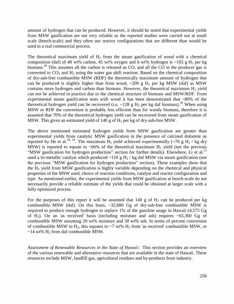
256

amount of hydrogen that can be produced. However, it should be noted that experimental yields

from MSW gasification are not very reliable as the reported studies were carried out at small

scale (bench-scale) and they often use reactor configurations that are different than would be

used in a real commercial process.

The theoretical maximum yield of H2 from the steam gasification of wood with a chemical

composition (daf) of 48 wt% carbon, 45 wt% oxygen and 6 wt% hydrogen is ~165 g H2 per kg

biomass.28

This assumes all the carbon is released as CO, and all the CO in the producer gas is

converted to CO2 and H2 using the water gas shift reaction. Based on the chemical composition

of dry-ash-free combustible MSW (RDF) the theoretically maximum amount of hydrogen that

can be produced is slightly higher than from wood, ~200 g H2 per kg MSW (daf) as MSW

contains more hydrogen and carbon than biomass. However, the theoretical maximum H2 yield

can not be achieved in practice due to the chemical structure of biomass and MSW/RDF. From

experimental steam gasification tests with wood it has been demonstrated that ~80% of the

theoretical hydrogen yield can be recovered (i.e. ~128 g H2 per kg daf biomass).28

When using

MSW or RDF the conversion is probably less efficient than for woody biomass, therefore it is

assumed that 70% of the theoretical hydrogen yield can be recovered from steam gasification of

MSW. This gives an estimated yield of 140 g of H2 per kg of dry-ash-free MSW.

The above mentioned estimated hydrogen yields from MSW gasification are greater than

experimental yields from catalytic MSW gasification in the presence of calcined dolomite as

reported by He et al.18, 19

. The maximum H2 yield achieved experimentally (~70 g H2 / kg dry

MSW) is reported to equate to ~66% of the theoretical maximum H2 yield (see the previous

“MSW gasification for hydrogen production” section for further details). Elsewhere, Li et al.21

used a tri-metallic catalyst which produced ~110 g H2 / kg daf MSW via steam gasification (see

the previous ”MSW gasification for hydrogen production” section). These examples show that

the H2 yield from MSW gasification is highly variable depending on the chemical and physical

properties of the MSW used, choice of reaction conditions, catalyst and reactor configuration and

type. As mentioned earlier, the experimental yields from MSW gasification at bench-scale do not

necessarily provide a reliable estimate of the yields that could be obtained at larger scale with a

fully optimized process.

For the purposes of this report it will be assumed that 140 g of H2 can be produced per kg

combustible MSW (daf). On this basis, ~32,680 Gg of dry-ash-free combustible MSW is

required to produce enough hydrogen to replace 1% of the gasoline usage in Hawaii (4,575 Gg

of H2). On an 'as received' basis (including moisture and ash) requires ~65,360 Gg of

combustible MSW assuming 20 wt% moisture and 30 wt% ash. In terms of percent conversion

of combustible MSW to H2, this equates to ~7 wt% H2 from 'as received' combustible MSW, or

~14 wt% H2 from daf combustible MSW.

Assessment of Renewable Resources in the State of Hawaii: This section provides an overview

of the various renewable and alternative resources that are available in the state of Hawaii. These

resources include MSW, landfill gas, agricultural residues and by-products from industry.

257

Assessment of MSW resources on Oahu: In this section a summary of the MSW resources on the

island of Oahu is provided. The information reported herein was obtained from the most recent

City and County of Honolulu Solid Waste Management report '2008 Integrated solid waste

management plan update'.29

Additional information was taken from the 2013 interim report 30

to

estimate the amount of MSW produced on Oahu in 2015.

There are five 'transfer stations' on the island of Oahu, three are operated by the State and two are

private. Limited information is available from private sites therefore they will not be discussed in

this report. Table A1.1 in Appendix A1 provides a breakdown of the amount of material

collected at the three State owned transfer sites from July 1st 2005 to 30th June 2006.

29 Table

A1.2 gives an overview of the total amount of waste generated on the island of Oahu from July

1st 2005 to 30

th June 2006 and shows the amounts sent to different locations; along with

estimates for 2015.30

Table A1.3 in Appendix A1 provides a breakdown of the results from the waste characterization

at Waimanalo gulch landfill29

in 2005 on an 'as received' basis. Table A1.4 displays the same

results as in Table A1.3 after excluding non-combustible materials. Table A1.5 shows the results

of the waste characterization study for the combined materials from H-power and Waimanalo

gulch landfill for 2005 on an 'as received' basis. Table A1.6 displays the same data as in Table

A1.5 after excluding non-combustible materials. Table A1.7 shows the results of the waste

characterization at Waimanalo gulch landfill estimated for 2015 by increasing the 2005 values by

18% in accordance with predicated increases in population.30

Table A1.8 displays the same data

as in Table A1.7 after excluding non-combustible materials.

Table A1.2 shows that in 2015 approximately 1.9 million tonnes of MSW will be generated on

Oahu. Just over a third of the waste is recycled, reused or composted with a similar amount being

used for electricity production at H-power. This leaves about 600,000 tonnes of MSW being sent

to landfill of which ~360,000 tonnes is sent to the Waimanalo gulch landfill (Table A1.2).

However, after the '2008 report' was published, H-power increased its capacity by ~270,000

tonnes per annum which is not accounted for in Tables A1.2 to A1.8. If it is assumed that the

additional material being sent to H-power reduces the amount being sent to Waimanalo gulch

landfill, the amount of material being landfilled is reduced from ~360,000 tonnes per annum (as

received) to ~90,000 tonnes per annum as of 2015. Assuming that roughly 50 wt% of the 90,000

tonnes of MSW is organic material suitable for combustion (excluding glass, metal, etc.) gives

~45,000 tonnes of combustible MSW. This 45,000 tonnes of combustible MSW contains ~50

wt% moisture and ash. Therefore, on a dry-ash-free basis this is ~22,500 tonnes of combustible

material that can be used for hydrogen production.

Note: In 2006 ~135,000 tonnes of MSW was diverted from H-power to landfill due to closures

for maintenance or un-anticipated shut-downs.29

It is possible that as of 2015 the only

combustible material that is currently being sent to Waimanalo gulch landfill is that which is

diverted from H-power due to closures for maintenance and unexpected shut-downs. However,

there is no data available regarding how much material is being diverted from H-power since

they increased capacity. In addition, there are media reports that since H-power increased its

capacity there is not enough waste to run the plant at full capacity. From the available data it

appears there is very little waste being sent to landfill on Oahu as of 2015 that is suitable for

258

energy applications or for generating hydrogen (less than 100,000 tonnes per annum, as

received). The values in Tables A1.1 to A1.8 (Appendix A1) are for the 'as received' waste which

contains significant amounts of moisture and ash (inorganics); hence the amount of material on a

dry-ash-free basis is estimated to be half of that reported in the tables.

Based on the data in Tables A1.2 to A1.8 it is possible to estimate the amount of combustible

MSW that is available for hydrogen production in 2015. The lower end of this range, estimated

after accounting for the increase in capacity at H-power (inc. by 270,000 Mg/annum). This gives

~90,000 Mg (as received) MSW which is ~45,000 Mg of 'combustible MSW' (as received), and

by assuming this material contains 50 wt% ash and moisture gives ~22,500 Mg of dry-ash-free

organic material that could be used for generating hydrogen. The upper end of the range is

~430,000 Mg of dry-ash-free material if all the combustible waste from Waimanalo gulch

landfill and H-power is used for hydrogen production (which is unlikely).

Assuming the combustible MSW has a similar chemical composition as RDF it is possible that

up to ~3,300 Mg of H2 (3.5 million kg) could be generated from 22,500 tonnes of combustible

MSW (daf), i.e. this is the low end of the range. This equates to approximately 0.8 % of the

gasoline used for transportation in Hawaii in 2014. Refer to the previous “Hydrogen capacity

required to meet potential DOE and civilian sector demand” section for the basis of this

estimation.

Tipping fees: H-POWER and the Waimanalo Gulch Landfill have a common tipping fee of

$100/Mg for trash commercial haulers unloading at either site. Tipping fees for C&D waste at

the PVT Landfill begin at $33 per Mg for large semi trailer loads.31

As of July 1st 2015 a new

tipping fee will be charged to businesses that drop off green waste at East and West Hawaii

recycling facilities, $23.38 per Mg.32

Assessment of MSW resources on Maui: In the county of Maui the only landfill site of

significant size is the Central Maui Landfill (~190,000 Mg per annum). According to the '2011

Waste Characterization Study' the main components are ~140,000 Mg MSW, ~24,000 Mg green

waste, ~22,000 Mg sewage sludge and 3,500 Mg fat oil and grease (FOG). This totals ~170,000

Mg of MSW excluding sewage sludge. The waste sent to landfill has been reported to contain

~42 wt% organics (i.e. combustible material), excluding sewage sludge.31

Therefore, 42 % of 170,000 tonnes equals ~71,500 tonnes of combustible MSW (as received).

On a dry-ash-free basis this is ~35,700 tonnes of combustible MSW that could be used to

produce hydrogen. However, it is probably not practical to transport MSW from Maui to Oahu

for conversion to hydrogen. A more viable pathway would be to pyrolyze the MSW to produce a

pyrolysis oil for transfer to Oahu which can then be used to produce hydrogen. Pyrolysis oil is

more energy dense than raw MSW making transportation more efficient.

It may also be possible to process agricultural residues from Maui in the same way (i.e. via

pyrolysis). The main crop on Maui is sugarcane which generates significant amounts of cane

trash and bagasse which could be used for hydrogen production. However, all the cane trash and

bagasse is already used on site for energy production which means it would be unlikely that

significant amounts of material would be available for hydrogen production.33, 34

259

At the time of writing this report (mid 2015) the Maui Resource Recovery Facility (MRRF) was

under construction which is planned to divert about 80% of the waste entering the Central Maui

landfill for other uses. Anaergia, the company operating the MRRF and the facility is scheduled

to be fully operational by 2017.35

The process has been described in a meeting between three

Maui Sierra Club directors and a representative from Anaergia on March 24, 2014 which is

summarized below:36

1) Trash is taken to the materials separation facility and recyclables are separated. Metal via

magnets, plastics via floating, and hand sorting of paper and cardboard.

2) Green waste goes to a composting operation. Other recyclables go to existing recycling

companies or is shipped.

3) Sewage sludge and other wet, digestible material that isn't composted is sent to a digester to

produce natural gas, a minimum of 500 million BTUs per day (0.5 million MJ/day). After

digestion the sludge can be composted provided it does not contain landfill leachate.

4) Non-inert materials including the sludge after digestion would be dewatered (and the water

used in the floating separation) and used to produce energy pellets. At the meeting it was pointed

out by one of the Sierra Club directors that it is unrealistic to think that the Hawaiian

Commercial & Sugar Company (HC&S) on Maui will take the pellets in lieu of coal since they

are already being investigated for their emissions violations and it is extremely unlikely that the

parent company A&B, which is primarily a developer, would invest the funds needed to upgrade

the emissions controls.

Note: No information could be found as to the chemical or physical properties of the 'energy

pellets' from the MRRF or in what quantity they will be produced. It is not possible therefore to

make an evaluation as to whether these pellets could be used elsewhere in the State for energy or

hydrogen production.

5) Medical, hazardous and construction waste is not accepted by the Maui County landfill. Tires

are not currently taken.

6) After recycling, producing natural gas, pellets and compost, the remainder (about 20 wt% of

the waste) is sent to the landfill and Anaergia pays tipping fees to the County. As of 2014 only

about 5% of the waste is recycled.

7) The Anaergia representative said: "they would probably sell the natural gas to the Hawaii gas

company to transport, pipe or whatever.". All the materials (recyclables, gas, pellets) are the

responsibility of Anaergia to find takers/buyers for. The Anaergia representative suggested" the

Oahu coal plant might take energy pellets and that if not, that shipping to Asia or the Mainland

is cheap because their ships deliver here and go back empty so the carbon footprint is lower than

one would think and the rates are lower too."

260

Tipping Fees: A summary of the tipping fees paid to MRRF by the County of Maui are

summarized in Table 7.4.10 along with the tipping fees paid by MRRF to the County of Maui.

There is no charge to residences who self haul waste to the Maui Central Landfill.

Table 7.4.10: Tipping fees paid to MRRF by the County of Maui and fee charged to MRRF by the County

of Maui.

Item

Fee the

County pays

to MMRF

Fee MMRF

pays to the

County

$ / ton (short) $ / ton (short)

Green waste 28 28

C&D 68 68

MSW 68 68

Sewage sludge 76 76

FOG* 100 100

Residues - 71

Unprocessible

materials

(appliances)

- 68

*The majority of the FOG is collected privately by

Pacific biodiesel.

In summary, since the construction of the MMRF there does not appear to be any significant

MSW resources available in the county of Maui that could be used for the production of

hydrogen. The MMRF is predicted to divert ~80 wt% of the 170,000 tonnes of MSW from

landfill, which leaves about 34,000 tonnes of MSW being landfilled. It is unclear what the

composition of this material will be, i.e. it is likely to contain significant greater amounts of non-

combustible materials such as glass and metal than typical MSW. If it is assumed that 40 wt% of

the MSW being landfilled is combustible material this give ~13,600 tonnes of combustible MSW

(as received) that could be used for hydrogen generation. Assuming this combustible MSW

contains 50 wt% ash and moisture, this gives ~6,800 tonnes of organic material (daf) suitable for

hydrogen production.

However, as the hydrogen is required on Oahu rather than on neighbor islands, the MSW on

Maui would either have to be converted to hydrogen on Maui with the hydrogen transported to

Oahu; or the MSW would have to be shipped to Oahu for conversion. Neither of these options

appears to be practical due to the low energy density of hydrogen and MSW. A more plausible

pathway would be to convert the MSW into an energy dense pyrolysis oil (or a slurry of oil and

char) locally and to ship the pyrolysis oil to Oahu for conversion to hydrogen. The pyrolysis

process is described in “Distributed Processing & Centralized Refining” section later in this

report, along with estimates of the amount of pyrolysis oil and char that could be produced from

MSW and how much hydrogen could be produced from the pyrolysis products.

Assessment of MSW resources on Hawaii Island: There are two main landfills on the big island,

South Hilo Sanitary Landfill and West Hawaii Sanitary Landfill at Pu`uanahulu in Kona that

jointly process approximately 190,000 tonnes of MSW per annum (as of 2006) excluding sewage

261

sludge. The most recent data that is available from the county of Hawaii is from the 'County of

Hawaii Integrated Resources and Solid Waste Management Plan Update 2009' 37

which uses data

from 2007 to 2008. Two thirds of the MSW goes to the West Hawaii Sanitary Landfill in Kona.

For the year 2007 to 2008 the amount of MSW generated on the Big Island was ~270,000 tonnes

with ~80,000 tonnes being recycled and 190,000 tonnes being landfilled.37

Of the MSW sent to landfill approximately 22 wt% is paper, 8 wt% plastic, 33 wt% organics

(mostly food waste) and 22 wt% C&D. It has been estimated that ~43 wt% of the MSW that is

sent to landfill is organic material (as received basis) which is potentially useful for energy or

hydrogen production, excluding sewage sludge.31

According to a report from 2010 the Hilo Landfill was supposed to close in August 2010;31

however, as of mid-2015 it was still operational. It is unclear what the fate of the South Hilo

Sanitary Landfill is. There was a feasibility study performed by R.W. Beck in 2012 that looked

at expanding the South Hilo Sanitary Landfill. The study concluded it is feasible to expand the

site but no information could be found regarding whether this had been, or will be, implemented.

In addition, there were reports of a plan for a private company to build a waste-to-energy

incinerator to replace Hilo’s landfill, however that project appears to have been cancelled and a

new project implemented. According to a press release from BioEnergy Hawaii LLC (BEH) on

March 11th

2015,38

BEH is planning to build a $50 million plant for MSW material handling and

energy conversion to reduce the amount of material sent to landfill on the big island. According

to the press release, up to 70% of the waste currently being sent to the West Hawaii Sanitary

Landfill will be diverted. The project was described as follows:38

"The BEH project will establish advanced recycling operations and produce multiple value

products from the incoming waste. In order to maximize the diversion rate, the facility design

integrates the recovery of three separate value streams: recyclable commodities, organics and

solid fuel.

The recyclable materials, which would have been buried in the landfill, will be recovered and

directed into the local recycling commodity market.

The wet organic waste (i.e. food and green waste); will be treated through an anaerobic

digestion (AD) process to stabilize the material and produce a nutrient rich natural fertilizer and

high-quality compost. The AD operations will also recover an energy rich biogas—a flexible fuel

source that can be used to generate electricity, be upgraded to pipeline quality renewable

natural gas (RNG), or compressed to create an alternative transportation fuel (known as bio-

CNG, i.e. compressed natural gas).

The residual solid fuel portion—items not suitable for use in the anaerobic digester such as

mixed paper, textiles, low-value plastic and wood—will be processed into a post-recycled

engineered fuel—a dry, light material suitable for thermal energy conversion operations.

Incoming waste will be handled and processed in an enclosed building to ensure dust and odor

control. The waste will be separated and sorted through a combination of automated and manual

262

recovery methods. Materials that cannot be recycled or processed into renewable fuel, fertilizer

and compost will be delivered to the Puuanahulu landfill—about 30% of the total volume.

Construction on the BioEnergy Hawaii facility is scheduled to begin during the summer of

2016."

Taking into account the amount of MSW that will be processed by the BEH plant leaves ~40,000

Mg per annum of MSW being sent to the West Hawaii Sanitary Landfill and ~60,000 Mg of

MSW going to the Hilo landfill (based on the 2007-2008 data). This means there is a total of

~100,000 Mg per annum of MSW (as received) being sent to landfill (excluding sewage sludge),

assuming the BEH plant goes ahead as planned. It has been estimated that 43 wt% of this MSW

is combustible material,31

i.e. ~43,000 Mg of combustible MSW (as received). Assuming that 50

wt% of the combustible material is ash and moisture means there is ~22,000 Mg of dry-ash-free

combustible MSW that could be used for hydrogen production.

As described in the previous sub-section, the most promising pathway for producing hydrogen

for use on Oahu from MSW resources on neighbor islands is through an intermediate conversion

process to produce pyrolysis oil and char. The pyrolysis oil and char can then be transported to

Oahu for conversion to hydrogen, see the “Distributed Processing & Centralized Refining”

section later in this report.

Tipping fees: The tipping at landfills on the Big Island are $93.50 per Mg of MSW.37

Assessment of MSW resources on Kauai: The most recent data for the amount of MSW being

landfilled in the county of Kauai is from the 'Integrated Solid Waste Management Plan 2009'.39

In this report it is predicted that the amount of MSW generated in 2013 would be ~90,000 Mg

per annum with a further 40,000 Mg being diverted from landfill (recycled).39

Based on numbers

from 2005, the amount of MSW landfilled on Kauai was ~75,000 Mg per annum.31

There is only one landfill site on Kauai, the Kekaha Landfill that was predicted to reach capacity

by 2014, with plans to expand the site as discussed in a meeting during 2013,40

although no

information could be found as to the current state of affairs.

The composition of the MSW on Kauai is: paper ~35 wt%, plastics ~14 wt%, yard waste ~7

wt%, food waste ~15 wt%, wood ~2 wt%, other organics ~2-5 wt% which totals to about 75

wt% excluding sewage sludge and C&D waste.39

Elsewhere it has been reported that ~30 to 40

wt% of the MSW being landfilled on Kauai is organic material (as received), excluding sewage

sludge 31

.

Using the 2013 predicted values,39

the amount of MSW being landfilled at the Kekaha Landfill is

90,000 Mg (as received). For the purpose of this report the combustible fraction of the MSW that

is suitable for use in hydrogen production is assumed to be 35 wt% of the 'as received' MSW; i.e.

35 wt% of 90,000 Mg of MSW equals ~32,000 Mg of combustible MSW (as received).

Assuming the combustible MSW contains 50 wt% moisture and ash gives ~16,000 Mg of dry-

ash-free combustible MSW per annum that is suitable for hydrogen.

263

As described in the previous sub-section, the most promising pathway for producing hydrogen

for use on Oahu from MSW resources on neighbor islands is through conversion to pyrolysis oil

and char. The pyrolysis oil and char could then be transported to Oahu for conversion to

hydrogen, see the Distributed Processing & Centralized Refining section later in this report.

Tipping fees (per Mg), Kekaha Landfill, Kauai:41

Municipal Solid Waste $130.90

Asbestos-containing materials $239.80

Dead animals $130.90

Minimum Fee for any load of Municipal Solid Waste and dead animals $23.10

Minimum Fee for any load of asbestos-containing materials $239.80

Chemical composition of combustible MSW: The key to a successful MSW gasification process

is a good understanding of the chemical composition of the feedstock in terms of amounts of

organic elements (C, H, N, O, S) and inorganic elements. However, this information is not

available for MSW that is produced in Hawaii. In lieu of this information the chemical

composition of MSW components from literature sources is provided in Table A1.9 for organics

(i.e. the values are not based on MSW generated in the State of Hawaii, instead they are taken

from the general literature). Table A1.10 shows the ash composition (inorganics) of various

MSW components, also taken from the general literature as this information is also not available

for MSW produced in

Paper is one of the main components of MSW which contains significant amounts of inorganic

additives from the coating process. These additives are mainly pigments (80-95%), binders (2-

20%) and chemical additives (1-2%).42

Clay is the single most common additive in the coating

process. Coated printing and writing paper also contains 10-15% of calcium carbonate filler.42

Mixed waste paper often contains extremely high concentrations of aluminum and titanium

oxides.26

Table A1.11 summarizes the pigments used in paper production and their chemical

composition.42

In addition, newspaper can contain up to ~ 0.10 mg Hg per kg of paper.43

The data in Tables A1.9 and A1.10 can not be used to reliably estimate the average properties of

the MSW produced in Hawaii as the composition of waste is highly variable from one region to

another. The information in Tables A1.9 and A1.10 is provided to give an indication of which

components of MSW are most likely to cause problems due to their composition and have the

potential to release harmful or toxic materials into the environment. If MSW gasification was to

be implemented in Hawaii, the first action to take is to quantify the chemical and physical

properties of the various waste streams.

Assessment of landfill gas resources in the State of Hawaii: It has been reported that landfill gas

could produce up to 26.9 million m3/yr or 2.3 million kg/yr of hydrogen (2,300 Mg H2) in the

State of Hawaii.31

This amount of hydrogen is equal to about 0.5% of the gasoline usage in

Hawaii in 2014. However, the landfills are located in fifteen sites spread throughout the State

and only seven of the landfills contain more than 1 million tonnes of MSW.44

According to the

EPA, three of the fifteen sites collect landfill gas, however, two of those sites flare the gas with

only one site using the gas for co-generation.44

However, the co-generation project at the Kapaa

264

landfill, Kailua, Oahu, ceased operation in 2000 according to the EPA. 44

Elsewhere it was

reported to have closed in 2002 due to operating difficulties.33, 34

The two sites that flare landfill gas are the central Maui landfill (~3.5 million tonnes of waste)

and the Waimanalo Gulch Landfill, Kapolei, Oahu (~5 million tonnes of waste). As the aim of

this study is the production of hydrogen on the island of Oahu, it is unlikely that landfill gas from

Maui can contribute in a significant way to this goal. It is unlikely to be practical to ship landfill

gas from Maui to Oahu, or to produce hydrogen on neighbor islands such as Maui and ship the

hydrogen to Oahu due to low energy densities and transportation costs.

According to the EPA the amount of landfill gas being flared from the Waimanalo Gulch

Landfill is ~10 million m³/annum.44

The steam-methane-reforming (SMR) process produces 1.0

m3 of hydrogen per 0.406 m

3 of methane.

45 Landfill gas contains ~50 vol.% methane, therefore

the amount of hydrogen that could be produced from the Waimanalo Gulch Landfill via steam

reforming is ~12.3 million m3/yr or 1,100 tonnes of H2 which is equivalent to ~0.24% of the

gasoline usage in Hawaii.

Glycerin for hydrogen production: : Big Island Biodiesel (BIB) currently produces 5.6 million

gallons of biodiesel per annum (as of 2014) and generates 0.66 million gallons of crude glycerin

as a byproduct (~2.5 million liters, 31,500 Mg).46

In addition to their biodiesel and crude

glycerin products, their high vacuum distillation unit generates column bottoms that are currently

used to meet the facility’s process heat demands with an excess of 0.22 million gallons per

annum which could be used to produce hydrogen. At the time of this writing (mid 2015) the BIB

facility was operating at 1/3rd

capacity, i.e. it could produce ~15 million gallons of biodiesel per

annum at full capacity.

A typical recent analysis of crude glycerin from the BIB facility is: 92.5 wt% glycerin, 2.9 wt%

H2O, 2.5 wt% ash, and 2 wt% MONG with a specific gravity of 1.26 g ml-1

.46

MONG refers to

'material-organic-non-glycerol' and includes fatty acid methyl esters, free fatty acids, methanol,

and glycerides that can contribute to H2 production.47

Glycerin with less than 99.7% purity is

considered crude glycerin in the marketplace. The composition of dry-ash-fee crude glycerin is

~59 wt% carbon, ~11 wt% hydrogen and ~30 wt% oxygen.46

On a dry-ash-free basis there is ~0.62 million gallons of crude glycerin (29,600 Mg daf) and at

least 0.10 million gallons (~5,000 Mg daf) of column bottoms produced per annum, assuming

the column bottoms have a ash and moisture content of 50 wt%. No data is available regarding

the composition of the column bottoms but it is likely to be similar to crude glycerin. For the

purpose of estimating the amount of hydrogen that could be produced from crude glycerine and

column bottoms, the column bottoms are assumed to have the same H2 production potential as

crude glycerin.

H2 production potential from steam reforming of pure glycerin (C3H8O3) is 7 moles H2 per mole

C3H8O3 or ~150 g H2 per kg C3H8O3.48

Direct thermal decomposition of pure glycerin produces 4

moles H2 and 3 moles CO per mole C3H8O3, theoretically.

265

For the purposes of this study it is assumed that the amount of H2 that can be produced from the

dry-ash-free crude glycerin and column bottoms is 75% of the ideal yield reported by Douette48

from steam reforming; i.e. ideal yield of H2 via steam reforming is 150 g / kg crude glycerin

which gives an estimated experimental yield of ~110 g H2 / kg crude glycerin (11 wt% daf)

assuming 75% conversion.

Based on 29,600 Mg crude glycerin (daf) the amount of hydrogen produced from steam

reforming is approximately 3.25 million kg of H2 (3,250 Mg). If the column bottoms are also

included the total amount of feed is 34,600 Mg (daf) that could produce 3,800 Mg of H2. To put

this in context, 3,800 Mg of H2 is equivalent to ~3.8 million gallons of gasoline, which is ~0.8 %

of the amount of gasoline used in Hawaii in 2014.

Assessment of agricultural residue resources in the State of Hawaii: Table A1.12 in Appendix

A1 provides a summary of the farmland in the State of Hawaii showing the number of farms on

the various islands, their size and activities; reproduced from 2012 Census of Agriculture,

USDA.49, 50

Note: there is no information in the census report regarding crop residues or fallow

farmland. The island of Hawaii has by far the most agricultural activity in the State followed by

Maui and then Oahu based on the number of farms. However, if the total amount of land in farms

is considered then Oahu has the least (~69,000 acres), followed by Kauai (~144,000 acres), Maui

(230,000 acres) and Hawaii has the most (~690,000 acres).

For the island of Oahu the main farming activities are livestock and poultry, of the crops farmed

on Oahu vegetables are the major product followed by land in orchards. In addition, the majority

of the farms on Oahu are less than 10 acres in size (~74% of the farms) with less than 5% of the

farms having a size larger than 180 acres and less than 2.5% have a size larger than 500 acres.

This information suggests that there are limited agricultural residue resources available on Oahu

for use in the production of hydrogen. In addition, the low density of farms on Oahu will

adversely affect the cost of collecting agricultural residues in terms of time and money, possibly

making collection impractical.

The most significant agricultural residue resources within the State are listed below.

Sugarcane bagasse and cane trash (Maui): Most, if not all, the cane trash and bagasse is already

used on site at Hawaiian Commercial & Sugar Company (HC&S) for energy and steam

production. Therefore, it is unlikely that this resource is available for hydrogen production.

Pineapple farms: The number of pineapple farms has decreased in recent years, and the existing

farms are typically small scale and are widely dispersed around the state.33, 34

In addition, the

residue from the plants is difficult to recover from the field. Due to these reasons, this resource is

unlikely to be economically viable for the production of hydrogen.

Macadamia nut shells (Hawaii): As of 2006 approximately 26,000 tonnes of nuts were harvested

which produced about 15,000 tonnes of nut shells with ~1.5 wt% moisture content.31

This is

potentially a useful source of biomass for generating hydrogen, although this material is already

being widely used as compost, as a soil amendment, as a boiler fuel to generate heat, for

266

electricity generation, and orchard road fill. It is estimated that about 10% of the shell residues

are bought and sold between factories on the big island.31

The ash content of macadamia nut shells is 0.8 wt%, dry basis.34

The chemical composition of

macadamia nut shells is: 55 wt% carbon, 42 wt% oxygen, 6 wt% hydrogen, 0.4 wt% nitrogen

and 0.05 wt% sulfur (daf basis). The chemical composition of macadamia nut shells is very

similar to wood, hence the amount of hydrogen that could be produced from the nuts shells is

assumed to the same as from the steam gasification of wood, which is ~128 g H2 per kg wood

(daf).28

The amount of nut shells on a dry-ash-free basis ~14,600 tonnes (15,000 tonnes of nut shells

with 1.5 wt% moisture and 0.8 wt% ash). Assuming that 128 g H2 can be produced per kg of nut

shells (daf) means that ~1,900 tonnes of H2 could be produced per annum.

However, rather than transporting the nut shells to Oahu for conversion into hydrogen, a better

approach may be to pyrolyze the nut shell on the Big Island and then ship the pyrolysis oil and

char to Oahu for conversion into hydrogen. See yjr Distributed Processing & Centralized

Refining section later in this report for estimates of the amount of pyrolysis oil and char that

could be produced from macadamia nut shells and how much H2 could be generated from the

pyrolysis products.

Summary of MSW and alternative resources (by county)

Table 7.4.11 provides a summary of the minimum amounts of MSW that are currently landfilled

in each county, and the approximate amount of hydrogen that could be produced from it by

steam gasification. In this assessment (Table 7.4.11) it is assumed that the MSW is converted to

H2 on the same island the MSW is produced on. However, this approach is unlikely to be

practical if the H2 is to be used solely on Oahu. If the H2 is to be used on Oahu, a more viable

pathway may be to first convert the MSW in to a more energy dense form locally using

pyrolysis. The pyrolysis oil and char could then be shipped to Oahu for conversion to H2, this

pathway is described in the Distributed Processing & Centralized Refining section later in this

report, along with estimates of the amount of hydrogen that could be produced.

Table 7.4.11: Summary of MSW resources in the state of Hawaii and the amount of H2 that could be

produced by steam gasification of the MSW locally. These values were derived using conservative

estimates of the amounts of MSW in each county.

Location

Amount of

combustible MSW

(daf basis)

H2

produced

Gallons of

gasoline

displaced

Mg Mg % of total 2014

Oahu 22,500 ~3,150 ~0.68

Maui 6,800 ~950 ~0.21

Hawaii

Island 22,000 ~3,100 ~0.67

Kauai 16,000 ~2,250 ~0.49

Total ~67,300 ~9,400 ~2.04

267

Note: Assumes 33,000 Mg daf MSW yields ~4,600 Mg H2 = 1

% gasoline

Table 7.4.12 details alternative resources that are available in the state which could be used for

the production of hydrogen. In Table 5.3 it is assumed that the all the feedstocks are directly

converted to hydrogen via steam gasification. The crude glycerine and column bottoms in Table

5.3 are already in liquid form and are energy dense, therefore these materials could be shipped

directly to Oahu for conversion to H2. For macadamia nut shells it may be advantageous to first

convert them into a more energy dense form via pyrolysis and to ship a slurry of pyrolysis oil

and char to Oahu for conversion to hydrogen, that approach is detailed in the Distributed

Processing & Centralized Refining section later in this report.

Table 7.4.12: Summary of alternative resource in the state of Hawaii that have significant potential for the

production of hydrogen.

Location - Resource

Amount of

alternative

resources

H2

produced

Gallons of

gasoline

displaced

Mg (daf basis) Mg % of total 2014

Hawaii - Macadamia nut shells 14,600 1,900 ~0.41

Maui - Crude glycerine (BIB)* 29,600 3,250 ~0.70

Maui - Column bottoms (BIB) 5,000 550 ~0.12

Oahu - Landfill gas 10,000,000 m3 1,100 ~0.24

Total n/a 6,800 ~1.47

* BIB is currently (2015) operating at 1/3rd capacity

Distributed Processing & Centralized Refining

Due to the low densities of farms on Oahu and limited availability of MSW since the expansion

of the H-power facility, there does not appear to be adequate resource on Oahu to produce

significant amounts of hydrogen via steam gasification.

A possible solution to this would be to identify locations on neighbor islands where significant

quantities of MSW and/or agricultural residues could be processed locally into a more energy

dense form for transport to Oahu. The most promising technology for this type of energy

densification is small scale fast pyrolysis units (which could be made portable, i.e. installed on a

foot print the size of standard shipping container)51

. Small pyrolysis units could be used to

convert MSW or agricultural residues or dedicated energy crops into a more energy dense form,

i.e. pyrolysis oil and char (as a slurry).

The pyrolysis oil/char slurry could then be shipped from neighbor islands to a centralized, large-

scale gasification plant on Oahu to produce hydrogen. Using the pyrolysis oil/char slurry to feed

a gasification unit has many benefits over attempting to upgrade pyrolysis oil into transportation

fuels such as gasoline or diesel. The main issues with pyrolysis oil from biomass or MSW are

that they contain a significant amount of water (up to 30 wt%), they are acidic which makes

storage and transportation an issue, they are reactive (aging reactions, polymerization) and they

268

contain particles of char. These issues complicate the upgrading of pyrolysis oil in to traditional

transportation fuels leading to severe coking on catalysts and loss of carbon as CO2. However,

the properties of pyrolysis oil are much less of an issue when it is used as a feedstock for steam

gasification, the only issue that remains a concern is the acidity of the pyrolysis oil in relation to

storage and transportation (normal steel vessels are inadequate).52

At present small scale mobile fast pyrolysis units are not considered commercially viable in

general situations.51

However, due to the high energy costs in Hawaii, the technology may be

more feasible here than in most other locations. The technology is well understood and is not

technically challenging. Numerous companies are developing and attempting to commercialize

mobile pyrolysis units.51

Transportation limitations

The maximum practical distance for transporting raw biomass (or MSW) by truck is typically in

the range of 75 to 100 miles for biomass to energy processes.31

However, due to Hawaii's

geography, high transportation fuel costs and infrastructure this distance it likely to be lower in

Hawaii and/or costs higher. It is also unlikely that it would be economical or practical to

transport raw biomass, MSW or agricultural residues between neighbor islands.31

A report by

HNEI from 2012 concluded that the interisland shipment of bulk solid fuel (based on sugar cane

bagasse) costs ~$1.0 per gallon of crude oil equivalent, whereas the shipment of liquid fuel (i.e.

pyrolysis oil made from biomass, etc.) costs ~$0.20 per gallon of crude oil equivalent.53

The cost

of shipping MSW would be similar to the bulk sugar cane bagasse case due to its low bulk

density. Although the accuracy of the cost estimates cannot be guaranteed, the relative cost

differential between shipping solid and liquid fuels is considered reliable - which clearly

indicates a considerable cost saving for transporting liquids rather than solid materials.

Pyrolysis of MSW and agricultural residues

MSW Pyrolysis: The fast pyrolysis of MSW has been studied.54

Under ideal conditions (small

particle size <200 µm, 0.25 s residence time, heating rate > 400 °C/s and reaction temperature of

500 °C) it is possible to convert ~40 wt% of the dry-ash-free MSW into bio-oil (daf) with ~10

wt% char (daf). Under more realistic conditions for a typical small commercial pyrolysis plant

(particle size ~3 mm and residence time of ~2 s) the bio-oil yield is likely to be less, ~30 wt%

bio-oil (daf) with ~20 wt% char (daf).

For the purposes of estimating the amount of hydrogen that could be generated from pyrolysis oil

and char from MSW it is assumed that 'combustible MSW' has a similar composition as RDF as

described in the Gas cleaning technologies section earlier in this report. Where combustible

MSW has a composition of 20 wt% moisture and 30 wt% ash on an as received basis. The

chemical composition of the dry-ash-free MSW is assumed to be 54 wt% carbon, 37 wt%

oxygen, 7.5 wt% hydrogen, 1.0 nitrogen, 0.8 wt% chlorine and 0.5 wt% sulfur.

The chemical composition of fast pyrolysis oil from MSW has not been reported, therefore it is

estimated by comparison to in-house data from the fast pyrolysis of banagrass 55

which produces

a similar low pyrolysis oil yield as MSW. Table 7.4.13 shows the elemental composition of raw

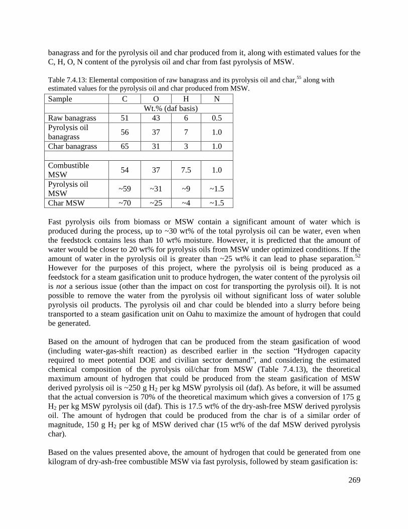
269

banagrass and for the pyrolysis oil and char produced from it, along with estimated values for the

C, H, O, N content of the pyrolysis oil and char from fast pyrolysis of MSW.

Table 7.4.13: Elemental composition of raw banagrass and its pyrolysis oil and char,

55 along with

estimated values for the pyrolysis oil and char produced from MSW.

Sample C O H N

Wt.% (daf basis)

Raw banagrass 51 43 6 0.5

Pyrolysis oil

banagrass 56 37 7 1.0

Char banagrass 65 31 3 1.0

Combustible

MSW 54 37 7.5 1.0

Pyrolysis oil

MSW ~59 ~31 ~9 ~1.5

Char MSW ~70 ~25 ~4 ~1.5

Fast pyrolysis oils from biomass or MSW contain a significant amount of water which is

produced during the process, up to ~30 wt% of the total pyrolysis oil can be water, even when

the feedstock contains less than 10 wt% moisture. However, it is predicted that the amount of

water would be closer to 20 wt% for pyrolysis oils from MSW under optimized conditions. If the

amount of water in the pyrolysis oil is greater than ~25 wt% it can lead to phase separation.52

However for the purposes of this project, where the pyrolysis oil is being produced as a

feedstock for a steam gasification unit to produce hydrogen, the water content of the pyrolysis oil

is not a serious issue (other than the impact on cost for transporting the pyrolysis oil). It is not

possible to remove the water from the pyrolysis oil without significant loss of water soluble

pyrolysis oil products. The pyrolysis oil and char could be blended into a slurry before being

transported to a steam gasification unit on Oahu to maximize the amount of hydrogen that could

be generated.

Based on the amount of hydrogen that can be produced from the steam gasification of wood

(including water-gas-shift reaction) as described earlier in the section “Hydrogen capacity

required to meet potential DOE and civilian sector demand”, and considering the estimated

chemical composition of the pyrolysis oil/char from MSW (Table 7.4.13), the theoretical

maximum amount of hydrogen that could be produced from the steam gasification of MSW

derived pyrolysis oil is ~250 g H2 per kg MSW pyrolysis oil (daf). As before, it will be assumed

that the actual conversion is 70% of the theoretical maximum which gives a conversion of 175 g

H2 per kg MSW pyrolysis oil (daf). This is 17.5 wt% of the dry-ash-free MSW derived pyrolysis

oil. The amount of hydrogen that could be produced from the char is of a similar order of

magnitude, 150 g H2 per kg of MSW derived char (15 wt% of the daf MSW derived pyrolysis

char).

Based on the values presented above, the amount of hydrogen that could be generated from one

kilogram of dry-ash-free combustible MSW via fast pyrolysis, followed by steam gasification is:

270

MSW Pyrolysis oil = 30 wt% (daf), which gives 300 g pyrolysis oil, assuming 17.5 wt%

conversion of pyrolysis oil to hydrogen means ~50 g H2 is generated from each kg of

combustible MSW (daf).

MSW Pyrolysis char: 20 wt% (daf) which gives 200 g char, assuming 15 wt% conversion

of char to hydrogen produces ~30 g H2 per kg of combustible MSW (daf).

The total amount of H2 that could be produced from MSW derived pyrolysis oil and char is ~80

g per kg daf combustible MSW (8 wt% daf basis), compared to ~14 wt% for direct steam

gasification of MSW (daf basis). A summary of the amount of H2 that could be produced from

MSW on the neighbor islands via fast pyrolysis, followed by steam gasification is provided in

Table 7.4.14.

Table 7.4.14: Estimated amount of hydrogen that could be produced by fast pyrolysis of MSW on

neighbor islands, followed by steam gasification on the pyrolysis products on Oahu.

Location

Amount of

combustible MSW

(daf basis)

H2 from

Pyrolysis

oil

H2 from

Pyrolysis

char

Total H2

produced

Gallons of

gasoline

displaced

Mg Mg Mg Mg % of total

2014

Maui 6,800 304 220 544 ~0.12

Hawaii

Island 22,000 1,100 660 1,760 ~0.38

Kauai 16,000 800 480 1,280 ~0.28

Total 44,800 ~2,240 ~1,344 3,584 ~0.78

Mac Nut Shells Pyrolysis: Rather than transporting nut shells to Oahu for conversion into

hydrogen, a better approach may be to pyrolyze the nut shells on the Big Island and then ship the

pyrolysis oil and char to Oahu for conversion into hydrogen. As macadamia nut shells have a

similar composition as wood it is reasonable to assume the same level of conversion into

pyrolysis oil. The amount of pyrolysis oil (dry-ash-free basis) that is typically produced from

wood is 55 wt% of the daf feedstock with ~15 wt% char. Starting with 14,600 Mg of daf nut

shells about 8,000 Mg of pyrolysis oil and ~2,200 Mg of char could be produced. Assuming the

chemical composition of the pyrolysis oil and char from nut shells is the same as from wood

means the nut shell pyrolysis oil will contain: ~56 wt% carbon, ~36 wt% oxygen, ~7 wt%

hydrogen, and ~1 wt% nitrogen; and the nut shell char: ~66 wt% carbon, ~30 wt% oxygen, ~2.5

wt% hydrogen and ~1 wt% nitrogen.

Steam gasification of pyrolysis oil from nut shells would produce ~150 g of H2 per kg of

pyrolysis oil, using the same basis as explained the earlier section “Pyrolysis of MSW and

agricultural residues”. The nut shell char could produce ~120 g H2 per kg of char. On this basis,

14,600 Mg of daf nut shells produces ~8,000 Mg of pyrolysis oil (daf) which could generate up

to ~1,200 Mg of H2 per annum. The char (daf) from nut shells (~2,200 Mg) could produce ~330

Mg H2. This gives a total H2 production of ~1,500 Mg from the pyrolysis oil and char produced

from macadamia nut shells.

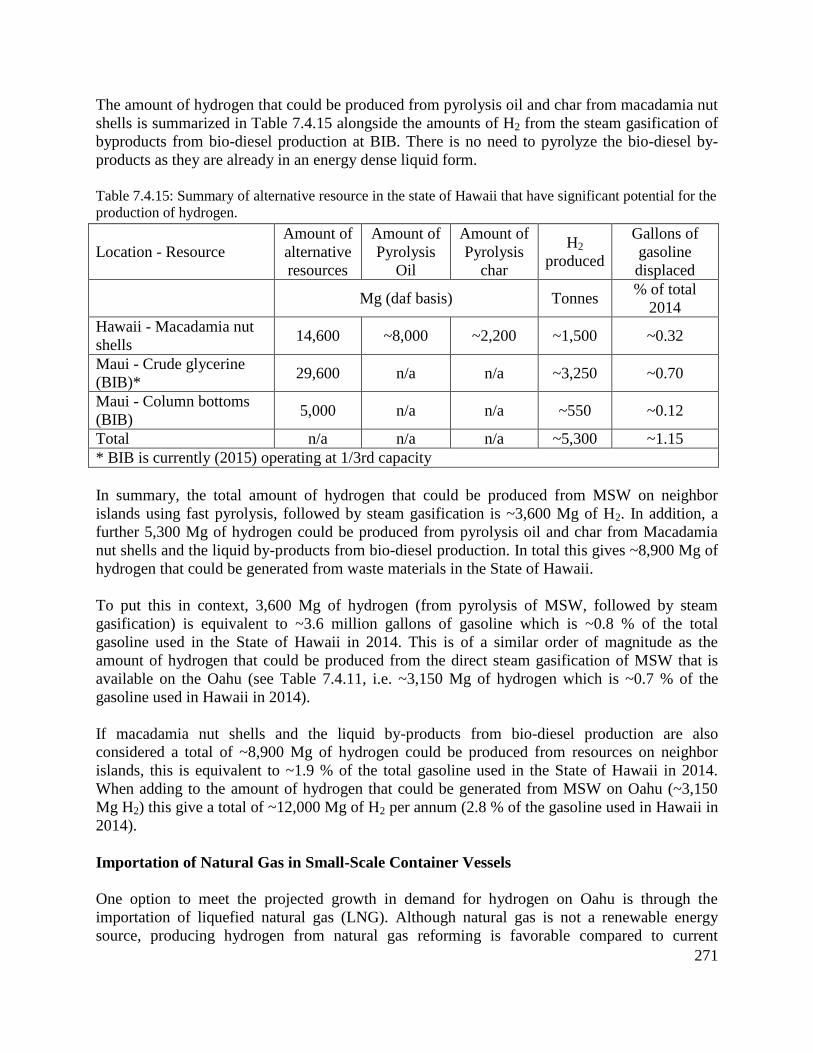
271

The amount of hydrogen that could be produced from pyrolysis oil and char from macadamia nut

shells is summarized in Table 7.4.15 alongside the amounts of H2 from the steam gasification of

byproducts from bio-diesel production at BIB. There is no need to pyrolyze the bio-diesel by-

products as they are already in an energy dense liquid form.

Table 7.4.15: Summary of alternative resource in the state of Hawaii that have significant potential for the

production of hydrogen.

Location - Resource

Amount of

alternative

resources

Amount of

Pyrolysis

Oil

Amount of

Pyrolysis

char

H2

produced

Gallons of

gasoline

displaced

Mg (daf basis) Tonnes % of total

2014

Hawaii - Macadamia nut

shells 14,600 ~8,000 ~2,200 ~1,500 ~0.32

Maui - Crude glycerine

(BIB)* 29,600 n/a n/a ~3,250 ~0.70

Maui - Column bottoms

(BIB) 5,000 n/a n/a ~550 ~0.12

Total n/a n/a n/a ~5,300 ~1.15

* BIB is currently (2015) operating at 1/3rd capacity

In summary, the total amount of hydrogen that could be produced from MSW on neighbor

islands using fast pyrolysis, followed by steam gasification is ~3,600 Mg of H2. In addition, a

further 5,300 Mg of hydrogen could be produced from pyrolysis oil and char from Macadamia

nut shells and the liquid by-products from bio-diesel production. In total this gives ~8,900 Mg of

hydrogen that could be generated from waste materials in the State of Hawaii.

To put this in context, 3,600 Mg of hydrogen (from pyrolysis of MSW, followed by steam

gasification) is equivalent to ~3.6 million gallons of gasoline which is ~0.8 % of the total

gasoline used in the State of Hawaii in 2014. This is of a similar order of magnitude as the

amount of hydrogen that could be produced from the direct steam gasification of MSW that is

available on the Oahu (see Table 7.4.11, i.e. ~3,150 Mg of hydrogen which is ~0.7 % of the

gasoline used in Hawaii in 2014).

If macadamia nut shells and the liquid by-products from bio-diesel production are also

considered a total of ~8,900 Mg of hydrogen could be produced from resources on neighbor

islands, this is equivalent to ~1.9 % of the total gasoline used in the State of Hawaii in 2014.

When adding to the amount of hydrogen that could be generated from MSW on Oahu (~3,150

Mg H2) this give a total of ~12,000 Mg of H2 per annum (2.8 % of the gasoline used in Hawaii in

2014).

Importation of Natural Gas in Small-Scale Container Vessels

One option to meet the projected growth in demand for hydrogen on Oahu is through the

importation of liquefied natural gas (LNG). Although natural gas is not a renewable energy

source, producing hydrogen from natural gas reforming is favorable compared to current

272

practices (electrolysis with high cost electricity, or via naphtha reforming). The benefits include

lower emissions of green house gases, SO2, HCl, NH4, and particulates, when compared to

naphtha reforming. These benefits will vary in relation to electrolysis however, depending on the

source of the electricity; i.e. if the electricity is produced from renewable sources (wind, solar,

biomass, geothermal) there are likely to be no benefits from using natural gas. Cost comparisons

between steam-methane-reforming (using LNG) vs electrolysis and steam reforming of naphtha

for hydrogen production are provided in the earlier sections “Electrolysis derived hydrogen - cost

and capacity” and “Petroleum naphtha derived hydrogen - cost and capacity” respectively. It

would seem that the main potential benefit of using LNG for hydrogen production is its

relatively low production cost, although there are substantial set-up costs, logistical and

regulatory issues related to LNG imports. The main issues are discussed below.

A recently report (2013) has assessed policy, economic and technical issues related to

importation of LNG into Hawaii.56

However, that report focuses on using LNG for power

production, i.e. it considers LNG imports on a much larger scale than would be required for

hydrogen production alone. In this section two scenarios related to LNG imports will be

considered, i) LNG for production of hydrogen, and ii) LNG for power generation and hydrogen

production.

Before examining these two scenarios a brief overview of salient points related to the

importation and use of LNG is provided. Information on policy and regulatory issues will not be

discussed herein, refer to the 2013 report for information on those topics.56

Note: The volumes of 'LNG' given throughout this report are for the volume of liquefied natural

gas at -163 °C and 1 bar pressure. For example, 1,000 m3 of LNG = 566,667 m

3 (21.2 million ft

3)

of NG in gaseous form at standard temperature and pressure (STP, 0 °C, 1 bar) which equals

~425 Mg. The density of LNG at -163 °C and 1 bar pressure is ~425 kg/m3

(~26.6 lb/ft3), and the

density of NG at STP is ~0.75 kg/m3

(~0.044 lb/ft3).

57 To convert m

3 LNG to m

3 NG multiply by

566.7.

One of the main points raised in the 2013 report is that LNG is usually purchased via long term

agreements that are made before a gas field is developed.56

If an agreement has not been made in

advance prices will be higher, unless a deal can be made with someone who already has an

agreement with the operator of the gas field. The potential suppliers of LNG to Hawaii that were

considered in the 2013 report are: Alaska, Australia, Canada, the US Gulf Coast (USGC), and

the US West Coast (USWC). LNG from Alaska, Australia, and Canada is expected to be priced

by index to international oil prices. LNG from the USGC and the USWC is expected to be

indexed to US natural gas prices.56

The production of hydrogen via natural gas reforming is a well understood, mature technology

that is used throughout the world (see the section on “Calculation for amount of LNG required to

produce enough H2 to displace 1% of gasoline usage in Hawaii” for a description of the

process). The key to whether hydrogen production from natural gas is viable in Hawaii is

therefore purely an economic, logistical and regulatory question. The main issues to consider are

shipping costs, cost of LNG, the cost/availability of storage and distribution infrastructure on

Oahu, and the cost of a NG reformer.

273

LNG required to produce H2 to displace 1% of gasoline usage in Hawaii

For the purpose of this estimate it is assumed that the LNG contains 90 vol.% methane, which is

based on the typical purity of LNG from various geographical locations as outlined in Table

7.4.16. The steam-methane-reforming (SMR) process requires 0.406 m3 of methane per 1 m

3 of

hydrogen produced.45

The amount of hydrogen required to displace 1% of the gasoline usage in

Hawaii is ~4,600 tonnes of H2 per annum (~52 million m3 of H2 at STP). To produce this amount

of H2 from SMR requires ~19 million m3 of natural gas at STP (~13,500 tonnes of NG per

annum).

For context, the amount of NG required for power production in Hawaii where it is assumed all

the electricity in the State that is produced from low sulfur fuel oil/diesel and coal is replaced by

NG is ~500,000 Mg per annum (~700 million m3 at STP).

56 Therefore, if LNG was used to

produce the majority of the electricity in Hawaii then the additional amount of NG that would

have to be imported for the production of hydrogen is 2.7 % more to displace 1% of gasoline

usage as of 2014.

Table 7.4.16: LNG Composition with Geographic Variation in Mole percent.


.

Source Methane Ethane Propane Butane Nitrogen

Alaska 99.72 0.06 0.0005 0.0005 0.20

Algeria 86.98 9.35 2.33 0.63 0.71

Baltimore

Gas &

Electric

93.32 4.65 0.84 0.18 1.01

New York

City 98.00 1.40 0.40 0.10 0.10

Sand Diego

Gas &

Electric

92.00 6.00 1.00 - 1.00

Steam methane reforming process and costs: In a conventional steam methane reforming

(SMR) process the natural gas entering the plant is first desulfurized. Steam is mixed with the

desulfurized natural gas and passed through catalyst filled tubes to produce hydrogen via the

following reactions (equations 1 and 2).59

CH4 + H2O → 3H2 + CO (1)

CO + H2O → H2 + CO2 (2)

The reforming typically occurs in the temperature range of ~760 °C to 870 °C (1,400 °F to 1,600

°F).59

Greater conversion of methane to hydrogen is achieved when operating at higher

temperature. An overview of the SMR process is provided in Figure 7.4.2. A more detailed

account of the SMR process can be found elsewhere.59

274

Figure 7.4.2: Block flow diagram for a typical hydrogen production process using steam methane

reforming. Reproduced from report by Wood 59

.

There are two options when considering how to implement SMR for hydrogen production, i)

centralized (>1,500 kg/day H2), or ii) distributed production (<1,500 kg/day H2). The choice as

to which of these options is best suited to Hawaii will largely depend on the required scale of

hydrogen production and the number of customers. The main advantage of distributed H2

production is that the production unit can be located at the consumers site and the capacity can

be tailored to the sites requirements.60

This approach removes the need for extensive hydrogen

distribution infrastructure and is possibly the most viable for introducing hydrogen to a new

location as it requires less capital investment.60

Table 7.4.17 provides a comparison of well to wheel greenhouse gas emissions from hydrogen in

comparison to gasoline when used for transportation. As well as the estimated cost of hydrogen

when production is based on the distributed scenario, assuming <1,500 kg/day H2. Figure 7.4.3

displays the sensitivity analysis for the main variables that influence the cost of hydrogen

produced using the SMR process.

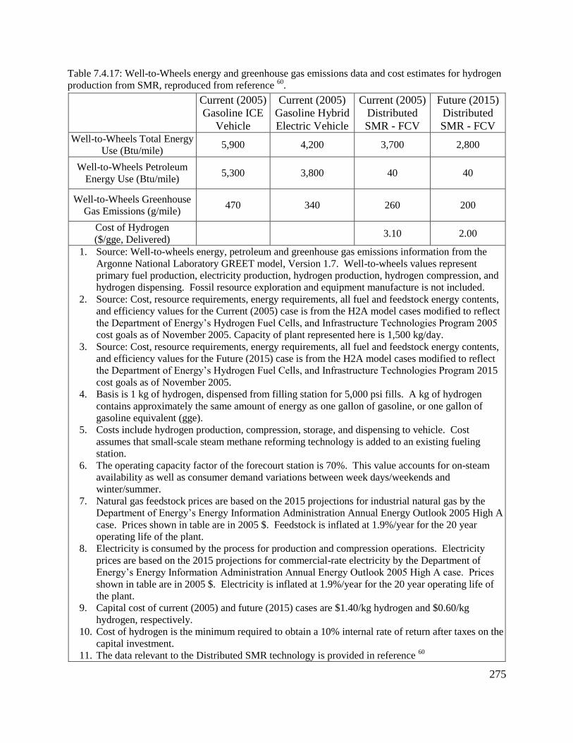
275

Table 7.4.17: Well-to-Wheels energy and greenhouse gas emissions data and cost estimates for hydrogen

production from SMR, reproduced from reference 60

.

Current (2005)

Gasoline ICE

Vehicle

Current (2005)

Gasoline Hybrid

Electric Vehicle

Current (2005)

Distributed

SMR - FCV

Future (2015)

Distributed

SMR - FCV Well-to-Wheels Total Energy

Use (Btu/mile) 5,900 4,200 3,700 2,800

Well-to-Wheels Petroleum

Energy Use (Btu/mile) 5,300 3,800 40 40

Well-to-Wheels Greenhouse

Gas Emissions (g/mile) 470 340 260 200

Cost of Hydrogen

($/gge, Delivered) 3.10 2.00

1. Source: Well-to-wheels energy, petroleum and greenhouse gas emissions information from the

Argonne National Laboratory GREET model, Version 1.7. Well-to-wheels values represent

primary fuel production, electricity production, hydrogen production, hydrogen compression, and

hydrogen dispensing. Fossil resource exploration and equipment manufacture is not included.

2. Source: Cost, resource requirements, energy requirements, all fuel and feedstock energy contents,

and efficiency values for the Current (2005) case is from the H2A model cases modified to reflect

the Department of Energy’s Hydrogen Fuel Cells, and Infrastructure Technologies Program 2005

cost goals as of November 2005. Capacity of plant represented here is 1,500 kg/day.

3. Source: Cost, resource requirements, energy requirements, all fuel and feedstock energy contents,

and efficiency values for the Future (2015) case is from the H2A model cases modified to reflect

the Department of Energy’s Hydrogen Fuel Cells, and Infrastructure Technologies Program 2015

cost goals as of November 2005.

4. Basis is 1 kg of hydrogen, dispensed from filling station for 5,000 psi fills. A kg of hydrogen

contains approximately the same amount of energy as one gallon of gasoline, or one gallon of

gasoline equivalent (gge).

5. Costs include hydrogen production, compression, storage, and dispensing to vehicle. Cost

assumes that small-scale steam methane reforming technology is added to an existing fueling

station.

6. The operating capacity factor of the forecourt station is 70%. This value accounts for on-steam

availability as well as consumer demand variations between week days/weekends and

winter/summer.

7. Natural gas feedstock prices are based on the 2015 projections for industrial natural gas by the

Department of Energy’s Energy Information Administration Annual Energy Outlook 2005 High A

case. Prices shown in table are in 2005 $. Feedstock is inflated at 1.9%/year for the 20 year

operating life of the plant.

8. Electricity is consumed by the process for production and compression operations. Electricity

prices are based on the 2015 projections for commercial-rate electricity by the Department of

Energy’s Energy Information Administration Annual Energy Outlook 2005 High A case. Prices

shown in table are in 2005 $. Electricity is inflated at 1.9%/year for the 20 year operating life of

the plant.

9. Capital cost of current (2005) and future (2015) cases are $1.40/kg hydrogen and $0.60/kg

hydrogen, respectively.

10. Cost of hydrogen is the minimum required to obtain a 10% internal rate of return after taxes on the

capital investment.

11. The data relevant to the Distributed SMR technology is provided in reference 60

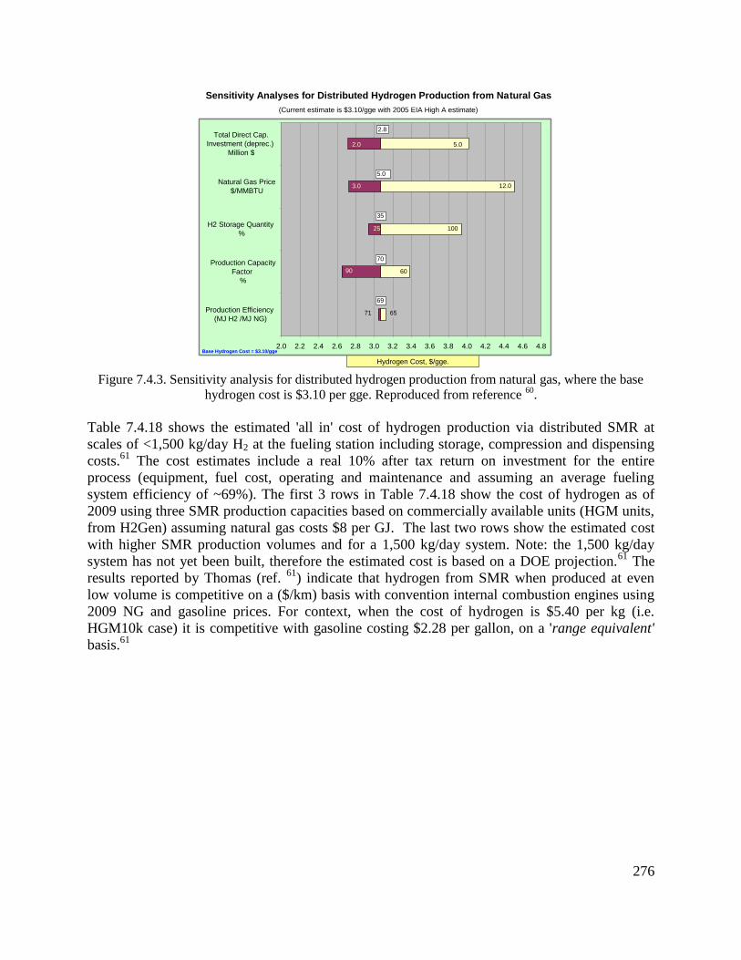
276

Figure 7.4.3. Sensitivity analysis for distributed hydrogen production from natural gas, where the base

hydrogen cost is $3.10 per gge. Reproduced from reference 60

.

Table 7.4.18 shows the estimated 'all in' cost of hydrogen production via distributed SMR at

scales of <1,500 kg/day H2 at the fueling station including storage, compression and dispensing

costs.61

The cost estimates include a real 10% after tax return on investment for the entire

process (equipment, fuel cost, operating and maintenance and assuming an average fueling

system efficiency of ~69%). The first 3 rows in Table 7.4.18 show the cost of hydrogen as of

2009 using three SMR production capacities based on commercially available units (HGM units,

from H2Gen) assuming natural gas costs $8 per GJ. The last two rows show the estimated cost

with higher SMR production volumes and for a 1,500 kg/day system. Note: the 1,500 kg/day

system has not yet been built, therefore the estimated cost is based on a DOE projection.61

The

results reported by Thomas (ref. 61

) indicate that hydrogen from SMR when produced at even

low volume is competitive on a ($/km) basis with convention internal combustion engines using

2009 NG and gasoline prices. For context, when the cost of hydrogen is $5.40 per kg (i.e.

HGM10k case) it is competitive with gasoline costing $2.28 per gallon, on a 'range equivalent'

basis.61

2.0 2.2 2.4 2.6 2.8 3.0 3.2 3.4 3.6 3.8 4.0 4.2 4.4 4.6 4.8

Production Efficiency

(MJ H2 /MJ NG)

Production Capacity

Factor

%

H2 Storage Quantity

%

Natural Gas Price

$/MMBTU

Total Direct Cap.

Investment (deprec.)

Million $

6571

6090

10025

5.02.0

12.03.0

69

70

35

5.0

2.8

Sensitivity Analyses for Distributed Hydrogen Production from Natural Gas

(Current estimate is $3.10/gge with 2005 EIA High A estimate)

Hydrogen Cost, $/gge.

Base Hydrogen Cost = $3.10/gge

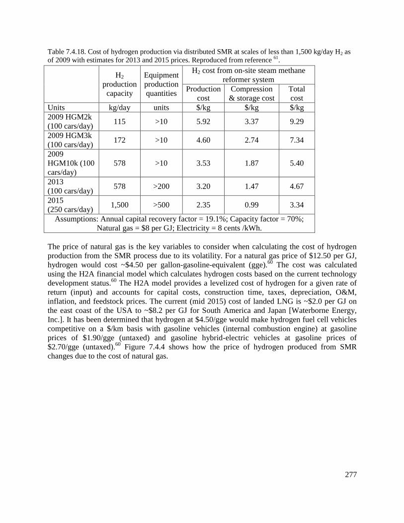
277

Table 7.4.18. Cost of hydrogen production via distributed SMR at scales of less than 1,500 kg/day H2 as

of 2009 with estimates for 2013 and 2015 prices. Reproduced from reference 61

.

H2

production

capacity

Equipment

production

quantities

H2 cost from on-site steam methane

reformer system

Production

cost

Compression

& storage cost

Total

cost

Units kg/day units $/kg $/kg $/kg

2009 HGM2k

(100 cars/day) 115 >10 5.92 3.37 9.29

2009 HGM3k

(100 cars/day) 172 >10 4.60 2.74 7.34

2009

HGM10k (100

cars/day)

578 >10 3.53 1.87 5.40

2013

(100 cars/day) 578 >200 3.20 1.47 4.67

2015

(250 cars/day) 1,500 >500 2.35 0.99 3.34

Assumptions: Annual capital recovery factor = 19.1%; Capacity factor = 70%;

Natural gas = $8 per GJ; Electricity = 8 cents /kWh.

The price of natural gas is the key variables to consider when calculating the cost of hydrogen

production from the SMR process due to its volatility. For a natural gas price of $12.50 per GJ,

hydrogen would cost ~$4.50 per gallon-gasoline-equivalent (gge).60

The cost was calculated

using the H2A financial model which calculates hydrogen costs based on the current technology

development status.60

The H2A model provides a levelized cost of hydrogen for a given rate of

return (input) and accounts for capital costs, construction time, taxes, depreciation, O&M,

inflation, and feedstock prices. The current (mid 2015) cost of landed LNG is ~$2.0 per GJ on

the east coast of the USA to ~$8.2 per GJ for South America and Japan [Waterborne Energy,

Inc.]. It has been determined that hydrogen at $4.50/gge would make hydrogen fuel cell vehicles

competitive on a $/km basis with gasoline vehicles (internal combustion engine) at gasoline

prices of $1.90/gge (untaxed) and gasoline hybrid-electric vehicles at gasoline prices of

$2.70/gge (untaxed).60

Figure 7.4.4 shows how the price of hydrogen produced from SMR

changes due to the cost of natural gas.

278

Figure 7.4.4: Plot showing the sensitivity of the cost of hydrogen production ($/gge) from SMR due to

variability of the price of natural gas in $ per million Btu ($/GJ) (HHV). Reproduced from reference 60

.

The costs contributing to the price of hydrogen from SMR using the distributed scenario are

broken down in Figure 7.4.5, where it is assumed the price of hydrogen is $3.10/gge (reproduced

from ref. 60

). This estimate is based on the best available research, projected to high volume, but

not yet validated under real-world operating conditions.60

Figure 7.4.5: Breakdown of costs involved in hydrogen production via SMR using the distributed

scenario. Reproduced from reference 60

.

In summary of SMR for the distributed production of hydrogen (<1,500 kg/day), the process is

competitive with gasoline on a cost basis assuming the price of natural gas is less than

~$12/million Btu and gasoline costs ~$2/gallon.60

When hydrogen is produced from SMR at

larger scale (centralized production) it becomes cheaper to produce and hence more competitive

against gasoline. However, the capital and logistics have to be carefully considered for the

centralized options, largely due to issues related to importing the LNG (shipping, storing,

Hydrogen Production Cost from Distributed Natural Gas Versus

Sensitivity to Natural Gas Price (HHV)

0

1

2

3

4

5

6

0 1 2 3 4 5 6 7 8 9 10 11 12 13 14 15 16 17 18 19 20

Natural Gas Price, $/MM Btu (HHV)

Hyd

rog

en

Co

st,

$/g

ge.

November 05 Price

≈ $12.5/MM Btu

Hydrogen Production Cost from Distributed Natural Gas Versus

Sensitivity to Natural Gas Price (HHV)

0

1

2

3

4

5

6

0 1 2 3 4 5 6 7 8 9 10 11 12 13 14 15 16 17 18 19 20

Natural Gas Price, $/MM Btu (HHV)

Hyd

rog

en

Co

st,

$/g

ge.

November 05 Price

≈ $12.5/MM Btu

Cost Breakdown of Hydrogen from

Distributed Natural Gas ($3.10/gge)

Other Variables

8%

NG Feedstock

30%

Capital Cost

44%

Fixed O&M

18%

Cost Breakdown of Hydrogen from

Distributed Natural Gas ($3.10/gge)

Other Variables

8%

NG Feedstock

30%

Capital Cost

44%

Fixed O&M

18%

279

transferring and distributing). The current (mid 2015) cost of landed LNG is ~$2.0 per GJ on the

east coast of the USA to ~$8.2 per GJ for South America and Japan [Waterborne Energy, Inc.].

Small scale LNG (SSLNG) technology

The following is reproduced from a 2015 Small Scale LNG report 62

: "Small scale LNG

technology is generally perceived to be a very interesting area because the small scale allows

faster deployment of new technologies and lower capex hurdles for “learn by doing”. Whereas

in conventional LNG production, more than 80% of the world capacity uses C3MR technology, a

broader portfolio of liquefaction technologies is used in SSLNG. On the other hand, to remain

cost effective, small scale relies on modular and standardized systems and specific technologies

rather than optimizing the most effective ones. For SSLNG import terminals, the variety of

technology is not as broad as in SSLNG production."

The typical main technology elements in SSLNG are:

Production

Storage

LNG transfer systems

Transportation

Regasification and import terminal

In the following subsections, summaries are provided for 'transportation (shipping)', 'transfer

systems', 'importation terminals' and 'storage'. For a more detailed discussion of these points or

for information on 'supply chain' or 'production costs' refer to reference 62

.

Transportation (shipping)

As of 2008 there were 235 LNG tankers (carriers) in operation worldwide.63

LNG tankers differ

from traditional oil tankers in that their cargo must be cooled to extremely low temperatures (-

260 °F, -163 °C) and has slightly different characteristics than oil (including a higher propensity

to burn).63

Small scale LNG tankers are defined as having a capacity of up to ~40,000 m3

(~17,000 tonnes), whereas 'normal' LNG carriers have a capacity of 125,000 to 266,000 m3 of

LNG at -163 °C (~53,000 to 113,000 tonnes).64

The number of SSLNG tankers worldwide as of

2014 was 49 ships. Out of the 49 vessels 24 are already in operation while 25 are currently on

order.64

Of the 49 SSLNG carriers 41 have long term charters and eight are potentially available

for hire, as of 2014. Of the SSLNG ships, 33 are pure LNG carriers and 16 are multiproduct

carriers (LNG, ethylene, ethane and or other petrochemicals).64

From 2015 Small Scale LNG Report62

: "It is observed that for economical and logistical

reasons, a significant part of the small scale LNG fleet is in operation for a combination of

products (LNG/Ethylene/LPG). Also, customers can charter the vessels based on a full time

charter (100%), but also on the basis of “contract of affreightments” (COA). In this situation the

customer may for example use the vessel for only one or two weeks per month. Ship brokers try

to match shipping capacity demand and supply."

280

"The difference between LNG small scale ships and large scale is primarily business related ….

The smallest LNG carrier currently in use is the one from Seagas, a 167 m3 (~71 tonnes) LNG

carrier used as bunker ship in the port of Stavanger. The roles of SSLNG carriers can be

different than large LNG carriers. Due to the expected growth of LNG as bunker fuel, it is very

likely that more LNG bunker vessels will be built in the future." 62

The following purposes are foreseen 62

:

Small scale LNG transport, inland and coastal, sometimes intercontinental

Small scale LNG bunker vessel, mainly port based

"As the LNG small scale business is growing, the fleet of small scale LNG carriers is also

expanding; see Appendix G (from 2015 report 62

) for existing and future overview of the fleet.

The CNG fleet on the other hand is very slowly picking up with only one 2,200 m3 ship in the

order book and no existing fleet." 62

Shipping cost

Reproduced from 2015 SSLNG report 62

: "A small scale LNG carrier’s investment cost is higher

per tonne LNG compared to large scale LNG vessels. For example, the investment cost (CAPEX)

for a 215,000 m3 LNG carrier is approximately $250 million ($1.16 million per 1,000 m

3), a

135,000 m3 LNG carrier is approximately $170 million ($1.26 million per 1,000 m

3), a 28,000

m3 LNG carrier is approximately $80 million ($2.86 million per 1,000 m

3), see Table 7.4. This

relates to a capital expenditure for small scale LNG ships to be typically in the range of 5,500 –

16,500 $/tonne, while large conventional shipping is 2,200 – 5,500 $/tonne."


: "The operational expenditures of small scale LNG

carriers are also higher per tonne LNG per mile compared to large scale LNG vessels. In

absolute, SSLNGCs are staffed with smaller crews and engine and cruise speed are usually much

lower than conventional LNGCs. Also, when suitably designed, small scale LNGCs will incur

reduced costs for mooring and port activities (like tug boats, pilots, shore handling, etc). In

situations where the ship crew operates the LNG satellite regas terminals, there are associated

cost savings on the terminal side as well. However, per ton LNG per mile the operational cost

are higher (i.e. lower economy of scale). Most of this cost is reflected in the day rate for a ship.

Typical daily rate cost for SSLNG carriers are $30,000 per day for a 15,000 m3 cargo vessel and

$35,000 per day for a 20,000 m3 (excluding fuel cost). Bigger ships require a larger number of

tug boats etc. so for any port on like for like basis – reduced tug boats / services will reflect in

lower costs for small scale LNG carriers per visit." A summary of shipping related costs are

provided in Table 7.4.19.

281

Table 7.4.19: Typical investment costs for LNG carriers and costs for crew and harbor use.

Adapted from 2015 LNG report 62

.

Size m3

(Mg)

CAPEX

million

$

CAPEX

$ per m3

CAPEX

$ per Mg

Typical

Crew

number

Typical

harbor cost

(Europe) per

visit

215,000

(91,375) ~250 ~1,200 ~2,750 30-35 $100-200 k

135,000

(57,375) ~170 ~1,300 ~3,000 25-35 $75-100 k

28,000

(11,900) ~80 ~2,850 ~6,725 15-20 $25-40 k

Import terminal


: "The modification from a conventional import or

export terminal to a terminal that can facilitate break bulk and small scale LNG transfers,

introduces challenges. Typical challenges are battery limit compatibility of existing

infrastructure with new SSLNG equipment (LNG trucks, small LNG carriers, manifold forces).

Another challenge might be LNG quality, especially when a certain methane number is needed

for LNG as fuel. Typically, also the increase of amount of stakeholders makes the operation and

ownership aspects more complex. Logistical challenges arise with the increasing amount of

smaller parcel sizes."

Small regasification and import terminals


: "Historically, regasification / import terminals grew

big so as to reduce cost of regasification handling massive quantities of LNG. To remain a

competitive solution, simpler processes/technologies have been used most of the time inspired by

the industrial gases industry in their design (e.g. air vaporizers). This has been also possible

because the footprints of small scale vaporizers are acceptable for the volume of LNG handled.

There are onshore and offshore (floating) terminals. Currently there are no small scale LNG

floating terminals (floating storage units (FSU’s) or floating storage regasification units

(FSRU’s)) that fall within the definition of small scale of this report."

Specific features of a small regasification / import terminal

The SSLNG terminals often have some specific features that are outlined below, reproduced

from 2015 SSLNG report 62

:

Very often, these installations are unmanned. In the few cases where they are manned,

the personnel is reduced to the minimum and they are only on site for maintenance or

unloading operations (where in some conventional terminals personnel can reach up to

200 people).

Most of the small scale regasification plants are built with prefabricated equipment (like

in the industrial gases industry) and pre-assembled modules brought directly to site,

282

providing a faster project schedule especially regarding the tank (which is usually the

long lead item on a conventional terminal). Portable regas skids are quite commonly

used as well.

In some cases, pressure build up is used in tanks prior to regasification instead of a

pump.

LNG inventory is lower, allowing in most cases scaled safety measures and simpler safety

devices, without compromising on the overall plant safety level.

Maintenance is reduced as there are very few rotating parts and instrumentation.

Very often the LNG transfer is through a flexible hose, using a dry break coupling as the

emergency disconnection system. Boil off gas generated naturally or due to LNG

processing is handled in the pressurized tank, until it is condensed with the next

subcooled delivered LNG or by utilization of backup liquid nitrogen.

Air vaporizers are the preferred equipment for their simplicity and the absence of

operating expenditures. They are installed in a redundant manner to let vaporizers

defrost while others are on duty.

Storage and boil off gas (BOG)


: "In small scale LNG, typically more different types of

storage and BOG solutions can be found than in large conventional scale. Pressurized storage

(range 3 – 10 bar, gauge) is typically seen in SSLNG only. Also, this opens up more possibilities

to contain BOG rather than (re)liquefying or depressurizing it." A summary of storage tank

types and BOG management options is provided in the following subsections.

Storage tank types


: "Typically the range of storage capacity for SSLNG

lies from 500 m3 to 5,000 m

3 (~210 to 2,100 tonnes), with prevailing pressurized storage tanks.

Above 5,000 m3, conventional technologies prevail. The amount of floating storage units (FSU)

are increasing as well. They can be equipped with a regasification unit (FSRU)."

In SSLNG there are different types of storage tanks in operation 62

:

Pressurized:

o Spherical tanks

o Bullet tanks

Atmospheric tanks

o Flat bottom

o Bullet tanks

Floating storage (FSU)

o Inside hull storage (typically atmospheric storage)

o Pontoons (can contain pressurized storage bullets)

283

Table 7.4.20: An overview of the advantages and disadvantages of the typical SSLNG storage tank types.


.

Mode Tank type Advantage Disadvantages

Pressurized

Bullet

Tank

Savings on BOG management

Saving possibly on pumps

Pre-fabricated (= fast track)

Lower Safety Factor

Limited storage

capacity

Spherical

Tanks

Higher capacity than bullet

Saving possibly on pumps


Limited storage

capacity

Lower Safety Factor

Atmospheric

Flat

bottom

High Safety

High capacity

Expensive

Long item to build

Bullet

Tank


Less expensive

Limited storage

capacity

Floating

LNG

carrier

Flexible in location, re-use

possible Expensive

Pontoons Pre-fabricated elsewhere

Marine berth / jetty /

quay and ship-shore

interface scope


: "Whether it deals with small scale or not, sizing

storage relies on good sense, and the following rules are applied as much as possible:"

Size will be chosen so as to receive the integrality of the cargo delivered by the ship

Size will be therefore in the same order of magnitude as the size of the ship carrying

LNG

The carrier ship type and size will be chosen so as to have a reasonable frequency of

delivery (provided that waterways and/or road are available for that purpose).

Thermodynamic state of LNG (cold or warm according to customer possibilities to adjust

or accept LNG temperature).

"Regular consumption of LNG and aging are constraints specific to LNG which impact the sizing

of the infrastructure, irrespective of the size/capacity (large or small). Due to its cryogenic

specific aspects it is difficult to store LNG longer than several weeks without liquefying it. Very

simply, pressurized tank options offer the possibility to save money on BOG management

expenses, and often make it possible to save time in installation. However, a pressurized system

will not be a good option if the customer needs cold LNG, unless a concept is applied where

liquid nitrogen is used to subcool the LNG if required. In a first approach, a facility of capacity

below 0.2 million tonnes per annum (mtpa) could grossly rely on a pressurized tank, and on

atmospheric for capacity above 0.2 mtpa." 62

For context, the amount of LNG required solely for hydrogen production on Oahu is 13,500

tonnes LNG per annum to displace 1 % of gasoline usage as of 2014; if LNG was to be used for

electricity production at least 500,000 tonnes of LNG is required per annum (0.5 mtpa). For more

further details on different types of storage vessel refer to reference 62

.

284

LNG storage cost


: "Very few cylindrical small sized tanks are

competitive, and the smallest are ~10,000 m3 if built in concrete for the outer shell. Cost is really

local content related for this type of tank. Cost wise, the comparison between a pressurized tank

and an atmospheric tank should take in consideration the BOG management associated

investment. But the choice relies not only on tank size, but also on storage duration: a BOG

management system offers longer storage duration capability."

"An atmospheric tank of 28,000 m3 (11,900 tonnes) could cost $60 million (~2,150 $/m

3 or

~5000 $/tonne), compared to a 170,000 m3 (72,250 tonnes) tank which costs $135 million (~800

$/m3 or ~1,900 $/tonne). The typical cost range observed currently is 800 – 3,000 $/m

3 (~2,000 -

5,500 $/tonne) for SSLNG storage, with lower cost per m3 when increasing capacity. Pressurized

tanks are in the lower range." 62

BOG management


: "Boil off gas (BOG) is a typical LNG storage related

issue compared to other hydrocarbon fuels. Due to heat ingress, mainly the lighter parts of the

liquefied gas (N2, CH4, etc) boil off. Typical boil-off rates are 0.1-0.5% per day in storage due to

heat ingress. Additional BOG is formed when the LNG leaves the piping that boils back to the

tank when heat ingress from cooling down the pump and heat generated by the pump and vapour

return from loading activities."

"By removing boil-off gas (recondense/ reliquefy/ sent out), pressure and temperature are kept

the same. If boil-off gas is not removed, pressure builds-up and – if not managed – would

eventually lead to the opening of pressure relief systems. When boil-off gas is removed to

maintain the pressure level, the methane number decreases because the LNG gets heavier. This

is important for LNG as fuel, because most engines require a minimum methane number to

prevent knocking." 62

"If not removed, boil-off gas can be contained under pressure. Pressure will be decreased by

emptying the tank and/or refilling it with sub cooled LNG recondensing BOG. BOG is an

important aspect in the LNG supply chain that must be taken into account during the complete

design, execute and operate phases." 62

BOG options


: "Some terminals with a capacity below 1 mtpa use

conventional technologies found in large scale LNG regasification terminals. Conventional and

specific small scale principles are depicted in Figures 7.4.6 and 7.4.7 for comparison."

285

Figure 7.4.6: Typical conventional LNG regasification / import terminal. Reproduced from reference

62.

Figure 7.4.7: Typical small scale LNG regasification / import terminal. Reproduced from reference

62.

LNG transfer


: "LNG product outlet from small-scale LNG facilities

or storage is typically by loading on trucks. Sometimes a small jetty will be required if loading

onto dedicated small LNG vessels is part of the business case."

"In any case, marine infrastructure requirements will be less demanding than for a world-scale

LNG installation, however their percentage of total cost should not be underestimated. The

transfer systems require typically quite some space due to safety distances, which in some

environments also requires significant civil work (jetty length, truck plot space). Other

equipment items found in the transfer area are safety systems (i.e. gas and fire detectors, ESD

panels and firefighting equipment), interface for the crew or truck driver (panels, control

rooms), custody transfers (coriolis or flow meters with gas chromatographs) and LNG spill

containment. For truck units, small loading arms or hoses are quite common. Typically, 3inch is

286

the largest hose diameter found for truck loading. For SSLNG ships typically hoses are only used

if the diameter is below 8inch. For 4inch and larger loading arms are often available." 62

"The transfer flow can be typically created by pressure build up when using pressurized storage,

submerged pumps or external sealless cryogenic pumps. For cooling down the transfer lines and

custody equipment before the transfer, a recycle line is required for recycling the initial BOG

creation during cool down. In most LNG systems, a purging option (typically N2) to purge out

the remaining amount of LNG after the transfer is also present. Alternatively, the lines can be

continuously kept cold by LNG recycle flows. Transfer of LNG generates typically some BOG

which needs to be handled. When there are BOG compressors, they need to be adequately sized

to cope with the fluctuating BOG by LNG transfer." 62

Logistic analysis and distribution methods


: "To perform a logistic analysis for a conventional

transport by large LNG carrier, the supply chain is further broken down into elements. Each of

these elements impacts the overall logistic performance of the supply chain, see Figure 7.4.8."

Figure 7.4.8: Elements within the logistic supply chain. Reproduced from reference

62.


: "Logistic analysis of a small scale supply network can

be done in a very similar way. However the logistic behavior of each element in SSLNG can be

different, because there is much more distribution flexibility (shipping, trucking, containers),

distances are shorter and/or the number of customers is larger. The starting point is obviously

the customer demand. From this point, an iterative exercise can be carried out to find out what is

the best balance from a cost standpoint between the size of the infrastructures at both ends and

the fleet. Some of the main differences between large, conventional LNG and small scale LNG in

the elements are given below in Table 7.4.21."

287

Table 7.4.21: Differences between the conventional LNG and SSLNG logistic elements within supply

chain. Reproduced from reference 62

.

Element Conventional transport Small scale transport

Supply LNG plant LNG plant, regas & import terminal / small

scale liquefaction plant

Storage Tanks at LNG plant Tanks at production / import & regasification

terminal

Transport lines Jetty Jetty, truck loading unit

Loading facility Berth Berth, jetty, ship to ship or truck loading

dock

Transport LNG carriers Small LNG carriers, LNG trucks, containers

and/or trains

Demand Customers at import /

regasification terminal

Customers at small terminals or direct

offloading to customers

Logistic SSLNG characteristics


: "In SSLNG, distances are typically much shorter

compared to conventional LNG, because there is an optimum coverage area for certain

production and distribution scales. Endurance of vessel depends on fuel storage vs. fuel

consumption per day or per nautical mile. Another consideration is regarding the company

policies and the amount of reserve required all the time and also accounting for un-pumpable in

the tanks. The typically small scale distribution radii observed for a conventional Qmax 266,000

m3 (~113,000 tonnes) vessel action radius is typically > 20,000 nautical miles, while the max

radius for a 7,500 m3 (~3,200 tonnes) vessel is approx. 1,500 – 2,500 nautical miles."


: "Parcel sizes are in the range 20 - 60 m3 per truck and

average size is 30 m3 (12.8 tonnes). For ships typical parcel sizes are in the range 500 – 30,000

m3

(~210 to 12,750 tonnes). Because the parcel sizes and distribution distances are smaller, the

number of logistical movements is much greater than in conventional LNG. With small carriers,

bunker ships and trucks there can be 5 - 30 loading/unloading operations on site per day, while

in large LNG sites normally a large LNG carrier comes a few times a week."

Challenges for small scale LNG logistics


: "When developing a logistical model for SSLNG, the

following challenges typically arise:"

Cost

Low priority for small ships

Limited fleet size


: "The distribution costs for SSLNG are relatively high

compared to other (hydrocarbon) products due to the cost of the cryogenic equipment required.

Especially for SSLNG shipping, berthing priority for small ships is often lower than large ships;

288

hence the probability of demurrage is higher if they do not have ‘dedicated’ jetties. This is not

different to other hydrocarbon products but more to other conventional large LNG vessels."

In addition, the SSLNG shipping fleet is still relatively small compared to other more mature

(hydrocarbon) markets, see the earlier section titled “Transportation (shipping)”.


: "There is currently no shipping spot market, almost all

SSLNG ships are contracted and built under long term time charter contracts. This means that

there is little flexibility as to what ships are available for development of fast opportunities."

A point that needs to be considered, if LNG is to be imported for electricity production in

Hawaii, is the need for reserve storage in case a delivery is missed due to losing a LNG carrier at

sea or other unforeseen issue. This is no different to the provisions that are in place regarding

current supplies of fuel for electricity production. However, due to Hawaii's isolated location and

the limited availability of LNG carriers, if a LNG carrier was lost finding a replacement is likely

to be expensive and have a significant lead time. This may mean that additional reserve storage

is required than is current practiced. It is unlikely to be practical to use LNG for the reserve due

to losses during storage, boil off losses of 0.1-0.5% per day are typical unless a BOG

management system is installed at additional cost. Instead the reserve fuel would more than

likely be low sulfur fuel oil or diesel as it is cheaper and easier to store for long periods of time.

Other risks associated with LNG imports are outlined in “. Risks associated with LNG” below.

Delivered cost of LNG to Hawaii

The information below on costs was reproduced from a 2013 report which assumes large scale

importation of LNG to Hawaii for electricity production.56

"By their nature, forecasts are uncertain. For this reason, major LNG imports should not be

undertaken unless the expected savings are substantial. Expected savings of, say, 10-15%, are

probably not enough to warrant the large investments and long-term commitments required for

bulk LNG imports; such savings could easily be wiped away by market fluctuations." 56

"Cost savings from LNG imports into Hawaii will clearly depend on where and how it is

procured. Under a base case LNG demand forecast of 500 ktpa (thousand tonnes per annum), it

appears that conventional, benchmark, onshore terminals using small (<40,000 m3, 17,000

tonnes), US-built, Jones Act compliant LNG carriers loading from the US West Coast can deliver

LNG to Oahu 31-47% cheaper than oil through 2030 (Table 7.4.22)." 56

289

Table 7.4.22: Savings in delivered energy cost, LNG vs Low-Sulfur Diesel *, 2012 $/MBtu (million Btu).


.

2015 2020 2025 2030

Alaska na na 8% 8%

Australia -8% 3% 3% 4%

Canada na 14% 15% 16%

US Gulf

Coast 33% 35% 32% 31%

US West

Coast na 47% 44% 43%

* Because of new EPA policies, LS diesel is

expected to be the main utility fuel in Hawaii

before 2020. At present, on Oahu LS diesel and

LS fuel oil are almost identical in cost per MBtu.

"Savings relative to oil are very large when the LNG is sourced from the Lower 48 (with the US

West Coast being the most attractive option). The savings are cut roughly in half if LNG is

sourced from Canada. The savings shrink dramatically when sourced from Alaska or Australia." 56

"In all of these cases, some additional savings could be made if larger LNG carriers could be

employed—at least up to the point where deliveries become so large that the cost of holding the

inventory becomes prohibitive. The feasibility of using larger carriers depends both on

engineering unknowns (e.g., can the vessels be accommodated on Oahu?) and political

unknowns (e.g., can Hawaii get a Jones Act waiver?)." 56

The Jones act is otherwise known as The Merchant Marine Act of 1920 (P.L. 66-261), it is a

United States federal statute that provides for the promotion and maintenance of the American

merchant marine. Among other purposes, the law regulates maritime commerce in U.S. waters

and between U.S. ports and requires that all goods transported by water between U.S. ports be

carried on U.S. flag ships, constructed in the United States, owned by U.S. citizens, and crewed

by U.S. citizens and U.S. permanent residents.

It is likely that the cost savings from using LNG for hydrogen production on Oahu would be of a

similar order of magnitude as described in Table 7.4.22 when compared to using naphtha for

hydrogen production. Although, due to the much lower amounts of LNG require for hydrogen

production alone, the savings are likely to be somewhat less than stated above.

The landed prices for LNG imports range from ~$2.0 per million Btu on the east coast of the

USA to ~$8.2 per million Btu for South America and Japan as of August 2015 [Waterborne

Energy, Inc.]. This works out as ~$110 to ~$450 per tonne of LNG (1 million Btu = 1.83 x 10-2

tonnes of LNG). The distributed production of hydrogen from LNG (<1,500 kg/day) is said to be

competitive with gasoline on a cost basis assuming the price of natural gas is less than ~$12

/million Btu and gasoline costs ~$2 / gallon (“Calculation for amount of LNG required to

produce enough H2 to displace 1% of gasoline usage in Hawaii”).60

When hydrogen is produced

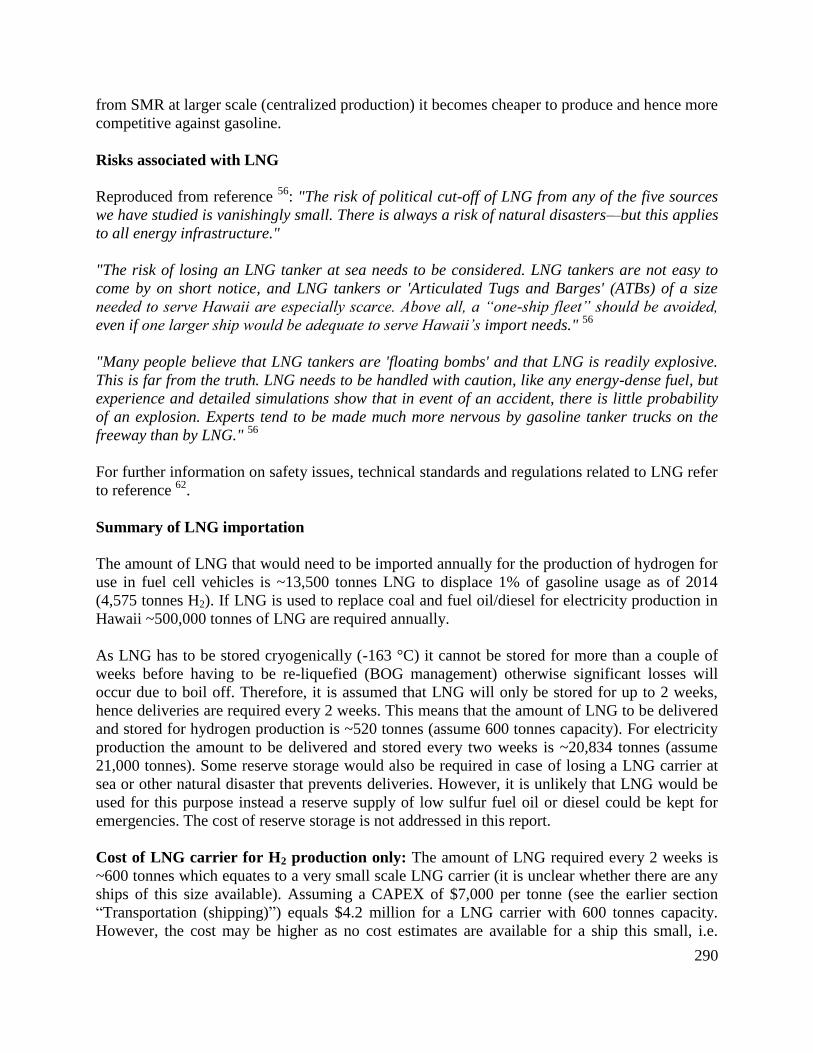
290

from SMR at larger scale (centralized production) it becomes cheaper to produce and hence more

competitive against gasoline.

Risks associated with LNG


: "The risk of political cut-off of LNG from any of the five sources

we have studied is vanishingly small. There is always a risk of natural disasters—but this applies

to all energy infrastructure."

"The risk of losing an LNG tanker at sea needs to be considered. LNG tankers are not easy to

come by on short notice, and LNG tankers or 'Articulated Tugs and Barges' (ATBs) of a size

needed to serve Hawaii are especially scarce. Above all, a “one-ship fleet” should be avoided,

even if one larger ship would be adequate to serve Hawaii’s import needs." 56

"Many people believe that LNG tankers are 'floating bombs' and that LNG is readily explosive.

This is far from the truth. LNG needs to be handled with caution, like any energy-dense fuel, but

experience and detailed simulations show that in event of an accident, there is little probability

of an explosion. Experts tend to be made much more nervous by gasoline tanker trucks on the

freeway than by LNG." 56

For further information on safety issues, technical standards and regulations related to LNG refer

to reference 62

.

Summary of LNG importation

The amount of LNG that would need to be imported annually for the production of hydrogen for

use in fuel cell vehicles is ~13,500 tonnes LNG to displace 1% of gasoline usage as of 2014

(4,575 tonnes H2). If LNG is used to replace coal and fuel oil/diesel for electricity production in

Hawaii ~500,000 tonnes of LNG are required annually.

As LNG has to be stored cryogenically (-163 °C) it cannot be stored for more than a couple of

weeks before having to be re-liquefied (BOG management) otherwise significant losses will

occur due to boil off. Therefore, it is assumed that LNG will only be stored for up to 2 weeks,

hence deliveries are required every 2 weeks. This means that the amount of LNG to be delivered

and stored for hydrogen production is ~520 tonnes (assume 600 tonnes capacity). For electricity

production the amount to be delivered and stored every two weeks is ~20,834 tonnes (assume

21,000 tonnes). Some reserve storage would also be required in case of losing a LNG carrier at

sea or other natural disaster that prevents deliveries. However, it is unlikely that LNG would be

used for this purpose instead a reserve supply of low sulfur fuel oil or diesel could be kept for

emergencies. The cost of reserve storage is not addressed in this report.

Cost of LNG carrier for H2 production only: The amount of LNG required every 2 weeks is

~600 tonnes which equates to a very small scale LNG carrier (it is unclear whether there are any

ships of this size available). Assuming a CAPEX of $7,000 per tonne (see the earlier section

“Transportation (shipping)”) equals $4.2 million for a LNG carrier with 600 tonnes capacity.

However, the cost may be higher as no cost estimates are available for a ship this small, i.e.

291

smallest there is data for has a capacity of ~11,900 tonnes (see the earlier section “Transportation

(shipping)”)).

Cost of LNG carrier for electricity production: ~21,000 tonnes of LNG would be required

every two weeks, which is too much for the largest 'small scale LNG carrier' (11,900 tonnes

capacity, “Transportation (shipping)”)). A LNG carrier with 21,000 tonnes capacity is about half

the size of the smallest normal sized LNG carrier (~57,000 tonnes capacity). The estimated cost

of a LNG carrier with 21,000 tonnes capacity is ~$94.5 million (assuming $4,500 per tonne).

In the case of importing LNG for electricity production it may be better to import the LNG on a

weekly basis, i.e. 10,500 tonnes LNG delivered every week (assume 11,000 tonnes). In this case,

a small scale LNG carrier could be used (max. capacity ~11,900 tonnes). The cost for one

SSLNG carrier with 11,000 tonnes capacity is ~$74 million assuming a CAPEX of $6,725 per

tonne (see the earlier section “Transportation (shipping)”)).

Cost of LNG storage for H2 production only: To build storage for ~600 tonnes of LNG is

estimated to cost ~$3.3 million assuming a CAPEX of $5,500 per tonne (see “Storage and boil

off gas (BOG)”). However, the cost will probably be higher as the capacity required is much

smaller than the smallest size there is cost data for. Assuming a CAPEX of $7,500 per tonne

equals $4.5 million to store 600 tonnes of LNG. Pressurized tanks are cheapest option at this

scale.

Cost of LNG storage for electricity production: To store ~21,000 tonnes of LNG is estimated

to cost ~$84 million assuming $4,000 per tonne (See “Storage and boil off gas (BOG)”). If the

CAPEX is higher, $5,000 per tonne, the cost will be ~$105 million. If deliveries of LNG are

made every week the amount to storage would be ~10,500 tonnes (assume 11,000 tonnes). The

cost of a storage unit with 11,000 tonnes capacity is ~$55 million assuming a CAPEX of $5,000

per tonne. Storage costs are difficult to gauge as they are influenced by local land, construction

and labor costs.

LNG Containers

A possible option for importing LNG to Hawaii for hydrogen production is via containers. A 40

ft shipping container can hold up to 47 m3 of LNG (~18 tonnes or 26,600 m

3 NG at STP). The

amount of LNG that would need to be imported for the production of hydrogen is ~13,500

tonnes per annum to displace 1% of gasoline usage. Assuming that LNG is delivered every two

weeks means the amount of LNG to be delivered and stored for hydrogen production is ~520

tonnes. This is about 29 containers (40 ft) of LNG every two weeks.

The payload of each 40 ft container is 18 tonnes (~39,000 lb) and the total weight of the truck

plus container is 40 tonnes (~88,000 lb). However, Hawaii has a ~36 tonnes (~80,000 lb) limit

for road transportation and will not permit overweight vehicles. Therefore the LNG containers

would have to be limited to 14 tonnes (31,000 lb) payloads, this means that ~37 containers are

required every 2 weeks to deliver ~13,500 tonnes of LNG per year.

292

The 40 ft LNG containers from Corban Energy Group Corp. have a hold time (storage time) of

55 to 80 days. According to Searates.com it takes ~7 days for a container vessel to travel from

California to Oahu.

Cost per container is ~$140,000 if buying less than ~80 units, or ~$130,000 - $135,000 for more

than ~80 units (Corban Energy Group Corp., New Jersey). Assuming a cost of $140,000 per

container and that 37 containers are required the cost is $5,180,000. Assuming 74 containers are

required (37 in use and 37 in transit) will cost $10,360,000 without account for spares. If we

assume 5% spare capacity in terms of additional containers, an additional 4 containers are

required giving a total of 78 containers, this works out at $10,920,000. Costs are somewhat

variable depending on the accessories chosen, i.e. sensors and other safety features fitted to the

containers. The costs outlined above are solely for the purchase of the LNG containers and does

not account for the cost of the LNG itself or transportation costs.

LPG Imports

Conversion of LPG to hydrogen is roughly the same as for natural gas, therefore approximately

13,500 tonnes of LPG would be required per annum to produce enough hydrogen to displace 1%

of gasoline usage in Hawaii (~4,575 tonnes H2). The price of LPG per 100,000 BTU's imported

to Hilo, Hawaii as of Nov 2015 was $2.16, this works out as ~$1030 per tonne of LPG and

~$13.9 million for 13,500 tonnes. Table 7.4.23 displays the conversion factors used to estimate

the price of LPG per tonne imported to Hawaii assuming properties of propane.

Table 7.4.23: Physical properties of propane used to convert from BTU's to tonnes and cost estimates per

tonne of LPG.

Units - Properties for propane

$ / 100,000 BTU * 2.16237

BTU / gallon 91,500

kJ / gallon 96,500

gallons / m3 264.172

kg / m3 493

lb / kg 2.2

BTU / lb 21,622

BTU / kg ~47,600

BTU / tonne ~47,600,000

BTU in 13,500 tonnes ~6.42 E+11

$ / tonne LPG ~1030

$ for 13,500 tonnes LPG ~13,900,000

Utility propane (Schedule 450 Commercial &

Industrial) imported to Hilo in Nov. 2015 was

$2.16237 per therm (there are 100,000 Btu per

therm) - Source: Hawaii Gas

293

Summary and Conclusions

Options to produce hydrogen for fuel cell vehicles in sufficient quantity to displace 1% of

Hawaii’s gasoline consumption were explored. Options included electrolysis, naptha reforming,

gasification of MSW, reforming landfill gas resources, reforming glycerin byproducts from

biodiesel production, pyrolysis of agricultural residues with subsequent reforming of the

pyrolysis-char slurry, and reforming of liquefied natural gas. All face challenges related to (1)

matching the scale of the primary energy source with the final demand, (2) maturity of the

technology at suitable scale, (3) supply chain logistics, and (4) overall cost of production, that

will need to be addressed.

References

1. H2 fuel quality standard J2719. SAE International. In Surface vehicle standard., 2011.

2. http://hawaii.gov/dbedt/info/economic/data_reports/reports-studies/energy-data-trend-

2011.pdf.

3. http://dbedt.hawaii.gov/economic/energy-trends-2.

4. http://www.energy.ca.gov/2007publications/CEC-600-2007-002/CEC-600-2007-002-

D.PDF.

5. Biomass Energy Data Book 2011 http://cta.ornl.gov/bedb.

6. Stoll, R. E., Linde, F. Hydrogen - what are the costs?

http://www.caloric.com/upload/Downloads/hydro.pdf.

7. NREL. State-of-the-Art Hydrogen Production Cost Estimate Using Water Electrolysis.

NREL/BK-6A1-46676.; 2009.

8. HECO Electric prices in Hawaii. http://www.heco.com/heco/Residential/Electric-

Rates/Average-Electricity-Prices-for-Hawaiian-Electric,-Hawaii-Electric-Light,-and-Maui-

Electric.

9. Rostrup-Nielsen, J. R., Rostrup-Nielsen, T. Large-scale hydrogen production.

http://www.topsoe.com/sites/default/files/topsoe_large_scale_hydrogen_produc.pdf.

10. Cooperative., K. I. U. Price of naphtha per barrel.

http://kauai.coopwebbuilder.com/sites/kauai.coopwebbuilder.com/files/2015-07-

perbarrel.pdf.

11. Arena, U., Process and technological aspects of municipal solid waste gasification. A

review. Waste Management 2012, 32, (4), 625-639.

12. Panepinto, D.; Tedesco, V.; Brizio, E.; Genon, G., Environmental Performances and Energy

Efficiency for MSW Gasification Treatment. Waste and Biomass Valorization 2015, 6, (1),

123-135.

13. E4tech - Review of technologies for gasification of biomass and wastes. NNFCC project

98/008; www.nnfcc.co.uk, 2009.

14. Riverside., U. o. C. Evaluation of emissions from thermal conversion technologies

processing municipal solid waste and biomass. Final report.;

www.bioenergyproducers.org/documents/ucr_emissions_report.pdf, 2009.

294

15. Davis, J., Gelman, R., Tomberlin, G., Bain, R. Waste-to-energy Hawaii and Guam energy

improvement technology demonstration project; NREL TP-7A40-60868

www.nrel.gov/publications, 2014.

16. Milne, T. A., Elam, C.C., Evans, R.J. Hydrogen from Biomass State of the Art and Research

Challenges.; NREL report, IEA/H2/TR-02/001, 2002.

17. Wallman, P. H.; Thorsness, C. B.; Winter, J. D., Hydrogen production from wastes. Energy

1998, 23, (4), 271-278.

18. He, M.; Hu, Z.; Xiao, B.; Li, J.; Guo, X.; Luo, S.; Yang, F.; Feng, Y.; Yang, G.; Liu, S.,

Hydrogen-rich gas from catalytic steam gasification of municipal solid waste (MSW):

Influence of catalyst and temperature on yield and product composition. International

Journal of Hydrogen Energy 2009, 34, (1), 195-203.

19. He, M.; Xiao, B.; Liu, S.; Guo, X.; Luo, S.; Xu, Z.; Feng, Y.; Hu, Z., Hydrogen-rich gas

from catalytic steam gasification of municipal solid waste (MSW): Influence of steam to

MSW ratios and weight hourly space velocity on gas production and composition.

International Journal of Hydrogen Energy 2009, 34, (5), 2174-2183.

20. Luo, S.; Zhou, Y.; Yi, C., Syngas production by catalytic steam gasification of municipal

solid waste in fixed-bed reactor. Energy 2012, 44, (1), 391-395.

21. Li, J.; Liao, S.; Dan, W.; Jia, K.; Zhou, X., Experimental study on catalytic steam

gasification of municipal solid waste for bioenergy production in a combined fixed bed

reactor. Biomass and Bioenergy 2012, 46, 174-180.

22. Sharma, S. D.; Dolan, M.; Park, D.; Morpeth, L.; Ilyushechkin, A.; McLennan, K.; Harris,

D. J.; Thambimuthu, K. V., A critical review of syngas cleaning technologies —

fundamental limitations and practical problems. Powder Technology 2008, 180, (1–2), 115-

121.

23. Sharma, S. D.; Dolan, M.; Ilyushechkin, A. Y.; McLennan, K. G.; Nguyen, T.; Chase, D.,

Recent developments in dry hot syngas cleaning processes. Fuel 2010, 89, (4), 817-826.

24. Dong, J.; Chi, Y.; Tang, Y.; Ni, M.; Nzihou, A.; Weiss-Hortala, E.; Huang, Q., Partitioning

of Heavy Metals in Municipal Solid Waste Pyrolysis, Gasification, and Incineration. Energy

& Fuels 2015.

25. Wang, Y.-R.; Wang, Z.-J.; Wang, A.-Q.; Li, C.-P., Heavy metals fraction and ecological

risk evaluation in municipal solid waste gasification slag non-burnt bricks. Toxicological &

Environmental Chemistry 2015, 97, (3-4), 417-428.

26. Vassilev, S. V.; Baxter, D.; Andersen, L. K.; Vassileva, C. G., An overview of the chemical

composition of biomass. Fuel 2010, 89, (5), 913-933.

27. Vassilev, S. V.; Baxter, D.; Andersen, L. K.; Vassileva, C. G.; Morgan, T. J., An overview

of the organic and inorganic phase composition of biomass. Fuel 2012, 94, (Copyright (C)

2012 American Chemical Society (ACS). All Rights Reserved.), 1-33.

28. Turn, S.; Kinoshita, C.; Zhang, Z.; Ishimura, D.; Zhou, J., An experimental investigation of

hydrogen production from biomass gasification. International Journal of Hydrogen Energy

1998, 23, (8), 641-648.

29. http://www.opala.org/solid_waste/pdfs/Draft_Revised_ISWMP_Update.pdf.

30.http://www.opala.org/solid_waste/pdfs/2013_Interim_Status_Report_on_the_Integrated_Soli

d_Waste_Management_Plan_2008.pdf.

295

31. Easterly, J., Cummer, K., Emsick, N., Hunsaker, M., Harper, B., Olson, S., Roush, B.,

Ogoshi, R., Yanagida, J. The potential for biofuels production in Hawai’i. Project Number

147375; Black and Veatech, 2010.

32. http://www.hawaiitribune-herald.com/news/local-news/new-tipping-fee-commercially-

hauled-greenwaste-begins-july-1.

33. Turn, S., Keffer, V., Staackmann, M. Biomass and bioenergy resource assessment.; Hawaii

Natural Energy Institute: http://www.hnei.hawaii.edu/node/338, 2002.

34. Turn, S., Keffer, V., Staackmann, M. Analysis of Hawaii biomass energy resources for

distributed energy applications.; Hawaii Natural Energy Institute.:

http://www.hnei.hawaii.edu/node/338, 2002.

35. http://www.anaergia.com/about-us/reference-facilities/municipal-solid-waste/maui.

36. http://mauisierraclub.org/maui-landfill-waste-to-energy-project.

37. http://www.hawaiizerowaste.org/uploads/files/1%20IRSWMP_Plan_Dec2009.pdf.

38. http://www.bioenergyhawaii.com/blog/2015/3/11/beh-plans-resource-recovery-energy-

conversion-system.

39.http://www.kauai.gov/Government/Departments/PublicWorks/SolidWaste/IntegratedSolidWa

steManagementPlan/tabid/445/Default.aspx.

40. http://www.kauai.gov/default.aspx?tabid=121.

41.http://www.kauai.gov/Government/Departments/PublicWorks/SolidWaste/KekahaLandfillInf

ormation/tabid/526/Default.aspx.

42. Sørum, L., Gran, I.R. Characterisation of MSW for combustion systems. Report TRA5395.;

SINTEF Energy Research: 2001.

43. Ward, P. L.; Wohlt, J. E.; Zajac, P. K.; Cooper, K. R., Chemical and Physical Properties of

Processed Newspaper Compared to Wheat Straw and Wood Shavings as Animal Bedding1.

Journal of Dairy Science 2000, 83, (2), 359-367.

44. http://www.epa.gov/lmop/projects-candidates/index.html#map-area.

45. Spath, P. L., Mann, M.K. Life cycle assessment of hydrogen production via natural gas

steam reforming. NREL Technical Report NREL/TP-570-27637; 2001.

46. Personal communication between B. King and S.Turn. In 2013.

47. Hu, S.; Luo, X.; Wan, C.; Li, Y., Characterization of Crude Glycerol from Biodiesel Plants.

Journal of Agricultural and Food Chemistry 2012, 60, (23), 5915-5921.

48. Douette, A. M. D.; Turn, S. Q.; Wang, W.; Keffer, V. I., Experimental Investigation of

Hydrogen Production from Glycerin Reforming. Energy & Fuels 2007, 21, (6), 3499-3504.

49.http://www.agcensus.usda.gov/Publications/2012/Full_Report/Volume_1,_Chapter_2_County

_Level/Hawaii/st15_2_001_001.pdf.

50.http://www.agcensus.usda.gov/Publications/2012/Full_Report/Volume_1,_Chapter_2_County

_Level/Hawaii.

51. Elliott, D.

http://www.pyne.co.uk/Resources/user/PyNe%20Newsletter%20June%202014%20v17.pdf.

52. Bridgwater, A. V., Review of fast pyrolysis of biomass and product upgrading. Biomass

Bioenergy 2011, 38, 68-94.

296

53. HNEI Biofuel Feedstock Inter-Island Transportation http://www.hnei.hawaii.edu/node/338,

2012.

54. Stiles, H. N.; Kandiyoti, R., Secondary reactions of flash pyrolysis tars measured in a

fluidized-bed pyrolysis reactor with some novel design features. Fuel 1989, 68, (Copyright

(C) 2012 American Chemical Society (ACS). All Rights Reserved.), 275-82.

55. Morgan, T. J.; Turn, S. Q.; George, A., Fast Pyrolysis Behavior of Banagrass as a Function

of Temperature and Volatiles Residence Time in a Fluidized Bed Reactor. PLoS ONE 2015,

10, (8), e0136511.

56. Inc., F. Liquefied Natural Gas for Hawaii: Policy, Economic, and Technical Questions.;

HNEI.: http://www.hnei.hawaii.edu/publications/technical-reports-0, 2013.

57. Cunningham, C. R., Roni, J.P., Oliver, L.T., Thermal Insulation Performance: Symposium.

1980.

58. Inc., C. F., Liquid Methane Fuel Characterization and Safety Assessment Report. Report

No. CFI-1600. 1991.

59. Wood, A. R. Report TEV-953. HTGR-Integrated Hydrogen Production via Steam Methane

Reforming (SMR) Process Analysis; Idaho National Laboratory: 2010.

60. US.gov. Distributed Hydrogen Production via Steam Methane Reforming.

www.hydrogen.energy.gov/docs/cs_distr_steam_methane_reform.doc.

61. Thomas, C. E. Hydrogen cost estimates via steam methane reforming.

http://www.cleancaroptions.com/Hydrogen_costs_per_mile.pdf.

62. union., I. g. Small Scale LNG. http://www.igu.org/sites/default/files/node-page-

field_file/SmallScaleLNG.pdf; 2015.

63. Asutin., U. o. T. a. LNG tankers. https://www.strausscenter.org/hormuz/lng-tankers.html.

64. LNGworldnews.com Small scale LNG Fleet. https://www.lngworldnews.com/infographic-

small-scale-lng-fleet.

Task 8. ENERGY-NEUTRAL ENERGY TEST PLATFORMS

Under this grant, HNEI undertook three subtasks relating to energy efficiency in buildings.

Under subtask 8.1, Off-Grid/Energy Neutral Test Platform, two second-generation energy-

neutral test platforms were designed and installed by Project Frog of San Francisco on the UH

Manoa campus. Construction was completed and the University began to use the platforms as

functioning classrooms in August 2016. Subtask 8.2, Platform Monitoring and Performance

Analysis involved instrumentation and monitoring of first-generation energy neutral test

platforms installed under previous funding. Two Project Frog platforms installed at the

Kawaikini New Century Public Charter School in Kauai were monitored for one year. Actual

performance was compared to the predictive models developed during the design phase. Under

subtask 8.3, Advanced Database Research Development and Testing , MKThink was contracted

to develop a data management platform to improve the acquisition, management and analysis of

297

structured and unstructured data in order to improve decisions related to sustainable energy

solutions.

8.1 Off-Grid/Energy-Neutral Test Platform

. Under subtask 8.1, Off-Grid Test Platforms, two second generation Project Frog platforms

were designed, fabricated, and installed on the UH Manoa campus. Occupancy and use of the

structures began in August 2016. Instrumentation for collection of building energy flows as well

as interior and exterior environmental conditions was installed during construction.

The objective of this subtask was to install and instrument two energy neutral platforms

including site preparation, permitting and installation.

The two second generation Project Frog platforms were completed in August 2016 culminating

2 years of planning and permitting and 9 months of site preparation, construction, hardscape and

landscape. These platforms will be used and administered by the UH College of Education with

HNEI having access to the platforms for energy and technology research purposes for 5 years.

Figure 8.1.1: Project Frog, 2nd Generation, UH Manoa College of Education.

This subtask was originally intended to install and test \Project Frog platformsin the hostile

environmental conditions found in the Hawaii Volcanoes National Park (HAVO) on the Island of

Hawaii. This was to include off-grid power generation and storage.

Due to site location and logistical constraints, an alternate site was selected at the University of

UH Manoa campus.

Planning for the UH Manoa Project Frog structures began in 2012. HNEI was responsible for the

installation of the structures, while site preparation including grading, drainage, landscaping and

hardscaping plans were the responsibility of the UH Manoa Facilities Management Office

(FMO).

298

Between 2012 and 2016 \detailed planning between the UH Manoa FMO, Project Frog, HNEI,

UH Manoa Telecommunications, City and County of Honolulu Fire Department, City and

County of Honolulu Board of Water Supply, and architectural consultants representing various

aspects of the project was conducted. At the time of project inception, Honolulu architectural

firm Group 70 was developing a 5 year master plan for UH Manoa campus. Group 70 worked

closely with Project Frog’s local architect of record, Bowers and Kubota, and with local

mechanical/electrical engineers, WSP Engineering, to finalize detailed site design and to provide

input into final architectural plans.

In August of 2013, Project Frog ended the manufacture of the building model constructed at the

previous Ilima and Kawaikini sites. An alternate floor plan included operable windows, ceiling

fans, sun shades, digital HVAC controls, floor mounted power outlets and hard surface flooring

was accepted by the project. The following timeline summarizes key project milestones.

299

Timeline:

Kick off Meeting UH Admin and FMO, B&K,

Group 70, HNEI

September 2012

Board of Water Supply negotiations (water access and

pressure)

September 2012- April 2014

Honolulu City Fire Department (water access, required

water pressure, building location and fire sprinkler

requirements)

September 2012- April 2014

Honolulu Planning and Permitting (Parking) November 2013 – April 2014

Ongoing design discussions between design team

(Frog, HNEI, B&K. Group 70) and UH FMO and

College of Education.

September 2013-December 2014

Bid documents prepared April 2015

Contractors selected (UH FMO and Project Frog) May 2015

Phase 1 bldg permits approved

Ground breaking

March 2015

June 15, 2015

Phase 2 bldg permits approved

Phase 2 Structure construction commences

August 2015

September 1, 2015

Phase 3 Landscaping and hardscaping begin April 11, 2016

Certificate of Occupancy obtained from City and County

of Honolulu

August 16, 2016

Structures furnished; classes commence August 22, 2016

Instrumentation

The HNEI staff designed and installed sensors and instrumentation to monitor the two structures.

An integrated building management system by Automated Logic Corporation (ALC) was

selected as a platform for the sensors and data gateway. The Hawaii-based vendor, Island

Controls, was subcontracted to provide the ALC systems. Each structure is monitored by a

system comprising Automated Logic LGR250 high speed router, ZN551 control modules and the

following series and count of sensors (per building):

Customized wall temperature sensors (3);

ALC ZS series combination temp/RH (2);

ALC ZS series combination temp/RH/CO2 (1);

Li-Cor 210 photometric sensors (2);

ALC ZS series combination temp/RH duct sensors (4).

Dent Instruments PowerScout 24 power meter monitoring approximately 24 branch

circuits

300

Gill Instruments MetPak Meteorological station (mounted on one structure only)

The sensors are compatible with the system controller, zone controllers and gateway to web-

based server hosted by the University. The system is expandable and flexible to allow

installation of additional sensors and devices in the future. The system includes web-based

software that provides data collection, data analytics, reporting and visualization of results. Data

collected is exportable in .csv format.

Characteristics of the Direct Digital Control (DDC) Systems:

DDC control/monitoring systems, Control Module and zone controllers. Supports

BACnet/IP, BACnet-over-Ethernet, ARCNET, MS/TP, and BACnet PTP

communications.

Building automation system data management, reporting and visualization software.

Web-based.

(2) Combination temperature/rh sensors, wall mounted, +-0.3C accuracy T; +-2% RH,

12VAC;

(1) Combination temperature, RH and CO2 sensor, wall mounted, +-0.3C accuracy T; +-

2% RH, +- 30 ppm Co2; 12VAC.

(2) Photometric sensors, 400-700nm response range, Calibration: 5% to NBS; Sensitvity-

30microA per 100klux; Linearity-max 1% to 100klux; Stability-<= 2% over 1 year;

24VDC. Li-Cor 210SZ

(2) Duct temperature/RH transmitter; 4” probe, accuracy at 25°C from 10-80% RH*

±2%; multi-point calibration; stability ±1% @ 20°C (68°F) annually, for two years

Island Controls provided the ALC system while HNEI provided the following monitoring

instrumentation:

PowerScout 24 power meter by Dent Instruments is used for branch circuit monitoring

and future solar PV system

Current transformers for branch circuit monitoring.

Custom wall surface temperature sensors.

Meteorological station.

Dashboard Interface

A dashboard monitor was installed in both UH Frogs to provide real-time feedback to building

users on consumption and disaggregation energy used as well as energy generated. The

dashboard is intended to provide data on real-time energy including actual energy compared to a

predictive model. The performance of the UH Frogs will be compared with the first generation

Frogs to determine if real-time energy feedback and situational awareness of the building’s

operation impacts discretionary energy use within a building.

The Alameda based architecture firm Loisos + Ubbelohde were contracted to perform the

energy modeling for the platforms, provide predictive algorithms that will use year-to-date actual

301

energy data, and calibrate annual predictive energy models that will be visualized on the web-

based dashboard. Loisos + Ubbelohde also designed and constructed the web-based dashboard.

Figure 8.1.2 below is the Frog 2 home screen that allows the viewer to select between the energy

screen or the environmental screen. Figure 8.1.3 is a screen shot of the energy flows, including

real time generation (from PV) and end use. It captures how much of the generated energy is

being used by the building and how much is flowing back to the grid. This screen also indicates

the status of annual generation to date compared to predicted energy and actual energy. Figure

8.1.4 illustrates the interior and exterior environmental and interior thermal comfort conditions.

Figures 8.1.5 illustrates the dashboard architecture and Figure 8.1.6 illustrates graphic analytic

tools used to develop predictive algorithms, in this case, air conditioning energy as a function of

observed outdoor air temperature.

302

Figure 8.1.2: Frog dashboard - Home page.

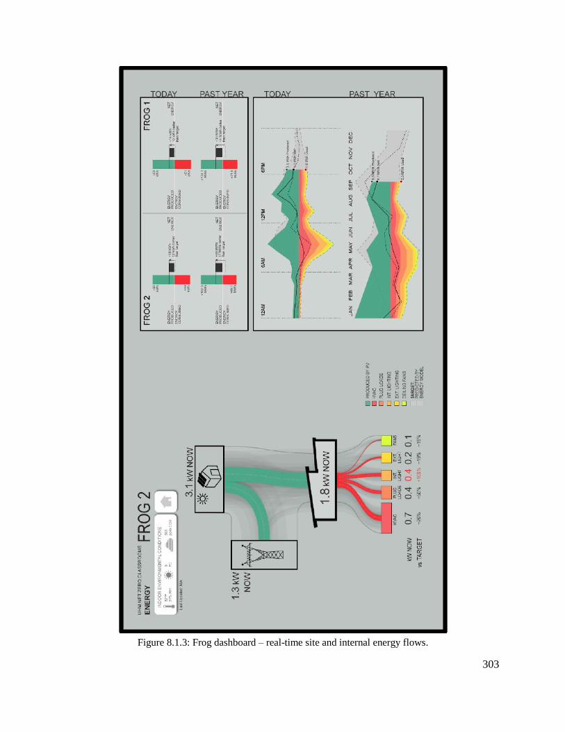
303

Figure 8.1.3: Frog dashboard – real-time site and internal energy flows.

304

Figure 8.1.4: Frog dashboard - environmental conditions

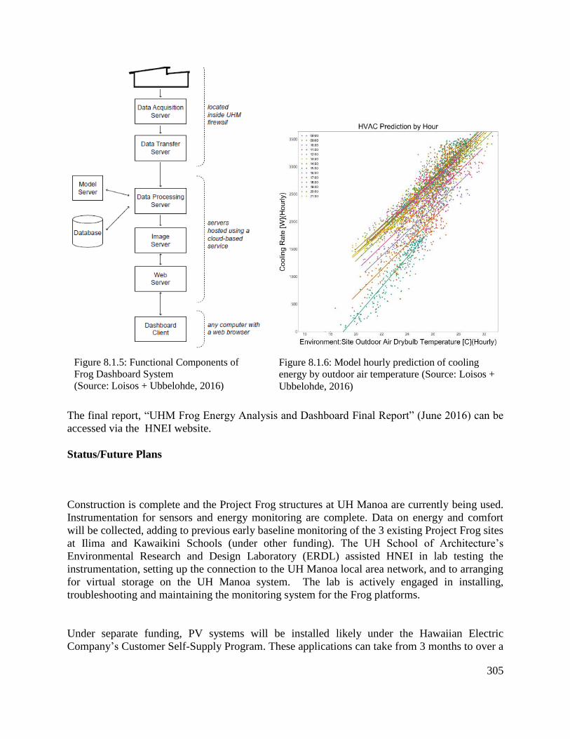
305

The final report, “UHM Frog Energy Analysis and Dashboard Final Report” (June 2016) can be

accessed via the HNEI website.

Status/Future Plans

Construction is complete and the Project Frog structures at UH Manoa are currently being used.

Instrumentation for sensors and energy monitoring are complete. Data on energy and comfort

will be collected, adding to previous early baseline monitoring of the 3 existing Project Frog sites

at Ilima and Kawaikini Schools (under other funding). The UH School of Architecture’s

Environmental Research and Design Laboratory (ERDL) assisted HNEI in lab testing the

instrumentation, setting up the connection to the UH Manoa local area network, and to arranging

for virtual storage on the UH Manoa system. The lab is actively engaged in installing,

troubleshooting and maintaining the monitoring system for the Frog platforms.

Under separate funding, PV systems will be installed likely under the Hawaiian Electric

Company’s Customer Self-Supply Program. These applications can take from 3 months to over a

Figure 8.1.5: Functional Components of

Frog Dashboard System

(Source: Loisos + Ubbelohde, 2016)

Figure 8.1.6: Model hourly prediction of cooling

energy by outdoor air temperature (Source: Loisos +

Ubbelohde, 2016)

306

year depending on the complexity of the design and the thoroughness of the technical support

provided with the application. With relatively simple and small systems, we anticipate approval

by the end of 2016.

8.2 Platform Monitoring and Performance Analysis

Under subtask8.2, HNEI subcontracted MKThink to complete a 1-year evaluation of two Project

Frog platforms at Kawaikini New Century Public Charter School in Kauai. The monitoring

results are available (on request) in a series of progress reports by MKThink and are summarized

in the final report: “Kawaikini New Century Public Charter School: Task 4.2 Final Report”

(March 2015), available on HNEI’s website. This monitoring effort is being continued for one

additional year under future ONR funding. This work includes also includes additional

instrumentation and monitoring of the Ilima Intermediate School Project Frog Platform, and 3

other school classroom typologies to collect comparable energy and comfort data.

The objective of this subtask is to record energy consumption information as well as other

performance metrics including daylighting, comfort, and visual and air quality and to evaluate

the interaction of active and passive systems; identify performance characteristics and optimal

operating strategies;

Results

Highlights of the first year of Kawaikini findings include:

Net Annual Energy: Results for the first year showed that both units used less energy than

was generated with the two platforms, and consumed an average of 45% less energy than the

“anticipated” energy model.

Comfort: The two platforms were within the prescribed American Society of Heating,

Refrigeration and Air Conditioning Engineers (ASHRAE) Comfort Zone for 25% and 45%

of the occupied hours respectively. Air quality, as indicated by CO2 levels in the classroom,

were above the ASHRAE threshold 99.9% of the occupied hours. Visual quality, as

represented by the ratio of contrast in wall to ceiling illuminance, was acceptable (less than a

ratio of 5) over 99.9% of the occupied hours.

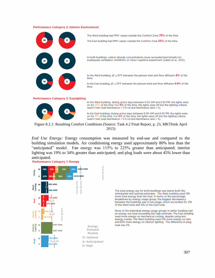
307

Figure 8.2.1: Resulting Comfort Conditions (Source: Task 4.2 Final Report, p. 23, MKThink April

2015)

End Use Energy: Energy consumption was measured by end-use and compared to the

building simulation models. Air conditioning energy used approximately 80% less than the

“anticipated” model. Fan energy was 115% to 225% greater than anticipated; interior

lighting was 19% to 34% greater than anticipated; and plug loads were about 45% lower than

anticipated.

308

Figure 8.2.2: Energy End Use Results (Source: Task 4.2 Final Report, p. 22, MKThink April

2015)

Conclusions

A comparison was conducted between the East and West Platforms to determine if performance

is consistent across platforms. It was discovered that 4 of 9 performance measures varied by

greater than 20% across platforms, with the majority (5 of 9) performance measures that

showed less than 20% difference in annual results. However, selected systems did show

moderate (20-50%) to significant (>50%) differences: Air Supply and distribution temperatures

varied significantly (>50%) due to increases in distribution temperature in the East Frog during

the last two quarters; Fan usage between the two buildings was moderately different (20-50%)

without a corresponding difference in AC usage; and Thermal Comfort conditions varied by

20% across the two platforms with the platform using the least fan energy having the higher

thermal comfort. This suggests the Predicted Mean Vote (PMV) model and assumptions are not

a good fit for the building type and/or user behavior.

Both platforms used less energy than anticipated (42-48% less), but also less than optimal. West

and East Frogs both out-performed model predictions of total annual energy consumption.

However, selected systems did not outperform their individual targets. Lighting systems were

used more than the anticipated/optimal amount, but that appears to be affected by outdoor

lighting being left on at night that may be related to security. Additionally, the AC systems were

used more than optimal and often at air temperatures below the optimal “kick-in” temp of 82°F,

especially in the E Platform.

Three of four performance measures were within standard recommendations for at least one

platform. While 3 of 4 performance measures showed >90% adherence to standards in at least

one platform, thermal comfort performance showed less than 50% adherence to standard

recommendations. However, it appears that the relatively low performance may be a result of

model assumptions for ASHRAE using clothing insulation and metabolic rates that, upon

further investigation, tend to cause large variations in model fit. Adjusting those assumptions to

fit user behavior as inferred through use of building systems may lead to a better calibration of

the PMV calculation and to a higher percentage of PMV scores within the comfort range (see

MKThink “Test Platform Performance Analysis Phase 2 Appendix”, March 2015, for details).

Lighting use and illuminance varied between the two platforms with East Frog meeting

illuminance criteria using daylighting more than West Frog, leading to higher than anticipated

indoor lighting loads at West Frog. Air Supply temperature stability across the distribution

plenums in the East Frog also showed less than 50% adherence to expectations and should be

inspected for issues.

Reports Resulting from Efforts

1. MKThink “Kawaikini New Century Public Charter School: Task 4.2 Final Report”, (March

2015).

2. MKThink “Test Platform Performance Analysis Phase 2” (March 2015)

3. MKThink “Test Platform Performance Analysis Phase 2 Appendix” (March 2015)

309

8.3 Advanced Database Research, Development and Testing (RD&T)

As data streams expand in size, the ability to manage, visualize and apply data weakens. Big data

can be found in both structured and unstructured formats. Structured data can be easily parsed

and organized in preparation for analysis, a process that can often be automated. Formats for

these data include but are not limited to: Comma Separate Values (CSV), Excel (XLS),

eXtensible Markup Language (XML), Geographic Information System (GIS), JavaScript Object

Notation (JSON) and other less common structured formats.

Unstructured data appear in visual, symbolic, textual, or other non-numeric formats. Recent

market research has attempted to quantify the split between structured and unstructured data.

Recent estimates indicate that between 80- 85% of an organization’s data are unstructured.

However, most organizations lack the processes and system requirements to effectively manage

this information leaving this potential untapped. Unstructured data files do not follow structured

data formats and thus inhibit facile aggregation with structured data models. Unstructured data

are generally in a text format although video, image and audio files are common as well. There is

great value in analyzing unstructured data independently, as well as converting them to a more

usable, structured format and combining them with structured data.

HNEI subcontracted this subtask, Advanced Database Research Development and Testing

(RD&T), to MKThink. With support from RoundhouseOne, MKThink expanded its Database

Management System (DBMS) called “4Daptive 1.0” platform a cloud-based data management

system for architects, sustainability coordinators, facilities managers, and other advocates for

sensor-driven building technology and building occupant health and comfort.

This project advanced the capabilities of 4Daptive 1.0, by developing techniques to improve the

acquisition, management, and analysis of large volumes of data, both structured and

unstructured. The proposed effort assumed prior collection and validation of the data, that is, it

did not consider real-time data collection and analysis. The final output of the project is a

platform called 4Daptive 2.0.

The objectives of the Advanced Database Research Development and Testing project were to:

1. Develop techniques to auto-acquire, manage, and visualize large volumes of data (> 1

billion data points per month) across multiple dimensions of both structured and

unstructured data.

2. Develop an advanced Database Management System that follows the DAMA-DMBOK

framework: data architecture; data development; database operations; data security;

reference and master data; data warehousing and business intelligence (visualization,

analysis, reporting); document and content management; meta data; data quality.

3. Develop techniques to visualize structured and unstructured data in combination to

improve usability for future decisions.

310

The effort considered multidimensional data in both the structured and unstructured data sets.

The range of the dimensions included cultural, environmental, and technological sources and

types.

Accomplishments under HEET10 include:

Structured data market research

The Data Management Association Data Management Body of Knowledge (DAMA-

DMBOK) framework was utilized to evaluate software tools and select those that

satisfied the data management requirements. From the DMBOK framework, 12 core

database and support functionalities (subcategories) were chosen. Over 500

companies and/or software tools were evaluated to determine 75 competitive

companies, for which a document was created to compare capabilities.

Unstructured data market research

Market research was performed for unstructured data types including video, text,

image, audio and handwriting. Over 58 companies and/or software tools were

evaluated to determine 14 viable companies across five different unstructured data

types.

Structuring text files – Text analysis module

Based on research, the relevant technologies for text were found to be classification,

data extraction, keyword extraction and sentiment analysis. The process for

integrating unstructured text data into 4Daptive was determined to be: 1) collect

unstructured text, 2) import text via API, 3) export in data interchange format, 4)

analyze data quality, 5) group similar results, 6) create tabular dataset, 7) integrate

with database. A prototype of a text analysis module was developed in 4Daptive, with

the ability to extract keywords from text sources.

Structuring video files – Video analysis

Based on research, the relevant technologies for video were found to be

demographics, dwell analysis, heat mapping, object detection, path mapping and

people counters. The process for integrating unstructured video data into 4Daptive

was determined to be: 1) collect unstructured video, 2) import video feed to 3rd party

program, 3) collect metrics from video feed, 4) create and store tabular dataset in the

cloud, 5) integrate tabular data into database. The 3rd party program selected for

integration has the ability to extract average occupancy, average dwell time and other

metrics from video feeds.

Flexible feature selection

311

4Daptive 1.0 was restructured to allow different modules to become active or inactive

depending on the users’ needs.

New 4Daptive modules were developed during the project

Project Setup module – Setup client and project information on the platform to

organize data and content securely; create project teams to organize and manage all

data and content across a project using security levels.

Auto Importer module – Using Extract-Transform-Load (ETL) tools found in the

Import Scheduler, users can schedule automatic structured data uploads; capability to

import 180,000 rows of data from 60 plus device types, tested using the Maui

Meadows Smart Grid data provided by HNEI.

Manual Importer module – Map item attributes to CSV columns and preview prior to

data import.

Data Grid module – Display user selected items, attributes and associated data that

exist in a project’s repository; sort rows alphabetically and numerically depending on

attribute data; filter rows by any attribute and/or value or multiple attributes and/or

values.

Analyzer module – Create data visualizations using numerous aesthetic and

quantitative visual customizations associated with representing, exploring and

expressing the data; plot values over time, values grouped by category and on scatter

plots; create custom formulas to perform calculations on data being visualized;

calculate statistics on data being visualized; create data cards containing visualization,

contextual metadata, statistics and findings associated with data; summarize numeric

columns using statistics.

Unstructured text tool – Process unstructured text data and output tabular structured

data for easy integration with other analysis tools.

Event detection tool (EDT) module – Utilize customized formulas to identify

“events” in the data to quickly find trends and anomalies; automatically calculate

distribution statistics on full data series, a zoomed range or selected events; accurately

visualize 1 billion data points in a readable format; tested using the Maui Meadows

Smart Grid data provided by HNEI.

File exchange module – Distribute and share drafts and items of any file type.

Inventory manager module – Store all findings related to a project all in one location

along with the data card to verify the authenticity of the discovery; manage content in

one centralized location with content briefcase; share and distribute drafts and other

work in progress items across a respective project.

Publisher module – View and edit PDF documents uploaded to project.

Nonfunctional 4Daptive capabilities

312

Data Architecture management – Utilize 4Daptive’s big data capability scalable to at

least 500 GB, tested using the Maui Meadows Smart Grid data provided by HNEI.

Database Management utilities – Utilize cloud-based system with https encryption

and an effective replication process with multi-site backup.

Data Security management – Database management system contains an integrated

firewall; 4Daptive 2.0 is compliant with ISO 27001, which is a security management

standard that specifies security management best practices and comprehensive

security controls.

Database Operations management – Ability to retain original raw uploaded le for up

to two years after its last use.

Details of the work can be found in the report prepared by MKThink, “Advanced

Database RD&T: Task 5 Final Integrated Report”, (August 2016), available on the HNEI

website.

References

.

1. M. Mosley, “DAMA-DMBOK Functional Framework”, Version 3.02, September 10,

2008, available on http://www.dama.org/

8.4 Energy-Efficient End-Use Technologies: Desiccant Dehumidification

In the past several years there have been significant advances in the performance and reliability

of desiccant dehumidification technology. When combined with newer air-management

processes, these technologies offer significant cost savings, particularly in high temperature, high

humidity areas characteristic of much of the Pacific region. Under subtask 8.4, HNEI conducted

an evaluation of currently available and the most promising desiccant dehumidification

technologies and air-management processes applicable to new building development and for the

retrofit of existing structures. Activities included

Conduct a literature review of state-of-the-art and emerging desiccant dehumidification

technologies.

Investigate the feasibility of desiccant dehumidification systems for their use in energy-

saving building cooling and ventilation systems, considering technical and economic

aspects.

Determine the most suitable candidate systems for the desiccant cooling applications in

Hawaii.

http://www.dama.org/

313

HNEI contracted Manfred Zapka, PhD, P.E. of Sustainable Design and Consulting, LLC to

conduct the literature search and feasibility studies. The results from this study are summarized

in this report, with full detail available inline in the following reports “Assessment of Desiccant

Dehumidification-Technical Feasibility and Summary Reports” (July 2016) and “Assessment of

Desiccant Dehumidification-Literature and Technology Review” (July 2016).

This literature review focused on the use of desiccant dehumidification technology in

conjunction with building air conditioning (AC). To date these applications have mostly used

solid desiccant material installed in vessel-swing operation or rotary wheel structures. The use of

desiccants in conventional AC has been mostly concerned with energy savings by recovering

sensible and latent loads in central AC systems. Such desiccant applications have become

standard applications for conventional AC systems. Liquid desiccant dehumidification in

conjunction with conventional has only received limited attention in the literature.

The feasibility study used a framework of four assessment criteria applied specifically for Hawaii

climatic conditions. As Figure 8.4.1 indicates, these criteria include the inherent characteristics

of desiccant cooling technologies, and three Hawaii specific criteria;the hot and humid climate in

Hawaii, the use of energy saving solar or low‐temperature heat sources, and comfort

enhancement measures.

Figure 8.4.1: Four assessment categories for the feasibility report.

Desiccant dehumidification systems can be used to reduce latent cooling loads when carried out

in parallel with conventional sensible space cooling strategies. Liquid or solid desiccant systems

were analyzed and both types of desiccant systems are suitable dehumidification technologies for

controlling the latent loads for buildings in Hawaii and other tropical regions.

Desiccant dehumidification does not remove sensible heat, in fact heat of sorption is added to air

passing through the desiccant material, and therefore cooling is typically required. This means

that the removal of sensible heat from the supply air is an indispensable part of the desiccant

cooling systems.

The climate in Hawaii is hot and humid, year round. The present feasibility study used a typical

314

meteorological year (TMY) file of Honolulu to determine the relevant climatic properties to

assess feasibility of desiccant cooling. The so‐called Ventilation Load Index (VLI) parameter was

used to quantify the latent and sensible load of the external air supply on an annual basis. The

VLI for Honolulu is one the highest in the nation, with the latent load being six times higher than

the sensible load. This high VLI emphasizes the importance of implementing energy efficient

desiccant dehumidification instead of the energy intensive cooling based dehumidification. The

analysis of the climatic records for Honolulu used the entire year and the daytime hours. The

results indicated different dehumidification and cooling needs for the year round and for the

daytime weather data, with higher dry bulb temperatures and lower relative humidity levels

during daytime hours.

The potential of solar heat for desiccant regeneration and thermally driven chillers was evaluated.

The potential for the use of solar heat in desiccant cooling is significant in Hawaii. Similarly, heat

derived from combined heat and power (CHP) systems can be a significant and energy saving

source for use in space conditioning. Hawaii has one of the highest energy costs in the nation, and

therefore high energy savings directly increase the competitiveness of desiccant cooling

applications.

Comfort enhancement measures can add to the feasibility of desiccant cooling, yet comfort

issues are typically only marginally considered. Ceiling fans represent a comfort enhancement

measure which is specifically suitable for Hawaii. The increased indoor air movement generated

by state‐of‐the‐art ceiling fans provide a highly energy efficient cooling effect. Spaces equipped

with conventional AC systems can only marginally take advantage of the ceiling fans due to

challenges to control humidity at higher indoor air temperatures, which are allowed when using

ceiling fans for added convective cooling. Buildings using desiccant cooling systems, on the

other hand, can take full advantage of the significant advantages of ceiling fans. The potential

contribution of ceiling fans in desiccant cooling was quantified in the present feasibility report

and used as a main criterion in determining energy savings.

Eight candidate systems, representing significantly different types of operation, were selected to

determine the applicability of desiccant cooling technologies for space conditioning in Hawaii.

These candidate systems were combinations of either solid or liquid desiccant dehumidification

and a range of sensible cooling systems. The differentiating factor of the desiccant cooling

candidate systems were thus the type of sensible cooling units. The eight systems were as

follows:

Candidate system A. Desiccant and Direct / Indirect Evaporative Cooling downstream of

desiccant dehumidification

Candidate system B. Enhanced evaporative cooling M‐Cycle downstream of desiccant

dehumidification

Candidate system C. Adsorption chiller downstream of desiccant dehumidification

Candidate system D. Absorption chiller downstream of desiccant dehumidification

Candidate system E. Magnetic (magneto caloric effect) chiller downstream of desiccant

dehumidification

Candidate system F. Integrated Desiccant Enhanced Evaporative Air Conditioning (DEVap)

membrane system,

315

Candidate system G. Liquid‐Desiccant Direct‐Expansion (LDDX) air‐conditioner, integrated

dehumidification and sensible cooling

Candidate system H. Conventional chiller, downstream of desiccant dehumidification

Some of the technologies are commercially available and have been tested in actual operation,

whereas others are emerging, yet very promising cooling technologies. The technologies are

evaluated and ranked differently depending on whether they are integrated into new construction

or as a retrofit. The leading candidate technology uses the conventional vapor compression cycle

in conjunction with liquid desiccant dehumidification (LDDX). This technology ranked highest

for retrofits and second for new construction based on potential energy savings.

The use of desiccants in conjunction with evaporative cooling was introduced about two decades

ago and has not seen a wide-spread use in building designs and operations, although such

systems can generate significant energy savings. Both solid and liquid desiccant systems are

suitable for integration with evaporative cooling applications.

While solid desiccant dehumidification integrations have the advantage of longer track record in

actual building installations, liquid desiccants have attracted much attention in recent

developments of desiccant cooling operations. In fact, since 2010 several groundbreaking liquid

desiccant cooling technologies have been proposed. These recent liquid desiccant technologies

developments suggest significant application potential for Hawaii, because of their favorable

process performance especially in Hawaii’s humid climate and their ability to work with low-

grade, unconventional heat sources, including solar heat and waste-heat from CHP applications.

In addition to identifying viable approaches to desiccant cooling system integration, the objective

of the feasibility study was to determine the most suitable candidate systems for the desiccant

cooling applications in Hawaii. The resulting ranking of technologies used a wide range of

criteria. Costs were not used as ranking criteria since some of the technologies are emerging

technologies with no detailed and confirmed first costs while other technologies analyzed have a

cost track record. Instead the projected saved energy relative to a conventional AC system was

used as a main criterion. The energy savings were calculated relative to a typical conventional

AC unit using cooling-based dehumidification. The resulting energy savings by technology-type

are depicted in Figure 8.4.2.

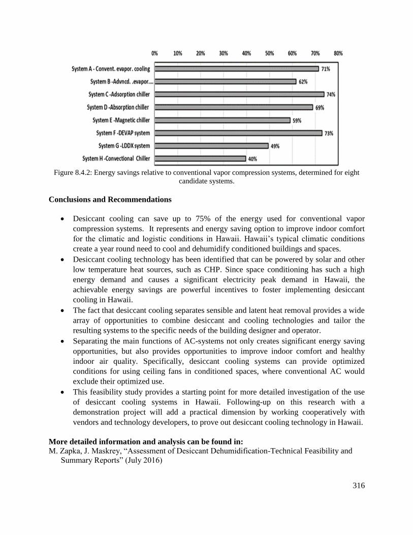
316

Figure 8.4.2: Energy savings relative to conventional vapor compression systems, determined for eight

candidate systems.

Conclusions and Recommendations

Desiccant cooling can save up to 75% of the energy used for conventional vapor

compression systems. It represents and energy saving option to improve indoor comfort

for the climatic and logistic conditions in Hawaii. Hawaii’s typical climatic conditions

create a year round need to cool and dehumidify conditioned buildings and spaces.

Desiccant cooling technology has been identified that can be powered by solar and other

low temperature heat sources, such as CHP. Since space conditioning has such a high

energy demand and causes a significant electricity peak demand in Hawaii, the

achievable energy savings are powerful incentives to foster implementing desiccant

cooling in Hawaii.

The fact that desiccant cooling separates sensible and latent heat removal provides a wide

array of opportunities to combine desiccant and cooling technologies and tailor the

resulting systems to the specific needs of the building designer and operator.

Separating the main functions of AC-systems not only creates significant energy saving

opportunities, but also provides opportunities to improve indoor comfort and healthy

indoor air quality. Specifically, desiccant cooling systems can provide optimized

conditions for using ceiling fans in conditioned spaces, where conventional AC would

exclude their optimized use.

This feasibility study provides a starting point for more detailed investigation of the use

of desiccant cooling systems in Hawaii. Following-up on this research with a

demonstration project will add a practical dimension by working cooperatively with

vendors and technology developers, to prove out desiccant cooling technology in Hawaii.

More detailed information and analysis can be found in: M. Zapka, J. Maskrey, “Assessment of Desiccant Dehumidification-Technical Feasibility and

Summary Reports” (July 2016)

317

M. Zapka, J. Maskrey, “Assessment of Desiccant Dehumidification-Literature and Technology

Review” (July 2016)

Task 9. ALGAL PRODUCTION STUDIES HNEI subcontracted with Hawaii BioEnergy to investigate the use of indigenous Hawaiian

algae strains to produce oil and protein as precursors to jet fuel and compound animal feeds.

This research focused on improving the economics of mixotrophic growth systems through

exploration of four areas: Environmental controls; Organic acids feeding strategies; Lipid

accumulation strategies, and; Strain sourcing and selection. Environmental controls to help

control bacteria and invasive microorganism species were investigated with laboratory and

outdoor, open cultures to optimize pH levels in to minimize bacteria and invasive organisms.

Feeding organic acids from common waste streams was tested on heterotrophic microalgal

strains. Lipid accumulation experiments were used to examine changes in nutrient levels and

types to improve cell size and/or lipid concentration. Algal strains capable of mixotrophic

growth, handling low pH levels and utilizing organic carbon were identified, sourced and tested

in the laboratory to develop baseline data. For complete details, see the final reports prepared by

Hawaii BioEnergy, compiled in “Algal Production Studies”.

FINAL TECHNICAL REPORT - HNEI

Documents

Transcript of FINAL TECHNICAL REPORT - HNEI