Article

Feasibility study of a new Cherenkov detector forimproving volcano muography

Domenico Lo Presti 1,2†,‡ , Giuseppe Gallo 1,3,‡,* , Danilo L. Bonanno 2,†,‡ , Daniele G.Bongiovanni‡, Fabio Longhitano and Santo Reito 2,‡

1 Department of Physics and Astronomy “E. Maiorana”, University of Catania, Via S. Sofia 64, 95123 CataniaItaly

2 INFN, Sezione di Catania, Via S. Sofia 64, 95123 Catania Italy3 INFN, Laboratori Nazionali del Sud, Via S. Sofia 62, 95123 Catania Italy* Correspondence: gallog@lns.infn.it† Current address: Via S. Sofia 64, 95123 Catania Italy‡ These authors contributed equally to this work.

Version January 21, 2019 submitted to Preprints

Abstract: Muography is an expanding technique for the investigation of the internal structure of1

targets of interest in geophysics. The flux of high penetrating muons produced by primary cosmic2

rays is attenuated by traversing kilometer size objects like X-ray flux is attenuated through the human3

body. This gives the possibility to study the internal structure of volcanoes or underground cavities,4

e.g., starting from the measure of the muon flux transmission through the target. Many groups of5

researchers working with this technique have to face with high background level that afflicts the6

reconstruction of muon tracks near the horizontal direction. An important source of background is7

the scattering of particles near the detector that produces a wrong reconstruction of the incoming8

direction. An innovative technique based on Cherenkov radiation was investigated by means of9

Monte Carlo simulations developed in Geant4 toolkit and MATLAB. The results reported in this10

paper show that the presented technique is able to correctly distinguish the incoming direction of11

particles with an efficiency higher than 98%. This new kind of detector could represent an alternative12

for high resolution charged particle tracking also for other applications.13

Keywords: Muography; Cherenkov radiation; Monte Carlo; Geant4; MATLAB; Particle detectors14

1. Introduction15

Muon radiography - or briefly muography - is a promising technique which aims at resolving16

the internal structure of large size objects by taking advantages of the high penetrating power of17

cosmic muons. Although the properties of muons interaction with matter have been known for a18

long time, the investigation of their potential as a probe to give information of large structures is a19

recent development. In the last years it is possible to found an increasing number of paper discussing20

the application of muography to target as volcanoes, underground cavities and also pyramids with21

impressive results [1–6].22

The muography technique is based on the reconstruction of the incident direction of the detected23

muons after crossing the target object. The basic element for a muography experiment is a tracker24

detector with at least two position sensitive planes in order to reconstruct the particle tracks. The25

incoming direction of the muons entering the detector may be distinguished from the slope of the26

reconstructed trajectory, assuming that the muon flux is downward oriented only. In this circumstance,27

muons detected, after being scattered near the detector and crossing it upward oriented, will be28

wrongly reconstructed. This contamination, together with the other sources of background, produces29

an overestimation of the muon counts that could be critical when compared with an very tiny expected30

flux.31

A proposed solution to overcome this source of background is the time-of-flight (TOF)32

measurement of the muons in traversing the detector [7,8]. The muon incoming direction can be33

Preprints (www.preprints.org) | NOT PEER-REVIEWED | Posted: 21 January 2019

© 2019 by the author(s). Distributed under a Creative Commons CC BY license.

Preprints (www.preprints.org) | NOT PEER-REVIEWED | Posted: 21 January 2019 doi:10.20944/preprints201901.0203.v1

© 2019 by the author(s). Distributed under a Creative Commons CC BY license.

Peer-reviewed version available at Sensors 2019, 19, 1183; doi:10.3390/s19051183

2 of 10

distinguished by the difference between the detection time ∆t in the external tracking planes of the34

detector. Being the path, between the two detection points, dependent on the angle between the35

particle trajectory and the normal to the telescope planes, the time distribution will be characterized36

by two lobes for ∆t > 0 and ∆t < 0, respectively, with a superimposition for ∆t ' 0, corresponding37

to particles perpendicular to the detection planes, which depends on time measurement resolution.38

Hence, for muons traveling the minimum distance in traversing the detector an uncertainty remains39

about their incoming direction.40

In this paper an alternative solution for this problem, based on the directionality of Cherenkov41

emission, is investigated by means of Monte Carlo simulations. The detector was designed as a possible42

upgrade of the muon telescope already working, developed inside the MEV project [9]. It consist43

of two adjacent radiator plates in which Cherenkov emission produced by muons takes place. The44

plates are separated by a foil of light absorbing material in order to prevent the Cherenkov radiation45

generated in a radiator from escaping and entering into the other one or could be reflected back.46

The two opposite faces of the detector are instrumented with light sensors to reveal the Cherenkov47

emission. The working principle is quite simple: the Cherenkov radiation should be revealed only in48

the second radiator traversed by the particle, in which the light is emitted toward the instrumented49

face of the plate.50

Different configurations of the Cherenkov detector were simulated by means of the Geant4 toolkit,51

changing the plate thickness and the number and arrangement of the light sensors. The results,52

reported in the following, show that the incoming direction of the muons can be distinguished with an53

efficiency of 98% for the best simulation scenario. Meanwhile, the possibility to develop a stand-alone54

muon telescope based on Cherenkov emission was considered and the tracking performance of this55

detector were studied, showing promising results also for other charged particle tracking applications.56

2. Results57

The design of the new detector under study is shown in figure 1. This is a module composed58

of two radiator of transparent material with size 20× 240× 240 mm3. In sight of a possible upgrade59

for the MEV project telescope, with a sensitive area of 1 m2, the final Cherenkov tag detector will be60

composed of a square matrix of 16 single modules to cover the sensitive area. The opposite side of each61

plate is equipped with light sensors to detect the Cherenkov radiation emitted in the corresponding62

radiator, while the lateral faces are coated with the same light absorbing material that separates the63

two plates.64

Figure 1. Lateral, front and perspective visualizations of the detector simulated in Geant4 for theconfiguration with a 16× 16 array of SiPMs (6× 6 mm2 sized) for the optical readout of each sensitiveface. The size of each radiator are 20× 240× 240 mm3.

The Cherenkov threshold is usually given in terms of the ratio between particle velocity and65

the speed of light, βth = 1/n, where n is the refractive index of the medium. Since E = γm0c2 and66

γ =(1− β2), the threshold can be expressed as:67

Preprints (www.preprints.org) | NOT PEER-REVIEWED | Posted: 21 January 2019 Preprints (www.preprints.org) | NOT PEER-REVIEWED | Posted: 21 January 2019 doi:10.20944/preprints201901.0203.v1

Peer-reviewed version available at Sensors 2019, 19, 1183; doi:10.3390/s19051183

3 of 10

Eth =m0c2√1− 1

n2

, (1)

in which is evident the dependence on particle rest mass m0. The mechanism of Cherenkov effect68

confines the photons to a cone with its vertex coincident with the point of first light emission. Also the69

aperture angle θC of the light cone is related to the particle velocity and to the refractive index of the70

medium according to the equation71

cos θC =1

nβ. (2)

With this in mind, it is possible to imagine what happens when a particle enters the detector from72

an instrumented side. The emission of Cherenkov photons immediately begins if the particle energy is73

over the typical threshold and the photons produced in the first radiator will be directed toward the74

light absorbing foil and will stop in it. Then, the particle enters the second radiator and the photons, in75

this case, will be emitted in the direction of the light sensitive surface. An example of the described76

interaction between a muon with kinetic energy equal to 105 MeV at the starting point, located at the77

left side of the detector, is shown in figure 2.78

Figure 2. Lateral, front and perspective visualizations of event of a muon with kinetic energy 105MeVsimulated in Geant4 for the configuration shown in fig.1. The optical photons internally reflected at theinterface between Plexiglas and air were suppressed to simplify the scene. Respect to fig. 1, plexiglassand light absorbing foils are drawn only as wire-frame in order to visualize photons trajectories inside.

2.1. Feasibility study for incoming particle direction discrimination79

The feasibility of the just exposed idea was verified by means of an extensive series of Monte80

Carlo simulations. The material chosen for the radiator was Plexiglas, with a refraction index slightly81

varying from 1.481 to 1.505 with increasing photons energies from 1.145 eV to 3.064 eV. For a value82

of the refraction index equal to 1.49 at the wavelength of nearly 600 nm, the energy thresholds for83

Cherenkov emission are Eth(µ) = 142.525 MeV, Eth(e−/e+) = 0.689 MeV, Eth(p) = 1265.66 MeV, for84

muons, electrons/positrons and protons respectively.85

The light sensitive side of each radiator is instrumented with SiPMs of 6× 6 mm2. The best86

strategy to distinguish the incoming direction of the particle was established by studying the number87

of SiPMs that produce a signal higher than a suitable threshold on each side of the detector, which in88

the following will be indicated as SiPM “fired”.89

The results of each set of simulation is reported as the percentage of successful recognized90

directions (“Successful tagged”). An event is considered well reconstructed when the discrimination91

condition is satisfied by only one instrumented side of the detector. The failure rate stands for the92

percentage of events when both instrumented sides pass the discrimination test - and it is impossible93

to establish which of them is the correct side - or no one. This last scenario is useful to take into account94

Preprints (www.preprints.org) | NOT PEER-REVIEWED | Posted: 21 January 2019 Preprints (www.preprints.org) | NOT PEER-REVIEWED | Posted: 21 January 2019 doi:10.20944/preprints201901.0203.v1

Peer-reviewed version available at Sensors 2019, 19, 1183; doi:10.3390/s19051183

4 of 10

border effects, i.e. particles that enter the detector from an instrumented face and exit the second95

radiator from a lateral side covered by coating foil; the Cherenkov light cone is directed, partially or96

completely, toward the lateral side and there are not sufficient photons to trigger the discrimination97

condition. In this case the incoming direction is not recognized at all. Furthermore, it is possible that98

no side passes the discrimination condition for low energy muons, when the angular aperture of the99

Cherenkov light cone is too low to hit a sufficient number of SiPMs or when β of the particles is under100

threshold. The mean number of SiPMs fired for each event is also included in the results.101

Four different detectors set-up were simulated, varying the size of the radiators and/or the102

number of SiPMs. In every case, the light sensors were placed following a regular pattern with SiPMs103

equally spaced. The simulated arrangements are:104

• Radiator size 30× 240× 240 mm3, 13× 13 SiPMs array;105

• Radiator size 20× 240× 240 mm3, 13× 13 SiPMs array;106

• Radiator size 20× 240× 240 mm3, 16× 16 SiPMs array;107

• Radiator size 20× 240× 240 mm3, 20× 20 SiPMs array.108

Excluding the second set-up in which the number of SiPMs was insufficient, in every case the failure109

rate is lower than 2% for muons with energy above Eth(µ). The results for successful configurations110

are reported in figure 3. These results were obtained with two primary particle sources, one for each111

entrance face of the detector, with the same geometric configuration. Each run of the simulation112

consists of 1000 muons shot randomly from one the two sources and with random direction, with113

angular distribution limited in order to hit the detector.114

The analysis of the simulations output was developed in MATLAB software environment, by115

means of which the figures that summarize the results were produced. It is possible to notice that for116

each subplot of figure 3 there are two different data series, one for Cherenkov photons and the other117

for photo-electrons (p.e.) generated after applying the “digitization” procedure that takes into account118

the SiPMs properties, including dark noise, described in detail in the following.119

For each scenario the best parameters for direction tagging were found and the results of figure 3120

refer to the following conditions: the threshold to consider a SiPM “fired” is equal to 5 photons or p.e.,121

respectively; the number of sensors fired on a single side has to be higher than 1, or 2 only for the case122

of 20× 20 SiPMs, to assign uniquely the incoming direction.123

2.2. High resolution position measurement124

The possibility to use the same detector for other purposes beyond the incoming direction tagging125

was also studied. In particular, the possibility to reconstruct the position of the crossing muon from the126

SIPMs signal was investigated. The very promising results of this study are reported in figure 4. The127

muon position at the exit point from the radiator was reconstructed by means of a two-dimensional128

Gauss fit on the matrix of the number of p.e. counted by each SiPM. The mean distance between the129

muon exit point and the centroid obtained from fit is between 2.0 and 4.5 mm, depending on the SiPM130

arrangement. This result could represent a strong enhancement for muography applications by means131

of an high resolution reconstruction of the tracks.132

Starting from the showed results, it is possible to affirm that the extensive simulations study133

conducted by means of Geant4 and MATLAB proves the principle of the proposed new technique for134

background discrimination in muography experiment. The efficiency of the set-up depends on the135

thickness of the radiator and on the number and arrangement of the SiPMs, but various configurations136

were found which give a failure rate lower than 2% at saturation energy. In fact, in each case for muons137

kinetic energies higher than 120 MeV, the mean number of SiPMs fired becomes constant, considering138

statistical fluctuations, and the efficiency follows a similar trend.139

3. Discussion140

The detector was initially ideated as an upgrade for the muon tracker telescope already built and141

operating inside the MEV project [9]. The Cherenkov direction discrimination prototype implemented142

Preprints (www.preprints.org) | NOT PEER-REVIEWED | Posted: 21 January 2019 Preprints (www.preprints.org) | NOT PEER-REVIEWED | Posted: 21 January 2019 doi:10.20944/preprints201901.0203.v1

Peer-reviewed version available at Sensors 2019, 19, 1183; doi:10.3390/s19051183

5 of 10

Figure 3. Results of Geant4 simulation as a function of the kinetic energy E of the primary particles(muons). Each column of subplot refers to a different simulation scenario, in which radiator size and/ornumber of SiPM have changed, as shown in the title.

in the simulation was a reduced scale version of the final detector. Plexiglas was chosen as radiator143

material to ensure high transparency to Cherenkov light, even if the UV wavelengths are cut down144

because its absorption length drops from several meters to only few millimeters in this spectral region.145

From the careful study of the simulation was observed that Cherenkov light emission by muons146

was not the unique relevant physical process. In fact, with a probability that depends on primary147

particle energy, muons can interact with the radiator medium, generating electrons by scattering. The148

energy of the scattered electrons, which depends, in turn, on the energy of primary particle, is of the149

order of 103 keV for the simulated muon energies. Since the energy of secondary electrons is higher150

than threshold for these particles, as established by equation (1), they generate Cherenkov radiation151

too. The electrons are emitted randomly because of the nature of the scattering process, their number152

is limited to some tens and their path through the medium is short. Taking into account all that, the153

signal produced by secondary electrons is very low respect to that of Cherenkov photons induced by154

fast muons and can be confused with the noise introduced by the digitization process in the SiPMs.155

Instead, for primary particle with energy lower than threshold, Cherenkov photons could be156

produced by scattered electrons only and they could mimic the signal of a higher energy muon leading157

to a wrong reconstruction of the incoming direction. This scenario was studied for the set-up with158

radiator of 20× 240× 240 mm3 and an array of 16× 16 SiPMs starting from 30 MeV for the energy159

Preprints (www.preprints.org) | NOT PEER-REVIEWED | Posted: 21 January 2019 Preprints (www.preprints.org) | NOT PEER-REVIEWED | Posted: 21 January 2019 doi:10.20944/preprints201901.0203.v1

Peer-reviewed version available at Sensors 2019, 19, 1183; doi:10.3390/s19051183

6 of 10

10 3 10 4 10 5

kinetic energy (MeV)

0

1

2

3

4

5

6

7m

m

mean distance

Rad. 30 mm, SiPMs 13x13Rad. 20 mm, SiPMs 16x16Rad. 20 mm, SiPMs 20x20

Figure 4. Mean distance between muon exit point from the radiator and 2D Gauss fir centroid in mm,for energies from 120 MeV to 105 MeV. In the legend are reported the radiator width in mm and thenumber of SiPMs in the array of sensors on the opposite face of the two radiator. The vertical error barsrepresent the standard deviation of each mean distance distribution.

spectrum. Slow muons loss all or the major part of their kinetic energy into the radiator and experience160

a strong Multiple Coulomb Scattering (MCS) such that they are heavily deflected respect their incoming161

directions or completely stopped in the detector. If we consider a system with two tracking planes162

and a direction discrimination detector in the middle of them, slow muons will not be a problem163

because after traversing the Cherenkov radiator they will be scattered outside the field of view of the164

whole system and, without coincidence on the second tracking plane, the acquisition of the signal will165

not be triggered. Otherwise, if a slow muon deflects and hit anyway both tracking planes, a linear166

fit discrimination will reject this event because the three impact points will be not aligned. Indeed,167

shutting down the signal produced by muons deflected more than 1◦, the efficiency is nearly zero,168

i.e. the discrimination of the incoming direction works as expected. The few failures are due to the169

digitization noise.170

Regarding the position measurement, the resolution of a single tracking module is higher than171

that of every system based on scintillating strips because the measure of the position is continuous172

and not discrete due to strips size. Until now, the continuous measure of the position in muography173

experiment was performed only by means of detector based on multi-wire proportional chamber174

(MWPC) or with nuclear emulsions, but with the latter the time information is inaccessible. In order to175

compare the performance of a muon tracker completely based on the new technique proposed in this176

paper with an apparatus like that described in ref. [5], it is required, at least, a simulation that includes177

three or more tracking planes, but this is beyond the scope of this work.178

If only the results about the capability of direction discrimination are considered, it will be difficult179

to establish which of the simulated configurations is the best. The main difference between them is180

the energy where the efficiency reaches a stable value greater than 98%. In a muography experiment181

to investigate the internal structure of large object such a volcano, the particles with low energy can182

be misleading because they are strongly deflected by MCS and their trajectory could be wrongly183

back-projected. This consideration, together with the advantage of limited number of electronic184

channels for signal read-out, could lead to chose the set-up with a thicker radiator and a lower number185

of SiPMs.186

But if the purpose of the system includes the position measurement, a closer spacing between187

light sensors will be useful. The configuration with two radiators, each 20 mm thick, and a regular188

array with 16× 16 SiPMs is the best between the ones investigated because it reaches approximately189

Preprints (www.preprints.org) | NOT PEER-REVIEWED | Posted: 21 January 2019 Preprints (www.preprints.org) | NOT PEER-REVIEWED | Posted: 21 January 2019 doi:10.20944/preprints201901.0203.v1

Peer-reviewed version available at Sensors 2019, 19, 1183; doi:10.3390/s19051183

7 of 10

the same efficiency of the set-up with a higher number of sensors and the resolution on the position190

measurement is slightly worst despite nearly only two third of SiPMs are used.191

Next step will be the comparison between experimental results in a reduced scale prototype and192

simulations. A 20× 60× 60 mm3 size prototype is under construction. Many solutions for the material193

of the radiator and the front-end electronics will be tested. For example, the use of optical gel in place194

of the plexiglass, could improve the transmission for UV Cherenkov photons and the optical coupling195

to PS optical window. The need for the measure of the number of photons detected by each SiPM,196

instead of a simple threshold, imposes severe constraints in the electronic chain regarding dead time197

and trigger strategy.198

4. Methods199

The simulations were performed using Geant4 [10], a toolkit for simulation of the passage of200

particles through matter. This toolkit is not specifically developed to work as a ray-tracer, but was201

chosen for this task because it accomplishes the generation of optical photons according the physical202

process involved in the interaction between a medium and a primary particle from the source.203

Geant4 provides a general model framework that allows the implementation of alternative204

physical models to describe the same process. In order to keep the simulation more general as possible205

and avoid to neglect some unexpected physical processes, the Physics List uses the approach of206

G4VModularPhysicsList. Technically speaking, a physics list can be implemented by specifying all207

the necessary particles and attaching to them the associated physics processes, but this requires a208

complete understanding of the whole physics involved. G4VModularPhysicsList, that is a sub-class of209

G4VUserPhysicsList, allows a user to organize physics processes into “building block”, or “modules”,210

and compose a physics list of such modules. This concept allows to group together desired combination211

of selected particles and related processes. The modules included into the physics list of the simulations212

discussed here are:213

• G4EmStandardPhysics;214

• G4DecayPhysics;215

• G4EmExtraPhysics;216

• G4HadronElasticPhysics;217

• G4HadronPhysicsFTFP_BERT;218

• G4OpticalPhysics.219

A description of the available physics models and processes within the Geant4 toolkit can be220

found in ref. [11].221

4.1. Detector construction222

Both radiator tiles are made of Plexiglas (C5H8O2, density = 1.19 g/cm3) with sizes 240 ×223

240 mm2 along y and z coordinates and 20 or 30 mm along x coordinate. Each tile has the lateral224

faces, those perpendicular to y and z axes, coated with a thin foil of polyvinyl chloride (PVC, C2H2Cl2,225

density = 1.7 g/cm3), 180 µm thick. One of two wider faces, perpendicular to x axis, is also coated226

with PVC foil, whereas the other one is left uncovered in order to allow the optical coupling with227

the light sensors. The two plates are arranged such that the larger coated surfaces face each other in228

contact.229

Each SiPM is constructed as a mother volume whit sizes 1.45× 6.0× 6.0 mm3, along x, y and230

z coordinates respectively, made of Silicon (Si). A second thinner box is placed inside the mother231

volume, with sizes 0.3× 6.0× 6.0 mm3, aligned along the x coordinate to a surface of the Si box. This232

inner volume represents the photosensitive window of the SiPM and is made with epoxy resin (CHO,233

density = 1.0 g/cm3). The “photosensitive surface” (PS) is a metal slab at the back end of the epoxy234

box that is only a very rough approximation of the real thing since it only absorbs or detects the235

photons based on its efficiency. The SIPMs are placed with the epoxy window faced to the uncoated236

surface of the radiator and arranged as an equally spaced NS × NS square array.237

Preprints (www.preprints.org) | NOT PEER-REVIEWED | Posted: 21 January 2019 Preprints (www.preprints.org) | NOT PEER-REVIEWED | Posted: 21 January 2019 doi:10.20944/preprints201901.0203.v1

Peer-reviewed version available at Sensors 2019, 19, 1183; doi:10.3390/s19051183

8 of 10

The world volume, which contains all the other volumes, is filled with air.238

4.2. Optical properties239

In order to correctly simulate the transportation of optical photons, Geant4 requires the user to240

provide the optical properties for both bulk materials and surfaces between them. This is a crucial241

point about processes involving optical photons, because without a documentation or a measure of242

the optical properties of the materials the optical physics processes will not be activated. The main243

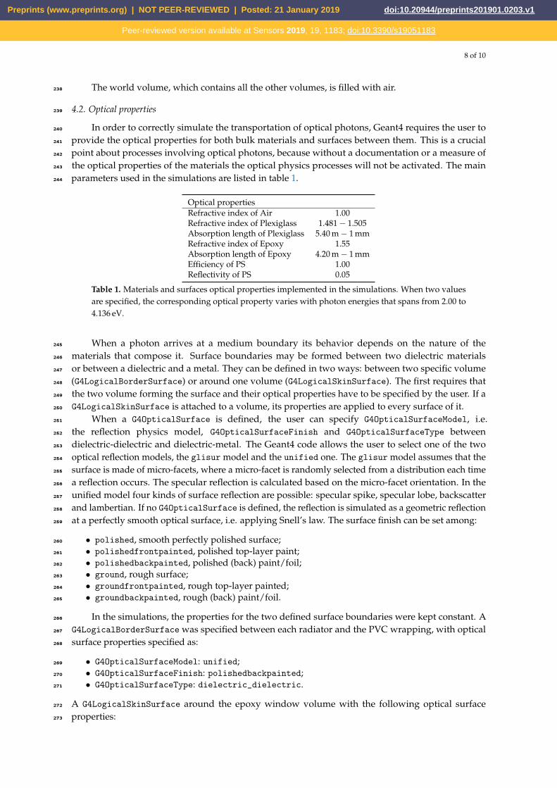
parameters used in the simulations are listed in table 1.244

Optical propertiesRefractive index of Air 1.00Refractive index of Plexiglass 1.481− 1.505Absorption length of Plexiglass 5.40 m− 1 mmRefractive index of Epoxy 1.55Absorption length of Epoxy 4.20 m− 1 mmEfficiency of PS 1.00Reflectivity of PS 0.05

Table 1. Materials and surfaces optical properties implemented in the simulations. When two valuesare specified, the corresponding optical property varies with photon energies that spans from 2.00 to4.136 eV.

When a photon arrives at a medium boundary its behavior depends on the nature of the245

materials that compose it. Surface boundaries may be formed between two dielectric materials246

or between a dielectric and a metal. They can be defined in two ways: between two specific volume247

(G4LogicalBorderSurface) or around one volume (G4LogicalSkinSurface). The first requires that248

the two volume forming the surface and their optical properties have to be specified by the user. If a249

G4LogicalSkinSurface is attached to a volume, its properties are applied to every surface of it.250

When a G4OpticalSurface is defined, the user can specify G4OpticalSurfaceModel, i.e.251

the reflection physics model, G4OpticalSurfaceFinish and G4OpticalSurfaceType between252

dielectric-dielectric and dielectric-metal. The Geant4 code allows the user to select one of the two253

optical reflection models, the glisur model and the unified one. The glisur model assumes that the254

surface is made of micro-facets, where a micro-facet is randomly selected from a distribution each time255

a reflection occurs. The specular reflection is calculated based on the micro-facet orientation. In the256

unified model four kinds of surface reflection are possible: specular spike, specular lobe, backscatter257

and lambertian. If no G4OpticalSurface is defined, the reflection is simulated as a geometric reflection258

at a perfectly smooth optical surface, i.e. applying Snell’s law. The surface finish can be set among:259

• polished, smooth perfectly polished surface;260

• polishedfrontpainted, polished top-layer paint;261

• polishedbackpainted, polished (back) paint/foil;262

• ground, rough surface;263

• groundfrontpainted, rough top-layer painted;264

• groundbackpainted, rough (back) paint/foil.265

In the simulations, the properties for the two defined surface boundaries were kept constant. A266

G4LogicalBorderSurface was specified between each radiator and the PVC wrapping, with optical267

surface properties specified as:268

• G4OpticalSurfaceModel: unified;269

• G4OpticalSurfaceFinish: polishedbackpainted;270

• G4OpticalSurfaceType: dielectric_dielectric.271

A G4LogicalSkinSurface around the epoxy window volume with the following optical surface272

properties:273

Preprints (www.preprints.org) | NOT PEER-REVIEWED | Posted: 21 January 2019 Preprints (www.preprints.org) | NOT PEER-REVIEWED | Posted: 21 January 2019 doi:10.20944/preprints201901.0203.v1

Peer-reviewed version available at Sensors 2019, 19, 1183; doi:10.3390/s19051183

9 of 10

• G4OpticalSurfaceModel: glisur;274

• G4OpticalSurfaceFinish: polished;275

• G4OpticalSurfaceType: dielectric_metal.276

A more detailed explanation about simulation of optical physics in Geant4 can be found in ref.277

[12].278

4.3. Digitization279

The analysis of the simulation output was developed in MATLAB. The number of generated280

photons which reach the PS at the back-layer of the epoxy window is counted. This number takes into281

account both Cherenkov radiation produced by primary muons and the one due to secondary electrons.282

The digitization procedure is needed to convert the number of photons, Nph, in the given event, into283

the number of p.e. generated in SiPM. Because the structure of the SiPM is not simulated, a statistical284

approach is required for the conversion. The number of p.e., Npe, is random generated from the285

Poisson distribution with mean parameter Nph and takes into account the photon detection efficiency286

(PDE) and the fill factor f of the SiPM, as Npe = poissrnd(Nph)× PDE× f , where poissrnd (λ) is the287

MATLAB function to extract random number from Poisson distribution with mean parameter λ. PDE288

and f are set equal to 0.5 and 0.74 respectively. The digitization procedure adds also a Gaussian noise289

to the signal, with mean and sigma equal to 2 and 1 respectively, in order to mimic the dark current290

rate of the SiPM.291

4.4. Position measurement292

When the incoming direction of the primary muons is correctly discriminated, an additionalanalysis can be done on the matrix of Npe for each SiPM of the instrumented radiator side which passesthe discrimination test. It consists of a surface fit on 3D set of points. The y and z coordinates of theSiPM center positions are set as independent variables, while the corresponding Npe(y, z) was thedependent one. The two-dimensional fit function is a 2D rotated Gaussian:

Npe(y, z) =

a + b exp

{−[(y− c1) cos(t1) + (z− c2) sin(t1)

w1

]2

−[−(y− c1) sin(t1) + (z− c2) cos(t1)

w2

]2}

,(3)

with the following parameters:293

• a, offset along Npe coordinate;294

• b, amplitude of the 2D gaussian;295

• c1, centroid y coordinate of the 2D gaussian;296

• c2, centroid z coordinate of the 2D gaussian;297

• t1, angle of rotation for the 2D gaussian;298

• w1, width along y of the 2D gaussian;299

• w2, width along z of the 2D gaussian.300

The reconstructed position of a muon going out the last radiator along its path is assigned equal301

to (c1, c2) on the (y, z) plane at x equal to the border of the radiator. Then the distance between (c1, c2)302

and the true exit position of the muon, retrieved from the simulation output is calculated to investigate303

the precision of this measurement, as showed in fig. 4.304

5. Conclusions305

In conclusion, it is possible to affirm the the feasibility study conducted and exposed in this paper306

opens a new promising possibility to reduce the background noise in muography applications. The307

working principle of the Cherenkov tag detector works well in simulations. Even if other aspetcs308

could be investigated, the next fundamental steps will be a comparison and a fine tuning between309

Preprints (www.preprints.org) | NOT PEER-REVIEWED | Posted: 21 January 2019 Preprints (www.preprints.org) | NOT PEER-REVIEWED | Posted: 21 January 2019 doi:10.20944/preprints201901.0203.v1

Peer-reviewed version available at Sensors 2019, 19, 1183; doi:10.3390/s19051183

10 of 10

simulations and the experimental study of a prototype, which include many technical constrains not310

reproducible in simulations.311

Author Contributions: Conceptualization D.L.P.; software G.G.; writing-review and editing D.L.P. G.G. and312

D.L.B.; all the authors contributed to investigation, validation and data processing.313

Funding: This research received no external funding.314

Conflicts of Interest: The authors declare no conflict of interest.315

316

1. Tanaka, H.K.M.; Nakano, T.; Takahashi, S.; Yoshida, J.; Takeo, M.; Oikawa, J.; Ohminato, T.; Aoki, Y.;317

Koyama, E.; Tsuji, H.; Niwa, K. High resolution imaging in the inhomogeneous crust with cosmic-ray318

muon radiography: The density structure below the volcanic crater floor of Mt. Asama, Japan. Earth and319

Planetary Science Letters 2007, 263, 104–113. doi:10.1016/j.epsl.2007.09.001.320

2. Lesparre, N.; Gibert, D.; Marteau, J.; Komorowski, J.C.; Nicollin, F.; Coutant, O. Density muon radiography321

of La Soufrière of Guadeloupe volcano: comparison with geological, electrical resistivity and gravity data.322

Geophysical Journal International 2012, 190, 1008–1019. doi:10.1111/j.1365-246X.2012.05546.x.323

3. Morishima, K.; Kuno, M.; Nishio, A.; Kitagawa, N.; Manabe, Y.; Moto, M.; Takasaki, F.; Fujii, H.; Satoh,324

K.; Kodama, H.; et al. Discovery of a big void in Khufu’s Pyramid by observation of cosmic-ray muons.325

Nature 2017, 552, 386–390. doi:10.1038/nature24647.326

4. Saracino, G.; Amato, L.; Ambrosino, F.; Antonucci, G.; Bonechi, L.; Cimmino, L.; Consiglio, L.;327

D’Alessandro, R.; Luzio, E.D.; Minin, G.; et al. Imaging of underground cavities with cosmic-ray muons328

from observations at Mt. Echia (Naples). Scientific Reports 2017, 7, 1181. doi:10.1038/s41598-017-01277-3.329

5. Oláh, L.; Tanaka, H.K.M.; Ohminato, T.; Varga, D. High-definition and low-noise muography330

of the Sakurajima volcano with gaseous tracking detectors. Scientific Reports 2018, 8, 3207.331

doi:10.1038/s41598-018-21423-9.332

6. Tanaka Hiroyuki K. M..; Oláh László. Overview of muographers. Philosophical Transactions of the Royal333

Society A: Mathematical, Physical and Engineering Sciences 2019, 377, 20180143. doi:10.1098/rsta.2018.0143.334

7. Jourde, K.; Gibert, D.; Marteau, J.; de Bremond d’Ars, J.; Gardien, S.; Girerd, C.; Ianigro, J.C.; Carbone,335

D. Experimental detection of upward going cosmic particles and consequences for correction of density336

radiography of volcanoes. Geophysical Research Letters 2013, 40, 6334–6339. doi:10.1002/2013GL058357.337

8. Cimmino, L.; Ambrosino, F.; Bonechi, L.; Ciaranfi, R.; D’Alessandro, R.; Masone, V.; Mori, N.; Noli, P.;338

Saracino, G.; Strolin, P. The MURAVES telescope front-end electronics and data acquisition. Annals of339

Geophysics 2017, 60, 0104. doi:10.4401/ag-7379.340

9. Lo Presti, D.; Gallo, G.; Bonanno, D.L.; Bonanno, G.; Bongiovanni, D.G.; Carbone, D.; Ferlito, C.; Immè, J.;341

La Rocca, P.; Longhitano, F.; et al. The MEV project: Design and testing of a new high-resolution telescope342

for muography of Etna Volcano. Nuclear Instruments and Methods in Physics Research Section A: Accelerators,343

Spectrometers, Detectors and Associated Equipment 2018, 904, 195–201. doi:10.1016/j.nima.2018.07.048.344

10. Agostinelli, S.; Allison, J.; Amako, K.; Apostolakis, J.; Araujo, H.; Arce, P.; Asai, M.; Axen, D.; Banerjee,345

S.; Barrand, G.; et al. Geant4—a simulation toolkit. Nuclear Instruments and Methods in Physics346

Research Section A: Accelerators, Spectrometers, Detectors and Associated Equipment 2003, 506, 250–303.347

doi:10.1016/S0168-9002(03)01368-8.348

11. User Support | geant4.web.cern.ch.349

12. Dietz-Laursonn, E. Peculiarities in the Simulation of Optical Physics with Geant4. arXiv:1612.05162350

[physics] 2016. arXiv: 1612.05162.351

Preprints (www.preprints.org) | NOT PEER-REVIEWED | Posted: 21 January 2019 Preprints (www.preprints.org) | NOT PEER-REVIEWED | Posted: 21 January 2019 doi:10.20944/preprints201901.0203.v1

Peer-reviewed version available at Sensors 2019, 19, 1183; doi:10.3390/s19051183