Design of the TORCH detector A Cherenkov based Time-of ...

CER

N-T

HES

IS-2

016-

039

24/0

2/20

16

Design of the TORCH detector

A Cherenkov based Time-of-Flight system for

particle identification

Maarten Willibrord Uriel van Dijk

A dissertation submitted to the University of Bristol in accordance with the requirements for

award of the degree of PhD in the Faculty of Science, Department of Physics (2016).

(Word count: 58,704)

ABSTRACT

The LHCb detector at the LHC collider has been very successfully operated over the past years,providing new and profound insights into the Standard Model, in particular through study ofb-hadrons to achieve a better understanding of CP violation. One of the key components of LHCbis its particle identification system, comprised of two RICH detectors, which allow for high preci-sion separation of particle species over a large momentum range. In order to retain and improvethe performance of the particle identification system in light of the LHCb upgrade, the TORCHdetector has been proposed to supplement the RICH system at low momentum (2-10 GeV/c).

The TORCH detector provides (charged) particle identification through precision timing ofparticles passing through it. Assuming a known momentum from the tracking, it is possible toderive the species of a particle from the time of flight from its primary vertex. This measurementis achieved by timing and combining photons generated in a solid radiator. The geometry of thedetector (composed of large plates of fused silica) is such that the generated Cherenkov photonsare trapped inside the plate by total internal reflection, and propagate to the periphery of theradiator. Here they are projected onto a plane of photodetectors, comprised of purpose designedMCP-PMTs. The photons detected for a track are combined into a time stamp for each parti-cle, finally resulting in the time of flight being measured so that the particle identity can be derived.

The final goal of the TORCH project is to prove the feasibility and desirability of the TORCHdetector as an addition to the LHCb particle identification system. This thesis will describe theprogress that has been made towards the key objectives of the TORCH project; in particular thedevelopment of optics, detectors and electronics.

Men love to wonder

and that is the seed of science

— Emerson

ACKNOWLEDGEMENTS

I hereby gratefully acknowledge support of the European Research Council in the funding of this

research (ERC-2011-AdG, 291175-TORCH).

Several people stand out for having gone above and beyond in helping me through this PhD.

Prof. Nick Brook, for dedicated and professional supervision, and above all for not beating

around the bush.

Dr. Jonas Rademacker, for help and guidance whenever it was needed.

Dr. Kostas Petridis, for some last minute feedback and help with LHCb data.

Special thanks go out to the TORCH collaboration - Prof. Neville Harnew, Dr. Roger Forty

and many others - for providing a friendly but fast paced and highly driven work environment.

To the TORCH folk at Bristol - Ana, Euan, David - it’s been a pleasure working with you.

A great many people deserve my gratitude for their unwavering support - Kathryn, Berna,

Gerard, Judith, Joris, Mirjam, Edwin, Charlotte, and many others: thanks for strengthening my

backbone when I needed it most.

Over the past few years I have flourished in the friendly environment of the Bristol High Energy

Physics group, and I would like to thank all its members (past and present) for providing a very

focused but also very social atmosphere.

To all my friends and family: I could not have done this without you. Thanks!

Dulcius ex asperis.

Maarten van Dijk, January 29, 2016

AUTHOR’S DECLARATION

I declare that the work in this dissertation was carried out in accordance with the requirements

of the University’s Regulations and Code of Practice for Research Degree Programmes and that

it has not been submitted for any other academic award. Except where indicated by specific

reference in the text, the work is the candidate’s own work. Work done in collaboration with, or

with the assistance of, others, is indicated as such. Any views expressed in the dissertation are

those of the author.

SIGNED: ............................................................. DATE:..........................

Contents

Introduction 18

1. Physics of the TORCH detector - Theory 21

1.1 B-physics and LHCb . . . . . . . . . . . . . . . . . . . . . . . . . . . . . . . . . . . 21

1.1.1 B-physics . . . . . . . . . . . . . . . . . . . . . . . . . . . . . . . . . . . . . 21

1.1.2 Design of LHCb . . . . . . . . . . . . . . . . . . . . . . . . . . . . . . . . . 23

1.2 RICH physics . . . . . . . . . . . . . . . . . . . . . . . . . . . . . . . . . . . . . . . 26

1.2.1 RICH theory . . . . . . . . . . . . . . . . . . . . . . . . . . . . . . . . . . . 26

1.2.2 RICH detectors . . . . . . . . . . . . . . . . . . . . . . . . . . . . . . . . . . 27

1.3 The RICH system - PID in LHCb . . . . . . . . . . . . . . . . . . . . . . . . . . . 30

1.3.1 Particle identification performance . . . . . . . . . . . . . . . . . . . . . . . 32

1.3.2 The LHCb upgrade . . . . . . . . . . . . . . . . . . . . . . . . . . . . . . . . 33

1.4 TORCH in LHCb . . . . . . . . . . . . . . . . . . . . . . . . . . . . . . . . . . . . . 36

2. Design of the TORCH detector 40

2.1 Basics of the TORCH detector . . . . . . . . . . . . . . . . . . . . . . . . . . . . . 42

2.2 The radiator plate . . . . . . . . . . . . . . . . . . . . . . . . . . . . . . . . . . . . 44

2.3 The focusing block . . . . . . . . . . . . . . . . . . . . . . . . . . . . . . . . . . . . 46

2.3.1 Metal coating of the focusing block . . . . . . . . . . . . . . . . . . . . . . . 48

2.4 Glue for the TORCH optics . . . . . . . . . . . . . . . . . . . . . . . . . . . . . . . 48

2.5 Detectors for TORCH . . . . . . . . . . . . . . . . . . . . . . . . . . . . . . . . . . 51

2.5.1 Pixellation requirements . . . . . . . . . . . . . . . . . . . . . . . . . . . . . 51

2.5.2 Multiple Coulomb scattering . . . . . . . . . . . . . . . . . . . . . . . . . . 52

2.5.3 Lifetime and rate capability requirements . . . . . . . . . . . . . . . . . . . 53

2.6 Electronics for TORCH . . . . . . . . . . . . . . . . . . . . . . . . . . . . . . . . . 54

2.7 Impact of glue and quantum efficiency . . . . . . . . . . . . . . . . . . . . . . . . . 56

2.8 Summary of requirements . . . . . . . . . . . . . . . . . . . . . . . . . . . . . . . . 56

3. The TORCH MCP-PMT 59

3.1 MCP detectors . . . . . . . . . . . . . . . . . . . . . . . . . . . . . . . . . . . . . . 60

11

3.2 Development of the TORCH MCP-PMT . . . . . . . . . . . . . . . . . . . . . . . . 61

3.3 Charge sharing and hybrid anode design . . . . . . . . . . . . . . . . . . . . . . . . 64

3.4 Testing the TORCH MCP-PMT . . . . . . . . . . . . . . . . . . . . . . . . . . . . 65

3.4.1 Equipment for testing the TORCH MCP-PMT . . . . . . . . . . . . . . . . 66

3.4.2 Quantum efficiency . . . . . . . . . . . . . . . . . . . . . . . . . . . . . . . . 69

3.4.3 Lifetime . . . . . . . . . . . . . . . . . . . . . . . . . . . . . . . . . . . . . . 70

3.4.4 Gain and time resolution . . . . . . . . . . . . . . . . . . . . . . . . . . . . 71

3.4.5 Gain and photocathode uniformity . . . . . . . . . . . . . . . . . . . . . . . 78

3.4.6 Spatial resolution . . . . . . . . . . . . . . . . . . . . . . . . . . . . . . . . . 79

3.4.7 Time resolution of the Phase 2 MCP-PMT . . . . . . . . . . . . . . . . . . 86

3.4.8 Rate capability . . . . . . . . . . . . . . . . . . . . . . . . . . . . . . . . . . 87

3.4.9 Looking ahead: The Phase-3 MCP-PMT . . . . . . . . . . . . . . . . . . . 88

3.5 Summary . . . . . . . . . . . . . . . . . . . . . . . . . . . . . . . . . . . . . . . . . 88

4. The TORCH detector in simulation 90

4.1 Relevant Geant processes . . . . . . . . . . . . . . . . . . . . . . . . . . . . . . . . 90

4.1.1 Cherenkov photon generation . . . . . . . . . . . . . . . . . . . . . . . . . . 91

4.1.2 Refractive indices in Geant . . . . . . . . . . . . . . . . . . . . . . . . . . . 91

4.1.3 Surface roughness of the radiator plate . . . . . . . . . . . . . . . . . . . . . 92

4.1.4 Surface reflections in Geant . . . . . . . . . . . . . . . . . . . . . . . . . . . 93

4.1.5 Rayleigh scattering . . . . . . . . . . . . . . . . . . . . . . . . . . . . . . . . 95

4.2 Implementing the optical design in Geant . . . . . . . . . . . . . . . . . . . . . . . 96

4.2.1 The radiator plate and the focusing block . . . . . . . . . . . . . . . . . . . 96

4.2.2 Number of generated Cherenkov photons . . . . . . . . . . . . . . . . . . . 97

4.2.3 Photons at the photodetector plane . . . . . . . . . . . . . . . . . . . . . . 99

4.2.4 Effects from photon scattering . . . . . . . . . . . . . . . . . . . . . . . . . 101

4.2.5 Implementing photodetectors in simulation . . . . . . . . . . . . . . . . . . 102

4.3 Photon timing reconstruction . . . . . . . . . . . . . . . . . . . . . . . . . . . . . . 103

4.3.1 Refractive index reconstruction . . . . . . . . . . . . . . . . . . . . . . . . . 104

4.3.2 Reconstruction of path length in the focusing block . . . . . . . . . . . . . . 105

4.3.3 Total path length and timing reconstruction . . . . . . . . . . . . . . . . . . 107

4.3.4 Expected timing performance . . . . . . . . . . . . . . . . . . . . . . . . . . 108

4.4 Simulated performance of the TORCH detector . . . . . . . . . . . . . . . . . . . . 112

4.4.1 Parameters of interest for the TORCH simulation . . . . . . . . . . . . . . 113

4.4.2 Input from LHCb . . . . . . . . . . . . . . . . . . . . . . . . . . . . . . . . . 114

4.4.3 Simulated performance of the single plate design of the TORCH detector . 115

12

4.5 Summary . . . . . . . . . . . . . . . . . . . . . . . . . . . . . . . . . . . . . . . . . 121

5. The TORCH testbeam setup 122

5.1 The TORCH testbeam prototype . . . . . . . . . . . . . . . . . . . . . . . . . . . . 122

5.1.1 The detector assembly . . . . . . . . . . . . . . . . . . . . . . . . . . . . . . 123

5.1.2 Quartz for testbeam . . . . . . . . . . . . . . . . . . . . . . . . . . . . . . . 124

5.1.3 The optical assembly . . . . . . . . . . . . . . . . . . . . . . . . . . . . . . . 127

5.1.4 The quartz finger - time reference . . . . . . . . . . . . . . . . . . . . . . . 130

5.1.5 The VELO telescope . . . . . . . . . . . . . . . . . . . . . . . . . . . . . . . 131

5.1.6 The trigger logic unit . . . . . . . . . . . . . . . . . . . . . . . . . . . . . . 132

5.1.7 The SPS beam line: H8 . . . . . . . . . . . . . . . . . . . . . . . . . . . . . 132

5.1.8 Pattern folding . . . . . . . . . . . . . . . . . . . . . . . . . . . . . . . . . . 134

5.2 Testbeam prototype - expected timing performance . . . . . . . . . . . . . . . . . . 136

5.2.1 Simulating the transit time spread of the detector and time reference . . . . 138

5.2.2 Time separation of reflections . . . . . . . . . . . . . . . . . . . . . . . . . . 139

5.3 Summary . . . . . . . . . . . . . . . . . . . . . . . . . . . . . . . . . . . . . . . . . 145

6. The TORCH testbeam analysis 147

6.1 Testbeam configurations . . . . . . . . . . . . . . . . . . . . . . . . . . . . . . . . . 147

6.2 Telescope tracking data . . . . . . . . . . . . . . . . . . . . . . . . . . . . . . . . . 148

6.3 Calibrations for testbeam . . . . . . . . . . . . . . . . . . . . . . . . . . . . . . . . 153

6.3.1 Width to charge calibration . . . . . . . . . . . . . . . . . . . . . . . . . . . 154

6.3.2 Time walk correction . . . . . . . . . . . . . . . . . . . . . . . . . . . . . . . 156

6.3.3 Integral non-linearity . . . . . . . . . . . . . . . . . . . . . . . . . . . . . . . 157

6.4 Testbeam data processing . . . . . . . . . . . . . . . . . . . . . . . . . . . . . . . . 158

6.4.1 Data quality control . . . . . . . . . . . . . . . . . . . . . . . . . . . . . . . 158

6.4.2 Clustering . . . . . . . . . . . . . . . . . . . . . . . . . . . . . . . . . . . . . 159

6.5 Initial testbeam data analysis . . . . . . . . . . . . . . . . . . . . . . . . . . . . . . 162

6.6 Further analysis on testbeam data . . . . . . . . . . . . . . . . . . . . . . . . . . . 165

6.6.1 Intra-cluster timing . . . . . . . . . . . . . . . . . . . . . . . . . . . . . . . 165

6.6.2 Weak secondary reflections . . . . . . . . . . . . . . . . . . . . . . . . . . . 167

6.6.3 Further investigations . . . . . . . . . . . . . . . . . . . . . . . . . . . . . . 168

6.7 Summary . . . . . . . . . . . . . . . . . . . . . . . . . . . . . . . . . . . . . . . . . 168

Conclusions 170

Bibliography 173

13

List of abbreviations 183

List of Figures

1.1 Unitarity triangles. . . . . . . . . . . . . . . . . . . . . . . . . . . . . . . . . . . . . 22

1.2 Opening angle of B and B hadrons relative to the beam angle in LHCb. . . . . . . 24

1.3 Schematic view of the LHCb detector. . . . . . . . . . . . . . . . . . . . . . . . . . 25

1.4 Refractive index of typical RICH and DIRC radiators. . . . . . . . . . . . . . . . . 29

1.5 Design of the RICH detectors at LHCb. . . . . . . . . . . . . . . . . . . . . . . . . 31

1.6 Expected and measured performance of the LHCb RICH. . . . . . . . . . . . . . . 31

1.7 Kaon and pion PID performance of the LHCb RICH. . . . . . . . . . . . . . . . . . 32

1.8 Impact of PID information on LHCb data analysis (B → h+h−). . . . . . . . . . . 33

1.9 RICH1 geometry after LHCb Upgrade. . . . . . . . . . . . . . . . . . . . . . . . . . 34

1.10 Kaon-pion separation before and after upgrade of the LHCb RICH system. . . . . 35

1.11 Expected RICH system PID efficiency after the RICH upgrade. . . . . . . . . . . . 36

1.12 Basic optical design of the TORCH detector. . . . . . . . . . . . . . . . . . . . . . 36

1.13 Theoretical kaon–pion separation provided by the TORCH detector relative to cur-

rent LHCb RICH system. . . . . . . . . . . . . . . . . . . . . . . . . . . . . . . . . 37

1.14 Expected PID performance of the TORCH detector for current and LHCb Upgrade

conditions. . . . . . . . . . . . . . . . . . . . . . . . . . . . . . . . . . . . . . . . . . 39

2.1 Definition of “tilt” . . . . . . . . . . . . . . . . . . . . . . . . . . . . . . . . . . . . 41

2.2 Refractive index of fused silica. . . . . . . . . . . . . . . . . . . . . . . . . . . . . . 43

2.3 Initial single plate design of the TORCH detector. . . . . . . . . . . . . . . . . . . 43

2.4 Total internal reflections in the TORCH detector (definition of angle θz). . . . . . 44

2.5 Transport of photons to perimeter of the TORCH radiator (definition of angle θx). 45

2.6 Modular design of the TORCH detector. . . . . . . . . . . . . . . . . . . . . . . . . 45

2.7 Initial design of the TORCH focusing optics. . . . . . . . . . . . . . . . . . . . . . 47

2.8 Current design of the TORCH focusing optics. . . . . . . . . . . . . . . . . . . . . 47

2.9 Reflectivity of mirror coating used on the TORCH focusing optics. . . . . . . . . . 48

2.10 Transmission spectra for Epotek glues under consideration for TORCH. . . . . . . 49

2.11 Refractive index for glues under consideration for TORCH. . . . . . . . . . . . . . 50

2.12 Expected angular deviation of tracks due to multiple Coulomb scattering. . . . . . 52

14

2.13 Quantum efficiency of a TORCH Phase 1 MCP-PMT. . . . . . . . . . . . . . . . . 54

2.14 Working principle of the NINO ASIC and illustration of time walk. . . . . . . . . 55

2.15 Comparison of quantum efficiency, glue transmission and Cherenkov spectrum. . . 57

3.1 Initial layout of the anode plane of the TORCH MCP-PMT. . . . . . . . . . . . . 59

3.2 Cut-away view of MCP and its charge multiplication mechanism . . . . . . . . . . 60

3.3 The TORCH Phase 1 MCP-PMT . . . . . . . . . . . . . . . . . . . . . . . . . . . . 62

3.4 The TORCH Phase 2 MCP-PMT. . . . . . . . . . . . . . . . . . . . . . . . . . . . 63

3.5 Coupling and PCB used for read-out of the TORCH Phase 2 MCP-PMT. . . . . . 64

3.6 Hybrid anode design of the TORCH MCP-PMT. . . . . . . . . . . . . . . . . . . . 65

3.7 Output pulse characteristics of the laser used for testing of the TORCH MCP-PMTs. 66

3.8 First configuration of the TORCH MCP-PMT testing setup. . . . . . . . . . . . . 68

3.9 Second configuration of the TORCH MCP-PMT testing setup. . . . . . . . . . . . 69

3.10 Quantum efficiency of a TORCH Phase 1 MCP-PMT. . . . . . . . . . . . . . . . . 70

3.11 Expected lifetime of the TORCH MCP-PMT. . . . . . . . . . . . . . . . . . . . . . 72

3.12 Principle of operation of constant fraction differentiation. . . . . . . . . . . . . . . 73

3.13 Charge spectrum and time relative to trigger for a TORCH Phase 1 MCP-PMT. . 74

3.14 Gain versus voltage on the MCP stack of a TORCH Phase 1 MCP-PMT. . . . . . 75

3.15 Linearity of gain of a TORCH Phase 1 MCP-PMT. . . . . . . . . . . . . . . . . . . 76

3.16 Histogram of time relative to trigger as measured on a TORCH Phase 1 MCP-PMT. 77

3.17 Time resolution as a function of gain of a TORCH Phase 1 MCP-PMT. . . . . . . 78

3.18 Relative detection efficiency and gain uniformity of a TORCH Phase 1 MCP-PMT. 79

3.19 Expected number of detected signals as a function of width (standard deviation) of

the point spread function. . . . . . . . . . . . . . . . . . . . . . . . . . . . . . . . . 81

3.20 Measurement of average amount of charge observed in four pixels (point spread

function). . . . . . . . . . . . . . . . . . . . . . . . . . . . . . . . . . . . . . . . . . 82

3.21 Assessment of random error in measuring the point spread function. . . . . . . . . 83

3.22 Point spread function after corrections and inclusion of errors. . . . . . . . . . . . . 84

3.23 Increased gain and width of point spread function observed over lifetime of TORCH

Phase 2 MCP-PMT . . . . . . . . . . . . . . . . . . . . . . . . . . . . . . . . . . . 85

3.24 Simultaneous measurement of time relative to trigger of four pixels. . . . . . . . . . 87

3.25 Centered and weighted combination of the time stamps measured on four pixels. . 88

4.1 Surface reflectivity of fused silica for several values of surface roughness. . . . . . . 94

4.2 Implementation of the TORCH optics in Geant. . . . . . . . . . . . . . . . . . . . . 96

4.3 Comparison of focusing of the TORCH optics in design and in Geant. . . . . . . . 97

15

4.4 Cherenkov spectrum from Geant and number of photons as a function of number

of secondaries. . . . . . . . . . . . . . . . . . . . . . . . . . . . . . . . . . . . . . . 98

4.5 Comparison of photon patterns from primary and secondary particles in simulation. 100

4.6 Comparison of photon patterns from primary and secondary particles in simulation,

for fully reflective optics. . . . . . . . . . . . . . . . . . . . . . . . . . . . . . . . . . 100

4.7 Assessment of the effect of Rayleigh scattering and surface roughness on perfor-

mance of the TORCH optics. . . . . . . . . . . . . . . . . . . . . . . . . . . . . . . 101

4.8 Forward / backward ambiguity at top of radiator plate. . . . . . . . . . . . . . . . 106

4.9 Mapping functions for the focusing block for angular position and path length. . . 106

4.10 Full pathlength calculation . . . . . . . . . . . . . . . . . . . . . . . . . . . . . . . 107

4.11 Modified pathlength mapping of the focusing block. . . . . . . . . . . . . . . . . . 109

4.12 Error on time resolution originating from uncertainty on the path length calculation.110

4.13 Impact on timing resolution from chromatic dispersion correction. . . . . . . . . . 111

4.14 Vertical angle versus momentum of particles measured on LHCb data. . . . . . . . 115

4.15 Assessment of performance of reconstruction algorithm for a single angle. . . . . . 116

4.16 Comparison of methods for reconstruction of group refractive index . . . . . . . . . 117

4.17 Reconstructible time resolution of the single plate design of the TORCH detector. 118

4.18 Number of reconstructible photons in the single plate design of the TORCH detector.120

5.1 Components used in the read-out of the TORCH MCP-PMT . . . . . . . . . . . . 124

5.2 Combination of MCP-PMT and electronics for the TORCH prototype, in design

and as implemented. . . . . . . . . . . . . . . . . . . . . . . . . . . . . . . . . . . . 124

5.3 Quartz for the TORCH testbeam prototype. . . . . . . . . . . . . . . . . . . . . . . 126

5.4 TORCH focusing block after application of mirror coating. . . . . . . . . . . . . . 126

5.5 Transmission of glue selected for the TORCH testbeam prototype. . . . . . . . . . 127

5.6 Process of blackening the mechanical support groove in the focusing block. . . . . 128

5.7 TORCH optical assembly after gluing the radiator and the focusing block together. 128

5.8 Full TORCH testbeam prototype. . . . . . . . . . . . . . . . . . . . . . . . . . . . 129

5.9 Time reference facility for the TORCH testbeam prototype. . . . . . . . . . . . . 130

5.10 VELO Timepix3 telescope. . . . . . . . . . . . . . . . . . . . . . . . . . . . . . . . 131

5.11 Trigger scheme used for the TORCH beam test. . . . . . . . . . . . . . . . . . . . . 132

5.12 Schematic overview of the TORCH testbeam prototype components. . . . . . . . 133

5.13 TORCH testbeam area at SPS. . . . . . . . . . . . . . . . . . . . . . . . . . . . . 133

5.14 Impact of pattern folding on monochromatic (direct) light in testbeam prototype. . 135

5.15 Impact of pattern folding on monochromatic (indirect) light in testbeam prototype. 135

5.16 Impact of pattern folding on full spectrum of light in testbeam prototype. . . . . . 136

16

5.17 Fresnel reflections at the air interface at the detector in the testbeam prototype. . 137

5.18 Expected transit time spread of time reference and MCP-PMT with electronics. . . 138

5.19 Expected time signature in testbeam prototype for two detector columns. . . . . . 139

5.20 Expected arrival time of photons in testbeam prototype for two detector columns. 141

5.21 Difference between time of arrival and reconstructed time for photons from several

reflections. . . . . . . . . . . . . . . . . . . . . . . . . . . . . . . . . . . . . . . . . 142

5.22 Difference between detected time and reconstructed time after applying cuts. . . . 143

5.23 Projection of detected time against position for both detector columns. . . . . . . . 144

5.24 Expected time difference between detected and reconstructed time in testbeam. . . 144

6.1 Deviations from parallel beam at the SPS as measured with the VELO telescope. . 149

6.2 Beam profile at the SPS as measured with the VELO telescope. . . . . . . . . . . . 150

6.3 Simulated time projection of photon pattern on a single column with and without

taking account for smearing from beam parameters. . . . . . . . . . . . . . . . . . 152

6.4 Difference between detected and reconstructed time, with and without accounting

for beam parameters. . . . . . . . . . . . . . . . . . . . . . . . . . . . . . . . . . . . 153

6.5 Location of different NINO / HPTDC combinations on read-out plane. . . . . . . 154

6.6 Width to charge calibration of four read-out channels. . . . . . . . . . . . . . . . . 155

6.7 Time walk correction of four read-out channels. . . . . . . . . . . . . . . . . . . . 157

6.8 Cluster size and charge as measured at the SPS. . . . . . . . . . . . . . . . . . . . 160

6.9 Time projection of photons detected on two columns for “high” beam configuration. 162

6.10 Time projection of photons detected on two columns for “low” beam configuration. 163

6.11 Comparison of simulated and observed difference between observed time and recon-

structed time for “high” beam configuration. . . . . . . . . . . . . . . . . . . . . . 164

6.12 Comparison of simulated and observed difference between observed time and recon-

structed time for “low” beam configuration. . . . . . . . . . . . . . . . . . . . . . . 164

6.13 Distribution of time difference between hits in cluster for the full dataset and for

calibrated channels only. . . . . . . . . . . . . . . . . . . . . . . . . . . . . . . . . . 166

6.14 Observation of significantly weaker than expected double reflection. . . . . . . . . . 167

17

List of Tables

1.1 Cherenkov thresholds for various particles in typical RICH and DIRC materials. . 30

3.1 Design properties of a TORCH Phase 1 MCP-PMT. . . . . . . . . . . . . . . . . . 62

3.2 Design properties of a TORCH Phase 2 MCP-PMT. . . . . . . . . . . . . . . . . . 62

4.1 Sellmeier constants for fused silica used in the TORCH prototype. . . . . . . . . . 92

4.2 Secondaries created by positive kaons passing through the TORCH radiator. . . . 98

6.1 Testbeam configurations investigated at SPS. . . . . . . . . . . . . . . . . . . . . . 149

18

INTRODUCTION

This thesis is focused on giving a thus-far overview of the TORCH (Timing Of internally Reflected

CHerenkov photons) detector, a novel detector design that combines time of flight (TOF) and

DIRC (Detection of Internally Reflected Cherenkov light) techniques to provide low-momentum

regime particle identification. The current design of the TORCH detector will be laid out in the

context of the LHCb (Large Hadron Collider beauty) experiment, for which a potential application

of the TORCH detector is proposed. The design of the TORCH optics is studied in simulation

and testbeam, and the custom photodetectors and electronics are benchmarked in the laboratory

and in testbeam.

The LHCb experiment is one of the four large experiments studying high energy collisions at

the Large Hadron Collider (LHC) at CERN (European Organisation for Nuclear Research). Its

primary purpose is to study charge parity (CP) violation in detail in the interactions of b-hadrons.

In the first two run periods of the LHC, large samples of b and c hadrons have been collected,

leading to a plethora of new physics results; in particular several previously unknown resonances

and several points of tension with the Standard Model.

The LHCb experiment is composed of several large subsystems providing high quality vertices,

momentum and tracking information, and calorimetry. In addition there are two RICH (Ring

Imaging Cherenkov) detectors specifically dedicated to particle identification (PID). It has been

shown that these detectors have performed well, but their performance is expected to deterio-

rate as luminosity increases further and further, as planned for the LHCb Upgrade. This will

be predominantly affect the low momentum regime. Already the RICH system has undergone

significant changes, with more planned in the LHCb Upgrade. The TORCH detector is proposed

to supplement the PID capabilities of LHCb in the low momentum regime (2-10 GeV/c).

The TORCH detector is a new combination of TOF with the DIRC detector concept, which

uses a solid radiator rather than the gas or liquid customary for a RICH detector. This has the

advantage that the light can be trapped on the inside of a flat geometry and can be extracted at

the periphery. Due to high density of the fused silica medium, the photon yield is vastly increased

relative to regular RICH radiators, leading to a thin detector that can be relatively easily inserted

into the existing geometry of LHCb. The TORCH detector time stamps charged particles by

timing photons originating from the tracks that are passing through the radiator; combining TOF

and RICH principles. The TOF is then combined with information from tracking and momentum

measurements - with the track, momentum and TOF known, the mass of the particle can be

derived.

The goals of the TORCH project are highlighted in the context of LHCb by introducing the

RICH detector concept, and how it extends to solid Cherenkov detectors (Chapter 1). This is

followed by a detailed explanation of and geometry for the TORCH detector and its requirements

(Chapter 2). The development program of a purpose made MCP-PMT (Micro Channel Plate

Photo Multiplier Tube) is set out, and the tests that the first two prototypes have been subjected

to are reported on (Chapter 3). The full description of the TORCH detector and its photodetectors

are then implemented in the Geant simulation environment, and used to construct a reconstruction

framework. Time resolution after reconstruction and number of detected photons are the critical

performance parameters of the TORCH detector. The Geant simulation is used to assess the time

resolution after reconstruction, and the measured detector parameters are implemented to derive

the number of detectable photons (Chapter 4).

The knowledge gained through the simulation has been used to aid construction of a small scale

prototype of the TORCH detector, which is examined in detail in testbeam at the SPS facility

at CERN (Super Proton Synchrotron at the European Organization for Nuclear Research). The

prototype and its implementation at the SPS are described. Simulation of the prototype is used

to extract the expected performance in testbeam, and to assess the factors that will be critical in

the analysis of testbeam data (Chapter 5). In light of the testbeam setup the required calibrations

are presented, which are necessary to translate the data from the testbeam setup to information

that can be interpreted by the reconstruction. The analysis of the testbeam data is performed and

the first preliminary results are presented (Chapter 6). Finally all the results from the previous

chapters are brought together in the conclusion.

20

1. PHYSICS OF THE TORCH DETECTOR - THEORY

The TORCH project has from the start been intended to provide PID that could be applied to a

broad range of experiments. This chapter will start with a brief introduction to B-physics and the

principles of Cherenkov radiation, leading to the working principles of RICH detectors in general.

In the design of a Cherenkov based detector several basic choices are necessary, each having its own

advantages and disadvantages. The history of RICH detectors is used to illustrate these. A basic

introduction of B-physics and its motivation is given, more specifically in the context of LHCb,

motivated by the potential application of the TORCH detector in this experiment. The need for

PID in LHCb is further clarified against the backdrop of several crucial measurements. Finally, a

basic layout of the TORCH detector is given (also see Chapter 2), resulting in the motivation for

TORCH in LHCb and a comparison of the current PID with the additions that TORCH could

offer.

1.1 B-physics and LHCb

The choice has been made to explore the TORCH detector in the context of LHCb, and the physics

motivation is given in this context. The LHCb experiment focuses on studying B-hadrons for the

effects of CP violation, which is the key mechanism in the standard model generating matter–

antimatter asymmetry. Hadrons containing b-quarks have been studied at both e+e− colliders

and hadron machines.

1.1.1 B-physics

The coupling of the three families of quarks is usually described by the CKM matrix (Cabibbo

Kobayashi Maskawa), which describes the relative coupling strength of down type quarks to up

type quarks. The CKM matrix expresses the relative strength of allowed (non-neutral) flavour-

changing weak decays in a three by three matrix, for which each component is described as Vq1q2 ,

where q1 and q2 are the quarks involved in the transition.

VCKM =

Vud Vus Vub

Vcd Vcs Vcb

Vtd Vts Vtb

(1.1)

Assuming three quark generations the CKM matrix has to be unitary (V †CKMVCKM = I3) leads

to nine conditions - six of which result in zero. The two most relevant to B-physics are shown in

Equations 1.2 and 1.3:

Vud V∗ub + Vcd V

∗cb + Vtd V ∗tb = 0 (1.2)

Vtb V ∗ub + Vts V ∗us + Vtd V ∗ud = 0 (1.3)

For convenience, the Wolfenstein parametrisation of the CKM matrix [1] can be used. In this

case, the expression will be limited to order three in λ, the sine of the Cabibbo angle, which is

the mixing angle between up and strange quarks: Vus = λ. This parametrisation is expressed

in Equation 1.4, splitting the mixing between quarks into a real part ρ and an imaginary part η.

The latter represents the CP violating phase.

VCKM ==

1− λ2/2 λ Aλ3 (ρ− iη)

−λ 1− λ2/2 Aλ2

Aλ3 (1− ρ− iη) −Aλ2 1

(1.4)

Using the expression in Equation 1.4 it is now possible to visually represent these unitarity

conditions as triangles in the complex plane, as shown in Figure 1.1.

10ρ(1−λ2/2)

η(1−λ2/2)

γ β

α

VudVub + VcdVcb + VtdVtb = 0∗ ∗ ∗

Re

Im

∗

(1−λ

2 /2)V

ubλ

|Vcb

| Vtdλ |V

cb |

(a) Visual representation of Equation 1.2 [2].

VtbVub + VtsVus + VtdVud = 0∗ ∗ ∗

ρ0

η

ηλ2

(1−λ2/2+ρλ2)

δγ

γ′

Re

Im

∗V

ubλ

|Vcb

|

(1−λ 2/2)V

td

λ |Vcb |

Vts

|Vcb|

(b) Visual representation of Equation 1.3 [2].

Fig. 1.1: Visual representation of imposing unitarity on the CKM matrix. Only two of the unitarity

triangles are shown. Figures replicated from [2]. The length of the sides is divided by a factor

VcdV∗cb. The angle labelled δγ is more commonly known as φs.

22

The angles α, β and γ described in Figure 1.1 describe the level of mixing between the quarks,

and can be written in terms of elements of the CKM matrix:

α = arg(− VcdV

∗cb

VtdV ∗tb

)β = arg

(− VtdV

∗tb

VudV ∗ub

)γ = arg

(− VudV

∗ub

VcdV ∗cb

) (1.5)

The main motivation for the LHCb experiment is to make precision measurements of the angles

and lengths of side laid out in the CKM triangles. LHCb benefits from copious amounts of b-quark

pairs produced at the LHC to study CP violation in the standard model. This is done through

measurement and comparison of the different decay modes of several B-hadrons. The main moti-

vation for LHCb is to pin down with precision measurements the amount of CP violation in the

standard model, which can be done with relative ratios of decay channels. Some particular mea-

surements that are undertaken at LHCb, as set out in the Technical Proposal [2], are the following:

1. β + γ from B0d → π+π−

2. β from B0d → J/ψKS

3. γ − 2φs from B0s → D±s K∓

4. φs from B0s → J/ψφ

5. γ from B0d → D0K∗0,D0K∗0,D1K∗0,

The forward-arm design of LHCb is particularly suitable for measuring these, and the exper-

iment has been designed specifically with the above measurements in mind. The main target

is to over-constrain the unitarity triangles of the CKM matrix to allow for multiple tests of the

Standard Model hypothesis and potentially uncover new physics.

1.1.2 Design of LHCb

LHCb is situated at Point 8 at the LHC, previously occupied by the DELPHI experiment (Detec-

tor with Lepton, Photon and Hadron Identification) at the e+e− collider LEP [3] (Large Electron

Positron collider), a general purpose detector that fully surrounded the interaction point. One

specific attribute of the DELPHI experiment was powerful particle identification, which is also

found in LHCb.

23

B-mesons are studied at both e+e− and hadron colliders. The first method works by colliding

particle-antiparticle pairs at a resonance, as has been done at BaBar (B−B experiment), colliding

electrons and positrons at the Υ(4S) resonance (10.58 GeV/c2 center of mass) [4]. The second

method is by colliding composite particles and producing b-quarks through the strong interaction.

This is the technique employed at the LHC, using protons to yield collisions of up to 14 TeV center

of mass.

Because of conservation of bottomness in the strong force, b-quarks are always produced in

quark-antiquark pairs. In LHCb this quark pair will have been produced in a boosted frame,

and be mainly projected in the forward at small angles to the beam axis. The correlation of the

production angle in the lab frame of each of the produced pair of hadrons relative to the beam

axis is shown in Figure 1.2.

01

23

1

2

3

θb [rad]

θb [rad]

Fig. 1.2: Angle of produced B and B hadrons relative to the beam axis. The two peaks indicate that the

opening angle between the two is typically rather small, and both are projected in either the

forward or the backward direction. Figure generated with the PYTHIA event generator [2].

Due to the production mechanism of the B-mesons, as illustrated in Figure 1.2, LHCb was

designed as a forward arm spectrometer. The full design of LHCb is shown in Figure 1.3 [5]. The

angular coverage of LHCb is from ∼10 mrad to 300 mrad in the magnet bending plane / 10 to

250 mrad in the magnet non-bending plane.

LHCb has gone through several major design stages, as detailed in the Letter of Intent [6],

the Technical Proposal [2] and finally the Technical Design Report [5]. The final detector design

is reported in [7]. The subdetectors of LHCb follow the typical conventions: tracking (VELO,

24

250mrad

100mrad

M1

M3M2

M4 M5

RICH2HCAL

ECALSPD/PS

Magnet

T1T2T3

z5m

y

5m

− 5m

10m 15m 20m

TTVertexLocator

RICH1

Fig. 1.3: Schematic view of the LHCb detector [5].

TT, T1–T3), calorimetry (PS, SPD, ECAL, HCAL), PID (RICH1, RICH2) and muon tracking

(M1–M5). The magnet allows for measurement of particle momentum combined with the various

tracking detectors.

One of the crucial choices for LHCb was to implement PID over a wide momentum range,

roughly 1–150 GeV/c. PID at LHCb is provided by the RICH1 and RICH2 subsystems [7]. Both

of these are based on the imaging of Cherenkov rings. RICH1 had (see Section 1.3.2) two radiators,

aerogel and C4F10, providing PID in the low to intermediate momentum regime (kaon threshold

is ∼2 and ∼9 GeV/c for aerogel and C4F10 respectively). The RICH2 has a CF4 radiator pro-

viding PID for higher momenta (kaon threshold ∼16 GeV/c). While the PID system allows for

separation between most charged hadron species, the crucial part is the separation of pions and

kaons. The importance of this separation for LHCb lies in the observation that by far most of the

final states of B-decays will contain copious amounts of pions and / or kaons. To select a given

decay mode it is thus helpful to add information from PID to make the signal emerge from the

background. Additionally, this separation greatly aids measurement of CP violating phases, since

the channels in which these are measured in LHCb often have slightly differing pion / kaon content.

The motivation for the particular layout of the RICH system is presented after the general

basis for RICH detectors has been explored. The added value of PID in the case of LHCb is

explored, which then results in the motivation for the TORCH detector to be applied in LHCb.

25

1.2 RICH physics

1.2.1 RICH theory

The foundation for RICH detectors was laid by P.A. Cherenkov in 1934, when he observed that

pure liquids emit visible light when exposed to γ radiation [8]. Subsequent papers detailed this fur-

ther [9], and the theoretical formalism for this was established in 1937 by I. Frank and I. Tamm [10].

The light observed by Cherenkov was found to be produced by Compton electrons generated

in the medium by inelastic scattering of γ radiation. These in turn create an electromagnetic

shockwave that has come to be known as Cherenkov radiation. This light is generated by any

charged particle exceeding the local speed of light at a characteristic angle, known as the Cherenkov

angle θc:

cos(θc) =1

nβ. (1.6)

Here β is the speed of the charged particle as a fraction of the vacuum speed of light and n is the

refractive index of the medium. It immediately follows that for a given refractive index, there is

a threshold at which a charged particle will emit radiation, known as the Cherenkov threshold;

β > 1/n. This makes the Cherenkov threshold dependent on the mass of the particle involved. The

angle under which the light is emitted is constant for a given refractive index, but the azimuthal

angle is random, resulting in light being radiated in a forward cone relative to the path of the

charged particle. The light yield in a given medium can be expressed as a function of the refractive

index, also known as the Frank-Tamm formula:

d2N

dEdx=

α

~c0Z2

(1− 1

n2β2

)(1.7)

Here the number of photons dN emitted over the energy range dE over a path of length dx is

expressed as a function of the energy dependent refractive index of the medium in question n

and the β of the incoming particle carrying charge Z. The constants α, ~ and c0 are the fine

structure constant, the reduced Planck constant and the speed of light in vacuum. This formula

can be simplified assuming a charge of ±1, which is true for any situation considered hereafter,

evaluating the constants, and assuming a straight path:

dN

dE= 370L

(1− 1

n2pβ2

)(1.8)

The number of photons generated over a path of length L (in cm) can now be calculated by inte-

grating over a given energy range (in eV) once the β of the incoming particle and the refractive

26

index of the medium are known. There is no inherent limitation placed on the type of mate-

rial used, as long as it is transparent. This means that it is possible to use gas, liquid, or solid

Cherenkov radiators.

The propagation speed of a photon in a medium can be expressed as a function of its refractive

index, but in a dispersive medium it is necessary to distinguish between the phase and group

refractive indices (np and ng). The phase refractive index is what is typically referred to as the

refractive index of a medium (as is the case in Equations 1.6, 1.7 and 1.8). The group refractive

index sets the propagation speed of the photons in that medium. It is linked to the phase refractive

index by the variation of the phase refractive index with energy:

ng = np + EdnpdE

(1.9)

Interactions in the medium are governed by the phase refractive index, but the propagation speed

of the resulting photons is set by the group refractive index. It is stated in Equation 1.6 that

the phase refractive index of the medium sets the angle under which the photons are emitted.

Assuming the effect of chromatic dispersion (variation of the refractive index with energy) is small

or corrected for, and the phase refractive index is known, this means that a measurement of the

Cherenkov angle allows for measurement of the β of the particle involved. Combined with other

detectors that measure the momentum of the particle, this means that the species of the particle

can be determined.

In a RICH detector, the Cherenkov light generated in the medium projected on a plane perpen-

dicular to the direction of propagation would form a disk. Typically what is used is a set of mirror

optics to project this onto a detector plane, turning it into a ring. Measuring the opening of this

ring is then a direct measurement of the Cherenkov angle once chromatic dispersion is allowed,

minimized or corrected for. This is then, finally, the principle on which all RICH detectors are

able to do PID: measuring the Cherenkov angle leads to PID.

1.2.2 RICH detectors

There are several techniques possible for PID, suitable for different energy regimes. It is possible to

measure the energy loss of a particle in a medium, which allows for the measurement of β through

the Bethe-Bloch formula. This was done for example at CLEO, a general purpose detector at

the Cornell Electron Storage Ring [11], operational in several phases from 1979 to 2008. This

technique is also employed at the ALICE heavy ion experiment at the LHC (operational since

about 2010) in its Inner Tracking System (ITS), and is typically useful for PID at relatively low

momentum (smaller than a few GeV/c) [12]. At intermediate momentum (∼1–5 GeV/c) a liquid

27

Cherenkov radiator (C6F14) is employed in ALICE, the only detector at the LHC to do so. At

higher momenta (∼>10 GeV/c) it is typical to employ a gaseous RICH detector, as for example in

LHCb [5], since the useable range of momentum is set by the product of β and the phase refractive

index (see Equation 1.6). Particle identification can also be achieved by detection of transition

radiation, employed at the ATLAS experiment, a general purpose detector at the LHC, to identify

electrons [13]. Finally, particle identification can also be performed by measuring the TOF of a

particle using more conventional methods, as done at the ALICE TOF detector [14].

The ring imaging technique of Cherenkov photons was pioneered by J. Seguinot and T. Ypsi-

lantis in 1977 [15]. It led to the first use of a RICH detector for PID in the spectrometer of the

E605 experiment at FNAL (Fermi National Accelerator Laboratory) [16]. The E605 experiment

was a wide-aperture high-resolution pair spectrometer designed to study hadron structure and

search for two-body resonances, and was operational from 1981 to 1985. A final notable applica-

tion of the RICH technique is found in the DELPHI experiment, where both gas and liquid based

RICH detectors were employed very successfully [3]. A historical survey of RICH detectors up to

about 1994 can be found in [16].

The BaBar experiment [4] at the PEP-II B-factory, situated at the Stanford Linear Accelera-

tor Laboratory (SLAC), saw the first application of the RICH technique using a solid medium in

the DIRC (Detector of Internally Reflected Cherenkov light) detector. BaBar was operated from

about 1999 to 2008. The BaBar DIRC employed highly polished bars of quartz (each measuring

35×17.2×1225 mm3, with four bars glued lengthwise for a total length of ∼4.9 m). The glue

employed to optically connect the bars together, and to the focusing optics, was Epotek 301-2,

which has become the standard glue used for solid radiator based Cherenkov detectors. The light

generated in the medium was expanded in a purified water volume onto an array of PMTs. Par-

ticle identification is provided by measurement of the Cherenkov angle. The time information

measured on the Cherenkov photons is not competitive with the position information for measur-

ing the Cherenkov angle, but is highly useful in background subtraction and resolving track / hit

ambiguities [4]. The DIRC formed a direct inspiration for TORCH, and the measurements done

for this detector form the foundation for most of the parameters relevant to TORCH. The most

important difference between TORCH and BaBar is that TORCH uses particle timing as a basis

for particle identification, aided by measurement of the Cherenkov angle, whereas in BaBar, the

Cherenkov angle measurement provided the particle identification, aided by timing information.

A notable extension to the DIRC principle is found in the imaging Time of Propagation (iTOP)

counter in Belle-II B-factory [17], which (in addition to the Cherenkov angle) measures the time

28

of propagation (TOP) of photons in a quartz medium. The TOP is slightly different for different

species at the same momentum since the Cherenkov angle is slightly different. Combination of

TOF and RICH principles leads to the TORCH detector, in which the TOF of particles is mea-

sured with high precision by combining the timing of individual Cherenkov photons.

To achieve high quality PID over a broad momentum spectrum the RICH technique is par-

ticularly suitable, and it has some very particular challenges - mainly the choice of medium and

how to detect the photons generated from the Cherenkov effect. The main parameters in the

material choice are the refractive index and the absorption / scattering length. In Figure 1.4, the

phase refractive index has been shown for a selected set of media representing the various different

materials that are commonly used in Cherenkov based detectors: gaseous, liquid, solid and aerogel.

Photon energy (eV)2 3 4 5 6 7 8

Red

uced

pha

se r

efra

ctiv

e in

dex

(n-1

)

-410

-310

-210

-110

1Fused silica

Aerogel

14F6C

4CF

10F4C

Reduced refractive index for various media

Fig. 1.4: Reduced phase refractive index (np−1) of various media as a function of photon energy, expressed

using appropriate parametrization: CF4 and C4F10 [7], C6F14 [18], silica aerogel [19] and quartz

[20].

The refractive index can vary greatly across a range of media, and the Cherenkov threshold

with it. Since measuring the Cherenkov angle yields a measure of the product of the phase refrac-

tive index and β, this measurement yields the most information for particles at speeds exceeding

but close to the Cherenkov threshold. In Table 1.1, the Cherenkov thresholds are indicated for

various particles in various media, evaluated for a photon energy of 5 eV.

The second implication from the wide range of refractive indices for various media is that the

photon yield per unit distance through a given medium varies strongly. Assuming β ≈ 1, photon

yield scales as 1 − 1/n2p. Using the refractive indices in Table 1.1, the photon yield for a solid

29

Refractive Muon Pion Kaon Proton

index @ 5 eV

Fused silica 1.50855 0.0935 0.123 0.437 0.831

C6F14 1.41946 0.105 0.139 0.490 0.931

Aerogel 1.03058 0.424 0.560 1.98 3.77

C4F10 1.00151 1.92 2.54 8.98 17.0

CF4 1.00051 3.31 4.38 15.5 29.4

Tab. 1.1: Cherenkov thresholds (GeV/c) for various media for the refractive indices as shown in Figure

1.4 evaluated at 5 eV.

Cherenkov detector made from fused silica is ∼ 200 eV −1cm−1, for aerogel this is ∼ 20 eV−1cm−1,

for CF4 this is ∼ 0.4 eV−1cm−1. The choice for the width of the radiator length also depends

on the absorption length in the medium and any further optical components (mirrors, glue, etc),

together with the quantum efficiency of the detector to be used. Here the quantum efficiency is

the likelihood of conversion of a photon on the photocathode into a photoelectron that can be

subsequently detected. These parameters are explored further in Chapters 2 and 3.

1.3 The RICH system - PID in LHCb

The RICH system provides PID for LHCb, in particular separation of charged hadrons; pions,

kaons and protons. To this end the Cherenkov angle is measured in three media, C4F10 and

aerogel in RICH1, and CF4 in RICH2. The schematic layout of these two detectors is shown in

Figure 1.5.

The main difference between the two detectors is the opening angle, 25-300 mrad for RICH1

and 15-120 mrad (15–100 mrad) for RICH2 in the magnet bending plane (non-bending plane).

The bottom limit on both is set by the beampipe limiting the radiator volume. Aside from the

double medium employed in the RICH1, the design of both of these is very similar. The Cherenkov

photons are generated in the radiator and the two mirrors transport the photons to the detectors

situated at the perimeter. For both systems hybrid photon detectors were used, which project

electrons generated from the photocathode onto a silicon pixel array.

The choice for three different media was made to cover the full momentum range for LHCb.

The two gaseous media cover the high end of the momentum spectrum, and the aerogel covers

the lower end. In Figure 1.6, the Cherenkov angle of the hadrons to be separated is shown, sup-

plemented by a performance plot from the RICH1, which has a C4F10 radiator. The Cherenkov

thresholds as listed in Table 1.1 are clearly visible.

30

(a) Design of the RICH1 detector of LHCb [7],

showing the combination of two different ra-

diators; C4F10 and aerogel, and the focusing

of the resulting light.

(b) Design of the RICH2 detector of

LHCb [7]. This detector only has

a single Cherenkov medium, CF4.

Fig. 1.5: Design of the RICH detectors at LHCb.

θ C(mrad)

250

200

150

100

50

01 10 100

Momentum (GeV/c)

Aerogel

C4F10gas

CF4gas

eµ

p

K

π

242mrad

53mrad

32mrad

θC max

Kπ

(a) Expected Cherenkov angles for

the radiators in RICH1 and 2

shown for a range of momenta [7].

Momentum (GeV/c)2

(b) Reconstructed Cherenkov angles in RICH1 for isolated

tracks for a range of momenta [21].

Fig. 1.6: Expected and measured performance of the Cherenkov angle in the LHCb RICH.

One key ability of the RICH relating to the underlying physics is that it allows for flavour

tagging; in the case of B-mesons this means determining whether a decay originated from a b

or b quark. Methods for determining this can be classified in two groups - same side (SS) and

opposite side (OS) tagging. SS tagging uses the charge of the final state particles in a decay chain

31

to correlate the flavour of the mother meson. OS tagging uses the determination of the flavour

of one of a pair of b-quarks to tag the other - since they are always produced as a bb pair. The

flavour tagging ability of LHCb is extensively exploited in physics analyses, see for example [22].

1.3.1 Particle identification performance

The performance of the PID system of LHCb has been benchmarked in Run 1 using a set of

suitable high statistics particle decays which can be identified with solely kinematic cuts [21]. The

decays that were identified for this purpose are K0s → π+π−, Λ → pπ−, D∗+ → D0

(K−π+

)π+

and their charge conjugate decays. All of these are clean decays that are easily separated from the

background without information from the RICH, and provides a complete set of charged particles

of interest: protons, kaons and pions.

The performance of the RICH is assessed in its ability to separate pions and kaons, protons

and kaons, and protons and pions. The kaon identification efficiency and the pion misidentification

rate are shown in Figure 1.7 (replicated from [21]), shown in terms of ∆log likelihood(K–π) larger

than 0 (more likely to be a kaon than a pion) and larger than 5 (very likely to be a kaon).

Momentum=bMeV/c)20 40 60 80 100

310×

Eff

icie

ncy

0

0.2

0.4

0.6

0.8

1

1.2

1.4)=>=0πLLbK=-∆

)=>=5πLLbK=-∆

K→K

K→π

==7=TeV=DatasLHCb

Fig. 1.7: Kaon identification efficiency (red) and pion misidentification rate (black) as a function of mo-

mentum, as measured in data from the LHCb RICH, using two log likelihood cuts. Derived using

a control sample for which particles can be identified based on purely kinematic cuts [21].

The PID system plays a crucial role in the physics of LHCb, as further elaborated on in Section

1.3. To illustrate the importance and impact of the RICH system on LHCb physics analysis, the

32

invariant mass spectrum for B→ h+h− is shown in Figure 1.8.

L2invariantBmassBgGeV/cπ−π+4.9 5.0B 5.1 5.2 5.3B 5.4 5.5 5.6 5.7 5.8

L2

Can

did

ates

B/BgB

9BM

eV/c

0200400600800

10001200140016001800200022002400

B →K+π−0

B →π+π−0

B →K+K−0

B →π+K−0

Λ →pK−

Λ →pπ−

B →3-bodyComb.Bbkg

s

b

b

LHCb

s

0

0

(a) Invariant mass spectrum of B → h+h− us-

ing just kinematic cuts [23].

)2invariantBmassBgGeV/cπ−π+5B 5.1 5.2 5.3B 5.4 5.5 5.6 5.7 5.8

0

100

200

300

400

500

600

700LHCb B →K+π−

0

B →π+π−0

B →K+K−0

B →π+K−0

Λ →pK−

Λ →pπ−

B →3-bodyComb.Bbkg

s

b

b

s

0

0

)2

Can

did

ates

B/BgB

0.02

BGeV

/c

(b) Invariant mass spectrum of B → h+h− in-

cluding RICH PID information [23].

Fig. 1.8: Impact of PID information on the invariant mass spectrum of B → h+h−, shown using just

kinematic cuts and using PID information from the RICH. Approach replicated from [21], figures

adapted from [23]).

As can be seen in Figure 1.8, the impact of the RICH PID system on the separation of the

signal from the background is profound. With just kinematic cuts, the signal is separable from

the background but dominated by it, after applying the RICH information it springs out, thus

allowing for much more efficient and precise studies of the underlying B-decays and, by extension,

the effects of CP violation.

The RICH system has been of critical importance for many of the analyses that have been

done on LHCb. The PID provided by the RICH gives a lot of information that helps in selecting a

particular decay channel and serves as an excellent tool to clean up the invariant mass spectrum,

as is obvious from Figure 1.8. The added information from the RICH allows for separation

of channels that have a very closely matched invariant mass, as for example B → π+π− and

B → K+π− [23]. Another example is the determination of the CKM weak phase angle γ, one of

the key measurements to be performed by LHCb, as set out in [24]. There are many channels that

can contribute to this measurement, and a combination of three of these, as measured by LHCb,

was published in 2013 [25].

1.3.2 The LHCb upgrade

The LHC has been operational since 2010 and many physics milestones have been achieved. Over

its run time so far, the centre of mass proton collision energy has been upgraded from 7 TeV (2010)

to 8 TeV (2012) and more recently to 13 TeV (2015). The instantaneous luminosity, a measure for

33

the collision rate, has similarly grown, and the LHCb experiment has been running at twice the

design luminosity since 2011. It is currently not feasible to push this further - the occupancy of

the detectors, radiation damage and trigger efficiency would suffer too much. In order to further

progress the physics of LHCb it is thus required to upgrade the detector. With the lessons learned

over the first run, some first steps were taken in the Long Shutdown 1 (LS1) over 2013-2014 and

are expected to continue in the LHCb Upgrade program, starting from LS2, currently scheduled

for 2018-2020 [26].

An upgraded geometry of the RICH system has been proposed [27]. The main changes are the

replacement of the photodetectors, removal of the aerogel radiator from RICH1, and subsequent

re-optimization of the focusing optics. The new spherical mirror of RICH1 has a larger radius

of curvature, and the photodetector plane is offset further to account for this. The result is that

occupancy is not expected to significantly degrade the PID performance in LHCb Upgrade condi-

tions. No changes are made to the optics of RICH2, save for replacement of the photodetectors.

The current and re-optimized layout of RICH1 are shown in Figure 1.9. Further information can

be found in [27].

2504mrad

Z

Y

Flat4Mirror

Focal4Plane

SphericalMirror

Quartz4window

(a)

985

2245

Z

Y

P3

P4

P8

P2

P1

Flat4Mirror

Focal4Plane

SphericalMirror

Quartz4window

(b)

Fig. 1.9: The optical geometries of (a) the current and (b) the upgraded RICH1 [27]. The points P1-P4

and P8 denote where the optics have been adjusted.

The aerogel radiator was removed from RICH1 during LS1. It was shown in simulation that

while both SS and OS tagging at LHCb work better at design luminosity with the aerogel, there

would be no improvement (SS) or even degradation (OS) from it under upgrade luminosity [26].

The underlying cause for this is a relatively low photoelectron yield for the aerogel radiator; typi-

cally ∼5 PE for the aerogel versus ∼20 for the C4F10 [28]). Due to the design of RICH1, removal

of the aerogel also reduces the amount of material. Visualized in Figure 1.10a and 1.10b is the

tradeoff between kaon identification efficiency and contamination from pion misidentification for

34

the current and upgraded RICH geometry for various luminosity conditions. Here Lumi4 refers to

the current instantaneous luminosity of 4 × 1032cm−2s−1 and Lumi20 to the expected instanta-

neous luminosity in the upgrade of 2× 1033cm−2s−1. Note that for both geometries it is assumed

that the photodetectors have been replaced.

KaonmIDmEfficiencym/mR60 65 70 75 80 85 90 95 100

Pio

nmM

isID

mEffi

cien

cym/m

R

1

10

Blackm :mLumi4m currentmgeometry

Bluem :mLumi10m currentmgeometry

Redm :mLumi20m currentmgeometry

Greenm :mLumi20m upgradedmgeometry













(a) Kaon identification efficiency versus pion

misidentification efficiency as a function of

momentum for various luminosity condi-

tions with the current and upgraded geom-

etry for the RICH [27].

KaonmIDmEfficiencym/md60 65 70 75 80 85 90 95 100

Pio

nmM

isID

mEffi

cien

cym/m

d

1

10

Blackm :m Lumi4m upgradedmgeometry

Bluem :m Lumi10mupgradedmgeometry

Redm :m Lumi20mupgradedmgeometry







(b) Kaon identification efficiency versus pion

misidentification efficiency as a function of

momentum for various luminosity condi-

tions with the upgraded geometry for the

RICH [27].

Fig. 1.10: Kaon-pion separation for various luminosity conditions as a function of momentum for the

current and upgraded geometry of the LHCb RICH system. In this geometry, the optics of

RICH1 have been re-optimized after removal of the aerogel radiator, and the detectors (for

both geometries) have been improved.

The PID efficiency for the full range of momentum has been reassessed in simulation for the

re-optimized design of the RICH, as set out in the LHCb PID TDR (Technical Design Report) for

the upgrade [27], and has been replicated in Figure 1.11.

The decision to remove the aerogel from RICH1 has a significant impact on the ability to do

PID in the low momentum regime. Because the Cherenkov threshold for kaons in the remaining

C4F10 radiator is ∼9 GeV it is no longer possible to have positive identification in the regime below

this. It is possible to use a veto condition; if a signal is observed but the particle has a momentum

below this threshold it is therefore a low mass particle. To fully recover and improve the ability

to do PID in the low (2–10 GeV/c) momentum regime the TORCH detector is proposed.

35

Momentums/sMeV/c20 40 60 80 100

310×

Effi

cien

cys/s

b

0

20

40

60

80

100

KaonsefficiencysDLL>5KaonsefficiencysDLL>0Pionsmis-IDsprobabilitysDLL>5Pionsmis-IDsprobabilitysDLL>0

Fig. 1.11: Expected RICH system PID efficiency as a function of momentum after the RICH upgrade [27].

1.4 TORCH in LHCb

The TORCH detector is very well suited to supplement the abilities of LHCb in upgrade condi-

tions. The design, as set forth fully in Chapter 2, calls for a 10 mm thick plate of quartz which

acts as a Cherenkov radiator. Because of the high refractive index of this material the Cherenkov

angle is such that the photons are trapped in the plate by total internal reflection (TIR), and can

be extracted at the periphery. Here they are projected onto a photodetector array by means of

a cylindrical mirror plated onto solid quartz, the focusing block. A basic sketch of the design is

shown in Figure 1.12.

Focusing block

Photodetectors

Quartz plate

Mirrored cylindrical surface

Fig. 1.12: Basic optical design of the TORCH detector [26].

The TOF of a charged particle is set by a combination of its mass and momentum:

36

t =x

c

√1 +

(mc

p

)2

≈ x

c

[1 +

1

2

(mc

p

)2]

(1.10)

Here x is the path length, c the speed of light, m the mass of the particle and p its momentum.

The TOF difference for a kaon and a pion over the same path length can now be written as:

∆tK−π ≈x

c

1

2p2

[m2K −m2

π

](1.11)

Precision timing of the particles over a sufficiently long path therefore allows for PID. For ap-

plication in LHCb, the TORCH detector would be ideally placed just in front of the RICH2, at

a distance of about 9.5 m from the interaction point (see Figure 1.3), and is intended to allow

for PID in the 2–10 GeV/c regime. At the end point of this, at 10 GeV/c, the TOF difference

between kaons and pions is about 36 ps. Separating these particle species to a confidence level of

three standard deviations at this momentum then requires a time resolution on individual charged

particles of about 12 ps. The theoretical performance has been calculated and is shown together

with the same curves for the RICH1 and RICH2 in Figure 1.13.

10mm

1 10 1001

10

100

TORCH

RICH1 RICH2

K-π

sepa

ratio

n (N

σ)

Momentum (GeV/c)

quartz

Fig. 1.13: Performance of the TORCH detector relative to the current RICH detector, expressed as the

confidence level in number of standard deviations separation between pions and kaons (Nσ) as

a function of momentum. For the TORCH detector, the impact of multiple Coulomb scattering

(MCS) for 10 mm quartz is also shown [29] (dark blue dashed line), see Section 2.5.2.

Also shown in Figure 1.13 is the influence of multiple Coulomb scattering (MCS) on perfor-

mance [29]. Particularly at low momenta incoming particles will deviate from their original path

37

through interaction with the medium. This gives rise to an uncertainty on the angle of the track

passing through the TORCH detector and the emitted Cherenkov photons, and impedes accurate

reconstruction of the path length of photons through the TORCH detector, which is necessary to

derive the timestamp of the incoming particle. MCS will be discussed in-depth in section 2.5.2.

From the Frank-Tamm relation (see Equation 1.7) it follows that for the Cherenkov photon en-

ergy regime of about 1.75–7 eV (following from optical cutoffs, see Section 2.7), about a thousand

Cherenkov photons will be generated along a 10 mm path in the quartz radiator. It is expected

that it is realistic that about 30 photoelectrons can be detected from this. Assuming the time

resolution varies with the root of the number of detected photons gives a required time resolution

of about 70 ps on individual photons.

In order to calculate the TOF of a given charged particle with this information a start time

is also required. Tracking information is used to find the path length, position and direction of

each particle that is passing through the radiator. The assumption is then made that all particles

passing through are pions - which is by far the most numerous of particle species passing through.

This assumption allows for calculation of a start time - with the photons originating from a kaon

on average being reconstructed at the wrong time. There is thus a primary peak from pions, and

a further spectrum for photons from other particles. Cutting close around this peak allows for

selection of the photons which originate from pions, and these can then be averaged over to best

determine the start time for a given vertex. Because information for all particles coming from a

single primary vertex can be combined it is expected that finding the start time with very high

precision is achievable - down to a few picoseconds [30].

The physics goals of LHCb have been set out in this chapter, and it has been shown that PID

is a crucial component. Improving PID in the low momentum regime is beneficial for some studies

more than others. In general, it would yield an improvement for many body decays, since the

momentum is unevenly divided between the daughter components, depending on the decay chain.

For example, precision study of the decay B0s → φφ [31] would benefit from the addition of the

TORCH detector, since the φ is likely to show as a charged kaon pair.

Another study to which the TORCH detector could make a sizeable contribution has been

proposed [32], to measure the CKM angle γ using B→ DK with D→ K+π−π+π−. Since a large

fraction of the momentum is carried off by the kaon from the initial decay, improved PID would

aid identifying the decay products of the D-meson.

38

An initial study of the performance of the TORCH detector has been made, assuming a single

large plane of quartz with a focusing block and detectors on the top and bottom. The kaon

identification efficiency and pion misidentification rate for a range of momenta are shown in Figure

1.14.

Track5momentum5(GeV/c)2 4 6 8 10 12 14 16 18 20

Par

ticl

e5id

enti

fica

tio

n5e

ffic

ien

cy

0

0.1

0.2

0.3

0.4

0.5

0.6

0.7

0.8

0.9

1)-1s-2cm

3210×K5(2→K

)-1s-2cm33

10×K5(2→K

)-1s-2cm32

10×K5(2→π

)-1s-2cm33

10×K5(2→π

Fig. 1.14: Kaon identification efficiency (black) and pion misidentification efficiency (red) of the TORCH

detector as a function of momentum for design luminosity (2 × 1032cm−2s−1) and upgrade

luminosity (2× 1033cm−2s−1) in LHCb for a simplified design of the TORCH detector [26].

39

2. DESIGN OF THE TORCH DETECTOR

The TORCH detector is designed to provide PID through precision timing of each charged travers-

ing particle. The physical basis on which the PID follows from the timing was explored in Chapter

1. This chapter will explore how the design of the TORCH detector exploits Cherenkov photons

to do this measurement.

Compared to similar concepts, particularly the BaBar DIRC detector [33] and the Belle-II

iTOP counter[17], the TORCH detector is unique in several aspects. In the BaBar DIRC, a tim-

ing measurement is used to improve the measurement of the Cherenkov angle, which provides the

basis for PID. In the TORCH detector, the Cherenkov angle is used to provide an improved time

resolution, which is the figure of merit.

One unique feature of the TORCH detector, however, is the unprecedented wavelength range

in which it intends to operate. In order to get to the goal of measuring ∼30 photons it is necessary

to place as few constraints as possible on the wavelength range. This is a tradeoff between quality

and quantity - mostly because chromatic dispersion is more present for higher energy photons. In

BaBar, the energy range was limited by the choice of glue, Epotek 301–2, used for optically bond-

ing various components together [34], cutting off at wavelengths below 300 nm (above 4.1 eV).

In the Belle-II iTOP counter, an optical filter is used specifically to reduce the chromatic error,

cutting off at 340 nm (∼3.6 eV) [35].

The TORCH detector therefore does not only require a thorough method for chromatic dis-

persion correction, it also means that the materials used for construction should be selected with

utmost care. This chapter deals with the TORCH detector concept and justifies the choices made

for the construction of the detector.

The fundamental technique of the TORCH detector depends on timing individual photons in

order to timestamp the charged particle passing through. Over the course of this (and following)

chapters, many factors will be identified that have uncertainties associated to them that impact

the time resolution of TORCH. These parameters will typically be expressed as an additional

uncertainty on top of existing uncertainties, expressed in standard deviations. Under the assump-

tion that the factors noted are independent of each other, they can be added in quadrature. After

deriving the most basic uncertainty, it is then appropriate to express additional uncertainties as

a ”smearing” term, to be added in quadrature to the existing terms, allowing for independent

comparison and assessment of all factors.

Reference will be made to various planes, axes and rotations. The coordinate system used will

be consistent throughout this thesis, and for simplicity’s sake has been taken to be identical to

that of LHCb, save for the zero point, which is placed in the center of the face of the TORCH

radiator closest to the interaction point. The coordinate system is right-handed, with its z axis

oriented from the interaction point through the detector. The y axis is oriented vertically in the

classical meaning of the word - upwards. Looking along the beam axis, this orients the x axis

in the left direction (with the y direction going up). Throughout the thesis “tilt” is defined as

rotation around the x axis. This is used in the context of the full simulation (Chapter 4), where

it describes the angle of tracks passing through the TORCH detector. In this case, the tracks

are tilted. In the case of testbeam measurements and simulations, the detector itself is physically

rotated. Figure 2.1 showcases a tilt of 5 of the radiator.

x z

y

Fig. 2.1: Definition of “tilt” of the radiator: a rotation around the x axis. A tilt of 5 is shown, projected

in the yz plane.

41

2.1 Basics of the TORCH detector

Cherenkov light is emitted instantaneously as the charged particle passes through the medium,

and therefore can be used to provide a precise time stamps. In Chapter 1 the spectrum and

number of generated photons were discussed, and the expectation was stated that it is possible

to measure about 30 photons per particle. From the requirement of three standard deviations

separation between pions and kaons (∼12 ps for a charged particle at 10 GeV/c) then follows the

requirement of a 70 ps time resolution for each individual photon.

Precisely timing every single photon, however, is not enough to reconstruct the time stamp

of a particle. The quartz medium to be used for the TORCH optics (specifically, synthetic fused

silica) has a highly dispersive refractive index and generates a wide spectrum of photons. The

part of this that can be detected is fundamentally limited by two factors - the quantum efficiency

of the detector at the low energy side and absorption in (necessary) bonding material on the high

energy side. To create a time stamp for each particle, each photon then has to have its path length

reconstructed, because the travel time of each photon is tied to the group refractive index, which

varies appreciably over the considered energy range. The group refractive index ng is dependent

on the phase refractive index np as:

ng = np + EdnpdE

(2.1)

The phase and group refractive indices are given in Figure 2.2, based on the Sellmeier relation

for fused silica [20]. The Sellmeier relation is a multi-term approximation for the phase refrac-

tive index of a medium based on its absorption bands, and will be further described in Section 4.1.2.

In the TORCH optics, the varying refractive index needs to be corrected for; since the varying

refractive index causes a spread of photon propagation time dependent on energy. This is referred

to as the chromatic dispersion correction, and is done by measuring the Cherenkov angle of each

photon. This allows for determination of the energy of the photon, and is also known as chromatic

dispersion correction. In order to prevent chromatic dispersion from being the leading source of

error, a requirement of 1 mrad resolution is set on both spatial angles measured in the TORCH

detector (θx and θz, see Figure 2.4 and 2.5) [30]. The smearing of timing precision as a result of

this requirement is expected to be ∼50 ps.

The TORCH detector functionally consists of two parts. The first of these is the Cherenkov

radiator plate, in which light is generated and transported towards the detector plane by TIR

(see Section 2.2). The second is the focusing block, which focuses the photons onto the detector

42

Energy (eV)2 3 4 5 6 7

Ref

ract

ive

inde

x of

fuse

d si

lica

1.5

1.6

1.7

1.8

1.9

2

2.1Phase refractive index

Group refractive index

Fig. 2.2: Group and phase refractive index of synthetic fused silica as a function of photon energy, as

calculated from the Sellmeier relation [20].

using a cylindrical mirror. This choice was made to limit the size of the detector plane, but also

with a particular type of detector in mind, the MCP-PMT (see Section 3.1). In the xy plane the

cylindrical mirror of the focusing block effectively functions as a flat mirror. The initial and most

basic design of the TORCH optics is shown in Figure 2.3. The exact working of both parts, and

how they work together, is discussed further in Sections 2.2 and 2.3.

zx

y

Quartz plate

Mirrored surface

26 cm

1cm

Photodetectors

(Not to scale)

Focusing block

Fig. 2.3: Initial monolithic design of the TORCH detector, showing the quartz radiator plate, focusing

block and detector placement [36]. This design was updated to a more realistic, modular design,

see Figure 2.6.

43

2.2 The radiator plate

The part of the detector in which the Cherenkov light is generated is referred to as the radiator

plate. It is, in the ideal case, a 10 mm thick plate of quartz covering the full area of the TORCH

detector, the size of which depends on where exactly in LHCb it would be placed. The generated

Cherenkov light is trapped on the inside face of the plate because of the high refractive index of the

medium. It propagates upwards through TIR, set by Snell’s law and dependent on the refractive

index. The principle is demonstrated in Figure 2.4.

Track

Quartz plate

L= h / zcosθ

z

C

h

z

θ

θ

θ

Fig. 2.4: Projection of the yz plane of the radiator plate of the TORCH detector [36], showing the definition

of the angle θz, and its relation with the path length of the photon L and the distance from the

top h for a given track.

The angle θz is defined as the angle of the path of the photon projected onto the yz plane

with the y axis, as shown in Figure 2.4. It is a combination of the Cherenkov angle, the azimuthal

angle and the angle of the track. This angle is projected onto the detector plane by the focusing

block (see Section 2.3). The other angle measured in the TORCH detector, θx, is defined as the

angle of the path of the photon projected onto the xy plane with the x axis, as shown in Figure 2.5.

The radiator plate itself is the source of two forms of scattering - the first due to surface

roughness and the second due to Rayleigh scattering or elastic scattering of light by the medium.

These are discussed in depth in Sections 4.1.3 and 4.1.5 in the context of simulation of these

effects. In order to have the radiator sufficiently reflective that most photons reach the detector

plane without scattering in any of typically hundreds of reflections, the plate needs to be highly

polished. For reference, the quartz bars used in BaBar were polished to a surface roughness of

5 nm [33], and similar requirements will be imposed on the medium of the TORCH radiator (also

see Section 4.1.3).

There have been several design iterations for the radiator plate since the design shown in

44

xθ

Detected photon

Track

Quartz platez

y

Fig. 2.5: Projection of the xy plane of the radiator plate of the TORCH detector [36], showing the definition

of the angle θx relative to the x axis (green dashed line). Figure adapted from [26].

Figure 2.3 is not feasible; while it would be possible to procure the base material with the right

dimensions the problem lies in having it polished. The limit is thus set by the size a supplier could

polish to the required precision. A modular design of the TORCH detector is therefore proposed,

with plates of 66×250 cm, as shown in Figure 2.6, employing a reflective edge at the interface

furthest from the focusing block.

Focusing block

Photodetectors

Quartz plate

Mirrored edge Beam pipe

66 cm

250 cm

Fig. 2.6: More realistic, modular design of the TORCH detector [26]. Each 66×250 cm module has a

focusing block of matching width and is read out by a set of 11 MCP–PMT’s.

The modular design has some particular features that need to be taken into consideration.

Particularly for the reconstruction, the shapes of the pattern undergo some significant changes.

At the same time the occupancy for detectors on the plates near the central region goes up sig-

45

nificantly because the concentration of particles passing through the radiator is much higher near

the beampipe. Additionally, the path length for photons going downward from some of the initial

positions on the plate means that they could mix with photons from the next event. The dimen-

sions of the plate are critical parameters. Vertically the single plate was split into two sections,

each capped by a focusing block. The width of each plate though is essentially a free parameter,

limited by what is available from industry. The impact of these issues is further explored by means

of simulation in Chapter 4.

The final design iteration gave the radiator plate a bevelled edge where it interfaces with the

focusing block. This made the design of the focusing block a lot simpler, while not impacting the

radiator plate. The design of the focusing block that matches this is shown in Figure 2.8.

2.3 The focusing block

The focusing block of the TORCH optics projects the angle θz onto the vertical dimension of the

detector plane. It will be made from the same material as the radiator plate, synthetic fused silica.

The focusing block sets the limits on the angular range in θz that is accessible by the experiment.

The range chosen for this is 0.45–0.85 rad, limited by the biggest Cherenkov angle that is generated

by a straight track and by the smallest angle that will still give TIR. The angular range covered

is therefore 400 mrad. The radius of curvature of the cylindrical mirror is 26 cm, and the focusing

block is laid out such that the focus is on the plane 2 mm beyond the exit surface, so that the

thickness of a detector window can be accounted for. A schematic layout is shown in Figure 2.7.

The design chosen for the focusing block is such that all photons passing the top of the plate

under the same angle are projected onto the same vertical position on the detector plane. The

cylindrical face of the focusing block covers the full intended angular range, and has a radius of

curvature of 26 cm. The design is such that the focal plane lies 2 mm beyond the detector face of

the focusing block to allow for the window of the detector. The remaining faces of the focusing

block will also produce reflections - some of which are beneficial and some of which are highly

detrimental. The effects of these reflections are described in more detail through simulation in

Chapter 4.

Several design iterations have taken place for the focusing block, and in correspondence with

industry some adaptations have been made to simplify the design. Rather than have a complicated

design for the entry face of the focusing block, the choice has been made to instead make a bevel

on the radiator plate. A groove was added for mechanical fixing of the focusing block. Finally, it

46

Fig. 2.7: Initial design of the focusing block for the TORCH optics [36]. A more recent design of the

focusing block is shown in Figure 2.8.

was shaped such that the entry face (coupling with the radiator) and the exit face (coupling with

the detectors) are flush, so that they can be polished together. The radius of curvature of 26 cm

has been retained. The current design iteration is shown in Figure 2.8.

θz = 0.45 rad

θz = 0.85 rad

Focusingblock

Focal plane

Radiatorplate

Fig. 2.8: Current design of the focusing block, adapted from [37].

47

2.3.1 Metal coating of the focusing block

It is necessary that the cylindrical surface of the focusing block is coated so that it is reflective

over the full angular range. Initial studies have been performed on the reflectivity of a Suprasil

quartz sample, which is by and large representative for the TORCH optics, covered with aluminum

through chemical vapour deposition (CVD). The result is shown in Figure 2.9.

Energy (eV)1.5 2 2.5 3 3.5 4 4.5 5 5.5 6 6.5

Ref

lect

ance

0.81

0.82

0.83

0.84

0.85

0.86

0.87

0.88

0.89

0.9

Reflectance of aluminum coated Suprasil as a function of energy

Fig. 2.9: Reflectivity of the mirror surface of the focusing block as a function of photon energy. Measured

on a 1 mm thick sample of Suprasil coated with ∼120 nm of aluminium at an angle of incidence

of 30 degrees (CERN PH-DT-DD group).

The reflectance of the surface shows small variations - there is about a 8% difference between

the lowest and highest regions. This variation is not expected to have a significant impact on the

performance of the detector.

2.4 Glue for the TORCH optics

Many possibilities exist for the optical adhesive to be used for the TORCH optics, and it has to

comply with a stringent set of parameters. Firstly, it will have to be mechanically strong enough

to maintain the bond between the focusing block and the radiator plate. Secondly, it should

constrain the energy acceptance of the photons as little as possible. Thirdly, if possible, it should

match the refractive index of the medium as closely as possible to minimize reflections. Finally,

it should be appropriately radiation hard.

As a baseline, a comparison is made of the transmission of various glues used in comparable

detectors. For BaBar, the choice of glue was Epotek 301–2 [34], cutting off around 4.1-4.4 eV.

For the PANDA (anti-Proton ANnihilations at DArmstadt) experiment Disc DIRC, the glue to

be used is as with BaBar, Epotek 301–2 was also used [38]. For the Belle-II iTOP counter, the

48

choice was initially Norland Optical Adhesive 63 (NOA–63) [39], cutting off around 3.9–4.1 eV

(see [40]).

The mechanical strength of Epotek 301–2 was one of the main reasons it was chosen for BaBar

[34]. For the TOP detector, the ultraviolet-curing properties were deemed to be the most im-

portant, especially given the wavelength filter (at 340 nm) that was implemented [35]. Recently,

the choice was made to move away from NOA–63 in favour of Epotek 301–2, after problems were

observed in a glue joint in the first assembled module, retaining the NOA–63 glue as a backup

option [41].

All of the glues considered will have a relatively sharp cutoff in the ultraviolet part of the

spectrum, as demonstrated clearly in [42]. To identify the energy range of photons that are poten-

tially useful in TORCH, the quantum efficiency of the photodetector is the main guideline, which

stretches well into the ultraviolet part of the light spectrum (see Figure 3.10). This means that

the glues used in the experiments mentioned above would have a marked impact on the photon

count. One other glue in particular stands out and is currently under study, namely Epotek 305,

which transmits light significantly further into the ultraviolet. In Figure 2.10, the transmission

of Epotek 301–2 [34] and Epotek 305 [37] are compared. The cut off for transmission from the

quartz medium itself lies around 6.8 eV [43].

Energy (eV)2 3 4 5 6 7

Tra

nsm

issi

on

0

0.2

0.4

0.6

0.8

1

Epotek 301-2

Epotek 305

Fig. 2.10: Transmission spectrum as a function of photon energy as measured for Epotek 301–2 [34]) and

Epotek-305 [37], corrected for Fresnel reflections.

Ideally, the refractive index would be perfectly matched between the radiator material and the

glue, but in practice this is difficult to achieve. The data available on the refractive indices of the

49

various glues under consideration, and currently in use for experiments comparable to TORCH,

are shown in Figure 2.11. From the transmission and the refractive index it seems likely that

Epotek 305 would be the most appropriate choice - but independent measurements of its proper-

ties should be made to confirm this. In particular, more information is required on its refractive

index towards higher energies. For comparison the refractive index of NOA–61 is shown, which

is comparable to the glue investigated for the TOP detector (NOA–63) with significantly more

information published on its properties. Both NOA–61 and NOA–63 are ultraviolet curing glues,

with NOA–61 curing in light of 320–380 nm (3.3–3.9 eV) [44] and NOA–63 curing in light of

350–380 nm (3.3–3.5 eV) [40].

Energy (eV)2 3 4 5 6 7

Ref

ract

ive

inde

x

1.45

1.5

1.55

1.6

1.65

1.7

1.75

1.8

1.85

1.9Fused silicaEpotek 301-2Epotek 305NOA-61

Fig. 2.11: Phase refractive index as a function of photon energy of quartz, Epotek 301–2 [42], Epotek 305

[45] and NOA–61 [44].

Finally, it is expected that there are relatively few constraints from radiation hardness, since

in the current design all the glue joints are located well outside the radiation intense areas. In

these areas a dose is expected of approximately 2–5 Gy for an integrated luminosity of 50 fb−1

at 14 TeV centre of mass collision energy, loosely based on radiation studies performed for the

LHCb tracker upgrade [46]. It is expected that the Epotek–305 would start showing effects at

doses exceeding 10 kGy [47], whilst NOA–61 is expected to not be affected at all [42]. Finally, it

is shown that Epotek 301–2 is not affected by a dose of ∼700 Gy [34]. As such, this criterion does

not place any additional constraints on the choice of glue.

The choice of glue is discussed further in Section 2.7, where the information presented in this

section is combined with the quantum efficiency of the detector proposed to be used for TORCH.

50

2.5 Detectors for TORCH

The design of the TORCH detector was made with a particular photodetector in mind, the MCP-

PMT. This is a type of photon detector which combines fast, precise timing with a high degree of

freedom in the design of the anode. It can be made square, which means the amount of dead space

can be minimised and allows for relatively simple focussing optics. At the point in time that this

choice was made, while different technologies were available, none fulfilled all the different aspects

- a relatively large active area, read-out speed (fast signals), time resolution (tens of picoseconds)

and very fine pixels. Except for the high degree of pixellation, all of these aspects are covered very

well by the MCP-PMT - and to address this the development program with Photek was started.

2.5.1 Pixellation requirements

The degree of pixellation required for the TORCH detector derives from the 1 mrad precision

requirement (see Section 2.1) in both angular directions. The choice was made to employ a square

detector with an active area of 53×53 mm and an outside diameter of 60×60 mm, based on a

combination of what would fit the criteria of the TORCH detector and what is available in in-

dustry. Given the angular coverage of 400 mrad this then sets the number of pixels that is required.

In the θz angular direction 128 pixels are employed, since the spatial resolution scales with

the pixel size as 1/√

12, the expected angular resolution in this direction is therefore 0.902 mrad,

meeting the requirement. In the θx angular direction, the photons will be projected along a long

lever arm, and hence a much coarser pixellation is acceptable. For a typical event, the photon

are projected along a lever arm that is expected to be ∼2 m. Therefore the choice for 8 pixels

(per detector) in the θx angular direction (of size 6.625 mm) is sufficient to achieve 0.956 mrad

resolution, meeting the second requirement on angular resolution. Each individual photodetector

will have 8× 128 pixels of size 6.625× 0.414 mm2.

The choice of pixellation has a quantifiable effect on the timing resolution because the angular

resolution limits the precision with which the path length can be reconstructed. Based on initial

simulations it is expected that the pixellation smears the time resolution in a Gaussian fashion

with a standard deviation of ∼55 ps [30]. This combines the effects of pixellation and chromatic

dispersion on the timing resolution, and has been investigated further aided by simulation in

Section 4.3.4.

51

2.5.2 Multiple Coulomb scattering

The performance of the TORCH detector is not just reliant on the spatial resolution of the detectors

but is impacted by MCS of the primary particle, which is highly dependent on momentum. It is

appropriate [48] to use a Gaussian approximation for the scattering angle, the width of which (in

standard deviations) is given by:

θ0 =13.6 MeV

βcpz

√x

X0

[1 + 0.038 ln

( x

X0

)](2.2)

where p is the particle momentum, z is its charge number, x the path in the medium and X0

the radiation length of the medium. For the fused silica used in the TORCH optics the radiation

length is 12.3 cm. The deviation in angle can be factored into two spatial angles by dividing by a

factor√

3, in which case they translate directly into added uncertainty on factors θx and θz. In

Figure 2.12 the impact of MCS is plotted for the momentum range under consideration for the

TORCH detector for pions and kaons.

Momentum (GeV/c)2 3 4 5 6 7 8 9 10

Dev

iatio

n to

spa

tial a

ngle

s du

e to

MC

S (

mra

d)

0

0.2

0.4

0.6

0.8

1

Kaons

Pions

Fig. 2.12: Expected maximal deviation of spatial angles θx and θz due to MCS as a function of momentum.

As can be seen, there is barely any difference between pions and kaons, since the only difference

at the same momentum comes from the β term (0.9976 for pions, 0.9709 for kaons, at 2 GeV/c

momentum). At low momenta, MCS is of the same order of magnitude as the resolution due

to pixel size - for both spatial angles. The effects of multiple scattering will be considered in

simulation together with the path length calculation and the reconstruction in Section 4.3.4. It

52

should be noted that the energy loss of the charged particle along its path in the TORCH radiator

is on the order of several MeV, or negligible compared to the energy it carries (several GeV).

Therefore the shift in β has no impact on the Cherenkov angle.

2.5.3 Lifetime and rate capability requirements

Both the lifetime and rate capability requirements set for the TORCH photodetectors derive from

the expected environment at LHCb. Taking the expected collision rate (40 MHz for upgrade condi-

tions [26]), assuming ∼100 charged particles hitting the TORCH detector per collision, and using

the expected number of 30 detected photons per charged particle, the photodetector plane is hit

at a rate of ∼17 MHz/cm2 on average, assuming two detector planes measuring 6×600 cm. The

rate requirement for the TORCH detector development was set at 10 MHz/cm2, as a compromise

on achievability within the time frame of the detector development.

The rate requirement for the TORCH photodetector development was set as a low estimate.

It does not account for several factors that will be problematic in the application in LHCb, lead-

ing to non-uniformity of occupancy across the detector plane. Two factors play a role; firstly,

charged particles do not hit the TORCH radiator in a homogenous fashion across the surface

of the radiator, and secondly, even if it were, the light is not evenly distributed over the (x, θz)

distribution detected on the detector surface (see Section 2.2 and 2.3). This non-homogeneity is

a strong concern, but in order to make realistic estimates needs to be addressed in the context of

the full LHCb simulation, which is not pursued in the context of this work.

The lifetime requirement has several additional factors. The following assumptions are made:

• LHC running 140 days per year

• Collision rate of 40 MHz

• 50% minimum bias collisions

• Hubner factor of 0.3 [49] (accounting for beam parameters)

• 100 charged particles per collision

• 30 detected photons per charged particle

• Gain of detector is 500,000

• Total of 200 detectors

• Sensitive area per detector is 5.3×5.3 cm

53

“The Hubner factor is an approximation that implicitly takes into account luminosity lifetime,

turnaround, unplanned interventions, etc” [49]. Multiplying the factors above together yields an

expected integrated charge of 3.1 C/cm2 per year of LHCb operation. The integrated charge

requirement for the TORCH photodetectors has been set at 5 C/cm2. It is a concern that the

MCP-PMTs will not be able to run for many years in TORCH, but this requirement was set as a

compromise between what is needed for operation of the TORCH detector in LHCb and available

technology.

As stated before (see Section 2.4), the energy range over which the MCP-PMT detectors are

expected to operate is ambitious, stretching significantly into the ultraviolet. This puts strict

requirements on the quantum efficiency of the photocathode. The quantum efficiency of a Phase 1

MCP-PMT has been measured [50] and is displayed in Figure 2.13. The measurement is further

elaborated on in Section 3.4.2.

Energy (eV)2 3 4 5 6 7

Qua

ntum

effi

cien

cy

0

0.05

0.1

0.15

0.2

0.25

0.3

TORCH MCP-PMT quantum efficiency

Fig. 2.13: Quantum efficiency of a TORCH Phase 1 MCP-PMT as a function of photon energy. Measure-

ment performed by colleagues at CERN [50].

Lifetime testing on an MCP-PMT representative for the TORCH Phase 1 MCP-PMT has been

performed, and is reported on in Section 3.4.3. Further measurements that have been done on

both the Phase 1 and Phase 2 MCP-PMTs are reported on in Chapter 3.

2.6 Electronics for TORCH

The read-out electronics form the final part of TORCH. They need to be capable of time tag-

ging single photons without significant degradation of the time resolution. The intrinsic timing

54

uncertainty of the MCP-PMT is due to uncertainty in the reconstruction caused by pixellation

(55 ps) and the inherent resolution of the MCP-PMT itself (∼30 ps). This leaves a similar factor

(∼50 ps) for the read-out electronics, in order to meet the single photon time resolution require-

ment of 70 ps. A suitable set of electronics meeting this requirement was found in a combination

of two ASICs (Application Specific Integrated Circuits), the NINO [51] (acronym unknown) and

the HPTDC (High Performance Time to Digital Converter) [52].

The HPTDC was first developed as a generic Time to Digital Converter (TDC) for high energy

physics applications. It was then further developed for the ALICE Time of Flight detector [53].

The NINO chip was developed as a building block between the HPTDC and the resistive plate

chambers to be used for the ALICE detector [54]. The NINO is a preamplifier / discriminator

that takes in the analog signal and converts it to a time over threshold (TOT) signal, as shown in

Figure 2.14. The figure also illustrates a key problem that needs to be corrected for: time walk

resulting from varying signal size.

Fig. 2.14: Working principle of the NINO ASIC [55], converting the analog signal into a flat pulse. The

variations in gain of the MCP-PMT lead to amplitude walk: the time at which the signal goes

over threshold varies with signal size, which needs to be corrected for (see Section 6.3.2).

The original NINO had eight channels, and has since been further developed [56] into a 32

channel version, which has comparable or better performance relative to the eight channel ver-

sion. It has been shown that these two ASICs make a good combination, and that they are well

suited to reading out MCP detectors [37, 57]. In addition, it has also been demonstrated that a

combination of an MCP read-out with an eight channel NINO and HPTDC is capable of rates up

to 10 MHz/cm2 [58].

Initial tests have been done on the timing resolution of the HPTDC and the NINO using fast

55

pulses, giving a standard deviation of 41.5 ps [59]. Further development of the NINO/HPTDC

combination into scalable electronics is underway. Thus far a resolution of 38 ps has been reported

[60], meeting the requirements.

The electronics will also have to cope with the relatively small signal from the detectors, ex-

pected to be about 500,000 electrons or about 80 fC of charge. This requirement is met by the

NINO, which has a front edge time jitter of 4–25 ps for a discriminator threshold set at 20–100 fC

[56]. More information about how the electronics and the detector work together can be found in

Section 3.3 and 6.3.

2.7 Impact of glue and quantum efficiency

There are many factors influencing the eventual photon yield of TORCH. There are varying factors

in efficiency in most parts of the system, of which several are particularly limiting to the number

of photons that can be observed. The Cherenkov spectrum can be estimated as flat as a function

of photon energy. At low energy, performance is limited by the quantum efficiency of the MCP-

PMT. At high energy, it is limited by the transmission of the glue. The transmission curves for the

two options for glue currently under consideration, the Cherenkov photon yield and the quantum

efficiency are normalized with respect to their maximum and shown in Figure 2.15 for comparison.

At low photon energy, the photon counting performance of the TORCH detector will be limited

by the quantum efficiency of the MCP-PMT, at high energy the performance will be limited by the

optical cut off of the glue. The choice for glue is not yet clear since the testing program is not yet

complete. Based on the curves shown above the photon yield using Epotek 301–2 is expected to

be ∼38% lower than when using Epotek 305. It is expected that the glue to be used will represent

a limiting factor in the photon counting capability of TORCH.

2.8 Summary of requirements

The requirements placed on the various components of the TORCH detector tie together in a

semi-hierarchical manner. The highest level goal is to achieve three standard deviations separation

between pions and kaons over a momentum range of 2–10 GeV/c.

• Goal: 3σ pion-kaon separation over 2–10 GeV/c momentum

• Requirement: 12 ps resolution per track

• Requirement: 70 ps resolution per single photon (assuming 30 detected photons)

56

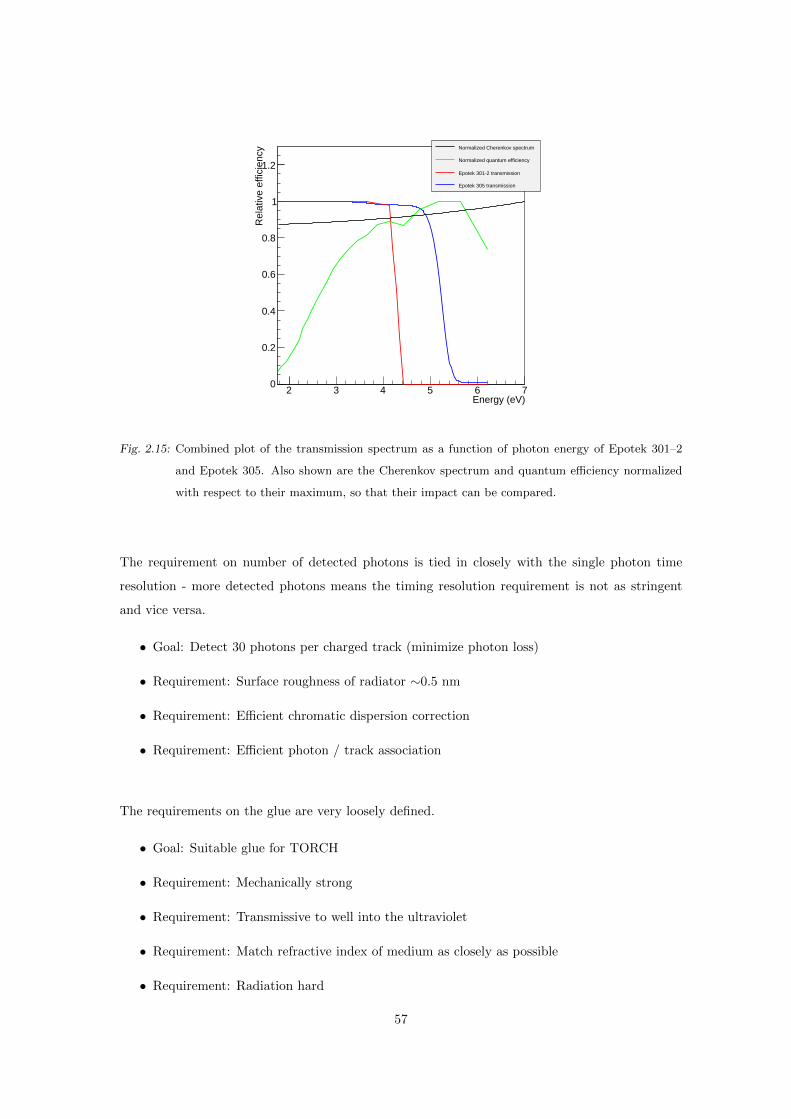
Energy (eV)2 3 4 5 6 7

Rel

ativ

e ef

ficie

ncy

0

0.2

0.4

0.6

0.8

1

1.2

Normalized Cherenkov spectrum

Normalized quantum efficiency

Epotek 301-2 transmission

Epotek 305 transmission

Fig. 2.15: Combined plot of the transmission spectrum as a function of photon energy of Epotek 301–2

and Epotek 305. Also shown are the Cherenkov spectrum and quantum efficiency normalized

with respect to their maximum, so that their impact can be compared.

The requirement on number of detected photons is tied in closely with the single photon time

resolution - more detected photons means the timing resolution requirement is not as stringent

and vice versa.

• Goal: Detect 30 photons per charged track (minimize photon loss)

• Requirement: Surface roughness of radiator ∼0.5 nm

• Requirement: Efficient chromatic dispersion correction

• Requirement: Efficient photon / track association

The requirements on the glue are very loosely defined.

• Goal: Suitable glue for TORCH

• Requirement: Mechanically strong

• Requirement: Transmissive to well into the ultraviolet

• Requirement: Match refractive index of medium as closely as possible

• Requirement: Radiation hard

57

Finally this then leads to a set of requirements for the MCP-PMTs and electronics under study

for the TORCH project.

• Goal: Suitable detector for TORCH

• Requirement: Quantum efficiency well into the ultraviolet

• Requirement: Pixellation of 8×128 over 53×53 mm2 active area within 59×59 mm2 envelope

• Requirement: >10 MHz/cm2 rate capability

• Requirement: >5 C/cm2 total integrated charge

• Requirement: Single photon timing by MCP of order ∼30 ps resolution

• Requirement: Electronics capable of order ∼30 ps resolution with 500,000 detector gain

58

3. THE TORCH MCP-PMT

The demands placed on photodetectors for the TORCH detector are high on nearly all possible

fronts: excellent timing resolution, high degree of pixellation, rate capability, lifetime - all over a

large area. To meet the criteria of the TORCH detector an MCP based photodetector was chosen,

developed in a multistage program at Photek1.

The layout of the detector is set by requirements on the precision with which the reconstruction

can be performed. The requirement is set that the contribution to time resolution from recon-

struction is of similar size to that of the full photon detection system. The precision with which

the reconstruction can be performed is limited by the pixelation (spatial resolution) of the pho-

todetector. It was derived in Section 2.5.1 that a pixellation of 8×128 pixels per detector of area

59×59 mm2 (active area 53×53 mm2) is appropriate. The detectors will be tiled in the horizontal

direction and will be situated at the exit surface of the focusing optics. The layout of the TORCH

photodetector is shown in Figure 3.1.

128

pixe

ls

2

8 columns

53 x 53 mmactive area

60 mm pitch

Fig. 3.1: Initial layout of the anode plane of the TORCH MCP-PMT [26].

This chapter will detail the concept of MCP-PMTs in general, and the progress so far on the

development program for the TORCH MCP-PMT, detailing the key laboratory tests that have

been performed on the first prototypes.

1 26 Castleham Road, St Leonards on Sea, East Sussex, TN38 9NS, United Kingdom, http://www.photek.com/.

http://www.photek.com/

3.1 MCP detectors

The MCP that provides electron multiplication in an MCP-PMT is a large area implementation

of microscopic continuous emission electron multipliers [61]. It is fabricated from a combination

of fibers which have an etchable core and a non-etchable glass cladding. By etching out the core

of each fiber after they have been bundled and processed, a hollow channel will emerge. The fibres

are bundled in a close-packed hexagonal fashion and fused together. The resulting ‘boule’ is then

sliced, typically at a small angle of 8–15 relative to the fiber direction. This results in disks, from

which the fibre cores are etched out resulting in a wafer with closely packed microscopic channels

- the MCP [62], see Figure 3.2. A metallic coating is deposited on the top and the bottom of the

plate to provide an electrical contact. Each microscopic pore now serves as a continuous electron

multiplier - by putting a high potential between the top and the bottom, electrons liberated from

a photocathode accelerate towards the MCP. They fall into the microchannels and collide with

the inside, liberating initially about 2–5 electrons. These then continue passing through the mi-

crochannel in a cascading process. The resulting avalanche is detected on an anode. The charge

multiplication mechanism is illustrated in Figure 3.2. More details on the history, features and

developments of the MCP-PMT can be found in [63].

Electroding(on each face)

ChannelsGlass

Structure

(Cutaway view)

Detector window

Photocathode

Microchannel plate

Microchannel plate

Anode

Charge avalanche

Fig. 3.2: Cut-away view of MCP with straight pores, adapted from [62] (Left), principle of operation of

an MCP-PMT (Right). Electrons are generated at the photocathode, accelerated towards the

MCP-plate, multiplied by liberating electrons from the inside of the channels and collected at

the anode.

All the components of the MCP-PMT are laid out in a linear structure and are in close

proximity. This structuring results in a very compact charge avalanche, and therefore gives a

time resolution on the order of tens of picoseconds [64, 65, 66], which meets the requirements of

TORCH. Two noteworthy processes occur in the collection of the photoelectrons when it meets

the MCP - aside from being multiplied, they can also be absorbed or reflected by the MCP itself

if they collide with the metal surface instead of falling into the pore. The odds of a photoelectron

being multiplied rather than absorbed relate to the ratio of the open pore area and the total area

[67]: the collection efficiency, typically about 65%. When an electron is reflected off the MCP it

60

is likely to come back to it at a later time, with a time delay and spatial offset depending on the

MCP-PMT geometry. This effect is commonly referred to as backscattering [68], and typically

about 5–10% of observed signals from an MCP-PMT are subject to this.

In addition to the extremely high degree of pixellation and small dead area of the design (see

next section), this development program has several other challenging aspects to it. The first of

these is very particular to the type of detector - the lifetime of an MCP-PMT, typically expressed

in terms of the total integrated charge extracted at the anode, is unusually short. It has been

shown [69, 70] that the performance of a typical MCP-PMT drops sharply with levels of integrated

charge as low as 100–200 mC/cm2, with the requirement for the TORCH photodetectors set at

5 C/cm2 (also see Section 3.4.3).

3.2 Development of the TORCH MCP-PMT

The development of suitable photodetectors for the TORCH detector is one of the key R&D goals

of the project. The design of the MCP-PMT has been made in collaboration with the industrial

partner of the TORCH project, Photek Ltd..

The development of the TORCH MCP-PMT at Photek has been set up in three stages, working

incrementally towards the fabrication of an MCP-PMT meeting all the requirements (see Section

2.8) over a period of three years. The three delivery stages that have been identified are:

• Phase 1 - Long life demonstrator MCP-PMT

• Phase 2 - High granularity multianode demonstrator

• Phase 3 - Square MCP-PMT with required granularity and lifetime

The first two stages of this program have been completed, and their design and characteristics

are shown below. Section 3.4 will detail the tests that have been performed on these MCP-PMTs.

The TORCH Phase 1 MCP-PMT is a round, single-channel MCP-PMT with a circular active

area of 25 mm diameter. The anode can be read out directly. Testing of this model is detailed

in Section 3.4, its characteristics are shown in Table 3.1. The ALD coating (where ALD refers

to the process by which it is deposited on the MCP, Anisotropic Layer Deposition) used for this

photodetector increases the lifetime of the MCP-PMT, and is further detailed in Section 3.4.3.

The TORCH Phase 2 MCP-PMT (see Table 3.2) has a double thickness MCP as its second

multiplication stage. The thickness of the MCP sets the number of collisions multiplying electrons

will have with the inside of the microchannels, and as such the gain that can be achieved over a

thicker MCP is increased. A thicker MCP also has the advantage that the maximum achievable

61

Size 25mm ∅

Photocathode Low noise S20 (multialkali)

Window 5.6 mm quartz

Number of MCP’s 2

MCP pore diameter 10µm

Anode Single

Anode coupling Direct

ALD coated Yes (Al2O3)

Design voltage ∼2400V

Gain @ design voltage ∼1.000.000

Tab. 3.1: Design properties of a TORCH Phase 1 MCP-PMT

Fig. 3.3: Frontal view of a TORCH Phase 1 MCP-PMT [50].

Size 40mm ∅, 26.5×26.5mm pixelated area

Photocathode Low noise S20 (multialkali)

Window 9 mm quartz

Number of MCP’s 2 (second one double thickness)

MCP pore diameter 10µm

Anode 4x32 pixels

Anode coupling Hybrid design

ALD coated No

Design voltage ∼4400V

Gain @ design voltage ∼9.000.000

Tab. 3.2: Design properties of a TORCH Phase 2 MCP-PMT

62

Fig. 3.4: The TORCH Phase 2 MCP-PMT viewed from the top, showing the wires for supplying the

various MCP layers with high voltage (through a resistive divider) (Left), from the rear with read-

out PCB (printed circuit board) coupled through anisotropic conductive film (ACF) (Center),

and without read-out PCB showing the bare vias (Right). The PCB is pressure coupled to the

MCP-PMT through the ACF.

gain is increased. If very many electrons are drawn from the inside of the pore and not recovered

quickly, no further multiplication can take place. A thicker MCP has a larger volume of electrons

available and is able to recover more quickly (much like more current can be drawn through a

thicker wire).

The second MCP stage can thus operate at significantly increased gain relative to a ”normal”

thickness MCP without saturating (reaching the maximal current draw). This means a much

wider gain range is accessible with this MCP-PMT, which makes experimenting and troubleshoot-

ing easier since the gain can be adjusted significantly.

In the TORCH Phase 2 MCP-PMT, the charge is transferred from the inside of the MCP-PMT

to the outside of the MCP-PMT through metal vias embedded in ceramic. To couple this charge

to the read-out PCB, a layer of anisotropic conductive film (ACF) is used, see Figure 3.5. ACF

consists of very short metal wires embedded in a non-conductive silicone rubber so that it only

conducts in one dimension. The diameter of the wires in the ACF is much smaller than that of

the vias on the output of the photodetector and the pads on the read-out PCB, so that neither

the pads or the vias get shorted together. The ACF acquired for this purpose is Shin-Etsu MT-P

type interconnect [71]. Use of the ACF replaces a pin-based coupling system. The “pins” in

the ACF are very much shorter (hundreds of µm) and thinner (40 µm diameter), and thus also

more numerous. Crosstalk between neighbouring wires in the ACF is much smaller than that in

a pin-based coupling, and even if it were significant the signal (per pixel pad) is routed through

many pins so it would have a relatively small impact.

63

Additionally, ACF provides very low resistance coupling. The ACF can also easily be removed

and replaced, whereas pins would be permanently in place. Finally, it avoids significant manufac-

turing difficulties in brazing individual pins to each anode pad. The ACF couples to a PCB with

4×32 pixels for read-out using a spring to press the ACF onto the contact pads of the MCP-PMT

and the PCB, see Figure 3.5.

Fig. 3.5: Shin-Etsu MT-P type interconnect - Anisotropic Conductive Film (ACF) [71] (Left), front face

of read-out PCB for the TORCH Phase 2 MCP-PMT, showing the read-out strips picking up

the charge from the MCP-PMT (Right). The copper strips on the PCB are coupled to the vias

shown in Figure 3.4 through the ACF.

3.3 Charge sharing and hybrid anode design

During the design process it was found that the high degree of pixellation of the anode, 8×128

pixels on a 53×53 mm2 area, is very difficult to fabricate. Two possibilities exist for reading out

the charge at the anode. The first is by direct coupling, using bare pixel pads that are directly

coupled through vias to the read-out. The second is a capacitively coupled contact, where the

charge is indirectly induced on the read-out pad.

In the design of the TORCH MCP-PMT, the read-out is performed by a hybrid of these two

types of read-out. On the inside of the MCP-PMT, a layer of dielectric material is deposited

on top of the bare pads that connect to the outside. On top of this, a layer of resistive ink is

64

deposited. When an avalanche falls on the (grounded) resistive layer, it capacitively couples to the

buried metal pads. The thickness of the layers sets the degree of coupling to the underlying pads.

This means that by adjusting this thickness, the number of underlying metal pads it couples to

can be tuned.

In principle, coupling to multiple pads (charge spreading) would be problematic. The TORCH

electronics however (see Section 2.6 simultaneously give a measurement of the time and the amount

of charge deposited in a channel. The amount of charge spreading is controlled, and scales as the

distance to a given pixel pad. Using a charge weighted method on the pixels that detect a signal

it is possible to pinpoint the center of the charge avalanche with a precision much better than

expected from pad size alone. Measurements verifying this principle have been performed by col-

leagues at CERN [72] and at Photek [73].

The combination of the direct and capacitively coupled anode applied in the TORCH MCP-

PMT will be referred to as the hybrid anode design. More information can be found in the pending

patent2.

The back of these vias embedded in the ceramic housing on the back of the MCP-PMT can

be seen in Figure 3.4. A schematic drawing is shown in Figure 3.6.

Vacuum side

Air side

Buried vias

Dielectric layer

Resistive ink

Fig. 3.6: Diagram of the hybrid anode design of the TORCH MCP-PMT, showing the vias coupled through

the ceramic, buried in a dielectric layer and covered with resistive ink on the vacuum side (patent

pending).

3.4 Testing the TORCH MCP-PMT

The first two generations of the TORCH MCP-PMT were tested extensively in laboratory condi-

tions, to verify that they meet the criteria set forth. Initial measurements were made by Photek

and verified by the TORCH collaboration.

2 Patent application number 1510859.0, filed in the United Kingdom on June 19th 2015

65

3.4.1 Equipment for testing the TORCH MCP-PMT

To check the various properties of the TORCH MCP-PMT it is necessary to test them in a well-

controlled environment. The test setup for the MCP-PMT needs tightly focused single photons,

high timing resolution, and the ability to smoothly and reproducibly shift the point of exposure.

A light-tight enclosure was specially fabricated with an optical breadboard serving as the base.

Various feedthroughs are slotted into the side panels. A schematic view of the full setup is shown

in Figures 3.8 and 3.9.

To achieve the required timing resolution, it is necessary that the system used to study the

MCP-PMT has a significantly higher resolution than is expected of the MCP-PMT. As a photon

source, a picosecond precise laser system was acquired from Advanced Laser Diode Systems3: a

WT1030 type laser diode with a PiL040X head [74], emitting light of wavelength 405 nm (3.1 eV).

This laser system was fitted with a microfocus with a focal distance of 18 mm, which lets the laser

be focused on a spot of size <10µm diameter. The timing performance of the laser is reproduced

in Figure 3.7, showing the laser pulse shape over time for several settings of the tune parameter,

as measured by the manufacturer, with the laser running at a repetition frequency of 100 kHz.

The tune sets the electrical pumping energy to the laser diode, with a lower tune setting in this

case indicating a higher pumping energy. The benefit of this is a more densely compressed initial

laser pulse, at the cost of introducing a secondary pulse.

Fig. 3.7: Pulse intensity as a function of time for the picosecond laser system (PiLas) for three tune

settings: 30% (red), 60% (black) and 90% (blue). Curves recorded by manufacturer using a

streak camera, with the laser operating at a repetition frequency of 100 kHz [74].

The sharpest primary peak of the laser occurs for lower tune settings, at the cost of a secondary

3 Schwarzschildstr. 6, D-12489 Berlin, Germany, http://www.alsgmbh.de/.

66

http://www.alsgmbh.de/

lower intensity pulse. If the laser is operated below 60% tune (25 ps FWHM, or ∼10 ps standard

deviation), the contribution of the laser to the measured time resolution is likely to be minimal,

with an expected resolution of the MCP-PMT of 20-30 ps.

To read out the pulses of the MCP-PMT, a sampling oscilloscope was used; a WaveRun-

ner 640 Zi oscilloscope [75] manufactured by Teledyne LeCroy4, sampling at 40GS/s on two chan-

nels or 20 GS/s on four channels, with 5 GHz bandwidth. Since it is expected that the full pulse will

be of order nanoseconds length, with approximately several hundreds of picoseconds in the lead-

ing edge, at least several samples will be made on this edge, allowing for high fidelity interpolation.

The laser and the oscilloscope are the principal components of the system. After the laser is

fibre-coupled into the light-tight environment its output face is mounted on a triple set of motion

stages. To scan the surface of the MCP-PMT, the horizontal and vertical axes are controlled by

motorized actuators: CONEX-LTA actuators connected to M-UMR motion stages, fabricated by

Newport5. The depth of focus is controlled using a manual control since it is expected that after

the initial alignment it will not be necessary to adjust this. The motorized actuators are controlled

from an external PC.

Several further points remain: in order to reliably test the timing properties it is necessary to

attenuate the laser to the single photon regime, and a time reference signal needs to be obtained

of similar quality to the MCP-PMT pulse. To create the time reference signal, a 50/50 optical

splitter manufactured by FONT6 is implemented within the light-tight environment with one arm

being used for the output face of the laser, and the other being directed towards a DET02AFC

high-speed silicon-based photodetector [76] from Thorlabs7. The output of the laser has a holder

directly in front of it, on which a set of neutral density filters [77] from Edmund Optics8 can be

placed. The drawback of this configuration is that it is not possible to use the microfocus option

on the laser fibre output - the physical space along the photon propagation direction required by

the ND filters is too large. In this iteration of the system the spot size of the laser is about 2 mm.

A conceptual drawing is shown in Figure 3.8.

Because of technical difficulty (failure of the photodiode, amongst others) some changes were

4 The Carriage Barn, Bartletts Court, Littlewick Green, Bath Road, Maidenhead, Berkshire SL6 3RX, UK,

http://teledynelecroy.com.5 MICRO-CONTROLE Spectra-Physics S.A.S., 1, rue Jules Guesde - Bat. B, ZI Bois de l’Epine - BP189, 91006

Evry Cedex, France, http://www.newport.com.6 2242 - 173 Street, Surrey, British Columbia, V3Z 9Z7 Canada, http://www.fontcanada.com/.7 1 St Thomas’ Place, Ely CB7 4EX, United Kingdom, http://www.thorlabs.de/.8 Unit 1, Opus Avenue, Nether Poppleton, York, YO26 6BL, UK, http://www.edmundoptics.com/optics/.

67

http://teledynelecroy.com

http://www.newport.com

http://www.fontcanada.com/

http://www.thorlabs.de/

http://www.edmundoptics.com/optics/

Lasercontroller LightOtightObox

Laserdiode

MCP-PMT50/50splitter

NDfilters

Fibreoutput

Oscilloscope

Photodiode

Fig. 3.8: First configuration of the TORCH MCP-PMT testing setup. The laser diode is controlled by

the laser controller (yellow line). When the laser fires, the light is propagated through the fibre,

reaching the photodiode and the fibre output (blue line). The signal from the photodiode is read

out using the oscilloscope (red line). The light from the fibre output (blue dots) is propagated

through free space through the neutral density filters, with single photons reaching the MCP-

PMT. The signal from the MCP-PMT (green line) is read out simultaneously with the photodiode

signal.

made after the first sets of measurements taken. The choice was made to simultaneously make

some further adjustments to improve measurement quality.

Uncontrolled reflections within the light-tight environment were causing a significant back-

ground in the MCP-PMT signal. For this reason the measurement setup was changed to take the

reference signal directly from the laser controller, and attenuating the light (before its free space

propagation) through a digital variable attenuator [78] from Oz Optics9. This also meant that

the microfocusing option could be implemented, allowing for significantly better in-depth focusing

(<10 µm width spot size).

The voltage on the various layers of the MCP-PMT was set using a resistive divider in con-

junction with a T2DP-050-205-EPU model high voltage source [79] manufactured by Iseg10. The

resistive divider consists of a series of resistors in between which the high voltage can be tapped.

Using this technique it is possible to supply all the layers of the MCP-PMT with high voltage

drawn from a single source. The drawback is, however, that the voltages go out of balance if the

resistive divider is used at a higher / lower voltage than intended. The inside of an MCP-PMT can

be divided into three regions: the front gap, the MCP stack and the rear gap (also see Figure 3.2).

The front gap is where the photoelectron is transported from the photocathode to the first MCP.

The MCP stack is the combination of (in this layout, two) MCPs where the avalanche is generated

9 219 Westbrook Road, Ottawa, ON K0A 1L0, Canada, http://www.ozoptics.com/.10 Bautzner Landstr. 23, D-01454 Radeberg / Rossendorf, Germany, http://iseg-hv.com/en.

68

http://www.ozoptics.com/

http://iseg-hv.com/en

Lasercontroller Light tight box

Laserdiode

MCPPMT

50/50splitter

Micro-focused

fibreoutput

OscilloscopeDigital

attenuator

Fig. 3.9: Second configuration of the TORCH MCP-PMT testing setup. The laser diode is controlled by

the laser controller (yellow line). When the laser fires, the light is propagated through the fibre

(blue line), and is reduced to single photons by the digital variable attenuator. It then reaches

the microfocused output, and propagates in free space towards the MCP-PMT. The MCP-PMT

signal (green line) is read out together with the laser trigger signal (red line). The splitter was

retained to minimize actions on the optical couplings in the system.

from the photoelectron. The rear gap is where the avalanche is transported to the anode, where

it is read out. It is desirable to keep the front and rear gap at identical voltages when scaling the

voltage on the MCP stack to adjust the gain. However, when using a resistive divider to supply

the various layers of the MCP-PMT with high voltage, this is not possible: when the voltage on

the divider is adjusted, all voltages will scale proportionally.

3.4.2 Quantum efficiency

The quantum efficiency is the likelihood of conversion of a photon on the photocathode into a

photoelectron that can be subsequently multiplied. It was measured by colleagues at CERN as a

function of photon energy for the first generation of MCP-PMTs, and is displayed in Figure 3.10.

The photocathode is Low Noise S20 (multialkali) coated on a quartz window, and was character-

ized with a spectrophotometer.

The shape of the quantum efficiency spectrum is typical for a multialkali photocathode, and

the occurrence of multiple bumps / maxima in the quantum efficiency spectrum has been observed

before for this type of photocathode [80]. The choice for a multialkali photocathode was made

because of a high quantum efficiency over a wide spectrum - an implicit requirement for the

TORCH detector to detect a sufficient quantity of photoelectrons. As detailed before in Chapter

2, it is expected that the quantum efficiency will be one of the limiting components in the number

of photons that can actually be detected for a single charged particle passing through TORCH.

69

Energy (eV)2 3 4 5 6 7

Qua

ntum

effi

cien

cy

0

0.05

0.1

0.15

0.2

0.25

0.3

TORCH MCP-PMT quantum efficiency

Fig. 3.10: Quantum efficiency as a function of photon energy of a TORCH Phase 1 MCP-PMT as measured

by colleagues at CERN [50].

3.4.3 Lifetime

The lifetime of the MCP-PMT has been one of the major focal points of R&D. The goal for lifetime

of the TORCH photodetectors is 5 C/cm2, compromising between available technology and the

requirements of the TORCH detector in LHCb. Technological developments, inside and outside

of the TORCH project, mean that addressing this issue has become relatively standard.

There are several effects caused by continued use of an MCP-PMT. It has been shown that as

the integrated anode charge increases the gain degrades over time. This is typically recoverable

by applying a higher voltage to the MCP. As the integrated anode charge increases the quantum

efficiency starts degrading, starting in the red part of the spectrum and proceeding further and

further towards the blue part of the spectrum. This is observed by the dark count rate falling

to low levels. A leading cause of dark count is thermal excitation in the photocathode. As the

quantum efficiency degrades from the red towards the blue part of the spectrum, the photon en-

ergy threshold for liberating a photoelectron increases and thus the dark count rate drops. The

timing performance stays more or less constant during this process if the voltage on the MCP is

adjusted such that constant gain is achieved [66], which is also consistent with this mode of failure.

Extensive research has been dedicated to the exact mode of failure of the MCP-PMT and

exactly how it progresses [69, 81, 82]. The current leading theory is that degradation of the

photocathode is due to feedback from outgassing of the MCP under high intensity electron bom-

bardment during the avalanche process. It is interesting to note there are two components to this

70

failure mode [81]. The first is ions liberated from the MCP during the electron avalanche which

are accelerated towards the photocathode, damaging it on impact. The second is from neutral

gases liberated from the MCP. In particular, it has been shown that small quantities of molecular

oxygen and / or carbon dioxide would deteriorate a multialkali photocathode [83].

The solution for the short lifetime problem has been found. First hinted at in [67], covering

the MCP with a protective layer of Al2O3 effectively seals in the contaminants. Coating the MCP

by a process referred to as atomic layer deposition (ALD) has become the commonly adopted

solution [81, 82, 84], and has been shown to raise the lifetime of MCP-PMTs to levels meeting

and exceeding the requirement of 5C/cm2.

Lifetime testing has been performed by Photek on an MCP-PMT functionally identical to the

TORCH Phase 1 MCP-PMTs [70], and the results are shown in Figure 3.11. For this particular

test, light was used stretching over the full spectrum to which the MCP-PMT is sensitive. The

extracted current from the MCP-PMT (a measure for the gain) was monitored as the integrated

extracted current increased. The mechanism through which the MCP-PMT is expected to deteri-

orate is degradation of the photocathode. This would be indicated by a decrease in the quantum

efficiency from the red part of the spectrum towards the blue part of the spectrum. Separate

measurements were taken to verify the quantum efficiency at various points during the lifetime

test.

Further lifetime studies are ongoing. Along with the total extracted charge, the quantum effi-

ciency of the MCP-PMT was also measured at regular intervals. Even at the full extracted charge

of >5C/cm2 no degradation of the quantum efficiency was observed (measurements not shown, see

[70]). However, since a full spectrum of light is used, any degradation of the quantum efficiency

would show as a further decrease of the photocurrent since in total fewer photoelectrons would be

converted - which is not the case.

The gain of the MCP-PMT can be suitably adjusted over the course of its lifetime by tuning

the high voltage, allowing its performance to stay constant over time. It is then expected that

it is possible in the full TORCH detector to run the MCP-PMT at constant performance, with

careful monitoring.

3.4.4 Gain and time resolution

One of the most important characteristics of the photodetectors to be used for the TORCH de-

tector is the time resolution. There are several contributions to the overall time resolution of the

71

Fig. 3.11: Lifetime of an MCP-PMT functionally identical to a TORCH Phase 1 MCP-PMT with ALD

coating (black) and an uncoated control sample (grey) as a function of collected anode charge

[70], as measured at Photek. The small jumps in the photocurrent (at 0.38C/cm2, 0.71C/cm2,

1.13C/cm2, etc) occurred when the detector was removed from the lifetime setup for quantum

efficiency and gain measurements.

full system. The principal parts of this are the MCP-PMT itself, and the electronics following it.

The final contribution comes from uncertainty in the reconstruction, which is limited by the pixel

size, for more details see Chapter 4.

The time resolution was measured directly on both the Phase 1 and Phase 2 prototypes, and

it was also assessed on the MCP-PMT in conjunction with the read-out chain. One of the ad-

ditional goals of the Phase 1 MCP-PMT was to test if the time resolution could be maintained

given the measures taken to prolong the lifetime. The timing performance of an MCP-PMT is

ultimately dependent on the avalanche characteristics, with an additional contribution made by

the backscattering mechanism.

The timing performance of the Phase 1 MCP-PMT was measured relative to a time reference,

in this case from the photodiode, using the setup described in Figure 3.8. The full waveform was

saved for both the time reference and for the MCP-PMT signal. The pulse height of the signal from

the MCP-PMT has a very wide range (several mV to tens of mV), and therefore it is necessary to

correct for time walk effects (see Figure 2.14). This can be done in two manners - by mapping the

time offset as a function of the pulse height / area, or by using constant fraction discrimination

72

(CFD) - the method employed here, illustrated in principle in Figure 3.12. This was implemented

by taking the timing from the halfway point between 30% and 70% of the maximum of the signal.

It is expected that the timing of a point at a constant fraction up the slope of the rising signal

should have a relatively low fluctuation in time. The signals that are considered for the timing

calculation have to pass a minimum threshold in pulse height. To this end, a histogram of the

pulse height was used to tell where the pedestal region ends and the signal region begins.

50% level

Fig. 3.12: Principle of operation of constant fraction differentiation (CFD), illustrated for the 50% level.

Subjecting the varying size signals to a threshold will introduce a time walk, but with a CFD

type calculation on the full waveform this can be negated.

Finally, the charge spectrum is fitted for the pedestal and first and second photoelectron peaks.

The model chosen for all three contributions is a single Gaussian. The pedestal is caused by signals

recorded when there is no charge avalanche observed, and therefore is represented by a fluctuation

around the baseline. The photoelectron peaks are also Gaussian, peaking around the average

gain level, with the standard deviation representing the fluctuation of gain, as is typical for an

MCP-PMT. The photoelectron peaks are integrated to assess the number of entries in each, and

the mean of the charge in the first photoelectron peak is taken as the average gain. Histograms of

the charge in each signal and the time relative to trigger are shown in Figure 3.13. It is observed

that each gain measurement is (on average) offset by the (non-zero, non-constant) center of the

pedestal, for which the calculated gain value should be corrected. This variation is attributed to

a slowly varying baseline, the cause of which remains unknown. It varies relatively slowly over

time, being stable over a period of tens of minutes.

The primary photoelectron peak in Figure 3.13 (Left) is observed at 0.156±0.001 pC relative

to the pedestal (equating to a gain of 9.7×105). The MCP-PMT is operated at 2400 V (1264 V

73

Measured charge in PMT signal (C)-0.1 0 0.1 0.2 0.3 0.4 0.5 0.6 0.7

-1210×

Cou

nts

1

10

210

310

410

Charge spectrumPedestal1 PE peak2 PE peakCombined fit

Time relative to trigger (s)-0.45 -0.4 -0.35 -0.3 -0.25 -0.2 -0.15 -0.1 -0.05

-910×

Cou

nts

0

100

200

300

400

500

Time relative to trigger

Main timing peak

Backscatter peak

Combined fit

Fig. 3.13: (Left) Histogram of calculated charge per individual MCP-PMT pulse. A combined fit (black)

is made to the histogram consisting of three Gaussians: pedestal (red), primary (blue) and

secondary (green) photoelectron peaks as measured on a TORCH Phase 1 MCP-PMT. (Right)

Time relative to trigger for photons detected by the TORCH Phase 1 MCP-PMT.

on the MCP stack). The time difference between the time reference and the leading edge of the

MCP-PMT signal is measured. Collecting a large number of these allows for assessment of the

intrinsic timing performance of the MCP-PMT, referred to as the time jitter of the MCP-PMT.

The main timing peak in Figure 3.13 (Right) has a standard deviation of 26.6±0.3ps, which

can be interpreted as the time resolution of the TORCH Phase 1 MCP-PMT at this high voltage

setting. The second peak in this plot is caused by a secondary pulse from the laser (see Figure 3.7).

The characteristics of a Phase 1 MCP-PMT were studied further for a range of voltages on

the MCP plates. For this test the laser was run at 30% tune, leading to a significant contribution

of photons from the secondary laser fire (see Section 3.4.1). Using the resistances of the resistive

divider the voltage on the MCP plates was extracted, allowing for the gain as a function of MCP

voltage to be compared with data from the manufacturer, as shown in Figure 3.14.

It is observed that the measured gain curve very closely matches that of the supplier, as ex-

pected. At the high end of the gain curve there is a small deviation (more gain observed than

expected). These differences can be attributed to the measurement technique - the measurement

was performed by the manufacturer by measuring the size of current spikes on the MCP-stack,

leading to a much more direct measurement. Finally, no error bars are known for the relatively

coarsely spaced data from the manufacturer, which could easily bring the two datasets in agree-

ment.

74

Voltage over full MCP stack900 1000 1100 1200 1300 1400 1500

Gai

n

310

410

510

610

710Gain curve from manufacturer

Gain curve measured in laboratory

Fig. 3.14: Gain as a function of voltage on the MCP stack (in V) of a TORCH Phase 1 MCP-PMT

(green) compared to the gain curve as supplied by the manufacturer (blue), measured with

single photons. The gain values were extracted from the MCP-PMT pulses by measuring the

position of the primary photoelectron peak (also see Figure 3.13) corrected for the position of

the pedestal. Vertical error bars drawn are propagated from the errors on the fitted values.

75

Using the fit to the charge spectrum it is also possible to assess the linearity of the gain of the

MCP-PMT, since a central value for both the first and second photoelectron peak is extracted.

By correcting for the position of the pedestal and taking the ratio of the second and the first

photoelectron peak, the linearity of the gain can be assessed as a function of the gain. The ex-

pectation is that this value is two - under ideal circumstances. It is found that for almost all

values of the gain this is consistent, and therefore the MCP-PMT meets this expectation. The

measured linearity is plotted together with the expectation in Figure 3.15, as a function of the gain.

Gain510 610

Rat

io o

f sec

ond

and

first

pho

toel

ectr

on p

eak

posi

tion

0

0.5

1

1.5

2

2.5

3

3.5 Expected linearity value

Measured linearity

Fig. 3.15: Linearity of gain of a TORCH Phase 1 MCP-PMT as a function of the gain itself, measured as

the ratio of the position of the second and first photoelectron peaks.

If the gain is fully linear and the MCP is not saturated, the gain of the second photoelectron

peak should be twice that of the primary photoelectron peak. The measured linearity of gain is

consistent with this expectation. However, the measurements used were specifically designed to

have a low content in the two photoelectron peak. It is possible to further investigate linearity

of gain at various settings, but the measurement could be much improved if the attenuation is

adjusted to be out of the single photon regime and closer to one or even two photons, so that

higher order photoelectron peaks can also be observed.

Because the diode was unavailable, the direct trigger from the laser controller was used as the

76

time reference to measure the time resolution for a variation of gain settings on the MCP-PMT

(see Figure 3.9). Over short time periods (less than about an hour) there is no significant detri-

ment to the time resolution compared to using the optical diode. The time resolution for each

of the measurement points was assessed in the same manner as described above, but the fit to

the main peak was restricted to a single Gaussian rather than a double Gaussian. This means

that the standard deviation gives a more complete representation of the timing performance of the

MCP-PMT since the contribution from backscattering cannot be removed or ignored. The time

relative to trigger for a single measurement series is shown in Figure 3.16.

Time relative to trigger (s)0.1 0.2 0.3 0.4 0.5 0.6 0.7 0.8

-910×

Cou

nts

0

20

40

60

80

100

120

140

160

180 Time relative to trigger

Main timing peak

Fig. 3.16: Time relative to trigger as measured on a TORCH Phase 1 MCP-PMT. The secondary laser

pulse (see Figure 3.7) is observed as the secondary peak around 0.5 ns.

The histogram of time relative to trigger allows for an assessment of the fundamental uncer-

tainty introduced by the MCP-PMT, typically referred to as time jitter. This is interpreted as the

time resolution of the MCP-PMT. For the fitted curve, the time resolution (standard deviation) is

31.7± 0.5 ps measured from a single Gaussian on the main peak at a voltage of 2400 V (primary

photoelectron peak at 0.122±0.003 pC, pedestal at 0.67±0.03fC, equivalent to a gain of 7.6×105).

Finally, the timing performance is extracted from the measurement series as a function of gain.

The result is shown in Figure 3.17. The performance of the MCP-PMT is as expected - at very

low gain the time resolution is poor, and as the gain increases the time resolution rapidly improves

up until about 200,000 gain. At higher gain there is some further improvement on the time res-

77

olution. Since the expectation is that the MCP-PMT will be run at 500,000 gain or higher, the

contribution to the timing resolution coming from effects inherent to the MCP-PMT will be small

(<30 ps) and will not limit the time resolution of TORCH.

Gain0 200 400 600 800 1000 1200 1400 1600

310×

Tim

e re

solu

tion

(ps)

20

40

60

80

100

120

140

Fig. 3.17: Gain as measured from fit to primary photoelectron peak corrected for the pedestal for a given

voltage setting (also see Figure 3.13) versus time resolution (measured as a single Gaussian fit

to the main peak, also see Figure 3.16).

3.4.5 Gain and photocathode uniformity

To assess the performance of the Phase 1 MCP-PMTs the surface uniformity is assessed to sup-

plement the quantum efficiency. This measurement is done using the setup described in Figure

3.9, scanning the focused laser over the area in the horizontal and vertical directions. There are

two relevant metrics in assessing this - performance of the photocathode and performance of the

MCP, which sets the gain. With a trigger coming from the laser it is possible to count the number

of registered signals of any size relative to the number of events in the pedestal. This means it is

possible to assess the performance of the photocathode convoluted with the collection efficiency,

which is expected to be flat. By fitting the resulting charge spectrum and extracting the position

of the primary photoelectron peak relative to the pedestal the gain can be calculated. The result-

ing surface area measurements are shown in Figure 3.18.

The photocathode of the TORCH Phase 1 MCP-PMT is found uniform over the full area

78

Horizontal position (mm)0 5 10 15 20 25

Ver

tical

pos

ition

(m

m)

20

25

30

35

40

45

0.8

0.82

0.84

0.86

0.88

0.9

0.92

0.94

0.96

0.98

1

Horizontal position (mm)0 5 10 15 20 25

Ver

tical

pos

ition

(m

m)

20

25

30

35

40

45

0

50

100

150

200

250

300

350

400

310×

Fig. 3.18: Simultaneous measurement of the photocathode (Left) and gain (Right) of a TORCH Phase 1

MCP-PMT run at 2400 V. The photocathode uniformity is normalized with respect to the

highest point, so that the deviations can be interpreted as a fraction. The minimum of the

colour scale was set to 0.80 in the left plot. The variations over the surface indicate to which

level the photocathode is uniform in gain and detection efficiency. Horizontal and vertical axes

denote the position of the laser, scanned in steps of 1.5 mm.

to within 10%, with an expected statistical fluctuation of around 1–2%. Detection efficiency

drops near the edge of the MCP-PMT - expected because the gain cannot fully develop since the

avalanche is geometrically limited. Simultaneously it is clearly observed that closer to the edge of

the photocathode the gain deteriorates. Within the interior of the MCP-PMT the gain is uniform

to the same level as the photocathode. There is some structure in the photocathode uniformity,

which is attributed to the photocathode fabrication process.

3.4.6 Spatial resolution

The pixel size requirement set for the TORCH photodetector is 0.414 mm in the fine direction

(equivalent to a spatial resolution of 0.12 mm, calculated by dividing by√

12). This can be

achieved with double the pixel size by introducing charge sharing and centroiding to the measured

signals. The actual level of charge sharing (introduced by the hybrid anode design, see Section

3.3) is of critical impact - a high degree of charge sharing means that a higher gain is required to

put a sufficient number of pixels over threshold, a low amount of charge sharing means that the

spatial resolution requirement is not met.

The impact of the absolute amount of charge sharing can be quantified as the mean number

of pixels that are firing for a charge avalanche of given size. It was shown in simulation [73] that

79

in order to reach the spatial resolution goal, it is sufficient to have an average of 1.36 pixels firing

per photoelectron.

The exact level of charge spreading can be measured by stepping a laser across the fine pixel

direction and assessing the average amount of charge recorded in a series of pixels. As the laser

approached the center of a pixel, its response will grow, and it should decline identically as it steps

beyond. The shape of this distribution will then give a quantitative measure of charge sharing.

It is referred to as the point spread function (PSF); the function that results when a point-like

photon source is multiplied.

The number of pixels responding to a signal is critically dependent on three parameters: the

threshold set in the electronics, the gain at which the MCP-PMT is operated and the width of the

PSF. In order to assess the relative impact of these, a small toy study was performed. For a charge

avalanche of known size and shape it is possible to move the charge distribution over an array of

pixels and assess the average number of pixels that will respond given a certain threshold setting.

The assumption was made that the shape of the charge avalanche can be taken as a Gaussian

distribution (see for example Figure 3.20). The mean number of pixel pads firing was calculated

for several gain and threshold settings, and is shown in Figure 3.19.

As the size (standard deviation) of the PSF increases, initially the number of pads that respond

goes up - for a given charge and threshold, there is an optimal size of the PSF at which a maximal

number of pads will respond. This indicates an efficient combination of gain of the MCP-PMT

and the threshold setting. The width of the PSF is set by the avalanche. It is necessary to tune it

relative to the threshold of the NINO in order to simultaneously minimize the number of channels

firing, which lowers the occupancy of the electronics, and minimize the gain, which increases the

lifetime. The lowest charge that the NINO is sensitive to is about 30 fC [56], though depending on

what can actually be achieved a more realistic threshold setting may correspond to about 50 fC,

to ensure that the measured signal is of sufficient and repeatable quality. More details on the

calibration of the NINO will be shown in Chapter 5.

The shape of the charge distribution on the MCP-PMT was measured on the Phase 2 MCP-

PMT. This was done with the laser focused on the photocathode, centered on one pixel column.

Using the measurement setup as set forth in Figure 3.9, the laser was stepped in fine increments

across a set of four neighbouring pixels under study, labelled as pixel 21 through 24 from right to

left. The pads for neighbouring pixels 20 and 25 were terminated with 50Ω resistances to ensure

correct shaping of the charge avalanche at the read-out pads. The four pixels were read out simul-

80

Sigma of PSF (mm)0.2 0.3 0.4 0.5 0.6 0.7 0.8 0.9 1

Mea

n nu

mbe

r of

pad

s fir

ing

0

0.5

1

1.5

2

2.5

3

Gain = 1E6, threshold = 30fC




Threshold for sufficient spatial resolution

Fig. 3.19: Mean number of pixels passing the NINO threshold for several values of threshold and charge

contained in avalanche, plotted against the standard deviation of the point spread function

(PSF). The charge is assumed to be spread over the pixels in a one dimensional Gaussian

oriented along the fine pixel direction - charge sharing along the long axis of the pixels is not

accounted for. The charge in an avalanche is assumed to always be exactly the listed value. The

limit above which the spatial resolution goal is attainable, 1.36 pads firing, has been indicated.

81

taneously using the oscilloscope. To optimize the efficiency of operation a specific trigger condition

was used to impose extra requirements on the signal; requiring a trigger from the laser followed by

a signal with height at least 2 mV on at least one of the four channels under study within a short

timing window removes virtually all dark noise from the measurement. For each signal passing

this combined requirement the charge in each channel was calculated, until a total of ten thousand

measurements per laser position was accumulated. The average charge per avalanche per channel

is shown in Figure 3.20.

Position (mm)3 4 5 6 7 8 9 10

Mea

n ch

arge

per

pix

el p

er e

vent

(pi

co C

oulo

mb)

-0.1

0

0.1

0.2

0.3

0.4

0.5

0.6

0.7

0.8

0.9pixel 21pixel 22pixel 23pixel 24

Fig. 3.20: Uncorrected measurement of average amount of charge observed in a set of four neighbouring

pixels as the laser is stepped across the fine pixel direction, centered in the coarse pixel direction.

Offset correction and error bars are calculated and applied in Figure 3.22.

To improve on this further, a separate study was done to estimate the error on these measure-

ments. The laser was placed in a fixed position between pixel 23 and 24, giving a relatively large

signal on pixel 23 and 24 while giving smaller signals on pixels 21 and 22. The laser was kept in

this position for several hours, and the fluctuation of charge was observed over this time period.

The resulting data were averaged per 5000 measured points, and plotted as a function of time,

shown in Figure 3.21a. To assess the fluctuation per pixel, a histogram was made of the averaged

charge in each individual pixel as a fraction of the total observed charge, shown in Figure 3.21b.

A Gaussian fit to each of the curves in Figure 3.21b showed that the random fluctuations on

82

Time elapsed (h)0 0.2 0.4 0.6 0.8 1 1.2 1.4 1.6 1.8

Ave

rage

cha

rge

obse

rved

in p

ixel

(pC

)

0.8−

0.7−

0.6−

0.5−

0.4−

0.3−

0.2−

0.1−

0

0.1


(a) Random fluctuations averaged per time

span equal to a single measurement point

for the PSF for the four pixels considered.

For this measurement, the laser is fixed into

place between pixel 23 and 24.

Fraction of charge in pixel w.r.t. total charge0.1− 0 0.1 0.2 0.3 0.4 0.5 0.6

0

2

4

6

8

10

12

14

pixel 21pixel 22pixel 23pixel 24

(b) Histogram of random charge fluctuations of

PSF for a single point, with the values for

each pixel normalized with respect to the

total charge observed in four pixels.

Fig. 3.21: Assessment of random fluctuations in charge during measurement of the PSF.

each pixel are about 0.4–0.7% of the sum of charge observed in all the channels. The error for the

charge measurement in each individual pixel can then be conservatively estimated as 1% of sum of

charge observed in all four pixels. Finally, the observation is made that each of the curves shown

in Figure 3.20 has a seemingly flat vertical offset. Integrated over time, this leads to an average

offset that differs per pixel. To remove this offset, a fit is made to Figure 3.20 of a Gaussian plus

an offset, after which the offset is subtracted. The width of the Gaussians fitted to the PSF is

found to be 0.799±0.009 mm, 0.743±0.009 mm, 0.783±0.009 mm, 0.803±0.009 mm for pixel 21,

22, 23, 24. The final resulting PSF is shown in Figure 3.22.

As is apparent in Figure 3.22, there is a final fluctuation that is not accounted for - as can

be noted in the various curves for the PSF not fully tending to zero as the laser is outside of the

range of that pixel. The reason for that is the same as the observation in Section 3.4.4 that the

pedestal does not stay in place, and should be corrected for. Since the method of measurement

used here inherently cuts out the pedestal, and the full charge spectrum is not recorded, with the

current dataset this fluctuation cannot be removed. It is estimated to be two to three times larger

than the errors indicated.

Shown in Figure 3.22 is just one of many measurement series taken. During this process a

83

Position (mm)3 4 5 6 7 8 9 10

Mea

n ch

arge

per

pix

el p

er e

vent

(pi

co C

oulo

mb)

-0.1

0

0.1

0.2

0.3

0.4

0.5

0.6

0.7

0.8


Fig. 3.22: Offset corrected PSF with 1% of total charge error bars (see Figure 3.21).

curious observation was made - that the gain of the MCP-PMT seemed to increase over time. To

investigate this further the amount of charge extracted from the MCP-PMT was estimated from

each PSF plot. When the laser is between the two central pixels, virtually all the charge should

get absorbed by one of the four pixels under observation. For each full PSF measurement, a single

representative gain was measured.

The MCP-PMT voltage was kept stable over the whole measurement series. The measurement

was also carried out on a different set of pixels on another part of the MCP-PMT, where the same

trend of slowly increasing gain was observed. This was interpreted as the effect being a global

effect on the MCP-PMT, rather than a local effect on a set of pixels. With the voltage kept stable,

the number of measured points is a direct indication of the time that elapsed with the MCP-PMT

was exposed to light. This was then plotted against the estimated charge of a full avalanche and

is shown in Figure 3.23. This indicates that as the MCP-PMT was used for a longer period of

time, under identical conditions, the gain was increasing. Simultaneously it was found that the

PSF also seemed to be getting broader, as also shown in Figure 3.23.

Each measurement of the charge was taken when the laser was centered in the middle of the

set of four pixels. While the high voltage was turned off in between measurements, the MCP-PMT

was always run at 4400 V while in operation. The number of measurement points is proportional

84

Estimate of number of points measured0 1000 2000 3000 4000 5000 6000 7000 8000

310×

Mea

sure

d to

tal c

harg

e

1

1.2

1.4

1.6

1.8

2

Observed gain w.r.t. integrated measurement time

Integrated charge (pC)1 1.1 1.2 1.3 1.4 1.5 1.6 1.7 1.8 1.9 2

Sig

ma

of p

oint

spr

ead

func

tion

0.6

0.65

0.7

0.75

0.8

0.85

0.9

0.95

Relation of integrated charge and width of PSF

Fig. 3.23: Observed increase in gain from measured PSF (Left) and associated widening of the PSF

(Right).

to the length of time for which the MCP-PMT was operated. As shown in Figure 3.23, the trend

that both the gain and width of the PSF were increasing was clearly established. This was partic-

ularly problematic because the integrated charge extracted here would correspond to a relatively

short period of operation in TORCH. To confirm that the observed increase in gain was an actual

physical effect and not an artifact from a component of the measurement setup, the MCP-PMT

was taken back to the manufacturer where the pulse height spectrum of the MCP-PMT was re-

measured, and was confirmed to indicate about a factor two increase in gain compared to the

measurement taken shortly after it was manufactured.

This observed increase in gain was investigated in the laboratory and by the manufacturer, and

it was found that some physical changes had occurred in the MCP-PMT, notably the resistance

between the last MCP surface and the anode had dropped by a large amount. Shortly after man-

ufacturing, this resistance was measured to be 1.2 GΩ at 1 kV, whereas after this measurement

series it was found to be about 140 MΩ. It should effectively be an open circuit (many GΩ).

Since this resistance acts in parallel with the resistance in the resistive divider, this resistance

drop lowers the voltage on the rear gap, and increases the voltage over the MCP stack. Therefore

the gain increases and the shaping decreases - leading to higher extracted charge and increasing

width of the PSF. In further produced MCP-PMTs the resistance on the rear gap was once again

found to be close to an open circuit. This will now be closely monitored during further production.

Finally, then, the measured PSF can be assessed. Assuming that the increase in width of the

PSF can be attributed to the mode of failure described above, the earliest measurements should

85

be indicative of the width of the PSF that can be achieved: about 0.6–0.7 mm standard deviation.

Assuming that the PSF at high gain (1−2×107) is identical in shape to that at low gain (∼ 1×106)

this would lead to a mean number of pads firing of about 1.5, meeting the spatial requirement goal.

Ideally, the PSF would be narrowed somewhat, to about 0.5 mm standard deviation. Preliminary

testing with MCP-PMTs with a thinner dielectric on the read-out pads indicate that this is indeed

achievable, bringing the width of the PSF down to about 0.5 mm standard deviation.

3.4.7 Time resolution of the Phase 2 MCP-PMT

To finish off this stage of testing of the TORCH Phase 2 MCP-PMT, a brief study was made of its

timing properties. The laser was fixed on the center of the same set of pixels used for the study of

the PSF. The MCP-PMT was operated at relatively high voltage (4200 V), so that a signal was

clearly visible on all four pixels under study. The charge spectra of the four individual pixels were

measured and summed, giving a single photoelectron peak relative to the pedestal at a total gain

of 5.48× 106.

From the pulse height spectrum it was determined that a suitable level for setting the signal

threshold was -2.5 mV. The four scope channels were connected to the four pixels under study,

with the trigger signal being taken from the ’external’ input on the oscilloscope. The laser was

operated at 1 kHz and 50% tune, moderated to single photon levels.

As before, CFD is used to determine the time stamp of each MCP-PMT signal (see Section

3.12). Rather than take the simple difference, however, a linear fit to the leading edge is made

between the 30% and 70% mark, which in principal allows for better use of the timing points in

between. From this fit, the timing at 50% level is determined. This time stamp, relative to the

trigger, is plotted in Figure 3.24.

The width of the four peaks is 35.7 ps, 31.0 ps, 31.8 ps and 56.0 ps for channels 1–4. The

offset between the peaks is attributed to track length difference on the board coupling the MCP-

PMT read-out to the oscilloscope. The gain is measured from the single photoelectron peaks at

7.83× 105, 2.20× 106, 1.92× 106 and 5.5× 105, for channels 1 through 4 respectively, summing to

a total gain of 5.48× 106. Fitting a single Gaussian to the curves in Figure 3.24 gives a standard

deviation of 35.7 ps, 31.0 ps, 31.8 ps and 56.0 ps. The two central pixels, which receive most of

the charge, have very good time resolution. The time resolution is degraded for the two peripheral

pixels. The expectation is that the timing resolution could be further improved by combining these

channels, scaling with the root of the number of samples if systematic effects on the individual

measurements are negligible. To this end, the time stamps of the central two pixels are corrected

86

Timestamp at 50% level of leading edge (s)0.4 0.45 0.5 0.55 0.6 0.65 0.7 0.75 0.8 0.85 0.9

-910×

Ent

ries

0

20

40

60

80

100

120

140

160

180

200

220

240Channel 1

Channel 2

Channel 3

Channel 4

Fig. 3.24: Histogram of time relative to trigger at 50% level of four neighbouring pixels relative to the

trigger signal, measured simultaneously.

for their offset, and combined, weighted by their time resolution. The outcome is shown in Figure

3.25.

The time resolution is slightly improved, but not by much - a single Gaussian fitted to this

peak has a standard deviation of 30.0 ps, suggesting that there is a significant systematic compo-

nent that does not reduce. One candidate would be the contribution of the trigger - since this is

only sampled with a precision of 50 ps, the effective contribution to the time resolution is about

14.4 ps, scaled with a factor√

12. If this contribution to both individual timing signals is taken

as a random, independent contribution, it starts to dominate the time resolution - with only the

contribution from statistical fluctuations from the MCP-PMT being improved from the combina-

tion of the timing signals.

3.4.8 Rate capability

Testing of the final demanding feature of the MCP-PMT, the rate capability, has not yet been

undertaken. The expectation is that the requirement set (10 MHz/cm2) is an achievable goal,

given the status of current technology. Intrinsically, the rate capability is limited by the recovery

time of the MCP. A rate study on an MCP-PMT employing the 8 channel NINO and HPTDC

87

Combined weighted timestamp (s)-0.25 -0.2 -0.15 -0.1 -0.05 0 0.05 0.1 0.15 0.2 0.25

-910×

Ent

ries

0

20

40

60

80

100

120

140

160

180

Fig. 3.25: Histogram of centered and weighted combination of the time stamps measured on channel 2

and 3.

ASICs [58] showed that the detected rate is linear with the input flux up to a count rate of about

10 MHz. While not directly applicable to the TORCH MCP-PMT and read-out system, this shows

that the goal set for the TORCH MCP-PMT is attainable, though this will have to be proven

with future testing.

3.4.9 Looking ahead: The Phase-3 MCP-PMT

The final phase of the three-phase program for development of the TORCH MCP-PMT is well

underway. The design has been solidified, and is currently pending some final steps in the exper-

imental testing to affirm the last design decisions. It is currently expected that the MCP-PMT

can be produced for delivery in Spring 2016. It will have a square active area of 53 × 53 mm

with 8× 64 pixels within an envelope of 60× 60 mm, and will implement the hybrid anode design

detailed in Section 3.3. The photocathode will be the same Low Noise S20 (multialkali) as used

for the Phase 1 and Phase 2 MCP-PMTs, with two ALD coated MCP plates.

3.5 Summary

The first two delivery stages of the TORCH MCP-PMTs have been completed, and both MCP-

PMTs have shown to have excellent performance in laboratory conditions. A new hybrid design

was proposed and implemented in the read-out of the TORCH Phase 2 MCP-PMT, with the ex-

88

plicit goal of promoting charge sharing in a carefully controlled manner. In this way, the avalanche

from a single photoelectron is detected on multiple channels, allowing for the central position to be

estimated to better than pixel resolution by employing a charge weighted algorithm. The amount

of charge sharing was measured by stepping a laser across a pixel column and simultaneously mea-

suring the extracted charge in each pixel, giving rise to the PSF. The width of the PSF determines

the level of charge sharing, and was established to be about 0.65–0.70 mm for an unaged TORCH

MCP-PMT. This is higher than optimal for implementation in the full-scale TORCH detector and

is currently in the process of being fine-tuned further for the final implementation in the Phase-3

MCP-PMT. The testing of some properties of both MCP-PMT designs is still underway, most no-

tably lifetime measurements by colleagues at CERN to confirm the results from the manufacturer.

The only other key measurements which has yet to be performed is a full assessment of the rate

capability.

89

4. THE TORCH DETECTOR IN SIMULATION

To aid in the design of both the TORCH prototype(s) and the eventual full version, a full simula-

tion of the optics was implemented in Geant4 [85], a specialized software platform to simulate the

passage of particles through matter. It is a commonly used package in a particle physics environ-

ment that uses highly accurate descriptions of particle decays. It implements all the processes that

are relevant for passage of particles through matter - one of which is the generation of Cherenkov

radiation. The optical processes of Geant are well established and have been thoroughly tested,

and it was judged that Geant would have all the capabilities necessary for simulating all processes

relevant to TORCH. It was thus used to create a simulation environment for TORCH, which was

used in turn to help iterate through several phases of decisions to be taken on the optical design.

In previous chapters, the basic optical design was set out. This chapter endeavours to explain

the design decisions that were taken on the optics and on the photodetectors. The optical design

as it was implemented in Geant is described. Information is recorded and processed using the

ROOT analysis framework (version 5.32–5.34 were employed over the course of this project) [86].

A separate reconstruction is written to use the recorded files to assess the performance of the full

plate design of TORCH. In Chapter 5 it is modified to simulate the first testbeam prototype and

the reconstruction is adapted to fit that situation.

Finally, the timing performance is judged by how well the reconstruction for the simulated

photons performs as a function of assumed beam parameters. This is tested by repeating individual

tracks to allow for the extraction of timing performance parameters. In this, no account will be

taken of the detector aside from its pixellation - effectively it is assumed that the MCP-PMT

and its electronics have infinitely high timing precision. It is then possible to test the timing

performance of the reconstruction for the TORCH detector as a whole.

4.1 Relevant Geant processes

The two critical goals of the simulation of the TORCH detector in Geant are to quantify pho-

ton losses and to assess timing performance. Photon losses can loosely be grouped as scattering

effects and absorption effects. The scattering effects stem from surface roughness and Rayleigh

scattering, and have a small chance of affecting photon behaviour at every point in the passage

through the optics. The only complete way to implement these effects is in the simulation itself

- they could literally affect photon behaviour at any step along its path. There is also a set of

absorption type processes, most of which take place around the focusing block: quantum efficiency

and collection efficiency from the detector, and the metalized mirror surface on the focusing block.

These factors can be implemented in the data processing, so that their impact can be more easily

assessed. This introduces a small error in the simulation by very slightly overestimating scattering

effects: some photons can be scattered over a slightly longer path instead of being absorbed at

the glue interface. It still gives a conservative assessment of the performance. The only optically

relevant component that was not physically implemented in the simulation is the glue layer be-

tween the radiator plate and the focusing block. This is because the choice for glue has not yet

been consolidated, and for the currently most favoured glue (Epotek 305) not all properties are

well understood - notably the refractive index (see Figure 2.11) meaning that it was not possible

to implement this characteristic. It is therefore assumed that the glue layer can be represented by

its transmission, which is implemented in the data processing.

The medium used for the optical components of the TORCH detector in simulation, the fo-

cusing block and radiator, is taken to be the material from which the testbeam prototype was

manufactured (Corning HPFS 7980 [87]). It is vitally important that the medium and its interac-

tions are simulated as close to reality as possible, in order to allow for estimation of not only the

time resolution but also the achievable photon count per charged particle. Significant care and

attention will be spent on the reconstruction of the group refractive index, since this will set how

well the chromatic dispersion correction can be performed.

4.1.1 Cherenkov photon generation

Photons are generated in the medium in Geant according to the Frank-Tamm relation, see Equa-

tion 1.8, with the Cherenkov angle based on the velocity and charge of the incident particle. The

generated photon spectrum is limited to the range for which a refractive index is specified. Its

polarization is linear and oriented perpendicular to the Cherenkov cone. The polarization is prop-

agated together with all its other properties, and is not considered further. The Cherenkov photon

generation is tested in simulation in Section 4.2.2.

4.1.2 Refractive indices in Geant

The phase refractive index np was calculated using a three-term Sellmeier equation based on data

from the manufacturer [87]:

91

n2p − 1 =A1λ

2

λ2 −B1+

A2λ2

λ2 −B2+

A3λ2

λ2 −B3(4.1)

for λ in nm, which is the typical representation for the refractive index. The values for the

constants are given in Table 4.1.

Sellmeier

constant

A1 0.68374049400

B1 0.00460352869

A2 0.42032361300

B2 0.01339688560

A3 0.58502748000

B3 64.49327320000

Tab. 4.1: Sellmeier constants for Corning HPFS7980 [87].

The phase refractive index calculated in this manner is used as input for Geant, which uses

it to calculate the group refractive indices setting the propagation speeds of the photons in the

quartz medium [88]. It will be necessary to reconstruct the group refractive index from measured

quantities for each individual photon so that the dispersion correction can be performed. Two

methods are explored for this - one based on a parametrization, the other based on a lookup table.

It is imperative that the most precise method for this is used, since imprecisions in the calculation

of the group refractive index have a very large effect on the performance of the dispersion correc-

tion. These methods will be further discussed in the context of the reconstruction, see Section 4.3.1.

4.1.3 Surface roughness of the radiator plate

There are several key parameters that will define the performance of the TORCH radiator. These

include such things as adherence to parallelism, orthogonality of the surfaces and many more - but

these are all set at manufacturing. For the purpose of simulation it is assumed that these factors

make no significant contribution.

The performance of the radiator plate surface is dependent on the degree of polishing that has

been applied to the plate. When the plate surface is relatively rough, the typical approach for

this is to assume the plate surface is made up of semi-randomly oriented microfacets, the size and

distribution of which describes the level of roughness. This approach allows for estimation of the

fraction of light that is scattered. As the size of the microfacets decreases and the distribution

becomes flatter, the surface roughness approaches the wavelength of the light that is scattered.

92

Around this point the surface scattering process becomes statistical in nature, with a photon hav-

ing a small chance to be scattered at each reflection. For application in TORCH, every single

photon will undergo ∼hundreds of reflections, and therefore the probability to scatter at each

reflection will have to be very small indeed to achieve a reasonable number of detected photons.

The surface roughness thus has a small effect per reflection that is referred to as the total

integrated scatter (TIS) [89], representing the fraction of light that is scattered from an incoming

beam of photons. It can also be reinterpreted as the chance that an individual photon will scatter.

The key point lies in the Rayleigh smallness criterion [90]. It states that if 2πσ/λ << 1, reflections

can be treated in a statistical manner - in other words, if the wavelength of the photon is much

larger than the size of the bumps it encounters. Every individual photon thus has a small chance

to scatter on the surface but will otherwise reflect in a specular manner. A full derivation can be

found in [90]. For the BaBar DIRC bar surface, the RMS surface roughness σ is ∼0.5 nm [33].

Assuming a similar surface roughness, the smallness criterion is always met for the wavelengths

used in TORCH. When considering reflection of a single photon, the probability of perfect reflection

is given by:

R = exp(−(4πσnp cos θ

λ

)2)≈ 1−

(4πσnp cos θ

λ

)2. (4.2)

The cosine term has been modified with a factor np for the refractive index, relative to [89] since

it deals with reflection on the inside face of the radiator, and not with reflections off a surface in

air. Here θ is the angle of incidence (the angle of the photon with the normal), which depends on

both of the angles θx and θz. As before, the angle θz is the angle with the y axis in the projection

of the photon vector onto the yz plane (see Figure 2.4) and the angle θx is the angle with the

x axis in the projection of the photon vector on the xy plane (see Figure 2.5). Figure 4.1 shows

the reflectivity of the surface for a single reflection under an angle of 50 degrees, relatively close

to the critical angle (39.1–43.5 for the range 1.75–7.00 eV).

It is expected that it will be necessary to polish the radiator of the TORCH detector to the

same level as the BaBar DIRC (0.5 nm), which had a similar number of reflections on a fused

silica interface. Assuming a typical number of ∼200 reflections leads to retaining approximately

90–95% of the photons.

4.1.4 Surface reflections in Geant

Optical effects at the interface of two dielectric media are treated in Geant through the so called

optical boundary process [92]. Two models are implemented in Geant4, the Unified model [93]

93

Photon energy (eV)2 3 4 5 6 7

Ref

lect

ivity

0.99

0.991

0.992

0.993

0.994

0.995

0.996

0.997

0.998

0.999

1

0.5 nm surface roughness



Fig. 4.1: Surface reflectivity as a function of energy, of fused silica for a single reflection at an angle of 50

(relative to the normal), for several values of surface roughness [91]

and the Glisur model [94], the latter being retained as the Geant3 implementation of optical re-

flections. The Unified model offers four possibilities to describe a surface: metal, painted, polished

or ground. The metal model implements a mirror-type surface, which either perfectly reflects a

photon or absorbs it. The painted model implements a perfectly diffuse surface - the photons are

either diffusely reflected or absorbed. The polished and ground models implement an approach

focused around microfacets, a set of miniature surfaces which can be described in a statistical

manner, meaning that they can be described by an average size and a distribution around this

size. For a given microfacet, a photon is transmitted or reflected based on the Fresnel equations

[95]. If no details on the microfacets are given this model acts as a perfectly smooth surface.

The ground model implements the reflective properties for a diffuse / transmissive type surface.

This can be set either through the properties of the microfacets, as before, or through four sets of

constants relating to the various components of reflectivity. These are the specular lobe, specular

spike, backscatter spike and diffuse lobe.

The specular lobe constants describes the probability of specular reflection relative to normal

of the microfacet. The specular spike constant describes specular reflection relative to the aver-

age surface normal. Both of these are, as before, moderated by the Fresnel equations to yield

reflection or transmission. The backscatter spike controls the probability of backwards reflection,

propagating the photon back along its original vector. Finally, the diffuse lobe constant controls

94

the probability of internal diffuse reflection, based on a Lambertian model [96], where the proba-

bility of reflection scales with the cosine of the angle with the normal of the surface.

It should be noted that, while other descriptions for surfaces are available that extend the above

it was not possible to set the reflectivity as a function of angle. Initially, the surface reflectivity was

set using the diffuse lobe and the specular spike constants, as a function of photon energy, which

allows for a conservative but unrealistic estimate. The surface reflectivity should be dependent on

both the angle of incidence and the photon energy, as described in Equation 4.2. An extension

was implemented in the Geant4 optical boundary process source code to resolve this issue, for

the very specific case of a highly polished surface. A surface roughness constant was added to

the material properties table. The extension only modifies the behaviour if the surface type is set

to polished, and the photon is selected by Geant as being reflected. Using the surface roughness

from the material properties table, the photon energy, the angle of incidence and the refractive

index, the reflectivity due to surface roughness is calculated using Equation 4.2. Interpreting this

as the probability of perfect reflection a boolean is generated. If it passes, the photon is specularly

reflected. If it fails, the photon undergoes diffuse (Lambertian) reflection. The full discussion on

the implementation can be found on the Geant4 hypernews1. The implementation was released in

Geant version 4.10.1p02 and can be found in the latest source code of the Geant4 optical boundary

process2.

4.1.5 Rayleigh scattering

As the photon passes through the medium there is a chance of it elastically scattering due to

interactions with the medium itself; Rayleigh scattering. It is expected that the material to be

used for the TORCH detector is similar to that of the BaBar DIRC [34]. At a wavelength λ0

of 442 nm, the attenuation length Λ0 for the fused silica of the BaBar DIRC was found to be

Λ0 = 500± 167 m. This measurement will likely have to be repeated for TORCH, once the final

material and manufacturer are chosen. Since the attenuation length Λ scales with the wavelength

λ as ∝ 1/λ4 [34], the transmissivity T of a path of length L at wavelength λ can be written as:

T = exp(− L

Λ0

(λ0λ

)4)(4.3)

It is expected that over the full optical spectrum in the TORCH detector the loss due to Rayleigh

scattering is about 5%.

1 http://hypernews.slac.stanford.edu/HyperNews/geant4/get/opticalphotons/549.html2 http://geant4.cern.ch/support/download.shtml

95

http://hypernews.slac.stanford.edu/HyperNews/geant4/get/opticalphotons/549.html

http://geant4.cern.ch/support/download.shtml

4.2 Implementing the optical design in Geant

4.2.1 The radiator plate and the focusing block

The optical design was taken from the design drawings for the TORCH testbeam prototype and

implemented in Geant, scaled up to the dimensions of the full TORCH. The design is shown in

Figure 4.2.

x

y

z

Fig. 4.2: Design of the radiator plate and focusing block as rendered in Geant. Length and width of the

radiator plate were set to 200 and 120 mm respectively; much different from the “full” detector

designs in Chapter 2. The cylindrical focusing surface is drawn flat. Some lines drawn in Geant

have been removed for cosmetic reasons.

To briefly test the focusing properties of the optical design as implemented in Geant, the Geant

simulation was used to replicate Figure 4.3. The design is replicated in Figure 4.3 together with its

implementation in Geant, with the same set of photons emitted from the same positions, showing

that the focusing block as implemented in Geant conforms to expectations.

It will be necessary for the reconstruction to map the path length and angle θz as a function of

the position that photons are focused onto the detector. This will be further addressed in Section

4.3.2.

96

θz = 0.45 rad

θz = 0.85 rad

Focusingblock

Focal plane

Radiatorplate

Fig. 4.3: The focusing block in design (Left) and as implemented in Geant (Right). The traces of five

photons are shown for five emission positions on the center of the entrance to the focusing block,

at 100 mrad intervals in the range 0.45–0.85 rad.

4.2.2 Number of generated Cherenkov photons

The performance of the Cherenkov photon generation in Geant is checked by counting the number

of generated photons. The number of expected Cherenkov photons is calculated by numerically

integrating the Frank-Tamm relation over the chosen wavelength range (1.77-7.00 eV, also see

Equation 1.8) using the single pole approximation for the phase refractive index and assuming

β ≈ 1. A yield of about 1079 Cherenkov photons is expected for a track of length 10 mm in

TORCH, for a positive kaon carrying 10 GeV/c of momentum.

The Cherenkov photon spectrum is sampled in Geant by generating 100,000 positive kaon

tracks with 10 GeV/c momentum passing through a sample piece of quartz, and recording the

photon information at generation. It was found however that the number of generated photons

is about 10% higher than expected. This was found to be due to non-optical secondary particles

generated in the process of the particle passing through the plate - mostly delta electrons. The

photons were grouped by their origin; from the primary particle and generated otherwise, resulting

in the curves shown in Figure 4.4. The number and species of these particles was recorded and

is shown in Table 4.2. To confirm that the light yield does indeed increase solely based on these

particles, the number of photons generated in an event is shown against the number of secondary

particles in an event.

The number of photons observed from primary particles conforms closely to expectation, and

it is clearly shown that the extra yield is caused by secondary particles meeting the Cherenkov

97

Photon energy (eV)2 3 4 5 6 7

Ent

ries

190

200

210

220

230

240

250310× All generated photons

Photons from primary particles

Frank-Tamm expectation

Number of non-optical secondaries0 5 10 15 20 25 30 35 40 45

Num

ber

of g

ener

ated

pho

tons

1000

1200

1400

1600

1800

2000

1

10

210

310

Fig. 4.4: (Left): Total spectrum of Cherenkov photons generated in the medium (green), Cherenkov pho-

tons originating from primary particles (blue) and expected number of photons from the Frank-

Tamm relation (red). (Right): Number of photons generated as a function of the number of non-

optical secondaries observed. All secondary particles that are not generated by the Cherenkov

process are classified as such. Both figures based on the same set of 100,000 positive kaon tracks

of 10 GeV/c momentum.

Particle type Number Percentage

Electron 380,747 98.58%

γ 5,027 1.301%

µ+ 159 0.04117

Neutrino 125 0.03236%

π+ 96 0.02485%

π0 61 0.01579

Positron 34 0.008803%

Total 386,249 100%

Tab. 4.2: Description of total number of secondaries (not considering optical photons) generated in the

TORCH simulation for 100,000 positive kaons at 10 GeV/c passing through 10 mm of fused

silica.

98

threshold. Since these are mostly delta electrons generated from the passage of a charged particle,

they will scatter significantly while generating this light. This implies that, unlike for the primary

particles, a significant part of the light generated will not meet the TIR criterion and leave the

plate. This is assessed in the following section.

4.2.3 Photons at the photodetector plane

One of the figures of merit for the TORCH detector is the number of photons that are observed at

the photodetector plane. The spectrum of photons is close to flat in energy - meaning the increase

of photon yield at the photodetector due to secondaries can be assessed without including any

detector effects. The parameters chosen are pions at 10 GeV/c, at an angle of 100 mrad upwards

relative to the plate normal (corresponding to θz = π/2−0.1 and θx = π/2). Initially, surface and

bulk scattering effects are not included (added in from Figure 4.7 onward). The radiator width

and height are 6000 mm and 5000 mm respectively, with the charged particle beam hitting the

center of the plate. The bottom edge of the radiator plate was made non-reflective, simulating

the behaviour of a second focusing block. On the focusing block, the cylindrical surface is fully

reflective (metalized), and the left / right side surfaces are assigned the same properties as the

radiator surface. The other surfaces of the focusing block are made non-reflective to prevent re-

flections. Finally, the photons are classified by their parent - photons from primaries, and photons

from secondaries, as shown in Figure 4.5. It is concluded that the extra photons generated from

secondaries do not give any significant detrimental effect. Firstly, they are not sufficient in num-

ber: for 1,000 kaons at 10 GeV/c, a total of 305,770 photons from primaries and 8,508 photons

from secondaries reach the photodetector plane. Secondly, they are not correlated to the pattern

of the photons from the primaries.

For a more realistic view, the focusing block is now made reflective - of identical quality to the

radiator surface. Once again, the number of photons from primary particles and secondaries for

a reflective focusing block is shown in Figure 4.6. Multiple additional patterns show up due to

unintentional, extra reflections - though they only overlap in a small area. The number of pho-

tons that reaches the photodetector plane still has a low contribution from secondaries: for 1,000

kaons at 10 GeV/c, 498,249 photons from primaries and 16,045 photons from secondaries reach

the photodetector plane. This affirms the conclusion that photons from secondaries do not have

a large impact. From this point onward, the separation between primary and secondary photons

is no longer made since they are fundamentally indistinguishable at the photodetector.

The number of photons in the Figure 4.6 (Right) is about 3.5% of the total number in Figure

4.6 (Left). No correlation in detected position or time of arrival is observed.

99

Horizontal position along detector plane (mm)-3000 -2000 -1000 0 1000 2000 3000

Ver

tical

pos

ition

alo

ng d

etec

tor

plan

e

-20

-10

0

10

20

0

100

200

300

400

500


Ver

tical

pos

ition

alo

ng d

etec

tor

plan

e

-20

-10

0

10

20

0

1

2

3

4

5

6

Fig. 4.5: Photons arriving at the photodetector plane of the TORCH detector originating from primary

particles striking the radiator center at a vertical angle with the normal of 100 mrad (Left) and

from resulting non-optical secondary particles (Right) for a blackened focusing block (excepting

mirror, entry and exit surface).


Ver

tical

pos

ition

alo

ng d

etec

tor

plan

e

-20

-10

0

10

20

0

100

200

300

400

500


Ver

tical

pos

ition

alo

ng d

etec

tor

plan

e

-20

-10

0

10

20

0

1

2

3

4

5

6

7

8

Fig. 4.6: Photons arriving at the photodetector plane of the TORCH detector originating from primary

particles (Left) and from secondary particles (Right) in the case of fully reflective optics.

100

4.2.4 Effects from photon scattering

The impact of scattering is of significant importance for TORCH. Two sources of scattering are

distinguished - Rayleigh scattering and scattering from surface roughness. When no forms of

scattering are implemented, a total of 514,294 photons is observed at the detector plane for 1,000

positively charged kaons at 10 GeV/c. In the situation where just Rayleigh scattering is imple-

mented, a total of 485,990 photons is observed - a loss of 5.5%. In the situation where only

scattering from surface roughness is implemented, 468,194 photons are observed (0.5 nm surface

roughness) or 369,228 photons are observed (1.0 nm surface roughness), a loss of 9.0% (0.5 nm

surface roughness) or 28.2% (1.0 nm surface roughness).

Implementing surface roughness and Rayleigh scattering together yields a total loss of 14.0%

(0.5 nm surface roughness) or 31.5% (1 nm surface roughness). Both of these are slightly better

than expected based on the simple addition of the two, which is attributable to the fact that both

Rayleigh scattering (see Section 4.1.5) and scattering due to surface roughness (see Figure 4.1) get

significantly stronger at higher photon energies - but a single scatter is typically enough to keep a

photon from being observed. The patterns with no scattering and both scattering effects (surface

roughness 0.5 nm) are shown for comparison in Figure 4.7.


Ver

tical

pos

ition

alo

ng d

etec

tor

plan

e

-20

-10

0

10

20

0

100

200

300

400

500


Ver

tical

pos

ition

alo

ng d

etec

tor

plan

e

-20

-10

0

10

20

0

100

200

300

400

500

Fig. 4.7: Photons arriving at the photodetector plane of the TORCH detector for a realistically reflective

focusing block, with no scattering effects (Left) and both scattering from surface roughness

(0.5nm) and Rayleigh scattering (Right).

Several effects are strongly visible. The part near the top of the main pattern is much more

101

strongly suppressed than the bottom of the main pattern - which is a visual representation for high

energy photons being more heavily suppressed, since they undergo more scattering over shorter

lengths and fewer reflections. Secondly, the extra reflections from the reflective faces of the focus-

ing block are also suppressed, following the same pattern.

The change in yield due to the scattering effects is about 14% for a typical event in TORCH,

assuming a surface roughness of 0.5 nm. Some reservations apply, but overall this number will be

representative.

The observation is made that the number of photons observed from reflections off unintentional

surfaces of the focusing block is significant - the number of photons reaching the detector plane is

63.6% higher if all surfaces of the focusing block are assumed to be of comparable quality as the

radiator, if no scattering effects are implemented. With scattering implemented, this increase is

67.7%. This can be addressed by painting these surfaces black or by making them highly scatter-

ing. The exact performance of these surfaces will be of significant impact for the performance of

TORCH, mostly for reasons of occupancy and photon-track association difficulty.

For the current iteration of the simulation the increased number of photons is not a large prob-

lem - only the photons that are reconstructible for the primary particle are accepted for further

analysis (see Section 4.3). As such, there is only pollution from the part of the extra photon

patterns that overlap with the main pattern - for most of which the reconstructed timing will

be far outside of the acceptable range. The real problem lies in constructing the photon-track

association, since there are many photons reaching the photodetector plane that should be thrown

away. This issue will be briefly addressed later in Chapter 6.7, but otherwise lies beyond the scope

of the current simulation.

4.2.5 Implementing photodetectors in simulation

In the previous section, scattering effects were addressed, based on the number of photons that

arrive at the detector plane. To be able to assess the performance of TORCH, however, it is

also necessary to implement the remaining factors relating to spectral cuts and the photodetector.

This is done by imposing that each photon passes a boolean condition with probability equal to

the transmission/efficiency at that photon energy. This is done for the glue expected to be used

(Epotek 305, see Figure 2.10), the reflection of the metal mirror surface (see Figure 2.9) and the

quantum efficiency of the MCP-PMT (see Figure 3.10). Finally a flat boolean condition (proba-

bility 65%, see Section 3.1) is applied to account for the collection efficiency of the MCP-PMT.

102

Finally the geometric factors need to be taken account of. The photodetectors are spaced at

60 mm intervals, and each photon that does not land on the 53×53 mm2 active area is cut. The

active area for each photodetector is tiled with pixels as shown in Figure 3.1, with 8×128 pixels.

This is done by taking the exact position on the detector plane, and setting the position of the

detected photon to the position of that pixel. This makes the implicit assumption that the charge

sharing solution for the MCP-PMTs (see Section 3.3) is tuned such that an effective number of

128 vertical pixels results. One hundred detectors are tiled along the photodetector plane over the

full width of 6000 mm.

4.3 Photon timing reconstruction

The timing reconstruction for the simulation of the full plate version of the TORCH detector

requires several key assumptions that will not hold for the modular version, meaning that the

results acquired from here on should be cautiously interpreted. To make a full assessment of the

timing reconstruction capabilities of the TORCH detector, it would be necessary to use a full

simulation of the modular version of the TORCH detector integrated with the LHCb framework.

The problems that need to be tackled are photon / track association, construction of the initial

time for each primary vertex and testing of several PID hypotheses against the combined timing

of said photons. This is a very complex problem, and fully solving this is beyond the scope of

the current work. Rather, an idealized version of the TORCH detector and its reconstruction is

implemented, allowing for a basic assessment of its performance against the single photon timing

requirements.

To test the timing performance, the passage of a single track through the TORCH detector

is repeated with known position, direction, momentum and particle species. The combination of

the species and momentum allows for β to be calculated. The clock for each primary particle is

started when the particle starts passing through the plate - comparable to saying the start time

and species of the particle in question are perfectly known.

Several consequences follow from these assumptions. Since the particle species and momentum

are assumed to be known, it is meaningless to test for more than a single particle species. For

all following simulations charged pions are used, since these are by far the most prolific particle

expected to be passing through TORCH. These are assumed to be charged positively.

Given a certain track, it can be predicted where the photon patterns are detected on the MCP-

103

PMT. This means that, effectively, a geometric cut can be made on which pixels would not be

able to detect a photon in the energy range under consideration. Since the energy is one of the

reconstructed quantities (further described in Section 4.3.1), it is possible to cut photon energies

that fall outside a permitted energy range. This range is set depending on the transmission

properties of the various components of TORCH, at low energy limited by the quantum efficiency

(see Figure 3.10) and at high energy limited by the chosen glue (see Figure 2.10).

4.3.1 Refractive index reconstruction

With the assumptions stated above, first of all the phase refractive index is calculated. The dot

product of the track and photon unit vectors equates to the cosine of the angle between the two,

the Cherenkov angle; it is thus a measurement of the phase refractive index:

cos(θc) =1

npβ= −→vt · −→vp (4.4)

where −→vt is the track unit vector and −→vp is the photon unit vector. Assuming −→vt to be known,

−→vp is found by combining the track information and the position at which the photon is detected.

The angle θx is derived from the horizontal position relative to the horizontal track position. The

angle θz follows combining the vertical position on the detector with the angular mapping (see

Section 4.2).

Two methods for reconstructing the group refractive index from the phase refractive index

have been tested, and will be compared in performance. For the first method, the phase refractive

index is approximated using a single-pole Sellmeier parametrization [97]:

np − 1 =A0

B−20 − λ−2=

A0

B−20 − 1240−2E2(4.5)

for λ in nanometer, E in eV, with A0 = 6.02 × 10−5, B0 = 86.2. This simple parametrisation is

useful because it is easily inverted. The phase refractive index, derived from information from the

tracker and the detected photon position (discussed in detail in Section 4.3) to yield the photon en-

ergy. The photon energy in turn allows for the group refractive index to be calculated from the com-

bination of Equations 2.1 and 4.1. To ensure that the parameters A0 and B0 are optimal for the ma-

terial involved, the refractive index curve from the manufacturer for the material used in the test-

beam prototype (HPFS 7980) is refitted, yielding A0 = 6.0264±0.0345×10−5, B0 = 86.242±0.221

- confirming that this is a suitable parametrization.

104

The second method used is simply a linked lookup table, tabulating the phase refractive index

and the group refractive index for a range of energies. After a phase refractive index is found,

the table is used to find the matching group refractive index. Both methods will be compared in

performance in the reconstruction, see Section 4.4.3.

4.3.2 Reconstruction of path length in the focusing block

In order to be able to reconstruct the timing of the photons that are detected it is necessary to

map the angles and distances in the focusing block to the position on the detector plane. This was

done using the Geant simulation. There are two properties of interest. The first is the distance

travelled through the focusing block as a function of angle, the second is the mapping of the de-

tector pixel position versus the angle θz. To this end a set of mapping functions was created, by

generating a set of photons at precisely known angles in the full range of interest. However, the

combination of the focusing block and the radiator plate introduces a problem: the bevel on top

of the radiator plate does not map nicely. When entering the focusing block all photons have a

positive z component in their direction vectors. At the flat top of the radiator plate, however, the

photons are a 50/50 mix of positive and negative z directionality. This introduces an ambiguity,

which is further illustrated in Figure 4.8.

To evaluate this ambiguity, a mapping is created from the flat top of the radiator plate rather

than from the entrance to the focusing block, and the full space for θz is mapped. The plane

z=0 mm is defined as the front face of the radiator plate.

To optimize creation of these mappings, scattering processes are turned off and all surfaces of

the focusing block except for the mirror face are set to perfectly absorb the photons. Mappings

are created for steps of 1 mm across the flat top of the radiator plate. Shown in Figure 4.9 is

the mapping of θz as a function of vertical position along the detector plane for emission point

z=5 mm, positive orientation (curves are not separable by eye, so only one is shown). Also shown

in Figure 4.9 is the path length through the focusing block as a function of the vertical position on

the detector plane for three mappings (z=0 mm, z=5 mm, z=10 mm) for positive and negative

z directionality. The detector plane is assumed to coincide with the focal plane, 2 mm away from

the exit surface of the focusing block.

As can be observed from Figure 4.9, the mapping for negative z directionality as measured at

z = 10 mm is not complete. This is caused by the bevel at the top of the radiator, which has an

angle of 36, causing all photons with an angle θz < 0.628 rad to be blocked by the slot in the

105

Fig. 4.8: Diagram from Geant simulation, showing the top of the radiator plate. The two photons emitted

are identical but have opposing z directionality, and the one with negative z directionality will

have a longer path. The pathlength from the entrance to the focusing block to the detector is

nearly identical for both.

Vertical position along detector plane (mm)-30 -20 -10 0 10 20 30

Cor

resp

ondi

ng a

ngul

ar c

oord

inat

e (r

ad)

0.4

0.45

0.5

0.55

0.6

0.65

0.7

0.75

0.8

0.85

0.9


Pat

hlen

gth

thro

ugh

focu

sing

blo

ck (

mm

)

255

260

265

270

275

280z=10 mm - negative

z=5 mm - negative

z=0 mm

z=5 mm - positive

z=10 mm - positive

Fig. 4.9: Mapping functions for the focusing block for angular position θz (Left) and path length through

the focusing block (Right) as a function of vertical position on the detector, as measured from

the flat top of the radiator plate. For z=0 mm the positive and negative directionality mappings

are identical since the negative is reversed instantaneously. For high z positions (z > 7 mm) part

of the mapping is lost due to not being accepted well into the focusing block.

106

focusing block. This causes some additional loss of photons - which can be estimated once a good

estimate for the θz distribution is available. To get the best estimate for both path length and

the angle, the positive and negative mapping for z = 5 mm are averaged and used as the mapping

function to reconstruct the angle and path length through the focusing block from a position at

which a photon is observed. Ultimately, the mapping is dependent on the thickness of the detector

window, and degrades if the window is thicker / thinner.

4.3.3 Total path length and timing reconstruction

The full pathlength L was derived from simple geometrical considerations using the angles θx (see

Figure 2.5) and θz (see Figure 2.4) and the vertical distance H to the detector. The relation

between the three coordinates is shown in Figure 4.10, together with its projection on the xy and

yz planes.

H

L

y

xz

θ

θ

x

z

Fig. 4.10: Graphical representation of the pathlength calculation, showing the relative locations of coordi-

nates H, θx and θz. The blue line represents the actual photon path within the radiator plate,

propagating with total internal reflection. The green dashed line represents the photon path

unfolded into the plane it travels. The red dashed line shows the projection on the yz plane.

Using trigonometric identities it is then trivial to derive the relation between the coordinates

(H, θx, θz) and the pathlength L:

107

L =

√H2

sin2 θx+

H2

cos2 θz−H2 (4.6)

To use this formula it is also necessary to use a height equivalent version of the focusing

block mapping, which is achieved by scaling the path length in the focusing block with a factor

1/ cos(θz,rec), with θz,rec being the reconstructed θz following from the angular mapping of the

focusing block. Finally, the calculated path length is combined with the group refractive index to

calculate the time of propagation of the photon through TORCH. Comparing the reconstructed

time with the Monte Carlo truth time from the simulation will allow for assessment of the precision

with which this calculation can be performed.

4.3.4 Expected timing performance

Over the course of this approach, several irreducible errors have been introduced. The recon-

struction of the path length and group refractive index will be taken into consideration, and the

effects that various factors have on this are individually estimated to assess which factors are most

critical to the achievable timing resolution of TORCH. In this section, these effects are listed, with

separate discussions on how each factor impacts the achievable time resolution of TORCH.

The path length is calculated using the vertical distance travelled through the radiator plus the

path length through the focusing block modified with a factor cos(θz). Assuming the vertical track

position is well known, the error from the mapping is the main contribution to the error on H.

The modified path length through the focusing block is shown for several mappings in Figure 4.11.

Figure 4.11 shows that since the distance between the curves is constant over the full width of

the mapping, that the error from the path length in the focusing block and emission position can

be equated to the error in vertical height. The curves are spaced about 8 mm apart over the full

mapping. Assuming the point and positive / negative directionality at which photons pass the

flat top of the radiator (see Figure 4.8) are homogenously distributed it is appropriate to scale it

with a factor√

12 to get its effect on the resolution: 2.3 mm. Assuming all factors in Equation

4.6 are independent the errors are easily propagated:

108


Sca

led

vert

ical

hei

ght t

hrou

gh fo

cusi

ng b

lock

(m

m)

160

180

200

220

240

260

z=10 mm - negative

z=5 mm - negative

z=0 mm

z=5 mm - positive

z=10 mm - positive

Fig. 4.11: Modified path length mapping, scaled with a factor cos(θz) representing the vertical distance

travelled through the focusing block for several emission positions along the flat top of the

radiator plate, as a function of the vertical detector position.

∆L =

√( ∂L∂H

)2∆H2 +

( ∂L∂θx

)2∆θ2

x +( ∂L∂θz

)2∆θ2

z

with

∂L

∂H=

√1

sin2 θx+

1

cos2 θz− 1

∂L

∂θx= − 1√

H2

sin2 θx+ H2

cos2 θz−H2

cos θx

sin3 θx

∂L

∂θz=

1√H2

sin2 θx+ H2

cos2 θz−H2

sin θzcos3 θz

(4.7)

The size of the error on the parameters H and θz is easily interpreted since they are not expected

to vary. However, the error on θx varies with the angle itself: the apparent pixel size gets smaller

as the angle gets bigger since the detector plane is flat. Additionally, the apparent pixel size also

shrinks for increasing H - since it is the error on the opening angle measured over a longer arm.

Finally, the expression is reduced with a factor√

12 since over each individual pixel it can be said

to be uniformly distributed. The expression for ∆θx is now:

109

∆θx =1√12

tan−1(W0 sin(θx)

H

)(4.8)

where W0 is the horizontal pixel width. This completes the calculation of the error on the path

length. In the current design, the error on θz is 0.902 mrad and the error on H is 2.3 mm. To allow

some insight into this, the expected error is calculated for constant θx and varying height, and

for constant height and varying θx, both as a function of θz, assuming a constant group refractive

index (1.6, average for the expected energy range). Both of these are shown in Figure 4.12.

0.4 0.5 0.6 0.7 0.8 0.9

Tim

e2re

solu

tion2

from

2pat

hlen

gth2

calc

ulat

ion2

(s)

10

15

20

25

30

35-1210× Height2H2=22.5m

Height2H2=22.0mHeight2H2=21.5mHeight2H2=21.0mHeight2H2=20.5m

Angle θ22z (rad) Angle0.4 0.5 0.6 0.7 0.8 0.9

Tim

ehre

solu

tionh

from

hpat

hlen

gthh

calc

ulat

ionh

(s)

10

15

20

25

30

35-1210× /2θhh=hπ x

/2h-h0.2θhh=hπ x

/2h-h0.4θhh=hπ x

/2h-h0.6θhh=hπ x

/2h-h0.8θhh=hπ x

θhhz (rad)

Fig. 4.12: Error on time resolution as a function of angle θz, originating from uncertainty on the path

length calculation, expressed for varying vertical height H and constant θx = 0 (Left) and for

constant H = 2 m and varying θx (Right). For both, the vertical path length through the

focusing block is added on top of the values quoted for H.

The parameter H is set by the position at which the particle passes through the plate. The

parameters θz and θx are set through the Cherenkov generation mechanism and the direction of

the primary particles passing through the plate. It is thus hard to predict how the two sets of

variations from Figure 4.12 influence each other as both are varied. Additionally, the track angle

will offset the distribution by shifting the full photon distribution towards smaller θz as the vertical

track angle with respect to the radiator normal increases. However, there is also a photon energy

dependent contribution on top of this - the chromatic dispersion correction is significantly less

precise for higher energy photons.

The calculation of the group refractive index - which is at the core of the timing reconstruction

- adds another irreducible level of uncertainty. The relevant parameter in this is the reconstructed

Cherenkov angle. This effectively follows from the combined measurement of θx and θz. If it is

110

assumed that this angle can be measured with precision similar to the two spatial angles, the

effect of this can be estimated. Assuming for a given particle that β is known, the group refractive

index can be calculated (see Section 4.3) from the reconstructed Cherenkov angle. The limited

resolution of the measurement of the Cherenkov angle, assumed to be about 1 mrad, will lead to

smearing the time resolution. This effect is estimated by varying the Cherenkov angle for a given

photon energy with plus / minus half a mrad, calculating the reconstructed group refractive index

for that value and applying it to a given path length. The resulting addition to timing resolution

based on chromatic dispersion is shown in Figure 4.13.

Energy (eV2 3 4 5 6 7

Tim

e re

solu

tion

from

pix

elsi

ze (

s)

0

0.02

0.04

0.06

0.08

0.1

0.12

0.14

-910×1m pathlength2m pathlength3m pathlength4m pathlength5m pathlength

Fig. 4.13: Impact on timing resolution from chromatic dispersion correction as a function of photon energy,

calculated by varying the Cherenkov angle by ±0.5 mrad, reconstructing ng and calculating the

resulting time difference. For a particle passing straight through the center of the radiator, the

typical photon path length is about 3.5–4 m.

Considering both the error from the path length calculation and the chromatic dispersion cor-

rection, there is a wide range of impact on the time resolution. However, several effects are clearly

visible. From Figure 4.12 it follows that the time resolution is more significantly impacted for

higher θz and larger vertical distance H. The time resolution is also more significantly impacted

for photons travelling at larger angles relative to the yz plane. All of these effects are expected

since they increase the path length the photon is projected over, decreasing the time resolution.

From Figure 4.13, it follows that the error on the timing reconstruction increases with photon

111

energy. The main cause for the chromatic dispersion error is the finite resolution with which the

Cherenkov angle can be reconstructed, which is limited by the pixel size on the detector. This

error scales linearly with the angular resolution on the Cherenkov angle and the path length to

the photodetector.

The final complicating factor comes from MCS. As shown in Figure 2.12, the average amount of

angular deviation incurred is dependent on the momentum of the particle. The angular deviation

accumulates along its path in the radiator, and can be interpreted as a smearing of the measure-

ment of the angles θx and θz, adding in quadrature to their respective errors. The additional error

from MCS is in the range 0.1–1 mrad, depending on the momentum and depth in the plate under

consideration. Rather than try and fold this into the error estimation as well, the effect of MCS is

not quantified further, and it is left to the simulation results to give more insight as to the regime

in which its contribution will be significant. MCS will worsen the achievable angular resolution,

which in turn deteriorates the achievable time resolution. It has the potential to worsen the timing

uncertainty from both the path length and the ng calculation each by up to 30–50%.

All considerations worked out in this section relate to vastly simplified versions of the TORCH

detector. In reality, the photon angles are not so easily pinned down since they vary significantly

due to the generation mechanism, the Cherenkov effect. It follows that no simple number for the

timing resolution due to the path length can be pinned down precisely - the total contribution of

the error on the path length calculation to the single photon time resolution is about 20–40 ps. The

error from chromatic dispersion has a similar problem - suffering from imprecision in estimation

of the Cherenkov angle from pixel size effects. For a track passing through the TORCH detector

at a vertical height H of 2.5 m, the path length L is expected to be about 4 m. For such a photon,

the contribution of reconstruction effects to the single photon time resolution is 60–80 ps. The

effect of MCS is expected to worsen this by up to a factor two.

4.4 Simulated performance of the TORCH detector

All the groundwork has been established: all expected effects have been inserted into the Geant4

framework, and the framework for the reconstruction has been established. What is left is the

consideration of the parameter space to be used for simulation. First, the parameters of interest will

be discussed, followed by an example of data taken from LHCb, showing what a dataset expressed

in that same parameter space would behave like. The timing performance of the TORCH detector

is established, and finally the timing performance of the TORCH detector averaged over the LHCb

112

dataset will be calculated.

4.4.1 Parameters of interest for the TORCH simulation

There are six parameters to be considered for studying the performance of the TORCH detec-

tor; these are the position it passes through the front face of the TORCH radiator (x, y), the

directionality (a 3D vector, but a 2D phase space, since a unit vector is fully described using two

spatial angles), and finally the particle species and momentum. The quantity that is taken as the

performance parameter of the TORCH detector has been chosen to be the reconstructible time

resolution. As asserted before - because of the assumptions used in the timing reconstruction

(known photon-track association, known track momentum, known β, see Section 4.3) it is mean-

ingless to vary the particle species - which has been fixed to positive pions.

The main problem with fully describing the parameters relevant to the simulation for a real-

istic setting of the TORCH detector in LHCb is the influence of the magnet. The magnetic field

sweeps particles in the horizontal direction and therefore influences both the horizontal position

and slope with respect to the horizontal axis. There are potentially two ways of describing the

resulting particle spread in a complete manner: using the full LHCb simulation, or using recorded

data for which the full particle trajectory has been conserved. Some qualitative description will

be presented in the following section.

The basic pattern of photons in the TORCH detector can be seen in Figure 4.5. The pattern

changes as the parameters of the incoming particles are changed. A shift of the primary parti-

cles along the x axis will simply shift the pattern by as much. Vertical displacement widens the

cone as the vertical height increases, since the Cherenkov cone is projected over a longer distance.

Rotating the primary tracks around the horizontal axis shifts the pattern up and down along the

detector plane, because of the effect of the cylindrical mirror in the focusing block. However, as

this effect increases, more and more of the photons from the Cherenkov cone are lost since the TIR

condition is no longer met for all of them. Rotation around the vertical axis has a similar effect;

it displaces the photon pattern on the photodetector plane horizontally, and increasing parts of

the Cherenkov cone are lost.

Finally, one more effect has to be taken into consideration. A part of the Cherenkov cone that

meets the TIR condition can reflect once off one of the vertical sides of the TORCH radiator,

causing an effect that will be referred to as pattern folding: part of the pattern on the detector

face seems to fold over itself. More details on this are given in the context of the TORCH testbeam

prototype simulation, see Section 5.1.8.

113

For the range of parameter space that will be studied in this section, the effect of pattern

folding is mostly irrelevant since it involves few photons relative to the main pattern. It be-

comes significant if a shift in the horizontal direction is studied, or a rotation around the vertical

axis - neither of which will be considered. It is studied qualitatively and quantitatively in the

context of the TORCH prototype, where this effect will play a large role (see Section 5.1.8). It

will also be of significant importance in the context of the modular design of the TORCH detector.

The choice is made to not consider translation along the horizontal axis or any rotation around

the horizontal axis. Aside from the effect of pattern folding, horizontal translation does not change

the observed photon patterns. Rotation around the vertical axis slightly shifts the photon pat-

terns, and influences the number of observable photons. With the achievable time resolution as

the main goal, it is expected that the added complication of considering an additional dimension

in the parameter space does not outweigh the amount of information it will yield.

Having ruled out the particle species as a parameter of interest, three parameters are left:

vertical angle with respect to the radiator plate normal, vertical position and the momentum

of the particle. On these, one final constraint is placed. Since the magnet does not sweep the

particles in the vertical direction, their vertical angle with respect to the normal is conserved from

the interaction point, and the vertical position at which the particle will hit the TORCH radiator

is determined by this angle, projected over a distance of 9500 mm, where the TORCH detector is

expected to be placed relative to the interaction point in LHCb.

4.4.2 Input from LHCb

It is now possible to get some insight from a dataset recorded at LHCb [98]. The dataset is

taken from a study involving a particular decay, B0 → J/ψK∗, and focused on J/ψ → µ+µ− and

K∗ → K+π− or its charge conjugate. This dataset was accumulated from 1 fb−1 of LHCb data

taken at 7 TeV/c2 and 2 fb−1 at 8 TeV/c2 centre of mass energy. An analysis of the 1 fb−1 of

7 TeV/c2 data was made in [99]. More information on the full 3 fb−1 dataset and its analysis is

available in [100].

From this dataset some basic information is extracted, using a minimal cut: demanding

the reconstructed B0 mass to be between 5.25 and 5.31 GeV/c2, around the expected mass of

5.28 GeV/c2. The decay products of the K∗ meson with a momentum of <10 GeV/c are then

selected. For these particles, the vertical angle with the normal is then calculated - the rotation

around the horizontal axis. Shown in Figure 4.14 is the distribution of the vertical angle and the

114

momentum spectrum for pions and kaons carrying < 10 GeV/c momentum.

Vertical angle w.r.t. normal (rad)0 0.05 0.1 0.15 0.2

Pio

n m

omen

tum

(G

eV/c

)

2

3

4

5

6

7

8

9

10

Ent

ries

200

400

600

800

1000


Kao

n m

omen

tum

(G

eV/c

)

2

3

4

5

6

7

8

9

10

Ent

ries

100

200

300

400

500

600

Fig. 4.14: Histogram of vertical angle with respect to normal versus momentum for momentum-selected

pions (Left) and kaons (Right) resulting from the decay B0 → J/ψK∗ with J/ψ → µ+µ− and

K∗ → Kπ [101].

Several valuable pieces of information follow from this dataset. The range of interest for the

vertical angle distribution for the simulation is about 0–200 mrad. In the final section of this

chapter, Section 4.4.3, the simulation is used to establish the achievable time resolution of the

TORCH detector. This timing resolution map is then combined with the map in Figure 4.14 to

measure the average time resolution that the TORCH detector would, ideally, be able to achieve.

For particles with a negative vertical angle the situation is symmetric, different only for the

photons that would be read out at the bottom of the Cherenkov radiator. The momentum range

taken under consideration will be 2–10 GeV/c. The vertical angle with the normal is assumed

to be preserved until the particle hits the TORCH detector. While MCS would render this as-

sumption moot, the tracking stations just in front of the TORCH detector would reestablish the

directional vector, effectively filtering this out. Assuming all particles come from the interaction

point the vertical position at which it hits the plate follows from this.

4.4.3 Simulated performance of the single plate design of the TORCH detector

To see if the reconstruction performs as specified, numerous datasets have been generated, span-

ning the full phase space of angle with respect to the vertical (0–240 mrad, steps of 10 mrad) and

momentum (2–10 GeV/c, steps of 1 GeV/c), with the vertical distance on the plate correlated with

115

the angle with the vertical as if the particle is coming from the interaction point. To investigate

the quality of the reconstruction, the distribution of the difference between the reconstructed time

and the true time the particle arrived at the detector is shown in Figure 4.15 for a subset, sliced

at one vertical angle - 100 mrad. All cuts for efficiencies are applied as set out in Figures 2.9 and

2.15. The range for reconstructed photon energy is set to 1.75–5.5 eV, the cut off expected from

Epotek 305 (see Figure 2.10).

Time reconstruction error (ns)-0.3 -0.2 -0.1 0 0.1 0.2 0.3

Ent

ries

0

200

400

600

800

1000

1200

1400

1600

1800

Pions - 10 GeV

Pions - 8 GeV

Pions - 6 GeV

Pions - 4 GeV

Pions - 2 GeV

Fig. 4.15: Histogram of difference between true time and reconstructed time at the detector, for pions

in the range 2–10 GeV/c at a vertical angle of 100 mrad with the normal. The width of

this distribution is effectively a measurement of the best possible performance of the timing

reconstruction, effectively using a pixelated detector with infinite timing precision.

It is clear from Figure 4.15 that a Gaussian is an appropriate choice for fitting these distri-

butions. Two factors determine the quality of the reconstruction. The first is the centering of

the distribution - which determines whether or not the group refractive index was on average

correctly reconstructed. The second is the spread of the distribution - which is the measure for

the fundamental precision with which the reconstruction can be performed.

As for the first, it is found that with the first reconstruction method based on a parametriza-

tion of the refractive index (as detailed in Section 4.3.1), there is a tendency for the mean of the

distribution to vary with the cuts that are applied on the photon energy. This means that the

116

group refractive index is not calculated well for the full range of photon energy. This was judged

to be likely to be caused by the limited accuracy of the parametrization used to reconstruct the

photon energy which is in turn used to derive the group refractive index. This is then compared

with the second method using a lookup table (LUT, also see Section 4.3.1). The full set of dis-

tributions for the full parameter space is compared in Figure 4.16, where the mean of the time

difference distribution is shown as a function of the vertical angle with respect to the normal and

the pion momentum that was used for that particular dataset. The parametrization is retained to

allow cutting on the reconstructed photon energy.


Pio

n m

omen

tum

(G

eV/c

)

2

3

4

5

6

7

8

9

10M

ean

of fi

t (ps

)

0

5

10

15

20

25


Pio

n m

omen

tum

(G

eV/c

)

2

3

4

5

6

7

8

9

10

Mea

n of

fit (

ps)

-25

-20

-15

-10

-5

0

Fig. 4.16: Comparison of performance of the timing reconstruction using two different methods of group

refractive index calculation (see Section 4.3.1) - the parametrization based method (Left) and

the LUT-based method (Right). The mean of the distribution of the difference between exact

detected time and reconstructed time is shown, which should be centered around zero. The

colour scale has been set so that the absolute values on both plots are directly comparable.

The parametrization based method is superior for 2 GeV/c momentum, but for all other values

varies highly as a function of the angle, indicating that it is not reconstructing the photon energy

correctly enough over the full range. The LUT-based method gets incrementally better at higher

momenta, and for momenta >3 GeV/c the mean of the distribution does not vary with the angle.

It is also found that, unlike the photon energy reconstruction based method, there is no systematic

error that is influenced by the choice of cuts applied to the data: the distribution is identically

centered before and after applying the quantum efficiency. The observation that the mean is not

centered for low momenta is indicative of an extra effect taking place at low momenta, which is

most likely dependent on the β of the incoming particle. For further investigations, the LUT-based

method for the reconstruction is used.

117

The second metric for performance of the reconstruction, the spread of the distribution, is

almost identical for both methods of reconstructing the group refractive index. The standard

deviation of the Gaussian fit to the time distributions is plotted for the phase space under con-

sideration and shown in Figure 4.17. This number can be considered to be the time resolution of

the reconstruction.


Pio

n m

omen

tum

(G

eV/c

)

2

3

4

5

6

7

8

9

10

Sig

ma

of fi

t (ps

)

30

40

50

60

70

80

90

Fig. 4.17: Reconstructible time resolution of the single plate design of the TORCH detector, correcting

for path length and chromatic dispersion, shown as a function of vertical angle with respect to

the normal and momentum of the incoming pion.

Two trends are clearly visible in Figure 4.17. The first is that as the angle increases the time res-

olution improves. The second is that as the momentum increases the time resolution also improves.

The improvement in the time resolution for lower path lengths is expected, since the error ∆L

is strongly dependent on the vertical height H, following Equation 4.7. A similar trend is present

for the chromatic dispersion correction, the impact of which scales linearly with the path length.

Finally, as the vertical angle with respect to the normal of the primary particles increases, the

photon pattern shifts towards lower θz on the detector plane. As shown in Figure 4.12, this also

leads to, on average, improved time resolution. On the horizontal axis of Figure 4.17, the timing

resolution flattens out towards a value of 25−−30 ps, which is consistent with the addition of the

118

error on path length estimated for low vertical height (Figure 4.12 (Left), about 15 ps) and the

error on the reconstruction of the group refractive index (Figure 4.13, about 15–20 ps for a path

length of about 0.5 m). Adding these in quadrature yields an expectation of 20-25 ps, close to the

observed 25–30 ps in the low path length approximation.

For larger path lengths (low angle / vertical height), the uncertainty from the variation of

the path length is expected to be 20–30 ps (see Figure 4.12 (Left), for vertical height 2.5 m) and

50–60 ps from the error on the reconstruction of the group refractive index (Figure 4.13, evaluated

for a path length of 3.5–4 m, for photon energies below 5.5 eV (due to Epotek 305 glue spectral

cutoff)). Adding these in quadrature gives an expected time resolution of about 50–70 ps, which

is consistent with the resolution observed for low angles and high momenta.

Finally, then, the time resolution is worst (∼ 100 ps) for low momenta and low vertical angle.

For these settings, as before, the average path length of photons through the TORCH optics is

about 3.5–4 m. This effect is attributed to MCS, which at low momenta is of the same magni-

tude (about 1.2 mrad) as the angular resolution of the TORCH detector (0.9 mrad). Assuming

these two add in quadrature, it is expected that the total angular uncertainty is about 1.5 mrad.

Firstly, this impacts the estimated error on the path length calculation (spread about 25–35 ps,

recalculated for a vertical height H of 2.5 m, with an angular uncertainty of 1.2 mrad added in

quadrature to both ∆θx and ∆θz). Secondly, it also impacts the error on the reconstruction of

the group refractive index. Adding the angles in quadrature, the error on the Cherenkov angle

becomes about 1.5 mrad, and the timing error from the reconstruction of the group refractive

index scales linearly with the angular error. With a path length of about 3.5–4 m, this yields an

error estimate of 80–100 ps, dominating the time resolution. Adding the two factors in quadrature

(∼85–105 ps) is consistent with the observed resolution (about 90–100 ps).

To test the conjecture that the deteriorated time resolution at low angles and low momenta

is mainly caused by MCS, scattering for hadrons is turned off in Geant, and a sole run is done

repeating the data point at 2 GeV/c and zero vertical angle. The timing resolution found is

59.8±0.1 ps, almost identical to the time resolution with MCS turned on at 10 GeV/c and zero

angle (61.4±0.1 ps). This conclusively proves the conjecture that the main degradation to time

resolution at low momenta is generated by MCS.

In Section 4.4.1, the expected pion / kaon distributions were shown for the decay B0 → J/ψK∗

with J/ψ → µ+µ− and K∗ → K+π− or its charge conjugate, as recorded at LHCb. Multiplying

the pion map (Figure 4.14 (Left)) and the observed timing resolutions (Figure 4.17) then allows for

119

calculation of the average resolution with which a photon from a pion (for this particular decay),

within the momentum range of the TORCH detector, resulting in an average time resolution of

55 ps. It should be noted that this average ignores the slope of the trajectory in the xz plane.

The final metric for measuring the performance of the TORCH detector is the number of re-

constructed photons that are observed for the various beam configurations. This is drawn from

the timing distributions, by counting the number of entries and averaging for the number of pions

passing through. This is shown in Figure 4.18.


Pio

n m

omen

tum

(G

eV/c

)

2

3

4

5

6

7

8

9

10

Num

ber

of r

econ

stru

ctab

le p

hoto

ns

13

14

15

16

17

18

19

20

21

Fig. 4.18: Number of photons that can be reconstructed in the TORCH detector, shown as a function of

vertical angle with respect to the normal and primary (pion) momentum.

It is clear from Figure 4.18 that there is no dependence of the number of observed photons

on the primary momentum, which is as expected, since the momentum of the primary particles

is far above the Cherenkov threshold. The requirement on number of observed photons, set at 30

photons observed per primary particle incident on the TORCH detector, however, is not met by

about a factor two. This is potentially due to conservative estimates in the various cuts made -

in particular the collection efficiency, which is currently a flat cut at 65%. Several factors can be

invoked to mitigate the impact of the relatively low photon count, and will be discussed further

in Chapter 6.7.

120

4.5 Summary

A full optical simulation for determining the timing performance of the TORCH detector has been

developed in Geant. To allow for full implementation of surface roughness effect, a new addition

was written into Geant3. It was shown that the expected photon losses due to scattering in the

full-scale version of the TORCH detector are expected to be about 14% if the radiator plate is

polished to 0.5 nm surface roughness. The effect of photon production from secondaries generated

along the path of the primary charged particle has been studied, giving an increase of Cherenkov

photon production of about 10%. It was found that this light does not cause significant problems

as a background.

An analysis framework was developed to reconstruct the time stamps of the photons detected

by the MCP-PMTs. It was found that the main sources of uncertainty on the timing reconstruc-

tion stem from the precision with which the path length can be calculated and the precision with

which the effects of chromatic dispersion can be corrected for. Both of these are critically de-

pendent on the measurement of the spatial angles at which the photon is detected, and thus the

influence from MCS can have a significant effect on the timing performance.

A study was made of the timing performance of the reconstruction, using a simulation of the

single plate version of the TORCH detector and a dataset from LHCb. It was found that the

contribution on timing uncertainty from reconstruction is on average 55 ps per single photon for

the dataset used. A brief additional study was made showing that the influence of MCS dom-

inates the reconstruction performance at low momenta (several GeV/c). Depending on where

the primary track passes through the plate, between 12 and 22 photons are expected to be de-

tected on the MCP-PMT. This only takes account of light moving upwards (directly towards

the detector), leading to the expectation that this number will improve if downwards photons

(moving towards what is, in the modular design, the reflective edge) are also included. It should

be noted, however, that the performance of the reconstruction for these photons will also be worse.

3 Adopted into the full release as of GEANT version 4.10.2

121

5. THE TORCH TESTBEAM SETUP

This chapter will lay out the setup used for the testbeam in May 2015 at the SPS facility at CERN.

A simulated model of the setup is developed for assessing the expected performance parameters

and for construction of an analysis framework for the testbeam data. This model is used to high-

light the issues expected in the data analysis, in preparation for the testbeam data discussed in

the final chapter.

The main aim of the testbeam was to benchmark the TORCH prototype as a full system in

a highly configurable environment, but will also yield information towards for the eventual goal:

application as a PID system. During the development of the testbeam prototype a simulation

was set up to aid in the design, and to help shed light on the expected timing performance. This

simulation is in essence a reduced version of the simulation set up for the single plate version of

the TORCH detector, set out in Chapter 4, with an appropriately sized radiator and focusing

block. Several effects came to the foreground while running this simulation, and an estimation of

the expected timing performance will be made by combining the reconstruction and the expected

detector and electronics performance.

5.1 The TORCH testbeam prototype

The TORCH testbeam prototype consists, in principle, of two pieces of optically coupled quartz,

plus the MCP-PMT and its electronics. Three distinct subsystems are identified: the optical

assembly (consisting of the focusing block and radiator), the detector assembly (the detector,

electronics, and the mechanics to hold them) and the mechanical assembly (the combination of

the optical assembly, the detector assembly, and all the components required to hold them in place).

To study the TORCH prototype in a testbeam environment requires triggering and a high

quality time reference. For the time reference a so-called ”quartz finger” was deployed, a small

square borosilicate bar with a single channel MCP-PMT connected to it. When a charged particle

passes through it, it generates Cherenkov light, and because the bar is relatively short, all the

photons are very closely spaced in time (∼tens of picoseconds). This allows for the generation of

multiple photoelectrons in the MCP-PMT, which is thus operating in multiphoton counting mode,

yielding a high quality time reference. More details on the quartz finger can be found in Section

5.1.4. The TORCH prototype and time reference are deployed together with the VELO telescope

(see Section 5.1.5), which was used to study the beam properties. Finally, a trigger logic unit

(TLU, see Section 5.1.6) is used to combine signals from two scintillators in the telescope with a

copy of the time reference signal. If a coincidence on all three is detected, a trigger is issued to

both the TORCH prototype and VELO telescope read-outs.

The mechanics of the TORCH prototype allow for tilting the optical assembly to test multiple

angles of incidence, identical to what was shown in Figure 2.1. The mechanical assembly is placed

within a light-tight box, which is placed on a stage to allow it to be translated vertically and

horizontally. The following subsections will outline the details of the various components.

5.1.1 The detector assembly

The photodetector chosen for this testbeam series was the TORCH Phase 2 MCP-PMT, as de-

scribed in Section 3.2. The original plan was to fully instrument the TORCH prototype with two

commercial MCP-PMTs. Due to problems in preparing these MCP-PMTs in time, only a single

TORCH Phase 2 MCP-PMT was available. This has a 9 mm thick window, compared to the focal

distance of the cylindrical mirror of 2 mm beyond the exit surface. The focal distance beyond the

exit surface was chosen on the basis of a 1 mm thick window on the delayed commercial MCP-

PMTs. This aberration will need to be corrected for in the reconstruction (see Section 4.2) as

much as possible.

The TORCH Phase 2 MCP-PMT was instrumented with a single read-out chain, containing

two NINO and two HPTDC ASIC’s, resulting in half of the area of the MCP-PMT being read out;

two columns of 32 channels each, covering a total area of 13.25×26.5 mm2. The MCP-PMT was

not fully instrumented because of the limited availability of read-out electronics. The columns are

labelled column 0 (at perimeter) and column 1 (bordering center of tube), the exact geometry is

shown in Figure 6.5 in Chapter 6.

The MCP-PMT was run at voltages that should result in a gain of about 1×106, as this is a

relatively low gain that still allows for benchmarking the setup. Not running the electronics at

the limit of their capability allows for much smoother debugging of the full system. The aim is to

eventually run the MCP-PMT at 5×105 gain for operation in a full-scale application.

The read-out of the MCP-PMT consists of a board hosting the NINO32, a board hosting the

HPTDC and a read-out board. A coupling board was required to ensure the electronics were

123

outside of the beam acceptance. All four boards are shown in the order they are functionally put

together in Figure 5.1. All the components are fitted together and held in a separate assembly, as

can be seen in Figure 5.8. The design and implementation of the detector assembly can be seen

in Figure 5.2.

Fig. 5.1: Components of the MCP-PMT read-out used in the TORCH testbeam prototype. From left to

right: NINO32 board, HPTDC board, coupling board, read-out board. The final read-out is

using a Labview interface on PC, receiving the information from the read-out board.

Fig. 5.2: Detector assembly in design, viewed from front (Left) and as implemented, viewed from back

(Right). The detector assembly mounted with the rest of setup is shown in Figure 5.8.

5.1.2 Quartz for testbeam

The quartz for the TORCH testbeam prototype was procured from Schott. The radiator plate was

originally specified to be 500 mm high, which was brought down to 350 mm following a recommen-

dation of the manufacturer. The bevels at the corners of the long side of the plate were specified

124

to be 1 mm wide, at an angle of 45 degrees. The required surface roughness of the radiator plate

was slightly relaxed with respect to the requirement for the final design of the TORCH detector.

It was set at 1.5 nm and delivered as 1–1.2 nm. This relaxation leads to slightly higher scattering

due to surface roughness; but this is not an issue because the number of reflections on the surface

is very small due to the relatively short length of the plate.

The focusing block was fabricated to the design shown in Figure 4.3, with a width of 120 mm,

allowing it to be instrumented with two full size MCP-PMTs (each size 60×60 mm2, active area

53×53 mm2). The exit surface of the focusing block where the detectors are to be placed has a

height of 54 mm. The focal distance of the cylindrical surface was specified to be 260±1.5 mm,

and found to be 259.8 mm. The side surfaces (equivalent to the side surfaces of the radiator) were

polished to a high degree, as were the sides of the radiator (specified to RMS surface roughness

<4 nm), so that they are highly reflective.

The top and bottom surfaces of the focusing block can be the source of significant amounts of

photons that form a correlated background. In the ideal situation, these surfaces would be per-

fectly absorbing, however this is difficult to implement. Two options were put forward - one was

to make the surfaces highly diffusive (scattering the light) and the other was to paint it (absorbing

the light). Whilst the latter option should always perform better, with more realistic black paint

suddenly a painted surface can have a significant reflectivity at grazing angles (angle of 70–80

with the normal). For a series of optically black paints [102], the reflectivity at grazing angles can

easily go to 10% or even as high as 30%. It was deemed likely that a diffusely reflective surface

would be more effective and thus no paint was applied. While there is still a chance for photons

to be reflected onto the detector surface, no background patterns will form. The radiator plate

and focusing block are shown in Figure 5.3.

To prepare the focusing block for testbeam it was necessary that the cylindrical face be made

reflective, which was achieved using a CVD process. The focusing block was covered with a layer

of aluminum sealed by a protective layer of magnesium fluoride. The rest of the focusing block

was shielded with kapton tape during this process. The finished focusing block is shown in Figure

5.4. The reflectivity was found to be virtually identical to the measurement done on a test piece

of fused silica that was shown in an earlier section, see Figure 2.9.

In order to prevent significant losses at the interface of the radiator plate and the focusing

block the two components have to be optically connected. There were many considerations for the

prototype but the major one was the ability to separate the radiator and focussing block without

125

Fig. 5.3: Quartz acquired from Schott for the TORCH testbeam prototype. (Left) The radiator plate of

size 120×350 mm with a bevel on the top, of which the sharp angle is 36. (Right) Matching

focusing block of width 120 mm, with a cylindrical surface with focal distance 260 mm, matching

the design shown in Figure 4.3.

Fig. 5.4: View of focusing block after covering the cylindrical surface with an aluminum coating. Viewing

angle is into the focusing block, showing the mirrored cylindrical focusing surface.

126

causing damage. To achieve a good optical transmission between the radiator and focusing block

an extensive measurement program was carried out by colleagues at CERN, testing many types of

glue and oil. Eventually the choice was settled on Pactan-8030, which provided the best transmis-

sion spectrum of all glues under test but was still easily removable from the test substrate. The

glue was clamped between two pieces of Spectrosil 2000 [103] and its transmission was measured

using a spectrophotometer. The losses due to Fresnel reflections at the initial / final interface are

corrected for by normalizing with respect to a measurement taken with a single piece of Spec-

trosil. The resulting transmission is shown in Figure 5.5, together with the transmission curves of

Epotek 301–2 and 305 for comparison. The choice to use the Pactan glue was made solely on the

basis of its transmissive properties. A further discussion of the effects of the glue on the testbeam

analysis is considered in Section 6.6.2.

Energy (eV)2 3 4 5 6 7

Tra

nsm

issi

on

0

0.2

0.4

0.6

0.8

1

Epotek 301-2

Epotek 305

Pactan 8030

Fig. 5.5: Transmission of glue selected for use in the TORCH testbeam prototype (Pactan 8030) as a

function of photon energy, compared to glue under consideration for the modular design of the

TORCH detector (Epotek 305) (both measured by colleagues at CERN) and the standard glue

for solid Cherenkov radiators (Epotek 301–2) [33], after factoring out Fresnel losses.

5.1.3 The optical assembly

Several steps were taken in preparing the testbeam prototype. After aluminizing the cylindrical

face of the focusing block the next step was to paint the mechanical support groove in the focusing

127

block with black paint. Light that reflects off this surface, diffusely or otherwise, still has a good

chance of reaching the detector surface. The groove was painted black to minimize this. The input

/ output face of the focusing block, before and after painting the mechanical support groove, is

shown in Figure 5.6.

Fig. 5.6: Process of blackening the mechanical support groove in the focusing block to minimize reflections

off its surfaces, before (Left) and after (Right) the black paint is applied. The detector will be

mounted on the large face above the support groove, and the radiator plate is glued to the bottom

face. For reference, see Figure 5.7.

The quartz was then mounted in a purpose-made set of mechanics constructed at CERN, which

also allowed for the two pieces to be glued together. Figure 5.7 shows the prototype, after the two

pieces have been connected with a 50 µm layer of Pactan 8030.

Fig. 5.7: TORCH optical assembly after gluing the radiator and the focusing block together with a 50 µm

thick layer of Pactan 8030. The radiator is covered with a layer of plastic for protection.

128

To allow for extensive probing of the phase-space of interest for the full-scale TORCH detector,

the TORCH prototype can be tilted with respect to the beam (as in Figure 2.1). It was shown

in simulation that only a small fraction of the detector would be illuminated by Cherenkov light

if the charged particles only impinged on the radiator perpendicularly (see Figure 4.5: the top of

the projected Cherenkov cone indicates which part of the detector will be illuminated). Under a

significant angle the TIR criterion is not met for all Cherenkov photons emitted in the downward

direction. This means that tilting the assembly effectively results in ensuring these photons do

not reach the detector plane, hence simplifying the reconstruction. Because the Cherenkov angle

is dependent on the refractive index, which is dependent on photon energy, the first photons that

are lost will be at the low energy end. As the tilt increases, this proceeds further towards higher

energy photons - but the full effect is a combination of the track tilt and the full photon direc-

tional vector. Further discussion of the photon patterns expected and how they factor into the

reconstruction can be found in Section 5.1.8. The design and implementation of the mechanical

assembly are shown in Figure 5.8.

Fig. 5.8: TORCH mechanical assembly in design (Left) and after assembly, with all the components

mounted (Center) and without detector assembly, viewed from the front (Right).

The mechanical assembly for the TORCH prototype, holding the optics and detectors, is placed

inside a light-tight cabinet, which allows for routing cables for power and data purposes. The inside

of the cabinet and other reflective non-optical components of the assembly are painted black to

minimise stray light in the cabinet. The cabinet opens from two sides, allowing for easy access

to adjust the optics and detectors. The full assembly is placed on a translation stage capable of

moving in horizontal and vertical direction, perpendicular to the beam direction. The translation

stage is controlled to a precision of 0.5 mm.

129

5.1.4 The quartz finger - time reference

In order to time stamp photons with the TORCH prototype a time reference is needed. This is

achieved using a small borosilicate bar which functions as a Cherenkov radiator, optically coupled

to a single channel MCP-PMT. The bar is tilted to an angle that optimizes direct light towards the

MCP-PMT. The bar is blackened to prevent reflections within the bar, preferentially promoting

the most direct light. While this drastically lowers the number of observed photoelectrons, the

expected time signature is sharper.

The MCP-PMT employed for this purpose is manufactured by Photonis, model PP0365G [104].

The output signal is coupled into a single channel ORTEC CFD module, which puts out a NIM

(Nuclear Instrumentation Module) signal. This signal is used as a time reference. The signal is

attenuated and capacitively coupled into a single channel on the NINO board, where it is read

out together with the rest of the data. Attenuation and capacitive coupling together should result

in about 80 fC being injected into the reference channel. The quantity of charge observed in the

time reference channel is discussed further in Section 6.4.2.

The blackened bar and its read-out are fixed in a light-tight box and mounted at the output

stage of the VELO Timepix3 telescope, so that it can follow its movements if and when required.

The bar is aligned relative to the telescope to optimize the observed signal. The opened box and

its positioning in the testbeam can be shown in Figure 5.9.

Fig. 5.9: Top view of opened box holding the TORCH time reference facility, showing the blackened

borosilicate bar and the Photonis PP0365G MCP-PMT (Left). Frontal view of the TORCH

time reference installed at the testbeam facility, also showing the direction of the beam (Right).

130

5.1.5 The VELO telescope

Originally it was planned to use the VELO telescope for tracking of the charged particles passing

through the TORCH prototype. This testing facility, of which the main use currently is to test in-

strumentation for the LHCb VELO upgrade [105], was placed at the SPS and also made available

for testing. This telescope is the next iteration of the original Timepix telescope [106], upgraded

by replacing its Timepix [107] sensors with the latest generation, the Timepix3 [108], designed

in 130 nm CMOS technology. Eight of these highly pixelated silicon sensors (256×256 pixels on

an area of 14×14 mm2) form the sensors for the telescope, divided into two arms of four sensors.

The sensors within an arm are spaced about 25 mm apart, with a distance of typically about

280 mm between the arms - adjustable to allow for a device to be tested between the two arms.

The individual sensor planes are tilted slightly with respect to the beam direction to improve their

efficiency. The telescope as implemented at the SPS testbeam facility at CERN is shown in Figure

5.10. The prototype TORCH module will be situated downstream from the telescope.

Fig. 5.10: VELO Timepix3 telescope, situated at the SPS testbeam facility at CERN [109].

In addition to the eight Timepix3 sensors the telescope is also outfitted with two small scintil-

lators (15×15 mm2, aligned with the Timepix3 sensors) of which the coincidence made available

for triggering purposes. In the TORCH beam test this signal is used by the trigger logic (see Sec-

tion 5.1.6). While the telescope is a self-triggering system with continuous read-out, it is capable

of accepting triggers and writing them into its data stream. In a later stage, these triggers are

associated to the tracks that are extracted from the data.

The VELO telescope provides high quality tracking, which was to be used for increasing the

131

timing precision of the TORCH prototype: precise tracking means that uncertainty of position /

direction can be actively ruled out as a factor in the data analysis. Due to unexpected levels of

difficulty however, synchronization of these two datasets has not been achieved. In Section 5.2,

the expected performance of the testbeam setup is set forth. In Section 6.2, the beam as seen by

the telescope will be shown, and the effect of smearing the position, drawing from the distribution

observed by the telescope, is assessed.

5.1.6 The trigger logic unit

In order to provide the TORCH prototype with trigger logic, a separate unit has been adapted

from the AIDA mini-TLU1 (where TLU stands for Trigger Logic Unit). This takes in the signals

from the telescope scintillators and the quartz finger, and sends out triggers to the telescope read-

out and to the TORCH prototype read-out. In the telescope, the trigger is stored with a time

stamp, independent of the data taking. The tracks are associated to the triggers in processing.

In the TORCH read-out the signal from the TLU is used to trigger data acquisition in a given

time window. A schematic overview of how the components described here interconnect is given

in Figure 5.11.

TORCHSreadout

TORCHprototype

QuartzSfinger(timeSref.)

TriggerSLogicUnit

TelescopeSreadout

TimepixTelescope

TelescopeScintillator

Fig. 5.11: Schematic drawing of the trigger scheme used for the TORCH beam test. The TORCH com-

ponents and their signals are shown in blue, the trigger logic and signals in green, and the

telescope components and signals in yellow. The TLU collects information from the quartz

finger and the telescope scintillators, and issues trigger signals to the TORCH prototype and

telescope read-out.

5.1.7 The SPS beam line: H8

The TORCH prototype was deployed at the SPS North Area H8. The beam used for testing

is a secondary beam, derived from the 400 GeV/c primary beam of the SPS. It is composed of

positive hadrons, and set to a momentum of 180 GeV/c. The beam composition, as measured at

200 GeV/c [110] is approximately 21% π+, 3% K+ and 76% p+. More recently it was measured

1 http://www.ohwr.org/projects/fmc-mtlu

132

http://www.ohwr.org/projects/fmc-mtlu

at 180 GeV/c to contain about 74±10% p+ [111]. From a TORCH perspective these particles are

completely indistinguishable. A schematic overview of the testbeam setup is given in Figure 5.12.

A photograph of the testbeam area is shown in Figure 5.13.

Downstreamscintillator

Upstreamscintillator Timepix #0

TORCH

Time referenceCherenkov finger

Telescope

Fig. 5.12: Schematic overview of the various components employed in the TORCH testbeam prototype.

Fig. 5.13: Photograph of testbeam area. On the left, the edge of the telescope containment is just visible.

The time reference facility is mounted together with the telescope. The large orange box

mounted on the motion stage contains the TORCH prototype. On the far right, the downstream

beam flange can be seen. The z direction is defined as along the beam direction, in this figure

from left to right.

The testbeam offers some flexibility, in particular the photodetector positioning on the focusing

block output surface, and the beam position and angle. These choices are correlated - the beam

parameters set where the photon pattern ends up on the detector surface. The angle of the

133

TORCH prototype can be set in 2.5 increments. Based on simulation of the testbeam prototype

(more information to follow in Section 5.1.8) the center of the detector was aligned with the center

of the focusing block exit surface, combined with a 5 tilt angle with respect to the vertical. In

this case, the top of the expected pattern, set by the Cherenkov angle plus the tilt, is well below

the top of the instrumented area, but allows for a significant part to be seen. Setting the angle to

7.5 shifts the pattern to just below the top of the instrumented area.

5.1.8 Pattern folding

The relatively narrow radiator used in the TORCH testbeam prototype means that reflections off

its sides heavily distort the light pattern. In principle, it is expected that a generated Cherenkov

ring splits into two parts - light with a positive vertical directional component (travelling upwards

towards the focusing block) and light with a negative vertical direction component (travelling

towards the bottom edge). Both of these result in a shape resembling a hyperbola on the detector

plane, like the one displayed in Figure 4.5. Additionally, depending on the track angle, part of the

emitted light will not meet the TIR criterion and escape from the radiator.

In the simulation of the full TORCH detector, this pattern can spread out over the full width

of the plate - this does not happen in the narrow plate of the prototype. Reflections off the side

cause the two hyperbola-like shapes to fold up. As an initial illustration of this effect, the sim-

ulation was used to generate Cherenkov-like monochromatic light. The photon energy chosen is

5 eV (where the detection efficiency is expected to peak) with a phase refractive index of 1.50855,

which sets the Cherenkov angle (assuming β = 1). Fresnel reflections are negated by filling in the

air gap at the detector with quartz.

For simplicity’s sake, a simplified Cherenkov-like photon emission pattern is used to generate

initial photon vectors in Geant which are then propagated. The x and y directions are defined as

before, with their zero in the center of the radiator. The z direction is defined along the beam

direction, with z = 0 mm being defined as the front face of the TORCH radiator. The emission

position is taken to be the center of the plate (z=5 mm), and the photons are generated by tak-

ing the Cherenkov angle and assigning a random azimuthal angle φ, as appropriate. Finally, the

resulting photon vector is tilted to the expected inclination of the radiator plate (5). Through

this procedure, a million photons are generated, and the photons that reach the detector are split

into two components - direct light (initially has a positive vertical directional component, Figure

5.14) and indirect (initially has a negative vertical directional component, Figure 5.15). At this

particular combination of angle and photon energy, all the light that is generated (regardless of

azimuthal angle) will be totally internally reflected in the radiator. The instrumented detector

134

area is outlined in black. The full photon pattern is actually about 10 mm high (as in Figure 4.5),

but by artificially limiting it to a single photon energy the band turns to a line.

Horizontal position on detector plane (mm)-60 -40 -20 0 20 40 60

Ver

tical

pos

ition

on

dete

ctor

plan

e (m

m)

-20

-10

0

10

20

200

400

600

800

1000

Fig. 5.14: Impact of pattern folding for monochromatic light emanating a single track passing through

the center of the radiator under an angle of 5. The hyperbola-like shape gets folded up by

reflection on the side of the relatively narrow plate. Only photons with initially a positive

vertical directional component are shown. The instrumented detector area is outlined in black.


Ver

tical

pos

ition

on

dete

ctor

plan

e (m

m)

-20

-10

0

10

20

100

200

300

400

500

Fig. 5.15: Impact of pattern folding for monochromatic light emanating a single track passing through

the center of the radiator under an angle of 5. Only detected photons with initially a negative

vertical directional component are shown, and found to be well outside of the instrumented

detector area, as intended. The pixels with which the detector plane is instrumented are outlined

in black.

135

The pattern folding that is observed, as shown in Figure 5.14, causes an additional layer of am-

biguity into the analysis. It is clearly visible that for higher orders of reflections, the same energy

photon ends up significantly lower on the detector. This means that it is possible that a photon

that is part of the first order of reflections off the side will end up being detected on the same pixel

as a different energy photon from the light that does not reflect off the side: parts of the photon

pattern start folding over itself. Once the timing information is included, the contributions from

various reflections can still be separable, depending on the time resolution of the full read-out chain.

Additionally, it should be noted that the progressive reflections get weaker, even though the

azimuthal angle φ was sampled homogenously. The interpretation of this is that each subsequent

reflection contains fewer and fewer photons - which is as expected since each subsequent reflection

is also sampled from a smaller subtended angle. To show the full impact of chromatic dispersion,

Figure 5.16 shows the position of photons arriving on the detector plane. The energy range of

photons considered is limited to 1.75–7.00 eV.


Ver

tical

pos

ition

on

dete

ctor

plan

e (m

m)

-20

-10

0

10

20

0

50

100

150

200

250

Fig. 5.16: Impact of pattern folding, showing all Cherenkov light arriving at the detector plane from a

single repeated track (180 GeV/c proton, repeated 2,000 times, angle with the vertical of 5).

The instrumented pixels are outlined in black.

5.2 Testbeam prototype - expected timing performance

The initial assumption was that the testbeam would be run using detectors with a relatively thin

window (1–2 mm). With the TORCH Phase 2 MCP-PMTs used instead, the window thickness

is 9 mm, which is inserted in the simulation. The final change is to also add in a thin layer of

136

air between the focusing block exit surface and the detector window, following the decision to

not glue the detector to the focusing block because of the requirement to be able to swap the

photodetectors easily.

As a consequence of the air gap at the detector, Fresnel reflections are introduced. In the final

design, it is expected that in the final application the detectors will be glued to the focusing block

exit face. An example of Fresnel reflection is shown in Figure 5.17 showing that Fresnel reflected

photons can still end up in the instrumented area. The Fresnel reflected light will contribute a

percentage of the observed light, expected to be on the order of <5%, with a time signature shifted

by at least 1.2–1.4 ns. This time shift is expected to be enough to remove it from consideration

for reconstruction purposes.

Regular photo

ns

Fresn

el refle

ctio

n

Fig. 5.17: Example of effect of Fresnel reflections at the air interface at the detector, visualized using the

Geant simulation. Ten photons are created at the top of the radiator plate, and are focused

towards the detector by the cylindrical mirror. One photon Fresnel reflects off the interface,

and is acted upon again by the cylindrical mirror, displacing its detected position relative to

the rest.

137

5.2.1 Simulating the transit time spread of the detector and time reference

In order to get a more realistic interpretation of the behaviour of the testbeam prototype it was

necessary that a description is made for the timing behaviour of the electronics. Both the detector

and the time reference contribute to the timing precision of the testbeam module; through their

inherent time spread and through the electronics. The transit time spread (TTS) for comparable

detector and quartz finger with electronics were measured by colleagues at CERN and are shown

in Figure 5.18.

Transit time spread (ns)-0.4 -0.2 0 0.2 0.4 0.6 0.8 1

Cou

nts

0

2000

4000

6000

8000

10000

12000

14000

16000

18000

20000

Transit time spread (ns)-0.4 -0.2 0 0.2 0.4 0.6 0.8 1

Cou

nts

0

1000

2000

3000

4000

5000

6000

7000

Fig. 5.18: Transit time spread (TTS) representative for the time reference (borosilicate bar with Photonis

PP0365G MCP-PMT) with single channel electronics (Left) and for a single channel of an 8×8

Planacon MCP-PMT outfitted with NINO8 and HPTDC electronics (Right) as measured by

colleagues at CERN. A double Gaussian fit to the data is shown in red. Both distributions are

centered around zero.

Rather than the TTS function itself, a fit is used so that the sampling is smooth and well con-

trolled. The center of the central peak of the distribution is set to zero. When the TTS functions

are applied, a number is randomly drawn for both finger and detector using the parameterized

distributions as a probability density function and added to the time signature of the photon.

For an indication of the timing quality observed in these; the main peak of the MCP-PMT plus

electronics has a standard deviation of 75 ps, for the quartz finger this is 21 ps if the secondary

contribution seen in both is not considered.

It is expected that the TTSs as displayed above are better than the same distributions are

expected to be in testbeam conditions. The NINO8 chip that was used in the measurement

representative for the TORCH detector is much more well behaved than the NINO32 has so far

shown to be in lab conditions. Additionally, the HPTDC was run in high resolution mode (25 ps

bin width) for this TTS measurement whereas it was run at 100 ps bin width for the TORCH

138

testbeam. The electronics employed in testbeam will be further discussed together with their

calibrations in Section 6.3.

5.2.2 Time separation of reflections

Time of arrival of photons adds a third dimension to the detected pattern. Rather than attempt

to show the whole pattern in three dimensions, the choice is made to just show the data for the

two detector columns separately, using the vertical detector axis and the time of arrival as the two

axes. Figure 5.19 shows where the timing signatures for single photons are expected. It is neces-

sary to specify an energy range over which the photons are to be detected, in this case the range

used is 2–6 eV. At the low energy end this is limited by the quantum efficiency of the detector

(see Figure 3.10), at the high energy end it’s limited by the silicon polymer glue (see Figure 5.5).

The energy range determines the width of the pattern, as measured along its trace. In this en-

ergy range, the width of the pattern is about 6 mm, equating to an angular range of about 45 mrad.

Vertical position on column 0 (mm)-10 -5 0 5 10

Tim

ebin

s (1

00ps

)

25

30

35

40

45

Direct photonsSingle reflectionSingle reflectionDouble reflectionDouble reflection


Tim

ebin

s (1

00ps

)

25

30

35

40

45

Direct photonsSingle reflectionSingle reflectionDouble reflectionDouble reflection

Fig. 5.19: Expected time projected signature on detector for the two instrumented columns stemming

from photons that arrive without reflections (red), a single reflection (blue / green) or a double

reflection (purple / black) on the side of the radiator, shown for the energy range 2–6 eV with

the beam spot centered at the center of the plate, with a tilt of 5. The earliest photons are low

energy, with increasing energy photons arriving at increasingly later time, following the group

refractive index. The photon energy is present in this plot in two ways - influencing the angle

(vertical position) at which the photon is detected, and in its time signature. The spread thus

represents the effect of chromatic dispersion.

The detected vertical position / time of a photon, as seen relative to the position of the full

139

pattern, is thus a measure for its energy. Since the group refractive index increases with photon

energy, red photons arrive earlier than the blue photons. It should be noted that because the effect

of chromatic dispersion gets significantly stronger for increasing energy - drastically impacting the

width of the pattern. For the energy range 2–5 eV, the width is about 4 mm (about 30 mrad in

angular space), for the energy range 2–4 eV the width is about 2.5 mm (about 20 mrad in angular

space). The time axis on Figure 5.19 is binned in 100 ps increments, corresponding to the timing

setting at which the HPTDC will be run.

The single and double reflections on the vertical sides of the radiator each have two traces, one

for a reflection off each vertical side. In order to separate the direct light from the first order of

reflections a single photon timing resolution is required that is better than the separation between

the two. Considering a single vertical position in Figure 5.19, it can be seen that for some positions

it is possible that photons from multiple reflections are detected. These different reflections will

have a different time signature and photon energy - since they are in a different position relative

to the full pattern for that particular reflection.

The single photon timing resolution is a combination of the reconstruction and the resolution

of the detector. To benchmark this, first the exact detected time is used for the reconstruction

before the effect of the TTS spread of the time reference and the detector chain (as shown in

Figure 5.18) are incorporated.

Detection of the photons arriving on the detector plane is simulated by application of the

quantum efficiency (Figure 3.10), the efficiency of the reflective surface (Figure 2.9) and the trans-

mission of the Pactan layer (Figure 5.5). The detected position is taken to be the position of the

pixel on which it arrives. This means that no account is taken for the effect of charge sharing. This

conservative approach was followed because the level of charge sharing was not yet well-tested,

and its effect combined with the electronics had not yet been established in laboratory conditions.

The detected photon pattern, under the assumptions discussed above, is shown in Figure 5.20.

From Figure 5.20 it becomes clear that with the testbeam setup as it is it will not be possible

to separate the two individual single reflections for either column (shown in blue and green in

Figure 5.19, since they are spaced very closely in time. In the case of the double reflections this

may be possible, but it is unlikely. For each detected photon, a reconstructed time is calculated

assuming it belongs to a given reflection. For the single reflection time stamps, this reconstructed

time signature is calculated by averaging between the reconstructed time for both single reflec-

tions. The same is done for the doubly reflected photons. The quality of the reconstruction can

140


Tim

ebin

s (1

00ps

)

20

25

30

35

40

0

50

100

150

200

250

300


Tim

ebin

s (1

00ps

)

20

25

30

35

40

0

100

200

300

400

500

Fig. 5.20: Exact expected arrival time of detected photons, plotted against detector position, for both

instrumented detector columns. The binning was done according to pixel size (0.828 mm) and

time bins (100 ps). This figure is comparable to Figure 5.19, showing the detection of the main

photon patterns for the various reflections off the side of the radiator.

be benchmarked by taking the difference between the observed time and the reconstructed time.

This quantity is calculated for all photons that are reconstructed in a given reflection, under the

condition that the reconstructed energy is within a selected range. The result is shown in Figure

5.21, showing the difference between the observed time stamp and the reconstructed time stamp

for each physical photon / reflection combination. The photons detected on column 0 and 1 are

combined.

Some photons are reconstructed in multiple reflections, but only one can be correct. This ex-

plains why all the curves have significant parts away from the main peak, which is centered around

zero. For the direct light and primary reflection, the main peak is split into two components. This

is caused by the mapping of the focusing block which averages over two components, with there

being path length difference for the photons depending on the directionality of the z component,

as explained in Section 4.2 (see Figure 4.9). It is not possible to remove this effect or account for

it - the timing difference due to the added path length difference is about 20–30 ps, so this effect

will be completely drowned out when the effect of the TTS of the detector and time reference is

added in.

There are several options for solving the problem of ambiguity. It is possible to take all the

possibilities and simply select the one that has its reconstructed time closest to the measured

141

Difference between observed and reconstructed time (ns)-1 -0.8 -0.6 -0.4 -0.2 0 0.2 0.4 0.6 0.8 1

Cou

nts

0

100

200

300

400

500Direct

Single reflection

Double reflection

Fig. 5.21: Difference between time of arrival and reconstructed time for photons detected directly (red),

with a single reflection (blue) or with a double reflection (black) on the side of the radiator,

using the exact detected time. Detection efficiencies (quantum efficiency, collection efficiency,

mirror reflectivity, glue absorption) are applied. The signatures of photons on both columns are

combined. Even under these conditions, it is not possible to achieve perfect reconstruction due

to the ambiguity in path length introduced by the mapping of the focusing block (see Section

4.3.2). Each peak has secondary peaks due to faulty reconstruction of photons belonging to a

different reflection.

142

signature. However, as the time resolution of the detector decreases, the patterns associated

with different reflections start overlapping with each other. This then means that there will be

a significant number of photons placed in a patently wrong reflection: this method of resolving

ambiguities introduces significant selection bias, potentially resulting in a highly inflated result

that presents the situation much better than it actually is. The only way to resolve this is to

first check, considering all potential candidates for reconstruction, if the time differences of the

different reflections are distinguishable. If this is the case, it motivates making a cut based on the

difference between the reconstructed time and the observed time.

This criterion should be set to a value less than the expected separation between the reflec-

tions - if not, then it does not actually prevent the various reflections from bleeding over into each

other - notably the direct light and the primary reflections. This separation (see Figure 5.19) is

expected to be about 300 ps. The final cut is to remove all photons from consideration that are

reconstructed in multiple reflections. In the current situation, this will remove some small amount

of ambiguities, its effect will be much more pronounced after applying the TTS of detector and

time reference. In Figure 5.22, the time difference is shown after applying the timing criterion and

after applying both the timing criterion and cutting out photons that are considered in multiple

reflections. This completes discussion of the set of cuts under consideration.

Difference between observed and reconstructed time (ns)-0.3 -0.2 -0.1 0 0.1 0.2 0.3

Cou

nts

0

50

100

150

200

250

300

350

400

450

Direct

Single reflection

Double reflection


Cou

nts

0

100

200

300

400

500Direct

Single reflection

Double reflection

Fig. 5.22: Difference between detected time and reconstructed time, after removing all photons from con-

sideration for a reflection if the absolute difference between observed time and reconstructed

time is >300ps (Left). It should be noted that this is still working with the exact observed time.

Secondly, a cut is applied to remove photons that are still ambiguous (Right). This removes a

significant part of the photons in the sides of the distributions but leaves the main peak intact,

indicating that few correctly reconstructed photons are cut.

As a final step for the simulation of the testbeam setup, the TTS of the detector and the time

143

reference are added in (as set out in Section 5.2.1) and the detected pattern is recalculated. In

Figure 5.23, the time projection of both columns is shown, and in Figure 5.24 the effect it has on

the reconstruction, after applying the cut on time difference (limited to be <300 ps) and cutting

out photons that remain ambiguous.


Tim

ebin

s (1

00ps

)

20

25

30

35

40

0

20

40

60

80

100

120

140

160


Tim

ebin

s (1

00ps

)

20

25

30

35

40

0

20

40

60

80

100

120

140

160

180

Fig. 5.23: Projection of detected time against position for both detector columns, after applying the TTS

functions for the detector and quartz finger (as set out in Section 5.2.1). This figure replicates

Figure 5.20 after incorporating the TTS functions.


Cou

nts

0

20

40

60

80

100

120

140

160

180

Direct

Single reflection

Double reflection


Cou

nts

0

20

40

60

80

100

120

140

160

180

200Direct

Single reflection

Double reflection

Fig. 5.24: Time difference between detected and reconstructed time after implementing the TTS of the

detector and the time reference, after removing all photons from consideration for a reflection

if the absolute difference is >300ps (Left). After this, a cut is applied to remove photons that

are still ambiguous (Right).

The pattern in Figure 5.23 shows that the different reflections are leaking into each other in

144

a small way, but they are still separable. The visual separation is key: if the reflections fail to

separate, there is effectively very little assurance a photon is correctly reconstructed. The time res-

olution for the direct light and primary and secondary reflections is 111±2 ps, 120±2 ps, 134±2 ps,

achieved with a pencil beam of protons focused at the center of the plate, at an angle with the

vertical of 5. This resolution is not currently dominated by the detector - but as the detector

time resolution gets worse the ability to separate between the reflections also deteriorates. This

has the unfortunate consequence that if the time resolution is significantly larger than anticipated,

the reconstruction is limited by not being able to separate the different reflections.

Pattern folding is an issue that is uniquely problematic to the testbeam prototype - it stems

from the very short path lengths in the current testbeam prototype. It is anticipated that the

time resolution in a prototype with a wider radiator (and in the modular design of the TORCH

detector) will be dominated by the detector and electronics.

As a general trend, as the particles are focused on a position further down the plate, the

separation between the reflections decreases. In the testbeam it is expected the best separation

should be achieved for positions close to the focusing block.

5.3 Summary

The TORCH testbeam prototype has been constructed, with the optical design explored in previ-

ous chapters being implemented with a radiator plate of 120×350×10 mm3 coupled to a matching

focusing block. Half the area of a TORCH Phase 2 MCP-PMT was instrumented and read out.

The full assembly was installed together with a time reference at the SPS testbeam facility.

In preparation for the testbeam, a smaller version of the Geant simulation was employed to

investigate the expected behaviour of the TORCH prototype in the testbeam. It was found that

there are significant added complications from a phenomenon dubbed pattern folding; referring

to the apparent folding up of the hyperbola-like structure observed on the photodetectors due

to reflection off the vertical sides of the radiator. This complicates the reconstruction because

the reflected structures can be so close in time that resolution effects from the timing of the

MCP-PMT and the electronics can lead to the reflections overlapping. In order to measure the

timing performance of the testbeam prototype it is necessary that the different reflections are

distinguishable. Separation of the different reflections can be observed; if the detected photons

can be separated in the time projection of the data along the pixel columns, and whether or not

separate peaks can be distinguished in the difference between observed and reconstructed time.

145

The separation is expected to improve as the beam position is focused higher on the radiator.

From the simulation it is expected that with the beam focused around the center of the plate

or higher, with the expected time resolution effects from the photodetector, read-out chain and

the time reference, it will be possible to separate the different reflections and measure the timing

performance of the prototype.

146

6. THE TORCH TESTBEAM ANALYSIS

An initial analysis of the testbeam data is presented, and the problems that this dataset brought

to the surface are addressed. A set of preliminary conclusions are presented and further areas of

study are highlighted.

Originally the plan was to minimize the impact of tracking from the data by using the data

from the telescope (see Section 5.1.5), but significant problems were encountered in attempting

the synchronization between the TORCH prototype and the telescope. Instead, the data from

the telescope are taken separately, and the beam parameters are inserted into the simulation.

This allows for comparison of the situation of no tracking (beam focused around known position,

but smeared by beam parameters) and perfect tracking (simulated ”perfect” beam, of which the

direction and the position are known).

During the testbeam, two sets of parameters were varied: the settings in the electronics and the

positioning of the beam on the radiator. Details of these settings are further discussed in Section

6.1. For the data processing it was necessary to establish several sets of calibrations, which was

done by colleagues at CERN in a laboratory environment (see Section 6.3). These calibrations

are applied to the testbeam data, and an analysis is made of the effects observed in the testbeam

data. The analysis of testbeam data will be shown, and compared with the relevant simulated

dataset. From this, preliminary conclusions about the performance and the impact of the various

calibrations will be drawn.

6.1 Testbeam configurations

The two sets of parameters that were varied in the testbeam are the settings in the electronics

and the beam positioning. The parameters of the electronics center around the sensitivity of the

NINO, characterized by its threshold. The NINO being a TOT based device, these levels should

effectively set the start and stop for the point at which the NINO goes over threshold. During

initial studies of the electronics, many different effects were found that did not meet the expected

performance of the chip - for example that the even and odd numbered channels behave in a differ-

ent fashion. However, due to the complicated layout of the ASIC itself and the board incorporating

it, no clear link between the thresholds and the effective range was established. Lacking this un-

derstanding, the NINO could still be calibrated by injecting a known charge using an RC circuit.

The level at which the threshold is set determines the sensitivity of the device; a high threshold

leads to a low sensitivity. In good conditions the actual charge threshold should be about 30 fC.

At low thresholds, a significant amount of noise is recorded as data, at high thresholds significant

amounts of signal are lost. Going forward, data will be presented using threshold settings which

are expected to be close to the aforementioned 30 fC level. Further data were taken with other

threshold settings, but will not be presented in this work.

In selecting the positioning and directionality of the beam to be used for the testbeam, the

main consideration was that the best reconstruction can be achieved when the light in different

reflections is maximally separated. The most obvious choice is to try and achieve the greatest

separation possible between the direct light and the first reflections, since the expectation is that

this light will be dominant and the easiest to reconstruct, allowing benchmarking of the testbeam

prototype. With the z axis oriented along the beam direction, there are four different transla-

tions possible: vertical, horizontal, rotation around the y axis and rotation around the x-axis (tilt).

Optimizing the light yield and separation of the direct light means that horizontally the beam

should be focused in the center of the plate. In the vertical direction, the higher up in the plate

the beam is focused, the better the separation between the direct light and primary reflection will

be. However, it is also generally of interest to investigate lower positions since this will be a more

realistic comparison with a full TORCH module. The tilt is set to 5, as discussed before (see

Section 5.1.8) - focusing the beam pattern higher on the detector plane, but not all the way. The

rotation is kept at zero degrees.

To attempt optimal separation between all the wings two more testbeam configurations were

investigated. It was found in simulation that optimal separation for a tilt of 5 occurs at x=-

40 mm, with the vertical position as high as possible. Additionally, the setup was tilted to 7.5,

for which improved separation occurs at x=-30 mm. In Table 6.1, a list of testbeam configurations

is given.

6.2 Telescope tracking data

The data of the telescope were recorded simultaneously with that of the TORCH data, ensuring

that both contain the same distribution of particles. The telescope data are processed by the

148

x position y position tilt

0.0 mm 11.2 mm 5

0.0 mm -13.8 mm 5

0.0 mm -63.8 mm 5

0.0 mm -113.8 mm 5

0.0 mm -163.8 mm 5

-40.0 mm -13.8 mm 5

-30.0 mm -13.8 mm 7.5

Tab. 6.1: Testbeam configurations investigated at SPS. Coordinates are relative to the center of the radi-

ator plate. The tilt refers to tilt of the full assembly of the testbeam prototype with respect to

the vertical axis, see Figure 2.1.

VELO group and made available containing full tracking information: a position relative to the

first Timepix plane and a direction. It should be noted that while a whole series of testbeam data

files was investigated, no significant differences in the parameters were found: the beam parame-

ters from a single telescope dataset are fully representative.

First, the directional information of the beam is analysed. Figure 6.1 shows histograms of the

horizontal and vertical slope of the individual particles passing through the telescope.

Horizontal slope (dx/dz)-0.004 -0.003 -0.002 -0.001 0 0.001 0.002 0.003 0.004

Cou

nts

0

50

100

150

200

250

300

350

400

310×

Vertical slope (dy/dz)-0.004 -0.003 -0.002 -0.001 0 0.001 0.002 0.003 0.004

Cou

nts

0

20

40

60

80

100

120

140

310×

Fig. 6.1: Distribution of slopes of tracks in horizontal (Left) and vertical direction (Right).

Gaussian fits to the data shown in Figure 6.1 give a mean (plus / minus standard deviation)

of −4.5 ± 8.2 × 10−5 for the horizontal spread and −5.6 ± 17.1 × 10−5 for the vertical spread.

Both are much smaller than anything the TORCH prototype would be sensitive to, which would

be on the order of 1× 10−3. With pathlengths on the order of 40–80 cm in the testbeam setup, a

149

deviation of 0.2 mrad would give rise to a spread of at most 2 ps - which is negligible. Therefore

all particles passing through the telescope can be considered to be passing through the TORCH

prototype oriented in parallel with the beam axis. The distance between the first telescope plane

and the TORCH detector is about 2.5 m. Projected over this distance, the horizontal and vertical

deviation from the normal are consistent with zero. For comparison, from metrology it is expected

that the TORCH prototype is well-positioned to about ±1 mm.

The beam position at which each individual track is detected is investigated. Given that the

beam is parallel to the z axis, the beam position at the plane of the TORCH prototype can be

fully represented by the position at the first Timepix plane. The aim is to use the telescope data

for generating tracks to be used in the TORCH simulation. This can either be done by drawing

a subset of particles from the telescope data, or by fitting the distribution and sampling from it.

On observation of the beam profile (see Figure 6.2) it becomes clear that the full beam profile is

not contained within the telescope acceptance as the top and the bottom part of the distribution

seems to be missing. As such, the fit is made to the area for which the beam profile seems to be

complete, but the sampling is done for the full beam. Figure 6.2 shows both the beam profile as

observed in telescope data (Left) and the beam profile as sampled after fitting (Right). The fit

to the data is performed using a bivariate Gaussian with non-zero correlation between the two

variables. Its functional form is described in Equation 6.1.

Horizontal position (mm)0 2 4 6 8 10 12 14

Ver

tical

pos

ition

(m

m)

0

2

4

6

8

10

12

14

0

200

400

600

800

1000

1200

Horizontal position (mm)0 2 4 6 8 10 12 14

Ver

tical

pos

ition

(m

m)

0

2

4

6

8

10

12

14

0

200

400

600

800

1000

1200

Fig. 6.2: Beam profile as measured from the VELO telescope data (Left) and as sampled from a fit to that

data (Right) for purposes of simulation. The cut-off on the top and bottom (Left) is attributed

to acceptance of the telescope, and is included in the simulated tracks (Right).

150

f(x, y) = A exp(− 1

2(1− ρ2)

[ (x− µx)2

σ2x

+(y − µy)2

σ2y

− 2ρ(x− µx)(y − µy)

σxσy

])(6.1)

Here the variables x and y denote the horizontal and vertical dimension. The variables µx

and µy describe the mean of the function in these variables. The variables σx and σy de-

scribe the standard deviation in the horizontal and vertical direction, and finally ρ describes

the correlation between the two. The variable A is a scaling parameter. The fit results in

µx = 7.846 ± 0.001, µy = 7.46 ± 0.01, σx = 0.562 ± 0.001, σy = 5.90 ± 0.03, ρ = −1.16 ± 0.01.

The value of the correlation parameter ρ indicates that there is a very high degree of correlation

between the variables x and y but the effect of this is largely washed out because the σy is so

much larger than σx.

An effect that is present in the data but not in the fit is that the beam profile is asymmetric in

the horizontal direction - as can be seen in the beam profile by comparing the width of the area

left and right of the main peak. This deviation is much less than mm level, and it is expected that

the impact is negligible.

The expectation is that the beam spread in the horizontal direction will have a very small effect

- the path length of the photons will be affected at a very minor level. From the fit described

above (see Figure 6.2), σx is about 0.56 mm - the impact this will have on the reconstruction is

negligible. The value of σy is about 5.9 mm. Interpreting this as a smear on parameter H (see

Equation 4.6, Section 4.3.3), and assuming a tilt of the TORCH prototype of 5 (also see Figure

2.1), the smear on path length L is about 7 mm. The expected smear of the timing performance

is 36–38 ps for direct light. As discussed in the context of the expected timing performance (see

Section 4.3.4 and Figure 4.12) the time resolution due to reconstruction effects is expected to

improve as the angle θx increases, at most by up to a factor two.

Ten thousand tracks are generated from the position distribution shown in Figure 6.2 (Right)

and run through the testbeam simulation for the configurations shown in Table 6.1. Additionally

a set of data with perfect tracking is also created, with the same number of tracks but no beam

profile implemented. Using the approach derived in Chapter 4, the impact of the spread observed

can be interpreted as an additional smear of timing performance.

It is expected that the time smear introduced by not synchronizing the tracking from the tele-

scope with the data of the TORCH prototype is most clearly visible in the data on pixel column

1 of the photodetector, for which the reflections are most clearly separated (see Figure 5.19). It

151

follows the influence from smearing due to tracking will be most distinct when the different reflec-

tions are most well separated, therefore the beam configuration x=0 mm, y=11.2 mm is chosen

to showcase this effect in simulation. In Figure 6.3, the simulated time projection for column 1 is

shown with (Left) and without (Right) tracking information.


Tim

ebin

s (1

00ps

)

25

30

35

40

45

0

100

200

300

400

500

600

700


Tim

ebin

s (1

00ps

)

25

30

35

40

45

0

100

200

300

400

500

600

700

Fig. 6.3: Simulated time projection of photons detected on column 1, without (Left) and with (Right)

taking into account smearing due to differing beam position, as sampled from the distribution

shown in Figure 6.2 (Right).

The last part to assess is what the impact is on the time difference of the reconstructed and

Monte Carlo time, as this is where the effect should fully express itself. In Figure 6.4, this is

shown, using only data from column 1. If data from the other column are also included, the effect

of tracking is already no longer visible because the difference between the two single reflections and

between the two double reflections already smears significantly more than the effect from tracking.

To optimize for the testbeam prototype optics, the timing cut is set to 250 ps, and photons that

are not uniquely assigned to one reflection are cut out.

The standard deviation of the distributions shown in Figure 6.4 is a measure for the perfor-

mance of the reconstruction. When the effects of smearing the beam position with the distribution

shown in Figure 6.2 are taken into account, the standard deviation of the three distributions goes

from 98.5 ps to 108.5 ps (direct light), from 111.0 ps to 114.6 ps (single reflection) and from

116.4 ps to 118.0 ps (double reflection). Assuming the effect of tracking stacks in quadrature,

separating out the time resolution effect from tracking gives 45.5 ps (direct light), 28.5 ps (single

reflection) and 19.4 ps (double reflection). The first of these is somewhat higher than the expec-

tation for direct light (36-38 ps) but the downwards trend holds true, as expected when the angle

152

Difference between observed and reconstructed time (ns)-0.25 -0.2 -0.15 -0.1 -0.05 0 0.05 0.1 0.15 0.2 0.25

Cou

nts

0

100

200

300

400

500

Direct

Single reflection

Double reflection

Difference between observed and reconstructed time (ns)-0.25 -0.2 -0.15 -0.1 -0.05 0 0.05 0.1 0.15 0.2 0.25

Cou

nts

0

100

200

300

400

500

Direct

Single reflection

Double reflection

Fig. 6.4: Histogram of time difference between observed time (exact time smeared with detector effects)

and reconstructed time, using only data from column 1, using a cut at 250 ps followed by

cutting out photons that have an ambiguous reconstruction. (Left) Time difference without

beam position effects and (Right) time difference with beam position effects.

θx increases (see Figure 4.12).

6.3 Calibrations for testbeam

From testing the MCP-PMT with the full read-out chain in laboratory conditions it follows that

each photoelectron will result in a signal on several neighbouring channels. To set the threshold

on the NINO, two pairs of voltages are applied per NINO chip, with a different set of thresholds

going to alternating channels. An unfortunate consequence of this is that no two neighbouring

pixels are governed by the same NINO thresholds. The channels are read out by two HPTDC

chips, one governing the top half of the channels, the other the bottom. Figure 6.5 shows which

physical channels are directed towards which TDC and NINO.

Because multiple channels can record a hit for a single photoelectron, it is necessary to imple-

ment clustering (see Section 6.4.2). Before this can take place, three sets of calibrations need to

be applied to correct for effects in the detector chain. The goal is to allocate to every individual

signal a charge and a time stamp. For the charge, the width of the signal is used, requiring a

charge to width calibration. For the time stamp, the time of the leading edge of the signal is

used, but this needs two corrections: one for time walk, and one to account for irregular time

bin spacing in the HPTDC chip. The latter is referred to as integral non-linearity (INL), and

further discussed in Section 6.3.3. After applying these calibrations on a per-channel basis, the

153

Fig. 6.5: Photograph of read-out plane, with indication of which set of channels is governed by which

NINO / TDC combination. Channels 0–31 are found on TDC B, channels 32–63 are found on

TDC A. Column 0 is on the left edge, column 1 is left of center.

data are ready for clustering and further processing. More details on the calibration procedure for

the TORCH read-out can be found in [72].

6.3.1 Width to charge calibration

The width to charge calibration is necessary to use the charge weighted positioning algorithm

set forth in Section 3.3, and was performed by colleagues at CERN. The behaviour of a NINO

channel should only be governed by the thresholds used for discrimination. Two sets of volt-

ages are applied per NINO chip, with each board containing two NINO chips. Because of time

limitations in preparation for the testbeam only four channels were calibrated, one representa-

tive for each subset of channels on the NINO. The calibration was performed by injecting charge

sourced from a stepped voltage over a capacitor, giving an MCP-PMT-like signal. The channels

to be calibrated were chosen as the four consecutive channels on column 1 at the interface of TDC

A and B (see Figure 6.5). The resulting width to charge calibration curves are shown in Figure 6.6.

It is important for the reconstruction that the range of calibration is close to identical for all

pixels and maps width uniquely to charge. As can be seen in Figure 6.6, the latter criterion does

not hold for channel 15. The choice was made to discard the last measured point to achieve the

one to one mapping, and to manually adjust the curve to the expected shape, seen in the other

three channels. This was judged to be a better solution than having the calibration curve stop

at ∼150 fC, because that would put the dynamic range for a quarter of the channels at half that

154

Signal width (100ps timebins)90 95 100 105 110 115 120 125 130 135 140

Cor

resp

ondi

ng c

harg

e (f

C)

0

50

100

150

200

250

300

350Width to charge ch. 14

Width to charge ch. 15



Fig. 6.6: Width to charge calibration for four NINO channels that are taken as representative for that

specific subgroup of channels - two per NINO chip to represent its odd and even channels. The

last two points on the curve for channel 15 have been altered and extended to mimic the behaviour

of the other channels, as indicated by the dashed line.

155

of the rest of the detector. This would significantly impact clustering and reconstruction. This

addendum to the calibration was made purely out of necessity and lack of further data, and should

be revisited and carefully remeasured.

In principle it is expected that the width to charge calibration for a channel is solely dependent

on the threshold setting, and does not vary further from channel to channel. In post-testbeam

analysis it was found that this seems to not be the case, and that channels do vary significantly

from channel to channel. Systematic studies of the NINO thresholds and their effects were revisited

in the context of later beam tests, but no further calibration relevant to this set of testbeam data

has been carried out thus far.

6.3.2 Time walk correction

The time walk correction (see section 2.6) is necessary to perform high quality timing measure-

ments on MCP-PMT signals of varying magnitude. The NINO uses its threshold settings to

determine when a signal goes over threshold and when it dips under again, putting out a low

voltage differential signal (LVDS) pulse of length corresponding to that. The goal of the time walk

correction is to correct the timing of the leading edges such that variation due to signal width is

eliminated. This is caused solely by the electronics, and as such the correction can be constructed

in laboratory conditions using a laser with an MCP-PMT and a full set of read-out electronics.

In principle it could be performed from testbeam data if the reconstruction for a given set of data

is unique, but this is subject to variations from many factors, notably chromatic dispersion. It is

expected that larger signals require a smaller time walk correction.

A set of measurements was performed by colleagues at CERN to determine the effect of time

walk, using charge injection on the NINO board. Four channels of the NINO were read out simul-

taneously with probes. Using the pulse going into the charge injection circuit as a trigger, it is

now possible to measure the time of arrival of the leading edge of the output pulse of the NINO,

measured simultaneously with the width. The resulting map of time of arrival and width is used

to determine an optimal time correction for all channels simultaneously. The result is shown in

Figure 6.7.

As with the width to charge calibration, the time walk calibration was only performed on the

same four channels for which the width to charge calibration was performed. It is expected, how-

ever, that there are significant channel to channel differences, and systematic differences between

groups of channels. One example of such is that there is a path length difference in the routing

on the coupling board directly on the back of the MCP-PMT - delaying the pixels in column 0

156

Signal width (100ps timebins)60 70 80 90 100 110 120 130 140

Cor

resp

ondi

ng ti

mew

alk

corr

ectio

n (1

00ps

tim

ebin

s)

0

1

2

3

4

5

6

7

8

9

10Timewalk correction ch. 14

Timewalk correction ch. 15



Fig. 6.7: Time walk correction (in 100ps time bin units, vertical axis) that needs to be applied to a signal

of a given width (100ps time bin units, horizontal axis).

slightly (order several cm path length difference) with respect to column 1.

The time walk correction was constructed with four channels of the NINO board, taken to be

representative for the full system. It has been found in the testbeam data analysis that only four

channels are not a good representation for the full read-out (see Section 6.5), and a significant

drop in quality of the time stamps of uncalibrated channels is found. Due to lack of manpower

and time, no further attempts were made to address this issue for this set of testbeam data.

6.3.3 Integral non-linearity

The final calibration to be considered springs from the HPTDC: the Integral Non-Linearity (INL)

calibration. The HPTDC uses a combination of phase locked loops and delay locked loops to split

the 40 MHz clock first into eight parts, each of which is segmented into 32 bins. These bins exhibit

non-linearity, meaning that they are not all the same effective length [112].

The effects of INL are all deterministic, though they do need to be calibrated for [112]. One

method of doing so is by gathering a large amount of time stamps that are uncorrelated with the

clock, which should mean that the time bins are all filled equally - if they are of equal width. By

plotting the frequency distribution histogram of the bin numbers, the shape will be dependent on

157

the widths of the time bins. The per-bin correction is then calculated by summing over the relative

deviation from average - the INL correction for bin j (counted from 0 to 255) can be expressed as:

INLj =

j−1∑i=0

Ni −Nµ

Nµ(6.2)

where Ni is the number of hits in bin i and Nµ is the average number of hits per bin. The bin for

which j = 0 is not corrected. The impact of the sheer number of entries can be estimated by filling

the bins with a set number of uniformly generated random numbers. This is assessed by gathering

the INL corrections into a histogram, and repeating this until a smooth distribution forms - the

process is repeated a thousand times. For 104 hits per repetition, this histogram has a standard

deviation of 1.04 time bins. This should, and was found to, decrease with the root of the number

of entries. Typically, for the TORCH prototype, the number of hits found per channel per dataset

is about 104 − 105. As such, there will be a significant contribution from statistical fluctuations.

Ideally, the INL calibration would be performed in laboratory. Unfortunately the only datasets

available are those taken in the testbeam - with no single dataset being large enough to perform

the full calibration. An attempt was made to calculate a set of calibrations by combining many

datasets - but no stable calibration was found, and therefore this correction will not be applied.

In Section 6.6.1, the effect of the time walk calibration on testbeam data is shown, with the

expectation that further improvements can be made by implementing the INL calibration.

6.4 Testbeam data processing

6.4.1 Data quality control

During the data analysis a number of cuts are made to improve the data quality. It will not

be possible to use data from detected hits for which the leading edge, the falling edge, or the

leading edge of the time reference are not detected. If all of these are present, it is still possi-

ble to have hits for which the width of the signal as measured by the HPTDC does not have a

calibration - in which case, by necessity, the hit must be removed. The effect of this for narrow

width signals is minimal - it would remove hits containing very low charge, barely impacting the

time or position resolution. The events that have a signal width longer than a calibration exists

for are either spurious, or do truly contain a significant amount of charge. In the latter case, the

neighbouring channels should also see a significant amount of charge. Because of the low gain

of the MCP-PMT, the pixel that is missing from what should be formed into a cluster will be

the central one. The impact of this will be assessed in the clustering process, where hits on chan-

nels that are not physically neighbouring but are very close in time will still be considered together.

158

Finally, one more cut remains. It was observed from data that there is are a few events for

which many channels fire - on the order of a dozen or more. Typically, it is expected that each

track passing through the radiator plate yields about a single detected photon, with a chance of

two (mainly because of limited detector area). With an expected number of ∼3-4 pixels firing, it

was judged that these events should be discarded - they will contain either very many photons,

indicating the passage of many particles or a very heavy charged particle, or picked up noise.

The exact cause of these events is currently unknown, and it has thus far not been possible to

reproduce these outside of the testbeam environment. The limit for the number of channels that

detect a signal in a single event, defined by a trigger from the TLU, is set at 10 channels. This

allows events with at most several photons, which is the level of occupancy expected for individual

tracks passing through the TORCH prototype.

6.4.2 Clustering

Following the cuts on the data outlined above, the width to charge calibration (see Section 6.3.1)

and the time walk corrections (see Section 6.3.2) are applied to the hits on the individual channels.

The INL calibration is not applied, since no high statistics dataset taken in a lab environment is

available, and it was found that the calibrations derived from testbeam data were not stable and

did not have a beneficial effect on the time stamp quality. The time stamp for each individual

hit is calculated, subtracting the time reference from the individual hit time stamp and applying

the time walk correction. This gives a time stamp relative to the timing. This time stamp is now

representative of the difference between the quartz finger and the detector, with an added offset

caused by cabling and other components. This time offset is estimated from data.

The next step is to sort the data into clusters. These clusters are typically made from 1–5

individual hits, to be grouped by time stamp and proximity. In a high gain event it is possible that

the width of the signal in the central pixel exceeds the width to charge calibration (see Section

6.3.1), leading to a gap in the cluster. The hits are grouped into clusters demanding that they

are vertical neighbours or have a single pixel gap, and simultaneously demanding that the time

difference between individual hits is <5 time bins (∼500 ps). Horizontal neighbours are not con-

sidered, to keep the data from the two columns fully separate so they can be individually assessed

and compared. There are only two columns of pixels available for analysis from this particular

testbeam period, and the full comparison has not yet been undertaken.

The data are separated in events which are split into clusters. To identify these, the first hit

in the event (whichever hit comes first in the data stream) is compared to all the other hits in the

event to check for neighbouring hits. Any that match the criterion are added to the cluster, and

159

the process is repeated, comparing all the unclustered hits to all the clustered hits, again adding

all the ones that match. Once no more new hits are found to add to the cluster, a unique cluster

ID number is assigned to all the hits that have been grouped. The event is checked for remaining

hits, for which the process is repeated with all hits that are not yet clustered. This process is

repeated until no more hits remain in the event. In the clustering process it was found (rarely,

<1%) that there can be two hits from the same channel in an individual cluster - most likely

indicating a glitch in the data acquisition. These events were discarded. Figure 6.8 shows the

distribution of cluster size (number of hits per cluster) and amount of charge in a single cluster,

for a typical dataset (Telescope run 6447).

Cluster size0 2 4 6 8 10

Cou

nts

0

5000

10000

15000

20000

25000

30000

35000

Collected charge per cluster (pC)0 0.1 0.2 0.3 0.4 0.5 0.6 0.7 0.8

Cou

nts

0

2000

4000

6000

8000

10000

Fig. 6.8: Histogram of cluster size (Left) and amount of charge per cluster (Right) for a typical testbeam

dataset.

The average cluster size that was found for this particular dataset is 3.14, with the charge

distribution peaking at about 0.2 pC (equal to a gain of 1.25×106). The gain is slightly higher

than expected. The MCP-PMT used in the testbeam was a TORCH Phase 2 MCP-PMT. It was

observed before for a similar MCP-PMT (see Section 3.4.6, Figure 3.19) that the expected width

of the PSF is about 0.65 mm, which would result in an average of 2.3 pixels responding at a

gain of 1×106 and a NINO threshold of 30 fC. The observed gain is about 1.25×106, but this

does not take account of the charge lost for signals that are below the NINO threshold and / or

calibration, which accounts for a loss of about 15%. Coupling losses between the output of the

MCP-PMT and the input of the NINO are likely <10%. This puts the actual gain at 15–25%

higher than the observed gain (about 1.5×106). Finally, it is observed that the MCP-PMT has

undergone significant lab testing and use in the testbeam, putting the standard deviation of the

PSF likely in the region of about 0.85 mm or higher (since it was also observed that the width of

160

the PSF is functionally dependent on the total extracted charge for this series of MCP-PMTs).

This would put the expected average number of channels per single photon event at about 3.1

(based on the model shown in Section 3.4.6). The observed number of 3.14 channels in an average

event is consistent.

In addition to the average charge per cluster, the charge injected on the time reference channel

is also measured and found to be about 50±8 fC. This is somewhat lower than the expected 80 fC

(see Section 5.1.4) but is well above the expected minimum sensitivity of the NINO (about 30 fC).

Some further observations are made on the basis of Figure 6.8. Both the charge distribution

and the cluster size distribution show a pedestal-like excess at low charge / size. These events are

attributed to incomplete clusters - either at the edge of the detector, or the clusters with a missing

central hit. Taking this into account pushes the average number of channels producing a hit for

a single event to higher than expected levels to about 3.5. This is slightly higher than expected.

One possibility for explaining this is that there are significant channel to channel deviations in the

charge to width calibration - causing the assumption that all channels can be modelled as just the

four displayed in Section 6.3.1 to fail. Finally, there are some limitations not taken into account

in the model, particularly coupling between channels and / or pixel pads, which would increase

the effective amount of charge sharing observed with the full detector chain. Any of these could

explain the increased number of average channels in a cluster.

The average number of channels firing being slightly higher than expected is beneficial. In

principle, both the spatial and the timing resolution benefit - the center of the avalanche can be

more precisely pinpointed, and there are more measurements contributing to the timing precision.

Finally the question remains on how to optimally calculate the time stamp for a cluster. Each

hit in a cluster is, in principle, an independent measurement of the timing of the cluster. However,

the quality of these varies - for the events with low charge, the leading edge can be less well deter-

mined, and the time walk correction is also less accurate. The theoretically ideal way to weight

these events is with the timing uncertainty for a given charge - which can be measured in lab

circumstances. However, this data are not currently available. With the lack of this additional

information, the time stamps of individual hits are simply charge weighted in the same manner as

the position.

161

6.5 Initial testbeam data analysis

With the final parts of the clustering, the full analysis chain has been established: after creating

the cluster positions and time stamps these are inserted into exactly the same algorithm as was

used to analyse the simulations (see Section 6.2). The interpretation changes slightly - rather

than the exact observed time smeared with the expected detector performance, the observed time

stamps from data are used. These time stamps are first used to construct the time projection

plots shown previously, so that the separation of the different reflections can be visually identi-

fied. A final cut is made to remove all clusters that are focused on the bottom pixels after it was

found that these two pixels have massively increased event rates, most of which are single or two

hit clusters. This indicates they are not complete, and can be considered an edge effect. Figure

6.9 (Dataset: Telescope run 6469) and Figure 6.10 (Dataset: Telescope run 6456) show the time

projection for both instrumented columns for two sets of testbeam data.


Tim

ebin

s (1

00ps

)

-265

-260

-255

-250

-245

50

100

150

200

250

300

350


Tim

ebin

s (1

00ps

)

-265

-260

-255

-250

-245

50

100

150

200

250

300

350

Fig. 6.9: Time projection of photons detected on column 0 (Left) and column 1 (Right), with the beam in

its highest configuration (x=0 mm, y=11.2 mm, tilt 5). The figure on the right can be compared

directly to its simulated counterpart, Figure 6.3 (Right).

Several effects are visible in the observed time projected patterns. Figures 6.9 and 6.10 indi-

cate that the position and shape of the observed pattern matches expectation, but separation is

not observed between the contributions from direct light and light from the primary reflections.

The secondary reflections are almost completely suppressed relative to the main pattern, clearly

seen when comparing Figure 6.3 (Right) and 6.9 (Right). Finally it is observed that the pattern

indicates that testbeam data need further calibration - for example at position y =-2 mm, which

has a notably weaker signal than its neighbours.

162


Tim

ebin

s (1

00ps

)

-265

-260

-255

-250

-245

100

200

300

400

500

600

700

800


Tim

ebin

s (1

00ps

)

-265

-260

-255

-250

-245

100

200

300

400

500

600

700

800

Fig. 6.10: Time projection of photons detected on column 0 (Left) and column 1 (Right), with the beam

in its lowest configuration (x=0 mm, y=-163.8 mm, tilt 5).

To finalize the initial analysis on these datasets, the timing reconstruction is performed fol-

lowing the procedure outlined for the simulation (see Section 5.2.2), with no cuts implemented on

the timing. The results are shown in Figures 6.11 and 6.12.

It is abundantly clear in Figure 6.11 and 6.12 that significantly more time spread is observed

in the results than would be expected from the simulation. The curves for the direct light and the

primary reflection show no signs of being composed of individual peaks that would be attributable

to photons from a different reflection being wrongly reconstructed; therefore it is not justified to

implement cuts to attempt separation of the peaks (as done for the simulated data in Section

5.2.2). This issue will be addressed further in Section 6.6.1.

With the beam focused on the highest position that was employed in the testbeam (see Figure

6.11), the contribution from double reflections is suppressed. This peak should be visible left of

the main pattern, comparable to what is shown in Figure 6.3 (Right). This is not a coincidence

for this dataset, but is mirrored across several other datasets taken near the top. As the beam

position is shifted down, the contribution of the secondary reflections becomes more and more

visible, until it is fully distinct as shown in Figure 6.10. There are some possibilities as to why

this may be the case, which are explored further in Section 6.6.2.

As a consequence of the lack of separation, it is hard to make significant statements about

163


Cou

nts

0

100

200

300

400

500

600

700

800

900

Direct

Single reflection

Double reflection


Cou

nts

0

50

100

150

200

250

300

350Direct

Single reflection

Double reflection

Fig. 6.11: Histogram of simulated (Left) and observed (Right) time difference between observed and re-

constructed time, with the beam in its highest configuration (x=0 mm, y=11.2 mm, tilt 5).

No separation between the direct light and the primary reflection is observed. The energy range

for reconstruction is limited to 2–5.8 eV. For the simulated performance, beam position spread

and the TTS functions of the MCP-PMT and the time reference (as discussed in Section 5.2.1)

are included.


Cou

nts

0

100

200

300

400

500

600

700

Direct

Single reflection

Double reflection


Cou

nts

0

100

200

300

400

500

600

Direct

Single reflection

Double reflection

Fig. 6.12: Simulated (Left) and observed (Right) time difference between observed and reconstructed

time, with the beam in its lowest configuration (x=0 mm, y=-163.8 mm, tilt 5). No separation

between the direct light (red) and the primary reflection (blue) is observed in data. The energy

range for reconstruction is limited to 2–5.8 eV. For the simulated performance, beam position

spread and the TTS functions of the MCP-PMT and the time reference (as discussed in Section

5.2.1) are included.

164

the timing resolution that was achieved in this testbeam series. This will be discussed further at

the end of this chapter, after potential causes of the high observed timing resolution have been

discussed.

6.6 Further analysis on testbeam data

In data from testbeam it was observed that the shape of the time projections more or less matched

expectations, but the timing performance is significantly worse. This section will further investi-

gate the indicators of the underlying issues.

6.6.1 Intra-cluster timing

The method used for timing each individual cluster is a weighted sum of the individual time

stamps. If the differences between the individual time stamps are taken within the cluster, in

the perfect situation a distribution peaking at zero would result. Taking into account errors from

time walk and INL in the HPTDC, the distribution will show how effective the corrections have

been. A subset of data is taken where only data from the four channels that were calibrated are

considered. This means that in many cases the clustering will be off - many clusters will not be

fully included, since many clusters will not fall fully within this subset of four channels. However,

even for incomplete clusters it is possible to compare the intra-cluster timing to give information

on how well the timing corrections perform. Figure 6.13 shows the distribution of intra-cluster

timing difference for only the four calibrated channels and the intra-cluster timing difference for

the full dataset. The time difference is calculated after the time walk correction for each unique

pair of hits within the cluster. The histogram is normalized with respect to the total amount of

entries so that the distributions for multiple size clusters can be compared.

It is observed that the performance is significantly better when considering just the calibrated

channels compared with extending these calibrations to the other channels. The shape of this

distribution is only influenced by the timing of the pads and the time walk correction - therefore

the conclusion is that the time walk correction is successful for the four neighbouring channels

it calibrates, but is much less successful when extended to the rest of the dataset. The average

time difference between hits in the cluster is 1.07, 1.03 and 1.34 time bins for clusters with 2, 3

and 4 hits respectively when considering all channels. When only considering the four calibrated

channels, this changes to 1.71, 0.87 and 0.79 time bins. The value for 2 hit clusters is unexpect-

edly bad, but there is a large improvement when comparing the 3 and 4 hit clusters. From this

it follows that the time walk correction is performing fairly well on the calibrated channels, with

165

Time difference between hits in cluster (100ps bins)0 1 2 3 4 5

Fra

ctio

n of

ent

ries

0

0.1

0.2

0.3

0.4

0.5

2 hit clusters

3 hit clusters

4 hit clusters

5 hit clusters

N>5 hit clusters

Time difference between hits in cluster (100ps bins)0 1 2 3 4 5

Fra

ctio

n of

ent

ries

0

0.1

0.2

0.3

0.4

0.5

2 hit clusters

3 hit clusters

4 hit clusters

5 hit clusters

N>5 hit clusters

Fig. 6.13: Distribution of time difference between hits in cluster for the full dataset (Left) and for calibrated

channels only (Right) for various cluster sizes, expressed as a fraction of total entries.

the expectation that the average time difference within the cluster can be brought down further

if the INL calibration is also applied.

The observation that the 2 hit clusters perform better over the full dataset than they do over

the calibrated channels is unexpected. In principle, it is expected that the 2 hit clusters perform

worse than the 3 and 4 hit clusters, since they contain less charge, and therefore will have a

relatively deteriorated performance. Because only four channels are calibrated, however, by and

large most of the contribution to the 2 hit clusters comes from incomplete clusters that are ac-

tually incomplete larger clusters centering over neighbouring pixels. With the available dataset,

these cannot be distinguished. Further conclusions are postponed until the point at which more

calibrations are available.

Overall, the results from this are encouraging; suggesting that if all channels are well calibrated,

it is possible to get significantly improved results. A final attempt is made to achieve separation by

selecting only the most encouraging subset - clusters that have four hits from the dataset restricted

to only calibrated channels. It is found that most of these hits center around one channel, rather

than be spread evenly between the two central channels as would be expected from the photon

pattern, further reinforcing the notion that the width to charge calibration needs further work as

well.

166

6.6.2 Weak secondary reflections

It was observed in the testbeam data that the secondary reflections are significantly weaker than

expected from simulation, indicating a serious problem. An example is shown in Figure 6.14,

comparing the simulation and the observed result for a single position (x=0 mm, y=11.2 mm,

tilt=5) for column 1.


Tim

ebin

s (1

00ps

)

25

30

35

40

45

0

100

200

300

400

500

600

700


Tim

ebin

s (1

00ps

)

-265

-260

-255

-250

-245

50

100

150

200

250

300

350

Fig. 6.14: Pattern expected in simulation (Left) and observed in testbeam (Right) for beam position

x=0 mm, y=11.2 mm, tilt=5 for column 1, showing that the secondary reflection (far left side

of both figures) is weaker than expected.

It is observed in Figure 6.14 that the secondary reflections expected on the left side of the

pattern (between -13 and -8 mm approximately) are observed to be significantly weaker than

expected. This observation is not unique to this beam position, but these reflections gradually

return when the beam position is shifted further down, see Figure 6.10. This implies that there is

a further dependency on the spatial angles with which the photons are propagated in the TORCH

prototype. Considering the two spatial angles θz and θx (see Section 2.2), the observation that

the photons contained in the secondary reflection become more visible the lower on the plate the

beam is focused means there is a dependency on θx that has not yet been accounted for in the

simulation. There are two candidates for such an effect: the MCP-PMT and the glue layer be-

tween the focusing block and the radiator plate.

If this effect was caused by the MCP-PMT it would mean that the sensitivity should decrease

as the angle with the normal increases. It has been established in literature, however, that this is

very likely not the case [113] - in fact, the sensitivity increases slightly with increasing angle due to

the photons effectively encountering a thicker photocathode, meaning they are more likely to be

167

absorbed. It is judged to be extremely unlikely that the observed effect of decreasing sensitivity

for higher spatial angles can be attributed to the MCP-PMT.

The remaining option is that the glue layer has more optical effects than just being a layer

with limited transmissivity. Several attempts were made to investigate the glue further but un-

fortunately this glue is not typically used for optical applications - it was originally meant to be

used for HV insulation. Virtually no information is available as to the optical properties of this

glue - not a single measurement of the refractive index was found. Assuming that the glue has

no birefringent properties, it should be possible to estimate its properties from several measure-

ments of the refractive index at several photon energies through the Fresnel equations. Without

further information, it is not possible to further assess the optical impact of the glue, and further

investigation of this problem is left as future work.

6.6.3 Further investigations

Significant time was spent on investigating other improvements to the data processing, other op-

tions that were considered for calculating the cluster time stamp are averaging, highest charge,

earliest time stamp, but none of these gave any improvement.

Another problem that could cause significant deviations is the exact angular alignment of the

testbeam prototype. It is possible to calibrate the alignment of the testbeam prototype from data

by considering the absolute timing position of all patterns for various beam configurations simul-

taneously. This calculation was attempted, but it was found that the current method of pattern

recognition combined with the bad time resolution does not allow this. In order to progress further

on this topic, two things are necessary; a significantly improved full-system time resolution and

position for the clusters, and a more sophisticated pattern recognition method. Functionally this

could mean matching the full observed pattern to the full expected pattern in a likelihood based

algorithm, taking into account all known information about quantum efficiency and the various

other efficiencies in the system. This would significantly improve the current method, where all

colours of photons within the allowed energy range are considered equally likely.

6.7 Summary

Following the outline of the testbeam setup and the expected performance from simulation, the

analysis of the testbeam data is performed. It was found in simulation, using data from the VELO

telescope, that it is possible to still achieve good time resolution without having full tracking in-

168

formation with the beam as it is observed at the SPS. An analysis framework for the data from

the TORCH prototype was developed based on the reconstruction from the simulation, for which

three sets of calibrations have been considered. Four channels were calibrated for the width to

charge and time walk calibrations, expected to be representative for the full set of 64 channels.

After analysis of the data it was observed that there are significant unexpected factors that

dominate the performance. Separation between the two contributions in the main pattern is not

observed, either in the time projection or in the difference between observed and reconstructed

time. Further investigations seem to indicate that significant improvements can be made if all

channels are calibrated rather than just the four; with in particular the time walk correction

being of critical importance. Additionally, it was observed that some features seem to be almost

completely absent from the observed patterns; indicating that not all effects were fully accounted

for in simulation. Following further investigation, a likely candidate for this is the glue that was

used to join the radiator to the focusing block, which needs to be investigated in greater detail.

169

CONCLUSIONS

The overall goal of the TORCH project is to prove the feasibility of implementing a Cherenkov

detector, as a TOF detector, for PID in LHCb. To further this goal, an intensive programme

has been presented that assesses the performance of individual components and the first testbeam

prototype in the laboratory and in simulation. A prototype detector was constructed and tested

at the SPS testbeam facility.

The first two phases of the MCP-PMT development program have been completed, both of

which were extensively tested. A new hybrid design meshing capacitive and direct read-out was

presented, which promotes charge sharing so that a much improved position resolution can be

achieved. The performance characteristics were shown to be excellent, with some minor work

pending on the PSF. A flaw in the Phase 2 MCP-PMT was found that led to slowly increasing

gain and width of the PSF, which will be closely monitored in future production runs.

A full simulation of the TORCH detector implemented in Geant was presented. To get the mod-

elling of the TORCH detector physically correct, new functionality for photon scattering off rough

surfaces was implemented in Geant. The simulation was used to check the chromatic dispersion

correction and to built a reconstruction algorithm for the TORCH detector, putting performance

expectations on a far greater footing. It was found that at low momenta, the timing performance

of the reconstruction is dominated by MCS. Averaging over pions in the relevant parameter space

from a dataset from LHCb, from reconstruction effects alone an average time resolution of 55 ps

is found. Finally, it was observed that between about 12 to 22 photons propagating towards the

detector can be reconstructed per charged particle track - significantly lower than what is required.

This can potentially be addressed by also considering downward photons (moving at production

towards what is, in the modular design, the reflective edge). The timing performance for these

photons will be degraded though.

A small prototype of the TORCH detector was constructed and tested at the SPS testbeam

facility at CERN. It consists of a small (120×350×10 mm3) fused silica radiator with a focusing

block of matching width. The photodetector is a TORCH Phase 2 MCP-PMT instrumented with

a single set of electronics, hosting 64 channels divided over two columns. Its expected performance

was benchmarked in simulation, and it was noted that, due to the prototype having a very narrow

radiator, reflections off the vertical sides lead to folding up of the photon pattern. These different

reflections can overlay onto the same pixels, and can only be separated by their time signature.

Two approaches to assess this critical parameter were investigated; based on the time projection

for each pixel column and based on the time difference between the observed time of arrival and

the reconstructed time. The separation is improves as the beam spot is focused higher and higher

on the radiator.

The expected impact of beam parameters at the SPS was assessed in simulation using data

recorded by the VELO in conjunction with the TORCH prototype. The expectation is that the

time resolution of the TORCH testbeam prototype could be improved on the level of 20–50 ps by

implementing tracking. To understand the testbeam data it was necessary to implement a width

to charge calibration and a time walk correction. A clustering algorithm was established, allowing

charge centroiding to be performed. The patterns that were found in the testbeam environment

directly matched the trends expected from simulation, but have significantly deteriorated time

resolution. It was not possible to separate between direct light and the primary reflection for any

beam position. Further analysis on the clusters showed that the time differences within clusters

are unexpectedly large; indicating that in particular the time walk calibration should be improved.

To test this hypothesis, the analysis was performed limited to just the calibrated channels, which

showed significantly improved results. An additional effect that was found was an unexpectedly

weak secondary reflection, associated to the vertical beam position on the radiator. This suggests

that there is a component that has not been fully accounted for in simulation, most likely the glue

connecting the radiator and focusing block, but due to lack of optical information on this glue this

hypothesis could not be investigated further.

It is clear that several aspects of the project need to be prioritised, particularly on the analysis

of testbeam data. The time walk correction has been shown to be a critical factor. It is expected

that the time resolution can be further improved by also correcting for the INL in the HPTDC.

Furthermore, the current pattern recognition is likely to improve significantly by also folding in

information from quantum efficiency and several other known components. This should allow for

construction of a log likelihood based algorithm where statements can be made on how likely it is

that a given photon belongs to a given reflection, based on the position it is detected and its time

stamp.

Looking forward, several topics are flagged for future work. The Geant simulation that has

171

been constructed could do with significantly more work; it would be a small step to upgrade the

current layout to the modular layout proposed for the TORCH detector in LHCb (see Figure

2.6). One critical feature that needs to be investigated further is the photon-track association,

adding another layer of complexity on top of the current reconstruction. It is expected that for

the relatively wide radiator in the modular design, the issue of pattern folding will be much more

easily resolved than it has been in the testbeam so far.

A second prototype of the TORCH detector is currently being progressed towards, and is ex-

pected to be the size of half a module (660×1250×10 mm3), with a focusing block of matching

width, and to be instrumented with the detectors of the final phase of the MCP-PMT develop-

ment and accompanying electronics. While presenting many additional hurdles, this prototype is

expected to be a full-scale demonstration of the TORCH detector design and its potential appli-

cation in LHCb.

In conclusion - a series of tests of the TORCH detector concept has been implemented in

the laboratory and in simulation, and the initial analysis of data from the first prototype in

testbeam is complete. On all of these fronts, this thesis has reported on major advances, showing

good results on timing performance measured in the laboratory and in simulation. Some work is

outstanding on the testbeam analysis, but it is expected that the existing analysis will show good

performance once all calibrations are fully complete. All aspects of the TORCH detector that

have been investigated so far have yielded encouraging results, and it is expected that, with time,

the viability of the TORCH detector concept will be fully proven.

172

BIBLIOGRAPHY

[1] L. Wolfenstein, “Parametrization of the Kobayashi-Maskawa Matrix”. Phys. Rev. Lett.,

vol. 51 (1983): p. 1945, http://dx.doi.org/10.1103/PhysRevLett.51.1945.

[2] The LHCb collaboration, “LHCb: Technical Proposal”, CERN, Geneva (1998), https:

//cds.cern.ch/record/622031.

[3] The Delphi Collaboration, “Performance of the DELPHI detector”. Nucl. Instrum. Methods

Phys. Res., Sect. A, vol. 378 (1996), no. 12: pp. 57 – 100, ISSN 0168-9002, http://dx.doi.

org/10.1016/0168-9002(96)00463-9.

[4] The BaBar Collaboration, “The BABAR detector”. Nucl. Instrum. Methods Phys. Res.,

Sect. A, vol. 479 (2002), no. 1: pp. 1 – 116, ISSN 0168-9002, Detectors for Asymmetric

B-factories, http://dx.doi.org/10.1016/S0168-9002(01)02012-5.

[5] The LHCb Collaboration, “LHCb reoptimized detector design and performance: Technical

Design Report”, CERN, Geneva (2003), https://cds.cern.ch/record/630827.

[6] The LHCb collaboration, “LHCb: Letter of Intent”, Tech. Rep. CERN-LHCC-95-5. LHCC-

I-8. CERN-LHCC-1995-005, CERN, Geneva (1995), http://cds.cern.ch/record/290868.

[7] The LHCb Collaboration, “The LHCb Detector at the LHC”. J. Instrum., vol. 3 (2008),

no. LHCb-DP-2008-001. CERN-LHCb-DP-2008-001: p. S08005, also published by CERN

Geneva in 2010, https://cds.cern.ch/record/1129809.

[8] P. Cherenkov, “Visible emission of clean liquids by action of γ radiation”. Proceedings of the

USSR Academy of Sciences, vol. 2 (1934): pp. 451–454.

[9] P. Cherenkov, “Influence of Magnetic Field on the Observed Luminescence of Fluids Induced

by γ Rays”. Proceedings of the USSR Academy of Sciences, vol. 3 (1936), no. 9: pp. 413–416.

[10] I. Frank and I. Tamm, “Coherent visible radiation of fast electrons passing through matter”.

Proceedings of the USSR Academy of Sciences, vol. 14 (1937), no. 3: pp. 109–115.

[11] R. Ehrlich et al., “Particle identification by ionization measurements: Description of the

CLEO dEdx system”. Nuclear Instruments and Methods in Physics Research, vol. 211 (1983),

no. 1: pp. 17 – 45, ISSN 0167-5087, http://dx.doi.org/10.1016/0167-5087(83)90555-0.

http://dx.doi.org/10.1103/PhysRevLett.51.1945

https://cds.cern.ch/record/622031


http://dx.doi.org/10.1016/0168-9002(96)00463-9

http://dx.doi.org/10.1016/0168-9002(96)00463-9

http://dx.doi.org/10.1016/S0168-9002(01)02012-5


http://cds.cern.ch/record/290868


http://dx.doi.org/10.1016/0167-5087(83)90555-0

[12] The ALICE collaboration, “Performance of the ALICE Experiment at the CERN LHC”.

Int. J. Mod. Phys., vol. A29 (2014): p. 1430044, 1402.4476, http://dx.doi.org/10.1142/

S0217751X14300440.

[13] G. Aad et al. (ATLAS), “The ATLAS Experiment at the CERN Large Hadron Collider”.

JINST, vol. 3 (2008): p. S08003, http://dx.doi.org/10.1088/1748-0221/3/08/S08003.

[14] The ALICE Collaboration, “The ALICE experiment at the CERN LHC”. Journal of In-

strumentation, vol. 3 (2008), no. 08: p. S08002, http://stacks.iop.org/1748-0221/3/i=

08/a=S08002.

[15] J. Seguinot and T. Ypsilantis, “Photo-ionization and Cherenkov ring imaging”. Nuclear

Instruments and Methods, vol. 142 (1977), no. 3: pp. 377 – 391, ISSN 0029-554X, http:

//dx.doi.org/10.1016/0029-554X(77)90671-1.

[16] J. Seguinot and T. Ypsilantis, “A historical survey of ring imaging Cherenkov counters”.

Nucl. Instrum. Methods Phys. Res., Sect. A, vol. 343 (1994), no. 1: pp. 1 – 29, ISSN 0168-

9002, http://dx.doi.org/10.1016/0168-9002(94)90531-2.

[17] T. Abe et al., “Belle II Technical Design Report”. ArXiv e-prints, (2010), 1011.0352.

[18] P. G. Moyssides, S. Maltezos and E. Fokitis, “A VUV prism spectrometer for RICH

radiator refractometry”. Journal of Modern Optics, vol. 47 (2000), no. 10: pp. 1693–

1706, http://www.tandfonline.com/doi/pdf/10.1080/09500340008231418, http://dx.

doi.org/10.1080/09500340008231418.

[19] M. Villoro et al., “Measurement of the dispersion law for hydrophobic silica aerogel SP-25”.

Nucl. Instrum. Methods Phys. Res., Sect. A, vol. 480 (2002), no. 23: pp. 456 – 462, ISSN

0168-9002, http://dx.doi.org/10.1016/S0168-9002(01)00956-1.

[20] W. L. Wolfe, “Properties of Optical Materials”, in “Handbook of Optics”, chap. 7, McGraw-

Hill (1978).

[21] M. Adinolfi et al., “Performance of the LHCb RICH detector at the LHC”. The European

Physical Journal C, vol. 73 (2013), no. 5: 2431, ISSN 1434-6044, http://dx.doi.org/10.

1140/epjc/s10052-013-2431-9.

[22] The LHCb Collaboration, “B flavour tagging using charm decays at the LHCb experiment”.

Journal of Instrumentation, vol. 10 (2015), no. 10: p. P10005, http://stacks.iop.org/

1748-0221/10/i=10/a=P10005.

174

1402.4476

http://dx.doi.org/10.1142/S0217751X14300440

http://dx.doi.org/10.1142/S0217751X14300440

http://dx.doi.org/10.1088/1748-0221/3/08/S08003

http://stacks.iop.org/1748-0221/3/i=08/a=S08002

http://stacks.iop.org/1748-0221/3/i=08/a=S08002

http://dx.doi.org/10.1016/0029-554X(77)90671-1

http://dx.doi.org/10.1016/0029-554X(77)90671-1

http://dx.doi.org/10.1016/0168-9002(94)90531-2

1011.0352

http://www.tandfonline.com/doi/pdf/10.1080/09500340008231418

http://dx.doi.org/10.1080/09500340008231418

http://dx.doi.org/10.1080/09500340008231418

http://dx.doi.org/10.1016/S0168-9002(01)00956-1

http://dx.doi.org/10.1140/epjc/s10052-013-2431-9

http://dx.doi.org/10.1140/epjc/s10052-013-2431-9

http://stacks.iop.org/1748-0221/10/i=10/a=P10005

http://stacks.iop.org/1748-0221/10/i=10/a=P10005

[23] The LHCb collaboration, “Measurement of b-hadron branching fractions for two-body decays

into charmless charged hadrons”. Journal of High Energy Physics, vol. 2012 (2012), no. 10:

37, http://dx.doi.org/10.1007/JHEP10(2012)037.

[24] The LHCb Collaboration, “Road map for selected key measurements from LHCb”, Tech.

Rep. LHCb-PUB-2009-029. CERN-LHCb-PUB-2009-029, CERN, Geneva (2010), https:


[25] The LHCb Collaboration, “Measurement of the CKM angle γ from a combination of B± →

Dh± analyses”. Phys. Lett. B, vol. 726 (2013), no. arXiv:1305.2050. CERN-PH-EP-2013-079.

LHCB-PAPER-2013-020: pp. 151–163, https://cds.cern.ch/record/1546538.

[26] The LHCb Collaboration, “Letter of Intent for the LHCb Upgrade”, Tech. Rep. CERN-

LHCC-2011-001. LHCC-I-018, CERN, Geneva (2011).

[27] The LHCb Collaboration, “LHCb PID Upgrade Technical Design Report”, Tech. Rep.

CERN-LHCC-2013-022. LHCB-TDR-014, CERN, Geneva (2013), http://cds.cern.ch/

record/1624074.

[28] C. Matteuzzi, “The LHCb RICH system: Detector performance”. Nucl. Instrum. Methods

Phys. Res., Sect. A, vol. 766 (2014): pp. 245 – 249, ISSN 0168-9002, proceedings of the

Eighth International Workshop on Ring Imaging Cherenkov Detectors Shonan, Kanagawa,

Japan, December 2-6, 2013, http://dx.doi.org/10.1016/j.nima.2014.04.076.

[29] K. Fohl, “TORCH - an Innovative High-Precision Time of Flight PID for the LHCb Up-

grade”. IEEE Transactions on Nuclear Science (to be published),, (2014), https://cds.

cern.ch/record/1981557.

[30] R. Forty, “The TORCH project”. JINST, vol. 9 (2014): p. C04024, http://dx.doi.org/

10.1088/1748-0221/9/04/C04024.

[31] R. Aaij et al. (LHCb), “Measurement of the B0s → φφ branching fraction and search for

the decay B0 → φφ”. JHEP, vol. 10 (2015): p. 053, 1508.00788, http://dx.doi.org/10.

1007/JHEP10(2015)053.

[32] S. Harnew and J. Rademacker, “Model independent determination of the CKM phase γ

using input from D0− D0 mixing”. Journal of High Energy Physics, vol. 2015 (2015), no. 3:

169, http://dx.doi.org/10.1007/JHEP03(2015)169.

[33] I. Adam et al., “The DIRC particle identification system for the BaBar experiment”. Nucl.

Instrum. Methods Phys. Res., Sect. A, vol. 538 (2005), no. 13: pp. 281 – 357, ISSN 0168-9002,

http://dx.doi.org/10.1016/j.nima.2004.08.129.

175

http://dx.doi.org/10.1007/JHEP10(2012)037






http://dx.doi.org/10.1016/j.nima.2014.04.076



http://dx.doi.org/10.1088/1748-0221/9/04/C04024

http://dx.doi.org/10.1088/1748-0221/9/04/C04024

1508.00788





[34] J. Cohen-Tanugi et al., “Optical properties of the DIRC fused silica Cherenkov radiator”.


0168-9002, http://dx.doi.org/10.1016/j.nima.2003.07.026.

[35] K. Inami, “TOP counter for particle identification at the Belle II experiment”. Nucl. Instrum.

Methods Phys. Res., Sect. A, vol. 766 (2014): pp. 5 – 8, ISSN 0168-9002, proceedings of the

Eighth International Workshop on Ring Imaging Cherenkov Detectors Shonan, Kanagawa,

Japan, December 2-6, 2013, http://dx.doi.org/10.1016/j.nima.2014.07.006.

[36] M. Charles and R. Forty, “TORCH: Time of flight identification with Cherenkov radiation”.

Nucl. Instrum. Methods Phys. Res., Sect. A, vol. 639 (2011): pp. 173 – 176, ISSN 0168-9002,


[37] L. Castillo Garcıa et al., “Micro-channel plate photon detector studies for the TORCH

detector”. Nucl. Instrum. Methods Phys. Res., Sect. A, (2014), ISSN 0168-9002, http://

dx.doi.org/10.1016/j.nima.2014.11.104.

[38] E. Cowie et al., “The PANDA focussing-lightguide Disc DIRC”. JINST, vol. 4 (2009): p.

P09006, http://dx.doi.org/10.1088/1748-0221/4/09/P09006.

[39] B. Wang, “The assembly of the Belle II TOP counter”. Nucl. Instrum. Methods Phys. Res.,

Sect. A, vol. 766 (2014): pp. 204 – 207, ISSN 0168-9002, proceedings of the Eighth In-

ternational Workshop on Ring Imaging Cherenkov Detectors Shonan, Kanagawa, Japan,

December 2-6, 2013, http://dx.doi.org/10.1016/j.nima.2014.04.054.

[40] Norland Products Inc., Norland Optical Adhesive 63 (Last updated: 27-7-2009), technical

Data Sheet, https://www.norlandprod.com/literature/63tds.pdf.

[41] M. Hoek, Private communication.

[42] M. Montecchi and Q. Ingram, “Study of some optical glues for the Compact Muon Solenoid

at the large hadron collider of CERN”. Nucl. Instrum. Methods Phys. Res., Sect. A, vol.

465 (2001): pp. 329 – 345, ISSN 0168-9002, http://dx.doi.org/10.1016/S0168-9002(01)

00678-7.

[43] Heraeus Quarzglas, Quartz Glass for Optics - Data and Properties (Last up-

dated: July 2015), http://optics.heraeus-quarzglas.com/media/webmedia_local/

downloads/FusedsilicaandQuartzGlassforOpticsDataandProperties.pdf.

[44] Norland Products Inc., Norland Optical Adhesive 61 (Last updated: 27-7-2009), Technical

Data Sheet, https://www.norlandprod.com/literature/61tds.pdf.

176






http://dx.doi.org/10.1088/1748-0221/4/09/P09006


https://www.norlandprod.com/literature/63tds.pdf

http://dx.doi.org/10.1016/S0168-9002(01)00678-7

http://dx.doi.org/10.1016/S0168-9002(01)00678-7

http://optics.heraeus-quarzglas.com/media/webmedia_local/downloads/FusedsilicaandQuartzGlassforOpticsDataandProperties.pdf

http://optics.heraeus-quarzglas.com/media/webmedia_local/downloads/FusedsilicaandQuartzGlassforOpticsDataandProperties.pdf

https://www.norlandprod.com/literature/61tds.pdf

[45] W. Light and F. Smolka, “Optical characteristics of a clear epoxy”. Applied Optics, vol. 17

(1978), no. 22: pp. 3518–3519.

[46] N. Lopez March and M. Karacson, “Radiation studies for the LHCb tracker up-

grade”, Tech. Rep. LHCb-PUB-2014-022. CERN-LHCb-PUB-2014-022. LHCb-INT-2013-

003, CERN, Geneva (2014), http://cds.cern.ch/record/1662546.

[47] M. T. Shetter and V. J. Abreu, “Radiation effects on the transmission of various optical

glasses and epoxies”. Applied Optics, vol. 18 (1979): p. 1132.

[48] K. A. Olive et al. (Particle Data Group), “Review of Particle Physics”. Chin. Phys., vol.

C38 (2014): p. 090001, http://dx.doi.org/10.1088/1674-1137/38/9/090001.

[49] M. Lamont, “Comparison of Integrated Luminosities”. Proceedings of Chamonix 2010 work-

shop on LHC Performance, (2010).

[50] T. Gys et al., “Performance and lifetime of micro-channel plate tubes for the TORCH

detector”. Nucl. Instrum. Methods Phys. Res., Sect. A, vol. 766 (2014): pp. 171 – 172, ISSN

0168-9002, proceedings of the Eighth International Workshop on Ring Imaging Cherenkov

Detectors, Shonan, Kanagawa, Japan, December 2-6, 2013, http://dx.doi.org/10.1016/

j.nima.2014.04.020.

[51] F. Anghinolfi, P. Jarron, F. Krummenacher, E. Usenko and M. Williams, “NINO, an

ultra-fast, low-power, front-end amplifier discriminator for the Time-Of-Flight detector in

ALICE experiment”, in “Nuclear Science Symposium Conference Record, 2003 IEEE”, ,

vol. 1pp. 375–379 Vol.1 (2003), ISSN 1082-3654, http://dx.doi.org/10.1109/NSSMIC.

2003.1352067.

[52] M. Mota et al., “A flexible multi-channel high-resolution time-to-digital converter ASIC”,

in “Nuclear Science Symposium Conference Record, 2000 IEEE”, , vol. 2pp. 9/155–9/159

vol.2 (2000), ISSN 1082-3654, http://dx.doi.org/10.1109/NSSMIC.2000.949889.

[53] A. Akindinov et al., “Design aspects and prototype test of a very precise TDC system

implemented for the Multigap RPC of the ALICE-TOF”. Nucl. Instrum. Methods Phys.

Res., Sect. A, vol. 533 (2004), no. 12: pp. 178 – 182, ISSN 0168-9002, proceedings of the

Seventh International Workshop on Resistive Plate Chambers and Related Detectors, http:

//dx.doi.org/10.1016/j.nima.2004.07.023.

[54] F. Anghinolfi et al., “NINO: an ultra-fast and low-power front-end amplifier/discriminator

ASIC designed for the multigap resistive plate chamber”. Nucl. Instrum. Methods Phys.

Res., Sect. A, vol. 533 (2004), no. 12: pp. 183 – 187, ISSN 0168-9002, proceedings of the

177


http://dx.doi.org/10.1088/1674-1137/38/9/090001



http://dx.doi.org/10.1109/NSSMIC.2003.1352067





Seventh International Workshop on Resistive Plate Chambers and Related Detectors, http:

//dx.doi.org/10.1016/j.nima.2004.07.024.

[55] T. Conneely, J. Lapington and J. Milnes, “Detector and electronics R&D for picosecond

resolution, single photon detection and imaging”. Nucl. Instrum. Methods Phys. Res., Sect.

A, vol. 639 (2011), no. 1: pp. 151 – 154, ISSN 0168-9002, proceedings of the Seventh Inter-

national Workshop on Ring Imaging Cherenkov Detectors, http://dx.doi.org/10.1016/

j.nima.2010.10.101.

[56] M. Despeisse, F. Powolny, P. Jarron and J. Lapington, “Multi-Channel Amplifier-

Discriminator for Highly Time-Resolved Detection”. Nuclear Science, IEEE Transactions

on, vol. 58 (2011), no. 1: pp. 202–208, ISSN 0018-9499, http://dx.doi.org/10.1109/TNS.

2010.2100409.

[57] J. Lapington, T. Ashton, D. Ross and T. Conneely, “Progress towards a 256 channel multi-

anode microchannel plate photomultiplier system with picosecond timing”. Nucl. Instrum.

Methods Phys. Res., Sect. A, vol. 695 (2012): pp. 78 – 82, ISSN 0168-9002, new Developments

in Photodetection NDIP11, http://dx.doi.org/10.1016/j.nima.2011.11.019.

[58] J. Lapington and T. Conneely, “Multi-channel picosecond photon timing with microchan-

nel plate detectors”. Nucl. Instrum. Methods Phys. Res., Sect. A, vol. 648, Supplement

1 (2011): pp. S186 – S189, ISSN 0168-9002, nIMA - 4th International Conference on

Imaging techniques in Subatomic Physics, Astrophysics, Medicine, Biology and Industry,


[59] R. Gao et al., “Development of precision Time-Of-Flight electronics for LHCb TORCH”.

Journal of Instrumentation, vol. 9 (2014), no. 02: p. C02025, http://stacks.iop.org/

1748-0221/9/i=02/a=C02025.

[60] R. Gao et al., “Development of scalable electronics for the TORCH time-of-flight detector”.

Journal of Instrumentation, vol. 10 (2015), no. 02: p. C02028, http://stacks.iop.org/

1748-0221/10/i=02/a=C02028.

[61] W. Wiley and C. Hendee, “Electron Multipliers Utilizing Continuous Strip Surfaces”. IRE

Transactions on Nuclear Science, vol. 9 (1962), no. 3: pp. 103–106, ISSN 0096-2015, http:

//dx.doi.org/10.1109/TNS2.1962.4315981.

[62] J. L. Wiza, “Microchannel plate detectors”. Nuclear Instruments and Methods, vol.

162 (1979), no. 13: pp. 587 – 601, ISSN 0029-554X, http://dx.doi.org/10.1016/

0029-554X(79)90734-1.

178





http://dx.doi.org/10.1109/TNS.2010.2100409

http://dx.doi.org/10.1109/TNS.2010.2100409



http://stacks.iop.org/1748-0221/9/i=02/a=C02025




http://dx.doi.org/10.1109/TNS2.1962.4315981

http://dx.doi.org/10.1109/TNS2.1962.4315981

http://dx.doi.org/10.1016/0029-554X(79)90734-1

http://dx.doi.org/10.1016/0029-554X(79)90734-1

[63] T. Gys, “Micro-channel plates and vacuum detectors”. Nucl. Instrum. Methods Phys. Res.,

Sect. A, (2014), ISSN 0168-9002, http://dx.doi.org/10.1016/j.nima.2014.12.044.

[64] F. Uhlig et al., “Performance studies of microchannel plate PMTs”. Nucl. Instrum. Methods

Phys. Res., Sect. A, vol. 695 (2012): pp. 68 – 70, ISSN 0168-9002, new Developments in

Photodetection NDIP11, http://dx.doi.org/10.1016/j.nima.2011.12.062.

[65] K. Matsuoka, “Development and production of the MCP-PMT for the Belle II TOP counter”.

Nucl. Instrum. Methods Phys. Res., Sect. A, vol. 766 (2014): pp. 148 – 151, ISSN 0168-9002,

proceedings of the Eighth International Workshop on Ring Imaging Cherenkov Detectors

Shonan, Kanagawa, Japan, December 2-6, 2013, http://dx.doi.org/10.1016/j.nima.

2014.05.003.

[66] K. Inami, “Timing properties of MCP-PMT”. PoS, vol. PD07 (2006): p. 020.

[67] A. Barnyakov et al., “R&D of microchannel plate phototubes”. Nucl. Instrum. Methods

Phys. Res., Sect. A, vol. 567 (2006), no. 1: pp. 17 – 20, ISSN 0168-9002, proceedings of

the 4th International Conference on New Developments in Photodetection - Beaune 2005,


[68] S. Korpar, P. Krian, R. Pestotnik and A. Stanovnik, “Timing and cross-talk properties

of BURLE multi-channel MCP PMTs”. Nucl. Instrum. Methods Phys. Res., Sect. A, vol.

595 (2008), no. 1: pp. 169 – 172, ISSN 0168-9002, proceedings of the Sixth International

Workshop on Ring Imaging Cherenkov Detectors, http://dx.doi.org/10.1016/j.nima.

2008.07.022.

[69] N. Kishimoto, M. Nagamine, K. Inami, Y. Enari and T. Ohshima, “Lifetime of MCP-PMT”.


0168-9002, http://dx.doi.org/10.1016/j.nima.2006.04.089.

[70] T. M. Conneely, J. S. Milnes and J. Howorth, “Extended lifetime MCP-PMTs: Character-

isation and lifetime measurements of ALD coated microchannel plates, in a sealed photo-

multiplier tube”. Nucl. Instrum. Methods Phys. Res., Sect. A, vol. 732 (2013): pp. 388 –

391, ISSN 0168-9002, vienna Conference on Instrumentation 2013, http://dx.doi.org/10.

1016/j.nima.2013.07.023.

[71] Shin-Etsu Polymer America, Inc., “Shin-Etsu MT-P type interconnector product

page”, http://www.shinpoly.com/products/interconnectors/mt_p01.shtml, accessed:

26 Oct. 2015.

179











http://www.shinpoly.com/products/interconnectors/mt_p01.shtml

[72] L. Castillo Garcıa, Study of a prototype module of a precision time-of-flight detector for parti-

cle identification at low momentum, Ph.D. thesis, Ecole Polytechnique Federale de Lausanne

(2016), to be published.

[73] T. Conneely et al., “The TORCH PMT: a close packing, multi-anode, long life MCP-PMT

for Cherenkov applications”. Journal of Instrumentation, vol. 10 (2015), no. 05: p. C05003,

http://stacks.iop.org/1748-0221/10/i=05/a=C05003.

[74] ALS GmbH., “Digital Variable Attenuator Datasheet”, http://www.alsgmbh.de/ds/

Datasheet%20PiLas.pdf, accessed: 28 Oct. 2015.

[75] Teledyne LeCroy, “Waverunner 6 Zi Oscilloscopes Datasheet”, http://cdn.

teledynelecroy.com/files/pdf/waverunner-6zi-datasheet.pdf, accessed: 26 Oct.

2015.

[76] Thorlabs, Inc., “High-Speed Fiber-Coupled Detectors product page”, http://www.

thorlabs.de/newgrouppage9.cfm?objectgroup_id=1297&pn=DET02AFC, accessed: 28

Oct. 2015.

[77] Edmund Optics, “Absorptive Neutral Density Filter Kit Technical Information”,

http://www.edmundoptics.com/optics/optical-filters/neutral-density-filters/

absorptive-neutral-density-nd-filters/63468/, accessed: 26 Oct. 2015.

[78] Oz Optics Ltd., “Digital Variable Attenuator Datasheet”, http://www.ozoptics.com/

ALLNEW_PDF/DTS0007.pdf, accessed: 26 Oct. 2015.

[79] Iseg Spezialelektronik GmbH, “Precision high voltage module technical datasheet”, http:

//iseg-hv.com/files/media/DPRvviii245_EPU.pdf, accessed: 26 Oct. 2015.

[80] W. E. Spicer, “Photoemissive, Photoconductive, and Optical Absorption Studies of Alkali-

Antimony Compounds”. Phys. Rev., vol. 112 (1958): pp. 114–122, http://dx.doi.org/10.

1103/PhysRev.112.114.

[81] T. Jinno et al., “Lifetime-extended MCP-PMT”. Nucl. Instrum. Methods Phys. Res., Sect.

A, vol. 629 (2011), no. 1: pp. 111 – 117, ISSN 0168-9002, http://dx.doi.org/10.1016/j.

nima.2010.10.145.

[82] A. Lehmann et al., “Improved lifetime of microchannel-plate PMTs”. Nucl. Instrum. Methods

Phys. Res., Sect. A, vol. 766 (2014): pp. 138 – 144, ISSN 0168-9002, proceedings of the Eighth

International Workshop on Ring Imaging Cherenkov Detectors Shonan, Kanagawa, Japan,

December 2-6, 2013, http://dx.doi.org/10.1016/j.nima.2014.04.005.

180


http://www.alsgmbh.de/ds/Datasheet%20PiLas.pdf

http://www.alsgmbh.de/ds/Datasheet%20PiLas.pdf

http://cdn.teledynelecroy.com/files/pdf/waverunner-6zi-datasheet.pdf

http://cdn.teledynelecroy.com/files/pdf/waverunner-6zi-datasheet.pdf

http://www.thorlabs.de/newgrouppage9.cfm?objectgroup_id=1297&pn=DET02AFC

http://www.thorlabs.de/newgrouppage9.cfm?objectgroup_id=1297&pn=DET02AFC

http://www.edmundoptics.com/optics/optical-filters/neutral-density-filters/absorptive-neutral-density-nd-filters/63468/

http://www.edmundoptics.com/optics/optical-filters/neutral-density-filters/absorptive-neutral-density-nd-filters/63468/

http://www.ozoptics.com/ALLNEW_PDF/DTS0007.pdf

http://www.ozoptics.com/ALLNEW_PDF/DTS0007.pdf

http://iseg-hv.com/files/media/DPRvviii245_EPU.pdf

http://iseg-hv.com/files/media/DPRvviii245_EPU.pdf

http://dx.doi.org/10.1103/PhysRev.112.114

http://dx.doi.org/10.1103/PhysRev.112.114




[83] D. S. P. Michelato, C. Pagani, “Multialkali Thin Photocathodes for High Brightness guns”.

Proceedings of the Fourth European Particle Accelator Conference, (1994): pp. 1456 – 1458,

poster presented at the Fourth European Particle Accelerator Conference, London, Eng-

land, June 27 - July 1, 1994., https://accelconf.web.cern.ch/accelconf/e94/PDF/

EPAC1994_1456.PDF.

[84] F. Uhlig et al., “Breakthrough in the lifetime of microchannel plate photomultipliers”. Nucl.

Instrum. Methods Phys. Res., Sect. A, (2014), ISSN 0168-9002, http://dx.doi.org/10.

1016/j.nima.2014.11.046.

[85] S. Agostinelli et al., “Geant4 – a simulation toolkit”. Nucl. Instrum. Methods Phys. Res.,

Sect. A, vol. 506 (2003), no. 3: pp. 250 – 303, ISSN 0168-9002, http://dx.doi.org/10.

1016/S0168-9002(03)01368-8.

[86] R. Brun and F. Rademakers, “ROOT – An object oriented data analysis framework”. Nucl.

Instrum. Methods Phys. Res., Sect. A, vol. 389 (1997), no. 12: pp. 81 – 86, ISSN 0168-

9002, new Computing Techniques in Physics Research V, http://dx.doi.org/10.1016/

S0168-9002(97)00048-X.

[87] Corning, Corning HPFS 7979, 7980, 8655 Fused Silica (Last updated: 2014), https://www.

corning.com/media/worldwide/csm/documents/5bf092438c5546dfa9b08e423348317b.

pdf.

[88] J. Armstrong, P. Gumplinger and J. Allison, “G4MaterialPropertiesTable Implementa-

tion”, Geant 4 source code, http://www.apc.univ-paris7.fr/~franco/g4doxy/html/

G4MaterialPropertiesTable_8cc-source.html, last updated: 12-05-2005, Accessed: 08

Nov. 2015.

[89] J. Elson, H. Bennett and J. Bennett, “Scattering from Optical Surfaces”, in “Applied Optics

and Optical Engineering”, , vol. VII chap. 7, Academic Press (1979).

[90] F. Bass and I. Fuks, “Wave Scattering from Statistically Rough Surfaces”, vol. 93, Pergamom

Press (1979).

[91] R. Hohler, Prototyp-Radiatoren eines Barrel-DIRC fur das PANDA-Experiment, Ph.D. the-

sis, J.W. Goethe Universitat Frankfurt (2011).

[92] P. Gumplinger, “Optical Photon Boundary Process Class Implementation”, Geant 4 source

code, http://www.apc.univ-paris7.fr/~franco/g4doxy/html/G4OpBoundaryProcess_

8cc-source.html, last updated: 01-06-2013, Accessed: 26 Nov. 2015.

181

https://accelconf.web.cern.ch/accelconf/e94/PDF/EPAC1994_1456.PDF

https://accelconf.web.cern.ch/accelconf/e94/PDF/EPAC1994_1456.PDF



http://dx.doi.org/10.1016/S0168-9002(03)01368-8

http://dx.doi.org/10.1016/S0168-9002(03)01368-8

http://dx.doi.org/10.1016/S0168-9002(97)00048-X

http://dx.doi.org/10.1016/S0168-9002(97)00048-X

https://www.corning.com/media/worldwide/csm/documents/5bf092438c5546dfa9b08e423348317b.pdf



http://www.apc.univ-paris7.fr/~franco/g4doxy/html/G4MaterialPropertiesTable_8cc-source.html

http://www.apc.univ-paris7.fr/~franco/g4doxy/html/G4MaterialPropertiesTable_8cc-source.html

http://www.apc.univ-paris7.fr/~franco/g4doxy/html/G4OpBoundaryProcess_8cc-source.html

http://www.apc.univ-paris7.fr/~franco/g4doxy/html/G4OpBoundaryProcess_8cc-source.html

[93] A. Levin and C. Moisan, “A more physical approach to model the surface treatment of scin-

tillation counters and its implementation into DETECT”, in “Nuclear Science Symposium,

1996. Conference Record., 1996 IEEE”, , vol. 2pp. 702–706 vol.2 (1996), ISSN 1082-3654,

http://dx.doi.org/10.1109/NSSMIC.1996.591410.

[94] R. Brun, F. Carminati, S. Giani et al., “GEANT detector description and simulation tool”.

CERN program library long writeup W, vol. 5013 (1993): p. 430.

[95] E. Hecht, “Optics”, Addison-Wesley (2002), ISBN 9780805385663, https://books.google.

co.uk/books?id=7aG6QgAACAAJ.

[96] J. Lambert, “Photometria sive de mensura et gradibus luminis, colorum et umbrae”,

Sumptibus Viduae Eberhardi Klett (1760), ”Avalailable from Google Books, https://

books.google.com/books?id=tbM6AAAAcAAJ.

[97] K. Inami, “Development of a TOP counter for the Super B factory”. Nucl. Instrum. Methods

Phys. Res., Sect. A, vol. 595 (2008), no. 1: pp. 96 – 99, ISSN 0168-9002, proceedings of the

Sixth International Workshop on Ring Imaging Cherenkov Detectors, http://dx.doi.org/

10.1016/j.nima.2008.07.045.

[98] K. Petridis, Private communication.

[99] The LHCb Collaboration, “Measurement of the polarization amplitudes in B0 →

J/ψK∗(892)0 decays”. Phys. Rev. D, vol. 88 (2013), no. arXiv:1307.2782. CERN-PH-

EP-2013-104. LHCB-PAPER-2013-023: p. 052002. 22 p, https://cds.cern.ch/record/

1561290.

[100] The LHCb collaboration, “Angular analysis of the B0 → K∗0µ+µ− decay”, Tech. Rep.

arXiv:1512.04442. CERN-PH-EP-2015-314. LHCB-PAPER-2015-051 (2015), http://cds.

cern.ch/record/2115087.

[101] The LHCb Collaboration, “Angular analysis of the B0 → K∗0µ+µ− decay”. (2015), http:


[102] S.M. Pompea and R.P. Breault, “Black Surfaces for Optical Systems”, in “Handbook of

Optics”, , vol. 2 chap. 37, McGraw-Hill (2001).

[103] Heraeus Quarzglas, Spectrosil 2000 (Last updated: April 2013), http:

//heraeus-quarzglas.com/media/webmedia_local/downloads/broschren_mo/

Spectrosil_syntheticfusedsilica.pdf.

182


https://books.google.co.uk/books?id=7aG6QgAACAAJ

https://books.google.co.uk/books?id=7aG6QgAACAAJ

https://books.google.com/books?id=tbM6AAAAcAAJ

https://books.google.com/books?id=tbM6AAAAcAAJ









http://heraeus-quarzglas.com/media/webmedia_local/downloads/broschren_mo/Spectrosil_syntheticfusedsilica.pdf



[104] L. Castillo Garcıa, “Systematic studies of micro-channel plate tubes model PP0365G from

Photonis”, Tech. Rep. LHCb-PUB-2013-017. CERN-LHCb-PUB-2013-017, CERN, Geneva

(2013), https://cds.cern.ch/record/1605838.

[105] The LHCb Collaboration, “LHCb VELO Upgrade Technical Design Report”, Tech. Rep.

CERN-LHCC-2013-021. LHCB-TDR-013, CERN, Geneva (2013), http://cds.cern.ch/

record/1624070.

[106] K. Akiba et al., “The Timepix Telescope for high performance particle tracking”. Nucl.

Instrum. Methods Phys. Res., Sect. A, vol. 723 (2013): pp. 47 – 54, ISSN 0168-9002, http:

//dx.doi.org/10.1016/j.nima.2013.04.060.

[107] X. Llopart, R. Ballabriga, M. Campbell, L. Tlustos and W. Wong, “Timepix, a 65k pro-

grammable pixel read-out chip for arrival time, energy and/or photon counting measure-

ments”. Nucl. Instrum. Methods Phys. Res., Sect. A, vol. 581 (2007), no. 12: pp. 485 – 494,

ISSN 0168-9002, proceedings of the 11th International Vienna Conference on Instrumenta-

tion, http://dx.doi.org/10.1016/j.nima.2007.08.079.

[108] T. Poikela et al., “Timepix3: a 65K channel hybrid pixel read-out chip with simultaneous

ToA/ToT and sparse read-out”. Journal of Instrumentation, vol. 9 (2014), no. 05: p. C05013,

http://stacks.iop.org/1748-0221/9/i=05/a=C05013.

[109] S. E. Richards, “The LHCb VELO Upgrade”. (2015), https://cds.cern.ch/record/

2023430.

[110] H. W. Atherton et al., “Precise measurements of particle production by 400 GeV/c protons

on beryllium targets”, CERN, Geneva (1980), http://cds.cern.ch/record/133786.

[111] M. Cascella, M. Gallas, W. Pokorski and A. Ribon, “Comparison between Geant4, Fluka and

the TileCal test-beam data”. Nucl. Instrum. Methods Phys. Res., Sect. A, vol. 617 (2010),

no. 13: pp. 74 – 77, ISSN 0168-9002, proceedings of the 11th Pisa Meeting on Advanced

Detectors, http://dx.doi.org/10.1016/j.nima.2009.09.112.

[112] J. Schambach (STAR TOF Group), “Proposed STAR time of flight read-out electronics and

DAQ”. eConf, vol. C0303241 (2003): p. MOGT006, nucl-ex/0305035.

[113] Hamamatsu Photonics, “Photomultiplier Tubes - Basics and Applications”, Hamamatsu

Photonics, Geneva (2007).

183












nucl-ex/0305035

LIST OF ABBREVIATIONS

ACF Anisotropic Conductive Film

ALD Atomic Layer Deposition

ALICE A Large Ion Collider Experiment (Experiment at the LHC)

ASIC Application Specific Integrated Circuit

ATLAS A Toroidal LHC ApparatuS (Experiment at the LHC)

BaBar B − B (Experiment at the Stanford Linear Accelerator Laboratory)

CERN European Organization for Nuclear Research

CFD Constant Fraction Discrimination

CKM Cabibbo Kobayashi Maskawa matrix

CMS Compact Muon Solenoid (Experiment at the LHC)

CVD Chemical Vapor Deposition

CP violation Charge - Parity violation

DELPHI Detector with Lepton, Photon and Hadron Identification (Experiment at the LEP)

DIRC Detection of Internally Reflected Cherenkov light

FNAL Fermi National Accelerator Laboratory

HPTDC High Performance Time to Digital Converter

INL Integral Non-Linearity

iTOP imaging Time of Propagation (sub-detector at Belle-II)

ITS Inner Tracking System (sub-detector at ALICE)

LEP Large Electron Positron Collider

LHC Large Hadron Collider

LHCb Large Hadron Collider beauty experiment (Experiment at the LHC)

LS Long Shutdown

LUT Lookup Table

LVDS Low Voltage Differential Signal

MCP Micro Channel Plate

MCS Multiple Coulomb Scattering

NIM Nuclear Instrumentation Module

NINO Amplifier and discriminator ASIC (acronym undefined)

NOA Norland Optical Adhesive

OS Opposite Side

PANDA anti-Proton ANnihilations at DArmstadt

PCB Printed Circuit Board

PID Particle IDentification

PiLas Picosecond Laser System

PMT Photo Multiplier Tube

PSF Point Spread Function

RICH Ring Imaging Cherenkov detector

SPS Super Proton Synchrotron

SS Same Side

TDC Time to Digital Converter

TDR Technical Design Report

TIR Total Internal Reflection

TIS Total Integrated Scatter

TLU Trigger Logic Unit

TOF Time Of Flight

TOP Time Of Propagation

TOT Time Over Threshold

TORCH Timing Of internally Reflected CHerenkov photons

TTS Transit Time Spread

VELO VErtex LOcator (Sub-detector at LHCb)

185

Design of the TORCH detector A Cherenkov based Time-of ...

Documents

Transcript of Design of the TORCH detector A Cherenkov based Time-of ...