D I S S E R TAT I O N

in

P H Y S I C S

for the degree

D O C T O R R E R U M N AT U R A L I U M

T H E C A S C A D E 1 0 B T H E R M A L N E U T R O N D E T E C T O R

A N D

S O I L M O I S T U R E S E N S I N G B Y C O S M I C - R A Y N E U T R O N S

O N T H E P H A S E F R O N T O F N E U T R O N D E T E C T I O N

by

D I P L . P H Y S .

M A R KU S O T T O KÖ H L I

Supervisor

P R O F. D R . U L R I C H S C H M I D T

Nuclear and Neutron Physics DivisonPrecision Experiments in Nuclear and Particle Physics

Physikalisches InstitutDepartment of Physics and Astronomy

A L M A M AT E R

U N I V E R S I TA S R U P E RT O - C A R O L A H E I D E L B E R G E N S I S

Nemesis

Reviewers:Prof. Dr. Ulrich Schmidt (Physikalisches Institut, Heidelberg University)

Prof. Dr. Ulrich Uwer (Physikalisches Institut, Heidelberg University)

Thesis Commitee:Prof. Dr. Matthias Bartelmann (Institute of Theoretical Astrophysics, Heidelberg University)

Prof. Dr. Ulrich Glasmacher (Institute of Earth Sciences, Heidelberg University)

Physikalisches InstitutFakultät für Physik und Astronomie

Ruprecht-Karls-UniversitätHeidelberg

Germany

Submission: March 25th, 2019Defense: June 5th, 2019

Abstract

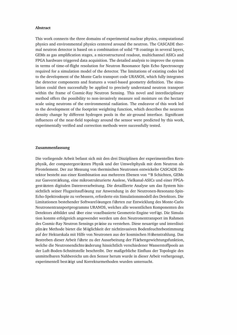
This work connects the three domains of experimental nuclear physics, computationalphysics and environmental physics centered around the neutron. The CASCADE ther-mal neutron detector is based on a combination of solid 10B coatings in several layers,GEMs as gas amplification stages, a microstructured readout, multichannel ASICs andFPGA hardware triggered data acquisition. The detailed analysis to improve the systemin terms of time-of-flight resolution for Neutron Resonance Spin Echo Spectroscopyrequired for a simulation model of the detector. The limitations of existing codes ledto the development of the Monte Carlo transport code URANOS, which fully integratesthe detector components and features a voxel-based geometry definition. The simu-lation could then successfully be applied to precisely understand neutron transportwithin the frame of Cosmic-Ray Neutron Sensing. This novel and interdisciplinarymethod offers the possibility to non-invasively measure soil moisture on the hectarescale using neutrons of the environmental radiation. The endeavor of this work ledto the development of the footprint weighting function, which describes the neutrondensity change by different hydrogen pools in the air-ground interface. Significantinfluences of the near-field topology around the sensor were predicted by this work,experimentally verified and correction methods were successfully tested.

Zusammenfassung

Die vorliegende Arbeit befasst sich mit den drei Disziplinen der experimentellen Kern-physik, der computergestützten Physik und der Umweltphysik mit dem Neutron alsPivotelement. Der zur Messung von thermischen Neutronen entwickelte CASCADE De-tektor besteht aus einer Kombination aus mehreren Ebenen von 10B Schichten, GEMszur Gasverstärkung, eine mikrostrukturierte Auslese, Vielkanal-ASICs und einer FPGA-gestützten digitalen Datenverarbeitung. Die detaillierte Analyse um das System hin-sichtlich seiner Flugzeitauflösung zur Anwendung in der Neutronen-Resonanz-Spin-Echo-Spektroskopie zu verbessern, erforderte ein Simulationsmodell des Detektors. DieLimitationen bestehender Softwarelösungen führten zur Entwicklung des Monte-CarloNeutronentransportprogramms URANOS, welches alle wesentlichen Komponenten desDetektors abbildet und über eine voxelbasierte Geometrie-Engine verfügt. Die Simula-tion konnte erfolgreich angewendet werden um den Neutronentransport im Rahmendes Cosmic-Ray Neutron Sensings präzise zu verstehen. Diese neuartige und interdiszi-plinäre Methode bietet die Möglichkeit der nichtinvasiven Bodenfeuchtebestimmungauf der Hektarskala mit Hilfe von Neutronen aus der kosmischen Höhenstrahlung. DasBestreben dieser Arbeit führte zu der Ausarbeitung der Flächengewichtungsfunktion,welche die Neutronendichteänderung hinsichtlich verschiedener Wasserstoffpools ander Luft-Boden-Schnittstelle beschreibt. Der maßgebliche Einfluss der Topologie desunmittelbaren Nahbereichs um den Sensor herum wurde in dieser Arbeit vorhergesagt,experimentell bestätigt und Korrekturmethoden wurden untersucht.

An den Mistral

C O N T E N T S

I T H E P H Y S I C S O F N E U T R O N S A N D C H A R G E D PA RT I C L E S

1 T H E P H Y S I C S O F N E U T R O N S 71.1 About the neutron . . . . . . . . . . . . . . . . . . . . . . . . . . . . . . 7

1.1.1 Fundamentals . . . . . . . . . . . . . . . . . . . . . . . . . . . . 71.1.2 Historical overview . . . . . . . . . . . . . . . . . . . . . . . . . 8

1.2 Neutron interactions . . . . . . . . . . . . . . . . . . . . . . . . . . . . . 91.3 Units and definitions . . . . . . . . . . . . . . . . . . . . . . . . . . . . . 10

1.3.1 Kinematics . . . . . . . . . . . . . . . . . . . . . . . . . . . . . . 101.3.2 Neutron flux . . . . . . . . . . . . . . . . . . . . . . . . . . . . . 11

1.4 Neutron transport . . . . . . . . . . . . . . . . . . . . . . . . . . . . . . 131.4.1 Slowing down . . . . . . . . . . . . . . . . . . . . . . . . . . . . 141.4.2 Thermal neutrons . . . . . . . . . . . . . . . . . . . . . . . . . . 16

2 T H E P H Y S I C S O F E L E C T R O M A G N E T I C I N T E R A C T I O N S 192.1 Energy loss in the medium . . . . . . . . . . . . . . . . . . . . . . . . . 19

2.1.1 Energy loss by ionization . . . . . . . . . . . . . . . . . . . . . . 192.1.2 Bremsstrahlung . . . . . . . . . . . . . . . . . . . . . . . . . . . 202.1.3 Multiple scattering . . . . . . . . . . . . . . . . . . . . . . . . . . 21

2.2 Processes in gaseous media . . . . . . . . . . . . . . . . . . . . . . . . . 212.2.1 Ionization . . . . . . . . . . . . . . . . . . . . . . . . . . . . . . 212.2.2 Energy resolution . . . . . . . . . . . . . . . . . . . . . . . . . . 222.2.3 Drift and diffusion . . . . . . . . . . . . . . . . . . . . . . . . . . 222.2.4 Gas gain . . . . . . . . . . . . . . . . . . . . . . . . . . . . . . . 24

II N E U T R O N S O U R C E S

3 N AT U R A L S O U R C E S : C O S M I C N E U T R O N S 273.1 From supernovae to sea level . . . . . . . . . . . . . . . . . . . . . . . . 273.2 Analytical description of the cosmic ray neutron spectrum . . . . . . . . 32

4 A RT I FI C I A L H I G H FL U X S O U R C E S 334.1 Overview of facilities . . . . . . . . . . . . . . . . . . . . . . . . . . . . . 334.2 Research centers . . . . . . . . . . . . . . . . . . . . . . . . . . . . . . . 354.3 The FRM II source . . . . . . . . . . . . . . . . . . . . . . . . . . . . . . 36

III U R A N O S M O N T E C A R L O T R A N S P O RT C O D E

5 M O D E L I N G A N D M O N T E C A R L O A P P R O A C H 415.1 Sampling . . . . . . . . . . . . . . . . . . . . . . . . . . . . . . . . . . . 41

5.1.1 Random number generation . . . . . . . . . . . . . . . . . . . . 415.1.2 Sampling free path length . . . . . . . . . . . . . . . . . . . . . . 425.1.3 Sampling thermal velocity distributions . . . . . . . . . . . . . . 435.1.4 Evaluated Nuclear Data Files . . . . . . . . . . . . . . . . . . . . 44

5.2 Neutron Monte Carlo codes . . . . . . . . . . . . . . . . . . . . . . . . . 475.2.1 General purpose packages . . . . . . . . . . . . . . . . . . . . . 475.2.2 Specific neutron interaction codes . . . . . . . . . . . . . . . . . 48

6 U R A N O S 496.1 URANOS concepts . . . . . . . . . . . . . . . . . . . . . . . . . . . . . . 506.2 Computational structure . . . . . . . . . . . . . . . . . . . . . . . . . . . 52

6.2.1 Startup . . . . . . . . . . . . . . . . . . . . . . . . . . . . . . . . 526.2.2 Geometry . . . . . . . . . . . . . . . . . . . . . . . . . . . . . . . 54

ix

6.3 Sources and energy . . . . . . . . . . . . . . . . . . . . . . . . . . . . . 566.3.1 The cosmic neutron source . . . . . . . . . . . . . . . . . . . . . 576.3.2 General sources . . . . . . . . . . . . . . . . . . . . . . . . . . . 57

6.4 Calculation scheme . . . . . . . . . . . . . . . . . . . . . . . . . . . . . 586.4.1 Loop nodes . . . . . . . . . . . . . . . . . . . . . . . . . . . . . . 586.4.2 Tracking in finite geometry regions . . . . . . . . . . . . . . . . . 596.4.3 Interaction channels . . . . . . . . . . . . . . . . . . . . . . . . . 62

6.5 Detector configurations . . . . . . . . . . . . . . . . . . . . . . . . . . . 656.5.1 Scoring options for CRNS . . . . . . . . . . . . . . . . . . . . . . 656.5.2 Neutron conversion evaluation for boron detectors . . . . . . . . 66

6.6 Basic performance examples . . . . . . . . . . . . . . . . . . . . . . . . 716.6.1 Diffusion length in water . . . . . . . . . . . . . . . . . . . . . . 716.6.2 Bonner Sphere evaluation . . . . . . . . . . . . . . . . . . . . . . 726.6.3 Cosmic spectrum evaluation . . . . . . . . . . . . . . . . . . . . 746.6.4 Performance benchmarks . . . . . . . . . . . . . . . . . . . . . . 76

IV C O S M I C - R AY N E U T R O N S E N S I N G

7 I N T R O D U C T I O N 1537.1 Soil moisture sensing techniques . . . . . . . . . . . . . . . . . . . . . .1537.2 Cosmic-Ray neutron sensing: the technique . . . . . . . . . . . . . . . .154

7.2.1 The COSMOS sensor . . . . . . . . . . . . . . . . . . . . . . . .1547.2.2 Signal corrections . . . . . . . . . . . . . . . . . . . . . . . . . .1557.2.3 Soil moisture determination . . . . . . . . . . . . . . . . . . . .156

8 U N D E R S TA N D I N G T H E C O S M I C - R AY N E U T R O N D E T E C T O R 1598.1 The detector model . . . . . . . . . . . . . . . . . . . . . . . . . . . . .1598.2 The energy response function . . . . . . . . . . . . . . . . . . . . . . . .1618.3 Energy dependence . . . . . . . . . . . . . . . . . . . . . . . . . . . . .1618.4 Detection probability within the case . . . . . . . . . . . . . . . . . . . .1628.5 Uncertainty analysis . . . . . . . . . . . . . . . . . . . . . . . . . . . . .1638.6 Implications of the sensitivity analysis . . . . . . . . . . . . . . . . . . .163

9 F O O T P R I N T I N V E S T I G AT I O N 1659.1 Footprint preludium . . . . . . . . . . . . . . . . . . . . . . . . . . . . .165

9.1.1 The cosmic-ray neutron spectrum assembly . . . . . . . . . . . .1659.1.2 Experimental verification . . . . . . . . . . . . . . . . . . . . . .1679.1.3 A closer look at the air-ground interface . . . . . . . . . . . . . .1699.1.4 Model setup . . . . . . . . . . . . . . . . . . . . . . . . . . . . .1709.1.5 Soil moisture and above-ground neutron density . . . . . . . . .1719.1.6 Tracking cosmic-ray neutrons in soil and air . . . . . . . . . . . .174

9.2 Cosmic-Ray neutron transport analysis . . . . . . . . . . . . . . . . . . .1769.2.1 Theoretical description by neutron transport equations . . . . .1769.2.2 Footprint definition . . . . . . . . . . . . . . . . . . . . . . . . .1789.2.3 Analytical characterization of the footprint . . . . . . . . . . . .1809.2.4 Analytical description of the penetration depth . . . . . . . . . .1819.2.5 Pressure dependency . . . . . . . . . . . . . . . . . . . . . . . .1829.2.6 Height dependency . . . . . . . . . . . . . . . . . . . . . . . . .183

9.3 Results . . . . . . . . . . . . . . . . . . . . . . . . . . . . . . . . . . . .1849.3.1 Intensity relation . . . . . . . . . . . . . . . . . . . . . . . . . . .1859.3.2 Penetration depth scaling . . . . . . . . . . . . . . . . . . . . . .1859.3.3 Footprint . . . . . . . . . . . . . . . . . . . . . . . . . . . . . . .1869.3.4 Where do neutrons come from? . . . . . . . . . . . . . . . . . .1889.3.5 Inhomogeneous terrain: roads . . . . . . . . . . . . . . . . . . .189

V S U M M A RY A N D C O N C L U S I O N

VI A P P E N D I X

A L I T E R AT U R E A N D R E F E R E N C E S 199A.1 Journal publications . . . . . . . . . . . . . . . . . . . . . . . . . . . . .199A.2 Conference contributions . . . . . . . . . . . . . . . . . . . . . . . . . .200A.3 Bibliography . . . . . . . . . . . . . . . . . . . . . . . . . . . . . . . . .201

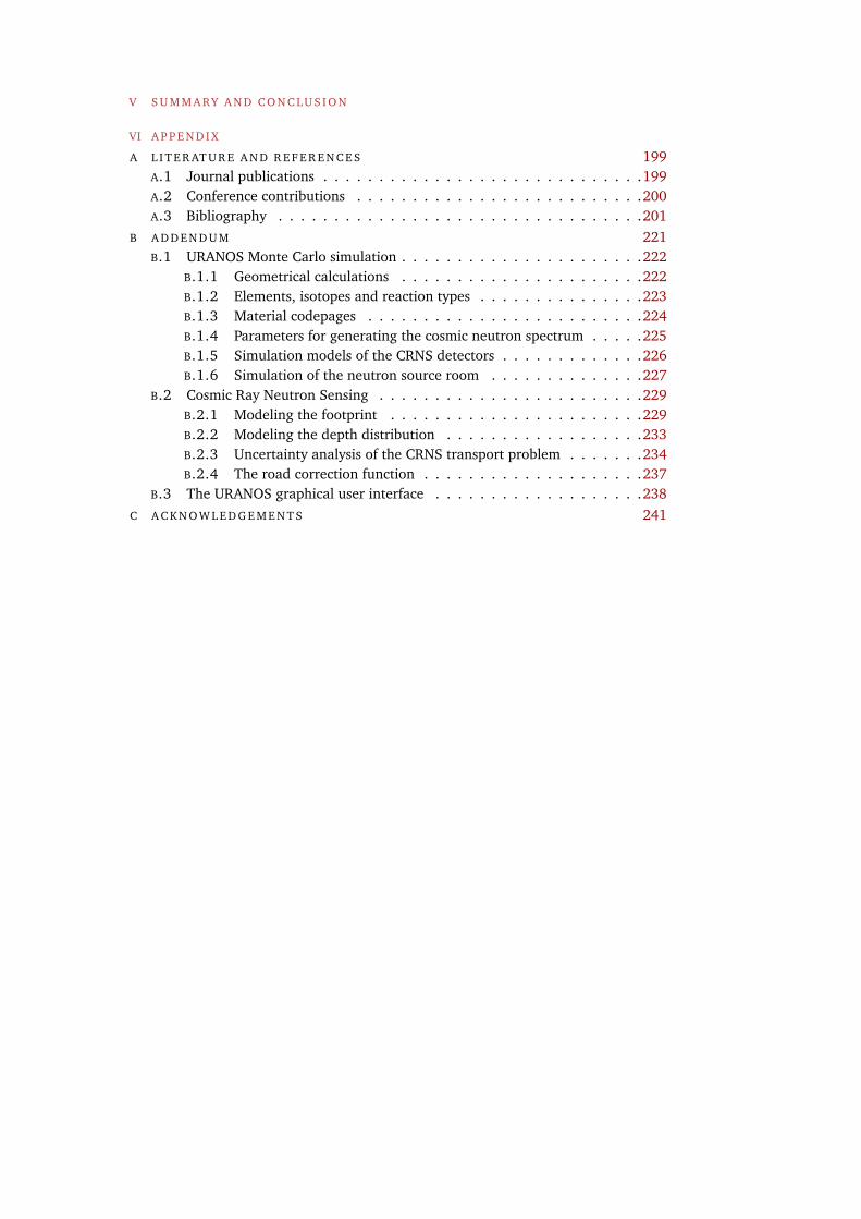
B A D D E N D U M 221B.1 URANOS Monte Carlo simulation . . . . . . . . . . . . . . . . . . . . . .222

B.1.1 Geometrical calculations . . . . . . . . . . . . . . . . . . . . . .222B.1.2 Elements, isotopes and reaction types . . . . . . . . . . . . . . .223B.1.3 Material codepages . . . . . . . . . . . . . . . . . . . . . . . . .224B.1.4 Parameters for generating the cosmic neutron spectrum . . . . .225B.1.5 Simulation models of the CRNS detectors . . . . . . . . . . . . .226B.1.6 Simulation of the neutron source room . . . . . . . . . . . . . .227

B.2 Cosmic Ray Neutron Sensing . . . . . . . . . . . . . . . . . . . . . . . .229B.2.1 Modeling the footprint . . . . . . . . . . . . . . . . . . . . . . .229B.2.2 Modeling the depth distribution . . . . . . . . . . . . . . . . . .233B.2.3 Uncertainty analysis of the CRNS transport problem . . . . . . .234B.2.4 The road correction function . . . . . . . . . . . . . . . . . . . .237

B.3 The URANOS graphical user interface . . . . . . . . . . . . . . . . . . .238C A C K N O W L E D G E M E N T S 241

P R E FA C E

The world of neutron detection is changing.Much of what once was established technology has been discarded. For them nowalternative ones have been presented. It began with production of tritium and peakedat the crisis of helium-3. Part of that was given to sciences for basic or applied research.Part for the industry, explorating oil deep in the rocks. And the largest part was given tohomeland security, which above all demanded for it for the protection against hazards.After the stockpile was nearly exhausted, alerts on the future supply, which are espe-cially critical to perspectives of the European Spallation Source led to developments ofreplacement technologies, most of them adapted from particle physics. The CASCADEthermal neutron detector is such a new generation system, which was designed specifi-cally for the purposes of Neutron Spin Echo (NSE) spectroscopy. This method and itssuccessors, Neutron Resonance Spin Echo (NRSE) and MIEZE (Modulation of IntEnsityby Zero Effort), demanded a highly granular and time-resolved detector to be operatedefficiently at high rates. Contrary to triple-axis spectrometry or standard time-of-flightmeasurements, NRSE methods can achieve a high energy resolution using wavelengthdistributions of up to 20 % width. In a research field, where beam intensity in generalis scarce due to limitations in the upscaling of the source, this technology offers incombination with a high-end detector the benefits which are looked for.The CASCADE design is based on a combination of solid 10B coatings in several layers,GEMs as gas amplification stages, a microstructured readout, multichannel ASICs andFPGA hardware triggered data acquisition. The developments of this work success-fully brought the CASCADE detector into operation at the Forschungs-NeutronenquelleHeinz Maier-Leibnitz at the instruments RESEDA and MIRA.

The world of neutron simulations is changing.What once was the most demanding domain for high performance computing infras-tructures can meanwhile be realized on a modern personal computer. Along with thisloss of exclusivity the heritage of those system architectures can be abandoned: Fortran-based ASCII interfaces, which aim for criticality calculations. And set back the scopeto focus on the neutron as a probe to the otherwise invisible and impenetrable. Whatmakes neutrons to messengers for hidden orders in matter, makes them likewise hardto control and hard to describe. They are produced randomly, their momentum andtheir interaction appear to be stochastic. While being less abundant than photons orelectrons but far from few-body systems in terms of numbers, the Monte Carlo simula-tion is the most suitable tool bridging the gap between thermodynamic flux models andanalytical calculations. Neutrons also interact with volumes rather than with surfaces.Hence, the essential unit to comprehend and implement a geometry model is the voxel,a threedimensional pixel.The URANOS Monte Carlo simulation has been created based on this computationalphilosophy and has been realized in a collaboration with environmental physics as avaluable community tool.

The world of neutron applications is changing.What began with the fission of uranium as source of energy and peaked with the devel-opment of a thermonuclear arsenal has been discarded. Large-scale research centerswith most recently the European Spallation Source being built are shaping the researchinfrastructure to consequently stretch out the scope of fundamental research to other

1

science domains. Sources like the FRM II, ILL, SNS or ISIS are equipped with dozens ofdifferent experiments to investigate structures on the nanoscale from complex crystalsto polymers or biomolecules, to image the magnetic ordering of superconductors orskyrmion lattices, to provide direct insights into storage cells or artifacts of cultural her-itage and also to support the production of radio-isotopes and the medical treatmentof cancer.Since the recent initiative of Desilets and Zreda the method of Cosmic-Ray NeutronSensing is gaining momentum. It allows to determine soil moisture on the hectare scaleby the density of neutrons created in the atmosphere and reflected from the ground.It represents a technology to quantify non-invasively the most essential resource infood production: water. The effect that soil moisture influences the above-ground neu-tron flux had been known at least since the 1960s. Several attempts, however, failedto comprehensively understand the signal dependencies due to the lack of resourcesand interest to address the complexity of the transport problem. With the develop-ment of URANOS using computationally efficient the nowadays available off-the-shelfhardware, the model dependencies within the environmental system have been trackeddown in extensive simulations. This work manages to unfold the intricacy of the cosmic-ray neutron transport, discovering the solution of a 50-year old problem and enablingCRNS to become an established hydrological method.

The world of neutrons is changing.

This is the phase front.

2

I N T R O D U C T I O N

COSMIC-RAY NEUTRON SENSING - THE CHALLENGE

From 2008 on the method of Cosmic-Ray Neutron Sensing rapidly developed. Its in-triguing aspects are the possibility to measure soil moisture non-invasively at so-calledintermediate scales, which cannot be accessed by other technologies, but especiallymatch typical soil water correlation lengths. The method relies on the fact, that incollisions with hydrogen neutrons are stopped much more efficiently than with anyother element due to the high cross section and the equal masses of the projectiles.High energetic cascades in the upper atmosphere generate neutrons, which finally tendto be reflected by dry soil or get moderated under wet conditions. A significant amountof data could be collected by deploying a network of standardized Cosmic-Ray Probes.Such are detectors sensitive to epithermal neutrons and similar in the buildup to Bon-ner Spheres with a one inch moderator around a proportional counter filled with aconverter gas. However, it became clear that the data sets could not be fully under-stood and several attempts of analyzing the soil response using the Monte Carlo toolMCNPX failed. In 2013, the pioneers of the method, Desilets and Zreda, published apaper, in which they stated the footprint of the method would be approximately 30 haand not significantly depend on the soil moisture content. As the data not at all showedevidence for such a relation, the interest rose for an accurate understanding of thesystem. The already existing code URANOS could be tailored to address the neutrontransport problem in the air-ground interface, yet requiring some modifications onthe scattering and scoring kernel and the implementation of additional processes likeinelastic scattering. Initial calculations showed already promising results as the simu-lation could reproduce experimental data already better than the results presented bythe authors of the mentioned paper. However, it turned out, that whereas some parts ofthe problem like the above-ground neutron intensity follow rather simple laws, otherslike the radial distribution revealed complex dependencies on different hydrogen pools.The sophisticated neutron transport problem, which indeed has remained unexplainedfor nearly 50 years, along with the possible fundamental impact of the method pavedthe ground for the necessity of a plain and conclusive analysis of the CRNS signalformation in this work.

3

Part I

T H E P H Y S I C S O F N E U T R O N S A N D C H A R G E DPA R T I C L E S

1T H E P H Y S I C S O F N E U T R O N S

1.1 ABOUT THE NEUTRON

1.1.1 FUNDAMENTALS

Figure 1: Artistic adapta-tion of measurement con-straints on the CKM ma-trix [1, 2], inspired byresults from [3]. Theelement 𝑉𝑢𝑑 [4], whichis located in the lowerleft corner of the uni-tarity triangle, representsthe transition probabilityfor up and down typequarks. It is, among oth-ers [5], linked to nuclearbeta decay and can be de-rived from neutron life-time measurements.

Mass 𝑚 = 1.0086649159(5) u

𝑚 = 939.565413(6) MeV

Spin 𝑠 = 1/2ℎ/(2𝜋)Lifetime 𝜏 = 880.2(1.0) s

Mean-square charge radius < 𝑟 2𝑁>= -0.1161(22) fm2

Charge 𝑞 = -0.2(8) 10−21 𝑒

Magnetic moment ` = -1.9130427(5) `𝑁Electric dipole moment 𝑑𝑁 < 0.30 10−25 𝑒cm (90 % CL)

Table 1: Basic physicalproperties of the neu-tron [1].

The neutron has a net charge of zero and a spin of 1/2 ℎ/(2𝜋). Its dipole moment isexpected to be 𝑑𝑁 ≈ (10−37−10−40) ecm according to the standard model and measure-ments with nuclear bound states and sensitivities up to 10−32 ecm so far confirm thisvalue [6]. Yet, they have a magnetic moment caused by small loop currents [7]. Its restmass is slightly higher than the one of the proton, therefore it can decay weakly [4]into an electron and an electron antineutrino by

n 𝜘→ p + e + ae

with a maximum kinetic energy transfer of 781.32 keV and a lifetime of approximately15 min [8]. Thus there are nearly no free neutrons in the universe as the only stablecondition available is the bound state in a nucleus.

7

1.1.2 HISTORICAL OVERVIEW

The term ’Neutron’ describing an electrically neutral entity of matter appeared as earlyas the end of the 20th century [9]. It was mainly discussed as an assumed bound stateof the electron and its counterpart, which could for example make up the ether[a] andexplain the results of experiments with cathode rays [10]. Though Rutherford[b] em-pirically discovered in 1911 [11] and theoretically described the nuclei of atoms, theneutron was proposed to be a particle comprised of a proton and an electron [12][c].Albeit in the late 1920s the newly developed quantum mechanics raised serious ques-tions about such a model of nuclear electrons regarding the incorrectly predicted spinof this compound and the escape probability of the electron due to its large wavelength,the fundamental questions about nuclei stayed unanswered.Experiments in 1930 by Bothe[d] [14] showed evidence of an at that time unknowntype of reaction. In a test series of exposing light elements to alpha particles, beryl-lium showed the production of hard gamma rays, which originated as they supposedfrom nuclear excitations, producing furthermore a new type of neutral radiation. Itcould knock off protons with kinetic energies of several MeV from a hydrogen-richmaterial through several centimeters of lead. In 1932, based on the experiments ofCurie[e] and Joliot[f] [15], it was quickly understood by kinetic considerations that thisradiation is made of particles as heavy as the proton - in terms of comments reportedfirst of Majorana[g] [16], then of Chadwick[h] [17]. Iwanenko[i], who had theoreticallyworked on the problems of spin statistics before, realized that the neutron could alsobe a constituent of the nucleus [18], which was then confirmed [19] and celebratedas the birth of the neutron. This discovery was the key to understand the structure ofatoms as composed of a shell and a small nucleus which itself is made up of protonsand neutrons [20].It is notable that in the first series of experimental trials boron has its first mentionas a neutron absorber [21] and furthermore that the cosmic radiation soon after itsdiscovery has been proposed to be partially made up of neutrons [22].

[a] to be noted: there was neither a common conception of the ether nor a consistent framework of theories.However, as in the case of the invention of the special relativity theory, this heritage can be considered animportant foundation.

[b] Ernest RUTHERFORD, *1871-†1937, New Zealand, United Kingdom of Great Britain.[c] Rutherford himself, however, had already mentioned in 1904 in a sidenote of his book ’Radio-activity’ [13]

a proper description of the neutron appearing as a form of radiation.[d] Walther Wilhelm Georg BOTHE, *1891-†1957, German Empire.[e] Iréne JOLIOT-CURIE, *1897-†1956, France.[f] Frédéric JOLIOT-CURIE, *1900-†1958, France.[g] Ettore MAJORANA, *1906-?1938, Kingdom of Italy.[h] Sir James CHADWICK, *1891-†1974, United Kingdom of Great Britain.[i] Dmitri� Dmitrieviq Ivanenko., *1904-†1994, Russian Empire.

8

1.2 NEUTRON INTERACTIONS

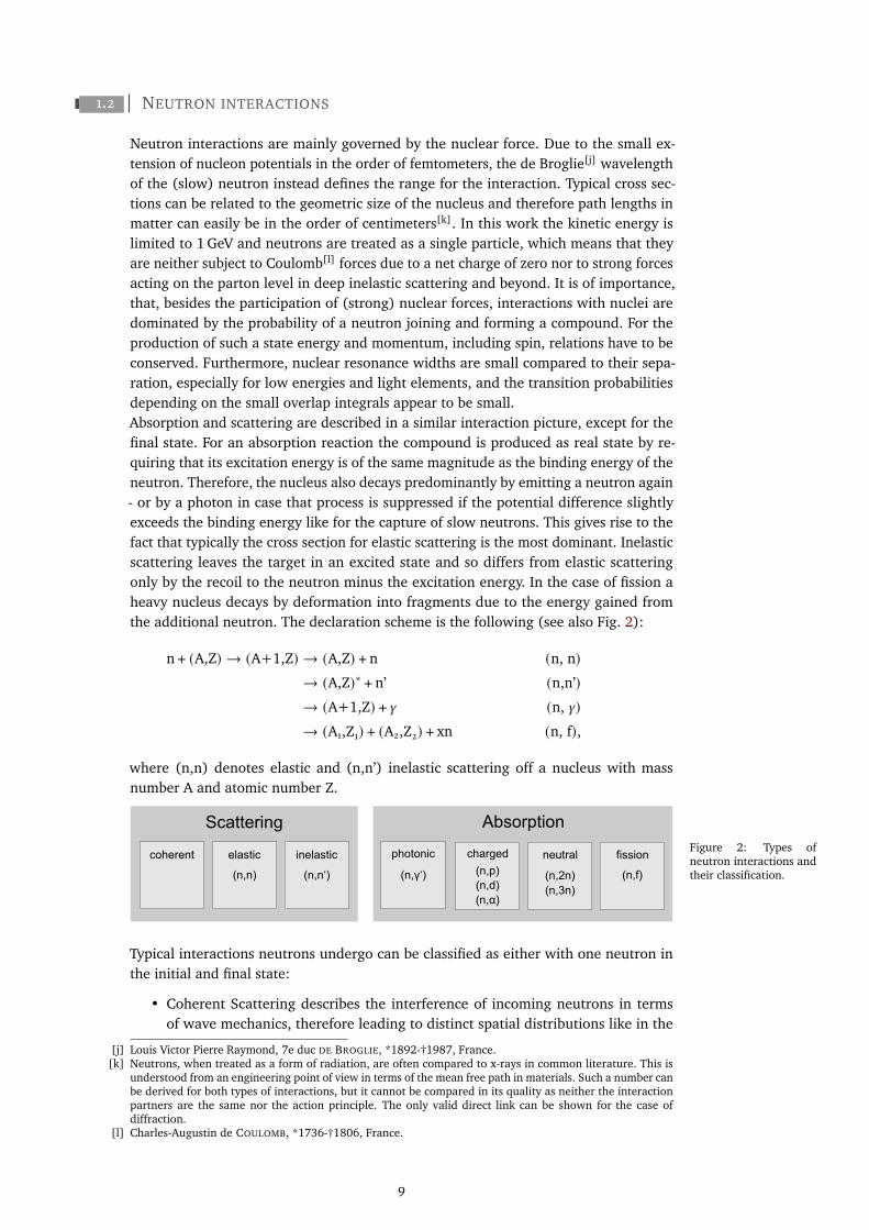
Neutron interactions are mainly governed by the nuclear force. Due to the small ex-tension of nucleon potentials in the order of femtometers, the de Broglie[j] wavelengthof the (slow) neutron instead defines the range for the interaction. Typical cross sec-tions can be related to the geometric size of the nucleus and therefore path lengths inmatter can easily be in the order of centimeters[k]. In this work the kinetic energy islimited to 1 GeV and neutrons are treated as a single particle, which means that theyare neither subject to Coulomb[l] forces due to a net charge of zero nor to strong forcesacting on the parton level in deep inelastic scattering and beyond. It is of importance,that, besides the participation of (strong) nuclear forces, interactions with nuclei aredominated by the probability of a neutron joining and forming a compound. For theproduction of such a state energy and momentum, including spin, relations have to beconserved. Furthermore, nuclear resonance widths are small compared to their sepa-ration, especially for low energies and light elements, and the transition probabilitiesdepending on the small overlap integrals appear to be small.Absorption and scattering are described in a similar interaction picture, except for thefinal state. For an absorption reaction the compound is produced as real state by re-quiring that its excitation energy is of the same magnitude as the binding energy of theneutron. Therefore, the nucleus also decays predominantly by emitting a neutron again- or by a photon in case that process is suppressed if the potential difference slightlyexceeds the binding energy like for the capture of slow neutrons. This gives rise to thefact that typically the cross section for elastic scattering is the most dominant. Inelasticscattering leaves the target in an excited state and so differs from elastic scatteringonly by the recoil to the neutron minus the excitation energy. In the case of fission aheavy nucleus decays by deformation into fragments due to the energy gained fromthe additional neutron. The declaration scheme is the following (see also Fig. 2):

n + (A,Z) → (A+1,Z) → (A,Z) + n (n, n)→ (A,Z)∗ + n’ (n,n’)→ (A+1,Z) +𝛾 (n, 𝛾)→ (A1,Z1) + (A2,Z2) + xn (n, f),

where (n,n) denotes elastic and (n,n’) inelastic scattering off a nucleus with massnumber A and atomic number Z.

Figure 2: Types ofneutron interactions andtheir classification.

Scattering Absorption

elastic

(n,n)

inelastic

(n,n‘)

coherent photonic

(n,γ‘)

neutral

(n,2n)

fission

(n,f)

charged

(n,p)

(n,d)

(n,α)(n,3n)

Typical interactions neutrons undergo can be classified as either with one neutron inthe initial and final state:

• Coherent Scattering describes the interference of incoming neutrons in termsof wave mechanics, therefore leading to distinct spatial distributions like in the

[j] Louis Victor Pierre Raymond, 7e duc DE BROGLIE, *1892-†1987, France.[k] Neutrons, when treated as a form of radiation, are often compared to x-rays in common literature. This is

understood from an engineering point of view in terms of the mean free path in materials. Such a number canbe derived for both types of interactions, but it cannot be compared in its quality as neither the interactionpartners are the same nor the action principle. The only valid direct link can be shown for the case ofdiffraction.

[l] Charles-Augustin de COULOMB, *1736-†1806, France.

9

case of Laue[m] diffraction. Originally coming from crystallography there is adistinction between elastic scattering, which refers to the prior mentioned process,and inelastic scattering, which refers to the additional excitation of phonons inthe sample. This definition is ambiguous in its terminology[n] taking into accountthe further mentioned interaction types. Furthermore, quasi-elastic scatteringapplies to the case of (thermal) motion of the atoms giving rise to a significantcontribution blurring the observed line shape.

• Elastic Scattering is the predominant mechanism of losing energy and can beunderstood as an elastic collision with energy and momentum conservation inthe center-of-mass frame.

• Inelastic Scattering is an inelastic collision with the nucleus leaving it in an ex-cited state. The allowed energy transfer is determined by the available nuclearexcitation levels and therefore this process is mostly suppressed for kinetic ener-gies below 1 MeV.

or such altering the target nucleus:

• Radiative Capture brings the nucleus into a A+1-state, which de-excites by emis-sion of a photon.

• Charged Capture means that after absorbing a neutron the nucleus will decay byemitting either electrons, protons or larger compounds like helium ions, whichin the case of light elements can be considered as fragments of the nucleus.

• Neutral Capture appears as an inelastic collision with similar initial and finalstates. Due to the absorption process and the following decay time constants andkinematics are different.

• Fission can occur for heavy elements absorbing a slow neutron if the final stateenergy budget is in favor of several fragments. Besides those, typically an energydependent number of neutrons is emitted which are not any more needed tostabilize the smaller nuclei.

• Spallation is not limited incoming neutron. Any high energetic projectile withenergies larger than approximately 100 MeV can induce the total breakup of anucleus, which is described as a hadron shower.

1.3 UNITS AND DEFINITIONS

1.3.1 KINEMATICS

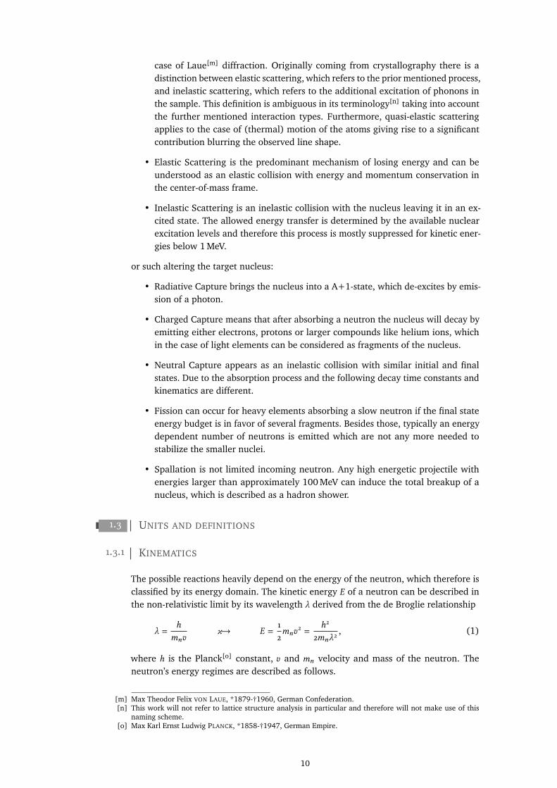
The possible reactions heavily depend on the energy of the neutron, which therefore isclassified by its energy domain. The kinetic energy 𝐸 of a neutron can be described inthe non-relativistic limit by its wavelength _ derived from the de Broglie relationship

_ =ℎ

𝑚𝑛𝑣𝜘→ 𝐸 =

1

2𝑚𝑛𝑣

2 =ℎ2

2𝑚𝑛_2, (1)

where ℎ is the Planck[o] constant, 𝑣 and 𝑚𝑛 velocity and mass of the neutron. Theneutron’s energy regimes are described as follows.

[m] Max Theodor Felix VON LAUE, *1879-†1960, German Confederation.[n] This work will not refer to lattice structure analysis in particular and therefore will not make use of this

naming scheme.[o] Max Karl Ernst Ludwig PLANCK, *1858-†1947, German Empire.

10

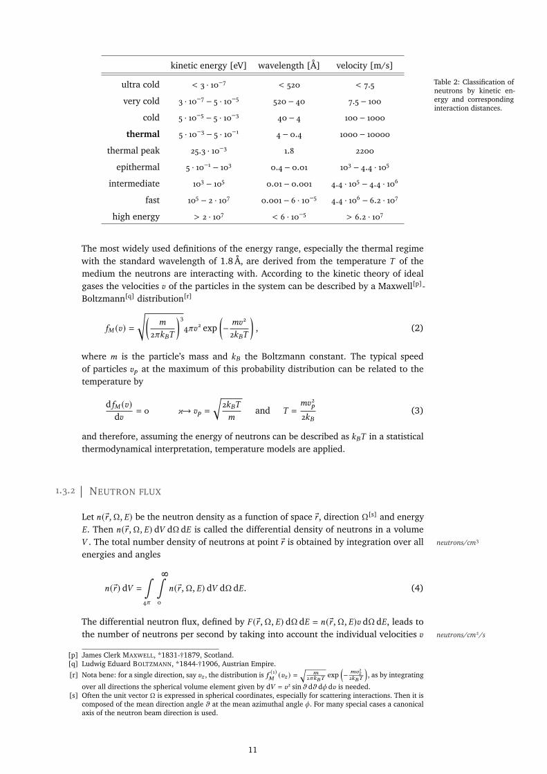
Table 2: Classification ofneutrons by kinetic en-ergy and correspondinginteraction distances.

kinetic energy [eV] wavelength [Å] velocity [m/s]

ultra cold < 3 · 10−7 < 520 < 7.5

very cold 3 · 10−7 − 5 · 10−5 520 − 40 7.5 − 100

cold 5 · 10−5 − 5 · 10−3 40 − 4 100 − 1000

thermal 5 · 10−3 − 5 · 10−1 4 − 0.4 1000 − 10000

thermal peak 25.3 · 10−3 1.8 2200

epithermal 5 · 10−1 − 103 0.4 − 0.01 103 − 4.4 · 105

intermediate 103 − 105 0.01 − 0.001 4.4 · 105 − 4.4 · 106

fast 105 − 2 · 107 0.001 − 6 · 10−5 4.4 · 106 − 6.2 · 107

high energy > 2 · 107 < 6 · 10−5 > 6.2 · 107

The most widely used definitions of the energy range, especially the thermal regimewith the standard wavelength of 1.8 Å, are derived from the temperature 𝑇 of themedium the neutrons are interacting with. According to the kinetic theory of idealgases the velocities 𝑣 of the particles in the system can be described by a Maxwell[p]-Boltzmann[q] distribution[r]

𝑓𝑀 (𝑣) =

√(𝑚

2𝜋𝑘𝐵𝑇

)34𝜋𝑣2 exp

(− 𝑚𝑣2

2𝑘𝐵𝑇

), (2)

where 𝑚 is the particle’s mass and 𝑘𝐵 the Boltzmann constant. The typical speedof particles 𝑣𝑝 at the maximum of this probability distribution can be related to thetemperature by

d𝑓𝑀 (𝑣)d𝑣

= 0 𝜘→ 𝑣𝑝 =

√2𝑘𝐵𝑇

𝑚and 𝑇 =

𝑚𝑣2𝑝

2𝑘𝐵(3)

and therefore, assuming the energy of neutrons can be described as 𝑘𝐵𝑇 in a statisticalthermodynamical interpretation, temperature models are applied.

1.3.2 NEUTRON FLUX

Let 𝑛(®𝑟 , Ω,𝐸) be the neutron density as a function of space ®𝑟 , direction Ω[s] and energy𝐸. Then 𝑛(®𝑟 , Ω,𝐸) d𝑉 dΩ d𝐸 is called the differential density of neutrons in a volume𝑉 . The total number density of neutrons at point ®𝑟 is obtained by integration over all neutrons/cm3

energies and angles

𝑛(®𝑟 ) d𝑉 =

∫4𝜋

8∫0

𝑛(®𝑟 , Ω,𝐸) d𝑉 dΩ d𝐸. (4)

The differential neutron flux, defined by 𝐹 (®𝑟 , Ω,𝐸) dΩ d𝐸 = 𝑛(®𝑟 , Ω,𝐸)𝑣 dΩ d𝐸, leads tothe number of neutrons per second by taking into account the individual velocities 𝑣 neutrons/cm2/s

[p] James Clerk MAXWELL, *1831-†1879, Scotland.[q] Ludwig Eduard BOLTZMANN, *1844-†1906, Austrian Empire.

[r] Nota bene: for a single direction, say 𝑣𝑧 , the distribution is 𝑓 (1)𝑀

(𝑣𝑧 ) =√

𝑚2𝜋𝑘𝐵𝑇

exp(− 𝑚𝑣2𝑧

2𝑘𝐵𝑇

), as by integrating

over all directions the spherical volume element given by d𝑉 = 𝑣2 sin𝜗 d𝜗 d𝜙 d𝑣 is needed.[s] Often the unit vector Ω is expressed in spherical coordinates, especially for scattering interactions. Then it is

composed of the mean direction angle 𝜗 at the mean azimuthal angle 𝜙 . For many special cases a canonicalaxis of the neutron beam direction is used.

11

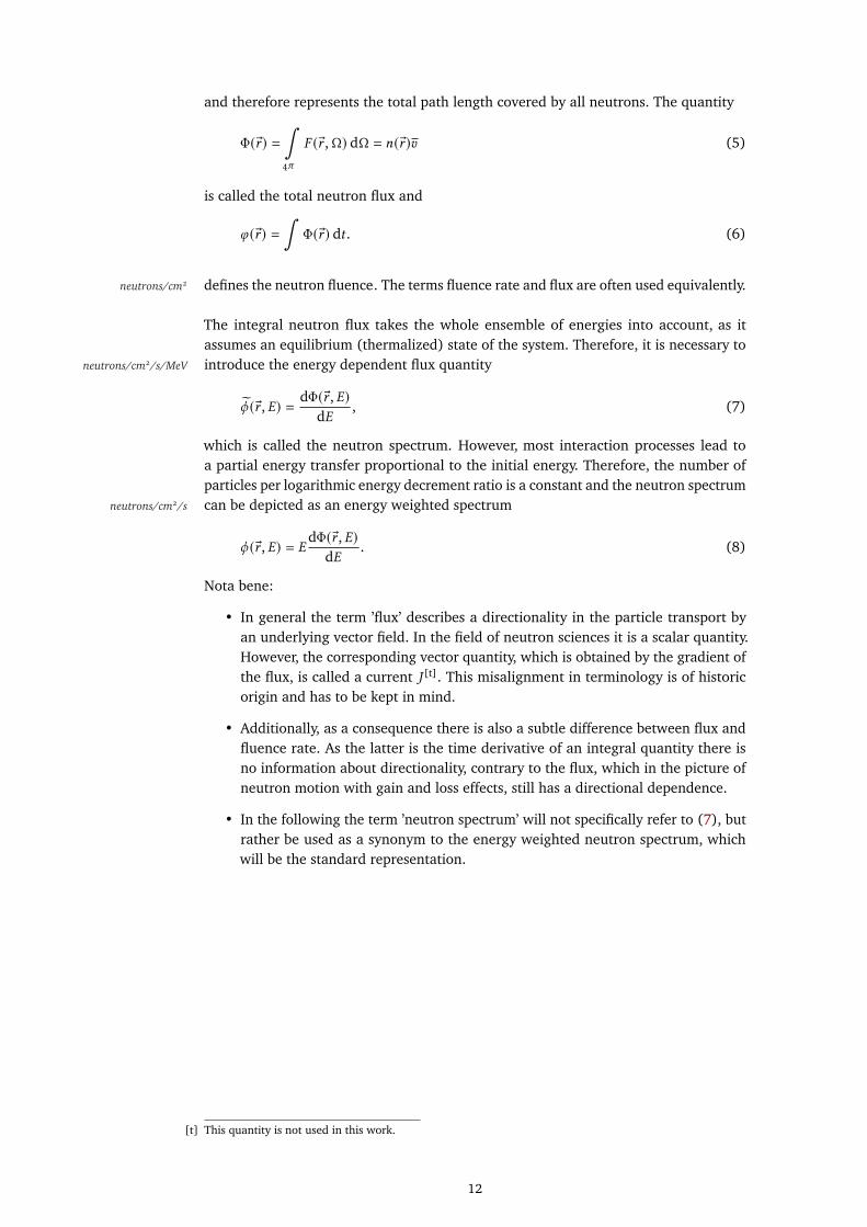
and therefore represents the total path length covered by all neutrons. The quantity

Φ(®𝑟 ) =∫4𝜋

𝐹 (®𝑟 , Ω) dΩ = 𝑛(®𝑟 )𝑣 (5)

is called the total neutron flux and

𝜑 (®𝑟 ) =∫

Φ(®𝑟 ) d𝑡 . (6)

defines the neutron fluence. The terms fluence rate and flux are often used equivalently.neutrons/cm2

The integral neutron flux takes the whole ensemble of energies into account, as itassumes an equilibrium (thermalized) state of the system. Therefore, it is necessary tointroduce the energy dependent flux quantityneutrons/cm2/s/MeV

𝜙 (®𝑟 ,𝐸) = dΦ(®𝑟 ,𝐸)d𝐸

, (7)

which is called the neutron spectrum. However, most interaction processes lead toa partial energy transfer proportional to the initial energy. Therefore, the number ofparticles per logarithmic energy decrement ratio is a constant and the neutron spectrumcan be depicted as an energy weighted spectrumneutrons/cm2/s

𝜙 (®𝑟 ,𝐸) = 𝐸dΦ(®𝑟 ,𝐸)

d𝐸. (8)

Nota bene:

• In general the term ’flux’ describes a directionality in the particle transport byan underlying vector field. In the field of neutron sciences it is a scalar quantity.However, the corresponding vector quantity, which is obtained by the gradient ofthe flux, is called a current 𝐽 [t]. This misalignment in terminology is of historicorigin and has to be kept in mind.

• Additionally, as a consequence there is also a subtle difference between flux andfluence rate. As the latter is the time derivative of an integral quantity there isno information about directionality, contrary to the flux, which in the picture ofneutron motion with gain and loss effects, still has a directional dependence.

• In the following the term ’neutron spectrum’ will not specifically refer to (7), butrather be used as a synonym to the energy weighted neutron spectrum, whichwill be the standard representation.

[t] This quantity is not used in this work.

12

1.4 NEUTRON TRANSPORT

Neutron transport theory describes the flux through a medium by a Boltzmann equationin order to model the neutron field by conserving the total number of particles. Thisbalance is kept by the four terms

• leakage out of the volume 1©,

• loss due to absorption and scattering out of the volume or energy range 2©,

• in-scattering from outside the volume and/or a different energy 3©,

• gain by a source inside the volume 4©.

𝛿𝑛(𝑟 , Ω,𝐸)𝛿𝑡

= − 𝑣Ω∇𝑛(𝑟 , Ω,𝐸) 1©− (Σ𝑎 (𝐸) + Σ𝑠 (𝐸))𝑣𝑛(𝑟 , Ω,𝐸) 2©

+∫4𝜋

8∫0

Σ𝑠 (Ω ′ → Ω,𝐸 ′ → 𝐸)𝑣𝑛(𝑟 , Ω ′,𝐸 ′) dΩ ′ d𝐸 ′ 3©

𝑆 (𝑟 , Ω,𝐸). 4© (9)

with the macroscopic cross sections, which are also called linear attenuation coeffi-cients, for absorption Σ𝑎 and scattering Σ𝑠 . Both are combined to the total macroscopic 1/cm

cross section

Σ𝑡 = Σ𝑎 + Σ𝑠 (+ . . . ). (10)

The macroscopic cross section Σ can be derived from the microscopic cross section[u] 𝜎 , cm2

which defines the probability of interaction in a mass element divided by the productof interaction centers and the fluence:

Σ = 𝜌𝑁𝐴

𝜎

𝑀, (11)

where 𝜌 denotes the density of a material with atoms of molar mass 𝑀 and 𝑁𝐴 theAvogadro[v] or also called Loschmidt[w] constant. On a microscopic level vice versa themicroscopic cross section is described as

𝜎 =1

𝑛𝑙. (12)

It has the dimension of an area and is defined as the inverse of the product numberdensity 𝑛 = 𝜌𝑁𝐴/𝑀 and the mean free path 𝑙 , which by themselves describe the inter-action opacity of the material[x]. The typical unit is the barn: 1 b = 10−28 m2.As reactions can depend on parameters like the incoming energy or the (emission)angle, one introduces the differential cross section d𝜎

dΩ .The cross section can be composed like the attenuation coefficient of a sum energydependent absorption 𝜎𝑎 and scattering 𝜎𝑠 contributions

𝜎 (𝐸) = 𝜎𝑎 (𝐸) + 𝜎𝑠 (𝐸) (+ . . . ). (13)

[u] In this work the term cross section will always refer to 𝜎 . For the macroscopic cross section the termattenuation coefficient is preferred.

[v] Lorenzo Romano Amedeo Carlo AVOGADRO, Conte di Quaregna e Cerreto, *1776-†1856, Italian Empire.[w] Johann Josef LOSCHMIDT, *1821-†1895, Austrian Empire.[x] To be noted: Macroscopic cross sections have the dimension of a reciprocal length, microscopic cross sections

the dimension of an area.

13

In case of a compound with weight fractions 𝑤𝑖 of 𝑛 elements the weighted sum ofcross sections is evaluated:

Σ𝑡 = 𝜌𝑁𝐴

𝑛∑𝑖=1

𝑤𝑖

𝜎𝑖

𝑀𝑖

. (14)

Therefore, the occurrence probability of an interaction type at an element can be cal-culated by the relative fraction of the cross sections 𝜎𝑖/𝜎 and is called reaction rate.

In a homogeneous medium the mean free path[y] between two interactions is

𝑙 (𝐸) = 1

Σ𝑡 (𝐸). (15)

Therefore, in case of dominant absorption, the abundance of neutrons follows theBeer[z]-Lambert[aa] attenuation law.

The probability distribution function can be denoted as

𝑝 (𝑙 ,𝐸) d𝑙 = Σ𝑡 (𝐸) exp (−Σ𝑡 (𝐸)𝑙) d𝑙 . (16)

Integrating over a finite length leads to the number of neutrons 𝑁 in a distance 𝐿

𝑁 (𝐿,𝐸)𝑁0

=

𝐿∫0

𝑝 (𝑙 ,𝐸) d𝑙 =

𝐿∫0

Σ𝑡 (𝐸) exp (−Σ𝑡 (𝐸)𝑙) d𝑙 = 1 − exp (−Σ𝑡 (𝐸)𝐿) . (17)

Therefore, the percentage of neutrons traversing a thin layer of thickness 𝑑 withoutinteraction is exp (−Σ𝑡 (𝐸)𝑑).

1.4.1 SLOWING DOWN

Neutrons of typical energies up to 200 MeV can be treated non-relativistically for col-lisions by energy and momentum conservation. As for elastic interactions only therelative rather than the absolute masses are required, the neutron can be considered ofmass 1 and a nucleus of mass 𝐴. It is furthermore convenient to transform the collision

Figure 3: Kinematics ofan elastic collision inthe laboratory (left) andcenter-of-mass frame(right).

m mM M

vvlab

Θcm vlab

vcm

Θlab

from the laboratory (lab) into the center-of-mass (cm) frame as in such the angulardistribution is isotropic. The velocity of the cm system with velocities of the neutron 𝑣

and the nucleus 𝑉 can be calculated as follows

𝑣cm =1

1 +𝐴 (𝑣l +𝐴𝑉l) =𝑣l

1 +𝐴 (18)

[y] also called the distance to the next collision.[z] August BEER, *1825-†1863, German Empire.

[aa] Johann Heinrich LAMBERT, *1728-†1777, France.

14

and within the cm system the velocities of the particles are

𝑣c = 𝑣l − 𝑣cm =𝐴

𝐴 + 1𝑣l (19)

𝑉c = −𝑣cm = − 1

𝐴 + 1𝑣l (20)

The energy of the neutron in the cm system 𝐸c can be derived as well according to

𝐸c =1

2𝑣c2 +

1

2𝐴𝑉 2

c =𝐴

𝐴 + 1

1

2𝑣2l =

𝐴

𝐴 + 1𝐸l. (21)

In the cm frame the absolute values of velocities of the particles do not change, so𝑣 ′

c = 𝑣c. The angles can be calculated as

tan𝜗l =𝑣 ′

c sin𝜗c

𝑣cm + 𝑣 ′c cos𝜗c

=sin𝜗c

1𝐴+ cos𝜗c

(22)

or by trigonometric transformation

cos(𝜋 − 𝜗c) =(𝑣 ′

c)2 + (𝑣cm)2 − (𝑣 ′l )

2

(𝐴 + 1)2 . (23)

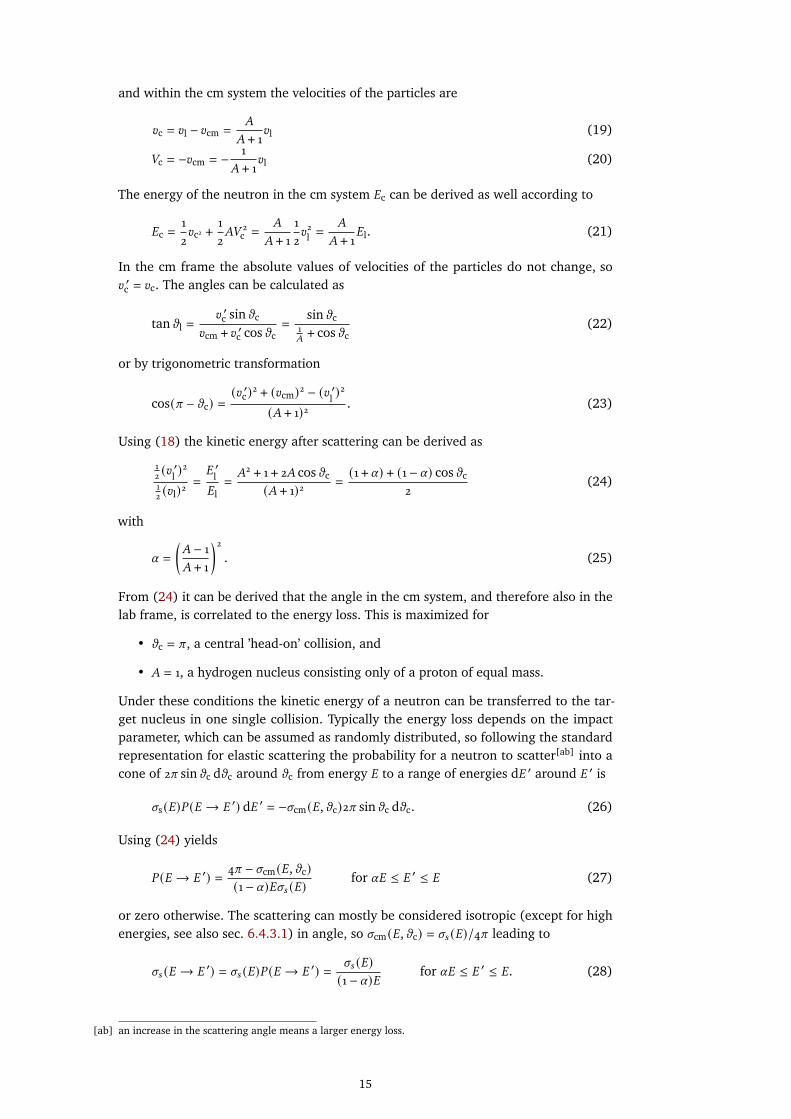
Using (18) the kinetic energy after scattering can be derived as

12(𝑣 ′

l )2

12(𝑣l)2

=𝐸 ′

l

𝐸l=𝐴2 + 1 + 2𝐴 cos𝜗c

(𝐴 + 1)2 =(1 + 𝛼) + (1 − 𝛼) cos𝜗c

2(24)

with

𝛼 =

(𝐴 − 1

𝐴 + 1

)2. (25)

From (24) it can be derived that the angle in the cm system, and therefore also in thelab frame, is correlated to the energy loss. This is maximized for

• 𝜗c = 𝜋 , a central ’head-on’ collision, and

• 𝐴 = 1, a hydrogen nucleus consisting only of a proton of equal mass.

Under these conditions the kinetic energy of a neutron can be transferred to the tar-get nucleus in one single collision. Typically the energy loss depends on the impactparameter, which can be assumed as randomly distributed, so following the standardrepresentation for elastic scattering the probability for a neutron to scatter[ab] into acone of 2𝜋 sin𝜗c d𝜗c around 𝜗c from energy 𝐸 to a range of energies d𝐸 ′ around 𝐸 ′ is

𝜎s (𝐸)𝑃 (𝐸 → 𝐸 ′) d𝐸 ′ = −𝜎cm (𝐸,𝜗c)2𝜋 sin𝜗c d𝜗c. (26)

Using (24) yields

𝑃 (𝐸 → 𝐸 ′) = 4𝜋 − 𝜎cm (𝐸,𝜗c)(1 − 𝛼)𝐸𝜎𝑠 (𝐸)

for 𝛼𝐸 ≤ 𝐸 ′ ≤ 𝐸 (27)

or zero otherwise. The scattering can mostly be considered isotropic (except for highenergies, see also sec. 6.4.3.1) in angle, so 𝜎cm (𝐸,𝜗c) = 𝜎𝑠 (𝐸)/4𝜋 leading to

𝜎𝑠 (𝐸 → 𝐸 ′) = 𝜎𝑠 (𝐸)𝑃 (𝐸 → 𝐸 ′) = 𝜎𝑠 (𝐸)(1 − 𝛼)𝐸 for 𝛼𝐸 ≤ 𝐸 ′ ≤ 𝐸. (28)

[ab] an increase in the scattering angle means a larger energy loss.

15

With the probability for each angle and consecutively for the corresponding energytransfer, the average energy loss can be calculated as

Δ𝐸 = 𝐸 −𝐸∫

𝛼𝐸

d𝐸 ′𝐸 ′𝑃 (𝐸 → 𝐸 ′) = 1

2(1 − 𝛼)𝐸 (29)

and the important quantity of the average logarithmic energy loss as

b =

𝐸∫𝛼𝐸

d𝐸 ′ ln(𝐸

𝐸 ′

)𝑃 (𝐸 → 𝐸 ′) (30)

= 1 + 𝛼

1 − 𝛼ln𝛼 = 1 − (𝐴 − 1)2

2𝐴ln

(𝐴 + 1

𝐴 − 1

). (31)

The logarithm represents the fact, that by elastic collisions not an absolute quantity butalways a fraction of the kinetic energy is lost. Therefore, the moderation power of amaterial is defined as the average number of collisions from an initial energy, say 𝐸0 =

10 MeV, until entering the thermal regime at 1 eV

𝑛col =𝑢

b=

ln(𝐸0/𝐸)b

, (32)

where the lethargy 𝑢 is defined as

𝑢 = ln(𝐸0

𝐸

). (33)

So b represents the average change in lethargy per collision. According to (31) thisproperty of a material decreases with nuclide mass and the slowing down requiresmore collisions.

1.4.2 THERMAL NEUTRONS

In the previous chapter 1.4.1 it has been assumed that the target nucleus is at rest. Yet,as soon as the kinetic energy of the neutron is

• comparable to the mean kinetic energy of atoms in a gas phase or

• in the order of the binding energy or excitation of modes of additional degreesof freedom in molecules

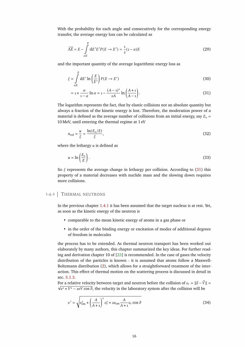
the process has to be extended. As thermal neutron transport has been worked outelaborately by many authors, this chapter summarized the key ideas. For further read-ing and derivation chapter 10 of [23] is recommended. In the case of gases the velocitydistribution of the particles is known - it is assumed that atoms follow a Maxwell-Boltzmann distribution (2), which allows for a straightforward treatment of the inter-action. This effect of thermal motion on the scattering process is discussed in detail insec. 5.1.3.For a relative velocity between target and neutron before the collision of 𝑣𝑟 = ‖®𝑣 − ®𝑉 ‖ =√𝑣2 +𝑉 2 − 2𝑣𝑉 cos𝜗 , the velocity in the laboratory system after the collision will be

𝑣 ′ =

√𝑣2cm +

(𝐴

𝐴 + 1

)2𝑣2𝑟 + 2𝑣cm

𝐴

𝐴 + 1𝑣𝑟 cos𝜗 (34)

16

and the largest and smallest velocities are

𝑣max = 𝑣cm + 𝐴

𝐴 + 1𝑣𝑟 and 𝑣min = 𝑣cm − 𝐴

𝐴 + 1𝑣𝑟 . (35)

The total cross section as to the third term of (9) is obtained by integrating the micro-scopic cross section

d𝜎 (𝑣 ′,𝑉 , cos𝜗) = 1

2

𝑣𝑟

𝑣 ′ 𝜎free𝑠 𝑝 (𝑉 ) d𝑉 dcos𝜗 , (36)

which relates the free elastic scattering cross section 𝜎 free𝑠 to the probability of interact-

ing with a target nucleus having a velocity distribution 𝑝 (𝑉 ). So the probability of avelocity change of the neutron 𝑣 𝜘→ 𝑣 ′ is represented by the modified cross section

𝜎 (𝑣 𝜘→ 𝑣 ′) d𝑣 =1

2

1

𝑣 ′

8∫0

d𝑉

1∫−1

𝑣𝑟 dcos𝜗 𝜎 free𝑠 𝑝 (𝑉 ) 𝑔(𝑣 ′ 𝜘→ 𝑣) d𝑣 (37)

with

𝑔(𝑣 ′ 𝜘→ 𝑣) =

0, 𝑣 < 𝑣min or 𝑣 > 𝑣max

2𝑣𝑣2max−𝑣2min

, 𝑣min < 𝑣 < 𝑣max.(38)

By integrating (36) over 𝑉 and cos𝜗 and substituting velocities by energy the totalcross section can be obtained[ac]:

𝜎𝑠 (𝐸 ′) = 𝜎 free𝑠

1

𝛽2√𝜋Ψ (𝛽) , (39)

where 𝛽2 = 𝐴𝐸 ′/𝑘𝐵𝑇 and

Ψ (𝛽) = 𝛽 exp (−𝛽2) + (2𝛽2 + 1)√𝜋

2erf(𝛽). (40)

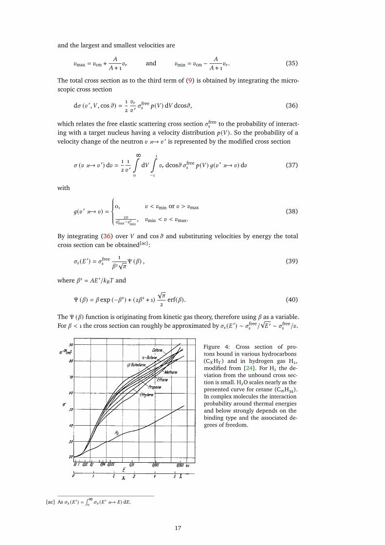
The Ψ (𝛽) function is originating from kinetic gas theory, therefore using 𝛽 as a variable.For 𝛽 < 1 the cross section can roughly be approximated by 𝜎𝑠 (𝐸 ′) ∼ 𝜎 free

𝑠 /√𝐸 ′ ∼ 𝜎 free

𝑠 /𝑣 .

Figure 4: Cross section of pro-tons bound in various hydrocarbons(C𝑋H𝑌 ) and in hydrogen gas H2,modified from [24]. For H2 the de-viation from the unbound cross sec-tion is small. H2O scales nearly as thepresented curve for cetane (C16H34).In complex molecules the interactionprobability around thermal energiesand below strongly depends on thebinding type and the associated de-grees of freedom.

[ac] As 𝜎𝑠 (𝐸 ′) =∫ 8

0𝜎𝑠 (𝐸 ′ 𝜘→ 𝐸) d𝐸.

17

2T H E P H Y S I C S O F E L E C T R O M A G N E T I CI N T E R A C T I O N S

All charged particles dissipate energy while crossing a medium. Depending on theparticle species and the material, different processes play a role. The most importantprocesses are in ascending order of the energy range: Electron excitation of atoms,ionization, Bremsstrahlung, pair production, nuclear excitation and following the rela-tivistic processes like Cherenkov and transition radiation, which are not relevant here.

2.1 ENERGY LOSS IN THE MEDIUM

2.1.1 ENERGY LOSS BY IONIZATION

The Bethe[a]-Bloch[b] equation describes the energy loss d𝐸 per length d𝑥 in a medium:

−d𝐸d𝑥

= 2𝜋𝑁𝐴𝑟2𝑒𝑚𝑒𝑐

2𝜌𝑍

𝐴

𝑧2

𝛽2

(ln

(2𝑚𝑒𝛾

2𝑐2𝛽2𝑊max

𝐼 2

)− 2𝛽2 − 𝛿 − 2

𝐶

𝑍

). (41)

𝑟𝑒 classical electron radius 𝜌 weight density

𝑚𝑒 electron mass 𝑧 projectile charge

𝑁𝐴 Avogadro number 𝛽 = 𝑣/𝑐 projectile velocity

𝐼 mean excitation potential 𝛾 = (1 − 𝛽2)−1/2

𝑍 charge number 𝛿 density correction

𝐴 atomic weight 𝐶 shell correction

The scaling constants are often combined to

^ = 2𝜋𝑁𝐴𝑟2𝑒𝑚𝑒𝑐

2 𝑍

𝐴

1

𝛽2. (42)

The maximum energy transfer𝑊max possible in a single head-on collision for an incidentprojectile of mass 𝑚𝐴 can be calculated as follows:

𝑊max =2𝑚𝑒𝑐

2𝛽2𝛾2

1 + 2𝑚𝑒

𝑚𝐴

√1 + 𝛽2𝛾2 + 𝑚2

𝑒

𝑚𝐴

. (43)

For 𝑚𝐴 �𝑚𝑒 the energy transfer can be approximated as

𝑊max ≈ 2𝑚𝑒𝑐2𝛽2𝛾2. (44)

The density factor is a correction for projectiles of high energies and describes thepolarization of the atoms in the medium along the path, whereas the shell correctionaccounts for projectiles which have a velocity in the order of or smaller than those of

[a] Hans Albrecht BETHE, *1906-†2005, German Empire.[b] Felix BLOCH, *1905-†1983, Switzerland.

19

the electrons orbiting the target atoms. These empirical constants are mainly importantfor relativistic particles. The mean excitation potential can be approximated by

𝐼 ≈ 16 eV · 𝑍0.9. (45)

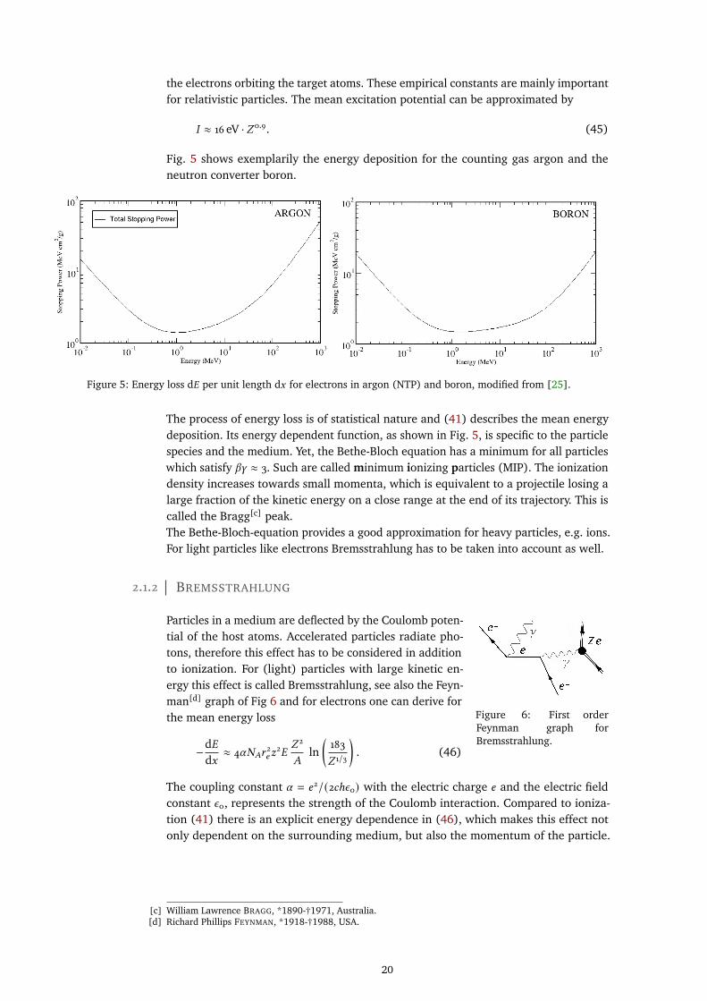
Fig. 5 shows exemplarily the energy deposition for the counting gas argon and theneutron converter boron.

Figure 5: Energy loss d𝐸 per unit length d𝑥 for electrons in argon (NTP) and boron, modified from [25].

The process of energy loss is of statistical nature and (41) describes the mean energydeposition. Its energy dependent function, as shown in Fig. 5, is specific to the particlespecies and the medium. Yet, the Bethe-Bloch equation has a minimum for all particleswhich satisfy 𝛽𝛾 ≈ 3. Such are called minimum ionizing particles (MIP). The ionizationdensity increases towards small momenta, which is equivalent to a projectile losing alarge fraction of the kinetic energy on a close range at the end of its trajectory. This iscalled the Bragg[c] peak.The Bethe-Bloch-equation provides a good approximation for heavy particles, e.g. ions.For light particles like electrons Bremsstrahlung has to be taken into account as well.

2.1.2 BREMSSTRAHLUNG

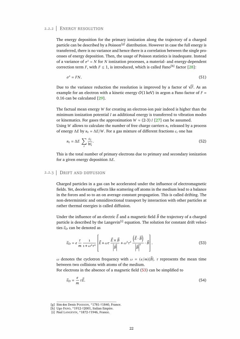
Particles in a medium are deflected by the Coulomb poten-

Figure 6: First orderFeynman graph forBremsstrahlung.

tial of the host atoms. Accelerated particles radiate pho-tons, therefore this effect has to be considered in additionto ionization. For (light) particles with large kinetic en-ergy this effect is called Bremsstrahlung, see also the Feyn-man[d] graph of Fig 6 and for electrons one can derive forthe mean energy loss

−d𝐸d𝑥

≈ 4𝛼𝑁𝐴𝑟2𝑒𝑧

2𝐸𝑍 2

𝐴ln

(183

𝑍 1/3

). (46)

The coupling constant 𝛼 = 𝑒2/(2𝑐ℎ𝜖0) with the electric charge 𝑒 and the electric fieldconstant 𝜖0, represents the strength of the Coulomb interaction. Compared to ioniza-tion (41) there is an explicit energy dependence in (46), which makes this effect notonly dependent on the surrounding medium, but also the momentum of the particle.

[c] William Lawrence BRAGG, *1890-†1971, Australia.[d] Richard Phillips FEYNMAN, *1918-†1988, USA.

20

Therefore one can summarize all constants of (46) under the term radiation length 𝑋0

and write

−d𝐸d𝑥

=𝐸

𝑋0

. (47)

As the differential equation (47) can be solved by an exponential function of the formexp(−𝑥/𝑋0), the radiation length defines the distance in which the energy of the particledrops to 1/𝑒 of its original value.

2.1.3 MULTIPLE SCATTERING

Multiple Scattering describes a manifold of Coulomb deflections. Such are mostly weak,which means that the trajectory of a particle keeps its general direction. A simplifiedmodel [26] of this statistical process leads to a particle of momentum 𝑝 after a distance𝑥 to a gaussian[e] distribution of the scattering angles around the original axis of thetrajectory 𝜗 = 0 with a width of

𝜎𝜗 =13.6MeV

𝛽𝑐𝑝

√𝑥

𝑋0

. (48)

2.2 PROCESSES IN GASEOUS MEDIA

Particles can be detected via their ionization track in a gas. In the case of neutrons a so-called converter captures the uncharged particle by nuclear absorption and then eitherfragments or releases excitation or binding energy in form of radiation. This chaptersummarizes the relevant physics starting from the ionization track to the transport andgas gain, which is necessary to detect the electron cloud.

2.2.1 IONIZATION

In a small finite volume the Landau[f] distribution [27] describes the possible energytransfer to a host atom. The Landau distribution approximates the energy loss for thinabsorbers, which do not significantly reduce the overall momentum of the propagatingparticle. Due to the large amount of collisions with small momentum transfer, theLandau distribution has a maximum at low values and has a positive skew towardshigher values, which model the unlikely hard collisions with large energy transfers. Ittakes the following form

𝑓 (Λ) = 1√2𝜋

𝑒−12 (Λ+𝑒−Λ) , (49)

whereas for a length element 𝑥 of an absorber of a density 𝜌 the quantity Λ = (Δ𝐸 −Δ𝐸𝑝 )/(^𝜌𝑥) describes the deviation of a possible energy loss Δ𝐸 from its most probablevalue Δ𝐸𝑝 , which is the maximum of the Landau distribution. It can be calculatedby [26]

𝐸𝑝 = ^𝜌𝑥

[ln

(2𝑚𝑒𝑐

2𝛽2

𝐼 (1 − 𝛽2)

)+ ln

(^𝜌𝑥

𝐼

)+0, 2 − 𝛽2 − 𝛿

(𝛽

1 − 𝛽2

)]. (50)

[e] Johann Carl Friedrich GAUSS, *1777-†1855, Holy Roman Empire.[f] Lev Davidovicq Landau, *1908-†1968, Russian Empire.

21

2.2.2 ENERGY RESOLUTION

The energy deposition for the primary ionization along the trajectory of a chargedparticle can be described by a Poisson[g] distribution. However in case the full energy istransferred, there is no variance and hence there is a correlation between the single pro-cesses of energy deposition. Then, the usage of Poisson statistics is inadequate. Insteadof a variance of 𝜎2 = 𝑁 for 𝑁 ionization processes, a material- and energy-dependentcorrection term 𝐹 , with 𝐹 ≤ 1, is introduced, which is called Fano[h] factor [28]:

𝜎2 = 𝐹𝑁 . (51)

Due to the variance reduction the resolution is improved by a factor of√𝐹 . As an

example for an electron with a kinetic energy O(1 keV) in argon a Fano factor of 𝐹 =

0.16 can be calculated [29].

The factual mean energy𝑊 for creating an electron-ion pair indeed is higher than theminimum ionization potential 𝐼 as additional energy is transferred to vibration modesor kinematics. For gases the approximation𝑊 ≈ (2-3) 𝐼 [27] can be assumed.Using𝑊 allows to calculate the number of free charge carriers 𝑛𝑡 released by a processof energy Δ𝐸 by 𝑛𝑡 = Δ𝐸/𝑊 . For a gas mixture of different fractions 𝑐𝑖 one has

𝑛𝑡 = Δ𝐸∑𝑖

𝑐𝑖

𝑊𝑖

. (52)

This is the total number of primary electrons due to primary and secondary ionizationfor a given energy deposition Δ𝐸.

2.2.3 DRIFT AND DIFFUSION

Charged particles in a gas can be accelerated under the influence of electromagneticfields. Yet, decelerating effects like scattering off atoms in the medium lead to a balancein the forces and so to an on average constant propagation. This is called drifting. Thenon-deterministic and omnidirectional transport by interaction with other particles atrather thermal energies is called diffusion.

Under the influence of an electric ®𝐸 and a magnetic field ®𝐵 the trajectory of a chargedparticle is described by the Langevin[i] equation. The solution for constant drift veloci-ties ®𝑣𝐷 can be denoted as

®𝑣𝐷 = 𝑒𝜏

𝑚

1

1 +𝜔2𝜏2

®𝐸 +𝜔𝜏®𝐸 × ®𝐵��� ®𝐵��� +𝜔2𝜏2

(®𝐸 · ®𝐵

)��� ®𝐵���2 · ®𝐵 . (53)

𝜔 denotes the cyclotron frequency with 𝜔 = (𝑒/𝑚) | ®𝐵 |. 𝜏 represents the mean timebetween two collisions with atoms of the medium.For electrons in the absence of a magnetic field (53) can be simplified to

®𝑣𝐷 =𝑒

𝑚𝜏 ®𝐸. (54)

[g] Siméon Denis POISSON, *1781-†1840, France.[h] Ugo FANO, *1912-†2001, Italian Empire.[i] Paul LANGEVIN, *1872-†1946, France.

22

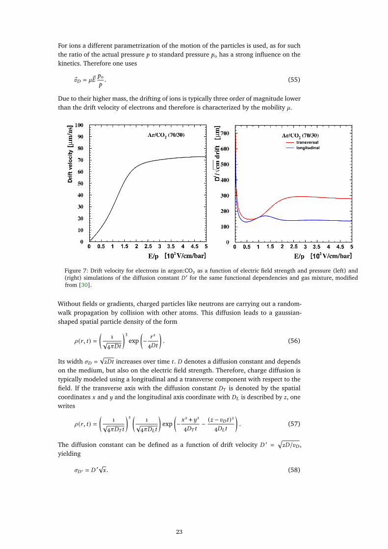
For ions a different parametrization of the motion of the particles is used, as for suchthe ratio of the actual pressure 𝑝 to standard pressure 𝑝0 has a strong influence on thekinetics. Therefore one uses

®𝑣𝐷 = ` ®𝐸 𝑝0

𝑝. (55)

Due to their higher mass, the drifting of ions is typically three order of magnitude lowerthan the drift velocity of electrons and therefore is characterized by the mobility `.

Figure 7: Drift velocity for electrons in argon:CO2 as a function of electric field strength and pressure (left) and(right) simulations of the diffusion constant 𝐷 ′ for the same functional dependencies and gas mixture, modifiedfrom [30].

Without fields or gradients, charged particles like neutrons are carrying out a random-walk propagation by collision with other atoms. This diffusion leads to a gaussian-shaped spatial particle density of the form

𝜌 (𝑟 , 𝑡) =(

1√4𝜋𝐷𝑡

)3exp

(− 𝑟 2

4𝐷𝑡

). (56)

Its width 𝜎𝐷 =√2𝐷𝑡 increases over time 𝑡 . 𝐷 denotes a diffusion constant and depends

on the medium, but also on the electric field strength. Therefore, charge diffusion istypically modeled using a longitudinal and a transverse component with respect to thefield. If the transverse axis with the diffusion constant 𝐷𝑇 is denoted by the spatialcoordinates 𝑥 and 𝑦 and the longitudinal axis coordinate with 𝐷𝐿 is described by 𝑧, onewrites

𝜌 (𝑟 , 𝑡) =(

1√4𝜋𝐷𝑇 𝑡

)2 (1

√4𝜋𝐷𝐿𝑡

)exp

(−𝑥

2 +𝑦24𝐷𝑇 𝑡

− (𝑧 − 𝑣𝐷𝑡)24𝐷𝐿𝑡

). (57)

The diffusion constant can be defined as a function of drift velocity 𝐷 ′ =√2𝐷/𝑣𝐷 ,

yielding

𝜎𝐷 ′ = 𝐷 ′√𝑥 . (58)

23

2.2.4 GAS GAIN

Typically the primary ionization is often not sufficient to generate a signal large enoughfor detection. A gaseous medium allows for applying the principle of charge multipli-cation. If electrons, e.g. the primary charge carriers, can be accelerated to energies,which are high enough to ionize other atoms of the medium, an avalanche effect oc-curs, which can increase the number of electrons by a factor of 104 to 106. The socreated additional electron-ion pairs d𝑁 for an actual number of electrons 𝑁 satisfiesthe differential equation

d𝑁 = 𝛼 (𝑟 )𝑁 (𝑟 )d𝑟 , (59)

whereas 𝛼 denotes the Townsend[j] coefficient, which depends on the track lengthcoordinate 𝑟 as far as the electric field strength changes. The solution for an initialnumber of final charge carriers 𝑁total for an initial number of charge carriers 𝑁0 takesthe following form

𝑁total = 𝑁0 exp ©­«𝑟2∫

𝑟 1

𝛼 (𝑟 )d𝑟ª®¬ . (60)

The ratio 𝐺 = 𝑁total/𝑁0 is called gas gain.

[j] Sir John Sealy Edward TOWNSEND, *1868-†1957, Ireland.

24

Part II

N E U T R O N S O U R C E S

3N AT U R A L S O U R C E S : C O S M I C N E U T R O N S

Due to the limited lifetime of approximately 15 minutes, all free neutrons, naturallyabundant or from laboratory sources, originate from an ongoing production mechanism- either the interaction of cosmic radiation with the atmosphere and the soil or naturalradioactivity, which can sometimes even scale up to so-called „natural reactors“ [31].The following section presents a short overview about how cosmic neutrons are created.A good summary can also be found in [32].

3.1 FROM SUPERNOVAE TO SEA LEVEL

Cosmic rays consist mostly of ionizedatomic nuclei with protons being the mostabundant species with a contribution of90 % of the total measured particle num-ber, followed by helium ions. The fractionof electrons, positrons, antiprotons, gammarays and neutrinos can be considered neg-ligible. The net charge of the cosmic radi-ation is highly positive with protons beingoverrepresented with a ratio of 10:1 [33].While in general sources, also on galacticscales [34], are charge conserving, the rea-son for this asymmetry is inverse Comptonscattering [35]. This effect leads to espe-cially light charged particles like electronslosing energy by interactions with photonsof the cosmic microwave background andtherefore being slowed down more effi-ciently than their hadronic partners.The cosmic ray spectrum, see Fig. 8, ex-tends from the MeV regime up to ZeV en-ergies with meanwhile more than a dozencandidates of extremely high energies of∼1020 eV, observed by the Fly’s Eye detec-tor [36].

Figure 8: Energies and rates of the primary cosmic ray par-ticles before entering the atmosphere from various experi-ments [37].

The lowest part of the spectrum is result of the solar wind, ∼1036 particles per secondreleased from the plasma of the Sun’s corona and especially from solar flares [38].Particles in the range of 1 GeV to ∼100 TeV mostly come from supernova remnants.Therefore, the cosmic ray flux has one component of extragalactic origin overlayed bythe charge emission from the Sun with a separation of low energy and high energycontributions. Theoretical considerations of the diffusive shock acceleration[a] neededto achieve such energies [39] as well as observations from the Crab nebula1 can heavily 1 NGC 1952

support these generators, see also the overview in [40]. For higher energies the pro-duction and transport mechanisms change around the points, which in the log-log plot

[a] thermal cosmic rays passing a dense matter distribution in which the strong magnetic gradient leads to anacceleration by turning several times around the ’shock’ region.

27

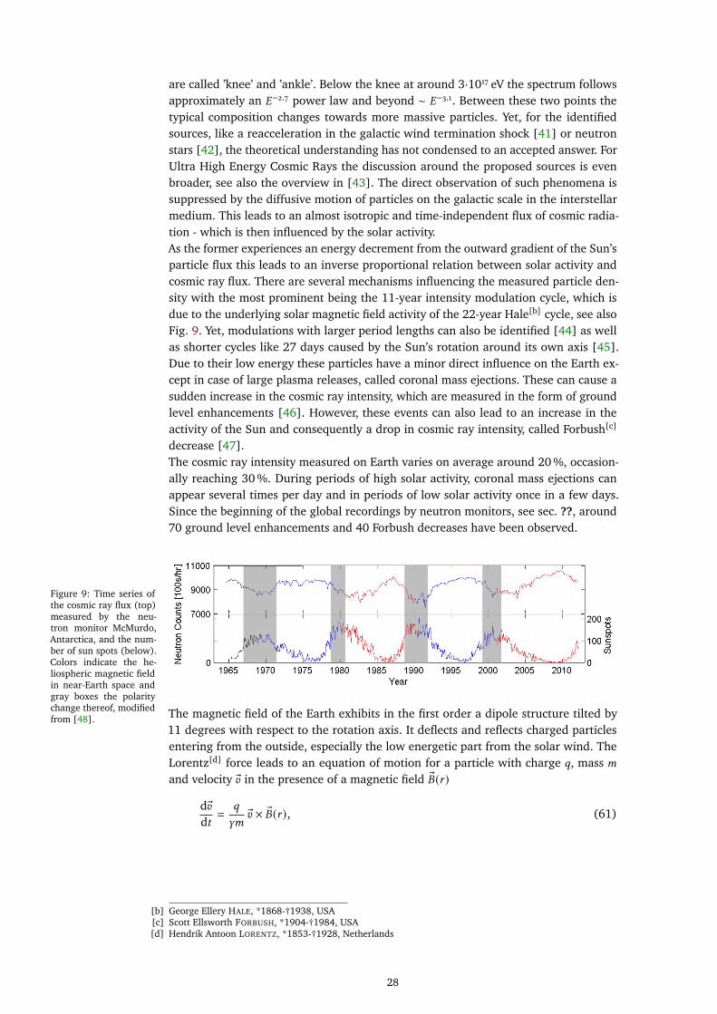
are called ’knee’ and ’ankle’. Below the knee at around 3·1017 eV the spectrum followsapproximately an 𝐸−2.7 power law and beyond ∼ 𝐸−3.1. Between these two points thetypical composition changes towards more massive particles. Yet, for the identifiedsources, like a reacceleration in the galactic wind termination shock [41] or neutronstars [42], the theoretical understanding has not condensed to an accepted answer. ForUltra High Energy Cosmic Rays the discussion around the proposed sources is evenbroader, see also the overview in [43]. The direct observation of such phenomena issuppressed by the diffusive motion of particles on the galactic scale in the interstellarmedium. This leads to an almost isotropic and time-independent flux of cosmic radia-tion - which is then influenced by the solar activity.As the former experiences an energy decrement from the outward gradient of the Sun’sparticle flux this leads to an inverse proportional relation between solar activity andcosmic ray flux. There are several mechanisms influencing the measured particle den-sity with the most prominent being the 11-year intensity modulation cycle, which isdue to the underlying solar magnetic field activity of the 22-year Hale[b] cycle, see alsoFig. 9. Yet, modulations with larger period lengths can also be identified [44] as wellas shorter cycles like 27 days caused by the Sun’s rotation around its own axis [45].Due to their low energy these particles have a minor direct influence on the Earth ex-cept in case of large plasma releases, called coronal mass ejections. These can cause asudden increase in the cosmic ray intensity, which are measured in the form of groundlevel enhancements [46]. However, these events can also lead to an increase in theactivity of the Sun and consequently a drop in cosmic ray intensity, called Forbush[c]

decrease [47].The cosmic ray intensity measured on Earth varies on average around 20 %, occasion-ally reaching 30 %. During periods of high solar activity, coronal mass ejections canappear several times per day and in periods of low solar activity once in a few days.Since the beginning of the global recordings by neutron monitors, see sec. ??, around70 ground level enhancements and 40 Forbush decreases have been observed.

Figure 9: Time series ofthe cosmic ray flux (top)measured by the neu-tron monitor McMurdo,Antarctica, and the num-ber of sun spots (below).Colors indicate the he-liospheric magnetic fieldin near-Earth space andgray boxes the polaritychange thereof, modifiedfrom [48]. The magnetic field of the Earth exhibits in the first order a dipole structure tilted by

11 degrees with respect to the rotation axis. It deflects and reflects charged particlesentering from the outside, especially the low energetic part from the solar wind. TheLorentz[d] force leads to an equation of motion for a particle with charge 𝑞, mass 𝑚and velocity ®𝑣 in the presence of a magnetic field ®𝐵(𝑟 )

d®𝑣d𝑡

=𝑞

𝛾𝑚®𝑣 × ®𝐵(𝑟 ), (61)

[b] George Ellery HALE, *1868-†1938, USA[c] Scott Ellsworth FORBUSH, *1904-†1984, USA[d] Hendrik Antoon LORENTZ, *1853-†1928, Netherlands

28

where 𝛾 = 1/√1 − 𝑣2/𝑐2 is the Lorentz factor. Depending on the inclination angle to the

field a particle spirals around the field lines with a radius 𝑟

𝑞®𝑣 × ®𝐵(𝑟 ) = 𝛾𝑚®𝑣2𝑟

, (62)

which can be written in scalar form as

𝐵𝑟 =𝛾𝑚𝑣

𝑞=𝑝

𝑞(63)

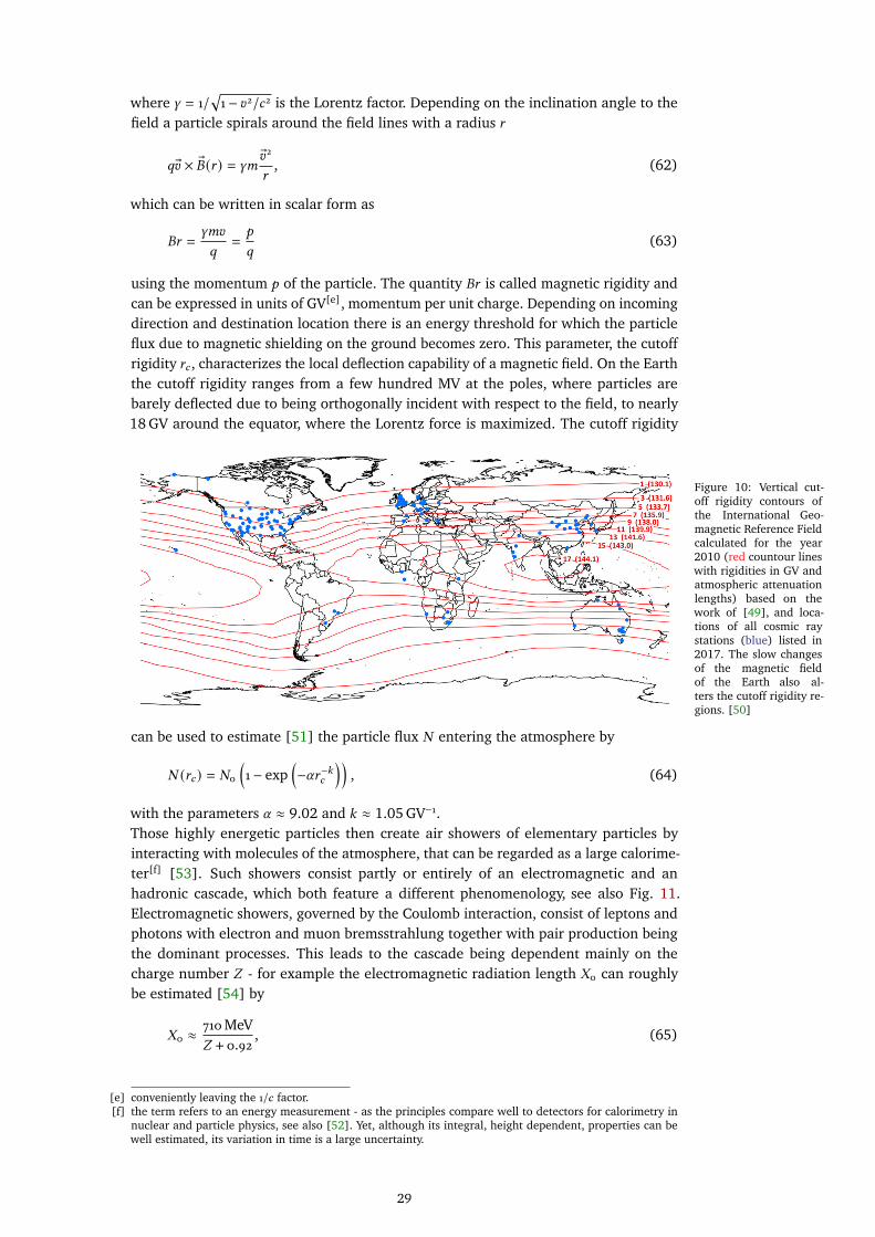
using the momentum 𝑝 of the particle. The quantity 𝐵𝑟 is called magnetic rigidity andcan be expressed in units of GV[e], momentum per unit charge. Depending on incomingdirection and destination location there is an energy threshold for which the particleflux due to magnetic shielding on the ground becomes zero. This parameter, the cutoffrigidity 𝑟𝑐 , characterizes the local deflection capability of a magnetic field. On the Earththe cutoff rigidity ranges from a few hundred MV at the poles, where particles arebarely deflected due to being orthogonally incident with respect to the field, to nearly18 GV around the equator, where the Lorentz force is maximized. The cutoff rigidity

Figure 10: Vertical cut-off rigidity contours ofthe International Geo-magnetic Reference Fieldcalculated for the year2010 (red countour lineswith rigidities in GV andatmospheric attenuationlengths) based on thework of [49], and loca-tions of all cosmic raystations (blue) listed in2017. The slow changesof the magnetic fieldof the Earth also al-ters the cutoff rigidity re-gions. [50]

can be used to estimate [51] the particle flux 𝑁 entering the atmosphere by

𝑁 (𝑟𝑐 ) = 𝑁0

(1 − exp

(−𝛼𝑟−𝑘𝑐

)), (64)

with the parameters 𝛼 ≈ 9.02 and 𝑘 ≈ 1.05 GV−1.Those highly energetic particles then create air showers of elementary particles byinteracting with molecules of the atmosphere, that can be regarded as a large calorime-ter[f] [53]. Such showers consist partly or entirely of an electromagnetic and anhadronic cascade, which both feature a different phenomenology, see also Fig. 11.Electromagnetic showers, governed by the Coulomb interaction, consist of leptons andphotons with electron and muon bremsstrahlung together with pair production beingthe dominant processes. This leads to the cascade being dependent mainly on thecharge number 𝑍 - for example the electromagnetic radiation length 𝑋0 can roughlybe estimated [54] by

𝑋0 ≈ 710MeV𝑍 + 0.92

, (65)

[e] conveniently leaving the 1/𝑐 factor.[f] the term refers to an energy measurement - as the principles compare well to detectors for calorimetry in

nuclear and particle physics, see also [52]. Yet, although its integral, height dependent, properties can bewell estimated, its variation in time is a large uncertainty.

29

which leads to 𝑋 air0 ≈ 86 MeV ≈ 37 g/cm2 ≈ 310 m for dry air [55]. One can com-

pare this value to the total scale height of the atmosphere ℎ0 ≈ 8400 m, known fromthe barometric pressure formula. Therefore, a substantial part of a shower will be ab-sorbed in the atmosphere. Hadronic showers are mainly created in collisions of protonswith other nuclei. They can also be comprised of an electromagnetic component[g]

but mainly consist of particles, which interact by the strong force, like pions. Unlikecascades governed by Coulomb force, hadronic interactions at high energies are muchmore complicated in their event topology and less well understood on the level of per-turbative quantum chromo dynamics. However, a number of phenomenological modelshave been developed. For energies in the lower GeV range soft multiparticle productionwith small transverse momenta are the dominant feature [56]. At higher energies ofthe projectile additionally hard scattering of partons carrying only a small fraction ofthe momentum of the hadron can take place, which leads to smaller sub-cascades [57].For much higher energies gluon interactions finally start to compete with quark-quarkinteractions.

Figure 11: Air showers: (left) Feynman graph representation of electromagnetic and hadronic cascades with thetypical interaction lengths [58] and (right) simulation of leptons, hadrons and heavy nuclei in the atmosphere (samescale) [59].

The hadronic interaction length _had therefore mainly depends on the atomic number𝐴 and their corresponding cross section.

_had ∼ 1

𝑛𝜎0𝐴2/3 , (66)

whereas the mean cross section 𝜎0 being specific for the particle species. For examplethe interaction length for GeV pions in air amounts to _𝜋had ≈ 120 g/cm2 [55]. This leadsto hadronic showers in general developing faster due to the multiplicity and lastinglonger as the hadronic cross section is smaller than in the electromagnetic case.One of the by-products in these cascades are neutrons. Although neither being presentin cosmic radiation nor being the dominant production channel neutrons make up alarge part of the particles at ground level as their interaction probability is smallercompared to charged particles and their lifetime is long enough to traverse the atmo-sphere, see also Fig. 12. The neutron density increases until a height of around 20 kmor (50-100) g/cm2, the so-called Pfotzer[h] maximum [60], by spallation reactions inthe upper atmosphere, and beyond it follows a simple exponential law as a functionof atmospheric depth. As seen in Fig. 12, the initial flux decreases by several ordersof magnitude with only marginal deviations of the base spectrum until reaching theground level.

[g] Muons are for example primarily produced by pion decay, which is mediated by the weak force.[h] Georg PFOTZER, *1909-†1981, German Empire

30

Figure 12: Atmosphericdepth dependencies of ef-fective dose rates at 𝑟𝑐 =

0GV for solar minimumconditions in log-linear(left) and log-log repre-sentation (right), calcula-tions carried out usingPARMA [61].

The spectrum of cosmic-ray induced neutrons, see Fig. 13, offers some distinct featureswith three prominent peaks, which originate from the physics involved from the processof creation until absorption, see here sec. 1.4. Highly energetic neutrons at ≈ 100 MeVare produced as secondary particles by intra-nuclear cascades and pre-equilibriumprocesses [62]. When high-energy neutrons or protons interact with atoms of theatmosphere, the excited nuclei evaporate neutrons at a lower energy. This processmanifests itself at the peak at ≈ 1 MeV and shows additional absorption fine structuredue to distinct resonances of non-hydrogen atoms, especially oxygen, compare alsothe cross sections in Fig. 31. Neutron interactions in the sub-MeV region are entirelydominated by elastic collisions, in which the energy loss is correlated to the mass ofthe target nucleus. Due to the mass of hydrogen being nearly equal to the one ofthe neutron, this energy band is most sensitive to water and organic molecules andthus most relevant for the method of cosmic ray neutron sensing. Below ≈ 1 eV thekinetic energy of the target, which is usually in thermal equilibrium at 𝑘B𝑇 ≈ 25 meV,significantly contributes to the neutron’s energy during a collision. As a consequence,neutrons finally become thermalized at ≈ 25 meV. Since neutrons cannot leave thethermal equilibrium they perform a random walk until they are absorbed[i].

Figure 13: The cosmicray neutron spectrumwith its differentdomains. Data (his-togrammed) from [65]and analytical descrip-tion (dashed line)by [66].

1 MeV1 keV1 eV

thermalized

neutrons

-2E

dφ/dE

[cm

/s,

arb

. sc

ale

]

deceleration

equilibrium

epithermal/fast neutrons fast neutron

creation by

evaporation

high-energy

neutrons

(primary)

1 meV 1 GeV

[i] The dominant channel [63] is absorption by nitrogen, 14N +𝑛 𝜘→14 C, being the main source of atmosphericcarbon-14 used in radiocarbon dating for inferring the chronometric age for materials recovered fromarcheological contexts [64].

31

3.2 ANALYTICAL DESCRIPTION OF THE COSMIC RAY NEUTRON SPECTRUM

Cosmic ray propagation in the atmosphere has been modeled extensively by Sato etal. [66] using PARMA [67], which is based on PHITS [68], see also sec. 5.2.1. Theyprovide an energy spectrum of cosmic ray neutrons for a variety of altitudes, cutoff-rigidities, solar modulation potentials and surface conditions. These simulations havebeen validated with various independent measurements, i.e. [65] and [69], at differentaltitudes and locations on Earth. Moreover, the analytical formulations of the spectraturned out to be effective in use for subsequent calculations. The presented energy-dependent flux 𝜙 (𝐸) is described by a mean basic spectrum 𝜙B, a function for neutronsbelow 15 MeV 𝜙L, an extension for thermal neutrons 𝜙th, and a modifier 𝑓G for thegeometry of the interface, which is defined by the ratio in comparison to a hypotheticalspectrum of a semi-infinite atmosphere:

𝜙 (𝑠, 𝑟𝑐 ,𝑑,𝐸,𝑤) = 𝜙B (𝑠, 𝑟𝑐 ,𝑑,𝐸) · (𝑓G (𝐸,𝑤) +𝜙th (𝐸,𝑤)) · 𝜙L (𝑠, 𝑟𝑐 ,𝑑) . (67)

The individual terms are

𝜙B (𝑠, 𝑟𝑐 ,𝑑,𝐸) =

0.229(𝐸

2.31

)0.721

exp(− 𝐸

2.31

)+ 𝑐4 (𝑑) exp

(− (log(𝐸) − log(126))2

2 (log(2.17))2)

+ 0.00108 log(

𝐸

3.331012

)·(1 + tanh

(1.62 log

(𝐸

9.59108

))) (1 − tanh

(1.48 log

(𝐸

𝑐12

))), (68)

log (𝑓G (𝐸,𝑤)) = −0.0235−0.0129(log(𝐸) −𝑔3 (𝑤)

) (1 − tanh

(0.969 log

(𝐸

𝑔5 (𝑤)

))), (69)

𝜙L (𝑠, 𝑟𝑐 ,𝑑) = 𝑎1 (𝑟𝑐 )(exp (−𝑎2 (𝑟𝑐 )𝑑) − 𝑎3 (𝑟𝑐 ) exp

(−𝑎4 (𝑟𝑐 )𝑑

) ), (70)

and

𝜙T (𝐸𝑇 ,𝑤) = 0.118 + 0.144 exp (−3.87𝑤)1. + 0.653 exp(−42.8𝑤)

(𝐸

𝐸𝑇

)2exp

(−𝐸𝐸𝑇

), (71)

denoting the solar modulation potential 𝑠, cutoff rigidity 𝑟𝑐 , the weight fraction of water𝑤 and atmospheric depth 𝑑. 𝐸𝑇 = 𝑘𝐵𝑇 represents the thermal energy. The calculation ofthe individual parameters is described in appendix B.1.4 by (160). For some parametersthe solar modulation potential can be set to a minimum and a maximum condition,whereas here the latter has been chosen allowing to already expand many numericalvalues.

32

4A R T I F I C I A L H I G H F L U X S O U R C E S

4.1 OVERVIEW OF FACILITIES

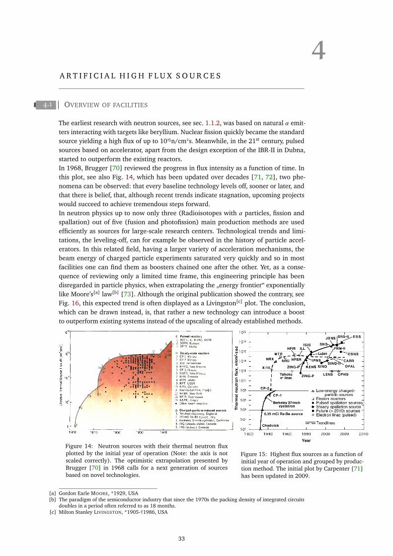
The earliest research with neutron sources, see sec. 1.1.2, was based on natural 𝛼 emit-ters interacting with targets like beryllium. Nuclear fission quickly became the standardsource yielding a high flux of up to 1015n/cm2s. Meanwhile, in the 21st century, pulsedsources based on accelerator, apart from the design exception of the IBR-II in Dubna,started to outperform the existing reactors.In 1968, Brugger [70] reviewed the progress in flux intensity as a function of time. Inthis plot, see also Fig. 14, which has been updated over decades [71, 72], two phe-nomena can be observed: that every baseline technology levels off, sooner or later, andthat there is belief, that, although recent trends indicate stagnation, upcoming projectswould succeed to achieve tremendous steps forward.In neutron physics up to now only three (Radioisotopes with 𝛼 particles, fission andspallation) out of five (fusion and photofission) main production methods are usedefficiently as sources for large-scale research centers. Technological trends and limi-tations, the leveling-off, can for example be observed in the history of particle accel-erators. In this related field, having a larger variety of acceleration mechanisms, thebeam energy of charged particle experiments saturated very quickly and so in mostfacilities one can find them as boosters chained one after the other. Yet, as a conse-quence of reviewing only a limited time frame, this engineering principle has beendisregarded in particle physics, when extrapolating the „energy frontier“ exponentiallylike Moore’s[a] law[b] [73]. Although the original publication showed the contrary, seeFig. 16, this expected trend is often displayed as a Livingston[c] plot. The conclusion,which can be drawn instead, is, that rather a new technology can introduce a boostto outperform existing systems instead of the upscaling of already established methods.

Figure 14: Neutron sources with their thermal neutron fluxplotted by the initial year of operation (Note: the axis is notscaled correctly). The optimistic extrapolation presented byBrugger [70] in 1968 calls for a next generation of sourcesbased on novel technologies.

Figure 15: Highest flux sources as a function ofinitial year of operation and grouped by produc-tion method. The initial plot by Carpenter [71]has been updated in 2009.

[a] Gordon Earle MOORE, *1929, USA[b] The paradigm of the semiconductor industry that since the 1970s the packing density of integrated circuits

doubles in a period often referred to as 18 months.[c] Milton Stanley LIVINGSTON, *1905-†1986, USA

33

To understand the limitations of actual neutron sources in their intensity, the character-istics of the production mechanisms are summarized in the following. Spallation andfission differ in their released neutron energy spectrum, which is significantly harderfor spallation. Both also contrast in their production mechanism. The overall numberof neutrons released per fission event is on average 2.4 for 235U, which is less thanthe incoming beam energy dependent 10-20 neutrons for spallation. Furthermore, infission one neutron is required to sustain the chain reaction and in typical fuel elementsnearly half of the remaining fraction of 239U ends in the production of plutonium. Forfission around 180 MeV is deposited as heat, for spallation in tungsten it is around32 MeV. In a fission process the average gamma energy deposited is 12 MeV, whereasfor spallation it is 2 MeV per neutron. Yet, for spallation the kinetic energy of the in-cident ion beam, which is dumped in the target, has to be added to the heat budget.Finally the limitation for the overall intensity is a trade-off between the source geom-etry, which focuses on maximizing the neutron flux in the surrounding moderator byminimizing self-absorption, and the cooling capabilities for a compact source or target.This effectively limits the thermal design power to ≈100 MW[d] and the total neutronflux to ≈ 1015 n/(cm2·s). Spallation sources can operate in a pulsed mode and thereforeachieve a much higher peak flux within the duty cycle.

Figure 16: The original Livingstonplot [74] shows the collision energy ofof different charged particle accelera-tors. The non-proton labeled entities de-note electron machines.

Figure 17: One of the rare graphs showingthat hadron and lepton synchrotrons and stor-age rings are reaching their technological lim-its in the 21st century [75].

Quod sumus, hoc eritis. Fuimus quandoque, quod estis.

[d] compared to 1500 MW per block for conventional nuclear power plants.

34

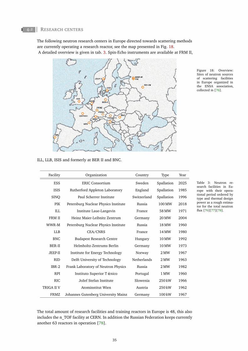
4.2 RESEARCH CENTERS

The following neutron research centers in Europe directed towards scattering methodsare currently operating a research reactor, see the map presented in Fig. 18.A detailed overview is given in tab. 3. Spin-Echo instruments are available at FRM II,

Figure 18: Overview:Sites of neutron sourcesof scattering facilitiesin Europe organized inthe ENSA association,collected in [76].

ILL, LLB, ISIS and formerly at BER II and BNC.

Table 3: Neutron re-search facilities in Eu-rope with their opera-tional period ordered bytype and thermal designpower as a rough estima-tor for the total neutronflux [76][77][78].

Facility Organization Country Type Year

ESS ERIC Consortium Sweden Spallation 2025

ISIS Rutherford Appleton Laboratory England Spallation 1985

SINQ Paul Scherrer Institute Switzerland Spallation 1996

PIK Petersburg Nuclear Physics Institute Russia 100 MW 2018

ILL Institute Laue-Langevin France 58 MW 1971

FRM II Heinz Maier-Leibnitz Zentrum Germany 20 MW 2004

WWR-M Petersburg Nuclear Physics Institute Russia 18 MW 1960

LLB CEA/CNRS France 14 MW 1980

BNC Budapest Research Centre Hungary 10 MW 1992

BER-II Helmholtz-Zentrums Berlin Germany 10 MW 1973

JEEP-II Institute for Energy Technology Norway 2 MW 1967

RID Delft University of Technology Netherlands 2 MW 1963

IBR-2 Frank Laboratory of Neutron Physics Russia 2 MW 1982

RPI Instituto Superior Técnico Portugal 1 MW 1960

RIC Jozef Stefan Institute Slowenia 250 kW 1966

TRIGA II V Atominstitut Wien Austria 250 kW 1962

FRMZ Johannes Gutenberg University Mainz Germany 100 kW 1967

The total amount of research facilities and training reactors in Europe is 48, this alsoincludes the n_TOF facility at CERN. In addition the Russian Federation keeps currentlyanother 63 reactors in operation [78].

35

4.3 THE FRM II SOURCE

The Forschungs-Neutronenquelle Heinz Maier-Leibnitz[e], FRM II, is a research reactorcooled by light water with a heavy water moderator. The compact fuel element [79],see Fig. 19 (left), has specifically been developed in order to achieve the highest ther-mal neutron flux [80] for its nominal power of 20 MW. The active core, see Fig. 19(right), consists of 113 curved AlMg3 embedded U3Si2 fuel elements between a cylinder6.75 cm (for the control rod) and 11.2 cm with an active region of 70 cm. The ura-nium is enriched to 93 % of 235U. A maximum of unperturbated thermal neutron fluxof 8·1014 n/cm2/s can be achieved, whereas typically a fuel element can be operatednon-stop for 60 days until the power density cannot be held any more, which meansthat the control rod is at its maximum position. Neutrons are extracted by guides whichare directed towards the region of highest flux but perpendicular to the line of sight tothe reactor core. This tangential arrangement significantly reduces the background ofgamma radiation and fast neutrons. Several dedicated moderators tailor the neutronenergy to the needs of specific instruments. Besides the room temperature (∼320 K) ofthe deuterium moderator there is a hot and a cold source, see below and Fig. 20. Thehot source consists of a cylindrical graphite block of 14 kg heated to 2300 K and the coldsource of a spherical containment for 12 l of liquid deuterium at 18 K. A fission neutronconverter can in turn again produce MeV-neutrons for the fast neutron tomography sta-tion [81]. Most of the eleven beam tubes (SR) supply experiments in the ExperimentalHall, which require the highest flux, and some are fanned out into the Neutron GuideHall (SR-1 split into six guides NL-1 to NL-6). The Spin Echo instruments RESEDA [82]and MIRA [83] are located at the end of NL-5 and NL-6, respectively. The HEiDi [84]single crystal diffractometer aims at the hot source.The spectrum of a moderator can be described in a first order approximation by aMaxwell-Boltzmann distribution (99), see also sec. 1.3.1. Fig. 20 shows the results ofsimulations of the neutron flux density at the beginning of the respective beam tubes.The D2O thermal neutron source can be well approximated by a distribution with atemperature of 318 K - as the heavy water moderator is sufficiently large to achieve athermally equilibrated flux. For the description of the hot and cold source the fit hasto be carried out by a sum of Maxwell-Boltzmann functions. As for technical reasonsboth vessels are limited in size the results are undermoderated spectra, which do notcorrespond to the temperature of the moderators but can be described by a thermalspectrum with shifts towards a cold or a hot thermal bath. Experiments then limit thephase space by wavelength selectors like choppers or monochromators.

Figure 19: Horizontalsection through the re-actor core with its dif-ferent moderators andbeam tubes (left). Thecylindrical fuel element(right) is specifically de-signed to maximize theflux per thermal power,modified from [85].

[e] Heinz MAIER-LEIBNITZ, *1911-†2000, Germany

36

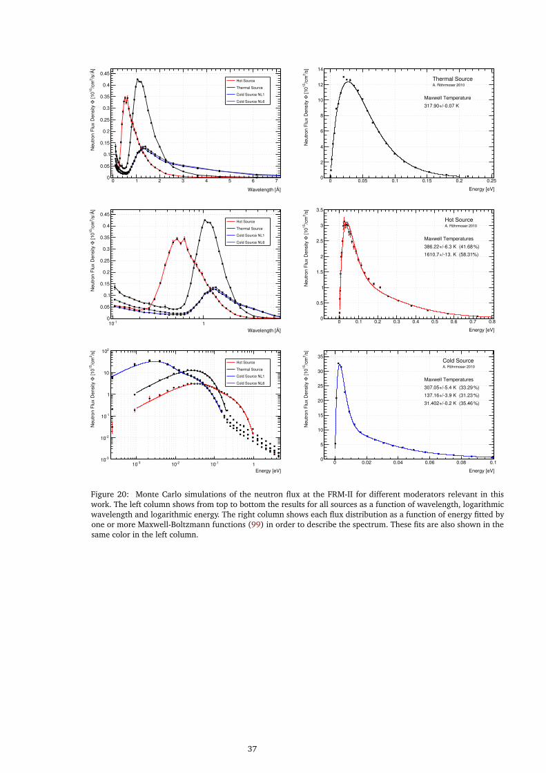
]ÅWavelength [

0 1 2 3 4 5 6 7

]Å

/s/

2/c

m15

[10

ΦN

eutr

on F

lux

Den

sity

0

0.05

0.1

0.15

0.2

0.25

0.3

0.35

0.4

0.45Hot Source

Thermal Source

Cold Source NL1

Cold Source NL6

Energy [eV]

0 0.05 0.1 0.15 0.2 0.25

/s]

2/c

m15

[10

ΦN

eutr

on F

lux

Den

sity

0

2

4

6

8

10

12

14

Thermal SourceA. Röhrmoser 2010

Maxwell Temperature

317.90+/-0.07 K

]ÅWavelength [

-110 1

]Å

/s/

2/c

m15

[10

ΦN

eutr

on F

lux

Den

sity

0

0.05

0.1

0.15

0.2

0.25

0.3

0.35

0.4

0.45Hot Source

Thermal Source

Cold Source NL1

Cold Source NL6

Energy [eV]

0 0.1 0.2 0.3 0.4 0.5 0.6 0.7 0.8

/s]

2/c

m15

[10

ΦN

eutr

on F

lux

Den

sity

0

0.5

1

1.5

2

2.5

3

3.5

Hot SourceA. Röhrmoser 2010

Maxwell Temperatures

)%386.22+/-6.3 K (41.68

)%1610.7+/-13. K (58.31

Energy [eV]

-310 -210 -110 1

/s]

2/c

m15

[10

ΦN

eutr

on F

lux

Den

sity

-310

-210

-110

1

10

210

Hot Source

Thermal Source

Cold Source NL1

Cold Source NL6

Energy [eV]

0 0.02 0.04 0.06 0.08 0.1

/s]

2/c

m15

[10

ΦN

eutr

on F

lux

Den

sity

0

5

10

15

20

25

30

35Cold SourceA. Röhrmoser 2010

Maxwell Temperatures

)%307.05+/-5.4 K (33.29

)%137.16+/-3.9 K (31.23

)%31.402+/-0.2 K (35.46

Figure 20: Monte Carlo simulations of the neutron flux at the FRM-II for different moderators relevant in thiswork. The left column shows from top to bottom the results for all sources as a function of wavelength, logarithmicwavelength and logarithmic energy. The right column shows each flux distribution as a function of energy fitted byone or more Maxwell-Boltzmann functions (99) in order to describe the spectrum. These fits are also shown in thesame color in the left column.

37

Part III

U R A N O S M O N T E C A R L O T R A N S P O R T C O D E

5M O D E L I N G A N D M O N T E C A R L O A P P R O A C H

The Monte Carlo [86] method is a brute-force calculation technique, which is usedfor complicated problems consisting of well-defined or independent sub-tasks. Themethod retains a close relation to the problem it is trying to solve by repeated randomsampling from a set of initial conditions. Although especially in high-energy physicsthe modeling of complicated particle interactions and transport problems by meansof such simulations have even become an own discipline, it has to be noted, that thefirst realization of this method in physics was carried out by the initiative of Fermi[a] inorder to solve problems of neutron transport. His FERMIAC [87], an analog computer,consisted of an adjustable trolley, which was able to ray-trace neutron paths on a twodimensional technical drawing. In the same year, 1947, von Neumann[b] then set upsimilar programs [88] on the first entirely digital computer, the ENIAC [89], in orderto calculate thermonuclear reactions in spherical symmetric geometry [90].

5.1 SAMPLING

The Monte Carlo approach is a stochastic method, in which a randomly chosen subsetof a system is used as an estimator for specific parameters, observables of the system.The requirements are

• the sample space 𝑆 is defined,

• the values associated with the sample space need to be accessible, either bya known probability distribution function 𝑓 (𝑥) or

an invertible cumulative probability distribution 𝐹 (𝑥) =𝑥∫

− 8

𝑓 (𝑡) d𝑡 ,

• a method for the generation of random numbers.

After one or more random numbers b𝑖 have been chosen there are two methods forevaluation. The sampling by rejection accepts a random number if sampling by rejection

𝑓 (b1) < b2, (72)

whereas for real b ∈ [0, 1] the support and the codomain of the function should benormalized accordingly, i.e. ‖ 𝑓 ‖max ≤ 1. Then the result will be 𝑥 = b .The sampling by the inverse cumulative distribution function calculates the resulting sampling by the inverse

cumulative functionnumber by

𝑥 = 𝐹−1 (b). (73)

5.1.1 RANDOM NUMBER GENERATION

The pseudo-random number generator TRandom3 uses the Mersenne[c]-Twister algo-rithm MT 19937 [91] based on the Mersenne prime number 19937. It has the followingfeatures:

[a] Enrico FERMI, *1901-†1954, Kingdom of Italy.[b] John VON NEUMANN, *1903-†1957, Austro-Hungarian Empire.[c] Marin MERSENNE, *1588-†1648, France.

41

• a very long period of 𝑝 = 219937 − 1 ≈ 4.3 · 106001[d],

• low correlation between subsequent numbers (k-distributed for the output se-quence),

• relatively fast, as it generates the output sequence of 624 32bit integers at once.

The random generator is seeded at the initialization of the program by the system timein milliseconds. This is taken as the first integer of the seed sequence, the remaining623 numbers[e] are generated by the multipliers from [92].

5.1.2 SAMPLING FREE PATH LENGTH

According to the definition of the macroscopic cross section Σ𝑡 , which in general isenergy dependent, see sec. 1.4, the probability 𝑝 of an interaction on a distance d𝑥 ina homogeneous material can be stated as

d𝑝 = Σ𝑡 d𝑥 . (74)

Solutions of this type of differential equation are exponential functions. For the non-interaction probability one therefore can write

𝑝 (𝑥) = exp (−𝑥Σ𝑡 ) . (75)

The probability distribution function for the distance to the next collision (75) assumingconditional probabilities transforms to

𝑝 (𝑥) d𝑥 = Σ𝑡 exp (−𝑥Σ𝑡 ) d𝑥 . (76)

The free path length 𝑙 is obtained by the cumulative probability distribution functionof (76)

𝑙∫0

𝑝 (𝑥) d𝑥 =

𝑙∫0

Σ𝑡 exp (−𝑥Σ𝑡 ) d𝑥 = 1 − exp (−Σ𝑡𝑙) = 𝑃 (𝑙). (77)

Now, in order to retrieve a path length, (77) can be sampled using the inversionmethod (73). This means, that the normalized cumulative function is set equal to arandom number b on a unit interval:

𝑙 = − ln(1 − b)Σ𝑡

= − ln(b)Σ𝑡

. (78)

As b is uniformly distributed in [0, 1) the same holds true for 1 − b, justifying the lattertransformation.

It is assumed in (78) that the material is homogeneous and the cross section andtherefore the energy stay constant. In case of an inhomogeneous material it is possiblethat the integral cannot be resolved in a closed form. The solution is to split the domaininto entities of homogeneous materials and only evaluate the path to the respectiveborder. This procedure is equal to the prerequisite already stated in (76), that theprobability at any point 𝑥 does not depend on the individual path history.

[d] A typical URANOS run can easily require more than 232 random numbers. TRandom3 takes approximately10 ns for each random number on a modern architecture, e.g. the one presented in sec. 6.6.4.

[e] If too many zeros are in the initial seed tuple it can take up to 105 calls until the output vector is equidis-tributed.

42

5.1.3 SAMPLING THERMAL VELOCITY DISTRIBUTIONS

In order to describe scattering processes with thermal neutrons an algorithm has tobe applied which preserves the thermally-averaged reaction rate. Such has been in-troduced by [93], whereas this modified version follows the implementation by [94]and [95]. Besides sampling a Maxwell-Boltzmann distribution, see also (2), for thevelocity of the target nuclide it has to be taken into account, that velocities that lead torelative velocities which correspond to a high cross section will have a larger effect onthe reaction rate. Therefore, by using the effect of thermal motion on the interactionprobability

𝑣𝜎 (𝑣 ,𝑇 ) =∫

𝑣𝑟𝜎 (𝑣𝑟 ) 𝑓 (1)𝑀

(𝑉 )d ®𝑉 , (79)

one has to conserve the reaction rate (integrand of (79))

𝑅(𝑉 ) = ‖®𝑣 − ®𝑉 ‖𝜎(‖®𝑣 − ®𝑉 ‖

)𝑓(1)𝑀

(𝑉 ), (80)

whereas 𝑓 (1)𝑀

(𝑉 ) denotes the speed distribution as in (2) for target nuclei of temperature𝑇 , velocity ®𝑉 and magnitude of velocity 𝑉 . The CM system of the collision of a neutronwith velocity ®𝑣 moves at 𝑣𝑟 = ‖ ®𝑣𝑟 ‖ = ‖®𝑣 − ®𝑉 ‖ =

√𝑣2 +𝑉 2 − 2𝑣𝑉 cos𝜗 . Such a probability

function can be constructed by

𝑝 (𝑉 )d𝑉 =𝑅(𝑉 )d𝑉∫𝑅(𝑉 )d𝑉

. (81)

Defining the denominator of (81) as the normalization factor 𝐶 and

𝛽 =

√𝑚

2𝑘𝐵𝑇(82)

as well as ` = cos𝜗 one obtains

𝑝 (𝑉 , `) d𝑉 d` =4𝜎 (𝑣𝑟 )√𝜋𝐶 ′

√𝑣2 +𝑉 2 − 2𝑣𝑉 `𝛽3𝑉 2 exp (−𝛽2𝑉 2) d𝑉 d`. (83)

In order to obtain a sampling scheme one can divide (83) into two parts such that

𝑝 (𝑉 , `) = 𝑔1 (𝑉 , `) 𝑔2 (𝑉 ) (84)

𝑔1 (𝑉 , `) = 4𝜎 (𝑣𝑟 )√𝜋𝐶 ′

√𝑣2 +𝑉 2 − 2𝑣𝑉 `

𝑣 +𝑉𝑔2 (𝑉 ) = (𝑣 +𝑉 )𝛽3𝑉 2 exp (−𝛽2𝑉 2) .

Here the reason for dividing and multiplying (83) by 𝑣 +𝑉 is that 𝑔1 is bounded. As‖®𝑣 − ®𝑉 ‖ can take on arbitrarily large values, dividing by the sum of the speeds as themaximum value ensures it to be bounded. In general a probability distribution function𝑞(𝑥) = 𝑔1 (𝑥)𝑔2 (𝑥) can sampled by sampling 𝑥 ′ from a normalized distribution 𝑞(𝑥)

𝑞(𝑥) d𝑥 =𝑔2 (𝑥)∫𝑔2 (𝑥)

(85)

and accepting it with a probability of

𝑝accept =𝑔1 (𝑥 ′)

max[𝑔1 (𝑥)], (86)

43

with 𝑔1 (𝑥) bounded. In order to determine 𝑞(𝑉 ) it is necessary to integrate 𝑔2 into (84)

8∫0

d𝑉 (𝑣 +𝑉 )𝛽3𝑉 2 exp (−𝛽2𝑉 2) = 1

4𝛽

(√𝜋𝛽𝑣 + 2

), (87)

leading to sampling the probability distribution function

𝑞(𝑉 ) d𝑉 =

(4𝛽4𝑣𝑉 2

√𝜋𝛽𝑣 + 2

+ 4𝛽4𝑉 3

√𝜋𝛽𝑣 + 2

)exp (−𝛽2𝑉 2) . (88)

By substituting 𝑥 = 𝛽𝑉 , likewise d𝑥 = 𝛽 d𝑉 , and 𝑦 = 𝛽𝑣 leads finally to

𝑞(𝑥) d𝑥 =

[( √𝜋𝑦

√𝜋𝑦 + 2

)4√𝜋𝑥2 exp (−𝑥2) +

(2

√𝜋𝑦 + 2

)2𝑥3 exp (−𝑥2)

]d𝑥 . (89)

The terms outside the parentheses are normalized probability distribution functionswhich allow to be sampled directly and the expressions inside the parentheses arealways < 1.The thermal neutron scattering sampling scheme therefore is the following:A random number b1 is sampled from [0, 1) and if

b1 <2

√𝜋𝑦 + 2

, (90)

the function 2𝑥3 exp (−𝑥2) is sampled using method (72), otherwise 4/√𝜋𝑥2 exp (−𝑥2).

The retrieved 𝑥 gives the value for 𝑉 by dividing by 𝛽.For this velocity it has to be decided to accept it based on (86). The cosine of the anglecan be sampled by another random number b2 in [0, 1] by

` = 2b2 − 1 (91)

and as the maximum of 𝑔1 is 4𝜎 (𝑣𝑟 )/√𝜋𝐶 ′ another sampling random number b3 can be

used to accept speed and angle by

b3 <

√𝑣2 +𝑉 2 − 2𝑣𝑉 `

𝑣 +𝑉 . (92)

If this condition is not met speed and cosine of the angle have to be resampled.

5.1.4 EVALUATED NUCLEAR DATA FILES

Experimental and theoretical results on neutron-nuclear interactions and their sub-sequent products are collected in libraries. The main data base is the ExperimentalNuclear Reaction Data Library (EXFOR) [96], which stores most of the accepted pub-lished results in a scheme of general observables. Such measurements are often notcomprehensive or contradictory, therefore so called evaluated data bases exist, whichassess the literature especially regarding the intercomparison of different results andcompress them to standardized and consistent values. The maintained data bases,which are used for this work are the United States Evaluated Nuclear Data File (END-F/B) [97] and the Japanese Evaluated Nuclear Data Library (JENDL) [98].

44

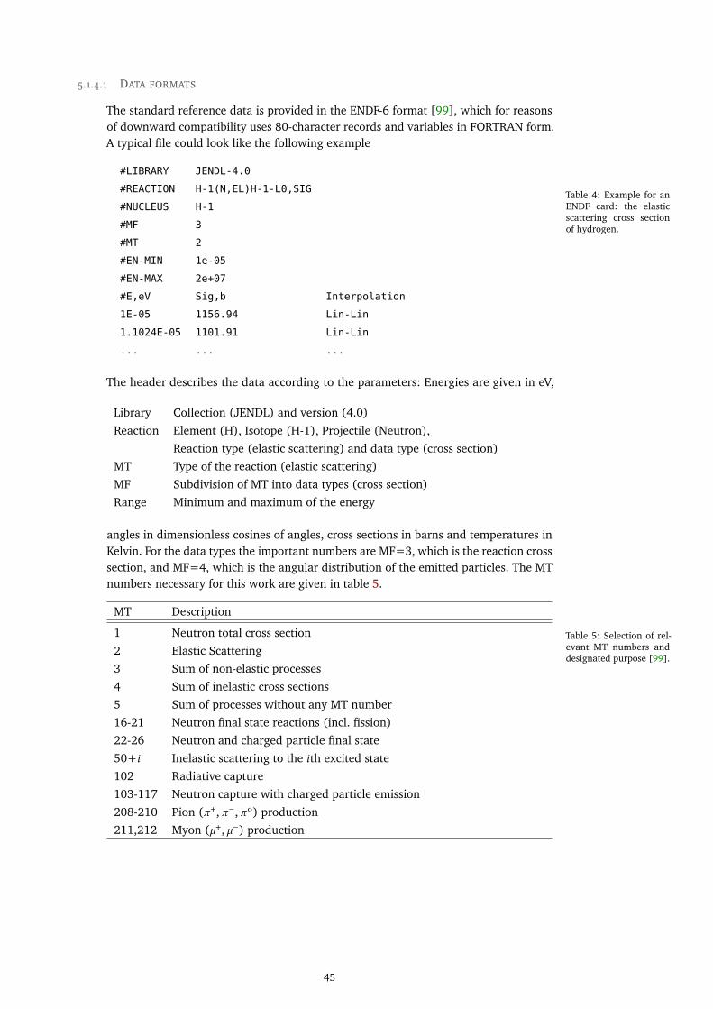
5.1.4.1 DATA FORMATS

The standard reference data is provided in the ENDF-6 format [99], which for reasonsof downward compatibility uses 80-character records and variables in FORTRAN form.A typical file could look like the following example

Table 4: Example for anENDF card: the elasticscattering cross sectionof hydrogen.

#LIBRARY JENDL-4.0

#REACTION H-1(N,EL)H-1-L0,SIG

#NUCLEUS H-1

#MF 3

#MT 2

#EN-MIN 1e-05

#EN-MAX 2e+07

#E,eV Sig,b Interpolation

1E-05 1156.94 Lin-Lin

1.1024E-05 1101.91 Lin-Lin

... ... ...

The header describes the data according to the parameters: Energies are given in eV,

Library Collection (JENDL) and version (4.0)

Reaction Element (H), Isotope (H-1), Projectile (Neutron),

Reaction type (elastic scattering) and data type (cross section)

MT Type of the reaction (elastic scattering)

MF Subdivision of MT into data types (cross section)

Range Minimum and maximum of the energy

angles in dimensionless cosines of angles, cross sections in barns and temperatures inKelvin. For the data types the important numbers are MF=3, which is the reaction crosssection, and MF=4, which is the angular distribution of the emitted particles. The MTnumbers necessary for this work are given in table 5.

Table 5: Selection of rel-evant MT numbers anddesignated purpose [99].

MT Description

1 Neutron total cross section

2 Elastic Scattering

3 Sum of non-elastic processes

4 Sum of inelastic cross sections

5 Sum of processes without any MT number

16-21 Neutron final state reactions (incl. fission)

22-26 Neutron and charged particle final state

50+𝑖 Inelastic scattering to the 𝑖th excited state

102 Radiative capture

103-117 Neutron capture with charged particle emission

208-210 Pion (𝜋+,𝜋−,𝜋0) production

211,212 Myon (`+, `−) production

45

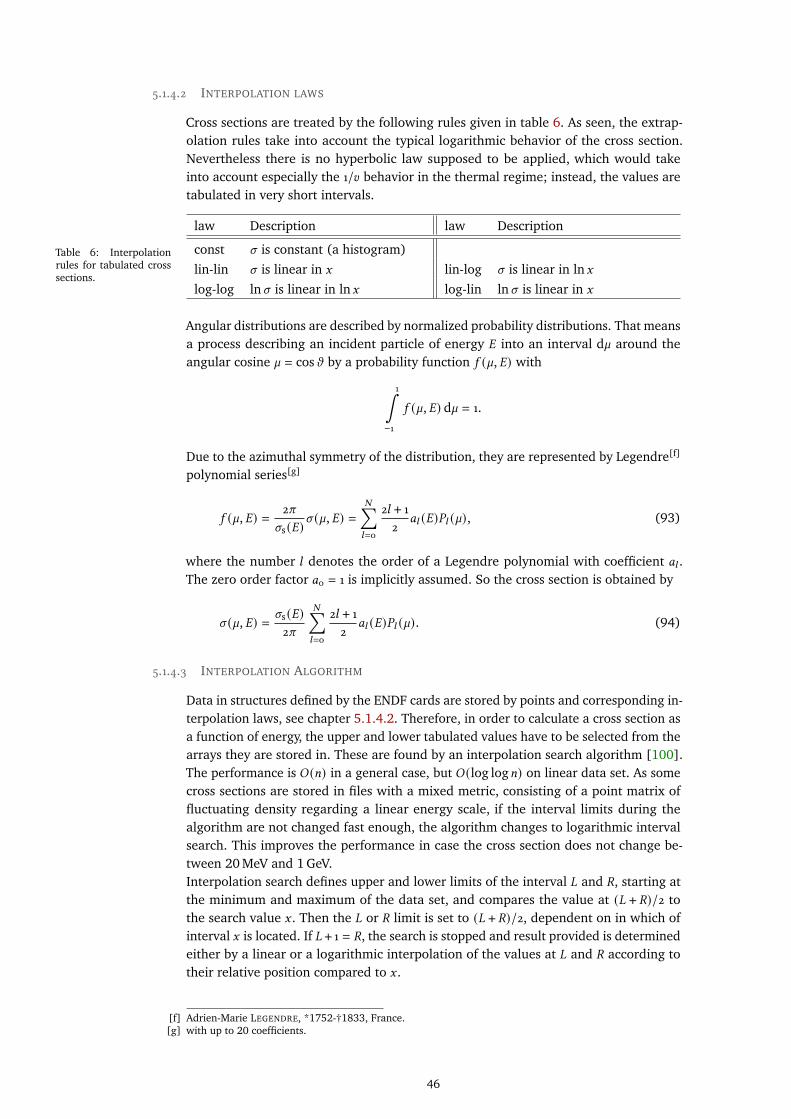
5.1.4.2 INTERPOLATION LAWS

Cross sections are treated by the following rules given in table 6. As seen, the extrap-olation rules take into account the typical logarithmic behavior of the cross section.Nevertheless there is no hyperbolic law supposed to be applied, which would takeinto account especially the 1/𝑣 behavior in the thermal regime; instead, the values aretabulated in very short intervals.

Table 6: Interpolationrules for tabulated crosssections.

law Description law Description

const 𝜎 is constant (a histogram)

lin-lin 𝜎 is linear in 𝑥 lin-log 𝜎 is linear in ln𝑥

log-log ln𝜎 is linear in ln𝑥 log-lin ln𝜎 is linear in 𝑥

Angular distributions are described by normalized probability distributions. That meansa process describing an incident particle of energy 𝐸 into an interval d` around theangular cosine ` = cos𝜗 by a probability function 𝑓 (`,𝐸) with

1∫−1

𝑓 (`,𝐸) d` = 1.

Due to the azimuthal symmetry of the distribution, they are represented by Legendre[f]

polynomial series[g]

𝑓 (`,𝐸) = 2𝜋

𝜎s (𝐸)𝜎 (`,𝐸) =

𝑁∑𝑙=0

2𝑙 + 1

2𝑎𝑙 (𝐸)𝑃𝑙 (`), (93)

where the number 𝑙 denotes the order of a Legendre polynomial with coefficient 𝑎𝑙 .The zero order factor 𝑎0 = 1 is implicitly assumed. So the cross section is obtained by

𝜎 (`,𝐸) = 𝜎s (𝐸)2𝜋

𝑁∑𝑙=0

2𝑙 + 1

2𝑎𝑙 (𝐸)𝑃𝑙 (`). (94)

5.1.4.3 INTERPOLATION ALGORITHM

Data in structures defined by the ENDF cards are stored by points and corresponding in-terpolation laws, see chapter 5.1.4.2. Therefore, in order to calculate a cross section asa function of energy, the upper and lower tabulated values have to be selected from thearrays they are stored in. These are found by an interpolation search algorithm [100].The performance is 𝑂 (𝑛) in a general case, but 𝑂 (log log𝑛) on linear data set. As somecross sections are stored in files with a mixed metric, consisting of a point matrix offluctuating density regarding a linear energy scale, if the interval limits during thealgorithm are not changed fast enough, the algorithm changes to logarithmic intervalsearch. This improves the performance in case the cross section does not change be-tween 20 MeV and 1 GeV.Interpolation search defines upper and lower limits of the interval 𝐿 and 𝑅, starting atthe minimum and maximum of the data set, and compares the value at (𝐿 + 𝑅)/2 tothe search value 𝑥 . Then the 𝐿 or 𝑅 limit is set to (𝐿 + 𝑅)/2, dependent on in which ofinterval 𝑥 is located. If 𝐿 + 1 = 𝑅, the search is stopped and result provided is determinedeither by a linear or a logarithmic interpolation of the values at 𝐿 and 𝑅 according totheir relative position compared to 𝑥 .

[f] Adrien-Marie LEGENDRE, *1752-†1833, France.[g] with up to 20 coefficients.

46

5.2 NEUTRON MONTE CARLO CODES

Among the existing Monte Carlo tools, most codes do have a long history and strongaim towards nuclear fuel calculations. Besides dedicated programs, the most widelyused in neutron physics is MCNP, especially for purposes of the ESS, GEANT4 can beconsidered the most important.

5.2.1 GENERAL PURPOSE PACKAGES

MCNP (Monte Carlo N-Particle) was developed in Los Alamos as a general purpose USA

software to treat neutrons, photons, electrons[h] and the coupled transport thereof.Versions until MCNP4 [101] were capable of simulating neutrons up to 20 MeV, whichis the maximum of most of the cross sections available in the evaluated data bases,and were written in FORTRAN 77 [102], which was until the mid-90s considered thestandard in scientific computing. With version 5 [103] the development was forkedto the MCNPX [104](MCNP eXtendend) branch, which converted the code to For-tran 90 [105] and included the LAHET [106] framework. This especially introducedthe extension of the energy range for many isotopes up to 150 MeV and some to GeVby using the continuously improved Cascade-Exciton Model (CEM) [62] and ontop theLos Alamos Quark-Gluon String Model (LAQGSM) [107]. It also can treat (heavy) iontransport for charged particles with energies larger than 1 MeV/nucleon by tabulatedranges. The actual version 6 [108] re-merged the X-branch into the main developmentbranch. Since it also provides an optional cosmic-ray source [109] it has gotten largeattention for the calculation of the cosmic neutron spectrum as seen in [110].A more recent general purpose tool is PHITS [68] (Particle and Heavy Ion Transport Japan

code System), as extension of the high energy particle transport code NMTC/JAM [111],which, besides the features mentioned above, also supports charged particles in mag-netic fields, dE/dx calculations in the Continuous-Slowing-Down Approximation [112](CSDA) and intra-nuclear cascade (JAM) [113] (Jet AA Microscopic Transport) mod-els up to 1 TeV. PHITS is also typically linked against the JENDL-4/HE(High Energy)data base, consisting of files evaluated by CCONE [114], which is a more sophisticatedmodel compared to INCL [115] and JAM. However, it comes along with many ad-justable parameters for each nucleus, which often leads to a better accuracy comparedto other physics models. PHITS also features a rudimentary graphical user interface.Like MCNP and the following codes it is also written in Fortran. One of the recentfollow-up developments is PARMA [67] (PHITS-based Analytical Radiation Model inthe Atmosphere). It calculates the spectra of leptons and hadrons providing effectivemodels for fluxes of particles of different species, especially with the aim of dose esti-mations.The FLUKA [116](FLUktuierende KAskade) code is mostly oriented towards charged CERN

hadronic transport and nuclear and particle physics experiments. For neutron calcula-tions, the full spectrum is divided into 260 energy groups, which are not directly linkedto an evaluated data base, but operate on their own set of reprocessed and simplifiedmean values. Especially for neutrons and geometrical representations, it contains reim-plementations from the MORSE [117] neutron and gamma ray transport code.GEANT4 [118] (GEometry ANd Tracking) can be regarded as FLUKA’s successor, based CERN

on multithreaded C++ and OpenGL visualizations. It is designed specifically for theneeds of high energy and accelerator physics. GEANT4 especially excels in describing acomplex geometry of the setup. Since 2011, also driven by requests from the EuropeanSpallation Source, an increasing number of low energy neutron calculation capabilities

[h] MCNP does not handle magnetic fields for charged particles.

47

were introduced. Meanwhile the software has advanced to a level where there is agood agreement with other codes like MCNP for fast neutrons [119] as well as slowneutrons [120].

5.2.2 SPECIFIC NEUTRON INTERACTION CODES

VIM [121] is a continuous energy neutron and photon transport code written mainlyUSA

in Fortran 90. It is developed by Argonne National Laboratory for reactor physics andshielding. The geometry is limited to hexagonal or rectangular lattices of combinatorialunit cells and especially focuses on the description of critical states.TRIPOLI [122] is a neutron, photon and electron transport code written in FOR-France

TRAN 77 and C by the Commissariat à l’énergie atomique, Saclay. It uses, unlike VIM,not only the ENDF data bases but is able to extract cross sections from several librariesby a specific interface allowing for example neutron energies up to 150 MeV.Similar to both mentioned programs there are a number of codes with approximatelythe same scope allowing photon and neutron transport. Among them are TART [123]USA

with 700 energy groups up to 1 GeV, but neutron calculations only up to 20 MeV.Whereas earlier versions were written in LRLTRAN, a language unique to the LawrenceLivermore National Laboratory to run on their Cray supercomputers[i], the releasesafter 1995 were ported to Fortran. It’s successor, MERCURY [124], then was rewrittenin C with improvements in geometry definitions by XML steering files. Furthermore,with dedicated scope on reactor analysis there are PRIZMA [125] and Shift [126],Russia

USA which partly includes also deterministic codes, Serpent [127], which does not onlyFinland use the average interaction length calculations, but also the Woodcock delta-tracking

method [128] that continues across geometrical borders by pseudo fictitious steps inthe subsequent material. This feature is also included in RMC [129](Reactor MonteChina

Carlo) and MORET [130]. These codes were developed at governmental institutionsFrance

and mostly for the research program pursued. For the MONK [131] code there alsoUK

have been made the approach to commercialize such a tool. The only German contribu-tion to be mentioned in the field of reactor analysis is KAMCCO [132], a pseudo MonteGermany

Carlo transport code, which was developed in Karlsruhe for the fast breeder reactor inthe 1970s [133].The most recent development is the publicly available MIT OpenMC [94]. AlthoughUSA

mostly written in Fortran 90, it features a Python [134] API and XML geometry defini-tion files as well as Jupyter [135] notebook parsers.

[i] Still holding the claim that TART would be the fastest Monte Carlo available.

48

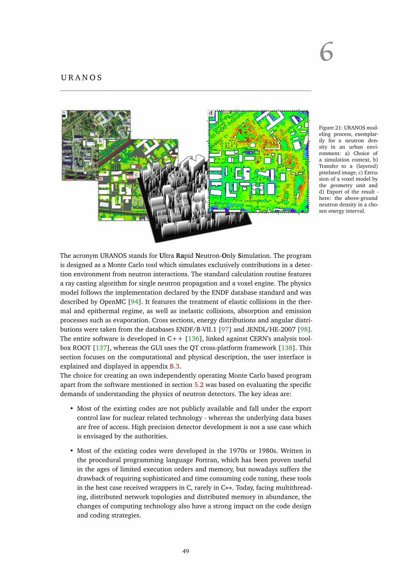
6U R A N O S

Figure 21: URANOS mod-eling process, exemplar-ily for a neutron den-sity in an urban envi-ronment: a) Choice ofa simulation context, b)Transfer to a (layered)pixelated image, c) Extru-sion of a voxel model bythe geometry unit andd) Export of the result -here: the above-groundneutron density in a cho-sen energy interval.

The acronym URANOS stands for Ultra Rapid Neutron-Only Simulation. The programis designed as a Monte Carlo tool which simulates exclusively contributions in a detec-tion environment from neutron interactions. The standard calculation routine featuresa ray casting algorithm for single neutron propagation and a voxel engine. The physicsmodel follows the implementation declared by the ENDF database standard and wasdescribed by OpenMC [94]. It features the treatment of elastic collisions in the ther-mal and epithermal regime, as well as inelastic collisions, absorption and emissionprocesses such as evaporation. Cross sections, energy distributions and angular distri-butions were taken from the databases ENDF/B-VII.1 [97] and JENDL/HE-2007 [98].The entire software is developed in C++ [136], linked against CERN’s analysis tool-box ROOT [137], whereas the GUI uses the QT cross-platform framework [138]. Thissection focuses on the computational and physical description, the user interface isexplained and displayed in appendix B.3.The choice for creating an own independently operating Monte Carlo based programapart from the software mentioned in section 5.2 was based on evaluating the specificdemands of understanding the physics of neutron detectors. The key ideas are:

• Most of the existing codes are not publicly available and fall under the exportcontrol law for nuclear related technology - whereas the underlying data basesare free of access. High precision detector development is not a use case whichis envisaged by the authorities.

• Most of the existing codes were developed in the 1970s or 1980s. Written inthe procedural programming language Fortran, which has been proven usefulin the ages of limited execution orders and memory, but nowadays suffers thedrawback of requiring sophisticated and time consuming code tuning, these toolsin the best case received wrappers in C, rarely in C++. Today, facing multithread-ing, distributed network topologies and distributed memory in abundance, thechanges of computing technology also have a strong impact on the code designand coding strategies.

49

• Meanwhile even more complex mathematical operations are readily availablefrom standard packages like the GSL [139] (GNU Scientific Library) and frame-works such as Root [137].

• The majority of codes focuses on the evaluation of radiation sources, includinggamma emissions. Signal generation in a boron based hybrid detector requirestwo additional steps of charged particle transport mechanisms - within the con-version layer itself and subsequently in the gas. In the most cases it is not possibleto integrate such a calculation path directly, but it would have to be added ontop of the simulation. Furthermore, typical codes expect for the geometry objectsof roughly equal size - boron layers having an aspect ratio of 105 due to the lowthickness cannot be described.

• All available codes propagate a take-off amount of neutrons in time due to thefact that in typical applications concerning criticality calculations the neutronsthemselves change the state of the environment, for example by generating asignificant amount of heat. Therefore, the whole ensemble has to be propagated,especially until an equilibrium state is reached. Due to limited computing re-sources this also required the multigroup method, see also the following keypoint.

• The multigroup method is a technique, which allows significant improvement ofthe calculation speed by not treating every neutron track individually but assign-ing an effective weight to propagating particle. This weight gets increased for(n,xn) processes and reduced, if a neutron is absorbed or loses enough energy todrop out of a specific interval. The method is derived from solving Fermi age dif-fusion equations [140] and is applied in many codes. However, it requires manyinteractions to generate enough randomness and thus it leads to a significantbias whether or not a neutron will undergo most probably only one collision. Yet,for the study of background contributions in detectors or albedo neutrons, sucha systematic error should be avoided.

The only software package which does not suffer from the mentioned drawbacks wasGEANT4. But at the beginning of this work the code did not at all feature any accu-rate low energy neutron calculation. Materials in GEANT4 are usually described undera free gas assumption with unbound cross sections with no information about inter-atomic chemical bindings, this especially comes into account when treating hydrogencollisions[a]. Therefore, the main part of the relevant physics would still have to beintegrated. In conclusion it has been decided to focus on a design from scratch inmodular, object oriented language.

6.1 URANOS CONCEPTS

The buildup of the software can be motivated based on the following general aspects:

• The geometry is represented in a 3-dimensional coordinate space.

• In typical situations the number of neutrons can easily reach 109, whereas therelevant neutrons contributing to an observable might scale down this initialamount by more than 106.

• Neutrons are neither as abundant nor as simple to describe as necessary to applymeans of ensemble statistics.

[a] GEANT4 though can be coupled to the constantly developed models for evaluating the JEFF-3.X [141] ACEformatted thermal scattering law files. For scattering in crystal structures meanwhile the NXSG4 exten-sion [142] has been released.

50

• Neither energy nor particle number is conserved, moreover both are linked toeach other depending on the medium, which implies complex transport equations,that often can only be solved numerically.

• In general interactions are not deterministic but of statistical nature.

• Important parameters like cross sections cannot be derived but are to be extractedfrom data bases.

• Whereas possible physical interactions are numerous, the relevant ones within aspecific energy interval are predominately not more than two different types.

• Secondary particles, except conversion ions, are typically not contributing.

One specific feature of URANOS is its layer geometry, which takes advantage of thesymmetry of the envisaged problem. The concept is presented in Fig. 22. In one case aneutron detector has to be simulated which consists of several mostly identical layers ofa boron coated substrate. Whereas along the horizontal and vertical axes the geometricscales vary significantly, the mean free path lengths are comparable. For example theabsorption probability for a neutron in a 500 nm film of boron might be around 3 %,the scattering probability in a polymer foil of 100 times the thickness is approximatelythe same number and in the air gap of 100 times the thickness of the plastic it may be0.3%. This also means that the spatial definitions in such a simulation should not bebuild on concepts requiring objects of roughly equal size. The solution of URANOS isusing layers. This allows to easily build up a geometry of homogeneous materials withthe main parameter being position and height of such a layer. Each layer furthermorecan be sub-structured by twodimensional matrices into voxels.URANOS uses ray casting [143], a technique, which refers to conducting a series of ray-

Figure 22: Idea of theURANOS layer geometryrepresenting two prob-lems: (left) simulation ofa neutron detector con-sisting of a stack of sub-strates coated with a con-verter and (right) evalu-ating the propagation ofalbedo neutrons.

Boronlayers

ReadoutDetector gas

GEMsAir

Soil

surface intersection tests in order to determine the first object crossed by tracks froma source. These intersections are either defined by analytical surfaces, like the layerstructure, or computed from extruded voxels, which do not at all consist of surfaces.Similar types of geometry definitions with mixed volume and surface data were forexample used in early computer games when no powerful hardware acceleration wasavailable[b] and nowadays for X-ray tomography image reconstruction in materialresearch [144], geociences [145] and especially medical imaging [146]. The methodof ray casting also allows to only record and store the variables necessary for each run.The neutron is physically propagated forward in time through the domain and flagsare used as boolean operators for each possible output. If for example the recordingobservable is defined as the density above the surface not the whole track but only thetracklet within the layer above the ground is kept in the memory.

[b] Notable examples are the Voxel Space engine by NovaLogic or the GAIA/Paradise-Engine by Appeal.

51

6.2 COMPUTATIONAL STRUCTURE

The basic concept of URANOS relies on looping over a set of neutrons, which featuresinitial conditions, predefined or randomized, and for each neutron a loop tracking itspath through the geometry. Both entities are referred to as ’stacks’. In each step thegeometrical boundaries are determined and handed over to the physics computationunit. For specific cases actual variables of the neutron or its track history are recordedemulating a real or a virtual detector. This process is called ’Scoring’ and can be invokedwhen passing a layer or an absorption in a converter takes place. A track is definedas the shortest path between two points of interaction. It can, as will be seen later, becut by layer or material boundaries, which dissects it into tracklets. The pseudo flowchart of Fig. 23 illustrates the entire simulation process, which will be described in thefollowing.

NeutronStack

E0

x0

f( )R

Initiation

f(E)

f( )R f(x)

LayerStack

xu xd

t0

Layer

t

f( )f(x)material N

Cross sections

σel σinel σabs

σth σevp

Scoring

x f(x)

3D-Track

x t

elements

Σσi

Element

d( )ϴm

Evaporation

E =d(E)0n+f(E) xx0=

Elastic

xx0=

Inelastic

E =E( ) - E0 iϴxx0=

Absorption

E =E( )0 ϴ

epithermal thermal

d(E)

gas non-gas

E =E( )0 ϴ

f(E)

10B

Ion Range

f(x)

Li

He

dE/dx in Gas

f(x)f(E)

f(E)

Readout

f(E) f( )

coordinate vectorx

f( )

d( )

E energy

ϴ scattering angle

σ

t time

cross section

function of

distribution of

from database

from matrix

De

tecto

r Sim

ula

tion

Collision

x f(x)

3D-Track

x t

f( )

kill

t f(x)

f(E)

t

N scalarR,

Figure 23: Pseudo flow chart of the internal buildup of URANOS. Each calculation step is represented by a blockdescribing the structural function in orange and the corresponding physics variables.

6.2.1 STARTUP

Before the main calculation routine shown in Fig. 23 three steps are performed:

• Assigning memory to objects, which will be used throughout the calculation, bycreating empty containers. These are at least 50 one and two dimensional roothistograms.

• Reading the configuration files, creating the geometry and, if available, readingthe voxel extrusion matrices.

• Reading the necessary tables from the ENDF library [99], see also sec. 5.1.4.1.

52

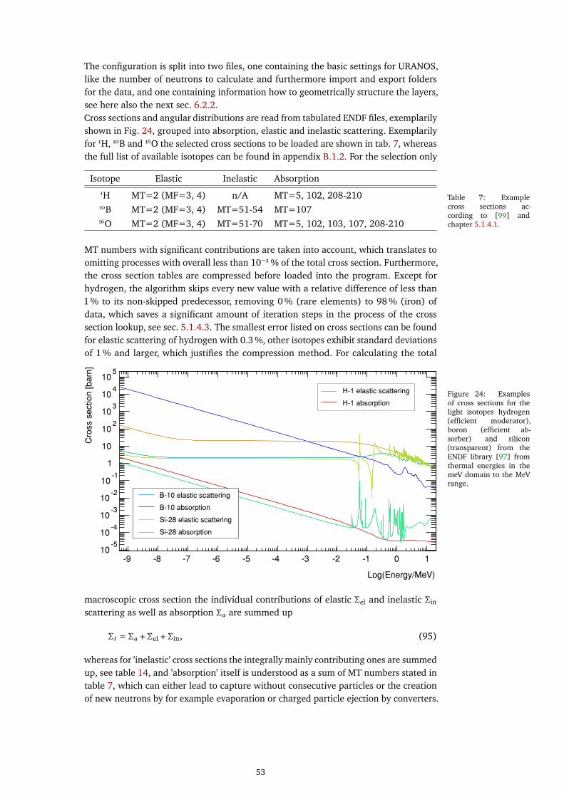
The configuration is split into two files, one containing the basic settings for URANOS,like the number of neutrons to calculate and furthermore import and export foldersfor the data, and one containing information how to geometrically structure the layers,see here also the next sec. 6.2.2.Cross sections and angular distributions are read from tabulated ENDF files, exemplarilyshown in Fig. 24, grouped into absorption, elastic and inelastic scattering. Exemplarilyfor 1H, 10B and 16O the selected cross sections to be loaded are shown in tab. 7, whereasthe full list of available isotopes can be found in appendix B.1.2. For the selection only

Table 7: Examplecross sections ac-cording to [99] andchapter 5.1.4.1.

Isotope Elastic Inelastic Absorption1H MT=2 (MF=3, 4) n/A MT=5, 102, 208-21010B MT=2 (MF=3, 4) MT=51-54 MT=10716O MT=2 (MF=3, 4) MT=51-70 MT=5, 102, 103, 107, 208-210

MT numbers with significant contributions are taken into account, which translates toomitting processes with overall less than 10−2 % of the total cross section. Furthermore,the cross section tables are compressed before loaded into the program. Except forhydrogen, the algorithm skips every new value with a relative difference of less than1 % to its non-skipped predecessor, removing 0 % (rare elements) to 98 % (iron) ofdata, which saves a significant amount of iteration steps in the process of the crosssection lookup, see sec. 5.1.4.3. The smallest error listed on cross sections can be foundfor elastic scattering of hydrogen with 0.3 %, other isotopes exhibit standard deviationsof 1 % and larger, which justifies the compression method. For calculating the total

Figure 24: Examplesof cross sections for thelight isotopes hydrogen(efficient moderator),boron (efficient ab-sorber) and silicon(transparent) from theENDF library [97] fromthermal energies in themeV domain to the MeVrange.

Cro

ss s

ectio

n [

ba

rn]

-510

-410

-310

-210

-110

1

10

210

310

410

510

H-1 elastic scattering

H-1 absorption

B-10 elastic scattering

B-10 absorption

Si-28 elastic scattering

Si-28 absorption

Log(Energy/MeV)

0 1-9 -8 -5 -3 -1-2-4-6-7

macroscopic cross section the individual contributions of elastic Σel and inelastic Σin

scattering as well as absorption Σ𝑎 are summed up

Σ𝑡 = Σ𝑎 + Σel + Σin, (95)

whereas for ’inelastic’ cross sections the integrally mainly contributing ones are summedup, see table 14, and ’absorption’ itself is understood as a sum of MT numbers stated intable 7, which can either lead to capture without consecutive particles or the creationof new neutrons by for example evaporation or charged particle ejection by converters.

53

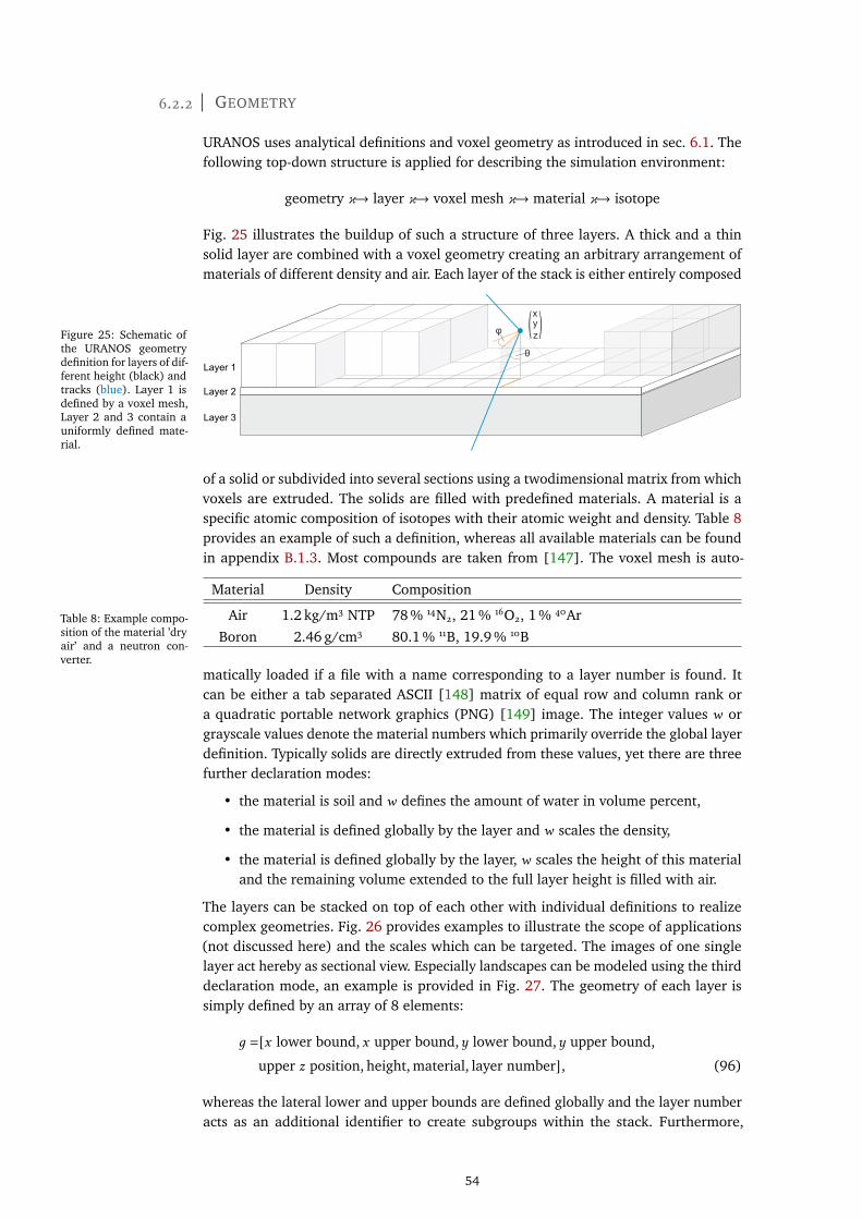
6.2.2 GEOMETRY

URANOS uses analytical definitions and voxel geometry as introduced in sec. 6.1. Thefollowing top-down structure is applied for describing the simulation environment:

geometry 𝜘→ layer 𝜘→ voxel mesh 𝜘→ material 𝜘→ isotope

Fig. 25 illustrates the buildup of such a structure of three layers. A thick and a thinsolid layer are combined with a voxel geometry creating an arbitrary arrangement ofmaterials of different density and air. Each layer of the stack is either entirely composed

Figure 25: Schematic ofthe URANOS geometrydefinition for layers of dif-ferent height (black) andtracks (blue). Layer 1 isdefined by a voxel mesh,Layer 2 and 3 contain auniformly defined mate-rial.

xyz

( (

Layer 1

Layer 2

Layer 3

θ

φ

of a solid or subdivided into several sections using a twodimensional matrix from whichvoxels are extruded. The solids are filled with predefined materials. A material is aspecific atomic composition of isotopes with their atomic weight and density. Table 8provides an example of such a definition, whereas all available materials can be foundin appendix B.1.3. Most compounds are taken from [147]. The voxel mesh is auto-

Table 8: Example compo-sition of the material ’dryair’ and a neutron con-verter.

Material Density Composition

Air 1.2 kg/m3 NTP 78 % 14N2, 21 % 16O2, 1 % 40Ar

Boron 2.46 g/cm3 80.1 % 11B, 19.9 % 10B

matically loaded if a file with a name corresponding to a layer number is found. Itcan be either a tab separated ASCII [148] matrix of equal row and column rank ora quadratic portable network graphics (PNG) [149] image. The integer values 𝑤 orgrayscale values denote the material numbers which primarily override the global layerdefinition. Typically solids are directly extruded from these values, yet there are threefurther declaration modes:

• the material is soil and 𝑤 defines the amount of water in volume percent,

• the material is defined globally by the layer and 𝑤 scales the density,

• the material is defined globally by the layer, 𝑤 scales the height of this materialand the remaining volume extended to the full layer height is filled with air.

The layers can be stacked on top of each other with individual definitions to realizecomplex geometries. Fig. 26 provides examples to illustrate the scope of applications(not discussed here) and the scales which can be targeted. The images of one singlelayer act hereby as sectional view. Especially landscapes can be modeled using the thirddeclaration mode, an example is provided in Fig. 27. The geometry of each layer issimply defined by an array of 8 elements:

𝑔 =[𝑥 lower bound,𝑥 upper bound,𝑦 lower bound,𝑦 upper bound,

upper 𝑧 position, height, material, layer number], (96)

whereas the lateral lower and upper bounds are defined globally and the layer numberacts as an additional identifier to create subgroups within the stack. Furthermore,

54

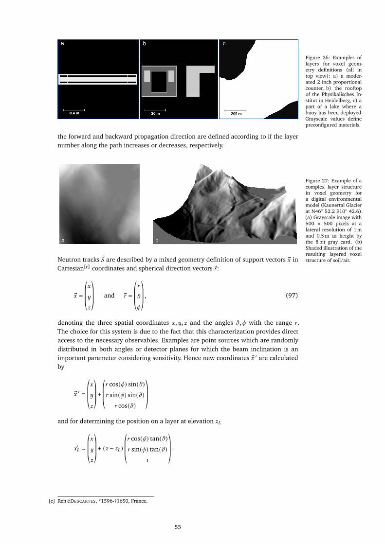
Figure 26: Examples oflayers for voxel geom-etry definitions (all intop view): a) a moder-ated 2 inch proportionalcounter, b) the rooftopof the Physikalisches In-stitut in Heidelberg, c) apart of a lake where abuoy has been deployed.Grayscale values definepreconfigured materials.

the forward and backward propagation direction are defined according to if the layernumber along the path increases or decreases, respectively.

Figure 27: Example of acomplex layer structurein voxel geometry fora digital environmentalmodel (Kaunertal Glacierat N46◦ 52.2 E10◦ 42.6).(a) Grayscale image with500 × 500 pixels at alateral resolution of 1 mand 0.5 m in height bythe 8 bit gray card. (b)Shaded illustration of theresulting layered voxelstructure of soil/air.Neutron tracks ®𝑆 are described by a mixed geometry definition of support vectors ®𝑥 in

Cartesian[c] coordinates and spherical direction vectors ®𝑟 :

®𝑥 =

©­­­«𝑥

𝑦

𝑧

ª®®®¬ and ®𝑟 =©­­­«𝑟

𝜗

𝜙

ª®®®¬ , (97)

denoting the three spatial coordinates 𝑥 ,𝑦, 𝑧 and the angles 𝜗 ,𝜙 with the range 𝑟 .The choice for this system is due to the fact that this characterization provides directaccess to the necessary observables. Examples are point sources which are randomlydistributed in both angles or detector planes for which the beam inclination is animportant parameter considering sensitivity. Hence new coordinates ®𝑥 ′ are calculatedby

®𝑥 ′ =©­­­«𝑥

𝑦

𝑧

ª®®®¬ +©­­­«𝑟 cos(𝜙) sin(𝜗)𝑟 sin(𝜙) sin(𝜗)

𝑟 cos(𝜗)

ª®®®¬and for determining the position on a layer at elevation 𝑧𝐿

®𝑥𝐿 =

©­­­«𝑥

𝑦

𝑧

ª®®®¬ + (𝑧 − 𝑧𝐿)©­­­«𝑟 cos(𝜙) tan(𝜗)𝑟 sin(𝜙) tan(𝜗)

1

ª®®®¬ .

[c] René DESCARTES, *1596-†1650, France.

55

Time is an indirect quantity. It is derived from the geometrical position of the neutroncalculated from energy and initial conditions.

In URANOS three layers can be assigned specific functions. These are source layer,detector layer and ground layer. The source layer defines the origin for all neutronhistories. Especially all height values for starting positions, see also sec. 6.3, are re-stricted to be initiated here. This layer may neither be the upper- nor lowermost asotherwise neutrons would escape the computational domain. The ground layer isused in cosmic neutron simulations to record the spectra at the air/ground interface.In the detector layer, which can be superimposed to another layer, either single real orvirtual detectors can be placed, or the layer itself acts as a virtual detector and recordsevery neutron passing, see also sec. 6.5.

6.3 SOURCES AND ENERGY

URANOS provides a variety of sources. A source is defined by a spatial distribution andan energy spectrum from which random values are sampled. They are either definedas

• point sources with all neutrons starting from the same coordinate vector,

• a plane source with all neutrons sharing the same 𝑧 coordinate within lateralboundaries,

• a volume source, which randomly distributes neutrons in the source layer withinlateral boundaries, and alternatively extends the volume source downwards tothe ground layer with exponentially distributed height values[d].

As explained in sec. 6.2.2 the source has to be placed in the source layer, which definesits 𝑧-position. For the coordinates (𝑥 ,𝑦) ∈ 𝐴 in the source area 𝐴 in case of plane orvolume sources the options are:

• rectangular boundaries with either equal aspect ratio (square) or any other, sam-pling the origins uniformly from possible positions in (𝑥 ,𝑦), and

• circular boundaries, sampling the origins either uniformly in radius 𝑟 from thecenter or in (𝑥 ,𝑦).

Furthermore, the starting angle 𝜗 can be set to:

• full or half sphere, sampling 𝜗 in [0 . . . 𝜋] or [0 . . . 𝜋/2], or

• unidirectional beam, which allows to set theta to a specific inclination. Addition-ally a divergence 𝑠𝜗 can be chosen. Then, the angles are sampled from a gaussianfunction centered around 𝜗 with a width of 𝑠𝜗 .

The starting energy for the neutrons are derived from normalized distributions, whichare described in the following sections. The method of sampling by rejection is appliedaccording to (72) in sec. 5.1. For source definitions on a linear support in [𝑎,𝑏], like insec. 6.3.2, the random variable b ∈ [0, 1] is scaled to the abscissa test quantity

b𝑡 = 𝑎 + (𝑏 − 𝑎)b .

For source definitions on a logarithmic support in [10𝑎, 10𝑏], like in sec. 6.3.1, b is scaledto

b𝑡 = 10𝑎+(𝑏−𝑎)b .[d] This option is called artificial cosmic source and accounts for neutrons which are generated by physical

processes URANOS is not capable of simulating like high energy protons, myons or induced cascades thereof.

56

6.3.1 THE COSMIC NEUTRON SOURCE

The cosmic neutron source definition is specifically designed for the problem of soilmoisture dependent neutron transport in the vicinity of the atmosphere-soil interface.Instead of propagating primary particles through several kilometers of atmosphere,a source definition near the ground level is chosen. Recent works, especially fromSato et al. [66], have provided analytical functions modeling cosmic-ray spectra forvarious conditions. As such spectra are always integrated over all trajectory angles,based on these models, which are covered in sec. 3.2, a net incoming spectrum hasbeen reconstructed. The procedure and a detailed description can be found in sec. 9.1.1and the result is used as the generalized cosmic neutron incoming spectrum. Furtherexplanation about the composition and features con be found in sec. 3.1.Fig. 28 shows the URANOS cosmic-ray neutron spectrum (cyan) and exemplarily thetotal spectrum above ground for dry conditions. The energy of neutrons can rangeover more than 12 orders of magnitude. The plot here as well as the following will bepresented logarithmically in units of lethargy, see (33) in sec. 1.4.1. The intensity 𝐼 orflux density per logarithmic unit of energy is given in units of

𝐼 = dΦ/d( log(𝐸)) = 𝐸 dΦ/d𝐸. (98)

0

0.2

0.4

0.6

0.8

1

1.2

1.4

1.6

1.8

2

2.2

Cosmic Spectrum

Downward Spectrum

Log(Energy/MeV)

0 1 2 3-5 -3 -1-2-4-6-7

-2F

lux E

dΦ/d

E [

cm

·/s

, a

rb.

sca

le]

Figure 28: TheURANOS CosmicNeutron SourceSpectrum: Totalangular integratedflux after inter-action with thesoil (blue) andonly incoming flux(cyan).

6.3.2 GENERAL SOURCES

Besides the cosmic neutron source definition in sec. 6.3.1, which expands over severaldecades of energy, energy distributions for specific sources have been implemented.These available source configurations allow sampling from thermal as well as fissionspectra. Exemplarily some are shown in Fig. 29.

• Monoenergetic: neutrons of energy 𝐸 or wavelength _,

• Thermal: neutrons at a temperature 𝑇 described by a Maxwellian distribution

𝑁 (𝐸) = 𝐸

(𝑘𝐵𝑇 )2exp

(− 𝐸

𝑘𝐵𝑇

). (99)

• Predefined: americium-beryllium spectrum from [150],

• Evaporation: assuming the nucleus to form a degenerate Fermi gas [151] onecan derive various forms of density distributions

𝑁 (𝐸) ∝ 𝐸 exp(− 𝐸

𝑘𝐵𝑇

), (100)

57

which are simply described by a temperature parameter [152]. Therefore, theenergy distribution of the neutrons released by fission are commonly representedeither by a Maxwellian distribution or the following Watt spectrum [153].

• Fission: A semi-empirical description is the Watt spectrum [154], especially usedfor 235U, which can be selected as a source although the isotope itself is notimplemented,

𝑁 (𝐸) = 0.4865 sinh(√

2𝐸

)exp(−𝐸), (101)

and for 252Cf [155]

𝑁 (𝐸) = sinh(√

2𝐸

)exp(−0.88𝐸), (102)

which are both specific cases of the more general form of a Maxwellian dis-tribution[e], which allows a more accurate modeling by introducing the Wattparameters 𝑎 and 𝑏 taking into account the mean neutron kinetic energy of andthose of the fission fragments:

𝑁 (𝐸) = 2

exp(−𝑎𝑏

4

)√𝜋𝑎3𝑏

sinh(√

𝑏𝐸

)exp

(−𝐸𝑎

). (103)

The parameters 𝑎,𝑏 are typically tabulated as a function of energy, element andisotope.

Figure 29: Differentpreconfigured sourcedistribution functionsin URANOS in the MeVrange covering differentuse cases: laboratory testsources like americium-beryllium (yellow) witha variety of resonances,spontaneous fission(green), evaporation(cyan) from de-excitationand fusion (blue)

Energy [MeV]

0 2 4 6 8 10 12 14 16

Inte

nsity

[a

.u.]

0

0.1

0.2

0.3

0.4

0.5

0.6

0.7

0.8

0.9

Am-Be

Evaporation

Fission

Monoenergetic

6.4 CALCULATION SCHEME

6.4.1 LOOP NODES

URANOS runs in the main calculation routine on two loops, these are

Neutron Stack 𝜘→ Layer Stack

whereas both are used differently - each onset neutron is a placeholder and only ini-tialized at runtime. Furthermore, the particle number is not conserved due to physical

[e] Although several earlier reports before [154] mention this formula, none of them states the origin.

58

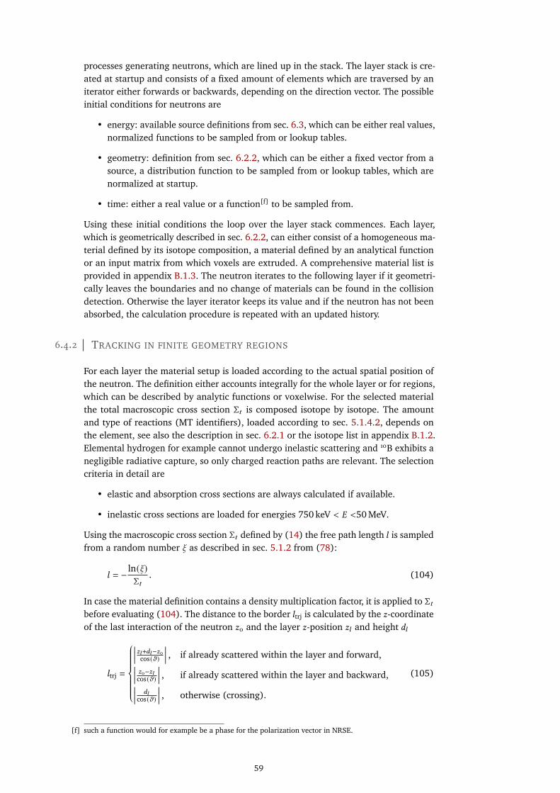
processes generating neutrons, which are lined up in the stack. The layer stack is cre-ated at startup and consists of a fixed amount of elements which are traversed by aniterator either forwards or backwards, depending on the direction vector. The possibleinitial conditions for neutrons are

• energy: available source definitions from sec. 6.3, which can be either real values,normalized functions to be sampled from or lookup tables.

• geometry: definition from sec. 6.2.2, which can be either a fixed vector from asource, a distribution function to be sampled from or lookup tables, which arenormalized at startup.

• time: either a real value or a function[f] to be sampled from.

Using these initial conditions the loop over the layer stack commences. Each layer,which is geometrically described in sec. 6.2.2, can either consist of a homogeneous ma-terial defined by its isotope composition, a material defined by an analytical functionor an input matrix from which voxels are extruded. A comprehensive material list isprovided in appendix B.1.3. The neutron iterates to the following layer if it geometri-cally leaves the boundaries and no change of materials can be found in the collisiondetection. Otherwise the layer iterator keeps its value and if the neutron has not beenabsorbed, the calculation procedure is repeated with an updated history.

6.4.2 TRACKING IN FINITE GEOMETRY REGIONS

For each layer the material setup is loaded according to the actual spatial position ofthe neutron. The definition either accounts integrally for the whole layer or for regions,which can be described by analytic functions or voxelwise. For the selected materialthe total macroscopic cross section Σ𝑡 is composed isotope by isotope. The amountand type of reactions (MT identifiers), loaded according to sec. 5.1.4.2, depends onthe element, see also the description in sec. 6.2.1 or the isotope list in appendix B.1.2.Elemental hydrogen for example cannot undergo inelastic scattering and 10B exhibits anegligible radiative capture, so only charged reaction paths are relevant. The selectioncriteria in detail are

• elastic and absorption cross sections are always calculated if available.

• inelastic cross sections are loaded for energies 750 keV < 𝐸 <50 MeV.

Using the macroscopic cross section Σ𝑡 defined by (14) the free path length 𝑙 is sampledfrom a random number b as described in sec. 5.1.2 from (78):

𝑙 = − ln(b)Σ𝑡

. (104)

In case the material definition contains a density multiplication factor, it is applied to Σ𝑡before evaluating (104). The distance to the border 𝑙trj is calculated by the 𝑧-coordinateof the last interaction of the neutron 𝑧0 and the layer 𝑧-position 𝑧𝑙 and height 𝑑𝑙

𝑙trj =

���𝑧𝑙+𝑑𝑙−𝑧0cos(𝜗)

��� , if already scattered within the layer and forward,��� 𝑧0−𝑧𝑙cos(𝜗)

��� , if already scattered within the layer and backward,��� 𝑑𝑙cos(𝜗)

��� , otherwise (crossing).

(105)

[f] such a function would for example be a phase for the polarization vector in NRSE.

59

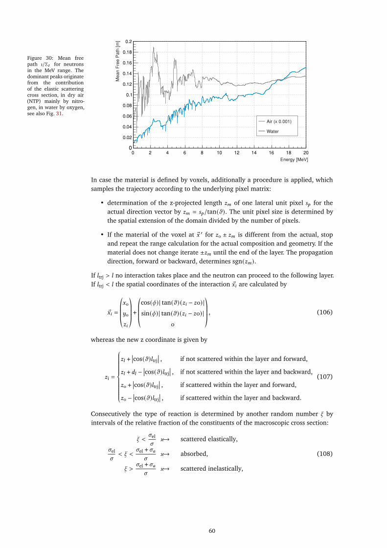
Figure 30: Mean freepath 1/Σ𝑡 for neutronsin the MeV range. Thedominant peaks originatefrom the contributionof the elastic scatteringcross section, in dry air(NTP) mainly by nitro-gen, in water by oxygen,see also Fig. 31.

0 2 4 6 8 10 12 14 16 18 200

0.02

0.04

0.06

0.08

0.1

0.12

0.14

0.16

0.18

0.2

Energy [MeV]

Me

an

Fre

e P

ath

[m

]Air (x 0.001)

Water

In case the material is defined by voxels, additionally a procedure is applied, whichsamples the trajectory according to the underlying pixel matrix:

• determination of the z-projected length 𝑧𝑚 of one lateral unit pixel 𝑠𝑝 for theactual direction vector by 𝑧𝑚 = 𝑠𝑝/tan(𝜗). The unit pixel size is determined bythe spatial extension of the domain divided by the number of pixels.

• If the material of the voxel at ®𝑥 ′ for 𝑧0 ± 𝑧𝑚 is different from the actual, stopand repeat the range calculation for the actual composition and geometry. If thematerial does not change iterate ±𝑧𝑚 until the end of the layer. The propagationdirection, forward or backward, determines sgn(𝑧𝑚).

If 𝑙trj > 𝑙 no interaction takes place and the neutron can proceed to the following layer.If 𝑙trj < 𝑙 the spatial coordinates of the interaction ®𝑥𝑖 are calculated by

®𝑥𝑖 =©­­­«𝑥0

𝑦0

𝑧𝑖

ª®®®¬ +©­­­«cos(𝜙) | tan(𝜗) (𝑧𝑖 − 𝑧0) |sin(𝜙) | tan(𝜗) (𝑧𝑖 − 𝑧0) |

0

ª®®®¬ , (106)

whereas the new z coordinate is given by

𝑧i =

𝑧𝑙 +��cos(𝜗)𝑙trj

�� , if not scattered within the layer and forward,

𝑧𝑙 +𝑑𝑙 −��cos(𝜗)𝑙trj

�� , if not scattered within the layer and backward,

𝑧0 +��cos(𝜗)𝑙trj

�� , if scattered within the layer and forward,

𝑧0 −��cos(𝜗)𝑙trj

�� , if scattered within the layer and backward.

(107)

Consecutively the type of reaction is determined by another random number b byintervals of the relative fraction of the constituents of the macroscopic cross section:

b <𝜎el

𝜎𝜘→ scattered elastically,

𝜎el

𝜎< b <

𝜎el + 𝜎𝑎𝜎

𝜘→ absorbed, (108)

b >𝜎el + 𝜎𝑎

𝜎𝜘→ scattered inelastically,

60

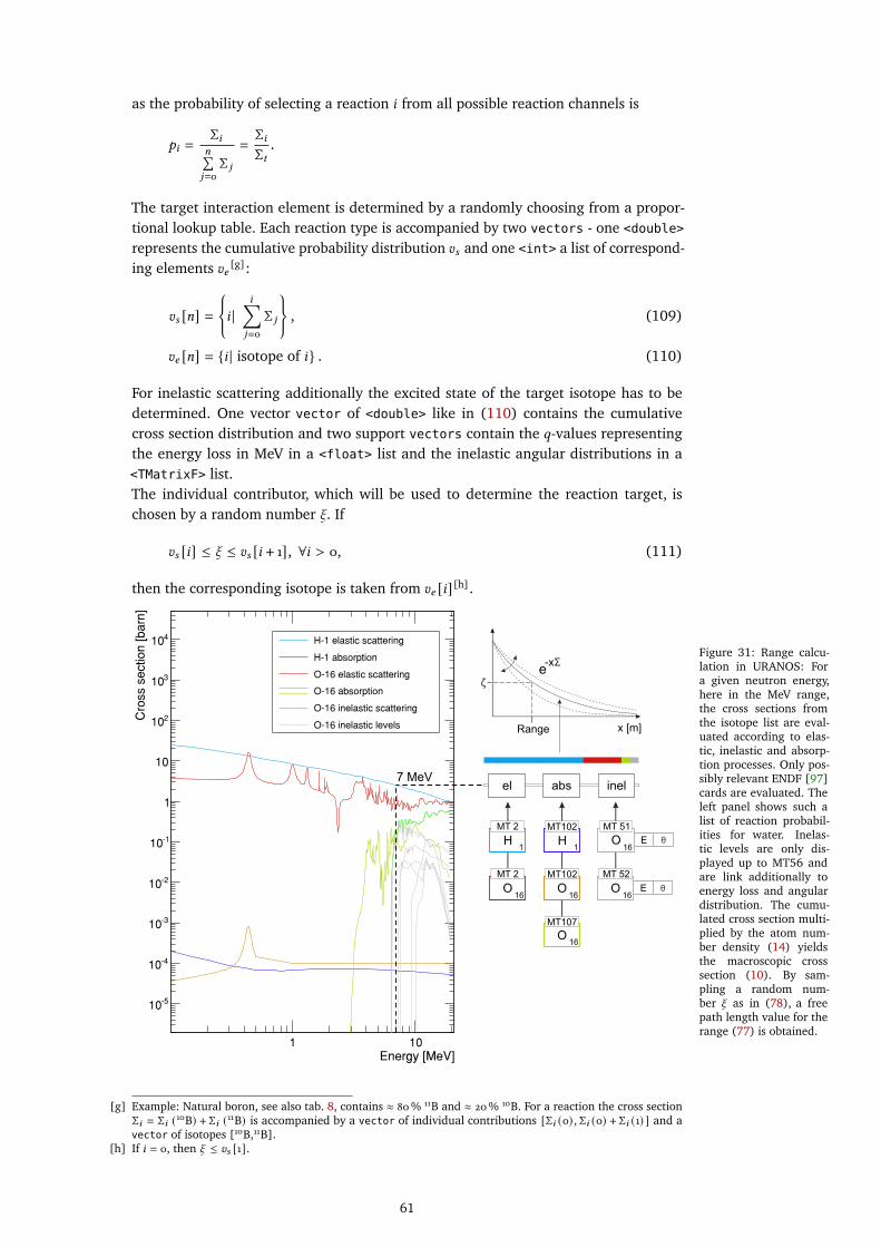
as the probability of selecting a reaction 𝑖 from all possible reaction channels is

𝑝𝑖 =Σ𝑖

𝑛∑𝑗=0

Σ 𝑗

=Σ𝑖Σ𝑡

.

The target interaction element is determined by a randomly choosing from a propor-tional lookup table. Each reaction type is accompanied by two vectors - one <double>

represents the cumulative probability distribution 𝑣𝑠 and one <int> a list of correspond-ing elements 𝑣𝑒 [g]:

𝑣𝑠 [𝑛] ={𝑖 |

𝑖∑𝑗=0

Σ 𝑗

}, (109)

𝑣𝑒 [𝑛] = {𝑖 | isotope of 𝑖} . (110)

For inelastic scattering additionally the excited state of the target isotope has to bedetermined. One vector vector of <double> like in (110) contains the cumulativecross section distribution and two support vectors contain the 𝑞-values representingthe energy loss in MeV in a <float> list and the inelastic angular distributions in a<TMatrixF> list.The individual contributor, which will be used to determine the reaction target, ischosen by a random number b . If

𝑣𝑠 [𝑖] ≤ b ≤ 𝑣𝑠 [𝑖 + 1], ∀𝑖 > 0, (111)

then the corresponding isotope is taken from 𝑣𝑒 [𝑖][h].

Figure 31: Range calcu-lation in URANOS: Fora given neutron energy,here in the MeV range,the cross sections fromthe isotope list are eval-uated according to elas-tic, inelastic and absorp-tion processes. Only pos-sibly relevant ENDF [97]cards are evaluated. Theleft panel shows such alist of reaction probabil-ities for water. Inelas-tic levels are only dis-played up to MT56 andare link additionally toenergy loss and angulardistribution. The cumu-lated cross section multi-plied by the atom num-ber density (14) yieldsthe macroscopic crosssection (10). By sam-pling a random num-ber b as in (78), a freepath length value for therange (77) is obtained.

Energy [MeV]1 10

Cro

ss s

ectio

n [

ba

rn]

-510

-410

-310

-210

-110

1

10

210

310

410 H-1 elastic scattering

H-1 absorption

O-16 elastic scattering

O-16 absorption

O-16 inelastic scattering

O-16 inelastic levels

H

O

H

O

O

O E θ

O E θ

MT107

MT 2

MT 2 MT 51

MT 52

1 1

1616 16

16

16

MT102

MT102

7 MeVel abs inel

e-xΣ

x [m]

ζ

Range

[g] Example: Natural boron, see also tab. 8, contains ≈ 80% 11B and ≈ 20% 10B. For a reaction the cross sectionΣ𝑖 = Σ𝑖 (10B) + Σ𝑖 (11B) is accompanied by a vector of individual contributions [Σ𝑖 (0), Σ𝑖 (0) + Σ𝑖 (1) ] and avector of isotopes [10B,11B].

[h] If 𝑖 = 0, then b ≤ 𝑣𝑠 [1].

61

6.4.3 INTERACTION CHANNELS

For each interaction the following quantities are updated:

• the position vector ®𝑥 , including time, by adding the path length 𝑙 to the lastposition,

• the direction vector ®𝑟 ,

• energy, including velocity 𝑣 and wavelength _.

6.4.3.1 ELASTIC AND INELASTIC SCATTERING

Scattering is described by the collision of a neutron with a nucleus of mass 𝐴 assumingenergy and momentum conservation according to (23), (24) and (25) of sec. 1.4.1.The problem has a radial symmetry regarding the impact parameter, therefore onlyone angle 𝜗CMS has to be calculated. The second angle can be determined by a randomnumber b in [0, 1)

𝜙cm = 𝜋 (2b − 1) . (112)

For inelastic scattering the energy loss is substituted by the 𝑞-value obtained from (111)and (110), respectively. The target velocity 𝑉 can be neglected for kinetic energies 𝐸

of the neutron:

𝑉 ≈ 0 if0.11 eV < 𝐸 < 1MeV in case of hydrogen,

0.15 eV < 𝐸 < 0.01MeV otherwise.(113)

For lower energies the interaction result has to be calculated by laws of thermal scat-tering taking into account the velocity distribution of the target material. In case ofamorphous material or fluids there is no analytical form to describe such, thereforeonly sampling from an effective thermal spectrum like (99) is carried out. For solidswith a crystal lattice Bragg scattering is the dominant channel. The kinetic theory ofgases allows a cohesive description of the scattering process. For such the energy andangle are sampled according to (90), (91) and (92) in sec. 5.1.3.

Figure 32: Energy depen-dent representation ofangular distributions inthe center of mass framefor two isotopes. Above20 MeV for hydrogenthere are 12 and below6 Legendre coefficients.For silicon 7,9 and 13coefficients are given forthe stated energies inascending order.

Angle

Pro

ba

bili

ty

0

0.05

0.1

0.15

0.2

0.25

0.3

0.35

0.4

0.45

Angular Distributions

H-1 at 1 MeV

H-1 at 15 MeV

H-1 at 85 MeV

Si-28 at 0.1 MeV

Si-28 at 1 MeV

Si-28 at 4 MeV

0 0.5 1 1.5 2 2.5 3

In case of higher energies than stated in the above limits the angular distribution inthe center of mass frame can be found in ENDF cards either tabulated or describedby Legendre polynomials. Depending on the energy for the interaction a set of (in-terpolated) factors is compiled according to (93). Exemplarily Fig. 32 shows suchdistributions. With increasing energy the forward direction is preferred, except for

62

hydrogen - here the asymmetry is much weaker than for heavy elements and only forvery high energies a significant deviation from an even distribution can be observed.

For inelastic scattering with an energy transfer 𝐸∗ the evaluation of the angular dis-tributions is carried out likewise, whereas the lowest energy, for which the reactioncan occur, is given by the 𝑞-value. Hence, the reaction kinematics of inelastic pro-cesses share some similarities with elastic processes of corresponding kinetic energies𝐸 ′ = 𝐸 − 𝐸∗.

Figure 33: Relative occurrence of scattering angles in an air-ground interface for selected isotopes. The distributionsin spherical coordinates are weighted by sin−1 of the scattering angle for the projection onto the theta axis, seealso (91). Due to the neutron having approximately the same mass as the proton in collisions with hydrogen atoms(top left) backward facing angles are not allowed as far as the relative velocity of the target is not considered (thermalcutoff). As the plots show in-situ distributions the dominant features in the MeV region for hydrogen originate fromthe relative abundance in the corresponding energy range by collisions with other elements, see also Fig. 28 and31. For oxygen (bottom left) the angular sampling up to 150 MeV is carried out via Legendre polynomials, see forexample Fig. 32, and above via tabulated distributions. For other elements like silicon (bottom right) the Legendrerepresentation is typically only available up to 20 MeV.

Figure 34: Projection ofthe weighted scatteringangles of the in-situ cal-culations of Fig. 33 for allenergies, exemplarily forH and O.

ϑAngle

# /

sin

( )

0

0.01

0.02

0.03

0.04

0.05

0.06

0.07

0

0.05

0.1

0.15

0.2

0.25

0.5 1.0 1.5 2.0 2.5 3.0

ϑ

ϑAngle

0 0.5 1.0 1.5 2.0 2.5 3.0

Hydrogen Oxygen

# /

sin

( ) ϑ

0

63

As the scattering kinematics have been calculated in the center of mass system, atransformation to the laboratory system is carried out via

𝜗l = arccos

(1 +𝐴 cos (𝜗cm)√

𝐴2 + 1 + 2𝐴 cos (𝜗cm)

), (114)

and added to the existing direction vectors

𝜗𝑢 = cos(𝜗old

)cos (𝜗cm) + sin

(𝜗old

)sin (𝜗cm) cos (𝜋 +𝜙cm) , (115)

𝜗new𝑙

= arccos (𝜗𝑢) , (116)

𝜙new = 𝜙old ± arccos©­­«

cos (𝜗cm) − cos(𝜗old

)𝜗𝑢

sin(𝜗old

)sin (𝜗cm)

ª®®¬ . (117)

Due to the choice of the coordinate system, see also the geometry definition (97),adding direction vectors is less convenient than the otherwise direct and intuitivedeclaration. The method presented here equals an Euler[i] rotation in \ and 𝜙 aroundthe direction axis given by the trajectory of the particle.

6.4.3.2 EVAPORATION

URANOS simplifies the calculation of the evaporation process as in the low-Z andintermediate energy range most otherwise for fissionable elements discussed quanti-ties are approximately invariable. The mean number of evaporated neutrons can beconsidered constant 𝑛evap ≈ 1 for projectile energies below several hundred MeV andmass numbers of 𝐴 < 100 [156]. Furthermore, for the emission energy a Maxwellianspectrum according to (100) with a mean neutron energy of 1.8 MeV [157] and a flatangular distribution [158] is assumed[j].

6.4.3.3 ABSORPTION

The neutron is either absorbed by a non-radiating process and consequently the calcu-lation is terminated or the material is a specific absorber, which leads to a scoring bythe detection unit, see the following sec. 6.5.

A specific case is the High Energy Cascade: URANOS mainly carries out neutron interac-tions. For the generation of high energetic radiation in the atmosphere charged particlesare also largely contributing to the production of the neutron component [159]. As faras for low energetic and albedo neutrons such can be neglected, in order to simulatemore than 100 m of atmosphere the generation of the primary spectrum is emulated byan effective model: For any absorption occurring above 16 MeV leading to otherwisethe generation of new particles the neutron is not eliminated if a random number b isbelow a specific value 𝑘HE, receiving only a fractional energy loss and angular deviation.This value 𝑘HE is tuned to emulate an effective atmospheric attenuation length 𝐿prim ofthe primary spectrum component of 145 cm2/g[k].

[i] Leonhard EULER, *1707-†1783, Old Swiss Confederacy.[j] In order to provide upper limits in comparison: 235U produces on average ≈ 2.4 +𝐸/MeV neutrons per fission.[k] Experimental values for 𝐿prim are in the range of (135-155) cm2/g, depending on the site. Here, the value

from [66] is taken.

64

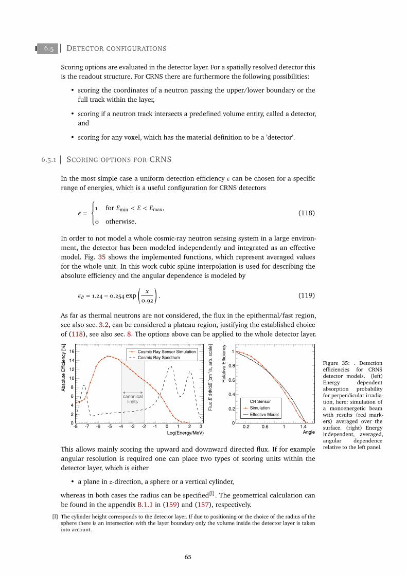
6.5 DETECTOR CONFIGURATIONS

Scoring options are evaluated in the detector layer. For a spatially resolved detector thisis the readout structure. For CRNS there are furthermore the following possibilities:

• scoring the coordinates of a neutron passing the upper/lower boundary or thefull track within the layer,

• scoring if a neutron track intersects a predefined volume entity, called a detector,and

• scoring for any voxel, which has the material definition to be a ’detector’.

6.5.1 SCORING OPTIONS FOR CRNS

In the most simple case a uniform detection efficiency 𝜖 can be chosen for a specificrange of energies, which is a useful configuration for CRNS detectors

𝜖 =

1 for 𝐸min < 𝐸 < 𝐸max,

0 otherwise.(118)

In order to not model a whole cosmic-ray neutron sensing system in a large environ-ment, the detector has been modeled independently and integrated as an effectivemodel. Fig. 35 shows the implemented functions, which represent averaged valuesfor the whole unit. In this work cubic spline interpolation is used for describing theabsolute efficiency and the angular dependence is modeled by

𝜖𝜗 = 1.24 − 0.254 exp(

𝑥

0.92

). (119)

As far as thermal neutrons are not considered, the flux in the epithermal/fast region,see also sec. 3.2, can be considered a plateau region, justifying the established choiceof (118), see also sec. 8. The options above can be applied to the whole detector layer.

Figure 35: . Detectionefficiencies for CRNSdetector models. (left)Energy dependentabsorption probabilityfor perpendicular irradia-tion, here: simulation ofa monoenergetic beamwith results (red mark-ers) averaged over thesurface. (right) Energyindependent, averaged,angular dependencerelative to the left panel.

Log(Energy/MeV)

-8 -7 -6 -5 -4 -3 -2 -1 0 1 2 3

Ab

so

lute

Effic

ien

cy [%

]

0

2

4

6

8

10

12

14

16 Cosmic Ray Sensor Simulation

Cosmic Ray Spectrum

Angle

Re

lativ

e E

ffic

ien

cy

0

0.2

0.4

0.6

0.8

1

Simulation

Effective Model

canonicallimits

0.2 0.6 1 1.4

CR Sensor

-2F

lux E

dΦ/dE

[cm

/s, a

rb. sca

le]

This allows mainly scoring the upward and downward directed flux. If for exampleangular resolution is required one can place two types of scoring units within thedetector layer, which is either

• a plane in 𝑧-direction, a sphere or a vertical cylinder,

whereas in both cases the radius can be specified[l]. The geometrical calculation canbe found in the appendix B.1.1 in (159) and (157), respectively.

[l] The cylinder height corresponds to the detector layer. If due to positioning or the choice of the radius of thesphere there is an intersection with the layer boundary only the volume inside the detector layer is takeninto account.

65

6.5.2 NEUTRON CONVERSION EVALUATION FOR BORON DETECTORS

Whereas in gaseous converters like 3He regarding the detection efficiency only themacroscopic cross section has to be taken into account, as nearly all converted neutronscan be detected, for hybrid solid state detectors the entire signal generation path hasto be considered. Compared to the attenuation length at _ = 1.8 Å of 20 µm the rangewithin a converter layer is < 4 µm. Even for thin layers therefore the efficiency canbe significantly reduced by inactive material. The two main absorption reactions inboron-10 are:

10B + n →7Li(0.84MeV) + 𝛼 (1.472MeV) +𝛾 (0.48MeV) (93.6%) [𝑎],7Li(1.013MeV) + 𝛼 (1.776MeV) (6.4%) [𝑏]. (120)

R He

Neutron

R Li

Helium

Lithium

Substrate Boron Converter Gas

1/e Absorption

R Gas

θRange (λ)

Figure 36: Physics of a hybridboron converter layer: a neutronimpinges at an angle 𝜗 normal tothe surface. The absorption prob-ability is wavelength dependent.By the conversion process lithium(Li) and helium (He) ions withfixed energies are created. In themedium itself they lose energyby collisions leading to a Braggdistributed range 𝑅, different forboth agents. After reaching the gasan ionization track is producedwith the remaining energy at theboundary. [K2016]

In the boron medium itself the particles are emitted isotropically and back to back. Twogeometries are possible: (1) the front side irradiation describes the case of the activesurface being oriented towards the incoming neutrons and therefore the detectionmedium being situated prior in beam direction. (2) Vice versa the backside irradiationrefers to the inverted geometry. Therefore, as only one of both can enter the gas, arandom number b1 determines[m] the type of ion 𝐼 and another random number b2

assigns the decay branch ([a] or [b]). Two more random numbers b2, b4 determine theemission angles

𝜗𝐼 = 0.5𝜋b3, (121)

𝜙𝐼 = 𝜋 (2b4 − 1). (122)

The remaining distance to the layer border 𝑑𝑆 can then be calculated either upwards ordownwards. The fragments lose kinetic energy mainly by ionization. These energy-range-relations have been calculated by SRIM [160] and transferred to analyticalmodels. For boron carbide the energy loss in the medium can be described as

Li+++: (𝐸0 = 1.013MeV) 𝐸out = 𝐸0 − (−0.209𝑑2𝑆 + 0.924𝑑𝑆 ),(𝐸0 = 0.840MeV) 𝐸out = 𝐸0 − (−0.2195𝑑2𝑆 + 0.8574𝑑𝑆 ),

He++: (𝐸0 = 1.776MeV) 𝐸out = 𝐸0 − (−0.0165𝑑3𝑆+ 0.1003𝑑2𝑆 + 0.289𝑑𝑆 ),

(𝐸0 = 1.472MeV) 𝐸out = 𝐸0 − (−0.0285𝑑3𝑆+ 0.1267𝑑2𝑆 + 0.3354𝑑𝑆 ), (123)

[m] All random numbers here are assumed to cover a range within [0, 1), hence the rule for the ion choice is b1 <0.5.

66

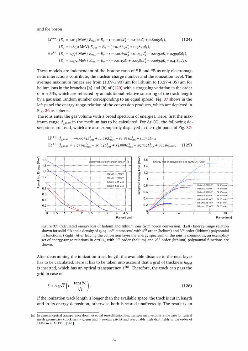
and for boron

Li+++: (𝐸0 = 1.013MeV) 𝐸out = 𝐸0 − (−0.019𝑑3𝑆− 0.1166𝑑2𝑆 + 0.8065𝑑𝑆 ), (124)

(𝐸0 = 0.840MeV) 𝐸out = 𝐸0 − (−0.1863𝑑2𝑆 + 0.7891𝑑𝑆 ),He++: (𝐸0 = 1.776MeV) 𝐸out = 𝐸0 − (−0.0069𝑑4

𝑆+ 0.047𝑑3

𝑆− 0.0732𝑑2𝑆 + 0.3998𝑑𝑆 ),

(𝐸0 = 1.472MeV) 𝐸out = 𝐸0 − (−0.0115𝑑4𝑆+ 0.0581𝑑3

𝑆− 0.0634𝑑2𝑆 + 0.4189𝑑𝑆 ).

These models are independent of the isotope ratio of 10B and 11B as only electromag-netic interactions contribute, the nuclear charge number and the ionization level. Theaverage maximum ranges are from (1.69-1.90) µm for lithium to (3.27-4.05) µm forhelium ions in the branches [a] and [b] of (120) with a straggling variation in the orderof 𝜎 ≈ 5 %, which are reflected by an additional relative smearing of the track lengthby a gaussian random number corresponding to an equal spread. Fig. 37 shows in theleft panel the energy-range-relation of the conversion products, which are depicted inFig. 36 as spheres.The ions enter the gas volume with a broad spectrum of energies. Here, first the max-imum range 𝑑𝑔,max in the medium has to be calculated. For Ar:CO2 the following de-scriptions are used, which are also exemplarily displayed in the right panel of Fig. 37:

Li+++: 𝑑𝑔,max = −6.6034𝐸4out + 18.215𝐸3out − 18.783𝐸2out + 11.732𝐸out,

He++: 𝑑𝑔,max = 4.7579𝐸5out − 20.64𝐸4out + 33.888𝐸3out − 25.727𝐸2out + 13.216𝐸out, (125)

Range [mm]

0 2 4 6 8 10

Inte

gra

ted

En

erg

y L

oss

[M

eV

]

0

0.2

0.4

0.6

0.8

1

1.2

1.4

1.6(70:30)

2Energy loss of conversion ions in ArCO

Helium 0.25 MeV orderrdFit 3

Helium 0.75 MeV orderrdFit 3

Helium 1.00 MeV orderrdFit 3

Helium 1.50 MeV orderrdFit 3

Lithium 0.25 MeV orderndFit 2

Lithium 0.75 MeV orderndFit 2

Lithium 1.00 MeV orderndFit 2

m]μRange [

0 0.5 1 1.5 2 2.5 3 3.5 4 4.5

Re

ma

inin

g E

ne

rgy

[Me

V]

0

0.2

0.4

0.6

0.8

1

1.2

1.4

1.6

1.8B10Energy loss of conversion ions in

Helium 1.47 MeV

Helium 1.78 MeV

Lithium 0.84 MeV

Lithium 1.02 MeV

Figure 37: Calculated energy loss of helium and lithium ions from boron conversion. (Left) Energy-range relationshown for solid 10B and a density of 13.05 · 1022 atoms/cm3 with 4th order (helium) and 3rd order (lithium) polynomialfit functions. (Right) After leaving the conversion layer the energy spectrum of the ions is continuous, an exemplaryset of energy-range relations in Ar:CO2 with 3rd order (helium) and 2nd order (lithium) polynomial functions areshown.

After determining the ionization track length the available distance to the next layerhas to be calculated. Here it has to be taken into account that a grid of thickness ℎGrid

is inserted, which has an optical transparency 𝑇 [n]. Therefore, the track can pass thegrid in case of

b < 0.5√𝑇

(1 − tan(𝜗𝐼 )√

𝑇

). (126)

If the ionization track length is longer than the available space, the track is cut in lengthand in its energy deposition, otherwise both is scored unaffectedly. The result is an

[n] In general optical transparency does not equal zero-diffusion flux transparency, yet, this is the case for typicalmesh geometries (thickness ≈ 50µm and ≈ 100µm pitch) and reasonably high drift fields in the order of1 kV/cm in Ar:CO2. [161]

67

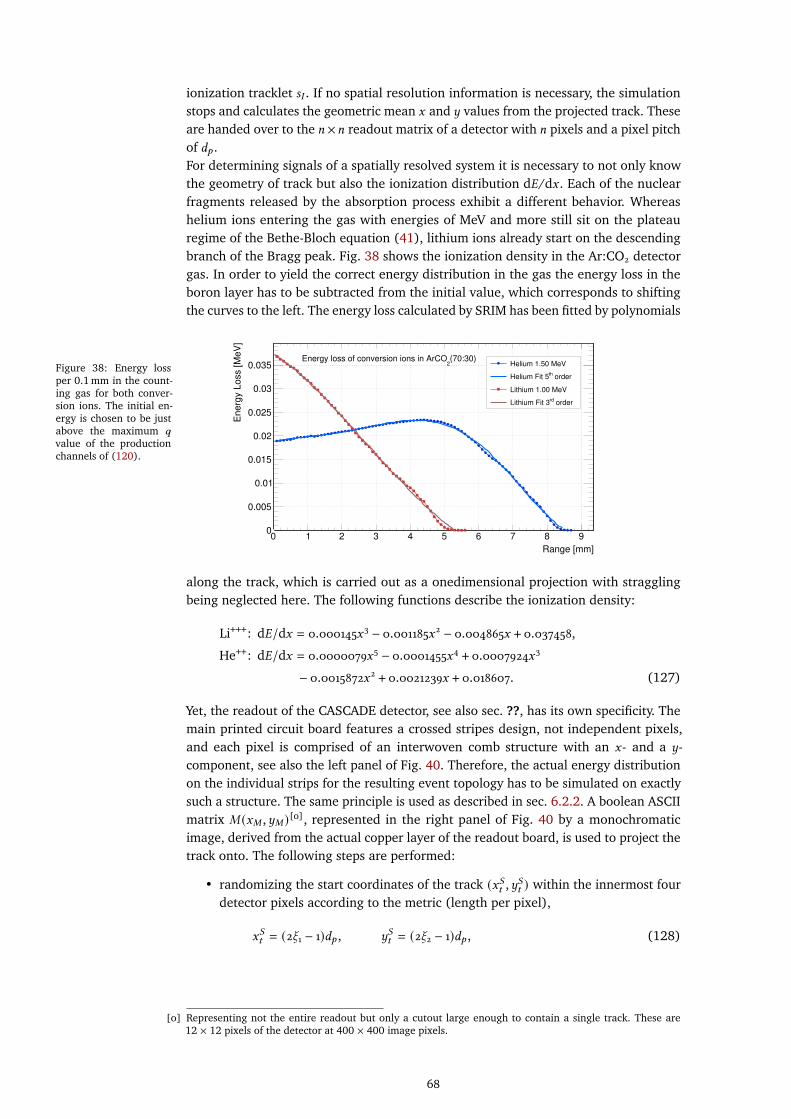
ionization tracklet 𝑠𝐼 . If no spatial resolution information is necessary, the simulationstops and calculates the geometric mean 𝑥 and 𝑦 values from the projected track. Theseare handed over to the 𝑛 ×𝑛 readout matrix of a detector with 𝑛 pixels and a pixel pitchof 𝑑𝑝 .For determining signals of a spatially resolved system it is necessary to not only knowthe geometry of track but also the ionization distribution d𝐸/d𝑥 . Each of the nuclearfragments released by the absorption process exhibit a different behavior. Whereashelium ions entering the gas with energies of MeV and more still sit on the plateauregime of the Bethe-Bloch equation (41), lithium ions already start on the descendingbranch of the Bragg peak. Fig. 38 shows the ionization density in the Ar:CO2 detectorgas. In order to yield the correct energy distribution in the gas the energy loss in theboron layer has to be subtracted from the initial value, which corresponds to shiftingthe curves to the left. The energy loss calculated by SRIM has been fitted by polynomials

Figure 38: Energy lossper 0.1 mm in the count-ing gas for both conver-sion ions. The initial en-ergy is chosen to be justabove the maximum 𝑞

value of the productionchannels of (120).

Range [mm]

0 1 2 3 4 5 6 7 8 9

Energ

y L

oss [M

eV

]

0

0.005

0.01

0.015

0.02

0.025

0.03

0.035(70:30)

2Energy loss of conversion ions in ArCO

Helium 1.50 MeV

orderthHelium Fit 5

Lithium 1.00 MeV

orderrdLithium Fit 3

along the track, which is carried out as a onedimensional projection with stragglingbeing neglected here. The following functions describe the ionization density:

Li+++: d𝐸/d𝑥 = 0.000145𝑥3 − 0.001185𝑥2 − 0.004865𝑥 + 0.037458,

He++: d𝐸/d𝑥 = 0.0000079𝑥5 − 0.0001455𝑥4 + 0.0007924𝑥3

− 0.0015872𝑥2 + 0.0021239𝑥 + 0.018607. (127)

Yet, the readout of the CASCADE detector, see also sec. ??, has its own specificity. Themain printed circuit board features a crossed stripes design, not independent pixels,and each pixel is comprised of an interwoven comb structure with an 𝑥- and a 𝑦-component, see also the left panel of Fig. 40. Therefore, the actual energy distributionon the individual strips for the resulting event topology has to be simulated on exactlysuch a structure. The same principle is used as described in sec. 6.2.2. A boolean ASCIImatrix 𝑀 (𝑥𝑀 ,𝑦𝑀 )[o], represented in the right panel of Fig. 40 by a monochromaticimage, derived from the actual copper layer of the readout board, is used to project thetrack onto. The following steps are performed:

• randomizing the start coordinates of the track (𝑥𝑆𝑡 ,𝑦𝑆𝑡 ) within the innermost fourdetector pixels according to the metric (length per pixel),

𝑥𝑆𝑡 = (2b1 − 1)𝑑𝑝 , 𝑦𝑆𝑡 = (2b2 − 1)𝑑𝑝 , (128)

[o] Representing not the entire readout but only a cutout large enough to contain a single track. These are12 × 12 pixels of the detector at 400 × 400 image pixels.

68

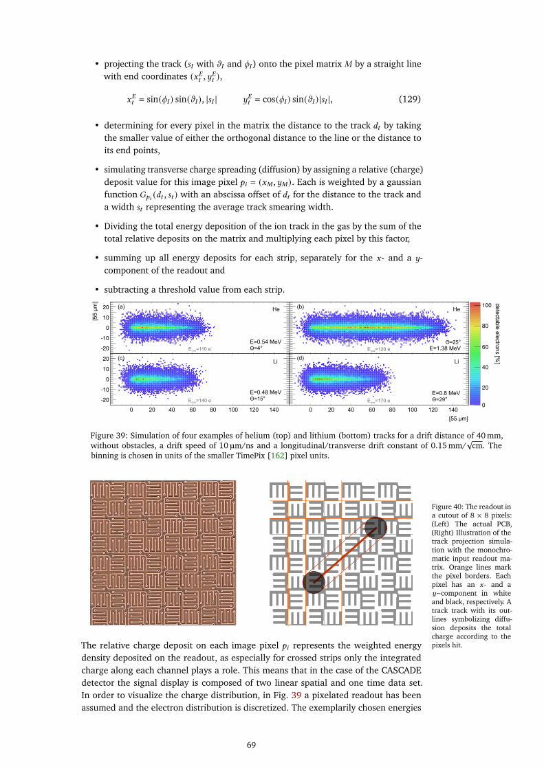
• projecting the track (𝑠𝐼 with 𝜗𝐼 and 𝜙𝐼 ) onto the pixel matrix 𝑀 by a straight linewith end coordinates (𝑥𝐸𝑡 ,𝑦𝐸𝑡 ),

𝑥𝐸𝑡 = sin(𝜙𝐼 ) sin(𝜗𝐼 ), |𝑠𝐼 | 𝑦𝐸𝑡 = cos(𝜙𝐼 ) sin(𝜗𝐼 ) |𝑠𝐼 |, (129)

• determining for every pixel in the matrix the distance to the track 𝑑𝑡 by takingthe smaller value of either the orthogonal distance to the line or the distance toits end points,

• simulating transverse charge spreading (diffusion) by assigning a relative (charge)deposit value for this image pixel 𝑝𝑖 = (𝑥𝑀 ,𝑦𝑀 ). Each is weighted by a gaussianfunction 𝐺𝑝𝑖 (𝑑𝑡 , 𝑠𝑡 ) with an abscissa offset of 𝑑𝑡 for the distance to the track anda width 𝑠𝑡 representing the average track smearing width.

• Dividing the total energy deposition of the ion track in the gas by the sum of thetotal relative deposits on the matrix and multiplying each pixel by this factor,

• summing up all energy deposits for each strip, separately for the 𝑥- and a 𝑦-component of the readout and

• subtracting a threshold value from each strip.

0

20

40

60

80

100

-20

-10

0

10

20

[55 m]μ

0 20 40 60 80 100 120 1400 20 40 60 80 100 120 140

-20

-10

0

10

20

E=0.54 MeV=4°Θ

He He

Li Li

E=0.48 MeV=15°Θ

E=0.8 MeV=29°Θ

E=1.38 MeVΘ=25°

[55

m

]μ

de

tecta

ble

ele

ctro

ns [%

]

(a) (b)

(c) (d)

-E =140 emax

-E =170 emax

-E =110 emax

-E =120 emax

Figure 39: Simulation of four examples of helium (top) and lithium (bottom) tracks for a drift distance of 40 mm,without obstacles, a drift speed of 10 µm/ns and a longitudinal/transverse drift constant of 0.15 mm/

√cm. The

binning is chosen in units of the smaller TimePix [162] pixel units.

Figure 40: The readout ina cutout of 8 × 8 pixels:(Left) The actual PCB,(Right) Illustration of thetrack projection simula-tion with the monochro-matic input readout ma-trix. Orange lines markthe pixel borders. Eachpixel has an 𝑥- and a𝑦−component in whiteand black, respectively. Atrack track with its out-lines symbolizing diffu-sion deposits the totalcharge according to thepixels hit.The relative charge deposit on each image pixel 𝑝𝑖 represents the weighted energy

density deposited on the readout, as especially for crossed strips only the integratedcharge along each channel plays a role. This means that in the case of the CASCADEdetector the signal display is composed of two linear spatial and one time data set.In order to visualize the charge distribution, in Fig. 39 a pixelated readout has beenassumed and the electron distribution is discretized. The exemplarily chosen energies

69

at rather slant angles visualize the spatial spread of the charge density shown in Fig. 38for a maximum (free) drift distance of 40 mm. At the beginning and the end of theionization tracklet the charge is effectively distributed in two dimensions, whereas inthe center the distribution can be considered as only being relevant orthogonal to themain axis.

This leads to the following effects:

• the effective width of the tracklet depends on the energy loss along its axis,therefore the tail is slightly more ’pointy’-shaped than the origin, which rendersa simple geometric description impossible,

• the origin is not located at the coordinate of highest d𝐸/d𝑥 even if in the case oflithium the track has its highest ionization density at the beginning. The reasonis that the diffusion leads to a relatively stronger smearing out at the ends ofthe track. Therefore, the origin is not directly correlated to the highest measuredd𝐸/d𝑥 .

In summary the schematic Fig. 41 describes the steps specific for calculating the ge-ometry and the readout in the CASCADE detector in a unit-cell like picture. A trackis generated from a neutron conversion inside the boron. Its length is calculated an-alytically by the energy loss in the converter and subsequently in the gas. Due to thenarrow drift spaces of the layer geometry a track can be limited in its extension bythe subsequent grid or GEM. Finally the track broadened by the diffusion in the gas isprojected onto the readout with discrete spacing (pixel) and time (clock cycles) units.

Figure 41: Elements ofthe CASCADE detector inURANOS from the parti-cle simulation to the sig-nal generation with focuson the description of thecharged particle track in-side the gaseous volume.

neutron

boron layer10dE/dx in B

conversion

dE/dx in Ar:CO2

readout

longitudinal&

transversalDiffusion

drift s

pace

E-field

[x,y,t]

THL THL[x ,y ,t ]min

-Gxe

gas gain

GEM

tbin

t

time walk

drift s

pace

70

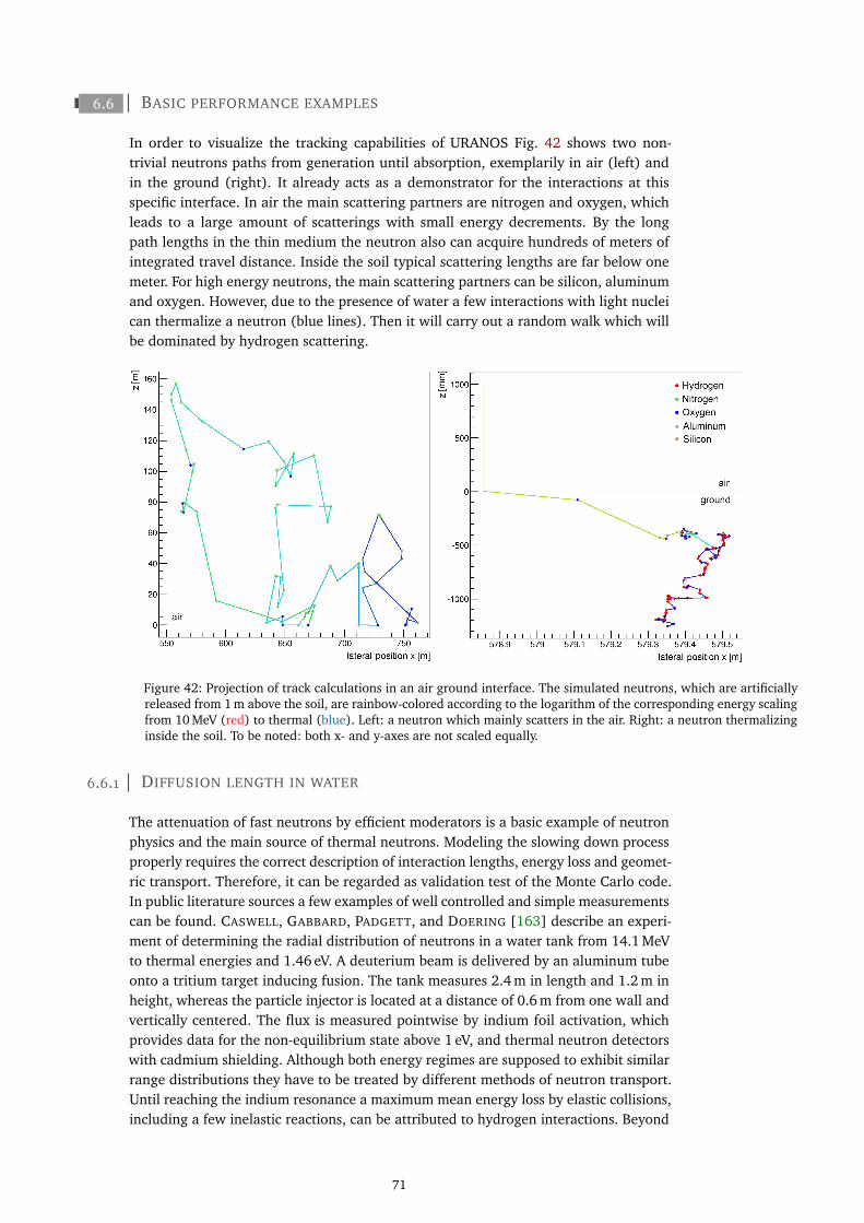
6.6 BASIC PERFORMANCE EXAMPLES

In order to visualize the tracking capabilities of URANOS Fig. 42 shows two non-trivial neutrons paths from generation until absorption, exemplarily in air (left) andin the ground (right). It already acts as a demonstrator for the interactions at thisspecific interface. In air the main scattering partners are nitrogen and oxygen, whichleads to a large amount of scatterings with small energy decrements. By the longpath lengths in the thin medium the neutron also can acquire hundreds of meters ofintegrated travel distance. Inside the soil typical scattering lengths are far below onemeter. For high energy neutrons, the main scattering partners can be silicon, aluminumand oxygen. However, due to the presence of water a few interactions with light nucleican thermalize a neutron (blue lines). Then it will carry out a random walk which willbe dominated by hydrogen scattering.

Figure 42: Projection of track calculations in an air ground interface. The simulated neutrons, which are artificiallyreleased from 1 m above the soil, are rainbow-colored according to the logarithm of the corresponding energy scalingfrom 10 MeV (red) to thermal (blue). Left: a neutron which mainly scatters in the air. Right: a neutron thermalizinginside the soil. To be noted: both x- and y-axes are not scaled equally.

6.6.1 DIFFUSION LENGTH IN WATER

The attenuation of fast neutrons by efficient moderators is a basic example of neutronphysics and the main source of thermal neutrons. Modeling the slowing down processproperly requires the correct description of interaction lengths, energy loss and geomet-ric transport. Therefore, it can be regarded as validation test of the Monte Carlo code.In public literature sources a few examples of well controlled and simple measurementscan be found. CASWELL, GABBARD, PADGETT, and DOERING [163] describe an experi-ment of determining the radial distribution of neutrons in a water tank from 14.1 MeVto thermal energies and 1.46 eV. A deuterium beam is delivered by an aluminum tubeonto a tritium target inducing fusion. The tank measures 2.4 m in length and 1.2 m inheight, whereas the particle injector is located at a distance of 0.6 m from one wall andvertically centered. The flux is measured pointwise by indium foil activation, whichprovides data for the non-equilibrium state above 1 eV, and thermal neutron detectorswith cadmium shielding. Although both energy regimes are supposed to exhibit similarrange distributions they have to be treated by different methods of neutron transport.Until reaching the indium resonance a maximum mean energy loss by elastic collisions,including a few inelastic reactions, can be attributed to hydrogen interactions. Beyond

71

this limit the kinetic energy of the neutron is becoming dominated by thermal scatter-ing leading to a constant average energy. This system can bee easily reproduced in amodel setup including the generalization of an infinitely large domain. The fluxes Φ

are scored at thermal (9-120) meV and indium resonance (1.3-1.6) eV energies on asphere of radius 𝑟 yielding a surface flux of 𝑟 2Φ. Fig. 43 shows the measured fluxesfrom [163] in comparison to the simulation results. Both attenuation distributions arein good agreement. The particle density in both cases peaks at around 15 cm followedby a nearly exponential decay with similar attenuation lengths[p].

Figure 43: Comparisonof the attenuationlength from [163] fordeuterium-tritium fusionneutrons emitted intowater. The sphericalsurface flux for thermaland indium resonanceneutrons as a functionof distance from thesource is compared tothe simulation resultsfrom URANOS.

Distance [mm]

0 200 400 600 800 1000 1200

[a.u

.]φ2

Neu

tron

Flu

x r

1

10

100

1000

Slowing down of 14.1 MeV neutrons

Simulation to thermal

Caswell (1957) to thermal

Simulation to 1.46 eV resonance

Caswell (1957) to 1.46 eV resonance

6.6.2 BONNER SPHERE EVALUATION

A case similar to the previous sec. 6.6.1 are Bonner Spheres, see also sec. ??, whichare proportional counters surrounded by shells of polyethylene. As this spectrometertype of array is used to monitor environmental fluxes, various studies were carried outfor the modeling of such [164–169]. Whereas the neutron range distribution in waterin the previous example demonstrated geometric transport and collision treatment,the Bonner Sphere offers the possibility to focus on an energy-dependent comparisonand on the interplay of moderator and absorber. Among the various existing technicalrealizations the helium-based version was chosen, equipped with a 3.2 cm sphericalcounter. For reasons of convenience, the whole model has been discretized in 17 layers,which are symmetrically arranged around the center and depicted in Fig. 44. Laterallythe resolution by the pixel matrix was set to 1 mm, therefore the voxel size of a 𝑋 inchsphere is 1 mm × 1 mm × (𝑋/17) ”. For the simulation the model was irradiated by aneutron beam of the same diameter as the sphere under an angle of 0 ◦.

Figure 44: DiscretizedURANOS Input files forthe upper half of a 2 inchBonner Sphere.

Furthermore, hydrogen atoms in polyethylene have been emulated by the scatteringkernel derived from the (oxygen-)bound cross section in water. This can yield ex-clusively for thermal energies a systematic uncertainty of around 10 %. Due to thestatistical nature of neutron transport the actual geometrical shape of a body has aminor influence compared to other parameters like overall volume or thickness. Exem-

[p] Fermi age transport theory, which is not taken into comparison here, can very well reproduce the attenuationat radial distances larger than 25 cm. For fluxes more close to the source the theoretical distribution peaksmuch earlier.

72

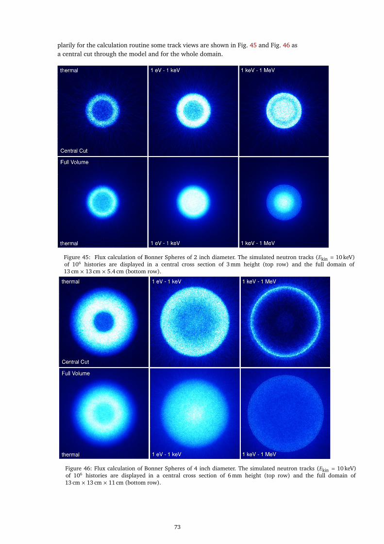
plarily for the calculation routine some track views are shown in Fig. 45 and Fig. 46 asa central cut through the model and for the whole domain.

Figure 45: Flux calculation of Bonner Spheres of 2 inch diameter. The simulated neutron tracks (𝐸kin = 10 keV)of 106 histories are displayed in a central cross section of 3 mm height (top row) and the full domain of13 cm × 13 cm × 5.4 cm (bottom row).

Figure 46: Flux calculation of Bonner Spheres of 4 inch diameter. The simulated neutron tracks (𝐸kin = 10 keV)of 106 histories are displayed in a central cross section of 6 mm height (top row) and the full domain of13 cm × 13 cm × 11 cm (bottom row).

73

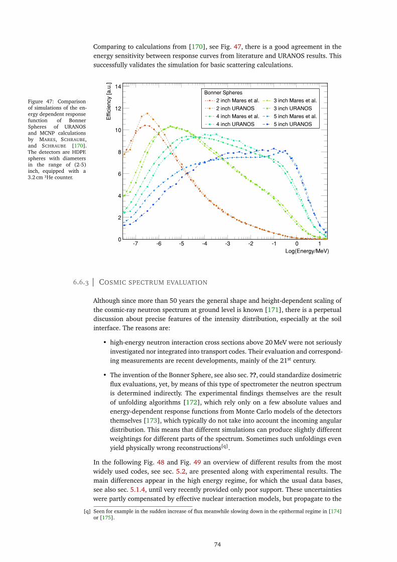
Comparing to calculations from [170], see Fig. 47, there is a good agreement in theenergy sensitivity between response curves from literature and URANOS results. Thissuccessfully validates the simulation for basic scattering calculations.

Figure 47: Comparisonof simulations of the en-ergy dependent responsefunction of BonnerSpheres of URANOSand MCNP calculationsby MARES, SCHRAUBE,and SCHRAUBE [170].The detectors are HDPEspheres with diametersin the range of (2-5)inch, equipped with a3.2 cm 3He counter.

Effic

ien

cy [a

.u.]

0

2

4

6

8

10

12

14Bonner Spheres

2 inch Mares et al. 3 inch Mares et al.

2 inch URANOS 3 inch URANOS

4 inch Mares et al. 5 inch Mares et al.

4 inch URANOS 5 inch URANOS

Log(Energy/MeV)

-7 -6 -5 -4 -3 -2 -1 0 1

6.6.3 COSMIC SPECTRUM EVALUATION

Although since more than 50 years the general shape and height-dependent scaling ofthe cosmic-ray neutron spectrum at ground level is known [171], there is a perpetualdiscussion about precise features of the intensity distribution, especially at the soilinterface. The reasons are:

• high-energy neutron interaction cross sections above 20 MeV were not seriouslyinvestigated nor integrated into transport codes. Their evaluation and correspond-ing measurements are recent developments, mainly of the 21st century.

• The invention of the Bonner Sphere, see also sec. ??, could standardize dosimetricflux evaluations, yet, by means of this type of spectrometer the neutron spectrumis determined indirectly. The experimental findings themselves are the resultof unfolding algorithms [172], which rely only on a few absolute values andenergy-dependent response functions from Monte Carlo models of the detectorsthemselves [173], which typically do not take into account the incoming angulardistribution. This means that different simulations can produce slightly differentweightings for different parts of the spectrum. Sometimes such unfoldings evenyield physically wrong reconstructions[q].

In the following Fig. 48 and Fig. 49 an overview of different results from the mostwidely used codes, see sec. 5.2, are presented along with experimental results. Themain differences appear in the high energy regime, for which the usual data bases,see also sec. 5.1.4, until very recently provided only poor support. These uncertaintieswere partly compensated by effective nuclear interaction models, but propagate to the

[q] Seen for example in the sudden increase of flux meanwhile slowing down in the epithermal regime in [174]or [175].

74

lower energetic parts of the flux distribution. For now only the general shape of thespectrum has to be considered. The peak structures at around 1 MeV, which are de factospectral lines of inelastic resonances, mostly oxygen, cannot be resolved experimentallyby spectrometers and are displayed only at times. By normalizing to the intensity ofthe thermal peak Fig. 48 accumulates possible uncertainties and therefore maximizesthe deviations between the presented evaluations. A better convergence is displayedin Fig. 49.In order minimize this general problem URANOS uses a validated neutron spectrumnear the surface as a source and releases it directly onto the ground to minimize typicaluncertainties of atmospheric propagation. The implementation of the works presentedby [66] and [159], which are based on [68] and [67], are discussed in sec. 6.3.1.

Figure 48: Energy dependent neutron flux at an altitudeof 1860 m calculated by MCNPX, GEANT with the twohigh energy models Bertini [176, 177] and BIC [178]and determined experimentally from [179]. [180]

Figure 49: Energy dependent neutron flux at 1 m alti-tude calculated by EXPACS, MCNPX, GEANT4 and de-termined experimentally from [181] and from [182].Environmental conditions are not the same. [183]

Fig. 50 presents the result from URANOS for the calculated neutron flux (black) abovethe surface in an infinite domain. The input is drawn in green. On the qualitative level

Figure 50: URANOScosmic-ray neutronspectrum comparison.The incoming spec-trum (green), whichis generated from theanalytical functions (68)and (69) from [66], isreleased onto the soil.The resulting intensitydistribution, shown inblack, is compared tothe original spectrum forthe same environmentalconditions from [66] inblue.

0

1

2

3

4

5

6

7

8

moistureVol%soil: 8

humidity%air: 0

Surface Spectra

Sato et al. (2006)

this work, Incoming

this work, Interface

Log(Energy/MeV)

0 1 2 3-5 -3 -1-2-4-6-8 -7 4

-2F

lux E

dΦ/d

E [cm

·/s

, a

rb. sca

le]

the underlying physics model correctly calculates the response to the soil. In the highenergy domain around 100 MeV the incoming flux is only reduced, no influence ofbackscattering can be observed. In the region around 1 MeV the evaporation peak ap-

75

pears correctly in width and mean energy value. The spike structure on the peak itselfis result of elastic scattering on strong nuclear resonances, mainly in oxygen - for ex-ample at 435 keV[r]. As there are no significant sources in the range of 1 eV to 0.1 MeV,in a lethargy-dependent plot there is a flat plateau between neutron generation andthermalization, the latter being truncated here. This plateau can feature a slant anglein case there are significant absorption processes involved, but no other features likebumps or steps should be visible. It has to be pointed out that the resulting spectrumhere requires nearly the full physics and tracking computation.For a quantitative investigation due to the lack of a generally accepted standardizedspectrum or a consensus in the literature, the evaluation of the URANOS code focuseson the capability to reproduce the above-ground cosmic neutron spectrum for typicalconditions. This implies that the input spectrum released on the ground should repro-duce the same densities as the input formulae (68) and (69). This test twice evaluatesthe computational correctness of the code - by yielding the same predictions as theMonte Carlo reference and indirectly by showing that the reverse-engineered inputspectrum has been modeled correctly.

6.6.4 PERFORMANCE BENCHMARKS

The performance of the code heavily depends on the setup, which is to be simulated.The most significant contributor is the mean lifetime of neutrons in terms of scatteringswithin the domain. In simple configurations like for the analysis of detectors mostneutrons undergo only a few interactions before either being absorbed or leaving thendomain. Atmospheric neutrons can have up to hundreds of scatterings before endingup thermalized, see also later 9.1.6. Additionally, depending on the chosen materialsand energy range, only a few cross sections like for elastic scattering plus absorptionare evaluated. In the MeV regime adding up all inelastic channels scales up to dozensof address requests.In order to provide some practical estimations a standard scenery can be definedas in table 9. This domain measures 900 m × 900 m with a source dimension of840 m × 840 m. It contains a minimum configuration of six layers for analyzing aneutron density which can be considered in spatial equilibrium in the innermost400 m × 400 m.

Table 9: The standardsetup for a layer compo-sition in cosmic neutronsensing.

Layer Position [m] Height [m] Material Function

1 -1000 920 air top buffer layer

2 -80 30 air source layer

3 -50 47.5 air -

4 -2.5 0.5 air detector layer

5 -2 2 air -

6 -0 3 soil ground layer

A similar setup has also been used for simulating the so-called ’UFZ site’ in the publica-tion [SK2017b] - an urban environment with many concrete buildings, streets, greenspaces, a railroad line, a lake and trees. From the twelve layers in total eight containeda pixel matrix of 1800 × 1800 voxel definitions. The composition 21 introducing theURANOS chapter shows the layer model setup as well as one of the calculation resultsfor the above-ground neutron density.

[r] The structure of the evaporation peak can rather be compared to a transmission spectrum, as those energiesare missing which correspond to resonances. There neutrons are scattered off to lower energies more likelythan otherwise.

76

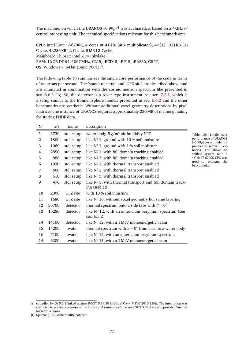
The machine, on which the URANOS v0.99𝜌[s] was evaluated, is based on a 4 GHz i7central processing unit. The technical specifications relevant for this benchmark are:

CPU: Intel Core i7-6700K, 4 cores at 4 GHz (40x multiplicator), 4×(32+32) KB L1-Cache, 4×256 KB L2-Cache, 8 MB L3-Cache,Mainboard Chipset: Intel Z170 Skylake,RAM: 16 GB DDR4, 1067 MHz, CL15, tRCD15, tRP15, tRAS36, CR2T,OS: Windows 7, 64 bit (Build 7601)[t].

The following table 10 summarizes the single core performance of the code in termsof neutrons per second. The ’standard setup’ and ’UFZ site’ are described above andare simulated in combination with the cosmic neutron spectrum like presented insec. 6.6.3 Fig. 50, the detector is a rover type instrument, see sec. 7.2.1, which isa setup similar to the Bonner Sphere models presented in sec. 6.6.2 and the otherbenchmarks are synthetic. Without additional voxel geometry descriptions by pixelmatrices one instance of URANOS requires approximately 230 MB of memory, mainlyfor storing ENDF data.

Table 10: Single coreperformance of URANOS(v0.99𝜌) for a number ofpractically relevant sce-narios. The above de-scribed system with a4 GHz i7-6700K CPU wasused to evaluate thebenchmarks.

No n/s name description

1 3730 std. setup water body, 5 g/m3 air humidity NTP

2 1800 std. setup like No 1, ground with 10 % soil moisture

3 1060 std. setup like No 1, ground with 1 % soil moisture

4 2850 std. setup like No 1, with full domain tracking enabled

5 880 std. setup like No 3, with full domain tracking enabled

6 1030 std. setup like No 1, with thermal transport enabled

7 600 std. setup like No 2, with thermal transport enabled

8 510 std. setup like No 3, with thermal transport enabled

9 470 std. setup like No 3, with thermal transport and full domain track-ing enabled

10 2000 UFZ site with 10 % soil moisture

11 1680 UFZ site like No 10, without voxel geometry but same layering

12 36700 detector thermal spectrum onto a side face with 𝜗 = 0◦

13 16250 detector like No 12, with an americium-beryllium spectrum (seesec. 6.3.2)

14 14100 detector like No 12, with a 1 MeV monoenergetic beam

15 14200 water thermal spectrum with 𝜗 = 0◦ from air into a water body

16 7100 water like No 15, with an americium-beryllium spectrum

14 6300 water like No 15, with a 1 MeV monoenergetic beam

[s] compiled by Qt 5.2.1 linked against ROOT 5.34.20 in Visual C++ MSVC 2010 32bit. The integration wasrestricted to previous versions of the library and runtime as far as no ROOT 5.34.X version provided binariesfor later versions.

[t] Spectre [184] vulnerability patched.

77

Part IV

C O S M I C - R A Y N E U T R O N S E N S I N G

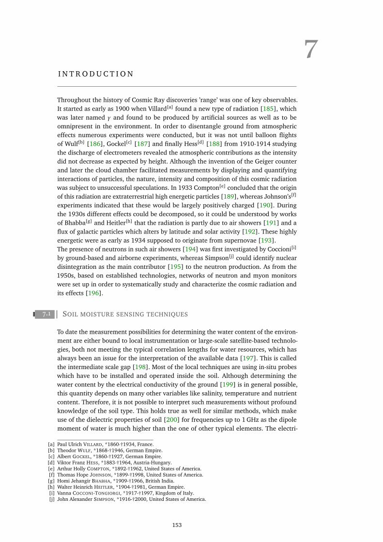
7I N T R O D U C T I O N

Throughout the history of Cosmic Ray discoveries ’range’ was one of key observables.It started as early as 1900 when Villard[a] found a new type of radiation [185], whichwas later named 𝛾 and found to be produced by artificial sources as well as to beomnipresent in the environment. In order to disentangle ground from atmosphericeffects numerous experiments were conducted, but it was not until balloon flightsof Wulf[b] [186], Gockel[c] [187] and finally Hess[d] [188] from 1910-1914 studyingthe discharge of electrometers revealed the atmospheric contributions as the intensitydid not decrease as expected by height. Although the invention of the Geiger counterand later the cloud chamber facilitated measurements by displaying and quantifyinginteractions of particles, the nature, intensity and composition of this cosmic radiationwas subject to unsuccessful speculations. In 1933 Compton[e] concluded that the originof this radiation are extraterrestrial high energetic particles [189], whereas Johnson’s[f]

experiments indicated that these would be largely positively charged [190]. Duringthe 1930s different effects could be decomposed, so it could be understood by worksof Bhabba[g] and Heitler[h] that the radiation is partly due to air showers [191] and aflux of galactic particles which alters by latitude and solar activity [192]. These highlyenergetic were as early as 1934 supposed to originate from supernovae [193].The presence of neutrons in such air showers [194] was first investigated by Coccioni[i]

by ground-based and airborne experiments, whereas Simpson[j] could identify nucleardisintegration as the main contributor [195] to the neutron production. As from the1950s, based on established technologies, networks of neutron and myon monitorswere set up in order to systematically study and characterize the cosmic radiation andits effects [196].

7.1 SOIL MOISTURE SENSING TECHNIQUES

To date the measurement possibilities for determining the water content of the environ-ment are either bound to local instrumentation or large-scale satellite-based technolo-gies, both not meeting the typical correlation lengths for water resources, which hasalways been an issue for the interpretation of the available data [197]. This is calledthe intermediate scale gap [198]. Most of the local techniques are using in-situ probeswhich have to be installed and operated inside the soil. Although determining thewater content by the electrical conductivity of the ground [199] is in general possible,this quantity depends on many other variables like salinity, temperature and nutrientcontent. Therefore, it is not possible to interpret such measurements without profoundknowledge of the soil type. This holds true as well for similar methods, which makeuse of the dielectric properties of soil [200] for frequencies up to 1 GHz as the dipolemoment of water is much higher than the one of other typical elements. The electri-

[a] Paul Ulrich VILLARD, *1860-†1934, France.[b] Theodor WULF, *1868-†1946, German Empire.[c] Albert GOCKEL, *1860-†1927, German Empire.[d] Viktor Franz HESS, *1883-†1964, Austria-Hungary.[e] Arthur Holly COMPTON, *1892-†1962, United States of America.[f] Thomas Hope JOHNSON, *1899-†1998, United States of America.[g] Homi Jehangir BHABHA, *1909-†1966, British India.[h] Walter Heinrich HEITLER, *1904-†1981, German Empire.[i] Vanna COCCONI-TONGIORGI, *1917-†1997, Kingdom of Italy.[j] John Alexander SIMPSON, *1916-†2000, United States of America.

153

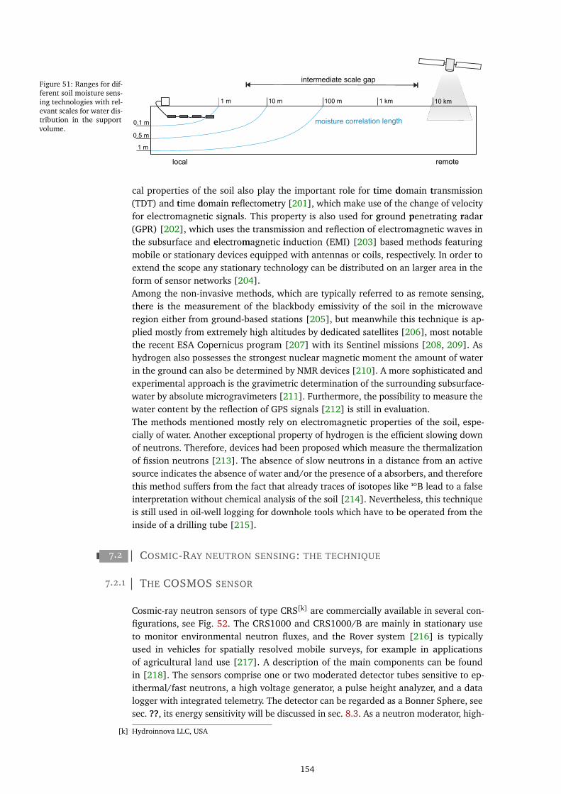
Figure 51: Ranges for dif-ferent soil moisture sens-ing technologies with rel-evant scales for water dis-tribution in the supportvolume.

1 m 10 m 100 m 1 km 10 km

0.1 m

1 m

0.5 m

moisture correlation length

intermediate scale gap

local remote

cal properties of the soil also play the important role for time domain transmission(TDT) and time domain reflectometry [201], which make use of the change of velocityfor electromagnetic signals. This property is also used for ground penetrating radar(GPR) [202], which uses the transmission and reflection of electromagnetic waves inthe subsurface and electromagnetic induction (EMI) [203] based methods featuringmobile or stationary devices equipped with antennas or coils, respectively. In order toextend the scope any stationary technology can be distributed on an larger area in theform of sensor networks [204].Among the non-invasive methods, which are typically referred to as remote sensing,there is the measurement of the blackbody emissivity of the soil in the microwaveregion either from ground-based stations [205], but meanwhile this technique is ap-plied mostly from extremely high altitudes by dedicated satellites [206], most notablethe recent ESA Copernicus program [207] with its Sentinel missions [208, 209]. Ashydrogen also possesses the strongest nuclear magnetic moment the amount of waterin the ground can also be determined by NMR devices [210]. A more sophisticated andexperimental approach is the gravimetric determination of the surrounding subsurface-water by absolute microgravimeters [211]. Furthermore, the possibility to measure thewater content by the reflection of GPS signals [212] is still in evaluation.The methods mentioned mostly rely on electromagnetic properties of the soil, espe-cially of water. Another exceptional property of hydrogen is the efficient slowing downof neutrons. Therefore, devices had been proposed which measure the thermalizationof fission neutrons [213]. The absence of slow neutrons in a distance from an activesource indicates the absence of water and/or the presence of a absorbers, and thereforethis method suffers from the fact that already traces of isotopes like 10B lead to a falseinterpretation without chemical analysis of the soil [214]. Nevertheless, this techniqueis still used in oil-well logging for downhole tools which have to be operated from theinside of a drilling tube [215].

7.2 COSMIC-RAY NEUTRON SENSING: THE TECHNIQUE

7.2.1 THE COSMOS SENSOR

Cosmic-ray neutron sensors of type CRS[k] are commercially available in several con-figurations, see Fig. 52. The CRS1000 and CRS1000/B are mainly in stationary useto monitor environmental neutron fluxes, and the Rover system [216] is typicallyused in vehicles for spatially resolved mobile surveys, for example in applicationsof agricultural land use [217]. A description of the main components can be foundin [218]. The sensors comprise one or two moderated detector tubes sensitive to ep-ithermal/fast neutrons, a high voltage generator, a pulse height analyzer, and a datalogger with integrated telemetry. The detector can be regarded as a Bonner Sphere, seesec. ??, its energy sensitivity will be discussed in sec. 8.3. As a neutron moderator, high-

[k] Hydroinnova LLC, USA

154

density polyethylene of 1 inch thickness is used to encase the proportional counter. TheCRS1000 uses helium-3, while the CRS1000/B uses boron trifluoride, which requireslarger detectors in order to achieve the same count rate due to its lower cross section(3837 b vs. 5330 b at 25.3 meV) [98] and pressure (0.5 bar vs. 1.5 bar) and thereforelower macroscopic cross section. The Rover is technically equivalent, but consists of sig-nificantly larger detectors than the stationary sensors and two tubes in one moderatedmodule to increase the event rate and therefore the time resolutions [219].

Figure 52: Variants ofthe cosmic-ray neutrondetectors modeled in thisstudy. Dimensions are inunits of millimeters. Toscale a Bonner Sphereis illustrated in compari-son. [KS2018]

CRS1000/B

CRS1000

revoR

Bonner Sphere

3"

900

400

180

260

1320

100 100 102

(top)

(side)(head-on)

7.2.2 SIGNAL CORRECTIONS

The cosmic-ray neutron spectrum is result of highly complex interplay of relativisticand non-relativistic particles, of leptons and baryons that create showers in the atmo-sphere like in a large calorimeter. Neutrons themselves as a by-product of these particlecascades make up a large part of the remaining radiation at ground level and are sen-sitive to the number of nucleons as long as being highly energetic and to hydrogenwhen being moderated. The neutron density 𝑁𝑛 at the soil interface is influenced byvarious factors, which turn out to exhibit a non-linear scaling, including correlations toother relevant environmental variables. Nonetheless, in order to derive a soil moisturevalue \ , there is a set of linear off-the-shelf corrections, which are used for example intime series, but have mostly been gained empirically. The fully corrected neutron countrate of a sensor 𝑁corr is calculated by

𝑁corr = 𝑁𝑛 ·𝐶𝐼 ·𝐶𝑝 ·𝐶ℎ, (130)

where 𝐶𝐼 denotes the incoming radiation correction, 𝐶𝑝 the atmospheric pressure cor-rection and 𝐶ℎ the air humidity correction - see also [220].As discussed in section 3.1, the cosmic radiation, which penetrates the upper atmo-sphere creating secondary neutrons, is not constant in its flux. Its intensity dependson the solar cycle and the vertical cutoff rigidity and other temporal variations. Thesefluctuations can hardly be predicted and therefore are measured by neutron monitors[l]

distributed in various locations around the world. Although these detectors primarilymeasure the highly-energetic proton component of the incoming radiation, there is asimilar dynamic assumed for neutrons [218] for regions of the same cutoff rigidity. TheNeutron Monitor Data Base (NMDB)[m] provides real-time data about the incomingradiation 𝐼 , which can be retrieved automatically. The established correction method

[l] see sec. ?? and the time series in Fig. 9.[m] accessible via http://www01.nmdb.eu/

155

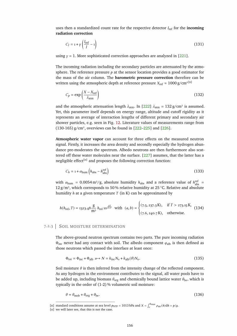
uses then a standardized count rate for the respective detector 𝐼ref for the incomingradiation correction

𝐶𝐼 = 1 +𝛾(𝐼ref

𝐼− 1

)(131)

using 𝛾 = 1. More sophisticated correction approaches are analyzed in [221].

The incoming radiation including the secondary particles are attenuated by the atmo-sphere. The reference pressure 𝑝 at the sensor location provides a good estimator forthe mass of the air column. The barometric pressure correction therefore can bewritten using the atmospheric depth at reference pressure 𝑋ref ≈ 1000 g/cm2[n]

𝐶𝑝 = exp(𝑋 −𝑋ref

_atm

)(132)

and the atmospheric attenuation length _atm. In [222] _atm = 132 g/cm2 is assumed.Yet, this parameter itself depends on energy range, altitude and cutoff rigidity as itrepresents an average of interaction lengths of different primary and secondary airshower particles, e.g. seen in Fig. 12. Literature values of measurements range from(130-165) g/cm2, overviews can be found in [222–225] and [226].

Atmospheric water vapor can account for three effects on the measured neutronsignal. Firstly, it increases the area density and secondly especially the hydrogen abun-dance pre-moderates the spectrum. Albedo neutrons are then furthermore also scat-tered off these water molecules near the surface. [227] assumes, that the latter has anegligible effect[o] and proposes the following correction function:

𝐶ℎ = 1 + 𝛼hum

(ℎabs −ℎref

abs

)(133)

with 𝛼hum = 0.0054 m3/g, absolute humidity ℎabs and a reference value of ℎrefabs =

12 g/m3, which corresponds to 50 % relative humidity at 25 ◦C. Relative and absolutehumidity ℎ at a given temperature 𝑇 (in K) can be approximated by

ℎ(ℎrel,𝑇 ) = 1323.48g

m3ℎrel 10

𝑎𝑇𝑏+𝑇 with (𝑎,𝑏) =

(7.5, 237.3K), if 𝑇 > 273.15K,

(7.6, 240.7K), otherwise.(134)

7.2.3 SOIL MOISTURE DETERMINATION

The above-ground neutron spectrum contains two parts. The pure incoming radiationΦinc never had any contact with soil. The albedo component 𝜑alb is then defined asthose neutrons which passed the interface at least once:

Φtot = Φinc + Φalb 𝜘→ 𝑁 = 𝑘inc𝑁0 + 𝑘alb (\ )𝑁0. (135)

Soil moisture \ is then inferred from the intensity change of the reflected component.As any hydrogen in the environment contributes to the signal, all water pools have tobe added up, including biomass \org and chemically bound lattice water \lw, which istypically in the order of (1-2) % volumetric soil moisture:

\ = \mob + \org + \lw. (136)

[n] standard conditions assume at sea level 𝑝NTP = 1013 hPa and 𝑋 =∫ ℎmax0

𝜌air (ℎ)dℎ = 𝑝/𝑔.[o] we will later see, that this is not the case.

156

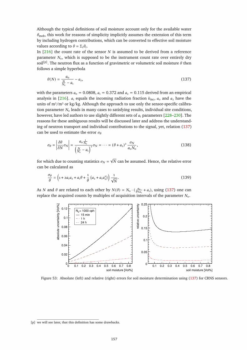
Although the typical definitions of soil moisture account only for the available water\mob, this work for reasons of simplicity implicitly assumes the extension of this termby including hydrogen contributions, which can be converted to effective soil moisturevalues according to \ = Σ𝑖\𝑖 .In [216] the count rate of the sensor 𝑁 is assumed to be derived from a referenceparameter 𝑁0, which is supposed to be the instrument count rate over entirely drysoil[p]. The neutron flux as a function of gravimetric or volumetric soil moisture \ thenfollows a simple hyperbola

\ (𝑁 ) = 𝑎0𝑁𝑁0

− 𝑎1− 𝑎2, (137)

with the parameters 𝑎0 = 0.0808, 𝑎1 = 0.372 and 𝑎2 = 0.115 derived from an empiricalanalysis in [216]. 𝑎1 equals the incoming radiation fraction 𝑘inc, 𝑎0 and 𝑎2 have theunits of m3/m3 or kg/kg. Although the approach to use only the sensor-specific calibra-tion parameter 𝑁0 leads in many cases to satisfying results, individual site conditions,however, have led authors to use slightly different sets of 𝑎𝑖 parameters [228–230]. Thereasons for these ambiguous results will be discussed later and address the understand-ing of neutron transport and individual contributions to the signal, yet, relation (137)can be used to estimate the error 𝜎\

𝜎\ =

���� 𝛿\𝛿𝑁 𝜎𝑁

���� = 𝑎01𝑁0(

𝑁𝑁0

− 𝑎1

)2𝜎𝑁 = · · · = (\ + 𝑎2)2𝜎𝑁

𝑎0𝑁0

, (138)

for which due to counting statistics 𝜎𝑁 =√𝑁 can be assumed. Hence, the relative error

can be calculated as

𝜎\

\=

(1 + 2𝑎1𝑎2 + 𝑎1\ +

1

\

(𝑎2 + 𝑎1𝑎22

) ) 1√𝑁

. (139)

As 𝑁 and \ are related to each other by 𝑁 (\ ) = 𝑁0 · ( 𝑎0\+𝑎2 + 𝑎1), using (137) one can

replace the acquired counts by multiples of acquisition intervals of the parameter 𝑁0.

soil moisture [Vol%]

0 0.1 0.2 0.3 0.4 0.5 0.6 0.7 0.8

ab

so

lute

un

ce

rta

inty

[V

ol%

]

0

0.02

0.04

0.06

0.08

0.1

0.12 = 1000 cph0N

15 min

1 h

24 h

soil moisture [Vol%]

0.1 0.2 0.3 0.4 0.5 0.6 0.7 0.8

rela

tive

un

ce

rta

inty

0

0.05

0.1

0.15

0.2

0.25

Figure 53: Absolute (left) and relative (right) errors for soil moisture determination using (137) for CRNS sensors.

[p] we will see later, that this definition has some drawbacks.

157

8U N D E R S TA N D I N G T H E C O S M I C - R A Y N E U T R O ND E T E C T O R

Part of the results about the CRNS probe presented in this chapter have been publishedin [KS2018].

In order to reduce the enormous computational effort, which inevitably goes alongwith the large scale differences of a ∼ 1 m3 detector in a ∼ 1 km3 environment, effectiveresponse models have to be applied rather than using the geometrical detector itselfin the simulation. The solution to increase the recorded flux is to adequately scaleup the volume of the detector entity. However, if the recorded flux is supposed to beincreased by use of such a detector with its actual enlarged geometry (e.g. moderatorand converter tube), this significantly alters its characteristics. A virtual sensor entitywith an effective model allows for the upscaling of the counting volume of a detector,while still retaining the same features as the unscaled type. It also allows to set themaximum detection probability within the operation range to 100 %. However, suchneutron detection models are sensitive to the specific response function of the detec-tor [231–233]. Previous studies, where the results of this work can be related to, werebased especially on the modeling of Bonner Spheres [164–168], and showed [169]that the detector response function can be approximated by the product of an energy-dependent efficiency term and an angular term. Monte Carlo models which rely on theimplementation of such functions, e.g. [234], are a subclass of global variance reduc-tion methods [235], which aim on increasing the computational efficiency, especiallyin undersampled regions.

8.1 THE DETECTOR MODEL

The detector models, which are actually used for Cosmic-Ray Neutron Sensing havebeen introduced in sec. 7.2.1. In URANOS the device is modeled by a voxel geometry.The central cutout of the rover configuration is shown exemplarily in Fig. 54, the otherdetectors are presented in appendix B.1.5. The sensor geometry has been derived fromactual devices and from supporting information provided by the manufacturer [236],see also Fig. 52. Details of the mechanical parts have been reduced to features that

Figure 54: Cross section of the Rover detector simulation model with a length of 132 cmand a width of 26 cm. It features two gas filled proportional counter tubes in a stainlesssteel casing (1), aluminum mounting brackets (2) and a HDPE moderator (3). [KS2018]

have a significant influence on the neutron response, and only materials with significantmacroscopic neutron cross sections have been considered. The size of the voxels hasbeen set to 1 mm × 1 mm × ℎ mm, whereas ℎ denotes the layer height to which thevoxel is extruded and varies from 1 mm, the generic cubic configuration, to 850 mm forthe length of the CRS1000/B tube. The materials used are: high-density polyethylene

159

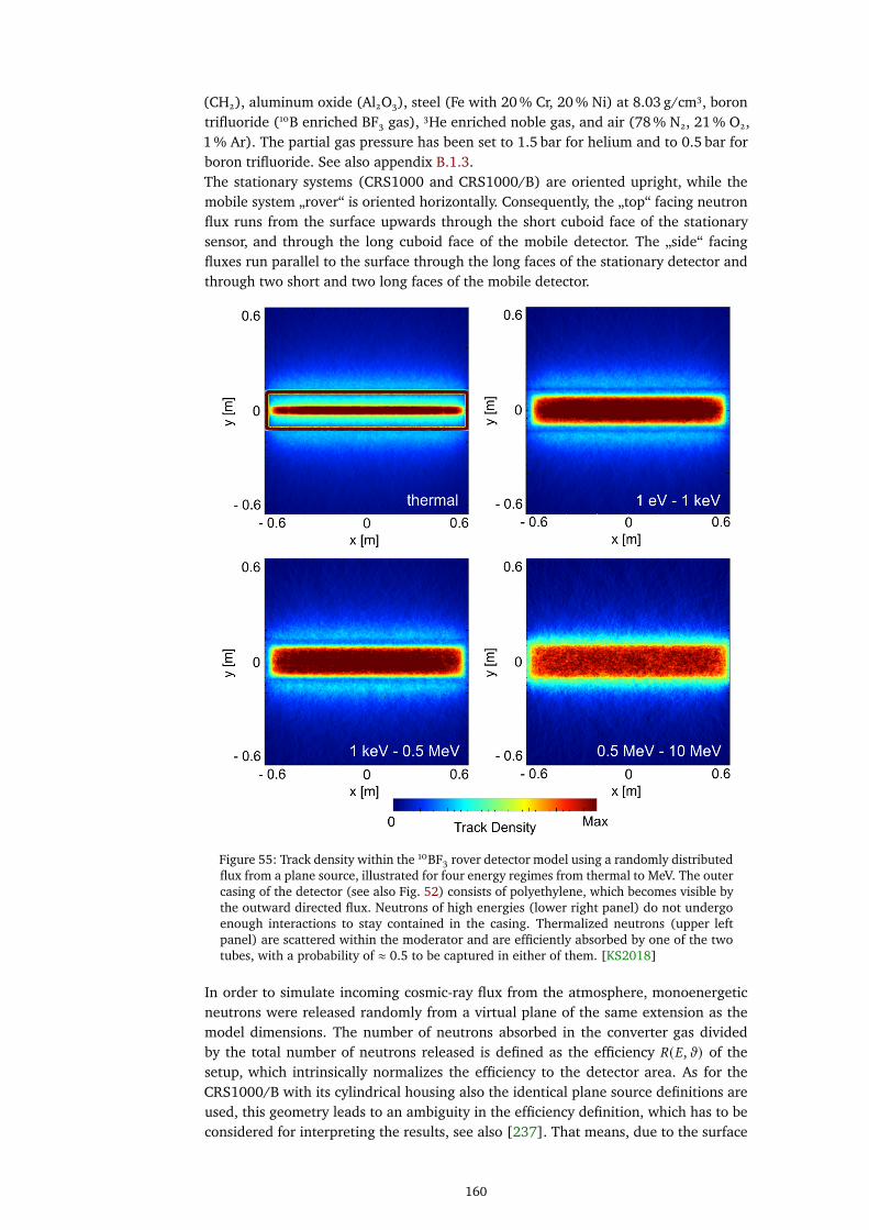
(CH2), aluminum oxide (Al2O3), steel (Fe with 20 % Cr, 20 % Ni) at 8.03 g/cm3, borontrifluoride (10B enriched BF3 gas), 3He enriched noble gas, and air (78 % N2, 21 % O2,1 % Ar). The partial gas pressure has been set to 1.5 bar for helium and to 0.5 bar forboron trifluoride. See also appendix B.1.3.The stationary systems (CRS1000 and CRS1000/B) are oriented upright, while themobile system „rover“ is oriented horizontally. Consequently, the „top“ facing neutronflux runs from the surface upwards through the short cuboid face of the stationarysensor, and through the long cuboid face of the mobile detector. The „side“ facingfluxes run parallel to the surface through the long faces of the stationary detector andthrough two short and two long faces of the mobile detector.

Figure 55: Track density within the 10BF3 rover detector model using a randomly distributedflux from a plane source, illustrated for four energy regimes from thermal to MeV. The outercasing of the detector (see also Fig. 52) consists of polyethylene, which becomes visible bythe outward directed flux. Neutrons of high energies (lower right panel) do not undergoenough interactions to stay contained in the casing. Thermalized neutrons (upper leftpanel) are scattered within the moderator and are efficiently absorbed by one of the twotubes, with a probability of ≈ 0.5 to be captured in either of them. [KS2018]

In order to simulate incoming cosmic-ray flux from the atmosphere, monoenergeticneutrons were released randomly from a virtual plane of the same extension as themodel dimensions. The number of neutrons absorbed in the converter gas dividedby the total number of neutrons released is defined as the efficiency 𝑅(𝐸,𝜗) of thesetup, which intrinsically normalizes the efficiency to the detector area. As for theCRS1000/B with its cylindrical housing also the identical plane source definitions areused, this geometry leads to an ambiguity in the efficiency definition, which has to beconsidered for interpreting the results, see also [237]. That means, due to the surface

160

normals being different for the cubic CRS1000 and the cylinder of the /B version,the directionality of an orthogonally incident flux cannot be defined consistently forboth[a]. To study the behavior of neutrons inside a detector system, the simulatedneutron track density is shown exemplarily for a 10BF3 rover detector in Fig. 55. Thetracks represent 4 · 107 histories of incident neutrons with kinetic energies spanning 10orders of magnitude. From the perspective of MeV neutrons, the path length throughthe polyethylene casing is in the order of the scattering length. This leads to an almostgeometrically homogeneous distribution, where reflected neutrons have a negligibleprobability of reentry. Neutrons with 𝐸 ≥ 1 keV exhibit shorter scattering lengths whilethe energy lost by moderation allows for more neutrons in the boundary region toescape the device (seen by the ’glow’ at the perimeter). For smaller energies, 𝐸 ≤ 1 keV,the leakage out of the device is minimized while the number of interactions within themoderator is maximized. In a cross section through the model (not shown) this equalsthe flux outside the polyethylene being lower compared to higher energy domains.As soon as neutrons are thermalized, their absorption in the converter gas gets mosteffective.

8.2 THE ENERGY RESPONSE FUNCTION

The energy response of a detector system, 𝑅(𝐸,𝜗), quantifies this sensitivity as a func-tion of neutron energy 𝐸 and incident angle 𝜗:

𝑅(𝐸,𝜗) = 𝜖 (𝐸) · 𝑔(𝜗) , (140)

where an angle of 𝜗 = 0 would correspond to an orthogonal neutron incidence. Av-eraged over the whole surface of the detector, the incoming flux can independentlycharacterized as a function of these quantities. The analysis of the energy dependenceis presented in the following. The results from the simulations of the angular sensitivitycan be found in appendix B.1.5.2.

8.3 ENERGY DEPENDENCE

The energy-dependent component of the neutron response, 𝜖 (𝐸), has been calculatedby URANOS simulations of different detector configurations. The results presented inFig. 56[b] show that all detector models exhibit qualitatively similar energy responsein the range from 0.1 eV to 1 MeV with a maximum between 1 eV and 10 eV. Themain differences in the resulting curves can be attributed to the absolute detectionefficiency, which is a function of the detector model, the converter gas and casing area.The latter is influenced by the geometry and orientation of the detector, as the surfaceneutron flux is averaged over the exposed area. Minor qualitative deviations of theresponse functions are noticeable for different aspect ratios of moderator and countertube, compare CRS1000 (top) and rover (side) in Fig. 56. The highest efficiency isachieved for neutrons in the energy range between 1 eV and 100 eV, while between0.1 eV and 0.1 MeV average efficiencies can be found. The latter range corresponds tothe ’water-sensitive domain’ for the CRNS technique. The manufacturer has stated thatthe working energy range for the detectors is within 100 eV to 10 keV (unpublisheddata). This energy window appears to be too narrow compared to the results presented

[a] Nota bene: this definition is not phase space conserving under angular variation - considering a neutronbeam incident onto the sensor from a specific direction, the effective projected area of the correspondingcuboid face has to be taken into account.

[b] The cosmic-ray neutron flux density is represented per logarithmic unit of energy, see (33) in sec. 1.4.1,given in units of dΦ/d( log(𝐸)) = 𝐸 dΦ/d𝐸.

161

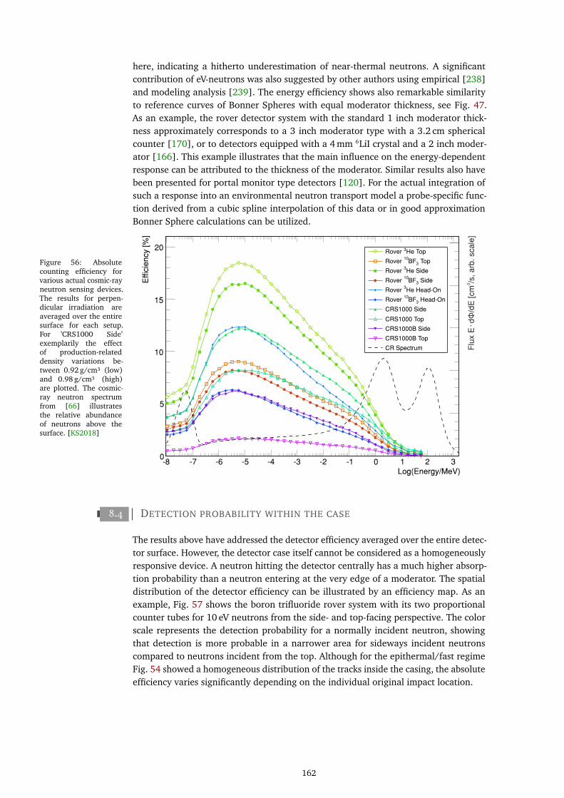
here, indicating a hitherto underestimation of near-thermal neutrons. A significantcontribution of eV-neutrons was also suggested by other authors using empirical [238]and modeling analysis [239]. The energy efficiency shows also remarkable similarityto reference curves of Bonner Spheres with equal moderator thickness, see Fig. 47.As an example, the rover detector system with the standard 1 inch moderator thick-ness approximately corresponds to a 3 inch moderator type with a 3.2 cm sphericalcounter [170], or to detectors equipped with a 4 mm 6LiI crystal and a 2 inch moder-ator [166]. This example illustrates that the main influence on the energy-dependentresponse can be attributed to the thickness of the moderator. Similar results also havebeen presented for portal monitor type detectors [120]. For the actual integration ofsuch a response into an environmental neutron transport model a probe-specific func-tion derived from a cubic spline interpolation of this data or in good approximationBonner Sphere calculations can be utilized.

Figure 56: Absolutecounting efficiency forvarious actual cosmic-rayneutron sensing devices.The results for perpen-dicular irradiation areaveraged over the entiresurface for each setup.For ’CRS1000 Side’exemplarily the effectof production-relateddensity variations be-tween 0.92 g/cm3 (low)and 0.98 g/cm3 (high)are plotted. The cosmic-ray neutron spectrumfrom [66] illustratesthe relative abundanceof neutrons above thesurface. [KS2018]

Effic

ien

cy [

%]

0

20

Log(Energy/MeV)-8 -7 -6 -5 -4 -3 -2 -1 0 1 2 3

He Top3Rover

Top3BF10

Rover

He Side3

Rover

Side3BF10

Rover

He Head-On3

Rover

Head-On3BF10

Rover

CRS1000 Side

CRS1000 Top

CRS1000B Side

CRS1000B Top

CR Spectrum

15

10

5

-2F

lux E

dΦ/d

E [

cm

·/s

, a

rb.

sca

le]

8.4 DETECTION PROBABILITY WITHIN THE CASE

The results above have addressed the detector efficiency averaged over the entire detec-tor surface. However, the detector case itself cannot be considered as a homogeneouslyresponsive device. A neutron hitting the detector centrally has a much higher absorp-tion probability than a neutron entering at the very edge of a moderator. The spatialdistribution of the detector efficiency can be illustrated by an efficiency map. As anexample, Fig. 57 shows the boron trifluoride rover system with its two proportionalcounter tubes for 10 eV neutrons from the side- and top-facing perspective. The colorscale represents the detection probability for a normally incident neutron, showingthat detection is more probable in a narrower area for sideways incident neutronscompared to neutrons incident from the top. Although for the epithermal/fast regimeFig. 54 showed a homogeneous distribution of the tracks inside the casing, the absoluteefficiency varies significantly depending on the individual original impact location.

162

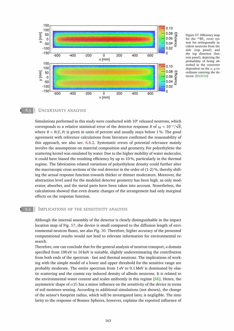
Figure 57: Efficiency mapfor the 10BF3 rover sys-tem for orthogonally in-cident neutrons from theside (top panel) andthe top direction (bot-tom panel), depicting theprobability of being ab-sorbed in the converterdependent on the 𝑥 , 𝑦 co-ordinate entering the de-tector. [KS2018]

x [mm]-600 -400 -200 0 200 400 600

y [m

m]

-150

-100

-50

0

50

100

150

y [m

m]

-150

-100

-50

0

50

100

150

Effic

ien

cy

0

x [mm]-600 -400 -200 0 200 400 600

0.10

0.08

0.06

0.04

0.02

Effic

ien

cy

0

0.10

0.08

0.06

0.04

0.02

8.5 UNCERTAINTY ANALYSIS

Simulations performed in this study were conducted with 106 released neutrons, whichcorresponds to a relative statistical error of the detector response 𝑅 of 𝑠𝑅 = 10−2/

√𝑅,

where 𝑅 = 𝑅(𝐸,\ ) is given in units of percent and usually stays below 1 %. The goodagreement with reference calculations from literature confirmed the reasonability ofthis approach, see also sec. 6.6.2. Systematic errors of potential relevance mainlyinvolve the assumptions on material composition and geometry. For polyethylene thescattering kernel was emulated by water. Due to the higher mobility of water molecules,it could have biased the resulting efficiency by up to 10 %, particularly in the thermalregime. The fabrication related variations of polyethylene density could further alterthe macroscopic cross sections of the real detector in the order of (1-2) %, thereby shift-ing the actual response function towards thicker or thinner moderators. Moreover, theabstraction level used for the modeled detector geometry has been high, as only mod-erator, absorber, and the metal parts have been taken into account. Nonetheless, thecalculations showed that even drastic changes of the arrangement had only marginaleffects on the response function.

8.6 IMPLICATIONS OF THE SENSITIVITY ANALYSIS

Although the internal assembly of the detector is clearly distinguishable in the impactlocation map of Fig. 57, the device is small compared to the diffusion length of envi-ronmental neutron fluxes, see also Fig. 30. Therefore, higher accuracy of the presentedcomputational results would not lead to relevant information for environmental re-search.Therefore, one can conclude that for the general analysis of neutron transport, a domainspecified from 100 eV to 10 keV is suitable, slightly underestimating the contributionfrom both ends of the spectrum - fast and thermal neutrons. The implications of work-ing with the simple model of a lower and upper threshold for the sensitive range areprobably moderate. The entire spectrum from 1 eV to 0.1 MeV is dominated by elas-tic scattering and the cosmic-ray induced density of albedo neutrons. It is related tothe environmental water content and scales uniformly in this regime [66]. Hence, theasymmetric shape of 𝜖 (𝐸) has a minor influence on the sensitivity of the device in termsof soil moisture sensing. According to additional simulations (not shown), the changeof the sensor’s footprint radius, which will be investigated later, is negligible. The simi-larity to the response of Bonner Spheres, however, explains the reported influence of

163

thermal neutrons on CRNS detectors [238, 239].Given the effective detection area of the cuboid sensor and its angular response, bothconformations do exhibit a different sensitivity to the neutron flux directly below thesensor. In other words, near-field effects as seen later, can be attributed to the relativelyhigh sensitivity to the downward direction and the flux distribution around the detector.In situations of small-scale changes of the topology below the sensor as for examplein the monitoring of snow cover [240] with height and snow pack variations or denseand time-varying biomass estimations [220] there is a direct influence of the externalflux field to the probe response.

164

9F O O T P R I N T I N V E S T I G AT I O N

9.1 FOOTPRINT PRELUDIUM

Part of the results about the footprint investigation presented in this chapter have been pub-lished in [KS2015] with complementary information in the follow-up publication [SK2017].

The aim of this work is to investigate the specific features of neutron transport atan air-ground interface. Specifically, the system can be regarded as an exponentiallydecreasing volume source from a low-density to a high-density region, whereas thelatter slows down neutrons much faster due to the higher abundance of water. Ashydrogen interactions also have a different scattering angle distribution the systembehaves asymmetrically regarding the domain particle density parity. The goal of thisstudy is to find and describe the ensemble dynamics in a highly non-linear system.

9.1.1 THE COSMIC-RAY NEUTRON SPECTRUM ASSEMBLY

Continuing from the description in sec. 3.2 the focus is set on parameters for maximalatmospheric depths (low altitude) 𝑑0 = 1020 g/cm2, solar maximum conditions 𝑠 =1700 MV and an exemplary cutoff rigidity of 𝑟𝑐 = 10 GV. This procedure might introducesmall differences for different places on Earth. However, measurements [65] show thatgeomagnetic latitude has only very small effects on the shape of the spectrum. Itdepends slightly on atmospheric depth, as at 𝑑0 the detectable particle flux can beregarded as the tails of the high energetic cascades, see sec. 3.1. A lower cutoff rigiditymeans a higher contribution of low energetic particles to the primary spectrum and ahigher altitude means a different ratio of proton and neutron fluxes, which each havedifferent interaction lengths [32][a].

Figure 58: Cosmic-rayneutron spectra startingfrom the analyticalangular integratedspectrum [66] (black)generating the down-ward flux only spectrum(cyan) by subtracting thealbedo from the totalspectrum (blue). Theratio (green) can becalculated independentlyover any, in this casewater, body. Neutronflux given in units oflethargy (98).

Log(Energy/MeV)0

0

0.2

0.4

0.6

0.8

1

1.2

Cosmic Spectrum

Downward Spectrum

Ratio albedo to totalΦ Φ

Sato et al. (2006)

1 2 3-5 -3 -1-2-4-6-7

-2F

lux E

dΦ/d

E [

cm

·/s

, a

rb.

sca

le]

[a] At sea level the hadronic flux can be estimated to be composed of 94 % neutrons, 4 % pions and 2 %protons. Therefore, the overall-nucleon flux is dominated by neutrons. Their attenuation length ranges from140 g/cm2 at evaporation energies to 160 g/cm2 in the GeV range. The high-energy proton attenuation length,however, is much lower with 110 g/cm2 due to electromagnetic interactions in addition to the hadronicchannels. Myons, as mainly electromagnetically interacting minimum ionizing particles, in comparison aremuch more penetrating with 520 g/cm2. This leads to a dynamic composition of the residual particles ofatmospheric cascades and especially in regard to the above-ground neutron flux.

165

As the MeV-and-below-neutron spectra Φ generally consist of an incoming Φinc as wellas a backscattered component Φa, an incident spectrum is obtained by two steps:

1. for the given spectrum a response spectrum is calculated over pure water,

2. the resulting backscattered spectrum is subtracted from the original spectrum.

𝐼inc = Φ − Φa = Φ (1 − 𝑟 ) (141)

with the ratio being defined as 𝑟 = Φa/Φ. This recalculated spectrum then containsonly incident neutrons and can be used as the source of incoming radiation for anysurface condition. Fig. 58 shows the result of this calculation. From the response of apure water body a factor for each energy bin is obtained which is used to generate thedownward-facing part from the analytical spectrum of [66]. This energy distributioncan be used to arrive again at the full spectrum in a simulation model. For epithermaland fast neutrons the flux is considered distributed in 2𝜋 . An exception to this otherwiseisotropic distribution are emission angles of high-energy neutrons above 10 MeV, whichare highly collimated along the downward facing direction (nadir angle \). Accordingto observations and simulations by Nesterenok [241] the non-uniformity of the angularspectrum 𝐽 (\ ) is given by[b]:

𝐽 (\ ) = 𝑒−2.5 (1−cos\ ) . (142)

This strategy combines a universal and validated source spectrum for cosmic neutronswith a high computational efficiency. As the location of the source is commonly tradedagainst computational effort, whereas the initial energy spectrum is bonded to a varietyof uncertainties, the modeling presented here can entirely focus on the description ofthe air-ground interface. A popular approach is to emit secondary cosmic-ray neutronsat approximately 8 km altitude and to perform a cascaded propagation through theatmosphere [224, 227, 243]. This strategy and related simplifications come with severaldrawbacks:

• Cross-sections of high-energy neutrons exhibit uncertainties of up to 50 % de-pending on element and type of reaction, though there has been progress in thelast two decades. As a consequence, inconsistencies are apparent throughoutdifferent codes for galactic and atmospheric cosmic-ray transport [244–246].

• Measurements of cosmic-ray energy spectra are additionally accompanied byobservational uncertainties. Comparative studies of Monte Carlo codes show dif-ferences of up to 20 % for calculating sensitivities of the neutron response toexperimental devices [247–249] and as well for the spectrum unfolding tech-nique [250].

• The exclusive neutron source at the top of the modeled atmosphere inadvertentlyneglects neutron generation throughout the atmosphere by other secondary par-ticles like protons, pions and muons.

• Atmospheric water vapor is often ignored, although hydrogen is the main mod-erator for neutrons[c].

• The large difference in scale of the domain requires high computational effort toreach sufficient statistics.

[b] The factor of 2.4 for (142) originally published in [241] for atmospheric depths of 1000 g/cm2 has beencorrected to 2.5 according to [242]. As a comparison: the angular distribution over all energies in[159]scales by a factor of 1.9.

[c] However, the analytical spectrum by Sato [61, 66, 251] used in this work also has this shortcoming.

166

Models which rely on particle propagation through the upper atmosphere incorporatea high complexity and vulnerability to such uncertainties.In the attempt to reduce computational effort, other studies identified the high-energycomponent of the cosmic-ray neutron spectrum as the precursor for the generationof fast neutrons in the soil [252, 253]. Since the attenuation process of high-energyneutrons in the ground is known, it seems likely that an artificial source in the soil issufficient to mimic the production of evaporation neutrons. However, some drawbacksof this method are important to note:

• Attenuation of high-energy neutrons in the soil follows an exponential decreasethat is dependent on soil type and location on Earth.

• There is no verified energy spectrum for neutrons in the soil.

• Evaporation neutrons are a significant part, but do not make up the spectrum as awhole, see Fig. 58. The incoming energy spectrum from the atmosphere exhibitslow-energy components and particularly neutrons which already evaporated inthe air.

Considering only evaporation neutrons in the soil can be an approach, especially fordry conditions, which tends to overestimate average neutron energies, as incident low-energy neutrons from the top are neglected, and thus also overestimates the footprintsize. Moreover, the deduced footprint appears to be insensitive to soil moisture, becauseits influence on neutron moderation is underestimated. Here, a different approach isapplied, which aims to combine the advantages as well as avoid the drawbacks of bothstrategies mentioned above. To minimize the uncertainties of the propagated energyspectrum, this study focuses on the domain close to the surface by using validatedresults from independent atmospheric simulations as model input.

9.1.2 EXPERIMENTAL VERIFICATION

Since the footprint definition is based on a radial symmetry, direct empirical evidenceis difficult to achieve with natural structures. However, approaching water surfacesand transiting the coast line has been a common procedure to determine the range ofdetected neutrons. For example, [254] moved the detector over a lake and interpretsthat the signal strength is hardly sensitive to neutrons from the land side at distancesgreater than 200 m. In the last years, many experiments with CRNS detectors havebeen performed across a water-land boundary. Data from Oceanside Pier (California,US) indicate that the sensitive distance is on the order of (100-200) m at sea level. WithURANOS attempts have been made to reproduce these transect experiments by movinga 4 m square-shaped detector over pure water and land with exemplary soil moisturesfrom 1 % to 30 % and fixed air humidity ℎ = 10 g/m3. Figure 59 illustrates the simula-tions and the two experiments mentioned above. The simulated signal strengths clearlycorrespond to the measurements and give an indication of the soil water content whichwas unknown at the time of the experiments.The signal gradient is asymmetric over water (Fig. 59 left) and land (Fig. 59 right),which agrees with results from [243], who investigated the influence of large wet struc-tures on the signal strength. However, direct observables for neutron transport cannotbe identified in the experiment as transect experiments do not give a direct measure ofthe footprint radius under conditions where the instrument is usually applied. Theseeffects can be explained by (1) the overestimation of dry over wet regions in the signal,as a consequence of the non-linear relation: \ ↦→ 𝑁 , (2) the effective removal of trav-eling neutrons due to the presence of a water body on their way to the detector, and(3) the non-radial geometry of the experiment. However, the presented data provide

167

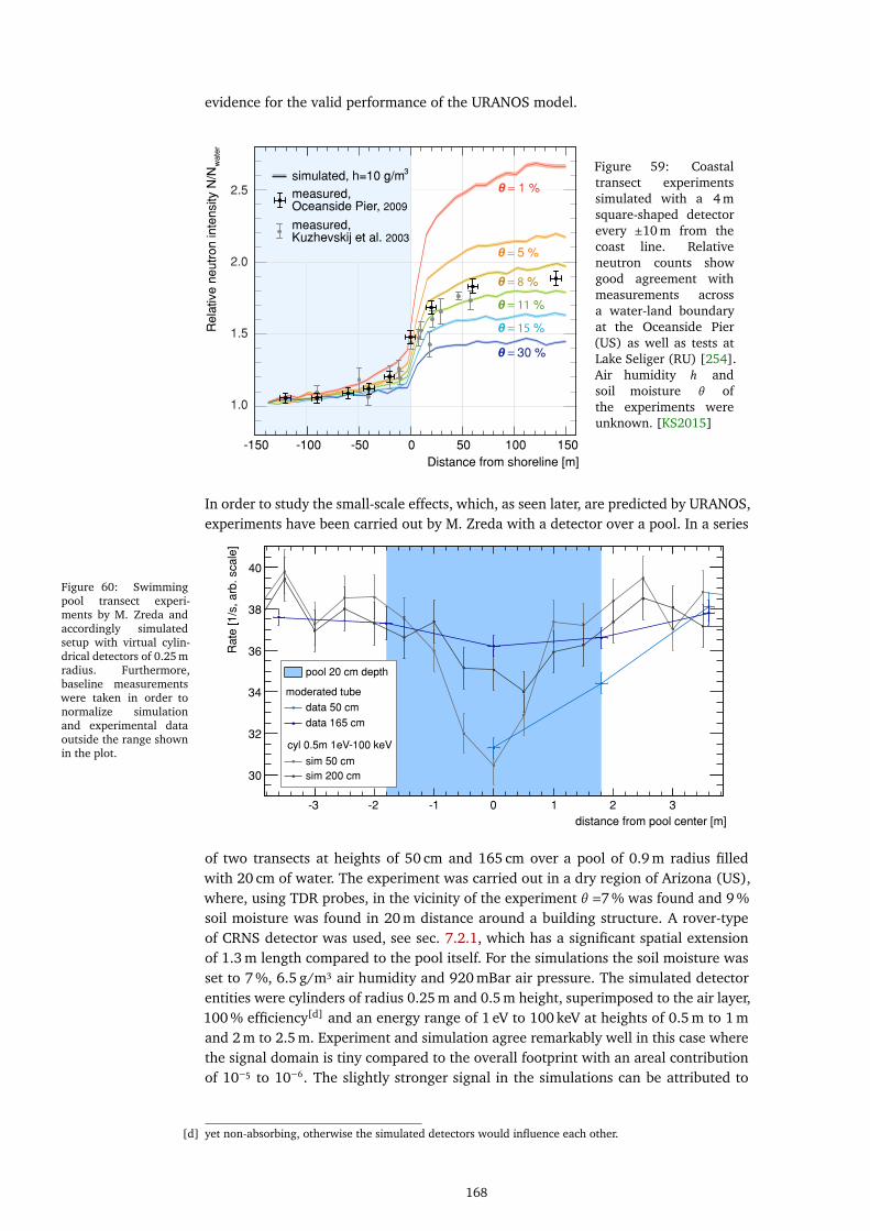
evidence for the valid performance of the URANOS model.

Distance from shoreline [m]

Re

lativ

e n

eu

tro

n in

ten

sity

N/N

wa

ter

-50 150-100 100-150 500

2.5

2.0

1.5

1.0

3simulated, h=10 g/m

θ = 30 %

θ = 15 %

θ = 11 %

θ = 8 %

θ = 5 %

θ = 1 %measured,Oceanside Pier, 2009

measured,Kuzhevskij et al. 2003

Figure 59: Coastaltransect experimentssimulated with a 4 msquare-shaped detectorevery ±10 m from thecoast line. Relativeneutron counts showgood agreement withmeasurements acrossa water-land boundaryat the Oceanside Pier(US) as well as tests atLake Seliger (RU) [254].Air humidity ℎ andsoil moisture \ ofthe experiments wereunknown. [KS2015]

In order to study the small-scale effects, which, as seen later, are predicted by URANOS,experiments have been carried out by M. Zreda with a detector over a pool. In a series

Figure 60: Swimmingpool transect experi-ments by M. Zreda andaccordingly simulatedsetup with virtual cylin-drical detectors of 0.25 mradius. Furthermore,baseline measurementswere taken in order tonormalize simulationand experimental dataoutside the range shownin the plot.

distance from pool center [m]

-3 -2 -1 0 1 2 3

Ra

te [1

/s, a

rb. sca

le]

30

32

34

36

38

40

pool 20 cm depth

moderated tube

data 50 cm

data 165 cm

cyl 0.5m 1eV-100 keV

sim 50 cm

sim 200 cm

of two transects at heights of 50 cm and 165 cm over a pool of 0.9 m radius filledwith 20 cm of water. The experiment was carried out in a dry region of Arizona (US),where, using TDR probes, in the vicinity of the experiment \ =7 % was found and 9 %soil moisture was found in 20 m distance around a building structure. A rover-typeof CRNS detector was used, see sec. 7.2.1, which has a significant spatial extensionof 1.3 m length compared to the pool itself. For the simulations the soil moisture wasset to 7 %, 6.5 g/m3 air humidity and 920 mBar air pressure. The simulated detectorentities were cylinders of radius 0.25 m and 0.5 m height, superimposed to the air layer,100 % efficiency[d] and an energy range of 1 eV to 100 keV at heights of 0.5 m to 1 mand 2 m to 2.5 m. Experiment and simulation agree remarkably well in this case wherethe signal domain is tiny compared to the overall footprint with an areal contributionof 10−5 to 10−6. The slightly stronger signal in the simulations can be attributed to

[d] yet non-absorbing, otherwise the simulated detectors would influence each other.

168

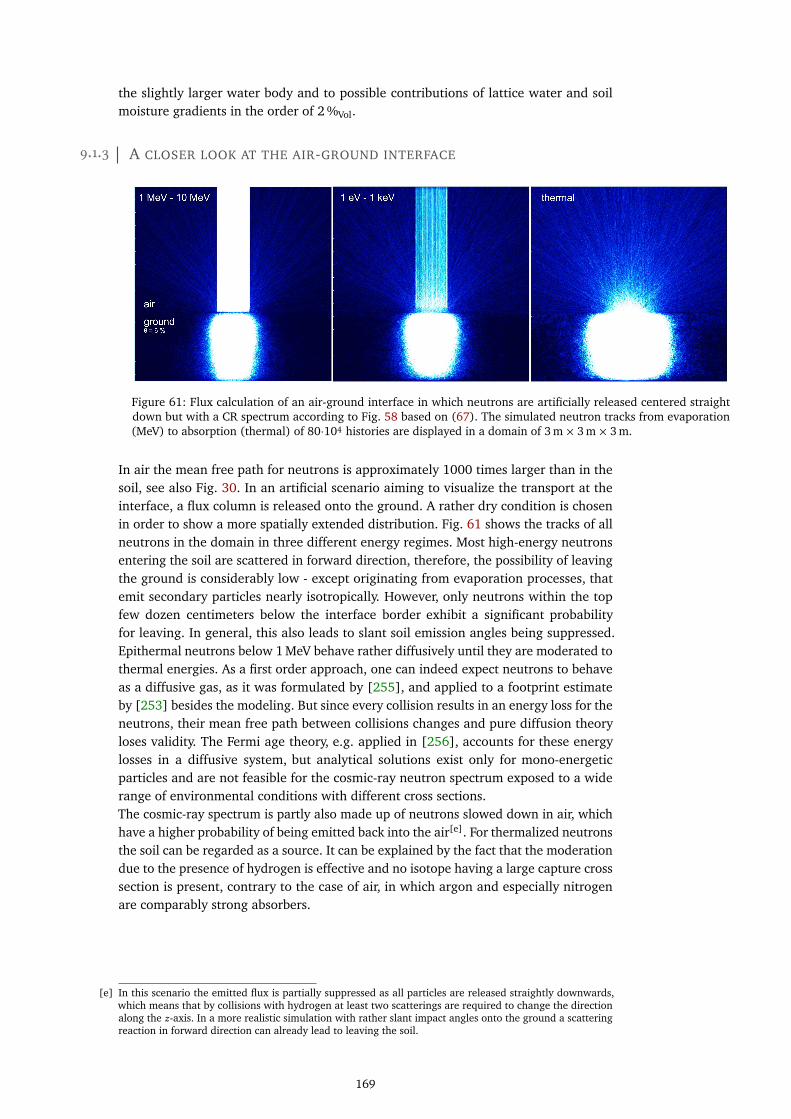
the slightly larger water body and to possible contributions of lattice water and soilmoisture gradients in the order of 2 %Vol.

9.1.3 A CLOSER LOOK AT THE AIR-GROUND INTERFACE

Figure 61: Flux calculation of an air-ground interface in which neutrons are artificially released centered straightdown but with a CR spectrum according to Fig. 58 based on (67). The simulated neutron tracks from evaporation(MeV) to absorption (thermal) of 80·104 histories are displayed in a domain of 3 m × 3 m × 3 m.

In air the mean free path for neutrons is approximately 1000 times larger than in thesoil, see also Fig. 30. In an artificial scenario aiming to visualize the transport at theinterface, a flux column is released onto the ground. A rather dry condition is chosenin order to show a more spatially extended distribution. Fig. 61 shows the tracks of allneutrons in the domain in three different energy regimes. Most high-energy neutronsentering the soil are scattered in forward direction, therefore, the possibility of leavingthe ground is considerably low - except originating from evaporation processes, thatemit secondary particles nearly isotropically. However, only neutrons within the topfew dozen centimeters below the interface border exhibit a significant probabilityfor leaving. In general, this also leads to slant soil emission angles being suppressed.Epithermal neutrons below 1 MeV behave rather diffusively until they are moderated tothermal energies. As a first order approach, one can indeed expect neutrons to behaveas a diffusive gas, as it was formulated by [255], and applied to a footprint estimateby [253] besides the modeling. But since every collision results in an energy loss for theneutrons, their mean free path between collisions changes and pure diffusion theoryloses validity. The Fermi age theory, e.g. applied in [256], accounts for these energylosses in a diffusive system, but analytical solutions exist only for mono-energeticparticles and are not feasible for the cosmic-ray neutron spectrum exposed to a widerange of environmental conditions with different cross sections.The cosmic-ray spectrum is partly also made up of neutrons slowed down in air, whichhave a higher probability of being emitted back into the air[e]. For thermalized neutronsthe soil can be regarded as a source. It can be explained by the fact that the moderationdue to the presence of hydrogen is effective and no isotope having a large capture crosssection is present, contrary to the case of air, in which argon and especially nitrogenare comparably strong absorbers.

[e] In this scenario the emitted flux is partially suppressed as all particles are released straightly downwards,which means that by collisions with hydrogen at least two scatterings are required to change the directionalong the 𝑧-axis. In a more realistic simulation with rather slant impact angles onto the ground a scatteringreaction in forward direction can already lead to leaving the soil.

169

9.1.4 MODEL SETUP

9.1.4.1 NEUTRON SOURCE AND DETECTOR

Neutrons are released from a volume source with randomly distributed origins from 2 mto 42 m above the surface. The amount of initial particles per run was chosen accordingto statistical errors - 107 histories are a reasonable trade-off between computationaleffort and precision for typical calculations presented here[f]. The simulations for thefootprint analysis, which will be presented in the following, do not make use of thelater implemented high energy cascade transport model.

2 m

0 m

42 m

detector layer

detection

thermalisation

origin

path

creation

air + water

soil 50% Vol

+ air + water

neutronsource layer

ϕ

ϑ

x

y

z

Figure 62: Setup ofthe simulation contain-ing a 40 m thick neutronsource layer in the atmo-sphere and a thin detec-tor layer at 2 m aboveground. A particle iscounted as an albedoneutron if it had pre-ceding contact with thesoil. [KS2015]

Neutrons are recorded individually in an horizontally infinite detector layer, see alsosec. 6.5.1. Any neutron that experienced interaction with the soil is counted as it passesthe layer. The infinite plane detector overlays the atmosphere by means of a 25 cm highsheet at a vertical position of (175-200) cm, a usual height for mounting cosmic-rayprobes. The detector layer is crossed by the neutrons and thus maps spatially theneutron density[g]. For the effective energy range to which the detector is sensitive,practical considerations by [253] and theoretical by for example [257], the detectionenergy is set to a window from 10 eV to 104 eV.The detection efficiency of moderatedhelium-3 detectors is nearly constant in that energy regime [258], which is why signalweighting for different energies is not necessary. However, common cosmic-ray neu-tron detectors, see sec. 7.2.1, are contaminated by approximately (10-20) % thermalneutrons [238]. It is not intended to account for this issue here, as this study aims toinvestigate characteristics for a detector ideally tailored to the needs of environmentalwater sensing.

9.1.4.2 AIR, SOIL AND WATER

The modeled pure air medium consists of 78 %Vol nitrogen, 21 %Vol oxygen and 1 %Vol

argon usually at a pressure of 1020 mbar. The soil extends to a depth of 3 m and the airto 1000 m. Both, soil and air are represented by planes of infinite extension, which canhave subdomains, either to create a density profile in depth or to add specific entitieslike water or a detector. The soil consists of 50 %Vol solids and a scalable amount ofH2O. The solid domain is comprised of 75 %Vol SiO2 and 25 %Vol Al2O3 at a compound

[f] At the time of investigating the footprint such a calculation, depending on the soil moisture, took around4 h. Due to further performance improvements URANOS meanwhile runs in such a setup approximately 250neutrons per core per GHz per second, which means 107 histories can be tracked in around 40 min.

[g] Multiple counts of a single neutron in the detector layer account for the measured density equivalent for asingle count per volume detector. This relation holds if (1) the dimension of the absorbing detector mediumstays below typical scale lengths of neutron interactions (10 m-100 m), and (2) particles do not scattermultiple times in that volume. That is very unlikely for non-thermal neutrons and furthermore does notfactorize in the count statistics.Caveat: Typically Monte Carlo simulations like MCNP score particle flux as track length per volume. In thecase presented here with no preferred detector orientation and infinite layer geometries this definition is atleast unhandy.

170

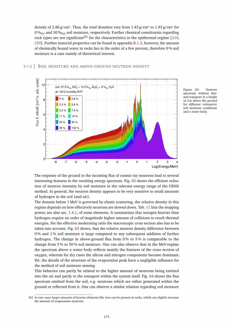
density of 2.86 g/cm3. Thus, the total densities vary from 1.43 g/cm3 to 1.93 g/cm3 for0 %Vol and 50 %Vol soil moisture, respectively. Further chemical constituents regardingrock types are not significant[h] for the characteristics in the epithermal regime [218,259]. Further material properties can be found in appendix B.1.3, however, the amountof chemically bound water in rocks lies in the order of a few percent, therefore 0 % soilmoisture is a case mainly of theoretical interest.

9.1.5 SOIL MOISTURE AND ABOVE-GROUND NEUTRON DENSITY

Figure 63: Neutronspectrum without ther-mal transport in a heightof 2 m above the groundfor different volumetricsoil moisture conditionsand a water body.

0

2

4

6

8

10

humidity NTP%air: 30

O2 HVol% + X3O2 AlVol% + 12.52 SiOVol%soil: 37.5

Log(Energy/MeV)

0 1 2 3-5 -3 -1-2-4-6-7 4-8

0 % 0.8 %

2.3 % 3.8 %

5.3 % 7.6 %

11 % 15 %

23 % 30 %

38 % 100 %

-2F

lux E

dΦ/d

E [cm

·/s

, a

rb. sca

le]

The response of the ground to the incoming flux of cosmic-ray neutrons lead to severalinteresting features in the resulting energy spectrum. Fig. 63 shows the efficient reduc-tion of neutron intensity by soil moisture in the relevant energy range of the CRNSmethod. In general, the neutron density appears to be very sensitive to small amountsof hydrogen in the soil (and air).The domain below 1 MeV is governed by elastic scattering, the relative density in thisregime depends on how effectively neutrons are slowed down. Tab. 11 lists the stoppingpower, see also sec. 1.4.1, of some elements. It summarizes that isotopes heavier thanhydrogen require an order of magnitude higher amount of collisions to reach thermalenergies. For the effective moderating ratio the macroscopic cross section also has to betaken into account. Fig. 63 shows, that the relative neutron density difference between0 % and 1 % soil moisture is large compared to any subsequent addition of furtherhydrogen. The change in above-ground flux from 0 % to 5 % is comparable to thechange from 5 % to 50 % soil moisture. One can also observe that in the MeV-regimethe spectrum above a water body reflects mainly the features of the cross section ofoxygen, whereas for dry cases the silicon and nitrogen components become dominant.Yet, the details of the structure of the evaporation peak have a negligible influence forthe method of soil moisture sensing.This behavior can partly be related to the higher amount of neutrons being emittedinto the air and partly to the transport within the system itself. Fig. 64 shows the fluxspectrum emitted from the soil, e.g. neutrons which are either generated within theground or reflected from it. One can observe a similar relation regarding soil moisture

[h] In rare cases larger amounts of heavier elements like iron can be present in rocks, which can slightly increasethe amount of evaporation neutrons.

171

Figure 64: Neutronspectrum emitted fromthe soil without thermaltransport in a height of2 m above the groundfor different soil moistureconditions and a waterbody.

0

1

4

6

8

10

humidity NTP%air: 30

O2 HVol% + X3O2 AlVol% + 12.52 SiOVol%soil: 37.5

0 % 0.8 %

2.3 % 3.8 %

5.3 % 7.6 %

11 % 15 %

23 % 30 %

38 % 100 %

Log(Energy/MeV)

0 1 2 3-5 -3 -1-2-4-6-7 4-8

-2F

lux E

dΦ/d

E [cm

·/s

, a

rb. sca

le]

Table 11: Slowing downof neutrons by interac-tion with different iso-topes from 2 MeV to ther-mal and to an exem-plary energy relevant forCRNS. Calculations ac-cording to (31) and (32).

avg. no. collisions 𝑛col

Element Mass [u] log. energy decrement b to thermal to 100 eV

H 1 1 18 10

H2O - 0.92 20 11

N 14 0.136 135 73

O 16 0.12 153 82

Al 27 0.0723 255 137

Si 28 0.0698 264 142

Fe 56 0.0353 522 280

changes as for the total spectrum, Fig. 63, which extends the trend to lower energies.In case of the total absence of hydrogen the system behaves nearly like a resonatorwith a small damping constant - neutrons are scattering within a domain which ratheracts as a reflector. Therefore, the presence of a small amount of hydrogen already leadsto a smooth scaling of the system.

Exemplarily also the effect of air humidity is presented in Fig. 65 for the scaling ofthe above-ground neutron flux for rather dry conditions. In temperate zones typicallyhumidities around 10 g/m3 can be expected and 33 g/m3 would correspond to a rainforest climate. For hydrogen in air the following observations can be made: The in-tensity scaling can be found in the sub-MeV region due to the fact, that contrary tosoil moisture it does not significantly change the direct albedo flux[i]. The scaling ofthe total neutron flux as a function of water vapor shows a nearly linear behavior, yetslightly more sensitive for low air humidities. However, the relative change in intensityalso depends on the soil moisture itself. In the example of 4 % soil moisture we find a15 % change in the epithermal regime for the given setups. This scaling decreases withcomparably larger amounts of water in the soil.

As seen from the discussion above and Fig. 63 the above-ground flux scales by a hy-perbolic law, as also already indicated by (137) from [216]. This description is alsounderlined by the results from this work. Fig. 66 provides a comparison of neutron

[i] As the spectrum is released in the vicinity of the ground interface effects of atmospheric water vapor, whichlead to a premoderation of the spectrum and an additional attenuation due to the increased area density,are neglected here.

172

Figure 65: Neutronspectrum without ther-mal transport in a heightof 2 m above the groundfor different air humidityconfigurations.

0

2

4

6

8

10

O2 HVol% + 43O2 AlVol% + 12.52 SiOVol%soil: 37.5

30 g/m 35 g/m

310 g/m 316 g/m

325 g/m 333 g/m

350 g/m

Log(Energy/MeV)

0 1 2 3-5 -3 -1-2-4-6-7 4-8

-2F

lux E

dΦ/d

E [

cm

·/s

, a

rb.

sca

le]

densities as a function of soil moisture normalized to (137). For URANOS settings withand without the high-energy transport model are presented, whereas the latter propa-gates the particles above 20 MeV with an interaction-balanced model yielding typicalattenuation lengths for the high-energy regime. In case this model is not used, theflux into ground is lower on average, which leads to a smaller amount of evaporationneutrons being emitted into the air. However, there is no qualitative difference betweenboth, which shows that the hyperbolic shape is entirely determined by the physics be-low 1 MeV. Results from MCNPX, see sec. 5.2.1, are presented in comparison, scaledto match the porosity. The slope appears to be slightly higher, yet both simulationsagree remarkingly well given the complexity of the underlying system. However, theempirical results from [216] are not supported by any modeling. As seen from otherexperiments carried out afterwards and for example presented in sec. 9.1.2, simulationmodels can provide a consistent picture of measured above-ground densities.

Figure 66: Above-ground neutron densityas function of soilmoisture, scored in theinterval 1 eV-10 keV(with and without highenergy particle trans-port) at ℎ = 3 g/m3 incomparison to MCNPXcalculations (ℎ = 0 g/m3)and to the commonlyused equation (137).

Soil moisture [%Vol ]

0 5 10 15 20 25 30 35 40

Re

lativ

e in

ten

sity

0.4

0.6

0.8

1

1.2

1.4

1.6

1.8

Desilets et al. 2010

MCNPX

this work (without HE model)

this work (with HE model)

As already seen from the exemplary spectra of Fig. 65 the above-ground neutronintensity also depends on the water concentration in the air. The results from theanalysis of the intensity scaling, see Fig. 67, are the following: The general response at

173

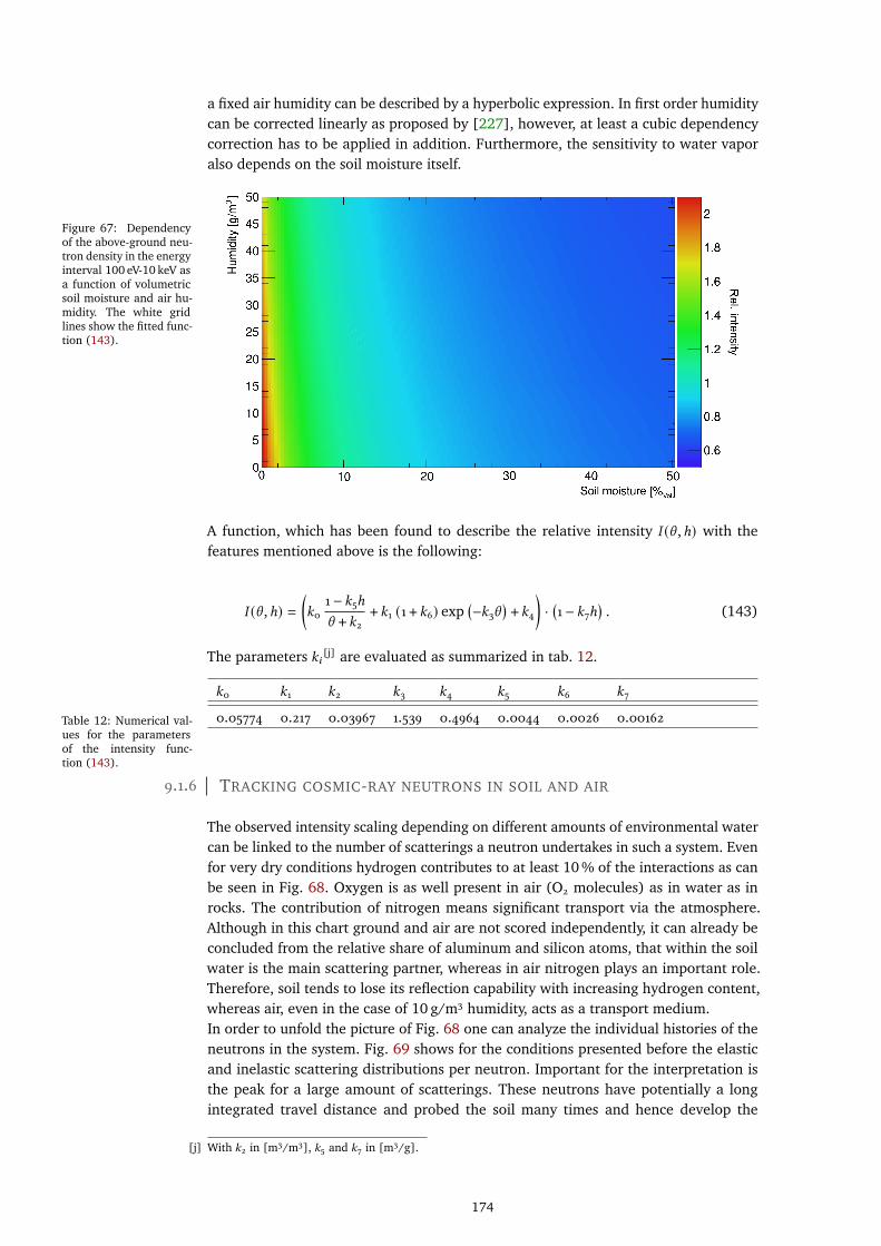
a fixed air humidity can be described by a hyperbolic expression. In first order humiditycan be corrected linearly as proposed by [227], however, at least a cubic dependencycorrection has to be applied in addition. Furthermore, the sensitivity to water vaporalso depends on the soil moisture itself.

Figure 67: Dependencyof the above-ground neu-tron density in the energyinterval 100 eV-10 keV asa function of volumetricsoil moisture and air hu-midity. The white gridlines show the fitted func-tion (143).

A function, which has been found to describe the relative intensity 𝐼 (\ ,ℎ) with thefeatures mentioned above is the following:

𝐼 (\ ,ℎ) =(𝑘0

1 − 𝑘5ℎ

\ + 𝑘2+ 𝑘1 (1 + 𝑘6) exp

(−𝑘3\

)+ 𝑘4

)·(1 − 𝑘7ℎ

). (143)

The parameters 𝑘𝑖 [j] are evaluated as summarized in tab. 12.

Table 12: Numerical val-ues for the parametersof the intensity func-tion (143).

𝑘0 𝑘1 𝑘2 𝑘3 𝑘4 𝑘5 𝑘6 𝑘7

0.05774 0.217 0.03967 1.539 0.4964 0.0044 0.0026 0.00162

9.1.6 TRACKING COSMIC-RAY NEUTRONS IN SOIL AND AIR

The observed intensity scaling depending on different amounts of environmental watercan be linked to the number of scatterings a neutron undertakes in such a system. Evenfor very dry conditions hydrogen contributes to at least 10 % of the interactions as canbe seen in Fig. 68. Oxygen is as well present in air (O2 molecules) as in water as inrocks. The contribution of nitrogen means significant transport via the atmosphere.Although in this chart ground and air are not scored independently, it can already beconcluded from the relative share of aluminum and silicon atoms, that within the soilwater is the main scattering partner, whereas in air nitrogen plays an important role.Therefore, soil tends to lose its reflection capability with increasing hydrogen content,whereas air, even in the case of 10 g/m3 humidity, acts as a transport medium.In order to unfold the picture of Fig. 68 one can analyze the individual histories of theneutrons in the system. Fig. 69 shows for the conditions presented before the elasticand inelastic scattering distributions per neutron. Important for the interpretation isthe peak for a large amount of scatterings. These neutrons have potentially a longintegrated travel distance and probed the soil many times and hence develop the

[j] With 𝑘2 in [m3/m3], 𝑘5 and 𝑘7 in [m3/g].

174

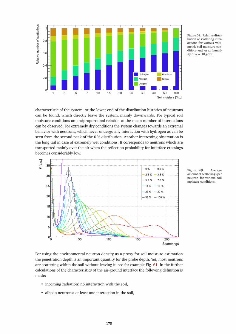
Figure 68: Relative distri-bution of scattering inter-actions for various volu-metric soil moisture con-ditions and an air humid-ity of ℎ = 10 g/m3.

Soil moisture [% ]Vol

Re

lativ

e n

um

be

r o

f sca

tte

rin

gs

0

0.2

0.4

0.6

0.8

1

Hydrogen Aluminum

Nitrogen Silicon

Oxygen

1 3 5 7 10 20 100 50 40 30 15 25

characteristic of the system. At the lower end of the distribution histories of neutronscan be found, which directly leave the system, mainly downwards. For typical soilmoisture conditions an antiproportional relation to the mean number of interactionscan be observed. For extremely dry conditions the system changes towards an extremalbehavior with neutrons, which never undergo any interaction with hydrogen as can beseen from the second peak of the 0 % distribution. Another interesting observation isthe long tail in case of extremely wet conditions. It corresponds to neutrons which aretransported mainly over the air when the reflection probability for interface crossingsbecomes considerably low.

Figure 69: Averageamount of scatterings perneutron for various soilmoisture conditions.

Scatterings

0 50 100 150 200

# [

a.u

.]

0

5

10

15

20

25

30

350 % 0.8 %

2.3 % 3.8 %

5.3 % 7.6 %

11 % 15 %

23 % 30 %

38 % 100 %

For using the environmental neutron density as a proxy for soil moisture estimationthe penetration depth is an important quantity for the probe depth. Yet, most neutronsare scattering within the soil without leaving it, see for example Fig. 61. In the furthercalculations of the characteristics of the air-ground interface the following definition ismade:

• incoming radiation: no interaction with the soil,

• albedo neutrons: at least one interaction in the soil,

175

• direct albedo radiation: only one interface crossing. The majority of these neu-trons are ’geometrically’ transported to the sensor without further (diffusive)scattering in the air.

Figure 70: Maximumscattering depth of neu-trons which reach the sur-face for various volumet-ric soil moisture condi-tions and ℎ = 10 g/m3.

Scattered Maximum Depth [mm]

0 200 400 600 800 1000 1200 1400 1600 1800

# [a

.u.]

0

0.5

1

1.5

2

2.5

3

3.5

4

0 % 0.8 %

2.3 % 3.8 %

5.3 % 7.6 %

11 % 15 %

23 % 30 %

38 % 100 %

It is important to note that probing the soil and its water content does not necessarilymean that a neutron had scattered off any hydrogen atom. Indeed, compared to thedry case any addition of soil moisture reduces the above-ground density, not only byslowing down neutrons faster, but also by reducing the escape probability once enteredinto the soil.Fig. 70 shows the distribution of the maximum probe depth, e.g. the most deep scat-tering centers or evaporation origins. For dry conditions neutrons can probe the soilbeyond depths of 1 m and for a pure water body information below 10 cm can hardlybe obtained. To the distribution of the scattering locations a similar scaling with soilmoisture like in the cases before can be attributes, however, the relation is not asstrongly dependent on the water content here. It can be explained by the fact that thisobservable quantifies the extreme values of the ensemble.

9.2 COSMIC-RAY NEUTRON TRANSPORT ANALYSIS

9.2.1 THEORETICAL DESCRIPTION BY NEUTRON TRANSPORT EQUATIONS

Considering a point source in an infinite medium the integral version of the transportequation (9) reduces to

Φ(𝑟 ) = 𝑄𝑒−Σ𝑡𝑟

4𝜋𝑟 2︸ ︷︷ ︸transientBΦtr

+∫

Σ𝑠Φ(𝑟 ′)𝑒−Σ𝑡 |𝑟−𝑟

′ |

4𝜋 (𝑟 − 𝑟 ′)2 d𝑉 ′︸ ︷︷ ︸diffusive transportBΦdt

, (144)

with as before Σ𝑡 being the total cross section and Σ𝑠 the scattering cross sectionfor changes from 𝐸 𝜘→ 𝐸 ′. The first term describes the direct/’geometric’ transportwithout any collision from a source of strength 𝑄 to a surface proportional to 𝑟 2. At

176

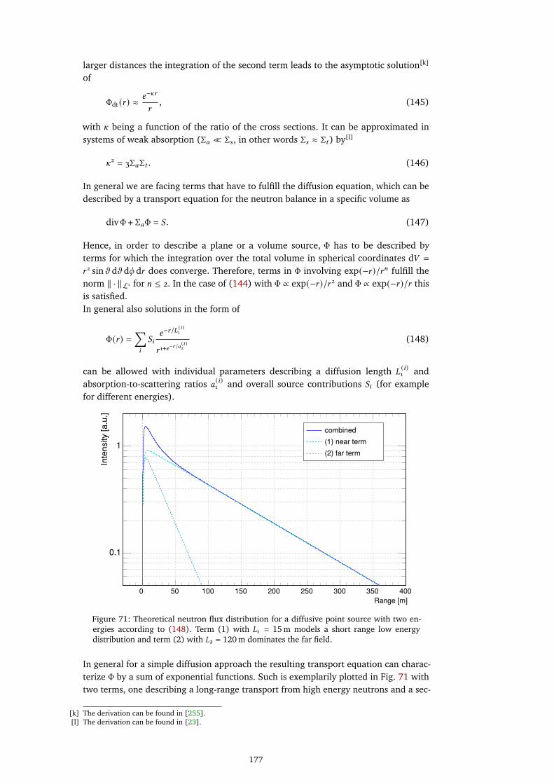
larger distances the integration of the second term leads to the asymptotic solution[k]

of

Φdt (𝑟 ) ≈𝑒−^𝑟

𝑟, (145)

with ^ being a function of the ratio of the cross sections. It can be approximated insystems of weak absorption (Σ𝑎 � Σ𝑠 , in other words Σ𝑠 ≈ Σ𝑡) by[l]

^2 = 3Σ𝑎Σ𝑡 . (146)

In general we are facing terms that have to fulfill the diffusion equation, which can bedescribed by a transport equation for the neutron balance in a specific volume as

divΦ + Σ𝑎Φ = 𝑆. (147)

Hence, in order to describe a plane or a volume source, Φ has to be described byterms for which the integration over the total volume in spherical coordinates d𝑉 =

𝑟 2 sin𝜗 d𝜗 d𝜙 d𝑟 does converge. Therefore, terms in Φ involving exp(−𝑟 )/𝑟𝑛 fulfill thenorm ‖ · ‖L1 for 𝑛 ≤ 2. In the case of (144) with Φ ∝ exp(−𝑟 )/𝑟 2 and Φ ∝ exp(−𝑟 )/𝑟 thisis satisfied.In general also solutions in the form of

Φ(𝑟 ) =∑𝑖

𝑆𝑖𝑒−𝑟/𝐿

(𝑖 )1

𝑟 1+𝑒−𝑟/𝑎 (𝑖 )2

(148)

can be allowed with individual parameters describing a diffusion length 𝐿(𝑖)1 and

absorption-to-scattering ratios 𝑎(𝑖)1 and overall source contributions 𝑆𝑖 (for example

for different energies).

Range [m]

0 50 100 150 200 250 300 350 400

Inte

nsity

[a

.u.]

0.1

1

combined

(1) near term

(2) far term

Figure 71: Theoretical neutron flux distribution for a diffusive point source with two en-ergies according to (148). Term (1) with 𝐿1 = 15 m models a short range low energydistribution and term (2) with 𝐿2 = 120 m dominates the far field.

In general for a simple diffusion approach the resulting transport equation can charac-terize Φ by a sum of exponential functions. Such is exemplarily plotted in Fig. 71 withtwo terms, one describing a long-range transport from high energy neutrons and a sec-

[k] The derivation can be found in [255].[l] The derivation can be found in [23].

177

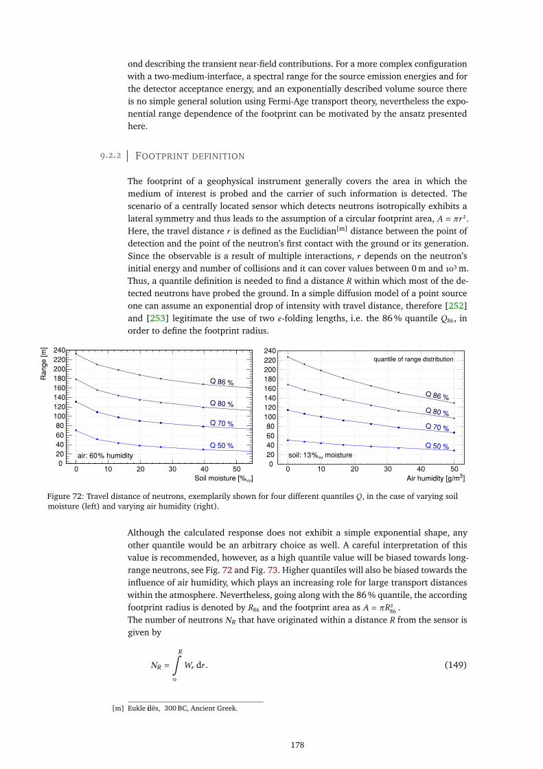
ond describing the transient near-field contributions. For a more complex configurationwith a two-medium-interface, a spectral range for the source emission energies and forthe detector acceptance energy, and an exponentially described volume source thereis no simple general solution using Fermi-Age transport theory, nevertheless the expo-nential range dependence of the footprint can be motivated by the ansatz presentedhere.

9.2.2 FOOTPRINT DEFINITION

The footprint of a geophysical instrument generally covers the area in which themedium of interest is probed and the carrier of such information is detected. Thescenario of a centrally located sensor which detects neutrons isotropically exhibits alateral symmetry and thus leads to the assumption of a circular footprint area, 𝐴 = 𝜋𝑟 2.Here, the travel distance 𝑟 is defined as the Euclidian[m] distance between the point ofdetection and the point of the neutron’s first contact with the ground or its generation.Since the observable is a result of multiple interactions, 𝑟 depends on the neutron’sinitial energy and number of collisions and it can cover values between 0 m and 103 m.Thus, a quantile definition is needed to find a distance 𝑅 within which most of the de-tected neutrons have probed the ground. In a simple diffusion model of a point sourceone can assume an exponential drop of intensity with travel distance, therefore [252]and [253] legitimate the use of two 𝑒-folding lengths, i.e. the 86 % quantile 𝑄86, inorder to define the footprint radius.

Soil moisture [% ]Vol

Ra

ng

e [

m]

0

20

40

60

80

100

120

140

160

180

200

220

240

Q 50 %

Q 70 %

Q 80 %

Q 86 %

humidity%air: 60

quantile of range distribution

]3Air humidity [g/m

0

20

40

60

80

100

120

140

160

180

200

220

240

0 10 20 30 5040 0 10 20 30 5040

moisture%Volsoil: 13

Q 50 %

Q 70 %

Q 80 %

Q 86 %

Figure 72: Travel distance of neutrons, exemplarily shown for four different quantiles 𝑄, in the case of varying soilmoisture (left) and varying air humidity (right).

Although the calculated response does not exhibit a simple exponential shape, anyother quantile would be an arbitrary choice as well. A careful interpretation of thisvalue is recommended, however, as a high quantile value will be biased towards long-range neutrons, see Fig. 72 and Fig. 73. Higher quantiles will also be biased towards theinfluence of air humidity, which plays an increasing role for large transport distanceswithin the atmosphere. Nevertheless, going along with the 86 % quantile, the accordingfootprint radius is denoted by 𝑅86 and the footprint area as 𝐴 = 𝜋𝑅2

86 .The number of neutrons 𝑁𝑅 that have originated within a distance 𝑅 from the sensor isgiven by

𝑁𝑅 =

𝑅∫0

𝑊𝑟 d𝑟 . (149)

[m] Eukleídes, 300 BC, Ancient Greek.

178

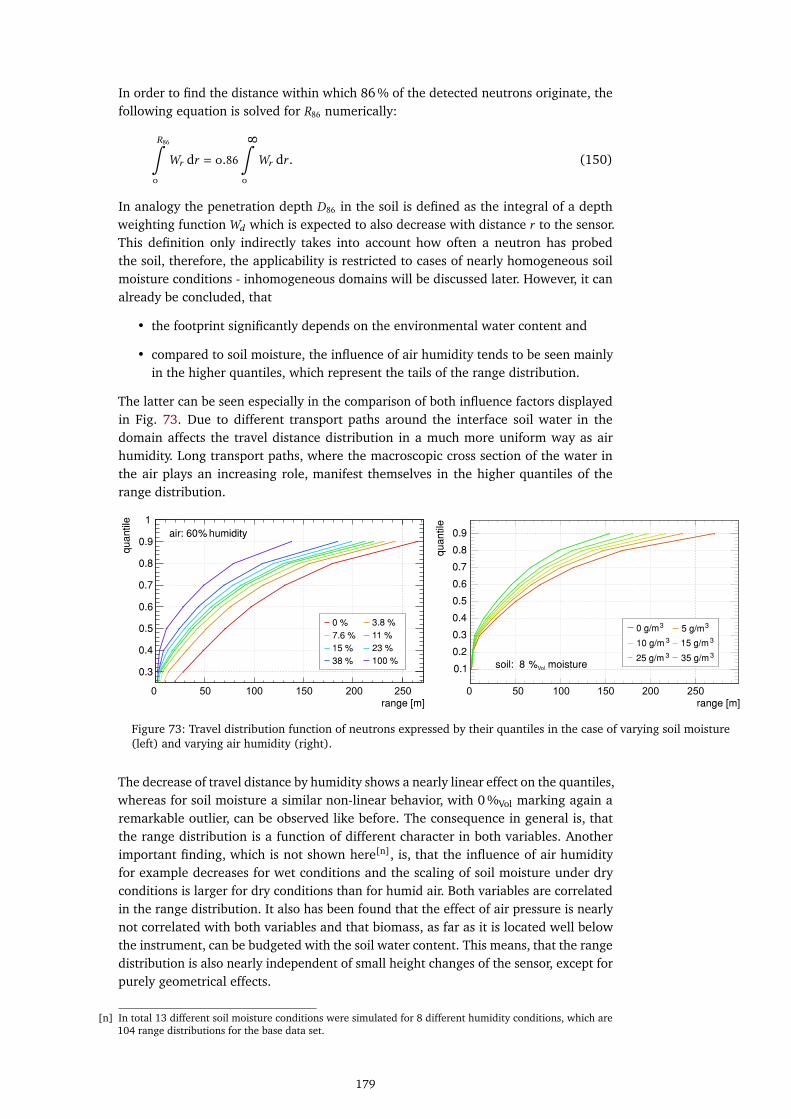
In order to find the distance within which 86 % of the detected neutrons originate, thefollowing equation is solved for 𝑅86 numerically:

𝑅86∫0

𝑊𝑟 d𝑟 = 0.86

8∫0

𝑊𝑟 d𝑟 . (150)

In analogy the penetration depth 𝐷86 in the soil is defined as the integral of a depthweighting function𝑊𝑑 which is expected to also decrease with distance 𝑟 to the sensor.This definition only indirectly takes into account how often a neutron has probedthe soil, therefore, the applicability is restricted to cases of nearly homogeneous soilmoisture conditions - inhomogeneous domains will be discussed later. However, it canalready be concluded, that

• the footprint significantly depends on the environmental water content and

• compared to soil moisture, the influence of air humidity tends to be seen mainlyin the higher quantiles, which represent the tails of the range distribution.

The latter can be seen especially in the comparison of both influence factors displayedin Fig. 73. Due to different transport paths around the interface soil water in thedomain affects the travel distance distribution in a much more uniform way as airhumidity. Long transport paths, where the macroscopic cross section of the water inthe air plays an increasing role, manifest themselves in the higher quantiles of therange distribution.

range [m]

qu

an

tile

0.3

0.4

0.5

0.6

0.7

0.8

0.9

1

humidity%air: 60

0 % 3.8 %

7.6 % 11 %

15 % 23 %

38 % 100 %

range [m]

qu

an

tile

0.1

0.2

0.3

0.4

0.5

0.6

0.7

0.8

0.9

30 g/m 35 g/m310 g/m 315 g/m

325 g/m 335 g/m

0 50 100 150 200 2500 50 100 150 200 250

moisture%Volsoil: 8

Figure 73: Travel distribution function of neutrons expressed by their quantiles in the case of varying soil moisture(left) and varying air humidity (right).

The decrease of travel distance by humidity shows a nearly linear effect on the quantiles,whereas for soil moisture a similar non-linear behavior, with 0 %Vol marking again aremarkable outlier, can be observed like before. The consequence in general is, thatthe range distribution is a function of different character in both variables. Anotherimportant finding, which is not shown here[n], is, that the influence of air humidityfor example decreases for wet conditions and the scaling of soil moisture under dryconditions is larger for dry conditions than for humid air. Both variables are correlatedin the range distribution. It also has been found that the effect of air pressure is nearlynot correlated with both variables and that biomass, as far as it is located well belowthe instrument, can be budgeted with the soil water content. This means, that the rangedistribution is also nearly independent of small height changes of the sensor, except forpurely geometrical effects.

[n] In total 13 different soil moisture conditions were simulated for 8 different humidity conditions, which are104 range distributions for the base data set.

179

9.2.3 ANALYTICAL CHARACTERIZATION OF THE FOOTPRINT

The range distributions can be fitted very well in a frame of exponential functionsby defining a near-field term below 50 m and a far-field term above. This approachis motivated by simple models of diffusion theory explained in sec. 9.2.1. The peakat 𝑟 < 10 m accounts for neutrons that directly emerge from the ground and have ahigh probability to be detected even though most of them come from the lower part ofthe neutron energy spectrum. The region up to 𝑟 < 50 m describes the average meanfree path of most of the environmental neutrons in humid air. For distances between50 m and 200 m neutrons interact with the soil multiple times until they are detected,which in turn means that with increasing 𝑟 , average neutron energies quickly becomeinsufficient in order to arrive at the detector before thermalization. From about 200 mon, detected neutrons are dominated by the higher energetic part of the spectrum,which appear to be higher in flux rates and are able to probe the soil very far from thedetector.The entire range distribution function is found to be

𝐼0 (ℎ,\ )𝑊𝑟 (ℎ,\ ) = 𝐼0 ·

(𝐹1 𝑒

−𝐹2 𝑟 ∗ + 𝐹3 𝑒−𝐹4 𝑟 ∗ ) (

1 − 𝑒−𝐹0 𝑟∗ )

, 0m < 𝑟 ≤ 1m

𝐹1 𝑒−𝐹2 𝑟 ∗ + 𝐹3 𝑒

−𝐹4 𝑟 ∗ , 1m < 𝑟 ≤ 50m

𝐹5 𝑒−𝐹6 𝑟 ∗ + 𝐹7 𝑒

−𝐹8 𝑟 ∗ , 50m < 𝑟 < 600m

(151)

with 𝐼0 representing the overall intensity and𝑊𝑟 denoting the radial weighting function.The parameters 𝐹𝑖 represent either signal contributions or attenuation coefficients fora rescaled distance 𝑟 ∗ (𝑟 ,𝑝,\ ), which can be considered as an unmodified distance 𝑟 forstandard environmental conditions. Each above defined interval contains one functionmodeling the main functional contributor, i.e. the soil moisture dependency, and onereflecting the second order correction. In order to account for the effect of the detectorlayer being positioned at a height of 2 m, for ranges below 1 m a purely geometricalfactor is added.

Inte

nsity

[a

.u.]

1

10

100

Inte

nsity

[a

.u.]

0

50

100

150

200

250

300

350

400

450

Θ = 23 %

Θ = 4 %

Θ = 23 %

Θ = 4 %

W( ,h)r ΘW( ,h)r Θ

air: 60 % humidity

range [m]50 100 150 200 2500 300 350

range [m]1 2 3 4 50 6 7 8

Figure 74: Test of the modeled function (162) with the parameter fits from tab. 16 in comparison to the simulatedrange distribution set in the near-field regime with focus on the first peak (left) and the far-field (right).

Finding a suitable analytic expression for the range distributions under typical en-vironmental conditions is a question of multi-variate modeling. Therefore, all rangedistributions have been fitted by 𝐼0 ·𝑊𝑟 (151) and parametrized as functions of soilmoisture and air humidity. At around 50 m the analytical description starts to deviatefrom the data. For this reason the value of 50 m has been chosen as a delimiter for both

180

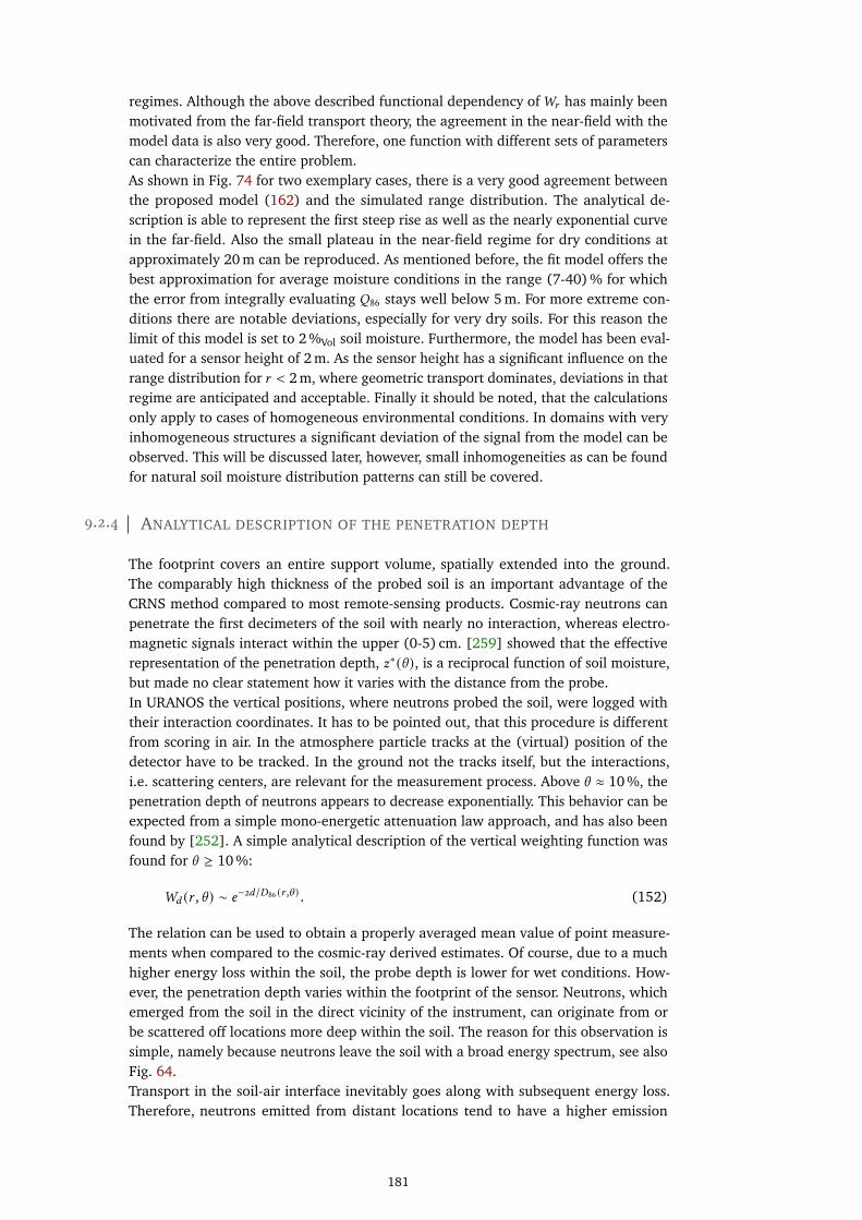
regimes. Although the above described functional dependency of𝑊𝑟 has mainly beenmotivated from the far-field transport theory, the agreement in the near-field with themodel data is also very good. Therefore, one function with different sets of parameterscan characterize the entire problem.As shown in Fig. 74 for two exemplary cases, there is a very good agreement betweenthe proposed model (162) and the simulated range distribution. The analytical de-scription is able to represent the first steep rise as well as the nearly exponential curvein the far-field. Also the small plateau in the near-field regime for dry conditions atapproximately 20 m can be reproduced. As mentioned before, the fit model offers thebest approximation for average moisture conditions in the range (7-40) % for whichthe error from integrally evaluating 𝑄86 stays well below 5 m. For more extreme con-ditions there are notable deviations, especially for very dry soils. For this reason thelimit of this model is set to 2 %Vol soil moisture. Furthermore, the model has been eval-uated for a sensor height of 2 m. As the sensor height has a significant influence on therange distribution for 𝑟 < 2 m, where geometric transport dominates, deviations in thatregime are anticipated and acceptable. Finally it should be noted, that the calculationsonly apply to cases of homogeneous environmental conditions. In domains with veryinhomogeneous structures a significant deviation of the signal from the model can beobserved. This will be discussed later, however, small inhomogeneities as can be foundfor natural soil moisture distribution patterns can still be covered.

9.2.4 ANALYTICAL DESCRIPTION OF THE PENETRATION DEPTH

The footprint covers an entire support volume, spatially extended into the ground.The comparably high thickness of the probed soil is an important advantage of theCRNS method compared to most remote-sensing products. Cosmic-ray neutrons canpenetrate the first decimeters of the soil with nearly no interaction, whereas electro-magnetic signals interact within the upper (0-5) cm. [259] showed that the effectiverepresentation of the penetration depth, 𝑧∗ (\ ), is a reciprocal function of soil moisture,but made no clear statement how it varies with the distance from the probe.In URANOS the vertical positions, where neutrons probed the soil, were logged withtheir interaction coordinates. It has to be pointed out, that this procedure is differentfrom scoring in air. In the atmosphere particle tracks at the (virtual) position of thedetector have to be tracked. In the ground not the tracks itself, but the interactions,i.e. scattering centers, are relevant for the measurement process. Above \ ≈ 10 %, thepenetration depth of neutrons appears to decrease exponentially. This behavior can beexpected from a simple mono-energetic attenuation law approach, and has also beenfound by [252]. A simple analytical description of the vertical weighting function wasfound for \ ≥ 10 %:

𝑊𝑑 (𝑟 ,\ ) ∼ 𝑒−2𝑑/𝐷86 (𝑟 ,\ ) . (152)

The relation can be used to obtain a properly averaged mean value of point measure-ments when compared to the cosmic-ray derived estimates. Of course, due to a muchhigher energy loss within the soil, the probe depth is lower for wet conditions. How-ever, the penetration depth varies within the footprint of the sensor. Neutrons, whichemerged from the soil in the direct vicinity of the instrument, can originate from orbe scattered off locations more deep within the soil. The reason for this observation issimple, namely because neutrons leave the soil with a broad energy spectrum, see alsoFig. 64.Transport in the soil-air interface inevitably goes along with subsequent energy loss.Therefore, neutrons emitted from distant locations tend to have a higher emission

181

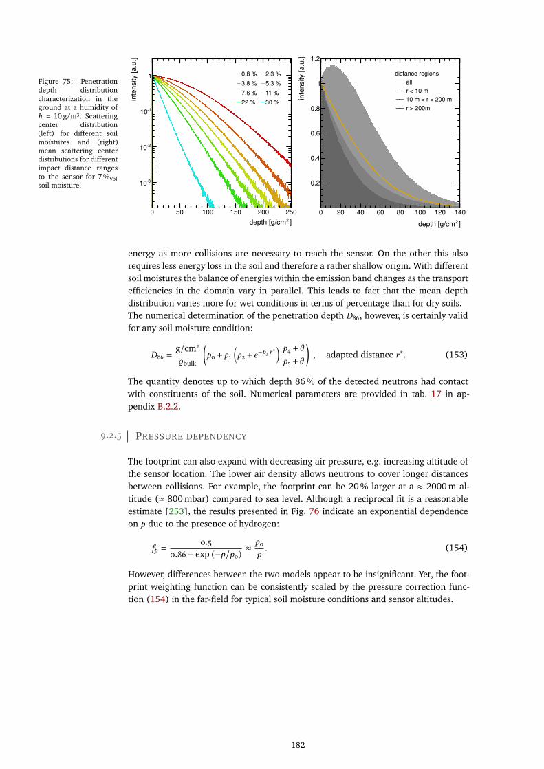
Figure 75: Penetrationdepth distributioncharacterization in theground at a humidity ofℎ = 10 g/m3. Scatteringcenter distribution(left) for different soilmoistures and (right)mean scattering centerdistributions for differentimpact distance rangesto the sensor for 7 %Volsoil moisture.

]2depth [g/cm

0 50 100 150 200 250

inte

nsity

[a

.u.]

-310

-210

-110

1 0.8 % 2.3 %

3.8 % 5.3 %

7.6 % 11 %

22 % 30 %

]2depth [g/cm

0 20 40 60 80 100 120 140

inte

nsity

[a

.u.]

0.2

0.4

0.6

0.8

1

1.2

distance regions

all

r < 10 m

10 m < r < 200 m

r > 200m

energy as more collisions are necessary to reach the sensor. On the other this alsorequires less energy loss in the soil and therefore a rather shallow origin. With differentsoil moistures the balance of energies within the emission band changes as the transportefficiencies in the domain vary in parallel. This leads to fact that the mean depthdistribution varies more for wet conditions in terms of percentage than for dry soils.The numerical determination of the penetration depth 𝐷86, however, is certainly validfor any soil moisture condition:

𝐷86 =g/cm2

𝜚bulk

(𝑝0 + 𝑝1

(𝑝2 + 𝑒−𝑝3 𝑟

∗) 𝑝4 + \𝑝5 + \

), adapted distance 𝑟 ∗. (153)

The quantity denotes up to which depth 86 % of the detected neutrons had contactwith constituents of the soil. Numerical parameters are provided in tab. 17 in ap-pendix B.2.2.

9.2.5 PRESSURE DEPENDENCY

The footprint can also expand with decreasing air pressure, e.g. increasing altitude ofthe sensor location. The lower air density allows neutrons to cover longer distancesbetween collisions. For example, the footprint can be 20 % larger at a ≈ 2000 m al-titude (' 800 mbar) compared to sea level. Although a reciprocal fit is a reasonableestimate [253], the results presented in Fig. 76 indicate an exponential dependenceon 𝑝 due to the presence of hydrogen:

𝑓𝑝 =0.5

0.86 − exp (−𝑝/𝑝0)≈ 𝑝0

𝑝. (154)

However, differences between the two models appear to be insignificant. Yet, the foot-print weighting function can be consistently scaled by the pressure correction func-tion (154) in the far-field for typical soil moisture conditions and sensor altitudes.

182

1.6

1.4

1.2

1.0

0.80.6 0.7 0.8 0.9 1.0 1.1

Air pressure p [mBar]/(1013 mBar)

simulation

p /p0

fitted equation

Range [m]

Inte

nsity

[a

.u.]

1

10

100

3Pressure comparison at 25 g/m

5 % soil moisture

40 % soil moisture

5 % soil moisture 700 hPa

40 % soil moisture 700 hPa

Fit scaled in x by 1.35

Fit scaled in x by 1.35

Re

lativ

e in

ten

sity

0 100 200 300 400 500

Figure 76: Pressure dependency of the range distribution for two exemplary soil moisture and air pressure conditions(left). The 1013 mb distributions are fitted by the far-field term of (151), if that function is then rescaled by acommon factor, it matches the corresponding range distribution of the designated pressure. This model for thepressure dependency is depicted in the right panel.

9.2.6 HEIGHT DEPENDENCY

Stationary sensors are typically placed in heights of approximately 2 m as well as rovingconstrains the elevation by the use of vehicles. These requirements justify the emphasisof this study to that common setup distance to the ground. However, measurements ofthe environmental flux at larger heights have been carried out as early as 1966 [260]using an antenna tower or [65] performing airborne surveys. With large-scale soilmoisture measurement campaigns on terrains, which cannot easily be accessed byroving, airborne measurements are discussed as a feasible solution. As discussed in theprevious sec. 9.2.1 the near-field is dominated by geometrical transport of neutronsfrom the direct vicinity of the instrument.

Figure 77: Height depen-dency of the range distri-bution for two soil mois-ture settings and eleva-tions up to 200 m. It isclearly visible how thenear-field is dominatedby geometric transport,whereas the far-field con-sistently remains nearlyunchanged. Lines andnumbers indicate 𝑄86 foreach respective distribu-tion, see also tab. 13.

Range [m]

0 50 100 150 200 250 300 350 400 450

Inte

nsity

[a

.u.]

200

400

600

800

1000

1200

1400 3ϴ = 40 %, h = 10 g/m

10 m (1)

25 m (2)

50 m (3)

100 m (4)

150 m (5)

190 m (6)

(7) (8) (9) (10) (11) (12)

(1) (2) (3) (4) (5) (6)

3ϴ = 5 %, h = 10 g/m

10 m (7)

25 m (8)

50 m (9)

100 m (10)

150 m (11)

190 m (12)

Elevating the sensor by several tens of meters already increases the footprint substan-tially. Fig. 77 shows simulations, where the detector layer has been placed at heightsup to 200 m. Two conclusions can be drawn from the depicted range distributions:

183

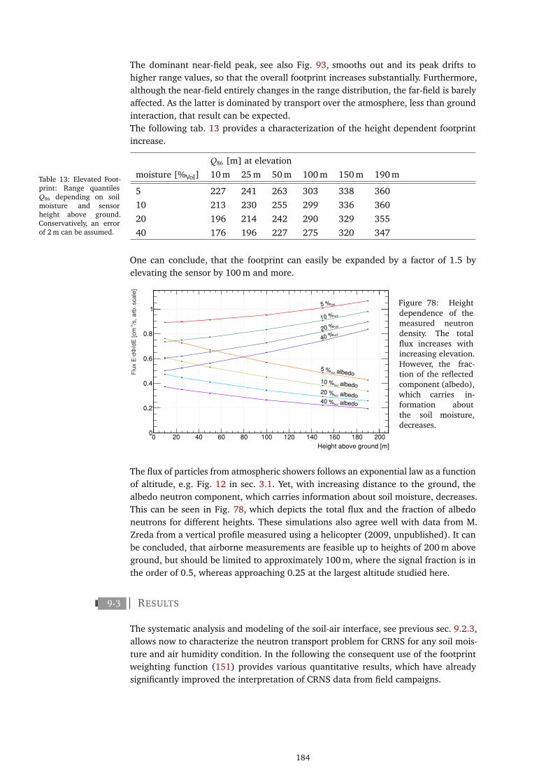
The dominant near-field peak, see also Fig. 93, smooths out and its peak drifts tohigher range values, so that the overall footprint increases substantially. Furthermore,although the near-field entirely changes in the range distribution, the far-field is barelyaffected. As the latter is dominated by transport over the atmosphere, less than groundinteraction, that result can be expected.The following tab. 13 provides a characterization of the height dependent footprintincrease.

Table 13: Elevated Foot-print: Range quantiles𝑄86 depending on soilmoisture and sensorheight above ground.Conservatively, an errorof 2 m can be assumed.

𝑄86 [m] at elevation

moisture [%Vol] 10 m 25 m 50 m 100 m 150 m 190 m

5 227 241 263 303 338 360

10 213 230 255 299 336 360

20 196 214 242 290 329 355

40 176 196 227 275 320 347

One can conclude, that the footprint can easily be expanded by a factor of 1.5 byelevating the sensor by 100 m and more.

Height above ground [m]

0 20 40 60 80 100 120 140 160 180 2000

0.2

0.4

0.6

0.8

1

40 % albedoVol

20 % albedoVol

10 % albedoVol

5 % albedoVol

5 %Vol

10 %Vol

20 %Vol

40 %Vol

-2F

lux E

dΦ/d

E [

cm

·/s

, a

rb.

sca

le]

Figure 78: Heightdependence of themeasured neutrondensity. The totalflux increases withincreasing elevation.However, the frac-tion of the reflectedcomponent (albedo),which carries in-formation aboutthe soil moisture,decreases.

The flux of particles from atmospheric showers follows an exponential law as a functionof altitude, e.g. Fig. 12 in sec. 3.1. Yet, with increasing distance to the ground, thealbedo neutron component, which carries information about soil moisture, decreases.This can be seen in Fig. 78, which depicts the total flux and the fraction of albedoneutrons for different heights. These simulations also agree well with data from M.Zreda from a vertical profile measured using a helicopter (2009, unpublished). It canbe concluded, that airborne measurements are feasible up to heights of 200 m aboveground, but should be limited to approximately 100 m, where the signal fraction is inthe order of 0.5, whereas approaching 0.25 at the largest altitude studied here.

9.3 RESULTS

The systematic analysis and modeling of the soil-air interface, see previous sec. 9.2.3,allows now to characterize the neutron transport problem for CRNS for any soil mois-ture and air humidity condition. In the following the consequent use of the footprintweighting function (151) provides various quantitative results, which have alreadysignificantly improved the interpretation of CRNS data from field campaigns.

184

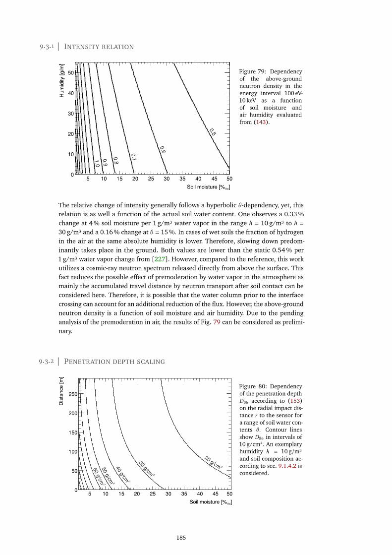
9.3.1 INTENSITY RELATION

Soil moisture [% ]Vol

3H

um

idity

[g

/m]

0

10

20

30

40

50

0.5

0.6

0.70

.80.9

1.0

5 10 15 20 25 30 35 40 45 50

Figure 79: Dependencyof the above-groundneutron density in theenergy interval 100 eV-10 keV as a functionof soil moisture andair humidity evaluatedfrom (143).

The relative change of intensity generally follows a hyperbolic \ -dependency, yet, thisrelation is as well a function of the actual soil water content. One observes a 0.33 %change at 4 % soil moisture per 1 g/m3 water vapor in the range ℎ = 10 g/m3 to ℎ =

30 g/m3 and a 0.16 % change at \ = 15 %. In cases of wet soils the fraction of hydrogenin the air at the same absolute humidity is lower. Therefore, slowing down predom-inantly takes place in the ground. Both values are lower than the static 0.54 % per1 g/m3 water vapor change from [227]. However, compared to the reference, this workutilizes a cosmic-ray neutron spectrum released directly from above the surface. Thisfact reduces the possible effect of premoderation by water vapor in the atmosphere asmainly the accumulated travel distance by neutron transport after soil contact can beconsidered here. Therefore, it is possible that the water column prior to the interfacecrossing can account for an additional reduction of the flux. However, the above-groundneutron density is a function of soil moisture and air humidity. Due to the pendinganalysis of the premoderation in air, the results of Fig. 79 can be considered as prelimi-nary.

9.3.2 PENETRATION DEPTH SCALING

Soil moisture [% ]Vol

5 10 15 20 25 30 35 40 45 50

Dis

tan

ce

[m

]

0

50

100

150

200

250

2

20 g/cm

30

2

g/cm

40

2

g/cm

50

2

g/cm

60

2

g/cm

Figure 80: Dependencyof the penetration depth𝐷86 according to (153)on the radial impact dis-tance 𝑟 to the sensor fora range of soil water con-tents \ . Contour linesshow 𝐷86 in intervals of10 g/cm2. An exemplaryhumidity ℎ = 10 g/m3

and soil composition ac-cording to sec. 9.1.4.2 isconsidered.

185

The average probe depth is typically a result of many interactions in the ground andnearly follows an exponential law with a soil moisture depending attenuation coeffi-cient. However, this value also depends on the distance, where the neutron enteredthe soil in the first place. Fig. 80 shows the penetration depths 𝐷86 (𝑟 ,\ ) as a functionof radial distance 𝑟 from the sensor for exemplary soil moisture values \ . For dry soil𝐷86 (𝑟 ,\ ≈ 1 %) ranges from 83 cm right below the sensor to 46 cm at 𝑟 = 300 m distance.At most, the penetration depth varies between 15 cm and 83 cm below the sensor forwet and dry soil, respectively. This is in close agreement with depths of (12-76) cmgiven by [252]. The reported values are rather confirmed than contradicted by URA-NOS, because they stemmed from experiences and various studies in the research fieldof cosmogenic nuclide production and are thus independent of the mentioned modelapproach. On average over the first tens of meters distance, the functional dependencyon \ , see (153), is relatively similar to the reciprocal model for the effective sensor depth𝑧∗ (\ ) from [259]. Their model was constrained on the limits introduced by [252] andvalidated with measurements and hydrodynamic simulations. Further evidence for thecorrect performance of the URANOS model provides the comparison with measure-ment depths of (50-100) cm on the Moon or Mars missions, where cosmic-ray neutronspenetrate dry ground of similar chemical composition [261, 262].

9.3.3 FOOTPRINT

The response to soil moisture variations is significant for humid climates between (15-50) %Vol as well as for very dry conditions < 3 %Vol. Previous studies underestimatedthe role of soil moisture for the footprint due to the choice of a modeled neutronsource below the surface. This detail is the major cause for the discrepancy to findingsfrom [253], who stated, that the footprint remains mainly unchanged for typical soilmoisture conditions.

Figure 81: Dependencyof the radial distancequantile 𝑄86 accordingto (151) for a rangeof soil water contents \ .Contour lines show 𝑄86

for different humidities.

]VolSoil moisture [%

Ra

ng

e [

m]

120

140

160

180

200

220

240

30 g/m

35 g/m

310 g/m

315 g/m

320 g/m

330 g/m

5 10 15 20 25 30 35 40 45 50

The footprint itself is a function of soil moisture. This effect can be attributed to thedifferent initial energies from the soil emission spectra and more importantly to thetransport efficiency of the interface. Neutrons cross the air-ground boundary on averagethree times before they reach the sensor. With increasing soil moisture the probabilityof leaving after re-entry decreases. Hydrogen contributes to this behavior in two ways:The energy loss is much higher compared to any other element, which significantlydecreases the average travel distance, and in elastic collisions backward-scattering ishighly suppressed, which requires at least two collision with hydrogen for a neutron to

186

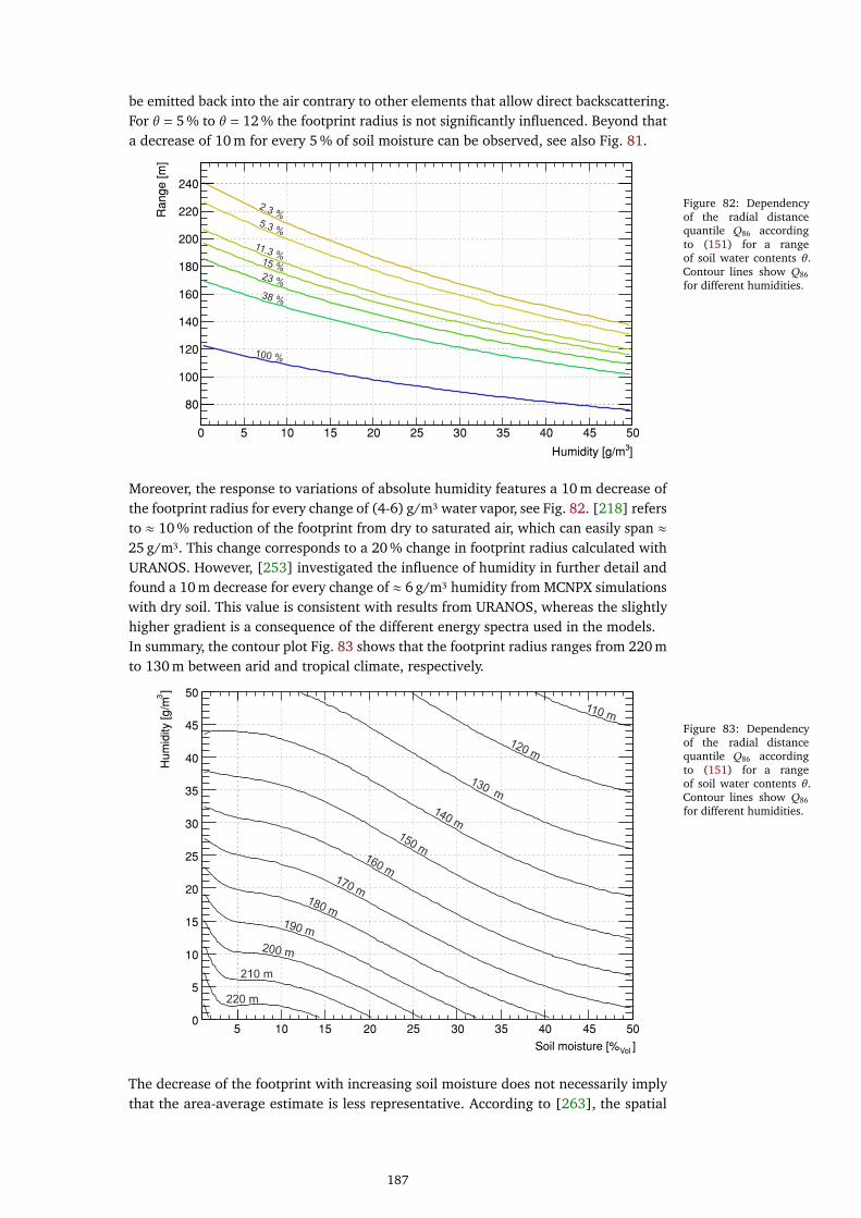
be emitted back into the air contrary to other elements that allow direct backscattering.For \ = 5 % to \ = 12 % the footprint radius is not significantly influenced. Beyond thata decrease of 10 m for every 5 % of soil moisture can be observed, see also Fig. 81.

Figure 82: Dependencyof the radial distancequantile 𝑄86 accordingto (151) for a rangeof soil water contents \ .Contour lines show 𝑄86

for different humidities.

]3Humidity [g/m

0 5 10 15 20 25 30 35 40 45 50

Ra

ng

e [

m]

80

100

120

140

160

180

200

220

240

2.3 %5.3 %

11.3 %15 %23 %

38 %

100 %

Moreover, the response to variations of absolute humidity features a 10 m decrease ofthe footprint radius for every change of (4-6) g/m3 water vapor, see Fig. 82. [218] refersto ≈ 10 % reduction of the footprint from dry to saturated air, which can easily span ≈25 g/m3. This change corresponds to a 20 % change in footprint radius calculated withURANOS. However, [253] investigated the influence of humidity in further detail andfound a 10 m decrease for every change of ≈ 6 g/m3 humidity from MCNPX simulationswith dry soil. This value is consistent with results from URANOS, whereas the slightlyhigher gradient is a consequence of the different energy spectra used in the models.In summary, the contour plot Fig. 83 shows that the footprint radius ranges from 220 mto 130 m between arid and tropical climate, respectively.

Figure 83: Dependencyof the radial distancequantile 𝑄86 accordingto (151) for a rangeof soil water contents \ .Contour lines show 𝑄86

for different humidities.

]VolSoil moisture [%

]3

Hu

mid

ity [g

/m

0

5

10

15

20

25

30

35

40

45

50

220 m

210 m

200 m

190 m

180 m

170 m

160 m

150 m

140 m

130 m

120 m

110 m

5 10 15 20 25 30 35 40 45 50

The decrease of the footprint with increasing soil moisture does not necessarily implythat the area-average estimate is less representative. According to [263], the spatial

187

variability of soil moisture tends to be low for rather wet soils. In this context, theeffective representativeness of the CRNS method appears to be almost unchanged.Conservatively, a total error of Δ𝑅86 = (4-6) % can be assumed, which scales from wetto dry conditions. A detailed error budget is listed in appendix B.2.3.

9.3.4 WHERE DO NEUTRONS COME FROM?

CRNS sensors are sometimes placed close to roads, trees or rivers. Mobile rover surveysinevitably pass alongside forests, lakes or fields of different land use. In most of thesecases an isotropic footprint cannot be expected, because large structures of differenthydrogen content vary the transport paths towards the sensor.

Detected neutron origins (first contact to soil)

Closest 86% of neutron origins for each sector

Neutron intensity for each sector [a.u.]

Footprint R86

3(5 g/m , 5 %) = 210 m for hom. soil

(a) (b) (c)

Water

dna L

River oadR

Figure 84: Anisotropy of detected neutron origins (black) and neutron intensity (red) determined for every 12◦

sectorof a circle around a centered detector. The displayed extent is 270 m in radius,whereas the dashed linerepresents the isotropic footprint. The three exemplary cases illustrate bare soil (white) with (a) a coast line to water(blue), (b) a 10 m river at 50 m distance and (c) a 10 m concrete road (yellow). [KS2015]

In order to quantify the anisotropy of detected neutrons, exemplary cases where suchscenarios are extreme have been simulated. In Fig. 84 the vicinity of a centered detectoris shown and the isotropic footprint 𝑅86 (ℎ = 5 g/m3,\ = 5 %) = 210 m is indicated(dashed line). Dots illustrate the origin of detected neutrons, where the closest 86 %of total neutrons are emphasized (black) in each direction. The area is discretized into12◦ sectors in order to quantify range (black dots) and intensity (red).In a coast line setup, Fig. 84a, the density of the origins (dots) and neutron intensity(sectors) appear to be much smaller in the ponded area. The range of neutrons de-creases by up to (30-40) % although neutrons still manage to travel long distances overwater. Their contribution to the count rate sharply drops to about 40 % at the interface.In Fig. 84b the detector is placed 50 m away from a 10 m wide river. This setup canespecially found for irrigated land-use. The neutron origins clearly show that the riverhardly contributes to the signal because most neutrons lose too much energy afterprobing water, see also point density and neutron intensity for water, Fig. 84a. This isalso visible in the respective intensity which shows a slight asymmetry towards the dryside. However, the setup reveals a slightly wider footprint in the direction to the river,as a consequence of the intensity gap.A detector carried on a dry, concrete road, see Fig. 84c, is the typical setup for roverapplications. The sensor detects about (10-20) % more neutrons from the road thanfrom other directions. However, the decrease of the footprint along the road due to

188

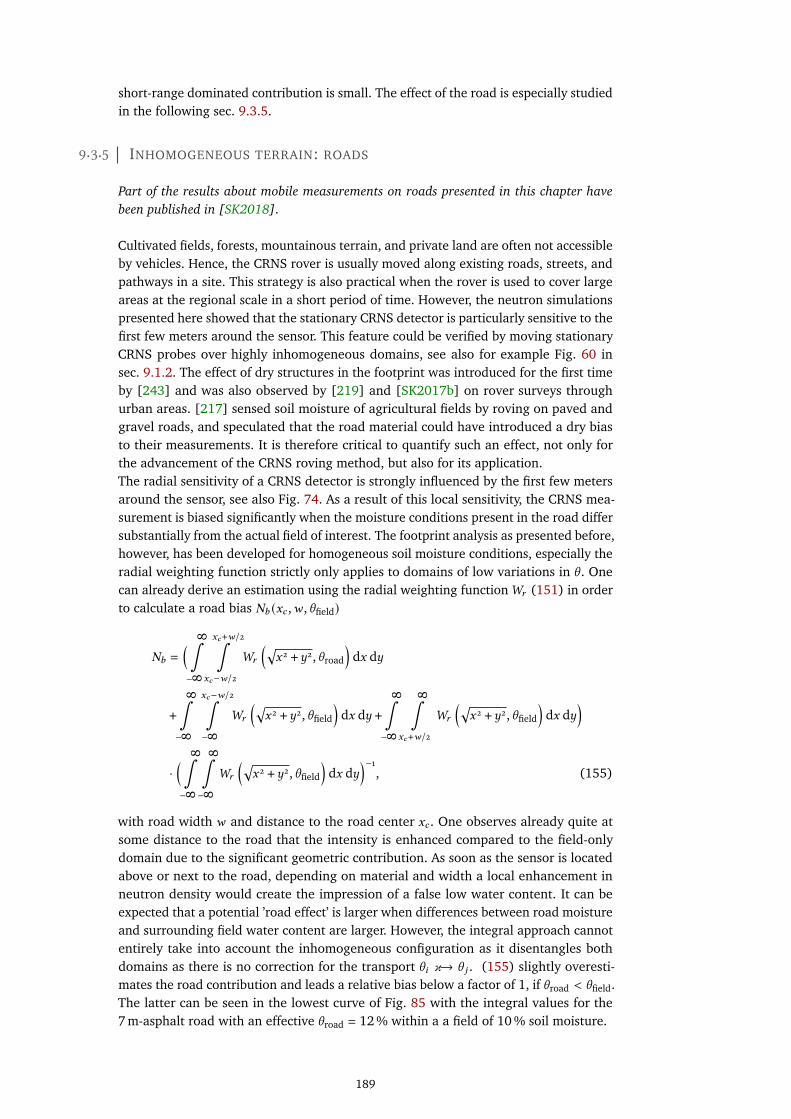
short-range dominated contribution is small. The effect of the road is especially studiedin the following sec. 9.3.5.

9.3.5 INHOMOGENEOUS TERRAIN: ROADS

Part of the results about mobile measurements on roads presented in this chapter havebeen published in [SK2018].

Cultivated fields, forests, mountainous terrain, and private land are often not accessibleby vehicles. Hence, the CRNS rover is usually moved along existing roads, streets, andpathways in a site. This strategy is also practical when the rover is used to cover largeareas at the regional scale in a short period of time. However, the neutron simulationspresented here showed that the stationary CRNS detector is particularly sensitive to thefirst few meters around the sensor. This feature could be verified by moving stationaryCRNS probes over highly inhomogeneous domains, see also for example Fig. 60 insec. 9.1.2. The effect of dry structures in the footprint was introduced for the first timeby [243] and was also observed by [219] and [SK2017b] on rover surveys throughurban areas. [217] sensed soil moisture of agricultural fields by roving on paved andgravel roads, and speculated that the road material could have introduced a dry biasto their measurements. It is therefore critical to quantify such an effect, not only forthe advancement of the CRNS roving method, but also for its application.The radial sensitivity of a CRNS detector is strongly influenced by the first few metersaround the sensor, see also Fig. 74. As a result of this local sensitivity, the CRNS mea-surement is biased significantly when the moisture conditions present in the road differsubstantially from the actual field of interest. The footprint analysis as presented before,however, has been developed for homogeneous soil moisture conditions, especially theradial weighting function strictly only applies to domains of low variations in \ . Onecan already derive an estimation using the radial weighting function𝑊𝑟 (151) in orderto calculate a road bias 𝑁𝑏 (𝑥𝑐 ,𝑤 ,\field)

𝑁𝑏 =

( 8∫− 8

𝑥𝑐+𝑤/2∫𝑥𝑐−𝑤/2

𝑊𝑟

(√𝑥2 +𝑦2,\road

)d𝑥 d𝑦

+

8∫− 8

𝑥𝑐−𝑤/2∫− 8

𝑊𝑟

(√𝑥2 +𝑦2,\field

)d𝑥 d𝑦 +

8∫− 8

8∫𝑥𝑐+𝑤/2

𝑊𝑟

(√𝑥2 +𝑦2,\field

)d𝑥 d𝑦

)·( 8∫− 8

8∫− 8

𝑊𝑟

(√𝑥2 +𝑦2,\field

)d𝑥 d𝑦

)−1, (155)

with road width 𝑤 and distance to the road center 𝑥𝑐 . One observes already quite atsome distance to the road that the intensity is enhanced compared to the field-onlydomain due to the significant geometric contribution. As soon as the sensor is locatedabove or next to the road, depending on material and width a local enhancement inneutron density would create the impression of a false low water content. It can beexpected that a potential ’road effect’ is larger when differences between road moistureand surrounding field water content are larger. However, the integral approach cannotentirely take into account the inhomogeneous configuration as it disentangles bothdomains as there is no correction for the transport \𝑖 𝜘→ \ 𝑗 . (155) slightly overesti-mates the road contribution and leads a relative bias below a factor of 1, if \road < \field.The latter can be seen in the lowest curve of Fig. 85 with the integral values for the7 m-asphalt road with an effective \road = 12 % within a a field of 10 % soil moisture.

189

distance from road center [m]

-20 0 20 40 60 80

rel.

ne

utr

on

inte

nsity

bia

s

1

1.05

1.1

1.15

1.2

1.25 stoney road 5 m

at 40 %Vol

at 30 %Vol

at 20 %Vol

at 10 %Vol

asphalt road 7 m

at 40 %Vol

at 30 %Vol

at 20 %Vol

at 10 %Vol

Figure 85: Road bias 𝑁𝑏

evaluated by (155) us-ing the readial weight-ing function (151). Thesensor is located at a dis-tance 𝑥𝑐 from the roadcenter, here two exam-ples of stone and as-phalt pavements. The in-fluence of the road leadsto a relative flux changecompared to the one ex-pected from a domainwith \field alone.

The application of roving on roads has been taken as an example of inhomogeneousterrain, which is in the following further studied using URANOS. In order to The roadis modeled as a 20 cm deep layer of either stone or asphalt, while the soil below was setto 5 % volumetric water content. Following the compendium of material compositiondata [147], asphalt pavement is modeled as a mixture of O, H, C, and Si, with aneffective density of 2.58 g/cm3, which corresponds to a soil water equivalent of \road ≈12 %. Stone/gravel is a mixture of Si, O, and Al, plus 3 % volumetric water content ata total density of 1.4 g/cm3. The wetness of the surrounding soil, \field, has been sethomogeneously to 10 %, 20 %, 30 %, and 40 % volumetric water content. The neutronresponse to roads was simulated for road widths of 3 m, 5 m, and 7 m.

Figure 86: (left)Schematic of the modelsetup used by URANOSto simulate the responseof cosmic-ray neutrons toground materials. (right)Exemplary URANOSmodel output showinga birds-eye view ofthe neutron density inthe horizontal detectorlayer for a 5 m stoneyroad and 50 % field soilmoisture. [SK2018]

The result from the simulation confirms that the bias increases with increasing fieldsoil moisture, increasing road width and decreasing road moisture. Fig. 87 plots thesimulated road bias over distance from the road center, showing that the bias is ashort-range effect that decreases a few meters away from the road, so that almost nomeasurable effect can be expected. Yet, there are two differences in the particle-trackingsolution compared to the integral approach (155). The road bias is slightly emphasizedfor the asphalt road and a few percent lower for the stone road. Furthermore, the long-range enhancement tails at distances far from the road center appear slightly weaker.The quantitative differences between both approaches might not be relevant in practicecompared to other sources of errors. It may be not feasible to estimate the hydrogenconcentration of the road precisely, therefore, biases which correspond to effective soilmoisture changes of the road in the order of 2 % can be expected. From this point ofview the analytical approach can already provide a reasonably good estimation for the’road effect’.

190

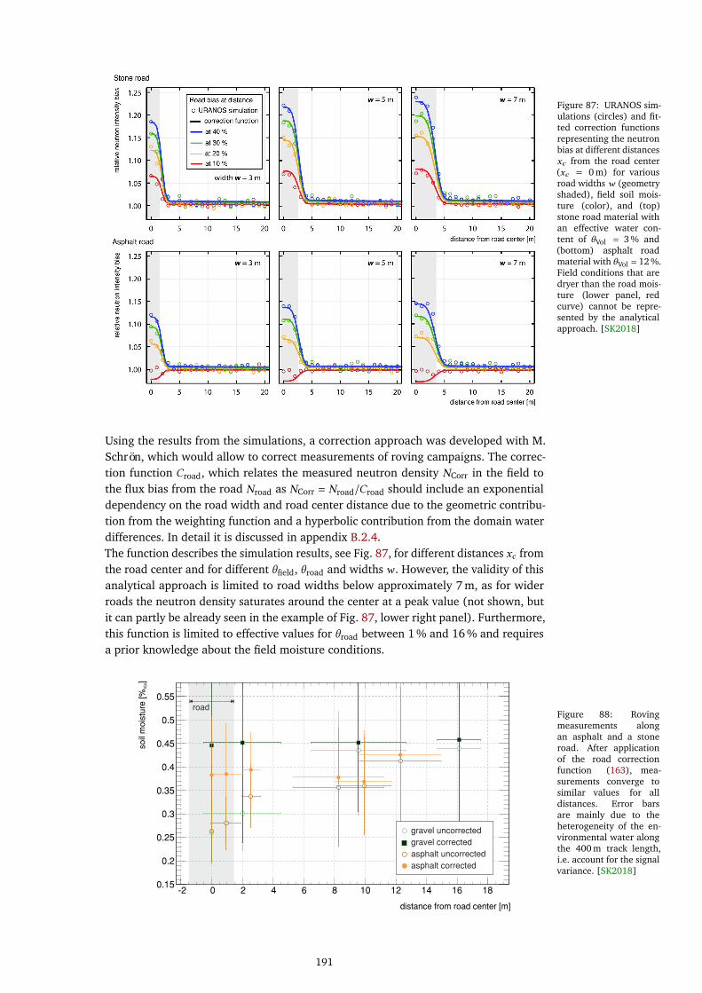
Figure 87: URANOS sim-ulations (circles) and fit-ted correction functionsrepresenting the neutronbias at different distances𝑥𝑐 from the road center(𝑥𝑐 = 0 m) for variousroad widths 𝑤 (geometryshaded), field soil mois-ture (color), and (top)stone road material withan effective water con-tent of \Vol = 3 % and(bottom) asphalt roadmaterial with \Vol = 12 %.Field conditions that aredryer than the road mois-ture (lower panel, redcurve) cannot be repre-sented by the analyticalapproach. [SK2018]

Using the results from the simulations, a correction approach was developed with M.Schrön, which would allow to correct measurements of roving campaigns. The correc-tion function 𝐶road, which relates the measured neutron density 𝑁Corr in the field tothe flux bias from the road 𝑁road as 𝑁Corr = 𝑁road/𝐶road should include an exponentialdependency on the road width and road center distance due to the geometric contribu-tion from the weighting function and a hyperbolic contribution from the domain waterdifferences. In detail it is discussed in appendix B.2.4.The function describes the simulation results, see Fig. 87, for different distances 𝑥𝑐 fromthe road center and for different \field, \road and widths 𝑤 . However, the validity of thisanalytical approach is limited to road widths below approximately 7 m, as for widerroads the neutron density saturates around the center at a peak value (not shown, butit can partly be already seen in the example of Fig. 87, lower right panel). Furthermore,this function is limited to effective values for \road between 1 % and 16 % and requiresa prior knowledge about the field moisture conditions.

Figure 88: Rovingmeasurements alongan asphalt and a stoneroad. After applicationof the road correctionfunction (163), mea-surements converge tosimilar values for alldistances. Error barsare mainly due to theheterogeneity of the en-vironmental water alongthe 400 m track length,i.e. account for the signalvariance. [SK2018]

distance from road center [m]

-2 0 2 4 6 8 10 12 14 16 18

so

il m

ois

ture

[%

]V

ol

0.15

0.2

0.25

0.3

0.35

0.4

0.45

0.5

0.55road

gravel uncorrected

gravel corrected

asphalt uncorrected

asphalt corrected

191

This function has extensively been applied in the study of [SK2018]. Here, exemplarilythe correction of the data set of R. Rosolem and M. Schrön collected in the Lambourncatchment in South England (51◦32’N, 1◦29’W) is shown. The general objective ofthese experiments was to clarify whether the road correction function and the underly-ing simulations can be used to transfer the apparent soil moisture patterns seen fromthe road to values that were taken in the actual field. The loamy clay soil has an av-erage bulk density of 𝜌bd = 1.25 g/cm3 and a water equivalent of additional hydrogenpools has been determined to be \Offset = 4 % with insignificant differences betweenthe fields. The road network consists of a paved major road (𝑤 = 3 m) made of anasphalt/stone mixture with an estimated moisture equivalent of 11 %. The main sideroads are made of a gravel/stone mixture with an estimated moisture equivalent of 7 %,mostly around 2.3 m wide, while the southern road is 4.5 m wide. Many non-sealedtracks (𝑤 = 3 m) follow the borders between fields which partly consist of sand, grass,and organic material, such that their average moisture equivalent was estimated to12 %.In the experiment a rover-type of cosmic-ray neutron detector, see sec. 7.2.1 and 8.1was driven along a 400 m track in various distances from a gravel/stone road and an as-phalt road. Upon application of the road correction function, see Fig. 88, measurementsconverge to similar values for all distances (right) and could also reveal different soilmoisture conditions for the northern and southern fields (not shown). The overall re-sult provides strong evidence that the analytical correction function properly representsthe road bias at different distances and for different materials.

192

Part V

S U M M A R Y A N D C O N C L U S I O N

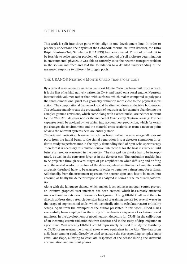
C O N C L U S I O N

This work is split into three parts which align in one development line. In order toprecisely understand the physics of the CASCADE thermal neutron detector, the UltraRApid Neutron-Only Simulation (URANOS) has been created. This tool turned out tobe feasible to solve another problem of a novel method of soil moisture determinationin environmental physics. It was able to correctly solve the neutron transport problemin the soil-air interface and laid the foundation to a detailed understanding of themeasured response to different hydrogen pools.

THE URANOS NEUTRON MONTE CARLO TRANSPORT CODE

By a radical reset an entire neutron transport Monte Carlo has been built from scratch.It is the first of its kind natively written in C++ and based on a voxel engine. Neutronsinteract with volumes rather than with surfaces, which makes compared to polygonsthe three-dimensional pixel to a geometry definition more close to the physical inter-action. The computational framework could be slimmed down at decisive bottlenecks.The software mainly treats the propagation of neutrons as for example abandoning thecomplex gamma emissions, which come along with excited nuclei, are neither relevantfor the CASCADE detector nor for the method of Cosmic-Ray Neutron Sensing. Furtherexpenses could be avoided by not taking into account heat production, which for exam-ple changes the environment and the material cross sections, as from a neutron pointof view the relevant systems here are entirely static.The original motivation, however, which has been realized, was to merge all relevantparts from the initial beam to the signal generation into a detector simulation in or-der to study its performance in the highly demanding field of Spin Echo spectroscopy.Therefore it is necessary to simulate neutron interactions for the host instrument untilbeing scattered or converted in the detector. The charged ion physics has to be incorpo-rated, as well in the converter layer as in the detector gas. The ionization tracklet hasto be projected through several stages of gas amplification while diffusing and driftingonto the nested readout structure of the detector, where multi-channel amplifiers witha specific threshold have to be triggered in order to generate a timestamp for a signal.Additionally, from the instrument upstream the neutron spin state has to be taken intoaccount, as finally the detector response is analyzed in terms of the measured polariza-tion.Along with the language change, which makes it attractive as an open source project,an intuitive graphical user interface has been created, which has already attractedusers without an extensive informatics background. Using URANOS allowed them todirectly address their research question instead of training oneself for several weeks inthe usage of sophisticated tools, which technically aim to calculate reactor criticalitysetups. Apart from the examples of the author presented in this work URANOS hassuccessfully been employed in the study of the detector response of radiation portalmonitors, in the development of novel neutron detectors for CRNS, in the calibrationof an incoming cosmic radiation neutron detector and in the study of drip irrigation inagriculture. Most recently URANOS could impressively be used to study the feasibilityof CRNS for measuring the integral snow water equivalent in the Alps. The data froma 3D laser scanner could directly be used to extrude the corresponding complex snowvoxel landscape, allowing to calculate responses of the sensor during the differentaccumulation and melt-out phases.

194

COSMIC-RAY NEUTRON SENSING

This work presents the most extensive study of neutron transport in the soil-air in-terface with specifically focusing on the dependency on hydrogen pools. To preciselyunderstand the system this work heavily relies on Monte Carlo simulations, whichallow to analyze the relevant observables with their influence factors. The so obtaineddata sets were parametrized by analytical functions, which describe the system withoutthe further necessity to repeat a series of case studies.The spatial distribution of neutrons can often be simplified in terms of thermodynamicmodels, however, it is very sensitive to initial energies and even to small amounts ofhydrogen. As a consequence, the complexity of environmental neutron transport seemsto impede any attempt to simplify the problem. Therefore, the need arose for revisitingneutron transport models and for addressing some of the open questions regarding theradial sensitivity, humid climate or terrain structures. As this study shows, the descrip-tion of the footprint and neutron intensity is nontrivial to an exceptional degree.Initially, the response functions of cosmic-ray neutron sensors were analyzed in terms ofenergy-dependent detection efficiency and angular sensitivity. The investigated detec-tors, which are specific models for hydrological research, comprise vertical (CRS1000)and horizontal configurations (Rover), each moderated by one inch of polyethyleneand equipped with either 10BF3 or 3He proportional counters. The results show, thatthe energy window of highest response ranges from 0.1 eV to 106 eV. Hence, the typi-cally used range of (102-104) eV provides a reasonable basis for CRNS investigations,yet, a significant fraction of neutrons are contributing to the signal of the sensor belowand above this range.The important result from this study for CRNS is, that the response to soil moisturevaries significantly for humid climates between (10-40) %Vol as well as for very dryconditions <3 %Vol. Previous studies underestimated the role of soil moisture for thefootprint due to the choice of a modeled neutron source below the surface. This detail isthe major cause for the discrepancy to findings from [253]. The footprint is defined bythe radius of the 86 % quantile of the range distribution function of neutrons probing asoil of homogeneous moisture content. It has been found to range from approximately160 m over a water body to 210 m over dry soil with a total error of about (4-6) %. Thecircular shape of the footprint remains isotropic for most field applications, like hillyterrain, nearby rivers or heterogeneous land. However, large water bodies or forestsnearby can reduce range and intensity of detected neutrons from that direction.The response to variations of absolute humidity features a 10 m decrease of thefootprint radius for every change of (4-6) g/m3 water vapor, which can easily span≈25 g/m3. This change corresponds to a 20 % change in footprint radius calculatedwith URANOS. The penetration depth 𝐷86 (𝑟 ,\ ) of detected neutrons directly belowthe sensor ranges from 15 cm to 83 cm depending on soil moisture. An exponentialdecrease with depth is a good estimate for the sensor’s vertical sensitivity, whereas thedepth in turn shrinks significantly with radial distance to the sensor.The function 𝑊𝑟 lays the basis for a refinement of the commonly applied samplingstrategy, which assigned weights according to a static exponential radial function. Incontrast, the present work shows that (1) the first tens of meters provide a dominantcontribution to the signal in a rather non-exponential relation, and (2) the shape of theweighting function changes temporally as it is affected by variable moisture conditions.Subsequently, data can be weighted with𝑊𝑟 (ℎ,\ ) in an iterative procedure.The revised footprint function could fundamentally improve the reliability of the CRNSmethod. Many deviations from the expected soil water response, which had beenfound in previous studies, can now be explained. Therefore, results from this workhave quickly been adopted by the community and are meanwhile the basis for inter-

195

preting CRNS measurements. The improved understanding also allows to correct forsystematic biases as have been found for the so-called „road effect“. This specificallyhigh near-field sensitivity plays an important role for mobile measurements. The vari-ability of the road width and material significantly influences the measurements andcan now be corrected for analytically.

196

Part VI

A P P E N D I X

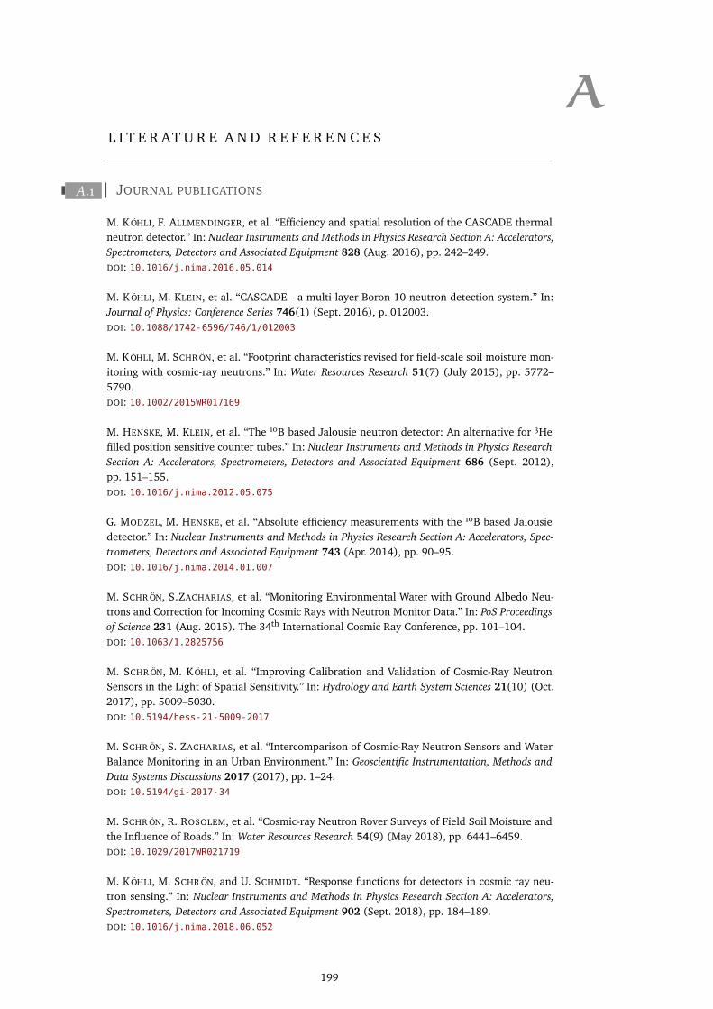
AL I T E R AT U R E A N D R E F E R E N C E S

𝐴.1 JOURNAL PUBLICATIONS

M. KÖHLI, F. ALLMENDINGER, et al. “Efficiency and spatial resolution of the CASCADE thermalneutron detector.” In: Nuclear Instruments and Methods in Physics Research Section A: Accelerators,Spectrometers, Detectors and Associated Equipment 828 (Aug. 2016), pp. 242–249.DOI: 10.1016/j.nima.2016.05.014

M. KÖHLI, M. KLEIN, et al. “CASCADE - a multi-layer Boron-10 neutron detection system.” In:Journal of Physics: Conference Series 746(1) (Sept. 2016), p. 012003.DOI: 10.1088/1742-6596/746/1/012003

M. KÖHLI, M. SCHRÖN, et al. “Footprint characteristics revised for field-scale soil moisture mon-itoring with cosmic-ray neutrons.” In: Water Resources Research 51(7) (July 2015), pp. 5772–5790.DOI: 10.1002/2015WR017169

M. HENSKE, M. KLEIN, et al. “The 10B based Jalousie neutron detector: An alternative for 3Hefilled position sensitive counter tubes.” In: Nuclear Instruments and Methods in Physics ResearchSection A: Accelerators, Spectrometers, Detectors and Associated Equipment 686 (Sept. 2012),pp. 151–155.DOI: 10.1016/j.nima.2012.05.075

G. MODZEL, M. HENSKE, et al. “Absolute efficiency measurements with the 10B based Jalousiedetector.” In: Nuclear Instruments and Methods in Physics Research Section A: Accelerators, Spec-trometers, Detectors and Associated Equipment 743 (Apr. 2014), pp. 90–95.DOI: 10.1016/j.nima.2014.01.007

M. SCHRÖN, S.ZACHARIAS, et al. “Monitoring Environmental Water with Ground Albedo Neu-trons and Correction for Incoming Cosmic Rays with Neutron Monitor Data.” In: PoS Proceedingsof Science 231 (Aug. 2015). The 34th International Cosmic Ray Conference, pp. 101–104.DOI: 10.1063/1.2825756

M. SCHRÖN, M. KÖHLI, et al. “Improving Calibration and Validation of Cosmic-Ray NeutronSensors in the Light of Spatial Sensitivity.” In: Hydrology and Earth System Sciences 21(10) (Oct.2017), pp. 5009–5030.DOI: 10.5194/hess-21-5009-2017

M. SCHRÖN, S. ZACHARIAS, et al. “Intercomparison of Cosmic-Ray Neutron Sensors and WaterBalance Monitoring in an Urban Environment.” In: Geoscientific Instrumentation, Methods andData Systems Discussions 2017 (2017), pp. 1–24.DOI: 10.5194/gi-2017-34

M. SCHRÖN, R. ROSOLEM, et al. “Cosmic-ray Neutron Rover Surveys of Field Soil Moisture andthe Influence of Roads.” In: Water Resources Research 54(9) (May 2018), pp. 6441–6459.DOI: 10.1029/2017WR021719

M. KÖHLI, M. SCHRÖN, and U. SCHMIDT. “Response functions for detectors in cosmic ray neu-tron sensing.” In: Nuclear Instruments and Methods in Physics Research Section A: Accelerators,Spectrometers, Detectors and Associated Equipment 902 (Sept. 2018), pp. 184–189.DOI: 10.1016/j.nima.2018.06.052

199

𝐴.2 CONFERENCE CONTRIBUTIONS

M. KÖHLI. Das CASCADE-Projekt: Neutronendetektion mittels Bor-10 als Alternative zu Helium-3.76th DPG Annual Conference. HK 42.2. Mainz, Germany, Mar. 2012

M. KÖHLI. Probing soil moisture by cosmic-ray induced Neutron Showers. 78th DPG Annual Con-ference. UP 7.3. Berlin, Germany, Mar. 2014

M. KÖHLI. Monte-Carlo Simulations on the Detector Sensitivity to Cosmic-Ray induced NeutronShowers. 4th COSMOS Workshop. Leipzig, Germany, May 2014

M. KÖHLI. The CASCADE Project - a perspective for solid state detectors. International Workshopon Position Sensitive Neutron Detectors. Jülich, Germany, June 2014

M. KÖHLI. Probing nano and macro scales: solid state detectors and cosmic neutron soil moisturedetermination. 9th Annual PNN and Well Logging Conference. Klingenbach, Austria, Sept. 2014

M. KÖHLI. CASCADE - eine alternative Perspektive für Festkörper-Neutronendetektoren. DeutscheTagung für Forschung mit Synchrotronstrahlung, Neutronen und Ionenstrahlen an Großgeräten2014. Bonn, Germany, Sept. 2014

M. KÖHLI. Soil moisture sensing by cosmic-ray induced neutron showers. 79th DPG Annual Confer-ence. UP 16.2. Heidelberg, Germany, Mar. 2015

M. KÖHLI. The CASCADE Dectector - high-resolution neutron detection by solid 10B layers. Designand Engineering of Neutron Instruments Meeting (DENIM). Budapest, Hungary, Sept. 2015

M. KÖHLI. The CASCADE Project - a multi-layer 10B neutron detection system. European Confer-ence on Neutron Scattering (ECNS). Zaragossa, Spain, Sept. 2015

M. KÖHLI. On the Phase Front of Neutron Detection. Neutronen in der Forschung und Industrie.München, Germany, Nov. 2015

M. KÖHLI. The method of soil moisture sensing by cosmic-ray neutrons. 80th DPG Annual Confer-ence. UP 15.1. Regensburg, Germany, Mar. 2016

M. KÖHLI. The CASCADE Project - On the Phase Front of Neutron Detection. 80th DPG AnnualConference. HK 70.6. Darmstadt, Germany, Mar. 2016

M. KÖHLI. Neutron Transport Modelling with URANOS and Footprint Sensitivity - Making Neutronsgreat again. 5th International COSMOS Workshop. Copenhagen, Denmark, Aug. 2016

M. KÖHLI. Soil moisture sensing by detection of cosmic-ray neutrons. 2nd ATTRACT TWD Sympo-sium in Detection and Imaging. Strasbourg, France, Nov. 2016

M. KÖHLI. Soil Moisture Measurement at the hectometer scale with cosmic-ray neutrons. 81th DPGAnnual Conference. UP 4.2. Bremen, Germany, Mar. 2017

M. KÖHLI. High Spatial Resolution in Thermal Neutron Detection: CASCADE. 81th DPG AnnualConference. HK 7.2. Darmstadt, Germany, Mar. 2017

M. KÖHLI. Soil moisture measurement at the hectometer scale using CRNS for mobile applications.82th DPG Annual Conference. UP 8.2. Erlangen, Germany, Mar. 2018

M. KÖHLI. URANOS - The Cosmic Ray Monte Carlo tool. EGU General Assembly. GI 2.7. Vienna,

Austria, Apr. 2018

200

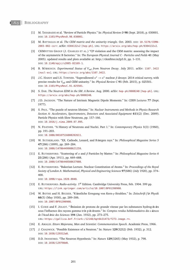
𝐴.3 BIBLIOGRAPHY

[1] M. TANABASHI et al. “Review of Particle Physics.” In: Physical Review D 98 (Sept. 2018), p. 030001.DOI: 10.1103/PhysRevD.98.030001.

[2] M. BATTAGLIA et al. The CKM matrix and the unitarity triangle. Oct. 2003. DOI: 10.5170/CERN-2003-002-corr. arXiv: 0304132v2 [hep-ph]. URL: https://arxiv.org/abs/hep-ph/0304132v2.

[3] CKMFITTER GROUP (J. CHARLES ET AL.) “CP violation and the CKM matrix: assessing the impactof the asymmetric B factories.” In: The European Physical Journal C - Particles and Fields 41 (May2005). updated results and plots available at: http://ckmfitter.in2p3.fr, pp. 1–131.DOI: 10.1140/epjc/s2005-02169-1.

[4] B. MÄRKISCH. Experimental Status of V𝑢𝑑 from Neutron Decay. July 2011. arXiv: 1107 . 3422

[nucl-ex]. URL: https://arxiv.org/abs/1107.3422.

[5] J.C. HARDY and I.S. TOWNER. “Superallowed 0+ → 0+ nuclear 𝛽 decays: 2014 critical survey, withprecise results for 𝑉𝑢𝑑 and CKM unitarity.” In: Physical Review C 91 (Feb. 2015), p. 025501.DOI: 10.1103/PhysRevC.91.025501.

[6] S. DAR. The Neutron EDM in the SM: A Review. Aug. 2000. arXiv: hep-ph/0008248 [hep-ph]. URL:https://arxiv.org/abs/hep-ph/0008248.

[7] J.D. JACKSON. “The Nature of Intrinsic Magnetic Dipole Moments.” In: CERN Lectures 77 (Sept.1977).

[8] S. PAUL. “The puzzle of neutron lifetime.” In: Nuclear Instruments and Methods in Physics ResearchSection A: Accelerators, Spectrometers, Detectors and Associated Equipment 611(2) (Dec. 2009).Particle Physics with Slow Neutrons, pp. 157–166.DOI: 10.1016/j.nima.2009.07.095.

[9] N. FEATHER. “A History of Neutrons and Nuclei. Part 1.” In: Contemporary Physics 1(3) (1960),pp. 191–203.DOI: 10.1080/00107516008202611.

[10] W. SUTHERLAND. “XX. Cathode, Lenard, and Röntgen rays.” In: Philosophical Magazine Series 547(286) (1899), pp. 269–284.DOI: 10.1080/14786449908621259.

[11] E. RUTHERFORD. “Scattering of 𝛼 and 𝛽 Particles by Matter.” In: Philosophical Magazine Series 621(286) (Apr. 1911), pp. 669–688.DOI: 10.1080/14786440508637080.

[12] E. RUTHERFORD. “Bakerian Lecture. Nuclear Constitution of Atoms.” In: Proceedings of the RoyalSociety of London A: Mathematical, Physical and Engineering Sciences 97(686) (July 1920), pp. 374–400.DOI: 10.1098/rspa.1920.0040.

[13] E. RUTHERFORD. Radio-activity. 1st Edition. Cambridge University Press, Feb. 1904. 399 pp.URL: https://link.springer.com/article/10.1007/BF01390908.

[14] W. BOTHE and H. BECKER. “Künstliche Erregung von Kern-𝛾-Strahlen.” In: Zeitschrift für Physik66(5) (May 1930), pp. 289–306.DOI: 10.1007/BF01390908.

[15] I. CURIE and F. JOLIOT. “Émission de protons de grande vitesse par les substances hydrogénéessous l’influence des rayons gamma très pénétrants.” In: Comptes rendus hebdomadaires des séancesde l’Académie des Sciences 194 (Jan. 1932), pp. 273–275.URL: https://gallica.bnf.fr/ark:/12148/bpt6k31473/f273.image.r=.

[16] E. AMALDI. Ettore Majorana, Man and Scientist: Commemoration Speech. Academic Press, 1966.

[17] J. CHADWICK. “Possible Existence of a Neutron.” In: Nature 129(3252) (Feb. 1932), p. 312.DOI: 10.1038/129312a0.

[18] D.D. IWANENKO. “The Neutron Hypothesis.” In: Nature 129(3265) (May 1932), p. 798.DOI: 10.1038/129798d0.

201

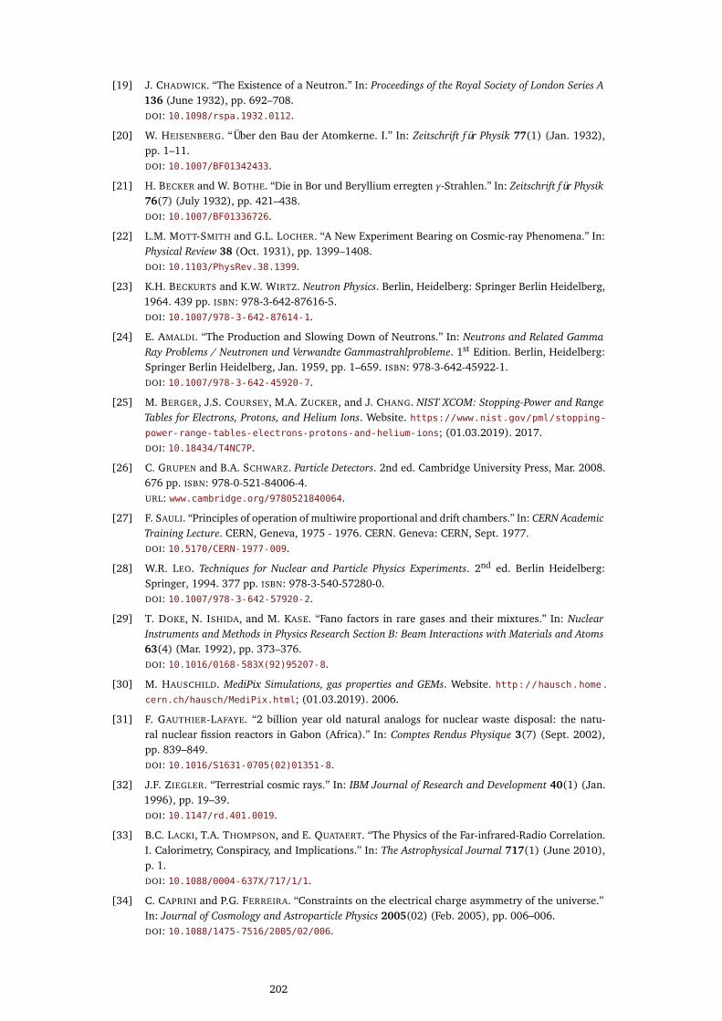
[19] J. CHADWICK. “The Existence of a Neutron.” In: Proceedings of the Royal Society of London Series A136 (June 1932), pp. 692–708.DOI: 10.1098/rspa.1932.0112.

[20] W. HEISENBERG. “Über den Bau der Atomkerne. I.” In: Zeitschrift für Physik 77(1) (Jan. 1932),pp. 1–11.DOI: 10.1007/BF01342433.

[21] H. BECKER and W. BOTHE. “Die in Bor und Beryllium erregten 𝛾 -Strahlen.” In: Zeitschrift für Physik76(7) (July 1932), pp. 421–438.DOI: 10.1007/BF01336726.

[22] L.M. MOTT-SMITH and G.L. LOCHER. “A New Experiment Bearing on Cosmic-ray Phenomena.” In:Physical Review 38 (Oct. 1931), pp. 1399–1408.DOI: 10.1103/PhysRev.38.1399.

[23] K.H. BECKURTS and K.W. WIRTZ. Neutron Physics. Berlin, Heidelberg: Springer Berlin Heidelberg,1964. 439 pp. ISBN: 978-3-642-87616-5.DOI: 10.1007/978-3-642-87614-1.

[24] E. AMALDI. “The Production and Slowing Down of Neutrons.” In: Neutrons and Related GammaRay Problems / Neutronen und Verwandte Gammastrahlprobleme. 1st Edition. Berlin, Heidelberg:Springer Berlin Heidelberg, Jan. 1959, pp. 1–659. ISBN: 978-3-642-45922-1.DOI: 10.1007/978-3-642-45920-7.

[25] M. BERGER, J.S. COURSEY, M.A. ZUCKER, and J. CHANG. NIST XCOM: Stopping-Power and RangeTables for Electrons, Protons, and Helium Ions. Website. https://www.nist.gov/pml/stopping-power-range-tables-electrons-protons-and-helium-ions; (01.03.2019). 2017.DOI: 10.18434/T4NC7P.

[26] C. GRUPEN and B.A. SCHWARZ. Particle Detectors. 2nd ed. Cambridge University Press, Mar. 2008.676 pp. ISBN: 978-0-521-84006-4.URL: www.cambridge.org/9780521840064.

[27] F. SAULI. “Principles of operation of multiwire proportional and drift chambers.” In: CERN AcademicTraining Lecture. CERN, Geneva, 1975 - 1976. CERN. Geneva: CERN, Sept. 1977.DOI: 10.5170/CERN-1977-009.

[28] W.R. LEO. Techniques for Nuclear and Particle Physics Experiments. 2nd ed. Berlin Heidelberg:Springer, 1994. 377 pp. ISBN: 978-3-540-57280-0.DOI: 10.1007/978-3-642-57920-2.

[29] T. DOKE, N. ISHIDA, and M. KASE. “Fano factors in rare gases and their mixtures.” In: NuclearInstruments and Methods in Physics Research Section B: Beam Interactions with Materials and Atoms63(4) (Mar. 1992), pp. 373–376.DOI: 10.1016/0168-583X(92)95207-8.

[30] M. HAUSCHILD. MediPix Simulations, gas properties and GEMs. Website. http://hausch.home.cern.ch/hausch/MediPix.html; (01.03.2019). 2006.

[31] F. GAUTHIER-LAFAYE. “2 billion year old natural analogs for nuclear waste disposal: the natu-ral nuclear fission reactors in Gabon (Africa).” In: Comptes Rendus Physique 3(7) (Sept. 2002),pp. 839–849.DOI: 10.1016/S1631-0705(02)01351-8.

[32] J.F. ZIEGLER. “Terrestrial cosmic rays.” In: IBM Journal of Research and Development 40(1) (Jan.1996), pp. 19–39.DOI: 10.1147/rd.401.0019.

[33] B.C. LACKI, T.A. THOMPSON, and E. QUATAERT. “The Physics of the Far-infrared-Radio Correlation.I. Calorimetry, Conspiracy, and Implications.” In: The Astrophysical Journal 717(1) (June 2010),p. 1.DOI: 10.1088/0004-637X/717/1/1.

[34] C. CAPRINI and P.G. FERREIRA. “Constraints on the electrical charge asymmetry of the universe.”In: Journal of Cosmology and Astroparticle Physics 2005(02) (Feb. 2005), pp. 006–006.DOI: 10.1088/1475-7516/2005/02/006.

202

[35] C.L. SARAZIN and R. LIEU. “Extreme-Ultraviolet Emission from Clusters of Galaxies: Inverse Comp-ton Radiation from a Relic Population of Cosmic-Ray Electrons?” In: The Astrophysical JournalLetters 494(2) (Feb. 1998), p. L177.DOI: 10.1086/311196.

[36] R.M. BALTRUSAITIS, R. CADY, et al. “The Utah Fly’s Eye detector.” In: Nuclear Instruments andMethods in Physics Research Section A: Accelerators, Spectrometers, Detectors and Associated Equip-ment 240(2) (Oct. 1985), pp. 410–428.DOI: 10.1016/0168-9002(85)90658-8.

[37] T.K. GAISSER. “The Cosmic-ray Spectrum: from the knee to the ankle.” In: Journal of Physics:Conference Series 47(1) (Mar. 2006), pp. 15–20.DOI: 10.1088/1742-6596/47/1/002.

[38] B.W. CARROLL and D.A. OSTLIE. An Introduction to Modern Astrophysics. Ed. by San FranciscoADDISON-WESLEY. 2nd. Pearson Education, July 2006. 1400 pp. ISBN: 978-0805304022.DOI: 10.1017/9781108380980.

[39] A.M. BYKOV, D.C. ELLISON, A. MARCOWITH, and S.M. OSIPOV. “Cosmic Ray Production in Super-novae.” In: Space Science Reviews 214(1) (Jan. 2018), p. 41.DOI: 10.1007/s11214-018-0479-4.

[40] L. MERTEN, C. BUSTARD, E.G. ZWEIBEL, and J.B. TJUS. “The Propagation of Cosmic Rays from theGalactic Wind Termination Shock: Back to the Galaxy?” In: The Astrophysical Journal 859(1) (May2018), p. 63.DOI: 10.3847/1538-4357/aabfdd.

[41] V.N. ZIRAKASHVILI and H.J. VÖLK. “Cosmic ray reacceleration on the galactic wind terminationshock.” In: Advances in Space Research 37(10) (Aug. 2006). Astrophysics, pp. 1923–1927.DOI: 10.1016/j.asr.2005.06.013.

[42] F.C. MICHEL. “Cosmic-ray acceleration by pulsars.” In: Advances in Space Research 4(2) (1984),pp. 387–391.DOI: 10.1016/0273-1177(84)90336-3.

[43] R. BLANDFORD, P. SIMEON, and Y. YUAN. “Cosmic Ray Origins: An Introduction.” In: Nuclear PhysicsB - Proceedings Supplements 256-257 (Dec. 2014). Cosmic Ray Origin - Beyond the StandardModels, pp. 9–22.DOI: 10.1016/j.nuclphysbps.2014.10.002.

[44] J. BEER, S.M. TOBIAS, and N.O. WEISS. “On long-term modulation of the Sun’s magnetic cycle.”In: Monthly Notices of the Royal Astronomical Society 473(2) (Jan. 2018), pp. 1596–1602.DOI: 10.1093/mnras/stx2337.

[45] K. KUDELA, H. MAVROMICHALAKI, A. PAPAIOANNOU, and M. GERONTIDOU. “On Mid-Term Periodici-ties in Cosmic Rays.” In: Solar Physics 266(1) (Sept. 2010), pp. 173–180.DOI: 10.1007/s11207-010-9598-0.

[46] K.G. MCCRACKEN, H. MORAAL, and M.A. SHEA. “The high-energy impulsive ground-level enhance-ment.” In: The Astrophysical Journal 761(2) (Nov. 2012), p. 101.DOI: 10.1088/0004-637X/761/2/101.

[47] H.V. CANE. “Coronal Mass Ejections and Forbush Decreases.” In: Space Science Reviews 93(1) (July2000), pp. 55–77.DOI: 10.1023/A:1026532125747.

[48] S.R. THOMAS, M.J. OWENS, and M. LOCKWOOD. “The 22-Year Hale Cycle in Cosmic Ray Flux -Evidence for Direct Heliospheric Modulation.” In: Solar Physics 289(1) (Jan. 2014), pp. 407–421.DOI: 10.1007/s11207-013-0341-5.

[49] M.A. SHEA and D.F. SMART. “Geomagnetic cutoff rigidities and geomagnetic coordinates appropri-ate for the Carrington flare Epoch.” In: Advances in Space Research 38(2) (Sept. 2006). The GreatHistorical Geomagnetic Storm of 1859: A Modern Look, pp. 209–214.DOI: 10.1016/j.asr.2005.03.156.

203

[50] M. ANDREASEN, K.H. JENSEN, D. DESILETS, T.E. FRANZ, M. ZREDA, H.R. BOGENA, and M.C. LOOMS.“Status and Perspectives on the Cosmic-Ray Neutron Method for Soil Moisture Estimation andOther Environmental Science Applications.” In: Vadose Zone Journal 16(8) (Aug. 2017), pp. 1–11.DOI: 10.2136/vzj2017.04.0086.

[51] L.I. DORMAN, S.G. FEDCHENKO, L.V. GRANITSKY, and G.A. RISHE. “Coupling and barometer coeffi-cients for measurements of cosmic ray variations at altitudes of 260-400 mb.” In: Acta Physica 2(Jan. 1970). Supplement to Volume 29, pp. 233–236.URL: http://adsabs.harvard.edu/full/1970ICRC....2..233D.

[52] C.W. FABJAN and F. GIANOTTI. “Calorimetry for particle physics.” In: Reviews of Modern Physics 75(Oct. 2003), pp. 1243–1286.DOI: 10.1103/RevModPhys.75.1243.

[53] C. LEROY and R.-G. RANCOITA. “Physics of cascading shower generation and propagation in matter:principles of high-energy, ultrahigh-energy and compensating calorimetry.” In: Reports on Progressin Physics 63(4) (Apr. 2000), pp. 505–606.DOI: 10.1088/0034-4885/63/4/202.

[54] B.B. ROSSI. High-energy Particles. Prentice-Hall physics series. New York, 1952. 569 pp. ISBN:978-0133873245.

[55] R. ULRICH, R. ENGEL, and M. UNGER. “Hadronic multiparticle production at ultrahigh energiesand extensive air showers.” In: Physical Review D 83 (Mar. 2011), p. 054026.DOI: 10.1103/PhysRevD.83.054026.

[56] A. CAPELLA, U. SUKHATME, C.-I. TAN, and J. TRAN THANH VAN. “Dual parton model.” In: PhysicsReports 236(4) (Jan. 1994), pp. 225–329.DOI: 10.1016/0370-1573(94)90064-7.

[57] S.D. ELLIS and M.B. KISLINGER. “Implications of parton-model concepts for large-transverse-momentum production of hadrons.” In: Physical Review D 9 (Apr. 1974), pp. 2027–2051.DOI: 10.1103/PhysRevD.9.2027.

[58] S. MOLLERACH and E. ROULET. “Progress in high-energy cosmic ray physics.” In: Progress in Particleand Nuclear Physics 98 (Jan. 2018), pp. 85–118.DOI: 10.1016/j.ppnp.2017.10.002.

[59] D. HECK, J. KNAPP, J.N. CAPDEVIELLE, G. SCHATZ, and T. THOUW. CORSIKA: A Monte Carlo code tosimulate extensive air showers. Tech. rep. FZKA 6019. Forschungszentrum Karlsruhe, 1998. 98 pp.URL: http://digbib.ubka.uni-karlsruhe.de/volltexte/fzk/6019/6019.pdf.

[60] G. PFOTZER. “Dreifachkoinzidenzen der Ultrastrahlung aus vertikaler Richtung in derStratosphäre.” In: Zeitschrift für Physik 102(1–2) (Jan. 1936), pp. 41–58.DOI: 10.1007/BF01336830.

[61] T. SATO. “Analytical Model for Estimating Terrestrial Cosmic Ray Fluxes Nearly Anytime andAnywhere in the World: Extension of PARMA/EXPACS.” In: PLOS ONE 10(12) (Dec. 2015), pp. 1–33.DOI: 10.1371/journal.pone.0144679.

[62] K.K. GUDIMA, S.G. MASHNIK, and V.D. TONEEV. “Cascade-exciton model of nuclear reactions.” In:Nuclear Physics A 401(2) (June 1983), pp. 329–361.DOI: 10.1016/0375-9474(83)90532-8.

[63] E.T. JURNEY, J.W. STARNER, J.E. LYNN, and S. RAMAN. “Thermal-neutron capture by 14N.” In:Physical Review C 56 (July 1997), pp. 118–134.DOI: 10.1103/PhysRevC.56.118.

[64] R.E. TAYLOR. “Radiocarbon dating: The continuing revolution.” In: Evolutionary Anthropology:Issues, News, and Reviews 4(5) (June 1995), pp. 169–181.DOI: 10.1002/evan.1360040507.

[65] P. GOLDHAGEN, J.M. CLEM, and J.W. WILSON. “The energy spectrum of cosmic-ray induced neu-trons measured on an airplane over a wide range of altitude and latitude.” In: Radiation ProtectionDosimetry 110(1–4) (Aug. 2004), pp. 387–392.DOI: 10.1093/rpd/nch216.

204

[66] T. SATO and K. NIITA. “Analytical Functions to Predict Cosmic-Ray Neutron Spectra in the Atmo-sphere.” In: Radiation Research 166(3) (Sept. 2006), pp. 544–555.DOI: 10.1667/RR0610.1.

[67] T. SATO, H. YASUDA, K. NIITA, A. ENDO, and L. SIHVER. “Development of PARMA: PHITS-based An-alytical Radiation Model in the Atmosphere.” In: Radiation Research 170(2) (Aug. 2008), pp. 244–259.DOI: 10.1667/RR1094.1.

[68] H. IWASE, K. NIITA, and T. NAKAMURA. “Development of General-Purpose Particle and Heavy IonTransport Monte Carlo Code.” In: Journal of Nuclear Science and Technology 39(11) (Aug. 2002),pp. 1142–1151.DOI: 10.1080/18811248.2002.9715305.

[69] M.S. GORDON, P. GOLDHAGEN, K.P. RODBELL, T.H. ZABEL, H.H.K. TANG, J.M. CLEM, and P. BAILEY.“Measurement of the flux and energy spectrum of cosmic-ray induced neutrons on the ground.”In: IEEE Transactions on Nuclear Science 51(6) (Dec. 2004), pp. 3427–3434.DOI: 10.1109/TNS.2004.839134.

[70] R.M. BRUGGER. “We need more intense thermal-neutron beams.” In: Physics Today 21(12) (Dec.1968), pp. 23–30.DOI: 10.1063/1.3034644.

[71] J.M. CARPENTER and W.B. YELON. “2. Neutron Sources.” In: Neutron Scattering. Ed. by K. SKÖLD

and D.L. PRICE. Vol. 23. Methods in Experimental Physics. Academic Press, 1986, pp. 99–196.DOI: 10.1016/S0076-695X(08)60555-4.

[72] K.H. ANDERSEN and C.J. CARLILE. “A Proposal for a Next Generation European Neutron Source.”In: Journal of Physics: Conference Series 746(1) (Oct. 2016), p. 012030.DOI: 10.1088/1742-6596/746/1/012030.

[73] G.E. MOORE. “Cramming more components onto integrated circuits.” In: Electronics 38(8) (Apr.1965). URL for IEEE reprint 2006, pp. 114–118.URL: https://ieeexplore.ieee.org/document/4785860/.

[74] M.S. LIVINGSTON. High-energy accelerators. Interscience tracts on physics and astronomy. NewYork, U.S.A.: Interscience Publishers, May 1954. 157 pp.

[75] M. TIGNER. “Does Accelerator-Based Particle Physics Have a Future?” In: Physics Today 54(1) (Jan.2001), pp. 36–40.DOI: 10.1063/1.1349610.

[76] THE EUROPEAN NEUTRON SCATTERING ASSOCIATION (ENSA). (accessed 26.08.2016). 2016. URL:http://www.neutrons-ensa.eu.

[77] M. ARAI and K. CRAWFORD. “Neutron Imaging and Applications: A Reference for the ImagingCommunity.” In: Neutron Scattering Applications and Techniques. Ed. by I.S. ANDERSON, R.L. MC-GREEVY, and H.Z. BILHEUX. Springer USA, 2009. Chap. Neutron Sources and Facilities, pp. 13–30.ISBN: 9780387786933.DOI: 10.1007/978-0-387-78693-3.

[78] INTERNATIONAL ATOMIC ENERGY AGENCY. Research Reactors. (accessed 10.03.2019). June 2016.URL: https://nucleus.iaea.org/RRDB/RR/ReactorSearch.aspx.

[79] A. RÖHRMOSER. “Core model of new German neutron source FRM II.” In: Nuclear Engineering andDesign 240(6) (2010), pp. 1417–1432.DOI: 10.1016/j.nucengdes.2010.02.011.

[80] K. BÖNING, W. GLÄSER, and A. RÖHRMOSER. “Physics of the Munich compact core design.” In:Proceedings of the 1988 International Meeting on Reduced Enrichment for Research and Test Reactors.Vol. 25. 17. ANL/RERTR/TM–13. July 1993, pp. 393–403.DOI: 10.1109/NSSMIC.2007.4436548.

[81] T. BÜCHERL and S. SÖLLRADL. “NECTAR: Radiography and tomography station using fissionneutrons.” In: Journal of large-scale Research Facilities 1(A19) (June 2015).DOI: 10.17815/jlsrf-1-45.

205

[82] C. FRANZ and T. SCHRÖDER. “RESEDA: Resonance spin echo spectrometer.” In: Journal of large-scale Research Facilities 1(A14) (June 2015).DOI: 10.17815/jlsrf-1-37.

[83] R. GEORGII and K. SEEMANN. “MIRA: Dual wavelength band instrument.” In: Journal of large-scaleResearch Facilities 1(A3) (June 2015).DOI: 10.17815/jlsrf-1-21.

[84] M. MEVEN and A. SAZONOV. “HEiDi: Single crystal diffractometer at hot source.” In: Journal oflarge-scale Research Facilities 1(A7) (June 2015).DOI: 10.17815/jlsrf-1-20.

[85] F. GRÜNAUER. “Design, optimization, and implementation of the new neutron radiography facilityat FRM-II.” PhD thesis. Institut E21, Technische Universität München, Sept. 2005. 199 pp.URL: https://www.physi.uni-heidelberg.de//Publications/phd_haeusler.pdf.

[86] S. Ulam N. METROPOLIS. “The Monte Carlo Method.” In: Journal of the American StatisticalAssociation 44(247) (Sept. 1949), pp. 335–341.DOI: 10.2307/2280232.

[87] F. COCCETTI. “The Fermiac or Fermi’s Trolley.” In: Il Nuovo Cimento C 39(2) (Sept. 2016).DOI: 10.1393/ncc/i2016-16296-7.

[88] N. METROPOLIS. “The Beginning of the Monte Carlo Method.” In: Los Alamos Science 15 (1987).Special Issue, Stanislaw Ulam 1909-1984, pp. 125–130.URL: https://permalink.lanl.gov/object/tr?what=info:lanl-repo/lareport/LA-UR-88-9067.

[89] A. BURKS, H.D. HUSKEY, C. CHU, J.A. CUMMINGS, J.H. DAVIS, T.K. SHARPLESS, and R.F. SHAW.Report on the ENIAC (Electronic Numerical Integrator and Computer). Technical Report. MooreSchool of Electrical Engineering. The University of Pennsylvania, June 1946. 786 pp.URL: https://www.dtic.mil/get-tr-doc/pdf?AD=ADA622372.

[90] T. HAIGH, M. PRIESTLEY, and C. ROPE. “Los Alamos Bets on ENIAC: Nuclear Monte Carlo Simula-tions, 1947-1948.” In: IEEE Annals of the History of Computing 36(3) (July 2014), pp. 42–63.DOI: 10.1109/MAHC.2014.40.

[91] M. MATSUMOTO and T. NISHIMURA. “Mersenne Twister: A 623-dimensionally EquidistributedUniform Pseudo-random Number Generator.” In: ACM Transactions on Modeling and ComputerSimulation 8(1) (Jan. 1998), pp. 3–30.DOI: 10.1145/272991.272995.

[92] D.E. KNUTH. The Art of Computer Programming, Volume 2 (3rd Ed.): Seminumerical Algorithms.Boston, MA, USA: Addison-Wesley Longman Publishing Co., Inc., Nov. 1997. 106 pp. ISBN: 0-201-89684-2.

[93] E.M. GELBARD. Epithermal scattering in VIM. Tech. rep. FRA–TM–123. Argonne National Labora-tory, 1979.

[94] P.K. ROMANO and B. FORGET. “The OpenMC Monte Carlo particle transport code.” In: Annals ofNuclear Energy 51 (Jan. 2013), pp. 274–281.DOI: 10.1016/j.anucene.2012.06.040.

[95] J.A. WALSH, B. FORGET, and K.S. SMITH. “Accelerated sampling of the free gas resonance elasticscattering kernel.” In: Annals of Nuclear Energy 69 (July 2014), pp. 116–124.DOI: 10.1016/j.anucene.2014.01.017.

[96] N. OTUKA, E. DUPONT, et al. “Towards a More Complete and Accurate Experimental Nuclear Reac-tion Data Library (EXFOR): International Collaboration Between Nuclear Reaction Data Centres(NRDC).” In: Nuclear Data Sheets 120 (June 2014), pp. 272–276.DOI: 10.1016/j.nds.2014.07.065.

[97] M.B. CHADWICK, M. HERMAN, et al. “ENDF/B-VII.1 Nuclear Data for Science and Technology: CrossSections, Covariances, Fission Product Yields and Decay Data.” In: Nuclear Data Sheets 112(12)(Dec. 2011). Special Issue on ENDF/B-VII.1 Library, pp. 2887–2996.DOI: 10.1016/j.nds.2011.11.002.

206

[98] K. SHIBATA, O. IWAMOTO, et al. “JENDL-4.0: A New Library for Nuclear Science and Engineering.”In: Journal of Nuclear Science and Technology 48(1) (Sept. 2011), pp. 1–30.DOI: 10.1080/18811248.2011.9711675.

[99] A. TRKOV, M. HERMAN, and D.A. BROWN. ENDF-6 Formats Manual. Report. Data Formats andProcedures for the Evaluated Nuclear Data Files ENDF/B-VI and ENDF/B-VII. National NuclearData Center. Brookhaven National Laboratory, Oct. 2012. 396 pp.URL: https://www-nds.iaea.org/public/endf/endf-manual.pdf.

[100] R. SEDGEWICK. Algorithms in C. Boston, USA: Addison-Wesley Longman Publishing Co., Inc., Dec.1990. 672 pp. ISBN: 0-201-51425-7.

[101] J.F. BRIESMEISTER et al. “MCNP-A general Monte Carlo N-particle transport code.” In: Version 4C,LA-13709-M (Dec. 2000).URL: https://permalink.lanl.gov/object/tr?what=info:lanl-repo/lareport/LA-13709-M.

[102] SUN PROGRAMMERS GROUP. Fortran 77 Reference Manual. Tech. rep. Version 1.0. Mar. 1995.513 pp.URL: http://wwwcdf.pd.infn.it/localdoc/f77_sun.pdf.

[103] X-5 MONTE CARLO TEAM. “MCNP-A general Monte Carlo N-particle transport code, Version 5.” In:LA-UR-03-1987 (Apr. 2003). Volume I: Overview and Theory.URL: https://laws.lanl.gov/vhosts/mcnp.lanl.gov/pdf_files/la-ur-03-1987.pdf.

[104] L.S. WATERS, G.W. MCKINNEY, J.W. DURKEE, M.L. FENSIN, J.S. HENDRICKS, M.R. JAMES, R.C.JOHNS, and D.B. PELOWITZ. “The MCNPX Monte Carlo Radiation Transport Code.” In: AIP Confer-ence Proceedings 896(1) (Mar. 2007), pp. 81–90.DOI: 10.1063/1.2720459.

[105] SUN PROGRAMMERS GROUP. Fortran 90 User’s Guide. Tech. rep. Version 1.0. Mar. 1995.URL: http://smdc.sinp.msu.ru/doc/Fortran90UsersGuide.pdf.

[106] R.E. PRAEL and H. LICHTENSTEIN. “User Guide to LCS: The LAHET Code System.” In: LA-UR-89-3014 (Sept. 1989).URL: https://permalink.lanl.gov/object/tr?what=info:lanl-repo/lareport/LA-UR-89-3014.

[107] K.K. GUDIMA, S.G. MASHNIK, and A.J. SIERK. “User Manual for the Code LAQGSM.” In: LA-UR-01-6804 (Dec. 2001).URL: https://permalink.lanl.gov/object/tr?what=info:lanl-repo/lareport/LA-UR-01-6804.

[108] T. GOORLEY, M. JAMES, et al. “Initial MCNP6 Release Overview.” In: Nuclear Technology 180(3)(Aug. 2012), pp. 298–315.DOI: 10.13182/NT11-135.

[109] G.W. MCKINNEY, H. ARMSTRONG, M.R. JAMES, J. CLEM, and P. GOLDHAGEN. “MCNP6 Cosmic-Source Option.” In: LA-UR-12-22318 (June 2012).URL: https://permalink.lanl.gov/object/tr?what=info:lanl-repo/lareport/LA-UR-12-22318.

[110] G.W. MCKINNEY. “MCNP6 Cosmic and Terrestrial Background Particle Fluxes.” In: LA-UR-13-24293(June 2013). Release 3.URL: https://mcnp.lanl.gov/pdf_files/la-ur-13-24293.pdf.

[111] K. NIITA, H. TAKADA, S. MEIGO, and Y. IKEDA. “High-energy particle transport code NMTC/JAM.”In: Nuclear Instruments and Methods in Physics Research Section B: Beam Interactions with Materialsand Atoms 184(3) (Nov. 2001), pp. 406–420.DOI: 10.1016/S0168-583X(01)00784-4.

[112] A.T. NELMS. Energy loss and range of electrons and positrons. National Bureau of Standards Circular577 and Suppl. July 1956, pp. 1–30.URL: https://catalog.hathitrust.org/Record/007291096.

[113] K. NIITA. “QMD and JAM Calculations for High Energy Nucleon-Nucleus Collisions.” In: Journalof Nuclear Science and Technology 39 (Aug. 2002). sup2, pp. 714–719.DOI: 10.1080/00223131.2002.10875198.

207

[114] O. IWAMOTO, N. IWAMOTO, S. KUNIEDA, F. MINATO, and K. SHIBATA. “The CCONE Code Systemand its Application to Nuclear Data Evaluation for Fission and Other Reactions.” In: Nuclear DataSheets 131 (Jan. 2016). Special Issue on Nuclear Reaction Data, pp. 259–288.DOI: 10.1016/j.nds.2015.12.004.

[115] A. BOUDARD, J. CUGNON, J.-C. DAVID, S. LERAY, and D. MANCUSI. “New potentialities of the Liègeintranuclear cascade model for reactions induced by nucleons and light charged particles.” In:Physical Review C 87 (Jan. 2013), p. 014606.DOI: 10.1103/PhysRevC.87.014606.

[116] G. BATTISTONI, T. BOEHLEN, et al. “Overview of the FLUKA code.” In: Annals of Nuclear Energy82 (Aug. 2015). Joint International Conference on Supercomputing in Nuclear Applications andMonte Carlo 2013, pp. 10–18.DOI: 10.1016/j.anucene.2014.11.007.

[117] M.B. EMMETT. “The MORSE Monte Carlo Transport Code System.” In: ORNL-4972/R2 (Feb. 1975).URL: https://inis.iaea.org/collection/NCLCollectionStore/_Public/16/029/16029296.pdf.

[118] S. AGOSTINELLI, ET AL. “GEANT4 - a simulation toolkit.” In: Nuclear Instruments and Methods inPhysics Research Section A: Accelerators, Spectrometers, Detectors and Associated Equipment 506(3)(July 2003), pp. 250–303.DOI: 10.1016/S0168-9002(03)01368-8.

[119] A.N. SOLOVYEV, V.V. FEDOROV, V.I. KHARLOV, and U.A. STEPANOVA. “Comparative analysis ofMCNPX and GEANT4 codes for fast-neutron radiation treatment planning.” In: Nuclear Energy andTechnology 1(1) (Sept. 2015), pp. 14–19.DOI: 10.1016/j.nucet.2015.11.004.

[120] B.M. VAN DER ENDE, J. ATANACKOVIC, A. ERLANDSON, and G. BENTOUMI. “Use of GEANT4 vs.MCNPX for the characterization of a boron-lined neutron detector.” In: Nuclear Instruments andMethods in Physics Research Section A: Accelerators, Spectrometers, Detectors and Associated Equip-ment 820 (June 2016), pp. 40–47.DOI: 10.1016/j.nima.2016.02.082.

[121] L.B. LEVITT and R.C. LEWIS. VIM-1, A Non-multigroup Monte Carlo Code for Analysis of Fast CriticalAssemblies. AI-AEC-12951. Jan. 1970. 94 pp.DOI: 10.2172/4615237.

[122] E. BRUN, F. DAMIAN, et al. “TRIPOLI-4, CEA, EDF and AREVA reference Monte Carlo code.” In:Annals of Nuclear Energy 82 (Aug. 2015). Joint International Conference on Supercomputing inNuclear Applications and Monte Carlo 2013, pp. 151–160.DOI: 10.1016/j.anucene.2014.07.053.

[123] D.E. CULLEN. “TART 2005 A Coupled Neutron-Photon 3-D, Combinatorial Geometry Time Depen-dent Monte Carlo Transport Code.” In: UCRL-SM-218009 (Nov. 2005).URL: https://e-reports-ext.llnl.gov/pdf/329012.pdf.

[124] R.J. PROCASSINI, D.E. CULLEN, G.M. GREENMAN, and C.A. HAGMANN. “Verification and Validationof MERCURY: A Modern, Monte Carlo Particle Transport Code.” In: Proceedings of the Monte Carlo2005 Conference, Chattanooga. UCRL-CONF-208667. Dec. 2004.URL: https://e-reports-ext.llnl.gov/pdf/314728.pdf.

[125] Y.Z. KANDIEV, E.A. KASHAEVA, et al. “PRIZMA status.” In: Annals of Nuclear Energy 82 (Aug. 2015).Joint International Conference on Supercomputing in Nuclear Applications and Monte Carlo 2013,pp. 116–120.DOI: 10.1016/j.anucene.2014.09.006.

[126] T.M. PANDYA, S.R. JOHNSON, G.G. DAVIDSON, T.M. EVANS, and S.P. HAMILTON. “Shift: A massivelyparallel Monte Carlo radiation transport package.” In: Proceedings of the ANS MC2015 - JointInternational Conference on Mathematics and Computation. Apr. 2015, pp. 19–23.URL: https://www.casl.gov/sites/default/files/docs/CASL-U-2015-0170-000.pdf.

208

[127] J. LEPPÄNEN, M. PUSA, T. VIITANEN, V. VALTAVIRTA, and T. KALTIAISENAHO. “The Serpent MonteCarlo code: Status, development and applications in 2013.” In: Annals of Nuclear Energy 82 (Aug.2015). Joint International Conference on Supercomputing in Nuclear Applications and MonteCarlo 2013, pp. 142–150.DOI: 10.1016/j.anucene.2014.08.024.

[128] E. WOODCOCK, T. MURPHY, P.J. HEMMINGS, and T.C. LONGWORTH. “Techniques used in the GEMcode for Monte Carlo neutronics calculations in reactors and other systems of complex geometry.”In: Proc. Conf. Applications of Computing Methods to Reactor Problems. Vol. 557. May 1965, pp. 557–579.URL: https://yiningkarlli.com/projects/specdecomptracking/references/Woodcock1965.pdf.

[129] K. WANG, Z. LI, D. SHE, J. LIANG, Q. XU, Y. QIU, J. YU, J. SUN, X. FAN, and G. YU. “RMC - AMonte Carlo code for reactor core analysis.” In: Annals of Nuclear Energy 82 (Aug. 2015). JointInternational Conference on Supercomputing in Nuclear Applications and Monte Carlo 2013,pp. 121–129.DOI: 10.1016/j.anucene.2014.08.048.

[130] B. COCHET, A. JINAPHANH, L. HEULERS, and O. JACQUET. “Capabilities overview of the MORET 5Monte Carlo code.” In: Annals of Nuclear Energy 82 (Aug. 2015). Joint International Conferenceon Supercomputing in Nuclear Applications and Monte Carlo 2013, pp. 74–84.DOI: 10.1016/j.anucene.2014.08.022.

[131] N. SMITH, T. SHUTTLEWORTH, M. GRIMSTONE, L. HUTTON, M. ARMISHAW, A. BIRD, N. FRANCE,and S. CONNOLLY. “The Current Status and Future Plans for the Monte Carlo Codes MONK andMCBEND.” In: Advanced Monte Carlo for Radiation Physics, Particle Transport Simulation andApplications: Proceedings of the Monte Carlo 2000 Conference, Lisbon. Berlin, Heidelberg: Springer,2001, pp. 637–642. ISBN: 978-3-642-18211-2.DOI: 10.1007/978-3-642-18211-2_102.

[132] G. ARNECKE, H. BORGWALDT, V. BRANDL, and M. LALOVIC. “KAMCCO, ein reaktorphysikalischerMonte Carlo Neutronentransportcode.” In: KFK 2190 (June 1976). Joint International Conferenceon Supercomputing in Nuclear Applications and Monte Carlo 2013.URL: https://publikationen.bibliothek.kit.edu/270009404/3811483.

[133] W. MARTH. The history of the construction and operation of the KNK II German Fast Breeder PowerPlant. Tech. rep. KFK–5155. IAEA INIS, Sept. 1993. 181 pp.URL: https://publikationen.bibliothek.kit.edu/270038327/3813557.

[134] G. VAN ROSSUM. The Python Language Reference Manual. Tech. rep. Version 3.5.4. Aug. 2017.URL: https://docs.python.org/3/library/.

[135] JUPYTER TEAM. Jupyter Documentation. Tech. rep. Version 4.1.1. Sept. 2017.URL: https://media.readthedocs.org/pdf/jupyter/latest/jupyter.pdf.

[136] Programming Languages - C++. Standard. Geneva, CH: International Organization for Standard-ization, May 2013. 1374 pp.URL: http://www.open-std.org/jtc1/sc22/wg21/docs/papers/2013/n3690.pdf.

[137] R. BRUN and F. RADEMAKERS. “ROOT - An Object Oriented Data Analysis Framework.” In: Pro-ceedings of AIHENP’96 Workshop, Lausanne. Vol. 389. see also https://root.cern.ch/. May 1997,pp. 81–86.DOI: 10.1016/S0168-9002(97)00048-X.

[138] THE QT COMPANY LTD. The Qt Framework. Jan. 2018. URL: https://www.qt.io/qt- for-

application-development/.

[139] M. GALASSI et al. GNU Scientific Library: reference manual for GSL version 2.3. Free SoftwareFoundation, Dec. 2016.URL: https://www.gnu.org/software/gsl/manual/gsl-ref.pdf.

[140] A. HÉBERT. “Multigroup Neutron Transport and Diffusion Computations.” In: Handbook of NuclearEngineering. Ed. by D.G. CACUCI. Boston: Springer US, Aug. 2010, pp. 751–911. ISBN: 978-0-387-98149-9.DOI: 10.1007/978-0-387-98149-9_8.

209

[141] A.J. KONING, E. BAUGE, et al. “Status of the JEFF Nuclear Data Library.” In: Journal of the KoreanPhysical Society 59(2) (Aug. 2011), pp. 1057–1062.DOI: 10.3938/jkps.59.1057.

[142] T. KITTELMANN and M. BOIN. “Polycrystalline neutron scattering for Geant4: NXSG4.” In: Com-puter Physics Communications 189 (Apr. 2015), pp. 114–118.DOI: 10.1016/j.cpc.2014.11.009.

[143] S.D. ROTH. “Ray casting for modeling solids.” In: Computer Graphics and Image Processing 18(2)(Feb. 1982), pp. 109–144.DOI: 10.1016/0146-664X(82)90169-1.

[144] E. MAIRE and P.J. WITHERS. “Quantitative X-ray tomography.” In: International Materials Reviews59(1) (Dec. 2013), pp. 1–43.DOI: 10.1179/1743280413Y.0000000023.

[145] V. CNUDDE and M.N. BOONE. “High-resolution X-ray computed tomography in geosciences: Areview of the current technology and applications.” In: Earth-Science Reviews 123 (Aug. 2013),pp. 1–17.DOI: 10.1016/j.earscirev.2013.04.003.

[146] L.W. GOLDMAN. “Principles of CT and CT Technology.” In: Journal of Nuclear Medicine Technology35(3) (Sept. 2007), pp. 115–128.DOI: 10.2967/jnmt.107.042978.

[147] R.J. MCCONN JR, C.J. GESH, R.T. PAGH, R.A. RUCKER, and R.G. WILLIAMS III. Compendium of Ma-terial Composition Data for Radiation Transport Modeling. Tech. rep. PNNL-15870 Rev. 1. Richland,Washington 99352: Pacific Northwest National Laboratory, Mar. 2011. 375 pp.URL: https : / / www . pnnl . gov / main / publications / external / technical _ reports / pnnl -

15870rev1.pdf.

[148] Information technology - ISO 7-bit coded character set for information interchange. Standard. Geneva,CH: International Organization for Standardization, Dec. 1991. 15 pp.URL: https://www.iso.org/standard/4777.html.

[149] Information technology - Computer graphics and image processing – Portable Network Graphics(PNG). Standard. Geneva, CH: International Organization for Standardization, Mar. 2004. 80 pp.URL: https://www.iso.org/standard/29581.html.

[150] Reference neutron radiations - Part 1. Standard. Geneva, CH: International Organization for Stan-dardization, Feb. 2001. 24 pp.URL: https://www.iso.org/standard/25666.html.

[151] V. WEISSKOPF. “Statistics and Nuclear Reactions.” In: Physical Review 52 (Aug. 1937), pp. 295–303.DOI: 10.1103/PhysRev.52.295.

[152] J. TERRELL. “Fission Neutron Spectra and Nuclear Temperatures.” In: Physical Review 113 (Jan.1959), pp. 527–541.DOI: 10.1103/PhysRev.113.527.

[153] M.R. IYER and A.K. GANGULY. “Neutron Evaporation and Energy Distribution in Individual FissionFragments.” In: Physical Review C 5 (Apr. 1972), pp. 1410–1421.DOI: 10.1103/PhysRevC.5.1410.

[154] B.E. WATT. “Energy Spectrum of Neutrons from Thermal Fission of 235U.” In: Physical Review 87(Sept. 1952), pp. 1037–1041.DOI: 10.1103/PhysRev.87.1037.

[155] A.B. SMITH, P.R. FIELDS, and J.H. ROBERTS. “Spontaneous Fission Neutron Spectrum of 252Cf.” In:Physical Review 108 (Oct. 1957), pp. 411–413.DOI: 10.1103/PhysRev.108.411.

[156] J. CUGNON, C. VOLANT, and S. VUILLIER. “Nucleon and deuteron induced spallation reactions.” In:Nuclear Physics A 625(4) (Nov. 1997), pp. 729–757.DOI: 10.1016/S0375-9474(97)00602-7.

210

[157] T. KAWANO, P. TALOU, I. STETCU, and M.B. CHADWICK. “Statistical and evaporation models forthe neutron emission energy spectrum in the center-of-mass system from fission fragments.” In:Nuclear Physics A 913(Supplement C) (Sept. 2013), pp. 51–70.DOI: 10.1016/j.nuclphysa.2013.05.020.

[158] R.L. BRAMBLETT and T.W. BONNER. “Neutron evaporation spectra from (p, n) reactions.” In:Nuclear Physics 20(Supplement C) (Nov. 1960), pp. 395–407.DOI: 10.1016/0029-5582(60)90182-6.

[159] T. SATO. “Analytical Model for Estimating the Zenith Angle Dependence of Terrestrial Cosmic RayFluxes.” In: PLoS ONE 11(8) (Aug. 2016), pp. 1–22.DOI: 10.1371/journal.pone.0160390.

[K2016] M. KÖHLI, F. ALLMENDINGER, W. HÄUSSLER, T. SCHRÖDER, M. KLEIN, M. MEVEN, and U. SCHMIDT.“Efficiency and spatial resolution of the CASCADE thermal neutron detector.” In: Nuclear Instru-ments and Methods in Physics Research Section A: Accelerators, Spectrometers, Detectors and Associ-ated Equipment 828 (Aug. 2016), pp. 242–249.DOI: 10.1016/j.nima.2016.05.014.

[160] J.F. ZIEGLER, M.D. ZIEGLER, and J.P. BIERSACK. “SRIM - The stopping and range of ions in matter(2010).” In: Nuclear Instruments and Methods in Physics Research Section B: Beam Interactionswith Materials and Atoms 268(11-12) (June 2010). 19th International Conference on Ion BeamAnalysis, pp. 1818–1823.DOI: 10.1016/j.nimb.2010.02.091.

[161] K. NIKOLOPOULOS, P. BHATTACHARYA, V. CHERNYATIN, and R. VEENHOF. “Electron transparency ofa Micromegas mesh.” In: Journal of Instrumentation 6(06) (June 2011), P06011.DOI: 10.1088/1748-0221/6/06/P06011.

[162] X. LLOPART, R. BALLABRIGA, M. CAMPBELL, L. TLUSTOS, and W. WONG. “Timepix, a 65k pro-grammable pixel readout chip for arrival time, energy and/or photon counting measurements.”In: Nuclear Instruments and Methods in Physics Research Section A: Accelerators, Spectrometers,Detectors and Associated Equipment 581(1–2) (Oct. 2007). VCI 2007, Proceedings of the 11th

International Vienna Conference on Instrumentation, pp. 485–494.DOI: 10.1016/j.nima.2007.08.079.

[163] R.S. CASWELL, R.F. GABBARD, D.W. PADGETT, and W.P. DOERING. “Attenuation of 14.1-Mev Neu-trons in Water.” In: Nuclear Science and Engineering 2(2) (Apr. 1957), pp. 143–159.DOI: 10.13182/NSE57-A25383.

[164] N.E. HERTEL and J.W. DAVIDSON. “The response of Bonner Spheres to neutrons from thermal ener-gies to 17.3 MeV.” In: Nuclear Instruments and Methods in Physics Research Section A: Accelerators,Spectrometers, Detectors and Associated Equipment 238(2) (Aug. 1985), pp. 509–516.DOI: 10.1016/0168-9002(85)90494-2.

[165] V. VYLET and A. KUMAR. “Energy response of Bonner Spheres to neutrons in parallel beam andpoint source geometries.” In: Nuclear Instruments and Methods in Physics Research Section A:Accelerators, Spectrometers, Detectors and Associated Equipment 271(3) (Sept. 1988), pp. 607–610.DOI: 10.1016/0168-9002(88)90329-4.

[166] V. MARES and H. SCHRAUBE. “Evaluation of the response matrix of a Bonner Sphere Spectrometerwith LiI detector from thermal energy to 100 MeV.” In: Nuclear Instruments and Methods in PhysicsResearch Section A: Accelerators, Spectrometers, Detectors and Associated Equipment 337(2) (Jan.1994), pp. 461–473.DOI: 10.1016/0168-9002(94)91116-9.

[167] S. GARNY, V. MARES, and W. RÜHM. “Response functions of a Bonner Sphere Spectrometer calcu-lated with GEANT4.” In: Nuclear Instruments and Methods in Physics Research Section A: Accelera-tors, Spectrometers, Detectors and Associated Equipment 604(3) (June 2009), pp. 612–617.DOI: 10.1016/j.nima.2009.02.044.

[168] A.W. DECKER, S.R. MCHALE, M.P. SHANNON, J.A. CLINTON, and J.W. MCCLORY. “Novel BonnerSphere Spectrometer Response Functions Using MCNP6.” In: IEEE Transactions on Nuclear Science62(4) (Aug. 2015), pp. 1689–1694.DOI: 10.1109/TNS.2015.2416652.

211

[169] E.A. BURGETT, N.E. HERTEL, and R.M. HOWELL. “Energy Response and Angular Dependence of aBonner Sphere Extension.” In: IEEE Transactions on Nuclear Science 56(3) (June 2009), pp. 1325–1328.DOI: 10.1109/TNS.2009.2019272.

[170] V. MARES, G. SCHRAUBE, and H. SCHRAUBE. “Calculated neutron response of a Bonner SphereSpectrometer with 3He counter.” In: Nuclear Instruments and Methods in Physics Research Section A:Accelerators, Spectrometers, Detectors and Associated Equipment 307(2) (Oct. 1991), pp. 398–412.DOI: 10.1016/0168-9002(91)90210-H.

[171] M. YAMASHITA, L.D. STEPHENS, and H.W. PATTERSON. “Cosmic-ray-produced neutrons at groundlevel: Neutron production rate and flux distribution.” In: Journal of Geophysical Research 71(16)(Aug. 1966), pp. 3817–3834.DOI: 10.1029/JZ071i016p03817.

[172] J. SWEEZY, N. HERTEL, and K. VEINOT. “BUMS - Bonner Sphere Unfolding Made Simple: an HTMLbased multisphere neutron spectrometer unfolding package.” In: Nuclear Instruments and Meth-ods in Physics Research Section A: Accelerators, Spectrometers, Detectors and Associated Equipment476(1) (Jan. 2002). International Workshop on Neutron Field Spectrometry in Science, Technol-ogy and Radiation Protection, pp. 263–269.DOI: 10.1016/S0168-9002(01)01466-8.

[173] D.J. THOMAS and A.V. ALEVRA. “Bonner Sphere Spectrometers - a critical review.” In: NuclearInstruments and Methods in Physics Research Section A: Accelerators, Spectrometers, Detectors andAssociated Equipment 476(1) (Jan. 2002). International Workshop on Neutron Field Spectrometryin Science, Technology and Radiation Protection, pp. 12–20.DOI: 10.1016/S0168-9002(01)01379-1.

[174] H. SCHRAUBE, J. JAKES, A. SANNIKOV, E. WEITZENEGGER, S ROESLER, and W. HEINRICH. “TheCosmic Ray Induced Neutron Spectrum at the Summit of the Zugspitze (2963 m).” In: RadiationProtection Dosimetry 70(1-4) (Apr. 1997), pp. 405–408.DOI: 10.1093/oxfordjournals.rpd.a031986.

[175] W. RÜHM, V. MARES, C. PIOCH, G. SIMMER, and E. WEITZENEGGER. “Continuous measurement ofsecondary neutrons from cosmic radiation at mountain altitudes and close to the north pole - adiscussion in terms of H*(10).” In: Radiation Protection Dosimetry 136(4) (Aug. 2009), pp. 256–261.DOI: 10.1093/rpd/ncp161.

[176] H.W. BERTINI. “Low-Energy Intranuclear Cascade Calculation.” In: Physical Review 131 (Aug.1963), pp. 1801–1821.DOI: 10.1103/PhysRev.131.1801.

[177] A. HEIKKINEN, N. STEPANOV, and J.P. WELLISCH. “Bertini intranuclear cascade implementationin GEANT4.” In: eConf C0303241 (June 2003). Proceedings, 13th International Conference onComputing in High-Energy and Nuclear Physics (CHEP 2003): La Jolla, California, March 24-28,2003, MOMT008.URL: http://www.slac.stanford.edu/econf/C0303241/proc/papers/MOMT008.PDF.

[178] G. FOLGER, V.N. IVANCHENKO, and J.P. WELLISCH. “The Binary Cascade.” In: The European PhysicalJournal A - Hadrons and Nuclei 21(3) (Aug. 2004), pp. 407–417.DOI: 10.1140/epja/i2003-10219-7.

[179] G. HUBERT, C.A. FEDERICO, M.T. PAZIANOTTO, and O.L. GONÇALES. “Long and short-term atmo-spheric radiation analyses based on coupled measurements at high altitude remote stations andextensive air shower modeling.” In: Astroparticle Physics 74 (Feb. 2016), pp. 27–36.DOI: 10.1016/j.astropartphys.2015.09.005.

[180] M.T. PAZIANOTTO, M.A. CORTÉS-GIRALDO, C.A. FEDERICO, G. HUBERT, O.L. GONÇALEZ, J.M. QUE-SADA, and B.V. CARLSON. “Extensive air shower Monte Carlo modeling at the ground and aircraftflight altitude in the South Atlantic Magnetic Anomaly and comparison with neutron measure-ments.” In: Astroparticle Physics 88 (Feb. 2017), pp. 17–29.DOI: 10.1016/j.astropartphys.2016.12.004.

212

[181] P. GOLDHAGEN, M. REGINATTO, T. KNISS, J.W. WILSON, R.C. SINGLETERRY, I.W. JONES, and W.VAN STEVENINCK. “Measurement of the energy spectrum of cosmic-ray induced neutrons aboardan ER-2 high-altitude airplane.” In: Nuclear Instruments and Methods in Physics Research Section A:Accelerators, Spectrometers, Detectors and Associated Equipment 476(1–2) (Jan. 2002), pp. 42–51.DOI: 10.1016/S0168-9002(01)01386-9.

[182] C.A. FEDERICO, O.L. GONÇALEZ, E.S. FONSECA, I.M. MARTIN, and L.V.E. CALDAS. “Neutron spectrameasurements in the south Atlantic anomaly region.” In: Radiation Measurements 45(10) (Dec.2010). Proceedings of the 11th Symposium on neutron and ion dosimetrty, pp. 1526–1528.DOI: 10.1016/j.radmeas.2010.06.038.

[183] M.T. PAZIANOTTO, M.A. CORTÉS-GIRALDO, C.A. FEDERICO, O.L. GONÇALEZ, J.M. QUESADA, and B.V.CARLSON. “Determination of the cosmic-ray-induced neutron flux and ambient dose equivalent atflight altitude.” In: Journal of Physics: Conference Series 630(1) (Apr. 2015), p. 012022.DOI: 10.1088/1742-6596/630/1/012022.

[SK2017b] M. SCHRÖN, S. ZACHARIAS, et al. “Intercomparison of Cosmic-Ray Neutron Sensors and WaterBalance Monitoring in an Urban Environment.” In: Geoscientific Instrumentation, Methods andData Systems Discussions 2017 (2017), pp. 1–24.DOI: 10.5194/gi-2017-34.

[184] P. KOCHER, D. GENKIN, D. GRUSS, W. HAAS, M. HAMBURG, M. LIPP, S. MANGARD, T. PRESCHER,M. SCHWARZ, and Y. YAROM. Spectre Attacks: Exploiting Speculative Execution. Aug. 2018. arXiv:1801.01203 [cs]. URL: https://arxiv.org/abs/1801.01203.

[185] P.U. VILLARD. “Sur la réflexion et la réfraction des rayons cathodiques et des rayons déviables duradium.” In: Comptes rendus hebdomadaires des séances de l’Académie des Sciences 130 (Jan. 1900),pp. 1010–1012.URL: https://gallica.bnf.fr/ark:/12148/bpt6k3086n/f1010.image.r=.

[186] T. WULF. “Über die in der Atmosphäre vorhandene Strahlung von hoher Durchdringungsfähigkeit.”In: Physikalische Zeitschrift 10(5) (Mar. 1909), pp. 152–157.

[187] A. GOCKEL. “Messungen der durchdringenden Strahlung bei Ballonfahrten.” In: PhysikalischeZeitschrift 12(14) (July 1911), pp. 595–597.

[188] V.F. HESS. “Über die Absorption der 𝛾-Strahlung in der Atmosphäre.” In: Physikalische Zeitschrift12(22) (Nov. 1911), pp. 998–1001.

[189] A.H. COMPTON. “A Geographic Study of Cosmic Rays.” In: Physical Review 43 (Mar. 1933), pp. 387–403.DOI: 10.1103/PhysRev.43.387.

[190] T.H. JOHNSON. “The Azimuthal Asymmetry of the Cosmic Radiation.” In: Physical Review 43 (May1933), pp. 834–835.DOI: 10.1103/PhysRev.43.834.

[191] H.J. BHABHA and W. HEITLER. “The Passage of Fast Electrons and the Theory of Cosmic Showers.”In: Proceedings of the Royal Society of London A: Mathematical, Physical and Engineering Sciences159(898) (Apr. 1937), pp. 432–458.DOI: 10.1098/rspa.1937.0082.

[192] S.E. FORBUSH. “World-wide cosmic ray variations, 1937–1952.” In: Journal of Geophysical Research59(4) (Dec. 1954), pp. 525–542.DOI: 10.1029/JZ059i004p00525.

[193] W. BAADE and F. ZWICKY. “Remarks on Super-Novae and Cosmic Rays.” In: Physical Review 46(July 1934), pp. 76–77.DOI: 10.1103/PhysRev.46.76.2.

[194] V. COCCONI-TONGIORGI. “Neutrons in the Extensive Air Showers of the Cosmic Radiation.” In:Physical Review 75 (May 1949), pp. 1532–1540.DOI: 10.1103/PhysRev.75.1532.

[195] J.A. SIMPSON and R.B. URETZ. “On the Latitude Dependence of Nuclear Disintegrations andNeutrons at 30,000 Feet.” In: Physical Review 76 (Aug. 1949), pp. 569–570.DOI: 10.1103/PhysRev.76.569.

213

[196] J.A. SIMPSON. “The Cosmic Ray Nucleonic Component: The Invention and Scientific Uses of theNeutron Monitor - (Keynote Lecture).” In: Space Science Reviews 93(1) (July 2000), pp. 11–32.DOI: 10.1023/A:1026567706183.

[197] H. VEREECKEN, J.A. HUISMAN, H. BOGENA, J. VANDERBORGHT, J.A. VRUGT, and J.W. HOPMANS.“On the value of soil moisture measurements in vadose zone hydrology: A review.” In: WaterResources Research 44(4) (Apr. 2008), W00D06.DOI: 10.1029/2008WR006829.

[198] D.A. ROBINSON, C.S. CAMPBELL, J.W. HOPMANS, B.K. HORNBUCKLE, S.B. JONES, R. KNIGHT, F. OG-DEN, J. SELKER, and O. WENDROTH. “Soil Moisture Measurement for Ecological and HydrologicalWatershed-Scale Observatories: A Review.” In: Vadose Zone Journal 7(1) (Feb. 2008), pp. 358–389.DOI: 10.2136/vzj2007.0143.

[199] J.D. RHOADES, P.A.C. RAATS, and R.J. PRATHER. “Effects of Liquid-phase Electrical Conductivity,Water Content, and Surface Conductivity on Bulk Soil Electrical Conductivity.” In: Soil ScienceSociety of America Journal 40(5) (Apr. 1976), pp. 651–655.DOI: 10.2136/sssaj1976.03615995004000050017x.

[200] T.J. DEAN, J.P. BELL, and A.J.B. BATY. “Soil moisture measurement by an improved capacitancetechnique, Part I. Sensor design and performance.” In: Journal of Hydrology 93(1) (Feb. 1987),pp. 67–78.DOI: 10.1016/0022-1694(87)90194-6.

[201] G.C. TOPP, J.L. DAVIS, and A.P. ANNAN. “Electromagnetic determination of soil water content:Measurements in coaxial transmission lines.” In: Water Resources Research 16(3) (June 1980),pp. 574–582.DOI: 10.1029/WR016i003p00574.

[202] R. KNIGHT. “Ground Penetrating Radar for Environmental Applications.” In: Annual Review ofEarth and Planetary Sciences 29(1) (May 2001), pp. 229–255.DOI: 10.1146/annurev.earth.29.1.229.

[203] E. DE JONG, A.K. BALLANTYNE, D.R. CAMERON, and D.W.L. READ. “Measurement of ApparentElectrical Conductivity of Soils by an Electromagnetic Induction Probe to Aid Salinity Surveys.” In:Soil Science Society of America Journal 43(4) (Mar. 1979), pp. 810–812.DOI: 10.2136/sssaj1979.03615995004300040040x.

[204] B. MAJONE, F. VIANI, E. FILIPPI, A. BELLIN, A. MASSA, G. TOLLER, F. ROBOL, and M. SALUCCI.“Wireless Sensor Network Deployment for Monitoring Soil Moisture Dynamics at the Field Scale.”In: Procedia Environmental Sciences 19 (July 2013). Four Decades of Progress in Monitoring andModeling of Processes in the Soil-Plant-Atmosphere System: Applications and Challenges, pp. 426–435.DOI: 10.1016/j.proenv.2013.06.049.

[205] C.A. LAYMON, W.L. CROSSON, T.J. JACKSON, A. MANU, and T.D. TSEGAYE. “Ground-based passivemicrowave remote sensing observations of soil moisture at S-band and L-band with insight intomeasurement accuracy.” In: IEEE Transactions on Geoscience and Remote Sensing 39(9) (Sept.2001), pp. 1844–1858.DOI: 10.1109/36.951075.

[206] J.R. EAGLEMAN and W.C. LIN. “Remote sensing of soil moisture by a 21-cm passive radiometer.”In: Journal of Geophysical Research 81(21) (July 1976), pp. 3660–3666.DOI: 10.1029/JC081i021p03660.

[207] I. MANAKOS and S. LAVENDER. “Remote Sensing in Support of the Geo-information in Europe.” In:Land Use and Land Cover Mapping in Europe: Practices & Trends. Ed. by I. MANAKOS and M. BRAUN.Dordrecht: Springer Netherlands, Jan. 2014, pp. 3–10. ISBN: 978-94-007-7969-3.DOI: 10.1007/978-94-007-7969-3_1.

[208] D. GEUDTNER, R. TORRES, P. SNOEIJ, M. DAVIDSON, and B. ROMMEN. “Sentinel-1 System capa-bilities and applications.” In: 2014 IEEE Geoscience and Remote Sensing Symposium. July 2014,pp. 1457–1460.DOI: 10.1109/IGARSS.2014.6946711.

214

[209] F.D. VAN DER MEER, H.M.A. VAN DER WERFF, and F.J.A. VAN RUITENBEEK. “Potential of ESA’sSentinel-2 for geological applications.” In: Remote Sensing of Environment 148 (May 2014),pp. 124–133.DOI: 10.1016/j.rse.2014.03.022.

[210] B. WOLTER and M. KRUS. “Moisture Measuring with Nuclear Magnetic Resonance (NMR).” In:Electromagnetic Aquametry: Electromagnetic Wave Interaction with Water and Moist Substances. Ed.by K. KUPFER. Berlin, Heidelberg: Springer Berlin Heidelberg, 2005, pp. 491–515. ISBN: 978-3-540-26491-0.DOI: 10.1007/3-540-26491-4_21.

[211] D.R. POOL and J.H. EYCHANER. “Measurements of Aquifer-Storage Change and Specific Yield UsingGravity Surveys.” In: Ground Water 33(3) (Aug. 1995), pp. 425–432.DOI: 10.1111/j.1745-6584.1995.tb00299.x.

[212] F. KOCH, F. SCHLENZ, M. PRASCH, F. APPEL, T. RUF, and W. MAUSER. “Soil Moisture RetrievalBased on GPS Signal Strength Attenuation.” In: Water 8(7) (July 2016), pp. 1–22.DOI: 10.3390/w8070276.

[213] I.F. LONG and B.K. FRENCH. “Measurement of Soil Moisture in the Field by Neutron Moderation.”In: Journal of Soil Science 18(1) (Mar. 1967), pp. 149–166.DOI: 10.1111/j.1365-2389.1967.tb01496.x.

[214] M. QUINTA-FERREIRA, J.F. DIAS, and S. ALIJA. “False low water content in road field compactioncontrol using nuclear gauges: a case study.” In: Environmental Earth Sciences 75(14) (July 2016),p. 1114.DOI: 10.1007/s12665-016-5901-1.

[215] D.V. ELLIS and J.M. SINGER. “Basic Neutron Physics for Logging Applications.” In: Well Logging forEarth Scientists. Dordrecht: Springer Netherlands, 2007, pp. 325–349. ISBN: 978-1-4020-4602-5.DOI: 10.1007/978-1-4020-4602-5_13.

[216] D. DESILETS, M. ZREDA, and T.P.A. FERRÉ. “Nature’s neutron probe: Land surface hydrology at anelusive scale with cosmic rays.” In: Water Resources Research 46(11) (Nov. 2010), W11505.DOI: 10.1029/2009WR008726.

[217] T.E. FRANZ, T. WANG, W. AVERY, C. FINKENBINER, and L. BROCCA. “Combined analysis of soilmoisture measurements from roving and fixed cosmic ray neutron probes for multiscale real-timemonitoring.” In: Geophysical Research Letters 42(9) (May 2015), pp. 3389–3396.DOI: 10.1002/2015gl063963.

[218] M. ZREDA, W.J. SHUTTLEWORTH, X. ZENG, C. ZWECK, D. DESILETS, T.E. FRANZ, and R. ROSOLEM.“COSMOS: The COsmic-ray Soil Moisture Observing System.” In: Hydrology and Earth SystemSciences 16(11) (Nov. 2012), pp. 4079–4099.DOI: 10.5194/hess-16-4079-2012.

[219] B. CHRISMAN and M. ZREDA. “Quantifying mesoscale soil moisture with the cosmic-ray rover.” In:Hydrology and Earth System Sciences 17(12) (Dec. 2013), pp. 5097–5108.DOI: 10.5194/hess-17-5097-2013.

[KS2018] M. KÖHLI, M. SCHRÖN, and U. SCHMIDT. “Response functions for detectors in cosmic ray neutronsensing.” In: Nuclear Instruments and Methods in Physics Research Section A: Accelerators, Spectrom-eters, Detectors and Associated Equipment 902 (Sept. 2018), pp. 184–189.DOI: 10.1016/j.nima.2018.06.052.

[220] H.R. BOGENA, J.A. HUISMAN, R. BAATZ, H.-J. HENDRICKS-FRANSSEN, and H. VEREECKEN. “Accuracyof the cosmic-ray soil water content probe in humid forest ecosystems: The worst case scenario.”In: Water Resources Research 49(9) (Sept. 2013), pp. 5778–5791.DOI: 10.1002/wrcr.20463.

[221] M. SCHRÖN. “Cosmic-ray neutron sensing and its applications to soil and land surface hydrology.”PhD thesis. University of Potsdam, June 2017. 226 pp. ISBN: 978-3-8439-3139-7.URL: https://nbn-resolving.org/urn:nbn:de:kobv:517-opus4-395433.

[222] D. DESILETS, M. ZREDA, and T. PRABU. “Extended scaling factors for in situ cosmogenic nuclides:new measurements at low latitude.” In: Earth and Planetary Science Letters 246(3-4) (June 2006),pp. 265–276.DOI: 10.1016/j.epsl.2006.03.051.

215

[223] D. DESILETS and M. ZREDA. “On scaling cosmogenic nuclide production rates for altitude andlatitude using cosmic-ray measurements.” In: Earth and Planetary Science Letters 193(1–2) (Nov.2001), pp. 213–225.DOI: 10.1016/S0012-821X(01)00477-0.

[224] C. ZWECK, M. ZREDA, and D. DESILETS. “Snow shielding factors for cosmogenic nuclide datinginferred from Monte Carlo neutron transport simulations.” In: Earth and Planetary Science Letters379 (Aug. 2013), pp. 64–71.DOI: 10.1016/j.epsl.2013.07.023.

[225] N. LIFTON, T. SATO, and T.J. DUNAI. “Scaling in situ cosmogenic nuclide production rates usinganalytical approximations to atmospheric cosmic-ray fluxes.” In: Earth and Planetary Science Letters386(0) (Jan. 2014), pp. 149–160.DOI: 10.1016/j.epsl.2013.10.052.

[226] J.F. ZIEGLER. “Terrestrial cosmic ray intensities.” In: IBM Journal of Research and Development42(1) (Jan. 1998), pp. 117–140.DOI: 10.1147/rd.421.0117.

[227] R. ROSOLEM, W.J. SHUTTLEWORTH, M. ZREDA, T.E. FRANZ, X. ZENG, and S.A. KURC. “The Effect ofAtmospheric Water Vapor on Neutron Count in the Cosmic-Ray Soil Moisture Observing System.”In: Journal of Hydrometeorology 14(5) (Oct. 2013), pp. 1659–1671.DOI: 10.1175/JHM-D-12-0120.1.

[228] C.A. RIVERA VILLARREYES, G. BARONI, and S.E. OSWALD. “Integral quantification of seasonal soilmoisture changes in farmland by cosmic-ray neutrons.” In: Hydrology and Earth System Sciences15(12) (Dec. 2011), pp. 3843–3859.DOI: 10.5194/hess-15-3843-2011.

[229] L. LV, T.E. FRANZ, D.A. ROBINSON, and S.B. JONES. “Measured and Modeled Soil Moisture Com-pared with Cosmic-Ray Neutron Probe Estimates in a Mixed Forest.” In: Vadose Zone Journal13(12) (Dec. 2014).DOI: 10.2136/vzj2014.06.0077.

[230] J. IWEMA, R. ROSOLEM, R. BAATZ, T. WAGENER, and H.R. BOGENA. “Investigating temporal fieldsampling strategies for site-specific calibration of three soil moisture–neutron intensity parameter-isation methods.” In: Hydrology and Earth System Sciences 19(7) (July 2015), pp. 3203–3216.DOI: 10.5194/hess-19-3203-2015.

[231] J.M. CLEM and L.I. DORMAN. “Neutron Monitor Response Functions.” In: Space Science Review93(1) (July 2000), pp. 335–359.DOI: 10.1023/A:1026508915269.

[232] H. KRÜGER, H. MORAAL, J.W. BIEBER, J.M. CLEM, P.A. EVENSON, K.R. PYLE, M.L. DULDIG, andJ.E. HUMBLE. “A calibration neutron monitor: Energy response and instrumental temperaturesensitivity.” In: Journal of Geophysical Research: Space Physics 113(A8) (Aug. 2008). A08101.DOI: 10.1029/2008JA013229.

[233] C. PIOCH, V. MARES, and W. RÜHM. “Influence of Bonner Sphere response functions above20 MeV on unfolded neutron spectra and doses.” In: Radiation Measurements 45(10) (May 2010),pp. 1263–1267.DOI: 10.1016/j.radmeas.2010.05.007.

[234] J.C. WAGNER, D.E. PEPLOW, and S.W. MOSHER. “FW-CADIS Method for Global and RegionalVariance Reduction of Monte Carlo Radiation Transport Calculations.” In: Nuclear Science andEngineering 176(1) (Jan. 2014), pp. 37–57.DOI: 10.13182/NSE12-33.

[235] A. HAGHIGHAT and J.C. WAGNER. “Monte Carlo variance reduction with deterministic importancefunctions.” In: Progress in Nuclear Energy 42(1) (Jan. 2003), pp. 25–53.DOI: 10.1016/S0149-1970(02)00002-1.

[236] D. DESILETS. CRS1000 and CRS1000/B User’s Guide. Report. Cosmic-Ray Soil Moisture/SnowSensing System. Hydroinnova. Albuquerque, USA, Apr. 2013. 48 pp.URL: http://hydroinnova.com/_downloads/CRS-1000_complete.pdf.

216

[237] D.S. MCGREGOR and J.K. SHULTIS. “Reporting detection efficiency for semiconductor neutrondetectors: A need for a standard.” In: Nuclear Instruments and Methods in Physics Research SectionA: Accelerators, Spectrometers, Detectors and Associated Equipment 632(1) (Mar. 2011), pp. 167–174.DOI: 10.1016/j.nima.2010.12.084.

[238] D. MCJANNET, T.E. FRANZ, A. HAWDON, D. BOADLE, B. BAKER, A. ALMEIDA, R. SILBERSTEIN, T.LAMBERT, and D. DESILETS. “Field testing of the universal calibration function for determinationof soil moisture with cosmic-ray neutrons.” In: Water Resources Research 50(6) (June 2014),pp. 5235–5248.DOI: 10.1002/2014WR015513.

[239] M. ANDREASEN, H. Karsten JENSEN, M. ZREDA, D. DESILETS, H. BOGENA, and C.M. LOOMS. “Model-ing cosmic ray neutron field measurements.” In: Water Resources Research 52(8) (2016), pp. 6451–6471.DOI: 10.1002/2015wr018236.

[240] P. SCHATTAN, G. BARONI, S.E. OSWALD, J. SCHÖBER, C. FEY, C. KORMANN, M. HUTTENLAU, andS. ACHLEITNER. “Continuous monitoring of snowpack dynamics in alpine terrain by abovegroundneutron sensing.” In: Water Resources Research 53(5) (May 2017), pp. 3615–3634.DOI: 10.1002/2016WR020234.

[KS2015] M. KÖHLI, M. SCHRÖN, M. ZREDA, U. SCHMIDT, P. DIETRICH, and S. ZACHARIAS. “Footprint char-acteristics revised for field-scale soil moisture monitoring with cosmic-ray neutrons.” In: WaterResources Research 51(7) (July 2015), pp. 5772–5790.DOI: 10.1002/2015WR017169.

[SK2017] M. SCHRÖN, M. KÖHLI, et al. “Improving Calibration and Validation of Cosmic-Ray Neutron Sensorsin the Light of Spatial Sensitivity.” In: Hydrology and Earth System Sciences 21(10) (Oct. 2017),pp. 5009–5030.DOI: 10.5194/hess-21-5009-2017.

[241] A. NESTERENOK. “Numerical calculations of cosmic ray cascade in the Earth’s atmosphere - Resultsfor nucleon spectra.” In: Nuclear Instruments and Methods in Physics Research B 295 (Jan. 2013),pp. 99–106.DOI: 10.1016/j.nimb.2012.11.005.

[242] A. NESTERENOK. personal communication. 2013.

[243] T.E. FRANZ, M. ZREDA, T.P.A. FERRÉ, and R. ROSOLEM. “An assessment of the effect of horizontalsoil moisture heterogeneity on the area-average measurement of cosmic-ray neutrons.” In: WaterResources Research 49(10) (Oct. 2013), pp. 6450–6458.DOI: 10.1002/wrcr.20530.

[244] Z.W. LIN, J.H. ADAMS JR., A.F. BARGHOUTY, S.D. RANDENIYA, R.K. TRIPATHI, J.W. WATTS, and P.P.YEPES. “Comparisons of several transport models in their predictions in typical space radiationenvironments.” In: Advances in Space Research 49(4) (Feb. 2012), pp. 797–806.DOI: 10.1016/j.asr.2011.11.025.

[245] F. LEI, A. HANDS, S. CLUCAS, C. DYER, and P. TRUSCOTT. “Improvements to and Validations of theQinetiQ Atmospheric Radiation Model (QARM).” In: IEEE Transactions on Nuclear Science 53(4)(Aug. 2006), pp. 1851–1858.DOI: 10.1109/TNS.2006.880567.

[246] R.J. SHEU and S.H. JIANG. “Cosmic-ray-induced neutron spectra and effective dose rates nearair/ground and air/water interfaces in Taiwan.” In: Health Physics 84(1) (Jan. 2003), pp. 92–99.DOI: 10.1097/00004032-200301000-00008.

[247] S. BARROS, V. MARES, R. BEDOGNI, M. REGINATTO, A. ESPOSITO, I. F. GONÇALVES, P. VAZ, andW. RÜHM. “Comparison of unfolding codes for neutron spectrometry with Bonner Spheres.” In:Radiation Protection Dosimetry 161(1-4) (Jan. 2014), pp. 46–52.DOI: 10.1093/rpd/nct353.

[248] K.-W. LEE, M.-C. YUAN, S.-H. JIANG, and R.-J. SHEU. “Comparing standard Bonner Spheres andhigh-sensitivity Bonner cylinders.” In: Radiation Protection Dosimetry 161(1-4) (Dec. 2014),pp. 233–236.DOI: 10.1093/rpd/nct333.

217

[249] D.J. THOMAS, N.P. HAWKES, L.N. JONES, P. KOLKOWSKI, and N.J. ROBERTS. “Characterization andutilization of a Bonner Sphere set based on gold activation foils.” In: Radiation Protection Dosimetry126(1–4) (May 2007), pp. 229–233.DOI: 10.1093/rpd/ncm047.

[250] W. RÜHM, V. MARES, C. PIOCH, S. AGOSTEO, A. ENDO, M. FERRARINI, I. RAKHNO, S. ROLLET, D.SATOH, and H. VINCKE. “Comparison of Bonner Sphere responses calculated by different MonteCarlo codes at energies between 1 MeV and 1 GeV - Potential impact on neutron dosimetry atenergies higher than 20 MeV.” In: Radiation Measurements 67(0) (May 2014), pp. 24–34.DOI: 10.1016/j.radmeas.2014.05.006.

[251] T. SATO. “Analytical Model for Estimating the Zenith Angle Dependence of Terrestrial Cosmic RayFluxes.” In: PLOS ONE 11(8) (Aug. 2016), pp. 1–22.DOI: 10.1371/journal.pone.0160390.

[252] M. ZREDA, D. DESILETS, T.P.A. FERRÉ, and R.L. SCOTT. “Measuring soil moisture content non-invasively at intermediate spatial scale using cosmic-ray neutrons.” In: Geophysical Research Letters35(21) (Nov. 2008), p. L21402.DOI: 10.1029/2008GL035655.

[253] D. DESILETS and M. ZREDA. “Footprint diameter for a cosmic-ray soil moisture probe: Theory andMonte Carlo simulations.” In: Water Resources Research 49(6) (June 2013), pp. 3566–3575.DOI: 10.1002/wrcr.20187.

[254] B.M. KUZHEVSKIJ, O.Y. NECHAEV, E.A. SIGAEVA, and V.A. ZAKHAROV. “Neutron flux variations nearthe Earth’s crust. A possible tectonic activity detection.” In: Natural Hazards and Earth SystemScience 3(6) (Jan. 2003), pp. 637–645.DOI: 10.5194/nhess-3-637-2003.

[255] S. GLASSTONE and M.C. EDLUND. The Elements of Nuclear Reactor Theory. New Jersey and NewYork: D. Van Nostrand Company, Nov. 1952. 416 pp.URL: https://babel.hathitrust.org/cgi/pt?id=mdp.39015026517386;view=1up;seq=1.

[256] L.M. BARKOV, V.K. MAKARIN, and K.N. MUKHIN. “Measurement of the slowing down of neutrons inthe energy range 1.46–0.025 eV in water.” In: Journal of Nuclear Energy (1954) 4(1) (Oct. 1957),pp. 94–102.DOI: 10.1016/0891-3919(57)90124-9.

[257] N.E. HERTEL and J.W. DAVIDSON. “The response of Bonner Spheres to neutrons from thermalenergies to 17.3 MeV.” In: Nuclear Instruments and Methods in Physics Research A 238 (Aug. 1985),pp. 509–516.DOI: 10.1016/0168-9002(85)90494-2.

[258] R.T. KOUZES, E.R. SICILIANO, J.H. ELY, P.E. KELLER, and R.J. MCCONN. “Passive neutron detectionfor interdiction of nuclear material at borders.” In: Nuclear Instruments and Methods in PhysicsResearch Section A: Accelerators, Spectrometers, Detectors and Associated Equipment 584(2–3) (Jan.2008), pp. 383–400.DOI: 10.1016/j.nima.2007.10.026.

[259] T.E. FRANZ, M. ZREDA, T.P.A. FERRÉ, R. ROSOLEM, C. ZWECK, S. STILLMAN, X. ZENG, and W.J.SHUTTLEWORTH. “Measurement depth of the cosmic ray soil moisture probe affected by hydrogenfrom various sources.” In: Water Resources Research 48(8) (Aug. 2012).DOI: 10.1029/2012WR011871.

[260] L.D. HENDRICK and R.D. EDGE. “Cosmic-Ray Neutrons near the Earth.” In: Physical Review 145(May 1966), pp. 1023–1025.DOI: 10.1103/PhysRev.145.1023.

[261] R.C. ELPHIC, P. CHU, S. HAHN, M.R. JAMES, D.J. LAWRENCE, T.H. PRETTYMAN, J.B. JOHNSON, andR.K. PODGORNEY. “Surface and downhole prospecting tools for planetary exploration: tests ofneutron and gamma ray probes.” In: Astrobiology 8(3) (Aug. 2008), pp. 639–652.DOI: 10.1089/ast.2007.0163.

[262] G.W. MCKINNEY, D.J. LAWRENCE, T.H. PRETTYMAN, R.C. ELPHIC, W.C. FELDMAN, and J.J. HAGERTY.“MCNPX benchmark for cosmic ray interactions with the Moon.” In: Journal of Geophysical Research:Planets 111(E6) (June 2006), E06004.DOI: 10.1029/2005JE002551.

218

[263] W. KORRES, T.G. REICHENAU, et al. “Spatio-temporal soil moisture patterns - A meta-analysis usingplot to catchment scale data.” In: Journal of Hydrology 520(0) (Jan. 2015), pp. 326–341.DOI: 10.1016/j.jhydrol.2014.11.042.

[SK2018] M. SCHRÖN, R. ROSOLEM, et al. “Cosmic-ray Neutron Rover Surveys of Field Soil Moisture and theInfluence of Roads.” In: Water Resources Research 54(9) (May 2018), pp. 6441–6459.DOI: 10.1029/2017WR021719.

[K2016b] M. KÖHLI, M. KLEIN, F. ALLMENDINGER, A.-K. PERREVOORT, T. SCHRÖDER, N. MARTIN, C.J.SCHMIDT, and U. SCHMIDT. “CASCADE - a multi-layer Boron-10 neutron detection system.” In:Journal of Physics: Conference Series 746(1) (Sept. 2016), p. 012003.DOI: 10.1088/1742-6596/746/1/012003.

[264] M. HENSKE, M. KLEIN, M. KÖHLI, P. LENNERT, G. MODZEL, C.J. SCHMIDT, and U. SCHMIDT. “The10B based Jalousie neutron detector: An alternative for 3He filled position sensitive counter tubes.”In: Nuclear Instruments and Methods in Physics Research Section A: Accelerators, Spectrometers,Detectors and Associated Equipment 686 (Sept. 2012), pp. 151–155.DOI: 10.1016/j.nima.2012.05.075.

[265] G. MODZEL, M. HENSKE, A. HOUBEN, M. KLEIN, M. KÖHLI, P. LENNERT, M. MEVEN, C.J. SCHMIDT,U. SCHMIDT, and W. SCHWEIKA. “Absolute efficiency measurements with the 10B based Jalousiedetector.” In: Nuclear Instruments and Methods in Physics Research Section A: Accelerators, Spec-trometers, Detectors and Associated Equipment 743 (Apr. 2014), pp. 90–95.DOI: 10.1016/j.nima.2014.01.007.

[SK2015] M. SCHRÖN, S.ZACHARIAS, M. KÖHLI, J. WEIMAR, and P. DIETRICH. “Monitoring EnvironmentalWater with Ground Albedo Neutrons and Correction for Incoming Cosmic Rays with NeutronMonitor Data.” In: PoS Proceedings of Science 231 (Aug. 2015). The 34th International Cosmic RayConference, pp. 101–104.DOI: 10.1063/1.2825756.

[284] I. MAUCH. “Aufbau eines Praktikumsversuchs und neutronenphysikalische Experimente.” Staat-sexamen. Physikalisches Institut, Heidelberg University, 1998. 46 pp.

[285] F. JAMES. MINUIT - Function Minimization and Error Analysis. Manual. D506. CERN. Geneva,Switzerland, Mar. 1994. 56 pp.URL: https://root.cern.ch/sites/d35c7d8c.web.cern.ch/files/minuit.pdf.

219

BA D D E N D U M

221

𝐵.1 URANOS MONTE CARLO SIMULATION

𝐵.1.1 GEOMETRICAL CALCULATIONS

The following calculations are based on the mixed geometry definition of cartesiansupport and spherical direction vectors

®𝑥 =

©­­­«𝑥

𝑦

𝑧

ª®®®¬ and ®𝑟 =©­­­«𝑟

𝜗

𝜙

ª®®®¬ .

𝐵.1.1.1 DISTANCE TO A VERTICAL LINE

Assuming a vertical line 𝐿 through point ®𝑃 = (𝑥𝑃 ,𝑦𝑃 , 𝑧𝑃 ) one can define regarding ®𝑥 thefollowing quantities

𝑛𝑥 = sin(𝜗) sin(𝜙),𝑛𝑦 = − sin(𝜗) cos(𝜙) (156)

and hence the distance to the line 𝑑𝐿 is calculated by

𝑑𝐿 =‖(𝑥 − 𝑥𝑃 )𝑛𝑥 + (𝑦 −𝑦𝑃 )𝑛𝑦 ‖√

𝑛2𝑥 +𝑛2𝑦. (157)

𝐵.1.1.2 DISTANCE TO A POINT

Assuming the point ®𝑃 has the coordinates (𝑥𝑃 ,𝑦𝑃 , 𝑧𝑃 ) one can define regarding ®𝑥 thefollowing quantities

𝑔𝑥 = sin(𝜗) cos(𝜙),𝑔𝑦 = sin(𝜗) sin(𝜙),𝑔𝑧 = cos(𝜗),𝑘𝑟𝑥 = 𝑔𝑦 (𝑧 − 𝑧𝑃 ) −𝑔𝑧 (𝑦 −𝑦𝑃 ),𝑘𝑟𝑦 = 𝑔𝑧 (𝑥 − 𝑥𝑃 ) −𝑔𝑥 (𝑧 − 𝑧𝑃 ),𝑘𝑟𝑧 = 𝑔𝑥 (𝑦 −𝑦𝑃 ) −𝑔𝑦 (𝑥 − 𝑥𝑃 ), (158)

and hence the distance to the point 𝑑𝑃 is calculated by

𝑑𝑃 =

√𝑘2𝑟𝑥 + 𝑘2𝑟𝑦 + 𝑘𝑟𝑧√𝑔2𝑥 +𝑔2𝑦 +𝑔2𝑧

. (159)

222

𝐵.1.2 ELEMENTS, ISOTOPES AND REACTION TYPES

The database of URANOS materials relies on a library of predefined elements. Suchare described by ENDF cards, which are extracted from the existing sources mentionedin chapter 5.1.4 and stored individually. The following tab. 14 is a comprehensive listof isotopes, which have been selected and implemented.

Table 14: Available iso-topes in URANOS andcross sections used, iden-tifiers according to [99]and chapter 5.1.4.1.

Isotope Elastic Inelastic Absorption and others1H MT=2 (MF=3, 4) n/A MT=5, 102, 208-2103He MT=2 (MF=3, 4) n/A MT=102, 103, 10410B MT=2 (MF=3, 4) MT=51-54 MT=10711B MT=2 (MF=3, 4) MT=51-54 MT=10712C MT=2 (MF=3, 4) MT=51-58 MT=5, 102, 103, 10714N MT=2 (MF=3, 4) MT=51-60 MT=5, 102-108, 208-21016O MT=2 (MF=3, 4) MT=51-70 MT=5, 102, 103, 105, 107, 208-21019F MT=2 (MF=3, 4) MT=51-54 MT=102, 103, 107

23Na MT=2 (MF=3, 4) MT=51-56 MT=5, 102, 103, 10727Al MT=2 (MF=3, 4) MT=51-58 MT=5, 102, 103, 107, 208-21028Si MT=2 (MF=3, 4) MT=51-58 MT=5, 102, 103, 107, 208-21032S MT=2 (MF=3, 4) MT=51-55 MT=5, 102, 103, 10735Cl MT=2 (MF=3, 4) MT=51-56 MT=5, 102, 103, 10740Ar MT=2 (MF=3, 4) MT=51-55 MT=5, 102, 103, 107, 208-21052Cr MT=2 (MF=3, 4) MT=51-55 MT=5, 102, 103, 10753Cr MT=2 (MF=3, 4) MT=51-55 MT=5, 102, 103, 10756Fe MT=2 (MF=3, 4) MT=51-58 MT=5, 102, 103, 107, 208-21058Ni MT=2 (MF=3, 4) MT=51-54 MT=5, 102, 103, 10763Cu MT=2 (MF=3, 4) - MT=10265Cu MT=2 (MF=3, 4) - MT=102155Gd MT=2 (MF=3, 4) MT=51-54 MT=102157Gd MT=2 (MF=3, 4) MT=51-54 MT=102

223

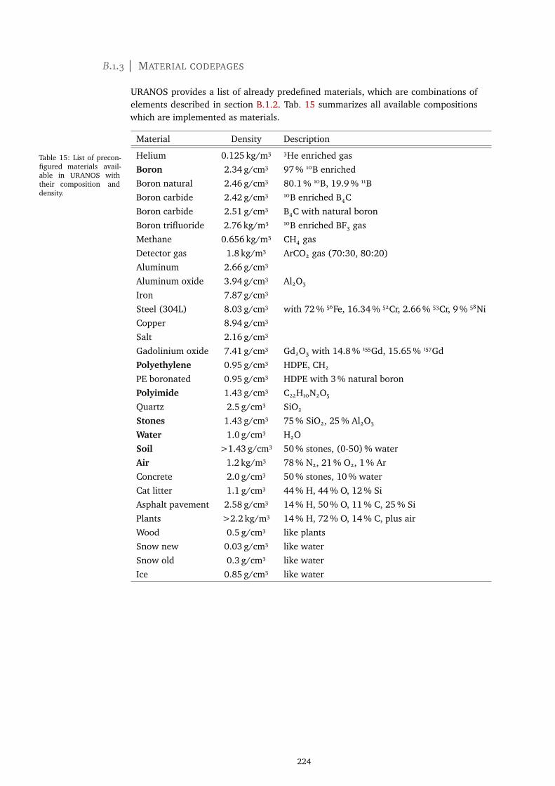
𝐵.1.3 MATERIAL CODEPAGES

URANOS provides a list of already predefined materials, which are combinations ofelements described in section B.1.2. Tab. 15 summarizes all available compositionswhich are implemented as materials.

Table 15: List of precon-figured materials avail-able in URANOS withtheir composition anddensity.

Material Density Description

Helium 0.125 kg/m3 3He enriched gas

Boron 2.34 g/cm3 97 % 10B enriched

Boron natural 2.46 g/cm3 80.1 % 10B, 19.9 % 11B

Boron carbide 2.42 g/cm3 10B enriched B4C

Boron carbide 2.51 g/cm3 B4C with natural boron

Boron trifluoride 2.76 kg/m3 10B enriched BF3 gas

Methane 0.656 kg/m3 CH4 gas

Detector gas 1.8 kg/m3 ArCO2 gas (70:30, 80:20)

Aluminum 2.66 g/cm3

Aluminum oxide 3.94 g/cm3 Al2O3

Iron 7.87 g/cm3

Steel (304L) 8.03 g/cm3 with 72 % 56Fe, 16.34 % 52Cr, 2.66 % 53Cr, 9 % 58Ni

Copper 8.94 g/cm3

Salt 2.16 g/cm3

Gadolinium oxide 7.41 g/cm3 Gd2O3 with 14.8 % 155Gd, 15.65 % 157Gd

Polyethylene 0.95 g/cm3 HDPE, CH2

PE boronated 0.95 g/cm3 HDPE with 3 % natural boron

Polyimide 1.43 g/cm3 C22H10N2O5

Quartz 2.5 g/cm3 SiO2

Stones 1.43 g/cm3 75 % SiO2, 25 % Al2O3

Water 1.0 g/cm3 H2O

Soil >1.43 g/cm3 50 % stones, (0-50) % water

Air 1.2 kg/m3 78 % N2, 21 % O2, 1 % Ar

Concrete 2.0 g/cm3 50 % stones, 10 % water

Cat litter 1.1 g/cm3 44 % H, 44 % O, 12 % Si

Asphalt pavement 2.58 g/cm3 14 % H, 50 % O, 11 % C, 25 % Si

Plants >2.2 kg/m3 14 % H, 72 % O, 14 % C, plus air

Wood 0.5 g/cm3 like plants

Snow new 0.03 g/cm3 like water

Snow old 0.3 g/cm3 like water

Ice 0.85 g/cm3 like water

224

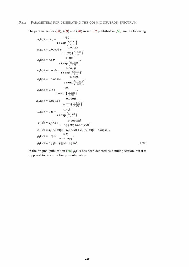
𝐵.1.4 PARAMETERS FOR GENERATING THE COSMIC NEUTRON SPECTRUM

The parameters for (68), (69) and (70) in sec. 3.2 published in [66] are the following:

𝑎1 (𝑟𝑐 ) = 12.9 + 15.7

1 + exp(𝑟𝑐−5.621.79

) ,

𝑎2 (𝑟𝑐 ) = 0.00706 + 0.00057

1 + exp(𝑟𝑐−5.991.94

) ,

𝑎3 (𝑟𝑐 ) = 0.975 − 0.210

1 + exp(𝑟𝑐−0.992.24

) ,

𝑎4 (𝑟𝑐 ) = 0.0084 + 0.004411 + exp

( 𝑟𝑐−2.242.66

) ,

𝑎5 (𝑟𝑐 ) = −0.00701 + 0.0258

1 + exp(𝑟𝑐−10.92.38

) ,

𝑎9 (𝑟𝑐 ) = 642 + 189

1 + exp(𝑟𝑐−2.320.897

) ,

𝑎10 (𝑟𝑐 ) = 0.00112 + 0.000181

1 + exp(𝑟𝑐−8.840.587

) ,

𝑎11 (𝑟𝑐 ) = 1.26 + 0.958

1 + exp(𝑟𝑐−3.181.47

) ,

𝑐4 (𝑑) = 𝑎5 (𝑟𝑐 ) +0.000171𝑑

1 + 0.53 exp (0.00136𝑑) ,

𝑐12 (𝑑) = 𝑎9 (𝑟𝑐 ) exp (−𝑎10 (𝑟𝑐 )𝑑) + 𝑎11 (𝑟𝑐 ) exp (−0.0133𝑑) ,

𝑔3 (𝑤) = −25.2 + 2.73𝑤 + 0.0715

,

𝑔5 (𝑤) = 0.348 + 3.35𝑤 − 1.57𝑤2. (160)

In the original publication [66] 𝑔3 (𝑤) has been denoted as a multiplication, but it issupposed to be a sum like presented above.

225

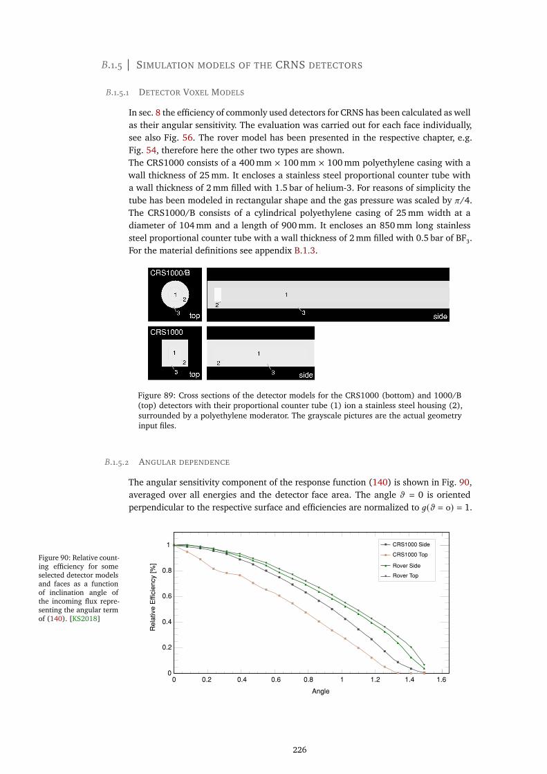
𝐵.1.5 SIMULATION MODELS OF THE CRNS DETECTORS

𝐵.1.5.1 DETECTOR VOXEL MODELS

In sec. 8 the efficiency of commonly used detectors for CRNS has been calculated as wellas their angular sensitivity. The evaluation was carried out for each face individually,see also Fig. 56. The rover model has been presented in the respective chapter, e.g.Fig. 54, therefore here the other two types are shown.The CRS1000 consists of a 400 mm × 100 mm × 100 mm polyethylene casing with awall thickness of 25 mm. It encloses a stainless steel proportional counter tube witha wall thickness of 2 mm filled with 1.5 bar of helium-3. For reasons of simplicity thetube has been modeled in rectangular shape and the gas pressure was scaled by 𝜋/4.The CRS1000/B consists of a cylindrical polyethylene casing of 25 mm width at adiameter of 104 mm and a length of 900 mm. It encloses an 850 mm long stainlesssteel proportional counter tube with a wall thickness of 2 mm filled with 0.5 bar of BF3.For the material definitions see appendix B.1.3.

Figure 89: Cross sections of the detector models for the CRS1000 (bottom) and 1000/B(top) detectors with their proportional counter tube (1) ion a stainless steel housing (2),surrounded by a polyethylene moderator. The grayscale pictures are the actual geometryinput files.

𝐵.1.5.2 ANGULAR DEPENDENCE

The angular sensitivity component of the response function (140) is shown in Fig. 90,averaged over all energies and the detector face area. The angle 𝜗 = 0 is orientedperpendicular to the respective surface and efficiencies are normalized to 𝑔(𝜗 = 0) = 1.

Figure 90: Relative count-ing efficiency for someselected detector modelsand faces as a functionof inclination angle ofthe incoming flux repre-senting the angular termof (140). [KS2018]

Angle

Re

lativ

e E

ffic

ien

cy [%

]

0

0.2

0.4

0.6

0.8

1 CRS1000 Side

CRS1000 Top

Rover Side

Rover Top

0 0.2 0.4 0.6 0.8 1 1.2 1.4 1.6

226

The detectors show lowest sensitivity to neutrons from directions parallel to the surface,as for slant angles (𝜗 = 𝜋/2 or 90◦) the probability of detection drops to zero. Highestsensitivity for all detectors is achieved for orthogonal incidence with 𝜗 = 0. This resultstresses the importance of accounting for neutron fluxes directly from atmosphericcosmic rays and directly from beneath the sensor. An analytical approximation for theangular distribution of the large faces can be given as:

𝑔(𝜗) = 1.24 − 0.254 exp (1.087𝜗) . (161)

Yet, for the CRS1000 top face a linear model is sufficient. Like discussed above, the ge-ometric arrangement of the moderator has a minor influence on the response function.For energies in the epithermal to fast regime the angular response does not changesignificantly.

𝐵.1.6 SIMULATION OF THE NEUTRON SOURCE ROOM

A simplified version of the radiation environment of the neutron source within its roomhas been simulated by URANOS. The room, which is sketched in Fig. 91, consists ofthe following elements, see also the material compendium in appendix B.1.3: air with5 g/m3 humidity, concrete floor, walls and ceiling, two aluminum tables with boronatedrubber mats and vertical polyethylene absorbers covered by boronated rubber mats,one wooden table, a fused silica window, wooden and steal doors. The source itselfconsists of a large block of boronated and non-boronated polyethylene. Beamport Ais open. At its inner center face, which is the moderator of the californium source, amoderated spectrum (??), based on simulations by U. Schmidt, is released in port di-rection into 2𝜋 . A more detailed description of the simulations and the source buildupcan also be found in [284].

Figure 91: Setup for the source room simu-lation: (1) Moderated shielded source withspectrum (??) through beamport A, (2) alu-minium tables with boron rubber mat coversand vertical absorbers, (3) wooden table, (4)doors, (5) window, (6) concrete wall and (7)isotope storage room.

The goal was to analyze whether an additional thermal shielding on the outside ofthe source buildup would reduce the background for measurements. The result of thissimulation is, that covering the source by an additional absorber has no significant in-fluence on the overall thermal neutron background. The reason can be easily identifiedin Fig. 92. The background, which can be measured for experimental setups on thetables (2), is not due to neutrons leaking out of the source, but rather originates fromthe fast neutron, which are scattered within the room and thermalize elsewhere. As thesource partly consists of boronated polyethylene, there is no direct contribution fromthermal neutrons coming from the source moderator, but instead from all other objects

227

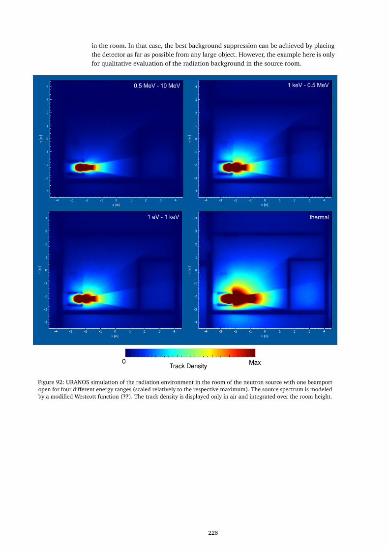
in the room. In that case, the best background suppression can be achieved by placingthe detector as far as possible from any large object. However, the example here is onlyfor qualitative evaluation of the radiation background in the source room.

Figure 92: URANOS simulation of the radiation environment in the room of the neutron source with one beamportopen for four different energy ranges (scaled relatively to the respective maximum). The source spectrum is modeledby a modified Westcott function (??). The track density is displayed only in air and integrated over the room height.

228

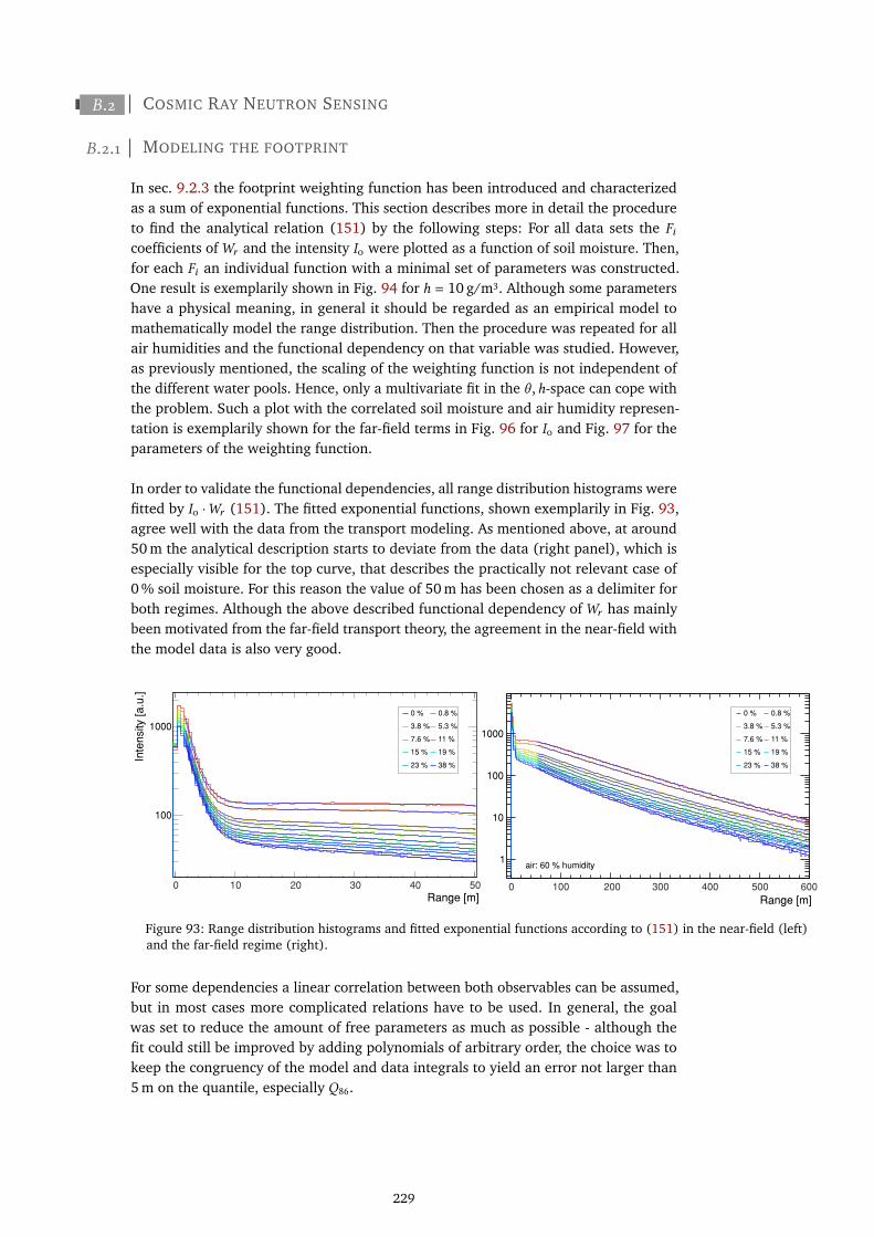
𝐵.2 COSMIC RAY NEUTRON SENSING

𝐵.2.1 MODELING THE FOOTPRINT

In sec. 9.2.3 the footprint weighting function has been introduced and characterizedas a sum of exponential functions. This section describes more in detail the procedureto find the analytical relation (151) by the following steps: For all data sets the 𝐹𝑖

coefficients of𝑊𝑟 and the intensity 𝐼0 were plotted as a function of soil moisture. Then,for each 𝐹𝑖 an individual function with a minimal set of parameters was constructed.One result is exemplarily shown in Fig. 94 for ℎ = 10 g/m3. Although some parametershave a physical meaning, in general it should be regarded as an empirical model tomathematically model the range distribution. Then the procedure was repeated for allair humidities and the functional dependency on that variable was studied. However,as previously mentioned, the scaling of the weighting function is not independent ofthe different water pools. Hence, only a multivariate fit in the \ ,ℎ-space can cope withthe problem. Such a plot with the correlated soil moisture and air humidity represen-tation is exemplarily shown for the far-field terms in Fig. 96 for 𝐼0 and Fig. 97 for theparameters of the weighting function.

In order to validate the functional dependencies, all range distribution histograms werefitted by 𝐼0 ·𝑊𝑟 (151). The fitted exponential functions, shown exemplarily in Fig. 93,agree well with the data from the transport modeling. As mentioned above, at around50 m the analytical description starts to deviate from the data (right panel), which isespecially visible for the top curve, that describes the practically not relevant case of0 % soil moisture. For this reason the value of 50 m has been chosen as a delimiter forboth regimes. Although the above described functional dependency of𝑊𝑟 has mainlybeen motivated from the far-field transport theory, the agreement in the near-field withthe model data is also very good.

Range [m]

100

1000

0 % 0.8 %

3.8 % 5.3 %

7.6 % 11 %

15 % 19 %

23 % 38 %

10 20 30 40 500

Inte

nsity

[a

.u.]

1

10

100

1000

Range [m]100 200 300 400 5000 600

air: 60 % humidity

0 % 0.8 %

3.8 % 5.3 %

7.6 % 11 %

15 % 19 %

23 % 38 %

Figure 93: Range distribution histograms and fitted exponential functions according to (151) in the near-field (left)and the far-field regime (right).

For some dependencies a linear correlation between both observables can be assumed,but in most cases more complicated relations have to be used. In general, the goalwas set to reduce the amount of free parameters as much as possible - although thefit could still be improved by adding polynomials of arbitrary order, the choice was tokeep the congruency of the model and data integrals to yield an error not larger than5 m on the quantile, especially 𝑄86.

229

800000

1000000

1200000

1400000

1600000

1800000 / ndf 2 73.17 / 6

p0 1257± 1.031e+005

p1 0.001514± -0.103

p2 2191± 5.666e+005

/ ndf 2χ

Prob 9.141e-014

p0

p1 ±

p2

5000

10000

15000

20000

25000

30000

35000 / ndf 2χ 23.86 / 7

Prob 0.001207p0 962 2.409e+004

p1 2.511± 26.56 p2 122.5± 7912

/ ndf 2χ 23.86 / 7

Prob 0.001207p0 962± 2.409e+004

p1 2.511± 26.56 p2 122.5± 7912

0.000008

0.00001

0.000012

0.000014

0.000016

0.000018

/ ndf 2χ 15.88 / 7

Prob 0.02625

p0 1.659e-007± -9.182e-006

p1 1.26 16.69

p2 1.553e-007± 1.676e-005

/ ndf 2χ 15.88 / 7

Prob 0.02625

p0 1.659e-007± -9.182e-006

p1 1.26± 16.69

p2 1.553e-007± 1.676e-005

-0.000002

0

0.000002

0.000004

0.000006

/ ndf 2χ 14.86 / 7

Prob 0.03788

p0 7.587e-007± -5.802e-006

p1 5.411 49.09

p2 2.981e-008± 6.891e-006

/ ndf 2χ 14.86 / 7

Prob 0.03788

p0 7.587e-007± -5.802e-006

p1 5.411 49.09

p2 2.981e-008± 6.891e-006

0

1000

2000

3000

4000

5000

6000

7000

8000 / ndf 2χ 2.132 / 6

Prob 0.9072

p0 3.668e+004± 1.704e+005

p1 2.144± 15.68

p2 281.8± 2641

p3 0.003337± 0.01878

/ ndf 2χ 2.132 / 6

Prob 0.9072

p0 3.668e+004± 1.704e+005

p1 2.144± 15.68

p2 281.8± 2641

p3 0.003337± 0.01878

0 0.1 0.2 0.3 0.4 0.5 0 0.1 0.2 0.3 0.4 0.5

Soil moisture [% ]Vol

0 0.1 0.2 0.3 0.4 0.5

0 0.1 0.2 0.3 0.4 0.5

Soil moisture [% ]Vol

0 0.1 0.2 0.3 0.4 0.5

±

Figure 94: Parameters from the fits for the far-field term of (151) (black dots with statistical errors) for ℎ = 10 g/m3.From the top left to the lower right panel: 𝐼0, 𝐹5, 𝐹6, 𝐹7 and 𝐹8. To each set, plotted here depending on soil moisture,the functions (162) are fitted.

]3humidity [g/m

0 10 20 30 40 50960000

965000

970000

975000

980000

985000

990000

995000

1000000

]3humidity [g/m

0 10 20 30 40 50 60 70 80 90

3500

4000

4500

5000

5500

]3humidity [g/m

0 10 20 30 40 50 60 70 80 90

0.000006

0.000007

0.000008

0.000009

0.00001

0.000011

]3humidity [g/m

0 10 20 30 40 50 60 70 80 90

0.000014

0.000016

0.000018

0.00002

0.000022

0.000024

]3humidity [g/m

0 10 20 30 40 50 60 70 80 90

8000

10000

12000

14000

16000

18000

/ ndf 2.814 / 6Prob 0.8319p0 153.3± 8309 p1 4.741± 102.2

2χ

/ ndf 9.372 / 6

Prob 0.1537

p0 3.888e-008± 6.101e-006

p1 1.355e-009± 6.344e-008

2χ / ndf 1.256 / 6Prob 0.974p0 222.6± 4916 p1 5.951± -12.26

2χ

/ ndf 18.41 / 6

Prob 0.005287

p0 1.594e-007± 1.435e-005

p1 4.416e-009± 1.124e-007

2χ

/ ndf 18.17 / 4

Prob 0.001141

p0 766.9± 9.625e+005

p1 78.51± 1067

p2 1.527± -6.692

2χ

Figure 95: Parameters from the fits for the far-field term of (151) (black dots with statistical errors) for \ = 11 %.From the top left to the lower right panel: 𝐼0, 𝐹5, 𝐹6, 𝐹7 and 𝐹8. To each set, plotted here depending on air humidity,the functions (162) are fitted.

230

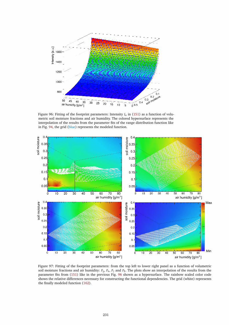
Figure 96: Fitting of the footprint parameters: Intensity 𝐼0 in (151) as a function of volu-metric soil moisture fractions and air humidity. The colored hypersurface represents theinterpolation of the results from the parameter fits of the range distribution function likein Fig. 94, the grid (blue) represents the modeled function.

Figure 97: Fitting of the footprint parameters: from the top left to lower right panel as a function of volumetricsoil moisture fractions and air humidity: 𝐹5, 𝐹6, 𝐹7 and 𝐹8. The plots show an interpolation of the results from theparameter fits from (151) like in the previous Fig. 96 shown as a hypersurface. The rainbow scaled color codeshows the relative differences necessary for constructing the functional dependencies. The grid (white) representsthe finally modeled function (162).

231

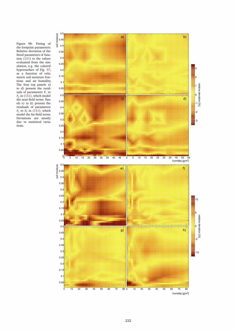
Figure 98: Fitting ofthe footprint parameters:Relative deviation of thefitted parameters of func-tion (151) to the valuesevaluated from the sim-ulation, e.g. the coloredhypersurface of Fig. 97,as a function of volu-metric soil moisture frac-tions and air humidity.The four top panels a)to d) present the resid-uals of parameters 𝐹1 to𝐹4 in (151), which modelthe near-field terms. Pan-els e) to h) present theresiduals of parameters𝐹5 to 𝐹8 in (151), whichmodel the far-field terms.Deviations are mostlydue to statistical varia-tions.

so

il m

ois

ture

0.05

0.1

0.15

0.2

0.25

0.3

0.35

0.4

0.45

0.5

0 10 20 30 40 50 60 70 80

0.05

0.1

0.15

0.2

0.25

0.3

0.35

0.4

0.45

0.5

]3humidity [g/m

0 10 20 30 40 50 60 70 80

-10

-5

0

5

10

rela

tive

de

via

tion

[%]

e) f)

g) h)

so

il m

ois

ture

0.05

0.1

0.15

0.2

0.25

0.3

0.35

0.4

0.45

0.5

-3

-2

-1

0

1

2

3

0 5 10 15 20 25 30 35 40 450

0.05

0.1

0.15

0.2

0.25

0.3

0.35

0.4

0.45

0.5

]3humidity [g/m

0 5 10 15 20 25 30 35 40 45 50

rela

tive

de

via

tion

[%]

a) b)

c) d)

232

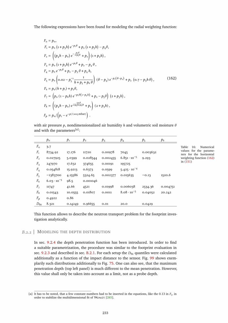
The following expressions have been found for modeling the radial weighting function:

𝐹0 = 𝑝0,

𝐹1 = 𝑝0(1 + 𝑝3ℎ

)𝑒−𝑝1\ + 𝑝2

(1 + 𝑝5ℎ

)− 𝑝4\ ,

𝐹2 =

( (𝑝4ℎ − 𝑝0

)𝑒− 𝑝1\

1+𝑝5\ + 𝑝2) (

1 + 𝑝3ℎ),

𝐹3 = 𝑝0(1 + 𝑝3ℎ

)𝑒−𝑝1\ + 𝑝2 − 𝑝4 \ ,

𝐹4 = 𝑝0 𝑒−𝑝1\ + 𝑝2 − 𝑝3 \ + 𝑝4 ℎ,

𝐹5 = 𝑝0

(0.02 − 𝑝−15

1

ℎ + 𝑝5 + 𝑝6 \

)(\ − 𝑝4) 𝑒−𝑝1 (\−𝑝4) + 𝑝2

(0.7 − 𝑝3ℎ \

),

𝐹6 = 𝑝0 (ℎ + 𝑝1) + 𝑝2\ ,

𝐹7 =

(𝑝0 (1 − 𝑝6ℎ) 𝑒−𝑝1\ (1−𝑝4ℎ) + 𝑝2 − 𝑝5\

) (2 + 𝑝3ℎ

),

𝐹8 =

((𝑝4ℎ − 𝑝0) 𝑒

−𝑝1\1+𝑝5ℎ+𝑝6\ + 𝑝2

)(2 + 𝑝3ℎ) ,

𝐹𝑝 = 𝑝0/(𝑝1 − 𝑒−𝑝/(1013mbar)

).

(162)

with air pressure 𝑝, nondimensionalized air humidity ℎ and volumetric soil moisture \

and with the parameters[a]:

Table 16: Numericalvalues for the parame-ters for the horizontalweighting function (162)in (151)

𝑝0 𝑝1 𝑝2 𝑝3 𝑝4 𝑝5 𝑝6

𝐹0 3.7

𝐹1 8734.92 17.176 11720 0.00978 7045 0.003632

𝐹2 0.027925 5.0399 0.028544 0.002455 6.851 · 10−5 9.293

𝐹3 247970 17.632 374655 0.00191 195725

𝐹4 0.054818 15.9213 0.6373 0.0599 5.425 · 10−4

𝐹5 −1383700 4.15586 5324.65 0.002377 0.015635 −0.13 1520.6

𝐹6 6.03 · 10−5 98.5 0.001046

𝐹7 11747 41.66 4521 0.01998 0.006038 2534.36 0.004751

𝐹8 0.01543 10.0555 0.01807 0.0011 8.08 · 10−5 0.04052 20.242

𝐹𝑝 0.4922 0.86

𝐷86 8.321 0.14249 0.96655 0.01 20.0 0.0429

This function allows to describe the neutron transport problem for the footprint inves-tigation analytically.

𝐵.2.2 MODELING THE DEPTH DISTRIBUTION

In sec. 9.2.4 the depth penetration function has been introduced. In order to finda suitable parametrization, the procedure was similar to the footprint evaluation insec. 9.2.3 and described in sec. B.2.1. For each setup the 𝐷86 quantiles were calculatedadditionally as a function of the impact distance to the sensor. Fig. 99 shows exem-plarily such distributions additionally to Fig. 75. One can also see, that the maximumpenetration depth (top left panel) is much different to the mean penetration. However,this value shall only be taken into account as a limit, not as a probe depth.

[a] It has to be noted, that a few constant numbers had to be inserted in the equations, like the 0.13 in 𝐹5, inorder to stabilize the multidimensional fit of TMinuit [285].

233

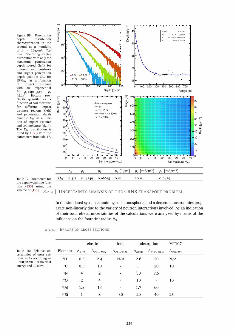
Figure 99: Penetrationdepth distributioncharacterization in theground at a humidityof ℎ = 10 g/m3. Toprow: Scattering centerdistribution with only themaximum penetrationdepth scored (left) fordifferent soil moisturesand (right) penetrationdepth quantile 𝐷86 for15 %Vol as a functionof impact distancewith an exponentialfit 𝑝0 exp(−𝑝1𝑟 ) + 𝑝2(right). Bottom row:Depth quantile as afunction of soil moisturefor different impactdistance regions (left)and penetration depthquantile 𝐷86 as a func-tion of impact distanceand soil moisture (right).The 𝐷86 distribution isfitted by (153) with theparameters from tab. 17.

Range [m]

0 100 200 300 400 500 600 700

]2

De

pth

[g

/cm

25

30

35

40

45±

±

±

±

/ ndf 2c 1577 / 37

p0 0.08077 17.76

p1 9.854e-005±

p2 0.0216

/ ndf 2 1577 / 37

p0 0.08077 17.76 +/-

p1 9.854e-005± 0.01196 +/-

p2 0.0216 27.33 +/-

0

100

200

300

400

500

600

700

0

10

20

30

40

50

60

70

80

90

Ra

ng

e [m

]

De

pth

[g

/cm

]2

]2Depth [g/cm

0 50 100 150 200 250

Inte

nsity

[a

.u.]

-410

-310

-210

-110

1

Soil moisture [% ]Vol

0 5 10 15 20 25 30 35 40

]2

De

pth

[g

/cm

20

30

40

50

60

70

80

90

100±

±

±

±distance regions

all

r < 10 m

10 m < r < 200 m

r > 200m

30 %

0 % 3.8 %

11 %

χ

Soil moisture [% ]Vol

0 5 10 15 20 25 30 35 40

Table 17: Parameters forthe depth weighting func-tion (153) using thescheme of (151).

𝑝0 𝑝1 𝑝2 𝑝3 [1/m] 𝑝4 [m3/m3] 𝑝5 [m3/m3]

𝐷86 8.321 0.14249 0.96655 0.01 20.0 0.0429

𝐵.2.3 UNCERTAINTY ANALYSIS OF THE CRNS TRANSPORT PROBLEM

In the simulated system containing soil, atmosphere, and a detector, uncertainties prop-agate non-linearly due to the variety of neutron interactions involved. As an indicationof their total effect, uncertainties of the calculations were analyzed by means of theinfluence on the footprint radius 𝑅86.

𝐵.2.3.1 ERRORS ON CROSS SECTIONS

Table 18: Relative un-certainties of cross sec-tions in % according toENDF/B-VII.1 at thermalenergy and 10 MeV.

elastic inel. absorption MT107

Element Δ𝜎 (th) Δ𝜎 (10 MeV) Δ𝜎 (10 MeV) Δ𝜎 (th) Δ𝜎 (10 MeV) Δ𝜎 (MeV)

1H 0.3 2.4 N/A 2.6 20 N/A12C 0.5 10 - 3 20 1014N 4 2 - 30 7.516O 2 4 - 10 - 1027Al 1.8 13 - 1.7 60 -28Si 1 8 30 20 40 25

234

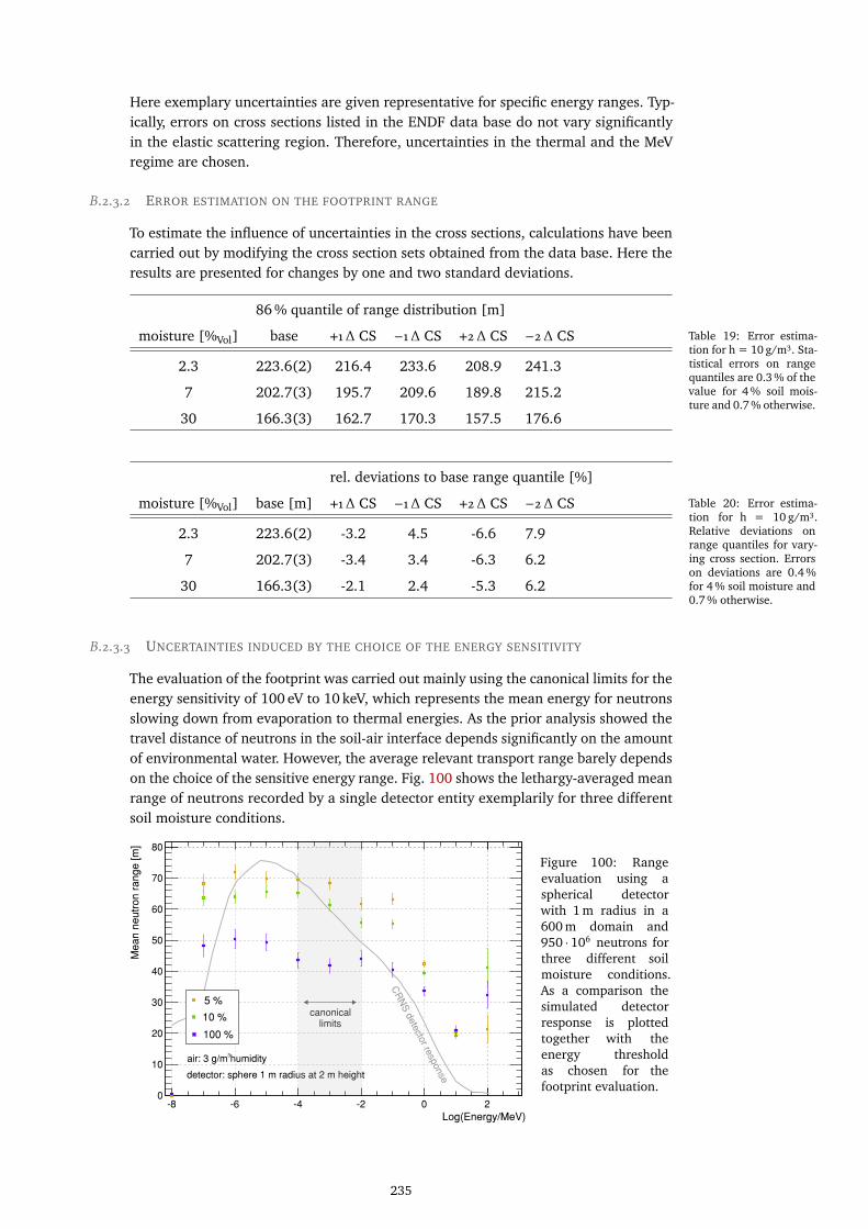
Here exemplary uncertainties are given representative for specific energy ranges. Typ-ically, errors on cross sections listed in the ENDF data base do not vary significantlyin the elastic scattering region. Therefore, uncertainties in the thermal and the MeVregime are chosen.

𝐵.2.3.2 ERROR ESTIMATION ON THE FOOTPRINT RANGE

To estimate the influence of uncertainties in the cross sections, calculations have beencarried out by modifying the cross section sets obtained from the data base. Here theresults are presented for changes by one and two standard deviations.

Table 19: Error estima-tion for h = 10 g/m3. Sta-tistical errors on rangequantiles are 0.3 % of thevalue for 4 % soil mois-ture and 0.7 % otherwise.

86 % quantile of range distribution [m]

moisture [%Vol] base +1Δ CS −1Δ CS +2Δ CS −2Δ CS

2.3 223.6(2) 216.4 233.6 208.9 241.3

7 202.7(3) 195.7 209.6 189.8 215.2

30 166.3(3) 162.7 170.3 157.5 176.6

Table 20: Error estima-tion for h = 10 g/m3.Relative deviations onrange quantiles for vary-ing cross section. Errorson deviations are 0.4 %for 4 % soil moisture and0.7 % otherwise.

rel. deviations to base range quantile [%]

moisture [%Vol] base [m] +1Δ CS −1Δ CS +2Δ CS −2Δ CS

2.3 223.6(2) -3.2 4.5 -6.6 7.9

7 202.7(3) -3.4 3.4 -6.3 6.2

30 166.3(3) -2.1 2.4 -5.3 6.2

𝐵.2.3.3 UNCERTAINTIES INDUCED BY THE CHOICE OF THE ENERGY SENSITIVITY

The evaluation of the footprint was carried out mainly using the canonical limits for theenergy sensitivity of 100 eV to 10 keV, which represents the mean energy for neutronsslowing down from evaporation to thermal energies. As the prior analysis showed thetravel distance of neutrons in the soil-air interface depends significantly on the amountof environmental water. However, the average relevant transport range barely dependson the choice of the sensitive energy range. Fig. 100 shows the lethargy-averaged meanrange of neutrons recorded by a single detector entity exemplarily for three differentsoil moisture conditions.

Log(Energy/MeV)-8 -6 -4 -2 0 2

Me

an

ne

utr

on

ra

ng

e [

m]

0

10

20

30

40

50

60

70

80

10 %

100 %

5 %

detector: sphere 1 m radius at 2 m height

3air: 3 g/m humidity

canonicallimits

CR

NS

detector response

Figure 100: Rangeevaluation using aspherical detectorwith 1 m radius in a600 m domain and950 · 106 neutrons forthree different soilmoisture conditions.As a comparison thesimulated detectorresponse is plottedtogether with theenergy thresholdas chosen for thefootprint evaluation.

235

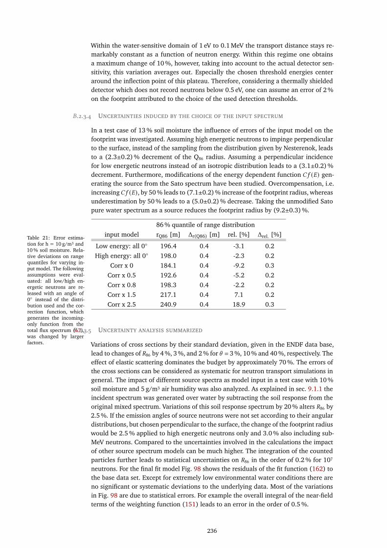
Within the water-sensitive domain of 1 eV to 0.1 MeV the transport distance stays re-markably constant as a function of neutron energy. Within this regime one obtainsa maximum change of 10 %, however, taking into account to the actual detector sen-sitivity, this variation averages out. Especially the chosen threshold energies centeraround the inflection point of this plateau. Therefore, considering a thermally shieldeddetector which does not record neutrons below 0.5 eV, one can assume an error of 2 %on the footprint attributed to the choice of the used detection thresholds.

𝐵.2.3.4 UNCERTAINTIES INDUCED BY THE CHOICE OF THE INPUT SPECTRUM

In a test case of 13 % soil moisture the influence of errors of the input model on thefootprint was investigated. Assuming high energetic neutrons to impinge perpendicularto the surface, instead of the sampling from the distribution given by Nesterenok, leadsto a (2.3±0.2) % decrement of the Q86 radius. Assuming a perpendicular incidencefor low energetic neutrons instead of an isotropic distribution leads to a (3.1±0.2) %decrement. Furthermore, modifications of the energy dependent function 𝐶𝑓 (𝐸) gen-erating the source from the Sato spectrum have been studied. Overcompensation, i.e.increasing𝐶𝑓 (𝐸), by 50 % leads to (7.1±0.2) % increase of the footprint radius, whereasunderestimation by 50 % leads to a (5.0±0.2) % decrease. Taking the unmodified Satopure water spectrum as a source reduces the footprint radius by (9.2±0.3) %.

Table 21: Error estima-tion for h = 10 g/m3 and10 % soil moisture. Rela-tive deviations on rangequantiles for varying in-put model. The followingassumptions were eval-uated: all low/high en-ergetic neutrons are re-leased with an angle of0◦ instead of the distri-bution used and the cor-rection function, whichgenerates the incoming-only function from thetotal flux spectrum (67),was changed by largerfactors.

86 % quantile of range distribution

input model rQ86 [m] Δr(Q86) [m] rel. [%] Δrel. [%]

Low energy: all 0◦ 196.4 0.4 -3.1 0.2

High energy: all 0◦ 198.0 0.4 -2.3 0.2

Corr x 0 184.1 0.4 -9.2 0.3

Corr x 0.5 192.6 0.4 -5.2 0.2

Corr x 0.8 198.3 0.4 -2.2 0.2

Corr x 1.5 217.1 0.4 7.1 0.2

Corr x 2.5 240.9 0.4 18.9 0.3

𝐵.2.3.5 UNCERTAINTY ANALYSIS SUMMARIZED

Variations of cross sections by their standard deviation, given in the ENDF data base,lead to changes of 𝑅86 by 4 %, 3 %, and 2 % for \ = 3 %, 10 % and 40 %, respectively. Theeffect of elastic scattering dominates the budget by approximately 70 %. The errors ofthe cross sections can be considered as systematic for neutron transport simulations ingeneral. The impact of different source spectra as model input in a test case with 10 %soil moisture and 5 g/m3 air humidity was also analyzed. As explained in sec. 9.1.1 theincident spectrum was generated over water by subtracting the soil response from theoriginal mixed spectrum. Variations of this soil response spectrum by 20 % alters 𝑅86 by2.5 %. If the emission angles of source neutrons were not set according to their angulardistributions, but chosen perpendicular to the surface, the change of the footprint radiuswould be 2.5 % applied to high energetic neutrons only and 3.0 % also including sub-MeV neutrons. Compared to the uncertainties involved in the calculations the impactof other source spectrum models can be much higher. The integration of the countedparticles further leads to statistical uncertainties on 𝑅86 in the order of 0.2 % for 107

neutrons. For the final fit model Fig. 98 shows the residuals of the fit function (162) tothe base data set. Except for extremely low environmental water conditions there areno significant or systematic deviations to the underlying data. Most of the variationsin Fig. 98 are due to statistical errors. For example the overall integral of the near-fieldterms of the weighting function (151) leads to an error in the order of 0.5 %.

236

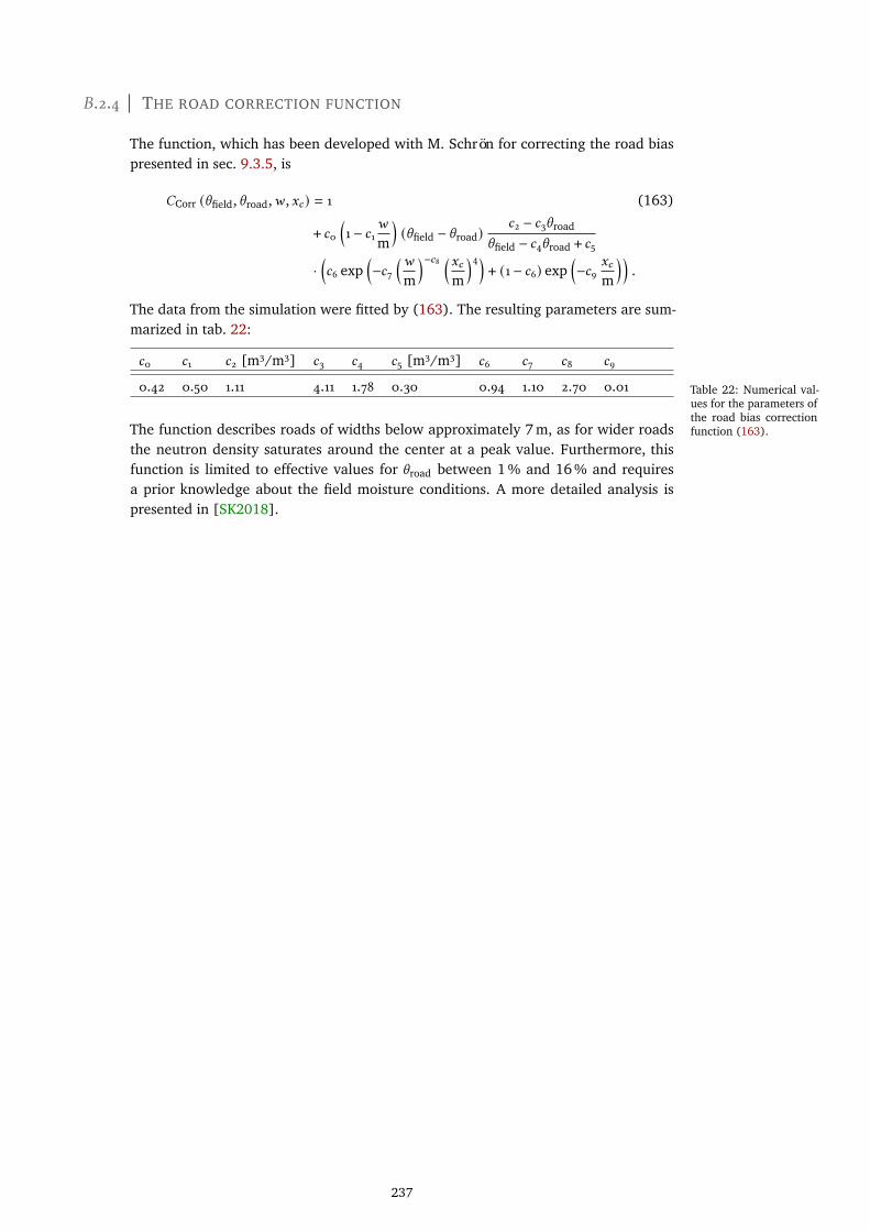
𝐵.2.4 THE ROAD CORRECTION FUNCTION

The function, which has been developed with M. Schrön for correcting the road biaspresented in sec. 9.3.5, is

𝐶Corr (\field,\road,𝑤 ,𝑥𝑐 ) = 1 (163)

+ 𝑐0(1 − 𝑐1

𝑤

m

)(\field − \road)

𝑐2 − 𝑐3\road

\field − 𝑐4\road + 𝑐5·(𝑐6 exp

(−𝑐7

(𝑤m

)−𝑐8 (𝑥𝑐m

)4)+ (1 − 𝑐6) exp

(−𝑐9

𝑥𝑐

m

)).

The data from the simulation were fitted by (163). The resulting parameters are sum-marized in tab. 22:

Table 22: Numerical val-ues for the parameters ofthe road bias correctionfunction (163).

𝑐0 𝑐1 𝑐2 [m3/m3] 𝑐3 𝑐4 𝑐5 [m3/m3] 𝑐6 𝑐7 𝑐8 𝑐9

0.42 0.50 1.11 4.11 1.78 0.30 0.94 1.10 2.70 0.01

The function describes roads of widths below approximately 7 m, as for wider roadsthe neutron density saturates around the center at a peak value. Furthermore, thisfunction is limited to effective values for \road between 1 % and 16 % and requiresa prior knowledge about the field moisture conditions. A more detailed analysis ispresented in [SK2018].

237

𝐵.3 THE URANOS GRAPHICAL USER INTERFACE

In collaboration with the Helmholtz Centre for Environmental Research - UFZ, Leipzig,and especially M. Schrön, a graphical user interface (GUI) for URANOS has beendeveloped, which specifically targets the needs of environmental sciences. URANOSGUIallows to run the Monte Carlo with the full feature list described in sec. 6 except forthe readout simulation for gaseous detector. It enables researchers to carry out neutrontransport simulations without the need of configuring the setup by text files[b], whichis the usual modus operandi for the codes mentioned in sec. 5.2. It especially does notrequire profound knowledge of the internal software buildup, as the relevant featuresand settings are all accessible from the graphical frontend. Instead of drop-down menusor child windows it uses a tabbed document interface, which is functionally split intotwo parts horizontally partitioned by the golden ratio. The left side functionally controlsthe program, its general settings and problem-related configurations. The right sidetabs provides a direct insight into the ongoing computation. It shows the actual neutrondensity and track distribution, interaction range and depth and detector scoring results.The top bar represents the dashboard for starting and stopping the simulation as wellas exporting the results. It also shows the expected time to accomplish the actualjob. A simulation, like presented in the following screenshots of the UFZ site Fig. 101to Fig. 104, is carried out by creating a layer structure, setting vertical positions anddefining a ground layer, a source layer and a detector layer for scoring. The GUI thenautomatically loads 𝑛.png or 𝑛.dat files, with 𝑛 being the layer number, placed in theconfigured work directory. According to the pixel or ASCII matrix voxels are extrudedbased on the predefined material codes of sec. B.1.3.

Figure 101: URANOS GUI main tabs: Setup for the layer arrangement for the vertical geometry and environmentalparameters (left) and birds-eye view with the above-ground neutron spectrum (right).

[b] It also offers for advanced users a command line option to be configured and run by steering files, whichalso provide access to features not available in the GUI.

238

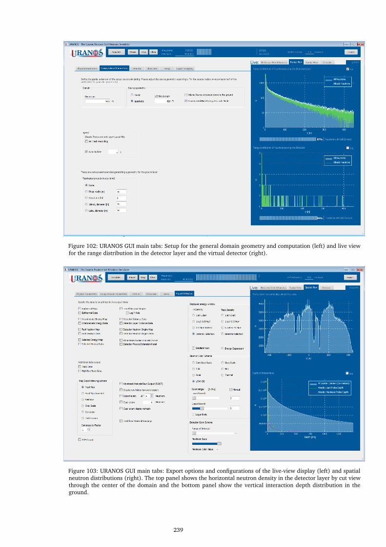
Figure 102: URANOS GUI main tabs: Setup for the general domain geometry and computation (left) and live viewfor the range distribution in the detector layer and the virtual detector (right).

Figure 103: URANOS GUI main tabs: Export options and configurations of the live-view display (left) and spatialneutron distributions (right). The top panel shows the horizontal neutron density in the detector layer by cut viewthrough the center of the domain and the bottom panel show the vertical interaction depth distribution in theground.

239

Figure 104: URANOS GUI main tabs: Setup for the scoring of the detector and detector layer (left) and distributionof neutron origins recorded by the virtual detector (right).

Figure 105: URANOS GUI high resolution track view with histories of thermal neutrons inte-grated over 1 s: Example of the simulation of a thermal neutron source inside a polyethylenedetector test box.

240

CA C K N O W L E D G E M E N T S

This work could not have been realized without the financial support during many yearsof research and experiments. The largest part of the funding has been provided by theBundesministerium für Bildung und Forschung (BMBF) in the frame of the project „Neu-tron Detectors for the MIEZE method“. Further contributions came from the Physikalis-ches Institut, Heidelberg University, from the Deutsche Forschungsgemeinschaft (DFG),from the Helmholtz Centre for Environmental Research-UFZ, Leipzig. Beam times atlarge-scale research facilities were additionally supported by the Technical UniversityMunich and the Institute of Nuclear Chemistry of the Mainz University. Part of themeasurements were performed at the single crystal diffractometer, which is jointlyoperated by the RWTH Aachen University Institute of Crystallography and the JülichCentre for Neutron Science (JCNS) as well as the RESEDA Spin Echo spectrometer,operated by the Technical University Munich, both located at the Heinz Maier-LeibnitzZentrum (MLZ) in Garching.

Furthermost I want to thank my collaborator Martin Schrön at the UFZ, Leipzig: sixjoint papers and more to come, numerous conferences and approximately 4700 mutualemails in total within approximately six years (which makes a remarkable 2.5 emailsper day, including the non-stop weekends) speak by itself.I am grateful for having nice, supportive and sometimes critical colleagues around meat the Physikalisches Institut: Fabian Allmendiger, Matthias Janke, Peter Augenstein,Jannis Weimar, Christoph Roick, Manuel Fohler, Peter Vivell, Lukas Raffelt, Dirk Wied-ner, Gerd Modzel, Max Lamparth, Carmen Ziener, Christian Färber, Martin Klein andMaarten DeKieviet.Among my students I especially want to acknowledge Michael Liebig, Boris Rivkin, JanHammerich and Fabian Schmidt for the good teamwork in the office and the laboratory.Many thanks also go to the excellent team of the electronics and mechanics workshopof the Physikalisches Institut as well as for the technical support of Markus Henske.At the UFZ my thanks go to Steffen Zacharias and Peter Dietrich.

Also I want to thank the meanwhile numerous scientists in team of the RESEDA and theMIRA instrument at the FRM II: Wolfgang Häußler, Christian Franz, Franz Haslbeck,Olaf Soltwedel, Steffen Säubert, Stefan Söllradl, Nicolas Martin, Thorsten Schröder,Tobias Weber and Robert Georgii along with Martin Meven, instrument scientist atHEiDi, and Malgorzata Makowska, instrument scientist at NECTAR.Honorable mentions for my beam times at the TRIGA reactor: Christian Stieghorst.

This acknowledgment should not close without a special mention to my internationalcollaboration partners in Cosmic-Ray Neutron Sensing: Marek Zreda, Darin Desilets,Paul Schattan and Tatsuhiko Sato.

Special thanks go to Ernst Peter Fischer, author and science historian, for his inspiringlectures and his contributions in my seminar „The most important mistakes in physics’history“.

Last, but not least, my supervisor Ulrich Schmidt, whom I would like to thank with thefollowing poem:

241

Eternal

I am in the corridor of days enclosedand burdened even by the skies.

I look into centuries, but live in minuteswaiting for the Saturday of Saturdays.

The end of troubles in my fate,blind wanderings of the soul.O day, come, deign me sightwith all bizarre to be known.

I will get another soulwith all the worries vault’d.I will bless the golden roadto the Sun from the soiled.

And he, who walked by my pathsin thunder and meek silence,

who was cruel to my pleasuresand merciful to my flaws,

who taught to fight and to bearand of all the ancient wisdom profound,

will lower the staff, turn around,and simply say: We are here.

Nikolay S. GUMILËV

translation from Gumil�v, Veqnoe (1912),with special thanks to D�et� - Antologi� (2007).

242

After all I want to also acknowledge the Kirchhoff-Institute of physics, which wasinvoluntarily and constantly subjected to my series of tricks.

243

Vente, gresle, gelle,

j’ay mon pain cuit.

François VILLON

244