Fuel 163 (2016) 98–111

Contents lists available at ScienceDirect

Fuel

journal homepage: www.elsevier .com/locate / fuel

Extension of the Eddy Dissipation Concept for turbulence/chemistryinteractions to MILD combustion

http://dx.doi.org/10.1016/j.fuel.2015.09.0200016-2361/� 2015 Elsevier Ltd. All rights reserved.

⇑ Corresponding author at: Avenue F.D. Roosevelt 50, 1050 Bruxelles, Belgium.Tel.: + 32 2 650 26 80; fax: +32 2 650 27 10.

E-mail address: Alessandro.Parente@ulb.ac.be (A. Parente).

Alessandro Parente a,b,⇑, Mohammad Rafi Malik a,b, Francesco Contino c,b, Alberto Cuoci d, Bassam B. Dally e

aUniversité Libre de Bruxelles, Ecole Polytechnique de Bruxelles, Aero-Thermo-Mechanics Laboratory, Bruxelles, BelgiumbUniversité Libre de Bruxelles and Vrije Universiteit Brussel, Combustion and Robust Optimization Group (BURN), Bruxelles, BelgiumcVrije Universiteit Brussel, Department of Mechanical Engineering, Bruxelles, Belgiumd Politecnico di Milano, Department of Chemistry, Materials, and Chemical Engineering ‘‘G. Natta”, Milano, Italye The University of Adelaide, School of Mechanical Engineering, South Australia, Adelaide, Australia

a r t i c l e i n f o a b s t r a c t

Article history:Received 10 April 2015Received in revised form 8 September 2015Accepted 9 September 2015Available online 25 September 2015

Keywords:Eddy Dissipation ConceptEnergy cascade modelFlameless combustionMILD combustionTurbulence/chemistry interactions

Over the past 30 years, the Eddy Dissipation Concept (EDC) has been widely applied in the industry forthe numerical simulations of turbulent combustion problems. The success of the EDC is mainly due toits ability to incorporate detailed chemical mechanisms at an affordable computational cost comparedto some other models. Detailed kinetic schemes are necessary in order to capture turbulent flames wherethere is strong coupling between the turbulence and chemical kinetics. Such flames are found inModerate and Intense Low-oxygen Dilution (MILD) combustion, where chemical time scales areincreased compared with conventional combustion, mainly because of slower reactions (due to thedilution of reactants). Recent modelling studies have highlighted limitations of the standard EDC modelwhen applied to the simulation of MILD systems, noticeably a significant overestimation of temperaturelevels. Modifications of the model coefficients were proposed to account for the specific features of MILDcombustion, i.e. an extension of the reaction region and the reduction of maximum temperatures. Thepurpose of the present paper is to provide functional expressions showing the dependency of the EDCcoefficients on dimensionless flow parameters such as the Reynolds and Damköhler numbers, taking intoaccount the specific features of the MILD combustion regime, where the presence of hot diluent and itsinfluence on the flow and mixing fields impacts on the reaction rate and thermal field. The approach isvalidated using detailed experimental data from flames stabilized on the Adelaide Jet in Hot Co-flow(JHC) burner at different co-flow compositions (3%, 6% and 9% O2 mass fraction) and fuel-jet Reynoldsnumbers (5000, 10,000 and 20,000). Results show promising improvement with respect to the standardEDC formulation, especially at diluted conditions and medium to low Reynolds numbers.

� 2015 Elsevier Ltd. All rights reserved.

1. Introduction

New breakthroughs in clean energy are needed to provide oursociety with the necessary resources in a way that also protectsthe environment and addresses the climate change issue. The needfor innovation is particularly important in combustion, consideringthat the energy derived from burning fossil fuels (coal, petroleumor natural gas) supplies over two thirds of the total world energyneeds. A certain number of new combustion technologies havebeen proposed in recent years. Among them, Moderate or IntenseLow-oxygen Dilution (MILD) [1–3] combustion is certainly one of

the most promising, as it is able to provide high combustionefficiency with low pollutant emissions. This mode of combustionis achieved through the strong exhaust gas and heat recirculation,achieved by means of the internal aerodynamics of the combustionchamber in conjunction with high-velocity burners [1]. Heat recov-ery by preheating the oxidant stream can also help in improvingthermal efficiency and maintaining the MILD regime. The resultingcombustion regime features reduced local oxygen levels, distribu-tion of reaction over the whole combustion chamber, no visible oraudible flame and thus the name flameless. The temperature fieldis more uniform due to absence of temperature peaks, which dras-tically reduces NOx formation [1,2,4–6], while ensuring completecombustion and low CO emissions [7–10]. MILD combustion canaccommodate large fuel flexibility, representing an ideal technol-ogy for low-calorific value fuels [11–14], high-calorific industrialwastes [15] as well as for hydrogen-based fuels [16,17].

A. Parente et al. / Fuel 163 (2016) 98–111 99

In recent years, attention has been paid to MILD combustionmodelling, due to the very strong turbulence/chemistry interac-tions of such a combustion regime. The Damköhler number inMILD conditions usually approaches unity [17] and both mixingand chemistry need to be taken into account with appropriate tur-bulent combustion models. This has also been proven by Parenteet al. [18], who analysed the correlation structure of MILD combus-tion data [19] using Principal Component Analysis (PCA) andshowed that the standard flamelet approach is not suited for suchcombustion regime. Recently, successful predictions of differentMILD combustion cases have been reported [17,20–22] usingReynolds-Averaged Navier–Stokes (RANS) modelling and the EddyDissipation Concept (EDC) [23]. However, several studies of the Jetin Hot Co-flow (JHC) configuration [19] also reported that the stan-dard EDC tends to over-predict maximum temperatures whenapplied to the MILD combustion regime [24,25]. Recently, Deet al. [26] carried out a detailed study on the performance of theEDC model on the Delft Jet in Hot Co-flow burner (DJHC) emulatingMILD conditions. The authors showed that the model describedcorrectly the mean velocity profiles and the Reynolds shear stressdistributions, but showed significant discrepancies between mea-sured and predicted temperatures. The mean temperature fieldshowed systematic deviations from experimental data, due to theunder-prediction of the lift-off height and the over-estimation ofthe maximum temperature level. This is mainly due to the over-estimations of the mean reaction rate in the EDC model. Theauthors showed that the prediction could be improved by adaptingthe standard coefficients of the classic EDC model, in particularincreasing the time scale value, Cs, from 0.4083 to 3. The resultswere further confirmed for the analysis of the Adelaide JHC flameswith methane/hydrogen mixtures [27] and with several ethylene-based blends [28]. Recently, Evans et al. [29] showed that adjustingthe EDC coefficients Cs and Cc from their default value, 0.4083 and2.1377, to 3.0 and 1.0, respectively, results in significantlyimproved performance of the EDC model under MILD conditions.Although the modification of the coefficients was shown to provideimproved agreement between experiments and numerical simula-tions, it is still necessary to identify clear guidelines for the modi-fication of the model coefficients in the context of MILDcombustion, based on the specific turbulence and chemicalfeatures of such a regime. Shiehnejadhesar et al. [30] showed, forinstance, that the standard EDC is not applicable for turbulentReynolds values below 64 and proposed a hybrid Eddy DissipationConcept/Finite-rate model calculating an effective reaction rateweighting a laminar finite-rate and a turbulent reaction rate,depending on the local turbulent Reynolds number of the flow.

The purpose of the present paper is to provide functionalexpressions showing the dependency of the EDC coefficients ondimensionless flow parameters such as the Reynolds and theDamköhler numbers. After a brief description of EDC and of theenergy cascade model it relies on, the novel approach for the deter-mination of the EDC coefficients will be presented. Results for theAdelaide JHC at different co-flow composition (3%, 6% et 9% O2

mass fraction) and fuel-jet Reynolds numbers (5000, 10,000 and20,000) will be presented, to assess the soundness of the currentapproach.

2. Eddy Dissipation Concept

The Eddy Dissipation Concept (EDC) by Magnussen [23] forturbulent combustion has found wide application for thesimulation of turbulent reacting flows, especially for cases wherecombustion kinetics plays a major role, as it happens for MILDconditions. EDC has the advantage of incorporating detailedkinetics at a computational cost which is affordable when

compared to more sophisticated models such as the transportedPDF methods. This advantage is maximised when EDC is used inconjunction with in-situ adaptive tabulation (ISAT) [31].

According to the EDC model, combustion occurs in the regionsof the flow where the dissipation of turbulence kinetic energytakes place. Such regions are denoted as fine structures and theycan be described as perfectly stirred reactors (PSR). The massfraction of the fine structures, ck, and the mean residence time ofthe fluid within them, s�, are provided by an energy cascade model[32], which describes the energy dissipation process as a functionof the characteristic scales:

ck ¼3CD2

4C2D1

!14 m�

k2

� �14

¼ Ccm�k2

� �14

ð1Þ

and

s� ¼ CD2

3

� �12 m�

� �12 ¼ Cs

m�

� �12 ð2Þ

where m is the kinematic viscosity and � is the dissipation rate ofturbulent kinetic energy, k. CD1 and CD2 are model constants setequal to 0.135 and 0.5, respectively, leading to fine structurevolume and residence time constants equal to Cc ¼ 2:1377 andCs ¼ 0:4083. Fine structures are assumed to be isobaric, adiabaticperfectly stirred reactors. The mean (mass-based) source term inthe conservation equation for the ith species is modelled assuggested by Gran and Magnussen [33]:

_xi ¼ � qc2ks� 1� c3kð Þ eyi � y�i

� �; ð3Þ

where q denotes the mean density of the mixture, y�i is the massfraction of the ith species in the fine structures and eyi representsthe mean mass fraction of the ith species between the finestructures and the surrounding state (indicated as y0i ):eyi ¼ c3ky

�i þ 1� c3k

� �y0i : ð4Þ

As indicated above, the expressions for ck and s� used in the meanreaction rate for the ith species are obtained from an energy cascademodel, based on Kolmogorov’s theory. In the following the model isbriefly summarised, to highlight the main hypothesis behind it.Then, the proposed modification of the EDC standard coefficientswill be presented and discussed.

2.1. Energy cascade model

The energy cascade model for EDC [32] starts with the transferrate of mechanical energy, w0, from the mean flow to the large tur-bulent eddies. The sum of the heat generated at each level,

Piqi, is

assumed to be equal to the turbulent dissipation rate �. The firstcascade level is characterised by a velocity scale u0 ¼

ffiffiffiffiffiffiffiffiffiffiffi2=3k

pand a

length scale L0, giving a strain rate x0 ¼ u0=L0, and it represents thewhole turbulence spectrum because it contains the effect of smallerscales. In the energy cascade model, it is assumed that the straindoubles at each level, so that x00 ¼ u00=L00 ¼ 2x0. The strain rate atlevel n is xn ¼ 2xðn�1Þ. In the original model formulation, the lastlevel is described by scales x�, u�; L�, which are considered to beof the same order of Kolmogorov scales, xk; uk; Lk.

The rate of production of mechanical energy, wi, and the rate ofviscous dissipation, qi, at each level of the cascade are expressed[32] in analogy to the production and dissipation terms appearingin the equation of turbulent kinetic energy, k. This implies, forlevel n:

wn ¼ 32CD1xnu2

n ¼ 32CD1

u3n

Ln; ð5Þ

Jet outlet

Oxidant inlet

Fuel inlet

Cooling gas outlet

Cooling gas inlet

Oxidant inlet

Internal burner

Perforated plate

Ceramic shield

Fig. 1. Schematic of the Jet in Hot Co-flow burner [19].

Table 1Cs and Cc as a function of global ReT and Dag values.

Flame ReT Dad Cs Cc

HM1 400 0.78 1.47 1.90HM2 400 1.15 1.00 2.14HM3 400 1.4 0.82 2.14HM1-5k 225 1.20 1.25 1.78HM1-20k 760 0.50 1.77 2.00

100 A. Parente et al. / Fuel 163 (2016) 98–111

qn ¼ CD2mx2n ¼ CD2m

u2n

L2nð6Þ

and, by the conservation of energy

wn ¼ qn þwnþ1: ð7ÞAt the fine structure level, where reaction occurs, the energy isdissipated into heat,

w� ¼ 32CD1

u�3

L�¼ q� ¼ CD2m

u�2

L�2: ð8Þ

In the original energy cascade formulation, the value of CD2 wasselected as best fit for several types of flow, whereas CD1 was chosenusing the approximation that, for Re � 1, nearly no dissipationtakes place at the highest cascade level. This implies:

e ¼ w0 ¼ q0 þw00 ¼ w00 ¼ 32CD1

u03

L0: ð9Þ

Under this assumption, a relation can be found between CD1 and thek—� turbulent model constant Cl, via the definition of the turbulentviscosity, mT :

u0L0 ¼ 32CD1

u04

�¼ 2

3CD1

k2

�: ð10Þ

0 10 20 30 40 50 60300

600

900

1200

1500

1800

r [mm]

T [

K]

ExpKEEGRI−2.11GRI−3.0

0 10 20300

600

900

1200

1500

1800

r

T [

K]

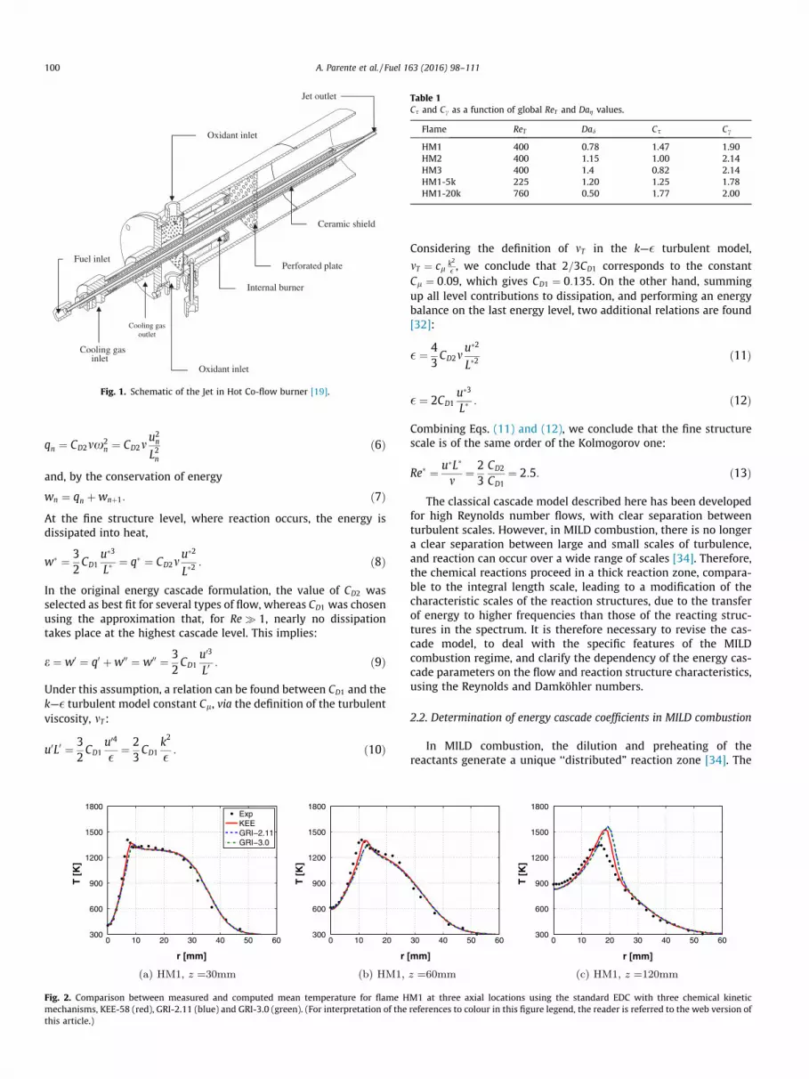
Fig. 2. Comparison between measured and computed mean temperature for flame Hmechanisms, KEE-58 (red), GRI-2.11 (blue) and GRI-3.0 (green). (For interpretation of thethis article.)

Considering the definition of mT in the k—� turbulent model,

mT ¼ cl k2

� , we conclude that 2=3CD1 corresponds to the constantCl ¼ 0:09, which gives CD1 ¼ 0:135. On the other hand, summingup all level contributions to dissipation, and performing an energybalance on the last energy level, two additional relations are found[32]:

� ¼ 43CD2m

u�2

L�2ð11Þ

� ¼ 2CD1u�3

L�: ð12Þ

Combining Eqs. (11) and (12), we conclude that the fine structurescale is of the same order of the Kolmogorov one:

Re� ¼ u�L�

m¼ 2

3CD2

CD1¼ 2:5: ð13Þ

The classical cascade model described here has been developedfor high Reynolds number flows, with clear separation betweenturbulent scales. However, in MILD combustion, there is no longera clear separation between large and small scales of turbulence,and reaction can occur over a wide range of scales [34]. Therefore,the chemical reactions proceed in a thick reaction zone, compara-ble to the integral length scale, leading to a modification of thecharacteristic scales of the reaction structures, due to the transferof energy to higher frequencies than those of the reacting struc-tures in the spectrum. It is therefore necessary to revise the cas-cade model, to deal with the specific features of the MILDcombustion regime, and clarify the dependency of the energy cas-cade parameters on the flow and reaction structure characteristics,using the Reynolds and Damköhler numbers.

2.2. Determination of energy cascade coefficients in MILD combustion

In MILD combustion, the dilution and preheating of thereactants generate a unique ‘‘distributed” reaction zone [34]. The

30 40 50 60

[mm]

0 10 20 30 40 50 60300

600

900

1200

1500

1800

r [mm]

T [

K]

M1 at three axial locations using the standard EDC with three chemical kineticreferences to colour in this figure legend, the reader is referred to the web version of

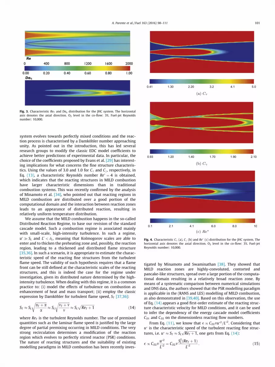
Fig. 3. Characteristic ReT and Dag distribution for the JHC system. The horizontalaxis denotes the axial direction. O2 level in the co-flow: 3%. Fuel-jet Reynoldsnumber: 10,000.

Fig. 4. Characteristic Cs (a), Cc (b) and Re� (c) distribution for the JHC system. Thehorizontal axis denotes the axial direction. O2 level in the co-flow: 3%. Fuel-jetReynolds number: 10,000.

A. Parente et al. / Fuel 163 (2016) 98–111 101

system evolves towards perfectly mixed conditions and the reac-tion process is characterised by a Damköhler number approachingunity. As pointed out in the introduction, this has led severalresearch groups to modify the classic EDC model coefficients toachieve better predictions of experimental data. In particular, thechoice of the coefficients proposed by Evans et al. [29] has interest-ing implications for what concerns the fine structure characteris-tics. Using the values of 3.0 and 1.0 for Cs and Cc, respectively, inEq. (13), a characteristic Reynolds number Re� ¼ 4 is obtained,which indicates that the reacting structures in MILD combustionhave larger characteristic dimensions than in traditionalcombustion systems. This was recently confirmed by the analysisof Minamoto et al. [34], who pointed out that reacting regions inMILD combustion are distributed over a good portion of thecomputational domain and the interaction between reaction zonesleads to an appearance of distributed reaction, resulting inrelatively uniform temperature distribution.

We assume that the MILD combustion happens in the so-calledDistributed Reaction Regime, to base our revision of the standardcascade model. Such a combustion regime is associated mainlywith small-scale, high-intensity turbulence. In such a regime,u0 � SL and L0 < dL, meaning that Kolmogorov scales are able toenter and to thicken the preheating zone and, possibly, the reactionregion, leading to a thickened and distributed flame structure[35,36]. In such a scenario, it is appropriate to estimate the charac-teristic speed of the reacting fine structures from the turbulentflame speed. The validity of such hypothesis requires that a flamefront can be still defined at the characteristic scales of the reactingstructures, and this is indeed the case for the regime underinvestigation, given its distributed nature determined by the high-intensity turbulence. When dealing with this regime, it is a commonpractice to: (i) model the effects of turbulence on combustion asenhancement of heat and mass transport; (ii) employ the classicexpression by Damköhler for turbulent flame speed, ST [37,36]:

ST � SL

ffiffiffiffiffiffiffiffiffiffiffiffiffiffiaT þ aa

r� SL

ffiffiffiffiffiffiffiffiffiffiffiffiffiffimT þ mm

r� SL

ffiffiffiffiffiffiffiffiffiffiffiffiffiffiffiffiReT þ 1

pð14Þ

where ReT is the turbulent Reynolds number. The use of premixedquantities such as the laminar flame speed is justified by the largedegree of partial premixing occurring in MILD conditions. The verystrong recirculation determines a modification of the reactionregion which evolves to perfectly stirred reactor (PSR) conditions.The nature of reacting structures and the suitability of existingmodelling paradigms in MILD combustion has been recently inves-

tigated by Minamoto and Swaminathan [38]. They showed thatMILD reaction zones are highly-convoluted, contorted andpancake-like structures, spread over a large portion of the computa-tional domain resulting in a relatively broad reaction zone. Bymeans of a systematic comparison between numerical simulationsand DNS data, the authors showed that the PSR modelling paradigmis applicable in the (RANS and LES) modelling of MILD combustion,as also demonstrated in [39,40]. Based on this observation, the useof Eq. (14) appears a good first-order estimate of the reacting struc-ture characteristic velocity for MILD conditions, and it can be usedto infer the dependency of the energy cascade model coefficientsCD1 and CD2 on the dimensionless reacting flow numbers.

From Eq. (11), we know that � / CD2mu�2=L�2. Considering thatu� is the characteristic speed of the turbulent reacting fine struc-tures, i.e. u� � ST � SL

ffiffiffiffiffiffiffiffiffiffiffiffiffiffiffiffiReT þ 1

p, one gets from Eq. (14):

� / CD2mu�2

L�2¼ CD2m

S2L ReT þ 1ð ÞL�2

: ð15Þ

Fig. 5. Comparison of measured and computed radial temperature profiles at different axial locations, for flames HM1 (a–c), HM2 (d–f) and HM3 (g–i).

102 A. Parente et al. / Fuel 163 (2016) 98–111

The length scale L� can be interpreted as the characteristic lineardimension of the reacting fine structures, being the reactions dis-tributed over many turbulent length scales. This implies that the

Table 2Relative error on the predicted maximum temperature at different axial locations,using the standard and modified EDC models for flames HM1-HM3.

z [mm] EDC-std EDC-mod –Global coefficients

EDC-mod –Local coefficients

Cs Cs & Cc

HM1, Relative error on Tmax [%]30 0.91 2.90 3.80 3.4860 5.00 0.50 3.60 1.75120 27.80 13.60 5.60 9.35

HM2, Relative error on Tmax [%]30 8.20 4.00 1.8460 10.80 6.10 4.37120 25.90 18.50 2.27

HM3, Relative error on Tmax [%]30 6.00 2.40 8.5660 8.50 5.10 10.49120 20.30 15.50 3.08

ratio L�=SL indicates a characteristic chemical time scale, sc , of thereacting structures, in line with the classic treatment of turbulentpremixed flames [36]. Consequently, sc can be expressed as a func-tion of the Kolmogorov mixing time scale, sg, using the flowDamköhler number. Thus, dissipation can be expressed as:

� / CD2m ReT þ 1ð Þ½ �s2c

¼CD2m ReT þ 1ð ÞDa2

g

h is2g

: ð16Þ

Here, the pertinent mixing time scale for comparison is the Kol-mogorov one, as indicated in the original energy cascade modelby Ertesvåg and Magnussen [32], explaining the use of the symbolDag, to indicate that the Damköhler number is evaluated at the Kol-mogorov scale gk, Dag ¼ sg=sc . Such a choice is motivated by theneed of comparing the reaction process occurring in the fine struc-tures to the molecular mixing process at the Kolmogorov scale. Theproblem could be also treated by introducing the Karlovitz (Ka)number, which intrinsically adopts the Kolmogorov scale, leadingto an equivalent formulation. However, the interpretation in termsof Damköhler number appears more immediate, being the observedDag number for MILD systems of order unity [41]. Expressing

sg ¼ ðm=�Þ12, we get the following dependency of CD2 on ReT and Dag:

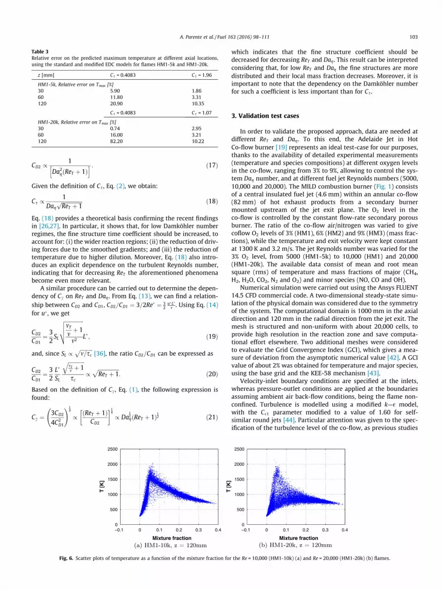
Table 3Relative error on the predicted maximum temperature at different axial locations,using the standard and modified EDC models for flames HM1-5k and HM1-20k.

z [mm] Cs = 0.4083 Cs = 1.96

HM1-5k, Relative error on Tmax [%]30 5.90 1.8660 11.80 3.31120 20.90 10.35

Cs = 0.4083 Cs = 1.07

HM1-20k, Relative error on Tmax [%]30 0.74 2.9560 16.00 3.21120 82.20 10.22

A. Parente et al. / Fuel 163 (2016) 98–111 103

CD2 / 1

Da2g ReT þ 1ð Þ

h i : ð17Þ

Given the definition of Cs, Eq. (2), we obtain:

Cs / 1Dag

ffiffiffiffiffiffiffiffiffiffiffiffiffiffiffiffiReT þ 1

p ð18Þ

Eq. (18) provides a theoretical basis confirming the recent findingsin [26,27]. In particular, it shows that, for low Damköhler numberregimes, the fine structure time coefficient should be increased, toaccount for: (i) the wider reaction regions; (ii) the reduction of driv-ing forces due to the smoothed gradients; and (iii) the reduction oftemperature due to higher dilution. Moreover, Eq. (18) also intro-duces an explicit dependence on the turbulent Reynolds number,indicating that for decreasing ReT the aforementioned phenomenabecome even more relevant.

A similar procedure can be carried out to determine the depen-dency of Cc on ReT and Dag. From Eq. (13), we can find a relation-ship between CD2 and CD1, CD2=CD1 ¼ 3=2Re� ¼ 3

2u�L�m . Using Eq. (14)

for u�, we get

CD2

CD1¼ 3

2SL

ffiffiffiffiffiffiffiffiffiffiffiffiffiffimTmþ 1

m2

vuutL�; ð19Þ

and, since SL /ffiffiffiffiffiffiffiffiffiffim=sc

p[36], the ratio CD2=CD1 can be expressed as

CD2

CD1¼ 3

2L�

SL

ffiffiffiffiffiffiffiffiffiffiffiffiffimTm þ 1

qsc

/ffiffiffiffiffiffiffiffiffiffiffiffiffiffiffiffiReT þ 1

p: ð20Þ

Based on the definition of Cc, Eq. (1), the following expression isfound:

Cc ¼ 3CD2

4C2D1

!14

/ ReT þ 1ð ÞCD2

14

/ Da12g ReT þ 1ð Þ12 ð21Þ

−0.1 0 0.1 0.2 0.3 0.40

500

1000

1500

2000

2500

T [

K]

Mixture fraction

Fig. 6. Scatter plots of temperature as a function of the mixture fraction for

which indicates that the fine structure coefficient should bedecreased for decreasing ReT and Dag. This result can be interpretedconsidering that, for low ReT and Dag the fine structures are moredistributed and their local mass fraction decreases. Moreover, it isimportant to note that the dependency on the Damköhler numberfor such a coefficient is less important than for Cs.

3. Validation test cases

In order to validate the proposed approach, data are needed atdifferent ReT and Dag. To this end, the Adelaide Jet in HotCo-flow burner [19] represents an ideal test-case for our purposes,thanks to the availability of detailed experimental measurements(temperature and species compositions) at different oxygen levelsin the co-flow, ranging from 3% to 9%, allowing to control the sys-tem Dag number, and at different fuel jet Reynolds numbers (5000,10,000 and 20,000). The MILD combustion burner (Fig. 1) consistsof a central insulated fuel jet (4.6 mm) within an annular co-flow(82 mm) of hot exhaust products from a secondary burnermounted upstream of the jet exit plane. The O2 level in theco-flow is controlled by the constant flow-rate secondary porousburner. The ratio of the co-flow air/nitrogen was varied to givecoflow O2 levels of 3% (HM1), 6% (HM2) and 9% (HM3) (mass frac-tions), while the temperature and exit velocity were kept constantat 1300 K and 3.2 m/s. The jet Reynolds number was varied for the3% O2 level, from 5000 (HM1-5k) to 10,000 (HM1) and 20,000(HM1-20k). The available data consist of mean and root meansquare (rms) of temperature and mass fractions of major (CH4,H2, H2O, CO2, N2 and O2) and minor species (NO, CO and OH).

Numerical simulation were carried out using the Ansys FLUENT14.5 CFD commercial code. A two-dimensional steady-state simu-lation of the physical domain was considered due to the symmetryof the system. The computational domain is 1000 mm in the axialdirection and 120 mm in the radial direction from the jet exit. Themesh is structured and non-uniform with about 20,000 cells, toprovide high resolution in the reaction zone and save computa-tional effort elsewhere. Two additional meshes were consideredto evaluate the Grid Convergence Index (GCI), which gives a mea-sure of deviation from the asymptotic numerical value [42]. A GCIvalue of about 2% was obtained for temperature and major species,using the base grid and the KEE-58 mechanism [43].

Velocity-inlet boundary conditions are specified at the inlets,whereas pressure-outlet conditions are applied at the boundariesassuming ambient air back-flow conditions, being the flame non-confined. Turbulence is modelled using a modified k—� model,with the C�1 parameter modified to a value of 1.60 for self-similar round jets [44]. Particular attention was given to the spec-ification of the turbulence level of the co-flow, as previous studies

−0.1 0 0.1 0.2 0.3 0.40

500

1000

1500

2000

2500

T [

K]

Mixture fraction

the Re = 10,000 (HM1-10k) (a) and Re = 20,000 (HM1-20k) (b) flames.

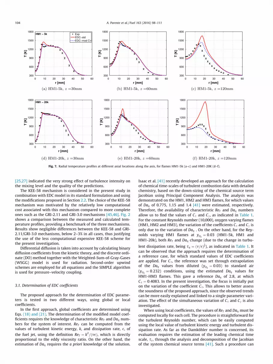
Fig. 7. Radial temperature profiles at different axial locations along the axis, for flames HM1-5k (a–c) and HM1-20K (d–f).

104 A. Parente et al. / Fuel 163 (2016) 98–111

[25,27] indicated the very strong effect of turbulence intensity onthe mixing level and the quality of the predictions.

The KEE-58 mechanism is considered in the present study incombination with EDC model in its standard formulation and usingthe modifications proposed in Section 2.2. The choice of the KEE-58mechanism was motivated by the relatively low computationalcost associated with this mechanism compared to more completeones such as the GRI-2.11 and GRI-3.0 mechanisms [45,46]. Fig. 2shows a comparison between the measured and calculated tem-perature profiles, providing a benchmark of the three mechanisms.Results show negligible differences between the KEE-58 and GRI-2.11/GRI-3.0 mechanisms, below 2–3% in all cases, thus justifyingthe use of the less computational expensive KEE-58 scheme forthe present investigation.

Differential diffusion is taken into account by calculating binarydiffusion coefficients from the kinetic theory, and the discrete ordi-nate (DO) method together with the Weighted-Sum-of-Gray-Gases(WSGG) model is used for radiation. Second-order upwindschemes are employed for all equations and the SIMPLE algorithmis used for pressure–velocity coupling.

3.1. Determination of EDC coefficients

The proposed approach for the determination of EDC parame-ters is tested in two different ways, using global or localcoefficients.

In the first approach, global coefficients are determined usingEqs. (18) and (21). The determination of the modified model coef-ficients requires the knowledge of characteristic ReT and Dag num-bers for the system of interest. ReT can be computed from thevalues of turbulent kinetic energy, k, and dissipation rate, �, ofthe fuel jet, using the definition ReT ¼ k2=ðm�Þ, which is directlyproportional to the eddy viscosity ratio. On the other hand, theestimation of Dag requires the a priori knowledge of the solution.

Isaac et al. [41] recently developed an approach for the calculationof chemical time-scales of turbulent combustion data with detailedchemistry, based on the down-sizing of the chemical source termJacobian using Principal Component Analysis. The analysis wasdemonstrated on the HM1, HM2 and HM3 flames, for which valuesof Dag of 0.775, 1.15 and 1.4 [41] were estimated, respectively.Therefore, the availability of characteristic ReT and Dag numbersallow us to find the values of Cs and Cc, as indicated in Table 1.For the constant Reynolds number (10,000), oxygen varying flames(HM1, HM2 and HM3), the variation of the coefficients Cs and Cc isonly due to the variation of Dag . On the other hand, for the Rey-nolds varying HM1 flames at yO2

¼ 0:03 (HM1-5k, HM1 andHM1-20k), both ReT and Dag change (due to the change in turbu-

lent dissipation rate, being sg ¼ ðm=�Þ12), as indicated in Table 1. Itcan be observed that the approach requires the determination ofa reference case, for which standard values of EDC coefficientsare applied. For Cs, the reference was set through extrapolationof the Dag values from diluted (yO2

¼ 0:03) to standard air(yO2

¼ 0:232) conditions, using the estimated Dag values forHM1-HM3 flames. This gave a reference Dag of 2.8, at whichCs ¼ 0:4083. In the present investigation, the focus is initially puton the variation of the coefficient Cs. This allows to better assessthe soundness of the proposed approach, since the observed trendscan be more easily explained and linked to a single parameter vari-ation. The effect of the simultaneous variation of Cs and Cc is alsoinvestigated.

When using local coefficients, the values of ReT and Dag must becomputed locally for each cell. The procedure is straightforward forthe turbulent Reynolds number, which can be easily computedusing the local value of turbulent kinetic energy and turbulent dis-sipation rate. As far as the Damköhler number is concerned, itsevaluation requires the estimation of the leading chemical timescale, sc , through the analysis and decomposition of the Jacobianof the system chemical source terms [41]. Such a procedure can

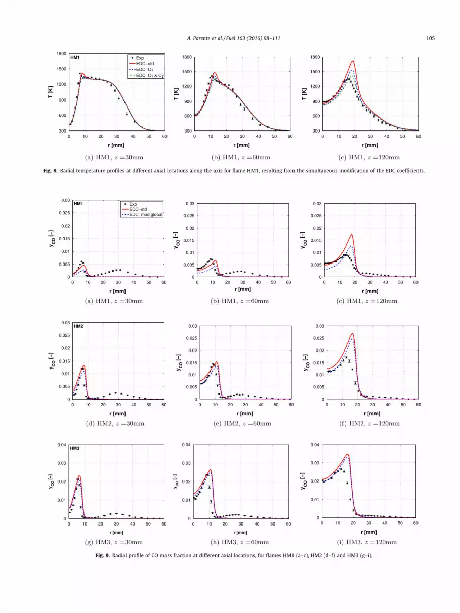
Fig. 8. Radial temperature profiles at different axial locations along the axis for flame HM1, resulting from the simultaneous modification of the EDC coefficients.

Fig. 9. Radial profile of CO mass fraction at different axial locations, for flames HM1 (a–c), HM2 (d–f) and HM3 (g–i).

A. Parente et al. / Fuel 163 (2016) 98–111 105

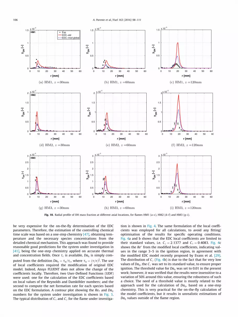
Fig. 10. Radial profile of OH mass fraction at different axial locations, for flames HM1 (a–c), HM2 (d–f) and HM3 (g–i).

106 A. Parente et al. / Fuel 163 (2016) 98–111

be very expensive for the on-the-fly determination of the EDCparameters. Therefore, the estimation of the controlling chemicaltime scale was based on a one-step chemistry [47], obtaining tem-perature and the necessary species concentrations from thedetailed chemical mechanism. This approach was found to providereasonable good predictions for the system under investigation in[41], being the one-step chemistry applied on accurate thermaland concentration fields. Once sc is available, Dag is simply com-

puted from the definition Dag ¼ sg=sc , where sg ¼ ðm=�Þ12. The useof local coefficients required the modification of original EDCmodel. Indeed, Ansys FLUENT does not allow the change of thecoefficients locally. Therefore, two User-Defined Functions (UDF)were used: one for the calculation of the EDC coefficients basedon local values of the Reynolds and Damköhler numbers; and thesecond to compute the net formation rate for each species basedon the EDC formulation. A contour plot showing the ReT and Dagnumbers for the system under investigation is shown in Fig. 3.The typical distribution of Cs and Cc for the flame under investiga-

tion is shown in Fig. 4. The same formulation of the local coeffi-cients was employed for all calculations, to avoid any fitting/optimisation of the results for specific operating conditions.Fig. 4a and b shows that the EDC local coefficients are limited totheir standard values, i.e. Cc ¼ 2:1377 and Cs ¼ 0:4083. Fig. 4cshows the Re� from the modified local coefficients, indicating val-ues in the range 3–5 in the ignition region, in agreement withthe modified EDC model recently proposed by Evans et al. [29].The distribution of Cc (Fig. 4b) is due to the fact that for very lowvalues of Dag, the Cc was set to its standard value, to ensure properignition. The threshold value for Dag was set to 0.01 in the presentwork; however, it was verified that the results were insensitive to avariation of 50% around this value, ensuring the robustness of sucha choice. The need of a threshold value is mostly related to theapproach used for the calculation of Dag, based on a one-stepchemistry. This is very practical for the on-the-fly calculation ofthe model coefficients, but it results in unrealistic estimations ofDag values outside of the flame region.

Fig. 11. Radial profile of CO2 mass fraction at different axial locations, for flames HM1 (a–c), HM2 (d–f) and HM3 (g–i).

A. Parente et al. / Fuel 163 (2016) 98–111 107

4. Results

This section describes the results obtained for the test cases atvarying co-flow concentrations and fuel-jet Reynolds numbers,with the objective of assessing the effect of the proposed modifica-tion of the EDC coefficients on the results. First, the results of theapproach based on global coefficients will be presented and dis-cussed. Then, the results of the local coefficients approach will beshown. To better assess the quantitative agreement betweenmodel predictions and measurements, the results shown in thepresent section do not only indicate the mean observed value ofthe scalar under consideration (temperature and species mass frac-tions) but also the 95% confidence for the true mean value, l, asso-ciated to the measurements, ye, calculated as [48]:

ye � ta2;m

sffiffiffin

p < l < ye þ ta2;m

sffiffiffin

p ð22Þ

where ta2;;m is the 1� a

2

� �quantile of Student’s t-distribution defined

by the n experimental observations. with m ¼ n� 1 degrees of free-dom, and s is the sample standard deviation,

s ¼ 1n� 1

Xni¼1

yie � ye� �2" #1

2

: ð23Þ

The calculation of the confidence intervals was made possible bythe availability of a large number of observations yie (�500) for eachmeasurement point.

4.1. Modified EDC – global coefficients

Fig. 5 shows the radial temperature profiles at different axiallocations, for flames HM1 (a–c), HM2 (d–f) and HM3 (g–i). Themodified EDC results shown are obtained through modificationof the coefficient Cs. It can be observed that the adjustment of Csdetermines a generalised improvement of predictions: the temper-ature over-prediction is strongly reduced and the radial tempera-ture distribution is better captured. At high axial distances, i.e.z ¼ 120 mm, the behaviour of the model remains unsatisfactory,although an improvement is noticeable with respect to the stan-dard EDC model. To further confirm the qualitative analysis based

Fig. 12. Radial profile of H2O mass fraction at different axial locations, for flames HM1 (a–c), HM2 (d–f) and HM3 (g–i).

108 A. Parente et al. / Fuel 163 (2016) 98–111

on the observation of Fig. 5, the relative error in the prediction ofthe maximum temperature at different axial locations is shownin Table 2. The peak temperature for the HM1 flame atz ¼ 120 mm decreased from 1716 K to about 1526 K, the experi-mental value being 1343 K, implying a reduction of the relativeerror from 28% to 14%. Similar improvements are observed forHM2 and HM3 flames, for which the error decreases from to 26%to 19% and from 20% to 16%, respectively. The trend is confirmedat all axial distances and for all flames, with the exception of loca-tion z ¼ 30 mm for HM1 flame, where the performances of stan-dard and modified models are comparable. In particular, themodified model performs remarkably well at z ¼ 60 mm whencompared to standard EDC settings. Interestingly, the coefficientmodification appears more beneficial as the departure from con-ventional combustion conditions is more important. This is ofstraightforward interpretation, being the developed model basedon theoretical considerations valid in the framework of distributedreaction regime limit. The quantitative results shown in Table 2support the proposed modification of the EDC coefficients and pro-vide a theoretical basis to previous results obtained by otherauthors [26–28].

The availability of experimental data at different fuel-jetReynolds numbers allows evaluating the performances of theproposed model when modifying the Reynolds number at theconditions of highest dilution (y02 ¼ 0:03Þ. The fuel-jet Reynoldsnumber is varied from 5000 (HM1-5k) to 20,000 (HM1-20k),resulting in different characteristic turbulent Reynolds numberswith respect to the base case (HM1) (Table 1). Fig. 7 shows theradial temperature profiles at different axial locations, for flamesHM1-5k (a–c) and HM1-20k (d–f). Results confirm the trendobserved for the varying oxygen cases, indicating that the modifiedmodel yields improved predictions of temperature distribution atboth Reynolds numbers. This is also proved by the quantitativeresults in Table 3, which shows in particular remarkable perfor-mances for the HM1-5k flame.

The HM1-20k flame deserves a separate discussion. The exper-imental data show a strong temperature reduction for increasingdistance from the burner nozzle, at z ¼ 120 mm, due to the partialextinction of the flame caused by the increased jet velocity. Thisphenomenon can be clearly observed in Fig. 6, which shows theinstantaneous temperature measurements as a function of themixture fraction for the HM1 flames at Reynolds numbers 10,000

Fig. 13. Radial temperature profiles at different axial locations, for flames HM1 (a–c), HM2 (d–f), HM3 (g–i) and HM1-5k (j–l).

A. Parente et al. / Fuel 163 (2016) 98–111 109

(a) and 20,000 (b), respectively. The amount of partial extinctionand re-ignition is significantly higher at higher Reynolds number,as indicated by the large data scatter in Fig. 6b compared toFig. 6a. This phenomenon is not captured by the standard EDCformulation, which results in a significant over-prediction of thetemperature levels at z ¼ 60 mm and z ¼ 120 mm (Table 3). The

modification of the EDC model coefficients improves the modelpredictions, as indicated by the error metrics in Table 3 and theradial temperature distributions in Fig. 7d–f. However, with themodified EDC formulation, the flame extinguishes for axialdistances higher than z ¼ 120 mm and the model is unable toreproduce the re-ignition observed experimentally. This indicates

110 A. Parente et al. / Fuel 163 (2016) 98–111

that the combination of RANS modelling with the EDC approach isnot adequate to model the HM1-20k flame, as the model provideseither a stable flame with temperature levels significantly higherthan those observed experimentally or an extinguishing but notre-ignition flame. It was attempted to model the HM1-20k flameusing the transported PDF approach, but this also resulted in globalextinction, as indicated in the literature [49]. This suggests thatmore complex approaches, i.e. unsteady simulations and/or LES,should be employed to model such a flame.

The effect of the simultaneous change of the two model coeffi-cients, Cs and Cc, on the results was also investigated. Fig. 8 showsthe radial temperature profiles at z ¼ 30 mm (a), z ¼ 60 mm (b)and z ¼ 120 mm (c) for the HM1 flame, providing a benchmarkbetween all the tested models. It appears evident that the modifi-cation of Cc has a minor influence at axial distances z < 60 mm,whereas a clear effect can be observed at z ¼ 120 mm, where theover-prediction of the temperature distribution is further reduced,leading to better agreement between measurements and simula-tions with respect to the case based on the modification of thecoefficient Cs only. This is confirmed quantitatively by the resultsin the first columns of Table 2, which shows a relative error metricfor maximum temperature decreasing from 13.6% to about 5%,when modifying simultaneously the two model coefficients.

To further assess the potential improvement associated withthe use of modified coefficients, the standard and modified formu-lation are compared against the experimental observation of major(CO2 and H2O) and minor species (CO) and radicals (OH). Fig. 9shows the radial profile of CO mass fraction at different axial loca-tions for the HM1 (a–c), HM2 (d–f) and HM3 (g–i) flames, using thestandard EDC formulation and the modified one with global coeffi-cients. The observed improvement in temperature distributions isexpected to yield better agreement for observed and measuredCO mass fractions. At z ¼ 30 mm for the HM1 case (Fig. 9a), themodified model formulation provides better prediction only farfrom the axis, underestimating the CO level at the centreline withrespect to the standard model. On the other hand, the improve-ments are significant and more clearly visible for the HM2 andHM3 (Fig. 9d and g, respectively), particularly at the centreline.The same conclusions can be drawn for the CO profiles atz ¼ 60 mm and at z ¼ 120 mm. A similar analysis for the OH radical(Fig. 10) shows that the use of the modified coefficients providesimproved results for increasing distances from the burner exit,whereas close to the burner the OH peak is better captured bythe standard EDC model. Moreover, it is possible to observe thatboth default and modified models perform poorly at z ¼ 120 mm.We mainly attribute this behaviour to the intermittent localisedflame extinction, documented in the literature for the flames underinvestigation [24,27], especially at diluted conditions. While the

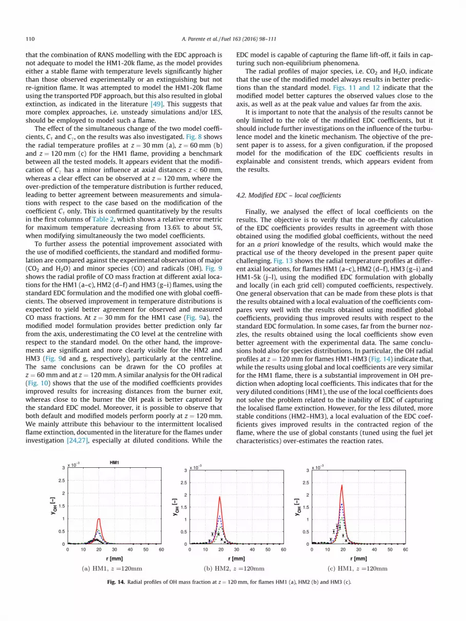
Fig. 14. Radial profiles of OH mass fraction at z ¼ 120

EDC model is capable of capturing the flame lift-off, it fails in cap-turing such non-equilibrium phenomena.

The radial profiles of major species, i.e. CO2 and H2O, indicatethat the use of the modified model always results in better predic-tions than the standard model. Figs. 11 and 12 indicate that themodified model better captures the observed values close to theaxis, as well as at the peak value and values far from the axis.

It is important to note that the analysis of the results cannot beonly limited to the role of the modified EDC coefficients, but itshould include further investigations on the influence of the turbu-lence model and the kinetic mechanism. The objective of the pre-sent paper is to assess, for a given configuration, if the proposedmodel for the modification of the EDC coefficients results inexplainable and consistent trends, which appears evident fromthe results.

4.2. Modified EDC – local coefficients

Finally, we analysed the effect of local coefficients on theresults. The objective is to verify that the on-the-fly calculationof the EDC coefficients provides results in agreement with thoseobtained using the modified global coefficients, without the needfor an a priori knowledge of the results, which would make thepractical use of the theory developed in the present paper quitechallenging. Fig. 13 shows the radial temperature profiles at differ-ent axial locations, for flames HM1 (a–c), HM2 (d–f), HM3 (g–i) andHM1-5k (j–l), using the modified EDC formulation with globallyand locally (in each grid cell) computed coefficients, respectively.One general observation that can be made from these plots is thatthe results obtained with a local evaluation of the coefficients com-pares very well with the results obtained using modified globalcoefficients, providing thus improved results with respect to thestandard EDC formulation. In some cases, far from the burner noz-zles, the results obtained using the local coefficients show evenbetter agreement with the experimental data. The same conclu-sions hold also for species distributions. In particular, the OH radialprofiles at z ¼ 120 mm for flames HM1-HM3 (Fig. 14) indicate that,while the results using global and local coefficients are very similarfor the HM1 flame, there is a substantial improvement in OH pre-diction when adopting local coefficients. This indicates that for thevery diluted conditions (HM1), the use of the local coefficients doesnot solve the problem related to the inability of EDC of capturingthe localised flame extinction. However, for the less diluted, morestable conditions (HM2–HM3), a local evaluation of the EDC coef-ficients gives improved results in the contracted region of theflame, where the use of global constants (tuned using the fuel jetcharacteristics) over-estimates the reaction rates.

mm, for flames HM1 (a), HM2 (b) and HM3 (c).

A. Parente et al. / Fuel 163 (2016) 98–111 111

We can therefore conclude that the use of local coefficients forEDC is a viable option for the practical implementation of the pro-posed functional dependencies between the EDC coefficients andthe dimensionless ReT and Dag numbers. The use of local coeffi-cients has clear advantages over the use of global ones, as it doesnot require prior knowledge of the characteristic dimensionlessnumbers (ReT and Dag) in the system. Moreover, it should bestressed out that the use of local coefficients does not have animpact on the simulation time, as the latter is dominated by thechemistry integration time. This method can thus be seen as aneffective way for on-the-fly calculations.

5. Conclusions

The Eddy Dissipation Concept (EDC) for turbulent combustion iswidely used to model turbulent reacting flows where chemicalkinetics may play an important role, as it is the case for MILD com-bustion. However, recent investigations have pointed out the lim-itations of the approach for such a regime. The present paperproposes a modification of the EDC model coefficients to allowits application in the context of MILD conditions. The main findingsof the present work can be summarised as follows:

� The energy cascade model, on which EDC is founded, was revis-ited in the limit of the distributed reaction regime, to deriveexplicit dependencies between the EDC model coefficients andthe Reynolds and Damköhler dimensionless numbers.

� The proposed approach was validated on several data sets col-lected on the JHC burner with different co-flow composition(3%, 6% et 9% O2 mass fraction) and fuel-jet Reynolds numbers(5000, 10,000 and 20,000). For the 20,000 Reynolds numbercase, the modification of the EDC model coefficients improvesthe model predictions close to the burner. However, the modelis unable to reproduce the re-ignition observed experimentallyat higher axial distance. This does not appear related to the EDCmodel itself, rather to the RANS modelling limitations.

� The proposed approach was first validated using modified glo-bal coefficients, determined on the basis of available simulationresults. Results based on the variation of the time scale coeffi-cient, Cs, show promising improvement with respect to thestandard EDC formulation close to the burner, especially atdiluted conditions and medium to low Reynolds numbers, forboth temperature and species measurements. Moreover, thesimultaneous modification of the time scale, Cs, and the massfraction coefficients, Cc, leads to improvements in the modelpredictions at large axial distances from the burner exit.

� The proposed approach was then validated using a local evalu-ation of the EDC model coefficients, using the local values of ReTand Dag numbers. The ReT value was estimated from the localvalues of turbulent kinetic energy and dissipation rate, whileDag was obtained from a one-step reaction, using the tempera-ture and species concentrations coming from the detailedmechanism employed for the gas-phase reactions. Results fromthe local approach are comparable or superior to those providedvia the modification of the global coefficients, thus indicatingthe viability of the approach.

Future work will investigate the influence of the turbulencemodel and kinetic mechanism on the predictions and their impacton the modified coefficients, using validation data from experi-ments and Direct Numerical Simulations. Moreover, more accurateapproaches for the determination of the chemical time-scale andDag number will be investigated.

Acknowledgements

The first and second Authors would like to acknowledge thesupport of Fédération Wallonie-Bruxelles, via ‘‘Les Actions deRecherche Concertée (ARC)” call for 2014–2019, to support funda-mental research.

References

[1] Wünning JA, Wünning JG. Prog Energy Combust Sci 1997;23:81–94.[2] Cavaliere A, de Joannon M. Prog Energy Combust Sci 2004;30:329–66.[3] Gupta AK. J Eng Gas Turbines Power 2004;126:9–19.[4] Choi GM, Katsuki M. Energy Convers Manage 2001;42:639–52.[5] Dally BB, Riesmeier E, Peters N. Combust Flame 2004;137:418–31.[6] Szego GG, Dally BB, Nathan GJ. Combust Flame 2008;154:281–95.[7] de Joannon M, Sabia P, Sorrentino G, Cavaliere A. Proc Combust Inst

2009;32:3147–54.[8] de Joannon M, Sorrentino G, Cavaliere A. Combust Flame 2012;159:1832–9.[9] Mardani A, Tabejamaat S, Hassanpour S. Combust Flame 2013;160:

1636–49.[10] Zou C, Cao S, Song Y, He Y, Guo F, Zheng C. Fuel 2014;130:10–8.[11] Hosseini SE, Wahid MA. Energy Convers Manage 2013;74:426–32.[12] Abuelnuor A, Wahid M, Hosseini SE, Saat A, Saqr KM, Sait HH, et al. Renew

Sustain Energy Rev 2014;33:363–70.[13] Mosca G, Lupant D, Gambale A, Lybaert P. In: Proceedings European

combustion meeting, Lund, Sweden.[14] Hosseini SE, Bagheri G, Wahid MA. Energy Convers Manage 2014;81:41–50.[15] Derudi M, Villani A, Rota R. Ind Eng Chem Res 2007;46:6806–11.[16] Sabia P, de Joannon M, Fierro S, Tregrossi A, Cavaliere A. Exp Therm Fluid Sci

2007;31:469–75.[17] Parente A, Galletti C, Tognotti L. Int J Hydrogen Energy 2008;33:7553–64.[18] Parente A, Sutherland J, Dally B, Tognotti L, Smith P. Proc Combust Inst

2011;33:3333–41.[19] Dally BB, Karpetis AN, Barlow RS. Proc Combust Inst 2002;29:1147–54.[20] Galletti C, Parente A, Derudi M, Rota R, Tognotti L. Int J Hydrogen Energy

2009;34:8339–51.[21] Parente A, Galletti C, Tognotti L. Proc Combust Inst 2011;33:3343–50.[22] Parente A, Galletti, Riccardi J, Schiavetti M, Tognotti L. Appl Energy

2012;89:203–14.[23] Magnussen BF. In: 19th AIAA aerospace science meeting, 1981.[24] Christo FC, Dally BB. Combust Flame 2005;142:117–29.[25] Frassoldati A, Sharma P, Cuoci A, Faravelli T, Ranzi E. Appl Therm Eng

2010;30:376–83.[26] De A, Oldenhof E, Sathiah P, Roekaerts D. Flow Turbul Combust

2011;87:537–67.[27] Aminian J, Galletti C, Shahhosseini S, Tognotti L. Flow Turbul Combust

2012;88:597–623.[28] Shabanian SR, Medwell PR, Rahimi M, Frassoldati A, Cuoci A. Appl Therm Eng

2013;52:538–54.[29] Evans M, Medwell P, Tian Z. Combust Sci Technol 2015;187:1093–109.[30] Shiehnejadhesar A, Mehrabian R, Scharler R, Goldin GM, Obernberger I. Fuel

2014;126:177–87.[31] Pope S. Combust Theor Model 1997;1:41–63.[32] Ertesvåg IS, Magnussen BF. Combust Sci Technol 2001;159:213–36.[33] Gran IR, Magnussen BF. Combust Sci Technol 1996;119:191–217.[34] Minamoto Y, Swaminathan N, Cant RS, Leung T. Combust Sci Technol

2014;186:1075–96.[35] Poinsot T, Veynante D. Theoretical and numerical combustion. R.T. Edwards,

Inc.; 2001.[36] Kuo K, Acharya R. Fundamentals of turbulent and multi-phase

combustion. Wiley; 2012.[37] Damköhler G. Zs Electrochemie 1940;6:601–52.[38] Minamoto Y, Swaminathan N. Int J Adv Eng Sci Appl Math 2014;6:65–75.[39] Duwig C, Fuchs L. Combust Sci Technol 2008;180:453–80.[40] Duwig C, Iudiciani P. Fuel 2014;123:256–73.[41] Isaac BJ, Parente A, Galletti C, Thornock JN, Smith PJ, Tognotti L. Energy Fuels

2013;27:2255–65.[42] Roache PJ. Verification and validation in computational science and

engineering. Albuquerque, NM: Hermosa Publishers; 1998.[43] Bilger R, Starner S, Kee R. Combust Flame 1990;80:135–49.[44] Morse AP. Axisymmetric turbulent shear flows with and without swirl [Ph.D.

thesis]. London University; 1977.[45] Bowman C, Hanson R, Davidson D, Gardiner JWC, Lissianski V, Smith G, et al.

GRI-Mech 2.11; 1995.[46] Smith GP, Golden DM, Frenklach M, Eiteener B, Goldenberg M, Bowman CT,

et al. GRI-Mech 3.0; 2000.[47] Westbrook C, Dryer F. Prog Energy Combust Sci 1984;10:1–57.[48] Oberkampf WL, Barone MF. J Comput Phys 2006;217:5–38.[49] Christo FC, Szego GG, Dally BB. In: 5th Asia-Pacific conference on combustion,

Adelaide, July 2005.