A theoretical model for the study of convective turbulence decay and comparison with large-eddy...

A THEORETICAL MODEL FOR THE STUDY OF CONVECTIVE

TURBULENCE DECAY AND COMPARISON WITH LARGE-EDDY

SIMULATION DATA

A. GOULARTURI-DCET, Santo Ângelo, Brazil

G. DEGRAZIA⋆

UFSM-DF, Santa Maria, Brazil

U. RIZZACNR-ISAC, Lecce, Italy

D. ANFOSSICNR-ISAC, Torino, Italy

(Received in final form 15 May 2002)

Abstract. The development of a theoretical model for a decaying convective boundary layer is

considered. The model relies on the dynamical energy spectrum equation in which the buoyancy and

inertial transfer terms are retained, and a closure assumption made for both. The parameterization

for the buoyancy term is given providing a factorization between the energy source term and its

temporal decay. Regarding the inertial transfer term a hypothesis of superposition is used to describe

the convective energy source and time variation of velocity correlation separately. The solution of the

budget equation for the turbulent kinetic energy spectrum is possible, given the three-dimensional

initial energy spectrum. This is done utilizing a version of the Kristensen et al. (see Boundary-LayerMeteorol. 47, 149–193) model valid for non-isotropic turbulence. During the decay the locus of

the spectral peak remains at about the same position as the heat flux decreases. Comparison of

the theoretical model is performed against large-eddy simulation data for a decaying convective

boundary layer.

Keywords: Convective boundary layer, Kinetic energy, Large-eddy simulation, Spectrum, Turbu-

lence decay.

1. Introduction

About half hour before sunset over land, the surface heat flux (positive during

the day) begins to decrease and then, during night-time, becomes negative and,

consequently, a stable boundary layer (SBL) develops near the ground. Above

this SBL, the convective boundary layer (CBL) starts to decay. The three main

physical processes governing the turbulence decay in the CBL are: The decay of

energy-containing eddies, the shear-driven turbulence generation and the turbu-

⋆ Corresponding author: Gervasio Annes Degrazia, Universidade Federal de Santa Maria, De-

partamento de Fısica/CCNE, 97105–900, Santa Maria, RS, Brazil, E-mail: [email protected]

Boundary-Layer Meteorology 107: 143–155, 2003.

© 2003 Kluwer Academic Publishers. Printed in the Netherlands.

144 A. GOULART ET AL.

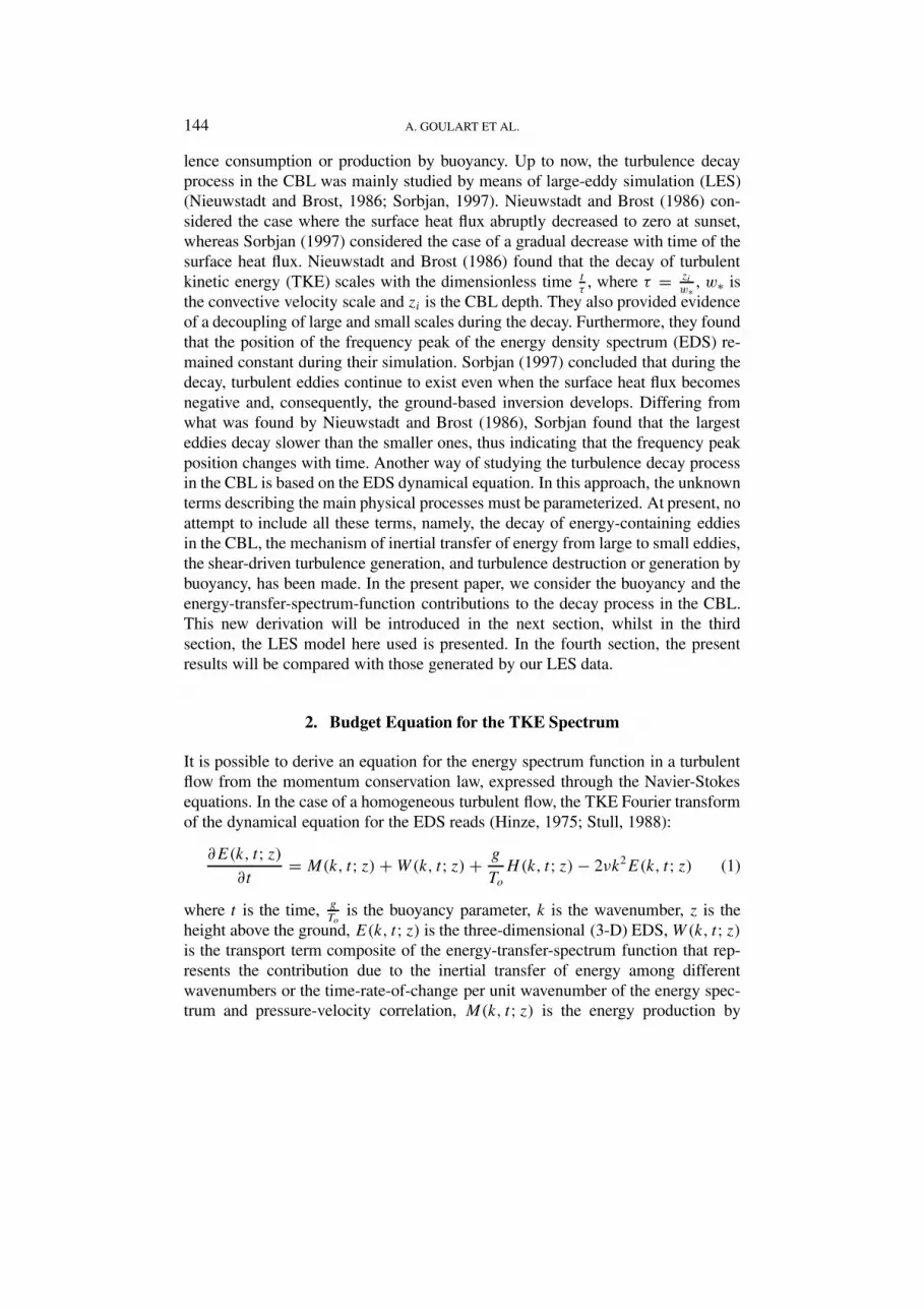
lence consumption or production by buoyancy. Up to now, the turbulence decay

process in the CBL was mainly studied by means of large-eddy simulation (LES)

(Nieuwstadt and Brost, 1986; Sorbjan, 1997). Nieuwstadt and Brost (1986) con-

sidered the case where the surface heat flux abruptly decreased to zero at sunset,

whereas Sorbjan (1997) considered the case of a gradual decrease with time of the

surface heat flux. Nieuwstadt and Brost (1986) found that the decay of turbulent

kinetic energy (TKE) scales with the dimensionless time tτ, where τ =

ziw∗

, w∗ is

the convective velocity scale and zi is the CBL depth. They also provided evidence

of a decoupling of large and small scales during the decay. Furthermore, they found

that the position of the frequency peak of the energy density spectrum (EDS) re-

mained constant during their simulation. Sorbjan (1997) concluded that during the

decay, turbulent eddies continue to exist even when the surface heat flux becomes

negative and, consequently, the ground-based inversion develops. Differing from

what was found by Nieuwstadt and Brost (1986), Sorbjan found that the largest

eddies decay slower than the smaller ones, thus indicating that the frequency peak

position changes with time. Another way of studying the turbulence decay process

in the CBL is based on the EDS dynamical equation. In this approach, the unknown

terms describing the main physical processes must be parameterized. At present, no

attempt to include all these terms, namely, the decay of energy-containing eddies

in the CBL, the mechanism of inertial transfer of energy from large to small eddies,

the shear-driven turbulence generation, and turbulence destruction or generation by

buoyancy, has been made. In the present paper, we consider the buoyancy and the

energy-transfer-spectrum-function contributions to the decay process in the CBL.

This new derivation will be introduced in the next section, whilst in the third

section, the LES model here used is presented. In the fourth section, the present

results will be compared with those generated by our LES data.

2. Budget Equation for the TKE Spectrum

It is possible to derive an equation for the energy spectrum function in a turbulent

flow from the momentum conservation law, expressed through the Navier-Stokes

equations. In the case of a homogeneous turbulent flow, the TKE Fourier transform

of the dynamical equation for the EDS reads (Hinze, 1975; Stull, 1988):

∂E(k, t; z)

∂t= M(k, t; z) + W(k, t; z) +

g

ToH(k, t; z) − 2νk2E(k, t; z) (1)

where t is the time,g

Tois the buoyancy parameter, k is the wavenumber, z is the

height above the ground, E(k, t; z) is the three-dimensional (3-D) EDS, W(k, t; z)

is the transport term composite of the energy-transfer-spectrum function that rep-

resents the contribution due to the inertial transfer of energy among different

wavenumbers or the time-rate-of-change per unit wavenumber of the energy spec-

trum and pressure-velocity correlation, M(k, t; z) is the energy production by

A THEORETICAL MODEL FOR THE STUDY OF CONVECTIVE TURBULENCE DECAY 145

mechanical (shear) effects, H(k, t; z) is the production or loss due to buoyancy

contribution and the last term on the r.h.s. of Equation (1) is the energy loss due to

viscous dissipation.

An analytical solution of Equation (1) is not yet available. In this study we take

into account the case in which the buoyancy and inertial energy transfer terms are

important. Under this condition, Equation (1) becomes

∂E(k, t; z)

∂t= W(k, t; z) +

g

T0

H(k, t; z) − 2νk2E(k, t; z). (2)

2.1. BUOYANCY EFFECT PARAMETERIZATION

In order to consider the time variation of the buoyancy production or loss term

of Equation (2), we assume that g

T0H(k, t; z) can be split into two functions, as

follows:

g

T0

H(k, t; z) =g

T0

H0(k; z)T (t) (3)

in which T (t) is a dimensionless function describing the temporal decrease of

surface heat flux and H0(k; z) (= H(k, 0; z)) depends only on the initial conditions,

that is from the quantities characterizing the turbulent flux in the CBL before the

beginning of the decay.

To determine H0(k; z) the Batchelor (1953) hypothesis, which assumed that the

transfer of energy from the mean flux occurs in a continuous way, will be con-

sidered. This allows, in particular, no explicit reference to any characteristic time

scale. Considering that H0(k; z) depends upon the vertical potential temperature

gradient (which, for a well-mixed layer, is represented by the countergradient term

γc), on the wavenumber k, on the rate of TKE dissipation ε and on the intensity

of kinetic energy of the eddy centred around the wavenumber k, i.e., kE0(k; z)

(kE0(k; z) being the CBL 3-D spectrum at the decay beginning) it is possible to

perform a dimensional analysis (Buckingham theorem) giving:

g

T0

H0(k; z) =g

T0

γcc1ε− 1

3 k− 23E0(k; z), (4)

where c1 is a dimensionless constant to be determined from experiments or model

simulations, γc ≈ 10−3 K m−1 (Nieuwstadt and Brost, 1986).

To calculate the dimensionless constant c1 we first consider Equation (4) and

the expression suggested by Moeng and Sullivan (1994) for the buoyancy term in

a CBL

g

T0

H0(z) =w3

∗

zi(1 − 1.2

z

zi). (5)


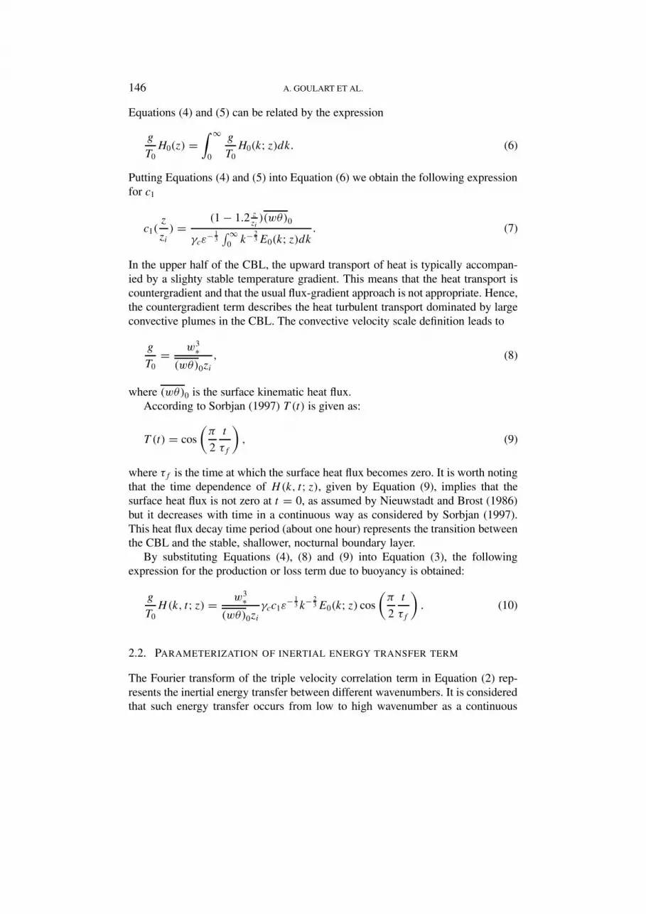
Equations (4) and (5) can be related by the expression

g

T0

H0(z) =

∫ ∞

0

g

T0

H0(k; z)dk. (6)

Putting Equations (4) and (5) into Equation (6) we obtain the following expression

for c1

c1(z

zi) =

(1 − 1.2 zzi)(wθ)0

γcε− 1

3

∫ ∞

0k− 2

3E0(k; z)dk. (7)

In the upper half of the CBL, the upward transport of heat is typically accompan-

ied by a slighty stable temperature gradient. This means that the heat transport is

countergradient and that the usual flux-gradient approach is not appropriate. Hence,

the countergradient term describes the heat turbulent transport dominated by large

convective plumes in the CBL. The convective velocity scale definition leads to

g

T0

=w3

∗

(wθ)0zi, (8)

where (wθ)0 is the surface kinematic heat flux.

According to Sorbjan (1997) T (t) is given as:

T (t) = cos

(

π

2

t

τf

)

, (9)

where τf is the time at which the surface heat flux becomes zero. It is worth noting

that the time dependence of H(k, t; z), given by Equation (9), implies that the

surface heat flux is not zero at t = 0, as assumed by Nieuwstadt and Brost (1986)

but it decreases with time in a continuous way as considered by Sorbjan (1997).

This heat flux decay time period (about one hour) represents the transition between

the CBL and the stable, shallower, nocturnal boundary layer.

By substituting Equations (4), (8) and (9) into Equation (3), the following

expression for the production or loss term due to buoyancy is obtained:

g

T0

H(k, t; z) =w3

∗

(wθ)0ziγcc1ε

− 13 k− 2

3E0(k; z) cos

(

π

2

t

τf

)

. (10)

2.2. PARAMETERIZATION OF INERTIAL ENERGY TRANSFER TERM

The Fourier transform of the triple velocity correlation term in Equation (2) rep-

resents the inertial energy transfer between different wavenumbers. It is considered

that such energy transfer occurs from low to high wavenumber as a continuous


process (Batchelor, 1953). Pao (1965) suggested an expression for the energy flux

valid for isotropic turbulence in the high Reynolds number regime. On the other

hand Frisch (1995, Eqs. 6.8 and 6.17), starting his considerations from the Karman-

Howarth-Monin equation (Monin and Yaglom, 1975), showed that the energy flux

is directly related to the time variations of mean velocity correlation and the en-

ergy source term. These results were obtained for homogeneous, but non-isotropic,

turbulence. Following Frisch’s deductions, we can parameterize the inertial energy

transfer term in Equation (2) as:

W(k, t; z) = Wa(k, t; z) + Wb(k, t; z). (11)

The first term on the r.h.s. is related to the time variations of mean velocity correl-

ations independently of the existence of the energy source. In this hypothesis, the

expression suggested by Pao (1965), can be used, namely

Wa(k, t; z) = −∂

∂k

(

α−1ε13 k

53E(k, t; z)

)

, (12)

where α is the Kolmogoroff constant (α ≈ 1.5).

The second term is related to the source of convective energy (large eddies),

and as a consequence Wb(k, t; z) is zero in the inertial subrange (small eddies). A

condition that must be imposed on the function Wb(k, t; z) is that the modulus of its

maximum value should be localized in a wavenumber range close to the maximum

of the heat flux cospectrum [g

T0H(k, t; z)]. Utilizing the dimensional analysis, an

expression that satisfies such a condition can be obtained, as:

Wb(k, t; z) = −∂

∂k

(

c2

w∗ziε

23 k

13E(k, t; z)

)

(13)

where c2 is a dimensionless constant determined from initial conditions.

To determine the dimensionless constant c2 we consider the component of in-

ertial energy transfer term related to the source of convective energy Wb(k, 0; z),

and given by Equation (13). We demand that the modulus of the maximum of this

term coincides with the modulus of the maximum of buoyancy term as suggested

by Moeng and Sullivan (1994) and estimated from Equation (5). As a consequence

we can write the following relation

[

|g

T0

H(k, 0, z)|

]

max

= [| − Wb(k, 0, z)|]max . (14)

Substituting Equations (13), (6) and (5) into Equation (14) yields an expression for

c2

c2

(

z

zi

)

=w4

∗(1 − 1.2 zzi)ε− 2

3

∫ ∞

0

∂

∂k(k

13E0(k; z))dk

. (15)


Considering Equations (10)–(13) and introducing the following dimensionless

parameters

t∗ =w∗t

zi, Re =

w∗zi

ν, #ε =

εzi

w3∗

(16)

we can write Equation (2) as follows

∂E(k′, t∗; z′)

∂t∗+

(

α−1#13ε (k

′)53 + c2#

23ε (k

′)13

)∂E(k′, t∗; z′)

∂k′

+

(

5

3α−1#

13ε (k

′)23 +

1

3c2#

23ε (k

′)−23 +

2

Re

(k′)2

)

E(k′, t∗; z′)

=w∗zi

(wθ)0

γcc1#− 1

3ε (k′)−

23E0(k

′, z′) cos

(

π

2

zi

w∗τft∗

)

, (17)

where k′ = kzi and z′ = zzi

.

Applying the Laplace transform to Equation (17), we obtain:

dE(k′, s; z′)

dk′+ η(k′, s; z′)E(k′, s; z′) = µ(k′, s; z′), (18)

where E(k′, s; z′) = L[E(k′, t∗; z′); t∗ → s], and

η(k′, s; z′) =s + 5

3α−1#

13ε (k

′)23 + 1

3c2#

23ε (k

′)−23 + 2

Re(k′)2

α−1#13ε (k′)

53 + c2#

23ε (k′)

13

, (19)

µ(k′, s; z′) =

(

w∗zi(wθ)0

γcc1#− 1

3ε (k′)−

23E0(k

′; z′))

s

s2+B2 + E0(k′; z′)

α−1#13ε (k′)

53 + c2#

23ε (k′)

13

, (20)

with B =(

π2

)

ziw∗τf

.

The well-known solution of Equation (18), given that t∗ = 0 → E(k′, t∗; z′) =

0, is

E(k′, s; z′) = e−∫ k′

0 η(k′′,s;z′)dk′′

∫ k′

0

e∫ ς

0η(k′′,s;z′)dk′′

µ(ς, s; z′)dς. (21)

Henceforth, the energy spectrum function E(k′, t∗; z′) is obtained by numeric-

ally inverting the transformed spectrum function E(k′, s; z′) using the Gaussian

quadrature scheme (Heydarian and Mullineaux, 1989),

E(k′, t∗; z′) =

8∑

i=1

AisE(k′, s; z′) (22)


with s =Pi

t∗. The parameters Ai and Pi are weights and roots, respectively, of the

Gaussian Quadrature scheme and are tabulated in Stroud and Secrest (1966).

The dynamical equation describing the turbulent flow is valid only in 3-D

space. Consequently, the spectrum E0(k; z) that represents the initial condition in

Equation (22) is the CBL turbulent 3-D spectrum. Since we are here considering

non-isotropic turbulence, we will use the formulation proposed by Kristensen et al.

(1989). This formulation allows determining the 3-D spectrum of a homogeneous

turbulent flow from the known 1-D spectra, namely:

E0(k; z) = k3 d

dk

1

k

dFL(k)

dk+ 2k4

∫ 1

k2

0

S2g′′′(S; z)dS

−14

9k

43

∫ 1

k2

0

S23g′′′(S; z)dS, (23)

with

FL(k) =ℓLσ

2L

π

1{

1 +

(

ℓLk

a(µL)

)2µL

}5

6µL

, (24)

where ℓL is the integral length, σL is the longitudinal component variance of the

velocity and µL is a dimensionless parameter. The function g′′′(s) is defined by the

following expression (Kristensen, 1989),

g′′′(s) = 2f ′′′o (σL, ℓL, µL;S) − f ′′′

o (σT , ℓT , µT ;S) − f ′′′o (σV , ℓV , µV ;S), (25)

with

S =1

k2(26)

and

f ′′′o (σi, ℓi, µi;S) =

(

1

96π

)

σ 2i a

2(µi)

ℓi

(

a2(µi)

ℓ2i

S

)− 16

×

4∑

n=1

Cn(µi){

1 +

(

a2(µi)

ℓ2i

S

)µi}

56µi

+n, (27)

where i = u, v,w represent the longitudinal, crosswind and vertical components.

The parameters σi, ℓi and µi are extracted from Kristensen et al. (1989, Figure 3).


TABLE I

The initial and calculated CBL parameters. Data from experiment B of Moeng

and Sullivan (1994).

Initial parameters Simulated CBL parameters

(zi)0 (Ug, Vg) (wθ)0 u∗ w∗ ziziL τ

m m s−1 m s−1 K m s−1 m s−1 m s

1100 10.0 0.24 0.56 2.02 1100 −18 540

3. Large-Eddy Simulation

Large-eddy simulation is a modelling technique first used in planetary boundary-

layer (PBL) meteorology by Deardorff (1972). This technique can be used to

predict turbulent characteristics of the PBL with high spectral resolution. In this

sense it can be seen as a surrogate of field data. The LES model used in the present

study was developed by C.H. Moeng at the National Center for Atmospheric Re-

search and described in detail by Moeng (1984) and Sullivan et al. (1994). The

numerical scheme is pseudo-spectral in the horizontal, with second-order centered

finite difference in the vertical direction. The grid resolution is 963 in a (5 × 5 × 2)

km3 domain. With such resolution the sub-grid eddies are of such small size that

they receive their own energy from the energy cascade, and are thus less sensitive

to flow geometry. The eddy viscosity model is the new formulation proposed by

Sullivan et al. (1994); this in particular allows better matching with surface-layer

similarity theory, as showed by the authors.

3.1. DESCRIPTION OF THE NUMERICAL EXPERIMENT

Turbulent regimes are generated by varying geostrophic wind and surface ver-

tical heat flux. Moeng and Sullivan (1994) made a sensitivity analysis over such

forcing parameters generating different turbulent regimes. We utilized data from

their labelled experiment B to initialize our simulation; the initial and calculated

CBL parameters are depicted in Table I, where (zi)0 is the initial inversion height,

(Ug, Vg) are the components of geostrophic wind, (wθ)0 is the surface temperature

flux, u∗ the friction velocity and finally τ is the large-eddy turnover time. Our

simulation lasted around 17 turnover times to reach a nearly stationary CBL, and

we started the decaying simulation from such a nearly stationary CBL state. Heat

flux was progressively reduced according to Sorbjan (1997),

(wθ)t = (wθ)0 cos

(

πt

2τf

)

, (28)

where τf = 5τ is the time at which heat flux becomes zero.


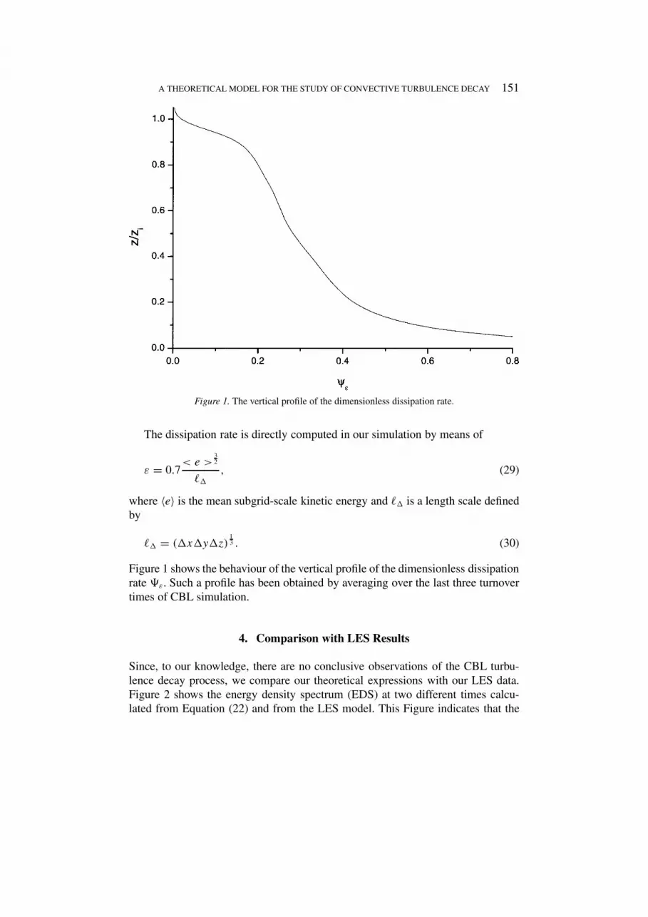
Figure 1. The vertical profile of the dimensionless dissipation rate.

The dissipation rate is directly computed in our simulation by means of

ε = 0.7< e >

32

ℓ8, (29)

where 〈e〉 is the mean subgrid-scale kinetic energy and ℓ8 is a length scale defined

by

ℓ8 = (8x8y8z)13 . (30)

Figure 1 shows the behaviour of the vertical profile of the dimensionless dissipation

rate #ε. Such a profile has been obtained by averaging over the last three turnover

times of CBL simulation.

4. Comparison with LES Results

Since, to our knowledge, there are no conclusive observations of the CBL turbu-

lence decay process, we compare our theoretical expressions with our LES data.

Figure 2 shows the energy density spectrum (EDS) at two different times calcu-

lated from Equation (22) and from the LES model. This Figure indicates that the


Figure 2. Temporal evolution of the 3-D energy density spectrum calculated at two different times

and averaged in the interval 0.2 ≤ zzi

≤ 0.8. The solid lines are calculated from Equation (22),

whereas dashed lines are simulated from LES model.

locus of EDS frequency peak calculated from LES data shifts slightly to larger

wavenumbers. However, for the whole convective turbulence decaying time, this

shifting is quite small, implying that for the characteristic sunset transition time

our theoretical spectrum agrees fairly well with the spectrum generated by LES

data. Curves are averaged over the height interval 0.2 ≤ zzi

≤ 0.8. In such a figure

the loss of turbulent energy is quite evident. Furthermore, to proceed with this

comparison we computed the turbulent kinetic energy per unit of mass averaged

over the domain volume, that is:

1

2σ 2(t) =

1

zi

∫ zi

0

< e > dz. (31)

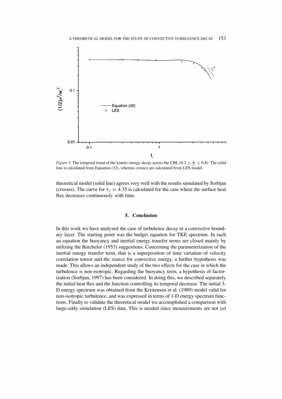
Figure 3 shows the temporal trend of the kinetic energy decay across the CBL

(0.2 ≤ zzi

≤ 0.8), made dimensionless by w2∗, as a function of t∗ (crosses). On

the other hand, Equation (22) gives the energy spectrum function, which can be

integrated to get the total energy, that is

1

2σ 2(t; z) =

∫ ∞

0

E(k, t; z)dk. (32)

This is indicated as the solid line in Figure 3, which points out the good agreement

between our theoretical model and LES data. Furthermore, Figure 4 shows that our


Figure 3. The temporal trend of the kinetic energy decay across the CBL (0.2 ≤ zzi

≤ 0.8). The solid

line is calculated from Equation (32), whereas crosses are calculated from LES model.

theoretical model (solid line) agrees very well with the results simulated by Sorbjan

(crosses). The curve for τf = 4.35 is calculated for the case where the surface heat

flux decreases continuously with time.

5. Conclusion

In this work we have analyzed the case of turbulence decay in a convective bound-

ary layer. The starting point was the budget equation for TKE spectrum. In such

an equation the buoyancy and inertial energy transfer terms are closed mainly by

utilizing the Batchelor (1953) suggestions. Concerning the parameterization of the

inertial energy transfer term, that is a superposition of time variation of velocity

correlation tensor and the source for convective energy, a further hypothesis was

made. This allows an independent study of the two effects for the case in which the

turbulence is non-isotropic. Regarding the buoyancy term, a hypothesis of factor-

ization (Sorbjan, 1997) has been considered. In doing this, we described separately

the initial heat flux and the function controlling its temporal decrease. The initial 3-

D energy spectrum was obtained from the Kristensen et al. (1989) model valid for

non-isotropic turbulence, and was expressed in terms of 1-D energy spectrum func-

tions. Finally to validate the theoretical model we accomplished a comparison with

large-eddy simulation (LES) data. This is needed since measurements are not yet


Figure 4. The temporal trend of the kinetic energy decay across the CBL (0.2 ≤ zzi

≤ 0.8). The solid

line is calculated from Equation (32). The crosses represent results obtained by Sorbjan from LES

model.

available for decay in the convective boundary layer. We utilized the initial mean

fields as described by Moeng and Sullivan (1994) to initialize our LES simulation.

Similarly the results of the present theoretical model were compared with LES

simulations accomplished by Sorbjan. The comparisons are pretty good for the

characteristic sunset transition time (1 hr). The modelling presented in this work is

potentially useful if one is interested in the study of dispersion parameterization in

a decaying CBL.

Acknowledgement

This work was partially supported by CNPq and FAPERGS.

References

Batchelor, G. K.: 1953, The Theory of Homogeneous Turbulence, Cambridge University Press, U.K.,

197 pp.

Deardorff, J. W.: 1972, ‘Numerical Investigation of Neutral and Unstable Planetary Boundary

Layers’, J. Atmos. Sci. 29, 91–115.

Frisch, U.: 1995, Turbulence, Cambridge University Press, U.K., 296 pp.


Heydarian, M. and Mullineaux, N.: 1989, ‘Solution of Parabolic Partial Differential Equations’, Appl.Math. Model. 5, 448–449.

Hinze, J. O.: 1975, Turbulence, McGraw Hill, 790 pp.

Kristensen, L., Lenschow, D., Kirkegaard, P., and Courtney, M.: 1989, ‘The Spectral Velocity Tensor

For Homogeneous Boundary-Layer Turbulence’, Boundary-Layer Meteorol. 47, 149–193.

Moeng, C. H.: 1984, ‘A Large Eddy Simulation Model for the Study of Planetary Boundary Layer

Turbulence’, J. Atmos. Sci. 41, 2052–2061.

Moeng, C. H. and Sullivan, P. P.: 1994, ‘A Comparison of Shear- and Buoyancy-Driven Planetary

Boundary Layer Flows’, J. Atmos. Sci., 51, 999–1022.

Monin, A. S. and Yaglom, A. M.: 1975, Statistical Fluid Mechanics: Mechanics of Turbulence, Vol.

2, MIT Press, Cambridge, 874 pp.

Nieuwstadt, F. T. M. and Brost, R. A.: 1986, ‘The Decay of Convective Turbulence’, J. Atmos. Sci.43, 532–546.

Pao, Y. H.: 1965, ‘Structure of Turbulent Velocity and Scalar Fields at Large Wavenumbers’, Phys.Fluids 8, 1063–1075.

Sorbjan, Z.: 1997, ‘Decay of Convective Revisited’, Boundary-Layer Meteorol. 82, 501–515.

Stroud, A. H., and Secrest, D.: 1966, Gaussian Quadrature Formulas, Prentice Hall, 334 pp.

Stull, R. B.: 1988, An Introduction to Boundary Layer Meteorology, Kluwer Academic Publishers,

Boston, 666 pp.

Sullivan, P., Williams, J., and Moeng, C. H.: 1994, ‘A Subgrid Scale Model for Large Eddy

Simulation of Planetary Boundary Layer Flows’, Boundary-Layer Meteorol. 71, 247–276.

A theoretical model for the study of convective turbulence decay and comparison with large-eddy...

Documents

Transcript of A theoretical model for the study of convective turbulence decay and comparison with large-eddy...