CSIRO PUBLISHING

International Journal of Wildland Fire, 2007, 16, 390–397 www.publish.csiro.au/journals/ijwf

Estimation of dead fuel moisture content frommeteorological data in Mediterranean areas.Applications in fire danger assessment

I. AguadoA,C, E. ChuviecoA, R. BorénB and H. NietoA

ADepartment of Geography, University of Alcalá Colegios, 2, E-28801 Alcalá de Henares, Spain.BMeteológica S. A., C/Almansa, 110, E-28027 Madrid, Spain.CCorresponding author. Email: inmaculada.aguado@uah.es

Abstract. The estimation of moisture content of dead fuels is a critical variable in fire danger assessment since it isstrongly related to fire ignition and fire spread potential. This study evaluates the accuracy of two well-known meteoro-logical moisture codes, the Canadian Fine Fuels Moisture Content and the US 10-h, to estimate fuel moisture content ofdead fuels in Mediterranean areas. Cured grasses and litter have been used for this study. The study was conducted in twophases. The former aimed to select the most efficient code, and the latter to produce a spatial representation of that indexfor operational assessment of fire danger conditions. The first phase required calibration and validation of an estimationmodel based on regression analysis. Field samples were collected in the Cabañeros National Park (Central Spain) for asix-year period (1998–2003). The estimations were more accurate for litter (r2 between 0.52) than for cured grasslands(r2 0.11). In addition, grasslands showed higher variability in the trends among the study years. The two moisture codesevaluated in this paper offered similar trends, therefore, the 10-h code was selected since it is simpler to compute. Thesecond phase was based on interpolating the required meteorological variables (temperature and relative humidity) tocompute the 10-h moisture code. The interpolation was based on European Centre for Medium Range Weather Forecast-ing (ECMWF) predictions. Finally, a simple method to combine the estimations of dead fuel moisture content with othervariables associated to fire danger is presented in this paper. This method estimates the probability of ignition based onthe moisture of extinction of each fuel type.

Additional keywords: dead fuel moisture content, fire danger assessment, meteorological data.

Introduction

Most operational fire danger rating systems base their estima-tion of fuel moisture conditions on meteorological data (Stockset al. 1989). Commonly, meteorological danger indices try toestimate fuel moisture content of dead materials present in theforest understorey or lying on the forest floor, which are the driestand most likely to ignite (Viegas et al. 1992). Dead fuel includesa wide range of materials (senescent grasses, dry leaves, smalltwigs and organic material in the topsoil).

The water content of fuels is inversely related to the probabil-ity of ignition, because of the fact that part of the energy neces-sary to start a fire is used up in the process of evaporation rightbefore the fire starts to burn (Dimitrakopoulos and Papaioannou2001). On the other hand, water content also affects fire prop-agation since the source of the flames is reduced with humidmaterials, therefore, flammability is reduced (Viegas 1998).

The moisture content of dead fuel changes frequently, as aresult mainly of atmospheric conditions (Simard 1968). Loss orgain of water content will vary depending on the physical andchemical characteristics of the fuel and the presence of varyingatmospheric activity (rain, condensation, etc.).

Most commonly in the forest fire literature, water content isexpressed as a percentage of the dry weight, and it is usuallyreferred to as ‘fuel moisture content’, FMC (Viney 1991). Dead

FMC is determined by various methods: field sampling, standardfuels and meteorological indices being the most common (Viney1991; Camia et al. 2003).

Field sampling provides accurate estimation, but it is costlyand labour intensive, especially when wide area estimations arerequired. In addition, this method does not provide an instan-taneous estimation, since the samples must be oven-dried for acertain number of hours (24 or 48 h are common).

The use of standard fuels has been suggested by some authors(Simard 1968). This method is based on monitoring weightchanges of previously calibrated wooden sticks that are assumedto be good representatives of certain fuel sizes. It reduces theeffort of field sampling and provides an instant estimation ofFMC, but also has little spatial significance, because the mea-surements are local. In addition, the standard fuels can lose theircalibration quite quickly.

Meteorological danger indices (MDIs) have been commonlyused to estimate dead FMC. These indices rely on current andpast weather conditions, since they try to estimate the degreeof dryness of different forest fuels. MDIs have the advantageof frequent updating and, in addition to estimating FMC, pro-vide other critical variables for fire ignition and fire propagationassessment. The MDIs vary in complexity and in the number ofrequired variables, from those that only need temperature and

© IAWF 2007 10.1071/WF06136 1049-8001/07/040390

Estimation of dead fuel moisture content Int. J. Wildland Fire 391

relative humidity to those that are based on complex numeri-cal models (see Viney 1991 for a review). There are two maindifficulties associated with MDIs in FMC estimation: spatialsignificance and calibration. The former is caused by the loca-tion of weather stations that may not be very appropriate for firedanger estimation, since they are commonly associated to mon-itoring agricultural or urban parameters. Consequently, spatialinterpolation techniques are required. These interpolation meth-ods always introduce a certain estimation error, which is addedto the actual estimation of FMC.

Another difficulty of using MDIs operationally for the estima-tion of dead FMC conditions is linked to the lack of calibration ofmoisture codes to different ecosystem or climate characteristics.The most well known MDIs were developed by the Canadianand US Forest Services, and in spite of their soundness, littleinformation is still available on their applicability to differentecosystems. For instance the Canadian FireWeather Index (FWI)is being used in a wide range of countries from Mexico andIndonesia to Mediterranean Europe, with good results (Viegaset al. 1996), although these countries include very different envi-ronmental conditions to those where the system was developed.

This paper aims to test the efficiency of two well-known mois-ture codes to estimate the FMC of dead fuels in Mediterraneanareas. This is part of a larger project that aims to develop anoperational fire danger assessment system.

A two-step process was adopted in this work. First, the suit-ability of the two meteorological indices to estimated Mediter-ranean conditions was tested, and an empirical model to estimatedead FMC from meteorological data was developed. Second,the selected index was mapped for our study region using spa-tial interpolation techniques from weather forecasted data. Sincethe final goal of our project is the integration of moisture sta-tus with other factors of fire danger (potential lightning, humanfactors, potential spread, values at stake, etc.), the paper alsodiscusses a simple method to convert the estimated FMC valuesof dead fuels into a standard scale of fire danger. The syn-thetic fire risk index is described in Chuvieco et al. (2003).The system was developed for the whole autonomous region ofMadrid (around 8000 km2) located in Central Spain (Fig. 1).This

Madrid

Caban~eros National Park

0 100 200 km

Fig. 1. Location of the study areas.

semi-operational system was developed for the summer of 2003,but it will be tested in more detail during the 2007 fire season.

Materials and methodsField samplingTo test which MDI provided a better estimation of dead FMC inMediterranean conditions, a calibration phase was undertakenbased on field sampling. The samples were collected in theCabañeros National Park (central Spain), located 200 km southof Madrid (Fig. 1). The area had been used for other projects byour group (Chuvieco et al. 2004b), and provides a good sam-pling scenario because of being a natural reserve. On the otherhand, this area has similar climatic characteristics to the Madridregion. The average annual temperature is 12.5◦C, with warmsummers that occasionally reach more than 40◦C. The averageprecipitation reaches 700 mm, the highest levels being in autumnand winter. The summer (June to September) is the driest period,with periodic summer rainstorms.

The field work was done between April and September from1998 to 2003. The samples were collected between 1200 and1400 hours GMT in order to reflect the hours of maximumfire danger. Field sampling was of both live and dead vegeta-tion species, but only the latter will be used in this paper (seeChuvieco et al. 2004b for a description of the FMC of livespecies). The plots were sampled every week between 1998 and2000 and every other week from 2001 to 2003. Three of the fieldplots were covered by grasslands, two by shrubs species and oneby deciduous oaks species (mainly Quercus faginea). Within thescope of this paper, only plots where grasslands and oak leaveswere collected will be used.

Grassland plots were ∼50 × 50 m2 in size, and the three plotswere distributed in a 10-km range to cover the global variationof FMC conditions within the National Park. Grassland sampleswere taken from whole plants in these plots, three samples perplot. They were considered dead fuels only when the measuredFMC was below 30%, which is a common threshold to definethe senescence of grasslands (Schroeder and Buck 1970). Thedeciduous oak plot was sampled for live and dead leaves, butonly litter samples were used for this paper. Dead oak leaves areconsidered a good representative of dead materials lying on theMediterranean forest floor, since they are widely found in theseecosystems. Each sample was of ∼100 g of each fuel type. Thesamples were put into an envelope and then weighed in the fieldwith a field scale (±0.1 g precision).Afterwards, they were driedin an oven for 48 h at 60◦C and then weighed again on the samescale, following procedures described by Desbois et al. (1997).The dry weight (Wd) was subtracted from the fresh weight (Wf )in order to obtain the FMC using the following equation:

FMC = 100 × (Wf − Wd)/Wd. (1)

A total number of 56 periods were available for senescentgrasslands and 92 for litter. Seventy percent of these measure-ments were used for calibrating the model and the remainingfor validation. Average values of the three plots of grasslandsand the oak plots were used for the statistical analysis, since wewere interested in multitemporal rather than spatial variabilityof FMC with meteorological data.

392 Int. J. Wildland Fire I. Aguado et al.

Meteorological indexesSince our model was intended to estimate the FMC of curedgrasses and litter, it should be based on those meteorologicalindices associated to the finest dead fuels. Two moisture codeswith this attribute were selected from the Canadian and the USfire danger indices: the Fine Fuel Moisture Code (FFMC) and the10-h code, respectively. Both the CFFWI (Canadian Forest FireWeather Index) and the NFDRS (National Forest Fire DangerRating System) have been used for fire prevention in severalMediterranean areas (Viegas et al. 1996; Sebastian-Lopez et al.2002).

The FFMC is part of the CFFWI, and tries to estimate mois-ture content of the top layer on the ground (L-layer) frommeasurements of temperature, relative humidity, wind veloc-ity and precipitation registered in the last 24 h (Van Wagner1987). This moisture code has an empirical character derivedfrom the relationship between these meteorological variables andthe water content of a standard fuel. Jack pine (Pinus banksiana)and Lodgepole Pine (Pinus contorta) were used to calibrate theindex. The index also integrates the cumulative effect of atmo-spheric conditions in the hours previous to the measurements.This index has a timelag of ∼0.66 days. The estimated FMC,which was derived from the FFMC, was obtained using theequation proposed by Van Wagner (1987):

FMC(FFMC) = 147.2 × (101 − FFMC)/(59.5 + FFMC) (2)

The 10-h moisture code is part of the NFDRS. This code esti-mates the water content of fuels with a width of 1.2 to 2.5 cm(Bradshaw et al. 1983), using the concept of equilibrium mois-ture content (EMC). The EMC is a function of the temperatureand the relative humidity (Simard 1968), as well as the atmo-spheric conditions present at the time the samples are measured.The 10-h code was estimated applying the equation proposed byBradshaw et al. (1983):

FMC (10-h) = 1.28 × EMC (%) (3)

The EMC was calculated from the temperature and relativehumidity in the fuel atmosphere interface using the formulaproposed by Simard (1968). This model is derived by apply-ing a regression on published values for woods. These inputparameters are modified to adjust the standard exposed instru-ment readings of relative humidity and temperature to fuel level.The adjustment parameters for air temperature and air relativehumidity were applied as recommended by Bradshaw et al.(1983).

The meteorological data used to calculate the meteorologicalindices was obtained from an automatic weather station operatedby our department. The station is located within the CabañerosNational Park, and in the vicinity (<7 km) of the field samplingplots. The meteorological indices correspond to the measure-ments obtained at 1400 hours GMT. The time periods where nodata was available were not used in this study.

Statistical analysisThe selection of the most efficient index to estimate the FMC ofsenescent grasses and litter was based on a multitemporal cor-relation between the field data and the meteorological moisturecodes. Yearly correlations were computed for each fuel type.

Linear regression analysis was conducted to obtain an empiri-cal model for the estimation of FMC. Two separate models werecreated for grasses and litter, plus another one that mixed thetwo fuel types. For all the regression models a random sample of70% of the study periods were selected to calibrate the model,and the remaining 30% were used for validation.

The performance of each index was measured by the Pearsonr value and the root mean standard error (RMSE):

RMSE =√∑

i=1,n(FMCobs − FMCest)2

n(4)

where FMCobs and FMCest are, respectively, the observed andestimated FMC values and n is the number of periods considered.

Spatial estimation of FMCOnce the most suitable meteorological index to describe the FMCtrends of dead materials was found, the second phase of our studywas addressed to apply the model to the whole autonomousregion of Madrid (8000 km2). To do so, spatial interpolationtechniques were used. Considering that the FMC of the deadfuels changes in short periods of time, the index needed to becomputed and updated quickly. Considering the current diffi-culties to obtain and process data that comes from numerousweather stations, it was decided to base the spatial interpolationon forecasted variables, instead of on actual measured variables.Short-term forecast (6 h) provides reliable estimates of mostmeteorological variables, and is, therefore, commonly used inoperational fire danger systems (Carlson and Burgan 2003).

Estimated fields of 1400 hours GMT meteorological inputvariables for the Madrid region were obtained by applying atwo-step method. First, downscaling and interpolation of thesurface temperature and relative humidity forecasts provided bythe European Centre for Medium Range Weather Forecasting’s(ECMWF) numerical weather prediction model (NWPM) wereperformed. This model determines parameters of the future stateof the atmosphere using a numerical integration of hydrody-namic equations from an initial state (ECMWF 1991). Forecastswere obtained by means of numerical solution (temporal inte-gration) of mass, momentum and energy fluxes among pointsof a three-dimensional grid that covers the atmosphere domain.Because of computational limitations, the horizontal grid reso-lution (0.5◦ × 0.5◦ in the ECMWF model) is not high enoughto depict important topographical features. For this reason, intopographically complex regions like Madrid, it became nec-essary to downscale the NWPM output of surface variables. Astatistical downscaling method, based upon empirical relation-ships between ECMWF forecasts and observations in 35 weatherstations in the Madrid region were applied.

Once the original 0.5◦ × 0.5◦ ECMWF forecasts were trans-formed into forecasts for 35 specific sites in the region, it wasnecessary to perform the spatial interpolation itself. The finaloutput fields had a spatial resolution of 500 × 500 m2. Theinterpolation algorithm took into account horizontal distancesbetween the grid point and the surrounding stations (quadraticinverse distance algorithm). The effect of altitude of each gridpoint over the value of the variable (temperature or humidity)was also considered by means of the variable altitude gradient

Estimation of dead fuel moisture content Int. J. Wildland Fire 393

detected in the former prediction for the 35 sites (that obviouslyhave different altitudes).

Conversion of FMC values to fire ignition dangerOnce the estimation of the dead FMC was accomplished andthe spatial interpolation generated, the final step of the projectwas to integrate the predictions with other factors of fire risk(not considered in this paper). To do so, a common scale of firedanger was required. This common scale was defined in termsof probability of fire occurrence, either related to human factorsor physical factors. To do so, we decided to transform all thedanger variables into a common scale of danger, which rangedfrom 0 (null probability) to 1 (maximum probability). In the caseof the FMC of dead fuels, the probability of fire occurrence wasbased on the concept of moisture of extinction (ME), which hadbeen successfully tested in a previous project (Chuvieco et al.2004a). ME is defined as the threshold moisture content abovewhich a fire cannot be sustained (Rothermel 1972). In spite ofsome criticism, this concept is widely used in the forest fire lit-erature (Simard 1968; Deeming et al. 1978; Burgan et al. 1998).Following the BEHAVE fire behaviour prediction system(Burgan and Rothermel 1984), the ME of dead fuels variesbetween 12 and 40% depending on the fuel types developed forthis program; NFFL, National Forest Fire Laboratory fuel clas-sification system (Burgan and Rothermel 1984). For the types ofdead fuels used in this study, we used standard BEHAVE valuesof ME for grasslands of 12% (NFFL model 1) and 15% (NFFLmodel 2), and litter 25% (NFFL model 9).

We assumed that ME values act as relative thresholds to igni-tion for each fuel, above which the ignition potential dramaticallydecreases. Although, the ignition probability (IP) for FMC val-ues higher than ME should be zero, a conservative approach wasfollowed, which assumed that a marginal IP existed even at highvalues of FMC. For this reason, we proposed to assign a maxi-mum IP of 0.2 to the FMC that equals the ME value of each fuel.Dead fuel FMC values lower than ME would have IP values inthe range of 0.2 to 1, the IP being linearly inversely proportionalto FMC values. For FMC values greater than the ME, IP valueswould range from 0.2 to 0. Null ignition potential (IP = 0) wasassigned to the maximum FMC value recorded in the historicalseries of FMC field measurements (1998–2003). Schematicallythis method is based on the following algorithm:

If FMC > ME then

IP = (1 − ((FMC − ME)/(FMCmax − ME))) × 0.2

else

IP = 0.2 + ((ME − FMC)/(ME − FMCmin)) × 0.8

where FMCmax and FMCmin are the maximum and minimumFMC values of each fuel type derived from field FMC samplings(see next paragraph).Although these values are site specific, theycan reasonably be applied to relatively large regions that havesimilar environmental conditions.

ResultsEstimation of FMCThe maximum and minimum values of FMC of the two typesof dead fuels sampled were 364.36 and 0.72% for grasslands

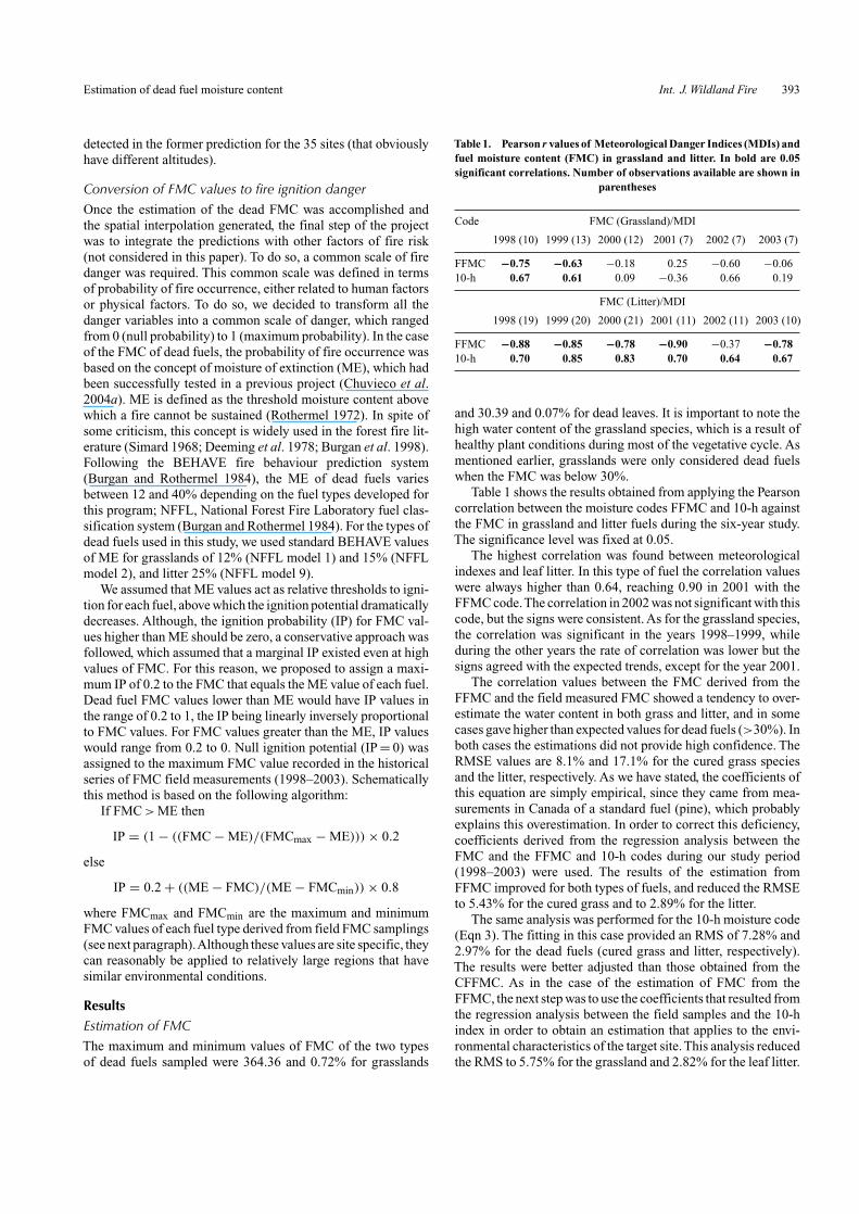
Table 1. Pearson r values of Meteorological Danger Indices (MDIs) andfuel moisture content (FMC) in grassland and litter. In bold are 0.05significant correlations. Number of observations available are shown in

parentheses

Code FMC (Grassland)/MDI

1998 (10) 1999 (13) 2000 (12) 2001 (7) 2002 (7) 2003 (7)

FFMC −0.75 −0.63 −0.18 0.25 −0.60 −0.0610-h 0.67 0.61 0.09 −0.36 0.66 0.19

FMC (Litter)/MDI

1998 (19) 1999 (20) 2000 (21) 2001 (11) 2002 (11) 2003 (10)

FFMC −0.88 −0.85 −0.78 −0.90 −0.37 −0.7810-h 0.70 0.85 0.83 0.70 0.64 0.67

and 30.39 and 0.07% for dead leaves. It is important to note thehigh water content of the grassland species, which is a result ofhealthy plant conditions during most of the vegetative cycle. Asmentioned earlier, grasslands were only considered dead fuelswhen the FMC was below 30%.

Table 1 shows the results obtained from applying the Pearsoncorrelation between the moisture codes FFMC and 10-h againstthe FMC in grassland and litter fuels during the six-year study.The significance level was fixed at 0.05.

The highest correlation was found between meteorologicalindexes and leaf litter. In this type of fuel the correlation valueswere always higher than 0.64, reaching 0.90 in 2001 with theFFMC code.The correlation in 2002 was not significant with thiscode, but the signs were consistent. As for the grassland species,the correlation was significant in the years 1998–1999, whileduring the other years the rate of correlation was lower but thesigns agreed with the expected trends, except for the year 2001.

The correlation values between the FMC derived from theFFMC and the field measured FMC showed a tendency to over-estimate the water content in both grass and litter, and in somecases gave higher than expected values for dead fuels (>30%). Inboth cases the estimations did not provide high confidence. TheRMSE values are 8.1% and 17.1% for the cured grass speciesand the litter, respectively. As we have stated, the coefficients ofthis equation are simply empirical, since they came from mea-surements in Canada of a standard fuel (pine), which probablyexplains this overestimation. In order to correct this deficiency,coefficients derived from the regression analysis between theFMC and the FFMC and 10-h codes during our study period(1998–2003) were used. The results of the estimation fromFFMC improved for both types of fuels, and reduced the RMSEto 5.43% for the cured grass and to 2.89% for the litter.

The same analysis was performed for the 10-h moisture code(Eqn 3). The fitting in this case provided an RMS of 7.28% and2.97% for the dead fuels (cured grass and litter, respectively).The results were better adjusted than those obtained from theCFFMC. As in the case of the estimation of FMC from theFFMC, the next step was to use the coefficients that resulted fromthe regression analysis between the field samples and the 10-hindex in order to obtain an estimation that applies to the envi-ronmental characteristics of the target site. This analysis reducedthe RMS to 5.75% for the grassland and 2.82% for the leaf litter.

394 Int. J. Wildland Fire I. Aguado et al.

0.00

5.00

10.00

15.00

20.00

25.00

30.00

35.00

3-4-98 14-6-98 9-8-98 18-9-98 30-4-99 25-6-99 27-7-99 24-4-00 19-6-00 7-9-00 3-4-01 1-8-01 23-4-02 12-7-02 29-4-03 13-8-03

FM

C

FMC obs Est (FFMC) Est (10 h)

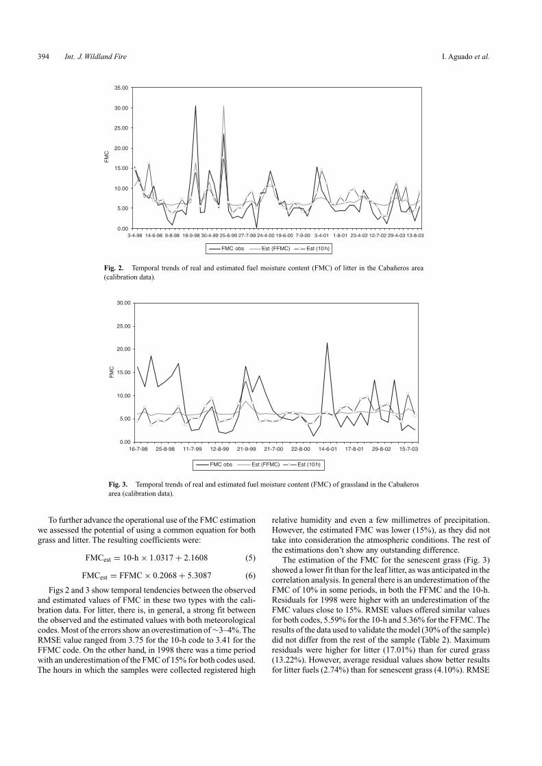
Fig. 2. Temporal trends of real and estimated fuel moisture content (FMC) of litter in the Cabañeros area(calibration data).

0.00

5.00

10.00

15.00

20.00

25.00

30.00

16-7-98 25-8-98 11-7-99 12-8-99 21-9-99 21-7-00 22-8-00 14-6-01 17-8-01 29-8-02 15-7-03

FM

C

FMC obs Est (FFMC) Est (10 h)

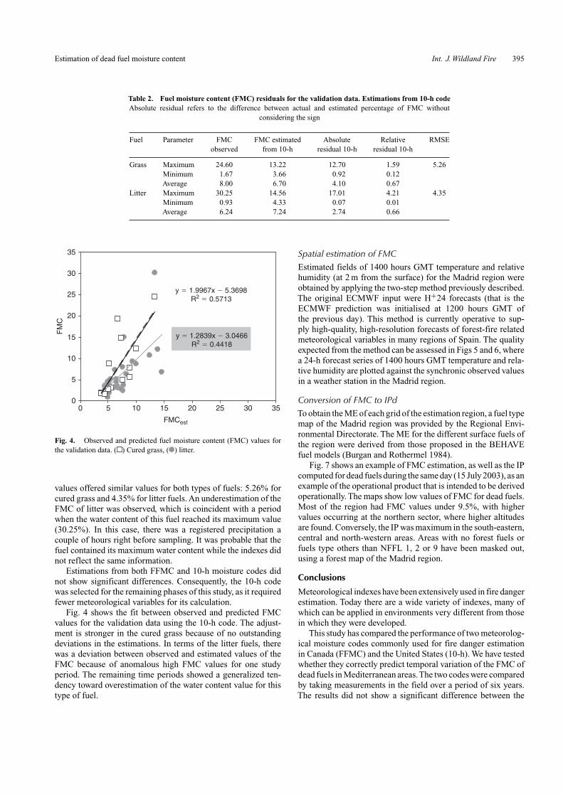
Fig. 3. Temporal trends of real and estimated fuel moisture content (FMC) of grassland in the Cabañerosarea (calibration data).

To further advance the operational use of the FMC estimationwe assessed the potential of using a common equation for bothgrass and litter. The resulting coefficients were:

FMCest = 10-h × 1.0317 + 2.1608 (5)

FMCest = FFMC × 0.2068 + 5.3087 (6)

Figs 2 and 3 show temporal tendencies between the observedand estimated values of FMC in these two types with the cali-bration data. For litter, there is, in general, a strong fit betweenthe observed and the estimated values with both meteorologicalcodes. Most of the errors show an overestimation of ∼3–4%.TheRMSE value ranged from 3.75 for the 10-h code to 3.41 for theFFMC code. On the other hand, in 1998 there was a time periodwith an underestimation of the FMC of 15% for both codes used.The hours in which the samples were collected registered high

relative humidity and even a few millimetres of precipitation.However, the estimated FMC was lower (15%), as they did nottake into consideration the atmospheric conditions. The rest ofthe estimations don’t show any outstanding difference.

The estimation of the FMC for the senescent grass (Fig. 3)showed a lower fit than for the leaf litter, as was anticipated in thecorrelation analysis. In general there is an underestimation of theFMC of 10% in some periods, in both the FFMC and the 10-h.Residuals for 1998 were higher with an underestimation of theFMC values close to 15%. RMSE values offered similar valuesfor both codes, 5.59% for the 10-h and 5.36% for the FFMC. Theresults of the data used to validate the model (30% of the sample)did not differ from the rest of the sample (Table 2). Maximumresiduals were higher for litter (17.01%) than for cured grass(13.22%). However, average residual values show better resultsfor litter fuels (2.74%) than for senescent grass (4.10%). RMSE

Estimation of dead fuel moisture content Int. J. Wildland Fire 395

Table 2. Fuel moisture content (FMC) residuals for the validation data. Estimations from 10-h codeAbsolute residual refers to the difference between actual and estimated percentage of FMC without

considering the sign

Fuel Parameter FMC FMC estimated Absolute Relative RMSEobserved from 10-h residual 10-h residual 10-h

Grass Maximum 24.60 13.22 12.70 1.59 5.26Minimum 1.67 3.66 0.92 0.12Average 8.00 6.70 4.10 0.67

Litter Maximum 30.25 14.56 17.01 4.21 4.35Minimum 0.93 4.33 0.07 0.01Average 6.24 7.24 2.74 0.66

y � 1.2839x � 3.0466R2 � 0.4418

y � 1.9967x � 5.3698R2 � 0.5713

0

5

10

15

20

25

30

35

0 5 10 15 20 25 30 35

FMCest

FM

C

Fig. 4. Observed and predicted fuel moisture content (FMC) values forthe validation data. ( ) Cured grass, ( ) litter.

values offered similar values for both types of fuels: 5.26% forcured grass and 4.35% for litter fuels. An underestimation of theFMC of litter was observed, which is coincident with a periodwhen the water content of this fuel reached its maximum value(30.25%). In this case, there was a registered precipitation acouple of hours right before sampling. It was probable that thefuel contained its maximum water content while the indexes didnot reflect the same information.

Estimations from both FFMC and 10-h moisture codes didnot show significant differences. Consequently, the 10-h codewas selected for the remaining phases of this study, as it requiredfewer meteorological variables for its calculation.

Fig. 4 shows the fit between observed and predicted FMCvalues for the validation data using the 10-h code. The adjust-ment is stronger in the cured grass because of no outstandingdeviations in the estimations. In terms of the litter fuels, therewas a deviation between observed and estimated values of theFMC because of anomalous high FMC values for one studyperiod. The remaining time periods showed a generalized ten-dency toward overestimation of the water content value for thistype of fuel.

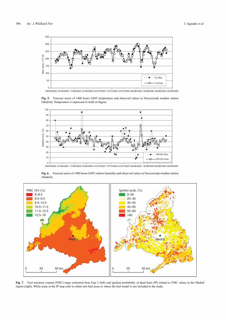
Spatial estimation of FMCEstimated fields of 1400 hours GMT temperature and relativehumidity (at 2 m from the surface) for the Madrid region wereobtained by applying the two-step method previously described.The original ECMWF input were H+24 forecasts (that is theECMWF prediction was initialised at 1200 hours GMT ofthe previous day). This method is currently operative to sup-ply high-quality, high-resolution forecasts of forest-fire relatedmeteorological variables in many regions of Spain. The qualityexpected from the method can be assessed in Figs 5 and 6, wherea 24-h forecast series of 1400 hours GMT temperature and rela-tive humidity are plotted against the synchronic observed valuesin a weather station in the Madrid region.

Conversion of FMC to IPdTo obtain the ME of each grid of the estimation region, a fuel typemap of the Madrid region was provided by the Regional Envi-ronmental Directorate. The ME for the different surface fuels ofthe region were derived from those proposed in the BEHAVEfuel models (Burgan and Rothermel 1984).

Fig. 7 shows an example of FMC estimation, as well as the IPcomputed for dead fuels during the same day (15 July 2003), as anexample of the operational product that is intended to be derivedoperationally. The maps show low values of FMC for dead fuels.Most of the region had FMC values under 9.5%, with highervalues occurring at the northern sector, where higher altitudesare found. Conversely, the IP was maximum in the south-eastern,central and north-western areas. Areas with no forest fuels orfuels type others than NFFL 1, 2 or 9 have been masked out,using a forest map of the Madrid region.

Conclusions

Meteorological indexes have been extensively used in fire dangerestimation. Today there are a wide variety of indexes, many ofwhich can be applied in environments very different from thosein which they were developed.

This study has compared the performance of two meteorolog-ical moisture codes commonly used for fire danger estimationin Canada (FFMC) and the United States (10-h). We have testedwhether they correctly predict temporal variation of the FMC ofdead fuels in Mediterranean areas.The two codes were comparedby taking measurements in the field over a period of six years.The results did not show a significant difference between the

396 Int. J. Wildland Fire I. Aguado et al.

0

50

100

150

200

250

300

350

28/05/2005 07/06/2005 17/06/2005 27/06/2005 07/07/2005 17/07/2005 27/07/2005 06/08/2005 16/08/2005 26/08/2005 05/09/2005

Max

. tem

p. (

°C*1

0)

Tx-Obs

Tx-Pred

Fig. 5. Forecast series of 1400 hours GMT temperature and observed values in Navacerrada weather station(Madrid). Temperature is expressed in tenth of degree.

0

10

20

30

40

50

60

70

80

90

100

28/05/2005 07/06/2005 17/06/2005 27/06/2005 07/07/2005 17/07/2005 27/07/2005 06/08/2005 16/08/2005 26/08/2005 05/09/2005

Rel

ativ

e hu

m. (

%)

HR12h-Obs

HR12h-Pred

Fig. 6. Forecast series of 1400 hours GMT relative humidity and observed values in Navacerrada weather station(Madrid).

FMC 10 h (%) Ignition prob. (%)8–8.58.5–9.59.5–10.510.5–11.511.5–12.512.5–16

0–2020–3030–4040–5050–60>60

0 25 50 km 0 25 50 km

Madrid Madrid

Fig. 7. Fuel moisture content (FMC) maps estimated from Eqn 5 (left) and ignition probability of dead fuels (IP) related to FMC values in the Madridregion (right). White areas in the IP map refer to either non fuel areas or where the fuel model is not included in the study.

Estimation of dead fuel moisture content Int. J. Wildland Fire 397

two. Therefore, the index that required less inputs, the NFDRS10-h code, is recommended for operational purposes. This indexallows an estimation of the FMC of flammable dead fuels withan RMSE close to 5%.

In addition, the spatial variation of the 10-h code was obtainedusing interpolation techniques. Target estimation variables,which in this case were air temperature and relative humidity,were generated for our study region. This estimation was basedon a two-step method of (1) downscaling and (2) interpolation ofECMWF predictions. The method is currently operative to sup-ply high-quality high-resolution forecasts of forest-fire relatedmeteorological variables in several regions of Spain.

Finally this paper has presented a proposal to obtain the igni-tion potential associated to dead FMC. We propose to transformthe original scale of FMC into an IP, defined as the likelihood ofa fire starting, in the range of 0 to 1, using the concept of ME,which should be adapted to each fuel type.

Since FMC can be mapped by gridded meteorological data,IP can also be mapped and, therefore, the assessment of ignitiondanger can be performed spatially. Moreover, this informationcan be easily integrated with other sources of danger (lightning orsocio-economic causes), within the framework of the geographicinformation systems derived for this purpose.

AcknowledgementsThis paper is derived from the Firemap project CGL2004-06049-C04-01/CLI, funded by the Spanish Ministry of Education. Authorities ofthe Cabañeros National Park greatly facilitated the field work. Fuel typemaps of the Madrid region were kindly provided by the Madrid RegionalEnvironmental Office.

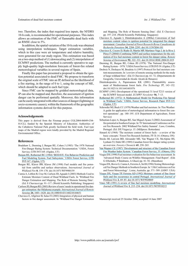
ReferencesBradshaw L, Deeming J, Burgan RE, Cohen J (1983) ‘The 1978 National

Fire-Danger Rating System: Technical Documentation.’ USDA, ForestService, GTR INT-169. (Ogden, UT)

Burgan RE, Rothermel RC (1984) ‘BEHAVE: Fire Behavior Prediction andFuel Modeling System. Fuel Subsystem.’ USDA Forest Service, GTRINT-167. (Ogden, UT)

Burgan RE, Klaver RW, Klaver JM (1998) Fuel models and fire poten-tial from satellite and surface observations. International Journal ofWildland Fire 8, 159–170. doi:10.1071/WF9980159

Camia A, Leblon B, Cruz M, Carlson JD, Aguado I (2003) Methods Used toEstimate Moisture Content of Dead Wildland Fuels. In ‘Wildland FireDanger Estimation and Mapping. The Role of Remote Sensing Data’.(Ed. E Chuvieco) pp. 91–117. (World Scientific Publishing: Singapore)

Carlson JD, Burgan RE (2003) Review of users’needs in operational fire dan-ger estimation: the Oklahoma example. International Journal of RemoteSensing 24, 1601–1620. doi:10.1080/01431160210144651

Chuvieco E, Allgöwer B, Salas FJ (2003) Integration of physical and humanfactors in fire danger assessment. In ‘Wildland Fire Danger Estimation

http://www.publish.csiro.au/journals/ijwf

and Mapping. The Role of Remote Sensing Data’. (Ed. E Chuvieco)pp. 197–218. (World Scientific Publishing: Singapore)

Chuvieco E, Aguado I, Dimitrakopoulos A (2004a) Conversion of fuelmoisture content values to ignition potential for integrated fire dangerassessment. Canadian Journal of Forest Research-Revue Canadienne deRecherche Forestiere 34, 2284–2293. doi:10.1139/X04-101

Chuvieco E, Cocero D, Riaño D, Martín MP, Martínez-Vega J, de la Riva J,Pérez F (2004b) Combining NDVI and surface temperature for the esti-mation of live fuel moisture content in forest fire danger rating. RemoteSensing of Environment 92, 322–331. doi:10.1016/J.RSE.2004.01.019

Deeming JE, Burgan RE, Cohen JD (1978) ‘The National Fire-DangerRating System – 1978.’USDA Forest Service, GTR INT-39. (Ogden, UT)

Desbois N, Deshayes M, Beudoin A (1997) Protocol for fuel moisture con-tent measurements. In ‘a review of remote sensing methods for the studyof large wildland fires’. (Ed. E Chuvieco) pp. 61–72. (Departamento deGeografía, Universidad de Alcalá: Alcalá de Henares)

Dimitrakopoulos A, Papaioannou KK (2001) Flammability assess-ment of Mediterranean forest fuels. Fire Technology 37, 143–152.doi:10.1023/A:1011641601076

ECMWF (1991) Development of the operational 31 level T213 version ofthe ECMWF forecast model. ECMWF Newsletter 56, 7–13.

Rothermel RC (1972) ‘A Mathematical Model for Predicting Fire Spreadin Wildland Fuels.’ USDA, Forest Service, Research Paper INT-115.(Ogden, UT)

Schroeder MJ, Buck CC (1970) Weather and fuel moisture. In ‘Fire Weather:A guide for application of meterological information to forest fire con-trol operations’. pp. 180–195. (US Department of Agriculture, ForestService)

Sebastian-Lopez A, Burgan RE, San Miguel-Ayanz J (2002) Assessment offire potential in Southern Europe. In ‘IV International Conference on For-est Fire Research. 2002 Wildland Fire Safety Summit’. Luso, Coimbra,Portugal. (Ed. DX Viegas) p. 15. (Millpress: Rotterdam)

Simard AJ (1968) ‘The moisture content of forest fuels – a review of thebasic concepts.’ Forest Fire Research Institute, FF-X-14. (Ottawa, ON)

Stocks BJ, Lawson BD, Alexander ME, Van Wagner CE, McAlpine RS,Lynham TJ, Dubé DE (1989) Canadian forest fire danger rating system:an overview. Forestry Chronicle 65, 258–265.

Van Wagner CE (1987) ‘Development and structure of the Canadian ForestFire Weather Index System.’ Canadian Forest Service, 35. (Ottawa, ON)

Viegas DX (1998) Fuel moisture evaluation for fire behaviour assessment. In‘Advanced Study Course on Wildfire Management. Final Report’. (EdsG Eftichidis, P Balabanis, A Ghazi) pp. 81–92. (Marathon)

Viegas DX, Bovio G, CamiaA, FerreiraA, Sol B (1996)Testing Meteorologi-cal Fire Danger Methods in Southern Europe. In ‘13th Conference on Fireand Forest Meteorology’. Lorne, Australia. pp. 571–589. (IAWF: USA)

Viegas DX, Viegas TP, Ferreira AD (1992) Moisture content of fine forestfuels and fire occurrence in central Portugal. International Journal ofWildland Fire 2, 69–85. doi:10.1071/WF9920069

Viney NR (1991) A review of fine fuel moisture modelling. InternationalJournal of Wildland Fire 1, 215–234. doi:10.1071/WF9910215

Manuscript received 25 October 2006, accepted 14 June 2007