
Plasmon Transmutation: Inducing New Modes in Nanoclusters by Adding Dielectric Nanoparticles
Physics Reports 493 (2010) 237–319
Contents lists available at ScienceDirect
Physics Reports
journal homepage: www.elsevier.com/locate/physrep
Electron spectroscopies and inelastic processes in nanoclusters andsolids: Theory and experimentSimone Taioli a,b,∗, Stefano Simonucci c,a, Lucia Calliari a, Maurizio Dapor a,da Interdisciplinary Laboratory for Computational Science (LISC), FBK-CMM and University of Trento, via Sommarive 18, I-38123 Trento, Italyb Department of Physics, University of Trento, Via Sommarive 14, I-38100, Trento, Italyc Department of Physics, University of Camerino, via Madonna delle Carceri 9, 62032 Camerino, Italyd Department of Materials Engineering and Industrial Technologies, University of Trento, via Mesiano 77, I-38123 Trento, Italy
a r t i c l e i n f o
Article history:Accepted 3 April 2010Available online 19 May 2010editor: D.L. Mills
Keywords:Scattering theoryX-ray photoelectron spectroscopyAuger electron spectroscopyElectron energy loss spectroscopyInelastic processesAb initio calculationsMonte Carlo simulations
a b s t r a c t
The recent, very significant developments in high intensity and brightness electron andphoton sources have opened new possibilities of applying electron spectroscopies, suchas photoemission, Auger and electron energy loss, to the study of many interestingfeatures in the dynamics of atoms, molecules and condensed-matter systems. In thelast few years it has become possible to obtain electron spectra with an overall energyresolution (electron/photon source and electron spectrometer) considerably smaller thanthe linewidth of the investigated level and to study quantitatively the combined effects ofthe intrinsic dynamical properties of the system, of features of the incident beam and ofthe electron spectrometer on the spectral lineshape. For all these reasons, it is importantto have theoretical methods that are able to analyze the dynamics of systems at any levelof aggregation under the influence of an incident radiation and, simultaneously, to predictspectral lineshapes quantitatively by correlating their features with internal dynamics ofthe perturbed system.In this report, we present experiments and a critical overview of theoretical methods
for interpreting electron spectra of atoms, molecules and solid-state systems. The generaltheoretical framework for this analysis is resonantmultichannel scattering theory. Electronspectroscopies are, in fact, based on scattering processes in which the initial state consistsof a projectile, typically photons or electrons, exciting a target to a resonant state, whichhas long lifetimes if compared to the collision time. This metastable state is embeddedin the continuum of final states characterized by the presence of a few fragments, whoseobservation provides useful information on the properties of the system under study. Evenif the general theory of scattering and decay phenomena has been largely developed, itsspecific application to electron spectroscopies in condensed matter and, in several casesalso to atoms andmolecules, presents difficulties that have hindered the production of highquality theoretical spectra until recently. This is mainly due to computational problemsrelated to treating a large number of decay channels, which prevent one from usingnumerical techniques for representing the electron as it moves outward through the fieldof the ionized system. Furthermore, another issue is represented by the need to account forshake processes and extrinsic energy losses due to the coupling with collective excitations.In this workwe present a theoreticalmethodwhich does not suffer from the limitations
of previous approaches, and allows one accurately to reproduce the experimental resultsin solids. This method provides an extension to condensed matter of Fano’s formulation of
∗ Corresponding author at: Interdisciplinary Laboratory for Computational Science (LISC), FBK-CMMandUniversity of Trento, via Sommarive 18, I-38123Povo, Trento, Italy.E-mail address: [email protected] (S. Taioli).
0370-1573/$ – see front matter© 2010 Elsevier B.V. All rights reserved.doi:10.1016/j.physrep.2010.04.003
238 S. Taioli et al. / Physics Reports 493 (2010) 237–319
the interaction between discrete and continuum states. It includes the combined effects ofintrinsic and extrinsic features on spectral lineshapes so that computed spectra are directlycomparable to acquired spectra, avoiding background subtraction or deconvolutionprocedures. This approach is sufficiently general to be applied not only to the analysis andinterpretation of autoionization, Auger and photoemission spectra, but also to the study ofother processes since its central feature is the ability of calculating accurate wavefunctionsfor continuum states of extended systems.
© 2010 Elsevier B.V. All rights reserved.
Contents
1. Introduction............................................................................................................................................................................................. 2392. Principles of photoemission, Auger and electron energy loss spectroscopy....................................................................................... 240
2.1. Features that are common to different electron spectroscopies ............................................................................................. 2402.1.1. Basic measurable spectroscopic parameters in electron spectroscopies................................................................. 2412.1.2. Basic computable spectroscopic parameters in electron spectroscopies ................................................................ 2422.1.3. From microscopic quantum systems to macroscopic observables .......................................................................... 242
2.2. Photoelectron and Auger spectroscopy..................................................................................................................................... 2432.2.1. Resonant photoemission ............................................................................................................................................. 246
2.3. Outline of electron energy loss spectroscopy (EELS): history and physics ............................................................................. 2463. Experimental photoemission and Auger spectra .................................................................................................................................. 247
3.1. Retrieval of intrinsic spectra from measured spectra .............................................................................................................. 2473.2. Example: the oxygen K-VV spectrum........................................................................................................................................ 248
4. Low energy EELS: theory and simulation .............................................................................................................................................. 2494.1. Methods for the theoretical interpretation of EEL spectra....................................................................................................... 2494.2. The inelastic scattering cross section ........................................................................................................................................ 250
4.2.1. The energy loss function ............................................................................................................................................. 2504.2.2. Calculation of the dielectric function ......................................................................................................................... 2534.2.3. Surface plasmons ......................................................................................................................................................... 255
4.3. The elastic scattering cross section............................................................................................................................................ 2555. The basic Monte Carlo strategies for simulating electron transport in solids..................................................................................... 256
5.1. The continuous slowing down approximation ......................................................................................................................... 2565.2. Energy straggling ........................................................................................................................................................................ 257
6. Simulation and modelling of electron energy loss spectra .................................................................................................................. 2586.1. Application of the Monte Carlo method to electron energy loss spectroscopy: the SiO2 REEL spectrum ............................ 2586.2. Application of the Monte Carlo method to electron energy loss spectroscopy: Al and Si REEL spectra............................... 2586.3. Ab initio calculation of electron energy loss spectra................................................................................................................. 259
7. Theoretical methods for the interpretation of photoemission, autoionization and Auger spectra ................................................... 2607.1. X-ray scattering .......................................................................................................................................................................... 2607.2. Ingoing boundary conditions ..................................................................................................................................................... 2617.3. Time-dependent theory of resonant scattering (Feshbach’s theory) ...................................................................................... 2617.4. Time-independent resonant multichannel scattering theory including channel interaction (Fano’s theory) ..................... 2637.5. The concept of autoionization and the Auger effect as resonant multichannel scattering ................................................... 2657.6. Construction of the theoretical spectrum ................................................................................................................................. 2667.7. Many-body perturbation theory................................................................................................................................................ 269
8. Calculation of photoemission and Auger spectra of atoms, molecules and solids ............................................................................. 2708.1. Calculation of spectral energy in atomic and molecular photoemission and Auger spectra................................................. 270
8.1.1. The Hartree–Fock (HF) method .................................................................................................................................. 2718.1.2. Configuration interaction method.............................................................................................................................. 2728.1.3. The Green function method ........................................................................................................................................ 2728.1.4. Post-Hartree–Fock energy calculations: DFT, MBPT, TDDFT .................................................................................... 273
8.2. Calculations of Auger decay rates in atoms .............................................................................................................................. 2748.2.1. The hypergeometric confluent method ..................................................................................................................... 2758.2.2. Perturbative methods.................................................................................................................................................. 275
8.3. Calculations of Auger decay rates in molecules........................................................................................................................ 2768.3.1. Monocentric vs. multicentric expansion of the orbitals ........................................................................................... 2768.3.2. Vibrational analysis of Auger and autoionization spectra ........................................................................................ 2778.3.3. The Stjeltjes imaging method ..................................................................................................................................... 2848.3.4. The Green function method ........................................................................................................................................ 284
8.4. Calculations of Auger decay rates in solids and nanoclusters ................................................................................................. 2858.4.1. Localization–delocalization issues ............................................................................................................................. 2858.4.2. Lander’s model of C-VV transitions ............................................................................................................................ 2868.4.3. Cini–Sawatzky model of C-VV transitions ................................................................................................................. 286
9. The importance of shake, screening effects and interchannel interaction in the core-hole decay ................................................... 2879.1. Normal Auger transitions ........................................................................................................................................................... 2889.2. KL-LLL shake-off processes......................................................................................................................................................... 289

S. Taioli et al. / Physics Reports 493 (2010) 237–319 239
9.3. K-LL shake-up processes ............................................................................................................................................................ 2909.4. Semiempirical construction of the theoretical spectrum ........................................................................................................ 2919.5. Screening effects in the core-hole decay................................................................................................................................... 293
10. Photoelectron and Auger electron angle-resolved distributions in molecules................................................................................... 29510.1. Two examples: angle-resolved photoionization and Auger spectra of CO and C2H2 ............................................................. 301
11. A unified framework: EEL spectra for quantitative understanding of electron spectra ..................................................................... 30611.1. The QMMC method..................................................................................................................................................................... 30611.2. Cluster choice and strategies for basis set reduction ............................................................................................................... 30711.3. Electronic structure calculations ............................................................................................................................................... 30811.4. The scattering wavefunction...................................................................................................................................................... 30811.5. On the use of projected potentials in scattering theory........................................................................................................... 31111.6. Evaluation of spectroscopic quantities...................................................................................................................................... 31311.7. Multisite correlation, ‘space-energy’ similarity procedure in Auger calculations and scaling issues................................... 31411.8. Energy loss .................................................................................................................................................................................. 31411.9. Calculation of Auger spectra from SiO2 nanoclusters including electron energy loss............................................................ 315References................................................................................................................................................................................................ 316
1. Introduction
The study of electronic and optical properties of matter is a topic of extraordinary importance for our understandingand control of physical, chemical and biological processes from the atomic scale to nanoclusters and solids [1]. Amongmanytechniques able to accomplish this goal, electron spectroscopy stands out as a unique tool to investigatematter by examininghow particles, notably photons and electrons [2], interact with it.Radiation damage of living cells [3], absorption of sunlight in the earth’s ionosphere [4], identification of chemical
composition [5] and electronic structure investigation of materials [6] are just a few examples where light–matter orelectron–matter interaction mechanisms play a fundamental role.Electron spectroscopy includes a broad range of techniques, having complementary characteristics that are useful for
specific studies of surfaces and bulk, depending on the type and energy of the incident particles: for example, low energyelectron diffraction (LEED) uses electron beams to analyze the surface structure of crystalline materials, whereas Augerelectron spectroscopy (AES) uses focused electron beams to investigate the electronic structure or to provide chemicalmaps of the surface of materials. The application of electron spectroscopy techniques helps to understand phenomena, suchas heterogeneous catalysis [7,8], chemical reactions [9], optical reflection [10], adhesion and corrosion [11], thermionicemission [12,13], which occur at the interface and surface of semiconductors and nanocrystals routinely used in industry.The study of the electronic properties of materials by electron spectroscopy has been driven by:
• the need to support each stage of research and development in the field of nanotechnology, from synthesis to structural,electronic and functional characterization of nanoscale components;• the fundamental desire to understand quasi-particle states of interacting many-fermion systems [14];• recent technological advances in high intensity, high brightness synchrotron radiation sources in the soft X-rayregion [15], notably grazing incidence monochromators and electron analyzers [16–18], which allow unprecedentedaccess to spectral features and hence to the local dynamics of many-fermion systems with a total (monochromator andelectron spectrometer) energy resolution considerably smaller than the core level investigated [19,20].
In this respect, we remember that energy redistribution following excitation forces the system to decay through a varietyof competing radiative, non-radiative and dissociative paths. The study of such decay mechanisms turned out to be relevantfor optical devices where, for instance, carrier recombination quenching is responsible for the reduced performance ofcarbon-based nanostructures used as photoluminescent devices [21,22].From the theoretical point of view, on the other hand, excitation and decay are inherentlymany-body processes: electron
spectroscopy investigations, considered beyond the single-particle framework, provide the opportunity to unravel theintricacies of many-body interactions in systems other than a Fermi gas. For atoms and molecules, our understandingof such mechanisms has progressed greatly, largely due to the accurate treatment of correlation in small systems. Fornanoclusters and condensed-matter systems, on the other hand, computational tools that are able to dealwith the increasingcomplexity and with delocalization issues in valence and core-level photoemission or Auger decay are still the subject ofintense research [23].Furthermore, a quantitative analysis of electron spectra from clusters and solids requires one to take into account energy
losses suffered by electrons during their way out of the solid, due to the interaction with additional degrees of freedom,notably nuclear vibrations and collective charge motions. While many methods, mainly based on mean-field approaches,such as Hartree–Fock (HF) and density functional theory (DFT) [24], together with their corrections to self-energy, suchas configuration interaction (CI) and many-body perturbation theory (MBPT) [25,26], have been developed for calculatingthe ground and excited states of a system, the construction of the continuum wavefunction with appropriate boundaryconditions that accurately include the main correlation effects (inter-channel coupling) and energy loss is still a challenge
240 S. Taioli et al. / Physics Reports 493 (2010) 237–319
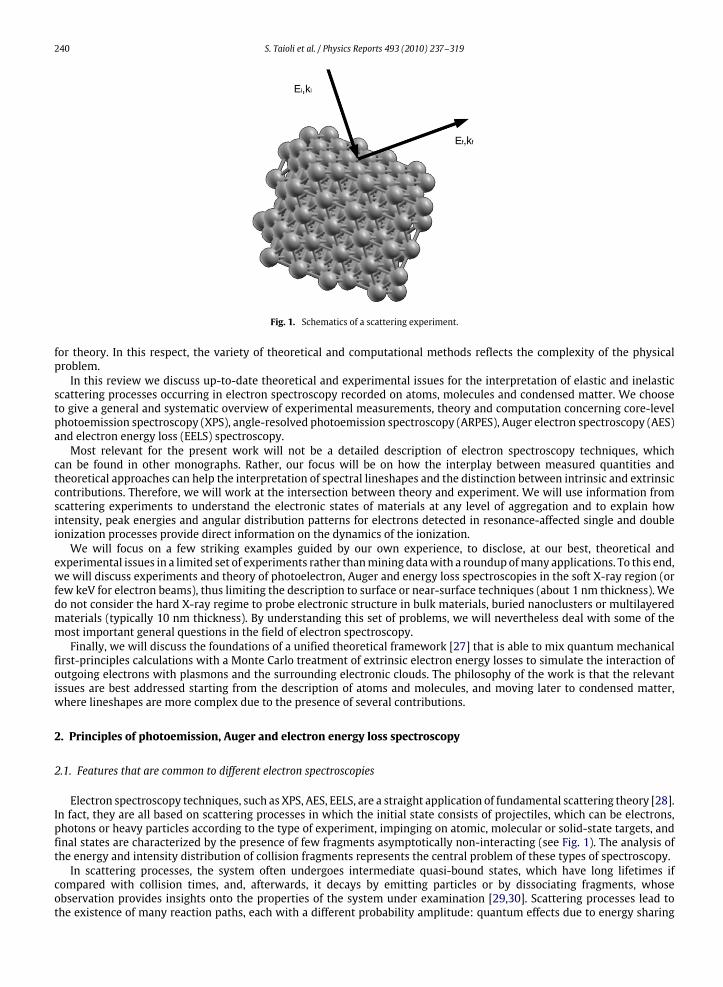
Fig. 1. Schematics of a scattering experiment.
for theory. In this respect, the variety of theoretical and computational methods reflects the complexity of the physicalproblem.In this review we discuss up-to-date theoretical and experimental issues for the interpretation of elastic and inelastic
scattering processes occurring in electron spectroscopy recorded on atoms, molecules and condensed matter. We chooseto give a general and systematic overview of experimental measurements, theory and computation concerning core-levelphotoemission spectroscopy (XPS), angle-resolved photoemission spectroscopy (ARPES), Auger electron spectroscopy (AES)and electron energy loss (EELS) spectroscopy.Most relevant for the present work will not be a detailed description of electron spectroscopy techniques, which
can be found in other monographs. Rather, our focus will be on how the interplay between measured quantities andtheoretical approaches can help the interpretation of spectral lineshapes and the distinction between intrinsic and extrinsiccontributions. Therefore, we will work at the intersection between theory and experiment. We will use information fromscattering experiments to understand the electronic states of materials at any level of aggregation and to explain howintensity, peak energies and angular distribution patterns for electrons detected in resonance-affected single and doubleionization processes provide direct information on the dynamics of the ionization.We will focus on a few striking examples guided by our own experience, to disclose, at our best, theoretical and
experimental issues in a limited set of experiments rather thanmining datawith a roundup ofmany applications. To this end,we will discuss experiments and theory of photoelectron, Auger and energy loss spectroscopies in the soft X-ray region (orfew keV for electron beams), thus limiting the description to surface or near-surface techniques (about 1 nm thickness). Wedo not consider the hard X-ray regime to probe electronic structure in bulk materials, buried nanoclusters or multilayeredmaterials (typically 10 nm thickness). By understanding this set of problems, we will nevertheless deal with some of themost important general questions in the field of electron spectroscopy.Finally, we will discuss the foundations of a unified theoretical framework [27] that is able to mix quantum mechanical
first-principles calculations with a Monte Carlo treatment of extrinsic electron energy losses to simulate the interaction ofoutgoing electrons with plasmons and the surrounding electronic clouds. The philosophy of the work is that the relevantissues are best addressed starting from the description of atoms and molecules, and moving later to condensed matter,where lineshapes are more complex due to the presence of several contributions.
2. Principles of photoemission, Auger and electron energy loss spectroscopy
2.1. Features that are common to different electron spectroscopies
Electron spectroscopy techniques, such as XPS, AES, EELS, are a straight application of fundamental scattering theory [28].In fact, they are all based on scattering processes in which the initial state consists of projectiles, which can be electrons,photons or heavy particles according to the type of experiment, impinging on atomic, molecular or solid-state targets, andfinal states are characterized by the presence of few fragments asymptotically non-interacting (see Fig. 1). The analysis ofthe energy and intensity distribution of collision fragments represents the central problem of these types of spectroscopy.In scattering processes, the system often undergoes intermediate quasi-bound states, which have long lifetimes if
compared with collision times, and, afterwards, it decays by emitting particles or by dissociating fragments, whoseobservation provides insights onto the properties of the system under examination [29,30]. Scattering processes lead tothe existence of many reaction paths, each with a different probability amplitude: quantum effects due to energy sharing

S. Taioli et al. / Physics Reports 493 (2010) 237–319 241
Fig. 2. Experimental set-up in a scattering experiment [33].Source: Reprinted from [33] with kind permission of the American Physical Society.
between electrons, collective oscillations and reactionmechanismsmake this study very rich and challenging for both theoryand experiments.Decays are well-known phenomena encountered in many different physical contexts [31]. Typical decay processes
are predissociation, autoionization, Auger, nuclear internal conversion, spontaneous emission of nuclear particles andelectromagnetic radiation.Depending on the final products, these transitions are usually classified as radiative or non-radiative depending on
whether the decay is followed by electromagnetic emission or not: such a classification remains valid irrespective of theincident particle (i.e. photons or electrons), although the resulting phenomena may be different. The basics components ofinstrumentation for electron spectroscopy are [32]:
• a device for producing the electronic or photonic beam, at typical energies between 1 and 30 keV necessary for theprimary ionization;• a target constituted by a solid sample or by a supersonic beam of atoms or molecules;• a spectrometer or analyzer, which collects the electrons emitted by the target after the collision.
In Fig. 2, we report a typical experimental layout. In the spectrometer, electrons are deflected and focused by an electricfield generated between two plates kept at a given voltage. The focalization point depends on both the energy of electronsand the electric field. Thereby, a definite relation exists between the energy of the collected electrons and the voltage of thespectrometer which registers the electronic yield.Electron spectroscopies can be used as a probe of the occupied and unoccupied density of states (DOS). Typically, an
impinging beam of X-ray photons or electrons excites a core electron, localized in an atomic site within the sample, toan unoccupied level above the chemical potential. Therefore, one can obtain simultaneous information on the localizedorbitals, through analysis of the core-electron binding energy and on the environment, through analysis of the final states.The local character of interactions analyzed by this set of spectroscopies is particularly evident in Auger spectroscopy, wherethe main transitions occur within a range of only a few atomic diameters and a reduced number of neighbours is requiredfor interpreting the Auger spectrum [34]: the rest of the solid enters as a perturbation affecting the part of the spectrumassociated with energy bands. While each of the three mentioned spectroscopies can be used to unravel the dynamics ofthe excitation in many-body systems, usually XPS is preferred to AES for the high signal to background ratio and for thesimplicity of interpretation. In particular, XPS [35] is used to study core-electron shifts due to chemisorption [36,37] and,with angular resolution spectra (ARPES) [38], one can select specific electronic states to reconstruct band dispersions. Augerelectron spectroscopy [6,39], on the other hand, has the potential to provide more information on the electronic structureof the sample and it is sensitive to electron state hybridization. Furthermore, the presence of two holes in the final state ofthe system allows one to investigate excitonic recombination, screening, localization/delocalization issues and electron andhole mobility in solids [40,41].Electron spectroscopies are eminently surface techniques, because of the low inelastic mean free path of electrons in the
relevant energy range.
2.1.1. Basic measurable spectroscopic parameters in electron spectroscopiesThe basic quantity obtainable from scattering experiments is the differential (or double differential) cross section. It is
defined as the probability to observe a scattered particle into a unit solid angle if the target is irradiated by a flux of oneparticle per surface unit. By plotting the electronic yield N(E) as a function of the binding energy (XPS), of the kinetic energy(AES) or of the energy loss (EELS) of the recorded electrons, one obtains a spectrum, which is a fingerprint of the materialunder investigation. Spectroscopic parameters measurable in electron spectroscopy experiments are the partial decay rateinto a specific channel, angular distribution patterns, spin polarization, kinetic energy of the final fragments and intensity. The firstobservable is related to the lifetime of the intermediate bound state and it is proportional to the linewidth, while angulardistribution and momentum analysis can be exploited in electron coincidence spectroscopy experiments when the decay

242 S. Taioli et al. / Physics Reports 493 (2010) 237–319
leads to the fragmentation of the system. In condensed matter, several processes, such as electron–phonon interactions,shake transitions and plasmon excitations, may contribute to broaden the lineshape [42].
2.1.2. Basic computable spectroscopic parameters in electron spectroscopiesInvolving collisions of particles and fields with matter, the general theoretical framework for interpreting electron
spectroscopies is the theory of scattering and decay [28], which, in principle, could be summarized in the calculation ofthe scattering matrix S, particularly in the search for its poles:
〈ψ−|χ+〉 = 〈ψ |Ω−Ω+|χ〉 = 〈ψ |S|χ〉 (1)
connecting asymptotic particle states in the Hilbert space of scattering channels. In Eq. (1), Ω± are the Möller operatorsmapping the solutions of the free Hamiltonian before the scattering, χ , to solutions of the complete Hamiltonian at thesame energy after the scattering, χ±:
χ±E = Ω±χ(E). (2)
The scatteringwavefunctionsχ± have asymptotically ingoing (+)or outgoing (−)boundary conditions: the former describethe incoming particle at time −∞; the latter, the scattered electron (out-state) at time +∞. Since the incoming waveboundary conditions describe the asymptotic motion of a particle with defined kinetic energy far from the scattering centre,they are suitable for electron spectroscopy calculations. By knowing the scattering matrix, one can compute microscopicquantities, such as differential or total cross sections. To simplify this analysis, one usually assumes that primary ionizationand the following decay are independent events: this approximation is appropriate if the interaction between the twoescaping electrons can be neglected. While the theoretical treatment of the electron–electron interaction [43] will notbe examined in this work, post-collisional effects (PCEs) [44] to simulate the interaction of the escaping electron with theremaining ion and the surrounding medium will be extensively discussed.The calculation of the scattering cross section in electron spectroscopy experiments requires three main ingredients:
control on the initial state, knowledge of many-body interactions and analysis of the final states. In XPS experiments, forinstance, the initial state is a localized atomic orbital, while, after the collision, different decay paths, each with a differentprobability, are possible due to the continuum–discrete interaction [30]. The construction of scattering wavefunctionsthat accurately take into account both electron correlation effects and extrinsic energy loss contributions, while includingappropriate boundary conditions, remains a topic of active research. Such wavefunctions are important for a detailedanalysis of electron energy loss spectra and for the interpretation of the dynamics of the associated processes, particularlyin the resonance energy region.In the standard approach to molecular quantum mechanics, the problem is solved using a time-dependent picture by
studying the time evolution ofwavepackets on scattering potentials. Unfortunately, thesemethods, while giving an intuitiveand direct insight into the scattering dynamics, are limited by the computational load, which increases exponentially withthe number of degrees of freedom. Therefore, typical electron spectroscopy analysis proceeds via time-independent theory,by diagonalizing a Hamiltonian, projected onto a Hilbert space spanned by suitable basis functions, and by studying thecurrents of stationary waves in the energy domain. Both time-dependent and time-independent pictures result in thecalculation of probability for different channels in the asymptotic region. These methods are largely known and developedin atomic and molecular physics. However, their specific application to condensed matter presents difficulties that havehindered the production of high quality spectra until recently [39,45]. Difficulties are mainly related to the theoretical andcomputational treatment of a large number of channels, of many-body correlations in excited states and of interchannelpotentials in extended systems with reduced symmetry [14]. Therefore, while a large number of computational techniqueshave been successfully developed for molecular systems [29,46,47] and several total energy calculations have been carriedout using standard ab initio methods for bound and excited states, this number is smaller for condensed matter, and fewcalculations of electron spectral lineshapes have been published [34,42,48,49].
2.1.3. From microscopic quantum systems to macroscopic observablesSince ab initiomethods necessarily involve approximations, the most important of which is the approximate form of the
scattering wavefunction in the continuum, it is important to validate the calculations against experiments. This comparisonimplies a connection between the microscopic parameters, notably the differential cross section of each scattering event,and themacroscopic observables coming out as a result of ameasure, such as refractivity and optical absorption cross sectionin photon beam experiments or energy loss for impinging electrons. The former quantity, for example, can be obtained froman expression, known in optics as the Beer–Lambert law [50]:
I(x) = I0 exp(−αx), (3)
relating the absorption of incident light (I0), travelling the distance x into the material, to the microscopic properties of thesystem, hidden in the absorption coefficient α. This parameter, related to the total absorption cross section, is a functionof the microscopic frequency-dependent dielectric function and bridges the gap between the micro-world and the macro-world. A connection between a macroscopic theory, based on Maxwell’s equations, and the long-wavelength limit of the
S. Taioli et al. / Physics Reports 493 (2010) 237–319 243
macroscopic dielectric function [51] is given by (G′ = q+ G)εav = lim
q→0ε(q, ω)G,G′=0, (4)
where
εG,G′(q, ω) =8π2
Ω
1q2∑v,c,G|〈c,G+ q| expiq·r |v,G〉|2δ(εc,G+q − εv,G − ω) (5)
is the microscopic dielectric function, q is a vector in the first Brillouin zone and G,G′ are reciprocal lattice vectors. InEqs. (4) and (5) and throughout this report, unless specifically indicated, atomic units are used. In the linear response regime,Eqs. (4) and (5) show a connection between the microscopic quantities, such as band structures and wavefunctions, and themacroscopic optical constants, such as the absorption coefficient (ABS) and the energy loss function (ELF ), observing that
ELF = −Im(1εav
)(6)
ABS = Im (εav) . (7)
2.2. Photoelectron and Auger spectroscopy
The interaction of light or electrons with atoms and molecules, in the gas phase or bound in periodical arrays, can resulteither in the excitation of the system to a resonant state, or in a direct ionization path to the continuum. Moreover, inner-shell ionization creates core-hole quasi-bound states embedded in the continuum of the next higher charge state of thesystem, with the primary ionization process often followed by the expulsion (shake-off) or excitation (shake-up) of outerelectrons.Both photoemission and Auger spectroscopy are based on scattering processes where the initial state consists of photons
or electrons colliding with atomic, molecular or solid-state targets, and final states are characterized by several ejectedphotons, electrons and fragments, whose observation provides useful information on the chemical composition and bondsof the system. Photoemission, particularly from X-ray excitation, was discovered by Hertz in 1887 in his attempt to verifyMaxwell’s equations. After some years (in 1905), the photoelectric effect was explained by Einstein using the new laws ofquantum mechanics.On the other hand, Auger (1925) [52], independently from Meitner [53], noticed a curious phenomenon when X-ray
irradiating a cloud chamber filled with inert gas. In his experiment, Auger observed the presence of pairs of electronic tracksoriginating from the same point, one having a variable length depending on the energy of the incident radiation, and theother of fixed, material-dependent, length.Auger interpreted this fact by supposing the presence of doubly ionized atoms in the gas. A theoretical explanationwas givenby Wentzel two years later [54]. Wentzel made the hypothesis of a two-step process consisting of a primary ionization anda following decay process: the incident radiation, having energy ω, ionizes the system in the inner shell S, whose energy,referred to the vacuum level, is ES . The electron escapes with energy
Ep = ω + ES (ES < 0) (8)
producing the track of variable length. This part of the process is called primary ionization.Subsequently, the system, ionized in the inner shell S, can decay by two alternative mechanisms.• A radiative process, in which one electron drops out of an outer shell R into the inner shell S, while a photon is emittedwith energy
ω′ = ER − ES . (9)
This process is allowed if ER > ES .• A non-radiative process, in which one electron drops out of an outer shell R into an inner shell S, and another electron isejected out of the shell R′ with energy
EAuger =k2
2= ER + ER′ − ES . (10)
This process is allowed if ER + ER′ − ES > 0.
Wentzel identified the Coulomb repulsion between electrons as the driving force of the Auger effect and also proposeda formula for predicting the decay probability that, if applied to the previous example, gives the following result:
PS−RR′ = 2π∫
dk(2π)3
∣∣∣∣〈ϕS(r1, σ1)ηk(r2, σ2)| 1r12 |ϕR(r1, σ1)ϕR′(r2, σ2)〉−〈ϕS(r1, σ1)ηk(r2, σ2)|
1r12|ϕR′(r1, σ1)ϕR(r2, σ2)〉
∣∣∣∣2 δ (ER + ER′ − ES − k22), (11)

244 S. Taioli et al. / Physics Reports 493 (2010) 237–319
where ϕS,R,R′ are the bound spin orbitals that describe respectively the electrons in the S, R and R′ shells, and ηk is thecontinuum spin orbital for the outgoing electron.The following photoemission (see Eq. (12)), Auger (see Eq. (13)) and shake-off processes (see Eq. (14)) in the Ne atom,
Ne+ photon −→ Ne+(1s−1)+ e−p (12)
Ne+(1s−1) −→ Ne++(2p−2)+ e−Auger (13)
Ne+ photon→ Ne++(1s−12p−1)+ 2e− → Ne3+(2p−3)+ 3e−, (14)
are identified as (K), (K-LL) and (KL-LLL) processes, respectively, i.e. they are labelled according to the core hole (K) in thesingly ionized target and according to the final bands (L, M) involved in the process.From a general point of view, one should remember that Auger and autoionizing transitions are in competition with
radiative decay processes. One can compare the fluorescence yield (α) with the non-radiative yield (a) using the followingexpressions:
YR =PR
PR + PNRYNR =
PNRPR + PNR
, (15)
where PR,NR indicates respectively the radiative and non-radiative decay probabilities. Typically, the non-radiative processis predominant for transitions with energies below 2 KeV, while the radiative decay probability becomes increasinglyimportant at higher energies. This is due to the fact that, while the Auger decay probability is independent of the nuclearcharge, the radiative decay probability is almost proportional to the fourth power of the nuclear charge [39].To illustrate this point we use theWentzel formula (11) for the decay probability andwe approximate thewavefunctions
φS,R,R′(Z, r, σ ) and ηk(Z)(Z, r, σ ) with those appropriate for describing an electron in the Coulomb field of a nucleus withcharge Z . We have the following scaling properties for bound orbitals:
φS,R,R′(λZ, r, σ ) = λ3/2φS,R,R′(Z, λr, σ ) (16)
and for the continuum orbital
ηk(λZ)(λZ, r, σ ) = λβηk(Z)(Z, λr, σ ), (17)
where λ3/2 is a normalization factor and the exponent β is determined by the normalization condition
〈ηk(Z)(Z, r, σ )|ηp(Z)(Z, r, σ )〉 = (2π)3δ[k(Z)− p(Z)]. (18)
From Eq. (10) applied to hydrogenic energies, the transition energy k2
2 is proportional to Z2:
k2
2= ER + E ′R − ES =
Z2
2n2R+Z2
2n2R′−Z2
2n2S, (19)
so k(λZ) = λk(Z). Therefore, Eq. (18) becomes
〈ηk(λZ)(λZ, r, σ )|ηp(λZ)(λZ, r, σ )〉 = 〈ηk(Z)(Z, r, σ )|ηp(Z)(Z, r, σ )〉λ−3+2β = λ−3δ[k(Z)− p(Z)], (20)
which implies that β = 0. Finally, by inserting Eqs. (16) and (17) into Eq. (11), one gets
PS−RR′(λZ) = PS−RR′(Z). (21)
This equation shows that the Auger decay probability is almost independent of the nuclear charge.For radiative transitions, on the other hand, the decay probability from an excited electronic state φR(Z, r, σ ) to a given
lower state φS(Z, r, σ ) can be written as follows:
PR−S(Z) =16π4(Eα)3
3|〈φR|r|φS〉|2, (22)
where E is the energy of the emitted photon and α the fine-structure constant. By using the scaling properties of φS,R,R′ andthe fact that E is proportional to Z2, one gets the following expression:
PR−S(λZ) = λ4PR−S(Z), (23)
according to which the radiative decay rate is proportional to the fourth power of the nuclear charge.Photoemission and Auger spectra can be recorded on atoms, molecules and solid samples [5,35,48,55–59]. From the
analysis of the energy, intensity and shape of photoemission and Auger peaks, one can identify the chemical species andchemical bonds on a surface and obtain a large piece of information on the electronic structure of the material underinvestigation. For molecules or solid samples, the initial information is usually deduced by comparing the spectrum withknown atomic spectra. Using this approach, onemakes the implicit assumption that the photoemission and Auger spectra of
S. Taioli et al. / Physics Reports 493 (2010) 237–319 245
Binding Energy (eV)
Arb
itrar
y U
nits
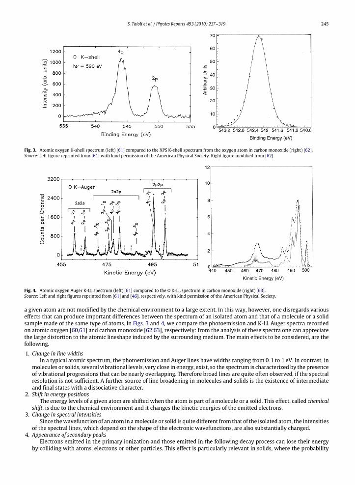
Fig. 3. Atomic oxygen K-shell spectrum (left) [61] compared to the XPS K-shell spectrum from the oxygen atom in carbon monoxide (right) [62].Source: Left figure reprinted from [61] with kind permission of the American Physical Society. Right figure modified from [62].
Kinetic Energy (eV)
Fig. 4. Atomic oxygen Auger K-LL spectrum (left) [61] compared to the O K-LL spectrum in carbon monoxide (right) [63].Source: Left and right figures reprinted from [61] and [46], respectively, with kind permission of the American Physical Society.
a given atom are not modified by the chemical environment to a large extent. In this way, however, one disregards variouseffects that can produce important differences between the spectrum of an isolated atom and that of a molecule or a solidsample made of the same type of atoms. In Figs. 3 and 4, we compare the photoemission and K-LL Auger spectra recordedon atomic oxygen [60,61] and carbon monoxide [62,63], respectively: from the analysis of these spectra one can appreciatethe large distortion to the atomic lineshape induced by the surrounding medium. The main effects to be considered, are thefollowing.
1. Change in line widthsIn a typical atomic spectrum, the photoemission and Auger lines have widths ranging from 0.1 to 1 eV. In contrast, in
molecules or solids, several vibrational levels, very close in energy, exist, so the spectrum is characterized by the presenceof vibrational progressions that can be nearly overlapping. Therefore broad lines are quite often observed, if the spectralresolution is not sufficient. A further source of line broadening in molecules and solids is the existence of intermediateand final states with a dissociative character.
2. Shift in energy positionsThe energy levels of a given atom are shifted when the atom is part of a molecule or a solid. This effect, called chemical
shift, is due to the chemical environment and it changes the kinetic energies of the emitted electrons.3. Change in spectral intensities
Since thewavefunction of an atom in amolecule or solid is quite different from that of the isolated atom, the intensitiesof the spectral lines, which depend on the shape of the electronic wavefunctions, are also substantially changed.
4. Appearance of secondary peaksElectrons emitted in the primary ionization and those emitted in the following decay process can lose their energy
by colliding with atoms, electrons or other particles. This effect is particularly relevant in solids, where the probability

246 S. Taioli et al. / Physics Reports 493 (2010) 237–319
of inelastic scattering is very high and the emitted electrons can excite plasma oscillations. The electrons, which havelost an amount of energy equal to a plasmon, produce secondary smaller peaks, while the electrons which undergoseveral collisions present a distribution in energy that is quite uniform apart for the low energy region where it blowsup. Other satellite lines at different energies and with smaller intensities [42] are produced by the so-called shake-upand shake-off processes (ormonopole excitations) which take place when the primary ionization process is accompaniedby simultaneous ionization (shake-off) or excitation (shake-up) of a valence electron. Usually these secondary processesgive a global contribution to the spectrum that is of the order of 20%. Their appearance, together with the presence ofperturbations, due, for example, to spin–orbit coupling in molecules containing heavy atoms or to interband effects insolids,makes the interpretation of photoemission andAuger spectra very difficult and requires the use of quantum theoryat a sophisticated level.
5. Initial state effectsIn molecules or solids, the spectral profiles are strongly dependent on the position of the initial hole produced
in the primary ionization, even if the final dicationic states produced by the decay process are the same. This isdue to the localized character of both the intermediate electronic state and several final states of the doubly ionizedsystem.
2.2.1. Resonant photoemissionResonant photoemission or autoionization may occur when the impinging particle has kinetic energy tuned to a
resonance of the target system. The resulting scattering is characterized by neutral excitation of one electron from an innershell into unoccupied states. This metastable state can decay by both electron and radiation emission. Autoionizing stateswere first observed by Beutler [64] in 1935, as broad asymmetric lines in photoabsorption spectra of argon, krypton andxenon. The explanation of the presence of asymmetric peaks in continuous absorption spectrawas first given by Fano in 1935[65], with a theory that was reformulated and generalized by Fano in 1961 [30]. The same theory can also be used for theinterpretation of Auger spectra, since there is no fundamental difference between Auger and autoionizing processes. In fact,resonant photoemission can be considered a particular type of Auger process where the intermediate state is characterizedby a local bound excitonic state rather than an ionized state.Autoionization in photoabsorption spectra can be described as follows: an incident radiation of energyω excites an atom
from the ground state A to a highly excited state A∗ with energy EA∗ = EA + ω. The A∗ state is metastable, being embeddedin a continuum of other states, and it decays with emission of one photon or one electron, as in the Auger process. Thefinal state A+ + e− can be reached also through a direct path, without undergoing intermediate quasi-bound resonances.The interference of different paths produces the so-called Fano–Beutler profiles in the observed differential cross section ofthe process. Resonant photoemission processes are labelled by specifying the initial excitonic configuration and final decaystates. The following autoionizing process, for example,
Ne+ photon→ Ne(1s−13p1)→ Ne+(2p−23p1)+ e−, (24)
can be identified as a (Ke-LLe) process with e indicating the excited electron that remains spectator during the decay.Examples of resonant and non-resonant photoemission and Auger spectra recorded from atoms, molecules and condensedmatter will be given below.
2.3. Outline of electron energy loss spectroscopy (EELS): history and physics
An electron beam impinging on a solid target may lose its energy and change momentum through a variety of collisionmechanisms with the sample atoms. While collisions with the nuclei approximately elastically deflect electrons withoutany relevant kinetic energy transfer due to the large mass difference, excitations, ejections of bound electrons and plasmonexcitations imply large energy losswith small deflections. To describe the interaction of the electron beamwith solid targets,one needs elastic and inelastic differential cross sections. The EELS techniquewas developed by Hillier and Baker in the early1940’s [66] but was not widely used up to the 1990’s, when its usage was associated with imaging microscopies, notablytransmission electronmicroscopy (TEM) and scanning electronmicroscopy (SEM). In fact, the energy loss of electrons can berecorded using TEM and SEM at high spatial resolution, revealing composition, atomic and electronic properties, structureand bonding at the atomic scale of the sample under examination [67–69].Analyzing different energy ranges in the final states of inelastic processes leads to many experimental techniques. In Fig. 5(see [70]), we sketch a typical energy loss spectrum spanning the collection energy range of the electron analyzer. At thehighest energy we have the elastic (or zero-loss) peak, where the final energy Ef is equal to the initial one Ei (right side inFig. 5); at lower energy one finds electrons inelastically scattered by nuclear vibrations in the range Ei − 0.1 eV ≤ E ≤ Eirecorded in high resolution electron energy loss spectroscopy (HREELS); the electrons inelastically scattered by plasmonexcitations in the range Ei − 50 eV ≤ E ≤ Ei recorded in EELS; electrons from direct ionization as well as secondaryelectrons in the range 50 eV ≤ E ≤ Ei−50 eV such as those recorded in AES; and, finally, electrons originating from cascadeprocesses in the range 0 ≤ E ≤ 50 eV recorded by SEM.

S. Taioli et al. / Physics Reports 493 (2010) 237–319 247
Fig. 5. Electron energy loss spectrum, showing the zero-loss peak (I) with phonon losses (inset), plasmon resonances (II), core-electron excitations (III)resulting in Auger processes (inset) and the peak of low energy secondary electrons (IV) [70].Source: Reprinted from [70] with kind permission of Springer-Verlag, Heidelberg, Berlin.
3. Experimental photoemission and Auger spectra
3.1. Retrieval of intrinsic spectra from measured spectra
Computation of Auger/photoemission spectra generates intrinsic spectra, i.e. ‘as-excited’ Auger/photoelectron spectrawhich include a so-called intrinsic electron background resulting from many-body effects (shake processes and plasmonexcitation) caused by the presence of the core hole. However, elastic and inelastic scattering events undergone by ‘source’(i.e. Auger or photoemitted) electrons during their transport out of the solid give rise to an additional, so-called extrinsic,background of inelastically scattered electrons. Comparison between experiment and theory requires therefore that thisextrinsic background is removed frommeasured spectra. The issue of retrieving intrinsic spectra has been treated at length inthe past within a two-stepmodel, i.e. under the assumption that electron excitation (inside the solid) and electron transport(to the surface of the solid) can be treated as separate events [71,72].We just remind that the background of inelastically scattered source (i.e. Auger or photoemitted) electrons does not
represent the only type of extrinsic background one should deal with. For instance, two additional sources of extrinsicbackground have to be accounted for in the case of electron excited spectra, namely inelastically scattered primary electronsand the secondary electron cascade at low energy [73,71]. For their description,we refer to previous papers [71,73–76]. Here,we only focus on the background of inelastically scattered source electrons.Historically, the approach used to get rid of the extrinsic background has been dependent on the context. For
investigations aimed at comparing experimental to computed spectra, the extrinsic background was removed bydeconvolution of a backscattered electron spectrum. On the other hand, to measure peak intensities for analytical(quantification) purposes, functions to describe the extrinsic background were proposed [77,78] and these functions weresubtracted from measured spectra. The latter approach has the advantage of being universally applicable to unknownsamples and of not requiring the acquisition of additional energy loss data. However, a series of papers on the subject ofbackground subtraction [73,79,80] showed that deconvolution of energy loss data should be the procedure of choice alsofor reliable peak area measurements.From amathematical point of view, themeasured spectrum is described as the convolution of the intrinsic spectrumwith
a function f (E)which provides the energy distribution associated with an electron travelling a path length l in the solid:
Smeas(E) =∫f (E − E ′)Sintr(E ′)dE ′. (25)
Retrieving Sintr requires therefore knowing the function f (E). It is generally accepted that a reflection electron energy lossspectrum acquired at the same energy of source electrons is a reasonable approximation to f (E). This is because, sincereflection electron energy loss spectroscopy (REELS) primary electrons and source electrons have the same energy, theywould also have the same inelastic mean free path, and the distribution of path lengths characteristic for energy loss, Augerand photoemission spectrawould be the same. A difference arises however in the fact that source electrons (generated insidethe solid) traverse the surface once, while REELS electrons traverse the surface layer twice. As a result, surface excitationsare expected to be overemphasized (at the expense of bulk excitations) for REELS as compared to Auger and photoemissionspectroscopies.A point often discussed concerns the width of the elastic (or zero-loss) peak in the electron energy loss spectrum. This
width is due partly to the thermal spread of the primary electron beam and partly to the analyzer resolution. The formercontribution, unrelated to Auger/photoemission spectra [80], should not be deconvoluted, to avoid undue narrowing of thespectrum. Therefore, it has been suggested to substitute the zero-loss peak in REELS with a delta function [80], so that only
248 S. Taioli et al. / Physics Reports 493 (2010) 237–319
1.0
0.8
0.6
0.4
0.2
0.0
INT
EN
SIT
Y (
coun
ts)
460 480 500 520
KINETIC ENERGY (eV)
O KVV
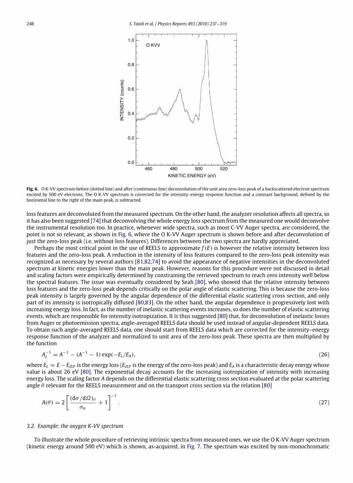
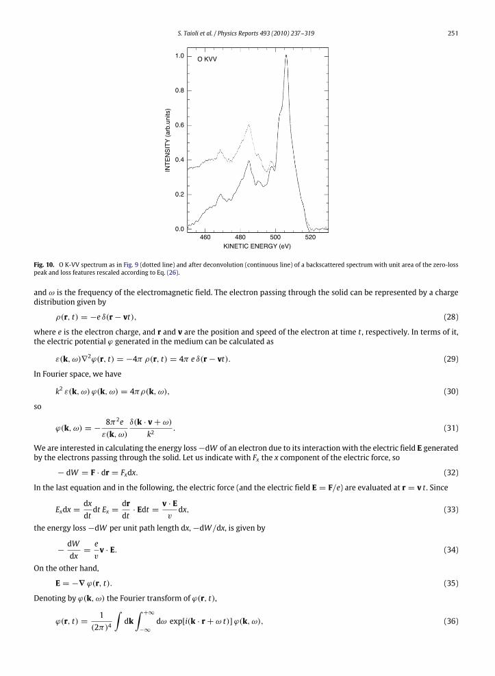
Fig. 6. OK-VV spectrum before (dotted line) and after (continuous line) deconvolution of the unit area zero-loss peak of a backscattered electron spectrumexcited by 500 eV electrons. The O K-VV spectrum is corrected for the intensity–energy response function and a constant background, defined by thehorizontal line to the right of the main peak, is subtracted.
loss features are deconvoluted from themeasured spectrum. On the other hand, the analyzer resolution affects all spectra, soit has also been suggested [74] that deconvolving thewhole energy loss spectrum from themeasured onewould deconvolvethe instrumental resolution too. In practice, whenever wide spectra, such as most C-VV Auger spectra, are considered, thepoint is not so relevant, as shown in Fig. 6, where the O K-VV Auger spectrum is shown before and after deconvolution ofjust the zero-loss peak (i.e. without loss features). Differences between the two spectra are hardly appreciated.Perhaps the most critical point in the use of REELS to approximate f (E) is however the relative intensity between loss
features and the zero-loss peak. A reduction in the intensity of loss features compared to the zero-loss peak intensity wasrecognized as necessary by several authors [81,82,74] to avoid the appearance of negative intensities in the deconvolutedspectrum at kinetic energies lower than the main peak. However, reasons for this procedure were not discussed in detailand scaling factors were empirically determined by constraining the retrieved spectrum to reach zero intensity well belowthe spectral features. The issue was eventually considered by Seah [80], who showed that the relative intensity betweenloss features and the zero-loss peak depends critically on the polar angle of elastic scattering. This is because the zero-losspeak intensity is largely governed by the angular dependence of the differential elastic scattering cross section, and onlypart of its intensity is isotropically diffused [80,83]. On the other hand, the angular dependence is progressively lost withincreasing energy loss. In fact, as the number of inelastic scattering events increases, so does the number of elastic scatteringevents, which are responsible for intensity isotropization. It is thus suggested [80] that, for deconvolution of inelastic lossesfrom Auger or photoemission spectra, angle-averaged REELS data should be used instead of angular-dependent REELS data.To obtain such angle-averaged REELS data, one should start from REELS data which are corrected for the intensity–energyresponse function of the analyzer and normalized to unit area of the zero-loss peak. These spectra are then multiplied bythe function
A−1L = A−1− (A−1 − 1) exp(−EL/EA), (26)
where EL = E−EZLP is the energy loss (EZLP is the energy of the zero-loss peak) and EA is a characteristic decay energy whosevalue is about 26 eV [80]. The exponential decay accounts for the increasing isotropization of intensity with increasingenergy loss. The scaling factor A depends on the differential elastic scattering cross section evaluated at the polar scatteringangle θ relevant for the REELS measurement and on the transport cross section via the relation [80]
A(θ) = 2[(dσ/dΩ)θ
σtr+ 1
]−1. (27)
3.2. Example: the oxygen K-VV spectrum
To illustrate the whole procedure of retrieving intrinsic spectra frommeasured ones, we use the O K-VV Auger spectrum(kinetic energy around 500 eV) which is shown, as-acquired, in Fig. 7. The spectrum was excited by non-monochromatic
S. Taioli et al. / Physics Reports 493 (2010) 237–319 249
8000
7000
6000
5000
4000
INT
EN
SIT
Y (
coun
ts)
KINETIC ENERGY (eV)
460 480 500 520
O KVV
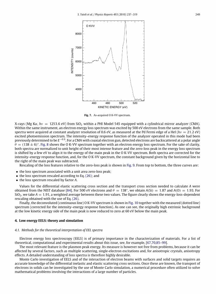
Fig. 7. As-acquired O K-VV spectrum.
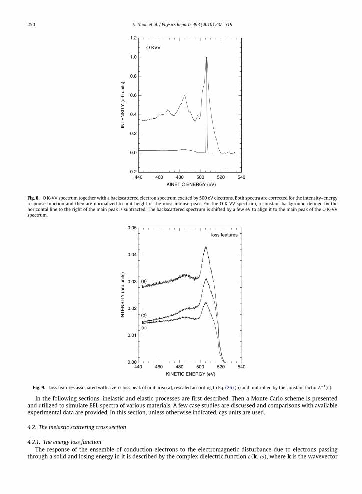
X-rays (Mg Kα, hν = 1253.6 eV) from SiO2 within a PHI Model 545 equipped with a cylindrical mirror analyzer (CMA).Within the same instrument, an electron energy loss spectrumwas excited by 500 eV electrons from the same sample. Bothspectra were acquired at constant analyzer resolution of 0.6 eV, as measured at the Pd Fermi edge of a HeI (hν = 21.2 eV)excited photoemission spectrum. The intensity–energy response function of the analyzer operated in this mode had beenpreviously determined to be E−0.9. For a CMAwith coaxial electron gun, detected electrons are backscattered at a polar angleθ = (138 ± 6). Fig. 8 shows the O K-VV spectrum together with an electron energy loss spectrum. For the sake of clarity,both spectra are normalized to unit height of their most intense feature and the zero-loss peak in the energy loss spectrumis shifted by a few eV to align it to the energy of the main peak in the O K-VV spectrum. Both spectra are corrected for theintensity–energy response function, and, for the O K-VV spectrum, the constant background given by the horizontal line tothe right of the main peak was subtracted.Rescaling of the loss features relative to the zero-loss peak is shown in Fig. 9. From top to bottom, the three curves are:
• the loss spectrum associated with a unit area zero-loss peak;• the loss spectrum rescaled according to Eq. (26); and• the loss spectrum rescaled by factor A.
Values for the differential elastic scattering cross section and the transport cross section needed to calculate A wereobtained from the NIST database [84]. For 500 eV electrons and θ = 138, we obtain A(Si) = 1.87 and A(O) = 1.93. ForSiO2, we take A = 1.91, a weighted average between these two values. The figure clearly shows the energy-loss-dependentrescaling obtained with the use of Eq. (26).Finally, the deconvoluted (continuous line) O K-VV spectrum is shown in Fig. 10 togetherwith themeasured (dotted line)
spectrum (corrected for the intensity–energy response function). As one can see, the originally high extrinsic backgroundat the low kinetic energy side of the main peak is now reduced to zero at 60 eV below the main peak.
4. Low energy EELS: theory and simulation
4.1. Methods for the theoretical interpretation of EEL spectra
Electron energy loss spectroscopy (EELS) is of primary importance in the characterization of materials. For a list oftheoretical, computational and experimental results about this issue, see, for example, [67,70,85–99].The most relevant feature is the plasmon peak energy. Its measure is however not free from problems, because it can be
affected by several factors, such as multiple scattering, single-electron excitations and, for anisotropic crystals, anisotropyeffects. A detailed understanding of loss spectra is therefore highly desirable.Monte Carlo investigation of EELS and of the interaction of electron beams with surfaces and solid targets requires an
accurate knowledge of the differential inelastic and elastic scattering cross sections. Once these are known, the transport ofelectrons in solids can be investigated by the use of Monte Carlo simulation, a numerical procedure often utilized to solvemathematical problems involving the interactions of a large number of particles.
250 S. Taioli et al. / Physics Reports 493 (2010) 237–319
1.2
1.0
0.8
0.6
0.4
0.2
0.0
-0.2
INT
EN
SIT
Y (
arb.
units
)
440 460 480 500 520 540
KINETIC ENERGY (eV)
O KVV
Fig. 8. O K-VV spectrum together with a backscattered electron spectrum excited by 500 eV electrons. Both spectra are corrected for the intensity–energyresponse function and they are normalized to unit height of the most intense peak. For the O K-VV spectrum, a constant background defined by thehorizontal line to the right of the main peak is subtracted. The backscattered spectrum is shifted by a few eV to align it to the main peak of the O K-VVspectrum.
0.05
0.04
0.03
0.02
0.01
0.00
INT
EN
SIT
Y (
arb.
units
)
KINETIC ENERGY (eV)
440 460 480 500 520 540
(a)
(b)
(c)
loss features
Fig. 9. Loss features associated with a zero-loss peak of unit area (a), rescaled according to Eq. (26) (b) and multiplied by the constant factor A−1(c).
In the following sections, inelastic and elastic processes are first described. Then a Monte Carlo scheme is presentedand utilized to simulate EEL spectra of various materials. A few case studies are discussed and comparisons with availableexperimental data are provided. In this section, unless otherwise indicated, cgs units are used.
4.2. The inelastic scattering cross section
4.2.1. The energy loss functionThe response of the ensemble of conduction electrons to the electromagnetic disturbance due to electrons passing
through a solid and losing energy in it is described by the complex dielectric function ε(k, ω), where k is the wavevector
S. Taioli et al. / Physics Reports 493 (2010) 237–319 251
1.0
0.8
0.6
0.4
0.2
0.0
INT
EN
SIT
Y (
arb.
units
)
KINETIC ENERGY (eV)460 480 500 520
O KVV
Fig. 10. O K-VV spectrum as in Fig. 9 (dotted line) and after deconvolution (continuous line) of a backscattered spectrum with unit area of the zero-losspeak and loss features rescaled according to Eq. (26).
and ω is the frequency of the electromagnetic field. The electron passing through the solid can be represented by a chargedistribution given by
ρ(r, t) = −e δ(r− vt), (28)
where e is the electron charge, and r and v are the position and speed of the electron at time t , respectively. In terms of it,the electric potential ϕ generated in the medium can be calculated as
ε(k, ω)∇2ϕ(r, t) = −4π ρ(r, t) = 4π e δ(r− vt). (29)
In Fourier space, we have
k2 ε(k, ω) ϕ(k, ω) = 4πρ(k, ω), (30)
so
ϕ(k, ω) = −8π2eε(k, ω)
δ(k · v+ ω)k2
. (31)
We are interested in calculating the energy loss−dW of an electron due to its interaction with the electric field E generatedby the electrons passing through the solid. Let us indicate with Fx the x component of the electric force, so
− dW = F · dr = Fxdx. (32)
In the last equation and in the following, the electric force (and the electric field E = F/e) are evaluated at r = v t . Since
Exdx =dxdtdt Ex =
drdt· Edt =
v · Evdx, (33)
the energy loss−dW per unit path length dx,−dW/dx, is given by
−dWdx=evv · E. (34)
On the other hand,
E = −∇ ϕ(r, t). (35)
Denoting by ϕ(k, ω) the Fourier transform of ϕ(r, t),
ϕ(r, t) =1
(2π)4
∫dk∫+∞
−∞
dω exp[i(k · r+ ω t)]ϕ(k, ω), (36)

252 S. Taioli et al. / Physics Reports 493 (2010) 237–319
we have
E(r, t) = −∇
1
(2π)4
∫dk∫+∞
−∞
dω exp[i(k · r+ ω t)]ϕ(k, ω). (37)
As a consequence,
−dWdx= Re
−8π2 e2
(2π)4 v
∫dk∫+∞
−∞
dω (−∇) exp[i(k · r+ ω t)] · vδ(k · v+ ω)k2 ε(k, ω)
∣∣∣∣r=v t
= Re
i 8π2 e2
16π4 v
∫dk∫+∞
−∞
dω (k · v) exp[i(k · r+ ω t)]δ(k · v+ ω)k2 ε(k, ω)
∣∣∣∣r=v t
. (38)
Taking into account that (i) the electric field has to be calculated at r = v t and (ii) we have the δ(k · v+ ω) distribution inthe integrand, we obtain
−dWdx= Re
i e2
2π2 v
∫dk∫+∞
−∞
dω (−ω) exp[i(−ω t + ω t)]δ(k · v+ ω)k2 ε(k, ω)
= Re
−i e2
2π2 v
∫dk∫+∞
−∞
dωωδ(k · v+ ω)k2 ε(k, ω)
. (39)
Since
Rei∫+∞
−∞
dωωδ(k · v+ ω)ε(k, ω)
= 2 Re
i∫+∞
0dωω
δ(k · v+ ω)ε(k, ω)
,
we conclude that [100]
−dWdx=e2
π2 v
∫dk∫∞
0dωω Im
[1
ε(k, ω)
]δ(k · v + ω)
k2, (40)
or
−dWdx=
∫∞
0dωω τ(v, ω), (41)
where
τ(v, ω) =e2
π2 v
∫dk Im
[1
ε(k, ω)
]δ(k · v+ ω)
k2(42)
is the probability that a non-relativistic electron of velocity v looses energy ω per unit path length. Let us assume that ε is ascalar (isotropic medium) and that it depends on just the magnitude of k and not on its direction,
ε(k, ω) = ε(k, ω), (43)
so
τ(v, ω) =e2
π2 v
∫ 2π
0dφ∫ π
0dθ sin θ
∫∞
0dk k2 Im
[1
ε(k, ω)
]δ(k v cos θ + ω)
k2
=2 e2
π v
∫ π
0dθ sin θ
∫∞
0dk Im
[1
ε(k, ω)
]δ(k v cos θ + ω). (44)
Let us introduce a new variable ω′ defined as
ω′ = −k v cos θ, (45)
so
dω′ = k v sin θdθ, (46)
and, hence,
τ(v, ω) =2 e2
π v
∫ k v
−k v
dω′
k v
∫∞
0dk Im
[1
ε(k, ω)
]δ(−ω′ + ω) =
2me2
π m v2
∫∞
0
dkkIm[
1ε(k, ω)
]. (47)
In conclusion, we can write that
τ(T , ω) =me2
π T
∫ k+
k−
dkkIm[
1ε(k, ω)
], (48)
S. Taioli et al. / Physics Reports 493 (2010) 237–319 253
where T = m v2/2 and
h k± =√2mT ±
√2m (T − hω). (49)
Indicating the energy loss byW = hω, and the maximum energy loss byWmax = hωmax, the electron inverse inelastic meanfree path, λ−1inel, can be calculated as
λ−1inel =me2
π h2 T
∫ Wmax
0dW
∫ k+
k−
dkkIm[
1ε(k, ω)
]. (50)
The differential inelastic scattering cross section dσinel/dW can be expressed as
dσineldW=
1Nπ T a0
∫ k+
k−
dkkIm[
1ε(k, ω)
], (51)
where N is the number of atoms per unit of volume in the target and
a0 =h2
me2(52)
is the Bohr radius. The energy loss function, f (k, ω), is defined as the reciprocal of the imaginary part of the dielectricfunction [100,101,85]
f (k, ω) = Im[
1ε(k, ω)
], (53)
so
dσineldW=
1Nπ T a0
∫ k+
k−
dkkf (k, ω). (54)
4.2.2. Calculation of the dielectric functionIf P is the polarization density of the material
P = χE, (55)
with
χ =ε − 14π
, (56)
the electric displacement D is
D = E+ 4πP = (1+ 4πχ)E = εE. (57)
If n is the electron density, i.e. the number of electrons per unit volume, and ξ is the electron displacement due to the electricfield, then
P = e n ξ, (58)
so that
E =4π e n ξε − 1
. (59)
Let us consider the classical model of elastically bound electrons, with elastic constants kn = mω2n (m= electron mass andωn = natural frequencies) subject to a damping effect (due to collisions, irradiation, etc.) described by a damping constantγ . The electron displacement satisfies the equation (see, for example, [86])
m ξ + βξ + k ξ = e E(t) (60)
where β = m γ . Assuming ξ = ξ0 exp(iω t), a straightforward calculation allows one to conclude that
ε(0, ω) = 1 −ω2p
ω2 − ω2n − iγω, (61)
where ωp is the plasma frequency defined as
ω2p =4π n e2
m. (62)

254 S. Taioli et al. / Physics Reports 493 (2010) 237–319
If the material is described by a superposition of free and bound oscillators, the dielectric function becomes (ωn = 0 for freeoscillators)
ε(0, ω) = 1− ω2p∑n
fnω2 − ω2n − iγnω
, (63)
where the γn are positive damping coefficients (which can depend on the transferred momentum k but do not depend onthe frequency ω) and the fn are the fractions of the valence electrons bound with energies hωn.The extension of the dielectric function from the optical limit (k = 0) to k > 0 can be performed by introducing an
energy hωk related to the dispersion relation so that
ε(k, ω) = 1− ω2p∑n
fnω2 − ω2n − ω
2k − iγnω
. (64)
The dispersion relation has to be established bearing in mind the Bethe ridge which imposes that hωk should approach thevalue hk2/2m as k → ∞. The simplest way to achieve this result is, of course, to require that, according to Yubero andTougaard [90] and to Cohen-Simonsen et al. [92],
hωk =h2 k2
2m. (65)
Ritchie [100] and, then, Ritchie and Howie [101] proposed instead
h2 ω2k =3 h2 v2F k
2
5+h4 k4
4m2, (66)
where vF is the Fermi velocity. The energy loss function can also be calculated from optical data. The optical loss functioncan be expressed as
Im[
1ε(0, hω)
]=−ε2
ε21 + ε22, (67)
where
ε = ε1 + i ε2, (68)
ε1 = µ2− ν2, (69)
ε2 = − 2µν, (70)
and the index of refraction µ and the extinction coefficient ν are given by [102]
µ = 1−e2
2πm c2λ2N
∑p
xpf1p, (71)
ν =e2
2πm c2λ2N
∑p
xpf2p. (72)
In these equations, c is the speed of light, N the number of molecules per unit volume, xp the number of atoms per molecule,and λ the photon wavelength, while f1p and f2p are the real and imaginary components of the atomic scattering factor,respectively. Calculation of the latter can be performed using the following equations [102]:
f1 = Z +mc2
2π2hce2ANA
∫∞
0
ε2µ(ε)
E2p − ε2dε, (73)
f2 =mc2
4π hce2ANAEpµ(Ep). (74)
In these equations, Ep is the incident photon energy, Z the atomic number, A the atomic weight, NA the Avogadro number,and µ the photoabsorption cross section expressed in cm2/g.When the energy loss function is calculated from optical data, the Ashley approximation [103] can be used to extend
it beyond the optical limit. This approximation corresponds to a simple quadratic extension of the energy loss function tok > 0 in the energy-transfer and momentum-transfer plane through
Im[
1ε(k, ω)
]=
∫+∞
0dω′ ω′ Im
[1
ε(0, ω′)
]δ[hω − (hω′ + h2 k2/2m)]
ω. (75)
S. Taioli et al. / Physics Reports 493 (2010) 237–319 255
With such an approximation, and using Eqs. (48) and (50), Ashley has shown that the inelastic mean free path of electronspenetrating in solid targets may be computed by using the following equation:
λ−1inel =me2
2π h2 T
∫ T/2
0Im[
1ε(0, hω)
]L(hωT
)d(hω). (76)
Note that in Eq. (76) the momentum transfer k is 0 because the ε dependence on k was factorized through the function L.L(x)may be approximated by [103]
L(x) = (1− x) ln4x−74x+ x3/2 −
3332x2. (77)
Exchange effects are included, in an approximate way, in Eq. (76). The differential inelastic scattering cross sectiondσinel/d hω can then be expressed, according to Eq. (76), as
dσineld hω
=me2
2π h2 N TIm[
1ε(0, hω)
]L(hωT
). (78)
4.2.3. Surface plasmonsSo far we have neglected surface effects, which are however important when the energy loss is measured for electrons
transmitted through very thin samples or for electrons reflected at a surface. Since in reflection electron energy lossspectroscopy individual momentum transfers are not detectable, this technique describes the average of all the momentumtransfers. The inelastic scattering is ruled by the differential inelastic scattering cross section, which is related to thedielectric function by Eq. (51). In the proximity of the surface, due to Maxwell’s equation boundary conditions, surfaceexcitation modes (surface plasmons) take place with a resonance frequency, ωs, slightly lower than the bulk resonancefrequency. Surface plasmon losses exhibit a strong depth dependence. They decay away from the surface approximately in anexponential way, with decay length v/ωs ∼ 5 Å [94]. As this length is smaller than the elastic mean free path, the trajectoryof electrons travelling through the surface-scattering zone is approximately rectilinear. In this zone, the differential (inenergy) surface excitation probability was given by Tung et al. ([91]), in atomic units, as
Ws(ω, θ, T ) = P−s (ω, θ, T )+ P+
s (ω, θ, T ) (79)where
P±s =1
π T cos θ
∫ k+
k−
|k±s |dkk3
Im(ε − 1)2
ε(ε + 1), (80)
k±s =[k2 −
(ω + k2/2√2T
)]1/2cosα ±
(ω + k2/2√2T
)sinα, (81)
and α is the polar angle of surface crossing. The surface excitation probability ns, a quantity of paramount importance fordescribing surface plasmon losses,is obtained by integrating Eq. (79) over the energy loss. Alternatively, the semiempiricalexpression proposed by Werner and coworkers [94] can be used for ns:
ns =1
as√T cosα + 1
(82)
where as depends on the target atomic number and can be found, for many elemental solids, in [93].
4.3. The elastic scattering cross section
The elastic scattering process can be described by calculation of phase shifts [104–106]. Since the large-r asymptoticbehaviour (r is the radial coordinate) of the radial wavefunction is known, the phase shifts can be computed by solvingthe Dirac equation for a central electrostatic field up to a large radius where the atomic potential can be safely neglected(relativistic partial wave expansion method, RPWEM) The differential elastic scattering cross section is given by
dσeldΩ=| f |2+ | g |2, (83)
where the direct and spin–flip scattering amplitudes f (ϑ) and g(ϑ) (ϑ is the scattering angle with respect to the incidencedirection) are given by
f (ϑ) =12iK
∞∑l=0
(l+ 1)[exp(2iδ−l )− 1] + l[exp(2iδ+
l )− 1]Pl(cosϑ), (84)
g(ϑ) =12iK
∞∑l=1
[− exp(2iδ−l )+ exp(2iδ+
l )]P1l (cosϑ). (85)

256 S. Taioli et al. / Physics Reports 493 (2010) 237–319
In these equations, K 2 = (T 2−m2c4)/ h2 c2, T is the electron kinetic energy,m the electron mass, c the speed of light, Pl areLegendre polynomials, and
P1l (x) = (1− x2)1/2
dPl(x)dx
. (86)
The phase shifts δ−l and δ+
l can be computed by using the equation
tan δ±l =Kjl+1(Kr)− jl(Kr)[ζ tanφ±l + (1+ l+ k
±)/r]Knl+1(Kr)− nl(Kr)[ζ tanφ±l + (1+ l+ k±)/r]
, (87)
where
ζ =T +mc2
hc. (88)
In Eq. (87), k+ = −l − 1, and k− = l, jl are the regular-spherical Bessel functions, and nl the irregular-spherical Besselfunctions. φ± has to be computed as
φ± = limr→∞
φ±(r), (89)
where φ±(r) is the solution of Dirac’s equation, which can be reduced, as shown by Lin et al. [107] and by Bunyan andSchonfelder [108], to the first-order differential equation
dφ±(r)dr
=k±
rsin[2φ±l (r)] −
mc2
hccos[2φ±l (r)] +
T − V (r)hc
. (90)
Here, V (r) is the electron–atom potential, which can be calculated using the Dirac–Hartree–Fock–Slater theory. The totalelastic scattering cross section σel(T ) can be numerically calculated by
σel(T ) = 2π∫ π
0
dσel(ϑ, T )dΩ
sinϑ dϑ (91)
while the transport cross section σtr(T ) is given by
σel(T ) = 2π∫ π
0(1− cosϑ)
dσel(ϑ, T )dΩ
sinϑ dϑ. (92)
5. The basic Monte Carlo strategies for simulating electron transport in solids
Monte Carlo simulation is the most powerful theoretical method for evaluating physical quantities related to theinteraction of electrons with a solid target.A Monte Carlo simulation can be considered as an idealized experiment. The simulation does not investigate the
fundamental principles of the interaction. It is necessary to know them – in particular energy loss and angular deflectionphenomena – to produce a good simulation. Cross sections and electron mean free paths have to be previously calculated:they are then used in the Monte Carlo code to obtain the macroscopic characteristics of the interaction processes bysimulating a large number of single-particle trajectories and then averaging them.As the Monte Carlo method is statistical, the accuracy of its results depends on the number of simulated trajectories and
on the pseudo-random number generator utilized. Due to recent evolution in computer calculation capability, we are nowable to obtain statistically significant results in very short times of calculation.
5.1. The continuous slowing down approximation
We first briefly describe the Monte Carlo method based on the continuous slowing down approximation.Let us adopt spherical coordinates (r, θ, φ) and assume that a beam of monoenergetic electrons irradiates a solid target
in the+z direction. The stochastic process for multiple scattering is assumed to follow a Poisson-type law. The step-length∆s is then given by
∆s = −λel ln(µ1), (93)
where µ1 is a random number uniformly distributed in the range (0, 1) and λel is the elastic mean free path:
λel =1Nσel
. (94)
S. Taioli et al. / Physics Reports 493 (2010) 237–319 257
Here N is the number of atoms per unit volume and σel is the total elastic scattering cross section. The energy loss∆W alongthe segment of trajectory∆x can be approximated by
∆W = (dW/dx)∆x, (95)
where −dW/dx is the electron stopping power. The probability of elastic scattering into an angular range from 0 to θ isgiven by
Pel(θ) =2πσel
∫ θ
0
dσeldΩ
sinϑdϑ, (96)
and the polar scattering angle θ after an elastic collision is calculated by sampling this probability in terms of a randomnumberµ2 uniformly distributed in the range (0, 1). The azimuthal angleφ can take any value in the range (0, 2π), selectedby a randomnumberµ3 uniformly distributed in that range. Both θ andφ are calculated relative to the last direction inwhichthe particle was moving before the impact. The direction θ ′z in which the particle is moving after the last deflection, relativeto the z direction, is given by
cos θ ′z = cos θz cos θ + sin θz sin θ cosφ, (97)
where θz is the angle relative to the z direction before the impact. The motion∆z along the z direction is then calculated by
∆z = ∆s cos θ ′z . (98)
The new angle θ ′z then becomes the incident angle θz for the next path length. Each electron is followed until its energybecomes lower than a given value, typically in the range 20–50 eV, or until it emerges from the target surface.
5.2. Energy straggling
The energy straggling approach requires a Monte Carlo strategy different from that based on the continuous slowingdown approximation. The stochastic process for multiple scattering is still assumed to follow a Poisson-type law. The step-length∆s is given by
∆s = −λ ln(µ1), (99)
where µ1 is a random number uniformly distributed in the range (0, 1), and λ is now given by
λ =1
N (σinel + σel). (100)
Here σinel is the total inelastic scattering cross section and σel is the total elastic scattering cross section.Before each collision, a random number µ2, uniformly distributed in the range (0, 1), is generated and compared with
the probability of inelastic scattering pinel, defined as
pinel =σinel
σinel + σel. (101)
The probability of elastic scattering is clearly pel = 1−pinel. If the randomnumberµ2 is less than or equal to pinel, the collisionis inelastic; otherwise, it is elastic. If the collision is elastic, the polar scattering angle θ is sampled from the probabilityPel(θ, E) of elastic scattering into an angular range from 0 to θ via a random number µ3, uniformly distributed in the range(0, 1), i.e.
µ3 = Pel(θ, E) =1σel
∫ θ
0
dσeldΩ
2π sinϑ dϑ. (102)
For inelastic collisions, the energy loss W of an incident electron with kinetic energy T is sampled from the probabilitypinel(W , T ) which provides the fraction of electrons losing energy less than or equal to W [109]. To this end, a randomnumber µ4, uniformly distributed in the range (0, 1), is used and the energy lossW is derived from the relation
µ4 = Pinel(W , E) =1σinel
∫ W
0
dσineldw
dw. (103)
For inelastic collisions, the polar scattering angle θ can be calculated by the classical binary-collision model, which issufficiently accurate for many practical purposes:
WE= sin2 θ. (104)
For both elastic and inelastic collisions, the azimuthal angle is determined by a random number uniformly distributed inthe range (0, 2π). The direction θ ′z in which the particle is moving after the last deflection, relative to the z direction,is calculated by Eq. (97). Each electron is followed until its energy becomes lower than a given fixed threshold or until itemerges from the target surface.

258 S. Taioli et al. / Physics Reports 493 (2010) 237–319
Fig. 11. Experimental (blue line) and MC simulated (green line) EEL spectra excited by 2 keV electrons in SiO2 . All spectra are normalized to a commonarea of the zero-loss peak. (For interpretation of the references to colour in this figure legend, the reader is referred to the web version of this article.)
6. Simulation and modelling of electron energy loss spectra
6.1. Application of the Monte Carlo method to electron energy loss spectroscopy: the SiO2 REEL spectrum
The REEL spectrum from SiO2 was simulated by the Monte Carlo method, according to the strategy illustrated in Section5, in [96]. In this case, the energy loss function was calculated from optical data obtained from the atomic scattering factorsby Henke et al. [110]. For energies lower than 40 eV, the Buechner experimental ELF [111]was used. The energy loss functionwas extended beyond the optical limit using the Ashley approximation [103]. Surface effects were neglected. The kindof agreement between experimental and simulated spectra obtained under these approximations is shown in Fig. 11 forelectrons with 2 keV energy. Both spectra are normalized to a common area of the zero-loss peak and loss energies up to60 eV are considered. The figure shows that the simulated spectrum (green line) reproduces, though with higher intensity,the basic loss features in the experimental spectrum (blue line), i.e. the plasmon peaks corresponding to single (∼23 eV)and double (∼46 eV) excitations. In the energy region below 10 eV on the other hand, while the simulated spectrum showsthe zero-loss intensity expected for an ideal wide gap material, the experimental spectrum exhibits nonzero intensity, thusrevealing the existence, for the real material, of defect-related states within the gap. These defect states are most likelydue to electron-induced rupture of Si–O bonds, leading to O desorption from the SiO2 surface. For a detailed discussion andassignment of features resolved within the single-scattering peak, the reader is referred to [96].
6.2. Application of the Monte Carlo method to electron energy loss spectroscopy: Al and Si REEL spectra
A further comparison between experimental and Monte Carlo (MC) simulated REEL spectra is given in Figs. 12 and 13,which show, respectively, Al and Si spectra excited by 2 keV electrons. Experimental (blue lines) and simulated (green lines)spectra are all normalized to a common area of the zero-loss peak.Al and Si belong to the class of elements whose REEL spectrum is characterized by the presence of well-resolved surface
and bulk plasmon peaks. The bulk plasmon peak is the most intense in both spectra and it lies around 15 eV for Al and 17 eVfor Si. The surface plasmon peak is less intense and it lies at lower energy loss compared to the bulk one (ωs ≈ ωp/
√2).
Amajor challenge for the simulation of these spectra is thus the ability to properly account for surface and bulk plasmons.In this case, the dielectric function was built according to the Drude–Lorentz model, Eq. (64), and it was extended beyondthe optical limit according to the Ritchie and Howie [101] prescription, Eq. (66). Bulk and surface energy loss functions werecalculated, respectively, as
fB(k, ω) = Im[
1ε(k, ω)
], (105)
fS(k, ω) = Im[
1ε(k, ω)+ 1
]. (106)
The role of the surface was taken into account by using the semiempirical formula, Eq. (82), given by Werner [94] for thesurface excitation probability ns. In other words, whenever an electron crosses the surface, we assign it probability ns to
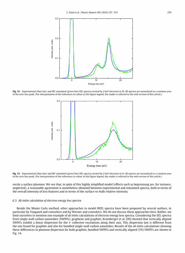
S. Taioli et al. / Physics Reports 493 (2010) 237–319 259
Fig. 12. Experimental (blue line) and MC simulated (green line) EEL spectra excited by 2 keV electrons in Al. All spectra are normalized to a common areaof the zero-loss peak. (For interpretation of the references to colour in this figure legend, the reader is referred to the web version of this article.)
Fig. 13. Experimental (blue line) and MC simulated (green line) EEL spectra excited by 2 keV electrons in Si. All spectra are normalized to a common areaof the zero-loss peak. (For interpretation of the references to colour in this figure legend, the reader is referred to the web version of this article.)
excite a surface plasmon. We see that, in spite of this highly simplified model (effects such as begrenzung are, for instance,neglected), a reasonable agreement is nonetheless obtained between experimental and simulated spectra, both in terms ofthe overall intensity of loss features and in terms of the surface-to-bulk relative intensity.
6.3. Ab initio calculation of electron energy loss spectra
Beside the Monte Carlo method, other approaches to model REEL spectra have been proposed by several authors, inparticular by Tougaard and coworkers and by Werner and coworkers. We do not discuss these approaches here. Rather, welimit ourselves to mention one example of ab initio calculations of electron energy loss spectra. Considering the EEL spectrafrom single-wall carbon nanotubes (SWNTs), graphene and graphite, Kramberger et al. [99] showed that vertically alignedSWNTs exhibit a linear dispersion for the π collective excitations along their axis. This dispersion law is different fromthe one found for graphite and also for bundled single-wall carbon nanotubes. Results of the ab initio calculations showingthese differences in plasmon dispersion for bulk graphite, bundled SWNTs and vertically aligned (VA) SWNTs are shown inFig. 14.
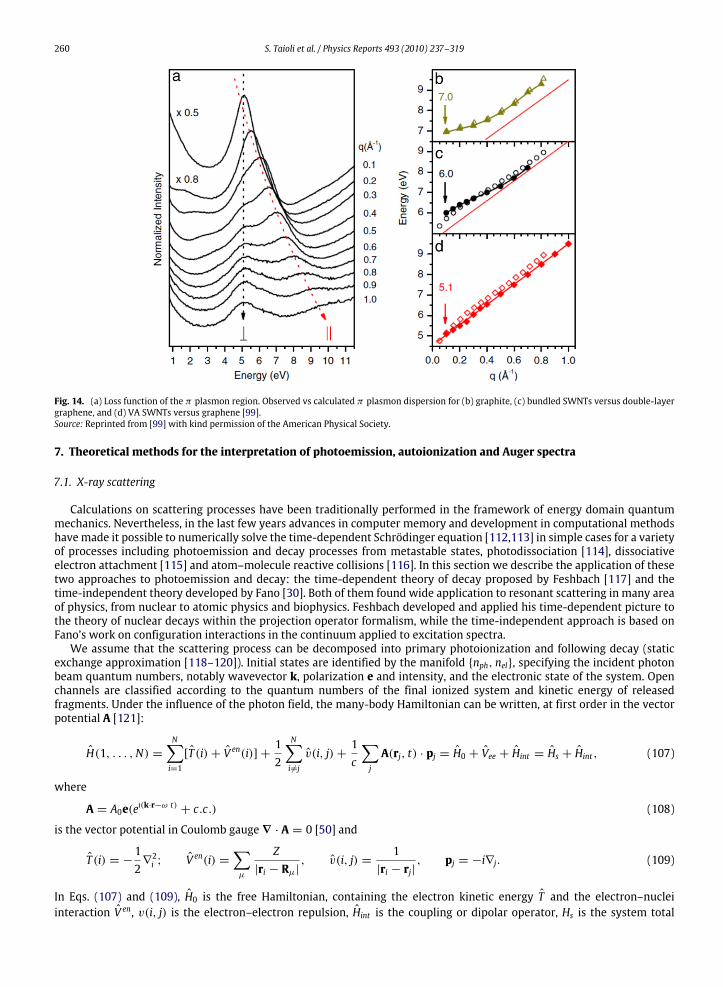
260 S. Taioli et al. / Physics Reports 493 (2010) 237–319
Fig. 14. (a) Loss function of the π plasmon region. Observed vs calculated π plasmon dispersion for (b) graphite, (c) bundled SWNTs versus double-layergraphene, and (d) VA SWNTs versus graphene [99].Source: Reprinted from [99] with kind permission of the American Physical Society.
7. Theoretical methods for the interpretation of photoemission, autoionization and Auger spectra
7.1. X-ray scattering
Calculations on scattering processes have been traditionally performed in the framework of energy domain quantummechanics. Nevertheless, in the last few years advances in computer memory and development in computational methodshavemade it possible to numerically solve the time-dependent Schrödinger equation [112,113] in simple cases for a varietyof processes including photoemission and decay processes from metastable states, photodissociation [114], dissociativeelectron attachment [115] and atom–molecule reactive collisions [116]. In this section we describe the application of thesetwo approaches to photoemission and decay: the time-dependent theory of decay proposed by Feshbach [117] and thetime-independent theory developed by Fano [30]. Both of them found wide application to resonant scattering in many areaof physics, from nuclear to atomic physics and biophysics. Feshbach developed and applied his time-dependent picture tothe theory of nuclear decays within the projection operator formalism, while the time-independent approach is based onFano’s work on configuration interactions in the continuum applied to excitation spectra.We assume that the scattering process can be decomposed into primary photoionization and following decay (static
exchange approximation [118–120]). Initial states are identified by the manifold nph, nel, specifying the incident photonbeam quantum numbers, notably wavevector k, polarization e and intensity, and the electronic state of the system. Openchannels are classified according to the quantum numbers of the final ionized system and kinetic energy of releasedfragments. Under the influence of the photon field, the many-body Hamiltonian can be written, at first order in the vectorpotential A [121]:
H(1, . . . ,N) =N∑i=1
[T (i)+ V en(i)] +12
N∑i6=j
v(i, j)+1c
∑j
A(rj, t) · pj = H0 + Vee + Hint = Hs + Hint , (107)
where
A = A0e(eı(k·r−ω t) + c.c.) (108)
is the vector potential in Coulomb gauge∇ · A = 0 [50] and
T (i) = −12∇2i ; V en(i) =
∑µ
Z|ri − Rµ|
, v(i, j) =1
|ri − rj|, pj = −i∇j. (109)
In Eqs. (107) and (109), H0 is the free Hamiltonian, containing the electron kinetic energy T and the electron–nucleiinteraction V en, v(i, j) is the electron–electron repulsion, Hint is the coupling or dipolar operator, Hs is the system total
S. Taioli et al. / Physics Reports 493 (2010) 237–319 261
Hamiltonian, and pj is the electron momentum. The resonant multichannel theory of scattering [6,29,121–123] aims to findpositive energy solutions of the Hamiltonian (107):
(H − E)|Ψ−α,ε〉 = 0, (110)
where the scattering wavefunction |Ψ−α,ε〉 describes themotion of a particle with kinetic energy εα = E−Eα , asymptoticallynot interacting with the scattering centre in the state Θα at energy Eα . Since the interaction term in Eq. (107) is treatedat the first order, the initial state wavefunction |Ψ+i 〉 = |Ψ0〉|N, ω〉, the tensorial product of the system ground-statewavefunction |Ψ0〉 with the radiation vector |N, ω〉, a linearly polarized monochromatic N photon beam with frequencyω, and the scattering states |Ψ−f 〉 = |Ψ
−α,ε〉|N − 1, ω〉 are eigenstates of H0 + Vee. Therefore, first-order perturbation theory
gives for the transition probability (per unit time)
Ti→f = 2π(A0c
)2|〈Ψ−f |e · e
ık·rp|Ψ+i 〉|2. (111)
7.2. Ingoing boundary conditions
Boundary conditions suitable for electron spectroscopies in resonant multichannel scattering are given by asymptoticsuperposition of stationary wavefunctions [32]. Asymptotic states are generally defined by outgoing wave conditions(labelled by ‘+’), if one specifies and controls the initial quantum state of the impinging particle, or by ingoing waveconditions (labelled by ‘−’), if the final scattering states are relevant for the experiment. These boundary conditions are time-reversal conjugate. Since experimental measurements in electron spectroscopy usually record electrons at large distance(r → ∞) from the scattering centre, the asymptotic wavefunctions are better normalized according to the ingoing waveboundary conditions [6]:
Ψ−α,E |r→∞ '
Nc∑γ=1
Ωγ
2ır
√2πkβ
(δγαe+ıθγ − SĎγαe−ıθγ ), (112)
where θγ is the phase shift for long-range Coulomb interactions andΩγ are symmetry-adaptedwavefunctions of the ionizedtarget. In Eq. (112), the asymptotic behaviour of thewavefunction is characterized by the scatteringmatrix S, whose elementSĎγα gives the probability amplitude for the emission of one electron into channel γ . The wavefunction in Eq. (112) isnormalized according to
〈Ψ−α,E |Ψγ ,E′ = δαγ δ(E − E ′
), (113)
satisfying the energy conservation
E − (Eα − Eγ ) =12k2αγ = ε, (114)
where kαγ is the electron momentum and ε is the electron kinetic energy.
7.3. Time-dependent theory of resonant scattering (Feshbach’s theory)
The decay process is studied theoretically [28,117], by analyzing the time evolution of a systemwhich initially (t = 0) isin the quasi-bound state |Φ〉 and evolves according to the time-independent Hamiltonian H as follows:
|Ψ (t)〉 = e−iHt |Φ〉. (115)
The probability of finding, at time t , the system still in the initial state |Φ〉 is given by
P(t) = |〈Φ|Ψ (t)|2 = |〈Φ|e−iHt |Φ〉|2. (116)
This quantity can be analyzed, in the energy domain, by using the Fourier transform, g(E), of the probability amplitudeexpressed in the time domain: f (t) = 〈Φ|e−iHt |Φ〉 θ(t). The expression obtained is the following:
g(E) =∫∞
−∞
iθ(t)〈Φ|ei(E−H)t |Φ〉dt = 〈Φ|1
E − H + i0|Φ〉, (117)
where θ(t) is the step function and g(E) is defined in the complex plane of the energy.Let us introduce the projection operator P = |Φ〉〈Φ|, and its orthogonal complement, Q = 1− P , in order to decompose
the Hamiltonian as follows:
H = H1 + H2, H1 = PHP + Q HQ , H2 = PHQ + Q HP. (118)
262 S. Taioli et al. / Physics Reports 493 (2010) 237–319
The following identities can be easily verified:
PH1 = H1P = EΦ P EΦ = 〈Φ|H|Φ〉 Q H1 = H1Q
P1
E − H1=
1E − H1
P =1
E − EΦP, Q
1E − H1
=1
E − H1Q
PH2 = H2Q Q H2 = H2P, (119)
from which one gets
1
E − H=
1
E − H1+
1
E − H1H2
1
E − H=
1
E − H1+
1
E − H1H2
1
E − H1+
1
E − H1H2
1E − H1
H2,1
E − H(120)
P1
E − HP =
PE − EΦ
+1
E − EΦ
(PH2
1
E − H1H2P
)P1
E − HP = P
1
E − EΦ − R(E)P, (121)
where
R(E) = PH21
E − H1H2P = PHQ
1
E − Q HQQ HP. (122)
From Eqs. (117)–(122), one obtains
g(E) = 〈Φ|1
E − H|Φ〉 =
1E − EΦ − R(E)
(123)
with
R(E) = 〈Φ|R(E)|Φ〉 = 〈Φ|HQ1
E − Q HQQ H|Φ〉. (124)
Moreover, by using the fact that
f (t) =12π
∫∞
−∞
g(E)e−iEtdE, (125)
one gets f (t) = 0 for t < 0, since the integration path is closed in the upper half-plane, where g(E) is analytical. In contrast,for t > 0, the value of f (t) is calculated by closing the integration path, in the lower half-plane, where g(E) is singular.Let us now suppose that R(E) is analytical in the upper half-plane and presents, in the lower part, a discontinuity surroundedby a path D. It follows that g(E) presents the same discontinuity and, moreover, isolated poles at the points Ep whereEp − EΦ − R(Ep) = 0. Therefore, at t > 0, f (t) is given by the sum of the Fourier integral in Eq. (125), made along apath Dwhich encloses the discontinuity, and of the residues of g(E) at the isolated poles.If R(E) is analytical in the neighborhood of such poles, one can use the following Taylor expansion:
R(E) = R(Ep)+ R′(Ep)(E − Ep)+R′′(Ep)(E − Ep)2
2+ · · · , (126)
which gives
g(E) =1
(E − Ep)[1− R′(Ep)] +R′′(Ep)(E−Ep)
2 + · · ·
. (127)
If [1 − R′(Ep)] 6= 0, the Fourier transform g(E) has an isolated pole at E = Ep with residue equal to 1[1−R′(Ep)]
. Therefore, att > 0, one has
f (t) =12π
∫Dg(E)e−iEtdE − i
∑p
1[1− R′(Ep)]
e−i(EΦ+∆p)t−(Γp/2)t , (128)
with ∆p = ReEp − EΦ and Γp/2 = ImEp. By disregarding the small integral along the discontinuity, f (t) is a sum ofexponential decays characterized by specific decay constants Γp.In order to connect this theoretical frameworkwith themeasured decay rates, one has to project the state |Ψ (t)〉 into the
final channel of interest, |χ−α,ε〉, this last described by a wavefunction with the appropriate boundary condition (incomingwave (−) for a typical decay process). By defining the following projection operator:
PE,α =
∫dεδ(E − Eα − ε)|χ−α,ε〉〈χ
−
α,ε |, (129)
S. Taioli et al. / Physics Reports 493 (2010) 237–319 263
the probability of finding the system in channel |χ−α,ε〉, at time t , is given by
PE,α(t) = 〈Φ|eiHtPE,αe−iHt |Φ〉 =∫dεδ(E − Eα − ε)f ∗α,ε(t)fα,ε(t), (130)
where
fα,ε(t) = iθ(t)〈χ−α,ε |e−iHt|Φ〉. (131)
By taking the Fourier transform gα,ε(E) of fα,ε(t):
gα,ε(E) = 〈χ−α,ε |1
E − H + i0|Φ〉 = 〈χ−α,ε |Q
1
E − H + i0P|Φ〉, (132)
where the projection operator Q has been introduced since |χ−α,ε〉 is orthogonal to |Φ〉; and observing that the operatorQ 1E−H+i0
P can be transformed, using Eq. (118)–(119), as follows:
Q1
E − H + i0P = Q
1
E − H1 + i0P + Q
1
E − H1 + i0H2
1
E − H + i0P = Q
1
E − H1 + i0Q H2P
1
E − H + i0P, (133)
one gets
gα,ε(E) = 〈χ−α,ε |1
E − Q HQ + i0Q H|Φ〉〈Φ|
1
E − H + i0|Φ〉. (134)
Furthermore, if |χ−α,ε〉 is an eigenstate of Q HQ with eigenvalue Eα + ε, it follows that
gα,ε(E) =1
E − Eα − ε + i0〈χ−α,ε |H|Φ〉〈Φ|
1
E − H + i0|Φ〉. (135)
Therefore, fα,ε(t) can be written as follows:
fα,ε(t > 0) = −i〈χ−α,ε |H|Φ〉[e−i(Eα+ε−i0)t
1Eα + ε − EΦ − R(Eα + ε)
+
∑p
1[1− R′(Ep)]
e−i(Ep+∆p)t−Γp/2t1
Ep − Eα − ε + i0
], (136)
with R(Eα + ε) defined by Eq. (124). This expression tells us that the decay amplitude into channel |α〉 consists of two parts,the latter of which goes exponentially to 0 for t → ∞. Thus, at large values of t , the decay rate into channel |α〉 becomestime independent, as shown by the following expression:
limt→∞
PE,α(t) = limt→∞|fα,ε(t)|2 =
|〈χ−α,ε |H|Φ〉|2
(Eα + ε − EΦ − ReR(Eα + ε))2 + ImR(Eα + ε)2. (137)
This expression is proportional, through the square of a matrix element that is slowly energy dependent, to a Lorentziancentered at E = EΦ + ReR(E) and having a half-width equal to ImR(E).
7.4. Time-independent resonant multichannel scattering theory including channel interaction (Fano’s theory)
In order to accurately solve the multichannel Hamiltonian equation (see Eq. (110)), including electronic correlation inthe final state wavefunctions beyond the independent channel approximation, Fano [30] developed a method similar toconfiguration interaction (CI) in bound-state calculations, where the scattering solution is obtained by linearly combiningthe interacting scattering channels:
|Ψ−α,ε〉 = aα(ε)|Φ〉 +Nc∑β=1
∫∞
0|χβ,τ 〉Cβ,α(τ , ε)dτ , (138)
where ε is the kinetic energy of the escaping electron (see Eq. (114)). In Eq. (138), a discrete quasi-bound configuration|Φ〉, lying above ionization threshold, interacts with the continuum states of the ionized target, |χβ,ε〉. The decay channels|χβ,ε〉 interact via the many-body Hamiltonian
〈χβε′ |H − E|χαε〉 = (ε + Eα − E)δ(ε′ + Eβ − ε − Eα)δβα + Vβα(ε, ε′, E). (139)
The interaction between metastable state and scattering channels results in the decay of the system. Using thisrepresentation of the final state wavefunction, Fano explained the origin of asymmetric profiles (Fano profiles) as due

264 S. Taioli et al. / Physics Reports 493 (2010) 237–319
to the interference between the direct ionization channel and the resonant path. Åberg [6] showed that the absence of theintermediate metastable state |Φ〉 in the final state wavefunction and of the interchannel interaction (see Eq. (139)),
|Ψ−α,ε〉 =
Nc∑β=1
∫∞
0|χβ,τ 〉Cβ,α(τ , ε)dτ , (140)
is the main reason of errors when comparing numerical results to experimental data. To specify the wavefunction inEq. (138), one needs to compute the coefficients aα, Cβ,α of the CI expansion: we will exemplify Fano’s method for anautoionization process in which one electron is excited to a discrete (resonant) state degenerate with several continua ofthe ionized target.Incomingwave boundary conditions are used throughout the description,meaning that, asymptotically, thewavefunction
|χ−α,ε〉 represents one electron released, with energy ε, into the channel |α〉 of the ionized target at energy Eα (see Eq. (112)).Finally, the final-state wavefunctions are energy normalized according to
〈Ψ−α,ε |Ψ−
β,ε′= δαβδ(Eα + ε − Eβ − ε′). (141)
The expansion coefficients in Eq. (138) are determined by requiring that
〈Φ|H − E|Ψ−α,ε〉 = 〈χ−
β,ε|H − E|Ψ−
α,ε〉 = 0 (142)
i.e. by solving the following set of equations:
(EΦ − E)aα(ε)+Nc∑β=1
∫∞
0M−β (τ , E)Cβα(τ , ε)dτ = 0 (143)
aα(ε)M−β (ε′, E)∗ + (ε + Eβ − E)Cβα(ε′, ε) = 0, (144)
with
M−β (ε, E) = 〈Φ|H − E|χ−
β,ε〉; (EΦ − E) = 〈Φ|H − E|Φ〉. (145)
By using the Dirac technique for treating the singularities which appear in the definitions of the coefficients aα, Cβα ofEqs. (143) and (144), one gets the following expression:
|Ψ−α,ε〉 = |χ−
α,ε〉 +M−α (ε, E)E − Er − iΓ2
[|Φ〉 + lim
ν→0
∑β
∫∞
0
|χ−β,τ 〉M−
β (τ , E)∗
E − Eβ − τ − iνdτ
], (146)
with Γ and Er defined as follows:
Γ =∑β
Γβ = 2π∑β
|M−β (εr , E)|2; εr = Er − Eα (147)
Er = EΦ +∆; ∆ =∑β
P
∫∞
0
|M−β (τ , E)|2
E − Eβ − τdτ . (148)
The asymptotic behaviour of the scattering wavefunction that represents the stationary state |Ψ−α,ε〉 is characterized bythe scattering matrix S, while S ′, whose element S ′βα gives the probability amplitude for the emission of one electron intochannel β [28], characterizes the asymptotic behaviour of the single-channel wavefunction |χ−β,ε〉. The explicit expressionof Sβα , obtained using Eqs. (112) and (146), is the following:
Sβα = S ′βα − 2π iM+α (εr , Er)M
+
β (εr , Er)∗
E − Er + iΓ2. (149)
From the knowledge of the stationary state |Ψ−α,ε〉 one can obtain the cross section for a process in which one electron isexcited to a discrete resonant state |Φ〉, through the absorption of one photon of appropriate energy, and the target decaysnon-radiatively into the channel |χ−α,ε〉. According to the general theory of scattering – see e.g. [28,124] – the cross sectionof this process is proportional to the square of the transition matrix Tr , which connects the initial and final states:
T+rβα(ε) = T+βα(ε)+〈χ−β,ε |H − E|Φ〉〈Φ|H − E|χ
−α 〉
ε − εr + iΓ2, (150)
calculated by using the formula
Tr(ε) =[1− S(E)
]2π ı
, (151)
S. Taioli et al. / Physics Reports 493 (2010) 237–319 265
which describes the scattering from channel α into channel β in the presence of a resonance at ε = εr . The matrixelement T+βα(ε) represents the direct scattering, while the second term in the right-hand side of Eq. (150) describes thescattering from α to β via the bound state |Φ〉. If the direct term is negligible in comparison to the resonant, one obtains theBreit–Wigner cross section [125] (see Eq. (155)). If we choose
P = |Φ〉〈Φ|, Q =∫∞
0
Nc∑β=1
|χ±βτ 〉〈χ±
βτ |dτ , (152)
provided that the orthogonality relations 〈Φ|χ±βτ = 0, β = 1, . . . ,Nc are satisfied andΦ, χ±βτ
is a complete basis set,
Fano’s method is equivalent to Feshbach’s projection operator approach.
7.5. The concept of autoionization and the Auger effect as resonant multichannel scattering
The calculation of photoemission, autoionization and Auger cross sections is a straight application of Fano’smultichannelresonance approach [29,30,126]. When the energy of the projectile exceeds the inner-shell ionization threshold of anN-electron system, the final-statewavefunctions describing electron emission or the formation of an inner-shell vacancy aregiven in Eq. (146). From the knowledge of these wavefunctions, one can evaluate the differential cross section for the globalionization process inwhich, for instance, the target in its ground state |Ψ0〉 is ionized by a linearly polarized, monochromaticN-photon beam with frequency ω (|N, ω〉). Using Eqs. (145) and (150), one obtains
T+fi (ε) = 〈χ−
α,ε;N − 1, ω|Hint |0;N, ω〉 +〈χ−α,ε |Hs − E|Φ〉〈Φ
−;N − 1, ω|Hint |0;N, ω〉
ε − εr + iΓ2, (153)
where the following definition has been used:
|Φ−〉 = |Φ〉 + limν→0
Nc∑β=1
∫∞
0
|χ−β,τ 〉M−
β (τ , E)∗
E − Eβ − τ − iνdτ ; ε = ω − (Eα − E0). (154)
By neglecting the first term in the right-hand side of Eq. (153), which represents the direct scattering, and using Eq. (154),the cross section of the process can be approximated:
dσfi(ε)dε
=4π2ωNc|T+fi (ε)|
2= σ(ω)
12π
Γα
(ε − εr)2 + Γ 2/4, (155)
where σ(ω) = (2π)2ωNc |〈Φ
−;N−1, ω|Hint |0;N, ω〉|2 is the cross section for the excitation process |0〉 → |Φ〉: this Lorentzian
distribution is obtained provided the relevant matrices Γα and Γ are weakly energy dependent in the range of interest. Thedifference in considering both terms in Eq. (153) is the formation of inner-shell vacancy or autoionizing states interferingwith the direct ionization path. In this case, Lorentzian distributions with characteristic half-widths are substituted byasymmetric probability distributions (Fano profiles). If one now takes into account the flux of photons N(ω), i.e. the numberof photons at frequencyω that cross a unit area per unit time, one obtains the expression for the number of electrons emittedper unit time at energy ε:
dNαdε= σ(ω)N(ω)
12π
Γα
(ε − εr)2 + Γ 2/4. (156)
If N(ω) is peaked at ω = ω0 and the product N(ω)σ (ω) remains practically constant over a range of energies larger thanthat in which Γα and Γ are constant, the total number of electrons emitted into channel α, per unit time, is given by thefollowing expression:
Nα =∫∞
0
dNαdεdε =
Γα
ΓN0; N0 = σ(ω0)N(ω0). (157)
This result indicates that Γα represents the decay rate into channel |α〉 and Γ the total decay rate.The only difference in inner-shell ionization is that the resonant state |Φτ 〉 consists actually of a distribution of discrete
and continuum states which represents a discrete (N−1) electron state plus an excited (autoionization) or outgoing (Auger)electron with energy τ . However, the Tmatrix of the process can be written as follows:
T+′αi = 〈χ−
α,ε1ε2;N − 1, ω|Hint |0;N, ω〉 +
∫∞
0
〈χ−α,ε1ε2 |Hs − E|Φτ 〉〈Φτ ;N − 1, ω|Hint |0;N, ω〉dτ
ε1 + ε2 − εr − τ + iΓ /2, (158)
where ε1 and ε2 are the energies of the outgoing electrons related to the other characteristic energies of the problem by therelationship: ε1 + ε2 = ω − (Eα − E0). The intermediate state |Φτ 〉 is a metastable state that, as long as ω Eα − Er , canbe approximated by an antisymmetrized product, A|Φ〉|τ 〉, where |τ 〉 represents the state of the primary electron. In a
266 S. Taioli et al. / Physics Reports 493 (2010) 237–319
similar way, the final state can be represented by A|χ−β,ε2〉|ε1〉, where |ε1〉 is the state of the primary electron. Therefore,in the right-hand side of Eq. (159), one can use the approximation
〈χ−β,ε1ε2 |Hs − E|Φτ 〉 ' 〈ε1|τ 〉〈χ−
β,ε2|Hs − E + ε1|Φ〉, (159)
with 〈ε1|τ 〉 = δ(ε1 − τ) and (E − ε1) the energy of the ionized system. Neglecting the first terms in the right-hand side ofEq. (159), which represent the probability amplitude of the double direct ionization process, one obtains
dσα(ε)dε
= σ(ε)12π
Γα
(ε − εr)2 + Γ 2/4; ε = ω − (Er − E0), (160)
where σ(ε) is the photoionization cross section of the primary process. Again, this result indicates that Γα is the rate of thenon-radiative decay process from the intermediate state |Φ〉 into channel |α〉 and Γ the total Auger decay rate.
7.6. Construction of the theoretical spectrum
The cross sections obtained in Section 7.5 represent the starting point for constructing the ab initio spectrum to becompared with the experimental one. They give the contributions to the spectrum due to the intrinsic features of the target,while the contributions of the specific incident radiation can be made evident by analyzing the expression of the transitionrate for a given transition in the energy range of interest.In the following, we perform this analysis in the simple case of an autoionization process where only one intermediate
state is present.We assume that the photoionization is produced by an incident radiationmade of a flux of photons polarizedalong eλ, having angular frequencies spread around a given value (ω0) and propagating along a given direction (Ω0) with asmall angular dispersion.The analytic representation of the flux, i.e. of the number of photons going through a unit surface per unit time and
frequency, can be chosen as
F 0λ (ω, Ω) =ω2
(2π)3c2A exp
(−2
(ω − ω0
γ0
)2)δ(Ω − Ω0), (161)
where A is an adimensional scale factor and γ0 gives the frequency spread of the photons. If one is to evaluate the differentialcross section of the photoionization process in terms of the momentum k of the emitted electron, Eq. (155) can be writtenby choosing a specific polarization λ:
∂σ0→α
∂k(k;ω, λ) =
(4π2ωc
)|〈0|Oλ|Φ−〉Λ−1〈Φ|H − E|χ−αk〉|
2δ
[(E0 + ω)−
(Eα +
k2
2
)], (162)
with
Λ = (E − Er)−∆− iΓ
2. (163)
In Eq. (162), the interaction operator Hint is
Hint =∑λ
AλOλ =∑λ
Aλeλ ·∑j
qjrj, (164)
where Aλ is the component of the vector potential along the polarization λ. A similar expressionwith 〈0|Oλ|Φ−〉 substitutedby 〈0|Oλ|Φ−ηk1〉 and, furthermore, 〈Φ|H − E|χ
−
αk〉 substituted by 〈Φ|H − E|χ−
αkηk1〉 and δ[(E0 + ω) − (Eα +k22 )] by
δ[(E0+ω)− (Eα+k2+k212 )], gives the double differential cross section in terms of the momenta of the emitted electrons (see
Eq. (160)):
∂σ0→α
∂k∂k1=
(4π2ωc
)|〈0|Oλ|Φε1〉Λ−1Mlα(E, k)|2δ
[(E0 + ω)−
(Eα +
k2 + k212
)]. (165)
The differential transition rate of the process( ∂Wλ0→α
∂k
)is defined in terms of the flux of photons F 0λ (ω, Ω) and of the
differential cross section ∂σ0→α∂k of the transition by the following relationship:
∂W λ0→α
∂k(k;ω0, γ0) =
∫∞
0dω∫dΩ
∂σ0→α
∂k(k;ω, λ) Fλ(ω, Ω). (166)
S. Taioli et al. / Physics Reports 493 (2010) 237–319 267
Since in our example there is only one intermediate state |Φ〉 in the autoionization process, the general expression of thedifferential cross section is that given in Eq. (154):
∂σ0→α
∂k(k;ω, λ) =
(4π2ωc
)|〈0|Oλ|Ψαk〉|2δ
[(E0 + ω)−
(Eα +
k2
2
)]
=
(4π2ωc
) ∣∣∣∣∣∣〈0|Oλ|χ−αk〉 + 〈0|Oλ|Φ−〉〈Φ|H − E|χ−αk〉(
Eα + k22
)−(Er + iΓ2
)∣∣∣∣∣∣2
δ
[(E0 + ω)−
(Eα +
k2
2
)], (167)
where E0 is the energy of the ground state |0〉 and Er = 〈Φ|H|Φ〉+∆ is the resonance energy. By inserting definitions (161)and (167) into Eq. (166) one gets the expression for the differential transition rate:
∂W λ0→α
∂k(k;ω0, γ0)=
A2πc3|〈0|Oλ|Ψ−αk〉|
2(εα0 +
k2
2
)3exp
(−2
((εα0 +
k22 )− ω0
γ0
))2, (168)
where εα0 = Eα − E0. In a similar way, the total transition rate is given by
W λ0→α(ω0, γ0) =
∫dkδW λ
0→α
δk(k;ω0, γ0) =
∫∞
0dε√2ε wλ0→α(ε;ω0, γ0), (169)
where
wλ0→α(ε;ω0, γ0) =A2πc3
(ε + εαo )3 exp
(−2
(ε + εα0 − ω0
γ0
)2)Dα,λ(ε)
Dα,λ(ε) =∫dk |〈0|Oλ|Ψ−αk〉|
2k=√2ε. (170)
The plot of wλo→α(ε;ω0, γ0) as a function of ε gives the number of electrons produced per unit time, in the transition|0〉 → |α〉, at the energy ε, i.e. the contribution of the transition to the electronic spectrum recorded in terms of thephotoelectron energy. On the other hand, the plot ofW λ
0→α(ω0, γ0) as a function of ω0 gives the total number of electronsproduced per unit time, in the same transition, at the mean photon energy ω0, i.e. the contribution of the transition to theelectronic spectrum recorded in terms of the photon energy.Since we are interested in the study of the spectrum from the point of view of the incident radiation, we will analyze the
main spectroscopic quantities in terms of the photon energy and photon bandwidth, separating also the contributions dueto the two terms, direct and resonant, in the definition of the differential cross section. We introduce the following meansquare dipole matrix elements for the two different ionization paths:
Ddirα,λ(ε) =∫dk |〈0|Oλ|χ−αk〉|
2k=√2ε=(2π)2√2ε|tλ0→α(ε)|
2 (171)
Dresα,λ(ε) =∫dk
∣∣∣∣∣ 〈0|Oλ|Φ−〉〈Φ|H − E|χ−αk〉ε − εrα − iΓ 2
∣∣∣∣∣2
k=√2ε
= (2π)2|tλ0→Φ(ε)|
2
√2ε
Γα(ε)
(ε − εrα)2 + (Γ2 )
2, (172)
where εrα = Er − Eα and
|tλ0→α(ε)|2= 2π
∫dp(2π)3
|〈0|Oλ|χ−αp〉|2 δ
(ε −
p2
2
)(173)
|tλ0→Φ(ε)|2= |〈0|Oλ|Φ−〉|2 (174)
Γα(ε) = 2π∫
dp(2π)3
∣∣∣∣〈Φ|H − (Eα + p22)|χ−αp〉
∣∣∣∣2 δ (ε − p22). (175)
Using these definitions, the transition rates of the direct and resonant paths become, respectively,
W dir0→α(ω0, γ0) = 2πNc3
∫∞
0dε (ε + εα0 )
3 e−2(ε+εα0 −ω0
γ0)2|tλ0→α|
2 (176)
268 S. Taioli et al. / Physics Reports 493 (2010) 237–319
and
W res0→α(ω0, γ0) = 2πNc3
∫∞
0dε(ε + εα0 )
3 e−2(ε+εα0 −ω0
γ0)2|tλ0→Φ |
2 Γα
(ε − εrα)2 + (Γ2 )
2. (177)
For the evaluation of these integrals one can observe that, in a typical inner-shell ionization process, themean photon energyis much larger than the energy difference between the ground and final states of the target, and also larger than the photonbandwidth. This means that ω0 εα0 and ω0 γ0.Furthermore, since thematrix elements defined in Eq. (175) have a smooth and slowdependence on ε, in the energy range
important for the evaluation of the transition rates, one can approximate the direct and resonant contributions respectivelyas
W dir0→α(ω0, γ0) = 2πNc3
√π
2|tλ0→α(ω0)|
2 ω30 γ0 (178)
and
W res0→α(ω0, γ0) = (2π)2 Nc3|tλ0→Φ(ω0)|
2 ω30Γα
ΓV (x, a), (179)
where
V (x, a) =aπ
∫∞
−∞
dye−y
2
(y− x)2 + a2; x =
(εr0 − ω0)√2
γ0; εr0 = Er − E0; a =
Γ
γ0√2. (180)
We see that the transition rate of the direct path is proportional to γ0ω30 , while that of the resonant path is modulated bythe so-called Voigt profile, V (x, a), which is defined in Eq. (180). This one is a convolution of a Gaussian with a Lorentzianand has two characteristic parameters: the damping constant a, which depends on the ratio between the natural linewidthand the photon bandwidth, and the scaled distance xmeasured from the resonance. It appears immediately that, for a givenω0 and a photon bandwidth appreciably smaller than the natural linewidth, one has
W res0→α(ω0, γ0) ∝ γ0 ω30
(Γα/2)(ω0 − ε
r0)2 + (Γ /2)2
. (181)
The same Lorentzian profile is also predominant at values ofω0 far out of resonance as comparedwith γ0, i.e. for |ω0−εr0| γ0.On the other hand, when the bandwidth of the incident photons is appreciably larger than the natural linewidth, one has
W res0→α(ω0, γ0) ∝ ω30Γα
Γe−2(
ω0−εr0
γ0)2. (182)
This means that, for γ0 Γ , the central part of the profile ofW res0→α(ω0, γ0) is represented by a Gaussian, while its wingsmaintain a Lorentzian character.Finally, it is clear that the global profile of W0→α(ω0, γ0) is made up by the contributions of both the direct and the
resonant term, which can interfere, producing an asymmetric lineshape.Let us now study the lineshape modifications due to the presence of an electron spectrometer with finite resolving
power. One can reproduce these effects by making a convolution of the transition rate per unit energy with a functionG(ε) representative of the analyzer window function. By assuming that the response of the instrument is the same all overthe energy range of interest, we can simply require, for generality, that the functional form of G(ε) satisfies the followingrelationships:∫
∞
−∞
G(ε)dε = 1;∫∞
−∞
G(ε) εdε = 0;∫∞
−∞
G(ε) ε2dε = B2, (183)
where B is a constant inversely proportional to the resolving power of the electron spectrometer.By convoluting G(ε) with the transition rate, we obtain the following expression for the experimental value of the
transition rate:
W exp0→α(ω0, γ0) =∫∞
−∞
dτ∫∞
0dε√2ε wλ0→α(ε;ω0, γ0) G(ε − τ)
=
∫∞
0dε√2ε wλ0→α(ε;ω0, γ0)
∫∞
−∞
dτ G(τ )
= W λ0→α(ω0, γ0). (184)
These expressions, obtained by exploiting the properties of the analyzer window function, show that the total transitionrate recorded in the experiment is independent of the finite resolving power of the electron spectrometer.
S. Taioli et al. / Physics Reports 493 (2010) 237–319 269
7.7. Many-body perturbation theory
The photoionization processes, discussed in the previous paragraphs, can be treated also in the framework of the many-body theory [47].Let us consider, for example, an Auger process. We start from Fano’s theory of Section 7.4 and rewrite the Hamiltonian ofEq. (107) in the second quantization formalism as follows:
Hs =∑j
εja+j aj +∑ij
vija+i aj +∑ijkl
gijkla+j a+
i akal
Hint =∑ν,jk
(cν,jkb+ν a
+
j ak + c∗
ν,jkbν a+
k aj), (185)
where a+j , ak are electron creation and annihilation operators, while b+ν , bν are photon creation and annihilation operators.
The cross section for the ionization process is given by Eq. (155), where, as explained in Section 7.5, the initial and the finalstates can be approximated by the following tensorial product, |Ψ+i 〉 = |0〉|N, ν〉 and |Ψ
−
f 〉 = |Ψ−
α,E1 2〉|N − 1, ν〉. The
transition matrix defined in Eq. (153) becomes
T+fi = 〈Ψ−
α,E1E2;N − 1, ν|
∑ν,jk
(cν,jkb+ν a
+
j ak + c∗
ν,jkbν a+
k aj)|0;N, ν〉
= 〈Ψ−α,E1E2;N − 1, ν|∑ν,jk
(c∗ν,jkbν a
+
k aj)|0;N, ν〉
=√N〈Ψ−α,E1E2 |
∑jk
c∗ν,jka+
k aj|0〉. (186)
If the state |Ψ−α,E1E2〉 is approximated by the product |Ψ−
α,E2〉|E1〉, one gets
T+fi =√N〈Ψ−α,E2 |
∑j
c∗ν,jE1 aj|0〉. (187)
Thus the cross section for the Auger process becomes
∂σfi
∂E1∂E2=4π2ωNc|T+fi |
2δ(E0 + ω − Eα − E1 − E2)
=4π2ωc
∑jl
c∗ν,jE1cν,lE1 |〈0|al|Ψ−
α,E2〉|2δ(E0 + ω − Eα − E1 − E2), (188)
where
〈Ψ−α,E2 |aj|0〉 =4π2ωc
∑jl
c∗ν,jE1cν,lE1ResGlj(ω − E1)
(189)
and ResGlj(E)
is the residue at the energy E of the one-particle Green function [113]. The last equality is true only if |0〉 is
a closed-shell state. In this case, matrix G(E) is given by
Gjl(E) = i∫∞
−∞
eiEt〈0|T [a+j (t)al(0)]|0〉dt
= 〈0|a+j1
E + E0 − Hs + iεal|0〉 + 〈0|al
1
E + E0 − Hs − iεa+j |0〉, (190)
where T means time-ordered product [127], and aj(t) = eiHst aje−iHst . We note that the exact G(E) is unknown unless theHamiltonian of Eq. (185) contains only one-particle terms. If we make the following decomposition:
H0 =∑j
εja+j aj; H1 = Hs − H0 =∑ij
vija+i aj +∑ijkl
gijkla+j a+
i akal, (191)
the one-particle Green function associated with H0 is given by G(0)jl (E) = δjl
1E−εj. This fact suggests a possible way
of calculating the exact G(E), starting from G(0)(E) and considering H1 as the perturbing potential defined in the mostconvenient way. When the interaction H1 is switched on, the poles of the Green function change their positions. Thus, forexample, the energy Eh of the h-th pole becomes, according to the Goldstone–Bruekener [128,129] theory,
Eh = 〈Φ0|a+h∑n
∑L(n)
H1
(1
E + EΦ − H0 + iεH1
)nah|Φ0〉, (192)

270 S. Taioli et al. / Physics Reports 493 (2010) 237–319
where∑L(n) indicates the sum over the linked diagram of order n and |Φ0〉 is the ground state of the Hamiltonian H0. We
can choose H0 so that the first-order term in Eq. (192) is equal to zero. This fact implies vij = −∑occk (gik,jk − gik,kj), which is
equivalent to taking H0 as the Hartree–Fock Hamiltonian. In this case, the second-order correction is given by
Eh = εh +∑kjm
(ghkjm − ghkmj)g∗hkjmεj + εm − εh − εk
= εh −∑kjmnr
MhkjmM∗hknrL(0)jmnr(εh + εk), (193)
where εj are the Hartree–Fock eigenvalues, Mlkjm = glkjm and L(0) is the Green function of two free particles defined asfollows:
L(0)jmnr(E) =δjnδmr − δjrδmn
E − εj − εm. (194)
This fact suggests that one can use the effective two-particle Green function L(E), instead of L(0)(E), in Eq. (193), thusincluding higher-order perturbation terms in the evaluation of Eh. The positions of the poles Eα of L(E) give the double-ionization energies, while the corresponding residues, ResL(Eα), can be interpreted as two-particle densitymatrices of thestates at the energies Eα . Finally, the relation between L(E) and L(0)(E) is the Bethe–Salpeter equation [130]:
L(E) = L(0)(E)+ L(0)(E)K(E)L(E), (195)
where K is the optical two-particle potential.One should remember that, if k runs over the continuum states, the sum in Eq. (193) must be replaced by an integral asfollows:
Eh = εh −∑jmnrµ
∫dτMhµjm(τ )M∗hµnr(τ )Ljmnr(εh + τ − iν)
= εh −∑jmnrµ
P
∫dτMhµjm(τ )M∗hµnr(τ )Ljmnr(εh + τ)+ iπ
∑jmnrµ
∫dτMhµjm(τ )M∗hµnr(τ )ResLjmnr(εh + τ), (196)
where τ and µ characterize the energy and the partial wave quantum index of the state k. The last term of Eq. (196) canbe identified as half of the total decay rate Γ /2. If ResL is different from zero only for a discrete set of energies Eα,corresponding to ionization energies, one gets
Γ =∑α
Γα (197)
Γα = 2π∑jmnrµ
Mhµjm(Eα − εh)M∗hµnr(Eα − εh)ResLjmnr(Eα). (198)
8. Calculation of photoemission and Auger spectra of atoms, molecules and solids
8.1. Calculation of spectral energy in atomic and molecular photoemission and Auger spectra
The interpretation of atomic,molecular and solid-state photoemission andAuger spectra requires the specific applicationof the general theory to the problem under investigation. This application presents several theoretical and computationaldifficulties that have hindered the production of high quality spectra until recently [40,55,131].In this section we will briefly discuss various techniques proposed for calculating resonance energies and decay rates
in atoms and molecules, discussing only in the last part the chapter the problems that arise when solid-state systems areconsidered.The energy (εA) of an Auger electron emitted into channel α can be approximated as the difference between the energy
(EΦ ) of the intermediate resonant state |Φ〉 and the energy (Eα) of the final state |α〉 of the doubly ionized target: εA = Er−Eα .This is equivalent to disregarding the energy shift∆, defined in Eq. (148), which usually represents a small correction to EΦ .Since the intermediate and final states of the ionized system are bound states, total energymethods using standard quantummechanical techniques can be applied. Similar considerations to Auger transitions apply to photoemission all throughoutthis section.A large number of ab initio calculations have been performed to predict the Auger energies of atomic andmolecular spec-
tra and the results obtained are generally in fairly good agreement with the experimental data; see, e.g., [42,49,132–142].Very different is the situation for solids and extended systems, where the theoretical and computational treatment of elec-tronic excitations, particularly neutral ones, still presents many difficulties. In this section we will briefly summarize the
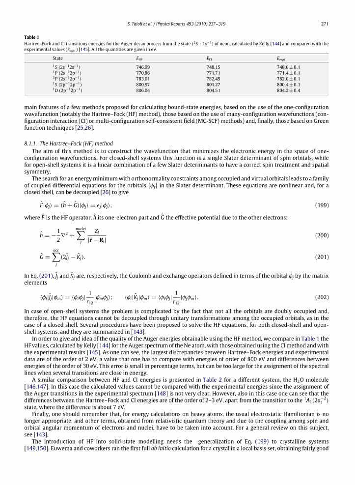
S. Taioli et al. / Physics Reports 493 (2010) 237–319 271
Table 1Hartree–Fock and CI transitions energies for the Auger decay process from the state (2S : 1s−1) of neon, calculated by Kelly [144] and compared with theexperimental values (Eexpt ) [145]. All the quantities are given in eV.
State EHF ECI Eexpt1S (2s−12s−1) 746.99 748.15 748.0±0.11P (2s−12p−1) 770.86 771.71 771.4±0.13P (2s−12p−1) 783.01 782.45 782.0±0.11S (2p−12p−1) 800.97 801.27 800.4±0.11D (2p−12p−1) 806.04 804.51 804.2±0.4
main features of a few methods proposed for calculating bound-state energies, based on the use of the one-configurationwavefunction (notably the Hartree–Fock (HF) method), those based on the use of many-configuration wavefunctions (con-figuration interaction (CI) or multi-configuration self-consistent field (MC-SCF) methods) and, finally, those based on Greenfunction techniques [25,26].
8.1.1. The Hartree–Fock (HF) methodThe aim of this method is to construct the wavefunction that minimizes the electronic energy in the space of one-
configuration wavefunctions. For closed-shell systems this function is a single Slater determinant of spin orbitals, whilefor open-shell systems it is a linear combination of a few Slater determinants to have a correct spin treatment and spatialsymmetry.The search for an energyminimumwith orthonormality constraints among occupied and virtual orbitals leads to a family
of coupled differential equations for the orbitals φj in the Slater determinant. These equations are nonlinear and, for aclosed shell, can be decoupled [26] to give
F |φj〉 = (h+ G)|φj〉 = εj|φj〉, (199)
where F is the HF operator, h its one-electron part and G the effective potential due to the other electrons:
h = −12∇2+
nuclei∑l
Zl|r− Rl|
(200)
G =occ∑j
(2Jj − Kj). (201)
In Eq. (201), Jj and Kj are, respectively, the Coulomb and exchange operators defined in terms of the orbital φj by the matrixelements
〈φi|Jj|φm〉 = 〈φiφj|1r12|φmφj〉; 〈φi|Kj|φm〉 = 〈φiφj|
1r12|φjφm〉. (202)
In case of open-shell systems the problem is complicated by the fact that not all the orbitals are doubly occupied and,therefore, the HF equations cannot be decoupled through unitary transformations among the occupied orbitals, as in thecase of a closed shell. Several procedures have been proposed to solve the HF equations, for both closed-shell and open-shell systems, and they are summarized in [143].In order to give and idea of the quality of the Auger energies obtainable using the HF method, we compare in Table 1 the
HF values, calculated byKelly [144] for the Auger spectrumof theNe atom,with those obtained using the CImethod andwiththe experimental results [145]. As one can see, the largest discrepancies between Hartree–Fock energies and experimentaldata are of the order of 2 eV, a value that one has to compare with energies of order of 800 eV and differences betweenenergies of the order of 30 eV. This error is small in percentage terms, but can be too large for the assignment of the spectrallines when several transitions are close in energy.A similar comparison between HF and CI energies is presented in Table 2 for a different system, the H2O molecule
[146,147]. In this case the calculated values cannot be compared with the experimental energies since the assignment ofthe Auger transitions in the experimental spectrum [148] is not very clear. However, also in this case one can see that thedifferences between the Hartree–Fock and CI energies are of the order of 2–3 eV, apart from the transition to the 1A1(2a−21 )state, where the difference is about 7 eV.Finally, one should remember that, for energy calculations on heavy atoms, the usual electrostatic Hamiltonian is no
longer appropriate, and other terms, obtained from relativistic quantum theory and due to the coupling among spin andorbital angular momentum of electrons and nuclei, have to be taken into account. For a general review on this subject,see [143].The introduction of HF into solid-state modelling needs the generalization of Eq. (199) to crystalline systems
[149,150]. Euwema and coworkers ran the first full ab initio calculation for a crystal in a local basis set, obtaining fairly good
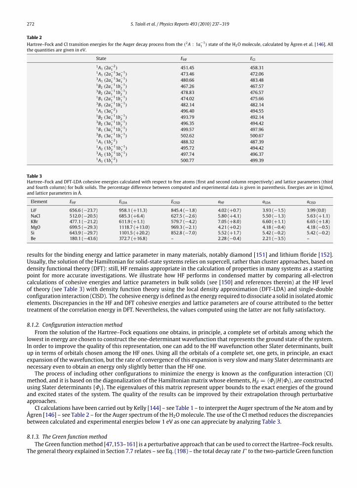
272 S. Taioli et al. / Physics Reports 493 (2010) 237–319
Table 2Hartree–Fock and CI transition energies for the Auger decay process from the (2A : 1a−11 ) state of the H2O molecule, calculated by Ågren et al. [146]. Allthe quantities are given in eV.
State EHF ECI1A1 (2a−21 ) 451.45 458.311A1 (2a−11 3a
−11 ) 473.46 472.06
3A1 (2a−11 3a−11 ) 480.66 483.48
1B2 (2a−11 1b−12 ) 467.26 467.57
3B2 (2a−11 1b−12 ) 478.83 476.57
1B1 (2a−11 1b−11 ) 474.02 475.66
3B1 (2a−11 1b−11 ) 482.14 482.14
1A1 (3a−21 ) 496.40 494.551B2 (3a−11 1b
−12 ) 493.79 492.14
3B2 (3a−11 1b−12 ) 496.35 494.42
1B1 (3a−11 1b−11 ) 499.57 497.96
3B1 (3a−11 1b−11 ) 502.62 500.67
1A1 (1b−22 ) 488.32 487.391A2 (1b−12 1b
−11 ) 495.72 494.42
3A2 (1b−12 1b−11 ) 497.74 496.37
1A1 (1b−21 ) 500.77 499.39
Table 3Hartree–Fock and DFT-LDA cohesive energies calculated with respect to free atoms (first and second column respectively) and lattice parameters (thirdand fourth column) for bulk solids. The percentage difference between computed and experimental data is given in parenthesis. Energies are in kJ/mol,and lattice parameters in Å.
Element EHF ELDA ECISD aHF aLDA aCISD
LiF 656.6 (−23.7) 958.1 (+11.3) 845.4 (−1.8) 4.02 (+0.7) 3.93 (−1.5) 3.99 (0.0)NaCl 512.0 (−20.5) 685.3 (+6.4) 627.5 (−2.6) 5.80 (+4.1) 5.50 (−1.3) 5.63 (+1.1)KBr 477.1 (−21.2) 611.9 (+1.1) 579.7 (−4.2) 7.05 (+8.0) 6.60 (+1.1) 6.65 (+1.8)MgO 699.5 (−29.3) 1118.7 (+13.0) 969.3 (−2.1) 4.21 (+0.2) 4.18 (−0.4) 4.18 (−0.5)Si 643.9 (−29.7) 1101.5 (+20.2) 852.8 (−7.0) 5.52 (+1.7) 5.42 (−0.2) 5.42 (−0.2)Be 180.1 (−43.6) 372.7 (+16.8) – 2.28 (−0.4) 2.21 (−3.5) –
results for the binding energy and lattice parameter in many materials, notably diamond [151] and lithium floride [152].Usually, the solution of the Hamiltonian for solid-state systems relies on supercell, rather than cluster approaches, based ondensity functional theory (DFT): still, HF remains appropriate in the calculation of properties in many systems as a startingpoint for more accurate investigations. We illustrate how HF performs in condensed matter by comparing all-electroncalculations of cohesive energies and lattice parameters in bulk solids (see [150] and references therein) at the HF levelof theory (see Table 3) with density function theory using the local density approximation (DFT-LDA) and single-doubleconfiguration interaction (CISD). The cohesive energy is defined as the energy required to dissociate a solid in isolated atomicelements. Discrepancies in the HF and DFT cohesive energies and lattice parameters are of course attributed to the bettertreatment of the correlation energy in DFT. Nevertheless, the values computed using the latter are not fully satisfactory.
8.1.2. Configuration interaction methodFrom the solution of the Hartree–Fock equations one obtains, in principle, a complete set of orbitals among which the
lowest in energy are chosen to construct the one-determinant wavefunction that represents the ground state of the system.In order to improve the quality of this representation, one can add to the HF wavefunction other Slater determinants, builtup in terms of orbitals chosen among the HF ones. Using all the orbitals of a complete set, one gets, in principle, an exactexpansion of the wavefunction, but the rate of convergence of this expansion is very slow andmany Slater determinants arenecessary even to obtain an energy only slightly better than the HF one.The process of including other configurations to minimize the energy is known as the configuration interaction (CI)
method, and it is based on the diagonalization of the Hamiltonian matrix whose elements, Hjl = 〈Φj|H|Φl〉, are constructedusing Slater determinants Φj. The eigenvalues of this matrix represent upper bounds to the exact energies of the groundand excited states of the system. The quality of the results can be improved by their extrapolation through perturbativeapproaches.CI calculations have been carried out by Kelly [144] – see Table 1 – to interpret the Auger spectrum of the Ne atom and by
Ågren [146] – see Table 2 – for the Auger spectrum of the H2Omolecule. The use of the CI method reduces the discrepanciesbetween calculated and experimental energies below 1 eV as one can appreciate by analyzing Table 3.
8.1.3. The Green function methodThe Green functionmethod [47,153–161] is a perturbative approach that can be used to correct the Hartree–Fock results.
The general theory explained in Section 7.7 relates – see Eq. (198) – the total decay rateΓ to the two-particle Green function

S. Taioli et al. / Physics Reports 493 (2010) 237–319 273
Table 4HFmolecule: transition energies for the Auger decay process from the state (2Σ : 1σ−1), calculated by Liegener [153] (EL) using the Green functionmethod,by Faegry and Kelly using the Hartree–Fock method (EFK), and compared with the experimental values (Eexpt ) [162]. All the quantities are given in eV.
State EL EFK Eexpt1Σ (2σ−2) 594.78 592.25 595.61Σ (2σ−13σ−1) 613.28 610.24 614.11Π (2σ−11π−1) 617.83 614.59 616.23Σ (2σ−13σ−1) 619.70 621.253Π (2σ−11π−1) 624.03 624.50 625.11Σ (3σ−2) 634.88 636.95 636.921Π (3σ−11π−1) 640.06 641.911Σ (1π−2) 643.40 642.44 642.361∆ (1π−2) 644.43 645.33 644.293Π (3σ−11π−1) 641.83 644.993Σ (1π−2) 646.20 648.28
L(E), the poles of which represent the double-ionization energies of the system. The relationship between L(0)(E) and theexact Green function L(E) is given by the following equation, analogous to Eq. (195):
L−1(E) = L(0)−1(E)− K(E). (203)
The Kmatrix, at the lowest order of approximation, is given by
Kklmn = gklmn − gklnm, (204)
where the gklmn are defined in Eq. (191). Note that explicit expressions of higher-order terms in the approximation of theexact matrix elements of K can be found in [159].Liegener [153,155] has used the Green functionmethod for calculating the double-ionization energies of the HFmolecule
(see [162]) reported in Table 4 where they are compared with the corresponding Hartree–Fock values [163]. As one can see,the difference between experimental and Hartree–Fock energies is of the order of a few eV, but it is reduced approximatelyby a factor two when the Green function method is applied.
8.1.4. Post-Hartree–Fock energy calculations: DFT, MBPT, TDDFTHF demonstrates its potentiality for many-electrons atoms, but for most condensed-matter applications neglecting
electron–electron correlation is a too drastic approximation. The main achievement of this approach is the idea to replace acomplex many-body Hamiltonian with many single electrons moving in an effective mean-field potential.Density functional theory (DFT) [1], on the other hand, provides a powerful theoretical framework for accurate
calculations of electronic properties in a system of interacting electrons. The distinctive feature of DFT is the statementthat the knowledge of the ground-state electron density n(r), whose cusps occurs at the positions of the nuclei, definescompletely the many-body Hamiltonian of the system, and, vice versa, the position and the charge of the nuclei determinecompletely the electronic wavefunction and the ground-state energy Eg . One can say that Eg is completely specified by n(r)for a given external potential V (r), or that Eg is a functional of n(r), Eg [n(r)]. The second fundamental statement concernsthe way n(r) can be obtained: the true ground-state energy of the system is obtained by minimizing Eg [n(r)] with respectto n(r), leading to a set of independent-particle equations [164]:
[−1/2∇2 + Vext(r)+ VHartree(r)+ Vxc(r)− εi]ψi(r) = 0, (205)
where Vext and VHartree are the electron–nuclei and the Hartree potentials, while Vxc is the exchange–correlation potential,hiding all the unknown physics of many-body interactions.The remarkable achievement of DFT is therefore to map a system of correlated electrons acted on by the potential V (r)
onto a system of independent non-interacting electrons acted on by the ‘effective’ potential Veff (r) = VHartree(r) + Vxc(r).These exact fundamental theorems and the ability to find a good approximation for the ‘effective’ potential are behindmostof the aspirations of DFT to be used as a standard tool in electronic structure calculations. Plenty of functionals have beensuggested to tackle this problemwith different capabilities: remarkable results have been obtained by using the local densityapproximation (LDA) [164] and functionals which depend upon the gradient of the density (GGA) [165].Nevertheless, DFT eigenvalues do not have a clear physical interpretation (differently from the HF ones) and, DFT
use is limited to only ground-state properties; furthermore, there are many known failures of this approach, such asunderestimation of the band gap in semiconductors [166], discontinuitywhen an electron is added to an insulator [167], andwrong prediction of the density of states (DOS) in metals [23]. The main reason for these failures is to be found in the DFTlocal, energy-independent functionals, which are known to have important pathologies. In fact, density-based approximatefunctionals are often inadequate, particularly if one is to access excited-state properties, such as removal (photoelectronspectroscopy) or addition (inverse photoemission spectroscopy) of an electron from a system in its ground state. In order tocorrect these inadequacies and to take into accountmore accurately the electron–electron correlation, two approaches havedemonstrated their potential: on the one hand, time-dependent density functional theory (TDDFT) [168] is an extension of
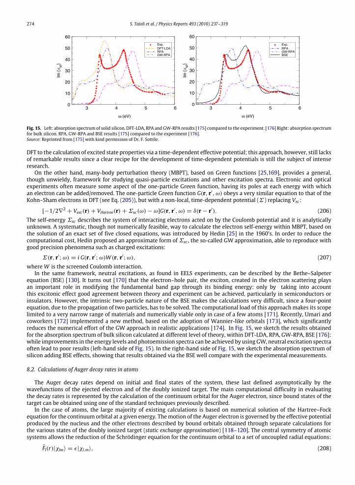
274 S. Taioli et al. / Physics Reports 493 (2010) 237–319
543 436
Exp.DFT-LDARPAGW-RPA
5 60
10
20
30
40
50
60
Exp.RPAGW-RPABSE
0
10
20
30
40
50
60
Fig. 15. Left: absorption spectrum of solid silicon. DFT-LDA, RPA and GW-RPA results [175] compared to the experiment. [176] Right: absorption spectrumfor bulk silicon. RPA, GW-RPA and BSE results [175] compared to the experiment [176].Source: Reprinted from [175] with kind permission of Dr. F. Sottile.
DFT to the calculation of excited state properties via a time-dependent effective potential; this approach, however, still lacksof remarkable results since a clear recipe for the development of time-dependent potentials is still the subject of intenseresearch.On the other hand, many-body perturbation theory (MBPT), based on Green functions [25,169], provides a general,
though unwieldy, framework for studying quasi-particle excitations and other excitation spectra. Electronic and opticalexperiments often measure some aspect of the one-particle Green function, having its poles at each energy with whichan electron can be added/removed. The one-particle Green function G(r, r′, ω) obeys a very similar equation to that of theKohn–Sham electrons in DFT (see Eq. (205)), but with a non-local, time-dependent potential (Σ) replacing Vxc :
[−1/2∇2 + Vext(r)+ VHartree(r)+Σxc(ω)− ω]G(r, r′, ω) = δ(r− r′). (206)The self-energy Σxc describes the system of interacting electrons acted on by the Coulomb potential and it is analyticallyunknown. A systematic, though not numerically feasible, way to calculate the electron self-energy within MBPT, based onthe solution of an exact set of five closed equations, was introduced by Hedin [25] in the 1960’s. In order to reduce thecomputational cost, Hedin proposed an approximate form ofΣxc , the so-called GW approximation, able to reproduce withgood precision phenomena such as charged excitations:
Σ(r, r′;ω) = i G(r, r′;ω)W (r, r′;ω), (207)whereW is the screened Coulomb interaction.In the same framework, neutral excitations, as found in EELS experiments, can be described by the Bethe–Salpeter
equation (BSE) [130]. It turns out [170] that the electron–hole pair, the exciton, created in the electron scattering playsan important role in modifying the fundamental band gap through its binding energy: only by taking into accountthis excitonic effect good agreement between theory and experiment can be achieved, particularly in semiconductors orinsulators. However, the intrinsic two-particle nature of the BSE makes the calculations very difficult, since a four-pointequation, due to the propagation of two particles, has to be solved. The computational load of this approach makes its scopelimited to a very narrow range of materials and numerically viable only in case of a few atoms [171]. Recently, Umari andcoworkers [172] implemented a new method, based on the adoption of Wannier-like orbitals [173], which significantlyreduces the numerical effort of the GW approach in realistic applications [174]. In Fig. 15, we sketch the results obtainedfor the absorption spectrum of bulk silicon calculated at different level of theory, within DFT-LDA, RPA, GW-RPA, BSE [176]:while improvements in the energy levels and photoemission spectra can be achieved by usingGW, neutral excitation spectraoften lead to poor results (left-hand side of Fig. 15). In the right-hand side of Fig. 15, we sketch the absorption spectrum ofsilicon adding BSE effects, showing that results obtained via the BSE well compare with the experimental measurements.
8.2. Calculations of Auger decay rates in atoms
The Auger decay rates depend on initial and final states of the system, these last defined asymptotically by thewavefunctions of the ejected electron and of the doubly ionized target. The main computational difficulty in evaluatingthe decay rates is represented by the calculation of the continuum orbital for the Auger electron, since bound states of thetarget can be obtained using one of the standard techniques previously described.In the case of atoms, the large majority of existing calculations is based on numerical solution of the Hartree–Fock
equation for the continuum orbital at a given energy. Themotion of the Auger electron is governed by the effective potentialproduced by the nucleus and the other electrons described by bound orbitals obtained through separate calculations forthe various states of the doubly ionized target (static exchange approximation) [118–120]. The central symmetry of atomicsystems allows the reduction of the Schrödinger equation for the continuum orbital to a set of uncoupled radial equations:
Fl(r)|χlm〉 = ε|χl,m〉, (208)
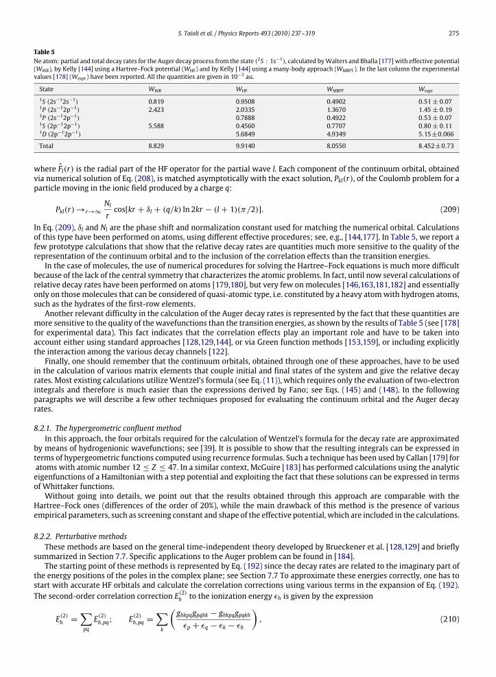
S. Taioli et al. / Physics Reports 493 (2010) 237–319 275
Table 5Ne atom: partial and total decay rates for the Auger decay process from the state (2S : 1s−1), calculated byWalters and Bhalla [177] with effective potential(WWB), by Kelly [144] using a Hartree–Fock potential (WHF) and by Kelly [144] using a many-body approach (WMBPT ). In the last column the experimentalvalues [178] (Wexpt ) have been reported. All the quantities are given in 10−3 au.
State WWB WHF WMBPT Wexpt1S (2s−12s−1) 0.819 0.9508 0.4902 0.51± 0.071P (2s−12p−1) 2.423 2.0335 1.3670 1.45± 0.193P (2s−12p−1) 0.7888 0.4922 0.53± 0.071S (2p−12p−1) 5.588 0.4560 0.7707 0.80± 0.111D (2p−12p−1) 5.6849 4.9349 5.15±0.066
Total 8.829 9.9140 8.0550 8.452±0.73
where Fl(r) is the radial part of the HF operator for the partial wave l. Each component of the continuum orbital, obtainedvia numerical solution of Eq. (208), is matched asymptotically with the exact solution, Pkl(r), of the Coulomb problem for aparticle moving in the ionic field produced by a charge q:
Pkl(r)→r→∞Nlrcos[kr + δl + (q/k) ln 2kr − (l+ 1)(π/2)]. (209)
In Eq. (209), δl and Nl are the phase shift and normalization constant used for matching the numerical orbital. Calculationsof this type have been performed on atoms, using different effective procedures; see, e.g., [144,177]. In Table 5, we report afew prototype calculations that show that the relative decay rates are quantities much more sensitive to the quality of therepresentation of the continuum orbital and to the inclusion of the correlation effects than the transition energies.In the case of molecules, the use of numerical procedures for solving the Hartree–Fock equations is much more difficult
because of the lack of the central symmetry that characterizes the atomic problems. In fact, until now several calculations ofrelative decay rates have been performed on atoms [179,180], but very few on molecules [146,163,181,182] and essentiallyonly on those molecules that can be considered of quasi-atomic type, i.e. constituted by a heavy atomwith hydrogen atoms,such as the hydrates of the first-row elements.Another relevant difficulty in the calculation of the Auger decay rates is represented by the fact that these quantities are
more sensitive to the quality of the wavefunctions than the transition energies, as shown by the results of Table 5 (see [178]for experimental data). This fact indicates that the correlation effects play an important role and have to be taken intoaccount either using standard approaches [128,129,144], or via Green function methods [153,159], or including explicitlythe interaction among the various decay channels [122].Finally, one should remember that the continuum orbitals, obtained through one of these approaches, have to be used
in the calculation of various matrix elements that couple initial and final states of the system and give the relative decayrates. Most existing calculations utilizeWentzel’s formula (see Eq. (11)), which requires only the evaluation of two-electronintegrals and therefore is much easier than the expressions derived by Fano; see Eqs. (145) and (148). In the followingparagraphs we will describe a few other techniques proposed for evaluating the continuum orbital and the Auger decayrates.
8.2.1. The hypergeometric confluent methodIn this approach, the four orbitals required for the calculation of Wentzel’s formula for the decay rate are approximated
by means of hydrogenionic wavefunctions; see [39]. It is possible to show that the resulting integrals can be expressed interms of hypergeometric functions computed using recurrence formulas. Such a technique has been used by Callan [179] foratoms with atomic number 12 ≤ Z ≤ 47. In a similar context, McGuire [183] has performed calculations using the analyticeigenfunctions of a Hamiltonian with a step potential and exploiting the fact that these solutions can be expressed in termsof Whittaker functions.Without going into details, we point out that the results obtained through this approach are comparable with the
Hartree–Fock ones (differences of the order of 20%), while the main drawback of this method is the presence of variousempirical parameters, such as screening constant and shape of the effective potential, which are included in the calculations.
8.2.2. Perturbative methodsThese methods are based on the general time-independent theory developed by Brueckener et al. [128,129] and briefly
summarized in Section 7.7. Specific applications to the Auger problem can be found in [184].The starting point of these methods is represented by Eq. (192) since the decay rates are related to the imaginary part of
the energy positions of the poles in the complex plane; see Section 7.7 To approximate these energies correctly, one has tostart with accurate HF orbitals and calculate the correlation corrections using various terms in the expansion of Eq. (192).The second-order correlation correction E(2)h to the ionization energy εh is given by the expression
E(2)h =∑pq
E(2)h,pq; E(2)h,pq =∑k
(ghkpqgpqhk − ghkpqgpqkhεp + εq − εk − εh
), (210)

276 S. Taioli et al. / Physics Reports 493 (2010) 237–319
1000
500
0
INT
EN
SIT
Y (
coun
ts/s
ec)
440 450 460 470 480 490 500 510 520
KINETIC ENERGY (eV)
Fig. 16. Experimental [148] and calculated [146] Auger spectrum of the H2O molecule. The solid line represents the experimental spectrum, while thevertical lines indicate calculated intensities and energies of Auger transitions.Source:Modified from [148].
where p and q identify two holes in the final configuration and h an inner-shell vacancy, while the denominator in Eq. (210)can vanish for some continuum state k. In this case one should add a small imaginary part η and use the following identity:
(D+ iη)−1 = PD−1 − iπδ(D), (211)
whereP is the Cauchyprincipal part and δ(D) gives the local density of states. The expression for the second-order correctionto the energy thus becomes as follows:
E(2)h,pq = P
∫dk[(gpqhk − gpqkh)ghkpqεp + εq − εk − εh
]− (iπ/k0)
[(gpqhk0 − gpqk0h)ghk0pq
], (212)
where k0 = [2(εp + εq − εh)]1/2 and the imaginary part gives the half-probability amplitude of the decay process. Theexpression of the diagrams associated with higher-order terms in the perturbative expansion are reported in [184]. Notethat Wentzel’s formula for the decay rate corresponds, in this approach, to a first-order term in the perturbative expansion.The results obtained by Kelly [144] applying this type of technique to the Ne atom are reported in Table 5 and are in fairly
good agreement with the experimental data.
8.3. Calculations of Auger decay rates in molecules
The calculation of the decay rates in molecules, although based on the same theory as for atoms, presents specificproblems relative to the determination of the continuum orbital for the outgoing electron. Various different techniqueshave been proposed that will be summarized in this section.
8.3.1. Monocentric vs. multicentric expansion of the orbitalsThe bound and continuum orbitals ηk(r, θ, φ) used in Wentzel’s formula (11) are expanded using a set of functions
centered on the heaviest atom of the molecule:
ηk(r, θ, φ) =∑l,m
cj;l,mφl,m(r)Yl,m(θ, φ). (213)
The Hartree–Fock equations for the radial part of these orbitals constitute an infinite system of differential equations thatare mutually coupled by the polycentric potential. Thus, for a closed-shell system one has
〈Ylm|F − ε|ηk〉r = −12
[1r2∂2
∂r2r2 −
l(l+ 1)r2
+ k2]cj;l,mφl,m +
∑l′,m′〈Ylm|VHF(r)|Yl′m′〉cj;l′,m′φl′,m′ , (214)
with the sum running over the denumerable infinity of spherical harmonics. In some calculations, this sum is truncated at agiven order and the radial components calculated numerically and matched asymptotically with the radial components ofthe appropriate Coulombwavefunction. This type of calculation has been used to predict the Auger spectrum of the hydratesof the first-row elements: HF, H2O, CH4 [146,163,185,186]. In Table 6, we present the results of a specific calculation on theH2O molecule [146], and in Fig. 16 we compare the experimental Auger spectrum with that constructed by expressing therelative intensity of the lines by means of calculated matrix elements.

S. Taioli et al. / Physics Reports 493 (2010) 237–319 277
Table 6H2O molecule: partial and total decay rates for the Auger process from the state (2A1 : 1a−11 ), calculated by Ågren et al. [146] in the Hartree–Fockapproximation (WHF) and taking into account the mixing of the decay channels (WHM ). All the quantities are given in 10−3 au.
State WHF WHM1A1 (2a−21 ) 0.593 0.3541A1 (2a−11 3a
−11 ) 0.467 0.374
3A1 (2a−11 3a−11 ) 0.177 0.166
1B2 (2a−11 1b−12 ) 0.318 0.258
3B2 (2a−11 1b−12 ) 0.141 0.119
1B1 (2a−11 1b−11 ) 0.414 0.335
3B1 (2a−11 1b−11 ) 0.197 0.164
1A1 (3a−21 ) 0.440 0.3931B2 (3a−11 1b
−12 ) 0.569 0.557
3B2 (3a−11 1b−12 ) 0.009 0.009
1B1 (3a−11 1b−11 ) 0.624 0.593
3B1 (3a−11 1b−11 ) 0.012 0.011
1A1 (1b−22 ) 0.358 0.3451A2 (1b−12 1b
−11 ) 0.553 0.533
3A2 (1b−12 1b−11 ) 0.000 0.000
1A1 (1b−21 ) 0.618 0.579
8.3.2. Vibrational analysis of Auger and autoionization spectraLet us analyze the typical situation in a molecular system, i.e. in which an isolated discrete electronic state (closed
channel), supporting a number of vibrational levels, is coupled to several electronic continua (open channels) with theirvibrational levels. In order to treat this problem, we consider the global Hamiltonian of the molecule:
H = TR + Hel, (215)
where TR is the nuclear kinetic energy operator and Hel the electronic Hamiltonian.We have to apply the general expressionsderived in Section 7.4, taking into account that each wavefunction contains both an electronic and a vibrational part.The molecular wavefunctions Φj, chosen to represent the intermediate states, are made up as
Φj(r,R) = ϕel(r,R)vj(R), (216)
where the electronic part ϕel – which depends parametrically on the ensemble of the nuclear coordinates (R) – is a linearcombination of Slater determinants constructed using one of the standard techniques (HF, MC-SCF, CI) for bound-statecalculations. The vibrational functions vj, which classify the intermediate states, can be obtained through the solutionof the differential equation[
TR + Eelϕ (R)]vj = Ejvj, (217)
where Eelϕ (R) =(ϕel|Hel|ϕel
)is the electronic potential energy surface relative to the intermediate bound state and (..|..)
indicates integration over the electronic coordinates. Note that to improve the representation one can also take into accountthe matrix element
(ϕel|TR|ϕel
)which, in the case of an isolated electronic state, simply introduces a local correction
to Eelϕ (R). In general, when several discrete electronic states are present, one can proceed either in the context of theBorn–Oppenheimer (BO) approximation, i.e. treating each channel separately, or through the inclusion of the coupling ofthe electronic states due to the nuclear motion and then diagonalizing H in the subspace of the intermediate discrete states.This second alternative is usually required only if the electronic states are not well separated in energy.Let us discuss now the way of representing the open channels in the case of a typical Auger process in which the
intermediate bound states are those of the ionized (N − 1)-electron target. A completely similar analysis can also beperformed in the case of an autoionization process.The open channels of the Auger process can be represented using a set of wavefunctions made up as
χαk(r,R) = χ elαk(r,R)θαnα (R) (218)
χ elαk(r,R) = A [ηk(r1;R)σ (s1)Θα(2, . . . ,N − 1;R)] (219)[TR + Eelα (R)
]θαnα = Eαnαθ
αnα , (220)
where A is the antisymmetrizer which also includes the normalization constant, σ is the spin function and the followingrelationships are satisfied:(
Θβ |HN−2el |Θα
)= Eelα (R)δαβ (221)

278 S. Taioli et al. / Physics Reports 493 (2010) 237–319(ηk(rj)|Θα(1, . . . ,N − 2)
)j = 0; ∀α, j, k (222)(
ηk|ηp)= (2π)3δ(k− p). (223)
The wavefunctions Θα, which represent discrete electronic states of the doubly ionizedmolecule, are linear combinationsof Slater determinants made up by orthogonal orbitals, and ηk is the continuum orbital orthogonal to the space of boundorbitals.Using Eqs. (218) and (220), and neglecting the effects of the nuclear kinetic energy operator on the electronic
wavefunctions, one obtains the expression for the matrix elements which couple the continuum functions:
〈χβk|HN−1 − E|χαp〉 ' 〈θβnβ |(χelβk|E
αnα − E
elα (R)+ H
N−1el − E|χ
elαp)|θ
αnα 〉. (224)
Then, assuming one has diagonalized the electronic part of the Hamiltonian and obtained the continuum functions χ el−αp which present the correct asymptotic behaviour,(
χ el−βk |HN−1el − E|χ
el−αp
)=
(Eelα (R)+
12p2 − E
)δαβ(2π)3δ(k− p), (225)
one can set up the wavefunctions
χ−αk(r,R) = χel−αk (r,R)θ
αnα (R), (226)
which diagonalize the molecular Hamiltonian in the BO approximation:
〈χ−βp|HN−1− E|χ−αk〉 =
(Eαnα +
12p2 − E
)δαβ(2π)3δ(k− p)δnαnβ . (227)
We observe that the use of the BO approximation is less justified when the electronic levels of the doubly ionized moleculeare close in energy. In these cases, the quality of the representation can be improved by including in these procedures thecoupling due to the nuclear kinetic energy operator.After the construction of two subsets of discrete and continuum functions, one has simply to evaluate their coupling
matrix elements Mlβ(E, p) in order to obtain the stationary state |Ψ−αk〉 of HN−1 at the energy E − Eαnα +
12k2. Using Eq.
(145), and in the framework of the BO approximation, one gets
Mlβ(E, p) = 〈Φl|HN−1 − E|χ−βp〉
= 〈vl|(ϕel|Eβnβ − E
elβ (R)+ H
N−1el − E|χ
el−βp )|θ
βnβ 〉
= 〈vl|Melβ (E, p;R)|θβnβ 〉, (228)
where Melβ represents the matrix element that couples the discrete electronic state ϕel with the continuum state χ el−βp .
To calculate the spectral parameters Γij and ∆ij from the knowledge of Melβ , one has simply to apply the previous
definitions. In particular, using the following resolution of the identity, I =∑nβ|θβnβ 〉〈θ
βnβ |, given in terms of the vibrational
functions of the electronic state β , one gets from Eq. (148)
Γlj = 〈vl|Γel(E;R)|vj〉, (229)
where
Γ el(E;R) = 2π∑β
∫dk(2π)3
Melβ (E, k;R)Mel+β (R; k, E)δ
(E − Eβnβ −
k2
2
). (230)
Similarly, for∆lj, one can derive the following approximate expression:
∆lj =∑β
∑nβ
P
∫d
p(2π)3
〈vl|Melβ (E, p;R)|θβnβ 〉〈θ
βnβ |Mel+β (R; p, E)|vj〉
E − Eβnβ
−p2
2
∼ 〈vl|∑β
P
∫d
p(2π)3
Melβ (E, p;R)Mel+β (R; p, E)
E − Eβ(R)− p22
|vj〉
= 〈vl|∆el(E;R)|vj〉, (231)
where the approximation consists in neglecting the kinetic energy of the nuclei with respect to their potential energy ateach internuclear distance.
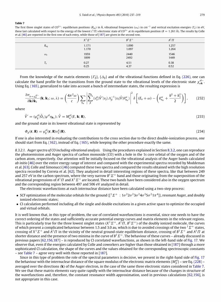
S. Taioli et al. / Physics Reports 493 (2010) 237–319 279
Table 7The first three singlet states of CO2+: equilibrium positions (Req) in Å, vibrational frequencies (ωe) in cm−1 and vertical excitation energies (Te) in eV,these last calculated with respect to the energy of the lowest (3Π) electronic state of CO2+ at its equilibrium position (R = 1.261 Å). The results by Colleet al. [46] are reported in the first row of each entry, while those of [187] are given in the second row.
X1Σ+ B1Σ+ A1Π
Req 1.171 1.090 1.2571.170 1.097 1.264
ωe 1959 2440 15461899 2492 1449
Te 0.27 4.51 0.380.25 4.37 0.52
From the knowledge of the matrix elements Γlj, ∆lj and of the vibrational functions defined in Eq. (226), one cancalculate the band profile for the transitions from the ground state to the vibrational levels of the electronic state χ el−αk .Using Eq. (165), generalized to take into account a bunch of intermediate states, the resulting expression is
∂σo→χel−α
∂k∂k1(k, k1;ω, λ) =
(4π2ωc
)∑nα
∣∣∣∣∣mb∑jl
〈vgo |V′|vj〉Λ
−1jl 〈vl|V |θ
αnα 〉
∣∣∣∣∣2
δ
[(Eo + ω)−
(Eαnα +
k2 + k212
)], (232)
where
V ′ = (ϕelg |Oλ|ϕelηk1); V = M
elα (E, k;R), (233)
and the ground state in its lowest vibrational state is represented by
Φg(r,R) = ϕelg (r,R)vgo (R). (234)
If one is also interested in evaluating the contributions to the cross section due to the direct double-ionization process, oneshould start from Eq. (162), instead of Eq. (165), while keeping the other procedure exactly the same.
8.3.2.1. Auger spectra of CO including vibrational analysis. Using the procedures explained in Section 8.3.2, one can reproducethe photoemission and Auger spectra of carbon monoxide (CO) with a hole in the 1s core orbital of the oxygen and of thecarbon atom, respectively. Our attention will be initially focused on the vibrational analysis of the Auger bands calculatedab initio [46] over the entire energy range of interest and compared with the experimental spectra recorded by Moddemanet al. [63]. Colle and Simonucci [46] computed these two spectra and compared the results obtainedwith the high resolutionspectra recorded by Correia et al. [62]. They analyzed in detail interesting regions of these spectra, like that between 249and 257 eV in the carbon spectrum, where the very narrow B1Σ+ band and those originating from the superposition of thevibrational progressions of A1Π and X1Σ+ are located. These two bands have been considered also in the oxygen spectrumand the corresponding region between 497 and 506 eV analyzed in detail.The electronic wavefunctions at each internuclear distance have been calculated using a two-step process:
• SCF optimization of themolecular orbitals for the ground ([1Σ+ : 1σ 22σ 23σ 24σ 25σ 21π4]), resonant Auger, and doublyionized electronic states;• CI calculation performed including all the single and double excitations in a given active space to optimize the occupiedand virtual orbitals.
It is well known that, in this type of problem, the use of correlated wavefunctions is essential, since one needs to have thecorrect ordering of the states and sufficiently accurate potential energy curves and matrix elements in the relevant regions.This is particularly true for the three lowest singlet states (X1Σ+, A1Π, B1Σ+) of the doubly ionized molecule, the curvesof which present a complicated behaviour between 1.5 and 3.0 au, which is due to avoided crossings of the two 1Σ+ states,crossing of X1Σ+ and A1Π in the vicinity of the neutral ground-state equilibrium distance, crossing of B1Σ+ and A1Π atshorter distance and the presence of twominima in the curve of B1Σ+. The behaviour of these curves – already discussed inprevious papers [62,156,187] – is reproduced by CI correlated wavefunctions, as shown in the left-hand side of Fig. 17. Weobserve that, even if the energies calculated by Colle and coworkers are higher than those obtained in [187] through a moresophisticated CI calculation, the shape of the curves and the values obtained for the corresponding spectroscopic constants– see Table 7 – agree very well with those reported in [187].Since in this type of problem the role of the spectral parameters is decisive, we present in the right-hand side of Fig. 17
the behaviour with the internuclear distance of the squaremodulus of the electronic matrix elements Melβ – see Eq. (228) –averaged over the directions (k) of the Auger electron, in the case of the same three electronic states considered in Table 7.We see that these matrix elements vary quite rapidly with the internuclear distance because of the changes in structure ofthe wavefunctions and, therefore, the constant resonance width approximation, used in previous calculations [62,156], isnot appropriate in this case.
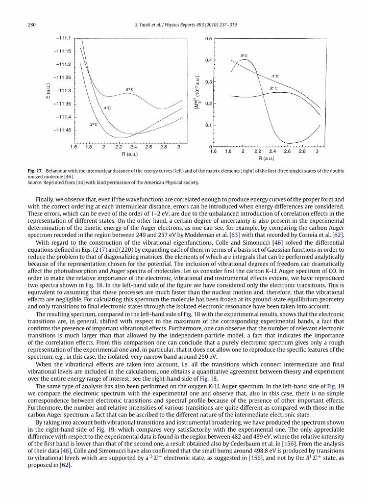
280 S. Taioli et al. / Physics Reports 493 (2010) 237–319
–111.1
–111.15
–111.2
–111.25
–111.3
–111.35
–111.4
–111.45
E (
a.u.
)
1.6 1.8 2 2.2 2.4 2.6 2.8 3
R (a.u.)
0.5
0.4
0.3
0.2
0.1
01.6 1.8 2 2.2 2.4 2.6 2.8 3
R (a.u.)
Fig. 17. Behaviour with the internuclear distance of the energy curves (left) and of thematrix elements (right) of the first three singlet states of the doublyionized molecule [46].Source: Reprinted from [46] with kind permission of the American Physical Society.
Finally,we observe that, even if thewavefunctions are correlated enough to produce energy curves of the proper formandwith the correct ordering at each internuclear distance, errors can be introduced when energy differences are considered.These errors, which can be even of the order of 1–2 eV, are due to the unbalanced introduction of correlation effects in therepresentation of different states. On the other hand, a certain degree of uncertainty is also present in the experimentaldetermination of the kinetic energy of the Auger electrons, as one can see, for example, by comparing the carbon Augerspectrum recorded in the region between 249 and 257 eV by Moddeman et al. [63] with that recorded by Correia et al. [62].With regard to the construction of the vibrational eigenfunctions, Colle and Simonucci [46] solved the differential
equations defined in Eqs. (217) and (220) by expanding each of them in terms of a basis set of Gaussian functions in order toreduce the problem to that of diagonalizingmatrices, the elements of which are integrals that can be performed analyticallybecause of the representation chosen for the potential. The inclusion of vibrational degrees of freedom can dramaticallyaffect the photoabsorption and Auger spectra of molecules. Let us consider first the carbon K-LL Auger spectrum of CO. Inorder to make the relative importance of the electronic, vibrational and instrumental effects evident, we have reproducedtwo spectra shown in Fig. 18. In the left-hand side of the figure we have considered only the electronic transitions. This isequivalent to assuming that these processes are much faster than the nuclear motion and, therefore, that the vibrationaleffects are negligible. For calculating this spectrum the molecule has been frozen at its ground-state equilibrium geometryand only transitions to final electronic states through the isolated electronic resonance have been taken into account.The resulting spectrum, compared in the left-hand side of Fig. 18with the experimental results, shows that the electronic
transitions are, in general, shifted with respect to the maximum of the corresponding experimental bands, a fact thatconfirms the presence of important vibrational effects. Furthermore, one can observe that the number of relevant electronictransitions is much larger than that allowed by the independent-particle model, a fact that indicates the importanceof the correlation effects. From this comparison one can conclude that a purely electronic spectrum gives only a roughrepresentation of the experimental one and, in particular, that it does not allow one to reproduce the specific features of thespectrum, e.g., in this case, the isolated, very narrow band around 250 eV.When the vibrational effects are taken into account, i.e. all the transitions which connect intermediate and final
vibrational levels are included in the calculations, one obtains a quantitative agreement between theory and experimentover the entire energy range of interest; see the right-hand side of Fig. 18.The same type of analysis has also been performed on the oxygen K-LL Auger spectrum. In the left-hand side of Fig. 19
we compare the electronic spectrum with the experimental one and observe that, also in this case, there is no simplecorrespondence between electronic transitions and spectral profile because of the presence of other important effects.Furthermore, the number and relative intensities of various transitions are quite different as compared with those in thecarbon Auger spectrum, a fact that can be ascribed to the different nature of the intermediate electronic state.By taking into account both vibrational transitions and instrumental broadening, we have produced the spectrum shown
in the right-hand side of Fig. 19, which compares very satisfactorily with the experimental one. The only appreciabledifferencewith respect to the experimental data is found in the region between 482 and 489 eV, where the relative intensityof the first band is lower than that of the second one, a result obtained also by Cederbaum et al. in [156]. From the analysisof their data [46], Colle and Simonucci have also confirmed that the small bump around 498.8 eV is produced by transitionsto vibrational levels which are supported by a 3Σ+ electronic state, as suggested in [156], and not by the B1Σ+ state, asproposed in [62].
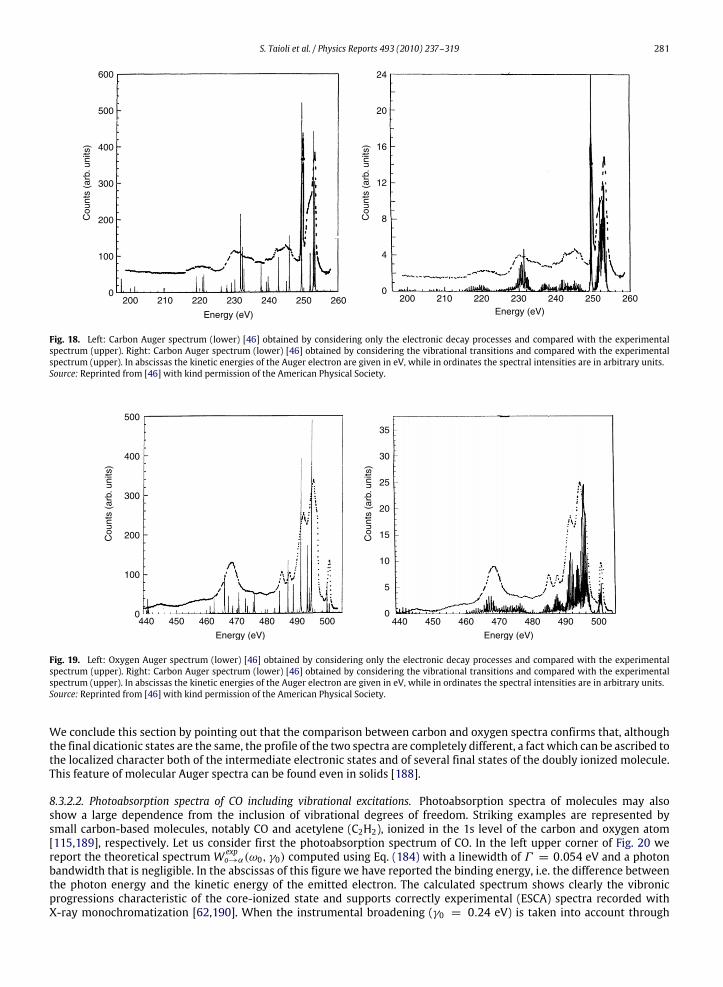
S. Taioli et al. / Physics Reports 493 (2010) 237–319 281
600
500
400
300
200
100
0
Cou
nts
(arb
. uni
ts)
Cou
nts
(arb
. uni
ts)
200 210 220 230 240 250 260
Energy (eV) Energy (eV)
24
20
16
12
8
4
0200 210 220 230 240 250 260
Fig. 18. Left: Carbon Auger spectrum (lower) [46] obtained by considering only the electronic decay processes and compared with the experimentalspectrum (upper). Right: Carbon Auger spectrum (lower) [46] obtained by considering the vibrational transitions and compared with the experimentalspectrum (upper). In abscissas the kinetic energies of the Auger electron are given in eV, while in ordinates the spectral intensities are in arbitrary units.Source: Reprinted from [46] with kind permission of the American Physical Society.
500
400
300
200
100
0
Cou
nts
(arb
. uni
ts)
Cou
nts
(arb
. uni
ts)
440 450 460 470 480 490 500
Energy (eV) Energy (eV)
35
30
25
20
15
10
5
0440 450 460 470 480 490 500
Fig. 19. Left: Oxygen Auger spectrum (lower) [46] obtained by considering only the electronic decay processes and compared with the experimentalspectrum (upper). Right: Carbon Auger spectrum (lower) [46] obtained by considering the vibrational transitions and compared with the experimentalspectrum (upper). In abscissas the kinetic energies of the Auger electron are given in eV, while in ordinates the spectral intensities are in arbitrary units.Source: Reprinted from [46] with kind permission of the American Physical Society.
We conclude this section by pointing out that the comparison between carbon and oxygen spectra confirms that, althoughthe final dicationic states are the same, the profile of the two spectra are completely different, a fact which can be ascribed tothe localized character both of the intermediate electronic states and of several final states of the doubly ionized molecule.This feature of molecular Auger spectra can be found even in solids [188].
8.3.2.2. Photoabsorption spectra of CO including vibrational excitations. Photoabsorption spectra of molecules may alsoshow a large dependence from the inclusion of vibrational degrees of freedom. Striking examples are represented bysmall carbon-based molecules, notably CO and acetylene (C2H2), ionized in the 1s level of the carbon and oxygen atom[115,189], respectively. Let us consider first the photoabsorption spectrum of CO. In the left upper corner of Fig. 20 wereport the theoretical spectrumW expo→α(ω0, γ0) computed using Eq. (184) with a linewidth of Γ = 0.054 eV and a photonbandwidth that is negligible. In the abscissas of this figure we have reported the binding energy, i.e. the difference betweenthe photon energy and the kinetic energy of the emitted electron. The calculated spectrum shows clearly the vibronicprogressions characteristic of the core-ionized state and supports correctly experimental (ESCA) spectra recorded withX-ray monochromatization [62,190]. When the instrumental broadening (γ0 = 0.24 eV) is taken into account through
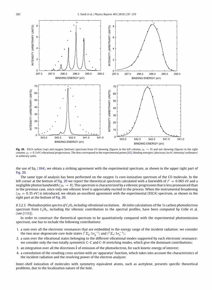
282 S. Taioli et al. / Physics Reports 493 (2010) 237–319
Fig. 20. ESCA carbon (top) and oxygen (bottom) spectrum from CO showing (figures in the left column, γ0 → 0) and not showing (figures in the rightcolumn, γ0 = 0.3 eV) vibrational progressions. The dots correspond to the experimental points [62]. Binding energies (abscissas) in eV, intensity (ordinates)in arbitrary units.
the use of Eq. (184), we obtain a striking agreement with the experimental spectrum, as shown in the upper right part ofFig. 20.The same type of analysis has been performed on the oxygen 1s core-ionization spectrum of the CO molecule. In the
left corner at the bottom of Fig. 20 we report the theoretical spectrum calculated with a linewidth of Γ = 0.065 eV and anegligible photon bandwidth (γ0 → 0). This spectrum is characterized by a vibronic progression that is less pronounced thanin the previous case, since only one vibronic level is appreciably excited in the process. When the instrumental broadening(γ0 = 0.35 eV) is introduced, we obtain an excellent agreement with the experimental (ESCA) spectrum, as shown in theright part at the bottom of Fig. 20.
8.3.2.3. Photoabsorption spectra of C2H2 including vibrational excitations. Ab initio calculations of the 1s carbon photoelectronspectrum from C2H2, including the vibronic contribution to the spectral profiles, have been computed by Colle et al.(see [115]).In order to construct the theoretical spectrum to be quantitatively compared with the experimental photoemission
spectrum, one has to include the following contributions:
1. a sum over all the electronic resonances that are embedded in the energy range of the incident radiation: we considerthe two near-degenerate core-hole states |2Σg :1σ−1g 〉 and |
2Σu:1σ−1u 〉;2. a sum over the vibrational states belonging to the different vibrational modes supported by each electronic resonance:we consider only the two totally symmetric C–C and C–H stretching modes, which give the dominant contributions;
3. an integration over all the directions k of emission of the photoelectron, for each kinetic energy of interest;4. a convolution of the resulting cross section with an ‘apparatus’ function, which takes into account the characteristics ofthe incident radiation and the resolving power of the electron analyzer.
Inner-shell ionization of molecules with symmetry equivalent atoms, such as acetylene, presents specific theoreticalproblems, due to the localization nature of the hole.
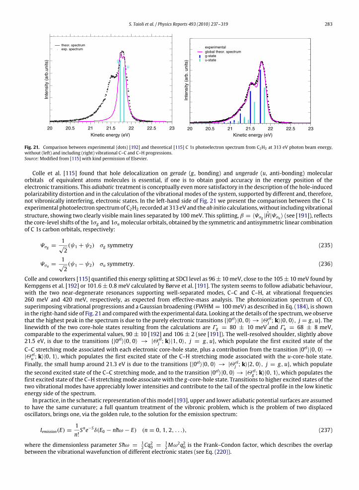
S. Taioli et al. / Physics Reports 493 (2010) 237–319 283
Kinetic energy (eV)
Inte
nsity
(ar
b.un
its)
theor. spectrumexp. spectrum
gu
Kinetic energy (eV)
Inte
nsity
(ar
b. u
nits
)
experimentalglobal theor. spectrumg-stateu-state
20 20.5 21 21.5 22 22.5 23 20 20.5 21 21.5 22 22.5 23
Fig. 21. Comparison between experimental (dots) [192] and theoretical [115] C 1s photoelectron spectrum from C2H2 at 313 eV photon beam energy,without (left) and including (right) vibrational C–C and C–H progressions.Source:Modified from [115] with kind permission of Elsevier.
Colle et al. [115] found that hole delocalization on gerade (g , bonding) and ungerade (u, anti-bonding) molecularorbitals of equivalent atoms molecules is essential, if one is to obtain good accuracy in the energy position of theelectronic transitions. This adiabatic treatment is conceptually evenmore satisfactory in the description of the hole-inducedpolarizability distortion and in the calculation of the vibrational modes of the system, supported by different and, therefore,not vibronically interfering, electronic states. In the left-hand side of Fig. 21 we present the comparison between the C 1sexperimental photoelectron spectrumof C2H2 recorded at 313 eV and the ab initio calculations,without including vibrationalstructure, showing two clearly visible main lines separated by 100meV. This splitting, β = 〈Ψσg |H|Ψσu〉 (see [191]), reflectsthe core-level shifts of the 1σg and 1σumolecular orbitals, obtained by the symmetric and antisymmetric linear combinationof C 1s carbon orbitals, respectively:
Ψσg =1√2(ψ1 + ψ2) σg symmetry (235)
Ψσu =1√2(ψ1 − ψ2) σu symmetry. (236)
Colle and coworkers [115] quantified this energy splitting at SDCI level as 96± 10meV, close to the 105± 10meV found byKempgens et al. [192] or 101.6± 0.8 meV calculated by Børve et al. [191]. The system seems to follow adiabatic behaviour,with the two near-degenerate resonances supporting well-separated modes, C–C and C–H, at vibrational frequencies260 meV and 420 meV, respectively, as expected from effective-mass analysis. The photoionization spectrum of CO,superimposing vibrational progressions and a Gaussian broadening (FWHM = 100meV) as described in Eq. (184), is shownin the right-hand side of Fig. 21 and comparedwith the experimental data. Looking at the details of the spectrum,we observethat the highest peak in the spectrum is due to the purely electronic transitions |0el〉|0, 0〉 → |Θelj ; k〉|0, 0〉, j = g, u. Thelinewidth of the two core-hole states resulting from the calculations are Γg = 80 ± 10 meV and Γu = 68 ± 8 meV,comparable to the experimental values, 90 ± 10 [192] and 106 ± 2 (see [191]). The well-resolved shoulder, slightly above21.5 eV, is due to the transitions |0el〉|0, 0〉 → |Θelj ; k〉|1, 0〉, j = g, u, which populate the first excited state of theC–C stretching mode associated with each electronic core-hole state, plus a contribution from the transition |0el〉|0, 0〉 →|Θelu ; k〉|0, 1〉, which populates the first excited state of the C–H stretching mode associated with the u-core-hole state.Finally, the small hump around 21.3 eV is due to the transitions |0el〉|0, 0〉 → |Θelj ; k〉|2, 0〉, j = g, u, which populatethe second excited state of the C–C stretching mode, and to the transition |0el〉|0, 0〉 → |Θelg ; k〉|0, 1〉, which populates thefirst excited state of the C–H stretchingmode associate with the g-core-hole state. Transitions to higher excited states of thetwo vibrational modes have appreciably lower intensities and contribute to the tail of the spectral profile in the low kineticenergy side of the spectrum.In practice, in the schematic representation of thismodel [193], upper and lower adiabatic potential surfaces are assumed
to have the same curvature; a full quantum treatment of the vibronic problem, which is the problem of two displacedoscillators, brings one, via the golden rule, to the solution for the emission spectrum:
Iemission(E) =1n!Sne−Sδ(E0 − nhω − E) (n = 0, 1, 2, . . .), (237)
where the dimensionless parameter Shω = 12Cq
20 =
12Mω
2q20 is the Frank–Condon factor, which describes the overlapbetween the vibrational wavefunction of different electronic states (see Eq. (220)).
284 S. Taioli et al. / Physics Reports 493 (2010) 237–319
8.3.3. The Stjeltjes imaging methodThis technique has been used to evaluate the second-order corrections to the energy values in the perturbative approach
of Section 7.7. In particular, one is interested in the imaginary parts of these corrections, which give the decay rates intofinal channels. The second-order correction can be written in the following way:
E(2)h =∑pq
E(2)h,pq (238)
E(2)h,pq =∑ν
(〈hν|g|pq〉〈pq|g|hν〉 − 〈hν|g|pq〉〈qp|g|hν〉)εx + εy − εh − εν
+
∫∞
0dE(〈hν(E)|g|pq〉〈pq|g|hν(E)〉 − 〈hν(E)|g|pq〉〈qp|g|hν(E)〉)
εx + εy − εh − E, (239)
where 〈hν|g|pq〉 is equal to ghνpq defined in Eq. (191). The expression of E(2)h,pq is formally analogous to that for the
polarizability [194]:
α(ω) =
∫∞
0
df (ε)ε2 − ω2
, (240)
with
df (ε)dε=
∑j
fjδ(ε − εj)+ g(ε). (241)
The Stjeltjes method consists in approximating g(ε) in Eq. (241) with an n-step function g(n)(ε) defined as follows:
g(n)(ε) = 0, 0 < ε < ε1(n) (242)
g(n)(ε) =12fi+1(n)+ fi(n)εi+1(n)− εi(n)
, εi(n) < ε < εi+1(n) (243)
g(n)(ε) = 0, εn(n) < ε. (244)
The quantities εj(n) and fj(n) define a set of momenta S(−k) of order k,
S(−k) =n∑i=1
εi(n)−kfi(n), (245)
whose values are determined by substituting the continuum orbital with an appropriate HF L2-orbitals in the calculation ofthe matrix elements relative to the decay channel.To explain this point, let us define the eigenvalues and eigenvectors of the Hartree–Fock operator for the decay channel
α:
Fα|ψl〉 = εl|ψl〉. (246)
In terms of these eigenvectors and eigenvalues, the momenta S(−k) have the following expression:
S(−k) =N∑l=1
ε−kl (〈hψl|g|pq〉〈pq|g|hψl〉 − 〈hψl|g|pq〉〈qp|g|hψl〉). (247)
The value of g(n)(ε) at a specific Auger energy gives the value of the decay rates into the corresponding channel. The stepfunction g(n)(ε) is then regularised by means, for example, of a few polynomials.Further details of this method are given in [194].
8.3.4. The Green function methodThis method uses the fact that the information on the final decay states can be extracted from the two-particle Green
function [153] and the decay rates into final channels are related to the residues of the two-particle Green function; seeEq. (198).Results of calculations performed using this technique on theHFmolecule [159] are given in Table 8. In these calculations,
the continuum orbital, used for calculatingMhµjm(τ ), has been approximated by means of a spherical wave centered on thehole produced by the primary ionization and the matrix elements have been evaluated using the one-centre approximationand employing the radial integrals calculated byMcGuire [183]. Thisway of estimating the transition rates, which disregardsimportant effects such as relaxation of final states and correlation effects in the initial and final states, allows one howeverto obtain a qualitative reproduction of the Auger spectra as shown, for example, in Fig. 22.

S. Taioli et al. / Physics Reports 493 (2010) 237–319 285
Fig. 22. Experimental [162] and calculated [153] Auger spectrum of the HF molecule. The solid line represents the experimental spectrum, while thevertical strokes represent the calculated intensities and energies of the Auger transition.Source:Modified from [153].
Table 8HF molecule: partial and total rates for the Auger decay process from the state (2Σ : 1σ−1), calculated by Liegener [153] (WL) and compared with theHartree–Fock results (WFK) of Faegry and Kelly [163]. All the quantities are given in 10−3 au.
State WL WFK1Σ (2σ−2) 0.454 0.9831Σ (2σ−13σ−1) 0.335 0.6421Π (2σ−11π−1) 0.672 1.2883Σ (2σ−13σ−1) 0.181 0.3023Π (2σ−11π−1) 0.330 0.5741Σ (3σ−2) 0.352 0.5641Π (3σ−11π−1) 1.017 1.6921Σ (1π−2) 0.338 0.5941∆ (1π−2) 1.143 1.9863Π (3σ−11π−1) 0.013 0.0213Σ (1π−2) 0.000 0.000
8.4. Calculations of Auger decay rates in solids and nanoclusters
8.4.1. Localization–delocalization issuesThe calculation of Auger spectra in solids presents specific difficulties due, in particular, to the high number of energy
levels involved and to the superposition of different vibrational progressions,which produce broadening of the spectral lines.The majority of existing calculations utilize directly the matrix elements obtained for the separate atoms inside Wentzel’sformula, without taking the periodicity of the system explicitly into account.A central difficulty is represented by the evaluation of the corrections to Hartree–Fock energies and decay amplitudes
due to the coupling between final states with different hole distributions. Apart from semiquantitative approaches basedon atomic decomposition, calculations of electronic spectra in condensed matter have been limited to the evaluation ofapproximate expressions for the transition matrix, such as in the methods developed by Cederbaum [47,181], Ohno [182]and Cini, Sawatzky and Verdozzi [14,41,195,196], and to the approximate description of the continuum electron, usuallyneglecting or crudely approximating correlation effects in the ionized system, interchannel coupling and collectiveexcitation phenomena.In solid-state applications, all of these approaches, rooted in Lander’s idea [197] that C-VV spectra should reflect the
self-convolution of the valence band density of states (DOS), recognize the importance of correlation effects in double-hole final states, which break the single-particle picture and are responsible for the large discrepancies between computedresults and experimental measurements. Such a correlation is taken into account by introducing either a semi-empiricalparameter (Cini–Sawatzky) or using a perturbative scheme (Cederbaum), which corrects the initial ‘atomic-like’ transitionmatrix elements.In the Cini–Sawatzky approach, in particular, the ‘band-like’ behaviour of the spectra is obtained by tuning an optimalparameter, representing the hole–hole correlation energy, until satisfactory agreement with the experiment is reached.In this framework, Cini and Sawatzky were able to explain the Auger spectra of transition metals, such as Zn, where thehole localization effects play a paramount role. While this approach can be very useful in order to gain insights on such
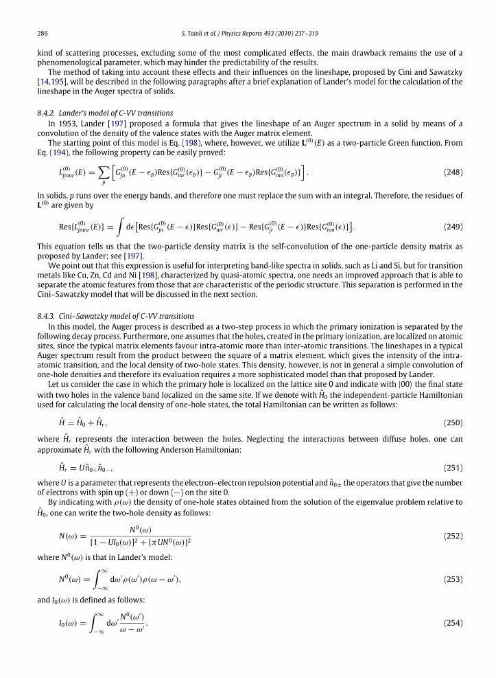
286 S. Taioli et al. / Physics Reports 493 (2010) 237–319
kind of scattering processes, excluding some of the most complicated effects, the main drawback remains the use of aphenomenological parameter, which may hinder the predictability of the results.The method of taking into account these effects and their influences on the lineshape, proposed by Cini and Sawatzky
[14,195], will be described in the following paragraphs after a brief explanation of Lander’s model for the calculation of thelineshape in the Auger spectra of solids.
8.4.2. Lander’s model of C-VV transitionsIn 1953, Lander [197] proposed a formula that gives the lineshape of an Auger spectrum in a solid by means of a
convolution of the density of the valence states with the Auger matrix element.The starting point of this model is Eq. (198), where, however, we utilize L(0)(E) as a two-particle Green function. From
Eq. (194), the following property can be easily proved:
L(0)jmnr(E) =∑p
[G(0)jn (E − εp)ResG
(0)mr (εp) − G
(0)jr (E − εp)ResG
(0)mn(εp)
]. (248)
In solids, p runs over the energy bands, and therefore one must replace the sum with an integral. Therefore, the residues ofL(0) are given by
ResL(0)jmnr(E) =∫dε[ResG(0)jn (E − ε)ResG
(0)mr (ε) − ResG
(0)jr (E − ε)ResG
(0)mn(ε)
]. (249)
This equation tells us that the two-particle density matrix is the self-convolution of the one-particle density matrix asproposed by Lander; see [197].We point out that this expression is useful for interpreting band-like spectra in solids, such as Li and Si, but for transition
metals like Cu, Zn, Cd and Ni [198], characterized by quasi-atomic spectra, one needs an improved approach that is able toseparate the atomic features from those that are characteristic of the periodic structure. This separation is performed in theCini–Sawatzky model that will be discussed in the next section.
8.4.3. Cini–Sawatzky model of C-VV transitionsIn this model, the Auger process is described as a two-step process in which the primary ionization is separated by the
following decay process. Furthermore, one assumes that the holes, created in the primary ionization, are localized on atomicsites, since the typical matrix elements favour intra-atomic more than inter-atomic transitions. The lineshapes in a typicalAuger spectrum result from the product between the square of a matrix element, which gives the intensity of the intra-atomic transition, and the local density of two-hole states. This density, however, is not in general a simple convolution ofone-hole densities and therefore its evaluation requires a more sophisticated model than that proposed by Lander.Let us consider the case in which the primary hole is localized on the lattice site 0 and indicate with |00〉 the final state
with two holes in the valence band localized on the same site. If we denote with H0 the independent-particle Hamiltonianused for calculating the local density of one-hole states, the total Hamiltonian can be written as follows:
H = H0 + Hr , (250)
where Hr represents the interaction between the holes. Neglecting the interactions between diffuse holes, one canapproximate Hr with the following Anderson Hamiltonian:
Hr = Un0+n0−, (251)
whereU is a parameter that represents the electron–electron repulsion potential and n0± the operators that give the numberof electrons with spin up (+) or down (−) on the site 0.By indicating with ρ(ω) the density of one-hole states obtained from the solution of the eigenvalue problem relative to
H0, one can write the two-hole density as follows:
N(ω) =N0(ω)
[1− UI0(ω)]2 + [πUN0(ω)]2(252)
where N0(ω) is that in Lander’s model:
N0(ω) =∫∞
−∞
dω′ρ(ω′)ρ(ω − ω′), (253)
and I0(ω) is defined as follows:
I0(ω) =∫∞
−∞
dω′N0(ω′)ω − ω′
. (254)
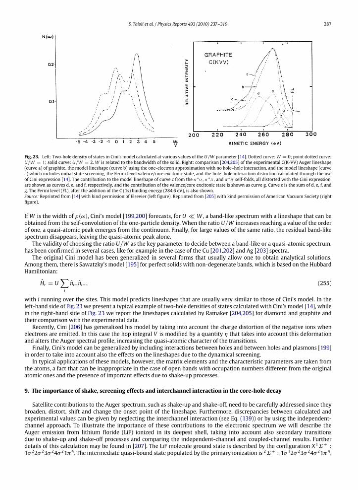
S. Taioli et al. / Physics Reports 493 (2010) 237–319 287
Fig. 23. Left: Two-hole density of states in Cini’s model calculated at various values of the U/W parameter [14]. Dotted curve:W = 0; point dotted curve:U/W = 1; solid curve: U/W = 2.W is related to the bandwidth of the solid. Right: comparison [204,205] of the experimental C(K-VV) Auger lineshape(curve a) of graphite, the model lineshape (curve b) using the one-electron approximation with no hole–hole interaction, and the model lineshape (curvec) which includes initial state screening, the Fermi level valence/core excitonic state, and the hole–hole interaction distortion calculated through the useof Cini expression [14]. The contribution to the model lineshape of curve c from the σ ∗σ , σ ∗π , and π∗π self-folds, all distorted with the Cini expression,are shown as curves d, e, and f, respectively, and the contribution of the valence/core excitonic state is shown as curve g. Curve c is the sum of d, e, f, andg. The Fermi level (FL), after the addition of the C (1s) binding energy (284.6 eV), is also shown.Source: Reprinted from [14] with kind permission of Elsevier (left figure). Reprinted from [205] with kind permission of American Vacuum Society (rightfigure).
IfW is the width of ρ(ω), Cini’s model [199,200] forecasts, for U W , a band-like spectrum with a lineshape that can beobtained from the self-convolution of the one-particle density. When the ratio U/W increases reaching a value of the orderof one, a quasi-atomic peak emerges from the continuum. Finally, for large values of the same ratio, the residual band-likespectrum disappears, leaving the quasi-atomic peak alone.The validity of choosing the ratio U/W as the key parameter to decide between a band-like or a quasi-atomic spectrum,
has been confirmed in several cases, like for example in the case of the Cu [201,202] and Ag [203] spectra.The original Cini model has been generalized in several forms that usually allow one to obtain analytical solutions.
Among them, there is Sawatzky’s model [195] for perfect solids with non-degenerate bands, which is based on the HubbardHamiltonian:
Hr = U∑i
ni+ni−, (255)
with i running over the sites. This model predicts lineshapes that are usually very similar to those of Cini’s model. In theleft-hand side of Fig. 23 we present a typical example of two-hole densities of states calculated with Cini’s model [14], whilein the right-hand side of Fig. 23 we report the lineshapes calculated by Ramaker [204,205] for diamond and graphite andtheir comparison with the experimental data.Recently, Cini [206] has generalized his model by taking into account the charge distortion of the negative ions when
electrons are emitted. In this case the hop integral V is modified by a quantity η that takes into account this deformationand alters the Auger spectral profile, increasing the quasi-atomic character of the transitions.Finally, Cini’s model can be generalized by including interactions between holes and between holes and plasmons [199]
in order to take into account also the effects on the lineshapes due to the dynamical screening.In typical applications of these models, however, the matrix elements and the characteristic parameters are taken from
the atoms, a fact that can be inappropriate in the case of open bands with occupation numbers different from the originalatomic ones and the presence of important effects due to shake-up processes.
9. The importance of shake, screening effects and interchannel interaction in the core-hole decay
Satellite contributions to the Auger spectrum, such as shake-up and shake-off, need to be carefully addressed since theybroaden, distort, shift and change the onset point of the lineshape. Furthermore, discrepancies between calculated andexperimental values can be given by neglecting the interchannel interaction (see Eq. (139)) or by using the independent-channel approach. To illustrate the importance of these contributions to the electronic spectrum we will describe theAuger emission from lithium floride (LiF) ionized in its deepest shell, taking into account also secondary transitionsdue to shake-up and shake-off processes and comparing the independent-channel and coupled-channel results. Furtherdetails of this calculation may be found in [207]. The LiF molecule ground state is described by the configuration X1Σ+ :1σ 22σ 23σ 24σ 21π4. The intermediate quasi-bound state populated by the primary ionization is 2Σ+ : 1σ 12σ 23σ 24σ 21π4,
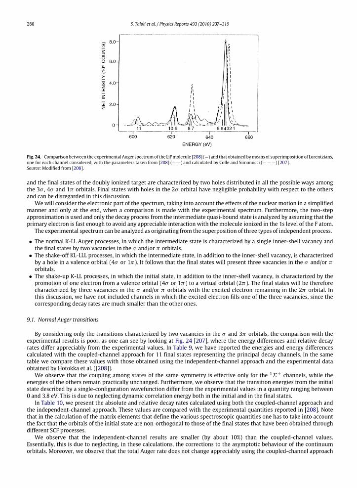
288 S. Taioli et al. / Physics Reports 493 (2010) 237–319
Fig. 24. Comparisonbetween the experimental Auger spectrumof the LiFmolecule [208] (—) and that obtainedbymeans of superimposition of Lorentzians,one for each channel considered, with the parameters taken from [208] (—·—) and calculated by Colle and Simonucci (— — —) [207].Source:Modified from [208].
and the final states of the doubly ionized target are characterized by two holes distributed in all the possible ways amongthe 3σ , 4σ and 1π orbitals. Final states with holes in the 2σ orbital have negligible probability with respect to the othersand can be disregarded in this discussion.We will consider the electronic part of the spectrum, taking into account the effects of the nuclear motion in a simplified
manner and only at the end, when a comparison is made with the experimental spectrum. Furthermore, the two-stepapproximation is used and only the decay process from the intermediate quasi-bound state is analyzed by assuming that theprimary electron is fast enough to avoid any appreciable interaction with the molecule ionized in the 1s level of the F atom.The experimental spectrum can be analyzed as originating from the superposition of three types of independent process.
• The normal K-LL Auger processes, in which the intermediate state is characterized by a single inner-shell vacancy andthe final states by two vacancies in the σ and/or π orbitals.• The shake-off KL-LLL processes, in which the intermediate state, in addition to the inner-shell vacancy, is characterizedby a hole in a valence orbital (4σ or 1π ). It follows that the final states will present three vacancies in the σ and/or πorbitals.• The shake-up K-LL processes, in which the initial state, in addition to the inner-shell vacancy, is characterized by thepromotion of one electron from a valence orbital (4σ or 1π ) to a virtual orbital (2π ). The final states will be thereforecharacterized by three vacancies in the σ and/or π orbitals with the excited electron remaining in the 2π orbital. Inthis discussion, we have not included channels in which the excited electron fills one of the three vacancies, since thecorresponding decay rates are much smaller than the other ones.
9.1. Normal Auger transitions
By considering only the transitions characterized by two vacancies in the σ and 3π orbitals, the comparison with theexperimental results is poor, as one can see by looking at Fig. 24 [207], where the energy differences and relative decayrates differ appreciably from the experimental values. In Table 9, we have reported the energies and energy differencescalculated with the coupled-channel approach for 11 final states representing the principal decay channels. In the sametable we compare these values with those obtained using the independent-channel approach and the experimental dataobtained by Hotokka et al. ([208]).We observe that the coupling among states of the same symmetry is effective only for the 1Σ+ channels, while the
energies of the others remain practically unchanged. Furthermore, we observe that the transition energies from the initialstate described by a single-configuration wavefunction differ from the experimental values in a quantity ranging between0 and 3.8 eV. This is due to neglecting dynamic correlation energy both in the initial and in the final states.In Table 10, we present the absolute and relative decay rates calculated using both the coupled-channel approach and
the independent-channel approach. These values are compared with the experimental quantities reported in [208]. Notethat in the calculation of the matrix elements that define the various spectroscopic quantities one has to take into accountthe fact that the orbitals of the initial state are non-orthogonal to those of the final states that have been obtained throughdifferent SCF processes.We observe that the independent-channel results are smaller (by about 10%) than the coupled-channel values.
Essentially, this is due to neglecting, in these calculations, the corrections to the asymptotic behaviour of the continuumorbitals. Moreover, we observe that the total Auger rate does not change appreciably using the coupled-channel approach

S. Taioli et al. / Physics Reports 493 (2010) 237–319 289
Table 9Energies (ECC) of the intermediate and final states of the LiFmolecule, classified according the their hole configuration. The corresponding energy differences(∆ECC) are compared with those obtained by using the independent-channel approach (∆EIC) and with the values (∆Eexpt ) reported in [208]. The energiesare given in atomic units and the energy differences in eV.
Transition Final states ECC ∆ECC ∆EIC ∆Eexpt
1σ−1: 2Σ+ −81.74327 – – –(1) 1π−2: 3Σ− −105.72328 652.53 652.53 652.2(2) 4σ−11π−1: 3Π −105.70529 652.04 652.04 650.3(3) 1π−2: 1∆ −105.62301 649.81 649.81 648.5(4) 4σ−11π−1: 1Π −105.60458 649.30 649.30 647.7(5) 1π−2: 1Σ+ −105.60213 649.29 647.08 646.6(6) 4σ−2: 1Σ+ −105.51853 646.96 647.42 644.8(7) 3σ−11π−1: 3Π −104.91668 630.59 630.59 630.5(8) 3σ−14σ−1: 3Σ+ −104.89927 630.11 630.11 629.6(9) 3σ−11π−1: 1Π −104.54173 620.38 620.39 621.8(10) 3σ−14σ−1: 1Σ+ −104.52395 619.90 619.91 620.3(11) 3σ−2: 1Σ+ −103.74809 598.79 600.48 602.6
Table 10Partial and total Auger decay rates calculated using the independent-channel approach (ΓIC) and the coupled-channel approach (ΓCC) and compared withthe experimental values (Γ relexpt ) [208]. The absolute values are given in 10
−3 au.
Transition Final states Γ absIC Γ relIC Γ absCC Γ relCC Γ relexp
(1) 1π−2: 3Σ− 0.000 0.000 0.000 0.000 0.01(2) 4σ−11π−1: 3Π 0.002 0.001 0.002 0.001 0.02(3) 1π−2: 1∆ 1.640 1.000 1.707 1.000 1.00(4) 4σ−11π−1: 1Π 1.621 0.989 1.685 0.987 0.91(5) 1π−2: 1Σ+ 0.491 0.299 0.825 0.483 0.27(6) 4σ−2: 1Σ+ 0.635 0.387 0.621 0.364 0.32(7) 3σ−11π−1: 3Π 0.437 0.267 0.442 0.259 0.20(8) 3σ−14σ−1: 3Σ+ 0.214 0.131 0.218 0.128 0.07(9) 3σ−11π−1: 1Π 1.029 0.627 0.899 0.526 0.42(10) 3σ−14σ−1: 1Σ+ 0.510 0.311 0.446 0.261 0.17(11) 3σ−2: 1Σ+ 0.761 0.464 0.438 0.257 0.21
Γtot 7.339 7.283
instead of the independent-channel approach. This fact also suggests that the coupled-channel value of the total decay rateis probably underestimated by about 10%. We can therefore estimate the total Auger width to be of the order of 0.22 eV, avalue similar to those measured by Svensson [209] respectively for the Ne (0.27 eV) and the F atom (0.1–0.2 eV) [210], butconsiderably smaller than the widths of the deconvoluted bands reported in [208]. These large observed linewidths havebeen attributed both to the dissociative character of the initial and/or final states and to the dimer formation in the targetvapor.As regards the partial decay rates, we observe that passing from the independent-channel results to the coupled-channel
results there is a clear improvement in the agreement between calculated and experimental values; see [208]. The onlyexception is represented by the transition to the final state (1π−2 : 1Σ+), very near in energy to the (4σ−11π−1 : 1Π )and (4σ−2 : 1Σ+) final states. This fact makes more questionable the reliability of the corresponding quantities reportedin [208] and obtained through a least square fit of Voigt functions to the experimental points. In fact, as pointed out also byHotokka et al. [208], the decomposition of an experimental peak into separated lines is not very accurate when these lineslie near to each other (separated by an amount approximately equal to the half-width of the standard line).Finally, we point out that the calculated total energy shift ∆ for the normal Auger decay process from the intermediate
state 2Σ+(1σ−1) is equal to 0.083 eV, a quantity comparable to the corresponding one for the Ne atom, but negligible ifcompared with the transition energies characteristic of the problem.
9.2. KL-LLL shake-off processes
In order to check if the poor agreement of the theoretical results with experiments is due to neglect shake processes, onehas to include different intermediate states that can be produced when the initial ionization process not only removes aninner-shell electron, but also a valence electron of the molecule. In Tables 11 and 12, we have reported the energies and thedecay rates of four different intermediate states.The one-configuration wavefunctions representing the 3Π , 3Σ+ and 1Π states have been obtained through separate SCF
calculations and their energies are upper bounds to the exact eigenvalues of the (N−2)-electron Hamiltonian. The energy ofthe 1Σ+ state, instead, has been calculated using one-configuration wavefunction with orbitals obtained for the 3Σ+ state,since a standard SCF process, without orthogonality constraints to the lower states of the same symmetry, can produce in

290 S. Taioli et al. / Physics Reports 493 (2010) 237–319
Table 11Transition energies (∆E) and absolute and relative values of the partial decay rates (Γ ) for the various ionic final states produced by four different shake-offprocesses. The energies are given in eV and the rates in 10−3 au.
Initial state 1σ−14σ−1 : 3Σ+ 1σ−14σ−1 : 1Σ+
Transition Final states ∆E Γabs Γrel ∆E Γabs Γrel
(1) 4σ−11π−2: 2∆ 633.94 2.128 1.000 637.46 2.122 1.000(2) 4σ−11π−2: 2Σ+ 632.21 0.850 0.399 635.73 0.848 0.400(3) 4σ−21π−1: 2Π 632.02 1.063 0.500 635.53 1.065 0.502(4) 3σ−14σ−11π−1: 4Π 619.31 0.440 0.206 622.83 0.000 0.000(5) 3σ−14σ−11π−1: 2Π 611.00 0.545 0.256 614.52 0.008 0.004(6) 3σ−14σ−2: 2Σ+ 609.07 0.537 0.252 612.59 0.015 0.007(7) 3σ−14σ−11π−1: 2Π 603.32 0.602 0.283 606.83 1.621 0.764(8) 3σ−24σ−1: 2Σ+ 585.15 0.547 0.257 588.67 0.608 0.287
Γtot 6.712 6.287
Table 12Transition energies (∆E) and absolute and relative values of the partial decay rates (Γ ) for the various ionic final states produced by four different shake-offprocesses. The energies are given in eV and the rates in 10−3 au.
Initial state 1σ−11π−1 : 3Π 1σ−11π−1 : 1ΠFinal states ∆E Γabs Γrel ∆E Γabs Γrel
(1) 4σ−11π−2: 4Σ− 637.95 0.001 0.001 641.43 0.000 0.000(2) 1π−3: 2Π 633.57 1.458 1.000 637.05 1.366 1.000(3) 4σ−11π−2: 2∆ 633.47 0.531 0.364 636.95 0.510 0.374(4) 4σ−11π−2: 2Σ− 633.47 0.795 0.545 636.95 0.774 0.566(5) 4σ−21π−1: 2Π 631.66 1.004 0.689 635.13 0.985 0.721(6) 4σ−11π−2: 2Σ+ 630.50 0.269 0.184 633.97 0.258 0.189(7) 3σ−11π−2: 4Σ− 619.27 0.225 0.154 622.75 0.000 0.000(8) 3σ−14σ−11π−1: 4Π 618.85 0.214 0.147 622.33 0.000 0.000(9) 3σ−11π−2: 2∆ 610.96 0.554 0.380 614.44 0.007 0.005(10) 3σ−14σ−11π−1: 2Π 610.53 0.264 0.181 614.01 0.007 0.005(11) 3σ−11π−2: 2Σ+ 607.98 0.271 0.186 611.46 0.004 0.003(12) 3σ−11π−2: 2Σ− 603.26 0.302 0.207 606.74 0.762 0.558(13) 3σ−14σ−11π−1: 2Π 602.86 0.292 0.200 606.34 0.807 0.591(14) 3σ−21π−1: 2Π 585.06 0.542 0.372 588.54 0.620 0.454
Γtot 6.722 6.101
this case a variational collapse. Therefore, the corresponding energy is only a rough estimate of the exact one. Furthermore,the decay rates calculated using this approximate representation of the 1Σ+ state are less reliable than those of the otherstates.We observe that the transition energies are distributed in two different regions:
• 630–640 eV, where the hole configurations of the final states are (4σ−11π−2), (4σ−21π−1), (1π−3). The most intensepeaks are around 632–633 eV and 635–637 eV.• 603–620 eV, where the hole configurations of the final states are (3σ−11π−2), (3σ−14σ−11π−1), (3σ−14σ−2).
The most intense peaks are around 602–603 eV and 606–611 eV.In [208], only a few of these transitions have been identified and, among these, the [(1σ−11π−1 : 1,3Π) → (1π−3 : 2Π)]ones have been located at energies ∆E = 637.76 eV and ∆E = 633.87 eV, very similar to those given by us in Table 12.As regards instead the [(1σ−11π−1) : 1,3Π → (3σ−11π−2 : 2,4Σ, 2,4∆)] transitions between 602 and 610 eV, we observethat, while the two final 2Σ states reported in Table IV of [208] at ∆E = 606.14 eV and ∆E = 602.25 eV can be identifiedwith those to the two 2Σ− states of Table 12 (∆E = 606.74 eV and∆E = 603.26 eV), the tentative assignment of the otherfinal states (4Σ , 2∆ and 2∆) proposed in [208] at energies ∆E = 609.38 eV, ∆E = 606.01 eV and ∆E = 602.11 eV is incomplete disagreement with results of Table 12. In this regard, we think that only from the simultaneous analysis of all themain possible decay states classified according to their spin and spatial symmetries can a reliable assignment of the variousexperimental transitions become possible.
9.3. K-LL shake-up processes
In Table 13, we have reported the energies and energy shifts of nine different intermediate states that can be producedwhen the initial process not only removes an inner-shell electron of themolecule, but also promotes a valence electron into a2π orbital. The one-configurationwavefunctions representing the various initial states have been constructed using orbitalswhich are eigenfunctions of an average Hartree–Fock operator. In Tables 14 and 15, we present absolute and relative decayrates to final states produced by shake-up processes. These quantities, together with the corresponding transition energies,
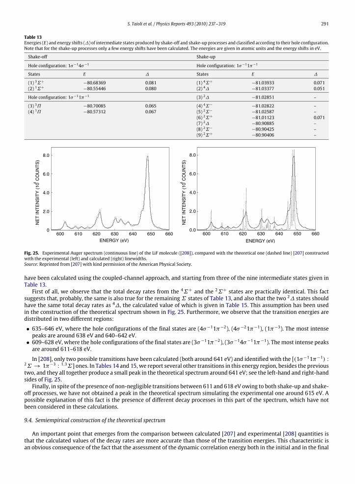
S. Taioli et al. / Physics Reports 493 (2010) 237–319 291
Table 13Energies (E) and energy shifts (∆) of intermediate states produced by shake-off and shake-up processes and classified according to their hole configuration.Note that for the shake-up processes only a few energy shifts have been calculated. The energies are given in atomic units and the energy shifts in eV.
Shake-off Shake-up
Hole configuration: 1σ−14σ−1 Hole configuration: 1σ−11π−1
States E ∆ States E ∆
(1) 3Σ+ −80.68369 0.081 (1) 4Σ+ −81.03933 0.071(2) 1Σ+ −80.55446 0.080 (2) 4∆ −81.03377 0.051
Hole configuration: 1σ−11π−1 (3) 2∆ −81.02851 –
(3) 3Π −80.70085 0.065 (4) 4Σ− −81.02822 –(4) 1Π −80.57312 0.067 (5) 2Σ− −81.02587 –
(6) 2Σ+ −81.01123 0.071(7) 2∆ −80.90885 –(8) 2Σ− −80.90425 –(9) 2Σ+ −80.90406 –
ENERGY (eV)
600 610 620 630 640 650 660
ENERGY (eV)
0
2.0
4.0
6.0
8.0
600 610 620 630 640 650 6600.0
2.0
4.0
6.0
8.0
Fig. 25. Experimental Auger spectrum (continuous line) of the LiF molecule ([208]), compared with the theoretical one (dashed line) [207] constructedwith the experimental (left) and calculated (right) linewidths.Source: Reprinted from [207] with kind permission of the American Physical Society.
have been calculated using the coupled-channel approach, and starting from three of the nine intermediate states given inTable 13.First of all, we observe that the total decay rates from the 4Σ+ and the 2Σ+ states are practically identical. This fact
suggests that, probably, the same is also true for the remainingΣ states of Table 13, and also that the two 2∆ states shouldhave the same total decay rates as 4∆, the calculated value of which is given in Table 15. This assumption has been usedin the construction of the theoretical spectrum shown in Fig. 25. Furthermore, we observe that the transition energies aredistributed in two different regions:
• 635–646 eV, where the hole configurations of the final states are (4σ−11π−2), (4σ−21π−1), (1π−3). The most intensepeaks are around 638 eV and 640–642 eV.• 609–628 eV, where the hole configurations of the final states are (3σ−11π−2), (3σ−14σ−11π−1). Themost intense peaksare around 611–618 eV.
In [208], only two possible transitions have been calculated (both around 641 eV) and identified with the [(1σ−11π−1) :2Σ → 1π−3 : 1,3Σ] ones. In Tables 14 and 15, we report several other transitions in this energy region, besides the previoustwo, and they all together produce a small peak in the theoretical spectrum around 641 eV; see the left-hand and right-handsides of Fig. 25.Finally, in spite of the presence of non-negligible transitions between 611 and 618 eV owing to both shake-up and shake-
off processes, we have not obtained a peak in the theoretical spectrum simulating the experimental one around 615 eV. Apossible explanation of this fact is the presence of different decay processes in this part of the spectrum, which have notbeen considered in these calculations.
9.4. Semiempirical construction of the theoretical spectrum
An important point that emerges from the comparison between calculated [207] and experimental [208] quantities isthat the calculated values of the decay rates are more accurate than those of the transition energies. This characteristic isan obvious consequence of the fact that the assessment of the dynamic correlation energy both in the initial and in the final
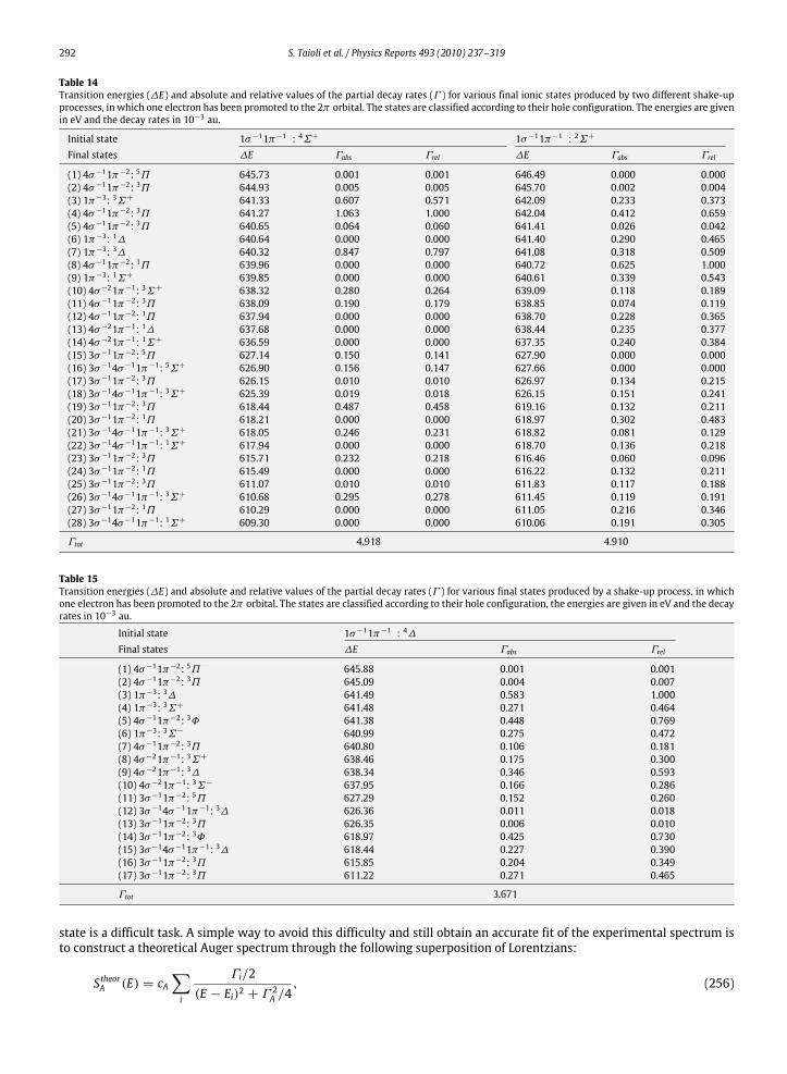
292 S. Taioli et al. / Physics Reports 493 (2010) 237–319
Table 14Transition energies (∆E) and absolute and relative values of the partial decay rates (Γ ) for various final ionic states produced by two different shake-upprocesses, in which one electron has been promoted to the 2π orbital. The states are classified according to their hole configuration. The energies are givenin eV and the decay rates in 10−3 au.
Initial state 1σ−11π−1 : 4Σ+ 1σ−11π−1 : 2Σ+
Final states ∆E Γabs Γrel ∆E Γabs Γrel
(1) 4σ−11π−2: 5Π 645.73 0.001 0.001 646.49 0.000 0.000(2) 4σ−11π−2: 3Π 644.93 0.005 0.005 645.70 0.002 0.004(3) 1π−3: 3Σ+ 641.33 0.607 0.571 642.09 0.233 0.373(4) 4σ−11π−2: 3Π 641.27 1.063 1.000 642.04 0.412 0.659(5) 4σ−11π−2: 3Π 640.65 0.064 0.060 641.41 0.026 0.042(6) 1π−3: 1∆ 640.64 0.000 0.000 641.40 0.290 0.465(7) 1π−3: 3∆ 640.32 0.847 0.797 641.08 0.318 0.509(8) 4σ−11π−2: 1Π 639.96 0.000 0.000 640.72 0.625 1.000(9) 1π−3: 1Σ+ 639.85 0.000 0.000 640.61 0.339 0.543(10) 4σ−21π−1: 3Σ+ 638.32 0.280 0.264 639.09 0.118 0.189(11) 4σ−11π−2: 3Π 638.09 0.190 0.179 638.85 0.074 0.119(12) 4σ−11π−2: 1Π 637.94 0.000 0.000 638.70 0.228 0.365(13) 4σ−21π−1: 1∆ 637.68 0.000 0.000 638.44 0.235 0.377(14) 4σ−21π−1: 1Σ+ 636.59 0.000 0.000 637.35 0.240 0.384(15) 3σ−11π−2: 5Π 627.14 0.150 0.141 627.90 0.000 0.000(16) 3σ−14σ−11π−1: 5Σ+ 626.90 0.156 0.147 627.66 0.000 0.000(17) 3σ−11π−2: 3Π 626.15 0.010 0.010 626.97 0.134 0.215(18) 3σ−14σ−11π−1: 3Σ+ 625.39 0.019 0.018 626.15 0.151 0.241(19) 3σ−11π−2: 3Π 618.44 0.487 0.458 619.16 0.132 0.211(20) 3σ−11π−2: 1Π 618.21 0.000 0.000 618.97 0.302 0.483(21) 3σ−14σ−11π−1: 3Σ+ 618.05 0.246 0.231 618.82 0.081 0.129(22) 3σ−14σ−11π−1: 1Σ+ 617.94 0.000 0.000 618.70 0.136 0.218(23) 3σ−11π−2: 3Π 615.71 0.232 0.218 616.46 0.060 0.096(24) 3σ−11π−2: 1Π 615.49 0.000 0.000 616.22 0.132 0.211(25) 3σ−11π−2: 3Π 611.07 0.010 0.010 611.83 0.117 0.188(26) 3σ−14σ−11π−1: 3Σ+ 610.68 0.295 0.278 611.45 0.119 0.191(27) 3σ−11π−2: 1Π 610.29 0.000 0.000 611.05 0.216 0.346(28) 3σ−14σ−11π−1: 1Σ+ 609.30 0.000 0.000 610.06 0.191 0.305
Γtot 4.918 4.910
Table 15Transition energies (∆E) and absolute and relative values of the partial decay rates (Γ ) for various final states produced by a shake-up process, in whichone electron has been promoted to the 2π orbital. The states are classified according to their hole configuration, the energies are given in eV and the decayrates in 10−3 au.
Initial state 1σ−11π−1 : 4∆Final states ∆E Γabs Γrel
(1) 4σ−11π−2: 5Π 645.88 0.001 0.001(2) 4σ−11π−2: 3Π 645.09 0.004 0.007(3) 1π−3: 3∆ 641.49 0.583 1.000(4) 1π−3: 3Σ+ 641.48 0.271 0.464(5) 4σ−11π−2: 3Φ 641.38 0.448 0.769(6) 1π−3: 3Σ− 640.99 0.275 0.472(7) 4σ−11π−2: 3Π 640.80 0.106 0.181(8) 4σ−21π−1: 3Σ+ 638.46 0.175 0.300(9) 4σ−21π−1: 3∆ 638.34 0.346 0.593(10) 4σ−21π−1: 3Σ− 637.95 0.166 0.286(11) 3σ−11π−2: 5Π 627.29 0.152 0.260(12) 3σ−14σ−11π−1: 3∆ 626.36 0.011 0.018(13) 3σ−11π−2: 3Π 626.35 0.006 0.010(14) 3σ−11π−2: 3Φ 618.97 0.425 0.730(15) 3σ−14σ−11π−1: 3∆ 618.44 0.227 0.390(16) 3σ−11π−2: 3Π 615.85 0.204 0.349(17) 3σ−11π−2: 3Π 611.22 0.271 0.465
Γtot 3.671
state is a difficult task. A simple way to avoid this difficulty and still obtain an accurate fit of the experimental spectrum isto construct a theoretical Auger spectrum through the following superposition of Lorentzians:
StheorA (E) = cA∑i
Γi/2(E − Ei)2 + Γ 2A /4
, (256)
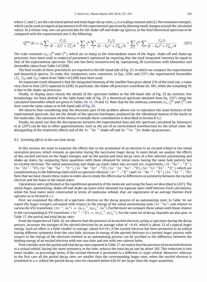
S. Taioli et al. / Physics Reports 493 (2010) 237–319 293
whereΓi andΓA are the calculated partial and total Auger decay rates, cA is a scaling constant and Ei the resonance energies,which can be used as empirical parameters to fit the experimental spectrumby allowing small changes around the calculatedvalues. In a similar way, one can proceed also for the shake-off and shake-up spectra, so the final theoretical spectrum to becompared with the experimental one is the following:
StheorA (E) = cA∑i
Γi/2(E − Ei)2 + Γ 2A /4
+
∑j=1
cSOj∑i
Γij/2(E − Eij)2 + Γ 2SO,j/4
+
∑j=1
cSUj∑i
Γij/2(E − Eij)2 + Γ 2SU,j/4
. (257)
The scale constants (cA, cSOj and cSUj ), which are as many as the intermediate states of the Auger, shake-off and shake-up
processes, have been used as empirical parameters optimized by requiring that the total integrated intensity be equal tothat of the experimental spectrum. This one has been reconstructed by superposing 20 Lorentzians with intensities andlinewidths taken from Table I of [208].The final results of these procedures are reported in the left-hand side of Fig. 25, in which we compare the experimental
and theoretical spectra. To make this comparison more consistent, in Eqs. (256) and (257) the experimental linewidths(ΓA,ΓSO and ΓSU) taken from Table I of [208] have been used.An important result obtained is that the integrated intensity of the satellite lines gives about 23% of the total one, a value
very close to that (25%) reported in [208]. In particular, the shake-off processes contribute for 18%, while the remaining 5%is due to the shake-up processes.Finally, to display more clearly the details of the spectrum hidden in the left-hand side of Fig. 25 by extrinsic line
broadenings, we have plotted in the right-hand side of Fig. 25 a theoretical spectrum obtained from Eq. (257) using thecalculated linewidths which are given in Tables 10, 11, 14 and 15. Note that for the arbitrary constants (cA, cSOj and c
SUj ) we
have used the same values as in left-hand side of Fig. 25.We observe that considering only the electronic part of the problem allows one to reproduce the main features of the
experimental spectrum, but not the details of the spectral lineshapes, produced by the vibrational motion of the nuclei inthe molecules. The extension of the theory to include these contributions is described in Section 8.3.2.Finally, we point out that the discrepancies between the experimental data and the spectrum calculated by Simonucci
et al. [207] can be due to other approximations, such as the use of an uncorrelated wavefunction for the initial state, thedisregarding of the relativistic effects and of the 1σ−13σ−1 shake-off and 3σ−21π−12π shake-up processes.
9.5. Screening effects in the core-hole decay
In this section, we want to examine the effects due to the promotion of an electron to an excited orbital in the initialionization process, which remains as spectator during the successive Auger decay. In more detail, we analyze the effectsof this excited electron on the Auger energies and on the partial and total decay rates of a few selected autoionizing andshake-up states, by comparing these quantities with those obtained for initial states having the same hole pattern, butno excited electrons. The initial autoionizing and shake-up states taken into account are, respectively, (1σ−15σ 1 : 3Σ+),(1σ−12π1 : 3Π ), (1σ−14σ−15σ 1 : 4Σ+), (1σ−14σ−12π1 : 4Π ), (1σ−11π−15σ 1 : 4Π ), (1σ−11π−12π1 : 4Σ+), which arecomplementary to the following states with no spectator electron: (1σ−1 : 2Σ+) and (1σ−14σ−1 : 3Σ+), (1σ−11π−1 : 3Π ).Note that we have chosen these states in order also to study the effects due to differences in symmetry between the excitedelectron and the holes in the initial states.Calculations were performed at the equilibrium geometry of the molecule and using the basis set described in [207]. The
initial Auger, autoionizing, shake-off and shake-up states were obtained via separate open-shell Hartree–Fock calculations,while the final states were constructed in terms of molecular orbitals that are eigenstates of an average Hartree–Fockoperator as in Section 8.1.1.First, we examined the effects of a spectator electron on the decay process of an autoionizing state. In Table 16, we
report the Auger energies calculated with respect to the energy of the initial autoionizing state (1σ−1nλ1) and relative tovarious Ke-VVe transitions: (1σ−1, nλ1)→ (n1λ−11 , n2λ
−12 , nλ
1). Furthermore we compare these values with those relativeto the corresponding K-VV transitions: (1σ−1 : 2Σ)→ (n1λ−11 , n2λ
−12 ). For the same set of decay channels we also give, in
Table 17, the partial and total decay rates.From the inspection of Table 16, we observe that the presence of an excited electron, acting as spectator during the decay
process, increases the energies of the ejected electrons by an average value of ∼6 eV, which is about 1% of a typical Augerenergy. Such an effect is a little smaller in average (about 0.4 eV), if the excited electron has been promoted to an orbitalhaving different symmetry from the core hole. Increase in energy of the ejected electrons in a normal Auger process withrespect to the energy of the electrons emitted in an autoionizing process can be ascribed to the difference between thebinding energy of an excited electron with one core hole and one with two valence holes.Ifwe consider now the partial and total decay rates reported in Table 17,wenotice that the presence of an excited electron
in a virtual orbital, having the same symmetry as the hole, reduces the total decay rate by about 18%. This reduction is twotimes smaller, in percentage terms, if the excited electron is promoted to a different (π-type) orbital. Moreover, whereasin the first case all the partial decay rates are smaller than the corresponding Auger ones, when the excited electron ispromoted to a π orbital the partial decay rates for channels below 630 eV are larger than the Auger quantities.
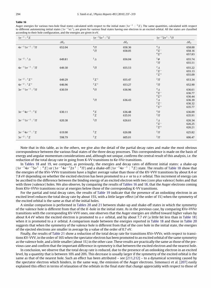
294 S. Taioli et al. / Physics Reports 493 (2010) 237–319
Table 16Auger energies for various two-hole final states calculated with respect to the initial state (1σ−1 : 2Σ). The same quantities, calculated with respectto different autoionizing initial states (1σ−1nλ1), are given for various final states having one electron in an excited orbital. All the states are classifiedaccording to their hole configuration, and the energies are given in eV.
1σ−1 : 2Σ 1σ−15σ 1 : 3Σ 1σ−12π1 : 3Π∆Eα ∆Eα ∆Eα
4σ−11π−1 : 3Π 652.04 4Π 658.36 4∆ 658.002Π 658.05 4Σ− 658.16
4Σ+ 657.83
1π−2 : 1∆ 649.81 2∆ 656.04 2Φ 655.742Π 655.51
4σ−11π−1 : 1Π 649.30 2Π 655.53 2∆ 655.222Σ− 655.132Σ+ 655.09
1π−2 : 1Σ+ 649.29 2Σ+ 655.47 2Π 653.34
4σ−2 : 1Σ+ 646.96 2Σ+ 653.27 2Π 652.90
3σ−11π−1 : 3Π 630.59 4Π 636.96 4∆ 636.614Σ− 636.774Σ+ 636.44
2Π 636.43 2∆ 636.392Σ− 636.322Σ+ 635.77
3σ−14σ−1 : 3Σ 630.11 4Σ 636.48 4Π 636.092Σ 635.91 2Π 635.91
3σ−11π−1 : 1Π 620.38 2Π 626.61 2∆ 626.342Σ− 626.252Σ+ 626.21
3σ−14σ−1 : 1Σ 619.90 2Σ 626.08 2Π 625.82
3σ−2 : 1Σ 598.79 2Σ 605.01 2Π 606.47
Note that in this table, as in the others, we give also the detail of the partial decay rates and make the most obviouscorrespondence between the various final states of the three decay processes. This correspondence is made on the basis ofenergy and angular momentum considerations and, although not unique, confirms the central result of this analysis, i.e. thereduction of the total decay rate in going from K-VV transitions to Ke-VVe transitions.In Tables 18 and 19, we compare, as previously, the energies and decay rates of different initial states: a shake-up
(1σ−14σ−15σ 1 : 4Σ) or (1σ−14σ−12π1 : 4Π ) and a shake-off (1σ−14σ−1 : 3Σ) state. The results of Table 18 show thatthe energies of the KVe-VVVe transitions have a higher average value than those of the KV-VVV transitions by about 8.4 or7.8 eV depending on whether the excited electron has been promoted to a σ or to a π orbital. This increment of energy canbe ascribed to the difference between the binding energy of an excited electron with two (core plus valence) holes and thatwith three (valence) holes. We also observe, by comparing the results of Tables 16 and 18, that the Auger electrons comingfrom KVe-VVVe transitions occur at energies below those of the corresponding K-VV transitions.For the partial and total decay rates, the results of Table 19 indicate that the presence of an onlooking electron in an
excited level reduces the total decay rate by about 15%, with a little larger effect (of the order of 1%) when the symmetry ofthe excited orbital is the same as that of the initial holes.A similar comparison is performed in Tables 20 and 21 between shake-up and shake-off states in which the symmetry
of the valence hole is different from that of the K -hole in the initial state. As in the previous case, by comparing KVe-VVVetransitions with the corresponding KV-VVV ones, one observes that the Auger energies are shifted toward higher values byabout 8.4 eV when the excited electron is promoted to a σ orbital, and by about 7.7 eV (a little bit less than in Table 18)when it is promoted to a π orbital. A comparison made between the energies reported in Table 18 and those in Table 20suggests that when the symmetry of the valence hole is different from that of the core hole in the initial state, the energiesof the ejected electrons are smaller in average by a value of the order of 0.7 eV.Finally, the results of Table 21 show a reduction of the total decay rate for transitions KVe-VVVe, with respect to transi-
tions KV-VVV, in the order of 16%when the spectator electron has been promoted to an excited orbital of the same symmetryas the valence hole, and a little smaller (about 1%) in the other case. These results are practically the same as those of the pre-vious case and confirm that the important difference in symmetry is that between the excited electron and the nearest hole.In conclusion, we observe that the total decay rate is reduced, due to the presence of an onlooking electron in an excited
level, by a quantity that is between 10% and 20%. This decrease is usually larger if the symmetry of the excited orbital is thesame as that of the nearest hole. Such an effect has been attributed – see [211,212] – to a dynamical screening caused bythe spectator electron which hinders, in the same way, the emission of the Auger electrons. Simonucci et al. [207] easilyexplained this effect in terms of relaxation of the orbitals in the final state that change appreciably with respect to those of
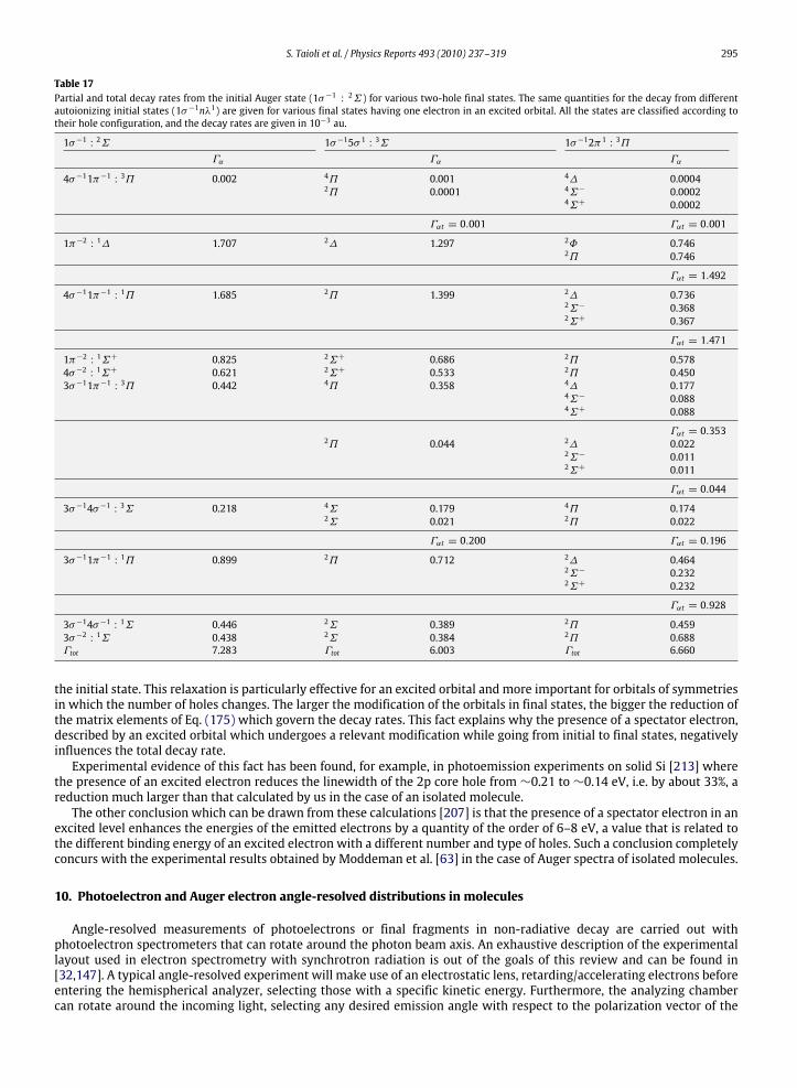
S. Taioli et al. / Physics Reports 493 (2010) 237–319 295
Table 17Partial and total decay rates from the initial Auger state (1σ−1 : 2Σ) for various two-hole final states. The same quantities for the decay from differentautoionizing initial states (1σ−1nλ1) are given for various final states having one electron in an excited orbital. All the states are classified according totheir hole configuration, and the decay rates are given in 10−3 au.
1σ−1 : 2Σ 1σ−15σ 1 : 3Σ 1σ−12π1 : 3ΠΓα Γα Γα
4σ−11π−1 : 3Π 0.002 4Π 0.001 4∆ 0.00042Π 0.0001 4Σ− 0.0002
4Σ+ 0.0002
Γαt = 0.001 Γαt = 0.001
1π−2 : 1∆ 1.707 2∆ 1.297 2Φ 0.7462Π 0.746
Γαt = 1.492
4σ−11π−1 : 1Π 1.685 2Π 1.399 2∆ 0.7362Σ− 0.3682Σ+ 0.367
Γαt = 1.471
1π−2 : 1Σ+ 0.825 2Σ+ 0.686 2Π 0.5784σ−2 : 1Σ+ 0.621 2Σ+ 0.533 2Π 0.4503σ−11π−1 : 3Π 0.442 4Π 0.358 4∆ 0.177
4Σ− 0.0884Σ+ 0.088
Γαt = 0.3532Π 0.044 2∆ 0.022
2Σ− 0.0112Σ+ 0.011
Γαt = 0.044
3σ−14σ−1 : 3Σ 0.218 4Σ 0.179 4Π 0.1742Σ 0.021 2Π 0.022
Γαt = 0.200 Γαt = 0.196
3σ−11π−1 : 1Π 0.899 2Π 0.712 2∆ 0.4642Σ− 0.2322Σ+ 0.232
Γαt = 0.928
3σ−14σ−1 : 1Σ 0.446 2Σ 0.389 2Π 0.4593σ−2 : 1Σ 0.438 2Σ 0.384 2Π 0.688Γtot 7.283 Γtot 6.003 Γtot 6.660
the initial state. This relaxation is particularly effective for an excited orbital and more important for orbitals of symmetriesin which the number of holes changes. The larger the modification of the orbitals in final states, the bigger the reduction ofthe matrix elements of Eq. (175) which govern the decay rates. This fact explains why the presence of a spectator electron,described by an excited orbital which undergoes a relevant modification while going from initial to final states, negativelyinfluences the total decay rate.Experimental evidence of this fact has been found, for example, in photoemission experiments on solid Si [213] where
the presence of an excited electron reduces the linewidth of the 2p core hole from ∼0.21 to ∼0.14 eV, i.e. by about 33%, areduction much larger than that calculated by us in the case of an isolated molecule.The other conclusion which can be drawn from these calculations [207] is that the presence of a spectator electron in an
excited level enhances the energies of the emitted electrons by a quantity of the order of 6–8 eV, a value that is related tothe different binding energy of an excited electron with a different number and type of holes. Such a conclusion completelyconcurs with the experimental results obtained by Moddeman et al. [63] in the case of Auger spectra of isolated molecules.
10. Photoelectron and Auger electron angle-resolved distributions in molecules
Angle-resolved measurements of photoelectrons or final fragments in non-radiative decay are carried out withphotoelectron spectrometers that can rotate around the photon beam axis. An exhaustive description of the experimentallayout used in electron spectrometry with synchrotron radiation is out of the goals of this review and can be found in[32,147]. A typical angle-resolved experiment will make use of an electrostatic lens, retarding/accelerating electrons beforeentering the hemispherical analyzer, selecting those with a specific kinetic energy. Furthermore, the analyzing chambercan rotate around the incoming light, selecting any desired emission angle with respect to the polarization vector of the
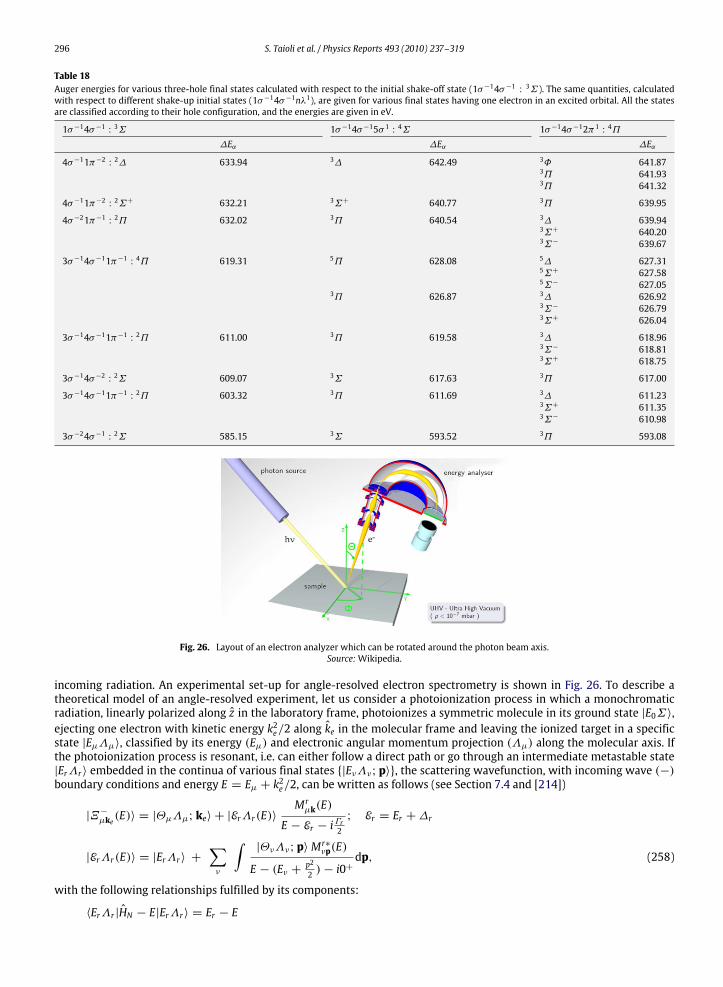
296 S. Taioli et al. / Physics Reports 493 (2010) 237–319
Table 18Auger energies for various three-hole final states calculated with respect to the initial shake-off state (1σ−14σ−1 : 3Σ). The same quantities, calculatedwith respect to different shake-up initial states (1σ−14σ−1nλ1), are given for various final states having one electron in an excited orbital. All the statesare classified according to their hole configuration, and the energies are given in eV.
1σ−14σ−1 : 3Σ 1σ−14σ−15σ 1 : 4Σ 1σ−14σ−12π1 : 4Π∆Eα ∆Eα ∆Eα
4σ−11π−2 : 2∆ 633.94 3∆ 642.49 3Φ 641.873Π 641.933Π 641.32
4σ−11π−2 : 2Σ+ 632.21 3Σ+ 640.77 3Π 639.95
4σ−21π−1 : 2Π 632.02 3Π 640.54 3∆ 639.943Σ+ 640.203Σ− 639.67
3σ−14σ−11π−1 : 4Π 619.31 5Π 628.08 5∆ 627.315Σ+ 627.585Σ− 627.05
3Π 626.87 3∆ 626.923Σ− 626.793Σ+ 626.04
3σ−14σ−11π−1 : 2Π 611.00 3Π 619.58 3∆ 618.963Σ− 618.813Σ+ 618.75
3σ−14σ−2 : 2Σ 609.07 3Σ 617.63 3Π 617.00
3σ−14σ−11π−1 : 2Π 603.32 3Π 611.69 3∆ 611.233Σ+ 611.353Σ− 610.98
3σ−24σ−1 : 2Σ 585.15 3Σ 593.52 3Π 593.08
Fig. 26. Layout of an electron analyzer which can be rotated around the photon beam axis.Source:Wikipedia.
incoming radiation. An experimental set-up for angle-resolved electron spectrometry is shown in Fig. 26. To describe atheoretical model of an angle-resolved experiment, let us consider a photoionization process in which a monochromaticradiation, linearly polarized along z in the laboratory frame, photoionizes a symmetric molecule in its ground state |E0Σ〉,ejecting one electron with kinetic energy k2e/2 along ke in the molecular frame and leaving the ionized target in a specificstate |EµΛµ〉, classified by its energy (Eµ) and electronic angular momentum projection (Λµ) along the molecular axis. Ifthe photoionization process is resonant, i.e. can either follow a direct path or go through an intermediate metastable state|ErΛr〉 embedded in the continua of various final states |EνΛν; p〉, the scattering wavefunction, with incoming wave (−)boundary conditions and energy E = Eµ + k2e/2, can be written as follows (see Section 7.4 and [214])
|Ξ−µke(E)〉 = |ΘµΛµ; ke〉 + |ErΛr(E)〉Mrµk(E)
E − Er − iΓr2; Er = Er +∆r
|ErΛr(E)〉 = |ErΛr〉 +∑ν
∫|ΘνΛν; p〉Mr∗νp(E)
E − (Eν +p22 )− i0
+
dp, (258)
with the following relationships fulfilled by its components:
〈ErΛr |HN − E|ErΛr〉 = Er − E

S. Taioli et al. / Physics Reports 493 (2010) 237–319 297
Table 19Partial and total decay rates from the initial shake-off state (1σ−14σ−1 : 3Σ) for various three-hole final states. The same quantities for the decay fromdifferent shake-up initial states (1σ−14σ−1nλ1) are given for various final states having one electron in an excited orbital. All the states are classifiedaccording to their hole configuration, and the decay rates are given in 10−3 au.
1σ−14σ−1 : 3Σ 1σ−14σ−15σ 1 : 4Σ 1σ−14σ−12π1 : 4ΠΓα Γα Γα
4σ−11π−2 : 2∆ 2.128 3∆ 1.798 3Φ 0.9163Π 0.1503Π 0.737
Γαt = 1.803
4σ−11π−2 : 2Σ+ 0.850 3Σ+ 0.721 3Π 0.740
4σ−21π−1 : 2Π 1.063 3Π 0.868 3∆ 0.4423Σ+ 0.2193Σ− 0.219
Γαt = 0.880
3σ−14σ−11π−1 : 4Π 0.440 5Π 0.379 5∆ 0.0345Σ+ 0.0945Σ− 0.094
Γαt = 0.2223Π 0.027 3∆ 0.011
3Σ− 0.0063Σ+ 0.006
Γαt = 0.023
3σ−14σ−11π−1 : 2Π 0.545 3Π 0.470 3∆ 0.2383Σ− 0.1103Σ+ 0.120
Γαt = 0.468
3σ−14σ−2 : 2Σ 0.537 3Σ 0.441 3Π 0.451
3σ−14σ−11π−1 : 2Π 0.602 3Π 0.496 3∆ 0.2573Σ+ 0.1363Σ− 0.127
Γαt = 0.520
3σ−24σ−1 : 2Σ 0.547 3Σ 0.511 3Π 0.525
Γtot 6.712 Γtot 5.639 Γtot 5.684
〈EνΛν |HN−1 − E|EµΛµ〉 = (Eµ − E) δνµ
〈ErΛr |HN − E|ΘµΛµ; ke〉 = Mrµke(E)
〈ΘνΛν; p|HN − E|ΘµΛµ; ke〉 = (Eµ + k2e/2− E) δνµ δ(ke − p). (259)
In Eq. (258), ∆r and Γr are the energy shift and natural width of the resonance defined in terms of the matrix elementswhich couple metastable and final states:
∆r =∑ν
P
∫|Mrνp(Er)|
2
Er − Eν − p2/2dp
Γr = 2π∑ν
∫|Mrνp(Er)|
2 δ(Er − Eν − p2/2)dp, (260)
whereP is the Cauchyprincipal part of the integral.We recall that |Ξ−µke(E)〉 is a stationary state, at the energy E = Eµ+k2e/2,
which is asymptotically defined by the momentum ke of the emitted electron and the state |EµΛµ〉 of the singly ionizedtarget (for autoionization or photoionization processes) or doubly ionized target (for an Auger process). The previous resultswere obtained following Fano’s approach to the resonance scattering discussed in Section 7.4. From the knowledge of thewavefunction in Eq. (258), one can evaluate the differential cross section, calculated at the first order of the perturbationtheory, as follows:
dσµ(ω)dke
=
(4π2ωc
) ∣∣∣∣∣〈Ξ−µke | − z ·∑j
rj|E0Σ〉
∣∣∣∣∣2
δ
(ω + E0 − Eµ −
k2e2
)(261)
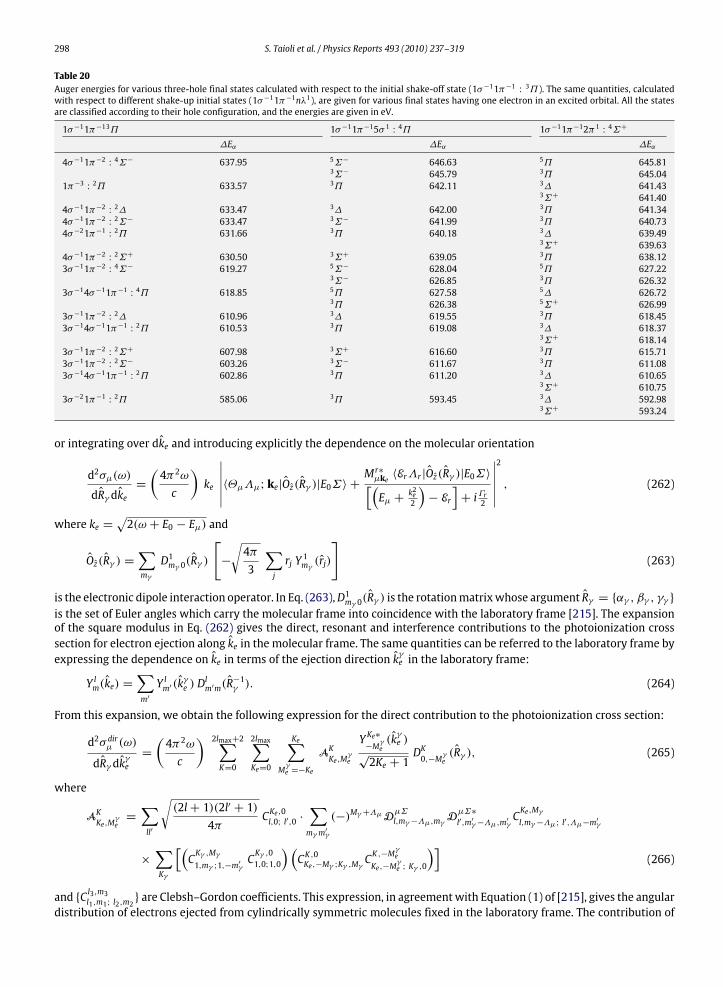
298 S. Taioli et al. / Physics Reports 493 (2010) 237–319
Table 20Auger energies for various three-hole final states calculated with respect to the initial shake-off state (1σ−11π−1 : 3Π ). The same quantities, calculatedwith respect to different shake-up initial states (1σ−11π−1nλ1), are given for various final states having one electron in an excited orbital. All the statesare classified according to their hole configuration, and the energies are given in eV.
1σ−11π−13Π 1σ−11π−15σ 1 : 4Π 1σ−11π−12π1 : 4Σ+
∆Eα ∆Eα ∆Eα
4σ−11π−2 : 4Σ− 637.95 5Σ− 646.63 5Π 645.813Σ− 645.79 3Π 645.04
1π−3 : 2Π 633.57 3Π 642.11 3∆ 641.433Σ+ 641.40
4σ−11π−2 : 2∆ 633.47 3∆ 642.00 3Π 641.344σ−11π−2 : 2Σ− 633.47 3Σ− 641.99 3Π 640.734σ−21π−1 : 2Π 631.66 3Π 640.18 3∆ 639.49
3Σ+ 639.634σ−11π−2 : 2Σ+ 630.50 3Σ+ 639.05 3Π 638.123σ−11π−2 : 4Σ− 619.27 5Σ− 628.04 5Π 627.22
3Σ− 626.85 3Π 626.323σ−14σ−11π−1 : 4Π 618.85 5Π 627.58 5∆ 626.72
3Π 626.38 5Σ+ 626.993σ−11π−2 : 2∆ 610.96 3∆ 619.55 3Π 618.453σ−14σ−11π−1 : 2Π 610.53 3Π 619.08 3∆ 618.37
3Σ+ 618.143σ−11π−2 : 2Σ+ 607.98 3Σ+ 616.60 3Π 615.713σ−11π−2 : 2Σ− 603.26 3Σ− 611.67 3Π 611.083σ−14σ−11π−1 : 2Π 602.86 3Π 611.20 3∆ 610.65
3Σ+ 610.753σ−21π−1 : 2Π 585.06 3Π 593.45 3∆ 592.98
3Σ+ 593.24
or integrating over dke and introducing explicitly the dependence on the molecular orientation
d2σµ(ω)
dRγ dke=
(4π2ωc
)ke
∣∣∣∣∣∣〈ΘµΛµ; ke|Oz(Rγ )|E0Σ〉 + Mr∗µke 〈ErΛr |Oz(Rγ )|E0Σ〉[(Eµ +
k2e2
)− Er
]+ iΓr2
∣∣∣∣∣∣2
, (262)
where ke =√2(ω + E0 − Eµ) and
Oz(Rγ ) =∑mγ
D1mγ 0(Rγ )
[−
√4π3
∑j
rj Y 1mγ (rj)
](263)
is the electronic dipole interaction operator. In Eq. (263),D1mγ 0(Rγ ) is the rotationmatrixwhose argument Rγ = αγ , βγ , γγ is the set of Euler angles which carry the molecular frame into coincidence with the laboratory frame [215]. The expansionof the square modulus in Eq. (262) gives the direct, resonant and interference contributions to the photoionization crosssection for electron ejection along ke in the molecular frame. The same quantities can be referred to the laboratory frame byexpressing the dependence on ke in terms of the ejection direction k
γe in the laboratory frame:
Y lm(ke) =∑m′Y lm′(k
γe ) D
lm′m(R
−1γ ). (264)
From this expansion, we obtain the following expression for the direct contribution to the photoionization cross section:
d2σ dirµ (ω)
dRγ dkγe=
(4π2ωc
) 2lmax+2∑K=0
2lmax∑Ke=0
Ke∑Mγe =−Ke
AKKe,Mγe
Y Ke∗−Mγe
(kγe )√2Ke + 1
DK0,−Mγe (Rγ ), (265)
where
AKKe,Mγe=
∑ll′
√(2l+ 1)(2l′ + 1)
4πCKe,0l,0; l′,0 ·
∑mγm′γ
(−)Mγ+ΛµDµΣ
l,mγ−Λµ,mγ DµΣ∗
l′,m′γ−Λµ,m′γCKe,Mγl,mγ−Λµ; l′,Λµ−m′γ
×
∑Kγ
[(CKγ ,Mγ1,mγ ;1,−m′γ
CKγ ,01,0;1,0
) (CK ,0Ke,−Mγ ;Kγ ,Mγ C
K ,−MγeKe,−M
γe ; Kγ ,0
)](266)
and C l3,m3l1,m1; l2,m2 are Clebsh–Gordon coefficients. This expression, in agreementwith Equation (1) of [215], gives the angular
distribution of electrons ejected from cylindrically symmetric molecules fixed in the laboratory frame. The contribution of
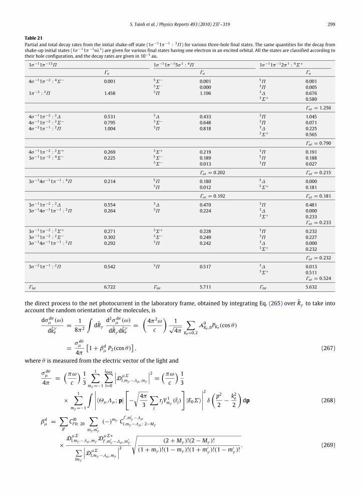
S. Taioli et al. / Physics Reports 493 (2010) 237–319 299
Table 21Partial and total decay rates from the initial shake-off state (1σ−11π−1 : 3Π ) for various three-hole final states. The same quantities for the decay fromshake-up initial states (1σ−11π−1nλ1) are given for various final states having one electron in an excited orbital. All the states are classified according totheir hole configuration, and the decay rates are given in 10−3 au.
1σ−11π−13Π 1σ−11π−15σ 1 : 4Π 1σ−11π−12π1 : 4Σ+
Γα Γα Γα
4σ−11π−2 : 4Σ− 0.001 5Σ− 0.001 5Π 0.0013Σ− 0.000 3Π 0.005
1π−3 : 2Π 1.458 3Π 1.196 3∆ 0.6763Σ+ 0.580
Γαt = 1.256
4σ−11π−2 : 2∆ 0.531 3∆ 0.433 3Π 1.0454σ−11π−2 : 2Σ− 0.795 3Σ− 0.648 3Π 0.0714σ−21π−1 : 2Π 1.004 3Π 0.818 3∆ 0.225
3Σ+ 0.565
Γαt = 0.790
4σ−11π−2 : 2Σ+ 0.269 3Σ+ 0.219 3Π 0.1913σ−11π−2 : 4Σ− 0.225 5Σ− 0.189 5Π 0.188
3Σ− 0.013 3Π 0.027
Γαt = 0.202 Γαt = 0.215
3σ−14σ−11π−1 : 4Π 0.214 5Π 0.180 5∆ 0.0003Π 0.012 5Σ+ 0.181
Γαt = 0.192 Γαt = 0.181
3σ−11π−2 : 2∆ 0.554 3∆ 0.470 3Π 0.4813σ−14σ−11π−1 : 2Π 0.264 3Π 0.224 3∆ 0.000
3Σ+ 0.233Γαt = 0.233
3σ−11π−2 : 2Σ+ 0.271 3Σ+ 0.228 3Π 0.2323σ−11π−2 : 2Σ− 0.302 3Σ− 0.249 3Π 0.2273σ−14σ−11π−1 : 2Π 0.292 3Π 0.242 3∆ 0.000
3Σ+ 0.232
Γαt = 0.232
3σ−21π−1 : 2Π 0.542 3Π 0.517 3∆ 0.0133Σ+ 0.511
Γαt = 0.524
Γtot 6.722 Γtot 5.711 Γtot 5.632
the direct process to the net photocurrent in the laboratory frame, obtained by integrating Eq. (265) over Rγ to take intoaccount the random orientation of the molecules, is
dσ dirµ (ω)
dkγe=
18π2
∫dRγ
d2σ dirµ (ω)
dRγ dkγe=
(4π2ωc
)1√4π
∑Ke=0,2
A0Ke,0PKe(cos θ)
=σ dirµ
4π
[1+ βdµ P2(cos θ)
], (267)
where θ is measured from the electric vector of the light and
σ dirµ
4π=
(πωc
) 13
1∑mγ=−1
lmax∑l=0
∣∣∣DµΣ
l,mγ−Λµ,mγ
∣∣∣2 = (πωc
) 13
×
1∑mγ=−1
∫ ∣∣∣∣∣〈ΘµΛµ; p|[−
√4π3
∑j
rjY 1mγ (rj)
]|E0Σ〉
∣∣∣∣∣2
δ
(p2
2−k2e2
)dp (268)
βdµ =∑ll′C l0l′0; 20
∑mγm′γ
(−)mγ Cl′,m′γ−Λµl,mγ−Λµ; 2−Mγ
×
DµΣ
l,mγ−Λµ,mγ DµΣ∗
l′,m′γ−Λµ,m′γ∑lmγ
∣∣∣DµΣ
l,mγ−Λµ,mγ
∣∣∣2√
(2+Mγ )!(2−Mγ )!(1+mγ )!(1−mγ )!(1+m′γ )!(1−m′γ )!
. (269)
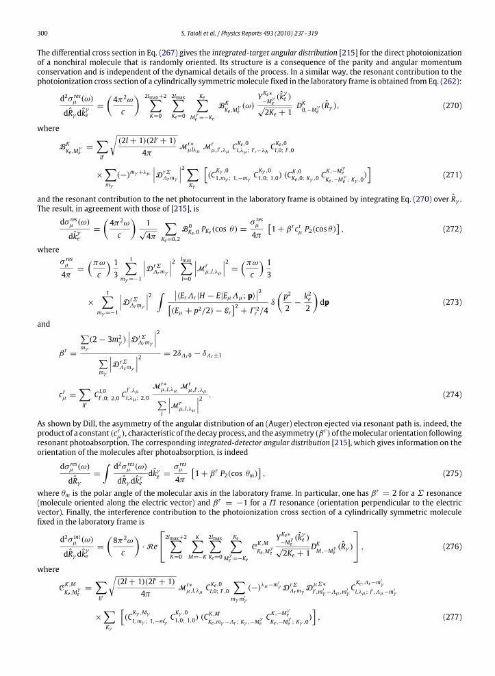
300 S. Taioli et al. / Physics Reports 493 (2010) 237–319
The differential cross section in Eq. (267) gives the integrated-target angular distribution [215] for the direct photoionizationof a nonchiral molecule that is randomly oriented. Its structure is a consequence of the parity and angular momentumconservation and is independent of the dynamical details of the process. In a similar way, the resonant contribution to thephotoionization cross section of a cylindrically symmetric molecule fixed in the laboratory frame is obtained from Eq. (262):
d2σ resµ (ω)
dRγ dkγe=
(4π2ωc
) 2lmax+2∑K=0
2lmax∑Ke=0
Ke∑Mγe =−Ke
BKKe,Mγe(ω)
Y Ke∗−Mγe
(kγe )√2Ke + 1
DK0,−Mγe (Rγ ), (270)
where
BKKe,Mγe=
∑ll′
√(2l+ 1)(2l′ + 1)
4πMr∗µlλµ Mr
µ,l′,λµ CKe,0l,λµ; l′,−λA
CKe,0l,0; l′,0
×
∑mγ
(−)mγ+λµ∣∣∣D rΣ
Λrmγ
∣∣∣2∑Kγ
[(CKγ ,01,mγ ; 1,−mγ C
Kγ ,01,0; 1,0) (C
K ,0Ke,0; Kγ ,0 C
K ,−MγeKe,−M
γe ; Kγ ,0
)]
(271)
and the resonant contribution to the net photocurrent in the laboratory frame is obtained by integrating Eq. (270) over Rγ .The result, in agreement with those of [215], is
dσ resµ (ω)
dkγe=
(4π2ωc
)1√4π
∑Ke=0,2
B0Ke,0 PKe(cos θ) =σ resµ
4π
[1+ βrcrµ P2(cos θ)
], (272)
whereσ resµ
4π=
(πωc
) 13
1∑mγ=−1
∣∣∣D rΣΛrmγ
∣∣∣2 lmax∑l=0
∣∣∣Mrµ,l,λµ
∣∣∣2 = (πωc
) 13
×
1∑mγ=−1
∣∣∣D rΣΛrmγ
∣∣∣2 ∫ ∣∣〈ErΛr |H − E|EµΛµ; p〉∣∣2[(Eµ + p2/2)− Er
]2+ Γ 2r /4
δ
(p2
2−k2e2
)dp (273)
and
βr =
∑mγ(2− 3m2γ )
∣∣∣D rΣΛrmγ
∣∣∣2∑mγ
∣∣∣D rΣΛrmγ
∣∣∣2 = 2δΛr0 − δΛr±1
crµ =∑ll′C l,0l′,0; 2,0 C
l′,λµl,λµ; 2,0
Mr∗µ,l,λµ Mr
µ,l′,λµ∑l
∣∣∣Mrµ,l,λµ
∣∣∣2 . (274)
As shown by Dill, the asymmetry of the angular distribution of an (Auger) electron ejected via resonant path is, indeed, theproduct of a constant (crµ), characteristic of the decay process, and the asymmetry (β
r) of themolecular orientation followingresonant photoabsorption. The corresponding integrated-detector angular distribution [215], which gives information on theorientation of the molecules after photoabsorption, is indeed
dσ resµ (ω)
dRγ=
∫ d2σ resµ (ω)
dRγ dkγedkγe =
σ resµ
4π
[1+ βr P2(cos θm)
], (275)
where θm is the polar angle of the molecular axis in the laboratory frame. In particular, one has βr = 2 for a Σ resonance(molecule oriented along the electric vector) and βr = −1 for a Π resonance (orientation perpendicular to the electricvector). Finally, the interference contribution to the photoionization cross section of a cylindrically symmetric moleculefixed in the laboratory frame is
d2σ intµ (ω)
dRγ dkγe=
(8π2ωc
)·Re
2lmax+2∑K=0
K∑M=−K
2lmax∑Ke=0
Ke∑Mγe =−Ke
CK ,MKe,M
γe
Y Ke∗−Mγe
(kγe )√2Ke + 1
DKM,−Mγe (Rγ )
, (276)
where
CK ,MKe,M
γe=
∑ll′
√(2l+ 1)(2l′ + 1)
4πMr∗µ,l,λµ C
Ke,0l,0; l′,0
∑mγm′γ
(−)λµ−m′γ D rΣ
Λrmγ DµΣ∗
l′,m′γ−Λµ,m′γCKe,Λr−m′γl,λµ; l′,Λµ−m′γ
×
∑Kγ
[(CKγ ,Mγ1,mγ ; 1,−m′γ
CKγ ,01,0; 1,0) (C
K ,MKe,mγ−Λr ; Kγ ,−M
γeCK ,−M
γe
Ke,−Mγe ; Kγ ,0
)], (277)
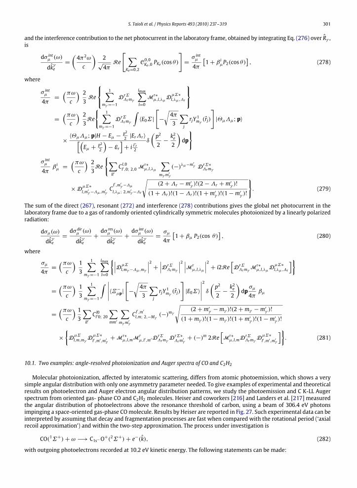
S. Taioli et al. / Physics Reports 493 (2010) 237–319 301
and the interference contribution to the net photocurrent in the laboratory frame, obtained by integrating Eq. (276) over Rγ ,is
dσ intµ (ω)
dkγe=
(4π2ωc
)2√4π
Re
[ ∑Ke=0,2
C0,0Ke,0 PKe(cos θ)
]=σ intµ
4π
[1+ β iµP2(cos θ)
], (278)
where
σ intµ
4π=
(πωc
) 23
Re
1∑mγ=−1
D rΣΛrmγ
lmax∑l=0
Mr∗µ,l,λµD
µΣ∗
l,λµ,Λr
=
(πωc
) 23
Re
1∑
mγ=−1
D rΣΛrmγ
∫〈E0Σ |
[−
√4π3
∑j
rjY 1mγ (rj)
]|ΘµΛµ; p〉
×〈ΘµΛµ; p|H − Eµ − p2
2 |ErΛr〉[(Eµ +
p22
)− Er
]+ iΓr2
δ
(p2
2−k2e2
)dp
σ intµ
4πβ iµ =
(πωc
) 23
Re
∑ll′C l,0l′,0; 2,0 Mr∗
µ,l,λµ
∑mγm′γ
(−)λµ−m′γ D rΣ∗
Λrmγ
×DµΣ∗
l,m′γ−Λµ,m′γCl′,m′γ−Λµl,λµ; 2,m′γ−Λr
√(2+Λr −m′γ )!(2−Λr +m′γ )!
(1+Λr)!(1−Λr)!(1+m′γ )!(1−m′γ )!
. (279)
The sum of the direct (267), resonant (272) and interference (278) contributions gives the global net photocurrent in thelaboratory frame due to a gas of randomly oriented cylindrically symmetric molecules photoionized by a linearly polarizedradiation:
dσµ(ω)
dkγe=dσ dirµ (ω)
dkγe+dσ resµ (ω)
dkγe+dσ intµ (ω)
dkγe=σµ
4π
[1+ βµ P2(cos θ)
], (280)
where
σµ
4π=
(πωc
) 13
1∑mγ=−1
lmax∑l=0
∣∣∣DµΣ
l,mγ−Λµ,mγ
∣∣∣2 + ∣∣∣D rΣΛrmγ
∣∣∣2 ∣∣∣Mrµ,l,λµ
∣∣∣2 + i2Re [D rΣΛrmγ Mr∗
µ,l,λµDµΣ∗
l,λµ,Λr
]
=
(πωc
) 13
1∑mγ=−1
∫ ∣∣∣∣∣〈Ξ−µp|[−
√4π3
∑j
rjY 1mγ (rj)
]|E0Σ〉
∣∣∣∣∣2
δ
(p2
2−k2e2
)dpσµ
4πβµ
=
(πωc
) 13
∑ll′C l0l′0; 20
∑mm′
∑mγm′γ
C l′,m′l,m; 2,−Mγ (−)
mγ
√(2+m′γ −mγ )!(2+mγ −m′γ )!
(1+mγ )!(1−mγ )!(1+m′γ )!(1−m′γ )!
×
DµΣ
l,m,mγ DµΣ∗
l′,m′,m′γ+Mr∗
µ,l,mMrµ,l′,m′D
rΣΛrmγ D rΣ∗
Λrm′γ+ (−)m 2Re
[Mr∗µ,l,mD rΣ
Λrmγ DµΣ∗
l′,m′,m′γ
]. (281)
10.1. Two examples: angle-resolved photoionization and Auger spectra of CO and C2H2
Molecular photoionization, affected by interatomic scattering, differs from atomic photoemission, which shows a verysimple angular distribution with only one asymmetry parameter needed. To give examples of experimental and theoreticalresults on photoelectron and Auger electron angular distribution patterns, we study the photoemission and C K-LL Augerspectrum from oriented gas- phase CO and C2H2 molecules. Heiser and coworkers [216] and Landers et al. [217] measuredthe angular distribution of photoelectrons above the resonance threshold of carbon, using a beam of 306.4 eV photonsimpinging a space-oriented gas-phase COmolecule. Results by Heiser are reported in Fig. 27. Such experimental data can beinterpreted by assuming that decay and fragmentation processes are fast when compared with the rotational period (‘axialrecoil approximation’) and within the two-step approximation. The process under investigation is
CO(1Σ+)+ ω −→ C1s−O+(2Σ+)+ e−(k), (282)
with outgoing photoelectrons recorded at 10.2 eV kinetic energy. The following statements can be made:
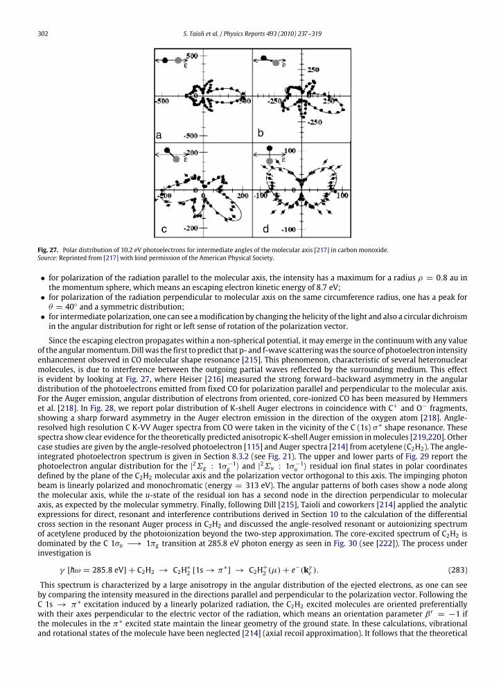
302 S. Taioli et al. / Physics Reports 493 (2010) 237–319
Fig. 27. Polar distribution of 10.2 eV photoelectrons for intermediate angles of the molecular axis [217] in carbon monoxide.Source: Reprinted from [217] with kind permission of the American Physical Society.
• for polarization of the radiation parallel to the molecular axis, the intensity has a maximum for a radius ρ = 0.8 au inthe momentum sphere, which means an escaping electron kinetic energy of 8.7 eV;• for polarization of the radiation perpendicular to molecular axis on the same circumference radius, one has a peak forθ = 40 and a symmetric distribution;• for intermediate polarization, one can see amodification by changing the helicity of the light and also a circular dichroismin the angular distribution for right or left sense of rotation of the polarization vector.
Since the escaping electron propagates within a non-spherical potential, it may emerge in the continuumwith any valueof the angularmomentum.Dillwas the first to predict that p- and f-wave scatteringwas the source of photoelectron intensityenhancement observed in CO molecular shape resonance [215]. This phenomenon, characteristic of several heteronuclearmolecules, is due to interference between the outgoing partial waves reflected by the surrounding medium. This effectis evident by looking at Fig. 27, where Heiser [216] measured the strong forward–backward asymmetry in the angulardistribution of the photoelectrons emitted from fixed CO for polarization parallel and perpendicular to the molecular axis.For the Auger emission, angular distribution of electrons from oriented, core-ionized CO has been measured by Hemmerset al. [218]. In Fig. 28, we report polar distribution of K-shell Auger electrons in coincidence with C+ and O− fragments,showing a sharp forward asymmetry in the Auger electron emission in the direction of the oxygen atom [218]. Angle-resolved high resolution C K-VV Auger spectra from CO were taken in the vicinity of the C (1s) σ ∗ shape resonance. Thesespectra show clear evidence for the theoretically predicted anisotropic K-shell Auger emission inmolecules [219,220]. Othercase studies are given by the angle-resolved photoelectron [115] and Auger spectra [214] from acetylene (C2H2). The angle-integrated photoelectron spectrum is given in Section 8.3.2 (see Fig. 21). The upper and lower parts of Fig. 29 report thephotoelectron angular distribution for the |2Σg : 1σ−1g 〉 and |
2Σu : 1σ−1u 〉 residual ion final states in polar coordinatesdefined by the plane of the C2H2 molecular axis and the polarization vector orthogonal to this axis. The impinging photonbeam is linearly polarized and monochromatic (energy = 313 eV). The angular patterns of both cases show a node alongthe molecular axis, while the u-state of the residual ion has a second node in the direction perpendicular to molecularaxis, as expected by the molecular symmetry. Finally, following Dill [215], Taioli and coworkers [214] applied the analyticexpressions for direct, resonant and interference contributions derived in Section 10 to the calculation of the differentialcross section in the resonant Auger process in C2H2 and discussed the angle-resolved resonant or autoionizing spectrumof acetylene produced by the photoionization beyond the two-step approximation. The core-excited spectrum of C2H2 isdominated by the C 1σu −→ 1πg transition at 285.8 eV photon energy as seen in Fig. 30 (see [222]). The process underinvestigation is
γ [hω = 285.8 eV] + C2H2 → C2H∗2 [1s→ π∗] → C2H+2 (µ)+ e−(kγe ). (283)
This spectrum is characterized by a large anisotropy in the angular distribution of the ejected electrons, as one can seeby comparing the intensity measured in the directions parallel and perpendicular to the polarization vector. Following theC 1s → π∗ excitation induced by a linearly polarized radiation, the C2H2 excited molecules are oriented preferentiallywith their axes perpendicular to the electric vector of the radiation, which means an orientation parameter βr = −1 ifthe molecules in the π∗ excited state maintain the linear geometry of the ground state. In these calculations, vibrationaland rotational states of the molecule have been neglected [214] (axial recoil approximation). It follows that the theoretical

S. Taioli et al. / Physics Reports 493 (2010) 237–319 303
Fig. 28. Angular distribution of Auger electrons from the narrow 1Σ+ line in carbon monoxide changing the polarization and the orientation of themolecular axis [221].Source: Reprinted from [221] with kind permission of the American Physical Society.
Fig. 29. Polar plot of the angle-resolved C 1s photoelectron spectrum of C2H2 in a plane defined by the molecular axis and the polarization direction of thelight orthogonal to the molecular axis. The upper and lower parts of the plot refer respectively to the g- and u-states of the residual ion. The polarizationof the incident photon (E = 313 eV) is perpendicular to the molecular axis [115].Source: Reprinted from [115] with kind permission of Elsevier.
spectrum includes neither vibrational structures (not even resolved in the experimental spectrum by Kivimäki et al. [222]),nor the broadening and profile deformation of the spectral lines due to vibrational transitions. Comparison with theexperimental spectrum requires one to account for the characteristics of both the incident radiation, almost perfectlypolarized along z, but having a finite dispersion ('0.6 eV in Kivimäki’s experiment) around the exciting frequency andthe finite energy resolution of the electron spectrometer: as by Eq. (184), we assume that either quantities are distributedas a normalized Gaussian function, whose full width at half maximum (FWHM = 2η1
√2 ln 2) is given by the sum of the
resolving power of the monochromator plus the energy resolution of the spectrometer. The convolution of the differentialcross section in Eq. (261) with the photon flux gives the differential transition rate of the process:
dW obsµ (ω)
dke∝
∫∞
0
Gη(|ε
′
k − εk|)dσµ(ε′)
dke
dε′k. (284)
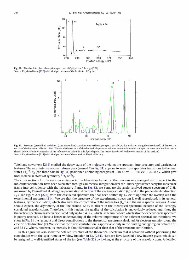
304 S. Taioli et al. / Physics Reports 493 (2010) 237–319
Fig. 30. The absolute photoabsorption spectrum of C2H2 at the C 1s edge [222].Source: Reprinted from [222] with kind permission of the Institute of Physics.
10203040Binding Energy (eV)
4
8
12
Inte
nsity
(ar
bitr
ary
units
) A
C
B
DE
Fig. 31. Resonant (green line) and direct (continuous line) contributions to the Auger spectrum of C2H2 for emission along the direction (x) of the electricvector of the incident radiation [214]. The detailed structure of the theoretical spectrum without convolutions with the spectrometer window function isshown below. (For interpretation of the references to colour in this figure legend, the reader is referred to the web version of this article.)Source: Reprinted from [214] with kind permission of the American Physical Society.
Taioli and coworkers [214] studied the decay state of the molecule dividing the spectrum into spectator and participatorfeatures. The most intense resonant Auger peak (named C in Fig. 31) appears to arise from spectator transitions to the finalstates 1π−2u 1πg (the three bars in Fig. 31) positioned at binding energies of −18.37 eV, −19.41 eV, −20.68 eV, which givefinal molecular states of symmetry 2Πg or 2Fg .The cross sections for the electron emission in the laboratory frame, i.e. the previous one averaged with respect to themolecular orientation, have been calculated through a numerical integration over the Euler angleswhich carry themolecularframe into coincidence with the laboratory frame. In Fig. 32, we compare the angle-resolved Auger spectrum of C2H2measured by Kivimäki et al. along the polarization direction of the exciting radiation (Ix) and in the perpendicular direction(Iy) (see Figure 2 of [222]) with the calculated spectrum that has been shifted by 1.2 eV to optimize the overlap with theexperimental spectrum [214]. We see that the structure of the experimental spectrum is well reproduced, in its generalfeatures, by the calculation, which also gives the correct ratio of the intensities (Ix/Iy) in the main spectral regions. As oneshould expect, the asymmetry of the line around 12 eV is absent in the theoretical spectrum, becuase of the stronglycorrelated wavefunctions. Therefore, in this region, the quality of the calculation is unavoidably reduced and, thus, thetheoretical spectrum has been calculated only up to'43 eV, which is the limit above which also the experimental spectrumis poorly resolved. To have a better understanding of the relative importance of the different spectral contributions, weshow in Fig. 31 the resonant and direct contributions to the theoretical spectrum calculated for electron emission along theelectric field direction (x). We see that the direct contribution is appreciable only in the binding energy region between 15and 35 eV, where, however, its intensity is about 50 times smaller than that of the resonant contribution.In this figure we also show the detailed structure of the theoretical spectrum that is obtained without performing the
convolution with the spectrometer window function in Eq. (284). Here we have labelled a few intense peaks which canbe assigned to well-identified states of the ion (see Table 22) by looking at the structure of the wavefunctions. A detailed
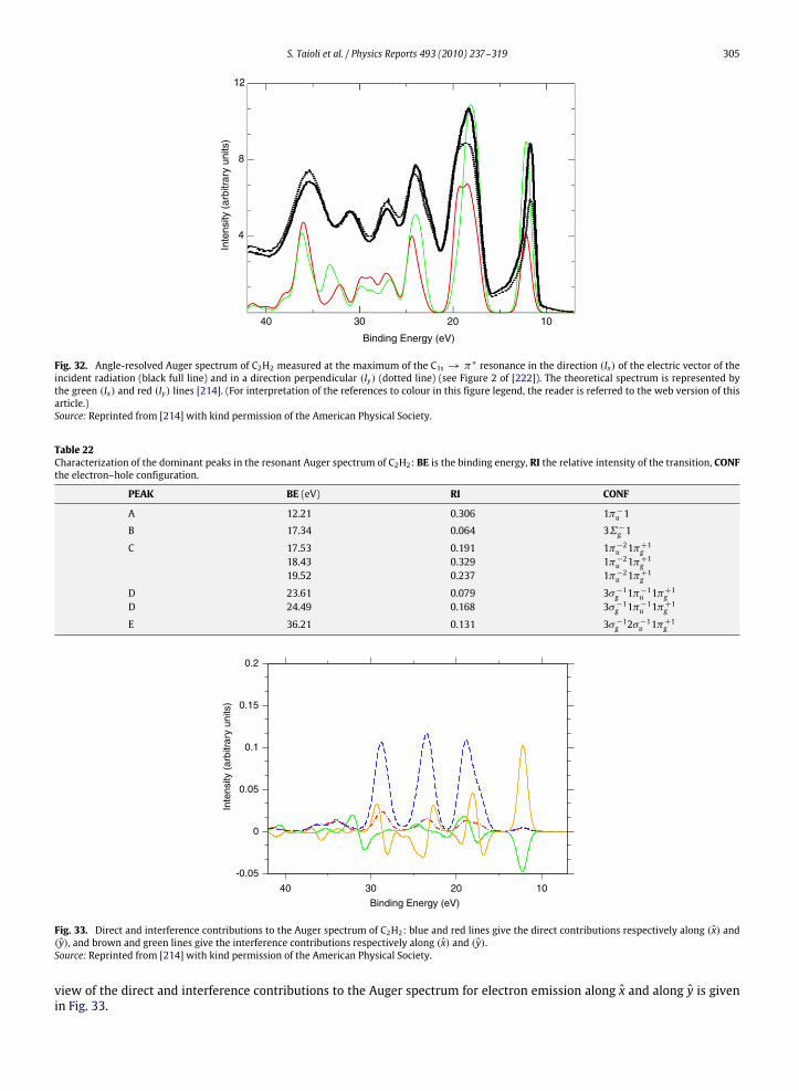
S. Taioli et al. / Physics Reports 493 (2010) 237–319 305
10203040
Binding Energy (eV)
4
8
12
Inte
nsity
(ar
bitr
ary
units
)
Fig. 32. Angle-resolved Auger spectrum of C2H2 measured at the maximum of the C1s → π∗ resonance in the direction (Ix) of the electric vector of theincident radiation (black full line) and in a direction perpendicular (Iy) (dotted line) (see Figure 2 of [222]). The theoretical spectrum is represented bythe green (Ix) and red (Iy) lines [214]. (For interpretation of the references to colour in this figure legend, the reader is referred to the web version of thisarticle.)Source: Reprinted from [214] with kind permission of the American Physical Society.
Table 22Characterization of the dominant peaks in the resonant Auger spectrum of C2H2: BE is the binding energy, RI the relative intensity of the transition, CONFthe electron–hole configuration.
PEAK BE (eV) RI CONF
A 12.21 0.306 1π−u 1
B 17.34 0.064 3Σ−g 1
C 17.53 0.191 1π−2u 1π+1g
18.43 0.329 1π−2u 1π+1g
19.52 0.237 1π−2u 1π+1g
D 23.61 0.079 3σ−1g 1π−1u 1π
+1g
D 24.49 0.168 3σ−1g 1π−1u 1π
+1g
E 36.21 0.131 3σ−1g 2σ−1u 1π
+1g
Binding Energy (eV)
Inte
nsity
(ar
bitr
ary
units
)
-0.05
0
0.05
0.1
0.15
0.2
10203040
Fig. 33. Direct and interference contributions to the Auger spectrum of C2H2: blue and red lines give the direct contributions respectively along (x) and(y), and brown and green lines give the interference contributions respectively along (x) and (y).Source: Reprinted from [214] with kind permission of the American Physical Society.
view of the direct and interference contributions to the Auger spectrum for electron emission along x and along y is givenin Fig. 33.
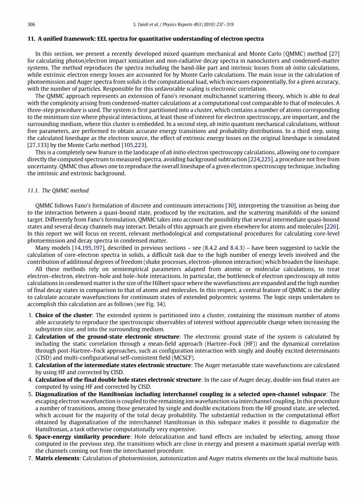
306 S. Taioli et al. / Physics Reports 493 (2010) 237–319
11. A unified framework: EEL spectra for quantitative understanding of electron spectra
In this section, we present a recently developed mixed quantum mechanical and Monte Carlo (QMMC) method [27]for calculating photon/electron impact ionization and non-radiative decay spectra in nanoclusters and condensed-mattersystems. The method reproduces the spectra including the band-like part and intrinsic losses from ab initio calculations,while extrinsic electron energy losses are accounted for by Monte Carlo calculations. The main issue in the calculation ofphotoemission and Auger spectra from solids is the computational load, which increases exponentially, for a given accuracy,with the number of particles. Responsible for this unfavorable scaling is electronic correlation.The QMMC approach represents an extension of Fano’s resonant multichannel scattering theory, which is able to deal
with the complexity arising from condensed-matter calculations at a computational cost comparable to that of molecules. Athree-step procedure is used. The system is first partitioned into a cluster, which contains a number of atoms correspondingto the minimum size where physical interactions, at least those of interest for electron spectroscopy, are important, and thesurrounding medium, where this cluster is embedded. In a second step, ab initio quantummechanical calculations, withoutfree parameters, are performed to obtain accurate energy transitions and probability distributions. In a third step, usingthe calculated lineshape as the electron source, the effect of extrinsic energy losses on the original lineshape is simulated[27,133] by the Monte Carlo method [105,223].This is a completely new feature in the landscape of ab initio electron spectroscopy calculations, allowing one to compare
directly the computed spectrum tomeasured spectra, avoiding background subtraction [224,225], a procedure not free fromuncertainty. QMMC thus allows one to reproduce the overall lineshape of a given electron spectroscopy technique, includingthe intrinsic and extrinsic background.
11.1. The QMMC method
QMMC follows Fano’s formulation of discrete and continuum interactions [30], interpreting the transition as being dueto the interaction between a quasi-bound state, produced by the excitation, and the scattering manifolds of the ionizedtarget. Differently from Fano’s formulation, QMMC takes into account the possibility that several intermediate quasi-boundstates and several decay channels may interact. Details of this approach are given elsewhere for atoms andmolecules [226].In this report we will focus on recent, relevant methodological and computational procedures for calculating core-levelphotoemission and decay spectra in condensed matter.Many models [14,195,197], described in previous sections – see (8.4.2 and 8.4.3) – have been suggested to tackle the
calculation of core-electron spectra in solids, a difficult task due to the high number of energy levels involved and thecontribution of additional degrees of freedom (shake processes, electron–phonon interaction) which broaden the lineshape.All these methods rely on semiempirical parameters adapted from atomic or molecular calculations, to treat
electron–electron, electron–hole and hole–hole interactions. In particular, the bottleneck of electron spectroscopy ab initiocalculations in condensedmatter is the size of theHilbert spacewhere thewavefunctions are expanded and the high numberof final decay states in comparison to that of atoms and molecules. In this respect, a central feature of QMMC is the abilityto calculate accurate wavefunctions for continuum states of extended polycentric systems. The logic steps undertaken toaccomplish this calculation are as follows (see Fig. 34).
1. Choice of the cluster: The extended system is partitioned into a cluster, containing the minimum number of atomsable accurately to reproduce the spectroscopic observables of interest without appreciable change when increasing thesubsystem size, and into the surrounding medium.
2. Calculation of the ground-state electronic structure: The electronic ground state of the system is calculated byincluding the static correlation through a mean-field approach (Hartree–Fock (HF)) and the dynamical correlationthrough post-Hartree–Fock approaches, such as configuration interaction with singly and doubly excited determinants(CISD) and multi-configurational self-consistent field (MCSCF).
3. Calculation of the intermediate states electronic structure: The Auger metastable state wavefunctions are calculatedby using HF and corrected by CISD.
4. Calculation of the final double hole states electronic structure: In the case of Auger decay, double-ion final states arecomputed by using HF and corrected by CISD.
5. Diagonalization of the Hamiltonian including interchannel coupling in a selected open-channel subspace: Theescaping electronwavefunction is coupled to the remaining ionwavefunction via interchannel coupling. In this procedurea number of transitions, among those generated by single and double excitations from the HF ground state, are selected,which account for the majority of the total decay probability. The substantial reduction in the computational effortobtained by diagonalization of the interchannel Hamiltonian in this subspace makes it possible to diagonalize theHamiltonian, a task otherwise computationally very expensive.
6. Space-energy similarity procedure: Hole delocalization and band effects are included by selecting, among thosecomputed in the previous step, the transitions which are close in energy and present a maximum spatial overlap withthe channels coming out from the interchannel procedure.
7. Matrix elements: Calculation of photoemission, autoionization and Auger matrix elements on the local multisite basis.
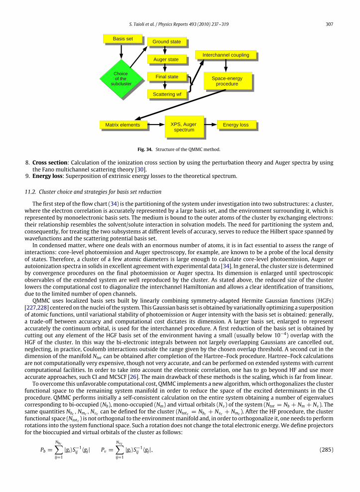
S. Taioli et al. / Physics Reports 493 (2010) 237–319 307
Fig. 34. Structure of the QMMC method.
8. Cross section: Calculation of the ionization cross section by using the perturbation theory and Auger spectra by usingthe Fano multichannel scattering theory [30].
9. Energy loss: Superposition of extrinsic energy losses to the theoretical spectrum.
11.2. Cluster choice and strategies for basis set reduction
The first step of the flow chart (34) is the partitioning of the system under investigation into two substructures: a cluster,where the electron correlation is accurately represented by a large basis set, and the environment surrounding it, which isrepresented by monoelectronic basis sets. The medium is bound to the outer atoms of the cluster by exchanging electrons:their relationship resembles the solvent/solute interaction in solvation models. The need for partitioning the system and,consequently, for treating the two subsystems at different levels of accuracy, serves to reduce the Hilbert space spanned bywavefunctions and the scattering potential basis set.In condensed matter, where one deals with an enormous number of atoms, it is in fact essential to assess the range of
interactions: core-level photoemission and Auger spectroscopy, for example, are known to be a probe of the local densityof states. Therefore, a cluster of a few atomic diameters is large enough to calculate core-level photoemission, Auger orautoionization spectra in solids in excellent agreementwith experimental data [34]. In general, the cluster size is determinedby convergence procedures on the final photoemission or Auger spectra. Its dimension is enlarged until spectroscopicobservables of the extended system are well reproduced by the cluster. As stated above, the reduced size of the clusterlowers the computational cost to diagonalize the interchannel Hamiltonian and allows a clear identification of transitions,due to the limited number of open channels.QMMC uses localized basis sets built by linearly combining symmetry-adapted Hermite Gaussian functions (HGFs)
[227,228] centered on the nuclei of the system. This Gaussian basis set is obtained by variationally optimizing a superpositionof atomic functions, until variational stability of photoemission or Auger intensity with the basis set is obtained: generally,a trade-off between accuracy and computational cost dictates its dimension. A larger basis set, enlarged to representaccurately the continuum orbital, is used for the interchannel procedure. A first reduction of the basis set is obtained bycutting out any element of the HGF basis set of the environment having a small (usually below 10−4) overlap with theHGF of the cluster. In this way the bi-electronic integrals between not largely overlapping Gaussians are cancelled out,neglecting, in practice, Coulomb interactions outside the range given by the chosen overlap threshold. A second cut in thedimension of the manifold Ntot can be obtained after completion of the Hartree–Fock procedure. Hartree–Fock calculationsare not computationally very expensive, though not very accurate, and can be performed on extended systems with currentcomputational facilities. In order to take into account the electronic correlation, one has to go beyond HF and use moreaccurate approaches, such CI and MCSCF [26]. The main drawback of these methods is the scaling, which is far from linear.To overcome this unfavorable computational cost, QMMC implements a new algorithm,which orthogonalizes the cluster
functional space to the remaining system manifold in order to reduce the space of the excited determinants in the CIprocedure. QMMC performs initially a self-consistent calculation on the entire system obtaining a number of eigenvaluescorresponding to bi-occupied (Nb), mono-occupied (Nm) and virtual orbitals (Nv) of the system (Ntot = Nb + Nm + Nv). Thesame quantities Nbc ,Nmc ,Nvc can be defined for the cluster (Ntotc = Nbc + Nvc + Nmc ). After the HF procedure, the clusterfunctional space (Ntotc ) is not orthogonal to the environmentmanifold and, in order to orthogonalize it, one needs to performrotations into the system functional space. Such a rotation does not change the total electronic energy. We define projectorsfor the bioccupied and virtual orbitals of the cluster as follows:
Pb =Nbc∑ij=1
|gi〉S−1ij 〈gj| Pv =Nvc∑ij=1
|gi〉S−1ij 〈gj|, (285)
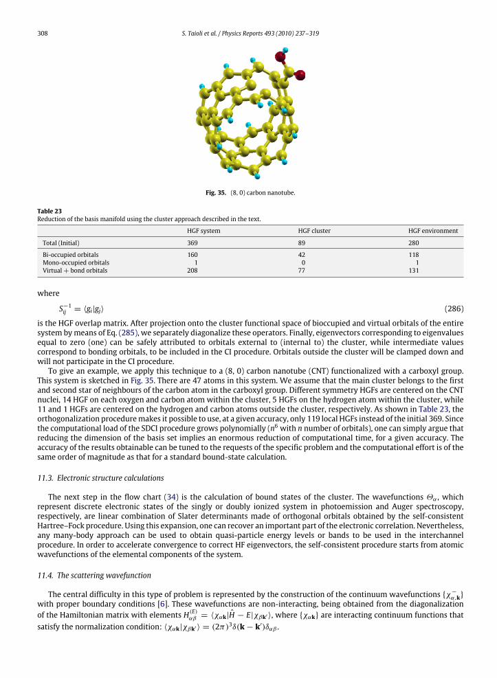
308 S. Taioli et al. / Physics Reports 493 (2010) 237–319
Fig. 35. (8, 0) carbon nanotube.
Table 23Reduction of the basis manifold using the cluster approach described in the text.
HGF system HGF cluster HGF environment
Total (Initial) 369 89 280
Bi-occupied orbitals 160 42 118Mono-occupied orbitals 1 0 1Virtual+ bond orbitals 208 77 131
where
S−1ij = 〈gi|gj〉 (286)
is the HGF overlap matrix. After projection onto the cluster functional space of bioccupied and virtual orbitals of the entiresystem bymeans of Eq. (285), we separately diagonalize these operators. Finally, eigenvectors corresponding to eigenvaluesequal to zero (one) can be safely attributed to orbitals external to (internal to) the cluster, while intermediate valuescorrespond to bonding orbitals, to be included in the CI procedure. Orbitals outside the cluster will be clamped down andwill not participate in the CI procedure.To give an example, we apply this technique to a (8, 0) carbon nanotube (CNT) functionalized with a carboxyl group.
This system is sketched in Fig. 35. There are 47 atoms in this system. We assume that the main cluster belongs to the firstand second star of neighbours of the carbon atom in the carboxyl group. Different symmetry HGFs are centered on the CNTnuclei, 14 HGF on each oxygen and carbon atom within the cluster, 5 HGFs on the hydrogen atom within the cluster, while11 and 1 HGFs are centered on the hydrogen and carbon atoms outside the cluster, respectively. As shown in Table 23, theorthogonalization proceduremakes it possible to use, at a given accuracy, only 119 local HGFs instead of the initial 369. Sincethe computational load of the SDCI procedure grows polynomially (n6 with n number of orbitals), one can simply argue thatreducing the dimension of the basis set implies an enormous reduction of computational time, for a given accuracy. Theaccuracy of the results obtainable can be tuned to the requests of the specific problem and the computational effort is of thesame order of magnitude as that for a standard bound-state calculation.
11.3. Electronic structure calculations
The next step in the flow chart (34) is the calculation of bound states of the cluster. The wavefunctions Θα , whichrepresent discrete electronic states of the singly or doubly ionized system in photoemission and Auger spectroscopy,respectively, are linear combination of Slater determinants made of orthogonal orbitals obtained by the self-consistentHartree–Fock procedure. Using this expansion, one can recover an important part of the electronic correlation. Nevertheless,any many-body approach can be used to obtain quasi-particle energy levels or bands to be used in the interchannelprocedure. In order to accelerate convergence to correct HF eigenvectors, the self-consistent procedure starts from atomicwavefunctions of the elemental components of the system.
11.4. The scattering wavefunction
The central difficulty in this type of problem is represented by the construction of the continuum wavefunctions χ−α,kwith proper boundary conditions [6]. These wavefunctions are non-interacting, being obtained from the diagonalizationof the Hamiltonian matrix with elements H(E)αβ = 〈χαk|H − E|χβk′〉, where χαk are interacting continuum functions thatsatisfy the normalization condition: 〈χαk|χβk′〉 = (2π)3δ(k− k′)δαβ .
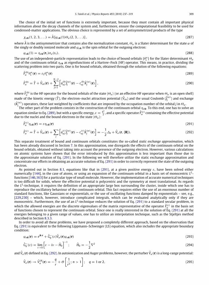
S. Taioli et al. / Physics Reports 493 (2010) 237–319 309
The choice of the initial set of functions is extremely important, because they must contain all important physicalinformation about the decay channels of the system and, furthermore, ensure the computational feasibility to be used forcondensed-matter applications. The obvious choice is represented by a set of antisymmetrized products of the type
χαk(1, 2, 3, . . .) = A [ϕαk(1)Θα(2, 3, . . .)] , (287)
where A is the antisymmetrizer that contains also the normalization constant,Θα is a Slater determinant for the state α ofthe singly or doubly ionized molecule and ϕαk is the spin orbital for the outgoing electron:
ϕαk(1) = ηαk(r1)σα(s1). (288)
The use of an independent-particle representation leads to the choice of bound orbitals θαL for the Slater determinantΘαand of the continuum orbital ηαk as eigenfunctions of a Hartree–Fock (HF) operator. This means, in practice, dividing thescattering problem into two parts. One is for bound orbitals, obtained through the solution of the following equations:
F (b)α θαL (r) = εLθαL (r) (289)
F (b)α = T + Ven(r)+N−2∑j=1
[a(b)αj J
(α)j (r)− c(b)αj K
(α)j (r)
], (290)
where F (b)α is the HF operator for the bound orbitals of the state |Θα〉 (or an effective HF operator whenΘα is an open shell)made of the kinetic energy (T ), the electron–nuclei attraction potential (Ven) and the usual Coulomb (J
(α)j ) and exchange
(K (α)j ) operators, these last weighted by coefficients that are imposed by the occupation number of the orbital j inΘα .The other part of the problem consists in the construction of the continuum orbital ηαk. To this end, one has to solve an
equation similar to Eq. (289), butwith a specific energy, ε = k22 , and a specific operator F
(c)α containing the effective potential
due to the nuclei and the bound electrons in the state |Θα〉:
F (c)α ηαk(r) = εηαk(r) (291)
F (c)α = T + Ven(r)+∑j
[a(c)αj J
(α)j (r)− c(c)αj K
(α)j (r)
]= −
12∆r + Vα(r, R). (292)
This separate treatment of bound and continuum orbitals constitutes the so-called static exchange approximation, whichhas been already discussed in Section 7. In this approximation, one disregards the effects of the continuum orbital on thebound orbitals, obtained without taking into account the presence of the outgoing electron. However, various calculationson atomic systems have shown that the error introduced by this approximation is less important than those due tothe approximate solution of Eq. (291). In the following we will therefore utilize the static exchange approximation andconcentrate our efforts in obtaining an accurate solution of Eq. (291) in order to correctly represent the state of the outgoingelectron.As pointed out in Section 8.1, equations like that in (291), at a given positive energy ε, have been solved either
numerically [144], in the case of atoms, or using an expansion of the continuum orbital in a basis set of monocentric L2-functions [146,163] for a particular type of small molecule. However, the implementation of accurate numerical techniquesis too difficult for solids, where the effective potential is polycentric and the symmetry at most translational. As regardsthe L2-technique, it requires the definition of an appropriate large box surrounding the cluster, inside which one has toreproduce the oscillatory behaviour of the continuum orbital. This fact requires either the use of an enormous number ofstandard functions, like Gaussians or exponentials, or the use of oscillating functions damped by exponentials – see, e.g.,[229,230] – which, however, introduce complicated integrals, which can be evaluated analytically only if they aremonocentric. Furthermore, the use of an L2-technique reduces the solution of Eq. (291) to a standard secular problem, inwhich the allowed energies are the discrete eigenvalues of the matrix representative of the operator F (c)α in the basis setof functions chosen to represent the continuum orbital. Since one is really interested in the solution of Eq. (291) at all theenergies belonging to a given range of values, one has to utilize an interpolation technique, such as the Stjeltjes methoddescribed in Section 8.3.3.In order to avoid all these problems, we have proposed a completely different approach, based on the observation that
Eq. (291) is equivalent to the following Lippmann–Schwinger (LS) equation, which also includes the appropriate boundarycondition:
ϕαk(r) = eik·r + G−0 (ε)Vα(r)ϕαk(r) (293)
G−0 (ε) = limν→0
[ε − iν − H0
]−1; H0 = −
12∇2 (294)
and Vα(r) defined in Eq. (292). In autoionization and Auger problems, however, the perturber Vα(r) is a long-range potential:
Vα(r)→ V LRα (r) = −qr+ O
[1rn; n > 1
]; q = 1 or 2, (295)

310 S. Taioli et al. / Physics Reports 493 (2010) 237–319
with a tail represented by a Coulomb potential plus higher-order corrections that depend on the type of system considered.The presence of this long-range potential forces one to include at least the Coulomb and static dipole components of thepotential in the zero-order Hamiltonian (H0), a fact that is very difficult to be implemented in a condensed-matter context.Whatwe have suggested, instead, [27,226], is the approximate representation of Vα in Eq. (291) bymeans of its expansion
(V tα) into a finite set of L2 functions |λ〉 as follows:
Vα ∼ V tα =∑λµντ
|λ〉S−1λµ 〈µ|Vα|ν〉S−1ντ 〈τ | (296)
Sλµ = 〈λ|µ〉. (297)
The elements of this basis set are chosen to minimize the difference (Vα − V tα)|ηαk〉 inside the region of interest. Thereplacement (Vα → V tα) allows one to solve the LS equation (293) as follows:
ηαk(r) = eik·r + G−0 (ε)Tα(ε)eik·r, (298)
where Tα is the transition operator defined by the equation
Tα = V tα + VtαG−
0 (ε)Tα. (299)The corresponding matrix equation, defined in the space spanned by the basis set |λ〉, gives
Tα = Vtα1
Vtα − VtαG−
0 (ε)VtαVtα. (300)
It follows that one can write ηαk in the form
ηαk = eik·r +∑λ
cλ(k, ε)fλ(ε, r), (301)
with
cλ =∑µ,ν,τ
S−1λµ 〈µ|Tα(ε)|ν〉S−1ντ 〈τ |k〉 (302)
fλ(ε, r) = G−0 (ε)|λ〉. (303)In practice, a general expression of the continuum functions fλ is obtained by applying the free-particle Green function toHermite Gaussian functions of any order and centre (see [231]).A striking difference, in this regard, between our approach and those used by all the above cited authors (and further
extensions of their work) [14,195,197] lies in the computation of the many-body Green function. According to our method,the many-body Green function is projected onto ‘localized’ states, which are a ‘local mixture’ of atomic states. Thus,differently frompreviousworks, ourmethodusesmulticentered local projectors thatmay includemany atomic space points;in other words, the role of themulticentered projectors is somehow similar to that played by localizedWannier functions insolid-state calculations [173],where a Fourier transformed set of planewaves brings to a complete basis set centered in somespace points selected on the basis of some criteria, such as minimal localization. The crucial point, in this type of approach,is the replacement (V tα → Vα), which seems particularly delicate, involving, as it does, truncation of the long-range part ofthe HF potential.To treat the long-range behaviour of the screened Coulomb potential, our method splits the scattering problem into
two separate regions: a problem for large distances, where analytical hydrogenic-like solutions are available, and a morechallenging problem for small distances, where the interaction of the electron with the remaining system is not negligible.However, we do not solve the asymptotic scattering problem using an ‘R-matrix like’ [232] procedure. In this method,according to an idea developed by Wigner for nuclear interactions, the orbital obtained through numerical solution of theinternal region problem can be matched with the analytically known asymptotic expression of the external region and itsderivative, once the best matching point has been determined. Our procedure rather utilizes two ‘Heaviside potentials’based on the idea that it is sufficient to have a projected potential V tα which, applied to ηαk, correctly reproduces the effectof the true potential Vα continuing into at least a part of the asymptotic region, i.e. where Vα(r) ' V LRα (r). V
tα is bi-electronic
within the interaction region and zero outside. This fact ensures, on the one hand, the correct form of the orbital insidethe molecular volume, i.e. where Vα(r) 6= V LRα (r), which is the important region for calculating the matrix elements thatcouple bound and continuum states. On the other hand, in the regionwhere
[Vα(r)− V LRα (r)
]ηαk(r) ' 0, one can represent
the LS orbital as a linear combination of eigenfunctions of the long-range potential at energy ε. This asymptotic potential iszerowithin the scattering region and built withmono-electronic integrals in the outer region. Furthermore, differently fromcommon R-matrix approaches using the configuration space, our working platform is a Hilbert space, where the functionaldivision in bound and scattering space maps the division in real ordinary space. This functional mapping allows either toenlarge ‘on the fly’ the internal region, fixed a priori in theR-matrix approach, by simply increasing the basis set, or to describemore accurately the scattering potential by simply using mono-electronic integrals, computationally less expensive.
S. Taioli et al. / Physics Reports 493 (2010) 237–319 311
11.5. On the use of projected potentials in scattering theory
Let us consider the case of an N-electron system with one electron in the continuum. We use the following electronicHamiltonian:
H(1, . . . ,N) =N∑i=1
[T (i)+ V enπ (i)] +12
N∑i6=j
vπ (i, j) (304)
T (i) = −12∇2i ; V enπ (i) = π(i)V
en(i)π(i) (305)
vπ (i, j) = π(i)π(j)v(i, j)π(i)π(j) (306)
π(i) =m∑l=1
|gl(i)〉〈gl(i)|, (307)
where π is the identity operator of one m-dimensional space (G) of L2(R3)-functions, spanned by the orthonormal set|gl〉; l = 1, . . . ,m. We use π to project both V en(i) = −
∑µ
Zµ|ri−Rµ|
, i.e. the electron–nuclei attraction potential, and
v(i, j) = 1|ri−rj|
, i.e. the electron–electron repulsion operator, obtaining the model Hamiltonian of Eq. (304) on which ourtheory is based.The reasons for using such a representation of the potential, which necessarily can be appropriate only inside a finite
volume, have been explained in Section 11.4, and will be more clear in this section by looking at the drastic simplificationthat can be obtained by exploiting the properties of this Hamiltonian type.We look for the eigenfunctions of Hamiltonian (304) only inside the Hilbert space spanned by a set of functions χαk
which represent the interacting decay channels of the problem built as in Eq. (287). The continuum and discrete orbitalssatisfy the relationships
〈Θα|HN−1|Θβ〉 = Eαδαβ (308)
〈ϕαk(j)|Θβ(1, . . . , j, . . . ,N − 1)〉j = 0; ∀ α, β, j, k (309)
〈ηk|ηp〉 = (2π)3δ(k− p). (310)
As one can see from Eq. (308), |Θα〉 are solutions of the secular problem for the (N − 1)-electron system that are obtainedinside the space spanned by the Slater determinants. These last are built up in terms of orbitals taken from a set of n boundorbitals |θj〉 which belong to the space G. Furthermore, the continuum orbitals |ηk〉 that have to satisfy Eq. (309) can beobtained as eigenfunctions of the kinetic energy operator T , orthogonal to the bound orbitals |θj〉. This means that theyare solutions of the eigenvalue equation
Tq|ηk〉 =k2
2|ηk〉; 〈ηk|ηp〉 = (2π)3δ(k− p), ∀ k, p (311)
Tq = (1− P)T (1− P) = T + VPK ; P =n∑j
|θj〉〈θj|, (312)
where VPK = −P T − T P+ P T P is an effective potential, due to the orthogonality constraints, which has the typical structureof a Phillips–Kleimann potential [233].Note that another possible way of constructing a set of bound and continuum orbitals that are mutually orthogonal and
appropriate to represent the decay channels is through the solution of HF equations with an effective operator, as explainedin Section 11.4. In this section, instead, we define the continuum orbitals |ηk〉 as the eigenfunctions of Tq, obtained throughthe solution of Eq. (311), a procedure that is equivalent to the other one as long as one utilizes all the degree of freedom ofthe chosen Hilbert spaces.By using the previous definitions, one gets the following expression for the matrix element that couples two interacting
channels:
〈χαk|HN |χβp〉 = (2π)3δ(k− p)δαβ(k2
2+ Eα
)+ 〈ϕαk|V enπ δαβ + W
αβπ |ϕβp〉, (313)
where
Wαβπ (1) =
N∑j=2
〈Θα(2, . . . , j, . . . ,N)|vπ (1, j)(1− P1,j)|Θβ(2, . . . , j, . . . ,N)〉, (314)

312 S. Taioli et al. / Physics Reports 493 (2010) 237–319
and P1,j is the operator that interchanges the (1, j) variables. If now we assume that the bound-state problem has beensolved, i.e. the eigenvectors (|Θ1〉, |Θ2〉, . . . , |ΘM〉) of HN−1 have been found inside the space of the Slater determinantsbuilt up using the θj orbitals, we can look at the matrix elements defined in Eq. (313) as the representation of an effectiveone-particle Hamiltonian over a set of basis vectors |ϕαk〉 = |ηk〉|α〉.This Hamiltonian, indeed, is that of a particle, with internal degrees of freedom, which moves in an effective potential
depending on the internal states |α〉 of the particle itself. Therefore, the N-particle problem can be reduced to an effectivesingle-particle problem, in which the scattering states can be obtained from the resolution of a Lippmann–Schwingerequation with the proper boundary condition. The basis vectors |ϕαk〉 are thus labelled by two indices, one continuous (k)and one discrete (α), and satisfy orthonormality constraints bothwith respect tok – see Eq. (310) – and toα, i.e. 〈α|β〉 = δαβ .By adopting this point of view, we see that our N-electron problem is reduced to the determination of the stationary
states of the one-particle Hamiltonian:
h(r, s) = h0(r, s)+ V (r, s); h0(r, s) = Tq(r)+ O(s). (315)
In this operatorwe have separated an unperturbed Hamiltonian h0 and a coupling operator V . The unperturbed Hamiltonianconsists of the kinetic energy term, defined in Eq. (312), plus the operator O for the internal degrees of freedomof the particle.The scattering stationary states of h0, characterized asymptotically by the wavevector k, are, at a given energy E,
h0|ϕkα(E)〉 = E |ϕkα(E)〉; |ϕkα(E)〉 = |ηk〉|α〉; E = Eα +k2
2(316)
Tq|ηk〉 =k2
2|ηk〉; O|α〉 = Eα|α〉. (317)
Furthermore, h0 has a finite set of independent discrete eigenstates, represented by vectors |ϕjα〉 = |θj〉|α〉; j =1, . . . , n; α = 1, . . . ,M, with eigenvalues Eα, each n-time degenerate. This follows from the fact that the operatorTq has a finite number of independent discrete eigenstates |θj〉; j = 1, . . . , n with eigenvalues equal to zero and a set ofscattering states |ηk〉 with continuum eigenvalues greater or equal to zero. No other independent eigenstates of Tq exist,as one can easily prove by looking at the structure of the Phillips–Kleimann potential.In what follows, we will consider only the Hilbert space H0(E) spanned by the scattering states of h0 at energy E. This
space is the tensorial product of two Hilbert spaces: one spanned by the scattering states of Tq and the other (O) spannedby theM independent eigenstates of O.Using the definition of V (see Eq. (313)), we observe that this operator couples the eigenstates of h0 through the matrix
elements:
V α,β(k, p) = 〈ϕαk|V |ϕβp〉 = 〈ϕαk|[V enπ δαβ + W
αβπ
]|ϕβp〉. (318)
The evaluation of these quantities requires the knowledge of the components of the continuum orbitals |ηk〉 only insidethe spaceG that has π as its identity operator. Therefore, we can represent the scattering potential bymeans of the followingstructure of projected potential:
V =M∑α,β
m∑i,j
|gi〉|α〉Vα,β
ij 〈β|〈gj|, (319)
where |gj〉 and |α〉 are orthonormal basis sets respectively for the finite spaces G andO, while the matrix elements V α,βij ,in accordance with Eqs. (313), (314) and (318), are defined as
V α,βij = 〈gi|[V enπ δαβ + W
αβπ
]|gj〉. (320)
The problem is now to find the scattering stationary states of h at energy E, starting from the knowledge of the continuumeigenstates of h0, at the same energy, defined by Eqs. (316) and (317). The standard procedure is to solve the followingeigenvalue equation under specific boundary conditions that, in a typical electron spectroscopy problem, are incoming (-)wave boundary conditions:
h |χ−αk(E)〉 = E |χ−
αk(E)〉. (321)
One can, equivalently, transform Eq. (321) into a Lippmann–Schwinger equation [28]:
|χ−αk(E)〉 = |ϕαk(E)〉 + G−
0 (E)V |χ−
αk(E)〉, (322)
where
G−0 (E) = limε→0[E − iε − h0]−1 =
P
E − h0+ iπδ(E − h0) (323)
S. Taioli et al. / Physics Reports 493 (2010) 237–319 313
and P is the Cauchy principal value. The formal solutions of Eq. (323) can be expressed in terms of the wave operators (Ω−)– see Eq. (1) – [28]:
|χ−αk(E)〉 = Ω−(E) |ϕαk(E)〉 (324)
Ω−(E) = [1+ G−(E)V ] = [1− G−0 (E)V ]−1, (325)
where G−(E), which is defined as in Eq. (323) with h0 replaced by h, is related to G−0 (E) by
G−(E) = G−0 (E)+ G−(E)V G−0 (E). (326)
We observe that, according to Eqs. (324) and (325) and to the structure of V , the correction to any given free-particlestate |ϕαk(E)〉 is represented by a linear combination of continuum functions: G−(E)|fjα〉, where |fjα〉 = |gj〉|α〉 is anorthonormal set of basis vectors for the space F = G
⊗O. Note that the identity operator in this space is Π = π ⊗ Io,
where Io =∑M
α |α〉〈α| is the identity of the space O and π that of the space G.By looking at the structure of the stationary state defined in Eq. (324), we see that each eigenvector |χ−αk〉 contains a linear
combination of elements of the type δ(E − h)|fjα〉 that are continuum eigenstates of h at energy E, as can be easily provedby noticing that the density of states can be written as
δ(E − h) =i2π[G+(E)− G−(E)]. (327)
The spectral analysis of this Hamiltonian shows that the subspace of the degenerate scattering eigenstates significant forthe physical problem is finite and isomorphous to the subspace of the functions used for representing the potential energyoperator. This fact allows a relevant reduction in the computational efforts required by the application of this approach.
11.6. Evaluation of spectroscopic quantities
The main theoretical feature characterizing core-electron spectroscopies is the interaction between metastable states,produced in the initial excitation process, and the continuum states of resonant affected scattering processes. We consideronly a discrete isolated intermediate state |Φj〉 and several continuum decay channels |Ψ−αε〉 that are characterized byincoming wave boundary conditions. In the time-independent picture, one can recognize that these processes are governedby matrix elements Mjα(ε, E) that couple discrete (|Φj〉) and continuum (|Ψ−αε〉) states:
Mjα(ε, E) = 〈Φj|H − E|Ψ−αε〉. (328)
In a similar way, if one is interested in evaluating photoionization cross sections, the quantities to be considered are thematrix elements of the transition operator between bound and continuum states.In order to interpret the main results of spectroscopies in which one or few electrons are ejected in the continuum, one
has to evaluate matrix elements that require the knowledge of the components of the continuum orbital only inside a finitespace of L2(R3)-functions. If this space is a subspace of that used to represent the scattering potential, one can exploit theresults of Section 11.5 and work efficiently using only a finite number of independent L2(R3)-functions.Let us give a specific example taken from the theory developed for autoionization and Auger processes. By looking at the
definition of the total decay rate (Γ ) and using Eq. (328), one can write
Γ = 2π∑α
∫δ(ε − Erα)〈Φj|H − E|Ψ−αε〉dε〈Ψ
−
αε |H − E|Φj〉
= 2π〈Φj|(H − E)δ(Er − HQ )(H − E)|Φj〉 (329)
∆ = P∑α
∫〈Φj|(H − E)|Ψ−αε〉
dε(Erα − ε)
〈Ψ−αε |H − E|Φj〉
= 〈Φj|(H − E)P1
(Er − HQ )(H − E)|Φj〉, (330)
where Er is the resonance energy, Erα = Er − Eα and HQ is the Hamiltonian of the system projected into the space of thescattering eigenstates of H .We point out the following two considerations.
1. The total decay rate (Γ ) and energy shift (∆) are mean values, taken over the bound state (H − E)|Φj〉, respectively, ofthe imaginary and real part of G−(Er) of HQ .
2. The many-electron integrals 〈Φj|(H − Er)|Ψ−αε〉, which characterize Eqs. (329) and (330), can be reduced to linearcombinations of overlap integrals such as 〈f |χ−αk(ε)〉, where |f 〉 belongs to the finite spaceF , and |χ−αk(ε)〉 is a scatteringeigenstate of the effective Hamiltonian h(r, s) defined in Eq. (315). Therefore, the calculation of total decay rate and
314 S. Taioli et al. / Physics Reports 493 (2010) 237–319
energy shift simply requires the knowledge of the matrix representation, in the space F , of the resolvent of h. This factallows to avoid the explicit integration over ε in Eqs. (329) and (330).
Analytic expressions have been derived for the cross section of photoemission, Auger and autoionizing transitions – seeEqs. (162) and (165) – and for the lineshapes of the corresponding spectra, studied as functions of the kinetic energy of theemitted electron and of the photon energy of the incident radiation. Particular attention has to be paid to the analysis of thedependence of these lineshapes on the specific features of the incident radiation and the electron spectrometer.
11.7. Multisite correlation, ‘space-energy’ similarity procedure in Auger calculations and scaling issues
The interpretation of electron spectra requires a computational method that is able accurately to represent the electroniccorrelation among bound electrons in the intermediate states of the system and the interaction between bound and escapingelectrons, represented by the projected scattering potential Vα(r). In order to accomplish this goal, one needs an efficientab initio procedure to account for multisite electron–electron, electron–hole and hole–hole interactions in applications ofcondensed matter, where the number of open transitions is enormous. The diagonalization of the interchannel interaction,including hole delocalization on valence bands and electronic excitations, is computed by using a so-called space-energysimilarity procedure [27], in which the Hamiltonian is ‘block diagonalized at each energy’. In this respect, the reductionof the system to a cluster of atoms embedded in the surrounding medium is not sufficient to lower the prohibitivecomputational cost of diagonalizing the interchannel Hamiltonian in the Hilbert space spanned by the vectorial sum ofbound and continuum basis sets.To include these effects, Taioli and coworkers [27] have generalized the use of the projectedpotentials by defining amodel
Hamiltonian inwhich final valence–valence hole states are first localized on the atomwhere the initial core hole is found andmultisite interactions enter naturally in this Hamiltonian as a perturbation. This idea stems from the quasi-atomic natureof core-level photoemission and Auger transitions, which forces the holes to remain on the atomwhere the initial core holeis created. Therefore, one can avoid the direct diagonalization of the large Hamiltonian found in solid-state applications ofmultichannel scattering, by selecting among the open channels a number of localized states, which account for the majorityof the total decay probability. The dimension of this multichannel space, where the model Hamiltonian is first diagonalized,is a trade-off between the computational load and the ability accurately to reproduce transition energies and intensities; thisdimension can be further increased if the interchannel procedure does not recover important parts of the correlation energy.As a result of the diagonalization of the interchannel Hamiltonian, one obtains a number of non-interacting channels, eachof which can be overlapped with configurations close in energy generated by perturbing the reference state with electronicexcitations. Among these transitions, only those presenting a maximum overlap with the selected localized channels willbe considered: this analysis recovers additional parts of the correlation energy and mimics the effect of hole delocalization(or ‘band effects’) away from the localized states. This technique makes it possible to construct the continuum orbital in theeffective field of the bound orbitals including interchannel coupling to recover the band-like part of the spectra, due to theinteraction among an enormous number of channels.Transition matrix elements are fixed during space-energy similarity steps to the values obtained after the interchannel
procedure and the square modulus of the overlap enters as a multiplicative factor in the lineshape analysis. Such analysis,which is the core of ourmethod, significantly reduces the computational effort to calculate the core-level photoemission andnon-radiative decay in large systems.With regard to scaling performances, the calculation cost of the interchannel procedurescales as the third power of the number of channels, whereas thememory cost scales as the second power. Finally, symmetrymay be used to further reduce the computational scaling, particularly in the interchannel procedure.
11.8. Energy loss
To complete the theoretical description of electron emission mechanisms from nanoclusters or solid targets, one has totake into account the energy losses suffered by electrons during their way out of the solid. This kinetic energy loss maybe due to single and multiple inelastic scattering or, if the coupling between plasmons and valence electrons is strong incomparison to the band width, to the interaction with collective excitations of the system. These losses affect the measuredlineshape and they should be deconvoluted from acquired spectra before comparing them to computed spectra. Proceduresto do this are discussed in Section 3.Alternatively to standard deconvolution procedures, one could simulate the effects of inelastic losses on the ‘original’
distribution by using the computed photoemission/Auger intensity distribution as a source of electrons which undergoinelastic processes. In this way one can avoid background subtraction by superimposing the inelastic energy loss to thephotoemission/non-radiative decay spectra and comparing the theoretical and acquired experimental spectra directly.A possible approach to account for the extrinsic loss is theMonte Carlomethod [234], as presented in Section 5. Assuming
that the theoretical lineshape is provided as input energy distribution and that the energy is lost in discrete collisions [96,105,223], one needs to calculate the elastic σel(E) and inelastic σinel(E) scattering cross sections, on which the overall accuracyof the Monte Carlo procedure relies. In the end, along with a full ab initio treatment of the hole–hole correlation (whichincludes intrinsic energy loss due to shake processes), extrinsic energy losses due to the interaction of the escaping electronwith the surrounding electronic clouds and to collective excitations of the system can be taken into account.
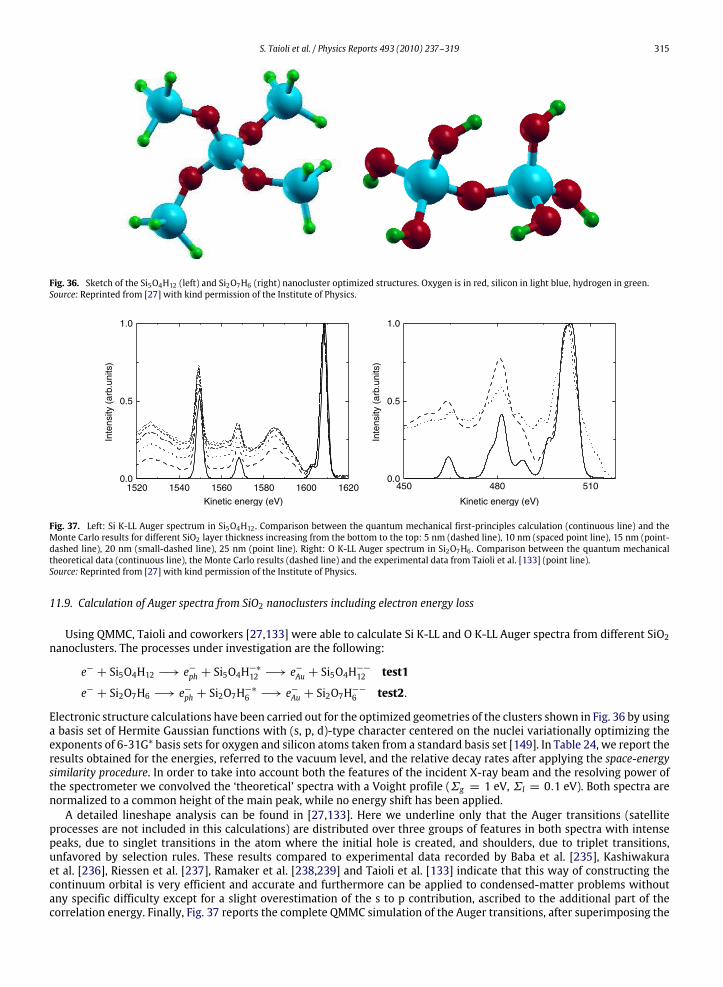
S. Taioli et al. / Physics Reports 493 (2010) 237–319 315
Fig. 36. Sketch of the Si5O4H12 (left) and Si2O7H6 (right) nanocluster optimized structures. Oxygen is in red, silicon in light blue, hydrogen in green.Source: Reprinted from [27] with kind permission of the Institute of Physics.
1.0
0.5
0.0
Inte
nsity
(ar
b.un
its)
1.0
0.5
0.0
Inte
nsity
(ar
b.un
its)
1520 1540 1560 1580 1600 1620
Kinetic energy (eV) Kinetic energy (eV)
450 480 510
Fig. 37. Left: Si K-LL Auger spectrum in Si5O4H12 . Comparison between the quantum mechanical first-principles calculation (continuous line) and theMonte Carlo results for different SiO2 layer thickness increasing from the bottom to the top: 5 nm (dashed line), 10 nm (spaced point line), 15 nm (point-dashed line), 20 nm (small-dashed line), 25 nm (point line). Right: O K-LL Auger spectrum in Si2O7H6 . Comparison between the quantum mechanicaltheoretical data (continuous line), the Monte Carlo results (dashed line) and the experimental data from Taioli et al. [133] (point line).Source: Reprinted from [27] with kind permission of the Institute of Physics.
11.9. Calculation of Auger spectra from SiO2 nanoclusters including electron energy loss
Using QMMC, Taioli and coworkers [27,133] were able to calculate Si K-LL and O K-LL Auger spectra from different SiO2nanoclusters. The processes under investigation are the following:
e− + Si5O4H12 −→ e−ph + Si5O4H−∗
12 −→ e−Au + Si5O4H−−
12 test1
e− + Si2O7H6 −→ e−ph + Si2O7H−∗
6 −→ e−Au + Si2O7H−−
6 test2.
Electronic structure calculations have been carried out for the optimized geometries of the clusters shown in Fig. 36 by usinga basis set of Hermite Gaussian functions with (s, p, d)-type character centered on the nuclei variationally optimizing theexponents of 6-31G* basis sets for oxygen and silicon atoms taken from a standard basis set [149]. In Table 24, we report theresults obtained for the energies, referred to the vacuum level, and the relative decay rates after applying the space-energysimilarity procedure. In order to take into account both the features of the incident X-ray beam and the resolving power ofthe spectrometer we convolved the ‘theoretical’ spectra with a Voight profile (Σg = 1 eV, Σl = 0.1 eV). Both spectra arenormalized to a common height of the main peak, while no energy shift has been applied.A detailed lineshape analysis can be found in [27,133]. Here we underline only that the Auger transitions (satellite
processes are not included in this calculations) are distributed over three groups of features in both spectra with intensepeaks, due to singlet transitions in the atom where the initial hole is created, and shoulders, due to triplet transitions,unfavored by selection rules. These results compared to experimental data recorded by Baba et al. [235], Kashiwakuraet al. [236], Riessen et al. [237], Ramaker et al. [238,239] and Taioli et al. [133] indicate that this way of constructing thecontinuum orbital is very efficient and accurate and furthermore can be applied to condensed-matter problems withoutany specific difficulty except for a slight overestimation of the s to p contribution, ascribed to the additional part of thecorrelation energy. Finally, Fig. 37 reports the complete QMMC simulation of the Auger transitions, after superimposing the
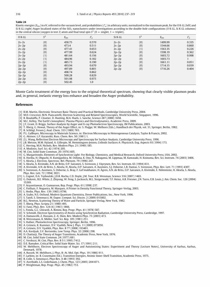
316 S. Taioli et al. / Physics Reports 493 (2010) 237–319
Table 24Kinetic energies (Ekin) in eV, referred to the vacuum level, and probabilities (Γα) in arbitrary units, normalized to themaximumpeak, for theOK-LL (left) andSi K-LL (right) Auger localized states of the SiO2 nanoclusters under investigations according to the double-hole configurations (O K-LL, Si K-LL columns)in the central silicon (oxygen in test 2) atom and final total spin S2 (0 = singlet, 1 = triplet).
O K-LL S2 Ekin Γα Si K-LL S2 Ekin Γα
2s–2s (0) 458.75 0.570 2s–2s (0) 1499.99 0.3352s–2p (0) 473.4 0.511 2s–2p (0) 1544.66 0.8602s–2p (0) 477.41 0.653 2s–2p (1) 1563.35 0.2262s–2p (0) 477.99 0.624 2p–2p (0) 1598.19 0.3622s–2p (1) 481.64 0.156 2p–2p (0) 1603.72 0.9982s–2p (1) 484.96 0.182 2p–2p (0) 1603.73 12s–2p (1) 485.73 0.190 2p–2p (0) 1661.11 0.0512p–2p (0) 493.94 0.670 2p–2p (0) 1714.15 0.0392p–2p (0) 497.89 0.801 2p–2p (0) 1716.26 0.4042p–2p (0) 498.74 0.8622p–2p (0) 500.28 0.8292p–2p (0) 501.98 0.9752p–2p (0) 502.45 1.0
Monte Carlo treatment of the energy loss to the original theoretical spectrum, showing that clearly visible plasmon peaksand, in general, inelastic energy loss enhance and broaden the Auger probability.
References
[1] R.M. Martin, Electronic Structure Basic Theory and Practical Methods, Cambridge University Press, 2004.[2] M.D. Crescenzi, M.N. Piancastelli, Electron Scattering and Related Spectroscopies, World Scientific, Singapore, 1996.[3] B. Boudaïffa, P. Cloutier, D. Hunting, M.A. Huels, L. Sanche, Science 287 (2000) 1658.[4] M.C. Kelley, The Earth’s Ionosphere: Plasma Physics and Electrodynamics, Academic Press, 2009.[5] J.T. Grant, D. Briggs, Surface Analysis by Auger and X-ray Photoelectron Spectroscopy, IM Publications, 2003.[6] T. Åberg, G. Howat, Theory of the Auger Effect, in: S. Flugge, W. Melhorn (Eds.), Handbuch der Physik, vol. 31, Springer, Berlin, 1982.[7] R. Schlögl, Fresen J. Anal. Chem. 333 (1989) 783.[8] P.L. GalBoyes, Microscopy in Materials Science, in: Electron Microscopy in Heterogeneous Catalysis, Taylor & Francis, 2002.[9] G. Akimov, L.P. Kazanskii, Russ. Chem. Rev. 50 (1981) 1.[10] Z.L. Wang, Reflection Electron Microscopy and Spectroscopy for Surface Analysis, Cambridge University Press, 1996.[11] J.B. Metson, M.M. Hyland, A. Gillespie, M. Hemmingsen-Jensen, Colloids Surfaces A: Physicoch. Eng. Aspects 93 (1994) 173.[12] C. Herring, M.H. Nichols, Rev. Modern Phys. 21 (1949) 185.[13] A. Modinos, Surf. Sci. 42 (1974) 205.[14] M. Cini, Solid State Commun. 20 (1976) 605.[15] G. Margaritondo, Elements of Synchrotron Light: For Biology, Chemistry, and Medical Research, Oxford University Press, USA, 2002.[16] K. Horiba, H. Ohguchi, H. Kumigashira, M. Oshima, K. Ono, N. Nakagawa, M. Lippmaa, M. Kawasaki, H. Koinuma, Rev. Sci. Instrum. 74 (2003) 3406.[17] S. Aksela, J. Electron. Spectrosc. Rel. Phenom. 79 (1996) 247.[18] S. Aksela, A. Kivimäki, A.N. de Brito, O.P. Sairanen, S. Svensson, J. Väyrynen, Rev. Sci. Instrum. 65 (1994) 831.[19] A. Kivimäki, A.N. de Brito, S. Aksela, H. Aksela, O.P. Sairanen, A. Ausmees, S.J. Osborne, L.B. Dantas, S. Svennson, Phys. Rev. Lett. 71 (1993) 4307.[20] S. Svennson, A. Ausmees, S. Osborne, G. Bray, F. Gel’mukhanov, H. Ågren, A.N. de Brito, O.P. Sairanen, A. Kivimäki, E. Niômmiste, H. Aksela, S. Aksela,
Phys. Rev. Lett. 72 (1994) 3021.[21] L. Cognet, D.A. Tsyboulski, J.D.R. Rocha, C.D. Doyle, J.M. Tour, R.B. Weisman, Science 316 (2007) 1465.[22] G. Dukovic, B.E. White, Z. Zhiyong, W. Feng, S. Jockusch, M.L. Steigerwald, T.F. Heinz, A.R. Friesner, J.N. Turro, E.B. Louis, J. Am. Chem. Soc. 126 (2004)
15269.[23] F. Aryasetiawan, O. Gunnarson, Rep. Progr. Phys. 61 (1998) 237.[24] C. Fiolhais, F. Nogueira, M. Marques, A Primer in Density Functional Theory, Springer-Verlag, 2003.[25] L. Hedin, Phys. Rev. 139 (1965) A796.[26] A. Szabo, N.S. Ostlund, Modern Quantum Chemistry, Dover Publications, Inc., New York, 1996.[27] S. Taioli, S. Simonucci, M. Dapor, Comput. Sci. Discov. 2 (2009) 015002.[28] R.G. Newton, Scattering Theory of Wave and Particle, Springer Verlag, New York, 1982.[29] T. Åberg, Phys. Scripta 21 (1980) 495.[30] U. Fano, Phys. Rev. 124 (6) (1961) 1866.[31] L. Fonda, G.C. Ghirardi, A. Rimini, Rep. Progr. Phys. 41 (1978) 587.[32] V. Schmidt, Electron Spectrometry of Atoms using Synchrotron Radiation, Cambridge University Press, Cambridge, 1997.[33] A. Damascelli, Z. Hussain, Z.-X. Shen, Rev. Modern Phys. 75 (2003) 473.[34] R. Weissmann, K. Müller, Surf. Sci. Rep. 105 (1981) 251.[35] S. Hufner, Photoelectron Spectroscopy, Springer, Berlin, 1996.[36] A. Grüneis, K. Kummer, D.V. Vyalikh, New J. Phys. 11 (2009) 073050.[37] A. Grüneis, D.V. Vyalikh, Phys. Rev. B 77 (2008) 193401.[38] A.A. Kordyuk, S.V. Borisenko, Low Temp. Phys. 32 (2006) 298.[39] D. Chattarji, The Theory of Auger Transitions, Academic Press, New York, 1976.[40] M. Cini, Solid State Commun. 24 (1977) 681.[41] C. Verdozzi, M. Cini, Phys. Rev. B 51 (1995) 7412.[42] D.E. Ramaker, Critical Rev. Solid State Mater. Sci. 17 (1991) 211.[43] W. Mehlhorn, Electron Spectroscopy of Auger and Autoionizing States: Experiment and Theory (Lecture Notes), University of Aarhus, Aarhus,
Denmark, 1978.[44] A. Russek, W. Mehlhorn, J. Phys. B: At. Mol. Opt. Phys. 19 (1986) 911.[45] F. Larkins, in: B. Crasemann (Ed.), Transition Energies, Atomic Inner-Shell Transition, Academic Press, 1975.[46] R. Colle, S. Simonucci, Phys Rev. A 48 (1993) 392.[47] V. Averbukh, L.S. Cederbaum, J. Chem. Phys. 123 (2005) 2041071.[48] P. Weightman, Rep. Progr. Phys. 45 (1982) 753.

S. Taioli et al. / Physics Reports 493 (2010) 237–319 317
[49] G.G. Kleiman, Appl. Surf. Sci. 11/12 (1982) 730.[50] J.D. Jackson, Classical Electrodynamics, 3rd ed., Wiley, 1998.[51] G. Grosso, G.P. Parravicini, Solid State Physics, 2nd ed., Academic Press, 2003.[52] P. Auger, P. Ehrenfest, R. Maze, J. Daudin, R.A. Frèon, Rev. Modern Phys. 11 (1939) 288–291.[53] L. Meitner, Z. Phys. 17 (1923) 54.[54] G. Wentzel, Z. Phys. 43 (1927) 521.[55] W. Schattke, M.A.V. Hove, F.J.G. de Abajo, R.D. Muiño, N. Mannella, Overview of core and valence photoemission, in: Solid State Photoemission and
Related Methods: Theory and Experiment, Wiley-VCH, Berlin, 2003.[56] K. Siegbahn, Science 217 (1982) 111.[57] T.X. Carroll, J. Hahne, T.D. Thomas, L.J. Saethre, N. Berrah, J. Bozek, E. Kukk, Phys. Rev. A 61 (2000) 042503.[58] Y. Ueda, J. Phys. B: At. Mol. Opt. Phys. 36 (2003) R1.[59] H. Aksela, S. Aksela, Rad. Phys. Chem. 76 (2007) 370.[60] R.P. Saxon, R.K. Nesbet, C.J. Noble, Phys. Rev. A 39 (1988) 1156.[61] C.D. Caldwell, M.O. Krause, Phys. Rev. A 47 (1992) R759.[62] N. Correia, A. Flores-Riveros, H. Ågren, K. Helenelund, L. Asplund, U. Gelius, J. Chem. Phys. 83 (1985) 2035.[63] W.E. Moddeman, T.A. Carlson, M.O. Krause, B.P. Pullen, W. Bull, G.K. Schweitzer, J. Chem. Phys. 55 (1971) 2317.[64] H. Beutler, Z. Phys. 93 (1935) 177.[65] U. Fano, Nuovo Cimento 12 (1935) 156.[66] J. Hillier, R.F. Baker, J. Appl. Phys. 15 (1944) 663.[67] R.F. Egerton, Electron Energy-Loss Spectroscopy in the Electron Microscope, Plenum, New York, 1986.[68] J.C.H. Spence, Rep. Progr. Phys. 69 (2006) 725.[69] K. Suenaga, Y. Sato, Z. Liu, H. Kataura, T. Okazaki, K. Kimoto, H. Sawada, T. Sasaki, K. Omoto, T. Tomita, T. Kaneyama, Y. Kondo, Nat. Chem. 1 (2009)
415.[70] H. Ibach, Electron Spectroscopy for Surface Analysis, Springer, Berlin, Heidelberg, 1977.[71] M.P. Seah, I.S. Gilmore, S.J. Spencer, Surf. Interface Anal. 31 (2001) 778.[72] S. Tougaard, Surf. Interface Anal. 26 (1998) 249.[73] M.P. Seah, Surf. Sci. 420 (1999) 285.[74] D.E. Ramaker, Crit. Rev. Solid State 17 (1992) 211.[75] E.N. Sickafus, Phys. Rev. B 16 (1977) 1436.[76] E.N. Sickafus, Phys. Rev. B 16 (1977) 1448.[77] D.A. Shirley, Phys. Rev. B 5 (1972) 4709.[78] S. Tougaard, Phys. Rev. B 34 (1986) 6779.[79] M.P. Seah, I.S. Gilmore, S.J. Spencer, Surf. Sci. 461 (2000) 1.[80] M.P. Seah, Surf. Sci. 471 (2001) 185.[81] H.H. Madden, D.M. Zener, J.R. Noonan, Phys. Rev. B 17 (1978) 3074.[82] D.E. Ramaker, Appl. Surf. Sci. 21 (1985) 243.[83] W.S.M. Werner, I.S. Tilinin, M. Hayek, Phys. Rev. B 50 (1994) 4819.[84] A. Jablonski, F. Salvat, C.J. Powell, NIST Electron Elastic-Scattering Cross-SectionDatabase (SRD64), Version 3.1, USDepartment of Commerce, National
Institute of Standards and Technology, Gaithersburg, MD, 2003.[85] S.E. Schnatterly, Inelastic Electron Scattering Spectroscopy, in: Solid State Phys., vol. 34, Academic Press, New York, 1979, pp. 275–357.[86] H. Raether, Excitation of Plasmons and Interband Transitions by Electrons, Springer-Verlag, Berlin, 1982.[87] R.F. Egerton, Rep. Progr. Phys. 72 (2009) 016502.[88] H. Ibach, D.L. Mills, Electron Energy Loss Spectroscopy and Surface Vibrations, Academic Press, New York, 1982.[89] D.L. Mills, Phys. Rev. B 34 (1986) 6099.[90] F. Yubero, S. Tougaard, Phys. Rev. B 46 (1992) 2486.[91] C.J. Tung, Y. Chen, C.M. Kwei, T.L. Chou, Phys. Rev. B 49 (1994) 161684.[92] A. Cohen-Simonsen, F. Yubero, S. Tougaard, Phys. Rev. B 56 (1997) 1612.[93] W.S.W. Werner, W. Smekal, C. Tomastik, H. Störi, Surf. Sci. 486 (2001) L461.[94] W.S.W. Werner, Phys. Rev. B 74 (2006) 075421.[95] L. Calliari, M. Dapor, M. Filippi, Surf. Sci. 601 (2007) 2270.[96] M. Filippi, L. Calliari, M. Dapor, Phys. Rev. B 75 (2007) 125406.[97] M. Dapor, L. Calliari, M. Filippi, Nucl. Instrum. Methods Phys. Res. B 255 (2007).[98] F.J.G. de Abajo, arXiv:0903.1669v1.[99] C. Kramberger, et al., Phys. Rev. Lett. 100 (2008) 196803.[100] R.H. Ritchie, Phys. Rev. 106 (1957) 874.[101] R.H. Ritchie, A. Howie, Phil. Mag. 36 (1977) 463.[102] B. Henke, P. Lee, T. Tanaka, R.L. Shimabukuro, B. Fujikawa, At. Data Nucl. Data Tables 27 (1982) 1.[103] J.C. Ashley, J. Electron Spectrosc. Related Phenom. 46 (1988) 199.[104] A. Jablonski, F. Salvat, C.J. Powell, J. Phys. Chem. Ref. Data 33 (2004) 409.[105] M. Dapor, Electron-Beam Interactions with Solids: Applications of the Monte Carlo Method to Electron Scattering Problems, in: Springer Tracts in
Modern Physics, vol. 186, Springer, Berlin, 2003.[106] P. Sigmund, Particle Penetration and Radiation Effects. General Aspects and Stopping of Swift Point Charges, Springer-Verlag, Berlin, 2006.[107] S.-R. Lin, N. Sherman, J.K. Percus, Nucl. Phys. 45 (1963) 492.[108] P.J. Bunyan, J.L. Schonfelder, Proc. Phys. Soc. 85 (1965) 455.[109] H. Bichsel, Nucl. Instrum. Meth. B 52 (1990) 136.[110] B.L. Henke, E.M. Gullikson, J.C. Davis, At. Data Nucl. Data Tables 54 (1993) 181.[111] U. Buechner, J. Phys. C: Sol. State Phys. 8 (1975) 2781.[112] N. Balakrishnan, C. Kalyanaram, N. Sathyamurthy, Phys. Rep. 79 (1997) 280.[113] W. Domcke, Phys. Rep. 208 (1991) 97.[114] A.U. Hazi, A.E. Orel, T.N. Rescigno, Phys. Rev. Lett. 46 (1981) 918.[115] R. Colle, D. Embriaco, M. Massini, S. Simonucci, S. Taioli, Nuc. Inst. Meth. Phys. Res. B 213 (2004) 65.[116] K.C. Kulander, A.E. Orel, J. Chem. Phys. 94 (1990) 2571.[117] H. Feshbach, Ann. Phys. 5 (1958) 357.[118] S. Huzinaga, C. Arnau, Phys. Rev. A 1 (1970) 1285.[119] H. Silverstone, M. Yin, J. Chem. Phys. 49 (1968) 2026.[120] D.P. Craig, T. Thirunamachandran, Molecular Quantum Electro-dynamics, Academic Press, London, 1984.[121] A.F. Starace, Theory of Atomic Photoionization, in: W. Mehlhorn (Ed.), Handbuch der Physik, Springer, Berlin, 1980.[122] G. Howat, T. Åberg, O. Goscinski, J. Phys. B 11 (1978) 575.[123] T. Åberg, Phys. Scr. 41 (1992) 71.[124] R.K. Nesbet, Electron-Atom Scattering Theory, Plenum Press, New York, 1980.[125] G. Breit, E.P. Wigner, Phys. Rev. 49 (1936) 519.

318 S. Taioli et al. / Physics Reports 493 (2010) 237–319
[126] R. Colle, S. Simonucci, in: S.G. Pandalai (Ed.), Recent Research Developments in Quantum Chemistry, vol. 2, 2001, (Transworld Research Network).[127] G.C. Wick, Phys. Rev. 80 (1950) 268.[128] K.A. Brueckner, Phys. Rev. 97 (1955) 1353.[129] K.A. Brueckner, Phys. Rev. 100 (1955) 36.[130] H.A. Bethe, E.E. Salpeter, Phys. Rev. 84 (1951) 1232.[131] M. Cini, Topics and Methods in Condensed Matter Theory, Springer, Berlin, Heidelberg, 2007.[132] G. Fratesi, M.I. Trioni, G.P. Brivio, S.U.andE. Perfetto, M. Cini, Phys. Rev. B 78 (2008) 205111.[133] S. Taioli, S. Simonucci, L. Calliari, M. Filippi, M. Dapor, Phys. Rev. B 79 (2009) 085432.[134] B.V. Andryushechkin, G.M. Zhidomirov, K.N. Eltsov, Y.V. Hladchanka, A.A. Korlyukov, Phys. Rev. B 80 (2009) 125409.[135] C. Buth, K. Schafer, Phys. Rev. A 80 (2009) 033410.[136] A. Jablonski, F. Salvat, C.J. Powell, J. Appl. Phys. 106 (2009) 053706.[137] S. Urpelainen, A. Caló, L. Partanen, M. Huttula, S. Aksela, H. Aksela, S. Granroth, E. Kukk, Phys. Rev. A 79 (2009) 023201.[138] M. Huttula, L. Partanen, A. Mäkinen, T. Kantia, H. Aksela, S. Aksela, Phys. Rev. A 79 (2009) 023412.[139] F.D. Pieve, D. Sébilleau, S.D. Matteo, R. Gunnella, R. Gotter, A. Ruocco, G. Stefani, C.R. Natoli, Phys. Rev. B 78 (2008) 035122.[140] K. Jänkälä, S. Urpelainen, M. Huttula, S. Fritzsche, S. Heinäsmäki, S. Aksela, H. Aksela, Phys. Rev. A 77 (2008) 062504.[141] L. Kövér, M. Uda, I. Cserny, J. Tóth, J. Végh, D. Varga, K. Ogasawara, H. Adachi, J. Vac. Sci. Technol. 19 (2001) 1143.[142] K. Ueda, S. Tanaka, Y. Shimizu, Y. Muramatsu, H. Chiba, T. Hayaishi, M. Kitajima, H. Tanaka, Phys. Rev. Lett. 85 (2000) 3129.[143] R. McWeeny, B.T. Sutcliffe, Methods of Molecular QuantumMechanics, Academic Press, London, 1969.[144] H.P. Kelly, Phys. Rev. A 11 (1975) 556.[145] H. Körber, W. Mehlhorn, Z. Phys. 191 (1966) 217.[146] V. Carravetta, H. Ågren, Phys. Rev. A 35 (1987) 1022.[147] H. Ågren, S. Svensson, U. Wahlgren, Chem. Phys. Lett. 35 (1975) 336.[148] H. Siegbahn, L. Asplund, P. Kelfve, Chem. Phys. Lett. 35 (1975) 330.[149] C. Pisani, R. Dovesi, C. Roetti, Hartree–Fock ab-initio of crystalline systems, in: Lecture Notes in Chemistry, vol. 48, Spinger Verlag, Heidelberg, 1988.[150] R. Dovesi, B. Civalleri, V.R. Saunders, R. Orlando, Ab Initio Quantum Simulation in Solid State Chemistry, Reviews in Computational Chemistry,
John Wiley & Sons, Inc., 2005.[151] R.N. Euwema, D.L. Wilhite, G.T. Surratt, Phys. Rev. B 7 (1972) 818.[152] R.N. Euwema, G.G. Wepfer, G.T. Surratt, D.L. Wilhite, Phys. Rev. B 9 (1974) 5249.[153] C.M. Liegener, Chem. Phys. Lett. 90 (1982) 188.[154] H. Agren, A. Cesar, C. Liegener, Adv. Quantum Chem. 23 (1992) 1.[155] C.M. Liegener, Chem. Phys. 76 (1983) 397.[156] L.S. Cederbaum, P. Campos, F. Tarantelli, A. Sgamellotti, J. Chem. Phys. 95 (1991) 6634.[157] F. Kaspar, W. Domcke, L.S. Cederbaum, Chem. Phys. 44 (1979) 33.[158] W. Domcke, L.S. Cederbaum, Phys. Rev. A 16 (1977) 1465.[159] C.M. Liegener, Mol. Phys. 43 (1981) 1.[160] L.S. Cederbaum, G. Hohlneicher, S. Peyerimhoff, Chem. Phys. Lett. 11 (1971) 421.[161] L.S. Cederbaum, G. Hohlneicher, W. von Niessen, Mol. Phys. 26 (1973) 1405.[162] R.W. Shaw, T.D. Thomas, Phys. Rev. A 11 (1975) 1491.[163] K. Faegri Jr., H.P. Kelly, Phys. Rev. A 19 (1979) 1649.[164] W. Kohn, L.J. Sham, Phys. Rev. 140 (1965) A1133.[165] J.P. Perdew, K. Burke, M. Ernzerhof, Phys. Rev. Lett. 77 (1996) 3865.[166] W.G. Aulbur, L. Jönsson, J.W. Wilkins, Solid State Phys. 54 (2000) 1.[167] L.J. Sham, M. Schlüter, Phys. Rev. Lett. 51 (1983) 1888.[168] E. Runge, E. Gross, Phys. Rev. Lett. 52 (1984) 997.[169] G. Onida, L. Reining, A. Rubio, Rev. Modern Phys. 74 (2002) 601.[170] Y.W. Son, M.L. Cohen, S.G. Louie, Phys. Rev. Lett. 97 (2006) 216803.[171] H.N. Rojas, R.W. Godby, R.J. Needs, Phys. Rev. Lett. 74 (1995) 1827.[172] P. Umari, G. Stenuit, S. Baroni, Phys. Rev. B 79 (2009) 201104.[173] N. Marzari, D. Vanderbilt, Phys. Rev. B 56 (1997) 12847.[174] S. Taioli, P. Umari, M.M. De Souza, Phys. Status Solidi (b) 246 (2009) 2572.[175] F. Sottile, Ph.D. Thesis presented to École Polytechnique.[176] P. Lautenschlager, M. Garriga, L. Vina, M. Cardona, Phys. Rev. B 36 (1987) 4821.[177] D.L. Walters, C.P. Bhalla, Atomic Data 3 (1971) 302.[178] U. Gelius, S. Svensson, H. Siegbahn, E. Basilier, A. Faxalv, K. Siegbahn, Chem. Phys. Rev. Lett. 28 (1974) 1.[179] E.J. Callan, Phys. Rev. 124 (1961) 793.[180] J. Bruneau, J. Phys. B 20 (1987) 713.[181] D. Minelli, F. Tarantelli, A. Sgamellotti, L.S. Cederbaum, J. Electron Spectrosc. Related Phenom. 74 (1995) 1.[182] M. Ohno, J. Electron Spectrosc. Related Phenom. 143 (2005) 13.[183] E.J. McGuire, Phys. Rev. 185 (1969) 1.[184] H.P. Kelly, in: B. Crasemann (Ed.), Many-Body Perturbation Approaches to the Calculation of Transition Probabilities, Atomic Inner-Shell Transition,
Academic Press, New York, 1975.[185] O.M. Kvalheim, K. Faegri Jr., Chem. Phys. Lett. 67 (1979) 127.[186] M. Higashi, E. Hiroike, T. Nakajima, Chem. Phys. 68 (1982) 377.[187] M. Larsson, B.J. Olsson, P. Sigray, Chem. Phys. 139 (1989) 457.[188] J.E. Castle, D. Epler, Proc. R. Soc. Lond. 339 (1974) 49.[189] R. Colle, S. Simonucci, Chem. Phys. Lett. 102 (1983) 573.[190] U. Gelius, E. Basilier, S. Svenson, T. Bergmark, K. Siegbahn, J. Electron Spectrosc. Related Phenom. 2 (1974) 405.[191] K.J. Børve, L.J. Sæthre, T.D. Thomas, T.X. Carrol, N. Berrah, J.D. Bozek, E. Kukk, Phys. Rev. A 63 (2000) 012506.[192] B. Kempgens, H. Köppel, A. Kivimäki, M. Neeh, L.S. Cederbaum, A.M. Bradshaw, Phys. Rev. Lett. 79 (1997) 3617.[193] R. Colle, S. Simonucci, Deep Level Spectroscopy and Auger Spectra, in: Encyclopedia of Condensed Matter Physics, Elsevier, Amsterdam, 2005.[194] P. Langhoff, C. Corcoran, J.S. Sims, F. Weinhold, R.M. Glover, Phys. Rev. A 14 (1976) 1042.[195] G.A. Sawatzky, Phys. Rev. Lett. 39 (1977) 504.[196] C. Verdozzi, M. Cini, Phys. Rev. B 51 (1995) 7412.[197] J.J. Lander, Phys. Rev. 91 (1953) 1382.[198] C.J. Powell, Phys. Rev. Lett. 30 (1973) 1179.[199] M. Cini, Phys. Rev. B 17 (1978) 2788.[200] M. Cini, F. Maracci, R. Platania, J. Electron Spectrosc. Related Phenom. 41 (1986) 37.[201] H.H. Madden, D.M. Zehner, J.R. Noonan, Phys. Rev. B 17 (1978) 3074.[202] P. Weightmann, P.T. Andrews, J. Phys. C 12 (1979) 943.[203] P. Weightmann, P.T. Andrews, J. Phys. C 13 (1980) 3529.[204] D. Ramaker, J. Vac. Sci. Technol. A7 (1989) 1614.

S. Taioli et al. / Physics Reports 493 (2010) 237–319 319
[205] J.W. Rogers, J.J. Houston, R.R. Rye, F.L. Hutson, D.E. Ramaker, J. Vac. Sci. Technol. A4 (1986) 1601.[206] M. Cini, J. Phys. 1 (1989) SB55.[207] R. Colle, S. Simonucci, Phys. Rev. A 42 (1990) 3913.[208] M. Hotokka, H. Ågren, H. Aksela, S. Aksela, Phys. Rev. A 30 (1984) 1855.[209] S. Svensson, N. Martensson, E. Basilier, P.A. Malmqvist, U. Gelius, K. Siegbahn, Phys. Scr. 141 (14) (1976).[210] O. Goscinski, J. Müller, E. Poulain, H. Siegbahn, Chem. Phys. Lett. 55 (1978) 407.[211] G. Strinati, Phys. Rev. Lett. 49 (1982) 1519.[212] G. Strinati, Phys. Rev. B 29 (1984) 5718.[213] K.L. Kobayashi, H. Daimon, Y. Murata, Phys. Rev. Lett. 50 (1983) 1701.[214] R. Colle, D. Embriaco, M. Massini, S. Simonucci, S. Taioli, Phys. Rev. A 70 (2004) 042708.[215] D. Dill, J.L. Dehmer, J. Chem. Phys. 61 (1974) 692.[216] F. Heiser, J. Viefhaus, R. Hentges, K. Wieliczek, U. Becker, Phys. Rev. Lett. 79 (1997) 2435.[217] A. Landers, T. Weber, I. Ali, A. Cassimi, M. Hattass, O. Jagutzki, A. Nauert, T. Osipov, A. Staudte, M.H. Prior, H. Schmidt-Böcking, C.L. Cocke, R. Dörner,
Phys. Rev. Lett. 87 (2001) 013002.[218] O. Hemmers, F. Heiser, J. Eiben, R. Wehlitz, U. Becker, Phys. Rev. Lett. 71 (1993) 987.[219] R.F. Fink, M.N. Piancastelli, A.N. Grum-Grzhimailo, K. Ueda, J. Chem. Phys. 130 (2009) 014306.[220] S. Bonhoff, K. Bonhoff, K. Blum, J. Phys. B 32 (1999) 1139.[221] T. Weber, et al., Phys. Rev. Lett. 90 (2003) 153003.[222] A. Kivimäki, M. Neeb, B. Kempgens, H.M. Köppe, K. Maier, A.M. Bradshaw, J. Phys. B 30 (1997) 4279.[223] M. Dapor, Surf. Sci. 600 (2006) 4728.[224] D.A. Shirley, Phys. Rev. 55 (1972) 4709.[225] S. Tougaard, Surf. Sci. 139 (1984) 208.[226] R. Colle, S. Simonucci, Phys. Rev. A 39 (1989) 6247.[227] A. Golebiewski, J. Mrozek, Int. J. Quantum Chem. 7 (1973) 1021.[228] R. Colle, A. Fortunelli, S. Simonucci, Nuovo Cimento 9 (1987) 969.[229] I. Cacelli, R. Moccia, V. Carravetta, Chem. Phys. 90 (1984) 313.[230] I. Cacelli, V. Carravetta, A. Rizzo, R. Moccia, Phys. Rep. 205 (1991) 283.[231] R. Colle, S. Simonucci, Nuovo Cimento D 11 (1989) 1587.[232] L. Eisenbud, E.P. Wigner, Phys. Rev. 72 (1947) 29.[233] J.C. Phillips, L. Kleimann, Phys. Rev. 116 (1959) 287.[234] R. Shimizu, Z.J. Ding, Rep. Progr. Phys. 55 (1992) 487.[235] Y. Baba, K. Yamamoto, T.A. Sasaki, Surf. Sci. 307 (1994) 896.[236] T. Kashiwakura, H. Araib, N. Kozuka, K. Odagawa, T. Yokohama, A. Kamata, S. Nakai, J. Electron Spectrosc. Related Phenom. 7 (1996) 207.[237] G.A. van Riessen, S.M. Thurgate, D.E. Ramaker, J. Electron. Spectrosc. Relat. Phenom. 161 (2007) 150.[238] D.E. Ramaker, Phys. Rev. B 21 (1980) 4608.[239] D.E. Ramaker, J.S. Murday, N.H. Turner, G. Moore, M.G. Lagally, J. Houston, Phys. Rev. B 19 (1979) 5375.
Copyright © 2022 FDOKUMEN