Search for Elastic and Inelastic Dark Matter Interactions in ...
137
Search for Elastic and Inelastic Dark Matter Interactions in XENON1T and Light Detection for XENONnT Dissertation zur Erlangung der naturwissenschaſtlichen Doktorwürde (Dr. sc. nat.) vorgelegt der Mathematisch-naturwissenschaſtlichen Fakultät der Universität Zürich von Adam Michael Brown aus dem Vereinigten Königreich Promotionskommission Prof. Dr. Laura Baudis (Vorsitz) Prof. Dr. Ben Kilminster Dr. Michelle Galloway Zürich, 2020
-
Upload
khangminh22 -
Category
Documents
-
view
2 -
download
0
Transcript of Search for Elastic and Inelastic Dark Matter Interactions in ...

Search for Elastic and InelasticDark Matter Interactions in XENON1Tand Light Detection for XENONnT
Dissertation
zurErlangung der naturwissenschaftlichen Doktorwürde
(Dr. sc. nat.)
vorgelegt derMathematisch-naturwissenschaftlichen Fakultät
derUniversität Zürich
vonAdam Michael Brown
ausdem Vereinigten Königreich
Promotionskommission
Prof. Dr. Laura Baudis (Vorsitz)Prof. Dr. Ben KilminsterDr. Michelle Galloway
Zürich, 2020

Abstract
A wide range of astrophysical observations indicates that baryonic matter makes up only asmall fraction of the total matter in the Universe. The rest, called dark matter, is over fivetimes more abundant by mass, but its particle content is unknown. One of the most popularcandidates is the weakly interacting massive particle (WIMP).
XENON1T was a dark matter detector based on a dual-phase xenon time projection chamber(TPC), located in the Gran Sasso National Laboratory (LNGS). The first part of this thesisdescribes searches for WIMPs scattering in XENON1T, via both elastic and inelastic inter-actions. A correction for the spatial dependence of the area of charge signals is developed.Event selection criteria are also shown, in particular a selection based on the fraction of thecharge signal seen by the top PMT array. These corrections and criteria helped XENON1T seta world-leading upper limit on the cross-section of spin-independent elastic WIMP-nucleonscattering, reaching 4.1 × 10−47 cm2 for 30 GeV/c2 WIMPs.
During inelastic scattering, the target nucleus is excited. Here, we consider scattering off129Xe. The expected signal is a 39.6 keV photon from the nuclear de-excitation, detectedtogether with the nuclear recoil from the WIMP interaction. By searching for such signals,XENON1T also sets a world-leading upper limit on the cross-section of inelastic scattering,with a minimum of 3.3 × 10−39 cm2 for 130 GeV/c2 WIMPs.
The second part of this thesis focuses on the photomultiplier tubes (PMTs) for XENONnT,the successor to XENON1T, and their read-out. A total of 368 new PMTs were tested forXENONnT, in both liquid and gaseous xenon, to ensure their suitability for long-term, stableoperation. Of these, 105 were tested at the University of Zurich. Particular attention waspaid to signs of light emission and afterpulses.
Each PMT has a voltage divider, or base, to power it. The preparation and installation ofthese bases is presented, as well as the cabling need to connect them to the PMT powersupplies and read-out electronics. Two different kinds of cable are used: 30 AWG Kapton-insulated wire for high voltage supplies and PTFE-insulated RG196A/U coaxial cables forPMT signals. Custom-design connectors are used to connect three sections of each cable inorder to simplify their installation.
Finally, details of the preparation, installation and testing of the two PMT arrays are shown.These were assembled in a cleanroom at LNGS, where the PMT bases and cables were alsoattached. Every PMT was tested before installing the arrays in the TPC, which is now in itsfinal position inside the cryostat. The cryostat has already been filled with gaseous xenonand at the time of writing is being cooled down ready for liquid to be filled.
ii

Acknowledgements
There are a great many people I would like to thank, and without whom I would never havebeen here writing this thesis. Although not all of them are mentioned here by name, theircontributions are greatly appreciated.
Firstly, I would like to thank my supervisor, Prof. Laura Baudis. She gave me the chance todelve into the field of astroparticle physics by offering my a position in her group, and hasaccompanied and supported me throughout my time as a PhD student. That her office doorwas always open has not gone unnoticed.
I would also like to thank the other members of my PhD committee, Prof. Ben Kilminsterand Dr Michelle Galloway, who have kept up with and supported my work throughout.
I am lucky to have been a member of a wonderful group at the University of Zurich – thankyou all. I have found the atmosphere to be very friendly and collaborative and our regulardiscussions, whether about physics or not, were always a joy. I have spent quite some timein the Irchel Bar over the last four years, gathering inspiration and new ideas – thank youto Frédéric, Kevin and Roman who shared more time with me there than most. Thanks alsoto all the postdocs from the group who have supported me: Patricia, Shayne, Ale, Shingoand Alex. Chiara and Giovanni have shared many experiences with me, both in Zurich andLNGS. Finally, thanks to Yanina, who has been in the group since I joined. To all of you, ourfriendships are cherished and I’m sure you’ll hear from me again!
Many members of the physics department have always been ready to help, from the twoworkshops, the administrative team and the other research groups. I would like to mentionDaniel Florin of the electronics workshop in particular, whose work on the XENONnT basesand cabling was instrumental to the success of the experiment.
I would like to thank all members of the XENON collaboration for warmly welcoming me.I have enjoyed numerous meetings and spent quite some time at LNGS – to all those whowere there with me, thank you for the good times spent together (even with an earthquakeand a pandemic).
Thank you to my family for their never-ending support and encouragement, and for visitingme in Zurich many times. And finally, a special thanks to Charlie, for helping me constantlyover the past years, putting up with my frequent absences to LNGS, and enduring the manyhours of travel between Munich and Zurich.
iii

Preface
The work presented in this thesis was performed as part of an international collaboration,and thus not everything which I mention is my own work. In the following I give a shortsummary of my contribution to the work described in each chapter.
• Chapter 3, Elastic WIMP scattering: The search for elastic WIMP scattering was acollaborative effort performed by a large analysis group. Mymajor direct contributionswere the S2 (𝑥 , 𝑦)-dependent correction (section 3.1.2), the S2 area fraction top cut(section 3.2.1) and the mis-identified S1 83mKr cut (section 3.2.2).
• Chapter 4, Inelastic WIMP scattering: All the analysis described in the chapter oninelasticWIMP scattering ismy ownwork. Nevertheless, this workwas based onmanyother collaboration members’ contributions to understanding the detector response.
• Chapter 5, PMT testing: The PMT tests performed at the University of Zurich anddescribed here were performed by myself. I must give credit, however, to Y. Wei andJ. Wulf for their work on the MarmotX testing facility and introducing me to it, and toS. Kazama and G. Volta, who worked with me for several of the tests and collaboratedwith me on the analysis of test data.
• Chapter 6, XENONnT: I was responsible, with G. Volta, for the preparation of XEN-ONnT’s bases (section 6.2) and cables (section 6.3). I worked on the cold tests ofthe PMT array sector (section 6.4.1) as part of a group of several people, notablyS. Lindemann. I was involved throughout the assembly of the arrays (section 6.4.2),which was performed by a team comprising the XENON PMT working group andother members of the collaboration.
iv

Contents
1 Searching for dark matter 11.1 Astrophysical evidence . . . . . . . . . . . . . . . . . . . . . . . . . . . . . . 1
1.1.1 Galaxy clusters . . . . . . . . . . . . . . . . . . . . . . . . . . . . . . 11.1.2 Galaxies . . . . . . . . . . . . . . . . . . . . . . . . . . . . . . . . . . 21.1.3 Cosmological effects . . . . . . . . . . . . . . . . . . . . . . . . . . . 4
1.2 Particle candidates . . . . . . . . . . . . . . . . . . . . . . . . . . . . . . . . . 51.2.1 The Standard Model . . . . . . . . . . . . . . . . . . . . . . . . . . . 51.2.2 Weakly interacting massive particles . . . . . . . . . . . . . . . . . . 61.2.3 Beyond WIMPs . . . . . . . . . . . . . . . . . . . . . . . . . . . . . . 7
1.3 The hunt for dark matter . . . . . . . . . . . . . . . . . . . . . . . . . . . . . 71.4 Direct dark matter detection . . . . . . . . . . . . . . . . . . . . . . . . . . . 9
1.4.1 Elastic WIMP-nucleus scattering . . . . . . . . . . . . . . . . . . . . 91.4.2 Inelastic WIMP scattering . . . . . . . . . . . . . . . . . . . . . . . . 131.4.3 Annual modulation of direct dark matter signals . . . . . . . . . . . 141.4.4 Selected experimental efforts . . . . . . . . . . . . . . . . . . . . . . 14
2 Dark matter detection with liquid xenon 182.1 Xenon as a dark matter target . . . . . . . . . . . . . . . . . . . . . . . . . . 192.2 Signals from dual-phase noble element TPCs . . . . . . . . . . . . . . . . . . 212.3 S1 and S2 signal detection . . . . . . . . . . . . . . . . . . . . . . . . . . . . 242.4 Challenges for dual-phase xenon TPCs . . . . . . . . . . . . . . . . . . . . . 262.5 The XENON1T TPC . . . . . . . . . . . . . . . . . . . . . . . . . . . . . . . . 272.6 XENON1T: the rest . . . . . . . . . . . . . . . . . . . . . . . . . . . . . . . . 292.7 Calibrating XENON1T . . . . . . . . . . . . . . . . . . . . . . . . . . . . . . 31
3 Elastic WIMP scattering 343.1 Event corrections . . . . . . . . . . . . . . . . . . . . . . . . . . . . . . . . . 36
3.1.1 Overview of detector effects which need correcting . . . . . . . . . . 363.1.2 S2 (x, y)-dependent correction . . . . . . . . . . . . . . . . . . . . . . 37
3.2 Quality cuts . . . . . . . . . . . . . . . . . . . . . . . . . . . . . . . . . . . . 423.2.1 S2 area fraction top cut . . . . . . . . . . . . . . . . . . . . . . . . . . 433.2.2 Misidentified S1 83mKr cut . . . . . . . . . . . . . . . . . . . . . . . . 453.2.3 Overall cut performance . . . . . . . . . . . . . . . . . . . . . . . . . 46
3.3 Signal and background modelling . . . . . . . . . . . . . . . . . . . . . . . . 473.4 Results . . . . . . . . . . . . . . . . . . . . . . . . . . . . . . . . . . . . . . . 49
v

Contents
4 Inelastic WIMP scattering 534.1 Expected signal . . . . . . . . . . . . . . . . . . . . . . . . . . . . . . . . . . 55
4.1.1 Uncertainties in the signal model . . . . . . . . . . . . . . . . . . . . 574.2 Background modelling . . . . . . . . . . . . . . . . . . . . . . . . . . . . . . 574.3 Statistical interpretation . . . . . . . . . . . . . . . . . . . . . . . . . . . . . 62
4.3.1 Binning structure optimisation . . . . . . . . . . . . . . . . . . . . . 634.3.2 Systematic uncertainties . . . . . . . . . . . . . . . . . . . . . . . . . 64
4.4 Results . . . . . . . . . . . . . . . . . . . . . . . . . . . . . . . . . . . . . . . 68
5 PMT testing 725.1 Photomultiplier tubes . . . . . . . . . . . . . . . . . . . . . . . . . . . . . . . 73
5.1.1 Photocathode . . . . . . . . . . . . . . . . . . . . . . . . . . . . . . . 735.1.2 Dynode design . . . . . . . . . . . . . . . . . . . . . . . . . . . . . . 73
5.2 The MarmotX PMT evaluation facility . . . . . . . . . . . . . . . . . . . . . . 755.3 The XENONnT PMT testing campaign . . . . . . . . . . . . . . . . . . . . . 76
5.3.1 Light emission . . . . . . . . . . . . . . . . . . . . . . . . . . . . . . 775.3.2 Afterpulses . . . . . . . . . . . . . . . . . . . . . . . . . . . . . . . . 79
5.4 Summary . . . . . . . . . . . . . . . . . . . . . . . . . . . . . . . . . . . . . . 83
6 XENONnT 856.1 Overview of XENONnT upgrade . . . . . . . . . . . . . . . . . . . . . . . . . 85
6.1.1 The XENONnT TPC . . . . . . . . . . . . . . . . . . . . . . . . . . . 866.2 PMT Bases . . . . . . . . . . . . . . . . . . . . . . . . . . . . . . . . . . . . . 87
6.2.1 Production . . . . . . . . . . . . . . . . . . . . . . . . . . . . . . . . . 906.2.2 Cleaning . . . . . . . . . . . . . . . . . . . . . . . . . . . . . . . . . . 91
6.3 Cables . . . . . . . . . . . . . . . . . . . . . . . . . . . . . . . . . . . . . . . 946.3.1 Cabling scheme . . . . . . . . . . . . . . . . . . . . . . . . . . . . . . 946.3.2 Cable screening and procurement . . . . . . . . . . . . . . . . . . . . 976.3.3 Connectors . . . . . . . . . . . . . . . . . . . . . . . . . . . . . . . . 996.3.4 Cleaning and installation . . . . . . . . . . . . . . . . . . . . . . . . . 1026.3.5 Installation of cabling . . . . . . . . . . . . . . . . . . . . . . . . . . 104
6.4 PMT arrays . . . . . . . . . . . . . . . . . . . . . . . . . . . . . . . . . . . . . 1056.4.1 Cold test . . . . . . . . . . . . . . . . . . . . . . . . . . . . . . . . . . 1076.4.2 Assembling the arrays . . . . . . . . . . . . . . . . . . . . . . . . . . 109
6.5 First light in XENONnT . . . . . . . . . . . . . . . . . . . . . . . . . . . . . . 114
7 Concluding remarks 116
vi

Chapter 1
Searching for dark matter
It has now been almost a century that we have known that ‘normal’, luminous matter makesup only a small fraction of the total mass of the Universe. Indeed, we shall see that there isa huge variety of astrophysical and cosmological observations which can only be explainedby the existence of ‘dark matter’, which has remained invisible until now except through itsgravitational effects. Unsurprisingly, the quest to find out what this dark matter is and todetermine its properties continues to receive considerable interest and experimental effort.
It is in the context of this worldwide effort searching for darkmatter that this thesis is written.After a brief introduction to the topic we will explore the XENON1T experiment, built to dir-ectly detect darkmatter interactions in its liquid xenon target. Wewill talk about searches forsignatures of both elastic and inelastic scattering of dark matter using data collected duringthe ∼ 2 years that XENON1T was operational. Later we turn towards the future, XENONnT,concentrating on the testing and installation of its light detectors and their connections, andwe see that the first light signals have already been recorded by those detectors.
1.1 Astrophysical evidence
1.1.1 Galaxy clusters
Galaxy clusters have provided evidence for dark matter since the beginning: Fritz Zwickyfirst studied the Coma Cluster in 1933 [1]. He determined that there was not enough visiblematter to explain the velocity dispersion in the cluster, although he proposed a far higheramount of dark matter (400 times the visible mass) than is accepted today.
Nowadays, most studies compare the distribution of baryonic matter to the overall mass dis-tribution. Typically the baryonic matter distribution is determined using electromagnetictelescopes; usually this means detecting X-rays emitted from hot intracluster gas. The over-all mass distribution can either be inferred from the X-ray measurements themselves [2], ormeasured directly using weak gravitational lensing measurements [3]. A particularly visu-ally appealing example is ‘Pandora’s Cluster’, Abell 2744, seen in figure 1.1. This consistsof several clusters which are actively merging, resulting in gas being stripped away from
1

Chapter 1 Searching for dark matter
Figure 1.1: Pandora’s Cluster (Abell 2744), with the density of gas (observed using X-rays) in red and thedensity of mass as determined from gravitational lensing in blue. Credit: X-ray: NASA/CXC/ITA/INAF/J. Merten et al. Lensing: NASA/STScI; NAOJ/Subaru; ESO/VLT Optical: NASA/STScI/R. Dupke
the dark matter halos. Lensing measurements show that much of the mass is concentratedaround different regions than the gas (which dominates the baryonic matter) [4]. Furtherexamples include the well-known ‘Bullet Cluster’ [5], Abell 1689 [6] and Abell 520, dubbeda ‘cosmic train wreck’ due to its very messy and complicated structure [7, 8].
1.1.2 Galaxies
Rotation curves of galaxies provide some of the most intuitive evidence for the existenceof dark matter. Indeed, it was when looking at motion within the Milky Way that JacobusKapteyn proposed searching for dark matter via its effect on galactic rotation, although hedid not find any evidence at the time [9]. In 1932, Jan Oort reached a different conclusion andclaimed that the total density in the MilkyWay is 1.8 times the density of visible matter∗ [10].
Modern efforts tend to compare rotation curves, showing the rotational velocity of stars andgas in galaxies as a function of radius from their centre, to the distribution of their visiblematter. These curves are often much ‘flatter’ than expected, by which we mean that thevelocity is constant as a function of radius, evenwell outside the discs containingmost visiblematter. In the absence of a dark matter halo extending out further than the visible matter,
∗Oort claimed evidence for ‘dark matter’, by which he meant ‘nebulous’ or ‘meteoric’ baryonic matter ratherthan a new particle, being present in the galactic disc. Our modern understanding is a little different: thedark matter forms a halo and more recent measurements find no evidence for dark matter being present inthe disc itself [11].
2

Chapter 1 Searching for dark matter
Figure 1.2: Rotation curve of NGC 6503. The contributions from the galaxy’s gas (dotted line), disk (dashedline) and halo (dot-dashed line) are shown, as is their sum (solid line). Figure from [13].
we would instead expect this to fall proportional to 1/√𝑟 . A flat curve suggests a dark matterdensity proportional to 1/𝑟2 at large radii. Prominent examples of such works include astudy of the Andromeda Galaxy by Vera Rubin [12], who pioneered this technique, and [13],in which ten spiral galaxies are studied (see figure 1.2).
While a lot of interest is in the behaviour of galaxies at large radii, it can also be interestingto know the shape of a dark matter halo at the galactic centre. For this, studies of low sur-face brightness galaxies are useful; these are galaxies in which dark matter dominates at allradii. Most observations suggest a so-called core at the centre of the halo – an approximatelyconstant density below a certain radius – whereas simulations have tended to prefer a cusp,or sharp density peak. This tension is commonly known as the cusp-core problem. Recentwork has indicated possible solutions, either by including baryons in the simulations or bymodifying certain assumptions about dark matter (for example, allowing significant interac-tions of dark matter with itself). A fairly recent review of the cusp-core problem and variouspossible resolutions can be found in [14].
Attempts to explain galactic rotation curves without requiring dark matter have proposedmodifying gravity instead. Most popular is the theory of modified Newtonian dynamics(MOND) and relativistic extensions of it such as TeVeS [15]; see [16] for a review. How-ever, while MOND can do a reasonable job of explaining rotation curves for most galaxies,it struggles to deal with the cosmological observations described in the next section [17].Gravitational wave detectors have provided a new way to test such theories. Based on theevent GW170817, many theories have been ruled because they predict different speeds forelectromagnetic and gravitational radiation, contrary to observations [18]. Furthermore, agalaxy has recently been found which doesn’t seem to contain dark matter [19]. This is verydifficult to explain with modified gravity, whose effects should apply universally.
3

Chapter 1 Searching for dark matter
2 10 100 500 1000 1500 2000 2500Multipole `
0
1000
2000
3000
4000
5000
6000
DTT
`[µ
K2]
2 10 100 500 1000 1500 2000 2500Multipole `
−100
−50
0
50
100
DTE
`[µ
K2]
2 10 100 500 1000 1500 2000Multipole `
0.01
0.1
1
10
20
30
40
DEE
`[µ
K2]
101 102 103
Multipole L
0.0
0.5
1.0
1.5
[L(L
+1)]
2/(2π
)Cφφ
L[1
07µ
K2]
Figure 1.3: CMB temperature power spectrum as measured by Planck, with the best-fit model shown inblue. Figure from [22].
1.1.3 Cosmological effects
When talking about cosmological evidence for dark matter, most people immediately turn tothe cosmic microwave background (CMB). Once the Universe had cooled to around 3000 K,neutral atoms were able to form from what were previously free electrons and protons –this time is known by the name recombination. For the first time, light was able to propag-ate with only a small probability of scattering off electrons, and has been travelling almostuninterrupted ever since. Nowadays, we can still see this radiation, which was produced asan almost perfect black-body spectrum at the temperature of the Universe at that time. Dueto the expansion of the Universe, it has by now been redshifted to a temperature of around2.7 K, with wavelengths in the microwave region.
By looking at temperature anisotropies in the CMB, we can gain an insight into fluctuationsin the matter density at the time of recombination. Recent measurements of the CMB havebeen made with incredibly high precision. This makes a very effective quantitative test ofdark matter theories possible and places strong constraints, in particular on its density [20].
Such comparisons are generally made by looking at the power spectrum of temperature fluc-tuations, as seen in figure 1.3. From such data, it is possible to find the relic abundance, orpresent-day density, of the three components: baryonic matter, dark matter and dark en-ergy. The height of the third peak in the spectrum is particularly sensitive to the dark matterrelic abundance. Current observations, most recently obtained by the Planck Collaboration[21], are explained extremely well by a ΛCDM model, standing for Λ cold dark matter. TheΛ refers to dark energy; the cold indicates that the dark matter has non-relativistic speeds atthe time of decoupling.
With such a model, Planck finds that the dark matter relic density is Ωcℎ2 = 0.120 ± 0.001,5.4 times the density of baryonic matter. Here, Ωc is the dark matter density, as a fractionof the critical density, and ℎ is the reduced Hubble constant (that is, the Hubble constantdivided by 100 km s−1 Mpc−1).
4

Chapter 1 Searching for dark matter
1.2 Particle candidates
Given that the existence of darkmatter is almost universally accepted, research focuses on thequestion of what the dark matter is. There is a huge variety of possible theories containingparticles which could make up the dark matter in the Universe. However, some are morepopular than others because of their simplicity and/or because they simultaneously solveother existing problems with the Standard Model of particle physics.
1.2.1 The StandardModel
The Standard Model of particle physics, which was developed during the second half ofthe 20th century, describes all currently known particles and their interactions. It con-tains twelve elementary fermions, all with spin 1/2, which can be divided into four groups ofparticles with very similar properties. Within each group, the three particles differ only intheir mass; these are referred to as generations. The fermions of the Standard Model are thethree charged leptons: electron, muon and tau; their neutral partners: the three neutrinos;and six quarks: three up-like with charge +2/3 (up, charm and top) and three down-likewith charge −1/3 (down, strange and bottom). According to the Standard Model, all fermi-ons have mass except the neutrinos, which are massless. However, the discovery of neutrinooscillations around the turn of the millennium [23, 24] means we know now that at least twoof the three neutrinos are massive.
As well as the fermions, there are a set of spin 1 gauge bosons. These mediate the interactionsof the Standard Model: electromagnetism by the massless photon, the weak force by themassive 𝑊 and 𝑍 bosons, and the strong force by eight massless gluons. Finally, the spinzero Higgs boson is required to explain why some of the gauge bosons (the 𝑊 and 𝑍 ) havemass.
The Standard Model works extremely effectively at explaining particle physics observations.It correctly predicted the existence of the top quark, tau neutrino and Higgs boson, beforethey were discovered in 1995 [25], 2000 [26] and 2012 [27, 28], respectively. Predictions of thefine-structure constant, which describes the strength of electromagnetic interactions, agreewith astonishing precision (better than one part in a billion) with experimental values [29].
Despite its many successes, there are some outstanding issues that are as yet unexplained.As well the fact that no StandardModel particle can make up the dark matter in the Universe,two particular problems which are relevant to the discussion here are the hierarchy problemand the strong CP problem. The hierarchy problem concerns itself with why the mass of theHiggs boson is so small. Loop-level corrections are expected to contribute an amount to itsmass on the order of ΛUV, an unknown energy scale up to which the Standard Model is validand after which new physics exists. The only known cutoff for the Standard Model’s validityis at the Planck mass, 2.435 × 10¹⁸ GeV/c2, many orders of magnitude higher than the massof the Higgs boson, (125.18 ± 0.16) GeV/c2 [30]. To explain this difference, the various loop-level corrections would have to almost perfectly cancel out, although there is no reason why
5

Chapter 1 Searching for dark matter
they should.
The strong CP problem concerns the fact that although weak interactions are observed toviolate charge-conjugation parity (CP) symmetry, no such observation has been made forinteractions of the strong force. This is despite the fact that such CP violation is perfectlyallowed in the Standard Model. The amount of CP violation is controlled by a single angle,which could reasonably take any value over a range of 2𝜋 . Experimental results, such as lim-its on the electric dipole moment of a neutron [31], rule out strong CP violation at anythingmore than a very tiny level, requiring this angle to be extremely small. This is an thereforean example of a fine-tuning problem.
These problems and others are summarised concisely in [32], along with a discussion of theirrelevance for dark matter.
1.2.2 Weakly interactingmassive particles
The most obvious place to start when seeking a particle which could be dark matter is surelywhat we already know. Of Standard Model particles, only the neutrino has the requiredproperties: it is neutral, weakly interacting and stable. Unfortunately, neutrinos are simplytoo light to form a significant fraction of dark matter [33]. Neutrinos are also relativistic –they would form hot, rather than cold, dark matter.
Supersymmetry is a class of independently motivated theories, first conjectured as a wayto solve the hierarchy problem in the Standard Model. In general, supersymmetric theoriespropose a symmetry between integer-spin bosons and half-integer-spin fermions. Thesecontribute equal but opposite loop-level corrections to the Higgs mass, so that they cancelout exactly. In the simplest models, such as the minimal supersymmetric extension to theStandard Model (MSSM), the number of particles is doubled by introducing a supersymmetricpartner for each Standard Model particle. A conserved parity, known as 𝑅-parity, is alsointroduced, which implies that supersymmetric particles can only be created or destroyed inpairs. As a result, whatever is the lightest supersymmetric particle (LSP) must be stable: itcannot decay to a supersymmetric particle since it has too little mass, and cannot decay toa Standard Model particle due to 𝑅-parity. This particle would be an excellent dark-mattercandidate. One of themost popular is the lightest of the four neutralinos, a linear combinationof the superpartners of the 𝑊 0, B and two Higgs bosons. For more complete treatments ofsupersymmetry in the context of dark matter, see reviews such as [34].
Neutrinos, LSPs, and other candidate dark matter particles share many properties and asa group are referred to as weakly interacting massive particles (WIMPs) [33]. These havebecome the most popular class of dark matter candidate, with a large number of experi-ments dedicated to hunting for them. The WIMP mass, 𝑚𝜒 , should be between 𝒪(1GeV)and 𝒪(100TeV) [35].To be a viable candidate, a particular model must have a working ‘production mechanism’.In other words, the theory must be able to predict the dark matter density which we observe
6

Chapter 1 Searching for dark matter
today. For WIMPs, the mechanism is known as freeze-out. In a nutshell, this says that atsome point in the Universe’s past, all elementary particles were in thermal equilibrium withone another. As the Universe cooled and temperature, 𝑇 , dropped below the mass of theparticle (𝑘B𝑇 < 𝑚𝜒 𝑐2), WIMPs decoupled from other particles and began annihilating. Thiscontinued until the expansion of the Universe became greater than the annihilation rate, atwhich point annihilation stopped: freeze-out. For standard models, this happens when thetemperature of the Universe is roughly 𝑚𝜒/20 [36]. After freezing out, its density is onlyaffected by the continued expansion of the Universe.
The relic abundance is smaller the greater the annihilation cross-section is, and is oftenquoted as Ω𝜒ℎ2 = 3 × 10⁻²⁷ cm3s−1/⟨𝜎A𝑣⟩ [34, 37], where 𝜎A is the dark matter annihila-tion cross-section, 𝑣 is its velocity, and the average is over the velocity distribution. A newparticle which interacts at the scale of the weak force has more-or-less the right ⟨𝜎A𝑣⟩ to ex-plain the observed relic abundance. This coincidence is known as the WIMP miracle is oftentaken to justify WIMPs as being the most promising class of candidate for dark matter.
1.2.3 BeyondWIMPs
WIMPs are only one of many possible dark matter candidates. One further example is the ax-ion, a natural consequence of Peccei and Quinn’s solution to the strong CP problem [38–40].Although the axion as proposed by them has been ruled out experimentally, other modelsremain possible [41]. Considering alternative production methods (other than freeze-out,described above) leads to more classes of dark matter candidates. For example, superweaklyinteracting massive particles (superWIMPs), could be produced if WIMPs which freeze outin the early Universe later decay into lighter particles [42]. Freeze-in is a proposal wherebydark matter interacts far more weakly than standard WIMPs, such that it is only slowly pro-duced in the hot early Universe and never reaches equilibrium [43]. We will not go intodetails of these or other models here, and the remainder of this work focuses on the searchfor WIMPs. The interested reader is referred to reviews such as [33] for more.
1.3 The hunt for darkmatter
A large number of experiments are ‘searching for’, or trying to ‘detect’ dark matter. Theseterms are somewhat loosely defined – have we not ‘found’ dark matter in that we knowwhere it is with a reasonable precision? The term usually means attempting to discovernon-gravitational interactions which would make it possible to identify the particles thatconstitute dark matter and their properties. Note that such interactions must exist if thedark matter was in thermal equilibrium in the early Universe. It is common to divide darkmatter experiments into three classes: direct detection, indirect detection, and production.In discussing these three, we focus primarily on WIMPs.
Direct detection refers to the observation of signals resulting from dark matter interactionsin a particle detector. Since we assume that the Milky Way is inside a dark matter halo,
7

Chapter 1 Searching for dark matter
dark matter particles should continuously be passing through the Earth. If we wait longenough and they are able to interact in some way other than just gravitationally, then one (orhopefully several) of them will eventually scatter in any target we construct. An observationof such scattering would be considered a direct detection of dark matter. The problem is thatdark matter, by its nature, interacts only very rarely with normal matter, so we expect onlyoccasional scattering. This means direct detection experiments must strive to minimise anybackgrounds that could look like dark matter and disguise a signal, and, where possible, tofind ways of distinguishing interactions of dark matter from those of ordinary particles.
The alternative way to ‘see’ dark matter is known as indirect detection. In practice, thismeans searching for the products of dark matter annihilation in the Universe. The obviousplace to look is where there is a lot of dark matter, since the annihilation rate should in-crease with the square of the dark matter density. This usually means looking at the centreof galaxies, where the dark matter halo is presumably densest, and by far the easiest galaxyto use is the Milky Way. An excess of WIMPs could also be expected at the centre of largeastronomical objects, where they could be captured by a combination of the object’s gravit-ational field and repeated energy loss due to scattering [44]. Experimentally, signatures ofdark-matter annihilation can either be spatial or spectral excesses. Some experiments de-tect gamma-rays, either directly (for example the space-based Fermi-LAT [45]), or from theshowers they produce when passing through the atmosphere (for example HESS [46, 47]and the up-coming Cherenkov Telescope Array (CTA) [48]). Others search for neutrinos,examples include Super-Kamiokande [49] and IceCube [50, 51]. Recent reviews of indirectsearches for dark matter can be found in [52] and [53].
When talking about production, we normally mean at particle colliders such as the LargeHadron Collider (LHC). In general the signature of dark matter being produced would besome missing energy, since the dark matter particle is extremely unlikely to then interactwith the detector. Attempting to probe the nature of dark matter using colliders carriessome severe challenges. Probably one of the most significant is that even if a new particle isdiscovered in this way, it is difficult to prove that it is the same type which naturally occursin the Universe – it may not even be stable. Furthermore, there are a large number of possibledark matter models and collider searches are inherently very model-dependent, looking fora specific signature present in a tiny fraction of events. It can be difficult to know where tolook, and indeed a vast number of searches have been performed at the LHC (a review can befound in [54]). Direct detection experiments tend to be more sensitive to spin-independentscattering, while the two approaches have comparable sensitivity to spin-dependent inter-actions. For heavier WIMPs, with TeV-scale masses or higher, current colliders run out ofenergy and direct detection experiments dominate. On the other hand, lighter WIMPs, withmasses below a few GeV, would deposit less energy in direct detection experiments’ tar-gets and therefore be difficult to detect, but could still be produced in colliders. The twoapproaches are therefore somewhat complementary in terms of their strengths.
8

Chapter 1 Searching for dark matter
1.4 Direct darkmatter detection
The final section of this chapter lays some of the groundwork needed for the remainder of thisthesis. Before talking about specific experiments, we will briefly cover some of the theoryunderpinning direct dark matter searches. The results of this section only concern WIMPs.While we try to remain general, at times we do specifically concentrate on scattering off axenon target, where it helps provide concreteness.
When trying to detect dark matter, it is possible to either look for its interactions with atomicnuclei or with the electrons around them. Since it carries no electric charge, we can generallyexpect scattering off the much more massive nuclei to be the most sensitive. However, due tokinematic considerations, this is only true for sufficiently heavy WIMPs. For masses lowerthan around 1 GeV/c2, the average nuclear recoil energy is too small to be detected, but amuch larger, detectable energy would be expected for electronic recoils [55]. Here we focuson the nuclear scattering of GeV to TeV scale WIMPs, to which experiments like XENON1Thave the most sensitivity.
1.4.1 Elastic WIMP-nucleus scattering
In general, the total rate of WIMP-nucleus scattering can be written as
𝑅 = 𝑁𝑛⟨𝑣𝜎⟩ (1.1)
where 𝑁 is the number of atoms in the target, 𝑛 is the number density of WIMPs aroundEarth, and 𝑣𝜎 is the product of the speed relative to the detector and cross-section of WIMPinteractions, averaged over the distribution of WIMP velocities.
In most experiments the energy imparted on the recoiling nucleus, 𝐸R, can be measured. Weare therefore interested not only in the total rate, but in the differential rate as a function ofenergy recoil:
d𝑅d𝐸R
= 𝜌0𝑚𝜒𝑚𝑁 ∫|v|
d𝜎d𝐸R
𝑓 (v) d3v, (1.2)
where 𝑚𝜒 is the mass of the WIMP, 𝑚𝑁 is the mass of the nucleus and v is the WIMP’sincident velocity.
A standard set of dark-matter-related astrophysical parameters are generally assumed tobe valid for the purpose of publishing experimental results, known as the standard halomodel [33, 56]. This makes it easier to compare results between experiments, since theseparameters are common to all experiments and affect their constraints in essentially thesame way. Dark matter in the Milky Way is thus assumed to have a flat rotation curve, ordensity 𝜌 ∝ 𝑟−2, and a local density (in the Solar System) of 𝜌0 = 0.3GeV cm−3. Dark matterparticles are further assumed to have a Maxwell-Boltzmann velocity distribution character-ised by its most probable speed 𝓋0 = 220 km s−1, but with a cutoff at the escape velocity of
9

Chapter 1 Searching for dark matter
0 100 200 300 400 500 600 700
Speed[km s−1
]0.000
0.001
0.002
0.003
0.004
PD
F[ km
−1
s]
Galacticframe
Earthframe
Figure 1.4: Distribution of WIMP speeds according to the standard halo model, in both the Galactic andlocal frame. The vertical orange dot-dashed line indicates the minimum impact speed neededto obtain a recoil of 7 keV (roughly the detection threshold in XENON1T [57]), and the greendotted line shows the minimum impact speed required for an inelastic recoil to be possible (with129Xe as the target nucleus). Both cases are for a 100 GeV/c2 WIMP.
the Milky Way, 𝓋esc = 544 km s−1:
𝑓 (v) ∝ exp (− v2
𝓋20) if |v| < 𝓋esc
0 if |v| ≥ 𝓋esc
(1.3)
We must also take into account the velocity of the detector, which is orbiting in the MilkyWay along with the rest of the Earth. Taking the Sun’s orbit to be circular with a speed of220 km s−1, we get to the WIMP impact speed distribution shown in figure 1.4. This intro-duces an anisotropy in the velocity distribution (although most detectors do not measure thedirection).
The standard halo model has significant attractions, notably its simplicity and widespreaduse. However, the precision of modern measurements has massively improved our under-standing of the local dark matter halo. The Gaia satellite is a space telescope primarily de-signed to measure the position and motion of stars in the Milky Way [58]. Perhaps one ofthe most significant discoveries is of a second, anisotropic component to the halo, likely theresult of the accretion of a large dwarf galaxy around 10 billion years ago [59]. Analysisof a combined dataset from the Sloan Digital Sky Survey and the second Gaia data releasesuggests there are significantly fewer dark matter particles in the high-speed tail of the dis-tribution, above about 550 km s−1 [60]. Analysis of Gaia data also provides a handle on thelocal dark matter density, which has been estimated at (0.61 ± 0.38) GeV cm−3 [61]. In [62]an updated standard halo model is proposed, with a local density of (0.55 ± 0.17) GeV cm−3
amongst other changes.
10

Chapter 1 Searching for dark matter
Non-relativistic kinematics gives the recoil energy as a function of WIMP velocity and scat-tering angle [63]:
𝐸R = 𝜇2𝓋2𝑚𝑁
(1 − cos 𝜃), (1.4)
in which 𝜇 is the reduced mass of the WIMP and nucleus, 𝜃 is the angle which the WIMP isscattered through, and 𝓋 = |v|. From this we can see that the maximum recoil energy, when𝜃 = 180°, is 𝐸max(𝑣) = 2𝜇2𝓋2/𝑚𝑁 .
Experiments usually consider two ways for dark matter to interact with nuclei: either spin-independently (SI) and spin-dependently (SD). The scattering cross-section is therefore thesum of these two, and we can write it as
d𝜎d𝐸R
= 𝑚𝑁2𝓋2𝜇2 (𝜎SI𝐹
2SI(𝐸R) + 𝜎SD𝐹 2SD(𝐸R)) , (1.5)
where the 𝜎s are the scattering cross-sections for each mode and the 𝐹(𝐸R) are the nuclearform factors, contributing to the energy dependence. We will discuss these components inturn, for both modes of interaction.
In the spin-independent case, dark matter interacts with all 𝑍 protons and (𝐴 − 𝑍) neutronspresent in the nucleus in the same way, regardless of their spin state. We can then write thetotal cross section in terms of the couplings to protons and neutrons, 𝑓𝑝 and 𝑓𝑛:
𝜎SI = 4ℏ2𝑐2𝜋 𝜇2 (𝑍𝑓𝑝 + (𝐴 − 𝑍)𝑓𝑛)
2 . (1.6)
Often these two couplings are assumed to be the same, and most experiments give theirresults in terms of a cross-section for scattering off a single nucleon 𝜎𝑛, by writing
𝜎SI = 𝐴2𝜇2𝜇2𝑛
𝜎𝑛, (1.7)
in which 𝜇𝑛 is the reducedmass of theWIMP and a single nucleon. This expressionmakes the𝐴2-dependence of the cross-section of spin-independent interactions clear, and an additionalscaling with 𝜇2. For heavy WIMPs (𝑚𝜒 ≫ 𝑚𝑁 ), the reduced mass is approximately thenuclear mass, and therefore also proportional to 𝐴; in this case the overall dependence isroughly 𝐴4. This better-than-quadratic increase in cross-section with the mass of the targetnuclei means that there are significant advantages to be had using heavy atoms in directdetection experiments.
The form factor describes the energy-dependence, which for spin-independent scatteringresults from a loss of coherence at higher energies and can be fairly easily understood, at leastqualitatively. When the momentum transfer is very small, the wavelength of the mediatorparticle is very large, so it will have the same value everywhere in the nucleus. This iswhat makes a coherent interaction possible and gives rise to the 𝐴2-dependence. As themomentum increases, this wavelength shrinks andwhen it becomes comparable to the size of
11

Chapter 1 Searching for dark matter
Figure 1.5: Expected differential scattering rate for a 100 GeV/c2 WIMP in various common target materials.Heavier targets are better at the lowest recoil energies, but suffer more due to the form factor atincreasing energies. Figure from [64].
the nucleus, the coherence gets lost. Since this is sooner for larger nuclei, the interaction ratedrops off more quickly with increasing recoil energy, as seen in figure 1.5. At certain valuesof momentum transfer the contributions of all the nucleons perfectly cancel one another out,and the scattering rate drops to zero. A quantitative treatment can be found in reviews suchas [63].
Spin-dependent scattering is a little more complex. In a naïve view, nuclei can only have asingle unpaired nucleon of each type (proton and neutron), and the spin-dependent inter-actions with all others cancel out. Firstly, this means there is no 𝐴2-dependence like in thecase of spin-independent scattering. Secondly, it means that only some isotopes are usefulfor searching for such interactions.
In reality, chiral two-body currents complicate the picture and mean that there is sensitivityto spin-dependent interactions even in isotopes with an even number of protons/neutrons,albeit much weaker. They are also largely responsible for an energy-dependence in the formfactor. It is generally expressed using a structure function 𝑆𝐴(𝐸R):
𝐹 2SD(𝐸R) =𝑆𝐴(𝐸R)𝑆𝐴(0)
, (1.8)
where 𝐴 is either 𝑝, for scattering off protons, or 𝑛, for neutrons. Computing these structurefunction involves detailed nuclear physics calculations; those reported in [65] were usedfor the elastic scattering search in XENON1T. It is still the case that results are presentedin terms of an interaction between a WIMP and a single nucleon to enable comparisonsbetween experiments with different target materials. However, protons and neutrons are
12

Chapter 1 Searching for dark matter
treated separately in this case, giving [66]
d𝜎SDd𝐸R
= 𝐸R3𝜇𝑝𝓋2
4𝜋2𝐽 + 1𝑆𝑝(𝐸R)𝜎𝑝 . (1.9)
The 𝑝 subscripts in this expressionmake clear that it assumesWIMPs scatter only off protons,and 𝜎𝑝 is the cross-section for scattering off an isolated proton, but we could equally replace𝑝 with 𝑛 and refer to neutrons.
1.4.2 Inelastic WIMP scattering
It would also be possible for WIMPs to inelastically scatter of xenon nuclei, leaving them inan excited nuclear state. In addition to the nuclear recoil like for elastic scattering, such aninteraction would result in an electronic recoil due to photon emission during the subsequentde-excitation.
The kinematics are slightly more complicated than we found before for elastic scattering.There is now a minimum, as well as a maximum, recoil energy. These are given by [67]
𝐸min/max =𝜇2𝓋22𝑚𝑁
(1 ∓√1 − 2𝐸∗
𝜇𝓋2)2, (1.10)
where 𝐸∗ is the energy of the excited state. We can also see from here that there is a minimumWIMP velocity in order to induce an inelastic recoil:
𝓋 >√2𝐸∗𝜇 . (1.11)
Taking the example of inelastic scattering off 129Xe, which is the topic of chapter 4, the low-est excited state has an energy 39.6 keV above the ground state. This means a 100 GeVWIMPwould need an impact velocity of at least 361 km s−1. By comparing this to the ∼ 270 km s−1which characterises the WIMP velocity distribution in the Milky Way, we see that inelasticscattering can only probe the upper tail of WIMP velocities. This heavily suppresses theinelastic channel relative to the elastic one, especially for heavier WIMPs and for isotopeswith higher-lying first excited states [68]. However, in a (hypothetical) detector with a rel-atively high energy threshold of 𝒪(10 keV) the rate of observable inelastic scattering eventsmay dominate, since the de-excitation photon can help to push the detected energy abovethe threshold [67].
Somewhat related to this is so-called inelastic dark matter [69]. This is a modification tothe standard WIMP model in which the dark matter particle itself is excited during interac-tions. Such a model was first conjectured as a way to resolve the tension between the annualmodulation signal reported by DAMA [70] and direct constraints on the cross-section ofWIMP interactions, from CDMS [71]. The kinematics of inelastic dark matter interactions
13

Chapter 1 Searching for dark matter
would be similar to those described here, but no de-excitation photon would be expected.The minimum WIMP velocity, which depends on the mass of the target nucleus, could ‘hide’inelastic dark matter from experiments based on lighter nuclei (such as the germanium inCDMS) while still allowing others to detect it (such as DAMA with its NaI target). The topicof this thesis, in chapter 4, is the inelastic scattering of standard WIMPs, where the nucleusis excited, not models in which the dark matter particle is excited.
1.4.3 Annual modulation of direct darkmatter signals
In section 1.4.1 we briefly mentioned that the Earth’s motion through the Milky Way affectsthe rate and energy spectrum of WIMP interactions in a direct detection experiment. Thismotion can be broken down into two components: the Solar System’s motion through theMilkWay, and the Earth’s orbit around the Sun. The latter is much slower, and only becomesinteresting when looking at the time behaviour of dark matter signals. When the Earth ismoving in the same direction as the Solar System, their velocities add up. This leads toa higher WIMP flux and a higher average WIMP velocity relative to the Earth, meaningdark matter interactions are more likely to be possible. Depending on the minimum WIMPvelocity required for an interaction, this leads to an annual modulation in the rate of 𝒪(1%)–𝒪(10%) [72].
1.4.4 Selected experimental efforts
To conclude this brief introduction to direct dark matter detection, we will see a short over-view of some of the most important experimental strategies, focusing on those which aresensitive to WIMPs’ interactions. The major experiments in the direct dark matter detectionworld tend to be one of two types: noble liquid or solid crystalline detectors.
Noble liquid detectors make use of either argon or xenon as the target material. We willexplore the way these work and why they are effective in the next chapter, but with a focuson dual-phase xenon TPCs. The choice between xenon and argon comes down to a few keydifferences. Up to now xenon experiments have (in most regions of the WIMP parameterspace) outperformed their argon counterparts, primarily because xenon does not containany radioactive isotopes, and its higher atomic mass number means a greater scattering ratefor the same WIMP-nucleon cross-section. A major disadvantage of xenon is its low naturalabundance of 86 parts per billion, which means it is very expensive (although larger argonexperiments must use argon depleted in its radioactive isotope 39Ar, which makes usingargon expensive as well). Argon also has the advantage that extremely efficient pulse-shapediscrimination is possible between electronic and nuclear recoils.
As well as the choice of target material, there are two different detector technologies inuse. The simpler of the two is the single-phase detector, where the usually-spherical, liquidtarget is surrounded by photon detectors with almost 4𝜋 coverage. An event’s position canbe determined from a combination of the light pattern and arrival time at different detectors,
14

Chapter 1 Searching for dark matter
with an accuracy of 𝒪(1 cm). Single-phase experiments can use pulse-shape discriminationto identify backgrounds. For argon this is very effective, rejecting all but a small fraction,∼ 10−8, of electronic recoil events [73, 74]. For xenon, on the other hand, the discriminationis substantially weaker (rejecting around 85%–95% of electronic recoils [75]). Prominentexamples of single-phase detectors include DEAP-3600 [76], using argon, and XMASS [77],using xenon.
The second technology is the dual-phase time projection chamber (TPC). These are generallycylindrical detectors, filled almost, but not quite, to the top with liquid xenon, with photo-detectors generally placed at the top and bottom. The addition of a gas layer, just belowthe upper layer of photodetectors, makes it possible to detect both light and ionisation sig-nals (for a detailed description of how TPCs work see the next chapter). Importantly forxenon, these allow electronic recoils to be identified from the charge-to-light ratio, albeit farless powerfully than pulse-shape-discrimination in argon. Position reconstruction is slightlymore precise than for single-phase detectors, especially in the vertical direction (along theaxis of the cylinder). Major dual-phase xenon TPCs include LUX [78], PandaX-II [79] andXENON1T [80], while the argon TPC world is dominated by DarkSide-50 [74].
Noble liquid detectors all suffer from being unable to measure the majority of the energydeposited in a dark matter interaction, which is lost as heat. This shows up most clearly intheir mass threshold, since lower mass WIMPs are unable to deposit as much energy andoften produce no or little scintillation or ionisation, and only heat. Crystalline detectors,where heat depositions can be recorded from the temperature increase of the crystal fol-lowing an interaction, are at an advantage here. By simultaneously measuring two formsof energy (heat and either scintillation or ionisation), it is possible to discriminate nuclearand electronic recoils much more effectively than in dual-phase noble TPCs. These detectorsuse germanium, silicon or CaWO4 crystals at cryogenic temperatures (tens of mK), wherethey have a very small heat capacity. Examples include SuperCDMS [81–83], CDEX [84]and EDELWEISS [85], all measuring heat and charge in germanium/silicon crystals; andCRESST-III, measuring heat and scintillation light in CaWO4 [86].
While the two categories of experiment described above dominate current efforts, there area variety of alternative techniques in use. Bubble chambers contain a superheated liquid inwhich a WIMP interaction can deposit enough energy to lead to a localised phase transition,leading to a bubble which continues to grow [87]. This is generally a refrigerant such as C3F8,which was used by the PICO collaboration to set world leading limits on the spin-dependentWIMP-proton scattering cross-section [88]. Bubble chambers excel at this channel, sincethey can quite flexibly choose the target compound. They often focus on compounds contain-ing fluorine, whose only stable isotope 19F is the most sensitive towards such spin-dependentscattering off protons [65].
Alternatively, by using a compound with a higher relative molecular mass, it is possibleto optimise bubble chambers’ sensitivity to spin-independent scattering, as PICO did withCF3I [89]. One of the main drawbacks of such bubble chambers is the long deadtime afterevents, since the liquid must be compressed to return it to its superheated liquid state with no
15

Chapter 1 Searching for dark matter
bubbles. A related technology is the superheated droplet detector, as used by PICASSO [90].Instead of a single superheated liquid volume, these contain many superheated droplets in apolymer structure. Because only one droplet is affected by each interaction, multiple interac-tions can be recorded before needing to re-liquefy. In both types of experiment, piezoelectricsensors are used to detect the acoustic signals accompanying bubble formation.
A fairly recent development is the use of silicon charge-coupled devices (CCDs) to searchfor dark matter. Holes produced by particles interacting in the bulk silicon are drifted by anelectric field to the surface where an image is created. This can contain tens of megapixels,giving precise two-dimensional position information. Measuring the amount that holes havediffused by gives information about the third dimension. CCD-based detectors have partic-ularly low energy thresholds, making them very effective tools for searching for light darkmatter. The most prominent such experiment is DAMIC, with seven 6 g CCDs [91].
Some experiments are designed to search for the annual modulation which is expected inthe rate of dark matter interactions, as described in section 1.4.3. Perhaps the most widelyknown of these is DAMA/LIBRA, using an array of NaI(Tl) scintillator crystals, with a total ofaround 250 kg of sensitive mass [92]. After collecting data over 20 full annual cycles (seven ofwhich with the smaller 115.5 kg DAMA/NaI experiment) DAMA/LIBRA claim 12.9𝜎 evidenceof a modulating dark matter signal [93]. This is in strong tension with limits set by otherexperiments, which have searched directly for an absolute rate of WIMP interactions ratherthan a modulation signature, although it is true that the DAMA/LIBRA signal is to somedegreemoremodel-independent. The COSINE-100 [94, 95] andANAIS-112 [96] experiments,both containing around 110 kg NaI(Tl) scintillator, will directly test the DAMA/LIBRA claimusing the same technology.
Many future detectors are planned, to build on the successes of the efforts mentioned above.Dual-phase xenon TPCs are destined to get larger, with three new multi-ton detectors beingcommissioned at the moment and hoping to start taking data this year: PandaX-4T [97],LUX-ZEPLIN [98] and XENONnT [99], which is the subject of the latter part of this thesis.Further in the future, DARWIN will push the target mass to 40 t [100]. The major currentargon collaborations are joining forces to work towards the future experiments DarkSide-20k [101] (20 t argon) and eventually Argo (300 t). Crystal-based detectors will also getlarger; the EURECA collaboration, combining the expertise of EDELWEISS and CRESST,and SuperCDMS SNOLAB are both planning to operate detectors with targets on the scaleof 100 kg [102, 103]. A further phase of EURECA is also planned, with a 1 t target.
A selection of upper limits on the cross-section of elastic, spin-independent WIMP-nucleonscattering, set by a variety of experiments we have discussed in this section, can be seen infigure 1.6.
16

Chapter 1 Searching for dark matter
100 101 102 103
WIMP mass [GeV / c2]
10−47
10−45
10−43
10−41
10−39
Cro
ss-s
ecti
on[c
m2]
PandaX-II
LUX
XENON1T
DEAP-3600
XMASSDarkSide-50
SuperCDMS
CDMSLite
CDEX
CRESST-III
DAMIC
Figure 1.6: Selected experimental results on the cross-section of spin-independent WIMP-nucleon scatteringfrom experiments mentioned in the text. All results are 90% confidence upper limits. Thelimits shown here were reported in [84] (CDEX), [86] (CRESST-III), [91] (DAMIC), [104, 105](DarkSide-50), [106] (PandaX-II), [107] (DEAP-3600), [108] (LUX), [109, 110] (SuperCDMS),[57, 111, 112] (XENON1T) and [113] (XMASS).
17

Chapter 2
Dark matter detectionwith liquid xenon
Having seen an overview of the dark matter detection landscape in the last chapter, we nowfocus on its search using liquid xenon. This will be the topic of the remainder of this thesis.
In particular, wewill explore certain aspects of the XENON darkmatter programme. XENONis an international collaboration searching for dark matter interacting in Earth-based liquid-xenon detectors. The collaboration is undertaking a science programme consisting of mul-tiple evolutions of the same concept: the dual-phase xenon time projection chamber (TPC).With each evolution the detector becomes larger, while the rate of backgrounds is reduced.From fairly humble (at least by modern standards) beginnings of XENON10 [114], with its14 kg instrumented xenon, followed by XENON100 [115] (62 kg instrumented), the collabor-ation has come a long way to operate XENON1T [80], with 2 t instrumented. The next stepin the journey will be XENONnT [99], with 5.9 t. Liquid xenon which will continue to beused to search for dark matter, in the DARWIN observatory (40 t instrumented), for severalyears to come [100].
This chapter describes the design and operation of dual-phase xenon TPCs in the context ofXENON1T, and sets the stage for the following two chapters about the analysis of XENON1Tdata. Chapter 6 provides an introduction to the next phase of the program, which is undercommissioning as this thesis is being written: XENONnT.
At the heart of XENON1T and similar experiments is a dual-phase TPC, immersed in a xenon-filled cryostat. The TPC is where dark matter interactions could be detected. It is only onepart of the experiment, however, whose other subsystems include the cooling needed forcryogenic operation, purification of the xenon, and data acquisition. The cryostat is locatedinside a water tank, which has two functions: firstly to act as a passive shield against externalradiation from the lab itself and the surrounding rock, and secondly as an active muon veto.
18

Chapter 2 Dark matter detection with liquid xenon
Table 2.1: Selected properties of xenon.
Property Value Unit Notes / referenceAtomic number 54Standard atomic weight 131.290 g mol−1 [116]Boiling point 165.11 K At 1 atmPressure 1.92 bar At 177 KTriple point 161.4 K [117]Density 2.86 g cm−3 At 177 K, [118]Most common isotopes 129Xe (26.4%), 132Xe (26.9%), 131Xe (21.2%)
134Xe (10.4%), 136Xe (8.9%)Fano factor ∼ 0.05 [119]Scintillation wavelength 175 nm At 168 K, [120]
2.1 Xenon as a darkmatter target
To beginwith, let us consider the detectionmedium itself: liquid xenon. Xenon is an excellentchoice of target material for detecting rare particle interactions, such as those that would beexpected from dark matter. It is the fifth noble gas in the periodic table, and the heaviestnoble gas with stable isotopes. Table 2.1 contains a few useful basic properties of xenon.
Xenon was given its name by William Ramsay, who discovered it in 1898 together withMorris Travers [121]. The name comes from the Greek word for stranger, ξένος, and refersto the very low natural abundance of xenon in air – less than one part in ten million [122] –which results in its thousands of euros per kilogram price tag.
In its liquid form, xenon has a fairly high density (2.86 g cm−3 at the 177 K operating tem-perature of XENON1T) [118]. This means that it has a high stopping power for externalradiation such as gamma rays (see figure 2.1), and also means that even detectors with alarge target mass are relatively compact.
Compared to other cryogenic fluids, xenon is liquified at a relatively high temperature, be-tween around 170 K and 180 K depending on the operation pressure (see the phase diagram infigure 2.2). This makes handling it straightforward and enables simple and efficient coolingusing liquid nitrogen (although experiments such as XENON1T tend to use active coolingwith pulse tube refrigerators for greater control and stability).
One of the most important properties for dark matter searches is the large atomic mass num-ber 𝐴 ≈ 131. Dark matter, at least when scattering spin-independently, can interact coher-ently with all the nucleons together, as we saw in chapter 1. Neglecting other factors, thisgives a ten-fold enhancement in scattering rates compared to argon, for example.
When reconstructing the energy of particle interactions, it is useful to know the averageenergy required to produce a single ion-electron pair 𝑊i = (15.6 ± 0.3) eV in xenon [126],
19

Chapter 2 Dark matter detection with liquid xenon
100 101 102 103
Energy [keV]
10−5
10−3
10−1
101
Mea
nat
ten
uat
ion
len
gth
[cm
]
Photons
Electrons
Figure 2.1: Length scales for photon and electron interactions in liquid xenon as a function of energy. Forphotons, the attenuation length is shown, using data from [123]. For electrons, the inversestopping power is shown, using data from [124].
155 160 165 170 175 180 185
Temperature [K]
10−1
100
101
Pre
ssu
re[b
ar]
Triple point
Figure 2.2: Phase diagram for xenon, in the region interesting for liquid-xenon-based experiments. The reddotted lines indicate the operating conditions of XENON1T. Figure data from [125].
20

Chapter 2 Dark matter detection with liquid xenon
and that to produce a single photon, 𝑊ph = (13.8 ± 0.9) eV [127]. For practical purposes, itis enough to consider a single value of the average energy per quantum produced – often𝑊 = 13.7 eV is used [128]. Ignoring the difference between scintillation and ionisation doesnot result in loss of generality modelling the response. A real detector will always havedifferent efficiencies for detecting each type of signal, which are able to ‘swallow up’ thedifference.
The Fano factor, 𝐹 , for liquid xenon is rather small. This relates the intrinsic energy resolution(due to fluctuations in the amount of scintillation and ionisation produced) to the energy ofan interaction, compared to what would be expected for a purely statistical process:
𝜎(𝐸) = √𝐹𝐸𝑊 . (2.1)
Precise measurements of 𝐹 are difficult, partly because any experiment has other factorsaffecting the resolution, and partly due to the uncertainty on 𝑊 , but it is around 0.05 [119].
Finally, and in contrast to alternative noble gases – notably argon – there are no relevantlong-lived radioactive isotopes of xenon which contribute significantly to the dark mattersearch background. The isotope 127Xe, decaying by electron capture, has a half-life of 36.3days. All other isotopes are either shorter-lived or stable, with the exception of two whosevery slow decays mean they are not a concern∗. These are 124Xe, decaying through doubleelectron capture with a half life of (1.8±0.05)×1022 years [129], and 136Xe, decaying throughdouble beta-decay with a half life of (2.165± 0.061) × 1021 years [130]. Indeed, as we will see,these two isotopes each provide an interesting experimental opportunity, with the formerhaving been observed for the first time by XENON1T.
2.2 Signals from dual-phase noble element TPCs
In this and following sections we delve into the design and operation of XENON1T’s TPC.First, we look at the physics which describes interactions in the liquid xenon and their im-mediate aftermath. Then, in the next section, we talk about how the light and charge signalsproduced are detected. Finally, we see details of the XENON1T TPC’s design specifically, aswell as the other systems which form the experiment and how they are connected.
In the following we occasionally distinguish between two types of interaction: electronicrecoils and nuclear recoils. As the name suggests, the former involves particles interactingwith the electrons in xenon atoms – this usually means the particle is an electron or photoninteracting electromagnetically. The latter involves interactions with nuclei and in practicalterms only those of electrically neutral particles. The name is a slightly inaccurate descrip-tion of the process, however, because in the low-energy nuclear recoils of interest to darkmatter experiments the electrons are (at least mostly) carried along with the nucleus after
∗While these isotopes contribute only a negligible background to searches for low-energy elastic WIMP scat-tering, 124Xe is relevant for the search for inelastic scattering described in chapter 4; 136Xe will becomerelevant for future detectors such as DARWIN [100].
21

Chapter 2 Dark matter detection with liquid xenon
the interaction. In that sense the term ‘atomic recoil’ could arguably be considered more ap-propriate. Only recently have experiments begun to pay attention to the possibility that theelectrons do not immediately follow the nucleus, leading to possible ionisation of the targetxenon atom with a corresponding electronic recoil signal: the Migdal effect [112, 131].
Energy depositions in the liquid xenon can initially result in a mixture of ionisation, excit-ation and heat production. Of these, only the first two are detectable by most experiments.One of the unusual properties of noble gases whichmakes them particularly useful in particledetectors is that they are transparent to their own scintillation light. Instead of de-excitingdirectly, excited xenon atoms (excitons, Xe*) rapidly interact with neighbouring xenon atomsto form excited dimers (excimers, Xe2*). It is during the decay of these excimers to separatexenon atoms that the characteristic scintillation light is released, with an average wavelengthof 175 nm in the vacuum ultraviolet range.
The excimers can form in either a spin-singlet or a spin-triplet state. In the latter case directdecay to the ground state is forbidden, leading to a longer decay time: ∼ 27 ns compared to∼ 2 ns for the singlet [132]. Because the ratio of singlet to triplet state excimers produceddepends on the type of interaction (nuclear or electronic recoil), this difference could in prin-ciple be used to distinguish between them. However, both of these decays are so fast thatthey cannot be distinguished experimentally, given the temporal resolution of most lightsensors and digitisers. In contrast, the triplet state in liquid argon has a lifetime of around amicrosecond, and argon-based experiments have shown excellent discrimination is possiblebased on this timing information, with typically ∼ 10−8 leakage fraction of electronic recoilsat ∼ 90% acceptance of nuclear recoils [73, 74].
Turning to the ionisation signal, an externally applied electric field drifts the freed electronsaway from the interaction point, to be detected at the top of the TPC (see the next section).The atomic xenon ions quickly combine with a neighbouring xenon atom to form a diatomicion, Xe2
+. Note that the positive charge is also drifted, in the opposite direction to the freeelectrons. It is not the ions themselves that drift (their drift speed of 𝒪(0.1mms−1) is tooslow [133]), but holes which are exchanged between xenon atoms (giving a charge drift speedof 𝒪(1mms−1) [134]).A rich set of microphysics describes the relative yields of photons and electrons. Here wedescribe only the main concepts and avoid lengthy quantitative treatment. For the interestedreader, an example of such is that used for the Noble Element Simulation Technique (NEST)model [128, 135, 136], which is widely used in the field of dual-phase xenon TPCs and for darkmatter searches in particular. We will talk about the various steps involved in production ofscintillation light and electron release in sequence; these are illustrated in figure 2.3.
We already said that energy deposited in the xenon can initially result in ionisation, excit-ation and heat. Electronic recoils result in negligible heat, whereas this is very importantfor low energy nuclear recoils. The fraction of energy, often called the quenching factor 𝐿,left for ionisation and excitation after heat loss is described using Lindhard’s treatment andincreases as a function of the recoil energy [137, 138].
22

Chapter 2 Dark matter detection with liquid xenon
Energydeposition
Light(S1 signal)
Driftedelectrons
Light(S2 signal)
Excitation
Heat
Ionisation
Recombination
Biexcitonic quenching
Figure 2.3: Main steps involved in the conversion from deposited energy to S1 and S2 signals in a TPC.
As discussed, the remaining energy 𝐸0𝐿, where 𝐸0 is the amount of energy deposited, is splitbetween ionisation and scintillation. The initial division between the two is described bythe mean exciton-to-ion ratio ⟨𝑁ex/𝑁i⟩. In general this ratio can depend on both the electricfield and the deposited energy. That said, for electronic recoils assuming a constant valueis sufficient. This has been theoretically predicted to be 0.06 [126] and measured to be ashigh as 0.20 ± 0.13 [139], albeit with considerable uncertainty. For nuclear recoils, there isa significant energy dependence: using the framework in [136], this ratio is predicted tobe 0.72 ± 0.06 for a 5 keV nuclear recoil and 1.00 ± 0.07 at 20 keV, with XENON1T’s electricfield of 81 kV/cm.
Two more processes can alter the division of energy between the three forms (and introduceenergy-dependence also for electronic recoils). The first is the recombination of electronsand ions to produce an excimer. This is a process where a diatomic xenon ion meets a freeelectron, neutralising it and producing a excimer. The amount of recombination dependson the type and energy of the interaction, since this affects the track density and thus theresulting charge distribution. Recombination is also heavily field dependent: at zero fieldmost electrons would eventually find their way to an ion and recombine; as the drift field isincreased it rapidly becomes easier to remove them before this happens.
The second, Biexcitonic quenching, also known as Penning quenching, is the process of twoexitons combining to form an electron/ion pair and an (unexcited) xenon atom:
Xe∗ + Xe∗ −−−→ Xe+ + e− + Xe.Thus, either a single photon or electron is produced, depending on whether there is recom-bination. This reduces the number of quanta produced by one compared to the normal pro-cess.
23

Chapter 2 Dark matter detection with liquid xenon
0.1 1 10Energy [keV]
0
10
20
30
40
50
60
70
80
Yield
[quanta/keV]
Figure 2.4: Charge (red) and light (blue) yields, as used for XENON1T analysis. The upper two lines are forelectronic recoils and the lower two for nuclear recoils. The varying start and end points resultfrom different energy thresholds for each type of recoil, due to the quenching of nuclear recoils.Adapted from [140].
Figure 2.4 shows the modelled charge and light yields as a function of recoil energy, as de-termined from XENON1T calibration data. These models, taking into account all the effectsabove, are described in detail in [140] and based on NEST’s treatment, with some adaptationto ensure a good description of XENON1T’s response. The significant quenching for nuclearrecoils is clearly visible by the much smaller yields (for both types of quanta).
2.3 S1 and S2 signal detection
The general operating principle of a TPC is shown in figure 2.5. The vacuum ultravioletscintillation photons can be detected directly by specially designed photomultiplier tubes(PMTs). This light signal, originating at the interaction site, is referred to as the S1, since itis the first of two signals. In XENON1T two arrays of PMTs perform this task: one at thetop and one at the bottom of the TPC. In total 248 Hamamatsu R11410-21 3” PMTs are used.Chapter 5 goes much deeper into the details of these PMTs, in the context of XENONnT.
Electrons which escape recombination are drifted upwards in the TPC, under an externallyapplied electric field. In the XENON1T TPC, this field was 120V cm−1 and 81V cm−1 forthe two main periods of data taking, respectively. Two electrode grids placed above andbelow the liquid-gas interface, with a separation of 5 mm in XENON1T, produce a higherextraction field of 8.1 kV cm−1, so called because it enables the ‘extraction’ of electrons intothe gas phase. As they are accelerated upwards in the gas, these electrons gain sufficientenergy between collisions with xenon atoms to excite those atoms and produce a secondlight signal, known as an S2. The size of the S2 is proportional to the number of electronsextracted and is amplified substantially by the multiple collisions in the gas phase, so that it ismuch larger than the S1 – in XENON1T around 28 photoelectrons are detected per extractedelectron [141].
24

Chapter 2 Dark matter detection with liquid xenon
e−e−e−
Elec
tric
field
S1
S2
e−e− e−
e−
Xe
Xe
XeXe
Xe
Xe
Xe
Xe
XeXe
e−
Xe
Xe
XFigure 2.5: Operating principle of a TPC, showing that an interacting particle (X) creates direct scintillation
light (S1) at the interaction site, and a second light signal (S2) via proportional amplificationafter drifting the electrons to the gas phase.
It is in this two-signal event response that the strength of a dual-phase TPC lies. The energydeposited in an event can be determined from the number of quanta produced. The locationof the deposition can be determined in all three dimensions. The depth (𝑧) can be found fromthe time delay between the detection of the S1 and the S2 light, knowing the average speedat which electrons drift in the TPC. This speed, in the range of mmµs−1, depends on the fieldstrength [142–144]. However, the dependence is only weak for relatively large fields andeventually saturates. The S2’s light pattern gives us the horizontal (𝑥 , 𝑦) location: since theelectrons are drifted vertically and the S2 light is produced close to the top PMT array, it isvery localised on that array.
Position resolution (in the transverse direction) can be affected by several factors. Transversediffusion of the drifting electron cloud is generally unimportant for the (𝑥 , 𝑦) resolution:typical diffusion coefficients around 50 cm2s−1 result in 𝒪(mm) size electron clouds [143,145, 146] (but the centre can still be determined with greater precision). The granularityof the PMT array is comparable to the gap between the amplification region and the arrayitself, which determines the size of S2s’ light patterns. Random fluctuations play a significantrole for small S2s, up to around 1000 pe, while for larger signals inaccuracies in the opticalsimulations needed to construct position reconstruction algorithms limit the resolution [141].
The transverse position resolution is generally on the order of a centimetre [141, 147]. On thevertical axis, resolution is a fewmillimetres and, due to longitudinal diffusion of the electronswhile drifting, depends on the depth of an interaction. This resolution is enough to performfiducialisation for dark matter searches, but not sufficient to resolve particle tracks. Thismeans that the direction from which a particle arrived can’t be determined. Because of itspotential usefulness, some interest has been shown in possible technologies providing direc-tional information (for high-pressure gaseous xenon detectors, rather than liquid) [148, 149].
25

Chapter 2 Dark matter detection with liquid xenon
As mentioned in the previous section, the charge and light yields are different for electronicand nuclear recoils. It is therefore possible to discriminate between these two types of events.This makes efficient rejection of background events possible, which as we will see predom-inantly induce electronic recoils.
For an electronic recoil, where quenching is irrelevant, the energy of an interaction canbe estimated from a linear combination of the number of photons, 𝑛𝛾 , and the number ofelectrons, 𝑛e. This is equivalent to a combination of the S1 and S2 signals:
𝐸 = 𝑊(𝑛𝛾 + 𝑛e) = 𝑊 (𝑆1𝑔1+ 𝑆2𝑔2
) . (2.2)
The 𝑔1 and 𝑔2 here define the proportionality between the number of photons/electrons pro-duced and the number of photoelectrons detected for each signal. For S1s, this is simply theefficiency of detecting photons; for S2s, it includes the secondary amplification. We havemade the common simplification of considering only a single value for the average energyneeded to create a quantum, 𝑊 . Recall that while the energy per scintillation photon andper ionisation electron are not quite the same, this simplification can be made without lossof precision due to the degeneracy with the parameters 𝑔1 and 𝑔2.
2.4 Challenges for dual-phase xenon TPCs
While electrons are being drifted upwards in the TPC towards the liquid surface, somemay becaptured and not reach the top. This is possible if they collide with electronegative impuritiesin the xenon, such as oxygen. It is important to maximise the proportion which reach thesurface and are extracted, both to improve resolution by reducing (relative) fluctuations andto lower the detection threshold for low energy events in which few electrons are releasedto start with. This is why an efficient xenon purification system (described in section 2.6)is essential. Quantitatively speaking, we usually talk about purity in terms of the electronlifetime: the average time before electrons are captured by an impurity. The electron lifetimeis inversely proportional to the concentration of impurities in the xenon.
In a similar vein, a high efficiency of detecting the scintillation photons produced in inter-actions is critical. In fact, it is the S1 signal’s threshold which dominates the overall eventdetection threshold for XENON1T, since the light yield becomes very small for events with𝒪(1 keV) energy [141]. Efficiency losses are mostly dominated by the quantum efficiencyof the PMTs. The PMTs used in XENON1T do have a high quantum efficiency for xenonscintillation light in relative terms; nevertheless this is only around 35% [150]. Since it ispretty much fixed and difficult to improve, it is only realistically possible to make gains byincreasing the chance of photons reaching the PMTs in the first place, commonly referred toas the light collection efficiency. This mandates the use of polished PTFE for all inward-facingsurfaces of the TPC, which has a very high reflectance (around 97%) for vacuum ultravioletlight [151], as well as high-transparency electrodes.
We already discussed the importance of the electron lifetime so that electrons reach the liquid
26
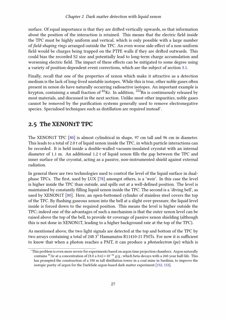
Chapter 2 Dark matter detection with liquid xenon
surface. Of equal importance is that they are drifted vertically upwards, so that informationabout the position of the interaction is retained. This means that the electric field insidethe TPC must be highly uniform and vertical, which is only possible with a large numberof field-shaping rings arranged outside the TPC. An even worse side-effect of a non-uniformfield would be charges being trapped on the PTFE walls if they are drifted outwards. Thiscould bias the recorded S2 size and potentially lead to long-term charge accumulation andworsening electric field. The impact of these effects can be mitigated to some degree usinga variety of position-dependent event corrections, which are the subject of section 3.1.
Finally, recall that one of the properties of xenon which make it attractive as a detectionmedium is the lack of long-lived unstable isotopes. While this is true, other noble gases oftenpresent in xenon do have naturally occurring radioactive isotopes. An important example iskrypton, containing a small fraction of 85Kr. In addition, 222Rn is continuously released bymost materials, and discussed in the next section. Unlike most other impurities, noble gasescannot be removed by the purification systems generally used to remove electronegativespecies. Specialised techniques such as distillation are required instead∗.
2.5 The XENON1T TPC
The XENON1T TPC [80] is almost cylindrical in shape, 97 cm tall and 96 cm in diameter.This leads to a total of 2.0 t of liquid xenon inside the TPC, in which particle interactions canbe recorded. It is held inside a double-walled vacuum-insulated cryostat with an internaldiameter of 1.1 m. An additional 1.2 t of liquid xenon fills the gap between the TPC andinner surface of the cryostat, acting as a passive, non-instrumented shield against externalradiation.
In general there are two technologies used to control the level of the liquid surface in dual-phase TPCs. The first, used by LUX [78] amongst others, is a ‘weir’. In this case the levelis higher inside the TPC than outside, and spills out at a well-defined position. The level ismaintained by constantly filling liquid xenon inside the TPC. The second is a ‘diving bell’, asused by XENON1T [80]. Here, an open-bottomed cylinder of stainless steel covers the topof the TPC. By flushing gaseous xenon into the bell at a slight over-pressure, the liquid levelinside is forced down to the required position. This means the level is higher outside theTPC; indeed one of the advantages of such a mechanism is that the outer xenon level can beraised above the top of the bell, to provide 4𝜋 coverage of passive xenon shielding (althoughthis is not done in XENON1T, leading to a higher background rate at the top of the TPC).
As mentioned above, the two light signals are detected at the top and bottom of the TPC bytwo arrays containing a total of 248 3” Hamamatsu R11410-21 PMTs. For now it is sufficientto know that when a photon reaches a PMT, it can produce a photoelectron (pe) which is
∗This problem is evenmore severe for experiments based on argon time projection chambers. Argon naturallycontains 39Ar at a concentration of (8.0 ± 0.6) × 10−16 g/g , which beta-decays with a 268-year half-life. Thishas prompted the construction of a 350 m tall distillation tower in a coal mine in Sardinia, to improve theisotopic purity of argon for the DarkSide argon-based dark matter experiment [152, 153].
27

Chapter 2 Dark matter detection with liquid xenon
Figure 2.6: Illustration of the XENON1T TPC design, with the main components labelled. Figure from [80].
amplified into a measurable charge signal or pulse. A more detailed treatment of the pho-tomultipliers can be found in chapter 5. Much of the TPC’s design is to maximise the chanceof photons from the S1 and S2 reaching one of these PMTs. Thewalls are linedwith interlock-ing diamond-polished PTFE panels, which have excellent reflectivity for xenon scintillationlight. The gaps between PMTs in their array are also covered with polished PTFE.
To maintain the drift and extraction fields, a total of five electrodes are used along with 74field-shaping rings around the outside of the PTFE reflectors. These are visible in figure 2.6.As well as the cathode and the gate electrode, which define the drift field, and the anodewhich defines the extraction field together with the gate, two screening meshes are locatedbelow the cathode and above the anode. These are biased at −1.5 kV, similar to the PMToperating voltage, and are intended to prevent the TPC’s electric fields from leaking into thePMT arrays and disrupting their operation.
Because of the need to minimise the background rate of interactions in the TPC, both nuc-lear and electronic recoils, it is important to use materials with a very low radioactivity.Essentially all materials used in or near the XENON1T TPC were screened for radioactiv-ity, and wherever possible the materials with the lowest radioactivity were selected. Twotechniques are used for such screening. The first, gamma-ray spectroscopy, uses germaniumcrystals in low-background, underground laboratories [154–156] to directly detect gamma-rays from radioactive decay in materials. The exact parts to be used can be measured and,since the decay radiation is observed directly, there are few systematic errors in the meas-urement. The second, inductively coupled plasma mass spectrometry (ICP-MS), measuresthe mass number of atoms in a material, allowing the identification of radioactive isotopes[157]. ICP-MS requires only a very small sample, but is destructive and is not always able
28

Chapter 2 Dark matter detection with liquid xenon
to reach the same sensitivity as gamma-ray spectroscopy. For more details of the materialscreening programme for XENON1T, see [158].
As well as these bulk radioactivity measurements, components with a significant surface areaare screened for radon emanation. This is the release of 222Rn from their surface into thesurrounding xenon. The 222Rn is produced from the alpha-decay of 226Ra, part of the decaychain of 238U, which is commonly known as the uranium series. Most detector materialscontain trace amounts of naturally occurring 238U; indeed, this one of the main targets of thebulk screening campaign discussed above. Since it is gaseous, 222Rn can diffuse to the surfaceof whichevermaterial it is produced in and escape into the surroundingmedium. A dedicatedscreening procedure is used tomeasure the 222Rn emanation rates of components [159]. Theyare filled or flushedwith a carrier gas, either helium or nitrogen. The radon is then trapped bypassing the helium through activated carbon at liquid nitrogen temperature (radon freezes at−71 ∘C). Afterwards, the radon is released from the carbon trap and filled into a proportionalcounter to measure its activity.
The TPC, in its cryostat, is contained inside a water tank with 9.6 m diameter and 10.2 mheight. The primary function of the water is to act as a shield against external radiationfrom the laboratory and surrounding rock. It is also instrumented and used as a muon veto.XENON1T is located in the Gran Sasso National Laboratory (LNGS) in central Italy, where itis covered by around 1300 m of rock. This is important in order to reduce the flux of cosmicmuons, which has been measured as (3.41 ± 0.01) × 10−4 m−2s−1 [160].
2.6 XENON1T: the rest
Up to now we have only discussed the XENON1T TPC. While this can be considered the‘heart’ of the experiment, it is far from the only component. Other systems which are closelyrelated to the TPC include the data acquisition system, xenon purification, distillation andcryogenics systems, and the xenon recovery and storage facility. The activemuon veto, usingthe water tank, is important for background reduction.
Most of these ancillary systems are located in the three-storey service building, adjacent tothewater tank. The top floor contains the cryogenic and xenon purification systems. In orderto maintain a high electron lifetime, xenon from the cryostat is continuously recirculated andpurified. Liquid xenon is extracted from the bottom of the cryostat through a heat exchanger,used to cool returning xenon gas and massively reduce the cooling power needed [161]. Twoloops, operated independently in parallel, pump the warm, gaseous xenon through a SAESPS4-MT50-R hot zirconium getter. This removes many impurities from the xenon by formingchemical bonds between them and the zirconium. Noble gases are not affected.
Three independent cold heads are used to cool and liquify the xenon, contained in the coolingtowers on the top floor. Two of these use Iwatani PC-150 pulse-tube refrigerators (PTRs)to provide the cooling power. Each can manage a load of around 250 W at the operatingtemperature of −96 ∘C, enough that one is sufficient for operation with one being spare. The
29

Chapter 2 Dark matter detection with liquid xenon
Figure 2.7: The XENON1T watertank and service building. Credit: the XENON collaboration.
third cold head is a backup in case of power loss and is cooled by liquid nitrogen. Enoughliquid nitrogen is stored on-site to keep the TPC cold for at least two days without PTRoperation.
A vacuum-insulated pipe connects the cryostat with the top floor of the service building,carrying the necessary liquid and gas xenon piping as well as cables for signals and voltagesupply from and to the detector.
The bottom floor of the service building houses the xenon storage and recovery system(ReStoX) [162]. This is a vacuum-insulated, liquid-nitrogen-cooled spherical vessel, able tocontain up to 7.6 t xenon in gaseous, liquid or solid form. By keeping ReStoX at a cold tem-perature, quick recovery of liquid xenon from the cryostat is possible in case of emergencythrough dedicated vacuum-insulated lines.
Also on the bottom floor is the krypton distillation column [163]. This roughly 5 m columnwas used to reduce the concentration of krypton to (0.66 ± 0.11) ppt∗ (mol/mol) [57], com-pared to a concentration on the ppb† to ppm‡ level in commercially available xenon. Anextremely low concentration of krypton is important because natural krypton contains 15±4ppt 85Kr [164], which undergoes beta-decay with a 10.7 year half-life and a 687 keV endpointenergy. Were it not for the distillation column, 85Kr would be the dominant electronic recoil
∗parts-per-trillion, 1 ppt = 10−12†parts-per-billion, 1 ppb = 10−9‡parts-per-million, 1 ppm = 10−6
30

Chapter 2 Dark matter detection with liquid xenon
background and result in a background rate more than 1000 times higher than that observedin XENON1T.
Finally, the middle floor of the service building contains the data acquisition system, as wellas a working space for underground operators. PMT signals and power supplies are carriedon cables running through the pipe to a breakout chamber on the top floor. From here theyare connected to Phillips 776 ten-fold amplifiers and high-voltage supply modules, respect-ively, on the middle floor. After amplification, signals are recorded with a 100 MHz samplingrate using CAEN V1724 digitisers. Every pulse reaching the threshold, equivalent to around0.3 photoelectrons, is digitised and saved. Six independent computers are used to read thedigitised data which is buffered locally before being stored remotely for further processing.The system can handle a maximum rate of 3000 MB s−1, which is equivalent to an event rateof approximately 100 Hz. Further details of the data acquisition system and trigger logic canbe found in [165].
The final system to be discussed here is the active muon veto [166], used to identify theinteractions of muon-induced neutrons. The water tank in which the cryostat is suspen-ded is instrumented with 84 Hamamatsu R5912ASSY 8” PMTs. These are used to detect theČerenkov light produced when charged particles pass through the water. Reflective foil onall surfaces of the water tank ensures a high photon detection efficiency despite a relativelysmall area coverage by the PMTs. Muons directly passing through the water tank can thus bedetected with an efficiency of 99.5%. It is also possible for muons to induce neutrons withoutthemselves passing through the water. In this case they can be tagged if particles from theirhadronic shower enter the tank, with an efficiency of 70%.
2.7 Calibrating XENON1T
Older liquid xenon TPCs were calibrated using a variety of gamma-ray sources positionednear the detector [115, 147]. The size of XENON1T means that gamma-rays originatingoutside the cryostat are unlikely to make it beyond the outer few centimetres of the TPC.Furthermore, the response to gamma particles is not identical to that to beta particles (thepredominant background), as we saw earlier. The response to electronic recoils is thereforedetermined using an internal beta-decaying source [167]. A chamber in the gas recirculationsystem containing a source of 228Th can be flushed with xenon gas which is on its way to theTPC. This decays to 220Rn, which can mix with the xenon and be carried into the detector.
The 220Rn alpha-decays with a half-life of 56 s via 216Po to 212Pb, after which a mixture ofbeta and alpha decays take it to the stable isotope 208Pb. This latter half of the decay chain,with a half-life of 10.6 hours determined by the 212Pb, provides low energy electronic recoilswhich mimic the main background for WIMP searches.
The nuclear recoil response is determined using neutron calibrations. Two independentsources of neutrons are used. The first, used throughout the lifetime of XENON1T, is an241AmBe source providing a range of neutron energies with a mean of about 4.2 MeV [168].
31

Chapter 2 Dark matter detection with liquid xenon
This is housed in a tungsten collimator, and can be lowered through a hatch in the roof of thewater tank to a position near the cryostat, using a system of belts. The second is a deuterium-deuterium plasma fusion neutron generator, which provides neutrons mostly with energiesin one of two peaks at 2.2 and 2.7 MeV [169].
In addition to the nuclear recoils induced by neutrons scattering elastically of xenon nuclei,the neutron sources produce a variety of mono-energetic gamma lines. These include linesfrom the decay of activated isomers at 164 keV (131mXe) and 236 keV (129mXe). Inelasticneutron scattering produces further gamma lines at 39.6 keV (129Xe) and 80.2 keV (131Xe),albeit with an additional but small nuclear recoil component – the importance of these lineswill become clear in chapter 4.
A final calibration source used for XENON1T is 83mKr, a second internal source first usedby LUX [170] after being tested in smaller research detectors at the University of Zurichand Yale University [171, 172]. This is produced from its parent 83Rb, which decays with ahalf-life of 86.2 days. As with 220Rn, a chamber containing the parent is flushed with xenonwhich is then returned to the TPC, carrying the 83mKr with it. The metastable isomer 83mKrdecays to its stable ground state with a half-life of 1.83 hours through two transitions, the firstreleasing 32.2 keV and the second releasing 9.4 keV. The intermediate stage has a half-life of157 ns, long enough that the two S1 signals are often separated (although the S2s are usuallymerged). This two stage decay means that it is easy to identify 83mKr events while rejectingbackground with a very high efficiency, since it is unlikely for two decays to coincidentallybe so close in time.
The utility of 83mKr calibrations will become apparent in the next chapter. Because its de-cays always deposit the same energy and are easy to select efficiently, they are useful foridentifying position-dependence in the detector’s response.
To conclude this section, let us briefly look at how the gain parameters 𝑔1 and 𝑔2 can bedetermined. Recall that these are required to relate the energy of an interaction to its chargeand light signals. There are at least two common and related methods used for this pur-pose. The first requires a calibration with a single mono-energetic line. When plotting thedistribution of such interactions’ S1 and S2 areas, they generally form a two-dimensionalGaussian, as illustrated in figure 2.8 (left). Fluctuations along the major axis correspond to aclear anti-correlation between the amounts of charge and light produced. Since energy mustbe conserved, if less scintillation light is produced, more ionisation must take place, and viceversa. The minor axis essentially represents the energy resolution of the detector.
By fitting this response and extracting the major axis it is easy to find 𝑔1 and 𝑔2: rearrangingequation 2.2 shows that the line through it is described by:
𝑆2 = 𝑔2 (𝐸𝑊 − S1
𝑔1) . (2.3)
The alternative is to look at several different mono-energetic peaks. When plotting theircharge and light yields, defined as the amount of charge/light (in detected photoelectrons)per unit energy deposited, these should all fall on a single line, with the 𝑥 and 𝑦 inter-
32

Chapter 2 Dark matter detection with liquid xenon
4 6 8 10Light yield [pe/keV]
0
100
200
300
400
500
600
Chargeyield[pe/keV]
83mKr (42 keV)
131mXe (164keV)129mXe (236keV)
60Co (1.17 MeV)60Co
(1.33MeV)
40K (1.46MeV)
S1
S2more
charge
ΔE
morelight
Figure 2.8: Determination of the photon detection efficiency and charge amplification factor from mono-energetic calibration lines. Left: illustration of the anti-correlation of charge and light signals fora single mono-energetic line. Right: the light and charge yields of several mono-energetic lines;the intercepts give the two values of interest. Figure adapted from internal XENON1T data.
cepts being 𝑔1/𝑊 and 𝑔2/𝑊 , respectively. This latter method is less affected by detectoreffects, since the central point of the two-dimensional Gaussians is less likely to be biasedby, for example, non-uniform light and charge detection efficiencies. This is the techniquewhich is used by XENON1T, with the data points used for its calibration shown in figure 2.8(right). The values extracted from fitting these points are 𝑔1 = (0.142 ± 0.002) pe/photonand 𝑔2 = (11.4 ± 0.2) pe/electron, where the latter considers only the part of S2s observedby the bottom PMT array (as we will see in the next chapter, this is less affected by position-dependent fluctuations).
33

Chapter 3
Elastic WIMP scattering
We have seen an introduction to the XENON1T experiment and explored the technologiesused by it, in particular in the time projection chamber. We now turn our attention to theanalysis of data which was collected by XENON1T, working towards a constraint on thecross-section of interactions between WIMPs and nuclei. In this chapter we concentrate onelastic interactions, and on the way we will go into some detail about aspects of the lower-level data analysis needed to convert flashes of light detected by PMTs into events withphysical values assigned, such as their energy and location. In the next, we turn to inelasticWIMP interactions, in which the target xenon nucleus is excited.
Elastic scattering is the primary focus of many experiments’ searches for WIMPs. Limits onthe cross-section of spin-independent, elastic WIMP-nucleus scattering in particular couldbe considered the canonical results obtained by most experiments seeking the direct detec-tion of dark matter. Experiments such as XENON1T are designed specifically with the searchfor such signals in mind; their ability to discriminate between nuclear recoils, expected fromsuch elastic WIMP interactions, and electronic recoils, expected from most background in-teractions, boosts their sensitivity to them. By searching for spin-independent interactions,experiments using fairly heavy target nuclei such as xenon gain an additional advantage:due to the ability of WIMPs to interact coherently, the scattering rate increases proportionalto 𝐴2𝜇2, where 𝐴 is the number of nucleons and 𝜇 is the WIMP-nucleus reduced mass, as wesaw in section 1.4.1.
Very roughly outlined, the data analysis pipeline used by XENON1T is as follows. First,individual hits from PMTs are grouped together according to their detection times, to formpeaks (borrowing notation from [141], where more details can be found). These peaks shouldcorrespond to individual S1 or S2 signals, and are classified as such based on their rise-time.To be classified as a physical signal, S1s must contain hits from at least three PMTs within100 ns; S2s must contain hits from at least four (with no timing requirement).
The peaks are grouped into events, which are defined as the collection of all signals in awindow 2 µs long, centred around a trigger. A single physical interactions in the TPC shouldlead to an individual event, containing the S1 and S2, but events can also sometimes containsignals from multiple interactions or collections of signals arising from other sources (moreon this later).
34

Chapter 3 Elastic WIMP scattering
1000 1005 1235 1240 1245 1250 1255 1260
Time [µs]
0
10
20
30
40
50
60
70
80
Am
plit
ud
e[p
e/b
in]
S1s
S2s
Figure 3.1: Example of a XENON1T waveform. This example is taken from a 83mKr calibration; the twoseparate S1s are clearly visible (in purple) while the S2s are merged (in red).
Basic properties of these events can then be computed, mostly information about the signalswithin them (for example, the S1’s and S2’s area and rise time or the time gap between them,which is used to compute the depth of the event). The contribution of individual PMTs toeach signal is also used to compute other properties; the most obvious is the (𝑥 , 𝑦) positionof the event, which is extracted from the distribution of S2 light on the top PMT array usinga neural network. Technically, the steps up to this point are performed by the Python-basedsoftware package pax (standing for ‘Processor for Analyzing XENON’) [173] – this part ofthe analysis chain is often referred to as data processing. An example waveform is shown infigure 3.1.
In latter stages of analysis, we first transform these event properties into more useful vari-ables. Many of the event properties that were computed need correcting, to counteractknown systematic effects, as detailed in the first section of this chapter. They can also becombined to calculate more physical variables, for example the energy of an event is estim-ated using a combination of the S1 and S2 area, as we saw in section 2.7. Now we can try tofilter out some of the noise by selecting only those events which are consistent with whatwould be expected of a physical interaction (see section 3.2). Finally, the ‘highest’ level ofanalysis aims to place constraints on fundamental physics by interpreting the events identi-fied up to now. This can be rather complex in its own right, and in this chapter on the searchfor elastic WIMP scattering is kept fairly concise; in the next one about inelastic scatteringthere are more details. Here, the focus is on my personal contributions to the analysis: theS2 (𝑥 , 𝑦)-dependent correction, S2 area fraction top cut and misidentified S1 83mKr cut.
35

Chapter 3 Elastic WIMP scattering
3.1 Event corrections
3.1.1 Overview of detector effects which need correcting
One of the reasons dual-phase time projection chambers are so widely used is their uniformresponse. Wherever a particle interacts in the TPC, more or less the same signal is observedon average. However, this uniformity is not perfect: there are small variations dependingon the position of the interaction. Most analyses therefore work with variables which havebeen corrected to account for these non-uniformities. These corrections are the subject ofthis section, in which we focus in particular on the interaction position and the S1 and S2areas.
The first effect we consider is due to the fact that the electric field is not perfectly uniform.In particular at the corners of the TPC, external fields can ‘leak’ in and create distortions.This means that especially for events from the lower, outer regions, electrons tend to driftinwards as they move up towards the liquid surface. As the S2 light used for reconstructingtheir position is produced at the top, bottom events’ interaction locations would be biasedinwards. To counter this effect, a correction is applied to convert observed positions (whichare the position that the S2 is produced, smeared according to the position resolution) intointeraction positions.
The light collection efficiency, defined as the probability of a photon, which has been pro-duced in a particle interaction, reaching a PMT photocathode, is also not uniform throughoutthe TPC’s volume. Events which occur in the middle of the TPC and just above the cathodehave the highest light collection efficiency. To correct for this effect, S1s’ areas are multi-plied by a correction factor depending on the position of the interaction. This correctionfactor is quantified by measuring the size of the S1s in 83mKr calibration data, in which allevents should produce the same number of photons on average. The general trend is thatthe efficiency decreases moving upwards in the TPC and moving closer to the PTFE wall.The reason for this is the increased probability of reflection off the wall, or at the top, off theliquid surface.
Since S2s are all produced at the top of the TPC, near the liquid-gas interface, we can di-vide systematic effects into two. Some may occur before S2 production, while the electronsare being drifted through the TPC, and should only depend on the depth of the interaction 𝑧.Others affect the S2 light production itself, and therefore depend only on the 𝑥 and 𝑦 coordin-ates where the S2 is observed. These two effects are considered separately, and referred toin the following as the electron lifetime correction and the S2 (x, y)-dependent correction.
The electron lifetime correction takes into account the fact that as electrons drift throughthe liquid xenon, some can be captured by electronegative impurities which they encounter.Since these impurities should be homogeneously distributed in the xenon, we expect a con-stant probability for an electron to be captured per unit distance drifted in the xenon. Thisresults in the electron cloud becoming exponentially smaller as it drifts, and can be charac-terised by the average ‘lifetime’ of an electron 𝜏e, where of course by lifetime we don’t refer
36

Chapter 3 Elastic WIMP scattering
to its decay, but rather the average time before capture.
The S2 (𝑥 , 𝑦)-dependent correction primarily considers the effects of non-uniformity in theextraction field, and PMT-related effects. We characterise these as a multiplicative correctionto the S2 area, depending on the position (𝑥obs, 𝑦obs). The subscript ‘obs’ is used in thischapter to refer specifically to the position at which an event is observed, as opposed towherethe interaction itself took place, or in other words the position before the field-distortioncorrection is applied. Further details about this correction can be found in section 3.1.2,below. Putting these effects together, the size of an observed S2 is related to the number ofelectrons produced in an interaction, 𝑛e, according to:
S2 = 𝑔2 exp (−𝜏𝜏e) 𝑐𝑥𝑦 (𝑥obs, 𝑦obs) 𝑛e, (3.1)
where 𝑐𝑥𝑦 is a function describing the (𝑥 , 𝑦)-dependence and 𝑔2 is the nominal S2 amplifica-tion factor, as defined in section 2.3.
Other corrections are important for different analysis regions but not needed for the resultspresented in this thesis. In particular, a desaturation correction is used for analyses lookingat high energy events, in the MeV region. At these energies, nonlinearities from the PMTs,their voltage-divider circuits and digitisers become important. Details of the correction canbe found in [174], and in chapters 5 and 6 we touch on the origins of such saturation effects,in the context of XENONnT.
Of the various types of calibration data taken, 83mKr is particularly suitable for characterisingsystematic effects which need correcting, thanks to the ease of tagging events as describedin the previous chapter. In general, events with the two S1s reconstructed separately andthe two S2s merged are used. A typical set of selection criteria, as used for the S2 (𝑥 , 𝑦)-dependent correction described below, would be to require that the two S1s are separated bybetween 0.6 and 2 µs (long enough to mean that the S1s are well separated but short enoughto avoid most random coincidences of two events) and that there is a good match betweenthe first S1’s light pattern and its reconstructed position∗.
3.1.2 S2 (x, y)-dependent correction
We can divide the sources of (𝑥 , 𝑦)-dependent effects on the S2 area into two categories. Thefirst is those that occur during the production of S2 light: these can be related to the extractionefficiency and the amplification factor of S2s. The other occurs during S2s’ detection, andis related to the S2 light collection efficiency. In practice, this is largely uniform except fordrops in regions where PMTs are turned off, so it introduces more localised variations. It onlyintroduces a significant effect for the part of S2s seen by the top PMT array (which we referto as ‘top S2s’, S2t) since these are localised on few PMTs. In contrast, S2 light is uniformly
∗This is quantified using the 𝜒 2 goodness-of-fit between the expected pattern for an event at that position andthe observed pattern.
37

Chapter 3 Elastic WIMP scattering
−40 −20 0 20 40
xobs [cm]
−40
−20
0
20
40
y ob
s[c
m]
0.850.90
0.95
−40 −20 0 20 40
xobs [cm]
0.85
0.90
0.95
4 6 8 10 12
cτe S2b [1000 pe]6 9 12 15 18
cτe S2t [1000 pe]
Figure 3.2: The analytic fit to the bottom (left) and top (right) S2 (x, y) variation, shown as contoursrelative to the maximum. The data used for the fit is shown behind, with colouring representingthe area of each event’s S2 as detected on the relevant PMT array.
spread out over the whole array by the time it reaches the bottom of the TPC, and, as we willsee, bottom S2s (S2b) display no such small-scale variations.
For the purposes of correcting S2s’ area, these two scales of variation are considered one ata time, and the S2 light seen by each PMT array is treated separately.
First, we correct for the large scale variation due to S2 production effects. This is assumedto be caused by variations in the strength of the extraction field: the electric field in thegap between the liquid surface and the anode, and in the length of this gap. These variationsarise from ‘sagging’ of the electrodes due to their mutual attractionwhen charged, or residualtilting of the TPC which means that the electrodes are not perfectly level.
The average area of an S2 detected at position (𝑥obs, 𝑦obs) due to this variation is assumed tofollow a quadratic dependence
S2 ∝ 1 − 𝑏 (𝑥obs − 𝑥0)2 + (𝑦obs − 𝑦0)2𝑟20
, (3.2)
where 𝑟0 is the radius of the TPC, 48 cm. The position (𝑥0, 𝑦0) is where observed S2s havethe greatest area, and 𝑏 represents the size of the non-uniformity.
Figure 3.2 shows the size of 83mKr events’ S2s (after correcting for electron lifetime only)on the bottom and top array, respectively, and the functional fit to them. It is already clear
38

Chapter 3 Elastic WIMP scattering
−40 −20 0 20 40
xobs [cm]
−40
−20
0
20
40
y ob
s[c
m]
−40 −20 0 20 40
xobs [cm]
0.60
0.65
0.70
0.75
0.80
0.85
0.90
0.95
1.00
Figure 3.3: Variations in the mean S2 on the bottom (left) and top (right) PMT arrays, after applying theelectron lifetime correction and correcting for the large-scale variations described analytically.The colour represents the mean S2 area in each bin, as a fraction of the largest bin.
that the average bottom S2 displays no significant small-scale structure, in contrast to thetop. Note that in the case of the top array, the quadratic is fit with different parameters eventhough the effects of electrode sagging are expected to affect both signals equally. Some ofthe PMT effects have biased the fit: the large number of turned-off PMTs in the upper-rightcorner means that S2s are generally lower there. This bias doesn’t affect the production of acorrection, since it will be properly accounted for in the next step, but it does mean that anyphysical interpretation of the effects described here should be done using bottom S2s only.
In the second step, the remaining small-scale variations are considered by binning the TPCand calculating the mean area in each bin, after correcting using the quadratic formula above.A radial and azimuthal binning structure is used, as seen in figure 3.3. The reader may bewondering why it wouldn’t be possible to jump straight to the second stage of the correctionand take into account all variations using the binned mean S2. The reason is that most of thevariation has almost∗ radial dependence; the small scale effects are also a smaller magnitude.In order to get the best correction, we would therefore tend to have bins which are quitesmall in radius, but which would then have to be quite large in arc length in order to haveenough statistics in them. By first taking out this effect, it is possible to choose squarish binsthat are better able to represent the small-scale variations. In addition, the radial binningstructure would tend to favour a correction depending on the radius from the centre of theTPC, i.e. with (𝑥0, 𝑦0) = (0, 0).The benefit of this correction can bemeasured by the spread in area of S2s from 83mKr events.With no correction, the standard deviation is 17.0%, after the analytic correction only thisbecomes 15.7%, and with the full correction 15.0%. Note that the relative effect on the energy
∗It is not quite a radial dependence, since the maximum position (𝑥0, 𝑦0) is a few centimetres from the centreof the TPC.
39

Chapter 3 Elastic WIMP scattering
resolution, while not quantified here, will be even better: the S2 resolution contains a con-stant spread due to the anti-correlation of S1s and S2s, which is removed when calculatingevents’ energy.
In order to simplify the application of the S2 (𝑥 , 𝑦)-dependent correction, a combined, up-sampled correction map was produced: the binned part of the correction was interpolatedon a finer grid, always using a distance-weighted mean of the nearest four bin centres, andcombined with the analytic part. As a final remark on the technical implementation, notethat the above technique is only useful for measuring relative differences in S2. An overallscaling factor is arbitrary, and would simply result in a different value of the constant 𝑔2 inequation 3.1. For XENON1T we chose to have the correction map normalised such that theaverage correction factor was unity.
Physical effects causing S2 variation
In the following we will delve more deeply into the physical effects which are behind the(𝑥 , 𝑦)-dependence described above. As mentioned above, this can be divided into three phys-ical origins, whose effects should multiplicatively combine:
𝑐𝑥𝑦 ∝ 𝜖ex 𝐺S2 𝜖PMT, (3.3)
where 𝜖ex is the relative efficiency with which electrons are extracted from the liquid to thegaseous phase, 𝐺S2 is the relative S2 amplification factor, and 𝜖PMT is the relative photondetection efficiency. The last term accounts for PMT effects (particularly turned-off PMTs),and is only relevant for top S2 signals.
To study the first two terms, we can look at the variation in the size of single electron signals.A background of single electrons is present throughout the operation of XENON1T; thereare a variety of origins including photo-ionisation of metal surfaces in the TPC, delayedextraction of electrons in an S2 signal, and slow release of electrons from impurities suchas oxygen [175–177]. For this study, single electrons signals present before the main S1 in83mKr event windows were used. In principle any data could be used for this, but at the timethis study was performed background data was blinded. By searching only the part of eachevent before the main interaction’s S1, any effects due to that interaction should be removed.
The advantage of looking at single electron events is that they are effectively a sample whereelectrons were extracted with 100% efficiency – a single electron can either be extracted ornot, and we only see the events where it is. The (𝑥 , 𝑦)-dependence of their area thereforeonly includes the latter two terms of equation 3.3. We can extract the dependence of 𝜖ex fromthe mean single electron area, S2SE, according to:
𝜖ex (𝑥obs, 𝑦obs) ∝𝑐𝑥𝑦 (𝑥obs, 𝑦obs)S2SE (𝑥obs, 𝑦obs)
. (3.4)
In fact, we will use the number of hits in the single electron peak, 𝑛hits, instead of its area,S2SE, since it is less affected by fluctuations. With a mean of only 22.0 hits per single electron
40

Chapter 3 Elastic WIMP scattering
−40 −20 0 20 40
xobs [cm]
−40
−20
0
20
40
y ob
s[c
m]
0.85
0.90
0.95
−40 −20 0 20 40
xobs [cm]
0.96
0.97 0.98
0.99
0.0 0.2 0.4 0.6 0.8
cxy/nhits
3.0 4.5 6.0 7.5 9.0
cτe S2b/εex [1000 pe]
Figure 3.4: Breakdown of the large-scale S2 (x, y) dependence into variation of electron extraction efficiency(left) and amplification factor (right). The data shown by colour in the latter case is the bottomS2 area divided by the estimated extraction efficiency at that point, from the fit shown on theleft.
shared across all the PMTs and over around 200 ns, it is very unlikely for any PMT to detectmore than one hit [178].
This is seen in figure 3.4 (left). There are two interesting things to see here: firstly, the sizeof the effect is similar to the overall variation that we saw in figure 3.2; secondly, the centre-point of the behaviour is very close to the centre-point of the TPC. This is what we may haveexpected: the extraction efficiency should depend purely on the electric field at the liquid-gas interface. This is influenced much more by sagging of the electrodes than tilting, whichwould not change their separation.
We are now also in a position to look at the variation of the S2 amplification factor 𝐺S2. Forthis we divide the area of bottom S2s from 83mKr events by the extraction efficiency foundabove, leaving this S2 amplification as the only variation. This can be seen in figure 3.4(right), where it is clear that the effect is much smaller (up to around 5% compared to 20% forthe full variation) and very off-centre. Again, this might be expected: tilting will result in alarger region being available for S2 amplification and thus a higher gain.
Finally, we can try to understand the origin of the PMT-related variations. Figure 3.5 showsthe ratio between the top and bottom S2 signals of 83mKr events, which should be propor-tional to 𝜖PMT. This is fit with a simple empirical function, starting with a uniform efficiency
41

Chapter 3 Elastic WIMP scattering
−40 −20 0 20 40
xobs [cm]
−40
−20
0
20
40
y ob
s[c
m]
Figure 3.5: Description of the S2 variation by turned of PMTs. The data plotted is the ratio of events’ topand bottom S2 areas. The contours are a simple model, with parameters fit to this data, asdescribed in detail in the main text.
and subtracting a two-dimensional Gaussian for every turned-off PMT:
𝜖PMT = 1 −∑𝑖∈𝑂
𝛼 exp (−−(𝑥 − 𝑥𝑖)2 + (𝑦 − 𝑦𝑖)22𝑟2out
) −∑𝑖∈𝐼
𝛽 exp (−−(𝑥 − 𝑥𝑖)2 + (𝑦 − 𝑦𝑖)22𝑟2in
). (3.5)
Here 𝑂 is the set of PMTs in the outer ring of the top array which are turned off and 𝐼 is the setof all other turned-off PMTs. The outer PMTs are considered separately because reflectionsoff the TPC wall can affect the region which they are sensitive to. The parameters 𝛼 , 𝛽 , 𝑟outand 𝑟in are free in the fit.
Visually, this is a good fit to the variations seen in XENON1T data. Residual variations areup to around 5%, and may be explained by a more complex model; this is however beyondthe scope of this work. We can nevertheless conclude that these smaller-scale variations arerelated to the reduced efficiency of collecting photons where PMTs are turned off.
3.2 Quality cuts
Not all events algorithmically identified are genuine particle interactions within the TPC.They may come from random coincidences of spurious S1-like and S2-like signals, such asPMT dark counts or the single electron background. In addition, some events are reconstruc-ted badly. Typical examples include events very close to the wall, where the electrons can betrapped on the PTFE surface, resulting in a smaller-than-expected S2. For events that occurnear an area with several turned-off PMTs, the position may be incorrectly reconstructed dueto the limited knowledge of their light pattern. These events are removed from the searchdata using a variety of quality criteria, which are the subject of this section.
42

Chapter 3 Elastic WIMP scattering
Broadly speaking, most quality criteria can be identified as belonging to one of three cat-egories. The first is time-based, and rejects events which occur close in time to a muoninteraction in the water tank or when the DAQ is ‘busy’ and unable to fully record data (inwhich case part of the event may not have been fully recorded). Other criteria identify un-usual properties of either the S1 or the S2, and reject those events. Some prominent examplesare the S1-based and S2-based single scatter cuts, which reject events where a second S1-likeor S2-like peak is present and there may be some confusion over which should be paired;cuts on the fraction of each peak seen by the top PMT array; and the S2 width cut, whichrejects events with an unusually long S2 peak.
Data quality cuts must be designed to have a high acceptance, the rate of good events beingkept, which should ideally be one. It is also important to know the acceptancewell, in order toknow how many signal events one would expect for a given interaction cross-section. Theyshould also have a reasonably high rejection power, their ability to remove bad events. It is,however, less important to know the rejection power very precisely, provided any significantpopulations of bad events which are not removed by any cut can be satisfactorily modelled.
Here we will explore two examples: the so-called S2 area fraction top cut and a cut targeting83𝑚Kr events with a misidentified S1. A detailed discussion of the full set of quality cuts isbeyond the scope of this work; a more comprehensive treatment can be found in [141].
3.2.1 S2 area fraction top cut
Various cuts are designed to remove events which are physical but either badly reconstructedor for some reason cannot be dark matter events. An example of these is the S2 area fractiontop (AFT) cut. This is based upon the corrected fraction of the S2 seen by the top PMT array,or cS2 AFT:
cS2 AFT = cS2tcS2 . (3.6)
This parameter is particularly suitable for identifying gas events: interactions which occurin the gaseous xenon, generally above the anode. Such interactions can produce both S1and S2 signals, like liquid events do. Any electrons produced are accelerated downwardstowards the anode, and can produce an S2 by secondary amplification in this region. Theelectric field above the anode is different from the usual extraction field and the distanceover which S2 amplification takes place depends on the interaction position. The xenonmicrophysics describing the ratio of electrons to photons produced is also different in gas andliquid. Therefore, the S2/S1 ratio can vary greatly between events and is not well modelled,unlike for usual liquid events. It is important to identify these events and remove them fromthe science data used to search for dark matter, to prevent them appearing as spuriousWIMPsignals.
The S2 light from gas events is produced in the region above the anode, and potentiallystarting from near the top screening mesh. It is therefore more likely to be detected by thetop array, so the cS2 AFT will in general be larger than for normal events.
43

Chapter 3 Elastic WIMP scattering
102 103 104
S2 [pe]
0.3
0.4
0.5
0.6
0.7
0.8
0.9
cS2
AF
T
Figure 3.6: Calibration data used to define the S2 area fraction top cut, and the cut definition. The blueshading represents the density of calibration events (from both 220Rn and 241AmBe calibrationdata), and the vertical histograms show the distribution of cS2 AFT within a series of cS2 slices.The 0.5th and 99.5th percentiles of these distributions are shown as black crosses; the cut isdefined using a fit to these points as shown in red.
Normal S2s, produced in the narrow gap between the liquid surface and anode, will have asingle average value of cS2 AFT. The exact cS2 AFT for a particular event depends on stat-istical fluctuations, and can be expected to follow a binomial distribution. We can thereforeexpect the fluctuations in the cS2 AFT to be proportional to 1/√S2. Note that we expect thedependence to be on S2 rather than cS2, since it is the number of photons produced in thegas which matter for these statistical fluctuations, not the number of electrons produced atthe interaction site.
Earlier versions of this cut were based on the S2 AFT (rather than cS2 AFT). However, theuncorrected values vary depending on whether the S2 is produced near PMTs which areturned off; by using the corrected top and bottom S2 signals, these variations are removed.The electron lifetime correction affects both top and bottom S2 equally, so is irrelevant whenconsidering the ratio.
The S2 AFT cut is designed to accept 99% of real liquid interactions, independent of theirS2 area. Events are accepted or not based on their location in the (S2, cS2 AFT) parameterspace. The expected distribution is determined from 220Rn calibration data. After dividingthe data into slices based on S2 area, the cS2 AFT in each is fit with a Gaussian distribution.The 0.5th and 99.5th percentiles of these distributions are shown in figure 3.6 as a functionof S2 area, on top of the data used for the fit. These percentile points are in turn fitted to givean analytic expression for the cut boundary; the final selection criterion is
0.629 − 1.89 ⋅ S2 < cS2 AFT < 0.634 + 1.57 ⋅ S2. (3.7)
44

Chapter 3 Elastic WIMP scattering
0 5000 10000 15000 20000 25000 30000
S2 [pe]
0.5
0.6
0.7
0.8
0.9
1.0
cS2
AF
T
Figure 3.7: Data for estimating the power of the S2 area fraction top cut at rejecting gas events. The purplepoints above the dashed line represent gas events removed by the cut; the red crosses are thosefive which are not removed. The green points below the dashed line are assumed to belong tothe population of good events. The cut definition is shown as black lines.
Given its definition based on quantiles of the cS2 AFT distribution recorded in calibrationdata, this cut’s acceptance should be 99%. We can try to estimate the efficiency at which thecut rejects gas events by selecting a sample rich in such events. For this we can use anothercut, which also primarily targets gas events: the S2 width cut. This is based on events’width, defined as the shortest time window which contains at least 50% of the S2’s area.As mentioned above, the S2 amplification takes place over a longer (and variable) distancefor gas events, so their width is generally unusually large. By reversing the S2 width cut,we obtain a sample high in gas events; this is shown in figure 3.7. After discounting thoseevents which are clearly not from the gas region (their cS2 AFT is far away from the rangegenerally seen for gas events), 1303 remain. Five of these are not removed by the S2 areafraction top cut. These five may or may not be gas events, since they are consistent witheither population. We can thus place a lower limit on the rejection efficiency at 99.6%.
3.2.2 Misidentified S1 83mKr cut
Not all selection criteria are built to search for good events by selecting those with propertiesthat behave as expected. Some are more directly targeted at known categories of bad events,to remove a specific contamination in the data. Here, we briefly look at one example, builtto remove certain events arising from 83mKr in background data.
As we have already seen, 83mKr is periodically injected into the liquid xenon and used asa calibration source. It is produced from the decay of its parent isotope, 83Rb, which hasa half-life of 86 days. During the operation of XENON1T a small amount of 83Rb leakedinside the main xenon volume, leading to a permanent 83mKr contamination. In generalthese events show up as normal electronic recoils, but other behaviour is also possible due tothe two-stage decay. One less common possibility is that the two S2 signals are merged (as
45

Chapter 3 Elastic WIMP scattering
−4 −3 −2 −1 0 1 2 3 4 5Time delay S1 to second S2 [µs]
0
50
100
150
200
250
300
350
400
Seco
ndS2
[pe]
Figure 3.8: Events in 83mKr calibration with the second-largest S2 near the main S1. The population circledin blue is where the 32.1 keV decay’s S1 is identified as an S2; for the population in orange it isthe 9.4 keV decay’s S1 which is misidentified. The small population circled in green is probablyevents where two merged S1s are identified as an S2 and an afterpulse is identifed as an S1.
happens most of the time) but the two S1s are not, and one of the S1s is misidentified as anS2. Since the false S2 will be rather small, these events are difficult to remove using the usualsingle-scatter selection criteria. On the other hand, because the S1 and S2 are effectivelycreated from different energy deposits the events can fall somewhere outside the ER band,and therefore not be considered by any background model.
Fortunately it is easy to select such events, which must have a characteristically sized secondS2, just before the S1. Figure 3.8 shows 83mKr calibration data, after applying all other qualitycuts, with the second S2’s area plotted against the time of this second S2 relative to the S1.Two populations due to mis-classified S1s are visible, where either the 32.1 or 9.4 keV decay’sS1 is classified as S2. It is the former which are most concerning, since the disparity betweenthe S1 (from only the 9.4 keV part) and the S2 (from the full 41.5 keV) is largest. We can tagsuch events with essentially perfect efficiency by looking for a second S2 up to 3 µs beforethe S1 and with an area of at least 100 photoelectrons.
Since this signature is extremely unlikely to randomly occur in good events, a cut removingall such tagged events will have a very good efficiency. We can estimate this by looking incalibration data, for events with a second S2 fulfilling the area criterion (at least 100 pho-toelectrons) before the main S1. In 220Rn calibration data, 0.038% of all events have such asecond S2 in the 1 ms before the S1. Given that we expect these to be random in time, theacceptance of the cut looking only at a 3 µs window should be very close to one, 1−1.1×10⁻⁶.
3.2.3 Overall cut performance
To estimate the overall acceptance rate of dark-matter-like interactions, the cumulative ef-fect of all the quality criteria applied must be considered. Most criteria have only negligiblecorrelation and their acceptances can simply be multiplied, but four S1-related cuts are cor-
46
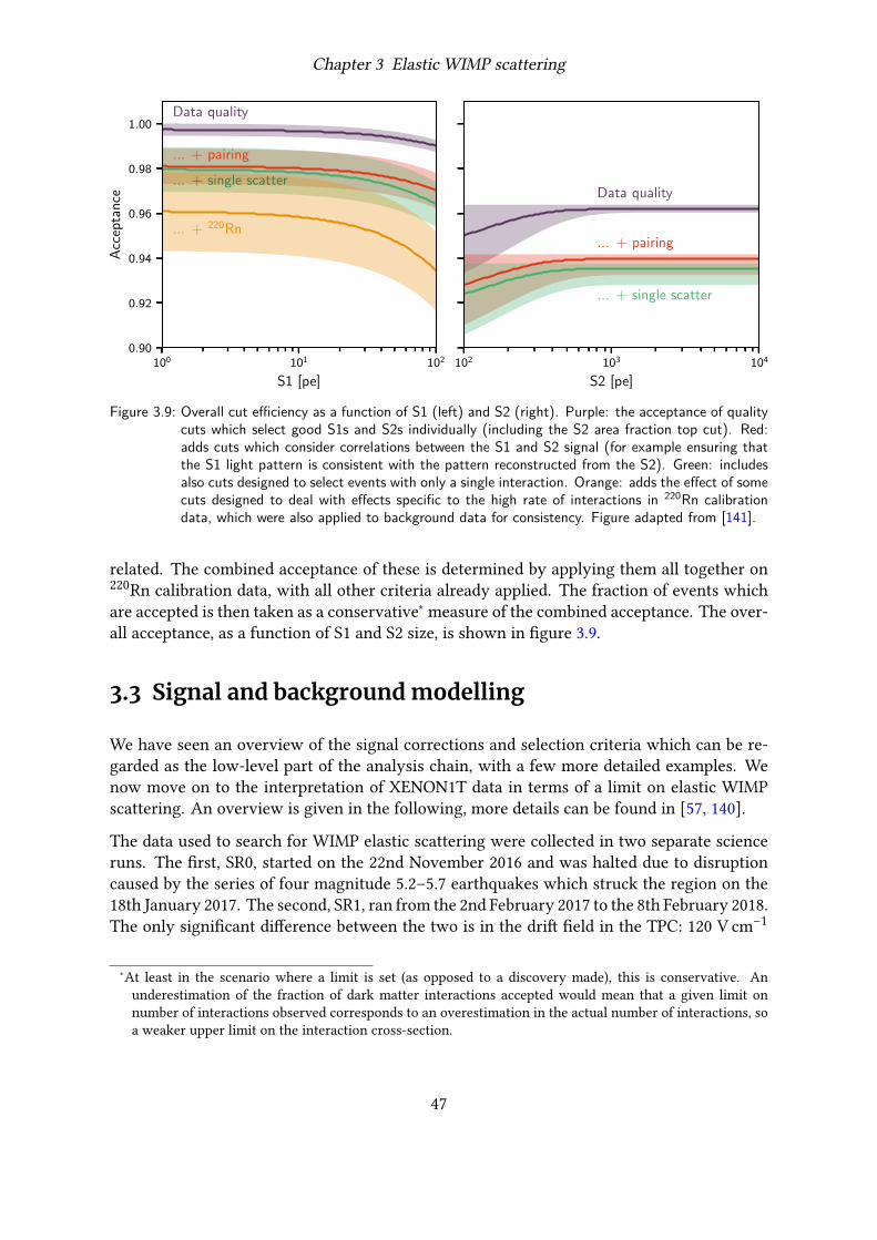
Chapter 3 Elastic WIMP scattering
100 101 102
S1 [pe]
0.90
0.92
0.94
0.96
0.98
1.00A
ccep
tan
ceData quality
... + pairing
... + single scatter
... + 220Rn
102 103 104
S2 [pe]
Data quality
... + pairing
... + single scatter
Figure 3.9: Overall cut efficiency as a function of S1 (left) and S2 (right). Purple: the acceptance of qualitycuts which select good S1s and S2s individually (including the S2 area fraction top cut). Red:adds cuts which consider correlations between the S1 and S2 signal (for example ensuring thatthe S1 light pattern is consistent with the pattern reconstructed from the S2). Green: includesalso cuts designed to select events with only a single interaction. Orange: adds the effect of somecuts designed to deal with effects specific to the high rate of interactions in 220Rn calibrationdata, which were also applied to background data for consistency. Figure adapted from [141].
related. The combined acceptance of these is determined by applying them all together on220Rn calibration data, with all other criteria already applied. The fraction of events whichare accepted is then taken as a conservative∗ measure of the combined acceptance. The over-all acceptance, as a function of S1 and S2 size, is shown in figure 3.9.
3.3 Signal and backgroundmodelling
We have seen an overview of the signal corrections and selection criteria which can be re-garded as the low-level part of the analysis chain, with a few more detailed examples. Wenow move on to the interpretation of XENON1T data in terms of a limit on elastic WIMPscattering. An overview is given in the following, more details can be found in [57, 140].
The data used to search for WIMP elastic scattering were collected in two separate scienceruns. The first, SR0, started on the 22nd November 2016 and was halted due to disruptioncaused by the series of four magnitude 5.2–5.7 earthquakes which struck the region on the18th January 2017. The second, SR1, ran from the 2nd February 2017 to the 8th February 2018.The only significant difference between the two is in the drift field in the TPC: 120 V cm−1
∗At least in the scenario where a limit is set (as opposed to a discovery made), this is conservative. Anunderestimation of the fraction of dark matter interactions accepted would mean that a given limit onnumber of interactions observed corresponds to an overestimation in the actual number of interactions, soa weaker upper limit on the interaction cross-section.
47

Chapter 3 Elastic WIMP scattering
for SR0 and 81 V cm−1 for SR1. A third science run, SR2, which began immediately after SR1and finished on the 3rd December 2018, is not used for this search.
In the combined SR0+SR1 dataset a total of 302.1 days of data were collected. A small fractionof the total is dead time, when any possible dark matter events would either not be recordedor not be considered as good events due to external influences. This can be introduced by thedata acquisition system being unavailable, activity in the muon veto or periods of delayedelectron extraction which follow large energy depositions. After subtracting the dead time,32.1 and 246.7 days of data remain in SR0 and SR1, respectively, to search for WIMP events.
The dataset was blinded while the event selection criteria were developed and the expectedsignal and background shapes were determined. Events which were below the −2𝜎 quantileof the expected electronic recoil band, based on preliminary models, were hidden from ana-lysts. This is a common technique for such searches, and is intended to reduce bias by pre-venting selection criteria or models being fine-tuned based on individual events. The datawere only unblinded once the full analysis chain was fixed.
For the purposes of searching for WIMPs, only a (1.30 ± 0.01) t sub-volume of the TPC wasused, in order to avoid regions near its boundary where the background rate is higher. Thisfiducial volume is bounded at 8.0 cm below the liquid surface, above which a small residualpopulation of gas events exists; 2.9 cm above the cathode, below which the electric field ismore non-uniform leading to biases in position reconstruction and the charge-to-light ratio;and 5.2 cm inside the TPC wall, outside which there are a very large number of surfaceevents (see below). In addition, the top and bottom of the fiducial volume vary as a functionof radius, such that there is no more than 10% increase in the background rate at its upperand lower boundaries.
The shape of the electronic and nuclear recoil bands is modelled following the treatmentused by NEST [136], as described in more detail in section 2.2. These models of the twobands are fit simultaneously to all 220Rn, 241AmBe and neutron generator calibration datataken during both science runs (with the field-dependence being considered as part of themodel). The resulting models allow a 99.7% rejection of electronic recoil events in a regionbetween the −2𝜎 quantile and median of a 200 GeV/c2 WIMP’s expected signal in (cS1, cS2b)space.
Seven sources of backgrounds are taken into account for the search. Backgrounds whichinduce electronic recoils include both intrinsic sources, that are mixed into the xenon itself,and those originating from natural radioactivity of the detector’s materials. The rate of thelatter is reduced by only searching within a smaller fiducial volume inside the TPC, thanksto the effective shielding of the xenon itself.
The important intrinsic sources of radioactivity are 85Kr and the daughters of 222Rn. Sinceboth of these are noble elements they are not efficiently removed by the getter. The formeris present in air (from which xenon is distilled), mostly due to emissions from nuclear re-processing [179]. Its concentration was reduced to subdominant levels by cryogenic distil-lation [163]. The latter is the result of radon emanation, as described in section 2.5. The
48

Chapter 3 Elastic WIMP scattering
decay chain of 222Rn includes 214Pb, whose beta-decay dominates the intrinsic backgroundspectrum at low energies. In the energy range 1.4 keV to 10.6 keV, which corresponds tothe region used for this analysis, these both have an almost-flat spectrum due to their beta-decays. Their combined rate is 82 +5−3(sys) ± 3(stat) events/(t yr keV).Nuclear recoils can be induced by solar neutrinos via coherent elastic neutrino-nucleus scat-tering (CE𝜈NS) [180] or by neutrons of both radioactive and cosmological origin. The mostimportant of these is radiogenic neutrons, expected to contribute 1.43 ± 0.66 events in the1 t yr exposure. Their rate is constrained using both a Geant4-based simulation [181, 182]and by searching for events in which one neutron scatters multiple times within the TPC.Cosmogenic neutrons are those induced by cosmic muons. They can be identified with avery high efficiency by the muon veto system, so they only contribute a negligible amountto the total NR background and are not considered.
Two final backgrounds, arising from detector effects, are also considered. The first is acci-dental coincidences of lone S1s or lone S2s, that happen to look like genuine particle-inducedevents. Samples from dedicated searches for lone S1s and lone S2s in the two science runsare paired randomly to create a model for such events. The second is so-called surface events.These are decays which occur on the surface of the PTFE walls of the TPC. Some of the elec-trons produced can be trapped on the wall, so the S2 is smaller than expected. These eventsare mostly from the decay of 210Pb and its daughters. These can be found on the TPC wallsdue to radon plate-out, a process whereby charged daughters of 222Rn become incorporatedinto the PTFE [183, 184].
Table 3.1 lists the sources of backgroundmentioned above togetherwith the expected numberof events for each, calculated using the likelihood’s best fit. The number of events are listedboth for the full analysis region, as seen in figure 3.10, and for a nuclear recoil ‘referenceregion’, defined as the region between the −2𝜎 quantile and the median of the 200 GeV/c2
WIMPmodel in (cS1, cS2b) space. This region is intended to illustrate the signal-like contentin the dataset, but is not directly used to constrain the cross-section.
3.4 Results
An unbinned extended likelihood is used to provide a statistical interpretation of the searchdata. Models used for this likelihood are produced in three dimensions: cS1, cS2b and radius.In addition a central region is identifiedwhich contains half of the fiducial volume, and eventsare categorised as being inside or outside this region. The central region is chosen becauseof its substantially smaller neutron rate (0.63 t−1 yr−1 compared to 1.43 t−1 yr−1 in the full1.3 t volume).
The same data and set of background models can be used to search for WIMPs scatteringwith a variety of physics channels. As mentioned in the introduction to this chapter, thecanonical route is to search for spin-independent scattering. Signal models are computed fora variety of WIMP masses between 6 and 1000 GeV/c2.
49

Chapter 3 Elastic WIMP scattering
Table 3.1: Expected number of events in the full dataset from each background and from a 200 GeV/c2
WIMP, based on the profiled likelihood.
Source EventsTotal Reference region
Electronic recoils 627 ± 18 1.62 ± 0.30Neutrons 1.43 ± 0.66 0.77 ± 0.35CE𝜈NS 0.05 ± 0.01 0.03 ± 0.01Accidental coincidence 0.47 +0.27−0.00 0.10 +0.06−0.00Surface events 106 ± 8 4.84 ± 0.40Total background 735 ± 20 7.36 ± 0.61100 GeV/c2 WIMP 3.56 1.70Observed 739 14
10 20 30 40 50 60 70
cS1 [pe]
102
103
cS2 b
[pe]
Figure 3.10: Data used to search for elastic WIMP scattering. Here, the expected region for ER events isshown in red and that for surface events in blue. The expected signal from a 100 GeV/c2 WIMPis shown in green. Figure adapted from [57]. The black dots show the locations of events withinthe 1.3 t fiducial volume after unblinding the data.
50

Chapter 3 Elastic WIMP scattering
101 102 103
WIMP mass [GeV / c2]
10−47
10−46
10−45
10−44
10−43
Cro
ss-s
ecti
on[c
m2]
XENON1T (2018)
LUX (2017)
PandaX-II (2017)
Figure 3.11: Upper limit on the cross-section of spin-independent elastic WIMP scattering off nucleons,obtained with XENON1T data. The shaded regions are the 1𝜎 and 2𝜎 range of expectedvalues, respectively. Limits published by the LUX [108] and PandaX-II [106] collaborations arealso shown for comparison. Figure adapted from [57].
To place constraints on the interaction cross-section for each of these masses, a profilelikelihood-ratio test is used, as described in [185]. The number of events observed in the ref-erence region is consistent with the background expectation to a level of 2.1𝜎 . Based on thelikelihood analysis, this slight excess is not consistent with a significantWIMP signal. A limitis therefore placed on the WIMP-nucleon scattering cross-section at 90% confidence level, asshown in figure 3.11. The most stringent limit is set at a cross-section of 4.1 × 10−47 cm2, for30 GeV/c2 WIMPs.
A similar technique can be used to set limits on spin-dependent WIMP interactions. Theresulting limits, at 90% confidence level, can be seen in figure 3.12.
In this chapter we have seen an overview of the analysis techniques which allow dual-phasexenon time projection chambers to achieve excellent background rejection and reach unbeat-able sensitivities to WIMP scattering. The limit set by XENON1T for the spin-independentelastic WIMP-nucleon scattering cross-section is, at the time of writing, the most stringentfor WIMPs heavier than 6 GeV/c2. As we will see in chapter 6, increasing the size of theexperiment while introducing new technology to reduce some backgrounds and veto others,will allow future experiments such as XENONnT to reach even greater sensitivity. This mayallow the discovery of dark matter interactions, and if not will certainly make it possible topush this upper limit further down.
51

Chapter 3 Elastic WIMP scattering
101 102 103
WIMP mass [GeV / c2]
10−42
10−41
10−40
10−39
10−38
10−37
10−36
Cro
ss-s
ecti
on[c
m2]
XENON1T (2019)LUX (2017)
PandaX-II (2018)
101 102 103
WIMP mass [GeV / c2]
XENON1T (2019)LUX (2017)
PandaX-II (2018)
Figure 3.12: Upper limits on the cross-section of spin-dependent elastic WIMP scattering off neutrons (left)and protons (right), obtained with XENON1T data. The shaded regions are the 1𝜎 and 2𝜎range of expected values, respectively. Limits published by the LUX [186] and PandaX-II [187]collaborations are also shown for comparison. Figure adapted from [66].
52

Chapter 4
Inelastic WIMP scattering
In the previous chapter we studied the search for the elastic scattering of WIMPs off xenonnuclei, resulting in an energy deposit in the form of a nuclear recoil. It is also possible forWIMPs to scatter inelastically, meaning that some of the energy of the interaction is usedto excite the target nucleus [68, 188]. The nucleus would subsequently return to the groundstate, emitting a photon in the process. The signature of such an interaction would thereforeconsist of both the nuclear recoil itself and an electronic recoil arising from absorption of thede-excitation photon.
Two isotopes of xenon could be interesting targets for inelastic WIMP scattering. These are129Xe, which has a 3/2+ excited state 39.6 keV above the 1/2+ ground state, and 131Xe, witha 1/2+ excited state 80.2 keV above its ground state. Both isotopes form a significant fractionof natural xenon, with abundances of 26% and 21%, respectively. The structure functions andresulting recoil spectra for inelastic scattering off both of these two isotopes were calculatedin [67], and are used for this analysis. A comparison of the recoil spectra for elastic andinelastic scattering, and of the inelastic spectra for a variety of WIMP masses, can be seen infigure 4.1. Here, we concentrate only on scattering off 129Xe, since the substantially higherenergy of the first excited state suppresses the rate for 131Xe by around an order ofmagnitude.
Because some of the energy transferred is used to excite the target nucleus, imposing a higherthreshold on WIMP velocity for inelastic scattering, the expected event rate is smaller at agiven cross-section than elastic scattering. However, the subsequent de-excitation of thenucleus also means that all events will be above the detection threshold. This is in starkcontrast to elastic scattering where the differential event rate increases towards arbitrarilysmall recoil energies.
Where inelastic scattering becomes especially interesting is in the case of a detection. Theinelastic event rate is expected to be many orders of magnitude smaller than the elastic ratefor spin-independent interactions, but much closer in the spin-dependent case. This means adetection of inelasticWIMP scattering would be strong evidence of a spin-dependent interac-tion [67, 189]. Although here we only consider standard spin-dependent scattering, Arcadi etal. recently showed that effective field theories contain certain operators for which inelasticWIMP scattering would provide even better sensitivity than elastic scattering [190].
53

Chapter 4 Inelastic WIMP scattering
0 25 50 75 100 125 150
Recoil energy [keV]
10−8
10−7
10−6
10−5
10−4
Diff
eren
tial
rate
[eve
nts
/kg/
keV
/day
]
129Xe inelastic
131Xe inelastic
129X
eelastic
131Xe elastic
0 25 50 75 100 125 150
Recoil energy [keV]
10−9
10−8
10−7
10−6
Diff
eren
tial
rate
[eve
nts
/kg/
keV
/day
]
100 GeV/c2
30 GeV/c2
10 TeV/c2
Figure 4.1: Left: comparison of recoil spectra for the elastic (dotted) and inelastic (solid) scattering of100 GeV/c2 WIMPs off 129Xe (purple) and 131Xe (red) nuclei. Right: recoil spectra for 30 GeV/c2
(red), 100 GeV/c2 (purple) and 10 TeV/c2 (green) WIMPs scattering inelastically off 129Xe nuclei.In each case the spectra are calculated using the results of [67], assuming a scattering cross-section of 10−40 cm2.
We saw in chapter 1 that the velocity threshold is different for elastic and inelastic WIMPscattering. Because of this, we can probe different parts of the local velocity distributionusing each type of interaction. A detection of both types of interaction would provide a wayto constrain the shape of that distribution, using a single Earth-bound detector, by comparingthe rates of each [67].
To search for inelasticWIMP scattering, data collected by XENON1T during SR1 is used. Thesame 1.3 t fiducial volume is used as for the search for elastic WIMP scattering, but unlikethere the 24 hours of data after every 83mKr calibration are excluded. This is because thebackground from 83mKr is very close to the signal expected from inelastic scattering, andremoving those 24 hour periods results in roughly a factor three reduction of the average83mKr background rate. As a result, the exposure is lower than for the elastic scatteringsearch, at 0.89 t yr.
A slightly different set of selection criteria was developed for use at energies of several tensof kilo-electron-volts, compared to the set used for the elastic scattering search. The sameselection criteria were used for the original search for 124Xe 2𝜈ECEC [129], with the onlydifference being that an additional criterion was used in that case to ensure that events wereinside the expected region for electronic recoils. A summary of these can be found in table4.1. Within the region of interest for this search, the combined acceptance of all cuts for goodevents is (93.6 ± 0.7) %.
Like the elastic scattering search, this analysis was performed using blinded data. Eventswith a cS1 between 250 pe and 550 pe, and a cS2b between 5000 pe and 13000 pe were hid-den by the blinding procedure; meaning the central 2𝜎 region of the expected signal model
54

Chapter 4 Inelastic WIMP scattering
Table 4.1: Overview of selection criteria used for the search for inelastic WIMP scattering.
Criterion DescriptioncS2b threshold cS2b must be at least 1000 pe.S2 Width Depth-dependent constraint on duration of S2 signal.Krypton mis-ID S1 Misidentified S1 83mKr cut (section 3.2.2).S2 area fraction top Constrains S2 fraction seen by top PMTs (section 3.2.1).Flash Rejects events occurring soon after a PMT flash.S2 single scatter Limit on the area of the second-largest S2-like peak.S1 single scatter Only one S1-like peak with a possible matching S2.S2 tails Rejects events in single-electron trains after large S2s [191].Pre-S2 junk Rejects noisy events with spurious signals before S2.S1 area fraction top Depth-dependent constraint on S1 fraction seen by top PMTs.S1 pattern likelihood Goodness-of-fit constraint for pattern of S1 light.DAQ veto Rejects events which are only partially recorded.Fiducial volume Events must be within 1.3 t fiducial volume.
was hidden for all WIMP masses. The expected signal response and all backgrounds werecharacterised without looking at the blinded events, in order to minimise unintentional bias.
4.1 Expected signal
In order to model the response of XENON1T to an inelastic WIMP-nucleus interaction, wemust consider both the nuclear recoil itself and the effect of its de-excitation.
For this analysis we rely on two assumptions about the interplay between these two energydeposits. Firstly, we consider them independently: we compute the expected light signalfrom each and assume that the total light signal is simply the sum, and the same for thecharge signal. This is important, since the light and charge responses of liquid xenon arenot linear (their yields vary with energy). The mean absorption length of a 39.6 keV photonis 150 µm [123]. On the other hand, ionisation electrons thermalise over a characteristicdistance of 4.6 µm in liquid xenon [192]. It is therefore safe to assume that the two electronclouds are well separated and don’t affect each other’s recombination probabilities.
Secondly, we assume that although the ER and NR signals are produced independently, theyoccur so close in both space and time that they are experimentally indistinguishable from asingle energy deposition. The 150 µm characteristic separation mentioned above is signific-antly less than the 𝒪(1mm) position resolution of XENON1T [141]. The 0.97 ns half-life ofthe excited state is smaller than the PMT sampling period (10 ns) and the decay time involvedin the scintillation process (3 ns or 27 ns for the singlet and triplet excited state, respectively).This means the two signals can safely be considered to be simultaneous.
55

Chapter 4 Inelastic WIMP scattering
150 200 250 300 350 400 450 500 550
cS1
4000
6000
8000
10000
12000
cS2 b
Figure 4.2: Best-fit model for inelastic scattering of neutrons off 129Xe (red lines, showing the 1𝜎 , 2𝜎 and 3𝜎contours). This is compared to data from calibration with the neutron generator (2D histogramindicated by shading within the 2𝜎 contout and individual events shown in green outside).
As mentioned, the nuclear recoil spectra are used as calculated in [67]. As in the search forelastic scattering, the expected detector response to the nuclear recoil is calculated usinga NEST-like model [136], with the parameters constrained by a Bayesian fit to XENON1Tcalibration data [140]. The only significant difference between this analysis and searchesfor elastic scattering is that the threshold criteria, such as the three-fold PMT coincidencerequirement for S1s, are not applied. Since the nuclear recoil will later be combined with asignificant electronic recoil, it will always pass the detector threshold.
In general, the (cS1, cS2b) distribution for events from a mono-energetic electronic recoilpeak is described by a two-dimensional Gaussian function [174]. The five parameters of thatfunction (the mean cS1, 𝜇1, and the mean cS2b, 𝜇2; the width in each direction, 𝜎1 and 𝜎2;and the correlation between cS1 and cS2b, 𝜌) are determined using the neutron generatorcalibration data.
The complete model for neutrons inelastically scattering off 129Xe is fitted to this calibrationdata by maximising the binned likelihood. The resulting best-fit model is shown in figure 4.2,together with the calibration data. An additional component is included in the fit, represent-ing the ER background. This is assumed to have the same distribution as 220Rn calibrationevents, and the normalisation is left free to be fitted. The expected distribution of likelihoodswas computed by generating Monte-Carlo datasets from the best fit model. By comparingthe likelihood for the real data to this distribution, it is possible to compute a p-value for thequality of the fit, which is 0.22.
Finally, to determine the response model forWIMPs’ inelastic scattering, the electronic recoilfrom the neutron fit is convolved with the expected nuclear recoil for the inelastic scatteringof a WIMP. Figure 4.3 shows the result for a variety of WIMP masses.
56

Chapter 4 Inelastic WIMP scattering
4.1.1 Uncertainties in the signal model
The final signal model depends on the value of eighteen parameters, listed in table 4.2. Fiveof these are related to the electronic recoil part of the signal. The other thirteen are physicalparameters used to describe the nuclear recoil part.
An uncertainty in each of these is evaluated, as discussed in the following. Signal modelsare also computed with each parameter being varied individually. The propagation of theseuncertainties into the search for inelastic WIMP scattering is discussed later, in section 4.3.2.For the nuclear recoil parameters, the width of the posterior probability distribution for eachis taken as the uncertainty. For the electronic recoil parameters, a confidence interval iscomputed by using the likelihood described above.
4.2 Backgroundmodelling
Four backgrounds are considered in the region of interest, from the decays of 214Pb, 83mKr,124Xe and 125I. The way that these are modelled is described in the following.
As for the elastic scattering search, a significant background for inelastic WIMP scatteringis the beta-decay of 214Pb. Both the energy spectrum and the cS2b/cS1 distribution of thesemust be modelled. The decay spectrum is determined from detailed Geant4 simulations ofthe detector. Data outside the blinded region can be used to verify the accuracy of this model,as seen in figure 4.4. Three models are needed to describe this data satisfactorily: 214Pb,discussed here, 133Xe, which is an unstable isotope of xenon produced by neutron captureduring neutron calibrations, and 83mKr. With these three models, the p-value determinedfrom the 𝜒2 of the best-fit is 0.57.
A small hint of an additional component is visible just at the edge of the blinding region,around 65 keV, but the significance is not large so it is not included here. As we will seebelow, this is probably caused by events from the decays of 124Xe and 125I. For energiesbelow 71 keV, 133Xe makes up less than 1% of the total rate. It is therefore not consideredas a background for the search for inelastic WIMP scattering. The upper energy limit of theregion of interest used for the search is defined by this energy, and 133Xe is not included inthe likelihood fit.
The cS2b/cS1 distribution, at a given energy, is determined using data from 220Rn calibrations.Within the region of interest for this analysis, we see only pure beta-decays of 212Pb with asimilar spectrum to that of the background 214Pb. To ensure that the cS2b/cS1 response isthe same as in background data, we again look at energies either side of the blinded region.At higher energies than the blinded region, the additional component, 133Xe, affects thisratio. Its beta-decay occurs only to excited states of 133Cs, and so electrons from the decayare always detected together with a photon of at least 81 keV. By excluding data within twomonths of a neutron calibration (with either an 241AmBe source or the neutron generator),it is possible to remove events from the decay of 133Xe, which has a half-life of 5.2 days.
57

Chapter 4 Inelastic WIMP scattering
200 250 300 350 400 450 500 550 600
cS1 [pe]
4000
6000
8000
10000
12000
14000
cS2 b
[pe]
30 GeV/c2
100 GeV/c2
10 TeV/c2
Figure 4.3: Expected signals from the inelastic scattering of 30 GeV/c2 (red), 100 GeV/c2 (purple) and10 TeV/c2 (green) WIMPs off 129Xe nuclei. The contours correspond to the 1𝜎 and 2𝜎 regions.
Table 4.2: The eighteen parameters affecting the expected signal model for inelastic WIMP scatteringoff 129Xe.
Symbol Constraint Description𝜇1 317.1 ± 1.3 Mean cS1, in pe𝜇2 7318 ± 42 Mean cS2b, in pe𝜎1 30.1 ± 1.1 Width in cS1, in pe𝜎2 1060 ± 34 Width in cS2b, in pe𝜌 0.476 ± 0.044 Correlation between cS1 and cS2b𝛼 1.240 ± 0.079 ⎫⎪⎪⎪
⎬⎪⎪⎪⎭
NR response parameters [136, 140]
𝜁 0.047 ± 0.009𝛽 239 ± 28𝛾 0.0139 ± 0.0007𝛿 0.062 ± 0.006𝜅 0.139 ± 0.003𝜂 3.3 ± 0.7𝜆 1.14 ± 0.45W 13.7 ± 0.2 Work function, in eVg1 0.142 ± 0.002 Mean cS1 gain, in pe/photong1 11.4 ± 0.2 Mean cS2b gain, in pe/electron
pdpe 0.18–0.24 Probability of detecting two pe per incident photon𝛿𝜏 e 0.00 ± 0.02 Electron lifetime – fractional deviation from best-fit
58

Chapter 4 Inelastic WIMP scattering
0
50
100
150
Eve
nts
/keV
214Pb
133Xe83mKr
Sum
20 40 60 80 100 120 140
Energy [keV]
−303
Res
idu
als
/σ
Figure 4.4: Energy spectrum of data outside the blinded region, compared to models. The 214Pb (orange)and 133Xe (green) models are from Monte-Carlo simulations using Geant4. The 83mKr (red)model is from calibration data. The sum is shown in purple. The grey shaded region indicatesbins where the blinding cut has an effect, and these bins are not included in the fit.
In contrast, at energies below 71 keV these events are not present and we can use the fullexposure. The comparison is performed in two bins between 15 keV and 25 keV, and threebetween 70 keV and 85 keV. The distribution within each of these bins can be found in figure4.5. In each bin, a Kolmogorov-Smirnov test is used to compute a p-value for the quality ofmatch between the cS2b/cS1 distributions for 220Rn calibration and background events. Wecan then use Fisher’s method to combine these into a single p-value, which is 0.13.
Having established that the simulated data and 220Rn calibration data describe the energyspectrum and cS2b/cS1 distribution, respectively, well, we can combine these to compute amodel for 214Pb events. The number of events expected in each bin are given by
𝑛𝑖𝑗 = 𝜏 𝑓MC,222Rn𝑖𝑓MC,220Rn𝑗
𝑓 cal,220Rn𝑖𝑗 , (4.1)
where 𝑓MC/cal,𝑋𝑖𝑗 is the fraction of the simulated/calibration 𝑋 events in energy bin 𝑖 and
cS2b/cS1 bin 𝑗.In the previous chapter, we mentioned that there is a contamination of the calibration source83mKr present throughout the XENON1T science data. While before we were concernedabout removing mis-reconstructed events, we are now concerned about the main peak ofproperly reconstructed decays. The total energy deposited in the two stages of 83mKr decayis 41.5 keV, only marginally greater than the 39.6 keV energy of the first excited state of129Xe. It is therefore important to properly account for this background and ensure thatit is not incorrectly interpreted as a dark matter signal. Fortunately, the abundant 83mKrcalibration data itself can be used to construct a high-statistics model.
The two remaining backgrounds both contribute mono-energetic peaks to the region of in-terest, and are considered in the same way. The first of these is from the decay of 124Xe
59

Chapter 4 Inelastic WIMP scattering
0.00
0.05
0.10 15 keV < E < 20 keV
0.00
0.05
0.1020 keV < E < 25 keV
0.00
0.05
0.10
En
trie
s
70 keV < E < 75 keV
0.00
0.05
0.1075 keV < E < 80 keV
10 15 20 25 30 35 40 45 50
cS2b/cS1 [pe]
0.00
0.05
0.1080 keV < E < 85 keV
Figure 4.5: Comparison between the cS2b/cS1 distribution in 220Rn calibration data (blue shaded region)and in background data (black data points and error bars), for a variety of energy ranges.
to 124Te via double electron capture with the emission of two neutrinos (2𝜈ECEC). The dif-ference in nuclear binding energies is carried away by the two neutrinos and not detected.Instead, the detectable signal is a cascade of Auger electrons and X-rays produced when thetwo vacancies are filled. This decay was first measured in [129]. The second is the decayof 125I to 125Te via electron capture (EC). Again, the detectable signal is produced when thevacancy in an inner electron shell is filled.
In 80.1% of 125I decays, it captures the electron from the K shell (referred to here as EC-K),while in 15.6% of cases it is from the L shell (EC-L) [193]. The remaining 4.3% is made up ofcapture from higher energy shells, but is not important here since the signal falls outside theregion of interest for this study. Similarly, when 124Xe decays, each electron can be capturedfrom either the K shell or the L shell. In 76% of cases both electrons are captured from the Kshell (2𝜈ECEC-KK); 23% of the time one is captured from the K shell and the other from theL shell (2𝜈ECEC-KL) [194]. Capture of both from the L shell, or from higher shells, happensin only 1% of cases, and is not considered here. These modes of decay are summarised in
60

Chapter 4 Inelastic WIMP scattering
Table 4.3: Summary of electron capture and double electron capture signals which create a background forthe search for inelastic WIMP scattering. Capture from higher energy shells, including 2𝜈ECEC-LL,is not included here since it produces signals outside the region of interest.
2𝜈ECEC-KK / EC-K 2𝜈ECEC-KL / EC-LDecay Energy [keV] Branching ratio Energy [keV] Branching ratio124Xe 2𝜈ECEC 64.3 76% 36.7 23%125I EC 67.3 80% 40.4 16%
table 4.3, together with the energies released when filling the vacancies.
Since these signals contain a mixture of Auger electrons and X-rays, modelling the observedlight and charge signals for them is complex. No attempt is made to predict the cS2b/cS1distribution of events from the two higher energy signals, from 2𝜈ECEC-KK and EC-K. Forthis reason, at energies above 55 keV the analysis bins are divided only by energy and coverthe full range of cS2b/cS1. Since these peaks only overlap with the high-energy tail of theexpected signal, and only for higher WIMP masses, this only has a limited effect on thesensitivity of the search.
On the other hand, the two lower-energy peaks, from 2𝜈ECEC-KL and EC-L, lie very close inenergy to the expected dark matter signal. It is therefore important to model the distributionof cS2b/cS1 for their events. Fortunately, we can make use of the nearby 83mKr signal to helpwith this. To do so, the contributions of Auger electrons and X-rays to the signal observedfor each decay is first computed using RELAX [195]. NEST [128] is then used to simulate thelight and charge signals for each. This is done by performing simulations assuming that thefull energy deposit is in the form of first electrons and then X-rays, and taking the weightedmean of these two signals according to the results from RELAX. NEST is also used to simulatethe signal from 83mKr. Finally, the observed distribution of (cS1, cS2b) for 83mKr events ismorphed by using the ratios of the expected light and charge signal sizes from 2𝜈ECEC/ECand from 83mKr.
In order to estimate the uncertainty arising from this template morphing procedure, thesame technique is used to predict the mean cS2b/cS1 of a pure 41.5 keV beta interaction.This is compared to 222Rn calibration data, selecting events between 41 keV and 42 keV. Thediscrepancy is converted into an uncertainty on the charge yield and light yield predicted byNEST. Since the number of quanta is fixed for a given energy, the uncertainties on each ofthese should be perfectly anti-correlated, and are estimated at 0.66 quanta/keV.
61

Chapter 4 Inelastic WIMP scattering
4.3 Statistical interpretation
The search for inelastic WIMP scattering is performed using a frequentist approach basedon the binned likelihood
lnℒscience =𝑛∑𝑖=1
𝑑𝑖 ln 𝑓𝑖 − 𝑓𝑖, (4.2)
where 𝑑𝑖 is the number of events observed in bin 𝑖, and 𝑓𝑖 is the expected number of events.This is calculated by summing the expectations from the four background sources andWIMPinelastic scattering:
𝑓𝑖 = 𝜖eff𝜇WIMP𝑓WIMP,𝑖 + 𝜇Rn𝑤𝑖𝐴𝑖 + ∑𝑆∈Kr,Xe,I
𝜇𝑆𝑓𝑆,𝑖 (4.3)
where 𝜇𝑆 is the number of events from the source 𝑆 and 𝑓𝑆,𝑖 is the fraction of those events inbin 𝑖. For the 222Rn background, 𝐴𝑖 is the fraction of events in 220Rn calibration data whichare in bin 𝑖 and 𝑤𝑖 is the per-bin weighting needed to transform these into the number ofexpected 222Rn events in that bin (essentially the first fraction from equation 4.1). We willencounter 𝜖eff, the effective efficiency parameter, shortly.
To produce limits on the scattering cross-section, we use the log likelihood ratio
𝑡 (𝜇WIMP) = −2 lnℒ (𝜇WIMP, 𝜃)ℒ (WIMP, 𝜃) , (4.4)
where 𝜇WIMP and 𝜃 are the values of theWIMP scattering rate parameter 𝜇WIMP and all other
parameters 𝜃 (the nuisance parameters) which together maximise the likelihood, and 𝜃 are thevalues of the nuisance parameters which maximise it for a given value of 𝜇WIMP.
Using the likelihood ratio as a test statistic to set limits means that we can switch from report-ing only upper limits, when there is insufficient evidence of WIMP scattering, to two-sidedintervals, once sufficient evidence exists. The correct coverage will also be preserved [185].This means that, whatever the true value of 𝜇WIMP, 90% of experiments like XENON1Twouldreport a limit or an interval containing the true value. This property is typically lost whenusing other methods of constructing limits, when switching from upper limits to two-sidedintervals. A decision to only report upper limits if the evidence for a signal is less than 3𝜎 ,however, leads to over-coverage, especially for small WIMP scattering cross-sections: morethan 90% of intervals would contain the true value.
In the remainder of this section we will first explore the motivation for the binning structureused to evaluate the likelihood, which is seen in figure 4.6. Thenwe discuss which systematicuncertainties are important for the result and how these are incorporated.
62
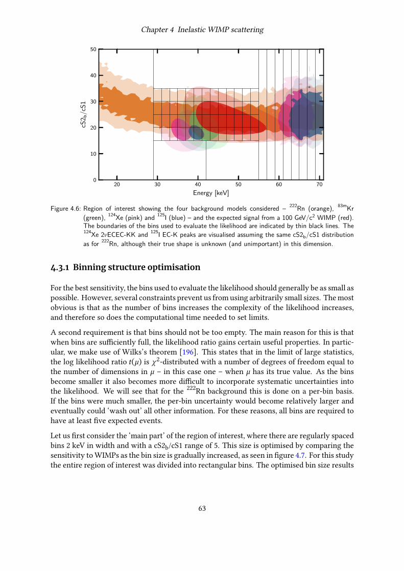
Chapter 4 Inelastic WIMP scattering
20 30 40 50 60 70
Energy [keV]
0
10
20
30
40
50
cS2 b
/cS
1
Figure 4.6: Region of interest showing the four background models considered – 222Rn (orange), 83mKr(green), 124Xe (pink) and 125I (blue) – and the expected signal from a 100 GeV/c2 WIMP (red).The boundaries of the bins used to evaluate the likelihood are indicated by thin black lines. The124Xe 2𝜈ECEC-KK and 125I EC-K peaks are visualised assuming the same cS2b/cS1 distributionas for 222Rn, although their true shape is unknown (and unimportant) in this dimension.
4.3.1 Binning structure optimisation
For the best sensitivity, the bins used to evaluate the likelihood should generally be as small aspossible. However, several constraints prevent us fromusing arbitrarily small sizes. Themostobvious is that as the number of bins increases the complexity of the likelihood increases,and therefore so does the computational time needed to set limits.
A second requirement is that bins should not be too empty. The main reason for this is thatwhen bins are sufficiently full, the likelihood ratio gains certain useful properties. In partic-ular, we make use of Wilks’s theorem [196]. This states that in the limit of large statistics,the log likelihood ratio 𝑡(𝜇) is 𝜒2-distributed with a number of degrees of freedom equal tothe number of dimensions in 𝜇 – in this case one – when 𝜇 has its true value. As the binsbecome smaller it also becomes more difficult to incorporate systematic uncertainties intothe likelihood. We will see that for the 222Rn background this is done on a per-bin basis.If the bins were much smaller, the per-bin uncertainty would become relatively larger andeventually could ‘wash out’ all other information. For these reasons, all bins are required tohave at least five expected events.
Let us first consider the ‘main part’ of the region of interest, where there are regularly spacedbins 2 keV in width and with a cS2b/cS1 range of 5. This size is optimised by comparing thesensitivity toWIMPs as the bin size is gradually increased, as seen in figure 4.7. For this studythe entire region of interest was divided into rectangular bins. The optimised bin size results
63

Chapter 4 Inelastic WIMP scattering
102 103 104
WIMP mass [GeV/c2]
0.0
0.1
0.2
0.3
0.4
0.5
Fra
ctio
nal
sens
itiv
ity
loss
Figure 4.7: Relative sensitivity loss as the size of bins is gradually increased. In each case the sensitivityis compared to that obtained with 56 1-keV-wide energy bins between 15 keV and 71 keV, and50 bins between 0 and 50 in cS2b/cS1. In purple: 28 × 25 bins, in red: 28 × 10 bins, in green:11 × 10 bins, and in orange: 11 × 5 bins. The black dotted line shows a projection onto energy,for comparison (i.e. 56 × 1 bins).
in roughly an 8% loss of sensitivity compared to the baseline (1 keV wide and a cS2b/cS1range of 1), which is considered acceptable.
The remaining structure in figure 4.6 can be explained as follows. At high energies (above71 keV), bins are divided only by energy, due to the lack of knowledge about the chargeand light yields for the 124Xe 2𝜈ECEC-KK and 125I EC-K peaks, as described in the previoussection. At low energies (below 15 keV) only a single large bin is used. This is becausethere is only one background present in that region (222Rn). Instead of being included in themain science likelihood, this bin is used to add a constraint to the 222Rn rate. This simplifiessensitivity estimation and provides a degree of protection against bugs (by ensuring the rateparameter remains within the central region of its constraint) without otherwise affectingthe result. Finally, at particularly low and high values of the ratio cS2b/cS1 (below 15 andabove 35), larger bins are used. This is to ensure the five-event criterion mentioned above ismet.
4.3.2 Systematic uncertainties
In this section we discuss the implementation of systematic uncertainties on each of themod-els in the likelihood. Most of the uncertaintes which are considered as nuisance parametersin the fit, which are summarised in table 4.4.
64

Chapter 4 Inelastic WIMP scattering
Table 4.4: Overview of parameters in the likelihood. Where a Gaussian constraint is included in the likelihoodfor that parameter, the mean and standard deviation of the constraint term are given. Theconstraint on the effective efficiency 𝜖eff varies between 0.936 ± 0.033 for 30 GeV/c2 WIMPs and0.936 ± 0.014 for 10 TeV/c2 WIMPs.
Symbol Constraint Description
𝜇Rn 1.00 ± 0.03 222Rn rate, relative to expectation from low-energy bin𝜇Kr – 83mKr rate𝜇Xe – 124Xe 2𝜈ECEC rate𝜇I – 125I EC rate𝜇WIMP – WIMP scattering cross-section, in units of 10−40 cm2
𝐸Xe,KK 64.3 ± 0.6 Mean energy of the 124Xe 2𝜈ECEC-KK peak, in keV𝜎Xe,KK 2.6 ± 0.3 Energy resolution for the 124Xe 2𝜈ECEC-KK peak, in keV𝐸I,K 67.3 ± 0.5 Mean energy of the 125I EC-K peak, in keV𝜎I,K 2.8 ± 0.5 Energy resolution for the 125I EC-K peak, in keVΔ𝑄EC𝑦 0.00 ± 0.66 Charge yield for KL and K relative to prediction, in quanta/keV𝜖eff Yes Effective efficiency𝜇2 7318 ± 42 Mean cS2b of inelastic ER, in photoelectrons
Data-driven backgrounds
Two of the backgrounds – the ER continuum due to 222Rn daughters and the 83mKr peak– are modelled using calibration data, in the former case combined with simulated data.Since these calibrations have finite statistics, there is an uncertainty on the number of eventsexpected in each bin. The proper way to treat these uncertainties is to say that there is a true,unknown model, which predicts the number of events in each bin of both the calibration andthe science data. This model should be determined by maximising the combined likelihoodlnℒ = lnℒscience + lnℒcalibration.
This procedure, commonly referred to as a combined fit, is also used for XENON1T searchesfor elastic WIMP scattering [140]. However, in that case an unbinned, not a binned, like-lihood is used and the uncertainties are not on the number of events in each bin but a setof physical parameters which describe the model. The problem here is that the combinedfit would include an additional 64 parameters: one per bin. Maximisation of the likelihoodwith so many parameters would be very challenging computationally, if not unfeasible. Asolution is provided by the method described in [197], which replaces this 64-dimensional fitwith 64 independent equations.
Turning now to the calibration datasets themselves, further simplification is possible. Firstly,the uncertainty in each bin arising from random fluctuations in the 83mKr calibration is nevermore than 0.4% of that from 220Rn calibration, so we can neglect any uncertainty in the 83mKrmodel. Secondly, at any given energy there are between 700 and 800 times as many simulated222Rn events as there are events in the 220Rn calibration data. It is therefore safe to ignore
65

Chapter 4 Inelastic WIMP scattering
uncertainties arising from the simulated data, and consider only the 220Rn calibration’s stat-istics. We are now at a point where there are only two datasets to include in the combinedfit: the science data itself and the 220Rn calibration. This allows a further simplification ofthe method from [197], since the 64 equations become analytic when there is only one cal-ibration source. They then manifest themselves as an analytic ‘adjustment’ to the per-binnumber of expected events in the 222Rn model, based on the distribution of events in thescience data. This adjustment is performed before maximising the likelihood.
Electron capture and double electron capture
The two backgrounds from 124Xe 2𝜈ECEC-KK and 125I EC-K have uncertainties coming fromhow well the energy scale and resolution of the detector are known. Writing these againexplicitly now, they enter the likelihood as
ℒ𝑋 = Gauss (𝐸𝑋 ||𝑋 , 𝛿𝐸𝑋 ) ⋅ Gauss (𝜎𝑋 |𝑋 , 𝛿𝜎𝑋 ) , (4.5)
where 𝑋 is either 2𝜈ECEC-KK or EC-K, 𝐸𝑋 is the mean energy of the corresponding peakin the energy spectrum and 𝜎𝑋 is its width, or energy resolution. Throughout this section,the notation refers to the best fit value of 𝑥 , from an independent measurement and 𝛿𝑥 toits uncertainty. The two decays’ expected mean energy and peak resolutions are as reportedin [129].
The dominant uncertainty in the models from 124Xe 2𝜈ECEC-KL and 125I EC-L is on the pre-dicted charge and light yields for both their decays and that of 83mKr. As we discussed insection 4.2, these impact the morphing procedure used to generate their expected distribu-tions. Given that signals from the two decays are generated via a very similar process, theuncertainties are assumed to be correlated between the two models. Therefore a single extraparameter, Δ𝑄EC𝑦 is introduced to the likelihood, along with a constraint term:
ℒ𝑄𝑦 = Gauss (Δ𝑄𝑦 ||0, 0.66) . (4.6)
This parameter describes an adjustment to the charge yield of the 2𝜈ECEC-KL and EC-Lpeaks, compared to the nominal value, with a simultaneous adjustment of −Δ𝑄EC𝑦 to thelight yield of each in order to preserve the total number of quanta. The origin of the value0.66 quanta/keV is described in section 4.2.
Signal model
As we saw in section 4.1, the shape of the expected dark matter signal depends on eighteenparameters. Including all of these in the likelihood fit would not be viable, both in terms ofcomputation time and the possibility of converging to a false (local) minimum. Instead, wetake each independently in turn, and investigate its effect on the parameter of interest: theinelastic cross-section.
66

Chapter 4 Inelastic WIMP scattering
µ1 µ2 σ1 σ2 ρ α ζ β γ δ κ η λ W g1 g2 pdpeδτe0
1
2
3
4
Eq
uiv
alen
tra
teu
nce
rtai
nty
[%]
Figure 4.8: Equivalent rate uncertainty for each parameter affecting the shape of the signal model, for30 GeV/c2 (red) and 100 GeV/c2 (purple) WIMPs. The first five parameters describe the elec-tronic recoil model; 𝛼–𝜆 describe the liquid xenon response to nuclear recoils and are definedin [140] and [136]; the remainder are detection-related: the work function, W, and the S1 andS2 gains, g1 and g2, were described in chapter 2, pdpe is the probability that a PMT emitstwo photoelectrons for a single incident photon, and 𝛿𝜏 e is the 2% uncertainty on the electronlifetime [140].
A collection of 100 simulated datasets, with no signal present, is produced by drawing eventsfrom the expected background distributions. Each signal model parameter is then taken inturn and three alternative signal models are computed, with the parameter at the best fit andvaried up and down by its uncertainty. A limit can then be set on the cross-section usingeach of these models, for all of the simulated datasets. We can therefore find an equivalentuncertainty on the signal rate 𝑟𝑗 for each parameter of its model, computed as the medianeffect of a one-sigma variation:
𝑟𝑗 =||||Median (𝑙
𝑗+1 − 𝑙 𝑗−12𝑙 𝑗0
)||||, (4.7)
where 𝑙 𝑗0/±1 is the limit set for a signal model in which parameter 𝑗 is set at its nominal valueor ±1𝜎 . Figure 4.8 shows the equivalent effect of the eighteen signal-model parameters fortwo different WIMP masses.
For low-mass WIMPs, the mean, 𝜇2, of the cS2b of the inelastic signal’s electronic recoil isdominant, with a 1𝜎 change resulting in a median of around a 5% difference in the limit. Thismakes some sense: for low masses the nuclear recoil only makes a minor contribution to thetotal signal (see figure 4.3), which is very similar to a pure 39.6 keV gamma-ray. The meanS2 of events from this gamma-ray strongly affects how will it can be distinguished from thenearby 83mKr peak and the 222Rn background. Due to its importance, 𝜇2 is included directlyin the likelihood fit with its constraint from the fit to neutron generator data as an additionalterm:
ℒ𝜇2 = Gauss (𝜇2|2, 𝛿𝜇2) . (4.8)
67

Chapter 4 Inelastic WIMP scattering
None of the other parameters reach this level of importance, and we therefore convert theminto an ‘effective rate uncertainty’. This parameter is essentially an additional scaling factorin the conversion from expected number of interactions in the TPC to expected number ofevents in the search data. Therefore, it has the same effect as an uncertainty on the efficiencyof the selection criteria, and we combine the two to produce the effective efficiency, 𝜖eff,which we encountered in equation 4.2, with the constraint
ℒ𝜖(𝜖eff) = Gauss (𝜖eff||| 𝜖, √𝛿𝜖2 +∑𝑟2𝑗 ) , (4.9)
where 𝜖 and 𝛿𝜖 are the estimated efficiency of the selection criteria and its uncertainty, re-spectively. The sum is over the seventeen remaining signal model parameters after excludingthe mean ER cS2b.
4.4 Results
Before unblinding the full dataset and computing a limit, three predefined checks were per-formed. These were designed to identify any mistakes or mis-modelling while there was stilltime to fix them without unnecessarily biasing the result.
The first check is to unblind only a selection of bins where no WIMP signal is expected.These are chosen to be any bins in which only 1% or less of the total expected number ofevents is fromWIMPs, if the cross-section is at the level of the 90% confidence upper limit setby XENON100 [198]. The 𝜒2 quality of fit of the data in these bins to the expectation is 21.5.This is compared to the 95th percentile of the expected distribution of 𝜒2 values, obtainedusing simulated datasets, which is 32.8. It is important to calculate the 95th percentile usingsimulated data instead of simply using the standard 𝜒2 distribution, because this simple testdoesn’t take into account variations of the nuisance parameters.
The second check involves maximising the likelihood using the full science dataset, butwithout looking at either the events themselves or the best-fit rate. Instead, we check howmuch each of the parameters which has a constraint term in the likelihood has been ‘pulled’.This is measured as its best-fit deviation from the nominal value, divided by the standarddeviation in the Gaussian constraint term: ( − )/𝛿𝑥 . Figure 4.9 shows the pull for eachrelevant parameter. It is clear that no parameter has been pulled very much from its nominalvalue (less than one standard deviation in every case). It is therefore unlikely that the resultis impacted by one of these being incorrectly modelled.
The final check is intended to protect against severe mis-modelling of the 2𝜈ECEC-KL andEC-L peaks. Since these are present at slightly lower energies than the expected signal, welook at the region between 29 keV and 35 keV. This contains a significant fraction of thetwo background peaks but no part of the central 2𝜎 region of the expected signal. Again wecompare the 𝜒2 quality of fit, 9.9, against the 95th percentile of the expected distribution, inthis case 18.2.
68

Chapter 4 Inelastic WIMP scattering
µRn EXe,KK σXe,KK EI,K σI,K ∆QECy
εeff µ2−3
−2
−1
0
1
2
3
Pu
ll
Figure 4.9: Parameters’ best-fit values, using the full unblind dataset, relative to their nominal values, meas-ured in number of standard deviations.
The unblinded data is shown in figure 4.10, compared to the background-only expectation:the expected number of events when the signal rate is set to zero and all nuisance parametersfit to the data. Using this data, an upper limit is placed on the cross-section for inelasticWIMP-129Xe scattering, at 90% confidence level. This can be seen in figure 4.11, where it isalso compared to the upper limit reported by the XMASS collaboration in [199]. The upperlimit from this analysis is the most sensitive forWIMPs heavier than 100 GeV/c2, and reaches3.3 × 10−39 cm2 for a mass of 130 GeV/c2. Because of the lower expected event rate and theless efficient discrimination between electronic recoil backgrounds and the expected signal,the upper limit is not as strong as for the search for spin-dependent elastic scattering, wherethe strongest limit of 6.3 × 10−42 cm2 is set for 30 GeV/c2 WIMP-neutron scattering.
Also visible in figure 4.11 is the expected range of upper limits. This is determined by sim-ulating datasets from the best-fit models, with no signal. The illustrated 1𝜎 and 2𝜎 bandscorrespond to the central 68% and 95% ranges of limits computed for these datasets.
Especially around 50 GeV/c2, there is a maximum of a roughly 2𝜎 upwards fluctuation ofthe limit. However, there is no significant (3𝜎 ) evidence of an excess and we therefore onlyreport an upper limit. That no particularly large excesses are visible in figure 4.10 suggeststhat this limit is produced by a genuine signal-like-nature of the dataset rather than a mis-modelling of one or more of the backgrounds. Figure 4.12 suggests the same; here, the binsare arranged according to their sensitivity to WIMP scattering, quantified by the expectedsignal content divided by the square root of the expected background.
In summary, the search for spin-dependent inelastic WIMP scattering using a 0.89 t yr ex-posure of XENON1T is the most sensitive search for this process to date, and the upper limitis the strongest for a wide range of WIMP masses.
69

Chapter 4 Inelastic WIMP scattering
30 35 40 45 50 550
5030 < cS2b/cS1 < 35
30 35 40 45 50 550
200
25 < cS2b/cS1 < 30
30 35 40 45 50 550
500
20 < cS2b/cS1 < 25
30 35 40 45 50 550
500 15 < cS2b/cS1 < 20
0
100 35 < cS2b/cS1 < 50
30 35 40 45 50 550
100
cS2b/cS1 < 15
55 60 65 700
50
100
150
200
250
300
Nu
mb
erof
even
ts
0.0 0.2 0.4 0.6 0.8 1.0
Energy [keV]
0.0
0.2
0.4
0.6
0.8
1.0N
um
ber
ofev
ents
Figure 4.10: Observed events in the full 0.89 t yr exposure shown as black error bars. The backgroundexpectation, from the likelihood best-fit, is shown in grey and the expected signal for a 50 GeV/c2
WIMP is shown in red, normalised to a cross-section of 10−37 cm2. The five histograms between29 keV and 55 keV correspond to the cS2b/cS1 bins used for the likelihood, which can be seenin figure 4.6.
102 103 104
WIMP mass [GeV/c2]
10−39
10−38
10−37
10−36
Cro
ss-s
ecti
on[c
m2]
XENON1T (2020)XMASS (2019)XENON100 (2017)
Figure 4.11: Limit on the cross-section of inelastic WIMP scattering off 129Xe, set using XENON1T data(black line) and the 1𝜎 and 2𝜎 range of expected limits (light and dark red shading, respect-ively). The limit is compared to those reported by the XMASS collaboration [199] (blue) andXENON100 [198] (green).
70

Chapter 4 Inelastic WIMP scattering
Increasing signal content0
500
1000
1500
2000
Nu
mb
erof
even
ts
Figure 4.12: Observed events after grouping the bins according to their sensitivity to inelastic scattering of50 GeV/c2 WIMPs. This is quantified using the ratio between the expected number of signalevents and the square root of the expected number of background events. The colours have thesame meaning as figure 4.10, but the signal is included in the fit and depicted with its best-fitrate. This grouping shows the origin of the 2𝜎 upwards fluctuation of the limit, as comparedto the expected range: there is a roughly 1𝜎 excess in the final bin, and roughly 2𝜎 in thepenultimate bin.
71

Chapter 5
PMT testing
The ‘eyes’ of XENONnT are its PMTs. These are what detect the tiny flashes of scintilla-tion light – often only a few photons in the S1 – expected from a dark matter interaction.PMTs are a relatively old and simple technology, first invented in 1935 [200]. Nevertheless,more modern alternatives such as silicon photomultipliers have not yet managed to achievecomparable performance for low-rate experiments, although there is considerable researchinterest [144, 201, 202].
The PMTs used for both XENON1T and XENONnT are the R11410, manufactured by Hama-matsu. This 3” model was developed specifically for use in liquid xenon experiments, withan operating temperature range of −110 ∘C to 50 ∘C and maximum pressure of 3 bar. Previousstudies have shown stable operation in the conditions typically encountered in dual-phasexenon TPCs [203].
The R11410 is available in a variety of versions, which are the result of iterative improve-ments, after collaboration between both the LUX and XENON collaborations and Hama-matsu [204, 205]. The specific model used by XENONnT is the R11410-21, which uses ex-tremely low radioactivity materials. In particular, the radioactivity of the ceramic stem, usedto insulate the various dynode connections, was minimised. The PMT body is construc-ted from Kovar, an iron-nickel-cobalt alloy which has a high magnetic permeability. Thiseffectively shields external magnetic fields which could otherwise affect the PMT’s opera-tion [206].
Of the 494 PMTs needed to instrument XENONnT’s TPC, only 153 were used in XENON1T.Due to a relatively high rate of failure (79 of the 248 PMTs) during the operation of XENON1T,the new PMTs for XENONnT were tested much more thoroughly before installing them.Every photomultiplier was operated at cryogenic temperatures in both gaseous and liquidxenon. This was intended to simulate the conditions for PMTs used in both arrays of XEN-ONnT – the top PMT array being above the liquid-gas interface. While cold, a variety of testdatawas collected for every PMT. The aim of this processwas firstly to identify severely prob-lematic PMTs which could not be considered for use in the detector, secondly to search forwarning signs that could point to problems developing during future operation, and thirdlyto provide a ranking of which of the ‘acceptable’ PMTs would be most preferred for eventualuse.
72

Chapter 5 PMT testing
The testing was carried out at three institutes, the Max Planck Institute for Nuclear Physicsin Heidelberg, Stockholm University and the University of Zurich, the last two of whichhave facilities for cryogenic xenon testing. In this chapter, after an introduction to PMTs, wefocus on the procedure used in Zurich, where in total 105 PMTs were tested, and the resultsobtained there. At the end of the chapter we look at these results in the context of the overalltesting campaign and its implications for XENONnT.
5.1 Photomultiplier tubes
Conceptually, a photomultiplier tube can be thought of in two parts. The first is the pho-tocathode, where incident photons are converted into electrons via the photoelectric effect.The second is an amplification stage, where the electron signal is multiplied by a factor ofseveral million in order to output a measurable charge. We will treat each of these in turn.
5.1.1 Photocathode
The most important property of a photocathode is its quantum efficiency: the probabilitythat when a photon reaches it, a photoelectron is released. This tends to prefer materialswith a low work function, although with a lower work function there will also be a greaterrate of thermal electron emission. Operating PMTs at low temperature reduces the latter. Forthe R11410, a bialkali (antimony-potassium-caesium) photocathode was developed by Hama-matsu [207]. This has a particularly high quantum efficiency for the low vacuum ultraviolet(VUV) wavelength of xenon scintillation light: 175 nm. According to the specification agreedbetween the XENON collaboration and Hamamatsu this is a minimum of 28%, but we find amuch higher average value of 34% for the PMTs purchased for XENONnT.
In general, a single photoelectron is emitted per incident photon. It is also possible, however,for two photoelectrons to be emitted. This is known as double photoelectron emission, andhappens for just over one fifth of emitted photoelectrons in the case of the R11410 [208].
A second property of a good photocathode is low resistance. In order to ensure a linear PMTresponse, all components must have low resistance. This is most important in the last stagesof the dynode chain, as we will see later, but also relevant for the photocathode. Unlike thedynodes, the alkali metals used for this are chosen primarily for their work function andspectral response, not their resistivity. By adding a small amount of bismuth Hamamatsuwas able to decrease the resistivity of the R11410-21’s photocathode material.
5.1.2 Dynode design
In order to produce a measurable charge from a single photoelectron, repeated stages ofelectron acceleration which induces secondary electron emission are used. This happens inthe dynode chain, a series of usually around ten electrodes. Each dynode is held at around
73

Chapter 5 PMT testing
Table 5.1: Dynode voltages recommended by Hamamatsu for operation of an R11410-21 PMT, assuming aphotocathode (K) voltage of −1500 V and a grounded anode (P).
Dynode voltage [V]K 1 2 3 4 5 6 7 8 9 10 11 12 P
−1500 −1176 −1054 −892 −811 −730 −649 −568 −486 −405 −324 −243 −122 0
Difference from previous dynode [V]
+324 +122 +162 +81 +81 +81 +81 +81 +81 +81 +81 +122 +122
100 V higher potential than the last. Electrons are accelerated into every dynode in turn.Here, secondary emission of additional electrons (proportional to the number of incidentelectrons) results in a multiplication of the signal. The final electrode, the anode, is designedto collect the charge signal, which by then has been amplified by a factor of typically severalmillion.
The relative voltages between the various dynodes are optimised by the manufacturer. Therecommended voltages for the R11410 PMTs used by XENONnT are shown in table 5.1. Thegeneral trend here is similar for many PMTs: the first few and last few dynodes are separatedby a greater potential difference than most. The reason for this can easily be explainedqualitatively, as found in [209], for example, and summarised here. At each dynode stage,some of the electrons might escape and either be lost completely or skip straight to thefollowing stage. If this happens to the photoelectron at the first dynode, no signal will beproduced at the anode. This potential signal loss is represented by the collection efficiency,which is around 90% for the R11410 [206]. Even in the second and third stages, it is especiallyimportant for the electrons to reach every dynode. There are fewer electrons propagatinghere, so random effects are not averaged out so effectively and fluctuations impact the overallresolution more severely.
The last few stages also benefit from a higher voltage difference, for a different reason. Thesestages are where the number of electrons is largest. Space-charge effects, or the effect on thepropagating electrons of their own electric field, are most severe. By increasing the externalelectric field, the relative effect of these can be minimised. This helps to ensure a constantamplification factor for a wide range of signal sizes, or in other words a linear response.
Linearity is important for accurate event reconstruction, especially for determining events’energies. As we saw in chapter 2, the energy deposited in an interaction can be found froma linear combination of the S1 and S2 signals. This computation becomes substantially moreinvolved if the signal measurement itself is non-linear. For analysing XENON1T’s data, a ‘de-saturation correction’ was used for high energy events (although the limited dynamic rangeof the digitisers was the dominant effect on linearity, not the PMTs). However, this involvedessentially discarding much of the information from the most illuminated photomultipliersand replacing it with a template [174]. This loss of information inherently leads to a lowerenergy resolution than might otherwise be achievable.
74
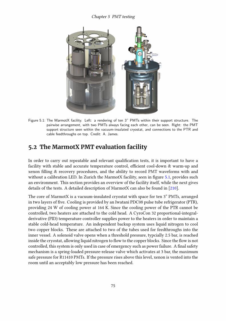
Chapter 5 PMT testing
Figure 5.1: The MarmotX facility. Left: a rendering of ten 3” PMTs within their support structure. Thepairwise arrangement, with two PMTs always facing each other, can be seen. Right: the PMTsupport structure seen within the vacuum-insulated cryostat, and connections to the PTR andcable feedthroughs on top. Credit: A. James.
5.2 TheMarmotX PMT evaluation facility
In order to carry out repeatable and relevant qualification tests, it is important to have afacility with stable and accurate temperature control, efficient cool-down & warm-up andxenon filling & recovery procedures, and the ability to record PMT waveforms with andwithout a calibration LED. In Zurich the MarmotX facility, seen in figure 5.1, provides suchan environment. This section provides an overview of the facility itself, while the next givesdetails of the tests. A detailed description of MarmotX can also be found in [210].
The core of MarmotX is a vacuum-insulated cryostat with space for ten 3” PMTs, arrangedin two layers of five. Cooling is provided by an Iwatani PDC08 pulse tube refrigerator (PTR),providing 24 W of cooling power at 164 K. Since the cooling power of the PTR cannot becontrolled, two heaters are attached to the cold head. A CyroCon 32 proportional-integral-derivative (PID) temperature controller supplies power to the heaters in order to maintain astable cold-head temperature. An independent backup system uses liquid nitrogen to cooltwo copper blocks. These are attached to two of the tubes used for feedthroughs into theinner vessel. A solenoid valve opens when a threshold pressure, typcially 2.5 bar, is reachedinside the cryostat, allowing liquid nitrogen to flow to the copper blocks. Since the flow is notcontrolled, this system is only used in case of emergency such as power failure. A final safetymechanism is a spring-loaded pressure-release valve which activates at 3 bar, the maximumsafe pressure for R11410 PMTs. If the pressure rises above this level, xenon is vented into theroom until an acceptably low pressure has been reached.
75

Chapter 5 PMT testing
The internal environment is monitored by eight Pt100 temperature sensors at a variety ofdepths and a vacuum pressure gauge. These are read out by custom software running onlinux. During operation the cold head temperature is generally chosen such that the internalpressure is ∼2.3 bar. This is close to the pressure experienced by PMTs in the bottom arrayof XENONnT.
An Iseg EDS-F-130n 16-channel high voltagemodule provides up to −3 kV to power the PMTs.PMT waveforms are recorded at a sampling rate of 100 MHz by two CAEN V1724 digitisers,after amplification by a factor of ten with a Philips 776 amplifier. An additional copy of theamplified signal is fed into a CAENN845 discriminator, whose output passes to a CAENV260scaler. The discriminator threshold is set to 11 mV, roughly half the amplitude of a singlephotoelectron signal from a PMT operated with a gain of 5 × 10⁶. The scaler is used to gainan accurate measurement of the total rate of signals from each PMT. A blue LED, within thecryostat, is used in conjunction with a pulse generator for calibrating PMTs.
The two layers of PMTs are arranged in pairs, one above and one below. Within a pair,the two PMTs are facing one another (window-to-window) and separated by only a smallgap. The PTFE plate betweeen the two layers, which acts as both a reflector and spacer, hascircular holes to ensure that paired PMTs can see one another. This is intended to ensurethat light emitted by one PMT can be seen by its partner, as detailed in section 5.3.1.
5.3 The XENONnT PMT testing campaign
All the new PMTs (those which were not used for XENON1T) were tested in liquid xenon,either at Stockholm University of the University of Zurich. A subset of those tested in Stock-holm were also tested at the Max Planck Institute for Nuclear Physics in Heidelberg, wherea cold nitrogen/argon facility is used instead. The focus of the Heidelberg tests was slightlydifferent, with the possibility to characterise properties such as the transit-time spread. Amanuscript providing an overview of the full testing campaign at all three centres is beingprepared; here we concentrate only on the tests performed with MarmotX at the Universityof Zurich.
During each test cycle, the MarmotX cryostat, with ten PMTs to be tested, was cooled downtwice. The first time, the inner cryostat vessel was filled with sufficient liquid xenon tocompletely cover both layers of photomultipliers (19 kg). The second time, only a smallamount of liquid xenon was filled so that the PMTs were in a gaseous xenon atmospherevery close to the phase transition temperature. These two conditions should mimic thosefor PMTs in the bottom and top arrays, respectively, when they are being operated in theXENONnT dual-phase TPC.
In both cases the cryostat was held at a constant (cold) temperature for one week beforewarming up and extracting the xenon. During that time a variety of diagnostic tests werecarried out, which are discussed in the remainder of this section. The aim of those tests wasto identify which photomultipliers are suitable to be used in XENONnT, avoiding any that
76

Chapter 5 PMT testing
may cause problems for stable operation.
5.3.1 Light emission
Light emission is a process whereby a PMT can produce individual photons, at a wavelengthsuch that the PMTs themselves are sensitive to it. Previous studies have shown that this canbe observed in R11410 PMTs [80, 211, 212]. The origin of light emission is not conclusivelyunderstood, but Hamamatsu have suggested that it may be the result of charge-up of thePMT’s ceramic stem [213]. The light can either be seen by the same PMT in which it isproduced (effectively a form of dark count) or by another one. Some degree of light emis-sion is present in all PMTs but the rate varies considerably. If the rate is too high, multiplePMTs may observe these small signals in coincidence and they could appear like a scintilla-tion signal. This could produce an additional background to searches for rare, low-energyinteractions.
We identify two categories of light emission. Micro light emission is a relatively small rate ofsingle photon emission. This happens continuously while a PMT is turned on and affects allPMTs, although to differing degrees. The rate of micro light emission depends on both thetemperature and the voltage that a PMT is operated at [211].
Certain PMTs exhibit a second kind of behaviour, whereby they emit light at a much greaterintensity but not continuously. This can be in the form of flashes, as identified in [150].These can be identified by sudden increases in the trigger rate of all PMTs (but especiallythe one which is flashing), followed by an exponential decrease lasting several minutes orhours. The origin of flashes is not fully known, but it is thought to involve discharges withinthe PMT [212]. Alternatively, PMTs can have intermittent light emission, meaning there areextended periods (several hours or days) during which they emit high intensity light, butwithout a characteristic exponential drop-off. Both cases are often induced by bright illu-mination – in XENON1T this was often due to a muon interacting in the TPC [80] – but canalso occur apparently spontaneously.
We performed a dedicated test to detect micro light emission, described in the following.Imagine we want to test a certain PMT (labelled here as PMT A) for light emission. Wemeasure the trigger rate in the PMT which is facing it (PMT B), as we adjust the powersupply voltage of PMT A. If we see that the the trigger rate of PMT B decreases while weturn down the voltage supplied to PMT A, we can conclude that the difference in triggerrate is due to light emitted by PMT A. To quantify the amount of micro light emission, werecord the difference in PMT B’s trigger rate when PMT A’s supply voltage is increased from900 V to 1500 V. It is difficult to convert this into an absolute measure, since it depends on thequantum efficiency of PMT B as well as geometrical effects. Nevertheless, this is sufficient forcomparing PMTs and identifying those with unusually high emission rates. Previous testingcampaigns defined the amount of light emission slightly differently, as the rate differencebetween 0 V and 1500 V [150]. However, we observed a slight increase below around 900 V,presumably due to sparking between the two PMTs, and therefore use this measure instead.
77

Chapter 5 PMT testing
10−1 100 101 102 103 104
Trigger rate difference [Hz]
0
5
10
15
20
25
30E
ntr
ies
0.9 1.0 1.1 1.2 1.3 1.4 1.5
Power supply voltage [kV]
50
60
70
80
Op
pos
ite
PM
Ttr
igge
rra
te[H
z]
Figure 5.2: Left: distribution of PMTs’ micro light emission rates, defined as the difference in rate (seenby the opposite PMT) between 0.9 kV and 1.5 kV operating voltage. Right: example of anindividual measurement, showing the opposite PMT’s trigger rate as a function of the operatingvoltage.
The micro light emission distribution for all PMTs tested in Zurich is shown in figure 5.2,together with an example of the measurement for a particular PMT. The worst PMTs, withrates of several hundred Hz or more, were not used in the XENONnT PMT arrays.
Strong light emission can spontaneously begin at any time. For that reason, the trigger rateof all PMTs is continuously monitored while they are being tested, for a total of at least twoweeks, and checked for unexplained increases. It can also be induced, and we therefore alsoperform a ‘stress test’ twice for each PMT: once in liquid and once in gaseous xenon. Thisis designed to simulate the most intense light that PMTs experienced in XENON1T, which isduring 220Rn calibrations. The stress test consists of two twelve-hour long periods. Duringthe first, the PMTs are illuminated with short (i.e. S1-like) light pulses creating signals ofa few hundred photoelectron signals. The second twelve hours is intended to represent S2signals, and the PMTs are illuminated with 2 µs pulses creating around 104 photoelectrons.
Figure 5.3 shows an example of intermittent light emission, occurring during a stress test. Inthis case, one of the PMTs begins emitting light around ten hours after the start of the stresstest, which is seen by the opposite PMT at a high rate. Towards the end of the test, all PMTstrip. This is presumed to be due to sudden bright illumination, most likely from the light-emitting PMT. All PMTs are turned back on at the end of the stress test, and light emissioncontinues. In order to verify which is the light emitting PMT, it and the PMT opposite it areeach turned off in turn. When the opposite PMT is turned off, only its trigger rate decreases.On the other hand, when the light emitting PMT is turned off, both trigger rates decreasesignificantly.
In total we observed four such cases of intermittent light emission out of the 105 PMTs tested.For three of these it was possible to identify a period of LED illuminationwhich first triggeredthe light emission. In the other case, the light emission appeared to begin spontaneously, butbecamemuchworse following a stress test. Of the four, two displayed sufficiently strong light
78

Chapter 5 PMT testing
0 5 10 15 20 25 30 35 40
Time [hours]
0
10000
20000
30000
40000
50000
60000
70000
80000T
rigg
erra
te[H
z]
LED on
Light emmitting PMT
Opposite PMTNormal PMT
Trip
23.50 23.75 24.00 24.25 24.50 24.750
10000
20000
30000 Zoom
Figure 5.3: Intermittent strong light emission, beginning during a stress test in liquid xenon. The lightemitting PMT (purple) shows the highest trigger rate, and significant light is also seen by thePMT facing it (red), whereas another separate PMT (green) sees only little light. The grey shadedregion indicates the time that the LED was turned on (pulsed). This includes a short period oflower-intensity illumination, for afterpulse characterisation, followed by the higher-intensity stresstest. The inset shows a zoom into the time when the light emitting PMT and the one oppositeit were turned off in turn.
emission that they were not considered for XENONnT.
5.3.2 Afterpulses
It is well known that PMTs can produce additional signals shortly after the usual pulse fromincident photons. These are referred to as afterpulses. A variety of types of afterpulse, withdistinct origins, have been proposed. These include elastic scattering of electrons off thefirst dynode [209] and electron-induced luminescence within the dynode chain [214], butboth of these produce only fairly small afterpulses soon after the main peak and they areunimportant for us. Here we concentrate on afterpulses produced by ionisation of residualgases in the PMT vacuum.
If a photoelectron encounters an atom of gas between being emitted from the photocathodeand reaching the first dynode, it can ionise it. The positively charged ion will then drift backtowards the photocathode and upon impact releases several electrons. For the electric po-tential present in PMTs such as the R11410 (𝑉 ∝ 𝑠2, where 𝑠 is distance from the cathode), thetime take for an ion to reach the cathode is almost independent of where it is produced [150],and is given by:
𝑡 = 1.134V1/2 µs cm−1√𝐿2𝑉0
𝑀𝑄 , (5.1)
where 𝐿 is the distance between the photocathode and first dynode, 𝑉0 is the voltage differ-ence between the photocathode and first dynode and𝑀/𝑄 is the mass-to-charge ratio of the
79

Chapter 5 PMT testing
ion, measured in atomic mass units per elementary charge.
In themselves, afterpulses pose only a minor problem for the experiment, provided that theyare properly accounted for when modelling the detector’s response. However, during theoperation of XENON1T, it was observed that PMTs with especially large afterpulse rates aremore susceptible to flashing than others [80]. In the more severe cases this required the PMTto be turned off. Furthermore, the afterpulse rate can increase over time if xenon is able toleak inside the PMT. This was also observed in XENON1T, and indeed most PMTs whichhad to be turned off showed evidence of a leak. A major aim of the testing campaign wastherefore to identify any leaky PMTs.
Given that xenon has such a low natural abundance in air, there is no reason for xenoncontamination to be present after the PMTs have been manufactured. We can safely assumethat any xenon-related afterpulse, even at a small rate, indicates that xenon leaked into thePMT during the test. This idea, of using afterpulses to check for leaks, has been used beforeby both XENON1T and PandaX-I [150, 212].
In order to characterise a PMT’s afterpulsing, we illuminate it with a reasonably large pulse oflight from the LED. The larger the pulse, the better the sensitivity, since each photoelectron inthe main signal can independently produce an afterpulse. All PMT signals in a 5 µs windowafter the main pulse are recorded.
The afterpulse characteristics of a PMT are often represented as a two-dimensional histogramwith the time delay between themain LED signal and the afterpulse on the 𝑥-axis and the areaof the afterpulse, in photoelectrons, on the 𝑦-axis. An example, for a leaky PMT, can be foundin figure 5.4. Three categories of afterpulses can be identified, which are labelled A1, A2 andA3 in [150]. There are small afterpulses with a charge of 𝒪(1 pe) present at all times (A2). Atsmall delay times the tail of a second population (A1) of small afterpulses is visible. Theseare possibly due to back-scattering of electrons off the first dynode or photoluminescence, asmentioned above. Most afterpulses of this latter type are not visible, since their delay timeis so small that they overlap with the main signal.
The third category (A3) is most interesting for this study, and consists of substantially largerafterpulses. These are found at characteristic delay times in the microsecond range, and aredue to ionisation of residual gases. The upper 𝑥-axis of figure 5.4 indicates the mass-to-charge ratio of the ions which would be expected to cause afterpulses at each time delay. Axenon afterpulse is clearly visible at a delay time of ∼2.7 µs.In order to search for and quantify the size of xenon afterpulses, we first select only thosesignals with an area of at least 2 pe. By doing this, most of the population of small afterpulsescan be removed while keeping most ion-induced signals.
A histogram of the remaining afterpulses’ time delays is then produced (as in figure 5.5, forthe same example PMT as before). The region where a xenon afterpulse would be expectedis fit with a Gaussian peak on top of a linear background. This doesn’t perfectly describethe data in every case, since there is a complex background of afterpulses at all time delays,whose shape varies from PMT to PMT. However, it is sufficient for identifying leaky PMTs,
80
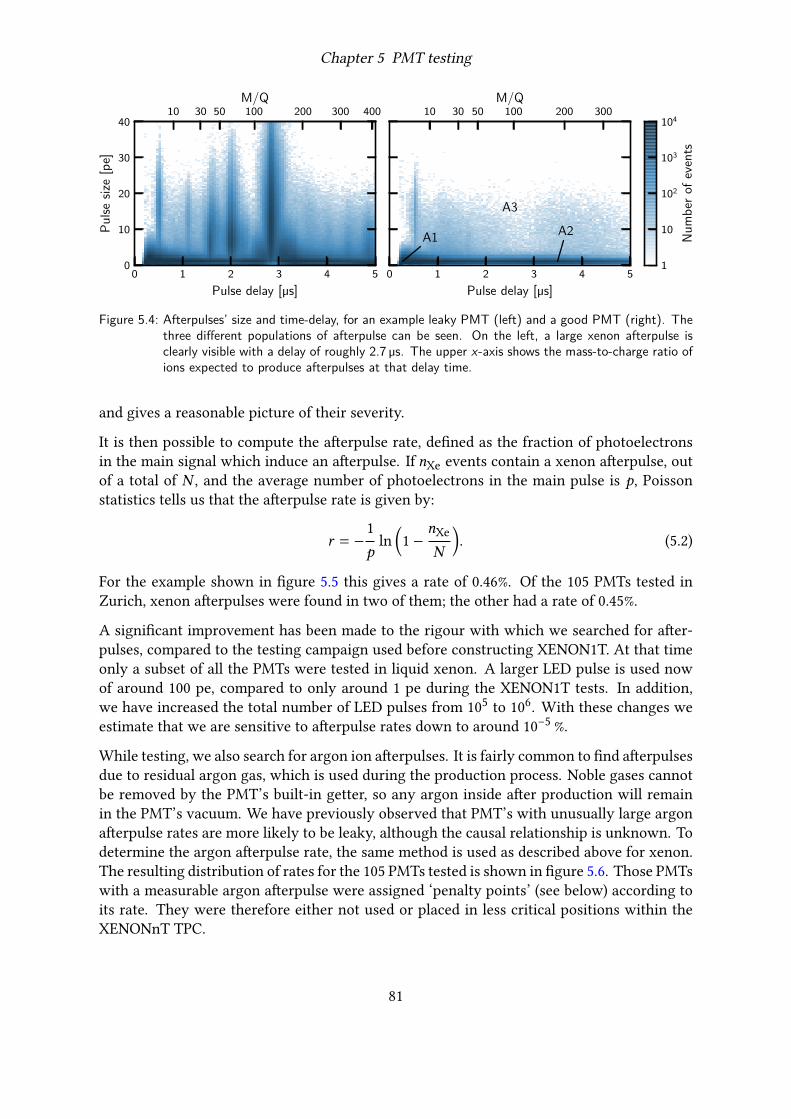
Chapter 5 PMT testing
10 30 50 100 200 300 400M/Q
0 1 2 3 4 5
Pulse delay [µs]
0
10
20
30
40
Pu
lse
size
[pe]
10 30 50 100 200 300M/Q
0 1 2 3 4 5
Pulse delay [µs]
A1 A2
A3
1
10
102
103
104
Nu
mb
erof
even
ts
Figure 5.4: Afterpulses’ size and time-delay, for an example leaky PMT (left) and a good PMT (right). Thethree different populations of afterpulse can be seen. On the left, a large xenon afterpulse isclearly visible with a delay of roughly 2.7 µs. The upper x-axis shows the mass-to-charge ratio ofions expected to produce afterpulses at that delay time.
and gives a reasonable picture of their severity.
It is then possible to compute the afterpulse rate, defined as the fraction of photoelectronsin the main signal which induce an afterpulse. If 𝑛Xe events contain a xenon afterpulse, outof a total of 𝑁 , and the average number of photoelectrons in the main pulse is 𝑝, Poissonstatistics tells us that the afterpulse rate is given by:
𝑟 = −1𝑝 ln (1 − 𝑛Xe
𝑁 ). (5.2)
For the example shown in figure 5.5 this gives a rate of 0.46%. Of the 105 PMTs tested inZurich, xenon afterpulses were found in two of them; the other had a rate of 0.45%.
A significant improvement has been made to the rigour with which we searched for after-pulses, compared to the testing campaign used before constructing XENON1T. At that timeonly a subset of all the PMTs were tested in liquid xenon. A larger LED pulse is used nowof around 100 pe, compared to only around 1 pe during the XENON1T tests. In addition,we have increased the total number of LED pulses from 105 to 106. With these changes weestimate that we are sensitive to afterpulse rates down to around 10−5 %.
While testing, we also search for argon ion afterpulses. It is fairly common to find afterpulsesdue to residual argon gas, which is used during the production process. Noble gases cannotbe removed by the PMT’s built-in getter, so any argon inside after production will remainin the PMT’s vacuum. We have previously observed that PMT’s with unusually large argonafterpulse rates are more likely to be leaky, although the causal relationship is unknown. Todetermine the argon afterpulse rate, the same method is used as described above for xenon.The resulting distribution of rates for the 105 PMTs tested is shown in figure 5.6. Those PMTswith a measurable argon afterpulse were assigned ‘penalty points’ (see below) according toits rate. They were therefore either not used or placed in less critical positions within theXENONnT TPC.
81

Chapter 5 PMT testing
10 30 50 100 200 300 400M/Q
0 1 2 3 4 5
Pulse delay [µs]
102
103
104
105
106
Nu
mb
erof
even
ts
Good PMT
Leaky PMT
Xe+Ar+ Xe++
Figure 5.5: Example afterpulse time-delay distributions, for the same leaky PMT (purple) and good PMT(red) as in figure 5.4. The best-fit model for the peak due to Xe+ ions is shown as a thick, lightpurple line. Prominent peaks are labelled according to their expected delay times.
0.00 0.05 0.10 0.15 0.20
Argon afterpulse rate [%]
0
10
20
30
40
50
60
70
Nu
mb
erof
PM
Ts
Figure 5.6: Distribution of fitted argon afterpulse rates of all PMTs tested in Zurich.
82

Chapter 5 PMT testing
Table 5.2: Summary of main problems identified in the new PMTs for XENONnT during the testing cam-paign.
Tested Leak identified Strong light emission Other problemIn total 368 13 11 2Tested at UZH 105 2 2 1
5.4 Summary
In total 368 new PMTs were tested for XENONnT, 105 of which at the University of Zurich.Each PMT was tested over a period of at least one week in liquid xenon followed by anotherweek in gaseous xenon. This mimicked the conditions for the bottom and top PMT arraysin a dual-phase XENON TPC.
During the test, particular attention was paid to two known potential problems: light emis-sion and afterpulsing, especially that related to xenon atoms in the vacuum which indicatesleaks. Table 5.2 summarises the PMTs which ‘failed’ the test – those with severe enoughproblems to immediately be removed from consideration for use in the XENONnT TPC.
The PMTs were tested much more thoroughly than they were for XENON1T, when only aselection were tested in xenon. We estimate that we are sensitive to xenon-related afterpulserates on the order of 10−5 % or larger. This would be sufficient to detect the smallest identifiedleaks in XENON1T PMTs, over the course of the two weeks in xenon. Although we cannotrule out the possibility that new leaks opened between the tests and installation in XENON1T,this gives us confidence that the overall fraction of leaky PMTs will be substantially smallerin XENONnT.
Two PMTs were rejected because we were unable to power them on, due to an extremelyhigh leakage current. These PMT was presumably damaged between being produced andarriving at their respective testing facilities.
For the remaining 342 PMTs, a system of ‘penalty points’ was developed to describe their per-formance overall. Each problem was assigned a certain number of points, including microlight emission, low-rate intermittent light emission and larger than average argon afterpulserates. In addition, points were given to PMTs which were manufactured in batches contain-ing several other PMTs which had developed serious problems. After removing those withserious problems, 197 PMTs from XENON1T were also included in this penalty point sys-tem (including 32 which were spare). The overall distribution of penalty points is shown infigure 5.7. In total, 497 PMTs had at most 2.0 penalty points; 494 of these were selected tobe used for the XENONnT PMT arrays. The number of penalty points was also consideredwhen arranging the PMTs within the two arrays. In the next chapter, we will see details ofthe construction and installation of the PMT arrays and their associated cabling.
83

Chapter 5 PMT testing
0.0 0.5 1.0 1.5 2.0 2.5 3.0
Penalty points
0
50
100
150
200
Nu
mb
erof
PM
Ts
Figure 5.7: Distribution of penalty points awarded to all PMTs, including those left over from XENON1T aswell as those acquired for XENONnT, whose testing is described in this chapter.
84

Chapter 6
XENONnT
The next stage in the XENON programme is XENONnT, an evolution of XENON1T, which isbeing commissioned as this thesis is being written. When XENON1Twas designed, attentionwas already being paid to a possible future upgrade, with a significantly larger amount ofxenon. The total amount of xenon will be 8.4 tonnes, or 2.6 times as much as before, and theincrease in size of the TPC itself is even greater, from 2.0 t to 5.9 t of instrumented xenon. Inaddition to themuch larger TPC, a new neutron veto and radon distillation systemwill enableimproved nuclear recoil background rejection and decrease the electronic recoil backgroundrate, respectively.
In this chapter we will first see an overview of XENONnT, concentrating on what is newand what is needed to make sense of the rest of this chapter. More details can be foundin [99]. Then we will move on to some details of the PMT arrays and cabling, starting withan overview of the bases’ design, before discussing their production and preparation for in-stallation in XENONnT. Later in the chapter is information about the cabling which connectsthese bases to the data acquisition system, in the service building adjacent to XENON’s wa-ter tank. Finally we will see some details of the assembly and installation of the PMT arraysand related cabling, now undergoing commissioning at LNGS. Here we attempt to includesufficiently detailed information to be useful as documentation of the cabling while avoidingunnecessary minutiae.
6.1 Overview of XENONnT upgrade
The following presents only a summary of the most important aspects of the XENONnTupgrade. By increasing the sensitivemass by almost a factor of three, the fiducial volume usedfor analysis may be almost four times as large. Much of the infrastructure from XENON1T isbeing reused, thus accelerating and simplifying the upgrade: the cryogenic and purificationsystems are being kept with a few important upgrades, the water tank and muon veto areunchanged (but see details of the neutron veto below), and the diameter of the outer cryostatis the same so that the old vessel can be reused with a simple extension.
A new neutron veto system in XENONnT will make it possible to reduce the nuclear re-coil background significantly, providing an 87% efficiency for tagging neutrons which have
85

Chapter 6 XENONnT
scattered once in the TPC. The neutron veto is based on the same technology as the existingmuon veto, with 0.2% gadolinium ions being added to the water. An inner region of the wa-ter tank will be optically isolated using expanded PTFE (ePTFE) reflectors, and instrumentedwith 120 eight-inch photomultipliers to detect the Čerenkov light which eventually followsneutron capture by gadolinium [215].
As already mentioned, the cryogenic and purification systems from XENON1T are largelybeing inherited, but some significant improvements have been made. These include newmagnetically-operated piston pumps to recirculate the xenon, which introduce significantlyless radon into the system [216]. A dedicated radon distillation column will make it possibleto remove radon from xenon being recirculated into the TPC with a high efficiency, effect-ively mitigating all sources of radon outside the cryostat itself [217]. With this distillationcolumn, it should be possible to reduce the 222Rn activity to around 1 µBq kg−1.
A new liquid xenon purification system, using a filter to remove oxygen and other elec-tronegative impurities from liquid xenon without needing to boil and re-condense it. Thisenables a much faster recirculation rate, meaning the xenon is cleaned more often. As a res-ult, XENONnT should have a longer electron lifetime of around 1000 µs (compared to around650 µs in XENON1T).
A full simulation-based study of the sensitivity of XENONnT can be found in [99], consid-ering the upgrades mentioned above. Combined with the lower target krypton concentra-tion of 0.1 ppt, the ER background rate in XENONnT is expected to be reduced by arounda factor six, to (13.1 ± 0.6) keV−1 t−1 yr−1. This will make it sensitive to elastic scatteringcross-sections more than an order of magnitude better than XENON1T, with an expectedsensitivity, to 50GeV c−2 WIMPs, of 1.4 × 10−48 cm2.
6.1.1 The XENONnT TPC
An illustration of XENONnT’s TPC can be seen in figure 6.1. The walls of the TPC are madeup of a total of 48 overlapping PTFE panels, with diamond-polished surfaces to maximisetheir reflectivity to scintillation light. The sensitive region of the TPC, when cold, is 149cm in height (between the two electrodes defining the drift region) and 133 cm in diameter(measured between two opposite panels of the wall, the exact value varies since the TPC hasa 48-sided, rather than a circular, cross-section).
In total the TPC contains five electrodes: three defining the drift and extraction fields and two‘screening electrodes’ at the top and bottom which prevent the electric fields from leakinginto the PMT arrays. These are all built from parallel stainless steel wires with a diameter of216 µm, except the cathode with a diameter of 304 µm. The gate and anode have additionalwires (two and four, respectively) running perpendicularly across the others. These are de-signed to reduce any deformation of the electrodes due to the electrostatic forces betweenthem. This minimises the position-dependent field dependence, which is what makes an S2(𝑥 , 𝑦)-dependent correction like we saw in chapter 3 necessary.
86

Chapter 6 XENONnT
Figure 6.1: Illustration of the XENONnT TPC. Figure from [99].
Outside the PTFE walls, copper field shaping rings ensure a good uniformity of the driftfield. There are two sets of these in XENONnT. The inner set consists of 71 wires with adiameter of 2 mm, which touch the outer surface of the PTFE. These are intended to mitigatecharge build-up on the PTFE, by providing a short path to a conductor. The other set contains64 rings, with a rounded rectangular 5 mm by 15 mm cross-section. These help with fielduniformity near the boundaries of the TPC, by preventing electric fields from leaking insidethe wires.
The significantly larger diameter than the 96-cm-wide XENON1T TPC leads to a requirementof 494 PMTs, 246 more than were used before. We saw details of the PMTs and theirqualific-ation tests in the previous chapter. We will first discuss the connections which provide thehigh voltages needed to operate them and a way to read out their signals, and later in thischapter we will see details about the construction and installation of the PMT arrays.
6.2 PMT Bases
The PMTs are powered and read out through their bases, small printed circuit boards con-nected directly to the PMTs. These are essentially voltage dividers, which supply the variousvoltages needed for the PMT’s dynodes from a single externally applied high voltage. Thebases are also the first step in the signal readout chain, forming the bridge between the anodeof the PMT and the cables carrying signals to the data acquisition system.
The design of the voltage divider circuit has been inherited from XENON1T [218], where it
87

Chapter 6 XENONnT
V10 MΩ 10 MΩ 7.5 MΩ 10 MΩ 7.5 MΩ
7.5 MΩ 1 kΩ
51 ΩSignal
10 nF 10 nF 10 nF 10 nF
10 nF
V+ Shield
K D1
G
D2 D3 D4 D5 D6 D7 D8 D951 Ω
D1051 Ω
D1151 Ω
D1251 Ω
P
4.99 MΩ
Figure 6.2: Base voltage divider circuit used in XENON1T and XENONnT, as developed in the frameworkof [218].
worked successfully during the lifetime of the experiment and no unforeseen problems wereidentified. The circuit diagram used is shown in figure 6.2.
The most important factor in the base design is the relative voltages of each dynode, whichdirectly impact the way electrons are propagated through the dynode chain. Since the base,at its core, is a voltage divider, this is determined by the ratio of resistances between thedynodes. These values are recommended by the manufacturer in order to optimise the PMTs’performance.
A second, somewhat more intricate consideration is linearity. We discussed the importanceof a linear PMT output in the previous chapter, and here we consider the influence of thebase design on this.
In the most simple case, where a base consists purely of a chain of resistors forming a voltagedivider, it begins to saturate when the current flowing between the dynodes is comparableto the base current: the steady current flowing through the voltage divider. The base cannotthen provide enough current to the dynodes without their voltage being affected. It is worthnoting that by reducing a PMT’s operating voltage, and thus its gain, saturation is also re-duced since the base current is proportional to the voltage, while the gain increases morequickly.
The simplest way to improve linearity is to decrease the total resistance of the base, therebyincreasing the current which flows through it. This has the side effect, however, of increasingthe power dissipated in the resistor chain. Particularly when the base is operated in a cryo-genic environment, the power dissipation must be kept fairly small, so there is a trade-offto be found between linearity and heat production. The XENONnT bases dissipate 0.024 Weach (when operated at 1500 V), or 12 W in total. For comparison, the total heat load inXENONnT is predicted to be around 275 W.
Other tricks are possible, in order to improve base linearity while keeping a low base cur-rent. These include the use of transistors or Zener diodes to stabilise the last few dynodes’voltages, having separate power supplies maintain the voltage on the final dynodes, or evenreplacing the voltage divider with a Cockroft-Walton generator. These techniques and theirimplications are discussed in detail in [209, 214]. None are optimal for a low-backgroundsetting, since all involve introducing extra material – active electronic components or sub-
88

Chapter 6 XENONnT
stantial additional cabling – which can significantly affect the radioactive background in thedetector.
A final technique involves adding decoupling capacitors in parallel to the last resistors inthe chain. In a TPC the PMTs are illuminated only by brief pulses of light, with relativelylong dark periods in between. Therefore, although the peak output current can be highcompared to the base current (during a pulse), the average output current is much lower.The decoupling capacitors can provide the higher peak current and limit saturation, andare recharged slowly between pulses. The number of photoelectrons per signal for whichsaturation will begin, 𝑛sat, then depends on the capacitance 𝐶 , the voltage 𝑉D12–P betweenthe final dynode and anode and the gain PMT’s gain 𝐺 according to [218]:
𝑛sat ∼𝐶𝑉D12–P
𝐺 ⋅ 𝑒 .
As can be seen in figure 6.2, the last few dynodes of the XENONnT bases are connected by10 nF capacitors in parallel with the resistor. This means we can expect signals with areas onthe order of a million photoelectrons or more to saturate, assuming a gain of around 5 millionat a 1500 V operating voltage. Indeed, in XENON1T data, base saturation was observed tobegin at around this point [174]. The dominant effect was saturation of the analogue-to-digital converters (ADCs) used to digitise signals, which happens for pulses with a chargegreater than around 104 pe. New dual gain amplifiers installed in XENONnT, with a ×0.5channel in addition to the ×10 already used, will increase this threshold by a factor of 20,meaning that base saturation will take on a greater importance.
A few more features are important in the base circuit design. Large enough pulses can resultin a phenomenon known as ringing, high-frequency oscillations in the falling part of a pulse.This can be mitigated by using damping resistors for the last few dynodes [209, 214]. Sig-nals from the PMTs are carried by several-metre long coaxial cables to the data acquisitionsystem. To avoid reflections, the output impedance of the base must be matched to the cableimpedance (which must in turn be matched to the input impedance of the amplifiers at theother end). This leads to the 50 Ω resistor at the signal output of the base.
Of course, only the relative voltages between a PMT’s dynodes are important, the absolutevoltage range makes no difference to its performance. This means that the PMT can beoperated with either the anode or the photocathode connected to ground∗. We use the formeroption, which has the advantage that signals from the PMT, which originate from the anode,are fluctuations around ground and easily amplified and digitised. The ground connection isalso generally less susceptible to high-frequency noise which is often present in the output ofhigh-voltage power supplies, so by connecting the anode to ground, signals are recorded ontop of a less noisy baseline. A corollary of the anode being grounded is that the photocathodeis at a large negative voltage, and therefore so is the exterior of the PMT. This is not a problem,but does mean that the PMT must be electrically insulated from any surrounding conductivestructures.
∗It would also be possible to operate a PMT with neither anode nor photocathode at ground, but this wouldbe unlikely to be useful.
89

Chapter 6 XENONnT
Figure 6.3: Left: A complete base, before attaching cabling. Right: schematic of a base PCB, showing traceson the front (red), back (blue), and connections between the two layers (green).
6.2.1 Production
We have seen a description and explanation of the base design, which has been kept thesame as that used for XENON1T. Where possible, the materials used to produce the baseswere also the same. In the following we discuss briefly these materials, their screening forradioactivity levels and the production of the bases.
By far the largest mass of material per base (not including cables) is the substrate upon whichthe printed circuit board (PCB) is produced. Standard PCB substratematerials, such as FR-4 (agrade of fibreglass), are not suitable for operation in cryogenic environments and are not gen-erally radioactively pure. Two alternative materials were considered for XENON1T: CuFlon(copper-plated PTFE, produced by Polyflon) and Cirlex (a laminate produced from Kaptonfilm). Although CuFlon was found to be somewhat cleaner [158], the PCB traces were foundto easily separate from the substrate and break during cooling [218].
The PCBs were produced by Fralock in the USA, who are also the exclusive manufacturer ofCirlex. The Cirlex was screened for radioactivity both before and after printing the traces,using the GeMPI gamma-ray spectrometer [155].
Where possible, identical electronic components were used to produce the bases as wereused for XENON1T. Enough spare of each component was procured for it to be screenedwith ICP-MS (see section 2.5). Comparing the screening results to those of the componentsused in XENON1T showed similar levels of radioactivity, as seen in table 6.1.
Components were soldered to the PCBs by Elfab in Switzerland. All materials were suppliedby us, including the solder paste: Genma NP303-CQS-2, which had been screened by ICP-MS. Figure 6.3 shows a finished base, with components but before adding the coaxial andKapton cabling (see section 6.3 for details about the cabling itself). A total of 567 such baseswere produced, accounting for some spare above the 494 needed.
The fully assembled bases were screened again, using the GeMSE facility [156], after being
90

Chapter 6 XENONnT
superficially cleaned by immersion in and wiping with ethanol∗ and bagged. The screeningresults are compatible with the sum of the individual electronic components’ contributions(the PCB itself is negligible in comparison). The base radioactivity is comparable to or lowerthan the PMTs for all isotopes considered: for example an activity of (650 ± 25) µBq com-pared to (600 ± 100) µBq for 226Ra, and (287 ± 45) µBq compared to (1200 ± 200) µBq for 40K.Individual screening results for each component can be found in table 6.1. Detailed simula-tions based on these results show that the bases are expected to contribute 5.7% of the totalelectronic recoil background rate and 5.5% of the nuclear recoil background [99]. The PMTsthemselves contribute 46.1% and 23.6% of the two backgrounds, respectively.
After production each base was tested under the application of high voltage at 1500 V to en-sure correct operation. We found that 66 of the 567 produced failed this test. The majority offailures were due a broken connection in one of the three vias, which connect the two layerson either side of the PCB. These were fixed by the electronics workshop of the University ofZurich physics institute, by soldering a small length of wire into the hole, ensuring a goodconnection. After the repair, bases were re-tested and found to work without problem. Morerarely a component was missing from the final base; in this case a spare base was used in-stead. A number corresponding to its position in the PMT array was laser-engraved intoeach base, allowing its individual test results to be traceable even after installation.
The signal and HV cables were also soldered to the bases by Elfab, using Stannol FlowtinKS115 solder wire, also screened by ICP-MS. Before attaching the cables the bases were ar-ranged on acrylic support structures, which replicate the placement of PMTs in the twoarrays. Each acrylic structure contained all bases corresponding to one PMT array sector, asubsection of the array, as we will see in section 6.3.3; these acrylic structures can be seen infigure 6.4. By doing this it is was possible to arrange the cables in the final configuration andsimplify the assembly of the arrays at LNGS. The acrylic structures doubled as protectionwhile transporting and cleaning the bases.
6.2.2 Cleaning
As with all components the bases were cleaned inside the cleanroom at LNGS before theassembly of the PMT arrays. Due to the variety of materials used, a fairly simple procedurewas followed in order to prevent chemical damage to the bases. They were first immersedin a soap bath for 15 minutes (see table 6.6 for details), before being rinsed thoroughly withdeionised water. Whereas most components are subjected to ultrasound during their soapcleaning, there was concern that this could damage the fragile bonding of the PCB traces tothe Circlex base substrate. However, it was deemed desirable to perform the full ultrasoniccleaning on the cables, which are soldered directly to the bases, especially due to their largesurface area. Therefore the bases were cleaned twice: first with only the cables immersed in
∗It is worth mentioning here that while cleaning the bases before screening, a small amount of brown residuewas noticed on the sides. At the time not much was thought of this, and it was assumed that it would beremoved during the later, more thorough cleaning, but it was discovered again after the PMT arrays hadalready been built – see section 6.4.2 for more details.
91

Chapter
6XEN
ONnT
Table 6.1: Measured radioactivity of the components used to produce bases. Some gaps are present due to the varying measurement and analysistechniques used. Results for components used in XENON1T bases are also shown, in blue, as are average values for a Hamamatsu R11410-21PMT (as measured for XENON1T) for reference [158]. The first highlighted row, “Total (no PCB)”, shows the totals expected per base (exceptthe PCB itself), based on the measurements of individual components. The second highlighted row, “Total with PCB”, shows measurementsof the finished bases, including components.
Radioactivity per component [µBq]Component 238U 226Ra 228Ra 228Th 40K 60Co 137Cs 210Pb10 MΩ < 30 4.7(4) 5.3(6) 4.7(4) 14(3) < 0.116 < 1.135 70(6)
(1T) < 40 5.4(4) 7.0(7) 5.7(6) 3.3(6) < 0.1 < 0.37.5 MΩ 21(2) 2.6(3) 1.0(2) 0.9(1) 13.0(2) < 0.12 < 0.11 272(20)
(1T) 1.0(2) 0.18(2) 0.14(3) 0.13(2) 1.2(2) < 0.03 < 0.024.99 MΩ 29(6) 1.4(1) 0.6(1) 0.6(1) 11(2) < 0.068 < 0.072 138(11)
(1T) < 40 2.1(5) < 2.8 < 1.1 21(5) < 0.5 < 0.81 kΩ 0.7(1) 0.26(3) 0.23(3) 0.17(2) 0.33(17) < 0.017 < 0.012 8.2(7)
(1T) < 145 3(1) < 3.9 < 4.0 < 9.4 < 0.8 < 1.551 Ω 1.7(3) 0.40(6) 0.53(7) 0.53(6) < 1.14 < 0.02 < 0.034 27.4(2.7)
(1T) < 120 < 1.5 3(2) < 2.6 < 10 < 0.9 < 0.810 nF 16(4) 119(6) 22(2) 13(1) < 7.8 < 0.4 < 0.098 142(20)
(1T) < 105 63(3) 26(3) 6(2) < 13.7 < 0.4 < 1.2Socket 87(29) 0.7(4) 1.9(6) 1.8(3) < 15.6 < 0.32 0.39(0.18) < 0.006
(1T) 100(20) 0.26(9) 0.9(2) 1.5(2) 3.1(8) < 0.08 < 0.09Total (no PCB) 1700(400) 640(30) 165(14) 116(7) 169(18) < 8.1 6(3) 2990(150)
+ < 90 + < 279 + < 4.9PCB 19.8(1.3) 1.4(0.6) 0.89(0.17) 7(3) < 0.49 < 0.24Total with PCB 1463(140) 650(25) 142(12) 53(3) 287(45) < 2.94 < 2.01PMT 8000(2000) 600(100) 700(200) 600(100) 1200(200) 840(90)
92

Chapter 6 XENONnT
Figure 6.4: Acrylic structures used to hold bases before assembling the PMT arrays. Top-left: bases in asingle sector’s structure, before cables were added; bottom-left: acrylic laid out in the pattern ofthe bottom array; right: one sector’s acrylic structure after adding cables.
Table 6.2: Components used to manufacture XENONnT bases.
ID Component Quantity Manufacturer Product1 10 MΩ 3 Rohm Semiconductor KTR03EZPF10052 7.5 MOhm 3 Vishay Dale CRCW08057M50FKEA3 4.99 MOhm 8 Vishay Dale CRCW08054M99FKEA4 1 kOhm 1 Yageo RC0402FR-071KL5 51 Ohm 5 Yageo RC0402FR-0751RL6 10 nF 5 Kemet C0603C103K2RACTUSMD7 Socket 15 TE Connectivity 2-331677-6
93

Chapter 6 XENONnT
Figure 6.5: Bases suspended above an ultrasonic bath while cables are cleaned with ultrasound in a soapsolution. The second bath, in the background, is used to rinse them with deionised waterafterwards.
the soap solution and the bases held above the surface (seen in figure 6.5), with the ultrasoundturned on; then with the bases and cables immersed but no ultrasound.
6.3 Cables
Each base has four electrical connections: the HV supply and return, signal output and aground connection. Given the 494 PMTs, thismeans almost 2000 base connections are neededin the cryostat. The reliable operation of such a large number of connections requires carefulplanning of the cabling scheme. The need for ultra-low radioactivity is a further challenge;the large mass of cables, totalling around 60 kg and more than 16 km, must not cause toomuch of an increase in background for the detector.
6.3.1 Cabling scheme
This section provides an overview of the cabling needs of XENONnT and how they are meton a conceptual level. We distinguish between two types of cable, needed to perform differ-ent roles. Signals are transmitted using coaxial cables, where the signal being carried on acentral conductor is isolated from electromagnetic noise by a conductive shield surroundingit. The high voltage power supply to the PMTs can be transmitted over cables with a singleconductor, which must however have a sufficiently high voltage rating. A schematic view of
94

Chapter 6 XENONnT
Table 6.3: Summary of total cable lengths installed in XENONnT. The numbers for cryostat refer to cablesbetween the bases and the connector at the cryostat end of the pipe. Numbers for the new/old piperefer to the entire length of cable between the two connectors, although some of the total lengthis with the cryostat and breakout chamber. All lengths are nominal; the production accuracy was±1%.
Coaxial High voltageNumber Length [m] Number Length [m]
Cryostat 531 1522.3 1030 1820.9Old pipe 432 4147.2 468 4492.8New pipe 110 1056.0 104 998.4Old breakout chamber 432 108.0 472 118.0New breakout chamber 144 36.0 104 26Air 576 3312.0 576 230.4
the cabling can be found in figure 6.6, with an explanation provided in the following. Table6.3 summarises the total lengths of cables used in each region of the experiment.
Each PMT requires a supply voltage of around 1.5 kV. It is desirable to be able to individuallycontrol the voltage supplied to any PMT. This allows the gains to be chosen individually,enabling optimisation of signal acceptance and energy resolution. It is also essential to beable to completely turn off certain PMTs if they develop problems; during the lifetime ofXENON1T several were turned off due to after-pulsing or flashing [80]. Therefore, eachPMT must have its own independent power supply cable.
As discussed in section 6.2, the PMTs are operated such that the anode is connected to groundand the photocathode is supplied with a negative high voltage. This simplifies the signalreadout electronics. The shielding of the coaxial signal cables should be fixed to the samesource of ground as the amplifiers to minimise noise. In order to avoid creating a groundloop, the high voltage supply∗ has a floating ground. This is connected to the signal cable’sshielding, and therefore to the common ground, through the base. A resistor (located outsidethe cryostat) between the two is intended to prevent voltage fluctuations from the powersupply unit from inducing noise in the signal cables.
To facilitate installation each connection is split into three sections, as can be seen in figure6.6. The first runs from the base to a connector at the top of the cryostat. These cables areone of two lengths: 3.7 m from the bottom PMTs and 2.2 m from the top. The signal and highvoltage supply cables are the same length for a given PMT. The second 9.6 m section passesthrough one of the two cable pipes. These pipes pass through the water tank and terminateinside the service building. There are two for historical reasons: during the construction ofXENON1T enough provision was made in the pipe to operate 432 PMTs [219]. However,
∗The high voltage supply is provided by CAEN A7030LN boards for PMTs in the bottom array and CAENA1536LN boards for those in the top array. There is no reason that each array uses a different model, theA7030 boards are simply newer.
95

Chapter 6 XENONnT
TPCHigh voltage
Connector types:
Connector 1
Connector 2
ReturnSignal
Figure 6.6: Cabling scheme, showing connections between photomultipliers and the data acquisition system.The connections to the two PMT arrays are indicated, as are the two cable pipes (the older oneon top and the newer one underneath) and the two breakout chambers. Figure not to scale.
the final XENONnT design, with an even-larger TPC than envisioned, requires 494. Theextra cabling needed is provided for in a new, second pipe while the old one remains in placeunchanged. The old pipe also contains much of the tubing needed for the cryogenic system,to feed liquid xenon into the cryostat and extract gaseous xenon into the purification system.Both pipes are initially vertical as they leave the cryostat, then bend and run diagonallyupwards to the top floor of the service building. They are vacuum insulated; although at thetop the xenon inside is at room temperature, at the bottom, where they meet the cryostat, itis close to the temperature of liquid xenon. The end of each pipe is connected to one of thetwo breakout chambers, where cabling and other connections are carried out of the xenonatmosphere into the surrounding air.
These breakout chambers are vacuum-tight vessels with several flanges available for vacuumfeedthroughs. The third section of cables, enclosed in a potted feedthrough, are what carry theconnections outside the xenon atmosphere. The potted feedthroughs, produced by ReliableHermetic Seals, are produced by sealing the cables in an empty flange with a black epoxy∗.A total of eight coaxial cable feedthroughs are need, each containing 72 cables potted in aDN 63 CF flange. All eight were purchased new for XENONnT since the old feedthroughs hada different length of cable on the air-side of the flange, and were terminated with LEMO 00rather than SMB connectors as are used now. The Kapton wires are potted in DN 40 CFflanges, with up to 104 in each. Since the design is unchanged, the four used for XENON1Tare kept and only an additional three were produced, of which one with 104 cables is used inthe new pipe’s breakout chamber while two with 80 cables each are added to the old pipe’schamber.
∗The exact composition of this epoxy is a trade secret. It is designed for use with vacuum on the inside, andgood experience has been had using it with xenon.
96

Chapter 6 XENONnT
Figure 6.7: Return collector. Left: photo of a return collector block with all wires soldered in place. Right:illustration of how the Kapton-insulated wires are fixed to the copper block, passing through onehole and being soldered in the second.
Outside the breakout chambers, the high voltage cables are plugged into sturdier multi-conductor cables from the high voltage supply modules; the coaxial cables are routed dir-ectly to the amplifiers. The difference in length between the internal signal cables for topand bottom PMTs is corrected for here in order to ensure that signals from both arrays havean equal travel time of 90 ns before reaching the amplifiers. Cables corresponding to topPMTs are 1.5 m longer on the air-side than those for the bottom array: 6.75 m instead of5.25 m, of which 25 cm is on the inside of the feedthrough in each case.
Because the ground is common to all bases, it makes sense to economise on the length ofcabling used by combining grounds within the cryostat. A 50 cmwire is used to carry groundfrom the base to a ‘return collector’. This is a copper block with two rows of 26 holes intowhich the 24 return wires from each PMT array sector’s bases are permanently soldered.The remaining two pairs of holes are used for shared wires connecting to the high voltagesupply modules. The two wires are connected in parallel to provide redundancy, so that asingle wire breaking cannot render an entire sector of 24 PMTs unusable.
6.3.2 Cable screening and procurement
The cables used must be operable in cryogenic conditions and compact enough to fit into thesmall space available, particularly around the edge of the TPC. It is also important to limittheir contribution to the radioactive background in the detector. Since the mass of cablesnear the TPC is relatively small, yet the total surface area within the xenon environment israther large, the most important factor is their rate of radon emanation. Whereas most otherradioactive impurities will decay within the cable and their radiation products are unlikelyto be detected, radon produced in the decay chain of naturally occurring 238U can drift insidethe xenon and end up inside the TPC.
For the PMT signals, RG196A/U coaxial cables were used. These were selected for XENON1Tdue to their low radioactivity and ease of handling [219]. The now defunct US militarystandard RG196A/U specifies the materials and dimensions of the conductor, dielectric and
97

Chapter 6 XENONnT
Table 6.4: Summary of the 222Rn emanation rates of various cables tested for use in XENONnT.
ID Manufacturer Insulation Emanation [µBq/m]1 Huber+Suhner1 PFA 0.5 ± 0.22 Habia2 PTFE 0.34 ± 0.123 Habia PTFE 12.6 ± 1.83
4A4B
4CHuber+Suhner PFA
< 2.0< 0.71.7 ± 0.8
5 Pasternack PTFE 0.5 ± 0.26 Accu-Glass Kapton 0.55 ± 0.197 Accu-Glass Kapton 0.41 ± 0.151 Measured for XENON1T, never used.2 Used in XENON1T.3 After wiping with alcohol (not standard procedure) this
was reduced to (10.3 ± 0.9) µBq/m.
shielding [220]. The material used for the external insulation depends on the manufacturer;we tested and used cables with both PTFE and PFA insulation. RG196A/U cables are about2 mm in diameter, with the conductor consisting of seven strands of 0.102 mm diametersilver-plated copper-clad steel wire. The dielectric is PTFE, making it perfect for use in low-radioactivity cryogenic environments.
Initially samples of cables produced by Habia, as used for XENON1T, were screened forradon emanation. These were found to emanate radon at more than 30 times the rate ofthe XENON1T sample. Although wiping with alcohol (which is not part of the usual proced-ure for measuring materials’ emanation rates) reduced the rate by around 20%, it remainedfar higher than desirable. Several alternative manufacturers were identified, and radio em-anation rates of cables from Pasternack and Huber+Suhner were measured. Huber+Suhnerproduced the total length of cable required in five batches; these were combined into threesamples (4A, 4B and 4C) for radon emanation measurements. The results can be found intable 6.4. Although not as clean as the cables which were used in XENON1T, both have amuch lower emanation rate than the new Habia cables. The Pasternack cable was somewhatcleaner, but the radon emanation rate of the Huber+Suhner cable was considered acceptableand this cable was chosen as the entire length had been purchased prior to screening.
Having split the cable into three batches for screening, it was possible to optimise the usage ofeach batch to minimise the overall radon budget in XENONnT. Inside the cryostat is the mostsensitive region. Radon emanated here is close to the TPC so has a good chance of endingup inside. In contrast, xenon is continuously extracted from the two breakout chambers,creating an overall flow along both pipes away from the cryostat. The extracted xenon isdistilled, so radon emanated in either of the pipes or breakout chambers is unlikely to endup inside the TPC.
98
Chapter 6 XENONnT
The cleanest cables were therefore used in the cryostat. In order of cleanliness these are theXENON1T cables, from which only the cables for the old bottom array are long enough to beused for the new top array; the Huber+Suhner screening batch 4B; and part of batch 4A. Theremainder of batch 4A and batch 4C were used for the new pipe. Table 6.5 provides moredetails of the usage of each batch. Habia RG196 cable was used to produce the new pottedcable feedthroughs. Since each cable extends only 25 cm on the inside of the flange, thesecontain only 2% of the total xenon-exposed coaxial cable length. Their contribution to thecable-related radon level in the TPC will be smaller still, thanks to the efficient extractionand distillation of xenon from the breakout chambers where the feedthroughs are installed.
High voltage supplies for the PMTs are carried over 30 AWG (0.255 mm diameter) single-core gold-plated copper wires with Kapton insulation, manufactured by Accu-Glass. Thesecables, with an outer diameter of 0.5 mm, are rated to be used with voltages up to 2 kV, morethan the 1750 V limit for XENONnT PMTs. The radon emanation of these cables is around afactor four smaller than the coaxial cables per unit length. Details can be found in table 6.4;the cable with screening ID 6 was used in the new cable pipe and screening ID 7 was used inthe cryostat.
6.3.3 Connectors
The three sections of each cable are joined at the top of the cryostat, near the pipes’ entrances,and in the two breakout chambers. Commercial connectors are used: D-subminiature pinsand sockets for the Kapton wire and MMCX, or micro-miniature coaxial, connectors for thecoaxial cable. In both cases, the male connector is used on the section of cable closer to thePMTs, while the female is used on the section closer to the data acquisition system.
To provide some structure, the PMTs are divided into groups of 24, which are referred toin the following as PMT array sectors. The division of each array into sectors is illustratedin figure 6.8. Custom-design blocks provide strain relief to avoid cables coming loose fromtheir connectors and to ensure reliable connection between the male and female parts [219].These blocks contain one PMT array sector’s worth of cables each – 24 coaxial cables or 26Kapton wires, including the two grounds. Dividing into 24 leaves over 13 PMTs on the top(sector 5) and one on the bottom. These are combined in terms of connectors, and the sharedground for sector 5 also supplies the single bottom PMT. Since the copper block where thegrounds are combined is located near sector 5, at the top of the TPC, this is the only PMTwith a longer (3.7 m) Kapton cable connecting the base and ground collector block.
The coaxial connector blocks consist of five layers of ridged PTFE, between which four layersof coaxial cables are sandwiched. Two stainless steel bolts clamp together the five pieces ofPTFE. When closed, the holes through which the coaxial cables pass are too small for theconnectors themselves to fit, holding them in place. Finally, two copper rods are used tofirmly hold together the male and female connectors’ blocks. These are threaded into thefemale side and attached to the male side using a small copper nut, at two opposite cornersof the block.
99

Chapter
6XEN
ONnT
Table 6.5: Usage of each batch of RG196A/U cable. The uses were chosen to optimise radioactive background levels in the TPC: the XENON1T cablewas used where possible, and the cleanest of the new cable was prioritised for being in the cryostat, where emanated 222Rn is more likely toenter the TPC.
Screening ID Manufacturer,Batch
Length[m]
Emanation[µBq/m]
Used in:New pipe Cryostat
2 Habia,XENON1T cable 120 × 2.2 m = 264 m (Top)
4A Huber & Suhner1003215228 1048 < 2.0 46 × 9.6 m = 441.6 m 52 × 3.7 m = 192.4 m (Bottom)
56 m1 (Sensors)
4B
Huber & Suhner1003215184 610
< 0.7
133 × 2.2 m = 292.6 m (Top)54 × 3.7 m = 199.8 m (Bottom)9 m1 (Sensors)
Huber & Suhner1003215196 604 135 × 3.7 m = 499.5 m (Bottom)
9 m1 (Sensors)
4C
Huber & Suhner1003215162 459
1.7 ± 0.828 × 9.6 m = 268.8 m
Huber & Suhner1003215259 576 36 × 9.6 m = 345.6 m
1 This length is estimated. The three batches making up screening samples 4A and 4B were used in roughly thisratio. The cables for each sensor were individually cut to length by hand depending on the position of the sensor.
100

Chapter 6 XENONnT
11 12 13 14 15 16 17 18 20 21190 1 2 3 4 5 6 7 9 108
Top array
Sectors:Sectors:
Bottom array
Figure 6.8: Division of the two PMT arrays into sectors. Both arrays are shown as viewed from above.Adapted from figure by G. Volta.
Figure 6.9: Left: female Kapton-wire connector block (before cleaning). Center: both types of connector,with the PEEK cable ties visible. Right: coaxial connector block after installation in the breakoutchamber. The arrangement of the 24 cables is visible, as are the two copper rods holding themale and female parts together.
101
Chapter 6 XENONnT
The blocks for Kapton wire have a slightly different design; here two plates of PTFE are used;each with 26 holes, one per wire. They sandwich a small ridge in the D-subminiature pinsand sockets, securing the small connectors reliably. Because of this design, the wires mustbe passed through one of the plates before crimping the connectors themselves, which hasimplications for the cleaning procedure used, as discussed below. The two plates are heldtogether by small stainless steel bolts. Finally, a D-shaped piece of copper, attached to thewire-side of the connector block, acts as a strain relief. When XENON1T was constructedsmall lengths of copper wire were used to secure the wires to these D-shapes. These werefound to break easily when repeatedly bent, and small loose pieces of them were later foundwhile installing the TPC. We therefore switched to PEEK cable ties for XENONnT; thesedouble as labels since they are engraved with the connector’s unique identifier. Nevertheless,copper wire remains in place on the connectors of wires in the old pipe; removing these andreplacing them would have been more risky than leaving them, both from the point of viewof copper dust and damage to the connectors themselves.
As mentioned above, the cable ties used to secure Kapton-insulated wires to their strainreliefs double as labels to uniquely identify each connector block. These are laser-engravedwith a code in the format pTnnG, where p, indicating the position of the connector, is either 1(at the cryostat end of the cable pipe) or 2 (in one of the breakout chambers); T, standing forthe type of cable, is either C (coaxial cable) or H (for high-voltage Kapton-insulated wire); nnis the number of the connector block from 00 to 24; and G is the connector gender, either Mor F. In the case of coaxial cables, these cable ties are simply fixed around the bundle of cablescorresponding to each connector block. The cables which are left over from XENON1T havean old style of labels, with only the PMT array sector number nn stamped on a copper plate,secured to the cables with copper wire. These were left in place during the upgrade and notreplaced.
The connectors used to terminate those cables which are potted in feedthroughs are different,in order to interface with the data acquisition system. The coaxial cables are terminated withfemale SMB connectors, which can be plugged into the amplifiers. The high voltage cablinguses 52-pin connectors produced by Radiall; since each connector is used for a single PMTarray sector only 26 of the 52 pins are connected.
6.3.4 Cleaning and installation
A detailed cleaning plan was developed in collaboration with the XENON cleanliness work-ing group, taking into account the peculiarities of the various commercial components. Mostparts for XENONnT are cleaned with a material-specific recipe; the general cleaning pro-cedure involves first a soap bath to remove greasy surface contamination, followed by acidcleaning which effectively removes contaminants – particularly oxidation products – nearthe surface. While these ‘standard’ material-specific procedures could be used for the smallcopper and PTFE connector-related components, the generally commercial, composite partsneeded greater care to be taken to avoid damaging them. For a short summary of the cleaningprocedures used for all cable-related parts see table 6.6, or find more details in the following.
102

Chapter 6 XENONnT
Table 6.6: Summary of cleaning procedures used for base- and cable-related parts. Concentrations of solu-tions used are 5% (EC-60), 1% (H2SO4), 3% (H2O2), 1% (citric acid), 6 molar (HNO3). US: inultrasound bath. Bases are cleaned together with the cables which are soldered directly to them.
Part Degreasing Surface treatmentCables EC-60, 15 min @ 40 ∘C, US –
Copper parts Acetone, > 30 min 1. H2SO4/H2O2, 10 min2. Citric acid, 10 min
PTFE parts EC-60, 15 min @ 40 ∘C, US HNO3, 10 min
Feedthroughs EC-60, 15 min @ 40 ∘C, US –
Bases 2× EC-60, 15 min @ 40 ∘C: –1. No US, bases+cables2. US, cables only
Loose cables (those intended for the new pipe), were cleaned using a soap solution and ultra-sonic bath. While coaxial cables were cleaned with just the MMCX connectors but no PTFEconnector blocks, theD-subminiature connectors onKaptonwireswere already in their PTFEblocks. In the latter case, a sacrificial copper strain-relief was used during the cleaning pro-cess and for transport, and later replaced with a properly-cleaned alternative. We used ElmaEC-60 soap, which is an acid-based soap intended for use in medical and dental settings, incombination with ultrasound. EC-60 is one of a few soaps which have been screened for ra-dioactivity and considered suitable for use, provided parts are rinsed thoroughly afterwards.The cables were cleaned in soap for 15 minutes, at 40 ∘C and with ultrasound. This wasfollowed by thorough rinsing and a further ultrasonic bath, also at 40 ∘C, in pure deionisedwater.
The feedthroughs were, like the loose cables, cleaned in a soap-solution ultrasound bath andrinsed with deionised water. The manufacturer, RHSeals, confirmed that it was safe to cleanthem using ultrasound and that this would not damage the potting material. The entirecoaxial cable feedthrough assemblies, including both the internal and long external sectionsof cable, could be submersed for cleaning. On the other hand, we wanted to avoid getting theRadiall connectors used on the air-side of the Kapton wire feedthroughs wet. Due to theirdesign, water which gets inside the connector may not dry easily or, worse, soap residuecould end up being stuck inside. We therefore wrapped the air-side part of the assemblies inplastic, to keep any dirt in and water out, and cleaned only the internal section of the wiresin soap. The ‘dirty’ air-side section was unwrapped only after closing the flange, so that itdid not re-contaminate the clean part. Since it is not in contact with any xenon, this sectionitself does not need to be clean.
Copper is one of the most critical materials to get right when it comes to cleaning since itis easily oxidised in air. We first degreased the copper parts by immersing them in acetone
103

Chapter 6 XENONnT
for at least half an hour. Tests showed that acetone performed better than EC-60, in thatparts degreased with acetone were visibly less oxidised after the entire cleaning procedurethan those degreased with soap. After degreasing, the copper was pickled for 10 minutesin a solution containing 1% sulphuric acid and 3% hydrogen peroxide. Pickling removessurface impurities, such as oxidation products and other contaminants. After pickling, pas-sivation using a ten minute bath in 1% citric acid prevents further oxidation from damagingthe part [221].
As a general rule, parts are cleaned inside the clean roomwhere they are going to be installed,so as not to expose them to dust after cleaning. Sometimes this is not possible due to logisticalconstraints, in which case a couple of workarounds can be used. The first is to clean the partsin an alternative clean room and seal them in a plastic bag, or plastic wrapping, until theyare needed. The alternative is to perform the main cleaning in a non-dust-free environment,and then wipe them with ethanol or deionised water to remove dust once they have beenbrought into the clean room for installation.
6.3.5 Installation of cabling
As we’ve seen, the central section of each cable is routed through a several-metre-long pipe,to bridge the space between the cryostat and service building. Most cables were alreadyinstalled for the construction of XENON1T, and are reused now in their original pipe. Toaccommodate the full number of additional PMTs, an extra pipe was needed containing110 coaxial and 104 high voltage cables, including some spares. Due to the very limitedspace in the water tank, we inserted the cables into the pipe before it was installed. This isthe procedure which was successfully used for the old pipe [219], and the preparation of thenew pipe is described here.
The cables had been cleaned using the procedure described above, but not in a clean room (al-though care had been taken to minimise their exposure to dust, by promptly bagging them).They were brought into the clean room bagged, and wiped once more with ethanol to re-move any dust. Having laid out the cables on a long strip of plastic film, the remainingwork needed for the connectors was done: the coaxial connectors were assembled fully atthis point, identifying the two ends of one cable by using a multimeter. The Kapton wireconnectors were already mostly assembled before cleaning; only the copper strain relief wasexchanged for one which had undergone the proper copper cleaning procedure. Once allthe connectors were prepared, the plastic strip was folded around the cable and heat-sealedalong its length to form a long sleeve. This sleeve had a diameter of around five centimetres,small enough to fit easily through the flange at the cryostat end of the pipe.
In order to insert the cables into the pipe itself, we first pushed through a fairly stiff steelwire, as a pilot. The wire was tied to all the connector blocks individually, taking care thatthey were not overly ‘bunched up’, to make it easier to fit the collection of all connectorsthrough the pipe. We then pulled the wire from the breakout-chamber end of the pipe, whilethe cables entered from the cryostat end. As the cables entered the pipe the plastic sleeve
104

Chapter 6 XENONnT
was removed, a small section at a time (although this operation was done in a clean room,it was necessary to lay the cables on the ground and the pipe was imperfectly clean, so weattempted to keep the cables wrapped as much as possible). After inserting the cables, wetied the wire which was used to pull them through the pipe to a special plug, which tightlyfits into the breakout-chamber end of the pipe. Since this is the higher end of the pipe afterinstallation, tying the cables here prevents them from sliding down the pipe under their ownweight. The pipe was installed in this form, with most of the extra cable length hanging fromthe end of the pipe, inside the cryostat.
The feedthroughs were added to the two breakout chambers after they had been installedtogether with the cable pipes in their final position. Each breakout chamber is a cylinder,with the flanges for feedthroughs in the curved wall and a large flange at each end allowingeasy access. We first installed the feedthroughs themselves in the new, smaller breakoutchamber. The feedthroughs had been wrapped while still inside the clean room, and wereonly unwrapped immediately before their installation. Once all had been installed, the largeaccess flange was opened and cables connected. A similar process was followed for the oldchamber, although in that case the old coaxial cable feedthroughs were removed first. Duringthe entire procedure, for both chambers, nitrogen gaswas flushed through in order to preventdust from getting inside.
Once the feedthroughs had been installed, we tested the connections of all cables in the pipeand potted feedthroughs. For this testing we used a multimeter, with one person in the ser-vice building touching each connector in turn, and one person in the water tank touchingthe other end of that cable. A few small problems, described in the following, were foundduring this testing; these were fixed immediately. In a few connectors which were left overfrom XENON1T, the ordering didn’t match on the inside and outside. This was resolved bychanging the order of the connectors at the cryostat end. More seriously, the connection wascompletely broken in some cases. Of the signal cables, one had no connection: cable 18-9(PMT array sector 18, connector 9). To enable the operation of this PMT we moved a con-nector from the incomplete block of spares to its position. Therefore the PMT at position 18-9is connected to the cable 22-10. Two of the Kapton wire blocks also had issues, both wereinstalled before the operation of XENON1T but not used until now. In one case, block num-ber 13, a single connector was not working. Since PMT array sector 5 only contains 14 PMTswe swapped blocks 13 and 5 such that the broken cable is unused. In the other case, blocknumber 17, several connectors didn’t work. This was swapped with block 12, the spare.
6.4 PMT arrays
In chapter 5 we saw details of the photomultiplier tubes used to detect light in XENONnT.Herewewill look at how they are incorporated into the TPC.We beginwith a brief discussionof the structures which hold the PMT arrays in place: their design and the considerationswhich led to it. Thenwewill see the story of constructing the arrays, how they were installedas part of the TPC, and the first steps of commissioning the new detector at LNGS.
105

Chapter 6 XENONnT
Figure 6.10: The bottom PMT array being rotated prior to assembly of the TPC. The honeycomb patternis clearly visible. Notice that six PMTs’ cutouts are incomplete. These PMTs overlap with thewalls of the TPC, and the filled-in section is not facing inside the TPC.
106

Chapter 6 XENONnT
There are two arrays of PMTs in the XENONnT TPC, holding 253 photomultipliers at thetop and 241 at the bottom. Looking at each array as if from the centre of the TPC, you seea polished PTFE plate with cutouts for each PMT, arranged in a hexagonal, honeycomb-likestructure as seen in figure 6.10. The PTFE is important in order to reflect light which is notincident on a photomultiplier and thus to maximise the overall collection efficiency of light.Further back, hidden by the PTFE, a copper plate provides support to the PMT array: holdingup the PMTs in the top array and preventing those in the bottom from floating upwards inthe liquid xenon. The PMTs themselves are fastened using circular clips, which securely holdtheir stem.
A particular challenge for the design of the arrays is the different thermal expansion coeffi-cients of PTFE and copper. During cooling, the copper plate will shrink less than the PTFE:0.2% and ∼1.5% compared to a room temperature of 25 ∘C, respectively [222, 223] (see belowfor more details about the contraction of PTFE). As a result, the PMTs cannot be clampeddirectly onto the copper, else they would move within the cutouts of the reflector duringcooling. To ensure that their windows always line up perfectly with the cutouts, the move-ment of the PMTs must instead be defined by the shrinkage of PTFE. This is achieved byfixing the clamps, at the back of each PMT, to the reflector by means of copper rods. Theeffect of this is that each PMT is sandwiched between the reflector and its clamp, and thustightly held in position. The rods pass through slots in the copper plate, allowing them tomove radially inwards when the PTFE contracts. A shoulder in the copper rod on one side,and a PEEK spacer on the other, fix the vertical position of the PTFE reflector relative to thecopper plate, as seen in figure 6.11, without restricting this radial movement. Only at thecentre of the array is there a single rod which has only a hole and no extended slot, this isthe point around which the entire array contracts or expands.
6.4.1 Cold test
This concept of the array design was tested before producing the full arrays, to ensure thatthe sliding design worked without hiccups. A sector of the full array was prepared for thetests, which were performed at the University of Zurich. The test sector, as seen in figure 6.12was approximately one sixth of the full top PMT array, including the central PMT of the array.While suspended from an overhead crane with three chains, the sector was lowered into alarge dewar, while being filmed in stop-motion from above. Inside the dewar, a shallow layerof liquid nitrogen provided cooling; the PMT array sector itself was lowered into the cold gasabove this.
For the first tests, a further PTFE sheet was used on the ‘back’ side of the copper (top infigure 6.12), instead of washers. This sheet was kept thin – 2 mm – to reduce the total ma-terial in the array structure. There was a tendency for whichever side of the sector wasfacing down, towards the liquid nitrogen, to cool more quickly. After several attempts try-ing different techniques, we were able to counteract this effect fairly efficiently by sprayingcold gaseous boil-off nitrogen onto the upper side. Nevertheless, the temperature differencebetween the two PTFE sheets reached around 20 ∘C during the cooling, and this resulted in
107

Chapter 6 XENONnT
PTFEreflector
Coppersupport
PEEK spacer
PTFE washer
PTFE washer
Copper rod
PMT clampattached here
Figure 6.11: PMT clamp attachment to array structure, showing the pillars used. The slot in the coppersupport plate extends into/out of the page in this view. The PMT clamp itself is screwed intothe top of the PEEK spacer. Figure to scale.
Figure 6.12: Final PMT array sector after performing the cooling test. The PTFE reflector can be seen at thebottom, with a Pt100 temperature sensor inserted. The black plastic parts are mockup PMTs,and their PTFE clamps can be seen at the top, which are attached to the PEEK spacers, andin turn to the copper rods which pass through the copper support plate.
108

Chapter 6 XENONnT
visible bending of the copper pillars. Although this didn’t seem to affect the performanceof the design, we observed that the thin PTFE sheet warped significantly, presumably dueto the different contraction rates, and was left with some plastic deformation upon warmingup the sector. We supposed that this sheet was too thin to provide any useful stability, andthat just the reflector and clamps were enough to ensure uniform shrinking. A final test wastherefore made, with the thin sheet replaced by small PTFE washers (as were already presenton the other side of the copper plate); this is the design seen in figure 6.12. With this newdesign the contraction and expansion were smooth when cooling down and warming up thearray sector.
During some of the tests wemeasured the amount bywhich the PTFE contracted during cool-ing. The generally accepted contraction from 25 ∘C to −96 ∘C is around 1.5%, but varies sub-stantially depending on the production process used and the residual stresses present in thematerial [223]. We observed the contraction of the PTFE reflector relative to an aluminiumbar, attached near the apex of the sector. The contraction of the bar itself was accountedfor by comparing its length, when cold, to a second identical but warm bar. We measureda contraction of (1.1 ± 0.2) %, where the uncertainty, due to the difficulty of observing themovement of the PTFE relative to the bar, was estimated by eye.
6.4.2 Assembling the arrays
This section describes the procedure for assembling and testing the two PMT arrays, withdetails of cleaning steps being one of the most important topics. We concentrate on the PMT-related assembly steps of the two arrays, and will not go into details of the array structure’sassembly itself. For logistical reasons the two array structures were ready at quite differenttimes, and the PMTs were therefore also inserted in two separate periods: the top array wasfinished October 2019 and the bottom array in December 2019.
A careful protocol was followed in order to bring the photomultipliers into the cleanroom.They were first wiped briefly with ethanol, to remove excessive grease, and blown withnitrogen, to remove dust. This was done close to the door of the anteroom, and they werebrought into the anteroom in batches of around six shortly after the external cleaning. In theanteroom they were cleaned again by more thoroughly wiping with ethanol, as is standardfor tools and materials being brought inside. They were then transferred to the main part ofthe cleanroom, again in small batches.
The final cleaning was done inside the cleanroom, using a combination of ‘dipping’ and‘swooshing’ the PMTs in an ethanol bath, and carefully wiping them. The aim was that thebath would be able to clean areas which are very difficult to wipe thoroughly, such as aroundthe stem of the PMT and between the pins. A small gap, or slot, between the window andbody, is another region that is almost impossible to wipe properly. We used analysis-grade(> 99.9%) absolute ethanol, and replaced the bath’s contents after approximately every 50photomultipliers with clean ethanol to avoid gradually accumulating contaminants. After theethanol cleaning, compressed nitrogen was again used to remove any residual dust. This was
109

Chapter 6 XENONnT
Figure 6.13: The bottom PMT array, seen in the cleanroom before being installed in the TPC array. Fromthis angle the copper rods which connect the reflector plate and PMT clamps are clearly visible.
Figure 6.14: The top PMT array, hanging in the bell before the field cage was added.
110

Chapter 6 XENONnT
Figure 6.15: PMTs being cleaned by dipping in an ethanol bath and wiping.
a last-resort measure, because while the nitrogen can effectively move dust around, doingso in a cleanroom means the dust will simply be moved onto another surface – the floor orwalls if lucky, but another PMT or the array structure if unlucky. Occasionally, we noticeddeposits on the PMT body after it had been cleaned. These were eventually determined tocome from our gloves, when it was held while still wet with ethanol. An attempt was madeto minimise the amount of contact with wet PMTs, and after the final nitrogen blowing allPMTs were inspected and cleaned again if deposits were found.
The PMT arrays were assembled gradually, inserting the PMTs sector-by-sector. This al-lowed us to attach the PMT bases as we progressed, and in particular to attach the bases atthe interior of the array while the outer PMTs were not in place. Once an entire sector’sPMTs were in place, the bases for that sector were attached, removing them from the acrylicstructures and placing them in the same arrangement on the PMTs. After attaching the basesof one sector, the last parts of the connectors were added: the coaxial connector blocks wereassembled and the copper parts replaced in the high voltage connector blocks.
At this point, the electric connections to each PMT were tested, simply by verifying con-nectivity between the relevant point on a base (anode, cathode, ground) and its correspond-ing connector. In a few cases a connection was broken, always because of a loose cable onthe base, and these were repaired in-situ. While soldering inside the cleanroom is far fromideal, no alternatives were deemed feasible. We took precautions to try to avoid unnecessarycontamination, by covering the entire array with plastic, leaving just a small hole for the basebeing repaired, and cleaning the cleanroom after performing the repairs.
After assembling the entire array, a further dust-removing step was followed. A length of5 mm diameter plastic tubing was connected to a pump (outside the cleanroom) to form a
111

Chapter 6 XENONnT
Figure 6.16: Deposits on a PMT after cleaning and drying. These were found to be released from cleanroomgloves when in contact with ethanol, and easily removed by wiping the PMT once more.
kind of fairly gentle vacuum cleaner. Using this we removed individual visible dust particleswhich we found on the PMT array. These were mostly copper or PEEK shavings, whichwe supposed to be from parts’ threads, particularly internal threads. After completing theassembly we also noticed some brown residues on the cut surfaces of PMT bases, presumedto be left over from production of the bases. It is possible that they were not removed duringthe cleaning procedure due to the lack of ultrasound. An ethanol-soaked wipe was used toclean the surfaces of all bases, this was effective at removing the residue.
Once each entire PMT array had been completed it was tested in a light-tight box. The sametable which had been used to construct the array acted as the base of the box, while a secondpiece covered the array. Black plastic foil taped around the bottom of the box and to the tableprovided additional protection against stray light. The cables were routed through four holeswith ∼10 cm diameter, with plastic elbows and additional black plastic foil to mitigate lightintrusion. The black box, after closing, can be seen in figure 6.18. Each PMT was rampedup to 1300 V in turn to ensure that dark count signals could be seen. During the testingone PMT was identified which did not work and the problem diagnosed to be a broken baseconnection. This was fixed and the PMT re-tested.
After the arrays had been installed in the TPC it was transported underground as a singleunit and raised almost into its final position, below the dome of the inner cryostat. The cableswere routed correctly around the exterior of the field cage, and connected on top of the bell.Trays running from the top to bottom of the field cage allowed cables from the bottom arrayto be neatly routed, and all cables were fastened on top of the bell using PEEK cable ties andmounts. While an attempt was made to maintain order on top of the bell, with the hugenumber of cables in a limited space, and additional constraints from the fragile optical fibres,inevitably it was difficult to keep the cabling tidy. It is unlikely this mess will cause serious
112

Chapter 6 XENONnT
Figure 6.17: Complete bottom PMT array, showing the reverse (cable side).
Figure 6.18: Black box containing the top PMT array, ready to be tested, and detail of the elbow throughwhich signal and high voltage cables are accessible.
113

Chapter 6 XENONnT
0
5
247
252Top
253
256
490
493Bottom
2.5
5.0
7.5
10.0
12.5
Gai
n[1
06]
Figure 6.19: Gains of the XENONnT PMTs at 1500 V operating voltage, as measured on the 24th July 2020.The five gaps are from the five PMTs with issues, as described in the text.
problems for XENONnT, but for any future larger experiments with even more channels,more thought will likely need to be given to how to keep cabling tidy and out of the way.
6.5 First light in XENONnT
The inner cryostat vessel was closed on the 20th March 2020. This was followed by a periodused for diagnostic measurements, includingmeasurements of the radon emanation rate, andsome time under vacuum conditions to allow outgassing of the materials inside. As of thebeginning of July 2020, all but five of the PMTs are working well. Of these five, three haveconnection problems, one has a large afterpulse rate due to air having leaked inside duringassembly, and the fifth reaches higher-than-usual base currents, maybe due to light emission.During this time, regular PMT calibration data have been taken, in particular to characterisetheir gains and afterpulse characteristics. An example of the results from a recent PMT gaincalibration are shown in figure 6.19.
The first xenon was filled into the cryostat on the 3rd July 2020. With this xenon inside, it ispossible to detect scintillation events. One event collected early on is shown in figure 6.20.Since there is no drift field in the TPC to extract electrons, only an S1 can be seen. The tailis longer than usual for an S1, due to the recombination of electrons which would have beendrifted away in the presence of an electric field.
As thesis is being submitted, the XENONnT cryostat is being cooled down, ready to be filledwith liquid xenon. This will happen in the coming months, while the remaining work on thenew neutron veto is carried out. This will be followed by an extended period of calibrationbefore the first science data, to be used to search for dark matter, is taken around the end of
114

Chapter 6 XENONnT
0 100 200 300 400 500
Time [ns]
0
5
10
15
20
25
Inte
nsi
ty[p
e/n
s]
Top Bottom
0 20 40 60
Detected pe
Figure 6.20: One of the first scintillation events detected in XENON1T, with gaseous xenon in the cryostat.This interaction was recorded on the 9th July 2020 at 17:55:16.
this year. The first results from XENONnT will then surely be eagerly awaited by many inthe community.
115

Chapter 7
Concluding remarks
There is widespread evidence, from a large variety of astronomical and cosmological sources,for the existence of a hitherto unseen form ofmatter. This is known as darkmatter, and is fivetimes more abundant than baryonic matter. Evidence suggests that this dark matter consistsof new particles, which are not part of the Standard Model of particle physics. One of themost popular candidates for these new particles are WIMPS, or weakly interacting massiveparticles. As we have seen, dual-phase xenon TPCs are an ideal technology with which tosearch for WIMP interactions.
The leading experiment using such technology is XENON1T, which was operating until 2018in LNGS, Italy. Inside its TPC, 2.0 t of liquid xenon acts as a target for darkmatter interactions.Light signals produced during particle interactions are detected by 248 PMTs, arranged in twoarrays at the top and bottom of the TPC.
Analysing the data collected by such an experiment is a rather complicated, multi-stage pro-cess. It is vitally important to effectively characterise every particle interaction, in order toknow which of these may be due to dark matter. This necessitates the use of corrections,to account for known biases in the reconstruction of events’ properties. We saw a detailedexample in chapter 3: the S2 (𝑥 , 𝑦)-dependent correction, designed to remove the effects of anon-uniform extraction field. We must also take care to remove poorly reconstructed eventsfrom the dataset. This is the job of a range of selection criteria, which identify suspiciousevents. We saw the example of the S2 area fraction top cut, which can identify events dueto interactions in the gaseous phase, as well as a cut designed to target a particular case ofmisidentifed 83mKr-decay events.
Having applied these corrections and selection criteria, we can look for dark matter inter-actions in a variety of ways. In this thesis we concentrated on searches for the elastic andinelastic scattering of WIMPs. For both of these, we can to some degree distinguish betweenWIMP interactions and background events based on the reconstructed charge and light sig-nals. That said, the discrimination is much better for elastic scattering interactions, andXENON1T is substantially more sensitive to these. Using data from a 1 t yr exposure ofXENON1T, a world-leading upper limit of 4.1 × 10−47 cm2 was placed on the cross-sectionof elastic, spin-independent WIMP interactions, for a mass of 30 GeV/c2, at a 90% confidencelevel. Inelastic scattering, while not providing sensitivity to quite such small cross-sections,
116

Chapter 7 Concluding remarks
gives us a complementary way to look for dark matter. Its detection would make it possibleto distinguish between the spin-dependent and spin-independent nature of a WIMP’s inter-action. Furthermore, the interplay between both the elastic and inelastic channels allows usto say more about dark matter than by looking for either alone. A search for inelastic scatter-ing was performed using a slightly smaller exposure than for elastic scattering, 0.9 t yr. Nosignificant evidence for dark matter interactions was found, and an upper limit was placedon the cross-section reaching 3.3 × 10−39 cm2 for 130 GeV/c2 WIMPs, also at a 90% confidencelevel. This limit is also world leading above 100 GeV/c2.
One of the many advantages of dual-phase time projection chambers is their scalability. Thisis illustrated very nicely by the example of the XENON programme, which started with thecommissioning of XENON10 in 2006, containing 14 kg of instrumented xenon. As this thesisis being written, the first data is flowing from XENONnT, the successor to XENON1T. Oneof the most important changes is a significant increase in the size of the TPC, now designedfor 5.9 t of liquid xenon.
Because the TPC is larger, more photomultipliers are needed to fully instrument it: 494 intotal. While 153 of these were reused fromXENON1T, the remainder were produced new. Allof these were tested thoroughly in both liquid and gas xenon, mimicking the conditions theywill experience in XENONnT, at either the University of Zurich or Stockholm University.Particular attention was paid to possible leaks, which can allow secondary signals known asafterpulses to develop. If the rate of afterpulses becomes too large, PMTs start to show otherproblems, including light emission. In the worst cases, they must be turned off. In order toidentify leaky PMTs, we searched for precisely those afterpulses which are caused by xenoncontamination of the PMT’s vacuum. These can be identified by their characteristic delayafter the main pulse, of around 2.7 µs. We identified leaks in 13 of the 368 PMTs tested.
A second focus of the testing campaign was on light emission by the PMTs. This can be inthe form of continuous micro light emission, or can be intermittent. If signals from lightemission and other sources happen to coincide in multiple PMTs, they can look like a darkmatter signal. This additional background weakens the sensitivity to genuine dark matterinteractions. Light emission was identified in 11 of the tested PMTs. The PMTs identified tohave leaks, light emission, or other serious problems were not used for the XENONnT TPC.As a result of this thorough testing campaign, we can be confident that the PMTs will workeffectively and reliably throughout the lifetime of XENONnT.
As well as the light detectors themselves, we have seen how their signals are carried awayfrom the innards of XENON1T. Each PMT has its own base, which divides up the singlevoltage supplied to it into 14 levels, for its 12 dynodes, photocathode and anode. These comein the form of a small printed circuit board, which is attached directly to the PMT. The basesare optimised for their low radioactivity and are therefore constructed from componentswhich have been screened for radioactivity. Kapton-insulated wires connect these bases tothe PMTs’ power supplies, while PTFE-insulated RG196 coaxial cables carry signals to beamplified and digitised. Custom connectors join together the three sections of each of these,which must be split to enable their installation. A detailed cleaning procedure, adapted to
117

Chapter 7 Concluding remarks
each of the components, was developed.
Finally, we have seen how the PMT arrays were assembled. As with most components of alow-background experiment like XENONnT, much of the effort here was to ensure a highlevel of cleanliness. Therefore, the assembly was performed in a cleanroom and a carefulprotocol established for cleaning the PMTs themselves. These were inserted into the PMTarrays and their bases (with cables) were attached in the cleanroom. After assembling eachof the two arrays, every PMT was tested in situ. They were then installed as part of the TPC,which was moved to its final position and connected inside the cryostat.
XENONnT is currently filled with gaseous xenon and in the process of being cooled down,ready to begin filling it with the total 8.4 t liquid xenon. The first calibration and commis-sioning data is already being taken.
Searching for the direct detection of dark matter is a very exciting and fast-moving field.In the coming months, both XENONnT and LUX-ZEPLIN expect to begin collecting sciencedata, with which to search for WIMPs and other rare interactions. Even larger experimentsare planned farther down the line: DARWIN, with 40 t xenon in its TPC, should be commis-sioned in 2026. Whether or not one of these experiments makes the discovery of dark matterthat we have all been waiting for, there are sure to be many interesting challenges, solutionsand results along the way.
118

Bibliography
[1] F. Zwicky, ‘Die Rotverschiebung von extragalaktischen Nebeln’, Helv. Phys. Acta 6,[Gen. Rel. Grav.41,207(2009)], 110–127 (1933).
[2] H. Katayama and K. Hayashida, ‘X-ray study of the darkmatter distribution in clustersof galaxies with Chandra’, Adv. Space Res. 34, 2519 (2004).
[3] R. Massey, T. Kitching and J. Richard, ‘The dark matter of gravitational lensing’, Rept.Prog. Phys. 73, 086901 (2010).
[4] J. Merten et al., ‘Creation of cosmic structure in the complex galaxy cluster mergerAbell 2744’, Mon. Not. Roy. Astron. Soc. 417, 333–347 (2011).
[5] D. Clowe, A. Gonzalez and M. Markevitch, ‘Weak lensing mass reconstruction of theinteracting cluster 1E0657-558: Direct evidence for the existence of dark matter’, As-trophys. J. 604, 596–603 (2004).
[6] A. N. Taylor, S. Dye, T. J. Broadhurst, N. Benitez and E. van Kampen, ‘Gravitationallens magnification and the mass of Abell 1689’, Astrophys. J. 501, 539 (1998).
[7] A. Mahdavi, H. Hoekstra, A. Babul, D. Balam and P. Capak, ‘A dark core in Abell 520’,Astrophys. J. 668, 806–814 (2007).
[8] M. Girardi, R. Barrena, W. Boschin and E. Ellingson, ‘Cluster Abell 520: a perspectivebased on member galaxies. A cluster forming at the crossing of three filaments?’,Astron. Astrophys. 491, 379 (2008).
[9] J. Kapteyn, ‘First attempt at a theory of the arrangement and motion of the siderealsystem’, Astrophys. J. 55, 302–328 (1922).
[10] J. H. Oort, ‘The force exerted by the stellar system in the direction perpendicular tothe galactic plane and some related problems’, B. Astron. I. Neth. 6, 249 (1932).
[11] J. Holmberg and C. Flynn, ‘The local density of matter mapped by Hipparcos’, Mon.Not. Roy. Astron. Soc. 313, 209–216 (2000).
[12] V. C. Rubin and J. Ford W. Kent, ‘Rotation of the Andromeda Nebula from a spectro-scopic survey of emission regions’, Astrophys. J. 159, 379–403 (1970).
[13] K. Begeman, A. Broeils and R. Sanders, ‘Extended rotation curves of spiral galaxies:dark haloes and modified dynamics’, Mon. Not. Roy. Astron. Soc. 249, 523 (1991).
[14] J. S. Bullock and M. Boylan-Kolchin, ‘Small-scale challenges to the ΛCDM paradigm’,Ann. Rev. Astron. Astrophys. 55, 343–387 (2017).
119

Bibliography
[15] J. D. Bekenstein, ‘Relativistic gravitation theory for the MOND paradigm’, Phys. Rev.D 70, [Erratum: Phys.Rev.D 71, 069901 (2005)], 083509 (2004).
[16] B. Famaey and S. McGaugh, ‘Modified Newtonian dynamics (MOND): observationalphenomenology and relativistic extensions’, Living Rev. Rel. 15, 10 (2012).
[17] B. Famaey and S. McGaugh, ‘Challenges for ΛCDM and MOND’, J. Phys. Conf. Ser.437, edited by L. Horwitz, L. Lusanna, T. Gill, M. Land and P. Salucci, 012001 (2013).
[18] R. Sanders, ‘Does GW170817 falsify MOND?’, Int. J. Mod. Phys. D 27, 14 (2018).
[19] P. van Dokkum et al., ‘A galaxy lacking dark matter’, Nature 555, 629–632 (2018).
[20] W. Hu and S. Dodelson, ‘Cosmic microwave background anisotropies’, Ann. Rev. As-tron. Astrophys. 40, 171–216 (2002).
[21] N. Aghanim et al. (Planck), ‘Planck 2018 results. VI. Cosmological parameters’, Astron.Astrophys. 641, A6 (2020).
[22] Y. Akrami et al. (Planck), ‘Planck 2018 results. I. Overview and the cosmological legacyof Planck’, Astron. Astrophys. 641, A1 (2020).
[23] Y. Fukuda et al. (Super-Kamiokande), ‘Evidence for oscillation of atmospheric neutri-nos’, Phys. Rev. Lett. 81, 1562–1567 (1998).
[24] Q. Ahmad et al. (SNO), ‘Direct evidence for neutrino flavor transformation from neut-ral current interactions in the Sudbury Neutrino Observatory’, Phys. Rev. Lett. 89,011301 (2002).
[25] F. Abe et al. (CDF), ‘Observation of top quark production in 𝑝𝑝 collisions’, Phys. Rev.Lett. 74, 2626–2631 (1995).
[26] K. Kodama et al. (DONUT), ‘Observation of tau neutrino interactions’, Phys. Lett. B504, 218–224 (2001).
[27] S. Chatrchyan et al. (CMS), ‘Observation of a new boson at a mass of 125 GeV withthe CMS experiment at the LHC’, Phys. Lett. B 716, 30–61 (2012).
[28] G. Aad et al. (ATLAS), ‘Observation of a new particle in the search for the StandardModel Higgs boson with the ATLAS detector at the LHC’, Phys. Lett. B 716, 1–29(2012).
[29] R. Bouchendira, P. Clade, S. Guellati-Khelifa, F. Nez and F. Biraben, ‘New determin-ation of the fine structure constant and test of the quantum electrodynamics’, Phys.Rev. Lett. 106, 080801 (2011).
[30] M. Tanabashi et al. (Particle Data Group), ‘Review of particle physics’, Phys. Rev. D98, 030001 (2018).
[31] C. Baker et al., ‘Improved experimental limit on the electric dipole moment of theneutron’, Phys. Rev. Lett. 97, 131801 (2006).
[32] J. L. Feng, ‘Dark matter candidates from particle physics and methods of detection’,Ann. Rev. Astron. Astrophys. 48, 495–545 (2010).
120

Bibliography
[33] G. Bertone, D. Hooper and J. Silk, ‘Particle dark matter: evidence, candidates and con-straints’, Phys. Rept. 405, 279–390 (2005).
[34] G. Jungman, M. Kamionkowski and K. Griest, ‘Supersymmetric dark matter’, Phys.Rept. 267, 195–373 (1996).
[35] L. Roszkowski, E. M. Sessolo and S. Trojanowski, ‘WIMP dark matter candidates andsearches—current status and future prospects’, Rept. Prog. Phys. 81, 066201 (2018).
[36] J. Silk et al., Particle dark matter: observations, models and searches, edited by G. Ber-tone (Cambridge Univ. Press, Cambridge, 2010).
[37] G. Steigman and M. S. Turner, ‘Cosmological constraints on the properties of weaklyinteracting massive particles’, Nucl. Phys. B 253, 375–386 (1985).
[38] R. Peccei and H. R. Quinn, ‘CP conservation in the presence of instantons’, Phys. Rev.Lett. 38, 1440–1443 (1977).
[39] S. Weinberg, ‘A new light boson?’, Phys. Rev. Lett. 40, 223–226 (1978).
[40] F.Wilczek, ‘Problem of strong 𝑃 and 𝑇 invariance in the presence of instantons’, Phys.Rev. Lett. 40, 279–282 (1978).
[41] L. Visinelli and P. Gondolo, ‘Dark matter axions revisited’, Phys. Rev. D 80, 035024(2009).
[42] J. L. Feng, A. Rajaraman and F. Takayama, ‘Superweakly interactingmassive particles’,Phys. Rev. Lett. 91, 011302 (2003).
[43] L. J. Hall, K. Jedamzik, J. March-Russell and S. M. West, ‘Freeze-in production of FIMPdark matter’, J. High Energy Phys. 03, 080 (2010).
[44] J. M. Gaskins, ‘A review of indirect searches for particle dark matter’, Contemp. Phys.57, 496–525 (2016).
[45] W. Atwood et al. (Fermi-LAT), ‘The Large Area Telescope on the Fermi Gamma-raySpace Telescope mission’, Astrophys. J. 697, 1071–1102 (2009).
[46] A. Abramowski et al. (H.E.S.S.), ‘Search for a dark matter annihilation signal from theGalactic center halo with H.E.S.S.’, Phys. Rev. Lett. 106, 161301 (2011).
[47] High Energy Stereoscopic System, https://www.mpi-hd.mpg.de/hfm/HESS.
[48] V. Lefranc, E. Moulin, P. Panci and J. Silk, ‘Prospects for annihilating dark matter inthe inner Galactic halo by the Cherenkov Telescope Array’, Phys. Rev. D 91, 122003(2015).
[49] S. Desai et al. (Super-Kamiokande), ‘Search for dark matter WIMPs using upwardthrough-going muons in Super-Kamiokande’, Phys. Rev. D 70, [Erratum: Phys.Rev.D70, 109901 (2004)], 083523 (2004).
[50] M. Aartsen et al. (IceCube), ‘Search for annihilating dark matter in the Sun with 3years of IceCube data’, Eur. Phys. J. C 77, [Erratum: Eur.Phys.J.C 79, 214 (2019)], 146(2017).
121

Bibliography
[51] M. G. Aartsen et al. (IceCube), ‘Search for neutrinos from dark matter self-annihilations in the center of the Milky Way with 3 years of IceCube/DeepCore’, Eur.Phys. J. C 77, 627 (2017).
[52] J. Conrad and O. Reimer, ‘Indirect dark matter searches in gamma and cosmic rays’,Nature Phys. 13, 224–231 (2017).
[53] P. A. Zyla et al. (Particle Data Group), ‘Review of particle physics’, Prog. Theor. Exp.Phys. 2020, 083C01 (2020).
[54] F. Kahlhoefer, ‘Review of LHC dark matter searches’, Int. J. Mod. Phys. A 32, 1730006(2017).
[55] R. Essig, J. Mardon and T. Volansky, ‘Direct detection of sub-GeV dark matter’, Phys.Rev. D 85, 076007 (2012).
[56] A. M. Green, ‘Astrophysical uncertainties on the local dark matter distribution anddirect detection experiments’, J. Phys. G 44, 084001 (2017).
[57] E. Aprile et al. (XENON), ‘Dark matter search results from a one ton-year exposureof XENON1T’, Phys. Rev. Lett. 121, 111302 (2018).
[58] T. Prusti et al. (Gaia), ‘The Gaia mission’, Astron. Astrophys. 595, A1 (2016).
[59] V. Belokurov, D. Erkal, N. W. Evans, S. E. Koposov and A. J. Deason, ‘Co-formation ofthe disc and the stellar halo’, Mon. Not. Roy. Astron. Soc. 478, 611–619 (2018).
[60] L. Necib, M. Lisanti and V. Belokurov, ‘Inferred evidence for dark matter kinematicsubstructure with SDSS-Gaia’, (2018).
[61] J. Buch, S. C. Leung and J. Fan, ‘Using Gaia DR2 to constrain local dark matter densityand thin dark disk’, J. Cosmol. Astropart. Phys. 04, 026 (2019).
[62] N. W. Evans, C. A. O’Hare and C. McCabe, ‘Refinement of the standard halo modelfor dark matter searches in light of the Gaia Sausage’, Phys. Rev. D 99, 023012 (2019).
[63] J. Lewin and P. Smith, ‘Review of mathematics, numerical factors, and corrections fordark matter experiments based on elastic nuclear recoil’, Astropart. Phys. 6, 87–112(1996).
[64] T. Marrodán Undagoitia and L. Rauch, ‘Dark matter direct-detection experiments’, J.Phys. G 43, 013001 (2016).
[65] P. Klos, J. Menéndez, D. Gazit and A. Schwenk, ‘Large-scale nuclear structure calcula-tions for spin-dependent WIMP scattering with chiral effective field theory currents’,Phys. Rev. D 88, [Erratum: Phys.Rev.D 89, 029901 (2014)], 083516 (2013).
[66] E. Aprile et al. (XENON), ‘Constraining the spin-dependent WIMP-nucleon cross sec-tions with XENON1T’, Phys. Rev. Lett. 122, 141301 (2019).
[67] L. Baudis et al., ‘Signatures of dark matter scattering inelastically off nuclei’, Phys.Rev. D 88, 115014 (2013).
[68] J. R. Ellis, R. A. Flores and J. D. Lewin, ‘Rates for inelastic nuclear excitation by darkmatter particles’, Phys. Lett. B 212, 375–380 (1988).
122

Bibliography
[69] D. Tucker-Smith and N.Weiner, ‘Inelastic darkmatter’, Phys. Rev. D 64, 043502 (2001).[70] R. Bernabei et al. (DAMA), ‘Search for WIMP annual modulation signature: Results
from DAMA / NaI-3 and DAMA / NaI-4 and the global combined analysis’, Phys. Lett.B 480, 23–31 (2000).
[71] S. Golwala et al. (CDMS), ‘Exclusion limits on the WIMP nucleon cross-section fromthe Cryogenic Dark Matter Search’, Nucl. Instrum. Meth. A 444, edited by P. de Korteand T. Peacock, 345–349 (2000).
[72] K. Freese, M. Lisanti and C. Savage, ‘Colloquium: Annual modulation of dark matter’,Rev. Mod. Phys. 85, 1561–1581 (2013).
[73] P.-A. Amaudruz et al. (DEAP), ‘Measurement of the scintillation time spectra andpulse-shape discrimination of low-energy 𝛽 and nuclear recoils in liquid argon withDEAP-1’, Astropart. Phys. 85, 1–23 (2016).
[74] P. Agnes et al. (DarkSide), ‘First results from the DarkSide-50 dark matter experimentat Laboratori Nazionali del Gran Sasso’, Phys. Lett. B 743, 456–466 (2015).
[75] K. Abe et al. (XMASS), ‘A measurement of the scintillation decay time constant ofnuclear recoils in liquid xenon with the XMASS-I detector’, J. Instrum. 13, P12032(2018).
[76] P.-A. Amaudruz et al. (DEAP-3600), ‘Design and construction of the DEAP-3600 darkmatter detector’, Astropart. Phys. 108, 1–23 (2019).
[77] K. Abe et al., ‘XMASS detector’, Nucl. Instrum. Meth. A 716, 78–85 (2013).
[78] D. Akerib et al. (LUX), ‘The Large Underground Xenon (LUX) experiment’, Nucl. In-strum. Meth. A 704, 111–126 (2013).
[79] A. Tan et al. (PandaX-II), ‘Dark matter results from first 98.7 days of data from thePandaX-II experiment’, Phys. Rev. Lett. 117, 121303 (2016).
[80] E. Aprile et al. (XENON), ‘The XENON1T dark matter experiment’, Eur. Phys. J. C 77,881 (2017).
[81] R. Agnese et al. (SuperCDMS), ‘Search for low-mass weakly interacting massiveparticles using voltage-assisted calorimetric ionization detection in the SuperCDMSexperiment’, Phys. Rev. Lett. 112, 041302 (2014).
[82] R. Agnese et al. (SuperCDMS), ‘Low-mass dark matter search with CDMSlite’, Phys.Rev. D 97, 022002 (2018).
[83] W. Rau (CDMS, SuperCDMS), ‘CDMS and SuperCDMS’, J. Phys. Conf. Ser. 375, editedby L. Oberauer, G. Raffelt and R. Wagner, 012005 (2012).
[84] H. Jiang et al. (CDEX), ‘Limits on light weakly interacting massive particles from thefirst 102.8 kg × day data of the CDEX-10 experiment’, Phys. Rev. Lett. 120, 241301(2018).
[85] E. Armengaud et al. (EDELWEISS), ‘Performance of the EDELWEISS-III experimentfor direct dark matter searches’, J. Instrum. 12, P08010 (2017).
123

Bibliography
[86] A. Abdelhameed et al. (CRESST), ‘First results from the CRESST-III low-mass darkmatter program’, Phys. Rev. D 100, 102002 (2019).
[87] A. Pullia, ‘Searches for dark matter with superheated liquid techniques’, Adv. HighEnergy Phys. 2014, 387493 (2014).
[88] C. Amole et al. (PICO), ‘Dark matter search results from the complete exposure of thePICO-60 C3F8 bubble chamber’, Phys. Rev. D 100, 022001 (2019).
[89] C. Amole et al. (PICO), ‘Dark matter search results from the PICO-60 CF3I bubblechamber’, Phys. Rev. D 93, 052014 (2016).
[90] E. Behnke et al., ‘Final results of the PICASSO dark matter search experiment’, Astro-part. Phys. 90, 85–92 (2017).
[91] A. Aguilar-Arevalo et al. (DAMIC), ‘Results on low-mass weakly interacting massiveparticles from a 11 kg-day target exposure of DAMIC at SNOLAB’, (2020).
[92] R. Bernabei et al. (DAMA), ‘The DAMA/LIBRA apparatus’, Nucl. Instrum. Meth. A592, 297–315 (2008).
[93] R. Bernabei et al., ‘First model independent results from DAMA/LIBRA-Phase2’, Uni-verse 4, [At. Energ.19,307(2018)], 116 (2018).
[94] G. Adhikari et al., ‘An experiment to search for dark-matter interactions using sodiumiodide detectors’, Nature 564, [Erratum: Nature 566, E2 (2019)], 83–86 (2018).
[95] G. Adhikari et al. (COSINE-100), ‘Search for a dark matter-induced annual modula-tion signal in NaI(Tl) with the COSINE-100 experiment’, Phys. Rev. Lett. 123, 031302(2019).
[96] J. Amaré et al., ‘First results on dark matter annual modulation from the ANAIS-112experiment’, Phys. Rev. Lett. 123, 031301 (2019).
[97] H. Zhang et al. (PandaX), ‘Dark matter direct search sensitivity of the PandaX-4Texperiment’, Sci. China Phys. Mech. Astron. 62, 31011 (2019).
[98] D. Akerib et al. (LZ), ‘The LUX-ZEPLIN (LZ) experiment’, Nucl. Instrum. Meth. A 953,163047 (2020).
[99] E. Aprile et al. (XENON), ‘Projected WIMP sensitivity of the XENONnT dark matterexperiment’, arXiv:2007.08796 (2020).
[100] J. Aalbers et al. (DARWIN), ‘DARWIN: towards the ultimate dark matter detector’, J.Cosmol. Astropart. Phys. 11, 017 (2016).
[101] C. Aalseth et al., ‘DarkSide-20k: A 20 tonne two-phase LAr TPC for direct dark matterdetection at LNGS’, Eur. Phys. J. Plus 133, 131 (2018).
[102] G. Angloher et al. (EURECA), ‘EURECA Conceptual Design Report’, Phys. Dark Univ.3, 41–74 (2014).
[103] R. Agnese et al. (SuperCDMS), ‘Projected Sensitivity of the SuperCDMS SNOLABexperiment’, Phys. Rev. D 95, 082002 (2017).
124

Bibliography
[104] P. Agnes et al. (DarkSide), ‘DarkSide-50 532-day dark matter search with low-radioactivity argon’, Phys. Rev. D 98, 102006 (2018).
[105] P. Agnes et al. (DarkSide), ‘Low-mass dark matter search with the DarkSide-50 ex-periment’, Phys. Rev. Lett. 121, 081307 (2018).
[106] X. Cui et al. (PandaX-II), ‘Dark matter results from 54-ton-day exposure of PandaX-IIexperiment’, Phys. Rev. Lett. 119, 181302 (2017).
[107] R. Ajaj et al. (DEAP), ‘Search for dark matter with a 231-day exposure of liquid argonusing DEAP-3600 at SNOLAB’, Phys. Rev. D 100, 022004 (2019).
[108] D. S. Akerib et al. (LUX), ‘Results from a search for dark matter in the complete LUXexposure’, Phys. Rev. Lett. 118, 021303 (2017).
[109] R. Agnese et al. (SuperCDMS), ‘Search for low-mass weakly interacting massiveparticles with SuperCDMS’, Phys. Rev. Lett. 112, 241302 (2014).
[110] R. Agnese et al. (SuperCDMS), ‘New results from the search for low-mass weaklyinteracting massive particles with the CDMS Low Ionization Threshold Experiment’,Phys. Rev. Lett. 116, 071301 (2016).
[111] E. Aprile et al. (XENON), ‘Light dark matter search with ionization signals inXENON1T’, Phys. Rev. Lett. 123, 251801 (2019).
[112] E. Aprile et al. (XENON), ‘Search for light dark matter interactions enhanced by theMigdal effect or bremsstrahlung in XENON1T’, Phys. Rev. Lett. 123, 241803 (2019).
[113] K. Abe et al. (XMASS), ‘A direct dark matter search in XMASS-I’, Phys. Lett. B 789,45–53 (2019).
[114] E. Aprile et al. (XENON), ‘Design and performance of the XENON10 dark matterexperiment’, Astropart. Phys. 34, 679–698 (2011).
[115] E. Aprile et al. (XENON100), ‘The XENON100 dark matter experiment’, Astropart.Phys. 35, 573–590 (2012).
[116] J. Meija et al., ‘Atomic weights of the elements 2013 (IUPAC technical report)’, PureAppl. Chem. 88, 265–291 (2016).
[117] J. R. Rumble, ed., Handbook of chemistry and physics (CRC, 2020).
[118] F. Theeuwes and R. J. Bearman, ‘The 𝑝, 𝑉 , 𝑇 behavior of dense fluids V: the vapor pres-sure and saturated liquid density of xenon’, J. Chem. Thermodyn. 2, 507–512 (1970).
[119] T. Doke, A. Hitachi, S. Kubota, A. Nakamoto and T. Takahashi, ‘Estimation of Fanofactors in liquid argon, krypton, xenon and xenon-doped liquid argon’, Nucl. Instrum.Meth. 134, 353–357 (1976).
[120] K. Fujii et al., ‘High-accuracy measurement of the emission spectrum of liquid xenonin the vacuum ultraviolet region’, Nucl. Instrum. Meth. A 795, 293–297 (2015).
[121] W. Ramsay, Nobel lecture: the rare gases of the atmosphere, https://www.nobelprize.org/prizes/chemistry/1904/ramsay/lecture/, Dec. 1904.
[122] The Merriam-Webster new book of word histories (Merriam-Webster, 1991).
125

Bibliography
[123] M. Berger et al., XCOM: photon cross section database (version 1.5), http://physics.nist.gov/xcom. National Institute of Standards and Technology, Gaithersburg, MD. 2010.
[124] M. Z.M.J. Berger J.S. Coursey and J. Chang, Stopping-power & range tables for electrons,protons, and helium ions, [Online] Available: https://www.nist.gov/pml/stopping-power-range-tables-electrons-protons-and-helium-ions [2020, July 2]. National Insti-tute of Standards and Technology, Gaithersburg, MD. 2017.
[125] Gas encyclopedia (Air Liquide, 2017).
[126] T. Takahashi et al., ‘Average energy expended per ion pair in liquid xenon’, Phys. Rev.A12, 1771–1775 (1975).
[127] T. Doke et al., ‘Absolute scintillation yields in liquid argon and xenon for variousparticles’, Jap. J. Appl. Phys. 41, 1538–1545 (2002).
[128] M. Szydagis et al., ‘NEST: a comprehensive model for scintillation yield in liquidxenon’, J. Instrum. 6, P10002 (2011).
[129] E. Aprile et al. (XENON), ‘Observation of two-neutrino double electron capture in124Xe with XENON1T’, Nature 568, 532–535 (2019).
[130] J. Albert et al. (EXO-200), ‘Improved measurement of the 2𝜈𝛽𝛽 half-life of 136Xe withthe EXO-200 detector’, Phys. Rev. C 89, 015502 (2014).
[131] M. Ibe, W. Nakano, Y. Shoji and K. Suzuki, ‘Migdal effect in dark matter direct detec-tion experiments’, J. High Energy Phys. 03, 194 (2018).
[132] S. Kubota, M. Hishida and J. Raun, ‘Evidence for a triplet state of the self-trappedexciton states in liquid argon, krypton and xenon’, J. Phys. C 11, 2645–2651 (1978).
[133] W. F. Schmidt, O. Hilt, E. Illenberger and A. G. Khrapak, ‘The mobility of positive andnegative ions in liquid xenon’, Radiation Physics and Chemistry 74, Professor RobertSchiller’s 70th Birthday, 152–159 (2005).
[134] O. Hilt and W. F. Schmidt, ‘Positive hole mobility in liquid xenon’, Chem. Phys. 183,147–153 (1994).
[135] M. Szydagis, A. Fyhrie, D. Thorngren and M. Tripathi, ‘Enhancement of NEST capab-ilities for simulating low-energy recoils in liquid xenon’, J. Instrum. 8, C10003 (2013).
[136] B. Lenardo et al., ‘A global analysis of light and charge yields in liquid xenon’, IEEETrans. Nucl. Sci. 62, 3387–3396 (2015).
[137] P. Sorensen and C. E. Dahl, ‘Nuclear recoil energy scale in liquid xenon with applic-ation to the direct detection of dark matter’, Phys. Rev. D 83, 063501 (2011).
[138] J. Lindhard, V. Nielsen, M. Scharff and P. V. Thomsen, ‘Integral equations governingradiation effects’, K. Dan. Vidensk. Selsk. Mat. Fys. Medd. 33 (1963).
[139] E. Aprile, K. Giboni, P. Majewski, K. Ni and M. Yamashita, ‘Observation of anti-correlation between scintillation and ionization forMeV gamma-rays in liquid xenon’,Phys. Rev. B 76, 014115 (2007).
126

Bibliography
[140] E. Aprile et al. (XENON), ‘XENON1T darkmatter data analysis: signal and backgroundmodels, and statistical inference’, Phys. Rev. D 99, 112009 (2019).
[141] E. Aprile et al. (XENON), ‘XENON1T dark matter data analysis: signal reconstruction,calibration and event selection’, Phys. Rev. D 100, 052014 (2019).
[142] L. Miller, S. Howe and W. Spear, ‘Charge transport in solid and liquid Ar, Kr, and Xe’,Phys. Rev. 166, 871–878 (1968).
[143] J. B. Albert et al. (EXO-200), ‘Measurement of the drift velocity and transverse diffu-sion of electrons in liquid xenon with the EXO-200 detector’, Phys. Rev. C 95, 025502(2017).
[144] L. Baudis et al., ‘The first dual-phase xenon TPC equipped with silicon photomulti-pliers and characterisation with 37Ar’, Eur. Phys. J. C 80, 477 (2020).
[145] S. Kobayashi et al., ‘Ratio of transverse diffusion coefficient to mobility of electronsin high-pressure xenon’, Jpn. J. Appl. Phys. 43, 5568–5572 (2004).
[146] V. M. Atrazhev et al., ‘Electron transport coefficients in liquid xenon’, in IEEE inter-national conference on dielectric liquids, 2005 (2005), pp. 329–332.
[147] D. Akerib et al. (LUX), ‘Calibration, event reconstruction, data analysis, and limit cal-culation for the LUX dark matter experiment’, Phys. Rev. D 97, 102008 (2018).
[148] F. Mayet et al., ‘A review of the discovery reach of directional dark matter detection’,Phys. Rept. 627, 1–49 (2016).
[149] G. Mohlabeng, K. Kong, J. Li, A. Para and J. Yoo, ‘Dark matter directionality revisitedwith a high pressure xenon gas detector’, J. High Energy Phys. 07, 092 (2015).
[150] P. Barrow et al., ‘Qualification tests of the R11410-21 photomultiplier tubes for theXENON1T detector’, J. Instrum. 12, P01024 (2017).
[151] F. Neves et al., ‘Measurement of the absolute reflectance of polytetrafluoroethylene(PTFE) immersed in liquid xenon’, J. Instrum. 12, P01017 (2017).
[152] S. Pandolfi, A 350-metre-tall tower to purify argon, (2017) https://home.cern/news/news/engineering/350-metre-tall-tower-purify-argon (visited on 02/07/2020).
[153] M. Simeone, TheARIA project: production of depleted argon for the DarkSide experiment,May 2018.
[154] L. Baudis et al., ‘Gator: a low-background counting facility at the Gran Sasso Under-ground Laboratory’, J. Instrum. 6, P08010 (2011).
[155] G. Heusser, M. Laubenstein and H. Neder, ‘Low-level germanium gamma-ray spec-trometry at the μBq/kg level and future developments towards higher sensitivity’, inRadionuclides in the environment, Vol. 8, edited by P. Povinec and J. Sanchez-Cabeza,Radioactivity in the Environment (Elsevier, 2006), pp. 495–510.
[156] M. von Sivers, B. Hofmann, Å. Rosén and M. Schumann, ‘The GeMSE facility for low-background 𝛾 -ray spectrometry’, J. Instrum. 11, P12017 (2016).
127
Bibliography
[157] S. Nisi, L. Copia, I. Dafinei and M. Di Vacri, ‘ICP-MS measurement of natural radio-activity at LNGS’, Int. J. Mod. Phys. A 32, 1743003 (2017).
[158] E. Aprile et al. (XENON), ‘Material radioassay and selection for the XENON1T darkmatter experiment’, Eur. Phys. J. C 77, 890 (2017).
[159] G. Zuzel and H. Simgen, ‘High sensitivity radon emanation measurements’, Appl.Radiat. Isot. 67, 889–893 (2009).
[160] G. Bellini et al. (Borexino), ‘Cosmic-muon flux and annual modulation in Borexino at3800 m water-equivalent depth’, J. Cosmol. Astropart. Phys. 05, 015 (2012).
[161] K. Giboni et al., ‘Xenon recirculation-purification with a heat exchanger’, J. Instrum.6, P03002 (2011).
[162] Facility andmethod for supplying liquid xenon, 2618038 (European Patent Office, 2013).
[163] E. Aprile et al. (XENON), ‘Removing krypton from xenon by cryogenic distillation tothe ppq level’, Eur. Phys. J. C 77, 275 (2017).
[164] C. Y. Chen et al., ‘Ultrasensitive isotope trace analyses with a magneto-optical trap’,Science 286, 1139–1141 (1999).
[165] E. Aprile et al. (XENON), ‘The XENON1T data acquisition system’, J. Instrum. 14,P07016 (2019).
[166] E. Aprile et al. (XENON1T), ‘Conceptual design and simulation of a water Cherenkovmuon veto for the XENON1T experiment’, J. Instrum. 9, P11006 (2014).
[167] R. F. Lang et al., ‘A 220Rn source for the calibration of low-background experiments’,J. Instrum. 11, P04004 (2016).
[168] J. Marsh, D. Thomas and M. Burke, ‘High resolution measurements of neutron energyspectra from AmBe and AmB neutron sources’, Nucl. Instrum. Meth. 366, 340–348(1995).
[169] R. F. Lang et al., ‘Characterization of a deuterium–deuterium plasma fusion neutrongenerator’, Nucl. Instrum. Meth. A 879, 31–38 (2018).
[170] D. Akerib et al. (LUX), ‘83mKr calibration of the 2013 LUX dark matter search’, Phys.Rev. D 96, 112009 (2017).
[171] A. Manalaysay et al., ‘Spatially uniform calibration of a liquid xenon detector at lowenergies using 83m-Kr’, Rev. Sci. Instrum. 81, 073303 (2010).
[172] L. Kastens, S. Cahn, A. Manzur and D. McKinsey, ‘Calibration of a liquid xenon de-tector with Kr-83m’, Phys. Rev. C 80, 045809 (2009).
[173] XENON Collaboration, The pax data processor v6.8.0, version 6.8.0, Mar. 2018.
[174] E. Aprile et al. (XENON), ‘Energy resolution and linearity in the keV to MeV rangemeasured in XENON1T’, Eur. Phys. J. C 80, 785 (2020).
[175] P. Sorensen and K. Kamdin, ‘Two distinct components of the delayed single electronnoise in liquid xenon emission detectors’, J. Instrum. 13, P02032 (2018).
128

Bibliography
[176] E. Aprile et al. (XENON100), ‘Observation and applications of single-electron chargesignals in the XENON100 experiment’, J. Phys. G 41, 035201 (2014).
[177] B. Edwards et al., ‘Measurement of single electron emission in two-phase xenon’,Astropart. Phys. 30, 54–57 (2008).
[178] J. Aalbers, ‘Dark matter search with XENON1T’, PhD thesis (University of Amster-dam, 2018).
[179] J. Ahlswede, S. Hebel, J. O. Ross, R. Schoetter and M. B. Kalinowski, ‘Update andimprovement of the global krypton-85 emission inventory’, Journal of EnvironmentalRadioactivity 115, 34–42 (2013).
[180] D. Akimov et al. (COHERENT), ‘Observation of coherent elastic neutrino-nucleusscattering’, Science 357, 1123–1126 (2017).
[181] S. Agostinelli et al. (GEANT4), ‘GEANT4: a simulation toolkit’, Nucl. Instrum. Meth.A 506, 250–303 (2003).
[182] E. Aprile et al. (XENON), ‘Physics reach of the XENON1T dark matter experiment’, J.Cosmol. Astropart. Phys. 1604, 027 (2016).
[183] M. Leung, ‘Surface contamination from radon progeny’, AIP Conf. Proc. 785, editedby B. Cleveland, R. Ford and M. Chen, 184 (2005).
[184] M. Stein et al., ‘Radon daughter plate-out measurements at SNOLAB for polyethyleneand copper’, Nucl. Instrum. Meth. A 880, 92–97 (2018).
[185] G. J. Feldman and R. D. Cousins, ‘Unified approach to the classical statistical analysisof small signals’, Phys. Rev. D 57, 3873–3889 (1998).
[186] D. S. Akerib et al. (LUX), ‘Limits on spin-dependent WIMP-nucleon cross section ob-tained from the complete LUX exposure’, Phys. Rev. Lett. 118, 251302 (2017).
[187] J. Xia et al. (PandaX-II), ‘PandaX-II constraints on spin-dependent WIMP-nucleon ef-fective interactions’, Phys. Lett. B 792, 193–198 (2019).
[188] M.W. Goodman and E.Witten, ‘Detectability of certain darkmatter candidates’, Phys.Rev. D 31, edited by M. Srednicki, 3059 (1985).
[189] C. McCabe, ‘Prospects for dark matter detection with inelastic transitions of xenon’,J. Cosmol. Astropart. Phys. 1605, 033 (2016).
[190] G. Arcadi, C. Dring, C. Hasterok and S. Vogl, ‘Inelastic darkmatter nucleus scattering’,J. Cosmol. Astropart. Phys. 1912, 053 (2019).
[191] D. Akerib et al. (LUX), ‘Investigation of background electron emission in the LUXdetector’, (2020).
[192] A. Mozumder, ‘Free-ion yield and electron-ion recombination rate in liquid xenon’,Chem. Phys. Lett. 245, 359–363 (1995).
[193] J. Katakura, ‘Nuclear data sheets for A = 125’, Nucl. Data Sheets 112, 495–705 (2011).
[194] M. Doi and T. Kotani, ‘Neutrino emitting modes of double beta decay’, Prog. Theor.Phys. 87, 1207–1231 (1992).
129

Bibliography
[195] D. E. Cullen, Electron photon interaction cross sections, https://www-nds.iaea.org/epics.
[196] S. S.Wilks, ‘The large-sample distribution of the likelihood ratio for testing compositehypotheses’, Ann. Math. Statist. 9, 60–62 (1938).
[197] R. J. Barlow and C. Beeston, ‘Fitting using finite Monte Carlo samples’, Comput. Phys.Commun. 77, 219–228 (1993).
[198] E. Aprile et al. (XENON), ‘Search for WIMP inelastic scattering off xenon nuclei withXENON100’, Phys. Rev. D 96, 022008 (2017).
[199] T. Suzuki et al. (XMASS), ‘Search for WIMP-129Xe inelastic scattering with particleidentification in XMASS-I’, Astropart. Phys. 110, 1–7 (2019).
[200] H. Iams and B. Salzberg, ‘The secondary emission phototube’, Proc. Ire. 23, 55–64(1935).
[201] R. G. Wagner et al., ‘The next generation of photo-detectors for particle astrophysics’,USDOE Office of Science Technical Report (2009).
[202] L. Baudis, M. Galloway, A. Kish, C. Marentini and J. Wulf, ‘Characterisation of siliconphotomultipliers for liquid xenon detectors’, J. Instrum. 13, P10022 (2018).
[203] L. Baudis et al., ‘Performance of the Hamamatsu R11410 photomultiplier tube in cryo-genic xenon environments’, J. Instrum. 8, P04026 (2013).
[204] D. Akerib et al., ‘An ultra-low background PMT for liquid xenon detectors’, Nucl.Instrum. Meth. A 703, 1–6 (2013).
[205] E. Aprile et al. (XENON), ‘Lowering the radioactivity of the photomultiplier tubes forthe XENON1T dark matter experiment’, Eur. Phys. J. C 75, 546 (2015).
[206] K. Lung et al., ‘Characterization of the Hamamatsu R11410-10 3-inch photomultipliertube for liquid xenon dark matter direct detection experiments’, Nucl. Instrum. Meth.A 696, 32–39 (2012).
[207] K. Nakamura, Y. Hamana, Y. Ishigami and T. Matsui, ‘Latest bialkali photocathodewith ultra high sensitivity’, Nucl. Instrum. Meth. A 623, edited by H. Iwasaki, T. K.Komatsubara and Y. Sugimoto, 276–278 (2010).
[208] B. López Paredes et al., ‘Response of photomultiplier tubes to xenon scintillation light’,Astropart. Phys. 102, 56–66 (2018).
[209] Photomultiplier tubes: basics and applications, 4th ed. (Hamamatsu Photonics, 2017).
[210] J. Wulf, ‘Direct dark matter search with XENON1T and developments for multi-tonliquid xenon detectors’, PhD thesis (Universität Zürich, 2018).
[211] D. Akimov et al., ‘Observation of light emission from Hamamatsu R11410-20 pho-tomultiplier tubes’, Nucl. Instrum. Meth. A 794, 1–2 (2015).
[212] S. Li et al., ‘Performance of photosensors in the PandaX-I experiment’, J. Instrum. 11,T02005 (2016).
[213] D. Akimov et al., ‘Peculiarities of the Hamamatsu R11410-20 photomultiplier tubes’,Proc. Sci. PhotoDet2015, 025 (2016).
130

Bibliography
[214] Photomultiplier tubes: principles & applications (Photonis, Brive, France, Sept. 2002).
[215] L. Marti et al., ‘Evaluation of gadolinium’s action on water Cherenkov detector sys-tems with EGADS’, Nucl. Instrum. Meth. A 959, 163549 (2020).
[216] E. Brown et al., ‘Magnetically-coupled piston pump for high-purity gas applications’,Eur. Phys. J. C 78, 604 (2018).
[217] E. Aprile et al., ‘222Rn emanation measurements for the XENON1T experiment’,(2020).
[218] A. Behrens, ‘Light detectors for the XENON100 and XENON1T dark matter searchexperiments’, PhD thesis (Universität Zürich, 2014).
[219] G. Kessler, ‘Inelastic WIMP-nucleus interactions in XENON100 and cables and con-nectors for XENON1T’, PhD thesis (University of Zurich, 2016).
[220] RF transmission lines and fittings, Vol. MIL-HDBK-216,Military StandardizationHand-book (Department of Defense, Jan. 1962).
[221] C. E. Aalseth et al., ‘Ultra‐low‐background copper production and clean fabrication’,in Aip conf. proc. Vol. 785, 1 (2005), pp. 170–176.
[222] I. I. Lifanov and N. G. Sherstyukov, ‘Thermal expansion of copper in the temperaturerange −185 to +300 ∘C’, Measurement Techniques 11, 1653–1659 (1968).
[223] R. K. Kirby, ‘Thermal expansion of polytetrafluoroethylene (Teflon) from −190 ∘C to+300 ∘C’, Journal of Research of the National Bureau of Standards 57, 91–94 (1956).
131