INTERPLAY OF ELASTIC AND INELASTIC SCATTERING OPERATORS IN EXTENDED KINETIC MODELS AND THEIR...
32
INTERPLAY OF ELASTIC AND INELASTIC SCATTERING OPERATORS IN EXTENDED KINETIC MODELS AND THEIR HYDRODYNAMIC LIMITS: REFERENCE MANUAL Jacek Banasiak, 1 Giovanni Frosali, 2 and Giampiero Spiga i 1 Department of Mathematics, University of Natal, Durban 4041, South Africa 2 Dipartimento di Matematica "G. Sansone," Università di Firenze-Via S. Marta 3, 1-50139 Firenze, Italy E-mail: [email protected] 3 Dipartimento di Matematica, Università di Parma-Via M. D'Azeglio 85,1-43100 Parma, Italy ABSTRACT In this paper we survey various hydrodynamic/diffusive limits which can occur in the linear kinetic equation describing elastic and inelastic collisions when the involved operators act on different time-scales. The first part of the review is devoted to the explanation to non-experts how to use the compressed Chapman-Enskog procedure to analyse the asymptotic behaviour of a kinetic equation when some physical parameters are small with respect to the others. In the second part is shown that all the formal steps of the
Transcript of INTERPLAY OF ELASTIC AND INELASTIC SCATTERING OPERATORS IN EXTENDED KINETIC MODELS AND THEIR...

INTERPLAY OF ELASTIC AND INELASTIC SCATTERING OPERATORS IN
EXTENDED KINETIC MODELS AND THEIR HYDRODYNAMIC LIMITS:
REFERENCE MANUAL
Jacek Banasiak,1 Giovanni Frosali,2 and Giampiero Spigai
1Department of Mathematics, University of Natal, Durban 4041, South Africa
2 Dipartimento di Matematica "G. Sansone," Università di Firenze-Via S. Marta 3, 1-50139 Firenze, Italy
E-mail: [email protected] 3Dipartimento di Matematica, Università di
Parma-Via M. D'Azeglio 85,1-43100 Parma, Italy
ABSTRACT
In this paper we survey various hydrodynamic/diffusive limits which can occur in the linear kinetic equation describing elastic and inelastic collisions when the involved operators act on different time-scales. The first part of the review is devoted to the explanation to non-experts how to use the compressed Chapman-Enskog procedure to analyse the asymptotic behaviour of a kinetic equation when some physical parameters are small with respect to the others. In the second part is shown that all the formal steps of the

188
BANASIAK, FROSALI, AND SPIGA SCATTERING OPERATORE IN EXTENDED KINETIC MODELS 189
procedure can be mathematically justified in a natural way lications, even if it missed a rigorous foundations. Theleading to a rigorous asymptotic theory.
practical appf
Hilbert and Chapman-Enskog theories are extensively discusseti in manymonographs devo 3dto kinetic equations; the reader can be referred to
KeY Words: Inelastic scattering; Lorentz gas; Asymptotic
1the monographs,
and more recently Ref. [15].analysis; Abstract Cauchy problems In recent years, there bave appeared numerous papers attempting to
AhiS Subject Classi cation: 82C40; 47D06; 35Q35
put the asymptotic theory of kinetic equations on a sound mathematicibasis. In this survey we shall focus on the compressed Chapman-Ensko
expansion procedure, as adapted by J. R. Mika at the end of 1970s to theasymptotic analysis of generai linear evolution equations. We apply this
1. INTRODUCTION
method to provide a complete description of the hydrodynamic/diffusivelimits which can occur in the linear kinetic equation modeling the interplaybetween elastic and inelastic collisione when these collisione are allowed to
Models in the kinetic theory can involve a large variety of different
act on different time scalee.phenomena, such as e.g., the elastic and inelastic collisions, thus it is natural
The exposition is divided finto severa) sections. We present theto investigate what happens when one (or more) of these phenomena is more
gimportane than the others. In such a case fit is customary to derive simpler,
description of the physical mode) in Sec. 2 and we sketch the eneralcompresseti Chapman-Enskog procedure in Sec. 3. Sections 4 and 5 are
approximate descriptions of the studied mode), introducing suitable new devoted to introducing the spectral projections which play the cruda) rolecontinuum or hydrodynamic quantities. Such a continuum approximation in the identification of the hydrodynamic subspaces of the equations, and toof the kinetic theory can be obtained mathematically by the asymptotic derive formally the approximate evolution equations for the hydrodynamicanalysis which, introducing suitable average quantities of the phase space and kinetic quantities. Without entering into the details and referring insteadparticle density, reduces the number of phase space independenYt variables to the present literature, we give the main ideas for the rigorous proofs infrom seven to four.
Secs. 6, 7, and 8. Finally we present a reference manual where the reader couldThe different importance of particular physical phenomena can be
find the hydrodynamic/diffusive limits for different scaling parameters.accounted for in the mathematical mode) by introducing nondimensionalparameters reeated to them and investigating the limiting equation whenthese parameters are very small or very large. The first analysis of this
2. THE PHYSICAL MODELtype was carried out by Hilbert in his celebrated paper of 19121261 wherehe expanded the solution of the Boltzmann equation in powers of a small
2.1. Description of the Modelparameter (which in this case was the scaled mean free path) obtaining aclass of approximate hydrodynamic solutions, valid when the particle
In recent years there has occurred a considerable development in thecollisions are dominant. The Hilbert theory has influenced much of the
kinetic theory describing inelastic collisions. The interest in this field stemslater research in the kinetic theory yielding numerous papers on the detailed
mainly from the fact that such collisions are important for electrondescription of the fluid approximation. However, a few years later there
transport even at low energies, such as in swarm propagation in gases andappeared the Chapman-Enskog theory which treated the problem of
slowing down electron beams in solids, and thus play a major role in theapproximation of the Boltzmann equation by fluid equations in a much
semiconductor theory. However, they are also important in other branchesmore accurate way. Even if it is difficult to explain (without entering into
of the kinetic/transport theory, describing interactions of point particlesdetails) the differente between the Hilbert and Chapman-Enskog theories,
with composite systems, like the interaction of high-energy neutronswe can say that Hilbert expands the solution in the power series of the small
with nuclei, or the interchange of kinetic energy by low-energy neutronsparameter (which yields the Euler equations at the first level of approxima-
propagating in gas media or solids.tion), whereas Chaprnan and Enskog expand the equations obtaining
From the physical point of view we consider a gas of test particleshigher-order (e.g., Navier-Stokes) systems. For many years the Chapman-
having mass m, endowed only with translational degrees of freedom,Enskog asymptotic procedure was used successfully in physics and in
propagating through a three-dimensiona! host medium of particles having
190
BANASIAK, FROSALI, AND SPIGA
mass M. Such field molecules are usually much heavier than the testparticles, have a quite complicated structure, and thus non-negligibleinternai degrees of freedom . As it is typical in the literature, also in thispaper such a structure is accounted for in a semiclassical way, that is, byconsidering the molecules as point particles obeying the classical dynamics,endowed with a set of quantum numbers which identify their internaiquantized state. Each of the several (infinite, in principle) discrete statescorresponds to a specific energy level, and thus the molecules in differentstates must be considered as separate species .
In this paper wc shall stick to the simplest possible assumption, namelythat for the background particles only the first two energy levels aresignificant (as it occurs al low temperatures), that is, the ground and thefirst excited levels which are spaced by an energy gap 4E. In addition, weassume the background to be al rest in thermodynamical equilibrium whichdetermines the distribution functions of the two background species, and weconsider the well-known Lorentz gas limit m/M -* 0 . In other words, thetest particles collide with something like a rigid net-they can be deflected(elastic collisions), or exchange quanta of energy with the background(inelastic collisions), but the classical continuous exchange of tl kineticenergy is ruled out . In all collisions the total amount of mass, momentum,and energy of the interacting particles is conserved, but the kinetic energy isconserved only in the elastic ones, since in the inelastic encounters thequantity AE of the global impinging kinetic energy is transferred to orfrom the internai energy of the field particle. Certainly, as it is implicit inthe transport theory, due to the much larger density of the field particles, theevolution of the test particle distribution function f is determined by thecollisions with them, since interactions of the test particles with themselvesare negligible . For the same reason, the test particles do not affect at ali theevolution of the field particle distribution function . This assumption makesthe problem linear, al least with respect to the test particles . However, it alsoimplies that their momentum and kinetic energy are not conserved sincethere occurs exchange with the external bath .
This subject is dealt with quite extensively in the literature . The
essential features are given partly in standard textbooks,[13,ta,2o,2s~ andpartly in some pioneering pieces of work, 1u,18,27,171 (we quote only someof them for the readers' convenience, without pretending to be exhaustive) .
A detailed analysis, based on the methods of the kinetic theory, with anexplicit derivation of the collision integrals in terms of the scattering cross-sections, and under the standard assumptions for the validity of the integro-differential Boltzmann equation, can be found in some more recentpapers .[22,3s,t,2a' We refer to these results as they are the starting point ofthe present investigations .
SCATTERING OPERATORS IN EXTENDED KINETIC MODELS
191
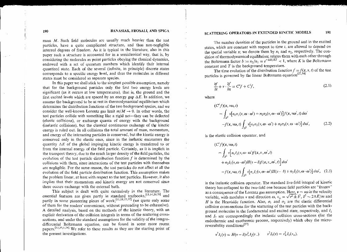
The number densities of the particles in the ground and in the excitedstates, which are constant with respect to time t, are allowed to depend on
the spatial variable x; we denote them by n l and n,, respectively . The con-dition of thermodynamical equilibrium relates them with each other through
the Boltzmann factor b := n,/n t = eAE/KT < 1, where K is the Boltzmannconstant and T is the background temperature .
The time evolution of the distribution function f = f (x, v, t) of the testparticles is governed by the linear Boltzmann equation[2 2,341
ar +v .à =Cef + C`f,
(2.1)
where
(Cef)(x, vto, t)
= f v[n to t (v, w -o)')+ n2o2(v, w . w )]f(x, Ve)', t) dwsz
f(x, vw, t) f~ v[n t o t (v, w w ) + n2o2(v, w ' ai)] dci ,
(2.2)
is the elastic collision operator, and
(C'f)(x, va), t)
= f v[nt I2(v, w • w)Î(x, v+w , t)s2
+ n,I1 (v, to • ci)H(v - 8)f (x, v- tu', t)] d(o'
- )'(X, v(O, t)f Z v[n t it (v, u~ tti)H(v - S) + n,I2 (v, w w )] dw', (2.3)s
is the inelastic collision operator . The standard five-fold integrai of kinetictheory has collapsed to the two-fold one because field particles are "frozen"as a consequence of the Lorentz gas assumption . Here, v = vaw is the velocity
variable, with modulus v and direction w, v. =,/v2 ± 82 82 = 2AE/m and
H is the Heaviside function . Also, a l and o, are the elastic differentialcollision cross-sections for the scattering of the test particles with the back-ground molecules in the fundamental and excited state, respectively, and I land 12 are correspondingly the inelastic collision cross-sections (for theendothermic and exothermic process, respectively) which obey the micro-
reversibility conditions[271
v2,1(v) = H(v - 8)vz I2(v_)
v2I2 (v) = v+II (v+) .

192
When no confusion arises, the dependence of cross-sections on the angularvariable w • w is omitted in the notation, but implicitly understood, and thesame applies to the dependence of the background densities on the position x .The Jacobian of the transformation between the precollisional andpostcollisional variables is not equal to one in the inelastic case, and thisfact has been used here, together with the microreversibility, in order tointerchange cross-sections and have ali of them evaluated at the same speed v .
The collision operators are more conveniently expressed by using theelastic and inelastic collision frequencies, gí (v) = va 1 (v), gz = va2 (v), g' (v) _vh(v) and g,(v) = vI2 (v) . In terms of the collision frequencies, the micro-reversibility conditions are
vg'(v) = H(v - 8)v_g'(v-)
(2.4)
vg'2(v) = v+gi(v+) •
(2.5)
For v > 8, one of these two relationships is redundant since Eq . (2.5) can beobtained from Eq . (2 .4) by taking v + in piace of v . For v < 8, however, thefirst relationship gives g'1 (v) = 0, an information that cannot be recoveredfrom the second relationship and that expresses the fact that the fxcitationcross-section must vanish when the kinetic energy of an incoming particle isbelow the inelastic threshold DE .
Using the collision frequencies (in the natural order as they appear)instead of the cross-sections wc write the collision operators in the form :
(C ef)(x, voi, t)
f (x, vw, t)f
in,g'(v, w oti) + 11295 (V, w - w')] do'
+
[ntgi(v, w • w) + n2g2 (v, w • w)]f(x, voti , t) dw',
(2.6)s
(Cf», ve), t)f(x, vw, t)
S2[n l gi (v, w • w)H(v - 8) + n 2g(v, w - w')] do'
and
BANASIAK, FROSALI, AND SPIGA
+ fZ In igl(v+, w • w) - f(x, 1'+w, t)
+ n,g2(v_, w • w)H(v - 8) v=f (x, v_w, t)] dw'
(2.7)v
Notice that the elastic collision operator is the same as for themonoenergetic neutron transport, [131 and that there are two possible targetfield particles, whose relative importance is determined by the macroscopic
SCATTERING OPERATORS IN EXTENDED KINETIC MODELS
193
collision frequencies ?k = nkgti (elastic scattering), and vk = nkgk (inelasticscattering), with k = 1, 2, where n2 < n i . In the elastic process the test particlespeed remains unchanged, and the global effect of scattering is isotropizationin direction . In the inelastic collision operator the threshold effect describedabove is accounted for by the Heaviside function H, and one may noticescattering-in contribution at the speed v from test particles at speed v +before collision (down-scattering), as well as from test particles at speed v_before collision (up-scattering) . If these were the only interaction mechanismspresent in the system, a test particle with a given initial kinetic energy wouldattain during its life only kinetic energies which differ from the initial one byinteger multiples of the energy DE . The test particles undergoing only inelas-tic scattering are thus partitioned into separate equivalence classes, moduloAE with respect to kinetic energy, and such a quantity is essentially a mereparameter with the range in the interval (0, DE) . Indeed, this is the actualsituation for our model, since the speed changes neither during free flight(force fields have been neglected), nor under elastic scattering . Consequently,the number of test particles in each class is bound to remain constant, andneither of them feels the presene of the other classes .
At this point, the microreversibility conditions could be used again inorder to relate the two inelastic collision frequencies with each other and toexpress C'f in terms of only one of them . Thus only (say) v 1 (x, v, (o • w) is afree physical parameter in the model, since the other follows then by micro-reversibility. On the contrary, the elastic quantities X k (x, v, o • w) are bothfree, since they are not correlated . They appear in the collision operator onlyin the combination .l l + ), 2, which will be labeled as À in the sequel . For similarreasons, the only inelastic parameter of interest, v 1 , will be renamed v .
For the readers' convenience, we rewrite the collision operators inEqs . (2 .6) and (2.7) in the more concise form, where time is omitted becauseit plays a role of a parameter :
f(x, ve» f ,l(x, v, w • w) do'SZ
+f
À(x, v,w • w')f (x, vw) do',
(2.8)s~
(Cf», v(o)
(C'f)(x, V(O)
= -f (x, V(O)
[H(v-8)v(x,v,co .o)')+bL+v(x,v+,co-(o) do'
+ v±
f v(x, v+ , w • w') f (x, v+w) daiv Sz
+ bJ
H(v - 8)v(x, v, w • (W) f (x, v_w) do' .
(2.9)s-

0 < a.min < X(X, v, -) < Àmax < +00
for all (v, z) E [0, oc[ x [-1,1] .Analogously, the following condition is required to hold true for the
independent inelastic collision frequency v = n i gi :
0 < vmin < v(x, v, w . (ti) < vmax < +00 , for v E [S, oo[ .
(2.10)
These assumptions are quite reasonable from the physical point of view .Even in the highly idealized case of inverse power intermolecular potentialswithout cutoff, they are valid for Maxwell molecules . However, they wouldnot be satisfied by the so called hard and soft potentials ; the latter could beincluded to some extent into our analysis (see e .g ., Refs . [2,3,7,8]), but thisproblem will not be considered here .
i
2.2. Derivation of the Scaled Equations
Equation (2 .1) can be adimensionalized in terms of a typical length L,a typical time -r, and typical values n*, gé and g; for density and collisionfrequencies. Concerning the molecular speed, as a typical value for it wc willtake the quantity S corresponding to the inelastic transition. That introducesspontaneously the Strouhal number [ ' 41 Sh = L/&c, and elastic and inelasticmean collision-free times 0, = 1/n*gé and 9 = 1/n*g,* . We assume that theelastic collision frequencies are of the saure order of magnitude, and that theparameter b, smaller than unity, is 0(1), but other situations might beanalogously investigated . Scaled space and time variables will be denotedby x and t again, and the saure applies for collision frequencies g withk = 1, 2, and gi, as well as for background densities nk . The dimensionlessvariable ~ = v 2/8 2 will be used instead of adimensionalized speed, with thejump in the inelastic transition equal to unity in the new scale . The newdistribution function, with split kinetic variables ~ and w, is labeled by fagain, and is given by
3
M, (o) = 2f(Vw)v=(82 ) 1/2
(2.11)
r
T
in front of the elastic and inelastic collision integrals, respectively . Thekinetic equation takes then the adimensionalized form
af
1 1/2
af _ I
e
1
at + Sh~w
ax Kne C f + KniCf
(2.13)
where the collision operators are defined, with referente to the kineticvariables only, by
Cf=-M,w) f ~,(~,w .w')dei' +f°X(~,w •(ti)f(~,ol)doti (2 .14)s2
s-
Cf = M, w) [H(~ - 1) f v(~, w • w) deis-
+b(~+1/2
1) f v(~+1 w w)s'-
+ 1 1/2 f+(
+
z v(~+1,w cti)f( +l,w')dai
and
+ b H(~ - 1) f v( , w . c)'f(~ - 1, ei) dai .
(2.15)
The numbers Sh, Kne , and Kni measure the relative importance of thestreaming, elastic collisions, and inelastic collisions in the balance equationfor the test particle distribution function. We shall further simplify ourconsiderations by requiring that these three numbers are functions of asingle parameter e, which might represent the chosen smallness parameter .Restricting our attention to regular functions of é we see that there is noharm in assuming that the three numbers are power functions of e . Thus, weshall consider Eq . (2 .13) in the form
at EPSf + ECef + Er Cif
(2 .16)
where p, q, r are integers, and the streaming operator S is defined by
aS = -~ I / 2 w
. -.
(2.17)
194
BANASIAK, FROSALI, AND SPIGA SCATTERING OPERATORS IN EXTENDED KINETIC MODELS 195
From a mathematical point of view, we assume that )l(x, v, w • co') is ameasurable function bounded almost everywhere :
Easy manipulations single out the "Knudsen" numbers [141
Kn e = ee
Kni = Bi (2.12)

196 BANASIAK, FROSALI, AND SPIGA
Sometimes, it proves convenient to resort to the quantity
2vf(vw)
Z ,
(2 . 18)-~s )
(the scalar flux of the neutron transport) as a new dependent variable . In thiscase the kinetic equation takes the same form as Eq . (2 .13), apart from aslightly different expression of the inelastic scattering operator
C`lp = -cp(~, Q)CH(~ - 1)f
v(~, w . w) d w's=
1/2+b(~
+i)l
)]+~ v( +l,cv cti)lp( +l,ai)dctisz
s2
1/2 ~+bH(~-1)C
1)
I v(~, o . w')q(~-1,cti)dcti .
(2 .19)
In any case, due to the negative powers of the variable ~ there appearsingular terms in the inelastic collision operator, the only differente beingits different location in Eqs . (2 .15) and (2 .19) . The singularity blisappearsfrom Eq . (2.19) when the parameter b vanishes (no up-scattering) .
For a later reference, let us note that the test particle number densityfollows from the different distribution functions as
n = f f(v) di, = f +~ f , ~ 1/2f(~, (9) d~ de) = +~ f , lp( , co) d dw .
(2 .20)
3 . THE COMPRESSED CHAPMAN-ENSKOGPROCEDURE
The goal of this section is to give a concise overview of the asymptoticanalysis which is the basis of this paper, and which essentially stems fromthe Chapman-Enskog procedure as revisited and modified by J . R. Mika inthe eighties . [3221
In order to introduce the reader into this asymptotic procedure,let us consider a particular case of singularly perturbed abstract initialvalue problem
Ms = AofE+ i A1f,+ i A'f,
(3.1)fE(O) = fo,
SCATTERING OPERATORS IN EXTENDED KINETIC MODELS
197
where presene of the small parameter c indicates that the phenomenonmodeled by the operator A, is more relevant than that modeled by A 1 ,which, in turn, is more relevant than that modeled by A o .
When in a kinetic equation the collision processes dominate over theothers, one is interested in finding a hydrodynamic evolution of the system,and in the sequel we shall analyze different situations fitting into thisscheme .
In a mathematical framework, we can suppose to have ori the right-hand side a family of operators {AE}E,o={Ao+(1/E)A1+(1/E2)A,}E,oacting in a suitable Banach space X, and a given initial datum . The classicalasymptotic analysis consists in looking for a solution in the forra of atruncated power series
f(n) (t) = f0(t) + Ef1(t) + E2f2(t) + . . . + l?'f (t),
and builds up an algorithm to determine the coefficiente fo ,f1 ,f2 , . . .—f,.
Then f(" ) ( t) is an approximation of order n to the solution ff (t) of theoriginal equation in the sense that we should have
fE(t) -f(" ) ( t)
for 0 < t < T, where T > 0. Sometimes this approximation does not hold ina neighbourhood of t = 0, because of the existence of an initial layer wherethe estimate is not uniform with respect to t . For this reason it is necessaryto introduce an initial layer correction .
A first way to look at the problem from the point of view of theapproximation theory is to find, in a systematic way, a new (simpler)family of operators, stili depending ori e, say BE , and a new evolutionproblem
aY0,
àt = BEwE,
supplemented possibly by an appropriate initial condition, such that thesolutions 10E (t) of the new evolution problem satisfy
Y= 0(é'),
11L(t) - 10<5(t)11X= o(E"), (3 .2)
for 0 < t < T, where T > 0 . In this case wc say that BE is an operatorapproximating A E to order n . This approach mathematically producesweaker results than solving system Eq . (3 .1) for each é and eventuallytaking the limit of the solutions as c -3 0 . But in real situation, c is smallbut not zero, and it is interestìng to find simpler operators B E for modeling a

198 BANASIAK, FROSALI, AND SPIGA
particular regime of a physical system of interacting particles. For this typeof approach, we refer the reader to papers of the authors . [7 ' 81
A slightly different point of view consists in requiring that the limitingequation for the approximate solution does not contain E . In other words,tbc task is now to find a new (simpler) operator, say B, and a new evolution
problem
with an appropriate initial condition, such that tbc solutions cp(t) of the new
evolution problem satisfy
IfÎE(t) - ~P(t) j1x - 0, asE -->0, (3.3)
for 0 < t < T, where T > 0 . In this case we say that B is tbc hydrodynamic
limit of operators A E as E -i 0. This approach can be treated as (and in factis) a particular version of the previous one as very often the operator B isobtained as tbc first step in tbc procedure leading eventually to the family{BE } E , o . For instance, for the nonlinear Boltzmann equation with the
originai Hilbert scaling, B would correspond to tbc Euler system, whereas
BE could correspond to the Navier-Stokes system with e-dependentviscosity, or to Burnett equation on yet higher level .
In this review wc shall follow indeed this second point of view, lookingfor suitable scalings of independent variables and physical parameters whichlead to tbc limitino equations not depending on c .
In any case the asymptotic analysis, should consist of two main points :
- determining an algorithm which provides in a systematic way theapproximating family BE (or tbc limit operator B),
- proving the convergence of fE in the sense of Eq . (3 .2) (or of
Eq . (3 .3)) .
Even if tbc formai part and the rigorous part of an asymptotic analysisseem not to be related, the formai procedure can be of great help in provingtbc convergence theorems .
The classical Chapman-Enskog procedure was adapted to a class oflinear evolution equations by J. R. Mika at the end of the 1970s . Later thisapproach was extended to singularly perturbed evolution equations arisingin tbc kinetic theory . The reader interested in reviewing the applications ofthe modified Chapman-Enskog procedure in tbc kinetic theory is referred tothe book by J. R . Mika and J . Banasiak . [311
The advantage of this procedure is that the projection of the solutionto the Boltzmann equation onto the null-space of the collision operator, that
SCATTERING OPERATORS IN EXTENDED KINETIC MODELS
199
is, the hydrodynamic part of tbc solution, is not expanded in E, and thus thewhole information carried by this part is kept together . This is in contrast tothe Hilbert type expansions, where, if applicable, only the zero order termof tbc expansion of the hydrodynamic part is recovered from the limitequation .
The main feature of the modified Chapman-Enskog procedure is thatthe initial value problem is decomposed into two problems, for the kineticand hydrodynamic parts of the solution, respectively . This decompositionconsists in splitting the unknown function into tbc part belonging tothe null space V of the operator A,, which describes tbc dominantphenomenon, whereas the remaining part belongs to the complementarysubspace W . Thus the first step of the asymptotic procedure is finding thenull-space of tbc dominant collision operator A, ; then tbc decompositionis performed using the (spectral) projection P onto tbc null-space V byapplying P and tbc complementary projection Q = I - P to Eq . (3 .1) .In this one obtains a system of evolution equations in tbc subspaces V and W.At this point the kinetic part of the solution is expanded in series of E, butthe hydrodynamic part of the solution is left unexpanded . In other words,we keep ali orders of approximation of the hydrodynamic part compressedinto a single function .
One of tbc main drawback of tbc classical approach is that tbc initiallayer contribution is neglected . To overcome this, two-time scaling isintroduced in order to obtain the necessary corrections . In generai, thecompressed asymptotic algorithm permits to derive in a natural way tbchydrodynamic equation, tbc initial condition to supplement it, andtbc initial layer corrections . Hence, it is possible to give, under suitableassumptions, an estimate for tbc error of tbc approximating solution,uniformly in t > 0, in tbc sense specified later .
Summarizing, the originai Chapman-Enskog method is improved bythe introduction of two new ingredients :
the projection of the originai equation onto tbc hydrodynamicsubspace,the analysis of tbc evolution equations in terms of the theory ofsemigroups .
Taking these new ingrediente into account, we obtain the followingmain advantages :
we can build an algorithm listing the steps of the procedure to befollowed,we are able to establish ali the mathematical properties of tbc fulland limit solutions needed for the rigorous convergence proof.

200
4. THE HYDRODYNAMIC SUBSPACES
As we indicated in the previous section, the first step in the compressedChapman-Enskog method is to decompose the suitable Banach space(usually LI ) into the hydrodynamic and kinetic subspaces . In this sectionwc shali find the null-spaces of the elastic scattering and of the inelasticscattering operators, respectively . It is remarkable that, in contrast . to thestandard kinetic theory, these spaces here are infinite dimensional . Next wcshall study the relevant properties of the collision operators .
First let us consider the operator C e , in the form given by Eq . (2 .8)made dimensionless by measuring v in units of 8 (unit spacing in the newspeed variable, labeled by v again) . The following theorem was . proved inRefs . [3,10] . Since in all the considerations of this section x plays the role ofa parameter, we sha11 drop it from the notation .
Theorem 4 .1 . Let all the assumptions of Sec. 2 be satisfied. Then the operatorCe is a bounded operator in X = L I (R 3 ) with the following properties
BANASIAK, FROSALI, AND SPIGA SCATTERING OPERATORS IN EXTENDED KINETIC MODELS 201
Analogous properties hold in any weighted space L 2 (IIR 3 , w(v) dv) Aere iv is ameasurable strictly positive (a .e.) firnction .
Proof. Since À is symmetric in w and tu', for any g E L,<,( llR 3 ) wc have
f52(gCef)()veodw =
-f , fX (v, w - ci)[g(vw)(f (vw) -f (veti))] dw dai
s- s=
hence
_-fS2 f52
X(v,w- (ó)[g(vw)(f(v(ti)-f(vw))]dwdcti,
f -
s- s-(gCef)(veo) da> = -f
2f .l(v, w • oi)[g(vw) - g(vw )]
sx [ f(v(») -f (veti )] dw dai.
Taking any bounded strictly increasing function K : ll --> fIR wc obtain
(i) For anyf E X and any non-decreasing firnction ic ive have2f (K( f)Cef)(vw) do - -f f, ),( v, w • w)[K( f(vw)) - K( f(vw ))]L
s2 s2f 3 K(f)Cefdv < 0 . (4 .1) x [ f (vw) -f (vcó)] do) dw'
< 0 .
(4.6)
(ii)In particular, C e is dissipative .The null-space of C e is given by
N(C e) _ { f E LI (R') ; f is independent of w} . (4 .2)
Integrating over the remaining variable wc get the H-theorem . If, inparticular, we take K(t) = sign(t) wc obtain
(iii) The range of Ce is given by
(4 .3)
f 3
sign(f)Cef d v< 0
which gives the dissipativity of Ce. This proves (i) .R(C e ) = W ={f E LI (IIR 3 ) ; f f do) = 01 .
1s Let Cef = 0 ; then the left hand side of Eq . (4 .6) is zero, but due tostrict monotonicity of K this is possible only ifThe spectral projection orto N(Ce) ( parallel to W) is given by
1 AVO» = f (veti),
(4.7)Pf = f f d w . (4 .4)
4~r s2
(iv) Forf E W we have
f sign(f)Cef(v o) dv < -47rl,,,i„Il f11X (4 .5)
for almost all v, that is, to the kernel of C e may belong only functionsindependent of w. On the other hand, such functions clearly belong toN(C e ), therefore the kernel of Ce is given by Eq . (4 .2) .
Next we turn our attention to the solvability of
and hence the spectral bound of Ce, S(Ce), satisfies s(Ce) < af(v)+f(v)f À(v,w w)dcti - f , X(v,w .(v)f(v(ó)dw =g(v)s2
s--47rXmin (4.8)

202
for g E L 1 (R 3 ) . Denote
W= j f E L I (R') ; f d =0l
s~
For f E W we get
f
Z (slgn(f)C ef(vw) dws
_ - 1 f S2 ~.(v, w • w)[sign( f (veo)) - sign( f (ve )))]2 S2
x [ f(vw) -f (veti)] dw dw
< - 1 >,(f f , sian( f (vw)) f (v(o) da> dw- 2 mins- s-
+ fs2fs2
sign( f(vw)f vo) dco dw
- f ` f sign( f (vw))f (vw) dco do)'
-f f,2 sign( f (vw)) f(vco) do) dw Is-
_ -47rÀmin lI f I L, (S`)
where, upon integration with respect to v, wc obtain that C' I li, - UI isdissipative for a > -47rXmin . Since C'IYv is bounded, C'I w - aI must beni-dissipative, therefore if a > -47rXmin, then a E p(Ce l w) .
It is also clear that the spectral projection onto N(C e ) is given byEq . (4.4) which ends the proof of (iii)-(iv) .
The statement for the L, space follows in the same way as all theoperation are first performed on the unit sphere and only later integratedwith respect to v to get the estimates valid on R3.
∎
The analysis of the inelastic kernel is considerably more involved . Thecase of purely inelastic collision operator C' has been thoroughly investi-gated in Ref. [1] . Analysis of the full operator C = C'+ Ce is similar but wcprovide it for the sake of completeness. Note that since C e is a boundedoperator, the domain of C equals the domain of C', that is, D(C) = D(C') .
It is worthwhile to analyse the operator C in two spaces : X = L 1(R)and X2 = L,(l& 3 , b- °2dv) where the Boltzmann factor b is defined in Sec . 2 .Here again x plays the role of a parameter and thus will be suppressed in thenotation .
BANASIAK, FROSALI, AND SPIGA
k
SCATTERING OPERATORS IN EXTENDED KINETIC MODELS
203
To avoid confusion we shall write down explicitly the definitions ofthe operatore which will appear in our considerations . For a continuousfunction f we split the full collision operator C as
(K+f)(v) = bH(v2 - 1)fs, v(v, w . wf(v_w)dw.
It follows that in X setting only the operatore K+ and N+ are unboundeddue to the singularity v-1 at 0. On the contrary, in X 2 setting the operatorK_ is also unbounded with singularity \/v2 - 1 at v = 1 . Multiplicationoperator N_ is bounded in both settings . 111
To characterize the domain of C, for an arbitrary positive measurablefunction g we denote the weighted space L I(R3,g(v)dv) by X3 . It follows .Ref. [1], that
D(C) = X 1+,, .
Similar considerations can be carried out in the space X' = L2 (l83 , b- "dv) .Then the domain will be denoted by D2(C) . Using analogous notation,wc have
D2(C) = X' , n XH(v2_ 1)v _, n X' .
In the sequel wc shall find convenient to use the notation : = v2 (introducedin Subsection 2 .2) and
Ow =f ~~),
(4.11)
Cf = -Nf + Kf .
defining
Nf = N+f + N-f, Kf = K+f + K_f, (4.9)
where
(N+f)(i') =f(v)b vi+ f , v(v+ , w . w) dws
(N-f)(v) = f(v)H(v2 - 1)fz v(v, w • w) do)'s (4.10)
(K-f)(v) = 1v f , v(v+, w • w)f(v+w) dotis

204 BANASIAK, FROSALI, AND SPIGA
so that f(vf(o)=0(x±1). By Ref. [1] wc may put D(C) = D(K) andD 2(C) = D2(K) .
The theorem below is an extension of Theorem 2 .2 of Ref . [1] to thecase that includes the elastic scattering term . Apart from one step, the proofsof both theorems are similar but for the sake of completeness we providebere the proof for the present case .
Theorem 4.2 .
(a) Let f E D(C), then Cf = 0 if and only if 0, defined by Eq . (4.11),satisfies for ~ E [0, 1[ and n E N
0(~+ n) = b"
Oo(~) (4.12)
where 00 E L 1 ([0, 1],d~) .(b) Let f ED 2 (C), then Cf = 0 if and only if Eq . (4 .12) holds with
0 0 E L2([0, 1], d~) .
Proof.
}(a) Firstly, wc consider the case with bounded C' in X . This can be
done by regularizing v as follows
(v, w . w) = v(v, w • co) for 1 + n -1 < vv„ (v,0
for v < 1 +n-1
Following some ideas from Ref. [28] (see also Ref. [1]) wc obtain for
g E X* = Lro(f 3 )
+ce
(g, C+,f) = fS2 fS2 f v+v,r(v+ , w . w')[f(v+w)g(vw) + bf(vw)g(v+w)
- bg(v(9) f (vw) - g(v+oi) f (v+(o)]v dv dw doi
12 sf f f
X(v, w ()[g(vw) - g(vw')]'- s'-
ox [f (vw) - f (veti )]v 2 dv dw dai
_ - R, f V v,, (v+, w • w)U(v+w) - bf(va)]
x [g(v+w) - g(vw)] doti dv
1 f f À(v, w w )b °2[g(vw) - g(vw )]2 ~a' s'
x [b- ` 2f (vw) - b-V f (veti)] dai dv,
(4 .14)
(4 .13)
SCATTERING OPERATORS IN EXTENDED KINETIC MODELS
205
where ( •, .) denotes the duality pairing between L1(R3) and L,,, (l83 ), and C„the collision operator corresponding to the regularized v,, . In particular, if Kis any bounded nondecreasing function, then we obtain
(K(b-, ,2f), Cnf )
L+ v (v+ (o , co)b,2+1 [b_v2_lf(v+w) - b-'2f(vw)]'3
S' vx [K(b-°--1f (v+w )) - K(b-°Zf (vw))]dw dv -
f f 2a (V, w . w)bv2
Q8 S
x [K(b-`2f(V(O)) - K(b-v2f(veti ))]2
2x [b-V f(va» -
b-vf (ve)')] do)' dv,
(4.15)
hence for any f E LI (R3) wc have the H-theorem
(K(b-"f), C„f) < 0 .
(4 .16)
If we take as K any bounded strictly increasing function, then we seethat if for some f we have C„ f = 0, then
(K(b-v2f), C„f) = 0,
and since each term in Eq . (4 .15) is nonpositive, this is only possible whenwc simultaneously have
f(v+(»') - bf (vw) = 0f(v(O) -f(v(0) = 0
for all w, cti E S2 and v E R+ . On the other hand, functions satisfyingEq. (4.17) belong to the null-space of C,,, N(C„ ), by Eq . (4 .14), hence it isdescribed fully by Eq . (4 .17). To characterize these functions explicitly wenote that by Eq . (4 .7), the second equation in Eq . (4 .17) shows that theelements of the kernel of C„ are independent of the angular variable . Hence,using notation (4 .11) for Eq . (4.17), by recurrence and Eq . (4.10) we get
0(~ + n) = b"Oo(~)
where ~ E [0, 1], which gives Eq . (4.12), showing that N(C„) = N(C,,) .Returning now to the original unbounded C, wc pass to the limit,
exactly as it was done in Ref . [1], Theorem 2.2, obtaining the samestatement .
(4 .17)

206 BANASIAK, FROSALI, AND SPIGA
(b) Let us consider now the problem in X2 . Again wc start with v„defined by Eq . (4 .13) . For arbitrary g E X2, similar calculations show thatby v„( ., w . a) = v„(, ai . w) we have
(g, GA -2 = (C g,f)x•2
that is C, is self-adjoint in X2. Let us take arbitrary f E X2; then
(f,C1j)x'--=- f~ f lvv, (v+,w •w)[f(v+w)-bf(vw)]2b- 1 daidv
1 f f X(v,w .w')[f(vw)-f(v(ti)] 2daidv .
(4 .18)2 u3 s 2
Equation (4 .18) shows that, as in X-setting, C„ f = 0 if and only ifO(() =f(,) satisfies
0(~ + n)= b"Oo(~),
(4 .19)
where ~ E [0, 1] and o e L,([0, 1], 4 d~) . The extension of this result tounbounded v is performed as in X, case .
i
∎
In the theory of hydrodynamic limits an important role is played bythe conditions of solvability of Cf = g . In this context we have the followingresult. Again, this teorem is an extension of the result of Ref . [1] to coverthe case with C = C'+ C e .
Theorem 4 .3 .
(a) Let C* be the adjoint to C in X and f E D(C*) . Then C*f = 0 ifand only if
f(v2 +,1) =fo(v)
for all v e [0 . 1[, n E N and somefo E L~([0, 1]) .(b) The closure of the range R(C) is characterized by
g E R(C) if and only if
Jv+12 g(~v2 + jw do) = 0
(4 .20)Ì=0
(c) tiVe have the "spectral" decomposition
X = N(C) $ R(C)
(4.21)
SCATTERING OPERATORS IN EXTENDED KINETIC MODELS
207
and the "spectral" projection onto N(C) along R(C) is given by
(Pf)(v2 +n) = b»Vfo(v 2)
Proof.(a) Let g E N(C*) . Since then g E D(C*), in particular it is a bounded
function, thus b" g E X2 . Moreover, if X is the weight function definingD2 (O), we obtain
+ro
2
f X(V)g2(v)b 2v2v"2 dv = f f X(vw)g2(vw)b v 2 di, dco < +oc,1 3
o
s-
where the integrability in neighbourhoods of v = 0 and v = 1 is due to theboundedness of g and integrability of v i and v= i over compact subsets of118 3 . Hence b"2 g E D 2(C) . Since X2 C X, if f E X2 is bounded at v = 0, thenf E D(C) . Moreover, the set of such functions is dense in X2 . Thus, byself-adjointness of C in X 2 wc have
0 = (C*g,f)x = (g, Cf)x = (b g, Cf),- (C(b'g),f)
(4.24)
and from the density wc see that g E D(C*) solves C*g = 0 if and only ifb" 2g E N(C) in X2 . This shows that g is a 1-periodic function of the variable
independent of the angle .(b) Since R(C) = N(C*) 1 , g e R(C) if and only if for any bounded
1-periodic function f of ~ = v 2
0 = f g(v)f(v) dv = 1f lOo(~) (~'A +jf, g(,/~ +j(,) dco) d~,00ua
2f
j=o
s
which, since 00 is arbitrary, gives
X:/v22 +jfs-g(Jv2 +jw) dw = 0 .
(4.25)j=o
(4 . 22 )
where
rjo w'+jfs2 Î(~/''-+yw)dwV5 0 (v2) =
47r ° obJ \/v+j(4 .23)
208 BANASIAK, FROSALI, AND SPIGA
0
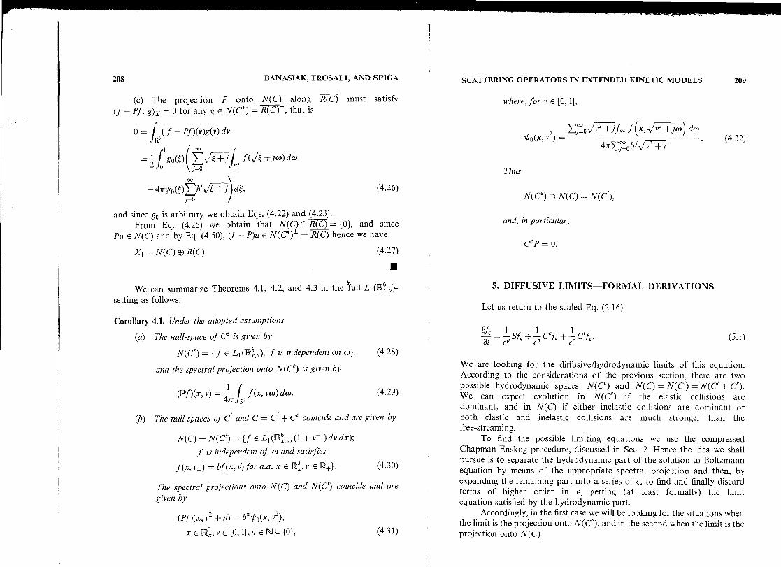
(c) The projection P onto N(C) along R(C) must satisfy(f - Pf, g)x = 0 for any g E N(C*) = R(C) 1 , that is
= f (f - Pf)(v')g(v) dv.3
=f 2 go(~) ~J +jf , f(/ +jw)dwo
i=o
s-
- 4nVo(~)Y-'blJ~ +f) d~,
(4.26)1=0
and since go is arbitrary wc obtain Eqs . (4.22) and (4.23) .From Eq. (4.25) wc obtain that N(C) rl R(C) = { 0}, and since
Pu E N(C) and by Eq . (4 .50), (I - P)u E N(C*)1 = R(C) hence wc have
X, = N(C) ® R(C) .
(4.27)
∎
We can summarize Theorems 4.1, 4 .2, and 4.3 in the ~ul1 LI (lR 6 v )-setting as follows.
Corollary 4.1. Under the adopted assumptions
(a) The null-space of C e is given by
N(C e) _ { f E L i (IIR6 , y ) ; f is independent on co} .
(4.28)
and the spectral projection onto N(C e) is given by
(Pf)(x, v) =1fsS
, f (x, m) do) .
(4.29)
(b) The null-spaces of C' and C = C'+ C e coincide and are given by
N(C) = N(C') _ { f E L I (R', v , ( 1 + v-') dv dx) ;
f is independent of w and satisfies
f(x, v + ) = bf(x, v) for a .a . x E llRx, v E QR+ } .
(4 .30)
The spectral projections onto N(C) and N(C') coincide and aregiven by
(Ff», v2 + n) = b",/i o (x, v2 ),xEIlRY,vE[0,1[,1lENU{0},
(4 .31)
SCATTERING OPERATORS IN EXTENDED KINETIC MODELS
Aere, for v E [0, 1 [,
(
~ rw
o,/l, +JfS2 f(xw 2 +lw) d(w
fio x 5 v ) =
Thus
N(C e) D N(C) = N(C')'
and, in particular,
CeP = 0 .
5. DIFFUSIVE LIMITS-FORMAL DERIVATIONS
47rr': bJ \/v2 +j
Let us return to the scaled Eq . (2 .16)
afE - ~ Sfl + ~ Cf, + 1 C fEót
E
E
E
Wc are looking for the diffusive/hydrodynamic limits of this equation .According to the considerations of the previous section, there are twopossible hydrodynamic spaces : N(C`) and N(C) = N(C) = N(C' + Ce ) .We can expect evolution in N(Ce) if the elastic collisions aredominant, and in N(C) if either inelastic collisions are dominant orboth elastic and inelastic collisions are much stronger than thefree-streaming .
To find the possible limiting equations wc use the compressedChapman-Enskog procedure, discussed in Sec . 2 . Hence the idea wc shallpursue is to separate the hydrodynamic part of the solution to Boltzmannequation by means of the appropriate spectral projection and then, byexpanding the remaining part into a series of c, to find and finally discardterms of higher order in c, getting (at least formally) the limitequation satisfied by the hydrodynamic part .
Accordingly, in the first case we will be looking for the situations whenthe limit is the projection onto N(Ce), and in the second when the limit is theprojection onto N(C) .
209
(4 .32)

210 BANASIAK, FROSALI, AND SPIGA
5.1 . Evolution in N(Ce ) (Elastic Collision Dominante)
To find possible limiting evolutions in N(C e ) we shall use theprojection P defined by Eq . (4 .4) . It is important to note that sinceN(Ce) D N(C), PC' and C'P are not equal to zero. Denoting 0 = I - P,we operate with these projections onto Eq . (5 .1), and denoting
vE = PfE and 1v E = Off,
we obtain
aV E IPSQw6 +
irPC'PV E +1,. PC ,. 0112,
at
Ep
E
Eai_vE _ I QSPV + 1 Q~sQ~w + 1 QC'Pv + iQ~CQw
(5.2)at
Ep
E
EP
E
Er
E
Er
E
+i Q1Ce Q~u' E .E
where we already used the fact that PSP = 0 (see Ref . [3]) . Sirice we assumedthat the elastic collisione are dominant, we must assume that q > max{ p, r} .Since we are looking for the limiting equations, the equation for theapproximation of v E cannot contain c . This yields r < 0 and shows that pmust be less or equal to the index k of the first nonzero term in the expan-sion of 1vE = wo + ew 1 + E2 1v 2 + • • • . Let us consider first the case whenp = k . Inserting this expansion into the second equation in Eq . (5 .2) we obtain
lVOE 9 (aa + E aatl-+. . . = Eq-poSpl,E + E9-p . SQ~(w0 + Ew 1 + . . .)
+ E9-rQC'pVE + Ea-rQC'Q(wo + EW1 + . • .)
+ QCeQ(wo + Ew1 + . . .)
Since q > r and q > p, wc obtain
QCzQpwo = 0
which yields w0 = 0, because Q is the complement to the spectral projection .Clearly, the first nonzero term in the expansion of 1v will be Wk with ksatisfying k = min{q - p, q - r} . However, if q - p > q - r, then r > p, butr < 0 yields p < 0 which contradicts the assumption that p = k . Thusk = q - p and q = 2p . In any case we obtain Wk = -PCQ)-1 QSw,(provided the inverse exists) . Changing now the notation from vE into p toemphasize the fact that the forthcoming equation is an approximating
SCATTERING OPERATORS IN EXTENDED KINETIC MODELS
211
(limiting) equation for v E , wc obtain the limiting equations, independent ofE, in the form
ap = -PSQ(QCeQ~) -1 Q~SPp + PC'Pp, if r = 0,
(5 .3)
and
ap = -PSQ(QCeQ) 1QSPp, if r < 0 .
(5.4)at
Ifp < k, then the power of the coefficient multiplying PSQ(QC eo) -1 xOSLPp is positive and therefore this term is negligible when e tends to zero .Then, the possible limiting equations are
ap = PC' Pp, if r = 0,
(5.5)
ap =at
0,
if r < 0 .
(5.6)
and
To summarize, wc consider the generic (simplest) combinations ofpowers of E giving particular limiting equations . Thus, wc see that Eq . (5 .3) is(formally) the limiting equation for the scaling
afE- SfE + CefE + C 'JE,
at
e
E
and Eq . (5 .4) for the scaling
aE= E SfE + É CefE + ECfE .
Further, Eq . (5 .5) is the limiting equation for the scaling
afE - Sf + E C efE + C'fE,
and Eq . (5 .6) for the scaling
E= SfE+C efE + EC fE .

212
5.2. Evolution in N(C) (Inelastic Collision Dominance)
As wc have seen in Sec . 4, the cases when either C', or C' + C e dom-inate have the same hydrodynamic subspace N(C) and the sameprojectors onto it. Since N(Ce) D N(C'), wc have CeP = PC' = 0, whereP is the projector defined by Eqs . (4.22) and (4.23) . Operating with P andQ = I - P onto Eq . (5 .1) and denoting
v E = PfE and lv E = QJ,
wc obtain
v = 1 PSQwE
alt, 1QSPv. + 1QSQwE + lr QC`QWE + QCeQIVE,
(5 .7)at - Ep
Ep
E
E
where wc used PSP = 0.J`? As before, we observe that p must~be less or equalto the index k of the first non-zero term wk in the expansionlv = w0 + Ewl + • • . . However, if it is strictly smaller, then the equation forp (the approximation to VE ) will be trivially reduced to
ap - 0,at
independently of what is happening in the second equation (though as wcshall sec in Subsection 8 .3, the initial layer corrector complementing thehydrodynamic equation changes slightly depending ori whether C' and C'are of the same or different magnitude) . Hence, wc can safely assume thatp = k > 0 . Let us then consider the expanded version of the second equationin (5 .7)
at(IV O + CIV I +
)
1= E QSPV E +
1E QSQ(wo + Ewl + . . .)
1+ r QC.Q(wo + Ewl + . . .) + 1E9 QCeQ(wo + Ewl + . . .),
(5.9)
Here we have to distinguish two cases : r > q and r = q (in both caseswe must have of course r > p) .
BANASIAK, FROSALI, AND SPIGA
t
SCATTERING OPERATORS IN EXTENDED KINETIC MODELS
Let us consider first the case r > q . Multiplying the last equation by Erwc obtain
aEr
at(Wp + Elvl + . . .)
= Er-PQSPV E + E r-POSO(w 0 + CIVI
+ QCQ(lv0 + CIVI +. . .) + Er 9QCeQ(wo + CIVI + . . .) .
Due to the definition of Q we have, as before, w 0 = 0 . Let lvk be thefirst non-zero term of the expansion of w. Because r - q > 0, wk at QCeQ ismultiplied by Er-q+k which is always of higher order than Ek . The term wk atOSO is multiplied by Er-P+k = Er , and since QSP is multiplied by E
r-k withk > 0, we see that Wk is to be determined from
OSPQ = -QCQwk
when r - p = k, that is r = 2p . The index q seems to have no significancewhatsoever on the final result . Consequently, the limiting equation for theapproximation p of v E is of the forra
ap = -PSQ(QC'Q) I QSPp,
(5 .10)
provided the inverse exists .The case r = q is similar . Multiplying Eq . (5 .10) by Er we obtain
Era
a (wo + Ew l + . . .) = E r-PQSPVE + Er-POSQ(WO + Ew l + . . .)
+ QCQ(wo + Ewl + • • •) + QCeQ(wo + CIV I + • • •) .
Due to the definition of Q wc have as before lv 0 = 0 . Let Wk be the firstnon-zero term of the expansion of lv . Here r - p > 0, and therefore the termwk at QSO is multiplied by E r- P+k = e' which is of higher order than Er-Psince k > 0, and consequently W k is to be determined from
QSPQ = -Q(C' + C e)Qwk
when r - p = k, that is r = q = 2p. Consequently, the limiting equation is ofthe forra
~p = - PSQ(Q(C' + C e)Q) l QSPp,
(5 .11)
provided the inverse exists .
213
214
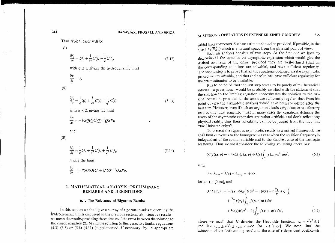
Thus typical cases will be
(i)
àE = S.ff, + CefE + C'fE,
with q < 1, giving the hydrodynamic limit
apar - 0,
afE _ 1
1 e
1ar E SfE+~~CfE+E? CfE,
with q < 2, giving the limit
8p _ -PSQ(QC'tQ) -1 QSPp
and
atE = ~ SfE + É CefE + Cf,
giving the limit
ap =ar
-PSQ(Q(C` + Ce)Q) - `QSPp .
BANASIAK, FROSALI, AND SPIGA
6. MATHEMATICAL ANALYSIS: PRELIMINARYREMARKS AND DEFINITIONS
6.1. The Relevance of Rigorous Results
In this section we shall give a survey of rigorous results concerning thehydrodynamic limits discussed in the previous section . By "rigorous results"wc mean the results providing the estimate of the error between the solution tothe kinetic equation (2.16) and the solution to the respective limiting equations(5.3)-(5 .6) or (5.8)-(5 .11) (supplemented, if necessary, by an appropriate
(5.12)
(5 .13)
(5 .14)
SCATTERING OPERATORS IN EXTENDED KINETIC MODELS 215
initial layer corrector) . Such an estimate should be provided, if possible, in thespace L1(llG v) which is a natural space from the physical point of view .
Such an analysis consists of two steps . At the first one we have todetermine all the terms of the asymptotic expansion which would give thedesired estimates of the error, provided they are well-defined (that is,the corresponding equations are solvable), and bave sufficient regularity .The second step is to prove that all the equations obtained via the asymptoticprocedure are solvable, and that their solutions bave sufficient regularity forthe error estimates to be available .
It is to be noted that the last step seems to be purely of mathematicalinterest-a practitioner would be probably satisfied with the statement thatthe solution to the limiting equation approximates the solution to the ori-ginal equations provided all the terms are sufficiently regular, thus from hispoint of view the asymptotic analysis would have been completed after thefirst step. However, even if such an argument leads very often to satisfactoryresults, one must remember that in many cases the equations defining theterms of the asymptotic expansion are rather artificial and don't reflect anyphysical reality ; thus their solvability cannot be judged from the fact that"the Universe exists" .
To present the rigorous asymptotic results in a unified framework wcshall limit ourselves to the homogeneous case when the collision frequency isindependent of the spatial variable and to the simplest case of the isotropicscattering . Thus wc shall consider the following scattering operators :
(Cef)(x, v) = -4nX(v)f(x, v) + X(v)fs,
f(x, v(i) dai,
(6.1)
with
0 < Xmin < ?(v) <- Xmax < +ce
for all v E [0, ce[, and
(Cf)(x, v) = f(x, v)47r(H(v 2 - 1)v(v) + b v+ v(v+))v
+vv
')(V+)f Z f(x, v+ (0) des
+ bv(v)H(v2 - 1)f f (x, v- o)') dai,
(6.2)sZ
where we recall that H denotes the Heaviside function, v± = _/V2 + 1and 0 < vmin < v(v) < Vmax < +oo for v E [1, ce[. We note that theextension of the forthcoming results to the case of x-dependent coefficients

216 BANASIAK, FROSALI, AND SPIGA
is straightforward even though computationally unpleasant . To allow moregenerai (but stili isotropie in v) scattering cross-sections is more demandingbut can be accomplished in several cases (see e.g ., Refs . [2,8]) . The extensionto to dependent scattering cross-sections seems to present serious difficultiesdue to the adopted L 1 -setting and the employed techniques .
6.2. Notation for Operators and Function Spaces
In this subsection wc introduce the function spaces relevant to thefurther considerations. Since from now on the dependence on the spatialvariable will become important, in contrast to the previous sections wc mustintroduce notation which will distinguish L 1 spaces in x and v variables .The basic space is
X = X r ®R X, = L 1 (Rr, Xv) = L 1 ([183 > X~) = L1(I6, ,),
where X,, = Li (R3) for a = x, v . Most considerations will be carried out inX, with fixed x . Typically, if A C is an operator in Xv (possibhv depending onx as a parameter), then by A we will denote the extension of this operator toX. If A C is unbounded in X, with domain D(A r ), then A is considered on thenatural domain
D(A) = {f E X; f (x, .) E D(Ax) for a .a . x, x -> (AXf)(x) E X} .
If A i does not depend on x, and it is clear from the context in whichspace it acts, we will omit the subscript x . The same convention will beapplied to operators A v acting in YC .
Occasionally, if the above procedure can be reverted, for acting in Xoperator A wc shall write Ar or A,, to denote this operator acting with x or v,respectively, fixed as a parameter (that is, e.g ., A Cf = A(f ® 1) where
f E X, if the latter defines an element ofXv ) .The asymptotic analysis requires some additional regularity of
the data. Typically, the required regularity in v variable is related to theintegrability with respect to a certain weight function and the requiredregularity in x variable is related to the differentiability . Accordingly, wcintroduce
X,, = L I (R, lv(v)dv)
and for the most typical "moment" weight w(v) = tiv(v) = 1 + vk , k e Z,wc denote
X,,, k = L 1 (R'V , ( 1 + Vk ) dv) .
SCATTERING OPERATORS IN EXTENDED KINETIC MODELS
217
Consequently, wc denote
X,r = L1 (R x, Xv, w
and
Xk = LI (R3x, Xv, k)
If A is an operator in X with domain D(A), then the domain of its partin Xk will be denoted by Dk(A) .
Combining the spatial and velocity regularity, for a given operator Awc introduce
Xlkm,A = {f E Xk ; 8 f E Dk(Am ), I8I < l},
(6.3)
where for the multi-index ,B = (PI, 8,,,8 3 ) with I$I = $ 1 + $2 + $3 wedenoted 8 =
x8~
z ~3 . This space can be normed by the natural graphnorm.
Note that the space XlkO,A is independent of the operator, thus it issensible to denote it by X lk ; we have then
XlkO,A - X1k - {f E Xk; 8 fE Xk, I/3I 1} .
In many cases the operator under considerations is independent of x .The most important example is rendered by the collision operatorand to illustrate the notation discussed above we specify it for thisparticular case .
It foliows from Sec . 4 that the domain of the operator C = C' + C e =C+ + C_ + C e in X, satisfies
D(C) = D(Ci) = X, , ,- 1,
thus, if treated as an operator in X, C has the domain D(C) = X_ 1 .Since the moment weight 1 + v k and the weight defining the domain of
C don't affect each other, it is easy to show that the domain of C in X,,, k isgiven by
Dk(C) = Xv,,k+,-1
(6.4)
(the term 1 can be omitted as any function integrable with respect to v k andv-1 is necessarily integrable) . Considering again C as an operator acting in
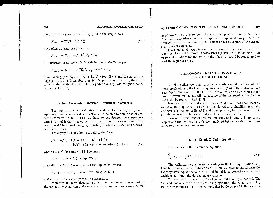
218 BANASIAK, FROSALI, AND SPIGA
the full space Xk , wc can write Eq . (6 .3) in the simpler form :
Xlkn',C = wí(R', Dk(C"')) .
(6.5)
Very often we shall use the space
XOkm, C = Xkm, C = L i (Rx3 , Dk(Cm)) .
In particular, using the equivalent definition of Dk(C), we get
«xXOkl,C = XkI,C = L1, X,,' +v ) - X k+v
Summarizing, f E X lk,,,, C if 8s f E Dk(C") for IsI < l and the norm x -.
II 8 f (x, •) II Dk(c») is integrable over R3 . In particular, if m = 1, then it issufficient that all the derivatives be integrable over IRi ~ with weight functiondefined in Eq . (6 .4) .
6 .3. Full Asymptotic Expansion-Preliminary Comments
The preliminary considerations leading to the hydrodynamicequations have been carried out in Sec. 5. To be able to obtain the desirederror estimates, in most cases wc have to supplement these equationswith bulk and initial layer correctors . This is done by an extension of thecompressed Chapman-Enskog asymptotic procedure of Secs . 3 and 5, whichis sketched below .
The asymptotic solution is sought in the form
J (t, r) =f(t) +f(v) = p(t) + lwo(t) + Elv l (t)+ . . .+ o(z)+Epl(i)+ . . .+tivo(r)+Ewl(r)+ . . .,
(6.6)
where r = t/E" for some n E fil . The terms
p, po, pl . . . E N(Ce) (resp . N(C)),
are called the hydrodynamic part of the expansion, whereas
ivo, tiv l , . . . . lvo , fv l , . . . E N(Ce)1 (resp . N(C)1),
and are called the kinetic part of the expansion .Moreover, the terms depending on t are referred to as the bulk part of
the asymptotic expansion and the terms depending on r are known as the
SCATTERING OPERATORS IN EXTENDED KINETIC MODELS
219
initial lager; they are to be determined independently of each other .Note that in accordance with the compressed Chapman-Enskog procedure,discussed in Sec. 3, the hydrodynamic term of the bulk part of the expan-sion, p, is not expanded .
The number of terms in each expansion and the value of n in thedefinition of r are determined in some sense a posteriori after having writtenthe formai equations for the error, so that the error could be conjectured tobe of the required order .
7 . RIGOROUS ANALYSIS: DOMINANTELASTIC SCATTERING
In this section wc shall provide a mathematical analysis of theprocedures leading to the limiting equations (5 .3)-(5 .6) in the hydrodynamicspace N(C e ) . WC start with the kinetic-diffusion equation (5 .3) which is themost interesting mathematically case ; some of the presented results for thismodel can be found in Refs . [3,5] .
Next we shall briefly discuss the case (5 .5) which has been recentlysolved in Ref. [4] . Equation (5.5) can be viewed as a simplified (spatiallyhomogeneous) version of Eq . (5 .3) and no surprisingly basic ideas of Ref . [4]play the important role in the analysis of the latter equation .
Two other equations of this section, Eqs . (5 .4) and (5 .6) are muchsimpler and though they haven't been analysed before, we shall limit our-selves to some generai comments .
7 .1 . The Kinetic-Diffusion Equation
Let us consider the Boltzmann equation
t = 1E
ESf + z Cef + Cf,
(7 .1)
The preliminary considerations leading to the limiting equation (5 .3)have been carried out in Subsection 5 .1 . Here wc have to supplement thehydrodynamic equations with bulk and initial layer correctors which willenable us to obtain the desired error estimates .
WC start with the system (5 .2) where wc put p = 1, q = 2, r = 0 . Theassumed isotropie form of the scattering operators allows us to simplifyEq. (5 .2) even further . To do this wc note that by Corollary 4 .1, the operator

220
C' reduces N(Ce) and since W = N(Ce ) 1 ', we get DC'O = QC'P = 0 .System (5.2) takes the forni
at -E PSQ~wE + PC'
.
PV' ,
ai,,E Q~SwE + (~SQ~wE + Q~C Q~IVE
EQC'O'V E ,
with the initial conditions
VI(0) = Pf = v,
w,(0) = Of = YV
Inserting Eq . (6 .6) finto Eq . (7 .2) and equating the terms at the samepowers of c we find that wc have to take r = t/E2 so that wc obtain thefollowing system
~t =-C~SQ~(QTlC eQ)-1 Q~SPp + PCPp,
OC, Q111V° = 0,QCeQw1 + QSP,0 = O,O CeWV2 + QSQ1V1 = 0,
ap0 - 0ar
avo _ Q Ce W1, o ,ar
BANASIAK, FROSALI, AND SPIGA
(7 .3)
which, as wc shall see, defines enough terms of the asymptotic expansion toobtain, at least formaily, the convergente of the differente E(t) -f (t, r) tozero as e - 0 .
In fact, let us assume for a time being that ali the equationsabove can be solved and that the solutions are sufficiently regular tomake the manipulations to follow available . It can be proved that onthis level of approximation the correct initial values for Eqs . (7 .3) and(7 .5) are
p(0) =1', ,
ll'o (0) =0w .
Note that the equations for w 1 and w, do not require any side condi-tions, and the solution to Eq . (7 .4) is determined by the stipulated decay to
SCATTERING OPERATORS IN EXTENDED KINETIC MODELS
221
zero as r -i co. Thus we obtain wo = po = 0 and
01 = -(QCe4~) 1 c Spp,Iv2 = _(OCeo)-1 QSOw1 = (QCQQu) -1 QpSQ(QCeQ)-I QSpp (7.6)
w0 = e tc ceQ w .Hence, we take the pair (p, îvo + E1V1 + E2d'2) as the approximation of
fE = (ve , VE ) ; the error of this approximation is given by
YE = VE - P' Z, = w E - l1'° - Ew1 - E2 VV2 . (7 .7)
Assuming that the solution and the terms of the asymptotic expansionare regular enough (we require that they belong to the domains of ali theoperators involved in Eq . (7 .2)) and taking into account Eqs . (7 .3)-(7 .5)wc obtain the following system of equations for the error
aYE-1 PSQZE - PC'PY E = EPSQ1V2 +
1 PSl o,
(7.8)at
E
E
a,_1 1
1at e
QSPY E - E OSO-' - QCrOZE -C2 OCeQZ E
= EQSQ1h'2 + e2Q C'Q11' 2 +1QISQwo + EQZ1C' QJlw1E
+ QC'ow E aw 1 - E2 a1v2° - al
at '
with the initial conditions
y, (0) = 0,
J E(O) = E(Q~C e Q~) -1 QSE V - E 2(Q~C eQ)-1 a sQ(OCeQ)-1Q SP V .
Keeping in mind our assumption that ali the terms of the asymptoticequation are sufficiently regular, we see that the error eE = Y E + zE is a classicalsolution of the problem
aee~ -l Se, - C'e, -
EZCee,
E (SWV2 +Q~C iOiV 1 +EQQC'(iV2 - a
atEw
tivl
a t
+1SQ wo +QC'Qivo ,
(7.9)E
e E(O) = E(QZlC eQ)-1 QSEP v -E2(QCeQ)-1 OSO(QCeQ)-1 QSE V .
- -
222 BANASIAK, FROSALI, AND SPIGA
The semigroup solving this equation is contractive in X, 11 thus usingthe Duhamel formula wc obtain the estimate
II eE(t) II x< E I (UCeO)-1 USp v - E(OCeo ) -1QSO(OCeU) -1 QS((D v-
X'Pr
a1~~2+ EJ
SQ1V2 (S) + Q C Q1V1(S) + EQC Q~w2(S) -alv,a (S) - Ea (S) } dS
(r''+ 1
JII SU11Vo(S/E2 ) + eoC 'QVO(s/E2 ) II x ds .
(7.10)E
From the above inequality we see that if ali the expressions in the first twoterms exist and are bounded in t on [0, to], 0 < to < oc, then the contributionof this integrai is of order of c on this interval . As far as the second integraiis concerned, the initial layer is assumed to be exponentially decaying withr - . oc, that is, to be of order of e`
/,2for some w > 0 . If this property is
preserved after having operated on 1vo with the operatore SU and QC'(,then upon integration we obtain that also the contribution of this term is oforder of e, thus IIeEI x = O(e) and the convergente is proved . Hence we seethat to complete the analysis we must prove that all the tern3s exist and havethe desired regularity . For instante, for QSci v2 to be well-defined we need
the existence of S3p or, in other words, the solvability of Eq . (5 .3) in the
moment space X 3 together with three-fold differentiability with respect to x ;wc also need certain regularity of the moments with respect to the operatorC' : the existence of QC'WV2 requires that S2p be in D(C), etc .
The first step is to establish the equivalente of the forms (7 .2) and (5 .1)
(with relevant scaling) . This requires the projections of the solution to Eq . (5 .1)
to belong to the domain of S. In this respect wc have the following lemma [41which also applies to any other case with dominant elastic scattering .
Lemma 7.1 . If f E D(S) n D(C), then Ir,, Qf, E D(S) n D(C') and thereforeEqs . (5 .1) and (7 .2) are equivalent .
The explicit form and the solvability of Eq . (5 .3) have been investi-
gated in Ref. [3] for much more generai models . In the theorem below we
shall summarize the main results of Ref. [3], specified to the case in hand .
Theorem 7 .1 .
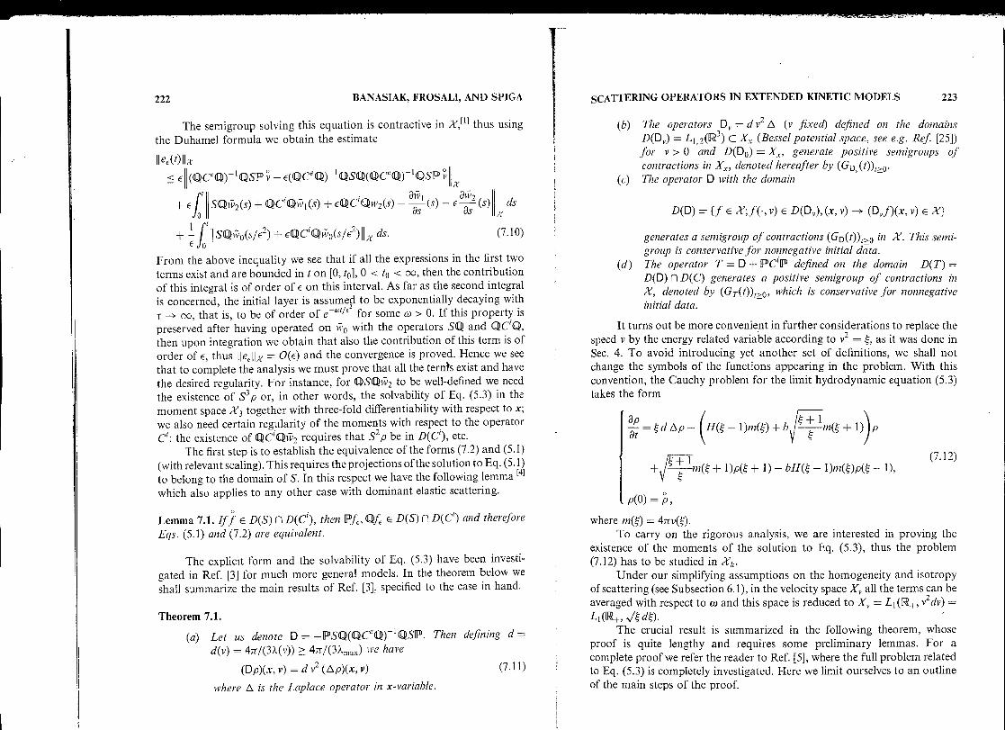
(a) Let us denote D = - pSU(UCeQ) -1 OSP. Then deflning d =d(v) = 4n/(3À(v)) > 47r/(3X nmx) we have
(Dp)(x, v) = d v2 (Ap)(x, v)
(7 .11)
Aere A is the Laplace operator in x-variable .
SCATTERING OPERATORS IN EXTENDED KINETIC MODELS
223
(b) The operatore D,, = d v 22 A (v fixed) defined on the domainsD(D,) = L 1 , 2(R3 ) C Xi (Bessel potential space, see e .g. Ref. [25])for v > 0 and D(D 0 ) = X,, generate positive semigroups ofcontractions in X c , denoted hereafter by (G D (t)) r>o .
(c) The operator D with the dornain
D(D) = {f E X; f(., v) E D(D,,), (x, v) - (D,, f)(x, v) E X}
generates a semigroup of contractions (G D (t)) r>o in X. This semi-group is conservative for nonnegative initial data .
(d) The operator T = D + PC'P defined on the domain D(T) _D(D) fl D(C) generates a positive semigroup of contractions inX, denoted by (GT(t))r>o, which is conservative for nonnegativeinitial data .
It turns out be more convenient in further considerations to replace thespeed v by the energy related variable according to v2 = ~, as it was done inSec. 4. To avoid introducing yet another set of definitions, we shall notchange the symbols of the functions appearing in the problem . With thisconvention, the Cauchy problem for the limit hydrodynamic equation (5 .3)takes the form
ap = ~ d Ap - H(~ - l)rn(~) + b
p(0) = p' ,
+~im( + 1)p( + 1)+bH(~- 1)lnOp(s~ - 1),
(7 .12)
where m(~) = 4mrv(~) .To carry on the rigorous analysis, we are interested in proving the
existence of the moments of the solution to Eq . (5 .3), thus the problem(7 .12) has to be studied in Xt. .
Under our simplifying assumptions on the homogeneity and isotropyof scattering (see Subsection 6.1), in the velocity space X, ali the terms can beaveraged with respect to co and this space is reduced to X, = L I (R+ , v2dv) _L i (R+, ~ d~)
The crucial result is summarized in the foliowing theorem, whoseproof is quite lengthy and requires some preliminary lemmas. For acomplete proof we refer the reader to Ref. [5], where the full problem relatedto Eq . (5 .3) is completely investigated. Here we limit ourselves to an outlineof the main steps of the proof.

224
Theorem 7.2. Fo,• any k > 0, the operator T = D + PC`P generates apositive semigroup in X k , denoted by (GT(t))r>o . Thus if p E Dk (T), then thecorresponding Cauchy problem (7 .12) :
ap Tat
pwith the initial condition
p(0) = p
has a unique solution p E C ([0, cc[, Xk ) .
BANASIAK, FROSALI, AND SPIGA
(7 .13)
(7 .14)
For the proof of this theorem it is convenient to split the operator Tinto the following sum
T=D+ff C`lP=D-N+K_+K+,
where N, K_ and K+ are defined by Eqs . (4 .9) and (4.10) . First it is possibleto prove that D - N generates a positive semigroup, using the fact that N isa multiplication by a non-negative measurable and almost tverywhere finitefunction .
It can be proved (Ref. [5]) that the resolvent of R(À, D - N + K+ )exists and is a positive operator in X k for any ? > 0, thus by Desch'stheorem (see e .g. Ref. [33], Theorem 8.1) it follows that D -N+ K+generates a positive semigroup . Finally, because K_ is a bounded positiveoperator in X, Theorem 7.2 is completely proved using the BoundedPerturbation Theorem e .g. Refs . [9,19] .
∎
Now we are ready to provide the error estimates . Let us recall thataccording to Eq . (6 .5) we have
Xlkm,T = {f E Xk ; 8~Xsf E D(Tm), I,Bj < 1} .
(7.15)
We have the following lemma, whose proof is given in Ref. [5] .
Lemma 7.2 . Let v = P f E X331, T . Then for each interval [0, t o ], 0 < to < +oo,there exists a constant M such that
II(QCeQ)-1 QSP v-E(UC eQ) -1QSQ(QaC eo ) -1 QSP v IIx
+ max SQw 2(t) + QC'QpW1(t) + EQIICQJi 2(t) -a8
t1 (t) - Er
aaf, (t)[ool
< M .
SCATTERING OPERATORS IN EXTENDED KINETIC MODELS
225
The regularity of the initial layer is dealt with in the next lemma .
Lemma 7.3 . Let w = l f E X111, ci . Then there exist a positive constant Lsuch that for any t > 0
IISQtii'o(t/E2)IIx+EIIQC'Q o(t/E 2 )IIx < Le, mi. t1 E2 .
(7.17)
Proof. Since the terms of the initial layer expansion are exactly the same asin Sec . 7.3, this lemma coincider with Lemma 4.3 of Ref. [4] .
Thus we have the theorem .
Theorem 7 .3 . Assume that P f E X331, T gnd Q f E X 111 , ci . Let fE be thesolution of Eq . (7 .1) witk the initial datura f, and p be the solution to Eq . (5 .3)with the initial value Pf . Then for each interval [0, to ], 0 < to < +oo, thereexists a constant K depending only on the initial data, the coefficients of theequation and to , such that
fE(t) - p(t) - e ar/EZQfx
uniformly on [0, t o ] .
Proof. For the proof wc note that the assumptions on the initial dataadopted here are not weaker than that of any lemma (in particular,D(T) c D(S) n D(D)) so that ali the steps of this subsection are justified .Hence using Lemmas 7.2 and 7.3 ; we have by Eq . (7 .10)
< KE
(7.18)
IleE(t)Ilx
< E (OCeo)-1 QSPv-E(QCeQ)-1 (QSQ(QCeQ)-1 (QSPvx
V
7t2+ E
Jr S4~W2 (s) + QC`Qpw 1 (s) + EQ~C`Q~11'2 (S) - aasl (s) - E 8s (s)
0r
+ 1 f IIS(QíV0(S/E 2) + EQ~C'Q) o(S/e2)IjX dsE o%lIE`
EMt0 + ELJ
e_~1min'dr < KE .0
The only difference now is that in Eqs . (7 .7) and (7.10) we had e E =f€ - p-wo - EW 1 - E2 vv2i whereas in Eq . (7 .18) the last two terms are missing .However, the estimates of Lemma 7.2 can be carried also for 1v 1 and w,
dsx

226
from8f
_ E sfE + É c ife + EC,ff
to Eq. (5 .4) which by Theorem 7 .1 is given by
ap = v2dOp
BANASIAK, FROSALI, AND SPIGA
alone, showing that they are bounded on [0, to] . Since they are multiplied by Eand c2 respectively, they can be moved to the right-hand side of the inequality(7 .18) without changing it .
∎
7.2. Purely Diffusive Hydrodynamic Limit
In this subsection we shall describe the steps leading asymptotically
(7.19)
(7 .20)at
Since the limiting equation is simpler than in the previous case, wc shall skipmost technical details .
Using the isotropy of the scattering wc arrive aY the followingcounterpart to Eq . (7 .2)
av, -1 PSQWE + EIPC`PV E ,at
EaaE _ 1 4~1SlvE + i Q~SQQ1V, + E~Q1C '0WE + QpCeQ~W E .
Apart from the hydrodynamic equation (5 .4), all the other terms of theasymptotic expansion coincide with those given by Eq . (7 .6) . Defining theapproximation and the error as in Eq . (7 .7), we obtain the error equations inthe form
aEE - PSQZE - EPCPYE = ePSQWZ + EPC`rp+!PSWWO ,
a z, _ 1 Qspy, - 1 QSWE - EOCQZE - ,, QC eQz = EQSwi',)ar
e
E
E
(7.22)+E34pCQW2 + 1Q sWv0 +E2Q~C`Q7w l
e
EQ~1CO1vO - Eaat`
- EZ aa
+
t2,
with the initial conditions
YE(0) = 0,
z E(0)=E(QC eQ) -I QSPv-E2(Qa1Ce (3) 1 QSQ(QCeQ) 1 Q3Spv .
(7 .21)
SCATTERING OPERATORS IN EXTENDED KINETIC MODELS
227
Clearly the estimates are analogous with the only difference that thistime p is a solution of the diffusion equation in x multiplied by v2 , as seenfrom Eq. (7 .20), and the solution to this equation must have the regularityrequired in Lemma 7 .2. Since the operatore of differentiation andmultiplication by vk commute with D, and D generates a C0-semigroup,the assumPtions will be much milder here and the proof of the counterpartof this lemma is much easier, hence we shall only sketch it . Recalling that
Xlk = WI(R',Xv,k),
wc have the following lemma .
Lemma 7 .4 . Let v = Pf E X44 . Then for each interval [0, t 0 ], 0 < t0 < +oo,there exists a constant M such that
II(OCe Qp) -I QSPV -e(0Ceo ) -1 c Sc (4Ce 1l) -I QpSPvIX
SeW2(t)+EQCQi 1(t)+e 20Ci11w2(t)- aat (t)_E aat2 (t)+ max ;1E [O, to]
< M.
(7 .23)
Proof. Following the approach of Lemma 7 .2 in the same order we seethat the estimate (7 .23) is satisfied if: v3 as~ v E X for 1f1 = 3, (v + l)a~e v E X
for 1,81 = 1, (v'` + v)as~ v E X for If I = 2, and v ka~, v E D(D) for I13I = k,k = 1, 2 . Recalling the definition of D(D) we see that if v E X44 , then allthe above requirements are satisfied .
∎
The initial layer terms are the same so that for the estimates wc can useLemma 7 .3 .
To make the statement of the final theorem more clear, wc recall thatthe space XI I I, C used in Lemma 7 .3 is given by
3X111, C - WI
I(Rr, X,,,,,+,-~).
o
To ensure that the fE is the classical solution we require that Pf ED(C) in addition to the assumptions of Lemma 7 .4. With these we have thefollowing counterpart of Theorem 7 .3 :
Theorem 7 .4 . Assume that P f E X44 ,, Co and Qf E X I 11, C . Let fE be the
solution of Eq . (7.19) with the initial datum f , and p be the solution to Eq . ( 7 .20)
with the initial val ue Pf . Then for each interval [0, t0 ], 0 < t0 < +oc, there
a
i

228
exists a constant K depending only on the initial data and the coe cients ofthe equation and t0 , such that
fE(t) - p(t) - ew
E2of
uniformly on [0, t0 ] .
x< Ke
BANASIAK, FROSALI, AND SPIGA
7.3 . Purely Kinetic Hydrodynamic Limit
Now we shall present the counterpart of Theorems 7 .3 and 7.4 forthe scaling
a E-Sf +
i CefE + Cfat
E
PC'Pp=-CH(~- 1)nz(:)+b ~+
+m(~+ 1)'p
1
yE - VE - p,
+1m( + l)p( + 1) +bH( - 1)m()p( - 1),
with m() = 47rv() .This problem was thoroughly investigateti in Ref . [4] so that wc
mention here only that the solvability of Eq . (7 .26) in the moment spacesXk presents similar (though technically less involved) difficulties to thoseencountered for Eq . (5 .3) .
It follows that in this case there is no need to go to 1v2 as the terms
p, iv l = -(QCeQ) 1 QSPp, w o = e'QC Q w0
where r = t/E, and p is the solution to Eq . (7 .26) with the initial conditionp(0) = v, suffice to obtain the desired estimates . This follows as the error ofthe approximation
zE =wE -11'0 - EYV1,
(7.24)
(7 .25)
resulting in the hydrodynamic limit (5.5)
ap = PC'Ip,
!
(7 .26)ar
where, as before,
SCATTERING OPERATORE IN EXTENDED KINETIC MODELS
229
formally satisfies
8yE- PSQzE - PC'Pyf = EDSQtiv1 + PSWV 0 ,
al
at- Qspy E - QsQzE - QC'Q ; - QCe ` zE
(7.27)
= e SjT'1 + QSQVp + EQC'(QYV1 + (QC'Qw0 - Euv iat ,
and the initial conditions
YE( 0 ) = 0>
zE(0) = -Ew1(0) = e(OCeQ)-1 Q5P v .
The conditions under which the error is of order of s are given in thefollowing theorem, which was originally proved in Ref. [4] .
oTheorem 7.5 . Assume that Pf E X221 C 1 and 0Q~f E X111 ci • Let f, be thesolution of Eq . (7 .25) with the oinitial datura f , and p be the solution toEq . (5 .5) with the initial value f . Then for each interval [0, t0], 0 < t 0 < +co,there exists a constant K depending only orl the initial data, the coe cients ofthe equation, and t 0 , such that
o
fE(t) - p(t) - e_" `I E(Q
f
uniformly, on [0, t0 ] .
x<_ Ke
(7.28)
7.4 . Continuity Equation as the Hydrodynamic Limit
The last case of the limit evolution in the hydrodynamic space N(Ce ) isgiven by the scaling
aaEE - SfE + EC'fE + E CefE ,
(7.29)
which produces formally the trivial hydrodynamic limit
ap0 .
ar =
For the sake of completeness we note that the standard asymptoticprocedure (with the initial layer time r = t/E) gives the saure terms of the

230
expansion as in tbc case of purely kinetic hydrodynamic limit . The errorequation takes the form
ayE- PSQzE - EDC'Py E = epsWY i + PS©tiv o + e C'ip,
at
z - tSPyE - QSQ?E - E6. COZE - 11 t3 C,Or,
(7.30)
= et SQw, + E ZQC'Uw 1 + USU1vo + EvVC'Q-Vwo - E aa t 1
with the initial conditions
yE(0) = 0,
z E (0) = E(QCeQ)-1 OSQD v,
and wc see that tbc only difference with Eq . (7 .27) (apart from possiblyhigher powers of E in some places) is the presence of the term EPC'EPpin tbc first equation of Eq . (7 .30) . However, the solution to tbc limitingequation is constant in time
p(t) = p(0) = v,
so that ali tbc regularity requirements for p will be satisfied provided theyare imposed on tbc initial value v .
Thus we can state tbc theoremo
oTheorem 7 .6 . Assume that P f E X221, ci and O f E Mi 11, c ; . Let f be thesolution of Eq . (7.29) with the initialdatum f. Then for each interval [0, to],0 < to < +oo, there exists a constant K depending only on the initial data,the coe cients of the equation, and t o such that
E(t) - Pf - e x`!EQfx
BANASIAK, FROSALI, AND SPIGA
(7 .31)
< Ke
(7 .32)
In this section we shall discuss the hydrodynamic limits in the caseswith dominant either inelastic, or both inelastic and elastic scattering . A
SCATTERING OPERATORS IN EXTENDED KINETIC MODELS
231
simplified version of these models (without C e) was thoroughly investi-gated in Refs . [2,8], and from the numerical point of view in Refs . [6,16,17] .
It follows that taking Ce into account does not change the overallpicture-the differences are rather cosmetic as was already noted in Sec . 4 .It is useful to remark that the null-spaces N(C) and N(C + Ce ) coincideand tbc inclusion of N(C) into N(Ce ) simplifies the asymptotic analysis .Thus in this section we shall present only formai considerations to show thattbc presente of Ce does not necessitate the introduction of any assumptionsother than those in the papers cited above. Recali also that by Corollary 4 .1tbc null-spaces and the projection operators P and Q coincide in all the casesdiscussed in this section .
8 .1 . The Case of C` and C e Being of the Same Magnitude
First we shall consider the Boltzmann equation with tbc scaling
aE = 1g + 1 CefE + 1 Cf',
(8.1)at
e
e
Ewhich as wc know has the hydrodynamic limit
aap = -PSQ[Q(C' + C e )Q]-1 QSPp .
Let us first note that the question of the invertibility of Q(C + C e)Q ismuch more complicated than in the cases with dominant elastic scattering .The case without the elastic collision operator Ce was investigated inRefs . [2,8] . Here wc shall show that the addition of Ce , as defined inEq . (6 .1), introduces only insignificant changes .
Due to tbc translational character of tbc operator C' it is convenient tointroduce the reduced energy ~ E [0, 1[ and to re-define all the functions asfunctional sequences in the following way : for n = 0, 1, 2 . . . and fixed~E[0,1[
P,A) _ ' ~' v»+1(0.
uniformly on [0, to] . P" (x, 0 = p(x, ~ +n),
8 . RIGOROUS ANALYSIS: DOMINANT
d„(~) = d(~ + n),
v,,(~) = v(~ + n),
INELASTIC SCATTERING ~» = '/~ + li,

232
It follows that using this notation wc can introduce the followingequivalent norm in Xk
I
i
Ilfllk= f ~olifo( •, ~)Ilx,d~+
k ~ 2f ~j11f( •, ~)IIY,d~<oc,
(8.2)0
j-1
0
and the domain Dk(C') can be identified by the finiteness of the followingexpression
o
1
1
f Il fo(,
y, d4+
'f s~jllf(4,w)IIY,d: < cc .
(8.3)j=1
0
To solve the equation (C + C')f = g we use the previous notation toobtain
go(x, 44 , w) = -4m[X0(4) + bpo(4)]fo(x, 4, w) +po fs
, fi (x, 4, w) do
+ Xo(4)f ` fo(x, 4, m') dai ,S
gn(x, 4, w) _ -4z[? n + bp„(4) + v, («f, (x, 4, (9)
+P"(0
f, +t (x, 4, o)) doi + bv„(4)f , f,-1 (x, s:, co) daifs
s-
+ x„(4)f ,f,(x,4,w)do),s~
(8 .4)
where n > 0 . If we decompose g„ = g„o + g„1, where
g„0(x,
(Pg,)(x, 4) =1 f g, (x, 4, w) dw,47r s2
and g„ 1 = g„ - g„o , and introduce the similar notation for the unknownfunction f, we see that due to Eq . (6 .1) wc must have
goo(x, 4) = -4irbpo(4)foo(x, 4) + 4zpo(4)f10(x, s:),
g»o (x, 4) = -47r[bp„ (4) + 1 ]f,o(x, 4) + 4zp„ (4)f,+1, o (x, 4) + 47rbf,-1, 0(x, 4-),
BANASIAK, FROSALI, AND SPIGA SCATTERING OPERATORS IN EXTENDED KINETIC MODELS
233
and in the same time
go1(x, 4, .w) = -4 r[À0(4) + bp0(4)]f01(x, 4, (9),
g, 1(x, S, w) =
+ bp»(4-) +
1(x, 4, w),
so that we see that the presence of the elastic scattering operator C e affectsonly the easy diagonal part of the equation, wheres the troublesome part isthe same as in the case C e = 0, and we can repeat the proof of Theorem 2 .1of Ref. [2] .
Thus, if wc denote by X° the subspace of X of functions satisfying thecompatibility condition of Theorem 4.3 :
, = {f E L, (Rb, v) ;j=0
for a .a . 4- E [O, 1],x E IIRx~,
and, as above, we decompose g = go + g1, where go = Pg and g 1 = g - go,then the following theorem is valid .
Theorem 8 .1 . Let k > 0 . If g E X° is such that g0 E Xk+2, then there exists aunique sohztion f e Dk(C) fl X° to the equation (C' + Ce)f = g, and thereexists a constant M such that for any such g
Ilfllxo,,, < M(Ilgollx'+ , + 1191 11x,1
Remark 8.1 . It is worthwhile to note that Theorem 8.1 gives only sufficientconditions for the solvability of (C'+ C e)f = g, and the condition (8 .7) isnot necessary, as can be checked by considerino , the sequence
(fo)n>1 = ((-1)"%, ln Z)„>1 with fo defined so that the compatibilitycondition is satisfied . It is straightforward to check that g = Cf does notsatisfy Eq . (8 .7) .
On the other hand it can be proved that if g is of constant sign at leastfor large velocities, then Eq . (8 .7) gives also the necessary condition for it tobelong to the range of C, hence C(D(C) n X°) ~ X ° . The details of theseconsiderations can be found in Ref . [8] .
J4 jf -
f (x, s/~ + fw) de) = 0S

234
Denote
1N = f E X; f f(x, s~, co)dw = 0 for a .a . x e R ~ E [0, oo[ } .s
JJJ-
Let us observe that W c X°, that is, any function annihilating constants onS2 automatically satisfies the compatibility condition (4.43) . This makes Wa very useful space as follows from the following corollary to Theorem 8 .1 .
Corollary 8 .1 . The operator C' + Ce is continuously invertible on W with theinverse given by
fo = -(fio + bpo)Igo>
.f;, = -(X„ + bp„ + v„) -lg, ,
Moreover C' + Ce is coercive in W and generates there a semigroup ofnegative tvpe -y = -(Xmin + bLmin) .
Proof. The first statement follows immediately from Eq . (8 .6) . The proofof tbc second statement is similar to the proof of Proposition 4.2of Ref. [2] .
∎
This corollary allows the construction of the diffusion operator . Beforedoing this we should however note that the structure of the diffusionoperator bere is completely different than that of for the dominant elasticscattering . In the latter case the diffusion reflected the feature of the elasticscattering that the particles could be only deflected without changing theirvelocity, thus the kinetic energy ~ E [0, ce[ entered the diffusion only as aparameter labeling particles coming from classes of different energy . Herethe inelastic collisions could change the energy of particles, however, for agiven particle this change could only occur among countably many states . Inother words, the particles are divided into non-overlapping classeswith energies taking values ~ + N, where ~ E [0, 1 [, and these classesremain separate throughout the evolution . As we shall see, this featureis to some extent reflected in the diffusion operator, where the energyparameter is free only in the interval [0, 1 [ and for higher energies thevalues of the solution are reproduced in a periodical manner .
BANASIAK, FROSALI, AND SPIGA
Xo(~)~o + be l vi (~)bj a~j
SCATTERING OPERATORS IN EXTENDED KINETIC MODELS
235
Let us recall that by Theorem 4.3 the spectral projeetion ontoN(C' + Ce ) is given by
00(Pf)„(x, ) = b"G -1 (oy~~j(pf)j(x>0,
(8 .9)j=0
1
where b = n )/n 1 < 1, (Pf)„ = ,,,f, and G(~) = F_j_ 0bl~j . Here ~ E [0, 1[ andx E ll8;. . It can be proved, Ref. [8], that
ceQ(f) = ref
j=0
is the proper hydrodynamical quantity, that is, it remains constantthroughout the evolution . Thus, our limiting diffusion equation will deter-mine the approximation of o . This will be defined only for ~ E [0, 1 [, and theextension to the approximation valid for all ~, according to Eq . (8 .9), isgiven by p = (p„),0 where
p„ = b"G-1Q .
(8 .10)
To find Q we have the following result which is a straightforwardgeneralization of Proposition 3.1 of Ref. [2] .
Proposition 8.1 . The diffusion equation (5 .11) is of the forni
aQ-
B(~)AQ,
(8 .11)at - 3G(~)
where
j=1 Xj(S)Sj + b~j+I vj+I (S) + Sjvj(S)
The existence of the initial layer is also not automatic as the operatorQ(C` + C')Q is not continuously invertible on QX. Therefore even ifQ(C' + Ce)Q generates a semigroup, this semigroup cannot be of negativetype and wc will not have the exponentially decaying initial layer . Tocircumvent this difficulty we use Corollary 8 .1 and restrict the initialvalues to such that
o
0
f =v+w=Pf+uf,
(8 .12)

236
that is, we assume that tiv e W . It follows from Eq . (8 .9)o that fQ = 0,hence for the initial values satisfying Eq . (8 .12) we have Q f =Q f .
Let us write down formai expressions for the remaining terms of theasymptotic expansion and for the error . The projected system takes the form
avE - PSQwE ,at
eaWE - 1 OSQwE + 1
QSPYE + 2at
E
E
EQ(C' + Ce)Q19E ,
uo
V,(0) = := Pf ,
wE(0) = tiv Qf,
where we have taken into account that PC = CF = 0 and that PSP = 0which follows from Eq . (8 .9) (see also Ref. [2]) . As before wc obtain thatfor the bulk part 0 0 = 0 and
TC, + C e)Qtivl = -QSPp,
Q(C' + Ce)Qtiv2 = }QSQwI, (8 .13)
where p is defined by Eqs . (8 .10) and (8 .11) . Fortunately, QSPp is linear in mand thus belongs to W, hence the equation for w l is solvable, defining
w l = -(Q(C' + Ce)Q)-1 QSPp .
Moreover, due to the presence of the exponential factor in Eq . (8 .10),QSQw I E X 0 fl Xk for any k (at least for sufficiently smooth in x function o) .Thus by Theorem 8 .1 the term w, is also well-defined .
The initial layer time is given by -c = t/E 2 and the standard procedureproduces po = 0 and
ai-VOa-V = Q(C' + Ce)QtivO .
(8 .14)
Due to the assumption (8 .12) wc restrict this equation to the subspace Wwhere, due to Corollary 8 .1, wc have the generation of a semigroup of anegative type.
Finally, we obtain that the proper initial values for Eqs . (8 .11) and(8 .14) are given by, respectively
BANASIAK, FROSALI, AND SPIGA
p(O) = v = Pf ,o
tii'o(0) = tiv =1f
SCATTERING OPERATORS IN EXTENDED KINETIC MODELS
237
Combining these results we see that the error(V E - p, w E - IV O- Ewl - E2w2) is (formally) the solution to
YEat - ~ PSQZ E _ e PSQwO + EPS_Oiv2, y,(0) = 0,
at - E QSPYE - E QSQZE - É Q(C` + Ce)Q~E (8 .15)1
ativ l
aw2_ QSQ1"vO + eQSQw 2 - e at -
Ezat ,
ZE(O) = -Ew l (0) - e2 w,(0) .
The rigorous analysis of this system is not different from that providedin Ref. [2] . However, due to a simpler form of the diffusion operator (theLaplacian commutes with the differentiation with respect to x) we can casethe assumptions on the spatial regularity of the initial value . It follows thatin this case we have the following theorem .
Theorem 8.2. Let us assume that v = Pf E X411 , c i and Qf E X11 c fl W.For any t0 < +oc there exists a constant M (depending on t o in an a ne way)such that
(Z E, YE) =
II fE(t) - p(t) - 00(t/e2)I1x < EM .
8.2. Strictly Dominant Inelastic Scattering
Here we shall consider the Eq . (5 .13) with q = 1 which presents themost involved case. That is, we have
t =CSfE +ECefE +e CE,
which, as wc know, has the hydrodynamic limit
ap _ -PSQ(QC'Q)- 'QSPp .
(8 .16)
(8 .18)
It is clear that due to Theorems 4 .2, 4.3, 8 .1 and Corollary 4 .1 theasymptotic analysis in this case will not differ much from that for Eq . (8 .1) .
The hydrodynamic part p is again given by Eq . (8 .10) with the onlydifference that the diffusion coefficient B in Eq . (8 .11) should be calculatedwith À,, = 0 for any n .

238BANASIAK, FROSALI, AND SpIG
It follows that w 0 , lv l , w0 are the same and lb'2 is the solution of
QSQw J + QCeQiv l = QC'Qtiv2 .(8 .19)
Note that the operation with QCeQ on w 1 does not change tbc properties ofiv i which are relevant to the solvability of Eq . (8 .19) (integrability withweight 1 + v k) so that the terra lv2 is well-defined as in Eq . (8 .13) .Defining the approximation as in the previous case we obtain the error
equations in the form
aYE 1
_ 1
_
_8t E PSQze ! PSQwO + EPSQlv2 ,
y€(0) = 0,azE
1
1
1at - E QSPYE - E QSQzE - EQCe QzE - - QC1QzEE_ 1
1
_= QSQ}t'o + . QCeQwO + EQCeQw2
(8 .20)
awl
2 8w2+ EQSQ }v2 - E ó- eót
t ,zE(0) _ _Ci,(0) - E2w2(0) .
We see that but for the terms É QCeQwO and EQCe QW2, Eq. (8 .20) isthe same as Eq . (8 .15) . However, since the operator QCeQ is bounded, theaddition of these terms will not affect the error estimates and we see
thatalso the main theorem will not change here .
Theorem 8.3 . Let us assume that v = Pf E X411, c, and Qf E Xi 11, ci n W .For any t0 < +oc there exists a constant M such that
J jfE(t) - p(t) - iVO(t/e2)IIX:5 EM. (8.21)
8.3. Continuity Equation as the Hydrodynamic Limit
The last case is when wc have the scaling
E= Sff+E Ceff +6
Cf,
(8 .22)
with q = 1 or q = 0, both giving the hydrodynamic limit
apat = 0 .
SCATTERING OPERATORS IN EXTENDED KINETIC MODELS
239
Let us consider first the case with q = 0 . Clearly, then p = p = Ff and
li, l = _(QC'Q) -1 QSP p .
It follows that the proper initial layer time is i = t/E ; apart from this the
initial layer corrector is defined as above by
ax'° = QC'Qw0,
1}'0(0) = W .
(8.23)àt
Defining the error by y = v E - p, z = w - Elv l - w 0 wc obtain the fol-
lowing equation
a t - PSQz6 = PSQivO + EPSQIVI, yE(0) = 0,at
1
at -QSPy.
- QSQZ e -QCeQZE
+ E QC'QZE= QSQIVO + QCeQii, o + EQCeQI1'1 + EQSQ_lvt,
7E(0) _ -EYV,(0)
where we used the fact that alv i /at = 0 .If wc take q = 1, then the only change will be that
lvl = -(Q(Ce + C`)Q) -1 QSPP,
and, with the same r and the initial value w0(0)
aW0 = Q(C e + C )Q 1N0 .az
(8.24)
(8 .25)
Wc know that the addition of C e doesn't affect relevant properties of C', sothe above equations are solvable as in the previous cases . The only differente
will be that in the error system (8 .24) wc won't have terms involving QCeQon the right hand side of the limiting equation but this doesn't affect the
error estimates . Thus, both cases can be treated as one .The regularity assumptions can be further relaxed here. Wc note
that for the estimates we require the existence of only two spatial
derivatives of p and the regularity with respect to v is o ensured by the
exponential factor appearing in the definition of p = Pf . All the other
assumptions on Ff come from the requirement that the error be the
classical solution of Eq . (8 .24) . The assumptions on Qf are the same as
in both previous cases, and are dictated by the solvability of Eqs . (8 .23)

240 BANASIAK, FROSALI, AND SPIGA
and (8 .25) . Thus wc can summarize this discussion by stating thetheorem .
Theorem 8.4. Let us assume that v = Pf E X, i1 ci and 1v = Qf e X111,cin
W. For any t 0 < +oe there exists a constant M such that
IIfE(t) - Pf -}1'0(0E)II x < EM.
9. REFERENCE MANUAL
In this section we have collected the main formular of this paper foreasy reference. Wc avoid here making any regularity assumptions-it isenouah to state that all the results are valid if the initial data are smoothwith respect to x and decay sufficiently fast to zero as v -+ oo . The onlyadditional assumption (adopted for technical reasons) is that the kinetic partof the initial datum annihilates constants over S 2 in the clses of dominantinelastic, or elastic and inelastic scattering . Wc are dealing with thefollowing Boltzmann equation
af E -_sfE + Cf, + ~P CIfEat
EP
eq
E
ivco ax + i (-47rkf +x
J
, f dco /s-
+- (-4,r(Hv+b i+v+) f + ll+ v+f 2f+ dw +bvHf f_dw),
s
s-
f€(0) =f
where v+ = w' ± 1, for any function g we denoted gf = g(wz ± 1) andH = H(v z - 1) is the Heaviside function . Functions 2, and v are functions ofv variable only and v + = v(v+) . In what follows we shall mainly use theenergy variable 4 = v'` . In all the cases the O(E) approximation inL 1 (R6, v ), uniform on finite intervals [0, t0 ], is given by
fE (t, x, v) = p(t, x, v) + W0(t/Ek , x, v) + 0(c),
where k is equal to the highest power of é in Eq . (9 .1), that is, either k = 1or k = 2 .
(8 .26)
SCATTERING OPERATORS IN EXTENDED KINETIC 1VIODELS
We define
lPf = 1ffdw.47r
'-
and0=I-P
9.1 .1 . The Case p = 1, q = 2, r = 0
The details are in Subsection 7 .1 .
Hydrodynamic limit
àt =~dAp- (H(~- 1)m(~)+bi m(~+ 1)1p
+~+lm( +1)p(~+1)+bH(~-1)m(~)p(i - 1),
op(o) = Pf ,
where m(4) = 4TrvO and the diffusion coefficient d is given by
d _ 4Tr
3)(v)
Initial layer corrector
tiv 0(t/E', x, v) = e-j(Vkl62~f(x, n
) .
9 .1 .2. The Case p = 1, q = 2, r = -
The details are in Subsection 7 .2 .
Hydrodynaric limit
apar
p(o) = P.f ,
9.1. Dominant Elastie Scattering
241
(9 .2)

242
where the diffusion coefficient d is given by
d
4rr3),(v)
Initial layer corrector
ivp(t/E 2 , x, v) = e a(i)t/EZQ (V, x) .
9 .1 .3 . The Case p=0, q= 1,r=0
The details are in Subsection 7.3 .
Hydrodynamic limit
a~ _- H(~ - 1)rn(~) + b
1 m(~ + 1) I p
+,/+
1 rn( + 1)p(~ + 1) + bH(~ - 1)m(~)p(~ - 1),~
p(O) = Pfo
where m(~) = 4nv(~) .
Initial layer corrector
o
lv o (t/E, x, v) = e -x(V)`IE(af(x, v) .
9 .1 .4 . The Case p-0, q= l,r=-1
The details are in Subsection 7.4 .
Hydrodvnamic limit
at = 0,at
p(o) = Pf ,
BANASIAK, FROSALI, AND SPIGA SCATTERING OPERATORS IN EXTENDED KINETIC MODELS
243
thus
p(t) = Pf
Initial layer corrector
Wo(t/E, x, v) = e-X(v)tl'O f (x, v) .
9.2. Dominant Inelastic Scattering
In this subsection it will be convenient to use the sequentialnotation for functions : f = (f„),,, o , where f (~ + n) = f„(4) for ~ E [0, 1 [and n = 0, 1, . . . .
The spectral projection on either N(C) or N(C` + Ce) is given by
(Pf)n(x, ) = b 77G-1 (~)
~j(Pf)j(x, 0,j=0
where b = n,/n 1 < 1, j
+j, GO _ ~job'~j and P is definedby Eq . (9 .2) .
9.2 .1 . The Casep= 1,q=r=2
The details are in Subsection 8 .1 .
Hvdrodvnamic limit
Wc have p = (p„),,, o where
p,, = b nG-1Q,
and Q is the solution to
I aQ
B(~)A
at
3G(~) cQ '0
Q(0) = Pf ,
where
B(4) _ 0bj a
X0(5) 0+belv1() j=1 À1( ) j+bj+1vj+1( )+ jvj( )

244
BANASIAK, FROSALI, AND SPIGA
Initial layer
In all cases below we require that w satisfy Pw = 0, and we use thestandard notation
p ( ) _ +n+1 v(~+n+ 1) .
With these
-(a0(~)+bp0($»t1E20
( /z
)
e
tivo(x, , w),wo, ,, t E , x, w =ie_(xn( )+bn„(g)+v (gpr/EZ tivn (x, ~, w) for n > 1 .
where
B() _ 0
b,
bitvi( ) +
a
E b j+tvj+1 ()+ j vj ( )
Initial layer
wo, (t/E2 , x, eco) =
e-b)0( )r/E2 11, 0(x, , w),e-(bp .( )+0„( ))VEZlv7(x
w) for n > 1 .
9 .2 .2 . The Case p= 1,q= 1,r=2
The details are in Subsection 8 .2 .
Hydrodynamic limit
We have p = (p, t ),,, o where
pi, = b"G-1 Q,
and e is the solution to
aQ _ B(~)at 3G(O
oQ(o) = Pf ,
SCATTERING OPERATORE IN EXTENDED KINETIC MODELS
245
9.2 .3 . The Case p = 0, q = r = 1
The details are in Subsection 8 .3 .
Hydrodynamic limit
We have
thus
thus
p(t, x, v) = Pf .
0
p(o) = Ff ,
p(t, x, v) = Ff.
Initial layer
e (fio($)+bpo())tlEH,°(x,,w),
Yt0,,,(t/E, x, (0) _ e(4(0+bv„A)+v,AMlEy°pn(x, ~, w) for n > 1 .
9.2 .4 . The Case p = 0, q = 0, r = 1
The details are also in Subsection 8 .3 .
Hydrodynamic limit
Wc have
p(o) = Pf ,

246 BANASIAK, FROSALI, AND SPIGA SCATTERING OPERATORS IN EXTENDED KINETIC MODELS
247
Initial lager 6 . Banasiak, J .; Demeio, L . Diffusion Approximations of a Linear
~, (o),($)+v„( ))t~E °
e bna ()t/E tiv o (x,1b'o,l ( t/e, x, ~(0) = (bP .
Kinetic Equation with Inelastic Scattering : Asymptotic Analysisand Numerical Results . Transport Theory Stat . Phys . 1999, 28(5),475-498 .e W,, (x, ~, o» for ti > 1 .
7 . Banasiak, J . ; Frosali, G . ; Spiga, G . Asymptotic Analysis for a Particle
ACKNOWLEDGMENTS 8 .
Transport Equation with Inelastic Scattering in Extended KineticTheory. Math. Mod. Meth . Appl. Sci . 1998, 8(5), 851-874 .Banasiak, J .; Frosali, G .; Spiga, G . Inelastic Scattering Models in
A significant part of this paper was prepared when one of the authorsTransport Theory and Their Small Mean Free Path Analysis . Math.Meth. Appl. Sci . 2000, 23, 121-145 .
(J . Banasiak) visited Dipartimento di Matematica Applicata "G. Sansone" 9 . Belleni-Morante, A .; McBride, A.C . Applied Nonlinear Semigroups ;at the Università di Firenze .National Group for MathematicalPhysics
The support receivedof the
for this visit fromIstituto Nazionale
thedi Alta 10 .
J. Wiley: Chichester, 1998 .Ben Abdallah, N . ; Degond, P. On Hierarchy of Macroscopie Models
Matematica (INdAM-GNFM)The work of J . Banasiak
is highly appreciated .was also partly supported by National 11 .
for Semiconductors . J. Math . Phys . 1996, 37(7), 3306-3333 .Bobylev, A.V . ; Spiga, G . On a Model Transport Equation with
Reseach Foundation of SouthThis work was also partly
Africa .supported by the Italian Ministery of 12 .
Inelastic Scattering . SIAM J. Appl. Math . 1998, 58, 1128-1137 .Caraffini, G.L . ; Catalano, C.E . ; Spiga, G . On the Small Mean Free
University (MURST National Project "Problemi matematici delle teorie
13 .
Path Asymptotics of the Transport Equation with Inelastic Scattering .Riv. Mat. Univ. Parma, Serie VI 1998, 1, 13-30 .Case, K.M . ; Zweifel, P .F . Linear Transport Theory ; Addison-Wesley :
cinetiche"), by the CNRFluidodinamica Molecolare,"
Special Projectand by the
"Metodi Dhatematici inEuropean TMR Network
"Asymptotic Methods in KineticThe authors would like
Theory."to express their sincere thanks to all the 14 .
Reading, 1967 .Cercignani, C . The Boltzmann Equation and Its Applications ; Springer
colleagues who, on variousstimulating discussions, suggestiona
occasiona, contributedand criticism .
to this paper through15 .
Verlag: New York, 1988 .Cercignani, C . ; Sattinger, D. Scalin
o16 .
Processes; Birkhàuser : Basel, 1998 .Demeio, L . ; Frosali, G. Diffusion Approximations of Kinetic
1 . Banasiak, J . Mathematicalin Linear Kinetic Theory,
REFERENCES
Properties ofMath. Mod. Meth .
Inelastic ScatteringAppl. Sci . 2000,
Models10(2), 17 .
Equations with Elastic and Inelastic Scattering : a Comparison ofDifferent Scalings, Sommari del IV Congresso Naz . Soc. Ital . diMatematica Industriale e Applicata SIMAI98, Giardini Naxos(Messina), 1-5 giugno 1998, Vol . 2, 316-319 .Demeio, L .; Frosali, G. Different Scalings in the Asymptotic Analysis
163-186 . of Kinetic Equations with Elastic and Inelastic Scattering, Università2 . Banasiak, J. Diffusion Approximation
in Linear Kinetic Theory .of an
Adv. Math . Sci .Inelastic Scattering
Appl . 2000, 10(1), 375-397 .Model
18 .di Ancona, Dipartimento di Matematica, Rapporto N .2-Aprile 1999 .Eliason, M.A . ; Hirschfelder, J.O. Generai Collision Theory Treatment
3 . Banasiak, J . On a Diffusion-KineticKinetic Theory . Math. Methods Appl . Sci .
Equation Arising in Extended2000, 23(14), 1237-1256 .
for the Rate of Bimolecular Gas Phase Reactions . J. Chem . Phys . 1959,30, 1426-1436 .
4 . Banasiak, J . The Existence of Moments of Solutions to Transport 19 . Engel, K .-J . ; Nagel, R . One-parameter Semigroups for Linear EvolutionEquations with InelasticAsymptotic Analysis . J .
Scattering andAppl. Analysis 2000,
Their Application6(2), 13-32 .
in the20 .
Equations, Graduate Texts in Mathematics; Springer Verlag : Wien, 1999 .Ferziger, J.H .; Kaper, H.G . Mathematical Theory of Transport
5 . Banasiak, J. On the Hydrodynamicwith Dominant Elastic Scattering .
Limit ofAtti. Sem.
a Linear Kinetic EquationMat. Fis . Univ. Modena 21 .
Processes in Gases ; North Holland : Amsterdam, 1972 .Frosali, G . Asymptotic Analysis for a Particle Transport Problem in
2001, IL(1), 221-245 . a Moving Medium. IMA J . Appl. Math . 1998, 60, 167-185 .

248
BANASIAK, FROSALI, AND SPIGA
22 . Garibotti, C.R . ; Spiga, G . Boltzmann Equation for InelasticScattering . J . Phys. A: Math. Gen . 1994, 27, 2709-2717 .
23 . Grad, H. Asymptotic Theory of the Boltzmann Equation . Physics ofFluids 1963, 6(2), 147-181 .
24 . Groppi, M .; Spiga, G . Kinetic Approach to Chemical Reactions andInelastic Transitions in a Rarefied Gas . J . Math. Chem . 1999,
25 . Henry, D . Geometrie Theory of Semilinear Equations ; LNM 840 .Springer Verlag : New York, 1981 .
26 . Hilbert, D . Begriindung der kinetischen Gastheorie . Math . Ann . 1912,72, 562-577 .
27 . Light, J.C . ; Ross, J . ; Shuler, K .E. Rate Coefficients, Reaction CrossSections, and Microscopie Reversibility . In Kinetic Processes in Gasesand Plasrnas ; Hochstim, A . R ., Ed.; Academic Press : New York, 1969 .
28 . Majorana, A. Space Homogeneous Solutions of the BoltzmannEquation Describing Electron-Phonon Interaction in Semiconductors .Transport Theory Stat . Phys . 1991, 20(4), 261-279 .
29 . Markowich, P .A . ; Ringhofer, Ch.A . ; Schmeiser, Ch . SemiconductorEquations; Springer Verlag : Wien, 1990 .
30. Markowich, P.A . ; Schmeiser, Ch. The Drift-Diffusion Limit forElectron-Phonon Interaction in Semiconductors . Math. Mod. Meth .Appl. Sci . 1997, 7(5), 707-729 .
31 . Mika, J.R . ; Banasiak, J . Singjdarly Perturbed Evolution Equationsti-vith Applications in Kinetic Theory; World Scientific : Singapore, 1995 .
32. Mika, J .R. New Asymptotic Expansion Algorithm for SingularlyPerturbed Evolution Equations . Math. Methods Appl . Sci . 1981, 3,172-188 .
33 . Mokhtar-Kharroubi, M . Mathernatical Topics in Neutron Theory : NewAspects; World Scientific : Singapore, 1997 .
34 . Rossani, A .; Spiga, G . Kinetic Theory with Inelastic Interactions,Transport Theory Stat . Phys . 1998, 27, 273-287 .
35 . Rossani, A . ; Spiga, G . A Note on the Kinetic Theory of ChemicallyReacting Gases . Physica A 1999, 272, 563-573 .
36 . Truesdell, C . ; Muncaster, R.G . Fundarnentals of Maxwell's KineticTheory of a Sirnple Monoatomic Gas; Academic Press : New York, 1980 .
37 . Wang Chang, C.S . ; Uhlenbeck, G.E . ; De Boer, J. The HeatConductivity and Viscosity of Polyatomic Gases . In Studies inStatistical Mechanics, Vol . 2, De Boer, J., Ed .; North Holland,Amsterdam, 1969 .
Received September 5, 2000Accepted March 23, 2002