Developments in direct thermochemical liquefaction of biomass: 1983-1990
Upload
independentCategory
view
0download
0
CENTER FOR GEOTECHNICAL MODELING REPORT NO. UCD/CGMDR-02/02
EFFECTS OF VOID REDISTRIBUTION ON LIQUEFACTION FLOW OF LAYERED SOIL – CENTRIFUGE DATA REPORT FOR EJM01
BY E. J. Malvick R. Kulasingam R. W. Boulanger and B. L. Kutter
Research supported by the National Science Foundation, CMS 0070111.The contents of this report reflect the views of the author who is responsible for the facts and the accuracy of the data presented herein. The contents do not necessarily reflect the official views or policies of the National Science Foundation. This report does not constitute a standard, specification, or regulation.
DEPARTMENT OF CIVIL & ENVIRONMENTAL ENGINEERING COLLEGE OF ENGINEERING UNIVERSITY OF CALIFORNIA AT DAVIS DECEMBER 2002
i
EFFECTS OF VOID REDISTRIBUTION ON LIQUEFACTION FLOW OF LAYERED SOIL – CENTRIFUGE DATA REPORT FOR EJM01
E. J. Malvick, R. Kulasingam, R. W. Boulanger, and B. L. Kutter
Center for Geotechnical Modeling Data Report UCD/CGMDR-02/02 Date: December, 2002 Date of testing: May, 2001 Project:
Effects of void redistribution on liquefaction flow of layered soil
Contract number: CMS 007011 Sponsor(s): National Science Foundation Previous reports in this test series:
UCD/CMGDR-02/01
ACKNOWLEDGMENTS This model test was funded by the National Science Foundation under grant CMS-0070111. The contents of this report are not necessarily endorsed by the National Science Foundation. The authors would like to acknowledge the suggestions and assistance of the Board of Consultants on this project that consists of Dr. Gonzalo Castro and Professors Ricardo Dobry, Izzat M. Idriss, Takeji Kokusho and Steven L. Kramer. The assistance of Bill Sluis and Daret Kehlet of the Department of Civil and Environmental Engineering, and Dr. Dan W. Wilson, Chad Justice, Tom Coker and Tom Kohnke from the Center for Geotechnical Modeling, UC Davis are also greatly appreciated. The model tests were performed using the large geotechnical centrifuge at UC Davis. Development of this centrifuge was supported primarily by the National Science Foundation, NASA and the University of California. Additional support was obtained from Tyndall Air Force Base, the Naval Civil Engineering Laboratory and Los Alamos National Laboratories. The large shaker was funded by the California Department of Transportation, the Obayashi Corporation, the National Science Foundation and the University of California. CONDITIONS AND LIMITATIONS Permission is granted for the use of these data for publications in the open literature, provided that the authors and sponsors are properly acknowledged. It is essential that the authors be consulted prior to publication to discuss errors or limitations in the data not known at the time of the release of this report. In particular, there may be later releases of this report. Questions about this report may be directed by email to [email protected].
TABLE OF CONTENTS
COVER PAGE .......................................................................................................................................... i
ACKNOWLEDGMENTS .........................................................................................................................i CONDITIONS AND LIMITATIONS ......................................................................................................i CONFIGURATION OF THE TEST........................................................................................................1 MODEL PREPARATION .......................................................................................................................2 SCALE FACTORS................................................................................................................................... 3
SOIL PROPERTIES.................................................................................................................................3 PORE FLUID PROPERTIES...................................................................................................................4 ORGANIZATION OF PLOTS FROM DATA ACQUISITION SYSTEM .............................................5 INSTRUMENTATION AND MEASUREMENTS.................................................................................7 KNOWN LIMITATIONS OF RECORDED DATA AND MODEL .....................................................17 REFERENCES.......................................................................................................................................18
1
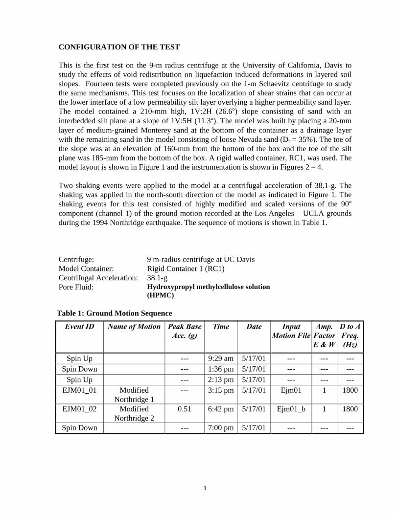
CONFIGURATION OF THE TEST This is the first test on the 9-m radius centrifuge at the University of California, Davis to study the effects of void redistribution on liquefaction induced deformations in layered soil slopes. Fourteen tests were completed previously on the 1-m Schaevitz centrifuge to study the same mechanisms. This test focuses on the localization of shear strains that can occur at the lower interface of a low permeability silt layer overlying a higher permeability sand layer. The model contained a 210-mm high, 1V:2H (26.6!) slope consisting of sand with an interbedded silt plane at a slope of 1V:5H (11.3!). The model was built by placing a 20-mm layer of medium-grained Monterey sand at the bottom of the container as a drainage layer with the remaining sand in the model consisting of loose Nevada sand (Dr = 35%). The toe of the slope was at an elevation of 160-mm from the bottom of the box and the toe of the silt plane was 185-mm from the bottom of the box. A rigid walled container, RC1, was used. The model layout is shown in Figure 1 and the instrumentation is shown in Figures 2 – 4. Two shaking events were applied to the model at a centrifugal acceleration of 38.1-g. The shaking was applied in the north-south direction of the model as indicated in Figure 1. The shaking events for this test consisted of highly modified and scaled versions of the 90! component (channel 1) of the ground motion recorded at the Los Angeles – UCLA grounds during the 1994 Northridge earthquake. The sequence of motions is shown in Table 1. Centrifuge: 9 m-radius centrifuge at UC Davis Model Container: Rigid Container 1 (RC1) Centrifugal Acceleration: 38.1-g Pore Fluid: Hydroxypropyl methylcellulose solution
(HPMC)
Table 1: Ground Motion Sequence
Event ID Name of Motion Peak Base Acc. (g)
Time Date Input Motion File
Amp. FactorE & W
D to A Freq. (Hz)
Spin Up --- 9:29 am 5/17/01 --- --- --- Spin Down --- 1:36 pm 5/17/01 --- --- ---
Spin Up --- 2:13 pm 5/17/01 --- --- --- EJM01_01 Modified
Northridge 1 --- 3:15 pm 5/17/01 Ejm01 1 1800
EJM01_02 Modified Northridge 2
0.51 6:42 pm 5/17/01 Ejm01_b 1 1800
Spin Down --- 7:00 pm 5/17/01 --- --- ---
2
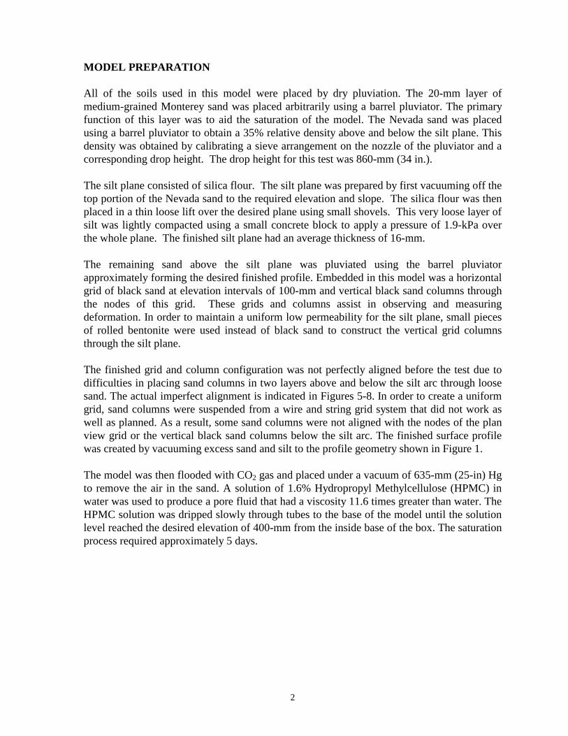
MODEL PREPARATION All of the soils used in this model were placed by dry pluviation. The 20-mm layer of medium-grained Monterey sand was placed arbitrarily using a barrel pluviator. The primary function of this layer was to aid the saturation of the model. The Nevada sand was placed using a barrel pluviator to obtain a 35% relative density above and below the silt plane. This density was obtained by calibrating a sieve arrangement on the nozzle of the pluviator and a corresponding drop height. The drop height for this test was 860-mm (34 in.). The silt plane consisted of silica flour. The silt plane was prepared by first vacuuming off the top portion of the Nevada sand to the required elevation and slope. The silica flour was then placed in a thin loose lift over the desired plane using small shovels. This very loose layer of silt was lightly compacted using a small concrete block to apply a pressure of 1.9-kPa over the whole plane. The finished silt plane had an average thickness of 16-mm. The remaining sand above the silt plane was pluviated using the barrel pluviator approximately forming the desired finished profile. Embedded in this model was a horizontal grid of black sand at elevation intervals of 100-mm and vertical black sand columns through the nodes of this grid. These grids and columns assist in observing and measuring deformation. In order to maintain a uniform low permeability for the silt plane, small pieces of rolled bentonite were used instead of black sand to construct the vertical grid columns through the silt plane. The finished grid and column configuration was not perfectly aligned before the test due to difficulties in placing sand columns in two layers above and below the silt arc through loose sand. The actual imperfect alignment is indicated in Figures 5-8. In order to create a uniform grid, sand columns were suspended from a wire and string grid system that did not work as well as planned. As a result, some sand columns were not aligned with the nodes of the plan view grid or the vertical black sand columns below the silt arc. The finished surface profile was created by vacuuming excess sand and silt to the profile geometry shown in Figure 1. The model was then flooded with CO2 gas and placed under a vacuum of 635-mm (25-in) Hg to remove the air in the sand. A solution of 1.6% Hydropropyl Methylcellulose (HPMC) in water was used to produce a pore fluid that had a viscosity 11.6 times greater than water. The HPMC solution was dripped slowly through tubes to the base of the model until the solution level reached the desired elevation of 400-mm from the inside base of the box. The saturation process required approximately 5 days.

3
SCALE FACTORS All of the dynamic data in this report is presented in prototype scale, unless otherwise explicitly stated. Table 2 lists factors that were used to convert the data from model to prototype scale. Table 2: Scale factors used to convert the model data to prototype units (N = 38.1)
Quantity Prototype Dimension / Model Dimension Time (dynamic) 38.1/1
Displacement, Length 38.1/1 Acceleration, Gravity 1/38.1
Pressure, Stress 1/1 Permeability 3.3/1 *
*The permeability is based on scaling down the permeability by 11.6 due to viscosity and then scaling it up by a factor of 38.1 due to centrifugal acceleration (see section on Pore Fluid Properties).
SOIL PROPERTIES Some of the soil properties of the sands and silt are summarized in Table 3. The range in relative density is based on the variability in repeated maximum and minimum density measurements according to ASTM D4253-83 and D4254-83. A Dr of 35% for the Nevada sand was obtained using data by Earth Technology Corporation (Arulmoli et at. 1991), which were the standards used in this test. A Dr of 36% is obtained using data by Woodward-Clyde (1997). The maximum and minimum densities and relative densities based on Woodward-Clyde tests are shown in parentheses in Table 3. Table 3: Some properties of the soils
Parameter
Coarse Sand Layer
Loose Sand Layer
Silt Layer
Soil type Monterey sand Nevada sand Silica Flour Specific gravity1 - 2.65 2.66 Mean grain size, D50 (mm) 0.603 0.17 0.02 Coefficient of uniformity, CU 1 1.64 - Maximum dry unit weight, γmax (kN/m3) - 17.3 (16.8) - Minimum dry unit weight, γmin (kN/m3) - 13.9 (14.0) - Relative density (%) - 35 (36) - Saturated unit weight (kN/m3) - - - Permeability2 (cm/sec) - 3.2 x 10⁻³ 3.0 x 10⁻⁶
Shear wave velocities were measured in-flight at 38.1-g using horizontal shear wave hammers consisting of a Teflon piston inside an evacuated metal tube (Arulnathan et al. 2000). The Teflon piston moved rapidly from one side of the tube to the other when the vacuum pressure on one side of the tube was changed. The motion and contact of this piston with the opposite end generates a small-strain shear wave propagating radially away from the
1 Cruz (1995) and Chen (1995)
4
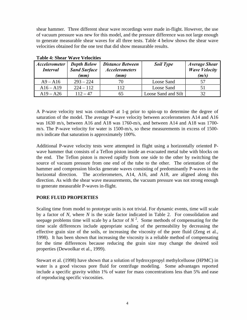
shear hammer. Three different shear wave recordings were made in-flight. However, the use of vacuum pressure was new for this model, and the pressure difference was not large enough to generate measurable shear waves for all three tests. Table 4 below shows the shear wave velocities obtained for the one test that did show measurable results. Table 4: Shear Wave Velocities Accelerometer
Interval Depth Below Sand Surface
(mm)
Distance Between Accelerometers
(mm)
Soil Type Average Shear Wave Velocity
(m/s) A9 – A16 293 – 224 70 Loose Sand 57
A16 – A19 224 – 112 112 Loose Sand 51 A19 – A26 112 – 47 65 Loose Sand and Silt 32
A P-wave velocity test was conducted at 1-g prior to spin-up to determine the degree of saturation of the model. The average P-wave velocity between accelerometers A14 and A16 was 1630 m/s, between A16 and A18 was 1760-m/s, and between A14 and A18 was 1700- m/s. The P-wave velocity for water is 1500-m/s, so these measurements in excess of 1500- m/s indicate that saturation is approximately 100%. Additional P-wave velocity tests were attempted in flight using a horizontally oriented P-wave hammer that consists of a Teflon piston inside an evacuated metal tube with blocks on the end. The Teflon piston is moved rapidly from one side to the other by switching the source of vacuum pressure from one end of the tube to the other. The orientation of the hammer and compression blocks generate waves consisting of predominantly P-waves in the horizontal direction. The accelerometers, A14, A16, and A18, are aligned along this direction. As with the shear wave measurements, the vacuum pressure was not strong enough to generate measurable P-waves in-flight. PORE FLUID PROPERTIES Scaling time from model to prototype units is not trivial. For dynamic events, time will scale by a factor of N, where N is the scale factor indicated in Table 2. For consolidation and seepage problems time will scale by a factor of N 2. Some methods of compensating for the time scale differences include appropriate scaling of the permeability by decreasing the effective grain size of the soils, or increasing the viscosity of the pore fluid (Zeng et al., 1998). It has been shown that increasing the viscosity is a reliable method of compensating for the time differences because reducing the grain size may change the desired soil properties (Dewoolkar et al., 1999). Stewart et al. (1998) have shown that a solution of hydroxypropyl methylcelluose (HPMC) in water is a good viscous pore fluid for centrifuge modeling. Some advantages reported include a specific gravity within 1% of water for mass concentrations less than 5% and ease of reproducing specific viscosities.

5
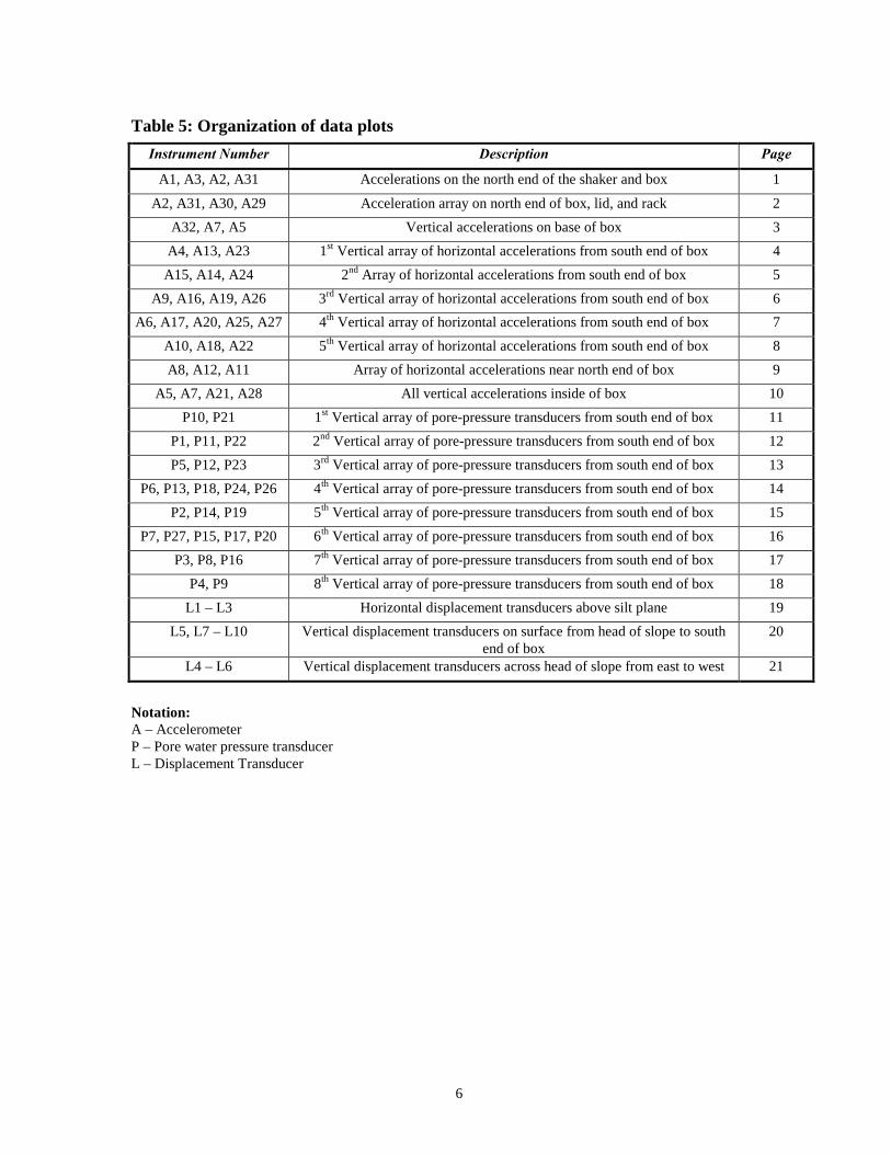
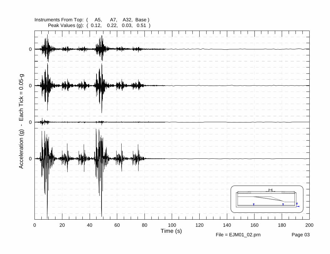
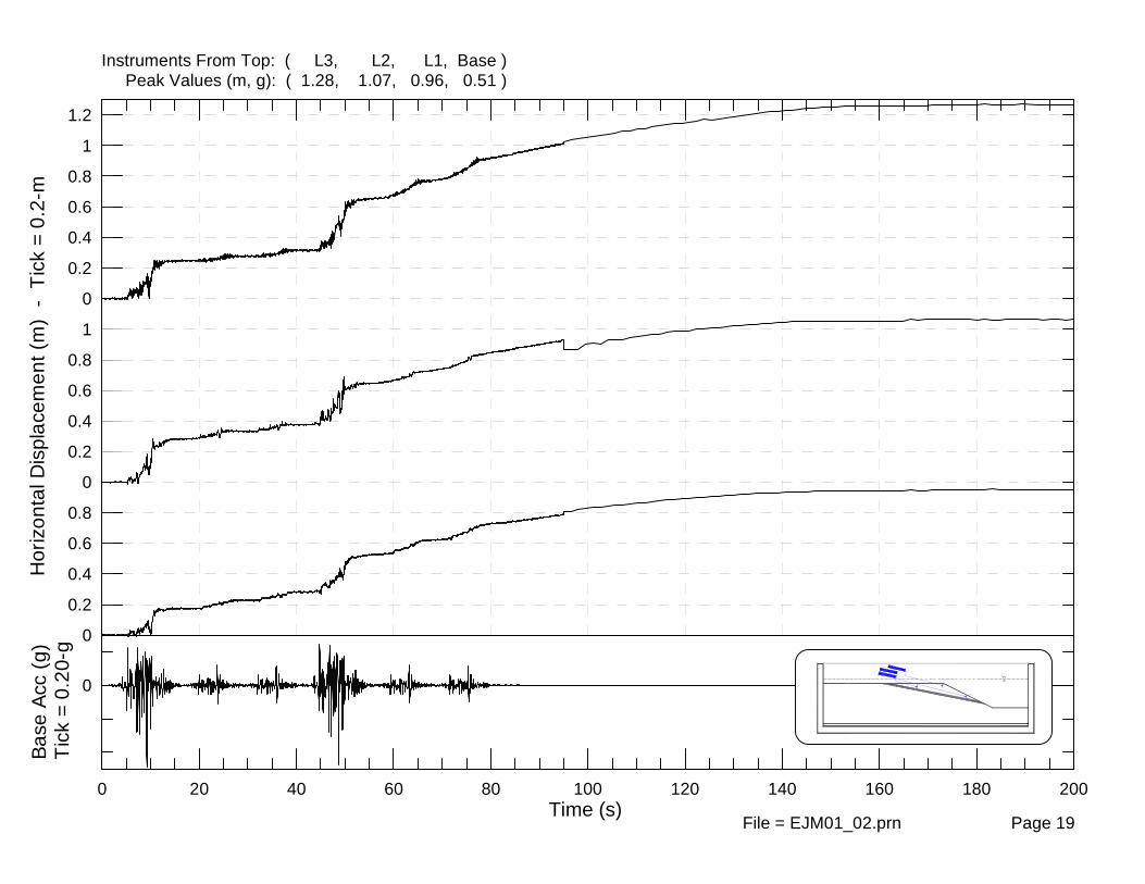
For this test HPMC was used as the pore fluid with a viscosity of 11.6-mm2/s. For comparison, water has a viscosity of 1-mm2/s. A small amount of benzoic acid is added as a preservative as suggested (Stewart et al., 1998). Since this test was conducted at 38.1-g, the viscosity does not completely compensate for the time scale differences. This value was chosen in an attempt to model the small centrifuge tests RKS02 – RKS11 that used HPMC at a viscosity of 25-mm2/s and were spun at 80-g. It has also been stated that proper consideration of the differences can be compensated for by appropriately scaling the permeability (Zeng et al., 1998). This model should scale the permeability by a factor of 3.3 to properly model the permeability obtained in small centrifuge experiments. ORGANIZATION OF PLOTS FROM DATA ACQUISITION SYSTEM The data for the shaking events (refer to Table 1 for event names) is reproduced on 21 pages of time histories as described in Table 5. Only data for the second shaking event are plotted. A computer system failure during the first shaking event prevented data from being recorded for that event. Data for the second shaking event was recorded for a period of 37.5 seconds at two different sampling frequencies. This data was sampled at 1800-Hz for 2.5-s and at 25-Hz for 35-s. The lowermost plot on each page is the base acceleration for that shaking event. The scale for acceleration on the plots with other accelerometers is the same for all accelerometer recordings on that plot. However, on plots where pore pressure recordings or displacement recordings are included, the scale for the instruments is different from the base accelerations as indicated on the plots.
6
Table 5: Organization of data plots
Instrument Number Description Page
A1, A3, A2, A31 Accelerations on the north end of the shaker and box 1
A2, A31, A30, A29 Acceleration array on north end of box, lid, and rack 2 A32, A7, A5 Vertical accelerations on base of box 3
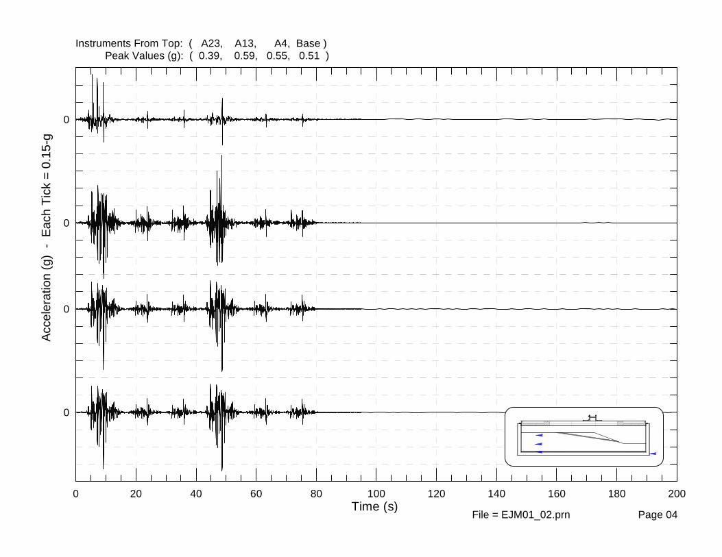
A4, A13, A23 1st Vertical array of horizontal accelerations from south end of box 4 A15, A14, A24 2nd Array of horizontal accelerations from south end of box 5
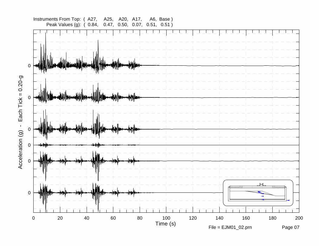
A9, A16, A19, A26 3rd Vertical array of horizontal accelerations from south end of box 6 A6, A17, A20, A25, A27 4th Vertical array of horizontal accelerations from south end of box 7
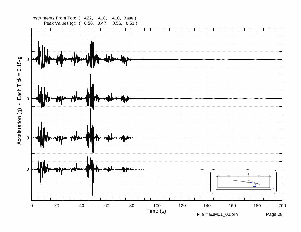
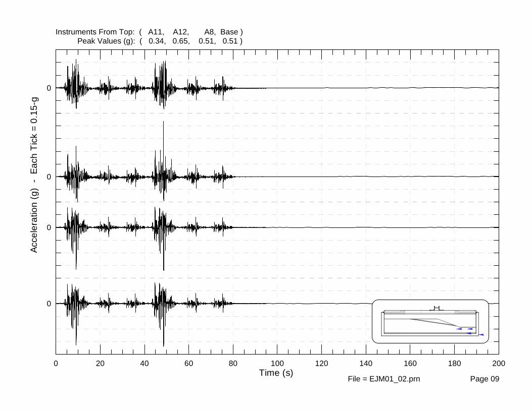
A10, A18, A22 5th Vertical array of horizontal accelerations from south end of box 8 A8, A12, A11 Array of horizontal accelerations near north end of box 9
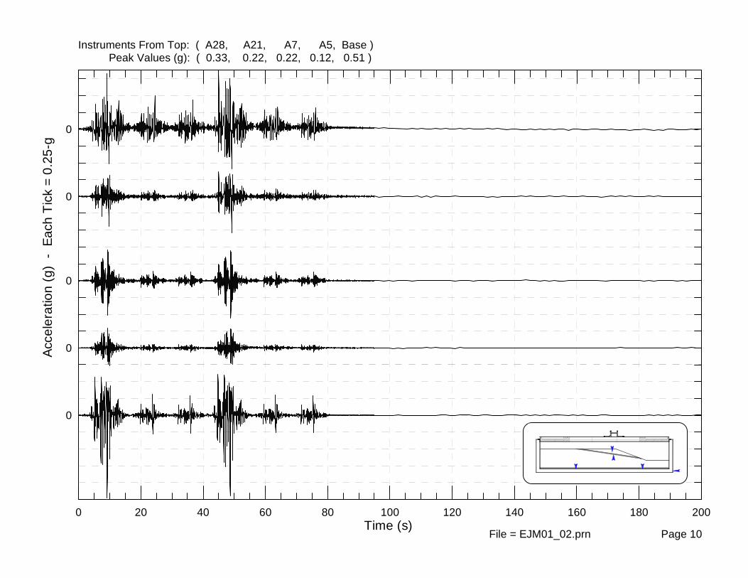
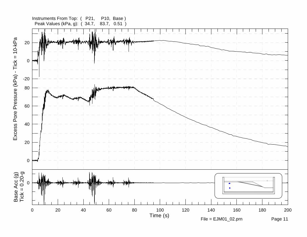
A5, A7, A21, A28 All vertical accelerations inside of box 10 P10, P21 1st Vertical array of pore-pressure transducers from south end of box 11
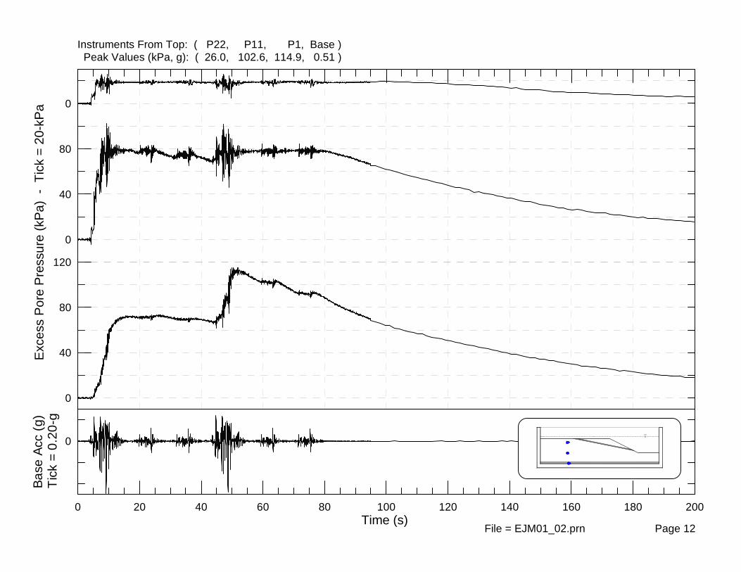
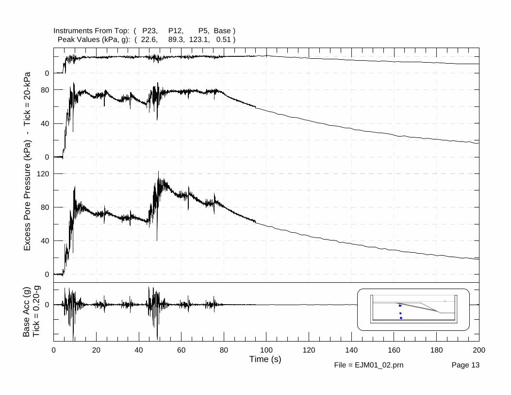
P1, P11, P22 2nd Vertical array of pore-pressure transducers from south end of box 12 P5, P12, P23 3rd Vertical array of pore-pressure transducers from south end of box 13
P6, P13, P18, P24, P26 4th Vertical array of pore-pressure transducers from south end of box 14 P2, P14, P19 5th Vertical array of pore-pressure transducers from south end of box 15
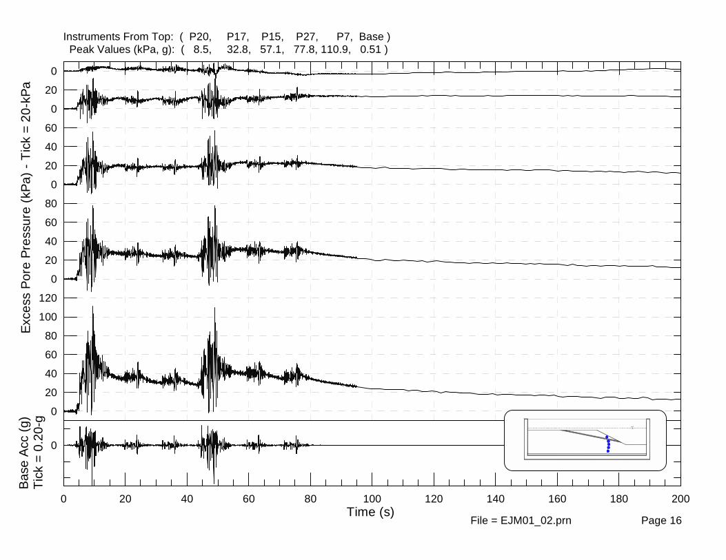
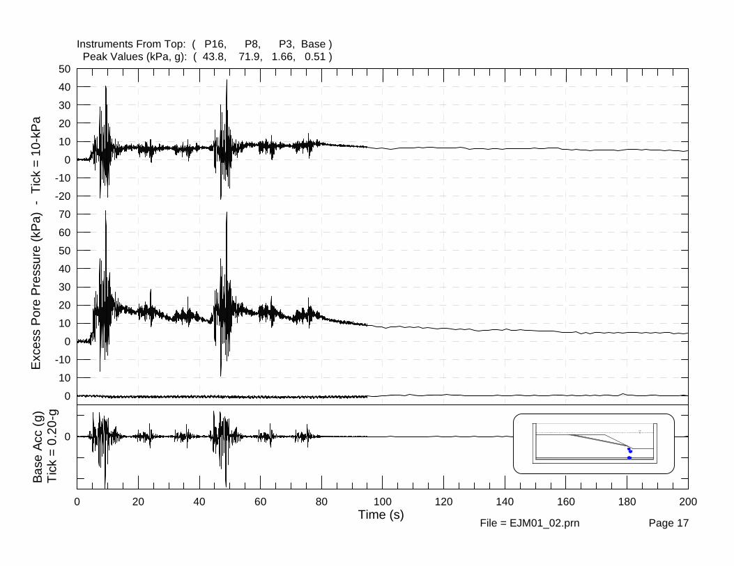
P7, P27, P15, P17, P20 6th Vertical array of pore-pressure transducers from south end of box 16 P3, P8, P16 7th Vertical array of pore-pressure transducers from south end of box 17
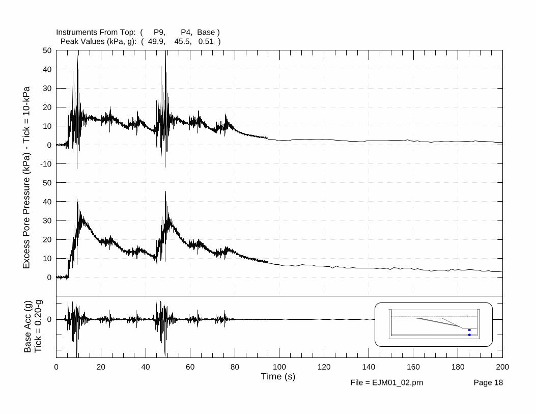
P4, P9 8th Vertical array of pore-pressure transducers from south end of box 18 L1 – L3 Horizontal displacement transducers above silt plane 19
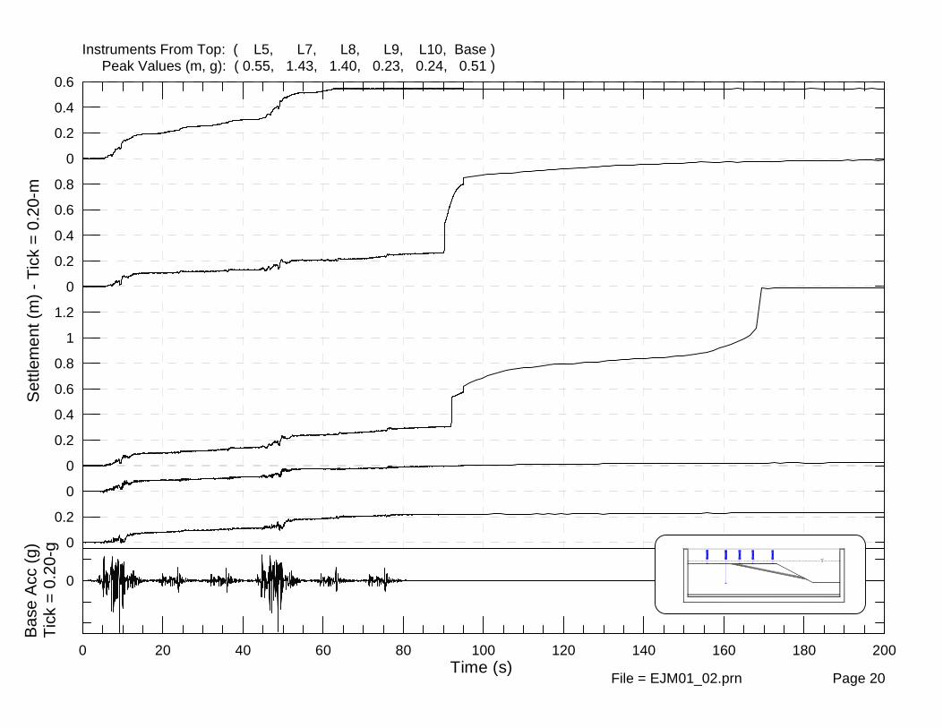
L5, L7 – L10 Vertical displacement transducers on surface from head of slope to south end of box
20
L4 – L6 Vertical displacement transducers across head of slope from east to west 21
Notation: A – Accelerometer P – Pore water pressure transducer L – Displacement Transducer
7
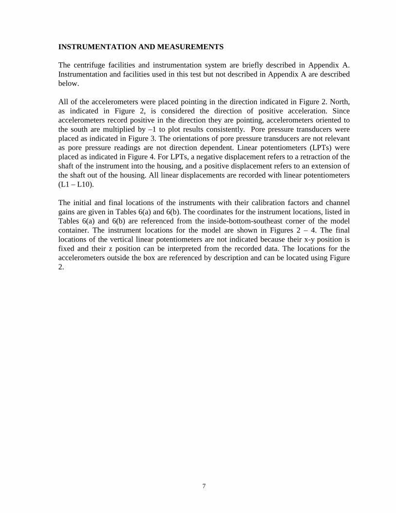
INSTRUMENTATION AND MEASUREMENTS The centrifuge facilities and instrumentation system are briefly described in Appendix A. Instrumentation and facilities used in this test but not described in Appendix A are described below. All of the accelerometers were placed pointing in the direction indicated in Figure 2. North, as indicated in Figure 2, is considered the direction of positive acceleration. Since accelerometers record positive in the direction they are pointing, accelerometers oriented to the south are multiplied by –1 to plot results consistently. Pore pressure transducers were placed as indicated in Figure 3. The orientations of pore pressure transducers are not relevant as pore pressure readings are not direction dependent. Linear potentiometers (LPTs) were placed as indicated in Figure 4. For LPTs, a negative displacement refers to a retraction of the shaft of the instrument into the housing, and a positive displacement refers to an extension of the shaft out of the housing. All linear displacements are recorded with linear potentiometers (L1 – L10). The initial and final locations of the instruments with their calibration factors and channel gains are given in Tables 6(a) and 6(b). The coordinates for the instrument locations, listed in Tables 6(a) and 6(b) are referenced from the inside-bottom-southeast corner of the model container. The instrument locations for the model are shown in Figures 2 – 4. The final locations of the vertical linear potentiometers are not indicated because their x-y position is fixed and their z position can be interpreted from the recorded data. The locations for the accelerometers outside the box are referenced by description and can be located using Figure 2.

8
Table 6(a): Instrumentation Details - pore pressure transducers and displacement transducers Instr. Loc. No.1
Instr. Type
Instr. Ser. No.
Orient-ation2 Initial Position3 Final Position3 Instr.
Range Amp6 Gain
DT7 Gain
Calibr. Factor4 and Units (Model)
Calibr. Factor5
and Units (Prototype)
x (mm) y (mm) z (mm) x (mm) y (mm) z (mm) P1 PPT 7720 - 421 317 0 421 317 0 100 psi 100 2 82.48 kPa/V 82.48 kPa/VP2 PPT 7722 - 1009 331 0 1009 331 0 100 psi 100 2 81.63 kPa/V 81.63 kPa/VP3 PPT 8044 - 1394 324 0 1394 324 0 100 psi 100 2 85.84 kPa/V 85.84 kPa/VP4 PPT 7991 - 1598 326 0 1598 326 0 100 psi 100 2 84.30 kPa/V 84.30 kPa/VP5 PPT 10037 - 605 314 50 603 315 43 100 psi 100 2 84.13 kPa/V 84.13 kPa/VP6 PPT 10038 - 811 321 56 751 313 46 100 psi 100 2 86.05 kPa/V 86.05 kPa/VP7 PPT 10035 - 1189 307 62 1193 303 58 100 psi 100 2 90.05 kPa/V 90.05 kPa/VP8 PPT 10039 - 1410 315 117 1421 320 112 100 psi 100 2 85.03 kPa/V 85.03 kPa/VP9 PPT 7709 - 1597 313 123 1601 313 123 50 psi 100 2 35.49 kPa/V 35.49 kPa/V
P10 PPT 7811 - 206 323 150 194 325 146 100 psi 100 2 80.48 kPa/V 80.48 kPa/VP11 PPT 7817 - 403 315 157 410 314 152 100 psi 100 2 81.59 kPa/V 81.59 kPa/VP12 PPT 7985 - 593 309 151 593 313 147 100 psi 100 2 81.91 kPa/V 81.91 kPa/VP13 PPT 10041 - 811 314 147 816 317 143 100 psi 100 2 82.88 kPa/V 82.88 kPa/VP14 PPT 10042 - 1019 320 146 1025 318 141 100 psi 100 2 88.81 kPa/V 88.81 kPa/VP15 PPT 7988 - 1201 327 152 1214 328 146 100 psi 100 2 81.97 kPa/V 81.97 kPa/VP16 PPT 6711 - 1390 325 155 1402 315 154 50 psi 100 2 37.69 kPa/V 37.69 kPa/VP17 PPT 7373 - 1193 316 219 1234 273 214 50 psi 100 2 34.98 kPa/V 34.98 kPa/VP18 PPT 7805 - 803 295 258 819 297 249 50 psi 100 2 36.28 kPa/V 36.28 kPa/VP19 PPT 7714 - 992 303 252 1014 294 240 50 psi 100 2 36.79 kPa/V 36.79 kPa/VP20 PPT 7810 - 1174 300 257 1223 290 247 50 psi 100 2 39.27 kPa/V 39.27 kPa/VP21 PPT 7719 - 200 299 313 208 300 306 50 psi 100 2 38.64 kPa/V 38.64 kPa/VP22 PPT 7368 - 407 320 314 407 322 308 50 psi 100 2 39.64 kPa/V 39.64 kPa/VP23 PPT 7371 - 588 326 314 598 326 302 50 psi 100 2 41.40 kPa/V 41.40 kPa/VP24 PPT 7370 - 806 299 294 824 303 286 50 psi 100 2 39.30 kPa/V 39.30 kPa/VP25 PPT 7713 - 1003 298 294 1048 300 280 50 psi 100 2 37.64 kPa/V 37.64 kPa/VP26 PPT 7367 - 813 310 322 844 317 310 50 psi 100 2 35.47 kPa/V 35.47 kPa/VP27 PPT 10043 - 1198 324 115 1203 324 110 100 psi 100 2 83.39 kPa/V 83.39 kPa/VL1 LPT 601 H 785 396 362 828 406 344 6" 1 2 15.24 mm/V 580.6 mm/VL2 LPT 602 H 987 466 362 1017 462 308 6" 1 2 15.24 mm/V 580.6 mm/VL3 LPT 603 H 1200 500 274 1256 497 252 6" 1 2 15.24 mm/V 580.6 mm/VL4 LPT 404 V 979 85 368 4" 1 2 10.16 mm/V 387.1 mm/VL5 LPT 201 V 942 356 368 2" 1 2 5.08 mm/V 193.5 mm/VL6 LPT 493 V 944 767 368 4" 1 2 10.16 mm/V 387.1 mm/VL7 LPT 604 V 784 476 368 6" 1 2 15.24 mm/V 580.6 mm/VL8 LPT 492 V 595 411 368 4" 1 2 10.16 mm/V 387.1 mm/VL9 LPT 202 V 490 548 368 2" 1 2 5.08 mm/V 193.5 mm/V
L10 LPT 402 V 189 458 368 4" 1 2 10.16 mm/V 387.1 mm/V1 Refer to Figure 3 for PPT locations and Figure 4 for LPT locations 2 Horizontal LPTs are oriented with the shaft directed towards the north. Vertical LPTs are oriented with the shaft directed downward. 3 Instrument positions are referenced from the SE-bottom-inside corner of the container. LPTs are located by target location for horizontal and shaft location for vertical. Final locations are not measured for vertical LPTs because the x-y position does not change, and z can be interpreted from the settlement measurements acquired during data acquisition. 4 The calibration factor converts the voltage readings to model scale and already includes the amplifier gain. 5 This calibration factor is a modification of the model scale calibration factor scaled according to the g-level. 6 This is the setting used on the amplifier to gain the signal recorded for an increased resolution 7 This is a gain set on the data acquisition system for visualizing data and does not show up in the data and does not need to be accounted for.
9
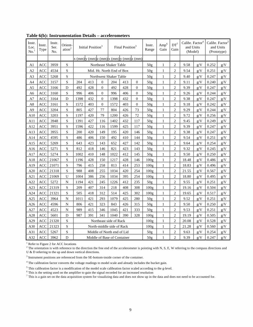
Table 6(b): Instrumentation Details – accelerometers Instr. Loc. No.1
Instr. Type
Instr. Ser. No.
Orient-ation2 Initial Position3 Final Position3 Instr.
Range Amp6 Gain
DT7 Gain
Calibr. Factor4 and Units (Model)
Calibr. Factor5 and Units
(Prototype)
x (mm) y (mm) z (mm) x (mm) y (mm) z (mm) A1 ACC 3959 S Northeast Shaker Table 50g 1 2 9.58 g/V 0.252 g/V A2 ACC 4534 S Mid. Ht. North End of Box 50g 1 2 9.54 g/V 0.251 g/V A3 ACC 5268 S Northwest Shaker Table 50g 1 2 9.40 g/V 0.247 g/V A4 ACC 3157 S 204 413 0 204 413 0 50g 1 2 9.11 g/V 0.240 g/V A5 ACC 3166 D 492 428 0 492 428 0 50g 1 2 9.39 g/V 0.247 g/V A6 ACC 3160 S 996 406 0 996 406 0 50g 1 2 9.26 g/V 0.244 g/V A7 ACC 3164 D 1398 432 0 1398 432 0 50g 1 2 9.38 g/V 0.247 g/V A8 ACC 3161 S 1572 403 0 1572 403 0 50g 1 2 9.18 g/V 0.242 g/V A9 ACC 3204 S 805 427 77 804 426 73 50g 1 2 9.29 g/V 0.244 g/V
A10 ACC 3203 S 1197 420 79 1200 426 72 50g 1 2 9.72 g/V 0.256 g/V A11 ACC 3948 S 1391 427 116 1402 432 117 50g 1 2 9.45 g/V 0.249 g/V A12 ACC 3951 S 1596 422 116 1599 425 117 50g 1 2 9.39 g/V 0.247 g/V A13 ACC 3955 S 200 420 149 195 420 146 50g 1 2 9.38 g/V 0.247 g/V A14 ACC 4595 S 486 406 150 492 410 144 50g 1 2 9.54 g/V 0.251 g/V A15 ACC 5269 S 643 423 143 652 427 142 50g 1 2 9.64 g/V 0.254 g/V A16 ACC 5271 S 812 418 146 821 423 143 50g 1 2 9.32 g/V 0.245 g/V A17 ACC 5274 S 1002 410 148 1022 412 145 50g 1 2 9.50 g/V 0.250 g/V A18 ACC 21067 S 1196 428 150 1217 428 146 100g 1 2 18.48 g/V 0.486 g/V A19 ACC 21071 S 796 415 258 813 414 253 100g 1 2 18.83 g/V 0.496 g/V A20 ACC 21318 S 988 408 255 1034 420 254 100g 1 2 21.55 g/V 0.567 g/V A21 ACC 21069 U 1004 386 256 1034 395 254 100g 1 2 18.80 g/V 0.495 g/V A22 ACC 5272 N 1194 421 245 1226 412 235 50g 1 2 9.55 g/V 0.251 g/V A23 ACC 21319 S 209 407 314 218 408 308 100g 1 2 19.16 g/V 0.504 g/V A24 ACC 21321 S 505 418 312 514 425 302 100g 1 2 19.65 g/V 0.517 g/V A25 ACC 3964 N 1011 421 293 1079 425 280 50g 1 2 9.52 g/V 0.251 g/V A26 ACC 4596 N 806 421 323 843 426 315 50g 1 2 9.50 g/V 0.250 g/V A27 ACC 4523 N 989 415 346 1045 421 333 50g 1 2 9.53 g/V 0.251 g/V A28 ACC 5601 D 987 391 341 1040 390 328 100g 1 2 19.19 g/V 0.505 g/V A29 ACC 21320 S Northeast side of Rack 100g 1 2 20.08 g/V 0.528 g/V A30 ACC 21323 S North-middle side of Rack 100g 1 2 21.28 g/V 0.560 g/V A31 ACC 5267 S Middle of North end of Lid 50g 1 2 9.63 g/V 0.254 g/V A32 ACC 3962 D Middle of Base of Container 50g 1 2 9.39 g/V 0.247 g/V
1 Refer to Figure 2 for ACC locations 2 The orientation is with reference to the direction the free end of the accelerometer is pointing with N, S, E, W referring to the compass directions and U & D referring to the up and down vertical directions. 3 Instrument positions are referenced from the SE-bottom-inside corner of the container. 4 The calibration factor converts the voltage readings to model scale and already includes the bucket gain. 5 This calibration factor is a modification of the model scale calibration factor scaled according to the g-level. 6 This is the setting used on the amplifier to gain the signal recorded for an increased resolution 7 This is a gain set on the data acquisition system for visualizing data and does not show up in the data and does not need to be accounted for.

10
The electronic data for this test are contained in two ASCII files: EJM01_02_mod.prn 2nd Shaking Event model scale EJM01_02_prot.prn 2nd Shaking Event prototype scale For these files, the columns and corresponding instruments are summarized in Table 7. Table 7: Instrument Channel List
Column No. Instrument Column No. Instrument 0 TIME 35 A14 1 P16 36 A9 2 P26 37 A24 3 P5 38 A16 4 P6 39 A20 5 P14 40 A19 6 P7 41 A12 7 P27 42 A28 8 P24 43 A22 9 P22 44 A26
10 P17 45 A11 11 P18 46 A8 12 P13 47 A18 13 P15 48 A10 14 P23 49 A15 15 No Instrument 50 A29 16 P12 51 A21 17 L1 52 A13 18 L10 53 A6 19 L3 54 A31 20 P11 55 A3 21 P21 56 A30 22 P10 57 A27 23 P3 58 A4 24 P8 59 A25 25 P4 60 A7 26 P1 61 A5 27 P19 62 A1 28 P2 63 L4 29 P9 64 L8 30 P20 65 L6 31 A2 66 L2 32 A17 67 L7 33 A23 68 L9 34 A32 69 L5
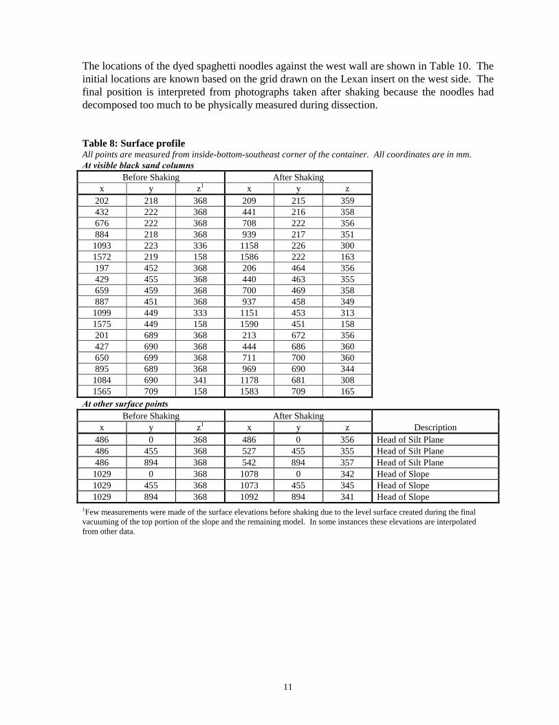
The surface profile was measured before and after the shaking events. These measurements are shown in Table 8. Dyed spaghetti noodles were placed up against the west side of the container on a 100-mm grid for video and photographic purposes. Grids of colored sand were placed in 100-mm increments of depth. The plan view spacing is aligned with the colored sand columns and is irregular. The location of the nodes for the black sand grid before and after shaking is shown in Tables 9(a) and 9(b). Figures 6 – 8 show the initial and final profiles of the colored sand through the N-S gridlines associated with the nodes shown in Figure 5.
11
The locations of the dyed spaghetti noodles against the west wall are shown in Table 10. The initial locations are known based on the grid drawn on the Lexan insert on the west side. The final position is interpreted from photographs taken after shaking because the noodles had decomposed too much to be physically measured during dissection. Table 8: Surface profile All points are measured from inside-bottom-southeast corner of the container. All coordinates are in mm. At visible black sand columns
Before Shaking After Shaking x y z1 x y z
202 218 368 209 215 359 432 222 368 441 216 358 676 222 368 708 222 356 884 218 368 939 217 351
1093 223 336 1158 226 300 1572 219 158 1586 222 163 197 452 368 206 464 356 429 455 368 440 463 355 659 459 368 700 469 358 887 451 368 937 458 349
1099 449 333 1151 453 313 1575 449 158 1590 451 158 201 689 368 213 672 356 427 690 368 444 686 360 650 699 368 711 700 360 895 689 368 969 690 344
1084 690 341 1178 681 308 1565 709 158 1583 709 165
At other surface points Before Shaking After Shaking
x y z1 x y z Description 486 0 368 486 0 356 Head of Silt Plane 486 455 368 527 455 355 Head of Silt Plane 486 894 368 542 894 357 Head of Silt Plane
1029 0 368 1078 0 342 Head of Slope 1029 455 368 1073 455 345 Head of Slope 1029 894 368 1092 894 341 Head of Slope
1Few measurements were made of the surface elevations before shaking due to the level surface created during the final vacuuming of the top portion of the slope and the remaining model. In some instances these elevations are interpolated from other data.

12
Table 9(a): Location of Grid Nodes All points are measured from inside-bottom-southeast corner of container. All coordinates in mm. At Grid Level 3 (z ≈ 311 mm)
Before Shaking After Shaking x y z1 x y z
202 218 311 211 218 301 432 222 311 441 222 301 651 222 311 674 223 301 884 218 311 931 228 299 197 452 311 199 456 301 429 455 311 439 457 301 650 459 311 667 454 302 659 Offset2 702 -- -- 887 451 311 922 455 302
1099 449 311 1158 454 301 201 689 311 209 682 299 427 690 311 438 684 301 648 699 311 670 683 301 650 Offset2 703 -- -- 895 689 311 959 678 292
1084 690 311 1177 677 288 At Grid Level 2 (z ≈ 211 mm)
Before Shaking After Shaking x y z1 x y z
202 218 211 208 219 211 432 222 211 438 221 211 651 222 211 671 226 208 884 218 211 888 229 211
1093 223 211 1117 221 210 197 452 211 205 448 211 429 455 211 437 446 208 650 459 211 663 444 208 884 452 211 886 446 206 887 Offset2 909 -- --
1099 449 211 1124 434 204 201 689 211 204 682 211 427 690 211 437 682 211 648 699 211 665 683 211
Grid Line3 885 674 208 904 689 211 914 674 208 895 Offset2 961 -- --
1084 690 211 1112 677 211 1Initial elevations come from assuming the surface is level after vacuuming for grid placement. The elevations also reflect the location of the Lexan inserts that did not sit flush to the bottom of the box. The sand grid was placed to match the Lexan grid as well as possible. 2The offset measures the x location above and below the lower silt-sand interface. The y and z are the same as for the coordinates in the row above. The initial x locations differ due to the difficulty in aligning the columns exactly during construction. 3One column did not align well with the rest of the grid, so the grid line was offset slightly.
13
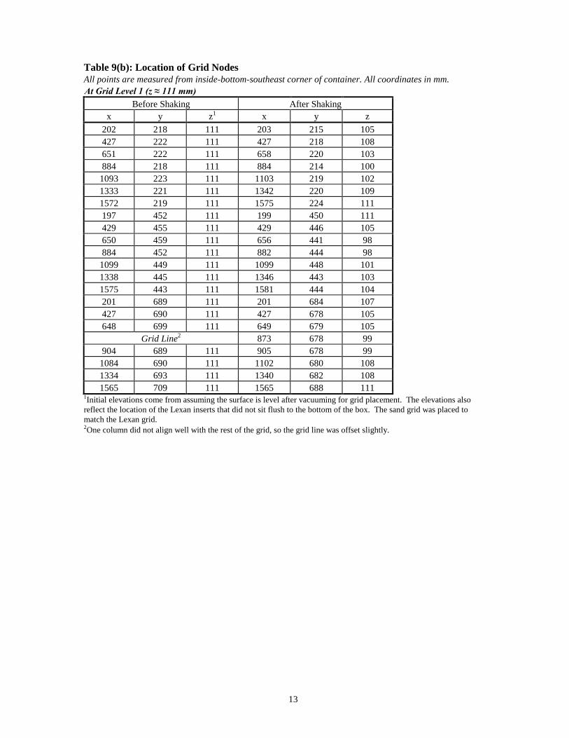
Table 9(b): Location of Grid Nodes All points are measured from inside-bottom-southeast corner of container. All coordinates in mm. At Grid Level 1 (z ≈ 111 mm)
Before Shaking After Shaking x y z1 x y z
202 218 111 203 215 105 427 222 111 427 218 108 651 222 111 658 220 103 884 218 111 884 214 100
1093 223 111 1103 219 102 1333 221 111 1342 220 109 1572 219 111 1575 224 111 197 452 111 199 450 111 429 455 111 429 446 105 650 459 111 656 441 98 884 452 111 882 444 98
1099 449 111 1099 448 101 1338 445 111 1346 443 103 1575 443 111 1581 444 104 201 689 111 201 684 107 427 690 111 427 678 105 648 699 111 649 679 105
Grid Line2 873 678 99 904 689 111 905 678 99
1084 690 111 1102 680 108 1334 693 111 1340 682 108 1565 709 111 1565 688 111
1Initial elevations come from assuming the surface is level after vacuuming for grid placement. The elevations also reflect the location of the Lexan inserts that did not sit flush to the bottom of the box. The sand grid was placed to match the Lexan grid. 2One column did not align well with the rest of the grid, so the grid line was offset slightly.
14
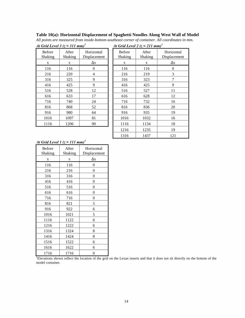
Table 10(a): Horizontal Displacement of Spaghetti Noodles Along West Wall of Model All points are measured from inside-bottom-southeast corner of container. All coordinates in mm. At Grid Level 3 (z ≈ 311 mm)1 At Grid Level 2 (z ≈ 211 mm)1
Before Shaking
After Shaking
Horizontal Displacement
Before Shaking
After Shaking
Horizontal Displacement
x x ∆x x x ∆x 116 116 0 116 116 0 216 220 4 216 219 3 316 325 9 316 323 7 416 425 9 416 425 9 516 528 12 516 527 11 616 633 17 616 628 12 716 740 24 716 732 16 816 868 52 816 836 20 916 980 64 916 935 19
1016 1097 81 1016 1032 16 1116 1206 90 1116 1134 18
1216 1235 19 1316 1437 121 At Grid Level 1 (z ≈ 111 mm)1
Before Shaking
After Shaking
Horizontal Displacement
x x ∆x 116 116 0 216 216 0 316 316 0 416 416 0 516 516 0 616 616 0 716 716 0 816 821 5 916 922 6
1016 1021 5 1116 1122 6 1216 1222 6 1316 1324 8 1416 1424 8 1516 1522 6 1616 1622 6 1716 1716 0
1Elevations shown reflect the location of the grid on the Lexan inserts and that it does not sit directly on the bottom of the model container.
15
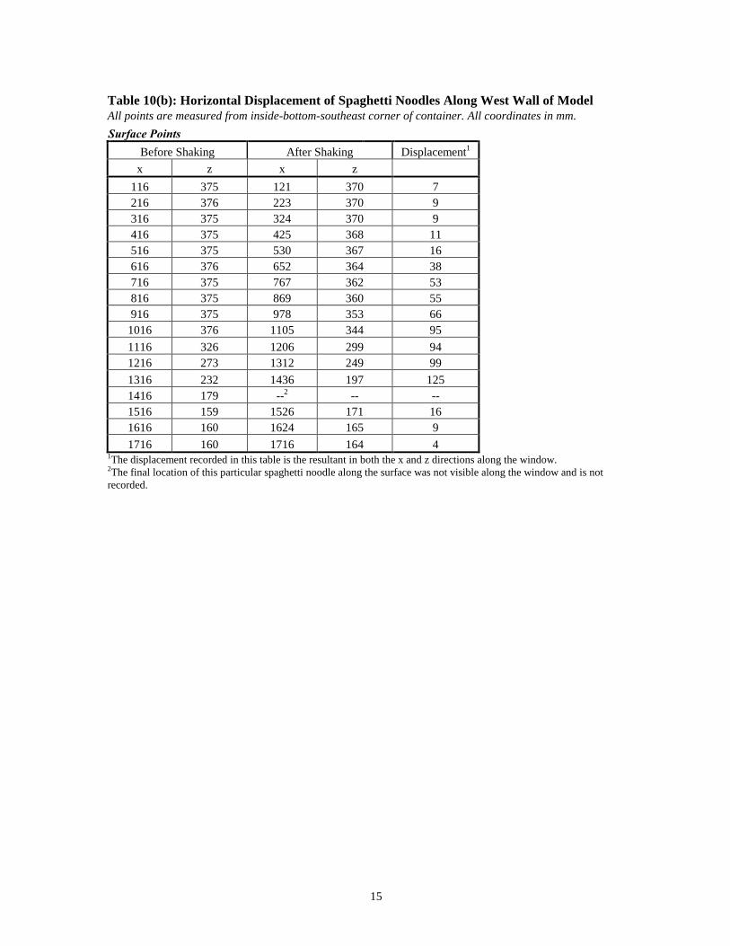
Table 10(b): Horizontal Displacement of Spaghetti Noodles Along West Wall of Model All points are measured from inside-bottom-southeast corner of container. All coordinates in mm. Surface Points
Before Shaking After Shaking Displacement1
x z x z 116 375 121 370 7 216 376 223 370 9 316 375 324 370 9 416 375 425 368 11 516 375 530 367 16 616 376 652 364 38 716 375 767 362 53 816 375 869 360 55 916 375 978 353 66
1016 376 1105 344 95 1116 326 1206 299 94 1216 273 1312 249 99 1316 232 1436 197 125 1416 179 --2 -- -- 1516 159 1526 171 16 1616 160 1624 165 9 1716 160 1716 164 4
1The displacement recorded in this table is the resultant in both the x and z directions along the window. 2The final location of this particular spaghetti noodle along the surface was not visible along the window and is not recorded.
16
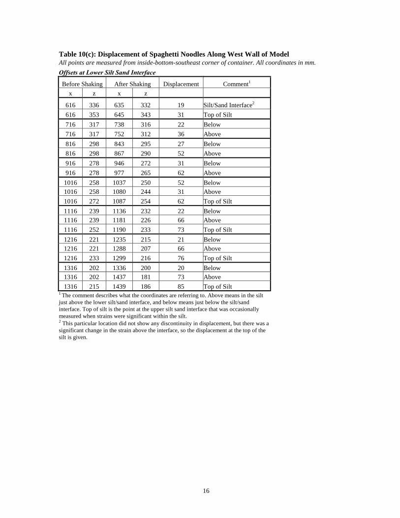
Table 10(c): Displacement of Spaghetti Noodles Along West Wall of Model All points are measured from inside-bottom-southeast corner of container. All coordinates in mm. Offsets at Lower Silt Sand Interface
Before Shaking After Shaking Displacement Comment1 x z x z
616 336 635 332 19 Silt/Sand Interface2 616 353 645 343 31 Top of Silt 716 317 738 316 22 Below 716 317 752 312 36 Above 816 298 843 295 27 Below 816 298 867 290 52 Above 916 278 946 272 31 Below 916 278 977 265 62 Above
1016 258 1037 250 52 Below 1016 258 1080 244 31 Above 1016 272 1087 254 62 Top of Silt 1116 239 1136 232 22 Below 1116 239 1181 226 66 Above 1116 252 1190 233 73 Top of Silt 1216 221 1235 215 21 Below 1216 221 1288 207 66 Above 1216 233 1299 216 76 Top of Silt 1316 202 1336 200 20 Below 1316 202 1437 181 73 Above 1316 215 1439 186 85 Top of Silt
1 The comment describes what the coordinates are referring to. Above means in the silt just above the lower silt/sand interface, and below means just below the silt/sand interface. Top of silt is the point at the upper silt sand interface that was occasionally measured when strains were significant within the silt. 2 This particular location did not show any discontinuity in displacement, but there was a significant change in the strain above the interface, so the displacement at the top of the silt is given.

17
KNOWN LIMITATIONS OF RECORDED DATA AND MODEL The data presented for instrument and grid locations in this report represent as built and after shaking positions. The interpreted displacements represent the accumulation as a result of two earthquake sequences. The data files and plots only show the second earthquake due to a computer failure during the first earthquake. All acceleration time histories in the electronic data files are raw recordings. Proper filtering and signal processing is required to obtain velocities, transient displacements, and other features of the dynamic response. Some instruments show a change in the steady voltage signal when the sampling frequency is changed (i.e. after shaking, as described previously). These “steps” in the data do not reflect actual changes in the measurand, and are the result of the change in sampling frequency. The shear wave velocity measurements reported were for a shear wave hammer test using the small shear hammers with a vacuum source. A total of 9 tests were attempted using either the S-wave hammer or P-wave hammer as discussed. Only one of the S-wave hammer tests appeared to give measurable results. It is likely that the vacuum was not strong enough to generate the recordings desired. It is also likely that the one recording that was obtained contains data that is not shear wave data. The shear wave measurements recorded are lower than expected for this type of sand and may reflect the influence of the above factors Instrument A9 displayed very little response with small jumps in voltage levels that indicate it did not function properly during the shake applied. Small responses by instruments A17 and A32 could also indicate a problem in the function of these accelerometers. Instruments P3 and P25 showed very little response and did not function during shaking. Instrument P25 was not recorded during shaking because it was known that it was not function properly and one amplifier was not working correctly. Instrument P15 showed an error in the zero reading for the amplifier that may have a slight influence on the recorded results. Instruments P24 and P26 as originally recorded showed responses that were consistent with the instruments being switched in location on the amplifier. Similarly P6 and P7 as originally recorded showed responses consistent with switched location on the amplifier. As a result, the Instrument Channel List has been modified by switching P6 & P7 and P24 & P26. The data plots are also in an already switched condition. That is, it was originally believed that these instruments were in opposite locations as mentioned above and have now been changed. Instruments L7 and L8 displayed large jumps in displacement after shaking that are not consistent with other settlement recordings. These instruments were placed on settlement pads that may moved or shifted so that the instrument fell off these pads. Instruments L5, L6, and L8 reached the limit of their range during the recording of data for the second event. All three were settlement transducers. L5 was a 2-inch linear potentiometer, but the configuration of the racks and lid made it difficult to place a larger linear potentiometer. The other two instruments were 4-inch linear potentiometers.
18
The location of the colored sand columns within the soil could not be deduced prior to the shakes. It is possible that the markers were not inserted entirely vertically or well aligned above and below the silt plane. Figures 6-8 show lines representing the locations of the sand columns before spinning. These lines were deduced base on measurements of the location of the top of the columns and the assumption that they were oriented vertically. REFERENCES 1. Arulmoli, K., Muraleetharan, K. K., Hossain, M. M. and Fruth, L. S. (1991). “VELACS
Laboratory Testing Program,” Preliminary Data Report to National Science Foundation, The Earth Technology Corporation.
2. Chen, Y. R. (1995). “Behavior of Fine Sand in Triaxial, Torsional and Rotational Shear
Tests,” Ph.D. Thesis, University of California, Davis. 3. Cruz, R. D. (1995). “Rate Dependent Shear and Consolidation of Remolded San
Francisco Bay Mud,” Ph.D Thesis, University of California, Davis. 4. Dewoolkar, M.M., Ko, H.-Y., Stadler, A.T., and Astaneh, S.M.F. (1999) “A Substitute
Pore Fluid for Seismic Centrifuge Modeling,” Geotechnical Testing Journal, GTJODJ, 22(3) pp. 196–210.
5. Fang, H.Y. (1991). “Foundation Engineering Handbook,” 2nd Ed. Chapman & Hall,
International Thomason Publishing, 7625 Empire Drive, Florence, KY. 6. Stewart, D.P., and Chen, Y.-R., and Kutter, B.L. (1998). “Experience with the Use of
Methylcelluose as a Viscous Pore Fluid in Centrifuge Models,” Geotechnical Testing Journal, 21(4) pp. 365–369.
7. Stewart, D.P. and Randoplh, M.F. (1991). “A New Site Investigation Tool for the
Centrifuge,” Centrifuge 91, Ed. Hon-Yim Ko, Balkema, pp. 531–538. 8. Woodward-Clyde (1997). “Experimental Results of Maximum and Minimum Dry
Densities of Nevada Sand,” Memo to Center for Geotechnical Modeling, University of California, Davis.
9. Zeng, X., Wu, J., and Young, B.A. (1998) “Influence of Viscous Fluids on Properties of
Sand,” Geotechnical Testing Journal, GTJODJ, 21(1) pp. 45–51.

Figure 1. Initial EJM01 model configuration in model scale. All dimensions are in mm.
53 typ
50 typ.
1010
1860
PPTs
ACCs905
Plan View
368
20
1759421
210
2001000
COARSE SAND
DIRECTION OF SHAKING
1029486
NEVADA SAND SILT
16
40030
158
59
Profile View – EastNotes: 1. All units are in mm 2. Grid spacing is 100-mm ×100-mm 3. A Lexan sheet with a 100-mm ×100-mm grid was placed on the inside of the East and West wall for
photographic purposes. However, the grid does not correspond to the grid shown in the above plans. 4. The origin for all coordinates is at the lower southeast corner of the box. x dimensions are positive in
the North direction. y dimensions are positive in the West direction. z dimensions are positive in the Up direction.
5. Accelerometer and Pore Pressure Transducer line in plan view is approximate line that accelerometers were placed along, exact locations are identified in Table 6 and Figures 2 and 3.
6. Linear Potentiometer Locations are identified in Table 6(a) and Figure 4.
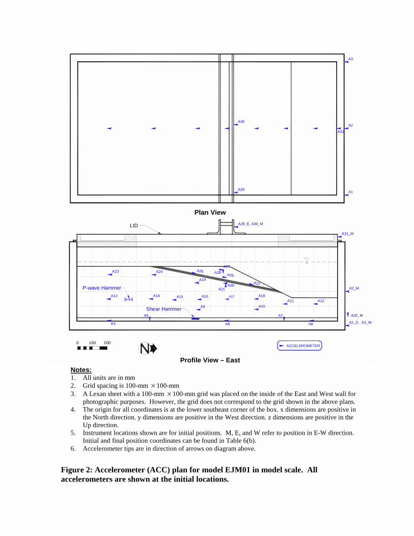
Figure 2: Accelerometer (ACC) plan for model EJM01 in model scale. All accelerometers are shown at the initial locations.
A29
A30
A1
A31
A3
A2
Plan View A29_E, A30_M
A5
A4
2001000
A6
A9
A24
A14
LID
A13
A23
A21A20
A27A28 A25
A26
A19
A16A15 A17A12A11
ACCELEROMETER
A8
A7
A10
A1_E, A3_W
A32_M
A22
A18
A2_M
A31_M
P-wave Hammer
Shear Hammer
Profile View – East Notes: 1. All units are in mm 2. Grid spacing is 100-mm ×100-mm 3. A Lexan sheet with a 100-mm ×100-mm grid was placed on the inside of the East and West wall for
photographic purposes. However, the grid does not correspond to the grid shown in the above plans. 4. The origin for all coordinates is at the lower southeast corner of the box. x dimensions are positive in
the North direction. y dimensions are positive in the West direction. z dimensions are positive in the Up direction.
5. Instrument locations shown are for initial positions. M, E, and W refer to position in E-W direction. Initial and final position coordinates can be found in Table 6(b).
6. Accelerometer tips are in direction of arrows on diagram above.
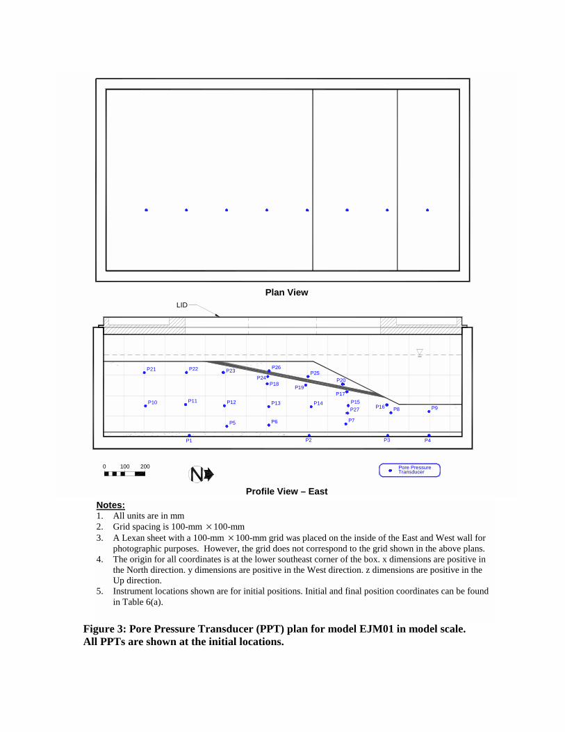
Figure 3: Pore Pressure Transducer (PPT) plan for model EJM01 in model scale. All PPTs are shown at the initial locations.
Plan View
P20
P17
P1
2001000
P2
P5 P6
P11P10
P22P21
LID
P19
P24P18
P23
P14P13P12
P25P26
P16P27 P9P8
P4P3
P7
TransducerPore Pressure
P15
Profile View – East Notes: 1. All units are in mm 2. Grid spacing is 100-mm ×100-mm 3. A Lexan sheet with a 100-mm ×100-mm grid was placed on the inside of the East and West wall for
photographic purposes. However, the grid does not correspond to the grid shown in the above plans. 4. The origin for all coordinates is at the lower southeast corner of the box. x dimensions are positive in
the North direction. y dimensions are positive in the West direction. z dimensions are positive in the Up direction.
5. Instrument locations shown are for initial positions. Initial and final position coordinates can be found in Table 6(a).
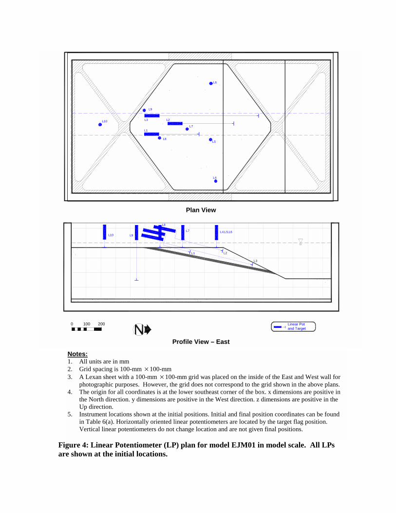
Figure 4: Linear Potentiometer (LP) plan for model EJM01 in model scale. All LPs are shown at the initial locations.
L10
L9
L8
L7
L6
L5
L4
L2
L1
L3
Plan View
2001000
L10 L9L7 L4,L5,L6
L2L1
and TargetLinear Pot
L3
L8
Profile View – East
Notes: 1. All units are in mm 2. Grid spacing is 100-mm ×100-mm 3. A Lexan sheet with a 100-mm ×100-mm grid was placed on the inside of the East and West wall for
photographic purposes. However, the grid does not correspond to the grid shown in the above plans. 4. The origin for all coordinates is at the lower southeast corner of the box. x dimensions are positive in
the North direction. y dimensions are positive in the West direction. z dimensions are positive in the Up direction.
5. Instrument locations shown at the initial positions. Initial and final position coordinates can be found in Table 6(a). Horizontally oriented linear potentiometers are located by the target flag position. Vertical linear potentiometers do not change location and are not given final positions.

Figure 5: Plan view of colored sand grid for initial model configuration in model scale. Colored sand column locations at base of silt plane and top of columns where silt plane is absent are identified by circled x’s.
West
Middle
East
2001000
Sand Column
Notes: 1. All units are in mm 2. This figure represents the initial model configuration 3. The sand column locations are for the locations at the tops below the silt plane. The locations above
the silt plane are identified in Figures 6 – 8. 4. The sand column locations identified by the circled x’s do not always line up with the node points of
the grid. 5. The grid shown is an approximation of the grid based on photographs and corrections during
placement for all elevations. 6. The origin for all coordinates is at the lower southeast corner of the box. x dimensions are positive in
the North direction. y dimensions are positive in the West direction. z dimensions are positive in the Up direction.
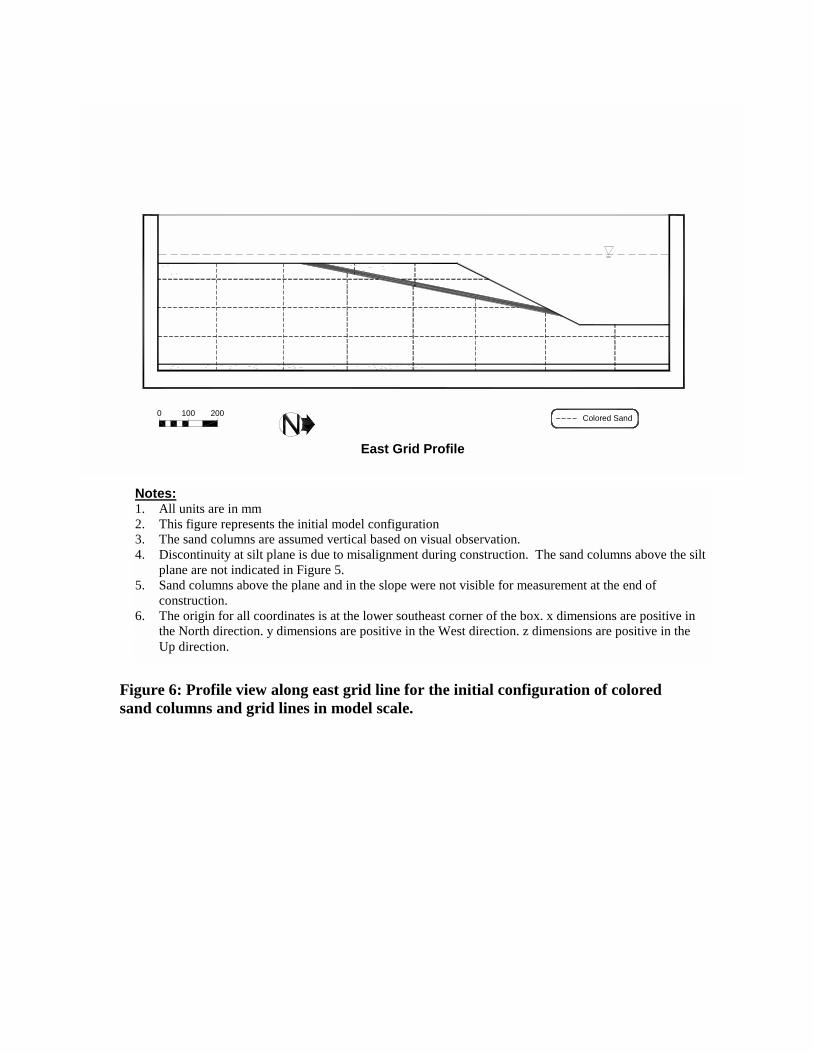
Figure 6: Profile view along east grid line for the initial configuration of colored sand columns and grid lines in model scale.
2001000 Colored Sand
East Grid Profile
Notes: 1. All units are in mm 2. This figure represents the initial model configuration 3. The sand columns are assumed vertical based on visual observation. 4. Discontinuity at silt plane is due to misalignment during construction. The sand columns above the silt
plane are not indicated in Figure 5. 5. Sand columns above the plane and in the slope were not visible for measurement at the end of
construction. 6. The origin for all coordinates is at the lower southeast corner of the box. x dimensions are positive in
the North direction. y dimensions are positive in the West direction. z dimensions are positive in the Up direction.
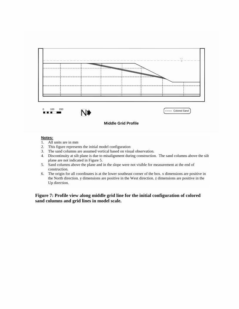
Figure 7: Profile view along middle grid line for the initial configuration of colored sand columns and grid lines in model scale.
2001000 Colored Sand
Middle Grid Profile
Notes: 1. All units are in mm 2. This figure represents the initial model configuration 3. The sand columns are assumed vertical based on visual observation. 4. Discontinuity at silt plane is due to misalignment during construction. The sand columns above the silt
plane are not indicated in Figure 5. 5. Sand columns above the plane and in the slope were not visible for measurement at the end of
construction. 6. The origin for all coordinates is at the lower southeast corner of the box. x dimensions are positive in
the North direction. y dimensions are positive in the West direction. z dimensions are positive in the Up direction.

Figure 8: Profile view along west grid line for the initial configuration of colored sand columns and grid lines in model scale.
0 100 200 Colored Sand
West Grid Profile
Notes: 1. All units are in mm 2. This figure represents the initial model configuration 3. The sand columns are assumed vertical based on visual observation. 4. Discontinuity at silt plane is due to misalignment during construction. The sand columns above the silt
plane are not indicated in Figure 5. 5. Sand columns above the plane and in the slope were not visible for measurement at the end of
construction. 6. The origin for all coordinates is at the lower southeast corner of the box. x dimensions are positive in
the North direction. y dimensions are positive in the West direction. z dimensions are positive in the Up direction.

Figure 9: Profile view along east grid line for the final deformed configuration of colored sand columns and grid lines in model scale superimposed over the original lines (Figure 6).
Notes: 1. All units are in mm 2. This figure shows the final model configuration based on direct measurements and interpolation from
photographs. The darker lines represent the colored sand and profile after shaking, and the lighter lines represent the original colored sand and profile.
3. The origin for all coordinates is at the lower southeast corner of the box. x dimensions are positive in the North direction. y dimensions are positive in the West direction. z dimensions are positive in the Up direction.
0 100 200 Colored SandColored Sand
East Grid Profile
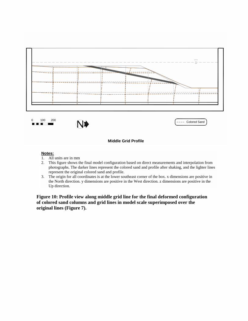
Figure 10: Profile view along middle grid line for the final deformed configuration of colored sand columns and grid lines in model scale superimposed over the original lines (Figure 7).
0 100 200 Colored Sand
Middle Grid Profile
Notes: 1. All units are in mm 2. This figure shows the final model configuration based on direct measurements and interpolation from
photographs. The darker lines represent the colored sand and profile after shaking, and the lighter lines represent the original colored sand and profile.
3. The origin for all coordinates is at the lower southeast corner of the box. x dimensions are positive in the North direction. y dimensions are positive in the West direction. z dimensions are positive in the Up direction.
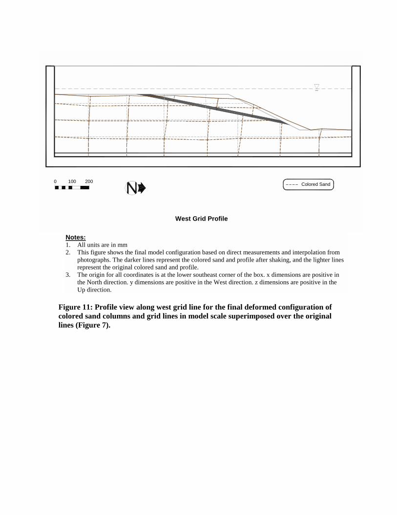
Figure 11: Profile view along west grid line for the final deformed configuration of colored sand columns and grid lines in model scale superimposed over the original lines (Figure 7).
0 100 200 Colored Sand
West Grid Profile
Notes: 1. All units are in mm 2. This figure shows the final model configuration based on direct measurements and interpolation from
photographs. The darker lines represent the colored sand and profile after shaking, and the lighter lines represent the original colored sand and profile.
3. The origin for all coordinates is at the lower southeast corner of the box. x dimensions are positive in the North direction. y dimensions are positive in the West direction. z dimensions are positive in the Up direction.

Figure 12: Profile view along west window for the initial configuration of the spaghetti noodles.
0 100 200 Spaghetti
West Window Profile
Notes: 1. All units are in mm 2. This figure shows the initial configuration for the spaghetti noodles placed along the inside of the west
wall. The spacing is approximately 100-mm between noodles. The coordinates are intended to start from the southeast corner as specified in note 3. However, the first noodle is placed at an x dimension of approximately 114-mm due to the box configuration.
3. Noodles are only placed in the vertical direction. Colored sand was used for the horizontal markings as shown in previous figures.
4. The origin for all coordinates is at the lower southeast corner of the box. x dimensions are positive in the North direction. y dimensions are positive in the West direction. z dimensions are positive in the Up direction.
0 100 200 Spaghetti
West Window Profile
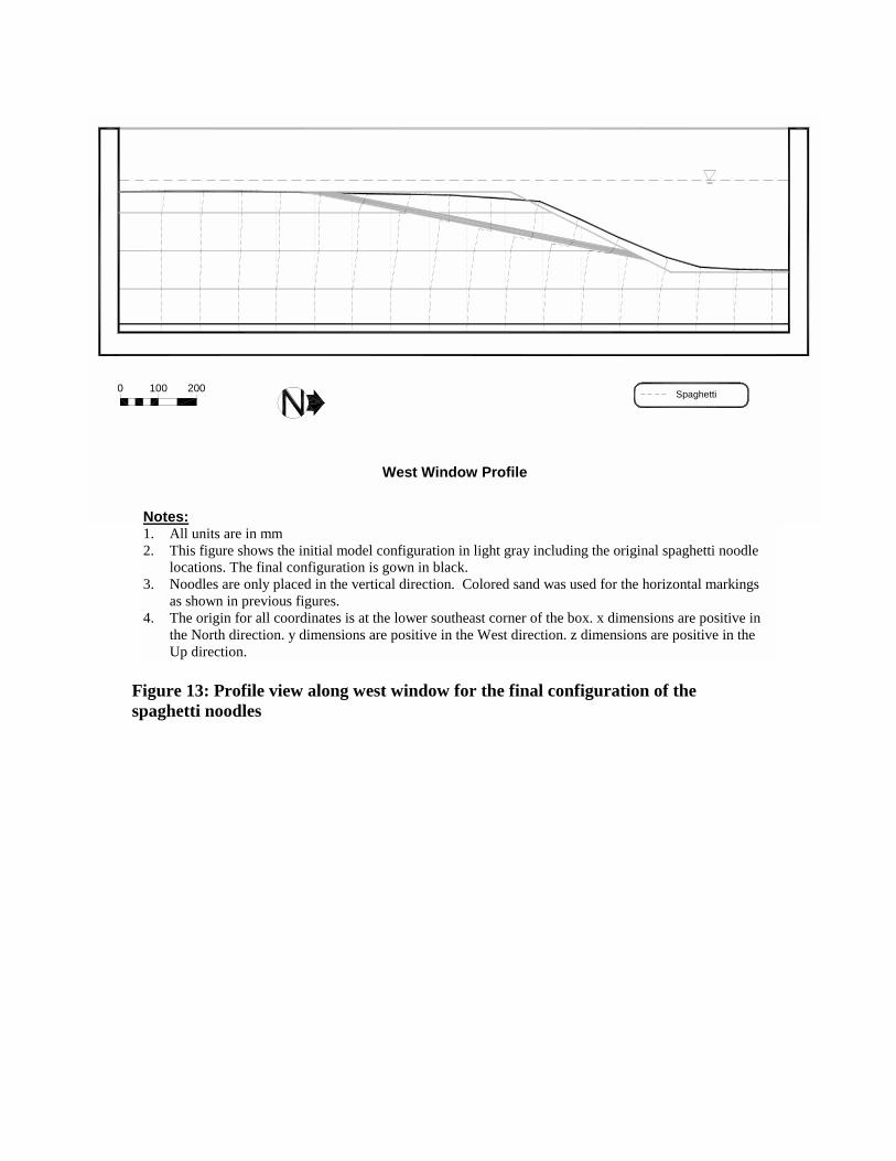
Figure 13: Profile view along west window for the final configuration of the spaghetti noodles
2001000 Spaghetti
West Window Profile
Notes: 1. All units are in mm 2. This figure shows the initial model configuration in light gray including the original spaghetti noodle
locations. The final configuration is gown in black. 3. Noodles are only placed in the vertical direction. Colored sand was used for the horizontal markings
as shown in previous figures. 4. The origin for all coordinates is at the lower southeast corner of the box. x dimensions are positive in
the North direction. y dimensions are positive in the West direction. z dimensions are positive in the Up direction.
0 20 40 60 80 100 120 140 160 180 200Time (s)
0
0
0
0
Acce
lera
tion
(g)
- Ea
ch T
ick
= 0.
25-g
0
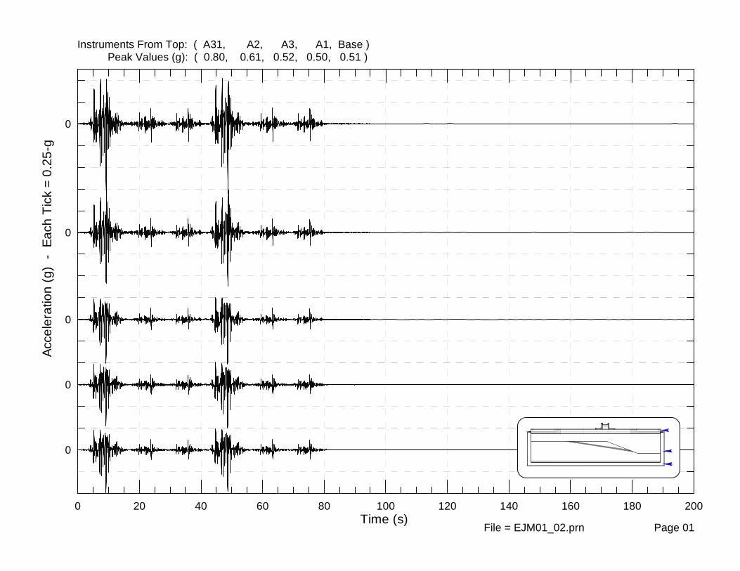
Instruments From Top: ( A31, A2, A3, A1, Base ) Peak Values (g): ( 0.80, 0.61, 0.52, 0.50, 0.51 )
File = EJM01_02.prn Page 01
0 20 40 60 80 100 120 140 160 180 200Time (s)
0
0
0
0
Acce
lera
tion
(g)
- Ea
ch T
ick
= 0.
25-g
0
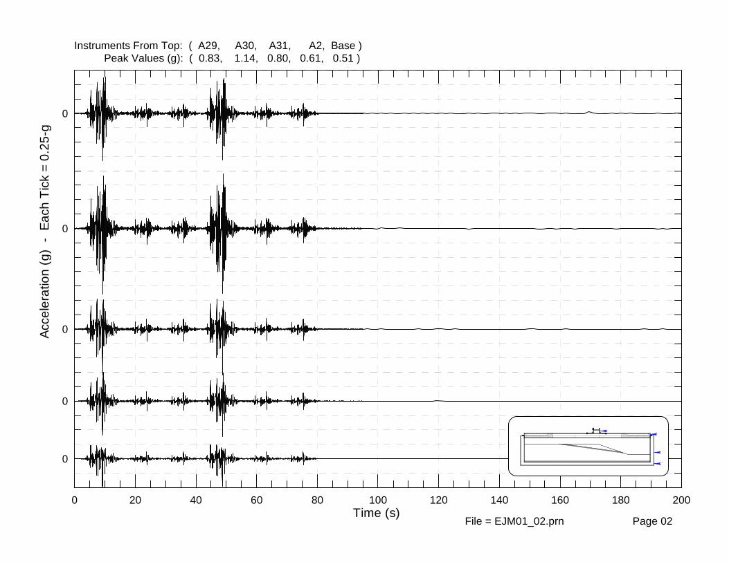
Instruments From Top: ( A29, A30, A31, A2, Base ) Peak Values (g): ( 0.83, 1.14, 0.80, 0.61, 0.51 )
File = EJM01_02.prn Page 02
0 20 40 60 80 100 120 140 160 180 200Time (s)
0
0
0
0
Acc
eler
atio
n (g
) -
Eac
h Ti
ck =
0.0
5-g
Instruments From Top: ( A5, A7, A32, Base ) Peak Values (g): ( 0.12, 0.22, 0.03, 0.51 )
File = EJM01_02.prn Page 03
0 20 40 60 80 100 120 140 160 180 200Time (s)
0
0
0
0
Acce
lera
tion
(g)
- Ea
ch T
ick
= 0.
15-g
Instruments From Top: ( A23, A13, A4, Base ) Peak Values (g): ( 0.39, 0.59, 0.55, 0.51 )
File = EJM01_02.prn Page 04

0 20 40 60 80 100 120 140 160 180 200Time (s)
0
0
0
0
Acce
lera
tion
(g)
- Ea
ch T
ick
= 0.
15-g
Instruments From Top: ( A24, A14, A15, Base ) Peak Values (g): ( 0.34, 0.57, 0.44, 0.51 )
File = EJM01_02.prn Page 05

0 20 40 60 80 100 120 140 160 180 200Time (s)
0
0
0
0
Acce
lera
tion
(g)
- Ea
ch T
ick
= 0.
15-g
0
Instruments From Top: ( A26, A19, A16, A9, Base ) Peak Values (g): ( 0.37, 0.64, 0.35, 0.08, 0.51 )
File = EJM01_02.prn Page 06
0 20 40 60 80 100 120 140 160 180 200Time (s)
0
0
0
0
Acce
lera
tion
(g)
- Ea
ch T
ick
= 0.
20-g
0
0
Instruments From Top: ( A27, A25, A20, A17, A6, Base ) Peak Values (g): ( 0.84, 0.47, 0.50, 0.07, 0.51, 0.51 )
File = EJM01_02.prn Page 07
0 20 40 60 80 100 120 140 160 180 200Time (s)
0
0
0
0
Acce
lera
tion
(g)
- Ea
ch T
ick
= 0.
15-g
Instruments From Top: ( A22, A18, A10, Base ) Peak Values (g): ( 0.56, 0.47, 0.56, 0.51 )
File = EJM01_02.prn Page 08
0 20 40 60 80 100 120 140 160 180 200Time (s)
0
0
0
0
Acce
lera
tion
(g)
- Ea
ch T
ick
= 0.
15-g
Instruments From Top: ( A11, A12, A8, Base ) Peak Values (g): ( 0.34, 0.65, 0.51, 0.51 )
File = EJM01_02.prn Page 09
0 20 40 60 80 100 120 140 160 180 200Time (s)
0
0
0
0
Acce
lera
tion
(g)
- Ea
ch T
ick
= 0.
25-g
0
Instruments From Top: ( A28, A21, A7, A5, Base ) Peak Values (g): ( 0.33, 0.22, 0.22, 0.12, 0.51 )
File = EJM01_02.prn Page 10
0 20 40 60 80 100 120 140 160 180 200Time (s)
0
Bas
e A
cc (g
)Ti
ck =
0.2
0-g
0
20
40
60
80
-20
0
20
Exc
ess
Pore
Pre
ssur
e (k
Pa) -
Tic
k =
10-k
Pa
Instruments From Top: ( P21, P10, Base ) Peak Values (kPa, g): ( 34.7, 83.7, 0.51 )
File = EJM01_02.prn Page 11
0 20 40 60 80 100 120 140 160 180 200Time (s)
0
Base
Acc
(g)
Tick
= 0
.20-
g
0
40
80
120
0
40
80
0
Exc
ess
Pore
Pre
ssur
e (k
Pa)
- Ti
ck =
20-
kPa
Instruments From Top: ( P22, P11, P1, Base ) Peak Values (kPa, g): ( 26.0, 102.6, 114.9, 0.51 )
File = EJM01_02.prn Page 12
0 20 40 60 80 100 120 140 160 180 200Time (s)
0
Base
Acc
(g)
Tick
= 0
.20-
g
0
40
80
120
0
40
80
0
Exce
ss P
ore
Pres
sure
(kPa
) -
Tick
= 2
0-kP
aInstruments From Top: ( P23, P12, P5, Base ) Peak Values (kPa, g): ( 22.6, 89.3, 123.1, 0.51 )
File = EJM01_02.prn Page 13

0 20 40 60 80 100 120 140 160 180 200Time (s)
0
Bas
e A
cc (g
)Ti
ck =
0.2
0-g 0
20
40
60
80
100
0
20
40
60
800
20
40
Exc
ess
Por
e P
ress
ure
(kPa
) - T
ick
= 20
-kP
a
0
20
-20
0
20
Instruments From Top: ( P26, P24, P18, P13, P6, Base ) Peak Values (kPa, g): ( 37.7, 23.2, 45.1, 82.0, 106.0, 0.51 )
File = EJM01_02.prn Page 14

0 20 40 60 80 100 120 140 160 180 200Time (s)
0
Base
Acc
(g)
Tick
= 0
.20-
g
0
40
80
120
0
40
80
0
40
Exce
ss P
ore
Pres
sure
(kPa
) -
Tick
= 2
0-kP
aInstruments From Top: ( P19, P14, P2, Base ) Peak Values (kPa, g): ( 41.1, 75.2, 129.2, 0.51 )
File = EJM01_02.prn Page 15
0 20 40 60 80 100 120 140 160 180 200Time (s)
0
Bas
e A
cc (g
)Ti
ck =
0.2
0-g 0
20
40
60
80
100
120
0
20
40
60
80
0
20
40
60
Exce
ss P
ore
Pres
sure
(kPa
) - T
ick
= 20
-kPa
0
20
0
Instruments From Top: ( P20, P17, P15, P27, P7, Base ) Peak Values (kPa, g): ( 8.5, 32.8, 57.1, 77.8, 110.9, 0.51 )
File = EJM01_02.prn Page 16
0 20 40 60 80 100 120 140 160 180 200Time (s)
0
Base
Acc
(g)
Tick
= 0
.20-
g
0
10
-10
0
10
20
30
40
50
60
70
-20
-10
0
10
20
30
40
50
Exc
ess
Pore
Pre
ssur
e (k
Pa)
- Ti
ck =
10-
kPa
Instruments From Top: ( P16, P8, P3, Base ) Peak Values (kPa, g): ( 43.8, 71.9, 1.66, 0.51 )
File = EJM01_02.prn Page 17
0 20 40 60 80 100 120 140 160 180 200Time (s)
0
Bas
e A
cc (g
)Ti
ck =
0.2
0-g
0
10
20
30
40
50
-10
0
10
20
30
40
50
Exce
ss P
ore
Pres
sure
(kPa
) - T
ick
= 10
-kPa
Instruments From Top: ( P9, P4, Base ) Peak Values (kPa, g): ( 49.9, 45.5, 0.51 )
File = EJM01_02.prn Page 18
0 20 40 60 80 100 120 140 160 180 200Time (s)
0
Base
Acc
(g)
Tick
= 0
.20-
g 0
0.2
0.4
0.6
0.8
0
0.2
0.4
0.6
0.8
1
0
0.2
0.4
0.6
0.8
1
1.2
Hor
izon
tal D
ispl
acem
ent (
m)
- Ti
ck =
0.2
-mInstruments From Top: ( L3, L2, L1, Base ) Peak Values (m, g): ( 1.28, 1.07, 0.96, 0.51 )
File = EJM01_02.prn Page 19
0 20 40 60 80 100 120 140 160 180 200Time (s)
0
Bas
e A
cc (g
)Ti
ck =
0.2
0-g 0
0.2
0
0
0.2
0.4
0.6
0.8
1
1.2
Set
tlem
ent (
m) -
Tic
k =
0.20
-m
0
0.2
0.4
0.6
0.8
0
0.2
0.4
0.6
Instruments From Top: ( L5, L7, L8, L9, L10, Base ) Peak Values (m, g): ( 0.55, 1.43, 1.40, 0.23, 0.24, 0.51 )
File = EJM01_02.prn Page 20

0 20 40 60 80 100 120 140 160 180 200Time (s)
0
Base
Acc
(g)
Tick
= 0
.20-
g 0
0.2
0.40
0.2
0.4
0
0.2
0.4
0.6
0.8
1
Set
tlem
ent (
m)
- Ti
ck =
0.1
-mInstruments From Top: ( L6, L5, L4, Base ) Peak Values (m, g): ( 0.92, 0.55, 0.49, 0.51 )
File = EJM01_02.prn Page 21

APPENDIX A: CENTER FOR GEOTECHNICAL MODELING July 2001 CENTER DIRECTORS: James A. Cheney 1983-1989 I. M. Idriss 1989-1996 Bruce L. Kutter 1996- present FACILITY MANAGEMENT: Bruce L. Kutter 1983-1990 Managing Director 1990-1996 Associate Director D. P. Stewart 1995-1997 Facility Manager
D. W. Wilson 1997- present Facility Manager DESCRIPTION OF CENTRIFUGE FACILITIES: 9 m CENTRIFUGE AND SHAKER In 1978, in response to a broad agency announcement from the National Science Foundation (NSF), the University of California, Davis, collaborated with the National Aeronautics and Space Administration (NASA) to propose the development of a large geotechnical centrifuge facility. The proposal was successful, and the centrifuge was constructed and installed at the NASA Ames Research Center. The centrifuge was first operated at NASA Ames in early 1984. In 1987, NASA dis-assembled the centrifuge and hauled it to UC Davis. Using funds from Tyndall AFB, Los Alamos National Laboratories, the National Science Foundation and the University of California, the centrifuge was installed and operated on a concrete slab in the open air in 1988; in this configuration, the maximum acceleration that could be achieved was 19 g. NSF then funded the construction of an enclosure around the centrifuge, which was completed in December 1989 and allowed the centrifuge to achieve accelerations of 50 g. From 1990-1995, great effort was expended to raise funds, design, and develop an earthquake simulation capability for the large centrifuge. Development of the shaker was supported by the NSF, Caltrans, the Obayashi Corporation, and the University of California, Davis. In April 1995, the first proof tests of the shaker were conducted at a centrifugal acceleration of 50 g. In 1996, the focus of the Center finally shifted from facility development to research utilization of the shaker and centrifuge facilities. This centrifuge, in terms of radius (9.1 m to bucket floor), maximum payload mass (5000 kg), and available bucket area (4.0 m2) is one of the largest geotechnical centrifuges in the world. At present, the centrifuge is limited to centrifugal accelerations of 40 g. The centrifuge capacity in terms of the maximum acceleration multiplied by the maximum payload is 40 g x 5000 kg = 200 g-tonnes.
The data acquisition system on the centrifuge is kept up to date by continual upgrades to the hardware and software. Low-level signals are conditioned with instrumentation amplifiers at the end of the centrifuge arm. Commercially available programmable gain, programmable cutoff frequency anti-aliasing amplifiers mounted at the center of the centrifuge are used prior to digitization. At present, the system has the capability to digitize over 100 channels of data at

about 2000 samples per second per channel. The digitization takes place onboard the centrifuge using a commercial data acquisition board (Data Translations DT2839) installed in a standard personal computer. The data is stored on a flash disk in the centrifuge computer and then transmitted to another computer in the control room via an Ethernet network and remote control software. Some specifications of the large servo-hydraulic shaker are summarized, below. A more detailed description is given in Kutter et al. (1994). For a rigid shaking mass of 2700 kg (model plus container), the actuators, operating with 3500 psi (24 MPa) oil pressure, theoretically have the capacity to produce 14 g shaking accelerations at frequencies up to 200 Hz. In practice, much larger accelerations (up to 40 g) can be obtained because the models do not behave like a rigid mass at high frequencies. The maximum absolute shaking velocity is about 1 m/s and the stroke is 2.5 cm peak to peak. To achieve this, two pairs of single acting actuators provide a net peak actuator force of 400 kN. One actuator pair is mounted on each side of the model container. Each actuator pair (patented by Team Corporation) consists of two-single-acting actuators bolted on opposite sides of a two-stage servo-valve block. The actuators are controlled by a conventional closed loop feedback control system. A simple correction scheme is used to precondition the command signal to improve the coherence and frequency content of the shaking table motions. In addition to step waves, sine waves and sine sweeps, simulations of ground motions recorded in a number of different earthquakes have been produced in the shaker. Two flexible shear beam containers (FSB1 and FSB2) and a rigid container with windows (RC1) are available for research projects. FSB2 and RC1 have dimensions of approximately 1.7 x 0.8 x 0.5 m (length x width x height), with the shaking in the direction of the length. FSB1 has dimensions of about 1.7 x 0.7 x 0.6 m. The FSB containers consist of a stack of rectangular rings of aluminum tubing and rubber. The rubber is flexible in shear, which allows the container to deform with the soil. The stiffness of the rubber is designed to make the natural frequency of the container (as a shear beam) to be less than the natural frequency of a soil layer. In the fall of 2000, UC Davis received a $4.6 million grant from the NSF, as a part of the Network for Earthquake Engineering Simulation (NEES) program, to upgrade and enhance the large centrifuge and become a NEES host facility, participating in the NEES Consortium. The upgrades include an in-flight robot, new sensor equipment, modifications to allow operations up to 80-g, a new hinged-plate container, a biaxial horizontal/vertical shaker, tele-observation and tele-operation capabilities, data visualization capabilities, and in-flight tomographic imaging and geophysical tools. These upgrades will be operational in 2004. For more information on the NSF NEES program, refer to the website: www.eng.nsf.gov/nees/default.htm. SCHAEVITZ CENTRIFUGE AND SHAKER The 1 m radius centrifuge can carry 90 kg models to 100 g or 27 kg models to 175 g. The centrifuge is equipped with a servo-hydraulic actuator, which is capable of simulating earthquake-like motions to the base of the model container during flight. The shaker has been used to study the dynamic behavior of retaining structures, liquefiable soil layers, response of soft soil sites, soil-pile-structure interaction, flow slides, embankments and port structures. Over a thousand earthquake simulations have been produced by this shaker, and it was the primary focus of the centrifuge modeling efforts of the faculty at UC Davis until completion of the large centrifuge and shaker in 1995.
The shaker on the 1 m centrifuge has a model container with dimensions 0.56 x 0.28 x 0.18 m. The shaker, capable of producing 30 g shaking accelerations is designed to operate at centrifuge accelerations up to 100 g. A computer outside the centrifuge is used to control the shaker and to acquire data from the experiment. Sixteen channels of data can be digitized at rates up to 2500 samples per second per channel. Sixteen variable gain amplifiers for strain gauge type instruments and eight variable gain charge amplifiers for accelerometers are mounted on the centrifuge to improve the signal to noise ratio. This centrifuge is equipped with four hydraulic rotary joints, which may be used for hydraulic oil, water supply, or compressed gas. On board accumulators store energy in compressed gas form to provide the short burst of high power required to produce large flow rates of high pressure oil to for the shaker. The hydraulic system also has been used to apply static loads to foundations and other mechanisms on the centrifuge. FURTHER INFORMATION Anyone interested in using or collaborating in the use of the centrifuge facilities is encouraged to contact: Bruce L. Kutter, Ph.D. Director, Center for Geotechnical Modeling Department of Civil & Environmental Engineering University of California One Shields Avenue Davis, CA 95616 Tel: 916 752 8099 Fax: 916 752 7872 email: [email protected] REFERENCES Kutter, B.L., Li, X.S., Sluis, W., and Cheney, J.A. (1991) "Performance and Instrumentation of the Large Centrifuge at UC Davis.", Centrifuge 91, Ko and McLean (eds.), Balkema, Rotterdam, pp. 19-26. Kutter, B.L., Idriss, I.M., Kohnke, T., Lakeland, J., Li, X.S., Sluis, W., Zeng, X., Tauscher, R.C., Goto, Y. Kubodera, I., (1994) "Design of a Large Earthquake Simulator at UC Davis.” Centrifuge 94, Leung, Lee, and Tan (eds.), Balkema, Rotterdam, pp. 169-175.
Copyright © 2022 FDOKUMEN