Liquefaction Opportunity Mapping via Seismic Wave Energy

LIQUEFACTION OPPORTUNITY MAPPING VIA SEISMIC WAVE ENERGY

By M. I. Todorovska1 and M. D. Trifunac2

ABSTRACT: An empirical, energy-based methodology for liquefaction hazard assessment and microzonationmapping is presented. The approach is probabilistic, considers the uncertainty in the liquefaction criterion, andis applicable to most earthquake-induced liquefaction analyses. The examples illustrated are for water-saturatedsands at level ground. The energy of ground shaking is estimated from the Fourier amplitude spectra of theincident waves. The susceptible materials are characterized only by their corrected standard penetration testvalue N and overburden pressure s0. Illustrative microzonation maps of liquefaction opportunity are shown forthe Los Angeles metropolitan area. Two types of maps are presented, one showing the average return period ofliquefaction occurrence (for given N and s0), and another one showing distribution of N with equal probabilityto liquefy during 50 years exposure (for given s0). An advantage of the method is that the result is given directlyin terms of in situ albeit simple soil characteristics rather than in terms of laboratory tests and peak acceleration.Possible applications of the computed opportunity maps are discussed.

INTRODUCTION

Liquefaction of water-saturated sands is believed to occurwhen the pore pressure approaches the confining pressure, sothat the material changes the state from solid to liquid (Kramer1996). When a layer liquefies, the ground loses strength, andmovement of large blocks of soil can be initiated (lateralspreading), causing damage to man-made structures. The needfor mapping a liquefaction hazard was recognized after the1964 Niigata (Japan) and Alaska (U.S.) earthquakes, and map-ping started in the early 1970s. Youd (1991) presents a state-of-the-art review of methodologies and case studies of lique-faction mapping worldwide. The mapping procedures aredivided into three groups: (1) Susceptibility mapping (of areasthat can liquefy if subjected to sufficiently strong and longground shaking); (2) opportunity mapping (of areas exposedto earthquake shaking capable of initiating liquefaction); and(3) potential mapping (of areas where there is both opportunityand susceptible material for liquefaction to occur).

This paper illustrates the application of an energy-basedmethodology to microzonation mapping of liquefaction op-portunity on level ground. The methodologies for opportunitymapping applied so far (Youd 1991) are based on: (1) mag-nitude-distance relation (Yegian and Whitman 1978; Youd andPerkins 1978; Tinsley et al. 1985); (2) magnitude-maximumacceleration relations (Atkinson et al. 1984; Kavazanjian et al.1985); and (3) liquefaction severity index (Youd and Perkins1987). The first two types consider only the initiation of liq-uefaction, whereas the third also considers the consequences.The magnitude-distance relations’ methodologies are based onthe simplest two-parameter characterization of strong shakingand decay of ground motion amplitudes with distance due toattenuation along the wave path. The magnitude-maximum ac-celeration relations’ methodologies consider ground accelera-tions at the site and use magnitude as a measure of the durationof shaking.

Peak acceleration has been the most widely mapped char-acteristic of strong ground shaking (Algermissen and Perkins1976) and has been used in many applications. Unfortunately,it is a poor indicator of the energy of ground motion and of

1Res. Assoc. Prof., Civ. Engrg. Dept., Univ. of Southern California,Los Angeles, CA 90089-2531.

2Prof., Civ. Engrg. Dept., Univ. of Southern California, Los Angeles,CA.

Note. Discussion open until May 1, 2000. To extend the closing dateone month, a written request must be filed with the ASCE Manager ofJournals. The manuscript for this paper was submitted for review andpossible publication on May 2, 1996. This paper is part of the Journalof Geotechnical and Geoenvironmental Engineering, Vol. 125, No. 12,December, 1999. qASCE, ISSN 1090-0241/99/0012-1032–1042/$8.001 $.50 per page. Paper No. 13173.

1032 / JOURNAL OF GEOTECHNICAL AND GEOENVIRONMENTAL ENG

the potential for damage. Response spectral amplitudes havealso been mapped as an indicator of the level of structuralresponse during ground shaking (Lee and Trifunac 1987; Lee1993). However, no soil liquefaction criterion, at least of thosewidely used, is based on spectral characterization of groundmotion. Spectral intensity (Benioff 1934) and the Arias inten-sity [proportional to * a2(t) dt, where a(t) is absolute groundacceleration and t is time (Trifunac and Brady 1975)] aresometimes used as measures of the destructive effects ofground shaking on structures, and recently for the assessmentof liquefaction potential (Kayen and Mitchell 1997). Theseintensities can be related to the energy dissipated by singledegree-of-freedom oscillators with frequencies in an interval(vL, vR) (for the Arias intensity, vL = 0 and vR = `) duringthe entire duration of the excitation. Liquefaction occurrence,however, should be correlated with the energy of seismicwaves propagating through the soil, which is proportional to* v 2(t) dt, where v is ground velocity (Trifunac 1972, 1999).This energy can be evaluated using various functionals, en-gaging different characteristics of shaking [e.g., broadbandFourier amplitude spectra of acceleration, peak velocity andduration of shaking, and Fourier amplitude spectra of velocity(Trifunac 1995)].

In this paper, the ‘‘en’’ model of Trifunac (1995) is brieflyreviewed, and its incorporation within the framework of prob-abilistic seismic hazard analysis is discussed. Then, illustra-tions and discussion follow on the application of this meth-odology to microzonation of the Los Angeles metropolitanarea. Application of the models of Trifunac (1995) to proba-bilistic seismic hazard assessment was first presented by To-dorovska (1996), with illustrations for one fault only (modeledby a vertical surface). The purpose of the study was to examinehow sensitive the results are on the model used, on the lowercutoff magnitude contributing to the hazard, and on Gaussianversus truncated Gaussian probability distribution function as-sumed for the model. The aim of this paper is to illustrate anapplication of the methodology to seismic zoning (spatial dis-tribution of the hazard) for a realistic seismic environment(consisting of many seismic sources), and to explore possiblefuture uses of microzonation maps.

The two main advantages of Trifunac’s (1995) ‘‘en’’ model(energy ; * v2 dt) over the conventional models are that: (1)It accounts for the effects of the local soil and site geologyboth on amplitudes and duration of strong shaking; and (2) ituses frequency-dependent attenuation function. The former in-cludes amplitude amplification and prolonged duration ofstrong motion by deep sediments, resulting in larger energyinput available to build up the pore pressure at the site. Thelatter, in the framework of our hazard model, weighs the con-tributions from different asperities at the source in a manneranalogous to the closest distance to the fault. The amplification

INEERING / DECEMBER 1999

of strong motion by sediments is more significant for longerperiods [e.g., >0.2–0.5 s for strong motion velocity (Trifunac1976a, 1993)]. An advantage of the ‘‘en’’ model over the Ariasintensity-based model by Kayen and Mitchell (1997) is that itis based on the direct representation of energy of the wavemotion in a continuum (;* v2 dt; recall the discussion in thethird paragraph in this section). A drawback of the Arias in-tensity (;* a2 dt) based model relative to the ‘‘en’’ model isthat the ground acceleration that the Arias intensity is basedon is a high-frequency characteristic of strong motion, andtherefore, is less sensitive to the amplification and prolongedduration of shaking on sediments (more pronounced for inter-mediate and long periods). Another consideration is that, forlarge amplitudes of shaking near the earthquake source [v(t)* 20 cm/s], the Fourier amplitude spectra at high frequencies(periods &0.2–0.5 s) and the peak accelerations can be re-duced by nonlinear site response (Trifunac and Trodorovska1996, 1998a,c). As a result, * a2 dt and to a lesser degree of* v2 dt, will underestimate the incident wave energy, whencomputing directly from recorded motions.

The methodology illustrated in this paper uses the simplestpossible field characterization of the soil by a corrected stan-dard penetration test (SPT) value. The SPT is a commonlyused in situ test. The cone penetration test (CPT) is also be-coming a popular in situ test. It is believed to be more reliable,economical, fast, and standardized for the continuous mea-surement of penetration resistance qc (Robertson et al. 1992).It is not used more often for the characterization of liquefac-tion resistance, despite the good body of data for the devel-opment of CPT-based correlations, because these requireknowledge of the fines content of the soil, which is not ob-tained from the CPT other than through approximate correla-tions. The liquefaction occurrence does depend on other site-specific parameters [e.g., grain size distribution, initial relativedensity, initial effective stress, amplitude of the excitation, andduration of shaking (Blazquez et al. 1980)], and the use ofcorrected SPT values to represent some of those parameterscollectively represents only a rough first-order approximation.

JOURNAL OF GEOTECHNICAL

METHODOLOGY

A methodology for probabilistic mapping of a liquefactionhazard requires a model of the sources of possible earthquakesthat may cause liquefaction (spatial, magnitude, and temporaldistribution), and a description of ground motion at a site fromthe possible earthquakes that can lead to liquefaction. The fol-lowing will describe those elements, as used in this paper.

Model of Seismic Sources

The seismicity model used in this paper is a modificationof models used earlier by other authors (Lee and Trifunac1987; Todorovska 1994a, 1995a,b; Todorovska et al. 1995;Todorovska and Trifunac 1996). The source zones are lines(along the traces of the major faults) or regions of ‘‘diffusedseismicity’’ [enclosed by dashed lines (Fig. 1)]. They are la-beled by a number, and their names, seismic moment rates M0,and maximum magnitudes Mmax are listed in Table 1. The mo-ment rates are consistent with those for the alternate model(Poissonian) proposed by the working group on Californiaearthquake probabilities (WGCEP) (Working 1995). The ge-ometry and segmentation of the source zones and the magni-tude distribution of the seismic moment rate are different. Themodel in this paper is simpler in that it has a smaller numberof segments (by combining shorter segments of the majorfaults, e.g., of the San Andreas and San Jacinto Faults, intofewer longer segments with a moment rate equal to the sumof the rates assigned to the individual segments). This simpli-fication eliminates the need for the cascade model, which al-lows several shorter contiguous segments of the major faultsto rupture together during a single larger magnitude event. Inthe illustrations in this paper, the earthquakes in the fault zonesoccur along buried lines at 8.5 km depth [approximately theequivalent depth for a vertical surface fault (Todorovska andLee 1995)]. An exception is the Simi-San Fernando Zone (No.33), which is modeled by a surface of diffused seismicity. Theother diffused seismicity zone (No. 34) encloses the entire re-gion (southern California), and accounts for earthquakes that

FIG. 1. Major Faults in Southern California, also Listed in Table 1. Dashed Polygons Represent Regions of Diffused Seismicity. SmallHatched Rectangle Is Area Considered for Microzoning in this Paper. [Modified from Lee and Trifunac (1987)]

AND GEOENVIRONMENTAL ENGINEERING / DECEMBER 1999 / 1033

TABLE 1. Southern California Seismicity Model—Moment Ratesa

Fault name(1)

3 1022dM 0

(dyn-cm/year)(2)

3 1022cM 0

(dyn-cm/year)(3)

Mmax

(4)

Elsinore-Whittier Fault 54 317 7.8Chino Fault 5 15 7.4Rose Canyon Fault 17 15 7.4Newport-Inglewood Fault Zone 17 24 7.3Palos Verde Fault 28 50 7.6San Jacinto Fault Zone 75 811 7.9San Andreas, Cajon Pass to Imperial Valley on North Branch 50 780 8.0Oakridge Fault 44 0 7.6Santa Susana Fault 22 2 7.5Sierra Madre-Cucamonga Fault Zone 63 18 7.8Malibu Coast-Santa Monica-Raymond Fault System 30 24 7.6Arroyo Parida-San Cayetano Fault Zone 89 0 7.8San Andreas Fault-Cajon Pass to San Luis Obispo 189 3,497 8.0Big Pine Fault 13 0 7.4Santa Ynez Fault 83 0 7.6San Gregorio-Hosgri Fault Zone 61 25 7.7Pinto Mountain Fault 18 1 7.3Pisgan-Bullion Fault 32 0 7.7South Death Valley Fault 43 0 7.7Calico-West Calico Fault 32 0 7.7Camp Rock-Emerson Fault Zone 32 0 7.7Lockhart-Lenwood Fault 32 0 7.7Garlock Fault 128 169 8.0Sierra Nevada Fault 37 0 7.6Panamint Valley Fault 44 0 7.7Elendale Fault 32 0 7.8White Wolf Fault 106 0 7.8Rinconada Fault 39 0 7.4San Andreas, Cajon Pass to Imperial Valley on South Branch 50 780 8.0North Frontal Fault 31 0 7.0Santa Cruz Fault 19 6 7.5Newport-Inglewood Fault-Offshore 13 15 7.4Simi-San Fernando Zone 21 57 7.3Diffused Seismicity Zone 1,493 0 7.5

aFor distributed and characteristic earthquakes and , respectively, and maximum magnitude Mmax.d cM M0 0

may occur away from the line source zones. The modeladopted in this paper (Fig. 1 and Table 1) covers approxi-mately the same area and has the same integral moment rate(over all of the source zones) as the alternate model of theWGCEP (Working 1995).

The WGCEP (Working 1995) classified all of the sourcezones into A, B, and C categories, depending on the detail ofinformation available. For Zones A and B, two populations ofearthquakes were assumed, one occurring randomly in time(as a Poissonian sequence), with frequency specified by a lin-ear Gutenberg-Richter relationship, log neq = a 2 bM (Richter1958), and magnitudes between M = 6 and M = Mmax, andanother one with ‘‘characteristic’’ earthquakes with M = Mmax.These two populations are assigned seismic moment rates

and The characteristic earthquakes for Zone B are alsod c˙ ˙M M .0 0

Poissonian as well as for Zone A in the alternate model. Inthe preferred model, a time-dependent hazard model was usedfor Zone A events, accounting for the elapsed time since themost recent characteristic event on the particular fault seg-ment.

In this paper, the characteristic earthquakes were assumedto be Poissonian for both Zones A and B, with magnitudesbetween M = 6.75 and Mmax, and frequency of occurrence logneq = a 2 bM, with b = 0.5. The ‘‘random’’ or ‘‘distributed’’earthquakes were assumed to be Poissonian in all of the zones,with magnitudes between M = 2.75 and Mmax, and frequencyof occurrence log neq = a 2 bM, with b = 1.0. In the calcu-lations, the magnitude was discretized with a step of 0.5 units,and M refers to the center of the interval. The seismic momentrates and Mmax are listed in Table 1. Fig. 2 shows the occur-rence rate of earthquakes with magnitudes greater than M pre-dicted by the model adopted in this paper (heavy solid line)


FIG. 2. Gutenberg-Richter Relationship for Model Adopted inthis Paper and for Alternate Model of WGCEP (1995), Plottedagainst Rate Observed since 1850 (M $ 6, Aftershocks Re-moved)

and by the alternate model of the WGCEP (Working 1995)(thin solid line) for the whole region. The dashed line corre-sponds to the observed earthquakes [M > 6 only, aftershocksexcluded (Working 1995)]. It is seen that for M < 7.625, theadopted model predicts a smaller number of earthquakes thanthe WGCEP alternate model, but agrees with the observedlong-term rate.

Despite the large uncertainties and ambiguities in modelingseismic sources, the probabilistic seismic hazard analysis is apowerful tool for the assessment of hazards and risks causedby earthquakes, and for developing design standards, because


it considers, in a balanced way, the likelihood of the earth-quake occurrences, their effects at the site, and considers si-multaneously contributions to the hazard from all known (sofar) seismic sources. Also, it allows a relative comparison ofearthquake-caused risks (of loss of life, injury, and monetarylosses), with risks caused by various other natural or man-made hazards [e.g., environmental, health, and traffic accidents(Fischhoff et al. 1981)], and therefore helps in decision-mak-ing processes.

Liquefaction Criterion

The initiation of liquefaction in water-saturated cohesionlesssands is assumed to occur when the effective stress in theground approaches zero. Starting from this hypothesis, Davisand Berrill (1982) formulated energy-based empirical criteriafor liquefaction, which were later refined by Berrill and Davis(1985) and Trifunac (1995). The methodology employed inthis paper uses the criteria proposed by Trifunac (1995), brieflyreviewed in the following.

Energy Methods and ‘‘en’’ Model

Let s0 and N be the overburden pressure and the corrected(for overburden pressure) SPT value for a liquefiable sandlayer, and let E be the seismic wave energy arriving at thatsite. Part of this energy will be dissipated in the soil and willcontribute toward pore pressure buildup. The dissipated energyis assumed to be proportional to where f is some21¯f(N)s E,0

function, and the increase in pore pressure Du is then propor-tional to (Davis and Berrill 1982)

¯f (N)Du ; E (1)1/2s0

In the absence of other loads, on level ground, the Du requiredjust to initiate liquefaction should be approximately equal tos0, which leads to

3/2¯f (N) ; s /E (2)0

Different functional forms for E (in terms of the earthquakeand site parameters) can lead to different liquefaction initiationcriteria, and can be calibrated based on empirical data. Onesuch model is the ‘‘en’’ model of Trifunac (1995), which wasused to calculate the results presented in this paper.

The wave energy of strong motion in the soil at a site isproportional to (Trifunac 1972, 1999)

t0

2E ; v (t) dt (3)E0

where t0 = total duration of strong motion shaking; and v =ground velocity at the site. From the Parseval’s theorem (Pa-paulis 1962), it follows that

` 2F(v)

E ; dw (4)E S Dv0

where F(v) = amplitude of Fourier spectrum of strong motionacceleration. The spectrum F(v) can be estimated from em-pirical scaling laws of the form

log F(v) = w(M, r, H, v, V, h, s, s , p) (5)L

where w designates a particular regression model, which re-quires as input, e.g., the earthquake magnitude M; source tostation distance r; source depth H; frequency v; component ofmotion (V = 0 for horizontal, V = 1 for vertical motion); localgeologic site conditions [via the thickness of sediments h orthe parameter s equal to 0 for sediments, 2 for basement rock,and 1 for intermediates sites (Trifunac 1990a)]; local soil site


conditions [sL = 0 for ‘‘rock’’ sites, 1 for ‘‘stiff’’ sites, and 2for ‘‘deep’’ soil sites (Trifunac 1990a)]; and the desired con-fidence of the estimate (p is the probability that the estimatewill not be exceeded).

The overall duration of strong motion at the site, when mea-sured from * a2 dt or * v2 dt, is the same (Trifunac and Brady1975), but the time rate of growth of * a2 dt is at first fasterthan for * v2 dt, during the first part of a strong motion inter-val, and faster than the measured (Holzer et al. 1989; Youdand Holzer 1994) buildup of pore-water pressure. For site-specific modeling of pore-pressure buildup with time, empir-ical scaling in terms of * v2 dt appears to be the most appro-priate, because v(t) is roughly proportional to the componentsof strain in the soil (Youd and Holzer 1994).

The current engineering methods for liquefaction assess-ment have been formulated on the basis of cyclic shear stress,which develops in the soil during excitation by incident earth-quake waves (Kramer 1996). The shear stress t in the soil isproportional to shear strain g (t ; mg, where m is the Lamemodulus for shear deformation, and g ; u/x, with u rep-resenting displacement, and x an appropriate coordinate);whereas the strain is proportional to the particle velocity v(t)[g(t) ; v(t)/c, where c is the ‘‘representative’’ phase velocity(Trifunac and Lee 1966)]. A differential of work done by thecyclic shear stress during wave motion in the soil is propor-tional to t ?du. Integrated over the entire volume in question,and over all time, the result is again proportional to * v2 dt.

The ‘‘en’’ model uses the broadband scaling laws proposedby Trifunac (1993, 1994), defined for frequencies beyond therange in which typical recorded strong ground motion has asignal-to-noise ratio greater than unity. This range depends onthe earthquake magnitude and distance from the source, andis typically 0.1–25 Hz (Lee et al. 1982). Within the recordablerange, the spectrum is given by empirical scaling models de-fined by regression analyses of strong motion data. All of themodels use a frequency-dependent attenuation function forstrong ground motion and representative source to station dis-tance (Trifunac and Lee 1990), and they differ in the set ofparameters describing the effects of the local site conditions(e.g., some models use simultaneously the geologic site char-acterization and the local soil characterization, whereas othersuse only the geologic site characterization; the models alsodiffer in whether the geologic site classification is in terms ofthe categorical variable s or in terms of thickness of sedimentsh). Outside the recordable frequency band, the spectrum isdefined based on the behavior of theoretical Fourier spectrum,and it is calibrated by data on the average fault slip and high-frequency attenuation characteristics of the medium, measuredindependently. When the integral on the right-hand side of (4)is evaluated for frequencies between 0.01 and 100 Hz, itsvalue, in units m2/s, will be denoted by ‘‘en.’’

The liquefaction initiation criterion specified by (2) requiresthat the function f(N) is specified. Trifunac (1995) assumedf(N) ; where the exponent n and the proportionality2nN ,factor are determined by regression. The regression analysisfor the ‘‘en’’ model gives

1/n(en)

N = c (6)mod F G3/2s0

with c = 572 and n = 2.5, for en in m2/s, s0 in kPa, and N incounts per foot (1 ft = 30.48 cm). The data set consists of 91observations worldwide of occurrence as well as nonoccur-rence of liquefaction after an earthquake (Davis and Berrill1982), evidenced by surface manifestations (sand boils, groundfissures, etc.). The constants c and n in (5) are such that theoccurrences are separated from the nonoccurrences, in a least-squares sense. The other empirical scaling models proposedby Trifunac (1995) were defined in a similar fashion, but for


different approximate representations of the integral ‘‘en,’’e.g., directly in terms of magnitude and distance, or in termsof peak velocity (Trifunac 1976b) and duration of strong shak-ing (Novikova and Trifunac 1993, 1995).

Local Site and Soil Conditions

The characteristics of strong earthquake shaking at a site,and consequently the seismic wave energy and liquefactionopportunity, depend, in a complex and nonlinear way, simul-taneously on: (1) the earthquake source (orientation and dis-tribution of slip along the rupture surface); (2) the propagationpath (e.g., waveguides, crossing of boundaries of high-im-pedance contrast, etc.); (3) the regional geology (topographyas well as deep geologic structure); and (4) the near-surfacegeology and local soil. The degree to which each of thesefactors affects the ground motion at a site is difficult to esti-mate. The associated effects cannot be easily separated, be-cause of insufficient or inadequate strong motion data for aparticular earthquake, and limitations in our knowledge of thegeology at depth along the wave path. Linear transfer-functionrepresentations of various source, transmission, and site effectsare not valid in the near-field region of destructive earth-quakes, not only because of the irregular spatial distributionof linear and nonlinear soil response (Trifunac and Todorovska1996, 1998a,b,c), but also because different bursts of strongmotion energy arrive from different asperities on large faults,and therefore arrive along different propagation paths, to befurther modified by local focusing, scattering, and diffractionfor different incident angles. Because strong earthquake shak-ing is rare, and the number of recorded accelerograms perearthquake event continues to be small [e.g., only about 200for the 1994 Northridge, Calif., earthquake (Todorovska andTrifunac 1997a,b)], these complexities are not likely to be re-solved in the near future. In the meantime, simplified modelswill be used in engineering applications, based on our currentlimited understanding of the mechanism of a few of the as-sociated effects.

Near-surface soils and sedimentary deposits can amplify theamplitudes of motion, as a result of 3D interference and fo-cusing. For large excitations, soft near-surface soils may re-spond nonlinearly, reducing the acceleration amplitudes, andleading to large strains and permanent deformation. Presently,the site effects on strong motion amplitudes are consideredeither via some site classification and direct scaling using re-gression models or by detailed site response studies using rockmotion as input. Sites may be classified based only on theshear-wave velocity in the upper 30–40 m below the surface(A, B, C, and D soil classification), based also on the soildepth (e.g., the rock soil, stiff soil, deep soil, and deep cohe-sionless soil classification), or considering simultaneously thelocal soil and the deeper geologic structure, through the thick-ness of sediments or geologic site classification s = 0 (sedi-ments), s = 2 (rock), and s = 1 (intermediate) (Trifunac 1990a).The path effects on the attenuation of strong motion ampli-tudes were considered for the first time only recently (Lee etal. 1995; Lee and Trifunac 1995a,b), in a simplified mannerby classification of path types. Although the focusing and am-plification effects will also depend on the horizontal dimen-sions of the soil and sedimentary deposits, those are usuallyignored both in direct scaling models and in site response anal-yses (Trifunac and Novikova 1995). Site response analyses canmodel in detail the soil properties, but they usually only con-sider the interference of vertically propagating shear waves.

Ideally, the analysis of liquefaction should consider at leastthe previously mentioned site characteristics used in scalingthe strong ground motion, as well as other relevant site specificvariables (e.g., elevation of the water table). Such supportingdata were not available in a systematic and uniform way for


the liquefaction occurrence data, reviewed by Davis and Ber-rill (1982). Therefore, the models of Trifunac (1995) were de-veloped assuming representative site conditions (stiff soil andsediments site geology). For microzonation mapping, it is val-uable to show the variability in the liquefaction opportunitydepending on the local geology. This can be done approxi-mately by evaluating the integral en in (4), i.e., F(v), as afunction of geology (via the site condition parameter s orthickness of sediments h) and local soil conditions. The effecton the microzonation maps would be an increase of opportu-nity at sites on sediments and a decrease at sites on basementrock. This will be illustrated in this paper.

The Los Angeles metropolitan area, for which results ofmicrozonation are illustrated in this paper, was recently shakenby the Northridge earthquake (January 17, 1994; M = 6.7).Ground motion was recorded by more than 200 strong motionstations at a wide range of distances from the source. Analysesof the strong motion data suggest a reduction of peak accel-eration at soft soil sites at distances up to about 30 km fromthe source for the horizontal component of motion, due tononlinear soil response (Trifunac and Todorovska 1996,1998a). The data on pipe breaks and observed soil distress arein favor of this hypothesis. Smooth contour maps of peak am-plitudes of motion and response spectrum amplitudes indicateclear and strong effects of the deeper geologic structure, suchas the amplification or reduction of amplitudes due to the con-structive and destructive interference of waves reflected fromthe boundaries of the geologic basement and sharp verticaldiscontinuities along faults, and the slower attenuation rates inthe Los Angeles Basin, due to ‘‘channeling’’ of wave energy(Todorovska and Trifunac 1997a,b).

Probability Distribution Function for Ncrit and CutoffCriteria

For specified s0 and ground shaking (en), (6) gives the crit-ical value of N for liquefaction to occur (if N at the site issmaller than Ncrit). This value will be denoted by Ncrit. Eq. (6)can also be viewed as the borderline that separates the casesof liquefaction from those of no liquefaction. By measuringthe distance from this borderline of the data points that vio-lated the predictions by the models, Trifunac (1995) deter-mined approximately the distribution of Ncrit. He approximatedthe distribution of the residuals (N 2 Nmod) by the normalprobability distribution function, with mean mres and standarddeviation sres. For the ‘‘en’’ model, mres = 21.95 and sres =5.45. The limited amount of data did not allow a rigorousstatistical analysis and a search for the most representativedistribution function.

Treating Ncrit as a random variable allows specifying theliquefaction criterion probabilistically. The probability that liq-uefaction will occur at a site, characterized by a corrected SPTvalue N, is equal to the probability that the Ncrit > N. ForGaussian Ncrit

` 21 1 x 2 m¯ ¯Prob{N > N} = exp 2 dx (7)crit E H S D J2 s¯2ps NÏ

The mean and standard deviations for Ncrit are

¯m = N 1 m and s = s (8a,b)mod res res

where Nmod = prediction by the model [given by (6) for the‘‘en’’ model]; and mres and sres = mean and standard deviationof the distribution of the residuals, respectively. Fig. 3 showsa plot, versus earthquake magnitude, of the mean of Ncrit forthe ‘‘en’’ model, for s0 = 50 kPa and for hypocentral distancesof 10, 40, and 100 km [the dependence on the representativedistance (Trifunac and Lee 1990), is implicit in the evaluationof Ncrit].


FIG. 3. Critical Corrected SPT Values versus EarthquakeNcrit

Magnitude M as Predicted by ‘‘en’’ Model for Overburden Pres-sure s0 = 50 kPa, and at Distances R = 10, 40, and 100 km fromSource

In this paper, a normalized truncated Gaussian distributionwas used as follows. The tails of the density function of Ncrit

are cut off at Ncrit = m 6 s, then the density function is ad-justed so that it is zero at Ncrit = m 6 s and the area underthe density function is equal to one (Todorovska 1996). Also,for sites with small N, additional adjustments are made. If theearthquake size is so small and it is so far from the site thatNcrit < 0, it is assumed that it will not liquefy the site. If theearthquake is such that Ncrit < s, then the probability densityfunction is further modified so that the left tail is cut off at N= 0, and it is normalized so that the area under the densityfunction is equal to one. In addition to this, other thresholdcriteria are applied for the earthquake magnitude and distance.It is assumed that the threshold magnitude for liquefaction tooccur is M = 4.75. The distance cutoff criterion is describedas follows.

Plots of earthquake magnitude versus distance for cases ofobserved liquefaction suggest that there may exist some max-imum distance, magnitude dependent Rmax(M), beyond whichearthquakes will not cause liquefaction (Kuribayashi and Tat-suoka 1975; Youd and Perkins 1978; Seed et al. 1984; Tinsleyet al. 1985; Ambraseys 1988; Youd 1991). The database ofdocumented cases of liquefaction is limited and incomplete,and the distances Rmax(M) will increase with time, as the ob-servation period increases and the database becomes morecomplete. The distances for future liquefaction at very softsites will likely surpass most of the currently defined Rmax(M).Therefore, the cutoff distance must be treated as a function ofthe in situ strength of the soil and all of the local factors(Yegian and Whitman 1978). The maximum distance in thispaper is defined based on the premise that there is some thresh-old energy, dependent on N and s0, below which liquefactionwill not occur at the site. This energy is expressed via a thresh-old value of en, enthreshold. The value of enthreshold is related tothe earthquake magnitude and distance and the site character-istics, via

` 2F(v, R , M, site characteristics)max

en = dv (9)threshold E S Dv0

and to the site characteristics N and s0, vian

N 1 mres3/2en = s (10)threshold 0 S Dc

Eq. (9) follows from the definition of en, and gives the thresh-old en to be supplied by the earthquake. Eq. (10) follows from(6) and (7), and represents the minimum en required for the


TABLE 2. Cutoff Distances (km)

M(1)

log(en) = 22.8a

(2)

Seed et al.(1984)

(3)

Tinsley et al.(1985)

(4)

Ambraseys(1988)

(5)

5.0 3.3 15.1 1.0 2.355.5 19.0 25.8 2.7 6.766.0 56.0 43.9 7.2 17.806.5 105.0 74.9 19.2 38.907.0 141.0 127.6 51.5 70.007.5 177.0 217.5 138.0 106.008.0 187.0 370.7 138.0 143.008.5 195.0 631.7 138.0 184.00

aFor site on 1-km-thick sediments.

site to liquefy. Then, from (9) and (10), distances Rmax(M, N,s0) can be computed once enthreshold is specified. Based on thedata tabulated by Berrill and Davis (1985), we adopted thevalue enthreshold = 1022.8 m2/s for the calculations in this paper.Table 2 shows Rmax(M) corresponding to enthreshold = 1022.8 m2/s, for a site underlain by 1-km-thick alluvium. For comparison,Rmax(M) defined by Seed et al. (1984), Tinsley et al. (1985),and Ambraseys (1988) are also shown. Validation against thedata for our choice of enthreshold, and implications for seismichazard estimates of different Rmax(M) curves will be presentedin a separate paper.

Hazard Model

The hazard is evaluated as follows. The locations of epi-centers of possible earthquakes are discretized, as well as theirmagnitudes. Indices k are assigned to the magnitude values,and indices l to distances to possible ruptures. An earthquakeof type (l, k) then refers to an event of magnitude Mk at dis-tance Rl. The expected number of times that mLiq liquefactionwill occur at a site during exposure of t years is

L K

¯ ¯m (N, s , t) = n (t)q (N, s ) (11)Liq 0 lk Liq,lk 0OOl=1 k=1

In (11), nlk(t) = expected number of earthquakes of type (l, k)to occur during exposure of t years; and qLiq,lk = conditionalprobability that liquefaction will occur given that an earth-quake of type (l, k) has occurred. The expected number ofearthquakes nlk(t) is evaluated from the expected number ofearthquakes for the source zone the lth location belongs to,based on adopted rationale for the spatial distribution of thepossible earthquakes within the zone (Todorovska and Lee1995). The conditional probability qLiq,lk can be evaluated from(7). The average return period of liquefaction occurrence canbe evaluated by dividing the exposure t by the average numberof occurrences mLiq(N, s0, t). The probability that liquefactionwill occur during exposure t is

¯2m (N,s ,t)Liq 0¯p(N, s , t) = 1 2 e (12)0

Eqs. (11) and (12) can be easily generalized to also includesources with a time-dependent hazard rate for which the earth-quake occurrence can be classified as a non-homogeneousPoissonian process (Todorovska 1994a,b).

RESULTS AND DISCUSSION

The Los Angeles metropolitan area is chosen to illustratethe proposed mapping methodology. The area with the majorfault lines and hills and mountains [shown by gray areas, afterYerkes et al. (1965)] is shown in Fig. 4, and it is also shownin Fig. 1 by a hatched rectangle. The local geologic conditions,characterized by thickness of sediments h are shown in Fig. 5at a grid of points equally spaced at 5-min intervals (Yerkes


FIG. 4. Los Angeles Metropolitan Area, Considered for Microzoning in this Paper, with Some of Major Cities, Fault Lines of Seismic-ity Model (Table 1) and Outlines of Hills and Mountains [Shown by Gray Areas as per Yerkes et al. (1965)]

et al. 1965; Lee and Trifunac 1987). The number at each nodeof the grid is the depth to basement rock in kilometers. Forthe purpose of this paper, the results were evaluated at thesegrid points and were then interpolated at a denser grid to definethe contours. The computer code NEQRISK (Lee and Trifunac1985) was used for the calculations.

For use in engineering applications, e.g., microzonation ofa metropolitan area, it would be necessary to model the ge-ometry of the seismic sources in more detail [using the full3D capabilities of NEQRISK (Todorovska and Lee 1995)],possibly with the use of time-dependent earthquake occurrencemodels (Todorovska 1994a,b), provide more detailed input onthe local soil and geologic conditions, and evaluate the liq-uefaction opportunity at a denser set of grid points. Such adetailed analysis is beyond the scope of this paper. However,the overall features and trends of the microzonation maps pre-sented here are not expected to change much when such de-tailed information is considered.

Fig. 6 shows the distribution of the average return periodof liquefaction for N = 10 and s0 = 40 kPa, assumed every-where in the area, and for thickness of sediments h assumedto be zero (i.e., all sites are assumed to be at basement rock).A longer return period indicates a smaller opportunity, andvice versa. It is seen that the return period varies between 80years (toward the northeast corner of the region) and 170 years(along the Pacific coast). For this case, the results depend sig-nificantly on the distance from the faults and their activity.Although there are some variations depending on the distancefrom the local faults, the contributions from the San AndreasFault dominate the hazard. Fig. 7 shows the average return


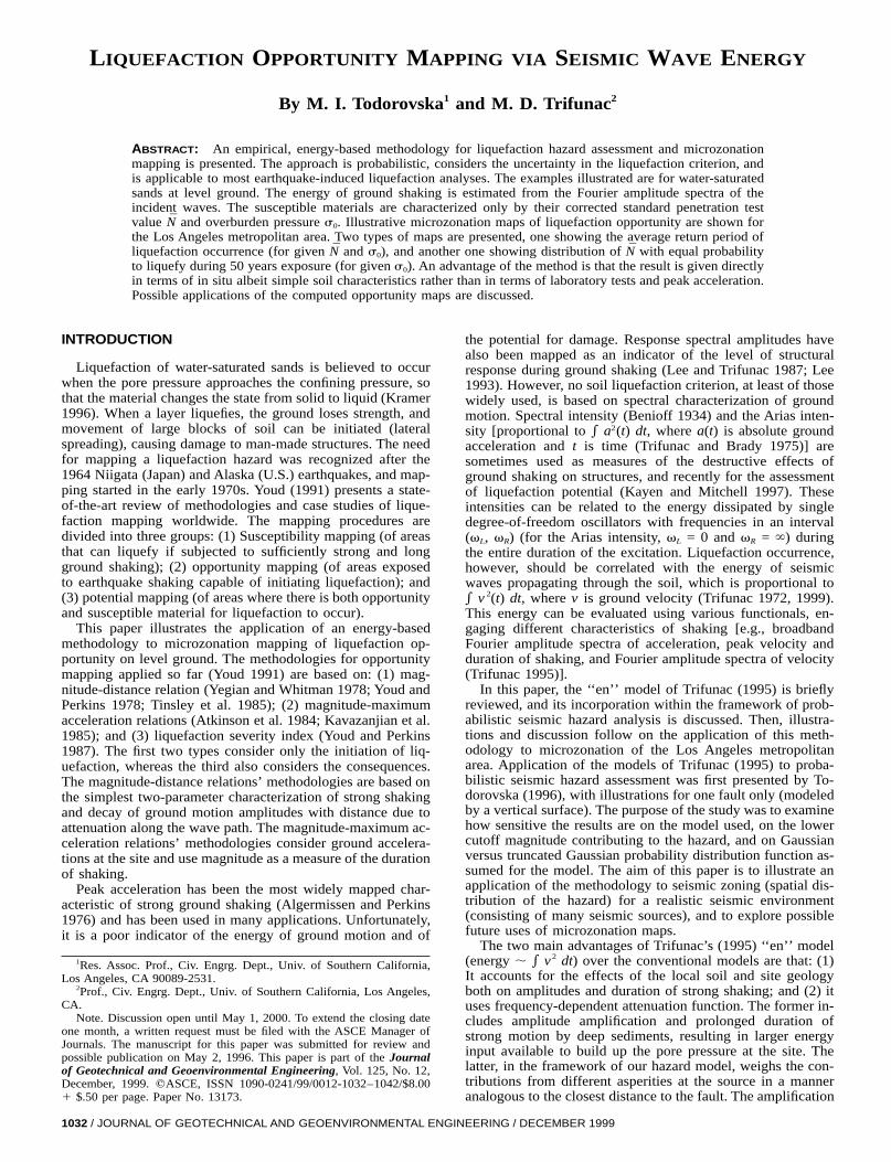
period of liquefaction for the same area if the thickness ofsediments is considered (Fig. 5). It is seen that the return pe-riod is in the range from 30 to 80 years in the San GabrielValley and from 20 to 30 years in the Los Angeles Basin(between the Whittier-Elsinore and the Newport-InglewoodFaults). Differences between the results shown in Figs. 6 and7 are caused by: (1) larger amplitudes of strong motion ve-locities (Trifunac 1976b); and (2) a longer duration of strongmotion (Novikova and Trifunac 1993, 1995) on deeper sedi-ments, both contributing to larger wave energy in the soil. Thesediments are deeper away from the two faults and reach amaximum depth of about 9 km (Fig. 5). Similar effects ofincreased hazard in the Los Angeles Basin have been observedin microzonation maps for peak spectral amplitudes and peaksurface strain (Lee and Trifunac 1987; Trifunac 1988, 1990b;Todorovska and Trifunac 1996). Increased amplitudes are alsoobserved in contour maps of peak acceleration, velocity, anddisplacement, and in pseudo spectral velocity (PSV) ampli-tudes during the 1994 Northridge earthquake, based on infor-mation from recorded strong ground motion (Todorovska andTrifunac 1997a,b). Fig. 8 shows the return period for N = 20and s0 = 40 kPa. It is seen that as s0 in the soil increases(relative to Fig. 7), the amplification effects by deeper sedi-ments become progressively less important, and the hazard isprogressively more governed by the San Andreas Fault.

Another way of presenting a spatial distribution of hazardis to map N for which liquefaction will occur, during the ex-posure period, with equal probability everywhere in the region(s0 is again a parameter with an assigned value). Fig. 9 showssuch a map for a 10% probability to liquefy during 50 years’


FIG. 5. Thickness of Sedimentary Deposits in Los Angeles Metropolitan Area at Grid of Points with 59 Interval [Major Faults AreShown by Heavy Lines, and Hills and Mountains by Gray Areas, after Yerkes et al. (1965)]

FIG. 6. Map of Average Return Period of Liquefaction (as Pre-dicted by ‘‘en’’ Model) for N = 10, s0 = 40 kPa, and Thickness ofSediments h = 0 Everywhere in Region (Major Faults Are Shownby Heavy Lines, and Hills and Mountains by Gray Areas)

JOURNAL OF GEOTECHNICAL A

FIG. 7. Map of Average Return Period of Liquefaction (as Pre-dicted by ‘‘en’’ Model) for N = 10, s0 = 40 kPa, and Thickness ofSediments h, as in Fig. 5 (Major Faults Are Shown by HeavyLines, and Hills and Mountains by Gray Areas)

ND GEOENVIRONMENTAL ENGINEERING / DECEMBER 1999 / 1039

FIG. 8. Map of Average Return Period of Liquefaction (as Pre-dicted by ‘‘en’’ Model) for N = 20, s0 = 40 kPa, and Thickness ofSediments h, as in Fig. 5 (Major Faults Are Shown by HeavyLines, and Hills and Mountains by Gray Areas)

FIG. 9. Map of N (as Predicted by ‘‘en’’ Model) for Probabilityof Occurrence p = 0.1, s0 = 40 kPa, and Thickness of Sedimentsh, as in Fig. 5

exposure to seismic activity, and for s0 = 40 kPa. Dependenceon the thickness of the sediments is included. In Fig. 9, Nvaries between 16 (in the Santa Monica Mountains, San Ga-briel Mountains, and Palos Verdes Peninsula) and 32 (north-east and along the Newport-Inglewood Fault Zone (No. 4 in


Fig. 4), north of Dominguez Hill, and northwest of HuntingtonBeach Mesa).

Plots of the expected number of liquefaction occurrencesmLiq(N s0, t) of the return period TLiq(N, s0) and the probabilityof liquefaction p(N, s0, t) provide useful information in anal-yses of liquefaction hazards at a site. Fig. 10 illustrates suchplots versus a corrected SPT value N for a site at King Harbor(shown by a triangle in Figs. 4–9), for exposure t = 50 years,and for s0 = 20, 40, 80, and 160 kPa. This site is in an areacharacterized by Tinsley et al. (1985) as being highly suscep-tible to liquefaction, and liquefaction was observed there dur-ing the 1994 Northridge earthquake. Plots such as those inFig. 10 would show, e.g., at locations where site improvementis planned, how the hazard would change with the degree ofstrengthening.

An efficient way to store the information on the spatial dis-tribution of liquefaction hazard is via maps (Figs. 7–9), for arange of N and s0 values, and of the probability of occurrencep. From a series of such maps, by reading the value of TLiq ata particular site, one can construct TLiq as a function of N forthat site. Similarly, from a series of equal probability maps,one can construct p as a function of N (Todorovska 1998).

Smaller N and s0 indicates higher liquefaction susceptibility.For values of s0 larger than 40 kPa and values of N largerthan 10, maps such as those in Figs. 7 and 8 will show longerreturn periods. For values of s0 larger than 20 kPa and/or p <0.1, maps such as that shown in Fig. 8 will show larger valuesof N.

The results in Fig. 7 are in qualitative agreement with thoseof Tinsley et al. (1985), whose zoning was based on the max-imum distance-magnitude criterion, and can be compared withour results for susceptible sites (small N). Based on this simpleempirical criterion, the area considered in this paper is withinthe 30 years return period zone.

The criterion for liquefaction used in this paper is definedby a probability distribution function rather than by ‘‘yes’’ or‘‘no,’’ and is therefore sensitive to different degrees of lique-faction susceptibility, and also to the site geology (which in-fluences the amplitudes and duration of ground motion).Therefore, it leads to more detailed and more general zoningmaps than those based on the maximum distance-magnitudecriterion.

SUMMARY AND CONCLUSIONS

A probabilistic method for liquefaction opportunity mappingduring specified exposure is presented. The condition leadingto liquefaction is governed by a physical model of seismicwave energy, calculated via broadband Fourier amplitude spec-tra of ground acceleration (Trifunac 1993, 1994). The mini-mum magnitude that can initiate liquefaction is assumed to beM = 4.75. For the examples shown in this paper, a maximumlimit for the distance for liquefaction to occur is defined byan empirical estimate of a threshold value of the energy factoren (F(v)/v)2 dw] equal to 1022.8 m2/s. Examples of628[=*0.0628

microzonation are presented for the Los Angeles metropolitanarea, for a seismicity model described in this paper. This modelassumes that the earthquakes occur in cycles with exponen-tially distributed interoccurrence intervals. The earthquakerates predicted by the seismicity model are consistent with theobserved rate since the year 1850. The presented results illus-trate the variability governed by the geologic site conditions,via thickness of sediments.

The purpose of this paper has been to explore the possibil-ities of using energy-based probabilistic assessment for liq-uefaction occurrence for microzonation mapping, and to illus-trate the methodology. The Los Angeles metropolitan area hasbeen chosen for the illustrations. The maps of the averagereturn period of liquefaction show variations between 30 and


FIG. 10. Results for Site at King Harbor (Fig. 4), for 50 Years’ Exposure: Return Period of Liquefaction, Expected Number of Occur-rences and Probability of Occurrence, All versus Corrected SPT Value N. Different Types of Lines Correspond to Overburden Pressures0 = 20, 40, 80, and 160 kPa

80 years, for N = 10 and s0 = 40 kPa. The equal probabilitymap shows that for s0 = 40 kPa and 50 years’ exposure, andfor 0.1 probability of occurrence, N varies between 16 and 32counts per foot. The maps show that the San Andreas Faulthas a prominent contribution to the hazard. The hazard is alsolarger in the San Gabriel Valley and Los Angeles Basin, dueto the amplification of ground motion amplitudes and a longerduration of shaking in sediments.

Detailed results (plots of return period of liquefaction, ex-pected number of occurrences in 50 years’ exposure, and prob-ability of occurrence, all versus the corrected SPT value andfor several values of the overburden pressure) are illustratedfor a site at King Harbor, where liquefaction occurred duringthe 1994 Northridge earthquake. Such curves can be con-structed from a series of microzonation maps for different val-ues of the parameters (Todorovska 1998).

In actual applications, maps will be used that considergreater detail in the geometry of the seismic sources, and moredetailed specification of the site geology. This will lead tomore detail in the computed contours, but the overall regionalamplitudes will not differ qualitatively from the maps pre-sented in this paper. The input on the earthquake occurrencerates can also be updated as new information becomes avail-able. The method can be improved further by studying in moredetail the threshold conditions for the energy-based liquefac-tion occurrence criterion.

The simple site characterization makes this method very at-tractive for hazard mapping purposes. The type of maps shownin this paper shows the liquefaction opportunity for a range ofsite properties. For liquefaction to occur, there should be aliquefiable layer at the site. Liquefaction potential can bemapped by overlaying opportunity with susceptibility maps(based on geology, geotechnical data, and eventually watertable maps). For a specific project, after N and s0 are estimatedfor the site, the probability for liquefaction occurrence (or theaverage return period of liquefaction) can be read directly orestimated by interpolation from the appropriate liquefactionopportunity map(s). A series of opportunity maps can be usedto construct the return period of liquefaction as a function ofN, or the probability of liquefaction as a function of N [both


for selected values of s0 (Todorovska 1998)]. Such curves canbe used in cost benefit analyses and in decision-making pro-cesses related to ground improvement projects.

APPENDIX. REFERENCES

Algermissen, S. T., and Perkins, D. M. (1976). ‘‘A probabilistic estimateof maximum acceleration in rock in the contiguous United States.’’Open File Rep. 76-416, U.S. Dept. of the Interior, Geological Survey.

Ambraseys, N. N. (1988). ‘‘Engineering seismology.’’ Earthquake Engrg.and Struct. Dynamics, 7, 70–105.

Atkinson, G. M., Finn, W. D. L., and Charlwood, R. G. (1984). ‘‘Simplecomputation of liquefaction probability for seismic hazard applica-tions.’’ Earthquake Spectra, 1(1), 107–123.

Benioff, H. (1934). ‘‘A physical evaluation of seismic destructiveness.’’Bull. Seismological Soc. of Am., 24, 389–403.

Berrill, J. B., and Davis, R. O. (1985). ‘‘Energy dissipation and seismicliquefaction of sands: Revised model.’’ Soils and Found., Tokyo, 25(2),106–118.

Blazquez, R. M., Krizek, R. J., and Bazant, Z. P. (1980). ‘‘Site factorscontrolling liquefaction.’’ J. Geotech. Engrg. Div., ASCE, 106(7), 785–801.

Davis, R. O., and Berrill, J. B. (1982). ‘‘Energy dissipation and seismicliquefaction in sands.’’ Earthquake Engrg. and Struct. Dynamics, 10,51–68.

Fischhoff, B., Lichtenstein, S., Slovic, P., Derby, S. L., and Keeney, R.(1981). Acceptable risk. Cambridge University Press, Cambridge,Mass.

Holzer, T. L., Youd, T. L., and Hanks, T. C. (1989). ‘‘Dynamics of liq-uefaction during the 1987 Superstition Hills, California, Earthquake.’’Sci., 244, 56–59.

Kavazanjian, E., Jr., Roth, R. A., and Echezuria, H. (1985). ‘‘Liquefactionpotential mapping for San Francisco.’’ J. Geotech. Engrg., ASCE,111(1), 54–76.

Kayen, R. E., and Mitchell, J. K. (1997). ‘‘Assessment of liquefactionpotential during earthquakes, by Arias intensity.’’ J. Geotech. andGeoenvir. Engrg., ASCE, 123(12), 1162–1174.

Kramer, S. L. (1996). Geotechnical earthquake engineering. Prentice-Hall, Englewood Cliffs, N.J.

Kuribayashi, E., and Tatsuoka, F. (1975). ‘‘Brief review of liquefactionduring earthquakes in Japan.’’ Soils and Found., 15, 81–92.

Lee, V. W. (1993). ‘‘Scaling PSV from earthquake magnitude, local soiland geological depth of sediments.’’ J. Geotech. Engrg., ASCE, 119(1),108–126.

Lee, V. W., Amini, A., and Trifunac, M. D. (1982). ‘‘Noise in earthquakeaccelerograms.’’ J. Engrg. Mech. Div., ASCE, 108(6), 1121–1129.


Lee, V. W., and Trifunac, M. D. (1985). ‘‘Uniform risk spectra of strongearthquake ground motion: NEQRISK.’’ Rep. CE 85-05, Dept. of Civ.Engrg., University of Southern California, Los Angeles.

Lee, V. W., and Trifunac, M. D. (1987). ‘‘Microzonation of a metropolitanarea.’’ Rep. CE 87-02, Dept. of Civ. Engrg., University of SouthernCalifornia, Los Angeles.

Lee, V, W., and Trifunac, M. D. (1995a). ‘‘Frequency dependent attenu-ation function and Fourier amplitude spectra of strong earthquakeground motion in California.’’ Rep. CE 95-03, Dept. of Civ. Engrg.,University of Southern California, Los Angeles.

Lee, V. W., and Trifunac, M. D. (1995b). ‘‘Pseudo relative velocity spec-tra of strong earthquake ground motion in California.’’ Rep. CE 95-04, Dept. of Civ. Engrg., University of Southern California, Los An-geles.

Lee, V. W., Trifunac, M. D., Todorovska, M. I., and Novikova, E. I.(1995). ‘‘Empirical equations describing attenuation of the peaks ofstrong ground motion, in terms of magnitude, distance, path effects andsite conditions.’’ Rep. CE 95-02, Dept. of Civ. Engrg., University ofSouthern California, Los Angeles.

Novikova, E. I., and Trifunac, M. D. (1993). ‘‘Duration of strong earth-quake ground motion: Physical basis and empirical equations.’’ Rep.CE 93-02, Dept. of Civ. Engrg., University of Southern California, LosAngeles.

Novikova, E. I., and Trifunac, M. D. (1995). ‘‘Frequency dependent du-ration of strong earthquake ground motion: Updated empirical equa-tions.’’ Rep. CE 95-01, Dept. of Civ. Engrg., University of SouthernCalifornia, Los Angeles.

Papaulis, A. (1962). The Fourier integral and its applications. McGraw-Hill, New York.

Richter, C. F. (1958). Elementary seismology. Freeman, San Francisco.Robertson, P. K., and Capanella, R. G. (1985). ‘‘Liquefaction potential

of sands using CPT.’’ J. Geotech. Engrg., ASCE, 111(3), 384–403.Robertson, P. K., Woeller, D. J., and Finn, W. D. L. (1992). ‘‘Seismic

cone penetration tests for evaluating liquefaction potential under cy-cling loading.’’ Can. Geotech. J., Ottawa, 29(4), 686–695.

Seed, H. B., Tokimatsu, K., Harder, L., and Chung, R. (1984). ‘‘Theinfluence of SPT procedures on soil liquefaction resistance evalua-tions.’’ Rep. No. 84-15, Earthquake Engrg. Res. Ctr., University ofCalifornia, Berkeley, Calif.

Shibata, S., and Teparaksa, W. (1988). ‘‘Evaluation of liquefaction poten-tials of soils using cone penetration tests.’’ Soils and Found., 28(2),49–60.

Tinsley, J. C., Youd, T. L., Perkins, D. M., and Chen, A. T. F. (1985).‘‘Evaluating liquefaction potential.’’ U.S. Geological Survey Profl. Pa-per 1360, 263–315.

Todorovska, M. I. (1994a). ‘‘Comparison of response spectrum ampli-tudes from earthquakes with lognormally and exponentially distributedreturn period.’’ Soil. Dyn. and Earthquake Engrg., 13(2), 97–116.

Todorovska, M. I. (1994b). ‘‘Order statistics of functionals of strongground motion for a class of renewal processes.’’ Soil Dyn. and Earth-quake Engrg., 13(6), 399–405.

Todorovska, M. I. (1995a). ‘‘Effects of earthquake source parameters onuniform probability response spectra.’’ Proc., 10th Eur. Conf. Earth-quake Engrg., Vol. 4, Balkema, Rotterdam, The Netherlands, 2579–2584.

Todorovska, M. I. (1995b). ‘‘Uniform probability response spectra forselecting site specific design motions.’’ Proc., 3rd Int. Conf. on RecentAdv. in Geotech. Earthquake Engrg. and Soil Dyn., Vol. II, 613–618.

Todorovska, M. I. (1996). ‘‘Liquefaction hazard assessment via seismicwave energy and SPT values.’’ Eur. Earthquake Engrg., 10(2), 24–37.

Todorovska, M. I. (1998). ‘‘Quick reference liquefaction opportunitymaps for a metropolitan area.’’ Geotechnical earthquake engineeringand soil dynamics III, Geotech. Spec. Publ. No. 75, Vol. 1, ASCE,Reston, Va., 116–127.

Todorovska, M. I., Gupta, I. D., Gupta, V. K., Lee, V. W., and Trifunac,M. D. (1995). ‘‘Selected topics in probabilistic seismic hazard assess-ment.’’ Rep. CE 95-08, Dept. of Civ. Engrg., University of SouthernCalifornia, Los Angeles.

Todorovska, M. I., and Lee, V. W. (1995). ‘‘A note on sensitivity ofuniform probability spectra on modeling the fault geometry in areaswith a shallow seismogenic zone.’’ Eur. Earthquake Engrg., 9(2), 14–22.

Todorovska, M. I., and Trifunac, M. D. (1996). ‘‘Hazard mapping ofnormalized peak strain in soil during earthquakes: Microzonation of ametropolitan area.’’ Soil Dyn. and Earthquake Engrg., 15(5), 321–329.

Todorovska, M. I., and Trifunac, M. D. (1997a). ‘‘Distribution of pseudospectral velocity during the Northridge, California, earthquake of 17January, 1994.’’ Soil Dyn. and Earthquake Engrg., 16(3), 173–192.

Todorovska, M. I., and Trifunac, M. D. (1997b). ‘‘Amplitudes, polarity


and time of peaks of strong ground motion during the 1994 Northridge,California, earthquake.’’ Soil Dyn. and Earthquake Engrg., 16(4), 235–258.

Trifunac, M. D. (1972). ‘‘Tectonic stress and the source mechanism ofthe Imperial Valley, California, Earthquake of 1940.’’ Bull. Seismolog-ical Soc. of Am., 62(5), 1283–1302.

Trifunac, M. D. (1976a). ‘‘Preliminary empirical model for scaling Fou-rier amplitude spectra of strong ground acceleration in terms of earth-quake magnitude, source to station distance, and recording site condi-tions.’’ Bull. Seismological Soc. of Am., 66(9), 1343–1373.

Trifunac, M. D. (1976b). ‘‘Preliminary analysis of the peaks of strongearthquake ground motion—Dependence of peaks on earthquake mag-nitude, epicentral distance and the recording site conditions.’’ Bull.Seismological Soc. of Am., 66, 187–219.

Trifunac, M. D. (1988). ‘‘Seismic microzonation mapping via uniformrisk spectra.’’ Proc., 9th World Conf. on Earthquake Engrg., Vol. VIII,75–80, Tokyo-Kyoto, Maruzen Co. Ltd., Tokyo, Japan.

Trifunac, M. D. (1990a). ‘‘How to model amplification of strong earth-quake motion by local geologic and soil site conditions.’’ EarthquakeEngrg. and Struct. Dynamics, 19(6), 833–846.

Trifunac, M. D. (1990b). ‘‘A microzonation method based on uniformrisk spectra.’’ Soil Dyn. and Earthquake Engrg., 9(1), 34–43.

Trifunac, M. D. (1993). ‘‘Long period Fourier amplitude spectra of strongmotion acceleration.’’ Soil Dyn. and Earthquake Engrg., 12(6), 363–382.

Trifunac, M. D. (1994). ‘‘Q and high frequency strong motion spectra.’’Soil Dyn. and Earthquake Engrg., 13(3), 149–161.

Trifunac, M. D. (1995). ‘‘Empirical criteria for liquefaction in sands viastandard penetration tests and seismic wave energy.’’ Soil Dyn. andEarthquake Engrg., 14(6), 419–426.

Trifunac, M. D. (1999). ‘‘Discussion of ‘Assessment of liquefaction po-tential during earthquakes,’ by R. E. Kayen and J. K. Mitchell.’’ J.Geotech. and Geoenvir. Engrg., ASCE, 125(7), 627.

Trifunac, M. D., and Brady, A. G. (1975). ‘‘A study on the duration ofstrong earthquake ground motion.’’ Bull. Seismological Soc. of Am.,65(3), 581–626.

Trifunac, M. D., and Lee, V. W. (1966). ‘‘Peak surface strains duringstrong earthquake motion.’’ Soil Dyn. and Earthquake Engrg., 15(5),311–319.

Trifunac, M. D., and Lee, V. W. (1990). ‘‘Frequency dependent attenua-tion of strong earthquake ground motion.’’ Soil. Dyn. and EarthquakeEngrg., 9(1), 3–15.

Trifunac, M. D., and Novikova, E. I. (1995). ‘‘State of the art review ofstrong motion duration.’’ Proc., 10th Eur. Conf. Earthquake Engrg.,Vol. 1, Balkema, Rotterdam, The Netherlands, 131–140.

Trifunac, M. D., and Todorovska, M. I. (1996). ‘‘Nonlinear soil response—1994 Northridge, California, earthquake.’’ J. Geotech. Engrg.,ASCE, 122(9), 725–735.

Trifunac, M. D., and Todorovska, M. I. (1998a). ‘‘Nonlinear soil responseas a natural passive isolation mechanism—1994 Northridge, California,earthquake.’’ Soil Dyn. and Earthquake Engrg., 17(1), 41–51.

Trifunac, M. D., and Todorovska, M. I. (1998b). ‘‘Amplification of strongground motion and damage patterns during the 1994 Northridge, Cal-ifornia, earthquake.’’ Proc., Spec. Conf. on Geotech. Engrg. and SoilDyn., Geotech. Spec. Publ. No. 75, Vol. I, ASCE, Reston, Va., 714–725.

Trifunac, M. D., and Todorovska, M. I. (1998c). ‘‘Damage distributionduring the 1994 Northridge, California, earthquakes relative to gener-alized categories of surficial geology.’’ Soil Dyn. and EarthquakeEngrg., 17(4), 239–253.

Working group on California earthquake probabilities. (1995). ‘‘Seismichazards in southern California: Probable earthquakes, 1994 to 2024.’’Bull. Seismological Soc. of Am., 85(2), 379–439.

Yegian, M. K., and Whitman, R. V. (1978). ‘‘Risk analysis for groundfailure by liquefaction.’’ J. Geotech. Engrg. Div., ASCE, 104(7), 921–938.

Yerkes, R. F., McCulloh, T. H., Schoellhamer, J. E., and Vedder, J. G.(1965). ‘‘Geology of the Los Angeles Basin, California—An introduc-tion.’’ U.S. Geological Survey Profl. Paper 420-A.

Youd, L. T. (1991). ‘‘Mapping of earthquake induced liquefaction forseismic zonation.’’ Proc., 4th Int. Conf. on Seismic Zonation, Vol. I,111–146.

Youd, L. T., and Holzer, T. L. (1994). ‘‘Piezometer performance at wild-life liquefaction site, California.’’ J. Geotech. Engrg., ASCE, 120(6),975–995.

Youd, L. T., and Perkins, D. M. (1978). ‘‘Mapping liquefaction inducedground failure potential.’’ J. Geotech. Engrg. Div., ASCE, 104(4), 433–446.

Youd, L. T., and Perkins, D. M. (1987). ‘‘Mapping of liquefaction severityindex.’’ J. Geotech. Engrg., ASCE, 113(11), 1374–1392.


Liquefaction Opportunity Mapping via Seismic Wave Energy

Documents

Transcript of Liquefaction Opportunity Mapping via Seismic Wave Energy