Liquefaction Resistance Evaluation of Soils using Arti cial ...

Liquefaction Resistance Evaluation of Soils usingArti�cial Neural Network for Dhaka City, BangladeshAbul Kashem Faruki Fahim

University of Dhaka Faculty of Earth and Environmental SciencesMd. Zillur Rahman

University of Dhaka Faculty of Earth and Environmental SciencesMd. Shakhawat Hossain

University of Dhaka Faculty of Earth and Environmental SciencesA S M Maksud Kamal ( [email protected] )

University of Dhaka Faculty of Earth and Environmental Sciences https://orcid.org/0000-0002-3896-2032

Research Article

Keywords: Earthquake, Liquefaction, Liquefaction potential index (LPI), Simpli�ed procedure, Arti�cialneural network (ANN)

Posted Date: May 18th, 2021

DOI: https://doi.org/10.21203/rs.3.rs-468975/v1

License: This work is licensed under a Creative Commons Attribution 4.0 International License. Read Full License

https://doi.org/10.21203/rs.3.rs-468975/v1

mailto:[email protected]

https://orcid.org/0000-0002-3896-2032

https://doi.org/10.21203/rs.3.rs-468975/v1

https://creativecommons.org/licenses/by/4.0/

1

Liquefaction resistance evaluation of soils using artificial neural network for Dhaka City, Bangladesh 1

Abul Kashem Faruki Fahim, Md. Zillur Rahman, Md. Shakhawat Hossain, and A. S. M. Maksud Kamal* 2

Department of Disaster Science and Management, University of Dhaka, Dhaka 1000, Bangladesh 3

*Corresponding Author: Dr. A. S. M. Maksud Kamal, Professor, Department of Disaster Science and 4

Management, University of Dhaka, Dhaka 1000, Bangladesh 5

e-mail: [email protected], cell: +880-1759760944 6

7

8

9

10

11

12

13

14

15

16

17

18

19

20

21

22

mailto:[email protected]

2

Abstract 23

Soil liquefaction resistance evaluation is an important site investigation for seismically active areas. To minimize the 24

loss of life and property, liquefaction hazard analysis is a prerequisite for seismic risk management and development 25

of an area. Liquefaction potential index (LPI) is widely used to determine the severity of liquefaction quantitatively 26

and spatially. LPI is estimated from the factor of safety (FS) of liquefaction that is the ratio of cyclic resistance ratio 27

(CRR) to cyclic stress ratio (CSR) calculated applying simplified procedure. Artificial neural network (ANN) 28

algorithm has been used in the present study to predict CRR directly from the normalized standard penetration test 29

blow count (SPT-N) and near-surface shear wave velocity (Vs) data of Dhaka City. It is observed that ANN model 30

have generated accurate CRR data. Three liquefaction hazard zones are identified in Dhaka City on the basis of the 31

cumulative frequency (CF) distribution of the LPI of each geological unit. The liquefaction hazard maps have been 32

prepared for the city using the liquefaction potential index (LPI) and its cumulative frequency (CF) distribution of 33

each liquefaction hazard zone. The CF distribution of the SPT-N based LPI indicates that 15%, 53%, and 69% of 34

areas, whereas the CF distribution of the Vs based LPI indicates that 11%, 48%, and 62% of areas of Zone 1, 2, and 35

3, respectively, show surface manifestation of liquefaction for a scenario earthquake of moment magnitude, Mw 7.5 36

with a peak horizontal ground acceleration (PGA) of 0.15 g. 37

Keywords: Earthquake, Liquefaction, Liquefaction potential index (LPI), Simplified procedure, Artificial neural 38

network (ANN) 39

40

41

42

43

44

45

46

3

1. Introduction 47

Liquefaction occurs when granular, loosely compacted or cohesionless, saturated or partially saturated sediments 48

lose their shear strength and transform from solid to liquid state at or near the ground surface resulting from cyclic 49

loading or other abrupt alteration of stress conditions (Castro 1969; Castro and Poulos 1977; Castro et al. 1982). The 50

loss of strength takes place in cohesionless soil due to reduction in effective stress resulting from increased pore 51

water pressure caused by rapid, usually cyclic loading exerted by strong ground shaking (Marcuson 1978). 52

During an earthquake, liquefaction can be devastating incurring widespread damage, which was revealed 53

by Niigata Earthquake in 1964, Alaska Earthquake in 1964, Loma Prieta Earthquake in 1989, Chi-Chi Earthquake in 54

1999, and Sulawesi Earthquake in 2018 (Seed and Idriss 1967; Ku et al. 2004; Lee et al. 2007; Chao et al. 2010; 55

Sassa and Takagawa 2019; Hossain et al. 2020). Therefore, in a seismic hazard-prone area, liquefaction resistance 56

evaluation is an integral part of site characterization. 57

Both in situ tests (e.g., SPT, Vs, Cone Penetration Test (CPT) data) and soil laboratory tests (e.g., cyclic 58

triaxial test) can be used to evaluate soil liquefaction resistance during seismic loading. Good-quality undisturbed 59

soil samples are essential to assess the soil liquefaction resistance by the laboratory tests. However, collecting such 60

samples from degraded loosely compacted silty or sandy soils are sometimes difficult and expensive. Due to these 61

drawbacks of the laboratory tests, geotechnical engineers widely use in situ tests as it is simple and economical 62

(Seed and Idriss 1971, 1982; Seed et al. 1983, 1984, 1985; Seed and de Alba 1986). Over the last five decades, the 63

Simplified Procedure, developed initially by Seed and Idriss (1971), has been used in liquefaction resistance 64

evaluation of soils. Since its inception in 1971, many researchers have updated, modified, revised, and validated this 65

method (e.g., Juang et al. 2003, 2000; Olsen 1997, 1988; Olsen and Koester 1995; Robertson and Wride 1998; Stark 66

and Olson 1995). To assess liquefaction resistance by this procedure, the corrected SPT-N is widely used as input 67

(Seed and Idriss 1971, 1982; Seed et al. 1983, 1984, 1985; Kayen et al. 1992; Juang et al. 2000; Youd et al. 2001; 68

Idriss and Boulanger 2004). 69

Using field Vs measurement, a method of liquefaction resistance estimation was introduced by Andrus et al. 70

(2000) and Andrus and Stokoe (1997). The use of the Vs data has more advantages than the SPT-N and CPT data as 71

the Vs data can easily be collected from stiff and gravelly soils. The soil profile can be easily obtained and the 72

4

analytical procedures that analyze the small-scale shear modulus for evaluating soil-structure interaction and 73

dynamic soil response are related to Vs value of the soil materials. 74

In Bangladesh, most of the subsurface lithology is characterized by unconsolidated, sandy and clayey 75

floodplain sediments. In alluvial deposits of Bangladesh, following the Srimangal Earthquake in 1918, Great Indian 76

Earthquake in 1897, and the Bengal Earthquake in 1885, the evidences of widespread liquefaction were documented 77

(Middlemiss 1885; Oldham 1899; Stuart 1920; Hossain et al. 2020). In the north and northeast areas of the country, 78

the evidences of liquefaction were observed during paleoseismic studies, which are considered to be triggered by a 79

series of earthquakes along the Dauki fault (Morino et al. 2011, 2014a, b). In addition, the country is sitting close to 80

the tectonically active Himalayan orogenic belt and Arakan megathrust where there are at least five major active 81

fault zones, which have shown evidence of large magnitude earthquakes (Aitchison et al. 2007). Steckler et al. 82

(2016) claimed a locked megathrust exists along the Indo-Burman mountain ranges, which reinforces the notion of 83

the resistance future for major earthquakes. Therefore, it is an absolute necessity for the country to further study the 84

liquefaction resistance evaluation of soils for the major cities. 85

Rahman et al. (2015) and Rahman and Siddiqua (2017) have conducted liquefaction potential studies for Dhaka, 86

Chittagong, and Sylhet cites in Bangladesh using limited standard penetration test blow count (SPT-N), cone 87

penetration test (CPT), and shear wave velocity (Vs) data. The studies observed that the Holocene alluvium of these 88

cities is susceptible to liquefaction. In those studies, the empirical equations of Youd et al. (2001) were used to 89

calculate the factor of safety (FS) of liquefaction, cyclic resistance ratio (CRR), cyclic stress ratio (CSR), and 90

magnitude scaling factor (MSF). The equations of Iwasaki et al. (1982) were used to calculate liquefaction potential 91

index (LPI). However, in present study, the ANN models were incorporated based on Juang et al. (2003, 2002, 92

2000) to predict the CRR. The ANN models are inherently bound to produce more realistic results and additional 93

SPT-N and Vs profiles were used to characterize the subsurface heterogeneity with more accuracy. Thus, this study 94

utilizes an improved, robust, and promising method in assessing liquefaction resistance of soils for Dhaka City. 95

The SPT-N and Vs data from Dhaka City have been used in the assessment of liquefaction resistance of 96

soils for a scenario earthquake of moment magnitude, MW 7.5 with a peak ground acceleration (PGA) of 0.15 g. 97

According to the proposed Bangladesh Nation Building Code (BNBC), the PGA value for Dhaka City is 0.2 g for 98

the maximum considered earthquake (MCE), which is equivalent to 2% probability of exceedance in 50 years 99

5

(2475-year return period). The PGA of the design basis earthquake (DBE) is equal to the 2/3 (two-third) of the 100

MCE. Therefore, the PGA of DBE in Dhaka City is 0.13 g. It is observed from historical record of earthquakes that 101

more than Mw 7.0 earthquakes occurred beyond 50 km radius from city center of Dhaka ((Middlemiss 1885; Oldham 102

1899; Stuart 1920). Therefore, the magnitude of earthquake is considered as Mw 7.5 with PGA of 0.15 g in this 103

study. 104

Artificial neural network (ANN) models were used to predict CRR where a variant of performance function 105

(Seed and Idriss 1971, 1982) termed as limit state function (LSF), was considered (Juang et al. 2002, 2000). Firstly, 106

a liquefaction indicator function was formulated for calculating the occurrence of liquefaction. Then, the points at 107

the limit state surface was formulated to determine CRR through simulating the neural network models that were 108

trained using the derived points at the limit state surface by a standard method (Youd et al., 2001). The CSR was 109

estimated on the basis of simplified procedure (Seed and Idriss 1971). The factor of safety (FS) of liquefaction was 110

calculated at selected locations of Dhaka City using estimated CSR and CRR values. Even though the FS may 111

provide an idea of the resistance of soils, it is not enough to represent the state of the liquefaction severity of any 112

location (Sonmez and Gokceoglu 2005). Therefore, the FS values up to the depth of liquefiable layers, which is 113

considered as 20 m depth, were used to determine the LPI of all selected locations of Dhaka City for both datasets 114

(SPT-N and Vs) based on the developed method of Iwasaki et al. (1982) to prepare liquefaction hazard maps for 115

calculating LPI values of the areas where SPT-N and Vs data were not available. For each georgical unit, the 116

liquefaction hazard is also predicted from the cumulative frequency (CF) distribution of the LPI according to Holzer 117

et al. (2006). 118

2. Surface geology of Dhaka City 119

Dhaka City, the capital of Bangladesh, located is on the bank of the Buriganga River, is now one of the world's 120

megacities. The city is encircled by the rivers of Buriganga, Balu, Turag, and Tongi Khal. It occupies an area of 121

about 321 square kilometers with a population of about 14 million. Dhaka City has an average elevation of 6.5 m 122

ranging between 2 and14 m (above the mean sea level) with many depressions (Rahman et al. 2015). Dhaka is 123

situated in the central part of Bangladesh bounded by the Shillong Massif in the north, Precambrian Indian Shield in 124

the west, the Indo-Burman Folded Belt in the east and it is open to the Bay of Bengal in south. Bangladesh covers 125

most part of the Bengal Basin with the maximum sedimentary thickness of 22 km (Alam 1989; Reimann 1993). 126

6

Dhaka City is developed partly on the Madhupur Terrace of the Pleistocene age and partly on the low-lying 127

floodplains of the Holocene age. The sediment of the Pleistocene terrace has been deposited on the older 128

floodplains, whereas the Holocene alluvium has been deposited on the recent floodplains of the Ganges-129

Brahmaputra River Systems (Morgan and McIntire, 1959). 130

In Dhaka City, six surface geological units have been identified based on the geomorphological, geological, 131

and geotechnical properties. These units are Artificial fill (af), Holocene Alluvial channel deposit (Qhc), Holocene 132

Alluvial valley fill deposit (Qhav), Holocene Alluvium (Qha), Holocene terrace deposit (Qhty), and Pleistocene 133

terrace deposit (Qpty) (Fig. 1) (Rahman et al. 2015). 134

7

135

Fig. 1 Surface geological map of Dhaka City with locations of the boreholes (modified from Rahman et al. (2015)) 136

137

The Pleistocene terrace deposits exposed in the central part of the city are primarily comprised of a 6-8 m 138

thick layer of reddish to yellowish-brown, medium stiff to stiff silty clay that is underlain by a layer of medium 139

dense to very dense silty sand and sand down to the depth of investigation of 20 m. The Holocene alluvium deposits 140

composed of very loose to loose sand, silt, and very soft to soft silty clay are present down to the depth of 141

investigation in northwestern, southeastern, and eastern parts of the city (Rahman et al. 2021). Gray sand, silty sand, 142

and clayey silt make up the artificial fills that are emplaced to the west and east portions of the city. For the 143

8

emplacement of the artificial fills, both hydraulic dragging from the river and trucks from the land were used, but the 144

ground was not compacted properly during filling, which creates the area prone to liquefaction (Rahman et al. 145

2015). 146

3. Seismotectonics of the region 147

The Bengal Basin is in the northeastern part of the Indian plate and bordering the Indian-Eurasian convergent plate 148

boundary where the Himalayan ranges the north and Indo-Burman ranges in east have been created due to the 149

collision between these plates (Curray et al. 1982; Aitchison et al. 2007). Besides Bangladesh, the Bengal Basin also 150

contains portions of Assam, Tripura, and West Bengal. 151

Dhaka, is seismically vulnerable due to its proximity to the Eurasian and Indian convergent plate boundary 152

(Rahman et al. 2020, 2021). Bangladesh, Myanmar, Nepal, and northeastern India experienced several historical 153

earthquakes (Table 1) that occurred along this plate boundary and associated faults. The Himalayan and the Arakan 154

subduction-collision systems (Fig. 2) also generated many devastating earthquakes in these regions. 155

The Dauki Fault (DF) and the Himalayan Frontal Thrust (HFT) are the main seismotectonic elements of the 156

Himalayan system, while the Arakan subduction-collision system manifests itself through the Indo-Burman Folded 157

Belt along with the megathrust beneath (Steckler et al. 2008; Wang et al. 2014). 158

Bilham and Hough (2006) anticipated that a large earthquake with a magnitude ranging from Mw 7.5 to 8.5 159

may occur in the Himalayan system because of the movement of the Indian plate at a rate of 4 cm/year towards the 160

north and at a rate of 6 cm/year towards the northeast. The 2015 Gorkha Earthquake (Mw 7.8) occurred in Nepal 161

along the subduction interface of the Himalayan System (Goda et al. 2015). It has been revealed by recent 162

paleoseismological investigations that the Dauki fault was activated three times during last thousand years (Yeats et 163

al. 1997; Morino et al. 2011, 2014a) The convergence of the tectonic plates and increasing frequency of earthquakes 164

with large magnitude are, therefore, the indication of active seismic activities in these regions (Rahman and Siddiqua 165

2017). 166

167

168

9

Table 1 Major earthquakes that caused damage and casualty in Bangladesh in the last 256 years (Rahman et al. 169

2020) 170

Date Earthquake

Moment

Magnitude

(Mw)

Number of

Casualty Structural Damage

April 2, 1762 Bengal-Arakan

Earthquake

8.5(1) 500 in Dhaka(2) The earthquake was very strong in

Dhaka and Chittagong.(2)

July 14, 1885 Bengal

Earthquake

6.87(3) Not reported The highest damage was reported in

Sirajganj, Bogra, Jamalpur and

Mymensingh. In Dhaka, the damage was

very low compared to other areas located

at similar distance from the epicenter.(4)

June 12, 1897 Great Assam

Earthquake

8.03(3) 545 in Sylhet(2) The highest damage was reported in

Shillong, Assam (India). In Dhaka,

almost all masonry buildings were badly

damaged, and some were entirely

collapsed. In Sylhet, most of the masonry

buildings were severely damaged.(5)

July 08, 1918 Srimangal

Earthquake

7.10(3) Exact numbers

were not

reported

Most of the tea factories and bungalows

at Srimangal (Moulvibazar) were

destroyed. Significant damage was

reported in Kishoreganj, Sylhet,

Habiganj, Agartala (India). In Dhaka,

several buildings were slightly cracked.(6)

Based to (1)Wang et al. (2014); (2)Banglapedia (accessed on 06 August, 2018); (3)Ambraseys and Douglas (2004), 171 (4)Middlemiss (1885); (5)Oldham (1899); and (6)Stuart (1920). 172

4. Material and methods 173

4.1. Database establishment 174

The SPT-N and Vs data from sixty-five (65) boreholes including relevant geotechnical properties of soils were used 175

to assess soil liquefaction resistance of Dhaka City in terms of the FS, which was estimated using the Simplified 176

Procedure of Seed and Idriss (1971). Then, the LPI of each borehole profile was estimated using all FS values of 177

each borehole that were estimated at every 1.5 m interval to a depth of 20 m below the ground surface according to 178

the method introduced by Iwasaki et al. (1978). The borehole sites were selected considering the variation of the 179

geological units in the city (Table 2). The surface geological map (Fig. 1) shows the borehole locations. 180

For training purpose, artificial neural network (ANN) requires the SPT-N and Vs data of the sites where the 181

historical data of liquefaction and non-liquefaction cases are available to find liquefaction indicator (LI) function 182

and points of the limit state function (LSF). The SPT-N data of the historical cases for liquefaction and non-183

liquefaction were primarily collected by Fear and McRoberts (1995) and later summarized by Idriss and 184

Boulanger (2010). The Vs data were compiled by Andrus et al. (1999). After screening as per the ANN model 185

10

applicability criteria of used parameters as described in Juang et al. (2000), total 225 SPT cases (127 cases 186

liquefied) and 225 Vs cases (97 cases liquefied) from 26 earthquakes over 70 sites identified by Andrus et al. 187

(1999) were used for the analysis of the present study. 188

189

Fig. 2 Recent and historical earthquakes of magnitude greater than Mw 6.5 from 1762 and 2016 (retrieved from 190

Rahman and Siddiqua (2017)) 191

192

193

194

195

11

Table 2 Number of boreholes in each surface geological unit of Dhaka City and classes of the geological materials 196

based on the Unified Soil Classification System (USCS) 197

Geological unit Number of Boreholes USCS soil type

Artificial fill (af) 6 SM, SP, MH

Holocene Alluvial valley fill deposits (Qhav) 7 SM, MH, CH

Holocene terrace deposits (Qhty) 4 SM, SP, CL

Holocene channel deposits (Qhc) 0 SM, SP

Holocene Alluvium (Qha) 10 SM, CL, MH, CH

Pleistocene terrace deposits (Qpty) 38 SM, SP, MH, CH, CL

198

4.2. Factor of safety of liquefaction (FS) 199

In this study, an updated simplified procedure proposed by Youd et al. (2001)is used in calculating the factor of 200

safety (FS) of liquefaction that is the ratio of the cyclic resistance ratio (CRR) to the cyclic stress ratio (CSR). 201

4.2.1. Calculation of CSR 202

The CSR defines the cyclic loading characteristic of soils, by which the seismic demand of the soil layer is 203

determined on a level ground condition. It is the ratio of the cyclic loading-induced average cyclic shear stress to the 204

initial vertical effective stress on the soil particles (Robertson and Campanella, 1985). The following equation of 205

Seed and Idriss (1971) that was slightly adjusted by Juang et al., (2003) has been used to estimate the CSR at z depth 206

from the ground surface due to earthquake loading: 207

(1) 208

where, = CSR adjusted to an earthquake magnitude of Mw 7.5 using a magnitude scaling factor (MSF); = 209

average cyclic shear stress exerted by an earthquake, = total vertical stress, = effective vertical stress at a 210

depth of question (z); = gravitational acceleration; = peak horizontal ground acceleration (PGA); Rp= 211

overburden pressure ratio ; SL= seismic loading parameter (amax/g)/MSF; = stress reduction coefficient 212

represents soil flexibility that depends on z. The calculation formula of according to Youd et al. (2001) is as 213

follows: 214

(2) 215

The MSF is the magnitude scaling factor used in liquefaction resistance adjustment to the MW 7.5 reference 216

magnitude earthquake (Youd et al., 2001). 217

12

MSF = -2.56 (3) 218

where, Mw= moment magnitude. 219

4.2.2. Calculation of CRR using ANN 220

The ability of soil to resist cyclic stress is denoted by the CRR. In the present study, Juang et al. (2000) and Juang et 221

al. (2002) recommended procedures were used for calculating CRR from LSFs derived using the SPT-N and Vs. 222

Initially, the LI function was produced by training with the cases of actual field performance using neural network. 223

The LI function is a trained neural network capable of predicting liquefaction or no liquefaction occurrences with 224

high precision. In general, the LI function (Eq. 4) is a multi-dimensional and highly nonlinear function. It can be 225

developed using a neural network model of three layers: 226

(4) 227

where, Bo refers to the output layer bias (consisting of one neuron only); Wk is the connection weight between kth 228

neuron in the hidden layer and the only one neuron of output layer; BHk refers to the bias at neuron k (k = 1, n) of the 229

hidden layer; Wik is the connection weight between input variable i (i = 1, m) and the neuron k of the hidden layer. 230

Secondly, a search mechanism is established using the LI function for searching points at the surface of the 231

limit state. Thirdly, the LSF is specified collectively by the generated points. Finally, neural network models were 232

trained for both datasets (SPT-N and Vs) to determine the CRR for the selected locations of Dhaka City using these 233

generated data points. Conceptually, the LI function of the SPT-N and Vs data may take the following ANN model 234

forms, respectively, as suggested by Juang et al. (2002, 2000): 235

LISPT = f ((N1 )60, FCI, , Rp, SL) (5) 236

LIVs = f (Vs1, FCI, CSR7.5) (6) 237

In this analysis, critical CSR = CRR = f (indices of soil properties) defines the limit state. The LSF, 238

conceptually illustrated in Fig. 3, is defined based on a robust but simple system, was introduced by Juang et al. 239

(2000). For each case in training data, either by increasing normalized soil strength (path B showed in Fig. 3) or by 240

lowering seismic load (path A shown in Fig. 3), the limit state could be reached when liquefaction has been 241

observed. Using path A, as an example, by lowering seismic load while keeping soil resistance unchanged, a new 242

13

data pattern is created. With a new input pattern, the LI function would generate a new output. Initially, it is 243

expected that the output would remain the same with a slight lowering of the seismic load. Nonetheless, if this cycle 244

continues to decrease seismic load, ultimately no-liquefaction will be implied by the output. In the given soil 245

condition, the critical load determining the limit state (also called critical CSR), is the upgraded seismic load 246

resulting in a shift in the LI function. Likewise, when any case shows no liquefaction, critical CRR values of the 247

LSF can be generated either by raising the seismic load (path C showed in Fig. 3) or by lowering the value of 248

normalized soil strength parameters (path D showed in Fig. 3). Note that, in some cases, critical CSR searches might 249

not be effective. It occurs when the upper limit of a normal load range is exceeded by seismic load using Path C in 250

Fig. 3 for example. As a result, the liquefaction output of the LI function remains the same. 251

From each search that would be successful, a data point on the surface of the limit state, which is 252

multidimensional is produced. Since CRR = CSR7.5 or critical CRR defines the limit state boundary surface by its 253

definition, an LSF is defined through CRR= f (indices of soil properties) once enough data points were obtained. 254

Fig. 4 illustrates the described searching mechanism. 255

256

Fig. 3 Conceptual model of the mechanism to search limit state boundary (after Chen and Juang, (2000)) 257

258

14

259

Fig. 4 Searching mechanism of critical cyclic stress ratio (CSR) (after Juang et al. (2000)) 260

261

After generating the boundary surface points based on the algorithm mentioned above, by training those 262

points with a feed-forward, three-layer neural network, connection weights and biases can be produced, that would 263

then be used in CRR estimation: 264

(7) 265

This equation is the same as Equation 4. 266

Conceptually, the LSF from the SPT-N and Vs data may take the following ANN model forms, 267

respectively, as suggested by Juang et al. (2002, 2000): 268

CRRSPT = f ((N1 )60, FCI, , Rp) (8) 269

CRRVs = f (Vs1, FCI) (9) 270

Table 3 and Table 4 show all specifications of the ANN model for training that were implemented using the 271

neural network toolbox of MATLAB for LI and LSFs, respectively. MATLAB offers an immersive computational 272

platform with numerous built-in algorithms, along with a programming language. It provides a network neural 273

15

toolbox containing source code for all such algorithms for training neural networks including the LM algorithm 274

(Levenberg-Marquardt) that could be adjusted according to the circumstances provided (Beale et al. 2017). 275

Table 3 Specifications for artificial neural network (ANN) models of liquefaction indicator (LI) and limit state 276

functions (LSFs) 277

Network Type Training Function (both

hidden and output layers)

Transfer Function

Adaption Learning

Function

Performance

Function

Feed-forward

Backpropagation

Levenberg-Marquardt

(TRAINLM)

Hyperbolic Tangent

Sigmoid (tansig)

Gradient descent

with momentum

(LEARNGDM)

Mean squared error

(MSE)

278

Table 4 Numbers of layers and hidden neurons in artificial neural network (ANN) model of liquefaction indicator 279

(LI) and limit state functions (LSFs) 280

LISPT LIVs CRRSPT CRRVs

Number of layers 3 3 3 3

Number of hidden neurons 8 6 5 4

281

4.2.3. Calculation of FS 282

The FS was calculated using Eq. 10 from the CSR, CRR, and MSF for earthquake magnitude other than Mw 7.5. The 283

CSR was calculated for all data points of two datasets (SPT-N and Vs) using Eq. 1 and the CRR was predicted from 284

the simulating normalized data (SPT-N and Vs) of Dhaka City using the developed ANN models of LSF. 285

FS = (10) 286

If FS ≤ 1 it is considered that liquefaction occurs; and if FS > 1 liquefaction is not likely to occur. 287

4.3. LPI Calculation 288

The calculation of the LPI uses the FS derived from the CRR and CSR. Iwasaki et al. (1978) suggested the LPI, 289

which can be estimated using the FS values calculated from the SPT-N, Vs, and CPT over the top 20 m, as follows: 290

LPI = (11)

where, ; z = Depth in meters 291

and 292

16

Iwasaki et al. (1982) mentioned that, if the LPI of a site is greater than 15, it is highly prone to severe 293

liquefaction and if the LPI of any site is lower than 5, the liquefaction is not expected to show surface manifestation. 294

5. Results 295

Based on the approach discussed above, initially using 225 field performance cases (85% for training and 15% for 296

testing) for the SPT-N and Vs were used separately to train the LI function for each data set. One of the most 297

effective ways to assess the ANN model efficiency is by observing the coefficient of determination (R) value. In the 298

case of the ANN model for the LI function, the R-value for the SPT-N data training was 0.886 and testing 0.92, and 299

the R values for the Vs data training and testing were 0.89. Next, points were generated in the limit state boundary 300

with the help of the respective LI functions for different datasets using the searching mechanism shown in Fig. 4. 301

From the searching, total of 143 and 236 points have been generated for the SPT-N and Vs datasets, 302

respectively, on the limit state surface. Then, to approximate the LSF for the respective datasets (Eqs. 8 and 9), these 303

data points were then used in training neural networks. The trained neural networks approximate the unknown but 304

real functional relation between the output (CRR) and the inputs (indices of soil properties). Plotting the output 305

values from training against the actual field performance value (or targeted value) also shows the performance of an 306

ANN model. Fig. 5 and Fig. 6 show such plots for the training and testing according to Eqs. 8 and 9 of generated 307

data points at limit state surface from the SPT-N and Vs data. Table 6 and Table 7 are showing the weights and 308

biases of connections obtained the trained ANN models for SPT-N and Vs data, respectively. 309

The FS values were calculated from the CSR and CRR values that were derived from simulating trained 310

ANN models for the LSF using normalized parameters (as in Eqs. 8 and 9) of each location. The LPI values were 311

calculated using Eq. 11 from the FS of the SPT-N and Vs datasets are shown in Table 8. 312

17

313

Fig. 5 Performance of CRRSPT model 314

315

Fig. 6 Performance of CRRVs model 316

317

318

319

320

321

322

323

324

18

Table 6 Weights and biases of connections in CRRSPT 325

Hidden neuron

(HN) no.

Weight Bias

Wik Wk Bk Bo

Input 1

(i=1)

Input 2

(i=2)

Input 3

(i=3)

Input 4

(i=4)

Output

neuron

Hidden

layer

Output

layer

HN1

(k=1) -1.9681 1.2399 0.93542 -0.71182 -36.1196 1.8671 -46.7613

HN2

(k=2) 0.52733 0.94369 -1.2764 1.735 20.171 -0.53251

HN 3

(k=3) -1.663 0.98884 1.0491 -0.56474 82.5362 2.175

HN4

(k=4) -4.7013 -2.7607 30.4863 -44.1878 0.28948 -33.1536

HN5

(k=5) 0.42838 0.93002 -1.2782 1.7321 -20.1837 -0.60614

326

Table 7 Weights and biases of connections in CRRVs 327

Hidden neuron

(HN) no.

Weight Bias

Wik Wk Bk Bo

Input 1

(i=1)

Input 2

(i=2)

Output

neuron

Hidden

layer

Output

layer

HN1

(k=1) 1.1607 0.032301 16.9411 -2.7486 17.0539

HN2

(k=2) -119.0633 -5.0242 -21.8624 -29.4215

HN3

(k=3) 109.4112 4.7075 16.1528 27.7892

HN4

(k=4) 106.6118 4.5549 -38.0221 26.6818

328

329

330

331

332

333

334

335

336

337

338

339

340

341

19

Table 8 The SPT-N and Vs based LPI values of each borehole for a scenario earthquake of Mw 7.5 with a PGA of 342

0.15 g. At each borehole, the SPT-N value and Vs measurement were taken at each 1.5 m interval down to a depth 343

21 m. 344

Borehole

No.

Coordinates Geomorphological Unit Unit

Symbol

Depth

of GWT

(m)

LPI

from

SPT-N

LPI

from

Vs Easting Northing

BH-01 543326.921 639885.898 Lower Madhupur Terrace Qpty 7.0 0.00 0.00

BH-02 543376.105 621458.48 Upper Madhupur Terrace Qpty 5.0 0.00 0.00

BH-03 550687.573 623127.326 Flood Plain Qha 3.0 11.94 19.19

BH-04 543419.417 637327.45 Deep Alluvial Gully Qhav 5.0 12.76 16.11



BH-08 535484.452 628074.969 Swamp/ Depression af 4.0 8.93 2.49


BH-11 537885.386 622550.343 Point Bar Qhty 4.5 12.76 0.00



BH-14 543787.064 627948.675 Deep Alluvial Gully af 1.5 19.99 13.57

BH-15 546267.801 631123.967 Swamp/ Depression Qha 1.5 9.79 7.78

BH-16 548501.53 631684.808 Upper Madhupur Terrace Qhav 4.5 2.79 9.95

BH-17 546282.102 635521.81 Lower Madhupur Terrace Qhav 1.5 23.08 17.16





BH-23 542752.243 634307.125 Shallow Alluvial Gully Qhav 2.5 1.30 2.89

BH-24 539372.339 638115.516 Shallow Alluvial Gully Qhav 3.0 2.38 0.69


BH-26 537796.56 634974.463 Shallow Alluvial Gully Qpty 4.0 3.54 0.00



BH-29 540012.645 621887.187 Point Bar Qhty 6.7 0.00 0.00

BH-30 537251.312 624212.582 Point Bar Qhty 5.5 0.00 2.46



BH-33 536272.23 634302.618 Madhupur Slope af 1.8 19.36 21.13








BH-41 534707.013 636900.28 Back Swamp Qha 1.5 17.63 7.45




BH-45 536010.634 626431.552 Back Swamp af 2.5 3.63 0.00




BH-49 550146.733 624520.859 Natural Levee Qhty 2.4 14.19 0.00



BH-52 540194.154 633499.907 Deep Alluvial Gully Qpty 15 0.00 0.00

20

















345

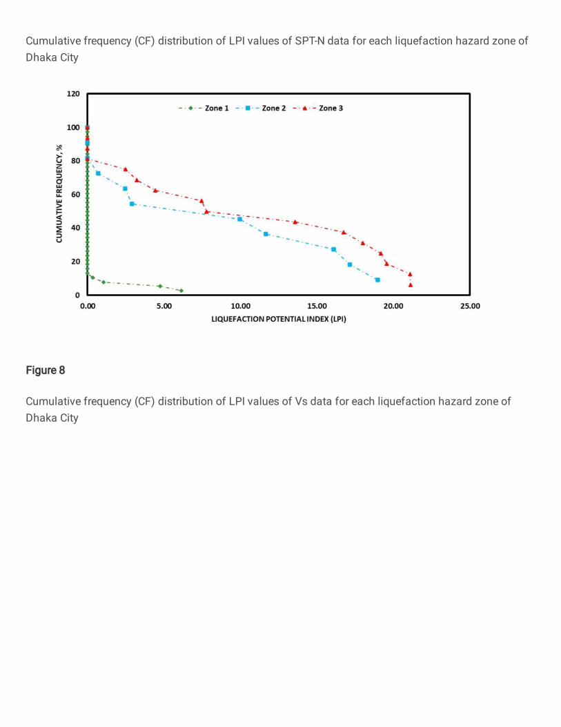
The surface geological units of Dhaka City is divided into three liquefaction hazard zones based on the LPI 346

values (Table 9). For each zone, the cumulative frequency (CF) distributions of the LPI values of the SPT-N and Vs 347

data are shown in Fig. 7 and Fig. 8, respectively. 348

Table 9 Liquefaction hazard zones along with their respective number of SPT-N and VS profiles 349

Zone Geological units Number of SPT-N

and VS profiles

Zone 1 Pleistocene terrace deposit

38

Zone 2 Holocene terrace deposit Holocene and Alluvial valley fill

deposit

11

Zone 3 Holocene Alluvium and Artificial fill 16

350

351

Fig. 7 Cumulative frequency (CF) distribution of LPI values of SPT-N data for each liquefaction hazard zone of 352

Dhaka City 353

21

354

Fig. 8 Cumulative frequency (CF) distribution of LPI values of Vs data for each liquefaction hazard zone of Dhaka 355

City 356

357

The LPI values of sixty-five (65) borehole profiles along with the contour of LPI values (0, 5, 10, 15, and 358

20) are shown on the maps to visualize the spatial distribution of liquefaction severity in the city (Fig. 9 and Fig. 359

10). One the basis of the LPI values, the liquefaction hazard of different areas of Dhaka City is classified according 360

Iwasaki et al. (1982) (Table 10) 361

Liquefaction hazard of each surface geological unit was also classified by the cumulative frequency (CF) 362

distribution at the LPI value of 5, which can be used to define the threshold for observing liquefaction surface 363

effects (Holzer et al. 2006). The map of the SPT-N data shows that 15%, 53%, and 69% areas, whereas the map of 364

the Vs data shows that 11%, 48%, and 62% of areas of Zone 1, Zone 2, and Zone 3, respectively, will exibit 365

liquefaction surface effects. 366

22

367

Fig. 9 Liquefaction hazard map for Dhaka City using the LPI values of the SPT-N data for a scenario earthquake of 368

Mw 7.5 with a peak horizontal ground acceleration (PGA) of 0.15 g. According to Iwasaki et al. (1982), liquefaction 369

hazard for LPI > 15 is very high, for 5 < LPI≤ 15 is high, for 0 <LPI ≤ 5 is low; and for LPI = 0 is very low. 370

According to Holzer et al. (2006), the cumulative frequency (CF) distributions of the LPI of three zones indicate that 371

15%, 53%, and 69% of areas of Zone 1, 2, and 3, respectively, exhibit surface manifestation of liquefaction 372

23

373

Fig. 10 Liquefaction hazard map for Dhaka City using the LPI values of the Vs data for a scenario earthquake of 374

Mw 7.5 with a peak horizontal ground acceleration (PGA) of 0.15 g. According to Iwasaki et al. (1982), liquefaction 375

hazard for LPI > 15 is very high, for 5 < LPI≤ 15 is high, for 0 <LPI ≤ 5 is low; and for LPI = 0 is very low. 376

According to Holzer et al. (2006), the cumulative frequency (CF) distributions of the LPI of three zones indicate that 377

15%, 53%, and 69% of areas of Zone 1, 2, and 3, respectively, exhibit surface manifestation of liquefaction 378

379

24

Table 10 Classes of liquefaction hazard on the basis of LPI values (after Iwasaki et al. (1982)) 380

LPI Liquefaction hazard

LPI > 15 Very High

5 < LPI ≤ 15 High

0 < LPI ≤ 5 Low

LPI = 0 Very low

381

A comparison between the LPI values derived from the SPT-N and Vs is illustrated in Fig. 11. In most of 382

the cases, the LPI values of the SPT-N data are higher than that of the Vs data. 383

384

Fig. 11 Comparison between LPI values of SPT-N and Vs datasets 385

386

6. Discussion 387

The liquefaction hazard map offers an opportunity to quantitatively estimate the liquefaction susceptibility of Dhaka 388

City. The spatial liquefaction potential was determined by calculating the LPI values from the liquefaction FS 389

estimated from both SPT-N and Vs at each 1.5 m interval of a borehole down to a depth of 20 m. The contour lines 390

of equal LPI values were drawn to represent the LPI values of the locations where there was no borehole. Three 391

25

liquefaction hazard zones were identified in the city based on the CF distribution of LPI of each geological unit to 392

determine the percentage of the area of these zones that are likely to liquefy in a defined scenario earthquake. 393

In Zone 1, up to 6 - 8 m depth is formed of stiff to hard, reddish- to yellowish-brown Pleistocene clayey 394

soils that is underlain by the medium to very dense, yellowish-brown Plio-Pleistocene sandy soils up to the depth of 395

investigation of 20 m. In the case of the SPT-N data, the liquefaction potential in Zone 1 ranges from low to very 396

low with the LPI values from 0 to 4.46, except boreholes BH-22 and BH-25 with the LPI values of 9.10 and 6.39, 397

respectively. The cumulative frequency (CF) distribution of the SPT-N based LPI values of Zone 1 suggests that 398

fifteen percent (15%) of the area of this zone would have liquefaction surface effects (Fig. 9). For the Vs data, the 399

liquefaction potential in Zone 1 is also from very low to low with the LPI values from 0 to 4.77, except 400

boreholesBH-37 with the LPI value of 6.12. The CF distribution of the Vs based LPI values of Zone 1 suggests that 401

eleven percent (11%) of the area of this zone would have liquefaction surface effects (Fig. 10). In case of outliers, 402

the SPT-N based LPI values of boreholes BH-22 and BH-25 are 9.10 and 6.39, respectively, but the Vs based LPI 403

values are 0 for both boreholes, which seems more accurate as these two boreholes are in the Pleistocene terrace 404

(Madhupur terrace)that is not likely to liquefy. On the other hand, at borehole BH-37, the Vs based LPI value is 6.12 405

while SPT-N based LPI is 3.84 and it is also in the Pleistocene terrace, therefore, the LPI value of 3.84 from the 406

SPT-N data seems more accurate. 407

Zone 2 includes the Holocene terrace deposits and alluvial valley fill where the terrace deposits are formed 408

of sandy and silty gray soils which include point and channel bars and natural levees of the existing rivers. The 409

valley-fill deposits that have been deposited in the depressions and valleys of the Pleistocene terrace, are comprised 410

of gray sandy soils and gray to dark gray clayey soils. In Zone 2, the SPT-N based LPI values range from 0 to 411

23.08,which imply a range of no potential to very high potential of liquefaction. The surface effects of liquefaction 412

will be exhibited in fifty-three percent (53%) area of Zone 2. The Vs based LPI values are from 0 to 18.98, which 413

also imply a range of no potential to very high potential of liquefaction in Zone 2. The surface effects of liquefaction 414

will be exhibited in forty-eight percent (48%) area of this zone. At boreholesBH-11 and BH-49 of this zone, the SPT 415

based LPI values are 12.76 and 14.19, respectively, whereas the Vs based LPI values are 0 at these boreholes. BH-11 416

is located on point bar and BH-49 is on the natural levee and both are usually more prone to liquefaction. Therefore, 417

the SPT-N provides a more accurate result in this case. 418

26

Zone 3 contains artificial fills and Holocene alluvium that are comprised of gray sandy and clayey soils. 419

The SPT-N based LPI values of this zone vary from 0 to 20.70, which indicate a range of no potential to very high 420

potential of liquefaction. The CF distribution of the SPT-N based LPI values suggest that the surface effects of 421

liquefaction will be exhibited in sixty-nine percent (69%) area of this zone. The Vs based LPI values of this zone 422

range from 0 and 21.13, which also indicate a range of no potential to very high potential of liquefaction. The CF 423

distribution of the Vs based LPI values suggest that the surface effects of liquefaction would be exhibited in sixty-424

two percent (62%) area of this zone. In case of Zone 3, the SPT-N based LPI values of boreholesBH-8, BH-19, BH-425

34, and BH-41 are 8.93, 6.66, 11.96, and 17.63, respectively, whereas the Vs based LPI values of these boreholes are 426

2.49, 16.73, 3.23, and 7.45. Borehole BH-8 is in the swamp, so the SPT-N based LPI value (8.93) appears more 427

reliable. Borehole BH-34 is in a floodplain, which is more likely to have an LPI value of more than 5, therefore, the 428

SPT-N based LPI value (11.96) appears more reliable than the Vs based LPI (3.23) value. Borehole BH-19 and BH-429

41 are in the floodplain and back swamp, respectively, and in both cases for both datasets their LPI values are 430

greater than 5, but it cannot be reliably said either of these will be greater than 15 or not as the output differs. 431

From the historical earthquake records of Bangladesh, it was observed that liquefaction occurred in silty and 432

sandy alluvium of the Holocene floodplains during the 1885 Bengal earthquake (Mw 6.87), 1897 Great Assam 433

earthquake (Mw 8.03), and 1918 Srimangal earthquake (Mw 7.2) (Middlemiss 1885; Oldham 1899; Stuart 1920). The 434

results of the present study also suggest that severe liquefaction may occur in the silty and sandy alluvium of the 435

Holocene floodplains and the Pleistocene terrace deposits are not likely to liquefy during an earthquake of Mw 7.5 436

having a PGA of 0.15 g. It can also be mentioned that during the 1995 Kobe earthquake in Japan, severe 437

liquefication occurred in loose fills (Hamada et al. 1995). Holzer et al. (2006) have also identified that the 438

Pleistocene deposits have low liquefaction potential and the artificial fills and alluvium have high liquefaction 439

potential. 440

7. Conclusions 441

In this study, both SPT-N and Vs data have been used to calculate the LPI for the preparation of liquefaction hazard 442

maps of Dhaka City using simplified procedure considering a scenario earthquake of MW 7.5 with a PGA of 0.15 g. 443

In the present study, ANN model has been used to predict the CRR from the SPT-N and Vs data, as it provides more 444

realistic and reliable results using sufficient actual field performance cases. From the results, it is noted that the SPT-445

27

N based LPI value is higher than the Vs based LPI value at most of the boreholes. Three liquefaction hazard zones 446

are identified in the city based on the CF distribution of the LPI of each geological unit and the LPI contour lines 0, 447

5, 10, 15, and 20 have been drawn to demonstrate spatial distribution of liquefaction hazard in the city. 448

The map of the SPT-N based LPI values indicates that 15%, 53%, and 69% areas, whereas the map of the 449

Vs based LPI values indicates that 11%, 48%, and 62% areas of Zone 1, 2, and 3 exhibit surface manifestation of 450

liquefaction for a scenario earthquake of Mw 7.5 with a PGA of 0.15 g. Therefore, it can be concluded that the CF 451

distribution of the LPI of both SPT-N and Vs data show almost similar severity of liquefaction in Zone 1, 2, and 3. 452

The uncertainties associated with the calculation of the LPI can be reduced by using more SPT-N, Vs data, 453

variation in groundwater level, accurate surface geological unit boundary delineation, and appropriate ground 454

motion. Finally, this liquefaction hazard map of Dhaka City can be used as a guide for future urban development and 455

planning to reduce the liquefaction associated damages and loss. 456

Acknowledgments 457

The authors would like to thank the Comprehensive Disaster Management Programme(CDMP), Department of 458

Disaster Science and Management (DSM), University of Dhaka, Bangladesh for providing the support to collect the 459

data of this research. The authors are also thankful to the University of Dhaka for allowing them to conduct this 460

research. 461

Authors’ contribution 462

ASMMK and AKFF initiated the study and carried out literature review. AKFF and MSH tested and interpreted the 463

data. ASMMK, MJR, AKFF drafted the manuscript and ASMMK supervised the whole work. Finally, all Authors 464

read, critically reviewed, and approved the final version of the paper. 465

Ethical considerations 466

Not applicable. 467

Availability of data and materials 468

Data set used in this study is available at 469

Conflict of Interest 470

Authors have no conflict of interest. 471

Funding source 472

28

This research has no funds. 473

Informed consent 474

Not applicable for this study. 475

476

References 477

Aitchison JC, Ali JR, Davis AM (2007) When and where did India and Asia collide? Journal of Geophysical 478

Research 112:1978–2012 479

Alam M (1989) Geology and depositional history of Cenozoic sediments of the Bengal Basin of Bangladesh. 480

Palaeogeography, Palaeoclimatology, Palaeoecology 69:125–139. doi: 10.1016/0031-0182(89)90159-4 481

Ambraseys NN, Douglas J (2004) Magnitude calibration of north Indian earthquakes. Geophysical Journal 482

International 159:165–206. doi: 10.1111/j.1365-246X.2004.02323.x 483

Andrus BRD, Member A, Ii KHS (2000) Liquefaction resistance of soils from shear-wave velocity. Journal of 484

Geotechnical and Geoenvironmental Engineering 126:1015–1025 485

Andrus RD, Stokoe KH (1997) Liquefaction resistance based on shear wave velocity. In: Proceeding of NCEER 486

workshop on evaluation of liquefaction resistance of soils. National Center for Earthquake Engineering 487

Research, Sate University of New York, Buffalo, pp 89–128 488

Andrus RD, Stokoe KH, Chung RM (1999) NISTIR6277 Draft Guidelines for Evaluating Liquefaction Resistance 489

Using Shear Wave Velocity Measurements and Simplified Procedures 490

Beale MH, Hagan MT, Demuth HB (2017) Neural Network Toolbox TM User’s Guide. 491

Castro G (1969) Liquefaction of Sands. PhD Thesis. Harvard University, Cambridge. 492

Castro G, Poulos SJ (1977) Factors affecting liquefaction and cyclic mobility. J Geotech Engng Div 103:501–516 493

Castro G, Poulos SJ, France JW, Enos JL (1982) Liquefaction induced by cyclic loading. Report by Geotechnical 494

Engineers, Inc., to the National Science Foundation, Washington, D.C 495

Chao SJ, Hsu HM, Hwang H (2010) Soil liquefaction potential in Ilan City and Lotung Town, Taiwan. Journal of 496

29

GeoEngineering 5:21–27. doi: 10.6310/jog.2010.5(1).3 497

Chen CJ, Juang CH (2000) Calibration of SPT- and CPT-based liquefaction evaluation methods. In: Mayne P, 498

Hryciw R (eds) Innovations and applications in geotechnical site characterization. 97, Geotechnical special 499

publication, ASCE, Reston, pp 49–64 500

Curray JR, Emmel FJ, Moore DG, Raitt RW (1982) Structure, tectonics, and geological history of the northeastern 501

Indian Ocean. In: The ocean basins and margins. Springer, pp 399–450 502

Fear CE, McRoberts EC (1995) Report on liquefaction potential and catalogue of case records. Internal Res. Rep., 503

Dept. of Civil Engineering, Univ. of Alberta, Edmonton, Alberta, Canada 504

Goda K, Kiyota T, Pokhrel RM, et al (2015) The 2015 Gorkha Nepal earthquake: Insights from earthquake damage 505

survey. Frontiers in Built Environment 1:1–15. doi: 10.3389/fbuil.2015.00008 506

Hamada M, Isoyama R, Wakamatsu K (1995) The 1995 Hyogoken-Nanbu Kobe earthquake-Liquefaction, ground 507

displacement, and soil condition in the Hanshin area. The School of Science and Engineering, Waseda 508

University, Tokyo 509

Holzer TL, Bennett MJ, Noce TE, et al (2006) Liquefaction hazard mapping with LPI in the greater Oakland, 510

California, area. Earthquake Spectra 22:693–708 511

Hossain MS, Kamal ASMM, Rahman MZ, et al (2020) Assessment of soil liquefaction potential: a case study for 512

Moulvibazar town, Sylhet, Bangladesh. SN Applied Sciences 2:. doi: 10.1007/s42452-020-2582-x 513

Idriss IM, Boulanger RW (2004) Semi-empirical procedures for evaluating liquefaction potential during 514

earthquakes. In: 11th International Conference on Soil Dynamics and Earthquake Engineering, and 3rd 515

International Conf. on Earthquake Geotechnical Engineering. Berkeley, pp 32–56 516

Idriss IM, Boulanger RW (2010) SPT-based liquefaction triggering procedure. Center for Geotechnical Modeling, 517

Department of Civil and Environmental Engineering, University of California, Davis, California 518

Iwasaki T, Tatsuoka F, Tokida K -i., Yasuda S (1978) A practical method for assessing soil liquefaction potential 519

based on case studies at various sites in Japan. In: Proc. of 2nd International Conference on Microzonation. 520

San Francisco, pp 885–896 521

30

Iwasaki T, Tokida K, Tatsuoka F, et al (1982) Microzonation for soil liquefaction potential using simplified 522

methods. In: Proceedings of 3rd International Earthquake Microzonation Conference. pp 1319–1330 523

Juang CH, Chen CJ, Jiang T, Andrus RD (2000) Risk-based liquefaction potential evaluation using standard 524

penetration tests. Canadian Geotechnical Journal 37:1195–1208. doi: 10.1139/t00-064 525

Juang CH, Jiang T, Andrus RD (2002) Assessing Probability-based Methods for Liquefaction Potential Evaluation. 526

Journal of Geotechnical and Geoenvironmental Engineering 128:580–589 527

Juang CH, Yuan H, Lee D-H, Lin P-S (2003) Simplified cone penetration test-based method for evaluating 528

liquefaction resistance of soils. Journal of Geotechnical and Geoenvironmental Engineering 129:66–80. doi: 529

10.1061/(ASCE)1090-0241(2003)129:1(66) 530

Kayen RE, Mitchell JK, Seed RB, et al (1992) Evaluation of SPT-, CPT-, and shear wave-based methods for 531

liquefaction potential assessment using Loma Prieta data. In: Proceedings of 4th Japan-U.S. Workshop on 532

Earthquake-Resistant Des. of Lifeline Fac. and Countermeasures for Soil Liquefaction. pp 177–204 533

Ku CS, Lee DH, Wu JH (2004) Evaluation of soil liquefaction in the Chi-Chi, Taiwan earthquake using CPT. Soil 534

Dynamics and Earthquake Engineering 24:659–673. doi: 10.1016/j.soildyn.2004.06.009 535

Lee YF, Chi YY, Lee DH, et al (2007) Simplified models for assessing annual liquefaction probability - A case 536

study of the Yuanlin area, Taiwan. Engineering Geology 90:71–88. doi: 10.1016/j.enggeo.2006.12.003 537

Marcuson WF (1978) Definition of terms related to liquefaction. Journal of the Geotechnical Engineering Division 538

104:1197–1200 539

Middlemiss CS (1885) Report on the Bengal earthquake of July 14, 1885. Records of Geological Survey of India 8 540

(4):200–221 541

Morgan JP, McIntire WG (1959) Quaternary geology of the Bengal Basin, East Pakistan and India. Bulletin of the 542

Geological Society of America 70:319–342 543

Morino M, Kamal ASMM, Akhter SH, et al (2014a) A paleo-seismological study of the Dauki fault at Jaflong, 544

Sylhet, Bangladesh: Historical seismic events and an attempted rupture segmentation model. Journal of Asian 545

Earth Sciences 91:218–226. doi: 10.1016/j.jseaes.2014.06.002 546

31

Morino M, Kamal ASMM, Muslim D, et al (2011) Seismic event of the Dauki Fault in 16th century confirmed by 547

trench investigation at Gabrakhari Village, Haluaghat, Mymensingh, Bangladesh. Journal of Asian Earth 548

Sciences 42:492–498. doi: 10.1016/j.jseaes.2011.05.002 549

Morino M, Monsur MH, Kamal ASMM, et al (2014b) Examples of paleo-liquefaction in Bangladesh. The Journal of 550

the Geological Society of Japan 120:VII–VIII. doi: 10.5575/geosoc.2014.0032 551

Oldham RD (1899) Report on the great earthquake of 12th June 1897. Memoirs of the Geological Survey of India 552

29:1–379 553

Olsen RS (1997) Cyclic liquefaction based on the cone penetration test. In: Proceeding of NCEER workshop on 554

evaluation of liquefaction resistance of soils. National Center for Earthquake Engineering Research, State 555

University of New York, Buffalo, pp 225–276 556

Olsen RS (1988) Using the CPT for dynamic response characterization. In: Proceedings of the Earthquake 557

Engineering and Soil Dynamics II Conference. American Society of Civil Engineers, New York, pp 111–117 558

Olsen RS, Koester JP (1995) Prediction of liquefaction resistance using the CPT. In: Proceedings of the 559

International Symposium on Cone Penetration Testing, CPT’95, Linkoping, Sweden, Vol. 2. SGS. pp 251–256 560

Rahman M, Siddiqua S, Kamal A (2015) Liquefaction hazard mapping by liquefaction potential index for Dhaka 561

City, Bangladesh. Engineering Geology 188:137–147. doi: 10.1016/j.enggeo.2015.01.012 562

Rahman MZ, Siddiqua S (2017) Evaluation of liquefaction-resistance of soils using standard penetration test, cone 563

penetration test, and shear-wave velocity data for Dhaka, Chittagong, and Sylhet cities in Bangladesh. 564

Environmental Earth Sciences 76:207. doi: 10.1007/s12665-017-6533-9 565

Rahman MZ, Siddiqua S, Kamal ASMM (2021) Site response analysis for deep and soft sedimentary deposits of 566

Dhaka City, Bangladesh. Natural Hazards. doi: 10.1007/s11069-021-04543-w 567

Rahman MZ, Siddiqua S, Kamal ASMM (2020) Seismic source modeling and probabilistic seismic hazard analysis 568

for Bangladesh. Springer Netherlands 569

Reimann K-U (1993) Geology of Bangladesh. Gebruder Borntraeger Verlagsbuchhandlung, Science Publishers, 570

Berlin 571

32

Robertson PK, Campanella RG (1985) Liquefaction potential of sands using the CPT. Journal of Geotechnical 572

Engineering 111:384–403 573

Robertson PK, Wride CE (1998) Evaluating cyclic liquefaction potential using the cone penetration test. Canadian 574

Geotechnical Journal 35:442–459. doi: 10.1139/t98-017 575

Sassa S, Takagawa T (2019) Liquefied gravity flow-induced tsunami: first evidence and comparison from the 2018 576

Indonesia Sulawesi earthquake and tsunami disasters. Landslides 16:195–200. doi: 10.1007/s10346-018-1114-577

x 578

Seed HB, de Alba P (1986) Use of SPT and CPT tests for evaluating the liquefaction resistance of sands. In: 579

Clemence SP (ed) Use of in situ tests in geotechnical engineering. American Society of Civil Engineers, 580

Geotechnical Special Publication 6, pp 281–302 581

Seed HB, Idriss IM (1967) Analysis of Soil Liquefaction: Niigata Earthquake. Journal of the Soil Mechanics and 582

Foundations Division 93:83–108 583

Seed HB, Idriss IM (1971) Simplified procedure for evaluating soil liquefaction potential. Journal of Soil Mechanics 584

and Foundations Division 97:1249–1273 585

Seed HB, Idriss IM (1982) Ground motions and soil liquefaction during earthquakes. Earthquake Engineering 586

Research Institute Monograph, Oakland 587

Seed HB, Idriss IM, Arango I (1983) Evaluation of liquefaction potential using field performance data. Journal of 588

Geotechnical Engineering 109:458–482 589

Seed HB, Tokimatsu K, Harder Jr. LF, Chung R (1984) The Influence of SPT procedures on soil liquefaction 590

resistance evaluations. Report No. UCB/EERC-84/15, Earthquake Engineering Research Center, University of 591

California, Berkeley 592

Seed HB, Tokimatsu K, Harder LF, Chung RM (1985) Influence of SPT procedures in soil liquefaction resistance 593

evaluations. Journal of Geotechnical Engineering 111:1425–1445. doi: 10.1061/(ASCE)0733-594

9410(1985)111:12(1425) 595

Sonmez H, Gokceoglu C (2005) A liquefaction severity index suggested for engineering practice. Environmetal 596

33

Geology 48:81–91. doi: 10.1007/s00254-005-1263-9 597

Stark TD, Olson SM (1995) Liquefaction resistance using CPT and field case histories. Journal of Geotechnical 598

Engineering ASCE, 121:856–869 599

Steckler MS, Akhter SH, Seeber L (2008) Collision of the Ganges-Brahmaputra Delta with the Burma Arc: 600

Implications for earthquake hazard. Earth and Planetary Science Letters 273:367–378. doi: 601

10.1016/j.epsl.2008.07.009 602

Steckler MS, Mondal DR, Akhter SH, et al (2016) Locked and loading megathrust linked to active subduction 603

beneath the Indo-Burman Ranges. Nature Geoscience 9:615–618. doi: 10.1038/ngeo2760 604

Stuart M (1920) The Srimangal earthquake of 8th July 1918. Memoirs of the Geological Survey of India 46 (1):1–70 605

Wang Y, Sieh K, Tun ST, et al (2014) Active tectonic and earthquake Myanmar region. Journal of Geophysical 606

Research: Solid Earth 119:3767–3822. doi: 10.1002/2013JB010762.Received 607

Yeats RS, Sieh K, Allen CR (1997) The Geology of Earthquakes. Oxford University Press 608

Youd BTL, Idriss IM, Andrus RD, et al (2001) Liquefaction resistance of soils: summary report from the 1996 609

NCEER and 1998 NCEER/NSF workshops on evaluation of liquefaction resistance of soils. Jounral of 610

Geotechnical and Geoenvironmental Engineering 127:817–833 611

612

Figures

Figure 1

Surface geological map of Dhaka City with locations of the boreholes (modi�ed from Rahman et al.(2015)) Note: The designations employed and the presentation of the material on this map do not implythe expression of any opinion whatsoever on the part of Research Square concerning the legal status of

any country, territory, city or area or of its authorities, or concerning the delimitation of its frontiers orboundaries. This map has been provided by the authors.

Figure 2

Recent and historical earthquakes of magnitude greater than Mw 6.5 from 1762 and 2016 (retrieved fromRahman and Siddiqua (2017)) Note: The designations employed and the presentation of the material onthis map do not imply the expression of any opinion whatsoever on the part of Research Squareconcerning the legal status of any country, territory, city or area or of its authorities, or concerning thedelimitation of its frontiers or boundaries. This map has been provided by the authors.

Figure 3

Conceptual model of the mechanism to search limit state boundary (after Chen and Juang, (2000))

Figure 4

Searching mechanism of critical cyclic stress ratio (CSR) (after Juang et al. (2000))

Figure 5

Performance of CRRSPT model

Figure 6

Performance of CRRVs model

Figure 7

Cumulative frequency (CF) distribution of LPI values of SPT-N data for each liquefaction hazard zone ofDhaka City

Figure 8

Cumulative frequency (CF) distribution of LPI values of Vs data for each liquefaction hazard zone ofDhaka City

Figure 9

Liquefaction hazard map for Dhaka City using the LPI values of the SPT-N data for a scenario earthquakeof Mw 7.5 with a peak horizontal ground acceleration (PGA) of 0.15 g. According to Iwasaki et al. (1982),liquefaction hazard for LPI > 15 is very high, for 5 < LPI≤ 15 is high, for 0 <LPI ≤ 5 is low; and for LPI = 0 isvery low. According to Holzer et al. (2006), the cumulative frequency (CF) distributions of the LPI of threezones indicate that 15%, 53%, and 69% of areas of Zone 1, 2, and 3, respectively, exhibit surface

manifestation of liquefaction Note: The designations employed and the presentation of the material onthis map do not imply the expression of any opinion whatsoever on the part of Research Squareconcerning the legal status of any country, territory, city or area or of its authorities, or concerning thedelimitation of its frontiers or boundaries. This map has been provided by the authors.

Figure 10

Liquefaction hazard map for Dhaka City using the LPI values of the Vs data for a scenario earthquake ofMw 7.5 with a peak horizontal ground acceleration (PGA) of 0.15 g. According to Iwasaki et al. (1982),liquefaction hazard for LPI > 15 is very high, for 5 < LPI≤ 15 is high, for 0 <LPI ≤ 5 is low; and for LPI = 0 isvery low. According to Holzer et al. (2006), the cumulative frequency (CF) distributions of the LPI of threezones indicate that 15%, 53%, and 69% of areas of Zone 1, 2, and 3, respectively, exhibit surfacemanifestation of liquefaction Note: The designations employed and the presentation of the material onthis map do not imply the expression of any opinion whatsoever on the part of Research Squareconcerning the legal status of any country, territory, city or area or of its authorities, or concerning thedelimitation of its frontiers or boundaries. This map has been provided by the authors.

Figure 11

Comparison between LPI values of SPT-N and Vs datasets

Liquefaction Resistance Evaluation of Soils using Arti cial ...

Documents

Transcript of Liquefaction Resistance Evaluation of Soils using Arti cial ...