Liquefaction Evaluation Module - January 2020 - Caltrans

Caltrans Geotechnical Manual

of 23 January 2020

Liquefaction Evaluation

Soil liquefaction may substantially increase the cost of bridge and highway projects. If liquefaction hazard is not reported in a timely manner, there may be an inaccurate allocation of funds and resources. For instance, if the soil is incorrectly characterized to liquefy, the project engineer may develop an expensive preliminary design with large diameter piles, deep foundations, or unnecessary soil mitigation measures. Conversely, if the project engineer incorrectly assumes that liquefaction will not occur then the project may be significantly delayed because the project cost estimate did not account for liquefaction design.

Liquefaction investigations during the planning phase (K or 0) are usually limited to the evaluation of existing information for a site (see Geotechnical Investigations). If liquefaction hazard potential is unknown or cannot be reliably determined based on the available information prior to Type Selection, an unsuitable foundation type may be selected. If the potential consequences of liquefaction appear to be substantial, the Geoprofessional should discuss with the Project Development Team (PDT) the option of performing site-specific subsurface investigations prior to Type Selection to better determine the liquefaction hazard. Refer to Memos to Designers (MTD) 20-14, “Quantifying the Impacts of Soil Liquefaction and Lateral Spreading on Project Delivery.”

This module presents:

• The criteria for preliminary screening or assessment of liquefaction potential at a site based on available information (e.g., published liquefaction hazard maps, As-Built Log of Test Boring, etc.) The results of this (generally qualitative) preliminary screening are reported in the DPGR, SPGR, or PFR.

• The guidance for site investigations in potentially liquefiable soils. • The methodology for performing quantitative analysis of liquefaction potential to

determine if liquefaction will occur based on site-specific field exploration and laboratory testing data in accordance with Youd et al (2001) and Boulanger and Idriss (2006). This information will be presented in an FR and/or a GDR.

• Appendix A: Cone Penetration Test (CPT) Example (Youd et al., 2001) • Appendix B: Standard Penetration Test (SPT) Example (Youd et al., 2001)

This module does not address the effects of liquefaction on a project, mitigation of the liquefaction hazard, or geotechnical design in areas of liquefaction.


of 23 January 2020

Preliminary Screening of Potentially Liquefiable Soils

Preliminary screening involves the evaluation of a site for soil liquefaction potential using existing information such as liquefaction hazard maps such as State “Seismic Hazard and Zones of Required Investigation Maps” and USGS “Liquefaction Hazards Maps”, groundwater information, reports, as-built plans/subsurface data, and in some cases existing sampling and testing. The purpose of the preliminary screening is to alert the PDT of the potential for soil liquefaction to occur at the site.

Use the following five (5) criteria for preliminary screening evaluation of soil liquefaction potential at a project site.

1. Groundwater Table (historic, current, or anticipated future level) 2. Age of Soil 3. Soil Type 4. In-situ Soil Density/Initial State 5. Design Peak Ground Acceleration and Earthquake Moment Magnitude

Use all five (5) criteria to make a preliminary screening assessment. If the preliminary screening indicates no liquefaction potential, the site investigation may be planned as if liquefaction is not expected. If there is a potential for liquefaction, or the potential is unknown, the Geoprofessional must report as discussed below, and the field investigation planned to include appropriate (CPT) soundings, drilling method and SPT blow count measurements and sampling of the potentially liquefiable soils. All field and laboratory works must be performed in accordance with the applicable ASTM standards.

1. Groundwater Table

Sites with potentially liquefiable soils and groundwater table within 50 feet of the ground surface are generally considered to be most susceptible to liquefaction. If the groundwater table is anticipated to be shallower than 50 feet, the Geoprofessional should anticipate the need for and plan to collect samples and perform necessary field tests for liquefaction potential, unless the potential for liquefaction hazard can be confidently ruled out based on other criteria (items 2-5 above). If the groundwater is known to be below 70 feet, the site may be considered non-liquefiable for preliminary screening purposes

Sources of groundwater data include “As-Built” boring logs, County well log data, water wells (Department of Water Resources), and historic ground water levels (USGS) and ground water plates published in the State Seismic Hazard Zone map reports.

2. Age of Soil

Holocene deposits (younger than 11,000 years) and man-made fills ranging from very loose to medium dense are susceptible to liquefaction. Geologic deposits older than Holocene age (> 11,000 years) are considered to have low liquefaction susceptibility. A source of soil age data is the CGS California Geologic Map for the site.

https://www.conservation.ca.gov/cgs/shp


http://www.water.ca.gov/waterdatalibrary

http://nwis.waterdata.usgs.gov/ca/nwis/gwlevels


http://www.quake.ca.gov/gmaps/GMC/stategeologicmap.html


of 23 January 2020

3. Soil Type

Soils types that are susceptible to liquefaction are sand, silty sand, low plasticity (PI<7) silt and, in unusual cases, gravel. Rock and most clay soils are not liquefiable.

4. In-situ Soil Density/Initial State

Granular/cohesionless soils with an initial state represented by a normalized, clean-sand equivalent CPT resistance (qc1N)cs >160, or SPT blow count (N1)60cs >30 are considered not susceptible to liquefaction irrespective of the other criteria or conditions.

5. Peak Ground Acceleration and Earthquake Magnitude

Liquefaction potential increases with increasing Peak Ground Acceleration (PGA) and earthquake magnitude (M). The site design PGA and M correspond to a return period of 975-years and are obtained from ARS Online webtool.

Field Investigation

If preliminary screening indicates liquefaction potential exists or is unknown, the field investigation should gather information for liquefaction assessment including the soil characteristics (classification/type, grain size distribution, density, Atterberg Limits) and spatial distribution of the potentially liquefiable soil, and the groundwater level. Typical field investigations use rotary wash or auger SPT sample borings and laboratory test samples, and/or CPT soundings as per applicable ASTM Standards. The depth of the exploration must be 70 feet below ground surface or 20 feet below the pile design tip elevation, whichever is greater.

Because the presence of liquefiable soils can substantially increase project costs, it is important to thoroughly characterize the site. The site exploration needs to determine if the liquefiable soils are extensive enough, both laterally and vertically, to constitute a hazard. Depending on the field conditions, geophysical methods, and CPT soundings can provide information on the lateral extent of liquefiable layers more economically than SPT borings.

CPT Soundings

CPT soundings offer advantages over other methods of estimating liquefaction resistance in both the detection of thin layers that may influence liquefaction triggering and subsequent pore pressure redistribution and in the reproducibility of results. CPT results are less dependent on the equipment operator than most other in situ test methods and CPT can be performed quickly and cheaply. The seismic CPT can also measure soil shear wave velocity (National Academies of Sciences, 2016) CPT does not only identify the presence of liquefiable soils, but it can also show if the liquefiable soils are extensive enough, both laterally and vertically, to constitute a hazard.


of 23 January 2020

When the CPT, without collecting any soil samples, is the primary investigative tool it is highly recommended that at least one SPT boring be performed “side by side” to a CPT sounding location for each bridge structure. This provides soil samples for laboratory testing to determine the required soil parameters (e.g., fines content, Atterberg Limits) and at least some limited site-specific correlations between SPT and CPT results. Whenever feasible, consider using CPT in the final liquefaction evaluation, in particular for sites with thinly bedded and/or highly variable subsurface soil conditions.

Standard Penetration Test (SPT)

SPT has been the most commonly used investigative tool for liquefaction evaluation. For large or important projects, in particular with highly variable subsurface conditions, SPT should be supplemented with CPT. Unlike the CPT, the SPT provides actual soil samples that can be visually examined and tested in the laboratory to evaluate soil parameters needed for more reliable liquefaction analysis.

Do not use hollow stem augers below the water table, or any non-standard exploration and/or testing methods for liquefaction assessment using either the SPT and/or the CPT.

Ground Water Level

Measure the elevation of the stabilized groundwater table or, where appropriate, of the piezometric surface in the borehole or piezometer. The CPT pore pressure dissipation test can also be used to determine the elevation of the groundwater table or the piezometric surface. Use a higher elevation than measured only if there is clear evidence for seasonal or long-term fluctuations. Do not use abnormally high or temporary groundwater level.

Geophysical Investigation

In gravelly soils where SPT blow counts are unreliable (or at depths greater than 70 feet) consider the shear wave velocity (Vs) method for performing liquefaction assessments (Andrus and Stokoe, 2000; Youd et al., 2001). The seismic cone, P-S logging, or surface wave methods are available to obtain shear wave velocity.

Laboratory Testing

Laboratory tests for quantitative liquefaction evaluation include:

• Particle Size Analysis (ASTM D 422) • % Finer Than the No. 200 (75 µm) Sieve (ASTM D 1140) • Atterberg Limits (ASTM D 4318)

The exact type(s) and the number of laboratory tests performed shall be selected based on the visual-manual description and identification (ASTM D2488), and the extent and field variability of the identified potentially liquefiable soils.


of 23 January 2020

Results from Atterberg Limit test(s) are necessary when the amount (%) and/or the plasticity index of the fines content are used in the final determination of an otherwise liquefaction susceptible soil as not liquefiable.

Quantitative Liquefaction Analysis

Quantitative liquefaction analysis uses site-specific field and laboratory test data. Use the procedure of Youd, et al (2001): Liquefaction Resistance of Soils: Summary Report from the 1996 NCEER and 1998 NCEER/NSF Workshops on Evaluation of Liquefaction Resistance of Soils October 2001 for quantitative liquefaction analysis. The procedure for CPT and SPT analysis consists of the following general steps:

1. Determine the design PGA and earthquake moment magnitude (M) 2. Determine the design groundwater table elevation 3. Determine which soil layers are susceptible to liquefaction and thus need to be

evaluated based on a quantitative liquefaction analysis 4. Determine the total soil unit weight for all soil layers or sublayer located above the

bottom elevation of the lowest soil layer susceptible to liquefaction. Then perform the following steps for each of the soil layer/sub layer identified in Step 3 as susceptible to liquefaction

5. Determine the Cyclic Stress Ratio (CSR) at the mid elevation 6. Determine the representative values of the field measured CPT tip and frictional

resistances or the SPT blow count 7. Correct and normalize the measured CPT tip resistance/SPT Blow Count 8. Determine the Fines Content Correction and the clean-sand equivalent CPT 9. Determine the clean-sand equivalent normalized CPT tip resistance/SPT Blow

Count and Calculate Cyclic Resistance Ratio (CRR)7.5 10. Calculate the Magnitude Scaling Factor (MSF), overburden correction (Kσ) and the

sloping ground correction factor (Kα). 11. Calculate the Factor of Safety Against Liquefaction

Modifications or elaborations to Youd et al (2001) are as follows:

• Use Youd et al (2001) to depths of 50 feet; with caution to 70 feet; do not use below 70 feet.

• Liquefaction evaluation below 70 feet require special analysis and consideration that is beyond the scope of this module.

• Do not combine liquefaction analysis with other extreme events or conditions (e.g., vessel impact, and abnormally high or temporary groundwater levels).

• Consider scour in liquefaction evaluation as specified in Article 10.5.5.3 of the AASHTO LRFD Bridge Design Specifications with California Amendments.


of 23 January 2020

• Do not use the “Modified Chinese Criteria” as it is unconservative for determining if certain fine-grained soils are liquefiable. Use Boulanger and Idriss (2006) to determine if fine grained soils are likely to behave as sand-like material and are thus should be considered as susceptible to liquefaction.

• Use the design PGA (5% probability of exceedance in 50 years or 975-year return period) in units of g (e.g., PGA=0.4g) evaluated as per Appendix B of the Seismic Design Criteria (SDC) and using ARS Online webtool. Here, g is acceleration of gravity. (Note: Youd et al, 2001 uses the parameter amax for PGA in units of g)

• Use the de-aggregated mean earthquake moment magnitude (M) for PGA as the design earthquake magnitude (Mw). (Note: Youd et al, 2001, uses both the symbols M and Mw to denote the moment magnitude of the design earthquake)

• Use a factor of safety against liquefaction of 1.0 • See Appendices A and B for examples of CPT and SPT based liquefaction

evaluation, respectively.

Reporting

Liquefiable soil can have significant impacts on a project’s scope, schedule and budget; it is important to communicate liquefaction information to the PDT in a timely manner. The content and confidence of recommendations, especially during the planning phase, will depend largely on the type of information available. If as-built LOTB and laboratory data are available during the project early stages, then quantitative liquefaction analysis may occur earlier than typical, and the results presented in the DPGR or SPGR. If little information is available, then only a qualitative assessment, i.e. preliminary screening, can be presented

Liquefaction potential is discussed in the following reports:

• District Preliminary Geotechnical Report (DPGR) • Preliminary Geotechnical Design Report (PGDR) • Geotechnical Design Report (GDR) • Structure Preliminary Geotechnical Report (SPGR) • Preliminary Foundation Report (PFR) • Foundation Report (FR)

Preliminary Reports

Language used in reporting liquefaction potential must be clear and direct. Do not use indefinite terms such as “low”, “moderate” and/or “high”. Acceptable language for preliminary reports (SPGR, PFR, DPGR, and PGDR) includes:

• “Liquefaction potential exists”,


of 23 January 2020

• “Liquefaction potential is unknown or cannot be determined based on the available information”,

• “Liquefaction potential does not exist”.

If the results of preliminary screening (reported in the SPGR or DPGR) indicate that liquefaction potential either exists or is unknown, the Project Development Team (PDT) should decide whether to perform some or all site investigations, including drilling, prior to type selection to more accurately evaluate liquefaction potential for the PFR and PGDR. For District items, such as standard plan structures and embankments, the PDT should decide whether liquefaction will be considered in the design. If the design will not be modified for liquefaction it is unnecessary to perform quantitative liquefaction analysis and related field work.

Final Reports

The results of the site investigation and quantitative analysis must be reported in the PFR and PGDR (if applicable), FR and/or GDR. The report should include:

• Areal limits of liquefaction • Vertical limits of liquefaction • Identification of liquefiable soils • For complex projects, or if requested by the designer, include a three-dimensional

plot of liquefiable soils at the site.

<Discussion of the consequences and mitigation of liquefaction hazards are, or will be, in separate modules. This would include: lateral spreading, seismic settlement, layer thickness, extent, connectivity, etc.>


of 23 January 2020

References

1. Andrus, R. D. and Stokoe, K. H., 2000, “Liquefaction Resistance of Soils from Shear-Wave Velocity,” Journal of Geotechnical and Geo-Environmental Engineering, ASCE, Vol. 126, No. 11

2. Boulanger, R. W. and Idriss, I. M., 2006, “Liquefaction Susceptibility Criteria for Silts and Clays,” Journal of Geotechnical and Geo-Environmental Engineering, ASCE, Vol. 132, No. 11

3. Caltrans, AASHTO LRFD Bridge Design Specifications with California Amendments

4. California Department of Conservation, Division of Mines and Geology (California Geological Survey), 2008, “Guidelines for Evaluating and Mitigating Seismic Hazards in California,” CDMG Special Publication 117A

5. Caltrans, Memo to Designers 20-14, “Quantifying the Impacts of Soil Liquefaction and Lateral Spreading on Project Delivery,” Caltrans Division of Engineering Services, Office of Earthquake Engineering

6. Caltrans, “Foundation Report Preparation for Bridges,” Caltrans Division of Engineering Services, Geotechnical Services.

7. Caltrans, “Guidelines for Preparing Geotechnical Design Reports, Version 1.3,” Caltrans Division of Engineering Services, Geotechnical Services.

8. National Academies of Sciences, Engineering, and Medicine, “State of the Art and Practice in the Assessment of Earthquake-Induced Soil Liquefaction and its Consequences”, Committee on the State of the Art and Practice in Earthquake Induced Soil Liquefaction Assessment; Board on Earth Sciences and Resources; Division on Earth and Life Studies, 2016.

9. Kulhawy, F.H and Mayne, P.W. “Manual on Estimating Soil Properties for Foundation Design,” Electric Power Research Institute, Palo Alto, Ca. 1990.

10. Seed, H.B., Tokimatsu, K., Harder, L. F., and Chung, R, 1985. “Influence of SPT Procedures in Soil Liquefaction Resistance Evaluation,” Journal of Geotechnical and Geo-Environmental Engineering, ASCE, Vol. 111, No. 12

11. Youd, T.L., et al., 2001, “Liquefaction Resistance of Soils: Summary Report from the 1996 NCEER and 1998 NCEER/NSF Workshops on Evaluation of Liquefaction Resistance of Soils,’ in Journal of Geotechnical and Geo-Environmental Engineering, October 2001

Caltrans Geotechnical Manual Appendix A

of 23 January 2020

Liquefaction Evaluation Example (CPT Method)

Seal Beach Blvd Overcrossing Bridge replacement is a proposed 2 span cast-in-place prestressed concrete box girder structure. A quantitative liquefaction analysis is required following the procedures described in Youd et al, (2001).

The following information is required:

• Seismic design ground motion parameters including peak ground acceleration (PGA) corresponding to a return period of 975-years, and the de-aggregated mean earthquake moment magnitude (M) for PGA. These data are obtained by running ARS Online webtool using the latitude and longitude 33.7736 N, -118.0749 W.

• Soil data from CPT results. (Figure 1) • Groundwater data as shown on the LOTB dated April 24, 2008. (Figure 2)

Figure 1: CPT Sounding Data


of 23 January 2020

Figure 2: Log of Test Boring (LOTB)

Step 1: Determine Groundwater Elevation

The design groundwater elevation is the level shown on the LOTB for boring R 08 003. There is no reason to adjust the groundwater elevation. GW elevation is 0 feet, 15 feet below the ground surface. (Figure 1)

Step 2: Identify the Soil Layers for Quantitative Liquefaction Analysis.

The CPT 08-152 sounding provides the soil behavior type in increments of 0.16 feet. The following table illustrates some representative layers throughout the depth, where the soil behavior type is evaluated.

Table 1: Liquefaction Evaluation for CPT-08-152

Depth (feet)

Elevation (feet)

Soil Behavior

Type

Layer Thickness

(feet)

Potential for Liquefaction Reason for Evaluation

1.15 13.9 Sand 0.16 Not Liquefiable Above Ground Water Surface

15.09 -0.1 Sand 0.16 Liquefiable Below Ground Water



15.58 -0.6 Clay 0.16 Not Liquefiable Clayey Soil

15.75 -0.8 Clay 0.16 Not Liquefiable Clayey Soil


of 23 January 2020

The layer at depth of 15.26 feet (elevation of -0.3 feet) shows the potential for liquefaction based on table 1. For this example, this sandy layer will be analyzed.

Step 3: Obtain CPT Data

Obtain cone tip bearing and sleeve friction values from the CPT printout.

Cone Tip bearing: qc = 40.2 tsf (depth 15.26 feet)

and

Cone Sleeve Friction: fs = 0.6 tsf (Obtained from the CPT report.)

Step 4: Soil Unit Weight

Determine soil unit weight = 0.06 tcf

Step 5: Calculate/Determine the CPT Soil Behavior Type Index

From Youd et al (2001), equation (14)

Ic: Soil Behavior Index

Ic = [(3.47 – log Q)2 + (1.22 + Log F)2]0.5 = 2.30

Where,

Q: Dimensionless normalized CPT penetration resistance

F: Normalized friction ratio


Q = [(qc – σv0)/Pa] [(Pa/σ΄ vo)n] = 43.16

and


F = [fs/qc – σvo)] x 100% = 1.48 %

n: Exponent = 1.0 (clay)

σv0: Total Overburden Pressure = 15.26 x 0.06 = 0.92 tsf


of 23 January 2020

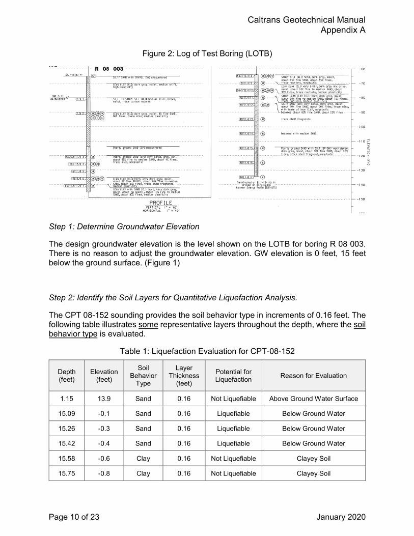
σ΄ vo: Effective Overburden Pressure = (15.26 -15) x (0.06 - 0.031) + (15 x 0.06) = 0.91 tsf

Pa = Atmospheric Pressure = 1.04 tsf

First calculate Soil Behavior Index (Ic) with n=1. If the calculated Ic is greater than 2.6, the soil behavior is clayey and is not liquefiable. If the calculated Ic is less than 2.6, the soil is most likely granular in nature and Q should be recalculated using an exponent, n = 0.5.

Since Ic < 2.6, Q is recalculated, with n= 0.5


Q = [(qc – σv0)/Pa] [(Pa/σ΄ vo)n] = 37.8 x1.07 = 40.48

n: Exponent = 0.5 (sand)

Pa = Atmospheric Pressure = 1.04 tsf

σv0: Total Overburden Pressure = 15.26 x 0.06 = 0.92 tsf

σ΄ vo : Effective Overburden Pressure = (15.26 -15) x (0.06 - 0.031) + (15 x 0.06) = 0.91 tsf

Step 6: Normalize Cone Penetration Resistance

Cone penetration resistance is corrected for overburden stress as follows:


qc1N: Dimensionless cone penetration resistance corrected for overburden stress

qc1N = CQ (qc/Pa) = 41.42

Where,

From Youd, equation (13)

CQ = (Pa/σ΄vo) n = 1.07

CQ is a normalizing factor for cone penetration resistance.


of 23 January 2020

Step 7: Calculate Clean Sand Equivalent Normalized Cone Penetration Resistance

Correct the normalized penetration resistance, (qc1N), of sands with fines to an equivalent clean sand value, (qc1N) cs:


(qc1N) cs = Kcqc1N = 84.16

Where the CPT correction factor for grain characteristics, Kc, is defined as:

From Youd et al (2001), equation (19a)

For Ic ≤ 1.64 Kc =1.0

From Youd et al (2001), equation (19b)

For Ic > 1.64 Kc = -0.403 Ic4 + 5.581 Ic3 -21.63 Ic2 + 33.75 Ic -17.88

Ic = 2.3 and Kc = 2.03 (8)

Step 8: Calculate Cyclic Resistance Ratio: CRR

From Youd et al (2001), equation (11b)

If 50 ≤ (qc1N) cs < 160 CRR7.5 = 93 [(qc1N) cs/1000]3 +0.08 = 0.14

Step 9: Determine Cyclic Stress Ratio (CSR)


CSR = 0.65 amax(σo /σ’o)rd

Where:

• σo and σ’o are total and effective vertical overburden stresses, respectively. • amax is peak horizontal acceleration (PGA) in g. • rd is a stress reduction coefficient.


of 23 January 2020

For this example:

amax = 0.6g

Determine Stress Reduction Coefficient, rd.

Depth (z) is 15.26’= 4.65 m

rd=1.0-0.00765 · z for z≤9.15 m

rd =1.0-0.00765 · 4.65 = 0.96

Step 10: Calculate the Magnitude Scaling Factor (MSF)

For this example, Mw = Mean Earthquake Moment Magnitude, M = 7.0

MSF = 102.24/Mw2.56 = 102.24/7.02.56 = 1.19

Step 11: Calculate the Factor of Safety against Liquefaction

FS = (CRR7.5/CSR) x MSF

FS = (.14/.38) x 1.19 = 0.42

Since the FS < 1, the geotechnical report must state that liquefaction is predicted to occur in this layer.

To complete the liquefaction analysis for the site, repeat the above steps for each layer identified as susceptible to liquefaction.

Caltrans Geotechnical Manual Appendix B

of 23 January 2020

Liquefaction Evaluation Example (SPT Method)

Live Oak Creek Bridge is a proposed single span bridge crossing Live Oak Creek. Preliminary screening, based on the “As-Built” LOTBs for the existing Live Oak Creek Bridge (Br. No. 57-0070), indicate the possibility of liquefaction. A quantitative liquefaction analysis is required following the SPT procedures described in Youd et al, (2001).

The following information is required:

• Seismic design ground motion parameters including peak ground acceleration (PGA) corresponding to a return period of 975-years and the de-aggregated mean earthquake moment magnitude (M). These data are obtained by running the ARS Online webtool using the latitude and longitude 33.31525 N, -117.194225W.

• Soil data from SPT results. Hammer efficiency and soil descriptions are shown on the LOTB dated 11-1-2012 (Attachment 1).

• Groundwater data as shown on the LOTB dated 11-1-2012 (Attachment 1).

Step 1: Determine Groundwater Elevation

The design groundwater elevation is the level shown on the LOTB for Boring RC-11-001. There is no reason to adjust the groundwater elevation.

Step 2: Identify the Soil Layers for Quantitative Liquefaction Analysis.

The LOTB shows two borings with soil data to be evaluated: RC-11-001 and RC-11-002.

RC-11-001 shows five soil layers; preliminary liquefaction evaluation results are presented in Table 1.


of 23 January 2020

Table 1: Preliminary Liquefaction Evaluation for Boring RC-11-001

Layer Elevation Soil Type Thickness Preliminary

Evaluation Reason for Evaluation

1 210-205 SP 5’ Not Liquefiable Above groundwater table

2 205-200 SM 5’ Not Liquefiable Above GW table, fines content > 30%

3 200-194 SP

3’

3’

Not Liquefiable above 197’

Liquefiable below 197’

Above the groundwater table

Granular, <5% fine, SPT N<30, below the GW

table

4 194-179 SW 15’ Liquefiable Granular, <5% fines, SPT N<30, below the

GW table.

5 179-150 SP 29’ Liquefiable Granular, <5% fines, SPT N<30, below the

GW table

Most of the soils below groundwater table show the potential for liquefaction based on preliminary qualitative analysis. Only the soil layer 4 at RC-11-001 is quantitively analyzed herein as an example.

Effective unit weights of the soil layers (from Soil Properties Module) are:

• Layer 1: 120 pcf.• Layer 2: 110 pcf.• Layer 3: 120 pcf from 200’ to 197’, 57.6 pcf from 197’ to 193’.• Layer 4: 67.6 pcf.


of 23 January 2020

Step 3: Correct SPT Blow Count Data

From Youd et al (2001), equation (8 and Table 2) the corrected SPT N-value is:

(N1)60 = Nm CN CE CB CR CS, where

• (N1)60 = corrected normalized SPT blow count. • Nm= measured SPT blow count.

• CN = depth correction factor = CN= (Pa /σ’vo)0.5 from Youd et al (2001) equation (9)

o Pa = 1 atm = 2116 psf and σ’vo = effective overburden pressure at the time the SPT was done.

• CE = hammer energy correction factor (ERi / 60) • CB = borehole diameter correction factor. • CR = rod length correction factor • CS = correction factor for samplers with or without liner.

For this example:

• Nm= 16 (Measured Blow count at 25’ depth) • CN = (2116/2225)0.5 = 0.975 • CE = 68 / 60 = 1.13 • CB = 1 • CR = .95 • CS = 1.2 (no liner used)

Thus

(N1)60 = Nm CN CE CB CR CS

= 16 x 0.975 x 1.13 x 1 x .95 x 1.2

= 20

Step 4: Determine Cyclic Stress Ratio (CSR)

From Youd et al (2001), equation (1), CSR = 0.65 amax(σvo /σ’vo)rd

Where:

• σvo and σ’vo are total and effective vertical overburden stresses, respectively. • amax is peak horizontal acceleration (PGA) in g.


of 23 January 2020

• rd is a stress reduction coefficient.

For this example:

amax = PGA-=0.4g

Step 4A: Calculate Overburden Stresses.

Use the approximate center elevation of the layer at 185’ (depth = 25’).

σ'v0=120 x 5 + 110 x 5 + 120 x 3 + 3 x 57.6 + 67.6 x 8 =2225 psf

σv0 = 120 x 5 +110 x 5 + 120 x 6 + 130 x 8 = 2910 psf

Step 4B: Determine Stress Reduction Coefficient, rd.

Depth (z) is 25’= 7.6m

From Youd et al (2001), equation (2a),

rd=1.0-0.00765 · z for z≤9.15 m

rd =1.0-0.00765 · 7.6 = 0.94

Step 4C: Determine CSR


CSR = 0.65 amax(σvo /σ’vo)rd

CSR= 0.65 x (0.4) x (2910/2225) x 0.94 = 0.32

Step 5: Fines Content Correction


(𝑁𝑁1)60𝑐𝑐𝑐𝑐 = 𝛼𝛼 + 𝛽𝛽(𝑁𝑁1)60, where

• (N1)60cs is the blow count corrected for fines content • α and β are coefficients that depend on the fines content.


of 23 January 2020

For this example

• α= 0 (Youd et al, 2001, equation 6a since the sample has < 5% fines) • β= 1.0 (Youd et al, 2001, equation 7a since the sample has <5% fines)

(N1)60cs = 𝛼𝛼 + 𝛽𝛽(𝑁𝑁1)60

(N1)60cs = 0 + 1(20)

= 20

Step 6: Calculate Cyclic Resistance Ratio (CRR)7.5


𝐶𝐶𝐶𝐶𝐶𝐶7.5 =1

34 − (𝑁𝑁1)60𝑐𝑐𝑐𝑐+

(𝑁𝑁1)60𝑐𝑐𝑐𝑐135

+50

[10(𝑁𝑁1)60𝑐𝑐𝑐𝑐 + 45]2−

1200

For this example:

(N1)60cs = 20

𝐶𝐶𝐶𝐶𝐶𝐶7.5 =1

34 − 20+

20135

+50

[10(20) + 45]2−

1200

CRR7.5 = 1/14 + 20/135 + 50/2452 - 1/200

= 0.071+0.148+0.001 - .005

= 0.22

CRR7.5 can alternatively be read directly from Youd et al (2001) Figure 2 replacing (N1)60 with (N1)60cs and using the liquefaction boundary curve identified as “SPT Clean Sand Base Curve”.

Step 7: Calculate the Magnitude Scaling Factor (MSF)

For this example, Mw =M= 7.6

From Youd et al (2001) equation (24)

MSF = 102.24/Mw2.56

MSF = 102.24/7.62.56 = 0.97


of 23 January 2020

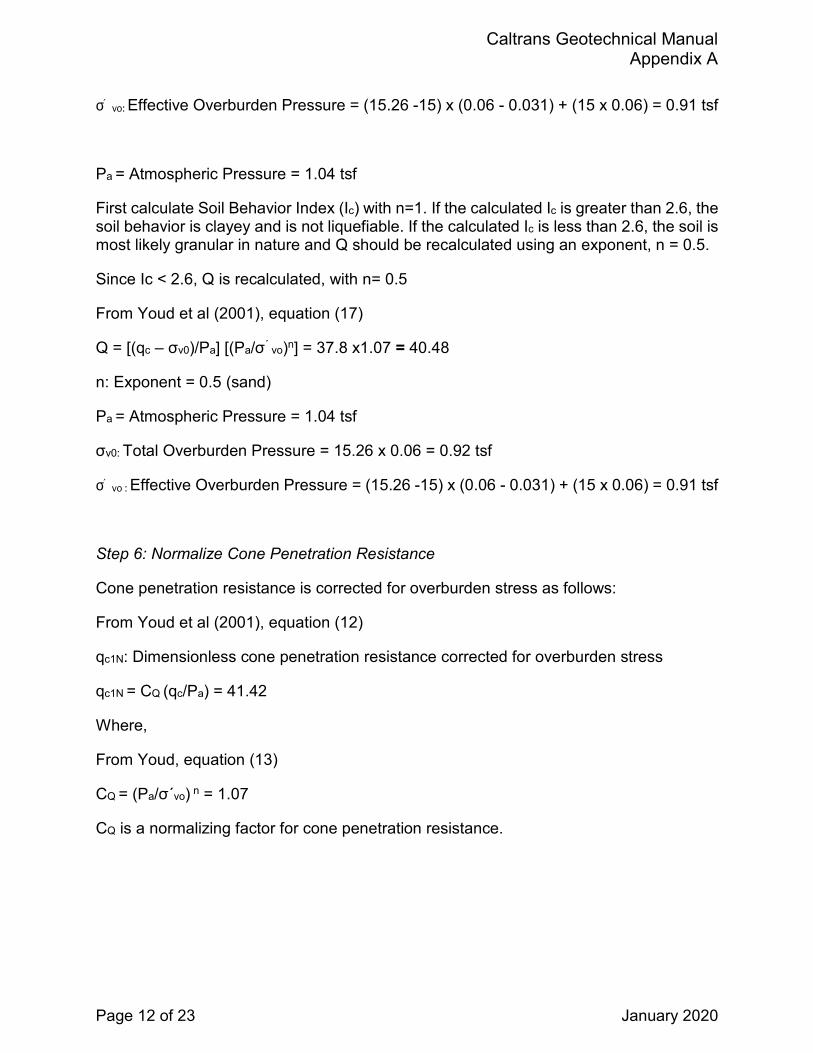
Step 8: Calculate the High Confining Pressure Correction Factor (Kσ)

From Youd et al (2001) equation (31)

Kσ = (σ΄v0/Pa) (f-1)

σ΄v0: Effective Overburden Pressure

Pa: Atmospheric Pressure

f: exponent that is a function of site conditions, including relative density, stress history, aging and overconsolidation ratio

From Kulhawy and Mayne (1990) , Equation 2-16:

Dr 2 = (N1)60 / (Cp.CA.COCR)

For normally consolidated (NC) unaged sand:

Cp = 60 + 25 log D50

Cp: Parameter for grain size

Dr: Relative density (%)

D50: Median diameter of sand (mm)

For aged sand:

CA= 1.2 + 0.05 log (t/100)

CA: Parameter for aging

t: Time since deposition in years

For overconsolidated (OC) sand:

COCR = OCR0.18

COCR: Parameter for overconsolidation


of 23 January 2020

OCR: Overconsolidation ratio: σ’p/ σ΄v0

Where:

σ'p: Preconsolidation pressure

σ΄v0: Effective overburden pressure

For this example:

Soil is normally consolidated sand and unaged

Cp = 60 + 25 log D50

D50 = 0.5 mm

Cp = 60 + 25 log (0.5) = 52.47

CA = 1

COCR = 1

Dr 2 = (N1)60cs / (Cp.CA.COCR)

(N1)60= 20

Dr 2 = 20/52.47 = 0.36

Dr = 60%

From Youd et al (2001), figure 15

For Dr = 60%, f = 0.7

Kσ = (2225/2116) (0.7-1)

= 0.985


of 23 January 2020

Step 9: Calculate the Sloping Ground Correction Factor (Kα)

For this example:

Level ground: Kα = 1

α: Static stress ratio

α = τh / σ΄v0

τh: Static shear stress on the horizontal plane

σ΄v0: Effective overburden pressure

Step 10: Calculate the Factor of Safety against Liquefaction

From Youd et al (2001), equation (30):

FS = (CRR7.5/CSR) x MSF x Kσ x Kα

FS = (.22/.32) x .97 x 1.0 x 0.985

=0.66

Since FS is less than 1, the geotechnical report needs to state that liquefaction is predicted to occur in this layer.

To complete the liquefaction analysis for the site, repeat the above steps for all other soil layer identified as potentially liquefiable.


of 23 January 2020

Attachment 1

Liquefaction Evaluation Module - January 2020 - Caltrans

Documents

Transcript of Liquefaction Evaluation Module - January 2020 - Caltrans