liquefaction analysis of level and sloping ground using - MAE ...

LIQUEFACTION ANALYSIS OF LEVEL AND SLOPING GROUND USINGFIELD CASE HISTORIES AND PENETRATION RESISTANCE

BY

SCOTT MICHAEL OLSON

B.S., University of Illinois at Urbana-Champaign, 1994M.S., University of Illinois at Urbana-Champaign, 1995

THESIS

Submitted in partial fulfillment of the requirementsfor the degree of Doctor of Philosophy in Civil Engineering

in the Graduate College of theUniversity of Illinois at Urbana-Champaign, 2001

Urbana, Illinois

i

ABSTRACT

The primary objective of this study was to develop simple, empirical tools to evaluate

liquefaction problems in level and sloping ground. The proposed correlations and

procedures are particularly useful as screening tools because of their simplicity. Specifically,

these procedures include:

1. CPT-based level ground liquefaction resistance relationships for sandy soils;

2. SPT- and CPT-based relationships to estimate the yield shear strength available

at the triggering of liquefaction in ground subjected to a static shear stress;

3. SPT- and CPT-based relationships to estimate the liquefied shear strength

available at large deformation after the triggering of liquefaction in ground

subjected to a static shear stress; and

4. A comprehensive liquefaction analysis procedure for ground subjected to a static

shear stress that addresses liquefaction susceptibility, triggering of liquefaction,

and post-triggering stability.

The author collected a database of 172 level ground liquefaction and non-

liquefaction case histories where CPT results are available. These cases were separated

into those involving clean sands (less than 5% fines content), silty sands (between 5 and

35% fines content), and silty sands to sandy silts (greater than 35% fines content) to

develop three separate liquefaction resistance relationships based on fines content

(percentage by weight passing the U.S. Standard #200 sieve). The proposed relationships

also use median grain size (D50

) to classify the case histories.

ii

The author collected thirty-three case histories of liquefaction flow failure where SPT

and/or CPT results are available or can be reasonably estimated. These flow failure case

histories were back-analyzed to evaluate the yield shear strength and yield strength ratio

mobilized at the triggering of liquefaction. Relationships between yield strength ratio and

corrected SPT and CPT resistance were developed for use in liquefaction triggering

analysis. The flow failure case histories also were back-analyzed to evaluate the liquefied

shear strength and liquefied strength ratio mobilized at large deformation. For cases with

sufficient information, the stability back-analysis incorporated the kinetics of failure (i.e.,

momentum). Relationships between liquefied strength ratio and corrected SPT and CPT

resistance were developed for use in post-triggering stability analysis.

Lastly, the author proposes a comprehensive liquefaction analysis procedure for

sandy soils to evaluate: (1) liquefaction susceptibility; (2) triggering of liquefaction; and (3)

post-triggering/flow failure stability. The procedure incorporates the proposed relationships

to estimate yield strength ratio and liquefied strength ratio, and does not require a suite of

laboratory tests or corrections for sloping ground and vertical effective stress. The procedure

is verified initially using the Lower San Fernando Dam case history, and is particularly useful

as a screening tool.

iii

ACKNOWLEDGMENTS

I would like to express my gratitude to everyone who has contributed to this study.

Special thanks are extended to: Dr. Timothy D. Stark, my Advisor, for his support and

encouragement, and for introducing me to the challenging and rewarding profession of

geotechnical engineering; Drs. Gholamreza Mesri, James H. Long, Youssef Hashash, and

Mr. Peter A. Lenzini for their constructive criticism and encouragement; Drs. David E. Daniel

and Edward J. Cording for their valuable advice; Mrs. Myrna Webber for her tireless support,

help, and friendship; Dr. Stephen F. Obermeier for his valuable advice and friendship; Dr.

Marawan Shahien for his constant willingness to discuss technical and non-technical issues;

my parents, Kenneth J. and Janet L. Olson, for their enduring support and encouragement

throughout my undergraduate and graduate years; Katrina, my wife, partner, and best

friend, for her never-ending love and strength – thank you for never letting me lose focus;

and my daughter, Hailey, who was too young to remember Dad trying to finalize this study,

but would always greet me with a smile after a long day of work.

This work was supported by the Earthquake Engineering Research Centers Program

of the National Science Foundation (NSF) under NSF Award Number EEC-9701785, as part

of the Mid-America Earthquake (MAE) Center headquartered at the University of Illinois-

Urbana-Champaign. Any opinions, findings, and conclusions or recommendations

expressed in this material are those of the author and do not necessarily reflect those of the

National Science Foundation. This support is gratefully acknowledged.

iv

TABLE OF CONTENTS

CHAPTER 1. INTRODUCTION...................................................................................1

1.1 INTRODUCTION TO THE PROBLEMS............................................................1

1.2 OBJECTIVES OF THE STUDY ........................................................................3

1.3 ORGANIZATION AND SCOPE.........................................................................5

CHAPTER 2. MECHANICS OF LIQUEFACTION........................................................6

2.1 INTRODUCTION ..............................................................................................6

2.2 TERMINOLOGY AND DEFINITIONS ...............................................................6

2.2.1 Flow Liquefaction .....................................................................................7

2.2.2 Cyclic Mobility ..........................................................................................8

2.2.3 Level Ground Liquefaction .......................................................................8

2.3 UNDRAINED STRESS-STRAIN BEHAVIOR....................................................9

2.3.1 Yield Shear Strength and Liquefied Shear Strength ...............................10

2.3.2 Soil State, State Parameter, and Steady State Line ...............................12

2.3.3 Effect of Increased Density at the Same Confining Stress......................13

2.3.4 Effect of Increased Confining Stress at the Same Density......................14

2.3.5 Effect of Mode of Shear..........................................................................15

2.3.6 Effect of Method of Preparation (Soil Structure) .....................................16

2.3.7 Effect of Grain Crushing at Large Confining Pressures ..........................17

2.4 SUMMARY .....................................................................................................18

CHAPTER 3. LEVEL GROUND LIQUEFACTION RESISTANCE USINGCASE HISTORIES AND CPT..............................................................31

v

3.1 INTRODUCTION ............................................................................................31

3.2 CYCLIC STRESS METHOD...........................................................................33

3.2.1 Evaluation of Cyclic Stress Ratio............................................................34

3.2.2 Evaluation of SPT Penetration Resistance.............................................35

3.2.3 Evaluation of CPT Penetration Resistance.............................................36

3.3 CPT BASED LIQUEFACTION RESISTANCE.................................................37

3.3.1 Liquefaction Resistance of Clean Sand..................................................39

3.3.2 Liquefaction Resistance of Silty Sand ....................................................42

3.3.3 Liquefaction Resistance of Silty Sand to Sandy Silt................................44

3.3.4 Discussion..............................................................................................45

3.4 COMPARISON OF PROPOSED CPT RELATIONSHIPS ANDSPT CASE HISTORIES..................................................................................47

3.4.1 Clarification of SPT-CPT Conversion .....................................................48

3.4.2 Comparison of CPT Liquefaction Resistance Relationships andSPT Based Field Data............................................................................52

3.5 CPT BASED LIQUEFACTION RESISTANCE OF GRAVELLY SOILS............53

3.6 SUMMARY .....................................................................................................54

CHAPTER 4. YIELD STRENGTH RATIO FROM LIQUEFACTIONFLOW FAILURES ...............................................................................74

4.1 INTRODUCTION ............................................................................................74

4.2 YIELD SHEAR STRENGTH AND YIELD STRENGTH RATIO........................75

4.3 EXISTING METHODS TO EVALUATE TRIGGERING OFLIQUEFACTION IN SLOPING GROUND .......................................................76

4.3.1 Poulos et al. (1985a,b); Poulos (1988) ...................................................77

4.3.2 Seed and Harder (1990); Harder and Boulanger (1997).........................77

4.3.3 Byrne (1991); Byrne et al. (1992) ...........................................................78

vi

4.3.4 Summary of Existing Procedures ...........................................................79

4.4 BACK-ANALYSIS OF LIQUEFACTION FLOW FAILURECASE HISTORIES..........................................................................................79

4.4.1 Procedure to Back-Calculate Yield Strength Ratio or MobilizedStrength Ratio ........................................................................................82

4.4.2 Procedure to Back-Calculate Yield or Mobilized Shear Strength ............84

4.5 FLOW FAILURE CASE HISTORY BACK-ANALYSIS RESULTS....................84

4.5.1 Flow Failures Triggered by Static Loading .............................................85

4.5.2 Flow Failures Triggered by Deformation/Global Instability......................86

4.5.3 Flow Failures Triggered by Seismic Loading ..........................................86

4.6 YIELD (AND MOBILIZED) STRENGTH RATIO AND PENETRATIONRESISTANCE.................................................................................................89

4.7 CONCLUSIONS .............................................................................................90

CHAPTER 5. LIQUEFIED STRENGTH RATIO FROM LIQUEFACTIONFLOW FAILURES ...............................................................................99

5.1 INTRODUCTION ............................................................................................99

5.2 LIQUEFIED SHEAR STRENGTH AND STRENGTH RATIO...........................99

5.2.1 Liquefied Shear Strength........................................................................99

5.2.2 Liquefied Strength Ratio.......................................................................101

5.2.3 Relation between Liquefied Strength Ratio andPenetration Resistance ........................................................................102

5.3 EXISTING METHODS TO ESTIMATE LIQUEFIED SHEARSTRENGTH OR STRENGTH RATIO ...........................................................103

5.3.1 Poulos et al. (1985a) ............................................................................103

5.3.2 Seed (1987) and Seed and Harder (1990) ...........................................104

5.3.3 Stark and Mesri (1992).........................................................................105

5.3.4 Ishihara (1993).....................................................................................107

vii

5.3.5 Konrad and Watts (1995) .....................................................................108

5.3.6 Fear and Robertson (1995) ..................................................................109

5.3.7 Summary of Existing Procedures .........................................................110

5.4 BACK-ANALYSIS OF LIQUEFACTION FLOW FAILURES...........................111

5.4.1 Simplified Stability Analysis of Post-Failure Geometry..........................112

5.4.2 Rigorous Stability Analysis of Post-Failure Geometry...........................113

5.4.3 Stability Analysis Considering Kinetics of Failure Mass Movements.....115

5.5 CASE HISTORIES OF LIQUEFACTION FLOW FAILURE............................120

5.5.1 Sources of Uncertainty in the Analyses and their Importance...............121

5.5.2 Magnitude of Uncertainties...................................................................123

5.6 INTERPRETATION AND DISCUSSION .......................................................124

5.6.1 Back-Calculation of Liquefied Shear Strength ......................................125

5.6.2 Effect of Fines Content on Liquefied Shear Strength andStrength Ratio ......................................................................................127

5.6.3 Effect of Kinetics on Liquefied Shear Strength .....................................127

5.6.4 Effect of Penetration Resistance on Liquefied Strength Ratio ..............128

5.7 APPLICATIONS OF LIQUEFIED STRENGTH RATIO..................................129

5.8 CONCLUSIONS ...........................................................................................130

CHAPTER 6. CONFIRMATION OF YIELD AND LIQUEFIED STRENGTHRATIOS USING LABORATORY DATA.............................................151

6.1 INTRODUCTION ..........................................................................................151

6.2 APPLICABILITY OF STRENGTH RATIOS FOR LIQUEFACTIONANALYSIS ....................................................................................................152

6.2.1 Laboratory Database of Sandy Soils ....................................................152

6.2.2 Slope of Steady State Line...................................................................152

viii

6.2.3 Steady State Line and Soil Compressibility ..........................................153

6.3 CONFIRMATION OF YIELD STRENGTH RATIO.........................................155

6.3.1 Laboratory Database Test Results .......................................................155

6.3.2 Collapse Surface from Laboratory Data ...............................................157

6.3.3 Relation between Collapse Surface and State Parameter ....................158

6.3.4 Comparison of Laboratory Collapse Surface with Field Data................159

6.4 CONFIRMATION OF LIQUEFIED STRENGTH RATIO ................................160

6.4.1 Liquefied Strength Ratio and State Parameter .....................................161

6.4.2 Comparison of Laboratory Strength Ratio and Field Data ....................162

6.4.3 Laboratory Strength Ratio and Relative Density...................................163

6.4.4 Conversion of Relative Density to Penetration Resistance ...................164

6.4.5 Comparison of Laboratory Strength Ratio/Penetration ResistanceRelationships and Field Strength Ratios...............................................166

6.5 CONCLUSIONS ...........................................................................................167

CHAPTER 7. LIQUEFACTION ANALYSIS PROCEDURE FOR GROUNDSUBJECTED TO STATIC SHEAR STRESS .....................................199

7.1 INTRODUCTION ..........................................................................................199

7.2 FLOW FAILURE SUSCEPTIBILITY ANALYSIS............................................200

7.3 LIQUEFACTION TRIGGERING ANALYSIS..................................................201

7.4 POST-TRIGGERING/FLOW FAILURE STABILITY ANALYSIS ....................203

7.5 VERIFICATION OF LIQUEFACTION ANALYSIS USING LOWER SANFERNANDO DAM CASE HISTORY .............................................................204

7.5.1 LSFD Susceptibility Analysis ................................................................205

7.5.2 LSFD Triggering Analyses ...................................................................206

7.5.3 LSFD Post-Triggering/Flow Failure Stability Analyses..........................207

ix

7.5.4 Discussion of Results...........................................................................208

7.6 CONCLUSIONS ...........................................................................................209

CHAPTER 8. SUMMARY AND CONCLUSIONS ....................................................219

REFERENCES ..........................................................................................................226

APPENDIX A. DESCRIPTION OF LIQUEFACTION FLOW FAILURE CASEHISTORIES AND ANALYSES...........................................................249

A.1 VLIETEPOLDER, ZEELAND PROVINCE, NETHERLANDS.........................249

A.1.1 Description of the Failure .....................................................................249

A.1.2 Site Geology and Soil Conditions .........................................................251

A.1.3 Representative Penetration Resistance ...............................................253

A.1.4 Yield Shear Strength and Strength Ratio Analyses ..............................255

A.1.5 Liquefied Shear Strength and Strength Ratio Analyses........................257

A.1.6 Sources of Uncertainty.........................................................................259

A.2 NORTH DIKE OF WACHUSETT DAM, MASSACHUSETTS, USA...............260







A.3 CALAVERAS DAM, CALIFORNIA, USA.......................................................277



x





A.4 SHEFFIELD DAM, CALIFORNIA, USA.........................................................291







A.5 HELSINKI HARBOR, FINLAND ....................................................................302







A.6 FORT PECK DAM, MONTANA, USA ...........................................................310






xi


A.7 SOLFATARA CANAL DIKE, MEXICO ..........................................................329







A.8 LAKE MERCED BANK, CALIFORNIA, USA .................................................339







A.9 KAWAGISHI-CHO APARTMENTS, NIIGATA, JAPAN..................................351







A.10 UETSU-LINE RAILWAY EMBANKMENT, JAPAN ........................................358


xii






A.11 EL COBRE TAILINGS DAM, CHILE .............................................................369







A.12 KODA NUMA HIGHWAY EMBANKMENT, JAPAN.......................................376







A.13 METOKI ROADWAY EMBANKMENT, JAPAN .............................................385





xiii



A.14 HOKKAIDO TAILINGS DAM, JAPAN ...........................................................392







A.15 LOWER SAN FERNANDO DAM, CALIFORNIA, USA ..................................399







A.16 TAR ISLAND DIKE, ALBERTA, CANADA.....................................................411







A.17 MOCHI-KOSHI TAILINGS DAM, JAPAN ......................................................417

xiv







A.18 NERLERK UNDERSEA BERM, BEAUFORT SEA, CANADA.......................430







A.19 HACHIRO-GATA ROAD EMBANKMENT, AKITA, JAPAN............................444







A.20 ÅSELE ROADWAY EMBANKMENT, SWEDEN ...........................................454




xv




A.21 LA MARQUESA DAM, CHILE.......................................................................463







A.22 LA PALMA DAM, CHILE...............................................................................475







A.23 FRASER RIVER DELTA, BRITISH COLUMBIA, CANADA...........................484







xvi

A.24 LAKE ACKERMAN ROAD EMBANKMENT, MICHIGAN, USA .....................489







A.25 CHONAN MIDDLE SCHOOL, CHIBA, JAPAN..............................................501







A.26 NALBAND RAILWAY EMBANKMENT, ARMENIA........................................509







A.27 MAY 1 SLIDE, TAJIKISTAN REPUBLIC, USSR ...........................................518



xvii





A.28 SHIBECHA-CHO EMBANKMENT, JAPAN...................................................527







A.29 ROUTE 272 EMBANKMENT, HIGASHIAREKINAI, JAPAN..........................538







1

CHAPTER 1

INTRODUCTION

1.1 INTRODUCTION TO THE PROBLEMS

The devastating earthquakes in 1964 in Prince William Sound, Alaska and Niigata,

Japan brought the phenomenon of earthquake-induced liquefaction of soils to prominence.

Seismically-induced liquefaction during these two earthquakes caused significant damage to

structures and bridges due to settlement, downdrag, lateral spreading, slope failures,

bearing capacity failures, and flotation of buried structures (e.g., Coulter and Migliaccio

1967, Ross 1968, and Seed 1968 for the 1964 Alaskan earthquake; Ohsaki 1966, Yamada

1966, and Ishihara and Koga 1981 for the 1964 Niigata earthquake).

Initial efforts to explain this behavior focused on laboratory cyclic triaxial compression

testing of reconstituted sand specimens. The liquefaction resistance (or cyclic strength) of

clean sands was found to depend primarily on the relative density of the specimen.

Therefore, Seed and Idriss (1971) developed the “simplified” method to correlate the

liquefaction resistance of sands to relative density. However, researchers soon recognized

that testing of reconstituted specimens did not explain the field behavior of many sandy

soils. Some of the reasons for discrepancy are the effects of in situ structure (or soil fabric),

aging, pre-straining, and overconsolidation, which cannot be adequately reproduced in the

laboratory (Terzaghi et al. 1996).

Researchers (e.g., Robertson and Campanella 1985) observed that factors such as

structure, aging, pre-straining, and overconsolidation affected in situ penetration resistance

in a similar manner as liquefaction resistance. For example, overconsolidated sands were

2

observed to have both higher penetration resistance and higher liquefaction resistance than

otherwise identical normally consolidated sands. Therefore, correlations were developed

between standard penetration test (SPT) blowcount (N) and liquefaction resistance (e.g.,

Seed et al. 1985).

Skempton (1986) and Seed et al. (1985) (among others) noted the limitations and

variability of the SPT. Despite efforts to “standardize” SPT results via operational control and

correction factors, there remains considerable variability in SPT results depending on test

procedure, equipment type, operator procedure, and use of corrections (Skempton 1986).

This led to the development of correlations between cone penetration test (CPT) results and

liquefaction resistance, e.g., Ishihara (1985), Robertson and Campanella (1985), Seed and

de Alba (1986), and Shibata and Teparaksa (1988). However, initial efforts to develop CPT-

based liquefaction resistance relationships were hindered by a lack of field case histories

where CPT penetration resistance was available to develop reliable relationships. Recently,

a large number of level ground liquefaction case histories with CPT results have become

available, allowing the development of a simple, yet reliable procedure to evaluate level

ground liquefaction potential using the CPT.

The liquefaction flow failure in the upstream slope of Lower San Fernando Dam

resulting from the 1971 San Fernando earthquake (MW = 6.6) illustrated the importance of

the shear strength of liquefied soils on the stability of slopes (e.g., Seed et al. 1973). The

liquefied shear strength is defined as the shear strength mobilized at large deformation after

liquefaction is triggered in saturated, contractive sandy soils.

A number of procedures have been developed to evaluate the liquefied shear

strength (e.g., Poulos et al. 1985a; Seed and Harder 1990; Stark and Mesri 1992; Ishihara

1993; Konrad and Watts 1995). However, each method has inadequacies for the practical

3

assessment of the liquefied shear strength. A simple, yet reliable procedure is needed to

evaluate the shear strength of liquefied soils for use in post-triggering stability analyses.

Lastly, while procedures to evaluate the triggering of liquefaction in ground subjected

to a static shear stress (e.g., slopes, embankments, or foundations of structures) are

available, they require a suite of expensive laboratory tests (Poulos et al. 1985a,b; Byrne

1991; Byrne et al. 1992) or correction factors that exhibit large uncertainty (Seed and Harder

1990; Harder and Boulanger 1997). Again, a simple, yet reliable procedure is needed to

evaluate the triggering of liquefaction in ground subjected to a static shear stress.

1.2 OBJECTIVES OF THE STUDY

The objectives of this study are to bridge a number of gaps in our understanding of

liquefaction behavior and provide practitioners with simple, reliable empirical procedures

(based on field case histories of liquefaction failures) to evaluate liquefaction problems.

Specifically, these procedures include:

1. CPT-based level ground liquefaction resistance relationships for sandy soils;

2. SPT- and CPT-based relationships to estimate the yield shear strength available

at the triggering of liquefaction in ground subjected to a static shear stress;

3. SPT- and CPT-based relationships to estimate the liquefied shear strength

available at large deformation after the triggering of liquefaction in ground

subjected to a static shear stress; and

4. A comprehensive liquefaction analysis procedure for ground subjected to a static

shear stress that addresses liquefaction susceptibility, triggering of liquefaction,

and post-triggering stability.

4

Olson and Stark (1998) collected a database of 172 level ground liquefaction and

non-liquefaction case histories where CPT results are available. These cases were

separated into those involving clean sands (less than 5% fines content), silty sands

(between 5 and 35% fines content), and silty sands to sandy silts (greater than 35% fines

content) to develop three separate liquefaction resistance relationships based on fines

content. (Fines content, FC, is defined as the percentage by weight passing the U.S.

Standard #200 sieve.) The proposed relationships also use median grain size (D50

) to

classify the case histories.

The author collected thirty-three case histories of liquefaction flow failure where SPT

and/or CPT results are available or can be reasonably estimated. These flow failure case

histories were back-analyzed to evaluate the yield shear strength and yield strength ratio

mobilized at the triggering of liquefaction. Relationships between yield strength ratio and

corrected SPT and CPT resistance were developed for use in liquefaction triggering

analysis. The flow failure case histories also were back-analyzed to evaluate the liquefied

shear strength and liquefied strength ratio mobilized at large deformation. For cases with

sufficient information, the stability back-analysis incorporated the kinetics of failure (i.e.,

momentum). Relationships between liquefied strength ratio and corrected SPT and CPT

resistance were developed for use in post-triggering stability analysis.

Lastly, a comprehensive liquefaction analysis procedure for sandy soils is proposed

to evaluate: (1) liquefaction susceptibility; (2) triggering of liquefaction; and (3) post-

triggering/flow failure stability. The procedure incorporates the relationships to estimate yield

strength ratio and liquefied strength ratio proposed herein, and does not require a suite of

laboratory tests (Poulos et al. 1985a,b; Byrne 1991; Byrne et al. 1992) or corrections for

5

sloping ground and vertical effective stress (Seed and Harder 1990; Seed and Harder

1997).

1.3 ORGANIZATION AND SCOPE

The remainder of this thesis is organized as follows. Chapter 2 presents a brief

review of liquefaction behavior. Chapter 3 presents the database of CPT-based level ground

liquefaction and non-liquefaction case histories, relationships to estimate the level ground

liquefaction resistance of sandy soils using the CPT, as well as the interpretation of the CPT

database.

Chapter 4 describes the concept and application of the yield strength ratio, then

presents the results of back-analyses of liquefaction flow failure case histories for the

evaluation of the yield strength ratio. Similarly, Chapter 5 describes the concept and

application of the liquefied strength ratio, then presents the results of back-analyses of

liquefaction flow failure case histories for the evaluation of the liquefied strength ratio.

Chapter 6 presents a database of laboratory test results compiled from the literature and

used to confirm the yield and liquefied strength ratio concepts. Lastly, a comprehensive

liquefaction analysis procedure for ground subjected to a static shear stress is presented

and initially verified in Chapter 7.

6

CHAPTER 2

MECHANICS OF LIQUEFACTION

2.1 INTRODUCTION

Over the last 35 years, tremendous effort has been expended to understand the

mechanics of liquefaction. Examination and back-analysis of field manifestations of

liquefaction, laboratory studies, and numerical modeling of liquefaction behavior have

proven useful to this end. Understanding liquefaction behavior begins with understanding

that liquefaction, in all its forms, is the frictional behavior of cohesionless soils under

elevated porewater pressure during rapid loading (Poulos 1981), and most likely even

during rapid flow (Iverson and LaHusen 1993; Iverson et al. 1997). Nearly all liquefaction

phenomena can be reasonably explained in terms of a simple concept developed 60 years

ago – the critical void ratio concept developed by Casagrande (1940).

2.2 TERMINOLOGY AND DEFINITIONS

Part of the difficulty in understanding liquefaction has been the use of the same

terminology to describe different phenomena, and use of different terminology to describe

the same phenomenon.

The term “liquefaction” has been used to describe a number of related, but different

phenomena that include the following behavior (for consistency, the nomenclature used

herein is slightly modified from that suggested by Casagrande 1976; Robertson 1994; and

Kramer 1996):

7

• Flow liquefaction, resulting in liquefaction flow failure

• Cyclic mobility, resulting in deformation, such as lateral spreading, that ceases

with the cessation of loading

• Level ground liquefaction (a subset of cyclic mobility)

The following paragraphs describe each of these phenomena in more detail.

2.2.1 Flow Liquefaction

Flow liquefaction is the process of strain-softening of contractive, saturated,

cohesionless soils during undrained shear. This behavior only occurs in loose (or

contractive), cohesionless soils and can be triggered by static or seismic undrained loading

or undrained deformation under constant load, as shown schematically in Figure 2.1.

Further, flow liquefaction only occurs in the field if the static shear stress is greater than the

liquefied (or steady state) shear strength (Poulos et al. 1985a). The manifestation of this

behavior is a liquefaction flow failure of a slope, embankment, or foundation. The static

shear stress mentioned above is the shear stress required for static equilibrium under a

driving force, e.g., embankment slope loading. This shear stress is not the shear stress

resulting from K0 stress conditions developed during deposition. Deposition does not create

shear stresses on horizontal planes. Examples of flow failures induced by static loading

and/or undrained deformation include Calaveras Dam (Hazen 1918) and Fort Peck Dam

(Casagrande 1965), and examples of flow failures induced by seismic loading include Lower

San Fernando Dam (Castro et al. 1989; Seed et al. 1989) and Sheffield Dam (Seed et al.

1969).

8

2.2.2 Cyclic Mobility

Cyclic mobility is the result of excess porewater pressure buildup and concurrent

degradation of shear stiffness resulting from seismic or cyclic loading, as shown

schematically in Figure 2.2. In contrast to flow liquefaction, the static shear stress in cases of

cyclic mobility is smaller than the liquefied (or steady state) shear strength of the soil. Cyclic

mobility typically occurs in loose to medium-dense soils, but may occur in dense soils if the

loading is strong enough and of sufficient duration, and the field conditions are favorable.

During seismic or cyclic loading under undrained conditions, cohesionless soils tend

to exhibit a progressive increase in excess porewater pressure. As the excess porewater

pressure increases, the stiffness of the soil decreases. Hence, after a period of seismic or

cyclic loading, significant permanent deformations can accumulate, particularly in the

direction of a static shear stress. However, when the loading ceases, the deformations stop.

Therefore this form of liquefaction is termed cyclic mobility. Cases of cyclic mobility failures

are typically subdivided into cases of limited deformation where static driving forces are

significant, e.g., Upper San Fernando Dam (Seed et al. 1973), and cases of lateral

spreading where driving forces are small, e.g., Heber Road (Youd and Bennett 1983).

2.2.3 Level Ground Liquefaction

Level ground liquefaction is a subset of cyclic mobility that occurs when the static

shear stress is zero [similar to the behavior illustrated in Figure 2.2(c)]. In this case, stress

reversal occurs during seismic or cyclic loading, resulting in a more rapid buildup of excess

porewater pressure than when stress reversal does not occur (Mohamad and Dobry 1986).

This form of liquefaction typically occurs in loose to medium-dense soils, but may occur in

9

dense soils if the loading is strong enough and of sufficient duration, and field conditions are

favorable.

As the excess porewater pressure increases during seismic or cyclic loading, shear

stiffness decreases. If the loading is of sufficient strength and duration, the soil can cycle

through momentary periods of zero effective stress. Since there is no driving stress,

permanent lateral deformations are often relatively small; however, large vertical settlements

may develop during the dissipation of seismically-induced excess porewater pressure.

These settlements can create large downdrag forces on deep foundations. If level ground

liquefaction occurs below a surface cap soil (soil of lower permeability), the cap soil can be

hydraulically fractured resulting in sand blow formation and loss of ground (Obermeier

1996). A cap soil also may separate from an underlying liquefied layer allowing potentially

large ground oscillations and large, chaotic vertical displacements to develop (Youd 1995).

2.3 UNDRAINED STRESS-STRAIN BEHAVIOR

Despite a number of disagreements in the literature, soil behavior during liquefaction

can be explained using the concepts of conventional and critical state soil mechanics, as

discussed in the following paragraphs. The following discussion provides a framework of

typical undrained stress-strain-strength behavior to understand the subsequent development

of concepts and empirical relationships. It is not intended to be a comprehensive discussion

of all aspects of undrained stress-strain-strength behavior, or to discuss all the factors that

may affect this behavior.

10

2.3.1 Yield Shear Strength and Liquefied Shear Strength

Figure 2.1 schematically presents the behavior of saturated, contractive, sandy soil

during undrained loading. The yield shear strength [su(yield)] is the peak shear strength

available during undrained loading (Terzaghi et al. 1996), as illustrated by point B in Figure

2.1. Undrained strain-softening behavior can be triggered by either static or dynamic loads,

or by deformation under a shear stress that is larger than the liquefied shear strength (i.e.,

creep). Eckersley (1990) and Sasitharan et al. (1993) also demonstrated that loading can be

completely drained prior to triggering undrained strain-softening response.

The shear strength mobilized at point C is the liquefied shear strength, su(LIQ). The

liquefied shear strength is the shear strength mobilized at large deformation after

liquefaction (undrained strain-softening behavior) is triggered in a saturated, contractive soil.

The liquefied shear strength has been referred to as the undrained residual shear strength,

sr (Seed 1987), undrained steady state shear strength, sus (Poulos et al. 1985), and

undrained critical shear strength, su(critical) (Stark and Mesri 1992). Based on a recent

National Science Foundation (NSF) international workshop (Stark et al. 1998), the term

liquefied shear strength is used herein because it is generic and does not imply

correspondence to any laboratory test condition.

In the laboratory, where drainage conditions are controlled, the term “undrained”

applies. However, in the field, as evidenced by observation and analysis of flow failures and

centrifuge test results, drainage may occur (Stark and Mesri 1992; Fiegel and Kutter 1994)

and therefore the term “undrained” may not be applicable to the shear strength mobilized in

the field. The term “mobilized liquefied shear strength” or simply “liquefied shear strength”

can be used to describe the shear strength mobilized during a liquefaction flow failure in the

field (including the potential effects of drainage, porewater pressure redistribution, soil

11

mixing, etc.). However, it is anticipated that the liquefied shear strength can be interpreted in

terms of the critical void ratio concept (Casagrande 1940).

An example of the stress-strain behavior of a contractive, saturated, cohesionless

specimen consolidated to an equal all-around pressure and subjected to monotonic

undrained triaxial compression is shown in Figure 2.3. As illustrated in Figure 2.3, the

process of undrained shearing of a contractive soil results in an increase in excess positive

porewater pressure. This occurs because the soil cannot contract due to the undrained

condition. The shear stress initially increases as the axial load is applied. The shear stress

continues to increase until a peak, or yield, strength is reached. Once the yield strength is

reached, the specimen becomes unstable, and straining to the steady state point is

inevitable. Continued straining results in a continued increase in excess porewater pressure

and a concurrent decrease in shearing resistance to liquefied shear strength. If the soil is

sufficiently contractive (as is the case in Figure 2.3), the increase in excess positive

porewater pressure corresponds to a large reduction in effective stress, resulting in a

relatively small magnitude of shear strength.

An example of the stress-strain behavior of a contractive, saturated, cohesionless

specimen consolidated anisotropically and subjected to undrained cyclic triaxial

compression is shown in Figure 2.4. As expected, cyclic loading causes an increase in

porewater pressure within the specimen. During cyclic loading and increase in porewater

pressure, the specimen begins to soften and accumulate strains. Unlike the behavior in

Figure 2.3, the specimen does not reach a unique yield strength, but does show marked

strain-softening and increase in positive porewater pressure after reaching a collapse, or

yield, surface (Sladen et al. 1985). (The collapse surface will be described in detail in

Chapter 4.) After reaching the collapse surface, the specimen becomes unstable and strains

12

to its liquefied (or steady state) shear strength, similar to the behavior exhibited under

monotonic loading in Figure 2.3.

2.3.2 Soil State, State Parameter, and Steady State Line

The undrained behavior of a saturated, cohesionless soil is a function of its void ratio

and confining pressure at the start of shear (Schofield and Wroth 1968). The tendency of a

soil to contract or dilate during shear is a function of its state, where state is a function of

initial void ratio and confining pressure as illustrated in Figure 2.5. Been and Jefferies (1985)

suggested a state parameter, ψ, to describe soil state. The state parameter is defined as:

ψ = eo - ess (2.1)

where eo is the in-situ void ratio prior to shearing at a given effective confining stress and ess

is the void ratio at the steady state line (defined in the following paragraph) for the same

effective confining stress.

The steady state line (SSL; originally termed the critical void ratio line) was

postulated by Casagrande (1940) as the locus of void ratios that are reached after large

strain for any combination of void ratio and confining pressure. Soils that have an initial state

above the SSL (i.e., loose of the SSL with a positive state parameter) are contractive and

soils with an initial state below the SSL (i.e., dense of the SSL with a negative ψ) are dilative

(see Figure 2.5). Soils that have an initial state near the SSL are mildly contractive at

intermediate strains, but then become mildly dilative at larger strains (Castro 1969; Ishihara

1993).

13

2.3.3 Effect of Increased Density at the Same Confining Stress

The effect of increased density at the same pre-shear confining stress is illustrated in

Figure 2.6 using the results of a series of triaxial compression tests conducted by Castro

(1969). The specimens were sheared using axial stress-controlled equipment, and the void

ratios after consolidation (and prior to shear) for specimens a, b, and c were 0.748, 0.689,

and 0.681, respectively. These void ratios correspond to relative densities (Dr) of 27%, 44%,

and 47%, respectively. All specimens were consolidated under an equal all-around pressure

of 400 kPa prior to shear. The initial states of the specimens with respect to the steady state

line of the sand are shown in Figure 2.7. The behavior of specimen “a” in Figure 2.6 is

similar to the behavior shown in Figure 2.3 for another loose specimen of the same sand

also subjected to triaxial compression. However, as illustrated in Figures 2.6 and 2.7, a

higher pre-shear density at the same confining pressure results in a lower state parameter

and significantly different stress-strain behavior.

The increase in relative density from 27% to 44% changes the state parameter of the

soil from 0.062 to 0.003. This change in relative density changes the stress-strain behavior

from highly contractive to mildly contractive at intermediate strains and mildly dilative at

larger strains. Castro (1969) termed this stress-strain behavior “limited liquefaction.”

Alarcon-Guzman et al. (1988) and Ishihara (1993) called the minimum shear resistance that

is reached while the soil is contracting the “quasi-steady state” shear strength. This quasi-

steady state shear strength is reached during intermediate strains prior to strain-hardening

to the steady-state shear strength. The quasi-steady state has been observed in numerous

testing programs, e.g., Mohamad and Dobry (1986), Alarcon-Guzman et al. (1988), Konrad

(1990a), Been et al. (1991), Verdugo (1992), Ishihara (1993), Vaid and Thomas (1995);

Norris et al. (1997), Yamamuro and Lade (1997), Lade and Yamamuro (1997), among

14

others. Many investigators consider this strength to be the liquefied shear strength because

it is not certain whether or not dilation at larger strains occurs in the field. On the other hand,

Zhang and Garga (1997) suggest that the quasi-steady state may be a test-induced

behavior resulting from end restraint, variations of membrane penetration and compression

of pore fluid, and from the conventional area correction.

An even more striking change in stress-strain behavior is observed in Figure 2.6

following the minor increase in relative density from 44% to 47%. Increasing the relative

density from 44% to 47% decreases the state parameter from 0.003 to –0.005. A negative

value of state parameter means that the initial state is below the steady-state line, i.e., in the

dilative regime, as shown in Figure 2.7. As expected, the change in state parameter

changes the stress-strain behavior from mildly contractive at intermediate strains and mildly

dilative at large strains (specimen “b”) to dilative at all strains (specimen “c”).

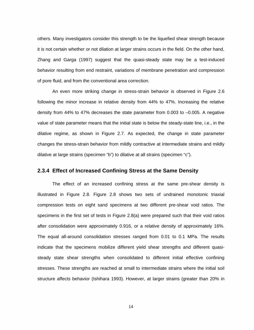
2.3.4 Effect of Increased Confining Stress at the Same Density

The effect of an increased confining stress at the same pre-shear density is

illustrated in Figure 2.8. Figure 2.8 shows two sets of undrained monotonic triaxial

compression tests on eight sand specimens at two different pre-shear void ratios. The

specimens in the first set of tests in Figure 2.8(a) were prepared such that their void ratios

after consolidation were approximately 0.916, or a relative density of approximately 16%.

The equal all-around consolidation stresses ranged from 0.01 to 0.1 MPa. The results

indicate that the specimens mobilize different yield shear strengths and different quasi-

steady state shear strengths when consolidated to different initial effective confining

stresses. These strengths are reached at small to intermediate strains where the initial soil

structure affects behavior (Ishihara 1993). However, at larger strains (greater than 20% in

15

this case), the initial structure of the specimen is destroyed and a unique steady state shear

strength is achieved, irrespective of initial effective confining stress.

Similar results are presented in Figure 2.8(b), where the four specimens were

prepared such that their void ratios after consolidation were approximately 0.833, or a

relative density of approximately 38%. The equal all-around consolidation stresses ranged

from 0.1 to 3.0 MPa. Again, at large strain (beyond about 20%), the initial structure of the

specimen is destroyed and a unique steady state shear strength is reached, irrespective of

initial effective confining stress.

2.3.5 Effect of Mode of Shear

Numerous investigators (e.g., Vaid et al. 1990; Riemer and Seed 1997; Yoshimine et

al. 1998) suggest that the steady state shear strength, and thus the position of the steady

state line, depends on the mode of shear. Figure 2.9 presents hollow cylinder torsional

shear results from Yoshimine et al. (1998) that indicate significantly different stress-strain

behavior and steady state shear strengths for numerous tests on Toyoura sand ranging from

conditions approaching axial compression (α = 15°) to conditions approaching axial

extension (α = 75°). Riemer and Seed (1997) presented similar results in terms of steady

state lines for Monterey #9 sand, as shown in Figure 2.10.

In contrast, numerous investigators (e.g., Been et al. 1991; Poulos 1998) suggest

that the steady state shear strength, and thus the position of the steady state line is

independent of the mode of shear. Poulos (1988) suggested that at large strains, often

beyond the range that can be measured in conventional laboratory equipment, a unique

steady state shear strength is achieved for a given void ratio, regardless of the mode of

shear. Been et al. (1991) also point out that many investigators appear to incorrectly

assume that the quasi-steady state corresponds to the true steady state, and therefore find

16

that the steady state depends on the mode of shear. Figures 2.11 and 2.12 present steady

state lines for Erksak 300/0.7 sand measured by Been et al. (1991) and Toyoura sand

(presented, but not tested, by Been et al. 1991), respectively. These results, which include

triaxial compression and triaxial extension results, indicate that the steady state line is

unique and independent of mode of shear. However, the peak (or yield) and quasi-steady

state shear strengths likely are dependent on the mode of shear because these strengths

are mobilized at small to intermediate strains where the initial soil structure affects stress-

strain behavior.

If present, differences in steady state shear strength that depend on the mode of

shear may be important in analysis of existing structures and back-analysis of flow failure

case histories (Finn 1990). However, this issue presently is unresolved. As a result, mode of

shear is not considered in the back-analysis of field case histories presented in this study.

2.3.6 Effect of Method of Preparation (Soil Structure)

Many investigators (e.g., Dennis 1988; Vaid et al. 1998) suggest that the steady

state shear strength, and thus the position of the steady state line, depends on sample

preparation and thus soil structure or fabric. Figure 2.13 presents results from Vaid et al.

(1998) that indicate significantly different stress-strain behavior and steady state shear

strengths for triaxial compression tests on Syncrude sand prepared by various methods.

Dennis (1988) presented similar results in terms of steady state lines for Ottowa Banding

sand, as shown in Figure 2.14.

In contrast, numerous investigators (e.g., Poulos et al. 1988; Been et al. 1991;

Ishihara 1993; Verdugo et al. 1995) suggest that the steady state shear strength, and thus

the position of the steady state line is independent of the sample preparation and thus soil

structure or fabric. Poulos et al. (1988) suggested that at large strains, often beyond the

17

range that can be measured in conventional laboratory equipment, a unique steady state

shear strength is achieved for a given void ratio, regardless of the sample preparation

method. Figures 2.15, 2.16, and 2.17 present steady state lines for Erksak 300/0.7 sand

(Been et al. 1991), Syncrude tailings sand (Poulos et al. 1988), and Toyoura sand (Ishihara

1993), respectively. These results (which include specimens prepared by moist tamping,

pluviation through air and water, and slurry placement) indicate that the steady state line is

unique and independent of initial soil structure. However, the peak (or yield) and quasi-

steady state shear strengths likely are dependent on the mode of shear because these

conditions occur at small to intermediate strains where the initial soil structure affects stress-

strain behavior.

Again, if present, differences in steady state shear strength depending on the soil

structure or fabric may be important in the analysis of existing structures and back-analysis

of flow failure case histories. However, this issue also is unresolved. For this study, effects

of soil structure are assumed to be reflected in penetration resistance, which is used to

assess yield and liquefied shear strength.

2.3.7 Effect of Grain Crushing at Large Confining Pressures

At large effective confining stresses, grain crushing can occur during shear,

particularly if the grains are angular (Been et al. 1991; Konrad 1998). Grain crushing

changes the grain size distribution of the material. Changes in grain size distribution due to

grain crushing cause a significant increases in the slope of the steady state line (Been et al.

1991; Ishihara 1993; Konrad 1998). An increase in slope of the steady state line is

expected, as indicated by Poulos et al. (1985a), who showed that the slope of the steady

state line is a function of the grain size distribution of the soil. Example steady state lines

18

that include tests conducted at large effective confining stresses are presented in Figures

2.15, 2.17, and 2.18.

Grain crushing typically occurs at effective confining stresses greater than 1 to 2

MPa (Konrad 1998), depending on the strength and angularity of the individual soil grains.

However, grain crushing may occur at lower effective confining stresses in some silty sands

or clean sands composed of relatively weak minerals. For example, grain crushing occurs in

Mai-Liao silty sand (see Chapter 6 for details regarding this silty sand) at a mean effective

stress of approximately 220 kPa (Huang et al. 1999). Based on available data, the effect of

grain crushing on steady state behavior probably does not affect most civil engineering

structures, however, more data on grain crushing of silty sands are needed to clarify this

issue.

2.4 SUMMARY

The following points summarize this review of work done by others regarding the mechanics

of liquefaction.

1. The use of the same terminology to describe different phenomena and different

terminology to describe the same phenomena has led to considerable confusion in the

profession. Herein, the term “flow liquefaction” defines strain-softening behavior

observed in contractive, saturated, cohesionless soils subjected to undrained loading.

This behavior results in a liquefaction flow failure if the static shear stress is greater

than the liquefied shear strength (Poulos et al. 1985a). The term “cyclic mobility” is the

result of excess porewater pressure buildup and concurrent degradation of shear

stiffness resulting from seismic or cyclic loading. In the case of cyclic mobility, the

19

static shear stress is smaller than the liquefied shear strength, and flow failure can not

occur. Cyclic mobility is commonly manifest as lateral spreading during earthquakes.

The term “level ground liquefaction” is a subset of cyclic mobility that occurs when the

static shear stress is zero (level ground conditions). Level ground liquefaction is most

commonly associated with sand blow development, post-seismic settlement of sandy

ground, and downdrag on deep foundations as a result of earthquakes.

2. A contractive, saturated, cohesionless soil subjected to undrained monotonic loading

will mobilize a yield (or peak) and liquefied (or large strain) shear strength. These

shear strengths are used later in this work to interpret a number of liquefaction failure

case histories.

3. The critical void ratio, or steady state, concept originally developed by Casagrande

(1940) can be used to interpret most liquefaction behavior.

4. The undrained behavior of a saturated, cohesionless soil is a function of its initial void

ratio and effective confining pressure (i.e., state) at the start of shear (Schofield and

Wroth 1968), and the state parameter (Been and Jefferies 1985) can be used to

indicate contractive or dilative behavior during shear.

5. The steady state line defines the loci of states (combinations of void ratio and effective

confining stress) that are reached after large strain. Soils with initial states above the

steady state line tend to contract during shear, and soils with initial states below the

steady state line tend to dilate during shear. Soils with states near to the steady state

line initially contract and reach a minimum strength (quasi-steady state strength) at

intermediate strains, then dilate to the steady state at larger strains (Castro 1969;

Ishihara 1993).

20

6. Specimens with a higher pre-shear density at the same pre-shear confining stress

become less contractive and more dilative.

7. Specimens with a higher pre-shear confining stress at the same pre-shear density

become more contractive and less dilative.

8. The mode of shear (i.e., compression, direct shear, or extension) significantly affects

small and intermediate strain behavior, i.e., the yield and quasi-steady state shear

strength, respectively. While many investigators indicate that the mode of shear should

have no effect on the large strain steady state shear strength, considerable laboratory

evidence exists to refute this conclusion. Some investigators suggest that

misinterpretation of test results and test equipment limitations cloud this issue. At

present, this issue is unresolved.

9. Sample preparation or soil structure (fabric) also significantly affects small and

intermediate strain behavior. While many investigators indicate that the mode of shear

should have no effect on the large strain steady state shear strength, considerable

laboratory evidence exists to refute this conclusion. Some investigators suggest that

misinterpretation of test results and test equipment limitations cloud this issue. At

present, this issue also is unresolved.

10. Grain crushing at large confining pressures causes an increase in the slope of the

steady state line. While this increase typically occurs at mean effective stresses of 1 to

2 MPa for most clean sands (Konrad 1998), crushing may occur at considerably lower

mean effective stresses for some weak mineral grains and silty sands (e.g., Huang et

al. 1999). The effect of grain crushing on the application of the state parameter is

unknown.

21

Figure 2.1. Schematic undrained response of a saturated, contractive sandy soil

22

Figure 2.2. Three cases of cyclic mobility shown in stress path space: (a) no stressreversal and combined static and cyclic shear stresses less than the steady statestrength; (b) no stress reversal and momentary periods where combined static andcyclic shear stresses exceed the steady state strength; and (c) stress reversal andcombined static and cyclic shear stresses less than the steady state strength (fromKramer 1996)

Figure 2.3. Stress-strain and porewater pressure response during undrained monotoniccompression test on loose Banding sand (from Castro 1969). σσ’3c is the minoreffective confining stress, σσd is the deviator stress, and ud is the shearinduced excess porewater pressure.

FailureEnvelope

CollapseSurface

Steady StateShear Strength

23

Figure 2.4. Typical stress-strain, porewater pressure, and stress path response duringundrained cyclic loading of anisotropically consolidated specimen of loosesand (from Sladen and Oswell 1989). p’cs is the mean principal effective stressat the critical (or steady) state, ∆∆q is the magnitude of cyclic deviator stress,qi is the deviator stress induced prior to cyclic loading, M is the slope of thecollapse surface, pi is the initial mean principal effective stress, and Ko is theratio of minor to major principal effective stress.

24

Figure 2.5. Steady state line concept and behavior of initially loose and initially densespecimens under drained and undrained conditions (from Kramer 1996).Note (a) is arithmetic scale and (b) is logarithmic scale.

Figure 2.6. Stress-strain and porewater pressure response of Banding sand in undrainedtriaxial compression tests. Curves a, b, and c correspond to specimens ofdifferent initial relative density. Curve d represents results of drained test onspecimen identical to that represented by a (from Castro 1969; Terzaghi et al.1996). σσ1 - σσ3 is deviator stress and ∆∆u is excess porewater pressure.

Dr = 27%

Dr = 44%

Dr = 47%

25

(a) (b)

Figure 2.7. Initial states of specimens a, b, and c shown in Figure 2.6

Figure 2.8. Stress-strain behavior of Toyoura sand in triaxial compression tests showingeffect of increasing initial confining pressure: (a) loose specimens; (b) looseto medium dense specimens (Ishihara 1993). σσ’o is initial mean effectiveconfining pressure.

a

b

c

0.60

0.65

0.70

0.75

0.80

10 100 1000

Minor Principal Effective Stress at Failure, σσ '3f (kPa)

Void

Rat

io, e

Steady State Linefor Banding Sand Bfrom Castro (1969)

InitialSpecimenStates

DILATIVE

CONTRACTIVE

26

Figure 2.9. Hollow cylinder torsional shear tests on Toyoura sand showing effect ofmode of shear (from Yoshimine et al. 1998)

Figure 2.10. Effect of mode of shear on steady state line of Monterey #9 sand (from Riemerand Seed 1997)

α σ1

27

Figure 2.11. Effect of mode of shear on steady state line of Erksak sand (from Been et al.1991). e is void ratio and p’ is mean effective stress.

Figure 2.12. Effect of mode of shear on steady state line of Toyoura sand (from Been et al.1991). e is void ratio and p’ is mean effective stress.

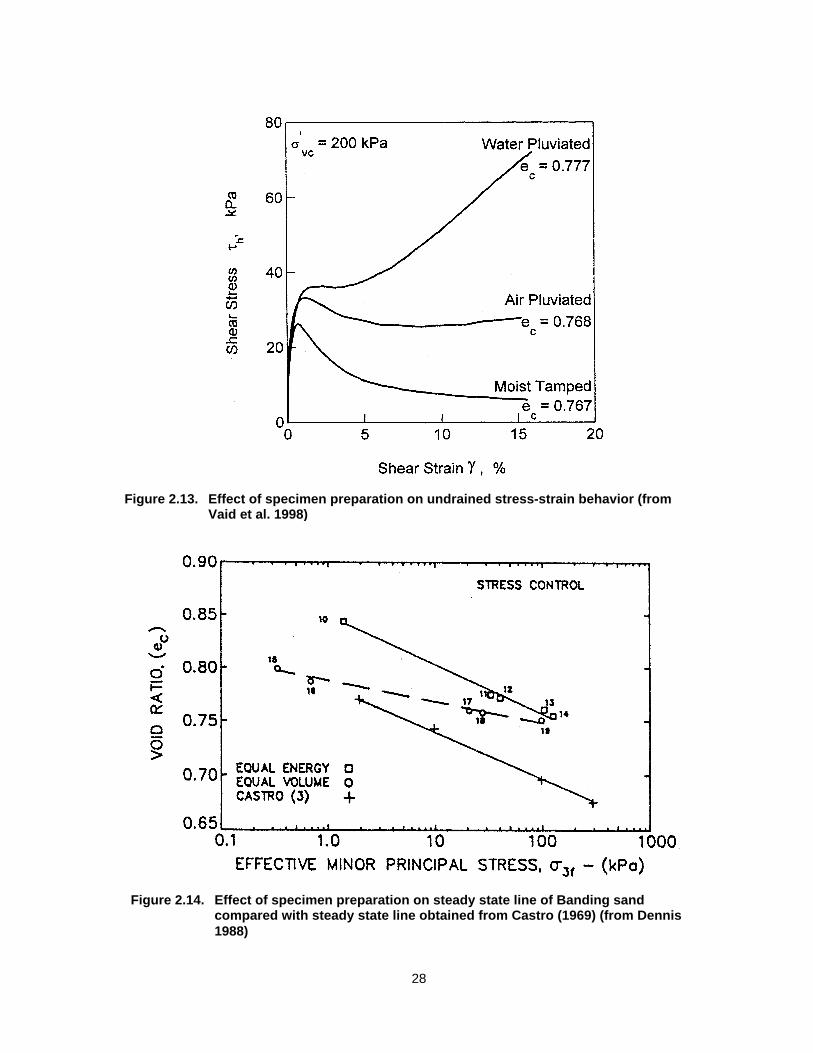
28

Figure 2.13. Effect of specimen preparation on undrained stress-strain behavior (fromVaid et al. 1998)

Figure 2.14. Effect of specimen preparation on steady state line of Banding sandcompared with steady state line obtained from Castro (1969) (from Dennis1988)

29

Figure 2.15. Effect of specimen preparation on steady state line of Erksak sand (fromBeen et al. 1991). e is void ratio and p’ is mean effective stress.

Figure 2.16. Effect of sample preparation on steady state line of Syncrude tailings sand(from Poulos et al. 1988).

30

Figure 2.17. Effect of sample preparation on steady state line of Toyoura sand (fromIshihara 1993)

Figure 2.18. Effect of grain crushing on steady state line of three sands (from Konrad 1998)

31

CHAPTER 3

LEVEL GROUND LIQUEFACTION RESISTANCE USING CASEHISTORIES AND CPT

3.1 INTRODUCTION

Peck (1979) stated that due to difficulties in understanding and modeling all of the

factors that affect the liquefaction resistance of a soil, in situ penetration testing is the

preferred method to estimate liquefaction resistance. Typical in situ penetration testing

includes the cone penetration test (CPT) and the standard penetration test (SPT). Because

the SPT is subject to numerous corrections including energy ratio, overburden correction,

borehole diameter, rod length, and sampling method (Youd and Idriss, eds., 1997), several

researchers (e.g., Robertson and Campanella 1985, Seed and de Alba 1986, Shibata and

Teparaksa 1988, Stark and Olson 1995, etc.), have investigated the use of the cone

penetration test to estimate the level ground liquefaction resistance of sandy soils.

The CPT offers several advantages over the SPT including:

• It can be more economical to perform than the SPT, which allows a more

comprehensive subsurface investigation.

• The test procedure is simpler, more standardized, and more reproducible than

the SPT.

• It provides a continuous record of penetration resistance throughout a soil

deposit, which provides a better description of soil variability and allows thin

(greater than 15 cm in thickness) liquefiable sand or silt seams to be located and

32

properly characterized. This is particularly important in sands and silts because

of the natural non-uniformity of these deposits.

Based on these advantages, it is desirable to develop relationships between CPT tip

resistance and liquefaction resistance, rather than relying on a conversion from SPT

blowcount to CPT tip resistance to develop CPT based liquefaction resistance relationships.

The main reasons why the CPT has not been used extensively for liquefaction

assessment are:

• The lack of a sample for soil classification and grain size analyses.

• A limited amount of CPT based field data pertaining to liquefaction resistance

was available.

• Limited availability of cone penetration test equipment in some locales.

Recently, the number of field case histories of liquefaction and non-liquefaction

where CPT results are available has increased significantly. Stark and Olson (1995)

compiled 180 field case histories of liquefaction and non-liquefaction to develop

relationships between liquefaction resistance and corrected CPT tip resistance. In

developing some of these case histories, more than one elevation within a single sounding

was evaluated. The evaluation performed by Stark and Olson (1995) was based on the

zones of liquefaction estimated by the original investigators. In nearly every case, the CPT

sounding was conducted shortly after the earthquake, and no correction was made to the

CPT tip resistance to account for any possible densification effects resulting from

earthquake shaking. It should be noted that no corrections are made in SPT blowcount to

account for post-earthquake densification in the current SPT case history database (T.L.

Youd, Brigham Young University, personal communication, 1999).

33

Olson and Stark (1998) re-evaluated these case histories so that only one critical

layer is considered per sounding. This reduced the database to 80 cases. In addition, 92

case histories of liquefaction and non-liquefaction presented by Suzuki et al. (1995) and

Boulanger et al. (1997) were added to the revised database. The revised database now

contains 172 field case histories of liquefaction and non-liquefaction, and confirms the

liquefaction resistance relationships proposed by Stark and Olson (1995). In comparison,

the SPT based liquefaction resistance relationships published by Seed et al. (1985) are

based on only 125 liquefaction and non-liquefaction case histories. The proposed CPT

relationships are compared with existing CPT based liquefaction resistance relationships

and liquefaction field case histories where SPT blowcounts are converted to CPT tip

resistance to investigate agreement among existing methods. Lastly, the liquefaction

resistance of clean and silty gravel is estimated from 18 field case histories where CPT

results are available.

3.2 CYCLIC STRESS METHOD

Seed and Idriss (1971) developed a procedure termed the “simplified,” or “cyclic

stress,” method, to evaluate the liquefaction resistance of sandy soils using relative density

and the shear stresses induced by earthquake loading. Since 1971, the cyclic stress method

has seen a number of updates and improvements, including the use of in situ penetration

tests as a measure of liquefaction resistance. In a later update, Seed et al. (1985) proposed

boundary lines that separate conditions causing liquefaction from conditions not causing

liquefaction in sandy soils, as shown in Figures 3.1 and 3.2, for an earthquake magnitude

(M) of 7.5. These correlations remain the standard of practice for the evaluation of level

ground liquefaction resistance using the standard penetration test (SPT) in many parts of

34

the world. In the cyclic stress method, earthquake-induced stresses are represented by the

cyclic stress ratio and soil resistance to porewater pressure increase is represented by in

situ penetration resistance, either corrected SPT blowcount (Seed et al. 1985) or corrected

CPT tip resistance (Robertson and Campanella 1985).

3.2.1 Evaluation of Cyclic Stress Ratio

Seed et al. (1985) used equivalent cyclic stress ratio, CSReq, to represent the

intensity of earthquake loading. Since CSReq pertains to a certain number of equivalent

laboratory loading cycles corresponding to a given earthquake magnitude, Stark and Mesri

(1992) proposed the term seismic (shear) stress ratio, SSR, to describe earthquake loading.

They suggested that SSR is more descriptive of field earthquake loading than equivalent

cyclic stress ratio. This was also suggested because liquefaction resistance is being

evaluated using field performance data, not laboratory test results.

Seed and Idriss (1971) proposed the “simplified” equation to estimate the equivalent

cyclic shear stress ratio (or seismic shear stress ratio) induced by an earthquake. The

resulting seismic (shear) stress ratio is defined as:

dvo

vo

vovo

aveeq r

g

aCSRSSR

'65.0

'65.0

'maxmax

σσ

στ

στ

≈≈== (3.1)

where τave is the average earthquake-induced shear stress, τmax is the maximum

earthquake-induced shear stress, σ'vo is the vertical effective stress, amax is the maximum

earthquake acceleration at the ground surface, g is the acceleration of gravity, σvo is the

vertical total stress, and rd is a depth reduction factor to account for the flexibility of the soil

35

column. Seed and Idriss (1971) presented the relation in Figure 3.3 to estimate rd. For this

study, the depth reduction factor was estimated as:

)012.0(1 zrd ⋅−= (3.2)

where z is depth in meters (Kayen et al. 1992). Seed and Idriss (1971) suggested the factor

0.65 to account for the difference between the maximum shear stress and the average

shear stress induced by an earthquake. The value of SSR is then corrected to an

earthquake (moment) magnitude (M) of 7.5 by dividing the SSR by the magnitude scaling

factor CM proposed by Seed and Idriss (1982). The magnitude scaling factor used for this

study is shown in Figure 3.4.

3.2.2 Evaluation of SPT Penetration Resistance

Seed et al. (1985) used corrected blowcount (N1)60 to represent soil resistance to

porewater pressure increase because of the variability of SPT systems. The corrected

blowcount, (N1)60, is defined as the SPT blowcount at a vertical effective stress of 100 kPa

and an energy level equal to 60% of the theoretical free-fall hammer energy applied to the

drill stem. Seed et al. (1985) proposed a "standard" blowcount, N60, which corresponds to a

transfer of approximately 60% of the theoretical free-fall hammer energy. Seed et al. (1985)

suggested the following equation to correct various SPT energy ratios to an energy ratio of

60% for use in liquefaction analyses:

⋅=

6060ER

NN (3.3)

36

where ER is the energy ratio (percent of the theoretical free-fall energy) of the SPT hammer

system and N is the field blowcount. The value of N60 is corrected to a vertical effective

stress of approximately 100 kPa by multiplying N60 by the overburden correction factor, CN,

which (as presented below) is slightly modified from Liao and Whitman (1986):

( )n

vo

aN

PNCNN

⋅=⋅=

'6060601 σ(3.4)

where Pa is one atmosphere of pressure in the units of σ'vo, and n is equal to 0.5 for sands.

For simplicity, n equal to 0.5 was used for all soils in this study.

The value of (N1)60 must then be corrected for borehole diameter, rod length, and

sampling spoon configuration (Youd and Idriss 1997).

3.2.3 Evaluation of CPT Penetration Resistance

Penetration resistance from CPT, similar to SPT blowcount, is influenced by soil

density, soil structure, cementation, aging, stress state, and stress history, and thus can be

used to estimate liquefaction resistance (Robertson and Campanella 1985). However, unlike

the SPT, CPT soundings can yield a continuous record of liquefaction resistance with depth

for a potentially liquefiable soil. Furthermore, SPT N-values must be corrected for effective

overburden stress, hammer type and release system, sampler configuration, and drill rod

length (as mentioned previously), while CPT data only needs to be corrected for vertical

effective stress.

The corrected CPT tip resistance, qc1, is obtained as follows:

37

qcc Cqq ⋅=1 (3.5)

where Cq is the CPT based overburden correction factor. Seed et al. (1983) developed an

overburden correction for the CPT, and this correction was later confirmed by Mitchell and

Tseng (1990) using cavity expansion theory to predict qc and qc1 from laboratory tests on

Monterey No. 0, Tincino, and Hokksund sands. Kayen et al. (1992) proposed the following

equation to describe the overburden correction factor proposed by Seed et al. (1983):

+

=

a

voq

P

C'8.0

8.1σ

(3.6)

This relationship provides very similar overburden corrections to Eq. (3.4) for the range of

stresses involved in the case histories presented herein. This study used Eq. (3.6) for most

of the case histories, with the exception of those where overburden information necessary to

utilize the correction was unavailable. In these 56 cases, the correction factor reported by

the original investigator(s) was used. Because the overburden correction factor results in

extremely large corrections to penetration resistance at low vertical effective stresses, a

maximum correction of 2.0 was used for this study.

3.3 CPT BASED LIQUEFACTION RESISTANCE

This study analyzed 172 independent level ground liquefaction and non-liquefaction

case histories compiled by Stark and Olson (1995), Suzuki et al. (1995), and Boulanger et

al. (1997). Table 3.1 presents the case history database. Each case history represents one

38

critical layer within a sounding. Clean sand case histories reported by Suzuki et al. (1995)

were used directly because data required to analyze these case histories are unavailable.

The representative value of qc for the critical layer for each case is the value reported by the

investigator(s), or is determined by averaging the tip resistance over the interval of sampling

where the value of median grain diameter, D50, and fines content were determined (typically

about 0.3 m). Values of qc1 were then calculated using Eq. (3.5). The occurrence of

liquefaction at a site was judged by the investigator(s) from the appearance of sand boils,

settlement and/or damage of overlying structures, ground cracking or lateral ground

spreading. The non-occurrence of liquefaction was assumed by the lack of the

aforementioned evidence.

Seed et al. (1985) showed that fines content (percent by weight passing U.S.

Standard Sieve No. 200) affects the relationship between SPT penetration resistance and

liquefaction resistance (Fig. 3.2). Stark and Olson (1995) anticipated that fines content

would have a similar effect on CPT penetration resistance and liquefaction resistance. Since

gradation and fines content both appear to influence CPT tip resistance, the correlations

proposed herein utilize both D50 and fines content (FC) to describe soil gradation. The CPT

field data were divided into three categories based on fines content (in percent) and D50 (in

mm). The three categories are clean sand (FC ≤ 5 and 0.25 < D50 < 2.0), silty sand (5 < FC

< 35 and 0.10 ≤ D50 ≤ 0.25), and silty sand to sandy silt (FC ≥ 35 and D50 < 0.10). Fines

content refers to non-plastic to low plasticity fines with a clay size fraction less than 15 to

20%, as suggested by Seed et al. (1983). Clay size fraction is defined as the percent by

weight finer than 0.005 mm. Fines content was used to classify most of the case histories,

and where fines content is not available, median grain size was used for classification.

39

3.3.1 Liquefaction Resistance of Clean Sand

Figure 3.5 presents a compilation of 105 liquefaction and non-liquefaction case

histories involving clean sand where CPT data are available. The boundary line presented

by Stark and Olson (1995) for clean sand is included in Figure 3.5. It can be seen that the

Stark and Olson (1995) relationship is in good agreement with the available case histories,

with only six case histories plotting below the boundary line. As noted by Stark and Olson

(1995), the relationship for clean sand is limited to values of D50 less than 2.0 mm because:

(1) liquefaction case histories in soils with D50 greater than 2.0 mm where CPT results are

available are limited; and (2) the use of a standard cone penetrometer (ASTM D3441) in

coarse sand and gravel (gravel content as low as 5%) may result in artificially large values of

qc.

Six cases of observed liquefaction fall below the boundary line. The case with a qc1

value of about 8.0 MPa and an SSR of 0.14 is touching the boundary line and does not

require additional consideration. The cases with [qc1 (MPa), SSR] values of (7.9, 0.11),

(12.2, 0.17) and (15, 0.30) were obtained from Suzuki et al. (1995) and no further scrutiny of

the data was possible. The case with a qc1 value of 12.3 MPa and an SSR of 0.17 was

reported by Boulanger et al. (1997). This case involved a layer of sand that was significantly

looser in its upper portion than in its lower portion. It is possible that liquefaction occurred in

the upper portion first, and porewater pressure re-distribution led to the liquefaction of the

lower portion. If this were the case, the representative qc1 value would be lower. The case

with a qc1 value of 10.2 MPa and an SSR of 0.15 represented a sounding that was

conducted in an area that liquefied, but was very near an area of no liquefaction. Therefore,

the reported tip resistance would be on the borderline of non-liquefiable soils.

40

Figure 3.6 compares the Stark and Olson (1995) liquefaction resistance relationship

with several existing liquefaction resistance correlations for clean sand and M 7.5. The

Mitchell and Tseng (1990) relationships for D50 = 0.40 mm and D50 = 0.20 mm are not

included in Fig. 3.6 because they nearly coincide with the relationships proposed by Shibata

and Teparaksa (1988) for D50 > 0.25 mm and Seed and de Alba (1986) for D50 = 0.8 and FC

< 5%, respectively. The Stark and Olson (1995) relationship agrees well with the Robertson

and Campanella (1985) relationship for values of SSR between 0.13 and 0.25. At values of

SSR less than 0.13 and greater than 0.25, the Stark and Olson (1995) relationship differs

from the Robertson and Campanella (1985) relationship. At values of SSR less than 0.13,

the Stark and Olson (1995) relationship can be extended to the origin as indicated by the

SPT and CPT based clean sand liquefaction resistance relationships proposed by Seed et

al. (1985) and Seed and de Alba (1986), respectively. At values of SSR greater than 0.25,

the Stark and Olson (1995) relationship is less conservative than the Robertson and

Campanella (1985) relationship. It should be noted that Stark and Olson (1995) developed

this relationship (and those that follow) using a different database.

The Seed and de Alba (1986) relationships were developed by converting the (N1)60

values corresponding to the SPT based clean sand liquefaction resistance relationship

(Figure 3.1; Seed et al. 1985) to qc1 values for various values of D50 using the qc/N60

relationship that they proposed, rather than utilizing case histories in which CPT data are

available. The Seed and de Alba (1986) qc/N60 relationship is shown in Figure 3.7 and will be

discussed subsequently.

Robertson and Campanella (1985) also used the Seed et al. (1984) SPT database to

develop CPT based liquefaction resistance relationships for clean sand and silty sand. The

SPT N values from the case histories presented by Seed et al. (1984) were converted to

41

CPT qc values using the Robertson and Campanella (1985) SPT-CPT conversion (also

shown in Figure 3.7). The Robertson and Campanella (1985) conversion differs from the

Seed and de Alba (1986) conversion for values of D50 greater than approximately 0.02 mm,

and thus explains the difference in these liquefaction resistance relationships.

Ishihara (1985) developed a liquefaction resistance relationship for clean sand

(Figure 3.6) using data in which field CPT qc values are available at the site of soil sampling,

and the corresponding cyclic shear strengths were determined from laboratory cyclic triaxial

tests. In summary, the Ishihara (1985) liquefaction resistance relationship for clean sand

does not use field case histories and is less conservative than the Stark and Olson (1995)

relationship.

Shibata and Teparaksa (1988) used a smaller database of field case histories

primarily from Japan and China where CPT qc values were available to develop liquefaction

resistance relationships. They developed a grain size correction to correct or calibrate qc

values of soils with D50 less than 0.25 mm to correspond to qc values obtained in clean

sands (D50 ≥ 0.25 mm). Shibata and Teparaksa (1988) assumed that the boundary between

liquefied and non-liquefied data is hyperbolic. This led to the development of a hyperbolic

equation relating qc1 to SSR with a correction for D50 < 0.25 mm. The equation was used to

estimate liquefaction resistance boundaries for soils with D50 < 0.25 mm. By inserting

various values of D50 < 0.25 mm into their equation, Shibata and Teparaksa (1988)

calculated liquefaction potential relationships for silty sand (D50 = 0.20 mm and D50 = 0.15

mm) and silty sand to sandy silt (D50 = 0.10 mm and D50 = 0.05 mm), which will be

presented subsequently.

Mitchell and Tseng (1990) developed two theoretical liquefaction resistance curves

for clean sand (D50 = 0.40 mm and D50 = 0.20 mm) based on laboratory measured values of

42

cyclic shear strength and theoretical values of CPT tip resistance predicted using cavity

expansion theory. As mentioned above, the relationship for D50 = 0.40 mm agrees with the

Stark and Olson (1995) clean sand liquefaction resistance relationship for values of SSR

less than 0.25. The relationship for D50 = 0.20 mm is less conservative than the Stark and

Olson (1995) relationship except for values of SSR greater than 0.35.

In summary, the proposed liquefaction resistance relationship presented in Fig. 3.6 is

generally in agreement with existing relationships. However, previous studies relied upon a

grain size correction (Shibata and Teparaksa 1988), a conversion of SPT blowcount to CPT

tip resistance (Robertson and Campanella 1985; Seed and de Alba 1986), or laboratory

cyclic triaxial data with estimated (Mitchell and Tseng 1990) or measured (Ishihara 1985)

values of CPT tip resistance to estimate the liquefaction resistance of clean sand. The Stark

and Olson (1995) relationship is based solely on CPT based liquefaction and non-

liquefaction case histories and utilizes 105 clean sand case histories to predict liquefaction

resistance. Therefore, the Stark and Olson (1995) relationship represents the best estimate

of the field behavior of clean sand during earthquakes using CPT data.

3.3.2 Liquefaction Resistance of Silty Sand


histories involving silty sand for which CPT data are available. The boundary line for silty

sand proposed by Stark and Olson (1995) is included in Figure 3.8. The relationship for silty

sand plots to the left of the relationship for clean sand. The increased fines content and

plasticity of the fines increases liquefaction resistance because the fines may reduce soil

particle movement and porewater pressure generation during shaking. Thus, a higher SSR

may be required to cause liquefaction in silty sand than in clean sand of equal relative

density. In addition, the fines content decreases the permeability and increases the

43

compressibility of the deposit. This results in reduced drainage during penetration, and may

lead to smaller CPT tip resistance in silty sand than in clean sand of equal relative density.

These two factors result in silty sands appearing more resistant to liquefaction than clean

sands of equal relative density.

Figure 3.8 indicates that the Stark and Olson (1995) relationship agrees well with the

available case histories, and only three non-liquefaction case histories plot above the

relationship. These three case histories are near the boundary, and may represent the

transition from liquefiable to non-liquefiable conditions, or the uncertainty in parameters such

as maximum ground acceleration.

The three liquefaction case histories that plot below the boundary line were obtained

from Kayen et al. (1992) and Boulanger et al. (1997) as shown in Table 3.1. The two cases

with qc1 values of 10 MPa with values of SSR near 0.2 represent cases where the tip

resistance and soil type changed considerably over the layer interval (from clean sand to

silty sand). If these soils were considered clean sands, liquefaction would have been

predicted correctly. The case with a qc1 value of 8.5 MPa and an SSR of 0.2 from Boulanger

et al. (1997) represents another case where soil type variations over the layer could have

affected the interpreted critical qc1 value. Further, Boulanger et al. (1997) reported that the

maximum ground acceleration could not be determined accurately, and probably ranged

from 0.2g to 0.3g, with a value of 0.25g used for interpretation. If the higher value of 0.3g is

used to estimate SSR, the data point would plot above the boundary relation.


for silty sand with existing liquefaction resistance correlations for silty sand and M 7.5. The

Stark and Olson (1995) relationship agrees with the Robertson and Campanella (1985)

relationship for silty sand (D50 < 0.15 mm) except for values of SSR less than approximately

44

0.2. The Stark and Olson (1995) relationship also shows good agreement with the Seed and

de Alba (1986) relationship for silty sand (D50 = 0.25 mm and FC ≈ 10%). However, poor

agreement is found with the Seed and de Alba (1986) relationship for silty sand (D50 = 0.20

mm and FC ≈ 15%). The Stark and Olson (1995) relationship plots between the Shibata and

Teparaksa (1988) relationships for values of D50 of 0.15 mm and 0.20 mm.

In summary, existing silty sand liquefaction resistance relationships are sensitive to

changes in D50. This uncertainty may be attributed to a lack of CPT based case histories to

clarify the effect of D50. The Stark and Olson (1995) relationship (Fig. 3.8) encompasses the

range of D50 (0.10 ≤ D50 ≤ 0.25) of existing relationships. As a result, the Stark and Olson

(1995) relationship appears to clarify the effect of D50 on the liquefaction resistance of silty

sand and provides an encompassing relationship.

3.3.3 Liquefaction Resistance of Silty Sand to Sandy Silt


histories involving silty sands and sandy silts where CPT data are available. The boundary

line for silty sand to sandy silt proposed by Stark and Olson (1995) is included in Figure

3.10. The Stark and Olson (1995) relationship is a slight modification of the relationship for

silty sand (D50 = 0.10 mm and FC ≥ 35%) proposed by Seed and de Alba (1986) to describe

recently obtained field data. Figure 3.10 indicates that the Stark and Olson (1995)

relationship is in good agreement with available case histories.

Only one of the 21 cases where liquefaction was observed lies outside of the Stark

and Olson (1995) boundary. This case history corresponds to the T-25 sounding from the

1976 Tangshan earthquake (Shibata and Teparaksa 1988). As noted by Stark and Olson

45

(1995), the investigators reported the anomalously large qc1 value without explanation, and

no further scrutiny is possible.

Two non-liquefaction cases plot above the Stark and Olson (1995) boundary. The

case history with an SSR of approximately 0.22 plots near the boundary and probably

represents the transition from liquefaction to non-liquefaction. The second case history (near

an SSR of 0.15) is the Middle School site from the 1975 Haicheng earthquake. As explained

by Stark and Olson (1995), the soil layer that was reported to have liquefied had a clay

fraction of more than 20%. This large clay size fraction probably accounts for the low qc1

value and a soil with a clay fraction of greater than 15 to 20% is unlikely to show typical

effects of liquefaction. Furthermore, the depth of liquefaction was reported as more than 10

meters. At this depth, surface manifestations of liquefaction may not be readily visible.


for silty sand to sandy silt with existing relationships for silty sand and sandy silt and M 7.5.

The Stark and Olson (1995) relationship is a modification of the Seed and de Alba (1986)

relationship for silty sand to sandy silt (D50 = 0.10 mm and FC ≥ 35%). Modifications to the

Seed and de Alba (1986) relationship were made to encompass the liquefaction case

histories near a value of SSR of 0.13. The Stark and Olson (1995) relationship plots

between the Shibata and Teparaksa (1988) relationships for D50 = 0.10 mm and D50 = 0.05

mm. Robertson and Campanella (1985) and Ishihara (1985) did not present relationships for

silty sand to sandy silt.

3.3.4 Discussion

In summary, fines content and median grain diameter influence the liquefaction

resistance of sandy soils. The revised CPT database confirms the applicability of the Stark

and Olson (1995) relationships to estimate the liquefaction resistance of sandy soils. The

46

Stark and Olson (1995) liquefaction resistance relationships are combined in Figure 3.12.

Figure 3.12 constitutes a design assessment chart that can be used to estimate the

liquefaction resistance of sandy soils for an earthquake M 7.5, a vertical effective stress

between approximately 50 and 150 kPa, and level ground conditions.

As recognized by previous investigators, the main disadvantage of the liquefaction

relationships in Figure 3.12, and thus the use of the CPT in liquefaction assessments, is that

an estimate of fines content and D50 is required. It is possible to estimate fines content from

soil classification charts, e.g., Olsen and Farr (1986), Suzuki et al. (1995), Robertson and

Wride (1997), based on CPT or piezocone (CPTU) values of tip resistance and/or friction

ratio. However, because of the uncertainties in estimating D50 from CPT results, it is

recommended that the CPT be used to delineate zones and/or seams of potentially

liquefiable soils. In zones of potential liquefaction, a sample and blowcount(s) should be

obtained to determine D50, fines content, and to verify liquefaction resistance using similar

SPT based relationships. This combination of CPTs and one or more borings has been used

in practice for many years, and thus should not significantly increase the cost of a site

investigation. Furthermore, the Stark and Olson (1995) CPT based liquefaction resistance

relationships allow the use of CPT data directly and should increase the effectiveness of

liquefaction assessments because of the continuous profile of tip resistance versus depth.

This profile allows the natural variability of sandy deposits to be characterized.

Several researchers have proposed independent CPT liquefaction resistance

relationships (e.g., Suzuki et al. 1995, Robertson and Fear 1997, and Olsen 1998). Youd

and Idriss (1997) concluded that the current state of development of these techniques is

insufficient to advocate their use. However, Gilstrap (1998) showed that CPT methods were

equally or more accurate in the prediction of liquefaction and no liquefaction than the SPT

47

method (Seed et al. 1985). In contrast, this study found insufficient data to develop

independent CPT liquefaction evaluation methods that: (1) differed sufficiently from existing

methods; and (2) were more accurate than the method discussed above and shown in

Figure 3.12. Therefore, this study does not propose an independent CPT liquefaction

evaluation procedure. However, this provides a potential avenue for continued research.

Olson and Stark (1998) also suggest that the use of qc1 values from more than one

critical layer within a single sounding may be justified. This is especially true for soundings

that penetrate strata of significantly different geologic age or penetration resistance. For

example, soundings at Juvenile Hall, California, described by Bennett (1989), penetrate

strata of different geologic age (and significantly different penetration resistance). Bennett

(1989) concluded that portions of the upper, younger stratum (with lower penetration

resistances) liquefied during the 1971 San Fernando Valley earthquake, while the lower,

older stratum (with higher penetration resistances) did not liquefy. Boulanger et al. (1997)

also used data from more than one elevation (layers with significantly different qc1 values)

within a single sounding. Olson and Stark (1998) suggested that lower bound qc1 values

could be obtained from both strata to define the site-specific boundary between liquefaction

and non-liquefaction.

3.4 COMPARISON OF PROPOSED CPT RELATIONSHIPS AND SPTCASE HISTORIES

In order to compare the large database of SPT based liquefaction and non-

liquefaction case histories (Seed et al. 1984) to the Stark and Olson (1995) CPT based

relationships, SPT N values must be converted to CPT qc values. Because of the large

variation in the qc/N60 conversion ratio for a given value of D50, several conversions have

48

been proposed (Figure 3.7). Seed and de Alba (1986), Robertson and Campanella (1985),

and Andrus and Youd (1989) developed conversions for use in liquefaction analyses.

Several conversions over a larger range of D50 also have been proposed for general use,

e.g., Kulhawy and Mayne (1990).

3.4.1 Clarification of SPT-CPT Conversion

Figure 3.7 presents existing SPT-CPT conversions, as well as the Stark and Olson

(1995) SPT-CPT conversion. Figure 3.7 also includes qc/N60 data presented by Seed and de

Alba (1986), Robertson and Campanella (1985), and additional data from field investigations

conducted by Youd and Bennett (1983), Bennett (1989), Bennett (1990), and Kayen et al.

(1992). The additional data exhibit a large variation in the ratio of qc/N60 for a given value of

D50. All SPT data was corrected to a SPT hammer energy of 60% as described previously,

and the data in Figure 3.7 are average values of qc/N60 reported by the investigators for

subsurface layers where CPT and SPT tests were conducted adjacent to one another. It

should be noted that the subsurface layers where adjacent CPT and SPT data are available

did not necessarily liquefy.

The SPT-CPT conversion suggested by Seed and de Alba (1986) is based on

median grain size and remains approximately constant for D50 values greater than

approximately 0.5 mm (Figure 3.7). As a result, Seed and de Alba (1986) used a value of

qc/N60 between 0.42 and 0.51 (MPa/blows/ft), which corresponds to a D50 between 0.25 mm

and 0.8 mm, to convert the SPT (N1)60 values that correspond to the clean sand liquefaction

resistance relationship (Seed et al. 1985) to qc1 values. These qc1 values were used to

develop their CPT liquefaction resistance relationships for clean sand (Seed and de Alba

1986) shown in Figure 3.6.

49

Robertson and Campanella (1985) also proposed an SPT-CPT conversion based on

median grain size, but used an average energy ratio of 55% for SPT N values. For

consistency, the Robertson and Campanella (1985) SPT-CPT conversion and data were

corrected to an energy ratio of 60% using Eq. (3.3), and are presented in Figure 3.7. Their

SPT-CPT conversion indicates that the value of qc/N60 should increase for all values of D50.

Andrus and Youd (1989) developed a SPT-CPT conversion by extending the Seed

and de Alba (1986) conversion to account for values of D50 up to 40 to 45 mm. The case

histories used to extend the SPT-CPT conversion involve the 1983 Borah Peak Earthquake

and gravelly soils. It should be noted that Andrus and Youd (1989) found no correlation

between qc and N60 when values of D50 were obtained from SPT samples. Andrus and Youd

(1989) suggested that this lack of agreement is the result of the diameter of the split spoon

sampler being too small to obtain a representative sample of the gravelly soil. However,

values of D50 obtained from 127-mm auger samples produced a logical correlation between

qc and N60 because a more representative value of D50 was obtained. Therefore, the values

of D50 from the 127-mm auger samples were used to extend the SPT-CPT conversion. The

values of CPT tip resistance used by Andrus and Youd (1989) were obtained using an

electric cone with a conical tip area of 15 cm2. This conical tip area is larger than the

standard cone (ATSM D3441), which is 10 cm2. The extended conversion developed by

Andrus and Youd (1989) is considerably lower than the Stark and Olson (1995) conversion.

This may be caused by the N values obtained from the SPT by Andrus and Youd (1989)

being slightly higher than would be expected for clean sand. If the SPT sampler

encountered large soil particles, the N value could be artificially high. Overestimated N

values would result in lower values of qc/N60.

50

The Kulhawy and Mayne (1990) conversion is based on statistical analysis of qc/N60

data from 197 cases, with values of D50 ranging from 0.001 to 10 mm. This database

includes the data from Robertson and Campanella (1985) and Seed and de Alba (1986).

For values of D50 greater than 1 mm, however, the data used by Kulhawy and Mayne (1990)

is limited, and does not include several of the cases from Andrus and Youd (1989).

The Stark and Olson (1995) SPT-CPT conversion was developed by determining the

qc/N60 ratios that yielded the best agreement between SPT liquefaction case histories and

the proposed CPT based liquefaction resistance relationships in Figure 3.12. The Stark and

Olson (1995) SPT-CPT conversion is intermediate to the Seed and de Alba (1986) and

Robertson and Campanella (1985) conversions (Figure 3.7). As expected from the

agreement between the Stark and Olson (1995) and Robertson and Campanella (1985)

clean sand liquefaction resistance relationships (Figure 3.5), the Stark and Olson (1995) and

Robertson and Campanella (1985) SPT-CPT conversions coincide at values of D50 greater

than 0.3 mm. Similarly, the Stark and Olson (1995) and Seed and de Alba (1986) SPT-CPT

conversions coincide at values of D50 less than 0.08 mm. However, the Stark and Olson

(1995) SPT-CPT conversion differs from existing conversions in Figure 3.7 for values of D50

between 0.08 and 0.3 mm. The Stark and Olson (1995) conversion deviates from the Seed

and de Alba (1986) relationship to the Robertson and Campanella (1985) relationship for

values of D50 between 0.08 and 0.3 mm.

Ratios of qc/N60 used to determine the Stark and Olson (1995) SPT-CPT conversion

were estimated by comparing the Stark and Olson (1995) CPT liquefaction resistance

relationships in Figure 3.12 to the Seed and de Alba (1986) SPT liquefaction resistance

relationships Figure 3.2. For example, the CPT clean sand liquefaction resistance

relationship (Figure 3.12) yields a value of qc1 of 12.5 MPa for a SSR of 0.25. In the SPT

51

clean sand liquefaction resistance relationship (Figure 3.2), the value of (N1)60

corresponding to a SSR of 0.25 is 21.8 blows/ft. Therefore the value of qc1/(N1)60 is 12.5

MPa divided by 21.8 blows/ft, or 0.57, at a SSR of 0.25. There is no difference between

qc1/(N1)60 and qc/N60 because Cq is equal to CN at a vertical effective stress of 100 kPa. The

ratio of qc1 (obtained from the CPT clean sand liquefaction relationship in Figure 3.12) to

(N1)60 (obtained from the SPT clean sand liquefaction relationship in Figure 3.2) ranges from

0.49 to 0.64 for all values of SSR. The weighted average value of qc1/(N1)60 for clean sands

is 0.57, which is plotted in Figure 3.7 with the corresponding range at an average D50 of 0.30

mm. Stark and Olson (1995) used this average value of qc1/(N1)60 to develop their SPT-CPT

conversion. The conversion of 0.57 is near the upper boundary of the data in Figure 3.7 for

a value of D50 between 0.2 and 0.3 mm. This suggests that the trend line in Figure 3.7

should increase for values of D50 greater than 0.25 mm rather than remaining constant as

proposed by Seed and de Alba (1986). This increase also agrees with the trend of the

Robertson and Campanella (1985) SPT-CPT conversion.

The process described above was repeated for the silty sand (average D50 of 0.17

mm) and silty sand to sandy silt (average D50 of 0.09 mm) liquefaction resistance

relationships in Figures 3.2 and 3.12. The range and weighted average values of qc1/(N1)60

for these liquefaction resistance relationships are shown in Figure 3.7. Additional support for

the Stark and Olson (1995) SPT-CPT conversion was obtained by determining the qc/N60

ratio required for the marginally liquefied SPT clean sand case histories to coincide with the

CPT based clean sand liquefaction resistance boundary. As shown in Figure 3.7, these data

plot slightly above the Stark and Olson (1995) SPT-CPT conversion and suggest that the

conversion should increase with increasing values of D50.

52

These data guided the development of the Stark and Olson (1995) SPT-CPT

conversion. Prior to this compilation of CPT liquefaction case histories and the comparison

with SPT based liquefaction resistance relationships, an estimate of the accuracy of SPT-

CPT conversions for liquefaction analyses was not available. The Stark and Olson (1995)

SPT-CPT conversion can be used for liquefaction resistance assessments because it is

based on field liquefaction performance and not simply adjacent SPT and CPT data.

However, the Stark and Olson (1995) SPT-CPT conversion is an average trend line, and

there is considerable variance in the data used to develop this conversion. Thus, site

specific conversions, if necessary, are more desirable than any average correlation.

3.4.2 Comparison of CPT Liquefaction Resistance Relationships andSPT Based Field Data

Table 3.2 presents recent level ground liquefaction case histories to augment the

SPT liquefaction case history database for sandy soils presented by Seed et al. (1984). The

SPT N values reported by Seed et al. (1984) and in Table 3.2 for liquefaction case histories

were converted to CPT qc values using the Stark and Olson (1995) SPT-CPT conversion

shown in Figure 3.7. Figures 3.13, 3.14, and 3.15 present the converted SPT based case

histories and the corresponding proposed CPT liquefaction resistance relationships for clean

sand, silty sand, and silty sand to sandy silt, respectively.

The converted SPT data in Figure 3.13 and 3.14 are in good agreement with the

proposed CPT liquefaction resistance relationships. The converted SPT data in Figure 3.15

are in excellent agreement with the proposed CPT liquefaction resistance relationship for

silty sand to sandy silt. Disparity between the SPT data and CPT relationships is typically

caused by the inability of the average SPT-CPT conversion to account for all case histories.

As discussed previously, the conversion proposed in Figure 3.7 represents an average of

53

the variable data. As evident in Figure 3.7, a large deviation from the Stark and Olson

(1995) conversion can exist for individual case histories. This reinforces the need for site-

specific SPT-CPT conversions.

3.5 CPT BASED LIQUEFACTION RESISTANCE OF GRAVELLY SOILS

Although far less common than cases of liquefaction in sandy soils, several case

histories involving liquefaction of gravelly soils have been documented. These case histories

include the 1948 Fukui earthquake (Ishihara 1974), 1964 Alaskan earthquake (Coulter and

Migliaccio 1967), 1975 Haicheng earthquake (Wang 1984), 1976 Tangshan earthquake

(Wang 1984), 1983 Borah Peak earthquake (Andrus and Youd 1987), and 1988 Armenia

earthquake (Yegian et al. 1994). Of these case histories, only the 1983 Borah Peak

earthquake yielded near-level ground liquefaction and non-liquefaction case histories where

CPT tip resistance data are available. Yegian et al. (1994) documented case histories in

which a low permeability layer located directly above the gravelly layer was believed to have

impeded drainage and led to liquefaction failures. Obermeier et al. (2000) indicate that even

a thin fine-grained cap can suffice to impede drainage and allow porewater pressure to

increase during shaking, but it is likely that the areal extent of the cap also needs to be

large. Earthquake magnitudes of M ~ 7 to 7.5 and shaking levels lower than 0.4 to 0.5g were

adequate to trigger liquefaction in the cases cited above. However, gravel-rich deposits

without fine-grained caps can withstand strong shaking (on the order of 0.5 to 1.0g) without

forming liquefaction features (Yegian et al. 1994).

The documented cases of liquefaction during the 1983 Borah Peak earthquake

include both clean and silty gravels. The Pence Ranch, Idaho site is underlain by a clean

gravel, with fines content ranging from 1 to 5%. The Whiskey Springs, Idaho site is underlain

54

by a silty gravel, with fines content ranging from 15 to 30%. Table 3.3 presents the pertinent

data from both Idaho sites.

At both sites, a cone with a conical tip area of 15 cm2, rather than the standard tip

area of 10 cm2, was employed to penetrate the gravelly soils. The values of SSR for the

sites were estimated using Eq. (3.1), identical to the sandy soil case histories. No correction

was employed for gravel content.

Figure 3.16 presents the available case histories for gravelly soils (D50 ≥ 2.0 mm).

The fines content of each of the case histories is displayed next to the data point. Stark and

Olson (1995) proposed tentative liquefaction resistance relationships for clean gravel (fines

content less than 5%) and silty gravel (fines content approximately 20%) based on the

separation of sites that experienced liquefaction and those that did not experience

liquefaction during the 1983 Borah Peak earthquake. For comparison, the proposed CPT

clean sand and silty sand liquefaction relationships are included in Figure 3.16. The

liquefaction resistance relationships for clean gravel and silty gravel plot above (or to the left

of) the liquefaction resistance relationships for clean sand and silty sand, respectively. This

indicates that gravelly soil exhibits greater liquefaction resistance than sandy soil at a given

SSR. Unfortunately, the data supporting this premise are limited. As more data become

available concerning the field behavior of gravelly soil during earthquakes, the relationships

in Figure 3.16 may need to be re-evaluated.

3.6 SUMMARY

The cone penetration test appears to be better suited to liquefaction assessments

than the standard penetration test because it is more standardized, reproducible, cost

effective, and most importantly, yields a continuous penetration record with depth. The

55

continuous profile is important in sandy soils, because these deposits are inherently non-

uniform. A considerable number of cone penetration tests can be conducted quickly and

economically to identify thick and thin layers of liquefiable soil, which may be cost prohibitive

with standard penetration tests.

Olson and Stark (1998) presented a revised database of 172 field case histories

where liquefaction was and was not observed in sandy soils and CPT tip resistance is

available. These data were used to confirm the Stark and Olson (1995) relationships

between soil resistance to liquefaction and corrected CPT tip resistance for clean sand, silty

sand, and silty sand to sandy silt and an earthquake magnitude of 7.5. The Stark and Olson

(1995) CPT liquefaction resistance relationships were developed to describe field case

histories where CPT data are available, and preclude the need to convert SPT blowcounts

to CPT tip resistance.

Stark and Olson (1995) presented tentative liquefaction resistance relationships for

clean gravel and silty gravel and an earthquake magnitude of 7.5 based on 18 liquefaction

and non-liquefaction field case histories. An electrical cone with a conical tip area of 15 cm2,

instead of the standard conical tip area of 10 cm2, was used penetrate the gravelly soils.

These relationships indicate that the liquefaction resistance of gravelly soil is greater than

the liquefaction resistance of sandy soil.

The main disadvantage of the CPT is the lack of a sample for soil classification and

grain size analyses. Since liquefaction resistance depends on fines content and median

grain size, it is recommended that a sample and blowcount(s) be obtained in potentially

liquefiable soil to determine D50, fines content, and verify liquefaction resistance using

similar SPT based relationships. The combination of CPTs and SPTs has been used in

practice for many years, and thus should not significantly increase the cost of a site

56

investigation. However, the proposed CPT liquefaction resistance relationships allow CPT

data to be used directly in liquefaction assessments instead of relying on a conversion of

CPT tip resistance to SPT blowcount.

Finally, the revised database considers only one critical layer per sounding.

However, Olson and Stark (1998) suggested that it may be acceptable to use more than one

critical value of qc1 from each sounding, provided that the critical values of qc1 represent soil

strata of different geologic age or significantly different penetration resistance. If this practice

is used for analysis of liquefied sites, there should be sufficient supporting evidence to

clearly define the zones of liquefaction. Such evidence might include inclinometer data

showing zones of lateral deformation due to liquefaction, or grain size analyses showing

similarities between surface ejecta and likely source beds.

57

Site M=7.5Ground Vertical Vertical Median Seismic SeismicWater Total Effective Grain Fines CPT Site Shear Shear

Case Liquefaction Depth Depth Stress Stress Diameter Content qc qc1 amax Stress StressRecord Site Sounding Observed? (m) (m) (kPa) (kPa) (mm) (%) (MPa) Cq (MPa) (g) rd Ratio Ratio Reference

(1) (2) (3) (4) (5) (6) (7) (8) (9) (10) (11) (12) (13) (14) (15) (16) (17) (18)

1 Kwagishi-Cho Yes 4.6 1.1 85.3 51.0 0.33 0-5 1.57 1.38 2.17 0.16 0.94 0.16 0.16 Shibata &2 Building Yes 4.8 2.0 89.2 61.8 0.33 0-5 5.34 1.28 6.82 0.16 0.94 0.14 0.14 Teparaksa

(1988)3 South Bank No 4.5 0.5 84.3 45.1 0.30 0-5 7.85 1.45 11.34 0.16 0.95 0.18 0.18

4 Juvenile Hall, 2 -B1 Yes 8.5 8.4 167.6 166.1 0.058 62 6.37 0.74 4.70 0.50 0.90 0.29 0.25 Bennett5 California 4 - B2 Yes 8.4 5.8 164.0 138.9 0.045 71 0.69 0.83 0.57 0.50 0.90 0.35 0.29 (1989)6 6 - B1 Yes 4.6 4.3 89.8 86.8 0.042 74 0.69 1.09 0.75 0.50 0.95 0.32 0.267 10 - B1 Yes 5.8 4.7 113.7 103.3 0.055 65 0.69 0.99 0.68 0.50 0.93 0.33 0.288 11 - B1 Yes 6.3 5.9 122.7 119.7 0.051 61 1.96 0.91 1.78 0.50 0.93 0.31 0.26

9 Paper Mill Site Yes 4.0 1.5 74.6 50.0 0.07 72 0.65 1.43 0.93 0.15 0.95 0.14 0.14 Arulanandanet al. (1986)

10 Glass Fibre Site Yes 3.0 1.5 55.9 41.2 0.08 42 0.53 1.53 0.81 0.15 0.96 0.13 0.13

11 Construction Building Site Yes 7.0 1.5 130.5 76.5 0.02 83 0.38 1.16 0.44 0.15 0.92 0.15 0.15

12 Fishery and Shipbuilding Site Yes 3.5 1.5 65.2 45.6 0.016 90 1.30 1.44 1.87 0.15 0.96 0.13 0.13

13 Middle School Site No 10.3 1.5 191.0 105.2 0.016 92 0.73 0.98 0.71 0.15 0.88 0.16 0.15

14 Chemical Fibre Site Yes 7.5 1.5 139.8 80.9 0.035 61 1.20 1.13 1.35 0.15 0.91 0.15 0.15

15 Tangshan T-10 Yes 7.8 1.5 145.1 83.4 0.25 n/a 5.59 1.11 6.20 0.40 0.91 0.41 0.42 Shibata &16 Area T-11 Yes 1.3 0.9 24.5 20.6 0.17 n/a 0.98 1.79 1.76 0.40 0.98 0.30 0.32 Teparaksa17 T-12 Yes 3.0 1.6 55.9 42.2 0.14 n/a 2.55 1.48 3.77 0.40 0.96 0.33 0.34 (1988)18 T-13 Yes 2.0 1.1 37.3 28.4 0.12 n/a 1.67 1.67 2.78 0.40 0.98 0.33 0.3419 T-14 Yes 1.5 1.3 28.4 26.5 0.17 n/a 5.39 1.70 9.15 0.40 0.98 0.27 0.2820 T-15 Yes 1.8 1.0 33.3 25.5 0.48 n/a 1.16 1.71 1.98 0.40 0.98 0.33 0.3421 T-16 No 4.0 3.5 74.5 69.6 0.16 n/a 11.25 1.21 13.61 0.40 0.95 0.26 0.2722 T-17 No 3.1 2.8 57.9 54.9 0.21 n/a 11.17 1.34 14.98 0.20 0.96 0.13 0.1423 T-18 Yes 4.7 3.6 87.3 76.5 0.17 n/a 1.62 1.16 1.87 0.20 0.94 0.14 0.1424 T-19 Yes 1.5 1.1 28.4 24.5 0.19 n/a 1.01 1.73 1.74 0.20 0.98 0.15 0.1525 T-20 No 1.7 1.1 31.4 25.5 0.17 n/a 12.81 1.71 21.92 0.20 0.98 0.16 0.16

(d) 1976 Tangshan Earthquake (M 7.8)

(a) 1964 Niigata Earthquake (M 7.5)

Table 3.1. Database of CPT based Liquefaction and Non-Liquefaction Case Histories in Sandy Soils

(b) 1971 San Fernando Valley Earthquake (M 6.4)

(c) 1975 Haicheng Earthquake (M 7.3) (Ying-Kou City)

58

(1) (2) (3) (4) (5) (6) (7) (8) (9) (10) (11) (12) (13) (14) (15) (16) (17) (18)

26 T-21 No 3.3 3.1 61.8 59.8 0.26 n/a 8.94 1.29 11.58 0.20 0.96 0.13 0.1327 T-22 Yes 3.7 0.8 68.6 40.2 0.16 n/a 1.90 1.50 2.86 0.20 0.96 0.21 0.2228 T-23 Yes 3.7 1.4 68.6 46.1 0.14 n/a 2.20 1.43 3.15 0.20 0.96 0.19 0.1929 T-24 Yes 3.2 1.0 59.8 38.2 0.16 n/a 2.94 1.53 4.50 0.20 0.96 0.20 0.2030 T-25 Yes 8.2 0.7 153.0 79.4 0.08 n/a 8.83 1.14 10.03 0.20 0.90 0.23 0.2331 T-26 Yes 5.2 0.8 97.1 53.9 0.14 n/a 1.96 1.35 2.65 0.10 0.94 0.11 0.1132 T-27 Yes 5.0 0.7 93.2 51.0 0.07 n/a 1.08 1.38 1.49 0.20 0.94 0.22 0.2333 T-28 No 11.4 0.7 212.8 107.9 0.08 n/a 6.37 0.97 6.15 0.10 0.86 0.11 0.1134 T-29 No 5.3 1.0 99.0 56.9 0.10 n/a 2.45 1.32 3.24 0.10 0.94 0.11 0.1135 T-30 No 6.0 2.5 111.8 77.5 0.25 n/a 13.85 1.15 15.93 0.10 0.93 0.09 0.0936 T-31 Yes 3.1 2.3 57.9 50.0 0.16 n/a 2.68 1.39 3.72 0.20 0.96 0.14 0.1537 T-32 Yes 3.8 2.3 70.6 55.9 0.21 n/a 2.88 1.33 3.84 0.20 0.95 0.16 0.1638 T-33 Yes 5.0 2.3 93.2 66.7 0.32 n/a 5.74 1.23 7.08 0.20 0.94 0.17 0.1839 T-34 Yes 2.6 2.5 48.1 47.1 0.13 n/a 1.84 1.42 2.62 0.20 0.97 0.13 0.1340 T-35 Yes 3.9 2.9 72.6 62.8 0.17 n/a 2.50 1.27 3.17 0.20 0.95 0.14 0.1541 T-36 No 6.0 2.3 111.8 75.5 0.22 n/a 7.85 1.16 9.14 0.20 0.93 0.18 0.18

42 Lutai Area L-1 No 12.0 0.4 223.6 110.6 0.067 n/a 4.46 0.95 4.25 0.20 0.86 0.23 0.2343 L-2 Yes 11.2 0.2 208.9 101.8 0.067 n/a 1.42 1.00 1.42 0.20 0.87 0.23 0.2444 L-3 Yes 11.5 0.4 214.8 104.6 0.067 n/a 1.75 0.98 1.71 0.20 0.86 0.23 0.2445 L-4 No 11.1 0.8 206.9 106.5 0.067 n/a 7.49 0.97 7.28 0.20 0.87 0.22 0.23

46 Dimbovitza Yes 7.0 1.0 130.4 71.6 0.20 n/a 1.29 1.19 1.55 0.22 0.92 0.24 0.23 Shibata &(Site 1) Teparaksa

(1988)

47 Heber Road A2 Yes 4.0 2.1 62.8 44.5 0.11 15-20 1.80 1.45 2.56 0.60 0.95 0.52 0.46 Youd &Bennett

48 River Park Unit C Yes 5.0 0.2 78.5 31.6 0.15 20 4.90 1.62 7.94 0.20 0.94 0.30 0.26 (1983)

49 Noshiro-Cho No 3.1 2.0 56.9 47.1 0.32 n/a 9.81 1.42 13.96 0.23 0.96 0.17 0.18 Shibata &Teparaksa

50 Yes 2.8 2.1 53.0 45.1 0.32 n/a 1.76 1.45 2.54 0.23 0.97 0.17 0.17 (1988)

51 Ferland, Yes 4.5 1.8 90.0 63.0 0.10 15 2.76 1.27 3.49 0.25 0.95 0.22 0.16 Tuttle etQuebec, Canada al. (1990)

52 San Fransisco MAR1 No 5.8 2.3 118.4 84.0 0.303 5 16.75 1.10 18.51 0.24 0.93 0.20 0.19 Bennett53 Marina MAR2 No 3.4 2.7 69.4 63.0 0.239 3 9.75 1.27 12.34 0.24 0.96 0.16 0.16 (1990)54 District MAR3 No 6.9 2.7 140.9 100.1 0.350 4 13.00 1.01 13.08 0.24 0.92 0.20 0.19

Table 3.1. (Cont.) Database of CPT based Liquefaction and Non-Liquefaction Case Histories in Sandy Soils

(e) 1977 Vrancea Earthquake (M 7.2)

(f) 1979 Imperial Valley Earthquake (M 6.6)

(g) 1983 Nihonkai-Cho Earthquake (M 7.7)

(h) 1988 Sanguenay Earthquake (M 5.9)

(i) 1989 Loma Prieta Earthquake (M 7.1)

59

(1) (2) (3) (4) (5) (6) (7) (8) (9) (10) (11) (12) (13) (14) (15) (16) (17) (18)

55 MAR4 Yes 6.1 2.9 115.0 83.6 0.160 21 0.75 1.11 0.83 0.24 0.93 0.20 0.1956 MAR5 Yes 6.4 2.4 120.6 81.8 0.197 3 1.20 1.12 1.34 0.24 0.92 0.21 0.2057 MAR6 No 7.0 5.5 131.9 117.1 0.244 6 5.50 0.92 5.06 0.24 0.92 0.16 0.15

58 Leonardini 39 Yes 2.3 1.4 45.6 36.4 0.10 20-25 1.30 1.55 2.02 0.14 0.97 0.11 0.10 Charlie et59 Farm 38 Yes 2.2 1.7 44.1 39.5 0.10 20-25 1.50 1.51 2.27 0.14 0.97 0.10 0.09 al. (1994)60 37 No 3.0 2.1 60.4 51.8 0.12 20-25 2.50 1.37 3.43 0.14 0.96 0.10 0.10

61 Port of POR2 Yes 5-7 2.5 108.9 66.2 0.07 57 1.7 1.24 2.11 0.16 0.93 0.15 0.14 Kayen et62 Richmond POR3 Yes 5-7 2.5 108.9 66.2 0.07 57 1.9 1.24 2.35 0.16 0.93 0.15 0.14 al. (1992)63 POR4 Yes 5-7 2.5 108.9 66.2 0.07 57 1.5 1.24 1.86 0.16 0.93 0.15 0.14 and

Mitchell64 San Francisco- SFOBB1 Yes 5-7.5 2.0 128.8 87.1 0.27 7 4.7 1.08 5.10 0.29 0.93 0.26 0.24 et al. (1994)65 Oakland Bay SFOBB2 Yes 6-9 2.0 154.5 100.6 0.26 12 10.0 1.00 10.04 0.29 0.91 0.26 0.2566 Bridge SFOBB3 Yes 6-8 2.0 154.5 100.6 >0.25 n/a 9.0 1.00 9.00 0.29 0.91 0.26 0.2567 SFOBB4 Yes 6-8 2.0 154.5 100.6 >0.25 n/a 5.0 1.00 5.00 0.29 0.91 0.26 0.2568 SFOBB5 Yes 6-8 2.0 154.5 100.6 >0.25 n/a 9.4 1.00 9.40 0.29 0.91 0.26 0.25

69 Port of POO7-1 Yes 5-8 3.0 130.5 91.2 >0.25 0-5 11.7 1.06 12.38 0.29 0.92 0.25 0.2370 Oakland POO7-2 Yes 5-7 3.0 111.8 82.4 0.30 3 8.7 1.12 9.71 0.29 0.93 0.24 0.2271 POO7-3 Yes 4-7 3.0 116.5 84.6 0.30 5 6.5 1.10 7.15 0.29 0.93 0.24 0.2272 POO7-4 No 7-12 3.0 177.1 113.3 >0.25 0-5 n/a 0.94 17.00 0.29 0.89 0.26 0.2473 POO7-5 Yes 4-6 3.0 93.2 73.6 >0.25 0-5 n/a 1.18 12.00 0.29 0.94 0.22 0.2274 POO7-6 Yes 4-7 3.0 102.5 78.0 >0.25 0-5 n/a 1.15 10.00 0.29 0.93 0.23 0.22

75 Oakland ACPT3 Yes 2-5 2.0 65.2 50.5 0.22 10 n/a 1.39 10.00 0.27 0.96 0.22 0.2076 Airport ACPT4 Yes 2-5 2.0 65.2 50.5 0.22 10 n/a 1.39 5.00 0.27 0.96 0.22 0.2077 ACPT7 Yes 2-5 2.0 65.2 50.5 0.22 10 5.3 1.39 7.35 0.27 0.96 0.22 0.20

78 Bay Farm BFI-P6 Yes 2-5 2.0 65.2 50.5 0.22 10 6.1 1.39 8.45 0.30 0.96 0.24 0.2379 Island BFI-DIKE No 3-5 2.0 74.6 54.9 0.22 20 26.0 1.34 34.87 0.30 0.95 0.25 0.2480 BFI-CPT1 Yes 2-4 2.0 55.9 46.1 0.22 n/a n/a 1.43 10.00 0.30 0.96 0.23 0.21

81 Moss Landing UC-14 Yes 3 1.8 n/a 40.9 0.28 1 3.8 1.50 5.68 0.25 0.96 0.20 0.18 Boulanger82 Area, UC-15 Yes 3 1.8 n/a 40.9 0.28 1 3.0 1.50 4.49 0.25 0.96 0.20 0.18 et al. (1997)83 State Beach UC-16 Yes 2.3 2.3 n/a 37.4 0.4 1 6.6 1.54 10.16 0.25 0.97 0.16 0.1584 UC-17 Yes 4.4 2.6 n/a 59.3 0.4 1 5.4 1.30 7.01 0.25 0.95 0.20 0.1885 UC-18 No 4 3.4 n/a 61.2 0.6 1 16.4 1.28 21.02 0.25 0.95 0.17 0.15


60

(1) (2) (3) (4) (5) (6) (7) (8) (9) (10) (11) (12) (13) (14) (15) (16) (17) (18)

86 Moss Landing UC-4 Yes 2.5 1.8 n/a n/a 0.8 2 7.7 1.60 12.32 0.25 0.97 0.19 0.1787 Area, UC-3 No 2.5 1.7 n/a n/a 0.7 4 8.7 1.60 13.92 0.25 0.97 0.20 0.1888 Sandholdt RC-1 Yes 1.4 1.4 n/a n/a 0.4 4 3.0 1.60 4.80 0.25 0.98 0.16 0.1589 Road UC-2 No 1.9 1.7 n/a n/a 0.7 4 10.4 1.60 16.64 0.25 0.98 0.17 0.1690 RC-4 Yes 5 1.8 n/a 60.3 0.6 1 9.0 1.29 11.61 0.25 0.94 0.23 0.2191 UC-6 No 6.5 1.7 n/a 73.6 0.6 1 15.5 1.18 18.27 0.25 0.92 0.25 0.22

92 Moss Landing RC-5 No 3.5 1.8 n/a 46.2 0.6 1 15.5 1.43 22.22 0.25 0.96 0.21 0.1993 Area, RC-6 No 4.1 2.6 n/a 56.6 0.6 1 13 1.32 17.22 0.25 0.95 0.20 0.1894 MBARI No. 3 RC-7 No 4.7 3.7 n/a 69.9 0.6 1 9.2 1.21 11.11 0.25 0.94 0.18 0.16

95 Moss Landing RC-9 No 3.5 2.0 n/a 46.8 0.7 4 12.4 1.43 17.69 0.25 0.96 0.21 0.19Area, MBARITechnology

96 Moss Landing CPT-1 No 3.4 1.9 n/a 44.9 0.6 4 8.5 1.45 12.31 0.25 0.96 0.21 0.1997 Area, CPT-2 No 2.5 1.8 n/a n/a 0.6 4 10.4 1.60 16.64 0.25 0.97 0.19 0.1798 MBARI No. 4 CPT-3 No 4.1 2.3 n/a 54.9 0.6 4 9.4 1.34 12.61 0.25 0.95 0.21 0.1999 CPT-4 No 1.9 1.5 n/a n/a 0.6 4 8.4 1.60 13.44 0.25 0.98 0.18 0.16

100 Moss Landing CPT-5 Yes 2.1 1.5 n/a n/a 0.6 4 2.5 1.60 4.00 0.25 0.97 0.19 0.17101 Area, General CPT-6 No 2.6 1.7 n/a n/a 0.6 4 10 1.60 16.00 0.25 0.97 0.20 0.18

Fish

102 Moss Landing UC-12 Yes 4.1 1.9 n/a 52.5 0.2 15 6.2 1.37 8.47 0.25 0.95 0.22 0.20103 Area, Harbor UC-13 Yes 4.1 1.9 n/a 52.5 0.2 15 4.3 1.37 5.87 0.25 0.95 0.22 0.20104 Office UC-20 Yes 4.7 3.0 n/a 65.4 0.3 10 4.1 1.25 5.11 0.25 0.94 0.20 0.18105 UC-21 Yes 4.2 2.7 n/a 58.4 0.3 10 4.9 1.31 6.41 0.25 0.95 0.20 0.18

106 Moss Landing UC-9 Yes 2.9 1.2 n/a n/a 0.4 5 6.6 1.60 10.56 0.25 0.97 0.23 0.21107 Area, UC-10 Yes 2.0 1.0 n/a n/a 0.4 5 3.1 1.60 4.96 0.25 0.98 0.22 0.20108 Woodward UC-11 Yes 2.2 1.0 n/a n/a 0.2 15 3.1 1.60 4.96 0.25 0.97 0.23 0.21109 Marine 15-A Yes 2.9 1.3 n/a n/a 0.4 3 5.1 1.60 8.16 0.25 0.97 0.23 0.21110 14-A Yes 3.6 1.2 n/a 43.1 0.5 3 7.8 1.47 11.46 0.25 0.96 0.24 0.22

111 Moss Landing UC-1 Yes 11.0 2.4 n/a 123.6 0.1 30 4.6 0.89 4.10 0.25 0.87 0.24 0.22112 Area, Marine UC-7 Yes 8.3 1.4 n/a 90.2 0.1 30 4.3 1.06 4.58 0.25 0.90 0.26 0.23113 Laboratory UC-8 Yes 8.6 1.3 n/a 92.0 0.1 30 4.3 1.05 4.53 0.25 0.90 0.26 0.23114 C2 Yes 9.8 2.2 n/a 110.6 0.13 27 3.8 0.95 3.61 0.25 0.88 0.24 0.22115 C3 Yes 4.4 1.5 n/a 53.3 0.8 3 8.2 1.36 11.13 0.25 0.95 0.24 0.22


61

(1) (2) (3) (4) (5) (6) (7) (8) (9) (10) (11) (12) (13) (14) (15) (16) (17) (18)

116 C4 Yes 5.5 2.8 n/a 71.1 0.8 3 1.9 1.20 2.28 0.25 0.93 0.21 0.19

117 Kushiro City, Yes n/a n/a n/a n/a n/a n/a n/a n/a 1.75 n/a n/a n/a 0.15 Suzuki et118 Nemuro City, Yes n/a n/a n/a n/a n/a n/a n/a n/a 1.81 n/a n/a n/a 0.16 al. (1995)119 Hakodate City, Yes n/a n/a n/a n/a n/a n/a n/a n/a 1.68 n/a n/a n/a 0.22120 Mori Town, and Yes n/a n/a n/a n/a n/a n/a n/a n/a 1.81 n/a n/a n/a 0.23121 Oshamanbe Yes n/a n/a n/a n/a n/a n/a n/a n/a 3.17 n/a n/a n/a 0.17122 Town Yes n/a n/a n/a n/a n/a n/a n/a n/a 3.1 n/a n/a n/a 0.24123 Yes n/a n/a n/a n/a n/a n/a n/a n/a 4.91 n/a n/a n/a 0.09124 Yes n/a n/a n/a n/a n/a n/a n/a n/a 3.68 n/a n/a n/a 0.14125 Yes n/a n/a n/a n/a n/a n/a n/a n/a 4.85 n/a n/a n/a 0.15126 Yes n/a n/a n/a n/a n/a n/a n/a n/a 4.4 n/a n/a n/a 0.15127 Yes n/a n/a n/a n/a n/a n/a n/a n/a 4.4 n/a n/a n/a 0.22128 Yes n/a n/a n/a n/a n/a n/a n/a n/a 5.1 n/a n/a n/a 0.26129 Yes n/a n/a n/a n/a n/a n/a n/a n/a 6.53 n/a n/a n/a 0.14130 Yes n/a n/a n/a n/a n/a n/a n/a n/a 6.34 n/a n/a n/a 0.15131 Yes n/a n/a n/a n/a n/a n/a n/a n/a 6.59 n/a n/a n/a 0.20132 Yes n/a n/a n/a n/a n/a n/a n/a n/a 6.34 n/a n/a n/a 0.21133 Yes n/a n/a n/a n/a n/a n/a n/a n/a 6.2 n/a n/a n/a 0.37134 Yes n/a n/a n/a n/a n/a n/a n/a n/a 5.82 n/a n/a n/a 0.36135 Yes n/a n/a n/a n/a n/a n/a n/a n/a 8.27 n/a n/a n/a 0.12136 Yes n/a n/a n/a n/a n/a n/a n/a n/a 7.76 n/a n/a n/a 0.14137 Yes n/a n/a n/a n/a n/a n/a n/a n/a 8.92 n/a n/a n/a 0.15138 Yes n/a n/a n/a n/a n/a n/a n/a n/a 8.4 n/a n/a n/a 0.15139 Yes n/a n/a n/a n/a n/a n/a n/a n/a 9.05 n/a n/a n/a 0.17140 Yes n/a n/a n/a n/a n/a n/a n/a n/a 10.54 n/a n/a n/a 0.18141 Yes n/a n/a n/a n/a n/a n/a n/a n/a 11.96 n/a n/a n/a 0.17142 Yes n/a n/a n/a n/a n/a n/a n/a n/a 8.28 n/a n/a n/a 0.19143 Yes n/a n/a n/a n/a n/a n/a n/a n/a 7.75 n/a n/a n/a 0.19144 Yes n/a n/a n/a n/a n/a n/a n/a n/a 8.34 n/a n/a n/a 0.21145 Yes n/a n/a n/a n/a n/a n/a n/a n/a 8.4 n/a n/a n/a 0.28146 Yes n/a n/a n/a n/a n/a n/a n/a n/a 8.99 n/a n/a n/a 0.31147 Yes n/a n/a n/a n/a n/a n/a n/a n/a 9.38 n/a n/a n/a 0.39148 Yes n/a n/a n/a n/a n/a n/a n/a n/a 10.86 n/a n/a n/a 0.38149 Yes n/a n/a n/a n/a n/a n/a n/a n/a 14.67 n/a n/a n/a 0.29150 Yes n/a n/a n/a n/a n/a n/a n/a n/a 12.09 n/a n/a n/a 0.24151 Marginal n/a n/a n/a n/a n/a n/a n/a n/a 4.33 n/a n/a n/a 0.12152 Marginal n/a n/a n/a n/a n/a n/a n/a n/a 14.61 n/a n/a n/a 0.20153 No n/a n/a n/a n/a n/a n/a n/a n/a 5.75 n/a n/a n/a 0.10154 No n/a n/a n/a n/a n/a n/a n/a n/a 10.28 n/a n/a n/a 0.10


(j) 1993 Kushiro-Oki, 1993 Hokkaido-Nansei-Toho-Oki, and 1994 Hokkaido-Toho-Oki Earthquakes

62

(1) (2) (3) (4) (5) (6) (7) (8) (9) (10) (11) (12) (13) (14) (15) (16) (17) (18)

155 No n/a n/a n/a n/a n/a n/a n/a n/a 10.86 n/a n/a n/a 0.10156 No n/a n/a n/a n/a n/a n/a n/a n/a 11.12 n/a n/a n/a 0.13157 No n/a n/a n/a n/a n/a n/a n/a n/a 13.8 n/a n/a n/a 0.13158 No n/a n/a n/a n/a n/a n/a n/a n/a 11.96 n/a n/a n/a 0.15159 No n/a n/a n/a n/a n/a n/a n/a n/a 11.96 n/a n/a n/a 0.16160 No n/a n/a n/a n/a n/a n/a n/a n/a 12.8 n/a n/a n/a 0.17161 No n/a n/a n/a n/a n/a n/a n/a n/a 17.84 n/a n/a n/a 0.10162 No n/a n/a n/a n/a n/a n/a n/a n/a 17.84 n/a n/a n/a 0.14163 No n/a n/a n/a n/a n/a n/a n/a n/a 16.62 n/a n/a n/a 0.23164 No n/a n/a n/a n/a n/a n/a n/a n/a 22.5 n/a n/a n/a 0.22165 No n/a n/a n/a n/a n/a n/a n/a n/a 22.5 n/a n/a n/a 0.23166 No n/a n/a n/a n/a n/a n/a n/a n/a 23.15 n/a n/a n/a 0.27167 No n/a n/a n/a n/a n/a n/a n/a n/a 19.33 n/a n/a n/a 0.28168 No n/a n/a n/a n/a n/a n/a n/a n/a 23.79 n/a n/a n/a 0.33169 No n/a n/a n/a n/a n/a n/a n/a n/a 22.5 n/a n/a n/a 0.37170 No n/a n/a n/a n/a n/a n/a n/a n/a 23.21 n/a n/a n/a 0.37171 No n/a n/a n/a n/a n/a n/a n/a n/a 29.8 n/a n/a n/a 0.09172 No n/a n/a n/a n/a n/a n/a n/a n/a 29.8 n/a n/a n/a 0.13

n/a = not available


63

M=7.5Ground Vertical Vertical Median SeismicWater Total Effective SPT Grain Fines Shear

Liquefaction Depth Depth Stress Stress (N1)60 Diameter Content qc1 StressSite Boring Observed? (m) (m) (kPa) (kPa) (blows/ft) (mm) (%) qc/N60 (MPa) Ratio Reference

Lake Ackermann, Yes 4.7 3.05 90.7 74.6 3.2 0.40 0-5 0.628 2.01 0.12 Hryciw etMichigan al. (1990)

Luzon Area, 13 No 9.4-10.7 0.9 187.3a 97.6a 22.9 0.13 8 0.414 9.48 0.203 TokimatsuA.B. Fernandez 4 Yes 2.4-6.1 0.9 79.2a 102.0a 15.3 0.13 0 0.414 6.33 0.203 et al. (1994)

Avenue 5 Yes 3.7-5.2 0.9 82.9a 48.1a 13.9 0.13 2 0.414 5.75 0.197 &10 No 4.6-6.5 0.9 103.4a 57.8a 12.0 0.13 15 0.414 4.97 0.200 Ishihara et15 No 10.0-11.5 0.9 200.4a 103.7a 31.4 0.13 9 0.414 13.00 0.210 al. (1993)

Luzon Area, 12 No 6.5-8.0 0.9 135.1a 72.8a 25.2 0.15 15 0.436 10.99 0.208Perez 2 Yes 1.2-8.0 0.9 85.7a 49.4a 5.8 0.15 10 0.436 2.53 0.224

Boulevard 3 Yes 7.6-9.3 0.9 157.5a 84.2a 15.1 0.15 10 0.436 6.58 0.2131 Yes 4.3-10.0 0.9 133.3a 72.0a 14.2 0.15 10 0.436 6.19 0.206

11 Yes 7.7-10.7 0.9 171.5a 90.1a 12.3 0.15 22 0.436 5.36 0.21116 Yes 4 0.9 74.6a 44.2a

20.0 0.15 9 0.436 8.72 0.191

a Values estimated from available information; not used for calculations

(a) 1987 Seismic Exploration

(b) 1990 Luzon, Philipines Earthquake (M 7.8)

Table 3.2. Additional SPT based Liquefaction and Non-Liquefaction Case Histories

64

Table 3.3. Database of CPT based Liquefaction and Non-Liquefaction Case Histories in Gravelly Soils

Site M=7.5Ground Vertical Vertical Median Seismic SeismicWater Total Effective Grain Fines CPT Site Shear Shear

Liquefaction Depth Depth Stress Stress Diameter Content qc qc1 amax Stress StressSite Sounding Observed? (m) (m) (kPa) (kPa) (mm) (%) (MPa) Cq (MPa) (g) rd Ratio Ratio Reference

Pence Ranch, HY1-C Yes 1.8-3.6 1.65 47.9 38.6 5.4 2 4.6 1.52 7.01 0.3 0.97 0.23 0.23 Andrus &Idaho -D No 3.6-5.0 1.65 77.9 51.8 12.0 2 15.2 1.37 20.86 0.3 0.95 0.28 0.27 Youd (1989),

HY2-C Yes 0.9-4.1 1.45 42.9 32.9 9.0 3 5.3 1.60 8.48 0.3 0.97 0.25 0.24 Stokoe et al. -D No 4.1-5.0 1.45 79.3 49.1 4.0 5 15.2 1.40 21.29 0.3 0.95 0.30 0.29 (1988), and

HY3-C Yes 0.8-3.1 1.35 33.7 28.0 n/aa n/a 5.6 1.67 9.36 0.3 0.98 0.23 0.22 Andrus & -D No 3.1-5.2 1.35 73.6 46.3 n/a n/a 17.1 1.43 24.49 0.3 0.95 0.29 0.29 Youd (1987)

BR1-C Yes 2.1-5.3 1.85 65.7 47.6 2.5 1 7.3 1.42 10.34 0.3 0.96 0.26 0.25 -D No 5.3-7.0 1.85 109.1 67.1 n/a n/a 17.0 1.23 20.92 0.3 0.93 0.29 0.29

PH1-C Yes 0.9-2.6 1.1 30.0 23.6 5.6 1 6.0 1.74 10.46 0.3 0.98 0.24 0.24 -D No 2.6-5.2 1.1 69.4 41.7 12.0 3 18.5 1.49 27.47 0.3 0.95 0.31 0.30

Whiskey WS1B-C1 Yes 1.8-4.0 0.8 58.3 37.4 10.0 21 5.65 1.54 8.70 0.5 0.97 0.49 0.48Springs, Idaho -D No 5.9-6.2 0.8 122.4 70.7 34.0 15 23.65 1.20 28.42 0.5 0.93 0.52 0.51

WS2-C1 Yes 2.4-4.3 2.4 63.2 54.2 2.0 30 4.69 1.35 6.32 0.5 0.96 0.36 0.35 -C3 No 4.3-6.0 2.4 100.5 74.1 >2.0 30 12.54 1.18 14.75 0.5 0.94 0.41 0.40 -D No 6.0-9.2 2.4 154.1 103.6 16.0 20 16.28 0.99 16.08 0.5 0.91 0.44 0.43

WS3-C1 Yes 6.7-7.8 6.7 136.2 131.0 13.0 21 6.89 0.86 5.93 0.5 0.91 0.31 0.30 -C3 No 7.8-9.3 6.7 163.8 145.9 3.5 23 13.69 0.80 11.00 0.5 0.90 0.33 0.32 -D No 9.3-12.5 6.7 215.7 174.5 3.5 17 21.35 0.71 15.24 0.5 0.87 0.35 0.34

an/a = not available

1983 Borah Peak Earthquake

65

Figure 3.1. Relationship between cyclic stress ratio triggering level ground liquefactionand (N1)60 values for clean sand and M=7.5 earthquakes (after Seed et al.1985)

Figure 3.2. Relationships between cyclic stress ratio triggering level groundliquefaction and (N1)60 values for clean and silty sand and M=7.5earthquakes (after Seed et al. 1985)

66

Figure 3.3. Seed and Idriss (1971) reduction factor range to estimate the variation ofseismic shear stress with depth below level or gently sloping groundcompared with reduction factor proposed by Kayen et al. (1992)

Relation usedfor this study

Figure 3.4. Magnitude scaling factor proposed by Seed and Idriss (1982)

67

Figure 3.5. Relationship between seismic (shear) stress ratio triggering level groundliquefaction and qc1 values for clean sands and M 7.5 earthquakes (fromOlson and Stark 1998)

Figure 3.6. Comparison of Stark and Olson (1995) proposed CPT liquefactionresistance relationship for clean sand with relationships from literature(from Stark and Olson 1995)

68

Figure 3.7. Conversion of SPT N values to CPT qc values using median grain diameter (from Stark and Olson 1995)

69

Figure 3.8. Relationship between seismic (shear) stress ratio triggering level groundliquefaction and qc1 values for silty sands and M 7.5 earthquakes (fromOlson and Stark 1998)

Figure 3.9. Comparison of Stark and Olson (1995) proposed CPT liquefactionresistance relationship for silty sand with relationships from literature (fromStark and Olson 1995)

70

Figure 3.10. Relationship between seismic (shear) stress ratio triggering level groundliquefaction and qc1 values for silty sands and sandy silts and M 7.5earthquakes (from Olson and Stark 1998)

Figure 3.11. Comparison of Stark and Olson (1995) proposed CPT liquefactionresistance relationship for silty sand to sandy silt with relationships fromliterature (from Stark and Olson 1995)

71

Figure 3.12. CPT Liquefaction Resistance Relationships for Sandy Soils and M 7.5Earthquakes (from Stark and Olson 1995)

72

Figure 3.13. Comparison of clean sand CPT liquefaction resistance relationship andconverted SPT field case histories (from Stark and Olson 1995)

Figure 3.14. Comparison of silty sand CPT liquefaction resistance relationship andconverted SPT field case histories (from Stark and Olson 1995)

73

Figure 3.15. Comparison of silty sand to sandy silt CPT liquefaction resistancerelationship and converted SPT field case histories (from Stark and Olson1995)

Figure 3.16. Relationship between seismic (shear) stress ratio triggering level groundliquefaction and qc1 values for gravels and M 7.5 earthquakes (from Starkand Olson 1995)

74

CHAPTER 4

YIELD STRENGTH RATIO FROM LIQUEFACTION FLOW FAILURES

4.1 INTRODUCTION

A liquefaction analysis for ground subjected to a static shear stress, i.e., slopes,

embankments, or foundations of structures, typically consists of three primary tasks: (1) a

flow failure susceptibility analysis, (2) a triggering analysis, and (3) a post-triggering/flow

failure stability analysis.

A flow failure susceptibility analysis involves determining whether a given soil deposit

is in a contractive state, i.e., susceptible to undrained strain-softening behavior and flow

failure, and is discussed in Chapter 7. Similarly, Chapter 5 discusses available procedures

to evaluate the liquefied shear strength for use in a post-triggering/flow failure stability

analysis (e.g., Poulos et al. 1985a; Seed and Harder 1990; Byrne 1991; this study).

In contrast, few procedures are available to evaluate the triggering of liquefaction in

ground subjected to a static shear stress. Existing procedures include: (1) a strain

comparison method; (2) a modification of the level ground liquefaction resistance evaluation

(as described in Chapter 3); and (3) finite element methods involving constitutive models of

sandy soils. These procedures require either a suite of laboratory tests or correction factors

that exhibit large scatter.

This study proposes a procedure to evaluate the triggering of liquefaction in ground

subjected to a static shear stress using the yield (or peak) shear strength and yield strength

ratio back-calculated from thirty liquefaction flow failures. The proposed triggering analysis

75

does not require a suite of laboratory tests or correction factors, and is incorporated into a

comprehensive liquefaction evaluation procedure proposed in Chapter 7.

4.2 YIELD SHEAR STRENGTH AND YIELD STRENGTH RATIO

Figure 4.1 schematically presents the behavior of saturated, contractive, sandy soil

during undrained loading. The yield shear strength [su(yield)] is the peak shear strength

available during undrained loading (Terzaghi et al. 1996), as illustrated in Fig. 4.1.

Undrained strain-softening behavior can be triggered by either static or dynamic loads, or by

deformation under static stresses that are larger than the liquefied shear strength (i.e.,

creep). As demonstrated by Eckersley (1990) and Sasitharan et al. (1993), loading can be

completely drained prior to the triggering of undrained strain-softening response.

Hanzawa et al. (1979) measured peak strengths during undrained triaxial

compression tests on saturated, contractive sands tested at the same void ratio but under

various effective confining pressures. These peak shear strengths produced an

approximately linear peak shear strength envelope in stress path space. Since that study,

numerous investigators have presented similar results and proposed various names for the

envelope of peak shear strengths and the surface that defines the stress path followed

during undrained strain-softening (e.g., Vaid and Chern 1985; Sladen et al. 1985a;

Sasitharan et al. 1993; Kramer 1996). Herein, this line of yield (or peak) shear strengths is

designated the “yield strength envelope” because it defines the stress conditions at which

the yield shear strength is mobilized. Hanzawa (1980) used a yield strength envelope to

evaluate the triggering of liquefaction in a loose, sandy foundation soil underlying an

embankment.

76

The yield strength ratio is defined as the yield shear strength normalized by the pre-

failure vertical effective stress [su(yield)/σ'vo]. The yield strength ratio is nearly equivalent to

the inclination of the yield strength envelope, expressed as:

yvo

u yields φσ

tan'

)( ≈ (4.1)

where φy is the mobilized friction angle at the yield shear strength (in a Mohr-Coulomb

diagram). The difference in these parameters is that the yield strength envelope uses the

normal effective stress at yield while the yield strength ratio uses the vertical effective stress.

However, for a large majority of the flow failures studied herein, the portion of the initial

failure surface within the zone of liquefaction approximates direct simple shear conditions.

Thus for most of the cases, the difference between vertical effective stress and normal

effective stress at yield is minimal.

4.3 EXISTING METHODS TO EVALUATE TRIGGERING OFLIQUEFACTION IN SLOPING GROUND

As mentioned above, existing procedures to evaluate the triggering of liquefaction in

sloping ground include: (1) a strain comparison method (Poulos et al. 1985a,b; Poulos

1988); (2) a modification of the level ground liquefaction resistance evaluation (Seed and

Harder 1990; Harder and Boulanger 1997); and (3) finite element methods involving

constitutive models of sandy soils (e.g., Byrne 1991; Byrne et al. 1992). These procedures

require either a suite of laboratory tests or correction factors that exhibit large scatter.

77

4.3.1 Poulos et al. (1985a,b); Poulos (1988)

The procedure proposed by Poulos et al. (1985a) compares the shear strain (or

deformation) induced by loading to the shear strain required to trigger undrained strain-

softening response. Poulos et al. (1985b) and Poulos (1988) concluded that practically any

induced shear strain will be sufficient to trigger liquefaction in non-plastic soils, while soils

with some plasticity can accommodate a finite shear strain prior to reaching their yield (or

peak) strength. However, a suite of laboratory tests are necessary to reasonably analyze the

induced shear strains for a given loading, and Poulos et al. (1985b) and Poulos (1988)

indicated that laboratory measured shear strains may not resemble shear strains induced in

situ, particularly for non-plastic soils.

4.3.2 Seed and Harder (1990); Harder and Boulanger (1997)

Seed and Harder (1990) presented an extension to the SPT based level ground

liquefaction analysis (Seed et al. 1985; see Chapter 3) to evaluate triggering of liquefaction

in ground subjected to a static shear stress. This procedure uses correction factors, Kα and

Kσ, to modify the level ground cyclic resistance ratio relationships to account for a static

shear stress and a vertical effective stress greater than approximately 100 kPa, respectively.

Despite the update by Harder and Boulanger (1997), these correction factors exhibit large

scatter, which results in uncertainty in their application. As a result, the corrections are

sometimes omitted on small and moderately-sized projects (e.g., Hedien et al. 1998), or

expensive site-specific corrections are developed for large projects (e.g., Pillai and Stewart

1994; Hedien et al. 1998).

78

4.3.3 Byrne (1991); Byrne et al. (1992)

Byrne (1991) and Byrne et al. (1992) extended the Newmark (1965) method of

estimating earthquake-induced displacements to account for the loss of soil stiffness

experienced as a result of liquefaction. The Newmark method assumes rigid block

displacement, i.e., a constant shear strength and stiffness. However, the loss of soil stiffness

as a result of liquefaction can result in large displacements of a structure because strains of

20 to 50% are commonly required to mobilize the liquefied shear strength (Byrne 1991).

Byrne et al. (1992) incorporated this concept into the finite element computer code

SOILSTRESS (Byrne and Janzen 1981), and used the finite element code to predict

liquefaction-induced displacements of numerous earthen structures, including Lower San

Fernando Dam (Byrne et al. 1992; Jitno 1995; Jitno and Byrne 1995). While the predictions

did not resemble the actual displacements of Lower San Fernando Dam, they did indicate

that flow failure would occur.

This method and several other finite element procedures reasonably predict

liquefaction triggering and moderate magnitudes of liquefaction-induced deformations.

However, numerous inputs are required for static and dynamic analysis of earthen

structures. Parameters such as shear and bulk modulus numbers, shear strengths at failure

(i.e., drained friction angles or undrained strength ratios), failure ratios (Rf), and several

others are required for typical hyperbolic stress-strain constitutive models. If soils are not

expected to follow hyperbolic stress-strain models, soil-specific constitutive models are

required.

Additional parameters such as liquefied shear strength, undrained and liquefied

stiffness, and limiting shear strains are required for dynamic analysis. While these

parameters can be estimated, reasonably accurate assessments of liquefaction triggering

79

and liquefaction-induced deformations require a suite of drained and undrained laboratory

tests to evaluate these parameters (Pillai and Salgado 1994). Pillai and Salgado (1994) also

showed that undrained shear stiffness is a function of static shear stress ratio, α = τh/σ'vo,

where τh is the shear stress on a horizontal plane. Evaluation of this relationship requires

more laboratory tests.

Thus, the extended Newmark method developed by Byrne (1991) and implemented

into a finite element code (Byrne et al. 1992), as well as other similar procedures, can

provide reasonably accurate evaluations of liquefaction triggering and liquefaction-induced

deformations. However, a suite of laboratory tests are required to evaluate the parameters

necessary for constitutive models of stress-strain behavior. These laboratory tests can be

cost-prohibitive for low and moderate risk projects, as well as for initial assessments of

large, high risk projects.

4.3.4 Summary of Existing Procedures

The procedures described above require either a suite of laboratory tests or

correction factors, i.e., Kα and Kσ, that exhibit large scatter. This results in considerable

expense and/or uncertainty in their application.

4.4 BACK-ANALYSIS OF LIQUEFACTION FLOW FAILURE CASEHISTORIES

The liquefaction flow failure case histories analyzed herein are divided into three

categories: (1) static loading-induced failures, (2) deformation-induced failures, and (3)

seismically-induced failures. Only cases of static loading-induced failure can be used

confidently to assess the yield shear strength and strength ratio because the back-

80

calculated shear strength and strength ratio correspond directly to the yield strength

envelope.

To illustrate this concept, consider an element within a saturated, loose sandy

deposit either within or underlying an embankment during construction. Point A in Figure 4.1

represents the prevailing stress and strain conditions in this element. Point A could have

been reached by drained, partially drained, or undrained loading during embankment

construction. During placement of the next fill lift, the element moves from Point A to Point B,

which is located on the yield strength envelope. This step assumes that the drainage

boundaries and permeability of the element and the loading rate result in the fill lift causing

an undrained condition in the element. Point B represents the peak shear strength that the

soil element can mobilize under undrained conditions. When the static shear stress in the

element induced by the embankment attempts to exceed Point B (the yield shear strength),

yielding and collapse of the loose soil structure occurs, and flow liquefaction is triggered.

The element then moves from Point B to Point C, which is the liquefied shear strength.

Therefore, for cases of static loading-induced flow failure, the shear stress mobilized in the

zone of contractive soil immediately prior to failure is approximately equal to the yield shear

strength. A limit-equilibrium stability analysis of the pre-failure geometry provides a

reasonable estimate of the yield shear strength and strength ratio mobilized within the zone

of liquefaction.

To illustrate conditions leading to deformation-induced failure, again consider a soil

element with stress and strain conditions represented by Point A in Figure 4.1. Point A could

have been reached by drained or undrained loading, and the static shear stress carried by

the element (Point A) is greater than its liquefied shear strength (Point C). In this case, the

static shear stress resulting from the embankment is large enough to initiate shear strain,

81

creep, or another deformation mechanism within the embankment and/or foundation. If the

shear deformation is large enough and element A is undrained, the element moves

horizontally from Point A to Point D, which is located on the yield strength envelope. At Point

D, flow liquefaction is triggered, and the element moves from Point D to Point C, the

liquefied shear strength. As shown in Figure 4.1, the shear stress and stress ratio

represented by Point A are less than the yield shear strength and strength ratio at the pre-

failure effective stress, respectively. Therefore, the shear stress and stress ratio obtained

from a limit-equilibrium analysis of the pre-failure geometry would be less than the yield

shear strength and strength ratio, respectively. However, as indicated in a subsequent

section, several deformation-induced failures exhibit pre-failure shear stress and stress ratio

conditions that correspond closely to the yield shear strength and strength ratio. This occurs

because the deformation that triggered flow liquefaction in these cases occurred

simultaneously with fill placement during construction.

Seismically-induced flow failures also may not represent stress conditions that

correspond to the yield shear strength and strength ratio. To illustrate this, consider a soil

element with stress and strain conditions represented by Point A' in Figure 4.1. Point A'

could have been reached by drained or undrained loading, and the static shear stress

carried by the element is greater than its liquefied shear strength. The element is then

subjected to a seismic or dynamic load. If the duration and intensity of the seismic or

dynamic load is sufficient to cause porewater pressure buildup that moves the element from

Point A' to Point E, flow liquefaction is triggered, and the element moves from Point E to

Point C. The shear stress and stress ratio represented by Point A' are less than the yield

shear strength and strength ratio at the pre-failure effective stress, respectively. Therefore,

82

the shear stress and stress ratio obtained from a limit-equilibrium analysis of the pre-failure

geometry would be less than the yield shear strength and strength ratio.

4.4.1 Procedure to Back-Calculate Yield Strength Ratio or MobilizedStrength Ratio

This study proposes a procedure to evaluate directly the yield strength ratio (from

static loading-induced failures) and the mobilized strength ratio (from deformation- and

seismically-induced failures). In this procedure, the approximate zone of contractive,

liquefiable soil must be known or estimated. Contours of pre-failure vertical effective stress

are determined within the zone of liquefaction, as illustrated in Figure 4.2 for MochiKoshi

Tailings Dam 1 (Ishihara 1984). For this study, vertical effective stress is calculated as:

∑ == n

i iiv H1'' γσ (4.2)

where Hi is the thickness of a subsurface stratum with a submerged unit weight of γ’i. If a

given stratum is above the phreatic surface, γ’i is equal to the total unit weight. Using a trial

value of strength ratio, different values of shear strength are assigned to each vertical

effective stress contour in the zone of liquefaction. Using the failure surface search option of

UTEXAS3 (Wright 1992) and Spencer’s (1967) stability method, the critical initial circular or

non-circular failure surface is identified. The strength ratio is then varied (which in turn varies

the shear strength mobilized below each σ'vo contour within the zone of liquefaction) until a

factor of safety of unity is achieved. Assumptions regarding the shear strengths of non-

liquefied soils and the dimensions of the zone of liquefaction resulted in a range of back-

calculated strength ratios for each case. The drained or undrained shear strengths of all of

the soils are assumed to be fully mobilized, i.e., progressive failure is not considered.

83

Appendix A details the assignment of shear strengths to non-liquefied soils and the

dimensions of the liquefied zones for each case history.

This analysis considers the entire range of pre-failure vertical effective stress

controlling the shear strength mobilized at the triggering of liquefaction. For subsequent

interpretations, it is useful to determine a representative pre-failure vertical effective stress

along the critical failure surface. The critical failure surface is divided into a number of

segments, and the weighted average vertical effective stress within the zone of liquefaction

is determined as:

∑∑

=

= ⋅=

ni i

ni iiv

voL

Lave

1

1 ,')('

σσ (4.3)

where σ'v,i is the vertical effective stress and Li is the length of segment i of the critical failure

surface. Equation (4.3) also is used to calculate a weighted average vertical total stress

[σvo(ave)] for each seismically-induced flow failure by substituting the vertical total stress of

segment i, σv,i, for σ'v,i in Eq. (4.3).

For nearly all of the cases studied, trial failure surfaces also were evaluated based

on descriptions of the failure, eyewitness accounts, post-failure morphology (i.e., locations of

broken pavement, intact portions of embankments, etc.), and other available information. In

most cases, trial failure surfaces based on observations were similar to critical failure

surfaces determined using the search option in UTEXAS3. In cases where the trial and

critical failure surfaces differed considerably, results from both failure surfaces were

incorporated into the range of strength ratios and shear strengths reported subsequently.

Appendix A presents the details of the analyses and assumptions for each case history.

84

4.4.2 Procedure to Back-Calculate Yield or Mobilized Shear Strength

In order to verify the relation observed in laboratory data between yield shear

strength and pre-failure vertical effective stress, this study also back-calculated yield shear

strengths from static loading-induced failures and mobilized shear strengths from

deformation- and seismically-induced failures. Similar to the strength ratio analyses, the

failure surface search option of UTEXAS3 and Spencer’s (1967) stability method were used

to back-calculate yield and mobilized shear strengths from pre-failure geometries. A single

value of shear strength was assigned to the liquefiable soil, and this value was varied until a

factor of safety of unity is achieved. Appropriate fully mobilized drained or undrained shear

strengths were assigned to the non-liquefied soils. This method is identical to that used by

Castro et al. (1989) and Seed et al. (1989) to estimate the pre-failure static shear stress in

the liquefiable upstream hydraulic fill prior to the 1971 failure of Lower San Fernando Dam.

Olson et al. (2000) used this method to estimate the yield shear strength of the liquefied soil

from the North Dike of Wachusett Dam. Appendix A presents the details of these analyses

for each case history.

4.5 FLOW FAILURE CASE HISTORY BACK-ANALYSIS RESULTS

Thirty-three cases of liquefaction flow failure were collected from the literature. In

thirty of the thirty-three cases, sufficient information regarding the pre-failure conditions was

available to conduct stability analyses. (All thirty-three cases are presented in the following

tables so that the numbering of case histories is consistent with Chapter 5.) Table 4.1

presents the liquefaction flow failures, the triggering mechanism, and available seismic

parameters for the seismically-induced failures. References for the case histories are

provided subsequently in Chapter 5. Table 4.2 presents the yield (or mobilized) shear

85

strengths and strength ratios back-calculated by stability analysis, and weighted average

pre-failure vertical effective and total stresses for the critical failure surface. Upper and lower

bound values of yield (or mobilized) shear strength and strength ratio also are presented in

Table 4.2.

The values of pre-failure σ'vo(ave) reported in Table 4.2 for yield strength ratio

analyses differ from those presented subsequently for liquefied strength ratio analyses.

These values differ because following the initial triggering of liquefaction in a zone of soil

near the failure surface, it is likely that more soil liquefies and participates in the flow failure.

This is particularly true in cases of retrogressive failure, such as Vlietepolder (case 1),

Helsinki Harbor (case 5), and the failures at Nerlerk berm (cases 19-21).

Table 4.3 presents the measured and estimated values of SPT and CPT penetration

resistance as well as selected soil grain characteristics for each case history. For cases

where either SPT or CPT penetration alone was measured, the corresponding value of the

other penetration resistance was estimated using the qc/N60 relationship proposed by Stark

and Olson (1995) (see Figure 3.7) and the median grain size of the liquefied soil. Appendix

A describes the back-analyses conducted, the evaluation of penetration resistance, and the

uncertainties and assumptions for each case history.

4.5.1 Flow Failures Triggered by Static Loading

As discussed previously, the shear strength and strength ratio mobilized at the

triggering of liquefaction are equal to the yield shear strength and yield strength ratio,

respectively, for flow failures triggered by static loading. Five cases of static loading-induced

liquefaction flow failure (cases 1, 2, 3, 5, and 16 in Table 4.1) were located in the literature

that provided sufficient documentation to conduct the proposed back-analyses. Figure 4.3

presents the values of su(yield) and σ'vo(ave) (with upper and lower bounds of each

86

parameter) for these flow failures. Yield strength ratios ranged from approximately 0.24 to

0.30. The author attributes this variation to differences in relative density, the ratio of

horizontal to vertical stress, among other factors. The increase in yield strength ratio is

subsequently described by increasing penetration resistance.

4.5.2 Flow Failures Triggered by Deformation/Global Instability

The shear strength and strength ratio back-calculated from flow failures triggered by

deformation may be less than the corresponding yield shear strength and strength ratio,

respectively. However, if the shear stress ratio existing prior to failure is near the yield

strength ratio, only small deformation is required to trigger flow liquefaction. Six cases of

deformation-induced (or dynamic loading-induced) liquefaction flow failure (cases 6, 19-21,

23, and 28) are presented in Tables 4.1 through 4.3. Dynamic loading-induced flow failures

are grouped with the deformation-induced flow failures for this analysis because of the high

frequency of motion experienced with respect to seismically-induced flow failures. Figure 4.3

includes the values of mobilized shear strength and σ'vo(ave) (with upper and lower bounds

of each parameter) for these six cases. Mobilized strength ratios for these six cases (for

conditions immediately prior to failure) ranged from approximately 0.20 to 0.28.

4.5.3 Flow Failures Triggered by Seismic Loading

The shear strength and strength ratio back-calculated from flow failures triggered by

seismic loading may be less than the corresponding yield shear strength and strength ratio,

respectively. However, if the shear stress ratio existing prior to flow failure is near the yield

strength ratio, only a small seismic disturbance is required to trigger liquefaction. On the

other hand, if the static shear stress ratio (or shear stress) is considerably smaller than the

yield strength ratio (or yield shear strength), considerable deformation and porewater

87

pressure increase during shaking are required to trigger liquefaction. Nineteen cases of

seismically-induced liquefaction flow failure are presented in Tables 4.1 through 4.3. Figure

4.3 includes the values of mobilized shear strength and σ'vo(ave) for these nineteen cases.

Mobilized strength ratios for these nineteen cases (for conditions immediately prior to failure)

ranged from approximately 0.15 to 0.32.

To evaluate the effect of seismic loading on these nineteen case histories, the

“simplified” equation (Eq. 3.1) proposed by Seed and Idriss (1971) for level ground was

used to estimate the average seismic stresses and stress ratios. As the large majority of the

cases studied involved slopes and embankments smaller than 10 m in height, the author

anticipated that the effect of sloping ground on the seismic stresses was minimal. For cases

of larger slopes and embankments, the liquefiable soil was located at depths considerably

below the surface of the slope or embankment. Therefore, the author anticipated that there

would be minimal amplification of the free-field shear stresses in the zone of liquefaction

within the slope or embankment. In addition, the “simplified” procedure provides the only

means to evaluate the majority of seismically-induced flow failures (16 of 19) because

insufficient information is available regarding the seismic loads and dynamic properties of

the materials to conduct more detailed analyses.

Average seismic shear stress and stress ratio were calculated as follows:

M

dvo

seismicave C

raveg

a

⋅⋅⋅=

)(65.0 max

,

στ (4.4a)

88

M

dvo

vo

vo

seismicave

C

rave

ave

g

a

ave

⋅⋅⋅

= )('

)(65.0

)('

max

, σσ

στ

(4.4b)

where amax is the free-field surface acceleration (see Table 4.1), g is the acceleration of

gravity, rd is the depth reduction factor described in Chapter 3, and CM is the lower bound of

the range of magnitude scaling factors recommended by Youd and Idriss (1997).

Figure 4.4 reproduces the mobilized shear strengths and the pre-failure vertical

effective stresses prior to seismic loading in the seismically-induced cases using open

triangles. The solid triangles in Figure 4 represent the combined static and seismic shear

stresses (at the same pre-failure vertical effective stress). The yield strength envelope

mobilized during the static loading-induced flow failures from Figure 4.3 also is included in

Figure 4.4. It can be seen that the combined static and seismic shear stresses for the

seismic case histories exceed the mean yield strength envelope. This suggests that

liquefaction would be triggered in each seismic case history and observed flow failure would

result.

It is understood that the effect of seismic loading would be represented more

accurately by induced porewater pressure increase or induced shear strain instead of the

“simplified” equation. However, using CM to normalize the seismic loading to a magnitude

7.5 earthquake (and the corresponding 15 cycles of loading) suggests that sufficient

porewater pressure increase to trigger liquefaction is induced by the earthquake.

Furthermore, the simplicity of this procedure and the correct prediction of liquefaction for all

seismically-induced flow failures (see Figure 4.4) justify the approach. Improved methods to

evaluate porewater pressure increase resulting from seismic loading for case history

analysis are being investigated.

89

4.6 YIELD (AND MOBILIZED) STRENGTH RATIO AND PENETRATIONRESISTANCE

Figure 4.5 presents the best estimates of yield and mobilized strength ratio and

mean (N1)60 value (from Tables 4.2 and 4.3) for the flow failures. Similarly, Figure 4.6

presents the best estimates of yield and mobilized strength ratios and mean qc1 values. For

each case history, a range of back-calculated strength ratio and measured (or estimated)

penetration resistance is presented in Tables 4.2 and 4.3. The ranges result from

uncertainties regarding: (1) the shear strength of non-liquefied soils; (2) the location of the

initial failure surface; (3) the dimensions of the zone of liquefaction; and (4) the location of

the phreatic surface, among other factors. Appendix A describes the uncertainties and

assumptions made for each case history.

Despite the uncertainties, a trend of increasing yield strength ratio with increasing

penetration resistance is observed in Figures 4.5 and 4.6 for the static loading- and

deformation-induced failures (plotted as solid circles and solid squares), excluding the

Nerlerk berm cases (cases 19-21). It can be seen that two of the deformation-induced and

several of the seismically-induced flow failures plot above the average trend of the static

loading-induced failures. Therefore, there may be greater variability in the relationship

between yield strength ratio and penetration resistance than that indicated by the static

loading-induced cases. As a result, the upper and lower bound trend lines were positioned

conservatively to account for this variability. The proposed average trend lines are described

as:

( )[ ] 04.00075.0205.0'

)(601 ±+= N

yields

vo

u

σfor (N1)60 ≤ 12 (4.5a)

90

( ) 04.00143.0205.0'

)(1 ±+= c

vo

u qyields

σfor qc1 ≤ 6.5 MPa (4.5b)

The Nerlerk berm cases (cases 19-21) were excluded from the evaluation of yield

strength ratio because Been et al. (1987) and Rogers et al. (1990) concluded that the

failures were initiated by global failure of the berm through an underlying foundation layer of

soft clay that was not removed prior to construction. However, as indicated by Sladen et al.

(1987), this failure mechanism does not explain the post-failure morphology. The author

anticipates that global failure probably initiated in the foundation clay, and this caused

sufficient deformation in the berm sands to trigger liquefaction. The analysis by Hicks and

Boughraruo (1998) supports this suggested failure mechanism. Therefore, the mobilized

strength ratios back-calculated for the Nerlerk berm case histories likely are considerably

lower than the corresponding yield strength ratios. The other deformation-induced flow

failures (such as Ft. Peck Dam) involved cases where deformation occurred simultaneously

with fill placement, and the shear strengths and strength ratios mobilized at the triggering of

liquefaction appear to correspond to the yield shear strength and strength ratio.

4.7 CONCLUSIONS

There are numerous limitations of existing methods (Poulos et al. 1985a,b; Seed and

Harder 1990; Byrne 1991) to analyze the triggering of liquefaction for ground subjected to

static shear stress. This study proposes an alternate procedure to evaluate the triggering of

liquefaction in ground subjected to a static shear stress using the yield strength ratio back-

calculated from liquefaction flow failures. The proposed procedure does not rely on

laboratory tests (Poulos et al. 1985a,b; Byrne 1991) or correction factors (Seed and Harder

91

1990). The results of the back-analyses indicate that there is a nearly linear relationship

between yield shear strength (the peak shear strength available at the triggering of

liquefaction) and pre-failure vertical effective stress for a wide range of effective stress, as

shown in Figure 4.3. Back-calculated yield strength ratios ranged from approximately 0.23 to

0.31 and the increase in yield strength ratio is correlated to corrected SPT and CPT

penetration resistance.

92

Case Triggering Approximate amax

History Structure Apparent Cause of Sliding1 Mechanism (g)(1) (2) (3) (4) (5)1 Zeeland - Vlietepolder 1889 High tide Static2 Wachusett Dam - North Dike 1907 Reservoir filling Static3 Calaveras Dam 1918 Construction Static4 Sheffield Dam 1925 Santa Barbara Eq. (ML=6.3) Seismic 0.155 Helsinki Harbor 1936 Construction Static6 Fort Peck Dam 1938 Construction Deformation7 Solfatara Canal Dike 1940 Imperial Valley Eq. (ML=7.1) Seismic > 0.3

8 Lake Merced Bank 1957 San Francisco Eq. (ML=5.3) Seismic > 0.12

9 Kawagishi-Cho Building 1964 Niigata Eq. (MW=7.5) Seismic 0.16

10 Uetsu Railway Embankment 1964 Niigata Eq. (MW=7.5) Seismic ~ 0.2

11 El Cobre Tailings Dam 1965 Chilean Eq. (ML=7 to 7.25) Seismic ~ 0.8

12 Koda Numa Highway Emb. 1968 Tokachi-Oki Eq. (ML=7.9) Seismic n/a2

13 Metoki Road Embankment 1968 Tokachi-Oki Eq. (ML=7.9) Seismic n/a

14 Hokkaido Tailings Dam 1968 Tokachi-Oki Eq. (ML=7.9) Seismic n/a

15 Lower San Fernando Dam 1971 San Fernando Eq. (MW=6.6) Seismic 0.5 - 0.616 Tar Island Dyke 1974 Construction Static17 Mochi-Koshi Tailings Dam - Dike 1 1978 Izu-Oshima-Kinkai Eq. Seismic 0.25 - 0.3518 - Dike 2 (ML=7.0) Seismic 0.25 - 0.3519 Nerlerk Berm - Slide 1 1983 Construction Deformation20 - Slide 2 Deformation21 - Slide 3 Deformation22 Hachiro-Gata Road Embankment 1983 Nihon-Kai-Chubu Eq. (M=7.7) Seismic 0.1723 Asele Road Embankment 1983 Pavement repairs Dynamic3

24 La Marquesa Dam - U/S slope 1985 Chilean Eq. (Ms=7.8) Seismic 0.625 - D/S slope Seismic 0.626 La Palma Dam 1985 Chilean Eq. (Ms=7.8) Seismic 0.4627 Fraser River Delta 1985 Gas desaturation and low tide Static28 Lake Ackerman Highway Emb. 1987 Seismic reflection survey Dynamic29 Chonan Middle School 1987 Chiba-Toho-Oki Eq. (M=6.7) Seismic 0.1230 Nalband Railway Embankment 1988 Armenian Eq. (Ms=6.8) Seismic 0.5 - 1.0

31 Soviet Tajik - May 1 slide 1989 Tajik, Soviet Union Eq. (ML=5.5) Seismic 0.1532 Shibecha-Cho Embankment 1993 Kushiro-Oki Eq. (M=7.8) Seismic 0.3833 Route 272 at Higashiarekinai 1993 Kushiro-Oki Eq. (M=7.8) Seismic > 0.3

1ML = local (Richter) magnitude, MW = moment magnitude, Ms = surface wave magnitude, M = magnitude scale not available

2n/a = not available 3Dynamically-induced flow failures are grouped with deformation-induced flow failures for analysis because of high frequency of motion experienced with respect to seismically-induced flow failures

Table 4.1. Case Histories of Liquefaction Flow Failure and Triggering Mechanisms

93

Weighted Average Weighted AveragePre-Failure Vertical Pre-Failure Vertical

Case Best estimate Lowerbound Upperbound Effective Stress Total Stress1

History Best estimate Lowerbound Upperbound (kPa) (kPa) (kPa) (kPa) (kPa)(1) (2) (3) (4) (5) (6) (7) (8) (9)

1 0.265 0.247 0.28 16.1 15.0 16.8 59.7 --2 0.26 0.26 0.30 37.6 37.6 41.9 141.6 --3 0.27 0.255 0.295 76.6 71.8 80.7 294.3 --4 0.228 0.207 0.249 15.4 12.7 18.0 68.4 84.35 0.24 0.21 0.26 3.8 2.2 4.4 15.1 --6 0.255 0.23 0.285 82.9 69.9 89.6 319.7 --7 0.225 0.172 0.25 6.0 3.9 6.75 26.5 37.88 0.32 0.30 0.34 17.7 15.7 18.1 55.4 89.19 -- -- -- -- -- -- -- --10 0.21 0.19 0.24 10.9 10.0 11.9 51.7 59.411 -- -- -- -- -- -- -- --12 0.24 0.225 0.27 5.3 4.5 5.7 20.9 23.913 0.25 0.2 0.29 9.0 8.5 11.1 34.8 42.914 0.195 0.155 0.21 11.7 10.3 12.7 59.9 70.215 -- -- -- -- -- -- -- --16 0.265 0.195 0.30 35.9 32.3 38.6 135.8 --17 0.27 0.24 0.30 21.1 18.0 23.9 73.8 116.118 0.22 0.16 0.25 16.0 10.5 18.7 69.2 110.019 0.21 0.17 0.23 2.7 2.7 4.0 12.7 --20 0.21 0.19 0.23 4.2 4.0 4.8 19.8 --21 0.20 0.165 0.23 4.8 4.2 5.7 24.7 --22 0.16 0.115 0.205 4.8 4.3 5.3 30.2 36.923 0.28 0.22 0.37 16.8 13.9 18.9 59.9 --24 0.20 0.155 0.27 9.3 6.7 13.4 46.0 101.025 0.25 0.195 0.30 12.9 7.7 15.6 51.4 58.426 0.26 0.245 0.32 10.1 9.1 12.2 39.7 57.627 -- -- -- -- -- -- -- --28 0.245 0.22 0.275 10.1 8.6 10.5 40.4 --29 0.215 0.20 0.24 12.2 12.0 12.9 56.4 64.830 0.18 0.155 0.21 8.9 8.6 9.6 48.9 78.831 0.30 0.28 0.32 31.6 30.4 32.3 106.0 170.432 0.24 0.21 0.32 15.8 14.8 18.7 66.6 81.733 0.25 0.25 0.255 13.1 13.0 13.4 52.3 71.1

1Determined for seismic loading-induced flow failures only

Pre-Failure Geometry Strength Ratio

Pre-Failure Geometry Shear Strength

Table 4.2. Back-Calculated Shear Strengths and Strength Ratios from Flow Failure Case Histories

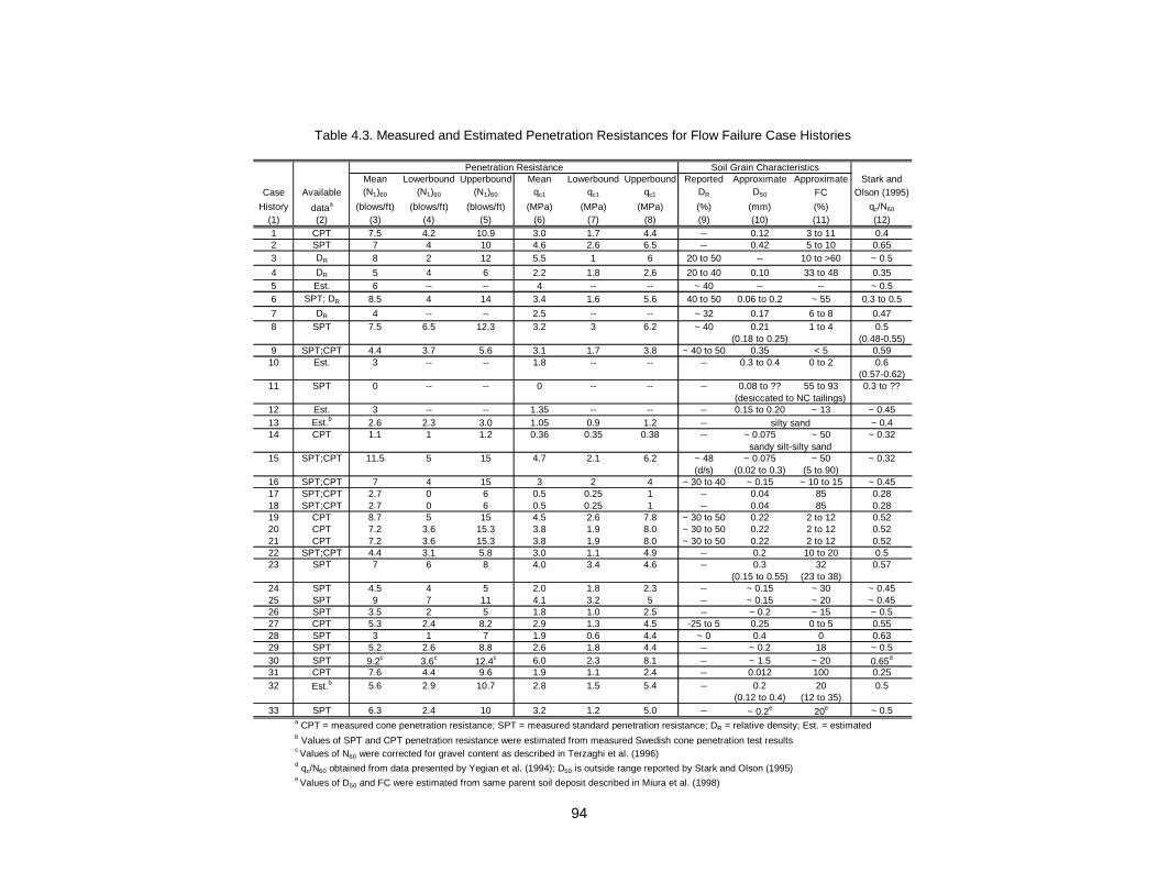
94

Mean Lowerbound Upperbound Mean Lowerbound Upperbound Reported Approximate Approximate Stark and

Case Available (N1)60 (N1)60 (N1)60 qc1 qc1 qc1 DR D50 FC Olson (1995)

History dataa (blows/ft) (blows/ft) (blows/ft) (MPa) (MPa) (MPa) (%) (mm) (%) qc/N60

(1) (2) (3) (4) (5) (6) (7) (8) (9) (10) (11) (12)

1 CPT 7.5 4.2 10.9 3.0 1.7 4.4 -- 0.12 3 to 11 0.42 SPT 7 4 10 4.6 2.6 6.5 -- 0.42 5 to 10 0.653 DR 8 2 12 5.5 1 6 20 to 50 -- 10 to >60 ~ 0.5

4 DR 5 4 6 2.2 1.8 2.6 20 to 40 0.10 33 to 48 0.355 Est. 6 -- -- 4 -- -- ~ 40 -- -- ~ 0.56 SPT; DR 8.5 4 14 3.4 1.6 5.6 40 to 50 0.06 to 0.2 ~ 55 0.3 to 0.5

7 DR 4 -- -- 2.5 -- -- ~ 32 0.17 6 to 8 0.478 SPT 7.5 6.5 12.3 3.2 3 6.2 ~ 40 0.21 1 to 4 0.5

(0.18 to 0.25) (0.48-0.55)9 SPT;CPT 4.4 3.7 5.6 3.1 1.7 3.8 ~ 40 to 50 0.35 < 5 0.59

10 Est. 3 -- -- 1.8 -- -- -- 0.3 to 0.4 0 to 2 0.6(0.57-0.62)

11 SPT 0 -- -- 0 -- -- -- 0.08 to ?? 55 to 93 0.3 to ??

12 Est. 3 -- -- 1.35 -- -- -- 0.15 to 0.20 ~ 13 ~ 0.4513 Est.b 2.6 2.3 3.0 1.05 0.9 1.2 -- ~ 0.414 CPT 1.1 1 1.2 0.36 0.35 0.38 -- ~ 0.075 ~ 50 ~ 0.32

15 SPT;CPT 11.5 5 15 4.7 2.1 6.2 ~ 48 ~ 0.075 ~ 50 ~ 0.32(d/s) (0.02 to 0.3) (5 to 90)

16 SPT;CPT 7 4 15 3 2 4 ~ 30 to 40 ~ 0.15 ~ 10 to 15 ~ 0.4517 SPT;CPT 2.7 0 6 0.5 0.25 1 -- 0.04 85 0.2818 SPT;CPT 2.7 0 6 0.5 0.25 1 -- 0.04 85 0.2819 CPT 8.7 5 15 4.5 2.6 7.8 ~ 30 to 50 0.22 2 to 12 0.5220 CPT 7.2 3.6 15.3 3.8 1.9 8.0 ~ 30 to 50 0.22 2 to 12 0.5221 CPT 7.2 3.6 15.3 3.8 1.9 8.0 ~ 30 to 50 0.22 2 to 12 0.5222 SPT;CPT 4.4 3.1 5.8 3.0 1.1 4.9 -- 0.2 10 to 20 0.523 SPT 7 6 8 4.0 3.4 4.6 -- 0.3 32 0.57

(0.15 to 0.55) (23 to 38)24 SPT 4.5 4 5 2.0 1.8 2.3 -- ~ 0.15 ~ 30 ~ 0.4525 SPT 9 7 11 4.1 3.2 5 -- ~ 0.15 ~ 20 ~ 0.4526 SPT 3.5 2 5 1.8 1.0 2.5 -- ~ 0.2 ~ 15 ~ 0.527 CPT 5.3 2.4 8.2 2.9 1.3 4.5 -25 to 5 0.25 0 to 5 0.5528 SPT 3 1 7 1.9 0.6 4.4 ~ 0 0.4 0 0.6329 SPT 5.2 2.6 8.8 2.6 1.8 4.4 -- ~ 0.2 18 ~ 0.530 SPT 9.2c 3.6c 12.4c 6.0 2.3 8.1 -- ~ 1.5 ~ 20 0.65d

31 CPT 7.6 4.4 9.6 1.9 1.1 2.4 -- 0.012 100 0.25

32 Est.b 5.6 2.9 10.7 2.8 1.5 5.4 -- 0.2 20 0.5(0.12 to 0.4) (12 to 35)

33 SPT 6.3 2.4 10 3.2 1.2 5.0 -- ~ 0.2e 20e ~ 0.5a CPT = measured cone penetration resistance; SPT = measured standard penetration resistance; DR = relative density; Est. = estimatedb Values of SPT and CPT penetration resistance were estimated from measured Swedish cone penetration test resultsc Values of N60 were corrected for gravel content as described in Terzaghi et al. (1996)d qc/N60 obtained from data presented by Yegian et al. (1994); D50 is outside range reported by Stark and Olson (1995)e Values of D50 and FC were estimated from same parent soil deposit described in Miura et al. (1998)

Penetration Resistance

Table 4.3. Measured and Estimated Penetration Resistances for Flow Failure Case Histories

sandy silt-silty sand

(desiccated to NC tailings)

silty sand

Soil Grain Characteristics

95

Figure 4.1. Schematic undrained response of a saturated, contractive sandy soil

96

Figure 4.2. Pre-failure vertical effective stress contours and critical failure surface used for yield strength analysis of Mochi-Koshi Tailings Dam No. 1

97

Figure 4.3. Comparison of yield and mobilized shear strength and pre-failure verticaleffective stress for static loading-induced, deformation-induced, andseismically-induced flow failures (for clarity, ranges only shown for staticloading- and deformation-induced failures)

Figure 4.4. Comparison of static driving shear stress and combined static and seismicshear stresses for seismically-induced flow failures with yield strengthenvelope

98

Figure 4.5. Comparison of yield and mobilized strength ratios and corrected SPTblowcount for liquefaction flow failures

Figure 4.6. Comparison of yield and mobilized strength ratios and corrected CPT tipresistance for liquefaction flow failures

99

CHAPTER 5

LIQUEFIED STRENGTH RATIO FROM LIQUEFACTION FLOWFAILURES

5.1 INTRODUCTION

Numerous procedures exist to estimate the liquefied shear strength or liquefied

shear strength ratio. These procedures utilize the results of laboratory tests, back-analysis of

case histories of flow failure and lateral spreading, or a combination of both. The procedures

that utilize flow failure case histories relate liquefied shear strength or strength ratio to

corrected SPT or CPT resistance, or to corrected shear wave velocity, Vs. This chapter

describes the development of the liquefied strength ratio concept and discusses the

shortcomings of existing procedures to evaluate liquefied shear strength or strength ratio.

Relationships then are proposed to estimate liquefied strength ratio based on the systematic

back-analysis of flow failure case histories where SPT or CPT resistance is available. The

back-analysis procedures are described in detail, and the effects of fines content, kinetics,

and penetration resistance on the proposed relationships are discussed.

5.2 LIQUEFIED SHEAR STRENGTH AND STRENGTH RATIO

5.2.1 Liquefied Shear Strength

As discussed in Chapter 2, the liquefied shear strength, su(LIQ), is the shear strength

mobilized at large deformation after flow liquefaction (undrained strain-softening behavior) is

triggered in saturated, contractive soils. The liquefied shear strength has been referred to as

100

the undrained residual shear strength, sr (Seed 1987), undrained steady state shear

strength, sus (Poulos et al. 1985), and undrained critical shear strength, su(critical) (Stark and

Mesri 1992). Based on a recent National Science Foundation (NSF) international workshop

(Stark et al. 1998), the term liquefied shear strength is used herein because it is generic and

does not imply correspondence to any laboratory test condition.

In the laboratory, where drainage conditions are controlled, the term “undrained”

applies. However, in the field, as evidenced by observation and analysis of flow failures,

drainage may occur (Stark and Mesri 1992; Fiegel and Kutter 1994). Therefore the shear

strength mobilized in the field may not be undrained. The term “liquefied shear strength” is

used to describe the shear strength actually mobilized during a liquefaction flow failure in the

field, including the potential effects of drainage, porewater pressure redistribution, soil

mixing, etc.

Laboratory shear tests on loose to medium dense laboratory specimens or loose

specimens under low effective consolidation pressure indicate that dilation often occurs at

large strain. These soils may exhibit a “quasi-steady state” (Ishihara 1993), or minimum

strength prior to strain hardening. However, as noted by Yoshimine et al. (1999), once

liquefaction is triggered and deformation begins in the field, the “…behavior may become

dynamic and turbulent due to inertia effects [i.e., kinetics]…” and the dilation observed in the

laboratory may not occur in the field. Despite some of these difficulties in interpreting the

liquefied shear strength mobilized in the field, one purpose of this study was to determine if

the liquefied shear strength can be interpreted in terms of the critical void ratio concept

proposed by Casagrande (1940).

101

5.2.2 Liquefied Strength Ratio

The liquefied strength ratio is defined as the liquefied shear strength normalized by

the pre-failure vertical effective stress, su(LIQ)/σ'vo. Recent laboratory testing (e.g., Ishihara

1993; Baziar and Dobry 1995; Vaid and Sivathalayan 1996) show that the liquefied shear

strength of many cohesionless soils is linearly proportional to initial major principal effective

stress. Figure 5.1 presents liquefied shear strengths measured on “remolded layered”

specimens of silty sand, Batch 7, from Lower San Fernando Dam (Baziar and Dobry 1995)

consolidated to various major principal effective stresses. “Remolded layered” means that

the specimen were reconstituted by sedimentation under water. This creates a segregated,

or layered, specimen. Chapter 6 provides additional examples of linear proportionality

between liquefied shear strength and initial effective confining stress.

As discussed in Chapter 2, laboratory investigations of cohesionless soils (e.g., Fear

and Robertson 1995) have indicated that, for a given method of deposition and mode of

shearing, there is a unique value of liquefied strength ratio for a given value of state

parameter. Been and Jefferies (1985) defined the state parameter, ψ, as:

ψ = eo - ess (5.1)

where eo is the in-situ void ratio at a given effective confining stress prior to shearing and ess

is the void ratio at the steady state line (SSL) for the same effective confining stress. As

discussed in Chapter 6, the consolidation line and steady state line are approximately

parallel for many compressible sandy soils. Therefore, for a given increase in effective

confining stress, the value of state parameter remains nearly constant and liquefied shear

strength increases in proportion to effective confining stress. Even if the consolidation

102

behavior and steady-state line are not exactly parallel, it may be reasonable to assume that

in many field conditions the consolidation behavior is approximately parallel to the steady

state line for the range of effective stress of engineering interest. Figure 5.2 presents an

example of this simplification for specimens of silty sand, Batch 7, from Lower San

Fernando Dam.

This study applies the concept of liquefied shear strength and effective consolidation

stress proportionality to the interpretation of liquefaction flow failures. Specifically, as the

pre-failure vertical effective stress increases, void ratio decreases, and therefore, liquefied

shear strength increases. The pre-failure vertical effective stress is used for normalization

because alternate pre-failure effective confining stresses such as the effective stress normal

to the failure surface (σ'n), octahedral effective stress (σ'oct), and major or minor principal

effective stress (σ'1c or σ'3c), are difficult to determine. Further, the failure surface within the

zone of liquefaction for the majority of the flow failures studied approaches direct simple

shear conditions, thus, the pre-failure σ'vo is nearly equal to σ'n.

5.2.3 Relation between Liquefied Strength Ratio and PenetrationResistance

Jefferies et al. (1990), Stark and Mesri (1992), and Ishihara (1993) related liquefied

strength ratio to modified penetration resistance. The correlation between liquefied strength

ratio and penetration resistance appears reasonable because both liquefied strength ratio

and penetration resistance are functions of soil density and effective confining stress. For

example, Been et al. (1987b) related normalized CPT tip resistance to state parameter,

which indicates that higher values of normalized penetration resistance correspond to lower

values of state parameter. Although Sladen (1989) discussed difficulties with the exact form

of this relationship, the author anticipates that the trend of the Been et al. (1987b)

103

relationship is correct. Studies by Ishihara (1993) and Fear and Robertson (1995) indicate

that lower values of state parameter correspond to higher values of liquefied strength ratio.

Therefore, higher values of liquefied strength ratio should correspond to higher values of

normalized penetration resistance.

5.3 EXISTING METHODS TO ESTIMATE LIQUEFIED SHEARSTRENGTH OR STRENGTH RATIO

A review of existing methods to estimate liquefied shear strength or strength ratio is

presented here to discuss shortcomings of these methods. After discussing these

shortcomings, alternate relationships are proposed to estimate the liquefied shear strength

ratio from corrected SPT or CPT penetration resistance. The methods discussed herein

include laboratory based methods, case history based methods, and methods that employ a

combination of laboratory test results and case histories.

5.3.1 Poulos et al. (1985a)

Poulos et al. (1985a) presented a laboratory-based procedure to estimate the in situ

liquefied shear strength from undrained triaxial compression tests on reconstituted and high

quality piston samples. Poulos et al. (1985a) assume that the steady state line determined

from reconstituted samples is parallel to the in situ steady state line and that the steady

state shear strength depends solely on the void ratio after consolidation (and prior to shear).

Undrained triaxial compression tests then are conducted on the high quality piston samples,

and the void ratio following consolidation is corrected to the in situ void ratio. Figure 5.3

illustrates the procedure.

104

While this method provides the reasonable procedure based on soil mechanics

principles to estimate the liquefied shear strength, it has been criticized because: (1) there

are several corrections required to evaluate the in-situ void ratio from that determined from

the piston samples; (2) slight errors in the determination of the in-situ void ratio can result in

large differences in laboratory steady state shear strength because of the small slope of the

steady state line (Kramer 1989); and (3) some recent studies (e.g., Vaid and Thomas 1995)

indicate that the steady state line may be influenced by the mode of shear, effective

confining pressure, and sample preparation methods (see discussion in Chapter 2).

5.3.2 Seed (1987) and Seed and Harder (1990)

As an alternative to the Poulos et al. (1985a) procedure, Seed (1987) presented a

relationship (later updated by Seed and Harder 1990) to estimate the liquefied shear

strength from the equivalent clean sand corrected SPT blowcount, (N1)60-cs. This approach is

based on the back-analysis of seventeen case histories of liquefaction flow failure and

lateral spreads. The relationship between su(LIQ) and (N1)60-cs is presented in Figure 5.4.

Because of its practicality, use of field case histories, and the correlation to a well-known

penetration value, (N1)60, the Seed and Harder (1990) relationship remains the state-of-

practice to estimate the liquefied shear strength.

Despite its ease of use, this method has numerous uncertainties and shortcomings

implicit in back-calculating the liquefied shear strength and in determining the

“representative” SPT blowcount. For example, six of the 17 case histories in the Seed and

Harder (1990) database are cases of liquefaction-induced lateral spreading, not liquefaction

flow failure. Recently, participants of an NSF international workshop (Stark et al. 1998)

concluded that the shear strength back-calculated from lateral spreads may not correspond

to the shear strength mobilized during a liquefaction flow failure and should be considered

105

separately. Secondly, Seed (1987) and Seed and Harder (1990) did not use the post-failure

geometry to back-calculate the liquefied shear strength in all cases. In several cases, the

lower bound value was estimated from the post-failure geometry and the upper bound value

from the pre-failure geometry. Thirdly, Seed and Harder (1990) reportedly considered the

kinetics of the failure movements to back-calculate liquefied shear strengths for an unknown

number of the 17 case histories, but did not present their methodology, and in many cases

their results differ from the results presented herein that explicitly incorporate kinetics.

Fourthly, in seven of the 17 case histories, SPT blowcounts were not available and had to

be estimated from an appraisal of relative density, and numerous cases had only a limited

number of penetration tests from which to select (N1)60. Fifthly, Seed and Harder (1990)

recommended that “the lower-bound, or near lower-bound relationship between [liquefied

shear strength] and (N1)60-cs be used…at this time owing to scatter and uncertainty, and the

limited number of case studies back-analyzed to date.” However, numerous studies have

suggested that the use of the lower bound relationship to estimate liquefied shear strength

results in very low factors of safety, particularly for large structures with large static shear

stresses (e.g., Pillai and Salgado 1994; Finn 1998; Koester 1998). Finally, the procedure

uses a correction factor, ∆(N1)60, (see Table 5.1) to augment the value of (N1)60 of silty sands

and sandy silts to that of clean sands of equal relative density based on the fines content of

the soil. This blowcount is termed the equivalent clean sand corrected blowcount, (N1)60-cs.

However, the specific values of the fines content correction factor are not supported by any

field or laboratory data.

5.3.3 Stark and Mesri (1992)

Stark and Mesri (1992) concluded that a larger pre-failure vertical effective stress

(i.e., vertical consolidation pressure) should result in a larger liquefied shear strength due to

106

consolidation under an increased confining stress. Accordingly, Stark and Mesri (1992)

developed an approach to estimate the liquefied shear strength from liquefaction case

histories as a function of the pre-failure vertical effective stress. Utilizing the cases from

Seed and Harder (1990) and three additional cases, Stark and Mesri (1992) presented a

relationship between liquefied strength ratio, su(LIQ)/σ'vo and (N1)60-cs, where σ'vo was a

“representative” pre-failure vertical effective stress in the zone of liquefaction. The liquefied

strength ratio describes a relationship between the liquefied shear strength mobilized during

flow failure and the pre-failure effective vertical stress, similar to relationships developed for

soft clays. Boundaries to encompass all the case histories were defined, and a lower bound

relationship (for use in design) was suggested, as shown in Figure 5.5 and 5.6, respectively.

Stark and Mesri (1992) suggested that the value of (N1)60 can be corrected by the

fines content correction derived from the Seed et al. (1985) SPT based level ground

liquefaction resistance relationships, rather than using a separate fines content correction

for liquefied shear strength, as suggested by Seed (1987). The corrections are compared in

Table 5.1. This alternate fines content correction was proposed because the use of the level

ground liquefaction fines content correction did not affect the position of the band (shown in

Figure 5.5) that encompassed the case histories. However, Stark and Mesri (1992)

presented no other supporting data.

Despite normalizing the data to the pre-failure vertical effective stress, their re-

analysis did not reduce the scatter of the case histories compared to the Seed and Harder

(1990) relationship. This is in part due to many of the difficulties discussed above for the

Seed and Harder (1990) approach. In addition, Stark and Mesri (1992) used a “single value”

of pre-failure vertical effective stress for the liquefied layer. This does not account for the

variation of vertical effective stress within the zone of liquefaction, and as will be indicated

107

subsequently, the values of vertical effective stress suggested by Stark and Mesri (1992)

differ considerably from those determined in this study.

Stark and Mesri (1992) also suggested that many of the liquefaction failures

experienced drainage during flow resulting in back-calculated shear strengths that did not

represent undrained conditions. Stark and Mesri (1992) discerned this because a

considerable number of the liquefied strength ratios exceed the level ground yield strength

ratios for the same SPT blowcount. They suggested that drainage probably caused the large

values of back-calculated liquefied strength ratio. However, this study suggests that there

are many other potential sources of uncertainty in their procedure.

5.3.4 Ishihara (1993)

Based on extensive laboratory testing, Ishihara (1993) confirmed the existence of a

relationship between liquefied shear strength and initial confining stress for silty sands and

sandy silts. Ishihara (1993) suggested that this relationship is not unique for all sands, but is

unique for a given soil (given steady state parameters) and a given K0. However, Ishihara

(1993) suggested that the quasi-steady state strength, not the steady state strength, should

be utilized in post-triggering stability analysis, and it is the quasi-steady state strength that

Ishihara (1993) related to initial confining pressure. For moderately loose to medium dense

soils, the quasi-steady state is the minimum shear strength available to a soil following the

triggering of liquefaction, and is often attained at strains of 4 to 10 percent. For these soils,

the true steady state occurs after dilation and increase in strength at much larger strains.

For very loose soils, the quasi-steady state does not exist and the steady state shear

strength was used for the relationships.

Ishihara (1993) developed relationships between estimated (N1)60 and laboratory-

determined liquefied strength ratio using the logic illustrated in Figure 5.7. These

108

correlations are compared with available SPT based field case histories collected by Stark

and Mesri (1992), and the correlations are converted to corrected CPT tip resistance for

comparison with CPT based field case histories reported by Ishihara et al. (1991). These

comparisons are shown in Figures 5.8 and 5.9, respectively.

However, this method does not clarify the estimation of liquefied shear strength. The

laboratory relations suggest considerably larger liquefied strength ratios than the SPT or

CPT based liquefaction case histories, and Ishihara (1993) does not provide a clear

explanation of the discrepancy. The author considers the discrepancy to be related to the

problems discussed above for the Seed (1987) and Stark and Mesri (1992) methods,

because the SPT data were obtained from Stark and Mesri (1992). The CPT data included

many cases that may be more closely related to lateral spreading than flow failure (e.g., the

Dagupan cases), and these back-calculated strength ratios may not correspond to the

liquefied strength ratio. In addition, laboratory-measured values of liquefied strength ratio for

clean sands can be considerably larger than liquefied strength ratios mobilized during flow

failures, depending on the values of state parameter of the laboratory specimen. (This is

discussed further in Chapter 6.)

5.3.5 Konrad and Watts (1995)

Konrad and Watts (1995) proposed a method to estimate liquefied shear strength

mobilized in the field from (N1)60-cs [referred to as ECS (N1)60] based upon a framework of

critical state soil mechanics (CSSM) in conjunction with a limited number of liquefaction flow

failure case histories. (N1)60-cs is estimated using the correction proposed by Seed (1987)

(see Table 5.1). The idealized approach is shown in Figure 5.10. A four-step procedure was

proposed to estimate the liquefied shear strength, as follows.

109

1. Site characterization - includes SPTs and obtaining representative samples of sand

for laboratory testing;

2. Laboratory tests - determination of maximum void ratio and critical state line;

3. Estimate χ - values of χ estimated from back-calculation of case histories of

liquefaction flow failure (see Figure 5.10b); and

4. Estimate mobilized liquefied shear strength using suo (laboratory-determined liquefied

shear strength corresponding to emax, see Figure 5.10a), χ, and (N1)60-cs where

( ) csuou Nss LIQ −+= 601log)(log χ (5.3)

Konrad and Watts (1995) use this procedure to correctly predict cases of flow failure

and non-flow failure for artificial sand fills constructed in the Beaufort Sea. However, this

method has some shortcomings, including the limited number of liquefaction case histories

used to develop the parameter χ, the need to determine the steady state line (to obtain the

slope λ) of the soil under consideration, and the assumption that sands at their maximum

void ratio always have zero penetration resistance.

5.3.6 Fear and Robertson (1995)

In a series of papers (Robertson et al. 1995, Cunning et al. 1995, and Fear and

Robertson 1995), Robertson and his co-workers used data from extensive laboratory tests

to develop an empirical relationship between soil state and corrected shear wave velocity,

Vs1. Using the framework of critical state soil mechanics, the state parameter is related to

both liquefied shear strength and liquefied strength ratio. Fear and Robertson (1995) then

related Vs1 to both liquefied shear strength and liquefied strength ratio of two sandy soils

110

with different fines contents. These results are presented together with results presented by

Sasitharan et al. (1994).

Fear and Robertson (1995) reached the following conclusions:

• Liquefied strength ratio is directly related to state parameter for a given sand,

however, there is no unique relationship for all sands (see Figure 5.11a);

• Liquefied shear strength is directly related to Vs1 for a given sand and a given K0

condition, however, again, there is no unique relationship for all sands [see Figure

5.11b and Figure 5.11c where Vs1 is converted to (N1)60]; and

• Liquefied strength ratio is related to Vs1 for a given sand and K0 condition, but is

stress-level dependent [see Figure 5.11d where Vs1 is converted to (N1)60]

This method also has shortcomings, including the need to conduct expensive

laboratory tests to evaluate the liquefied shear strength of a given sand deposit, and the

difficulty in determining K0 for a given deposit.

5.3.7 Summary of Existing Procedures

Existing methods to estimate liquefied shear strength or strength ratio utilize

laboratory tests, field case histories, or a combination of both. The methods that use

laboratory tests, while perhaps more technically sound, require difficult and expensive tests

to be conducted. Furthermore, literature regarding laboratory testing of loose sands contains

many apparently contradictory results (see Chapter 2). This leads to difficulty in interpreting

the results of laboratory tests for a specific project. In addition, these difficulties with

laboratory methods make them more difficult to apply to design.

One alternative to the use of laboratory based methods is to develop relationships to

estimate liquefied shear strength or strength ratio on the basis of liquefaction case histories.

111

However, studies that utilize field case histories have not been satisfactory to date, because

of differences in interpretation of the case histories, inconsistent analysis of existing case

histories, and the general lack of case histories that lend themselves to back-analysis.

Methods that utilize both laboratory testing and field case histories improve

interpretation of the case histories on the basis of theoretical studies and laboratory tests.

However, these methods also assume the difficulties inherent in both individual methods.

Furthermore, methods that utilize both laboratory tests and field case histories suffer from

the existence of very few case histories with sufficient laboratory data to allow interpretation

in terms of the laboratory or theoretical framework.

5.4 BACK-ANALYSIS OF LIQUEFACTION FLOW FAILURES

In order to overcome many of the shortcomings of the methods previously discussed,

this study proposes a systematic procedure to analyze liquefaction flow failure case

histories. Three types of stability analysis were used to back-calculate the liquefied strength

ratio from the thirty-three flow failures. The stability analyses represent three levels of

complexity. The appropriate type of analysis depended on the detail and quality of

information available for each case history. For cases with minimal available information, a

simplified analysis was conducted to estimate the liquefied strength ratio. For the majority of

cases (21 of 33 cases), sufficient information was available to allow a rigorous slope stability

analysis and the direct back-calculation of the liquefied strength ratio. For cases with

appropriate documentation and failure conditions, an additional kinetics analysis was

conducted to back-calculate the liquefied strength ratio.

112

5.4.1 Simplified Stability Analysis of Post-Failure Geometry

Numerous investigators (e.g., Meyerhof 1971, Lucia 1981, and Ishihara et al. 1990a)

developed simplified methods to estimate the shear strength mobilized during flow slides.

The Ishihara et al. (1990a) method was adopted for the simplified analysis, and is briefly

reviewed.

Ishihara et al. (1990a) made the following assumptions to estimate the liquefied

shear strength mobilized during several flow failures: (1) the ground surface and the surface

of the flowed material are approximately parallel when the mass comes to rest; (2) side

forces are equal, opposite, and co-linear; and (3) the shear strength mobilized at the

moment the failed mass comes to rest is equal to the liquefied shear strength. Force

equilibrium in the direction of flow indicates that (see Figure 5.12):

αα

cos)(sin0

BsWF LIQux∑ +−== (5.4)

where W is the weight of the slice, B is the width of the slice, and α is the angle of inclination

of the sliding surface and surface of flowed material. If the flowed material has an average

thickness of H and unit weight of γt, Eq. (5.4) can be rewritten as:

ααγ cossin)( Hs tu LIQ = (5.5)

where γt is total and submerged unit weight above and below the water table, respectively.

Equation (5.5) was used to estimate values of liquefied shear strength for cases with

insufficient information to conduct the rigorous analysis and where the above assumptions

113

were satisfied. Numerous flow failure cases in the literature did not meet these minimum

assumptions, and therefore were not included in this study. The simplified procedure only

provides a value of liquefied shear strength. Therefore, a representative pre-failure vertical

effective stress was estimated from the pre-failure geometry in order to calculate values of

liquefied strength ratio. Because this simplified analysis does not explicitly consider kinetics,

values of su(LIQ)/σ'vo estimated using this method may be smaller than the actual

su(LIQ)/σ'vo of the liquefied soil.

5.4.2 Rigorous Stability Analysis of Post-Failure Geometry

A rigorous stability analysis procedure to back-calculate the liquefied strength ratio

directly was conducted for the majority (21 of 33) of cases. The rigorous stability analysis

used Spencer’s (1967) slope stability method as coded in the microcomputer program

UTEXAS3 (Wright 1992). Because this analysis also does not explicitly consider kinetics,

values of su(LIQ)/σ'vo estimated using this method may be smaller than the actual

su(LIQ)/σ'vo of the liquefied soil.

In this analysis, either the geometric extents of the liquefied soil must be known or

the initial failure surface must be assumed to pass approximately through the center of the

zone of liquefaction. This study examined a limited number of well-documented flow failures

and found that initial failure surfaces do pass approximately through the center of the zones

of liquefaction. Therefore, this assumption appears valid for the analysis of other flow

failures. The post-failure sliding surface is divided into a number of segments. Based on the

lengths of the post-failure segments, corresponding lengths of liquefied soil are defined

within the pre-failure geometry, i.e., within the zone of liquefaction or near the initial failure

surface.

114

This procedure is illustrated in Fig. 5.13 for the flow failure of Lower San Fernando

Dam. The post-failure sliding surface (Fig. 5.13b) was broken into 14 segments of various

length. Based on the post-failure geometry segment lengths, corresponding lengths of

liquefied soil are defined in the pre-failure zone of liquefaction (Fig. 5.13a). The vertical

distance between the pre-failure segments is approximately equal to the average final

thickness of the liquefied soil estimated from the post-failure geometry. Segments 1 through

9 of the post-failure sliding surface consist of liquefied soil, while segments 10-14 consist of

non-liquefied soil (namely, segments 10-13 correspond to core material, and segment 14

corresponds to ground shale hydraulic fill and rolled fill). Therefore, only segments 1 through

9 are located in the liquefied zone in the pre-failure geometry in Fig. 5.13b. The pre-failure

σ'vo is determined for each segment in the liquefied soil (segments 1-9) and is assigned to

the corresponding segment in its post-failure position. Rearranging the segment positions

has little effect on the back-calculated liquefied strength ratio, as long as the segments are

equally spaced in the zone of liquefaction or centered around the initial failure surface.

Using the individual σ'vo values for each segment and a single value of su(LIQ)/σ'vo,

individual values of liquefied shear strength are assigned to each segment of the post-failure

geometry for the stability analysis (i.e., segments 1 through 9 in Fig. 5.13). This allows the

variation in pre-failure σ'vo within the zone of liquefaction to be reflected in variable liquefied

shear strengths along the final sliding surface. Soils initially above the phreatic surface or

otherwise known not to have liquefied (e.g., segments 10-14 in Fig. 5.13) are assigned

appropriate drained or undrained shear strengths (see Appendix A for details of shear

strength assignment for each of the case histories). The liquefied strength ratio is then

varied (which in turn varies the liquefied shear strength mobilized along each segment of the

post-failure geometry) until a factor of safety of unity is achieved.

115

This analysis considers the entire range of pre-failure vertical effective stress within

the zone of liquefaction rather than a single “representative” value of pre-failure σ'vo.

Therefore, liquefied strength ratios back-calculated using this technique are considered

more appropriate than those reported elsewhere, e.g., Stark and Mesri (1992) and Ishihara

(1993). For comparison to values calculated in Chapter 4, the weighted average pre-failure

vertical effective stress for each case history was calculated as follows:

∑∑

=

= ⋅=

ni i

ni iiv

voL

Lave

1

1 ,')('

σσ (5.6)

where σ'v,i is the pre-failure vertical effective stress for segment i and Li is the length of

segment i.

5.4.3 Stability Analysis Considering Kinetics of Failure MassMovements

To obtain a best estimate of liquefied shear strength mobilized during failure, the

stability analysis should consider the kinetics of failure (Davis et al. 1988; Olson et al. 2000).

The reason for this is illustrated in Figure 5.14 using the calculations made for the

liquefaction flow failure of the North Dike of Wachusett Dam (Olson et al. 2000). At the onset

of a liquefaction flow failure, only small strains are required to reduce the shear strength

from the yield (or peak) shear strength to the liquefied shear strength (Davis et al. 1988).

These strains occur while the driving stress remains relatively unchanged. Therefore, for

simplification, the liquefiable soil is assumed to be in a post-peak condition and the

mobilized strength at the beginning of failure (at time, t = 0) is equal to the liquefied shear

strength (as indicated in Figure 5.14a). The initial static shear stress in the zone of

116

liquefaction is determined from a static slope stability analysis assuming a factor of safety of

unity (Castro et al. 1989; Seed et al. 1989). Because the initial static driving shear stress is

larger than the liquefied shear strength (this is a prerequisite for a liquefaction flow failure),

the mass begins to accelerate downslope (Figure 5.14b). Therefore, the velocity of the

failure mass increases from zero (Figure 5.14c), and downslope displacement occurs

(Figure 5.14d). The downslope displacement of the failure mass, in turn, decreases the

static driving shear stress because of the curvature of the center of gravity travel path.

When the driving shear stress is reduced to the liquefied shear strength (in Figure

5.14a, the mobilized shear resistance is less than the liquefied shear strength as a result of

hydroplaning, as discussed subsequently), the failure mass has an acceleration of zero and

has attained its maximum velocity (Figures 5.14b and 5.14c). However, because the failure

mass has a finite velocity, it continues to displace and deform, decreasing the driving shear

stress to a value less than the liquefied shear strength, thereby decelerating the failure mass

(i.e., upslope acceleration; Figures 5.14a and 5.14b). When the failure mass reaches a

velocity of zero and comes to rest, the driving shear stress may be considerably less than

the liquefied shear strength (Figure 5.14a). At the instant the failure mass comes to rest, the

mobilized shear resistance decreases to that required for static stability, i.e., the driving

shear stress obtained from the post-failure geometry (Figure 5.14a).

The kinetics analysis used for this study was adapted from the procedure outlined by

Davis et al. (1988) and is reviewed briefly. This analysis is based on Newton’s second law of

motion, as follows:

∑ = aF m (5.7)

117

where F are the forces acting on the moving mass (in vector form), m is the mass of the

failed material (weight divided by acceleration due to gravity, g), and a is the acceleration of

the center of gravity of the failed material. Referring to Figure 5.14, the net force, ΣF, acting

on the failure mass in the direction of the movement of the center of gravity is given by the

driving weight of the failure mass minus the mobilized shear resistance of the soil, as:

( ) ( )[ ]∑ =−= aF mLsW uθsin (5.8)

where W is the weight of the failure mass, θ is the angle between the horizontal and the

tangent to the curve describing the movement of the failure mass center of gravity (see

Figure 5.14), su is the mobilized shear resistance, and L is the length of the failure surface.

At the start of sliding, the weight term is larger than the shear resistance term, and

acceleration is downslope. Near the end of sliding, the weight term is smaller than the shear

resistance term, and acceleration is upslope (thereby decelerating the mass; Figures 5.14a

and 5.14b).

This study examined a limited number of well-documented flow failure case histories

and found that most initial and final failure surfaces could be approximated using third order

polynomials. Therefore, the movement of the center of gravity of the sliding mass for the ten

cases analyzed using kinetics was assumed to follow a third order polynomial. A third-order

polynomial has the form:

y = ax3 + bx2 + cx + d (5.9)

118

where a, b, c, and d are constants that can be calculated based on: (1) the x and y

coordinates of the initial and final positions of the center of gravity of the failure mass; and

(2) the curvature of the travel path of the center of gravity. This curvature was assumed to

parallel the curvature of the final sliding surface. Using the slope (dy/dx) of the tangent to the

curve described in Eq. (5.9) at any point, the sine of θ is given by:

( )21sin

dydx

dydx

+=θ (5.10)

where dy and dx are the vertical and horizontal displacements of the center of gravity of the

failure mass along the curve defined by Eq. (5.9).

The acceleration of the failure mass center of gravity is estimated using the second

derivative of the displacement, ∆, with respect to time, t, as:

2

2

dt

d ∆=a (5.11)

Substituting into Eq. (5.8) yields the following:

( ) ( )[ ]2

2

sindt

d

g

WLsW u

∆⋅=−θ (5.12)

Equation (5.12) can be solved for displacement numerically or by direct integration. This

study employed a time-step numerical solution using a spreadsheet program. A trial value of

119

liquefied shear strength is assumed, and Eq. (5.12) is solved to estimate the total

displacement and duration of movement. The trial shear strength then is revised to obtain

reasonable agreement with the observed displacement of the center of gravity of the failure

mass. The approximate duration of sliding is only available for two cases, therefore

agreement was based on center of gravity movement.

The kinetics analysis also should account for potential hydroplaning (slide material

“riding” on a layer of water), mixing with water, and the increase in void ratio of the liquefied

material if the failure mass slid into a body of water (Castro et al. 1992). To account for

these potential effects, the shear strength mobilized along the failure surface in the body of

water (beyond the original limits of the pre-failure geometry) is assumed to be equal to 50%

of the value of shear strength mobilized within the limits of the pre-failure slope geometry, as

suggested by Castro et al. (1992). For each case, reduction factors of 0% and 100% also

were used to ascertain the sensitivity of the liquefied shear strength to the effect of

hydroplaning and to obtain a range of possible values of liquefied shear strength. The same

reduction factors were used by Castro et al. (1992) to back-calculate the possible range of

liquefied shear strength mobilized during the flow failure of Lower San Fernando Dam.

The kinetics analysis also considered the change in weight of the failure mass if the

mass slid into a body of water, and the change in the length of the failure surface during

flow. These changes during failure are incorporated into the solution of Eq. (5.12) as a

function of the distance traveled by the center of gravity of the failure mass with respect to

its total distance of travel. Lastly, appropriate drained or undrained shear strengths of non-

liquefied soils are incorporated after the solution of Eq. (5.12) using the following adjustment

to su(LIQ):

120

−

⋅−

=

1001

100)(

d

dd

u

u L

sL

ss LIQ (5.13)

where su is determined by the solution of Eq. (5.12), Ld is the percentage of the total length

of the post-failure sliding surface that incorporates soils that did not liquefy, and sd is the

average shear strength of the soils that did not liquefy. Appendix A details the assignment of

shear strength to non-liquefied soils for each case history.

The kinetics analysis only provides the “best estimate” of liquefied shear strength.

This value of su(LIQ) was divided by the weighted average pre-failure σ'vo (Eq. 5.6) to obtain

the “best estimate” of liquefied strength ratio. These values of liquefied shear strength and

strength ratio are “best estimates” because they incorporate the kinetics of failure, potential

hydroplaning and mixing effects, and the shear strength of non-liquefied soils.

5.5 CASE HISTORIES OF LIQUEFACTION FLOW FAILURE

This study collected thirty-three liquefaction flow failure case histories for which SPT

and/or CPT results are available or could be reasonably estimated. Appendix A describes in

detail the available information, the analyses conducted, the evaluation of penetration

resistance, and the uncertainties involved in each case history. The case histories and

corresponding references are summarized in Table 5.2. The liquefied strength ratios back-

calculated using the simplified or rigorous stability analysis and weighted average pre-failure

σ'vo are presented in Table 5.3. Table 5.3 also includes values of liquefied shear strength

back-calculated independently for each case. The back-calculation of these values will be

121

discussed subsequently. For the ten cases with sufficient documentation to perform a

kinetics analysis, the “best estimate” liquefied shear strengths and strength ratios

considering the kinetics of failure are presented in Table 5.4. As expected, the “best

estimate” liquefied shear strengths and strength ratios values estimated from the kinetics

analysis are greater than the values estimated from the rigorous stability analysis (Table

5.3). Measured or estimated penetration resistances and selected soil properties available

for the case histories are presented in Table 5.5. For cases where either SPT or CPT

penetration alone was measured, the corresponding value of the other penetration

resistance was obtained using the qc/N60 relationship presented by Stark and Olson (1995)

and the median grain size of the liquefied soil. Figure 5.15 presents the “best estimate”

liquefied strength ratios and mean (N1)60 values for each of the cases. Figure 5.16 presents

“best estimate” liquefied strength ratios and mean qc1 values. The numbers adjacent to each

of the data points is the average fines content of the liquefied soil. This will be discussed in

more detail subsequently.

5.5.1 Sources of Uncertainty in the Analyses and their Importance

For a given case history, there often was a considerable range of back-calculated

liquefied strength ratios and measured penetration resistance (see Tables 5.2, 5.3, and 5.4).

The uncertainty in back-calculated strength ratios resulted from several factors, including:

(1) limits of the zone of liquefaction; (2) shear strength of the non-liquefied soils; (3) location

of the initial and final surfaces of sliding; (4) location of the phreatic surface within the slope

in some cases; (5) potential of drainage or porewater pressure redistribution occurring

during flow (i.e., undrained condition is not maintained); and (6) location of the post-failure

slope toe in a few cases. Appendix A describes the uncertainties involved in each case

history. Uncertainty due to the potential of drainage or porewater pressure redistribution

122

occurring during flow is inherent in all studies of liquefaction case histories, and simplified

methods to account for this potential effect have not been developed.

There is also considerable uncertainty in defining a “representative” penetration

resistance due to the inherent variability of natural deposits and the typical segregation or

layering encountered in some man-made deposits. This uncertainty is apparent for some

large values of upper bound penetration resistance (see Table 5.5). In some cases,

sufficient penetration resistance results are available to interpret reasonable upper and

lower bounds to the data. Unfortunately, in many cases, insufficient data are available to

make a reasonable judgment. Therefore, the upper bound value for these cases is the

highest value of penetration resistance measured near or in the zone of liquefaction, despite

the fact that the highest value is very unlikely to be representative of the material that

liquefied. In cases where penetration resistance was converted using the qc/N60 relationship

(Stark and Olson 1995) or where penetration resistance is estimated from relative density

and vertical effective stress, additional uncertainty is unavoidable in the estimate of

representative penetration resistance. Other uncertainties in interpreting penetration

resistance include: (1) effects of flow, re-consolidation, and aging when the penetration tests

were conducted some time after failure; (2) position of the phreatic surface at the time of

testing; (3) differences in penetration resistance when penetration tests were conducted

near (or opposite to) the location of failure (e.g., Lower San Fernando Dam); and (4) upper

limit of the overburden correction for conditions of low vertical effective stress (a maximum

correction of two was used for this study). Appendix A details the interpretation of

representative, lower bound, and upper bound penetration resistances and the uncertainties

for each case history.

123

5.5.2 Magnitude of Uncertainties

Tables 5.3, 5.4, and 5.5 show large ranges of reported values, particularly for

penetration resistance. However, these are the same ranges of upper and lower bound

strength and penetration resistance implicit in relationships developed by Seed (1987), Seed

and Harder (1990), Stark and Mesri (1992), and Ishihara (1993), although these

investigators do not describe the magnitude or sources of uncertainty involved in the case

histories. For example, for Lower San Fernando Dam (LSFD), the “representative” value of

(N1)60 within the zone of hydraulic fill that likely liquefied has been reported as 15 by Seed

(1987), 5.5 by Davis et al. (1988), 11.5 by Seed et al. (1989) and Seed and Harder (1990),

12 (with a range of 9 to 15) by Jefferies et al. (1990), 7 (with a minimum representative value

of 4) by McRoberts and Sladen (1992), and 8.5 by Poulos (1988) and Castro (1995). These

“representative” values vary from 4 to 15 – a considerable range in itself. In the downstream

fill of the dam, the actual measured values of (N1)60 ranged from 6 to over 40. Correcting

these values to correspond to the upstream slope (Seed et al. 1989), the (N1)60 values are

approximately 3 to 37.

The true range of (N1)60 values (from 3 to 37) for LSFD is not shown in existing

relationships between liquefied shear strength or strength ratio and (N1)60 because this

range would plot off the chart. Individual investigators determined mean and/or median

values of (N1)60 within the zone of liquefaction and used engineering judgment to evaluate if

these values were “representative” of the hydraulic fill that liquefied and led to the observed

failure. Large (N1)60 values (probably above 15 to 20) are likely too dense to be contractive

under the effective stresses present in the upstream slope of LSFD, and are therefore too

large to be representative. Small (N1)60 values (probably less than about 5 or 6) are

somewhat anomalous and probably are not continuous enough to control stability.

124

Therefore, mean, median, or values of (N1)60 based on judgment are reported in the

literature and used in existing relationships between liquefied shear strength or strength

ratio and penetration resistance.

This study uses the same approach and “representative” values of (N1)60 and qc1 are

taken as the mean values. So the actual ranges can be examined, upper and lower bound

values of penetration resistance are included in Table 5.5. As aforementioned, sufficient

penetration resistance results are available for some cases to interpret reasonable upper

and lower bounds to the data. However, in many cases, insufficient data are available to

make a reasonable judgment. For these cases, the upper bound is the maximum value of

penetration resistance measured near or in the zone of liquefaction, despite the fact that the

highest value is very unlikely to be representative of the material that liquefied.

5.6 INTERPRETATION AND DISCUSSION

Despite the uncertainties for each case, a reasonable trend in the data is apparent,

particularly for the cases where the most information was available (cases plotted with a

solid, half-solid, or open circle in Figures 5.15 and 5.16). Upper bound, lower bound, and

average trend lines are proposed in Figures 5.15 and 5.16. The average trend lines are

linear regressions of the data excluding the cases where only the simplified analysis was

conducted (cases plotted as triangles). The trend lines are described as:

( )[ ] 03.00075.003.0'

)(601 ±+= N

s

vo

u LIQ

σfor (N1)60 ≤ 12 (5.14a)

125

( ) 03.00143.003.0'

)(1 ±+= c

vo

u qs LIQ

σfor qc1 ≤ 6.5 MPa (5.14b)

The upper and lower trend lines in Figures 5.15 and 5.16 approximately correspond to plus

and minus one standard deviation (the standard deviation for both trend lines was ±0.025).

Included in Figure 5.15 are the boundaries of liquefied strength ratio proposed by

Stark and Mesri (1992) and the design lines proposed by Stark and Mesri (1992) and Davies

and Campanella (1994). The data in Figure 5.15 show considerably less scatter compared

to the bounds presented by Stark and Mesri (1992) as a result of the analyses conducted in

this study. The design lines proposed by Stark and Mesri (1992) and Davies and

Campanella (1994) are conservative [for all values of (N1)60] and unconservative [for (N1)60

values greater than 8], respectively. Included in Figure 5.16 is the design line presented by

Olson (1998). The Olson (1998) design line is conservative for all values of qc1. It should be

noted that part of the conservatism of the Stark and Mesri (1992) and Olson (1998) design

lines results from incorporating a fines content correction, while the data in Figures 5.15 and

5.16 are plotted without any correction for fines content.

5.6.1 Back-Calculation of Liquefied Shear Strength

In order to evaluate the correlation between liquefied shear strength and pre-failure

vertical effective stress, “single values” of liquefied shear strength also were back-calculated

from the case histories. As suggested by Seed (1987) and Seed and Harder (1990), “single

values” of su(LIQ) were evaluated from a static slope stability analysis of the post-failure

geometry using Spencer’s (1967) method as coded in the computer program UTEXAS3

(Wright 1992). The “single value” of su(LIQ) was varied until a factor of safety of unity was

achieved. Appropriate drained or undrained shear strengths were assigned to non-liquefied

126

soils. As aforementioned, ten cases had sufficient documentation to perform a kinetics

analysis of the failure. This analysis also estimated su(LIQ). Values of su(LIQ) back-

calculated using the simplified and static stability analyses are presented in Table 5.2, while

values incorporating kinetics are found in Table 5.3. Appendix A details the individual case

history analyses.

Figure 5.17 presents the “single values” of su(LIQ) (see Tables 5.2 and 5.3) and

weighted average pre-failure σ’vo (Eq. 5.6 and Table 5.2). Despite differences in density,

mode of deposition, grain size distribution, grain shape, state parameter, modes of shear,

and steady state friction angle of the liquefied soils, the data in Figure 5.17 illustrate that an

approximately linear relationship exists between su(LIQ) and weighted average pre-failure

σ’vo for liquefaction flow failures. The relationship ranges from approximately su(LIQ) = 0.05

to 0.12σ'vo with an average value (from linear regression) of 0.09σ'vo. As illustrated in Figure

5.15 and 5.16, the variation in su(LIQ)/σ'vo from 0.05 to 0.12 is explained in terms of

increasing corrected penetration resistance.

Baziar and Dobry (1995) also presented bounding relationships between liquefied

shear strength and pre-failure vertical effective stress as shown in Figure 5.17. With the

exception of Lower San Fernando Dam, Baziar and Dobry (1995) used the values of su(LIQ)

and pre-failure σ'vo presented by Stark and Mesri (1992) to develop these boundaries. As

discussed previously, the analysis procedures of this study yield different values of su(LIQ)

and pre-failure σ'vo than those reported by Stark and Mesri (1992). Figure 5.17 illustrates

that this re-evaluation of case histories results in considerably less scatter between the

upper and lower bound relationships of su(LIQ) and pre-failure σ'vo. In summary, the case

history data presented in Figure 5.17 confirm laboratory data that indicate a linear

127

relationship between liquefied shear strength and initial vertical effective stress (e.g., Figure

5.1 from Baziar and Dobry 1995; Ishihara 1993).

5.6.2 Effect of Fines Content on Liquefied Shear Strength and StrengthRatio

Previous case history studies (Seed and Harder 1990; Stark and Mesri 1992)

incorporated fines content corrections to estimate an equivalent clean sand blowcount and

to evaluate the liquefied shear strength or strength ratio. No fines content correction was

adopted in this study. In Figures 5.15 and 5.16, the fines content of the liquefied soil is

provided next to each data point. The data reveal no trend in liquefied strength ratio with

respect to fines content. The author anticipates that although soils with higher fines contents

should exhibit lower values of penetration resistance (as a result of greater soil

compressibility and smaller hydraulic conductivity), these soils are more likely to maintain an

undrained condition during flow. This combination of factors may, in effect, offset each other,

resulting in no apparent difference in values of liquefied strength ratio for cases of clean

sands and sands with higher fines contents. Therefore, this study recommends no fines

content correction for estimating liquefied strength ratio from the proposed relationships.

5.6.3 Effect of Kinetics on Liquefied Shear Strength

The ten cases that explicitly consider the kinetics of failure (Table 5.3) provide “best

estimates” of liquefied strength ratio because the kinetics analysis accounts for the

momentum of the failure mass in the back-calculation of su(LIQ). However, in cases where

the center of gravity of the failure mass did not move a considerable vertical distance, the

author anticipated that kinetics would have a minor effect on the liquefied shear strength.

128

The effect of kinetics on the liquefied shear strength was examined with respect to:

(1) the loss of potential energy of the failure mass as a result of sliding; and (2) the pre-

failure height of the embankment or slope. The loss of potential energy was calculated as

the average weight of the failure mass (from the pre- and post-failure geometry) multiplied

by the change in vertical position of the centroid of the failure mass as a result of sliding.

The effect of kinetics on the back-calculated su(LIQ) was examined in terms of the difference

in liquefied shear strength considering kinetics [su(LIQ, Kinetics)] minus the liquefied shear

strength not considering kinetics [su(LIQ)]. As illustrated in Fig. 5.18a, the effect of kinetics

on the back-calculation of liquefied shear strength is not significant unless the loss of

potential energy of the failure mass is greater than approximately 1x103 to 1x104 kJ/m.

Considering this issue in a simpler manner, Fig. 5.18b illustrates the effect of the pre-failure

height of the embankment/slope on the back-calculated liquefied shear strength. As shown

in Fig. 5.18b, kinetics has a minor effect on the liquefied shear strength for

embankments/slopes less than about 10 m in height. All but one of the 23 case histories

where a kinetics analysis was not conducted involves embankments/slopes with heights of

less than about 10 m. Therefore, liquefied strength ratios back-calculated using the

simplified or rigorous stability analyses also are “best estimates.” Furthermore, for design

and/or remediation, kinetics does not appear to play a significant role in

embankments/slopes that are less than 10 m in height.

5.6.4 Effect of Penetration Resistance on Liquefied Strength Ratio

As noted previously, mean values of penetration resistance are plotted in Figures

5.15 and 5.16. However, most failures occur through the weakest zones of soil, not through

the mean value zones. Therefore, it may be more appropriate to use the minimum or 20th

percentile values of corrected penetration resistance (Yoshimine et al. 1999) to develop the

129

relationships proposed in Figures 5.15 and 5.16. Unfortunately, in most cases there are

insufficient penetration test results available to reasonably estimate a 20th (or other)

percentile value of penetration resistance.

When assessing liquefaction triggering and post-triggering stability in practice,

minimum values of penetration resistance often are used in empirical relationships. If a

minimum value of penetration resistance is used in conjunction with the relationships

proposed in Figures 5.15 and 5.16, a practitioner may consider selecting a liquefied strength

ratio greater than the average relationship. In addition, because the upper and lower bounds

of the relationships proposed in Figures 5.15 and 5.16 correspond approximately to plus and

minus one standard deviation, the desired level of conservatism can be used to estimate the

liquefied strength ratio.

5.7 APPLICATIONS OF LIQUEFIED STRENGTH RATIO

The liquefied strength ratio allows the variation in liquefied shear strength throughout

a zone of liquefied soil to be incorporated in a post-triggering stability analysis. Increases in

su(LIQ) can be the result of increases in pre-failure vertical effective stress, increases in

corrected penetration resistance, or both. To incorporate a strength ratio in a stability

analysis, a liquefied soil layer can be separated into a number of sublayers of equal σ'vo

(stress contours) and/or equal penetration resistance (penetration contours). For example,

each vertical effective stress contour would have an equal value of su(LIQ), and su(LIQ)

would increase as the σ'vo contours increased.

Additionally, liquefied strength ratios can be used to facilitate remediation studies.

Two common remediation techniques for seismic dam stability are the use of stabilizing

berms and soil densification. If a stabilizing berm is added, σ'vo contours incorporating the

130

berm weight can be developed to estimate the new liquefied shear strength. The increase in

vertical effective stress caused by the weight of the stabilizing berm decreases the void ratio

of the liquefiable material and results in an increase in su(LIQ). If soil densification is used,

penetration tests typically are conducted to verify the success of the densification effort.

These additional penetration tests can be used to revise the liquefied strength ratio, and

thus revise values of su(LIQ). Alternatively, penetration resistance values corresponding to

the su(LIQ) required for stability can be used as an acceptance criterion. Densification often

increases the horizontal effective stress, σ'ho (and thus penetration resistance), without

significantly increasing the vertical effective stress. However, the increase in σ'ho caused by

densification should decrease the void ratio of the liquefiable material and result in an

increase in su(LIQ).

On high-risk projects, the compressibility of the liquefiable soil should be compared

to the slope of the steady state line to confirm the applicability of the strength ratio concept

(see Chapter 6 for additional discussion and guidelines). If the compressibility of the soil is

not found to be reasonably parallel to the slope of the SSL, at least over the range of

effective stresses of interest, the strength ratio concept may not be valid for the particular

soil. If the compressibility is significantly smaller than the slope of the SSL, the strength

ratios proposed herein may lead to unconservative estimates of su(LIQ). Practitioners should

be particularly wary of this potential for remediation projects involving large berms.

5.8 CONCLUSIONS

This study re-evaluates liquefaction flow failure case histories using a stability

analysis specifically developed to back-calculate the liquefied strength ratio. This approach

allows the entire range of vertical effective stress acting on the liquefied material prior to

131

failure to be considered in the back-calculation of the liquefied strength ratio, rather than

using a single “representative” value of pre-failure vertical effective stress. In addition,

analyses that incorporate the kinetics of failure were conducted to obtain “best estimates” of

liquefied strength ratio. These analyses show that the effect of kinetics on the back-

calculation of liquefied strength ratio is important for embankments/slopes greater than 10 m

in height.

A number of uncertainties were considered in back-analyzing the case histories. The

factors contributing to the uncertainty of both the back-calculation of liquefied strength ratio

and corrected penetration resistance have been discussed. Despite these uncertainties,

there are clear trends of increasing mobilized liquefied strength ratio with increasing

corrected standard and cone penetration resistance.

The resulting relationships between liquefied strength ratio and penetration

resistance exhibit considerably less scatter than relationships previously proposed (e.g.,

Stark and Mesri 1992). The trend lines presented in Figures 5.15 and 5.16, or in Eqs.

(5.14a) and (5.14b), can be used to estimate the liquefied strength ratio from SPT or CPT

corrected penetration resistance, respectively. These relationships provide liquefied strength

ratios that are greater than previously proposed. Liquefied strength ratios obtained using the

proposed procedure can be used in post-triggering stability analyses to assess the potential

for flow failure (see Chapter 7). By using a liquefied strength ratio, rather than a single value

of liquefied shear strength, the increase in liquefied shear strength with vertical effective

stress can be incorporated in a post-triggering stability analysis. Applications for and

practical implementation of a liquefied strength ratio have been discussed, illustrating the

simple use of the liquefied strength ratio for a number of design scenarios.

132

Table 5.1. Fines content corrections, ∆∆∆∆(N1)60, suggested by Stark and Mesri (1992) andSeed (1987), respectively, to augment corrected SPT blowcount, (N1)60, toequivalent clean sand corrected blowcount, (N1)60-CS

FINESCONTENT ∆(N1)60 based on ∆(N1)60 based on

(%) level ground liquefaction sloping ground liquefaction

0 0 0

10 2.5 1

15 4 —

20 5 —

25 6 2

30 6.5 —

35 7 —

50 7 4

75 7 5

133

CaseHistory Structure Apparent Cause of Sliding References

(1) (2) (3) (4)1 Zeeland - Vlietepolder 1889 High tide Koppejan et al. (1948)2 Wachusett Dam - North Dike 1907 Reservoir filling Olson et al. (2000)3 Calaveras Dam 1918 Construction Cleary (1914); Hazen (1918, 1920); Hazen and Metcalf (1918)4 Sheffield Dam 1925 Santa Barbara Eq. (ML=6.3) Engineering News-Record (1925); Nunn (1925); Willis (1925); U.S. Army Corp of

Engineers (1949); Seed et al. (1969)5 Helsinki Harbor 1936 Construction Andresen and Bjerrum (1968)6 Fort Peck Dam 1938 Construction U.S. Army Corps of Engineers (1939, 1976); Middlebrooks (1942); Casagrande (1965,

1976); Marcuson and Krinitzsky (1976); Marcuson et al. (1978)7 Solfatara Canal Dike 1940 Imperial Valley Eq. (ML=7.1) Ross (1968)

8 Lake Merced Bank 1957 San Francisco Eq. (ML=5.3) Ross (1968)

9 Kawagishi-Cho Building 1964 Niigata Eq. (MW=7.5) Yamada (1966); Ishihara et al. (1978); Ishihara and Koga (1981); Seed (1987)

10 Uetsu Railway Embankment 1964 Niigata Eq. (MW=7.5) Yamada (1966)

11 El Cobre Tailings Dam 1965 Chilean Eq. (ML=7 to 7.25) Dobry and Alvarez (1967)12 Koda Numa Highway Emb. 1968 Tokachi-Oki Eq. (M=7.9) Mishima and Kimura (1970)13 Metoki Road Embankment 1968 Tokachi-Oki Eq. (M=7.9) Ishihara et al. (1990a)14 Hokkaido Tailings Dam 1968 Tokachi-Oki Eq. (M=7.9) Ishihara et al. (1990a)15 Lower San Fernando Dam 1971 San Fernando Eq. (MW=6.6) Seed et al. (1973, 1975); Lee et al. (1975); Castro et al. (1989); Seed et al. (1989);

Vasquez-Herrera and Dobry (1989); Castro et al. (1992)16 Tar Island Dyke 1974 Construction Mittal and Hardy (1977); Plewes et al. (1989); Konrad and Watts (1995)17 Mochi-Koshi Tailings Dam - Dike 1 1978 Izu-Oshima-Kinkai Eq. Marcuson (1979); Marcuson et al. (1979); Okusa and Anma (1980); Okusa et al. (1980, 18 - Dike 2 (ML=7.0) 1984); Ishihara (1984); Ishihara et al. (1990a)19 Nerlerk Berm - Slide 1 1983 Construction Mitchell (1984); Sladen et al. (1985a,b, 1987); Been et al. (1987a); Sladen (1989);20 - Slide 2 Sladen and Hewitt (1989); Rogers et al. (1990); Konrad (1991); Lade (1993); Hicks and21 - Slide 3 Boughraruo (1998)22 Hachiro-Gata Road Embankment 1983 Nihon-Kai-Chubu Eq. (M=7.7) Ohya et al. (1985)23 Asele Road Embankment 1983 Pavement repairs Ekstrom and Olofsson (1985); Konrad and Watts (1995)24 La Marquesa Dam - U/S slope 1985 Chilean Eq. (Ms=7.8) de Alba et al. (1987)25 - D/S slope26 La Palma Dam 1985 Chilean Eq. (Ms=7.8) de Alba et al. (1987)27 Fraser River Delta 1985 Gas desaturation and low tide McKenna et al. (1992); Chillarige et al. (1997a,b); Christian et al. (1997a,b)28 Lake Ackerman Highway Emb. 1987 Seismic reflection survey Hryciw et al. (1990)29 Chonan Middle School 1987 Chiba-Toho-Oki Eq. (M=6.7) Ishihara et al. (1990a); Ishihara (1993)30 Nalband Railway Embankment 1988 Armenian Eq. (Ms=6.8) Yegian et al. (1994)

31 Soviet Tajik - May 1 slide 1989 Tajik, Soviet Union Eq. (ML=5.5) Ishihara et al. (1990b)

32 Shibecha-Cho Embankment 1993 Kushiro-Oki Eq. (ML=7.8) Miura et al. (1995, 1998)

33 Route 272 at Higashiarekinai 1993 Kushiro-Oki Eq. (ML=7.8) Sasaki et al. (1994)

Table 5.2. Case Histories of Liquefaction Flow Failure and Corresponding References

134

Weighted AveragePre-Failure Vertical

Case Calculation Best estimate Lowerbound Upperbound Effective StressHistory methoda Best estimate Lowerbound Upperbound (kPa) (kPa) (kPa) (kPa)

(1) (2) (3) (4) (5) (6) (7) (8) (9)

1 1 0.048 0.032 0.096 5.5 4.5 6.5 114.72 2 & 3 0.026 -- -- 3.8 -- -- 151.23 2 & 3 0.012 0.007 0.033 3.6 2.2 10.5 307.54 1 0.053 0.035 0.07 3.6 2.4 4.8 68.45 1 0.06 0.037 0.098 1.55 1.1 2.0 25.06 2 & 3 0.011 0.002 0.041 3.8 0.7 15.1 351.57 1 0.08 0.04 0.12 2.4 1.2 3.6 29.98 2 0.108 0.073 0.12 6.9 4.8 7.4 65.79 2 0.075 0.057 0.093 5.3 4.5 5.7 70.610 2 & 3 0.009 0.005 0.031 0.6 0.3 1.9 61.311 1 0.02 0.017 0.024 1.9 1.8 2.0 93.212 2 & 3 0.04 0.036 0.082 1.0 0.8 1.9 23.213 1 0.043 0.034 0.051 1.8 1.4 2.2 41.914 1 0.073 0.062 0.116 4.8 4.1 6.6 65.915 2 & 3 0.029 0.026 0.076 4.8 4.3 12.2 166.716 1 0.058 0.037 0.105 12.0 7.7 21.6 205.917 1 0.06 0.033 0.12 3.6 2.4 7.2 59.918 1 0.104 0.071 0.136 5.4 4.8 6.0 52.219 2 0.086 -- -- 2.5 -- -- 29.520 2 0.06 0.025 0.094 1.7 1.0 2.4 31.121 2 0.034 0.029 0.041 1.5 1.2 1.7 44.322 2 & 3 0.042 0.033 0.05 1.4 1.1 1.6 32.123 1 0.104 0.083 0.125 6.3 5.0 7.5 59.924 2 0.07 0.04 0.10 3.1 1.9 4.3 43.625 2 0.11 0.04 0.18 5.3 2.2 9.8 47.926 2 0.12 0.08 0.20 4.8 2.4 7.9 37.827 4 0.10 -- -- -- -- -- --28 2 & 3 0.066 0.054 0.097 3.4 2.9 4.8 51.529 2 0.091 0.066 0.116 4.8 3.8 6.0 53.630 2 0.109 0.10 0.12 5.7 5.3 6.2 52.731 2 0.082 0.026 0.16 8.4 2.9 15.6 103.932 2 & 3 0.078 0.066 0.095 5.0 4.1 6.2 64.733 2 & 3 0.059 0.059 0.061 2.9 2.9 3.0 49.3

aMethod 1 = Simplified Analysis; Method 2 = Rigorous Stability Analysis; Method 3 = Stability Analysis Considering Kinetics (see Table 3); Method 4 = Laboratory Steady State Testing

Post-Failure Geometry Shear StrengthPost-Failure Geometry Strength Ratio

Table 5.3. Back-Calculated Liquefied Strength Ratios and Liquefied ShearStrengths from Flow Failure Case Histories

135

Best Estimate Lowerbound UpperboundCase Shear Strength Shear Strength Shear Strength Best Estimate

History (kPa) (kPa) (kPa) Strength Ratio(1) (11) (12) (13) (14)

2 16.0 14.8 19.9 0.1063 34.5 28.7 37.8 0.1126 27.3 21.6 34.0 0.07810 1.7 -- -- 0.02712 1.2 -- -- 0.05215 18.7 15.8 24.9 0.1222 2.0 1.0 3.2 0.06228 3.9 3.9 4.4 0.07632 5.6 4.2 8.0 0.08633 4.8 4.8 5.7 0.097

Shear Strength and Strength Ratio Considering Kinetics

Table 5.4. Back-Calculated Liquefied Shear Strength andStrength Ratios Considering Kinetics of Failure

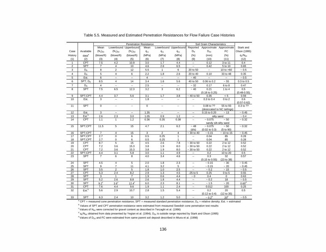
136

Mean Lowerbound Upperbound Mean Lowerbound Upperbound Reported Approximate Approximate Stark and

Case Available (N1)60 (N1)60 (N1)60 qc1 qc1 qc1 DR D50 FC Olson (1995)

History dataa (blows/ft) (blows/ft) (blows/ft) (MPa) (MPa) (MPa) (%) (mm) (%) qc/N60

(1) (2) (3) (4) (5) (6) (7) (8) (9) (10) (11) (12)

1 CPT 7.5 4.2 10.9 3.0 1.7 4.4 -- 0.12 3 to 11 0.42 SPT 7 4 10 4.6 2.6 6.5 -- 0.42 5 to 10 0.653 DR 8 2 12 5.5 1 6 20 to 50 -- 10 to >60 ~ 0.5

4 DR 5 4 6 2.2 1.8 2.6 20 to 40 0.10 33 to 48 0.355 Est. 6 -- -- 4 -- -- ~ 40 -- -- ~ 0.56 SPT; DR 8.5 4 14 3.4 1.6 5.6 40 to 50 0.06 to 0.2 ~ 55 0.3 to 0.5

7 DR 4 -- -- 2.5 -- -- ~ 32 0.17 6 to 8 0.478 SPT 7.5 6.5 12.3 3.2 3 6.2 ~ 40 0.21 1 to 4 0.5

(0.18 to 0.25) (0.48-0.55)9 SPT;CPT 4.4 3.7 5.6 3.1 1.7 3.8 ~ 40 to 50 0.35 < 5 0.59

10 Est. 3 -- -- 1.8 -- -- -- 0.3 to 0.4 0 to 2 0.6(0.57-0.62)

11 SPT 0 -- -- 0 -- -- -- 0.08 to ?? 55 to 93 0.3 to ??

12 Est. 3 -- -- 1.35 -- -- -- 0.15 to 0.20 ~ 13 ~ 0.4513 Est.b 2.6 2.3 3.0 1.05 0.9 1.2 -- ~ 0.414 CPT 1.1 1 1.2 0.36 0.35 0.38 -- ~ 0.075 ~ 50 ~ 0.32

15 SPT;CPT 11.5 5 15 4.7 2.1 6.2 ~ 48 ~ 0.075 ~ 50 ~ 0.32(d/s) (0.02 to 0.3) (5 to 90)

16 SPT;CPT 7 4 15 3 2 4 ~ 30 to 40 ~ 0.15 ~ 10 to 15 ~ 0.4517 SPT;CPT 2.7 0 6 0.5 0.25 1 -- 0.04 85 0.2818 SPT;CPT 2.7 0 6 0.5 0.25 1 -- 0.04 85 0.2819 CPT 8.7 5 15 4.5 2.6 7.8 ~ 30 to 50 0.22 2 to 12 0.5220 CPT 7.2 3.6 15.3 3.8 1.9 8.0 ~ 30 to 50 0.22 2 to 12 0.5221 CPT 7.2 3.6 15.3 3.8 1.9 8.0 ~ 30 to 50 0.22 2 to 12 0.5222 SPT;CPT 4.4 3.1 5.8 3.0 1.1 4.9 -- 0.2 10 to 20 0.523 SPT 7 6 8 4.0 3.4 4.6 -- 0.3 32 0.57

(0.15 to 0.55) (23 to 38)24 SPT 4.5 4 5 2.0 1.8 2.3 -- ~ 0.15 ~ 30 ~ 0.4525 SPT 9 7 11 4.1 3.2 5 -- ~ 0.15 ~ 20 ~ 0.4526 SPT 3.5 2 5 1.8 1.0 2.5 -- ~ 0.2 ~ 15 ~ 0.527 CPT 5.3 2.4 8.2 2.9 1.3 4.5 -25 to 5 0.25 0 to 5 0.5528 SPT 3 1 7 1.9 0.6 4.4 ~ 0 0.4 0 0.6329 SPT 5.2 2.6 8.8 2.6 1.8 4.4 -- ~ 0.2 18 ~ 0.530 SPT 9.2c 3.6c 12.4c 6.0 2.3 8.1 -- ~ 1.5 ~ 20 0.65d

31 CPT 7.6 4.4 9.6 1.9 1.1 2.4 -- 0.012 100 0.25

32 Est.b 5.6 2.9 10.7 2.8 1.5 5.4 -- 0.2 20 0.5(0.12 to 0.4) (12 to 35)

33 SPT 6.3 2.4 10 3.2 1.2 5.0 -- ~ 0.2e 20e ~ 0.5a CPT = measured cone penetration resistance; SPT = measured standard penetration resistance; DR = relative density; Est. = estimatedb Values of SPT and CPT penetration resistance were estimated from measured Swedish cone penetration test resultsc Values of N60 were corrected for gravel content as described in Terzaghi et al. (1996)d qc/N60 obtained from data presented by Yegian et al. (1994); D50 is outside range reported by Stark and Olson (1995)e Values of D50 and FC were estimated from same parent soil deposit described in Miura et al. (1998)

Penetration Resistance

Table 5.5. Measured and Estimated Penetration Resistances for Flow Failure Case Histories

sandy silt-silty sand

(desiccated to NC tailings)

silty sand

Soil Grain Characteristics

137

Figure 5.1. Relationship between liquefied shear strength and initial major principaleffective stress for remolded layered specimens of silty sand, Batch 7,Lower San Fernando Dam (from Baziar and Dobry 1995)

Figure 5.2. Comparison of consolidation behavior and steady state line for remoldedlayered specimens of silty sand, Batch 7, Lower San Fernando Dam (fromBaziar and Dobry 1995)

138

Figure 5.3. Poulos et al. (1985a) procedure to determine the liquefied shear strength fora soil at its in situ void ratio

Figure 5.4. Relationship between liquefied shear strength from liquefaction casehistories and equivalent clean sand corrected blowcount (from Seed andHarder 1990)

139

Figure 5.5. Relationship between liquefied shear strength ratio from liquefaction casehistories and equivalent clean sand corrected blowcount (from Stark andMesri 1992)

Figure 5.6. Relationship between lower bound liquefied strength ratio and equivalentclean sand corrected blowcount including SPT based level ground cleansand liquefaction relationship and laboratory liquefied strength ratio data(from Stark and Mesri 1992)

140

Figure 5.7. Illustration of Ishihara (1993) method to develop relations between liquefiedstrength ratio and corrected SPT blowcount

141

Figure 5.8. Ishihara (1993) relationship between liquefied strength ratio and (N1)60 basedon laboratory-determined quasi-steady state line compared with field datafrom Stark and Mesri (1992)

Figure 5.9. Ishihara (1993) relationship between liquefied strength ratio and qc1 based onlaboratory-determined quasi-steady state line compared with field data from Ishiharaet al. (1990a) and Ishihara (1993)

142

Figure 5.10. A. Idealized relationship between liquefied shear strength and (N1)60

B. Relationship between χ and λ (slope of the steady state line) obtained fromliquefaction case histories and laboratory tests (from Konrad and Watts 1995)

(A)

(B)

143

Figure 5.11. (A) Relationship between liquefied strength ratio and state parameter basedon undrained triaxial compression tests of Ottawa and Alaska sands; (B)Relationship between liquefied shear strength and corrected shear wavevelocity for Ottawa and Alaska sands for indicated range in Ko; (C)Relationship between liquefied shear strength and (N1)60 for Ottawa andAlaska sands compared with data from Duncan Dam and Seed and Harder(1990) case history bounds; and (D) Relationship between liquefied strengthratio and (N1)60 for Ottawa and Alaska sands compared with Stark and Mesri(1992) case history bounds

(A) (B)

(C) (D)

144

Figure 5.12. Schematic force diagram for simplified stability analysis. W’ is effective slice weight, N’ is effective normal force,su is undrained shear resistance, E is slice side force, B is slice width, H is thickness of flowed material, γγγγt is totalor effective unit weight, αααα is slope of ground surface and flowed material.

E

E

145

Figure 5.13. (a) Simplified pre-failure geometry of Lower San Fernando Dam for determination of pre-failure vertical effectivestresses used in liquefied strength ratio stability analysis; (b) Simplified post-failure geometry and assumed finalpositions of the liquefied soil segments (segments 10-14 did not liquefy)

146

Figure 5.14. Freebody diagram used for kinetics analysis and kinetics analysis for NorthDike of Wachusett Dam

147

Figure 5.15. Proposed relationship between liquefied strength ratio and corrected SPTblowcount and comparison with SPT based liquefied strength ratiorelationships in literature

148

Figure 5.16. Proposed relationship between liquefied strength ratio and corrected CPTtip resistance and comparison with CPT based liquefied strength ratiorelationships in literature

149

Figure 5.17. Evaluation of strength ratio concept using liquefaction flow failure casehistories

150

Figure 5.18. Difference in back-calculated shear strength with and without consideringkinetics compared to (a) loss of potential energy resulting from flow failure;and (b) pre-failure height of embankment

151

CHAPTER 6

CONFIRMATION OF YIELD AND LIQUEFIED STRENGTH RATIOSUSING LABORATORY DATA

6.1 INTRODUCTION

The yield and liquefied strength ratio concepts presented in Chapters 4 and 5,

respectively, appear to apply to field case histories of liquefaction flow failure. This chapter

presents an evaluation of these concepts using laboratory data to confirm their application to

conditions and situations outside those represented by the case history database.

The yield strength ratio, or collapse surface, concept is relatively well-established for

a number of individual sands (e.g., Hanzawa 1980; Sladen et al. 1985a; Vaid and Chern

1985; Ishihara 1993; Sasitharan et al. 1993). However, to the author’s knowledge, the

universal applicability of this concept to a large number of sandy soils has not been

determined.

The liquefied strength ratio, while gaining more widespread acceptance, still has not

generally been accepted to hold for most sandy soils. Recent laboratory testing (e.g.,

Ishihara 1993; Baziar and Dobry 1995; Vaid and Sivathalayan 1996) show that the liquefied

shear strength of many cohesionless soils is linearly proportional to initial major principal

effective stress. However, the liquefied strength ratio is a function of state parameter (Fear

and Robertson 1995), and the liquefied strength ratio is only a constant if the consolidation

behavior parallels the steady state line (Finn 1998). It has not been shown under what

conditions the consolidation and steady state lines are parallel, and if there is a unique

relationship between state parameter and liquefied strength ratio for sandy soils.

152

To this end, a database of laboratory test results, primarily triaxial compression tests,

was collected and interpreted. The database was examined to address issues of: (1)

parallelism of consolidation behavior and steady state line; (2) confirmation and applicability

of the yield strength ratio concept; and (3) confirmation and applicability of liquefied strength

ratio concept.

6.2 APPLICABILITY OF STRENGTH RATIOS FOR LIQUEFACTIONANALYSIS

6.2.1 Laboratory Database of Sandy Soils

Table 6.1 presents the database of sandy soils collected for this study. Table 6.1

contains grain characteristics, maximum and minimum void ratios, and references for each

of the sands studied. Table 6.2 presents the steady state line parameters and steady state

(or constant volume) effective friction angles, as well as compressibility data available for the

sands studied. In Table 6.2, the slope of the steady state line in e-log p' space is defined as

λ, and the intercept @ 1 kPa (sometimes referred to as Γ) is the value of void ratio on the

steady state line at a mean effective stress of 1 kPa. Both one-dimensional compressibility

index, Cc, and the consolidation behavior during increase in isotropic confining stress (i.e.,

slope of the e-log pmean' line) are reported if available.

6.2.2 Slope of Steady State Line

The slope of the steady state line is affected by soil gradation (Poulos et al. 1985a).

Minor changes in gradation can cause significant changes in the slope of the steady state

line. Poulos et al. (1985a) also stated that increasing grain angularity increases the slope of

153

the steady state line. Fear and Robertson (1995) and Zlatovic and Ishihara (1995) presented

data that suggest that the slope of the steady state line of a given soil increases with

increasing fines content.

A comparison of fines content and slope of the steady state line for the sands in

Table 6.1 and 6.2 is presented in Figure 6.1. Figure 6.1 shows no trend between the steady

state line and increasing fines content. These data indicate that grain angularity may affect

the slope of the steady state line more significantly than fines content, as the soil in the

laboratory database with the steepest steady state line is an angular clean sand (Sand A,

Castro 1969).

6.2.3 Steady State Line and Soil Compressibility

As discussed in Chapters 2 and 5, when the steady state line parallels the

consolidation behavior, the state parameter is constant and the liquefied strength ratio is

constant. Figures 5.2 and 6.2 through 6.6 present the slopes of steady state lines and

consolidation behaviors for a number of sandy soils. For these sandy soils, the slopes of

steady state line and consolidation behavior are generally parallel, at least for a given range

of effective stresses. The question then becomes: under what conditions (fines content,

stress range, etc.) is it reasonable to assume a parallel steady state line and consolidation

behavior?

Figure 6.7 presents a comparison of steady state line slope and slope of the

consolidation behavior for the sandy soils in Tables 6.1 and 6.2. The data are classified in

terms of the Unified Soil Classification System (USCS), where clean sands with less than

5% fines content are classified as SP, sandy soils with fines content between 5 and 12% are

classified as SP-SM, silty sands with fines content between 12 and 50% are classified as

154

SM, and sandy silts and silts with fines content greater than 50% (see Terzaghi et al. 1996

for details of the USCS).

It is well-known that the consolidation behavior of sands depends on the initial

density at deposition. Sands that are deposited in a dense state are less compressible than

the identical sand initially deposited in a loose state (e.g., Ishihara 1993). Since liquefaction

only occurs in loose (or contractive) sandy soils, the slopes of the consolidation behavior

reported in Table 6.2 were obtained from specimens deposited in initially loose states. As

the fines content of the soil increases, the range of initial densities for different depositional

procedures tended to decrease. Therefore, differences in compressibility appear to

decrease with increasing fines content.

In general, the data in Figure 6.7 suggest that for many sandy soils (with a large

range of fines contents, grain sizes and shapes, and steady state line slopes) the slopes of

the steady state line and consolidation behavior generally are parallel. Therefore, the

liquefied strength ratio should be a constant for a given soil. In particular, sandy soils with

fines content greater than 12% exhibit nearly parallel slopes of the steady state line and

consolidation behavior. This parallelism holds for a wide range of effective stresses

applicable to civil engineering structures, as indicated in Table 6.2. It should be noted that

blanks in the stress range column in Table 6.2 indicate that the reported values of steady

state line and consolidation behavior slopes were reasonably constant over the entire range

of laboratory test results.

In summary, the liquefied strength ratio concept appears reasonable for many sands,

at least over the range of effective stresses applicable to civil engineering structures. This is

particularly true for silty sands, sandy silts, and silts with fines content greater than 12%.

155

6.3 CONFIRMATION OF YIELD STRENGTH RATIO

As discussed in Chapter 4, Hanzawa et al. (1979) indicated that peak shear

strengths measured during shear tests produced an approximately linear peak shear

strength envelope in stress path space. Sladen et al. (1985a) defined a collapse surface in

three-dimensional void ratio-shear stress-normal stress space to represent conditions that

would lead to the triggering of flow liquefaction, or strain-softening behavior. The collapse

surface represents the locus of peak (or yield) shear stresses that a given soil can reach for

varying combinations of void ratio and normal effective stress. A number of other

investigators (e.g., Vaid and Chern 1983,1985; Kramer and Seed 1988; Vasquez-Herrera

and Dobry 1989; Ishihara 1993; Konrad 1993; Sasitharan et al. 1993, 1994; among others)

identified similar collapse conditions and proposed various names for these conditions.

Figures 6.8 through 6.10 show examples of the collapse surface (or peak strength envelope)

in normalized stress path space for a number of clean and silty sands (see Tables 6.1 and

6.2 for details regarding the sands).

Herein, this line of yield (or peak) shear strengths is denoted the yield strength

envelope (see Chapter 4) because it defines the stress conditions at which the yield shear

strength is mobilized. Direct comparisons of yield conditions defined in stress path space (p’-

q), Mohr-Coulomb space (shear stress-normal stress), and other conditions can be made by

known trigonometric conversions.

6.3.1 Laboratory Database Test Results

Table 6.3 presents available triaxial compression test results for the sands listed in

Table 6.1. Initial conditions of void ratio (ec), relative density (DR), state parameter (ψ), and

major and minor principal effective stresses at the end of consolidation (σ’1c and σ’3c,

156

respectively) are reported, if available. Values of deviator stress and porewater pressure at

yield [qu(yield) and ∆uyield], at the quasi-steady state [qu(min) and ∆umin], and at the steady

state [qus and ∆uss] during shear also are reported. The yield shear strength and liquefied

shear strength are defined as:

2

)()(

yieldqyields u

u = (6.1a)

ssus

uq

s LIQ 'cos2

)( φ= (6.1b)

respectively, where φ'ss is the steady state (or constant volume) friction angle reported in

Table 6.2.

Direct simple shear, torsional or rotation shear, and triaxial extension tests were not

included in Table 6.3. The reasons for not including these data are: (1) considerably fewer

test results using these modes of shear are available in the literature; (2) at small to

intermediate strain levels, the yield and quasi-steady state shear strengths will differ

depending on the mode of shear; and (3) the purpose of this study is to confirm the yield

and liquefied strength ratio concepts, not to develop correlations for use in design. In

addition, only tests conducted at equal all-around pressures (isotropic confining pressures)

were included for simplicity and consistency. While anisotropic consolidation stress

conditions do not affect the position of the collapse surface or liquefied shear strengths, the

actual magnitudes of yield strength are affected.

As discussed in Chapters 4 and 5, the mode of shear approximates direct shear

conditions within the zone of liquefaction for most of the flow failure case histories. For direct

157

comparison to the field data, laboratory direct, simple or torsional shear test results would be

required. Unfortunately, direct shear, simple shear, and torsional or rotation shear test

results for loose sands are limited in the literature.

6.3.2 Collapse Surface from Laboratory Data

The laboratory database again was classified as clean sands (SP), clean sands to

silty sands (SP-SM), silty sands (SM), and sandy silts to silts (ML). Figure 6.11 presents

collapse surface data in p'-q space for the clean sands. The slope of the collapse surface in

p'-q space is referred to as ML (or MP by some investigators). The slope ML can be related to

an equivalent Mohr-Coulomb friction angle at the yield strength envelope, φy, as follows:

L

Ly M

M

+=

6

3sinφ (6.2)

As indicated by Eq. (4.1), the tangent of the equivalent friction angle at the yield strength

envelope is approximately equivalent to the yield strength ratio.

Referring to Figure 6.11, the slope of the collapse surface in triaxial compression

ranges from approximately 0.615 to 0.9 for nearly all clean sands. Note that the slope of 0.9

has an apparent intercept on the q-axis of approximately 55 kPa. At values of mean

effective stress, p', less than 700 kPa, the upper bound value of ML can be approximated as

1.0. These values of collapse surface slope correspond to equivalent friction angles at the

yield strength envelope of 16 to 23° (with a maximum value of 25° at mean effective

stresses less than 700 kPa).

Figure 6.12 presents collapse surface data for the SP-SM sands. For two sands,

individual data that could be used to evaluate the slope of the collapse surface were not

158

presented. However, the investigators did provide measured values of ML. These data are

plotted in Figure 6.12 as dashed lines over the applicable range of mean effective stresses.

The SP-SM data in Figure 6.12, in general, plot within the upper and lower bound collapse

surface values determined for clean sands.

Similarly, Figure 6.13 presents collapse surface data for the SM and ML sands. In

three cases, investigators reported ML values rather than individual test results. These

collapse surface data were plotted over the range of applicable mean effective stresses.

Again, the SM and ML data plot within the upper and lower bound collapse surface values

determined for clean sands.

In summary, the collapse surface in triaxial compression for many sandy soils ranges

from 0.615 to 1.0. This corresponds to a range of equivalent friction angles at the yield

strength envelope of 16 to 23° (with an upper bound of 25°). In turn, this corresponds to

yield strength ratios ranging from 0.29 to 0.42 (with an upper bound of 0.47). As discussed

previously, the author anticipates that values of yield strength ratio determined for triaxial

compression should be greater than values determined for direct shear, which should be

greater than values determined for triaxial extension.

6.3.3 Relation between Collapse Surface and State Parameter

Because of the range of potential yield strength ratios determined for triaxial

compression, attempts were made to correlate yield strength ratio to state parameter. The

author suspected that increases in yield strength ratio may correspond to decreases in state

parameter (i.e., increases in density at a given effective stress). To test this hypothesis,

Figure 6.14 plots values of collapse surface slope against state parameter. Only sands with

more than three data points were used in this plot so that trends could be evaluated

reasonably.

159

As indicated in Figure 6.14, there is no unique relation between the slope of the

collapse surface and state parameter. However, for several individual sands, a general trend

of increasing collapse surface slope with decreasing state parameter is noted.

Unfortunately, data are too limited to make additional conclusions regarding any possible

correlation. It is also possible that an alternate definition of state [such as the state index

(Ishihara 1993), excess porewater pressure ratio at steady state (Yoshimine and Ishihara

1998), or excess porewater pressure ratio at yield] would provide a better correlation with

yield strength ratio. This appears to be a potential avenue of future research.

6.3.4 Comparison of Laboratory Collapse Surface with Field Data

Figure 6.15 presents a comparison of the range of collapse surface determined for

laboratory triaxial compression test results with the equivalent range of yield strength ratios

determined from flow failure case histories in Chapter 4. The yield strength ratios

determined from flow failure case histories ranged from 0.231 to 0.306. This corresponds to

equivalent friction angles at the yield strength envelope of 13 to 17°, and collapse surface

slopes of approximately 0.49 to 0.65 (using Eq. 6.2). Mean effective stresses at yield for the

case history bounds were determined by assuming K0 = 0.5.

As expected, the field case history bounds plot slightly below the laboratory bounds.

That result is expected because the laboratory bounds correspond to triaxial compression

while the field case history bounds correspond approximately to direct simple shear

conditions. The author anticipates that triaxial extension collapse surfaces would plot slightly

below the field case history bounds (direct shear conditions). This also presents an avenue

for future research.

No attempts were made to relate laboratory yield strength ratio to corrected

penetration resistance. This was not attempted because no clear correlation exists between

160

the slope of the collapse surface and state parameter for the laboratory database. It may be

possible to relate yield strength ratio to other measures of state, as suggested in Section

6.3.3. Again, this presents an avenue for future research. However, the laboratory data

support the yield strength ratio concept for many sandy soils, and the field data are in

agreement with expected laboratory behavior.

6.4 CONFIRMATION OF LIQUEFIED STRENGTH RATIO

As discussed in Chapter 5, recent laboratory testing (e.g., Ishihara 1993; Pillai and

Salgado 1994; Baziar and Dobry 1995; Vaid and Sivathalayan 1996) has shown that the

liquefied shear strength of many cohesionless soils is linearly proportional to the initial major

principal effective stress. Figures 5.1, 6.16, and 6.17 present examples of this behavior.

Fear and Robertson (1995) indicated that for a given method of deposition and mode of

shearing, there is a unique value of liquefied strength ratio for a given value of state

parameter, as shown in Figure 5.11(a). A similar example of this relation is shown for Fraser

River Sand in Figure 6.18. Vaid and Sivathalayan (1996) measured liquefied shear

strengths over a wide range of void ratio using simple shear tests and plotted the resulting

liquefied strength ratios against increasing void ratio. Increasing void ratio in Figure 6.18

corresponds to increasing state parameter. Lastly, relationships such as those proposed in

Chapter 5 between liquefied strength ratio and corrected penetration resistance (Figures

5.15 and 5.16) assume a relation between decreasing state parameter (or increasing

relative density) at a given vertical effective stress and increasing corrected penetration

resistance. The following sections will explore the validity of these relations using the

laboratory database of triaxial compression test results presented in Table 6.3.

161

The following relations use the quasi-steady state shear strength as the liquefied

shear strength, as suggested by Ishihara (1993) and Yoshimine et al. (1999) (among others)

and as discussed in Chapter 5. The use of the quasi-steady state rather than the ultimate

steady state shear strength may explain the observation by Fear and Robertson (1995) that

the relationship between state parameter and liquefied strength ratio for a given sand

depends on the method of deposition and mode of shear. However, only very loose to loose

sands are susceptible to liquefaction flow failure and for these sands the quasi-steady state

and steady state are equivalent (Ishihara 1993; Gutierrez 1998; Olson 1998), therefore, it

appears reasonable to base the following relations on the quasi-steady state shear strength.

6.4.1 Liquefied Strength Ratio and State Parameter

Relationships between liquefied strength ratio and state parameter such as those

presented in Figure 5.11(a) were examined for the two sands in the database with sufficient

test results, namely Sand B (Castro 1969) and Toyoura sand (Ishihara 1993). Figure 6.19

presents the individual values of liquefied shear strength and major principal effective

confining stress, σ'1c, for Sand B. State parameters for each of the specimen are shown

beside the data points. Contours of equal state parameter were determined by regression

analysis. These data indicate that as state parameter increases (i.e., soil becomes more

contractive or looser with respect to the SSL), liquefied strength ratio decreases.

Figure 6.20 presents a similar relation between liquefied strength ratio and state

parameter for Toyoura sand. Although the contours of constant state parameter are not

linear, they indicate that an increase in state parameter corresponds to a decrease in

liquefied strength ratio.

Figure 6.21 presents relationships between liquefied strength ratio and state

parameter for the five sands in the laboratory database with sufficient data to define a clear

162

trend. In general the shapes of the trend lines are similar to those in Figure 5.11(a) and

6.18, and indicate decreasing liquefied strength ratio with increasing state parameter.

However, this relation is not unique for all sandy soils.

6.4.2 Comparison of Laboratory Strength Ratio and Field Data

Flow failure case histories indicated a trend of increasing liquefied strength ratio with

increasing vertical effective stress (Figure 5.17). Figure 6.22 presents a similar plot for the

laboratory database of triaxial compression tests. Only laboratory tests conducted at mean

effective stresses less than 1 MPa were included in Figure 6.22. The reason for this is

because grain crushing typically occurs at mean effective stresses greater than 1 MPa

(Konrad 1998). Grain crushing signicantly increases the slope of the steady state line, and it

is not clear whether relations based on state parameter hold when grain crushing occurs.

The data in Figure 6.22 indicate that for all sandy specimens with positive values of

state parameter (corresponding to specimens initially loose of the SSL) in the laboratory

database, the liquefied strength ratio ranges from approximately 0.02 to 0.22. Careful

examination of Figure 6.22 indicates that, in general, increasing values of state parameter

correspond to decreasing values of liquefied strength ratio for all sands.

For comparison, the field case history bounds determined in Figure 5.17 are

reproduced in Figure 6.22. The field case histories fall well within the boundaries of the

laboratory data. However, as discussed previously, direct comparison of the traixial

compression laboratory test data and the field data (corresponding to direct shear) is only

appropriate if the steady state is independent of the mode of shear. The discussion in

Section 2.3.5 indicates that this issue is unresolved. If direct comparison is appropriate, it

appears that the case history data roughly correspond to laboratory data with state

parameters ranging from 0.02 to 0.10.

163

6.4.3 Laboratory Strength Ratio and Relative Density

For eventual comparison to field data, Figure 6.23 presents a comparison between

relative density and liquefied strength ratio for the clean sand laboratory data. Figure 6.23

includes an upper and lower bound relationship between relative density and liquefied

strength ratio for clean sands tested in triaxial compression. The lower bound relationship

approaches a vertical asymptote at a relative density of approximately 60%. This vertical

asymptote of DR ~ 60% is very similar to those suggested by Thevanayagam et al. (1996a,b)

of approximately 60 to 75% for sands with less than 12% fines content.

Figure 6.24 presents a similar plot of relative density and liquefied strength ratio for

sand with some fines (SP-SM), silty sands (SM), and sandy silts to silts (ML). It can be seen

that the SP-SM data plot above the lower bound relation for clean sands. Therefore, the

clean sand bound may be applicable to sands with less than about 12% fines content. In

addition, while there are significantly fewer data in these plots, a lower bound relation for

silty sands was included based on similar relations proposed by Thevanayagam et al.

(1996a,b). The lower bound relationship for silty sands tested in triaxial compression

approaches a vertical asymptote at a relative density of approximately 87%. This vertical

asymptote of DR ~ 87% is very similar to those suggested by Thevanayagam et al. (1996a,b)

of approximately 77 to 97% for sands with between 12 and 50% fines content. From Figure

6.24, it is evident that silty soils may have very low liquefied strength ratios, even at very

large relative densities. Lade and Yamamuro (1997), Yamamuro and Lade (1998), and

Thevanayagam (1998) observed similar low strength behavior in silty sands with large

relative densities.

164

6.4.4 Conversion of Relative Density to Penetration Resistance

To compare the laboratory data with the relations between liquefied strength ratio

and corrected penetration resistance proposed in Chapter 5, it was necessary to relate

relative density to corrected penetration resistance. While some investigators, e.g., Been et

al. (1987b) and Konrad (1998), have proposed relations between corrected CPT tip

resistance and state parameter, others, e.g., Sladen (1989) and Huang et al. (1999), have

indicated that these relations are not universally applicable. Therefore, this study did not use

these relations to estimate corrected penetration resistance. However, this is a potential

avenue of future research. Furthermore, correlations between relative density and corrected

penetration resistance based on calibration chamber testing of clean sands may not apply to

sands with significant fines content, unless the penetration-induced porewater pressure is

considered (Peterson 1991). However, for preliminary comparison, relationships between

relative density and corrected penetration resistance developed for clean sands will be

used.

Tokimatsu and Seed (1987) proposed the following relation between (N1)60 and

relative density:

( ) 2601 44 RDN ⋅= (6.3)

based on field density measurements, relative density measurements from samples

obtained using in situ freezing, and Meyerhof’s (1957) proposed relationship between

relative density, vertical effective stress, and SPT blowcount. To account for the effect of

grain size on the relation between (N1)60 and relative density observed by Skempton (1986),

Kulhawy and Mayne (1990) proposed the following relation:

165

( )502

601 log2560 DD

N

R

+= (6.4)

This study assumes D50 equal to 0.3 mm for clean sands and 0.17 mm for silty sands (as

suggested in Chapter 3). The (N1)60 values obtained from Eqs. (6.3) and (6.4) were

averaged for use in the following analysis.

Jamiolkowski et al. (1985) proposed the following relation between qc1 and relative

density (as interpreted by Yoshimine et al. 1999):

PaD

PaNcc CCqq R ⋅=⋅= + ]66/)65[(11 10 (6.5)

where qc1N is the dimensionless corrected penetration resistance and CPa is a constant equal

to 0.1 MPa to convert qc1N to qc1 in MPa. This relationship is based on calibration chamber

testing of 5 normally consolidated clean sands. Based on calibration chamber testing of

Toyoura sand where penetration-induced porewater pressure was considered, Yoshimine et

al. (1999) suggested a relation proposed by Tatsuoka et al. (1990) between qc1N and relative

density as follows:

PaD

PaNcc CCqq R ⋅=⋅= + ]76/)85[(11 10 (6.6)

The qc1 values obtained from Eqs. (6.5) and (6.6) were averaged for use in the following

analysis.

166

6.4.5 Comparison of Laboratory Strength Ratio/PenetrationResistance Relationships and Field Strength Ratios

Values of relative density for the upper and lower bound DR-su(LIQ)/σ'vo relationships

for clean and silty sand (Figures 6.23 and 6.24, respectively) were converted to (N1)60 and

qc1 as described in Section 6.4.4.

Figure 6.25 presents the upper and lower bound relations between (N1)60 and

liquefied strength ratio for clean and silty sand. Figure 6.25 includes liquefied strength ratios

back-calculated from flow failure case histories and the case history boundaries presented

in Figure 5.15. Figure 6.25 indicates that the case history data all plot above the lower

bound relation for silty sands tested in triaxial compression, and most are above the lower

bound relation for clean sands tested in triaxial compression. Therefore, the conclusions

made and relationships proposed in Chapter 5 appear to be valid. Further, relationships

between corrected penetration resistance and liquefied strength ratio based on laboratory

testing of one sand are not applicable to all sands and do not describe flow failure case

histories.

Similarly, Figure 6.26 presents the upper and lower bound relations between qc1 and

liquefied strength ratio. Figure 6.26 includes the liquefied strength ratios back-calculated

from flow failure case histories and the case history boundaries presented in Figure 5.16.

Figure 6.26 indicates that the case history data all plot above the lower bound relation for

silty sands tested in triaxial compression, and most are above the lower bound relation for

clean sands tested in triaxial compression. Therefore, the relationships proposed and

conclusions made in Chapter 5 appear to be valid.

Ishihara (1993) presented similar relations between liquefied strength ratio and

corrected SPT penetration resistance for Toyoura, Chiba, and Kiyosu sand tested in triaxial

compression. These sands approached vertical asymptotes at (N1)60 values of

167

approximately 4.4, 8.5, and 11, respectively. These asymptotes for individual sand plot

between the upper and lower bound relationships presented in Figure 6.25. The relations

presented by Ishihara (1993) are based on individual sands (tested in triaxial compression),

and therefore are not universally applicable. As such, these relations for individual sands do

not provide a reasonable basis for comparison with field case history data.

Yoshimine et al. (1999) also presented relations between liquefied strength ratio,

relative density, and dimensionless corrected CPT tip resistance for Toyoura sand. The

relations based on triaxial compression tests approach vertical asymptotes at a relative

density of approximately 32 to 36% and a corrected penetration resistance of 3.5 to 4.0

MPa. These asymptotes plot between the upper and lower bound relationships presented in

Figures 6.23 and 6.26, respectively. Again, the relations presented by Yoshimine et al.

(1999) are based on one sand (in triaxial compression) and are not universally applicable.

As such, the Yoshimine et al. (1999) relationship does not provide a reasonable basis for

comparison with field case history data.

6.5 CONCLUSIONS

Laboratory triaxial compression test results from clean sands, silty sands, sandy silts,

and silts reported in the literature were collected to confirm the strength ratio concepts

presented in Chapters 4 and 5. The database was examined to address the following

issues: (1) parallelism of consolidation behavior and steady state line; (2) confirmation and

applicability of the yield strength ratio concept; and (3) confirmation and applicability of the

liquefied strength ratio concept.

The steady state line and consolidation behavior are generally parallel for a wide

range of fines content, grain sizes and shapes, and steady state line slopes, at least for a

168

given range of effective stresses. Therefore, as discussed in Chapter 5, the liquefied

strength ratio should be constant for a given soil deposited in a consistent manner. In

particular, sandy soils with fines content greater than 12% exhibit nearly parallel slopes of

steady state line and consolidation behavior. This parallelism holds for a wide range of

effective stresses applicable to civil engineering structures. As the large majority of flow

failure case histories involve sands with some silt, this finding helps explain the relation

between liquefied shear strength and vertical effective stress observed for case histories.

The laboratory data exhibited yield strength ratios ranging from 0.29 to 0.42 (with an

upper bound of 0.47 at mean effective stresses less than 700 kPa). These bounds

correspond to equivalent friction angles at the yield strength envelope of 16 to 23° (with an

upper bound of 25° at mean effective stresses less than 700 kPa). In comparison, yield

strength ratios back-calculated from flow failure case histories ranged from approximately

0.23 to 0.31. This corresponds to equivalent friction angles at the yield strength envelope of

13 to 17°.

As expected, the yield strength ratios back-calculated from flow failure case histories

are smaller than those determined from laboratory triaxial compression tests. This result is

expected because the yield shear strength is mobilized at small strains. At small strain, the

mobilized strength is a function of the mode of shear, with yield strengths being largest in

triaxial compression, smaller in direct or simple shear, and smallest in triaxial extension. The

stress conditions in the zones of liquefaction for most of the case histories correspond

approximately to direct simple shear conditions, and therefore, yield strength ratios back-

calculated from the case histories should be smaller than those measured in the database of

laboratory triaxial test results.

169

The liquefied strength ratio measured in laboratory triaxial compression tests is

shown to be a function of state parameter. For contractive sandy soils (i.e., soils susceptible

to flow failure) tested in triaxial compression, the liquefied strength ratio ranged from 0.02 to

0.22 over a wide range of initial major principal effective stress. Comparison with liquefied

strength ratios back-calculated from flow failure case histories show that the case histories

fall well within the laboratory bounds of liquefied strength ratio. Assuming that the back-

calculated liquefied shear strengths can be directly compared to the liquefied strength ratios

measured in the laboratory tests (which includes some values of quasi-steady state shear

strengths taken as the liquefied shear strength), the case histories appear to have state

parameters of roughly 0.02 to 0.10.

Lastly, upper and lower bound relationships between laboratory liquefied strength

ratios and relative density are presented for relatively clean sands (less than 12% fines

content) and silty sands (between 12 and 50% fines content). These relationships were

converted to relationships between liquefied strength ratio and corrected SPT and CPT

penetration resistance for comparison with field data. The comparisons indicate that the

case history data all plot above the lower bound relation for the laboratory SM data, and

most plot above the lower bound relation for the SP data. This result suggests that the

relationships proposed and conclusions made in Chapter 5 are valid. Furthermore, relations

between liquefied strength ratio and corrected penetration resistance based on laboratory

testing of one sand (from a given site) can be unconservative for preliminary design at other

sites.

170

Sand D50 FCNo. Sand Name (mm) (%) emax Method5 emin Method6 Reference1 Dune sand (DS) 0.21 3 0.91 A 0.54 a Konrad (1990a)

2 well-rounded silica sand (WA) 0.175 1 1.06 A 0.67 a Konrad (1990a)

3 Fraser River Delta sand (FRD) 0.25 3-15 1.00 A 0.60 a Chillarige et al. (1997)

4 Duncan Dam sand (DD) 0.2 6.5 1.15 --7 0.76 -- Pillai and Stewart (1994)

5 Hostun RF sand (HRF) 0.38 0 1 -- 0.656 -- Canou et al. (1994)

6 Garnet tailings (GT) 0.17 20 1.52 -- 0.53 b Highter and Tobin (1980); Highter and Vallee (1980)

7 Zinc tailings (ZT) 0.2 17 1.43 -- 0.49 b "

8 Natural silt (NS) 0.013 98 1.526 -- 0.434 -- Dyvik and Hoeg (1998)

9 fine - coarse sand (FCS) 0.33 1 0.796 -- 0.404 -- Dierichs and Forster (1985)

10.1 Ottowa Banding sand (OBS)1 0.19 2 0.82 -- 0.51 -- Dennis (1988)

10.2 Ottowa Banding sand (OBS)2 0.19 2 0.82 -- 0.51 -- "



11 Nevada fine sand (NFS) 0.12 -- 0.87 -- 0.57 -- Arulanandan et al. (1993)

12.1 Nerlerk 0% - 2% (N2) 0.23-0.28 0-2 0.94 C 0.62 c Sladen et al. (1985a)

12.2 Nerlerk 12% (N12) 0.28 12 0.96 B 0.43 c "

13 Leighton Buzzard (LBS) 0.86 0 0.75 C 0.58 c "

14 Syncrude tailings sand (STS) 0.17 10 0.93 A 0.55 a Sladen and Handford (1987)

15 Tottori sand (TS) 0.28 0 1.008 D 0.638 d Takeshita et al. (1995)

16 Monterey #9 sand (M9S) 0.35 0 0.86 E 0.53 e Riemer et al. (1990); Riemer and Seed (1992);

Riemer and Seed (1997)

17 Sydney sand (SS) 0.3 -- 0.855 -- 0.565 -- Chu (1995)

18 Arabian Gulf sand (AGS) -- 40 -- -- -- -- Hanzawa (1980)

19 Hostun RF sand (HRFS) 0.32 0 1 -- 0.655 -- Konrad (1993)

20 Till sand (TillS) 0.11 32 0.835 -- 0.3625 -- "

21 Massey Tunnel sand (MTS) 0.25 3 1.102 F 0.712 f Konrad and Pouliot (1997)

22 Quebec sand (QS) 0.5 0 0.79 B 0.54 f Konrad (1998)

23 Erksak 330/0.7 (E330) 0.33 0.7 0.753 -- 0.469 -- Been et al. (1991)

24 Ottowa sand (C109) 0.34 0 0.82 A 0.5 a Sasitharan et al. (1993; 1994)

25 Sand F 0.205 0 1.88 G 1.23 g Castro and Poulos (1977); Castro (1969)

26 Sand B 0.16 0 0.84 G 0.5 g "

27 Sand C 0.27 1 0.99 G 0.66 g "

28 Sand H 0.66 13 0.73 G 0.36 g "

Void ratio data

Table 6.1. Laboratory Database of Sandy Soils Used to Examine Strength Ratio Concepts

171

Sand D50 FCNo. Sand Name (mm) (%) emax Method5 emin Method6 Reference29 Sand A 0.2 2 1.88 G 1.23 g Castro (1969)

30 Alcan tailings (AT) 0.002 99 n/a -- -- -- Poulos et al. (1985b)

31 Mai-Liao sand (MLS) 0.105 15 1.06 -- 0.59 -- Huang et al. (1999)

32 Star Morning tailings (SMT) 0.062 51 -- -- -- -- Bryant et al. (1983)

33 Bunker Hill tailings (BHT) 0.0097 87 -- -- -- -- "

34 Coeur Mine tailings (CMT) 0.06 54 -- -- -- -- "

35 Galena tailings (GT) 0.086 40 -- -- -- -- "

36 Lucky Friday tailings (LFT) 0.065 53 -- -- -- -- "

37 Mission tailings (MT) 0.04 60 -- -- -- -- "

38 Morenci tailings (MoT) 0.086 47 -- -- -- -- "

39 Climax tailings (CT) 0.026 67 -- -- -- -- "

40 Lornex Mine tailings (LMT) 0.256 7 -- -- -- -- "

41 Ottowa sand F125 (F125) 0.1 12 -- -- -- -- Vasquez-Herrera and Dobry (1988) &

42 Sand A (SA) 0.15 13 -- -- -- -- Baziar and Dobry (1995)

43 San Fernando SF7 sand (SF7) 0.075 50 0.72 -- 0.34 -- Baziar and Dobry (1995); Seed et al. (1989)

44 Toyoura sand (ToS) 0.17 0 0.977 D 0.597 d Ishihara (1993)

45 Lagunillas sandy silt (LSS) 0.05 74 1.389 D 0.766 d "

46 Tia Juana silty sand (TJSS) 0.16 12 1.099 D 0.62 d "

1Strain control, equal energy

2Strain control, equal volume

3Stress control, equal energy

4Strain control, equal volume 5Methods to determine emax: (A) ASTM D2049; (B) Kolbuszewski (1948); (C) unspecified ASTM procedure; (D) JSSMFE; (E) dry pluviation; (F) ASTM D4254; (G) non-standard procedure

6Methods to determine emin: (a) ASTM D2049; (b) Modified Proctor compaction; (c) unspecified ASTM procedure; (d) JSSMFE; (e) modified Japanese method; (f) ASTM D4254; (g) non-standard procedure

7-- = not available

Table 6.1. Laboratory Database of Sandy Soils Used to Examine Strength Ratio Concepts (cont.)

Void ratio data

172

Sand slope intercept φφφφ'ss

No. Sand Name λλλλ @ 1 kPa (o) Cc Isotropic (kPa)6

1 Dune sand (DS) 0.1625 1.1521 34.4 -- 0.103 50-3000

2 well-rounded silica sand (WA) 0.02932 1.0095 34 -- --

3 Fraser River Delta sand (FRD) 0.07 1.11 30 0.27 0.12 < 800

4 Duncan Dam sand (DD) --5 -- -- 0.15 -- 100-1500

5 Hostun RF sand (HRF) -- -- 33.4 -- --

6 Garnet tailings (GT) 0.255 1.59 -- -- --

7 Zinc tailings (ZT) 0.179 1.3275 -- -- --

8 Natural silt (NS) -- -- 36 -- --

9 fine - coarse sand (FCS) -- -- -- -- --

10.1 Ottowa Banding sand (OBS)1 0.069 0.900 30 -- --




11 Nevada fine sand (NFS) 0.0657 0.832 29.1 -- --

12.1 Nerlerk 0% - 2% (N2) 0.04 0.883 30 -- --

12.2 Nerlerk 12% (N12) 0.07 0.80 31 -- --

13 Leighton Buzzard (LBS) 0.08 1.00 30 -- --

14 Syncrude tailings sand (STS) 0.039 0.845 29.7 -- 0.039 100-1200

0.039 -- -- 0.01 5-100

15 Tottori sand (TS) -- -- 35.5 -- 0.02 50-1000

16 Monterey #9 sand (M9S) -- -- 32.3 -- --

17 Sydney sand (SS) -- -- 31 -- --

18 Arabian Gulf sand (AGS) -- -- -- -- --

19 Hostun RF sand (HRFS) 0.0735 1.0546 33.4 -- --

20 Till sand (TillS) 0.1415 0.791 34.6 -- --

21 Massey Tunnel sand (MTS) -- -- 39 -- --

22 Quebec sand (QS) 0.021 0.757 -- -- --

23 Erksak 330/0.7 (E330) 0.0306 0.820 30 -- --

0.310 1.167 -- -- > 1000

24 Ottowa sand (C109) 0.0387 0.864 30.6 -- --

25 Sand F 0.55 -- -- 0.46 -- > 50

26 Sand B 0.05 0.804 30 0.03 -- > 10

CompressibilitySteady State Data

Table 6.2. Steady State and Compressibility Parameters ofLaboratory Database

173

Sand slope intercept φφφφ'ss

No. Sand Name λλλλ @ 1 kPa (o) Cc Isotropic (kPa)6

27 Sand C 0.05 1.005 35 0.037 -- < 200

28 Sand H 0.076 -- -- 0.074 -- > 100

29 Sand A 0.75 -- 38 0.56 -- > 100

30 Alcan tailings (AT) 0.51 -- 32.9 0.514 -- 10-100

0.51 -- 0.47 -- > 100

31 Mai-Liao sand (MLS) 0.119 -- 31.6 0.153 -- < 200

0.276 -- 0.27 -- > 200

32 Star Morning tailings (SMT) 0.242 -- -- 0.216 -- < 5

0.076 -- > 5

33 Bunker Hill tailings (BHT) 0.42 -- -- 0.394 -- < 4

0.098 -- > 4

34 Coeur Mine tailings (CMT) 0.103 -- -- 0.07 --

35 Galena tailings (GT) 0.294 -- -- 0.144 -- < 3

0.042 -- > 3

36 Lucky Friday tailings (LFT) 0.046 -- -- 0.046 --

37 Mission tailings (MT) 0.13 -- -- 0.127 --

38 Morenci tailings (MoT) 0.45 -- -- 0.395 -- < 5

0.136 -- > 5

39 Climax tailings (CT) 0.104 -- -- 0.104 -- > 3

40 Lornex Mine tailings (LMT) 0.298 -- 34.8 0.079 -- 50-100

0.298 -- 0.183 -- 100-1000

41 Ottowa sand F125 (F125) 0.052 0.881 33.7 -- --

42 Sand A (SA) -- -- 33.7 -- --

43 San Fernando SF7 sand (SF7) 0.113 -- 33.7 -- 0.146

44 Toyoura sand (ToS) 0.02 -- 31 -- 0.03 50-200

45 Lagunillas sandy silt (LSS) 0.082 -- 31 -- 0.099 100-200

46 Tia Juana silty sand (TJSS) 0.063 -- 30.5 -- 0.073 100-200

1Strain control, equal energy


3Stress control, equal energy


5-- = not available

6Range of applicable effective stress

Table 6.2. Steady State and Compressibility Parameters ofLaboratory Database (cont.)

Steady State DataCompressibility

174

Sand Sand Test DR σ'1c σ'3c qu(yield) ∆uyield qu(min) ∆umin qus ∆uss

No. Symbol No. ec (%) ψ (kPa) (kPa) (kPa) (kPa) (kPa) (kPa) (kPa) (kPa)

1 DS L7 0.715 52.7 0.123 2800 2800 1000 1746 612 2539 612 2539

1 L18 0.67 64.9 0.078 2800 2800 1132 1925 780 2520 780 2520

1 L17 0.68 62.2 0.088 2800 2800 1194 1925 920 2396 920 2396

1 L16 0.63 75.7 0.038 2800 2800 1224 1746 1180 2252 1500 2240

1 L15 0.62 78.4 0.028 2800 2800 -- -- 1310 2194 1730 2149

1 L14 0.59 86.5 -0.002 2800 2800 -- -- -- -- 2650 1813

1 L6 0.75 43.2 0.158 2800 2800 1082 1924 502 2600 502 2600

1 L13 0.74 45.9 0.019 450 450 240 224 190 382 236 371

2 WA W7 0.93 33.3 -0.007 300 300 -- -- 206 189 232 217

2 W8 0.94 30.8 0.003 300 300 -- -- 194 189 228 228

2 W4 0.95 28.2 0.013 300 300 158 173 108 257 108 257

2 W2 0.98 20.5 0.050 500 500 284 295 30 488 30 488

2 W5 0.96 25.6 0.023 300 300 178 174 100 246 100 246

3 FRD UDFR3 1.03 -7.5 0.090 265 265 233 165 18 257 18 257

3 UDFR5 1.00 0.0 0.074 427 427 217 257 47 407 47 407

3 UDFR10 0.99 2.5 0.056 325 325 118 180 64 296 64 296

5 HRF 1 0.911 26.0 --1 200 200 78 102 8 197 8 197

5 2 0.966 10.0 -- 50 50 22 -- 3 -- 3 --

5 3 0.966 10.0 -- 100 100 40 -- 4 -- 4 --

5 4 0.966 10.0 -- 200 200 89 -- 23 -- 23 --

5 5 0.966 10.0 -- 400 400 157 -- 45 -- 45 --

6 GT 1 -- -- -- 192 192 84.6 117.7 11 186 11 186

6 2 -- -- -- 98 98 52 45.5 10 92 10 92

8 NS Test 1 0.812 65.4 -- 50 33 -- -- -- -- 164 -31

8 Test 6 0.726 73.3 -- 50 33 32.6 7.5 9 29 9 29

8 Test 8 0.728 73.1 -- 50 33 25.2 7.5 12 28 23 21

9 FCS 1 0.637 40.6 -- 109 109 44 39.8 -- -- -- --

9 2 0.626 43.4 -- 256 256 104 97.3 -- -- -- --

9 3 0.637 40.6 -- 309 309 121 114 -- -- -- --

9 4 0.634 41.3 -- 363 363 156 131 -- -- -- --

9 5 0.634 41.3 -- 594 594 246 186 -- -- -- --

10.1 OBS 1 0.861 -13.2 0.121 207 207 72 -- 5 204 5 204

10.1 2 0.749 22.9 0.034 483 483 380 -- 345 296 -- --

10.2 5 0.833 -4.2 0.082 207 207 74 -- 7 205 7 205

Test Conditions

Table 6.3. Triaxial Compression Test Results for Sands in Laboratory Database

175



10.2 OBS 6 0.826 -1.9 0.075 207 207 79 -- 10 202 10 202

10.2 7 0.805 4.8 0.064 345 345 159 -- 40 325 40 325

10.2 8 0.787 10.6 0.046 345 345 168 -- 74 309 74 309

10.2 9 0.772 15.5 0.038 483 483 252 -- 168 394 -- --

10.3 10 0.844 -7.7 0.099 207 207 87 -- 7 206 7 206

10.3 11 0.775 14.5 0.030 207 207 118 -- 50 174 50 174

10.3 12 0.772 15.5 0.036 345 345 180 -- 66 304 66 304

10.3 13 0.761 19.0 0.025 345 345 265 -- 126 242 126 242

10.3 14 0.755 21.0 0.026 483 483 354 -- 145 358 145 358

10.4 15 0.799 6.8 0.061 345 345 189 -- 12 345 12 345

10.4 16 0.787 10.6 0.044 207 207 121 -- 28 206 28 206

10.4 17 0.76 19.4 0.017 207 207 133 -- 54 186 54 186

10.4 18 0.758 20.0 0.015 207 207 181 -- 122 179 122 179

10.4 19 0.751 22.3 0.013 345 345 292 -- 222 248 222 248

11 NFS 2 0.83 13.3 0.151 212 212 71 -- 5 -- 5 --

11 3 0.77 33.3 0.109 400 400 138 -- 31 -- 31 --

12.1 N2 1 -- -- -- 755 755 376 394 125 681 125 681

12.2 N12 1 -- -- -- 912 912 575 521 435 710 435 710

12.2 N12 2 -- -- -- 314 314 130 202 30 284 30 284

12.2 N12 3 -- -- -- 300 300 132 151 21 290 21 290

12.2 N12 4 -- -- -- 750 750 366 381 122 686 122 686

12.2 N12 4 -- -- -- 750 750 366 381 122 686 122 686

14 STS 1 0.738 50.7 0.013 1200 1200 418 543 115 1012 115 1012

14 2 0.788 37.5 0.063 1200 1200 555 464 245 943 245 943

14 3 0.800 34.2 0.034 105 105 54 36 4.5 95 4.5 95

14 4 0.731 52.4 0.005 1100 1100 662 407 335 901 335 901

14 5 0.778 40.1 0.039 535 535 275 236 102 450 102 450

14 6 0.751 47.1 -0.004 200 200 105 57 30 191 30 191

14 7 0.818 29.5 0.071 323 323 96 86 9 250 9 250

14 8 0.808 32.2 0.062 360 360 123 143 30 299 30 299

14 11 0.757 45.4 0.026 830 830 646 257 433 612 433 612

15 TS 1 0.993 4.1 0.063 98 98 52 -- 15 -- -- --

15 2 1.008 0.0 0.090 196 196 111 -- 29 -- -- --

15 3 0.960 13.0 0.054 294 294 155 -- 59 -- -- --

Table 6.3. Triaxial Compression Test Results for Sands in Laboratory Database (cont.)

Test Conditions

176



15 TS 4 0.963 12.2 0.069 392 392 204 -- 104 -- -- --

15 5 0.944 17.3 0.062 490 490 251 -- 145 -- -- --

16 M9S SS5 0.844 4.8 0.037 196 196 63 103 7 186 -- --

16 1 0.819 12.4 0.001 245 245 248 -- 238 -- -- --

16 2 0.819 12.4 0.010 375 375 332 -- 307 -- -- --

16 3 0.819 12.4 0.018 500 500 406 -- 345 -- -- --

16 4 0.819 12.4 0.028 700 700 509 -- 396 -- -- --

17 SS 6 0.838 5.9 0.071 600 600 471 212 294 477 294 477

17 7 0.849 2.1 0.082 600 600 441 240 160 552 160 552

17 8 0.876 -7.2 0.086 300 300 144 95 39 142 39 142

19 HRFS 24 0.917 24.1 0.026 170 170 93 72 24 155 24 155

19 25 0.922 22.6 0.080 770 770 316 444 62 735 62 735

19 34 0.918 23.8 0.020 135 135 86 70 32 125 32 125

19 35 0.928 20.9 -0.018 30 30 26 10 17 22 17 22

19 36 0.914 24.9 0.038 265 265 163 125 41 248 41 248

19 37 0.928 20.9 0.064 390 390 183 225 70 366 70 366

20 TillS T3 0.562 57.8 0.122 300 300 129 180 56 278 56 278

20 T4 0.544 61.6 0.104 300 300 141 180 63 276 63 276

20 T6 0.481 74.9 0.041 300 300 190 167 92 262 92 262

20 T7 0.528 65.0 0.088 300 300 209 173 118 254 118 254

20 T9 0.600 49.7 0.160 300 300 119 180 30 289 30 289

20 T10 0.622 45.1 0.182 300 300 122 180 20 295 20 295

21 MTS 28 0.941 41.3 -- 73 73 60 40 19 70 19 70

21 36 0.929 44.4 -- 433 433 233 267 163 373 163 373

21 39 0.924 45.6 -- 832 832 424 471 269 750 269 750

22 QS No. 3 0.730 24.0 0.021 200 200 119 103 31 195 31 195

22 No. 5 0.725 26.0 0.021 350 350 225 215 70 325 70 325

23 E330 L-601 0.757 -1.4 0.025 499 499 -- -- 108 435 108 435

23 L-603 0.787 -12.0 0.048 300 300 -- -- 5 296 5 296

23 L-604 0.772 -6.7 0.044 699 699 -- -- 50 644 50 644

23 L-605 0.771 -6.3 0.039 500 500 -- -- 8 484 8 484

23 L-606 0.763 -3.5 0.035 701 701 -- -- 65 649 65 649

23 L-607 0.751 0.7 0.023 701 701 -- -- 270 531 270 531

23 C-609 0.800 -16.5 0.068 500 500 -- -- 6 492 6 492


Test Conditions

177



23 E330 C-612 0.773 -7.0 0.041 500 500 -- -- 22 460 22 460

23 C-632 0.652 35.6 -0.092 200 200 -- -- -- -- 3022 -660

23 C-634 0.667 30.3 -0.077 200 200 -- -- -- -- 2692 -1040

23 C-635 0.588 58.1 -0.156 200 200 -- -- -- -- 3900 -848

23 C-636 0.618 47.5 -0.126 200 200 -- -- -- -- 3714 -1329

23 C-637 0.580 60.9 -0.183 50 50 -- -- -- -- 4011 -845

23 C-639 0.596 55.3 -0.130 800 800 -- -- -- -- 4335 -523

23 C-641b 0.687 23.2 -0.058 200 200 -- -- -- -- 2010 -608

23 C-642 0.566 65.8 -0.160 800 800 -- -- -- -- 3897 -700

24 C109 2 0.793 8.4 0.027 348 348 192 150 65 321 65 321

24 3 0.793 8.4 0.033 475 475 210 246 65 448 65 448

24 4 0.791 9.1 0.029 433 433 207 201 65 406 65 406

24 5 0.804 5.0 0.038 350 350 139 185 54 340 54 340

24 6 0.805 4.7 0.047 550 550 215 276 45 544 45 544

24 7 0.809 3.4 0.045 384 384 132 188 22 368 22 368

24 8 0.758 19.4 0.017 1470 1470 852 740 703 1159 703 1159

26 Sand B .3-1 0.769 20.9 0.038 29 29 17 16 3 27 3 27

26 .3-2 0.769 20.9 0.038 29 29 18 13 4 27 4 27

26 .3-3 0.742 28.8 0.011 29 29 20 12 16 21 -- --

26 1-1 0.787 15.6 0.083 98 98 43 46 -- -- -- --

26 1-2 0.778 18.2 0.074 98 98 46 51 1 97 1 97

26 1-3 0.733 31.5 0.029 98 98 60 56 30 85 30 85

26 1-4 0.727 33.2 0.023 98 98 65 49 56 71

26 4-1 0.770 20.6 0.096 392 392 160 181 9 389 9 389

26 4-2 0.748 27.1 0.074 392 392 187 245 23 381 23 381

26 4-3 0.740 29.4 0.066 392 392 186 196 24 385 24 385

26 4-4 0.714 37.1 0.040 392 392 225 208 79 355 79 355

26 4-5 0.694 42.9 0.020 392 392 260 212 231 274 -- --

26 4-6 0.689 44.4 0.015 392 392 248 221 207 294 -- --

26 4-7 0.685 45.6 0.011 392 392 247 217 233 266 -- --

26 10-1 0.723 34.4 0.069 981 981 512 512 54 964 54 964

26 10-2 0.699 41.5 0.045 981 981 587 521 156 912 156 912

26 10-3 0.685 45.6 0.031 981 981 625 521 380 806 380 806

26 10-4 0.678 47.6 0.024 981 981 630 551 392 798 392 798


Test Conditions

178



27 Sand C 1-1 0.950 12.1 0.045 98 98 105 54 22 90 22 90

27 1-3 0.927 19.1 0.022 98 98 124 45 41 83 41 83

27 4-1 0.947 13.0 0.072 392 392 224 253 22 386 22 386

27 4-2 0.921 20.9 0.046 392 392 251 261 87 356 87 356

27 4-3 0.914 23.0 0.039 392 392 253 271 84 363 84 363

29 Sand A 1-1 1.82 -- -- 98 98 49 69 34 86 34 86

29 1-2 1.77 -- -- 98 98 48 65 35 84 35 84

29 4-1 1.55 -- -- 392 392 181 279 163 335 163 335

29 10-1 1.18 -- -- 981 981 476 778 392 862 392 862

41 F125 52 0.783 -- 0.037 400 400 129 176 15 396 15 396

41 54 0.814 -- 0.068 400 400 -- -- 22 -- 22 --

41 55 0.826 -- 0.080 400 400 127 -- 20 -- 20 --

41 56 0.800 -- 0.055 400 400 132 -- 28 -- 28 --

43 SF7 -- -- -- -- 22 22 -- -- 5 -- 5 --

-- -- -- -- 50 50 -- -- 11 -- 11 --

-- -- -- -- 88 88 -- -- 16 -- 16 --

-- -- -- -- 88 88 -- -- 22 -- 22 --

-- -- -- -- 36 18 -- -- 14 -- 14 --

-- -- -- -- 167 84 -- -- 62 -- 62 --

-- -- -- -- 174 87 -- -- 62 -- 62 --

-- -- -- -- 529 265 -- -- 201 -- 201 --

44 ToS -- 0.949 7.4 0.037 98 98 -- -- 0 -- -- --

44 -- 0.935 11.1 0.023 98 98 -- -- 0 -- -- --

44 -- 0.930 12.4 0.018 98 98 53 -- 0 -- -- --

44 -- 0.915 16.3 0.003 98 98 85 -- 41 -- -- --

44 -- 0.912 17.1 0.000 98 98 -- -- 48 -- -- --

44 -- 0.911 17.4 -0.001 98 98 -- -- 67 -- -- --

44 -- 0.910 17.6 -0.002 98 98 -- -- 77 -- -- --

44 -- 0.909 17.9 -0.003 98 98 -- -- 89 -- -- --

44 -- 0.878 26.1 -0.034 98 98 -- -- 99 -- -- --

44 -- 0.833 37.9 -0.079 98 98 -- -- 68 -- -- --

44 -- 0.832 38.2 -0.080 98 98 -- -- 97 -- -- --

44 -- 0.805 45.3 -0.107 98 98 -- -- 96 -- -- --

44 -- 0.758 57.6 -0.154 98 98 -- -- 66 -- -- --


Test Conditions

179



44 ToS -- 0.745 61.1 -0.167 98 98 -- -- 134 -- -- --

44 -- 0.735 63.7 -0.177 98 98 -- -- 135 -- -- --

44 -- 0.930 12.4 0.041 294 294 154 -- 0 -- -- --

44 -- 0.920 15 0.031 294 294 -- -- 47 -- -- --

44 -- 0.896 21.3 0.007 294 294 -- -- 189 -- -- --

44 -- 0.889 23.2 0.000 294 294 -- -- 184 -- -- --

44 -- 0.874 27.1 -0.015 294 294 -- -- 246 -- -- --

44 -- 0.842 35.5 -0.047 294 294 -- -- 350 -- -- --

44 -- 0.827 39.5 -0.062 294 294 -- -- 305 -- -- --

44 -- 0.764 56.1 -0.125 294 294 -- -- 258 -- -- --

44 -- 0.746 60.8 -0.143 294 294 -- -- 334 -- -- --

44 -- 0.930 12.4 0.058 490 490 -- -- 0 -- -- --

44 -- 0.910 17.6 0.038 490 490 243 -- 97 -- -- --

44 -- 0.901 20 0.029 490 490 -- -- 162 -- -- --

44 -- 0.887 23.7 0.015 490 490 -- -- 263 -- -- --

44 -- 0.883 24.7 0.011 490 490 308 -- 265 -- -- --

44 -- 0.868 28.7 -0.004 490 490 -- -- 395 -- -- --

44 -- 0.861 30.5 -0.011 490 490 -- -- 492 -- -- --

44 -- 0.816 42.4 -0.056 490 490 -- -- 493 -- -- --

44 -- 0.800 46.6 -0.072 490 490 -- -- 575 -- -- --

44 -- 0.762 56.6 -0.110 490 490 -- -- 459 -- -- --

44 -- 0.723 66.8 -0.149 490 490 -- -- 481 -- -- --

44 -- 0.933 11.6 0.094 981 981 353 -- 0 -- -- --

44 -- 0.925 13.7 0.086 981 981 -- -- 63 -- -- --

44 -- 0.921 14.7 0.082 981 981 413 -- 76 -- -- --

44 -- 0.918 15.5 0.079 981 981 -- -- 190 -- -- --

44 -- 0.906 18.7 0.067 981 981 484 -- 227 -- -- --

44 -- 0.900 20.3 0.061 981 981 -- -- 0 -- -- --

44 -- 0.899 20.5 0.060 981 981 500 -- 300 -- -- --

44 -- 0.856 31.8 0.017 981 981 -- -- 707 -- -- --

44 -- 0.833 37.9 -0.006 981 981 -- -- 972 -- -- --

44 -- 0.812 43.4 -0.027 981 981 -- -- 953 -- -- --

44 -- 0.766 55.5 -0.073 981 981 -- -- 1069 -- -- --

44 -- 0.735 63.7 -0.104 981 981 -- -- 904 -- -- --


Test Conditions

180



44 ToS -- 0.725 66.3 -0.114 981 981 -- -- 1121 -- -- --

44 -- 0.911 17.4 0.101 1471 1471 -- -- 162 -- -- --

44 -- 0.896 21.3 0.086 1471 1471 -- -- 286 -- -- --

44 -- 0.883 24.7 0.073 1471 1471 -- -- 385 -- -- --

44 -- 0.879 25.8 0.069 1471 1471 -- -- 588 -- -- --

44 -- 0.855 32.1 0.045 1471 1471 -- -- 887 -- -- --

44 -- 0.842 35.5 0.032 1471 1471 -- -- 1068 -- -- --

44 -- 0.832 38.2 0.022 1471 1471 -- -- 1191 -- -- --

44 -- 0.822 40.8 0.012 1471 1471 -- -- 1243 -- -- --

44 -- 0.767 55.3 -0.043 1471 1471 -- -- 1543 -- -- --

44 -- 0.908 18.2 0.127 1961 1961 -- -- 210 -- -- --

44 -- 0.843 35.3 0.062 1961 1961 -- -- 1142 -- -- --

44 -- 0.833 37.9 0.052 1961 1961 1225 -- 1316 -- -- --

44 -- 0.743 61.6 -0.038 1961 1961 -- -- 2101 -- -- --

44 -- 0.735 63.7 -0.046 1961 1961 -- -- 2160 -- -- --

44 -- 0.890 22.9 0.161 2942 2942 -- -- 405 -- -- --

44 -- 0.879 25.8 0.150 2942 2942 -- -- 459 -- -- --

44 -- 0.870 28.2 0.141 2942 2942 -- -- 510 -- -- --

44 -- 0.857 31.6 0.128 2942 2942 -- -- 735 -- -- --

44 -- 0.833 37.9 0.104 2942 2942 1583 -- 1422 -- -- --

44 -- 0.829 38.9 0.100 2942 2942 -- -- 1371 -- -- --

44 -- 0.787 50 0.058 2942 2942 -- -- 2365 -- -- --

44 -- 0.738 62.9 0.009 2942 2942 -- -- 3189 -- -- --

44 -- 0.735 63.7 0.006 2942 2942 -- -- 2995 -- -- --

45 LSS WS 0.875 82.5 -- 33 33 -- -- 10 -- -- --

45 0.850 86.5 -- 50 50 -- -- 16 -- -- --

45 0.832 89.4 -- 115 115 -- -- 36 -- -- --

45 0.824 90.7 -- 170 170 -- -- 51 -- -- --

45 0.810 92.9 -- 200 200 -- -- 63 -- -- --

45 DD 0.920 75.3 -- 100 100 -- -- 20 -- -- --

45 0.870 83.3 -- 200 300 -- -- 60 -- -- --

45 0.849 86.7 -- 500 500 -- -- 98 -- -- --

46 TJSS WS 0.844 53.2 -- 50 50 -- -- 21 -- -- --

46 0.838 54.5 -- 100 100 -- -- 41 -- -- --


Test Conditions

181



46 TJSS WS 0.834 55.3 -- 150 150 -- -- 61 -- -- --

46 0.831 55.9 -- 200 200 -- -- 79 -- -- --

46 DD 0.891 43.4 -- 100 100 -- -- 35 -- -- --

46 0.872 47.4 -- 200 200 -- -- 70 -- -- --

46 0.858 50.3 -- 300 300 -- -- 101 -- -- --

46 0.847 52.6 -- 400 400 -- -- 122 -- -- --

46 0.840 54.1 -- 500 500 -- -- 169 -- -- -- 1-- = not available or not applicable


Test Conditions

182

Figure 6.1. Catalog of fines contents and steady state line slopes for sandy soils inlaboratory database

Figure 6.2. Comparison of consolidation behavior and steady state line for four sandysoils (from Castro and Poulos 1977)

0

0.1

0.2

0.3

0.4

0.5

0.6

0.7

0.8

0 10 20 30 40 50 60 70 80 90 100

Fines Content (%)

Slop

e of

Ste

ady

Stat

e Li

ne,

SP SP-SM

SM ML

183

Figure 6.3. Comparison of consolidation behavior and steady state line slope of Alcantailings sand (from Poulos et al. 1985b)

Figure 6.4. Comparison of consolidation behavior and steady state line for Lagunillassandy silt (modified from Ishihara 1993). ICL is isotropic consolidation line,D.D. is dry deposition, QSSL is quasi-steady state line, and W.S. is watersedimentation.

184

Figure 6.5. Comparison of consolidation behavior and steady state line slope Toyourasand (from Ishihara 1993). ICL is isotropic consolidation line, IDL is initialdividing line, QSSL is quasi-steady state line, and SSL is steady state line.

Figure 6.6. Comparison of consolidation behavior and steady state line for Tia Juanasilty sand (modified from Ishihara 1993). ICL is isotropic consolidation line,D.D. is dry deposition, and W.S. is water sedimentation.

185

Figure 6.7. Comparison of consolidation behavior and steady state line slope for sandsin laboratory database (Table 6.1). Compressibility is either slope of one-dimensional consolidation behavior, Cc, or slope of isotropic consolidationbehavior.

0

0.1

0.2

0.3

0.4

0.5

0.6

0.7

0.8

0 0.1 0.2 0.3 0.4 0.5 0.6 0.7 0.8

Compressibility

Slop

e of

Ste

ady

Stat

e Li

ne,

SP - 1D

SP - Isotropic

SP-SM - 1D

SP-SM - Isotropic

SM - 1D

SM - Isotropic

ML - 1D

ML - Isotropic

1

1

186

Figure 6.8. Summary of undrained triaxial compression test results for Hostun RF sandpresented in normalized stress space (from Konrad 1993). q is deviatorstress, p’UF is mean effective stress at the steady state, p is meanconsolidation stress, and ESP is effective stress path. See Konrad (1993) fordescription of UF and LF conditions.

187

Figure 6.9. Summary of undrained triaxial compression test results for Till sandpresented in normalized stress space (from Konrad 1993). q is deviatorstress, p’UF is mean effective stress at the steady state, p’ is mean effectiveconsolidation stress, and ESP is effective stress path. See Konrad (1993) fordescription of UF and LF conditions.

188

Figure 6.10. Summary of undrained triaxial compression test results for LeightonBuzzard, Nerlerk (0 to 2% fines), and Nerlerk (12% fines) sands presented innormalized stress space (from Sladen et al. 1985a). q is deviator stress, p’ssis mean effective stress at steady state, and p’ is mean effectiveconsolidation stress.

189

Figure 6.11. Summary of yield strength data from clean sands in laboratory database

0

200

400

600

800

1000

1200

1400

0 200 400 600 800 1000 1200 1400 1600

Mean Effective Stress at Failure, p' = (σσσσ'1 + 2σσσσ'3)/3 (kPa)

Dev

iato

r Str

ess,

q =

( σ σσσ' 1

- σ σσσ' 3)

(kPa

)

DS WA HRF

N2 M9S SS

HRFS MTS QS

C109 Sand B Sand C

Sand A

1

1

10.9

10.615

190

Figure 6.12. Summary of yield strength data from SP-SM sands in laboratory database

0

200

400

600

800

1000

1200

1400

0 200 400 600 800 1000 1200 1400 1600


Dev

iato

r Str

ess,

q =

(σ σσσ'

1 - σ σσσ

' 3) (k

Pa)

FRD N12

STS F125

TJSS 1

1

10.9

10.615

191

Figure 6.13. Summary of yield strength data from SM and ML sands in laboratorydatabase

0

200

400

600

800

1000

1200

1400

0 200 400 600 800 1000 1200 1400 1600


Dev

iato

r Str

ess,

q =

( σ σσσ' 1

- σ σσσ' 3)

(kPa

)

GT NS

TillS SA

SF7 LSS

1

1

10.9

10.615

192

Figure 6.14. Relation between state parameter and slope of collapse surface in q-p’space for several sands in laboratory database

Figure 6.15. Comparison of collapse surface data from laboratory database and flowfailure case histories

0.0

0.2

0.4

0.6

0.8

1.0

1.2

1.4

0.00 0.02 0.04 0.06 0.08 0.10 0.12 0.14 0.16 0.18 0.20

State Parameter, ψψψψ

Slop

e of

Col

laps

e Su

rfac

e in

q-p

' Spa

ce

DS WA M9S

SS HRFS QS

C109 Sand B Sand C

FRD STS TillS

Trend of Till Sand (TillS)

Trend of Sand B

Trend of Sand C109 (C109)

0

100

200

300

400

500

600

700

0 100 200 300 400 500 600 700 800

Mean Effective Stress at Failure, p' = ( σσσσ'1 + 2σσσσ'3)/3 (kPa)

σσσσ

σσσσ

0.9

0.9

11

10.615

Range of Equivalent Yield Strength Ratios Back-Calculated from Static Flow Failure Case Histories

Range of Collapse SurfaceSlopes, ML, Measuredfrom Triaxial CompressionTests on Sandy Soils

193

Figure 6.16. Relation between liquefied shear strength (at quasi-steady state) and initialeffective confining stress for Tia Juana silty sand (from Ishihara 1993)

Figure 6.17. Relation between liquefied shear strength (at quasi-steady state) and initialeffective confining stress for Lagunillas sandy silt (from Ishihara 1993)

194

Figure 6.18. Variation of liquefied strength ratio (measured in simple shear) with voidratio for Fraser River Sand (after Vaid and Sivathalayan 1996). Sr is liquefiedshear strength, and σσσσ’vc is effective vertical confining stress.

Figure 6.19. Relations between liquefied shear strength and major principle effectiveconfining stress for various values of state parameter for Sand B.

0.045

0.038

0.011

0.0740.029

0.023

0.0960.066 0.074

0.040

0.015

0.0110.020

0.069

0.031

0.024

0

50

100

150

200

250

300

0 200 400 600 800 1000 1200

Major Principal Effective Confining Stress, σσσσ'1c (kPa)

Min

imum

Und

rain

ed S

hear

Stre

ngth

, su(

min

) (k

Pa)

ψ = 0.015

ψ = 0.095ψ = 0.070

ψ = 0.045

ψ = 0.030

Numbers beside datapoints indicate valuesof state parameter atend of consolidationfor individual specimen

195

Figure 6.20. Relations between liquefied shear strength and major principle effectiveconfining stress for various values of state parameter for Toyoura sand

Figure 6.21. Relation between liquefied strength ratio and state parameter for five sandsin laboratory database

0

200

400

600

800

1000

1200

1400

1600

0 200 400 600 800 1000 1200 1400 1600 1800 2000 2200 2400 2600 2800 3000

Major Prinicipal Effective Confining Stress, σσσσ'1c (kPa)

Min

imum

Und

rain

ed S

hear

Str

engt

h, s

u(m

in)

(kPa

)

-0.04 to 0

0 to 0.02

0.02 to 0.04

0.04 to 0.06

0.06 to 0.08

0.08 to 0.10

0.10 to 0.12

0.12 to 0.14

0.14 to 0.16

ψ = -0.02

ψ = 0.01

ψ = 0.03

ψ = 0.05

ψ = 0.07

ψ = 0.09

ψ = 0.11

ψ = 0.13

ψ = 0.15

State Parameter Values

0

0.05

0.1

0.15

0.2

0.25

0.3

-0.02 0 0.02 0.04 0.06 0.08 0.1 0.12 0.14 0.16

State Parameter, ψψψψ

Und

rain

ed S

tren

gth

Rat

io, s

u(m

in)/

' 1c

WA OBS

E330 C109

Sand B

Sand B Trend

WA Trend

C109 Trend

E330 Trend

OBS Trend

196

su(min)/σ'1c = 0.22

su(min)/σ'1c = 0.02

0

50

100

150

200

250

300

350

0 200 400 600 800 1000 1200

Major Principal Effective Confining Stress, σσσσ'1c (kPa)

0 - 0.02

0.02 - 0.04

0.04 - 0.06

0.06 - 0.08

0.08 - 0.10

0.10 - 0.12

> 0.12

State Parameter Values

Case History Data Rangesu(LIQ)/σ'vo = 0.05 - 0.12

Flow Probably Not PossibleAbove This Line -Represents ψ ~ 0

Figure 6.22. Comparison of liquefied strength ratio data from laboratory database and flow failure case histories

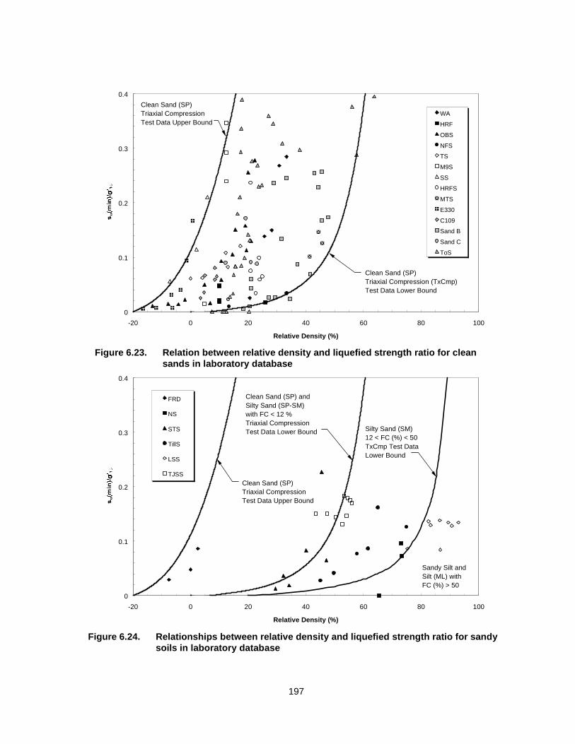
197

Figure 6.23. Relation between relative density and liquefied strength ratio for cleansands in laboratory database

Figure 6.24. Relationships between relative density and liquefied strength ratio for sandysoils in laboratory database

0

0.1

0.2

0.3

0.4

-20 0 20 40 60 80 100

Relative Density (%)

σ σσσ

FRD

NS

STS

TillS

LSS

TJSS

Clean Sand (SP) andSilty Sand (SP-SM)with FC < 12 %Triaxial CompressionTest Data Lower Bound Silty Sand (SM)

12 < FC (%) < 50TxCmp Test DataLower Bound

Sandy Silt andSilt (ML) withFC (%) > 50

Clean Sand (SP)Triaxial CompressionTest Data Upper Bound

0

0.1

0.2

0.3

0.4

-20 0 20 40 60 80 100

Relative Density (%)

σ σσσWA

HRF

OBS

NFS

TS

M9S

SS

HRFS

MTS

E330

C109

Sand B

Sand C

ToS

Clean Sand (SP)Triaxial Compression (TxCmp)Test Data Lower Bound

Clean Sand (SP)Triaxial CompressionTest Data Upper Bound

198

Figure 6.25. Comparison of relationships between liquefied strength ratio and correctedSPT blowcount for laboratory database and flow failure case histories

Figure 6.26. Comparison of relationships between liquefied strength ratio and correctedCPT tip resistance for laboratory database and flow failure case histories

0

0.1

0.2

0.3

0.4

0 1 2 3 4 5 6 7 8 9 10

Corrected CPT Tip Resistance, qc1 (MPa)

σ σσσ

Clean Sand (SP) andSilty Sand (SP-SM)with FC < 12%TxCmp Test DataLower Bound

Silty Sand (SM)12 < FC (%) < 50TxCmp Test DataLower Bound

Liquefaction Flow FailureCase History Bounds

Data Points are Field Case Histories - See Figure 5.16 for Symbol Description (shaded symbol = half-filled symbol from Figure 5.16)

Clean Sand (SP)TxCmp Test DataUpper Bound

0

0.1

0.2

0.3

0.4

0 2 4 6 8 10 12 14 16 18

Corrected SPT Blowcount, (N1)60

σ σσσClean Sand (SP) andSilty Sand (SP-SM)with FC < 12%TxCmp Test DataLower Bound

Silty Sand (SM)12 < FC (%) < 50TxCmp Test DataLower Bound

Liquefaction Flow FailureCase History Bounds

Data Points are Field CaseHistories - See Figure 5.15for Symbol Description(shaded symbol = half-filledsymbol from Figure 5.15)

Clean Sand (SP) andTxCmp Test DataUpper Bound

199

CHAPTER 7

LIQUEFACTION ANALYSIS PROCEDURE FOR GROUNDSUBJECTED TO STATIC SHEAR STRESS

7.1 INTRODUCTION

A liquefaction analysis for ground subjected to a static shear stress, i.e., slopes,

embankments, or foundations of structures, typically consists of three primary tasks: (1) a

flow failure susceptibility analysis, (2) a liquefaction triggering analysis, and (3) a post-

triggering/flow failure stability analysis. A susceptibility analysis involves determining

whether a given soil deposit is in a contractive state, i.e., susceptible to undrained strain-

softening behavior or flow failure. Numerous investigators (e.g., Sladen and Hewitt 1989;

Ishihara 1993; Fear and Robertson 1995; Baziar and Dobry 1995) have proposed

susceptibility boundary lines between penetration resistance (a measure of soil density) and

effective stress to separate contractive from dilative soil states. Similarly, procedures are

available to evaluate the liquefied shear strength for use in a post-triggering/flow failure

stability analysis (e.g., Poulos et al. 1985a; Seed and Harder 1990; this study). This study

(Chapter 5) proposed a procedure to estimate the liquefied strength ratio, su(LIQ)/σ'vo, using

corrected standard penetration test (SPT) or cone penetration test (CPT) resistance. The

liquefied strength ratio can be used in a post-triggering stability analysis.

Using values of yield and liquefied strength ratio back-calculated from liquefaction

flow failures (discussed in Chapters 4 and 5, respectively), this study proposes a

comprehensive procedure for liquefaction analysis of ground subjected to a static shear

stress. This procedure addresses flow failure susceptibility, triggering of liquefaction, and

200

post-triggering/flow failure stability. The procedure is verified initially by successfully

predicting the behavior of Lower San Fernando Dam.

7.2 FLOW FAILURE SUSCEPTIBILITY ANALYSIS

The first step of a liquefaction analysis for ground subjected to a static shear stress is

to determine if the soil is contractive; i.e., susceptible to flow failure. Figure 7.1 presents SPT

based susceptibility relationships from the literature with the case history data. The pre-

failure σ'vo plotted in Figure 7.1 (and later in Figure 7.2) is the average of the values of

σ'vo(ave) from the yield strength ratio analysis (see Table 4.2) and the liquefied strength ratio

analysis (see Table 5.3).

Fear and Robertson (1995) developed a susceptibility boundary relationship using

critical state soil mechanics theory and laboratory test results, and their boundary

encompasses all but two of the mean (N1)60 values for the case histories. Based on the

agreement with theory, laboratory results, and field case histories, the Fear and Robertson

(1995) boundary is recommended for practice to delineate field conditions susceptible and

not susceptible to flow failure. Similarly, Figure 7.2 presents CPT based liquefaction

susceptibility relationships from the literature with the case history data. The Fear and

Robertson (1995) boundary (converted to CPT) encompasses all but one of the mean qc1

data for the case histories and is therefore recommended for practice. The Fear and

Robertson (1995) boundary was converted to CPT using using qc/N60 = 0.6, obtained from

Stark and Olson (1995) using a median D50 typical for clean sands. The recommended

boundary relations can be approximated as:

201

( ) ( )[ ] 7863.4601

4105812.9' Nboundaryvo−×=σ (7.1a)

or

( ) ( ) 7863.41

2101047.1' cboundaryvo q−×=σ (7.1b)

where σ'vo and qc1 have units of kPa and MPa, respectively, and σ'vo is less than about 350

kPa. These boundary relations can be incorporated easily into a spreadsheet file that

contains the penetration data. Furthermore, it appears reasonable to graphically extrapolate

these relationships to effective stresses larger than 350 kPa.

In the design of new structures or evaluation of existing structures, records of (N1)60

and/or qc1 should be plotted against vertical effective stress. These plots should include the

corresponding recommended liquefaction susceptibility relationship (Eq. 7.1a or 7.1b). Using

these plots, layer(s) of soil that are contractive (and therefore susceptible to flow failure) can

be identified. With sufficient field penetration tests, zones of contractive soil can be

delineated in two- and three-dimensions.

7.3 LIQUEFACTION TRIGGERING ANALYSIS

The next step is to determine whether the combined static, seismic, and/or other

shear stresses exceed the yield shear strength of the contractive soil(s). This is

accomplished through the following procedure (and can be conducted easily using a

spreadsheet). Section 7.5.2 illustrates the ease and functionality of this step.

1. Conduct a slope stability analysis of the pre-failure geometry to estimate the static

shear stress (τdriving) in the contractive (liquefiable) soil(s). A single, trial value of

202

shear strength is assumed for the liquefiable soils, and this shear strength is

modified until a factor of safety of unity is achieved. Fully mobilized drained or

undrained shear strengths are assigned to the non-liquefiable soils. The slope

stability search should consider both circular and non-circular potential failure

surfaces.

2. Divide the critical failure surface into a number of segments. Based on analyses

conducted for this study, 10 to 15 segments are satisfactory.

3. Determine the weighted average value of σ'vo along the critical failure surface and

calculate the average static shear stress ratio, τdriving/σ'vo(ave).

4. Estimate the average seismic shear stress (τave,seismic) applied to each segment of the

failure surface using Eq. (4.3a) or a site response program.

5. If applicable, estimate other shear stresses (τother) applied to each segment of the

critical failure surface using appropriate analyses.

6. Determine the value of su(yield)/σ'vo using corrected SPT and/or CPT penetration

resistance and the relationships presented in Eqs. (4.4a) and (4.4b), respectively,

which were derived from Figs. 4.5 and 4.6. The desired level of conservatism can be

incorporated by using a penetration resistance larger or smaller than the mean

value, or by selecting a yield strength ratio higher or lower than the mean value.

7. Calculate the values of su(yield) and τdriving for each segment of the critical failure

surface by multiplying the yield strength ratio and static shear stress ratio by the σ’vo

for the segment, respectively.

8. The potential to trigger liquefaction in each segment can then be estimated using a

factor of safety against triggering of liquefaction as follows:

203

otherseismicavedriving

uTriggering

yieldsFS

τττ ++≈

,

)((7.2)

Segments with a FSTriggering greater than or equal to unity are unlikely to liquefy.

These segments should be assigned their yield shear strength for a post-triggering stability

analysis. Segments with a FSTriggering less than unity are likely to liquefy and these segments

should be assigned the liquefied shear strength for a post-triggering stability analysis. The

author recommends that both the critical circular and non-circular failure surfaces

(determined in Step 1 above) be analyzed using this procedure, as the ratio of

τdriving/τave,seismic may vary between potential failure surfaces. Analyzing both circular and non-

circular critical failure surfaces should result in failure surfaces that vary considerably in

depth and location within the zone(s) of contractive soil. If the circular and non-circular

failure surfaces cross the zone(s) of contractive soil at about the same location and depth,

one or two additional potential failure surfaces that cross the zone(s) of contractive soil at

different locations also should be analyzed.

7.4 POST-TRIGGERING/FLOW FAILURE STABILITY ANALYSIS

If liquefaction is triggered, a post-triggering stability analysis of the structure (using

the pre-failure geometry) must be conducted to determine whether the static shear forces

are greater than the available shear resistance (including the liquefied shear strength). The

liquefied strength ratio is estimated from Figures 5.15 and 5.16 (or Eqs. 5.14a and 5.14b) in

Chapter 5. Appropriate values of liquefied shear strength are calculated (using the value of

σ'vo for the segment) and assigned to the segments of the critical failure surface predicted to

liquefy in the triggering analysis. Fully mobilized drained or undrained shear strengths are

204

assigned to the non-liquefied soils. This analysis should be conducted for all of the potential

failure surfaces that were evaluated in the triggering analysis.

If the factor of safety against flow failure, FSFlow, determined from the stability

analysis is less than or equal to unity, flow failure of the structure is predicted to occur.

However, if the FSFlow is between unity and about 1.1, some deformation probably will occur.

If this is the case, segments of the failure surface with marginal FSTriggering (approximately 1.0

to 1.1) should be reassigned the liquefied shear strength. Then repeat the post-triggering

stability analysis and determine a new FSFlow. This accounts for the potential for

deformation-induced liquefaction and progressive failure of the entire structure. Obviously,

the minimum FSFlow corresponds to a condition where all zone(s) of contractive soil are

triggered to liquefy and assigned their liquefied shear strengths for the post-triggering/flow

failure stability analysis. This condition can be analyzed to determine the worst case FSFlow

and to aid judgments regarding the need for re-design or remediation.

7.5 VERIFICATION OF LIQUEFACTION ANALYSIS USING LOWER SANFERNANDO DAM CASE HISTORY

On February 9, 1971, a massive slide occurred in the upstream (u/s) slope of the

Lower San Fernando Dam (LSFD) as a result of the San Fernando earthquake (MW = 6.6).

Seed et al. (1973) conducted an extensive field and laboratory investigation to evaluate the

causes of the slide. A pre- and post-failure cross-section of the Lower San Fernando Dam

determined by Seed et al. (1973) is shown in Fig. 7.3. Seed et al. (1973) concluded that

seismic shaking triggered liquefaction of the hydraulic fill within the upstream slope of the

dam, and seismoscope records indicated that the slide occurred about 30 seconds after the

end of shaking (Seed 1979). Only gravitational forces were available to initiate the slope

205

failure. Therefore, it appears that the slide was the result of the loss of strength in the

liquefied soils rather than the result of inertia forces during earthquake shaking (Castro et al.

1989; Seed et al. 1989).

7.5.1 LSFD Susceptibility Analysis

Figure 7.4a presents (N1)60 data from the downstream (d/s) slope of LSFD (obtained

in the 1985 field investigation). Two boundary relations are shown in the figure, with the

solid boundary corresponding to the Fear and Robertson (1995) relation shown in Figure 7.1

and the dashed boundary augmented to correspond to conditions in the upstream slope of

LSFD. The augmented boundary was developed by increasing the (N1)60-axis of the original

boundary by 3. This increase accounts for post-earthquake densification [(N1)60 increase of

2] and differing effective stress conditions between the d/s and u/s slopes [(N1)60 increase of

1] as recommended by Seed et al. (1989).

Figure 7.4b presents available qc1 data also from the d/s slope of LSFD. The solid

line represents the average qc1 values and the dashed lines are the minimum and maximum

qc1 values with depth. Included in Figure 7.4b are boundary relations that separate

contractive from dilative conditions. The solid boundary relation was converted from the SPT

relationship as shown in Figure 7.2. Similar to the SPT relation, the dashed CPT boundary

was augmented to correspond to u/s slope conditions by increasing the qc1–axis by 1.2

MPa. The increase was estimated by multiplying the (N1)60 increase of 3 by qc/N60 ≅ 0.4

(using the median D50 from LSFD of approximately 0.12 mm; Stark and Olson 1995).

Averaging the SPT and CPT results in Figure 7.4 suggests that the hydraulic fill in

the upstream slope at initial vertical effective stresses (σ'vo) greater than 120 kPa is

contractive and therefore susceptible to flow failure. In the downstream slope, hydraulic fill at

206

σ'vo greater than 190 kPa is contractive. The zones of contractive soil are hatched in Figure

7.5.

7.5.2 LSFD Triggering Analyses

The initial failure surface shown in Figure 7.5 (from Castro et al. 1992) resulted in an

average static driving shear stress of 31 kPa, with a range of 25 to 36 kPa. This value

agrees with values obtained by Seed et al. (1989) and Castro et al. (1989) for slightly

deeper failure surfaces. The shear strengths presented in Table 7.1 (from Castro et al.

1989) were used for the analyses. The yield (initial) failure surface was divided into 16

segments. Of these 16 segments, only segments 5 through 12 are within the zone of

liquefiable soil (as shown in Figure 7.5). Table 7.2 presents the liquefaction triggering

analysis for segments 5 through 12. As indicated in Table 7.2, the combined static driving

and seismic shear stresses trigger liquefaction in segments 5 to 12. The zone of soil

predicted to liquefy by this analysis is nearly identical to that predicted by Seed et al. (1973)

and agrees reasonably with the observations of Seed et al. (1989) (compare zones of

liquefaction in Figures 7.3 and 7.5).

A number of other triggering analyses were conducted to evaluate the ability of the

proposed technique to predict the performance of LSFD. These analyses, summarized in

Table 7.3 and discussed in a subsequent section, include:

• U/S slope subjected to 1971 San Fernando earthquake (M~6.6);

• U/S slope subjected to 1952 Kern County earthquake (M~7.7);

• U/S slope subjected to a hypothetical M~6.6 earthquake to determine the amax

required to cause a flow failure;

207


required to cause a flow failure;

• U/S slope subjected to 1971 San Fernando earthquake using the deeper failure

surface suggested by Castro et al. (1989) (see Figure 7.5);


required to cause a flow failure along the deeper failure surface suggested by

Castro et al. (1989); and

• D/S slope subjected to 1971 San Fernando earthquake using the failure surface

suggested by Castro et al. (1989) (see Figure 7.5).

7.5.3 LSFD Post-Triggering/Flow Failure Stability Analyses

In several of the LSFD triggering analysis, liquefaction is predicted to occur in one or

more segments. Therefore, post-triggering stability analyses of the structure (using the pre-

failure geometry) must be conducted to determine whether the static driving forces are

greater than the available shear resistance. The liquefied shear strength ratio was estimated

using the average trendlines in Figures 5.16 and 5.17 (or Eqs. 5.14a and 5.14b).

Appropriate values of su(LIQ) then were calculated (using the segment values of σ'vo) and

assigned to the segments of the failure surface predicted to liquefy. Fully mobilized drained

or undrained shear strengths (see Table 7.1) were assigned to the non-liquefied soils.

The results of the post-triggering stability analyses conducted for both the u/s and d/s

slopes of LSFD under a variety of triggering conditions are summarized in Table 7.3 and

discussed in the following section.

208

7.5.4 Discussion of Results

As indicated in Table 7.3, the proposed liquefaction analysis procedure predicts that

liquefaction was triggered in the upstream slope during the 1971 San Fernando earthquake.

The resulting FSFlow was approximately 0.85, correctly predicting that a flow failure would

occur. The same conclusion was reached using the u/s failure surface suggested by Castro

et al. (1989), with FSFlow of approximately 0.72. For comparison, Castro et al. (1989)

calculated FSFlow = 0.54, and Seed et al. (1973, 1989) calculated FSFlow = 0.80 when su(LIQ)

was assumed to be zero.

The 1952 Kern County earthquake (M~7.7) was the largest earthquake that LSFD

was subjected to prior to 1971. Castro et al. (1989) indicated that the 1952 earthquake likely

caused peak surface accelerations on the order of 0.05 to 0.12g at the dam site. Seed et al.

(1989) reported that slightly elevated porewater pressures were measured in the foundation

soils below the downstream rolled fill buttress two days after the 1952 earthquake. Because

the u/s hydraulic fill was looser than the soil within and below the d/s fill, it should have

experienced a larger porewater pressure increase, but this does not necessarily imply that

liquefaction was triggered.

These observations agree with the performance of the upstream slope predicted by

the proposed procedure. The proposed procedure indicates that no liquefaction would be

triggered under the minimum acceleration (0.05g), with FSTriggering of approximately 1.2 to

1.3. Under the maximum acceleration (0.12g), segments 5 to 9 (see Fig. 7.5) of the u/s

slope liquefy marginally, with a FSTriggering of approximately 0.9 to 1.0. The resulting FSFlow

averaged 1.23 and 1.01 for the minimum and maximum accelerations, respectively,

indicating marginal stability despite the possibility that liquefaction may have been triggered.

209

Castro et al. (1989) suggested that LSFD could have withstood a M ~ 6.6 earthquake

that produced accelerations of 0.12 to 0.15g without causing a flow failure. Seed et al.

(1989) suggested that LSFD could have withstood slightly larger accelerations of 0.13 to

0.30g. The proposed liquefaction analysis procedure indicates that LSFD could have

withstood similar accelerations, from approximately 0.09 to 0.17g during a M 6.6 and about

0.12g during a M 7.7 earthquake without causing a flow failure.

Finally, Castro et al. (1989) suggested that the downstream slope had a FSFlow of

approximately 1.0 prior to the upstream slide. Seed et al. (1989) reported that minor excess

porewater pressures were measured below the downstream slope following the 1971

earthquake, in agreement with analytical results from Seed et al. (1973). The performance

of the downstream slope predicted by the proposed method agrees well with the observed

performance. Calculations using the proposed procedure indicated that only minor

liquefaction was possible, but not likely, in the d/s slope during the 1971 earthquake, and the

FSFlow for the d/s slope (prior to the u/s slide) was approximately 1.55 to 1.72.

7.6 CONCLUSIONS

There are numerous limitations of existing methods (Poulos et al. 1985a,b; Seed and

Harder 1990; Byrne 1991, Byrne et al. 1992) to analyze the triggering of liquefaction for

ground subjected to static shear stress. This study proposes an alternate procedure to

evaluate liquefaction in ground subjected to a static shear stress using the yield and

liquefied strength ratios back-calculated from liquefaction flow failures. The proposed

procedure does not rely on laboratory tests (Poulos et al. 1985a,b; Byrne 1991, Byrne et al.

1992) or correction factors (Seed and Harder 1990).

210

The liquefaction analysis procedure consists of the following basic steps: (1)

determine liquefaction susceptibility using relationships between corrected penetration

resistance and vertical effective stress that separate contractive from dilative conditions; (2)

determine static shear stress using a conventional limit-equilibrium analysis of the pre-failure

geometry; (3) estimate additional shear stresses, e.g., seismic shear stresses; (4) determine

the yield strength ratio using penetration resistance; (5) evaluate the triggering of

liquefaction by comparing yield shear strength to combined static and additional shear

stresses; (6) determine the liquefied strength ratio using penetration resistance if

liquefaction is triggered; and (7) evaluate the post-triggering stability using a conventional

limit-equilibrium analysis of the pre-failure geometry.

The proposed liquefaction analysis procedure was initially verified and illustrated

using the Lower San Fernando Dam case history. The proposed procedure accurately

predicted the performance of both the upstream and downstream slopes when subjected to

the 1971 San Fernando and the largest previous earthquake. Firstly, the proposed

procedure predicts liquefaction and flow failure of the upstream slope during the 1971

earthquake, while predicting only minor to no liquefaction in the downstream slope.

Secondly, the analysis predicted satisfactory performance of the upstream slope during the

1952 Kern County earthquake, the largest previous earthquake to which the dam was

subjected. Lastly, parametric studies indicated that the dam likely could have withstood

shaking on the order of 0.09 to 0.17g without causing a flow failure. This result agrees with

results from Castro et al. (1989) (amax ~ 0.12-0.15g) and Seed et al. (1989) (amax ~ 0.13-

0.3g).

211

Layer c φ c φNo. Soil description (kPa) (o) (kPa) (o)

1 Alluvium 0 40 0 40

2Starter dikes, non-liquefiable hydraulic fill, rolled fill, and

ground shale0 30 0 35

31929-1930 Rock blanket and

1940 Berm0 40 0 40

4 Upper core 62 0 94 05 Middle core 77 0 115 06 Lower core 91 0 136 07 U/S liquefiable hydraulic fill b/c1 0 b/c 0

8 D/S liquefiable hydraulic fill b/c 0 b/c 0 1b/c = back-calculated value

Minimum Maximum

Table 7.1. Shear Strength Values for Back-Calculation of Lower San Fernando Dam (from Castro et al. 1989)

212

Average Segment Segment Segment Average

Segment σ'vo su(yield) σvo τdriving τave,seismic τother Liquefaction su(LIQ)

No. Liquefiable? (kPa) (kPa) (kPa) (kPa) (kPa) (kPa) FSTriggering Triggered? (kPa)

1 No -- -- -- -- -- -- -- -- --2 No -- -- -- -- -- -- -- -- --3 No -- -- -- -- -- -- -- -- --4 No -- -- -- -- -- -- -- -- --5 Yes 120 33.8 247 21.8 57.3 0 0.43 Yes 12.86 Yes 144 40.6 293 26.1 62.6 0 0.46 Yes 15.47 Yes 156 43.9 322 28.3 65.1 0 0.47 Yes 16.68 Yes 168 47.4 345 30.5 66.6 0 0.49 Yes 17.99 Yes 178 50.1 357 32.2 67.1 0 0.50 Yes 19.010 Yes 189 53.3 374 34.3 67.8 0 0.52 Yes 20.211 Yes 207 58.4 374 37.6 67.8 0 0.55 Yes 22.112 Yes 216 60.7 351 39.1 66.9 0 0.57 Yes 23.013 No -- -- -- -- -- -- -- -- --14 No -- -- -- -- -- -- -- -- --15 No -- -- -- -- -- -- -- -- --16 No -- -- -- -- -- -- -- -- --

Table 7.2. Summary of Liquefaction Triggering Analysis for the Upstream Slope of Lower SanFernando Dam Subjected to 1971 San Fernando Earthquake (M ~ 6.6, amax ~ 0.55g, CM ~ 1.39)

213

Actual amax req'd to cause Segments Average

amax cause flow failure triggered FS against FSFlow

Slope Earthquake ML (g) (g) to liquefy flow failure range1

U/S 1971 San Fernando 6.6 0.5 (min) -- 5 - 12 (all) 0.85 0.77 - 0.920.6 (max) -- 5 - 12 (all)

U/S 1952 Kern County 7.7 0.05 (min) -- none 1.23 1.15 - 1.300.12 (max) -- 5 - 9 1.01 0.94 - 1.08

U/S Hypothetical 6.6 -- 0.17 5 - 9 1.01 0.94 - 1.08U/S Hypothetical 7.7 -- 0.12 5 - 9 1.01 0.94 - 1.08U/S 1971 San Fernando using 6.6 0.5 (min) -- 2 - 10 (all) 0.72 0.64 - 0.79

Castro et al. failure surface 0.6 (max) -- 2 - 10 (all)U/S Hypothetical using 6.6 -- 0.09 2 - 6 0.95 0.87 - 1.02

Castro et al. failure surfaceD/S 1971 San Fernando using 6.6 0.5 (min) -- none 1.72 1.63 - 1.80

Castro et al. failure surface 0.6 (max) -- 3, 9, 10 1.55 1.46 - 1.63 1FS range reports values obtained using lower and upper bound shear strengths in the non-liquefied soils and core

Table 7.3. Summary of Liquefaction Triggering and Flow Failure Stability Analyses forLower San Fernando Dam

214

Figure 7.1. Relationships separating contractive from dilative conditions using flow failurecase histories and corrected SPT blowcount

CONTRACTIVE DILATIVE

215

Figure 7.2. Relationships separating contractive from dilative conditions using flow failurecase histories and corrected CPT tip resistance

CONTRACTIVE DILATIVE

216

Figure 7.3. Cross-section through Lower San Fernando Dam showing: (a) conditions after 1971 earthquake; and (b) schematicreconstruction of failed cross-section (from Castro et al. 1992)

217

Figure 7.4. Comparison of 1985 penetration test results with contractive/dilative boundaries (CPT data from soundings 101,103, 104, 106, 108, and 109)

0

50

100

150

200

250

300

350

400

0 10 20 30 40 50

SPT Blowcount, (N1)60

Pre-

Failu

re σ σσσ

' vo (k

Pa)

S101

S103

S104

S111

Fear and Robertson (1995)

Boundarycorrected toupstream LSFDconditions

FlowFailure

Possible

0 5 10 15 20 25

CPT Tip Resistance, qc1 (MPa)

Minimum

Average

Maximum

Boundarycorrected toupstream LSFDconditions

FlowFailure

Possible

Fear andRobertson (1995)qc/N60 = 0.6

218

Figure 7.5. Pre-failure geometry of Lower San Fernando Dam showing zones of contractive soil and potential upstream anddownstream yield failure surfaces

219

CHAPTER 8

SUMMARY AND CONCLUSIONS

As illustrated in this thesis, liquefaction problems are some of the most controversial

issues facing the geotechnical profession today. Empirical relations and procedures are

proposed herein to improve understanding of these problems and to provide practitioners

with simple-to-use procedures to tackle these problems. The proposed correlations and

procedures are particularly useful as screening tools because of their simplicity. The

following points summarize the findings of this work and highlight important conclusions.

A. LEVEL GROUND LIQUEFACTION RESISTANCE USING CASEHISTORIES AND CPT

1. The cone penetration test (CPT) appears to be better suited to liquefaction

assessments than the standard penetration test (SPT) because it is more

standardized, reproducible, cost effective, and most importantly, yields a continuous

penetration record with depth.

2. Olson and Stark (1998) presented a revised database of 172 field case histories where

liquefaction was and was not observed in sandy soils and CPT tip resistance is

available.

3. These data are used to confirm the Stark and Olson (1995) liquefaction resistance

relationships for clean sand, silty sand, and silty sand to sandy silt and an earthquake

magnitude of 7.5.

220

4. Stark and Olson (1995) presented tentative liquefaction resistance relationships for

clean gravel and silty gravel and an earthquake magnitude 7.5 based on 18

liquefaction and non-liquefaction case histories where CPT results are available.

These relationships indicate that the liquefaction resistance of gravelly soil is greater

than that of sandy soil.

5. A combination of CPTs and SPTs should be conducted at a site for a comprehensive

liquefaction analysis. SPTs allow the direct determination of median grain size, D50,

and fines content, as well as verification of the CPT results.

6. The revised sandy soil database uses only one critical value of tip resistance from

each sounding. However, it may be acceptable to use more than one critical tip

resistance value if those values represent soil strata of different geologic age or

significantly different penetration resistance, or if supporting evidence of liquefaction

within a specific horizon (such as inclinometer data) is available.

B. YIELD STRENGTH RATIO FROM LIQUEFACTION FLOW FAILURES

7. There are numerous limitations of existing procedures to evaluate the triggering of

liquefaction in ground subjected to a static shear stress. The Poulos et al. (1985a,b)

method requires a suite of laboratory tests that must be carefully interpreted. The Seed

and Harder (1990) method relies on correction factors that exhibit large scatter. The

Byrne (1991) method requires complex computational models and a suite of laboratory

tests to evaluate the required soil behavior parameters.

8. The yield strength ratio [su(yield)/σ’vo] (analogous to the collapse surface concept

proposed by Sladen et al. 1985a) is proposed to evaluate the stress conditions present

in a number of flow failure case histories at the instant liquefaction was triggered.

221

9. A back-analysis technique is developed to directly evaluate the yield strength ratio

mobilized at the instant liquefaction is triggered. This precludes the need to separately

back-calculate the yield shear strength and vertical effective stress conditions at the

time of failure along the failure surface.

10. Back-analysis of flow failure case histories indicates that an approximately linear

relationship exists between the yield shear strength and pre-failure vertical effective

stress at the triggering of liquefaction for a wide range of effective stresses.

11. Back-calculated yield strength ratios range from approximately 0.23 to 0.31. These

yield strength ratios correspond to equivalent friction angles at the yield strength

envelope of 13 to 17°. The variation in yield strength ratio is correlated to corrected

SPT and CPT penetration resistance.

C. LIQUEFIED STRENGTH RATIO FROM LIQUEFACTION FLOWFAILURES

12. There are numerous limitations of existing procedures to evaluate the shear strength

available to liquefied soils at large strain. This study overcomes many of these

deficiencies using a method for back-analysis of flow failure case histories developed

to back-calculate the liquefied strength ratio directly. This precludes the need to

separately evaluate the liquefied shear strength and the appropriate vertical effective

stress acting on the liquefied material.

13. An analysis that incorporates the kinetics of failure was developed and used to obtain

“best-estimates” of liquefied strength ratio. These analyses show that the effects of

kinetics on the back-calculation of liquefied strength ratio is important for

embankments/slopes greater than about 10 m in height.

222

14. A number of uncertainties were considered in back-analyzing the case histories. The

factors contributing to the uncertainty of both the back-calculation of liquefied strength

ratio and corrected penetration resistance are discussed in Chapter 5 and Appendix A.

15. Despite these uncertainties, clear trends of increasing liquefied shear strength with

increasing vertical effective stress and increasing liquefied strength ratio with corrected

penetration resistance are evident.

16. The liquefied strength ratio varies from 0.05 to 0.12 for the flow failure case histories.

The variation in liquefied strength ratio is related to corrected penetration resistance.

17. Applications for and practical implementation of a liquefied strength ratio in design are

discussed in Chapter 5.

D. CONFIRMATION OF YIELD AND LIQUEFIED STRENGTH RATIOSUSING LABORATORY DATA

18. The steady state line and consolidation behavior of a number of sandy soils are

generally parallel over a wide range of fines content, grain sizes and shapes, and

steady state line slopes, at least for a given range of effective stress. Therefore, the

liquefied strength ratio should be nearly constant for a given soil deposited in a

consistent manner.

19. Sandy soils with fines content greater than 12% exhibit nearly parallel slopes of steady

state line and consolidation behavior over large ranges of effective stress. As the large

majority of flow failure case histories involve sands with at least some silt, this finding

helps explain the relation between liquefied shear strength and vertical effective stress

observed for the case histories.

223

20. Laboratory triaxial compression test data for all sands (with fines contents from 0 to

over 90%) exhibit yield strength ratios ranging from 0.29 to 0.42 (with an upper bound

of 0.47 at mean effective stresses less than 700 kPa). These bounds correspond to

equivalent friction angles at the yield strength envelope of 16 to 23° (with an upper

bound of 25° at mean effective stresses less than 700 kPa).

21. Yield strength ratios back-calculated from flow failure case histories ranged from

approximately 0.23 to 0.31. This corresponds to equivalent friction angles at the yield

strength envelope of 13 to 17°. As expected, the yield strength ratios back-calculated

from flow failure case histories are smaller than those determined from laboratory

triaxial compression tests. This result is expected because the yield shear strength is

mobilized at small strains. At small strain, the mobilized strength is a function of the

mode of shear, with yield strengths being largest in triaxial compression, smaller in

direct or simple shear, and smallest in triaxial extension. The stress conditions in the

zones of liquefaction for most of the case histories corresponds to direct simple shear

conditions, therefore, yield strength ratios back-calculated from the case histories

should be smaller than those measured in the laboratory database.

22. Liquefied strength ratios measured in laboratory triaxial compression tests are shown

to be a function of state parameter. For contractive sandy soils (i.e., susceptible to flow

failure) tested in triaxial compression, the liquefied strength ratio ranged from

approximately 0.02 to 0.22 over a wide range of initial major principal effective stress.

23. Liquefied strength ratios back-calculated from flow failure case histories show that the

case histories fall well within the laboratory bounds of liquefied strength ratio.

Assuming that the back-calculated liquefied strength ratios (ranging from 0.05 to 0.12)

can be directly compared to the liquefied strength ratios measured in the laboratory

224

tests (which include some values of quasi-steady state shear strengths taken as the

liquefied shear strength), the case histories appear to have state parameters of

roughly 0.02 to 0.10.

24. Upper and lower bound relationships between laboratory liquefied strength ratios and

relative density are presented for relatively clean sands (less than 12% fines content)

and silty sands (between 12 and 50% fines content). These relationships were

converted to relationships between liquefied strength ratio and corrected SPT and CPT

penetration resistance for comparison with field data. The comparisons indicate that

the case history data all plot above the lower bound relation for the laboratory SM

data, and most plot above the lower bound relation for the SP data. This result

suggests that the relationships proposed in Chapter 5 are valid. Furthermore, relations

between liquefied strength ratio and corrected penetration resistance based on

laboratory testing of one sand (from a given site) can be unconservative for preliminary

design for another site.

E. LIQUEFACTION ANALYSIS PROCEDURE FOR GROUND SUBJECTEDTO A STATIC SHEAR STRESS

25. This study proposes a procedure to evaluate liquefaction in ground subjected to a

static shear stress using the yield and liquefied strength ratios back-calculated from

liquefaction flow failures. The proposed procedure does not rely on laboratory tests

(Poulos et al. 1985a,b; Byrne 1991, Byrne et al. 1992) or correction factors (Seed and

Harder 1990).

26. The liquefaction analysis procedure consists of the following basic steps: (1) determine

liquefaction susceptibility using relationships between corrected penetration resistance

225

and vertical effective stress that separate contractive from dilative conditions; (2)

determine static shear stress using a conventional limit-equilibrium analysis of the pre-

failure geometry; (3) estimate additional shear stresses, e.g., seismic shear stresses;

(4) determine the yield strength ratio using penetration resistance; (5) evaluate the

triggering of liquefaction by comparing yield shear strength to combined static and

additional shear stresses; (6) determine the liquefied strength ratio using penetration

resistance if liquefaction is triggered; and (7) evaluate the post-triggering stability using

a conventional limit-equilibrium analysis of the pre-failure geometry.

27. The proposed liquefaction analysis procedure was initially verified and illustrated using

the Lower San Fernando Dam case history. The proposed procedure accurately

predicts the performance of both the upstream and downstream slope when subjected

to the 1971 San Fernando and the largest previous earthquakes. Firstly, the proposed

procedure predicts liquefaction and flow failure of the upstream slope during the 1971

earthquake, while predicting only minor to no liquefaction in the downstream slope.

Secondly, the proposed analysis predicts the satisfactory performance of the upstream

slope during the 1952 Kern County earthquake, the largest previous earthquake to

which the dam was subjected. Lastly, parametric studies indicated that the dam likely

could have withstood shaking on the order of 0.09 to 0.17g without causing a flow

failure. This result agrees with results from Castro et al. (1989) (amax ~ 0.12-0.15g) and

Seed et al. (1989) (amax ~ 0.13-0.3g).

226

REFERENCES

Alarcon-Guzman, A., Leonards, G.A., and Chameau, J.L. (1988). “Undrained monotonic and

cyclic strength of sands.” Journal of Geotechnical Engineering, ASCE, 114(10), 1089-1109.

Andresen, A. and Bjerrum, L. (1968). “Slides in subaqueous slopes in loose sand and silt.”

Norwegian Geotechnical Institute Publication No. 81, 1-9.

Andrus, R.D. and Youd, T.L. (1987). “Subsurface investigation of a liquefaction-induced

lateral spread, Thousand Springs Valley, Idaho.” Geotechnical Laboratory Miscellaneous

Paper GL-87-8, U.S. Army Corps of Engineers, 131 p.

Andrus, R.D. and Youd, T.L. (1989). “Penetration tests in liquefiable gravels.” Proc., 12th

International Conference on Soil Mechanics and Foundation Engineering, Rio de Janero,

Brazil, 679-682.

Arulanandan, K., Yogachandran, C., Meegoda, N.J., Ying, L., and Zhauji, S. (1986).

“Comparison of the SPT, CPT, SV and electrical methods of evaluating earthquake induced

liquefaction susceptibilty in Ying Kou City during the Haicheng Earthquake." Use of In Situ

Tests in Geotechnical Engineering, ASCE Geotechnical Special Publication No. 6, 389-415.

Arulanandan, K., Seed, H.B., Yogachandran, C., Muraleetharan, K.K., Seed, R.B., and

Kabilamany, K. (1993). “Centrifuge study on volume changes and dynamic stability of earth

dams.” Journal of Geotechnical Engineering, ASCE, 119(11), 1717-1731.

Baziar, M.H. and Dobry, R. (1995). “Residual strength and large-deformation potential of

loose silty sands.” Journal of Geotechnical Engineering, ASCE, 121(12), 896-906.

Been, K. and Jefferies, M.G. (1985). “A state parameter for sands.” Geotechnique, 35(2),

99-112.

Been, K., Conlin, B.H., Crooks, J.H.A., Fitzpatrick, S.W., Jefferies, M.G., Rogers, B.T., and

Shinde, S. (1987a). “Back analysis of the Nerlerk berm liquefaction slides: Discussion.”

Canadian Geotechnical Journal, 24, 170-179.

Been, K., Jefferies, M.G., Crooks, J.H.A., and Rothenburg, L. (1987b). “The cone

penetration test in sands: part II, general inference of state.” Geotechnique, 37(3), 285-299.

227

Been, K., Jefferies, M.G., and Hachey, J. (1991). “The critical state of sands.” Geotechnique,

41(3), 365-381.

Bennett, M.J. (1989). “Liquefaction analysis of the 1971 ground failure at the San Fernando

Valley Juvenile Hall, California.” Bulletin of Association of Engineering Geologists, 26(2),

209-226.

Bennett, M.J. (1990). “Ground deformation and liquefaction of soil in the Marina District.”

Effects of the Loma Prieta Earthquake on the Marina District, San Francisco, California,

Dept. of the Interior, U.S. Geological Survey, Open File Report 90-253, 44-79.

Bjerrum, L. (1971). “Subaqueous slope failures in Norwegian fjords.” Publication 88,

Norwegian Geotechnical Institute, Oslo.

Boulanger, R.W., Mejia, L.H., and Idriss, I.M. (1997). “Liquefaction at Moss Landing during

Loma Prieta earthquake.” Journal of Geotechnical Engineering, ASCE, 123(5), 453-467.

Bryant, S.M., Duncan, J.M., and Seed, H.B. (1983). “Application of tailings dam flow

analyses to field conditions.” Report No. UCB/GT/83-03, Dept. of Civil Engineering, Univ. of

California, Berkeley, CA.

Byrne, P.M. (1991). “A model for predicting liquefaction induced displacements.” Proc.,

Second International Conf. on Recent Advances in Geotechnical Earthquake Engineering

and Soil Dynamics, St. Louis, Vol. 2, 1027-1035.

Byrne, P.M. and Janzen, W. (1981). “SOILSTRESS: A computer program for nonlinear

analysis of stresses and deformations in soil.” Soil Mechanics Series #52, Dept. of Civil

Engineering, Univ. of British Columbia, updated Jan. 1989.

Byrne, P.M., Salgado, F., and Jitno, H. (1992). “Earthquake induced displacement of soil-

structure systems.” Proc., Tenth World Conf. on Earthquake Engineering, Madrid, Spain,

Vol. 3, 1407-1412.

Canou, J., Bahda, F., Saitta, A., and Dupla, J.C. (1994). “Initiation of sand liquefaction under

monotonic and cyclic loading.” Proc., 13th International Conf. on Soil Mechanics and

Foundation Engineering, January 5-10, New Delhi, India, Vol. 3, 1297-1300.

Casagrande, A. (1940). “Characteristics of cohesionless soils affecting the stability of slopes

and earth fills.” Contributions to Soil Mechanics, 1925-1940, Boston Society of Civil

Engineers, October, (Originally published in the Journal of the Boston Society of Civil

Engineers, January, 1936), 257-276.

228

Casagrande, A. (1965). “Second Terzaghi Lecture: the role of "calculated risk" in earthwork

and foundation engineering.” Journal of the Soil Mechanics and Foundations Division,

ASCE, 91(SM4), 1-40.

Casagrande, A. (1976). “Liquefaction and cyclic deformation of sands: a critical review.”

Harvard Soil Mechanics Series No. 88, Harvard University Cambridge, MA.

Castro, G. (1969). “Liquefaction of sands.” Ph.D. Thesis, Harvard University, Cambridge,

Massachusetts.

Castro, G. (1995). “Empirical methods in liquefaction evaluation.” Proc., First Annual

Leonardo Zeevaert International Conference, Vol. 1, 1-41.

Castro, G. and Poulos, S.J. (1977). “Factors affecting liquefaction and cyclic mobility.”

Journal of Geotechnical Engineering Division, ASCE, 103(GT6), 501-516.

Castro, G., Poulos, S.J., and Leathers, F.D. (1985). “Re-examination of slide of Lower San

Fernando Dam.” Journal of Geotechnical Engineering, ASCE, 111(9), 1093-1106.

Castro, G., Keller, T.O., and Boynton, S.S. (1989). “Re-evaluation of the Lower San

Fernando Dam: Report 1, an investigation of the February 9, 1971 slide.” U.S. Army Corps

of Engineers Contract Report GL-89-2, Vols. 1 and 2, U.S. Army Corps of Engineers

Waterways Experiment Station, Vicksburg, Mississippi.

Castro, G., Seed, R.B., Keller, T.O., and Seed, H.B. (1992). “Steady-state strength analysis

of Lower San Fernando Dam slide.” Journal of Geotechnical Engineering, ASCE, 118(3),

406-427.

Charlie, W.A., Doehring, D.O., Brislawn, J.P., Scott, C.E., and Butler, L.W. (1994).

“Liquefaction evaluation with the CSU piezovane.” Proc., 13th International Conference on

Soil Mechanics and Foundation Engineering, New Delhi, India.

Chillarige, A.V., Robertson, P.K., Morgenstern, N.R., Christian, H.A. (1997a). “Evaluation of

the in situ state of Fraser River sand.” Canadian Geotechnical Journal, 34, 510-519.

Chillarige, A.V., Morgenstern, N.R., Robertson, P.K., and Christian, H.A. (1997b). “Seabed

instability due to flow liquefaction in the Fraser River delta.” Canadian Geotechnical Journal,

34, 520-533.

229

Christian, H.A., Woeller, D.J., Robertson, P.K., and Courtney, R.C. (1997a). “Site

investigation to evaluate flow liquefaction slides at Sand Heads, Fraser River delta.”

Canadian Geotechnical Journal, 34, 384-397.

Christian, H.A., Mosher, D.C., Mulder, T., Barrie, J.V., and Courtney, R.C. (1997b).

“Geomorphology and potential slope instability on the Fraser River delta foreslope,

Vancouver, British Columbia.” Canadian Geotechnical Journal, 34, 432-446.

Chu, J. (1995). “An experimental examination of the critical state and other similar concepts

for granular soils.” Canadian Geotechnical Journal, 32, 1065-1075.

Cleary, A.J. (1914). “The Calaveras dam, California, the highest earth dam.” Engineering

News, 72(14), 692-695.

Coulter, M. and Migliaccio, L. (1966). “Effects of the earthquake of March 27, 1964 at

Valdez, Alaska.” Professional Paper 542-C, U.S. Geological Survey, U.S. Dept. of the

Interior, Washington, D.C.

Cunning, J.C., Robertson, P.K., and Sego, D.C. (1995). “Shear wave velocity to evaluate in

situ state of cohesionless soils.” Canadian Geotechnical Journal, 32, 848-858.

Davies, M.P. and Campanella, R.G. (1994). “Selecting design values of undrained strength

for cohesionless soils.” Proc., 47th Canadian Geotechnical Conference, Halifax, Nova Scotia,

Vol. 1, 176-186.

Davis, A.P. Jr., Poulos, S.J., and Castro, G. (1988). “Strengths backfigured from liquefaction

case histories.” Proc., 2nd Int. Conf. on Case Histories in Geotechnical Engineering, June 1-

5, St. Louis, MO, 1693-1701.

de Alba, P., Seed, H.B., Retamal, E., and Seed, R.B. (1987). “Residual strength of sand

from dam failures in the Chilean earthquake of March 3, 1985.” Earthquake Engineering

Research Center Report No. UCB/EERC-87-11, University of California, Berkeley, CA.

de Alba, P.A., Seed, H.B., Retamal, E., and Seed, R.B. (1988). “Analyses of dam failures in

1985 Chilean earthquake.” Journal of Geotechnical Engineering, ASCE, 114(12), 1414-

1434.

Dennis, N.D. (1988). “Influence of specimen preparation techniques and testing procedures

on undrained steady state shear strength.” Advanced Triaxial Testing of Soil and Rock,

ASTM STP 977, R.T. Donaghe, R.C. Chaney, and M.L. Silver, eds., American Society for

Testing and Materials, Philadelphia, 642-654.

230

Dierichs, D. and Forster, W. (1985). “Results of liquefaction tests under static conditions.”

Proc., 11th International Conf. on Soil Mechanics and Foundation Engineering, August 12-

16, San Francisco, CA, Vol. 2, 437-441.

Dobry, R. and Alvarez, L. (1967). “Seismic failures of Chilean tailings dams.” Journal of the

Soil Mechanics and Foundations Division, ASCE, 93(SM6), 237-260.

Dyvik, R. and Høeg, K. (1999). “Comparison of tests on undisturbed and reconstituted silt

and silty sand.” Intl. Workshop on the Physics and Mechanics of Soil Liquefaction, P. Lade

and J. Yamamuro, eds., Johns Hopkins University, Baltimore, Maryland.

Eckersley, D. (1990). “Instrumented laboratory flow slides.” Geotechnique, 40, 489-502.

Ekstrom, A. and Olofsson, T. (1985). “Water and frost – stability risks for embankments of

fine-grained soils.” Proc., Symposium on Failures in Earthworks, Institution of Civil

Engineers, London, March 6-7, Vol. 1, 155-166.

Engineering News-Record. (1925). “What happened to municipal utilities at Santa Barbara.”

Engineering News-Record, 95(4), 146-149.

Fear, C.E. and Robertson, P.K. (1995). “Estimating the undrained strength of sand: a

theoretical framework.” Canadian Geotechnical Journal, 32(4), 859-870.

Fiegel, G.F. and Kutter, B.L. (1994). “Liquefaction induced lateral spreading of mildly sloping

ground.” Journal of Geotechnical Engineering, ASCE, 120(12), 2236-2243.

Finn, W.D.L. (1990). “Analysis of post-liquefaction deformations in soil structures.” Proc.

H.Bolton Seed Memorial Symposium, Bi-Tech Publishing Ltd., Vol. 2, 291-311.

Finn, W.D.L. (1998). “Seismic safety of embankment dams: developments in research and

practice 1988-1998.” Proc., Geotechnical Earthquake Engineering and Soil Dynamics III,

ASCE Geotechnical Special Publication No. 75, Vol. 2, 812-853.

Gilboy, G. (1942). Discussion of “Fort Peck slide.” by T.A. Middlebrooks, Transactions of the

American Society of Civil Engineers, 107, 723-764.

Gilstrap, S.D. (1998) “CPT based liquefaction resistance analysis evaluated using case

histories” M.S. Thesis, Brigham Young University, Provo, Utah, 304 p.

Gu, W.H., Morgenstern, N.R., and Robertson, P.K. (1993). “Progressive failure of Lower San

Fernando Dam.” Journal of Geotechnical Engineering, ASCE, 119(2), 333-349.

231

Gutierrez, M. (1998). “Liquefaction and post-liquefaction behavior of granular soils.” Proc.,

Shear Strength of Liquefied Soils, editors: T.D. Stark, S.M. Olson, S.L. Kramer, and T.L.

Youd, University of Illinois-Urbana-Champaign, Illinois, 88-89. (Available only on the World

Wide Web at http://mae.ce.uiuc.edu)

GZA GeoEnvironmental, Inc. (1991). “Wachusett Dam – Clinton, Massachusetts – North

Dike Stability.” Stage I Report, Volume II, Report to the Commonwealth of Massachusetts,

Metropolitan District Commission, Boston, Massachusetts.

Haley & Aldrich, Inc. (1984a). “Report on Phase II Investigation, Wachusett Reservoir Dam,

Clinton, Massachusetts.” Prepared for the Commonwealth of Massachusetts, Metropolitan

District Commission, Boston, Massachusetts, February.

Haley & Aldrich, Inc. (1984b). “Report on Phase II Investigation, Wachusett Reservoir, North

Dike, South Dike, Clinton, Massachusetts.” Prepared for the Commonwealth of

Massachusetts, Metropolitan District Commission, Boston, Massachusetts, February.

Hanzawa, H. (1980). “Undrained strength and stability analysis for a quick sand.” Soils and

Foundations, 20(2), 17-29.

Hanzawa, H., Itoh, Y., and Suzuki, K. (1979). “Shear characteristics of a quick sand in the

Arabian Gulf.” Soils and Foundations, 19(4), 1-15.

Harder, L.F. Jr. and Boulanger, R. (1997). “Application of Kσ and Kα correction factors.”

Proc., NCEER Workshop on Evaluation of Liquefaction Resistance of Soils, T.L. Youd and

I.M. Idriss, eds., NCEER-97-0022, 167-190.

Hazen, A. (1918). “A study of the slip in the Calaveras Dam.” Engineering News-Record,

81(26), 1158-1164.

Hazen, A. (1920). “Hydraulic-fill dams.” Transactions of the American Society of Civil

Engineers, Paper No. 1458, 1713-1821 (including discussions).

Hazen, A. and Metcalf, L. (1918). “Middle section of upstream side of Calaveras dam slips

into reservoir.” Engineering News-Record, 80(14), 679-681.

Hedien, J.E., Anderson, R.J., and Niznik, J.A. (1998). “Evaluation of liquefaction potential

and seismic safety for Tennessee Valley Authority embankment dams.” Proc., Conference

on Current Earthquake Engineering Research in the Central United States (CEERICUS ’98),

D.F. Laefer and J.P. Arnett, eds., University of Illinois-Urbana-Champaign, April, II-1 – II-8.

232

Hicks, M.A. and Boughrarou, R. (1998). “Finite element analysis of the Nerlerk underwater

berm failures.” Geotechnique, 48(2), 169-185.

Highter, W.H. and Tobin, R.F. (1980). “Flow slides and the undrained brittleness index of

some mine tailings.” Engineering Geology, 16, 71-82.

Highter, W.H. and Vallee, R.P. (1980). “The liquefaction of different mine tailings under

stress-controlled conditions.” Engineering Geology, 16, 147-150.

Hoeg, K., Dyvik, R., and Sandbaekken, G. (2000). “Strength of undisturbed versus

reconstituted silt and silty sand specimens.” Journal of Geotechnical and Geoenvironmental

Engineering, ASCE, 126(7), 606-617.

Holtz, W.G. and Gibbs, H.J. (1979). Discussion of “SPT and relative density in coarse sand.”

Journal of the Geotechnical Engineering Division, ASCE, 105(GT3), 439-441.

Hryciw, R.D., Vitton, S., and Thomann, T.G. (1990). “Liquefaction and flow failure during

seismic exploration.” Journal of Geotechnical Engineering, ASCE, 116(12), 1881-1899.

Huang, A.-B., Hsu, H.-H., Chang, J.-W. (1999). “The behavior of a compressible silty fine

sand.” Canadian Geotechnical Journal, 36(1), 88-101.

Inada (1982). “Methods of in situ soil investigations.” Japanese Society of Soil Mechanics

and Foundation Engineering, 217 p.

Ishihara, K. (1974). “Liquefaction of subsurface soil during earthquakes.” Technocrat

Volume 7, Fuji Marketing Research Co., Ltd., No. 5, 1-32.

Ishihara, K. (1984). “Post-earthquake failure of a tailings dam due to liquefaction of the pond

deposit.” Proc., Inter. Conf. on Case Histories in Geotechnical Engineering, Rolla, Missouri,

May 6-11, Vol. 3, 1129-1143.

Ishihara, K. (1985). “Stability of natural deposits during earthquakes.” Proc., 11th

International Conference on Soil Mechanics and Foundation Engineering, San Francisco,

CA, Vol. 1, 321-376.

Ishihara, K. (1993). “Liquefaction and flow failure during earthquakes.” Geotechnique, 43(3),

351-415.

Ishihara, K., Silver, M.L., and Kitagawa, H. (1978). “Cyclic strengths of undisturbed sands

obtained by large diameter sampling.” Soils and Foundations, 18(4), 61-76.

233

Ishihara, K. and Koga, Y. (1981). “Case studies of liquefaction in the 1964 Niigata

earthquake.” Soils and Foundations, 21(3), 35-52.

Ishihara, K., Yasuda, S., and Yoshida, Y. (1990a). “Liquefaction-induced flow failure of

embankments and residual strength of silty sands.” Soils and Foundations, 30(3), 69-80.

Ishihara, K., Okusa, S., Oyagi, N., and Ischuk, A. (1990b). “Liquefaction-induced flow slide

in the collapsible loess deposit in Soviet Tajik.” Soils and Foundations, 30(4), 73-89.

Ishihara, K., Acacio, A.A., and Towhata, I. (1993). “Liquefaction-induced ground damage in

Dagupan in the July 16, 1990 Luzon earthquake.” Soils and Foundations, 33(1), 133-154.

Iverson, R.M. and LaHusen, R.G. (1993). “Friction in debris flows: inferences from large-

scale flume experiments.” Proc., Hydraulic Engineering ’93, 1993 Conf. of the Hydraulics

Division of the American Society of Civil Engineers, Vol. 2, 1604-1609.

Iverson, R.M., Reid, M.E., and LaHusen, R.G. (1997). “Debris-flow mobilization from

landslides.” Annual Review of Earth Planetary Science, 25, 85-138.

Jamiolkowski, M., Ladd, CC., Germaine, J.T., and Lancellotta, R. (1985). “New

developments in field and laboratory testing of soils.” Proc., 11th International Conf. on Soil

Mechanics and Foundation Engineering, San Francisco, CA, Vol. 1, 57-153.

Jefferies, M.G., Been, K., and Hachey, J.E. (1990). “Influence of scale on the constitutive

behavior of sand.” Proc. Canadian Geotechnical Engineering Conference, Laval University,

Quebec, Canada, Vol. 1, 263-273.

Jitno, H. (1995). “Liquefaction induced deformation of earth structures.” Ph.D. Thesis, Civil

Engineering Dept., Univ. of British Columbia, Vancouver, B.C.

Jitno, H. and Byrne, P.M. (1995). “Predicted and observed liquefaction response of

Mochikoshi tailings dam.” Proc., 1st International Conf. on Earthquake Geotechnical

Engineering, Nov. 14-16, Tokyo, Japan, Vol. 2, 1085-1090.

Kaneko, M., Sasaki, Y., Nishikawa, J., Nagase, M., and Mamiya, K. (1995). “River dike

failure in Japan by earthquakes in 1993.” Proc., 3rd International Conf. on Recent Advanes in

Geotechnical Earthquake Engineering and Soil Dynamics, April 2-7, St. Louis, MO, Vol. 1,

495-498.

Kayen, R.E., Mitchell, J.K., Seed, R.B., Lodge, A., Nishio, S., and Coutinho, R. (1992).

“Evaluation of SPT-, CPT-, and shear wave-based methods for liquefaction potential

234

assessments using Loma Prieta data.” Proc., 4th Japan-U.S. Workshop on Earthquake

Resistant Design of Lifeline Facilities and Countermeasures for Soil Liquefaction, Honolulu,

Hawaii, Vol. 1, 177-192.

Koester, J.P. (1998). “Discussion group: theoretical/conceptual issues: soil mechanics

perspective.” Proc., Shear Strength of Liquefied Soils, editors: T.D. Stark, S.M. Olson, S.L.

Kramer, and T.L. Youd, University of Illinois-Urbana-Champaign, Illinois. (Available only on

the World Wide Web at http://mae.ce.uiuc.edu)

Kolbuszewski, J.J. (1948). “An experimental study of the maximum and minimum properties

of sand.” Proc., 2nd International Conf. on Soil Mechanics and Foundation Engineering,

Rotterdam, 158-165.

Konrad, J.M. (1990a). “Minimum undrained strength of two sands.” Journal of Geotechnical


Konrad, J.M. (1990b). “Minimum undrained strength versus steady-state strength of sands.”

Journal of Geotechnical Engineering, ASCE, 116(6), 948-963.

Konrad, J.M. (1991). “The Nerlerk berm case history: some consideration for the design of

hydraulic sand fills.” Canadian Geotechnical Journal, 28, 601-612.

Konrad, J.M. (1993). “Undrained response of loosely compacted sands during monotonic

and cyclic compression tests.” Geotechnique, 43(1), 69-89.

Konrad, J.M. (1998). “Sand state from cone penetration tests: a framework considering grain

crushing stress.” Geotechnique, 48(2), 201-215.

Konrad, J.M. and Watts, B.D. (1995). “Undrained shear strength for liquefaction flow failure

analysis.” Canadian Geotechnical Journal, 32, 783-794.

Konrad, J.M. and Pouliot, N. (1997). “Ultimate state of reconstituted and intact samples of

deltaic sand.” Canadian Geotechnical Journal, 34, 737-748.

Koppejan, A.W., van Wamelen, B.M., and Weinberg, L.J.H. (1948). “Coastal flow slides in

the Dutch province of Zeeland.” Proc., 2nd International Conf. Of Soil Mechanics and

Foundation Engineering, Rotterdam, Netherlands, June 21-30, 89-96.

Kramer, S.L. (1989). “Uncertainty in steady-state liquefaction evaluation procedures.”


235

Kramer, S.L. (1996). Geotechnical Earthquake Engineering. Prentice Hall, New Jersey, 653

p.

Kramer, S.L. and Seed, H.B. (1988). “Initiation of soil liquefaction under static loading

condition.” Journal of Geotechnical Engineering, ASCE, 114(4), 412-430.

Kulhawy, F.H. and Mayne, P.W. (1990). “Manual on estimating soil properties for foundation

design.” Electric Power Research Institute EL-6800, Project 1493-6, August, 400 pp.

Kulhawy, F.H. and Mayne, P.W. (1991). “Relative density, SPT, and CPT interrelationships.”

1st International Symposium on Calibration Chamber Testing, June 28-29, Potsdam, New

York, 197-211.

Lade, P.V. (1993). “Initiation of static instability in the submarine Nerlerk berm.” Canadian

Geotechnical Journal, 30, 895-904.

Lade, P.V. and Yamamuro, J.A. (1997). “Effects of nonplastic fines on static liquefaction of

sands.” Canadian Geotechnical Journal, 34, 918-928.

Lee, K.L., Seed, H.B., Idriss, I.M., and Makdisi, F.I. (1975). “Properties of soil in the San

Fernando hydraulic fill dams.” Journal of the Geotechnical Engineering Division, ASCE,

101(GT8), 801-821.

Liao, S.C., and Whitman, R.V. (1986). “Overburden correction factors for SPT in sand.”


Ligtenberg-Mak, C.E., Krajicek, P.V.F.S., and Kuiter, C. (1990). “Geological study of flow

slide sensitive sediments.” Proc., 6th International Congress, International Association of

Engineering Geology, Amsterdam, Vol. 1, 691-695.

Lucia, P.C. (1981). “Review of experiences with flow failures of tailings dams and waste

impoundments.” Ph.D. Thesis, University of California, Berkeley, Calif.

Luternauer, J.L. and Finn, W.D.L. (1983). “Stability of the Fraser River delta front.” Canadian


Marcuson, W.F., III. (1979). “Visit to Japan to observe damage which occurred during the

Near Izu Oshima earthquakes January 14 and 15, 1978.” Miscellaneous Paper GL-79-20,

U.S. Army Corps of Engineers Waterways Experiment Station, Vicksburg, MS.

236

Marcuson, W.F., III, and Krinitzsky, E.L. (1976). “Dynamic analysis of Fort Peck dam.”

Technical Report S-76-1, U.S. Army Engineer Waterways Experiment Station, Vicksburg,

MS, March.

Marcuson, W.F., III, Ballard, R.F., Jr., and Cooper, S.S., (1978). “Comparison of penetration

resistance values to in situ shear wave velocities.” Proc., 2nd International Conf. on

Microzonation for Safer Construction – Research and Application, San Francisco, CA, Nov.

26 – Dec. 1, Vol. 2, 1013-1023.

Marcuson, W.F., III, Ballard, R.F., Jr., and Ledbetter, R.H. (1979). “Liquefaction failure of

tailings dams resulting from the Near Izu Oshima earthquake, 14 and 15 January, 1978.”

Proc. 6th Pan-American Conf. on Soil Mechanics and Foundation Engineering, Lima Peru,

Vol. 2, 69-80.

Marcuson, W.F., III, Hynes, M.E., and Franklin, A.G. (1990). “Evaluation and use of residual

strength in seismic safety analysis of embankments.” Earthquake Spectra, 6(3), 529-572.

McKenna, G.T., Luternauer, J.L., and Kostaschuk, R.A. (1992). “Large-scale mass-wasting

events on the Fraser River delta front near Sand Heads, British Columbia.” Canadian


McRoberts, E.C. and Sladen, J.A. (1992). “Observations on static and cyclic sand-

liquefaction methodologies.” Canadian Geotechnical Journal, 29, 650-665.

Mesri, G., Feng, T.W., and Benak, J.M. (1990). “Postdensification penetration resistance of

clean sands.” Journal of Geotechnical Engineering, ASCE, 116(7), 1095-1115.

Meyerhof, G.G. (1957). “Discussion on sand density by spoon penetration.” Proc., 4th Intl.

Conf. on Soil Mechanics and Foundation Engineering, Vol. 3, 110.

Meyerhof, G.G. (1971). “The mechanism of flow slides in cohesive soils.” Geotechnique, 1,

41-49.

Middlebrooks, T.A. (1942). “Fort Peck slide.” Transactions of the American Society of Civil

Engineers, 107, 723-764.

Mishima, S. and Kimura, H. (1970). “Characteristics of landslides and embankment failures

during the Tokachioki earthquake.” Soils and Foundations, 10(2), 39-51.

Mitchell, D.E. (1984). “Liquefaction slides in hydraulically placed sands.” Proc., 4th

International Symposium on Landslides, Toronto, Ontario, Vol. 1, 141-146.

237

Mitchell, J.K. and Tseng, D.J. (1990). “Assessment of liquefaction potential by cone

penetration resistance.” Proc., H.B. Seed Memorial Symposium, BiTech Publishing, Vol. 2,

335-350.

Mitchell, J.K., Lodge, Angela, L., Coutinho, R.Q., Kayen, R.E., Seed, R.B., Nishio, Shinya,

and Stokoe, K.H., III. (1994). “Insitu test results from four Loma Prieta earthquake

liquefaction sites: SPT, CPT, DMT, and shear wave velocity.” Report No. UCB/EERC-

94/04, Earthquake Engineering Research Center, Univ. of California, Berkeley, CA, April.

Mittal, H.K. and Hardy, R.M. (1977). “Geotechnical aspects of a tar sand tailings dyke.”

Proc., Conference on Geotechnical Practice for Disposal of Solid Waste Materials, ASCE

Specialty Conference of the Geotechnical Engineering Division, Vol. 1, 327-347.

Miura, K., Yoshida, N., and Wakamatsu, K. (1995). “Damage to fill embankment during the

1993 Kushiro-oki earthquake.” Proc., 1st International Conf. on Earthquake Geotechnical

Engineering, Nov. 14-16, Tokyo, Japan, Vol. 2, 1057-1062.

Miura, K., Yoshida, N., Nishimura, M., and Wakamatsu, K. (1998). “Stability analysis of the

fill embankment damaged by recent two major earthquakes in Hokkaido, Japan.” Proc.,

1998 Geotechnical Earthquake Engineering and Soil Dynamics Specialty Conference,

ASCE Geo-Institute Geotechnical Special Publication No. 75, Vol. 2, August 3-6, Seattle,

Washington, 926-937.

Mohamad, R. and Dobry, R. (1986). “Undrained monotonic and cyclic triaxial strength of

sand.” Journal of Geotechnical Engineering, ASCE, 112(10), 941-958.

Mori, S. (1993). “Reconnaissance report on the liquefaction aspects of the Kushiro-oki

earthquake, January 15, 1993.” Proc., 28th Japan National Conf. on Soil Mechanics and

Foundation Engineering, 1091-1094.

Meyerhof, G.G. (1957). Discussion of “Research on determining the density of sands by

spoon penetration testing.” by H.J. Gibbs and W.G. Holtz, Proc., International Conf. on Soil

Mechanics and Foundation Engineering, Vol. 3, 110.

NAVFAC (Naval Facilities Engineering Command). (1986). Design Manual 7.01 Soil

Mechanics, United States Navy, Alexandria, Virginia.

Newmark, N. (1965). “Effects of earthquakes on dams and embankments.” Geotechnique,

15(2), 139-160.

238

Norris, G., Siddharthan, R., Zafir, Z., and Madhu, R. (1997). “Liquefaction and residual

strength of sands from drained triaxial tests.” Journal of Geotechnical and

Geoenvironmental Engineering, ASCE, 123(3), 220-228.

Nunn, H. (1925). “Municipal problems of Santa Barbara.” Bulletin, Seismological Society of

America, 15(4), 308-319.

Obermeier, S.F. (1996). “Use of liquefaction-induced features for paleoseismic analysis - an

overview of how seismic liquefaction features can be distinguished from other features and

how their regional distribution and properties of source sediment can be used to infer the

location and strength of Holocene paleoearthquakes.” Engineering Geology, 44, 1-76.

Obermeier, S.F., Pond, E.C., and Olson, S.M., with contributions by Green, R. Stark, T.D.

and Mitchell, J. (2000). “Paleoliquefaction studies in continental settings – geologic and

geotechnical factors in interpretation and back-analysis.” Open File Report 01-29, U.S.

Geological Survey (also Invited paper, Geological Society of America).

Ohsaki, Y. (1966). “Niigata earthquake, 1964 building damage and soil condition.” Soils and

Foundations, 6(2), 14-37.

Ohya, S., Iwasaki, T., and Wakamatsu, M. (1985). “Comparative study of various

penetration tests in ground that underwent liquefaction during the 1983 Nihon-Kai-Chubu

and 1964 Niigata earthquakes.” Proc., Workshop on In-Situ Testing Methods for Evaluation

of Soil Liquefaction Susceptibility, San Francisco, California, Vol. 1, 56-88.

Okusa, S. and Anma, S. (1980). “Slope failures and tailings dam damage in the 1978 Izu-

Ohshima-Kinkai earthquake.” Engineering Geology, 16, 195-224.

Okusa, S., Anma, S., and Maikuma, H. (1980). “Liquefaction of mine tailings in the 1978 Izu-

Ohshima-Kinkai earthquake, central Japan.” Proc., 7th World Conf. on Earthquake

Engineering, Sept. 8-13, Istanbul, Turkey, Vol. 3, 89-96.

Okusa, S., Anma, S., and Maikuma, M. (1984). “The propagation of liquefaction pressure

and delayed failure of a tailings dam dike in the 1978 Izu-Oshima-Kinkai earthquake.” Proc.,

8th World Conf. on Earthquake Engineering, July 21-28, San Francisco, CA, Vol. 1, 389-396.

Olsen, R.S. and Farr, J.V. (1986). “Site characterization using the cone penetrometer test.”

Proc., INSITU '86, ASCE Specialty Conference on Use of In Situ Testing in Geotechnical

Engineering, ASCE Geotechnical Special Publication No. 6, Virginia Tech, Blacksburg, VA,

854-868.

239

Olsen, R.S. (1997). “Cyclic liquefaction based on the cone penetrometer test.” Proc.,

NCEER Workshop on Evaluation of Liquefaction Resistance of Soils, T.L. Youd and I.M.

Idriss, eds., NCEER-97-0022, 225-276.

Olson, S.M. (1998). “Post-liquefaction shear strength from laboratory and field tests: field

tests.” Proc., Shear Strength of Liquefied Soils, editors: T.D. Stark, S.M. Olson, S.L. Kramer,

and T.L. Youd, University of Illinois-Urbana-Champaign, Illinois, 130-152. (Available only on


Olson, S.M. and Stark, T.D. (1998). “CPT based liquefaction resistance of sandy soils.”

Proc., 1998 Geotechnical Earthquake Engineering and Soil Dynamics Specialty Conference,

ASCE Geo-Institute Geotechnical Special Publication No. 75, Vol. 1, August 3-6, Seattle,

Washington, 325-336.

Olson, S.M., Stark, T.D., Walton, W.H., and Castro, G. (2000). “Static liquefaction flow

failure of the North Dike of Wachusett Dam.” Journal of Geotechnical and Geoenvironmental


Olson, S.M. and Stark, T.D. (2001). “Liquefaction analysis of Lower San Fernando Dam

using strength ratios." Paper No. 4.05, Proc., 4th International Conf. on Recent Advances in

Geotechnical Earthquake Engineering and Soil Dynamics, March 26-31, San Diego, CA.

Peck, R.B. (1979). “Liquefaction potential: science versus practice.” Journal of Geotechnical


Peterson, R.W. (1991). “Penetration resistance of fine cohesionless materials.” Proc., 1st

International Symposium on Calibration Chamber Testing, June 28-29, Potsdam, New York,

315-328.

Pillai, V.S. and Salgado, F.M. (1994). “Post-liquefaction stability and deformation analysis of

Duncan Dam.” Candian Geotechnical Journal, 31, 967-978.

Pillai, V.S. and Stewart, R.A. (1994). “Evaluation of liquefaction potential of foundation soils

at Duncan Dam.” Canadian Geotechnical Journal, 31, 951-966.

Plewes, H.D., O'Neil, G.D., McRoberts, E.C., and Chan, W.K. (1989). “Liquefaction

considerations for Suncor tailings pond.” Proc., Dam Safety Seminar, Edmonton, Alberta,

Sept., Vol. 1, 61-89.

Poulos, S.J. (1981). “The steady state of deformation.” Journal of Geotechnical Engineering

Division, ASCE, 17(GT5), 553-562.

240

Poulos, S.J. (1988). “Liquefaction and related phenomena.” in Advanced Dam Engineering

for Design, Construction, and Rehabilitation, R.B. Jansen, ed., Van Nostrand Reinhold, New

York, 292-320.

Poulos, S.J. (1998). “Comments on laboratory determination of undrained steady state

shear strength.” Proc., Shear Strength of Liquefied Soils, editors: T.D. Stark, S.M. Olson,

S.L. Kramer, and T.L. Youd, University of Illinois-Urbana-Champaign, Illinois, 152-232.

(Available only on the World Wide Web at http://mae.ce.uiuc.edu)

Poulos, S.J., Castro, G. and France, W. (1985a). “Liquefaction evaluation procedure.”


Poulos, S.J., Robinsky, E.I., and Keller, T.O. (1985b). “Liquefaction resistance of thickened

tailings.” Journal of Geotechnical Engineering, ASCE, 111(12), 1380-1394.

Poulos, S.J. Castro, G., and France, W. (1988). Closure to discussion of “Liquefaction

evaluation procedure.” Journal of Geotechnical Engineering, ASCE, 114(2), 251-259.

Prandtl, L. (1921). “On the penetrating strengths (hardness) of plastic construction materials

and the strength of cutting edges.” Zeit. angew. Math. Mech., 1(1), 15-20.

Richter, C.F. (1958). Elementary Seismology. W.H. Freeman and Company, San Francisco,

CA.

Riemer, M.F., Seed, R.B., Nicholson, P.G., and Jong, H.L. (1990). “Steady state testing of

loose sands: limiting minimum density.” Journal of Geotechnical Engineering, ASCE, 116(2),

332-337.

Riemer, M.F. and Seed, R.B. (1992). “Observed effects of testing conditions on the residual

strength of loose, saturated sands at large strains.” Proc., 4th Japan-U.S. Workshop on

Earthquake Resistant Design of Lifeline Facilities and Countermeasures for Soil

Liquefaction, Tech. Rpt. No. NCEER-92-0019, M. Hamada and T.D. O’Rourke, eds., Vol. 1,

223-237.

Riemer, M.F. and Seed, R.B. (1997). “Factors affecting apparent position of steady-state

line. Journal of Geotechnical and Geoenvironmental Engineering, ASCE, 123(3), 281-288.

Robertson, P.K. (1994). “Suggested terminology for liquefaction.” Proc., 47th Canadian

Geotechnical Conf., Halifax, Nova Scotia, 277-286.

241

Robertson, P.K. and Campanella, R.G. (1983). “Interpretation of cone penetration tests. Part

I: sand.” Canadian Geotechnical Journal, 20(4), 718-733.

Robertson, P.K. and Campanella, R.G. (1985). “Liquefaction potential of sands using the

CPT.” Journal of Geotechnical Engineering Division, ASCE, 111(3), 384-403.

Robertson, P.K., Sasitharan, S., Cunning, J.C., and Sego, D.C. (1995). “Shear-wave velocity

to evaluate in-situ state of Ottawa sand.” Journal of Geotechnical Engineering, ASCE,

121(3), 262-273.

Robertson, P.K., and Wride (Fear), C.E. (1998). “Evaluating cyclic liquefaction potential

using the cone penetrometer test.” Canadian Geotechnical Journal, 35(3), 442-459.

Rogers, B.T., Been, K., Hardy, M.D., Johnson, G.J., and Hachey, J.E. (1990). “Re-analysis

of Nerlerk B-67 berm failures.” Proc., 43rd Canadian Geotechnical Conf. - Prediction of

Performance in Geotechnique, Quebec, Canada, Vol. 1, 227-237.

Ross, G.A. (1968). “Case studies of soil stability problems resulting from earthquakes.”

Ph.D. Thesis, University of California, Berkeley, Calif.

Saito, K. and Ine, N. (1993). Private communication to K. Miura, reported in Miura et al.

(1998).

Sasaki, Y., Oshiki, H., and Nishikawa, J. (1994). “Embankment failure caused by the

Kushiro-Oki earthquake of January 15, 1993.” Proc., 13th International Conf. on Soil

Mechanics and Foundation Engineering, New Delhi, India, Vol. 1, 61-68.

Sasaki, Y., Tamura, K., Yamamoto, M., and Ohbayashi, J. (1995). “Soil improvement work

for river embankment damaged by the 1993 Kushiro-Oki earthquake.” Proc., Earthquake

Geotechnical Engineering, Nov. 14-16, Tokyo, Japan, Vol. 1, 43-48.

Sasaki, T., Finn, W.D.L., Shibano, A., and Nobumoto, M. (1996). “Settlement of

embankment above a liquefied ground which is covered by non-liquefiable surface layer.”

Proc., 6th Japan-U.S. Workshop on Earthquake Resistant Design of Lifeline Facilities and

Countermeasures Against Soil Liquefaction, Technical Report NCEER-96-0012, M. Hamada

and T. O’Rourke, editors, 361-390.

Sasitharan, S., Robertson, P.K., Sego, D.C., and Morgenstern, N.R. (1993). “Collapse

behavior of sand.” Canadian Geotechnical Journal, 30, 569-577.

242

Sasitharan, S., Robertson, P.K., Sego, D.C., and Morgenstern, N.R. (1994). “State-

boundary for very loose sand and its practical implications.” Canadian Geotechnical Journal,

31, 321-334.

Schmertmann, J.H. (1987). Discussion of “Time-dependent strength in freshly deposited or

densified sand.” by J.K. Mitchell and Z.V. Solymar, Journal of Geotechnical Engineering,

ASCE, 113(2), 173-175.

Schofield, A.N. and Wroth, C.P. (1968). Critical State Soil Mechanics. McGraw-Hill, London.

Seed, H.B. (1968). “Landslides during earthquakes due to soil liquefaction.” Journal of the

Soil Mechanics and Foundation Division, ASCE, 94(SM5), 1055-1122.

Seed, H.B. (1979). “Considerations in the earthquake-resistant design of earth and rockfill

dams.” Geotechnique, 29(3), 215-263.

Seed, H.B. (1987). “Design problems in soil liquefaction.” Journal of Geotechnical

Engineering Division, ASCE, 113(8), 827-845.

Seed, H.B. and Idriss, I.M. (1971). “Simplified procedure for evaluating soil liquefaction

potential.” Journal of the Soil Mechanics and Foundation Division, ASCE, 97(SM9), 1249-

1273.

Seed, H.B., Lee, K.L., and Idriss, I.M. (1969). “Analysis of Sheffield Dam failure.” Journal of

the Soil Mechanics and Foundations Division, ASCE, 95(SM6), 1453-1490.

Seed, H.B., Lee, K.L., Idriss, I.M., and Makdisi, F. (1973). “Analysis of the slides in the San

Fernando Dams during the earthquake of Feb. 9, 1971.” Earthquake Engineering Research

Center 73-2, University of California, Berkeley, Calif.

Seed, H.B., Lee, K.L., Idriss, I.M., and Makdisi, F. (1975). “Dynamic analysis of the slide in

the Lower San Fernando Dam during the earthquake of February 9, 1971.” Journal of the

Geotechnical Engineering Division, ASCE, 101(GT9), 889-911.

Seed, H.B. and Idriss, I.M. (1982). Ground Motions and Soil Liquefaction During

Earthquakes. Monograph No. 5, Monograph Series, Earthquake Engineering Research

Institute, 82 pp.

Seed, H.B., Idriss, I.M. and Arango, I. (1983). “Evaluation of liquefaction potential using field

performance data.” Journal of Geotechnical Engineering Division, ASCE, 109(3), 458-482.

243

Seed, H.B., Tokimatsu, K., Harder, L.F., and Chung, R. (1984). “The influence of SPT

procedures on soil liquefaction resistance evaluations.” Report No. UCB/EERC-84/15,

Earthquake Engineering Research Center, Univ. of California, Berkeley, CA, October.

Seed, H.B., Tokimatsu, K., Harder, L.F., and Chung, R. (1985). “Influence of SPT

procedures in soil liquefaction resistance evaluations.” Journal of Geotechnical Engineering

Division, ASCE, 111(12), 861-878.

Seed, H.B. and de Alba, P. (1986). “Use of SPT and CPT tests for evaluating the

liquefaction resistance of sands.” Proc., INSITU '86, ASCE Specialty Conference on Use of

In Situ Testing in Geotechnical Engineering, Virginia Tech, Blacksburg, VA, Geotechnical

Special Publication No. 6, 281-302.

Seed, H.B., Seed, R.B., Harder, L.F., and Jong, H.-L. (1989). “Re-evaluation of the Lower

San Fernando Dam: Report 2, examination of the post-earthquake slide of February 9,

1971.” U.S. Army Corps of Engineers Contract Report GL-89-2, U.S. Army Corps of

Engineers Waterways Experiment Station, Vicksburg, Mississippi.

Seed, R.B. and Harder, L.F. Jr. (1990). “SPT-based analysis of cyclic pore pressure

generation and undrained residual strength.” Proc. H.Bolton Seed Memorial Symposium, Bi-

Tech Publishing Ltd., Vol. 2, 351-376.

Shibata, T. and Teparaksa, W. (1988). “Evaluation of liquefaction potentials of soils using

cone penetration tests.” Soils and Foundations, 28(2), 49-60.

Silvis, F. and de Groot, M.B. (1995). “Flow slides in the Netherlands: experience and

engineering practice.” Canadian Geotechnical Journal, 32, 1086-1092.

Skempton, A.W. (1951). “The bearing capacity of clays.” Proc., British Building Research

Congress, Vol. 1, 180-189.

Skempton, A.W. (1986). “Standard penetration test procedures and the effects in sand of

overburden pressure, relative density, particle size, ageing, and overconsolidation.”

Geotechnique, 36, 425-447.

Sladen, J.A. (1989). “Problems with interpretation of sand state from cone penetration test.”

Geotechnique, 39(2), 323-332.

Sladen, J.A., D'Hollander, R.D., and Krahn, J. (1985a). “The liquefaction of sands, a

collapse surface approach.” Canadian Geotechnical Journal, 22, 564-578.

244

Sladen, J.A., D'Hollander, R.D., Krahn, J., and Mitchell, D.E. (1985b). “Back analysis of the

Nerlerk berm liquefaction slides.” Canadian Geotechnical Journal, 22, 579-588.

Sladen, J.A. and Handford, G. (1987). “A potential systematic error in laboratory testing of

very loose sands.” Canadian Geotechnical Journal, 24, 462-466.

Sladen, J.A., D'Hollander, R.D., Krahn, J., and Mitchell, D.E. (1987). “Back analysis of the

Nerlerk berm liquefaction slides: Reply.” Canadian Geotechnical Journal, 24, 179-185.

Sladen, J.A. and Hewitt, K.J. (1989). “Influence of placement method on the in situ density

of hydraulic sand fills.” Canadian Geotechnical Journal, 26, 453-466.

Sladen, J.A. and Oswell, J.M. (1989). “The behaviour of very loose sand in the triaxial

compression test.” Canadian Geotechnical Journal, 26, 103-113.

Spencer, E. (1967). “A method of analysis of the stability of embankments assuming parallel

inter-slice forces.” Geotechnique, 17(1), 11-26.

Stark, T.D. and Mesri, G. (1992). “Undrained shear strength of liquefied sands for stability

analysis.” Journal of Geotechnical Engineering, ASCE, 118(11), 1727-1747.

Stark, T.D. and Olson, S.M. (1995). “Liquefaction resistance using CPT and field case

histories.” Journal of Geotechnical Engineering, ASCE, 121(12), 856-869.

Stark, T.D., Olson, S.M., Kramer, S.L., and Youd, T.L. (1998). “Shear strength of liquefied

soils.” Proc., Workshop on Post-Liquefaction Shear Strength of Granular Soils, April 17-18,

1997, University of Illinois at Urbana-Champaign, Urbana, Illinois, 288 p. (Available only on


Stokoe, K.H., II, Andrus, R.D., Rix, G.J., Sanchez-Salinero, I., Sheu, J.C., and Mok, Y.J.

(1988). “Field investigations of gravelly soils which did and did not liquefy during the 1983

Borah Peak, Idaho, earthquake.” Geotechnical Engineering Report. GR87-1, Civil Eng.

Dept., University of Texas, Austin, 206 p.

Sully, J.P., Fernandez, A., and Zalzman, S. (1995). “Backanalysis of deformations for case

histories involving flow-type failures.” Proc., 3rd International Conf. on Recent Advances in

Geotechnical Earthquake Engineering and Soil Dynamics, April 2-7, St. Louis, MO, Vol. 1,

499-502.

245

Suzuki, Y., Tokimatsu, K., Koyamada, K., Taya, Y., and Kubota, Y. (1995). “Field correlation

of soil liquefaction based on CPT data.” Proc., International Symposium on Cone

Penetration Testing (CPT ’95), Vol. 2, Linköping, Sweden, October, 1995, 583-588.

Takeshita, S., Takeishi, M., and Tamada, K. (1995). “Static liquefaction of sands and its

liquefaction index.” Proc., 1st International Conf. on Earthquake Geotechnical Engineering,

Nov. 14-16, Tokyo, Japan, Vol. 1, 177-182.

Tatsuoka, F., Zhou, S., Sato, T., and Shibuya, S. (1990). Evaluation method of liquefaction

potential and its application. Report on Seismic Hazards on the Ground in Urban Areas,

Ministry of Education of Japan, Tokyo, 75-109 (in Japanese).

Terzaghi, K., Peck, R.B., and Mesri, G. (1996). Soil Mechanics in Engineering Practice,

Third Edition. John Wiley & Sons, Inc., New York, 549 p.

Thevanayagam, S. (1998). “Effect of fines and confining stress on undrained shear strength

of silty sands.” Journal of Geotechnical and Geoenvironmental Engineering, ASCE, 124(6),

479-491.

Thevanayagam, S., Ravishankar, K., and Mohan, S. (1996a). “Steady state strength,

relative density and fines content relationship for sands.” Proc. Transportation Research

Board Annual Meeting, January, Washington, D.C.

Thevanayagam, S., Wang, C.C., and Ravishankar, K. (1996b). “Determination of post-

liquefaction strength: steady state vs. residual strength.” Proc., Uncertainty in the Geologic

Environment: From Theory to Practice, ASCE Geotechnical Special Publication No. 58, July

31-August 3, Madison, Wisconsin, Vol. 2, 1210-1224.

Tocher, D. (1959). “Seismographic results from the 1957 San Francisco earthquakes.” in

Special Report 57, State of California Division of Mines, San Francisco, CA.

Tokimatsu, K. and Seed, H.B. (1987). “Evaluation of settlements in sands due to earthquake

shaking.” Journal of Geotechnical Engineering, ASCE, 113(8), 861-878.

Tokimatsu, K., Kojima, H., Kuwayama, S., Alie, A., and Midorikawa, S. (1994). “Liquefaction-

induced damage to buildings in 1990 Luzon earthquake.” Journal of Geotechnical

Engineering Division, ASCE, 120(2), 290-307.

Tsuchida, H. (1970). “Prediction and countermeasure against the liquefaction of sand

deposits.” Abstract of the Seminar in the Port and Harbor Research Institute, 3.1-3.33.

246

Tuttle, M., Law, K.T., Seeber, L., and Jacob, K. (1990). “Liquefaction and ground failure

induced by the 1988 Saguenay, Quebec, earthquake.” Canadian Geotechnical Journal, 27,

580-589.

U.S. Army Corps of Engineers. (1939). “Report on the slide of a portion of the upstream face

of the Fort Peck Dam, Fort Peck, Montana.” United States Government Printing Office,

Washington, D.C.

U.S. Army Corps of Engineers. (1949). “Report on investigation of failure of Sheffield Dam,

Santa Barbara, California.” Office of the District Engineer, Los Angeles, California, June.

Vaid, Y.P. and Chern, J.C. (1983). “Effect of static shear on resistance to liquefaction.” Soils

and Foundations, 23(1), 47-60.

Vaid, Y.P. and Chern, J.C. (1985). “Cyclic and monotonic undrained response of saturated

sands.” in Advances in the Art of Testing Soils under Cyclic Conditions, V.Khosla, ed.,

ASCE, New York, 120-147.

Vaid, Y.P. and Thomas, J. (1995). “Liquefaction and post-liquefaction behavior of sand.”


Vaid, Y.P. and Sivathayalan, S. (1996). “Static and cyclic liquefaction potential of Fraser

Delta sand in simple shear and triaxial tests.” Canadian Geotechnical Journal, 33(2), 281-

289.

Vaid, Y.P., Sivathayalan, S., and Stedman, D. (1998). ‘Influence of specimen reconstituting

method on the undrained response of sand.” submitted to ASTM Geotechnical Testing

Journal.

Vasquez-Herrera, A. and Dobry, R. (1989). “Re-evaluation of the Lower San Fernando Dam:

Report 3, the behavior of undrained contractive sand and its effect on seismic liquefaction

flow failures of earth structures.” U.S. Army Corps of Engineers Contract Report GL-89-2,

U.S. Army Corps of Engineers Waterways Experiment Station, Vicksburg, Mississippi.

Verdugo, R. (1992). “Characterization of sandy soil behavior under large deformation.”

Ph.D. Thesis, Dept. of Civil Engineering, University of Tokyo, Japan.

Verdugo, R., Castillo, P., and Briceño, L. (1995). “Initial soil structure and steady state

strength.” Proc., 1st International Conf. on Earthquake Geotechnical Engineering, Nov. 14-

16, Tokyo, Japan, Vol. 1, 209-214.

247

Wang, W. (1984). “Earthquake damages to earth dams and levees in relation to soil

liquefaction.” Proc., International Conference on Case Histories in Geotechnical

Engineering, St. Louis, MO.

Willis, B. (1925). “A study of the Santa Barbara earthquake of June 29, 1925.” Bulletin,

Seismological Society of America, 15(4), 255-278.

Wride (Fear), C.E. (1996). “In situ testing for liquefaction evaluation of sandy soils.” Ph.D.

Thesis, University of Alberta, Edmonton, Alberta.

Wride (Fear), C.E., McRoberts, E.C., and Robertson, P.K. (1999). “Reconsideration of case

histories for estimating undrained shear strength in sandy soils.” Canadian Geotechnical

Journal, 36, 907-933.

Wright, S.G. (1992). UTEXAS3: A computer program for slope stability calculations.

Geotechnical Engineering Software GS86-1, Dept. of Civil Engineering, University of Texas,

Austin.

Yamada, G. (1966). “Damage to earth structures and foundations by the Niigata earthquake

June 16, 1964, in JNR.” Soils and Foundations, 6(1), 1-13.

Yamamuro, J.A. and Lade, P.V. (1997). “Static liquefaction of very loose sands.” Canadian


Yamamuro, J.A. and Lade, P.V. (1998). “Steady-state concepts and static liquefaction of

silty sands.” Journal of Geotechnical and Geoenvironmental Engineering, ASCE, 124(9),

868-877.

Yashima, A., Oka, F., Konrad, J.M., Uzuoka, R., and Taguchi, Y. (1997). “Analysis of a

progressive flow failure in an embankment of compacted till.” Proc., Deformation and

Progressive Failure in Geomechanics, Vol. 1, 599-604.

Yasuda, S. et al. (1993). “Mechanical properties of soil where ground failure occurred during

the Kushiro-oki earthquake.” Proc., 22nd JSCE Earthquake Engineering Symposium, 395-

398.

Yegian, M.K., Ghahraman, V.G., and Harutinunyan, R.N. (1994). “Liquefaction and

embankment failure case histories, 1988 Armenia earthquake.” Journal of Geotechnical


248

Yoshimine, M. and Ishihara, K. (1998). “Flow potential of sand during liquefaction.” Soils and

Foundations, 38(3), 189-198.

Yoshimine, M., Robertson, P.K., and Wride (Fear), C.E. (1999). “Undrained shear strength

of clean sands to trigger flow liquefaction.” Canadian Geotechnical Journal, 36(5), 891-906.

Youd, T.L. (1995). “Liquefaction-induced lateral ground displacement.” Proc., 3rd

International Conf. on Recent Advances in Geotechnical Earthquake Engineering and Soil

Dynamics, April 2-7, St. Louis, MO, Vol. 2, 911-925.

Youd, T.L. and Bennett, M.J. (1983). “Liquefaction sites, Imperial Valley, California." Journal

of Geotechnical Engineering Division, ASCE, 109(3), 440-457.

Youd, T.L. and I.M. Idriss (1997). “Summary report.” Proc., NCEER Workshop on Evaluation

of Liquefaction Resistance of Soils, NCEER-97-0022, 1-40.

Zlatovic, S. and Ishihara, K. (1995). “On the influence of nonplastic fines on residual

strength.” Proc., 1st International Conf. on Earthquake Geotechnical Engineering, Nov. 14-

16, Tokyo, Japan, Vol. 1, 239-244.

Zhang, H. and Garga, V.K. (1997). “Quasi-steady state: a real behavior?” Canadian


249

APPENDIX A

DESCRIPTION OF LIQUEFACTION FLOW FAILURE CASEHISTORIES AND ANALYSES

A.1 VLIETEPOLDER, ZEELAND PROVINCE, NETHERLANDS

A.1.1 Description of the Failure

Several hundreds of liquefaction flow failures have been reported along the

coastlines of the Dutch Province of Zeeland in the last 200 years (Silvis and de Groot 1995).

Liquefaction in this region is most likely triggered by: (1) an oversteepening of the alluvial

deltas along the shorelines; and (2) low tide conditions resulting in seepage out of the bank

(Koppejan et al. 1948). As with nearly all submarine flow slides, it is difficult to determine the

pre- and post-failure profiles because the shoreline must be surveyed on a regular basis to

determine the pre-failure condition with any accuracy, and the post-failure geometry must be

determined shortly after the failure to ensure minimal erosion of the failed material. One flow

slide in the Netherlands was located in the literature where these criteria were met.

On September 11, 1889, a large liquefaction flow failure occurred in the area known

as Vlietepolder (see location map in Figure A.1, Koppejan et al. 1948). Approximately

935,000 m3 of bank and delta deposit were displaced and an area of 58,000 m2 of land

above the low water mark disappeared. The approximate pre- and post-failure geometries of

the slide are presented in Figure A.2. Koppejan et al. (1948) indicated that the last survey

made prior to the failure showed a maximum slope angle of 27°, while the post-failure slope

averaged approximately 4°.

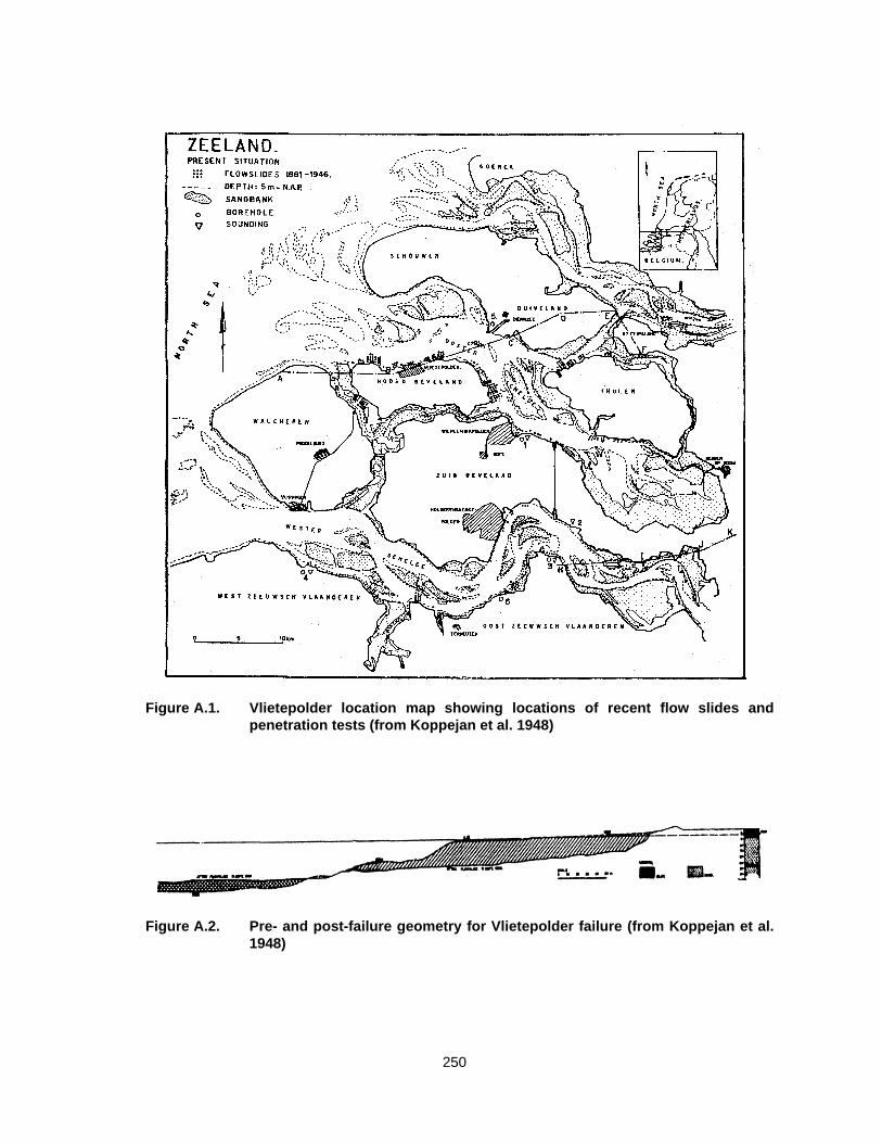
250

Figure A.1. Vlietepolder location map showing locations of recent flow slides andpenetration tests (from Koppejan et al. 1948)

Figure A.2. Pre- and post-failure geometry for Vlietepolder failure (from Koppejan et al.1948)

251

Observations made during this and numerous other liquefaction flow failures in

Zeeland and other coastal regions suggest that the flow slide was retrogressive. A

retrogressive flow slide initiates in a small section of the deposit near the steepest portion of

the toe of the bank (Andresen and Bjerrum 1968; Bjerrum 1971; Casagrande 1976), where

failure is triggered by local oversteepening, large exit seepage gradients, and/or local toe

scour. As this portion of the bank moves away from the deposit, it creates another

oversteepened zone of soil. This zone, in turn, liquefies and flows away from the bank. The

failure retrogresses into the bank material until a more dense zone is encountered or until a

sufficient portion of the newly formed bank is above the watertable and not susceptible to

liquefaction.

A.1.2 Site Geology and Soil Conditions

The soil deposits of the Zeeland region are dominated by delta formation from the

Rhine, Meuse, and Scheldt Rivers, tidal currents, and sea-level variations (Silvis and de

Groot 1995). A typical geologic profile in Zeeland is presented in Figure A.3. The Holocene

age Dunkirk and Calais deposits consist of sandy tidal channel fills and clay deposited on

subtidal flats (Silvis and de Groot 1995). Deposition of the sandy channel fills commonly

occurred rapidly, resulting in a loose soil structure, i.e., low relative density (Koppejan et al.

1948). The Holland peat was deposited during a period of low sea level. The Pleistocene

age Twente formation consists of fine-grained eolian and medium-grained glaciofluvial

sands, while the Tegelen formation consists of fluvial sands and gravels (Silvis and de Groot

1995). As indicated in Figure A.3, the foreset beds of the delta consist primarily of Dunkirk

and Calais sands. Of 700 flow slides identified by Ligtenberg-Mak et al. (1990),

approximately 85% occurred in Dunkirk channel fills, 14% in Calais channel fills, and only

1% in Pleistocene age sands.

252

Figure A.3. General geology of Zeeland coastline (from Silvis and de Groot 1995)

U.S. Standard Sieve Size

0

10

20

30

40

50

60

70

80

90

100

0.0010.010.1110100

Grain Size Diameter (mm)

Perc

ent F

iner

by

Wei

ght

2in

1in

3/4in

1/2in

No4

No20

No40

No60

No100

No200

No10

Pleistocene-ageSands

Dunkirk andCalais Sands

Figure A.4. Typical grain size ranges for Pleistocene and Holocene Age ZeelandDeposits (from Koppejan et al. 1948)

253

The typical range of grain sizes encountered in the Dunkirk and Calais sands is

presented in Figure A.4 (Koppejan et al. 1948). These sands are uniform and fine-grained,

with an average D50 of approximately 0.12 mm, well within the boundaries of most liquefiable

soils (Tsuchida 1970). The typical range of grain sizes encountered in the Pleistocene age

sands is also included in Figure A.4 (Koppejan et al. 1948). These sands are coarser and

typically more dense than the younger sands.

A.1.3 Representative Penetration Resistance

Koppejan et al. (1948) presented the results of four mechanical CPT soundings

conducted in the area near Vlietepolder. The CPT tip resistances measured in these

soundings are presented in Figure A.5. Also in Figure A.5 are the results of adjacent borings

conducted to verify subsurface stratigraphy. While none of the soundings were conducted at

the exact location of this failure, all the soundings penetrated the same geologic material

deposited under nearly identical environmental and geologic conditions. Therefore, these

soundings and the corresponding penetration resistances are used to represent the

conditions at Vlietepolder at the time of failure.

As discussed in a subsequent section, the average depth of the failure surface at

Vlietepolder is approximately 13 m. Therefore, the values of CPT tip resistance measured in

the four soundings from a depth of approximately 12 to 14 m were averaged to determine

the “representative” value of penetration resistance. A unit weight of 18.85 kN/m3 (120 pcf)

was assumed to calculate vertical effective stresses for the overburden correction and

subsequent analyses. Upper and lower bounds of penetration resistance were taken as the

mean value plus and minus the standard deviation, respectively. The resulting average,

upper bound, and lower bound values of qc1 are approximately 3.0, 4.4, and 1.7 MPa,

respectively.

254

Figure A.5. CPT soundings available in Zeeland region. Number of sounding indicates location in Figure B.1. Soil type fromnearby boring shown adjacent to sounding. CPT tip resistance, qc, shown on x-axis (100 kg/cm2 ~ 10 MPa).Elevation shown on y-axis. (From Koppejan et al. 1948)

255

Values of SPT blowcount were not measured anywhere in the region. Therefore,

“representative” values of SPT blowcount were determined using the qc/N60 ratio proposed

by Stark and Olson (1995). For D50 = 0.12 mm, qc/N60 ≅ 0.4. Therefore, the average, upper

bound, and lower bound values of (N1)60 are approximately 7.5, 10.9, and 4.2, respectively.

A.1.4 Yield Shear Strength and Strength Ratio Analyses

A.1.4.1 Yield Shear Strength Analysis

The pre-failure geometry is presented in Figure A.6. Numerous potential failure

surfaces were searched to determine the failure surface requiring the minimum value of

shear resistance for equilibrium (i.e., factor of safety of unity). Because this case is a static

liquefaction flow failure, the minimum shear resistance is equal to the yield shear strength

(see Chapter 4 for discussion). As indicated in Figure A.6, all reasonable failure surfaces

were completely subaqueous. Therefore, the analysis considered three possible scenarios

to evaluate the yield shear strength and strength ratio. These scenarios were: (1) all the

submarine material liquefied at approximately the same time and no drainage occurred prior

to failure; (2) the toe segment is near enough to a drainage boundary that liquefaction was

not possible in this segment, and the toe segment was assigned a drained shear strength of

30°; and (3) the heel segment (closest to the initial scarp) is near enough to a drainage

boundary that liquefaction was not possible in this segment, and the heel segment was

assigned a drained shear strength of 30°. Different combinations of these assumptions were

used along each of the trial surfaces.

The critical failure surface is shown in Figure A.6. The best estimate of yield shear

strength for this failure is 16.1 kPa. The upper bound yield shear strength was obtained

256

Figure A.6. Pre-failure geometry of Vlietepolder shoreline used for yield shear strength and strength ratio analyses showingcritical failure surfaces determined by stability analyses

-30

-20

-10

0

10

0 40 80 120 160 200 240 280 320 360

Distance (m)

Elev

atio

n (m

)

Post-failure geometry

Yield failure surfacesfrom stability analysis Pre-failure geometry

-50

-30

-10

10

-200 -160 -120 -80 -40 0 40 80 120 160 200 240 280 320 360

Distance (m)

Elev

atio

n (m

)

Post-failure geometry

Failed mass

Pre-failure geometry

Figure A.7. Pre- and post-failure geometry of Vlietepolder shoreline used for liquefied shear strength and strength ratioanalyses

257

when the failure surface passed through an alternate location. The lower bound yield shear

strength was obtained when the toe segment was drained. These additional analyses

resulted in upper and lower bound yield shear strength values of 16.8 and 15.0 kPa

respectively.

The weighted average vertical effective stress for the critical failure surface for the

yield shear strength analysis was determined using Eq. 4.3 as approximately 59.7 kPa.

A.1.4.2 Yield Strength Ratio Analysis

Numerous trial failure surfaces were analyzed to estimate the yield strength ratio at

the triggering of failure. Again, various combinations of toe and heel drainage were

considered in this analysis. The critical failure surface is shown in Figure A.6. The average

values of vertical effective stress were determined for each of the slices, and the yield

strength ratio was varied (in turn varying the yield shear strength mobilized along each slice)

until a factor of safety of unity was achieved. The best estimate of yield strength ratio using

this method was 0.265.

An upper bound yield strength ratio was obtained when the failure surface passed

through an alternate location. A lower bound yield strength ratio was obtained when the toe

segment of the slope was drained. These additional analyses resulted in upper and lower

bound yield strength ratios of 0.28 and 0.247 kPa respectively.

A.1.5 Liquefied Shear Strength and Strength Ratio Analyses

A.1.5.1 Liquefied Shear Strength Analysis

Because the post-failure geometry is incomplete (see Figure A.7) and because of the

retrogressive nature of the failure, the liquefied shear strength was estimated using the

258

simplified analysis described in Chapter 5. Using a slope of the failed material and slope of

the seabed of 4°, an average thickness of failed mass of 8.5 m [see Figure A.7, and Eq.

(5.5)], the liquefied shear strength was estimated to be 5.5 kPa. Lower and upper bound

values were estimated using failed mass thicknesses of 7 and 10 m, respectively. The

resulting lower and upper bound liquefied shear strengths are 4.5 and 6.5 kPa, respectively.

A.1.5.2 Liquefied Strength Ratio Analysis

The liquefied strength ratio was estimated by dividing the liquefied shear strength

determined above by the representative pre-failure vertical effective stress. Examining the

critical failure surfaces for the yield shear strength and strength ratio analyses, the average

segment depth is approximately 67% of the maximum depth. Assuming that this value of

67% is approximately correct for all the retrogressive failure surfaces at Vlietepolder, the

average pre-failure vertical effective stress of all the liquefied material can be determined as

the vertical effective stress at 67% of the average maximum depth along the entire failure

surface. The average maximum (upper bound) depth is approximately 19 m. Therefore, the

representative depth of the failure surface is approximately 12.7 m. A lower bound

representative depth is taken as 33% of the average maximum depth. Therefore, a depth of

6.3 m is used to determine a lower bound pre-failure vertical effective stress.

Using these depths, representative, upper bound, and lower bound vertical effective

stresses of 115, 172, and 57 kPa, respectively, were estimated. Combining these vertical

effective stresses with the value of liquefied shear strength determined above results in

average, upper bound, and lower bound liquefied shear strength ratios of 0.048, 0.096, and

0.032, respectively.

259

A.1.6 Sources of Uncertainty

The following sources of uncertainty were involved in estimating the yield shear

strength and strength ratio: (1) the actual limits of the initial zone of liquefaction; (2) the

shear strength of the non-liquefied soils; (3) the location of the initial failure surface; and (4)

potential for porewater pressure or void redistribution during failure. Because the actual

limits of the initial zone of liquefaction are not known with certainty, the yield shear strength

and strength ratio analysis considered possible drainage at both the toe and the heel of the

slope, as discussed above. No strength tests were available for the sands; therefore the

average drained friction angle for the toe and heel segments was taken as 30°. Because the

exact location of the initial failure surface could not be identified, a number of trial failure

surfaces were analyzed using various combinations of drained and undrained shear

strengths until a best-estimate value could be ascertained.

The following sources of uncertainty were involved in estimating the liquefied shear

strength and strength ratio: (1) variations in the slopes of both the failed material and the

seabed; (2) the thickness of failed material; (3) location of the post-failure toe; and (4) the

potential for porewater pressure or void redistribution during flow. Slight variations in both

the failed material and the seabed are indeterminable because additional submarine profiles

are not available. However, a change in slope of 1° causes a change in liquefied shear

strength of only 1.7% (Eq. 5.5). Because the location of the post-failure toe is not known, the

average thickness of the failed material may differ from the estimated value of 8.5 m.

Differences of 1 m in average failed material thickness changes the estimated liquefied

shear strength by less than 10%. Therefore, minor variations in either the slope of the failed

material (or seabed) or in the failed mass thickness does not considerably change the

estimated value of liquefied shear strength.

260

The following sources of uncertainty were involved in estimating the “representative”

penetration resistance: (1) the fact that the CPT soundings were not conducted at the

location of the Vlietepolder failure; (2) the timing of the CPT soundings with respect to initial

deposition and failure in that region; and (3) the use of a CPT-SPT conversion to estimate

SPT blowcount. As the soundings were not conducted at the location of the Vlietepolder

failure, there is obvious uncertainty in use these soundings to estimate “representative” CPT

tip resistance for this case history. However, all the available soundings penetrated the

same geologic material deposited under nearly identical environmental and geologic

conditions. Therefore, it seems reasonable to use these soundings to estimate the

“representative” tip resistance at Vlietepolder. As discussed above, no SPTs were

conducted in the Vlietepolder region, and SPT blowcounts had to be estimated using the

Stark and Olson (1995) CPT-SPT conversion. This conversion adds an unknown level of

uncertainty to the “representative” SPT blowcount for this case.

A.2 NORTH DIKE OF WACHUSETT DAM, MASSACHUSETTS, USA


Olson et al. (2000) described the failure and stability analyses of the North Dike of

Wachusett Dam in detail. The descriptions herein are taken from this source.

The 3200 m long North Dike was constructed using controlled placement and

compaction for the cut-off wall and core materials and uncontrolled fill methods (dumping

from horse-drawn carts) for the shells. Construction of the North Dike began in 1898 with the

excavation of main and secondary cut-off trenches. Trench excavation was completed in

1899. Backfilling of the trenches commenced in 1900 and was completed in 1901.

261

In 1902, construction of the dike sections began. The materials for the core were

stripped from the reservoir area and consisted of sandy silt to silty sand. A large portion of

the shell fill soils consisted of fine sand, which was spoil from the cut-off trenches. The core

soils were placed in 0.15 m lifts and rolled by horse-drawn carts. No direct measurements of

the density of the core material were made, either at the time of construction or during the

recent investigations. However, tube samples obtained during the recent investigations

indicated saturated unit weights in the range of 18.9 to 20.4 kN/m3. The core was sloped in

the upstream direction of the dam at a slope of 1 horizontal to 1 vertical (1H:1V) and has a

maximum width of approximately 30.5 m. The pre-failure cross-section of the North Dike

near the location of the slope failure (centered near Station 23+20) is presented in Figure

A.8.

The downstream shell fill consists of sand to silty sand with some gravel. The

downstream shell soils reportedly were placed in 2.3 m lifts and were compacted by flooding

with water. Approximately 0.15 to 0.3 m of settlement was observed following saturation of

each 2.3 m lift. The slope of the downstream shell varies from 4H:1V immediately

downstream of the crest to approximately elevation 122.5 m, then slopes at 30H:1V toward

Coachlace Pond, as indicated in Figure A.8.

The upstream shell fill also consists of sand to silty sand with some gravel. Unlike the

downstream fill, the upstream fill received no compaction or saturation. The upstream fill

was placed at a 2H:1V to 3H:1V slope from the crest of the dike to a 6 m wide bench at

approximately elevation 122.5 m. The bench consists of riprap placed at a slope of

1.25H:1V to approximately elevation 117 m. Below this elevation, the shell was placed at a

slope of 2H:1V from the existing ground surface, shown in Figure A.8.

262

Figure A.9. Cross-section through the failed portion of the North Dike of Wachusett Dam showing the approximate locationof the sliding surface through the dike (from Olson et al. 2000)

Figure A.8. Pre-failure cross-section of the North Dike of Wachusett Dam at Station 23+20 (from Olson et al. 2000)

263

Fill placement for the North Dike was completed in 1904, three years prior to the

slope failure. In-situ permeability tests conducted during recent investigations indicated that

the upstream and downstream shell soils have a permeability on the order of 1x10-5 m/s.

Therefore, based on the elapsed time and the high permeability of the shell soils, it is highly

unlikely that any excess porewater pressures resulting from saturation existed in the

downstream fill at the time of the slope failure.

On April 11, 1907, a slope failure occurred during initial filling of the reservoir. The

failure involved approximately 46,500 cubic meters of material from a 213 m long section of

the North Dike. The failure was centered over the former river channel (between Stations

22+50 and 25+00), where the dike reached its maximum height of 24.4 m. The reservoir

was approximately at elevation 114 m, or a depth of 12.8 m, at the time of failure. As

indicated in Figure A.9, the failure mass flowed into the reservoir for a maximum horizontal

distance of approximately 100 m and the crest dropped a maximum vertical distance of

approximately 12 m. The failure mass came to rest below the reservoir water level at an

angle of approximately 5 to 6°.

The failed zone of the North Dike was rebuilt in 1907 at a slope of approximately

4H:1V to 5H:1V (prior to failure the upstream slope was 2H:1V) by dumping fill soils into the

reservoir to form a 9 to 17 m wide berm to approximately 0.6 m above the post-failure

reservoir level. No attempt was made to remove the slide mass, and dumped fill was placed

atop the slide mass without compaction. Loose or cracked portions of the embankment

above the berm level were excavated, and the original dike geometry of approximately

2H:1V was maintained by placing granular fill in 0.3 m lifts, compacting it with horse-drawn

carts, and saturating the fill with water pumped from the reservoir. Above the berm level, jets

of water were forced into the fill along the interface between the new and old construction to

264

promote mixing and co-sedimentation of the materials. Reconstruction was completed on

October 30, 1907, and reservoir filling was resumed without incident to a maximum pool

elevation of approximately 120 m. An approximate cross-section of the North Dike at Sta.

23+20 following reconstruction is presented in Figure A.10.


The eastern section of the North Dike is located in a pre-glacial valley of the Nashua

River. Following glaciation, the Nashua River re-routed to its present course, and this valley

became choked with sand and gravel. The eastern section of the North Dike crosses a

former river channel that connected the Coachlace Pond to the north and Sandy Pond to the

south prior to impoundment (see Figure A.11). Figure A.12 presents a longitudinal cross-

section along the eastern section of the North Dike along the centerline of the main cut-off

wall and core. As indicated in Figure A.12, the cut-off wall and core extend over the entire

length of the North Dike, and the dike has a maximum height of 24.4 m over the river

channel. The natural soils underlying the North Dike generally consist of dense to very

dense sands, gravels, and nonplastic silts. Along the former river channel, an intermittent

natural organic silt and fibrous peat deposit is present.

Prior to construction of Wachusett Dam and the supporting dikes, over 1000 borings

were drilled along the proposed location of the North Dike. One boring located 61 m west of

the channel south from Coachlace Pond encountered bedrock at approximately 91 m below

the ground surface. No other boring reached bedrock, but based on local geology, bedrock

is estimated to be on the order of 150 m below the original ground surface.

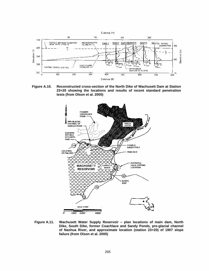
265

Figure A.10. Reconstructed cross-section of the North Dike of Wachusett Dam at Station23+20 showing the locations and results of recent standard penetrationtests (from Olson et al. 2000)

Figure A.11. Wachusett Water Supply Reservoir – plan locations of main dam, NorthDike, South Dike, former Coachlace and Sandy Ponds, pre-glacial channelof Nashua River, and approximate location (station 23+20) of 1907 slopefailure (from Olson et al. 2000)

266

Figure A.12. Longitudinal cross-section of the North Dike of Wachusett Dam along the centerline of the main cut-off wall andcore showing the locations of the stream channel and 1907 slope failure (5x vertical exaggeration) (from Olson etal. 2000)

Figure A.13. Determination of pre-failure vertical effective stresses for yield strength ratio analysis (from Olson et al. 2000)

267


As a part of a GZA GeoEnvironmental, Inc. (1991) geotechnical study, numerous

borings and standard penetration tests (SPT), as well as a suite of laboratory tests, were

conducted. The purpose of this study was to investigate the current seismic stability of the

North Dike. Borings drilled in 1983 within the zone of the 1907 slope failure as a part of a

Haley & Aldrich, Inc. (1984a,b) geotechnical study are also available. All borings were drilled

using mud rotary techniques, and SPT tests were conducted using a “donut ring” hammer.

Therefore, an energy ratio (ER) of 45 percent (%) was applied in calculating (N1)60 (Seed et

al. 1985).

As indicated in Figure A.10, six borings were drilled in the 1980’s and 1990’s in the

reconstructed upstream portion of the North Dike along Sta. 23+20. Based on the soil

descriptions from the boring logs, it appears that thirty SPT tests were conducted in the shell

soils involved in the 1907 failure. The values of (N1)60 in these soils averaged 8 blows per

foot (bpf; blows/0.3 m), with a range of 1 to 21 bpf. Thirteen SPT tests were conducted near

the estimated failure surface of the 1907 flow failure. These (N1)60 values are shown as open

circles in Figure A.10 and average around 6 to 7 bpf. Therefore, an (N1)60 value of 7 bpf was

considered representative of the density of the upstream shell soils (as measured between

1983 and 1991) that liquefied during the 1907 failure. This value agrees with other (N1)60

values measured during the recent investigations in both the upstream and downstream

shell of the North Dike outside of the 1907 failure zone.

Reconstruction of the North Dike involved the placement of up to 6.1 m (with an

average thickness of approximately 4.6 m) of new fill over the shell material that had

liquefied and failed. The liquefied soils probably reconsolidated under their own weight by

the time the new fill was placed and further consolidated due to the weight of the added fill.

268

Thus it is possible that the pre-failure density of the soils that liquefied was lower than that

indicated by the blowcounts recently measured in the reconstructed dike. In addition,

granular soils are known to exhibit an increase in penetration resistance following

disturbance or densification as a result of secondary compression and aging (Schmertmann

1987; Mesri et al. 1990). As there is no rational means to estimate the density changes and

aging effects from 1907 to 1991, it was concluded that the current average (N1)60 value of 7

bpf may be higher than the actual value of (N1)60 at the time of failure in 1907. The jetting of

water that was done as a part of reconstruction likely only affected fill soils near to and

above the phreatic surface in the North Dike, as illustrated in Figure A.9. Therefore, it is

unlikely that the jetting of water significantly affected the measured (N1)60 values, with the

possible exception of those measured in boring WND-3.

The soil in the estimated failure zone has a representative median grain size, D50, of

approximately 0.42 mm and a fines content of 5 to 10%. As aforementioned, the

permeability of the shell soils was measured to be approximately 1x10-5 m/s. As a result, it is

reasonable to assume that the phreatic surface in the upstream shell reached hydraulic

equilibrium almost immediately during the first filling of the reservoir. The core consists of

sandy silt to silty sand and has a lower permeability than the shell soils. Therefore, a change

in the slope of the phreatic surface at the core (compared to the slope of the phreatic

surface in the upstream shell) would occur during first filling of the reservoir. However, the

position of the phreatic surface in the core has no effect on the stability calculations

presented herein. As shown in Figure A.9, the failure surface crosses the core material

above the phreatic surface and reservoir level at the time of failure. Therefore, the slope of

the phreatic surface through the North Dike at the time of failure was assumed to be parallel

269

to the steady-state slope of the phreatic surface measured as a part of the GZA

GeoEnvironmental, Inc. (1991) study.



The mechanism triggering liquefaction in the upstream shell of the North Dike was

likely a decrease in effective stress due to reservoir filling under a nearly constant shear

stress. The failure occurred at the location where the driving shear stress was largest (i.e., at

the location of the maximum dike height). As the reservoir level rose, the vertical effective

stress within the upstream shell decreased considerably. However, as about half of the dike

was still above the phreatic surface at the time of the failure, the shear stress on the failure

surface only decreased slightly (about 15%). Sasitharan et al. (1993) showed that this stress

path triggers liquefaction in loose sands if the stress conditions reach the yield envelope (or

collapse surface as defined by Sladen et al. 1985a) and the driving shear stress is greater

than the liquefied shear strength. At the moment of failure, i.e., when the factor of safety

against slope failure is equal to unity, the shear strength mobilized just prior to collapse and

liquefaction should be representative of the yield shear strength.

Using the pre-failure geometry and the failure surface shown in Figure A.9, values of

shear strength below the phreatic surface were varied until a factor of safety of unity was

achieved. Soils above the phreatic surface were assigned φ' = 30° to 35°. The resulting yield

shear strength ranged from 37.6 to 41.9 kPa.

270


The pre-failure slope geometry also was analyzed to obtain the yield strength ratio

mobilized at the onset of failure. This was accomplished by assuming that the indicated

failure surface passes approximately through the center of the zone of liquefaction. Thus,

the actual zone of liquefaction did not need to be estimated. The initial sliding surface was

divided into 13 segments, as shown in Figure A.13. Segments 1 through 9 correspond to

liquefied soils (i.e., loose shell soils below the phreatic surface), while segments 10 through

13 correspond to soils above the phreatic surface that did not liquefy. Pre-failure vertical

effective stresses (σ'vo) were determined for segments 1 through 9 in Figure A.13 (i.e., the

liquefied soil). Using the individual σ'vo values for each segment and a single value of

strength ratio, individual values of shear strength were assigned to each segment for the

stability analysis. The strength ratio was then varied (which in turn varies the shear strength

mobilized along segments 1 through 13) until a factor of safety of unity was achieved.

The resulting yield strength ratio ranged from 0.26 to 0.30. The upper value of the

range corresponds to φ' = 30° in the non-liquefied soils (segments 10-13 in Figure A.13) and

the lower value corresponds to φ' = 35° in the non-liquefied soils. A weighted average pre-

failure vertical effective stress of 141.6 kPa can be calculated for segments 1 through 9 (in

Figure A.13) using Eq. (4.3).



Examining the pre- and post-failure geometry, a reasonable failure surface for the

North Dike was ascertained, as shown in Figure A.9. The failure surface was divided into a

271

liquefied and non-liquefied zone. The non-liquefied zone accounts for the fill soils that

initially were above the phreatic surface and did not liquefy. These soils were assumed to be

drained during failure and were assigned an effective constant volume (or steady-state)

friction angle, φ'cv, of 30°. In this analysis, the shear strength in the liquefied zone was varied

until a factor of safety of unity was achieved. A lower bound liquefied shear strength of

approximately 3.8 kPa was obtained.


The post-failure slope geometry also was analyzed to obtain a lower bound value of

liquefied strength ratio. This was accomplished by assuming that the initial failure surface

passes approximately through the center of the zone of liquefaction. Thus, the actual

extents of the zone of liquefaction did not need to be determined. The post-failure sliding

surface was divided into 16 segments, as shown in the upper portion of Figure A.14.

Segments 1 through 13 correspond to liquefied soils (identical to the length of liquefied soil

in Figure A.9), while segments 14 through 16 correspond to soils initially above the phreatic

surface that did not liquefy. Based on the lengths of the post-failure segments,

corresponding lengths of liquefiable soil were defined within the pre-failure geometry.

Segments 1 through 5 were located on the initial failure surface, while segments 6 through 9

and segments 10 through 13 were placed equal distances below and above the initial failure

surface, respectively. Additional analyses showed that rearranging the positions of the

segments had little effect on the back-calculated liquefied strength ratio, as long as the

segments were centered around the initial failure surface.

Pre-failure vertical effective stresses (σ'vo) were determined for segments 1 through

13 (i.e., the liquefied soil) in their pre-failure positions and were assigned to the

272

Figure A.14. Determination of pre-failure vertical effective stresses for liquefied strengthratio analysis (from Olson et al. 2000)

Figure A.15. Kinetics analysis results for North Dike of Wachusett Dam

273

corresponding segments in their post-failure positions. Using the individual σ'vo values for

each segment and a single value of liquefied strength ratio, individual values of liquefied

shear strength were assigned to each post-failure geometry segment for the stability

analysis. This allows the liquefied shear strength to model the variation in pre-failure σ'vo of

the liquefied soil along the final sliding surface. Segments 14 through 16 were initially above

the phreatic surface and were assigned a φ'cv = 30°. The liquefied strength ratio was then

varied (which in turn varies the liquefied shear strength mobilized along segments 1 through

13) until a factor of safety of unity was achieved. This analysis yielded a lower bound

liquefied shear strength ratio of approximately 0.026. A weighted average pre-failure vertical

effective stress of 151.2 kPa can be calculated from the liquefied shear strength ratio

analysis using Eq. 5.6.

A.2.5.3 Liquefied Shear Strength and Strength Ratio ConsideringKinetics

The initial result of the kinetics analysis assumed that all soils along the failure

surface mobilized the liquefied shear strength. This over-estimated the actual liquefied shear

strength because a portion of the failed soils initially were above the phreatic surface and

did not liquefy, as discussed in Chapter 5. Therefore, the liquefied shear strength was

adjusted to account for the strength of the non-liquefied soils. Approximately 12% of the

post-failure sliding surface length involved soils that did not liquefy. These soils (i.e.,

segments 14 through 16 in Figure A.14) were assigned an average shear strength of 47.8 to

57.4 kPa for values of φ’ of 30° to 35°, respectively, and the liquefied shear strength was

reduced using Equation 5.13, where su is the liquefied shear strength determined in the

initial kinetics analysis (using Eq. 5.12), Ld is the length of the post-failure sliding surface

(percent of the total length of the failure surface) that did not liquefy (approximately 12%),

274

and sd is the average shear strength of the fill soils that did not liquefy (approximately 47.8 to

57.4 kPa).

The kinetics analysis shown in Figure A.15 yielded the following results:

• Liquefied shear strength ≅ 16.0 kPa (range of 10.4 to 19.1 kPa)

• Liquefied shear strength ratio ≅ 0.106 (range of 0.070 to 0.126)

This liquefied shear strength resulted in a calculated displacement of the center of gravity of

the failure mass of approximately 9.4 m vertically and 44.5 m horizontally. This agrees well

with the observed/measured displacement of the center of gravity of approximately 9.4 m

vertically and 44.8 m horizontally.

The kinetics analysis only provides a value of liquefied shear strength. Therefore, the

liquefied shear strength ratio reported above was determined by dividing the liquefied shear

strength of 16.0 kPa by the weighted average vertical effective stress of 151.2 kPa obtained

from the post-failure geometry analysis.

These values of liquefied shear strength and strength ratio include the effects of

kinetics, hydroplaning, and the shear strength of the soils that did not liquefy and therefore

are considered best estimates. These values are roughly one-half of the sum of the upper

and lower bounds computed from the pre- and post-failure geometries, respectively. This

result is reasonable because as illustrated in Figure A.15, the driving shear stress is

approximately equal to the liquefied shear strength when the failed mass has moved

approximately half-way between its pre-failure and post-failure position.



strength and strength ratio: (1) the limits of the initial zone of liquefaction; (2) the shear

275

strength of the non-liquefied soils; (3) location of the initial sliding surface; (4) the location of

the phreatic surface within the slope at the time of failure; and (5) the potential for porewater

pressure or void redistribution during failure. It was assumed that all the soil below the

phreatic surface liquefied and mobilized the yield shear strength. Preliminary calculations of

drainage time for the liquefied soil were made using an mv (coefficient of volume change)

estimated from both Robertson and Campanella (1989) and Shahien (1998) and a minimum

drainage path distance of approximately 1.5 m (segment 9 in Figure A.14). These

calculations indicate that 20 to 30 seconds are required to reach approximately 50%

consolidation for the segment. Therefore, it was assumed that all the soil below the phreatic

surface liquefied and mobilized the yield shear strength. As the strength of the non-liquefied

soils (i.e., soil above the phreatic surface) were not known, drained friction angles, φ’ = 30 to

35° were used in the yield shear strength and strength ratio analysis to account for the likely

range of mobilized drained shear strength. As aforementioned, the initial sliding surface was

ascertained by examination of the pre- and post-failure geometry. Using these geometries, a

reasonable failure surface was readily determined as shown in Figure A.9. The location of

the phreatic surface was determined as described previously. Only the phreatic surface

within the core material is likely to differ from that shown in Figure A.9, however, changes of

the phreatic surface within the core do not affect the stability calculations because the failure

surface only crosses the core material above the phreatic surface.


strength and strength ratio, including the kinetics analysis: (1) the limits of the zone of

liquefaction; (2) the shear strength of the non-liquefied soils; (3) the location of the final

surface of sliding; and (4) the location of the post-failure geometry toe. As indicated in the

previous paragraph, it appears reasonable to assume that all the material below the phreatic

276

surface liquefied and remained in a liquefied state during flow. There were no shear strength

tests conducted on this material, therefore a typical value of constant volume (or steady

state) friction angle, φ’cv, of 30° (Terzaghi et al. 1996) was assigned to the non-liquefied soil

above the phreatic surface. The final sliding surface was ascertained based on the interface

between the original dense foundation soil and the failed material and by comparing the pre-

and post-failure geometries. The topography of the final 25 m (left side of Figure A.9) was

not available from the original references, however, extrapolation of the existing post-failure

geometry provided a clearly reasonable estimate of the post-failure toe.


penetration resistance: (1) the effects of flow, re-consolidation, and aging; and (2) the effects

of water jetting during reconstruction. As discussed by Olson et al. (2000), Reconstruction of

the North Dike involved the placement of up to approximately 6.1 m (with an average

thickness of approximately 4.6 m) of new fill over the shell material that had liquefied. The

shell soils probably reconsolidated under their own weight by the time the new fill was

placed and further consolidated due to the weight of the added fill. Thus it is likely that the

pre-failure density of the material that liquefied was lower than that indicated by the

blowcounts recently measured in the reconstructed dike. In addition, granular soils are

known to exhibit an increase in penetration resistance following disturbance or densification

as a result of secondary compression and aging (Schmertmann 1987; Mesri et al. 1990). As

there is no rational means to estimate the density changes and aging effects from 1907 to

1991, it was concluded that the current average (N1)60 value of 7 bpf probably represents an

upper bound for the actual value of (N1)60 at the time of failure in 1907. The jetting of water

that was done as a part of reconstruction likely only affected fill soils near to and above the

phreatic surface in the North Dike, as illustrated in Figure A.9. Therefore, it is unlikely that

277

the jetting of water significantly affected the measured (N1)60 values, with the possible

exception of those measured in boring WND-3.

A.3 CALAVERAS DAM, CALIFORNIA, USA


Calaveras Dam was to be the largest earth dam in the world (at the time) with a final

height of 73 m (Cleary 1914). Calaveras Dam, started in 1914, was constructed using

hydraulic fill for the core and interior portions of the shells and uncompacted dumped fill for

the majority of the upstream and downstream shells. On the morning of March 24, 1918,

over 600,000 m3 of material from the central to eastern side of the upstream slope of the

dam failed and slid into the reservoir. The dam had a maximum height of approximately 61

m and the reservoir had a maximum depth of approximately 23 m at the time of failure. Over

215 m of the original 385 m width of the dam was involved in the failure as illustrated in

Figure A.16. Hazen and Metcalf (1918), Hazen (1918), and Hazen (1920) describe the

construction and failure of Calaveras Dam, as well as initial analyses conducted in an

attempt to explain the failure. All descriptions herein were taken from these sources.

Shortly after the failure, surveys of the post-failure geometry were made. Figure A.17

shows the pre-failure and post-failure geometries of the dam. Hazen and Metcalf (1918)

described eyewitness accounts of the failure as follows:

“The final movement at the time of failure on March 24, 1918 was very rapid. The

greater part of it probably took place within a space of not more than five minutes. The

reinforced concrete outlet tower was thrown forward into the reservoir…It seems likely

that the first considerable movement was a drop in the level of the central pool on the

top of the dam, accompanied by a slow lifting, or moving forward, of the surface of the

278

Figure A.16. Aerial photograph taken after the March 24, 1918 failure of Calaveras Dam (from Hazen 1920)

Figure A.17. Pre- and post-failure geometry of Calaveras Dam (from Hazen 1918)

150

250

-200 -100 0 100 200 300 400 500

Distance (m)

Elev

atio

n (m

)

Pre-Failure Geometry Post-Failure Geometry Reservoir Level at Time of Failure

Original Ground SurfaceCore

FAILED MASS

279

upstream toe above the water level. The lower part of the toe had been paved with

concrete, and this extended about 13 feet above the water level. The top of the

concrete formed a conspicuous line, and observers say this seemed to rise several feet.

This may have represented an actual rise, or it may simply have been a lifting at the

edge by the forward movement of the mass. There was then a forward movement of the

whole central section. The section that moved was about 700 feet long…when the

material was released it started to flow almost like water. At first it came through the

narrow breach as a turbid cataract with a steep slope, but the opening rapidly widened

and the slope flattened until the center was drained down to within a few feet of the

water level in the reservoir. Probably within five minutes the rapid movement was over,

although the clay continued to flow at a reduced rate for some time. The more solid

material of the upstream part of the dam, consisting largely of heavy rock fill, had then

moved forward and downward and had filled a space for several hundred feet beyond

where the toe had been. This material must be piled up to a height in places of 70 feet,

and it stands high above the water and far into the reservoir.”

Prior to the failure, considerable movements had occurred in the upstream shell. On

June 18, 1917, approximately 0.5 m of horizontal displacement had been measured at a

point on the upstream face. An additional 0.15 m of horizontal displacement occurred over

the next 12 hours. At the same time, cracks occurred along a 213 m length of the upstream

concrete facing. Cracks also occurred at the crest at a downward angle toward the reservoir

of approximately 45°. Filling was stopped and the movements slowed almost immediately

and essentially ceased. This process of observed movement and stoppage of filling

occurred twice more prior to the failure. One day prior to the failure, approximately 1.2 m of

horizontal movement had been measured on the upstream face.

The failure appears to have initiated in the center of the upstream face, and after

some time, a part of the failure mass apparently rotated horizontally like a door hinged

vertically about the eastern abutment. Hazen (1918) indicated that:

280

“The men who saw the dam go state that at first the whole mass seemed to move

forward as a unit. Afterward it seemed to separate, and the parts that were farthest back

stopped, while those that were further advanced continued to move forward…the

material was carried forward on a good lubricant, and that the lubricant first became

used up or expelled near the center of the dam and left the higher parts of the dam on

solid bottom while there was still lubricant to carry forward the lower and more advanced

portions.”

These observations suggest to the author that the liquefied shell soil (the “good lubricant”)

near the center of the dam had a higher shear strength than the liquefied shell soil farther

from the center of the dam. These observations support the concept of a liquefied shear

strength ratio, where the liquefied shear strength increases with increasing effective

confining stress. After the upstream shell began to flow away from the dam, the central pool

and core were exposed and also flowed through this opening. However, it should be noted

that the failure of the upstream shell occurred prior to any movement of the core material,

and the core material only failed after the movement of the upstream shell exposed the core.

Following the flow failure, Hazen (1918) found it “surprising” that the failed mass

(which had flowed over 200 m horizontally and approximately 30 m vertically) appeared

“hard and solid,” being highly resistant to test piles that were driven to qualitatively evaluate

density. As a result, investigators suspected that soft clay material from the core may have

been present (in the form of horizontal lenses) in the upstream shell which then acted as a

low strength material to enable flow. However, post-failure investigations (Hazen 1918) were

unable to locate any considerable quantity of soft clay within the failure mass. Therefore,

Hazen (1920) speculated that failure initiated in the sandy shell material and suggested that:

“As water pressure is increased, the pressure on the edges is reduced and the friction

resistance of the material becomes less. If the pressure of the water in the pores is great

281

enough to carry all the load, it will have the effect of holding the particles apart and of

producing a condition that is practically equivalent to that of quicksand…A sharp blow,

as with the foot, however, liquefies a certain volume and makes quicksand. The

condition of quicksand lasts for only a few seconds until the surplus water can find its

way out. When this happens the grains again come to solid bearings and stability is

restored. During a few seconds after the sand is struck, however, it is almost liquid, and

is capable of moving or flowing or of transmitting pressure in the same measure as a

liquid…The conditions that control the stability or lack of stability in quicksand may also

control the stability or lack of stability of materials in dams…It may be that after the first

movement there was some readjustment of the material in the toe [upstream slope]

which resulted in producing temporarily this condition of quicksand, and which destroyed

for a moment the stability of the material and facilitated the movement that took place.”

This explanation is the first known description of liquefaction, i.e., the significant loss of

shear strength of a soil as a result of increased porewater pressure.


The base of the dam (up to approximately elevation 180 m) was filled with sluiced

and steam shovel-placed gravel fill from the existing creek bed. The gravel fill contained little

to no fines and contained grain sizes ranging from approximately 0.1 mm to 127 mm

(approximately 5 inches; Hazen 1918). The sluiced gravel had an approximated saturated

unit weight of 15.7 kN/m3.

The remainder of the dam was constructed using hydraulic fill and uncompacted

steam shovel-placed fill. The fill material was obtained from the surrounding sandstone hills,

however, the sandstone was only weakly cemented and consisted of non-durable minerals.

Therefore, following borrow, the fill material consisted of a large range of grain sizes, from

coarse sand to clay-sized particles. The uncompacted steam-shovel fill was placed in 1.2 to

1.5 m lifts primarily in the central to outer portions of the shells to construct “starter dikes”

282

allowing placement of hydraulic fill. The shell material was primarily sand with some gravel

to silty sand, with approximate saturated unit weights of 18.9 kN/m3 near the bottom of the

dam and 17.3 kN/m3 near the top of the dam. Based on descriptions of the material (Hazen

1918; 1920), it seems likely that the fines content of the sandy fill comprising the shells of

the dam was on the order of 10 to 50%.

The clayey core consisted of material with a grain size range from approximately

0.002 to 0.02 mm and a unit weight of approximately 15.7 kN/m3 (Hazen 1918; 1920).

Therefore the fines content of the core material was 100%. Davis et al. (1988) suggested

that the average fines content of the failed soil for Calaveras Dam was greater than 60%.

This estimate was likely based on an average of the fines contents of the sandy shells and

the clayey core fills. However, as liquefaction initiated in the upstream shell fill, it seems

more appropriate to estimate the fines content for Calaveras Dam as approximately 30%

(the average of 10 and 50%, estimated above).


No penetration tests are available for this case history. Therefore, “representative”

SPT and CPT penetration resistances were estimated from an appraisal of relative density

and vertical effective stress using correlations developed by Holtz and Gibbs (1979) and

Robertson and Campanella (1983).

Davis et al. (1988) indicated that fill lifts on the order of 1.2 to 1.5 m in thickness,

without moisture control, should be well below 85% relative compaction based on Modified

Proctor maximum unit weight (ASTM D1557). As the fill contains some fines, the relative

compaction may be as low as 75%. Poulos (1988) suggests that the relative compaction of

the shell soils was approximately 76%. A relative compaction of 75 to 85% (based on

Modified Proctor maximum unit weight) corresponds to approximately to a relative density of

283

20 to 50%. (The calculation was made based on approximate values of 100% Modified

Proctor, maximum, and minimum dry unit weights suggested by NAVFAC DM 7.01, p. 7.1-

22, for “well-graded silty sand.”) An average relative density of 35% for the shell materials of

Calaveras Dam is consistent with (but on the low end of) measured relative densities in

other hydraulic fill dams such as Fort Peck Dam (Marcuson and Krinitzsky 1976) and Lower

San Fernando Dam (Seed et al. 1989).

Using a relative density of approximately 35% and an average vertical effective

stress of 307.5 kPa (3.2 tsf; see Section A.3.5.2) yielded “representative” values of (N1)60

and qc1 of approximately 8 and 5.5 MPa, respectively. As Hazen (1918) suggests that the

shell material had a high compressibility, the relationship for Hilton mines sand (high

compressibility; Robertson and Campanella 1983) was used to estimate qc. The

“representative” (N1)60 value of 8 falls between the value of 12 suggested by Seed (1987)

and Seed and Harder (1990) and the value of 2 suggested by Poulos (1988).



The mechanism triggering liquefaction in the upstream slope of Calaveras Dam

appears to be that the driving shear stress resulting from dam filling exceeded the yield

shear strength of the sandy shell soils. Therefore, this failure is considered a “static”

liquefaction flow failure. Only static shear stresses led to the observed failure. The

deformations and shear straining observed on two occasions prior to failure indicate that the

shell soils were loaded close to the point of liquefaction prior to March 24, 1918. However,

during the previous two occasions, filling was ceased, allowing excess porewater pressure

284

in the upstream fill to dissipate, restoring the strength of the sandy shell soils, and

preventing liquefaction.

Because the loading prior to failure was static, the shear strength mobilized in the

sandy shell soils just prior to collapse and liquefaction (i.e., when the factor of safety against

slope failure is equal to unity) should be equal to the yield shear strength. Therefore, back-

analysis of the pre-failure geometry was consider appropriate to determine the yield shear

strength and strength ratio.

The pre-failure geometry and approximate level of the phreatic surface through the

upstream slope is shown in Figure A.18. As the construction techniques and loading

conditions prior to failure were similar to that for Lower San Fernando Dam, it was assumed

that the zone of liquefaction would be similar. The assumed zone of liquefaction for

Calaveras Dam also is shown in Figure A.18.

Several trial failure surfaces passing approximately through the center of the zone of

liquefaction were analyzed, as shown in Figure A.18, and values of yield shear strength

within the zone of liquefaction were varied until a factor of safety of unity was achieved. The

shear strength of the soils outside the zone of liquefaction was varied from φ' = 30° to 35° to

obtain a range of possible values of yield shear strength. The best estimate of yield shear

strength was 76.6 kPa, with a likely range from 71.8 to 80.7 kPa. Davis et al. (1988)

estimated the value of pre-failure driving stress to be approximately 71.8 kPa, equal to the

lower-bound value estimated herein.


A second analysis using the same pre-failure geometry was conducted to estimate

the yield strength ratio. Several trial failure surfaces passing approximately through the

center of the zone of liquefaction were analyzed, as shown in Figure A.18, and values of

285

Figure A.18. Pre-failure geometry of Calaveras Dam used for yield shear strength and strength ratio analyses. Assumed zone ofliquefaction is shaded.

Figure A.19. Post-failure geometry of Calaveras Dam used for liquefied shear strength and strength ratio analyses

150

200

250

300

-150 -50 50 150 250 350 450

Distance (m)

Elev

atio

n (m

) Pre-Failure Geometry Post-Failure Geometry Reservoir Level at Time of Failure

Original Ground Surface

Core CP 1

CP 2

1 2 3 4 5 6 7 8 9 10 11 12 13 14 15 16 17 18

Approximate FinalSliding Surface

15

13 1814

125

67

4

179

11

8

310

16

Post-FailureGeometry Segments

Pre-Failure Locations of SegmentsUsed to Determine Pre-FailureVertical Effective Stresses

150

200

250

-150 -100 -50 0 50 100 150 200 250

Distance (m)

Pre-Failure Geometry Reservoir Level atTime of Failure


CoreAssumed Zoneof Liquefaction

Trial Failure Surfaces

286

pre-failure vertical effective stress were determined for each segment of a given trial failure

surface. Using these values of pre-failure vertical effective stress and a single value of yield

strength ratio, various values of yield shear strength were assigned to each segment of the

pre-failure geometry. The factor of safety against slope failure was then evaluated. Using an

iterative process, the value of yield strength ratio was varied (in turn, varying the yield shear

strength assigned to each pre-failure segment) until a factor of safety of unity was achieved.

The shear strength of the soils outside the zone of liquefaction was varied from φ' =

30° to 35° to obtain a range of possible values of yield shear strength. The best estimate of

yield strength ratio was determined as 0.27, with a likely range from 0.255 to 0.295. The

weighted average pre-failure σ'vo was calculated using Eq. (4.3) as 294 kPa.



The post-failure geometry is reproduced in Figure A.19. The final failure surface

shown in Figure A.19 was ascertained from examination of the post-failure geometry and

from the post-mortem studies described by Hazen (1920). Hazen (1920) indicated that “near

the center line of the dam it was clear that the line of slippage was approximately 60 ft. (18.3

m) above the bottom of the valley.” This provided one control point (CP1) for estimating the

final failure surface, as shown in Figure A.19. Hazen (1920) also indicated that “at the base

of the upper toe all the material slipped (including the gravel from the creek bed that had

been placed hydraulically), extending clear down to the natural surface…” This provided a

second control point (CP2), as shown in Figure A.19. Lastly, Hazen (1920) indicated that the

slip surface most likely was inclined over the majority of the upstream shell. Using this

information, a probable failure surface was ascertained, as shown in Figure A.19.

287

Assigning φ' = 30° to 35° to the length of the final failure surface that corresponds to

the length of material in the pre-failure geometry that did not liquefy, a likely range of

liquefied shear strengths were obtained. The back-calculated shear strength was

approximately 3.6 kPa, with a possible range from 2.2 to 10.5 kPa. The upper bound of this

range considers the effects of hydroplaning when material entered the reservoir (Davis et al.

1988).


Using the same post-failure sliding surface, an analysis to back-calculate the

liquefied strength ratio was conducted. Using the same assumptions for the shear strength

of originally non-liquefied materials, the liquefied strength ratio was estimated as 0.012, with

a possible range from 0.007 to 0.033. The pre-failure σ'vo is equal to 307.5 kPa [Eq. (5.6)].


The pre- and post-failure geometries are reproduced in Figure A.20. Figure A.20 also

shows the pre- and post-failure centers of gravity, the final sliding surface, and the probable

path of travel of the center of gravity during flow failure. The initial result of the kinetics

analysis assumed that all soils along the failure surface mobilized the liquefied shear

strength. This over-estimated the actual liquefied shear strength because a portion of the

failed soils initially were above the phreatic surface and did not liquefy, as aforementioned.

Therefore, the liquefied shear strength was adjusted to account for the strength of the non-

liquefied soils. Approximately 7% of the post-failure sliding surface length involved soils that

did not liquefy. These soils (i.e., segments 1 and 2 in Figure A.19) were assigned an

average shear strength of 104 kPa for φ’ of 30°, respectively, and the liquefied shear

288

Figure A.20. Movement of center of gravity during flow failure of Calaveras Dam

Figure A.21. Kinetics analysis of Calaveras Dam

150

200

250

300

-150 -50 50 150 250 350 450

Distance (m)

Elev

atio

n (m

) Pre-Failure Geometry Post-Failure Geometry Reservoir Level at Time of Failure


Core CP 1

CP 2Approximate FinalSliding Surface

Post-FailureCenter of Gravity

Pre-Failure Center of Gravity

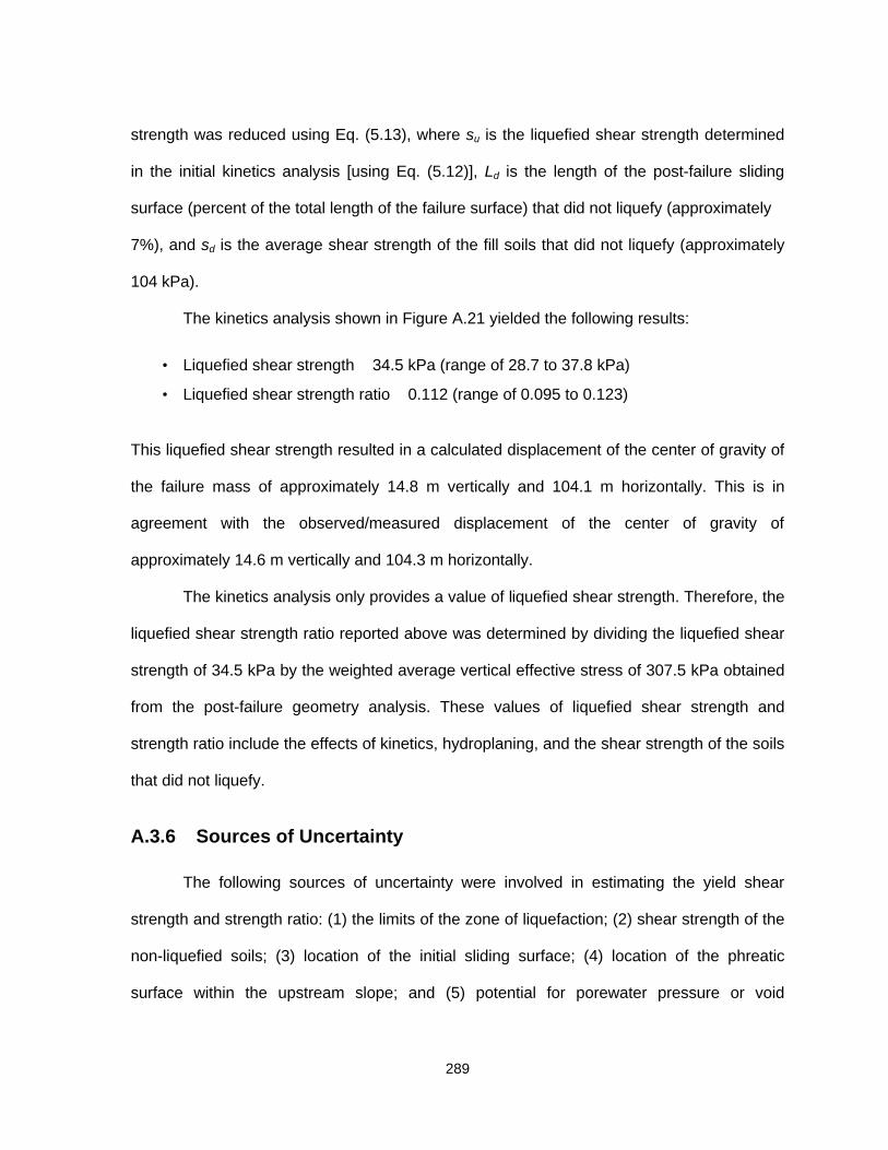
289

strength was reduced using Eq. (5.13), where su is the liquefied shear strength determined

in the initial kinetics analysis [using Eq. (5.12)], Ld is the length of the post-failure sliding

surface (percent of the total length of the failure surface) that did not liquefy (approximately

7%), and sd is the average shear strength of the fill soils that did not liquefy (approximately

104 kPa).

The kinetics analysis shown in Figure A.21 yielded the following results:




the failure mass of approximately 14.8 m vertically and 104.1 m horizontally. This is in

agreement with the observed/measured displacement of the center of gravity of

approximately 14.6 m vertically and 104.3 m horizontally.




from the post-failure geometry analysis. These values of liquefied shear strength and

strength ratio include the effects of kinetics, hydroplaning, and the shear strength of the soils

that did not liquefy.



strength and strength ratio: (1) the limits of the zone of liquefaction; (2) shear strength of the

non-liquefied soils; (3) location of the initial sliding surface; (4) location of the phreatic

surface within the upstream slope; and (5) potential for porewater pressure or void

290

redistribution during failure. As explained above, the zone of soil that liquefied during loading

was estimated from comparison with other, better documented case histories. However, the

use of larger and smaller zones of liquefaction had little bearing on the analysis, as long as

the critical failure surface passed approximately through the center of the zone of

liquefaction. No strength tests were conducted on the shell materials, therefore, the friction

angle of the non-liquefied shell material (see Figure A.18) was assumed to be 35°. The

exact location of the initial failure surface is not known, however, a stability analysis search

was conducted (to back-estimate the yield shear strength), and the critical failure surface

was very close to the trial failure surfaces shown in Figure A.18. As no piezometric

measurements were made during filling, the phreatic surface was estimated from the

location of the core and reservoir pools. The location of the phreatic surface within the slope

(as shown in Figures A.17 to A.20) was estimated based on the shape of phreatic surfaces

in other hydraulic fill dams (Hazen 1920; U.S. Army Corps of Engineers 1939; Middlebrooks

1942).


strength and strength ratio, including the kinetics analysis: (1) the limits of the zone of

liquefaction; (2) the shear strength of the non-liquefied soils; (3) the location of the phreatic

surface within the slope; and (4) the potential for porewater pressure or void redistribution

during flow. As above, the exact limits of the zone of liquefaction were not known, but were

estimated from comparison with other, better documented case histories. There were no

shear strength tests conducted on this material, therefore a typical value of constant volume

(or steady state) friction angle, φ’cv, of 30° (Terzaghi et al. 1996) was assigned to the non-

liquefied soil. The location of the phreatic surface within the failed slope was assumed to go

291

from the known reservoir level into the slope along the pre-failure phreatic surface and then

along the upper surface of the failed material, as shown in Figure A.19.

No penetration tests were conducted either before or after the failure for this case.

Therefore the fact that the “representative” values of penetration resistance had to be

estimated from published correlations provides (by far) the greatest source of uncertainty.

This source of uncertainty was unavoidable. Additional sources of uncertainty also were

involved in estimating the “representative” penetration resistance: (1) the position of the

phreatic surface prior to failure; and (2) the large values of vertical effective stress applicable

within the zone of liquefaction are slightly beyond the upper limit of the SPT-based

correlation. The location of the phreatic surface within the pre-failure upstream slope was

described above. As the weighted average vertical effective stress within the zone of

liquefaction was only slightly higher than the upper limit of the correlation (upper limit was

approximately 287 kPa while the weighted average pre-failure vertical effective stress was

307.5 kPa), it was considered reasonable to extrapolate the correlation to the value of

vertical effective stress for Calaveras Dam.

A.4 SHEFFIELD DAM, CALIFORNIA, USA


Sheffield Dam and Reservoir was constructed in the winter of 1917 as a distribution

reservoir of the Santa Barbara Municipal Water Department (U.S. Army Corps of Engineers

1949). The dam was constructed in a ravine underlain by recent alluvial terrace deposits 1.2

to 3 m thick, overlying sandstone bedrock. The earth dam had a maximum crest height of

approximately 7.6 m and was approximately 220 m long. At the time of failure, the reservoir

level was approximately 4.6 to 5.5 m deep (Seed et al. 1969). A cross-section of the dam

292

prior to the failure is shown in Figure A.22. The upstream and downstream slopes were

approximately 1 vertical to 2.5 horizontal. The upstream slope was capped with a 1.2 m

thick clay blanket that extended 3 m into the foundation to act as a cutoff wall, as shown in

Figure A.22.

On June 29, 1925, a ML ~ 6.3 earthquake struck the region. The epicenter of the

earthquake was located approximately seven miles northwest of Sheffield Dam. On the

basis of approximate Rossi-Forell intensity ratings of VIII to IX, Seed et al. (1969) estimated

that the free-field peak surface acceleration at the site was on the order of 0.15g, and the

eye-witnesses placed the duration of strong shaking between 15 and 18 seconds.

No eyewitness accounts are available to confidently describe the events that

occurred during failure. However, a number of engineers examined the dam following the

failure. Based on examination of the failure mass, it appeared that the failure occurred along

the base or foundation of the dam, and a 130 m section of the downstream slope of the dam

flowed over 60 m with the embankment largely intact (Engineering News-Record 1925). A

plan view of the post-failure configuration of the dam is shown in Figure A.23, and Figure

A.24 shows a photograph of the dam shortly after failure (both the plan view and photo are

from Engineering News-Record 1925). In fact, plant growth on the downstream slope was

largely undisturbed following the failure. As the failure mass moved downstream, it also

appears to have rotated horizontally as if it were hinged about its right side.

Nunn (1925) gave the following description:

“After examination by several prominent engineers, the conclusion has been reached

that the base of the dam had become saturated, and that the shock of the

earthquake…had opened vertical fissures from base to top; the water rushing through

these fissures simply floated the dam out in sections.”

293

Figure A.22. Pre-failure geometry of Sheffield Dam (after Seed et al. 1969)

0

5

10

15

0 5 10 15 20 25 30 35 40 45 50

Distance (m)

Elev

atio

n (m

)

Reservoir Level

Clay Blanket

CompactedSandy Silt toSilty Sand

Sandy Silt to Silty Sand

Pre-Failure Geometry

Bedrock Surface

Piezometric Surface

294

Figure A.23. Plan view of post-failure configuration of Sheffield Dam (from EngineeringNews-Record 1925)

Figure A.24. Photograph of Sheffield Dam shortly after failure (from Engineering News-Record 1925)

FAILED MASS

295

Willis (1925) reported that:

“The foundations of the dam had become saturated and the rise of the water as the

ground was shaken formed a liquid layer of sand under the dam, on which it floated out,

swinging about as if on a hinge.”

Seed et al. (1969) concluded that the failure occurred due to liquefaction and

strength loss in the soils along the base of the dam as a result of shaking during the 1925

Santa Barbara earthquake. Following the failure, the majority of the dam was removed and

reconstructed using a more conservative geometry.


Sheffield Dam was constructed of pit-run material obtained from excavations within

the reservoir limits. This material was an alluvial terrace deposit consisting of silt, sand, and

sandstone with cobbles. Occasional stringers of clayey sand to sandy clay and gravelly

clayey sand were also present. The U.S Army Corps of Engineers (1949) report indicates

that no formal stripping of the upper loose foundation material was done prior to

embankment construction. Compaction of the dam was only achieved by the routing of light

construction equipment over the fill. No compaction records or tests are available. Seed et

al. (1969) estimated the location of the phreatic surface within the dam on the basis of post-

failure investigations and reports, as well as on known phreatic surfaces measured in similar

dams.

As a part of the U.S. Army Corps of Engineers (1949) study, five borings (0.4 m in

diameter) were drilled and sampled to determine the character of the foundation soils

underlying the dam. Because the reconstruction of the dam included removal of the

foundation material from under the original dam geometry, the boring were drilled in areas

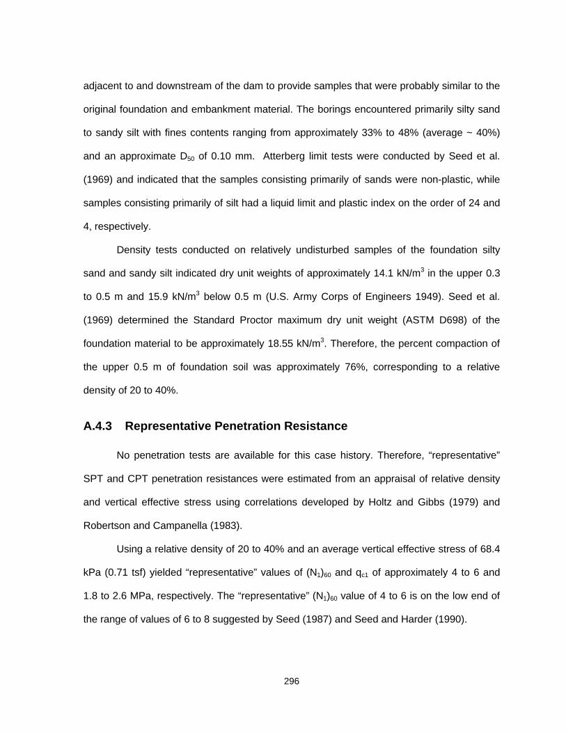
296

adjacent to and downstream of the dam to provide samples that were probably similar to the

original foundation and embankment material. The borings encountered primarily silty sand

to sandy silt with fines contents ranging from approximately 33% to 48% (average ~ 40%)

and an approximate D50 of 0.10 mm. Atterberg limit tests were conducted by Seed et al.

(1969) and indicated that the samples consisting primarily of sands were non-plastic, while

samples consisting primarily of silt had a liquid limit and plastic index on the order of 24 and

4, respectively.

Density tests conducted on relatively undisturbed samples of the foundation silty

sand and sandy silt indicated dry unit weights of approximately 14.1 kN/m3 in the upper 0.3

to 0.5 m and 15.9 kN/m3 below 0.5 m (U.S. Army Corps of Engineers 1949). Seed et al.

(1969) determined the Standard Proctor maximum dry unit weight (ASTM D698) of the

foundation material to be approximately 18.55 kN/m3. Therefore, the percent compaction of

the upper 0.5 m of foundation soil was approximately 76%, corresponding to a relative

density of 20 to 40%.


No penetration tests are available for this case history. Therefore, “representative”

SPT and CPT penetration resistances were estimated from an appraisal of relative density

and vertical effective stress using correlations developed by Holtz and Gibbs (1979) and

Robertson and Campanella (1983).

Using a relative density of 20 to 40% and an average vertical effective stress of 68.4

kPa (0.71 tsf) yielded “representative” values of (N1)60 and qc1 of approximately 4 to 6 and

1.8 to 2.6 MPa, respectively. The “representative” (N1)60 value of 4 to 6 is on the low end of

the range of values of 6 to 8 suggested by Seed (1987) and Seed and Harder (1990).

297



The mechanism that most likely led to the observed failure is liquefaction and

strength loss in the foundation silty sand to sandy silt resulting from seismic shaking. Seed

et al. (1969) determined that the entire base of the dam liquefied during the earthquake and

that the water pressure acting on the concrete facing of the upstream slope pushed the dam

downstream.

As discussed in Chapter 4, the shear strength and strength ratio mobilized at the

instant of failure in cases of liquefaction flow failure triggered by seismic loading do not

necessarily represent the yield shear strength and yield strength ratio, respectively.

Therefore, back-calculated values of shear strength and strength ratio likely do not

represent the yield shear strength and yield strength ratio.

A slope stability search was conducted to determine the critical initial failure surface.

A single value of shear strength was assigned to the liquefied foundation soil, and a drained

friction angle of 34° was assigned to the embankment material above the phreatic surface

(based on consolidated-drained triaxial testing conducted by Seed et al. 1969). The friction

angle of the embankment material below the phreatic surface was varied between 34° and

15° (based on the total stress friction angle determined using data from both Seed et al.

1969 and U.S. Army Corps of Engineers 1949). No inertia forces were considered in the

embankment, as a result of the softening/isolation effect of liquefaction along the base of the

dam.

The critical failure surface (i.e., the surface requiring the lowest value of mobilized

shear strength in the zone of liquefaction for stability) for Sheffield Dam is shown in Figure

298

A.25. Other failure surfaces that were considered are also shown in Figure A.25. The values

of mobilized shear strength in the zone of liquefaction ranged from 12.7 to 18.0 kPa

depending on the assumption regarding the mobilized friction angle of the embankment

material below the phreatic surface. The best estimate of mobilized shear strength in the

zone of liquefaction was taken as the average of these values, or 15.4 kPa.


A second analysis was conducted on the pre-failure geometry to estimate the

mobilized strength ratio in the zone of liquefaction. Contours of vertical effective stress were

determined throughout the foundation material. Using the contours of pre-failure vertical

effective stress and a single value of mobilized strength ratio in the zone of liquefaction,

contours of mobilized shear strength were determined for the foundation material below the

pre-failure geometry of the dam. The factor of safety against slope failure was then

evaluated using a slope stability search. Using an iterative process, the value of mobilized

strength ratio was varied (in turn, varying the mobilized shear strength assigned to each pre-

failure segment in the zone of liquefaction) and the slope stability search re-conducted until

a factor of safety of unity was achieved.

The critical failure surface (i.e., the surface requiring the lowest value of yield

strength ratio for stability) for Sheffield Dam is shown in Figure A.25. Other failure surfaces

that were considered are also shown in Figure A.25. The values of mobilized strength ratio

ranged from 0.207 to 0.249 depending on the assumption regarding the mobilized friction

angle of the embankment material below the phreatic surface. The best estimate of yield

shear strength was taken as the average of these values, or 0.228. The pre-failure σ'vo is

equal to 68.4 kPa [Eq. (4.3)].

299

Figure A.25. Pre-failure geometry of Sheffield Dam showing locations of yield failure surfaces determined in yield strength ratioand yield shear strength back-analyses. Location of the zone of liquefaction estimated from Seed et al. (1969) isalso included.

0

5

10

15

0 5 10 15 20 25 30 35 40 45 50

Distance (m)

Reservoir Level

Clay Blanket

CompactedSandy Silt toSilty Sand

Sandy Silt to Silty Sand


Bedrock Surface

Piezometric Surface

Yield Failure Surfaces

Zone ofLiquefaction

300



Again, Seed et al. (1969) determined that the entire base of the dam liquefied during

the earthquake and that the water pressure acting on the concrete facing of the upstream

slope pushed the dam downstream. Seed (1987) conducted a simple analysis of this failure

mechanism and suggested that the liquefied shear strength was likely on the order of 2.4

kPa. Seed and Harder (1990) suggested that the liquefied shear strength was on the order

of 3.6 ± 1.2 kPa.

Using the plan view of the failure (Figure A.23) and photographs available of the

post-failure conditions, an estimate of both the slope and thickness of the post-failure

geometry were made. Using these values of slope angle and post-failure thickness, Eq.

(5.5) was used to estimate a liquefied shear strength of 4.0 kPa. Therefore, the range of

shear strength of 3.6 ± 1.2 kPa was considered representative of the liquefied shear

strength mobilized during the liquefaction failure of Sheffield Dam.


As the cross-section of the post-failure geometry is not known with any certainty, a

rigorous slope stability analysis of the post-failure geometry was not possible. Therefore, the

liquefied strength ratio was estimated by dividing the liquefied shear strength by the

weighted average vertical effective stress. The weighted average vertical effective stress

was estimated as 68.4 kPa using the entire base of the dam (shown as shaded zone of

liquefied soil in Figure A.25). Dividing the liquefied shear strength of 3.6 kPa by the weighted

301

average vertical effective stress to determine the liquefied strength ratio of 0.053, with a

range from 0.035 to 0.070 (based on the range of liquefied shear strength).



strength and strength ratio: (1) the limits of the zone of liquefaction; (2) the shear strength of

the non-liquefied soils; (3) the location of the initial surface of sliding; and (4) the location of

the phreatic surface within the dam. Liquefaction was assumed to occur all along the base

of the dam, according to the analysis of Seed et al. (1969). The shear strength of the

embankment soil above the phreatic surface is relatively well-known, based on triaxial

testing conducted by Seed et al. (1969). However, the drainage conditions of the

embankment soils below the phreatic surface is not known with certainty. Therefore,

analyses were conducted assuming both full drainage (using a drained friction angle of 34°)

and no drainage (using a total stress friction angle of 15°). It is most likely that some

drainage did occur during the earthquake, therefore, the best estimate of mobilized shear

strength and strength ratio at the initiation of failure was taken as the average of the results

of analyses considering both drainage conditions. No eyewitness accounts are available for

the failure, therefore, the initial failure surface can not be accurately ascertained. Therefore,

slope stability searches were conducted to determine both the mobilized shear strength and

strength ratio at the triggering of liquefaction. Seed et al. (1969) estimated the location of the

phreatic surface within the dam on the basis of post-failure investigations and reports, as

well as on known phreatic surfaces measured in similar dams. Their estimate of the phreatic

surface was used for this analysis.


strength and strength ratio: (1) the post-failure geometry; and (2) the potential of porewater

302

or void redistribution occurring during flow. Clearly, the largest uncertainty regarding this

failure is the fact that sectional views of the post-failure geometry are not available.

Therefore, the liquefied shear strength was estimated from a simple analysis of the forces

acting on the pre-failure geometry of the dam (Seed 1987) and assumed values of the slope

angle of the surface and thickness of the post failure geometry for use in Eq. (5.5). In

addition, because sectional views of the post-failure geometry are not available, a rigorous

stability analysis of the post-failure geometry could not be conducted to determine the

liquefied strength ratio. However, as it is likely that the entire base of the dam was involved

in the resulting flow failure, therefore the weighted average pre-failure vertical effective

stress determined from Figure A.22 probably is appropriate.




This source of uncertainty was unavoidable.

A.5 HELSINKI HARBOR, FINLAND


Toward the end of 1936, an extension to Helsinki harbor was constructed in the

southern portion of the harbor. The extension was constructed by placing blasted rock to

build up an outer berm behind which sand was placed hydraulically. When the hydraulic

placement of sand was started, the rock berm was not complete, with a 25 m gap existing

as shown in Figure A.26 (Andresen and Bjerrum 1968).

By November 30, 1936, the sand fill had reached the level shown in Figure A.26.

During the night, a small slide in the sand fill occurred at the location of the gap in the rock

303

Figure A.26. Pre- and post-failure section and plan view of Helsinki Harbor (from Andresenand Bjerrum 1968)

304

berm. Despite this small slide, filling was continued. Upon placement of a few additional

loads of sand, a larger flow slide was initiated. Approximately 6,000 m3 of sand flowed

through the gap in the rock berm over a distance of 80 to 100 m into the harbor (Figure

A.26; Andresen and Bjerrum 1968). After the slide came to rest, the sand still within the

basin had a slope of approximately 4 to 5°, while the edges of the slide scar had slopes

ranging from 18 to 22°.

Initial investigations following the slide suggested that the failure may have been

triggered by failure in the foundation clay underlying the sand fill. However, more detailed

investigations of the site indicated that the foundation clay was undisturbed, and a 2 to 3 m

thick layer of sand fill still overlaid the foundation clay following the failure. Further, the failed

sand simply re-deposited itself on the foundation clay when it came to rest in the harbor

without eroding the clay, despite the low density of the clay.


The soils comprising Helsinki Harbor are primarily deltaic and estuary-deposited silty

sands and clays. At the location of the harbor expansion and subsequent failure, the upper

soils consisted of a 5 to 10 m thick bed of loose silty sand and soft clay. The depth of water

in the harbor typically ranged from 2 to 8 m. At the time of failure, the best estimate of the

depth of water is shown in Figure A.26. The sand used as fill was obtained from a nearby

borrow pit, therefore it is likely that the sand contained some fines, similar to the deltaic

deposits encountered at the harbor. Unfortunately, no other geologic or geotechnical

descriptions of the foundation material or sand fill (e.g., grain size, fines content, etc.) are

available. The saturated unit weight of the sand was assumed to be 18.9 kN/m3.

305


No penetration tests were conducted in the sand fill either before or after the flow

failure. Therefore, “representative” values of both SPT and CPT penetration resistance must

be estimated from relative density-effective overburden relations. The relative density of the

sand fill is estimated from measurements of other hydraulic fill constructed in a similar

manner.

Sladen and Hewitt (1989) indicated that hydraulic fills placed using a point source

distribution typically have relative densities on the order of 40 to 50%. Using the

approximate weighted average pre-failure vertical effective stress of 25.0 kPa from the

liquefied strength ratio analysis (see below) and Dr ~ 40%, the “representative” (N1)60 was

estimated as 6 using the Holtz and Gibbs (1979) and Seed and Tokimatsu (1987) relations

and the “representative” qc1 was estimated as 4.0 MPa using the Robertson and

Campanella (1983) and Jamiolkowski et al. (1985) relations.



The mechanism that likely triggered flow failure at Helsinki Harbor was the rapid rate

of filling while the fill sand was already in a marginally stable condition. In fact, a small failure

in the steepest area of the fill occurred shortly before the main flow failure. Continued filling

behind the rock berm triggered undrained collapse of the loose sand fill. As the failure

occurred during filling, the shear strength and strength ratio mobilized at the time of failure is

equal to the yield shear strength and strength ratio, respectively.

The pre-failure geometry is shown in Figure A.27. As the exact zone of material

where liquefaction was triggered is not known, it was assumed that all the sand fill below the

306

Figure A.27. Pre-failure geometry of and yield failure surfaces for Helsinki Harbor used for yield shear strength and strengthratio analyses

-10

-5

0

5

-10 0 10 20 30 40 50 60 70

Distance (m)

Elev

atio

n (m

)


Post-Failure GeometryYield Failure Surfaces

Water Level at Time of Failure

307

water level liquefied. Using this assumption, a slope stability search was conducted to

determine the critical initial failure surface. The critical failure surface is also shown in Figure

A.27, and is similar to the estimated failure surface for the initial slide reported by Andresen

and Bjerrum (1968). The yield shear strength was determined as 3.8 kPa for this failure

surface. The range of potential values of yield shear strength was determined by

considering other failure surfaces. A range of yield shear strength from 2.2 to 4.4 kPa was

considered possible for this flow failure.


A second analysis was conducted to estimate the yield strength ratio mobilized at the

triggering of liquefaction. Several trial failure surfaces, including the critical failure surface

from the yield shear strength analysis were considered, as shown in Figure A.27, and values

of pre-failure vertical effective stress were determined for each segment of a given trial

failure surface. Using these values of pre-failure vertical effective stress and a single value

of yield strength ratio, various values of yield shear strength were assigned to each segment

of the pre-failure geometry. The factor of safety against slope failure was then evaluated.

Using an iterative process, the value of yield strength ratio was varied (in turn, varying the

yield shear strength assigned to each pre-failure segment) until a factor of safety of unity

was achieved. A best estimate of yield strength ratio was determined as 0.24, with a

possible range of 0.21 to 0.26 determined using other failure surfaces. The pre-failure σ'vo is

equal to 15.1 kPa [Eq. (4.3)].

308



As a result of the very flat post-failure geometry, a rigorous slope stability analysis

may not have given a reasonable estimate of the liquefied shear strength. Therefore, a

simplified analysis (as described in Chapter 5) was conducted to estimate the liquefied

shear strength. The slope of the post-failure geometry and seafloor was taken as 4 to 5°

(Andresen and Bjerrum 1968), and the thickness of the failed material was estimated from

Figure A.26 to be 1.8 to 2.5 m. The saturated unit weight of the hydraulic fill is unknown,

therefore a value of 18.9 kN/m3 was assumed. This results in a buoyant unit weight of 9.0

kN/m3, which was used in Eq. (5.5). Using Eq. (5.5), the liquefied shear strength was

estimated as 1.1 to 2.0 kPa, with an average value of 1.55 kPa.


Using the same procedure to estimate the pre-failure vertical effective stress that

was used for Vlietepolder (described earlier in Section A.1.5), the representative thickness

of the pre-failure mass was estimated as 4 m. Using this thickness, the pre-failure vertical

effective stress was estimated as 25.0 kPa, with a possible range from 20.1 to 29.9 kPa.

Using these values of pre-failure vertical effective stress, values of liquefied strength ratio

were determined to range from 0.037 to 0.098, with a best estimate value of 0.060.



strength and strength ratio: (1) the limits of the zone of initial liquefaction; (2) the location of

the initial surface of sliding; and (3) the potential of porewater or void redistribution during

309

initial failure. As the limits of the zone of initial liquefaction are not known, the entire sand fill

was estimated to liquefy at the same time. The location of the initial surface of sliding was

determined using a slope stability search procedure and was similar to the failure surface of

the small slide reported by Andresen and Bjerrum (1968).


strength and strength ratio: (1) the slope of the post-failure geometry and seafloor; (2) the

thickness and unit weight of the failed mass; and (3) the potential for porewater or void

redistribution during flow. The slope of the post-failure geometry and seafloor were

estimated from the measured slope of the sand fill remaining in the basin. Even if this were

not the actual slope of the post-failure geometry and seafloor, the slope of the sand fill in the

basin are representative of the shear strength available to sand during flow. The thickness

of the failed material was measured from Figure A.26, but a range of possible values was

used because of the uncertainty in its determination. The unit weight of 18.9 kN/m3 was

assumed from typical values of sand fill obtained from NAVFAC DM 7.01 and Terzaghi et al.

(1996).




This source of uncertainty was unavoidable. In addition, as a result of the low values of pre-

failure vertical effective stress, the overburden correction factor approached the value of 2,

the upper limit used in this study. However, the value of overburden correction factor did not

exceed 2.

310

A.6 FORT PECK DAM, MONTANA, USA


The failure of Fort Peck Dam has been studied in detail by numerous agencies and

researchers. Therefore, the background information provided in the following sections will be

brief. Detailed descriptions of the construction, failure, and reconstruction of Fort Peck Dam

can be found in U.S. Army Corps of Engineers (1939, 1976), Middlebrooks (1942; including

numerous discussions), Casagrande (1965, 1976), Marcuson and Krinitzsky (1976),

Marcuson et al. (1978), and a website dedicated to Fort Peck Dam at

‹http://www.midrivers.com/~rafter/lake/›. All descriptions herein are taken from these

sources.

The Fort Peck Dam is located on the Missouri River in northeastern Montana. The

dam is a hydraulic-fill structure, with a maximum height of 76.3 m over the original riverbed.

The crest length of the dam is over 3224 m, with a maximum width of 960 from station

30+00 to 70+00. West of the main dam is a 3184 m long dike, giving the dam a total storage

capacity of over 2.4 x 1010 m3 of water.

Operation of the first dredge began on October 13, 1934, and by September 22,

1938, filling of the main dam was nearly complete, with a maximum height of approximately

62.8 m. However, that morning settlements of over 0.5 m were noted on the crest of the

upstream face near station 15+00 (close to the eastern abutment), despite the fact that

nearby settlement points had settled only slightly over 0.1 m.

At about 1:15 p.m., as engineers were deciding upon a course of action, a major

slide occurred in the upstream slope, as shown in Figures A.28 through A.30. In all, the slide

affected the dam from stations 2+50 to 31+00 (nearly 870 m in length), and involved

between 4 million and 8 million m3 of material from the dam. The slide mass traveled a

311

Figure A.28. Post-failure plan view Fort Peck Dam (from U.S. Army Corps of Engineers 1939)

312

Figure A.29. Oblique aerial view (looking westward) of Fort Peck Dam following thefailure (from http://www.midrivers.com/~rafter/lake/)

Figure A.30. Aerial photo of Fort Peck Dam following the failure (fromhttp://www.midrivers.com/~rafter/lake/)

N

313

maximum distance between 365 and 460 m, with a maximum drop in height of about 40 m.

Figure A.31 presents a pre- and post-failure cross-section of the dam at station 15+00,

where the slide probably initiated. The entire failure, including regressive slumping of the

western limit of the core and the downstream shell material lasted approximately 10

minutes. However, the primary movement of the failed mass likely occurred much more

quickly. About 180 men were in the vicinity of the slide at the time of failure. Thirty-four of

these men were carried along with the sliding mass, and eight of these men lost their lives.

Casagrande (1965) provides the best description of the failure:

“The movement began by a bulging out of the western portion of the affected

upstream slope with simultaneous subsidence of the core pool. Then a transverse crack

developed at the western end which widened rapidly into a deep gap while the moving

portion of the slope started to swing in a rotational movement as if hinged at the

abutment. Through this gap the core pool drained with enormous speed. The western

portion which was moving out faster and further, broke into several large blocks and

came to rest in the fan-shaped pattern seen in the aerial photographs, [Figures A.28 to

A.30]. Next to the abutment, at the fulcrum of the rotational movement, a major wedge-

shaped break developed.

“By reference to the stations and ranges in [Figure A.31] one can see how far some

parts moved; e.g., the railroad tracks from the berm at El. 2212; the upper and lower

boundaries of the quarry stone riprap; the trestle pile bents which were embedded in the

gravel toe 900 ft [274 m] upstream of the axis, many of which were moved to the

locations indicated by the crosses [see Figure A.31]. In very few minutes some of these

well identified features moved as much as 1500 ft [457 m] from their original position.

Including secondary sliding, particularly the caving of the steep back slopes in the

downstream shell, all movements lasted about 10 minutes. The [post-failure geometry] in

[Figure A.32], shows the almost level surface of the slide mass when it came to rest. The

underwater slopes averaged 1 on 20, and the material that flowed into the inlet channel

came to rest with an average slope of about 1 on 30.”

314

Figure A.31. Pre- and post-failure geometry of Fort Peck Dam (after Middlebrooks 1942 and Casagrande 1965)

550

600

650

700

750

-150-100-50050100150200250300350400450500550600650700750800850

Distance (m)

Elev

atio

n (m

)


Core

Original Surface of Alluvium Post-Failure Geometry

Pre-Failure Reservoir and Piezometric Level

315

Figure A.32. (a) Pre- and (b) post-failure plan views of Fort Peck Dam showing locations ofidentifiable structures (from Casagrande 1965)

316

Casagrande (1965) also described his initial observations upon visiting the site.

Casagrande observed intact blocks of the upstream slope “floating like islands in a mass of

thoroughly disturbed material.” The material between the intact blocks was “dangerously

quick,” and he observed numerous sand boils still discharging sand and water about ten

days after the failure.

A Board of Consultants was established to identify the cause of the failure. As a part

of the failure investigation, an extensive field exploration and laboratory testing program was

conducted. The Board of Consultants agreed that the failure was triggered by sliding along

weak, nearly horizontal beds of bentonitic Bearpaw shale (U.S. Corps of Engineers 1939;

Middlebrooks 1942). A few of the Board members (Gilboy 1942; Casagrande 1965)

concluded that the initial movement along the weak shale bed triggered liquefaction within

the interior shell sands and core material and/or in the foundation sands. However, the

majority of the Board did not share this view, and the Board summarized the cause of sliding

as follows:

“After a careful consideration of all the pertinent data the Board has concluded that the

slide in the upstream portion of the dam near the right abutment was due to the fact that

the shearing resistance of the weathered shale and bentonite seams in the foundation

was insufficient to withstand the shearing force to which the foundation was subjected.

The extent to which the slide progressed upstream may have been due, in some degree,

to a partial liquefaction of the material in the slide.”

Despite the disagreement of the Board, Casagrande (1965) and Gilboy (1942)

continued to believe that liquefaction occurred. Casagrande (1965) reported the following

evidence to support their conclusion:

317

1. The post-failure morphology of the slide (slopes of 20H:1V to 30H:1V) suggest

that the shear strength mobilized during the slide must have dropped

considerably from its value at the start of the slide.

2. The rate and distance of movement of the slide was greatest where the thickness

of the foundation sand was the greatest.

3. The rate and distance of movement of the slide could not have been caused by

shear failure of the bentonitic shale alone.

4. Strains necessary to trigger liquefaction were building for a number of hours prior

to the slide, as evidenced by settlement of the core and bulging of the upstream

slope.

5. The slide mass “stretched” horizontally and laterally suggesting that the failed

material was riding on a layer of liquefied soil that was becoming thinner with

distance.


The dam is underlain by alluvial floodplain deposits of gravel, sand, silt, and clay, as

well as scattered deposits of glacial till. The stratigraphy of the site is presented in Figure

A.33. As shown in Figure A.33, the stratigraphy is rather complex. The majority of the site is

covered by an overbank clay deposit which was stripped prior to embankment construction.

In many places the clay cap is underlain by a fine sand that becomes thicker near the

eastern abutment. The maximum thickness of these deposits is approximately 50 m. The

alluvial materials (primarily fine grained sand) were used as hydraulic fill for the dam.

Bedrock underlies the alluvium and consists of Bearpaw shale, interbedded with thin

layers of bentonite. The shale is weathered to various depths as indicated in Figure A.33.

318

Figure A.33. Stratigraphy of natural deposits at Fort Peck Dam (from U.S. Army Corps of Engineers 1976)

319

The Bearpaw shale is estimated to be approximately 300 m thick in this area.

The approximate zoning of the dam is shown in Figure A.34. Since the dam was

constructed by hydraulic fill, the material boundaries are only approximate. Gilboy (1942)

and Casagrande (1965) imply that the interior zone 1 sands, as well as the sands in zones 2

and 3 likely liquefied following the initial slide along the shale. The U.S. Army Corps of

Engineers (1976) conducted an extensive study of Fort Peck Dam to assess its current

static and dynamic stability. As a part of this study, a detailed field exploration was

conducted, including SPT, Dutch cone, and undisturbed sampling. The sampling program

indicated that the sands in zones 2 and 3 had a D50 of 0.06 to 0.2 mm and an average fines

content of about 55%. Ranges of grain sizes for various fill materials are presented in Figure

A.34. Figure A.34 was developed in part during the original investigation for Fort Peck Dam

and in part during the re-analysis conducted by U.S. Army Corps of Engineers (1976).

The reservoir was at elevation 645.4 m (2117.5 ft) at the time of the failure.

Middlebrooks (1942) presented the piezometric level in the dam at the time of the failure as

shown in Figure A.31.


As mentioned above, the U.S. Army Corps of Engineers (1976) study included SPTs

and Dutch cone tests. Only limited Dutch cone test results were available, therefore,

representative penetration resistance values are based primarily on SPT results and

correlation with relative density.

The relative density of samples obtained from the interior shell material (probably

similar to zone 2 material) ranged from 40 to 50%, but may have been as high as 65%. The

author suspects that the core material (zone 3) would likely have been looser than these

values.

320

ZoneElevation

(ft)Average D10

(mm)

AverageClay Content

(%)1 and 6 Below 2100 > 0.1 < 31 and 6 2100 – 2180 > 0.1 < 51 and 6 Above 2180 > 0.05 < 82 and 5 Below 2255 > 0.005 < 10

3 Below 2200 < 0.005 > 10 & < 303 Above 2200 < 0.01 < 304 Below 2255 Same as Zone 3 or Zone 5

Sand Plugs Below 2180 < 0.1 < 20Above Sand Plugs 2180 - 2255 < 0.01 < 30

Figure A.34. Fort Peck Dam cross section at station 42+00 (from U.S. Army Corps of Engineers 1976)

321

Averaging the blowcount data available in the zone 2 and 3 sands, the

representative SPT blowcount is approximately 8.5, with lower and upper bound values of

approximately 4 and 14, respectively. The representative (N1)60 value is between the values

of 5.3 reported by Poulos (1988), 10 and Seed and Harder (1990), and 11 to 12 reported by

Seed (1987). Seed and Harder (1990) and Seed (1987) estimated (N1)60 based on an

appraisal of relative density, while Poulos (1988) did not explain how he arrived at his

estimate.

Using an approximate qc/N60 value of 0.4 (range from about 0.3 to 0.5; Stark and

Olson 1995), the representative qc1 value is approximately 3.4 MPa, with lower and upper

bound values of 1.6 and 5.6, respectively. These values agree with the available Dutch cone

tip resistance values.



The mechanism that likely triggered flow failure is deformation of the fill sands as a

result of the sliding of the structure along weak bentonitic shale beds. As indicated above,

settlement of the core and bulging of the upstream slope was occurring prior to the main

failure. This indicates straining was occurring in the fill sands. When sufficient strain was

accumulated to reach the yield envelope, the fill sands liquefied and flowed, resulting in the

rapid failure of the structure. Therefore, this case is considered a “deformation-induced”

liquefaction flow failure. The author anticipates that the slope failure was localized because,

as discussed by Gilboy (1942), a nearly horizontal shelf of weak shale existed near the

eastern abutment approximately between stations 11+50 and 19+00 (see Figure A.33).

322

Station 15+00 (where the failure likely initiated) is nearly centered over this shelf of weak

shale.

The pre-failure geometry and approximate phreatic surface in the reservoir and

through the upstream slope is reproduced in Figure A.35. As discussed by Gilboy (1942)

and Casagrande (1965), the sandy fills in zone 2 and zone 3 (and possibly the interior zone

1 fills) likely liquefied. The approximate zone of liquefaction is shaded in Figure A.35.


liquefaction were analyzed, with the critical circular and non-circular failure surfaces shown

in Figure A.35. Values of yield shear strength within the zone of liquefaction were varied

until a factor of safety of unity was achieved. The non-liquefied soils were assigned φ' = 30°.

The best estimate of yield shear strength was 82.9 kPa, with a likely range from 69.9 to 89.6

kPa. This agrees well with the value of pre-failure driving stress of 86.2 estimated by Davis

et al. (1988). However, this value is considerably larger than the pre-failure driving stress of

33.5 kPa reported by Seed (1987).



the yield strength ratio. The critical failure surfaces shown in Figure A.35 were analyzed.

The failure surfaces were divided into a number of segments and values of pre-failure

vertical effective stress were determined for each segment. Using these values of pre-failure

vertical effective stress and a single value of yield strength ratio, various values of yield

shear strength were assigned to each segment of the pre-failure geometry. The value of

yield strength ratio then was varied (in turn, varying the yield shear strength assigned to

each pre-failure segment) until a factor of safety of unity was achieved. The non-liquefied

soils were assigned φ' = 30°. The best estimate of yield strength ratio was 0.255, with lower

323

Figure A.35. Pre-failure geometry of Fort Peck Dam showing zone of liquefaction and yield failure surfaces

Figure A.36. Post-failure geometry of Fort Peck Dam used for liquefied shear strength and strength ratio analyses

FAILED MASS

550

600

650

700

750

-150-100-50050100150200250300350400450500550600650700750800850

Distance (m)

Elev

atio

n (m

) Pre-Failure Geometry Core

Original Surface of Alluvium

Post-Failure Geometry


1234567891011121314151617

Final Surfaceof Sliding

600

650

700

750

-100-50050100150200250300

Distance (m)


Core

Original Surface of Alluvium Yield Failure Surfaces


Zone of Liquefaction

324

and upper bounds of 0.23 and 0.285, respectively. The weighted average pre-failure vertical

effective stress was 319.7 kPa [Eq. (4.3)].



The post-failure geometry is reproduced in Figure A.36. The final sliding surface

estimated from the post-failure geometry is also shown in Figure A.36. Assigning φ' = 30° to

the length of the final sliding surface that corresponds to the length of material in the pre-

failure geometry that did not liquefy, the back-calculated shear strength was approximately

3.8 kPa. A range of back-calculated shear strengths was obtained using alternate final

sliding surfaces (not shown in Figure A.36). The lower and upper bound values were

approximately 0.7 to 15.1 kPa.

The back-calculated shear strength agrees with the values of post-failure driving

stress of 2.4 kPa estimated by Davis et al. (1988), 12.0 kPa estimated by Lucia (1981), and

11.5 kPa estimated by Bryant et al. (1983). Seed (1987) estimated the liquefied shear

strength to be 28.7 kPa (a “reasonable” value based on a pre-failure driving stress of 33.5

kPa and the liquefied shear strength of 11.5 obtained by Bryant et al. 1983). Seed and

Harder estimated a liquefied shear strength of 16.8 kPa, reportedly considering the kinetics

of failure (see section A.6.5.3).


Using the same post-failure sliding surface, an analysis to back-calculate the

liquefied strength ratio was conducted. The post-failure sliding surface was divided into a

number of segments as shown in Figure A.36. These segments were assigned pre-failure

325

locations within the zone of liquefaction (see Figure A.36), and values of pre-failure vertical

effective stress were determined for each segment. The non-liquefied segment (segments 1

in Figure A.36) was assigned φ' = 30°. Segment 2 was varied between its liquefied shear

strength and φ' = 30°.

The resulting liquefied strength ratio was estimated as 0.011, with a possible range

from 0.002 to 0.041. The pre-failure vertical effective stress was 351.5 kPa.



shows the pre-and post-failure centers of gravity, the final sliding surface, and the probable



strength. This inaccurately estimated the actual liquefied shear strength because a portion

of the failed soils initially were above the phreatic surface and did not liquefy, in the interior

of the core, and near the toe of the dam. Therefore, the liquefied shear strength was

adjusted to account for the strength of the non-liquefied soils. Approximately 25% of the

post-failure sliding surface length probably involved very soft clayey material in the interior

core. This length of the failure surface was assigned an average shear strength of 4.8 kPa,

and the liquefied shear strength was corrected using Equation (5.13), where su is the

liquefied shear strength determined in the initial kinetics analysis [using Eq. (5.12)], Ld is the

length of the post-failure sliding surface (percent of the total length of the failure surface)

that was originally in the interior core (approximately 25%), and sd is the average shear

strength of the fill soils that did not liquefy (approximately 4.8 kPa).

The kinetics analysis presented in Figure A.38 yielded the following results:

326

Figure A.37. Movement of center of gravity during flow failure of Fort Peck Dam

550

600

650

700

750

-150-100-50050100150200250300350400450500550600650700750800850

Distance (m)

Elev

atio

n (m

)Pre-Failure Geometry

Core

Original Surface of Alluvium

FinalSlidingSurface


Initial Center ofGravity Position


Final Center ofGravity Position

Figure A.38. Kinetics analysis of Fort Peck Dam

327




the failure mass of approximately 16.6 m vertically and 217.8 m horizontally. This agrees

well with the observed/measured displacement of the center of gravity of approximately 16.2

m vertically and 218.5 m horizontally.

This liquefied shear strength falls about in the middle of estimates of liquefied shear

strength of 33.5 by Davis et al. (1988), 28.7 kPa by Seed (1987), 16.8 kPa by Seed and

Harder (1990), 12.0 kPa by Lucia (1981), and 11.5 kPa by Bryant et al. (1983).










the non-liquefied soils; (3) the location of the initial sliding surface; and (4) the potential for

porewater pressure or void redistribution during failure. As explained above, the zone of

liquefaction was estimated from discussions by Gilboy (1942) and Casagrande (1965), as

well as comparison with other, better documented case histories. The friction angle of non-

liquefied soils was estimated to be 30° on the basis of test results reported by U.S. Army

328

Corps of Engineers (1939) and Marcuson and Krinitzsky (1976). The exact location of the

initial failure surface is not known, however, a stability analysis search was conducted to

estimate its location.



non-liquefied and core materials; and (3) the potential for porewater pressure or void

redistribution. As above, the limits of the zone of liquefaction were estimated from available

literature on the failure. Non-liquefied soils were assigned a drained friction angle of 30°. As

a considerable portion of the failure surface likely incorporated very soft interior core soils,

the author anticipated that these soils would have very low shear strength. Therefore, they

were conservatively assigned a shear strength of 4.8 kPa for the kinetics analysis.


penetration resistance: (1) the effect of aging since deposition; and (2) the conversion of

SPT blowcount to CPT tip resistance. As the blowcount data was obtained about 35 years

after the failure, some aging and secondary compression is likely to have affected the

measured penetration resistance values. However, as the penetration resistance would

have been smaller at the time of the failure, the author conservatively assumed that there

were minor changes in penetration resistance. As only one CPT sounding was available in

the interior sandy soils, and this sounding only penetrated to a shallow depth, the CPT data

were obtained by converting SPT blowcount to CPT tip resistance. This step involves an

unknown level of uncertainty.

329

A.7 SOLFATARA CANAL DIKE, MEXICO


During the May 18, 1940 Imperial Valley earthquake (ML = 7.1, Richter 1958),

numerous irrigation canal dikes and sections of roadway embankments were destroyed as a

result of soil liquefaction (Ross 1968). In total, nearly 100 kilometers (60 miles) of canal

dikes were destroyed or damaged during the earthquake. However, of the failures described

by Ross (1968), only a section of the Solfatara Canal dike in Mexico had sufficient

information available regarding the failure to conduct reasonable back-calculations. The

approximate epicenter of the earthquake, fault trace, and locations of dike failures are

shown in Figure A.39.

The Solfatara Canal dikes were essentially destroyed over a 19 kilometer (12 mile)

stretch, from a point corresponding to the 1940 Imperial Valley earthquake fault trace. Two

photocopied photographs available in Ross (1968) show the typical damage pattern to the

canal dike. Ross (1968) indicates that the dikes were badly fissured along their length, and

settled over 2 m into the foundation soil. Ross (1968) investigated a 300 meter stretch of

dike that was reported to flow northward approximately 23 m.

On the basis of eye-witness descriptions and reconstruction from existing

photographs, Ross (1968) reconstructed the pre- and post-failure geometry of the Solfatara

Canal dike shown in Figure A.40. As indicated in Figure A.40, the northernmost levee

completely collapsed and was reported to move laterally (to the north) for a distance of

approximately 23 m. Damage to the southern dike included settlement and probable

slumping into the canal. Ross (1968) indicates that the canal needed to be dredged

following the earthquake as a result of slumping of the southern levee, and both the northern

and southern dikes required extensive repair. However, no investigations were made of the

330

Figure A.39. Location map showing region affected by 1940 Imperial Valley earthquake(from Ross 1968)

331

Figure A.40. Approximate pre-and post-failure geometry of Solfatara Canal at kilometer marker 13 (north levee was leveled forabout 12 miles in this area; from Ross 1968)

332

southern dike. The Volcano Lake levee suffered little to no damage. The reason for the

disparity in damage probably is related to geometry. Geometrically, the Volcano lake levee

is buttressed to the north by the southern levee for Solfatara Canal. To the south, the

ground surface is approximately 1.5 to 3 m higher than the surface to the north of Solfatara

canal, creating a buttressing effect and meaning that the ground watertable is 1.5 to 3 m

lower than on the north side of the canal.

The level of shaking experienced at the site is not known with certainty, as no

instrumentation was located near the site. However, instrumentation located in the city of El

Centro measured a peak ground surface acceleration of 0.33g with accelerations greater

than 0.1g lasting for 25 seconds. As shown in Figure A.39, the stretch of the Solfatara canal

dike that failed is located closer to the fault trace than the city of El Centro, therefore, the

level of shaking most certainly was larger than 0.3g.


Ross (1968) conducted two borings near the location of the 1940 failure. The

locations of the borings are shown in Figure A.40. The borings were hand augered, and no

drilling fluid was used. A hand-held probe was used to penetrate the bottom of the boring to

qualitatively evaluate the density of the soil beyond the point at which the boring began to

collapse.

Boring S-1 was conducted through the southern levee. The boring encountered fill

soils only, but the probe appears to have encountered natural soils. The dike fill soils consist

of clean fine grained sand, without stratification, and were reported to be loose during

augering (Ross 1968). One piston sample was obtained from this boring, and the grain size

distribution of the fill soil is shown in Figure A.41. The fill soil has an approximate D50 of 0.20

mm and contains no fines. The relative density of the piston sample was estimated as 32%,

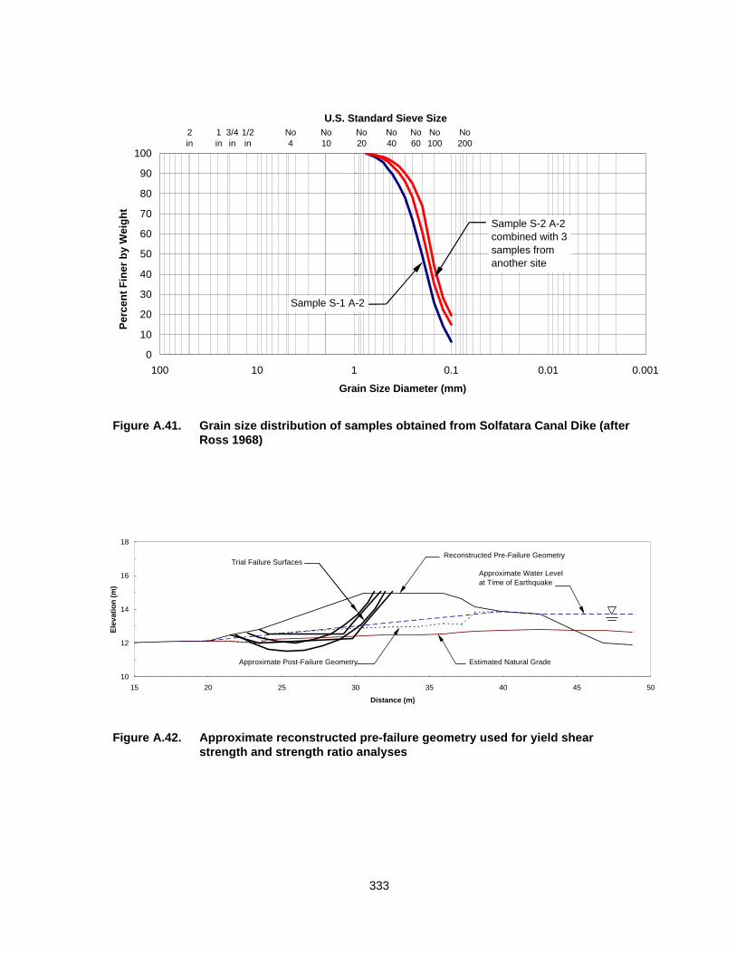
333

Figure A.41. Grain size distribution of samples obtained from Solfatara Canal Dike (afterRoss 1968)

Figure A.42. Approximate reconstructed pre-failure geometry used for yield shearstrength and strength ratio analyses


0

10

20

30

40

50

60

70

80

90

100

0.0010.010.1110100


Perc

ent F

iner

by

Wei

ght

2in

1in

3/4in

1/2in

No4

No20

No40

No60

No100

No200

No10

Sample S-1 A-2

Sample S-2 A-2combined with 3samples fromanother site

10

12

14

16

18

15 20 25 30 35 40 45 50

Distance (m)

Elev

atio

n (m

)

Reconstructed Pre-Failure Geometry

Estimated Natural GradeApproximate Post-Failure Geometry

Approximate Water Levelat Time of Earthquake


334

with emax and emin of 0.92 and 0.52, respectively. The saturated unit weight of the sand was

assumed to be 19.6 kN/m3.

Boring S-2 was conducted through a bench in the northern levee, near the canal

water level. Approximately 1 m of organic soil was encountered below the ground surface.

Below the organic-rich soil, a fine sand with silty lenses was encountered. Ross (1968)

considered this to be the natural soil based on the geology of deposition from Volcano Lake.

Because of the very loose to loose condition of the sand and because the sand was located

below the watertable, piston samples of the sand could not be retrieved. However, auger

samples were used to estimate the grain size distribution of the natural sand, which also is

presented in Figure A.41. The natural sand has an approximate D50 of 0.17 mm and fines

content of 6 to 8%. Probing from the bottom of the boring indicated the presence of loose

sands to a depth of approximately 2.3 m.


No penetration tests were conducted in the sand fill either before or after the flow

failure. Therefore, “representative” values of both SPT and CPT penetration resistance must

be estimated from relative density-effective overburden relations. Using the approximate

weighted average pre-failure vertical effective stress of 29.9 kPa (see below) and Dr ~ 30%,

the “representative” (N1)60 was estimated as 4 using the Holtz and Gibbs (1979) and Seed

and Tokimatsu (1987) relations and the “representative” qc1 was estimated as 2.5 MPa using

the Robertson and Campanella (1983) and Jamiolkowski et al. (1985) relations. Seed (1987)

and Seed and Harder (1990) estimated the (N1)60 values as 5 and 4, respectively.

335



The mechanism that likely triggered flow failure of the northern dike of Solfatara

Canal is the seismically-induced liquefaction of the sand fill below the phreatic surface and

natural sand deposit underlying the levee. As discussed in Chapter 4, the shear strength

and strength ratio mobilized at the instant of failure in cases of liquefaction flow failure

triggered by seismic loading do not necessarily represent the yield shear strength and yield

strength ratio, respectively. Therefore, values of shear strength and strength ratio likely do

not represent the yield shear strength and yield strength ratio.



friction angle of 30° was assigned to the embankment material above the phreatic surface.

No inertia forces were considered in the embankment, as a result of the softening/isolation

effect of liquefaction along the base of the levee. To account for the very small drainage

path at the toe of the dike, the toe segment of each failure surface was considered to be

drained and was assigned a drained friction angle of 30°.


shear strength in the zone of liquefaction for stability) for the northern dike of Solfatara

Canal is shown in Figure A.42. Other failure surfaces that were considered also are shown

in Figure A.42. The values of mobilized shear strength in the zone of liquefaction ranged

from 3.9 to 6.75 kPa depending on the assumptions regarding toe drainage and the location

of the failure surface. The best estimate of mobilized shear strength in the zone of

liquefaction was obtained from the critical failure surface as 6.0 kPa. This value is very close

336

to the pre-failure driving stress of 6.2 kPa along the base of the dike determined by Seed

(1987).












possible range of 0.172 to 0.25 determined using other failure surfaces and the potential for

drainage at the toe of the slope. The weighted average pre-failure vertical effective stress

was determined as 26.5 kPa using Eq. (4.3).



As indicated in Figure A.40, the post-failure geometry is not known with any

certainty. Therefore, a rigorous slope stability analysis is not possible for this case history. In

order to conduct a simplified back-analysis, an area balance of the difference between the

pre-failure geometry and post-failure geometry was made. The area balance suggests that

337

the thickness of the failed material was on the order of 1.8 m over the length of the runout.

The slope of the failed mass was assumed to be the same as the mass of the natural grade,

determined as 3 to 4°. Using these assumptions, the liquefied shear strength was

determined using Eq. (5.5) as 2.4 kPa, identical to that determined by Seed and Harder

(1990). The range of liquefied shear strength suggested by Seed and Harder (1990) was

adopted, giving upper and lower bound liquefied shear strength values of 3.6 and 1.2 kPa,

respectively.


Again, the cross-section of the post-failure geometry is not known with any certainty,

therefore, the liquefied strength ratio was estimated by dividing the liquefied shear strength

by the weighted average pre-failure vertical effective stress. The weighted average of

vertical effective stress was estimated as 29.9 kPa from Figure A.40. Dividing the liquefied

shear strength of 2.4 kPa by the weighted average vertical effective stress, the liquefied

strength ratio is 0.080, with a range from 0.040 to 0.12 (based on the range of liquefied

shear strength).




the non-liquefied soils; (3) location of the initial surface of sliding; and (4) the location of the

phreatic surface within the dike. Liquefaction was assumed to occur in all the soil below the

phreatic surface, on the basis of the strength of seismic shaking and the very loose to loose

condition of the dike and foundation soils. Therefore, this appears to be a minor source of

uncertainty. The shear strength of the dike soil above the phreatic surface was taken as a

338

typical value of friction angle for loose soils. However, the drainage conditions of the dike

and foundation soils below the phreatic surface are not known with certainty. Therefore,

analyses were conducted assuming both full drainage (using a drained friction angle of 30°)

and no drainage (using a single value of mobilized shear strength or strength ratio) in the

toe segment. It is most likely that some drainage did occur during the earthquake, therefore,

the best estimate of mobilized shear strength and strength ratio at the initiation of failure was

taken as the average of the results of analyses considering both drainage conditions. No

eyewitness accounts are available for the failure, therefore, the initial failure surface can not

be accurately ascertained. Thus, a slope stability searches were conducted to determine

both the mobilized shear strength and strength ratio at the triggering of liquefaction. The

position of the phreatic surface was estimated from the 1967 water levels measured in the

canal and in a drainage ditch to the north of the northern dike, as shown in Figure A.40.


strength and strength ratio: (1) the post-failure geometry; and (2) the potential for porewater

or void redistribution occurring during flow. Clearly, the largest uncertainty regarding this

failure is the fact that cross-sections of the post-failure geometry are not available.

Therefore, the liquefied shear strength was estimated from a simple analysis using rough

estimates of the slope angle of the surface and thickness of the failed mass. In addition,

because cross-sections of the post-failure geometry are not available, a rigorous stability

analysis of the post-failure geometry could not be conducted to determine the liquefied

strength ratio. However, as it is likely that the entire base of the dike was involved in the

resulting flow failure, the weighted average pre-failure vertical effective stress determined

from Figure A.40 probably is appropriate.

339


Therefore, the fact that the “representative” values of penetration resistance had to be


This source of uncertainty was unavoidable. Another source of uncertainty was the fact that

the dikes were reconstructed following the 1940 earthquake, and the borings were made

through the rebuilt dikes. Therefore, some reconsolidation and aging probably occurred

under the weight of the rebuilt dikes. Both this factor and the potential for density increase

during piston sampling suggest that the “representative” values of penetration resistance

may be lower than those used herein, but are not likely to be larger.

A.8 LAKE MERCED BANK, CALIFORNIA, USA


During the March 22, 1957 San Francisco earthquake (ML = 5.3, Tocher 1958),

numerous small sloughs and runs occurred in fill slopes along slopes near the ocean and

along the shoreline of Lake Merced (Ross 1968). Ross (1968) investigated two slides along

the bank of Lake Merced that were considerably larger. The two larger slides involved

approximately 244 m of shoreline. These failures occurred at a distance of 4 to 6.4 km from

the center of the rupture zone, as shown in Figure A.43 (Ross 1968).

The locations of these two failures are presented in Figure A.44. The cross-section

for Slide 1 is shown in Figure A.45. Unfortunately, the final location of the failed mass is not

available for Slide 2. As shown in Figure A.44 and A.45, the majority of the failure occurred

in fill soil and the slide mass moved approximately 18 m into the lake, on the basis of the

final position of several slabs of intact pavement. The fill soil was placed by end-dumping

into the lake and therefore it seems unlikely that the fill received any compaction. The slope

340

Figure A.43. Location map showing region affected by 1957 San Francisco earthquake (fromRoss 1968)

341

Figure A.44. Plan view of Lake Merced showing locations of slides and areas of cut material(marked C) (from Ross 1968)

342

Figure A.45. Cross-section through slide 1 at Lake Merced (from Ross 1968)

Figure A.46. Surficial geology of Lake Merced bank determined by nearby borings (from Ross 1968)

343

of the embankment fill was on the order of 1.5H:1V, while the slope of the natural grade was

on the order of 3H:1V to 4H:1V. As Ross (1968) indicated, the failure does not appear to be

a rotational failure. The post-failure geometry is indicative of a liquefaction flow failure of the

sandy fill soil, and possibly the upper portion of the natural sandy foundation soil.

The level of shaking experienced at the site is not known with certainty, as no

instrumentation was located near the site. However, instrumentation situated on a bedrock

outcrop in Golden Gate Park in San Francisco (approximately 11.2 km from the earthquake

epicenter) measured a peak ground surface acceleration of 0.12g, with only 2 to 3 cycles

with accelerations larger than 0.1g and accelerations greater than 0.05g lasting for only 5

seconds. As aforementioned, the failures along the bank of Lake Merced are located closer

to the epicenter than Golden Gate Park, therefore, the level of shaking most likely was

larger than 0.12g.


The surficial geology of the region around Lake Merced was shown in Figure A.43.

Lake Merced is located in the Merced valley, a deformed remnant of a structural trough that

parallels the San Andreas fault (Ross 1968). Ross (1968) estimated the depth to bedrock

directly below the lake to be at least 460 m. The trough is filled primarily with marine

sediments during the upper Pliocene and early Pleistocene. In the mid-Pleistocene, the

trough was folded again and elevated to its current position. The near surface sediments are

primarily fluvial and eolian sands, with some fluvial and lacustrine silts, clays, and gravels. A

geologic cross-section of the near surface soils located north of the failures is presented in

Figure A.46.

Ross (1968) conducted two borings with SPT measurements at Lake Merced to

determine local soil conditions near each of the two major slides. The log for Boring 1 is

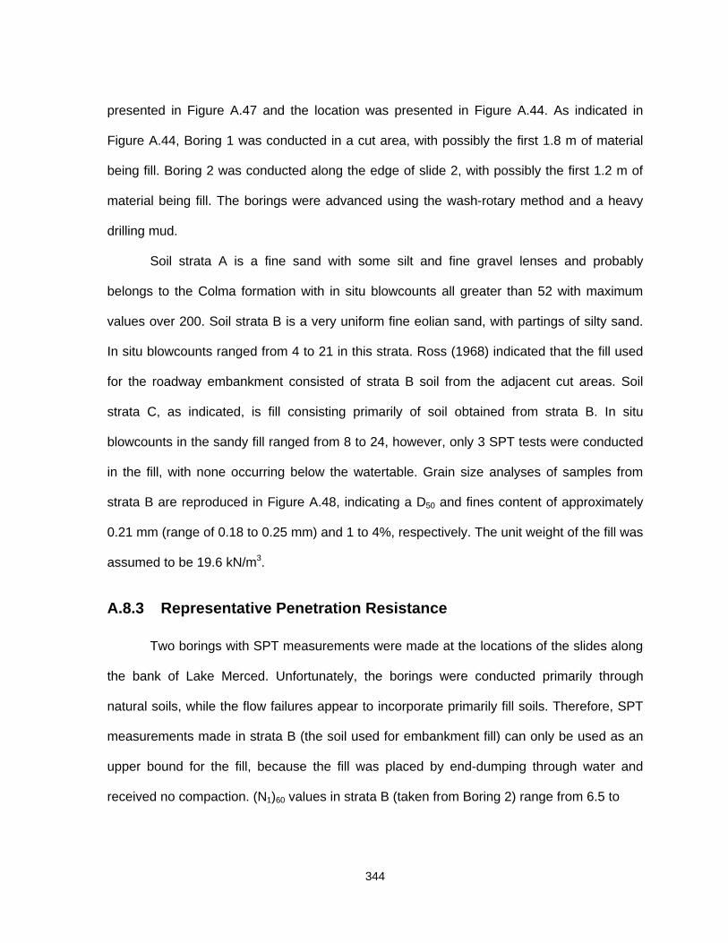
344

presented in Figure A.47 and the location was presented in Figure A.44. As indicated in

Figure A.44, Boring 1 was conducted in a cut area, with possibly the first 1.8 m of material

being fill. Boring 2 was conducted along the edge of slide 2, with possibly the first 1.2 m of

material being fill. The borings were advanced using the wash-rotary method and a heavy

drilling mud.

Soil strata A is a fine sand with some silt and fine gravel lenses and probably

belongs to the Colma formation with in situ blowcounts all greater than 52 with maximum

values over 200. Soil strata B is a very uniform fine eolian sand, with partings of silty sand.

In situ blowcounts ranged from 4 to 21 in this strata. Ross (1968) indicated that the fill used

for the roadway embankment consisted of strata B soil from the adjacent cut areas. Soil

strata C, as indicated, is fill consisting primarily of soil obtained from strata B. In situ

blowcounts in the sandy fill ranged from 8 to 24, however, only 3 SPT tests were conducted

in the fill, with none occurring below the watertable. Grain size analyses of samples from

strata B are reproduced in Figure A.48, indicating a D50 and fines content of approximately

0.21 mm (range of 0.18 to 0.25 mm) and 1 to 4%, respectively. The unit weight of the fill was



Two borings with SPT measurements were made at the locations of the slides along

the bank of Lake Merced. Unfortunately, the borings were conducted primarily through

natural soils, while the flow failures appear to incorporate primarily fill soils. Therefore, SPT

measurements made in strata B (the soil used for embankment fill) can only be used as an

upper bound for the fill, because the fill was placed by end-dumping through water and

received no compaction. (N1)60 values in strata B (taken from Boring 2) range from 6.5 to

345

Figure A.47. Boring logs and SPT blowcounts (field values) from Lake Merced bank (fromRoss 1968)

Figure A.48. Grain size distribution of soil type B from Lake Merced bank (after Ross1968)


0

10

20

30

40

50

60

70

80

90

100

0.0010.010.1110100


Perc

ent F

iner

by

Wei

ght

2in

1in

3/4in

1/2in

No4

No10

No20

No40

No60

No100

No200

Range of grain sizes from 6samples, representative of 95%of the material sampled fromSoil B

346

12.3, with an average of 9. Using the D50 value of 0.21 mm to obtain qc1/(N1)60= 0.5,

approximate qc1 values in strata B range from 3.3 to 6.2 MPa, with an average of 4.5 MPa.

No reliable measurements of penetration resistance were made in the fill material.

Therefore, “representative” SPT and CPT penetration resistances were estimated from an

appraisal of relative density and vertical effective stress using correlations developed by

Holtz and Gibbs (1979) and Kulhawy and Mayne (1990) for the SPT and Robertson and

Campanella (1983) and Jamiolkowski et al. (1985) for the CPT.

Using a relative density of 40% typical of sand fill deposited through water and an

average pre-failure vertical effective stress of 58.7 kPa (0.61 tsf) yielded “representative”

values of (N1)60 and qc1 of approximately 7 to 8 and 3.0 to 3.4 MPa, respectively. The

“representative” (N1)60 value of 7 to 8 is slightly larger than the value of 5 suggested by Seed

(1987) and 6 suggested by Seed and Harder (1987), but is in agreement with the value of 7

suggested by Wride et al. (1999).



The mechanism that likely triggered flow failure was seismically-induced liquefaction

in the submerged portion of the sand fill and possibly the upper strata of the natural sandy

soil. As discussed in Chapter 4, the shear strength and strength ratio mobilized at the instant

of failure in cases of liquefaction flow failure triggered by seismic loading do not necessarily

represent the yield shear strength and yield strength ratio, respectively. Therefore, values of

shear strength and strength ratio likely do not represent the yield shear strength and yield

strength ratio.

347



friction angle of 35° was assigned to the embankment material above the phreatic surface.

No inertia forces were considered in the embankment, as a result of the softening/isolation

effect of liquefaction along the base of the embankment. To account for the very small

drainage path at the toe of the embankment, the toe segment of each failure surface was

considered to be drained and was assigned φ’ of 35°. A drained friction angle for both the

embankment material above the phreatic surface and at the toe of the embankment was

used because of the relatively large SPT blowcounts measured in the fill material.

Blowcounts measured in the fill material ranged from 8 to 24, with an average of 16. This

average blowcount corresponds to an (N1)60 value of approximately 25. Using the empirical

relationship between (N1)60 and for fine-grained sands suggested by Terzaghi et al. (1996),

φ’ is approximately 35° for this material.


shear strength in the zone of liquefaction for stability) is shown in Figure A.49. Other failure

surfaces that were considered also are shown in Figure A.49. The values of mobilized shear

strength in the zone of liquefaction ranged from 15.7 to 18.1 kPa depending on the

assumptions regarding toe drainage and the location of the failure surface. The best

estimate of mobilized shear strength in the zone of liquefaction was obtained from the

critical failure surface as 17.7 kPa.





348

Figure A.49. Pre-failure geometry of Lake Merced bank used for yield shear strength and strength ratio analyses

-10

-5

0

5

10

15

0 10 20 30 40 50 60 70 80

Distance (m)

Elev

atio

n (m

)

Geometry Unknownfrom this Location


Natural Grade prior to Road Construction Lake Level



Figure A.50. Post-failure geometry of Lake Merced bank used for liquefied shear strength and ratio analyses

-10

-5

0

5

10

15

0 10 20 30 40 50 60 70 80

Distance (m)

Elev

atio

n (m

)

Geometry Unknownfrom this Location


Natural Grade prior to Road Construction Lake Level


Final Failure Surface

349








possible range of 0.30 to 0.34 determined using other failure surfaces and the potential for

drainage at the toe of the slope. The weighted average pre-failure vertical effective stress




The post-failure geometry is reproduced in Figure A.50. Trial failure surfaces shown

in Figure A.50 were ascertained from examination of the post-failure geometry and the

known interface between natural ground and embankment fill determined by Ross (1968).

Assigning φ' = 35° to the length of the final failure surface that corresponds to the length of

material in the pre-failure geometry that did not liquefy (i.e., above the phreatic surface and

at the toe), a likely range of liquefied shear strengths were obtained. The back-calculated

shear strength was approximately 6.9 kPa, with a possible range from 4.8 (from Seed 1987)

to 7.4 kPa.

350


Using the same post-failure sliding surfaces shown in Figure A.50, a rigorous back-

analysis of the liquefied strength ratio (as described in Chapter 5) was conducted. Using the

same assumptions for the shear strength of originally non-liquefied materials above the

phreatic surface and at the toe, the liquefied strength ratio was estimated as 0.108, with a

possible range from 0.073 to 0.12.



strength and strength ratio: (1) the limits of the zone of liquefaction; (2) shear strength of the

non-liquefied soils; (3) location of the initial sliding surface; and (4) the potential for void or

porewater pressure redistribution during failure. As the true limits of liquefaction are not

known, it was assumed that all the fill below the phreatic surface was in a state loose

enough to liquefy, with the exception of the material near the toe of the embankment where

the very short drainage path would preclude porewater pressure increase. The shear

strength of the non-liquefied soils also was not known, therefore, SPT blowcounts measured

in the fill material above the lake level were used to estimate the approximate drained

friction angle of the non-liquefied soils (primarily the soils above the lake level, but also

those at the toe). The initial sliding surface was not known as there were no eyewitnesses of

the failure. Therefore, numerous trial failure surfaces were studied to determine the best

estimates of yield shear strength and strength ratio.


strength and strength ratio: (1) the shear strength of the non-liquefied soils; (2) location of

the final surface of sliding; (3) location of the post-failure toe; and (4) the potential for void or

351

porewater pressure redistribution during flow. The shear strength of the non-liquefied soils

was taken as 35°, as explained above. The location of the final surface of sliding was

ascertained based on visual examination of the pre- and post-failure geometries. Several

trial failure surfaces that incorporated the entire slide mass were studied. Ross (1968) did

not determine the location of the post-failure toe of the sliding mass. The location of the toe

was determined by extending the pre-earthquake natural and lake bed grades and using an

area balance between the pre- and post-failure geometries. A horizontal lake bed must be

assumed to provide a value of liquefied shear strength even reasonably close to that

determined by Seed (1987) and Seed and Harder (1990). If a horizontal lake bed is

assumed, the liquefied shear strength decreases by approximately 15% from the best

estimate reported above.

No penetration tests were conducted either before or after the failure within the fill

that probably liquefied. Therefore, “representative” values of penetration resistance had to

be estimated from published correlations and this constitutes (by far) the greatest source of

uncertainty. This source of uncertainty was unavoidable. However, the value of

“representative” SPT blowcount determined using the relative density correlation was

reasonably close to the value measured in soil strata B in Boring 2. This agreement provides

some credibility to the estimate.

A.9 KAWAGISHI-CHO APARTMENTS, NIIGATA, JAPAN


During the 1964 Niigata, Japan earthquake (MW = 7.5), severe liquefaction occurred

throughout the city of Niigata and the surrounding region (Yamada 1966; Ishihara et al.

1978; Ishihara and Koga 1981). Particularly hard-hit was the reclaimed land along the

Shinano River in Niigata. Numerous occurrences of sand blows, surface cracking, lateral

352

spreads, and building damage due to settlement and tilting developed during and following

the earthquake, as illustrated in Figures A.51 and A.52. A peak surface acceleration of

0.16g was measured near the site (Ishihara and Koga 1981).

The most dramatic case of liquefaction-induced damage occurred at an apartment

complex in Kawagishi-cho. The location of the apartment complex was shown in Figure

A.51. The apartment complex consisted of 8 four-story buildings with approximate

dimensions of 30 m by 8 m, constructed on reclaimed land. All of the buildings experienced

severe settlement and various degrees of tilting, as shown in Figure A.53. Ishihara and

Koga (1981) reported that Building No. 4 had the “poorest foundation work” among the eight

apartment structures and experienced tilting of approximately 80° from vertical. Ishihara and

Koga noted that all the buildings tilted toward the side of the building where water tanks

were placed on the roofs. Therefore, the tilting occurred toward the building center of

gravity, as expected.


As aforementioned, the apartment buildings were constructed on land reclaimed

from the Shinano River. Ishihara and Koga (1981) indicated that from approximately 1945 to

1955, the Kawagishi-cho area (an inlet of the Shinano River) was gradually reclaimed using

sand fill. The method of filling is not precisely known, but it is likely that the fill was “carried to

waterfronts by means of hand-pushing carts, railway cars or trucks and then dumped into

the river without employing any artificial compaction technique (Ishihara and Koga 1981).”

Sampling and in situ penetration testing was conducted at a location approximately

20 m from the apartment complex. Nine large diameter and seven Osterburg samples were

obtained from the test site near the apartment complex. One boring with SPT tests and one

Dutch CPT test also were conducted at the test site. Figure A.54 presents the results of the

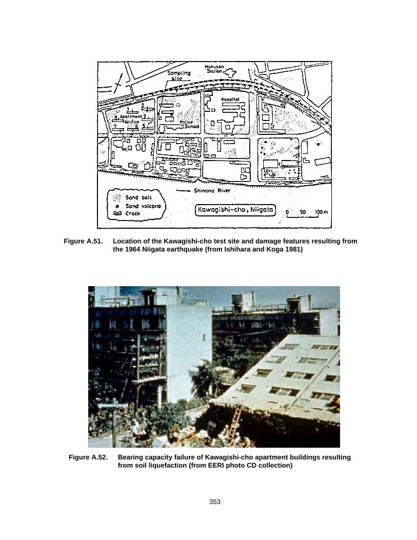
353

Figure A.51. Location of the Kawagishi-cho test site and damage features resulting fromthe 1964 Niigata earthquake (from Ishihara and Koga 1981)

Figure A.52. Bearing capacity failure of Kawagishi-cho apartment buildings resultingfrom soil liquefaction (from EERI photo CD collection)

354

Figure A.53. Aerial view of damage to Kawagishi-cho apartment buildings (from EERIphoto CD collection)

Figure A.54. Stratigraphy, SPT results, location of sampling, and Dutch cone sounding atKawagishi-cho (from Ishihara and Koga 1981)

355

penetration tests. The depth to the watertable was 2.0 m. The fill soil is a medium-grained

clean sand with D50 between 0.24 to 0.52 mm, with an average and standard deviation of

0.35 mm and ±0.08 mm. The fines content of the Niigata sand is less then 5%. The unit

weight of the sand is approximately 18.9 kN/m3.

Ishihara and Koga (1981) determined maximum and minimum void ratios for each

sample in order to evaluate in situ relative density. The relative density of the sand at

Kawagishi-cho ranged from 40 to 50%, with outside ranges of approximately 20 to 80%. It

should be noted that the process of sampling and subsequent handling and preparation

likely densified the soil to some extent, therefore, the soil may have been looser in situ, but

is unlikely to have been denser.


Standard penetration test results from the test site were presented in Figure A.54. As

discussed subsequently, the approximate depth of the failure was 2 to 4 m. No details of the

SPT hammer and system configuration are available, therefore it is assumed that a

Japanese rope and pulley system was used (rather than a Japanese mechanical trip

hammer). Seed et al. (1985) suggested that the energy ratio of typical Japanese rope and

pulley systems is on the order of 67%. This provides a smaller energy ratio, and thus a

smaller correction to the measured SPT values, than if a trip hammer was assumed (with an

energy ratio of 78%). Using total and saturated unit weights of 18.9 kN/m3, the values of

(N1)60 average 4.4 (with a range of 3.7 to 5.6) from depths of 2 to 4 m.

Dutch cone penetration test results also were presented in Figure A.54. Using the

same total and saturated unit weights, the values of qc1 average 3.1 MPa (with a range of

1.7 to 3.8 MPa) from depths of 2 to 4 m.

356



The mechanism leading to the failure of the Kawagishi-cho apartment buildings is

likely seismic liquefaction of the fill soils comprising the building foundation. Ishihara and

Koga (1981) showed that liquefaction was likely triggered from depths of approximately 2 to

13 m. However, no yield shear strength analysis was conducted for this case history

because the mechanism of failure (i.e., bearing capacity failure) is difficult to back-analyze

using conventional analysis procedures.


Similarly, no yield strength ratio analysis was conducted for this case history.



As aforementioned, it appears likely that this liquefaction failure occurred as a result

of seismic liquefaction occurring in the foundation sands resulting in strength loss in the

sand and subsequent bearing capacity failure of the apartment building. Therefore, Seed

(1987) suggested that a bearing capacity analysis could be used to evaluate the liquefied

shear strength available during failure. the bearing capacity equation is as follows

(Skempton 1951):

+

+=

B

D

LB

sq funetd LIQ 2.012.01)(5)(

357

Assuming a net applied base pressure [qd(net)] of the building of 28.7 kPa, a depth of

foundation (Df) of 1 m, and building width (B) and length (L) of 3 and 3 m, respectively, for

an individual footing to 8 and 30 m, respectively, for the entire building, and solving for

su(LIQ), we obtain su(LIQ) = 4.5 to 5.3 kPa. This value agrees with the value of 5.7 kPa

obtained by Seed (1987). Therefore, the best estimate of liquefied shear strength is taken as

5.3 kPa.


Analysis of the liquefied strength ratio was done indirectly by determining the

representative depth of the bearing capacity failure. Using the Prandtl (1921) solution for

bearing capacity, and assuming φ = 0 conditions apply during liquefaction, the depth of

influence of the footing is from Df to (Df + 0.7B). Assuming that the width of an individual

footing is on the order of 2 to 4 m, the depth of influence is on the order of 1 m to 4 m.

Assuming liquefaction was triggered below 2 m, the depth of influence in the liquefied

material is from approximately 1.5 m to 4 m.

Using this depth of influence, the pre-failure vertical effective stress (including the

average base pressure of the building of 28.7 kPa) ranged from 61.5 to 79.5 kPa. Therefore,

the best estimate of liquefied strength ratio is approximately 0.075, with a range from 0.057

to 0.093.



strength and strength ratio: (1) the method of back-calculation; and (2) the parameters used

in back-calculation. As this is the only liquefaction case history not involving the failure of a

slope or embankment, the method of back-analysis differed from the methods used for the

358

other cases. The method of analysis is based on the limit equilibrium bearing capacity

equation as modified by Skempton (1951) to account for the shape and depth of the

foundation. Back-analysis using this equation is assumed to provide an estimate of the

liquefied shear strength. In addition, because the weight of the building, as well as the type,

size, and depth of the foundation are not known with certainty, these values had to be

estimated, adding a degree of uncertainty to the analysis.


penetration resistance: (1) the penetration tests were conducted approximately 20 m from

the apartment complex; (2) the use of Japanese SPT equipment; and (3) the use of Dutch

cone penetration equipment. Penetration testing and sampling occurred at a small distance

from the actual failures, however, because the material did not likely vary considerably

throughout the reclaimed area, this source of uncertainty was considered minor. The use of

Japanese SPT equipment results in a different energy ratio than American equipment. Two

standard types of SPT equipment were available in Japan at the time of testing, and the

energy ratio was chosen as the smaller of the values for the two equipment types, resulting

in a smaller correction to field SPT blowcounts. No correction from the Dutch mechanical

CPT tip resistance readings to electronic CPT tip resistance was made, as details of the

equipment used at the site were unavailable, and a correction of this nature is relatively

minor (Kulhawy and Mayne 1991).

A.10 UETSU-LINE RAILWAY EMBANKMENT, JAPAN


As mentioned in section A.9, severe liquefaction-induced damage occurred

throughout the Niigata area during the 1964 earthquake. Yamada (1966) described a

359

number of embankment failures during the earthquake, indicating that large sections of

sandy fill embankments that were larger than 5 to 6 m suffered severe damage, including

flow failure, slumping, settlement, and lateral spreading. In particular, the Uetsu-Line railway

embankment suffered considerable damage in the epicentral region.

The pre- and post-failure cross-sections of the Uetsu-Line railway embankment

between Dedo St. and Nishime St. in the city of Niigata are presented in Figure A.55. The 8

m high embankment had settled into the underlying peat nearly 1.5 m prior to the

earthquake, allowing the lower portion of the embankment to become saturated. During the

earthquake, it appears that the saturated portion of the fill (and likely the zone of fill that was

saturated by capillarity) liquefied and flowed into the surrounding rice field for a distance of

over 110 m. The section of embankment that failed was on the order of 150 m in length

(Yamada 1966). The slope of the surrounding ground is between 1 and 2° and the average

slope of the failed material is approximately 4°.

The following description of the failure is provided in Yamada (1966):

“A farmer who worked near the fill at [the] time of the earthquake recognized that the

middle part of [the] slope broke out initially and flow over the ground surface at relatively

high speed. The upper part of the roadbed with ballast fell down vertically and [the

railroad] track became like a ladder.”

Yamada (1966) also indicated that the flow slide occurred entirely within the sand fill, as the

ground surface along both the sides of the failure and below the embankment and sliding

mass showed no signs of disturbance.

360

Figure A.55. Cross-section of failed Uetsu-Line railway embankment showing naturalstratigraphy (from Yamada 1966)

Figure A.56. Pre-failure geometry of Uetsu-Line railway embankment used in yield shearstrength and strength ratio analyses

0

5

10

15

20

25

-20 -15 -10 -5 0 5 10 15 20 25 30

Distance (m)

Elev

atio

n (m

)



Approximate Piezometric Surface

Trial Yield Surfaces

361


Yamada (1966) indicated at this location the Uetsu-Line embankment was

constructed in a flat and shallow valley between sand hills. The stratigraphy underlying the

embankment is shown in Figure A.55. As seen in Figure A.55, the sand fill settled into the

underlying peat foundation up to 1.5 m, causing the lower portion of the embankment fill to

become saturated. The best estimate of the level of ground watertable level within the

embankment is shown in Figure A.56. The location of the watertable in the fill was estimated

based on review of several similar case histories documented by Kaneko et al. (1995) and

Sasaki et al. (1993;1994;1995). Outside of the embankment, the watertable is at the ground

surface.

The grain size distributions of the flowed sand, the embankment sand (remaining

after the failure), and the borrow source sand are shown in Figure A.57. From this figure it

appears that no segregation occurred during flow. Therefore, the values of D50 and fines

content are taken as 0.3 to 0.4 mm and 0 to 2%, respectively. The unit weight of the fill was



Unfortunately, no penetration tests were conducted at this site. It does not appear

that the sand received any compaction based on a description of construction techniques for

embankments and dikes available in Sasaki et al. (1994; 1995). However, numerous SPT

tests through sand fill dikes with similar grain size distributions and constructed by similar

techniques exhibit field blowcounts on the order of 2 to 5 (Sasaki et al. 1996). Further, Seed

(1987) suggested that the value of (N1)60 must be on the order of 3 based on the satisfactory

performance of the fill under train loading.

362

Figure A.57. Grain size distributions of soils involved in Uetsu-Line railway embankment failure (after Yamada 1966)

Figure A.58. Post-failure geometry of Uetsu-Line railway embankment used for liquefied shear strength and strengthratio analyses

0

5

10

15

20

25

-20 0 20 40 60 80 100 120

Distance (m)

Elev

atio

n (m

)





Approximate Final Sliding Surface


0

10

20

30

40

50

60

70

80

90

100

0.0010.010.1110100


Perc

ent F

iner

by

Wei

ght

2in

1in

3/4in

1/2in

No4

No10

No20

No40

No60

No100

No200

Material sampled from slide mass

Material from embankment fill

Material from borrow source

363

On this basis, a SPT (N1)60 value of 3 was selected as “representative” of the

uncompacted fill. Using the qc/N60 ratio of 0.6 corresponding to D50 ~ 0.35 mm (Stark and

Olson 1995), a “representative” qc1 value of 1.8 MPa was selected.



The mechanism that likely triggered flow failure at this site was seismically-induced

liquefaction of the saturated, uncompacted, sand fill within the lower portion of the

embankment. This includes both the sand fill below the ground watertable and the sand

saturated via capillarity as shown in Figure A.56. The 1964 Niigata earthquake (MW ~ 7.5)

was estimated to have produced a peak ground surface acceleration of 0.2g at this site. As

discussed in Chapter 4, the shear strength and strength ratio mobilized at the instant of

failure in cases of liquefaction flow failure triggered by seismic loading do not necessarily

represent the yield shear strength and yield strength ratio, respectively. Therefore, back-

calculated values of shear strength and strength ratio likely do not represent the yield shear

strength and yield strength ratio.

The pre-failure geometry is shown in Figure A.56. A slope stability search was

conducted to determine the critical initial failure surface. The search for the critical failure

surface was guided by the description provided by Yamada (1966). The description

indicated that the middle part of the slope broke out initially and flowed over the ground

surface. A single value of shear strength was assigned to the liquefied foundation soil, and a

drained friction angle of 30 to 35° was assigned to the embankment material above the

phreatic surface. No inertia forces were considered in the embankment, as a result of the

softening/isolation effect of liquefaction along the base of the embankment. Because the

364

flowed material became very thin prior to coming to rest (see Figure A.55), no drainage in

the toe of the embankment was considered in this analysis.


shear strength in the zone of liquefaction for stability) is shown in Figure A.56. Other failure

surfaces that were considered also are shown in Figure A.56. The values of mobilized shear

strength in the zone of liquefaction ranged from 10.0 to 11.9 kPa depending on the

assumptions regarding embankment strength and the location of the failure surface. The

best estimate of mobilized shear strength in the zone of liquefaction was obtained from the

critical failure surface as 10.9 kPa.


A second analysis was conducted to estimate the strength ratio mobilized at the







Using an iterative process, the value of mobilized strength ratio was varied (in turn, varying

the mobilized shear strength assigned to each pre-failure segment) until a factor of safety of

unity was achieved.

A best estimate of mobilized strength ratio at the triggering of liquefaction was

determined as 0.21, with a possible range of 0.19 to 0.24 determined using other failure

surfaces and differing values of embankment strength. The weighted average pre-failure

vertical effective stress was determined as 51.7 kPa using Eq. (4.3).

365



The post-failure geometry is reproduced in Figure A.58. The final failure surface

shown in Figure A.58 was ascertained from examination of the post-failure geometry and

the known interface between natural ground and embankment fill determined by Yamada

(1966). Assigning φ' = 30° to the length of the final failure surface that corresponds to the

length of material in the pre-failure geometry that did not liquefy (i.e., above the phreatic

surface), a likely range of liquefied shear strengths were obtained. The back-calculated

shear strength was approximately 0.6 kPa, with a possible range from 0.3 to 1.9 kPa. The

upper bound value of liquefied shear strength was determined using Eq. (5.5), a total unit

weight of 18.9 kN/m3, average failed material thickness of 2.0 m, and a slope angle of 3°

(the average of the ground surface and the failed material surface). The value of liquefied

shear strength from the simplified analysis agrees with the value determined by Seed

(1987).


Using the same post-failure sliding surface shown in Figure A.58, a rigorous back-

analysis of the liquefied strength ratio (as described in Chapter 5) was conducted. Using the

same assumptions for the shear strength of originally non-liquefied materials above the

phreatic surface, the liquefied strength ratio was estimated as 0.009, with a possible range

from 0.05 to 0.031. The weighted average of vertical effective stress was estimated using

Eq. (5.6) as 61.3.

366



shows the pre- and post-failure centers of gravity, the final sliding surface, and the probable



strength.

The kinetics analysis in Figure A.60 yielded the following results:

• Liquefied shear strength ≅ 1.7 kPa

• Liquefied shear strength ratio ≅ 0.027


the failure mass of approximately 3.6 m vertically and 59.5 m horizontally. This is in

agreement with the observed/measured displacement of the center of gravity of

approximately 3.5 m vertically and 60.0 m horizontally.




from the post-failure geometry analysis. The liquefied shear strength and strength ratio

back-calculated with appropriate consideration of the kinetics of failure are considered best

estimates.



strength and strength ratio: (1) the limits of the initial zone of liquefaction; (2) the location of

367

Figure A.59. Movement of center of gravity during flow failure of Uetsu-Line railwayembankment

Figure A.60. Kinetics analysis of Uetsu-Line railway embankment

0

5

10

15

20

25

-20 0 20 40 60 80 100 120

Distance (m)

Elev

atio

n (m

)





Center of Gravity Movement

368

the phreatic surface within the embankment; (3) the position of the initial failure surface; (4)

the shear strength of the non-liquefied soil; and (5) the potential for void or porewater

pressure redistribution during failure. The first two sources of uncertainty correspond to the

same issue. It was assumed that all the fill below the phreatic surface liquefied during the

earthquake, but the location of the phreatic surface is not known. Therefore, the position of

the phreatic surface was estimated based on review of several similar case histories

documented by Kaneko et al. (1995) and Sasaki et al. (1993;1994;1995). Outside of the

embankment, the watertable is at the ground surface. The position of the initial failure

surface was guided by eyewitness description, but the actual position was not known.

Therefore, numerous trial failure surfaces were studied to determine the critical surface. The

shear strength of the material above the phreatic surface was taken 30°–a typical value for

loose sands.


strength and strength ratio including the kinetics analysis: (1) the limits of the zone of

liquefaction; (2) the location of the initial and final surfaces of sliding; (3) the potential for

void and porewater pressure redistribution. Again, the limits of the zone of liquefaction are

not known with certainty. The exact locations of the initial and final surfaces of sliding are

required for the kinetics analysis, and were determined by stability analysis search.


Therefore, “representative” values of penetration resistance were estimated from other sites

constructed using similar methods and fill soils. These “representative” values of penetration

resistance were confirmed using published correlations provides (by far) the greatest source

of uncertainty. The “representative” penetration resistances also were confirmed based on

performance of the embankment fill (e.g., Seed 1987). Because penetration resistance was

369

estimated, this represented the largest source of uncertainty. The other sources of

uncertainty include the location of the phreatic surface and the unit weight of the fill soil,

however, these sources of uncertainty are minor with respect to estimating the penetration

resistance.

A.11 EL COBRE TAILINGS DAM, CHILE


During the March 28, 1965 Chile earthquake (ML = 7.0 – 7.25), catastrophic failures

occurred at numerous tailings dams throughout central Chile (Dobry and Alvarez 1967). In

particular, the failures of the El Cobre tailings dams released more than 2x106 tons of

tailings into the surrounding valley, destroying part of the town of El Cobre and killing more

than 200 people (Dobry and Alvarez 1967). The town of El Cobre suffered damage

corresponding to a Modified Mercalli Intensity of VIII to IX, probably corresponding to a peak

ground acceleration on the order of 0.8g (Kramer 1996). The nearest instrumentation was

located in Santiago, which recorded a peak ground acceleration of 0.18g.

The El Cobre tailings dam was started in the 1930, and consisted of three separate

dams, the Old Dam, the Small Dam, and the New Dam. At the time of the earthquake, the

Small Dam was out of service, the Old Dam served as an emergency dam only, and the

New Dam was active. (Filling of the New Dam started in 1963.) The earthquake caused

complete failure of the Old and New Dams, however, only the Old Dam has sufficient

information regarding cross-sections and material properties to conduct a reasonable

analysis.

370

Unfortunately, there were no eyewitnesses to the failure of the Old Dam due to the

dust thrown into the air from the desiccated crust during shaking. Dobry and Alvarez (1967)

provided the following description of the failure:

“The front slope of the southern corner of the Old Dam receded 65 m, making the

adjacent intermediate terrace disappear completely; the scarp produced was almost

vertical…All the fine and unconsolidated tailings flowed out, and from the upper part only

a horseshoe-shaped shell was left, which bound the back and sides of the large

depression left by the material which had flowed out. The bottom of this central

depression was formed by several almost horizontal terraces (2% slope toward the

valley)…several chunks of the upper dry crust were left on these terraces.”

The pre- and post-failure cross-sections of the Old Dam at El Cobre are shown in Figure

A.61.


The stratigraphy of the Small Dam is shown in Figure A.62. Dobry and Alvarez

(1967) indicate that this stratigraphy should be nearly identical to that at the Old Dam

because both were filled over the same period of time using the same techniques. A

relatively dry, upper crust had formed to a depth of approximately 4.6 m in the tailings. It is

assumed that this thickness is the same in the Old Dam. Below this was a 7 m thick layer of

underconsolidated tailings (as indicated by the water content being larger than the liquid

limit of the material). Dobry and Alvarez (1967) suggest that this thickness was probably

closer to 10 m in the Old Dam. Below the underconsolidated tailings, a 2.8 m thick layer of

normally (or nearly normally) consolidated tailings was found, with water contents slightly

below the liquid limit of the material. The normally consolidated tailings are underlain by the

371

Figure A.61. Pre- and post-failure geometry of the El Cobre Old Dam (after Dobry andAlvarez 1967)

Figure A.62. Stratigraphy, SPT results, fines content, water content and liquid limit ofmaterial in El Cobre Small Dam (from Dobry and Alvarez 1967)

Location used to determine pre-failure σσ’vo

Post-failurethickness~ 2 m

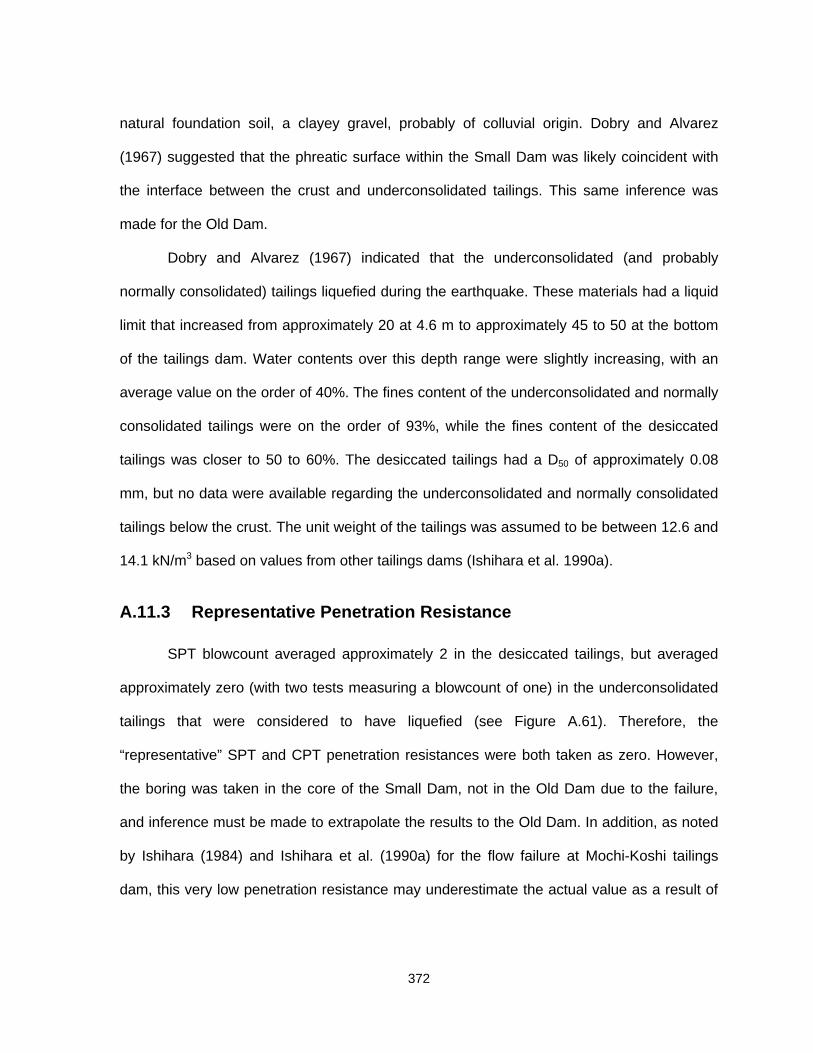
372

natural foundation soil, a clayey gravel, probably of colluvial origin. Dobry and Alvarez

(1967) suggested that the phreatic surface within the Small Dam was likely coincident with

the interface between the crust and underconsolidated tailings. This same inference was

made for the Old Dam.

Dobry and Alvarez (1967) indicated that the underconsolidated (and probably

normally consolidated) tailings liquefied during the earthquake. These materials had a liquid

limit that increased from approximately 20 at 4.6 m to approximately 45 to 50 at the bottom

of the tailings dam. Water contents over this depth range were slightly increasing, with an

average value on the order of 40%. The fines content of the underconsolidated and normally

consolidated tailings were on the order of 93%, while the fines content of the desiccated

tailings was closer to 50 to 60%. The desiccated tailings had a D50 of approximately 0.08

mm, but no data were available regarding the underconsolidated and normally consolidated

tailings below the crust. The unit weight of the tailings was assumed to be between 12.6 and

14.1 kN/m3 based on values from other tailings dams (Ishihara et al. 1990a).


SPT blowcount averaged approximately 2 in the desiccated tailings, but averaged

approximately zero (with two tests measuring a blowcount of one) in the underconsolidated

tailings that were considered to have liquefied (see Figure A.61). Therefore, the

“representative” SPT and CPT penetration resistances were both taken as zero. However,

the boring was taken in the core of the Small Dam, not in the Old Dam due to the failure,

and inference must be made to extrapolate the results to the Old Dam. In addition, as noted

by Ishihara (1984) and Ishihara et al. (1990a) for the flow failure at Mochi-Koshi tailings

dam, this very low penetration resistance may underestimate the actual value as a result of

373

disturbance during shaking and due to the large increase in excess porewater pressure

during penetration.



The mechanism that likely triggered flow failure was liquefaction of the

underconsolidated and normally consolidated tailings as a result of shaking. This increased

pressure and possible inertia forces on the tailings dam shell triggered an initial failure near

the corner of the dam (Dobry and Alvarez 1967). This allowed the release of the liquefied

tailings, in turn leading to severe erosion of the shell material and catastrophic failure of the

dam.

As previously mentioned, the failure of the tailings dam initiated in a corner,

indicating that three-dimensional effects may have played a role in the failure. Conventional

stability analyses can only represent two-dimensional conditions, and therefore can not

provide a reasonable back-analysis of conditions at the triggering of failure for this case.

Furthermore, the location of the transition or interface between the more sandy shell

material and the silty tailings material is not known. As a result of these two conditions, it

was decided not to conduct stability analyses of the pre-failure geometry.


As discussed in the previous section, no analyses of the pre-failure geometry were

conducted.

374



The pre- and post-failure geometries were shown in Figure A.61. As observed in the

figure, the complete post-failure geometry is not available for this case. However, if the

thickness of the tailings at the left end of Figure A.61 is taken as representative of the

thickness of the entire failure mass, a crude estimate of liquefied shear strength can be

obtained using the simplified analysis and Eq. (5.5).

The thickness of failed mass was taken as 2 m, the slope of the failed mass and the

underlying foundation was taken as 4°, and the total unit weight of the tailings was estimated

as 12.6 to 14.1 kN/m3. Entering these values into Eq. (5.5) results in a liquefied shear

strength of 1.8 to 2.0 kPa, with a best estimate of 1.9 kPa.


As a rigorous slope stability analysis was not possible for this case history, the

liquefied strength ratio was determined using a “single value” estimate of the pre-failure

vertical effective stress. The pre-failure vertical effective stress was determined at the point

labeled in Figure A.61. This point was selected as follows: (1) the maximum pre-failure

thickness of the tailings dam was approximately 33 m; (2) the shape of the stored tailings is

approximately triangular; (3) the representative thickness of the tailings was therefore

selected as approximately 67% of the maximum thickness; (4) as it is likely that only the

underconsolidated and normally consolidated tailings liquefied, the middle of this layer was

selected as the representative depth—13.6 m below the tailings surface.

375

Using a total unit weight ranging from 12.6 to 14.1 kN/m3 results in values of σ’vo of

82.6 to 103.9 kPa. Therefore, the possible range of liquefied strength ratio was determined

to be 0.017 to 0.024, with a “best estimate” value of 0.020.



strength and strength ratio: (1) the limits of the zone of liquefaction; (2) the shape of the

post-failure geometry; (3) the location of the phreatic surface within the slope; (4) estimation

of a “single value” of pre-failure vertical effective stress; and (5) the potential for void or

porewater pressure redistribution during flow. On the basis of blowcounts measured in the

tailings and the large accelerations probably experienced at the site, it is likely that all of the

tailings that were saturated liquefied during the earthquake. However, as noted in item (3)

above, the exact position of the phreatic surface was not known with certainty, thus the zone

of saturated tailings is not known with certainty. The position of the phreatic surface was

judged by Dobry and Alvarez (1967) based on changes in blowcount and comparison of

water content with liquid limit. The greatest source of uncertainty for this case is the shape

of the post-failure geometry. As only the geometry closest to the toe of the original dam is

available, the thickness of the failed material at this point was taken as representative.

However, using this thickness to estimate the liquefied shear strength may not be

representative of the actual liquefied shear strength mobilized during flow. The location of

the “single value” pre-failure vertical effective stress was determined as logically as possible,

however, as the actual zone of liquefaction is not known with certainty, this value also

involves considerable uncertainty. Further, the value of total and saturated unit weight of the

tailings was assumed, adding some uncertainty to the analysis of liquefied strength ratio.

376

Therefore a range of values (typical of tailings material) was used to estimate the pre-failure

vertical effective stress.


penetration resistance: (1) the boring was conducted in the core of the Small Dam, not the

Old Dam; (2) the effect of disturbance due to shaking; and (3) the effects of re-consolidation

and aging following shaking. As aforementioned, the boring was conducted in the Small

Dam, not the Old Dam. However, as both dams were filled over the same time using the

same material and methods, the differences between the Small Dam and the Old Dam

should be minimal. Therefore, this source of uncertainty was considered minor. Shaking

almost certainly triggered liquefaction throughout the saturated tailings as evidenced by

numerous sand and silt boils observed in the failed area of the dam. However, Dobry and

Alvarez (1967) do not discuss the extent of liquefaction in the Small Dam. Therefore, the

effects of disturbance due to shaking, re-consolidation following liquefaction, and aging from

the time of the earthquake until the time of the penetration tests cannot be determined

quantitatively.

A.12 KODA NUMA HIGHWAY EMBANKMENT, JAPAN


During the 1968 Tokachi-Oki Earthquake (ML = 7.9), numerous landslides occurred

in natural slopes and manmade embankments. The damage to highway and railway

embankments ranged from minor cracking and bulging to flow slides of the entire

embankment. As indicated by Mishima and Kimura (1970), the potential for landslides and

embankment failure was increased significantly by four days of heavy rainfall that preceded

the earthquake. Mishima and Kimura (1970) indicate that many of the embankments that

failed were saturated (at least near the base) as a result of the rainfall.

377

One of the failures described by Mishima and Kimura (1970) is the failure of a

highway embankment at Koda-Numa. The Koda-Numa embankment was 2.5 m high and

constructed of uniform, fine silty sand. The pre- and post-failure geometry and estimated

piezometric level in the embankment are presented in Figure A.63. The piezometric level

was estimated from similar case histories described by Kaneko et al. (1995) and Sasaki et

al. (1993;1994;1995). As indicated in Figure A.63, the embankment fill flowed nearly 20 m

from the original toe of the slope and dropped in height a maximum of 1.5 m. The slide mass

came to rest at a average angle of about 5°.

Unfortunately, the author was unable to assess the level of shaking associated with

this earthquake because Mishima and Kimura (1970) did not provide the precise location of

this failure.


The Koda-Numa site is underlain by a layer of surficial clay with a thickness of about

1 m, which in turn, is underlain by a deposit of medium dense to dense sand (as estimated

from Swedish cone penetration soundings). As a result of the heavy rainfall, the watertable

is assumed to be at the original ground surface, with a “mounding” of groundwater within the

embankment itself (see Figure A.63).

The Koda-Numa embankment consists of a uniform, fine silty sand. Mishima and

Kimura (1970) indicate that the sand had a water content of 16.4%, total unit weight of 16.0

kN/m3, a degree of saturation of 64.5%, and a void ratio of 0.70. However, they provide no

description of where the sample was obtained, how much time elapsed between the slide

and sampling, or the testing procedures. Therefore, these data cannot be considered

reliable. Mishima and Kimura (1970) also indicate that the sand fill contained approximately

7.5% silt and 5.5% clay, with a D60 of 0.20 mm and D10 of 0.024 mm. Thus, the author

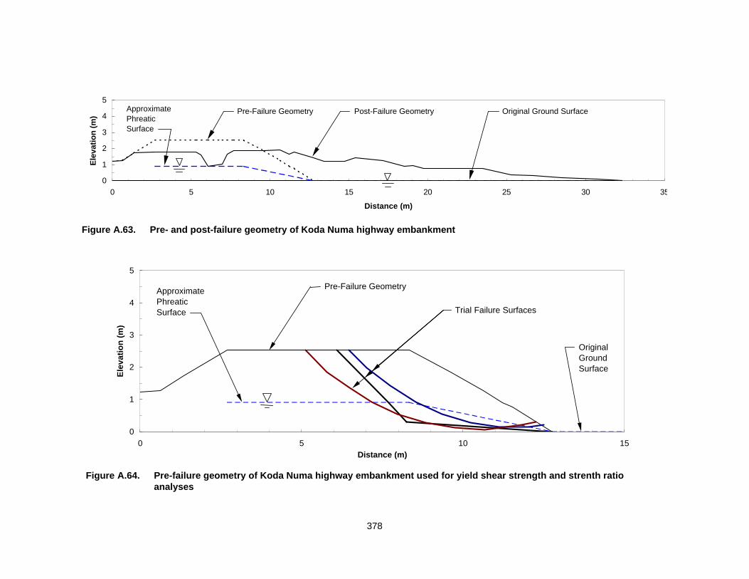
378

Figure A.63. Pre- and post-failure geometry of Koda Numa highway embankment

Figure A.64. Pre-failure geometry of Koda Numa highway embankment used for yield shear strength and strenth ratioanalyses

0

1

2

3

4

5

0 5 10 15 20 25 30 35

Distance (m)

Elev

atio

n (m

) Pre-Failure Geometry Post-Failure Geometry Original Ground SurfaceApproximatePhreaticSurface

0

1

2

3

4

5

0 5 10 15Distance (m)

Elev

atio

n (m

)

ApproximatePhreaticSurface

OriginalGroundSurface



379

assigned this case a D50 of between 0.15 and 0.20 mm, and a fines content of about 13%.

Mishima and Kimura did not indicate that this sample was obtained from Koda-Numa;

however, these values appear reasonable for the Koda-Numa fill based on the description

provided by Mishima and Kimura (1970).


No penetration tests other than Swedish cone soundings were conducted at the site.

However, only small portions of the soundings penetrated the failed material. In addition,

Mishima and Kimura (1970) did not determine relative density for the failed material. Seed

(1987) estimated that the (N1)60 value of the fill must have been 3 to 4 based on the

performance of fill under traffic loading. Seed and Harder (1990) adopted the (N1)60 of 3.

Assuming a value of DR of 20 to 40%, and using a ratio of (N1)60/DR2 of 40 (Kulhawy

and Mayne 1990; approximate D50 of 0.15 mm), a (N1)60 value of 2 to 6. A similar range is

obtained using the Holtz and Gibbs (1979) relation. Therefore, the value of 3 suggested by

Seed (1987) and Seed and Harder (1990) was considered “representative.” Using a value of

qc/N60 of 0.45 (Stark and Olson 1995; approximate D50 of 0.15 to 0.20 mm) results in a

“representative” qc1 value of 1.35 MPa. A similar value is obtained by averaging values from

the Robertson and Campanella (1983) and Jamiolkowski et al. (1985) relations.



The mechanism that likely triggered flow failure is seismic liquefaction of the

saturated, sandy fill within the lower portion of the embankment. Liquefaction of the fill

resulted in a flow failure of the embankment. Because liquefaction was triggered by seismic

380

loading, the shear strength and strength ratio back-calculated from the pre-failure geometry

may not represent the yield shear strength and strength ratio (see Chapter 4 for discussion).

The pre-failure geometry of the embankment is shown in Figure A.64. A slope

stability search was conducted to determine the critical initial failure surface. All fill below the

piezometric surface was assumed to liquefy, and material above the piezometric surface

was assigned a drained friction angle of 30 to 35°. No inertia forces were considered in the

embankment. No drainage was considered in the toe for this case.

The critical initial failure surface is shown in Figure A.64 along with two other failure

surfaces that provided similar values of back-calculated shear strength. The shear strength

mobilized in the assumed zone of liquefaction ranged from 4.5 to 5.7 kPa depending on the

assumptions regarding the embankment strength and the location of the failure surface. The

best estimate of mobilized shear strength in the zone of liquefaction was 5.3 kPa.



triggering of liquefaction. Several trial failure surfaces were considered, as shown in Figure

A.64. Each trial failure surface was divided into a number of segments, and values of pre-

failure vertical effective stress were determined for each segment. Using these values of

pre-failure vertical effective stress and a single value of strength ratio, various values of

mobilized shear strength were assigned to each segment of the pre-failure geometry. Again,

the material above the phreatic surface was assigned a drained friction angle of 30 to 35°.

The best estimate of mobilized strength ratio was 0.24, with a range from 0.225 to

0.27, dependent on the location of the failure surface and the shear strength of the

unsaturated embankment fill. the weighted average pre-failure vertical effective stress was

determined as 20.9 kPa using Eq. (4.3).

381



The post-failure geometry is reproduced in Figure A.65. Trial failure surfaces were

ascertained from the post-failure morphology of the sliding mass and the knowledge that

sliding did not disturb the natural ground (Mishima and Kimura 1970). Assigning φ' = 30° to

the length of the final failure surface that corresponds to the length of material in the pre-

failure geometry that did not liquefy (i.e., above the phreatic surface), a likely range of

liquefied shear strengths were obtained. The back-calculated shear strength was

approximately 1.0 kPa, with a possible range from 0.8 to 1.9 kPa. The upper bound value of

liquefied shear strength agrees with the value obtained using Eq. (5.5), a total unit weight of

18.9 kN/m3, an average failed material thickness of 1.0m, and a slope angle of 5° (the

average slope the failed mass). The value of liquefied shear strength of 1.0 kPa agrees well

with the value of 1.2 kPa determined by Lucia (1981). However, Seed (1987) increased the

estimated liquefied shear strength to 2.4 kPa without explanation. Seed and Harder (1990)

adopted this value, and it is considerably higher than the value obtained by this study.


Using the same post-failure trial sliding surfaces shown in Figure A.65, a rigorous

back-analysis of the liquefied strength ratio (as described in Chapter 5) was conducted.

Using the same assumptions for the shear strength of originally non-liquefied materials

above the phreatic surface, the liquefied strength ratio was estimated as 0.04, with a

possible range from 0.036 to 0.082. The weighted average of vertical effective stress was

estimated using Eq. (5.6) as 23.2 kPa.

382

Figure A.65. Pre-failure geometry of Koda Numa highway embankment used for liquefied shear strength and strength ratioanalyses

Figure A.66. Pre- and post-failure geometry of Koda Numa highway embankment used for kinetics analyses showingprobably path of travel of failure mass center of gravity

0

1

2

3

4

5

0 5 10 15 20 25 30 35

Distance (m)

Elev

atio

n (m

) Pre-Failure Geometry Post-Failure Original Ground SurfaceApproximatePhreaticSurface Final Sliding

Surface

0

1

2

3

4

5

0 5 10 15 20 25 30 35

Distance (m)

Elev

atio

n (m

) Pre-Failure Geometry Post-Failure Geometry Original Ground SurfaceApproximatePhreaticSurface Center of Gravity

Movement

383



shows the pre- and post-failure centers of gravity and the probable path of travel of the

center of gravity during flow failure. The initial result of the kinetics analysis assumed that all

soils along the failure surface mobilized the liquefied shear strength.

The kinetics analysis yielded the following results:

• Liquefied shear strength ≅ 1.2 kPa

• Liquefied shear strength ratio ≅ 0.052








from the post-failure geometry analysis. The liquefied shear strength and strength ratio

back-calculated with appropriate consideration of the kinetics of failure are considered best

estimates.



strength and strength ratio: (1) the limits of the initial zone of liquefaction; (2) the location of

the phreatic surface within the embankment; (3) the position of the initial failure surface; (4)

384

the shear strength of the non-liquefied soil; and (5) the potential for void or porewater

pressure redistribution during failure. The first two sources of uncertainty correspond to the

same issue. It was assumed that all the fill below the phreatic surface liquefied during the

earthquake, but the location of the phreatic surface is not known. Therefore, the position of

the phreatic surface was estimated based on review of several similar case histories

documented by Kaneko et al. (1995) and Sasaki et al. (1993;1994;1995). Outside of the

embankment, the watertable is at the ground surface. The position of the initial failure

surface was not known. Therefore, numerous trial failure surfaces were studied to determine

the critical surface. The shear strength of the material above the phreatic surface was taken

30 to 35°–typical values for loose sands.


strength and strength ratio including the kinetics analysis: (1) limits of the zone of

liquefaction; (2) the location of the initial and final surfaces of sliding; (3) the potential for

void and porewater pressure redistribution. Again, the limits of the zone of liquefaction are

not known with certainty. The exact locations of the initial and final surfaces of sliding are

required for the kinetics analysis, and were determined by stability analysis search.


Therefore, “representative” values of penetration resistance were estimated from other sites

constructed using similar methods and fill soils. These “representative” values of penetration

resistance were confirmed using published correlations, but provide (by far) the greatest

source of uncertainty. The “representative” penetration resistances also were confirmed

based on performance of the embankment fill (e.g., Seed 1987). Because penetration

resistance was estimated, this represented the largest source of uncertainty. The other

sources of uncertainty included the location of the phreatic surface and the unit weight of the

385

fill soil, however, these sources of uncertainty are minor with respect to estimating the

penetration resistance.

A.13 METOKI ROADWAY EMBANKMENT, JAPAN


The 1968 Tokachi-Oki earthquake caused the failure of numerous roadway and

railway embankments throughout northern Japan (Ishihara et al. 1990a; also see Section

A.12). Ishihara et al. (1990a) described a flow failure of a roadway embankment at Metoki

triggered by the 1968 earthquake. Figure A.67 presents a plan view of the slide and Figure

A.68 shows the cross-section f-f’ with a detour road. Using these plots, a pre-failure

geometry of the original 5 m high roadway embankment was reconstructed as shown in

Figure A.68. The reconstructed original geometry assumes that the slopes of the original

embankment were the same those of the detour road (1.6H:1V). The water table was

assumed to be near the ground surface at the time of failure (Ishihara et al. 1990a), as

shown in Figure A.68. Ishihara et al. (1990a) indicated that the embankment fill flowed

approximately 50 m from the original embankment centerline.


Ishihara et al. (1990a) indicated that the embankment rested on a “soft” silty sand

deposit. It was assumed that the embankment consisted of a similar silty sand, probably

borrowed from nearby the site. As shown in Figure A.68, a “medium soft soil” underlies the

“soft” silty sand. A “stiff soil” underlies the “medium soft soil.” No further description of the

soils is available. The location of the water table within the embankment was estimated

based on the description given by Ishihara et al. (1990a) and the review of several similar

386

Figure A.67. Plan view of flow failure at Metoki roadway embankment (from Ishihara et al. 1990a)

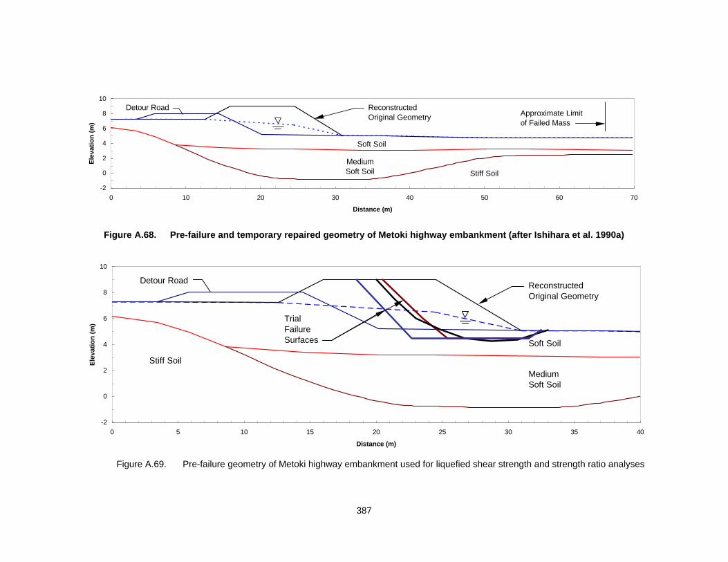
387

Figure A.68. Pre-failure and temporary repaired geometry of Metoki highway embankment (after Ishihara et al. 1990a)

Figure A.69. Pre-failure geometry of Metoki highway embankment used for liquefied shear strength and strength ratio analyses

-2

0

2

4

6

8

10

0 10 20 30 40 50 60 70

Distance (m)

Elev

atio

n (m

)

Detour Road

Soft Soil

Medium Soft Soil Stiff Soil

ReconstructedOriginal Geometry Approximate Limit

of Failed Mass

-2

0

2

4

6

8

10

0 5 10 15 20 25 30 35 40

Distance (m)

Elev

atio

n (m

)

Detour Road

Soft Soil

MediumSoft Soil

Stiff Soil

ReconstructedOriginal Geometry

TrialFailureSurfaces

388

case histories documented by Kaneko et al (1995) and Sasaki et al. (1993;1994;1995).

Outside the embankment, the watertable was assumed to be at the ground surface. The unit

weight of the fill was assumed to be 18.1 kN/m3.


Twenty-three Swedish cone penetration tests were conducted at this site following

the failure. Standard penetration test blowcounts for the silty sand were estimated as 1.5 to

2 using the Inada (1982) correlation between Swedish cone and SPT tests. Using the

“representative” pre-failure vertical effective stress discussed subsequently, the mean (N1)60

was estimated as 2.6, with lower and upper bound values of 2.3 and 3.0, respectively.

Because no grain size information is available, the qc/N60 of the silty sand was

estimated as 0.4, corresponding to a D50 of 0.12 mm, typical for silty sands. Converting the

estimated SPT (N1)60 values to qc1 resulted in a mean qc1 value of 1.05 MPa, with lower and

upper bound values of 0.9 and 1.2 MPa, respectively.



The mechanism that likely triggered flow failure was seismically-induced liquefaction

of the saturated silty sand fill and foundation soils underlying the embankment. The pre-

failure geometry is presented in Figure A.69. Figure A.69 also presents various yield failure

surfaces determined by stability analysis. The analysis considered four scenarios to

evaluate the yield shear strength and strength ratio. The scenarios were: (1) all material

below the phreatic surface liquefied and the soil above the phreatic surface was assigned φ'

= 30°; (2) all material below the phreatic surface liquefied and the soil above the phreatic

389

surface was assigned φ' = 35°; (3) the toe segment of the material below the phreatic

surface was near enough to a drainage boundary that liquefaction was not possible in this

segment and it was assigned a drained friction angle of φ' = 30°; and (4) the toe segment

was drained and assigned a drained friction angle of φ' = 35°.

The best estimate of yield shear strength for this scenarios was 9.0 kPa. Upper and

lower bound yield shear strengths of 11.1 and 8.5 kPa, respectively, were obtained using a

different failure surfaces. The weighted average pre-failure vertical effective stress was

determined as approximately 34.8 kPa [Eq. (4.3)].


Numerous trial failure surfaces were analyzed to estimate the yield strength ratio.

The various combination of drainage and drained friction angles were also considered for

the strength ratio analysis. The best estimate of yield strength ratio was determined as 0.25,

with lower and upper bounds of 0.20 and 0.29, respectively.



Due to the minimal information available, the post-failure geometry cannot be known

with certainty. However, Ishihara et al. (1990a) reported that the original embankment

flowed approximately 50 m from its pre-earthquake position, as shown in Figures A.67 and

A.68. The approximate thickness of failed mass was estimated as 2.3 m using this distance

of flow and the original embankment area. The liquefied shear strength can then be

estimated using the simplified stability analysis (Eq. 5.5). The unit weight of the

embankment material was estimated as 18.1 kN/m3, and the slope of the failed material was

390

estimated as 2 to 3 degrees. The resulting liquefied shear strength was 1.8 kPa, with a

range of 1.4 to 2.2 kPa.

This value is considerably smaller than the value of 6.2 kPa estimated by Ishihara et

al. (1990a). No explanation for the discrepancy could be determined. However, to obtain a

liquefied shear strength of 6.2 kPa using a unit weight of 18.1 kN/m3 and a thickness of 2.3

m, the slope of the failed mass must have been over 8.5 degrees. Alternately, using a slope

of 2.5 degrees, the failed mass must have been 7.9 m thick. Neither of these cases seem

reasonable, therefore, the author anticipates that the liquefied shear strength was probably

closer to 1.8 kPa.


Using the simplified analysis [Eq. (5.5)] only provides a value of liquefied shear

strength. To determine the liquefied strength ratio, a “representative” pre-failure vertical

effective stress was estimated. The “representative” pre-failure σ'vo was estimated as the

average vertical effective stress determined 1 m below the phreatic surface within the

original embankment (to the right of the detour road geometry, as this material may not have

failed). The “representative” pre-failure σ'vo was 41.9 kPa. Using this value, the liquefied

strength ratio was estimated as 0.043, with a range of 0.034 to 0.051.


Insufficient information is available for this case to conduct a kinetics analysis.


The following sources of uncertainty were involved in estimated the yield shear


391

shear strength of the non-liquefied soils; (3) the location of the initial failure surface; (4) the

location of the phreatic surface within the slope; and (5) potential for porewater pressure or

void redistribution during failure. Because the actual limits of liquefaction were not known, all

material below the phreatic surface was assumed to liquefy. Because the limits of

liquefaction were not known, potential drainage was considered in the toe segment, as

discussed above. No strength tests were available for the embankment sands, therefore, the

average drained friction angle was varied from 30 to 35°. Because the exact location of the

initial failure surface could not be identified, a number of trail failure surfaces were analyzed

using various combinations of drained and undrained shear strengths until a best estimate

of yield shear strength and strength ratio could be ascertained.


strength and strength ratio: (1) the slope and thickness of the failed material; (2) the limits of

the liquefied material; and (3) the potential for porewater pressure or void redistribution

during flow. The slope and thickness of the failed material was estimated from the extent of

the failed mass reported by Ishihara et al. (1990a) and balancing the pre- and post-failure

geometry areas. Because a simplified analysis was used, the limits of the liquefied zone are

of importance in estimating the pre-failure vertical effective stress. The estimate was

explained above.


penetration resistance: (1) only Swedish cone soundings were available and had to be

converted to SPT blowcount using an empirical correlation; (2) converting from SPT

blowcount to CPT tip resistance using the Stark and Olson (1995) qc/N60 conversion; and (3)

the location of the phreatic surface within the embankment affecting the overburden

correction.

392

A.14 HOKKAIDO TAILINGS DAM, JAPAN


Another significant failure triggered by the 1968 Tokachi-Oki earthquake was the

failure of a mine tailings dam in Hokkaido (Ishihara et al. 1990a). Figure A.70 presents a

plan view of the failure and Figure A.71 presents a portion of the original section of the

tailings dam labeled A-A’ in Figure A.70. As indicated in Figure A.71, the surface of the

tailings behind the starter dike following the failure was between 4 and 5 degrees.

Unfortunately, no estimate of the severity of shaking experienced near the site is

available.


Ishihara et al. (1990a) described the mines tailings as a silty sand. Based on this

description and other typical mine tailing deposits, the D50 and fines content of this material

were assumed to be around 0.075 mm and 50%, respectively. The unit weight of the tailings

was estimated as 19.6 kN/m3 from Ishihara et al. (1990a).

No information is available regarding the subsurface conditions, however, as

indicated in Figure A.71, the failure of the dam did not involve foundation soils, and in fact,

did not disturb the original starter dike. Therefore, the subsurface conditions are of little

relevance to the analyses conducted herein.

The phreatic surface within the dam is shown in Figure A.71. The phreatic surface

was assumed to drop to the ground surface very quickly when it reached the free-draining

material likely to comprise the starter dike.

393

Figure A.70. Plan view of flow failure of Hokkaido tailings dam (from Ishihara et al. 1990a)

Figure A.71. Pre-failure geometry and post-failure surface of tailings in dam at Hokkaidotailings dam (from Ishihara et al. 1990a)

394


Following the failure, Dutch cone penetration tests were conducted at the dam. Two

of the soundings are presented in Figure A.72. Ishihara et al. (1990a) indicated that the

average depth to the failure surface was likely about 4 m. At this depth, both soundings give

nearly identical values of tip resistance, with qc1 ranging from 0.35 to 0.38 MPa and

averaging about 0.36 MPa.

As no standard penetration tests were conducted at the site, representative SPT

values were estimated using the qc/N60 ratio proposed by Stark and Olson (1995). Assuming

a D50 of 0.075 mm, qc/N60 is 0.32 and the representative value of (N1)60 becomes 1.1, with a

range from 1 to 1.2.



The mechanism that likely triggered flow failure is seismic liquefaction of the mine

tailings. Liquefaction of the tailings resulted in a flow failure of the upper portion of the dam.

Because liquefaction was triggered by seismic loading, the shear strength and strength ratio

back-calculated from the pre-failure geometry may not represent the yield shear strength

and strength ratio (see Chapter 4 for discussion).

The pre-failure geometry of the dam is shown in Figure A.73. A slope stability search

was conducted to determine the critical initial failure surface. All the tailings below the

phreatic surface was assumed to liquefy, and the material above the phreatic surface was

assigned a drained friction angle of 30 to 35°. No inertia forces were considered in the

embankment.

395

Figure A.72. Results of Dutch cone penetration tests conducted after the failure ofHokkaido tailings dam (from Ishihara et al. 1990a)

0

2

4

6

8

10

0 10 20 30 40 50 60

Distance (m)

Elev

atio

n (m

)

StarterDike

Pre-FailureGeometry

Post-Failure Tailings Surface

Phreatic Surface

Yield FailureSurfaces

Figure A.73. Pre-failure geometry of Hokkaido tailings dam used for yield shear strengthand strength ratio analyses

396

Two trial failure surfaces are shown in Figure A.73. The shear strength mobilized in

the assumed zone of liquefaction ranged from 10.3 to 12.7 kPa depending on the

assumptions regarding the shear strength of the tailings above the phreatic surface. The

best estimate of mobilized shear strength in the zone of liquefaction was 11.7 kPa.


A second analysis was conducted to estimate the strength ratio mobilized in the

tailings at the triggering of liquefaction. Several trial failure surfaces were considered,

including the two shown in Figure A.73. Each trial failure surface was divided into a number

of segments, and values of pre-failure vertical effective stress were determined for each

segment. Using these values of pre-failure vertical effective stress and a single value of

strength ratio, various values of mobilized shear strength were assigned to each segment of

the pre-failure geometry. Again, the material above the phreatic surface was assigned a

drained friction angle of 30 to 35°.


0.21, depending on the location of the failure surface and the shear strength of the

unsaturated tailings. The weighted average pre-failure vertical effective stress was




Due to the minimal information available for this case, the post-failure geometry

cannot be known with certainty. Thus, only the simplified analysis could be conducted for

this study. However, the plan view in Figure A.70 indicates that the failed material flowed

397

about 160 m from the toe of the starter dike along section A-A’. Using an area balance, the

average thickness of the failed material was probably on the order of 2.5 to 3 m. This is

somewhat smaller than the value of 4 m suggested by Ishihara et al. (1990a), however,

Ishihara et al. based their estimate of failed mass thickness on the thickness of the mass of

tailings missing from the original section of the dam. This is not the correct value to use for

the simplified analysis.

Using Eq. (5.5), a thickness of failed material of about 3 m, and a total unit weight of

19.6 kN/m3, the best estimate of liquefied shear strength is about 4.8 kPa. The lower and

upper bound values were estimated as 4.1 kPa (using a thickness of 2.5 m) and 6.6 kPa

(from Ishihara et al. 1990a), respectively.


The weighted average vertical effective stress mid-way between the phreatic surface

and the post-failure surface of the tailings in the dam (see Figure A.71) is approximately

65.9 kPa. Therefore, the best estimate of liquefied strength ratio is 0.073, with lower and

upper bounds of 0.062 and 0.116. The upper bound was taken from Ishihara (1993).

Ishihara (1993) did not provide separate estimates of su and σ'vo, but assuming the value of

su = 6.6 kPa (from Ishihara et al. 1990a), it seems that Ishihara (1993) estimated the pre-

failure vertical effective stress to be 56.9 kPa, reasonably close to the value of 65.9

estimated in this study.


The following sources of uncertainty were involved in estimated the yield shear


shear strength of the non-liquefied tailings; (3) the location of the initial failure surface; and

398

(4) potential for porewater pressure or void redistribution during failure. Because the actual

limits of liquefaction were not known, all the tailings below the phreatic surface was

assumed to liquefy. No strength tests were available for the tailings silty sands, therefore,

the average drained friction angle was varied from 30 to 35°. Because the exact location of

the initial failure surface could not be identified, a number of trail failure surfaces were

analyzed using various combinations of drained and undrained shear strengths until a best

estimate of yield shear strength and strength ratio could be ascertained.


strength and strength ratio: (1) the slope and thickness of the failed material; (2) the limits of

the liquefied material; and (3) the potential for porewater pressure or void redistribution

during flow. The slope and thickness of the failed material was estimated from the extent of

the failed mass reported by Ishihara et al. (1990a) and balancing the pre- and post-failure

geometry areas. Because a simplified analysis was used, the limits of the liquefied zone are

important in estimating the pre-failure vertical effective stress. The estimate was explained

above.


penetration resistance: (1) only Dutch cone soundings were available and were assumed to

provide tip resistance values similar to electric and electronic CPT devices; and (2)

converting from CPT tip resistance to SPT blowcount using the Stark and Olson (1995)

qc/N60 conversion with an assumed value of D50. Unfortunately, uncertainty due to the CPT-

SPT conversion was unavoidable. However, because the values of CPT tip resistance were

consistent with other tailings dams (e.g., El Cobre tailings dam, Mochi-Koshi tailings dams),

and the value of tip resistance was rather small, this uncertainty seems minor.

399

A.15 LOWER SAN FERNANDO DAM, CALIFORNIA, USA


A major slide developed in the upstream slope of the 43 m high Lower San Fernando

Dam following the 1971 San Fernando earthquake (MW ~ 6.6). Seed et al. (1973, 1975) and

Lee et al. (1975) document a comprehensive study of the construction, failure, and analysis

of both the Lower and Upper San Fernando Dams. These studies concluded that seismic

liquefaction of the silty sand and sandy silt hydraulic fill in the upstream slope led to the

failure of the slope. In 1985, in light of several newly developed procedures to predict

liquefaction in level and sloping ground (e.g., Seed 1979; Castro et al. 1985), the U.S. Army

Corps of Engineers funded another study of the failure of Lower San Fernando Dam

(LSFD). The resulting reports (Castro et al. 1989; Seed et al. 1989; and Vasquez-Herrera

and Dobry 1989) supported the findings of previous studies. Since 1985, numerous

investigators have analyzed LSFD, e.g., Davis et al. (1988), Marcuson et al. (1990), Seed

and Harder (1990), Castro et al. (1992), Gu et al. (1993), Olson and Stark (2001), just to

name a few. LSFD is by far the most studied and best documented liquefaction flow failure

available in the literature, therefore this study will not spend much time describing the

failure, geology, and soil conditions. Interested readers should refer to the aforementioned

reports and literature for more detailed information.

The post- and pre-failure cross-sectional geometry of Lower San Fernando Dam is

presented in Figure A.74. The zone of liquefaction within the upstream hydraulic fill is shown

in both Figures A.74 (a) and (b). As illustrated in the figure, large blocks of intact

embankment material moved into the reservoir, “floating” on the liquefied soil. After the slide

came to rest, liquefied soil was found to have flowed as far as 61 m beyond the toe of the

dam and also flowed up between the intact soil blocks. The original toe of the dam moved

400

Figure A.74. Cross-section through Lower San Fernando Dam showing: (a) conditionsafter 1971 earthquake; and (b) schematic reconstruction of failed cross-section (from Castro et al. 1992)

Figure A.75. Grain size distribution of Zone 5 hydraulic fill that liquefied during 1971earthquake (from Castro et al. 1992)

401

approximately 46 m into the reservoir, and the slope dropped a maximum vertical distance

of about 15 m.

Seismoscopes located on the abutment and crest of the dam recorded peak

accelerations of 0.55g and 0.5g, respectively. The seismoscope records also indicated that

the slide occurred between 20 and 40 seconds after shaking had stopped (Seed 1979; Seed

and Harder 1990).


The dam site is underlain by alluvium, consisting primarily of stiff clay with layers of

sand and gravel. Embankment construction began in 1912.

The majority of the dam consists of hydraulic fill placed between 1912 and 1915. The

hydraulic fill was sluiced from the reservoir area and placed from upstream and downstream

starter dams. The upstream and downstream hydraulic fills were raised symmetrically and

placed in similar manners, therefore, it is reasonable to assume that the fills have similar

characteristics. The shells consist primarily of stratified sand and silt, with the core

consisting primarily of clayey soils. The grain size distribution of the lower hydraulic fill

obtained from the downstream shell (believed to be similar to the upstream fill that liquefied)

is shown in Figure A.75. From Figure A.75, the average D50 and fines content of the

liquefied hydraulic fill is approximately 0.075 and 50%, respectively. Seed et al. (1989)

reported the relative density of the downstream fill was on the order of 48% prior to the

earthquake. Samples obtained for laboratory testing were considerably more dense as a

result of earthquake shaking and post-earthquake re-consolidation, with relative densities on

the order of 52 – 55%. Furthermore, because the effective stresses within the upstream fill

were considerably less than those in the downstream fill, it is likely that the relative density

of the upstream fill was on the order of 40 to 50% prior to the earthquake.

402

In 1916, a 3 to 4.6 m thick layer of ground-up shale was hydraulically-placed above

the main hydraulic fill. Between 1916 and 1930, a number of layers of rolled fill were placed

to raise the dam to its final height of 43 m. In 1929-30, a thin drainage blanket was placed

on the downstream slope. Finally, in 1940, a downstream berm was added to complete the

dam as shown in Figure A.74(b).


Standard penetration tests were conducted in the downstream fill in 1967, 1971, and

1985. Cone penetration tests were conducted in the 1985 investigation only. Compilations of

standard and cone penetration tests in the downstream hydraulic fill are presented in

Figures A.76 and A.77, respectively. The hydraulic fill from 1023 to 995 ft (312 to 303 m) is

considered representative of the upstream liquefied hydraulic fill.

Because the penetration tests were conducted in the downstream fill and after any

earthquake-induced densification, the penetration test results were reduced to correct the

penetration values to pre-earthquake upstream fill conditions. Seed et al. (1989) suggested

that the SPT (N1)60 values in the downstream fill should be reduced by 3. These corrections

account for differences in vertical effective stress between the upstream and downstream

fills [∆(N1)60 = 1] as well as the densification that resulted from shaking [∆(N1)60 = 2]. A

similar correction was applied to CPT results, with all qc1 values being reduced by 1.2 MPa

[using qc/N60 = 0.4 to convert the ∆(N1)60 value to ∆qc1].

Applying these corrections and using judgment to select reasonable upper and lower

bound values (as discussed in detail in Section 5.5.2), “representative” SPT and CPT

penetration resistances were determined. The “representative” (N1)60 value was selected as

11.5, with reasonable lower and upper bound values of 5 and 15, respectively. The

403

Figure A.76. Results of standard penetration tests in downstream shell of Lower SanFernando Dam from 1971 and 1985 investigations (from Seed et al. 1989)

404

Figure A.77. Results of cone penetration tests in downstream shell of Lower SanFernando Dam in 1985 investigation (CPT data provided by Dr. RichardOlsen, USACOE Waterways Experiment Station)

980

1000

1020

1040

1060

1080

1100

1120

1140

0 5 10 15 20 25

qc1 (MPa)

Elevation(ft)

CPT-101 CPT-103

CPT-104 CPT-106

CPT-108 CPT-109

405

“representative” qc1 value was selected as 4.7 MPa, with reasonable lower and upper bound

values of 2.1 and 6.2 MPa, respectively.



The mechanism that likely triggered flow failure is seismic liquefaction of the lower

zone of the upstream hydraulic fill. Seed (1979), Seed et al. (1989), and Castro et al. (1992)

speculate that the delay between the earthquake and the slide was the result of porewater

pressure redistribution to zones of dilatant soil that may have developed negative porewater

pressure during shaking. The hypothesis is that as the strength of the dilatant soils

decreased from their higher undrained values to lower drained values, the slide occurred.

This case history is used to initially verify the proposed liquefaction triggering

analysis (see Chapter 7). Therefore, yield shear strength and strength ratio analyses were

not conducted for Lower San Fernando Dam.


This case history is used to initially verify the proposed liquefaction triggering

analysis (see Chapter 7). Therefore, yield shear strength and strength ratio analyses were

not conducted for Lower San Fernando Dam.



The simplified post-failure geometry is reproduced in Figure A.78(b). The final sliding

surface estimated from the post-failure geometry is also shown in Figure A.78(b). Assigning

406

Figure A.78. (a) Simplified pre-failure geometry of Lower San Fernando Dam for determination of pre-failure vertical effectivestresses used in liquefied strength ratio stability analysis; (b) Simplified post-failure geometry and assumed finalpositions of the liquefied soil segments (segments 10-14 did not liquefy)

407

φ' = 30° to the length of the final sliding surface that corresponds to the rolled fill and ground

shale and assigning su = 28.3 kPa to the length of the final sliding surface that corresponds

to the core material (Castro et al. 1989), the back-calculated shear strength was

approximately 4.8 kPa. A range of back-calculated shear strengths were obtained using

alternate values of shear strength for the rolled fill and ground shale (φ' = 35°) and using

reduced values of shear strength for the liquefied soil that entered the reservoir. The lower

and upper bound values were approximately 4.3 to 12.2 kPa, respectively.


Using the same post-failure sliding surface and the same assumptions for shear

strength of non-liquefied soils, an analysis to back-calculate the liquefied strength ratio was

conducted. The post-failure sliding surface was divided into a number of segments as

shown in Figure A.78(b). These segments were assigned pre-failure locations within the

zone of liquefaction [see Figure A.78(a)], and values of pre-failure vertical effective stress

were determined for each segment. The non-liquefied segment (rolled fill and ground shale

– segment 14 in Figure A.78) was assigned φ' = 30 to 35°. Segments 10 to 13 (core

material) were assigned su = 28.3 kPa.

The resulting liquefied strength ratio was estimated as 0.029, with a possible range

from 0.026 to 0.076. The pre-failure vertical effective stress was 166.7 kPa [Eq. (5.6)].



shows the pre-and post-failure centers of gravity, the final sliding surface, and the probable

path of travel of the center of gravity during flow failure. The kinetics analysis discounted

408

Figure A.79. Movement of center of gravity during flow failure of Lower San FernandoDam

Figure A.80. Kinetics analysis of Lower San Fernando Dam

960

1000

1040

1080

1120

1160

-600 -500 -400 -300 -200 -100 0 100 200 300

Station (ft)

Elev

atio

n (ft

)

OriginalGround Surface Center of Gravity Movement

Post-FailureGeometry

FinalSlidingSurface

Pre-FailureGeometry

Reservoir Level atTime of Failure

409

segments 1, 2, and 3 shown in Figure A.74 because these segments were only involved in

secondary sliding or slumping and not part of the main flow failure (Davis et al. 1988).

Therefore, calculation of the center of gravity positions did not include the weights of these

segments.


surface mobilized the liquefied shear strength. This inaccurately estimated the actual

liquefied shear strength because a portion of the failed soils initially were above the phreatic

surface and did not liquefy (rolled fill and ground shale) and in the core. Therefore, the

liquefied shear strength was adjusted to account for the strength of the non-liquefied soils.

Approximately 22% of the post-failure sliding surface length probably involved clayey

material in the core and 11% involved rolled fill and ground shale. These lengths of the

failure surface were assigned an average shear strengths of 28.3 and 47.9 kPa,

respectively, and the liquefied shear strength was corrected using Equation 5.13. The shear

strength of the rolled fill and ground shale was estimated using φ' = 30°.








This liquefied shear strength falls toward the lower end of liquefied shear strength

estimates of 35.9 kPa by Seed (1987; this value was back-calculated from the pre-failure

geometry); 23.9 to 47.9 by Poulos (1988); 24.4 kPa by Davis et al. (1988); 24.9 kPa by

410

Castro et al. (1989; this is the mean minus one standard deviation value estimated from

steady state testing); 14.4 to 23.9 kPa by Seed et al. (1989; with the upper value reportedly

back-calculated considering kinetics); 27.8 by Seed et al. (1989; this is the 35 percentile of

the steady state testing results); 19.2±4.8 kPa by Seed and Harder (1990); and 19.2 to 23.9

kPa by Castro et al. (1992).









strength and strength ratio: (1) the shear strength of non-liquefied and core materials; (2) the

limits of material considered in the kinetics analysis; and (3) the potential for porewater

pressure or void redistribution. Non-liquefied fill and core materials were assigned a drained

friction angle of 30 to 35° and an undrained shear strength of 28.3 kPa, respectively. The

limits of material considered in the kinetics analysis was based on the location of the initial

failure surface (Davis et al. 1988) and discounts material that slumped after the main flow

failure.


penetration resistance: (1) the effect of post-earthquake densification; and (2) the

differences in upstream and downstream conditions. Seed et al. (1989) suggested

corrections to account for both of these factors and this study adopted these corrections.

411

However, these corrections add an unknown level of uncertainty to the estimate of

“representative” penetration resistance. Furthermore, it was clear from Figures A.76 and

A.77 that there is considerable variation in penetration resistance throughout the portion of

downstream fill believed to resemble the upstream fill that liquefied. Considerable judgment

was necessary to estimate the “representative” penetration resistances in light of this

variability.

A.16 TAR ISLAND DIKE, ALBERTA, CANADA


The Suncor Inc. open pit mine is located in northern Alberta and mines oil sand for

the extraction of bitumen. Following extraction, the waste tailings, predominantly fine sands,

are hydraulically placed in containment ponds. Between the years of 1972 and 1974, four

static liquefaction flow failures occurred in the uncompacted beach sands that comprise the

upstream slopes of Tar Island Dike. Mittal and Hardy (1977), Plewes et al. (1989), and

Konrad and Watts (1995) describe various aspects of the construction of Tar Island Dike,

the hydraulic sand properties, and the static liquefaction flow failures. Of the four failures,

only one failure that occurred on August 23, 1974, was described in sufficient detail to

conduct back-analyses.

The Dike was constructed using the upstream method, typically involving the

construction of compacted sand “step overs” above beach sands deposited below water, as

illustrated in Figure A.81. During the construction of the step over shown in Figure A.81, a

liquefaction-induced flow slide occurred in the submerged beach sands below the step over.

The slide caused the step over to settle nearly 5 m. The flow slide resulted in changes in the

beach slope for a distance of 240 to 275 m from the compacted step over mat.

412

Figure A.81. Pre- and post-failure geometry of Tar Island Dike following August 23, 1974 failure (from Plewes et al. 1989)

Figure A.82. Pre-failure geometry of Tar Island Dike used for yield shear strength and strength ratio analyses

270

280

290

300

310

270 280 290 300 310 320 330 340 350 360 370

Distance (m)

Beach Sand RecentlyDeposited Below Water(Assumed to Liquefy)

Previously Overboarded Sand(Probably Did Not Liquefy)

PreviouslyCompacted

Sand

Original "Step Over" Berm ElevationPosition of "StepOver" Berm AfterLiquefaction Failure

Trial Initial Failure Surfaces

Pond Level atTime of Failure

413

At the time of the failure, the step over mat was approximately 12.8 m thick and 37 m

wide. The average rate of fill placement was about 0.13 m/day, but was as high as 0.66

m/day for a six-day period during construction. The failure caused the mat to settle and tilt

slightly, but no lateral movements or toe uplift of the mat were observed. Mittal and Hardy

(1977) state that, “It appeared that a layer of beach sand about 15 ft (4.5 m) thick below the

mat liquefied and flowed out into the pond.” Mittal and Hardy (1977) also indicated that the

mat settled as a rigid block and broke into numerous blocks as a result of the failure.


The foundation in the Tar Island Dike area consists of a soft silt and clay layer (with a

maximum thickness of about 12 m) overlying a fine sand, in turn overlying limestone

bedrock. As the foundation conditions did not affect this failure, no further description is

provided herein.

The tailings predominantly consist of fine, subangular quartz sand. The fines content

of the tailings sand is typically about 10 to 15%, but may range from 5% to 30%. The

median grain size is typically about 0.15 mm. The relative density of the beach sand when

deposited below water is typically less than 30 to 40% (Plewes et al. 1989). Dry densities of

the beach sand when deposited below water are typically between 14.1 and 14.8 kN/m3.

The water level in the tailings pond at the time of the failure was at elevation 951 ft

(289.9 m), as shown in Figure A.81.


Both standard and cone penetration tests are available for the beach sand at Tar

Island Dike. Konrad and Watts (1995) indicated that the “representative” (N1)60 value of the

414

beach sand deposited below water is about 7. This study also obtained a “representative”

(N1)60 value of 7, with a possible range from 4 to 15.

The “representative” CPT qc1 was determined from available soundings to be about 3

MPa, with a typical range from about 2 to 4 MPa.



The mechanism that likely triggered flow failure was the rapid fill placement for

construction of the step over mat. The rapid placement of fill caused an increase in

porewater pressure in the loose beach sand underlying the mat, and when the stress path of

the beach sand reached the yield envelope (or collapse surface), liquefaction was triggered

and the shear strength of the beach sand decreased to its liquefied shear strength.

Because the loading prior to failure was static, the shear strength mobilized in the

sandy shell soils just prior to collapse and liquefaction (i.e., when the factor of safety against

slope failure is equal to unity) should be equal to the yield shear strength. Therefore, back-

analysis of the pre-failure geometry was consider appropriate to determine the yield shear

strength and strength ratio.

The pre-failure geometry and approximate level of the phreatic surface in the tailings

pond is shown in Figure A.82. Mittal and Hardy (1977) indicated that probably initiated

between 4.6 and 9.1 m below the step over mat. However, based on the relatively large

vertical effective stress exerted on the beach sand due to the weight of the mat, the author

anticipates that all the beach sand below the water level to the interface with the previously

overboarded sand probably liquefied. The zone of beach sand hypothesized to have

liquefied is shaded in Figure A.82.

415


liquefaction were analyzed, as shown in Figure A.82, and values of yield shear strength

within the zone of liquefaction were varied until a factor of safety was achieved. The

compacted mat soils were assigned φ' = 34° based on laboratory test results. The best

estimate of yield shear strength was 35.9 kPa, with a likely range from 32.3 to 38.6 kPa.



the yield strength ratio. Several trial failure surfaces passing approximately through the

center of the zone of liquefaction were analyzed, as shown in Figure A.82, and values of

pre-failure vertical effective stress were determined for each segment of a given trial failure

surface. Using these values of pre-failure vertical effective stress and a single value of yield

strength ratio, various values of yield shear strength were assigned to each segment of the

pre-failure geometry. The factor of safety against slope failure was then evaluated. Using an

iterative process, the value of yield strength ratio was varied (in turn, varying the yield shear

strength assigned to each pre-failure segment) until a factor of safety of unity was achieved.

The compacted mat soils again were assigned φ' = 34°. The best estimate of yield

strength ratio was determined to be 0.265, with a likely range from 0.195 to 0.30.



The post-failure geometry was shown Figure A.81. Unfortunately, the information is

insufficient to conduct a rigorous slope stability back-analysis. Therefore, a simplified

analysis was conducted for this case history. As indicated in Figure A.81, the slope of the

416

beach sands is approximately 4° and the average thickness of the failed material is

approximately 9.1 m. Using Eq. (5.5), the liquefied shear strength is determined as 12.0

kPa. Lucia (1981) estimated the liquefied shear strength to be approximately 8.0 kPa, while

Plewes et al. (1989) suggested a range from 7.7 to 21.6 kPa. Thus, the best estimate of

liquefied shear strength is probably 12.0 kPa, with a range from 7.7 to 21.6 kPa.


Plewes et al. (1989) suggested a “representative” pre-failure vertical effective stress

of approximately 205.9 kPa. This study obtained values of pre-failure vertical effective stress

of 192.8 to 233.5 kPa, depending on the influence of the final lift of compacted mat soils

(placed in the 5 days leading up to the failure) on the vertical effective stress in the zone of

liquefaction. The author considers the value of 205.9 kPa to be reasonable, and this study

adopts this value of pre-failure vertical effective stress.

Using this value of pre-failure vertical effective stress, the best estimate of the

liquefied strength ratio is 0.058, with a range from 0.037 to 0.105.


No kinetics analysis was conducted for the flow failure at Tar Island Dike.



strengths and strength ratios: (1) the limits of the zone of liquefaction; (2) the location of the

initial failure surface; and (3) the potential for drainage or porewater pressure redistribution

during triggering of liquefaction. As the compacted mat exerted a considerable weight on the

beach sands, it seems likely that nearly all of the loose, submerged beach sand liquefied

417

during placement of the final lift of the mat. Several trial failure surfaces were evaluated that

were consistent with the final settlement of the compacted mat.


strengths and strength ratios: (1) the thickness of the flowed material; (2) the slope of the

beach sand; and (3) the potential for drainage or porewater pressure redistribution during

flow. The thickness of the failed mass and slope of the beach sands was estimated from the

partial post-failure geometry available (see Figure A.81). Because these values resulted in a

liquefied shear strength in good agreement with values estimated by other investigators,

they seem to be reasonable.

The following sources of uncertainty were involved in determining the

“representative” penetration resistance: (1) the location of the available soundings and

borings is not clear; and (2) the best estimate of SPT (N1)60 was based on a personal

communication from H Plewes, as reported by Konrad and Watts (1995). The actual

locations of the available penetration tests are not reported, but the implication is that the

tests were conducted in similar beach sands deposited below water. Therefore, this source

of uncertainty is probably minor. The value of “representative” (N1)60 attributed to H. Plewes

is in good agreement with available SPT results, and is probably appropriate.

A.17 MOCHI-KOSHI TAILINGS DAM, JAPAN


The 1978 Izu-Ohshima-Kinkai earthquake, with a main shock ML ~ 7.0 (January 14,

1978) and a large aftershock ML ~ 5.8 (January 15, 1978), caused extensive damage

throughout the Izu peninsula of Japan (Okusa and Anma 1980). Two of the more

spectacular failures were those of two dikes of the Mochi-Koshi tailings dam. Information

418

regarding the failure of Mochi-Koshi tailings dam can be found in Marcuson et al. (1979),

Marcuson (1979), Okusa and Anma (1980), Okusa et al. (1980, 1984), Ishihara (1984), and

Ishihara et al. (1990a). Peak ground accelerations at the site resulting from the main shock

were between 0.25g (Ishihara 1984) and 0.35g (Marcuson et al. 1979). No estimates of

acceleration are available for the aftershock.

A plan view of the tailings dam is shown in Figure A.83. The dam was located in a

slightly depression in a mountainous area, and three dams were constructed to contain the

tailings. Tailings Dam No. 1 is shown in Figure A.84. The starter dam was constructed in

1965 to a height of 16 m using crushed volcanic soil, directly on volcanic bedrock. Tailings

Dam No. 2 is shown in Figure A.85. This dam also was constructed in 1965 to a height of 12

m using the same techniques as Dam No. 1. Subsequent raises to both dams were built

using the upstream method, at a rate of about 2.2 m per year to their current heights of 32 m

(Dam No. 1) and 22 m (Dam No. 2). Tailings Dam No. 3 was constructed some time later on

higher ground. This dam had a height of about 7 m with 4 m of freeboard.

Tailings Dam No. 1 failed immediately after the main shock of the 1978 Izu-Ohshima-

Kinkai earthquake (ML ~ 7.0). Ishihara (1984) described one eyewitness account as follows:

“within a matter of 10 seconds after the main shock, the frontal wall of the dike swelled and

the breach took place at the upper part in proximity to the left abutment, followed by a huge

mass of slime rushing down the valley…” The valley floor slope below Dam No. 1 was

between 10 and 20°, typically about 16°. The tailings flowed down the valley to the Mochi-

Koshi River, sedimenting in the river bed to a thickness of 1.0 to 1.9 m over a distance of

about 800 m (Ishihara 1984). Marcuson et al. (1979) noted that the tailings were about 1.5

m thick during flow and in the streambed. The post-failure geometry of the dam is shown in

Figure A.84. The post-failure slope of the tailings behind Dam No. 1 was between 4 and 8°.

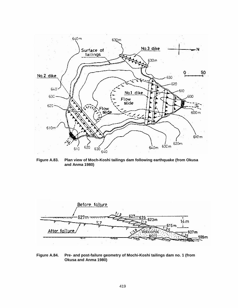
419

Figure A.83. Plan view of Moch-Koshi tailings dam following earthquake (from Okusaand Anma 1980)

Figure A.84. Pre- and post-failure geometry of Mochi-Koshi tailings dam no. 1 (fromOkusa and Anma 1980)

420

Figure A.85. Pre- and post-failure geometry of Mochi-Koshi tailings dam no. 2 (fromOkusa and Anma 1980)

Figure A.86. Grain size distribution of tailings material (from Okusa and Anma 1980)


0

10

20

30

40

50

60

70

80

90

100

0.0010.010.1110100


Perc

ent F

iner

by

Wei

ght

2in

1in

3/4in

1/2in

No4

No20

No40

No60

No100

No200

No10

Range of TailingsMaterial in Pond

From ValleyDeposit belowTailings Dam No. 1

From SandySilt VolcanoFound in Pond

421

Tailings Dam No. 2 failed about 5 hours and 20 minutes following the largest

aftershock on January 15, 1978. Ishihara (1984) and Okusa et al. (1984) hypothesized that

the failure of this tailings dam was delayed as earthquake-induced porewater pressure

migrated from the wetter tailings near Dam No. 1 to the drier tailings near Dam No. 2. The

valley floor slope below this dam was about 10°, and the tailings flowed over a distance of

about 150 m before coming to rest. However, Ishihara (1984) reported that the tailings from

Dam No. 2 flowed over a distance of about 240 m and Figure 7 of Ishihara (1984) indicates

that at least a portion of the failed tailings had a final thickness of 1.6 to 2.0 m. The post-

failure geometry of the dam is shown in Figure A.85. The post-failure slope of the tailings

behind Dam No. 2 was between 9 and 10°.

Dam No. 3 did not sustain any damage.


The tailings dams were constructed directly on volcanic rock, and the starter dikes

were constructed using crushed volcanic soil. The starter dikes were compacted by tracking

with bulldozers.

The tailings consisted of alternating layers of sandy silt and silt sized tailings, with the

layers typically 3 to 7 cm in thickness. The tailings had water contents typically around 36 to

37%, with an upper limit of around 50% (throughout the pond) and a lower limit of around

18% (near Dam No. 2). The void ratio of the tailings was about 0.98 and 1.0 and the specific

gravity was about 2.72 to 2.74. The sandy silt tailings were non-plastic, while the silt tailings

had a plasticity index of 10 (LL ~ 21; PL ~ 11). The range of grain sizes of the tailings

material (including in situ sandy silt and silt samples; samples from sand boils that erupted

following the earthquake; and samples from near Dams No. 1 and 2) is shown in Figure

A.86. The tailings had an approximate unit weight of 17.6 kN/m3.

422

As the tailings dam was active at the time of the failure, the watertable probably was

at the pond surface. Ishihara (1984) and Okusa et al. (1984) indicated that the phreatic

surface in the dike materials was as shown in Figures A.87 and A.88.


Standard penetration tests and portable cone penetration tests were conducted

about three weeks after the failure. Field blowcounts in the starter dikes ranged from about 3

to 7, while field N-values in the tailings ranged from about 0 to 4. Ishihara (1984) suggested

that the considerable number of zero blowcounts resulted from liquefaction and disturbance

of the tailings. He suggested that the pre-earthquake blowcount of the tailings should have

been larger than zero.

Correcting for effective overburden pressure and differences in Japanese and

American SPT system configurations (ER/60 ~ 1.2; Seed et al. 1985) resulted in a

“representative” SPT (N1)60 of about 2.7, with a range from 0 to 6. Seed (1987) estimated an

(N1)60 value of 6 (allowing for the high fines content of the tailings), while Seed and Harder

(1990) estimated an (N1)60 value of 5.

Portable cone penetration test results indicated a “representative” qc1 value of

approximately 0.5 MPa, with a range from 0.25 to 1.0 MPa.



The mechanism that likely triggered flow failure of Dam No. 1 is seismic liquefaction

of the loose tailings material. The flow failure of Dam No. 2 was likely triggered by

liquefaction of the loose tailings and excess porewater pressure migration from near Dam

423

No. 1. As discussed in Chapter 4, the shear strength and strength ratio mobilized at the



Therefore, back-calculated values of shear strength and strength ratio may not represent the

yield shear strength and yield strength ratio.

The pre-failure geometry of tailings Dam No. 1 is shown in Figure A.87. A slope

stability search was conducted to determine the critical failure surface. A single value of

shear strength was assigned to the liquefied soil, and a drained friction angle of 35° was

assigned to the dike materials, as a result of their probable angular particle shape. No inertia

forces were considered in the dike.

The critical failure surface is shown in Figure A.87. Other failure surfaces that were

considered also are shown in Figure A.87. The values of mobilized shear strength in the

zone of liquefaction ranged from 18.0 to 23.9 kPa. The best estimate of mobilized shear

strength in the zone of liquefaction was 21.1 kPa.

The pre-failure geometry of tailings Dam No. 2 is shown in Figure A.88. A slope


shear strength was assigned to the liquefied soil, and a drained friction angle of 35° was

assigned to the dike materials, as a result of their probable angular particle shape. No inertia

forces were considered in the dike.


considered also are shown in Figure A.88. The values of mobilized shear strength in the

zone of liquefaction ranged from 10.5 to 18.7 kPa. The best estimate of mobilized shear

strength in the zone of liquefaction was 16.0 kPa.

424

Figure A.87. Pre-failure geometry of tailings dam no. 1 used in yield shear strength andstrength ratio analyses

Figure A.88. Pre-failure geometry of tailings dam no. 2 used in yield shear strength andstrength ratio analyses

590

600

610

620

630

640

40 60 80 100 120 140 160

Distance (m)

Elev

atio

n (m

)

Post-FailureGeometry Hard Base


StarterDike

ApproximatePhreatic Surface

Pre-FailureTailings Surface

Potential InitialFailure Surfaces

600

610

620

630

640

20 30 40 50 60 70 80 90 100

Distance (m)

Elev

atio

n (m

)


Hard Base


ApproximatePhreatic Surface

StarterDike

Potential YieldFailure Surfaces

Pre-FailureTailings Surface

425


Additional analyses were conducted to estimate the shear strength ratios mobilized

at the triggering of liquefaction. The pre-failure geometry of tailings Dam No. 1 is reproduced

in Figure A.89. Contours of vertical effective stress also are shown in Figure A.89. Using the

vertical effective stress contours and a single value of strength ratio, values of mobilized

shear strength were assigned to each of the contours. A slope stability search was

conducted to determine the critical failure surface. A single value of shear strength was

assigned to the liquefied soil, and a drained friction angle of 35° was assigned to the dike

materials, as a result of their probable angular particle shape. No inertia forces were

considered in the dike.


considered also are shown in Figure A.89. The values of mobilized strength ratio in the zone

of liquefaction ranged from 0.24 to 0.30. The best estimate of mobilized strength ratio in the

zone of liquefaction was 0.27.

The pre-failure geometry of tailings Dam No. 2 was shown in Figure A.88. Several

trial surfaces were considered and values of pre-failure vertical effective stress were

determined for each segment of a given trial failure surface. Using these values of pre-

failure vertical effective stress and a single value of mobilized strength ratio, various values

of shear strength were assigned to each segment of the pre-failure geometry. The factor of

safety was then evaluated. A drained friction angle of 35° was assigned to the dike

materials.

The values of mobilized strength ratio in the zone of liquefaction ranged from 0.16 to

0.25. The best estimate of mobilized strength ratio in the zone of liquefaction was 0.22.

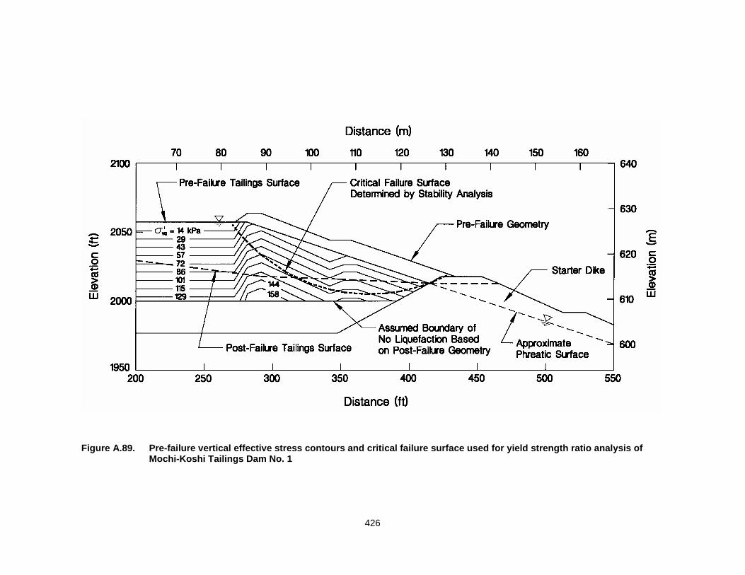
426

Figure A.89. Pre-failure vertical effective stress contours and critical failure surface used for yield strength ratio analysis ofMochi-Koshi Tailings Dam No. 1

427



Only simplified analyses could be conducted for the failure of Mochi-Koshi tailings

Dams No. 1 and 2. The tailings from Dam No. 1 flowed at a thickness of about 1.5 m

(ranged from 1.0 to 1.9 m) and came to rest at a slope of about 8°. Using Eq. (5.5), the

liquefied shear strength is estimated to be between 2.4 and 7.2 kPa, with a best estimate of

3.6 kPa. Ishihara et al. (1990a) estimated a liquefied shear strength of 14.7 kPa using the

depth to the final sliding surface (~ 6 m) within the original pond geometry, resulting in a

considerably higher value of liquefied shear strength. However, using the depth to the final

sliding surface within the original pond geometry violates the assumptions required to apply

Eq. (5.5), and therefore is inappropriate. Lucia (1981) and Bryant et al. (1983) estimated the

liquefied shear strength to be about 10.0 kPa. Seed (1987) increased this estimate to 12.0

kPa without explanation. Seed and Harder (1990) estimated a value of 12.0±7.2 kPa.

The tailings from Dam No. 2 flowed at a thickness of about 1.8 m (ranged from 1.6 to

2.0 m) and came to rest at a slope of about 10°. Using Eq. (5.5), the liquefied shear strength

is estimated to be between 4.8 and 6.0 kPa, with a best estimate of 5.4 kPa. Ishihara et al.

(1990a) estimated a liquefied shear strength of 17.1 kPa using the depth to the final sliding

surface (~ 6 m) within the original pond geometry, resulting in a considerably higher value of

liquefied shear strength. However, using the depth to the final sliding surface within the

original pond geometry violates the assumptions required to apply Eq. (5.5), and therefore is

inappropriate.

428


As rigorous slope stability analyses were not possible for Mochi-Koshi, the liquefied

strength ratios were determined using “single value” estimates of pre-failure vertical effective

stress.

The representative pre-failure vertical effective stress for tailings Dam No. 1 was

estimated as 59.9 kPa, using a weighted average depth to the final sliding surface of about

7.7 m. This results in a best estimate liquefied strength ratio of 0.06, with a range of 0.033 to

0.12.

The representative pre-failure vertical effective stress for tailings Dam No. 2 was

estimated as 52.2 kPa, using a weighted average depth to the final sliding surface of about

6.7 m. This results in a best estimate liquefied strength ratio of 0.104, with a range of 0.071

to 0.136.


No kinetics analyses were conducted for the Mochi-Koshi tailings dams.



strengths and strength ratios: (1) the shear strength of the non-liquefied soil; (2) the location

of the initial failure surface; and (3) the potential for drainage or porewater pressure

redistribution during triggering of liquefaction. As the dikes were constructed of crushed

(probably angular) volcanic rock, they were assigned a drained friction angle of 35°. The

locations of initial failure surfaces were determined using slope stability searches, and the

sliding surfaces are consistent with the post-failure geometry (i.e., not considerably deeper

429

and do not intersect the starter dikes). In the case of tailings Dam No. 2, it is likely that

porewater pressure redistribution played a major role in the failure (Ishihara 1984; Okusa et

al. 1984).


strengths and strength ratios: (1) the thickness of the flowed material; (2) the slope of the

ground where the failure mass came to rest; and (3) the potential for drainage or porewater

pressure redistribution during flow. The thickness of the failed mass is extremely important,

as illustrated in section A.17.5. This study used the thickness of the failed mass where it

came to rest, as reported by various investigators. Ishihara et al. (1990a) and possibly Seed

(1987) and Seed and Harder (1990) used the depth to the failure surface within the original

geometry of the tailings pond. The depth to the failure surface in the tailings pond is

inappropriate because it does not necessarily reflect conditions during or at the end of flow.

Ground slopes where the sliding masses came to rest was obtained from various

investigator’s site reports, however, there was some variation in reported slopes. Average

slope values were used for this study.


“representative” values of penetration resistance: (1) the effects of liquefaction and

remolding due to earthquake shaking; and (2) the use of a non-standard cone penetrometer.

As discussed by Ishihara (1984), a large number of the standard penetration tests resulted

in weight-of-rods resistance. However, these zero blowcount values were likely due

liquefaction and remolding of the loose tailings material. The pre-earthquake blowcount was

likely larger than zero. Therefore, very little emphasis was placed on SPTs conducted near

the failed areas. Thus, a non-zero “representative” blowcount was obtained. A non-standard

cone penetrometer was used in the field investigation of the Mochi-Koshi failures. Ishihara et

430

al. (1990a) implied that there is little difference in penetration resistance of the non-standard

cone and standard cones. Therefore, no correction to cone penetration resistance was

applied in this study.

A.18 NERLERK UNDERSEA BERM, BEAUFORT SEA, CANADA


The Nerlerk hydraulic fill undersea sand berm was designed to form part of a bottom-

founded, offshore, hydrocarbon exploration platform at Nerlerk in the Canadian Beaufort

Sea. In 1983, five liquefaction flow failures occurred as a result of fill placement. [Actually six

failures occurred, with the first occurring in 1982. The first failure has not been reported in

the open literature (Rogers et al. 1990).] The Nerlerk failures have been extensively studied

(Mitchell 1984; Sladen et al. 1985a,b, 1987; Been et al. 1987a; Rogers et al. 1990; Lade

1993; Hicks and Boughrarou 1998) and a number of related studied have been published

(Sladen 1989; Sladen and Hewitt 1989; Konrad 1991). Therefore, this discussion will be

brief and reference is made to the literature for detailed descriptions of the failures.

The location of the site is shown in Figure A.90. Numerous berms built for the same

purpose had been constructed using procedures similar to that at Nerlerk, therefore,

designers did not anticipate difficulties at Nerlerk. Construction began in 1982 with the

placement of sand (by hopper dredges) obtained from a borrow site at Ukalerk. Later in

1982 and into 1983, sand obtained from a borrow site near Nerlerk was placed by point

source discharge. Placement by this method resulted in considerably flatter slopes (10H:1V)

than design (5H:1V) as shown in Figure A.91, and placement was temporarily halted while

changes were made to the discharge equipment.

431

Figure A.90. Location of some undersea berm sites in Beaufort Sea (from Sladen andHewitt 1989)

Figure A.91. Typical Nerlerk berm geometry and foundation subsoil stratigraphy (fromBeen et al. 1987)

432

Construction recommenced in July 1983, and on July 20, 1983, bathymetric surveys

revealed that a significant part of the berm had disappeared. Three more slides occurred

between July 25 and August 2, 1984. A fifth slide was purposely triggered on August 4,

1984, by the concentrated placement of fill at the crest of the northeastern slope. The

location of the slides from Sladen et al. (1985b) is presented in Figure A.92. It should be

noted that Rogers et al. (1990) did not agree with the locations and areas of these slides.

Approximate pre- and post-failure geometries for the five slides are presented in Figure A.93

(note the vertical exaggeration). As seen in Figure A.93, only slides 1 through 3 have

reasonably sufficient post-failure geometry data to estimate the entire post-failure

geometries of the slide masses. Therefore, only slides 1 through 3 are examined in this

study.

The profiles in Figure A.93 indicate that pre-failure slopes were on the order of 10 to

12°, with local areas as steep as about 18°. The depth of the failures ranged from 5 to 12 m.

Bathymetric data beyond the toe of the berm indicate post-failure slopes as flat as 1 to 2°.

All of the failed material was comprised of Nerlerk sand, and none of the failures penetrated

the Ukalerk sand core. Bathymetric data for slide 4 is presented in Figure A.94. Sladen et al.

(1987) indicated that the other slides had similar pre- and post-failure bathymetry.

After a loss of about $100 million, the Nerlerk site was abandoned.


The berm site is underlain by a 1 to 2 m thick layer of high plasticity clay and silt.

Below the clay and silt layer, poorly graded sand with trace silt is encountered. The sand is

frozen and well bonded from about 34 m below the seabed.

Grain size distributions of the Nerlerk and Ukalerk sands are presented in Figure

A.95. The Nerlerk sand has an average D50 of approximately 0.22 mm and a fines content

433

Figure A.92. Plan of Nerlerk berm showing slide locations and profile lines (from Sladenet al. 1985b)

Figure A.93. Typical sections through slides, showing pre- and post-failure profiles Note5x vertical exaggeration (from Sladen et al. 1985b)

434

Figure A.94. Three-dimensional morphologies of slide 4 based on detailed bathymetry:(a) pre-slide; (b) post-slide; and (c) interpretation of slide morphologysuperimposed on view (b) (from Sladen et al. 1987)

Figure A.95. Typical grain size distribution for Ukalerk (Erksak) and Nerlerk sands (fromSladen and Hewitt 1989)

435

from 2 to 12% (average of about 10% from Sladen et al. 1985b versus average of about 3%

from Rogers et al. 1990). In contrast, the Ukalerk sand has an average D50 of approximately

0.31 mm and a fines content from 0 to 3% (average of about 2%; Sladen et al. 1985b and

Rogers et al. 1990). Sladen et al. indicate that the Nerlerk sands have relative densities

ranging from 20 to 70%, with mean values between 30 and 50%. There is some contention

in the literature regarding the in situ state of the Nerlerk sand, with Sladen et al. (1985b)

suggesting a state parameter between 0.05 and 0.15; Been et al. (1987a) suggesting values

between 0 and -0.25; and Rogers et al. (1990) suggesting typical values between 0 and -

0.20. The submerged unit weight of the sand is approximately 10.1 kN/m3.


In total, 26 cone penetration tests were conducted during 1983 construction.

Unfortunately, only a few of the individual soundings are available, but several literature

sources provide summaries of CPT tip resistance, including maximum, mean, minimum and

mean plus/minus one standard deviation values.

Using individual soundings available near slides 1 and 2 (and assigning the values

for slide 2 to slide 3), the “representative” mean and lower and upper bound qc1 values for

each of the slides are:

• Slide 1 “representative” qc1 = 4.5 MPa, ranging from 2.6 to 7.8 MPa



As no SPT results are available for Nerlerk berm, (N1)60 values were estimated using

qc/N60 = 0.52 (Stark and Olson 1995; D50 = 0.22 mm). Thus, the “representative” mean and

lower and upper bound (N1)60 values for each of the slides are:

436

• Slide 1 “representative” (N1)60 = 8.7, ranging from 5 to 15

• Slide 2 “representative” (N1)60 = 7.2, ranging from 3.6 to 15.3

• Slide 3 “representative” (N1)60 = 7.2, ranging from 3.6 to 15.3



The flow failures at Nerlerk berm were likely a result of initial failure of the foundation

soft clay layer, resulting in sufficient deformation in the Nerlerk berm sand to trigger

liquefaction. The hypothesis proposed by Lade (1993) and the finite element analysis by

Hicks and Boughrarou (1998) support this failure mechanism. Because liquefaction was

triggered by foundation deformation, the shear strength and strength ratio back-calculated

from the pre-failure geometry may not represent the yield shear strength and strength ratio

(see Chapter 4 for discussion).

The pre-failure geometry of slide 1 is shown in Figure A.96. A slope stability search

was conducted to determine the critical failure surface. All the sand was assumed to liquefy

and a single value of shear strength was assigned to the liquefied soil. Trial failure surfaces

also are shown in Figure A.96. The values of mobilized shear strength in the zone of

liquefaction ranged from 2.7 to 4.0 kPa. The best estimate of mobilized shear strength in the

zone of liquefaction was 2.7 kPa.





437

Figure A.96. Pre-failure geometry of Nerlerk slide 1 used for yield shear strength and strength ratio analyses


-45

-35

-25

-15

80 110 140 170 200

Distance (m)

Elev

atio

n (m

)

Ukalerk Sand Nerlerk Sand

Seabed Clay




-45

-35

-25

-15

20 50 80 110 140

Distance (m)

Elev

atio

n (m

)

Ukalerk Sand Seabed Clay

Nerlerk Sand


Pre-Failure GeometryPotential YieldFailure Surfaces

438










Additional analyses were conducted to estimate the shear strength ratios mobilized

at the triggering of liquefaction. The pre-failure geometry of slide 1 was shown in Figure

A.96. Several trial surfaces were considered and values of pre-failure vertical effective

stress were determined for each segment of a given trial failure surface. Using these values

of pre-failure vertical effective stress and a single value of mobilized strength ratio, various

values of shear strength were assigned to each segment of the pre-failure geometry. The

factor of safety was then evaluated. The values of mobilized strength ratio in the zone of

liquefaction ranged from 0.17 to 0.23. The best estimate of mobilized strength ratio in the

zone of liquefaction was 0.21. The weighted average pre-failure vertical effective stress was

12.7 kPa.

The pre-failure geometry of slide 2 was shown in Figure A.97. Several trial surfaces

were considered and values of pre-failure vertical effective stress were determined for each

segment of a given trial failure surface. Using these values of pre-failure vertical effective

stress and a single value of mobilized strength ratio, various values of shear strength were

assigned to each segment of the pre-failure geometry. The factor of safety was then

439


Figure A.99. Post-failure geometry of Nerlerk slide 1 used for liquefied shear strength and strength ratio analyses

-45

-35

-25

-15

50 80 110 140 170 200

Distance (m)

Elev

atio

n (m

)

Ukalerk Sand



Nerlerk Sand

Seabed Clay


-45

-35

-25

-15

50 100 150 200 250 300 350

Distance (m)

Elev

atio

n (m

)

Ukalerk Sand Nerlerk Sand

Seabed Clay

? ?



440

evaluated. The values of mobilized strength ratio in the zone of liquefaction ranged from

0.19 to 0.23. The best estimate of mobilized strength ratio in the zone of liquefaction was

0.21. The weighted average pre-failure vertical effective stress was 19.8 kPa.

The pre-failure geometry of slide 3 was shown in Figure A.98. Several trial surfaces

were considered and values of pre-failure vertical effective stress were determined for each

segment of a given trial failure surface. Using these values of pre-failure vertical effective

stress and a single value of mobilized strength ratio, various values of shear strength were

assigned to each segment of the pre-failure geometry. The factor of safety was then

evaluated. The values of mobilized strength ratio in the zone of liquefaction ranged from

0.165 to 0.23. The best estimate of mobilized strength ratio in the zone of liquefaction was

0.20. The weighted average pre-failure vertical effective stress was 24.7 kPa.



The post-failure geometry of slide 1 is presented in Figure A.99. An area balance

was required to estimate the entire post-failure geometry. The final sliding surface is

assumed to be the top of the pre-failure geometry. The best estimate of the back-calculated

shear strength was approximately 2.5 kPa. No other assumptions were available to back-

calculate a range of shear strengths.


was required to estimate the entire post-failure geometry. Two possible final geometries and

sliding surfaces are shown in Figure A.100. The average back-calculated shear strength

was approximately 1.7 kPa. The lower and upper bound values were approximately 1.0 to

2.4 kPa.

441



-45

-35

-25

-15

0 50 100 150 200 250 300 350

Distance (m)

Elev

atio

n (m

)

Ukalerk Sand Seabed Clay

Nerlerk SandPost-Failure Geometry

Pre-Failure GeometryAlternate Post-FailureToe Geometries

??

?

?

-45

-35

-25

-15

0 50 100 150 200 250 300 350 400 450

Distance (m)

Elev

atio

n (m

)

Ukalerk Sand??


Post-Failure GeometryAlternate Post-Failure

Toe GeometriesNerlerk Sand

Seabed Clay

442


was required to estimate the entire post-failure geometry. Two possible final geometries and

sliding surfaces are shown in Figure A.101. The average back-calculated shear strength

was approximately 1.5 kPa. The lower and upper bound values were approximately 1.2 to

1.7 kPa.


The assumed post-failure geometry for slide 1 was shown in Figure A.99. Using this

geometry, an analysis to back-calculate the liquefied strength ratio was conducted. The

post-failure sliding surface was divided into a number of segments, these segments were

assigned pre-failure locations within the zone of liquefaction, and values of pre-failure

vertical effective stress were determined for each segment. The resulting liquefied strength

ratio was estimated as 0.086. The weighted average pre-failure vertical effective stress was

29.5 kPa.

Two possible post-failure geometries for slide 2 were shown in Figure A.100. Using

this geometries, analyses to back-calculate the liquefied strength ratio were conducted. The



vertical effective stress were determined for each segment. The resulting average liquefied

strength ratio was estimated as 0.06, with lower and upper bound values of 0.025 and

0.094, respectively. The weighted average pre-failure vertical effective stress was 31.1 kPa.

Two possible post-failure geometries for slide 3 were shown in Figure A.101. Using

this geometries, analyses to back-calculate the liquefied strength ratio were conducted. The



443

vertical effective stress were determined for each segment. The resulting average liquefied

strength ratio was estimated as 0.034, with lower and upper bound values of 0.029 and

0.041, respectively. The weighted average pre-failure vertical effective stress was 44.3 kPa.


No kinetics analyses were performed for the failures at Nerlerk berm because too

much of the post-failure geometry had to be assumed using area balances.



strengths and strength ratios: (1) the locations of the initial failure surfaces; and (2) the

potential for drainage or porewater pressure redistribution during triggering of liquefaction.

The locations of the initial failure surfaces were in good agreement with the analysis of

Sladen et al. (1985b) and in general agreement of zones of high shear stress ratio within the

berm sands calculated by Hicks and Boughrarou (1998). Thus, these initial failures surfaces

were considered reasonable.


strengths and strength ratios: (1) the post-failure geometry; and (2) the potential for drainage

or porewater pressure redistribution during triggering of liquefaction. By far, the largest

source of uncertainty for the Nerlerk cases is the post-failure geometry. As the entire post-

failure geometries were not available in the literature, the author estimated post-failure

geometries using area balances. However, numerous possible post-failure geometries are

possible. This study analyzed two possible post-failure geometries for slides 2 and 3, and

444

found that back-calculated shear strengths and strength ratios could vary considerably.

Therefore, the results of these back-analyses should be used cautiously.


“representative” values of penetration resistance: (1) the distance between available CPT

soundings and the slides; and (2) the conversion of CPT tip resistance to SPT blowcount.

The sounding(s) conducted nearest to a given slide was used to estimate “representative”

penetration resistances, however, as in the case of slide 3, nearby soundings were not

available. Therefore, penetration resistances for slide 3 were estimated from the nearest

slide (slide 2) and compared to available tip resistance summaries. As no SPT data are

available, CPT tip resistances were converted to SPT blowcounts. This step involves an

unknown level of uncertainty.

A.19 HACHIRO-GATA ROAD EMBANKMENT, AKITA, JAPAN


The 1983 Nihon-Kai-Chubu (M = 7.7) earthquake caused considerable damage in

the Akita region of Japan as a result of liquefaction of sandy sediments. A peak ground

acceleration of 0.168g was measured in the town of Akita. One notable failure is the flow

slide of the Hachiro-Gata road embankment leading to the Gomyoko Bridge (Ohya et al.

1985).

Figure A.102 presents the pre- and post-failure geometry of the embankment. The

figure shows considerable slumping, cracking, and flow of the embankment in both

directions. As the post-failure geometry is more complete on the left-hand side of the figure,

this study analyzed this side of the embankment. Ohya et al. (1985) noted that sand boils

formed at the toe of the slope following the earthquake. Differential settlements between the

445

Figure A.102. Pre- and post-failure geometry of Hachiro-Gata road embankment (fromOhya et al. 1985)

Figure A.103. Boring log and soil properties from Hachiro-Gata road embankment (fromOhya et al. 1985)

446

approach embankment and the bridge were on the order of 0.5 to 1.0 m. Post-earthquake

field tests were conducted around the toe of the slope of the road.


The embankment, consisting of loose, fine sand, is underlain by a medium dense,

fine sand layer about 5 m thick, a dense sand layer about 6 m thick, and a soft clay to the

depth of the field investigation. Available soil properties for the lower portion of the

embankment and the foundation soils are presented in Figure A.103. Assuming the

embankment sands resemble the upper foundation soils, the approximate values of D50 and

fines content are 0.2 mm and 10 to 20%, respectively. A unit weight of 18.1 kN/m3 was

assumed.


The field investigation at this site included SPT, CPT, CPTU (piezocone), and five

other in situ penetration test devices. Ohya et al. (1985) reported that the Japanese SPT

system has an energy ratio of about 68%, therefore measured blowcounts were multiplied

by 0.88 (=60/68). The results of the field tests are presented in Figure A.104.

The “representative,” lower, and upper bound (N1)60 values were determined as 4.4,

3.1, and 5.8, respectively. The “representative,” lower, and upper bound qc1 values were

determined as 3.0, 1.1, and 4.9 MPa, respectively.

447

Figure A.104. Results of in situ penetration tests conducted at Hachiro-Gata road embankment (from Ohya et al. 1985)

448



The mechanism that likely triggered flow failure of the Hachiro-Gata road

embankment is seismic liquefaction of the loose embankment sands (Ohya et al. 1985). As

discussed in Chapter 4, the shear strength and strength ratio mobilized at the instant of

failure in cases of liquefaction flow failure triggered by seismic loading do not necessarily

represent the yield shear strength and yield strength ratio, respectively. Therefore, back-

calculated values of shear strength and strength ratio likely do not represent the yield shear

strength and yield strength ratio.

The pre-failure geometry of the Hachiro-Gata embankment is shown in Figure A.105.

A slope stability search was conducted to determine the critical failure surface. All the loose

soil below the phreatic surface was assumed to liquefy. A single value of shear strength was

assigned to the liquefied soil, and a drained friction angle of 30° was assigned to the

embankment soils above the phreatic surface. Further, because of the short drainage path,

drainage was also considered in the toe segment of the embankment, and this segment was

assigned a drained friction angle of 30°. No inertia forces were considered in the dike.

Trial failure surfaces are shown in Figure A.105. The values of mobilized shear

strength in the zone of liquefaction ranged from 4.3 to 5.3 kPa. The best estimate of

mobilized shear strength in the zone of liquefaction was 4.8 kPa.



triggering of liquefaction. Several trial failure surfaces were considered, as shown in Figure

449

Figure A.105. Pre-failure geometry of Hachiro-Gata roadway embankment used for yield shear strength and strength ratioanalyses

Figure A.106. Post-failure geometry of Hachiro-Gata roadway embankment used for liquefied shear strength and strength ratioanalyses

-5.0

0.0

5.0

-5 0 5 10 15 20 25 30

Distance (m)

Rel

ativ

e El

evat

ion

(m)

Assumed Portionof Geometry

Medium Dense Sand

Loose Sand

Post-Failure GeometryPre-Failure Geometry

Phreatic Surface Potential YieldFailure Surfaces

-5.0

0.0

5.0

-5 0 5 10 15 20 25 30

Distance (m)

Rel

ativ

e El

evat

ion

(m)


Medium Dense Sand

Loose Sand


Phreatic Surface Final Surfaceof Sliding

450

A.105. Each trial failure surface was divided into a number of segments, and values of pre-

failure vertical effective stress were determined for each segment. Using these values of

pre-failure vertical effective stress and a single value of strength ratio, various values of

mobilized shear strength were assigned to each segment of the pre-failure geometry. Again,

the material above the phreatic surface was assigned a drained friction angle of 30°, and

potential drainage of the toe segment was considered.


0.205, dependent on the location of the failure surface and whether or not drainage occurred

near the toe. The weighted average pre-failure vertical effective stress was determined as

30.2 kPa using Eq. (4.3).





liquefaction probably did not occur in the underlying medium dense sand (Ohya et al. 1985).

Assigning φ' = 30° to the length of the final failure surface that corresponds to the length of

material in the pre-failure geometry that did not liquefy (i.e., above the phreatic surface), a

likely range of liquefied shear strengths were obtained. The back-calculated shear strength

was approximately 1.4 kPa, with a possible range from 1.1 to 1.6 kPa.




451






The pre- and post-failure geometries are reproduced in Figure A.107. Figure A.107

also shows the pre-and post-failure centers of gravity, the final sliding surface, and the

probable path of travel of the center of gravity during flow failure. The initial result of the

kinetics analysis assumed that all soils along the failure surface mobilized the liquefied

shear strength. This inaccurately estimated the actual liquefied shear strength because a

portion of the failed soils initially were above the phreatic surface and did not liquefy.

Therefore, the liquefied shear strength was adjusted to account for the strength of the non-

liquefied soils. Approximately 18% of the post-failure sliding surface length probably

involved soils that did not liquefy. This length of the failure surface was assigned an average

shear strength of 8.3 kPa, and the liquefied shear strength was corrected using Equation

(5.13), where su is the liquefied shear strength determined in the initial kinetics analysis

[using Eq. (5.12)], Ld is the length of the post-failure sliding surface (percent of the total

length of the failure surface) that did not liquefy (approximately 18%), and sd is the average

shear strength of the fill soils that did not liquefy (approximately 8.3 kPa).




452

Figure A.107. Movement of center of gravity during flow failure of Hachiro-Gata roadwayembankment

Figure A.108. Kinetics analysis of Hachiro-Gata roadway embankment

-5.0

0.0

5.0

-5 0 5 10 15 20 25 30

Distance (m)

Rel

ativ

e El

evat

ion

(m)


Medium Dense Sand

Loose Sand


Phreatic Surface FailureSurface

Center of GravityPath of Travel

453













strength and strength ratio: (1) the limits of the initial zone of liquefaction; (2) the position of

the initial failure surface; (3) the shear strength of the non-liquefied soil; and (4) the potential

for void or porewater pressure redistribution during failure. It was assumed that all the fill

below the phreatic surface liquefied during the earthquake based on the description and

analyses of Ohya et al. (1985). Potential drainage in the toe segment of the slope was

considered. The position of the initial failure surface was not known. Therefore, numerous

trial failure surfaces were studied to determine the critical surface. The shear strength of the

material above the phreatic surface was taken 30°–a typical values for loose sands.


strength and strength ratio including the kinetics analysis: (1) limits of the zone of

liquefaction; (2) the location of the initial and final surfaces of sliding; (3) the location of the

post-failure geometry toe; and (4) the potential for void and porewater pressure

454

redistribution. Again, the limits of the zone of liquefaction is not known with certainty, but all

loose soil below the phreatic surface was assumed to liquefy. The exact locations of the

initial and final surfaces of sliding are required for the kinetics analysis, and were determined

by stability analysis search. The location of the post-failure geometry toe was estimated

using an area balance and extrapolating the known post-failure geometry.

The following source of uncertainty were involved in determining the “representative”

values of penetration resistance: (1) the effects of flow and re-consolidation because the

penetration tests were conducted after the failure. This factor resulted in an unknown level

of uncertainty for estimating the “representative” penetration resistance values.

A.20 ÅSELE ROADWAY EMBANKMENT, SWEDEN


On October 4, 1983, a road embankment near Åsele in northern Sweden failed

during pavement repair (Ekstrom and Olofsson 1985; Konrad and Watts 1995; Yashima et

al. 1997). The embankment carried Road No. 351 through a partially impounded reservoir

for a new hydro-electric power station on a nearby river. The slide was triggered by a 3.3

metric ton (3.6 ton) tractor-drawn vibratory roller that was being used as a part of surface

pavement repair work. The tractor and roller slid into the reservoir along with the

embankment, killing the operator.

Figures A.109 and A.110 present a photograph and cross-section of the failed

portion of the embankment, respectively. According to Ekstrom and Olofsson (1985), the

slide occurred very suddenly, lasting about 10 seconds, when the vibratory roller was

making its first pass alongside the railing on the upstream side of the embankment (see

455

Figure A.109. View of flow failure of Asele road embankment, October 4, 1983 (fromEkstrom and Olofsson 1985)

Figure A.110. Pre- and post-failure geometry of Asele road embankment (from Konrad andWatts 1995; after Ekstrom and Olofsson 1985)

456

Figure A.110). No cracking or settlement of the shoulder was observed immediately before

the failure. The slide comprised nearly the entire width of the embankment over a length of

about 60 m.

Despite specifications to the contrary, the embankment was constructed during

winter months using a “wet fill” method, leaving the fill susceptible to freezing. Ekstrom and

Olofsson (1985) suggest that freezing of the fill precluded proper compaction resulting in a

loose soil structure. Further, the post-failure investigation found layers of very loose fine

sandy till scattered throughout the fill on both sides of the failed area. The combined

thickness of these layers amounted to 1 to 2 m of the 7.5 m embankment (as measured at

the centerline of the roadway).


The site is underlain by firm till along the edges of two lakes. No other information is

available for the foundation conditions.

The embankment was designed with 1.5H:1V slopes, with a facing consisting of

blasted rock and a layer of gravel protecting the sandy till core, as shown in Figure A.111.

Typical grain size distribution for the till is shown in Figure A.112. The average D50 and fines

content of the till is 0.3 mm (range from 0.15 to 0.55 mm) and 32% (range from 23 to 38%),

respectively. The friction angle of the sandy till ranged from 27° (loose) to over 35° (dense)

when sheared in a dry state (Ekstrom and Olofsson 1985). The unit weight of the till was

taken as 18.9 kN/m3.

The reservoir level and phreatic surface within the embankment at the time of the

failure is shown in Figure A.110.

457

Figure A.111. Proposed design section of Asele road embankment (from Ekstrom andOlofsson 1985)

Figure A.112. Grain size distribution of till used for embankment fill (after Ekstrom andOlofsson 1985)


0

10

20

30

40

50

60

70

80

90

100

0.0010.010.1110100


Perc

ent F

iner

by

Wei

ght

2in

1in

3/4in

1/2in

No4

No20

No40

No60

No100

No200

No10

Range of Grain Sizesof Till Used as Fill Material

458


Konrad and Watts (1995) reported a personal communication to Prof. Rainer

Massarsch who conducted the post-failure investigation of the Åsele embankment. This

communication indicated that the embankment fill had an average (N1)60 value of

approximately 6 to 8. Therefore, the “representative” (N1)60 is taken as 7, with a range from 6

to 8.

The “representative” CPT qc1 value was determined using qc/N60 = 0.57 (for D50 =

0.3 mm; Stark and Olson 1995). This results in a “representative” value of 4.0 MPa, with a

range from 3.4 to 4.6 MPa.



The mechanism that likely triggered flow failure is dynamic loading-induced

liquefaction of the saturated, loose sandy till used as embankment fill. The tractor-drawn

vibrating roller (3.3 metric tons) was sufficient to cause large porewater pressure increases

in the fill (Yashima et al. 1997) and trigger flow failure. As the failure occurred almost

simultaneously with loading (Ekstrom and Olofsson 1985), the author suspects that the pre-

failure conditions must have been very near the yield envelope for the till. This observation

agrees with the stability analyses conducted by Ekstrom and Olofsson (1985) that indicate

that the embankment was only marginally safe in drained conditions when the reservoir was

at its level at the time of failure.

The pre-failure geometry of the Åsele road embankment is shown in Figure A.113.

Because of the extremely rapid nature of the failure, the base of the initial failure surface

459

Figure A.113. Pre-failure geometry of Asele road embankment used for yield shear strength and strength ratio analyses

6

11

16

21

5 10 15 20 25 30 35 40 45

Distance (m)

Elev

atio

n (m

) (+3

10 m

)

Position of Vibro-Roller at Failure Pre-Failure

GeometryWater Level at Failure

Natural Firm


Trial InitialFailure Surfaces

460

was assumed to correspond the post-failure geometry surface of the remaining

embankment fill. Therefore, the initial failure surface was assumed to be bilinear, and a

slope stability search was conducted to determine the critical failure surface. All

embankment fill below the phreatic surface was assumed to liquefy, and a single value of

shear strength was assigned to the liquefied soil. The facing of the embankment consisted

of blasted rock and was assigned a friction angle of 35°. The embankment fill above the

phreatic surface was assigned a drained friction angle of 32°. Further, because of the short

drainage path and the high permeability of the rock facing, drainage was also considered in

the segment of the embankment near the facing. These segments also were assigned a

drained friction angle of 32°. The static load of the vibratory roller was also considered.

Assuming a contact area of 1.5 m (perpendicular to road) by 0.3 m (parallel to road), the

contact pressure is approximately 69 kPa.

Trial failure surfaces are shown in Figure A.112. The values of mobilized shear





triggering of liquefaction. Identical assumptions regarding the failure surface, drainage, and

shear strength of the materials were used for this analysis. Several trial failure surfaces were

considered, as shown in Figure A.113. Each trial failure surface was divided into a number




the pre-failure geometry.

461


0.37, dependent on the location of the failure surface and whether or not drainage occurred

near the facing. The weighted average pre-failure vertical effective stress was determined

as 59.9 kPa using Eq. (4.3).



Due to the minimal information available, the post-failure geometry cannot be known

with certainty. However, Ekstrom and Olofsson (1985) reported that the tractor and roller

were found approximately 60 m from the road. Assuming that this represents the distance of

flow, Konrad and Watts (1995) used the Lucia (1981) method to back-calculate a liquefied

shear strength of 5 to 7.5 kPa. As the Lucia (1981) method results in liquefied shear

strengths similar to those back-calculated using the simplified method, the values of

liquefied shear strength back-calculated by Konrad and Watts were adopted for this study.

Therefore, the liquefied shear strength is approximately 6.3 kPa, with a range of 5.0 to 7.5

kPa.


To determine the liquefied strength ratio, a “representative” pre-failure vertical

effective stress was estimated. The “representative” pre-failure σ'vo was estimated as the

average vertical effective stress determined between 1 m and 4 m below the phreatic

surface within the original. A total unit weight of 18.9 kN/m3 was assumed for the till. The

“representative” pre-failure σ'vo was 59.9 kPa. Using this value, the liquefied strength ratio

was estimated as 0.104, with a range of 0.083 to 0.125.

462


No kinetics analyses were performed for the Åsele embankment.




the initial failure surface; (3) the shear strength of the non-liquefied soil; (4) the actual

contact pressure of the vibratory roller; and (4) the potential for void or porewater pressure

redistribution during failure. It was assumed that all fill below the phreatic surface liquefied

based on the short duration of the failure. Potential drainage in the toe segment of the slope

was considered. The position of the initial failure surface was not known, however, the base

of the failure surface was assumed to correspond the post-failure geometry till surface. The

shear strength of the till above the phreatic surface was estimated as 32° based on

laboratory tests reported by Ekstrom and Olofsson (1985). The friction angle for the rockfill

was assumed to be 35°.

Konrad and Watts (1995) back-calculated the liquefied shear strength using a

method similar that provides similar liquefied shear strengths as the simplified method

discussed in Chapter 5. Therefore, these values of liquefied shear strength were adopted for

this study. An unknown level of uncertainty is involved in adopting these values.

Actual penetration test results were not reported in the open literature. However, the

“representative” penetration resistance values reported herein are based on measured SPT

results. Therefore, there is an unknown level of uncertainty involved in adopting the values

reported by Konrad and Watts (1995) without reviewing the actual test data.

463

A.21 LA MARQUESA DAM, CHILE


The March 3, 1985 central Chile earthquake (Ms = 7.8) caused the failure of two

earthen dams, La Marquesa and La Palma, located within approximately 80 km of the

epicenter. The failures are described in detail in de Alba et al. (1987, 1988), and also

discussed in Sully et al. (1995) and Castro (1995). Therefore, this study will only briefly

discuss the generalities of the case.

The location of La Marquesa Dam is shown in Figure A.114. de Alba et al. (1987)

estimated the peak ground surface acceleration at the dam site to be on the order of 0.6g.

The dam, constructed in 1943, had a pre-failure height of about 10 m and a crest length of

220 m. As a result of earthquake shaking, major slides occurred in both the upstream and

downstream slopes, as shown in Figure A.115. The largest displacements of 2 m vertically

and 11 m horizontally (at the toe) occurred in the upstream direction. The downstream

horizontal displacement was approximately 6.5 m (at the toe). Extensive longitudinal

cracking occurred, with crack widths up to 0.8 m and crack depths up to 2 m.


A reconstructed cross-section of the dam is provided in Figure A.116 (de Alba et al.

1987). Borings conducted prior to the earthquake and as part of the post-earthquake field

investigation indicated that a thin layer of silty sand underlies the dam. The thickness of the

“contact” silty sand ranged from 0.8 to 1.7 m in the borings, although de Alba (1987, 1988)

argued that the pre-earthquake thickness of the silty sand across the site was probably at

least 1.4 m. The fines content of the contact silty sand was approximately 30% under the

upstream slope and 20% under the downstream slope. As shown Figure A.116, the silty

464

Figure A.114. Map of central Chile showing epicentral area, recorded peak accelerationsin 1985 earthquake, and locations of investigated dams (from de Alba et al.1987)

Figure A.115. Cracking and slumping in upstream slope of La Marquesa Dam (from deAlba et al. 1987)

465

Figure A.116. Post-failure and reconstructed pre-failure geometry of La Marquesa Dam (from de Alba et al. 1987)

466

sand was removed where the core was keyed into the foundation. The author estimated a

value of D50 of about 0.15 mm based on the uniformity and fines content of the silty sand.

SPT blowcounts in this material (discussed in next section) indicate a low relative density,

particularly under the upstream slope.

A residual clayey sand/sandy clay underlies the contact silty sand. Blowcounts, fines

content, and plasticity simultaneously increase in this layer, with (N1)60 values typically

greater than 20.

The dam was constructed of material stripped from the reservoir floor and the

abutment walls. The core of the dam consists of the more plastic sandy clay. The core is

surrounded by silty and clayey sand shells constructed directly on the contact silty sand. As

aforementioned, the contact silty sand was removed under the core.


Based on analyses by de Alba (1987, 1988), it appears likely that liquefaction of the

contact silty sand led to the failure of both the upstream and the downstream slope of the

dam. Therefore, “representative” penetration resistance values were determined for this

layer.

Blowcounts measured under the upstream portion of the dam indicate (N1)60 values

from 4 to 5. Therefore, the “representative” (N1)60 value was taken as 4.5, with a range from

4 to 5. As no CPT results are available for this case, qc1 values were estimated using the

Stark and Olson (1995) qc/N60 conversion. Using qc/N60 = 0.45, the “representative” qc1 value

is 2.0 MPa, with a range from 1.8 to 2.3 MPa.

Blowcounts measured under the downstream portion of the dam indicate a

“representative” (N1)60 value of 9, with a range from about 7 to 11. Using qc/N60 = 0.45, the

“representative” qc1 value is 4.1 MPa, with a range from 3.2 to 5.0 MPa.

467

It should be noted that Castro (1995) argues for a “representative” (N1)60 value of 4

for the downstream slope of La Marquesa Dam. Castro (1995) argued that failure probably

occurred in the silty and clayey sand in the lower portion of the embankment (also below the

phreatic surface with a corrected blowcount of about 4) than in the higher density contact

silty sand (with a corrected blowcount of 9). Castro (1995) continued by stating that the

contact silty sand under the reach of the dam that did not fail had a similar larger value of

(N1)60.

The author anticipates that the “representative” blowcount of the downstream slope

should be larger than that of the upstream slope because the morphology of the failure

indicates a lower strength material in the upstream slope. The upstream slope displaced

approximately 11 m, while the downstream slope displaced only 6.5 m and maintained a

greater post-failure slope. While hydroplaning and mixing in the reservoir may have

influenced the post-failure morphology of the upstream slope, the author anticipates that a

larger penetration resistance is more appropriate for the downstream slope.



The mechanism that likely triggered flow failure is seismic liquefaction of the contact

silty sand. As discussed in Chapter 4, the shear strength and strength ratio mobilized at the





468

The pre-failure geometry of the upstream slope of La Marquesa Dam is reproduced

in Figure A.117. A slope stability search was conducted to determine the critical failure

surface. A single value of shear strength was assigned to the liquefied soil, an undrained

shear strength of 23.9 to 31.1 kPa, a drained friction angle of 30 to 34° was assigned to the

embankment soils above the phreatic surface and toe slices that may have been drained

due to their proximity to a drainage boundary. No inertia forces were considered in the dam.

The critical failure surface is shown in Figure A.117. The values of mobilized shear



The pre-failure geometry of the downstream slope of La Marquesa Dam is

reproduced in Figure A.118. A slope stability search was conducted to determine the critical

failure surface. The same shear strengths were assigned to various soils and assumptions

were made as for the upstream slope.

The critical failure surface is shown in Figure A.118. Other failure surfaces in the toe

area that were considered also are shown in Figure A.118. The values of mobilized shear





triggering of liquefaction for both the upstream and downstream. Identical assumptions

regarding the failure surface, drainage, and shear strength of the materials were used for

this analysis. Several trial failure surfaces were considered, as shown in Figures A.117 and

A.118 for the upstream and downstream slopes, respectively. Each trial failure surface was

divided into a number of segments, and values of pre-failure vertical effective stress were

469

Figure A.117. Pre-failure geometry of upstream slope of La Marquesa Dam used for yield shear strength and strength ratioanalyses

Figure A.118. Pre-failure geometry of downstream slope of La Marquesa Dam used for yield shear strength and strength ratioanalyses

0

5

10

15 20 25 30 35 40 45 50

Distance (m)

Elev

atio

n (m

)


Core

Silty Sand

Reservoir Level andPhreatic Surface

Silty andClayey Sand

Assumed CrackBased on Post-Failure Geometry

Initial Failure Surface

0

5

10

0 5 10 15 20 25 30 35

Distance (m)

Elev

atio

n (m

) Pre-Failure Geometry

Core

Silty Sand





Silty Sand


470

determined for each segment. Using these values of pre-failure vertical effective stress and

a single value of strength ratio, various values of mobilized shear strength were assigned to

each segment of the pre-failure geometry.

For the upstream slope, the best estimate of mobilized strength ratio was 0.20, with a

range from 0.155 to 0.27, dependent on the shear strength of the core and embankment

material, and whether or not drainage occurred near the toe of the slope. The weighted

average pre-failure vertical effective stress was determined as 46.0 kPa using Eq. (4.3).

For the downstream slope, the best estimate of mobilized strength ratio was 0.25,

with a range from 0.195 to 0.30, dependent on the location of the failure surface, the shear

strength of the core and embankment materials, and whether or not drainage occurred near

the toe of the slope. The weighted average pre-failure vertical effective stress was




The post-failure geometry of the upstream slope is reproduced in Figure A.119. Trial

failure surfaces were derived from the analysis by de Alba et al. (1987) and from the post-

failure morphology of the sliding mass. The length of the final failure surface that

corresponds to the core and the embankment material above the phreatic surface were

assigned an undrained shear strength of 23.9 kPa and φ' = 30°, respectively. The back-

calculated shear strength was approximately 3.1 kPa, with a possible range from 1.9 to 4.3

kPa.

These values fall near the lower of the values of 3.6 to 16.3 kPa back-calculated by

de Alba et al. (1987, 1988). de Alba et al. (1987, 1988) used the pre-failure geometry to

471

Figure A.119. Post-failure geometry of upstream slope of La Marquesa Dam used for liquefied shear strength and strength ratioanalyses

Figure A.120. Post-failure geometry of downstream slope of La Marquesa Dam used for liquefied shear strength and strengthratio analyses

0

5

10

15 20 25 30 35 40 45 50

Distance (m)

Elev

atio

n (m

)


Core

Silty Sand



Final FailureSurface


0

5

10

0 5 10 15 20 25 30 35

Distance (m)

Elev

atio

n (m

)


Core

Silty Sand





Silty Sand


472

back-calculate the upper bound liquefied shear strength. However, as discussed in Chapter

4, the pre-failure geometry provides an estimate of the shear strength mobilized at the

triggering of liquefaction, not the shear strength mobilized during flow. Further, de Alba et al.

(1987, 1988) did not consider the higher shear strengths mobilized in the clayey core or in

the embankment material above the phreatic surface.

The post-failure geometry of the downstream slope is reproduced in Figure A.120.

Trial failure surfaces were derived from the analysis by de Alba et al. (1987) and from the

post-failure morphology of the sliding mass. The length of the final failure surface that




kPa.

These values fall below the values of 12.7 to 27.8 kPa back-calculated by de Alba et

al. (1987, 1988). de Alba et al. (1987, 1988) used the pre-failure geometry to back-calculate

the upper bound liquefied shear strength. However, as discussed in Chapter 4, the pre-

failure geometry provides an estimate of the shear strength mobilized at the triggering of

liquefaction, not the shear strength mobilized during flow. Furthermore, de Alba et al. (1987,

1988) did not consider the higher shear strengths mobilized in the clayey core or in the

embankment material above the phreatic surface.



back-analysis of the liquefied strength ratio (as described in Chapter 5) of the upstream

slope was conducted. Using the same assumptions made in the liquefied shear strength

analysis, the liquefied strength ratio was estimated as 0.07, with a possible range from 0.04

473

to 0.10. The weighted average of vertical effective stress was estimated using Eq. (5.6) as

43.6 kPa.


back-analysis of the liquefied strength ratio (as described in Chapter 5) of the downstream




47.9 kPa.


No kinetics analyses were conducted for the upstream or downstream slope of La

Marquesa Dam. The mechanics of the failures are inconsistent with assumptions required

for the kinetics analyses.





for void or porewater pressure redistribution during failure. It was assumed that all contact

silty sand below the phreatic surface liquefied during the earthquake based on the

description and analyses of de Alba et al. (1987). Potential drainage in the toe segment of

the slope was considered. The position of the initial failure surface was not known.

Therefore, numerous trial failure surfaces were studied to determine the critical surface. The

shear strength of the core material was taken as 23.9 to 31.1 kPa–conservative values for a

474

lightly compacted clayey material. The embankment material above the phreatic surface

was assigned φ’ = 30°–a typical values for loose sands and reasonably conservative for

lightly compacted silty and clayey sands.


strength and strength ratio: (1) limits of the zone of liquefaction; (2) the location of the initial

and final surfaces of sliding; (3) the shear strength of non-liquefied soils; and (4) the

potential for void and porewater pressure redistribution. Again, the limits of the zone of

liquefaction is not known with certainty, but all loose contact silty sand below the phreatic

surface was assumed to liquefy. The location of the final failure surface was determined by

examination of the post-failure geometry, analyses conducted by de Alba et al. (1987), and

stability analyses conducted during this study. The assumptions regarding the shear

strength of non-liquefied soils were discussed above.



penetration tests were conducted after the failure; (2) the possible over-estimate of

penetration resistance as a result of mis-interpreting the critical layer; and (3) the conversion

of SPT blowcount to CPT tip resistance. de Alba et al. (1987, 1988) indicated that where

comparison was available, the effects of flow and re-consolidation appeared minimal, i.e.,

SPT penetration resistance was similar between the failed and non-failed reaches of the

dam and similar before and after the earthquake. An alternate interpretation of penetration

resistance based on the location of the critical layer was discussed in section A.21.3. An

alternate interpretation of the downstream failure surface could result in a reduction of the

“representative” penetration resistance by about 50%. “Representative” CPT values were

475

obtained by converting SPT blowcount to CPT tip resistance. This step involves an unknown

level of uncertainty.

A.22 LA PALMA DAM, CHILE


The March 3, 1985 central Chile earthquake (Ms = 7.8) caused the failure of two

earthen dams, La Marquesa and La Palma, located within approximately 80 km of the

epicenter. The failures are described in detail in de Alba et al. (1987, 1988), and also

discussed in Jitno and Byrne (1995) and Castro (1995). Therefore, this study will only briefly

discuss the generalities of the case.

The location of La Palma Dam was shown in Figure A.114. de Alba et al. (1988)

estimated the peak ground surface acceleration at the dam site to be on the order of 0.46g.

The dam, constructed before 1935, had a pre-failure height of about 10 m and a crest length

of 140 m. As a result of earthquake shaking, a major slide developed over the middle third

of the dam, with the upstream slope moving about 5 m into the reservoir, slumping of up to

1.5 m, and the failed embankment breaking into blocks (see Figure A.121). Extensive

longitudinal cracking [see Figure A.121(a)] occurred, with crack widths up to 1.2 m, crack

lengths up to 80 m, and slumping of up to 1.5 m at the cracks.


A reconstructed cross-section of the dam is provided in Figure A.122 (de Alba et al.

1987). Borings conducted prior to the earthquake and as part of the post-earthquake field

investigation indicated that a thin layer of silty sand underlies the dam. The thickness of the

“contact” silty sand typically was less than 1.0 m. The fines content of the contact silty sand

476

Figure A.121. Cracking and slumping in upstream slope of La Palma Dam: (a) Cracking in slope of dam; (b) slumping of damcrest – tree was on crest of dam prior to earthquake (from de Alba et al. 1987)

(a) (b)

477

Figure A.122. Post-failure and reconstructed pre-failure geometry of La Palma Dam (from de Alba et al. 1987)

478

was approximately 15%. As shown Figure A.121, the silty sand was removed where the

core contacted the foundation. The author estimated a value of D50 of about 0.2 mm based

on the uniformity and fines content of the silty sand. SPT blowcounts in this material

(discussed in next section) indicate a low relative density. Layers of silt, sandy silt, and

clayey sand/sandy clay underlie the contact silty sand.

The dam was constructed of material stripped from the reservoir floor and the

abutment walls. The core of the dam consists of the more plastic sandy clay. The core is

surrounded by silty and clayey sand shells constructed directly on the contact silty sand. As

aforementioned, the contact silty sand was removed under the core.


Based on analyses by de Alba (1987, 1988), it appears likely that liquefaction of the

contact silty sand led to the failure of the upstream slope of the dam. Therefore,

“representative” penetration resistance values were determined for this layer. The contact

silty sand below the downstream slope was above the phreatic level, and therefore not

susceptible to liquefaction.

Blowcounts measured under the upstream portion of the dam indicate (N1)60 values

from 2 to 5. Therefore, the “representative” (N1)60 value was taken as 3.5, with a range from

2 to 5. As no CPT results are available for this case, qc1 values were estimated using the

Stark and Olson (1995) qc/N60 conversion. Using qc/N60 = 0.5, the “representative” qc1 value

is 1.8 MPa, with a range from 1.0 to 2.5 MPa.

479



The mechanism that likely triggered flow failure is seismic liquefaction of the contact

silty sand. As discussed in Chapter 4, the shear strength and strength ratio mobilized at the





The pre-failure geometry of La Palma Dam is reproduced in Figure A.123. A slope


shear strength was assigned to the liquefied soil, an undrained shear strength of 23.9 to

31.1 kPa, a drained friction angle of 30 to 34° was assigned to the embankment soils above

the phreatic surface and toe slices that may have been drained due to their proximity to a

drainage boundary. No inertia forces were considered in the dam.

The critical failure surface is shown in Figure A.123. The values of mobilized shear





triggering of liquefaction for both the upstream and downstream. Identical assumptions

regarding the failure surface, drainage, and shear strength of the materials were used for

this analysis. Several trial failure surfaces were considered, and the critical surface is shown

in Figure A.123. Each trial failure surface was divided into a number of segments, and

480

Figure A.123. Pre-failure geometry of La Palma Dam used for yield shear strength andstrength ratio analyses

Figure A.124. Post-failure geometry of La Palma Dam used for liquefied shear strength andstrength ratio analyses

0

2

4

6

8

10

12

16 21 26 31 36 41

Distance (m)

Elev

atio

n (m

) (+9

0 m

)

Sandy Clay andClayey Sand

Silt andSilty Sand

Clayey andSilty Sand

Core



Reservoir Levelat Time of FailureInitial Failure

Surface


Silty Sand

0

2

4

6

8

10

12

16 21 26 31 36 41

Distance (m)

Elev

atio

n (m

) (+9

0 m

)

Sandy Clay andClayey Sand

Silt andSilty Sand

Clayey andSilty Sand

Core



Reservoir Levelat Time of FailureFinal Failure

Surface

Silty Sand

481

values of pre-failure vertical effective stress were determined for each segment. Using these

values of pre-failure vertical effective stress and a single value of strength ratio, various

values of mobilized shear strength were assigned to each segment of the pre-failure

geometry.


0.32, dependent on the shear strength of the core and embankment material, and whether

or not drainage occurred near the toe of the slope. The weighted average pre-failure vertical

effective stress was determined as 39.7 kPa using Eq. (4.3).



The post-failure geometry of the upstream slope is reproduced in Figure A.124. Trial

failure surfaces were derived from the analysis by de Alba et al. (1987) and from the post-

failure morphology of the sliding mass. The length of the final failure surface that




kPa.

These values fall near the lower end of values of 5.7 to 14.4 kPa back-calculated by

de Alba et al. (1987, 1988). de Alba et al. (1987, 1988) used the pre-failure geometry to

back-calculate the upper bound liquefied shear strength. However, as discussed in Chapter

4, the pre-failure geometry provides an estimate of the shear strength mobilized at the

triggering of liquefaction, not the shear strength mobilized during flow. Further, de Alba et al.

482

(1987, 1988) did not consider the higher shear strengths mobilized in the clayey core or in

the embankment material above the phreatic surface.







37.8 kPa.


No kinetics analyses were conducted for La Palma Dam. The mechanics of the

failure is inconsistent with assumptions required for the kinetics analyses.





for void or porewater pressure redistribution during failure. It was assumed that all contact

silty sand below the phreatic surface liquefied during the earthquake based on the

description and analyses of de Alba et al. (1987, 1988). Potential drainage in the toe

segment of the slope was considered. The position of the initial failure surface was not

known. Therefore, numerous trial failure surfaces were studied to determine the critical

surface. The shear strength of the core material was taken as 23.9 to 31.1 kPa–

483

conservative values for a lightly compacted clayey material. The embankment material

above the phreatic surface was assigned φ’ = 30°–a typical values for loose sands and

reasonably conservative for lightly compacted silty and clayey sands.





liquefaction is not known with certainty, but all loose contact silty sand below the phreatic

surface was assumed to liquefy. The location of the final failure surface was determined by

examination of the post-failure geometry, analyses conducted by de Alba et al. (1987), and

stability analyses conducted during this study. The assumptions regarding the shear

strength of non-liquefied soils were discussed above.



penetration tests were conducted after the failure; and (2) the conversion of SPT values to

CPT values. de Alba et al. (1987, 1988) indicated that where comparison was available, the

effects of flow and re-consolidation appeared minimal, i.e., SPT penetration resistance was

similar between the failed and non-failed reaches of the dam and similar before and after the

earthquake. In addition, “representative” CPT values were obtained by converting SPT

blowcount to CPT tip resistance. This step involves an unknown level of uncertainty.

484

A.23 FRASER RIVER DELTA, BRITISH COLUMBIA, CANADA


Five known liquefaction flow slides occurred near Sand Heads in the Fraser River

delta, British Columbia, Canada between 1970 and 1986 (McKenna et al. 1992). The 1985

flow slide called considerable attention to the problem of flow slides and mass wasting of the

delta, as the 1985 slide approached within 100 m of the Steveston North Jetty and Sand

Heads Lighthouse. Prior to this event, the delta was known to be susceptible to seismically-

induced liquefaction under moderate to strong shaking (Luternauer and Finn 1983),

however, the susceptibility of the delta slopes to static liquefaction was not fully appreciated.

McKenna et al. (1992), Chillarige et al. (1997a,b), and Christian et al. (1997a,b)

document an extensive effort to investigate, model, and analyze the 1985 failure, as well as

predict future performance of the delta slopes. The Fraser River delta has also resulted in

numerous other studies of its liquefaction resistance and stability, e.g., Luternauer and Finn

(1983) and Vaid and Sivathayalan (1996). As these studies describe the pre-failure

conditions and the 1985 failure of a slope in the Fraser River delta in considerable detail,

this study will only highlight the salient facts of the aforementioned studies. All following

descriptions are taken from these studies.

Bathymetric surveys conducted between June 27 and July 11, 1985 indicated that a

large flow slide (greater than 1x106 m3 of soil involved) occurred along the foreslope of the

Fraser River delta near Sands Head. The location of the 1985 is shown in Figure A.125. The

upper portion of the failure occurred under about 10 m of water. Figure A.126 shows the

pre-failure geometry of the slope along section 1-1 shown in Figure A.125 (note the vertical

exaggeration of 18). The foreslope had a maximum inclination of 23° over a vertical distance

of about 40 m. The post-failure scarp was relatively steep over a vertical distance of about

485

Figure A.125. Morphology of Fraser River delta foreslope off Main Channel – box indicatesarea of 1985 flow slide (from Chillarige et al. 1997)

Figure A.126. Slope along section 1-1 of Figure A.125 (from Chillarige et al. 1997)

486

15 m with the base of the post-failure geometry paralleling the dip of the original seafloor of

about 6 . The failure most likely initiated in the extreme portion of the slope and retrogressed

shoreward until the slide reached a more stable or dense material (Chillarige et al. 1997b).


As a part of the studies mentioned previously, a considerable field investigation and

sampling program was conducted. This included seismic, resistivity, and piezocone

penetration testing, vapor sampling, SASW analysis conducted from the seabed, and

disturbed and undisturbed sampling.

The stratigraphy of the delta typically consists of an surficial layer of loose clayey silt

and sand. Underlying this clayey silt and sand is a thick layer (to the limits of the soundings

and borings) of loose clean fine sand interbedded with organic silt. This is the material that

comprised the failure mass. The mean particle size of the clean sand is about 0.25 mm and

the uniformity coefficient is 1.7. The fines content of the sand is assumed to be between 0

and 5% based on the descriptive term “clean.” Based on in situ state interpreted from shear

wave velocity measurements, the relative density of the sand ranged from about –25%

(nearer to the surface) to about 5% (well below the surface). State parameters of the sand

ranged from about 0.15 (nearer to the surface) to about 0.02 (well below the surface).

However, for the majority of the analyzed failure surface suggested by Chillarige et al.

(1997b), the state parameter is typically about 0.08.


As mentioned above, numerous cone penetration soundings were made during the

field investigation. Four of the soundings conducted near the failure zone are available in the

487

open literature. Using these soundings (from average depths of 5.9 m to 19.5 m), the

“representative” qc1 value is 2.9 MPa, with a range from 1.3 to 4.5 MPa.

No standard penetration tests were conducted at the Fraser River delta. Therefore,

the “representative” SPT values were estimated using qc/N60 = 0.55 (Stark and Olson 1995;

D50 = 0.25 mm). The resulting “representative” (N1)60 value is 5.3, with a range of 2.4 to 8.2.



Chillarige et al. (1997b) concluded that rapid sedimentation, surface waves, and tidal

changes can not trigger liquefaction flow failure, at least in the Fraser River delta. However,

these factors can bring slopes to a stress state that nears the collapse surface. Chillarige et

al. (1997b) suggested that gas generation within the sediments desaturated the sediments.

Tidal drawdown then created residual porewater pressures in the sediments during low tide

and can lead to liquefaction flow failures during extreme low tide conditions.

Because of this complicated failure mechanism, and equally because of the poorly-

defined pre-failure geometry, yield shear strength and strength ratio analyses were not

conducted for this case history.


As discussed above, yield shear strength and strength ratio analyses were not

conducted for this case history.

488



No post-failure geometry is available for this case history. This is not surprising as is

often the case in submarine failures, subsea erosion can occur very quickly and before a

post-failure survey can be conducted. Therefore, it was not possible to conduct a liquefied

shear strength analysis.


As no post-failure geometry is available for this case, no liquefied strength ratio

analysis was conducted. However, Chillarige et al. (1997b) indicated that a liquefied

strength ratio of 0.10 was measured from laboratory tests on reconstituted Fraser River

delta sand. This study adopted a liquefied strength ratio of 0.10 for this case history.


No kinetics analysis was conducted for this case.



strength and strength ratio: (1) the liquefied strength ratio is based on laboratory test results.

It is unknown if the results of the laboratory test results apply to field conditions. However,

the analysis by Chillarige et al. (1997b) using a liquefied strength ratio of 0.10 correctly

predicted the 1985 flow failure of a slope of the Fraser River delta.


“representative” values of penetration resistance: (1) possible differences between soil

489

conditions where penetration tests were conducted and the conditions where the failure

occurred; and (2) the conversion of CPT tip resistance to SPT blowcount. As CPT soundings

were conducted outside the area of the failure, it is possible that there were differences

between soil conditions between the location of the tests and the location of the failure.

However, as the failure occurred where it did, it seems reasonable to conclude that soil

conditions were probably looser in the area of the failure. “Representative” CPT values were

obtained by converting SPT blowcount to CPT tip resistance. This step involves an unknown

level of uncertainty.

A.24 LAKE ACKERMAN ROAD EMBANKMENT, MICHIGAN, USA


On July 24, 1987, a unique liquefaction flow failure of a roadway embankment

occurred on Highway 24 in Michigan’s Upper Peninsula (Hryciw et al. 1990). Liquefaction of

hydraulically-placed sand fill was triggered by six 196 kN (22-ton) trucks conducting a

seismic reflection survey. This caused a flow slide and the collapse of a 91 m section of the

embankment and roadway.

The location of the six trucks at the time of the failure is shown in Figure A.127.

Following is a description of the failure from Hryciw et al. (1990):

“The first truck in the crew was just able to pull up onto the pavement as the roadway

collapsed behind him. The driver of the last truck reported watching the failure develop

in front of him. He alertly shifted his truck into reverse and also avoided sliding into the

lake. The second, third and fifth trucks fell into the lake. All of the trucks fell onto the

passenger sides and rolled over into the water…The fourth truck remained upright on

an intact section of the roadway…The drivers reported feeling as if the ground had

490

Figure A.127. Location of trucks at time of failure and areal extent of failure (from Hyrciwet al. 1990)

Figure A.128. Photo of failed embankment (view looking west). Trucks No. 2 and 3 arealmost submerged on left side of photo (from Hyrciw et al. 1990)

491

completely disappeared beneath them and free-falling rather than progressively sliding

into the lake.”

The failure created a 4.5 m wave that crossed the 122 m lake and destroyed a boat

dock. Dock remnants and debris were strewn about 9 m into the woods.

A photograph of the failure is shown in Figure A.128 and the pre- and post-failure

geometry is shown in Figure A.129. The lakeward side of the geometry was extrapolated

from the known geometry. That is, the excavation line and pre-failure slope of the

embankment were extended to form the pre-failure geometry. The lakeward side of the

sliding mass was extended to the excavation line to form the post-failure geometry. In total,

the crest of the embankment dropped over 3 m vertically and moved roughly 12 to 15 m

laterally from the toe of the slope.

Based on the description of the failure quoted above, the author suspects that the

initial failure surface probably intersected the surface of the embankment directly

underneath or just to the right (south) of the trucks. This would cause the trucks to fall over

on the passenger side as the slide mass moved away from the embankment. Further, the

intact portion of the embankment in the lake suggests that the initial failure surface

intersected the embankment crest at least 1 m north of the shoulder of the embankment.

The remainder of the failure may have involved slumping or additional sliding.


The roadway embankment was constructed over the northern edge of Lake

Ackerman (see Figure A.127) in the mid-1950’s. Approximately 1.2 m of lakebed mud was

excavated prior to fill placement. The fill material was clean, medium to fine, subrounded

sand borrowed from nearby road cuts. The sand fill was end-dumped into the lake, and

492

Figure A.129. Embankment cross-section at station 871+00 (from Hyrciw et al. 1990)

Figure A.130. Grain size distribution of Lake Ackerman sand (from Hyrciw et al. 1990)

493

resulted in a very loose hydraulic fill as deep as 3.7 m. Fill placed above the lake level was

moderately compacted, but Hryciw et al. (1990) did not describe the compaction method.

Figure A.130 presents the grain size distribution for the Lake Ackerman sand. From

Figure A.130, the average D50 of the sand is 0.4 mm and the fines content of 0%. Hryciw et

al. (1990) suggested that the relative density of the hydraulically-placed sand was on the

order of 0%. The unit weight of the sand is approximately 19.3 kN/m3.

Below the embankment, after the removal of the peat layer, the investigations

encountered a dense to very dense medium to fine sand.


Standard penetration tests, flat plate dilatometer, and “push-auger” tests were

conducted at the site following the failure. Standard penetration test (N1)60 values ranged

from about 1 to 7 below the lake elevation, and from 3 to 11 above the lake elevation. In

agreement with Hryciw et al. (1990), the “representative” (N1)60 value was select as 3, with a

range from 1 to 7.

As no CPTs were conducted at the site, tip resistance values were estimated from

SPT results. Using qc/N60 = 0.63 (D50 = 0.4, Stark and Olson 1995), the “representative” qc1

value becomes 1.9 MPa, with a range from 0.6 to 4.4 MPa.



The mechanism that likely triggered flow failure was liquefaction of the hydraulically-

placed clean sand fill induced by vibrations from the seismic reflection survey. This

mechanism agrees well with the analysis conducted by Sully et al. (1995). Hryciw et al.

494

(1990) indicated that the seismic reflection survey induced a cyclic stress ratio of about 0.12

in the sand fill. For this study, the dynamically-induced flow failures were grouped with the

deformation-induced cases because of the high frequency of vibration associated with the

triggering source. Thus, the shear strength and strength mobilized at the triggering of

liquefaction may not correspond to the yield shear strength and strength ratio.

The pre-failure geometry of Lake Ackerman is reproduced in Figure A.131. The

location of the toe was estimated by extending the surfaces of the failed mass and the

lakebed into the lake. An area balance confirmed this toe location. A slope stability search

was conducted to determine the critical failure surface. In addition, trial surfaces based on

the post-failure morphology were also considered. A single value of shear strength was

assigned to the fill below the lake level (all submerged fill was assumed to liquefy), and

based on DMT results a drained friction angle of 32° was assigned to the embankment soils

above the phreatic surface. Toe slices also were assigned a drained friction angle of 32°

due to their proximity to a drainage boundary. No inertia or dynamic forces were considered

in the embankment. The surface loading of the trucks was incorporated using a distributed

load of 9.6 kPa over the 2.1 m width of the truck.

The critical failure surface is shown in Figure A.131. Other failure surface

combinations that were considered also are shown in Figure A.131. The values of mobilized

shear strength in the zone of liquefaction ranged from 8.6 to 10.5 kPa. The best estimate of





shear strength of the materials were used for this analysis. Several trial failure surfaces were

495

Figure A.131. Pre-failure geometry of Lake Ackerman highway embankment used for yield shear strength and strength ratioanalyses

Figure A.132. Post-failure geometry of Lake Ackerman highway embankment used for liquefied shear strength and strengthratio analyses

4

6

8

10

12

14

16

5 10 15 20 25 30 35 40 45 50

Distance (m)

Rel

ativ

e El

evat

ion

(m)

Position of Truck LoadCenterlineof road Pre-Failure Geometry

Post-Failure Geometry Lake Level

Dense Sand

Loose Sand


4

6

8

10

12

14

16

5 10 15 20 25 30 35 40 45 50

Distance (m)

Rel

ativ

e El

evat

ion

(m)



Dense Sand

Loose Sand


496

considered, as shown in Figures A.131. Each trial failure surface was divided into a number




the pre-failure geometry.


0.275, dependent on the position of the failure surface and whether or not drainage occurred

near the toe of the slope. The weighted average pre-failure vertical effective stress was




The post-failure geometry of Lake Ackerman is reproduced in Figure A.132. Trial

failure surfaces were derived from the analysis by Sully et al. (1995) and from the post-

failure morphology of the sliding mass and are shown in Figure A.132. The length of the final

failure surface that corresponds the embankment material above the phreatic surface was

assigned φ' = 32°. The resulting back-calculated liquefied shear strength was approximately

3.4 kPa, with a range from 2.9 to 4.8 kPa.

These values fall well below the values of 8.1 to 12.5 kPa back-calculated by Hryciw

et al. (1990). Hryciw et al. (1990) used the pre-failure geometry to back-calculate the upper

bound liquefied shear strength. However, as discussed in Chapter 4, the pre-failure

geometry provides an estimate of the shear strength mobilized at the triggering of

liquefaction, not the liquefied shear strength.

497





analysis, the liquefied strength ratio was estimated as 0.066, with a possible range from

0.054 to 0.097. The weighted average of vertical effective stress was estimated using Eq.

(5.6) as 51.5 kPa.

These values fall well below the values of 0.19 to 0.30 suggested by Sully et al.

(1995). However, since these values were obtained using the values of liquefied shear

strength suggested by Hryciw et al. (1990), it is not surprising that the strength ratios are

larger than those back-calculated herein.



also shows the pre-and post-failure centers of gravity, the final sliding surface, and the

probable path of travel of the center of gravity during flow failure. Similar to the kinetics

analysis for Lower San Fernando Dam, the kinetics analysis for Lake Ackerman only

considered soils involved in the initial failure zone, shown in Figure A.131. The initial result

of the kinetics analysis assumed that all soils along the failure surface mobilized the

liquefied shear strength. This inaccurately estimated the actual liquefied shear strength

because a portion of the failed soils initially were above the phreatic surface and did not

liquefy. Therefore, the liquefied shear strength was adjusted to account for the strength of

the non-liquefied soils. Approximately 14% of the post-failure sliding surface length probably

involved soils that did not liquefy. This length of the failure surface was assigned an average

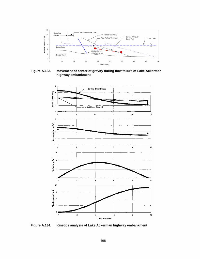
498

Figure A.133. Movement of center of gravity during flow failure of Lake Ackermanhighway embankment

Figure A.134. Kinetics analysis of Lake Ackerman highway embankment

4

6

8

10

12

14

16

5 10 15 20 25 30 35 40 45 50

Distance (m)

Rel

ativ

e El

evat

ion

(m)



Dense Sand

Loose Sand

Soils Consideredin Kinetics Analysis

Center of GravityTravel Path

499

shear strength of 7.3 kPa (based on φ’ = 32°), and the liquefied shear strength was

corrected using Equation (5.13), where su is the liquefied shear strength determined in the

initial kinetics analysis [using Eq. (5.12)], Ld is the length of the post-failure sliding surface

(percent of the total length of the failure surface) that did not liquefy (approximately 14%),

and sd is the average shear strength of the fill soils that did not liquefy (approximately 7.3

kPa).


















500

for void or porewater pressure redistribution during failure. It was assumed that all

hydraulically-placed sand below the lake level liquefied based on the analyses by Hyrciw et

al. (1990). Potential drainage in the toe segment of the slope was considered. The position

of the initial failure surface was not known, however, the description of the failure and the

intact segment of the embankment that came to rest in the lake provided excellent guides

for trial failure surfaces. The embankment material above the phreatic surface was assigned

φ’ = 32° based on DMT results (Hyrciw et al. 1990).





liquefaction are not known with certainty, but all hydraulically-placed sand below the lake

level was assumed to liquefy. The location of the final failure surface was estimated by

examining the post-failure geometry and the stability analyses conducted during this study.

The assumptions regarding the shear strength of non-liquefied soils were discussed above.



penetration tests were conducted after the failure; and (2) the conversion of SPT values to

CPT values. The effect of flow and re-consolidation is unknown, however, the low values

measured in the failure zone agree well with other cases of hydraulically-placed sands

studied herein. “Representative” CPT values were obtained by converting SPT blowcount to

CPT tip resistance. This step involves an unknown level of uncertainty.

501

A.25 CHONAN MIDDLE SCHOOL, CHIBA, JAPAN


The December 17, 1987 Chiba-Toho-Oki earthquake (M = 6.7; amax ~ 0.12g at the

site) caused considerable liquefaction throughout Tokyo Bay and in recent fills in numerous

river valleys. One such relatively well-documented liquefaction failure is the playground

embankment fill of the Chonan Middle School (Ishihara et al. 1990a; Ishihara 1993). Along

the edge of the playground, a small liquefaction-induced slump occurred in the sandy fill.

The slide width was about 30 m. Numerous sand boils also occurred in the playground area.

The site of the failure is shown in Figure A.135.

The pre- and post-failure geometry of the Chonan Middle School fill is shown in

Figure A.136. Approximately 3 m of movement occurred and Ishihara et al. (1990a)

concluded that as a result of the narrow failure zone, sufficient displacement occurred to

mobilized the liquefied shear strength. Ishihara (1993) concluded that a “complete failure

was precluded by the buttress action of a relatively hard crust of surface soil at the toe.” The

toe heaved approximately 1 m as a result of the slide (Figure A.136).


The embankment was constructed around 1960 by excavation of surrounding

hillsides. The borrow soil was placed without compaction to a thickness of 5 to 10 m on the

existing valley floor. Prior to construction of the school buildings, four borings with SPTs

were conducted at locations A-D in Figure A.135. The profile from boring B is presented in

Figure A.137. The profile from the boring indicate that the embankment fill consists primarily

of very fine sand to silty sand, with thin interbeds of clayey sand and sandy silt, to a depth of

approximately 8 m. The fines content of the fill soil is approximately 18%, and the author

502

Figure A.135. Plan view of Chonan Middle School (from Ishihara et al. 1990a)

503

Figure A.136. Cross-section of the slide at Chonan Middle School (from Ishihara et al.1990a)

Figure A.137. Soil profile and SPT results from Chonan Middle School (from Ishihara 1993)

504

estimates the D50 as 0.2 mm, based on the soil description (very fine gradation) and the

fines content. The density of the fill is not available, however, Ishihara (1993) tested

samples prepared by the moist tamping method to match the in situ dry density. These tests

indicated that the sandy fill had a state parameter of approximately 0.07. The unit weight of

the soil was approximately 18.1 kN/m3.

Figure A.136 shows the depth of the original ground surface at the site of the failure.

As seen in the boring log (Figure A.137), the natural soils are primarily dense to very dense

sandy soils, with SPT blowcounts generally over 50.


As aforementioned, four borings with SPT tests were conducted at the site prior to

the earthquake. Unfortunately, only one of these borings is available in the open literature.

In addition to SPT tests, a number of Swedish cone soundings were conducted following the

failure (Figure A.135), including six tests along the failed cross-section (five of which are

shown in Figure A.136).

The SPT blowcounts measured below the phreatic surface were used as the primary

indicator for evaluating penetration resistance. It was assumed that typical Japanese SPT

equipment with an energy ratio of 68% was used (Seed et al. 1985). Swedish sounding

results (converted to SPT blowcounts using the conversion reported by Ishihara 1990a)

were used to confirm the measured SPT blowcounts. Based on these results, the

“representative” (N1)60 value was selected as 5.2, with a range of 2.6 to 8.8.

“Representative” CPT tip resistance values were determined using qc/N60 = 0.5

(Stark and Olson 1995; D50 = 0.2 mm). The resultant “representative” qc1 value is 2.6 MPa,

with a range of 1.8 to 4.4 MPa.

505



The mechanism that likely triggered flow failure is seismic liquefaction of the silty

sand fill. As discussed in Chapter 4, the shear strength and strength ratio mobilized at the





The pre-failure geometry of the Chonan Middle School fill is reproduced in Figure

A.138. This study adopted the initial failure surface suggested by Ishihara et al. (1990a).

This failure surface was developed through review of the pre- and post-failure geometry,

and zones of looser soil identified in the Swedish cone soundings. All submerged fill was

assumed to liquefy (with exceptions) and a single value of shear strength was assigned to

the liquefied soil. Ishihara (1993) measured a drained friction angle of 34° for the

embankment fill soils. This value was assigned to the embankment soils above the phreatic

surface and toe slices (some or all of the material beyond the toe of the slope) that may

have been drained due to their proximity to the ground surface. No inertia forces were

considered in the embankment.

The values of mobilized shear strength in the zone of liquefaction ranged from 12.0

to 12.9 kPa. The best estimate of mobilized shear strength in the zone of liquefaction was

12.2 kPa. Ishihara (1993) also back-calculated a shear strength of 12.2 kPa from the pre-

failure geometry.

506

Figure A.138. Pre-failure geometry of Chonan Middle School used for yield shear strength and strength ratio analyses

Figure A.139. Post-failure geometry of Chonan Middle School used for liquefied shear strength and strength ratio analyses

-2

0

2

4

6

8

0 5 10 15 20 25 30 35

Distance (m)

Rel

ativ

e El

evat

ion

(m)


Post-Failure Geometry Failure Surface

Phreatic Surface

-2

0

2

4

6

8

0 5 10 15 20 25 30 35

Distance (m)

Rel

ativ

e El

evat

ion

(m)


Post-Failure Geometry Failure Surface

Phreatic Surface

507




shear strength of the materials were used for this analysis. The trial failure surface was






0.235, depending on whether or not (and how much) drainage occurred near the toe of the

slope. The weighted average pre-failure vertical effective stress in the liquefied segments




The post-failure geometry is reproduced in Figure A.139. This study adopted the final

failure surface suggested by Ishihara et al. (1990a). This final failure surface was developed

through review of the pre- and post-failure geometry, and zones of looser soil identified in

the Swedish cone soundings. All submerged fill was assumed to liquefy (with exceptions)

and a single value of shear strength was assigned to the liquefied soil. Drainage of toe

slices (some or all of the material beyond the toe of the slope) due to their proximity to the

ground surface was considered. The length of the final failure surface that corresponds to

the embankment material originally above the phreatic surface was assigned φ' = 34°.

508

The back-calculated shear strength was approximately 4.8 kPa, with a possible

range from 3.8 to 6.0 kPa. Ishihara (1993) back-calculated a slightly higher liquefied shear

strength of 6.3 kPa. However, it does not appear that Ishihara (1993) accounted for the

drained shear strength of the original length of the material above the phreatic surface.



analysis of the liquefied strength ratio (as described in Chapter 5) of the upstream slope was

conducted. Using the same assumptions made in the liquefied shear strength analysis, the

liquefied strength ratio was estimated as 0.091, with a possible range from 0.066 to 0.116.

This value of liquefied strength ratio is nearly identical to that of 0.088 measured in

laboratory undrained triaxial compression tests (Ishihara 1993). The weighted average of

vertical effective stress was estimated using Eq. (5.6) as 53.6 kPa.


As indicated by Ishihara (1993), the displacement of the failed mass was limited by

the presence of a hard surface crust at the toe of the embankment slope. Because of the

limited movements, the kinetics analysis was not applicable to this case history.




the initial failure surface; (3) the extent of drainage at the toe of the slope; and (4) the

potential for void or porewater pressure redistribution during failure. It was assumed that all

uncompacted sand below the phreatic surface liquefied based on low values of penetration

509

resistance. The position of the initial failure surface was not known, however, Ishihara et al.

(1990a) suggested a reasonable surface based on the pre- and post-failure geometry and

the location of looser zones from the Swedish cone soundings. Potential drainage in the toe

segments of the slope was considered by varying the shear strength at the toe from the

yield shear strength to the drained shear strength.


strength and strength ratio: (1) limits of the zone of liquefaction; (2) the potential for drainage

at the toe of the slope; and (3) the potential for void and porewater pressure redistribution.

Again, it was assumed that all uncompacted sand below the phreatic surface liquefied

based on low values of penetration resistance. Potential drainage in the toe segments of the

slope was considered by varying the shear strength at the toe from the liquefied shear

strength to the drained shear strength.

The following source of uncertainty was considered in determining the

“representative” values of penetration resistance: (1) the conversion of SPT values to CPT

values. “Representative” CPT values were obtained by converting SPT blowcount to CPT tip

resistance. This step involves an unknown level of uncertainty.

A.26 NALBAND RAILWAY EMBANKMENT, ARMENIA


The December 7, 1988 Armenia earthquake (Ms ~ 6.8) caused extensive damage

throughout northwestern Armenia. More than 40,000 people lost their lives as a result of

earthquake damage. Yegian et al. (1994) documented several cases of liquefaction-induced

ground and slope failure, in particular the failure of a railway embankment near the town of

Nalband. The location of this and other failures is shown in Figure A.140. Yegian et al.

510

Figure A.140. Map of western Armenia and the earthquake damage region with points ofinterest (from Yegian et al. 1994)

Figure A.141. Photo of failed embankment at Nalband railway station (from Yegian et al.1994)

511

(1994) estimated the peak ground acceleration at the site to be between 0.5 and 1.0 g. A

photograph of the failed embankment is shown in Figure A.141.

The pre- and post-failure geometry of the embankment is presented in Figure A.142.

The embankment deformed as much as 2 m laterally and 3 m vertically. Yegian et al. (1994)

evaluated the possibility that the failure was the result of inertia forces and not liquefaction,

but found that inertia forces alone could only account for about 0.5 m of deformation.

Therefore, they concluded that liquefaction of the gravelly sand fill was the cause of the

failure.


The railway embankment is located in the Pambak River valley, which is primarily

filled with deep (140 m) of alluvial silty gravelly sands. Within the alluvium are two primary

layers of volcanic tuff, however, the first layer of tuff is approximately 40 m below the ground

surface. As a result of its proximity to the Pambak River, the watertable within the

embankment was very near or at the ground surface (Figure A.142).

The embankment for the railroad and railroad station at Nalband was constructed by

loosely placing (without compaction) a layer and berm of gravelly sand fill on the naturally

sloping deposit of volcanic tuff (Figure A.142). The grain size distribution of samples of the

gravelly sand was obtained from borings conducted after the earthquake. The gravelly sand

fill has average values of D50 = 1.5 mm, fines content of 20% (10-25%), and gravel content

of 20% (15-40%). Yegian et al. (1994) suggested that this is the layer that liquefied during

the earthquake. The embankment itself consists of compacted silty sand, and appears to

have broken into intact blocks, as shown in Figure A.142. The gravelly sand berm was

overlain by about 0.5 m of “impermeable” vegetative soil that impeded drainage over most of

the failure surface.

512

Figure A.142. Cross-section of railway embankment before and after the earthquake (from Yegian et al. 1994)

513


Standard penetration tests were conducted at the site following the earthquake. It

was assumed that the SPT equipment used at the site had an energy ratio of about 60%.

The correction for gravel content suggested by Terzaghi et al. (1996) was used to account

for the average 20% gravel content of the liquefied soil. Making the appropriate corrections,

the “representative” (N1)60 was 9.2, with a range from 3.6 to 12.4.

Cone penetration tests were not conducted at this site. Therefore, it is necessary to

use a qc/N60 ratio to estimate qc1 values. However, the large D50 value (1.5 mm) is outside

the range of D50 values reported by Stark and Olson (1995). Fortunately, CPTs were

conducted adjacent to SPTs at another failure site in the Pambak River valley through the

same alluvial soils. Comparison of penetration tests results at this site suggests that a value

of qc/N60 = 0.65 is appropriate for the Pambak River valley gravelly sands. Using this qc/N60

value, the “representative” qc1 was 6.0 MPa, with a range from 2.3 to 8.1 MPa.



The mechanism that likely triggered flow failure is seismic liquefaction of the gravelly

sand fill. As discussed in Chapter 4, the shear strength and strength ratio mobilized at the





514

The pre-failure geometry of the Nalband railway embankment is reproduced in

Figure A.143. A limited slope stability search was conducted to determine the critical failure

surface. The search was limited in that it considered only block surfaces and used the basal

sliding plane suggested by Yegian et al. (1994), but searched for the critical sloping portions

of the failure surface. All gravelly sand below the phreatic surface was assumed to liquefy

and a single value of shear strength was assigned to the liquefied soil. The compacted silty

sand embankment material was assumed to be drained and was assigned a drained friction

angle of 30 to 35°. No inertia forces were considered in the slope.

The values of mobilized shear strength in the zone of liquefaction ranged from 8.6 to

9.6 kPa. The best estimate of mobilized shear strength in the zone of liquefaction was 8.9

kPa.



triggering of liquefaction. Identical assumptions regarding the failure surface and shear

strength of the materials were used for this analysis. Trial failure surfaces were divided into

a number of segments, and values of pre-failure vertical effective stress were determined for

each segment. Using these values of pre-failure vertical effective stress and a single value

of strength ratio, various values of mobilized shear strength were assigned to each segment

of the pre-failure geometry.


0.21, dependent on the location of the initial failure surface. The weighted average pre-

failure vertical effective stress in the liquefied segments was determined as 48.9 kPa using

Eq. (4.3).

515

Figure A.143. Pre-failure geometry of Nalband railway embankment used for yield shear strength and strength ratio analyses

Figure A.144. Post-failure geometry of Nalband railway embankment used for liquefied shear strength and strength ratio analyses

2

7

12

17

2 12 22 32 42 52 62 72

Distance (m)

Rel

ativ

e El

evat

ion

(m) Pre-Failure GeometryPost-Failure Geometry

Compacted SiltySand Fill

Volcanic Tuff

Phreatic SurfaceTrial InitialFailure Surfaces

Gravelly Sandwith Silt

2

7

12

17

2 12 22 32 42 52 62 72

Distance (m)

Rel

ativ

e El

evat

ion

(m) Pre-Failure GeometryPost-Failure Geometry

Compacted SiltySand Fill

Volcanic Tuff

Phreatic Surface

Final Failure Surface

Gravelly Sandwith Silt

516





liquefaction probably did not occur in the dense silty sand embankment (Yegian et al. 1994).

Assigning φ' = 30-35° to the length of the final failure surface that corresponds to the length

of material in the pre-failure geometry that did not liquefy (i.e., above the phreatic surface), a

likely range of liquefied shear strengths were obtained.


range from 5.3 to 6.2 kPa. Yegian et al. (1994) back-calculated a similar range of liquefied

shear strengths from 5 to 6.2 kPa.









Because of the limited failure movements, the kinetics analysis was not applicable to

this case history.

517




the initial failure surface; (3) the shear strength of the non-liquefied soils; and (4) the


uncompacted gravelly sand below the phreatic surface liquefied based on low values of

penetration resistance and the severe level of shaking (amax ~ 0.5-1.0g). The position of the

initial failure surface was not known, however, Yegian et al. (1994) suggested a reasonable

surface based on the pre- and post-failure geometry and this surface was finalized using a

slope stability search. The compacted silty sand embankment was assigned φ’ = 35°.


strength and strength ratio: (1) limits of the zone of liquefaction; and (2) the potential for void

and porewater pressure redistribution. Again, it was assumed that all uncompacted gravelly

sand below the phreatic surface liquefied based on low values of penetration resistance and

severe level of shaking.


“representative” values of penetration resistance: (1) the effect of gravel content on SPT

results; and (2) the conversion of SPT values to CPT values. Gravel content can artificially

increase SPT results (Terzaghi et al. 1996). Therefore, SPT blowcounts were reduced for

gravel content as recommended by Terzaghi et al. (1996). “Representative” CPT values

were obtained by converting SPT blowcount to CPT tip resistance. This step involves an

unknown level of uncertainty, particularly given the large value of D50 for this case. However,

as a deposit-specific conversion was used, the uncertainty was decreased.

518

A.27 MAY 1 SLIDE, TAJIKISTAN REPUBLIC, USSR


Ishihara et al. (1990b) described a series of flow slides that developed in the Gissar

area of the Tajikistan, USSR, as a result of the January 23, 1989 Soviet Tajik earthquake

(ML = 5.5). The Gissar area lies along the fault that triggered the earthquake, as shown in

Figure A.145. Records from nearby strong motion seismographs indicated that the Gissar

area probably experienced slightly more than 4 seconds of strong shaking, with a peak

ground acceleration of about 0.15g. The region experienced a damage level corresponding

to a Modified Mercalli Intensity (MMI) of 7.

The flow slides developed in loessial bluffs overlooking the Gissar area. In one

instance, a flow slide developed into 5 m deep mud slides and traveled up to 2 km, killing

about 220 villagers. One of these slides, overlooking the village of May 1, was studied

herein. The May 1 slide encompassed an area approximately 100 m in length and 100 m in

width. The pre- and post-failure geometry of the slide are presented in Figure A.146. This

slide did not progress very far, and a 7 m high pressure ridge developed over the firm knob

of soil near the toe, preventing large lateral displacements. However, Ishihara et al. (1990b)

suggest that the failure zone appeared narrow enough such that the liquefied shear strength

was almost certainly mobilized along the sliding surface.


The Gissar area has a hilly topography consisting of windblown loess. The loess

thickness typically at least 30 to 40 m, overlying a gravelly sand up to 200 m thick. The grain

size distribution of the loess is shown in Figure A.147. The D50 and fines content of the loess

are about 0.012 and 100%, respectively. The clay content is typically about 15%.

519

Figure A.145. Map of Dushanbe and its vicinity, location of Iliakckin fault, and damagezone, intensity distribution, and peak ground accelerations from January1989 earthquake (after Ishihara et al. 1990b)

0.1 g

0.125 g

0.03 g0.06 g

0.03 g0.05 g

0.09 g

0.06 g

7

6

520

Figure A.146. Pre- and post-failure geometry of the slide at May 1 (after Ishihara et al. 1990b)

-10

0

10

20

30

40

-25 0 25 50 75 100 125

Distance (m)

Rel

ativ

e El

evat

ion

(m)

Sliding Surface fromIshihara et al. (1990b)

IrrigationDitch

ApproximatePre-FailurePhreatic Surface

ApproximatePost-FailurePhreatic Surface



521

Figure A.147. Grain size distribution of the loess soil (after Ishihara et al. 1990b)


0

10

20

30

40

50

60

70

80

90

100

0.0010.010.1110100


Perc

ent F

iner

by

Wei

ght

2in

1in

3/4in

1/2in

No4

No20

No40

No60

No100

No200

No10

Silt (Loess)Gissar, Tajik

522

The water content of the loess varies significantly as a result of local irrigation efforts.

As indicated in Figure A.145, a 3 m wide and 2 m deep unlined irrigation channel was

present near the crest of the slope. This resulted in an elevated water table in the slope and

elevated water contents in the loess near the irrigation channel. The general water table is

about 5 m below the ground surface (Ishihara et al. 1990b). The probable pre-failure water

table position is shown in Figure A.146. The depth to the phreatic surface probably changed

as a result of sliding. Further, no ponding of water was noted after the failure. Therefore, the

post-failure phreatic surface was assumed to be at the level shown in Figure A.146.

The depth of cracking in the loess also plays an important role in its saturation and

water content. Ishihara et al. (1990b) indicated that the depth of cracking in the loess was on

the order of 15 to 25 m. The water content of the loess increased from near the plastic limit

at 5 m (at the water table) to water contents in excess of the liquid limit from depths of about

7 to 17 m. Below 20 m, the loess was practically dry, with water contents well below the

plastic limit. Further, at a depth of 15 to 20 m, the permeability of the loess decreases by 4

to 5 orders of magnitude, precluding the infiltration of water. Thus, Ishihara et al. (1990b)

concluded that the loess from depths from 7 to 17 m was on the verge of hydraulic collapse,

and highly susceptible to collapse due to earthquake shaking.


A portable cone penetrometer was used to evaluate penetration resistance (Ishihara

et al. 1990b). The penetration tests were conducted from the bottom of a crack in the post-

failure sliding mass. At the depth of the sliding surface, the qc1 value ranged from

approximately 1.1 to 2.4 MPa, with a “representative” value selected as 1.9 MPa.

523

As no SPT results are available, (N1)60 values were estimated using an CPT-SPT

conversion. Using qc/N60 = 0.25 (Stark and Olson 1995; D50 = 0.012 mm), the

“representative” (N1)60 value was 7.6, with a range from 4.4 to 9.6.




saturated loessial soil from depths of 7 to 17 m, discussed above. As discussed in Chapter

4, the shear strength and strength ratio mobilized at the instant of failure in cases of

liquefaction flow failure triggered by seismic loading do not necessarily represent the yield

shear strength and yield strength ratio, respectively. Therefore, back-calculated shear

strength and strength ratio may not represent the yield shear strength and strength ratio.

The pre-failure geometry of the May 1 slope is reproduced in Figure A.148. This

study adopted the failure surface suggested by Ishihara et al. (1990b), however, the location

of the toe segment was determined by a slope stability search. This failure surface was

developed through review of the pre- and post-failure geometry. All loess was assumed to

liquefy (with exceptions discussed below) and a single value of shear strength was assigned

to the liquefied soil. Toe slices (some or all of the material beyond the toe of the slope) that

may have been drained due to their proximity to the ground surface were assigned a

drained friction angle of 30°. No inertia forces were considered in the slope. A crack depth of

10 m below the bottom of the irrigation channel was incorporated at the scarp.



31.6 kPa.

524

Figure A.148. Pre-failure geometry of May 1 slope used for yield shear strength and strength ratio analyses

Figure A.149. Post-failure geometry of May 1 slope used for liquefied shear strength and strength ratio analyses

-10

0

10

20

30

40

-25 0 25 50 75 100 125

Distance (m)

Rel

ativ

e El

evat

ion

(m)


IrrigationDitch

ApproximatePre-FailurePhreatic Surface



EstimatedCrack Depth

Alternate ToeLocations

-10

0

10

20

30

40

-25 0 25 50 75 100 125

Distance (m)

Rel

ativ

e El

evat

ion

(m)


IrrigationDitch

ApproximatePost-FailurePhreatic Surface



525



triggering of liquefaction. Identical assumptions regarding the failure surface, drainage,

crack depth, and shear strength of the materials were used for this analysis. Trial failure

surfaces were divided into a number of segments, and values of pre-failure vertical effective

stress were determined for each segment. Using these values of pre-failure vertical effective

stress and a single value of strength ratio, various values of mobilized shear strength were

assigned to each segment of the pre-failure geometry.


0.32, dependent on whether or not (and how much) drainage occurred near the toe of the

slope. This value is consistent with static liquefaction flow failures, and is consistent with

Ishihara et al. stating that the slope was on the verge of collapse prior to the earthquake.

The weighted average pre-failure vertical effective stress in the liquefied segments was




The post-failure geometry, with an altered phreatic surface, is reproduced in Figure

A.149. This study adopted the final failure surface suggested by Ishihara et al. (1990b). This

final failure surface was developed through review of the pre- and post-failure geometry. All

initially submerged loess was assumed to liquefy (with exceptions discussed below) and a

single value of shear strength was assigned to the liquefied soil. Drainage of toe segments

526

(some or all of the material beyond the toe of the slope) due to their proximity to the ground

surface was considered. These segments were assigned φ' = 30°.


range from 2.9 to 15.6 kPa. Ishihara (1993) back-calculated a similar liquefied shear

strength of 8.0 kPa.



analysis of the liquefied strength ratio (as described in Chapter 5) of the upstream slope was

conducted. Using the same assumptions made in the liquefied shear strength analysis, the

liquefied strength ratio was estimated as 0.082, with a possible range from 0.026 to 0.16.

The weighted average of vertical effective stress was estimated using Eq. (5.6) as 103.9

kPa.


As indicated by Ishihara et al. (1990b), the displacement of the failed mass was

limited by the presence of a hard natural soil knob at the toe of the slope. Because of the

limited movements, the kinetics analysis was not applicable to this case history.




the initial failure surface; (3) the shear strength of the non-liquefied soils; and (4) the


loess below the phreatic surface liquefied based on the Ishihara et al. (1990b) analysis that

527

suggested the loess from 7-17 m was on the verge of collapse before the earthquake. The

position of the initial failure surface was not known, however, Ishihara et al. (1990b)

suggested a reasonable surface based on the pre- and post-failure geometry and this

surface was finalized using a slope stability search. The loess near the toe was assigned φ’

= 30°.


strength and strength ratio: (1) limits of the zone of liquefaction; and (2) the position of the

post-failure phreatic surface; and (3) the potential for void and porewater pressure

redistribution. Again, it was assumed that all loess between 7 and 17 m below the phreatic

surface liquefied. The position of the post-failure phreatic surface was estimated based on

the post-failure morphology.


“representative” values of penetration resistance: (1) the non-standard cone penetrometer;

and (2) the conversion of CPT to SPT values. No information is available to determine a

correlation between this non-standard cone and the standard cone penetrometer. Thus, this

step involves an unknown level of uncertainty. “Representative” SPT values were obtained

by converting CPT tip resistance to SPT blowcount. This step involves an unknown level of

uncertainty, particularly given the small value of D50 for this case.

A.28 SHIBECHA-CHO EMBANKMENT, JAPAN


The January 15, 1993 Kushiro-Oki earthquake (M = 7.8) caused considerable

damage in the city of Kushiro, Hokkaido and the surrounding region. In particular, flow

528

failure-type deformations occurred in an embankment in the Kayanuma district, Shibecha-

cho, about 30 km north-northwest of Kushiro (Miura et al. 1995, 1998). Miura et al.

(1995;1998) estimated a peak ground acceleration of 0.38g (measured at a nearby rock

outcrop) for the site.

Figures A.150 and A.151 present the plan view of the Shibecha-cho embankment

and resort housing district and the pre- and post-failure geometry along section line B-B,

respectively. The embankment suffered severe cracking, slumping and flow over an

approximately 200 m long section. All damage to the resort houses occurred in fill areas.

The houses constructed in cut areas typically were undamaged.

Miura et al. (1995; 1998) indicated that the damage to the embankment was most

severe along section B-B. At this location, the embankment displaced a maximum of 5 m

vertically and approximately 23.5 m laterally from the original embankment toe.


The embankment was constructed by cutting back the existing hillsides and using

this material as fill for the embankment. The hillsides are part of the Early Pleistocene

Terrace group that consists of volcanic ash known as the Kussharo Pumice Flow Deposit

and deposits of sand, gravel and clay. At the base of the hillsides, the valley is 15 m above

sea level and is overlaid by a soft peat deposit. Miura et al. (1995;1998) indicated that the

peat was undisturbed as the result of the failure.

The embankment fill consists primarily of volcanic silty sand and received some

compaction from construction traffic, but was not compacted in any controlled manner.

Figure A.152 shows the grain size distribution of the terrace material that was used as a

borrow source and of a sample obtained from a sand boil. The D50 of the silty sand fill

ranges from about 0.12 to 0.4 mm, with an average value of about 0.2 mm. The fines

529

Figure A.150. Areal depiction of resort development and damage pattern during 1993Kushiro-oki earthquake (from Miura et al. 1998)

Figure A.151. Cross-sections along four profile lines in Figure B.150 (from Miura et al.1998)

530

Figure A.152. Grain size distributions of the fill soils at Shibecha-cho (after Miura et al. 1998)


0

10

20

30

40

50

60

70

80

90

100

0.0010.010.1110100


Perc

ent F

iner

by

Wei

ght

2in

1in

3/4in

1/2in

No4

No20

No40

No60

No100

No200

No10

Boiled Sand(Mori 1993)

Colluvial Deposit(Yasuda et al. 1993)

Colluvial Deposit(Saito and Ine 1993)

531

content of the fill ranges from about 12 to 35%, with an average of about 20%. The unit

weight of the soil is approximately 15 kN/m3.

The phreatic surface in the embankment is as shown in Figure A.151 (Miura et al.

1998).


Only Swedish cone penetration tests were conducted following the earthquake.

Therefore, SPT blowcounts were estimated from the Swedish cone results using the

correlation in Ishihara et al. (1990a). CPT tip resistance was estimated using qc/N60 = 0.5

(Stark and Olson 1995; D50 ~ 0.2 mm). Four Swedish cone soundings were conducted along

section B-B, as shown in Figure A.151. Miura et al. (1995; 1998) analyzed the triggering of

liquefaction using finite element procedures, and concluded that all the fill below the phreatic

surface liquefied during the earthquake. Therefore, Swedish cone results measured below

the water level were used to evaluate “representative” penetration resistance values.

The “representative” (N1)60 value was selected as 5.6, with a range from 2.9 to 10.7.

The “representative” qc1 value was selected as 2.8 MPa, with a range from 1.5 to 5.4 MPa.




saturated silty sand fill (Miura et al. 1995; 1998). As discussed in Chapter 4, the shear

strength and strength ratio mobilized at the instant of failure in cases of liquefaction flow

failure triggered by seismic loading do not necessarily represent the yield shear strength and

532

yield strength ratio, respectively. Therefore, back-calculated values of shear strength and

strength ratio likely do not represent the yield shear strength and yield strength ratio.

The pre-failure geometry of the Shibecha-cho embankment section B-B is

reproduced in Figure A.153. A slope stability search was conducted to evaluate the location

of the initial failure surface. This search was guided by the post-failure morphology, where

the location of the face of the embankment can be seen in the post-failure geometry. All

submerged silty sand fill was assumed to liquefy (with exceptions discussed below) and a

single value of shear strength was assigned to the liquefied soil. Fill soil initially above the

phreatic surface and toe slices that may have been drained due to their proximity to the

ground surface were assigned a drained friction angle of 35° (Miura et al. 1998). No inertia

forces were considered in the embankment.



15.8 kPa.




shear strength of the materials were used for this analysis. Trial failure surfaces were






0.32, dependent on whether or not (and how much) drainage occurred near the toe of

533

Figure A.153. Pre-failure geometry of Shibecha-cho embankment used for yield shear strength and strength ratio analyses

Figure A.154. Post-failure geometry of Shibecha-cho embankment used for liquefied shear strength and strength ratio analyses

0

5

10

15

20

0 10 20 30 40 50 60 70 80 90

Distance (m)

Rel

ativ

e el

evat

ion

(m)

Peat

Base SoilPhreatic Surface

FillSoils




0

5

10

15

20

0 10 20 30 40 50 60 70 80 90

Distance (m)

Rel

ativ

e el

evat

ion

(m)

Peat


FillSoils



Final FailureSurfaces

534

the slope. The weighted average pre-failure vertical effective stress in the liquefied

segments was determined as 66.6 kPa using Eq. (4.3).



The post-failure geometry of Shibecha-cho embankment section B-B is reproduced

in Figure A.154. Trial failure surfaces were derived from the post-failure morphology of the

sliding mass and a slope stability search as shown in Figure A.154. The length of the final

failure surface that corresponds the embankment material above the phreatic surface was

assigned φ' = 30-35°. The resulting back-calculated liquefied shear strength was 5.0 kPa,

with a range from 4.1 to 6.2 kPa.







(5.6) as 64.7 kPa.



also shows the pre-and post-failure centers of gravity and the probable path of travel of the

center of gravity during flow failure. The kinetics analysis discounted material to the left of

535

Figure A.155. Movement of center of gravity during flow failure of Shibecha-choembankment

Figure A.156. Kinetics analysis of Shibecha-cho embankment

0

5

10

15

20

0 10 20 30 40 50 60 70 80 90

Distance (m)

Rel

ativ

e el

evat

ion

(m)

Peat


FillSoils



Soils Incorporatedin Kinetics Analysis


536

the initial failure surface shown in Figure A.155 because this portion of the embankment

appears only to be involved in secondary sliding or slumping and not part of the main flow

failure. This argument is supported an area balance analysis and by the finite element

analyses conducted by Miura et al. (1995; 1998). Therefore, calculation of the center of

gravity positions did not include the weights of this area.




surface and did not liquefy. Therefore, the liquefied shear strength was adjusted to account

for the strength of the non-liquefied soils. Approximately 16% of the post-failure sliding

surface length probably involved fill soils initially above the phreatic surface. This length of

the failure surface was assigned an average shear strength of 19.2 to 23.9 kPa,

respectively, and the liquefied shear strength was corrected using Eq. (5.13). The shear

strength of the silty sand fill was estimated using φ' = 30-35°.











537






strength and strength ratio: (1) the position of the initial failure surface; (2) the shear strength

of the non-liquefied soils; and (3) the potential for void or porewater pressure redistribution

during failure. The position of the initial failure surface was not known. However, using a

slope stability search and comparing this to the post-failure morphology and intact portion of

the embankment allowed some confidence in locating the yield failure surface. The

unsaturated fill was assigned φ’ = 35°.


strength and strength ratio and kinetics analyses: (1) the effect of secondary sliding and

slumping on the kinetics analysis; and (2) the potential for void and porewater pressure

redistribution. As discussed earlier, the post-failure morphology suggests that considerable

secondary slumping occurred which did not affect the position of the sliding mass toe.

Similar to the Lower San Fernando Dam analysis, this material was excluded from the

kinetics analysis.


“representative” values of penetration resistance: (1) conversion of Swedish cone

penetration resistance to SPT values; and (2) the conversion of SPT to CPT values. The

step of converting Swedish cone results to SPT blowcounts involves an unknown level of

uncertainty. “Representative” CPT values were obtained by converting SPT blowcount to

CPT tip resistance. This step also involves an unknown level of uncertainty.

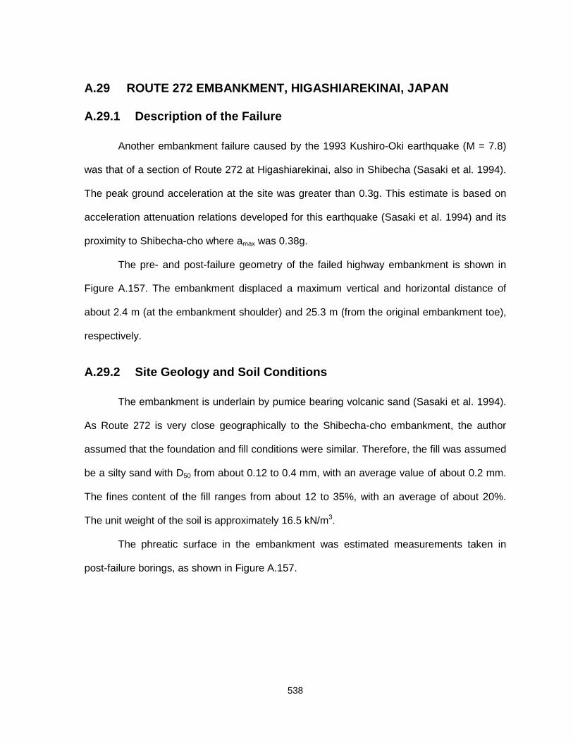
538

A.29 ROUTE 272 EMBANKMENT, HIGASHIAREKINAI, JAPAN


Another embankment failure caused by the 1993 Kushiro-Oki earthquake (M = 7.8)

was that of a section of Route 272 at Higashiarekinai, also in Shibecha (Sasaki et al. 1994).

The peak ground acceleration at the site was greater than 0.3g. This estimate is based on

acceleration attenuation relations developed for this earthquake (Sasaki et al. 1994) and its

proximity to Shibecha-cho where amax was 0.38g.

The pre- and post-failure geometry of the failed highway embankment is shown in

Figure A.157. The embankment displaced a maximum vertical and horizontal distance of

about 2.4 m (at the embankment shoulder) and 25.3 m (from the original embankment toe),

respectively.


The embankment is underlain by pumice bearing volcanic sand (Sasaki et al. 1994).

As Route 272 is very close geographically to the Shibecha-cho embankment, the author

assumed that the foundation and fill conditions were similar. Therefore, the fill was assumed

be a silty sand with D50 from about 0.12 to 0.4 mm, with an average value of about 0.2 mm.

The fines content of the fill ranges from about 12 to 35%, with an average of about 20%.

The unit weight of the soil is approximately 16.5 kN/m3.

The phreatic surface in the embankment was estimated measurements taken in

post-failure borings, as shown in Figure A.157.

539

Figure A.157. Cross-section of Route 272 highway embankment before and after the 1993 Kushiro-Oki earthquake (from Sasakiet al. 1994)

540


SPT blowcounts were measured in the failed fill. It was assumed that the Japanese

SPT equipment had an energy ratio of 72% (Seed et al. 1985; Ishihara 1993). The

“representative” (N1)60 value for the fill soils below the phreatic surface was 6.3, with a range

from 2.4 to 10.

CPT penetration resistance was estimated using qc/N60 = 0.5 (Stark and Olson 1995;

D50 ~ 0.2 mm). The resulting “representative” qc1 value was 3.2 MPa, with a range from 1.2

to 5 MPa.




saturated silty sand fill (Sasaki et al. 1994). As discussed in Chapter 4, the shear strength

and strength ratio mobilized at the instant of failure in cases of liquefaction flow failure

triggered by seismic loading do not necessarily represent the yield shear strength and yield

strength ratio, respectively. Therefore, back-calculated values of shear strength and strength

ratio likely do not represent the yield shear strength and yield strength ratio.

The pre-failure geometry of the Route 272 embankment is reproduced in Figure

A.158. A slope stability search was conducted to locate the initial failure surface. All

submerged fill was assumed to liquefy (with exceptions) and a single value of shear strength

was assigned to the liquefied soil. Fill soil initially above the phreatic surface was assigned a

drained friction angle of 30-35° (Miura et al. 1998). No inertia forces were considered in the

embankment.

541

Figure B.158. Pre-failure geometry of Route 272 embankment used for yield shear strength and strength ratio analyses

Figure B.159. Post-failure geometry of Route 272 embankment used for liquefied shear strength and strength ratio analyses

8

12

16

20

0 10 20 30 40 50 60

Distance (m)

Rel

ativ

e El

evat

ion

(m)

Volcanic Sand and TuffDense Fine Sand to Silt

Pre-Failure Geometry Post-Failure GeometryPhreaticSurface


8

12

16

20

0 10 20 30 40 50 60

Distance (m)

Rel

ativ

e El

evat

ion

(m)




542



13.1 kPa.



triggering of liquefaction. Identical assumptions regarding the failure surface and shear

strength of the materials were used for this analysis. Trial failure surfaces were divided into

a number of segments, and values of pre-failure vertical effective stress were determined for

each segment. Using these values of pre-failure vertical effective stress and a single value

of strength ratio, various values of mobilized shear strength were assigned to each segment

of the pre-failure geometry.


0.255, depending on the shear strength of the unsaturated fill and the location of the failure

surface. The weighted average pre-failure vertical effective stress in the liquefied segments




The post-failure geometry of Route 272 embankment is reproduced in Figure A.159.

Trial failure surfaces were derived from the post-failure morphology of the sliding mass and

a slope stability search as shown in Figure A.159. The length of the final failure surface that

corresponds the embankment material above the phreatic surface was assigned φ' = 30-35°.

543

The resulting back-calculated liquefied shear strength was 2.9 kPa, with a range from 2.9 to

3.0 kPa.







(5.6) as 49.3 kPa.



also shows the pre-and post-failure centers of gravity and the probable path of travel of the

center of gravity during flow failure.




surface and did not liquefy. Therefore, the liquefied shear strength was adjusted to account

for the strength of the non-liquefied soils. Approximately 9% of the post-failure sliding

surface length probably involved fill soils initially above the phreatic surface. This length of

the failure surface was assigned an average shear strength of 9.6-11.5 kPa, respectively,

and the liquefied shear strength was corrected using Eq. (5.13). The shear strength of the

silty sand fill was estimated using φ' = 30-35°.

544

Figure A.160. Movement of center of gravity during flow failure of Route 272embankment

Figure A.161. Kinetics analysis of Route 272 embankment

8

12

16

20

0 10 20 30 40 50 60

Distance (m)

Rel

ativ

e El

evat

ion

(m)



Final SlidingSurface


545












strength ratio include the effects of kinetics and the shear strength of the soils that did not

liquefy.



strength and strength ratio: (1) the initial zone of liquefaction; (2) the position of the initial

failure surface; (3) the shear strength of the non-liquefied soils; and (4) the potential for void

or porewater pressure redistribution during failure. It was assumed that all fill soil below the

phreatic surface liquefied. This is consistent with the analyses for Shibecha-cho

embankment, which exhibited similar conditions. The position of the initial failure surface

was not known. However, using a slope stability search and comparing this to the post-

failure morphology allowed some confidence in locating the yield failure surface. The

unsaturated fill was assigned φ’ = 30-35°.

546


strength and strength ratio and kinetics analyses: (1) the limits of the zone of liquefaction;

and (2) the potential for void and porewater pressure redistribution. As discussed above, all

fill below the phreatic surface was assumed to liquefy.


values of penetration resistance: (1) effects of flow and reconsolidation on penetration

resistance because the penetration tests were conducted after the failure; and (2) the

conversion of SPT values to CPT values. The effect of flow and re-consolidation is

unknown, however, the low values measured in the failure zone agree well with the

Shibecha-cho embankment case history. “Representative” CPT values were obtained by

converting SPT blowcount to CPT tip resistance. This step involves an unknown level of

uncertainty.

liquefaction analysis of level and sloping ground using - MAE ...

Documents

Transcript of liquefaction analysis of level and sloping ground using - MAE ...