soil liquefaction hazard assessment along - University of Malaya
234
SOIL LIQUEFACTION HAZARD ASSESSMENT ALONG SHORELINE OF PENINSULAR MALAYSIA HUZAIFA BIN HASHIM FACULTY OF ENGINEERING UNIVERSITY OF MALAYA KUALA LUMPUR 2017 University of Malaya
-
Upload
khangminh22 -
Category
Documents
-
view
1 -
download
0
Transcript of soil liquefaction hazard assessment along - University of Malaya

SOIL LIQUEFACTION HAZARD ASSESSMENT ALONG SHORELINE OF PENINSULAR MALAYSIA
HUZAIFA BIN HASHIM
FACULTY OF ENGINEERING
UNIVERSITY OF MALAYA KUALA LUMPUR
2017
Univers
ity of
Mala
ya

SOIL LIQUEFACTION HAZARD ASSESSMENT
ALONG SHORELINE OF PENINSULAR MALAYSIA
HUZAIFA BIN HASHIM
THESIS SUBMITTED IN FULFILMENT OF THE
REQUIREMENTS FOR THE DEGREE OF DOCTOR OF
PHILOSOPHY
FACULTY OF ENGINEERING
UNIVERSITY OF MALAYA
KUALA LUMPUR
2017 Univers
ity of
Mala
ya

ii
UNIVERSITY OF MALAYA
ORIGINAL LITERARY WORK DECLARATION
Name of Candidate: HUZAIFA BIN HASHIM
Matric No: KHA110047
Name of Degree: DOCTOR OF PHILOSOPHY
Title of Project Paper/Research Report/Dissertation/Thesis (―this Work‖):
SOIL LIQUEFACTION HAZARD ASSESSMENT ALONG SHORELINE OF
PENINSULAR MALAYSIA
Field of Study: GEOTECHNICAL ENGINEERING
I do solemnly and sincerely declare that:
(1) I am the sole author/writer of this Work;
(2) This Work is original;
(3) Any use of any work in which copyright exists was done by way of fair
dealing and for permitted purposes and any excerpt or extract from, or
reference to or reproduction of any copyright work has been disclosed
expressly and sufficiently and the title of the Work and its authorship have
been acknowledged in this Work;
(4) I do not have any actual knowledge nor do I ought reasonably to know that
the making of this work constitutes an infringement of any copyright work;
(5) I hereby assign all and every rights in the copyright to this Work to the
University of Malaya (―UM‖), who henceforth shall be owner of the
copyright in this Work and that any reproduction or use in any form or by any
means whatsoever is prohibited without the written consent of UM having
been first had and obtained;
(6) I am fully aware that if in the course of making this Work I have infringed
any copyright whether intentionally or otherwise, I may be subject to legal
action or any other action as may be determined by UM.
Candidate‘s Signature Date: 17/08/17
Subscribed and solemnly declared before,
Witness‘s Signature Date:
Name:
Designation:
Univers
ity of
Mala
ya

iii
ABSTRACT
The thesis provides a complete liquefaction potential hazard study for shoreline of
1972 km covering 40 shoreline districts of 11 major states of Peninsular Malaysia. Two
main aspects are considered in defining soil liquefaction study which consists of
regional geotechnical settings and regional seismicity information. 4 interrelating
approaches are introduced in study; soil liquefaction screening, cyclic triaxial testing,
earthquake study and liquefaction hazard mapping. In this study, governing factors
contributing to soil liquefaction hazard were selected and adapted in soil liquefaction
screening in highlighting soil liquefaction potential areas. The cyclic loading was
applied on sand and clay samples to establish the shear modulus reduction curves and
damping ratio curves that represents regional soil performance for seismic response.
Probabilistic seismic hazard analysis (PSHA), spectrum matching procedure (SMP) and
site response analysis (SRA) was adapted in seismic study in generating ground motion
of studied sites. Soil liquefaction assessment approach based on Simplified Procedure
was used in developing the hazard map for shoreline of Peninsular Malaysia. A
mitigation chart is also introduced the in the study as a precursory measure in promoting
safe built environment in the region. Findings revealed that shoreline area consist of
vulnerable conditions to soil liquefaction hazard. The ground motion generated presents
high amplification factor on the east coast region of Peninsular Malaysia specifically in
the state of Terengganu and Kelantan. In general, the hazard map produced indicates
that shoreline areas are vulnerable to soil liquefaction hazard. This soil liquefaction
study will contribute towards promoting preparedness and enhanced awareness in the
changing environment in today‘s context.
Univers
ity of
Mala
ya
iv
ABSTRAK
Tesis ini merangkumi kajian menyeluruh mengenai potensi pencecairan tanah di
sepanjang pantai yang berukuran 1972 km meliputi 40 daerah pantai dalam 11 negeri di
Semenanjung Malaysia. Kajian ini terbahagi kepada 2 aspek penting iaitu keadaan
geoteknik dan juga keadaan seismik kawasan kajian. 4 kaedah yang berkait dalam
kajian ini adalah penapisan kawasan pencecairan tanah, ujian kitaran 3-paksi, kajian
gempa bumi dan peta bahaya pencecairan tanah. Di dalam kajian ini, faktor-faktor
penyumbang kepada pencecairan tanah telah dipilih dan diterapkan kedalam penapisan
kawasan pencecairan tanah untuk mengenal pasti kawasan yang berpotensi kepada
bahaya pencecairan tanah. Beban kitaran yang dikenakan ke atas sampel tanah pasir dan
tanah liat telah menghasilkan beberapa parameter tanah untuk mengkaji prestasi tanah
terhadap beban yang dikenakan. Analisa kebarangkalian bahaya seismik (PSHA),
prosedur persamaan spektrum (SMP) dan analisa tindakbalas lapangan (SRA) telah
digunakan untuk menjana ciri-ciri gempa di kawasan kajian. Analisis pencecairan
menggunakan kaedah mudah telah diterapkan dalam kajian untuk menghasilkan peta
bahaya pencecairan tanah di sepanjang pantai Semenanjung Malaysia. Carta mitigasi
juga telah dihasilkan untuk tujuan langkah berjaga-jaga ke arah pembangunan yang
lebih selamat di rantau ini. Hasil kajian mendapati kawasan-kawasan yang berpotensi
terhadap bahaya pencecairan tanah. Ciri-ciri gempa bumi yang dihasilkan adalah
kritikal di negeri Terengganu dan negeri Kelantan. Secara amnya, peta yang dihasillkan
menunjukkan kawasan kajian mempunyai potensi terhadap bahaya pencecairan tanah.
Kajian pencecairan tanah ini merupakan penyumbang kepada langkah-langkah berjaga-
jaga dan peningkatan kesedaran terhadap bahaya-bahaya alam di persekitaran.
Univers
ity of
Mala
ya

v
ACKNOWLEDGEMENTS
All praise is due to هللا we praise Him and seek His aid and forgiveness. Furthermore, we
seek refuge in هللا from our souls‘ and actions‘ evil. Whomsoever هللا guides there is none
to misguide, and whomsoever هللا misguide there is none to guide. I bear witness there is
none worthy of worship except هللا and that (ملسو هيلع هللا ىلص) دمحم is His slave and messenger.
Secondly I would like to thank my family, especially Wan Samsiah binti Wan Latif and
Hashim bin Abdul Razak for the continuous comfort, warmness and hospitality
throughout my days.
In preparing this thesis, I was in contact with academicians, and practitioners. They
have contributed towards my understanding on study. In particular, I wish to express my
sincere appreciation to my supervisor, Dr. Meldi Suhatril, for the encouragement,
guidance, critics and friendship. I am also thankful to Prof. Ir. Dato‘ Dr. Roslan bin
Hashim and Dr Hendriyawan for the guidance, advices and motivation. Without their
continued support and interest, this thesis would not have been the same as presented
here.
I am also indebted to University of Malaya (UM) for providing the research facilities.
Staff at the Engineering Faculty also deserves special thanks for their assistance. I also
like to extend my thanks to Ministry of Education Malaysia, Jabatan Kerja Raya (JKR)
and Kumpulan IKRAM Sdn. Bhd. My fellow postgraduate combats should also be
recognized for their support at various occasions. Their views and tips are useful indeed.
Lastly the reviewers for all the motivation and encouragement. Unfortunately, it is not
possible to list all of them in this limited space.
Huzaifa bin Hashim
Univers
ity of
Mala
ya

vi
TABLE OF CONTENTS
Abstract ............................................................................................................................ iii
Abstrak ............................................................................................................................. iv
Acknowledgements ........................................................................................................... v
Table of Contents ............................................................................................................. vi
List of Figures ................................................................................................................... x
List of Tables................................................................................................................. xvii
List of Symbols and Abbreviations ................................................................................ xix
CHAPTER 1: INTRODUCTION .................................................................................. 1
1.1 Soil Liquefaction Hazard ......................................................................................... 2
1.2 Aim of Study ........................................................................................................... 3
1.3 Problem Statement ................................................................................................... 3
1.4 Objectives of Study.................................................................................................. 4
1.5 Scope of Work ......................................................................................................... 4
CHAPTER 2: LITERATURE REVIEW ...................................................................... 5
2.1 Historical Liquefaction Events ................................................................................ 6
2.2 Soil Liquefaction Susceptibility ............................................................................ 11
2.2.1 Soil Liquefaction Susceptibility ............................................................... 12
2.2.2 Groundwater Table ................................................................................... 14
2.2.3 Soil Type .................................................................................................. 14
2.2.4 Particle Size Gradation ............................................................................. 17
2.2.5 Malaysia‘s Context in Soil Liquefaction Hazard ..................................... 18
2.3 Regional Data Collection ....................................................................................... 21
2.3.1 Regional Geological Content ................................................................... 21
Univers
ity of
Mala
ya

vii
2.3.2 Regional Seismicity and Ground Motion ................................................. 24
2.3.3 Regional Hydrogeological ........................................................................ 28
2.3.4 Regional and Neighboring Hazard Map ................................................... 30
2.3.5 Regional Seismic Hazard Analysis .......................................................... 33
2.4 Liquefaction Hazard Assessment .......................................................................... 37
2.4.1 The Padang Earthquake 2009 ................................................................... 37
2.4.2 The Tohoku Earthquake 2011 .................................................................. 39
2.4.3 The Christchurch Earthquake 2010 – 2011 .............................................. 43
2.5 Literature Review Summary .................................................................................. 45
CHAPTER 3: METHODOLOGY ............................................................................... 46
3.1 Soil Liquefaction Screening .................................................................................. 46
3.1.1 Studied location ........................................................................................ 47
3.1.2 Database of Soil Collection ...................................................................... 48
3.1.3 Site Investigation Report .......................................................................... 50
3.1.4 SI Report, Soil Sampling, SPT-N correction ........................................... 51
3.1.5 Illustrations, Chart and Tabulated Information ........................................ 51
3.2 Cyclic Triaxial Testing .......................................................................................... 53
3.2.1 Laboratory Testing Program..................................................................... 53
3.2.2 Materials ................................................................................................... 61
3.2.3 Controlled Parameters and Parameters Obtained from Dynamic Cyclic
Triaxial Tests ............................................................................................ 63
3.3 Earthquake Study ................................................................................................... 64
3.3.1 Probabilistic Seismic Hazard Analysis (PSHA) ....................................... 64
3.3.2 Spectral Matching Procedure (SMP) ........................................................ 69
3.3.3 Site Response Analysis (SRA) ................................................................. 71
3.4 Liquefaction Hazard Mapping ............................................................................... 75
Univers
ity of
Mala
ya

viii
3.4.1 Simplified Procedure by Seed and Idriss ................................................. 76
3.4.2 Soil Strength Measurement from SPT ...................................................... 82
3.4.3 Soil Liquefaction Method Adapted in Study ............................................ 87
3.4.4 Liquefaction Factor of Safety ................................................................... 91
3.4.5 Addressing Liquefaction Severity ............................................................ 91
CHAPTER 4: RESULTS AND DISCUSSIONS ........................................................ 93
4.1 Soil Liquefaction Screening .................................................................................. 93
4.1.1 Perlis ......................................................................................................... 93
4.1.2 Kedah ........................................................................................................ 97
4.1.3 Penang .................................................................................................... 102
4.1.4 Perak ....................................................................................................... 107
4.1.5 Selangor .................................................................................................. 110
4.1.6 Negeri Sembilan ..................................................................................... 114
4.1.7 Melaka .................................................................................................... 118
4.1.8 Johor ....................................................................................................... 122
4.1.9 Pahang .................................................................................................... 128
4.1.10 Terengganu ............................................................................................. 132
4.1.11 Kelantan .................................................................................................. 136
4.1.12 Susceptibility of Soil at Study Location ................................................. 140
4.1.13 Summary ................................................................................................ 147
4.2 Cyclic Triaxial Test ............................................................................................. 149
4.2.1 Soil Liquefaction Observation ................................................................ 149
4.2.2 Stress-Strain Behavior ............................................................................ 152
4.2.3 Shear Modulus Reduction and Damping Ratio Curves .......................... 153
4.2.4 Summary ................................................................................................ 155
4.3 Earthquake Study ................................................................................................. 156
Univers
ity of
Mala
ya

ix
4.3.1 Probabilistic Seismic Hazard Assessment (PSHA) ................................ 156
4.3.1.1 Generation and Simulation of Synthetic Ground Motion ....... 156
4.3.1.2 De-Aggregation Hazard .......................................................... 161
4.3.1.3 Scaled Spectrum ...................................................................... 167
4.3.2 Generation and Simulation of Synthetic Ground Motion ...................... 169
4.3.3 Microzonation Line (Amplification Factor) ........................................... 176
4.3.4 Comparative Study of Recent Findings to Previous Works ................... 184
4.3.5 Summary ................................................................................................ 185
4.4 Liquefaction Hazard Assessment and Mapping .................................................. 187
4.4.1 Graphical Illustration of Liquefaction Zones ......................................... 187
4.4.2 Liquefaction Hazard Map ....................................................................... 195
4.4.3 Mitigation Zoning ................................................................................... 196
4.4.4 Summary ................................................................................................ 200
CHAPTER 5: CONCLUSION AND RECOMMENDATION ............................... 201
5.1 Conclusions ......................................................................................................... 201
5.2 Recommendation for Future Work ...................................................................... 202
5.3 Implication and Application of Study ................................................................. 202
References ..................................................................................................................... 203
List of Publications and Papers Presented .................................................................... 213
Univers
ity of
Mala
ya

x
LIST OF FIGURES
Figure 1.1: Normal condition at site ................................................................................. 2
Figure 1.2: Soil liquefaction condition at site ................................................................... 2
Figure 2.1: Side by side damage in Japan and New Zealand due to liquefaction (Aydan
et al., 2012; Tokimatsu et al., 2012; Wilkinson et al., 2013) .......................................... 10
Figure 2.2: Liquefaction plot (Tsuchida, 1970). ............................................................. 17
Figure 2.3: The National Physical Plan (Bhuiyan et al., 2013)....................................... 19
Figure 2.4: Malaysia Tourism Master Plan (Marzuki, 2010) ......................................... 20
Figure 2.5: 8th edition of Peninsular Malaysia geological map (Hutchison, 1989) ....... 22
Figure 2.6: Recent Peninsular Malaysia geological map (Tate et al., 2008) .................. 23
Figure 2.7: Plate boundaries of earth (DeMets et al., 2010). .......................................... 24
Figure 2.8: Earthquakes catalog (Adnan et al., 2006) ..................................................... 25
Figure 2.9: Seismotectonic map of Peninsular Malaysia (Ngah et al., 1996) ................. 27
Figure 2.10: Open arrows show velocities of neighboring plates (Gao et al., 2011) ...... 28
Figure 2.11: Hydrogeological map of Peninsular Malaysia (Chong & Pfeiffer, 1975) .. 29
Figure 2.12: Hazard map of Thailand (Ornthammarath et al., 2011) ............................. 30
Figure 2.13: Co-seismic deformation model (Vigny et al., 2005) .................................. 32
Figure 2.14: Hazard map of Malaysia (Petersen et al., 2004) ......................................... 33
Figure 2.15: De-aggregation in Kuala Lumpur (Petersen et al., 2004) ........................... 34
Figure 2.16: PGA contour map 10% PE in 50 years (Irsyam et al., 2008) ..................... 35
Figure 2.17: Deaggregation hazard and scaled response spectra (Irsyam et al., 2008) .. 35
Figure 2.18: Seismic maps of Thailand and adjacent areas (Pailoplee et al., 2010) ....... 36
Figure 2.19: Grain size distribution plot (Muntohar, 2014) ............................................ 38
Figure 2.20: Soil Liquefaction in Padang (Hakam & Suhelmidawati, 2013) ................. 38
Figure 2.21: Grain size distribution plot (Hakam & Suhelmidawati, 2013) ................... 38
Univers
ity of
Mala
ya

xi
Figure 2.22: Grain size distribution plot (Unjoh et al., 2012) ......................................... 40
Figure 2.23: Grain size distribution plot (Tsukamoto et al., 2012) ................................. 40
Figure 2.24: Liquefaction affected site (Tsukamoto et al., 2012) ................................... 41
Figure 2.25: Erupted ground due to soil liquefaction (Tsukamoto et al., 2012) ............. 42
Figure 2.26: Soil profile of the studied area (Tsukamoto et al., 2012) ........................... 42
Figure 2.27: A map highlighting soil details (Wotherspoon et al., 2015) ....................... 43
Figure 2.28: Grain size distribution plot (Green et al., 2013) ......................................... 44
Figure 2.29: Soil profile observation on liquefy site (Green et al., 2013) ...................... 44
Figure 2.30: Site investigation on liquefy site (Green et al., 2013) ................................ 44
Figure 3.1: Main process in soil liquefaction screening ................................................. 46
Figure 3.2: Distribution of studied borehole along shoreline ......................................... 47
Figure 3.3: Typical borelog properties from SI report .................................................... 50
Figure 3.4: Set-up of the cyclic triaxial test .................................................................... 53
Figure 3.5: Actuator on test system ................................................................................ 54
Figure 3.6: Power up electronics at the base of system .................................................. 54
Figure 3.7: Dynamic control system (bottom) and pneumatic controller (top) .............. 54
Figure 3.8: Standard controller for backpressure ............................................................ 55
Figure 3.9: PC system with pre-installed software ......................................................... 56
Figure 3.10: Object/Hardware window ........................................................................... 57
Figure 3.11: Triaxial cell installed on the main load frame ............................................ 58
Figure 3.12: Sample preparation on the base plate of the load frame ............................. 60
Figure 3.13: Soil samples used in lab works ................................................................... 61
Figure 3.14: Particle size distribution of sands ............................................................... 62
Figure 3.15: Fault source model...................................................................................... 67
Univers
ity of
Mala
ya

xii
Figure 3.16: Logic Tree used in the analysis (Megathrust) ............................................ 68
Figure 3.17: Logic Tree used in the analysis (Benioff) .................................................. 69
Figure 3.18: 1-D layered soil deposit system (Bardet & Tobita, 2001) ......................... 74
Figure 3.19: General terminology in SRA (Bardet & Tobita, 2001) .............................. 74
Figure 3.20: SPT-Based empirical method (Seed & Idriss, 1971) adapted in study ...... 75
Figure 3.21: Early liquefaction chart by (Seed, 1976) .................................................... 77
Figure 3.22: Revised liquefaction chart by Youd and Idriss (2001) ............................... 78
Figure 3.23: Sketch of common approach in Simplified Procedure ............................... 80
Figure 3.24: Equivalent cycles versus earthquake magnitude (Seed, 1976) ................... 81
Figure 3.25: Stress reduction factor versus depth (Andrus & Stokoe II, 2000) .............. 82
Figure 3.26: Magnitude Scaling Factor versus magnitude.............................................. 83
Figure 3.27: Correction factor ‘o (Seed et al., 1983) .................................................... 86
Figure 3.28: Correction factor for ‘o (Liao & Whitman, 1986) ................................... 87
Figure 3.29: Typical borehole information in Kelantan district ..................................... 88
Figure 3.30: CRR7.5 using different approach ................................................................. 90
Figure 3.31: Factor of safety using different approach ................................................... 90
Figure 4.1: Kuala Perlis beach front ............................................................................... 93
Figure 4.2: Perlis state map and study location .............................................................. 95
Figure 4.3: Grain size distribution plot in liquefaction margin of Perlis ........................ 95
Figure 4.4: Soil layer composition of Perlis shoreline .................................................... 96
Figure 4.5: Distribution of SPT-N blow counts of Perlis shoreline ................................ 96
Figure 4.6: Distribution of SPT-N blow counts of Perlis shoreline ................................ 97
Figure 4.7: Kedah state map and study location ............................................................. 98
Figure 4.8: Grain size distribution plot in liquefaction margin of Kedah ....................... 99
Univers
ity of
Mala
ya

xiii
Figure 4.9: Soil layer composition of Langkawi Island shoreline ................................ 100
Figure 4.10: Distribution of SPT-N blow count of Langkawi Island shoreline ............ 100
Figure 4.11: Soil layer composition of Kedah (Mainland) shoreline............................ 101
Figure 4.12: Distribution of SPT-N blow count of Kedah (Mainland) shoreline ......... 101
Figure 4.13: Seberang Perai beach front overlooking Penang Island ........................... 102
Figure 4.14: Penang state map and study location ........................................................ 103
Figure 4.15: Grain size distribution plot in liquefaction margin of Penang.................. 104
Figure 4.16: Soil layer composition of Penang (Island) shoreline ................................ 105
Figure 4.17: Distribution of SPT-N blow count of Penang (Island) shoreline ............. 105
Figure 4.18: Soil layer composition of Penang (Mainland) shoreline .......................... 106
Figure 4.19: Distribution of SPT-N blow count of Penang (Mainland) shoreline ........ 106
Figure 4.20: Teluk Rubiah located in Manjung district, Perak ..................................... 107
Figure 4.21: Perak state map and study location........................................................... 108
Figure 4.22: Grain size distribution plot in liquefaction margin of Perak .................... 109
Figure 4.23: Soil layer composition of Perak shoreline ................................................ 109
Figure 4.24: Distribution of SPT-N blow count of Perak shoreline ............................. 110
Figure 4.25: A small fishing village Sabak Bernam, Selangor ..................................... 111
Figure 4.26: Selangor state map and study location ..................................................... 111
Figure 4.27: Grain size distribution plot in liquefaction margin of Selangor ............... 112
Figure 4.28: Soil layer composition of Selangor shoreline ........................................... 113
Figure 4.29: Distribution of SPT-N blow count of Selangor shoreline ........................ 113
Figure 4.30: Port city in Port Dickson, Negeri Sembilan ............................................. 114
Figure 4.31: Port city in Port Dickson, Negeri Sembilan ............................................. 115
Figure 4.32: Grain size distribution plot in liquefaction margin of Negeri Sembilan .. 116
Univers
ity of
Mala
ya

xiv
Figure 4.33: Soil layer composition of Negeri Sembilan shoreline .............................. 117
Figure 4.34: Distribution of SPT-N blow count of Negeri Sembilan shoreline............ 117
Figure 4.35: Melaka city overlooking south direction .................................................. 118
Figure 4.36: Melaka city overlooking north direction .................................................. 118
Figure 4.37: Melaka state map and study location ........................................................ 119
Figure 4.38: Grain size distribution plot in liquefaction margin of Melaka ................. 120
Figure 4.39: Soil layer composition of Melaka shoreline ............................................. 121
Figure 4.40: Distribution of SPT-N blow count of Melaka shoreline........................... 121
Figure 4.41: Johor Bahru city overlooking Singapore .................................................. 122
Figure 4.42: Johor state map and study location ........................................................... 123
Figure 4.43: Grain size distribution plot in liquefaction margin of West Johor ........... 124
Figure 4.44: Grain size distribution plot in liquefaction margin of East Johor............. 124
Figure 4.45: Soil layer composition of West Johor shoreline ....................................... 125
Figure 4.46: Distribution of SPT-N blow count of West Johor shoreline .................... 126
Figure 4.47: Soil layer composition of East Johor shoreline ........................................ 127
Figure 4.48: Distribution of SPT-N blow count of East Johor shoreline ...................... 127
Figure 4.49: Pantai Cherating located in Kuantan district, Pahang .............................. 128
Figure 4.50: Pahang state map and study location ........................................................ 130
Figure 4.51: Grain size distribution plot in liquefaction margin of Pahang.................. 130
Figure 4.52: Soil layer composition of Pahang shoreline ............................................. 131
Figure 4.53: Distribution of SPT-N blow count of Pahang shoreline ........................... 131
Figure 4.54: Northern coastal area of Terengganu state ............................................... 132
Figure 4.55: Terengganu state map and study location................................................. 133
Figure 4.56: Grain size distribution plot in liquefaction margin of Terengganu .......... 134
Univers
ity of
Mala
ya
xv
Figure 4.57: Soil layer composition of Terengganu shoreline ...................................... 135
Figure 4.58: Distribution of SPT-N blow count of Terengganu shoreline ................... 135
Figure 4.59: Pantai Cahaya Bulan, Tumpat district (northern area) ............................. 136
Figure 4.60: Pantai Irama, Bachok district (southern area) .......................................... 137
Figure 4.61: Kelantan state map and study location ..................................................... 137
Figure 4.62: Grain size distribution plot in liquefaction margin of Kelantan ............... 138
Figure 4.63: Soil layer composition of Kelantan shoreline........................................... 139
Figure 4.64: Distribution of SPT-N blow count of Kelantan shoreline ........................ 139
Figure 4.65: Ground water table location for west coast areas ..................................... 145
Figure 4.66: Ground water table location for east coast areas ...................................... 146
Figure 4.67: Plot of deviator stress vs number of cycle of load application (sand) ...... 150
Figure 4.68: Plot of axial strain vs number of cycle (sand) .......................................... 150
Figure 4.69: Plot of pore pressure vs number of cycle (sand) ...................................... 150
Figure 4.70: Plot of axial displacement vs number of cycle (sand) .............................. 150
Figure 4.71: Plot of axial strain vs number of cycle (clay) ........................................... 151
Figure 4.72: Plot of pore pressure vs number of cycle (clay) ....................................... 151
Figure 4.73: Plot of axial displacement vs number of cycle (clay) ............................... 151
Figure 4.74: Stress-strain behavior of sand subjected to controlled loading ................ 152
Figure 4.75: Stress-strain behavior of clay subjected to controlled loading ................. 152
Figure 4.76: Shear modulus reduction curve for sand .................................................. 153
Figure 4.77: Shear modulus reduction curve for clay ................................................... 153
Figure 4.78: Damping ratio curve for sand ................................................................... 154
Figure 4.79: Damping ratio curve for clay .................................................................... 154
Figure 4.80: Typical probabilistic hazard at west coast areas for PGA ........................ 159
Univers
ity of
Mala
ya

xvi
Figure 4.81: Typical probabilistic hazard at east coast areas for PGA ......................... 161
Figure 4.82: De-aggregration hazard of 500 year return period for west coast ............ 165
Figure 4.83: De-aggregration hazard of 500 year return period for east coast ............. 166
Figure 4.84: Bedrock spectrum with 500 year return period of hazard ........................ 168
Figure 4.85: Bedrock spectrum with 2500 year return period of hazard ...................... 168
Figure 4.86: Simulation from bedrock (PGA) to surface (PSA) of west coast region.. 173
Figure 4.87: Simulation from bedrock (PGA) to surface (PSA) of east coast region ... 175
Figure 4.88: Microzonation line of 11 states in Peninsular Malaysia ........................... 183
Figure 4.89: Liquefaction layer of Perlis ...................................................................... 187
Figure 4.90: Liquefaction layer of Langkawi ............................................................... 188
Figure 4.91: Liquefaction layer of Kedah ..................................................................... 188
Figure 4.92: Liquefaction layer of Penang Island ......................................................... 189
Figure 4.93: Liquefaction layer of Seberang Perai ....................................................... 189
Figure 4.94: Liquefaction layer of Perak ...................................................................... 190
Figure 4.95: Liquefaction layer of Selangor ................................................................. 190
Figure 4.96: Liquefaction layer of Negeri Sembilan .................................................... 191
Figure 4.97: Liquefaction layer of Melaka ................................................................... 191
Figure 4.98: Liquefaction layer of West Johor ............................................................. 192
Figure 4.99: Liquefaction layer of East Johor ............................................................... 192
Figure 4.100: Liquefaction layer of Pahang .................................................................. 193
Figure 4.101: Liquefaction layer of Terengganu .......................................................... 194
Figure 4.102: Liquefaction layer of Kelantan ............................................................... 194
Figure 4.103: Liquefaction hazard map of shoreline areas of Peninsular Malaysia ..... 196
Univers
ity of
Mala
ya

xvii
LIST OF TABLES
Table 2.1: Summary of topic in literature review ............................................................. 5
Table 2.2: Records of liquefaction cases during earthquake............................................. 9
Table 2.3: Earthquake magnitude scales (McGuire, 2004) ............................................. 13
Table 2.4: Approximate correlations between seismic indicator (Day, 2002). ............... 13
Table 2.5: Susceptibility of coastal soil (Boulanger & Idriss, 2008). ............................. 14
Table 2.6: Main criteria for a cohesive soil to liquefy (Wang, 1979) ............................. 15
Table 2.7: Liquefaction susceptibility of silty soils (Andrews & Martin, 2000) ............ 16
Table 2.8: Soil classification system in general (Holtz & Kovacs, 1981) ...................... 16
Table 2.9: Earthquake events in Bukit Tinggi area (Shuib, 2009). ................................. 26
Table 3.1: Summary of data collection ........................................................................... 48
Table 3.2: Detail summary of data collection ................................................................. 49
Table 3.3: Engineering properties of soil ........................................................................ 62
Table 3.4: Controlled parameters for cyclic triaxial testing ............................................ 63
Table 3.5: Properties of selected earthquake records for SMP of study ......................... 71
Table 3.6: Field test SPT-N corrections (Soils et al., 1997) ........................................... 84
Table 4.1: General information of shoreline areas ........................................................ 142
Table 4.2: The susceptibility of soil at studied area ...................................................... 143
Table 4.3: Decision making process for soil liquefaction screening ............................ 144
Table 4.4: The deaggregration hazard of 500 year return period for 11 states ............. 167
Table 4.5: Amplification factor of 11 studied states for 500 years return period ......... 175
Table 4.6: Comparative study of PGA for 500 years return period .............................. 185
Table 4.7: Input for score .............................................................................................. 198
Table 4.8: Output 1 for the shoreline zoning and soil liquefaction category ................ 198
Univers
ity of
Mala
ya

xviii
Table 4.9: Output 2 for the severity level, action and mitigation ................................. 198
Table 4.10: Liquefaction zone for 40 shoreline districts of Peninsular Malaysia ......... 199
Univers
ity of
Mala
ya

xix
LIST OF SYMBOLS AND ABBREVIATIONS
amax : Maximum peak ground acceleration
BMG : Indonesian Meteorology Agency
: Damping Ratio
: Density
ISC : International Seismological Center
mb : Body-wave magnitude (short period)
mB : Body wave magnitude (long period)
Me : Energy magnitude
ML : Local magnitude
Ms : Surface wave
Mw : Moment magnitude
MMD : Malaysian Meteorological Department
PGA : Peak ground acceleration
PSHA : Probabilistic seismic hazard analysis
SI : Site investigation
: Shear stress
G : Shear Modulus
SMP : Spectral matching procedure
SPT : Standard penetration test
SRA : Site response analysis
: Unit weight
Univers
ity of
Mala
ya

xx
Univers
ity of
Mala
ya

1
CHAPTER 1: INTRODUCTION
Natural hazard related to the instability of saturated soil due to strong ground motion
commonly termed as soil liquefaction have significant impact on built environment. The
human mind is limited to a degree in which its capability is only able to adapt to the
changing environment and improve to a certain extend. Hence common practice in
geotechnical earthquake engineering involves assessment of the impacts by disaster and
quantifying them to make an analytical solution in which assumptions are based upon to
prepare for worse scenario.
In general, the process involves investigation and identification of the source
mechanism of an earthquake, the extraction of basic soil parameters using geotechnical
testing and laboratory works, determining the performance of regional soil samples
under cyclic loading, quantifying ground motion waves which propagates through
different medium of soil layers, and provide hazard indicator using specific variables to
develop hazard map in which indicates different levels of vulnerability of a studied area
to a potential seismic threat.
The geotechnical earthquake engineers carry responsibility in providing optimized,
near-sufficient and appropriate information on design earthquake for structural
engineers in assisting them in designing earthquake resistance structures. Lessons from
the past earthquake event is a sign, a guide and essential tool to learn in which it provide
us with a way we could improve the built environment around us and enhanced
preparedness in the future.
Univers
ity of
Mala
ya

2
1.1 Soil Liquefaction Hazard
Earthquake induced liquefaction event throughout the world have presented us with
different pattern of damage effect in which soil conditions at site are very close related
to the intensity of ground motion. Figure 1.1 presents normal condition at site. Under
normal condition in soil liquefaction context, the structures and facilities are supported
by areas of flat, low lying land with groundwater table near the surface. Figure 1.2
below shows another sketch of a condition during earthquake disaster related to soil
liquefaction hazard. The main contribution factors are vulnerable soil deposits,
groundwater table and large ground motion.
Figure 1.1: Normal condition at site
Figure 1.2: Soil liquefaction condition at site
Univers
ity of
Mala
ya

3
1.2 Aim of Study
The aim of study is to provide reader from different background with adequate
information and solution to soil liquefaction hazard. Past events as major contribution in
the development of study provide fundamental in the overall process of assessing soil
liquefaction hazard. Hence by conducting investigation on selected location allows
access in the hidden information of the regional ground setting.
1.3 Problem Statement
In the context of development in Peninsular Malaysia, the management and
modification of natural environment into built environment are increasing every year.
The land use planning includes projects such as residential, coastal road, port cities and
iconic structures to cater increasing population by providing basic needs and facilities.
Most of the existing built environment does not take into account of any seismic loading
in the design as natural disaster such as earthquake are not a priority or a major issue in
the country. Missing information on regional earthquake is likely to be a major
disadvantage in the sense towards promoting safe and quality built environment. The
damage effect from such event in neighboring country has presented increase resources
in handling maintenance and repair on assets and facilities after shock event. Many
parties may lose trust which could result in decreasing revenues and profits. Moreover it
further affects the construction quality reputation besides risking public safety.
Therefore prior to the problem statement the questions arise as follows:
1. Is Peninsular Malaysia vulnerable towards soil liquefaction hazard?
2. How severe is the impact if soil liquefaction occurs in the region?
3. What is the solution if a development is to be taken placed in a liquefied site?
Univers
ity of
Mala
ya

4
1.4 Objectives of Study
A total of 4 objectives are as follows:
i. To assess soil liquefaction potential hazard along the shoreline area of
Peninsular Malaysia.
ii. To established geotechnical properties and performance of regional soil
(sand and clay) under cyclic loading for seismic local site response
iii. To generate synthetic ground motions using probabilistic seismic hazard
analysis (PSHA), spectrum matching procedure (SMP) and site response
analysis (SRA) for site study.
iv. To develop soil liquefaction hazard map and mitigation chart for shoreline of
Peninsular Malaysia.
1.5 Scope of Work
The study focuses on the following:
i. Shoreline areas of 40 shoreline district in Peninsular Malaysia.
ii. A nonlinear approach with one dimensional wave propagation method is
adapted in the earthquake study.
iii. The ground motion design covers design peak ground acceleration for 500
years return period.
iv. The liquefaction analysis is conducted using soil penetration test (SPT) data.
Univers
ity of
Mala
ya

5
CHAPTER 2: LITERATURE REVIEW
In recent years, severe liquefaction during earthquake event has been reported in
number of countries such as Indonesia, Japan and New Zealand. The definition and
awareness of soil liquefaction becomes a major concern in Peninsular Malaysia
especially with rapidly increasing number of high-rise buildings and important
structures such as ports and power station being constructed on reclaimed land which is
likely prone to liquefy during intense shaking. 4 main topics are reviewed as presented
Table 2.1 which covers the compilation of various documentations around the world on
soil liquefaction during earthquake event and how it is assessed. This chapter includes
findings on the first liquefaction event ever recorded until the current time.
Table 2.1: Summary of topic in literature review
Heading Topic Discussions
2.1 Records of liquefaction
event
Early and current case of liquefaction
around the world
Photos of damage
2.2 Liquefaction
susceptibility
Factors concerning liquefaction
susceptibility
Malaysia‘s context on soil liquefaction
2.3 Regional data collection
Geological Content
Seismicity and Ground Motion
Hydrogeological
Hazard Map
Seismic Hazard Analysis
2.4 Liquefaction Assessment
The Padang Earthquake 2009
The Tohoku Earthquake 2011
The Christchurch 2011 – 2011
Similar Damage in Local Settings
Univers
ity of
Mala
ya

6
2.1 Historical Liquefaction Events
A compilation of soil liquefaction cases during earthquake event is presented in
Table 2.2. Each of the reference summarizes the detail properties of the earthquake
event and the liquefaction damage which triggered during the event, beginning year
1811 in New Madrid, Missouri USA compiled by (Liu & Li, 2001) to the recent
Christchurch earthquake in 2011 documented by (Cubrinovski & Robinson, 2016).
Selected reports compiled in Table 2.2 present a clear image of catastrophic events
mainly the damage on built environment. A key note learned from the early events
documented to the current event which takes place in remote areas is that structures
were not designed or engineered to cater unforeseen incident but they are just built
extensively. The variety of magnitude and peak ground acceleration (PGA) in Table 2.2
contributes solely to the liquefaction damage along with different soil profile. In Taiwan
liquefaction site assessment on soil profile was found to be high sand concentration and
the location of ground water table ranged 0.5 meter to 5 meter below surface (Wang &
Guldmann, 2016). Moreover, the potential liquefiable properties demonstrate
performance of the site in the earthquake which resulted in settlement and sand boiling
phenomenon that is related to soil liquefaction (Kawamura & Chen, 2013).
A different approach by reported coseismic coastal uplift and subsidence associated
with the 2010 Maule earthquake (Melnick et al., 2012). Photos on field view of
coseismic displacement presented by in the study produced systematic quantification
using sessile intertidal organisms to highlight difference between pre- and post-
earthquake event. A continuous assessment is well presented in Japan literatures ranging
from newspaper report, research article and technical papers on soil liquefaction event.
Referring to the 1964 Niigata earthquake in Japan, other nearby continent experienced
almost the same disaster (Bhattacharya et al., 2014; Isobe et al., 2014; Kang et al., 2014;
Kramer et al., 2016; Xu et al., 2013). Access of soil profile in most of the Japan
Univers
ity of
Mala
ya

7
literatures was found to be highly sand concentrated. Reports shows newly reclaimed
land shows severe damage compared to existing land in the same earthquake location.
The sand is also vulnerable to scouring effect when water table rises and flooding takes
place resulting in liquefaction-induced damage (Tokimatsu et al., 2012).
In other part of the continent, a soil liquefaction report observed in Christchurch with
the continuous earthquake triggered 3 times in 2011. A compilation of borehole from
literatures was found to be in accordance to liquefaction main contributing factors
which is highly dense concentrated loose soil, water table near ground surface and
increase amplitude of seismic wave (Bouziou & O‘Rourke, 2017; Bray et al., 2016,
2017; Bretherton, 2017; Cubrinovski & Robinson, 2016; MacAskill & Guthrie, 2017;
Maurer et al., 2015; Wotherspoon et al., 2015). The liquefaction damage effect in New
Zealand since its first appearance related to build environments is ground settlement,
lateral spreading and uplifts (Cubrinovski & Robinson, 2016). The 3 effect listed
contributes to damage such as tilting and turnover of high rise structure, broken
underground pipelines, expose of structure's foundation and underground storage tanks,
skewed railway and roadways, uplift of underground sewerage system, sand boils,
sinking structures, abutment failure of a bridge and the damage of telecommunication
poles and tower.
Soil liquefaction is also observed in Southeast Asia region (Hatmoko &
Suryadharma, 2015). The recorded event in 2004 by presents soil liquefaction in Banda
Acheh and Meulaboh which damage embankments adjacent to bridge abutments. The
event destroys most of the path way for quick evacuation for the people. Another event
in 2009 during earthquake event in Padang, Indonesia, soil liquefaction tends to worsen
the tremor effect by continuous damage to houses, water facilities and road ways.
Numerous sand boils were observed prior to the disastrous event at roadway, river bank
Univers
ity of
Mala
ya

8
and play grounds. Furthermore, based on laboratory testing the soil sample at site satisfy
the criteria of liquefaction susceptibility of more than 65% of fine-sand grain (Hakam &
Suhelmidawati, 2013). Other significant and similar soil liquefaction event is also
observed in Turkey (Akçal et al., 2015) and Canada(Robertson et al., 2000). A
collection of photos on soil liquefaction damage on structures and environments is
presented in Figure 2.1 which indicates the same damage type in two different
earthquakes prone location in Japan and New Zealand.
Univers
ity of
Mala
ya

9
Table 2.2: Records of liquefaction cases during earthquake
Location Year M* PGA (g) Damage* Reference
Alaska
1964
9.2
0.18
B, Br, R,
Rw
Hansen (1965)
McCulloch and Bonilla (1970)
Youd and Bartlett (1989)
Niigata 1964 7.6 0.15 B, Br, R
Ohsaki (1966)
Kawakami and Asada (1966)
Kawasumi (1968)
Miyagi
1978 7.7 0.44 B, R Iwasaki and Tokida (1980)
Kobe 1995 7.3 0.80 B, Br, R,
P, Rw
Sonoda and Kobayashi (1997)
Pollitz and Sacks (1997)
Chang (2000)
Chang and Nojima (2001)
Menoni (2001)
Chi-Chi
1999
7.3
1.01
B. Br, R
Tsai and Hashash (2008)
Indonesia
2009
7.6
0.40
B, Br, R
Hakam and Suhelmidawati (2013)
Chile 2010 8.8 0.94 B, Br, R,
P, Rw, D
Yasuda et al. (2010)
Huang and Yu (2013)
Christchurch
2010
7.1
1.26
B, Br, R,
Rw
Orense et al. (2011)
Christchurch 2011 6.3 2.20
B, Br, R,
Rw
Villemure et al. (2012)
Tokyo
2011
9.0
2.70
B, Br, R,
P, Rw
Huang and Yu (2013)
M* = Earthquake Magnitude
Damage* = Buildings, Br = Bridges, R = Routes, P = Ports, Rw = Railways, D = Dams
Univers
ity of
Mala
ya

10
Japan Damage New Zealand
Large ground
settlement
Lateral
ground
spreading
Tilted
building
Uplift
manhole
Expose pile
foundation
Boiled sand
at location
Figure 2.1: Side by side damage in Japan and New Zealand due to liquefaction
(Aydan et al., 2012; Tokimatsu et al., 2012; Wilkinson et al., 2013)
Univers
ity of
Mala
ya

11
2.2 Soil Liquefaction Susceptibility
In order to understand unforeseen hazard at local site, preliminary assessment of
available data is crucial in meeting the actual condition at site. Field observations and
studies in literatures conducted on damage in the previous topic resulted in the
investigation of several factors that may have caused the sudden and large-scale disaster
phenomenon. From the past to recent information listed in Table 2.2, it can be
concluded that the governing factors are mainly the ground motion characteristics from
an earthquake point of view and the type of soil at site from the geological aspect. 4
selected factors that govern liquefaction from literatures listed in Table 2.2 are as
follows;
1. Earthquake intensity and duration
2. Groundwater table at site
3. Soil type and soil composition
4. Particle size distribution of soil deposits
For each of the factors mentioned, the findings from Malaysia‘s context are
discussed in providing evidence on the importance of this research for shoreline areas of
Peninsular Malaysia. Two official maps are presented. The geological map and
hydrogeological map showing the soil distribution in Peninsular Malaysia and measured
ground water table. As from the seismological aspect, a map of recent earthquakes is
presented. Having both the geological and seismological information of local soil at
hand, the data collection process presents informative approach in assessing the
vulnerability study of local ground performance in the shoreline areas of Peninsular
Malaysia.
Univers
ity of
Mala
ya

12
2.2.1 Soil Liquefaction Susceptibility
Earthquake event can be measured as acceleration and duration of shaking. In the
event of earthquake, the ground motion will generate movement of the soil particles and
develop excess pore water pressures leading to unstable soil condition and complicated
water path. Soil type which is highly susceptible to liquefaction tends to lose its strength
and as seismicity energy dissipates into the soil there will be increase in pore water
pressure which controls the amplification of wave through soil layer which affect the
intensity and duration of triggering effect (Davis & Berrill, 1996).
It can be summarized from previous study listed in Table 2.2 that as the seismicity
energy increase, the intensity of liquefaction is increased. From observed literatures in
this study, the range of earthquake magnitude that triggers liquefaction ranges from 6.3
to 9.2 magnitude and the peak ground acceleration ranges from as low as 0.15 g to as
high as 2.7 g. As for measuring the size of earthquake, seismologist have proposed
scales which is used in almost in any earthquakes event reported or measured. The
variety of earthquake magnitude scales are summarized in Table 2.3 (McGuire, 2004).
Approximate correlations between local magnitude ML, peak ground acceleration
(amax), duration of shaking, and earthquake intensity using modified Mercalli level of
damage near vicinity of fault rupture is presented in Table 2.4 summarized by (Day,
2002). From Table 2.3 and Table 2.4, it can be concluded that with increase intensity
and duration of earthquake will increase potential of liquefaction hazard. Moreover
higher magnitude result in increase in peak ground acceleration and the duration of
ground shaking.
Univers
ity of
Mala
ya

13
Table 2.3: Earthquake magnitude scales (McGuire, 2004)
Designation Symbol
Local magnitude ML
Body-wave magnitude (short period) mb
Body wave magnitude (long period) mB
Surface wave Ms
Energy magnitude Me
Moment magnitude Mw
Table 2.4: Approximate correlations between seismic indicator (Day, 2002).
Local magnitude
ML
Typical peak ground
acceleration amax near the
vicinity of the fault
rupture
Typical duration of
ground shaking near
the vicinity of fault
rupture
Modified Mercalli
intensity level near
the vicinity of the
fault rupture
< 2 - - I-II
3 - - III
4 - - IV-V
5 0.09g 2s VI-VII
6 0.22g 12s VII-VIII
7 0.37g 24s IX-X
> 8 > 0.50g > 34s XI-XII
Univers
ity of
Mala
ya

14
2.2.2 Groundwater Table
Based on observation on literatures the liquefaction phenomenon occurred at sites
where groundwater table is near the surface. The site could be a bay area, reclaimed
land (Tokimatsu et al., 2012) and also few saturated loose deposits areas far from sea
reported in New Zealand by (Brackley, 2012). Most of the areas significantly affected
by liquefaction induced damage coincide with low lying land where the ground surface
is near the ground water table. In contrast, sites which are of higher elevation where the
ground surface is higher than the groundwater table is less affected by liquefaction
hazard (Van Ballegooy et al., 2014).
2.2.3 Soil Type
Terminologically, soil type which is vulnerable to liquefaction is saturated,
cohesionless loose granular deposits (Liyanapathirana & Poulos, 2004; Thevanayagam
& Martin, 2002). A table of susceptibility of soil deposits to liquefaction during ground
motion at coastal zone is presented in Table 2.5.
Table 2.5: Susceptibility of coastal soil (Boulanger & Idriss, 2008).
Type of
deposit
Distribution of
cohesion less
sediments in
deposit
Likelihood that cohesion less sediments, when saturated,
would be susceptible to liquefaction
<500
years Holocene Pleistocene
Pre-
Pleistocene
Delta Widespread Very high High Low Very low
Estuarine Locally variable High Moderate Low
Very low
Beach –high
wave energy Widespread Moderate Low Very low Very low
Beach –low
wave energy Widespread High Moderate Low Very low
Lagoonal Locally variable High Moderate Low
Very low
Foreshore Locally variable High Moderate Low
Very low
Univers
ity of
Mala
ya

15
Although clean and silty sand are found in almost all of the liquefaction records
reported in this study, it does not limit the liquefaction susceptibility to other broader
range of soil types. For this study the discussion on variety type of soil are simplified
into 4 types of soil which is gravel, sand, silty and clay. A research conducted on
liquefaction susceptibility of cohesive soil such as clay needs to agree with 4 main
criteria as presented and compiled by (Chávez et al., 2017) in order for liquefaction to
take place. Table 2.6 presents main criteria for a cohesive soil to liquefy.
Table 2.6: Main criteria for a cohesive soil to liquefy (Wang, 1979)
Criteria
Clay fraction (finer than 0.0005 mm) < 15%
Liquid limit, LL < 35%
Natural water content > 0.90LL
Liquidity index < 0.75
In addition other cohesive soil such as silty soil is also observed in recent study. A
recent susceptibility liquefaction study on silty soil conducted by Andrews and Martin
(2000) and Thevanayagam and Martin (2002) shows evidence that silty soils are also
vulnerable to liquefaction. A summary of the liquefaction susceptibility of silty soils
study result is presented in Table 2.7. As a result liquefaction occurs not limited to sand
but also in silty and clay soil if it meets the criteria in research literature mentioned. A
figure of grain size distribution according to variety of soil classification standard is
presented in Table 2.8 which can be useful in identifying the type of soil which is
vulnerable to liquefaction phenomenon.
Univers
ity of
Mala
ya

16
Table 2.7: Liquefaction susceptibility of silty soils (Andrews & Martin, 2000)
Clay content Liquid Limit <32 Liquid Limit > 32
Clay content < 10% Susceptible
Further Studies Required
(Considering plastic non-
clay sized grains – such as
Mica)
Clay content > 10%
Further Studies Required
(Considering non-plastic
clay sized grains – such as
mine and quarry tailings)
Non susceptible
Table 2.8: Soil classification system in general (Holtz & Kovacs, 1981)
Classification
System*
Soil Group
USC
Gravel Sand Fines (silt and clay)
75 – 4.75 4.75 – 0.075 < 0.075
AASHTO Gravel Sand Silt Clay
75 - 2 2 – 0.05 0.05 – 0.002 < 0.002
MIT Gravel Sand Silt Clay
>2 2 – 0.06 0.06 – 0.002 < 0.002
ASTM Gravel Sand Silt Clay
>4.75 4.75 – 0.075 0.075 – 0.002 < 0.002
USDA
Gravel Sand Silt Clay
75 - 2 2 – 0.05 0.05 – 0.002 < 0.002
* USC - Unified Soil Classification,
AASHTO - The American Association of State Highway and Transportation Officials,
MIT - Massachusetts Institute of Technology,
ASTM - American Society for Testing and Materials,
USDA - United States Department of Agriculture
Univers
ity of
Mala
ya

17
2.2.4 Particle Size Gradation
Cubrinovski and Robinson (2016) reported that soil in uniform gradation is highly
susceptible to liquefaction. On the other hand, well-graded soil are found to be more
stable to liquefaction hazard because during earthquake, small particles and big particles
collides and filling of voids occurs which resulting in very small pore water pressure
being generated making a stable arrangement of soil to liquefaction hazard (Day, 2002).
A report by Tsuchida (1970) adapted in Koester and Tsuchida (1988) illustrates a grain
size distribution for soil which are liquefiable and non-liquefiable (Figure 2.2). The
boundary developed in the chart is a summarization of results conducted using sieve
analysis performed on samples of alluvial and diluvial soils. The soil sample is known
to have liquefied and not liquefy during earthquakes in Japan. In accordance to this
chart, a sieve analysis could be an initial observation whether a soil sample obtained
from field is likely to liquefy or not by means of comparative study of soil sample.
Figure 2.2: Liquefaction plot (Tsuchida, 1970).
Univers
ity of
Mala
ya

18
2.2.5 Malaysia’s Context in Soil Liquefaction Hazard
Tremors felt in Malaysia have been significantly increasing resulted in the demand of
safer building design environment. An observation and lesson learned on soil
liquefaction in the neighboring countries and throughout the world have resulted in
critical thinking and new perspective for Malaysia. Impacts on the human safety, built
environment and the socio-economy are the main concern in soil liquefaction. Hence a
step in venturing in an understanding on this disaster could be a main discussion in
today‘s time in Malaysia prior to the physical development plan (Marzuki, 2010).
Figure 2.3 presents The National Physical Plan in the Ninth Malaysia Plan. The
development observed in figure is the planning of coastal road which connects the main
attraction. The high population in each state is also highlighted as a turning point from
rural areas to developed areas as presented in Figure 2.4 on the Malaysia Tourism
Master Plan by Marzuki (2010). Awareness among the citizen and the government
needs to be improved in understanding the natural surroundings. A unique cycle is seen
in this matter whereby an impact on other country are being considered and taken as
lesson here due to the effect that triggers the country. A preparation in minimizing the
effect could be a challenge for Malaysia especially in the building construction industry.
The research may lead to a finding in preparing for soil liquefaction hazard in the near
future.
Univers
ity of
Mala
ya

19
Figure 2.3: The National Physical Plan (Bhuiyan et al., 2013)
Univers
ity of
Mala
ya

20
Figure 2.4: Malaysia Tourism Master Plan (Marzuki, 2010)
Proposed guidelines from study in adapting to a location which may be triggered by
soil liquefaction can be summarized into 3 main procedures which begin with
preliminary study which includes site visit, photo visuals, data collection and screening.
Each of the data will undergo screening and evaluation process in achieving a reliable
decision on the subject matter. The second process takes into account of detail study on
the geological and seismological content. Field testing such logging, boring, sampling
and testing are carried out to extract the soil details and parameters. Soil sample is taken
to the laboratory for assessment in static and dynamic aspect. Last procedure is to
conduct liquefaction analysis. The result will indicate a decision making process
(building construction context) which may involve the owner, engineer and contractor
to decide whether the location is a suitable place to be developed. In following the
guidelines, one may benefit from this study in many aspect; public safety, building
performance, repair and maintenance and future investment.
Univers
ity of
Mala
ya

21
2.3 Regional Data Collection
The assessment on soil liquefaction is inclusive of the geological and the
seismological environment. Two main environments are being considered in this study
for observation and evaluation which will later be discussed in the later chapter. The sub
topic below will be presenting on the Malaysia‘s geological and seismological
environment obtained from available sources. Each of the data provided will be
discussed on the relevancy and significant on conducting this research.
2.3.1 Regional Geological Content
An 8th revised edition of geological map of Peninsular Malaysia was produced in
1985 indicating the type of soil distribution (Harun, 2002). Figure 2.5 presents the early
version of the geological map. Few years later, a revised version of the map is reprinted
in 2004 presented in Figure 2.6 which indicates few changes of geological content from
the color and details output. It is found on the map that the coastal zone which stretches
approximately 2068 km are found to be concentrated with marine and continental
deposits; clay, sand and peat with minor gravel. Basalt of early Pleistocene age is
observed in Kuantan, Pahang area. Also the beaches can be categorized into two types
which are muddy and sandy beaches. Sandy beaches are found mostly in the east of
Peninsular Malaysia running north along Kelantan shoreline and all the way south to
eastern Johor while the muddy beaches are found concentrated in the western part of
Peninsular Malaysia (Malaysia, 2007). From the map a clear summarization is that, the
shoreline area fulfilled one of the main governing factors of soil type which is
vulnerable to liquefaction. Further investigation is needed to find the soil particle size
and other related parameters in the liquefaction studies for initial screening of the site in
this research.
Univers
ity of
Mala
ya

22
Figure 2.5: 8th edition of Peninsular Malaysia geological map (Hutchison, 1989)
Univers
ity of
Mala
ya

23
Figure 2.6: Recent Peninsular Malaysia geological map (Tate et al., 2008)
Univers
ity of
Mala
ya

24
2.3.2 Regional Seismicity and Ground Motion
A view of the earth plate boundaries is presented in Figure 2.7 (DeMets et al., 2010).
The plates which are connected in the surrounding area of Malaysia are consisted of
Eurasia, India, Australia, Philippines Sea and Yangtze. Peninsular Malaysia sits on
Sundaland plate which is reported to be a stable tectonic plate ranging from low to
moderate seismic activity level and also being considered a low seismicity and strain
rates. Having referred to as a low seismicity country, large earthquake generally
produced by neighboring country is reported to have triggered quite a number of areas
in Peninsular Malaysia since 1976 recorded by the Malaysian Meteorological
Department (MMD), Malaysia.
Figure 2.7: Plate boundaries of earth (DeMets et al., 2010).
The seismic network in the region consists of 17 seismological stations throughout
the nation along with 10 strong motion stations located in the city center. This study
compiles data on the historical earthquake recorded around Peninsular Malaysia from 1
Univers
ity of
Mala
ya

25
May 1900 until the 31 December 2009. Figure 2.8 presents the historical earthquake
recorded around Peninsular Malaysia. The map shows 7359 locations of earthquake
epicenters scattered with different variable parameters on the magnitude of earthquake
(the bigger dot the bigger magnitude) and the depth of earthquake (yellow dot indicate
depth of 0 – 50 km, blue dot indicate depth of 50 – 100 km and red dot indicate depth of
100 – 200 km).
Figure 2.8: Earthquakes catalog (Adnan et al., 2006)
Buildings in Peninsular Malaysia have been experiencing ground motion from
earthquake ranging 300 – 600 km distance from two main sources namely the Sumatra
subduction fault and Sumatra fault (Balendra & Li, 2008; Petersen et al., 2004). Local
fault are also reported to have contribute to tremors in Peninsular Malaysia(Ghani et al.,
2008; Lat & Ibrahim, 2009; Nabilah & Balendra, 2012).Shuib (2009) reported tremors
Univers
ity of
Mala
ya

26
in Bukit Tinggi area along the Selangor and Pahang Boundary are emerging from Bukit
Tinggi fault. A series of earthquake event is presented in Table 2.9 which occurs in the
Bukit Tinggi area.
Table 2.9: Earthquake events in Bukit Tinggi area (Shuib, 2009).
Date Time (MST) Latitude Longitude
Magnitude (Mw)
Depth
(km)
30/11/2007 10.13 am 3.36°N 101.80°E 3.5 2.3
30/11/2007 10.42 am 3.34°N 101.80°E 2.8 <10
30/11/2007 8.42 pm 3.31°N 101.84°E 3.2 6.7
4/12/2007 6.12 pm 3.40°N 101.80°E 3.0 <10
5/12/2007 3.57 am 3.37°N 101.81°E 3.3 <10
6/12/2007 11.23 pm 3.36°N 101.81°E 2.7 <10
9/12/2007 8.55 pm 3.33°N 101.82°E 3.5 4.9
12/12/2007 6.01 pm 3.48°N 101.76°E 3.2 <10
31/12/2007 5.19 pm 3.32°N 101.81°E 2.5 <10
10/01/2008 9.26 pm 3.17°N 101.61°E 1.7 1.2
10/01/2008 11.38 pm 3.39°N 101.80°T 2.5 3.0
13/01/2008 10.24 am 3.30°N 101.90°E 2.9 <10
13/01/2008 6.18 pm 3.30°N 101.80°E 2.5 <10
13/01/2008 11.59 pm 3.40°N 101.86°E 1.9 3.0
14/01/2008 11.45 pm 3.42°N 101.79°E 3.4 <10
15/01/2008 6.24 am 3.63°N 101.24°E 2.9 <10
15/01/2008 12.41 pm 3.35°N 101.77°E 2.5 <10
10/01/2008 11.38 pm 3.39°N 101.73°E 3.0 <10
15/03/2008 8.50 am 3.30°N 101.70°E 3.3 <10
15/03/2008 7.35 am 3.50°N 101.80°E 1.8 <10
15/03/2008 7.16 am 3.30°N 101.70°E 2.8 <10
27/03/2008 9.46 am 3.80°N 102.40°E 3.0 <10
25/05/2008 9.36 am 3.31°N 101.65°E 3.0 <10
Univers
ity of
Mala
ya

27
A seismotectonic map of Peninsular Malaysia in Figure 2.9 mentioned in (Ngah et
al., 1996) indicate 4 local faults mainly Bukit Tinggi fault, KL fault, Lebir fault, Baubak
fault and Bentong suture. All of which is considered insignificant to any ground tremors
and few highlighted as active seismic source. Figure 2.10 presents the seismotechtonic
map of Peninsular Malaysia. There are about 70 tremors of Mw > 7.0 occurring from
1977 to 2007 in the South Asian region, those of which being felt in the Peninsular
Malaysia region. The local settings are bordered to the west and to the south by
seismically active Sunda-Banda Volcanic Arc which moves at 6-8 cm/yr and to the east
by the Philippines-Pacific Plate which moves at 11 cm year.
Figure 2.9: Seismotectonic map of Peninsular Malaysia (Ngah et al., 1996)
Univers
ity of
Mala
ya

28
Figure 2.10: Open arrows show velocities of neighboring plates (Gao et al.,
2011)
2.3.3 Regional Hydrogeological
Another important aspect which is highlighted is the hydrogeological setting of
Peninsular Malaysia. Figure 2.11 presents the simplified hydrogeological map of
Peninsular Malaysia mentioned in Chong and Pfeiffer (1975) . By observing the map, a
high concentration of alluvial aquifers (sand and gravel) located on the shoreline areas
is an indication of liquefaction susceptibility in the areas. Extensive distribution of
aquifers along the shoreline areas is very important for the study.
Univers
ity of
Mala
ya

29
Figure 2.11: Hydrogeological map of Peninsular Malaysia (Chong & Pfeiffer,
1975)
Univers
ity of
Mala
ya

30
2.3.4 Regional and Neighboring Hazard Map
The initiation of seismic hazard study are conducted by referring to available
literatures including neighboring countries by incorporating secondary data obtained
from government and local authorities. A report by U.S Geological Survey (USGS)
highlighted interest in the local seismicity settings presented after the 26 December,
2004 Sumatran earthquake measuring 9.2. The objectives mainly concentrate in
developing seismic hazard maps as a guideline for reaching out seismic information to
the public and policy makers corresponding to seismic hazard matters and mitigation of
related risk. A team from Universiti Teknologi Malaysia consists of earthquake hazard
and building code expertise has initially presented seismic study of the local settings to
be implemented in the building code. The study is expanded with a series of workshops
with USGS experts in the matter. Figure 2.12 presents hazard map cases of neighboring
Malaysia, Thailand which will be a reference in generating seismicity of local surface
ground motion.
Figure 2.12: Hazard map of Thailand (Ornthammarath et al., 2011)
Univers
ity of
Mala
ya

31
The study of regional seismic study has been emphasized since the 26 December
2004 Sumatra-Andaman megathrust earthquake. The continuing subduction process
along the Sumatra trench has been highlighted in many reports concerning the effect in
regional settings (Balendra & Li, 2008). Many of which incorporate significant findings
using available methodology applied in high intensity earthquake region. The crustal
deformation caused by the earthquake has been studied extensively in Southeast Asia
using GPS measurements. Figure 2.13 presents the findings from of co-seismic
displacement field derived from GPS observation. The study reports large co-seismic
displacement of 17 cm on Langkawi Island, Malaysia which is situated more than 400
km away from the epicenter.
The study also reported potential triggering of earthquake on surrounding faults due
to the stress transfer which provide crucial information related to earthquake mechanism
and on possible follow on scenarios for the Peninsular Malaysia. A motivation from the
local expertise and government officials enhanced more study to be developed in the
regional seismic study context in adjusting to the uncertainties in the environment
today. In venturing more on the seismic study, a revised national annex on earthquake
properties of the region is in progress at the recent time along with platform offered in
higher education level on seismicity study being planned to educate the young minds in
learning more about the earthquake (Ramli & Adnan, 2004).
Univers
ity of
Mala
ya

32
Figure 2.13: Co-seismic deformation model (Vigny et al., 2005)
Univers
ity of
Mala
ya

33
2.3.5 Regional Seismic Hazard Analysis
Probabilistic approach in the development of seismic hazard analysis is commonly
used in evaluating the earthquake probability of a study location. A study conducted by
(Petersen et al., 2004) resulted in the development of earthquake source models and
attenuation functions of 2% and 10% probability of exceedance in 50 years for rock site
conditions earthquake design for Sumatra, Indonesia and across the Southern Malaysian
Peninsula. Figure 2.14 presents hazard map for southern Malaysian peninsula at 10%
probability of exceedance in 50 years on rock site conditions. The regional hazard of the
study presents a relatively high level across the Sumatran region. In contrast a low to
moderate level is observed across Malaysia.
Figure 2.14: Hazard map of Malaysia (Petersen et al., 2004)
Univers
ity of
Mala
ya

34
Figure 2.15 presents the de-aggregation hazard as a function of magnitude and
distance at a site in Kuala Lumpur, Malaysia. However the analysis did not consider
amplification of soils or basin response which can increase the ground motion and
significant consideration in site-specific analysis. As a summary, the result obtained
from the study is limited to a certain degree that refinement in the seismographic
registration is needed in better estimate of seismic hazard. In addition the earthquake
originating from the local settings also needs to be considered in the earthquake hazard
model.
Figure 2.15: De-aggregation in Kuala Lumpur (Petersen et al., 2004)
A similar approach is presented by on the seismic hazard analysis for Jakarta City,
Indonesia. Figure 2.16 and Figure 2.17 present the peak ground acceleration contour
map 10% PE in 50 years and the deaggregation hazard and scaled response spectra at
bedrock. The result presents a significant finding when compared to the existing
regional seismic design code which does not consider parameters used in the PHSA.
Univers
ity of
Mala
ya

35
The higher values of seismic characteristics from study denote that the existing seismic
design code needs revision in adapting to the recent earthquake characteristics and
analysis approach. Although the development of result were based on nonlinear
response of a regional soil deposit, the study is limited to Jakarta city as the risk are
observed higher compared to other cities in Indonesia.
Figure 2.16: PGA contour map 10% PE in 50 years (Irsyam et al., 2008)
Figure 2.17: Deaggregation hazard and scaled response spectra (Irsyam et al.,
2008)
Univers
ity of
Mala
ya

36
A seismic hazard analysis is also developed for Thailand. Figure 2.18 presents the
seismic maps of Thailand and adjacent areas. The earthquake catalog covers 1963-2007
seismic records. The resulted maps present ground motion of 0.4g to 1.0g in the
northern and western Thailand and 0.0g to 0.4g in other part of the study areas. The
findings can be improved with the consideration of recent earthquake in the Malaysia
region. A unique finding from different researchers is defined as the approach and
source model adapted varies from one researcher to the other.
Figure 2.18: Seismic maps of Thailand and adjacent areas (Pailoplee et al.,
2010)
Univers
ity of
Mala
ya

37
2.4 Liquefaction Hazard Assessment
The initiation of soil liquefaction screening and assessment are conducted based on
available literatures on recent soil liquefaction cases using secondary data obtained from
government and local authorities. The findings highlight key points which could be an
indicator and motivation of further studies of soil liquefaction in shoreline areas of
Peninsular Malaysia. 3 main literatures are discussed and compared for the extraction of
input and process of study.
2.4.1 The Padang Earthquake 2009
Padang is located in the west region of Sumatra, Indonesia. A major shock measuring
a magnitude of Mw 7.6 occurred in 30th of September 2009 left extensive damage to
buildings, houses, public facilities and roadways. According to Grundy (2010) a total of
1150 people were killed and 1200 people were injured. Soil liquefaction was observed
at various locations in which is identified by numerous sand boils right after the
earthquake. Soil samples from affected site were collected and examined in the
laboratory to determine the soil grain size distributions. It was found that most of the
soil satisfies the criteria of liquefaction susceptibility when plotted in the limit curve in
Figure 2.19. A map was also introduced in Figure 2.20 in presenting the identified
location of soil liquefaction in Padang area. The plotted map shows affected areas are
likely to be concentrated along riverbeds and beaches in which there is high possibility
of saturated deposits exist in the areas. Prior to the findings, laboratory was conducted
on the soil sample and CPT was conducted to further analyze the effected site. Figure
2.21 shows the grain size distribution plot of the study in which is similar to the findings
by (Grundy, 2010) mentioned previously. As a conclusion the area was further analyzed
using soil liquefaction analysis and result shows high potential in soil liquefaction
hazard.
Univers
ity of
Mala
ya

38
Figure 2.19: Grain size distribution plot (Muntohar, 2014)
Figure 2.20: Soil Liquefaction in Padang (Hakam & Suhelmidawati, 2013)
Figure 2.21: Grain size distribution plot (Hakam & Suhelmidawati, 2013)
Univers
ity of
Mala
ya

39
2.4.2 The Tohoku Earthquake 2011
Japan have been known to have experiencing a number of large earthquake scenarios
which have demonstrated massive damage by turning the land upside down as
documented by Kawakami and Asada (1966) and Yoshida and Kudo (2000) during the
‗Niigata Earthquake‘ in 1964. The continuous natural hazard occurrence in Japan has
contributed to the revolution in the engineering practice and mindset in the people on
the aspect. Many significant researchers have made it possible to expand the knowledge
on theory and technology prior to the observation from the surroundings. In 2011,
earthquake with a magnitude of 9 have produced soil liquefaction in wide area from the
Tohoku district to the Kanto district in which produce serious ground failure. An
observation study conducted by Yamaguchi et al. (2012) and Ashford et al. (2011)
presents detail investigation on soil liquefaction occurrence in the Kanto district and
Tohoku district. Various sizes of sand boils are observed in farm land, river dikes and
flood channels mainly consisted of sand and silty clay. A reclamation site was also
observed to have extensive damage to the buildings and facilities. Remedial measures
reported to have adapted in airport runaway by infiltration sodification and X-jet
grouting method have made it possible for excavation and hospitality. Another
observation made presents a massive area of reclaimed site affected by soil liquefaction
during the same Tohoku Earthquake in 2011. The report documented widespread of
liquefaction in Tokyo Bay. The site involves reclaimed land, fill areas and site having
young alluvium. Moreover the main findings by Bhattacharya et al. (2014) is that the
liquefaction hazard is dependent on the age of fill material, type of fill material and the
type of ground improvement carried out. Figure 2.22 and Figure 2.23 presents the grain
size distribution plot from sieve analysis on soil sample of various affected liquefaction
site conducted by Unjoh et al. (2012) and Tsukamoto et al. (2012).
Univers
ity of
Mala
ya

40
Figure 2.22: Grain size distribution plot (Unjoh et al., 2012)
Figure 2.23: Grain size distribution plot (Tsukamoto et al., 2012)
Univers
ity of
Mala
ya

41
The map of liquefaction site in Figure 2.24 by Tsukamoto et al. (2012) highlight the
widespread of soil liquefaction on areas of reclamation. The hazard is situated near
public facilities and important structures which is the port area. Figure 2.25 presents a
photo on the erupted ground due to the hazard. Prior to the findings from this study,
proper ground improvement method need to be implemented at liquefy site for future
reference. Hence the initial pre-assessment study is much important in an area with no
available information on the ground profile and performance of the local site. Figure
2.26 summarized the soil profile in which liquefies soil deposits is highlighted in the
affected areas.
Figure 2.24: Liquefaction affected site (Tsukamoto et al., 2012)
Univers
ity of
Mala
ya

42
Figure 2.25: Erupted ground due to soil liquefaction (Tsukamoto et al., 2012)
Figure 2.26: Soil profile of the studied area (Tsukamoto et al., 2012)
Univers
ity of
Mala
ya

43
2.4.3 The Christchurch Earthquake 2010 – 2011
A series of continuous tremors in early September 2010 to early June 2011 have
witnessed a severe event which left the city paralyzed. The magnitude ranging from 6.0
to 7.2 is followed by aftershock recording significant impact in the history of natural
hazard in New Zealand. Soil liquefaction widespread in extreme populated area left
almost half the structures in the city center destroyed. An investigation carried out by
Wotherspoon et al. (2012) highlighted loose deposits of silts and sands in many of the
affected site which is a reclaimed site and old river channels which have been diverted
away (Figure 2.27). Figure 2.28 presents the grain size distribution plot reported by
(Green et al., 2013) . Most of the soil deposits resting on liquefy areas falls within the
boundary of liquefied soil of which explains the widespread of the hazard. Soil profile
investigation also presents a variety of potential soil that have played important role in
reacting with ground tremors leaving instability to ground condition which is dangerous
to underground facilities or structures lies in or above it. Figure 2.29 shows the soil
profile plot of studied area based on Figure 2.30 of the excavation site of liquefy area.
Figure 2.27: A map highlighting soil details (Wotherspoon et al., 2015)
Univers
ity of
Mala
ya

44
Figure 2.28: Grain size distribution plot (Green et al., 2013)
Figure 2.29: Soil profile observation on liquefy site (Green et al., 2013)
Figure 2.30: Site investigation on liquefy site (Green et al., 2013)
Univers
ity of
Mala
ya

45
2.5 Literature Review Summary
Main observation which is highlighted in all of the literatures mentioned was the
damage scenarios in previous events, the liquefaction susceptibility, regional geological
and seismological content towards hazard and general liquefaction assessment
throughout the world. There are very few studies conducted hence resulted in limited
resources and information for the development of liquefaction hazard study in
Peninsular Malaysia. Significant contribution from soil investigation is the soil
properties ranging from depth, type and basic parameters from geotechnical testing of
soil deposits. Hence field test such as the standard penetration testing, cone penetration
test, shear wave test or seismic refraction test is crucial in conducting the preliminary
study of soil liquefaction on the shoreline areas of Peninsular Malaysia. Photographs of
studied site is also important in finding different aspect of environment definition such
as population type, facilities and structures, socio-economy and area size in developing
further study of the main research.
Univers
ity of
Mala
ya

46
CHAPTER 3: METHODOLOGY
This section includes 4 main methodologies which are continuously interrelates to
one another in developing the thesis structure as presented in Table 1.2 in Chapter 1.
3.1 Soil Liquefaction Screening
Data collection was conducted prior to site visit. Secondary data is the main source
of the study input. Hence SI (site investigation) report contributed most in study. A first
approach in quantifying hazard and risk assessment is based on quantitative approach
based on soil liquefaction susceptibility. The aim is to estimate the potential of hazard at
studied site. An easy way of looking into the study is by collections of available data
within the study scope and evaluation being made result in indication as an output in a
form of graphical illustrations, chart and tabulated findings. Figure 3.1 presents the
process in soil liquefaction screening. Based on the basic principal of soil liquefaction
susceptibility, parameters which are being observed are basically the soil properties for
the first 20 meters depth and location of ground water table (Arion et al., 2015).
Figure 3.1: Main process in soil liquefaction screening
Site Visit
•Observation on natural environment
•Documented Reports
Data Collection
•Basic Soil Parameters from SI and Laboratory Works
•Soil Type
•Soil Depth
•Soil Gradation
•Fines Content
•Ground Water Table
Data Extraction Process
•Quantitative Approach
Data Presentation
•Graphical Illustration and Tabulate Findings
Univers
ity of
Mala
ya

47
3.1.1 Studied location
The study location covers approximately 1972 km stretch of coastal line which
includes 11 states in the Peninsular Malaysia. Figure 3.2 presents map of Peninsular
Malaysia with distribution of studied boreholes (red symbol) along shoreline. The
distribution of studied borehole location is site specific hence updating of data will be a
continuous process in developing updated soil liquefaction hazard map. In this study the
uncertainties in natural environment in most part of the shoreline which are inaccessible
due to natural formation is merged using spatial analysis in presenting the findings of
this study.
Figure 3.2: Distribution of studied borehole along shoreline
Univers
ity of
Mala
ya

48
3.1.2 Database of Soil Collection
Borehole exploration soil investigation was promoted through the collection of SI
report based on SPT. The availability of data within the study location significantly
increases the database of project for wider coverage of information on local grounds. A
quick summary of database detail is presented in Table 3.1 and Table 3.2. 11 states
containing 40 shoreline districts are identified for soil liquefaction screening. Database
of research contains a total of 325 number of location with 2074 number of borehole.
The SI report is of 1987 to 2014 projects consists of coastal roads, schools, service
apartments, clinics, residential units and bridges. Each state and shoreline district is
given a codename based on the car plate number for easy referencing in later process of
study.
Table 3.1: Summary of data collection
Pen
insu
lar
Mal
aysi
a
State State Label No. Location No. Borehole
Perlis R 8 86
Kedah K 17 104
Pulau Pinang P 31 178
Perak A 42 210
Selangor B 13 79
Negeri Sembilan N 2 20
Melaka M 8 27
Johor J 71 384
Pahang C 12 103
Terengganu T 95 546
Kelantan D 26 341
Total 11 325 2074
Univers
ity of
Mala
ya

49
Table 3.2: Detail summary of data collection
Pen
insu
lar
Mal
aysi
a
State State
Label
Shoreline District
Shoreline
Distance
(km)
Shoreline
District Label
Perlis R Perlis 20 R1
Kedah K Langkawi 148 K1
Kubang Pasu K2
Kota Setar K3
Yan K4
Kuala Muda K5
Penang P Penang Island 152 P1
Seberang Perai P2
Perak
A Kerian 230 A1
Larut, Matang &
Selama
A2
Manjung A3
HIlir Perak A4
Selangor B Sabak Bernam 213 B1
Kuala Selangor B2
Klang B3
Kuala Langat B4
Sepang B5
Negeri
Sembilan
N Port Dickson 58 N1
Melaka M Alor Gajah 73 M1
Melaka Tengah M2
Jasin M3
Johor J Muar 492 J1
Batu Pahat J2
Pontian J3
Johor Bahru J4
Kota Tinggi J5
Mersing J6
Pahang C Kuantan 271 C1
Pekan C2
Rompin C3
Terengganu T Besut 244 T1
Setiu T2
Kuala Terengganu T3
Marang T4
Dungun T5
Kemaman T6
Kelantan D Tumpat 71 T7
Kota Bharu T8
Bachok T9
Pasir Puteh T10
Total 11 40 1972 40
Univers
ity of
Mala
ya

50
3.1.3 Site Investigation Report
Soil data recorded with SPT sampler at different depths and geologic layers provide
important information for studying local site effects. The soil data compiled in a log
report consists of geotechnical information on the subsoil conditions which is generally
required for the purpose of design and construction works. It comprises of field and
laboratory data. The field investigation includes the drilling works, undisturbed
samplings and standard penetration test, whereas, the laboratory testing performed on
undisturbed samples to obtained basic soil parameters. Laboratory tests which includes
the moisture content test, bulk and dry density determination tests, unconsolidated
undrained triaxial compression test and consolidation undrained triaxial test are carried
out for the evaluation of shear strength, compressibility characteristics and classification
of soil properties. A summary of soil strata is presented as the main output of the report
along with boreholes location plan and site photographs. Figure 3.3 presents typical
borehole log report from SI report.
Figure 3.3: Typical borelog properties from SI report
Univers
ity of
Mala
ya

51
3.1.4 SI Report, Soil Sampling, SPT-N correction
The SI report collected presents information of the ground according to B.S 1377:
Part 9: 1990, ―Determination of the penetration resistance using split-barrel sampler‖,
using a self-tripping hammer of 63.5 + 0.5 kg weight of designated design. Soil
samples were taken in the form of undisturbed or disturbed but representative when
drilling. The disturbed samples are used for laboratory classification tests. The samples
were sealed in polythene bags before sending to laboratory for further investigation
whereas the undisturbed samples were collected by applying hydraulic thrust on thin
wall sampling tubes of 60 mm diameter for very soft cohesive soils. The sampling tubes
are later secured with wax to maintain water content. All the samples were placed in
cushioned boxes and transported to laboratory to ensure minimum disturbance.
The SPT-N value is subjected to a large number of variables that affect the results.
SPT-N values are standardized to N(1)60 values in reducing the significant variability.
Therefore correction factors are adapted study regardless of the equipment used at site.
The approach is to ensure SPT-N data used is close representation of the actual
subsurface condition.
3.1.5 Illustrations, Chart and Tabulated Information
3 illustrations are developed for the soil liquefaction screening. Each shoreline
district is presented with soil composition, SPT-N distribution and ground water table
(GWT) location. The soil composition consists of 4 soil types; clay, silt, sand and
gravel. The SPT-N distribution on the other hand presents the stiffness of each layer.
The harder the layer denotes by the higher value of SPT-N blow counts. Lastly is the
GWT location which presents the zone of saturation (dry and wet zone). All the 3
illustrations are made possible using linear stratigraphy correlation method to represent
the governing factor of soil liquefaction; ground water table and loose deposits.
Univers
ity of
Mala
ya

52
The vulnerability of soil is further analyzed using liquefaction margin. The
liquefaction margin is developed by Tsuchida (1970) in the form of particle size
distribution curve. The liquefaction margin defined 2 level of liquefaction potential
which is high possibility of liquefaction and possibility of liquefaction.
The tabulated information consist of general information of shoreline areas, the
susceptibility of soil at studied areas and decision making process for soil liquefaction
screening. The general information highlights type of beach, district areas, district
population and economy. The second tabulated information highlight governing factors
of soil liquefaction hazard (soil type, depth of deposits, soil grading, GWT and fine
content). The last presentation of tabulated information is the remarks on liquefaction
evaluation. The significant aspect of land usage and also the level of seismic hazard is
adapted for the decision making process whether the shoreline district needs further
analysis in soil liquefaction hazard.
Univers
ity of
Mala
ya

53
3.2 Cyclic Triaxial Testing
This section will be describing on the test instruments and materials used for testing
program. The cyclic triaxial cell is working in the same way as the static triaxial cell
with the advantage of applying any kind of load sequence to the test sample.
3.2.1 Laboratory Testing Program
In general the test system consists of both electrical and mechanical parts. Figure 3.4
presents the set-up of the cyclic triaxial test consists of a cyclic triaxial cell which could
sample up to 100 mm diameter and 200 mm height. It has a dynamic upgrade which is a
linear bearing that holds the triaxial ram laterally stiff and reduces the friction during
dynamic testing. The main load frame of the triaxial system has an actuator (Figure 3.5)
installed on the top which is responsible for moving and controlling the system
operation converting energy into motion. The base part of the triaxial system holds
electronics which power up the system (Figure 3.6). A dynamic control system (DCS) is
a 16-bit high speed data acquisition which is a 5 kHz high speed control capable up to 5
Hz for the system (Figure 3.7). The system also comes with a standard controller for the
backpressure and pneumatic controller for the cell pressure (Figure 3.8).
Figure 3.4: Set-up of the cyclic triaxial test
Univers
ity of
Mala
ya

54
Figure 3.5: Actuator on test system
Figure 3.6: Power up electronics at the base of system
Figure 3.7: Dynamic control system (bottom) and pneumatic controller (top)
Univers
ity of
Mala
ya

55
Figure 3.8: Standard controller for backpressure
The connection of system is by using 25 pin to 25 pin, male to female cable for the
analog signal between the DCS box and the triaxial load frame and 9 pin to 9 pin, male
to female digital cable. Both cables are connected to the back of the load frame. A
normal IEC connector and large blue sleeve connector type is used to power up the DCS
box and the load frame respectively. Both power supplies run from 110-115V or 220-
240V. The DCS is connected to a PC system using USB cable. Specific software,
GDSLAB and HASP dongle file is pre-installed in the PC system in order to run a test
(Figure 3.9). Transducers device for converting physical quantity into an electrical
signal are connected to the DCS by respective channels on the DCS. Channel 0 on the
DCS is for the load cell because it has an input range of + 30 mV. Channel 1and
Channel 2 both have an input range of + 200 mV specifically designed for pressure
transducers. Channel 3 has an input range of + 10 V, specifically for output of the
pneumatic pressure controller which is connected with a 3-pin to 5-pin connector. The 3
pin goes into the front of the pneumatic pressure controller and the 5 pin goes into the
10 v channel, Channel 3. The measuring of displacement is by using the high accuracy
integrated displacement encoder built in the actuator.
Univers
ity of
Mala
ya

56
Figure 3.9: PC system with pre-installed software
A specific software known as GDSLAB is the main communication between the
cyclic triaxial system and the end user. The first step after running the GDSLAB is to
create a station from the control window and save it with a .ini extension suitable for the
test. Next is to highlight the Object/Hardware Display tab. A new window (Figure 3.10)
will eventually popped out and the DCS figure is highlighted. The DCS is configured
using this control panel with 4 different tab. On the ‗System tab‘, the respective DCS is
selected using the serial number in the selection tab. A system message indicating
successful connection is mentioned whenever the main load frame is turn on. The next
setting is on the ‗Control‘ tab which needs to follow two main procedures namely set
platen position and move platen. The set platen position allows the actuator ram to be
set to a particular height, relative to its full stroke. For example when the value is set to
50, the platen will be positioned in the center of its stroke. The full stroke of the system
is 100 mm so it will move to 50 mm. The nominal stroke is 100 mm so first it needs to
detect and calculate exactly what the full stroke is. If set position is highlighted, the
platten will go to the top of its stroke and then it will track down to the bottom of its
stroke, finally calculate the full stroke compared to its limit and then move to a position
50% between those limits. The position of ram and stroke details is important for the
Univers
ity of
Mala
ya

57
test. The preferable value is 50 for the test is selected. On the move platen section, a
unique control of platen position can be defined by the user giving a simple movement
for the control of actuator position. The third tab is the ‗DIO Status‘ which presents the
important information for diagnosis purposes of the system. The final tab on the DSC
control panel is the ‗RT Graphs‘ which indicates changes in the specimen during testing
in the form of graph presentation. The channels on the DCS can be selected and is
limited to 2 graphs per viewing.
Figure 3.10: Object/Hardware window
The transducers can also be found in the Object/Hardware window. The first
transducer which is the load cell is highlighted and a tab will eventually popped out
presenting 3 main tab. ‗Detail‘ tab presents the status of transducers. The ‗Advanced‘
tab shows a more detail technical information on the device which can be configured
accordingly such as calibration values and safety limits settings. The last tab is the
‗Calibration‘ which allows the settings for sensitivity configuration. The next transducer
is the displacement device. The option for general setting similar to the load cell is
presented in the control menu and can be adjusted accordingly. Having both the
Univers
ity of
Mala
ya

58
tranducers setup, a sanity check is conducted to check that all the system are working
accordingly. By taking out the entire submersible load cell out of the triaxial cell and
apply pressure on the load cell by the body weight and observed the pressure value in
the measurement control panel. The value need to be the same with the pressure applied
by the body weight. The second sanity check in on the encoder device. The
displacement setting is measured using a ruler and check accordingly with the value
setup in the PC. Finally, having all the system in order, the dynamic test is conducted by
installing the triaxial cell in the main load frame (Figure 3.11).
Figure 3.11: Triaxial cell installed on the main load frame
Univers
ity of
Mala
ya

59
By having the triaxial cell in place and positioned in the main load frame, the cell
pressure line is connected from the pnematic controller to the triaxial cell. The 8 mm air
line connector is connected on the top of the triaxial cell in preventing water from
entering the bottom of cell throughh the air pressure controller. The final hydraulic
connector is the backpressure tube which connects the standard controller for
backpressure to the base of triaxial cell. Before connecting the backpressure tube, air is
flushed out of the backpressure tube before making a connection. The final part of the
setup within the load frame is to clamp the cell down to the base using the adjustable
clamping bars. The bars are to ensure the triaxial cell to be in the frame throughout the
dynamic loading test.
The first test is to run the saturation test followed by consolidation test and lastly the
dynamic test. Three main items are needed in the dynamic test which is the load on the
sample, cell pressure and backpressure. At the very beginning of dynamic test, the
sample is docked to be in contact with the load cell by setting a load target from the
‗Load Control‘ panel of the Object/Hardware Display. After docking process, a starting
position test is configured by cell pressure is set constant at 100 kPa. The backpressure
is set slightly higher and the ramp load cell value is set at 1 kN at 4 minute. By
observing the graph in the GDSLAB, the load cell value is 1 kN and the cell pressure is
100 kPa. The starting position process is paused and the deflection reading is set at
‗zero‘ so that the test is easier with a datum of ‗zero‘ as a starting point. The next
process is to add another test on dynamic loading displacement control. For starters, the
test is configured at frequency of 1 Hz, datum at existing datum which is zero,
amplitude of + 2 mm. The cell pressure is set to 100 kPa. On the next step of the test
configuration, backpressure is set again. Cycles are set to 10. Point per cycle is the data
points we can acquire throughout the cycle. After starting the test, real time graphs can
be observed in the software. There are two option available for dynamic cyclic test
Univers
ity of
Mala
ya

60
namely the displacement control test and the load control test in which is differ by the
estimation of stiffness for the load control. The high stiffness value indicates stiff
sample and the system are able to accommodate the loadings for the sample tested.
Unlike a soft sample whereby the stiffness is low, hence the system is more aggressive
in term of the loading to achieve the desired loading. Figure 3.12 presents the Sample
preparation on the base plate of the load frame.
Figure 3.12: Sample preparation on the base plate of the load frame
Univers
ity of
Mala
ya

61
3.2.2 Materials
Two (2) type of soil sample was used in the performed tests. The soil sample is of
sand and clay. The sand obtained from Pahang state which represents the east coast of
Peninsular Malaysia whereas the clay obtained from Johor state which represents the
west coast of Peninsular Malaysia. Both are located on the shoreline area and the depth
of which the sample are taken are within 1 meter from the beach surface. Figure 3.13
presents the clay sample taken from clayey type beach and the sand taken from the
sandy type beach. The laboratory works was carried out in limited time frame of 5 days
in Universiti Teknologi Malaysia (UTM) Skudai, managed to utilize 2 samples of clay
and 5 samples of sand. The best presentation of each soil type in term of proper end
result is chosen for further study.
Although the study covered approximately 1972 km shoreline and the properties of
soil varies with different site, the laboratory works is limited to Pahang and Johor areas
only.
Figure 3.13: Soil samples used in lab works
(b) clay (a) sand Univers
ity of
Mala
ya

62
The engineering properties and particle size distribution of sands are presented in
Table 3.3 and Figure 3.14 respectively.
Table 3.3: Engineering properties of soil
Engineering parameters Sand Clay
D10 (mm) 0.34 -
D30 (mm) 0.36 -
D50 (mm) 0.41 -
D60 (mm) 0.45 -
Cu 1.32 -
Cc 0.85 -
0.075 mm < Particle sizes <2.36 mm (%) 2 0
Particle sizes < 0.075 mm 0 100
Density,(g/cm3) 1.48 1.12
Specific Gravity, Gs 2.70 2.57
Void ratio, emax 0.85 1.90
Natural Moisture Content (%) 13.49 37.52
Bulk Density (Mg/m3) 1.457 1.469
Dry Density (Mg/m3) 1.300 0.885
Degree of Saturation 91.542 89.064
Liquid Limit (%) - 37
Plastic Limit (%) - 18
Plastic Index - 19
Figure 3.14: Particle size distribution of sands
0102030405060708090
100
0.010 0.100 1.000 10.000
Pe
rce
nt
Pas
sin
g (%
)
Particle size (mm)
Sand
Univers
ity of
Mala
ya

63
3.2.3 Controlled Parameters and Parameters Obtained from Dynamic Cyclic
Triaxial Tests
Table 3.4 summarizes the controlled parameters for the cyclic triaxial testing
conducted in this study.
Table 3.4: Controlled parameters for cyclic triaxial testing
Controlled parameters Value
Sand Clay
Loading Frequency (Hz) 0.5, 1 and 2 1
Amplitude 0.1, 0.5
Stiffness Estimate 1
Number of Cycles 40, 400
Cell Pressure for consolidation (kPa) 450 210
Back Pressure for consolidation (kPa) 350 200
Confining pressure (kPa) 400 300
Diameter (mm) 38
Height (mm) 76
Type of Cyclic Loading 2-way
Mass (g) 145 97
There are many aspects of the dynamic cyclic response of soils that can be
investigated (Kaya & Erken, 2015; Kumar et al., 2017). As for this study the aim is to
determine the modulus and damping properties of soils (Srbulov, 2014).
Univers
ity of
Mala
ya

64
3.3 Earthquake Study
The earthquake study is inclusive of Probabilistic Seismic Hazard Analysis (PSHA),
Spectral Matching Procedure (SMP) and the Site Response Analysis (SRA).
3.3.1 Probabilistic Seismic Hazard Analysis (PSHA)
The total probability theorem introduced by McGuire (1976) in PSHA was based on the
probability concept originally by Cornell (1968) and takes basic form as follows, [
] ∬ [ | ] [3-1]
The source of these parameters for [3-1] as follows:
fM = density function of magnitude, fR = density function of hypocenter distance
P[I > i M and R] = conditional probability of random intensity, I exceeding value i at
the site for a given earthquake magnitude M and hypocenter distance R
The assumptions made in (3-1) is that the earthquake magnitude, M and the
hypocenter distance, R is a continuous independent random variable. As for calculating
set of the source zones, I in the common form as follows:
[3-2]
[3-3]
Equation [3-2] and [3-3] can be modified into
[ ]
[3-4]
The source of these parameters for [3-2], [3-3] and [3-4] as follows:
R = distance measured to the earthquake rupture
C1, C2, C3 and C4 = earthquake rupture
12
= constants, independent of M and R
Univers
ity of
Mala
ya

65
* = normal complementary cumulative distribution function
ln I (m,r) = value of ln I obtain from equation [3-2] and [3-3] by setting = 0
In equation [3-1], the distribution of magnitude is generally assumed to be doubly
truncated exponential as follows:
( ) [3-5]
Youngs and Coppersmith (1985) introduced the characteristics model as an
alternative to the exponential magnitude distribution by the equation:
( ) [3-6]
( (
⁄ ) ) ⁄ [3-7]
The source of these parameters for [3-5], [3-6] and [3-7] as follows:
ki = (1- exp(βi(m-Moi)))-1
= normalizing constant
ki‘ = normalizing constant for [3-6] and [3-7] integrated to 1
Moi = threshold magnitude, Mmaxi = largest magnitude in the source
As for the distance, the distribution is obtained by the dimensions of the source and
its distance and orientation relative to the site. The distribution of distance depends on
the magnitude when the ruptured is assumed in the calculation of distance. Two aspects
are being considered in the calculation of distance which is the finite dimensions of
rupture and the dependence of rupture size on earthquake magnitude. The detail location
(depth and horizontal) of earthquake rupture are assumed to be uniformly distributed.
The rupture length can be calculated as follows:
[3-8]
Univers
ity of
Mala
ya

66
[3-9]
The source of these parameters for [3-8] and [3-9] as follows:
LR = fault/rupture length, WR = fault/rupture width
AL, BL and SIGL = define the rupture length as a function of magnitude m according
to [3-8] where the rupture length (horizontal) is measured in
kilometers and has a standard deviation SIGL.
= the width of the characteristic portion for the characteristic magnitude model
The horizontal and vertical locations of the rupture are decoupled for a simpler
calculation presentation. By adapting to this simple modification, the rupture length at a
depth is different from LR, where LR represents measured rupture length at surface in
the case whereby the rupture extends between two segments of a dipping fault. The
differences are small due to the slight changes of strike of the fault between segments.
In general the fault sources are characterized into three definitions for distance R as
presented in Figure 3.15:
R0 = the shortest distance to the rupture
R1 = based on the shortest distance to the horizontal projection of the rupture
R2 = based on the shortest distance to the surface expression of the rupture
Univers
ity of
Mala
ya

67
Figure 3.15: Fault source model
By modifying [3-1], a representative of seismic hazard sequence calculations for
fault sources are as follow:
[ ] ∫ ∫ ∫ [ ] [3-10]
Gutenberg and Richter (1956), introduced a linear relationship between earthquake
magnitudes and the frequency at which they occur at a particular site namely the
frequency distribution equation (FMD) as follows;
[3-11]
The source of these parameters for [3-11] as follows:
N(M) = number of events greater than or equal to magnitude M, M = earthquake
magnitude, b = slope which related the log of the frequency to the event magnitude, a =
constant characteristics of the source area examined.
Univers
ity of
Mala
ya

68
Another aspect in the analysis are relationship between the annual total probability of
earthquakes with the intensity, I > i at a particular site (Baker & Jayaram, 2008). The
probability of each source is summed as follows;
∑ [ ] [3-12]
The source of these parameters for [3-12] as follows:
NA = total annual earthquake occurrence with intensity I > i from all sources, P[I > i] =
the risk of single event with intensity I > I for one seismic source, N1 [M > mo] = the
annual earthquake occurrence with magnitude M > m for one source zone
The uncertainties in model parameters are cater by applying the logic tree approach
and using multiple attenuation equations in highlighting the uncertainty in the ground
motion calculations. The logic tree (Kulkarni et al., 1984; Youngs & Coppersmith,
1985) are introduced in study to allow uncertainty in selection of models for recurrence
models, recurrence rates, attenuation functions and minimum magnitudes. Figure 3.16
and Figure 3.17 presents the logic tree used in analysis for Megatrust and Benioff
respectively. The logic tree features various weights assigned to recurrence models and
attenuation equations.
Figure 3.16: Logic Tree used in the analysis (Megathrust)
Univers
ity of
Mala
ya

69
Figure 3.17: Logic Tree used in the analysis (Benioff)
3.3.2 Spectral Matching Procedure (SMP)
The second main procedure in this article is the spectral matching procedure (SMP).
Target response spectrum developed from the PSHA along with selected acceleration
time history records are inserted as input in SMP to generate acceleration time series
which represent the study area. The procedure involves adjustment of frequency content
of the empirical recordings from past earthquakes to match the design spectrum at all
spectral periods. A review of spectral matching techniques is presented by Youngs and
Coppersmith (1985). The study is emphasized in the later years with the introduction of
new algorithm behind the SMP (Al Atik & Abrahamson, 2010). In general all the
methods start from a sample accelerogram. The characteristics of the sample are
selected based on closeness to the target spectrum. The sample is later altered iteratively
to allow adjustment so that good agreement between its spectrum and the target
spectrum is achieved. The backbone of SMP is based on the tapered cosine wavelet as
follows:
[ ( ] [
] [3-13]
Univers
ity of
Mala
ya

70
[3-14]
The source of these parameters for [3-13] and [3-14] as follows:
= set of adjustment functions
= time of the peak response of the jth
oscillator under the action of the jth
wavelet
= frequency
= frequency dependent coefficient used to adjust the duration of the adjustment
function
= difference between the time of peak response and the reference origin of the
wavelet
The selection of initial time series for SMP are based on earthquake magnitude,
style-of-faulting, directivity condition, site condition, peak ground acceleration,
hypocentral distance and earthquake mechanism. The earthquake records for study are
selected based on the de-aggregation hazard result from PSHA for each state. The
magnitude ranges 6.5M to 9M with distance of 152 km to 520 km. The Pacific
Earthquake Engineering Research Center (PEER) and the Consortium of Organizations
for Strong-Motion Observation Systems (COSMOS) provide various recording of
ground motion. Table 3.4 presents the properties of the selected records for SMP of the
study.
Univers
ity of
Mala
ya

71
Table 3.5: Properties of selected earthquake records for SMP of study
Earthquake Date Station Mw Latitude Longitude Depth
(km)
Site
Condition
Kobe, Japan 1995
Tottori, Shin-
Osaka,
Osaka,
Okayama,
Mzh, Hikari,
Fukuyama,
6.9 34.5948 135.0121 18 Rock
Victoria,
Mexico 1980 Chihuahua 6.4 32.1850 -115.0760 11 Rock
Imperial
Valley,
California
1995 Compuertas 6.5
32.6435 -115.3088
10 Rock
Kuril Islands,
Japan 2013 Betsukai 7.2 46.2210 150.7880 110 Rock
Auckland
Islands, New
Zealand
2007
Dunedin
Kings High
School
7.4 -49.2710 164.1150 10 Rock
SW Haast,
New Zeland 1925 Westport 5.7 -43.9400 169.0100 55 Rock
3.3.3 Site Response Analysis (SRA)
The simulation of wave propagation from the bedrock to the surface in study is
analyzed by using one-dimensional (1-D) site response analysis based on nonlinear
approach (Bardet & Tobita, 2001). An assumption is being made whereby the shear
wave‘s propagates vertically in 1-D layered system. Each layer is assumed to be in
similar soil properties throughout the horizontal direction, infinite horizontal distance
and restricted only to horizontal motion from bedrock. The 1-D layered soil deposit
system and its spatial discrezation is illustrated in Figure 3.18. General terms in the
analysis are illustrated in Figure 3.19. The term free surface motion means the motion at
the surface of soil layer whereas the bedrock motion is the motion at the base of the soil
layer. Another term is the rock outcropping motion which define motion at where the
Univers
ity of
Mala
ya

72
bedrock is exposed on the surface level. The main equation and algorithm in relation to
Figure 3.18 and Figure 3.19 is as follows:
[3-15]
[3-16]
The step by step algorithm start with the initialization for each layer is as follows:
n = 1, = 0, = 0, = 0, = 0, = 0, i = 1, …, N and = 0, = 0
Next step is to calculate the strain, strain increment and stress (i=1, …, N-1)
[3-17]
[3-18]
[3-19]
The velocity input from prescribed acceleration and predicted velocity as
follows:
⁄ [3-20]
At node N (bottom)
⁄
[3-21]
At node i = 2, …, N-1
[3-22]
Univers
ity of
Mala
ya

73
At node 1 (surface)
[3-23]
Next is to calculate the displacement, velocity and acceleration (i=1,…,N)
[3-24]
⁄ [3-25]
⁄ [3-26]
Finally for the next n, n+1, the step is repeated from [3-17] to [3-26] again
The source of these parameters for [3-15] and [3-26] as follows:
ρ = unit mass of soil, d = horizontal displacement, z = depth, t = time, τ = shear
stress, η = mass-proportional damping coefficient
Univers
ity of
Mala
ya

74
Figure 3.18: 1-D layered soil deposit system (Bardet & Tobita, 2001)
Figure 3.19: General terminology in SRA (Bardet & Tobita, 2001)
Univers
ity of
Mala
ya

75
3.4 Liquefaction Hazard Mapping
Figure 3.20 presents the simple methodology presentation in the form of flowchart
which is adapted in this study. A total of 10 significant steps are selected for the main
soil liquefaction analysis. Each of the parameters involved and development of
formulation in the analysis is discussed in detail in this chapter.
Figure 3.20: SPT-Based empirical method (Seed & Idriss, 1971) adapted in
study
Step 1
Extraction of soil details and soil parameters from boring log into series of soil layers information
Step 2
Computation of the vertical total stress (vo) and vertical effective stresses ('vo)
Step 3
Estimation of peak ground acceleration (amax) and design moment magnitude
Step 4
Computation of shear stress reduction coeffienct, rd
Step 5
Computation of Cyclic Stress Ratio (CSR)
Step 6
Computation of (N1)60
Step 7
Adjustment of (N1)60 by considering fines content in equivalent of clean sand (N1)60cs
Step 8
Tabulation of Cyclic Resistance Ratio for Magnitude 7.5 earthquake, CRR7.5
Step 9
Computation of Magnitude Scaling Factor (MSF)
Step 10
Calculation of Factor of Safety (FS) against soil liquefaction and settlement of each liquefied layer
Univers
ity of
Mala
ya

76
Soil liquefaction and its effects can be defined using state of the art (SOA) and state
of practice (SOP) method. The SOA discussed earlier is mainly produce from laboratory
measurements and correlations of basic soil parameters resulting in a very big amount
of data, a number of significant models, information on mechanism behind soil
liquefaction and a simulation of ground shaking by intense cyclic loading. In SOA, the
sand properties obtained from laboratory measurements are correlated to void ratio or
relative density. In contrast, the SOP are developed based on earthquake case histories
using empirical indicator which is based on field charts and correlations produced from
field measurement test. The common field measurement tests are from penetration
resistance, SPT or CPT. There are also literatures reporting field measurements based
on shear wave velocity but the literature discussion is mainly focusing on SPT. In this
section the theory behind SOP is presented and discussed in meeting the output that will
be developed for this study on liquefaction hazard assessment.
3.4.1 Simplified Procedure by Seed and Idriss
The evaluation of soil liquefaction resistance of soil deposits has been developed
throughout the years with many approaches being consistently being introduced and
revised. Since the first soil liquefaction incident occurred in which motivates researches
and engineers studying the causes and factors contribute to this natural disaster result in
quantifying the parameters from earthquake loading and soil resistance. An evaluation
procedure based on field SPT measurement originally developed by Seed and Idriss
(1971) commonly known as Simplified Procedure becomes the standard of practice in
North America and in many other countries. The charts in this procedure are developed
by using standard penetration resistance of the sand and vertical overburden pressure of
each blowcount, (N1)60. The (N1)60 is originally refering to N1 in Seed (1976) .The data
are then calibrated with actual case histories during ground tremors. The procedure is
revised, modified, improved and updated prior to recent case histories specifically on
Univers
ity of
Mala
ya

77
soil liquefaction. The early version of the chart is presented in Figure 3.21. The chart is
later modified in a workshop (Youd & Idriss, 2001) and is presented in Figure 3.22. The
magnitude of earthquake in which the chart is developed is 7.5 and need to futher
modified in analysis which will be discussed in the next heading.
Figure 3.21: Early liquefaction chart by (Seed, 1976)
Univers
ity of
Mala
ya

78
Figure 3.22: Revised liquefaction chart by Youd and Idriss (2001)
Similar charts are also developed from other field measurement such as the CPT and
shear wave velocity which uses the same background approach and share the same
properties. During earthquakes occurence these charts have indicate good correlation
which makes it a good prediction tool for soil liquefaction study. Prior to the findings
Idriss and Boulanger (2008) and Youd and Idriss (2001) have defined seismic
Univers
ity of
Mala
ya

79
liquefaction evaluation on saturated sand sites. Figure 3.23 presents sketch of common
approach in Seed and Idriss Simpified Procedure which produced the deterministic chart
in Figure 3.21 and Figure 3.22. The features from the chart is summarized as follows:
1. The chart is related to an earthquake case of moment magnitude, Mw = 7.5. A
conversion factor is needed in corresponding to other magnitudes through
Magnitude Scalling Factor (MSF).
2. The chart contains Cyclic Resistance Ratio (CRR) curve versus a normalized
soil liquefaction resistance parameter which separates liquefaction zones and
non-liquefaction zones. CRR introduced in the procedure represent limiting
conditions to liquefaction occurrence.
3. Data points were plotted from calculation of Cyclis Stress Ratio (CSR) based on
actual soil liquefaction cases and the CRR curve is adjusted accordingly to cover
the data points.
4. For future liquefaction evaluation, CSR is first calculated using design
earthquake parameters. Then, new points are plotted in the chart. In general, data
points which is plotted above the CRR curve, liquefaction is predicted, whereas
if the data points is plotted below, the site is safe from liquefaction. Hence, CSR
represents the earthquake loading and CRR is the soil resistance against
earthquake loading. Thus when CSR > CRR, soil liquefaction is likely to occur.
The main equation of the procedure is the calculation of CSR regardless of whether it
is historic or future assessment of site.
CSR τc
σ′vo
65τmax
σ′vo
65amax σvord
g σ′vo
[3-27]
Univers
ity of
Mala
ya

80
The source of these measurements for [3-27] as follows:
amax = maximum horizontal acceleration at the ground surface, max = maximum
horizontal shear stress in the liquefiable layer, vo = total vertical normal stress before
the earthquake, ‘vo = effective vertical normal stress before the earthquake, rd = stress
reduction coefficient (rd = 1 at surface and rd < 1 below ground surface or can be
obtained from Figure 3.24)
Figure 3.23: Sketch of common approach in Simplified Procedure
The factor 0.65 have been introduced in the beginning of the liquefaction study as an
indicator of comparative approach between the field assessment study associated with
unique time histories and laboratory measurements which in general uses uniform stress
cycles. Hence, the unique time history generated by actual earthquake acting in the soil
layers are represented by an equivalent number of cycles related to Mw of uniform stress
acceleration. By looking back at [3-27], c 0.65 max (0.65 amax/g)vo rd. The
introduction of c in [3-27] does not contribute to the development of the chart but only
to relate to the laboratory measurements associated with uniform stress cycles.
Univers
ity of
Mala
ya

81
Theoretical assumptions in developing [3-27] is that, a max and max is not related to
pore pressure buildup during ground motion unlike the SOA method in laboratory in
which stresses on the matter in particular. In general the parameter mentioned are
generated based on actual earthquake loading mainly consisted of widely unique cycles
represented by acceleration and various stresses.
The characterization of earthquake loading in liquefaction analysis can be determine
by either a detailed ground response analysis or the simplified procedure. Figure 3.25
presents the equivalent cycles versus earthquake magnitude. Based on this chart c can
be evaluated directly. Another approach of evaluating the earthquake loading is by
computing rd and a max. Figure 3.24 presents the stress reduction factor versus depth.
Figure 3.24: Equivalent cycles versus earthquake magnitude (Seed, 1976)
Univers
ity of
Mala
ya

82
Figure 3.25: Stress reduction factor versus depth (Andrus & Stokoe II, 2000)
3.4.2 Soil Strength Measurement from SPT
A term which is suitable to describe the CRR mentioned in the previous chapter is
the soil strength. According to Blake (1997) the CRR can be determined using the
formula as follows:
7 5
[3-28]
The source of these measurements for [3-28] as follows:
x = (N1)60f, a = 0.048, b = -0.1248, c = - 0.004721, d = 0.009578, e = 0.0006136, f =
-0.0003285, g = -1.673 x 10⁻⁵
, h = 3.714 x 10⁻⁶
As noted previously, the chart in Figure 3.20 was developed in accordance to
earthquake magnitude 7.5. In order to address other magnitudes in analysis, MSF is
Univers
ity of
Mala
ya

83
introduced in soil liquefaction analysis (Figure 3.26). The CRR obtained from standard
chart designed for 7.5 magnitude of earthquake needs to be multiplied with MSF.
Figure 3.26: Magnitude Scaling Factor versus magnitude
The magnitude correction of CRR discussed in Robertson and Fear (1997) is given as
7 5 [3-29]
The source of these measurements for [3-29] as follows:
CRR7.5 = Based on earthquake of magnitude 7.5, CRRM = magnitude corrected
CRRv for a given magnitude, MSF = Magnitude scaling factor
Further discussion on result obtained from field measurement, SPT is on the number
of blow counts. A correction introduced by (Soils et al., 1997) is adapted in
Univers
ity of
Mala
ya

84
normalizing the blow count to an effective overburden pressure of 100 kPa. Correction
factors in Table 3.5 are applied on raw data accordingly to obtain equation as follows:
6 C C C Cr C [3-30]
The source of these measurements for [3-30] as follows:
Nm = number of blow counts from SPT raw data measured from field test, Cn = depth
correction factor, Ce = hammer energy ratio (ER) correction factor, Cb= borehole
diameter correction factor, Cr = rod length correction factor, Cs = Correction factor for
samplers with or without liners
Table 3.6: Field test SPT-N corrections (Soils et al., 1997)
Term Factor Equipment Variable Correction
Cn Overburden pressure -
Ce Energy ratio Safety Hammer
Donut Hammer
Automatic Trip Hammer
0.6 < Ce < 1.17
0.45 < Ce < 1.00
0.9 < Ce < 1.6
Cb Borehole diameter 65 mm < < 115 mm.
= 150 mm
= 200 mm
1.00
1.05
1.15
Cr Rod length
3 m < Cr < 4 m
4 m < Cr < 6 m
6 m < Cr < 10 m
10 m < Cr < 30 m
Cr > 30 m
0.75
0.85
0.95
1.00
< 1.00
Cs Sampling method Standard sampler
Sampler without liners
1.00
1.20
Univers
ity of
Mala
ya

85
The overburden stress correction factor presented in Table 3.5 is given by:
[3-31]
The correction factor for the effective overburden pressure, Cn, is introduced by
(Seed et al., 1983) in which the curves are valid for depths greater than 3 meters
(approximately 50 kPa). A limitation to depth lower than 3 meter and limited to 2
meters in another similar concept, introduced by Liao and Whitman (1986). Curves by
both findings are presented in Figure 3.27 and Figure 3.28. Cn by Liao and Whitman
(1986) is indicated by:
[3-32]
The source of these measurements for [3-31], [3-32] as follows:
= the effective vertical overburden stress in kPa
The CRR developed by Youd and Idriss (2001) are based on clean sand. Adjustment
to the number of blow count however is needed to cater for fines content which in the
field measurement consists of silt and clay deposits. In practice, soil which contains
fines are more liquefaction resistant compared to a clean sand. Hence the number of
blow count from field measurement should be adjusted to the fine content in which
increases its liquefaction resistance. Thus Soils et al. (1997) have developed fines
content correction as follows:
6 6 [3-33]
The source of these measurements for [3-33] as follows:
= 0; = 1.0 for FC < 5%
Univers
ity of
Mala
ya

86
= exp [1.76 – (190/FC2) ] ; = 0.99 + FC
1.5/1000 for 5 < FC < 35%
= 5.0; = 1.2 for FC > 35%
(N1)60f = corrected blow count, FC = fines content in %
Figure 3.27: Correction factor ’o (Seed et al., 1983)
Univers
ity of
Mala
ya

87
Figure 3.28: Correction factor for ’o (Liao & Whitman, 1986)
3.4.3 Soil Liquefaction Method Adapted in Study
The simplified techniques based on SPT are commonly used to evaluate seismic
liquefaction potential. Many of the methods mentioned are developed from the
liquefaction boundary using liquefaction cases. Each approach varies with each other in
the aspect of calculation types, updated records of liquefaction cases, coefficients and
properties introduced. In order to choose the best method and address liquefaction
hazard in this study, a typical borehole from the database is presented in Figure 3.29. SI
report in Kelantan has been selected since the data indicate the most vulnerable setting
in the sense of liquefaction susceptibility. The sand layer reach up to 20 meter and the
water table location is near surface level. In addition the size grain distribution is well
graded and present very small amount of fines content in the first upper layer.
Univers
ity of
Mala
ya

88
Project Kelantan District
Name BH1
Depth (m)
SPT-N % Fines
0 1 1
2 1 1
4 1 1
6 2 1
8 3 5
10 3 7
12 5 8
14 5 10
16 8 10
18 10 13
20 12 20
22 15 22
24 20 54
26 25 60
28 50 89
30 50 95
Indicator
Sand Layer Magnitude = 8.25
Clay layer amax = 0.238
Figure 3.29: Typical borehole information in Kelantan district
The available methodology are NCEER Workshop 1997, Boulanger and Idriss 2004,
Vancouver Task Force 2007, Cetin 2004, Seed 1983, Japanese Highway Bridge Code,
Tokimatsu & Yoshimi 1983, Shibata 1981and Kokusho 1983. As mentioned in the
previous section, liquefaction procedure was originally developed by Harry Bolton Seed
and Izzat M. Idriss using SPT-N blow counts related with a parameter representing the
seismic loading of the soil, commonly termed as CSR. The CSR is compared to CRR of
the soil. If the CSR exceeds CRR, the soil is likely to liquefy. The overburden stress
correction factor is applied in Vancouver Task Force 2007, NCEER Workshop 1997,
Univers
ity of
Mala
ya

89
Cetin 2004 and Idriss and Boulanger 2004. The particle diameter corresponding to 50
percent passing, D50 in sieve analysis curve is introduced in Japanese Bridge Code.
Figure 3.30 presents the CRR7.5 results evaluated from available liquefaction
assessment methodology. It is found that the result evaluated from all method follows a
similar pattern except for Cetin 2004 method. Figure 3.31 presents the factor of safety
against liquefaction using different approach. Similar findings with Figure 3.30 are
obtained which clearly shows significant pattern in Cetin 2004 method.
Cetin 2004 and Seed 1983 used 201 case histories in the development of the
procedures. According to Youd and Provo (2011), Idriss and Boulanger 2004 re-
evaluates the Cetin 2004 and Seed 1983, using 160 case histories, introduced new
datasets of 70 case histories outside Japan and deleting 40 case histories mainly from
Japan. In total Idriss and Boulanger 2004 used 230 data sets consisted of highest quality
field performance cases in the development of the method. Hence Idriss and Boulanger
2004 are chosen as liquefaction method in this study.
Univers
ity of
Mala
ya

90
Figure 3.30: CRR7.5 using different approach
Figure 3.31: Factor of safety using different approach
0.00
0.50
1.00
1.50
2.00
2 6 10 14 18 22 26 28
CR
R7
.5
Depth (m)
NCEER Workshop (1997)
Boulanger & Idriss (2004)
Vancouver Task Force (2007)
Kokusho et al. (1983)
Seed et al. (1983)
Japanese Highway Bridge Code
Tokimatsu & Yoshimi (1983)
Shibata (1981)
Cetin et al. (2004)
0.00
1.00
2.00
3.00
4.00
5.00
6.00
2 6 10 14 18 22 26 28
FAC
TOR
OF
SAFE
TY
Depth (m)
NCEER Workshop (1997)
Boulanger & Idriss (2004)
Vancouver Task Force (2007)
Kokusho et al. (1983)
Seed et al. (1983)
Japanese Highway Bridge Code
Tokimatsu & Yoshimi (1983)
Shibata (1981)
Cetin et al. (2004)Univers
ity of
Mala
ya

91
3.4.4 Liquefaction Factor of Safety
The factor of safety against liquefaction, FS is the ultimate result of the liquefaction
analysis and is estimated as:
[3-34]
The source of these measurements for [3-34] as follows:
CRR = cyclic resistance ratio
CSR = cyclic stress ratio
FS > 1, there is no potential of liquefaction; If FS < 1, there is potential in
liquefaction
3.4.5 Addressing Liquefaction Severity
The FS alone however does not provide sufficient indicator and parameter for
evaluation of liquefaction and its damage potential at site inclusive of thickness and
depth of the liquefiable layer and the FS respectively. Hence a method proposed by
Iwasaki et al. (1978) namely liquefaction potential index (LPI) is adapted in study due
to the inclusion of the 3 parameters mentioned as an input to summarize a site severity
and is a widely used tool in liquefaction studies conducted by many researchers (Chung
et al., 2014). The LPI discussed in Iwasaki et al. (1978) and Iwasaki et al. (1982) was
developed in addressing foundation damage associated with liquefaction. A significant
assumption of this method is that the severity of liquefaction is proportional to the
thickness of liquefied soil layer, approximate depth of layer from surface and zones of
which the factor of safety is less than 1. The first 20 m depth is considered to be crucial
Univers
ity of
Mala
ya

92
for analysis compared to deeper depth than 20 m which cause only minor damage to
surface structure. LPI is defined as
∫
[3-35]
where z denotes the depth to the soil stratum and w is the depth weighting factor
For FS < 1; F = 1 – FS, For FS > 1 for F = 0
For z < 20 m, w (z) = 10 – 0.5 z
For z > 20 m, w (z) = 0
The liquefaction hazard is categorized using the LPI values; VERY LOW for LPI =
0, LOW for 0 < LPI < 5, HIGH for 5 < LPI < 15 and VERY HIGH for LPI > 15.
Univers
ity of
Mala
ya

93
CHAPTER 4: RESULTS AND DISCUSSIONS
This section includes 6 main findings as presented in Table 1.2 in Chapter 1.
4.1 Soil Liquefaction Screening
4.1.1 Perlis
Relative to the size of its population, Perlis is the most diminutive state observed in
the Peninsular Malaysia regional map. Perlis covers approximately 819.31 km2 land
area with only 20 km coastal line stretching from the northern part of the west coast of
Peninsular Malaysia. The state is bordered by Satun and Songkla provinces of Thailand
on the northern border and Kedah state on the south. At the present time, Kuala Perlis
which overlies the coastal areas is a maritime center. A jetty located near the river
mouth of Perlis river offers ferry service to Langkawi Island. Figure 4.1 presents the
Kuala Perlis beach front where the jetty to Langkawi Island is located. A significant
development in the soil liquefaction context observed in Kuala Perlis is its coastal road
(Jalan Persisir Pantai) which connects Kuala Perlis and Kuala Sanglang approximately
18.5 km. Apart from that, development are observed at the mouth of the river with
variety of building, services and fundamental facilities.
Figure 4.1: Kuala Perlis beach front
Univers
ity of
Mala
ya

94
A map of Perlis state is presented in Figure 4.2. Observation being made on the 1- 2
kilometers northern shoreline areas presents concentration of abundant muddy
sediments on the surface layer with a series of asymmetrical ridges running parallel to
the coast and separated by shallow runnels approximately 100-200 meter wide. As for
the southern region, the beach morphology changes from dissipative type of beach to a
reflective type of beach. Due to high winds on wave currents, coastal degradation were
observed in most of the areas on the southern part. Hence rocks of varying sizes as
coastal embankment are seen in protecting the shoreline areas. A collection of 86
borehole reports at 8 locations along the shoreline made it possible in addressing the
first 20 meter depth of Perlis shoreline areas. Figure 4.3 presents the grain size
distribution plot in liquefaction margin of Perlis soil. Most of the silty and sandy soil is
found to be positioned within the margin with possibility of liquefaction and high
possibility of liquefaction. The vulnerable soil are mostly consist of silt and fine sand
deposits with very small fines contents as less than 3%.
A wider visual of the soil composition under the ground are presented in Figure 4.4.
Hard layer is visualized at 17 m below ground surface. The depth of sand and silt layer
ranged between 10 to 18 m. Another visual of the hardness of layer in terms of SPT-N
blow counts are presented in Figure 4.5. The lowest SPT blow counts are observed on
the first 3 to 5 m at almost all the studied locations. At the lower depths, the SPT counts
increase and consistency of the soils at these depths can be defined as dense to very
dense. At deeper depths, the SPT blow counts are observed as 30-50. As a result, the
SPT indicates the presence of some layers vulnerable to liquefaction in the north region
and Kuala Perlis region.
Univers
ity of
Mala
ya

95
Figure 4.2: Perlis state map and study location
Figure 4.3: Grain size distribution plot in liquefaction margin of Perlis
Univers
ity of
Mala
ya

96
The water table for each location is observed on the surface and the first 5 m below
ground level (Figure 4.4). Most of the layer below water table is found to be saturated.
The high population in Kuala Perlis and location in which the water table are close to
the surface which underlies vulnerable deposits should be highlighted for further soil
liquefaction analysis.
Figure 4.4: Soil layer composition of Perlis shoreline
Figure 4.5: Distribution of SPT-N blow counts of Perlis shoreline
Univers
ity of
Mala
ya

97
4.1.2 Kedah
Small traditional Malay rural township is observed at almost all the river mouth of
Kedah state where local fishermen are located. Village houses are scattered along the
shoreline areas and some areas are observed with a long stretch of coastal road. Similar
to Perlis, coastal degradation were observed in most of study areas. 4 shoreline districts
observed in Kedah mainland, which are Kubang Pasu, Kota Setar, Yan and Kuala
Muda. Another part of Kedah is an island, Pulau Langkawi which consisted of
mountains, vast paddy field and rural villages. Figure 4.6 presents Langkawi Island
beach front. Figure 4.7 presents the Kedah state map and study location. Similar to
Perlis, coastal degradation were observed in most of study areas in Kedah mainland
which result rocks of varying sizes as coastal embankment. A collection of 104 borehole
reports at various locations along the shoreline made it possible in addressing the soil
exploration of Kedah mainland and Langkawi Island shoreline areas.
Figure 4.6: Distribution of SPT-N blow counts of Perlis shoreline
Univers
ity of
Mala
ya

98
Figure 4.7: Kedah state map and study location
Throughout the study area, different soil types are observed. Figure 4.8 presents the
grain size distribution plot in liquefaction margin of Kedah soil. Most of the silty and
sandy soil is found to be positioned within the margin with possibility of liquefaction
and high possibility of liquefaction. Sand deposits observed to be in 3 categories of fine,
medium and coarse type with very little fine contents. As for the first 20 m soil
visualization, 4 figures are presented to illustrated Kedah mainland and Langkawi Island
shoreline soil properties (Figure 4.9 to Figure 4.12). Figure 4.9 and Figure 4.10 presents
the soil layer composition and N-SPT blow counts for Langkawi Island shoreline.
Almost 80% of the soil is sandy type with minor concentration of clay at few locations.
Bedrock was found at near 10 m from surface at Teluk Burau. 4 significant location
indicates some layers prone to liquefaction; Ulu Melaka, Teluk Burau, Pantai Chenang
and Kuah. Low SPT blow counts are observed until 10 m depth at Tanjung Burau and
Kuah. Ulu Melaka underlies silty soil with low blow counts for the first 5 m below
Univers
ity of
Mala
ya

99
ground level. Water table near surface ranged at 0.1 m to 3.0 m was found at almost all
the location. Figure 4.11 and Figure 4.12 presents the soil layer composition and N-SPT
blow counts for Kedah mainland shoreline. According to the report summary, the
location in which soil liquefaction should be further investigated is at Ayer Hitam and
Kuala Muda district areas. Thick silty soil is found at Ayer Hitam having very low SPT
blow counts on the first 2 m depth. As for Kuala Muda (Location 1), a thick 10 m sand
are found to have low blow counts at first 5 m depth. At deeper depth, the SPT blow
counts increase except at Yan and Kuala Muda (Location 2) which presents low blow
counts at 20 m and 13 m respectively. A safe condition is found at Yan, although the
blow count is low at deeper depth, the type of soil is not prone to liquefaction as
presented in early literatures and in the liquefaction margin of grain size distribution
plot. The water table location varies at each location with most significant location
which needs to be addressed is at Kuala Muda district. The important development
observed in Kedah state is the coastal road and concentrated town at river mouth with
moderate buildings and basic facilities.
Figure 4.8: Grain size distribution plot in liquefaction margin of Kedah
Univers
ity of
Mala
ya

100
Figure 4.9: Soil layer composition of Langkawi Island shoreline
Figure 4.10: Distribution of SPT-N blow count of Langkawi Island shoreline
Univers
ity of
Mala
ya

101
Figure 4.11: Soil layer composition of Kedah (Mainland) shoreline
Figure 4.12: Distribution of SPT-N blow count of Kedah (Mainland) shoreline
Univers
ity of
Mala
ya

102
4.1.3 Penang
Similar to Kedah state, Penang state consist of two main part which is the Penang
mainland (Seberang Perai) and Penang Island. 31 locations containing 178 boreholes
data of Penang were used in illustrating the soil profile and details of the state. The
industrialization period in since 1972 has seen a lot of changes in the beach morphology
in the present time. Penang Island is observed to be a busy city with various
reclamation projects to cater residential, business hub and port areas in which generates
incomes for the country (Figure 4.13). Hence the changes of natural surrounding for
development have affected almost all the location in Penang result in complex behavior
of the surroundings. Observation made on site reveals the shoreline area in the northern
and southern region of Penang Island is of rocky type and partially sandy beach.
Whereas Seberang Perai is mainly a muddy type beach with a port located in the city
center. During the early years, most of the forest land and swamp land was cleared to
make way for agricultural land. Figure 4.14 presents the Penang state map and study
location which covers approximately 152 km of distance.
Figure 4.13: Seberang Perai beach front overlooking Penang Island
Univers
ity of
Mala
ya

103
Figure 4.14: Penang state map and study location
Figure 4.15 shows the grain-size distribution curves with upper and lower bound
curves for liquefaction susceptibility for both Penang Island and mainland. As observed
in figure, the soils which are prone to liquefaction consist of medium to coarse type
sand with very little fine contents. Medium type is found mostly in Seberang Perai
whereas the coarser type of sand is mostly found in Penang Island.
A visual summary of the soil composition and distribution of SPT-N blow count of
Penang shoreline is presented in Figure 4.16 to Figure 4.19. 4 important places are
highlighted for the discussion as being the most significant observation in the soil
liquefaction context. Thick layer of soil up to 23 m are found at Tanjung Bungah,
Georgetown and Gelugor whereas in Bayan Lepas overlies 23 m silt deposits. The first
5 m depth in Tanjung Bungah and Gelugor reveals the lowest N-SPT blow count.
Whereas in Georgetown and Bayan Lepas, the lowest N-SPT blow counts was found in
the first 15 m depth. The water table at the highlighted location is within 0.1 m to 2.0 m.
Univers
ity of
Mala
ya

104
In Seberang Perai, 3 location are highlighted which shows thick sand content ranging
from 5 m to 10 m with water table near surface. The lowest SPT-N blow count are
found at the first 5 meter in Butterworth and South SP areas except for Central SP, the
soft layer covers up to 20 m depth. There is no rock or hard stratum defined in Seberang
Perai area within the first 20 m depth area. Clay and silt deposits occupy 60% of the
overall studied areas leaving 40% prone sand deposits to soil liquefaction.
Figure 4.15: Grain size distribution plot in liquefaction margin of Penang
Univers
ity of
Mala
ya

105
Figure 4.16: Soil layer composition of Penang (Island) shoreline
Figure 4.17: Distribution of SPT-N blow count of Penang (Island) shoreline
Univers
ity of
Mala
ya

106
Figure 4.18: Soil layer composition of Penang (Mainland) shoreline
Figure 4.19: Distribution of SPT-N blow count of Penang (Mainland) shoreline
Univers
ity of
Mala
ya

107
4.1.4 Perak
Perak shoreline is blessed with attractive natural environment which includes
undisturbed beaches, coastal hill forest, heath forest and sea turtle nesting areas.
Physical facilities, agricultural and logging activities are found scattered at various
locations along the 230 km stretch shoreline. The removal of the natural environment
accelerate coastal erosion as observed in some areas in Perak overload by coastal
embankment running parallel to the shoreline . 42 locations with 210 boreholes made it
possible for soil exploration of studied area. Wide mud shores and coastal forests rich in
biodiversity are concentrated along Perak stretch due to the mild wave climate of the
Straits of Malacca. Figure 4.20 shows Teluk Rubiah in Manjung district, Perak. Figure
4.21 presents the Perak state map and study location in selected district. Development is
observed in location close to the river mouth where moderate buildings and basic
facilities are built for the community.
Figure 4.20: Teluk Rubiah located in Manjung district, Perak
Univers
ity of
Mala
ya

108
Figure 4.21: Perak state map and study location
Figure 4.22 shows the grain-size distribution curves with upper and lower bound
curves for liquefaction susceptibility for Perak state. As observed in figure, the soils
which are prone to liquefaction consist of silty and medium to coarse type sand with
very little fine contents.
A visual summary of the soil composition and distribution of SPT-N blow count of
Perak shoreline is presented in Figure 4.23 and Figure 4.24. 2 important places are
highlighted for the discussion as being the most significant observation in the soil
liquefaction context. Thick layer of sand up to 20 m are found at Lumut and Teluk
Rubiah whereas in Bagan Datoh overlies 10 m silt deposits. Both places are reported to
have low N-SPT blow count of first 10 m and 23 m below ground level. The water table
at the highlighted location is within 0.1 m to 3.0 m. There is no rock or hard stratum
Univers
ity of
Mala
ya

109
defined in Perak area within the first 20 m depth. Clay and silt deposits occupy 50% of
the overall studied areas leaving another 50% prone sand deposits to soil liquefaction.
Figure 4.22: Grain size distribution plot in liquefaction margin of Perak
Figure 4.23: Soil layer composition of Perak shoreline
Univers
ity of
Mala
ya

110
Figure 4.24: Distribution of SPT-N blow count of Perak shoreline
4.1.5 Selangor
Numerous agricultural activities are observed in the northern part of Selangor
shoreline. This muddy coast is rich with soil which is suitable for vegetation and
plantation. Hence along the stretch line, the clearance of mangrove areas and coastal
forestation made it possible for agricultural activities. As the stretch moves south, a
significant port for Malaysia is defined in which shipping activities takes place. Further
south recreational spots are developed with scattered high end resorts and fishing
villages. The typical type of beach in Selangor is of mudflat and silty beach. Figure 4.25
presents the beachfront at Sekinchan, Selangor. At some location where coastal erosion
is critical, embankment consisted of random granite blocks are observed running
parallel to the coastal road. Reflective beach are observed on the northern part whereas
dissipative beach are concentrated in the southern region. Significant development is
observed in the Klang district as a busy port city is defined. Reclamation project are also
Univers
ity of
Mala
ya

111
observed in the southern areas. 13 locations with 79 boreholes information are used to
assess the soil beneath the Selangor ground (Figure 4.26).
Figure 4.25: A small fishing village Sabak Bernam, Selangor
Figure 4.26: Selangor state map and study location
Univers
ity of
Mala
ya

112
Figure 4.27 shows the grain-size distribution curves with upper and lower bound
curves for liquefaction susceptibility for Selangor state. As observed in figure, the soils
which are prone to liquefaction consist of silty and medium to coarse type sand with
very little fine contents. The soil susceptibility covers both possibility and high
possibility of liquefaction.
Figure 4.27: Grain size distribution plot in liquefaction margin of Selangor
A visual summary of the soil composition and distribution of SPT-N blow count of
Selangor shoreline is presented in Figure 4.28 and Figure 4.29. Sungai Besar in Sabak
Bernam district overlies thick soft clay deposits making it less vulnerable to soil
liquefaction hazard. Thick layer of sand up to 23 m are found at Kuala Langat and
Sepang areas whereas in Kuala Selangor overlies 6 m silt deposits. The first 3 m depth
in all location reported low N-SPT blowcounts. A critical case is observed in Kuala
Selangor, Klang and Kuala Langat district where the low N-SPT blow counts occupies a
10 m depth and more. As for the water table, the values are in ranged 0.1m – 2.0 m.
Univers
ity of
Mala
ya

113
Clay and silt deposits occupy 70% of the overall studied areas leaving another 30%
prone sand deposits to soil liquefaction. As development is observed heavy in Klang for
port, in Kuala Langat and Sepang for agricultural and tourism sector along with
reclamation project, further investigation is needed.
Figure 4.28: Soil layer composition of Selangor shoreline
Figure 4.29: Distribution of SPT-N blow count of Selangor shoreline
Univers
ity of
Mala
ya

114
4.1.6 Negeri Sembilan
Land reclamation in Port Dickson is increasing in giving way to the expansion of
port and tourism industries. The northern part is developed whereas the southern part is
preserved with coastal forestation in Tanjung Tuan. The type of beach observed is of
reflective near the port area and dissipative in the less developed areas. This second
smallest stretch covers approximately 58 km of shoreline areas. 2 locations with 20
boreholes details are observed for Negeri Sembilan shoreline district. Figure 4.30
presents the port city in Port Dickson, Negeri Sembilan where tourism areas are located
neraby. In the early years, Port Dickson is well known for its flat beach but as years
passed by, heavy coastal erosion takes place due to development leaving behind areas
which are not safe for swimming due to the high wave current prior to the beach
morphology. Figure 4.31 present the Negeri Sembilan state map and study location.
Figure 4.30: Port city in Port Dickson, Negeri Sembilan
Univers
ity of
Mala
ya

115
Figure 4.31: Port city in Port Dickson, Negeri Sembilan
Figure 4.32 shows the grain-size distribution curves with upper and lower bound
curves for liquefaction susceptibility for Negeri Sembilan state. As observed in figure,
the soils which are prone to liquefaction consist of silty to medium sand with very little
fine contents. The soil susceptibility covers both possibility and high possibility of
liquefaction. In general, the silt deposits show a uniformly graded soil in which there is
high possibility of liquefaction potential. Similar findings are observed in the sand
deposits. By observing the surface ground layer to 5 m below ground, the soil are found
to be in saturated and loose state condition. The deposits in this condition are expected
to have very low N-SPT blowcounts and are prone to liquefaction hazard.
Univers
ity of
Mala
ya

116
Figure 4.32: Grain size distribution plot in liquefaction margin of Negeri Sembilan
Port Dickson shoreline is likely to made of 80% silt, 20% clay and only 10% sand. A
visual summary of the soil composition and distribution of SPT-N blow count of Negeri
Sembilan shoreline is presented in Figure 4.33 and Figure 4.34. The north of Port
Dickson overlies thick layer of silt deposit. Similar observation was found in the most
of the areas in the south except the existence of thick sand layer at few places near the
Negeri Sembilan-Melaka border. Thick layer of silt up to 23 m are observed at most of
the boreholes and sand thickness up to 20 m are found in few locations. In the hardness
aspect, the first 5 m below ground is observed with low N-SPT blow counts which
makes it most probably consist of very loose particle content. As for the water table, the
values are in ranged 0.1m – 1.0 m. There is hard stratum defined in four locations as
highlighted in figure. One of which defined a rocky type beach as the stratum was found
very close to the surface layer. As development are observed heavy in port Dickson
with the expansion of in oil and gas industry and tourism along with reclamation
project, further investigation is needed for the proper land usage of the studies areas.
Univers
ity of
Mala
ya

117
Figure 4.33: Soil layer composition of Negeri Sembilan shoreline
Figure 4.34: Distribution of SPT-N blow count of Negeri Sembilan shoreline
Univers
ity of
Mala
ya

118
4.1.7 Melaka
The Melaka state consists of 3 main districts of which covers a total of 73 km
shoreline distance makes it the fourth shortest shoreline state in Peninsular Malaysia.
The middle district in which the city center is located is a busy city compared to the
other 2 district. Tall residential buildings are located very close to the shoreline areas
and also on reclaimed land. Two man-made island approximately 0.5 km of the coast of
Melaka covers reclaimed area of 40 ha and 50 ha respectively to cater marine theme
park, marina, hotels and waterfront activities. Figure 4.35 and Figure 4.36 presents a
typical view of Melaka city overlooking the north and south direction. Figure 4.37
presents the Melaka state map and study location.
Figure 4.35: Melaka city overlooking south direction
Figure 4.36: Melaka city overlooking north direction
Univers
ity of
Mala
ya

119
Figure 4.37: Melaka state map and study location
Throughout the study area, different soil types are observed. Figure 4.38 presents the
grain size distribution plot in liquefaction margin of Melaka. Most of the silty and fine
sandy soil is found to be positioned within the margin with possibility of liquefaction
and high possibility of liquefaction. Sand deposits observed to be in 2 categories of silt
and fine sand type with very little fine contents.
As for the first 20 m soil visualization, 2 figures are presented to illustrated Melaka
shoreline soil properties. Figure 4.39 and Figure 4.40 presents the soil layer composition
and N-SPT blow counts for Melaka shoreline. Almost 80% of the soil is silt with minor
concentration of clay at few locations. Sand occupies 15% of the findings. Hard stratum
is found at average 20 m below ground surface. 3 significant location indicates some
layers prone to liquefaction; Kuala Sungai Baru, Melaka Tengah and Pantai Siring. Low
SPT blow counts are observed until 7 m depth at Kuala Sungai Baru which underlies
Univers
ity of
Mala
ya

120
thick silt with water table near surface ranged at 1.5 m to 2.3 m was found at almost all
the location. Melaka Tengah shows similar findings with thick silt with sandy ground
surface. The low SPT blow counts are up to 23 m. In addition the water table is found
near surface. Whereas in Pantai Siring 4 m of thick sand occupies the surface ground
with low SPT blow counts up to 7m. The water table is also near surface level.
Figure 4.38: Grain size distribution plot in liquefaction margin of Melaka
The important development observed in Melaka state is the coastal road, artificial
islands and land residential building development along the shoreline areas and also on
reclaimed land. Prior to the increasing population and building development, the city
holds significant iconic projects and holds many historic buildings as the main attraction
to the state. Therefore further investigation on soil liquefaction context need to be
introduced in the state of Melaka especially in the city center in optimizing the
development to its full potential towards natural hazard.
Univers
ity of
Mala
ya

121
Figure 4.39: Soil layer composition of Melaka shoreline
Figure 4.40: Distribution of SPT-N blow count of Melaka shoreline
Univers
ity of
Mala
ya

122
4.1.8 Johor
Measuring a distance of 492 km shoreline distance, Johor state consists of 6
significant shoreline districts. The west coast area consist of 4 shoreline district; Muar,
Batu Pahat, Pontian and Johor Bahru whereas the east coast consist of 2 shoreline
district; Mersing and Kota Tinggi. In general, the west coast areas are made up of
wetland consisted of river mouth, coastal mudflat and mangrove. The threats observed
from site visit which have significant impact to the environment are severe erosion,
tourism, domestic pollution, housing development and oil palm. In contrast the east
coast areas features long stretch coastal sand beach with lesser threats except from port
industries. Figure 4.41 presents the Johor Bahru beach front overlooking Singapore.
Figure 4.42 present the Johor state map and study location. A total of 71 locations with
384 boreholes have been identified for soil assessment and visualization of Johor state.
Figure 4.41: Johor Bahru city overlooking Singapore
Univers
ity of
Mala
ya

123
Figure 4.42: Johor state map and study location
The presentation of Johor is divided into 2 parts; the west coast Johor and east coast
Johor. Figure 4.43 presents the grain size distribution plot in liquefaction margin of
Johor on the west coast areas. The shoreline is found highly silt concentrated with few
sand concentrated areas. About 90% of silt deposits and 40% sand of medium type are
found prone to liquefaction. In contrast, Johor on the east coast areas are highly sand
concentrated ranging from fine to medium type sand deposits (Figure 4.44). Both silt
and sand are prone to liquefaction and found to be more than 90% of the findings,
whereas only 20% of the silt is prone to liquefaction. In both findings, the gradation of
deposits is found to be of uniformly graded soil in sand. Clean silt is also found in
certain areas in Johor. In addition most of the prone soils are found to be located in the
first 10 m depth below near ground surface.
Univers
ity of
Mala
ya

124
Figure 4.43: Grain size distribution plot in liquefaction margin of West Johor
Figure 4.44: Grain size distribution plot in liquefaction margin of East Johor
Univers
ity of
Mala
ya

125
The soil visualization of west Johor is presented in Figure 4.45 and Figure 4.46 in
term of soil layer composition and distribution of N-SPT blow counts. In general most
of the areas are not significant to liquefaction due to abundant clay deposits
approximately 70% of the overall study depth except for few locations in Batu Pahat
and Johor Bahru in which silt and sand are made up of the 5 m depth near ground
surface level. The ground water table is in range 0.1 m – 1.5 m. The condition of soil
below ground water is mostly saturated as being very close to the sea. 4 selected for
discussion are Muar, Batu Pahat, Pontian and Johor Bahru. Muar are observed to be
safest place in respect to liquefaction hazard as it is fully concentrated area. In Batu
Pahat few areas are found to be of loose silt and sand type with very low N-SPT blow
counts. Similar findings are found in Pontian as clay occupies most of the soil content.
In contract Johor Bahru presents are more complicated soil composition with a mixture
of 4 types of soil. The fisrt 5 m are needed to further investigate as it shows a prone
liquefaction condition. Hard stratum is defined at average 10 m depth below ground
surface.
Figure 4.45: Soil layer composition of West Johor shoreline
Univers
ity of
Mala
ya

126
Figure 4.46: Distribution of SPT-N blow count of West Johor shoreline
Figure 4.47 and Figure 4.48 presents soil layer composition and distribution of N-
SPT blow counts of east Johor consist of Kota Tinggi and Mersing. The visualization
features 90% soil deposits mainly consisted of silt and sand. 5% are made out of clay
and the remaining are of gravel. Water table is located near the surface are in ranged 0.1
– 2.0 m. The soil below ground water is reported to be of loose saturated particle. As the
low N-SPT blow counts are found in the first 4 m below ground level, location which
consist of sand and silt are observed to be prone to liquefaction. The similar information
is found in Mersing except for few places, water table is found to be deeper up to 5 m
below ground surface level. This condition lessens the possibility of liquefaction. Hard
stratum is occupying most of the study areas with average position of 10 m below the
ground. As reported earlier, port industries are being the main economy in Kota Tinggi.
Proper land development of port industry is crucial as severe damage is observed in
previous literatures on past earthquake-induced liquefaction events, whereas in Mersing
building development is concentrated in Mersing town which is a river mouth. In
Univers
ity of
Mala
ya

127
comparison with the findings for west of Johor, the hardness of soil are likely to be a
major issue in the context of building development as soil improvement technique are
needed in preventing from settlement in high concentrated clay areas.
Figure 4.47: Soil layer composition of East Johor shoreline
Figure 4.48: Distribution of SPT-N blow count of East Johor shoreline
Univers
ity of
Mala
ya

128
4.1.9 Pahang
The 271 km shoreline is the key to the growth of its tourism and fishing industries. A
multipurpose port is located 25 km to the north of Kuantan city facing the South China
Sea. High population is observed at the river mouth, whereas the shoreline is dotted
with resorts and scattered fishing village. Figure 4.49 presents the Pantai Cherating
located in Kuantan district, Pahang.
Figure 4.49: Pantai Cherating located in Kuantan district, Pahang
Figure 4.50 presents the Pahang state map and study area. Observation being made
on Kuantan shoreline areas presents concentration of sandy beach running the entire 3
main shoreline district. Due to high winds on wave currents, coastal degradation was
observed in few areas in Kuantan. The natural formation due to the coastal degradation
defined most of the beach area resulting in reflective and dissipative beach type of the
shoreline. A collection of 103 borehole reports at 12 locations along the shoreline made
it possible in addressing the first 20 meter depth of Pahang shoreline areas. Figure 4.51
presents the grain size distribution plot in liquefaction margin of Pahang soil. Most of
Univers
ity of
Mala
ya

129
the sandy soil is found to be positioned within the margin with possibility of
liquefaction and high possibility of liquefaction. The vulnerable soil consist mainly of
fine sand deposits with very small fines contents as less than 3%.
A visual summary of the soil composition and distribution of SPT-N blow count of
Pahang shoreline is presented in Figure 4.52 and Figure 4.53. Thick layer of sand up to
15 m are found at most of the shoreline district with low N-SPT blow counts whereas a
thick 7 m silt are observed in Kuantan and Rompin areas. Only 10% of clay is observed
in the soil content. The water table at the highlighted location is within 0.1 m to 3.0 m.
There are no rocks defined in Pahang area within the first 20 m depth but a hard stratum
of sand and clay are found at average 20 m below ground level. Sand deposits occupy
70% of the overall studied areas leaving another 30% silt and clay deposits. The
condition of soil below water table is saturated and mostly consists of uniformly loose
deposits as presented in the grain size distribution plot.
Preliminary studies conducted on Pahang shoreline areas shows significant findings
in the context of soil liquefaction. The thick layer of saturated loose sand and silt
deposits and near surface water table concludes the studied areas to be at high risk in
liquefaction hazard. Hence the future development of shoreline areas in Pahang needs to
incorporate further liquefaction assessment for proper planning of land development.
Univers
ity of
Mala
ya

130
Figure 4.50: Pahang state map and study location
Figure 4.51: Grain size distribution plot in liquefaction margin of Pahang
Univers
ity of
Mala
ya

131
Figure 4.52: Soil layer composition of Pahang shoreline
Figure 4.53: Distribution of SPT-N blow count of Pahang shoreline
Univers
ity of
Mala
ya

132
4.1.10 Terengganu
Terengganu offers a wide coverage of pristine beaches stretching 244 km distance.
The beach is quiet and is a home to scattering peaceful fishing village (Figure 4.54). A
number of resorts located in the shoreline areas are constructed in a very simple way as
to accommodate tourist and local travelers. The shoreline areas are well preserved in the
northern coast districts; Besut and Setiu as there are very few development and changes
in the natural environment. As the stretch line reaches the capital state of Terengganu,
the beaches are no longer picture-perfect due to serious level of erosion. The erosion is
caused by strong waves during monsoon season, coastal development projects and
various man-made structures. Figure 4.55 present the Terengganu state map and study
location.
Figure 4.54: Northern coastal area of Terengganu state
Univers
ity of
Mala
ya

133
Figure 4.55: Terengganu state map and study location
A collection of 546 borehole reports at 95 locations along the shoreline made it
possible in addressing the first 20 meter depth of Terengganu shoreline areas. Figure
4.56 presents the grain size distribution plot in liquefaction margin of Terengganu state.
More than 95% of the soil content extracted from the soil report shows sand ranging
fine to medium type prone to liquefaction. Observation made on data collection shows
uniformly graded sand with very few fine contents. The size of sand is of medium type.
A visual summary of the soil composition and distribution of SPT-N blow count of
Terengganu shoreline is presented in Figure 4.57 to Figure 4.58. 6 important districts
are highlighted for the discussion as being the most significant observation in the soil
liquefaction context. Thick layer of sand up to 20 m are found at Besut, Setiu, Marang
and Kemaman. Most of the sand is of clean sand type.
Univers
ity of
Mala
ya

134
Thick layer of silt up to 15 m are also observed in Marang areas. The selected areas
reveal the lowest N-SPT blow count for the first 5 m depth. At the average of 20 m
depth, the soil layer defined hard stratum with N-SPT blow counts more than 30. The
water table at the highlighted location are within 0.1 m to 4.0 m. The beach front
highlights a significant zone of saturation when observed from the SI report. This
feature is one of the governing factor of soil liquefaction hazard as discussed in Chapter
2 of thesis. Clay occupies 30% of the overall studied areas leaving 70% prone condition
to soil liquefaction.
Figure 4.56: Grain size distribution plot in liquefaction margin of Terengganu
Univers
ity of
Mala
ya

135
Figure 4.57: Soil layer composition of Terengganu shoreline
Figure 4.58: Distribution of SPT-N blow count of Terengganu shoreline
Univers
ity of
Mala
ya

136
4.1.11 Kelantan
The shoreline in Kelantan state covers approximately 71 km distance and is bordered
by 6 district; Tumpat, Kota Bharu, Bachok and Pasir Puteh. At the present time, a busy
town overlooking the South China Sea is located in Kota Bharu. The rest of the district
is in natural formation as few development observed in the areas. Due to high winds on
wave currents, coastal degradation was observed in most of the studied areas. Hence
rocks of varying sizes as coastal embankment are seen in protecting the shoreline areas.
A collection of 341 borehole reports at 26 locations along the shoreline made it possible
in addressing the first 20 meter depth of Kelantan shoreline areas. Figure 4.59 and
Figure 4.60 presents the northern and southern beach location which is a picnic spot
mostly to local community.
Figure 4.59: Pantai Cahaya Bulan, Tumpat district (northern area)
Univers
ity of
Mala
ya

137
Figure 4.60: Pantai Irama, Bachok district (southern area)
Figure 4.61 presents the Kelantan state map and study location. Observation made on
site visit shows a sandy type of beach for the entire studied shoreline district in Kelantan
state.
Figure 4.61: Kelantan state map and study location
Univers
ity of
Mala
ya

138
Figure 4.62 presents the grain size distribution plot in liquefaction margin of
Kelantan state. More than 97% of the soil content extracted from the soil report shows
sand prone to liquefaction at the first 10 m depth. The type of sand are mostly consist of
medium type sand similar to the findings in Terengganu state. In addition, the
information obtained presents saturated loose sand deposits of uniformly graded
particles near ground level in which the condition is vulnerable to soil liquefaction.
Figure 4.62: Grain size distribution plot in liquefaction margin of Kelantan
A visual summary of the soil composition and distribution of SPT-N blow count of
Kelantan shoreline is presented in Figure 4.63 to Figure 4.64. 4 important districts are
highlighted for the discussion as being the most significant observation in the soil
liquefaction context. Thick layer of sand up to 6 m at all the shoreline district. Thick
layer of silt up to 6 m are also observed in Tumpat areas. The selected areas reveal the
lowest N-SPT blow count for the first 6 m depth. The water table at the highlighted
Univers
ity of
Mala
ya

139
location are within 0.1 m to 2.0 m. Clay occupies 20% of the overall studied areas
leaving 80% prone condition to soil liquefaction.
Figure 4.63: Soil layer composition of Kelantan shoreline
Figure 4.64: Distribution of SPT-N blow count of Kelantan shoreline
Univers
ity of
Mala
ya

140
4.1.12 Susceptibility of Soil at Study Location
Based on site visit and secondary data collection, this section concludes overall
findings in a table presentation. Simple tabulated approach is applied in developing this
section by considering factors which likely to aid further investigation on liquefaction
context in the studied areas. Hence a decision-making process is being made for studied
area in whether a site needs to be evaluated for further liquefaction analysis or not. For
preliminary liquefaction assessment study, 3 significant tables are presented for the
decision-making process. The first tabulated findings are Table 4.1 which presents the
significant contribution from general shoreline description view. The tabulated result
from site visit and survey includes the selected basic parameters; type of beach, district
area, district population and main economy of the studied area. The overall findings
conclude the typical shoreline details of the area in providing information for further
details of the areas.
The type of beach prone to liquefaction based on literatures is consisted of loose
saturated deposits (Cubrinovski et al., 2011; Trifunac, 2003). Hence a sandy and muddy
type beach should be highlighted as possible contributing aspect to soil liquefaction
hazard. The population plays an important aspect whereby as population increase result
in expansion of built environment. Reclaimed land could be motivated with demand
from population (Tokimatsu & Asaka, 1998) . Lastly is the economy aspect which
presents significant main activity along shoreline. The crucial economy is found to be
port industries and coastal city that leads to the risk of soil liquefaction hazard
(Tokimatsu et al., 2012). The increase population observed at river mouth where busy
town is located motivates the land usage of nearby areas including the opening of
reclaimed land in catering iconic projects and the upgrading of coastal road to cater
increasing traffic found in the west coast area.
Univers
ity of
Mala
ya

141
The second table is Table 4.2 presents the susceptibility of soil at studied shoreline
area. The studied parameter in developing the table includes soil type, sand depth, soil
grading, ground water table and fine content. As presented in earlier discussion, sand is
mostly found in the east coast areas whereas silt concentration is high in the west coast
area which defines most of the mud beach areas. The second table is most crucial in
screening a site with preliminary findings. Concentration of high sand content in
shoreline areas should be given a priority in soil liquefaction screening (Lade, 1992).
The depth of loose deposits is another contributing aspect to hazard. The propagation of
waves in loose deposit amplifies greatly compared to compact deposits. Depth of
vulnerable soil deposit within the first 20 m from ground surface needs full attention
(Arion et al., 2015). The gradation of soil which is significant is uniformly distributed or
termed as ‗clean sand‘. The stability drastically reduced when subjected to ground
motion (Aydan et al., 2012). Another aspect is the GWT. Sites having water table near
surface is reported to be at risk to hazard (up to 2.0 m) (Cubrinovski et al., 2011).
Moreover Kishida (1969) reported liquefaction of soils with up to 70% fines content can
occur just like during Mino-Owari, Tohnankai and Fukui earthquakes.
Lastly is the decision-making process presentation in Table 4.3. The parameters
involves is the existing development, MMI, future development and remarks. The
development aspect noted some significant changes in the land usage which can be a
risk to hazard (Ashford et al., 2011; Aydan et al., 2012). The uncertainties in the
changing environment enhanced the risk hence MMI scale with more than III level
defines an important aspect in the factors leading to soil liquefaction (Papathanassiou et
al., 2012). The remarks in Table 4.3 relates back to all 3 tables presented. The more
significant aspect is fulfilled result in priority in the liquefaction analysis. Figure 4.65
and Figure 4.66 presents the compiled graphical illustration of the ground water table
measurement.
Univers
ity of
Mala
ya

142
Table 4.1: General information of shoreline areas
Code
Area Type of beach
District Area
(km2)
District
Population Economy
R1 sandy 810 225 630 Main port
K1 sandy 479 92 784 Tourism
K2 muddy/sandy 946 214 479 Prawn Farming
K3 muddy/sandy 665 357 176 Main Jetty
K4 muddy/sandy 246 66 606 Fishery
K5 muddy/sandy 923 443 488 Fishery
P1 sandy 295 510 996 Main City/Tourism
P2 muddy/sandy 755 818 197 Industrial/Commercial
Hub
A1 muddy/sandy 958 120 192 Agricultural
A2 muddy/sandy 2095 245 015 Agricultural
A3 muddy/sandy 1168 211 113 Tourism/Fishery
A4 muddy/sandy 1752 128 143 Agricultural/Fishery
B1 muddy/sandy 1056 46 354 Fishery
B2 muddy/sandy 1195 205 257 Tourism/Fishery
B3 muddy/sandy 573 744 062 Main port
B4 muddy/sandy 885 220 214 Tourism/Fishery
B5 muddy/sandy 612 207 354 Tourism
N1 sandy 6686 110 991 Tourism
M1 sandy 660 173 712 Tourism/Fishery
M2 sandy 314 484 885 Industrial/Commercial
Hub
M3 sandy 679 131 539 Tourism/Fishery
J1 muddy 1376 239 027 Tourism/Fishery
J2 muddy 1873 401 902 Tourism/Fishery
J3 muddy 907 149 938 Tourism/Fishery
J4 sandy 1816 1 334 188 Tourism/Fishery
J5 sandy 3489 187 824 Tourism/Fishery
J6 sandy 2836 69 028 Tourism/Fishery
C1 sandy 3805 105 587 Tourism/Fishery
C2 sandy 2960 443 796 Tourism/Fishery
C3 sandy 5296 109 848 Tourism/Fishery
T1 sandy 243 136 563 Tourism/Fishery
T2 sandy 1360 54 563 Tourism/Fishery
T3 sandy 605 337 553 Tourism/Fishery
T4 sandy 666 95 283 Tourism/Fishery
T5 sandy 2735 149 851 Tourism/Fishery
T6 sandy 2536 166 750 Main port
D1 sandy 170 147 179 Fishery
D2 sandy 403 468 438 Fishery
D3 sandy 280 126 350 Fishery
D4 sandy 434 113 191 Fishery
Univers
ity of
Mala
ya

143
Table 4.2: The susceptibility of soil at studied area
Code
Area Soil Type
Sand/Silt
Depth (m)
Soil
Grading
Ground Water
Table (m)
Fine
content
%
R1 Sand/Silt > 20 uniform Full 1
K1 Sand/Silt < 10 uniform Full 1
K2 Sand/Silt < 10 uniform Full 12
K3 Sand/Silt < 10 uniform Full 20
K4 Sand/Silt < 10 uniform Full 2
K5 Sand/Silt < 10 uniform 1.35 11
P1 Sand > 20 uniform 0.40 1
P2 Sand > 20 uniform 1.70 1
A1 Sand/Silt > 20 uniform 0.50 9
A2 Sand/Silt 15-20 uniform Full 11
A3 Sand/Silt > 20 uniform 0.12 2
A4 Sand/Silt 15-20 uniform 0.09 3
B1 Sand/Silt > 20 uniform 0.47 1
B2 Sand/Silt > 20 uniform 2.20 4
B3 Sand/Silt > 20 uniform 0.44 3
B4 Sand/Silt 15-20 uniform Full 3
B5 Sand/Silt > 20 uniform Full 7
N1 Sand /Silt < 10 uniform 2.00 9
M1 Sand/Silt < 10 uniform 1.00 11
M2 Sand/Silt < 10 uniform Full 2
M3 Sand/Silt < 10 uniform Full 19
J1 Silt < 10 uniform 0.60 1
J2 Silt 15-20 uniform Full 5
J3 Silt < 10 uniform Full 2
J4 Sand /Silt 15-20 uniform Full 1
J5 Sand /Silt < 10 uniform Full 1
J6 Sand /Silt 15-20 uniform Full 2
C1 Sand > 20 uniform Full 4
C2 Sand < 10 uniform 1.12 6
C3 Sand > 20 uniform 0.20 1
T1 Sand > 20 uniform Full 5
T2 Sand > 20 uniform Full 1
T3 Sand > 20 uniform Full 6
T4 Sand > 20 uniform Full 1
T5 Sand > 20 uniform Full 1
T6 Sand > 20 uniform Full 1
D1 Sand 15-20 uniform Full 1
D2 Sand 15-20 uniform Full 1
D3 Sand > 20 uniform Full 1
D4 Sand 15-20 uniform 0.20 2
Univers
ity of
Mala
ya
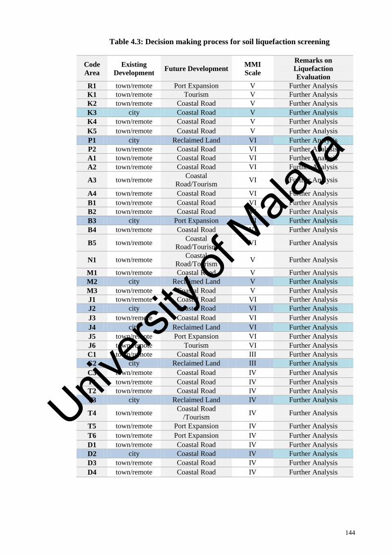
144
Table 4.3: Decision making process for soil liquefaction screening
Code
Area
Existing
Development Future Development
MMI
Scale
Remarks on
Liquefaction
Evaluation
R1 town/remote Port Expansion V Further Analysis
K1 town/remote Tourism V Further Analysis
K2 town/remote Coastal Road V Further Analysis
K3 city Coastal Road V Further Analysis
K4 town/remote Coastal Road V Further Analysis
K5 town/remote Coastal Road V Further Analysis
P1 city Reclaimed Land VI Further Analysis
P2 town/remote Coastal Road VI Further Analysis
A1 town/remote Coastal Road VI Further Analysis
A2 town/remote Coastal Road VI Further Analysis
A3 town/remote Coastal
Road/Tourism VI Further Analysis
A4 town/remote Coastal Road VI Further Analysis
B1 town/remote Coastal Road VI Further Analysis
B2 town/remote Coastal Road VI Further Analysis
B3 city Port Expansion VI Further Analysis
B4 town/remote Coastal Road VI Further Analysis
B5 town/remote Coastal
Road/Tourism VI Further Analysis
N1 town/remote Coastal
Road/Tourism V Further Analysis
M1 town/remote Coastal Road V Further Analysis
M2 city Reclaimed Land V Further Analysis
M3 town/remote Coastal Road V Further Analysis
J1 town/remote Coastal Road VI Further Analysis
J2 city Coastal Road VI Further Analysis
J3 town/remote Coastal Road VI Further Analysis
J4 city Reclaimed Land VI Further Analysis
J5 town/remote Port Expansion VI Further Analysis
J6 town/remote Tourism VI Further Analysis
C1 town/remote Coastal Road III Further Analysis
C2 city Reclaimed Land III Further Analysis
C3 town/remote Coastal Road IV Further Analysis
T1 town/remote Coastal Road IV Further Analysis
T2 town/remote Coastal Road IV Further Analysis
T3 city Reclaimed Land IV Further Analysis
T4 town/remote Coastal Road
/Tourism IV Further Analysis
T5 town/remote Port Expansion IV Further Analysis
T6 town/remote Port Expansion IV Further Analysis
D1 town/remote Coastal Road IV Further Analysis
D2 city Coastal Road IV Further Analysis
D3 town/remote Coastal Road IV Further Analysis
D4 town/remote Coastal Road IV Further Analysis
Univers
ity of
Mala
ya

145
Figure 4.65: Ground water table location for west coast areas
Univers
ity of
Mala
ya

146
Figure 4.66: Ground water table location for east coast areas
Univers
ity of
Mala
ya

147
4.1.13 Summary
The initiation of liquefaction hazard in Peninsular Malaysia is affected by a number
of parameters. A comprehensive investigation was undertaken to determine the findings
of liquefaction susceptibility factors; soil details and ground water table of shoreline
districts in Peninsular Malaysia. The conclusion is highlighted in point form as follows:
1. Sandy type beaches occupy almost 90% of east shoreline areas whereas muddy
type beaches are found on the west shoreline areas. The soil deposit which is
vulnerable to soil liquefaction is found highly concentrated at almost all the
studied location near surface ground level.
2. Sand with very little fine content in the particle gradation study are found in
90% study location which in general define a uniformly graded material
vulnerable to soil liquefaction hazard.
3. Clean sand and silt found from site investigation report increase the risk of
hazard and enhance further investigation to be carried out in the selected areas.
4. The location of ground water table near surface at studied location makes a
wider coverage of the hazard as most of the deposit underlying the water table is
in saturated condition
Univers
ity of
Mala
ya

148
5. The expansion and increasing of reclaimed land observed in selected state shows
significant changes in the natural environment which will lead to more
uncertainties in the surrounding areas.
6. In the present condition, the east coast areas are less significant to hazard in
general due to few developments compared to the west coast areas with iconic
project built on reclaimed land although the east coast are highly sand
concentrated. Without proper consideration on the soil liquefaction hazard effect
in the development design, future development and valuable assets are at stake
with the uncertainties from the environment.
7. Proper management of the shoreline areas are needed in providing safe
environment for the community. Hence guideline on hazard information needs
to be reached out to local authorities and community of the ground condition.
8. All the studied areas along the shoreline areas of Peninsular Malaysia shows
significant indicator for further liquefaction evaluation.
Univers
ity of
Mala
ya

149
4.2 Cyclic Triaxial Test
The soil performance is observed from cyclic triaxial test. The main result is to
obtain the dynamic properties of sample mainly the modulus reduction and damping
ratio curve.
4.2.1 Soil Liquefaction Observation
Figure 4.67 to Figure 4.70 shows the dynamic response of regional sand. The cyclic
deviator stress was applied with a frequency of 1 Hz and amplitude value of 0.5. An
approximation of 0.5 kN continuous axial force is observed. For the test, the initial cell
pressure and backpressure were 350 kPa and 250 kPa respectively. The confining
pressure is calibrated to 100 kPa. Based on 400 cycles of applied axial stress, Figure
4.67 presents the plot of deviator stress versus number of cycle of load application. Due
to the loading applied, a continuous deviator stress is observed until the setup reaches
400 cycles. The nature of axial strain, pore pressure and axial deformation due to the
loading is shown in Figure 4.68 to Figure 4.70. By using the Terzaghi‘s principle, when
the pore pressure equals to the confining pressure which will result in zero effective
confining pressure, this notes one of the termination criteria in soil liquefaction. Another
criteria is when the axial strain exceeded 20% which is a condition of a liquefy state. In
Figure 4.68, after about 387 cycles, the axial strain exceeded 20%. However the pore
pressure becomes equal to the confining pressure at 233 cycles (Figure 4.69). The pore
pressure is observed constant after reaching the confining pressure. This condition can
be explained with the remaining resistance of the soil to deform and also to the fact that
the soil dilates. During dilation the pore pressure is reduces and helps stabilization of
soil under loading as mentioned in Seed (1979) and commonly known as cyclic
mobility. Figure 4.70 present the plot of axial displacement versus number of cycle of
load application. As the stress continuously applied on sand, the deformation of soil is
observed in linear behavior similar to the plot of axial strain (Figure 4.68). As the axial
Univers
ity of
Mala
ya

150
strain reaches 20%, the deformation of soil reaches more than 10 mm. Hence the
termination criteria for this result are based on the 20% axial strain.
Figure 4.67: Plot of deviator stress vs number of cycle of load application (sand)
Figure 4.68: Plot of axial strain vs number of cycle (sand)
Figure 4.69: Plot of pore pressure vs number of cycle (sand)
Figure 4.70: Plot of axial displacement vs number of cycle (sand)
-200
0
200
400
0 50 100 150 200 250 300 350 400 450
Dev
iato
r St
ress
(k
Pa)
Number of Cycle
0
10
20
30
0 50 100 150 200 250 300 350 400 450Axi
al S
trai
n (
%)
Number of cycle
300
400
500
0 50 100 150 200 250 300 350 400 450
Po
re P
ress
ure
(k
Pa)
Number of Cycle
0
10
20
30
0 50 100 150 200 250 300 350 400 450
Axi
al D
isp
lace
men
t (m
m)
Number of cycle
Univers
ity of
Mala
ya

151
Another similar test setup is conducted using clay samples. Figure 4.71 to Figure
4.73 presents the plots of clay behavior towards cyclic loading. The deviator stress plot
is similar as presented in Figure 4.67. In contrast, clay presents insignificant findings in
the soil liquefaction context. The axial strain and axial displacement is very small
compared to the findings in sand samples. As for the pore pressure, there is only a slight
increase as the cycle reaches 400. Moreover the pore pressure is very low. The nature of
clay with high fine particles makes it not susceptible to soil liquefaction.
Figure 4.71: Plot of axial strain vs number of cycle (clay)
Figure 4.72: Plot of pore pressure vs number of cycle (clay)
Figure 4.73: Plot of axial displacement vs number of cycle (clay)
0
1
2
3
0 50 100 150 200 250 300 350 400 450Axi
al S
trai
n (
%)
Number of Cycle
38
40
42
44
46
0 50 100 150 200 250 300 350 400 450
Po
re P
ress
ure
(kP
a)
Number of Cycle
0
0.5
1
1.5
2
0 50 100 150 200 250 300 350 400 450
Axi
al D
isp
lace
men
t (m
m)
Number of Cycle
Univers
ity of
Mala
ya

152
4.2.2 Stress-Strain Behavior
The stress-strain behavior of sand and clay subjected to control loading is presented
in Figure 4.74 and Figure 4.75 respectively. In general, it can be observed that an
increase in the cyclic stress leads to an increase in the axial strain. From the figures, a
decrease in the modulus and increase in the hysteresis loop area indicates material
degradation. The degradation is faster in sand with observed increased area of hysteresis
loop compared to clay samples. This emphasized the significant features of sand as a
deposit which is highly susceptible to soil liquefaction.
Figure 4.74: Stress-strain behavior of sand subjected to controlled loading
Figure 4.75: Stress-strain behavior of clay subjected to controlled loading
-100
-80
-60
-40
-20
0
20
40
60
80
100
0 0.2 0.4 0.6 0.8 1 1.2 1.4
Dev
iato
r St
ress
(kP
a)
Axial Strain (%)
-100
-80
-60
-40
-20
0
20
40
60
80
100
0 0.2 0.4 0.6 0.8 1 1.2 1.4
De
viat
or
Stre
ss (
kPa)
Axial Strain (%)
Univers
ity of
Mala
ya

153
4.2.3 Shear Modulus Reduction and Damping Ratio Curves
Based on the hysteresis loop in Figure 4.74 and Figure 4.75, the shear modulus
reduction and damping ratio curves are developed. Figure 4.76 and Figure 4.77 presents
the shear modulus reduction curves of sand and clay respectively. The shear modulus
reduction curve for sand obtained has shown good agreement with the previous
published work. Both sand and clay are greatly depends on shear strain. The shear
modulus was found decreasing with the increasing shear strain. As the strain increases,
the material indicates loss of stiffness. At any level of strain, the shear modulus of sand
is lesser than the shear modulus of clay.
Figure 4.76: Shear modulus reduction curve for sand
Figure 4.77: Shear modulus reduction curve for clay
0.00
0.20
0.40
0.60
0.80
1.00
1.20
0.0001 0.001 0.01 0.1 1 10
G/G
max
Strain
Studied Sand Seed and Idriss (1970) LUSH &I
0.00
0.20
0.40
0.60
0.80
1.00
1.20
0.0001 0.001 0.01 0.1 1 10
G/G
max
Strain
Studied Clay Seed and Sun (1989) Sun et al.(1988)
LUSH &I Vucetic - Dobry
Univers
ity of
Mala
ya

154
Figure 4.78 and Figure 4.79 presents the damping ratio curves of sand and clay
respectively. At smaller cyclic shear strains, the damping ratio of clay is higher than the
damping ratio in sand, while at larger shear strains, the damping ratio of clay is lower
than the damping ratio in sand. This behavior is close to a study conducted by Idriss
(1990).
Figure 4.78: Damping ratio curve for sand
Figure 4.79: Damping ratio curve for clay
-5
0
5
10
15
20
25
30
35
0.0001 0.001 0.01 0.1 1 10
Dam
pin
g (%
)
Strain
Studied Sand Idriss (1990) Seed and Idriss (1989) LUSH S&I
-5
0
5
10
15
20
25
30
35
0.0001 0.001 0.01 0.1 1 10
Dam
pin
g R
%)
Strain
Studied Clay Idriss (1990) Vucetic-Dobry Sun et al.(1988) LUSH S&I
Univers
ity of
Mala
ya

155
4.2.4 Summary
In this study, a series of the cyclic triaxial tests were conducted on 2 types of soil
deposits which consists of sand and clay. The shear modulus reduction and damping
ratios curves versus cyclic shear strain were analyzed under different soil type. Then the
estimated shear modulus and damping ratio curves are compared with existing
published work. The following conclusions can be drawn:
1. The regional sand tested is susceptible to soil liquefaction whereas the clay are
not susceptible to soil liquefaction. This have been presented in the compiled
reports in Chapter 2 of thesis study where most of the reports are consisted of
sand and silt deposits vulnerable to soil liquefaction.
2. Sand degrades faster during cyclic loading compared to clay. The study
emphasized the important characteristics that sand poses which makes
significant contribution to stress application.
3. In both test samples, when the strain increases, the shear modulus decreases,
whereas damping ratio increases. In general, the behavior is similar to published
work used for comparative study. The stiffness in clay is higher compared to
sand when the stress is applied repeatedly under cyclic loading.
4. In general different soil samples produce unique behavior towards any stress
application. Hence the result obtained is most valid for liquefaction assessment
of regional site condition where the samples are collected.
Univers
ity of
Mala
ya

156
4.3 Earthquake Study
4.3.1 Probabilistic Seismic Hazard Assessment (PSHA)
Based on PSHA, 3 main outputs of studied area are presented under this section
mainly the probabilistic hazard, de-aggregation hazard and scaled spectrum. The
characterization of earthquake loading in liquefaction analysis of this study is evaluated
using a detailed ground response analysis due to different ground condition and
geotechnical setting of the shoreline.
4.3.1.1 Generation and Simulation of Synthetic Ground Motion
Hazard curves developed presents the contribution from various earthquake sources.
In this study a total of 21 earthquake sources consists of far field and nearby faults were
carefully selected for the development of hazard curves. The type of seismic source
controls hazard at various spectral accelerations. The typical probabilistic hazard in the
west coast areas and the east coast areas which consists of 9 site location of studied state
from PGA source is shown in Figure 4.80 and Figure 4.81. The plot of annual frequency
of exceedance versus the peak ground acceleration presents constant decreasing of
graph results as the earthquake sources distance from site.
The Peninsular Malaysia experienced tremors, some of which caused damage to both
buildings and infrastructures. Hence the evaluation of the probabilistic hazard consists
of nearby faults which have significant contribution to the earthquake hazard. The
hazard curves from nearby moderate magnitude are observed to be different from that
large-magnitude subduction zone earthquake. The most significant to the studied area
are seismic source from far field earthquake namely the Tripa fault segment. Other far
field seismic source such as Renun, Toru and Angkora are less significant to the studied
areas follow by the remaining benioff type seismic source.
Univers
ity of
Mala
ya

157
(a) Perlis
(b) Kedah
Univers
ity of
Mala
ya
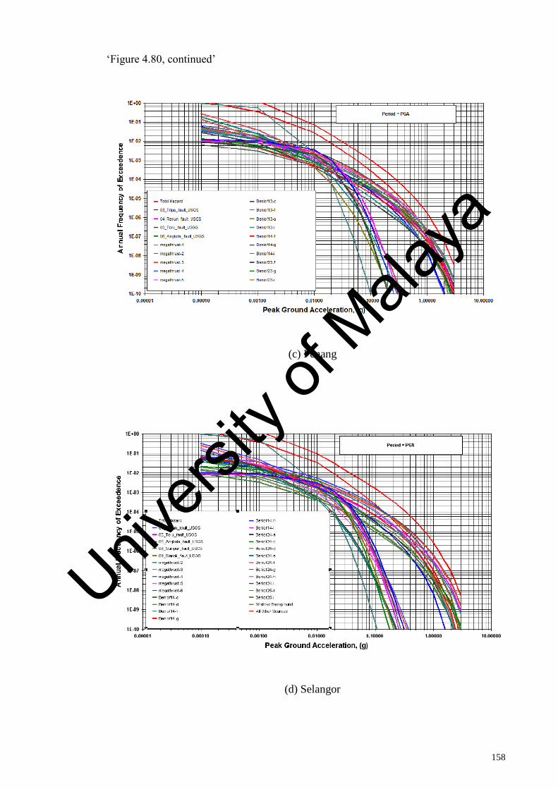
158
‗Figure 4.80, continued‘
(c) Penang
(d) Selangor
Univers
ity of
Mala
ya

159
‗Figure 4.80, continued‘
(e) Melaka
Figure 4.80: Typical probabilistic hazard at west coast areas for PGA
(a) East Johor
Univers
ity of
Mala
ya

160
‗Figure 4.81, continued‘
(b) Pahang
(c) Terengganu
Univers
ity of
Mala
ya

161
‗Figure 4.81, continued‘
(d) Kelantan
Figure 4.81: Typical probabilistic hazard at east coast areas for PGA
4.3.1.2 De-Aggregation Hazard
Based on hazard curve presented in 4.3.1.1 which combines all the sources,
magnitudes and distances, the intuitive understanding about controlling hazard sources
are difficulty hence hazard de-aggregation plot is needed (Kim & Hashash, 2013). The
hazard de-aggregation plot identify likely major contributor to seismic hazard. It helps
to identify the magnitudes and distances of controlling seismic sources. De-aggregation
generates the relative contributions to ground motion from seismic sources in terms of
ground motion magnitude and source-to-site distance.
The typical de-aggregation hazards for the studied state consist of west coast areas
and east coast areas are shown in Figure 4.82 to Figure 4.83 respectively. Typical
Univers
ity of
Mala
ya

162
simple de-aggregation has a unimodal distribution with one clear peak or most frequent
value. The result for most state highlights increasing value at first, rising to a single
peak where it then decreases. The peak presents nearby earthquakes whereas the tail
includes a larger and more distance earthquakes. For location in Kelantan and
Terengganu, a broader peak of hazard contributions is observed. This is due to the low
activity and remote location from high activity zones. The hazard contributions are
consists mainly of wide range of magnitudes and earthquakes.
For the studied west coast site, the primary contributors to hazard are at a distance of
237.5 km with a magnitude of 8.25 whereas the east coast areas are at a distance of
587.5 km with a magnitude of 8.25. The west coast is closer to the seismic source as to
compare to the east coast area which is further from the fault. However the magnitude
remains same with a value of 8.25 for both findings.
(a) Kangar
Univers
ity of
Mala
ya

163
‗Figure 4.82, continued‘
(b) Kedah
(c) Penang
Univers
ity of
Mala
ya

164
‗Figure 4.82, continued‘
(d) Selangor
(e) Melaka
Univers
ity of
Mala
ya

165
‗Figure 4.82, continued‘
(f) West Johor
Figure 4.82: De-aggregration hazard of 500 year return period for west coast
(a) Pahang
Univers
ity of
Mala
ya

166
‗Figure 4.83, continued‘
(b) Terengganu
(c) Kelantan
Figure 4.83: De-aggregration hazard of 500 year return period for east coast
Univers
ity of
Mala
ya

167
Table 4.4 presents the deaggregration hazard of 500 year return period for selected
states. The main indicator which will later be used to select the ground motion in the
spectral matching procedure extracted from this chart is the distance and magnitude.
Table 4.4: The deaggregration hazard of 500 year return period for 11 states
Shoreline State Distance (m) Magnitude (M)
Perlis 312.5 8.25
Kedah 287.5 8.25
Pulau Pinang 237.5 8.25
Perak 237.5 8.25
Selangor 262.5 8.25
Seremban 262.5 8.25
Melaka 212.5 8.25
West Johor 337.5 8.25
East Johor 587.5 8.25
Pahang 587.5 8.25
Terengganu 612.5 8.25
Kelantan 437.5 8.25
4.3.1.3 Scaled Spectrum
The scaled spectrums for 11 state of Peninsular Malaysia for return period of 500 and
2500 years are shown from Figure 4.84 and Figure 4.85. It has been observed that for
selected sources, as the distance from the fault increases, the value of spectral
acceleration reduces. Hence, the east coast of Peninsular Malaysia (Kelantan,
Terengganu, Pahang, and East Johor) presents lower value of spectral acceleration. As
the period increases, the result of scaled spectrum tends to become asymptotic. These
results will be useful in carrying out the spectral matching procedure to obtain the
ground motion at bedrock.
Univers
ity of
Mala
ya

168
Figure 4.84: Bedrock spectrum with 500 year return period of hazard
Figure 4.85: Bedrock spectrum with 2500 year return period of hazard
0.00
0.02
0.04
0.06
0.08
0.10
0.12
0.14
0.16
0.18
0.01 0.1 1 10
Spec
tral A
ccel
erat
ion
(g)
Period (Second)
Kelantan
Terengganu
Pahang
Johor East
Johor West
Melaka
NegeriSembilan
Selangor
Perak
Penang
Kedah
Perlis
0.00
0.05
0.10
0.15
0.20
0.25
0.30
0.35
0.40
0.01 0.1 1 10
Sp
ec
tral A
cc
ele
rati
on
(g
)
Period (Second)
Kelantan
Terengganu
Pahang
Johor East
Johor West
Melaka
NegeriSembilan
Selangor
Perak
Penang
Kedah
PerlisUnivers
ity of
Mala
ya

169
4.3.2 Generation and Simulation of Synthetic Ground Motion
This study analyzed nearly 2074 SPT samples from over 325 locations that were
drilled along the shoreline area of Peninsular Malaysia, to access the characteristics of
wave behavior propagating through different layer of soils. These data allowed a
subsurface investigation and evaluation of peak surface acceleration to be assigned in
the liquefaction analysis. Figure 4.86 and 4.87 presents the result simulation of bedrock
(PGA) bedrock and also surface (PSA) for all the studied states. The variety of color
represents ground motion at different shoreline state of Peninsular Malaysia. The
maximum PGA is observed at the west coast areas. Lower PGA is defined in most of
places in the east coast region. The longest period of which the ground motion ends was
found to be located in Seremban. However the development of PSA shows significant
effect in most of the region in the east coast region. The propagation of seismic waves
in soil varies with different setting of soil strata. Bedrock propagates direct dispersion of
energy whereas when seismic waves pass through loose deposits the energy is released
in a complex way that it tends to show increment of energy (Holzer et al., 1989).
(a) Perlis
-0.25
-0.20
-0.15
-0.10
-0.05
0.00
0.05
0.10
0.15
0.20
0 10 20 30 40 50 60
Acc
eler
atin
(m
/s2 )
Time (s)
Surface Bedrock
Univers
ity of
Mala
ya

170
‗Figure 4.86, continued‘
(b) Kedah
(c) Penang
-0.35
-0.30
-0.25
-0.20
-0.15
-0.10
-0.05
0.00
0.05
0.10
0.15
0.20
0 10 20 30 40 50 60
Acc
eler
atio
n (
m/s
2 )
Time (s)
Surface Bedrock
-0.25
-0.20
-0.15
-0.10
-0.05
0.00
0.05
0.10
0.15
0.20
0.25
0 10 20 30 40 50 60
Acc
eler
atio
n (
m/s
2 )
Time (s)
Surface Bedrock
Univers
ity of
Mala
ya

171
‗Figure 4.86, continued‘
(d) Perak
(e) Selangor
-0.25
-0.20
-0.15
-0.10
-0.05
0.00
0.05
0.10
0.15
0.20
0.25
0 5 10 15 20 25 30 35 40
Acc
eler
atio
n (
m/s
2 )
Time (s)
Surface Bedrock
-0.25
-0.20
-0.15
-0.10
-0.05
0.00
0.05
0.10
0.15
0.20
0 10 20 30 40 50
Acc
eler
atio
n (
m/s
2 )
Time (s)
Surface Bedrock
Univers
ity of
Mala
ya

172
‗Figure 4.86, continued‘
(f) Negeri Sembilan
(g) Melaka
-0.25
-0.20
-0.15
-0.10
-0.05
0.00
0.05
0.10
0.15
0.20
0 20 40 60 80 100
Acc
eler
atio
n (
m/s
2 )
Time (s)
Surface Bedrock
-0.3
-0.25
-0.2
-0.15
-0.1
-0.05
0
0.05
0.1
0.15
0.2
0.25
0 10 20 30 40 50 60
Acc
eler
atio
n (
m/s
2 )
Time (s)
Surface Bedrock
Univers
ity of
Mala
ya

173
‗Figure 4.86, continued‘
(h) West Johor
Figure 4.86: Simulation from bedrock (PGA) to surface (PSA) of west coast region
(a) East Johor
-0.2
-0.15
-0.1
-0.05
0
0.05
0.1
0.15
0.2
0 10 20 30 40 50 60 70 80 90
Acc
eler
atio
n (
m/s
2 )
Time (s)
Surface Bedrock
-0.25
-0.2
-0.15
-0.1
-0.05
0
0.05
0.1
0.15
0.2
0.25
0 20 40 60 80 100
Acc
eler
atio
n (
m/s
2)
Time (s)
Surface Bedrock
Univers
ity of
Mala
ya

174
‗Figure 4.87, continued‘
(b) Pahang
(c) Terengganu
-0.25
-0.2
-0.15
-0.1
-0.05
0
0.05
0.1
0.15
0.2
0 10 20 30 40 50 60 70 80 90
Acc
eler
atio
n (
m/s
2 )
Time (s)
Surface Bedrock
-0.2
-0.15
-0.1
-0.05
0
0.05
0.1
0.15
0.2
0 10 20 30 40 50 60 70 80 90
Acc
eler
atio
n (
m/s
2 )
Time (s)
Surface Bedrock
Univers
ity of
Mala
ya

175
(d) Kelantan
Figure 4.87: Simulation from bedrock (PGA) to surface (PSA) of east coast region
Table 4.5 presents the summary of significant values extracted from the ground
motion simulation from the bedrock to the surface for all the studied area. The high
amplification values are demonstrated at Kelantan and Terengganu mainly due to the
high concentration of deep loose soil layer which enhanced the propagation of wave
through the soil layers (Ishac & Heidebrecht, 1982).
Table 4.5: Amplification factor of 11 studied states for 500 years return period
Shoreline State PGA PSA Max. Amplification Factor
Perlis 0.04 0.19 4.62
Kedah 0.04 0.24 6.67
Pulau Pinang 0.06 0.23 3.99
Perak 0.06 0.23 3.65
Selangor 0.07 0.23 3.49
Seremban 0.06 0.14 2.35
Melaka 0.06 0.24 3.74
West Johor 0.07 0.24 3.49
East Johor 0.03 0.21 6.43
Pahang 0.03 0.18 6.01
Terengganu 0.02 0.20 8.72
Kelantan 0.02 0.24 11.02
-0.3
-0.2
-0.1
0
0.1
0.2
0.3
0 10 20 30 40 50 60 70 80 90
Acc
eler
atio
n (
m/s
2 )
Time (s)
Surface Bedrock
Univers
ity of
Mala
ya

176
4.3.3 Microzonation Line (Amplification Factor)
The amplification factor generated from the seismological data through the PSHA
has been applied in microzonation chart line of 1972 km shoreline. Figure 4.88 presents
the amplification factor of 11 states along shoreline. By observing the chart, maximum
amplification factor in west coast region was found in Kedah state with a value of 7.8
factors. The rest of the state in west coast region shows constant amplification factor in
the range of 2 to 5 factor. A closer look of high amplification factor is concentrated in
major cities mainly due to the strategic location and natural formation such as lagoon,
river mouth and long beach (Bhuiyan et al., 2013; Yasuda et al., 2012). Hence the risk is
high at highly populated area which defines heavily congested built environment.
Reclaimed land in parts of west coast region especially in Penang Island and Melaka is
also at risk based on the amplification factor generated for this study. Sudden peak in
Penang Island is mainly due to formation of loose deposits concentration in the area.
Proper management, earthquake resistant design and preparation plan is recommended
at specific area with high amplification factor(Adalier & Elgamal, 2004).
On the other hand east coast region define a much higher amplification factor
significantly in Terengganu and Kelantan region. Ports, power plant and harbor
facilities are at high risk during ground motion which scattered in most of the shoreline
district of Terengganu. The highest amplification factor was found in Tumpat district,
Kelantan follow by Pasir Puteh district with a factor of 14.7 and 11 respectively.
Terengganu shows constant factor of nearing 8 at most of the shoreline district. At the
moment the Kelantan shoreline is not heavily developed hence the risk is low. The
future development of the areas needs critical attention as the amplification is found the
highest among the other states of the west coast region.
Univers
ity of
Mala
ya

177
(a) Perlis
(b) Langkawi Island
0.0
1.0
2.0
3.0
4.0
5.0
6.0
1 4 7 10 13 16 19 22 25 28 31 34 37 40 43 46 49 52 55 58 61 64 67 70 73 76 79 82 85
Am
plif
icat
ion
Fac
tor
Borehole Number
Sanglang Simpang Empat Kuala Perlis
0.0
1.0
2.0
3.0
4.0
5.0
6.0
7.0
1 3 5 7 9 11 13 15 17 19 21 23 25 27 29 31 33 35 37 39 41 43 45 47 49 51 53 55 57 59 61 63
Am
plif
icat
ion
Fac
tor
Borehole Number
Kuah Pantai Chenang Teluk Burau Ulu Melaka
Univers
ity of
Mala
ya

178
‗Figure 4.88, continued‘
(c) Kedah Mainland
(d) Penang Island
0.0
1.0
2.0
3.0
4.0
5.0
6.0
7.0
8.0
9.0
1 3 5 7 9 11 13 15 17 19 21 23 25 27 29 31 33 35 37 39 41
Am
plif
icat
ion
Fac
tor
Borehole Number
Kuala Muda Yan Ayer Hitam
0.0
1.0
2.0
3.0
4.0
5.0
6.0
1 6
11
16
21
26
31
36
41
46
51
56
61
66
71
76
81
86
91
96
10
1
10
6
11
1
11
6
12
1
12
6
13
1
13
6
14
1
Am
plif
icat
ion
Fac
tor
Borehole Number
Bayan Lepas Gelugor Georgetown Tanjung Bungah
Univers
ity of
Mala
ya

179
‗Figure 4.88, continued‘
(e) Seberang Perai
(f) Perak
0.0
0.5
1.0
1.5
2.0
2.5
3.0
3.5
4.0
1 2 3 4 5 6 7 8 9 1011121314151617181920212223242526272829303132333435
Am
plif
icat
ion
Fac
tor
Borehole Number
South SP Central SP Butterworth
0.0
0.5
1.0
1.5
2.0
2.5
3.0
3.5
4.0
1 7
13
19
25
31
37
43
49
55
61
67
73
79
85
91
97
10
3
10
9
11
5
12
1
12
7
13
3
13
9
14
5
15
1
15
7
16
3
Am
plif
icat
ion
Fac
tor
Borehole Number
Bagan Datoh Lekir Teluk Rubiah Lumut Kuala Kurau
Univers
ity of
Mala
ya

180
‗Figure 4.88, continued‘
(g) Selangor
(h) Negeri Sembilan
0.0
0.5
1.0
1.5
2.0
2.5
3.0
3.5
4.0
1 3 5 7 9 11131517192123252729313335373941434547495153555759616365
Am
plif
icat
ion
Fac
tor
Borehole Number
Sepang Kuala Langat Klang Kuala Selangor Sungai Besar
0.0
0.5
1.0
1.5
2.0
2.5
3.0
3.5
1 2 3 4 5 6 7 8 9 10 11 12 13 14 15 16 17 18 19 20
Am
plif
icat
ion
Fac
tor
Borehole Number
South Central North
Univers
ity of
Mala
ya

181
‗Figure 4.88, continued‘
(i) Melaka
(j) West Johor
0.0
0.5
1.0
1.5
2.0
2.5
3.0
3.5
4.0
1 2 3 4 5 6 7 8 9 10 11 12 13 14 15 16 17 18 19 20 21 22 23 24 25 26 27 28 29
Am
plif
icat
ion
Fac
tor
Borehole Number
Pantai Siring Melaka Tengah Kuala Sungai Baru
0.0
0.5
1.0
1.5
2.0
2.5
3.0
3.5
1 4 7 10 13 16 19 22 25 28 31 34 37 40 43 46 49 52 55 58 61 64 67 70 73 76 79
Am
plif
icat
ion
Fac
tor
Borehole Number
Johor Bahru Pontian Batu Pahat Muar
Univers
ity of
Mala
ya

182
‗Figure 4.88, continued‘
(k) East Johor
(l) Pahang
0.0
1.0
2.0
3.0
4.0
5.0
6.0
7.0
1 9
17
25
33
41
49
57
65
73
81
89
97
10
5
11
3
12
1
12
9
13
7
14
5
15
3
16
1
16
9
17
7
18
5
19
3
20
1
20
9
Am
plif
icat
ion
Fac
tor
Borehole Number
Kota Tinggi Mersing
0.0
1.0
2.0
3.0
4.0
5.0
6.0
7.0
8.0
1 4 7 10 13 16 19 22 25 28 31 34 37 40 43 46 49 52 55 58 61 64 67 70 73 76
Am
plif
icat
ion
Fac
tor
Borehole Number
Rompin Pekan Kuantan
Univers
ity of
Mala
ya

183
‗Figure 4.88, continued‘
(m) Terengganu
(n) Kelantan
Figure 4.88: Microzonation line of 11 states in Peninsular Malaysia
0.0
1.0
2.0
3.0
4.0
5.0
6.0
7.0
8.0
9.0
10.0
1
20
39
58
77
96
11
5
13
4
15
3
17
2
19
1
21
0
22
9
24
8
26
7
28
6
30
5
32
4
34
3
36
2
38
1
40
0
41
9
43
8
45
7
47
6
49
5
51
4
53
3
Am
plif
icat
ion
Fac
tor
Borehole Number
Kemaman Dungun Marang Kuala Terengganu Setiu Besut
0.0
2.0
4.0
6.0
8.0
10.0
12.0
14.0
16.0
1 6
11
16
21
26
31
36
41
46
51
56
61
66
71
76
81
86
91
96
10
1
10
6
11
1
11
6
12
1
12
6
13
1
13
6
Am
plif
icat
ion
Fac
tor
Borehole Number
Pasir Puteh Bachok Kota Bharu Tumpat
Univers
ity of
Mala
ya

184
4.3.4 Comparative Study of Recent Findings to Previous Works
Different sources of seismic information is selected and tabulated in Table 4.6. 3
works which was previously documented in the last 8 years are compiled for
comparative study on the PGA value at bedrock. The works are Petersen et al. (2008),
Adnan et al. (2005) and Azmi et al. (2013). This study consists of 7359 working file of
the earthquake catalog from 1 May 1900 to 31 December 2009. Petersen et al. (2008)
introduced earthquake catalog which contains 6710 records from 1964 to 2006 and
presents close value of PGA at bedrock with the recent study. In contrast Adnan et al.
(2005) presents low value of PGA compared to recent study. On the other hand, Azmi et
al. (2013) introduced higher range of PGA values with more than 60% increase for
Pulau Pinang.
The earthquake data from Adnan et al. (2005) are obtained from USGS, International
Seismological Center (ISC) and MMD. The working file is 12149 with dated
earthquake events between 27 February 1903 and 30 December 2000. The earthquake
catalogs from Azmi et al. (2013) are acquired from USGS and Indonesian Meteorology
Agency (BMG) with earthquake records compiled from 1871 to 2011. The different
aspect of seismicity properties and considerations adapted in each works contribute to
the different PGA values at bedrock in Peninsular Malaysia. The presentation of PGA
differs due to the seismic parameters applied in the main seismic analysis. A site
specific is also another contribution of differences in the findings. Hence the value is
best represented with latest and updated content of the seismic parameters introduced in
the main seismic analysis.
Univers
ity of
Mala
ya

185
Table 4.6: Comparative study of PGA for 500 years return period
Shoreline State
Recent study
PGA at
bedrock
2016
PGA at
bedrock
(M. Petersen
et al., 2008)
PGA at
bedrock
(Adnan et al.,
2005)
PGA at
bedrock
(Azmi et al.,
2013)
Perlis 0.04 0.05 0.01 - 0.02 -
Kedah 0.04 0.05 0.01 - 0.02 -
Pulau Pinang 0.06 0.05 0.01 - 0.02 0.09 - 0.10
Perak 0.06 0.06 0.01 - 0.02 -
Selangor 0.07 0.06 0.02 - 0.03 -
Negeri Sembilan 0.06 0.06 0.02 - 0.03 -
Melaka 0.06 0.05 0.02 - 0.03 -
West Johor 0.07 0.05 > 0.03 -
East Johor 0.03 0.05 0.02 - 0.03 -
Pahang 0.03 0.04 0.02 - 0.03 -
Terengganu 0.02 0.04 < 0.01 -
Kelantan 0.02 0.04 < 0.01 -
4.3.5 Summary
The microzonation study has summarized the output from PSHA, SMP and SRA in
modelling the seismicity in the regional settings and in generating the microzonation
line. The following conclusions can be drawn:
1. In PSHA, the aggregation of hazard model of 500 years return earthquake period
design presents wide magnitude and distance of the earthquakes that
contribution most of the hazard at selected stats in Peninsular Malaysia. The
results indicate that very near seismic sources of relative higher magnitudes are
the dominating sources of hazard for the selected states of Peninsular Malaysia
generally the west coast areas. The contributions from distance sources are
Univers
ity of
Mala
ya

186
relatively low but cannot be neglected due to intrinsic uncertainties and limited
seismic catalogues.
2. The SMP conducted presents unique ground motion at bedrock for each of the
studied location. Similar to the PSHA, the west coast areas presents a stronger
ground motion at bedrock in compared to the east coast areas.
3. In SRA, the east coast areas present stronger ground motion on the surface
compared to the west coast areas. High amplification values are achieved in
states such as Kelantan and Terengganu (AF > 8). Kedah, Pahang and East Johor
simulate AF between 6 and 7, where the rest of the state presents AF < 5. This is
due to the composition of concentrated loose and soft soil which enhanced the
amplification of wave propagating through the soil layer. Thick layer of sand
and silt as presented in section 4.1 have found generating the stronger ground
motion in the seismicity study.
Univers
ity of
Mala
ya

187
4.4 Liquefaction Hazard Assessment and Mapping
4.4.1 Graphical Illustration of Liquefaction Zones
Based on simplified procedure, a presentation of liquefaction layer in each of the
studied area is presented in Figure 4.89 to Figure 4.102. The liquefaction layer
illustrations are developed for shoreline areas of Peninsular Malaysia corresponding to
ground motion developed from PSHA for annual probability of exceedance equal to
10% in 50 years (equal to return periods of 500 years) provide screening aid to assess
liquefy layer at studied site. Figure 4.89 illustrates the liquefaction layer of Perlis. It
appears as though the whole shoreline areas are exposed to liquefaction threat for the
first 5 meter below ground level as indicated by the red zone of potentially liquefied
zone. Major concern of findings is the coastal roads that stretch along these areas which
are a significant asset for the state in providing mobility for goods and services. In
summary, the combination of high groundwater within loose sandy sediments
constitutes a significant liquefy layer beneath Perlis. Hence it is recommended for future
developments located in designated liquefaction hazard zones to adapt procedures and
guidelines for improvement of the existing built environment along the shoreline areas
as to provide safety and minimized effect from liquefaction hazard.
Figure 4.89: Liquefaction layer of Perlis
Univers
ity of
Mala
ya

188
Similar findings are observed in the state of Langkawi and the mainland of Kedah
which is a tourist spot and business hub of the country illustrated in Figure 4.90 and
Figure 4.91. The loose sandy sediments with high groundwater have defined danger
zoned for the entire studied areas. The major concern is sites which presents liquefied
layer for the whole 20 m observed in Ulu Melaka, Pantai Chenang, Ayer Hitam and
Yan.
Figure 4.90: Liquefaction layer of Langkawi
Figure 4.91: Liquefaction layer of Kedah
Univers
ity of
Mala
ya

189
Figure 4.92 and Figure 4.93 illustrated the liquefaction layer of Penang state. The
mainland of Penang presents a denser zone of liquefied soil compared to the island.
Approximately 40% of the Penang Island is developed along the shoreline area and the
remaining is in its natural state. The spreading liquefy zones in the first 5 m below
surface is supporting built environment consist of multiple high rise buildings,
residential units and town city. All of which is densely populated area.
Figure 4.92: Liquefaction layer of Penang Island
Figure 4.93: Liquefaction layer of Seberang Perai
Univers
ity of
Mala
ya

190
Figure 4.94 illustrates the liquefaction layer of Perak. As there are no significant
development observed in Perak, existing infrastructures should take cautious measures
in as it presents liquefy layer for more than 70% of the overall studied layer.
Figure 4.94: Liquefaction layer of Perak
Figure 4.95 presents the liquefaction layer of Selangor. The liquefy zone are found to
be in random distribution. Some areas such as Kuala Langat present significant threat to
liquefaction hazard.
Figure 4.95: Liquefaction layer of Selangor
Univers
ity of
Mala
ya

191
Only 5% of areas in the southern portion of Port Dickson presents liquefy zone,
whereas other shows no threat to the hazard (Figure 4.96). In contrast Melaka presents 2
locations which are vulnerable to the threat; Melaka Tengah and Pantai Siring, both of
which a town city and a tourist spot (Figure 4.97). The expansion of land through
reclamation method should be investigated further with special design for substructure
in countering the liquefaction hazard.
Figure 4.96: Liquefaction layer of Negeri Sembilan
Figure 4.97: Liquefaction layer of Melaka
Univers
ity of
Mala
ya

192
Figure 4.98 and Figure 4.99 present the Johor result of the west coast areas and east
coast areas. The distribution of liquefy zone does not present constant pattern as it is
more observed as a scattered data. Significant areas in the west coast are Batu Pahat and
Pontian as the liquefy zones exist on the surface level. Similar findings are found in the
east coast areas in few areas in Kota Tinggi and Mersing. In defining an ideal design of
built environment, areas with liquefy zone close to the surface should be abandoned and
preserved in its natural state as to prevent for disaster during liquefaction hazard.
Figure 4.98: Liquefaction layer of West Johor
Figure 4.99: Liquefaction layer of East Johor
Univers
ity of
Mala
ya

193
Pahang state presents liquefy zone of 60% of overall studied layer (Figure 4.100).
The existing of liquefy layer after 2 m below ground surface denotes the importance of
special design for substructure penetrating into the soil especially in Kuantan areas.
Pekan and Rompin are less developed compared to Kuantan shows advantage of lesser
effect during earthquake hazard. The existing of port in Kuantan presents the
importance of adapting soil improvement method and special subsurface design in
minimizing the liquefaction hazard. A vulnerable place in Pekan should enhanced
awareness of future development as the layer of liquefy zone at most of the areas can
reach up to 23 meters below ground surface. As safer location defined in Rompin, the
place could be a shelter to accommodate victims from the earthquake hazard provided
the road are in good performance after the disaster to transfer people, foods and
services.
Figure 4.100: Liquefaction layer of Pahang
Figure 4.101 and Figure 4.102 presents liquefaction layer of Terengganu and
Kelantan. Approximately 50% of the areas in Terengganu are affected with liquefaction
where more than 60% affected areas are found in Kelantan. Major concern should be
provided in Kuala Terengganu as it is the main concentration of built environment. The
Univers
ity of
Mala
ya

194
northern areas are less develop; Besut and Setiu. Hence the liquefaction context shows
no significant contribution to the place unless future development with heavily built
environment is constructed at the place. Dungun and Kemaman also need further
investigation as main ports are located at these locations. Similar findings are observed
in Kelantan where the concentration of population is located in Kota Bharu. The
liquefaction definition is made significant when the location is developed unlike a
location in natural state where the surroundings presents lesser damaging effect after
earthquake disaster.
Figure 4.101: Liquefaction layer of Terengganu
Figure 4.102: Liquefaction layer of Kelantan
Univers
ity of
Mala
ya

195
4.4.2 Liquefaction Hazard Map
By using LPI to summarize the studied area, a map of liquefaction hazard along the
shoreline areas of Peninsular Malaysia is plotted in Figure 4.103. The east coast areas
present multiple higher intensity of liquefaction hazard compared to the areas in the
west coast. This is due to the high concentration of vulnerable loose deposits in east
coast region. The Kelantan and Terengganu state are at high risk based on the hazard
intensity due to the ‗clean sand‘ observed in the soil composition figure generated in
section 4.1.10 and section 4.1.11. Although the PGA generated for east coast region is
less significant compared to the west coast region however the PSA generated shows
high propagation in the east coast region compared to the east coast region. The findings
is similar with the one found in Christchurch and Tokyo Bay Japan where soil
liquefaction was found to be critical at sites with similar settings (Yasuda et al., 2012).
The existing development along the shoreline are recommended for further study to
introduced proper mitigation method against soil liquefaction on existing structures.
On the other hand vulnerable silt which exists more than 60% in the west coast areas
contributes to the high hazard intensity in the areas. The shallow ground water table in
all the studied location also makes most areas vulnerable to hazard. The northern part of
west coast region shows higher hazard intensity compared to the southern part. Seismic
source from long distance earthquake presented in section 4.3.1.1 plays significant role
in defining the severity of the specific site. Reclaimed land is recommended to be
continuously monitored as to provide safe built environment towards sudden changes in
the environment. A proper planning for preparedness and mitigation towards hazard is
crucial as the region is moving at very fast pace in the development context. Lesson
learnt from previous soil liquefaction induced ground motion are a motivation and a
step forward in benefiting the regional ground and natural formation of the geological
setting of Peninsular Malaysi.
Univers
ity of
Mala
ya

196
Figure 4.103: Liquefaction hazard map of shoreline areas of Peninsular Malaysia
4.4.3 Mitigation Zoning
The general procedure in making hazard-informed evaluation is to highlight potential
hazard zones along the shoreline areas in addressing authorities and local councils about
soil liquefaction threat for future improvement, mitigation and remediation works. The
quantification is subjected to contributing factors of hazard. Observation from available
Univers
ity of
Mala
ya

197
data which was made in section 4.1 on the decision making process result in addressing
high possibility and uncertain situations in the most optimized manner in the context of
Peninsular Malaysia. The wide use of resources is to ensure that appropriate action is
taken quickly and efficiently in reducing unknown hazard in the location. Limited
resources are prioritized accordingly in generating Table 4.7 to Table 4.8 for soil
liquefaction hazard quantification (Law & Ling, 1992; Tokimatsu & Asaka, 1998;
Wang, 1979). The tables are summarized with a summation of the scores for the driving
effect of hazard which is then concluded under respected zones and categories of hazard
level. The zones are presented with a description of severity level ranging from low to
high level. By using available mitigation in the wide scope of the present research, each
category of hazard level is related to the mitigation aspect respectively (Ashford et al.,
2000; El Mohtar et al., 2012; Mitchell, 2008; Porbaha et al., 1999; Shenthan et al.,
2004; Yegian et al., 2007).
Table 4.9 and Table 4.10 summarize the hazard level at each studied locations along
with the hazard category in providing the mitigation information according to existing
literature (Chávez et al., 2017; MacAskill & Guthrie, 2017; Tokimatsu et al., 2012;
Wotherspoon et al., 2015). This approach is to acknowledge individuals as well as the
community about hazard information in the areas which could lead them in making safe
decisions and effective planning of their surroundings (Bouziou & O‘Rourke, 2017;
Bretherton, 2017; Wang & Guldmann, 2016). This information could trigger more detail
research to be carried out by local and also international governing bodies from research
institution as well as engineering firms in shaping good measures in the near
development of Peninsular Malaysia (Bhuiyan et al., 2013).
Univers
ity of
Mala
ya

198
Table 4.7: Input for score
SL-INPUT-01 LPI Index Score
> 30 100 15 75 10 50 5 25 0 0
Table 4.8: Output 1 for the shoreline zoning and soil liquefaction category
SL-OUTPUT-01
Score Shoreline Zone
Soil Liquefaction Category SL-0 SL-1 SL-2 SL-3 SL-4
76 - 100 Z-5 20 40 60 80 100 51 - 75 Z-4 16 32 48 64 80 26 – 50 Z-3 12 24 36 48 60 21 - 25 Z-2 8 16 24 32 40 0 - 20 Z-1 4 8 12 16 20
Table 4.9: Output 2 for the severity level, action and mitigation
SL-OUTPUT-02 SL-OUTPUT-03
Zone Severity Level Category Action Mitigation
Z-5 Critical impact SL-4 Forest restoration
and rehabilitation Abandon site
Z-4 Important impact SL-3
Conduct site
specific
investigation
Special
Analysis for
Structure
Z-3 Moderate impact SL-2 Further Analysis
Ground
Improvement
Techniques
Z-2 Low impact SL-1 Monitor No Action
Z-1 Insignificant impact SL-0 No Action No Action
Univers
ity of
Mala
ya

199
Table 4.10: Liquefaction zone for 40 shoreline districts of Peninsular Malaysia
Area SL-
INPUT-01
SL-INPUT-
02
SL-INPUT-
03
SL-INPUT-
04
Total INPUT
SL-OUTPUT-
01
SL-OUTPUT-
03 R1 25 25 25 25 100 Z-5 SL-4 L1 15 10 25 25 75 Z-4 SL-4 K1 15 5 25 15 60 Z-4 SL-3 K2 25 5 25 10 65 Z-4 SL-3 K3 25 10 25 25 85 Z-5 SL-3 K4 25 10 25 15 75 Z-5 SL-3 P1 25 25 25 25 100 Z-5 SL-4 P2 15 25 25 25 90 Z-5 SL-4 A1 15 25 25 25 90 Z-5 SL-4 A2 15 15 25 15 70 Z-4 SL-3 A3 25 25 25 25 100 Z-5 SL-4 A4 25 25 25 25 100 Z-5 SL-4 B1 25 25 25 25 100 Z-5 SL-4 B2 25 25 15 25 90 Z-5 SL-4 B3 25 25 25 25 100 Z-5 SL-4 B4 25 25 25 25 100 Z-5 SL-4 B5 25 25 25 25 100 Z-5 SL-4 N1 15 5 15 25 60 Z-4 SL-2 M1 15 10 25 15 65 Z-4 SL-2 M2 25 5 25 25 80 Z-5 SL-3 M3 25 10 25 15 75 Z-5 SL-3 J1 25 10 25 25 85 Z-5 SL-3 J2 25 15 25 25 90 Z-5 SL-4 J3 25 5 25 25 80 Z-5 SL-4 J4 25 25 25 25 100 Z-5 SL-4 J5 25 10 25 25 85 Z-5 SL-4 J6 25 25 25 25 100 Z-5 SL-4 C1 25 25 25 25 100 Z-5 SL-4 C2 25 10 25 25 85 Z-5 SL-4 C3 25 25 25 25 100 Z-5 SL-4 T1 15 25 25 25 90 Z-5 SL-4 T2 25 25 25 25 100 Z-5 SL-4 T3 15 25 25 25 90 Z-5 SL-4 T4 15 25 25 25 90 Z-5 SL-4 T5 15 25 25 25 90 Z-5 SL-4 T6 25 25 25 25 100 Z-5 SL-4 D1 25 15 25 25 90 Z-5 SL-4 D2 25 15 25 25 90 Z-5 SL-4 D3 15 25 25 25 90 Z-5 SL-4 D4 15 15 25 25 80 Z-5 SL-4
Univers
ity of
Mala
ya

200
4.4.4 Summary
The illustration of graphical contents of liquefaction zone and the liquefaction hazard
map presents significant awareness in regional settings. The information presents more
than 90% of studied areas are prone to liquefaction hazard. The following conclusions
can be drawn:
1. East coast areas present higher intensity of liquefaction hazard compared to the
west coast areas. This put future development at stake if to be constructed at site
located on the shoreline areas.
2. More than 60% of shoreline areas in east coast region are in natural state. Less
development is observed makes the region much safer in the context of
earthquake disaster.
3. Vulnerable silt deposit exists in most of the studied location in west coast
region. Hence the existing built environment are at stake as there has not been
designed to cater the earthquake loading and liquefaction effect. Reclaimed
projects in Penang, Selangor and Melaka are advised to adapt to earthquake
resisting design as some of the areas are prone to liquefaction hazard. This scene
is demonstrated in most of the built environment in Tokyo Bay, Japan as
presented in the literature review of thesis study.
Univers
ity of
Mala
ya

201
CHAPTER 5: CONCLUSION AND RECOMMENDATION
5.1 Conclusions
The conclusions are as follows:
i. The liquefaction assessment study presents condition of Peninsular Malaysia in
the context of soil liquefaction hazard. It was found that most of the areas are
prone to liquefaction hazard and needs further liquefaction assessment in
evaluating the level of severity.
ii. Modulus reduction curves and damping ratio curves extracted from cyclic
triaxial testing presents unique behavior of soil when subjected to cyclic loading.
The sand sample tested shows vulnerability towards cyclic loading whereas the
clay sample tested shows good resistance towards cyclic loading.
iii. The ground motion generated from earthquake study presents unique
amplification factor for studied site. The highest amplification factor occurs in
the east coast region whereas the west coast region shows much lower
amplification factor due soil layers which affect the propagation of waves.
iv. Soil liquefaction hazard map developed in study provides the severity of hazard
at studied sites. Most of shoreline areas present significant vulnerability towards
hazard. The mitigation chart developed in study shows most of areas need
special design of foundation for the construction of structures along the
shoreline of Peninsular Malaysia.
Univers
ity of
Mala
ya

202
5.2 Recommendation for Future Work
The future works are as follows:
i. The graphical illustrations presented can be further updated with more borehole
data collection and present general description.
ii. Soil samples from site specific can be tested. Hence unique findings of the
regional soil performance can be observed
iii. Recent earthquake can be included in the earthquake study.
iv. Recent procedure of liquefaction assessment can be implemented.
5.3 Implication and Application of Study
The study can be an eye-opener for Malaysian to observe the natural surroundings
around them which can lead to natural disaster when not managed in proper way.
Development should be led by team of expertise that provides concrete evidence on
impact when it comes to land development and usage. As for the application of study,
any building development along the shorelines can adapt this thesis as reference or
guideline in exploring the soil underneath and evaluate its performance in the context of
soil liquefaction hazard.
Univers
ity of
Mala
ya

203
REFERENCES
Adalier, K., & Elgamal, A. (2004). Mitigation of liquefaction and associated ground
deformations by stone columns. Engineering Geology, 72(3), 275-291.
Adnan, A., Hendriyawan, A. M., & Irsyam, M. (2006). Development of seismic hazard
map for peninsular malaysia. Paper presented at the Proceeding on Malaysian
Science and Technology Congress.
Adnan, A., Hendriyawan, H., Marto, A., & Irsyam, M. (2005). Seismic hazard
assessment for Peninsular Malaysia using gumbel distribution method.
Akçal, A. N., Acar, M. H., & Budak, G. (2015). Research on the Liquefaction Potential
of the Yamansaz Region in Antalya, Turkey. Procedia Earth and Planetary
Science, 15, 271-277.
Al Atik, L., & Abrahamson, N. (2010). An improved method for nonstationary spectral
matching. Earthquake Spectra, 26(3), 601-617.
Andrews, D. C., & Martin, G. R. (2000). Criteria for liquefaction of silty soils. Paper
presented at the Proc., 12th World Conf. on Earthquake Engineering.
Andrus, R. D., & Stokoe II, K. H. (2000). Liquefaction resistance of soils from shear-
wave velocity. Journal of geotechnical and geoenvironmental engineering,
126(11), 1015-1025.
Arion, C., Calarasu, E., & Neagu, C. (2015). Evaluation of Bucharest soil liquefaction
potential. Math Model Civil Eng, 11(1), 5-12.
Ashford, S., Rollins, K., Bradford V, S., Weaver, T., & Baez, J. (2000). Liquefaction
mitigation using stone columns around deep foundations: Full-scale test results.
Transportation Research Record: Journal of the Transportation Research
Board(1736), 110-118.
Ashford, S. A., Boulanger, R. W., Donahue, J. L., & Stewart, J. P. (2011). Geotechnical
quick report on the Kanto Plain region during the March 11, 2011, Off Pacific
Coast of Tohoku earthquake, Japan. GEER Association Report No GEER-025a,
Geotechnical Extreme Events Reconnaissance (GEER).
Aydan, Ö., Ulusay, R., Hamada, M., & Beetham, D. (2012). Geotechnical aspects of the
2010 Darfield and 2011 Christchurch earthquakes, New Zealand, and
geotechnical damage to structures and lifelines. Bulletin of Engineering Geology
and the Environment, 71(4), 637-662.
Azmi, M., Kiyono, J., & Furukawa, A. (2013). Development of probabilistic seismic
hazard map of Penang Island, Malaysia. 歴史都市防災論文集, 7, 153-160.
Baker, J. W., & Jayaram, N. (2008). Correlation of spectral acceleration values from
NGA ground motion models. Earthquake Spectra, 24(1), 299-317.
Univers
ity of
Mala
ya

204
Balendra, T., & Li, Z. (2008). Seismic hazard of Singapore and Malaysia. EJSE special
issue: earthquake engineering in the low and moderate seismic regions of
Southeast Asia and Australia.
Bardet, J., & Tobita, T. (2001). A Computer Program for Non-linear Earthquake
Response Analyses of Layered Soil Deposits. Department of Civil Engineering,
University of Southern California.
Bhattacharya, S., Tokimatsu, K., Goda, K., Sarkar, R., Shadlou, M., & Rouholamin, M.
(2014). Collapse of Showa Bridge during 1964 Niigata earthquake: A
quantitative reappraisal on the failure mechanisms. Soil Dynamics and
Earthquake Engineering, 65, 55-71.
Bhuiyan, M. A. H., Siwar, C., & Ismail, S. M. (2013). Tourism development in
Malaysia from the perspective of development plans. Asian Social Science, 9(9),
11.
Blake, T. (1997). Summary Report of Proceedings of the NCEER Workshop on
Evaluation of Liquefaction Resistance of Soils. Youd TL, and Idriss IM: eds.,
Technical Report NCEER 97-0022.
Boulanger, R. W., & Idriss, I. (2008). Soil liquefaction during earthquake. Engineering
monograph, EERI, California, USA, 266.
Bouziou, D., & O‘Rourke, T. D. (2017). Response of the Christchurch water
distribution system to the 22 February 2011 earthquake. Soil Dynamics and
Earthquake Engineering, 97, 14-24.
Brackley, H. (2012). Review of liquefaction hazard information in eastern Canterbury,
including Christchurch City and parts of Selwyn, Waimakariri and Hurunui
Districts: Environment Canterbury Regional Council.
Bray, J. D., Markham, C. S., & Cubrinovski, M. (2016). Reprint of Liquefaction
assessments at shallow foundation building sites in the Central Business District
of Christchurch, New Zealand. Soil Dynamics and Earthquake Engineering, 91,
234-245.
Bray, J. D., Markham, C. S., & Cubrinovski, M. (2017). Liquefaction assessments at
shallow foundation building sites in the Central Business District of
Christchurch, New Zealand. Soil Dynamics and Earthquake Engineering, 92,
153-164.
Bretherton, J. (2017). Christchurch's High Performance Rebuild. Procedia Engineering,
180, 1044-1055.
Chang, S. E. (2000). Disasters and transport systems: loss, recovery and competition at
the Port of Kobe after the 1995 earthquake. Journal of transport geography,
8(1), 53-65.
Chang, S. E., & Nojima, N. (2001). Measuring post-disaster transportation system
performance: the 1995 Kobe earthquake in comparative perspective.
Transportation research part A: policy and practice, 35(6), 475-494.
Univers
ity of
Mala
ya

205
Chávez, V., Mendoza, E., Silva, R., Silva, A., & Losada, M. A. (2017). An experimental
method to verify the failure of coastal structures by wave induced liquefaction of
clayey soils. Coastal Engineering, 123, 1-10.
Chong, F. S., & Pfeiffer, D. (1975). Hydrogeological Map of Peninsular Malaysia: Peta
Hidrogeologi Semenanjung Malaysia: Director General of Geological Survey,
Malaysia.
Chung, C.-K., Kim, H.-S., & Sun, C.-G. (2014). Real-time assessment framework of
spatial liquefaction hazard in port areas considering site-specific seismic
response. Computers and Geotechnics, 61, 241-253.
Cornell, C. A. (1968). Engineering seismic risk analysis. Bulletin of the seismological
society of America, 58(5), 1583-1606.
Cubrinovski, M., Bray, J. D., Taylor, M., Giorgini, S., Bradley, B., Wotherspoon, L., &
Zupan, J. (2011). Soil liquefaction effects in the central business district during
the February 2011 Christchurch earthquake. Seismological Research Letters,
82(6), 893-904.
Cubrinovski, M., & Robinson, K. (2016). Lateral spreading: Evidence and interpretation
from the 2010–2011 Christchurch earthquakes. Soil Dynamics and Earthquake
Engineering, 91, 187-201.
Davis, R., & Berrill, J. (1996). Liquefaction susceptibility based on dissipated energy: A
consistent design methodology. Bulletin of the New Zealand National Society for
Earthquake Engineering, 29(2), 83-91.
Day, R. W. (2002). Geotechnical earthquake engineering handbook: McGraw-Hill.
DeMets, C., Gordon, R. G., & Argus, D. F. (2010). Geologically current plate motions.
Geophysical journal international, 181(1), 1-80.
El Mohtar, C., Bobet, A., Santagata, M., Drnevich, V., & Johnston, C. (2012).
Liquefaction mitigation using bentonite suspensions. Journal of geotechnical
and geoenvironmental engineering, 139(8), 1369-1380.
Gao, X., Ma, X., & Li, X. (2011). The great triangular seismic region in eastern Asia:
Thoughts on its dynamic context. Geoscience Frontiers, 2(1), 57-65.
Ghani, A. A., Azirun, M. S., Ramli, R., & Hashim, R. (2008). Geochemical contrast
between Beroga (Kuala Kelawang pluton) and Semenyih (Kuala Lumpur pluton)
granites in Kuala Kelawang area, Negeri Sembilan. Bulletin of the Geological
Society of Malaysia, 54, 71-47.
Green, R. A., Maurer, B. W., Bradley, B. A., Wotherspoon, L., & Cubrinovski, M.
(2013). Implications from liquefaction observations in New Zealand for
interpreting paleoliquefaction data in the central eastern United States (CEUS).
US Geological Society Final Technical ReportCounty of San Diego low impact
development handbook (2009). Geotechnical consideration.
Univers
ity of
Mala
ya

206
Grundy, P. (2010). The padang earthquake 2009–lessons and recovery. Paper presented
at the Australian Earthquake Engineering Society 2010 Conference.
Gutenberg, B., & Richter, C. F. (1956). Earthquake magnitude, intensity, energy, and
acceleration (second paper). Bulletin of the seismological society of America,
46(2), 105-145.
Hakam, A., & Suhelmidawati, E. (2013). Liquefaction Due to September 30th 2009
Earthquake in Padang. Procedia Engineering, 54, 140-146.
Hansen, W. R. (1965). Effects of the earthquake of March 27, 1964, at Anchorage,
Alaska: US Government Printing Office.
Harun, Z. (2002). Late mesozoic-early tertiary faults of Peninsular Malaysia. Geological
Society of Malaysia Bulletin, 45, 117-120.
Hatmoko, J. T., & Suryadharma, H. (2015). Prediction of Liquefaction Potential Study
at Bantul Regency the Province of Special Region of Yogyakarta Indonesia.
Procedia Engineering, 125, 311-316.
Holtz, R. D., & Kovacs, W. D. (1981). An introduction to geotechnical engineering.
Holzer, T., Youd, T., & Hanks, T. (1989). Dynamics of liquefaction during the 1987
Superstition Hills, California, earthquake. Science, 244(4900), 56-59.
Huang, Y., & Yu, M. (2013). Review of soil liquefaction characteristics during major
earthquakes of the twenty-first century. Natural hazards, 65(3), 2375-2384.
Hutchison, C. S. (1989). Geological evolution of South-east Asia (Vol. 13): Clarendon
Press Oxford.
Idriss, I. (1990). Response of soft soil sites during earthquakes. Paper presented at the
Proc. H. Bolton Seed Memorial Symposium.
Idriss, I., & Boulanger, R. W. (2008). Soil liquefaction during earthquakes: Earthquake
Engineering Research Institute.
Irsyam, M., Dangkua, D. T., Hoedajanto, D., Hutapea, B. M., Kertapati, E. K., Boen, T.,
& Petersen, M. D. (2008). Proposed seismic hazard maps of Sumatra and Java
islands and microzonation study of Jakarta city, Indonesia. Journal of earth
system science, 117(2), 865-878.
Ishac, M. F., & Heidebrecht, A. C. (1982). Energy dissipation and seismic liquefaction
in sands. Earthquake Engineering & Structural Dynamics, 10(1), 59-68.
Isobe, K., Ohtsuka, S., & Nunokawa, H. (2014). Field investigation and model tests on
differential settlement of houses due to liquefaction in the Niigata-ken Chuetsu-
Oki earthquake of 2007. Soils and Foundations, 54(4), 675-686.
Iwasaki, T., Tatsuoka, F., Tokida, K.-i., & Yasuda, S. (1978). A practical method for
assessing soil liquefaction potential based on case studies at various sites in
Japan. Paper presented at the Proc., 2nd Int. Conf. on Microzonation.
Univers
ity of
Mala
ya

207
Iwasaki, T., & Tokida, K.-i. (1980). Studies on Soil Liquefaction Observed During the
Miyagi-Ken Oki Earthquake of June 12, 1978: publisher not identified.
Iwasaki, T., Tokida, K., Tatsuoka, F., Watanabe, S., Yasuda, S., & Sato, H. (1982).
Microzonation for soil liquefaction potential using simplified methods. Paper
presented at the Proceedings of the 3rd international conference on
microzonation, Seattle.
Kang, G.-C., Chung, J.-W., & Rogers, J. D. (2014). Re-calibrating the thresholds for the
classification of liquefaction potential index based on the 2004 Niigata-ken
Chuetsu earthquake. Engineering Geology, 169, 30-40.
Kawakami, F., & Asada, A. (1966). Damage to the ground and earth structures by the
Niigata earthquake of June 16, 1964. Soils and Foundations, 6(1), 14-30.
Kawamura, M., & Chen, C.-c. (2013). Precursory change in seismicity revealed by the
Epidemic-Type Aftershock-Sequences model: A case study of the 1999 Chi-Chi,
Taiwan earthquake. Tectonophysics, 592, 141-149.
Kawasumi, H. (1968). General report on the Niigata Earthquake of 1964: Electrical
Engineering College Press.
Kaya, Z., & Erken, A. (2015). Cyclic and post-cyclic monotonic behavior of Adapazari
soils. Soil Dynamics and Earthquake Engineering, 77, 83-96.
Kim, B., & Hashash, Y. M. (2013). Site response analysis using downhole array
recordings during the March 2011 Tohoku-Oki earthquake and the effect of
long-duration ground motions. Earthquake Spectra, 29(s1), S37-S54.
Kishida, H. (1969). Characteristics of liquefied sands during Mino-Owari, Tohnankai
and Fukui earthquakes. Soils and Foundations, 9(1), 75-92.
Koester, J., & Tsuchida, T. (1988). Earthquake-induced liquefaction of fine-grained
soils-considerations from Japanese research. Final report, October 1986-
September 1988: Army Engineer Waterways Experiment Station, Vicksburg,
MS (USA). Geotechnical Lab.
Kramer, S. L., Sideras, S. S., & Greenfield, M. W. (2016). The timing of liquefaction
and its utility in liquefaction hazard evaluation. Soil Dynamics and Earthquake
Engineering, 91, 133-146.
Kulkarni, R., Youngs, R., & Coppersmith, K. (1984). Assessment of confidence
intervals for results of seismic hazard analysis. Paper presented at the
Proceedings of the Eighth World Conference on Earthquake Engineering.
Kumar, S. S., Krishna, A. M., & Dey, A. (2017). Evaluation of dynamic properties of
sandy soil at high cyclic strains. Soil Dynamics and Earthquake Engineering,
99, 157-167.
Lade, P. V. (1992). Static instability and liquefaction of loose fine sandy slopes. Journal
of Geotechnical Engineering, 118(1), 51-71.
Univers
ity of
Mala
ya

208
Lat, C. N., & Ibrahim, A. T. (2009). Bukit Tinggi earthquakes: November 2007–January
2008. Bulletin of Geological Society of Malaysia, 55, 82-86.
Law, K., & Ling, Y. (1992). Liquefaction of granular soils with non-cohesive and
cohesive fines. Paper presented at the Proc., 10th World Conf. on Earthquake
Engineering.
Liao, S. S., & Whitman, R. V. (1986). Overburden correction factors for SPT in sand.
Journal of Geotechnical Engineering, 112(3), 373-377.
Liu, L., & Li, Y. (2001). Identification of liquefaction and deformation features using
ground penetrating radar in the New Madrid seismic zone, USA. Journal of
Applied Geophysics, 47(3), 199-215.
Liyanapathirana, D., & Poulos, H. (2004). Assessment of soil liquefaction incorporating
earthquake characteristics. Soil Dynamics and Earthquake Engineering, 24(11),
867-875.
MacAskill, K., & Guthrie, P. (2017). Organisational complexity in infrastructure
reconstruction – A case study of recovering land drainage functions in
Christchurch. International Journal of Project Management, 35(5), 864-874.
Malaysia, T. (2007). About Tourism Malaysia. Malaysia Truly Asia.
Marzuki, A. (2010). Tourism development in Malaysia. A review on federal
government policies. Theoretical and Empirical Researches in Urban
Management, 5(8 (17), 85-97.
Maurer, B. W., Green, R. A., Cubrinovski, M., & Bradley, B. A. (2015). Fines-content
effects on liquefaction hazard evaluation for infrastructure in Christchurch, New
Zealand. Soil Dynamics and Earthquake Engineering, 76, 58-68.
McCulloch, D. S., & Bonilla, M. G. (1970). Effects of the earthquake of March 27,
1964, on the Alaska Railroad: US Government Printing Office.
McGuire, R. (1976). EQRISK: Evaluation of earthquake risk to site. US Geol. Surv.
Open-File Rep, 76-67.
McGuire, R. K. (2004). Seismic hazard and risk analysis: Earthquake Engineering
Research Institute.
Melnick, D., Cisternas, M., Moreno, M., & Norambuena, R. (2012). Estimating
coseismic coastal uplift with an intertidal mussel: calibration for the 2010 Maule
Chile earthquake (Mw = 8.8). Quaternary Science Reviews, 42, 29-42.
Menoni, S. (2001). Chains of damages and failures in a metropolitan environment: some
observations on the Kobe earthquake in 1995. Journal of Hazardous Materials,
86(1), 101-119.
Mitchell, J. K. (2008). Mitigation of liquefaction potential of silty sands From research
to practice in geotechnical engineering (pp. 433-451).
Univers
ity of
Mala
ya

209
Muntohar, A. S. (2014). Research on Earthquake Induced Liquefaction in Padang City
and Yogyakarta Area. Jurnal Geoteknik HATTI IX (1), ISSN, 0853-4810.
Nabilah, A., & Balendra, T. (2012). Seismic hazard analysis for Kuala Lumpur,
Malaysia. Journal of Earthquake Engineering, 16(7), 1076-1094.
Ngah, K., Madon, M., & Tjia, H. (1996). Role of pre-Tertiary fractures in formation and
development of the Malay and Penyu basins. Geological Society, London,
Special Publications, 106(1), 281-289.
Ohsaki, Y. (1966). Niigata earthquakes, 1964 building damage and soil condition. Soils
and Foundations, 6(2), 14-37.
Orense, Kiyota, T., Yamada, S., Cubrinovski, M., Hosono, Y., Okamura, M., & Yasuda,
S. (2011). Comparison of liquefaction features observed during the 2010 and
2011 Canterbury earthquakes. Seismological Research Letters, 82(6), 905-918.
Ornthammarath, T., Warnitchai, P., Worakanchana, K., Zaman, S., Sigbjörnsson, R., &
Lai, C. G. (2011). Probabilistic seismic hazard assessment for Thailand. Bulletin
of Earthquake Engineering, 9(2), 367-394.
Pailoplee, S., Sugiyama, Y., & Charusiri, P. (2010). Probabilistic seismic hazard
analysis in Thailand and adjacent areas by using regional seismic source zones.
Terrestrial, Atmospheric and Oceanic Sciences, 21(5), 757-766.
Papathanassiou, G., Caputo, R., & Rapti-Caputo, D. (2012). Liquefaction phenomena
along the paleo-Reno River caused by the May 20, 2012, Emilia (northern Italy)
earthquake. Annals of Geophysics, 55(4).
Petersen, M., Harmsen, S., Mueller, C., Haller, K., Dewey, J., Luco, N., . . . Lidke, D.
(2008). New USGS Southeast Asia seismic hazard maps. Paper presented at the
The 14th World Conf. Earthquake Engineering.
Petersen, M. D., Dewey, J., Hartzell, S., Mueller, C., Harmsen, S., Frankel, A., &
Rukstales, K. (2004). Probabilistic seismic hazard analysis for Sumatra,
Indonesia and across the Southern Malaysian Peninsula. Tectonophysics, 390(1),
141-158.
Pollitz, F. F., & Sacks, I. S. (1997). The 1995 Kobe, Japan, earthquake: A long-delayed
aftershock of the offshore 1944 Tonankai and 1946 Nankaido earthquakes.
Bulletin of the Seismological Society of America, 87(1), 1-10.
Porbaha, A., Zen, K., & Kobayashi, M. (1999). Deep mixing technology for
liquefaction mitigation. Journal of infrastructure systems, 5(1), 21-34.
Ramli, M. Z., & Adnan, A. (2004). Earthquake engineering education plan for low
intensity Eearthquake region. Paper presented at the Conference On Engineering
Education.
Robertson, & Fear. (1997). Cyclic liquefaction and its evaluation based on the SPT and
CPT Technical report NCEER (Vol. 97, pp. 41-87): US National Center for
Earthquake Engineering Research (NCEER).
Univers
ity of
Mala
ya

210
Robertson, P. K., Wride, C. E., List, B. R., Atukorala, U., Biggar, K. W., Byrne, P. M., .
. . Zavodni, Z. (2000). The Canadian Liquefaction Experiment: an overview.
Canadian Geotechnical Journal, 37(3), 499-504.
Seed, H. B. (1976). Evaluation of soil liquefaction effects on level ground during
earthquakes. Liquefaction problems in geotechnical engineering, 2752, 1-104.
Seed, H. B. (1979). Considerations in the earthquake-resistant design of earth and
rockfill dams. Geotechnique, 29(3), 215-263.
Seed, H. B., Idriss, I., & Arango, I. (1983). Evaluation of liquefaction potential using
field performance data. Journal of Geotechnical Engineering, 109(3), 458-482.
Seed, H. B., & Idriss, I. M. (1971). Simplified procedure for evaluating soil liquefaction
potential. Journal of Soil Mechanics & Foundations Div.
Shenthan, T., Nashed, R., Thevanayagam, S., & Martin, G. R. (2004). Liquefaction
mitigation in silty soils using composite stone columns and dynamic
compaction. Earthquake Engineering and Engineering Vibration, 3(1), 39.
Shuib, M. K. (2009). The recent Bukit Tinggi earthquakes and their relationship to
major geological structures. Bulletin of Geological Society of Malaysia, 55, 67-
72.
Soils, N. W. o. E. o. L. R. o., Youd, T. L., & Idriss, I. M. (1997). Proceedings of the
NCCER Workshop on Evaluation of Liquefaction Resistance of Soils: National
Center for Earthquake Engineering Research.
Sonoda, K., & Kobayashi, H. (1997). On impact-like failure of reinforced concrete
structures by Hyogo-ken Nanbu Earthquake (Kobe, 1995). Publication of:
Computational Mechanics Publications.
Srbulov, M. (2014). Geo-testing Practical Guide to Geo-Engineering (pp. 15-55):
Springer.
Tate, R., Tan, D., & Ng, T. (2008). Geological Map of Peninsular Malaysia. Scale, 1(1),
000.
Thevanayagam, S., & Martin, G. (2002). Liquefaction in silty soils—screening and
remediation issues. Soil Dynamics and Earthquake Engineering, 22(9), 1035-
1042.
Tokimatsu, K., & Asaka, Y. (1998). Effects of liquefaction-induced ground
displacements on pile performance in the 1995 Hyogoken-Nambu earthquake.
Soils and Foundations, 38(Special), 163-177.
Tokimatsu, K., Tamura, S., Suzuki, H., & Katsumata, K. (2012). Building damage
associated with geotechnical problems in the 2011 Tohoku Pacific Earthquake.
Soils and Foundations, 52(5), 956-974.
Univers
ity of
Mala
ya

211
Trifunac, M. (2003). Nonlinear soil response as a natural passive isolation mechanism.
Paper II. The 1933, Long Beach, California earthquake. Soil Dynamics and
Earthquake Engineering, 23(7), 549-562.
Tsai, C.-C., & Hashash, Y. M. A. (2008). A novel framework integrating downhole
array data and site response analysis to extract dynamic soil behavior. Soil
Dynamics and Earthquake Engineering, 28(3), 181-197.
Tsuchida, H. (1970). Evaluation of liquefaction potential of sandy deposits and
measures against liquefaction induced damage. Paper presented at the
Proceedings of the Annual Seminar of the Port and Harbour Research Institute,
pp.(3-1)-(3-33)(in Japanese).
Tsukamoto, Y., Kawabe, S., & Kokusho, T. (2012). Soil liquefaction observed at the
lower stream of Tonegawa river during the 2011 off the Pacific Coast of Tohoku
Earthquake. Soils and Foundations, 52(5), 987-999.
Unjoh, S., Kaneko, M., Kataoka, S., Nagaya, K., & Matsuoka, K. (2012). Effect of
earthquake ground motions on soil liquefaction. Soils and Foundations, 52(5),
830-841.
Van Ballegooy, S., Malan, P., Lacrosse, V., Jacka, M., Cubrinovski, M., Bray, J., . . .
Cowan, H. (2014). Assessment of liquefaction-induced land damage for
residential Christchurch. Earthquake Spectra, 30(1), 31-55.
Vigny, C., Simons, W., Abu, S., & Bamphenyu, R. (2005). Insight into the 2004
Sumatra-Andaman earthquake from GPS measurements in southeast Asia.
Nature, 436(7048), 201.
Villemure, M., Wilson, T., Bristow, D., Gallagher, M., Giovinazzi, S., & Brown, C.
(2012). Liquefaction ejecta clean-up in Christchurch during the 2010-2011
earthquake sequence.
Wang, C.-H., & Guldmann, J.-M. (2016). A spatial panel approach to the statistical
assessment of seismic impacts and building damages: Case study of Taichung,
Taiwan. Computers, Environment and Urban Systems, 57, 178-188.
Wang, W. (1979). Some findings in soil liquefaction: Earthquake Engineering
Department, Water Conservancy and Hydroelectric Power Scientific Research
Institute.
Wilkinson, S., Grant, D., Williams, E., Paganoni, S., Fraser, S., Boon, D., . . . Free, M.
(2013). Observations and implications of damage from the magnitude M w 6.3
Christchurch, New Zealand earthquake of 22 February 2011. Bulletin of
Earthquake Engineering, 1-34.
Wotherspoon, Pender, & Orense. (2012). Relationship between observed liquefaction at
Kaiapoi following the 2010 Darfield earthquake and former channels of the
Waimakariri River. Engineering Geology, 125(0), 45-55.
Wotherspoon, L. M., Orense, R. P., Green, R. A., Bradley, B. A., Cox, B. R., & Wood,
C. M. (2015). Assessment of liquefaction evaluation procedures and severity
Univers
ity of
Mala
ya

212
index frameworks at Christchurch strong motion stations. Soil Dynamics and
Earthquake Engineering, 79, Part B, 335-346.
Xu, L.-Y., Cai, F., Wang, G.-X., Ugai, K., Wakai, A., Yang, Q.-Q., & Onoue, A.
(2013). Numerical assessment of liquefaction mitigation effects on residential
houses: Case histories of the 2007 Niigata Chuetsu-offshore earthquake. Soil
Dynamics and Earthquake Engineering, 53, 196-209.
Yamaguchi, A., Mori, T., Kazama, M., & Yoshida, N. (2012). Liquefaction in Tohoku
district during the 2011 off the Pacific Coast of Tohoku Earthquake. Soils and
Foundations, 52(5), 811-829.
Yasuda, S., Harada, K., Ishikawa, K., & Kanemaru, Y. (2012). Characteristics of
liquefaction in Tokyo Bay area by the 2011 Great East Japan earthquake. Soils
and Foundations, 52(5), 793-810.
Yasuda, S., Verdugo, R., Konagai, K., Sugano, T., Villalobos, F., Okamura, M., . . .
Towhata, I. (2010). Geotechnical damage caused by the 2010 Maule, Chile
earthquake. ISSMGE Bulletin, 4(2), 16-27.
Yegian, M., Eseller-Bayat, E., Alshawabkeh, A., & Ali, S. (2007). Induced-partial
saturation for liquefaction mitigation: experimental investigation. Journal of
geotechnical and geoenvironmental engineering, 133(4), 372-380.
Yoshida, N., & Kudo, K. (2000). Geotechnical re-evaluation of liquefaction at
Kawagishi-cho site during 1964 Niigata earthquake, Summaries of the Technical
Papers of Annual Meeting of AIJ, Tohoku. Structure II, 293-294.
Youd, & Bartlett, S. F. (1989). Case histories of lateral spreads from the 1964 Alaskan
earthquake. Paper presented at the Proceedings, Third Japan-US Workshop on
Earthquake Resistant Design of Lifeline Facilities and Countermeasures for Soil
Liquefaction.
Youd, T., & Idriss, I. (2001). Liquefaction resistance of soils: summary report from the
1996 NCEER and 1998 NCEER/NSF workshops on evaluation of liquefaction
resistance of soils. Journal of geotechnical and geoenvironmental engineering,
127(4), 297-313.
Youd, T. L., & Provo, U. (2011). A look inside the debate over EERI Monograph MNO
12. Paper presented at the The California Geotechnical Engineering Association
(CalGeo), 2011 Annual Conference.
Youngs, R. R., & Coppersmith, K. J. (1985). Implications of fault slip rates and
earthquake recurrence models to probabilistic seismic hazard estimates. Bulletin
of the seismological society of America, 75(4), 939-964.
Univers
ity of
Mala
ya

213
LIST OF PUBLICATIONS AND PAPERS PRESENTED
Hashim, H., Suhatril, M., & Hashim, R. (2017, June). Preliminary study of soil
liquefaction hazard at Terengganu shoreline, Peninsular Malaysia. In Materials Science
and Engineering Conference Series (Vol. 210, No. 1, p. 012020).
Univers
ity of
Mala
ya