AN ABSTRACT OF THE THESIS OF

Roberto MI11n Nuñez for the degree of Master of Science

in Oceanography presented on November 24, 1980

Title: Effects of Physical Phenomena on the Distribution of

Nutrients and Phytoptankton Productivity in a Coastal Lagoon

Abstract approved:

David M. Nelson

Sea level, salinity, temperature, nitrate, nitrite, phosphate,

silicate, chiorophylls a, b and c, and their pheophytins, phytoplank-

ton abundance, and phytoplankton productivity time series were

generated for the mouth and three interior locations of Bahia

San Quintin, Baja California, Mexico, for ten days during summer of

1979. The samples were taken once every two hours. This 'nas done

to describe space and time variability of these ecological properties

and to elucidate the main factors that cause this variability.

Bahia San Quintin is of considerable interest because of its develop-

ing mariculture potential, and because it is representative of a

type of coastal lagoon that is rapidly being altered by man's

activities.

Upwelling events propagate throughout the bay with a lag similar

to that of tides. In comparison with available information on

nutrients limiting growth of planktonic algae, nutrients are almost

Redacted for privacy

never limiting to phytoplankton growth during the sample period.

Phytoplankton cell abundances at the extremes of the lagoon are an

order of magnitude lower than at the mouth. Chlorophyll

concentrations at the extremes are about one third of those of the

mouth. Primary productivity decreases from the mouth to the

interiors in the same manner as chlorophyll does. There is not

much difference in cell size between phytoplankton at the bay mouth

and those at the extremes of the bay. Assimilation ratios are not

significantly different throughout the bay. Primary productivity

in the bay is comparable to the productivity maxima of other

upwelling areas. There is no clear permanent dominance of diatoms

over dinoflagellates, or vice versa, throughout the bay. The

alternation of upweuing events and diurnal and semidiurnal tides

were the main physical factors causing temporal variability of

ecological properties throughout the bay.

Effects of Physical Phenomena on the Distributionof Nutrients and Phytoplankton Productivity

in a Coastal Lagoon

by

Roberto Nillan-Nuflez

A THESIS

Submitted to

Oregon State University

in partial fulfillment ofthe requirements for the

degree of

Master of Science

Completed November 24, 1980

Commencement June 1981

APPROVED:

Assistant Professor of School of Oceanography

Dean o'Schoo1 of Qceanogra'

Dean of Grduate School

Date thesis is presented November 24, 1980

Typed by Joan A. Neuman for Roberto Millán Nuñez

Redacted for privacy

Redacted for privacy

Redacted for privacy

With love, respect and infinite gratitude to my parents

Alfonso Mil]An-Bextitez

Reyna Nuflez-de-Millán

To my wonderful family. With their love, patience and

encouragement that every day bring so much meaning and joy to my

life: my wife and daughters

Yolanda Aguiñaga-de-Millán

Yolanda Millán-Aguiñaga

Yanel Millán'-Aguinaga

Yeimmy Nillán-Aguiflaga

ACKNOWLEDGNTS

I thank my major professor, Dr. David M. Nelson, for his

valuable help throughout my graduate work. His time, guidance and

suggestions will be specially remembered, to Dr. Lawrence F. Small

for his criticisms and suggestions of this work. I also want to

thank the Director of the Centro de Investigacion Cientifica y de

Educacion Superior de Ensenada, Baja California (CICESE), Dr. Saul

Alvarez-Borrego for his friendship, his help, and his personal

influence in many aspects of my academic life.

I also want to express my thanks to the TtConsejo Nacional de

Ciencia y Tecnologia" of Mexico for their support while working on

my M.S. program.

Without the time and effort spent during the sampling period

of the following, this work would not have been possible. Manuel

Acosta-Ruiz, Gilberto Gaxiola-Castro, Eduardo Millán-Nufiez, Felipe

Ortiz-Cortez, Josue Alvarez-Borrego, Eduardo Morales, M.S. Salvador

Farreras, M.S. liomero Cabrero-Muro, Luis Galindo-Bect, Silvia

Ibarra-Obando, Claudia Farfan, Elsie Millán de Alvarez, Teresa

Gutierrez and Sila Najera de Muiioz.

I also want to thank the different CICESE groups that supported

this work. To N.S. Ruben Lara-Lara, Dr. Antoine Badan-Dangon, I

thank sincerely for his time and valuable suggestions during my

work. My thanks also to the captain of the R/V SIRIUS I, Mr. Leonardo

Lopez. Special thanks to Mr. Alfonso Vela who permitted us to use

his motel for laboratory purposes.

I also want to express my thanks to all those people who

contributed in their own special way to this thesis.

TABLE OF CONTENTS

Page

INTRODUCTION 1

GENERAL DESCP.IPTION OF SAN QIJINTIN BAY 3

GENERAL OCEANOGRAPm 6

OBJECTIVES OF' THIS WORK 9

DATA COLLECTION AND ANALYSIS 10

STATISTICAL ANALYSIS 13

RESULTS 14

Description of time series of seawater properties 14

Spectral analysis of time series 31

Cross correlation among variables at the same stations 39

DISCUSSION 46

CONCLUSIONS 55

LITERATURE CITED 56

LIST OF FIGURES

Figure P age

1 Bahia San Quintin. Time series anchor stations 4(Lx). Bathymetry in meters.

2 Tide heightSalinity tii

station wastime seriesand C (0).of high arid

time series (upper) at station D. 16ne series (middle) at station D, thissampled every two hours. Salinity(lower) at stations A (a), B (I)These stations were sampled at timeslow tide at station D.

3 Temperature time series at the four sampling 17stations. The letters (A,B,C,D) indicate thestations. Numbers mark midnight.

4 Nitrate time series at the four sampling 18stations. Numbers mark midnight.

5 Nitrite time series at the four sampling 19stations. Numbers mark midnight.

6 Phosphate time series at the four sampling 20stations. Numbers mark midnight.

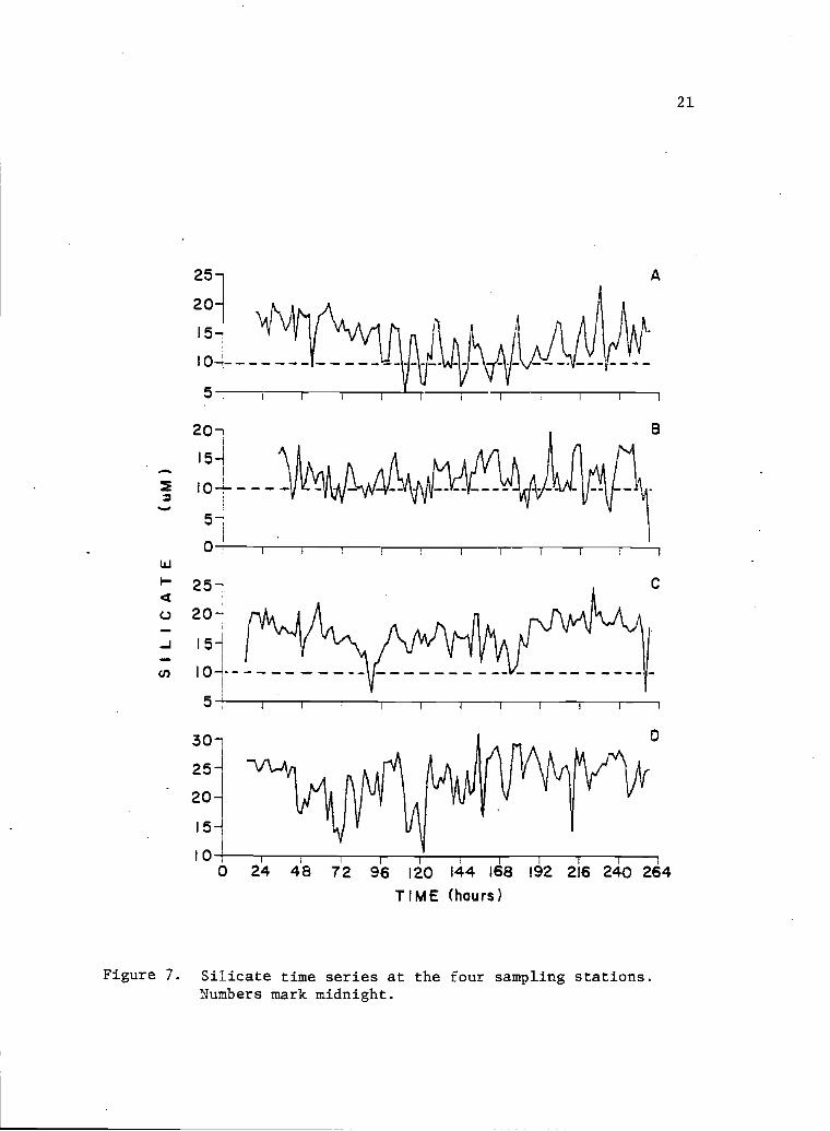
7 Silicate time series at the four sampling 21stations. Numbers mark midnight.

8 Chlorophyll a time sereis at the four sampling 24stations. Numbers mark midnight.

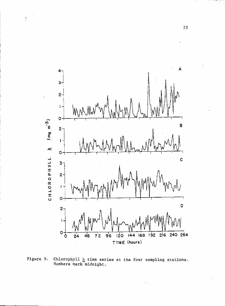
9 Chlorophyll b time series at the four sampling 25stations. Numbers mark midnight

10 Chlorophyll c time series at the four sampling 26stations. Numbers mark midnight.

11 Pheophytin a time series at the four sampLing 27stations. Numbers mark midnight.

12 Phytoplankton abundance time series at the four 28sampling stations. Numbers mark midnight.

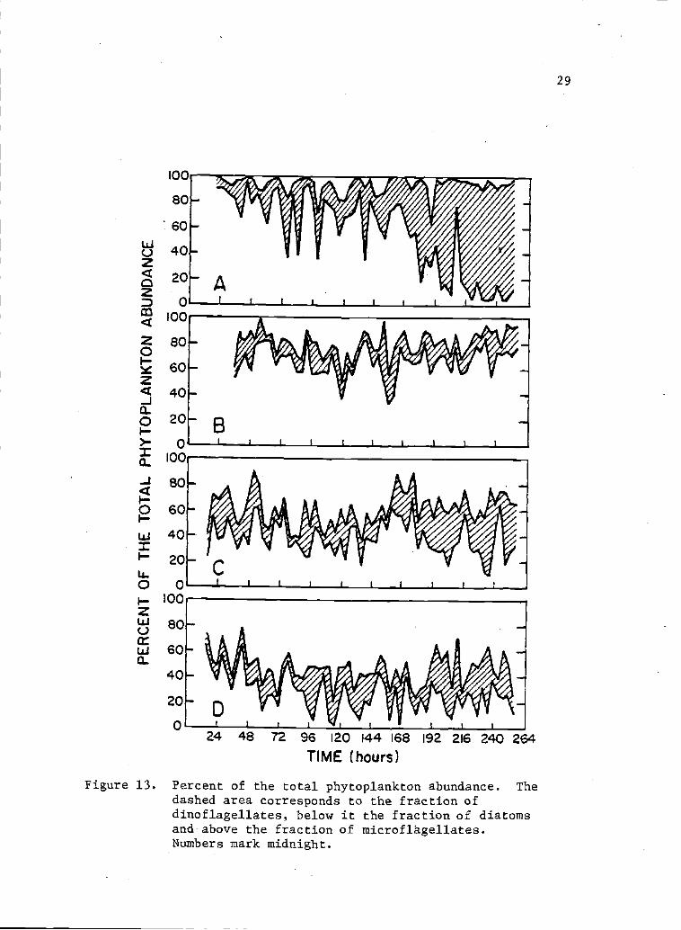
13 Percent of the total phytoplankton abundance. 29The dashed area corresponds to the fraction ofdinoflagellates, below it the fraction of diatomsand above the fraction of microflagellates.Numbers mark midnight.

Figure

14 Phytoplankton productivity (mgC in hr (filled 30

circle) and assimilation ratio {iugC(mgChlaY1hr- (open circle). uinbers mark midnight, theline above the numbers mark the dark period.

15 Spectral density of tide (left) and salinity 32(right) at station D.

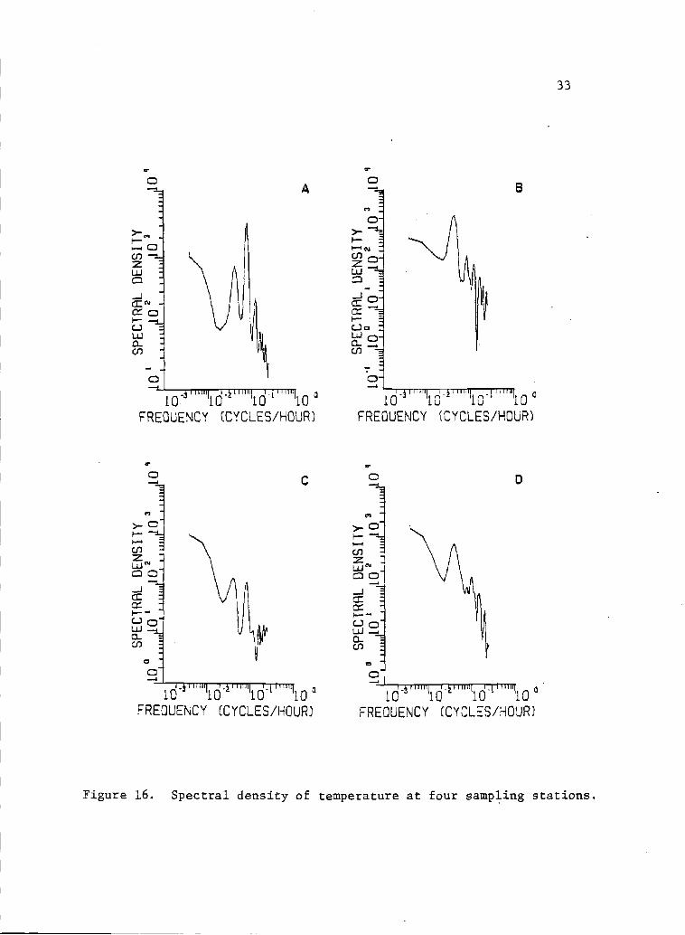
16 Spectral density of temperature at four sampling 33stations.

17 Spectral density of nitrate at four sampling 34stations.

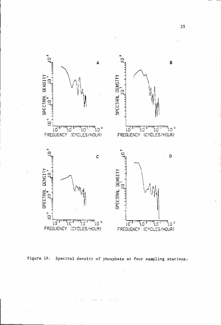
18 Spectral density of phosphate at four sampling 35stations.

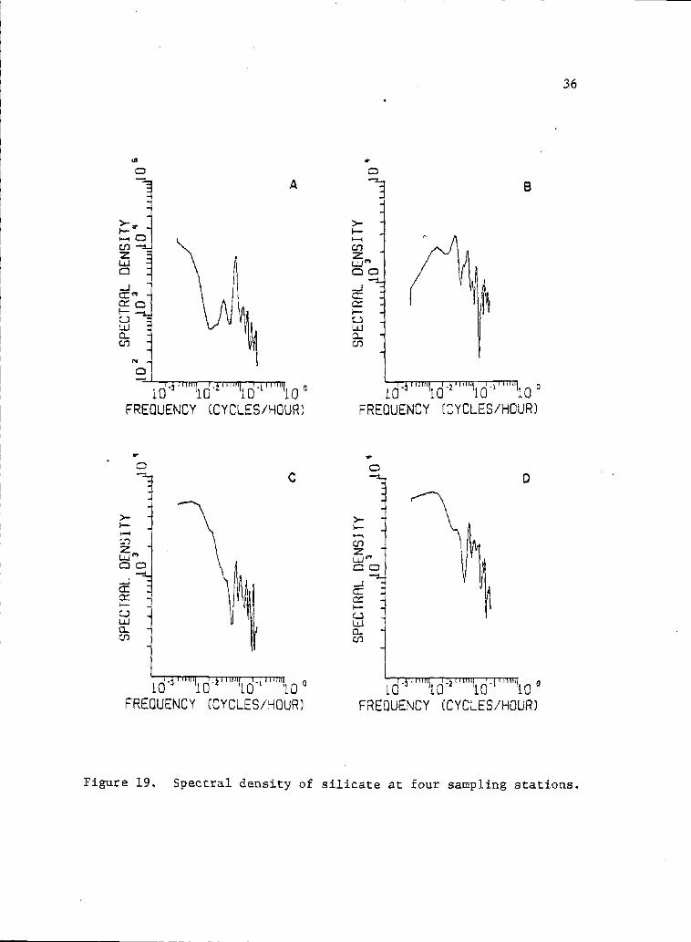
19 Spectral density of silicate at four sampling 36stations.

20 Spectral density of chlorophyll a at four 37sampling stations.

21 Spectral density of total phytoplankton 38abundance at four sampling stations.

22 Variation of cross correlation coefficients with 45lagged units.

Table

LIST OF TABLES

Page

Cross correlation coefficients and numbers of 40

lags (in parentheses) needed to maximize thecorrelation coefficients at station A. Thetime series of the variables in the column atthe left are moved forward in time the numberof lag units as indicated in each case. Lagunit equal to two hours. ++ significanceat 99% confidence level. + significance at95% confidence level.

II Cross correlation coefficients and numbers of 41lags (in parentheses) needed to maximize thecorrelation coefficients at station B. Thetime series of the variables in the column atthe left are moved forward in time the numberof lag units as indicated in each case. Lagunit equal to two hours. +4- significanceat 99% confidence level. + = significance at95% confidence level.

III Cross correlation coefficients and numbers of .42

lags (in parentheses) needed tQ maximize thecorrelation coefficients at station C. Thetime series of the variables in the column atthe left are moved forward in time the numberof lag units as indicated in each case. Lagunit equal to two hours. ++ = significanceat 99% confidence level. + significance at95% confidence level.

IV Cross correlation coefficients and numbers of 43

lags (in parentheses) needed to maximize thecorrelation coefficients at station D. Thetime series of the variables in the column atthe left are moved forward in time the numberof lag units as indicated in each case. Lagunit equal to two hours. ++ = significanceat 99% confidence level. + significance at95% confidence level.

EFFECTS OF PHYSICAL PHENONA ON THE DISTRIBUTIONOF NUTRIENTS AN!) PHYTOPLANKTON PRODUCTIVITY

IN A COASTAL LAGOON

INTRODUCTION

During the last eight years, there has been an increased

interest in developing ruaricultures in the coastal lagoons of the

Baja California peninsula. The main interest has been concentrated

on oyster culture. Very successful experiments with Crassostrea

igas, the Japanese oyster, and Ostrea edulis, the European oyster,

have been carried out in most of the coastal lagoons of the

peninsula's Pacific coast. Most of these coastal lagoons are very

much in their natural state. But, as development goes on from the

two ends of the peninsula, human activities are making an impact

upon their ecology. Some of the northern and southern lagoons are

already undergoing changes due to urban and touristic development,

besides the effect of fishing on (mainly) crustaceans and molluscs.

There is still a unique opportunity to carry on basic ecological

studies in some of these coastal lagoons before significant changes

are made by man's activities. These studies can give us the

background ecology against which the situations of the future may be

compared. Also, the studies can be designed to gain useful

information that might be applied to make rational decisions as

maricultures are developed. For example, it is important to know

the spatial and temporal ranges of important ecological variables

as temperature and salinity; the relative food availability in

different lagoons; the mechanisms that are responsible for greater

or less fertility of some lagoons with respect to others and with

respect to the open ocean; and the water exchange rate between

the lagoons and the adjacent ocean (Lara-Lara, Alvarez-Borrego, and

Small, 1980).

3

GENERAL DESCRIPTION OF SAN QUINTIN BAY

Bahia San Quintin is a coastal lagoon located between

30°24tN-30°30'N, and 115°57'W-116°Ol'W, on the Pacific coast of

Baja California, Mexico (Fig. 1). The bay is some 300 km south of

the Mexico-U.S.A. border. The bay is "Y" shaped with a single

permanent entrance at the foot of the Y. It has a north-south

orientation, and an area of about 41.6 km2. The lagoon is

extremely shallow, and at lower low tide 20% of the bottom is

exposed to the air. There are narrow channels that rarely exceed

8 meters in depth. The western arm is named Bahia Falsa and the

eastern arm is called specifically Bahia San Quintin (Barnard,

1962). The continental shelf is very narrow off Bahia San Quintin

and the wave energy is very high on the open coast (Lankford, 1976).

The climate is arid along the coast and in the mountains.

The amount of annual precipitation (5-10 cm) comes mostly in winter.

The relatively cool California Current offshore of Bahia San Quintin

is partly responsible for the benign climate of the region.

Upwelling occurs in the open ocean immediately off the mouth of the

bay during spring and summer (Dawson, 1951), a result of northwesterly

winds during these seasons. The upwelling process accounts for the

presence of fog off the bay in spring and summer.

Flood runoff occurs sometimes in winter, but there are no

flowing streais coming into the bay. The westernmost seaward edge

of the bay is a long sandspit connecting two cinder cones (Fig. 1),

the southern of which marks the entrance to the bay. The south shore

3O3C'N

(CLoborator)\,Molino Viejo

Mt. Kenton(280m) 2

3Q0 24' Lcguno

PACIPIC -: 5OCEAN

Figure IL. Bahia San Quintin. Time series anchor stations (A).Bathymetry in meters.

5

on the open sea trends east and west, being formed of a sandspit

(Punta Azufre) protecting bayward marshes. The two northward

trending arms of the bay are split by two prominent cones, Mt.

Ceniza and. Mt. Kenton and most of this middle peninsula is formed

of volcanic material (Barnard, 1962).

The mainly shallow mud-flat character of the bay provides for

two kinds of dominant vegetation. One is a marine flora consisting

of eelgrass, Zostera marina, which forms broad, dense strands

occupying the greater part of the muddy bottom of the lagoon. The

other is a salt marsh flora of extensive development along nearly

half of the low-lying margins of the lagoon subjected to tidal

flooding (Dawson, 1962).

GENERAL OCEANOGRAPHY

In general, all the year around, there are horizontal salinity

and temperature gradients, with values increasing from the mouth

to the extremes of the lagoon. Sometimes during the winter, with

cold air temperatures (0-4°C), the seawater temperature gradients

reverses, with values near 15°C at the mouth and near 12°C at the

extremes of the bay. The lowest surface temperatures at the mouth

have been recorded during summer, with values sometimes below 12°C.

These low temperatures are the result of upwelling events during

summer, in the adjacent oceanic area. Surface temperatures in the

extremes may be higher than 23°C during summer, due to solar

radiation input. Bahia San .Quintin, the eastern arm, has greater

salinity values than Bahia Falsa with a difference of about 1°I

This is due to the greater residence time of water in the former

location. Salinity may be higher than 37°/ in the extreme of the

eastern arm, and lower than 33°/a, at the mouth. Average surface

salinities for the whole lagoon do not change significantly from

winter to summer. Tidal and solar radiation cycles cause large diel

changes of the different water properties in all areas of the lagoon,

so that any graph showing the spatial distribution of a seawater

property is only a first approximation because. sampling cannot be

really synoptic (Chavez-de-Njshjkawa and Alvarez-Borrego, 1974;

Alvarez-Borrego, Ballesteros-Grijalva and Chee-Barragan, 1975).

Alvarez-Borrego and Chee-Barragan (1976) reported that phosphate

and silicate surface values increase in general from th.e mouth to

the extremes. These authors have suggested that the inorganic

7

nutrient distribution may result from high concentration of sea

grasses in the lagoon bottom. The grasses act to trap the suspended

material that is carried from the adjacent oceanic zone into the

lagoon by the tidal currents. This trapping action causes a high

deposition of organic material, which is remineralized to inorganic

compounds and finally redistributed in the water by tidal currents

and wind-induced turbulence. During spring and summer, in addition

to the above mechanism, the system receives impulses of inorganic

nutrients from the adjacent oceanic area during upwelling events.

This causes nutrient concentrations at the mouth to be greater

during summer than during winter. Reported ranges for phosphate for

the whole bay have been. 1.5 to 2.9 iM for summer and 0.7 to 2.0 iiM

for winter; and for silicate, 13 to 18 )IN for summer and 5 to 35 jiM

for winter.

Alvarez-Borrego and Lopez-Alvarez (1975) reported for the mouth

a phytoplankton total abundance of 485 cells m1 in July and 340

cells ml in January, with diatoms dominating in July and dma-

flagellates in January. Phytoplankton abundance decreases toward

the extremes especially toward the head of the eastern arm, where

values are an order of magnitude smaller than at the mouth. Lara-Lara

and Alvarez-Borrego (1975) studied the surface distribution of

photosynthetic pigments in Bahia San Quintin during one annual cycle.

They found the lowest concentrations in winter (average chlorophyll a

concentration of 1.5mg increased amounts in spring (average

chlorophyll a concentration of 2.0 mg m3), and highest values in

summer (average chlorophyll a concentrations of 3.0 mg m3). Highest

chlorophyll a concentrations were always found in the area between

the mouth and the vertex of the "Y". Here, summer maximum values

of 8.0 mg m and winter maximum values of 3.5 mg m were found.

Alvarez-Borrego, Lara-Lara and Acosta-Ruiz (1977) generated

four 26-hr time series of salinity, temperature, oxygen, phosphate,

nitrate, chlorophyll and metereological variables, once every

season at the bay mouth. The variables were measured every hour.

They found that chlorophyll concentration can sometimes change by

an order of magnitude within an hour. Lara-Lara, Alvarez-Borrego,

and Small (1980) generated an 18 day time series, also at hourly

intervals, of several ecological variables for the mouth of Bahia

San Quintin, during the summer of 1977. Variables were: sea level,

current velocity, temperature, salinity, oxygen, inorganic phosphate,

chlorophyll a, seston, phytoplankton species abundance, particulate

organic carbon and nitrogen and primary productivity. They concluded

that alternation of upwelling events was the main cause of variability

for all properties except temperature. Semidiurnal tides were the

main cause of variability for temperature. Diatoms were always the

most abundant phytoplankton group. Primary productivity was always

greatest at the surface, with a mean value of 27 mgC m hr through

the sampling period. Maximum surface productivity values were obtained

for the upwej.ling relaxation period (up to 44 ingC in hr1)

The mean

surface assimilation ratio was 6.6 mgC(mgChla)hr which indicates

nutrient-rich waters.

OBJECTIVES OF THIS WORK

The objectives of this work were to study Bahia San Quintin

(Fig. 1) to determine the effects of diurnal and seinidiurnal tides,

the alternation of spring and neap tides, the alternation of upwell-

ing events off the bay mouth and other physical factors on the

distribution of nutrients, phytoplankton abundance and phytoplanktoa

productivity.

Ten-day time series were generated simultaneously at four

strategic points (Fig. 1) for sea level, temperature, salinity,

nutrients (nitrate, nitrite, phosphate and silicate), chiorophylls

a, b and c and their pheophytins, phytoplankton abundance by gross

taxonomic groups, and phytoplankton productivity. Sampling was done

so that surface horizontal distribution of properties and their

dynamics with time could be described.

10

DATA COLLECTION AND ANALYSIS

Time series sampling was carried out, day and night, simultan-

eously at four anchor stations (Fig. 1), from June 25 to July 5,

1979. Samples were collected only at the surface.

Tide height was measured at Molino Viejo (Point D, Fig. 1)

by a Fisher and Porter Model 1550 digital tide gauge. In order to

generate the sea level time series for the other three points (A,B

and C, Fig. 1) the phase lag as taken from Monreal (1980).

Water temperatures were read off bucket thermometers every two

hours. Salinity was analyzed at a shore-based laboratory (Fig. 1)

with a conductivity salinometer, Beckman Model 118WA200. Salinity

samples were taken every two hours at point D but only twice a day

at the other points. Salinity data taken once every two hours at

points A, B, and C with a conductivity meter, Kahisico Model

l88WA300, proved not to be accurate nor precise, therefore they are

not included in this thesis.

Nutrients, chlorophyl.ls and phytoplankton samples were always

taken from the same Van-Dot-n bottle, sampling every two hours. Two

drops of a saturated solution of HgC12 were added to each nutrient

sample iuunediately after collection. Then samples were frozen to

be transported to the laboratory. They were analyzed at O.S.U.

School of OceanographyTs laboratory for phosphate, silicate, nitrate

and nitrite, using a Technicon II AutoAnalyzer.

Chlorophyll samples were obtained using 0.45 .im pore-sized

Millipore filters. Filters were frozen to be transported to the

11

laboratory of Centro de Investigacion Cientifica y de Educacion

Superior de Ensenada (CICESE) at Ensenada. Chlorophyll analysis was

done basically by the SCOR-UNESCO (1966) method, but with some

modifications. Second readings at 665, 645, and 630 nm were done

after acidification, following Loreuzen (1967). A 1-to-i volume

solution of 90% acetone and dimethyl sulfoxide was used as a solvent

to improve the pigment extraction (Shoaf and Lium, 1976). Spectrophoto-

metric equations developed by Millán-Nuftez and Alvarez-Borrego (1978)

were used to estimate concentration of chiorophylls a, b, and c, and

pheophytins a, b, and c. The equation for chlorophyll a is exactly

the same as that of Lorenzen (1967) due to the chlorophyll b:

pheopigment b and chlorophyll c pheopigment ratios at 665 ntri

being equal to one.

Phytoplankton abundance by gross taxonomic groups was determined

by the TJtermohl (1958) inverted scope technique using a Carl Zeiss

invertoscope D microscope.

Three times a day during daylight hours, surface (0.5 in)

carbon-14 incubations of one hour duration were done at high,

intermediate, and low tide. Seawater samples for carbon-14

incubations were not taken from the same Van Dorn samplings for

chlorophyll and phytoplankton. Sampling was done specifically for

the incubations. The vials containing the filtered samples were

transported to the O.S.U. School of Oceatiography, where the radio-

activity of the samples was determined in a scintillation spectrometer.

Inorganic carbon-14 was purged from the vials with nitrogen gas

before the radioactivity measurements. Conversion of radioactivity

12

to carbon productivity was done as indicated by Strickland and

Parsons (1972).

13

STATISTICAL ANALYSIS

Sometimes it is necessary to study the relationship between

two processes with possibly different scales of measurement or

different variances. In this situation it is necessary to define

the cross correlation function:

CL)L)

where S and S2 are the sample standard deviations of series 1 and

2, respectively, S12 is the covariance of series 1 and 2, and R is

the correlation coefficient between series 1 and 2. The symbol L

is the number of "lags" of a given time unit that one series must

be displaced with respect to the other in order to maximize the

correlation coefficient between the two series (Jenkins and Watts,

1969). In this work the time unit chosen for each lag is two hours.

One application of lagged cross correlation is in the measurement

of time delay between two processes.

From Platt and Dennian (1975), spectral analysis of a series of

data may be regarded as an analysis of variance in which the total

variance of a variable or property fluctuation is partitioned into

contributions arising from processes with different characteristic

time scales. Thus, spectral analysis of a record of observations

results in a sorting of total variance of the record into its

component frequencies. The spectral analysis results presented here

were computed with a fast Fourier transform algorithm. The output

presents the frequency components in cycles per hour.

14

RESULTS

Description of time series of seawater properties

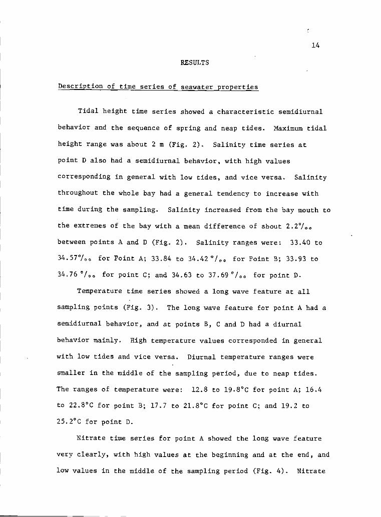
Tidal height time series showed a characteristic semidiurnal

behavior and the sequence of spring and neap tides. Maximum tidal

height range was about 2 m (Fig. 2). Salinity time series at

point D also had a semidiurnal behavior, with high values

corresponding in general with low tides, and vice versa. Salinity

throughout the whole bay had a general tendency to increase with

time during the sampling. Salinity increased from the bay mouth to

the extremes of the bay with a mean. difference of about 2.2°I

between points A and D (Fig. 2). Salinity ranges were: 33.40 to

34.57°/ for Point A; 33.84 to 34.42°/a,, for Point B; 33.93 to

34.76 °/ for point C; and 34.63 to 37.69 °/ for point D.

Temperature time series showed a long wave feature at all

sampling points (Fig. 3). The long wave feature for point A had a

seiuidiurnal behavior, and at points B, C and D had a diurnal

behavior mainly. High temperature values corresponded in general

with low tides and vice versa. Diurnal temperature ranges were

smaller in the middle of the sampling period, due to neap tides.

The ranges of temperature were: 12.8 to 19.8°C for point A; 16.4

to 22.8°C for point B; 17.7 to 21.8°C for point C; and 19.2 to

25.2°C for point D.

Nitrate time series for point A showed the long wave feature

very clearly, with high values at the beginning and at the end, and

low values in the middle of the sampling period (Fig. 4). Nitrate

15

time series for points B, C and D did not show the long wave feature

clearly, although values at the beginning of the sampling were in

general higher than those towards the end. High nitrate values at

point E at the beginning of the sampling were due to an ending

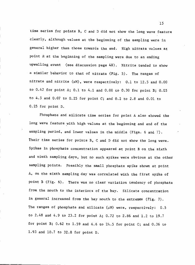
upwelling event (see discussion page 48). Nitrite tended to show

a similar behavior to that of nitrate (Fig. 5). The ranges of

nitrate and nitrite (i.IN), were respectively: 0.1 to 12.5 and 0.00

to 0.42 for point A; 0.1 to 4.1 and 0.00 to 0.30 for point B; 0.03

to 4.5 and 0.07 to 0.25 for point C; and 0.2 to 2.8 and 0.01 to

0.25 for point D.

Phosphate and silicate time series for point A also showed the

long wave feature with high values at the beginning and end of the

sampling period, and lower values in the middle (Figs. 6 and 7).

Their time series f or points B, C and D did not show the long wave.

Spikes in phosphate concentration appeared at point B on the sixth

a-nd ninth sampling aays, but no such spikes were obvious at the other

sampling points. Possibly the small phosphate spike shown at point

A, on the sixth sampling day was correlated with the first spike of

point B (Fig. 6). There was no clear variation tendency of phosphate

from the mouth to the interiors of the bay. Silicate concentration

in general increased from the bay mouth to the extremes (Fig. 7).

The ranges of phosphate and silicate (uN) were, respectively: 0.5

to 2.48 and 4.9 to 23.2 for point A; 0.72 to. 2.86 and 1.2 to 19.7

for point B; 0.62 to 1.59 and 6.6 to 24.5 for point C; and 0.36 to

1.93 and 10.7 to 32.8 for point D.

3.0

E2.5

I-

2.0

LU

I.5LU

L0

0.5

1

37a

-S

zJcn35

34

35

S

34

z

(/)33

1

4a

Co0 0 0

00

10A

D a

a a

24 48 72 96 120 144 168 192 216 240 26TIME (hours)

16

Figure 2. Tide height time series (upper) at station D. Salinitytime series (middle) at station D, this station wassampled every two hours. Salinity time series (lower)at stations A (0), B () and C (a). These stationswere sampled at times of high and low tide at station D.

2019

18

'7

16

15

'4

13

12

23222l

2O

LU18

17)- I64

LU 22-

21

20i- 19

18

17

2524232221

20'9

96 tO 144TIME (hours)

17

B

C

Figure 3. Temperature time series at the four sampling stations.The letters (A,B,C.D) indicate the stations. Numbersmark midnight.

Ui

E1

I I I

__

z C

4:1 I

2

jIII0 24 48 72 9 20 144 168 192 216 240 264

TtME (1cur)

Figure 4. Nitrate time series at the four sampiing stations.Numbers mark midnight.

0.3

O2

0.I

W OHI.-

0.3

0,2

0

19

B

C

Ii]

24 48 72 96 20 44 168 192 2i6 240 2TIME (hours

Figure 5. Nitrite time series at the four sampling stations.Numbers mark midnight.

20

3.0

2.5

2.0

IS

l.a

i-054z 200q .5

CLO

B

I 120 144 168 192 2

TIME (hours)

Figure 6. Phosphate time series at the four sampling stations.Numbers mark midnight.

21

0 I

I III Ii'

30

25

15

to24 48 72 96 120 144 168 192 216 240

TIME (hours)

Figure 7. Silicate time series at the four sampling stations.Numbers mark midnight.

22

The time series at point A for chlorophyll a, b and c showed

a general tendency to increase with time during sampling (Figs. 8,

9 and 10). Generally, the highest values for all three pigments

at the bay mouth station were found at the end of the sampling

period. Pigment time series for sampling points B, C and D showed

a complicated patchiness, with no clear variation tendency. The

ranges of chiorophylls a, b and c (mg m3) were respectively: 0.5

to 37.9, 0.0 to 3.8 and 0.0 to 16.1 fbr point A; 0.5 to 18.7, 0.0

to 1.9 and 0.0 to 12.6 for point B; 0.5 to 4.8, 0.0 to 2.7 and 0.2

to 8.7 for point C; and 0.5 to 4.9, 0.0 to 2.0 and 0.1 to 7.0 for

point D. Pheopigment time series showed a very patchy distribution

at all four sampling points. Pheophytin b and c often were not

significantly different from zero (not illustrated). Pheophytin a

concentrations had less value than their respective chlorophyll

concentration (Fig. 11).

Phyto'plankton abundance time series at the four locations did not

show the long wave feature of temperature and nutrients; instead,

these time series showed very patchy distribution (Fig. 12). In

general phytoplankton total abundance decreased from the bay mouth

to the bay extremes. At the' extremes, abundance was an order of

magnitude less than at the bay mouth. At point B there were patches

of high abundance during the first half of the sampling period. Cell

abundance at point B was similar to that at points C and D during the

second half of the sampling period. There was no clear, permanent

dominance of diatoms over dinoflagellates, or vice versa, at any of

the sampling stations except station B, where diatoms outnumbered

23

dinoflagellates for most of the sampling period (Fig. 13). For any

given taxonomic group there was no consistent difference in cell

size between stations A, B, C and D. The ranges of phytoplankton

total abundance (cells ml) were: 42 to 1815 for point A; 43 to

2580 for point B; 20 to 182 for point C; and 18 to 246 for point D.

Phytoplankton productivity time series showed a very irregular

variation at point A and B (Fig. 14). There was a tendency for

productivity to increase with time during sampling at point A, but

not at point B. This corresponded with pigment changes through

time at the two stations. Primary productivity also showed a

tendency to decrease from the bay mouth to the extremes. Assimilation

ratios showed irregular variation with time at all stations; however,

mean values at each location were not significantly different from

one another. Means and ranges of phytoplankton primary productivity

(mgC m3 hr1) were respectively: 33.4, 5.3 to 91.4 for point A;

16.5, 1.6 to 63.0 for point B; 12.5, 2.2 to 23.4 for point C; and

12.3, 1.9 to 27.4 for point D. Neans and ranges of assimilation

ratios [mgC(mgCh1a) hr] were respectively: 6.4, 0.6 to 13.7 for

point A; 7.8, 0.8 to 26.2 for point B; 5.4, 0.6 to 12.5 for point C;

6.0, 0.8 to 15.0 for point D.

24

(38)

201 A

'5

5

r-02O

E

'5

I0-j

-J

>.. 5

a.

o.00-j

I0

0 24 48 72 96 120 144 168 L92 216 240 2

TIME (hours)

Figure S. Chlorophyll a time series at the four sampling stations.Numbers mark midnight.

E

E-S.

1

-j

>-

=

0

0-i

=0

25

BS

C

0S

T1ME (hours)

Figure 9. Chlorophyll b time series at the four sampling stations.Numbers mark midnight.

20

5

15

10

"I

10

0

0-J

zo

5

'-4

B

C

Fil

TIME (hours)

4

26

Figure 10. Chlorophyll c time series at the four sampling stations.Numbers mark midnight.

L]

I;;- 4

0

27

A

ci8 B

0UJ

C2H

O A&M PA A AJVFi

TIME (hours)

Figure 11. Pheophytin a time series at the four sampling stations.Numbers mark midnight.

U,

UN0'C

0

-I

UiUz< 2'

z

z0I-

zJ0I-

=a-

. Ill lIllillIl lIEU 11111111111111111111111111111 fUll 11111 lIII

24 48 72 96 120 144 168 92 216 240 264

TIME (hours)

28

Figure 12. Phytoplankton abundance time series at the four samplingstations. Numbers mark midnight.

29

LsJC-)

0z

ICC

Z 8C0I-

z4C

-J

02>- aI

-I BC

IgSCuj 4C=' 2CU..

o C

IzUiC-,

Uia-

ri

24 48 72 96 120 144 168 192 216 240 264

TIME (hours)

Figure 13. Percent of the total phytoplankton abundance. Thedashed area corresponds to the fraction ofdinoflagellates, below it the fraction of diatomsand above the fraction of mi.croflhgellates.Numbers mark midnight.

-S

EUE

I-

IUa0

>-

20

24 48 72 96 120 144 168 192 216 240 264

TIME (hours)

30

15

10a-

5.;-_

3001

25 U20 '

15 U

010

SQI-

0_jl5

ir (I).1

5

[.J

Figure 14. Phytoplankton productivity (mgCm3 hr') (filled1circle) and assimilation ratio (mgC(mgChla)-hr )

(open circle). Numbers mark midnight, the lineabove the numbers mark the dark period.

31

Spectral analysis of time series

The tide variance spectrum showed most of the variance at the

diurnal (freq. 0.04l eph) arid semidiurnal (freq. 0.083 eph) periods

(Fig. 15). The variance spectra of all other seawater properties

tended to show high variance components at these two frequencies,

although distinct peaks were not always obvious (Figs. 15, 16, 17,

18, 19, and 20). Salinity, temperature, nitrate, phosphate, silicate,

and sometimes chlorophyll a, clearly showed a high variance component

at the lowest frequency (0.0025 eph). These low frequency variance

components might be associated with the alternation of upwelling

events (.Lara-Lata, Alvarez-Borrego and Small, 1980). They might

also be associated with the alternation of the spring and neap tides.

Variance components at high frequencies (>0.l cph) are likely

related to turbulence and irregular mixing conditions created by

the lagoon bathymetry and the associated heating by solar radiation

input.

C"

C

-j4I-CLiJ

0

0

C

IO 1O-'

FREQUENCY (CYCLES/HOUR)

I

NC

I

O 1D 10

FREQUENCY CCYCLES/HOURJ

32

Figure 15. Spectral density of tide (left) and salinity (right) atstation B.

33

a. a.

C C-- A B

I,IIlflf IIlIlII I[IIIII I_ItIII _JIIIIII ;llIrrI

10 10 10 10 10 10 10 10

FREQUENCY (CYCLES/HOUR) FREQUENCY (CYCLES/HOUR)

a.

Ca.

CI- 4

CJ, \ (0

CC- CC

'I 1' 4-IVHt

.3 liii l_l1lllI lll3

I FliJhiI l_lliIIiI p llll

10 10 10 10 10 10 u10 10

FREQUENCY (CYCLES/HOUR) FREQUENCY (CYCLES/HOUR)

Figure 16. Spectral density of temperature at four sampling stations.

34

1 C,

CA

C,, I

3 \

z 1

(\I

LU ICCI\Ik

j

I-] Iw 1 ml LU I

o__ -jII a-. -f

Cf,I

id "'id"1j

L"fta

FREQUENCY (CYCLES/HOUR)

C,

C

B

III_j III

id 4''id" 10 100

FREQUENCY (CYCLES/HOUR)

A-I

A--4

UJ - LUC \ / C

C.,

C

-J\J

-L) C_)

LU d LUa_ -4

(fl-f

0_I 0

CI Ca

id''''id'ti_d 10

FREQUENCY (CYCLES/HOUR) FREQUENCY (CYCLES/HOUR)

Figure 17. Spectral density of nitrate at four sampling stations.

NC

.4

zw

J

LJ

Cs,

-4IIIlIIll IiIlIIIl 1.1111119

O 'tO tO tO

FREQUENCY (CYCLES/HOUR)

N

C

f_IIIIII1011tOio to

°

FREQUENCY CCYCLES/HOUR)

N

B

>I-

-4c-f,zLLJ

J

ciuJ

0D

1LIllIl tflttt4 1%fl a

10 10 10 10

FREQUENCY (CYCLES/HOUR)

NC

>-

-4CS)

LJJ'

J

Ciw(/)

lIIillI I_lIlI1P jIlIla

10 10 10 10

FREQUENCY (CYCLES/HOUR)

35

Figure 18. Spectral density of phosphate at four sampling stations.

36

A

>-. I >-I.-. 1

r.nzLU -i

__I

H-I

I.- -

LJ L JLU

I

LU

I0

B

''td "1id 1"to

FREQUENCY (CYCLES/HOUR) FREQUENCY (CYCLES/HOUR)

.. S0 0

I -cJlz z

LU"00-J

li

C) 1i

LUI. LU

10 '1O'i0 id2 'idt'"toFREQUENCY (CYCLES/HOUR) FREQUENCY (CYCLES/HOUR)

Figure 19. Spectral density of silicate at four sampling stations.

37

>-

-J

c-J

LU

(J

*C

A

'III,,!

tO t0 I.0

FREQUENCY CCYCLES/HOUR)

0,

C

C

4ci-)zLUCC-J

FC-,

LU

B

'"'"i.d2id'"to

FREQUENCY (CYCLES/HOUR)

CI,

C

:iJC:,

LU

-J

F- I

LU I LUa... -

Ct) (1) -1

C C4jIIlTII TJI4III I IIItIIIF IIIIIII I_11ji119

to. i.o i0 1.0° 10 'tO 10 10

FREQUENCY CCYCLES/HOUR) FREQUENCY CCYCLES/HOUR)

Figure 20. Spectral density of chlorophyll a at four samplingstations.

38

a a

A

)-. -i >- -1

1.I-I

I

Cs,z z -1

UJ' U.J

1k ccl. (

I I flI-1 U -4

i .4 I -

LH1

LU I LUCL. CL 1

llItj I_IILFII 1.11111'!0

LO 10 10 10

FREQUENCY (CYCLES/HOUR)

-4

C

I IIlI1

tO 10' 10 L0

FREQUENCY (CYCLES/HOUR)

Al

>- -1I -I

AAzI

LU LL1Z

¶1 41 II

II -

C..) .4

LU LU0_ D.. -I

-1ci2 Tj- t0 0

FREQUENCY (CYCLES/HOUR) FREQUENCY (CYCLES/HOUR)

Figure 21. Spectral density of total phytop].ankton abundance atfour sampling stations.

Cross correlation among variables at the same sampling point.

Table I shows the cross correlation coefficients and the number

of lags needed to maximize the correlation coefficients (lag unit

equal to -two hours) between nitrate, nitrite, silicate, phosphate,

chlorophyll a, chlorophyll b, chlorophyll c, pheophytin a, temperature

and tidal heights, all at point A. The highest cross correlation

coefficients were: NO3-NO2(0.78 with zero lags), NO3-PO4(0.76 with

zero lags), T°C-tide (-0.71 with zero lags).

Table II shows the cross correlation coefficients for point B.

The highest cross correlation coefficients were: NO3-T°C(.-0.4l with

zero lags), NO2-Chla(0.5l with zero lags), Chla-Chlc(0.68 with zero

lags).

Table III shows the cross correlation coefficients for point C.

The highest cross correlation coefficients were: NO3-NO2(0.66 with

zero lags), NO3-tide (0.53 with zero lags), Si02-PO4(0.60 with zero

lags), Chia-Chic (0.61 with zero lags).

Table IV shows the cross correlation coefficients for point D.

The highest cross correlation coefficients were: NO2-PO4(0.65 with

zero lags), Si02-PO4(0.73 with zero lags), and S°!.,0 tide(-0.80

with zero lags).

Cross correlation coefficients higher than 0.20 and 0.26 were

statistically significant at the 95% and 99% confidence levels,

respectively. However, such low coefficients indicated that only a

small fraction of the variability of the dependent variable could be

accounted for by linear relationship with the independent variable.

NO3 t402 PG4 Chia Chib Chic PhLOa ['CTide

NO O.78 O.60 0.76 -0.31 -0.16 -0.i6 -0.137 -Q.63 O.24(0) (0) (0) (5) (4) (2) (-4) (0) (0)

NO2 O.55 O.58 -0.3O -0.3O' -0.25k -0.10 -O.39 0.13(0) (0) (1) (3) (3) (0) (2) (2)

Sf02

O.66 -0.12 O.25 0.12 -0.13 I_O59 -0.26(°) (1) (°) (0) (0) (3) (3)

PO4 -Q.32 -0.13 -0.17 -0.16 -O.4i 0.10(5) (2) (1) (-5) (1) (-4)

Clija O.33 0.49 0.17 0.21* 0.24k(5) (0) (0) (-4)

Chib0.59 -0.11

(-4)

0.23*

I . (0) (0) (0) (3)

C[dc0.15 -0.20k

(0) (-6) (6)

0.19(-3) (0)

TC-O.71

Table I. Cross correlation coefficients and numbers of lags (in parentheses) needed to maximizethe correlation coefficients at station A. The time series of the variables in thecolumn at the left are moved forward js time the number of lag units as indicated ineach case. Lag unit equal to two hours. ++ significance at 99% confidence level.+ = significance at 95% confidence level.

NO NO SiO. P0 Chia Chib Chic Pheoa T°C1

3 2 2 4 Tide

NOo41H-

0.36 _0.21+ O.26* 0.13 O.27 0.35 -0.41 _O.21+(0) (0) (-1) (i) (0) (4) (4) (0 (2)

No042f+

O.29 O.51 -0.17 0.34 0.45 -O.23 Q372(0) 10) (0) (-5) (0) (0) (0) (-4)

SiO, O.44 o.ii -0.18 0.19 -O.22 -0.282(0) (0) (4) (2) (4) (0) (1)

P0 O.2O 0.17 -014 0.15 0.41 -0.29(0) (1) (2) . (2) (5) (0)

Chia 0.11 ++O. ++0.31

-s--f-0.23

- +-0.37

(0) (0) (0) (-2) (-1)

Club 0.27 -O.38 -0.13 -0.08(0) (0) (0) (-1)

Chic 0.29 -0.24k -0.22k(0) (1) (-1)

Pheoa -0.09 -0.10-(3) (1)

T°C 0.35(0)

Table II. Cross correlation coefficients and numbers of lags (in parentheses) needed to maximizethe correlation coefficients at station B. The time series of the variables in thecolumn at the left are moved forward in time the number of lag units as indicated ineach case. Lag unit equal to two hours. -H-- = significance at 99% confidence level.+ significance at 95% confidence level.

NO NO Sf0 P0 Chia Club Chic Pheoa T°CTide3 2 2 4

NO 0.66 0.09 -0.15 -O.38 -0.17 -0.24k -0.18 -O.50 053(0) (3) (1) (-2) (-2) (-2) (0) (0) (0)

NO O.3O 0.36 0.11 0.16 0.16 -O.21 0.292(0) (3) (2) (2) (1) (-1) (5) (IL)

Sf0. O.6O 0.18 O.23 -0.12 0.11 -O.27 -0.142(0) (-1) (-4) (3) (1) (-2) (0)

P0 0.18 0.09 0.16 -0.08 -O.1I(2) (-4) (1) (1) (-3) (-1)

Chia 0.S6 O.61 0.52 Q.46 -0.21(0) (0) (0) (-2) (2)

Chib 0.60 -O.38 0.29 0.08-(0) (0) (-1) (0)

Chic -0.37 O.29 0.2O(0) (-2) (2)

Pheoa-0.21k 0.33(-2) (3)

T'CO.33

____ ____ -________ _____- (-.--- -.-_______ - ____Table III. Cross correlation coefficients and numbers of lags (in parentheses) needed to

maximize the correlation coefficients at station C. The time series of the is

variables in the column at the left are moved forward in time the number of lagunits as indicated in each case. Lag unit equal to two hours. ++ significanceat 99% confidence level. + significance at 95% confidence level.

NO3 NO2 S102 PD4 Chia Chib Chic Ptieoa TC S/ TI-de

NO 0.39' -0.16 0.22k 0.13 0.12 0.28' -O.27 -0.59(0) (-1) (0) (0) (3) (0) (-1) (0) (0) (0)

NO o.si O.6? 0.16 -0.20 0.09 0.31 -0.55 0.34 -0.3O2(0) (0) (0) (1) (0) (-1) (4) (-4) (-4)

SiO U./3 0.2O -0.13 0.1 0.14 -0.2) 0.45 -0.312(0) (1) (3) (1) (4) (-3) (1) (0)

PU 0.13 -0.13 0.0) O.3i -O.2S 0.20k -0.11(4) (0) (1) (2) (0) (1) (-2)

0.41j 0.43 0.59 -0.2? 0.21 0.2?(0) (0) (0) (-4) (1) (3)

Chib O.38' -0.43' -0.19 0.11 -0.13(0). (0) (-3) (0) (0)

Chic -0.2? -0.27 0.2? -0.10-(0) (-4) (4) (4)

Pheoa -0.21k 0.10 -0.13

_________(1) (-2) (3)

TC___.___..___I____________________

-0.2? 0.33'(3) (3)

-0.80++l ()

Table IV. Cross correlation coefficients and numbers of lags (in parentheses) needed tomaximize the correlation coefficients at station B. The time series of thevariables in the column at the left are moved forward in time the number of lagunits as indicated in each case. Lag unit equal to two hours. -H- = significanceat 99% confidence level. + = significance at 95% confidence level.

-Is

44

Three examples were chosen to show the variation of cross

correlation coefficients with lagged units from -12 to +12 units:

first, strong variation from positive to negative cross correlation

coefficients (Fig. 22a), second, high positive cross correlation

coefficients at all lagged periods (Fig. 22b) and third, low cross

correlation coefficients at all lagged periods (Fig. 22c).

Temperature vs tide cross correlation coefficient variation

(Fig. 22a) is obviously due to the typical inverse relation between

the two variables. We can see the high negative cross correlation

coefficient every six and twelve lags {corresponding to 12 hours

(semidiurnal) and 24 hours (diurnal) component of tidal cycles].

High positive cross correlation coefficients lagged every three and

nine 1gs (corresponding to 6 and 18 hours, respectively).

Figure 22b shows the cross correlation coefficient between

nitrate and phosphate. The cross correlation coefficient is always

positive, regardless of the lag period, and also shows the periodic-

ities every six lags (12 hours).

Figure 22c shows the variation in cross correlation coefficients

between silicate and chlorophyll a. It describes the independence

of these two variables, with low cross correlation coefficients at

all lag periods.

).0

.8

.6

.4

.2

0

-2

-4

'3 -.6

-.8

Vo -LOU

0

0

V

0

0U,

0

.8

.6

.4

.2

0

-.2

.bNOPO4'I, 'I' l.l.I'l''1,I' I

.2 cSi02-Chla

-0 -8 -6 -4 -2 0 .2 .4 .6 .8 +10 +12

-4. Lags

45

Figure 22. Variation of cross correlation coefficients with laggedunits.

46

DISCUSSION

The generation of time series to study the variability of

seawater properties is a relatively old technique. Legendre

(1908) explained the oxygen, temperature, salinity and density

variations in the coastal zone of Concarneau, France in terms of

tidal and solar radiation cycles by generating time series as long

as 22 days. He concluded that photosynthesis was the most important

variation factor for the oxygen concentration, and aereation by

wind-induced turbulence was secondary.

Alvarez-Borrego and Alvarez-Borrego (in prep.) generated one

year hourly temperature time series for the same four locations as

this work, from May 1979 to May 1980. Their time series for the

Bahia San Quintin mouth shows the alternation of upwelling events

in the adjacent oceanic area, from Nay to September. Lara-Lara,

Alvaraz-Borrego and Small (1980) clearly showed that suimner seawater

temperatures near 12°C at the Bahia San Quintin mouth are the product

of upwelling, because dissolved oxygen percent saturation was found

to be as low as 60% and this is characteristic of the upwelling water.

Alvarez-Borrego and Alvarez-Borrego's temperature time series indicates

that sampling for the work reported here started at the beginning of

an upwelling relaxation period, and ended when the strongest upwelling

event of the year was about to begin. Also, sampling for my study

started at spring tides, continued through neap tides, and ended at

the beginning of the following spring tides (Fig. 2).

47

Minimum temperatures during the upwelling event previous to my

sampling were about 12°C, while they were about 11°C for the one

after my sampling (Alvarez-Bor-rego and Alvarez-Borrego, in prep.).

TJpwelling previous to my sampling was weaker than the first upwelling

detected by Lara-Lara, Alvarez-Borrego and Small (1980). Their

minimum temperatures were below 12°C, compared with a minimum

temperature of 12.8°C in my sampling. They measured phosphate

values up to 4.4 1iM, compared with a maximum of 2.5 i-tM in my case.

Within the lagoon, the effects of the alternation of upwelling

events and those of spring and neap tides on the variation of

-seawater properties are not easy to separate, because their periods

are similar.

Lara-Lara, Alvarez-Borrego and Small (1980) concluded that

variability at the mouth of Bahia San Quintin was mainly caused by

three factors during summer: upwelling events, the tidal cycles,

and the solar radiation cycle. During winter, upwelling is two

orders of magnitude weaker than during summer (Bakun, 1973); thus,

tidal and solar radiation cycles should be the two most important

variation factors in winter. Spectral analyses of salinity,

temperature, nitrate, phosphate, silicate, chlorophyll a and total

phytoplankton abundance time series (Figs. 15, 16, 17, 18, 19, 20

and 21), from points A, B, C and D, show that the same main factors

that cause variability of seawater properties at the bay mouth do it

also throughout the bay. However, in general semidiurnal tides have

greater effect on the variability of properties at the bay mouth than

at the other three sampling points.

The bay region between points A and Z is very much affected by

conditions in the oceanic region adjacent to the bay mouth. The

greater residence times in the extremes cause different conditions

to develop at points C and D. Salinity and temperature are higher

at points C and D due to solar radiation input and evaporation.

The temperature long wave feature of points C and D (Fig. 3) may be

due to alternation of spring and neap tides, to the alternation of

upwellittg events that make their impact in the whole bay, or both.

If this long wave feature were mainly due to the alternation of

spring and neap tides, it would mean that spring tides were bringing

colder water from the mouth region to points C and D while, during

neap tides the water was nving in and Out, near points C and D,

without much exchange with the oceanic region, the net effect being

to warm the water relative to the spring tides. The salinity time

series at point D shows that this is not what happened (Fig. 2). If

it were, salinity values at the spring tide would be lower than those

for neap tides. But they are not lower, they are indeed higher. Thus,

the temperature long wave feature for points C and P (Fig. 3) must be

due mainly to the alternation of upweiling events. Upwelling is

propagated throughout the bay. My time series are too short to

estimate the lag of this propagation between the mouth and points C

and D. Alvarez-Borrego and Alvarez-Borrego (in prep.) found that the

upwelling lag, measured by temperature change, is practically that of

the tide.

49

Lara-Lara, Alvarez-Borrego and Small (1980) calculated mean

fluctuation fluxes of seawater properties between Bahia San Quintin

and the adjacent oceanic area. A fluctuation flux is the flux that

results from variability of a particular sea water property with

time. If the water entering the bay on the incoming tide is higher

in (for example) nitrate concentration than the water leaving the

bay on the ebb tide, this phase relationship between nitrate

concentration and tide will result in a net flux of nitrate into the

bay. Their mean fluctuation fluxes were not significantly different

from zero in most cases. From their results, they inferred that

possibly much of the water that goes Out from the lagoon during ebb

flow comes back into the lagoon during flood flow. This phenomenon

can happen if there are relatively weak net horizontal currents in

the adjacent ocean. During spring tides, up to 80% of the bay water

may go out. when an upwelling event occurs, water leaving the bay

on ebb tide mixes to a certain extent with the newly upwelled water.

Then, the flood flow brings water with changed properties into the

bay. Ultimately a dynamic equilibrium is reached unless properties

outside the bay change again before equilibrium is established.

Upwelled water has lower temperature, chlorophyll concentration, oxygen,

phytoplankton abundance, primary productivity and higher inorganic

nutrient concentrations and salinity (Lara-Lara, Alvarez-Borrego and

Small, 1980). During the relaxation of upwelling, greater water

residence time in the bay allows for an increase in chlorophyll

concentration and productivity, and increased consumption of inorganic

nutrients.

50

Lara-Lara, Alvarez-Borrego and Small (1980) reported rates of

phytoplanktom primary productivity in Bahia San Quintin tiouth about

2 to 3 times greater than average rates in the Gulf of California

(Zeitzchel, 1969), in the upwelling areas off the west coast of

Baja California (Sb, data report, 1969), and off Oregon (Curl and

Small, 1965). Productivity In Bahia San Quintin mouth during

summer is similar to the highest productivity found by Small and

Menzies (in press) in narrow bands of the nearshore Oregon upwelling

system. Productivity rates at Bahia San Quintin mouth, may be more

comparable than rates averaged over broad upwelling zones. Similar

high rates have been reported by Beers, Stevenson, Eppley and Brooks

(1971), and Barber, Dugdale, MacIsaac, and Smith (1971) for the Peru

upwelling zone and by Huntsman and Barber (1977) and Smith, Barber

and Huntsman (1977) for the Northwest Africa upwelling zone. My

results for phytoplankton primary productivity and assimilation ratio

for the bay mouth are very similar to those found by Lara-Lara,

Alvarez-Borrego and Small (1980). Surface primary productivity

decreases from the bay mouth to the two extremes, along with

chlorophyll concentration (Figs. 8 and 14). Mean assimilation ratios

are not significantly different at the four sampling points. At

the extremes, while both primary productivity and chlorophyll a

are about one third of the values at the bay mouth, total phytoplankton

cell abundance is only about one tenth (Figs. 8, 12, and 14).

This indicates that chlorophyll content per cell at the extremes

is about three times that at the mouth. The higher chlorophyll per

51

cell may be due to turbidity being greater, and light penetration

less at the extremes than at the bay mouth.

There is not much difference in cell size between phytoplankton

at the bay mouth and those at the extremes of the bay for any given

taxonomic group. Beardall and Morris (1976) did experiments with

Phaeodactylum tricornutusi in order to determine the rate of photo-

synthesis and adaptation at different light intensities. They

concluded that phytoplankton can be adapted to low light intensity,

and this adaptation consists of an increased chlorophyll content per

cell, and decreased rate of light-saturated photosynthesis per unit

chlorophyll.

It could be that the. phytoplankton at the extremes of the bay

are adapted to low light intensity. Water at the extremes is more

turbid [secchi disk reading about a half (1.5 m) of that of the

bay mouth], resulting in less light penetration, and causing the

phytoplankton cells to increase their chlorophyll content. At

the extremes we found ten times lower phytoplankton abundance, three

times lower productivity, three times lower total chlorophyll, three

Limes higher chlorophyll per cell, higher turbidity (shallower secc.hi

disk depth), shallow bottom depth (2 m vs 9 in) than the bay mouth.

Therefore, light limitation, probably resulting from absorption of

light by resuspended bottom sediments, is probably the most important

factor causing phytoplankton abundance and productivity to be much

lower at the extremes than the bay mouth. Since, as it was described

above, seawater for carbon-l4 incubations and phytoplankton abundance

analyses were not taken from the same sampling, results of these two

52

sets of measurements might not be directly comparable. At location B,

phytoplankton abundance was low the last five days of the sampling

period, while primary productivity was high the seventh and eighth

sampling days (Figs. 12 and 14). A possible explanation for these

latter higher values is that they corresponded to patches of high

chlorophyll concentrations.

Comparison of measured nutrient concentrations (Figs. 4, 5, 6

and 7) with numerous reported studies of the kinetics of nutrients

limited growth of planktonic algae (Paasche, 1975; Conway, 1977;

fineko, 1974; Eppley et al., 1969) indicates that nutrient concentra-

tions were almost never low enough to limit phytoplankton growth

during the sampling period, at any of the four locations of the bay.

At the mouth, during the relaxation of upwelling (Figs. 4, 5, 6 and 7),

the effect of nutrient uptake by the phytoplankton is clear. All

inorganic nutrients were in high concentration at the beginning of

the upwelling relaxation period and decreased until the eighth or

ninth sampling day. At the end of the sampling period all nutrient

concentrations were starting to increase again, as a result of the

following upwelling event. Inside the bay mixing by tidal currents

and winds, stirring up the sediments, may be of great importance

for nutrient concentrations and distributions. Uptake of phosphate

and nitrogen compounds by seagrasses may also be of importance in

the spatial distribution of nutrients, but its effects cannot be

estimated with the present data. Horizontal gradients of nutrients

within the bay are highly variable. Sometimes nutrient concentrations

are higher at the mouth than at the extremes. Such is the case

53

for nitrate, nitrite and phosphate during an. upwelling event

(Figs. 4, 5 and 6). And sometimes the situation reverses, such as

during the relaxation period. In general, the spatial distribution

of nutrients is very patchy, as is the case for chlorophylls and

phytoplankton abundance. In general, silicate concentration

increases from the mouth to the extremes even during an upwelling

event (Fig. 7). At the extremes, dissolution of exoskeletons,

mainly of diatoms, may be the main source of dissolved silicate.

The phosphate spike detected at point B the sixth sampling day, and

the more moderate spike detected the ninth sampling day, did not

have a clear correspondence with the other nutrient values in the

same point, or with similar phosphate spikes on the other three

sampling points (Figs. 4, 5, 6 and 7). At point A there are small

phosphate spikes lagging those at point B by about one day (Pig. 6).

Lara-Lara, Alvarez-Borrego and Small (1980) detected a phosphate

spike at the Bahia San QuintIn mouth, which was correlated, to a

certain extent, with an inorganic seston spike. They explained

these spikes in terms of stirring of sediments by wind-induced

turbulence. Point B, being at the base of the "Y" may have greater

turbulence caused by tidal currents during ebb flow. If this is

coupled with relatively strong winds, it may cause a greater stirring

effect in the sediments. If wind-induced turbulence alone were the

cause of these spikes, they would have been detected at all four

sampling points, (or at least in a similar fashion at points B and

C). The fact that the other nutrients did not show similar spikes

indicates different remineralizatlon processes for them. Nitrogen

54

from the sediments probably are mostly in reduced forms. It is not

explainable why there are no silicate spikes in correspondence with

phosphate spikes. Silicate has high values, but with no clear effect

from turbulence.

Lara-Lara, Alvarez-Borrego and Small (1980) found that diatoms

were the most abundant group at the bay mouth, followed by dino-

flagellates and microflagellates. They also found dinoflagellates

and rnicroflagellates were in greater abundance than diatoms toward

the bay extremes. My results show that diatoms were not always

more abundant than dinoflagellates at the mouth (Fig. 13). Also,

diatoms were often more abundant than dinoflagellates at points B, C

and D. Thus, there is no clear, permanent pattern for these

phytoplankion groups throughout Bahia San Quintin. More detailed

studies are needed to explain the shifting of phytoplartkton groups

in the bay.

For time series generated at fixed points, if the number of lags

is different from zero, cross correlation coefficients do not neces-

sarily have a proper physical meaning. For example, if, in order to

find the maximum cross correlation coefficient, the chlorophyll time

series is lagged one time unit with respect to the temperature time

series, a relationship is established between variables of possibly

different water bodies. For the bay mouth, with maximum current

speeds, the water body with the chlorophyll concentrarion may be

more than a mile removed from the water body in which the temperature

was measured. when using time series analysis to find cause-effect

relationships for ecological variables under natural non-controlled

55

conditions, a more proper sampling design is needed. Ideally the

sampling platform should move with the seawater. This is not easy

in a coastal lagoon, with bathymetric limitations

CONCLUSIONS

l. tn general the variability of seawater properties at the bay

mouth was influenced more by semidiurnal processes than those at

the extremes of the bay; these were in general dominated by diurnal

variation.

2. At low frequencies the effect of upwelling events on the distribu-

tion of seawater properties was stronger than the effect of spring

and neap tidal cycles throughout the bay.

3. Comparison of nutrient concentrations in the bay with the

available information on the kinetics of nutrients limited growth of

planktonic algae indicates that nutrient concentrations were almost

never low enough to limit phytoplankton growth during the sampling

period, at the four locations in the bay.

4. At the extremes of the bay, turbidity and light penetration

appears to be the most important limiting factors for phytoplankton

abundance, and phytoplankton productivity.

56

LITERATURE CITED

Alvarez-Borrego, .3., S. Alvarez-Borrego. Variabilidad espacialy temporal de temperatura en dos lagunas costeras (In Spanish).Ciencias Marinas. In prep.

Alvarez-Borrego, S., G. Ballesteros-Grijalva, and A. Chee-Barragan.1975. Estudio de algunas variables fisicoquimicas superficialesen Bahia San Quintin, en verano, otofio e invierno (In Spanish).Ciencias Marinas 2, 1-9.

Alvarez-Borrego, S., and C. Lopez-Alvarez. 1975. Distribucion debiomasa de fitoplancton por grupos taxonomicos en Bahia SanQuintin, B.C. a traves de un ciclo anual (In Spanish). Reportepara I.N.P. de la S.I.C. y la Dirección de Acuacultura de laS.R.H. (Unpublished).

Alvarez-Borrego, S. and A. Chee-Barragan. 1976. Distribuci6nsuperficial de fosfatos y silicatos en Bahia San Quintin, B.C.(In Spanish). Ciencias Marinas 3, 51-61.

Alvarez-Borrego, S., J.R. Lara-Lara, M. de .3. Acosta-Ruiz. 1977b.Parametros relacionados con la productividad organica primariaen dos antiestuarios de Baja California (In Spanish). CienciasMarinas 4, 12-21.

Bakun, A. 1973. Coastal upwelling indices, west coast of NorthAmerica, 1964-71, NOAA Technical Report NMFS SSRF-671, 103 p.

Barber, T.R., R.C. Dugdale, J.J. MacIsaac, and R.L. Smith. 1971.Variations in phytoplankton growth associated with the sourceand conditioning of upwelling water. mv. Pesq. 35, 171-193.

Barnard, J.L. 1962. Benthic marine exploration of Bahia de SanQuintin, Baja California, 1960-1961. Pac. Nat., 2(6):251-269.

Beardall, .3. and .3. Morris. 1976. The concept of light intensityadaptation in marine phytoplankton: some experiments withPhaeodactylurn tricornutum. Mar. Biol., 37, 377-387.

Beers, J.R., M.R. Stevenson, R.W. Eppley, and E.R. Brooks. 1971.Plankton populations and upwelling off the coast of Peru, June1969. Fishery Bull. 69, 859-876.

Chavez-de-Njshikawa, A.G. and S. Alvarez-Borrego. 1974. Hidrologiade Bahia San Quintin en invierno y primarvera (In Spanish).Ciencias Marinas 1, 31-62.

Conway, H.L. 1977. Interactions of inorganic nitrogen in the uptakeand assimilation by marine phytoplankton. Mar. Biol. 39, 221-232.

57

Curl, H., Jr. and L.F. Small. 1965. Variations in photosyntheticassimilation ratios in natural marine phytoplankton communities.Lininol. Oceanogr. 10, supp. :R67-R73.

Dawson, E.Y. 1951. A further study of upwelling and vegetationalong Pacific Baja California, Mexico, Jorn. Mar. Res. 10, 39-58.

Dawson, E.Y. 1962. Marine and marsh vegetation. Benthic marineexploration of Bahia de San Quintin. Baja California. 1960-61.Pac. Nat. 3, 275-280.

Eppley, R.W., J.N. Roger and J.J. McCarthy. 1969. Half saturationconstant for uptake of nitrate and ammonium by marinephytoplankton. Limnol. Oceanogr. 14, 912-920.

Fineko Z.Z. and Krupatkina-Akinina. 1974. Effect of inorganicphosphorus on the growth rate of diatoms. Mar. Biol. 26, 193-201.

Huntsinan, S.A. and R.T. Barber. 1977. Primary productivity offNorthwest Africa: the relationship to wind and nutrientconditions. Deep-Sea Res. 24, 25-33.

Jenkins, G.M. and D.G. Watts. 1969. Spectral analysis and itsapplications. San Francisco Holden-Day. 525 pp.

Lankford, R.R. 1976. Coastal lagoons of Mexico, their origin andclassification. In M. Wiley (ed.), Estuarine Processes.Academic Press.

Lara-Lara, J.R. and S. Alvarez-Borrego. 1975. Ciclo anual declorofilas y produccion organica primaria en Bahia de San Quintin,B.C. (In Spanish). Ciencias Marinas 2, 77-97.

Lara-Lara, J.R., S. Alvarez-Borrego, and L.F. Small. 1980.Variability and tidal exchange of ecological properties in acoastal lagoon. Estuaririe and Coastal Marine Science, II.

Legendre, R. 1908. Recherches ocanographiques faites dans largion littorale de concarneau pendant l't de 1907 (In French).Bulletin de L'Institut 0canographique. 111:1-29.

Lorenzen, C.J. 1967. Determination of chlorophyll and phaeopigments:spectrophotometric equations. Limnol. Oceanogr. 12, 343-346.

Millán Nuñez, R. and S. Alvarez-Borrego. 1978. Ecuacionesespectrofotometricas tricromaticas para la determinacion declorofilas a, b, c y sus feofitinas (In Spanish). CienciasMarinas 5, 47-55.

Monreal-Gomez, M.A. 1980. Aplicaciones de un modelo de dispersionen Bahia San Quintin Baja California, Mexico. (In Spanish).M.S. thesis Centro de Investigacion Cientifica y de EducacionSuperior de Ensenada. Ensenada Baja California.

Paasche, E. 1975. Growth of the plankton diatom ThalassiosiraNordenskioeldii Cleve at low silicate concentrations. J. exp.mar. Biol. Ecol., Vol 18(2), 173-183.

Platt, T. and K.L. Denman. 1975. Spectral analysis in ecology.Ann. Rev, of Ecol. and Syst. 6, 189-210.

SCOR-UNESCO. 1966. Determination of photosynthetic pigments.Monogr. Oceanogr. Methodol. 1-18 p.

Scripps Institution of Oceanography. 1969. Cruise TO-64-1 andcruise TO-64-2 Data Report. University of California atSan Diego, Scripps Institution of Oceanography Reference 69-4.57 pp.

Shoaf, W.T. and B.W. Lium. 1976. Improved extraction of chlorophylla and b from algae using dimethyl sulfoxide. Limnol. Oceanogr.21, 926-928.

Small, L..F. and D. Menzies. Patterns of primary productivity andbiomass in a coastal upwelling region. (In press). Deep-SeaResearch.

Smith, W.O., Jr., R.T. Barber, and S. Huntsman. 1977. Primaryproduction off the coast of Northwest Africa: Excretion ofdissolved organic matter and its heterotrophic uptake.Deep-Sea Res. 24, 35-47.

Strickland, J.D. and T.R. Parsons. 1972. A practical handbook ofseawater analysis. 2nd Ed., Bull, Fish. Res. Bd. Canada. 167.

Utermöhl, H. 1958. Zur Vervollkoimnnung der quantitativenPhytoplankton-Methodik (In German). Mitt. mt. Verein Theor.Angew. Limnol. 9, 1-38.

Zeitzchel, B. 1969. Primary productivity in the Gulf of California.Mar. Biol. 3, 201-207.