THE INFLUENCE OF NUTRIENTS ON FLOC PHYSICOCHEMICAL

PROPERTIES AND S T R U C T W IN ACTIVATED SLUDGE PROCESSES

BOON CHONG LEE

A thesis submitted in confonnity with the requirements

for the Degree of Master of Applied Science

Graduate Department of Chernical Engineering and Applied Chemistry

University of Toronto

O Copyright by Boon Chong Lee 1997

National Library m*m of Canada Bibliothèque nationale du Canada

Acquisitions and Acquisitions et Bibliographic Services services bibliographiques

395 Wellington Street 395. nie Wellington OttawaON K1AON4 OrtawaON K1AON4 Canada Canada

The author has granted a non- L'auteur a accordé une licence non exclusive licence allowing the exclusive permettant à la National Library of Canada to Bibliothèque nationale du Canada de reproduce, loan, distribute or seil reproduire, prêter, distribuer ou copies of this thesis in microform, vendre des copies de cette thèse sous paper or electronic formats. la forme de rnicrofiche/nlm, de

reproduction sur papier ou sur format électronique.

The author retains ownership of the L'auteur conserve la propriété du copyright in this thesis. Neither the droit d'auteur qui protège cette thèse. thesis nor substantial extracts fkom it Ni la thèse ni des extraits substantiels may be printed or otherwise de celle-ci ne doivent être imprimés reproduced without the author's ou autrement reproduits sans son permission. autorisation.

The Influence of Nutrients on Floc Physicochemical Properties and Structure in Activated Sludge Y rocesses

Boon Chong Lee. Master of Applied Science. 1 997 Department of Chernical Engineering and Applied Chemistry. University of Toronto

ABSTFUCT

The influence of nutrient levels (C0D:N:P) on floc properties was studied using a labotatory sequencing

batch reactor (SBR) system fed a glucose Sased synthetic waste. The SBR system permitted control of

the floc thus having uti1it-y in studying the effect of various parameters on floc properties and structure.

FIoc physicochemical properties characterized included size, settling velocity, density, porosity, and the

compositions of extracellular polymeric substances (EPS). FIoc structural analysis involved a minimal

perturbation approach and correlative microscopy (CM). Various nutritional conditions were

investigated: nutrient rich (Run l), nutrient starved (Run 2), and nutrient limited (Run 3 and 4). Nutrient

rich conditions (C0D:N:P of 100: 10: 1 , 1 OO:5:2, 3005: 1 ) did not improve system performance and had

no effect on floc sizes, settleability and floc morphology. Lack of N and P resulted in a deterioration of

system performance. The deficiency in P resulted in an initia1 increase in floc sizes and settleability, but

prolonged P-limited condition decreased settleability and density. although the floc sizes were still large

and COD rernoval eficiency was good. The N-limited condition did not affect the system performance

but affected floc settleability and size. Correlative microscopy (CM), including transmission electron

microscopy (TEM), scanning confocal laser microscopy (SCLM) and conventional optical microscopy

(COM), revealed heterogeneity in the EPS and distribution of the cellular and bioorganic components.

The EPS in the flocs was shown to have differences in composition and spatial distribution. Total

carbohydrates and protein were the major components of EPS. Under the P-starved condition. the

concentrations of carbohydrates, protein and DNA of EPS increased. A similar trend was observed for

the P-limited condition, but an increase in acidic polysaccharides was also detected. The N-limited

condition resulted in a significant decrease of protein and DNA concentrations. The presence of Fe, S.

and P within the EPS of flocs was detected by TEM and energy dispersive spectroscopy (EDS). The

increase in DNA concentration in EPS and the accumulation of P within the EPS under the P-starved

condition suggest a possible mechanism for recycling P within the system during transitional nutrient

deficient conditions.

ACKNOWLEDGMENTS

1 am grateful to my two supervisors, Drs. S.N. Liss and D.G. Allen, for being the speciai teachers

they are and for their untiring understanding and patience. 1 would like to especially thank Dr.

Liss. who supported me financially through the Natural Sciences and Engineering Research

Council of Canada Strategic Grant for this work and for my participation at the IAWQ Bienniai

Conference in Singapore 1996. for being not o d y a valuable mentor but also a fiiend.

Thanks are extended to Ian Droppo and Gary Leppard of National Water Research Institute.

Burlington, Ontario. and Demck F1anniga.n of McMaster University for their tremendous help

and advice in making this degree possible.

1 wodd like to acknowledge the laboratory assistance provided by Samuel lacquey. Salima

Dewji. Renata Bura Jennine Finlayson, and Valene Farnigia. Thanks also go to al1 the staff and

facuity in the University of Toronto and Ryerson Polytechnic University.

To those in the Biotechnology Laboratory in Ryerson: Sam. Jennine. Valene. Mee. and Liao. and

those in the University of Toronto: Madjid. Ana, Christina, Chandra. Ying, Cathy and Eduardo, 1

thank them for their fiiendship, suggestions and nurnerous discussions about my works.

Especially Eduardo. thanks for being such a great friend.

A very special thank goes to my farnily members without whose understanding and moral

support this endeavor rnay have never been possible.

... I I I

TABLE OF CONTENTS

MSTRACT ................................................................................................................. ii A C K N O ~ E D G M E N T S .......................................................................................... iii TABLE OF CONTENTS .......................................................................................... iv LIST OF FIGURES ...................................................................................................... v i LIST OF TABLES ...................................................................................................... ix NOMENCLATURE ................................................................................................... X

CHAPTER 2 LITERATURE REMEW ................................................................... 3 3.1 NUTMENTS ...................................................................................................... 3 2.2 FLOC SIZE M D SAMPLE HANDLNG ........................................................ 6

.................................................................... 2.3 FLOC SETTLING VELOCITY 8

2.4 FLOC DENSITY P~;VD POROSITY .................................................................... 11 .......................................... 2 . j EXTRACELLULAR POLYMEMC SUBSTANCES 13

2.6 SEQUENCNG BATCH REACTORS ................................................................ 15 ........................ 2.7 CORRELATIVE MICROSCOPY ............................................... 18

GENERAL DESCRJPTlON ............................................................................... 21

LABORATORY SEQUENCING BATCH REACTOR SYSTEM .......W..............* 22 SWTHETIC FEED ........................................................................................... 26 WOCULUM ...................................................................................................... 27

................................. E , v ENMENTAL PROCEDUE AND CONDITIONS 27 ........................................................................................ 3 . j . 1 SBR operations 27

3.5.2 werimenra[ Conditions ............*.........*................................................. 28 STANDARD WASTEWATER ANALYSIS ...................................................... 30 3.6. 1 MiXed Liquor Silspended Soli& .............................................................. 30 3.6.2 Chemka[ Oxygen Demmd ...................................................................... 30 3.6.3 Dissolved Oxygen ................................................................................... 31

3.7 CHEMICAL mwxsrs OF EXTRACELLULAR POLYMERIC SUBSTANCES ................................................................................................... 31

3.8 FLOC A N u Y S I S .........................................................*................................ 33 3.8. 1 FIoc Sompling and Stabilizotion ........................................................ 33

................................................................... 3.8.2 Floc Size Measztrement 34 3.8.3 FIoc Settling Ve[ocip Tesr ......... ...................m.................. .................a 35 3.8. -/ Floc Densi@ and Poros i~ ................................................................... 38

3.8.5 Strttcturul Analysis Using Correlative Microscopy * * - = - * * - - * - = - - - = - - - - = - = = - = * - - - * * 10

3.9 STATISTICAL ANALYSlS ............................................................................... 44

SEQUENCNG BATCH REACTOR (SBR) SYSTEM PERFORMANCE * = * * - O - - = 47

4 . 1. I Chernical Oxygen Demand (COD) Removal Eficiency .............*....*........ 47

4.1 . 2 iMixed Liquor Suspended Solids (AMLSS) Concentration ......................***. 48 RJJ'N 1 - NUTRIENT PJLH CONDITIONS ........................................................ 53 4 Floc Size Distributions .......................................................................... 57 4.2.2 FIoc Settling V e l o c i ~ Densiv and Poros i~ .......................................a 59

4.2-3 Floc Strrtcrttre ...................................................................................... 61

R m 2 - NUTRIENT STARVED COND[TIONS ............................................ 63 4.3. 1 Floc Size Disrribrttions .....................................................................*..... 63 4.3.2 Floc Setl[ing Veloci@ Density and Porosiv ........................................... 65 4.3.3 Exrracefirlar Polymeric Substances (EPS) .............................................. 68

4.3.4 Floc Stnictural Analysis using Correhive iMicroscopy - * = * - - * - - * - - - * - - - * * - * - - * * 69

RUN 3 AND 4 - NUTRJENT LIMITEZ CONDITIONS .................................. 74 -( . 4 . 1 Floc Size Disfribrrtions ............................................................................ 74 -/ . -1.2 Floc Sert[ing V r l o c i ~ Densi@ Porosiw .......................................... 78 3 Extrace/[u[ar PoIymeric Sltbstances (EPS) .............................................. 81

4 4 4 Floc Strztctural Analysis using Correlative Microscopy - * g * * * * * g o * * * - * * * * * * * - * * * 83

SUMMARY OF RJZSULTS ............................................................................... 91

............................................................................... C H U T E R 5 DISCUSSIONS 92

5.1 THE SEQUENCING BATCH REACTOR (SBR) SYSTEM . . . . . . . . . . . . . . . . . . . . . . . . . . . . . 92

5.2 EFFECTS OF NUTRIENTS ON SYSTEM PERFORMANCE ....................*...W. 92

FLOC SIZE, SETTLING VELOCITY, DENSITY AND POROSITY m A L y s 1 s .......................................................... ...............-.....o.................*..*.. 95

5.3-3 Effeects of fitrients .....-.-..-.. --.---......o......-.-..-*-..-*---.--oo..o--.**-.-...-..............~.. 97

FLOC COMPOSITIONAL AND STRUCTURAL ANALYSIS - - * * = * * * = - * * = - - = - - * - - - 99

5-41 Extraction M e t h d for Exrracellular Polymeric Substances (EPS) - * - - * - * - - * - - 99 j Efects of Nlilrtrients on EPS ...o........o.....*......-...-......-.-......-...................*... 100 j 3 EPS Distribzttion in FIoc ......... ...... *........m...........-...-......-..**........ ...... ... 100 j.4.4 Effects of Nrltriens on FIoc Strztcture .*.-..-.-....-......-...-....-.-.-*-..............*.... 103 E N G N E E W G SIGNIFICANCE ......................................... ........................ .... 103

CHAPTER 6 CONCLUSIONS AND RECOMMENDATIONS - - * * * - - - = - * * - - ~ * ~ * * - - - * - - - - - * 106

CHAPTER 7 REFERENCES ................ . ............................. ....... ...................... . ..... .... 108

APPENDICES

APPENDIX A MLSS DATA

APPENDIX B COD DATA

APPENDIX C FLOC SIZE DISTRIBUTIONS DATA

APPENDIX D SETTLING TEST D.4TA

APPENDIX E EPS DATA

APPENDIX F STATISTICAL DATA

APPENDIX G BOUND WATER DATA

APPENDIX H SAMPLE CALCULATIONS

LIST OF FIGURES

Figure Page

Scheme of experimentd sequence ....................................................................... a . Picture of the laboratory SBR set up .............................................................. b . Schematic flow diagram of the SBR system ................................................... The laboratory sequencing batch reactor ............................................................ Plankton chamber used in floc stabilization ........................................................ Floc size measurement set up. ........................................................................... Detemiination of floc Senling velocity ................................................................. a Settling test apparatus used in Runs 2 . 3 and 4 .................................................. b Schematic diagram of the senling test set up ...................................................... Four-fold multipreparatory technique for ultrastructural analysis of flocs .........W.

4.1 MLSS profile in Run 1 (12 daYs SRT). ................................................................ 4.2 MLSS profile in Ru 3 (6 daYs SRT) ................................................................. 1.3 MLSS profile in Run 3 (6 daYs SRT) ................................................................. 4.4 MLSS profile in Run 4 (6 daYs SRT) ................................................................. 4.5 Floc size distribution in Run 1 rneasured on day 57 ............................................. 4.6 Floc size distribution in Ru 1 rneasured on day 64 ............................................. 4.7 Cumulative floc size distributions in Run 1. day j 7 ............................................. 4.8 Cumulative floc size distributions in Run 1 . day 64 .............................................

.............................. 1.9 Settling velocity in Run 1 on day 35 (acclimatization period) 4.10 Settling velocity under nutrient rich conditions in Run i (day 64. experirnental

period) ............................................................................................................... 1.11 Floc density and porosity as a function of ESD under nutrient rich conditions

in Run 1 .............................................................................................................. 1-12 Representative COM images of floc- in Run 1 .................................................... 1.13 Thin section of glutaraldehyde fixed TEM images of floc samples in Run 1 ...W..D

4-14 FIoc size distribution in Ru 2 rneasured on day 63 ......................................... 4-15 Floc size distribution in Run 2 rneasured on day 7 1 ..........a..............................

.............................. 1.16 Settling velocity in Run 2 under nutrient starved conditions 4.17 Floc density and porosity as a function of ESD under nutrient stawed conditions

in Run 2 .............................................................................................................. ......................... 4.18 COM images of flocs under nutrient starved conditions in Run 2

vii

viii

LIST OF TABLES

Constituents of the standard synthetic feed (COD = 300 m@. C0D:N:P = 100~5: 1). ......................................... ......... ... .............................................

Cornparison of mean ESD of the flocs in the control reactor (RI) in Runs 2. 3. and 4, .................................................................................. ........................

NOMENCLATURE

Pr

PS

PW

K v

A

BOD

CM

COD

COM

DO

EPS

ESD

E

HRT

MLSS

11, A

P

Re

SBR

SCLM

SRT

TEM

v

floc shape factor

floc effective density [g/cm3]

dry sludge density [g/crn3]

density of water [g/cm3]

dynarnic viscosity of the water [Pa-s]

floc 7-dimensional area [pm']

biochemical oxygen demand [mg/L]

correlative microscopy

chernical oxygen demand [m@]

conventional optical microscopy

dissolved oxygen [rng/L]

extracellular polyrneric substances

equivalent spherical diameter [pm]

floc porosity [-]

hydraulic retention time pour]

mixed liquor suspended solids [mg/L]

power coefficients

floc 2-dimensional perirneter [pm]

Reynolds number

sequencing batch reactor

scanning confocal laser microscopy

sludge retention time [day]

transmission electron microscopy

floc settling velocity [mm/s]

CHAPTER 1 INTRODUCTION

1.1 Background and Objectives

Activated sludge processes are the rnost commonly used biological methods for treating

industrial and domestic wastewater. The performance of an activated sludge system depends on

the biological conversion of colloidal and dissolved organic matters into suspended microbial

mas . and the physical separation of the resulting microbial mass fiom the treated effluent.

Microbial flocculation plays an important role in the solid-liquid separation o c c h n g in the

settling tank in activated sludge processes. Satisfactory microbial flocculation must be

maintained so that subsequent sedimentation of the flocs is achieved efficiently.

The three major factors known to affect flocculation of microorganisms are genetic/physiologicaI

factors. environmental and nutritional factors (Esser and Kües. 1983). In many of the industrial

activated sludge systems, nutrients quite ofien are limited and have to be added to the wastewater

to achieve maximum treatment efficiency. An example of these systems is the activated sludge

system treating bleached Kraft pulp mil1 effluent. The importance of nutrients in microbial

flocculation has also been widely regconized (Saunamaki 1994; Grau 1991: Horan and

Shanmugan 1986; Pavoni et al.. 1972). The understanding of nutritional requirements and its

effect on flocculation of microorganisrns have important implications for the operation and

performance of activated sludge systems.

Past research on nutrient effects in activated sludge processes has focused mostly on the growth

of filamentous microorganisms and bulking. Little attention has been paid to the floc structure

and floc physicochemical characteristics under the effects of nutrients. which are the basic and

underlying factors ultimately dfecting the control and overail treatrnent efficiency of activated

sludge processes. Moreover, the study of floc structure has largely been devoted to the gross

scale (Liss et al.. 1996), and the impact of sarnple handling and manipulation on floc structure

and its properties have not been addressed.

The specific objective of this thesis was to investigate the influence of rnacronutrient ratio

(C0D:N:P) variations on floc size, settling velocity, density. porosity and structure using an

improved expenmental approach for floc sampling and processing. Through this study. the

effect of nutrients on floc physicochemical properties and structure can be better examined and

understood, by employing a combination of wastewater analysis and microscopic examination of

activated sludge flocs while achieving minimal perturbation.

A laboratory sequencing batch reactor (SBR) system and a glucose based synthetic feed were

used in this study. There are a total of four expenmental runs in this study. In these four runs. a

broad range of nutrient variations were examined including the nutrient rich. nutrient starved.

and nutrient limited conditions. The effects of these conditions on floc properties were then

studied. with emphasis on the SBR system performance in terms of chemical oxygen demand

(COD) removal efficiency. and floc structural variations (morphology and ce11 fibrils).

1.2 Outline of Tbesis

Chapter 2 of this thesis surveys the works which have been done previously in microbial

flocculation and various factors affecting this process. The basic background and principles of

the methodology and experimental approach used in this study are also discussed in this chapter.

Chapter 3 outlines the experimental conditions. chemicals used. equipment set up and statistical

analysis performed in this study. Chapter 4 presents and summarizes results obtained in this

study. The detailed discussion of the results is included in Chapter 5. Conclusions and

recommendations (Chapter 6) are given at the end of this thesis. Experimental data are included

in the Appendices.

Chapter 1 Introduction

CHAPTER 2 LITERATURE: REVIEW

The efficiency of the activated sludge process is based on the suficient growth of microbial

populations, particularly the flocculating bacteria which have the ability to promote floc

formation. thereby facilitating the separation of sludge fkom treated water. The behavior of flocs

depends upon the physicochemical characteristics produced during aggregation. including size.

density. shape and structure. Floc size and density are particularly important in sedimentation

processes where the efiiciency and rate of floc settling affect the system operation (Glasgow and

Hsu. 1984). Floc size and density are closely related to its structure. The morphology and

surface characteristics of microbial flocs are important in settling, mass transfer and sludge

dewatering operations. In short, die floc size-density-structure relationship is important for

optimizing phase separation in activated sludge process (Bottero et al.. 1990; Clark and Flora

1 99 1 ; Jorand et al., 1995).

Many of the factors affecting microbial flocculation have been studied in the past. ïhese factors

include pH and temperature, substrate loading intensity. rnixing intensity, and nutrients. Among

these factors. the concepts of nutrients and nutrient limitations are not always well understood

and interpreted clearl y enough (Grau. 1 99 1 ).

This chapter introduces definitions and methodologies applied to floc analyses. Previous studies

on flocs are critically examined.

2.1 Nutrients

By definition. nutrients are al1 elements utilized by rnicroorganisms for their biosynthesis and

ceIl metabolism (Grau, 1991). Nutrients can be classified into three general categones as

macronutrients (C, O. H, N, P, S), micronutrients (e.g. Fe, S, Na, Ca, K, Mg) and trace elements

(e.g. Zn, Cu. Mn. Mo). Microorganisms require adequate amounts of these nutrients to

synthesize ce11 mass and carry out specific enzymatic reactions. ï h e understanding of the

nutritional requirements of microorganisms has important implications for the operation and

performance of activated sludge systems.

For conventional activated sludge systems designed for biochemical oxygen demand (BOD) or

chemical oxygen demand (COD) removal. the nutritional requirements of the microorganisms is

the major factor controlling the efficiency of carbon oxidation and removal of nutrients. The

impact of this factor is usually assessed in terms of a carbon:nitrogen:phosphonis (C:N:P) ratio.

If this ratio (UN or CP) is too high as compared to microbial requirements. energy and

biosynthesis might not be fully coupled. resulting in a lower BODKOD removal efficiency. If

the ratio is too low. limited N or P removal is observed. Traditionally. a BOD,:N:P of 1005: 1 is

regarded as the minimum nutrient requirements of activated sludge systems designed for carbon

rernoval. It should be noted that although the ratio may be usehl as a rough index. it does not

accurately indicate specific requirements of the activated sludge for a given operating condition

and type of wastewater to be treated.

In industrial wastewater treatment systems N and/or P are quite often the limiting nutrients. For

example. in a pulp and paper wastewater treatment facility. N and P have to be added to achieve

satisfactory BOD removal efficiency and system performance. Further more. Eckenfelder (1989)

stated that there are numerous examples. especially in the pulp and paper industry. in which

severe filamentous bulking resulted from inadequate N in the system. N is needed for the

synthesis of protein. nucleic acids and other substances. and P is present in nucleic acids.

phospholipids. and other ce11 components. They are considered as the most important

rnacronutnents because the lack of these nutrients may significantly affect microbial growth in

activated sludge systems and can favour undesirable filamentous growth: on the other hand.

elevated concentrations of N and P in effluents from wastewater treatment plants contribute to

eutrophication of receiving waters (Wanner. 1994b: Grau, 199 1 ; Jenkins et al.. 1986). Therefore.

addition of nutrients in activated sludge systems rnust be controiled to optimize microbial growth

and to minimize residual nutrients discharge.

Significant changes in the intemal and surface properties of microbial flocs under various

nutrient growth conditions have been observed (Busch and Stumm, 1968). Duguid (1948)

reported that morphology and chemical structure of Aerobacter aerogenes grown in N-limited

cultures were high in cell polysaccharide and low in ce11 protein. Wu (1976) studied effluent

- -

Chaprer 2 Literature Review

fiom a municipal wastewater treatment plant and found ce11 capsule formation under N-limited

growth conditions. Wu (1978) stated that bacterial morphology was related to the extemai

nutritional environment in which microorganisms must grow. He fürther reported that the sludge

organisms fiom a municipal treatment plant grown in P- and N-restricted media possess large

capsules and producr a higher surface charge per unit of dry weight. Ericsson and Eriksson

(1988) reported that an increase in BODP ratio resulted in increased production of extracellular

polysaccharides. while Sezgin et al. (1978) reported that this is a favourable condition for

filamentous growth. Other researchers have also looked at the effects of nutrients in activated

sludge systems. Horan and Shanrnugan (1986) used a laboratory-scale batch reactor and

synthetic wastewater to study settiing of activated sludge under low BOD load conditions

(O.Oskg BOD/kg MLSS-day). They found that this caused a decline in sludge settleability and

ease of dewatenng mainly due to ce11 lysis and the formation o f pin-point flocs. Alphenaar et al.

(1993) studied the effect of P limitation on an upflow anaerobic sludge bed reactor (UASB)

performance and found that the treatment efficiency was not significantly reduced, but suggested

that the P-limited conditions might stimulate dispersed growth of flocs. Saunamaki (1994)

reported no improvement in BOD reduction when excess P was added to laboratory-scale

activated sludge reactors. On the other hand. filamentous growth in an activated sludge plant c m

be controlled by additions of limiting nutrients, but this requires the knowledge of the chernical

compositions of the treated wastewater and results of pilot tests on the nutritional effects

(Wanner. 1994a).

I t is clear from this short review that N and P are the main subjects in studying the effect of

nutrients on flocs. Most of these studies only examined the effects of nutrient limitations on

eross floc structure and performance of activated sludge systems. The actual effect of nutrient C

limitation on floc structure (from the gross to the fine scale). and how this in turn affects

microbial flocculation and systern treatment efficiency are not known. Specifically.

ultrastructural analysis (nrn) on chernical compositions and its distributions on the surface of

activated sludge flocs grown under nutrients limited conditions were not done. In conclusion,

the relationship among nutrients. floc structure and floc physicochemical properties have

be hlly established.

yet to

Chapter 2 Lirerature Review

2.2 Floc S u e and Sample Handling

Microbial floc size is widely considered as the most important floc charactenstic in the activated

sludge process (Phillips and Walling, 1995) influencing properties such as mass transfer.

biomass separation (Li and Ganczarczyk. 1993) and sludge dewatenng (Bruus et al.. 1992).

Since flocs are non-sphericai and are generaily observed as two dimensionai projections, there is

no simple means of specifjhg size or shape (Bache et al., 1991). Many different definitions

have been used to charactenze floc size. Droppo and Ongley (1992), Ozturgut and Lavelle

(1984). and Magara et al. (1976) have used the equivdent spherical diameter (ESD) to

characterize floc size. Bache et al. (1991) used maximum (dm3 and minimum (d,,,,,) dimensions

across the 2-D floc image and defined the effective diarneter as the geometric mean d(dm,*d,,,3.

Barbusieski and Koscielniak (1995) and Li and Ganczarczyk (1988) adapted an average floc

diameter defined as one half of the sum of the longest and shortest dimensions of the flocs to

descnbe floc size. Depending on the nature and the sizing technique employed in the study.

there is no evidence to show which definition is the best representation of floc size. Flocs are

highly irregular in shape, porous. and 3 dimensional, therefore there is really no ideal way to

characterize floc sizes. Some researchers (Glasgow. 1989; Li and Ganczarczyk, 1989; Logan and

Wilkinson. 1991; Nimer and Ganczarczyk, 1994) used fiactal geometry to descnbe floc

structure. ESD is the most fiequently used term to represent floc size due to its simplicity, and

the widely used Stokes' law equation to estimate floc density From the ESD and settling velocity

data. In general. flocs range in size fiom a few pm to a few mm when measured by ESD.

Many methods and instruments have been developed in the past to measure floc size

distributions of natural and engineered systems. These methods include automated image

analysis systems (Glasgow et al., 1983; Li and Ganczarczyk, 1986; Droppo and Ongley. 1992).

microscopic observations (Sezgin et al.. 1978; Pipes, 1979; Palmer and Burelle, 1996) and

p hotographic techniques (Magara et al., 1 976; Tambo and Watanabe, 1979). The photographic

size measurement, although easy to employ, does not allow measurement of very small flocs.

The automated image analysis systems usually comprise a microscope and a computerized

digitizer which allow for more accurate, reproducible and fast estimates of floc morphological

parameters. The Coulter couriter has been used to measure floc size (Smith and Coackley, 1984;

Andreadakis, 1993), but this method is destructive due to its impact on breakage and

compression of larger flocs. Other instruments developed recently include a field-portable laser

backscatter particle analyser (Phillips and Walling, 1995) and an in situ settling velocity

instrument (Fennessy et al.. 1994). The main advantage of these instruments is their ability to

measure floc size on site without further sample processing. However, they were developed for

the natural environment. and rnay be dificult to apply in an engineered environment. They are

also generally expensive. Other less common floc sizing methods, including filtration.

centrifugation and image projection technique (Finstein and Heukelekian. 1967). usually do not

work due to artificial floc breakup or aggregations and are t h e consurning.

In siru measurement of floc size is clearly preferable because any sample handling may break up

existing flocs or promote formation of larger flocs. Unfortunately. this is expensive and not

possible with the existing activated sludge systems. Therefore. the cntical step in floc size

measurements is the sample handling and preparation. Floc sampling is considered to be the first

and most critical step in size measurements. Considerable efforts have been given to overcome

perturbation which may be associated with sampling and specimen preparation. For floc size

measurements performed not in situ. floc sarnples are usually collected from the activated sludge

systems in bulk suspension and trmsported to laboratory for floc sizing. Depending on the

sizing methods, m h e r floc sampling might be required. For size measurements using image

analysis systems or microscopic observation. sub-sampling of flocs ont0 microscope slides is

normally done using a pipette. The opening of the pipette used to collect floc sarnples has to be

wide enough (2 to 3 mm) to prevent floc breakage and disaggregation (Gibbs and Konwar.

1982). Floc stabilization before any further sample handling has also been practiced. Droppo et

(il. ( 1 996a. b) descnbed a method of utilizing low melting point agarose to physically stabilize

rnicrobial flocs before any further saniple handling. This technique was found to have no

significant effects on floc size distributions. Ganczarczyk et al. (1992) used a similar approach

in physically stabilizing microbial flocs. n i e floc stabilization technique of Droppo et al.

(1996a. b) was used in this study. There are several other factors which are considered to have

an affect on floc size distributions in activated sludge systems. These factors include agitation,

dissolved oxygen (DO) concentration. sludge age, substrate loading intensity and the availability

of nutrients. The agitation intensity and method of aeration atrect floc size directly. Agitation

rnay disaggregates flocs and cause surface darnage to or dismption of individuai cells (Stratford

and Wilson. 1990). This suggestion is supported by the observation of larger flocs in air

diffusion aeration tanks thm in mechanical aeration tanks (Matson and Characklis. 1976).

Several past studies have examined the effect of DO concentration on floc size distribution.

Starkey and Karr (1984) found that under a period of low DO concentration. floc size was

smaller and this caused a turbid effluent: Sezgin et al. (1978) reported that activated sludge floc

size tended to increase as DO decreased: while Knudson et a!. ( 1982) reported no changes in floc

size at different DO levels. The later finding was supported by Li and Ganczarczyk (1993). Li

and Ganczarczyk stated that the effect of DO levels on floc size varies and is dependent on the

substrate loading intensity of the systern. They further concluded that the organic loading and

the availability of DO per unit of organic loading were the two most significant factors

influencing floc size distribution in activated sludge systems. Barbusifiski and Koscielniak

(1 995) also reported that activated sludge floc size showed a direct proportionality to the changes

of the organic load.

Floc size has been shown to increase with increasing sludge age (Mueller et al.. 1968). Junkins

et al. (1 983) reported a lack of nutrients could result in the formation of smaller flocs. Horan and

Shanmugan (1 986) found that nutrient starvation of aerated activated sludge resulted in escessive

growth of pin-point flocs. Miirdén et al. (1985) studied the short tetm nutnent starvation of

marine bacteria and found that ce11 volume decreased during the starvation period.

2.3 Floc Settling Velocity

Settling velocity measurements of activated sludge flocs are important for studying the solids

rernoval from the treated effluents and in the estimation of floc wet density. Floc settling

velocity has been found to increase with increasing floc size (Li and Ganczarczyk. 1987; Zahid

and Ganczarczyk. 1990; N h e r and Ganczarczyk, 1993; Lee et al.. 1996). Floc sealing under

gravity is also affected by the shape and settling orientation. The effect of fluid drag force on the

settling velocity of a non-spherical particle is larger than that on a spherical particle (Leman,

Chapter 2 Literature Review

1979: Ozturgut and Lavalle. 1984). Leman (1979) d so reported that the fastest settling rate is

for particles of spherical shape, followed by cyiindncal, needle-like. and disc-like. Li and

Ganczarczyk (1987) reported that floc settling velocity is Bected by the settling orientations of

the flocs because the drag force depends on the floc area facing the settling direction. Li and

Ganczarczyk (1988) studied the flow through flocs containing biomass carrier (i.e. flocs grown

on a solid material such as activated carbon and coke) and found that this has an effect on floc

settling velocity. The results indicate that fluid flow through the intemal structure of flocs is

important. since a floc with fluid flow through it would experience reduced hydrodynamic

resistance that experienced by solid rnatenal. and settle faster. Zahid and Ganczarczyk (1990)

stated that the computation of settling velocity by Stokes' law from the size and density

measurernents has to consider the effect of floc permeability. This, however. is in contradiction

to the usual way of calculating wet density of fiocs from the size-settling velocity measurements.

Klimpel et al. (1986) examined the effect of floc permeability on its settling velocity and

concluded that the effect is negligible. This statement was later supported by Nimer and

Ganczarczyk (1993). Magara et al. (1976) studied the settling characteristics of an activated

sludge acclimated by synthetic waste and a laboratory unit, and found tiiat it was affected by

organic loading of the system.

The most common way to measure floc settling velocity is by the multiple exposure

photographic technique (Magara er al.. 1976; Tmbo and Watanabe, 1979: Li and Ganczarczyk.

1987). This technique is effective in measuring floc size and settling velocity. but it iacks the

precision in measuring fine flocs. Klimpel et al. (1 986) used a cinematographic technique to

measure larger flocs (>IO0 pm), and the multiple exposure technique to measure smaller flocs

(-4 00 pm). Droppo (1 995, in press) developed a videographic technique to measure floc settling

velocity. This technique involves using a stereoscopic microscope and a video camera to capture

images of settling floc in a column filled with a media similar to the native environment of the

samples. A small quantity (- 1 ml) of floc samples is introduced at the top of the column. A

sufficient travel distance is allowed for flocs to reach terminal velocity. Settling images of flocs

are then recorded on a VCR as they pass though the focal plane of the microscope. These images

are then analyzed using a cornputer imaging software for size and settling velocity.

Chopter 2 Literature Review

There is no simple equation relating the settling velocity of activated sludge flocs to their size.

Ganczarczyk and his co-workers have studied the settling velocity of activated sludge flocs and

used different methods to express settling velocity as a function of floc size. Settling velocity of

flocs is not predicted by Stokes' law. which is defined as follows:

where v = terminal settling velocity p, = wet density of particle p, = density of water (assume settling in water) g = gravitational constant p = viscosity of water (assume settling in water) d = diameter of particle

Li and Ganczarczyk ( 1987) used a power fûxiction of the form. v = A Ln . and a linear function.

v = .4 + BL. to correlate floc settling velocity (v) with its longest dimension as a characteristic

size (L), where A. B and n are the equation coefficients determined experimentally. The power

function is considered to be a better way to described the relationship because the power lünction

predicts that the velocity will be zero when floc size approaches zero while the linear function

does not. Ganczarczyk ( 1994). N h e r and Ganczarczyk (1 993) and Zahid and Ganczarczyk

(1990) used a similar power function to describe the settling velocity of activated sludge flocs

obtaincd from biological filters. However. the measured settling velocities had coefficients

lower that that predicted by Stokes' law (n = 2). The power law coefficients (n) calculated fiom

the power function generally ranged fiom 0.55 to 0.88. ï h e number of flocs measured in these

studies were as low as 21 and as high as 343. Lee et al. (1996) managed to measure a total of

1385 flocs for settling velocity and size determinations and reported a power coefficient of 0.7-

0.8. Ganczarczyk (1994) also used a modified linear mode1 incorporating the floc settling shape

factor and found this irnproved the correlation coefficient (R') of the linear relationship.

In short. floc settling is related to size, and this relationship is best described by a power law

equation. Ideally. in measuring floc settling velocity, the nurnber of flocs rneasured should be as

large as possible and the size range included shouid be as broad as possible. This, although not

Chapter 2 Literuture Review

impossible, requires enormous arnount of time and labour to perform. The use of power law

equation usually gives a correlation between floc size and velocity in terms of R' ranges fkom 0.7

to 0.9.

2.4 Floc Density and Porosity

Floc density and porosity are two important floc charactenstics in activated sludge systems.

Along with floc size and shape. floc density is a factor in the removal eficiency in the secondary

clarifier (Darnmel and Schroeder, 1991). Floc porosity on the other hand. has important

implications in sludge dewatering and filterability. Density is usually derived From the settling

velocity-size measurements using Stokes law or modified Stokes' law. The following equation

is used to calculate floc porosity from density:

where p, and p, are the dned sludge density (1.34 - 1.69 g/cm3) and floc density. respectively.

and p, is the liquid density. Derivation of this equation is s h o w in Chapter 3.

Andreadakis (1 993) made use of interference microscopy for floc density determination and used

the above equation to calculate floc porosity. Density determinations for aggregates are usually

based upon observations of terminal velocity. although a method based upon a series of sucrose

solutions of incremented densities has been presented by Lagvankar and Gernrneil (1968).

Onurgut and Lavelle (1984) employed a linear-density stratified column which allows flocs to

settle to their isopycnic levels to measure low density but sealeable wastewater enluent flocs.

Damrnel and Schroeder (1 99 1 ) used a similar density gradient centrifugation technique. which

allows the flocs to settle in a fluid of continuous increasing density until the flocs become

stationary. to measure the density of activatcd sludge flocs. This technique. however. does not

measure floc size concurrently with its density. thus. a size and density relationship might not be

established easily. In addition, the ionic strength of the suspension medium and the nature of the

medium itself have to be compatible and non-toxic with the biological flocs.

Chapter 2 Lirerature Review

The method of deriving density fiom the settling velocity and size measurements using Stokes'

law or modified Stokes' law are more commonly used (Magara et al.. 1976; Tarnbo and

Watanabe. 1979; Glasgow and Hsu. 1984; Klimpel et al., 1986: Li and Ganczarczyk, 1987;

Zahid and Ganczarczyk, 1990; N h e r and Ganczarczyk, 1993; Lee et al.. 1996). The vaiidity of

this approach has been questioned because it usually assumes spherical flocs and the settling

velocity and size relationship does not follow Stokes law. Zahid and Ganczarczyk (1990) stated

that there were a nurnber of uncertainties involved in the density calculation fiom Stokes' law.

therefore the approach was regarded only as an approximation. Lee e t al. (1996) also supported

this approach since it provides at least qualitatively valid density estimation.

Floc density models have been proposed by many researchers. Magara et al. (1 976) proposed the

following floc effective density @,) mode1 based on Stokes' law.

pe = p, - pw = 0.003698 p, v d-' (2.3)

where p, and p , are the floc density and liquid density respectively (g/cm'), A. is the liquid

viscosity (g/cm'-s). v is the floc settling velocity (cm/s) and d is the floc ESD (cm). Tarnbo and

Watanabe (1979) suggest a mode1 based on Stokes' law for effective floc density and size :

assuming a drag coefficient of 45Re and a Roc sphericity of 0.8. Andreadakis (1 993) suggested

that the floc density (p,) is a function of its size (4.

p, = 1 + 0.30 dq8' (2.5)

assuming that the dried sludge density of 1.34 g/cm3. Glasgow and Hsu (1984) developed an

empirical equation for kaolin-polymer aggregate to relate its density (p) to diarneter (4 and pH.

= 1-05. dl-O WjSplf+O 00716) (2 -6)

assuming a sphericity of 1 .O.

Zahid and Ganczarczyk (1990) plotted effective density as a fûnction of average diarneter on a

logarithmic scale and developed the following equation for the floc effective density and the

average diameter (D),

Chapter Zt%erciture Review

0,005 P. = Dl"

where the two constants, 1.2 1 and 0.005. represent the slope of the straight line and the effective

density of a 1 .O mm diameter particle, respectively. Accordingly. the size-porosity h c t i o n was

expressed as:

Although there are many empirical models available for the estimation of floc density and

porosity. none of them can be considered as a universal rnodel. This is simply because al1 these

models were developed from their specific conditions such as the type of activated sludge

systems, the type of microorganisms, the hydrodynarnic conditions, and the experimental

techniques used. Therefore. floc density and porosity must be experimentally determined in al1

situations.

2.5 Extracellular Polyrneric Substances

Extracellular polymenc substances (EPS) can be described as being high molecular weight

compounds (> 10.000) produced by microorganisms under certain environmental conditions

(Morgan et al.. 1990). EPS is one of the major components of activated sludge flocs (Li and

Ganczarczyk. 1990). The importance of the effects of EPS on the physical properties of the

activzted sludge and microbial bioflocculation have been realized for sometimes (Forster. 1971 :

Pavoni e! al, 1972). Specifically. E P S are considered important in the study of floc structure.

floc charge. settling properties and the dewatenng properties (Fralund et al.. 1996). In addition.

EPS has also been s h o w to have a role in metal removal in the activated sludge process (Brown

and Lester. 1982). The ability of EPS to bridge bactenal cells and to adsorb metal ions suggest

its important role in bioflocculation (Sanin and Vesilind. 1996). Excess EPS in activated sludge

flocs. however. has also been seen to be associated with poor settling and formation of pin point

flocs (Harris and Mitchell, 1975; Gulas et al., 1979; Urbain et al., 1993).

Chapter 2 Literuture Review

Analytical methods for EPS measurements are two-step procedures (Figueroa and Silverstein.

1989). The first step is to remove EPS fiom the flocs. and the second step is to analyze the EPS

concentration in the supernatant liquid. Many methods have been developed to extract EPS fiom

activated sludge samples. These methods c m be classified into chemical stripping such as alkali

stripping (Sato and Ose, 1980) and ethanolic extraction (Pavoni et al.. 1972: Forster and Clarke.

1983) which involve adding reagents to remove capsule fiom cells. and physical stripping such

as steaming (Wallen and Davis. 1972). Gehr and Henry (1983) exarnined the steps involved to

extract and collect EPS and concluded that the washing step to remove slirne and the blending

step to strip the capsule are vital. Novak and Haugen (1981) compared these techniques using

activated sludge and found considerable variation in the relative abundance of the polymer

constituents. depending on the severity of the method. This suggests that no universal method

exists to extract EPS quantitatively and that comparison between different authors' results must

be made with caution (Morgan et al.. 1990). Brown and Lester (1980) used five different

extraction techniques which included steam extraction. NaOH extraction and EDTA (ethylene-

diamine-tetraacetic acid) to study EPS in different cultures. They found that steam extraction

was the most effective technique for the activated sludge flocs since it released a significant

amount of EPS from the flocs and caused less cellular disruption than other techniques. Frolund

et al. (1996) used a cation exchange resin (DOWEX in Na-form) to extract activated sludge

samples and found that the extract mainly consist of protein. humic compounds. carbohydrate.

uronic acids and DNA. The variation in EPS composition can be attributed to the difference in

activated sludge source studied. the difference in techniques and analytical tools employed

(Urbain et al.. 1993). The extraction step is the criticai step in EPS determination. A good

extraction procedure must be effective. cause minimal ce11 lysis and does not disrupt the EPS

(Gehr and Henry. 1983). The steam extraction technique similar to that of Brown and Lester

(1980) was used in this study. The chernicd analysis methods used to measure concentration of

different components in EPS are similar among researchers.

The main components in EPS are protein, carbohydrate. nucleic acids and lipid (Goodwin and

Forster. 1985). The extracted EPS in different studies generally accounts for approximately 15-

33% of the sludge suspended solids (Urbain et al., 1993). The chemical composition of the EPS

Chapter 2 Literature Review

matrix is reported to be very heterogeneous (Fralund et al.. 1996). However. the polysaccharide

component has been shown to be the most dominant in activated sludge systems (Figueroa and

Silverstein. 1989; Morgan et al., 1990). Sutherland (1 985) and Horan and Eccles (1 986) studied

the composition of bacterial extracellular polysaccharides and activated sludge polymers. and

suggested that polymen produced by certain bacterial species are cornposed almost entirely of

neutral sugars and a limited nurnber of uronic acids. Pavoni et al. (1 972) reported that chemical

compositions of EPS are made up of polysaccharides. protein, RNA, and DNA.

EPS has undoubtedly an important role in microbial flocculation in activated sludge. It has been

s h o w that nutrients have significant effect on EPS production (Forster. 1971 : Wu. 1976. 1978:

Pere et al. 1993). The precise function of EPS in relation to bioflocculation. especially its effect

on floc settleability, surface charge. hydrophobicity. and its spatial distribution in floc structure.

is not completely understood. The interaction between nutrients and EPS. therefore. would be

important in understanding flocculation.

2.6 Sequencing Batch Reactors (SBR)

The first wastewater treatment based on an activated sludge process in 1914 was operated in

batch mode (Fang et al.. 1993). The batch operation was discontinued later in favour of

continuous operation for various reasons. However. as the continuous activated sludge process

became more complex and sophisticated. Irvine and his CO-workers (Irvine and Busch. 1979:

Irvine er al.. 1979) re-examined the fill-and-draw type of batch operation. renaming it sequencing

batch reactor (SBR). They found that the advantages of using SBR include small capital

investment and minimum operational skills. which are attractive for a small rural treatment plant.

In addition. the biomass in an SBR could be subject to high substrate loading and this provides

an effective means for filamentous bulking control. SBR has s h o w to be effective in nutrients

removal (Alleman and Iwine, 1980; Palis and Irvine, 1985; Manning and Irvine. 1985).

Norcross (1992) also reported the excellent removal efficiency of biochemical oxygen demand

(BOD). total suspended solids (TSS). nitrogen and phosphorus in full scale industrial and

municipal wastewater treatment plants.

Chapter 2 Lireraurc Review

The SBR is a fill-and-draw tvpe activated sludge system involving a single completely mixed

reactor in which al1 steps of the activated sludge process occur (Metcalf and Eddy, 1991). Each

reactor in a SBR system has four discrete periods in each cycle: fill. react. settle. and draw.

Biological reactions are initiated as the raw wastewater fills the tank. During the fill and react

phase. the waste is aerated in the same fashion as an activated sludge unit. After the react phase.

the mixed liquor suspended solids (MLSS) are allowed to settle. The treated effluent is

discharged during the draw phase. Some SBR systems include an idle stage to provide time for

one reactor to complete its fil1 cycle before switching to another unit (Metcalf and Eddy. 1991).

The aeration and sedimentation of sludge occur in the same reactor and mixed liquor remains in

the reactor during al1 cycles. thereby eliminating the need for a separate secondary clarifier and

the sludge retum system.

As a result of the changing conditions dunng the react phase. the SBR may be considered to

represent a plug flow reactor. In practice. the SBR can mimic a plug flow reactor (PFR) by

reducing the number of cycles. The control of the laboratory SBR used in this study is based on

the nurnber of cycles per day (N). the operating sludge age or sludge retention time (SRT). and

the hydraulic retention rime (HRT). As described before. there are four distinct penods which

define the cyclic operation of a SBR:

where Tc = total cycle time TF = fil1 time TR = react time T, = settle time Tw = withdraw time

The fil1 time, TF. is a significant portion of the cyclic operation. changing the reactor volume

from V, to V,. The fill volume per cycle. V,. and the number of cycles per day, N, define the

flow rate of the system per day. Q. as follows:

Q = N v, (2.1 O)

and

The HRT is the average arnount of time the wastewater spends in the reactor and mathematically

defined as:

5- HRT = - 0

For a cyclic operation. the specific substrate removal rate. q. which is equivalent to the

conventionai term. food to microorganism ratio (F/M). becornes:

where S, = influent substrate level [mg CODIL] S = effluent substrate Ievel [mg CODK] X = mixed liquor suspended solids (MLSS) [mg MLSS/L] q or F/M = [mg COD/mg MLSS-day]

The FA4 ratio is an important control parameter in activated sludge systems. If the F/M ratio is

too low. biological activities are severed and filarnentous bulking and foaming may occur. On

the other hand, if F/M is too high. inadequate treatment may result. Floc size is strongly affkcted

by FM ratio (Barbusifiski and Koscielniak. 1995). At high FA4 ratio. the number of large flocs

would decrease (Li and Ganczarczyk. 1993).

The sludge retention tirne. SRT. sornetirnes called mean ce11 residence time (MCRT). is a

measure of the average time that microorganisms are held in the system. SRT control is

important in the operation of activated sludge systems. Wanner (1994b) has shown that various

filarnentous microorganisms wi1l grow at different SRT. so the SRT value can be controiled to

outcompete the filarnentous microorganisms fiom the activated sludge. SRT is defined

conventiondly as follows:

Chapter 2 Literature Review

where X, = MLSS concentration in the wasted sludge [mg MLSS/L] Qw = waste sludge flow rate [L/day] XE = MLSS concentration in the treated effluent [mg MLSSL] QE = treated effluent flow rate [Wday]

For the SBR system in this study, the XE value was small and sludge was wasted manually from

the reactor, such that X, = X, Equation 2.13 is rewritten as follows (Gulas et al.. 1979) :

rr

2.7 Correlative Microscopy

Leppard (1992b) defines correlative microscopy (CM) as a strategy of using multiple

rnicroscopic techniques which include using conventional optical rnicroscopy (COM), scanning

confocd laser microscopy (SCLM), and transmission electron microscopy (TEM), and allow one

to detect. assess and minimize artifacts that might &se from using one technique only. CM has

been successfûlly used by Liss et al. (1 996) with a minimal perturbation approach in snidying

natural and engineered flocs. A recent minimal perturbation approach (Droppo el al.. 1996a. b)

involves the use of sarnple stabilization in low melting point agarose and a four fold multi-

preparatory technique. They demonstrated that the use of a four-fold multiple preparatory

technique and CM would maintain the stmctural integrity of the sarnples through the

stabilization. staining and washing procedures. The use of only one rnicroscopic technique can

bias or limit the information acquired because of the artifacts which arise in specific sarnple

preparations and the resolution constraint associated with a particular technique.

Microscopy is an important analytical technique for the investigation of floc size and structure

(Liss et al., 1996). The use of COM is the most cornmon rnicroscopic approach in the analysis of

extemal gross-scale floc structure (Chao and Keinath, 1979; Wu et al., 1984; Li and

Ganczarczyk. 1986; Barbusinski and Koscielniak, 1995; Iorand et al., 1995). High resolution

TEM is ofien used to investigate the fine structure of natural and engineered flocs (nrn),

especially in the study of EPS distribution within floc structure (Mirdén et al.. 1985; Leppard,

Chapter 2 Literasure Rmiew

1986; Jorand er al.. 1995; Leppard. 1993: Zartarian et al., 1994: He et al, 1996; Heissenberger et

al.. 1996). In TEMI a beam of energetic electrons is focused ont0 a thin section of sample. The

bearn is formed into an image by magnetic lenses. This image can be magnified hundreds of

thousands of time. The samples prepared rnust be very thin (50 -100 nm) so that the electron

beam can penetrate through the section (Attia et al., 1987). This is generaily done by stabilizing

sarnples in a fixing agent such as glutaraldehyde. then embedding in Spurr resin or Nanoplast.

and the ultrathin section is obtained from the embedded sample by slicing with an

ultrarnicrotome and a diarnond knife. This ultrathin section is then placed in a copper gx-id for

further staining (e.g. uranyl acetate) to give better contrast. although at TEM resolution fibnls.

bacterial cells and other components of floc are visible. TEM can be used in conjunction with

energy dispersive spectroscopy (EDS) to detect metal accumulation and to give elemental

composition in EPS. In its simplest term, EDS makes use of an electron beam to excite a

selected portion of a specimen to produce X-rays which can be captured by an X-ray detector and

analyzed by a computer.

SCLM is one of the most recent microscopic techniques used to snidy activated sludge flocs

(Wagner et al.. 1994). and has been shown to be a useful technique in bridging the resolution gap

between COM and TEM (Liss et al.. 1996). Images are scanned with a laser beam and collected

in a point-by-point fashion by a photodetector system (Caldwell el al.. 1993). These collected

images are stored in the computer memory for Further image processing and analysis. The

advantages of SCLM over conventional light microscopy include the reduction of image blurring

caused by light scattering. with a concomitant increase in effective resolution. SCLM also

allows the examination of a thick specimen such as animal tissue and biological flocs by

scanning a series of planar images (X-Y plane) dong a vertical axis (2) one at a time. These

series of planar images c m be reconstructed in a computer imaging analysis system (e.g.

Northem Exposure. Spyglass) into a 3D image of the sample. The number of optical sections

required to generate a meaningfid and representative 3D image of the sample varies from 10

(Lawrence et al., 1991) to over 20 (Liss et al., 1996). Another usehl feature of SCLM is that it

can be used in combination with fluorescent molecular probes (lectin stains) to study the spatial

distribution of ce11 viability, pH gradient, proteins, RNA, lipids, and other components of floc

Chaprer 2 Literature Review

nondestnictively. Examples of commercially available lectin stains include FITC (fluorescein

isothiocyanate), Concanavalin A (conjugated with FITC or Texas red) and Wheat germ

(conjugated with FITC or Texas red). Because of the sugar specificity of these lectin stains. it is

possible to identi- the rnonomers and genetic sequences present in EPS for the purpose of

chernical components identification and quantification in EPS. SCLM provides a unique tool in

studying microbial floc structure quantitatively.

The thickness constraint of ultrathin sections (50 -100 MI or less) in the preparation of TEM

images has restricted the floc sarnple volume. which has a diameter as large as 1 mm. that can be

examined due to the consideration of cost and time. According to Liss et al. (1996). COM and

SCLM images are useful in indicating the nurnber of TEM sections required to be collected for

determining the representative images of fîocs. This approach was adapted in this study.

CHAPTER 3 EXPERIMENTAL

3.1 General Description

A laboratory scale sequencing batch reactor (SBR) system fed with a synthetic feed was used in

the expenments. Similar SBR systems have been used in other wastewater research and found to

perform well in chemical oxygen demand (COD) removd (Fang et al.. 1993; Lyn, 1996). Use of

a SBR system offers several advantages including a smaller reactor volume requirement than a

conventional reactor, its resemblance of a plug flow reactor, minimal feed requirements, and

good foaming and bulking control. A glucose based synthetic feed was used so that the nutrients

levels and the concentrations of the chemical components can be easily manipulated. as opposed

to using industrial wastewaters which usuaily fluctuates daily, weekly, and seasonally. making

the control of nutrients levels and concentration of toxic substances entering the reactors nearly

impossible. The use of the synthetic feed. on the other hand, allows the easy manipulation of

nutrient levels and a well controlled environment in the reactors.

There were a total of four experimentai runs in this study. The general expenmental approach is

shown in Figure 3.1. For each of the four m s , an inoculum was obtained from a municipal

wastewater plant. The inoculum was acclimatized in the reactors fed with a standard synthetic

feed (C0D:N:P = 100:s: 1) for a minimum of three sludge retention times (SRT). Afier the

acclimatization period, the experirnental period began for a duration of another three SRTs.

during which time the nutrients levels in the feed to each reactors were adjusted to the desired

experirnental C0D:N:P ratio. Nutrients levels in each reactor were altered by changing die

C0D:N:P ratio in the synthetic feed. Samples of rnixed liquor from each reactor were collected

throughout the acclimatization and experirnentai penod for standard wastewater analysis.

chemical and floc analysis.

This chapter details the equipment. chemicals used in the study, and expenmental conditions for

each mn.

Four Parallei SERS

- - - - _T . _ . - -

Synthetic Feed Experimenbl Pwiod -

parying C0D:N:P rab] b

3 SRTS - - - b Chernial halysis ~ t n c e i ~ ~ i a r ~oîymeric substances - - P S I

f loc Analysis

Sae

Settling Velocity, ûensity and Porosity

Stnidural Anaiysis using Comlative Microscopy (CM}

Figure 3.1 Scheme of experimental sequence.

3.2 Labontory Sequencing Batch Reactor System

The SBR system consisted of a refngerated feed storage. a preheater unit. four parallel

sequencing batch reactors. four pH controllers with pH buffer. and a circulating water bath. Feed

was kept in the feed storage at 4 OC to prevent premature degradation of COD and other nutrients.

The 4 "C feed was w m e d up in the preheater unit to 27 O C before being pumped to the reactors.

pH controllers were used to maintain pH in reactors using NaOH solution. The water bath was

used to circulate 27 OC water through the jackets of the reactors to maintain the operating

temperature at 27 OC. Penstaltic pumps (Cole-Pamer Instrument Co.. Niles, Illinois, USA) were

used in al1 the fluid transfer steps. Figure 3.2a & b show the set up of the SBR system. A

detailed description of the components used in the SBR system is as follows:

Tl2e Feed Storage. The feed was stored in four 9 L autoclavable rectangular

polypropylene carboys (Nalgene Company, Rochester, NY) which were housed in a bar size

refngerator (W.C. Wood Co. Ltd., Guelph. ON) maintained at 4 O C .

The Prehearer Unir. The preheater unit consisted of four holding tanks (95 mm inside

diameter. 340 mm length, 2 L capacity) which were suspended in a water tank (340 mm x 360

mm x 500 mm). The holding tanks were custom made cylindrical g l a s tanks of 2 L capacity

with flanged rims and outlet port at the bottom. The water tank was made of Lucite and

rnaintained at 27 O C using an aquarium type immersion heater (Thermal Compact Pre-set

Submersible Aquarium Heater. Rolf C. Hagen. Inc.. Saint Laurent, PQ). Each of the four fixed-

speed peristaltic pumps was attached with a level controller (Single Point Controller. IMA

Industries. Plainville. CT) with an adjustable height polypropylene Boat switch (Madison Co..

Branford, CT), to control the transfer of 0.6 L feed purnped to each holding tank in each cycle.

The Sequencing Barch Reactors. The four reactors (RI. R2. R3, R4) were jacketed g l a s

reactors of 2 L capacity (Figure 3.3). Five outlet ports were positioned at reactor volumes of O.

0.4. 0.5. 0.8. and 1 L. The 0.4 L port was used to decant treated effluent. and the 0.5 L port was

used to collect mixed liquor samples. The rest of the unused ports were plugged with rubber

septa (Suba-Seal white rubber septa, Aldrich C hemical Company Inc.. Milwaukee, WI). A

rubber stopper with a hollow ring made of Lucite was used to hold the aeration tube. the feed

tube. the pH probe. and the pH buffer tube in each of the four reactors. Aeration in each reactor

was achieved using an aquarium type air pump (Hush III Air Pump. Metaframe Living World.

Toronto, ON) and a plastic air diffuser (Rolf C. Hagen Inc., Montreal. PQ) positioned at a level

of approximately 0.5 L reactor volume. Mixing in each reactor was achieved using a magnetic

stirrer (VWR-Canlab, Toronto, ON) with a magnetic spin bar. The operating temperature in the

reactors was maintained at 27 OC using a variable speed pex-istaltic pump drive with four pump

heads (Masterflex Standard Pump Drive and Mastefflex LIS size 18 Purnp Head, Cole-Parmer

Instrument. Co.. Niles, Illinois, USA) to circulate the 28 OC water (1 "C above the operating

temperature due to heat losses dong the tubes) fiom the constant temperature water bath (VWR

24

Scientific Canada Ltd.. London, ON) through the reactor jackets. The reactors were housed and

secured in a wooden frame (Fig. 3.2a).

The pH Controllers and Bufer. A pH probe (Cole-Parmer Instrument Co.. Niles. Illinois,

USA) is immersed at the 0.5 L reactor volume level in each of the four reactors. Each probe is

comected to a pH controller (LED pW0R.P Controller, Cole-Parmer Instrument Co.. Niles.

Illinois. USA) which in turn controls a metenng pump (Compact Diaphragm Pump. Cole-Parmer

Instrument Co., Niles, Illinois, USA) to add 0.20 mM NaOH solution to the reactor to maintain

the pH in the reactor above the set point pH of 7.0.

The Timers. On-and-off programmable timers (Sper Scientific Mode1 810030. Sper

Scientific Ltd., Scottsdale. Arizona, USA) were used to convoi the operation of the SBR system

(Figure 3.2b). Timers were used to control the transfer of the cold feed to the preheater unit, the

transfer of feed from the preheater unit to the reactors, the length of the aeration and mixing time,

and the withdrawal of the treated effluents. Control was achieved by switching the equipment

on and off using the timers at the appropriate times in the cycles of the SBR operations.

Figure 3.2a. Picture of the laboratory SBR set up.

Chapter 3 Experirnental

F e e d Storage Reheater Unit 4 =C

27 O C

69 --353

Figure 3.2b. Schematic flow diagram of the SBR system.

1 L P o r t c : 350 m m - p H

a probe

l di f fuser

1 i

Figure 3.3 The laboratory sequencing batch reactor (1 05 mm ID. 1 34 mm OD, 340 mm height).

3.3 Synthetic Feed

The composition of the standard synthetic feed is s h o w in Table 3.1. The standard feed

contained a COD Ievei of 300 mg/L and a C0D:N:P ratio of 1005: 1 . The standard feed was

used throughout the acclimatization penod in al1 four runs. Stock solutions of glucose. KH2P0,.

NH,CI, and inorganic salts were prepared separately every week and kept at 4 OC before use. The

synthetic feed was prepared fresh every two days and kept at 4 "C in the feed storage. Al1

chemicals used were of analytical grade. Al1 dilution was done using deionized distilled water

(Milli-Q Water Systems. Millipore Corporation, MA).

Table 3.1. Constituents of the standard synthetic feed (COD = 300 mgK. C0D:N:P = lOO:5: 1 ) .

Nutrients Compounds Concentration (mg/L) Sources

C-source Glucose 28 1.25 (1 12.5 mg C) ICN Biochemicals

N-source NH,CI 57.32 (15 mg N) Fisher Scientific

P-source KHJ'04 13.17 (3 mg P) Sigma Chernical

others M@O, 2.48 (0.5 mg Mg) Fisher Scientific

FeSO,.7H,O 2.49 (0.5 mg Fe) Fisher Scientific

Na2Mo0,dHZ0 1.26 (0.5 mg Mo) Fisher Scientific

M n S 0 p 4 H 2 0 0.308 (0.1 mg Mn) Allied Chemical

CuSO,rSH,O 0.393 (0.1 mg Cu) Fisher Scientitïc

ZnSO4*7H,O 0.440 (0.1 mg Zn) BDH Chemicals

NaCl 0.254 (0.1 mg Na) BDH C hemicals

CaS0,.2H20 0.430 (0.1 mg Ca) BDH Chernicals

CoC1p6H20 0.404 (0.1 mg Co) Fisher Scientific

3.4 Inoculum

The inoculum used in this study was a mixed liquor sample obtained from the Toronto Main

Treatrnent Plant (ON. Canada). The inoculum was collected and transported to the laboratory.

and added in the reactors immediately upon return to the laboratory (less than 5 hours).

3.5 Experimental Procedure and Conditions

3.5.1 SBR Operations

The reactors operated on a n hour per cycle. and N cycles per day basis. The value of n and N in

each of the four runs is shown in Table 3.2. In each cycle, there were four discrete stages: fill.

aeration. sedimentation. and withdrawal. The synthetic feed was pumped from the preheater unit

to the reactors in fill mode. When the reactor volume reached approximately 0.8 L. the aeration

mode with mixing started. At the end of the aeration mode, the stirrers and air diffusers were

turned off and the mixed liquors were allowed to settle down to the bottom of the reactors

(sedimentation mode). A volume of 0.6 L of the treated effluent, which is 60 % of the total

operating volume of 1 L. was withdrawn from the reactors during the withdrawal mode. The

cyclic operation continued. The length of each operating mode in each run is shown in Table

3 2.

Table 3.2. The SBR cycles for each experimental m.

Run 1 Run 2 . 3 and 4

Length of cycle. n (hours) 8

Number of cycles per day. N 3

Length of operation mode :

Fil1 (min) 10

React (hr) 7

Settle (min) 40

Withdraw (min) I O

Chapter 3 Experimental

3.5.2 Experimental Conditions

The inoculum was acclimatized in the reactors for a period of three sludge retention times (SRT)

using the standard synthetic feed. Stable operating conditions were assurned to be achieved in

three SRTs. This assumption was validated using the data obtained fkom mixed liquor suspended

solids (MLSS) concentration and chemicai oxygen demand (COD). The SRT and the hydraulic

retention time (HRT) in each of the four runs are statcd in Table 3.3. After the acclimatization.

the experimental period began for another three SRTs. During the experimental period. the

C0D:N:P ratios in each reactor were changed. R1 remained as the control reactor throughout the

course of the study. The SRT was controlled by wasting a constant arnount of MLSS from the

SBRs. according to Equation 2-15. The wasting of MLSS (mg/L-day) was divided and canied

out at three separate cycles near the end of the reaction mode of the SBRs.

Run I was the nutrient nch condition. Each of the three macronutrients (C. N. P) was doubled

individually in different reactors. Run 7 was the nutrients starved condition where N. P. or N and

P were eliminated from the feed in different reactors. Run 3 was the nutrients limited condition

where P and N were provided at 20 % of the original level in R3 and R4. respectively. The P

eliminated condition in Run 2 was repeated in EU of Run 3. Interesting results were obtained in

Runs 2 and 3. which are discussed fkther in the Discussion part of this thesis: therefore.

conditions in Run 3 were repeated in Run 4 in order to better explain the results obtained under

these conditions (Run 2 and 3). Summary of the C0D:N:P ratios of each reactor in each of the

four runs are shown in Table 3.3.

The pH of the reacton was maintained at 6.8 - 7.5 in al1 runs. and the dissolved oxygen

concentration (DO) was maintained at 5 - 6 m@. The experimental conditions are surnmarized

in Table 3.3.

Mixed liquor sarnples fiom the reactors were collected (equivalent to MLSS wasting per day)

throughout the acclimatization and experimental period for standard wastewater analysis (COD

and MLSS), chernical and floc analysis.

Chapter 3 Experimenral

Table 3.3. Summary of the experimental conditions in each experimentd run.

-

Run 1 Run 2 Run 3 Run 4

PH 6.8 - 7.5 6.8 - 7.5 6.8 - 7.5 6.8 - 7.5

DO (mg O&) 5 - 6 5 - 6 5 - 6 5 - 6

Temperature (OC) 27 27 27 27

SRT (day) 12 6 6 6

HRT (lus) 13.3 6.7 6.7 6.7

MLSS ( m o ) ' : R1 1118k58 2480 $: 108 2100 + 57 1978 + 38

R2 1117i71 2463 + 60 2003 i 53 1965 + 52

R3 1151 f 66 2479 f 77 21444 111 1991 + 61

R4 1144 + 58 2490 i 58 2169 + 85 1948 I 8 1

Average 1133 2478 2104 1970

Feed COD ( r n f l ) ' 367 335 317 320

COD Removal (%) ' 92 95 95 95

COD : N : P ratios :

FIM (mg COD/mg MLSS-day) 0.58 0.48 0.54 0.58

l at the end of the acclimation period. 3 - at the end of the acclimation period. average value of RI. R2, R3 and R4. 3 at the end of the acclimation period, average value of R 1, EU. R3 and R4.

3.6 Standard Wastewater Analysis

3.6.1 Mixed Liquor Suspended Solids

Mixed liquor suspended solids (MLSS) were measured in accordance with Standard Methods

(APKA, 1980). MLSS is composed of active microbial mass, non-active microbial mass, non-

biodegradable organic mass. and inmganic mass. Mixed liquor volatile suspended solids

(MLVSS) which represent the organic fraction of the solids and are traditionally used as an index

of biomass in the modelling and operation of activated sludge systems. were not measured in this

study. This is because the C-source. glucose. is a highly biodegradable substrate which is readily

taken up by the cells for metabolic activities. Thus. it is expected that in this study the MLSS

will be very similar to the MLVSS. This assumption was experimentally tested. and it was found

that for the activated sludge in this study. the MLVSS was over 92 % of MLSS. Therefore. the

assumption is considered valid. The effluent MLSS was also rneasured. The constant values of

MLSS and COD over time were used as the basis for assessing the stable operating conditions of

the expenments.

3.6.2 Chernical Oxygen Demand

The closed reflux. calorimetric method (section 5220D in APHA. 1980) was used to determine

chemical oxygen demand (COD) of the feed and the treated effluent. The treated effluent was

first filtered through a 0.45 Fm pore size filter paper (Gelman Sciences filter paper. 47 mm)

before being analyzed for COD. Sample volume of 2.5 ml was placed in a culture tube with

Tetlon lined caps (Hach Co.. Loveland. CO. USA). Another 1.5 ml of digestion solution ( 1 0.216

g K2Cr20, and 33.3 g HgSO, in 167 ml H2S0,. diluted with deionized distilled water) and 3.5 ml

of H2S0, reagent (5.5 g Ag2S0, per kg H,SO,) were added to the sarnple. The culture tubes were

then placed in a COD block heater (Hach COD Reactor, mode1 45600-00. Hach Co.. Loveland.

CO. USA), and refluxed at 150 OC for 2 hours. The cooled samples were then measured

spectrophotometrically (Bausch & Lomb Spectronic ZOD with Hach 19320-00 Adapter) at 600

nm along with potassium hydrogen phthalate (KHP) standards.

Chapier 3 Experimental

3 1

3.6.3 Dissolved Oxygen

The dissolved oxygen (DO) levels in the reactors were regularly rneasured using a DO meter

(Mode1 600 Oxygen Analyzer, Engineered Systems & Designs, Newark. DE). The DO levels

were maintained at 5 - 6 mg/L in each reactor.

3.7 Chemical Analysis of Extracellular Polymeric Substances

The study of the biopolymer in activated sludge requires the separation of the extracellular

polymeric substances (EPS) material from the activated sludge flocs. The separation was

accomplished in the preiirninary extraction step. Biopolymer in activated sludge flocs can be

grossly classified into cell-surface and effluent polymers (Wahlberg, 1992). Effluent polymers

are those found in the bulk medium. and cell-surface polymers are those which rernain attached

to the cell surface including those incorporated into floc structure. In this study. only the cell-

surface polymers were measured due to their more active role in biofloccuiation processes

(Sheintuch. 1 979).

Approximately 30 ml of mixed liquor samples from each of the four SBRs were collected near

the end of the aeration mode. These samples were centrifuged at 3000g for 10 minutes to

separate the supernatant from the solids. The solids were then washed and refilled with

deionized distilled water. The rinsing step was repeated three times. Samples were then

autoclaved at 1 O5 O C for 10 minutes for polymer extraction. High speed centrifugation (12000g.

10 minutes. 4 O C ) was perfomed to separate the extracted polymers from the solids. The

supernatant was collected for EPS measurements. Carbohydrate content. uronic acid

concentration. DNA and protein were rneasured in Runs 3 and 4. Sarnples from Run 1 were not

measured for their EPS contents. Carbohydrate content and uronic acid concentration were

measured in Run 2.

Sarnples from Runs 2, 3 and 4 were measured for their carbohydrate content using the Anthrone

method (Gaudy. 1962). A sample (2 ml) was placed in a culture tube with Teflon lined caps

(Hach Co., Loveland, CO, USA). and 5 ml of Anthrone reagent (anthrone in concentrated

sulphunc acid. 0.200% w/v) was added. The culture tubes were placed in a hot water bath for 15

Chapter 3 Experimenlal

minutes. Cooled sarnples were measured for their absorbance at 620 nm in a spectrophotometer

(Bausch & Lomb Spectronic 20D with Hach 19320-00 Adapter). Glucose was used as the

standard solution.

Uronic acids were also measured in Runs 2. 3 and 4, using the modified rn-hydroxydiphenyl

sulphuric acid method of Filisetti-Coni and Carpita (1991). The volumes of samples and

reagents were doubled to make use of the Hach culture tubes and the Bausch & Lomb Spectronic

20D with Hach adapter. Sample (0.8 ml) was added to 80 pl of 4 M sulfmic acid-potassium

sulfamate (pH=1.6 adjusted with KOH) in the Hach culture tubes and mixed thoroughly. A

volume of 4.8 ml of analytical grade (96.4%) H2S04 containing 75 m M sodium tetraborate was

added to the tubes; they were mixed vigorously and capped. The culture tubes were then placed

in a near boiling water bath for 20 minutes. The tubes were later cooled in an ice bath to room

temperature. Another 160 pl of 0.15% (w/v) rn-hydroxydiphenyl in 0.5% (w/v) NaOH was

added to the cooled samples and mixed vigorously. Pink colour developed in 5 to 10 minutes.

Absorbance was read at 525 nrn. D-glucuronic acid was used as the standard solution. Al1

chemicals used were of analytical grades fiom Sigma Chemical Co. or Aldrich Chemical

Company. Inc.

Protein concentration within the EPS was measured in Run 4 using the colorimetric method of

Lowry et al. (1951). using the Folin reaction. About 1 ml of sample was added to 5.0 ml of

reagent C (20 g Na,CO, - - in 1 L of O. 1 N NaOH, mixed with 0.5 g CuS0,.SH20 dissolved in a 1%

(\v/v~ aqueous solution of sodium tartrate) in a Hach culture tube and mixed well. The mixture

was allowed to stand for 10 minutes at room temperature. Another 0.5 ml of Folin reagent

(diluted Folin and Ciocalteu's phenol reagent, 18 ml to 90 ml of deionized distilled water. Sigma

Chemical Co., MO) was then added to the mixture and mixed immediately. Samples were

measured spectrophotometrically (Bausch & Lomb Spectronic 2OD with Hach 19320-00

Adapter) at 750 nm. Bovine senim albumin was used as the standard solution. The procedure is

summarized in Manual of Methods for General Bacteriology (ASM, 1981). Al1 chemicals used

were of analytical grade. EPS was also extracted using the cation exchanged resin method

(DOWEX in Na-form) developed by Frdund et al. (1996). The extracted EPS was measured for

Chapter 3 Experimental

DNA according to the rnethod of Palmgren and Nielsen (1996) with Salmon testes DNA as the

standard solution.

3.8 Floc Analysis

StnicturaI analysis of floc is the essentid part of the study. The approach and methods used in

this study were developed by Liss et al. (1 996) and Droppo et al. (1 996a b). The experimental

methods applied in the floc andysis involved floc sampling with minimal perturbation to

determine floc physicochemical properties and structure. The properties measured were size

distribution, settling velocity. and extracellular polymeric substances (EPS). Structural analysis

was performed using correlative microscopy (CM) for gross and fine scale observation of floc

intemal structure and ultrastructure. The minimal perturbation approach has been applied by

Liss et al. (1996) and found to be useful in preserving floc structural integnty and in studying

floc properties.

3.8.1 Floc Sampling and Stabilization

To prevent the activated sludge flocs collected fiom the SBR from possible distortion in their

structure and properties. al1 samples were collected using a minimal perturbation approach.

Initially in the study, Run 1, the approach of Droppo et al. (1 996a. b) wns followed. Floc

sarnples were taken from the reactors close to the end of the aeration mode in a cycle. using a

wide mouth pipette, and placed into a plankton chamber shown in Figure 3.4 (Droppo and

Ongley. 1992; Droppo et al., 1996a b) for settling. The settled flocs were then physically

stabilized with Iow melting point agarose (0.75 w/v %) at 35 O C which was allowed to solidifi in

1-2 minutes. The resulting stabilized floc samples were contained within a clear and highly

porous medium. Al1 slides of the plankton chambers were wrapped with parafilm and kept at 4

OC to prevent dehydration.

In Runs 2. 3, and 4, the method of Droppo et al. (1996a, b) was modified for the high

concentration sarnples in these nins. Activated sludge samples were collected (0.20 - 0.35 ml)

using an Eppendorf pipette and placed into a microcentrifuge tube (ca. 1.7 ml). Low melting

point agarose (0.60 - 0.65 ml) was added to the microtube. The microtube was then irnmediately

capped and inverted &ce. The mixture was poured ont0 the slide of the plankton chamber. The

agarose solidified in less than a minute. Al1 slides were wrapped with parafilm and kept at 4 O C .

Within 24 hours, the stabilized samples were transported to the laboratory at the National Water

Research Institute (NWRI, Environment Canada, Burlington, Ontario) for floc size analysis.

3.8.2 Floc Size Measurement

The agarose embedded floc samples were analyzed directly for size distribution using a Zeiss

Axiovert 100 inverted conventionai optical microscope (COM) interfaced w-ith a Sony CCD

B&W video camera, Optomax V image analysis system and an IBM computer. Figure 3.5

shows the schernatic set up of the floc size measurements. The entire microscope slide was

digitized; approximately 800 to 3000 floc particles were classified. Distributions were

represented as percent by count and percent by volume as a f i c t i on of floc equivalent sphencal

diameter (ESD). The ESD is defined as follows,

ESD = - ,14:A where A is the 2 dimensional (2-D) area of floc

In each run, the floc size distribution obtained under different nutrients conditions (M. R3. R4)

were compared statistically using Equation 3.15 to that obtained from the control reactor (Rl).

Cumulative floc size distribution as % count was plotted against the ESD. The median size. D,,.

was obtained and used as a reference value to compare the distributions.

Figure 3.4. Plankton chamber used in floc stabilization (4 %" plate width, 1 %" chamber height. Final chamber volume d e r removal of column = 3 ml).

Chapter 3 Experimenral

Sony CCD Video

lnverted Optomax V Automated PC for Data Storage Microscope Image Analysis System

Figure 3.5. Floc size measurement set up.

3.8.3 Floc Settling Velocity Test

The settling test is similar to the photographic techniques used by many researchers (Magara et

al.. 1976; Tambo and Watanabe. 1979; Li and Ganczarczyk, 1987) but offers a better image

resolution for gravitational settling flocs. The videographic technique also allows the instant

replay of the recorded settling flocs conveniently. so that the settling path of flocs c m be

followed over a distance of at least 2 mm (depending on the calibration). This is not possible

with the photographic technique. The videographic technique makes use of a CCD video

canera. stereoscopic microscope and a S-VHS recorder to capture images of settling flocs. The

experimental set up is shown in Figure 3.7.

In run 1, approximately 40 ml of mixed liquor sarnples was collected using a wide mouth pipette

fiom each reactor near the end of the aeration mode in a cycle, and placed in 50 ml scintillation

vials. Al1 samples were then kept at 4 O C . Within 24 hours, the samples were transported to the

laboratory in NWRI. The settled samples were gently resuspended by inverting the vials a few

times. A drop (ca. 0.20 ml) of the mixed sample was introduced to a 2.5 L capacity settling

colurnn filled with filtered synthetic feed (same synthetic feed as that in the respective reactor

36

filtered through 0.45 p m Whatman 934-AH filter). The settling column is one of 5x10~50 cm

with the distance of settling until detection in the microscope of approximately 35 cm. The

travel distance of 35 cm was needed so that the flocs reached their terminal velocities before they

were measured. and this also minimized the effect of turbulence caused by sample introduction

on the settling velocity measurements.

In run 2. 3 and 4. each settling velocity test was similar to the one described above. except that

the. were performed using another settling colurnn which was in the same laboratory. This

eliminates the problems arise fiom samples transportation. Approximately 0.20 ml of the mixed

liquor was collected using a wide mouth pipette and immediately introduced to a 2.5 L settling

column (same dimension as the one in NWRI).

In al1 m s , the settling flocs were videotaped using the S-VHS recorder as they passed through

the focal plane of the microscope. The videotaped images were then analyzed using the imaging

system Northern Erposure Th' for settling velocity measurements. Settling velocity and floc size

were denved by digitally overlaying two captured video images of a known number of frames

apart therefore known time interval of settling. The distance travelled by the same floc and its

equivalent spherical diameter were then digitized in the combined image. as illustrated below:

Frame 2 /

Figure 3.6 Determination of floc settling velocity.

Chaprer 3 Experimentaf

A total number of 40 to 100 flocs was measured. Floc settling velocity was then plotted as a

function of ESD, and a power function of the following form was used to correlate the

relationship:

where

v = settling velocity [mm/s]

A. n = power constant and coefficient, respectively

d = ESD [-ml

Equation 3.2 c m be further linearized as follows:

log v = log A+n logd

The linearized equations obtained from different reactors were then compared statistically against

that obtained from the control reactor, using Equation 3.1 5.

Figure 3.7a. Settling test apparatus used in Runs 2, 3 and 4 (identical to Run 1 ).

Chapter 3 Experirnental

.lated Settling Column

Northern ~rposure"'

Figure 3.7b. Schematic diagram of the settling test set up.

3.8.4 Floc Density and Porosity

Effective density of flocs @,) was calculated from the settling velocity measurements using a

rnodified Stokes' law. taking into account the shape factor (4) of flocs. This was done by

calculating the Reynolds number (Re) of the floc first to determine the flow regime of the fioc.

Re is defined as follows :

where d = ESD [ml v = settling velocity [m/s] p, = density of the fluid [kg/m3] kV = dynarnic viscosity of the fluid [Pa-s]

For non-spherical Rocs, if Re < 0.2. the flow is in the Stokes' regime. and the correction factor

for Stokes' regime, k,, is defined as follows (Pettyjohn and Chnstiansen, 1948; Nàmer and

where ( is the shape factor and it is defined as follows:

where A = 2-D area of the floc P = 2-D perimeter of the floc

The effective density, p,' is then calculated form the following modified Stokes' equation:

where p, = floc density kg/rn3] g = gravitational acceleration [9.8 1 m/sL]

However. if the Reynolds nurnber is in the Newton's regime (1000 < Re < 300.000). the

correction factor for Newton's regime. k,,, and the effective density of flocs are defined as follows

(Pettyjohn and Christiansen, 1948; Nàmer and Ganczarczyk 1993) :

k , = 5.3 1 - 4.884 (3-8)

If the Reynolds number is in the transition range (0.2 < Re < 1000). the following correction

factor and effective density are used (Geldart, 1990; Nàmer and Ganczarczyk 1993) :

Floc porosity (E) is defined as :

where V,. Vfand V , are the volume of the solid part @nmary particle) of floc, the total volume

of floc and the void volume (volume of water), respectively. Frorn the mass balance. the

following relationship is O btained (Tarnbo and Watanabe, 1 979) :

PI V, =PA + p W V w (3.12)

Chapter 3 Experimental

where p, p, and p, are the density of floc. density of the solid part (primary particle) and density

of water (void volume), respectively. Using Equation 3.1 1 and 3.12, the floc porosity can be

calculated fiom the following relationship (Li and Ganczarczyk 1987: Andreadakis. 1993: Nimer

and Ganczarczyk. 1993) :

n i e density of solid matenal (p,) in the floc has a value of 1.3 - 1.7 g/ml. Li and Ganczarczyk

(1987) assumed the dry solid density as 1.4 g/ml; Zahid and Ganczarczyk (1990) measured the

dry sludge density of biological filter effluent and found the value to be 1.69 @ml: Andreadakis

(1993) used a dry sludge density as 1.34 g/ml; and Lee et al. (1996) found that the dried sludge

density was about 1.45 g/ml. In this study. the dry sludge density will be assumed to be 1.45

dml. which is in close agreement with these experimentally determined values. -

3.8.5 Stmctural Analysis using Correlative Microscopy

Floc structures were analyzed using correlative microscopy (CM) (Leppard. 1992a. b). CM is a

rnicroscopic strategy which employs multi-microscope techniques to analyze a specimen. thus

avoiding artifacts which might arise from using one technique only. It includes transmission

electron microscopy (TEM) which provides details of floc ultrastructure (m). scanning confocal

laser microscopy (SCLM) which provides the advantages of visualizing the three dimensional (3-

D) disposition of various particles and potential difîusional gradients. and conventional optical

microscopy (COM) which provides gross morphological characteristics of a fioc and floc

distribution.

The agarose embedded floc sarnples were viewed directly in COM (Zeiss Axiovert 100 inverted

conventional optical microscope) for gross structural observations. The same sample was then

further analyzed in SCLM and TEM. Samples for SCLM and TEM analysis were prepared

following the methods of Liss et al. (1996).

Chapter 3 Experimentaf

For SCLM. the agarose embedded samples were sliced into a nurnber of pieces, depending on the

number of fluorescent stains used. Table 3.4 sumarizes the different conjugated lectin stains

used in each nin and the sugar specificity of the lectin stains. Lectins are proteins or

glycoproteins of non-immune origin that agglutinate cells ancilor precipitate complex

carbohydrates. During the course of this study. additional lectins were tested and adapted to use

in SCLM. and therefore not al1 lectins were used in al! runs. Nevertheless. FITC (fluorescein

isorhiocyanate) was used in al1 runs (except Run 3) as a generd observation for spatial ce11

distribution in floc structure.

Images of the stained flocs were obtained by SCLM using a Zeiss Micro System LSM (mode1

LSM 10 BioMed). The SCLM is equipped with an argon laser with emission lines at 418 and

5 14 nrn. SCLM images were aiso collected at a fixed vertical interval (e-g. 1 pm) These images

were later stacked together using image analysis software to construct the 3-D distribution of

specific bacterial cells in floc structure which were stained by one specific conjugated lectin

stain.

Table 3.4. List of conjugated lectin stains used in SCLM in each run.

Source of Lectin Stain Sugar Specificity Conjugate used in Run

Caragana arborescens * (Siberian pea tree)

N-acetyi-D-galactosamine FITC 4

Lathyrus odoratus * (sweet pea)

-- -

a-rnannosyl end groups, D-glucose FITC & N-acetyl glucosamine

Limulus polyphemus * (horseshoe crab)

N-acetylneuraminic acid, FITC 3.4 glucuronic acid &

phosphorylcholine analogs

Triticum vulgaris ** (wheat germ)

. - - pp - - - - - - - - -

N-acetyl-P-D-glucos-aminyl TR

N-acetyl-p-D-glucosamine

oligomers

Bandeiraea simplicifolia BS-I * N-a~etyl-~-gh~osaniine FITC 4

(griffonia sirnplicifolia)

Concanavalin A ** a-D-mannosyl and a-D-glucosyl TR 2.3.4 residues

FITC ** protein 1.2.4

Livemead ** live and dead cells 2.4

Gram Stain ** gram sign living cells 4

TR : Texas Red, FITC = Fluorescein Isothiocyanate * from Sigma Chemical Co., St. Louis. MO ** from Molecular Probes, Inc.. Eugene. OR

A four-fold multipreparatory approach was used to prepare samples for TEM analysis (Liss et

al.. 1996: Droppo et al.. 1996a, b). Figure 3.8 outlines the schematic sequences of the multi-

method approach. The advantages and disadvantages of using these four treatrnents have been

discussed before (Liss et al., 1996) and will not be addressed here. Four slices of the agarose

embedded samples fiom each reactor (Rl, R2, R3, R4) were used in the four different treatments.

Chapter 3 Experimenraf

For the MO aldehyde treatments. a piece of agarose embedded sample from each reactor \iras

added to a vial containing glutaraldehyde (2 %) buffered with 0.1 M Na-cacodylate (pH = 7.1).

Another piece was added to a second via1 containing the buffered 2 % glutaraldehyde. as above.

with the addition of 0.05% (wlv) rutheniun red (RR). The samples were incubated in ice for one

hour. and washed three times in 0.1 M Na-cacodylate buffer (pH = 7.1). The samples were

resuspended in 1 % osmium tetraoxide (first vial) or 1 % osmium tetraoxide with 0.05 % RR

(second vial). The samples were M e r incubated in ice for another one hour and then rinsed

twice with cold distilled water. The sarnples were finally dehydrated for 10 minutes each by 50.

70. 90. 100. and 100 % ethanol. The samples were then ernbedded in Spurr resin and placed into

molds. The resin was polymerized at 70 "C for 8 hours.

Two slices of the sarne agarose embedded sarnples from each reactor were also fixed in

Nanoplast. The Nanoplast was first prepared fiom a hydrophilic melamine resin and acid

catalyst (J.B. EM Services Inc.. PQ). A piece of sample from each reactor (R 1. W. R3. R4) was

added to a vial containing the Nanoplast and another piece was placed in a via1 containing the

Nanoplast and 0.25% (wh) uranyl acetate. Both sets of sarnples were put into a desiccator which

was then placed in a 40 O C oven. After 48 hours. the samples were removed from the desiccator

and polymenzed for 48 hours at 60 OC. The samples were then backfdled with Spurr resin which

was then polymerized at 70 O C for 8 hours.

Al1 samples were then sectioned identically. Ultrathin sections (ca. 70 nm) for structural analysis

were obtained from the polymerized resins by sectioning with a diamond knife mounted in an

ultramicrotome ( M C Ultramicrotome MT-7). The sections were mounted on formvar-covered

copper grids. The Spurr sections were counterstained with uranyl acetate and then lead citrate.

The Nanoplast sections were counterstained with 1 % aqueous uranyl acetate.

The ultrathin sections were then observed in the TEM (JEOL 1200 EX II TEMSCAN) at an

accelerating voltage of 80 kV. Bacterial cells and other floc subcomponents were documented

by TEM.

Chapter 3 Experirnental

in DESICCATOR 40 deg. C OVEN - - - - - -

POLYMEFUZE @ 70 deg. C

- - -v - - . - - POST STAIN - --

Figure 3.8. Four-fold multipreparatory technique for ultrastructural analysis of flocs (Liss et al., 1996). N : Nanoplast; G : glutaraldehyde; UA : uranyl acetate; RR: ruthenium red.

3.9 Statistical Analysis

Floc sizes measured in Run I were normalized and categorized as distributions % by count and

by volume. Statistical cornparisons of the floc size in Run I were performed on these nomalized

distributions % by count and by volume using the Mann-Whitney test (Ostle et al.. 1996). In

Runs 2, 3 and 4, the Mann-Whitney test was also used to analyze al1 floc ESD and volume data

(not normalized and not categorized) statistically. The Mann-Whitney test is a nonparametric

which does not assume normality of the distibutions. For each run, the distributions obtained

from R2. R3 and R4 were compared against the distribution obtained fkom the control reactor

(RI). The compositions of the extracellular polymeric substances (EPS) were compared (R2, R3,

Choper 3 Experimentaf

and R4 against RI) using the paired t-test. The critena for rejection and acceptance of the nul1

hypothesis (Ho) of no differences are listed below for both test :

paired t-test on EPS Cornparison : Accept Ho i f P r 0.70. reject Ho i f P 5 0.05. Withhold decision i f O. 05 r Pc 0.20

Mann-Whitney test on Floc Size Distribution % by count and by volume in Run 1 : .4ccept Ho i f P a O. 2. rejec r Ho i f P c O. 05. Withhold decision if 0.05 c P c O. 20

Mann-Whitney test on Floc ESD and Volume (al1 data) in Runs 2. 3 and 4: Accepr Ho i f P a O. 2. reject Ho if P s 0.05. Withhold decision if 0.05 s P 5 0.20

P is the probability of the test. Al1 statistical calculations were done using statistical software

SigmaStot (SigmaStat for Windows Version 1 .O. 1994 Jandel Corporation).

For the floc settleability cornparison. the linearized settling velocity of Equation (3.3) O btained

under different nutrient ratios conditions among reacton (RI. EU, K. R4) in each mns were

compared using 2-tailed t-test of the following form :

- - A n . A t n . .J

6 JN (3.1 5 )

S n . .4

where r,, .., is the calculated t-distribution of n or A: 4, is the difference between the fitted

value ( n or A ) and the test value. n, or C,.; Sn,), is the biased sample variance of n or A: N is

the sample size; and u is the degree of freedom which equals N-2. The nul1 hypothesis (Ho) of

no difference was rejected at a = 0.05. and it was accepted at a = 0.20. by comparing the value

of the calculated r,, ,, to that tabulated t value at their a.

CHAPTER 4 RESULTS

This study investigated the eflect of nutrients (C0D:N:P ratio) on floc properties in a well

controlled laboratory sequencing batch reactor (SBR) system. A total of four experimental nins

were performed. The experimental conditions in each run are surnrnarized in Table 3.3. In each

experimental run. there was an initial acclimatization penod during which tirne al1 reactors

received a standard synthetic feed with a C0D:N:P of 100:j: 1. and an experimental penod when

the C0D:N:P ratio in the feeds for different reactors was varied. The lengths of each of these

two periods were at least 3 sludge retention times (SRT) (> 25 days). Table 4.1 sumarizes the

duration in each run.

The floc properties investigated include floc size distribution. settling velocity. density. porosity,

extracellular polymenc substance (EPS). and structure (gross and fine scale). The overall

performance of the sequencing batch reactor (SBR) system fed with synthetic feed was examined

in rems of system stability. chernical oxygen demand (COD) removal. and ease of control. Al1

measurements were done during stable operating conditions.

The floc properties and methods of comparison reported in this chapter are listed in Table 1.2.

Several of the floc properties measured (floc size distribution, settling velocity. EPS content. and

st~ucture) were used to assess the effects of nutrients on floc by comparing the results fiom the

experimental reactors (M. W. and R4) where the nutrient ratios varied, to that of the control

reactor (RI) receiving the standard feed (C0D:N:P = 100:5:1). The paired t-tests were used for

comparing the concentrations of EPS components extracted from flocs obtained from each of the

four reactors. Linearized settling equations were compared using the t-test. The floc size

comparison in Run 1 was made using the Mann-Whitney test on the normalized and categorized

size distributions % by count and by volume. Floc size cornparisons by count and volume of al1

flocs measured (> 800 flocs/sample) in Runs 2.3 and 4 were performed using the Mann-Whitney

test. The size comparisons are discussed M e r in Chapter 5. The comparisons of floc structure

were made using correlative microscopy (CM). The nul1 hypothesis (Ho) of no statistical

difference was rejected at a = 0.05 and it was accepted at a = 0.20 for the Mann-Whitney test and

the t-test; othenvise the decision was withheld,

Table 4-1 Duration of each of the four experimental iuns in this study.

Run Total Length of Experimental Period Acclimatization Period

Experirnent (Days) (Days) ( D a ~ s

Table 4.2 Floc properties measured and methods of comparison used in this study.

Floc Properties measured Parameter obtained method of cornparison fIoc size distribution floc sizes Mann- Whitney test

settling vetocity settling velocity equation t-test

EPS concentration of EPS components 2-tailed paired t-test

Structure gross and fine scale floc images correlative microscopy

4.1 Sequencing Batch Reactor (SBR) System Performance

4.1.1 Chernical Oxygen Demand (COD) Removal Efficiency

The performance of the SBR system was evaluated based on the COD removal efficiency and the

stability of the mixed liquor suspended solids (MLSS) concentration. The COD removal

efficiencies of the SBR system in a11 runs were excellent (over 90%. Table 3.3) when the

standard feed of C0D:N:P = lOO:5: 1 was used. The high COD removal efficiency was achieved

in less than two hours. This is the basis for changing the cycle time of 8 hours in Runs 1 to 4

hours in subsequent mns.

The COD removal results are summarized in Table 4.3. In general. nutrient rich conditions (Run

1) did not enhance the system performance significantly. On the other hand, lack of N or P or

both (Runs 2. 3 , and 4) severely lowered the COD removal efficiency (< 40%). Limited P or N

conditions (a higher C/P or C/N ratio) did not appear to have any effect on the ovenll COD

removal eficiency (Runs 3 and 4).

Table 4.3 Effects of C0D:N:P ratio on COD removal eficiency and MLSS.

Rwi Parameter RI R2 R3 R4

Run 1 C0D:N:P 100:s': 1 100: 10: 1 1 00:5:2 2005: 1

COD removal % 95.0 r 0.2 93.1 5 0.3 93.5 z 3.4 95.0 2 2.2

MLSS (mg/L) 1116 = 92 994 z 61 1356i104 2046*88

Run 2 C0D:N:P 1 00:5: 1 100:O: 1 1 00:5:0 100:O:O

COD ternoval% 9 . 5 3 . 1 28.3 z 5.6 92.7 12.5 31.7 = 6.9

MLSS (mg/L) 2 5 1 7 4 5 3681107 47432165 429192

Run 3 C0D:N:P 100:5: 1 100:5:0~- 100:5:0.2 100:1:1

COD removal % 91.8 r 1.5 93.0 2 3.0 92.2 2 2.9 91.3 = 3.5

MLSS (mg/L) 203 1 r 125 2424 + 43 1 2940 s 165 2805 i 266 - - - - - - - -

Run 4 C0D:N:P 1005: 1 100:5:0 100:5:0.2 1OO:I :1

COD removal % 97.3 r 0.9 11.7 2 2.4 97.4 r 1.5 97.7 = 0.9

MLSS (mg/L) 1970 r 29 148 r 57 1583 5 32 1825 r 60

41.2 Mixed Liquor Suspended SoIids (MLSS) Concentration

The MLSS concentration over tirne for al1 runs are s h o w in Figures 4.1.4.2.4.3, and 4.4. These

figures show that constant MLSS concentration was achieved during the acclimatization period

in al1 runs. The variation in the experimental data is small except that of Run 3 (Figure 4.3).

When the expenmental penod began afier three SRTs (> 25 days), the MLSS concentrations

changed.

Number of Days

Figure 4.1 MLSS profile in Run 1 (12 days SRT).

- - -- - -

acclimatization period

- -- -

cn

+Ri (100:S:l)

Number of Days

Figure 4.2 MLSS profile in Run 2 (6 days SRT).

4 R2 (1 OO:5:O)

'O0 - A R3 (100:5:0.2) - - experiment startebon - - - - - .

x R4 (100:l:l) Day # 25

0 - . - ..- - - A - - - -- - --A- - - - - - O 5 10 15 20 25 30 35 40

Number of Days

Figure 4.3 MLSS profile in Run 3 (6 days SRT).

Number of Days

Figure 4.4 MLSS profile in Run 4 (6 days SR?').

A stable system operating condition was assurned to be achieved afler three sludge retention

times (SRT). The assumption was generally valid. since stable COD removal eficiencies and

MLSS concentrations were obtained in most of the reactors in each of the experimental runs in

three SRTs. For the reactor which received synthetic feed lacking P (R3 of Run 2. R2 of Runs 3

and 4), the MLSS concentrations was found to change with length (days) of the experimental

penod. The different results obtained under P-starved conditions in the synthetic feed of Runs 2.

3 and 4 are sumrnarized in Table 4.4.

Table 4.4 MLSS levels in reactor which received synthetic feed lacking P.

R3 of Run 2 R2 of Run 3 R2 o f Run 4

SRT (day) 6 6 6

Days received feed lacking P before 23 17 17 reaching maximum MLSS

Maximum MLSS (mg/L) 4927 165 2940 i 43 t 3487 31

TotaI number of days receiving no P 29 20 47

Final MLSS (mg/L) 4743 = 165 2424 2 43 1 148 I 57

As shown in Table 4.4. in R3 of Run 2. the MLSS reached an exceptionally high value (4977

mpL) 23 days after (> three SRTs) receiving the synthetic feed lacking P. and this high value

was stable for another week. The P-starved condition was repeated in Run 3 (R2) due to the

unique response observed by the biomass in the absence of P in the synthetic feed. The duration

of the experimental penod was shorter in R m 3. A similar MLSS profile was observed 17 days

afier receiving feed lacking P, but the maximum value of MLSS was less than 3000 m f l . The

MLSS concentration dropped M e r to approximately 2400 mg/L by the end of the experiment

(3 days later). The same condition was again repeated in Run 4 (R2). For the final 5 days MLSS

concentrations in Run 3 (Figure 4.3). the MLSS concentrations appeared to be starting to

decrease. Therefore, it was decided to carry out Run 4 with a relatively longer experirnental

period (46 days) as compared to that of Runs 2 (30 days) and 3 (20 days). Similar maximum

MLSS values seen in Runs 2 and 3 were observed 17 days after receiving the feed lacking P.

However. a rapid decrease in the MLSS concentration was observed about 10 days afier reaching

the maximum value, and a final MLSS of less than ZOG mg/L was rneasured. The decrease was

so significant that the COD removal efficiency deteriorated to about 12 %.

Excess filamentous growth and bulking were not observed in the SBR system in al1 r u s . Very

few filamentous microorganisms were observed under nutrient starved conditions (Run 2). The

identification and occurrence of these filamentous microorganisms are reponed in a later section

(Section 4-35). The SBR system used in this study permitted the snidy of floc properties and

structure under well-controlled environmental conditions. and without the interference of typical

problems such as filamentous bulking and foaming which occurs in activated sludge systems.

4.2 Run 1 - Nutrient Rich Conditions

42.1 FIoc Size Distributions

The floc size distributions obtained in Run 1 under nutrient nch conditions

(day 57 and 64). These are shown in Figures 4.5 (day 57) and 4.6 (day

were measured twice

64). Approximately

1000-2300 flocs were measured and automaticaily categorized into 35 size classes using an

automated image sizing system (Droppo et al.. 1996b). The distributions were norrnalized as a

percentage of total count and total volume.

Figure 4.5 Floc size distribution in Run 1 measured on day 57. Empty bars represent distribution % by count. solid ban represent distribution % by volume, y-axis is percentage, x-axis is ESD in Pm.

Chapter 4 Resulrs

Figure 4.6 Floc size distribution in Run 1 measured on day 64. Empty bars represent distribution % by count. solid bars represent distribution % by volume. y-axis is percentage. x-axis is ESD in prn.

Chapter 4 Resuits

Floc size distribution based on equivalent spherical diarneter (ESD) ranged from 3.64 pm to

about 1024 pm (Figures 4.5 and 4.6). More than 70% of the total number of flocs were less than

100 Fm. but they represent an insignificant portion of the total volume of the sludge sample.

Flocs larger than 100 Fm, however. constituted more than 90% of the total volume, as indicated

from the cumulative size distributions (Figures 4.7 and 4.8). In general. the cumulative floc

number curve always lagged behind the cumulative floc volume curve since smaller flocs

constituted a large proportion of total flocs by number but represented a low proportion by

volume. Some of the flocs encountered in this work have a significantly larger volume than the

average volume of the flocs measured. This is reflected in the histogram of floc distribution

when presented based on volume (Figure 4.5 -RI. R4). and the large deviation in cumulative floc

volume curves (Figure 4.7). These few large flocs are not significant when represented by

number. They are. however. important in floc analysis since they comprised a large volume

percentage of the samples and could have a significant impact on floc properties and system

performance. Neglecting the floc size distribution by volume will underestimate the importance

of larger flocs. The statistical representation of the data is best achieved with both the floc

number distribution and the volume distribution.

Since floc size distribution are not normal, the floc sizes were compared statistically using the

Mann-Whitney test on the normalized and categorized distributions. The results are summarized

in Table 4.5. Statistical analysis shows that the distributions obtained under nutrient rich

conditions (W. R3 and R4) are not statistically different from the nutrient balanced condition

(RI. C0D:N:P = 100:5:1). The values of the median ESD obtained in K. R3. and R4 were

similar to that of R1. although no statistical test was performed on the two median ESD data.

The median ESD was obtained from the cumulative % count as a function of ESD gr-phs. as

shown in Figure 4.7 (day 57) and Figure 4.8 (day 64). Another way to compare the floc size

statistically would be to obtain a series of median ESDs (more than three) over a period of time

and compare them against that of the control reactor using the paired t-test. This was not done in

this study.

day 64

Table 4.5 Cornparison of floc size distributions in Run 1 .

Reactor RI (control) R2 R3 R4

(C0D:N:P) (100 : 5 : 1 ) (100 : 10 : 1) (100 : 5 : 3) (200 : 5 : 1)

Size Cornparison ' day 57 941 count na NSD NSD NSD

941 volume na NSD NSD NSD

O/O count na NSD NSD NSD

O/O volume na NSD NSD NSD

.L'nmber ofJIocs measured

day 57 1605 1245 989 2108

day 64 2256 2000 1188 1957

.\'ledian ESD. dSo (pm)

day 57 4 1 33 29 36

day 64 3 O 37 30 33

' Mann-Whitney test at a = 0.05 (reject Ho) or a = 0.20 (accept Ho) na : not applicable; NSD : not statisticalty different from R I at a = 0.15

Figure 4.7 Cumulative floc size distributions in Run 1. day 57. Open symbols are cumulative floc number distribution, closed symbols are cumulative floc volume distribution.

Chapter 4 Results

Figure 4.8 Cumulative floc size distributions in Run 1. day 64. Open symbols are cumulative floc number distribution. closed symbols are cumulative floc volume distribution.

4.2.2 Floc Settling Velocity, Density and Porosity

Figures 4.9 and 4.10 show the settling velocities as a fùnction of ESD fined to the power law

equations, on day 35 (acclirnatization period) and day 64 (experimental period) for this m. The

Iinearized equations (Equation 3.3) in al1 R2. K. and R4 were compared against R1. using the t-

test (Equation 3.14). The comparison is surnmarized in Table 4.6. The coefficients (n and IogA)

of the linearized velocity equations were statisticall y significant (greater than zero) at a = 0.05.

except the logA of R.2 (a = 0.15).

The velocity equations obtained on day 35 (acclimatization penod) in al1 four reactors were

different From one another, although they were acclimated identically and gave similar MLSS

concentrations and similar COD removal efficiencies over a penod of 7 days. This might be

reiated to aggregation and disaggregation process occurring due to sample manipulation resulting

from sample transport (Toronto to Burlington) and resuspension. In addition, the settling

velocity of the flocs is not a simple function of ESD, but rather a complex function of floc

- - - - --

Chapter 4 Results

density. porosity. orientation of fiee settling, shape factor. and treatment operational conditions.

The settling velocity cornparison was. therefore. not made against the control reactor (RI) as in

other runs. For each reactor, including the control reactor, the linearized settling velocity

equation obtained on day 64 (expenmental penod) was compared to that obtained on day 35

(acclimatization period). The statistical test was perforrned on the coefficients n and logA. For

each reactor. and hence each nutrient rich condition, when either n and logA obtained on day 64

is statistically different from that of day 35 (the nul1 hypothesis Ho of no statistically significant

difference is rejected at a = 0.05). the particular nutrient rich condition is said to have an effect

on floc settling velocity. On the other hand. the nutrient nch condition is said to have no effect

on floc settling velocity when both n and IogA obtained on day 64 is not statistically different

from that of day 35 (the nul1 hypothesis Ho of no statistically significant difference is accepted at

Table 4.6 The values of coefficients in the settling velocity equations logv= log A + n l o g d inRun 1.

Reactor Day 35 (acclirnatization)

al1 fed with C0D:N:P = 1 OO:5: 1

# of n log.4 Correlation floc Coefficient

R 1 37 0.43 -1.07 0.56

Day 64 (experimental)

Reac tor # of n logri Correlation (C0D:N:P) floc Coefficient

1

' SS : statistical significance, comparing coefficients between day 35 and day 64 for each reactor NSD : not statistically different; SD : statistically different

NSD

SD

NSD

NSD

-

The settling velocities of R3 and R4 (C0D:N:P = 100:5:2, 2005: 1) did not improve significantly

under nutrient rich conditions. The fioc settling equation in R 2 changed under the N-nch

condition. Although the statistical test showed significant difference for settling velocity

obtained on day 35 and to that on day 64 for the N-rich condition. no conclusive statement can be

made at this point due to the large variation in the settling velocity data (low correlation

coefficient). The results suggest that there is no significant effect on settling velocity when

C0D:N:P ratio is changed from 1005: 1 to 1 OO:5:2 or 200:s: 1.

The floc effective density and porosity as a function of ESD obtained on day 64 (experimental

period) are plotted in Figure 4.1 1. The floc density approaches the density of water as the ESD

increases. Floc density as a fùnction of ESD curves exhibit power-law relationships as found by

others (Magara and Narnbu 1976; Andreadakis 1993). In al1 reactors, floc density increases

sharply for floc size smaller than 600 Pm, similar to that found by Glasgow and Kim (1989).

The effective density ranges from alrnost zero to about 0.08 g/cm3. The floc porosity curves are

the mirror image of the floc density curves. In this study, the porosity measured was generally

high (> 0.85). In general, floc porosity approached unity as floc size increased.

Figure 4.9 Settling velocity in Run 1 on day 35 (acclimatization period).

Chapter 4 Results

Figure 1.10 Settling velocity under nutrient rich conditions in Run 1 (&y 64, experimental period).

F i g m 4.11 Floc densiry and porosity as a function of ESD under nutrient rich conditions in Run 1.

4.2.3 Floc Structure

Representative flocs denved fiom COM images for ail reactors under nutrient rich conditions are

shown in Figure 4.12. The flocs are irregular in shape and appear to be highly porous. Very few

filamentous microorganisms were observed. At the COM scale, no apparent structural

differences were observed. The shapes of these flocs, however, appear to be different. Detailed

observations were made under TEM. as shown in Figure 4.1 3. The bacterial cells are surrounded

by extensive polymeric fibrils which appear to link them together. The entanglement of cells by

fibrils suggests that these fibrils, usually referred to as EPS, play a role in bioflocculation. This

observation has prompted this study to include EPS rneasurements in the three other runs. The

TEM images also reveal the morphological heterogeneity of bacterial ce11 types in these reactors.

Figure 4.12 Representative COM images of fiocs in Run 1. Sarnples were stabilized in agarose and observed under phase contrast.

Figure 4.13 Thin section of glutaraidehyde fixed TEM images of floc sarnples in Run 1, (a) RI (12K magnification), (b) R2 (20K magnification), (c) R3 (25K magnification). and (d) R4 (20K magnification). Bar = 1 Pm.

Chaprer 4 Results

4.3 Rua 2 - Nutrient Starved Conditions

4.3.1 Floc Size Distributions

Run 2 consisted of three nutrient stanred conditions. narnely N-starved (R2), P-starved (R.3). and

N- and P-starved (R4) condition. R1 remained as the nutrient balanced reactor (control) as in

Run 1. Floc size distributions were measured on day 28 (acclimatization period), 63 and 71

(experhental penod). The size distribution obtained under nutrient starved conditions are

shown in Figure 4.14 (day 63) and 4.15 (day 71). Floc size distributions based on ESD were

found to have a smaller size range than Run 1. The size ranged fiom 4 pm to about 600 Fm in

al1 reactors.

Figure 4-14 Floc size distribution in Run 2 measured on day 63. Empty bars represent distribution by % count. soiid bars represent distribution by % volume, y-mis is percentage, x-axis is ESD in Fm.

Chapter 4 Resulfs

Figure 4-15 Floc size distribution in Run 2 measured on day 71. Empty bars represent distribution by % count. solid bars represent distribution by % volume. y-mis is percentage, x -a i s is ESD in prn.

Both the size distribution % by count and by volume were not normally distributed. The floc

sizes were compared statistically using the Mann-Whitney-Wilcoxon test. The test was

performed by cornparhg both the ESD and volume of al1 flocs (> 600 flocs/sample) obtained in

each experimental reactor (R2. R3 and R4) to that of the control reactor (RI). The results are

summarized in Table 4.7.

Chapter 4 Resuirs

Table 4.7 Comparison of floc size distributions in Run 2.

Reactor RI R2 R3 R4

(C0D:N:P) (100 : 5 : 1) (100 : 0 : 1) (100: 5 :O) (100 : 0 : 0)

Day 28 ESD volume

Day 63 ESD volume

Day71 ESD volume

na NSD NSD NSD na NSD NSD NSD na NSD SD SD na NSD SD SD na SD S D SD na SD SD SD

Nurnber of flocs measured day 28 1049 1343 1335 1349 day 63 855 79 5 706 1307 day 7 1 977 1 O25 617 Il30

Mean ESD (pm) day 28 70 71 68 69 day 63 76 76 117 6 1 day 7 1 69 56 1 IO 45

' Comparison using Mann-Whitney-Wilcoxon test: na : not applicable; SD : statistically different from R I at a = 0.05; NSD : not statistically different from RI at a = 0.15

The statistical c o m p ~ s o n s in Table 4.6 show that the floc size distributions in al1 four reactors

receiving the same standard feed (C0D:N:P = 100:5:1) at the end of the acclimatization period

(day 28) were not statistically different fiom one another. However. under nutrient starved

conditions the floc size differed from the control. Specifically. the N- and P-starved condition

(R4) resulted in the formation of smaller flocs. Under the N-starved condition (R2). the floc ESD

and volume were not statistically different from that of the control on day 63. However. by day

71, the floc ESD and volume were found to be significantly smaller than that of the control.

Both measurements were taken at the stable experimental condition. This indicates that floc size

continued to decrease 8 days d e r the first size measurement. The most interesting result is the

P-stwed condition (R3). Under the P-starved condition, larger floc sizes were measured.

4.3.2 Floc Settling Velocity, Density and Porosity

Figure 4.16 shows the settling velocity of the floc samples as a f i c t i o n of ESD fitted to the

power law equations obtained near the end of the experimental period (day 68). The linearized

Chapter 4 Results

equations (Equation 3.3) in ail R2, W. and R4 were compared against R1. using the t-test

(Equation 3.14). The coefficients (n and logA) of the linearized velocity equations were found to

be statistically significant (greater than zero) at a = 0.05.

The settling velocities were measured on day 36 (acclimatization period) and day 68

(experimental period). The results of the statistical test on the settling velocity equations using

the t-test are surnmarized in Table 4.8. The settling velocities obtained on day 36

(acclimatization penod) in al1 four reactors were not statistically different. Hence. the effects of

nutrient starved conditions were exarnined by comparing the settling velocity equations of N-

starved (EU), P-starved (W), and N- and P-starved (R4) conditions to that of the control on day

68. In this nin and in the subsequent m s , unlike Run 1. the sample storage. transportation and

resuspension were avoided since the settling velocity was measured in the laboratory (Toronto)

immediatel y d e r sarnpling .

Based on the cornparisons made on settling velocity, the settleability of sarnples in R2 and R4

(C0D:N: P = 1 00:O: 1. 1 00:O:O) deteriorated. This observation, however, is accompanied with a

relatively low number of data points (49-54), and the correlation coefficient of R2 is low (0.51).

The settleability of sarnples in R3 improved even though there was a lack of P in the synthetic

feed.

Table 4.8 The values of coefficients in the settling velocity equations Iogv= log A+nIogd inRun2.

Chapter 4 Results

Reactor Day 36 (acclirnatization) al1 fed with C0D:N:P = 1005: 1 of n logA Correlation SS1

floc Coefficient

R4 69 0.27 -0.58 0.82 NSD

Day 68 (experimental)

Reactor # of n logA CorreIation SS1 (C0D:N:P) floc Coefficient

R4 54 O. 14 -0.28 0.76 SD (1 00:O:O)

' SS : statistical significance, crimparing coefficients to that of the control reactor (RI). na : not applicable; NSD : not statistically different; SD : statistically different

The effective density and porosity as a function of ESD under nument s w e d conditions are

showm in Figure 4.17. The effective density ranged kom about O to 0.05 mgK. The N - m e d

(RI) and N- and P - s w e d (R4) conditions appear to have caused the effective density to

decrease (Figure -1. ln, and a higher porosity than the control (R 1). The P-starved condition

(K). however. did not have apparent differences in density and porosity when compmd to the

control (RI ).

Figure -1.16 Senling velocity in Run 2 under nutrient stawed conditions.

0 .O50 1.000

A

0.045 - - E 0.040- \

' .- 0.035 - -'-- porosity R I (100.5.1) - 0.950

.," 0.030 - - - )r - R2 (1 W:0:1) - V)

- V)

0.025 - R3 (100:S:O) 0, O

effective density - lu4 (100:o:o) a - 0.900

w 0.005 - 0.850

Figure 4.17 Floc densiry and porosity as a h c t i o n of ESD under nutrient starved conditions in Run 2.

Chanter 4 Results

3.3.3 ExtracelluIar Polymeric Substances (EPS)

The total carbohydrate and uronic acid content of the EPS were rneasured. Table 4.9 sumrnarizes

the concentrations and relative ratios of these components.

Table 4.9 Compositions of the EPS under the nutrient starved conditions in Run 2.

Reactor R l R2 R3 R4

(C0D:N:P) (100:5:1) ( 100:O: 1 ) ( 1 00:5:0) ( 1 0O:O:O)

Carbohydrates ' 47 i 6 26 r 6 74 r 10 38 = 10

compared wirh RI : na SD SD NSD

Uronic Acid ' 4.9 0.6 14 2 2 2.1 = 1.7 5.6 5 1.0

compareci with RI : na SD withhold withhold

Uronic Acid 1 Carbohydrate O. 1 0.6 O 0.3

' averaged value. al1 concentrations in mg/g MLSS ' paired t-test. except for RI-R3 cornparison Mann-Whitney-Wilcoxon test was used (normaIity test failed) na : not applicable: NSD : not statistically different at a = 0.20; SD : statistically different a = 0.05 withhold : decision withheld for 0.2 < a < 0.05.

The total carbohydrate was rneasured in higher concentrations than the uronic acid in sarnples

obtained from a11 four reactors. The uronic acickarbohydrate ratio ranged from O to 0.6. Paired

t-tests were performed to compare the content of EPS components obtained under nutrient

starved conditions (EU. R3. and R4) to that of the nutrient balanced condition (control. RI) .

Under the N-starved condition. the uronic acid concentration is significantly higher than that of

the control reactor. while the total carbohydrate is significantly lower than that of the control

reactor. This resulted in a higher uronic acid to carbohydrate ratio. Under the P-stwed

condition. a higher amount of carbohydrate was rneasured. In the absence of both N and P. the

total carbohydrate content of EPS did not change significantly. Although the uronic acid content

of EPS did differ on average in R3 (P-starved) and R4 (N- and P-starved), these were not

statistically significant at a = 0.05.

Chapter 4 Results

4.3.4 Floc Structural Analysis using Correlative Microscopy

Distinctive structural differences of the flocs fiom each of the reactors were evident by COM

(Figure 4.20). Pin-point flocs were observed under the N-starved condition. An amorphous EPS

layer surrounding the flocs was observed under the P-starved condition. The size of these flocs

also appeared to be much larger than that of R2 (N-starved) and R4 (N- and P-starved). Pin-

point flocs and a few filamentous microorganisms were present in R4 (N- and P-starved

condition). The dominant species were identified, based on the method adapted fiom that of

Jenkins et al. (1986), as Type 0041, Type 0021, and Thiothrix 1. occurring at different

proportions in different reactors in these nins. but their growth was never abundant.

(c) R3 (C0D:N:P = 1 OO:5:O)

Figure 4.18. COM images (phase contrast) of flocs under nutrient starved conditions in Run 2 .

The 3-dimensional reconstmcted SCLM images of flocs are shown in Figure 4.19. The spatial

distributions of sugars stained specifically by Concanavalin A conjugated with Texas red

(specific for a-D-mannosyl and a-D-glucosyl residues) appear to be different for the nutrient

starved conditions (R2, R3. and R4) when compared to that of the nutrient balanced condition

(Rl). The distribution of sugars in R1 was concentrated, while the distributions in the others

(R2. R3, and R4) were more dispersed. This might suggest the nutrient starved conditions

caused the changes in EPS distribution within floc structure. Hence, nutrient starved conditions

appear to have caused compositional changes on flocs.

(a) R1 (3 D reconstruction of 5 1 images at 5 pm step, 10x Lens, 1 x zoom)

(c) R3 (3D reconstruction of 46 images at 4 pm step. 1 Ox Lens, 1 . 2 ~ zoom)

(b) R2 (3D reconstruction of 49images at 5 pm step, 10x Lens, 1 . 4 ~ zoom)

(d) R4 (3D reconstruction of 46 images at 5 prn 10x Lens, 1 . 2 ~ zoom)

Figure 4.19 SCLM images of flocs stained with concanavalin A lectin conjugated with Texas red. Bar = 100 Pm.

Detailed observations made under TEM, as show in Figure 4.20, reveals that an arnorphous EPS

layer surrounded cells (R2 and R3). Electron dense regions were observed in the EPS, as sho~vn

in Figure 4.2 1. These electron dense regions were observed again in later runs (Run 3 and 4) and

energy dispersive spectroscopy (EDS) were employed to analyze the elements in these regions

(next section). Figure 4.22 reveals two different arrangements of EPS in the floc structure at two

magnifications (2,000 and 12.000). One kind of EPS appears to be closely attached to ce11 wdls.

and the other one appean to be extending out of the imer EPS and linking ce11 colonies together.

Figure 4.20 TEM images of flocs from Run 2, (a) R2 (10K magnification, fixed glutaraldehyde stained with nithenium red; (b) R3 (10K magnification, fixed Nanoplast stained with uranyl acetate. Bar = 1 Pm.

Figure 4.21 TEM images of flocs showing electron dense regions. (a) R1 (20K magnification, fixed in Nanoplast); (b) R2 ( 7 . K magnification, fixed in glutaraidehyde); (c) R3 (40K magnification, fixed in Nanoplast stained with uranyl acetate). Bar = 1 Fm.

Figure 4.22 TEM images of flocs revealing two different arrangements of EPS. (a) R2 (bar = 2 Pm. 2K magnification. fixed in glutaraldehyde stained with ruthenium red); (b) R7 (bar = 1 Pm. 12K magnification, fixed in Nanoplast).

Chaprer 4 Results

4.4 Runs 3 and 4- Nutrient Limited Conditions

Runs 3 and 4 are duplicated runs. In these two runs. R2 was fed with synthetic feed lacking P (P-

starved), R3 and R4 were the P-limited (C0D:N:P = 100:5:0.2) and N-limited (C0D:N:P =

100: 1 : 1) reactors, respectiveiy. Runs 3 and 4 were similar runs except that Run 4 was carried out

beyond the experimental penod of Run 3 (20 days) to observe the response of biomass under

prolonged nutrient limited conditions (46 days).

1.4.1 Floc Size Distributions

Floc size distributions were measured in Run 3 on day 25 (acclimatization period). 39 and 43

(both in expenmental period). In Run 4. floc size distributions were measured on day 34

(acclimatization period), 7 1 and 78 (both in experimental period). Representative floc size

distributions are shown in Figure 4.23 (Run 3. day 39) and 4.24 (Run 4. day 78). respectiveiy.

About 1500 - 4700 flocs were measured. Smaller size range was measured in Run 3 and 4 as

compared to Run 1 and 2. The mean ESD in the control reactor (Rl) in Run 4 was smaller than

that in Run 3 (Table 4.10 and 4.1 1 ).

From the normaiized and categorized size classes. the distributions % by volume were plotted in

Figure 4.23 and 4.24 and these appear to be normally distributed. However. using the normality

test (the Kolmogorov Smimov test) on ail data of floc ESD and volume (> 1500 flocs/sampk) it

was found that the distributions were not normal at a = 0.05. Again. owing to the non-

pararnetrïc nature of the size distributions. the floc sizes were compared statistically using the

Mann-Whitney-Wilcoxon test. Tables 4.10 and 4.1 1 summarize the statistical results in Run 3

and 4. respectively.

In both Runs 3 and 4. the P-starved (R2) and P-limited conditions resulted in larger floc sizes.

consistent with the results observed in Run 2 (R3). The N-limited (R4) condition in Run 3

resulted in a smailer floc size. For the N-limited condition (R4) in Run 4. the floc size increased.

this suggests that the floc size under N-limited conditions initially decreased but later increased

when the N-limited condition was prolonged. However. this increase in size is small.

Nonetheless, From both runs. it is clear that under the P-limited or P-starved conditions the floc

Chaprer 4 Results

size increased. As in Run 2. the MLSS concentration under P-starved (R2) or P-limited (R3)

conditions in Runs 3 and 4 increased drastically to a maximum value during the first 17-20 days

of the experimental period. When the experiment was allowed to continue in Run 4 under

prolonged P-starved condition. the MLSS eventually dropped to a very low level. This was

accompanied with a decrease in the overall system performance.

*. * C, F, - . " , m l -

.. .

Figure 4.23

rri " : z ; = . m m - . r - . e . * . 2 rn m -. m m m -. m P. m m W. -. W.

- - - - - Z N N N E N - - . -. - - - - - - - - - - - - - - - -- - - -- - - - - - -- - - -. . - . . - - - . . - - . - - - . - -

Floc size distribution in Run 3 rneasured on day 39. Empty bars represent distribution by % count. solid bars represent distribution by % volume. y-axis is percentage, x-mis is ESD in Fm.

Chapter 4 Resulrs

- J O - -. - - - - - - - - - - - - - -

I . O . .

Figure 4.24 Floc size distribution in Run 4 measured on day 78. Empty bars represent distribution by % count, solid bars represent distribution by % volume, y-a~is is percentage, x-mis is ESD in Pm.

Table 4.10 Comparison of floc size distributions in Run 3.

Reactor RI R2 R3 R4 (C0D:N:P) (IO0 : 5 : 1) (100 : 5 : 0) (100: 5 : 0.2) (100: 1 : 1) Size distribution ' day 25 ESD na NSD NSD NSD

Volume na NSD NSD NSD day 39 ESD na SD SD SD

Volume na SD SD SD day 43 ESD na SD SD SD

Volume na SD SD SD Number of flocs measured

day 25 21 1 1 1868 2214 1910 day 39 2513 1972 2544 4745 day 43 1900 1558 1696 2422

Mean ESD (pm) day 25 50 47 52 5 1 day 39 6 1 92 85 34 day 43 52 87 69 33

' Comparison using Mann- Whitney- W itcoxon test: na : not applicable: SD : statistically different fiom RI at a = 0.05; NSD : not statistically different from RI at a = 0.15

Table 4.1 1 Comparison of floc size distributions in Run 4.

Reactor R1 R2 R3 R4 (C0D:N:P) (100 : 5 : 1 ) (100:s :O) (100: 5 : 0.2) (100: 1 : 1 ) day 34 ESD na NSD NSD NSD

Volume na NSD NSD NSD day 74 ESD na SD SD SD

Volume na SD SD SD day 78 ESD na SD SD SD

Volume na SD SD SD Number of flocs measured

day 34 3360 3314 3294 3472 day 74 3366 2253 294 1 4066 day 78 4229 1484 2362 4084

Mean ESD (pm) day 34 42 43 39 43 day 74 39 66 59 45 day 78 40 67 6 1 42

' Comparison using Mann-Whitney-Wilcoxon test; na : not applicable; SD : statistically different from RI at a = 0.05; NSD : not statistically different from RI at a=0 .15

Chapter 4 Resulrs

4.42 Floc Settling Velocity, Density and Porosity

Table 4.12 surnmarizes the cornparisons of the coefficients obt ained for the linearized settling

velocity equations. Figure 4.25 and 4.26 for Runs 3 and 4. respectively. show the settling

velocity of the floc samples as a function of ESD fitted to the power law equations. The

linearized equations (Equation 3.3) in al1 R2. R3, and R4 were compared against R1, using the t-

test (Equation 3.11). The coefficients (n and hgA) of the linearized velocity equations were

found to be statistically significant (greater than zero) at a = 0.05. In both Runs 3 and 4. the

settling velocities obtained at the end of acclimatization periods in al1 four reactors were not

statistically different. Hence. al1 settling velocities cornparisons were made on measurements

obtained at the experimental period on day 42 (Run 3) and day 75 (Run 4).

Figure 4.25 Settling velocity in Run 3 under nutrient limited conditions (Day 42).

Chapter 4 Results

Figure 4.26 Settling velocity in Run 4 under nutrient limited conditions (day 75).

Comparing the settling velocities in Run 3. the formation of larger flocs under the P-starved

condition (R2) improved the settleability. However, the floc settleability eventually decreased

under the prolonged P-starved condition (R2) in Run 4 (47 expenmental days). The correlation

of the floc size and settling velocity relationship as described by Equation 3.1 1 in R2 of Run 4 is

very low. This low correlation coefficient (0.21) may be due to the low biomass concentration (<

200 m g L ) which in turn causes problerns in obtaining representative floc sarnples from the

reactor. There was no apparent change in settleability under the N-limited or P-limited

conditions in Run 3. However. under the prolonged N-limited or P-limited conditions in Run 4.

the settling velocities decreased.

The effective density as a Function of ESD obtained in Run 4 is plotted in Figure 4.27. The

effective density under the P-starved condition (R2) appears to be lower than that of the nutrient

balanced condition in the control reactor (RI) over a wide range of floc sizes. The effective

density ranged frorn about O to 0.02 mg/L in both rum. and the flocs were highly porous p0.95).

Table 4.12 The values of coefficients in the settling velocity equations log v = log A + n log d under the nutrient limited conditions in Runs 3 and 4.

Day 42 in Run 3 SS' 1 Day 75 in Run 4 S S '

Reactors rr of n logri Correlation

W 73 0.62 -1.34 0.73 NSD 1 82 0.25 -0.34 0.74 SD

$ of n logri CorreIation

(C0D:N:P) floc Coefficient

R 1 76 0.57 - 1 -24 0.70 na

( 100:5: 1 )

R2 75 0.74 - 1 5 0 0.75 SD

( 100:o: 1 )

R4 68 0.61 -1.39 0.64 NSD 1 67 0.46 -0.94 0.63 SD

floc Coefficient

74 0.72 -1.56 0.8 1 na

49 0.45 -0.96 0.2 1 SD

I

' SS : statistical significance, comparing coefficients to that of the controI reactor (RI) na : not applicable: NSD : not statisticalty different: SD : statisticaIIy different

porosity - R I (100:5:1) R2 (100:5:0)

- R 3 (1 00:5:02)

-R4 (100:l:l)

Figure 4.27 Effective density and porosity as a function of ESD in Run 4.

44.3 Extracellular Poiymeric Substances (EPS)

The components of EPS were measured for total carbohydrates, protein and uronic acid in these

two nuls. The results are shown in Figure 4.28 (Run 3) and 4.29 (Run 4). Another component of

EPS. DNA. was analyzed separately. For DNA, the EPS was extracted and analyzed using the

DOWEX (Na-fom) extraction method (Frorlund et al., 1996; Pdmgren and NieIsen, 1996).

Measurements of EPS contents are surnmarized in Table 4.13.

- - - Muronic acid - . -

RI (100:5:1) R2 (100:5:0) R3 (100:5:0.2) R4 (100:1:1)

Figure 4.28 EPS compositions in Run 3.

n Uronic Acid

0 Protein

Ri (100:5:1) R2 (1 00:5:0) R3 (1 00:5:0.2) R4 (100:l:l)

Figure 4.29 EPS compositions in Run 4.

Chapter 4 Results

Table 4.13 Compositions of the EPS under the nutrient limited conditions in Runs 3 and 4.

Reactor RI R2 R3 R4 (C0D:N:P) ( 100:s: 1 ) (1 00:s':O) ( 1 00:5:0.2) (1OO:l:I)

Run 3

Carbohydrates 28.2 0.2 5 0 r 1 58.3 0.1 28.1 2 O. 1

Uronic Acid 1.2 = 0.1 O r 0 9.8 I 0.0 1 4.5 r 0.3

Protein 8 5 = 1 106 2 4 98.8 5 1.5 20.3 = 0.4

DNA ' 0.52 = 0.00 6.5 -, 0.4 0.94 = 0.09 0.34 = 0.00

Run 4

Carbohydrates 40 5 8 319 r 254 54 r 17 36 5 34

cornparen with RI na SD SD NSD

Uronic Acid 4.6 z 2.2 3.6 = 3.3 13 = 2 4.2 2: 2.3

conpareci ivirh RI na NSD SD NSD

compareci with R 2 na SD SD SD

compared rvith R / na SD NSD SD

Uronic Acid / Carbohydrate Run 3 0.04 .- 0.00 O 5 O 0.1 7 r 0.00 0.16 r 0.00 Run 4 0.1 i 0.0 O r 0 0.25 z 0.07 0.13 r 0.05

Protein 1 Carbohydrate Run 3 3.0 = 0.0 2.1 i 0.0 1.7 r 0.0 0.7 z 0.0 Run 4 6.9 2 0.6 4.0 r 1.5 6.5 I 0.5 3.3 : 0.4

' averaged value. a11 concentrations in mg/g MLSS ' al1 cornparisons used were the paired t-test (reject Ho at a=0.05. accept at a-0.20) ' EPS extraction method using cation exchanged resin DOWEX (Na-fom)

The compositions of the EPS (carbohydrates. protein and uronic acid) extracted in Run 3 were

approximately 2 - 10 times smaller than that in Run 4 (Figure 4.28 and 4.29). The results.

however. show similar proportions of carbohydrate, uronic acid and protein (Table 4.13). The

discrepancy in the compositions of the EPS between Runs 3 and 4 may be due to the s t e m

extraction method employed which may have caused some ce11 lysis. Cornparison of the

compositions of the EPS in Run 4 was made using a paired t-test. No statistical test was done for

EPS data in Run 3 due to insufficient data.

Chapter J Results

From the results in Run 4, the carbohydrates, protein, and DNA contents of the EPS under the P-

starved condition (R2) increased significantly when compared to that of the control reactor (RI).

A similar trend was obsewed in Run 3. The uronic acid content of the EPS. on the other hand,

decreased under the P-starved condition in Run 3. A similar decrease in the uronic acid contents

of the EPS was observed in Run 4 although it was not statistically significant. In Run 4. under

the P-limited condition. the most significant increase in the EPS content was the uronic acid

concentration. Significant increases in carbohydrates and protein were also observed under the

P-limited conditions, although not as large as that under the P-starved conditions (R2). The N-

limited condition (R4) in Run 4 resulted in a significant decrease in protein and DNA

concentrations. For the P-limited and N-limited conditions, similar trends were observed in Run - 3 .

4.4.4 Floc Stmctural Analysis using Correlative Microscopy

In Figure 4.30, COM images show an arnorphous EPS layer around flocs under the P-starved

(R2) and P-limited (R3) conditions in Run 3. This amorphoils layer was also observed in Run 4

under the sarne conditions (Figure 4.3 1). The thickness of this arnorphous layer could be as large

as 50 Pm, as shown in Figure 4.3 lc. This EPS nch layer was not seen in the control reactor (Rl)

and the N-Iimited reacior (R4). as shown in Figure 4.3 1 a and d. This arnorphous layer is similar

to that observed in R3 (P-starved condition) of Run 2.

Figure 4.30 COM images (phase contrast) of flocs in R2 and R3 of Run 3.

Chaprer 4 Results

Figure 4.3 1 COM images (phase contrat) of flocs in Run 4 (Bar = 50 pm).

The EPS material observed by COM was M e r analyzed microscopically using SCLM coupled

with various fluorescent lectin stains. Figure 4.32b shows the SCLM image of a floc from the P-

limited condition (R3) in Run 4 stained with Larhyrus odoratus lectin (specific for a-mannosyl

end groups. D-glucose & N-acetyl glucosamine, conjugated with FITC). Comparing to the

unstained COM image of the same floc, the amorphous layer seems to be stained partially and

differently from the core body of the floc. Figure 4.33b shows the SCLM image of a floc from

the sarne sample stained with Concanavalin A (specific for a-D-mannosyl and a-D-glucosyl

residues, conjugated with TR). A different staining reaction was obtained. The amorphous

layer was stained by Concanavalin A to a lesser degree as compared to the previous Iectin stain

(Larhyrus odorarus). The EPS layer seen as arnorphous regions in COM contain more

polysaccharides compnsed of sugar residues specific to Lathyrzis odorarus. Although differences

Chapter 4 Results

in staining reactions using Concanavalin A stain were observed in Run 2 (Figure 4.19). no

significant differences in the staining reactions were observed for flocs from other reactors when

these two stains were used in Run 3 and 4.

Some other lectin stains listed in Table 3.4 were dso used in trying to identiQ these polymers.

The results, however, did not differ to the sarne extent as the two lectin stains shown above.

In general, cells of various shapes and sizes were observed. Bacterial cells enmeshed in rich EPS

matrix were observed in the P-starved and P-limited condition (R2 and R3) of both nins (Figure

4.34a, c and d). The TEM images of floc samples obtained under the P-starved and P-limited

conditions show mesh-like fibrils (Figure 4 .34~ and d) surrounding and linking bacterial cells

together. This is different From the web-like fibrils seen in the nutrient balanced condition

(Figure 4.34b). Different arrangements of fibrils were also seen in Figure 4.35. Figure 4.35a

(control reactor RI) shows a polymer arrangement different fiom that seen in Figure 4.35b (P-

limited condition). Figure 4 . 3 5 ~ reveals two different arrangements of EPS in the floc structure.

similar to that seen in Figure 4.22.

(a) COM image @hase contrast) (b) SCLM image (Lothyrus odoratus-FITC)

Figure 4.32 Staining reaction of the arnorphous layer in R3 of Run 4 by Lathyrus odoratus lectin (Bar = 50 pm).

Chapter 4 Results

i gure

(a) COM image (phase contrat)

4.33 Staining reaction of the amorp (Bar = 50 pm).

@) SCLM image (Concanavalin A-TR

ayer in R3 of Run 4 by Concanavalin A

.)

iectin

Electron dense regions similar to that in Run 2 (Figure 4.21) were observed, as s h o w in Figure

4.36. These electron dense regions were probed by energy dispersive spectroscopy (EDS)

analysis using the TEM connected with a Princeton Gamma Tech SirLi] X-ray detector and Imix

multichannel analyzer to provide spectra of elements. The EDS analysis shows the

accumulations of Fe. S. and P on EPS in the flocs. A representative EDS spectnim is s h o w in

Figure 4.37.

Figure 4.34 TEM images of flocs grown in Runs 3 and 4. (a) R2, Run 3 (bar = 2 Fm, 3K magnification. fixed in Nanoplast stained with uranyl acetate); (b) control reactor RI (bar = 200 nrn. 60K rnagnification, fixed in glutaraldehyde stained with mtheniurn red); (c) P-starved condition in R2 (bar = 1 Fm, 12K magnification, fixed in glutaraldehyde stained with ruthenium red); and (d) P-limited condition in R3 (bar = 400 nm, 25K magnification, fixed in glutaraldehyde).

Chapter 4 Resulfs

Figure 4.35 TEM images showing different fibnl types and arrangements in Run 4. (a) control reactor R1 (50K magnification, fixed in glutaraidehyde); (b) P-limited condition in R3 (75K magnification. fixed in glutaraldehyde stained with ruthenium red); and (c ) N-limited condition in R4 (2OK magnification, fixed in glutaraldehyde). Bar = 200 nrn.

Chapter J Results

Figure 4.36 TEM images showing electron dense region in Runs 3 and 4. (a) P-starved condition in R2. Run 3 (bar = 400 MI, 20K magnification. fixed in glutaraldehyde); (b) P-limited condition in R3, Run 3 (bar = I Fm, 15K magnification. fixed in glutaraldehyde); (c) P-starved condition in R2, Run 4 (bar = I Pm. 12K magnification, fixed in Nanoplast stained with uranyl acetate).

Figure 4.37 Representative EDS spectra indicating Fe. P, and S accumulation within the EPS of flocs (P-stanted and P-limited conditions).

4.5 Summary of Resutts

The effect of C0D:N:P ratio on Roc physicochemical properties was significant. Lack of N and

P resulted in a deterioration of system performance. Pin-point flocs and filamentous

microorganisms were observed under the N-starved and N- and P-starved conditions. The

deficiency in P apparently resulted in an initial increase in floc size and settleability. but

prolonged P-limited condition resulted in a lower settleability and a decrease in floc density.

although the floc sizes were still large compared to that of the nutrient balanced condition and

system performance was good in terms of COD removal efficiency. Nutrient rich conditions did

not improve system performance and did not affect floc size. settleability and floc morphology.

The N-limited condition did not affect the system performance but affected floc settleability and

size.

The compositions of EPS were affected by the nutritional condition in the synthetic feed. The

most profound effect was observed for the P-starved and P-limited conditions. Under the P-

starved condition. the concentrations of several components of EPS (carbohydrates. protein. and

DNA) increased. Under the P-limited condition, significant increases in the concentrations of

carbohydrates. uronic acid. DNA and protein were also observed. with the largest being the

increase in uronic acid concentration. The N-limited condition resulted in a significant decrease

in protein and DNA concentrations. The P-starved and P-limited conditions also affected floc

morphology. Flocs grown under these conditions were embedded in an amorphous EPS layer.

The nutrient rich and the N-limited conditions were observed to have no effect on floc

rnorphology. The EPS in the Rocs was shown to have differences in compositions and spatial

distributions. Electron dense regions were observed in the EPS using TEM and EDS analysis.

The EDS analysis shows the accumulation of Fe. S . and P within the EPS of flocs. TEM images

reveal the morphological heterogeneity of bacterial cells. Bacterial cells were seen enmeshed in

EPS matrix in the flocs. Detailed observations made under TEM show an arnorphous EPS layers

around cells for the P-starved and P-limited conditions. Two different EPS arrangements were

also observed under TEM.

Chapter 4 Resulls

CHAPTER 5 DISCUSSIONS

5.1 The Sequencing Batch Reactor (SBR) System

The high COD removd efficiencies measured in this study suggest that the SBR system is an

excellent tool in treating the glucose based synthetic waste. The use of the SBR and the synthetic

feed produced biomass of stable mixed liquor suspended solids (MLSS) concentrations (Figure

4.1, 4.2. and 4.4). The COD removal eficiency and MLSS levels in the control reactor (RI) of

Run 2. 3. and 4 (sarne operating conditions) were sirnilar. This indicates a good reproducibility

of the COD and MLSS measurements using the SBR system fed with the synthetic feed. The

effluent MLSS was periodicdly measured and was found to be less than 10 % of the total MLSS

in the reactors. In addition, filamentous bacterial growth was never excessive in this study. even

at nutrient limited conditions. Foaming and bulking were never observed. This excellent COD

removal efficiency. low effluent MLSS concentration and absence of filaments observed under

N- or P-limited conditions might be attributed to the SBR system. The SBR has been previously

shown to be excellent in filamentous bulking control (Norcross. 1992) and COD or BOD

removal (Lyn. 1996; Irvine et al.. 1979; Fang et al.. 1993).

This study demonstrated the utility and advantages of the experimental approach and the SBR

system. This allows for the determination of changes in floc physicochemical characteristics and

floc structure that might be due to changes in C0D:N:P ratio. The use of the SBR system aliows

precise control of floc properties which offers the potential to manipulate the floc and the EPS

matrix through perturbations such as changes in C0D:N:P ratio.

5.2 Effects of Nutrients on System Performance

In this study, the nutrient rich conditions (Run 1) studied were found to have no significant effect

on the SBR system performance. sirnilar to that obtained by Lyn (1996) on a sirnilar system

treating pulp mil1 effluent. Although excess nutrients were available to the rnicroorganisms in

the system, no improvements in performance were observed. The nutrient starved conditions, on

the other hand. had an significant effect on COD removal efficiency and MLSS concentration.

92

Lack of nutrients (N and P) caused loss of biomass and promoted growth of pin-point fiocs and

filamentous microorganisms. which eventually led to poor COD reduction (< 20 %).

Lack of N or N and P resulted in a significant decrease in MLSS concentration and COD

removal eficiency. P and N limitations did not affect the COD removai efficiency of the system.

The P-starved conditions in each of the runs (Run 2, 3, and 4) resulted in a higher MLSS level(>

3000 mglL) initially before dropping to a lower value (< 300 mg/L) under prolonged P-starved

conditions (beyond 20 experimental days as in Run 4). Similar trends were observed for the P-

limited condition in Run 4. but the final stable MLSS level was still high (around 1500 ma).

The microorganisms may have developed an ability to retain or to recycle P in the reactor so that

they may survive the P-starved condition initially. The energy dispersive spectroscopy (EDS)

analysis also indicated an accumulation of P within the EPS matrix. The increase in the total

carbohydrates, protein. and DNA under these conditions show that this hypothesis of P

accumulation or recycle within floc is possible. DNA might provide P to the P-starved

microorganisms. This did not explain the significantly higher MLSS value measured as

compared to the nutrient balanced condition. It is possible that this maximum MLSS value was

due to the accumulation of carbon in the matrix of the floc structure. From the material balance

(based on the biomass and the carbon concentration provided in the feed) during the P-starved

condition of Run 4. the following values were calculated:

Length of the increasing MLSS period = 17 days

Carbon provided to microorganisms per day = 112.5 mg C L 0.6 Licycle 6 cycles/day = 405 mg Clday

Total amount of C provided to the microorganisms = 405 mg Clday * 17 days = 6885 mg C

Difference in final and initial MLSS concentrations = (3487 mg/L - 1970 m g L ) * 1 L = 15 17 mg MLSS

MLSS wasted over the 17 days period (using Equation 2.15, assumed average MLSS = 2729 mg4, included emuent MLSS) = 0.168 L/day * 2729 mg/L * 17 days = 7794 mg MLSS

Total amount of MLSS generated over the 17 days period = 15 17 mg + 7794 mg = 93 1 1 m g MLSS

Ratio of total C to total MLSS = 6885193 1 1 = 0.74

From the simple calculations shown above. the total amount of carbon provided to the

microorganisms and the total increase in MLSS concentration are very close. The discrepancy in

these values might simply due to the assurnptions made in the calculations. Therefore, it can be

Chaprer 5 Discussions

hypothesized that the increase in MLSS concentration was due to the carbon accurnulated in the

Roc matrix. After the 17 days increasing concentration penod. the MLSS concentration started

to decrease owing to a loss of cells and possible loss of the EPS matrix. This corresponded to a

decrease in COD removai eficiency. The high concentration of carbohydrate recovered in the

extracted EPS could be due to combination of material loss fiom cells owing to lysis at this point

as well as higher carbon content in the EPS. The yield coefficient (Y), which is defined as the

ratio of the mass of cells fonned to the m a s of the substrate consumed, was calculated fiom the

following equation :

vr x Y = (Equation 5.1 )

SRT V , N (S, - S )

where V, = total volume in the SBRs [ = 1 LI V, = fil1 volume [ = 0.6 LI N = 6 cycledday SRT = sludge retention time [ = 6 days] S = influent substrate level [assumed negligible] S, = effluent substrate level [assumed to be 300 mg COD/L] X = mixed liquor suspended solids (MLSS) [mg MLSS/L]

The yield coefficient during the 17 days period increased fiom 0.30 to 0.54 mg MLSS/mg COD.

Further experiments are required to firmly conclude that the increase in MLSS concentration

under the P-starved conditions is due to an increase in EPS contents.

The differences in MLSS concentrations for the reactors receiving synthetic feed lacking P in

Run 2. 3 and 4 can be attIibuted to the differences in the length of the experimental mn. In Run

3 and 3. the P starved condition gave a significantly higher MLSS concentration and stayed close

to the maximum value for another week. In Run 4, a similar maximum value was measured but

the MLSS started to drop to a lower value 10 days after that. Therefore, it is reasonable to Say

that the MLSS concentration in Run 2 (R3) and Run 3 (R2) would eventually &op to a low value

similar to that in Run 4 (R.2). if the P-starved condition was maintained for another 20 days or

longer. Altematively, it is reasonable to state that the physicochemical properties of flocs

obtained under the maximum MLSS period in Run 2 (R3) and Run 3 (R2) would be similar to

that of Run 4 (R2) at the similar high MLSS period.

Chaprer 5 Discwsions

5.3 Floc Size, Settling Velocity, Density and Porosity Analysis

5.3.1 Methods in Floc sizing

No studies have been done in the past in size andysis and size comparisons of activated sludge

flocs obtained under different conditions. In this study, flocs were stabilized in low melting

point agarose and measured for size using an automated sizing system. This method had been

s h o w earlier to work well (Droppo et ai.. 1996 a. b) and again in this study. The most

challenging aspect of floc size analysis lies in selecting the right statistical method for size

comparisons. Floc sizes are ofien nomalized as percentage and categorized into different size

classes. The size classes are then ploaed as histograrns to show size distributions. However.

statistical tests should not be performed on these nonnalized and categorized floc sizes. One of

the reasons is that al1 flocs which Iie in the sarne size class are assumed to have the sarne size.

which is not true. Secondly. the number of flocs rneasured (sample size) is important for the

statistical test. In general. a larger sample size is more representative than a smaller one.

Normalization of floc sizes. however. ignores the importance of number of flocs measured.

Statistical tests on floc sizes should include al1 flocs measured. both by ESD and by volume.

In this study. size distributions % both by count and by volume were not normal. In Run 1. the

floc sizes rneasured were autornatically categorized and normalized in the automated sizing

system. Hence. the comparisons were made based on the size classes using the non-pararnetric

method of the Mann-Whitney test. In the subsequent runs (Run 2. 3. and 4), al1 floc sizes and

volume were collected. and were included in the statistical test using the Mann-Whitney test. In

these runs (R2. R3. and R4). floc size distributions obtained in the acclirnatization period during

which al1 reactors received the sarne standard feed (C0D:N:P = 100:5:1) were found to be not

statistically significantly different. Changes in size distributions were observed under different

C0D:N:P conditions. This suppons the validity of using al1 the data of floc ESD and volume

rneasured for the statistical floc size analysis.

Floc size is often expressed as rnean floc size (Li and Ganczarczyk, 1986; Palmer and Burelle.

1996). However, great caution must be exercised when this is done since the mean floc size

calculated usually includes a few very large flocs (> 500-1000 pm) which would increase the

Chapter 5 Discussions

mean value numencaily but ignore the fact that the % number of these larger flocs is

insignificant. To avoid this problem. a larger sample size (> 1000 flocs) should be taken in floc

size measurements. Altematively, the median floc size might be used in comparing floc sizes.

In this study. mean ESD was used to express the relative floc sizes in different C0D:N:P

conditions. When comparing the mean ESD of the control reactor (Rl) operating under identical

conditions (Run 2. 3 and 4). the variation within runs is small. but variation among runs is large.

as shown in Table 5.1. This might be attributed to problems of consistency in sample handling.

although the floc stabilization and sizing methods used in this study have avoided many cornmon

problems such as floc breakagej shrinkage and unnecessary sample handling in floc analysis.

while maintaining fioc structural integrity. Given this variability. cornparisons of floc sizes

were. therefore. only made on flocs obtained arnong different reactors within each run. This

reproducibility problem may be solved by taking more floc size measurements.

Table S. 1 Cornparison of mean ESD of the flocs in the control reactor (RI) in Runs 2. 3 and 4.

Run 2 Run 3 Run 4

mean ESD (prn)

acclimation period (standard feed) 70 50 42

expenmental period 1 76 61 39

experimental period 2 69 52 40

Floc size distribution % by volume should also be included in the analysis along with

distribution % Sy count as was used in this study. Although smaller fiocs constitute a large

proportion of total flocs by number. the larger flocs represent a significantly higher proportion by

volume. In most engineering applications. the volume and hence the m a s of activated sludge

flocs are more important than the numbers. Volume and mass of flocs have strong implications

in waste adsorption. water retention. density and porosity of sludge. and settleability.

Chapter 5 Discussiom

5.3.2 Floc Settling Velocity, Density and Porosity Calculations

The comparison of settleability based on the settling velocity measurements is not ideal, since the

experimental variabiiity is great and only limited data (30 - 100) can be measured. In addition.

the limitation of the free settling test is its inability to measure smaller flocs (< 100 pm)

accurately due to the resolution Iimit of COM. Nevertheless. it offers a first hand quantitative

comparison of settleability among the reactors. The settling velocity is not predicted by Stokes'

law which states n = 2 (Equation 3.3). The overall range of n values found in this study ranges

from 0.14 to 0.85, which is broader than the range of 0.5 - 0.8 reported in the literature (Li and

Ganczarczyk. 1987; Zahid and Ganczarczyk. 1990: N h e r and Ganczarczyk. 1993; Lee et al..

1996). The settling equations fitted with a power law function usually give a low correlation

coefficients (< 0.90). with as !ow as 0.20 seen in this study. In view of this. other settleability

indicators such as the sludge volume index (SVI) should be incorporated into the floc analysis to

get a better understanding of the effects of nutrients on floc settleability.

The difference in the values of n measured in floc settling and that predicted by Stokes' law is

probably due to the fact that floc settling is affected by floc shape, settling orientation. fluid flow

through the floc and density. The estimation of floc density and porosity from the settling

velocity using Stokes' law. to the first approximation, is still useful since most of free seniing of

flocs in this study are with Re < 1 (Appendix D), which is in the Stokes' regime. Density and

porosity are important factors affecting sludge filterability, substrate diffusion in flocs. fluid flow

in flocs. and settleability of flocs. Density and porosity of flocs are also affected by the

compositions of EPS. since the bound water contents in flocs are strongly associated with EPS.

Increase in EPS concentration wili result in an increase in bound water content. and this causes a

decrease in floc density (increase in porosity) which eventually lead to poor settleability. In this

study, poor settling was observed for the P-starved and P-limited conditions. and the EPS

concentration in these two conditions were higher than that of the control (nutrient balanced).

5.3.3 Effects of Nutrients

The effects of nutrients on the physical properties of flocs in this study were measured. The

nutrient rich conditions (Run 1) studied were found to have no significant effect on floc size and

Chapter 5 Discussions

settling velocity. In general, floc size < 100 pm represents a majority of the flocs. but oniy

constituted < 15 % of the total volume. The settling velocity equations c m be fitted with power

law functions and c m be subsequently used for estimating the floc density and porosity. It was

found that as floc size increases, the density decreases while the porosity increases. The increase

in density or decrease in porosity were more profound for floc sizes smaller than 100 Pm.

The results obtained under the P-starved and P-limited conditions (Runs 2.3. and 4) showed that

the initial microbial response to the nutrient stressed environments were larger floc size. better

settling, and higher density. However. when the P-starved and P-limited conditions were

prolonged. settleability and density decreased. even though the floc sizes were still large as

compared to that of the control. Sludge swelling was observed for the P-limited condition during

sedimentation of the sludge. The height of the settled sludge was visually determined as higher

than (as high as double) that of the control. Sludge swelling was also observed by Ericsson and

Eriksson (1988) in studying P-limited conditions in a hl1 scale sewage treatrnent plant. Although

floc sizes obtained in the P-limited environment were still large relative to that of the control. the

decrease in density was so significant that the settleability decreased. The high porosity obtained

also indicates an increase in bound water content within the floc structure. Al1 these account for

a swelling sludge. A separate study (results included in Appendix G) carried out on floc samples

obtained from the sarne reactor confirrned an increase in bound water content under the P-limited

conditions. This phenornenon was also related to the EPS components under the P-limited

condition which is discussed in the next section. The swelling sludge observed under the P-

limited conditions are not desirable. since these may cause problems during sludge dewatering

and thickening processes (Sanin and Vesilind. 1994).

In Runs 3 and 4. the P-starved (RZ) and P-limited (R3) conditions resulted in the formation of

larger floc sizes. In Run 3, the N-limited (R4) conditions resulted in a smailer mean floc size.

but for the N-limited condition (R 4) in Run 4 the mean floc size increased. This suggests that

under the N-limited condition the floc size decreased initiaily (Run 3). but then increased as the

N-limited condition was continued (Run 4). However, this increase in floc size was not large.

Further experimental runs are required to confirm this. From both u s , it is clear that under the

Chapter 5 Discussions

P-starved or P-limited conditions, floc size increased. Similar increases in floc size were aIso

observed in R.3 of Run 2 under the P-starved condition.

Nutrients are important to the activated sludge processes (Wanner. 1994b: Grau. 199 1 : Jenkins

et al.. 1986). Activated sludge systems should be maintained at the nutrient adequate conditions

in order to produce "heaithy" flocs which settle well and have low porosity. in addition to the

basic requirements of good COD reduction and low effluent turbidity. This study shows that a

larger floc size does not always result in an increase of settleability (e.g. the P-starved an P-

limited conditions). Density, porosity and the EPS of flocs appear to be more important than size

in relation to floc settleability. There exists a strong relationship among floc density. porosity

and EPS, and this relationship needs to be M e r examined. The relationship between floc size

and EPS might not be as clear. The standard C0D:N:P ratio of 100:j:l used in this study is

strictly a "text-book" ratio which has been developed fiom simple mass and energy balance

around the biomass. The standard ratio should only be regarded as a index or reference value

instead of the minimum nutritional requirements for good system performance. The nutritional

requirements for full scale wastewater treatment plants are different from plant to plant and

should be determined experimentally in the laboratory. It is still possible that the ultimate

nutritional requirement (C0D:N:P ratio) for the SBR system is different from that used in this

study.

5.1 Floc Compositionai and Structural Analysis

5.4.1 Extraction Method for Extracellular Polymeric Substances (EPS)

There is no universal standard method available for the extraction of EPS. The steam extraction

technique was used to extract carbohydrates, uronic acids and protein of EPS in the flocs. The

large variation obsewed in the EPS results of R u s 3 and 4 indicates that this extraction

technique might not be the best technique since it might cause extensive ce11 lysis. The

technique is not sensitive and dificulties were encountered in reproducing results. However.

other methods such as chemical stripping (Sato and Ose, 1980; Forster and Clarke, 1983) and

centrifuga1 stripping (Pavoni el al., 1972) contain similar problems. A separate study performed

on the sarnples fiom this study. using the recently developed extraction method of employing the

--

Chapter 5 Discussions

cation exchange resin DOWEX in Na-fom (Frdund et al., 1996) to extract EPS, yielded lower

EPS concentrations in general. The DOWEX method was used in this study to extract DNA in

EPS. It is not known and difficult to prove if one method is better than the others. Compatisons

of EPS in different studies must be canied out with caution due to the differences in extraction

methods. The DOWEX extraction method looks promising but it is still not widely used.

Although the variation in the EPS data (especially carbohydrates, protein and uronic acid) is high

in Run 4 as expressed by large standard deviations, the differences in EPS concentration are

sufficiently larger than this variation. Hence, the EPS concentration obtained from 8ocs in each

reactor can still be compared statistically in Run 4.

5.4.2 Effects of Nutrients on EPS

The components of the EPS extracted from the activated sludge flocs in this study were affected

by the nutritional conditions in the synthetic feed. The results indicate that large portions of the

EPS are carbohydrates and protein. The carbohydrate concentration obtained in this snidy is

high compared to that obtained by other researchers (Urbain er al.. 1993 -- 6.5-24.8 mg/g dry

matter: Frolund et al.. 1994 -- 6.5 mg/g VSS; Morgan et al.. 1990 -- 2-28 rngg SS). One of the

reasons which may explain the large variation in carbohydrates concentration among researchers

is that the extraction methods for EPS are different. In addition. the sarnple storage time and

methods have a significant impact on the EPS contents in flocs (Bura and Liss. 1996). Takii

(1977) conducted a bacteriological study on activated sludge plants treating carbohydrate wastes

and found that bactena which were able to accumulate polysaccharide were abundant in the

sludge treating waste containing readily utilized carbohydrate as the major constituent. This

laboratory SBR system which was used to treat the glucose based synthetic waste might have a

rnicrobial population behaving similarly to that investigated by Takii. and thus a high

carbohydrate concentration was measured. Uronic acid was found at a Iower concentration

compared to carbohydrate concentration. Although the absolute level of EPS measured might be

high in this study. the relative ratio of carbohydrate to uronic acid is still within the range as that

found by many others. which are usually low (O - 0.5) (Forster. 1971; Fralund et al., 1994). No

Chapter 5 Discussions

cornparisons were made on the relative arnounts of DNA to other EPS components since they

were extracted using different techniques.

The compositions of the EPS were affected by the decrease in nutrients in the feed. Under the P-

starved condition, the concentrations of several components of EPS (carbohydrates. protein, and

DNA) increased. Under the P-limited condition. a significant increase in the concentrations of

carbohydrates. uronic acid, DNA and protein were also observed. with the largest increase in

uronic acid concentration. The b o n d water content measured (Appendix G) for flocs grown

under the P-limited condition was higher than that of the control. The increase in EPS under the

P-starved or P-limited conditions is in agreement with what others have found. Wu (1978) and

Eriksson and Hiîrdin (1987) studied activated sludge flocs in a P-depleted environment and

concluded that an increase in BODR would result in increased production of EPS. Strycek et al.

(1 992) studied the ability of freshwater algae and cyanobacteria to fom extracellular fibrils and

found that extracellular uronic acid production was higher in P-limited medium in some species.

In this study. under the P-starved or P-limited condition. the increase in EPS materials resulted in

an increase in floc porosity and a decrease in settleability. Poor settleability accompanied by

high EPS production has been observed by others (Magara et al., 1976: Urbain et ai., 1993:

Horan and Eccles. 1986). Harris and Mitchell (1975) also reported that the presence of large

quantities of natural or artificial polymen stabilized bacteriai suspensions. and prevented

flocculation. Higher DNA concentrations were measured in flocs grown under the P-starved

conditions when compared to others. This increase in DNA concentration might help the

microorganisms to survive the P-starved condition for a short period of time by supplying P to

the microorganisms.

Protein and carbohydrate are the two major components in EPS in Runs 3 and 4. The protein to

carbohydrate ratio measured in this study lies in the range of 0.7 - 3 (whv) in Run 3 and 3 - 6

(w/w) in Run 4. which in this case is in agreement with the range 0.3 - 5 (w/w) found by Frdund

et al. (1996) who used a cation exchange resin for EPS extraction. The N-limited conditions

resulted in a significant decrease in protein and DNA concentrations. Under the N-limited

condition. the production of protein decreased while the production of carbohydrate remained

Chapter 5 Discussions

unchanged. This observation is consistent with that obtained in Run 1 where a dense fibril layer

around bacterial cells grown under excess N conditions were visually recognizable by TEM.

EPS is a major component of activated sludge flocs (Li and Ganczarczyk. 1990: Chudoba. 1985).

The EPS is also recognized to play an important role in microbial flocculation in activated sludge

processes (Tenney and Sturnm, 1965; Pavoni et al., 1972; Gehr and Henry. 1983. Unz 1987;

Eriksson and Alm, 1991; Bruus et al., 1992). The precise function of EPS in relation to

bioflocculation is not completely understood. In this study, bacterial cells were seen surrounded

by fibrils acting as bridges linking al1 cells together to f o m large colonies. These colonies. or

rnicroflocs. are the building blocks for larger and settleable rnacroflocs. Excess EPS, however.

are also seen in flocs expenencing settling problems. as presented in this study.

5.4.3 EPS Distribution in Floc

The EPS rnaterials were stained using various fluorescent lectin stains in SCLM. The

distributions of the EPS in flocs were shown to be non-homogeneous. Not al1 the lectin stains

used in ?bis study revealed compositional differences in floc structure. Larhyrus odorarus lectin

conjugated with FITC and Concanavalin A lectin conjugated with TR were the two stains which

revealed differences in EPS distributions within flocs.

In this study, it was also possible to employ SCLM coupled with various molecular specific

stains to locate the EPS spatial distribution in flocs. The arnount of EPS matenals would be

difficult to measure in SCLM but any information obtained from SCLM cm be correlated to the

chemical analysis of EPS. This was attempted in this study. With the advancement of SCLM

technology, and more commercially available rnolecular specific stains such as lectin stains

being developed for the labelling of specific monomers known to exist in different components

of EPS (e.g. protein. acidic polysaccharide. nucleic acid and lipids), this would be a powerfil

tool in identifying the EPS components within floc structure.

5.4.4 Effects of Nutrients on Floc Structure

Flocs were analyzed in this study using correlative microscopy (CM). The floc structure was

highly irregular in shape as observed in COM. Cells, EPS. and other materials present in a floc

were analyzed using SCLM coupled with various lectin stains specific for different sugar

monomers or genetic sequences in nucleic acids. Ultrastructure of flocs was further examined in

TEM. At the TEM scaie (nm), rnorphological heterogeneity of bacterial cells and distribution of

EPS was observed. In general, flocs appeared to be highly porous by COM. The pores might be

filled with EPS materials, water. and inorganic salts. The extensive EPS matrix which fills up the

apparent void space seen in COM has been observed by Liss et al. (1996).

Physicochemical properties change brought about by the changes in nutrient levels resulted in

observed changes in floc structure. Under the nutrient rich conditions (Run 1). dense EPS

materials can be seen from TEM micrographs. It is. however. difficult to compare the relative

amount of EPS materials under the various nutrient nch conditions in different reactors from the

TEM images. COM images show distinctive structural differences arnong flocs grown in various

nutrient limited conditions. Lack of N or N and P caused loss of biomass and disintegration of

macroflocs into smaller pin-point flocs. The P-starved and P-limited conditions caused the

formation of capsule-like material around flocs when observed by TEM. This material appeared

amorphous in COM. TEM images showed that this material was EPS. This observation is in

agreement with the high concentrations of EPS contents in the chemical analysis of these

samples. TEM images also showed the formation of microflocs by EPS bridging among cells.

The distribution of EPS was found to be not homogeneous within a floc structure. The EPS

matrix produced under the P-starved and P-limited conditions appeared to be different fiom that

of the control in their attachment ont0 ce11 surface and linkage among different cells.

Two different types of EPS were observed in this study and this supports the floc model

proposed by Jorand er al. (1995), which suggest two types of polymers (Type 1 and Type II)

linking cells and pnmary particles together to form a floc. In their model. Type 1 polymer links

secondary particles (13 pm) together. and the Type II polymer links cells inside the secondary

particle together. Similar Type II polymers were observed by Droppo et al. (1996b). It is not

Chapter 5 Discussions

known at this point, the exact nature of these two types of polymers and how they interact with

each other. The spatial arrangement of these polymers clearly has an impact on floc structure

and microbial flocculation in activated sludge processes.

5.5 Engineering Significance

The activated sludge process is the most widely used process in treating wastewater biologically.

As demands on the process for better emuent quality escalate, irnproved microbial flocculation.

which detemines the solid-liquid separation step, must be achieved. Improvement in

flocculation relies on a better knowledge about its mechanisms. and important extemal factors

which affect flocculation. Nutrients are one of the most basic and important factors affecting

microbial flocculation. Quite often nutrients have to be added to the activated sludge system to

achieve maximum treatment efficiency.

This study demonstrated the importance of nutrients on the physicochemical properties and

structure of flocs in the Iaboratory SBR system. The experimental approach introduced in this

study could be used to investigate the optimum nutritional conditions for improving microbial

flocculation. The addition of nutrients must be adequate. but not in excess owing to economical

reasons and system performance. Excess nutrients were shown in this study to have no

significant effect on the treatment efficiency (COD). In addition. excess nutrients in any

treatment systems have to be removed pior to discharge of the treated effluent to meet

government regulations. [t is possible that many treatment facilities are operating at an excess

nutnents (N or P) conditions. This study indicates that a Iower P concentration might improve

treatment eficiency while saving chemical cost to the plants. and meeting governrnent

regulations.

The influence of nutrients on the EPS in activated sludge fiocs was shown in this study. EPS is

important in the application of sludge dewatering and sludge thickening (Sanin and Vesilind,

1994). Varying the nutritionai conditions (especially P) would cause changes in compositions of

EPS. This ability to manipulate natural biopolymers in activated sludge flocs would aid in the

research of their effects on sludge properties. Moreover, the EPS was s h o w in this study to be

capable of helping to accommodate the P-starved conditions by accumulating DNA and provide

P to the microorganisms. EPS is also important in the removal of metal ions from aqueous phase

in activated sludge process (Brown and Lester, 1979. 1982). In this study. Fe accumulation was

observed in the EPS matrix, especially for EPS produced under the P-limited condition. The iron

entrapment was also found by He et al. (1996) employing TEM in the study of activated sludge

sarnples from a municipal wastewater treatment plant. The ability of EPS in activated sludge

flocs to bind and to adsorb metal ions offers a potential technology for the environmental cleanup

and recovery of metals (Unz, 1987). This snidy shows that nutrients can be used to research the

adsorption of metal ions ont0 the EPS matrix by varying compositions of EPS with metal

adsorption capacity. Depending on the specific needs of application. enhanced flocculation.

adsorption of metal ions fiom aqueous phase or sludge thickening. nutrients c m be used as a

simple tool to increase or decrease EPS production in activated sludge process. while still

achieving satisfactory system performance.

Microbial flocculation in activated sludge processes is a complex phenornenon. The results in

this study do not atternpt to recommend an ideal C0D:N:P ratio for designing activated sludge

processes. since this ratio may be highly specific to the type of plant and wastewater to be

treated. Rather. this study offers an irnproved understanding of the effects of nutritional factors

on floc properties and structure. With this understanding, a wastewater treatrnent plant can

operate and manage its nutritional requirements in achieving optimum treatment eficiency. and

ultimatelp improving the quality of receiving waters.

CHAPTER 6 CONCLUSIONS AND RECOMMENDATIONS

nie purpose of this study was to achieve a better understanding of the effects of nutrients on the

physicochemical properties of activated sludge flocs. On the basis of the results obtained. a more

complete knowledge of nutritional importance in microbial flocculation has been gained.

Specific conclusions that can be drawn fiorn the results presented are listed below :

1. Excess nutrients did not improve COD reduction and has no significant effect on floc

properties. On the other hand, lack of N or N and P decreased COD removal efficiency.

resulted in the formation of pin-point flocs with decreases in biomass concentration and

floc settleability. Under prolonged N- or P-limited conditions. floc settleability decreased

but the COD removal efficiency was not affected.

3. Flocs grown under the P-limited or the P-starved conditions undenvent an initial

improvement in settleability with increases in size and density. The settleability decreased

under the prolonged P-starved or P-limited conditions. The N-limited condition resulted in

a decrease in sealeability and formation of larger flocs.

3. The major cornponents of extracellular polymeric substances (EPS) in activated sludge

flocs were carbohydrates. protein. DNA. and uronic acid.

4. The components of EPS were affected by nutrients. The N-limited condition caused a

decrease in protein and DNA compositions in EPS. The P-starved condition. however,

stimulated an increase in concentrations of carbohydrates. protein. and DNA in EPS. A

similar trend was observed under the P-limited condition, except that a significant increase

in uronic acid concentration was also observed. The high concentrations of EPS observed

under the P-starved or P-limited conditions was accompanied with poor settleability. The

distribution of EPS components within flocs \vas not homogeneous.

5. Chemicai analysis of EPS was supported by correlative rnicroscopic anaiysis of the flocs.

Energy dispersive spectra analysis revealed accumulation of Fe, S. and P within the EPS

matrix.

6. The increase in DNA concentration in EPS and the accumulation of P within the EPS under

the P-starved condition suggest a possible mechanism for recycling P within the system

during transitional nutrient deficient conditions.

7. The SBR system permitted the study of the effects of nutrients on floc properties and

structure under a well controlled environment. and without the interference of problems

such as filamentous bulking and foaming which are common to activated sludge systems.

The following areas are recommended for future studies of activated sludge flocs :

1. Floc size distributions should be compared in reference to median floc size instead of mean

floc size due to the presence of a nurnber of larger flocs in most activated sludge samples.

2. Different extraction techniques for EPS are available. No single method is considered

universal and standard. Tnerefore. any EPS analysis and cornparisons must be made with

the same extraction technique to minimize errors. However. these different techniques

might be tested and the one that obtains the highest EPS yield without causing ceIl lysis

should be used. The DOWEX extraction method appears to be prornising in this aspect.

3. The potential of using SCLM as an alternative tool for EPS analysis should be expiored.

SCLM coupled with various molecular specific stains such as lectin stains can be as an

alternative tool in identifying and quantiQing components of EPS and their distributions

within activated sludge flocs. This approach will eliminate the need of an extraction step in

the study of EPS, hence provide a better understanding about EPS in relation to microbial

flocculation.

Chapter 6 Conclusions and Recommendaiion

CHAPTER 7 REFERENCES

Alleman. J.E. and R.L . Irvine ( 1 %O), S torage-induced Denitrification using Sequencing Batch Reactor Operation. Wuf. Res., Vol. 14. pp. 1483-1488

Alphenaar. P.A., R. Sleyster, P.D. Reuver. G-J. Ligthart and G. Lettinga (1993), Phosphorus Requirement in High-rate Anaerobic Wastewater Treatment, Wat. Res.. Vol. 27. No. 5. pp. 749-756

Andreadakis. A.D. (1993). Physical and Chernical Properties of Activated Sludge Floc. Wot. Res., Vol. 27. No. 12. pp. 17074714

APHA (1980), Standard Methods for the Examination of Water and Wastewater. 17th Edition. American Public Health Association, American Water Works Association. and Water Pollution Control Federation, Washington. DC

ASM (198 l), Manual of Methods for General Bacteriology, American Society for Microbiology

Attia. Y.A.. K. Melton. C. Wickersham and L. Vassamillet (1987). Investigation of Polymer Adsorption with Electron Microscopic Techniques, In Flocculution in Biorechnology and Sepamrion Systems. Edited by Y.A. Attia. Elsevier Science. Amsterdam

Bache. D.H., M.D. Hossain, S.H. Al-Ani and P.J. Jackson (1991). Optimum Coagulation Conditions for a Coloured Water in Terms of Floc Size. Density and Strength. Water Supply. Vol. 29. pp. 93- 102

Barbusioski. K.. and H. Koscielniak (1995). Influence of Substrate Loading Intensity on Floc Size in Activated Sludge Process. Wat. Res., Vol. 29. No. 7. pp. 1703- 17 10

Bottero. J.Y., D. Tchoubar. M.A. Axelos. P. Quienne and F. Fiessinger (1990). Flocculation of S ilica Colloids with Hydroxy Aluminium Polycations. Relation Between Floc Structure and Aggregation Mechanisms. Langmuir. 6. pp. 596-602

Brown. M.J. and J.N. Lester (1979). Meta1 Rernoval in Activated Sludge : the Role of Bacterial Extracellular Polymers, War. Res.. Vol. 1 3. pp. 8 17-83 7

Brown. M.J. and J.N. Lester (1980), Cornparisons of Bacterial Extracellular Polymer Extraction Methods, Appl. Environ. Microbiol.. Vol. 40. No. 2, pp. 179-1 85

Brown. M.J. and J.N. Lester (1 982). Role of Bacterial Extracellular Polymers in Metal Uptake in Pure Bacterial Culture and Activated Sludge -- 1, Wut. Res., Vol. 16, pp. 1539- 1548

Bruus. J.H., P.H. Nielsen and K-Keiding (1992), On the Stability of Activated Sludge Flocs with Implications to Dewatering, Kat. Res., Vol. 26, No. 12, pp. 1 597- 1604

Bura. R. and S.N. Liss (1996). unpublished laboratory results

Busch. P.L. and W. Stumm (1968). Chernical Interactions in Aggregation of Bacteria Bioflocculation in Waste Treatment. Environ. Sci. T e ~ h n o l . ~ Vol. 2, pp. 49-53

Caldwell. D.E., D.R. Korber and J.R Lawrence (1993), Andysis of Biofilm Formation using 2D vs 3D Digital Imaging, J of Appl. Bacteriology Symp. Supplement. Vol. 74, pp. 52s-66s

Chao. A C , and T.M. Keinath (1979), Influence of Process Loading Intensity on Sludge Clarification and Thickening Characteristics. Wu?. Res.. Vol. 13. pp. 12 13- 1223

Chudoba, J. (1 985), Inhibitory EfTect of Refiactory Organic Compounds Produced by Activated Sludge Microorganisms on Microbial Activity and Flocculation. CVat. Res.. Vol. 19. No. 2. pp. 197-200

Clark. M.M., and J.R.V. Flora (1991), Floc Restructuring in Varied Turbulent Mixing. J. Colloids Surf, Vol. 147. pp. 407-421

Darnmel, E.E.. and E.D. Schroeder (199 1 ), Density of Activated Sludge Solids. Wat. Res., Vol. 25, NO. 7, pp. 841 -846

Droppo. I.G.. and E.D. Ongley (1 992). The State of Suspended Sediment in the Freshwater Fluvial Environment: A Method of Analysis. Waf. Res., Vol. 26. No. 1. pp. 65-72

Droppo. I.G.. G.G. Leppard. D.T. Flannigan. S.N. Liss (1995-in press). The Freshwater Floc : A Functional Reiationship of Water and Organic and Inorganic Flocs Constituents Affecting Suspended Sediment Properties, Water, Air and So il Po IIurion

Droppo. I.G.. D.T. Flannigan. G.G. Leppard. C. Jaskot and S.N. Liss (1996a). Floc Stabilization for Multiple Microscopie Techniques. Appl. Environ. ~Wcrobiol.. Vol. 62. No. 9. pp. 3508- 3515

Droppo, I.G., D.T. Flannigan, G.G. Leppard and S.N. Liss (1996b), Microbial Floc Stabilization and Preparation for Structural Analysis by Correlative Microscopy. Wat. Sci. Tech.. Vol. 34. NO. 5-6, pp. 155- 162

Duguid. J.P. (1948), The Influence of Cultural Conditions on Morphology of Bacteriurn aerogenes. J. Patho Iogy and Bacteriology, Vol. 60. pp. 265-274

Eckenfelder. W.W. (1 989). industrial Water Pollution Control, McGraw-Hill Book Co., U.S.A.

Eriksson, L., and B. Aim (1991), Study of Flocculation Mechanisms by Observing Effects of a Complexing Agent on Activated Sludge Properties, Wat. Sci Tech.. Vol. 24. No. 7. pp. 2 1-28

Eriksson. L., and A.-M. Hardin (1987). Flocculation of E. coli Bactena with Cationic Polyelectrolytes, In Flocculation in Biotechnology and Separation Systems. Edited by Y.A. Attia, Elsevier Science, Amsterdam

Ericsson. L.. and L. Eriksson (1988), Activated Sludge Characteristics in a Phosphoms Depleted Environment, Wat. Res., Vol. 22. No. 2. pp. 15 1 - 162

Esser. K.. and U. Kües (1983). Flocculation and its Implication for Biotechnology. Process Biochemistry. December, pp. 2 1 -23

Fang, H.H.P.. C.L.Y. Yeong, K.M. Book and C.M. Chiu (1993), Removal of COD and Nitrogen in Wastewater using Sequencing Batch Reactor with Fibrous Packing, Wat. Sci Tech.. Vol. 28. NO. 7, pp. 123-1 3 1

Fennessy. M.I., K.R. Dyer and D.A. Huntley (1994), MSSEV: An Instrument to Measure the Size and Settling Velocity of Flocs in situ. Marine Geology, 1 17. pp. 107-1 17

Figueroa. L.. and J.A. Silverstein (1989), Rutheniurn Red Adsorption Method for Measurement of Extracellular Polysaccharides in Sludge Flocs. Biorechnol. Bioeng.. Vol. 33. pp. 941- 947

Filisetti-Cozzi, T.M.C.C., and N.C. Carpita (1991), Measurement of Uronic Acids without Interference from Neutra1 Sugars. Analyrical Biochemistry. Vol. 1 97. pp. 1 5 7- 1 62

Finstein, M.S., and H. Heukelekian (1967). Gross Dimensions of Activated Sludge Flocs with Reference to Bulking, J. WPCF. Vol. 39. pp. 3340

Forster. C.F. (1 97 1). Activated Sludge Surfaces in Relation to the Sludge Volume Index, Wat. Rrs.. Vol. 5, pp. 86 1-870

Forster, CF. . and A.R. Clarke (1983), The Production of Polymer fiom Activated Sludge by Ethanolic Extraction and Its Relation to Treatrnent Plant Operation, Wat. Pollzti. Control, Vol. 82, pp. 430-433

Fralund B., K. Keiding and P.H. Nielsen (1994), A Comparative Study of Biopolymers fiom a Conventional and an Advanced Activated Sludge Plant, Wat. Sci Tech.. Vol. 29. No. 7, pp. 137-141

Frdund B., R-Palmgren, K. Keiding and P.H. Nielsen (1996), Extraction of Extracellular Polymers from Activated Sludge using a Cation Exchange Resin. Wat. Res.. Vol. 30, NO. 8, pp. 1549- 1758

Re ferences

Ganczarczyk, J.J.. W.M. Zahid and D.H. Li (1992), Technicd Note : Physical Stabilization and Embedding of Microbial Aggregates for Light Microscopy Studies. Wat. Res.. Vol. 26. No. 12. pp. 1695-1699

Ganczarczyk, J.J. (1 994), Microbial Aggregates in Wastewater Treatment. Wat. Sci Tech.. Vol. M. No. 8, pp. 87-95

Gaudy. A.F. Jr (1962), Colorimetric Determination of Protein and Carbohydrate. Indtarriui Water and Wastes. Vol. 7. pp. 1 7-22

Gehr. R.. and J.G. Henry (1983), Removal of Extracellular Matenal : Techniques and Pitfdls. Wat. Res.. Vol. 17, No. 12, pp. 17434748

Geldart. D. (1990). Estimation o f Basic Properties for Use in Fluid-particle Process Calculation. Power Tech., Vol. 60, pp. 1- 13

Gibbs. R.J.. and L.N. Konwar (1982), Effect of Pipetting on Mineral Flocs. Environ. Sci Technol.. Vol. 16. pp. 1 19- 12 1

Glasgow. L.A.. R.J. Pollock and W.A.Barkley (1983). Particle Size Reduction by Breakage in Biological Wastewater Treatment, Biotech. Bioeng.. Vol. 25, pp. 90 1-9 1 8

Glasgow. L.A.. and J.P. Hsu (1984), Floc Characteristics in Water and Wastewater Treatment. Particidate Science and Technology, Vol. 2. pp. 285-303

Glasgow. L.A. (1989). Effects of the Physicochemical Environment on Floc Properties. Chernical Engineering Progress. August. pp. 5 1-55

Glasgow. L.A.. and Y.H. Kim (1989), A Review of the Role of the Physicochernical Environment in the Production of Certain Floc Properties. Wat-. Air.. and Soi! Polltit. Vol. 47. pp. 153-1 74

Goodwin, J.A.S.. and C.F. Forster (1985), A Further Examination into the Composition of Activated Sludge Surfaces in Relation to Their Settling Charactenstics, Wat. Res.. Vol. 19. NO. 4. pp. 527-533

Grau. P. ( 1 99 1 ). Criteria for Nutrient-Balanced Operation of Activated Sludge Process. Wat. Res.. Vol. 24, No. 3/4, pp. 25 1-258

Gulas, V., M. Bond and L. Benefield (1979), Use of ExocelIular Polymers for Thickening and Dewatering Activated Sludge, J. ?'PCF, Vol. 5 1. No. 4, pp. 798-807

Harris, R.H.. and R. Mitchell (1975), Inhibition of the Flocculation of Bacteria by Bioploymers, Wat. Res.. Vol. 9, pp. 993-999

References

He. Q.H.. G.G. Leppard. C.R. Paige and W.J. Snodgrass (1996). Transmission Electron Microscopy of a Phosphate Effect on the Colloid Structure of Iron Hydroxide. Wat. Res.. Vol. 30, No. 6. pp. 1345- 1352

Heissenberger, A.. G.G. Leppard and G.J. Hemdl (1996), Relationship between the Intracellular Integrity and the Morphology of the Capsular Envelope in Anached and Free-Living Marine Bacteria, Appl. and Environ Microbiol.. Vol. 62, No. 12. pp. 452 1-4528

Heukelekian. H. and E. Weisberg ( 1 956). Bound Water and Activated S ludge Bulking, Sewage and Industrial Was te, April. pp. 5 5 8-5 74

Horan. N.J.. and C.R. Eccles (1986). Purification and Characterization of Extracellular Polysaccharides from Activated Sludge. Wat. Res.. Vol. 20. pp. 1427-1432

Horan, N.J.. and P. Shanmugan (1986). Effects of Starvation and Nutrient Depletion on the Settling Properties of Activated Sludge. Wat. Res.. Vol. 20. No. 5. pp. 661-666

Irvine. R.L. and A. W. Busch (1 979). Sequencing Batch Biological Reactors - An Overviekv. J. W C F . Vol. 51. No. 2. pp. 235-243

Irvine. R.L. R.G. Miller and A.S. Bharnrah (1979), Sequencing Batch Treatment of Wastewaters in Rural Area. J. WPCF. Vol. 5 1. No. 2. pp. 244-254

Jenkins. D.. MG. Richard. G.T. Daigger (1 986), Manual on the Causes and Control of Activated Sludge Bulking and Foaming. WRC Pretoria and U.S. EPA Cincinnati

John. P.W.M. (1990), Statistical Methods in Engineering and Quality Assurance. John Wiley & Sons. Inc.. USA

Jorand. F.. F. Zartaria., F. Thomas. J-C. Block. J.Y. Bottero, G. Villemin. V. Urbain and J. Manem (1995). Chernical and Structural (2D) Linkage Between Bacteria Within Activated Sludge Flocs. Wat. Res.. Vol. 29. No. 7. pp. 1639-1 647

Junkins. R.. K. Reeny and T. Eckhoff (1983), The Activated Sludge Process : Fundamentals of Operation. Ann Arbor Science Publishers. Ann Arbor. MI

Iüimpel. R.C.. C. Dirican and R. Hogg (1986), Measurement of Agglomerate Density in Flocculated Fine Particle Suspensions. Particulaie Science & Technology.. Vol. 4, pp. 45- 59

Knudson. M.K.. K.J. Williamson and P.O. Nelson (1982). Influence of Dissolved Oxygen on Substrate Utilization Kinetics of Activated Sludge. J. WPCF. Vol. 54. pp. 52-60

Re ferences

Lagvankar. A L . and R.S. Gemme11 (1968), A Size-Density Relationship for Flocs. Journal A W A . 60: 1 050- 1 O46

Lawrence. J.R., D.R. Korber, B.D. Hoyle, J.W. Costerton, D.E. Caldwell (1991), Optical Sectioning of Microbial Biofilms. J. of Bucteriology, Vol. 173. pp. 6558-6567

Lee. D.J.. G.W. Chen. Y.C. Liao and C.C. Hsieh (1996). On the Free-settling Test for Estimating Activated Sludge Floc Density. W& Res., Vol. 30. No. 3. pp. 541-550

Leppard, G.G. (1 986). A Description of the Aggregation Properties of Aquatic Pedogenic Fulvic Acids, Wat. Res.. Vol. 30, No. 2, pp. 185-196

Leppard. G.G. (1992a), Evaluation of Electron Microscope Techniques for the Description of Aquatic Colloids. Environment Particles. Vol. 1. J. Buffle and H.P. van Leeuwen eds.. Lewis Publishers. Boca Raton. pp.23 1-289

Leppard, G.G (1992b), Size. Morphology and Composition of Particulates in Aquatic Ecosystems : Solving Speciation Problems by Correlative Microscopy. Analyst. Vol. 1 1 7. pp. 595-603

Leppard. G.G. (1993). Organic Flocs in Surface Waters : Their Native State and Aggregation Behaviour in Relation to Contaminant Dispersion, In Parrictrlaie Matter and Aquatic Contarninanrs. S.S. Rao (ed.) , Lewis Publishers. Boca Raton. pp. 169- 195

Leman. A. ( 1 979), Geochemical Processes: Water and Sediment Environment, Wiley. N. Y.

Li. D.H.. and J.J. Ganczarczyk (1986), Application of Image Analysis System for Study of Activated Sludge Flocs. Wat. Polhit. Res. J. Con., Vol. 2 1. pp. 130- 140

Li. D.H.. and J.J. Ganczarczyk (1987). Stroboscopic Determination of Settling Velocity. Size and Porosity of Activated Sludge Flocs. Wa!. Res.. Vol. 2 1. No. 3. pp. 357-262

Li. D.H.. and J.J. Ganczarczyk (1988). Research Note : Flow Through Activated Sludge Flocs. Wat. Res.. Vol. 22. No. 6. pp. 789-792

Li. D.H.. and J.J. Ganczarczyk (1989). Fractal Geometry of Particle Aggregates Generated in Water and Wastewater Treatrnent Processes. Environ. Sci. Technul.. Vol. 23. pp. 1 3 85- 1389

Li. D.H.. and J.J. Ganczarczyk (1990), Structure of Activated Sludge Flocs, Biotech. and Bioeng., Vol. 35, pp. 57-65

Li. D.H., and J.J. Ganczarczyk (1993), Factors Affecting Dispersion of Activated Sludge Flocs, Water Environ. Res., Vol. 65, No. 3. pp. 258-263

Liss. SN.. I.G. Droppo. D.T. Flannigan. and G.G. Leppard (1996), Floc Architecture in Wastewater and Natural Riverine System. Environ. Sci Techno[.. Vol. 30. No. 2. pp.680- 686

Logan, B.E.. and D.E. Wilkinson (1991). Fractal Dimensions and Porosities of Zoogloea ramigera and Saccharomyces cerevisae Aggregates, Biotech. and Bioeng., Vol. 38. pp. 3 89-3 96

Lowry, O.H.. N.J. Rosenbrough. A.L. Farr. and R.J. Randal1 (1 95 1 ). Protein Measurement with the Folin Phenol Reagent. J. of Biol. Chern., Vol. 193, pp. 265

Lyn. W. ( 1 996), The Influence of Nutrients on the Removal of Chlorinated Organic Compounds from Bleached Kraft Pulp Mill Effiuent in an Activated Sludge Reactor. M.A.Sc. Thesis. Dept. of Chem. Eng. & Appli. Chem.. U. of Toronto. Toronto

Magara. Y.. S. Narnbu and K. Utosawa (1976), Biochemical and Physical Properties of an Activated Sludge on Settling Characteristics, Wuf. Res.. Vol. 10. pp. 71 -77

Manning, J.F. and R.L. Irvine (1985), The Biological Removal of Phosphorus in a Sequencing Batch Reactor. J. WPCF. Vol. 57. No. 1. pp. 87-94

Mardén. P.. A. Tunlid. K. Malrncrona-Friberg, G. Odham and S. Kjelleberg (1985). Physiological and Morphological Changes During Short Tenn Starvation of Marine Bactenal Isolates. Arch. Microbiol.. Vol. 142. pp. 326-332

Matson. J.V.. and W.G. Characklis (1 976). Difhsion into Microbial Aggregates. War. Res.. Vol. 10. pp. 877-885

Metcalf and Eddy. Inc.. Wastewater Engineering: Treatment. Disposal. and Reuse. McGraw-Hill. Inc.. U.S.A.

Morgan. J.W.. C.F. Forster and L. Evison (1990). A Comparative Study of the Nature of Biopolymers Extracted from Anaerobic and Activated Sludges. Waf. Res.. Vol. 24. No. 6. pp. 743-750

Mueller, I.A.. W.C. Boyle and E.N. Lightfoor (1 968). Oxygen Diffusion Through Zoogloeal Flocs. Biotech. Bioeng.. Vol. 10. pp. 33 1-358

Nàmer, J., and 3.J. Ganczarczyk (1993). Settling Properties of Digested Sludge Particle Aggregates. Wat. Res., Vol. 27. No. 8, pp. 1285-1294

Nàmer, J., and J.J. Ganczarczyk (1994), Fractal Dimensions and Shape Factors of Digested Sludge Particle Aggregates. Wuter Pol!. Res. J. Canada. Vol. 29. No. 4. pp. 441-455

References

Norcross, K.L. (1992). Sequencing Batch Reacton - An Overview. War. Sci Tech.. Vol. 26. No. 9-1 1, pp. 2523-2526

Novak, J.T.. and B.E. Haugen (l981), Polymer Extraction from Activated Sludge. J WPCF, Vol. 53, NO. 9, pp. 1420-1425

Ostle. B.. K.V. Turner. Jr.. C.R. Hicks and G.W. McElrath (1996). Engineering Statistics : The Industrial Experience, Wadsworth Publishing Company, USA

Ozturgut. E.. and J.W. Lavelle (1984). New Method of Wet Density and Settling Velocity Determination for Wastewater Effluent, Environ. Sci. TechnoL. Vol. 1 8. No. 12. pp. 947- 952

Palis. J-C. and R.L. Irvine (1985). Nitrogen Removal in a Low-loaded Single Tank Sequencing Batch Reactor, J. WPCF. Vol. 57. No. 1. pp. 82-86

Palmer. M., and L. Burelle (1 996), Aerated Stabilization Basin Floc Size Treatment Implication. Warer @al. Res. J. Can.. Vol. 3 1. No. 4. pp. 787-799

Palmgren. R., and P.H. Nielsen (1996), Accumulation o f DNA in the Exopolymenc Matrix of Activated Sludge and Bactenal Cultures. Wat. Sci Tech.. Vol. 34. No. 5-6. pp. 233-240

Pavoni, J., M. W. Tenney and W.F. Echelberger. Jr. (1 972), Bacterial Exocellular Polymers ad Biological Flocculation, J. WPCF. Vol. 44. No. 3. pp. 414-43 1

Pere. J.. R. Alen. L. Viikari and L. Eriksson (1993). Characterization and Dewatenng of Activated Sludge from the Pulp and Paper Industry, War. Sci Tech.. Vol. 28, No. 1, pp. 193-20 I

Pettyjohn. E.A.. and E.B. Christiansen (1948), Effect of Particle-shape on Free Settling Rates of Isometric Particles, Chem. Engg. Prog., Vol. 44. pp. 157- 173

Phillips. J.M.. and D.E. Walling (1995). An Assessrnent of the Effects of Sarnple Collection. Storage and Resuspension on the Representativeness of Measurements of the Effective Particle Size Distribution of Fluvial Suspended Sediment, Wat. Res.. Vol. 19. No. 1 1. pp. 2498-2508

Pipes. W.O. (1 979). Bulking, Deflocculation and Pinpoint Floc, J WPCF, Vol. 5 1. No. 1, pp. 62- 70

Sanin. F.D., and P.A. Vesilind (1994). Effect of Centrifugation on the Removal of Extracellular Polyrners and Physical Properties of Activated Sludge, Wat. Sci Tech.. Vol. 30, No. 8, pp. 117-127

References

Sanin. F.D.. and P.A. Vesilind (1996), Synthetic Sludge : A PhysicaYChemical Mode1 in Understanding Bioflocculation, Wai. Environ. Res.. Vol. 68, No. 5. pp. 927-933

Sato. T.. and Y. Ose (1 980). Floc-forming Substances Extracted fiom Activated Sludge with Ammonium Hydroxide and EDTA Solutions. Wat. Sci Tech.. Vol. 17. pp. 5 1 7-528

Saunamaki, R. (1994), Experimental Study on the Control of Nutrients in Activated Sludge Treatment. Wai. Sci. Tech.. Vol. 29. No. 5-6. pp. 329-342

Sezgin. M.. D. Jenkins and D.S. Parker (1978), A Unified Theory of Filamentous Activated Sludge Bulking. J. IVPCF. No. 50. pp. 362-3 8 1

Sheintuch. M. (1 987), Steady State Modelling of Reactor-settler Interaction. Wai. Re*. Vol. 21. pp. 1463

Smith. P.G. and P. Coackley (1984). Diffùsivity, Tortuosity and Pore Structure of Activated Sludge. Wat. Res.. Vol. 18. No. 1. pp. 117-122

Starkey. J.E.. and P.R. Karr (1984), Effect of Low Dissolved Oxygen Concentration on Effluent Turbidity, J WPCF. Vol. 56. No. 7. pp. 837-847

Stratford, M.. and P.D.G. Wilson (1 WO), Agitation Effects on Microbial Cell-cell Interactions. Letters in Appl. Microbiol.. Vol. I 1. pp. 1-6

Strycek. T.. J. Acreman, A. Kerry, G.G. Leppard. M.V. Nemut, and D. Kushner (1992), Extracellular Fibril Production by Freshwater Algae and Cyanobactena. Microb. Ecol.. Vol. 23. pp. 53-74

Sutherland. 1. W. (1 985), Biosynthesis and Composition of Gram Negative Bacterial Extracellular and Wall Polysaccharides. A. Rev. ~Microbiol.. Vol. 39. pp. 243-270

Takii, S. (1977). Bacterial Characteristics of Activated Sludge Treating Carbohydrate Wastes. ?Vat. Res.. Vol. 1 1. pp. 85-89

Tarnbo. N.. and Y. Watanabe (1979). Physical Characteristics of Flocs -- II Strength of Floc. Wat. Res.. Vol. 13. pp. 42 1-427

Tenney. M.W.. and W. S t u m m (1965). Chernical Flocculation of Microorganisms in Biological Waste Treatment, J. WPCF, Vol. 3 7. No. 1 0, pp. 13 70- 1 3 88

Unz. R.F. (1 987), Aspect of Bioflocculation : An Overview, in Flocczrlation in Biotechnology and Separalion Systems, Edited by Y.A. Attia, Elsevier Science. Amsterdam

Urbain, V., J.C. Block and J. Manem (1993), Bioflocculation in Activated Sludge : Analytical Approach, Wat. Res., Vol. 27. No. 5, pp. 829-838

Wagner, M., B. Abmus, A. Hartmann. P. Hutzler and R. Amann (1994). In Situ Analysis of Microbial Consortia in Activated Sludge using Fluorescently Labelled. rRNA-targeted Oligonucleotide Probes and Confocal Scanning Laser Miscroscopy. J. Microscopy. Vol. 176, pp. 181-187

Wahlberg, E.J. (1992), Activated Sludge Bioflocculation : Measurements. Influencing Factors. and Physical Enhancement. Ph.D. Dissertation, Clemson University

Wallen, L.L., and E N . Davis (1972), Biolpolymers of Activated Sludge. Wai. S c i Tech.. No. 6. pp. 161-164

Wanner. J. (1994a). The Irnplementation of Bulking Control in the Design of Actiavted Sludge Systems. Wat. Res., Vol. 29. No. 7. pp. 193-202

Wanner. J. (1 994b3, Activated S l u d g Population Dynamics. Wat. Res.. Vol. 30. No. 1 1. pp. 159- 169

Wu. Y.C. (1976). Role of Nitrogen in Activated Sludge Process, J. Environ. Erg. Div. ASCE. Vol. 102, pp. 897-907

Wu. Y.C. (1978). Chemical Flocculability of Sludge Organisrns in Response to Growth Conditions, Biotechnol. and Bioeng.. Vol. XX, pp. 677-696

Wu. Y.C.. S.L. Arnold and K.C. Ou (1984). Ecological Study of Activated Sludge Settling Property in the Completely Mixed System. Wat. Res.. Vol. 18. No. 12. pp. 153-1543

Zahid. W.M., and J.J. Ganczarczyk (1 990). Suspended Solids in Biological Filter Effluents. ?Var. Res.. Vol. 24. No. 2. pp. 2 13-220

Zaîtarian. F.. C. Mustin. J.Y. Bonero. G. Villemin. F. Thomas. L. Ailléres. M. Champenois. . P. Grulois and J. Manem (1994). Spatial Arrangement of the Components of Activated Sludge Flocs. Wat. Sci. Tech.. Vol. 30. No. 11. pp. 243-250

References

APPENDIX A MLSS DATA

MLSS Data in Run 1 (al1 concentrations in mg MLSS/L) Date Acclim. Day # Total Day # RI St. Dev. R2 St. Dev. R3 St. Dev. R4 St. Dev.

Oct. 23 8 8 1147 23 1493 153 1287 31 1253 42

Oct. 27 12 12 1233 70 1773 197 1353 42 1353 23

Oct. 30 15 15 1307 50 1753 12 1627 81 1487 101

Oct. 3 1 16 16 1333 76 1733 61 1340 35 1373 12

Nov. 02 18 18 1373 42 1580 20 1447 12 1387 42

Nov. 06 -- 77 22 1507 150 1393 99 1507 237 1573 167

Nov. 07 23 23 1613 23 1453 162 1480 242 1527 311

Nov. 08 24 24 1180 80 1193 70 1210 70 1127 92

Nov. 09 25 25 1113 12 1193 130 1160 64 1153 31

Nov. 10 26 26 1167 46 1187 76 1200 20 1170 50

Nov. 11 27 27 1193 42 1193 101 1187 42 1167 81

Nov. 12 28 28 II47 95 1167 76 1187 110 1167 170

Nov. 13 29 39 II33 31 1153 130 II67 162 1160 53

Nov. 16 32 3 2 1047 42 1100 106 1200 53 I l47 31

Nov. 17 33 33 1147 42 1010 I O 1149 45 1177 47

Nov. 18 34 3 4 1143 81 1047 21 1097 23 1113 15

Nov. 19 35 3 5 1003 131 1030 26 1100 78 1070 53

Average (Acclirn. X 26-35) 1118 72 1117 69 1151 45 1144 35

Date Espt. Day Pt Total Day # RI St, Dev. R2 St. Dev. R3 St. Dev. R4 St. Dev.

Nov. 20 I 3 6 1163 76 897 68 1417 29 1303 5 7

Nov. 21 2 37 1037 38 1040 128 1357 78 1653 67

Nov. 22 3 38 1063 42 9 17 23 1263 92 1890 50

Nov. 23 4 3 9 1 043 6 727 12 I l83 15 1907 75

Nov. 24 5 40 1037 47 780 3 5 1363 95 1787 57

Nov. 25 6 4 1 957 15 790 36 1250 62 1837 29

Nov. 36 7 42 1033 31 753 6 1283 68 2193 200

Nov. 27 8 43 893 3 1 693 12 1407 120 2403 185

Nov. 29 10 45 923 47 747 125 1400 156 2241 133

Dec. 01 12 4 7 827 35 693 3 8 1303 72 2193 100

Dec. O4 15 50 957 12 897 116 1273 35 2183 120

Dec. 06 17 52 1207 35 905 44 1523 163 2220 35

Dec. O8 19 54 1087 32 1085 21 1490 17 1957 95

Dec. 1 t 22 5 7 1233 31 9 10 3 5 1483 55 2020 306

Dec. 13 24 59 Il50 61 945 66 1310 140 2213 144

Dec. 15 26 6 1 1180 53 995 3 6 1273 55 2043 25

Dec. 18 29 64 IO77 32 1015 40 1260 26 2000 50

Dec. 19 30 65 970 17 1013 64 1320 151 2040 203

Average (Expt. Day # 19-30) Il16 92 994 6 1 1356 104 2046 88

Appendir A MLSS Data

MLSS Data in Run 2 (al1 concentrations in mg MLSSL) Date Acclim- Day Total Day RI Std. Dev. R2 Std. Dev. R3 Std. Dev. R4 Std. Dev.

X #

Feb. 16 1 1 3 693 3 1 3813 122 3387 636 41 13 316

Feb. 21 6 6 3307 170 3460 386 3500 231 3440 69

Feb. 22 7 7 3000 262 2987 186 2993 196 2953 283

Mar. O8 22 -- 7.7 2400 197 2533 241 2540 164 2487 175

Mar. 09 23 23 2540 92 2447 153 2440 131 2527 95

Mar. I I 25 2 5 2487 270 2433 181 2500 1 1 1 2487 140

Mar. 12 26 26 2473 136 2433 23 2420 11 1 2467 1 I O

Mar. 13 27 27 2327 221 2487 64 2460 92 2427 90

Mar. 16 30 3 O 2420 216 2427 129 2420 144 2533 3 1

Mar. 17 3 1 3 1 2420 183 2420 40 2493 133 2467 136

Mar. 18 32 32 2487 42 2460 20 2500 87 2540 3 5

Mar. 19 33 3 3 2553 130 2527 42 2533 76 2540 92

Mar. 20 3 4 34 2440 40 2407 12 2433 6 1 2427 42

Mx. 2 l 3 5 35 2507 133 2500 80 2487 3 1 2473 64

Mar. 32 36 3 6 2460 72 2513 70 2493 42 2440 O

Mar. 23 3 7 3 7 2527 129 2173 58 2440 53 2500 20

Average (Acclim. Day # 30 - 38) 2480 48 2463 43 2479 39 2490 42

Date Expt. Day it Total Day RI Std. Dev. R2 Std. Dev. R3 Std. Dev. R4 Std. Dcv. it

Mar. 23 1 39 2447 8 1 2440 87 2433 12 2487 12

Mar. 27 - 7 4 I 2427 23 2473 92 2480 87 2467 12

Mar. 3 1 6 4 5 2513 8 1 73 13 12 2467 6 1 2453 3 1

Xpr. 02 8 4 7 2480 131 2353 3 1 2527 133 2160 144

Apr. 04 10 49 2447 50 2020 80 2807 12 21 13 76

Apr. 13 19 5 8 2413 50 893 12 3833 181 1007 12

Apr. 16 22 6 1 2413 3 1 180 5 3 4540 72 493 I l 7

Apr. 17 23 62 2467 46 3 27 3 1 4927 514 380 60

Apr. 20 26 6 5 2607 12 3 53 3 1 4840 72 367 6 1

Apr. 2 1 2 7 66 2593 70 333 76 4947 110 367 6 1

Apr. 22 28 67 2587 50 260 20 4827 6 1 367 64

.4pr. 23 29 68 2407 42 213 3 1 4700 8 7 360 125

Average (Expt. Day # 20 - 29) 25 17 85 3 68 107 4743 165 429 92

Appendix A MLSS Data

MLSS Data in Run 3 (al1 concentrations in mg MLSSL) Date Acclim. Total Day RI St. Dev. R2 St. Dev. R3 St. Dev. RJ St. Dev.

Day # #

13-May 8 8 1773 61 2000 92 2113 181 2020 72

15-May 10 1 O 2040 170 2130 127 2520 5 7 2520 85

Average (Acclim. Day it 17 - 24) 21 00 1 14 2003 190 2 144 179 2 169 I JI

Date Expt Day # Total Day RI St. Dev. R2 St Dev. R3 St. Dev. R4 St. Dev. #

02-fun 4 28 2390 99 2610 14 2870 99 2990 42

1 8-Jun 20 44 2187 103 1920 87 2913 103 2353 8 1

Average (Expt. Day 8 15 - 20) 203 1 125 2424 43 1 2940 2 1 7 2805 266

Appendix A MLSS Data

MLSS Data in Run 4 fail concentrations in mg MLSS/L) Date Acclim. Day # Total Day # RI St Dev R2 St Dev R3 St Dev R4 St Dev

Sept. 09 7 7 1640 140 1913 61 1740 20 2 1 07 42

Sept. 1 1 9 9 1493 110 1940 40 1660 111 1960 159

Sept. 14 12 12 1807 46 1927 42 1860 53 1813 3 1

Sept. 16 14 14 1673 42 1700 72 1747 61 1707 3 1

Sept. 17 15 15 1653 31 1907 50 1913 110 1807 127

Sept. 18 16 16 1727 31 1893 64 1873 31 1793 99

Sept. 19 17 17 1607 110 1900 40 1827 90 1753 160

Sept. 21 19 19 1493 90 1780 191 1807 200 1693 76

Sept. 22 20 70 1560 178 1827 247 1693 241 1673 194

Sept. 23 2 1 2 1 1794 48 1720 28 1723 138 1870 99 Sept. 24 -- î 7 -- 17 2027 58 1940 53 1960 20 1987 8 1

Sept. 25 23 23 1920 92 1940 131 1900 100 2093 289

Sept. 27 25 25 1993 76 1907 23 1867 12 1820 40

Sept. 28 26 26 1947 12 1933 133 1927 32 1887 42

Sept. 29 37 27 1953 133 1933 64 2047 101 1913 110

Oct. 01 29 29 2007 81 1940 40 2093 83 2033 90

Oct. 05 3 3 33 1920 100 1927 122 2007 42 2020 125

Oct. 06 3 4 3 4 1990 42 1987 12 1960 106 1840 122

Oct. 07 3 5 35 2033 147 1940 80 1933 42 1847 1 I O

Oct. 08 3 6 3 6 1953 92 1953 130 1933 95 1993 58

Oct. 09 37 3 7 1987 42 2073 12 1967 50 1987 3 1

Averrige (Acclim. Day f: 27 - 37) 1978 38 1965 52 1991 61 1948 8 1

Date Expt. Da? fC Total Day # RI St Dev R2 St Dev R3 St Dev R4 St Dev

Oct. 13 4 4 1 2000 IO6 2307 64 1920 20 2 153 12 1

Oct. 15 6 43 2040 60 2493 136 1960 53 2627 76

Oct. 21 12 49 1867 64 2947 115 2567 1 10 2460 3 5

Oct. 22 13 50 1953 42 3207 61 2580 40 2147 101

Oct. 26 17 54 1967 140 3487 31 2787 50 23 O0 120

Oct. 30 2 1 5 8 1940 20 2940 125 2540 53 1893 8 1

Nov. O4 26 63 1987 83 1580 125 3247 200 2573 397

Nov. 06 2 8 65 1927 61 1140 30 2947 168 2473 162

Nov. 07 29 66 1920 87 807 58 2833 121 1987 20 1

Nov. 08 30 67 1913 162 1027 175 2747 95 1967 6 1

Nov. 1 I 3 3 70 1893 145 653 31 1993 70 1813 12 1

Nov. 12 3 4 7 1 1893 50 407 31 1987 12 1940 13 1

Nov. 13 3 5 72 2000 28 250 14 1670 71 1680 8 5

Nov. 15 3 7 74 2010 14 190 14 1630 14 1890 99

Nov. 19 4 I 78 1970 14 190 14 1570 71 1790 42

Nov. 21 43 80 1960 28 70 14 1560 57 1760 85

Nov. 24 46 83 1940 28 140 O 1570 42 1860 5 7

Average (Expt. Day # 37-46) 1970 29 148 57 1583 32 1825 60

Appendk A MLSS Data

APPENDIX B COD DATA

COD RemovaI O h Data in Run 1

Date Acclim. Day # Total Day ff RI R2 R3 R4 % Removal % Removal % Removal % Removal

Oct. 18 3 3 92.8 90.9 89.6 89.3 Oct. 23 8 8 94.4 9 1.2 92.0 85.1 Oct. 26 I I 1 I 85.8 84.2 86.2 83.6 Nov. 06 -- 7 7 -- 77 87.9 84.8 93.6 91.8 Nov. 08 24 24 94.8 93.9 94.2 94.2 Nov. I l 27 27 96.4 96.4 94.9 97.1

Average 92.0 90.2 91.8 90.2 St. Dev. 4.2 4.9 3.3 5 -2

Date Expt. Day # Total Day # RI R2 R3 R4 % Removal % Removal % Removal % Removal

Nov. 21 - 3 37 90.9 91.0 90.8 95.1 Nov. 24 5 40 93.2 94.2 91.0 93.9 Nov. 28 9 44 95.3 9 1 .O 93.1 96.8 Dec. 0 1 12 47 91.1 85.2 89.8 94.5 Dec. 07 18 53 97.4 95.8 93 .O 94; 1- Dec. 08 19 54 97.4 95.8 93 .O 94.1 Dec. 12 23 58 97.1 95.5 97.7 93.8 Dec. 19 30 65 97.4 96.1 99.5 97.7

Average 95.0 93.1 93 -5 95.0 (Expt. Day # 19 -30)

St. Dev. 0.2 0.3 3 -4 2.2

Calibration : Absorbance COD (rndL) O O 0.007 30 0.028 1 O0 0.072 200 0.17 400 0.23 600 0.33 900

Calibration Equation : COD = 2645.1 Absorbance Correlation Coefficient : 0.994

Appendix B COD Daru

COD Removal Oh Data in Run 2

Date Acclim. Day # Total Day X RI R2 FG R4 % Removal % Removal % Removal % Removal

Feb. 16 1 1 95.8 93 -7 91.1 93.7

Feb. 22 7 7 95.8 89.9 93 -2 89.0 Mar. 12 26 26 99.1 96.5 95.6 99.1 Mar. 18 32 32 97.4 96.5 95.6 98.2 Mar. 20 34 34 98.3 95.3 96.6 98.3 Mar. 23 37 37 98.3 99.1 95.7 99.1 Mar. 24 38 38 97.5 96.6 94.9 97.0

Average 98.1 96.8 95.7 98.4 (Acclim. Day # 26 - 38)

St. Dev. 0.7 1.4 0.6 0 -9

Date Expt. Day # Total Day # RI R2 R3 R4 % Removal % Removal % Removal % Removal

Mar. 28 3 42 89.9 89.5 90.6 89 .O

Mar. 30 5 44 92.7 90.4 91.5 94.5 Apr. OS 8 47 93.1 70.2 92.7 76.6 Apr. 10 16 55 95.2 53 -3 92.2 67.9

- - - -

Apr. 16 -- 3 3 6 1 91.7 5 .il 97.2 18.4

Apr. 19 25 64 99.1 17.5 91.7 18.9

Apr. 22 28 67 98.6 17.0 91.2 3.1

Apr. 27 33 72 94.4 17.5 9 1.7 18.9

Apt. 29 35 74 96.1 17.9 92 2 18.3

Average 95.5 28.3 92.7 31.7 (Expt. Day +# 22 - 35)

St. Dev 3.1 5.6 2.5 6.9

CaIibration : Absorbance O 0.005 0.038 0.080 O. 146 0.196 0.3 16

COD (rndI-1 O 20 1 O0 200 400 600 900

Calibration Equation : COD = 2868.2 * Absorbance Correlation Coefkient : 0.996

Appendix B COD Data

COD Removal % Data in Run 3

Date AccIim. Day # Total Day # RI R2 R.3 R4 % Removal % Removal % Removal % Removal

15-May 1 O 10 85.2 86.0 92.6 92.6 17-May 12 12 93.4 95.9 91.4 92.2 19-May 14 14 95.5 96.4 95.1 93.1

24-May 19 19 98.8 95.2 96.0 95.6 25-May 20 20 91.1 92.3 92.3 93.1 27-May -- 37 -- 7 7 92.7 93.1 94.6 91.9 29-May 24 24 94.2 95 .O 95.4 95.4

Average 93 -9 95.1 94.8 94.4 (Acclim. Day # 14-24)

St. Dev. 3.6 1.9 1.7 2.4

Date Expt. Day Cf Total Day # RI R2 R3 R4 % Removal % Removal % Removal % Removal

03-Jun 5 29 91.5 93.1 93 -9 96.8

06-Jun 8 3 2 93.1 96.8 96.0 93.1

07-Jun 9 3 3 97.7 96.9 95.7 94.1 09-lun 1 1 3 5 93.8 97.3 95.7 96.1 1 1 Jun 13 37 93.5 96.6 97.0 95.8 I Mun 15 39 91.2 92.4 90.5 91.2 15-Jun 17 4 1 9 1 .2 90.5 92.0 90.1 16-Jun 18 42 89.3 89.7 89.7 87.8 17-Jun 19 43 91.1 91.1 90.4 87.1 18-Jun 20 44 92.3 93 -7 90.4 91.1

Average 91.8 93 .O 92.3 9 1.3 (Expt. Day # 1 1-20)

St. Dev. 1.5 3 .O 2.9 3 -5

Calibration : 1 Absorbance O 0.009 0.036 0.075 0.158 0.235 0.36 1

COD ( m a ) O 20 1 O0 200 400 600 900

Calibration Equation 1 : COD = 25 18.8 * Absorbance Correlation Coefficient : 0.999

Calibration Equation 2 : COD = 2573.4 * Absorbance Correlation Coefficient : 0.999

2 Absorbance O 0.0 1 0.039 0.07 0.149 0.233 0.354

COD ( m a ) O 20 1 O0 200 400 600 900

Appendix B COD Data

COD Removal % Data in Run 4

Date Acclim. Day if Total Day # RI R2 R3 R4 % Removal % Removal % Removal % Removal

Sept. I I 9 9 95.0 93.1 98.2 97.2 Sept. 15 13 13 93.4 95.7 95.1 97.7 Sept. 2 1 19 19 97.8 95.9 96.2 94.5 Sept. 22 20 20 97.3 94.1 94.1 95.3 Sept. 28 26 26 90.0 97.4 85.7 99.1

Average 95.0 95.8 92.0 96.3 (Acciim. Day # 19-26)

St. Dev. 4.4 1.6 5.6 2.5 Date Day # Total Day # RI R2 R3 R4

% Removal % Removal % Removal % Removal Oct. 10 1 38 98.2 96.9 98.7 97.8

Oct. 15 7 43 99.1 96.9 96.9 97.3 Oct. 28 19 56 99.1 98.4 95.9 97.5 O c t 30 2 1 58 97.9 50.8 95.3 6 1.8 Nov. 05 27 64 98.3 16.0 99.6 97.4 Nov. 12 3 4 71 96.5 14.1 95.6 97.1 Nov. 2 1 43 80 97.0 11.8 98.3 98.7

Nov. 25 47 84 98.3 9 2 98.3 97.4

Average 97.3 11.7 97.4 97.7 (Expt. Day + 34-47)

St. Dev. 0.9 2 -4 1.5 0.9

Calibration : 1 Absorbance 0.000 0.010 0.01 1 0.030 0.033 0.062 0.075 0.140 0.135 0.2 14 0.2 15 0.305 0.320

COD (rn-g/L) O 20 30 1 O0 1 O0 200 200 400 400 600 600 900 900

Calibration Equation 1 : COD = 286 1 * Absorbance Correlation Coeficient : 0.998

Calibration Equation 2 : COD = 2622.9 * Absorbance Correlation Coeficient : 0.992

2 Absorbance 0.000 0.006 0.009 O .O40 0.045 0.090 0.089 O. 175 O. 160 0.240 0.220 0.330 0.330

COD (rng/L) O 20 20 100 1 O0 200 200 400 400 600 600 900 900

Appendix B COD Data

APPENDIX C FLOC SIZE DISTRIBUTIONS DATA

Floc Size Distributions Data in Run 1 on Day 57 (al1 size in Pm, al1 volume in pm3)

RI Size Classes Median Count Count % Volume Volume % Cumulative % Cumulative %

Nurnber Volurnc 6.20 - 7.20 1 .03E+04 0.000 2.55 0.00

Total count within range Total Volume Min. Spherical Diameter Mau. Spherical Dianieter Median S p h e n d Diameter bfcan Spherical Diarncter Min. Volume Maximum Volume

Appendir C Floc Ske Disrriburions Data

Floc Size Distributions Data in Run 1 on Day 57 (al1 size in Pm, al1 volume in pm3)

R.2

Size Classes Median Count Count O h Volume Volume % Cumulative '10 Cumulative ?GY

Number VoIumt. 6.20 - 7.20 3.05 9.52E+03 0.000 3.05 0.00

Total count within range Total Volume Min. Spherical Diameter Ma.. . Spherical Diameter Median Spherical Diameter Mean Spherical Diameter Min. Volume h4axirnum Volume

Appendix C Floc Ske Distributions Data

Floc Size Distributions Data in Run 1 on Day 57 (a11 size in pm, al1 volume in pn3)

R3 Size Classes Median Count Count % Volume Volume ?6 Cumulative '/O Cumulative ?/o

ipm) Number VoIume 6-10 - 7.20 1.08€+04 0.000 1.35 0.00

Total count within range Total Volume Min. Spherical Diameter Max. Spherical Diameter Median Spherical Diameter Mean Spherical Diameter Min. Volume Maximum Volume

A ppendk C Floc Size Dis frib uf ions Data

Floc Size Distributions Data in Run t on Day 64 (al1 size in Pm, al1 volume in pm3)

R.2 Size Classes Median Count Count O/O Volume Volurnc O h Cumulative % Cumulative ?/0

( ~ m ) Number Votume 6.20 - 7.20 6.70 75 3.75 1.88€+04 0.001 3.75 0.00

Total count within range Total Volume Min. Spherical Diarneter Max. Spherical Diameter Median Spherical Diametcr Mcan Spherical Diameter Min. Volume Maximum Volume

AppendUc C Ffoc Si=e Distributions Data

Floc Size Distributions Data in Run 1 on Day 64 (a11 size in Pm, al1 volume in pm3)

R4

Size Classes Median Count Count % Volume Volume 96 Cumulative O/O Cumulative O h (PW Number Volume

6.20 - 7.20 6.70

Total count within range TotaI Volume Min. Spherical Diameter Mau. Spherical Diarneter Median Spherical Diameter Mean Spherical Diameter Min. Volume Maximum Volume

Appertdix C FIoc Size Distributions Data

Floc Size Distributions Data in Run 2 on Day 28 (al1 size in Pm. al1 volume in pm3)

R1 Sizr Classes Median count % Count Total Volume % Volume Cumulative O/O Cumulative % Volume

Mm) Number 3 -23 13 321 30.60 4.7tE+05 0.065 30.60 0.06

TOTAL 1049 100 7.27€+08 1 O0

R2 Size CIasscs Median count 9'0 Count Total Volume 96 Volume Cumulative % Count Cumulative % Volume

(uml

363-383 373 O TOTAL 1343 100 8.1OE+08 1 O0

R3

SizeClasses Median count 90 Count Total Volume % Volcme Cumulative O h Count Cumulative % Volume Wm)

3 -23 13.0 389 36.63 8.37E+05 0.101 36.63 0.10 23 - 43 33.0 135 10.11 2.73E+06 0.329 46.74 0.43 43 - 63 53 .O l 13 8.36 9.44E+06 1.136 55.2 1 1.57 63 - 83 73 .O 1 O0 7.49 2.1 1 E+07 2.534 62.70 4.10 83 - 103 93.0 126 9.44 5.59E+07 6.735 72.13 10.84

Appendir C Floc Size Distributions Daru

R3 (continued) SizeClasses Median count 96 Count Total Volume O/O Volume Cumulative % Count Cumulative % Volume

363 - 383 373.0 O 0.00 0.00E+00 0.000 100.00 100.00 TOTAL 1335 100 8.3 1 E+08 1 O0

RQ

Sizc Classes Median count S i Count Total Volume ?/o Volume Cumulative % Count Cumulative % Voiumc (Pm)

3 -23 13.0 493 36.55 8.12Ei05 0.077 36.55 0.08 23 - 43 33.0 1 40 10.38 2.75E+06 0.262 46.92 0.34 43 - 63 53.0 113 8.38 9.44306 0.901 55.30 1.24 63 - 83 73.0 1 O0 7.4 1 2.1 1 Et07 2.009 62.7 1 3.25 83 - IO3 93.0 126 9.34 5.59E+07 5.338 72.05 8.59 103 - 123 113.0 I 03 7.64 6.93E+07 6.6 1 O 79.69 15.20 123 - 143 133.0 105 7.78 1.24E+08 I 1.878 87.47 27.08 143-163 153.0 6 7 4.97 1.16E+08 11.1 15 92.44 38.19 163 - 183 173.0 5 2 3.85 1.44E+08 13.779 96.29 5 1-97 183-203 193.0 18 1.33 6.70E+O7 6.39 1 97.63 58.36 203 - 223 2 13-0 6 0.43 3.16E+07 3.012 98.07 61.37 223 - 243 233.0 4 0.30 2.54E+07 2.425 98.37 63 -80 243 - 263 253.0 O 0.00 O.OOE*OO 0.000 98.37 63.80 263 - 283 273.0 3 0.22 3. 57Et07 3.3 13 98.59 67.1 1 283 - 303 293.0 9 0.67 1.17E-08 11.185 99.26 78.30 303 - 323 3 13.0 1 0.07 1 .52E+O7 1.437 99.33 79.74 323 - 343 333.0 I 0.07 2.1 0E+07 2.008 99.4 1 8 1 -75 343 - 363 353.0 5 0.3 7 1. 1 l E+08 10.603 99.78 92.35 363 - 383 373.0 3 0.22 8.0 1 E+07 7.656 100.00 100.00

TOTAL 1349 IO0 I.O5E+09 100

Floc Size Distributions Data in Run 2 on Day 63 (ail size in prn, al1 volume in pm3)

RI Size Classes Median count % Count Total Volume % Volume Cumulative % Cumulative %

(pm) Count Volume 3 -23 13 189 22.1 1 2.50€+05 0.04 1 22.1 1 0.04

23 - 43 3 3 104 12.16 2.25E+06 0.369 34.27 0.4 1 43 - 63 53 II3 13.22 9.44E+06 1.550 47.49 1.96 63 - 83 73 100 11.70 2. l l E+07 3.456 59.18 5.42 83 - 103 93 101 11-81 4.28E+07 7.028 70.99 12.41 103 - 123 113 78 9.12 5.80E+07 9.5 18 80.12 2 1.96 123 - 143 133 56 6.55 6.57E+07 10.78 1 86.67 32.74 143 - 163 153 51 5.96 9.45E+07 15.514 92.63 48.26 163 - 183 173 23 2.69 6.40€+07 10.504 95.32 58.76

Appendir C Floc Ske Distributions Data

RI (continued)

Size Classes Median count ?6 Count Total Volume % Volume Cumulative % Cumulative % (pm) Count Volume

183 - 203 193 20 2.34 7.19E+07 1 1.798 97.66 70.56 203 - 223 2 13 6 0.70 3.00E+07 4.928 98.36 75.49 223 - 233 23 3 8 0.94 5.36€+07 8.804 99.30 84.29 243 - 263 253 1 0.12 7.96E+06 1.306 99.42 85.60 263 - 283 273 2 0.23 2.30E-07 3.774 99.65 89.3 7 283 - 303 293 O 0.00 0.00E+00 0.000 99.65 89.3 7 303 - 323 3 13 1 O. 12 1.67E+07 2.745 99.77 92.1 1 323 - 343 333 1 0.12 2.08E+07 3.416 99.88 95.53 343 - 363 353 O 0.00 0.00E-00 0.000 99.88 95.53 363 - 383 373 1 0.12 2.72E+07 4.469 100.00 100.00 383 - 403 3 93 O 0.00 0.00E+00 0.000 100.00 100.00 403 - 423 4 13 O 0.00 0.00E+00 0.000 100.00 100.00 423 - 443 43 3 O 0.00 O.OOE+OO 0.000 100.00 100.00 443 - 463 353 O 0.00 0.00E+00 0.000 100.00 100.00 463 - 483 473 O 0.00 O.OOE+OO 0.000 100.00 100.00 483 - 503 493 O 0.00 0.00€+00 0.000 100.00 100.00 503 - 523 513 O 0.00 0.00E+00 0.000 100.00 100.00 523 - 543 533 O 0.00 O.OOE1OO 0.000 100.00 100.00 543 - 563 553 O 0.00 0.00E+00 0.000 100.00 100.00 563 - 583 5 73 O 0.00 0.00E+00 0.000 100.00 100.00 583 - 603 593 O 0.00 0.00E+00 0.000 100.00 100.00

TOTAL 855 100 6.09E+O8 1 O0

R2 Size Median count ?/o Count Total Volume 76 Volume Cumulative 96 Cumuiative O h

Classes (pm) Count Volume 3 - 23 13 190 23.90 1.50E+O5 0.025 23.90 0.03

Appendix C Floc Size Distributions Data

FU (continued) Size Median count ?/a Count Total Volume % Volume Cumulative O h Cumulative O h

Classes (pm) Count Volume 583 -603 593 O 0.00 0.00€+00 0.000 100.00 100.00

TOTAL 795 100.00 5.97E+08 100.00

IO. 48 7.65 13.88 10.76 10.48 8.92 7.08 5.38 5.52 3.82 4.25 2.55 2.27 1-70 1.27 0.99 0.57 0.7 1 0.42 0.28 0.42 0.00 0.00 0.14 0.14 0.00 O. 14 0.00 0.00 O. IJ

R3 Size Mcdian count O h Count Total Volume ?/a Volume Cumulative 96 Cumulative %

Classes (pm) Count Volume 8.12E+04 0.004 10.38 0.00

TOTAL 706 100.00 1.97E+09 100.00

R4

Sizc Median count % Count Total Volume % Volume Cumulative YO Cumulative O/*

Classes (pm) Count Volume 3 -23 13 343 26.24 3.99E+05 0.066 26.24 0.07

23 - 43 3 3 207 15.84 JSJE+06 0.748 42.08 0.8 1 13 - 63 5 3 228 17.44 1.84E+07 3 .O26 59.53 3.84 63 - 83 73 178 13.62 3.70€+07 6.092 73.1 4 9.93 83 - 103 93 115 8.80 4.75E+07 7.8 15 81.94 17.75 IO3 - 123 113 77 5.89 5.59E+07 9.199 87.83 26.95 123-143 133 80 6.12 9.74E+07 16.046 93.96 42.99 143-163 153 3 5 2.68 6.69€+07 1 1.021 96.63 54.0 1 163-183 173 17 1.30 4.65Et07 7.663 97.93 6 1.67 183-203 193 9 0.69 3.36€+07 5.536 98.62 67.2 1 203-223 213 4 0.3 1 1.96E+07 3.223 98.93 70.43 223 - 243 233 5 0.38 3.25E+07 5.357 99.3 1 75.79 243 - 263 253 O 0.00 0.00E+00 0.000 99.3 1 75.79 263 - 283 273 2 0.15 2.24E+07 3.697 99.46 79.49

Appendix C Floc Size Distriburions Dura

R4 (continued) Size Median count 94 Count Total Volume % Volume Cumulative % Cumulative %

Classes (pm) Coun t Volume 253 - 303 293 3 0.23 3.90E+07 6.425 99.69 85.91 303-323 313 l 0.08 1.54E+07 2.534 99.77 88-45 323 - 343 333 I 0.08 1 -87E~07 3.088 99.85 91-53 343-363 353 1 0.08 2.33E+07 3.842 99.92 95.38 363 - 383 373 1 0.08 2.8 1 E+07 4.623 100.00 100.00 383 -403 393 O 0.00 0.00E+00 0.000 100.00 100.00 403-423 413 O 0.00 0.00E+00 0.000 100.00 100.00 423 - 443 433 0 0.00 0.00€+00 0.000 100.00 100.00 443 - 463 453 O 0.00 O.OOEAOO 0.000 100.00 100.00 463 - 483 473 O 0.00 0.00E-00 0.000 100.00 100.00 483 - 503 493 O 0.00 0.00E+00 0.000 100.00 100.00 503-523 513 O 0.00 0.00€+00 0.000 100.00 100.00 523 - 543 533 O 0.00 0.00E-00 0.000 100.00 100.00 543 - 563 553 O 0.00 0.00E+00 0.000 100.00 100.00 563 - 583 573 O 0.00 0.00E+00 0.000 100.00 100.00 583 - 603 593 O 0.00 O.OOE+OO 0.000 100.00 100.00

TOTAL 1307 100.00 6.07E+08 100.00

Floc Size Distributions Data in Run 2 on Day 71 (al1 size in pm, ail volume in pn3)

RI Size Classes Median count '41 Count Total Volume % Cumulative % Cumulative %

(pm) Volume Count Volume 3 - 23 13 266 27.23 3.74E+OS 0.061 27.23 0.06

TOTAL 977 100.0 6.1OE+O8 100.0

R2

Size Classes Median count 96 Count Total Volume 96 Volume Cumulative % Cumulative % (P) Count Volume

3 - 23 13 274 26.65 3.36E+05 0.101 26.65 0.10 23 - 43 3 3 177 17.22 3.69E+06 1.1 13 43.87 1.21 43 - 63 53 21 1 20.53 1.69E+07 5.089 64.40 6.30

rippendix C Floc Size Distributions Data

R2 (continued) Size Classes Median count 96 Count Total Volume 96 Volume Cumulative O h Cumulative ?h

(pm) Count Volume 63 - 83 73 154 14.98 3.1 4E+07 9.490 79.3 8 15.79

4-43 - 463 453 O 0.00 0.00E+00 0.000 100.00 100.00

TOTAL 1028 100.00 3 -3 1 E+08 100.000

R3 Size Classes bledim count % Count Total Volume O h Volume Cumulative % Count Cumulative O h

( pm Volume 3 - 23 13 74 1 1.99 1.07E+05 0.008 1 1.99 0.0 1

TOTAL 617 100.0 !.40E+09 100.0

RJ Size Classes Median count 96 Count Total Volume % Volume Cumulative % Cumulative %

(rim) Count Volume

Appendix C Floc Size ~is tr ibufio& Data

R4 (continued) Size Classes Median count % Count Total VoIume O h Volume Cumulative % Cumulative '?6

(pm) Count Volume 43 - 63 5 3 235 20.80 1.79E+07 7.809 76.19 10.65 63 - 83 73 153 13.54 3 -03 €+O7 13.180 89.73 23 -83 83 - 103 93 50 4.42 2.08E+07 9.075 94.16 32.9 1 103 - 123 Il3 29 2.57 2. I JE+07 9.33 1 96.73 42.24 123 - 143 133 23 2.05 2.7 1 E+07 11.812 98.76 54.05 143 - 163 153 2 O. 18 3.6 l €+O6 1 .572 98.94 55.62 163 - 183 1 73 3 0.27 7.43 E+06 3.236 99.20 58.86 183 - 203 193 1 0.09 3 .99E+06 1.737 99.29 60.60 203 - 223 213 .. 7 0.18 9.37E+06 4.082 99.47 64.68 223 - 243 233 I 0.09 6.98€+06 3.038 99.56 67.72 243 - 263 253 2 0.18 1.67Ei07 7.287 99.73 75 .O0 263 - 283 273 - 7 0.18 2.24E+07 9.753 99.9 1 84.76 283 - 303 293 1 0.09 3.50E+07 15.244 100.00 100.00 303 - 323 3 13 O O 0.00E+00 0,000 100.00 100.00 323 - 343 333 O O 0.00E+00 0.000 100.00 100.00 343 - 363 353 O O 0.00€+00 0.000 100.00 100.00 363 - 383 3 73 O O 0.00E+00 0.000 100.00 100.00 383 - 403 3 93 O O 0.00E+00 0.000 100.00 100.00 403 - 423 413 O O 0.00Et00 0.000 100.00 100.00 423 - 443 433 O O 0.00€+00 0.000 100.00 100.00 443 - 463 453 O O 0.00€+00 0.000 100.00 100.00

TOTAL 1130 100.0 2.3OE-eO8 100.0

Floc Size Distributions Data in Run 3 on Day 25 (al1 size in Pm, al1 volume in j1m3)

R1 Size Classes Median count 96 Count Total Volume Oh Volume Cumulative Cumulative

( pm) Count O h Volume 96 3 - 23 13 575 27.24 1.43 Eco6 0.27 27.24 0.27

Appendix C Ffoc Size Distributions Data

RI (continued) Size Classes Median count O h Count Total Volume % Voiume Cumulative Cumulative

(pm) Count % Volume % 443 - 463 453 O O O O 100.00 100.00

TOTAL 2111 1 O0 5.22E+08 1 O0

R2 Ski: Classes Median count 96 Count Total Volume O h Volume Cumulative Count Cumulative

( ~ m ) 3'0 Volume % 3 - 23 13 433 23.18 5.70EL05 O. 167 23-18 0.17

23 - 43 33 552 29.55 1.17E-07 3.417 52.73 3.58

43 - 63 5 3 42 1 22.53 3.27E+07 9.56 1 75.27 13.15

63 - 83 73 262 14.03 5 . I ZE+07 14.980 89.29 28.13

83 - 1 03 93 105 5.62 4.35E+07 12.717 94.9 1 40.84

103 - 123 II3 40 2. 14 3.04E+07 8.893 97.06 49.74

123 - 1-13 133 24 1.28 2.86EA07 8.358 98.34 58.09

1-13 - 163 153 8 0.43 1.52E+07 4.448 98.77 62.54

163 - 183 173 9 0.48 2.3 1 E+07 6.744 99.25 69.29

183 - 203 193 6 0.32 2.32E+07 6.777 99.57 76.06

203 - 223 213 1 0.05 4.74E+06 1.385 99.63 77.45

223 - 243 7 233 - 0.1 1 1.36E+07 3.990 99.73 81.44

243 - 263 253 2 0.1 l 1.81 E+07 5.304 99.84 86.74 263 - 283 273 1 0.05 I .O4E-07 3.038 99.89 89.78 283 - 303 293 O 0.00 0.00EdlO 0.000 99.89 89.78

303 - 323 313 l 0.05 1 .50E+07 4.374 99.95 94.15 323 - 343 3 33 I 0.05 2.00E+07 5.846 100.00 100.00 343 - 363 3 53 O 0.00 0.00€+00 0.000 IOO.OO 100.00

363 - 383 3 73 O 0.00 0.00E+00 0.000 100.00 100.00 383 - 403 3 93 O 0.00 0.00E+00 0.000 100.00 100.00

403 - 423 113 O 0.00 0.00€+00 0.000 100.00 100.00 423 - 443 433 O 0.00 0.00E+00 0.000 100.00 100.00 443 - 463 453 O 0.00 0.00E+00 0.000 1 00.00 100.00

TOTAL 1868 100 3 .42E-O8 100

R3

Size Classes Median count 96 Count Total Volume O/O Volume Cumulative Curnulativt: (pmi Count % Volume %

3 - 23 13 513 23.17 7.34E+05 O. 122 23. 17 0.12

AppendU: C Floc Size Distriburions Data

R3 (continued) Sizc Classes Median count 94 Count Total Volume % Volume Cumulative Cumulative

(pm) Count % Volume % 163 - 283 273 4 0.18 4.26E+07 7.089 99.82 88.12

283 - 303 293

303 - 323 3 13

323 - 343 333

343 - 363 353

363 - 383 3 73

383 - JO3 393

103 - 523 413

423 - 443 433

443 - 463 453

TOTAL

RJ Size Classes Median count 94 Count Total Volume % Vehme Cumulative Cumulative

( pm i count 5% V O I U ~ C ?e 3 -23 13 333 17.43 3.73 E+05 0.069 17.43 0.07

23 - 43 3 3 6 13 32.09 127E+07

43 - 63 5 3 469 24.55 3.55E-07

63 - 83 73 245 12.83 4.86E+07

83 - 103 93 96 5.03 3.95E+07

103 - 123 113 69 3.61 4.90E+07

123 - 143 133 3 2 1.68 3.97E+07

143 - 163 153 12 0.63 2.08E+07

163 - 183 173 13 0.68 3.44E+07 183 - 203 193 6 0.3 1 2.19E+07

203 - 223' 2 13 5 0.26 2.47E+07

223 - 213 23 3 7 0.37 4.82E+07

243 - 263 253 3 0.26 4. I OEi-07

263 - 283 273 2 0. 10 2.3OE-07

283 - 303 293 O 0.00 0.00E+00

303 - 323 3 13 O 0.00 0.00€+00

323 - 343 333 O 0.00 0.00E+00

343 - 363 353 I 0.05 2.24E+07

363 - 383 3 73 1 0.05 t.84E+07

383 - -103 393 O 0.00 0.00€+00

403 - 423 413 O 0.00 0.00E+00 423 - 443 433 O 0.00 0.00E+00 443 - 463 453 1 0.05 4.80€+07

TOTAL 19 10 1 O0 5.38E+08

Appendk C Floc Size Distributions Data

Floc Sue Distributions Data in Run 3 on Day 39 (al1 size in Pm, al1 volume in pn3)

RI Size Classes Median count Oh Count Total Volume % Volume Cumulative Count % Cumulative Volume %

TOTAL 2513 100.0 9.OE+O8 100.0

R2

S ize ,Median count 96 Count Total Volurnc O/O Volume Cumulative Count Cumulative Volume Oh Classes (pm) 96

3 - 2 3 13.0 26.0 1.32 6.8E+O4 0.005 1.318 0.005

Appendk C Floc Ske Distriburions Data

RZ (continued)

Size Median count % Count Total Volume Oh Volume Cumulative Count Cumulative Volume 96 Classes (pm) Y0

423 - 443 433.0 0.0 0.00 O.OE+OO 0.000 100.000 100.000 443 - 463 453.0 0.0 0.00 O.OE+OO 0.000 100.000 100.000 463 - 483 473.0 0.0 0.00 O.OE+OO 0.000 100.000 100.000 483 - 503 493.0 0.0 0.00 O.OE+OO 0.000 100.000 100.000 503-523 513.0 0.0 0.00 O.OE+OO 0.000 100.000 100.000 523 - 543 533.0 0.0 0.00 O.OE+OO 0.000 100.000 100.000

TOTAL 1972.0 100.0 1.4E+09 100.0

R3

Size Classes Median count % Count Total Volume % Volume Cumulative Count % Cumulative Volume 96

(pm) 3 - 23 13.0 159.0 6.25 1.8E+O5 0.010 6.250 0.0 1 O

Size Classes Median count ?/o Count Total Volume % Volume Cumulative Count O h Cumulative Volume O h

Appendk C Floc Size Distributions Data

Size Classes Median count O h Count Totd Volume O h Volume Cumulative Count % Cumulative Volume %

TOTAL 4745 100.0 5.4E+08 100.0

Floc Size Distributions Data in Run 3 on Day 13 (ali size in Pm, al1 volume in pm3)

RI Sizr Class Median count 96 Count Total Votume ?'O Volume Cumulative Count Cumulative Volume

(pm) 0'0 ?/O

3 - 23 13 479 25.2 9.3 1 E+G5 0.230 25.2 1 0.23

283 - 303 293 O 0.0 0.00E+00 0.000 100.00 100.00

TOTAL 1900 1 O0 4.05E+08 IO0

R2 Size Class Median count % Count Total Volume % Volume Cumulative Count Cumulative Volume

Oh ?'O

3 - 23 13.0 248.0 15.9 5.06E+05 1 5.92 0.04 0.04 l

AppendLx C Floc Size Disrriburions Data

R2 (continued) Size Class Median count % Count Total Volume ?/o Volume Cumulative Count Cumulative Volume

‘!40 O/o

123 - 143 133.0 135.0 8.7 1.65E+O8 13.343 83.25 36.2 1

283 - 303 293 .O 2.0 O. 1 2.65E+07 2.152 100.00 100.00

TOTAL 1558 1 O0 1.23 €+O9 1 O0

R3 Size Class Median count % Count Total Volume O h Volume Cumulative Count Cumulative Volume

?/O O h

3 -23 13.0 524.0 30.9 6.72E+05 0.076 30.90 0.08

263 - 283 273 .O 0.0 0.0 0.00€+00 0.000 100.00 100.00 283 - 303 293.0 0.0 0.0 0.00E+00 0.000 100.00 100.00

TOTAL 1696 1 O0 8.89E+08 100

R.5 Size Class Median count Oh Count Total Volumc O h Volume Cumulative Count CumuIative Volume

96 O h

3 - 2 3 13.0 1221.0 50.4 1.75E+06 0.846 50.4 1 0.85

Appendu C Floc Size Distributions Data

R4 (continued)

Size Class Median count % Count Total Volume S'o Volume Cumulative Count Cumulative Volume Y0 Y0

243 - 263 253.0 0.0 0.0 0.00€+00 0.000 100.00 100.00

TOTAL 2422 1 O0 2.07E+O8 100

Floc Size Distributions Data in Run 4 on Day 34 (al1 size in Pm, a11 volume in pn3)

RI Size Classes Median count O h Count Total Volume % Volume Cumulative Cumulative

Mm) Count % Volume % 3 - 2 3 13 1592 17.4 2.28€+06 0.3 47.4 0.3

23 - 43 33 658 19.6 1.22Et07 1.4 67.0 1.7 43 - 63 5 3 389 11.6 2.97E-07 3.5 78.5 5.2 63 - 83 73 23 O 6.8 4.5SE+07 5 -4 85.4 10.6 83 - 103 9 3 178 5.3 7. 46E+07 8.8 90.7 19.4 103 - 123 113 99 2.9 7.6 1 Et07 9.0 93 -6 28.4 123 - 143 133 56 1.7 6.91E+07 8.2 95.3 36.6 143 - 163 153 3 5 1 .O 6.72€+07 7.9 96.3 44.6 163 - 183 173 5 5 I .6 1.53E-O8 18.0 98.0 62.6 183 - 203 193 44 1.3 1.6 1 €+O8 19.1 99.3 81.6 203 - 223 213 7 0.2 3.12E+07 3.7 99.5 85.3 223 - 243 23 3 8 0.2 5.73 E+07 6.8 99.7 92.1 243 - 263 253 4 O. 1 3.36€+07 4.0 99.9 96.1 263 - 283 373 3 O. 1 3.32€+07 3.9 99.9 100.0 283 - 303 293 O 0.0 O.OOE+OO 0.0 99.9 100.0 303 - 323 3 13 O 0.0 0.00E+00 0.0 99.9 100.0 323 - 343 333 O 0.0 0.00€+00 0.0 99.9 100.0 343 - 363 353 1 0.0 2.3 1 E+07 2.7 100.0 102.7 363 - 383 373 1 0.0 2.88E+07 3.3 100.0 106.1

TOTAL 3360 1 O0 8.46E+08 1 O0

RZ

Size Classcs Median count O h Count Total Volume O h Volume Cumulative Cumulative (P) Count % Volume ?/o

3 - 23 13 1546 46.65 2.28E+06 0.23 5 46.65 0.24

Appendù C Floc Size Distributions Data

R2 (continued) Size Classes Median count % Count Total Volume % Volume Cumulative Cumulative

(pm) Count % Volume O h

223 - 233 23 3 8 0.24 5.73E+07 5.916 99.52 78.7 1

363 - 383 373 2 0.06 5.77E+07 5.956 100.00 100.00

TOTAL 33 14 1 O0 9.69E+08 I O0

R3 Size Classes Median count 96 Count Total Volume % Volume Cumulative Count Cumulative Volume Oh

Mm) O h

3 - 23 13 1592 18.26 2.28E-06 0.358 48.26 0.36

TOTAL 3299 100 6.3 7E-08 100

R4 Size Classes Median count O h Count Total Volume Oh Volume Cumulative Count Cumulative Volume Oh

(vm) Y0 3 -23 13 1592 45.85 2.28€+06 0.3 12 45.85 0.3 1

- - --

Appendir C Floc Sire Distributions ~ o r ~

R4 (continued) Size Classes Median count ?/o Count Total Volume % Volume Cumulative Count Cumulative Volume 96

Mm) O h

203 - 223 213 4 O. 12 2.03E+07 2.778 99.97 98.18 223 - 243 23 3 O 0.00 0.00E+00 0.000 99 97 98.18 243 - 263 253 O 0.00 0.00E+00 0.000 99.97 98.18 263 - 283 273 O 0.00 0.00E+00 0.000 99.97 98.18 283 - 303 293 I 0.03 I .33E+07 1.825 100.00 100.00 303 - 323 313 O 0.00 0.00E+00 0.000 100.00 100.00

323 - 343 333 O 0.00 0.00E+00 0.000 1 00.00 100.00 343 - 363 3 53 O 0.00 0.00E+00 0.000 100.00 100.00 363 - 383 3 73 O 0.00 0.00E+00 0.000 100.00 100.00

TOTAL 3472 100 7.3 1 E+08 1 O0

Floc Size Distributions Data in Run 4 on Day 74 (al1 size in Pm, al1 volume in p 1 3 ) R I

SizeClasses iMedian count 96 Count Total Volume O h Volume Cumulativ= Cumulative Mm) Count O/O Volume %

13 1632 48-48 2.28E+06 0.382 48.4s 0.38

----- .--- TOTAL 3360

R2 Size Classes Median count O/O Count Total Volume % Volume Cumulative Count Cumulative

ipm) O h Volume % 3 - 23 13 57 1 25.34 1.26E+06 0.1 03 25.34 0.10

-- A,c -2ndi.r C rCIw Size Distributions Data

R î (continued) Size Classes M e d i a count O h Count Toul Volume % Volume Cumulative Cumulative

( P l Count % Volume % 223 - 243 233 8 0.24 5.flE+07 5.9 16 99.52 78.7 1

363 - 383 3 73 7 0.06 5.77E+07 5.956 100.00 100.00

TOTAL 33 14 1 O0 9.69E+08 1 O0

R3 Size Classes Median count % Count Total Volume % Volume Cumulative Count Cumulative Volume %

(pm) ?'O

3 - 33 13 1592 48.26 2.28E46 0.358 48.26 0.36

343 - 363 3 53 O 0.00 0.00E+00 0.000 100.00 100.00

363 - 383 3 73 O 0.00 0.00E+00 0.000 100.00 100.00

TOTAL 3299 1 O0 6.37E+08 1 O0

R1 Size Classes Median count % Count Total Volume % Volume Cumulative Count Cumulative Volume 96

Appendir C Floc Size Distributions Data

R4 (continued)

Size Classes Median count O h Count Total Volume ?/o Volume Cumulative Count Cumulative Volume S/o (riml =%O

203 - 223 213 4 0.12 2.03 E+07 2.778 99.97 98.18 223 - 243 233 O 0.00 0.00E+00 0.000 99.97 98.18 243 - 263 253 O 0.00 0.00 E+00 0.000 99.97 98.18

263 - 283 273 D 0.00 0.00€+00 0.000 99.97 98.18 383 - 303 293 1 0.03 1.33E+07 1.825 100.00 100.00 303 - 323 3 13 O 0.00 0.00E+00 0.000 100.00 100.00 323 - 343 333 O 0.00 0.00E+00 0.000 100.00 100.00

343 - 363 353 O 0.00 0.00E+00 0.000 100.00 100.00 363 - 383 373 O 0.00 0.00E+00 0.000 100.00 100.00

TOTAL 3472 100 7.3 1 E+08 100

Floc Size Distributions Data in Run 4 on Day 74 (al1 size in Pm. all volume in p13) RI

Size Classes Median count % Count Total Volume Oh Volume Cumulative Cumulative (pm) Count 96 Volume 96

3 - 23 13 1632 48.48 2.28E+06 0.382 48.48 0.38

TOTAL 3366 1 O0 5.98E+08 1 O0

R2 S i x Cluses Median count % Count Total Volume % Volume Cumulative Count Cumulative

(pm) YO Volume % 3 - 23 13 57 1 25.34 1.26E+06 O. 1 03 25.34 0.10

Appendix C Flac Size Distributions Data

R2 (continued)

SizeClasses Median count % Count Total Volume % Volume Cumulative Count Cumulative ( F I Y0 Volumc %

83 - 103 93 202 8.97 8.67E+07 7.078 78.25 14.3 1

103 - 123 113 157 6.97 1.20E+O8 9.773 85.22 24.08 123 - 143 133 Il4 5.06 1.4OE+08 l 1.426 90.28 35.5 1

143 - 163 153 80 3.55 1.48E+08 12.050 93.83 47.56 163 - 183 173 56 2.59 1.49E+08 12.178 96.32 59.73 183 - 203 193 3 2 1-32 I .2OE+08 9.826 97.74 69.56 203 - 223 213 24 1 .O7 I .15E+08 9.422 98.80 78.98

223 - 243 23 3 9 0.40 5.80E+07 4.735 99.20 83 .72

243 - 263 25 3 8 0.36 6.57E+07 5.363 99.56 89.08 263 - 283 273 4 0. 18 4. 18E+07 3 .JO8 99.73 92.49

283 - 303 293 1 0.04 1.33E+07 I .O80 99.78 93.57

303 - 323 3 13 5 0.22 7.88E+07 6.432 100.00 100.00 323 - 343 333 O 0.00 0.00E+00 0.000 100.00 100.00 343 - 363 353 O 0.00 0.00E+00 0.000 100.00 100.00 363 - 383 373 O 0.00 0.00E+00 0.000 100.00 100.00 383 - 403 3 93 O 0.00 0.00E+00 0.000 100.00 100.00 403 - 423 413 O 0.00 0.00E+00 0.000 100.00 100.00

423 - 483 453 O 0.00 0.00E+00 100.00 100.00 0.000

TOTAL 2253 1 O0 1 -23 E+09 1 O0

R3

Size Classes Median count 96 Count Total Volume 96 Volume Cumulative Cumulativc (ciml Count O h Voiume ah

3 - 23 13 646 2 1.97 1.63 E+06 O. 166 2 1.97 0.17 23 - 43 33 666 22.65 I .37E+07 1.295 44.6 1 I .56 43 - 63 53 517 17.58 4. 1 I €+O7 4.198 62.19 5.66

63 - 83 7 3 422 14.35 8.55E+07 8.730 76.54 14.39 83 - IO3 93 270 9.18 I.I3E+08 1 I .496 85.72 25.89 103 - 123 113 187 6.36 1.39E+08 14.237 92.08 40. 12

123 - 143 133 99 3.37 1.2 1 E+08 12.373 95.44 52.50 143 - 163 153 54 1.84 1 .O 1 E+O8 10.3 18 97.28 62.8 1 163 - 183 173 3 2 1 .O9 8.7 1 E-07 8.889 98.37 71.70 183 - 203 193 19 0.65 7. IOE+07 7.244 99.0 1 78.95

203 - 223 213 13 0.4 1 5.87E+07 5.996 99.42 84.94 223 - 243 23 3 7 0.24 4.49E+07 4,580 99.66 89.52 243 - 263 25 3 6 0.20 4.97E+07 5.072 99.86 94.59

263 - 283 273 2 0.07 2.08E+07 2.120 99.93 96.72 283 - 303 293 1 0.03 1 -25 E+07 1.277 99.97 97.99 303 - 323 3 13 O 0.00 0.00E+00 0.000 99.97 97.99 323 - 343 333 1 0.03 1.97E+07 2.008 100.00 100.00 343 - 363 353 O 0.00 0.00E+00 0.000 100.00 100.00 363 - 383 3 73 O 0.00 0.00E+00 0.000 100.00 100.00 353 - 403 393 O 0.00 0.00E+00 0.000 100.00 100.00 403 - 423 3 13 O 0.00 0.00E+00 0.000 100.00 1 OO.O@ 423 - 483 453 O 0.00 0.00E+00 0.000 100.00 100.00

TOTAL 2941 100 9.80E+08 1 O0

Appendir C Floc Size DDisrributions Data

RI (continued)

Size Classes Median count % Count Total Volume % Volume Cumulative Cumulative Volume % ( ~ m ) Count %

323 - 343 333 1 0.03 2.03 €+O7 2.623 100.00 100.00

343 - 363 3 53 O 0.00 0.00E+00 0.000 100.00 100.00

363 - 383 3 73 O 0.00 0.00E+00 0.000 100.00 100.00 383 - 403 393 O 0.00 0.00E+00 0.000 100.00 100.00

403 - 423 413 O 0.00 0.00E+00 100.00 100.00 0.000 423 - 483 453 O 0.00 0.00E+00 0.000 100.00 100.00

2879 100 7.75€+08 1 O0

R2

Size Classes med di an count O h Count Total Volume % Volume Cumulative CumuIative (pm) Count % Volume %

3 - 23 13 314 25.57 7.02E+05 0.058 25.57 0.06

- - - --

R3

Size Classes Median count O h Count Total Volume 0/o Volume Cumulative Cumulative Count % Volume Oh

3 -23 13 32 1 21.60 1.18€+06 0.06 2 1.60 0.06

23 - 43 3 3 198 13.32 7.34E+06 0.35 34.93 0.40

43 - 63 5 3 191 12.85 1.5 1 E+07 0.72 47.78 1.12 63 - 83 73 151 IO. 16 2.99€+07 1.42 57.94 2.53

83 - 103 93 1 09 7.34 4.64E+07 2.20 65.28 4.73

IO3 - 123 113 121 8.14 9.16€+07 4.33 73.42 9.06 123 - 143 133 87 5.85 1.05€+08 4.95 79.27 14.0 I

143 - 163 153 82 5.52 1.52E+08 7.18 84.79 21.19

Appendir C Floc Size Distributions Data

R3 (continued)

Size Classes Median count % Count Total Volume % Volume Cumulative Cumulative Count % Volume %

163 - 183 173 47 3.16 1.28€+08 6.07 87.95 27.25

183 - 203 193 50 3.36 1.85E+08 8.73 91.32 35.99

203 - 223 2 13 3 4 2.29 1.71 E+08 8.08 93.6 1 44.07 223 - 243 23 3 28 1-88 1.88E+08 8.87 95.49 52.94

233 - 263 253 17 1.14 1 .4OE+08 6.6 1 96.64 59.55 263 - 283 273 19 1.28 2.00€+08 9.46 97.9 1 69.0 1

283 - 303 293 5 0.34 6.62E-07 3.13 98.25 72-14

303 - 323 313 7 0.47 1. I OE+O8 5.22 98.72 77.36 323 - 343 333 7 0.47 1 -3 6E+08 6.44 99.19 83.80 343 - 363 353 7 0.47 1.63E+08 7.73 99.66 9 1.53 363 - 383 3 73 O 0.00 0.00E+00 0.00 99.66 9 1.53 383 - 403 393 3 O. 13 6.35E+07 3 .O0 94.80 94.54 403 - 423 4 13 2 O. 13 7.14E+07 3.38 99.93 97.9 1 423 - 483 453 I 0.07 4.4 l E+07 2.09 100.00 100.00

1486 100 2.1 1 €+O9 100

R4 Sizc Classes Median count 94 Count Total Volume % Volume Cumulative Count Cumulative

(PM YO Volume O 6

3 -23 13 1 103 39.73 2.52E+06 0.279 39.73 0.28 23 - 43 3 3 654 23.56 1.4 I E+07 1.558 63.29 1.84 43 - 63 53 23 5 8.47 3.73€+07 4.125 71.76 5.96 63 - 83 73 20 1 7.24 7.36E+07 8.139 79.00 14.10

83 - 103 93 199 7.17 9.87E+07 10.912 86.17 25.0 1 103 - 123 113 148 5.33 1.1 lE+08 12.290 91-50 3 7.30 113 - 143 133 99 3.57 1 2 3 E+08 13.625 95.06 50.93 133 - 163 153 6 5 2.34 1.19E+08 13.155 97.4 1 64.08 163 - 183 173 35 1.16 9.42Et07 10.417 98.67 74.50 183 - 203 193 15 0.54 5.34€+07 5.910 99.2 1 80.4 1 203 - 223 213 1 O 0.36 5.07E+07 5.605 99.57 86.0 1 223 - 243 233 4 0.14 2.58E+07 2.857 9" 7 ; 88.87 243 - 263 253 - 3 0.07 1.57€+07 1 -740 99.78 90.6 1 263 - 283 273 3 0.1 1 3.04E+07 3.362 99.89 93.97

283 - 303 293 1 0.04 1.34Ei07 1.588 99.93 95.56

303 - 323 313 O 0.00 0.00E+00 0.000 99.93 95.56

323 - 343 333 1 0.04 1.86E+07 2.062 99.96 97.62

343 - 363 353 1 0.04 2.1 5E+07 2.376 100.00 IOO.OO

363 - 383 373 O 0.00 0.00E+00 0.000 100.00 100.00 383 - 403 3 93 O 0.00 0.00€+00 0.000 100.00 100.00 403 - 423 4 13 O 0.00 0.00E+00 IOO.00 100.00 0.000 423 - 483 453 O 0.00 0.00E+00 0.000 100.00 100.00

2776 1 O0 9.04E+08 1 O0

Appendix C Floc Size Distributions Data

APPENDIX D SETTLMG TEST DATA

R2 (continued) X Distance k e a Perirneter Shape ESD Velocity Re k, k, k Effective Porosih

Factor Density = 553 45700 962.8 0.619 241.2 0.66 0.13 0.83 2.29 0.83 0.025 0.9438

Appendix D Settling Test Data

R3 (time travelled = 25 frames 1/30 slframe = 0.833 s) Distance Area Perimeter Shape ESD Vclocity Re I;cs k, k Effective Porostty

Factor Density 1 513 25900 649.7 0.771 181.6 0.62 0.1 1 0.91 1.55 0.91 0.038 0.9162

Appendix D Settling Test Dura

R3 (continued)

# Distance Area Perirneter Shape ESD Velocity Re ks k, k Effective Porosity Factor Densip

47 1318 286400 3183.1 0.355 603.9 1.58 0.95 062 3.58 0.62 0.013 0.9716

48 Il43 295800 2971.4 0.421 613.7 1.37 0.84 0.68 3.26 0.68 0.010 0.9783

49 1222 298700 6945.6 0.078 616.7 1.47 0.90 0.07 4.93 0.07 O . IO6 0.7651

50 1560 325100 3569.4 0.321 643.4 1.87 1.20 0.58 3.74 0.58 0.014 0.9685

51 1205 341 100 4035.6 0.263 659.0 1.45 0.95 0.51 4.03 0.51 0.012 0.9735

52 151 5 370200 3840.1 0.3 15 686.6 1.82 I .ZJ 0.58 3.77 0.58 0.012 0.9728

53 1577 383800 3904.3 0.3 16 699.0 1.89 1.32 0.58 3.77 0.58 0.012 0.9728

54 1370 744600 5551.0 0.303 973.7 1.64 1.59 0.56 3.83 0.56 0.006 0.9875

55 1881 795600 8063.8 0.154 1006.5 2.26 2.26 0.32 4.56 0.32 0.013 0.9713

R4 (tirne travelled = 25 frames 1/30 slframe = 0.833 s)

3 Distance Area Perimeter Shape ESD Veiocity Re ks k, k Effective Porosip Factor Density

0.63 3.52 0.63

Appendrjc D Settling Test Data

R4 (continued) 3 Distance Area Perimeter Shape ESD Velocity Re ks k, k Effective Porosity

Factor Densih 80 1773 8 19400 5234 0.376 1021.4 2.13 2.17 0.64 3.48 0.63 0.0058 0.9871 8 1 1990 849700 5993 0.297 1040.1 2.39 2.57 0.56 3.86 0.56 0.0073 0.9839 82 1826 1030500 13597 0.070 1145.5 2.19 2.50 0.03 4.97 0.03 0.1 122 0.7517 83 21 18 151 1500 8344 0.273 1387.3 2.54 3.51 0.53 3.98 0.52 0.0046 0.9898 84 2365 1839500 15082 O. 102 1530.4 2.83 4.33 O. 16 4.81 O . 16 0.0136 0.9699

Settling Velocity Data in Run 1, Day 64 (distance, perimeter, ESD in Pm, Area in pm2, velocity in mmls, density in &m3)

R I (time travelkd = 20 frames * 1/30 siframe = 0.667 s)

i? Distance Area Perimeter Shape Factor ESD Velocip Re k, k, k Effective Porosih Densiry

582 29799 1198 0.26 1 194.8 0.87 0.17 0.51 4.04 0.51 0.083 0.8161

.4ppendk D Settling Test Data

RZ (time travelled = 20 frames 1/30 slframe = 0.667 s)

Distance Area Prrimetrr Shape ESD Vcloci~ Re k, k, k Effective Porosity Factor Density 0.604 247.1 1-50 0.37 0.82 2.36 0.82 0.055 0.8776

+pend& D Settling Test Dafa

R3 (time travelled = 20 frnmes * 1/30 dframe = 0.667 s) fC Distance Area Perimcter Shape ESD Velocity Re ks k, k Effective Porosi~

Factor Densi ty I 433 38826 999 0.489 222.3 0.65 0-14 0.74 2.92 0.74 0.033 0.9276

Rppendix D Sertling Test Data

R3 (continued) :: Distance Area Penmeter Shape ESD Velocih Re ks kn k Effective Porosity

Factor Density 48 877 421947 4900 0.221 733.0 1.32 0.96 0.45 4.23 0.45 0.010 0.9778

R4 (tirne travelled = 20 frarnes 1/30 slfrarne = 0.667 s) Distance Area Perimoter Shape ESD Velocity Re ks k, k Effective Porosity

Factor Density 59599 1246 0.483 275.5 0.92 0.25 0.73 2.95 0.73 0.030 0.9331

Appendix D Setrling Test Data

R4 (continued)

Dismcr Area Perirnrter Shape ESD Vetoci l Re kS k, k Effetive Porosip Factor Densip

26 IO54 347109 5094 O. 168 665.8 1.58 1.05 0.35 4.49 0.35

Appendix D Settling Test Data

Settiing Velocity Data in Run 2, Day 36 (distance, perirneter, ESD in Fm, Area in pd, velocity in mrn/s, density in g/crn3)

RI (tirne travelled = 20 frames 1/30 slfrarne = 0.667 s)

Distance Area Perirneter Shape ESD Vclocity Re ks Effective Porosity Factor Density

510.0 2600 186.5 0.939 57.5 0.765 4.38E-O5 0.978 0.043 5 0.9039

Appendix D Settling Test Data

R l (continued) Distance A r a Penrneter Shape ESD Velocity Re ks Effective Porosity

Factor Density 45 971.0 64500 1316.0 0.468 286.6 1.457 4.16E-04 0.723 0.0035 0.9900

RZ (tirne travelled = 20 frames 1/30 siframe = 0.667 s) 3 Distance Arca Perimcter Shape ESD Velocity Re ks Effective Porosity

Factor Density 1 895 4200 234.853 0.880 73.1 1.343 9.78E-05 0.954 0.0484 0.8929

2 522 4600 250.71 1 0.920 76.5 0.783 5.97E-05 0.970 0.0253 0.9439

Appendix D Settling Test Data

Rt (continued)

3 Distance A m Prrimrter Shape ESD Virlocity Re ks Effective Porosie Factor Density

1 1 831 10800 5.1 1.421 0.697 1 17.3 1.246 1.46E-04 0.868 0.0 1 92 0.9576

Appendix D Setrling Test Data

R2 (continued)

Dis~ance Area Penmeter Shape ESD Velocity Re ks Effective Porosity Factor Densitv

IU (time travelled = 20 Crames 1/30 dfrarne = 0.667 s) # Distance Area Perimeter Shape ESD Velocin Re ks Eîfèctivc P o r o s i ~

Factor Density 1 544.7 6900.0 796.6 0.986 93.7 0.817 7.63E-05 0.995 0.0 172 0.9620

AppendOr D Settling Tes! Data

R3 (continued)

# Distance Area Perimetcr Shape ESD Velocity Re ks Effective Porosity Factor Density 0.175 478.5 1.395 6.65E-04 0.362 0.003 1 0.9932

R4 (time travelled = 10 frarnes * 1/30 dfrarne = 0.667 s) 8 Distance Area Perirneter Shape ESD Vetocil Re ks Effective Porosity

Factor Density 284 1886 167.0 0.850 49.0 0.851 4.15E-O5 0.941 0.0692 0.8368

p p p p p p

Appendk D Setrling Test Data

R4 (continued)

Distance Area Perimeter Shape ESD Vclociy Re ks Effective Porosip Factor Dcnsity

0.691 0.0046 0.9898

Appendir D Settling Test Data

Settling VeIocity Data in Run 2, Day 68 (distance, perimeter. ESD in pm, Area in pn2. velocity in mmls, density in glcm3)

RI (tirne travelled = 15 frames * 1/30 sfframe = 0.667 s) 4 Distance Xrea Pcrimcrer Shape ESD Veiocity Re ks Effective Porosity

Factor Densitv

-4ppendùc D Settling Test Data

RI (continued) 8 Distance Area Perirnrtrr Shape ESD Vrlocity Re ks Effective Porosih

Factor Density 45 590.00 43623.2 1096.4 0.456 235.7 1.180 0.23 0.7 1 0.0055 0.9879

Appendk D Settling Test Data

RI (continued) # Distance Area Perimeter Shape ESD Velocity Re Xr, Effective Porosity

Factor Dcnsity 91 1100.00 547599.2 3 155.7 0.691 835.0 2.200 1.53 0.87 0.0007 0.9985

92 970.00 575489.5 2922.0 0.847 856.0 1.940 1.38 0.94 0.0005 0.9989

93 990. I O 589014.1 3 100.4 0.770 866.0 1.980 1.43 0.9 1 0.0005 0.9988

94 930.69 593 102.1 2952.5 0.855 869.0 1.861 1.35 0.94 0.0005 0.9989

95 1 1 10.00 623512.7 3243.0 0.745 891.0 2.220 1.65 0.89 0.0006 0.9987

96 1090.00 627718.5 4747.4 0.350 894.0 2.180 1.62 0.62 0.0008 0.9982

97 933.33 648959.6 3589.3 0.633 909.0 1.867 1.4 1 0.83 0.0005 0.9989

98 960.45 653250.2 3795.0 0.570 912.0 1.921 1.46 0.79 0.0005 0.9988

99 970.30 699896.6 3701.3 0.641 944.0 1.941 1.52 0.84 0.0005 0.9989

100 1009.90 7103 14.9 4362.6 0.469 951 .O 2.020 1.60 0.72 0.0006 0.9987

101 976.67 713305.7 3499.3 0.732 953.0 1.953 1-55 0.89 0.0004 0.9990

102 3 193.33 735936.9 4007.0 0.576 968.0 2.387 1.92 O. 80 0.0006 0.9987

103 1076.67 764827.0 4679.0 0.439 986.8 2.153 1.77 O. 70 0.0006 0.9987

R2 (time travelled = 15 frames * 1/30 s/frame = 0.667 s) Distance Area Perimeter Shape ES0 Velocip Re ks Effective Porosih

Factor Densin. 1 136.7 7254.2 363.7 0.689 96.1 0.273 0.02 0.86 0.0063 0.986 1

R.2 (continued) n Distance Area Perimcter Shapr ESD Vclocity Re ks Effective Porosin

Factor Drnsity 30 306.7 529390.6 2907.4 0.787 821.0 0.613 0.42 0.9 1 0.0002 0.9996

R3 (time travelled = 15 frames 1130 slframe = 0.667 s)

# Distance .4rea Perimeter Shapr ESD Vrlocip Re ks Effective Porosity Factor Density

534.7 6273.9 287.8 0.952 89.4 1.069 0.08 0.98 0.0250 0.9146

Appendir D Settling Test Data

R3 (continued) 3 Distance Area Perirneter Shaps ESD Vrlocity Rc k, EEective Porosity

Factor Density 854.3 0.800 243.2 1.600 0.32 0.92 0.0054 0.9880

Appendix D Sertfing Test Data

R3 (continued) S Distance Area Perimeter Shape ESD Velocity Re ks Effective Porosin

Factor Density 69 910.9 353618.5 2365.7 0.794 671.0 1.822 1.02 0.92 0.0008 0.9982

RJ (tirne travelled = 15 frames * 1/30 siframe = 0.667 s)

# Distance Area Penmeter Shape ESD Velocity Re ks Effective P o r o s i ~ Factor Density

1 586.7 7548.3 3 13.4 0.966 98.0 1.173 0.99 0.0227

AppendUr D Settling Test Data

R4 (continued) # Distance Area Perirneter Shape ESD Velocity Re ks Effective Porosity

Factor Density 23 533.3 29506.9 685.1 0.790 193.8 1.067 0.17 0.91 0.0057 0.9874

Settling Velocity Data in Run 3, Day 24 (distance, perimeter, ESD in Pm, Area in p n 2 , velocity in mm/s, density in g/cm3)

R l (time travelled = 15 frames ' 1/30 slframe = 0.667 s)

tt Distance Area Perirncter Shape ESD Velocity Re kS Effective Porosity Factor Density

1 277.8 6344.3 332.4 0.722 89.9 0.556 4.97E-05 0.88 1 0.0143 0.9683

2 574.1 8916.3 419.6 0.636 106.5 1.148 1.22E-04 0.835 0.0223 0.9508

3 287.0 8916.3 427.2 0.614 106.5 0.574 6.09E-05 0.822 0.01 13 0.9750

4 592.6 12259.9 464.3 0.715 124.9 1.18 5 1.47E-O4 0.878 0.0159 0.9648

5 537.0 12945.8 482.8 0.698 128.4 1.074 1.37E-04 0.869 0.0138 0.9695

6 574.1 13374.5 458.9 0.798 130.5 1.148 1.49E-04 0.918 0.0135 0.9701

Appendir D Settling Test Data

RI (continued)

i? Distance Area Perimeter Shape ESD Velocity RI: ks Effective Porosity Factor Density

7 463.0 14660.5 469.7 0.835 136.6 0.926 1.26E-O4 0.935 0.0098 0.9783

Appendir D Settling Test Data

Rl (continued) Rr Distance Area Perimeter Shape ESD Velocip Re ks Effective Porosity

Factor Density 53 1 101.9 53 155.0 1257.8 0.422 260.2 2.204 5.71 E-04 0.685

R2 (time travelled = 15 frames * 1/30 slframe = 0.667 s)

Distance Arta Perirneter Shape ESD Velocity Re ks Effective Porosity Factor Dcnsity

1 361.1 12.13 t .J 5 16.7 0.585 125.8 0.722 9.05E-05 0.805 0.0104 0.9769 2 620.4 12945.8 590.7 0.466 128.4 1.241 l.59E-04 0.721 0.0192 0.9576

3 638.9 13546.0 518.9 0.632 131.3 1.178 1.67E-04 0.833 0.0164 0.9638 4 388.9 173 18.2 616.9 0.572 148.5 0.778 1.15E-04 0.796 0.0081 0.9820 5 416.7 18604.3 656.2 0.543 153.9 0.833 1.28E-04 0.777 0.0083 0.9816 6 574.1 20576. l 620.1 0.672 161 -9 1 .l48 1.85E-03 0.855 0.0094 0.9792 7 592.6 221 19.3 609.3 0.749 167.8 1.185 1.98E-04 0.895 0.0086 0.9809 8 601.9 23405.3 674.7 0.646 172.6 1.204 2.07E-04 0.841 0.0088 0.9805 9 287.0 24005.5 693.2 0.628 173.8 0.574 1.00E-04 0.830 0.0042 0.9908 I O 660.0 29739.7 809.8 0.570 193.6 1.320 2.56E-04 0.795 0.0081 0.9822 1 I 657.4 29835.4 808.8 0.573 194.9 1.315 2.55E-04 0.797 0.0080 0.9823 12 416.7 31035.7 793.5 0.619 198.8 0.833 1.65E-04 0.825 0.0047 0.9896 13 509.3 3 1721.5 783.6 0.649 201 .O 1.019 2.04E-04 0.843 0.0055 0.9878 1 J 635.0 33350.5 809.8 0.639 206.1 1.270 2.61E-04 0.837 0.0066 0.9855

Appendix D Setiling Test Data

R2 (continued) t: Distance A m Perimeter Shape ESD Velocip Re Effective Porosi&

Factor Density 61 787.1 129972.6 1927.1 0.440 406.8 1.573 6.38E-01 0.700 0.0025 0.9945

R3 (time travelled = 15 frames * 1/30 slframe = 0.667 s)

d Distance Area Perimcter Shape ESD Vslocity Re k, Effective Porosity Factor Densi?

350.0 6430.0 342.3 0.690 90.5 0.700 6.3 IE-05 0.865 0.01 82 0.9598

Appendir D Settling Test Data

R3 (continued) X Distaoce Area Perirneter Shapr ESD Velocity Re ks Effective Porosity

Factor Density 18 1027.8 23662.6 698.7 0.609 173.6 2.056 3.55E-04 0.819 0.0153 0.9661

Appendix D Serrling Test Data

R3 (continued)

t Distance Area Perïmetrr Shape ESD Velocity Re k, Effective Porosih Factor Densi'y

64 1 120.4 140689.3 1561.8 0.725 423.2 3.241 9.45E-04 0.883 0&0026 0.9942

65 1675.9 142232.5 1645.7 0.660 425.6 3.352 I.42E-03 0.849 0.0040 0.991 1

66 1 175.9 151663.2 21 15.4 0.426 439.4 2.352 1.03E-03 0.688 0.0033 0.9928

67 1453.7 151834.7 1634.9 0.714 439.7 2.907 1.27E-03 0.877 0.0032 0.9930

68 2305.6 153635.1 1673.2 0.690 442.3 4.611 2.03E-03 0.865 0.0050 0.9889

69 1472.2 156635.8 1639.4 0.732 446.6 2.944 1.31E-03 0.887 0.0031 0.9932

70 1055.6 200017. l 2157.0 0.540 504.6 2. I l I 1.06E-03 0.775 0.0020 0.9957 71 1925.9 2349t0.8 1962.8 0.766 546.9 3.852 2.10E-03 0.903 0.0026 0.9942

72 759.3 361625.5 3809.5 0.3 13 678.6 1 .SI9 1.03E-03 0.576 0.001 1 0.9977

73 1490.7 305092.6 2800.1 0.649 718.2 2.98 1 2.13E-03 0.843 0.00 13 0.9972

74 21 1 1.1 405092.6 4045.2 0.3 1 1 718.2 4.222 3.02E-03 0.573 0.0026 0.9942

75 22 13.0 493055.5 2889.1 0.742 792.3 4.426 3.49E-03 0.892 0.00 15 0.9968

76 223 1.5 632973.2 3502.3 0.648 897.7 4.463 3.99E-03 0,842 0.0012 0.9973

R4 (tirne travelled = 15 frames * 1/30 slframe = 0.667 s)

d Distance Area Perirneter Shape ESD Vrlocih Re ks Effective Porosity Factor Density

I 465.0 14060.4 540.6 0.605 133.8 0.930 1.24E-04 0.816 0.01 17 0.9741

cippendir D Settling Test Data

R4 (con tinued) # Distance Area Perimeter Shape ESD Velocity Re ks Effective Porosity

Factor 0.522 0.366

0.559

0.378 0.280

0.255 0.209

O. 193

0.200 0.2 10

Density 0.00 18 0,0026

0.00 19 0.0023

0.0020

0.00 16 0.00 13 0.00 15 0.00 15 0.0009

Settling Velocity Data in Run 3, Day 42 (distance, perimeter, ESD in pm, Area in pn2, velocity in mmls, density in glcm3)

R1 (time travelled = 15 frames + 1/30 slframe = 0.667 s)

* Distance Xrea Perimeter Shape ESD Velocity Re ks Effective Porosity Factor Densin.

953.3 736221.4 5730.0 0.282 968.2 1.907 1.84E-03 0.537 0.0007 0.9985

- - - - - - -

Appendi. D Settling Test Data

R l (continued) d Distance Area Perirneter Shape ESD Velocity Re k, Effective Porosity

Factor Density 36597.1 929.5 0.532 215.9 1.009 2.17E-04 0.770 0.0052 0.9886

Appendk D Settling Test Data

Rl (continued)

X Distance Area Perimeter Shape ESD Vclocity Re ks Effective Porosity Factor Density

74 439.3 54327.9 1049.4 0.620 263.0 0.879 2.30E-04 0.826 0.0028 0.9937

75 495.3 43 147.9 1089.0 0.457 234.4 0.991 2.3 1E-04 0.714 0.0046 0.9897

76 392.5 38693.3 997.8 0.488 222.0 0.785 1.74E-04 0.738 0.0040 0.9912

EU (tirne travelled = 15 frames 1/30 slframe = 0.667 s)

iY Distance Arra Perimeter Shape ESD Velocity Re k, Effective Porosity Factor Densic

400.0 1 1 1 73.7 18.7 401.915 119.3 0.800 9.50E-05 3.196 0.0032 0.9928

Appendix D Settling Test Data

R2 (continued)

# Distance Area Pcrimetcr Shape ESD VelociQ Re k, Eftèctive Porosity Factor Density

40 1 1 12.1 121233.3 2167.5 0.324 392.9 2.224 8.70E-04 0.588

R3 (time travelled = 15 frames 1/30 slframe = 0.667 s) # Distance Area Perimeter Shape ESD Velocity Re k, Effective Porosity

Factor Density 1 1280.4 583457.0 4460.0 0.369 861.9 2.561 2.20E-O3 0.635 0.0010 0.9978

Appendù: D Settiing Test Data

R3 (continued) 4 Distance Area ferimeter Shape ESD Velocity Re ks Effective Porosity

Factor Density 747.7 156520.2 2230.0 0.396 446.4 1.495 6.65E-04 0.661 0.0021 0.9954

Appendk D Setrling Test Data

R3 (continued) Distance Perirneter Shape ESD Velocity Re ks Effective Porosity

Factor 0.487 0.420

0.277

0.433

0.423

0.592

0.506 0.672

0.468

0.349

0.384

0.392

0.732

0.5 16

0.475

0.371

0.425

0.369

0.339

0.550

0.428

R4 (time travelled = 15 frames 1/30 dframe = 0.667 s)

Distance Area Prrirnçter Shape ESD Velocity Re ks Effective Porosity Factor Densiw

Appendir D Settling Test Daia

R4 (continued) X Distance Area Perimcter Shape ESD Velociv Re ks Effective Porosity

Factor Density 814.1 0.657 210.1 0.916 1.92E-04 0.847 0.0045 0.9900

AppendLr D Sertling Test Data

Settling VeIocity Data in Run 4. Day 34 (distance. perimeter. ESD in pm, Area in velocity in mm/s, density in @crn3)

R I (tirne travelled = 15 frames 1/30 dframe = 0.667 s) # Distance Area Perimeter Shape ESD Velocity Re ks Effective Porosity

Factor Density 1 320.0 6647 258.9 1.246 92.0 0.640 5.86E-05 1.081 0.0129

Appendix D Settling Test Data

R I (continued) d Distance Area Prnmeter Shape ESD Velocity Re k, Effective Porosih

Factor Density 45 456.0 36096 806.2 0.698 214.4 0.912 1.95E-04 0.869 0.0042 0.9907

Appendk D Seftling Test Data

RI (continued) # Distance Area Perimeter Shape ESD Vclocity Re kS Effective Porosity

Factor Densiîy 91 1462.0 546701 6870.0 0.146 834.3 2.924 2.43E-03 O 295 0.0026 0.9942

92 1480.0 592512 7240.0 0.142 868.6 2.960 2.56E-03 0.286 0.0025 0.9944

R2 (time travelled = 15 frarnes * 1/30 dirame = 0.667 s) # Distance Area Penmeter Shape ESD Velocity Re kS Effective Porosie

Factor Density 3 12.0 10432 410.3 0.779 115.2 0.623 7.16E-05 0.909 0.0095 0.9790

Appendk D Seuiing Test Data

R2 (continued) d Distance Area Perimeter Shape ESD Velocity Re ks Effective Porosity

Factor Densiv 0.805 0.0052 0.9885

Appendix D Setrling Test Data

R3 (tirne travelled = 15 frames * 1/30 dframe = 0.667 s)

# D i m c r Arca Perimetrr Shape ESD Velocity Re ks Effective Porosity Factor Drnsity

266.0 8847 368.4 0.819 106.1 0.532 5.62E-05 0.928

Appendix D Settling Test Data

R3 (continued) ft Distance Area Pcnmeter Shape ESD Vclocity Re ks Effective forosity

Factor Density 47 482.0 41 187 910.3 0.625 229.0 0.964 2.20E-04 0.828

R4 (time travelled = 15 frames 1/30 slframe = 0.667 s) Ff Distance Area Perimeter Shape ESD Velocity Re k, Effective Porosity

Factor Density 1 228.0 3392 244 0.717 65.7 0.456 2.98E-05 0.879 0.0221 0.951 1

R4 (continued) # Distance Area Perimeter Shape ESD Velocity Re ks Effective Porosity

Factor Density 376.0 i4528 520 0.674 136.0 0.752 I.OZE-04 0.856 0.0087 0.9807

Appendir D Senling Test Data

R4 (continued)

# Distance Area Perimeter Shape ESD Velocity Re ks Effective Porosity Factor Densi'y

C 9 0.0050 0.9889

Appendix D Settling Test Data

Settling Velocity Data in Run 4, Day 75 (distance, perimeter, ESD in Pm, Area in velocity in mmh, density in g/crn3)

R1 (tirne travelled = 15 frames 1/30 slfrarne = 0.667 s) i# Distance Area Perimcter Shape ESD Vclocity Re ks Effective Porosity

Factor Densin. 328.0 6854 3 29 0.798 93.4 0.656 0.0 15 1 0.9667

R1 (continued) # Distance Area Perirneter Shape ESD Velocity Re ks Effective Porosic

Factor Density 2.95E-04 0.6 16 0.0065 0.9857

Rt (time travelled = 15 frames 1/30 slframe = 0.667 s)

+ Distance Area Perimeter Shripe ESD Velocip Re k, Effective Porosity Factor Drnsity

1 413.5 17197 52 1 0.797 148.0 0.827 1.22E-O4 0.918 0.0076 0.9833

Appendk D Seftling Test Data

R2 (continued) # Distance Area Perimeter Shape ESD Velocity Re ks Effective Porosity

Factor Density 750.0 46135 918 0.688 3.62E-04 0.864 0.0054 0.9880

3.5 1 E-04

3.06E-O4 4.30E-O4

4.1 I E-O4 4.69E-04 4.7 1 E-04

5.28E-04

5.67E-04 4.1 1 E-O4 5.25E-04 5.46E-04

5.12E-04 5.36E-O4

5.58E-O4 5.08E-04 5.73E-04

6.34E-04 5.19E-04 5.4 I E-04 8.3 1 E-OS

8.20E-04 9.02E-04

7.64E-04

6.08E-O4

8.35E-04 9.19E-O4

6.32E-04 1.02E-03

1 .O 1 E-03 1.1 IE-03 8.09E-04

1. I6E-04

1.35E-03

2.45E-03 3.65E-03

R3 (tirne travelled = 15 frames 1/30 s/frame = 0.667 s) # Distance A r a Perimeter Shape ESD Velocity Re k, Effective Porosity

Factor Density 1 785.5 15514 612 0.521 140.5 1.577 2-21 E-04 0.762 0.0193 0.9574

-- - -

Rppendk D Settling Test Data

R3 (continuai) a Distance Area Perimeter Shripe ESD Vclocity Re k, Effective Porosity

Factor Density 8 987.0 44841 898 0.699 238.9 1.971 1.70E-O4 0.870 0.0073 0.9838

Appendk D Settling Test Data

R3 (continued) R Distance Area Perimeter Shape ESD Velocity Re ks Effective Porosity

Factor Densiiy 54 990.4 154771 1928 0.523 443.9 1.981 8.76E-O4 0.764 0.0024 0.9946

RJ (tirne travelled = 15 frames + 1/30 slfrarne = 0.667 s)

# Distance Area Psrimrter Shape ESD Velocity Re ks Effective Porosit). Factor Density

1 711.0 19892 765 0.427 f 59.1 1.422 2.25E-O4 0.689 0.0150 0.9669

Appendix D Settling Test Data

R4 (continued) # Distance Area Perirnetrr Shape ESD Velocity Re k, Efiective Porosity

Factor Density 461.5 49001 1278 0.377 239.8 0.923 2.30E-O4 0.644 0.0042 0.9906

Appendù D Settling Test Data

R4 (continued) d Distance Arm Perimcter Shapc ESD Velocity Re ks Effective Porosity

Factor Density 63 1057.7 563979 6293 0.179 847.4 2.115 1.79E-03 0.371 0.0015 0.9968 64 1182.7 570544 4889 0.300 852.3 2.365 2.0 1 E-03 0.560 0.00 1 f 0.9976

rippendir D Settling Test Data

EPS DATA

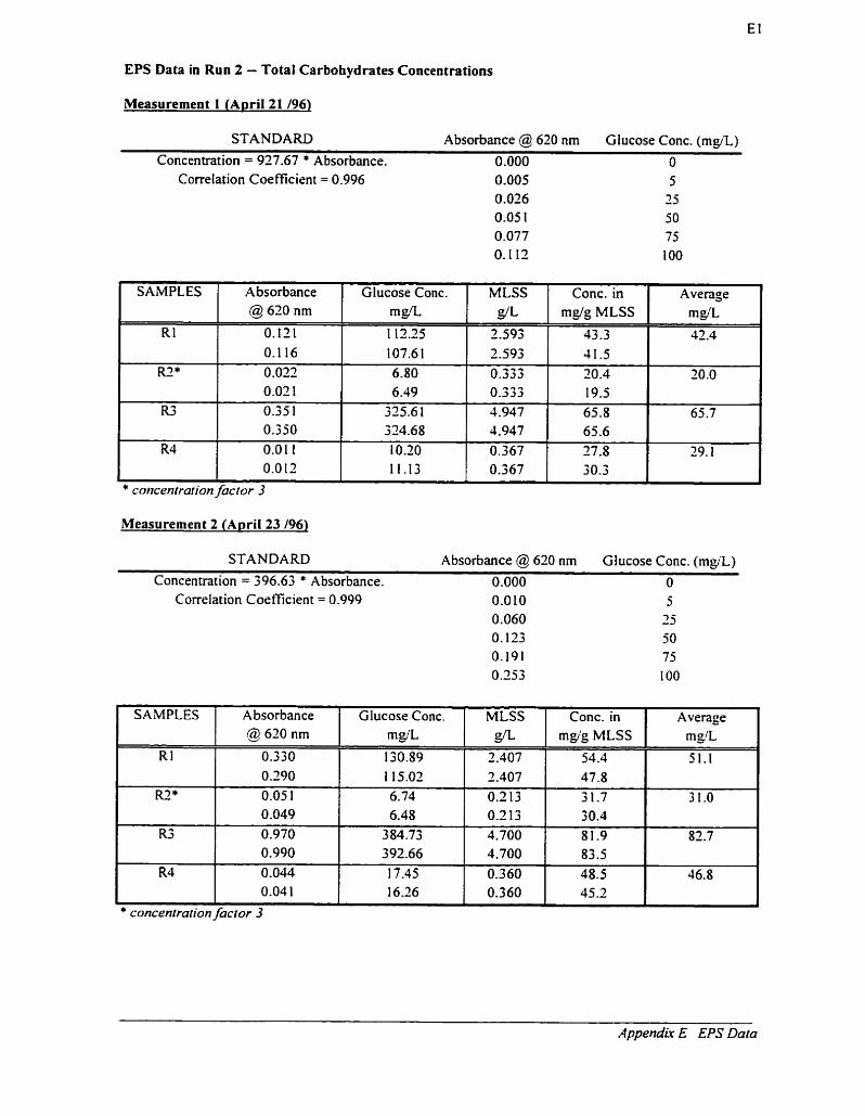
EPS Data in Run 2 - Total Carbohydrates Concentrations

Measurement 1 (April21 196)

STANDARD Absorbance @ 620 nm Glucose Conc. (my'L) Concentration = 927.67 * Absorbance. 0.000 O

Correlation Coefficient = 0.996 0.005 5 0.026 2 5 0.05 1 50 0.077 7 5 0.1 12 1 O0

Measurement 2 (ApriI23 196)

SAMPLES

RI

RZ*

R3

R4

STANDARD Absorbance @ 630 nm Glucose Conc. (my'L)

Concentration = 396.63 * Absorbance. 0.000 O Correlation Coefficient = 0.999 0.010 5

0.060 2 5 O. 123 5 0 0.191 7 5 0.253 1 O0

* concentra!ion factor 3

A bsorbance @ 620 nm

0.121 0.1 16 0.022 0.02 1 0.35 1 0.350 0.0 1 1 0.0 12

AppendUc E EPS Data

SAMPLES

R1

RZ*

R3

R4

Glucose Conc.

mp/L 1 12.25 107.6 1 6.80 6.49 325.6 1 324.68 10.20 11.13

* concentration factor 3

A bsorbance @ 620 nrn

0.330 0.290 0.05 1 0.049 0.970 0.990 0.044 0.04 1

MLSS

d L 2.593 2.593 0.333 0.333 4.947 4.947 0.367 0.367

Glucose Conc.

="p/L 130.89 1 15.02 6.74 6.48 384.73 392.66 17.45 16.26

Conc. in mg/g MLSS

43 -3 41.5 30.4 19.5 65.8 65.6 27.8 30.3

Average

m a 42.4

20 .O

65.7

29.1

MLSS s/L 2.407 2.407 0.213 0.2 13 4.700 4.700 0.360 0.360

Conc. in mpig MLSS

54.4 47.8 31.7 30.4 81.9 83.5 48.5 45.2

Average

m&L 51.1

3 1.0

82.7

46.8

EPS Data in Run 2 - Uronic Acid Concentrations

Measurement 1 (April21 /96)

STANDARD Absorbante @ 540 nm Glucouronic Conc. mp/L Concentration = 260.3 * Absorbance. 0.000 O

Correlation Coefficient = 0.989 0.020 4 0.08 1 20 0.168 5 O 0.333 80 0.371 1 O0

Average

mp/L Glucouronic Con.

m!3'L

1 1.45 1 1.97 4.42 3.90 7.8 1 8.85 1.82 1.82

* conc. factor of 3

Measurement 2 (April23 196)

MLSS P/L 2.593 2.593 0.233 0.333 4.947 4.947 0.367 0.367

STANDARD Absorbance @ 540 nm GIucouronic Conc. mg/L Concentration = 627.3 * Absorbance. 0.000 O

Conc. in mg/g MLSS

4.4 4.6 13.3 11.7 1.6 1.8 5 .O 5 .O

Correlation Coefficient = 0.

Glucouronic Con. MLSS Conc. in mg/g MLSS

SAMPLES

RI

R2*

R3

R4

Average

mt& 5.3

15.7

2.3

6.1

A bsorbance @ 540 nm

0.022 0.0 I9 0.0 17 0.0 15 0.0 18 0.017 0.004 0.003

--- - - . - -

* conc. factor of 3

Appendix E EPS Data

EPS Data in Run 3

Total Carbohvdrates Concentrations (June 18 /96)

STANDARD Absotbance @ 630 nm Glucose Con. (mg/L) Concentration = 90.18 Absorbance 0.000 O

Correlation Coeficient = 0.998

Uronic Acid Concentrations (June 18 196)

SAMPLES

RI

R2

R3

R4

STANDARD Absorbance @ 540 nm Glucouronic Conc. mpiL Concentration = 185.16 Absorbance 0.000 O

Correlation Coefticient = 0.997

MLSS of the concentnted samples

Absorbance @ 620 nrn

1 .O22 1.013 0.352 0.362 1.73 5 1.742 0.928 0.925

Appendîr E EPS Data

Glucose Con.

rn@L 92.16 91.35 3 1.74 33.65 156.46 157.09 83.69 83 -42

SAMPLES

R1

EU

R3

R4

MLSS * dL

3 260 3.260 0.650 0.650 2.690 2.690 2.980 2.980

* MLSS of the concentrated samples

Absorbance @ 540 nrn

0.02 1 0.020 0.000 0.000 O. 142 0.141 0.076 0.069

Conc. in mg/gMLSS

28.3 28.0 48.8 50.2

58.2 58.4 28.1 28.0

Glucouronic Con.

m f l 3.89 3.70 0.00 0.00

26.29 26.1 1 14.07 12.78

Average

mgiL 28.15

49.53

58.28

28.04

MLSS * S/L

3.260 3 -260 0.650 0.650 2.690 2.690 2.980 2.980

Conc. in mg/gMLSS

1 2 1.1 0 .O 0.0 9.8 9.7 4.7 4.3

Average

mg'L 1

1.2

0.0

9.7

4.5

EPS Data in Run 3

Protein Concentrations (June 18 196)

STANDARD Absorbance @ 750 nm Bovine Concentration (rng/L)

Concentration = 1864.3 * Absorbance 0.000 O Correlation Coeficient = 0.968 0.185 250

0.304 500 0.405 750 0.493 1 O00

Bovine MLSS

m e

SAMPLES

RI

R2

R3

R4

Conc. in mg/g MLSS

A bsorbance @ 750 nm

O, 150 O. 148 0.036 0.038 0.144 0.141 0.033 0.032

DNA Concentrations (June 18 /96) - Extracted us in^ DOWEX

STANDARD Fluorescence Salmon Testes DNA. mg/L Concentration = 0.3382 * Fluorescence 0.0 0 .O

Correlation Coefficient = 0.982 3 .O 1 .O 3 -5 1 .O 6.0 2 .O 7.0 2.0 16.0 5.0 18.0 5.0 28 .O 10.0 28.0 10.0

SAMPLES Fluorescence DNA MLSS Conc. in

mgk g/L mg/g MLSS RI 5 .O 1.69 3 -260 0.52

5 .O 1.69 3.260 0.52 W 13.0 4.40 0.650 6.76

13.0 4.06 0.650 6.24 R3 8.0 3.7 1 2.690 1 .O1

7.0 2.37 2.690 0.88 R4 3 .O 1-01 2.980 0.34

3 .O 1 .O1 2.980 0.34

Average

mp/L 1 St. Dev.

Appendk E EPS Data

EPS Data in Run 4 - Total Carbohydrates Concentrations

Measurement 1 (Nov. 15 1961 STANDARD Absorbance @ 630 nm Glucose Conc. ( m a )

Concentration = 107.78 * Absorbance 0.000 O Correlation Coefficient = 0.553 0.0 1 1

0.025 0.096 0.106 0.426 0.406 0.925 0.93 5

R4

* Dilution factor

Average m@

Measuremen t 2 (Nov. 2 1 196)

Glucose Con.

mg/L SAMPLES MLSS

gL

STANDARD Absorbante @. 620 nm Glucose Conc. (mg/L) Concentration = 7 1.754 * Absorbance 0.000 O

Absorbance @ 620 nm

Conc. in rng/gMLSS

Correiation Coeficient = 0.998

SAMPLES Absorbance Glucose Con. MLSS Conc. In @ 620 nm m a g/L mg/g MLSS

Average

Appendh E EP S Data

EPS Data in Run 4 - Total Carbohydrates Concentrations

EPS Data in Run 4 - Uronic Acid Concentrations

Measurement 3 (Nov. 24 /96) STANDARD Absorbance @ 620 nm Gtucose Conc. (mg/L)

Concentration = 7 1 -754 * Absorbance 0.000 O Correlation Coefficient = 0.998 0.152 10

O. 152 1 O 0.334 25 0.376 25 0.742 50 0.688 50 1.360 1 O0 1.400 1 O0

Measurement 1 (Nov. 15 196) STANDARD Absorbance @ 540 nm Glucouronic Conc. (rng/L)

Concentration = 2 12.12* Absorbance 0.000 O

SAMPLES

R1

R 2 *

R3

R4

Appendùc E EPS Data

* Dilrttion factor of 3

Absorbance @ 620 nm

0.992 0.98 1

0.040 0.042 0.8 16 0.792 0.384 0.428

Correlation Coefficient = 0.984 0.075 20 O. 100 20 0.184 40 0.204 40 0.23 8 50 0.227 50 .

SAMPLES

RI

R2*

R3

R4

Glucose Con.

mg/L 71.18 70.39 8.6 1 9.04 58.55 56.83

27.55 30.7 1

conc. Jactor of 3

Absorbance @ 540 nm

0.053 0.082 0.075 0.0 IO 0.095 0.102 0.068 0.059

Average

m g L I

36.5

63 .O

36.7

15.7

MLSS g/L 1.940 1.940 O. 140 O. 140 1.570 1.570 1.860 1 360

Glucouronic Con.

mg/L 1 1.24 1 7.29 1.77 0.7 1

20.15 2 1.64 14.42 13.53

Conc. in mg/g MLSS

36.7 36.3 61.5 64.6 3 7.3 36.2 14.8 16.5

Average

mg/L 7.1

6.5

13.8

7.1

MLSS g L 2.0 1 O 2.010 O. 190 O. 190 1.630 1.630 1.890 1.890

Conc. in mg/g MLSS

5.6 8.6 9.3 3 -7 11.4 13.3 7.6 6.6

EPS Data in Run 4 - Uronic Acid Concentrations

Measurement 2 (Nov. 21 196) STANDARD Absorbante @ 540 nrn Glucouronic Conc. (mg/'L)

Concentration = 177.47* Absorbance 0.000 O Correlation Coefficient = 0.998

,

Appendix E EPS Data

Measurement 3 (Nov. 24 1961 STANDARD Absorbance @ 540 nm GIucouronic Conc. ( m e )

Concentration = 187.97 * Absorbance 0.000 O Correlation Coefficient = 0.98 1 0.062 1 O

0.056 10 0.149 2 5 0.128 25 0.268 50 0.282 50 0.570 I O0 0.470 1 O0

* conc. facror of 2.5

SAMPLES

RI

R2*

R3

R4

SAMPLES

RI

FU*

R3

R4

Absorbante @ 540 nrn

0.036 0.038 0.002 0.005

O. 136 0.120 0.029 0.022

* conc. factor of 3

Absorbance 3 540 nm

0 .O3 2 0.036 0.00 1 0.002 0.097 0.079 0.026 0.032

Glucouronic Con.

m@ 6.39 6.74 O. 14 0.35 24. 14 21.21

5.15 3-90

Glucouronic Con.

mg/L

6 .O2 6.77 0.06 0.13

18.23 14.85 4.89 6.02

MLSS

g/L 1.960 1.960 0.070 0.070 1.560 1.560 1.760 1.760

MLSS

g/L.

1.940 1.940 O. 140 O. 140 1 -570 1.570 1.860 1.860

Conc. in mg/g MLSS

3 -3 3 -4 2.0 5.1 15.5 13.6 2 -9 2.2

Conc. in mg/g MLSS

3.1 3 -5 0 -4 0.9 11.6 9.5 2.6 3 2

Average

mg/L 3.4

3.5

14.5

2.6

Average mg/L

1

3.3

0.7

1 0.5

2.9

EPS Data in Run 4 - Total Carbohydrates Concentrations

Measurement 1 (Apri121196) STANDARD Absorbance @ 750 nm Bovine Concentration ( m a )

Concentration =4777 Absorbarice 0.000 O Correlation Coefficient = 0.97 1 0.055 200

0.087 400 0.1 17 600

Appendk E EPS Data

SAMPLES

RI

R 2

R3

R4

Measurement 2 and 3 (April21 & 24 1961 STANDARD Absorbance @ 750 nm Bovine Concentration (rngjrL)

Concentration 4777 * Absorbance 0.000 O Correlation Coefficient = 0.97 1 0.054 200

0.096 400 0.121 600

Nov. 22 SAMPLES

RI

R2

R3

R4

Absorbante @ 750 nrn

O. 140 0.143 0.044 0.045

O. 152 O. 154

0.083 0.090

Absorbante @ 750 nrn

0.1 1 1 0.1 12

0.022 0.023

0.1 13 0.1 17

0.038 0.036

Bovine

mp/L 667.7 680.3

2 10.3 215.0

728.0 734.3

396.2 428.6

Nov. 24

Bovine

m g L 502.9

508.6 100.1 104.6 513.9 532.3

1 7017 164.9

SAMPLES

r

R1

R3

R3

R4

MLSS

S/L 2.0 1 O 2.010

O, 190 O. 190

1.630 1.630

1.890 1.890

MLSS

d L 1.960 1.960

0.070 0.070 1.560 1.560 1.760 1.760

A bsorbance @ 750 nm

0.109 0.096 0.0 1 1 0.0 IO 0.087 0.082

0.0 19 0.0 18

Conc. in mg/g MLSS

332.2 338.5

1 106.3 1131.4

446.6 450.5

209.6 226.8

Average mg!L

335.3

1 1 18.8

448.6

2 18.2

Conc. in mg/g MLSS

256.6 259.5 1429.8 1494.8 329.4 34 1.2 97.0 93.7

Bovine

mg/L 493 -9 434.8 50.0 45.5 396.7 372.4 86.9 81.1

Average

mgiL 258.1

1462.3

335.3

95.3

MLSS

a 1.940

1.940 O. 140 O. 140

1 S70 1 -570 1.860 1 A60

Conc. in mg/g MLSS

254.6

224.1 357.5 325.0 252.7 237.2 46.7 43 -6

Average

mg/t 239.3

34 1.2

244.9

45.1

EPS Data in Run 4 - DNA (DOWEX Extraction)

STANDARD Fluorescence Salmon Testes DNA (rng'L) Concentration = 0.3389 * Fluorescence 0.0 0.00

Correlation Coefficient = 0.989

Average

mg/t

SAMPLES

R1

R2

R3

St. Dev.

Appendix E EPS Data

Fluorescence

4.0 4.0 4.0 6.0 6 .O 6.0 6.0 4.0 5 .O

DNA

m g L 1-36 1-36 1-36 2.03 2.03 2.03 2.03 1.36 1.69

MLSS g/L

2.920 2.920 2.920 0.450 0.450 0.4 50 2.170 3.1 70 2.170

Conc. in mg/g MLSS

O .464 0.464 0.464

4.5 19 4.5 19 4.5 i 9 0.937 0.625 0.78 1

EPS Data in Run 2 - Summary of ResuIts

Reactor Carbohydrate Uronic Acid (mgg MLSS) (mg& MLSS)

Apr-2 l Apr-23 Apr-2 1 Apt-23

RI 43.3 54.4 4.4 5.7 41 -5 47.8 4.6 5 .O

EPS Data in Run 3 - S u m m a w of Results

Reactor Carbohydnte Average St. Dev. Uronic Acid Average St. Dev. Protein Average St. Dev. RI 28.3 28-15 O. 18 1.2 1-16 0.04 85.8 85.2 1 0.8 1

28.0 1.1 84.6 R2 48.8 49.53 0.98 0.0 0.00 0.00 1 03.3 106.12 4.06

50.2 0.0 109.0 R3 58.2 58.28 0.17 9.8 9.74 0.05 99.8 98.76 1.47

58.4 9.7 97.7 R4 28.1 28.04 0.06 4.7 4.50 0.3 1 20.6 20.33 0.44

28.0 4.3 20.0

EPS Data in Run 4 - Summary of Results

Carbohydrate Uronic Protein Acid

Measurement 1 7 3 1 2 3 1 - 7 3

RI 48.3 3 3 -2 36.7 5.6 3.3 3 1 332.2 256.6 354.6 53 .O 34.4 36.3 8.6 3.4 3.5 338.5 359.5 234.1

R2 240.0 609.9 61.5 9.3 2.0 0.4 1106.3 1429.8 357.5 299.5 635.5 64.6 3.7 5.1 0.9 1131.4 1494.8 325.0

R3 76.7 49.1 37.3 12.4 15.5 11.6 446.6 329.4 252.7 73.2 5 1.3 36.2 13.3 13.6 9.5 450.5 34 1.2 237.2

R4 66.7 25.1 14.8 7.6 2.9 3.6 209.6 97.0 46.7 67.1 26.4 16.5 6.6 -.- 3 7 3.2 226.8 93.7 33.6

AppendUr E EPS Data

APPENDIX F STATISTICAL DATA

STATISTICAL TEST ON FLOC SUE CLASSES - RUN 1 Summary o f Mann-Whitney Test Results from SigrnaStat for Windows Version 1.0 Note : StatisricaI test performed on normalked and categorizedfloc skes and volume.

Run 1 - Day 57

Floc Volume N Median 25% 75% 35 0.28 0.0048 4.2 35 0.3 1 0.0068 4.6 35 0.09 1 0.0038 5 2 35 0.48 0.0085 4.9

RI R2 R3 R4

RI-IU

RI-R.3

RI-R4

Normalitv Test T P SS

Floc Sue N Median 25% 75% 35 3 -4 0.93 4.5 35 3.3 0.98 4.1 35 2.9 1.09 4.0 35 3.1 0.86 4.6

Norrnality Test T P SS Failed 1249.5 0.9391 NSD

(P = 0.0035) Failed 1277.0 0.6896 NSD

(P = 0.0402) Failed 1348.0 0.9532 NSD

(P = 0.0094)

Failed 1250.0 0.9345 NSD (P = <o.ooo 1 )

Failed 1275.0 0.7070 NSD (P = <O.OOO 1 )

Failed 1222.5 0.8188 NSD (P = <o.ooo 1 )

Run 1 - Dav 64

R l R2 R3 R4

Appendk F Statistical Data

RI-R2

RI-R3

RI-R4

Floc Size N Median 25% 75% 35 3 -5 0.56 4.7 35 3.6 0.55 4.4 35 3.2 1.18 4.1 35 3 -5 1.24 4.0

Floc VoIume N Median 25% 75% 35 0.52 0.0 1 O0 3.1 35 0.22 0.0050 5.1 35 0.18 0.0050 3 -3 35 0.1 1 0.0030 3 2

Normality Test T P SS Failed 1288.0 0.5971 NSD

(P = 0.0002) Failed 1283.0 0.6469 NSD

(P = 0.0248) Failed 1294.5 0.5452 NSD

(P = 0.0005)

Normality Test T P SS Failed 1262.0 0.8234 NSD

(P = <O.OOO 1) Failed 1277.0 0.6896 NSD

(P = <O.OOO 1 ) Failed 1304.0 0.4737 NSD

(P = <o.ooo 1)

STATISTICAL TEST ON FLOC SIZE CLASSES - RUN 2 Sumrnary of Mann-Whitney Test ResuIts from SigmaStat for Windows Version 1.0 ,voie : Sîatisiicaf test per/med on affj[oc sizes and voiurne.

Run 2 - Day 28

RI R2 R3 R4

RI-R2

Run 2 - Dav 63

RI-IR3

R1-R4

Floc Size N Med ian - 75% 75%

1049 55.7 18.9 106.7 1343 60.4 17.5 113.6 1335 51.9 16.7 107.1 1349 51.1 16.7 107.1

Normality Test T P SS Failed 1243869.0 0.502 NSD

Normality Test T P SS Failed 653284.0 0.757 NSD

(P = <o.ooo 1 ) Failed 63421 1.0 0.000 SS

(P = -=O.OOO 1 ) Failed 1007002.5 0.000 SS

(P = <o.ooo 1 1

Floc Volume N Median 25% 75%

IO49 90386.5 3542.6 635449.3 1343 115153.7 2785.3 767598.6 1335 73033.6 2330.0 64323 1.8 1349 698 19.7 2430.0 643789.1

Normality Test T P SS Failed 1243 763 -5 0.500 NSD

(P = <o.ooo 1 ) Failed 1262138.0 0.502 NSD

(P = <O.OOO 1 ) Fai led t2733 16.5 0.371 NSD

(P = <o.ooo 1 )

RI R2 R3 R4

Run 2 - Day 71

(P = <o.ooo 1) Failed 126 1945.5 0.509 NSD

(P = <o.ooo 1) Failed 1273333.5 0.371 NSD

(P = <O.OOO 1)

Normality Test T P SS Failed 653207.0 0.682 NSD

(P = <O.OOO I ) Failed 633920.0 0.000 SS

(P = <o.ooo 1 ) Failed 1 00808 1 .O 0.000 SS

(P = <o.ooo 1 )

Floc Size N Median 25% 75%

855 67.5 28.8 1 10.5 795 67.6 35.0 108.2 706 95.9 51.6 iG4.9 1307 52.4 21.2 85.8

Floc Volume N Median 2 506 75%

855 16 1 107.7 12477.6 706068.4 795 161810.8 8201.5 663396.1 706 462 158.8 7 1957.0 2347 17 1.2 1307 75202.8 5006.1 33060 1.8

Normalitv Test T P SS

Floc Size N Median - 35% 75%

977 57.4 19.3 103.6 1028 48.8 20.6 76.3 617 87.7 45.5 165.7 Il30 38.5 19.3 61.0

Failed 1031617.5 0.000 SS (P = <o.ooo 1 )

Failed 581091.5 0.000 SS (P = <o.ooo 1 )

Failed 1145869.0 0.000 SS (P = <O.OOO 1 )

Floc Volume N Median 25% 75%

977 992 15.1 3741.2 852381.3 1 028 60726.3 4570.9 232260.6 617 3527 12.4 49437.4 2384 183.0 1130 29929.9 374 1.2 1 18942.8

Normality Test T P SS Failed 1 033077.0 0.000 SS

(P = <o.ooo 1 ) Failed 580764.0 0.000 SS

(P = <o.ooo 1 ) FaiIed 1 147722.0 0.000 SS

(P = <o.ooo 1 )

Appendix F Statisiical Daia

STATISTICAL TEST ON FLOC SIZE CLASSES - RUN 3 Summary of Mann-Whitney Test Results from SigmaStat for Windows Version 1.0 Note : Statistical test performed on alljloc si'es and volume.

Run 3 - Day 25

RI R2 R3 R-t

RI-R2

Run 3 - Dav 39

Floc Size N Median 25% 75%

2111 42.0 21.5 66.2 1868 41.2 23.6 62.8 22 14 44.5 25.2 66.6 1910 43.3 28.2 64.0

RI-R3

RI-R4

Floc Size

Floc Volume N Median 25% 75%

21 1 1 38730.8 5228.5 152062.0 1868 36567.4 6873.1 139571.5 22 14 46 157.5 8397.3 154826.7 1910 32502.6 1 1735.6 137156.5

Normality Test T P SS Failed 3651767.5 0.070 NSD

Normality Test T P SS Fai led 5437532.0 0.000 SS

(P = <o.ooo 1 ) Failed 5391 117.5 0.000 SS

(P = <o.ooo 1 ) Failed 1 1509992.5 0.000 SS

(P = <o.ooo 1 )

Normality Test T P SS Failed 365 1767.5 0.070 NSD

(P = <o.ooo 1 ) Failed 4524860.0 0.3 15 NSD

(P = <o.ooo 1 ) Failed 3883244.5 0.251 NSD

(P = <o.ooo 1)

Floc Volume N Median 25% 75%

2513 83523.4 12626.7 305488.4 1972 315102.7 101615.4 898087.3 2544 259758.9 592 10.3 748733.0 4745 7622.5 68 1.8 53032.8

(P = <o.ooo 1 ) FaiIed 4524860.0 0.3 15 NSD

(P = <o.ooo 1 ) Fai led 3383244.5 0.25 1 NSD

(P = <o.ooo 1 )

Normality Test T P SS Failed 5437532.0 0.000 SS

(P = <o.ooo 1 ) Failed 5390660.5 0.000 SS

(P = <o.ooo 1 ) Failed 1 153930 1.5 0.000 SS

(P = <o.ooo 1 )

Run 3 - Day 43

R1 R2 R3 R4

RI-R2

Appendùr F Sratistical Data

Floc Size N Median 25% 75%

1900 45.7 22.9 71.9 1558 83.3 40.1 124.3 1696 59.5 16.7 110.1 2422 22.7 10.6 46.7

(P = <o.ooo 1 ) Failed 327 13 16.0 0.000 SS

(P = <O.OOO 1 ) Failed 4900291.5 0.000 SS

(P = <O.OOO 1 )

Floc Volume N Median 25% 75%

1900 49973.5 6302.3 194385.3 1558 302546.9 33800.8 1006079.3 1696 1 102 14.0 2445.4 699 144.1 2422 6143.8 630.4 53375.0

NormaIity Test T P SS Failed 3354677.5 0.000 SS

(P = <o.ooo 1) Fai Ied 327 13 16.0 0.000 SS

(P = <o.ooo 1 ) Failed 490029 1.5 0.000 SS

(P = <o.ooo 1)

Normality Test T P SS Failed 3254635.0 0.000 SS

STATISTICAL TEST ON FLOC SlZE CLASSES - RUN 4 Summary of Mann-Whitney Test Results from SigmaStat for Windows Version 1.0 Note : Statisrical test perjiorrned on allfloc sizes and volume.

Run 4 - Day 34

1 Floc Size 1 Floc Volume

Run 4 - Dav 74

RI-=

RI-R3

RI-€24

Normality Test T P SS Failed 1 1 137383.0 0.3285 NSD

(P = <O.OOO 1 ) Fai led 10867862.0 0.2356 NSD

(P = <o.ooo 1 ) Failed 11327931.0 0.0630 NSD

(P = <O.OOO 1 )

R1 R2 R3 R4

Nomality Test T P SS Failed 1 1 137383.0 0.3285 NSD

(P = <o.ooo 1 ) Failed 1 087 1224.0 0.2530 NSD

(P = <o.ooo 1) Fai Ied 1 1327928.0 0,0630 NSD

(P = <O.OOO 1 )

RI-R2

Run 4 - Day 78

Floc Size 1 Floc Volume

Floc Size N Median 25% 759'0

3366 24.1 11.5 53.6 2253 50.8 22.4 95.6 294 1 48.6 25.0 80.3 4066 17.8 8.1 48.2

RI-R3

Rl-R4

Floc Volume N Median - 35% 7530

3366 7369.8 798.5 807 17.6 2253 68759.2 5915.0 457421.8 294 1 59966.5 8 136.3 27 1376.5 4066 2968.9 282.3 58456.9

Normality Test T P SS Failed 7706001.0 0.000 SS

Nomality Test T P SS Failed 7708889.0 0.000 SS

(P = <o.ooo 1 ) Failed 1 1030005.5 0.000 SS

(P = <o.ooo 1 ) Fai led 13277823.0 0.000 SS

(P = <O.OOO 1 )

RI R2 R3 RQ

Appendïx F Statistical Data

(P = <o.ooo 1 ) Fai led 11034571.5 0.000 SS

(P = <o.ooo 1 ) Failed 13277820.5 0.000 SS

(P = <o*ooo 1 )

Normality Test T P SS Failed 4636178.0 0.000 SS

(P = <o.ooo 1 ) Failed 8083548.0 0.000 SS

(P = <o.ooo 1 ) Failed 16752727.0 0.040 SS

(P = <o.ooo 1 )

N Median 25% 75% 4229 29.1 15.0 522 1484 36.7 10.9 1 15.2 2362 30.2 11.5 88.5 4084 26.2 1 . 5 61.1

Normality Test T P SS Failed 46 1 1 845.5 0.000 SS

(P = -=O.OOO 1 ) Failed 8083548.0 0.000 SS

(P = <o.ooo 1 ) Failed 16752727.0 0.040 SS

(P = <o.ooo 1 )

N Media. 25% 75% 4329 12928.5 1769.9 74658.6 1484 2582 1.5 68 1.8 800903.7 2362 14472.8 798.5 362793.9 4084 9468.6 798.5 1 19578.9

APPENDIX G BOLND WATER DATA

Bound Waier Content Measurements in Run 4 (followed the method of Heukelekian and Weisberg, 1956). Results obtained from B. Liao and S.N. Liss (University of Toronto).

Reac tor C0D:N:P Bourid Water (mI/g dried solids)

RI 100:2: 1 24 R2 100:5:0 ND R3 1 00:5:0.2 53 R4 100:1:1 16

ND : Not Detennined.

Appendir G Bound Water Data

APPENDIX H SAMPLE CALCULATIONS

A. SampIe Calculation for Settling Velocitv ( v ) and Shape Factor (4

Run 1. Day 3 5. Data # 1. Distance traveled = 304 1 Fm. Tirne traveied = 40 -es * 1/30 s/frame = 1.33 s Perirneter = 992.5 Pm. Area = 3 1600 pm'

(Equation 3.6)

B. Sample Calculation for Re. k,. k, lc Effective den si^ (DJ and Porositv (E) - - -

(Equation 3 -4)

. Since 0.2 < Re = 0.3 1 < 2000. the correction factor. k was calcuiated as follows.

k, = 0.843 * log (0.403 1 0.065) = 0.67 k, = 5.3 1 - 4.88 * 0.403 = 334

(Equation 3 3) (Equation 3 -8)

(Equation 3.9)

The effective density. p.. and porosity. E. were calculated as follows.

- 18 * 1.53 * 0.00 102 * 1 * 1 0 ci &rn3 = 0.1 05 g/crn3 (Equation 3.1 0) - 0.67 * 9.8 1 * 200.6

(Equation 3.1 3 )

C. Sample Calculation for Statistical Test on the Linearized Settling: Velocitv (t-test)

Using the data of Run 1. R 1. Day 3 5. and from Equations F 1. F2. F3. and F4. the following were calculaied.

log A (Y-intercept) = - 1 -069 n (dope) = 0.4324 X[(Y,-YA'] = 0.29

C .Y: = 27233 N = 3 7 y = 2.70

iippendk H Sample Cafarlariom

Test Values. n, = 0.00. Zog4, = 0.00.

(Equation F 1 )

(Equation F2)

(Equation F3)

(Equation F4)

(Equation F5)

(Equation F6)

The P values correspond to the t values were. Pn = 0.000 and P,o, = 0.000. therefore. the two values tested are statistically different fiom 0.00.

1 iv imuc CvnLun I IVIY

TEST TARGET (QA-3)

APPLIED IMAGE. lnc - - - 1653 East Main Street - -. , Rochester, NY 14609 USA I -- - - Phone: 71ôi402-0300 -- -- - - Fax: 71 6/288-5989

O 1993. Wied image. Inc.. Ail Rights Reserved