NOTE TO USERS

The original manuscript received by UMI contains pages with slanted print. Pages were microfilmed as received.

This reproduction is the best copy available

KINEMATICS AND DESIGN OF A CLASS OF PARALLEL MANIPULATORS

by

Roger Barry Hertz

A thesis submitted in conformity with the requirements for the degree of Doctor of Philosophy

Graduate Department of Aerospace Engineering University of Toronto

@ Copyright by Roger Barry Hertz (1 998)

National Library 1+1 ofCanada Bibliothèque nationale du Canada

Acquisitions and Acquisitions et Bibliographie Services services bibliographiques

395 Wellington Street 395, rue Wellington OttawaON K I A W OttawaON K l A W Canada Canada

The author has grrmted a non- exclusive licence allowing the National LLbrary of Canada to reproduce, loan, distriiute or sell copies of this thesis in microform, paper or electronic formats.

The author retains ownership of the copyright in this thesis. Neither the thesis nor substantial extracts fiom it may be printed or otherwise reproduced without the author's permission.

L'auteur a accordé une licence non exclusive permettant a la Bibliothèque nationale du Canada de reproduire, prêter, distri'buer ou vendre des copies de cette thèse sous la fome de rnicrofiche/nIm, de reproduction sur papier ou sur format électronique.

L'auteur conserve la propriété du droit d'auteur qui protège cette thèse. Ni la thèse ni des extraits substantiels de celle-ci ne doivent être imprimés ou autrement reproduits sans son autorisation,

Abstract

Kinematics and Design of a Claçs of Parallel Manipulators Doctor of P hilosophy, 1 998 Roger Barry Hertz Graduate Department of Aerospace Engineering University of Toronto

This disertation is concerned with the kinematic d y s i s and design of a cl= of three-

degme-of-fieedom, spatial parde1 manipulators. The class of manipulators is characterized

by two platfom, between which are three legs, each possessing a succession of revolute,

sphericai, and revolute joints. The class is temed the "revolute-sphericd-revolute" class

of parallel manipulators.

Two members of this class are examined. The first mechanism is a double-octahedral

variable-geometry tniss, and the second is tenned a double tripod The history the mecha-

nisms is explored-îhe variable-geomeûy tniss data back to 1984, whüe predecessors of

the double tri@ mechanisn date back to 1869.

This work centers on the displacement analysis of these three-degree-ofkdom

mechanism. Two types of problem are solved: the forward displacement analysis (forward

kinematics) and the inverse dispIacement adysis (inverse kinematics). The kinematic

mode1 of the class of mechanism is g e n d in nature. A classification scheme for

the revolute-spherical-revolute class of mechankm is introduced, which uses dominant

geometric features to gûup designs into 8 different subclasses.

The fornard kinematics problem is discussed: given a set of independaitly controllable

input variables, solve for the relative position and orientation betwem the two platfonns.

For the variable-geometry tniss, the controllable input variables are assumed to be the

linear (prismatic) joints. For the double tripod, the controliable input variables are the tbree

revolute joints adjacent to the base (proximal) platform.

Multiple solutions are presented to the forward kinematics problem, indicating that

there are many Mixent positions (assemblies) that the manipulator can assume with

@valent inputs. For the double tripod these solutions can be expressed as a 16th degree

poiynomial in one imknown, while for the variable-geometry &US there exist two 16th

degree polynomials, giving rise to 256 solutio~~. For special cases of the double tripod, the

forward kinematics problem is shown to have a closed-form solution.

Numerical examples are presented for the solution to the forward kinematics. A double

tri@ is presented that admits 16 unique and real forward kinematics solutions. Another

example for a variable geometry tniss is given that possesses 64 real solutions: 8 for each

16th order polynomial.

The inverse kinematics problem is aiso discussed: given the relative position of the

hand (end-effector), which is rigidly attached to one platfonn, solve for the independently

controUed joint variables. Iterative solutions are propsed for both the variable-geometry

tniss and the double tripod. For special cases of both mechanisms, closed-form solutions

are given.

The practical problems of designing, building, and controlling a double-tripod manipu-

lator are addressed. The resulting mlinipulator is a first-of-its kind prototype of a tapered

(asymmetric) double-tripod manipulator. Real-tirne forward and inverse kinematics algo-

rithms on an industrial robot controller is presented. The resulting performance of the

prototype is impressive, since it was to achieve a maximum tool-tip speed of 4064 d s ,

maximum acceleration of 5 g, and a cycle tirne of 1.2 seconds for a typical pick-and-place

Pa=

Acknowledgments

This thesis would not have been possible if not for the support of many people and orgdzatioons throughout my doctoral programme. I'd Iüce to specifically acknowledge the following individu& and organizations who have helped me and supported me throughout my PIID thesis.

1 owe many thanks to Professor Peter Hughes, who has supported me financially and supavised my work throughout my thesis. His wise advice and timely academic guidance durÏng my doctoral programme are greatly appreciated Thierry Cherpiilod's technical support and teamwork for the power-ampllias used in the errperirnenîal portion of my thesis are gratefbily acknowledged Thanks is aiso due to Trevor Jones, of CRS Robotics Corporation, for his support of my thesis by giving me the flexibility for time off of work dirring the later stages of my &te-up. I aclmowledge the Natural Science and Engineering Researcb Councii (NSERC) and Ontario Graduate Schokmhips (OGS) for financial support dufing large port;ions of my thesis. 1 thank my parents Barry and Eileen, who instilleci in me a desire to do my best at whatever 1 do, and supported me in m y decision to pursue my doctorate. Special thanks is owed to m y father-in-law Howard Heineman, who spent s e v d days with me during Christmas of 1993 fabricating components of "Clem," the experimental robot in my thesis. 1 would like to thank God for giving me constant wisdom, guidance, and strength. Finally and moa importantiy, is my indebtedness to my wife Susan, who has loved me, supported me, and helped motivate me through the highs and lows of m y thesis.

Contents

1 Introduction 1 1.1 Ovenriew of This Document . . . . . . . . . . . . . . . . . . . . . . . . 1

. . . . . . . . . . . . . . . . . . . . . . . . . . . . . . . . 1 2 Background 2 12 .1 bematicGeametry . . . . . . . . . . . . . . . . . . . . . . . . 2

. . . . . . . . . . . . . . 122 Mechanismc. Manipulators and Robots 2 . . . . . . . . . . . . . . . . . . . . . . . . Adopted Definitions 2

0therDefhitior.u . . . . . . . . . . . . . . . . . . . . . . . . . 3 Interrelations Between Terms . . . . . . . . . . . . . . . . . . . 4

. . . . . . . . . . . . . . . . . . . 1.2.3 Serial vs P d e i Manipulators 6 . . . . . . . . . . . . . . . . . . . . . . . . . . . . . Overview 6

. . . . . . . . . . . . . . . . . . . . . . . . Serial Manipulators 8 Parallel Manipulators . . . . . . . . . . . . . . . . . . . . . . . 9

. . . . . . . . . . . . . . . . . . . . ParaUeI-Serial Manipulators 9 . . . . . . . . . . . . . . . . . . Parailel-In-Series Manipulators 11

. . . . . . . . . . 1.3 History of the Revolute-Spherical-Revolute Mechanism I l . . . . . . . . . . . . . . . . . . . . . . . . . 13.1 ClemensCoupling 12

. . . . . . . . . . . . . . . . . . . . 1.3 2 Reflected-Tripod Coupling 16 . . . . . . . . . . . . . . . . . . . 1.3 3 Reflected-Tripod Manipdator 17

. . . . . . . . . . . . . . . . . . . . . 1 3 .4 Variable-Geometry Tniss 17 . . . . . . . . . . . . . . . . . . . . 1.3.5 Poly-Retractile Mechanism 18 . . . . . . . . . . . . . . . . . . . . 1.3.6 Variable-Geometry Tnisses 19

. . . . . . . . . . . . . . 1.3.7 Variable-Geometry-Tniss Manipulator 19 . . . . . . . . . . . . . . . . . . . . 1.3.8 Double-Tripod Manipulator 20

1.4 LiteratureSwey . . . . . . . . . . . . . . . . . . . . . . . . . . . . . 20 . . . . . . . . . . . . . . . . . . . . . . . . 1 A . 1 Kinematic Modeling 20

. . . . . . . . . . . . . . . . . . . . . . Single OctaheM Form 21 . . . . . . . . . . . . . . . . . . . . . Double Octahedral Form 21

. . . . . . . . . . . . . . . . . . . . . . . . 1 4 Forward Kinematics 23

. . . . . . . . . . . . . . . . . . . . . . . . 1.4.3 InverseKinematics 23 . . . . . . . . . . . . . . . . . . . . . . . 1.4.4 Laboratory Rototypes 23

. . . . . . . . . . . . . . . . . . . . . 1.5 Contributions of This Dissertation 24

CONTENTS

Mathematical Preliminaries 25 . . . . . . . . . . . . . . . . . . . . . . . . . . . . . . . . . 2.1 Kinematics 25

. . . . . . . . . . . . . . . . . . . . . . . . . . . . . . 2.1.1 Vectors 25 . . . . . . . . . . . . . . . . . . . . . . . . . . . Nomenclature 25

. . . . . . . . . . . . . . . . . . Vectors and Reference Frames 26 . . . . . . . . . . . . . . . . . . . . . . . . . Rotation Matrices 26

. . . . . . . . . . . . . . . . . . . Successive Rotation Matrices 27 . . . . . . . . . . . . . . . . . . . . . . . . . . . . . Operations 28

. . . . . . . . . . . . . . . . . . . . . . . . . . 2.1.2 PositionVectors 29 . . . . . . . . . . . . . . . . . . 2.1.3 Homogeneous Transformations 29

. . . . . . . . . . . . . . . . . . . . . . . . . . 22 AnalysisofMechankms 30 . . . . . . . . . . . . . . . . . . . . . . . . . . . . . . 2.2.1 Mobility 30

. . . . . . . . . . . . . . . . . . . . . . . . 2.22 Degree of Freedom 31 . . . . . . . . . . . . . . . . 22.3 Denavit-Hartenberg Representation 31

. . . . . . . . . . . . . . . . . . . . . . . . 2.2.4 Cornpanion Indices 35

Kinematic Mode1 37 . . . . . . . . . . . . . . . . . . . . . . . . . . . . . . . 3.1 Classification 37

. . . . . . . . . . . . . . . . . . . . . . . . . . . . . 3 2 Mobility Analysis 41 . . . . . . . . . . . . . . . . . . . . . . . . . . . 32.1 DoubleTnpod 41

. . . . . . . . . . . . . . . . . . . . . 3.23 Variable-Geometry Tniss 41 . . . . . . . . . . . . . . . . . . . . . . . . . . . PractidVGT 42

. . . . . . . . . . . . . . . . . . . . . . . . . . . . . IdealVGT 42 . . . . . . . . . . . . . . . . . . . . . . . . . 3.3 General Kinematic Mode1 43

. . . . . . . . . . . . . . . . . . . . . . 3.3.1 ModelingAssumptiom 44 . . . . . . . . . . . . . . . . . . . . . . . . . 3-32 KinematicModel 44

Legs . . . . . . . . . . . . . . . . . . . . . . . . . . . . . . . . 44 RoximalPlatform . . . . . . . . . . . . . . . . . . . . . . . . . 47

. . . . . . . . . . . . . . . . . . . . . . . . . . Distal Platfonn 49 . . . . . . . . . . . . . . . . . . . . . . . . . . . . 3.3.3 Applications 50 . . . . . . . . . . . . . . . . . . . . . . . . . . . DoubleTnpud 51

. . . . . . . . . . . . . . . . . . . . . Variable-Geometry Tniss 51

4 Forward Kinematics 53 . . . . . . . . . . . . . . . . . . . . . . . . . . . . . . . . . 4.1 Overview 53

4.1.1 Forward Kinematics Algorithms for VGT and DT . . . . . . . . . 53 . . . . . . . . . . . . . . . . . . . . . Variable Geometry Truss 53

. . . . . . . . . . . . . . . . . . . . . . . . . . . DoubleTripod 54 . . . . . . . . . . . . . . . . . . . . . . . Comrnon Atgorithms 55 . . . . . . . . . . . . . . . . . . . . . . 4.11 ûrganhtion of Chapter 55

4.1.3 SummaryofNotableRdts . . . . . . . . . . . . . . . . . . . 56 . . . . . . . . . . . . . . . . . . . . . . . . . . . . . 4.2 ClosureEquations 56 . . . . . . . . . . . . . . . . . . . . . . . . . . . . . 4.2.1 OverYiew 56

CONTENTS vii

42.2 VectorClosureEquations . . . . . . . . . . . . . . . . . . . . . 57 42.3 ScalarClosureEquations . . . . . . . . . . . . . . . . . . . . . 58 42.4 Special Case: Symmetnc Geometry . . . . . . . . . . . . . . . . 59

4.3 LengthEquations . . . . . . . . . . . . . . . . . . . . . . . . . . . . . 61 4.4 PetaIEquations . . . . . . . . . . . . . . . . . . . . . . . . . . . . . . 63

4.4.4.1 Proximal Petal Equatiom . . . . . . . . . . . . . . . . . . . . . 63 4.4.2 Distal Petal Equations . . . . . . . . . . . . . . . . . . . . . . . 64 4.4.3 Implicit Closed-Fom Solution of Petal Angles . . . . . . . . . . 67

Tanget Half-Angle Substitution . . . . . . . . . . . . . . . . . . 68 . . . . . . . . . . . . . . . . . . . . . . . . . . Eliminati~noft~ 70 . . . . . . . . . . . . . . . . . . . . . . . . . . EIimination of t2 70

. . . . . . . . . . . . . . . . . . . . . . . . . . . Solution for ti 72

. . . . . . . . . . . . . . . . . . . . . . . . . . . Solution for t2 73

. . . . . . . . . . . . . . . . . . . . . . . . . . . Solution for 74 Solution for 9; . . . . . . . . . . . . . . . . . . . . . . . . . . . 74

. . . . . . . . . . . . . . . . . 4.4.4 Iterative Solution of Petal Angles 74 4.5 ExtraAngles . . . . . . . . . . . . . . . . . . . . . . . . . . . . . . . . 75

. . . . . . . . . . . . . . . . . . . . . . . . . . . 4.6 Numericai Examples : 76 . . . . . . . . . . . . . . . . . . . . . . 4.6.1 C-Code Implementation 76 . . . . . . . . . . . . . . . . . . . . . . Algorithm Flow Charts 76

4.62 A Double Tnpod with 16 Real Forward Kinematic Solutions . . . 80 . . . . . . . . . . . . . . . . . . . . . . . . . Kinematic Inputs 81

. . . . . . . . . . . . . . . . . . . Forward Kinematics Solution 82 Discussion of Forward Kinematics Solution . . . . . . . . . . . . 88

4.6.3 A VGT with 64 Fomard bernatic Solutions . . . . . . . . . . . 90 . . . . . . . . . . . . . . . . . . . . . . . . . KinematicInputs 90

. . . . . . . . . . . . . . . . . . . Forward Kinematics Solution 92 . . . . . . . . . . . . . . . . . . . . . . . Discussion of Solution 92

5 Inverse Kinematics 95 . . . . . . . . . . . . . . . . . . . . . . . . . . . . . . . . . 5.1 Overview 95

. . . . . . . . . . . . . . . . . . . . . . 5 2 Forward Displacement Method 96 . . . . . . . . . . . . . . . . . . . . . . . . . 5.3 Closure Equation Method 98

. . . . . . . . . . . . . . . . . . . . 5.4 Special Case: Symmetric Geometry 101

6 Design and Control 103 . . . . . . . . . . . . . . . . . . . . . 6.1 Overview: Laboratory Prototypes 103

6.1.1 Clem-A Double-Tripod Manipdator . . . . . . . . . . . . . . . 103 6.1 2 Trussarm-A Variable-Geometry-Tm Marnipulator . . . . . . . 104

. . . . . . . . . . . . . . . . . . 6 2 Design of a Double Tripod ManipuIator 107 . . . . . . . . . . . . . . . . . . . . . . . . . . . 6 2 1 SystemDesign 107

. . . . . . . . . . . . . . . . . . . . . . . System Design Goals 107 . . . . . . . . . . . . . . . . . . . . . . . . Controller Selection 107

CONTENTS vüi

622 Mechanical Design . . . . . . . . . . . . . . . . . . . . . . . . 109 Robot Interfhce Requirements . . . . . . . . . . . . . . . . . . . 109

. . . . . . . . . . . . . . . . . . . . . . . . . Actuator Selection 110 . . . . . . . . . . . . . . . . . . Kinematic Parameter Selection 110

. . . . . . . . . . . . . . . . . . . . . . . Arm and Joint Design 114 . . . . . . . . . . . . . . . . . . . . . . . . 62.3 KinematicModehg 117 . . . . . . . . . . . . . . . . . . . . . . . . 62.4 Workspace Analysis 122

. . . . . . . . . . . . . . . . . . 6.3 Control of a Double Tnpod Manipulator 126 . . . . . . . . . . . . . . . . . . . . . . . 6.3.1 Kinematic Algorithms 126

. . . . . . . . . . . . . An Ovewiew of the Kinematics Interface 126 . . . . . . . . . . . . . . . . . . . . . . Algorithm Benchmarks 128

. . . . . . . . . . . . . . . . . . . . . . . . 6-32 PedomceResults 129 . . . . . . . . . . . . . . . . . . . . . . . . . . . Pick and Place 129

. . . . . . . . . . . . . . . . . . . . . . Straight Line Trajectory 132 . . . . . . . . . . . . . . . . . . . . . . . . High-Speed Slewing 136

7 Conclusions. Contributions. and Suggestions for Future Work 142 . . . . . . . . . . . . . . . . . . . . . . . . . . . . . . . . 7.1 Conclusions 142

. . . . . . . . . . . . . . . . . . . . . . . . . . . 72 Original Contributions 144 . . . . . . . . . . . . . . . . . . . . . . . . 7.3 Suggestions for Future Work 144

Appendices

A Forward Kinematics Coefficients 153 . . . . . . . . . . . . . . . . . . . . . . . . . . . . . . . . Al Background 153

. . . . . . . . . . . . . . . . . . . . . . . A 2 Pseudo-Univariate Polynomial 153 . . . . . . . . . . . . . . . . . . . . . . . . . . . A3 Univariate Polynomial 155

List of Figures

1.1 Interrelation of the Tenns "Mechanism". "Manipulator" and "Robot" . 5 i 2 The Gough-Stewart Platform . . . . . . . . . . . . . . . . . . . . . . . 7 I . 3 Trussarm-An example of a Hybrid Manipuiator . . . . . . . . . . . . . 8

. . . . . . . . . . . . . . . . . . . . . . . . . . 1.4 The Pollard Manipulator 10 . . . . . . . . . . . . . 1.5 LamberVs Polyarticulated Retractile Mechanism 12

1.6 The Mecha nisns . a) Double.Tripod, and b) Variable-Geometry Truss . . 13 . . . . . . . . . . . . . . . . . . . . . . . 1.7 FamilyTreeforDTandVGT 14

1.8 Clemens Couphg: An Apparatus for Transmitting Rotary Motion . . . . 15 . . . . . . . . . . . . . . 1.9 The Reflected-Tripod Constant Speed Coupling 16

. . . . . . . . . . . . . . . . . . . . . 1.1 O Lambert's Elementary Mechanian 18

. . . . . . . . . . . . . . . . . . . . . . . . . . . . . . 2.1 Position Vectors 29 2.2 The Denavit-Hartenberg Representation of Linkages . . . . . . . . . . . 33

. . . . . . . . . . . . . . . . . . . . . . . . . 2.3 Use of Companion Indices 35

3.1 Mechani- with Non-Planar Geometry . . . . . . . . . . . . . . . . . . 39 . . . . . . . . . . . . . . . . . . . . . 3.2 Mechanisms with Planar geomerty 40

. . . . . . . . . . . . . . . . . . 3.3 The General Double-Tripod Mechanism 41 . . . . . . . . . . . . 3.4 The hc t ica l Variable-Geometry-TNSS Mechanism 42

. . . . . . . . . . . . . . 3.5 The Ideal Variable-Geometry-Tm Mechanism 43 3.6 The Denavit-Hartenkg Kinematic Mode1 of a General Leg . . . . . . . 45 3.7 Proximal Platform General Mode1 . . . . . . . . . . . . . . . . . . . . . 47

. . . . . . . . . . . . . . . . . . . . . . 3.8 Distal Platforrn General Mode1 50

. . . . . . . . . . . Fomard Kinematics Solution FIowchart for the VGT Forward Kinematics Solution Flowchart for the DT . . . . . . . . . . . . Vector and F m e Placement for the Fomard Kinematic Problem . . . . .

. . . . . . . . . . . . . . . . . . . . . . . . Closure Frames and Vectors Midplane Geometry for the Symmetric Mechanism . . . . . . . . . . . . Polynomial Elimination Method Used to Find the Closed-Form Solution of the Petal Angle Eqyations . . . . . . . . . . . . . . . . . . . . . . .

. . . . . . . . . Flowchart for the Solution to the Extra Spherical Angles Flowchaa for the Fornard Kinematics Algorithm . . . . . . . . . . . . .

. . . . . . . . . . Nowchart for the Closed Form Petai Angle Algorithm

LIST OF FIGURES x

4.10 Flowchart for the Iterative Petal Angle Algonthm . . . . . . . . . . . . . 79 4.1 1 Flowchart of the Comrnon Ciosme Equation Algorithm . . . . . . . . . . 80 4.12 Double Tnpod Sotutions 1 Through 4 . . . . . . . . . . . . . . . . . . . 84 4.13 DoubleTnpodSolutions5Through8 . . . . . . . . . . . . . . . . . . . 85 4.14 Double Tripod Solutions 9 Through 12 . . . . . . . . . . . . . . . . . . 86 4.15 Double Tripod Solutions 13 Though 16 . . . . . . . . . . . . . . . . . . 87

. . . . . . . . . . . 4.16 Assembly Conditions for the Double Tripod Example 89 . . . . . . . . . . . . . . . 4.17 Selected Variable-Geometry Truss Soiutims 93

5.1 Forward Displacement Method . . . . . . . . . . . . . . . . . . . . . . 98 5.2 Closure Equation Method . . . . . . . . . . . . . . . . . . . . . . . . . 99

. . . . . 6.1 System Diagram of Clem: A Double-Tnpod Manipulator System 104 6 2 Components of Clem . . . . . . . . . . . . . . . . . . . . . . . . . . . 105 6.3 System Diagram of Trussarm Mark 1: A Variable-Geometry-Tniss Manip-

uiator System . . . . . . . . . . . . . . . . . . . . . . . . . . . . . . . 105 6.4 CornponentsofTnissannMarkI . . . . . . . . . . . . . . . . . . . . . . 106

. . . . . . . 6.5 A Variable-Geometry-Tniss Manipulator with a Serial Wrist 108 . . . . . . . . . . . . 6.6 SpeecUTorque C w e for Clem's revolute Actuators 111

. . . . 6.7 Geometry Relationships and Target Masses Di~nniution for Clem 112 6.8 Simplifieci Mass D i s t n i o n for Clem . . . . . . . . . . . . . . . . . . 113 6.9 Characteristic Lengths for Two Design Cases . . . . . . . . . . . . . . . 114 6.10 Spherical Pitch Joint Required Ranges of Motion . . . . . . . . . . . . . 116 6.1 1 Spherical Joint Arrangments:(a) RollœPitch.Roll, and (b) Roll-Pitch-Yaw . 1 16 6.12 DHPararnetersforClem . . . . . . . . . . . . . . . . . . . . . . . . . . 118 6 . 13 Frame Placements for Link 0: Proximal Platform . . . . . . . . . . . . . 119 6.14 Frame Placement for Link 5: Distal Platform . . . . . . . . . . . . . . . 120 6.15 Frame Placement for Link I : Proximal Ann . . . . . . . . . . . . . . . . 121 6.16 Frame Placement for Link 2: U-Joint Yoke . . . . . . . . . . . . . . . . 121 6.17 Frame Placement for Link 3: U-Joint Center . . . . . . . . . . . . . . . . 122 6.18 Frame Placement for Link 4: Distal Arm . . . . . . . . . . . . . . . . . 122 6.19 Kinematic Chain with ûi, = {45,90, -90, -63, 40) . . . . . . . . . . . . 123 6.20 Workspace Cube Visualization for Clem . . . . . . . . . . . . . . . . . 124 621 Proximal Workspace . . . . . . . . . . . . . . . . . . . . . . . . . . . . 125 6.22 Distal Workspace . . . . . . . . . . . . . . . . . . . . . . . . . . . . . 126 6.23 Pattern for Pick-and-Place Demonstration . . . . . . . . . . . . . . . . . 130 6.24 Pick-and-Place Test: Motor Coordintes vs . time . . . . . . . . . . . . . . 132 6.25 Pick-and-Place Test: Cartesian Coordintes:(a) vs . T ï e , and @) 3D Plot . 133 6.26 Straight Line Test: Motor Coordintes vs . thne . . . . . . . . . . . . . . . 134

. . . 6.27 Straight Line Test: Cartesian Coordinates:(a) vs . t h e , and (b) 3d plot 135 . . . . . . . . . . . . . 6.28 High-Speed Slew Test: Encoder Position vs Tirne 137

6.29 High-Speed Slew Test: Encoda Position Error vs . Time . . . . . . . . . 138 6.30 High-Speed Slew Test: Cartesian Coordintes:(a) vs . Thne, and (b) 3D Plot 139

LIST OF FIGURES xi

6.3 1 High-Speed Slew Test: Cartesian Velocity Estimation . . . . . . . . . . . 140 632 High-Speed Slew Test: Cartesian Acceleration Estbation . . . . . . . . 141

List of Tables

SimpMjring Assumptions for Single-Octahedral Mechanisms . . . . . . . 21 Simplifjrhg Assumptions for Double-Octahedral type VGT's . . . . . . . 22

Link Parameters for the rth General Leg . . . . . . . . . . . . . . . . . . 46 OveMew of Parameters for the rth Leg of the G e n d Mode1 . . . . . . . 51 Controlled and Passive DOF for the Double Tnpod . . . . . . . . . . . . 51 Controlîed and Passive DOF for the Muiable-ûeometry T m . . . . . . 52

Types of Algorithms used in the Forward Kinematics the VGT and DT . . 55 Size of Final Polynomial Coefficients . . . . . . . . . . . . . . . . . . . 72 Kinematic Parameters for the Rational Double Tripod . . . . . . . . . . . 82

. . . . . . . . . . . Polynomial Coefficients for Double Tripod Example 83 16RdPetalAngleSo~edwithRespectt08~~ . . . . . . . . . . . . . . 83 Classification of the 16 Assemb1y Solutions . . . . . . . . . . . . . . . . 88 Kinematic Parameters for the VGT Numerical Example . . . . . . . . . . 91 Distal Polynomial Coefficients for theVGT Example . . . . . . . . . . . 92 Petal Angle Solutions for the VGT Example . . . . . . . . . . . . . . . . 94

Weight Distribution for Two Design Cases of Clem . . . . . . . . . . . . 115 Running T h e Benchmark for Kinematics Algorithms . . . . . . . . . . 129

Chapter 1

Introduction

1.1 Overview of This Document Parallel manipulators have begun to play an important role in the area of industrial robotics. The need for high-speed, hi& bandwidth mechmical systems has caused robot designers to consider mechanisns other than the cornmon serial arrangements.

One approach to utilipng paralle1 mechanisms is to combine them with serial mech- anisns, forrning hybrid manipulators. This approach has proven successful with many industrial robots utüizing a two-degree-of-&dom (2-WF) parallel mechanism as part of the positioning mechanism of the msuiipulator. Recently, researchers have been motivated to investigate the use of 3-DOF spatial mechanisms in the same application.

This dissertation is concenied with the kinematic analysis of a particuiar class of S-DOF, spatial parallel manipulators. The class is termed the revolute-sphexical-revolute class of p d e l manipufators, ckacterized by two platforms, between which are thm legs, each possessing a succession of revolute, spherical, and revolute joints. Such mechanisms show promise for use in industrial manipulator applications.

The remainder of Chapter 1 deals with tenninology preliminanes and a review of the relevant literature. The double tripod and the (double-octahedral) variable-geometry tniss are introduced For both mechanisms the historical origins are traced, and a summary of the contributions of this dissertation is given.

Chapter 2 deals with mathematical pre-es. In Chapter 3, a g e n d kinematic mode1 and classification scheme are introducd Chapter 4 deals with the forward displacement (kinematics) problem. Multiple

solutions are presented, indicating that then are many different positions (assemblies) that the manipulator can assume with @valent inputs. Numerical r d t s are included.

The inverse kiaematics problem is disnissed in Chapter 5. The problem is defined as follows: given the relative position of the hand (end-effector), which is rigidly attached to one platfonn, solve for the independently controlled joint variables.

Tht design and wntrol of the double tripod and variable-geometry tniss manipulators is discussed in Cbapter 6. The discussion is focused mainly on the double-tri@ manipulator named Clem-a robot built specifTdy ta test kinematic algorithms developed in this

Introduction 2

dissertation. Experimental results are included In Chapter 7 the conclusions and suggestions for kture work are presented.

1.2 Background

1.2.1 Kinematic Geometry The word kinematics is the English version of cinématique coined by Ampère from the Greek r;ivvpa, movement[l]. Kinematic geometxy is a subset of kinematics, and deals with displacements: the foudation of kinematics. It does not deal with t h e , the displacements or movements can be pnfomed at any speed, fast or slow.

&ùremcrtic geometry U a subset of h e m & titat de& wirh dispIacernen& und movementk, irrespective of &ne.

In robotics the term kinematic geomeby is often shortened to kinematics for breviw. This should not be confused with kinematics as defïned in [2]:

' 'Kinematics b the brunch of theoretical mechanics dealing with the geomem of motion, irrespective of the coures that produce motion. P #

Analysis of robotic manipulators usually involves typical areas of geometric modeling, forward (or direct) kinematics, inverse kinematics, and differentid kinematics (or Jacobian analysis) [3, 4, 51. The adjectives "forward" and "inverse" deal with the subset of kinernatic geometry, while "differential kinematics" deals with kinematics as a whole. In this work, for the sake of brevity and agreement with previous works. fornard and inverse bernatic geometry will be refmed to as forward and inverse kinematics.

1.2.2 Mechanisms, Manipulators and Robots

In the field of robotics, the terms mechanisnr, manipuiator and robot are used extensively, and at times interchangeably, to describe a plethora of cornplex devices. There is often confusion as to what each term denotes, and appropriate contexts for their use.

Adopted Def initions

TO avoid ambiguity, and to clearly define the scope of this work, termiaology for rnechanism, munipuIator and robot will be introdud The definition for mechanism in [2] has been altered slightly, to make it c!eer that Wfloating mechani- are included, and relaxing the nead to keep one body ked:

A mechaniscn is a device comprisrng one or more linRcga

Introduction 3

The term body is adopted instead of Iink to avoid circularity in the definition, and to better harmonize with terminology used in the field of dynamics. Note that kinematic pairs in a linkage may include gears and cams, as well as revolute, mew, cylindrical, planar and spherical joints [6]. Using this definition, a mechanisn can be a device as simple as a wheel, or as complex as a robotic manipulator. Similarly, any device that lacks a linkage is not considered a mechanism.

A mmipulator serves the hction of performing dexterous tasks such as: grasping, painting, picking, plachg, moving and grinding. These tasks .&ay or may not involve an object per se (painting, for example), but al1 involve the notion of dexterity:

This definition differs from [2] in that it aiiows process oriented tasks that do not involve objects. As weU, the word "dexterous" is used instead of "gripping and controlled movement-" With this definition, a device is considered a Inanipulator if it is used to peflorm tasks requiring dexterity. Devices that perfonn non-dexterous tasks should be considered tools, or machines, rather than manipulators. It is noteworthy to mention that "manipulator" derives its meaning fkom the Latin manus, or hand. Humans have an acute sense of control and ability for accurate movements with the hand. Devices that function wiîh a hi@ level of accuracy and controllability are termed hand-ke, even without the benefit of hand-like mechanical appendages. "Dexterous" iiterally means mi-sided or fight-handed, which ailudes to performing demanding and dexterous tasks. As defined, a manipulator can be as simple as an device that extends the human han& or as complex as a device that mimics the motion of a human am^ The later type of device was first used in the early 1940's to manipulate radioactive substances, controlled remotely through cables to mimic the motions of human operator [4].

With the advent of cornputers and numerical control, devices could be programmed once to repeat a task many times. With such a device, many tasks considered dangerous or drudgerous to humans could be be perforxned automatically-a slave or robot to its human operator. Although robot translates iiterally fiom Czech serf, it has corne to mean a device with the ability to sense and adapt to its environment:

This diff' from the definition given in [2]; the device must be reprognunmable to be considered a robot.

Other Definitions

An entire issue of MechsiniSm and Machine Theory 121 in 1991 was devoted to this terminology in the four languages of English, French, German and Russian. The definitions put forth (in English) were as follows:

Introduction 4

"A mechanism is a finematic chain with one of its components (link or joint) &ed "

"A maniplator i s n device for gripping und the controlled movement of objects. ' '

"A robot is a mechunical system under automatic control thar pe@Ùnnr operatuns such as handling and ïocomotion. "

When a defmition is proposed it oflen nias the ri& being too narrow and specific- agreeing with only one field of speciabtion. An example of this is the definition for robot adopted by the Robotics Industries Association (RIA):

':A robot is a reprog~mmuble multi-finctional manipulator designed to move matenal, ports, took or Specuked devices through variable programmed motions for thepe@onnance of a variety of t&."

While this terminology may hold for industrial robots, its application to the field of mobile robots is questionable.

Interrelations Between Terms

Several questions can be asked to probe the interrelations of the terms mechanism. manipulator and robot. Can these terms be mutually exclusive in describing various devices? Can a device be described with any two of these terms, but not a third? For example. can a device be a mechaniSm, but not a msnipulator or robot? Or, can a device be a msinipulator and a robot, but not a mechanisn? Such questions open up the possibility for seven classifications of devices, al1 stemming fiom unique combinations of the three terms.

These definitions are general in nature so that, when combine& they form different classifications of many devices used today. Figure 1.1 depicts how the three t e m can be grouped to fomi seven distinct classifications for devices. The classifications are as follows:

Mechmism, Manipulator and Robot

This group includes all reprogFammable devices that possess W g e s and automatic wntrol in order to perform a task requUing dexterity. Examples of this include most industrial robots used in automated assembly operatiom. This group of devices match with the RIA definition of robot,

Mechanimi and Robot (excluding Manipulator).

This group includes ail devices that possess linkages, are reprogrammable, and use automatic conml to pcrform a nondextexous ta& An example ofthis include many types of mobile robots.

Figure 1.1 : Interrelation of the T e m " Mechanism" , "Manipulatory ' and "Robot' '

3. Mechanism and Manipulator (excluding Robot). This group includes all devices that possess linkages and are used for tasks r-g dexterity, but either are not programmable or do not use automatic control to perfomi the task. Examples of this include construction m e s and tele-operated amis.

4. Manipulator and Robot (excluding Mechanisn).

This group includes ail reprogrammable devices that use automatic cont~ol to perform a task requiring dextenty, but do not contain linkages-

5. Mechanisn (excluding Maniplator and Robot). This group includes all devices that have U g e s , but are not used to perform repro- grammable dexterous tasks automatically. Examples of these include a slidedcrank mechanisn, a universal joint, and a door hinge.

6. Manipulator (excludhg MechaniSm and Robot).

This group includes al1 devices used to perfom dexterous tasks, yet are not programmable and do not possess ünkages or automatic control. Although examples of these are not plentiful, any device that uses hydrodynamics, air pressure or magnaiSm to apply forces to move abjects are included.

7. Robot (excluding Mechanism and Manipulator).

Introduction 6

This group includes all reprognunmable devices that use automatic control to perform non-dexterous tasks, yet do not contain Iinkages. Examples for this would be, again, devices that use hydrodynamics, air pressure or magnetism, and that is reprogrammable. One example wodd be an air-bladder-driven inch-worm robot, that guides a sensor down the length of a pipe.

The discussion in this document will involve the anaiysis of specific mechanisms for manipulation and robotic tasks-covering groups 1,4, and 7. The discussion will exclude devices that do not possess mechanians, or robots that do not function as manipulators.

Since a robot is a reprogrammable device that p e d o m tasks under automatic control, and a manipulator is a device that perfonns tasks requiring dexterity, a robotic manipulator uses a computer to perform dexterous tasks. Using kinematic geometr-y, the computer is able to control the end-effector accurately and repeatably, relating the joint rn-ements to end-eflector position and orientation, and vice versa

1.2.3 Seriai vs. Parallel Manipulators Overview

A large majority of manipulators are composed of single open-loop linkages, interconnected by and actuated at revolute joint kinematic pairs. These serial mechanim~ are popular for many reasons, some of which include excellent reach, simple mechanical design, and anthropomorphic lilceness. A serial manipulator often sufTérs, however, from a relative lack of stiffness. For industrial applications, this problem is addressed by stiffening the serial linkage, but this in tum tends to increase the mass of the mechanism, putting additional static and dynamic load on the actuators of the mmipuiator.

ParaZJeZ mechanisms-those which possess closed-loop linkages-are an attractive alternative to serial mechanisms. Not only can load be shared among Linkages, but the -tors can be placed adjacent to the base [A. This advantage, in spite of the fact that workspace is more limited, and the larger overall nwnber of joints, has made paralle1 manipulators popular in robotics and mechanisns research. An example of a parallel mechanism is the Gough-Stewart Platfonn, depicted in Figure 12. Although this mechanisn is &y attributed to Stewart [8] in 1965, Gough independently devised one sevaal years eariier, in 1962, with Whitehall[9].

Other manipulators have also been proposed that use a combination of both serial and parallel mechani';ms. Such hybrid mechanisms possess both open-loop and closed-loop linkriges, to varying degrees. 'Ihe hybrid manipulator is popular because it combines favorable properties of both serial and parailel manipulators. Serial manipulators have excellent workspace, yet SUner h m relatively low stiflhess and high mass. P d e l msnipdators, on the other han& have hi& st3fhess and low mas, yet have a relatively Iimited workspace. The combination of both parallel and serial elements can produce a manipuiator with the strengths of both mechsuiisma types. One such popular example is what is hown in the industrial robotics industzy as a "verLically jointed" arm. In this mangement, a four body parallel Linkage is used in conjunction with an open-loop

Introduction 7

Figure 1.2: The Gough-Stewart Platfonn [l O]

Linkage. The paralle1 linkage is used primarily so that the am-joint motors can be located adjacent to the base, resulthg in a stiffer mechanism with rnuch better dynamic performance capabilities. Another example of a hybrid mechanism is Trussarm, a manipulator constructed out of serially stacked padel mechanism segments (or bays). A four-bay tnissarm is aiso depicted in Figure 1.3. By stachg paralle1 elements in series (in this case 3 W F parallel elanents), a much larger workspace is possible than with just a purely parallel mechanism. In the case of Tnissarm, the manipulator is stronger and more dexterous (due to redundancy) than any of its serial u>unterpartsarts

Many of the manipulators in the literaîure can be divideci into the following three cate- gones: serial, pardel, and hybrid. AIthough the teminology for describing the different types of later manipulators are diverse, the following scheme will be adopted: pardel- seriol will describe hybrid manipulators with a mUr of paralle1 and serial mechanism, parallei-in-series will d d b e hybrid manipulators with parallel elements combined in series, and serial-in-paralle1 wil l ddesck hybrid manipulators with serial mechanisms combined in parallel with other seriai mechanisms. An analysis of other styles of hybrid manipulators has been conducted by Etemadi-Zanganeh and Angeles in [Il].

A summary of the original research in these three caîegories will now be provided. It is interesthg to note that the first type of research in manipulators was not conducted on Senal tnanipuiators, as one may expect, but on hybrid manipulators (parailel-serial type) in 1942 [12]. It has only been in the last two decades that research has been conducted spanning the classes of mechankm [l, 7.

Introduction 8

Figure 1.3: Trussam-An example of a Hybrid Manipulator

Serial Manipulators

Serial manipulators will refer to those with piirely serial mechanisns. Historidy, one of the first uses of serial mlinipdators was in WWLI, for the handling of radioactive waste 141. These mechanisms containeci 5 or 6 DOF, and mimicked the motion of the human arm. At nrst these arms were tehperatom-remotely controiled by a human operator who

obsexyes the actions of the robot and acts as the feedback link in the control process [î]. Devol 3atented a reprogrammable manipulator in 1954 after a similar structure [13], which was later purchased by Engelberger, who founded Unimation in 1956 [3]. A majority of industrial robots manufactured since that t h e have been designed after this purely serial mechankm type.

Parallel Manipufators

Paxde1 manipulators will refer to those with purely p d e l mechanim. The first purely paraUel mmipulator was developed independently by Gough and Stewart. Gough invented a device in 1947 for the manipulation and testing of automobile tires [IO]. The platform possessed six linear actuators, and was used to study tire-to-ground forces and movements [14,9]. Stewart presented a simiiar device in 1965, intmded for use with fight simulators Pl*

These types of mechanisn were suggested for industrial manipulation tasks by Hunt [l]. Hunt also examined many other types of arrangements for parallel manipulators, including 3-DOF and 6-DOF classes [7]. Since that t h e there has been an outpouring of research on paralle1 manipulators, motivated in the most part by their favorable mecfianical properties [15, 16, 17, 181, [19,207 21,22,23,24,25] and [26,27,28,29,30,3 11. Notable parailei manipulators include the 3-DOF Delta [32], and the dDOF Hexa [33].

Parailel-Serial Manipulators

Parallel-serial manipulators will refer to those which have a combination of parailel and senal mechanisms. Pollard first proposed using a parallei-serial mechanisrn for a manipulaior in 1942, before eitûer senal or planar mechankm were king used for robotic tasks [12]. This manipdator used a 3-DOF parallel ami, together with a 2-F serial wrist, as shown in Figure 1.4. The hybrid arm was designed for position (and orientation) control, and was suggested for painting tasks in automotive assembly plants. It is not known if Poliard built the ami at that tirne, but the invention has been investigated recently at Ecole Polytechnique de Federale de Laussane in Switzerland (EPFL) by Clavel[34].

The use of hydraulic hezu actuators in early robots in the sixties made closed- lwp linlcages a necessity [13]. Many early robots consisted therefore of parallel-serial mec-* with u d y a planar 2-DOF paralle1 mechanisni incorporated hto the position arm, and a 3-DOF serial mecbankm in the e s t . A mon ment example of this type of arrangement is the Cincinnati Milacron T3-756. As the technology of electric motors improved, the five-bar linkage was popularized by Asa& and Youcef-Toumi as a means to locatt selected motors adjacent to the base of the robot [13]. Although this pardel-serial manipuiator was first devised to be used with low-gear-ratio (direct-drive) revolute actuators, most industrial robot nxmufacturers presently employ this technique for high-gear-ratio revolute actuators as weli. One has only to browse though a recent product catalog, for example [35l, to see the extent to which the five-bar mechanism is used. Hybnd manipulators are clearly state-of-the-art in industrial robotics. The combination of p d e l

Introduction 10

Figure 1.4: The Poliard Manipulator

and serial elements gives the manipulator both workspace and dynamic performance necessary for demanding tasks in ind~sfry.

Examining these types of manipulator more closely, it is evident that the mechaniSm cari be partitioned into two elements: 1) 3-DOF arm, and 2) 3-DOF wrist (in some cases a 2-DûF M s t is used). The a m is used for gros positioning (and fine orientation), while the wrist is used for gros orientation (and fine positioning) [5]. The use of pandiel mechanhm is usually constrained to the am, more specifically to joints 2 and 3. As mentioned previously, this allows the two actuators to be located in close proximity to the base, rather than cantilevered on the structure of the arm. While admittedly other means can be employed to b ~ g the actuators closer to the base (for example, belts or chains), the pardel r n ~ ~ has extra stifsiess by sharing load between linkages, rather than transmission elements.

Spatial (rather than planar of spherical) parailel rnechaniglls with 3-DOF are of particular interest, as they can be used in conjmction with a 2 or 3-DOF wrist to mate a paraüel-serial hybrid msinipuiator. Due the success of the 2-DOF parallel mechanisms in industriai robots, 3-DOF parallel mechanisms also bave a potential to increase the

Introduction 11

performance of inciustrial robots drastically. To this en4 researchers have been motivated to study parallel-serial manipulators more

dong the h e s of Pollard's work Poliard investigated a 3-DOF ann that was paralle! in a spatial sense, rather than just a 2-DOF planar linkage. Pollard used a 2-DOF senal wrist, much iike on today's robots, to give the orientation necessary for painMg applications. Hunt suggested in 1978 using a 3-DOF parallel mechanism, cailed a Clemens Iinkage, together with three serial joints to forn an industrial robot (see page 427 of [LI). Thorton and his associtixs at Marconi Research Laboratories in England have investigated the use of parallel armz and serial wrists as weil, one example of which is called "Tetrabot" [36]. Another example in the literature is [37].

Yet another option available to researchers is to utilize a 6-DOF paralle1 mechanism together with a 6-DOF serial mechanism. This is done most ofien using a rniniaturized 6-DOF parallel a m (Gough-Stewart platform, for exampie) mounted on the end of an industrial robot. Examples of work in this area are [30], 1383, [39] and [40].

ParaIlel-InSeries Manipulators

Parailel-in-series manipulators d l refer to those with parallel mechanisms combined is series with other parallel mechsinisms. Since pardel manipulators often lack the workspace of their serial counterparts, pardel-in-series hybnd arrangements can help to gain workspace, while retaining much of the stifniess that parallel mechanisms are known for. This concept was suggested by Hunt (page 427 of [Il), in conjunction with the 3-DOF "Clemens's" linkage. He envisioned that these parailel mechanisns could be "series-joined" to form a viable rnanipulator. A French researcher narned Lambert independently designed a "poly-articulatecf retractile mechanian" -identical to Hunt's suggestion-with 3-DOF p d e 1 mechanisms stacked end-to-end [41, 421 depicted in Figure 1 S. Of startling sirnilarity is the variable-geometry-tniss (VGT) concept introduced by Mura in Jappa [43]-the predecessory work to Trussarm at the University of Toronto (show in Figure 1.3). Although Mura devised severai VGT geometries, one specific geometry, containing actuators every second plane, M e r s fkom Lambert's only in one respect: hear actuators actuate the mechanisn rather than revolute. Other examples of parallel-in-series manipulators include work on "hyper-redundant manipulators'' by Chirilg'ain [44], and a 6-DOF manipuiator built by Shahllipwr [45].

1.3 History of the Revolute-Spherical-Revolute Mech- anism

l'Re revalu*-spherica(-revol'te dpps of mechanbs ttace heir ancestral n o @ back to Clenens, who paten fed a constant speed coupling in 1869.

The double tri@ is shown in F i p 1.6(a), and the variable-geometry truss is shown in Figure 1.6(b). As shown in a f a d y tree diagram in Figure 1.7, the variable-geometry tniss

Introduction 12

Base

Figure 1.5: h b e r t ' s Polyarticuiated Retractile Mechanism 1421

traces its ongin to Miura in 1984 [43]. The double t r i p 4 on the other hand, traces its roots back to Clemens in 1869 [46$

In this section, the following historicd developments of the revolute-sphencal-revolute class of mechanisms are tracked: 1) Clemem coupling, 2) reflected-tripod couphg, 3) reflected-tripod manipulator, 4) variable-geometry truss, 5) poly-retractile mechani- 6) variable-geometry-tniss manipulator, 7) double-trïpod mechanism.

1.3.1 Clemens Coupling

In 1869, Clemens patented an "Apparatus for Transmitting Rotary Motion" [46] This device, now known as a Clemens coupling, was referred to by Hunt as a "reflected-*od constant velocity coupling' ' Cl].

Clemens' device was in effect a c o u p h g 4 for joiniag two moving members, e-g. two shafts at their ends [2]. 'Zne coupling was used to transmit rotary motion between two shafts, intersecting at angles, without change in rotary speed This type of devke has been t e d a constant velocity coupling (angular implied) in the literature, which is incorrect in a vectorial sense. The purpose of the device is to change the vector of the (angular) velocig, and keep its magnitude constant. This device would be more aptly termed a constant velocity rnagnihcde coupling, or more simply a constant speed coupling [471.

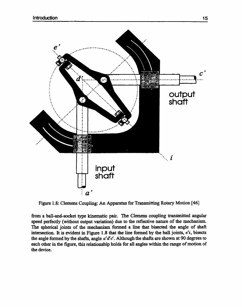
The Clemens coupling is depi& in Figure 1.8. This first version of the device contained only two arms and permitted planar misalignments of the shafts. Later versions contaiued tbree arrns and pemiitted spatial m&dignments of the shafts. The device shown in Figure I .8 comprised two shaffs, intercomected by two linEtages. Each linkage contained ~ W O bodies (or links), and a succession of revolute, spherical and revolute joints. Power

Introduction 13

Figure 1.6: The Mechanisns: a) Double-Tripod, and b) Variable-Geometry Tmss

and motions were transmitted through these Iinkages fkom one shaft to the other. 'Ine shafts were dowed to misalign in a plane, guided by a supporthg frame and set of grooves. Spherical weights were attached to the side of =ch link, so as to cornterbalance static and dynamic forces during rotation, Some detail is provided in Figure 1.8 of the two Links and spherical joints attached to one shaft, showing that each sphericd joint was cofl~t~cted

Introduction 14

VGT Miura, 1984

Tripod 994

Reflected Tripod Hunt, 1973

Clemens Coupling Clemens, 1869

Figure 1.7: Family Tree for DT and VGT

Introduction 15

input t/l shaft

Figure 1.8: Clemem Coupling: An Apparatus for Transmittllig Rotary Motion [46]

from a bd-and-socket type kinematic pair. The Clemens coupling transmitted angdar speed perfectly (without output variation) due to the reflective nature of the mechanism. The sphexicd joints of the mechanism f o d a line that bisected the angle of shaft intersection. It is evident in Figure 1.8 that the line formeci by the ball joints, e'i, bisects the angle fomed by the shah, angie a'd'd. Although the shafts are shown at 90 degrees to each other in the figure, this relatiodp holds for ail angles within the range of motion of the device.

Introduction 16

Figure 1.9: The Reflected-Tripod Constant Speed Coupling

1.3.2 Reflected-Tripod Coupling As mentioned previously, the Clemem coupling was designed for shafts that were misaligned in a plane. The principle of this couplhg applies to shah rhat rnisaliga spatially as well, as is the case with the reflcted-@~od constant speed coupling.

It is not clear fkom the hown literature whether or not Clemens constnicted couplings for spatial misalignment. Most citations of this type of coupling refer to Clemens, however. An early example is a discussion on universal joints by Steeds, who credits Clemens for the revolute-spherical-revolute type universal joint [48]. Wallace and Freudenstein also cite Clemens in the context of spatial couplings [49]. Hunt states that the reflcted-tnpod constant speed couplùlg is "based on the principle of Clemens coupling" [Il . Clemens did lay claim in his patent, however, to devices with "one or more pairs of pivoted crank-arms" C461-

The reflected-tripod coupling employs three linkages? an=a.nged radiallys for transmitting power and motion between two misaligned shafts? as depicted in Figure 1.9. As with Clemens' device, the geometry of the mechanism is reflective about the bisecting plane. The intersecting plane formed by the three spherical joints, as with the Clemens coupling, bisectr the angle for& by the two shafts. This mechanism can be thought of in a planar sense, when one considers it in the context of the plane formed by the two intersecting shah. The common liae formed by the intersection shaft plane and the bisecting plane is quivalent to the bisecting line e'i in Figure 1.8. Hunt temied the couphg reflected-tnpod because the device comgrised two identicai tripods, adjoined at their feet at three spherical

joints. As mently as 1994, Reinholtz and his associates presented the Clmens coupling under

the false pretense that it was a new design 1501. They showed that the coupling could be used effectively for large angles of misaiigmnent.

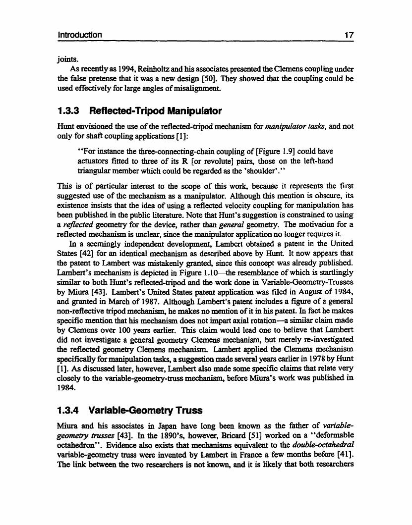
1.3.3 Reflected-Tripod Manipulator Hunt envisioned the use of the reflected-îripod mechanism for manipuloor tasks? and not oniy for shafi coupling applications [Il:

"For instance the three-comecting-chah coupling of [Figure 1.91 could have actuators fitted to three of its R [or revolute] pairs, those on the lefi-hand triangular member which could be regarded as the 'shoulder'."

This is of particular interest to the scope of this work, because it represents the first suggested use of the mechanisn as a d p u i a t o r . Although this mention is obscure, its existence insists that the idea of using a reflected velocity couphg for manipulation has been published in the public literature. Note that Hunt's suggestion is consaained to using a re/ected geornetry for the device, rather than general geometry. The motivation for a reflected mechanism is unclear, since the msnipdator application no longer requires it.

In a seemingly independent development, Lambert obtained a patent in the United States [42] for an identical mechanism as describecl above by Hunt It now appears that the patent to Lambert was mistakdy grantecl, since this concept was already published. Lambert's mechanisn is depicted in Figure 1.10-the resemblance of which is startlingly similar to both Hunt's reflected-tripod and the work done in Variable-Geometry-Trusses by Mima [43]. Lambert's United States patent application was f i l 4 in August of 1984, and granted in March of 1987. Aithough Lambert's patent inciudes a figure of a general non-reflective tripod mechanism, he &es no mention of it in his patent. In fact he makes specific mention that his mechanisn does not @art axial rotation-a similar claim made by Clemens o v a 100 years earlier. This claim wouid lead one to believe that Lambert did not investigate a general geornetry Clemens mechanian, but merely re-investigated the reflected geometry Clemens rnechanism k b e r t applied the Clemens mechanisn specifïcally for msuiipulation tasks, a suggestion made several years earlier in 1978 by Hunt [Il. As discussed later, however, Lambert also made some specific claims that relate very closely to the variable-geometry-truss mechaniSm, before Miura's work was published in 1984.

1.3.4 Variable-Geometry Truss Mnw and his associates in Japan have long been known as the father of vanable- geomem trrcsses [43]. In the 1890 '~~ however, Briard [51] worked on a "deforniable octahedron". Evidence also exists that mechanhm equivdent to the double-octohedral variable-geometry tniss were invented by Lambert in France a few months before [41]. The ünk baween the two researchers is not known, and it is Iürely that both researchers

Introduction 18

Figure 1.10: Lambert's Elementary Mechanism [42]

envisioned similar concepts independently. Soon after Miura, researchers began investi- gating similar concepts with variable-geometry trusses for mnipuiator applications. These include Rhodes and Mikulas [52], Sincarsin and Hughes [53], and Reinhola and Gokhale [541.

1.3.5 Poly-Retractile Mechanism Lambert's French patent for a poly-retractile mechanian was obtained in 1984 [4 11. His device, shown in Figure 1.5, is functionally very similar to that studied at the University of Toronto in Figure 1.3. This was revealed to the author during a recent visit to Switzerland [34]. In the U.S. version of his patmt [42], Lambert suggests many applications of the device, which include: 1) underwater or space manipulators contriining a spatial tunnel, 2) lifting and orientation platforms, 3) ceapon, reflector, antenna support m e t s , and 4) numerous other applications.

Close examination of Lambert's elementary mechanian, s h o w in Figure 1.10 shows that it is in fact a Clemens coupling, published previously for such applications by Hunt [ 11, shown in Figure 1.9. This would imply that such a m e c M s n is public howledge, nullifying most, if not all, of Lambert's c I W . Another interesthg item in Lambert's patent is that he mentions many different actuation schemes for the mechanisn, one of which is equivaient to variable-geometry tmsses. The actuation methods include:

Introduction 19

(a) two points on opposing platforms, (b) two points on the same leg, (c) two points belonging to different legs', or (d) two points on one leg and one platform.

2- rotary actuators, and

3. "infiatable structure" actuators (assumed to be non-mechankm actuators controlled via air pressure)

Note that linear actuation option (lc), when the linear actuators are placed between the three spherical joints on the three legs, forms the double-octahedron variable-geometry truss shown in Figure 1.6(b).

1.3.6 Variable-Geometry Trusses As mentioned previously, Miura invented a similar concept of variable-geometry tmsses, apparently independently, around 1984 [43]. While Lambert se& to focus on the mechanical aspects of his device, Mura focused on the truss aspects of his device. The design of the stacked octahedral tniss was inspireci by work he conducted on deployable structures.

Miura and his associates discussed various applications of octahedral types of variable- geometry tnisses in the original papa 1431. Specificaily, the double-octahedron topology (or geometry), with actuators on every second section of the huss, was suggested for robotic mmipuiator applications. Miura and his colleagues went on to build several Iaboratory models, ali containing single octahedd topology however, perhaps an indication of their focus on "adaptive structures" rather than on " manipulators" per se [55]. Other researchers in North America began investigating the double octahedral topology, with special interest in space manipulator applications.

Around the same time, researchers at the NASA Langiey Research Center developed a double-octahedral tniss to demonstrate its capabilities for deployment applications [S2]. The truss was also used in active viiration contrd experiments by Robertshaw 1561.

1.3.7 Variable-Geometry-Truss Manipulator In an effort to fkd a variable-gwm- topology suitable for manipulator applications, Dynacon Enterprises Ltd. of Toronto conducted a study comparing s e v d candidate topologies [53]. Candidate topologies included 1) stacked actahedral, 2) stacked cubic, 3) stacked irregular tetrahedral, and 4) stacked regular tetrahedral. Two conclusions of the study were that the stacked d e d r a l geometry was the most suitable for t m s a d , and

'This arrangement is eqivaient to the doublbOCt8hcdral variabI+geomctry truss. 'The nsmt "~nissann*~ was coinai by HU- to descri i variable-geomctry-truss mauipuiaîors in

g e n d . Latcr, the proposeci foin-bay 12-DOF fàcility and prototypes thcrwf at University of Toronto were known as Tntssarm (capitabed).

that actuators were best located on every second segment of the miss, in order to simpiify hinge design as much as possiile. These conclusions, dong with a synopsis on kinematics, dynarnics gt control, and laboratory models were later summarized in [57l. A depiction of the Trussarm laboratory prototype is given in Figure 1.6(b).

Almost in parallel, researchers at Virginia Polytechnical Institute and State University (VPI&SU) started investigating the double-octahedral variable-geometry tniss for d p ulator applications [54]. The -archers also developed a laboratory prototype, u t i l k g it for applications such as vibration control and manipulation [58].

1.3.8 Double-Tripod Manipulator M e n the assumption of reflected geometry of the reflected--hipod mechanism is relaxe4 the mechanism can be refmed to as a double-nipod mechanism.

With the double-tripod mechanian (or more simply, double tripod), no assumption of symmetry is made, either axially or relative to the midplane. The mechanisn is made up of three linkages that interconnect two platfonn bodies. Each linkage comprises a revolute-spherical-revolute succession of kinematic pairs. No assumption is made about either the length of each iink, or the attachment point of the revolute joints on the platform bodies.

Hunt included the kinematic structure used by the double tripod in a paper that enmerateci the kinematic arrangements of various paraiiel manipulators [7$ Although he presented a general kinematic structure, he d i s c d it in the context of the reflected-tripod ody. To the knowledge of the author, the double tripod shown in Figure 1.6(a) has not been studied for its application to manipuiator tasks.

1.4 Literature Survey This section provides a Literature survey in the context of the work presented in this thesis. The areas discussed include: 1) kinematic modeling, 2) forward kinernatics, 3) inverse kinematics, 4) laboratory prototypes.

1.4.1 Kinematic Modeling Although the double tripod was enumerated for manipulator applications by Hunt [7], to the knowledge of the author, no work bar beenpublished on the kinemaîîcs for maniplator applications. Hunt investigated the mdmn.ism in temis of its mobility, suggesting that it could be applicable for robotic tasks. Most of the previous work in modeling the variable-geomeîry truss has focused on

planar versions of the mechaaism, rather more general types. For the planar version of the mechaniSm, two distinct approachw exist in the literature:

Introduction 21

* Gcugb-Stewart platfonn

Table 1.1 : Simplifjmg Assumptions for Single-Octahedral Mechanisms

Single Octahedroa Modeis

1. Modeiing the variable-georneûy tniss as two repeated unis of single octahedrons.

Simplifying Assumptions Authors

Tidwell et al. [60]

2. Modeling the variable-geomeîry tniss as one unit containing two stacked octahedrons.

Planar Base

r / Type VGT

By considering each octahedron separately, the first approach can apply much of the related work on the Gough-Stewart platforni almost directly. Many insights can be gained by considering the variable-geometry miss as a whole, since it is not practical for robotic applications in a single octahedral fom.

Planar Plat50n.n

r / d J J

Arun et al. [6 11

Griffis and Duffy [62] bocenti and Parenti-castet% [59]

Single Octahedral form

Table 1.1 lists several researchers who have investigated the single octahedron form of the VGT. As well, a sampling of pertinent papers on the Gough-Stewart platform is provided. In dI cases, except for [59], the octahedral VGT, by definition, has been assumed to have planar platforms.

Tidwell et ai. [60] developed a mode1 for the VGT based on planar base. Anin et al. [61] also investigated the VGT assuming a planar base. These kinematic models are very similar to those used by researchers who investigated the Gough-Stewart platform. Both Griffis and DufQ [62] and Innocenti and Parenti-CasteIli [59] used kinematic models essUming planar platforms in the Gough-Stewart mechanism. This kinematic model can be applied to the VGT by redefining the variable length components in the mechanism. Wbile Griffis and DufQ investigated a mechanism with a planar base as well, Innocenti and Parenti-CasteIli extended this by studying Gough-Stewart platfonn with a kinematic model that containeci a non-planar base.

VGT GS' GS'

Double OctahedraZ Form

d

d

As discussed, another approach to the modeling of the VGT is to consider both octahedrons together. 'Ihis is motivated by several facts, one of which is that both octahedrons are necessary to achieve a workable mechanism, since for many applications two rigid platforms are required. Unlike the single-octahedron equipped Gough-Stem platform, the VGT must contain a pair of octahedrons for robotic applications, the intersection of *ch is actuated.

Introduction 22

Double Oct. VGT Models Authors

Miura and Fuyura [43]

* Prese%ed in Section 3.3

Hertz and Hughes [47]

Hertz (this dissertation)'

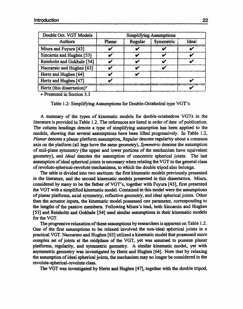
Table 12: S i m p m g Gssumptions for Double-Octahedral type VGT's

S i m p m g Assumptions

A summary of the types of kùiematic models for double-octahedron VGTs in the literature is provided in Table 1.2. The references are listed in order of date of publication. The column he8dings denote a type of simplmg assumption has been applied to the models, showing that several assuniptions have been lifted progressively. In Table 12, PZanar denotes a planar platfom assumption, ReguZar denotes regularity about a common axis on the platform (dl legs have the same geometry), Synimehlc denotes the assumption of mid-plane symmetry (the upper and lower portions of the mechanian have equivalent geometry), and Ideal denotes the assumption of concentric spherical joints. The 1st assumption of ideal spherical joints is necessary whai relating the VGT to the general class of revolute-spherical-revolute mecbnisms, to which the doubb tripod also belongs.

The table is divided into two sections: the nrst kinematic models previously presented in the literature, and the second kinematic models presented in this dissertation. Miura, considered by many to be the father of VGT's, together with Fuyura [43], first presented the VGT with a simplifieci bernatic model. Contained in this model were the assrmiptions of planar platfonns, axial symmeûy, reflective geometxy, and ideal spherical joints. Other than the actuator inputs, the kinematic mode1 possessed one parameter, corresponding to the lengths of the passive mwbers. Following Miurays lead, both Sincarsin and Hughes [53] and Reinholtz and Gokhale 1541 used s i d m assumptions in their kinematic models for the VGT.

The progressive relaxation of these assumptiow by researchers is apparent on Table 1 2 . One of the first 8ssumptions to be relaxed involved the non-ideal spherical joints in a practical VGT. Naccarato and Hughes [63] utilized a kinematic model that possessed more cornplex set of joints at the midplane of the VGT, yet was assumeci to possess pl- platforms, regularity, and symmetric geometry. A similar kinematic model, yet with asymmetric geometry was investigated by Hertz and Hughes [64]. Note that by relaxing the assumption of ideal sphezical joints, the mechaniSm may no longer be considered in the revolute-sphefical-revolute class.

The VGT was investigated by Hertz and Hughes [47], together with the double tripod,

Planar

a4

d

Sincarsin and Hughes [53] Reinholtz and Gokhde [54] Naccarato and Hughes [63] Hertz and Hughes 1641

d

d

Repuiar Wf w' O/ w' d

d d d #

Symmetric

Wf d d d

Ideal r/ rf fl

I

Introduction 23

using a kinematic model that was asymmetric and irregular. The assumption of planar platforms was made, as was the assumption of idul spherical joints. These mechanisms belong to the revolute-sph&d-revolute class, and define the scope of this dissertation. The progressive relaxation of the planar assumption is made in this work, and is contained in the following section. Note that dthough the investigation of non-ideal spherical joints is noteworthy, it is beyond the scope set for this dissertation.

1 A.2 Forward Kinematics

To the author's laiowledge, the forward and inverse kinematics of the double tripod manipulator has not been addressed in the literature. The variable-geometry truss (VGT) has been studied by Miura et al. 14331, Padmanabhan et al. [65], Naccarato and Hughes [63], Anui et al. [66], and Hertz and Hughes [64]. The VGT is itself closely related to the Gough-Stewart platform, the kinematics of which have been presented in Griffis and Duffy 1621 and Innocenti and Parenti-Casîeili [59].

As with the development of the kinematic models, the respective forward and inverse kinematic solutions have been developed with progressive comp1exity. Miura et al. [43] presented an iterative forward kinematics solution of the VGT with a single parameter, fully symmetric and regular kinematic model. The forward kinematics of the VGT was investigated more closely by Anui et al. [6q, who used homotopy methods to show that 16 solutions exist for the basic octahedrd building block of the VGT. These results were dso presented for the octahedral Gough-Stewart platforni by Gnffis and Duffy [62] and Innocenti and Parenti-Csstelli 1591. In these works, polynomial elimination was used to reduce the forward kinematic closure equations of the parallel mechanism to a single polynomial in one iinknown. The respective d t s showed that for planar platforms, 8 &rs of reflected solutions exisf and for non-planar platfonns, 16 unique solutions exia Hertz and Hughes [64] examined the VGT c a s of non-reflective midplane geometry and planar platforms. The forward kinematic solution r d t e d in 256 possible unique assemblies.

1.4.3 Inverse Kinematics The inverse kin-tics of the VGT has been examiDeci by Padmmabhan et al. 1651 and Nacarrat0 and Hughes [63]. In both Papen, the closed-foxm inverse kinematics solution was solved for the planar platfonn, symmetric class of the VGT. In this dissertation, we focus on the inverse kinematics of the general class of both the VGT and DT, neither of which have been dealt with in the literature, except in previousIy published work by the author [47].

1.4.4 Laboratory Prototypes To the author's knowledge, the oniy prototype manipulator projects for the revolute- sphezicai-revolute class of xnanîpulator include the foliowing for the VGT:

Introduction 24

0 Rehholtz and Gokhale's double-octahedral VGT [54]

O Hughes et al. Tnissarm Mark 1, a single bay double-octahedral VGT [57]

a Hughes et al. T~ssarm Mark IL7 a 4 bay VGT [67l

and for the double-tripod, only the protoytpe presented in this thesis has been identified.

1.5 Contributions of This Dissertation In this chapter, the extensive literature search identifies an early reference for the use of revolute-spherical-revolute mechanisms ( 1 869, over 125 years old). The double tripod mechanism is first described The variable-geometry tniss and double tripod are show to belong to the same rnechsuiism classes.

in Chapter 3 a novel classification scheme for the revolute-spherical-revolute class of manipulators is presented. The scheme gives 8 possible ciassifications, based on platform planarity, mechanisn symmetry, and axial regularity. A complete general kinematic model is deviseci, which anploys Denavit-Hartenberg notation for each ieg, modeling each as -a 5R chain, with additional end-effector and base transfomation,

A sizeable portion of analytical work is presented in Chapter 4, dealing with the solution of the forward kinematic problem. The solution proceeds in a unified manner for both mechanisns. A solution method temieci the "petal angle method" in the literature is employed in the forward kinematics. The double tripod is shown to have a maximum of 16 real solutions, alI of which are shown grapiiically for a specific double üipod. The variable-geometry huss has a maximum of 256 solutions. An explicit closed-form solution to the forward kinematics is found for the reflective double-tripd. The ciosed-form implicit solution is presented for an axially symmehric version of the planar platform model, using the method of polynomial eliminiition, that is applicable to both mechanim.

The inverse kinematics for both mechanisns is provided in Chapter 5. Iterative solutions are employed for the solution of both the generalized and planar platform kinematic models, while closed-form solutions are presented for the reflective form of the double-tripod and double-octahedral variable-geometry tniss. A computationally efficient iterative inverse kinematics algorithm is presented, based on the forward kinematics solution.

Chapter 6 contaias details of the design and contxol of "Clan," a first-of-its-kind double-trïpod manîpulator deveioped specifically for this dissertation. With Clem, the kinematics of the planar platfonn model are verified experimentdy.

Chapter 2

Mathematical Preliminaries

2.1 Kinematics

2.1.1 Vectors A vector is ubstract if it is defined without a reference h e . Reference frarnes need not be introduced to perform such operations as dot products and cross products on abmc t vectors. Reference h e s simply allow the abstract vector to be expressed in ternis of a set of vector coordinates-scalar entities describing an abstract vector in ternis of other abstract vectors.

While column matrices are commonly termed vectors, and vise versa, this is not entirely correct. Column matrices are simply a convenient mathematical construct used to organire entities. The entity is usually a scalar, but this is not always the case. For example, a column ma& of abstract vectors will be introduced Later. Very often the scalar coordinates of a vector are stored in a column rnatrix.

Nomenclature

The notation used in this dissertation is similar to that introduced by Hughes in [68]. S e v d key points with the notation are as foilows:

O Vectors are abstruct, th& physical properties of magnitude and direction are invariant. Vectors will be denoted by a lowercase letîer with a boldface upright font (i.e. a vector v). Unit vectors will be M e r identifid by an overhat symbol (Le. a unit vector 6).

O Reference frzunes fom a basLÎ for expressing a vector in terms of scalar values. Mathematically, they are a collection of unit vectors. These unit vectors that make up a given reference h u e can be conveniently orgunked using column matrices1, so as to introduce a mathematical means to define, change, and manipulate reference h e s and the r d t i n g vector coordinates. Reference fiames will be nslmed with

'These column matrix/dces of v e r s were wined veciridvecrrices 6y Hughes in [68].

Mathematical Preiirninaries 26

a script letter F, and will be dmoted matftematically by a boldface letter F (Le. reference finune F', and its matfiematicai equivalent Fo).

O Coordinates of vectors will be arranged in column matrices, which will in g e n d be denoted by a Lowercase bold-italics font (i.e. the vector coordinates u and unit vector coordinates O). General rectangular matrices will be denoted by an uppercase bold-iacs font (i.e. a rectangular matrur U).

Vectors and Reference Frames

To illustrate the notation, consider an arbitrary vector p and a reference frame Fo. The vector p can be expressed in ternis of a reference b c Fo and coordinates p with the following simple mtrk relationship:

where

where Fo is a vectrix of unit Gibbsian vectors %, Y, and go. When (2.1) is expanded by perfonning the matrir inner product, the foiiowing common vector relationship results:

Rotation Matrices

It may also be desirable to express p in terms of another reference frame FI. Instead of (2.1 ), the vector equation is

P = P , ~ F I (2.3)

where

Mathematicai Prelirninaries 27

The transfomtion between the two sets of vector coordinates can be solved by equating the right hand sides of (2.1) and (2.3). and simpl3ying the equation as follows:

The dot product on the left hand side of (2.4) can be evaluated by expanding it to a 3 x 3 matrix and evaluating each member

Assuming that Fo represents an orthonormai fiame, the dot product reduces to

The dot product on the right hand side of (2.4) can be expanded similarly:

The mat& Col is termed a rotation matrix, and is populated with an array of direction cosines that relate Fo and FI to each other. Upon simplification of (2.4), the vector coordinates in (2.1) and (2.3) ain be expressed in a purely matrix fom:

Successive Rotation Matrices

Consider the following rotation matrix:

If rotation matrices to and fiom an intermediate h e FI are known, the rotation matrix C o z c m be calculated as the following product

where

Substituthg (2.9) and (2. IO) into (2.8) results in

c ~ ~ = F ~ - F T F ~ - F : Now, the identity dyad has the foliowing properties

for any vector v, and F o - 1 = F o

for any reference h e Foe And it c m be easiiy shown that

With the definition of the identity dyad, (2.1 1) can be simplified

Operations

Vector operations can be expressed as quivalent opemiions for vector coordinates, when expressed in the same reference b e

U X W u x w

where

Mathematical Preliminaries 29

Figure 2.1 : Position Vectors

2.1.2 Position Vectors Consider two reference fiames and a point in space, as shown in Figure 2.1. The reference -es are denoted Fo and F 1, while the point is named P. Two position vectors are constructeci fiom Fo and Pl, named p, and p, , respectively.

A position vector of apointis dcjined us the vector thaî star& ut the un'giik of a referenceframe und ends at thepoin~

The position vectors are related to their respective vector coordinates as follows:

where p, = col{^,^,^.} and pl = col{prz, mu,fiz). The relationship between the vector coordinates p, and pl can be exprtssed in tenns of a homogeneous transformation.

2.1.3 Homogeneous Transformations In robotics kinematics, homogeneous trmLFfo~tions arc used extensively to describe rigid body dirpucementr and rotations. The concepts of vectors, referuce fiames, and vector coordinates caa be employed to examine this c h of transformations.

Starting with a vector equation, the position vectors in p, and pl are related to the inter-frame position vector (see Figure 2.1). as follows:

Mathematical Preliminaries 30

Note that do, is simply a position vector of the origin of FI related to Po. Substituting (2.1 6) and (2.1 7) into the vector relationship (2.1 8) resuits in

If (2.19) is premultiplied by Fo- and subsequentiy simplified, it becomes

The above equation can reworked into what can be tenned as the vector expanded form of the homogeneous equation:

This demonstrates how, in general, the coordinates of two position vectors are related in terms of vectors.

Tlie hornogeneous îransf0mimion relates the coordUta&s ofposrtjon vectors to each other.

The vector expunded homogeneous tramfionnation is defined a s follows:

The finai form of the homogeneous equation in (221) cm be expressed as

where po = col{po, 1 ) and pi = col{p, , 1 ). The transformation in (2.22) can be written in a more recognizable m u h form through

the substitution of rotation ma& in (2.5) and the coordinates of the inter-fmme position V ~ C ~ O ~ F O * do1 = doi = col{do~rt Aïr)

2.2 Analysis of Mechanisms

2.2.1 Mobility Mobility is defined in [69] as follows:

"The mobility of a system of bodies corresponds to the number or independent pimuneters reqrcired to wmpletely ~pecrïjt the geometry ofthe system "

Mathematical Preliminaries 31

The mobility of a spatial mechanism can be found with the knowledge of the number of bodies, and the nlmiber and types of kinematic pairs in the linkage. The relationship is known as the Grübler Fonnula [l]:

where m is the mobility, n' is the number of bodies (including the base), g is the number of joints, fi is the degrees of fieedom for the ith joint.

It is convenient to intmduce n, the number of bodies ercluding the base to (2.25). As weU, the sum of the degrees of hedom in each joint in (225) wiU be referred to simply as the joint degree-of-fieedom (JDOF). This results in the following "compact" mobility eqyation for a spatial mechanism:

where

22.2 Degree of Freedom The degrees of finedom of a mechanism will be les than or equal to the mobility, depending on whether idle or spin DOF exist An idle DûF is one that does not trammit motion into the end-effector of a manipulator.

where I D 0 F denote the number of idle DOF.

2.2.3 Denavit-Harten berg Representation In 1955, Denavit and Hartenberg developed a method to represent the kinematic relationship between bodies connected via cylndrZcaZ joints that used homogeneous transformations [70]. Since a cylindrical joint is equivalent to a combined revolute and prismatic joint, either of which is common in manipulators, their representation has found widespread application in robotics. The representation also introduced a means by which links could be mdeled with 4 parameters. These parameters, considered to be standard for kinematic models, include two distances and two mgles.

With the Denavit-Hartenbag P H ) representation, referaice fhmes an sttached rigidly to each link in the mechanhm The orientation and positionhg of each reference h m e within each lin. is pdetemhed. Successively located reference fiames for a linkage

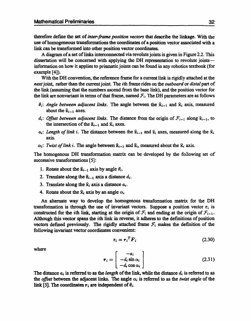
Mathematical Prelirninaries 32

therefore define the set of inter-fiame position vectors that describe the Linkage. With the use of homogeneous tramformations the coordinates of a position vector associateci with a link can be transformed into otha position vector coordinates.

A diagram of a set of links intercomected via revolute joints is given in Figure 2.2. This dissertation will be concerned with applying the DH representation to revoiute joints- information on how it applies to prismatic joints cm be found in any robotics textbook (for exampie [4 1). With the DH convention, the referrnce fiame for a cumnt Link is rigidly attached at the

nert joint, ratfier than the current joint. The ith fiame rides on the ouiboard or d a 1 part of the Link (assuming that the numbers ascend fiom the base Mc), and the position vector for the iink are nonvariant in terms of that £hune, named Fi. The DEI parameters are as follows

8;: Angle between adjacent links. The angle between the g-l and axis, measured about the axes.

di: Wset between adjacent linh. The distance fkom the origin of 3i- dong Oi- l , to the intersection of the Ji-l and axes.

ai: Length of link i. The distance between the Ziel and Z j axes, measured dong the jii axis.

a;: T h t of link i. The angle between 4-1 and Oi, measured about the X. axis.

The homogenous DH transformation matrix can be developed by the following set of successive transformations [5]:

1. R o t . about the 2i-l axis by angle Bi.

2. Translate dong the 4-1 axis a distance di.

3. Translate dong the %- axis a distance a;.

4. Rotate about the axis by an aagle a;

An altemate way to develop the homogenous transformaton matrix for the DH transformaton is through the use of invariant vectors. Suppose a position vector ri is coIlSbCUcted for the ith link, starting at the origin of 3; and ending at the origin of 3;-1. Aithough this vector spans the ith link in reverse, it adheres to the definitions of position vectors defineci previoudy. The rigidly attached firame Fi F i e s the definition of the following invariant vector coorninates convenient:

where -ai

t i = [ -disha; ] -dj COS Cri

The distance ai is referred to as the length of the Link, while the distance 4 is referred to as the offset between the adjacent links. The angle a; is r e f d to as the twist angle of the link [SI. The coordinates t i art independent of Bi.

Mathematical Preliminaries 33

Figure 2.2: The Denavit-Hartenberg Repfe~efltation of Linkages

Mathematical Preliminaries 34

The controiied angle Bi of the ith link defines the relative oriptation of the ünk i with Link i - 1, and constitutes the fourth DH parameter, which is refmed to as simply the angle of the link The angle is dehed about the axis of the i - 1 fiame Fi-1, and is the rotation nom 4-1 to Xi, the unit vectors belonging to fianies Fi-l and Fi, respectively, s h o ~ n in Figure 2.2.

The homogeneous transformation can be obtained between links i - 1 and i by using the vector form of the relationship introduced in (222). It is evident that the vector equation in (2.18) is applicable when ushg the following inter-frame position vector:

With this substitution md the consideration of the general numbering of the m e s , (2.22)

The subsequent substitution of the invariant coorninates of ri expressed in (2.30) into (2.33) results in

The rotation matrix is expressed parameticaliy in temis of the two rotation angles Bi

and a;, about the Piwl and Q axes, respectively. These rotations are expressed as:

COS Bi - s h Bi COS a j sin Bi sin a; sin Bi COS Bi COS a - COS sin ai

= [ O sin CU^ cos a; I Furthemore, by substituthg (2.37) and (23 1) into (2.35). the following simplification of the set inter-me displacement coordinates resuits:

The homogeneous transformation for the ith link is therefore:

Mathematical Preliminaries 35

Figure 2.3: Use of Companion Indices

Successive hornogeneous transforrnatiorts can be used for solving the kinematics of manipulators. Suppose the hornogeneous transformation for an n link serial linkage is desired. If the first reference frame Fo is denoted the base, and the nth reference M e F , the end-effector, the base to end-effector aansformation Th can be solved as foliows:

The coordinates of the position vectors, as well as the unit direction of the end-effector f'rame can then be solved,

where eo represents the coordinates of the end-effector position vector e, expressed in terms of Fo.

2.2.4 Companion Indices The concept of companion indices is used extensively in the kinematic analysis of the double tripod and variable-geometry tmss. The technique is extremely useful for generalizùig kinematic relationships for parailel manipulators with three legs. Innocenti and Parenti- Caste& used the same concept in their îreatment of the forward kinematics of a class of Gough-Stewart platfoxms [59].

The use of companion indices can be illustrateci considexhg an arbitrary triangle Pl P2 P3, as shown in Figure 2.3, the side lengths of which are Il, l,, and 13. In definhg the sides of the triangle, one could use the scheme:

where (Pi Pj 1 denotes the distance betwee~~ points Pi and Pi. Using cornpanion indices, however, (2.42) is reduced to the following compact form:

17 = IPrEl (2.43)

Mathematical Preliminarïes 36

where

The operation r mod 3 is short for r modulo 3, or the remainder of r divided by 3. The relationship in (2.43) represents the generalized side length equation for the triangle pl p2 p3 -

Oftentimes the index r is used alone to develop kinematic properiies of a single gmeralized leg. When relationships between legs and thei. neighbors ensue, both indices r and s are used to describe the kinematics with complete generality.

Chapter 3

Kinematic Model

A kinematic model forms the ba i s for representing a mechanisn mathematically. In this Chapter, a general kinematic model for the revolute-spherical-revolute class of mechanisns is presented.

3.1 Classification The revolute-sphmicai-revolute parallel mechanism can be classified in te- of three types of geometric features. They include:

Mechanfsm Platform Geometry

The platform geometry of a revolute-spherîcal-revolute mechanism is classified as either planar or non-planar. For a mechsaism to be planar, both platforms must be individually planar. An individual platfom is pl- if the axes of the revolute joints lie in a cornmon plane. In this thesis, a revolute-spherical-revolute mecbankm will therefore be classified with respect to its geometry as eitherplmor or non-planar.

Mechanism Symmetry

The symmetry is defined for the revolute-spherical-revolute mechanism with respect to a specific plane. This plane is denned as the midplane-the plane containing the three spherid joints of the mechanism. The mechaaism is classifieci as symmetric if both the platform and leg geometries are symmetric about the midplane of the mechanîsm- A mechankm can therefore be classified with respect to its geometry as either symrnehic or asyntmehic.

Mechanism Regularlty

The repuiarity of the mechankm is dehed with respect to the geometry of each of the three legs. The leg geometry includes revolute joint aitachment to each of the platfornu,

and the lcngths of the leg segments. A mecbanism is dehed as regular if the geometry of the legs are equal. The revolute-sphericall-rwolute mechani'cm can therefore be classified with respect to its geornetry as either regulm or irregulur.

Tlie three ~Iassifications are mutually exclusive-a platform can be described in each of the three geometric classifications independently.

Each of the classifications possesses a state of generality and simplification. For example, an asymmetric mechankm is considered a generalized form of the symmetric mechanism. Similar statements can be formulated for the planar and regular classifications of the mechaaism,

The combinaiion of each of the classifications result in a way of descri'bing a total of eight possible revolute-spherical-revoiute mechanians.

1. general mechanism -, non-planar, asymmetric, and irreguiar geometry.

2. regular mezhanism -, non-planar, asymmetric, and regular geometry.

3. symmetric mechanism -, non-planar, symmetric, and irregular geometry.

4. symmetnc regular mechanism + non-planar, regular, and symmetric geometry.

5. planar mechanism + planar, asymmetric, and irregular geometry.

6. planar regular mechanism + planar, asymmetnc, and regular geometry.

7. planar symmetric mechanisn + planar, symmetric, and irregular geumetry.

8. planar symmetric regular mechanisn -, planar, symmetric, and regular geometry.

The ordering of the above List of classifications has ken with respect to a binaiy representation of the Planar, Symmetric, and Regular states. This binary number contains the digits PSR, where P = {O, l}, S = {O, l}, and R = {O, 1). The zero state corresponds to the more g e n d geometry, and the non-zero state corresponds to one of the three geometnc assumptions. For example, the general mechaniSn corresponds to geomeixy PSR = 000, while the plana. regdar symmetric mechaoisms corresponds to geometry PSR = 111. It is evident fkom the list that the classification number can be related to the PSR geometry as follows:

Classification = PSR + 1

The following Figures contain examples of each of tht 8 classifications. Classifications 1 through 4 are non-planar, and are shown in Figure 3.1. Revolute joints are depicted as cyhders in the figure, the axes of which are show as slender mabers. Spherical joints are shown as spheres, and legs an show as slender members. Platfoms for non-planar mechanisms are shown as a group of six members. Three of the members are axes of the revolute joints, and the remainder simply connect the axes together to complete a rigid platform.

The mechanilMn labelleci " 1 " in Figure 3.1 is an example of a general mechanism. The plaflonns are both non-plamr, the geometry on either aide of the midplane is asymmetric,

Kinematic Modei 39

1. general, PSR = 000 2. regular, PSR = 001

3. symmetric, PSR = 010 4. symmetric reguiar, PSR = 01 1

Figure 3.1 : Mechanisms with Non-Planar Geometry

and each leg has unique geometry. Mechanism "2" is an example of a regular mechsnism, since each leg has identical geomeüy with regard to revolute joint attachment and arm lengths. The mechanism is classified as non-planar due to the skew axes of the lower platform, and is asymmetric because of its taperai geometry. Although it is somewhat d i f f id t to visualize, mechaniSm "3" possesses midplane symmetry, and is thzefore classïiïed as symmetric. Note that the platfonns are non-planars and the leg geometry is irregular. Mechanism ' '4" in Figure 3.1 is an example of a symmetric regular classification. The platfoxms are non-plan.ars yet the geometry is symetric about the midplane, and the geometry of the legs are e q d .

Classincations 5 through 8 are pianars and are shown in Figure 3 2 . In this figure, the platforms of the mechanism.c are represented as triangles, each of which is made up of the

5. planar, PSR = 100 6. planar regular, PS R = 10 1

7. planar symmetric, PS R = 1 10 8. planar symmetric regular, PS R = 1 1 1

Figure 3.2: Mechanisns with Planar geomerty

axes of the revolute joints. The mechanism labelied "5" in Figure 3 2 is an example of a planar mechanism,

since both of its platforms form planes. Note as well that its geometry is asymmetric and irregular. Mechanhm "6" is an example of a planar regular mechanisn, since each of the platfoxms is planar, and each of the legs has r e m geometry. Note that the mechanism is asymmetric due to its tapered geometry. Mechanism "7" possesses plana. platforms and midplane symmetry, yet is irregular due to unique leg geometries. The last mechanism "8" is an example of a planar symnietric regular mechanism, since its platfonns are planar, it has midplane symmetry, and its three legs have epual geometry.

Kinematic Model 41

Figure 3.3: The General Double-Tripod Mechmism

Mobility Analysis

3.2.1 Double Tripod A general depiction of the Links and joints of the double-ûipod mechanism is shown in Figure 3.3.

me doubfe tnîpod h a 3 DOF and no idle DOF.

Iiicludhg the base, the double tri@ contsiins two ternmy links (those connected to three other bodies) and six binmy Links. Each leg has 3 joints* g i ~ g a totai of 9 joints. From (228), the JDOF for the mechanism is 15 (5 for each Ieg). Excluding the base, the total number of bodies is 7. The inputs to (226) are therefore:

n = 7 g = 9

JDOF = 15

which gives the mechanian 3 DOF. Note that no IDOF exists for the double tnpod, and the DûF of the mechanisrn is therefore 3 fkom (229).

3.2.2 Variable-Geornetry Truss As show11 in [69], variable-geometxy trusses can be nnalyzed with eitherpmcticaI or ideal joints. By ideal, it is assumai that the hear actuators intersect each other at spherical joints. Practical construction of joints usually p l u d e s such arrangements, however. The mobility for both practical and ideal (doubie-octahedron) variable-geometry tnisses WU be presented hem.

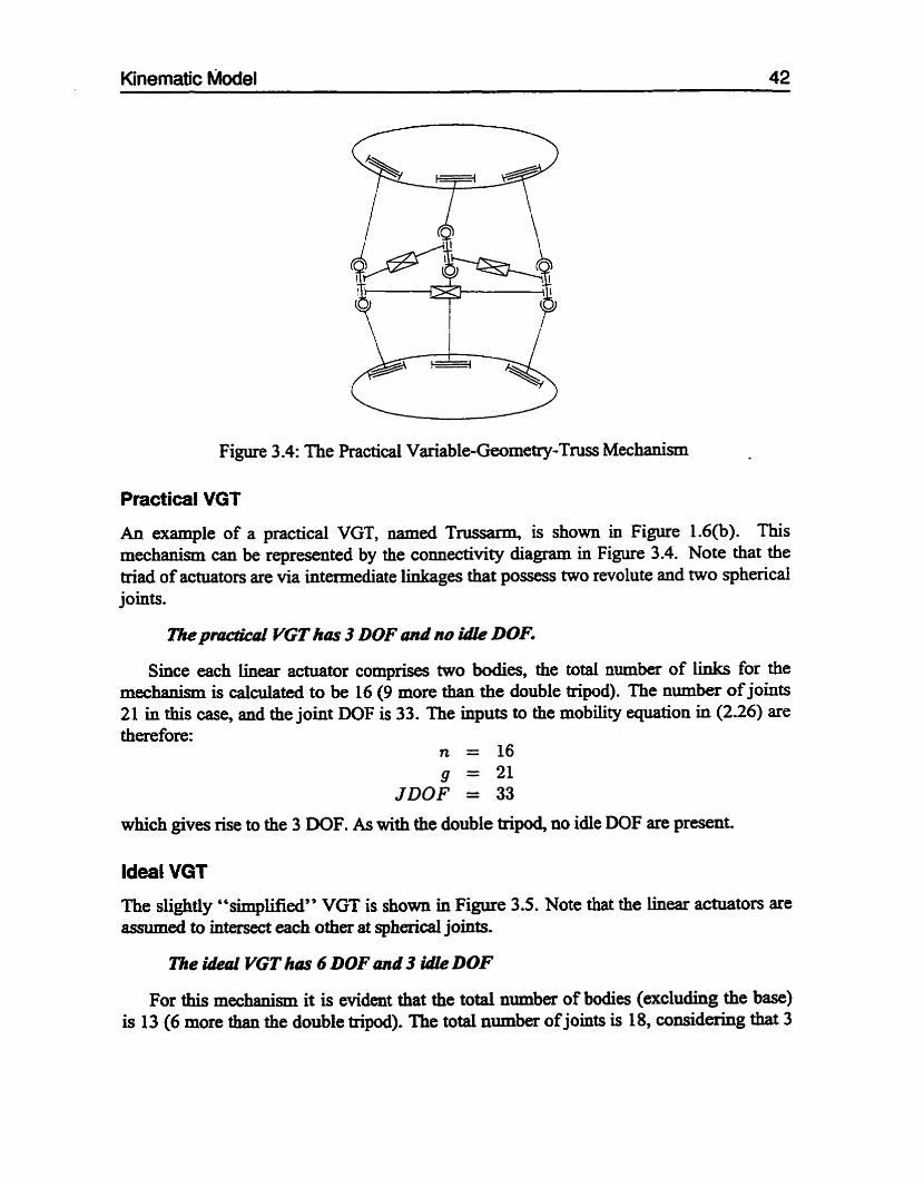
Kinematic fÜlodel 42

Figure 3.4: The Practical Variable-Geometry-TNSS Mechanism

Practical VGT

An example of a practical VGT, named Tnissarm, is shown io Figure 1.6(b). This mechanism can be represented by the connectivity diagram in Figure 3.4. Note that the triad of actuators are via intermediate linkages that possess two revolute and two spherical joints.

ThcprOCtiC11i1 VGT kas 3 DOF and no M e DOF.

Since each hear actuator comprises two bodies, the total number of links for the mechanian is calculated to be 16 (9 more than the double mpd). The number of joints 21 in this case, and the joint DOF is 33. The inputs to the mobility equation in (2.26) are there fore:

n = 16 g = 21

JDOF = 33

which gives rise to the 3 DOF. As with the double tri@, no idle DOF are present.

ldeal VGT

The slightly "simpMed" VGT is shown in Figure 3.5. Note that the linear actuators are assumed to intersect each other at spherical joints.

The ideal VGT has 6 DOF md 3 tdle DOF

For this mechanism it is evident that the total number of bodies (excluding the base) is 13 (6 more than the double tnpod). The total number of joints is 18, considaing that 3

Figure 3.5: The Ideal Variable-Geometry-Tniss Mechanisrn

concentric ball joints are present at each "elbow." The total number of joint DOF is 36. The inputs to the mobility eqyation of (2.26) are then

which gives rise to a mobility of 6. 'Ihree ide DOF are evident for the linear actuators in Figure 3.5, which results in the DOF for the mechanism to be 3 from (2.29).

3.3 General Kinematic Model A general model for the revolute-spherical-revolute class of mechanisns is introâuced in this section. The general mode1 consists of two platforms and three legs. The platform modeling is completely g e n d , and each rewlute-spherical-revolute leg is modeled with a set of g e n d Deaavit-Hartenberg PH) parameters.

Although DH parameters are used extensively in robotics, their use in the kinernatics of p d e I manipulators has been limited, This Îs attributed to the complexity of the closed- loop linkages in parailel manipulators. making the application the parameters cumbersume. Some researchers, however, have used DH parameters to model each leg of the parallel mechanism. One example is the work by Cl- and Brooks for the SmartEE manipulator. The dDOF mechanism containeci 3 legs, each of which was modeled by DH parameters WI*

A similar approach is usod here for the revolute-~pherical~~volute class of mec-- modeling the each leg with a set of DH parametas. This mode1 can be applied directly to the doubletripod. It cm also be applied to the VGT, with the definition of prismatic

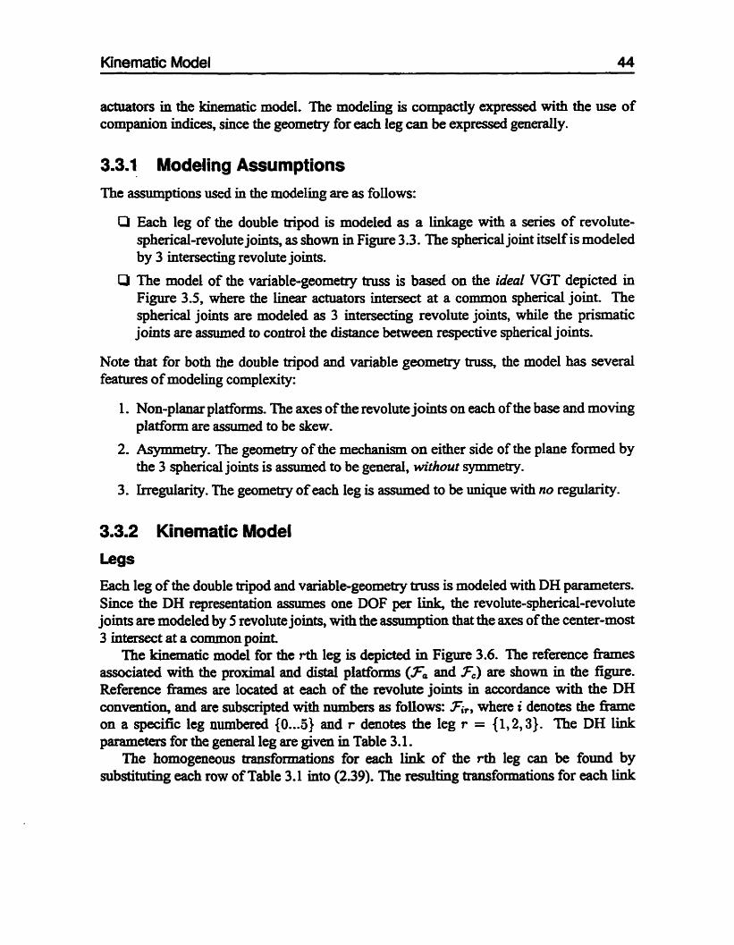
Kinematic Mode1 44

actuators in the kinematic model. The rnodeling is compactly expressed with the use of cornpanion indices, since the geometry for each leg can be expressed generaily.

3.3.1 Modeling Assumptions The assumptions used in the modeling are as follows:

O

O

Note

Each kg of the double ûipod is modeied as a Linkage with a series of revolute- sphericai-revolute joints, as shown in Figure 3.3. The spherical joint itself is modeled by 3 intersecting revolute joints.

The model of the variable-geometry truss is based on the ideal VGT depicted in Figure 3.5, where the linear actuators intersect at a common spherkal joint. The spherical joints are modeled as 3 intersecting revolute joints, while the prismatic joints are assumed to control the distance between respective spherical joints.

that for both the double ûipod and variable geometry truss, the model has several features of modeling complexity:

1. Non-planar platforms. The axes of the revolute joints on each of the base and moving platform are assumed to be skew.

2. Asymmetry. The geometry of the mechanism on either side of the plane formed by the 3 sphencal joints is assumed to be general, without symmetry.

3. Irregularity. The geometry of each leg is assumai to be unique with no regularity.

3.3.2 Kinematic Model

Each leg of the double tri@ and variable-gmrneûy truss is modeled with DH parameters. Since the DH representation assumes one DOF per link, the revolute-spherical-revolute joints are modeled by 5 revolute joints, with the assumption that the axes of the center-most 3 intersect at a cornmon point,

nie kinematic mode1 for the rth leg is depicted in Figure 3.6. The refefence h e s associated with the proximal and distal platforms (Fa and Fc) are shown in the figure. Reference -es are located at each of the revolute joints in accordance with the DH convention, and are subscripted with nimibns as foilows: 3ir, where i denotes the frame on a specific leg numbered {O ... 5) and r denotes the leg r = {1,2,3). The DH link parameters for the general leg are given in Table 3.1.

The homogeneous tran&ormatiom for each link of the rth leg can be fomd by substituthg each row of Table 3.1 into (2.39). The resulting traiisfonnations for each Link

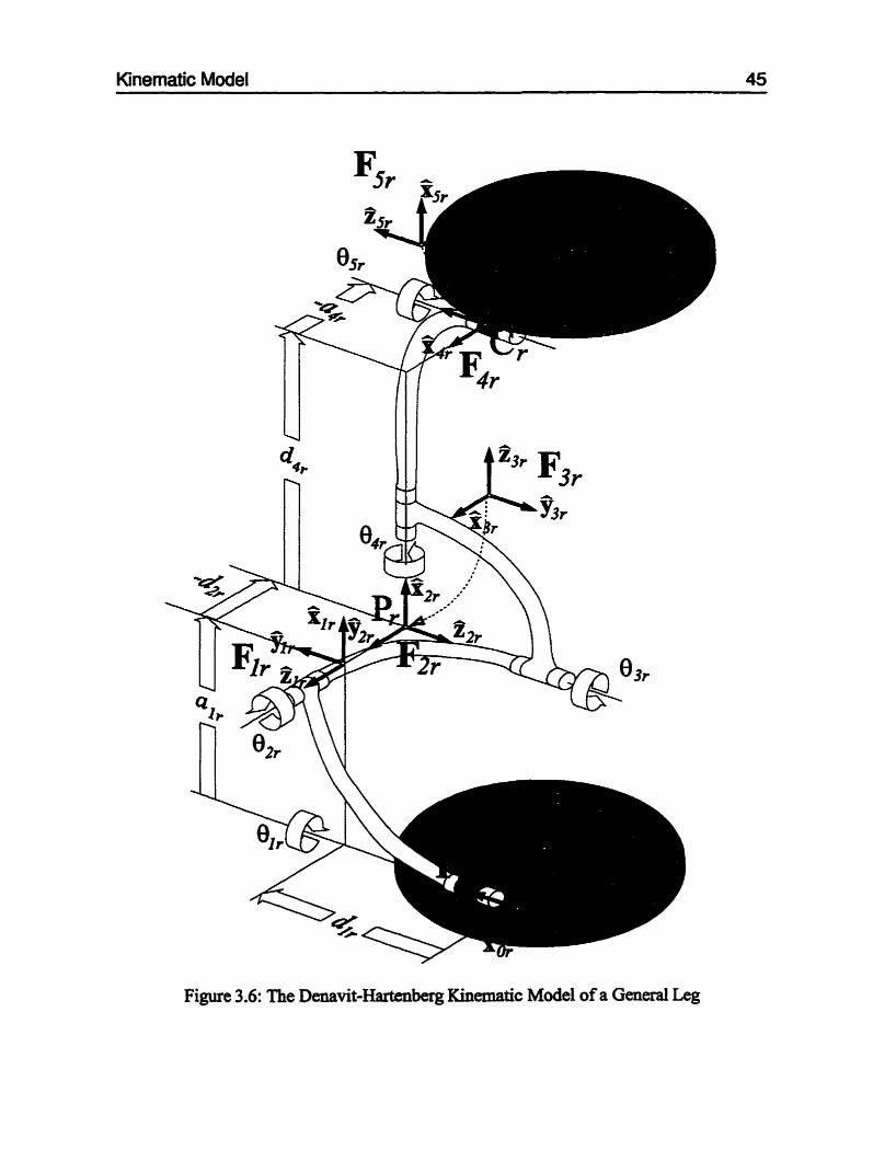
Kinematic Model 45

Figure 3.6: The Davit-Hartenberg Kinematic Model of a General Leg

Kinematic Model 46

are

Table 3.1 : Link Parameters for the rth General Leg

H45.r =

The "depicted"

COS Olr sin 61,

O O

[ COS

sin O O

l COS 03, sin 03,

O O

[ COS 04+ sin O*,

O O

COS OSr sin OLT

O O

- sin dl, cos al, COS O*, COS al,

sin al, O

- sin 62r COS 012,

COS 02, COS azr sin a!~,

O

- sin 03, COS a3,

COS est COS a ~ , sin as,

O

- ~h 64t COS 014,

COS O(, COS CY4,

sin a4, O

- sine5, O O c0se5+ O O

O 1 O O O 1 1

sin 81, sin al, - COS elr sin al,

COS a l ,

O sin sin a*, - COS SU^ Q2,

COS a 2 r

O

sin sin u3r

- cos 03, sin a3,

COS a3,

O

sin d4r sin a4,

- COS 04r S h

COS a d r

O

column in Table 3.1 refers to the angles shown in the Figure 3.6 example. Substituthg the depicted angles into the homogeneous transformations for each link r d t s in the following "shown" relationships in Figure 3.6:

1 O O al, O 1 O dl, 1

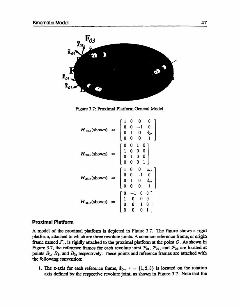
Kinematic Model

Figure 3.7: Proximal Platfonn General Model

Proximal Platform

A mode1 of the proximal platform is depicted in Figure 3.7. The figure shows a ngid platform, attached to which are three revolute joints. A common reference h e , or origin h e named Fa, is rigidly attached to the proximal platfonn at the point O. As shown in Figure 3.7. the reference fiames for each revolute joint Foi, Fol, and Fm are located at points BI, B2, and B3, respectively. These points and reference h e s are attached with the following convention:

1. The z-aW for each reference fiame, &, r = {1,2,3) is located on the rotation axis defïned by the respective revolute joint, as shown in Figure 3.7. Note that the

Kinematic Model 48

direction dong the revolute axis is arbitrary? and defines the positive rotation of the joint.

2. Points Br locate the reference fiames dong the joint axes. Each point located an arbitrary distance dong the axis.

3. The x-axis for each reference fiame, G, r = {1,2,3} is set arbitrarily? and defines the zero angle rotation of the respective revolute joint.

4. The y-axis for each reference h u e , YoT. r = {1,2,3) is denned fkom % and Zor according to dextral convention.

The position vectors for points BI, Bz, and B3 are dehed as bl , b2. and bs, respectively, and ai1 originate from the common reference h m e Fa (see Figure 3.7).

The vector diagram in Figure 3.7 can be succinctly represented by a set of homogeneous transformations, where each leg has a transformation. The ma& form of the homogeneous transformation introduced in (2.24) can be used to descnie the rth revolute joint position vector. This transformation is given as:

where Cao, is the rotation matrix between reference fiame Fa and Fe, and br are the vector coordinates of b, expressed in Fa.

The set of displacement variables used to represent the rotation ma& is the following z-y-x set of yaw, pitch, and roll Euler angles. The rotation ma& is given as:

where a,, Pp,, and ,ûRr are the angles of successive rotations about the Z,g, and 2 axes, respectively. The expansion of (3.8) yields

which when simplified resuits in

Note that in (3.9) and (3. IO), c and s are short for cos and sin, respectively. The relationship in (3.10) holds for the values of r = {1,2,3} conesponding to each revolute joint on the lower platform.

The displacement coordinates in (33 , which represent the zero-th fiame of each leg in tenns of the base pladorm fiame Fa, are as follows:

forr = {1,2,3). Conesponding relationships can be expressed for each of the r legs, substituting (3.1 1)

and (3.10) into (3.7) for legs r = (1,2,3}. Considering that each leg (or more properly each leg's proximal revolute joint) can be expressed by 6 parameters, the proximal platform is described by a total of 18 parameters. These parameters are enumerated as follows:

first proximal revolute joint -t bl, by h, ai BPI ,&1

second proximal revolute joint -, ba, 62, 62, Pm thirdproximal revolutejoint -, b3, 03, b3, h3 pR3

A mode1 of the distal platform is depicted in Figure 3.8, which shows the planorni viewed fiom undemeath. Similar conventions to the proximal platfonn are used for the attachent of the distal reference fiames. The common reference fkme is t e d Fc, and is fixed to the platfonn at an arbitrary point D. The reference fkames corresponding to the revoiute joints denoted 35i, &, and Fa, are located at points Cl, C2, and C3, respectively. As shown in Figure 3.8, the numbering of the points proceeds in a positive direction defined by the z-axis of the common reference frame (Z,).

The convention used to locate the direction of each unit vector for the reference fiames is expivalent to that used for the proximal platform. Note, however, that the axes are onented differendy fkom their proximal counterparts. These axes are arbitrary, and once p l a d define the zero angle measurement of the respective revolute joint. The placement of the x-axes for the upper platform will becorne more apparent when the DH convention is introduced for each leg.

The set of homogeneous transformations that express the position vectors dl, d2, and d3 in Fe is given as:

where r = {1,2,3). The position vector coordinates &, are

Note as weïï nom Figure 3.8 that the joint coordinates (3.13) are de- in opp0Ste directi0n.s compared to the proximal-hm the joint fiame to the common fiame. AS with

Kinernatic Model 50

Figure 3.8: Distal Platform General Model (viewed from undemeath)

the proximal platforrn, the rotation ma& of the rth distal joint is expressed in terms of an yaw-pitch-roll Euler angle set:

When expanded, this is of the same form as (3.10). Unlike the proximal platforrn, the distal axis coordinates are express4 in temis of the joint reference fnune, F5,, rather the cornmon h e .

The distal platform can therefore be describeci by the following set of 18 parameters:

hrst distal revolute joint -r dl+, dl,, dl,, W I VPI rlm second distai revolutejoint + db, d ~ t , wz I)P? ?RZ

third distal revolute joint -+ dkc d*, d 3 ~ c W3 I ) P ~ 9 ~ 3

3.3.3 Applications In ~umma~y. the general kinernatic mode1 ain be described by a set of 63 panmeters and 15 variables. The parameters include 18 for each of the two platfonns, and 9 for each of the 3 legs. Each leg or kinematic chain can be uniquely describecl starhg from the common fiame Fa and finishing at the cornmon fiame 3, by 6 proximal revolute joint parameters, 9 DH parameters. and 6 distal revolute joint parameters. Table 3 2 s u m a r k s these parametem. In addition to the 63 parameters, 15 variables are defined. These variables correspond to the ith joint DOF in the rth kg. and are denoted

The general kinematic model cm be applied to both the double tripod and variable- geornetry tniss. For robotic the controiIed input variables and the passive variables must be identifieci. For the double tripod, this application is straightforward, and with the additional definition of actuator lengths, the model may be applied to the variable-geometry tmss.

Kinematic Model 51

- - -.

rpanmieter Type 1 Parameter Name 1 Description 1 r kox&d ~latform ( b,,, b,, b,, 1 proximal joint coordinates 1 &.r, B P ~ , @fi proximal joint roll-pitch-yaw

al,, dl,, dzr, al,, 4, DH iength and offset parameters

-

Table 32: OveMew of Parameters for the rth Leg of the General Model

Distai Platform

Table 3.3: Controlled and Passive DOF for the Double Tnpod

&, dm, dTz ~ r * PT, V R ~

Double Tripod

distal joint coordinates distal joint roll-pitch-yaw

Description leg #I input leg #2 input ieg #3 input

leg #1 passive DOF leg #2 passive DOF lep #3 passive DOF

DOF Controlled

Passive

The g e n d kinematic model applies directly to the double tri@ manipulator. It is assumed that the three proximal revolute joints (one for each leg) are actuated, and that the rernainder of the joints are passive. The controlled DûF and the passive joint DOF for the double tripod are S11I11IlliiTiZed in Table 3.3.

Variable Name 011 812 013

Bzi , 03*, &, 051 622, 03*, &,

t?,, dm, Ou. 8,

Variable-Geometry Tniss

For a variable-geometry truss, the general mode1 cm be utilized by defining hear acniator lengths? and using these lengths as controlled inputs. It is assumecl the linear actuators lie paralle1 to the midplane defined by spherical joints, located at points Pl, P2, and P3- The distance between these points may be defined as the set of actuator lengths.

The actuator lengths cm be related to the g e n d model by first considerhg a single point Pr. The position vector coordinate conesponding to this point can be extracted h m the product of the proximal platform and fÏrst liak homogeneous transfomtions. The transformations and the corresponding product H a 2 , are

where &O,,. Hm,, , and Hi2.r are defined in ( 3 3 , (3.21, and (3.3, respectively. The

Kinernatic Model 52

Table 3.4: Controlled and Passive DûF for the Variable-Geometry Tniss

coordinates for p, are given as

R = [ri] The actuator vector coordinates 1, can be calculateci from the difference between successive position vectors. using the cornpanion indices r and s defined in (2.44) and (2.45). This difference is expressed as

I r =Pa - P r (3.18)

The actuator lengths can be found fiom the magnitude of (3.18), which is

With this definition, actuator r spans leg r and leg S. Recalling that r = {1,2,3) and s = r mod 3 + 1 fkom (2.44) and (2.45), followhg relationship reSuIts:

I l spans Pl and Pz l* spans P2 and P3 1, spans P3 and Pl

These controiied degrees of fiedom, together with the passive joint variables in (3.15), are summanzed in Table 3 -4.

Chapter 4

Forward Kinematics

The solution of the forward kinematics involves determining the one or more a.ssembZie.s of the mechanian given a set of actuator inputs. Multiple forward kinematic solutions are typical of parailel mechanisns.

4.1 Overview The forward kinematics problem is solving the shape of the manipulator given the angles or lengths of the input variables. In the case of the double tripod, the input is a set of three revolute joints, while for the VGT, the input is a set of achiator lengths.

The forward kinematics of the revolute-sphericd-revolute mechanisn is based on the general kinematic model presented in Section 3.3. There wil l be tirnes, however, when we introcluce several assumptions to examine special-case solutions.

4.1.1 Forward Kinematics Algorithms for VGT and DT Variable Geometry Tniss

The forward kinematics problem for the VGT can be fornulateci as foilows: given the three input actuator lengths, find the displacement and orientation of the distal platforni (denoted by the Ha, homogeneous transfonn). Additional variables of interest are the passive W F (or extra angles) in the kinematics d e l .

The VGT forward kinematics dgonthm is depicted in Figure 4.1, and conaiins the following seps:

1. ProXimai Petd Equation: 1, + &, For input lengths l,, solve the proximal petal equatiom to find the set of leg angles @in r = {L2,3}.

2. Distal Petai Wtions: I, + es, For input length I,, solve the dista1 petd quatiotts to fbd the set of leg angles @srif = (1,293)-

Figure 4.1 : Forward bernatics Solution Flowchart for the VGT

3. Mechanism Closure Equations: dl,, -+ Ha, Using the angles fumd in the previous two steps, find the homogeneous transforma- tion HaC for the manipufator nom the closure equatiom of the mechanism.

4- Extra Angles (Optional): OIT, 6 5 r 7 Hat + e(2-4) r

Solve for the -a angles of the DT mechanism. These are not pertinent to the position and orientation of the mechanisn, but are sometimes needed in order to analyze the kinernatics of passive joints.

Double Tripod

The forward kinematics algorithm for the DT is similar to that of the VGT, except the inputs are 81, rather than C. The DT algorithm is therefore identical to the VGT algonthm, except for the first step. Rather than c a l d a h g the proximal petd angles fiom the lengths, the inverse operation is used, since the lengths are a necessary input to the distal petal equations. The DT forward kinematics aigorithm is shown in Figure 42, and contains the following seps:

1. Length Eqyation: el, + Zr For input angles O,, find the distance between each of the elbow nodes (given by 1,) with the length equation. This step is the inverse of step 1 for the VGT forward kinematics.

2. Distal Petai Equation: 1, + Solve the distal petal equations, as with the VGT, to hnd the set of leg angles &r,r = ( 1 7 2 7 3).

3. Mechanhm Closure Equations: el,, OSr -+ Ha= Using the h o w n mgles, find the homogeneous transformation H , from the closure equotiom of the mechanism.

Forward Kinematics 55

Figure 4.2: Forward Kinematics Solution Flowchart for the DT

Algorithm VGT DT Length Equation & + zT J

1 Proximal Petal Equation 1, 3 91, I d 1 1 Distal Petal Equation 1, + 05, 1 I J

Table 4.1 : Types of Algorithms used in the Forward Kinematics the VGT and DT

Common Algorithms

As shown in Table 4.1, there is a great deal of commonality between the forward kinematics of the VGT and DT. In fact, the DT can be thought as a subset of the VGT forward kinematics algorithm.

4.1 9 Organization of Chapter This chapter wiU contain the algorithmic steps show in Table 4.1. We d l , however, organize the presentation of the material stamng at the closure equations of the mechanism, then proceed to the length equations, petai equations, and extra angles. By doing so, the important vectors and geomeîry will be introduced first, and then the algorithm to solve for each wiIl be discussed:

1. CZosu~e Equc~tiotts. The forward kinematic solution for Ha, will be presented, which is baseci on the closure equatiom for the manipulaior. Special cases for the DT, where closed-fonn solutions exist, are aiso discussed.

2. Length Eipati011~. The imgth equatiom wÏii be presented, which also form the basis for the VGT p r o d petal equations.

3. Petal E@iatiomIIS Both the proximal and distal petal equatiom will be given. The following methods for finding a solution to these eqyatiom will then be presented

(a) Implicit Closed-Form Solution (using polynomial elimination). This method wili indicate the maximum number of solutions of each of the petal equatiom*

@) Iterative Solution. This method will give us a means to solve the petal equatiom in r d time.

Both the proximal and distal p e t . equations will be presented, but since there is commonality between them, solution methods will be studied only for the proximal set of equations.

4. &a Angles (optionaA')). The solution to the extra angles is then presented.

4.1.3 Summary of Notable Results

1. The proximal and distal petal equatiom, 1, + 01, and 1, + each have 16 solutions.

2. The forward kinematics of the VGT, represented by the closure equations &,, 05, -t

Hac has 256 solutions (or assemblies).

3. The forward kinematics of the DT, represented by the closure equations O,,, B5r +

Ha, has 16 solutions (or assemblies).

4. A symmetric DT mezhanisn has a closed-form solution to the closure equations 81r, 95r 3 Huc-

4.2 Closure Equations

The fornard kinematics problem is to solve for the homogeneous transformation between the proximal and distal platforms, denotexi by Huc:

where A c,,= F.-F,T

and d f ~ . * d

The reference fiames Fa and Fc are attached to the proximal and distal platfonns, respectively. Givm an arbitrary end-effêctor vector

rigidly attached to the distal platform, its displacement relative to the proximal platform will be

e' = HaCtf (4-5)

Forward Kinernatics 57

Figure 4.3: Vector and Fnune Placement for the Forward Kinematic Roblem

where

The diagram showing the the placement of vectors and reference fTames is show in Figure 4.3.

We will start the andysis by examining the abstract vector closure equations, which are independent of h e s of reference. Next we will introduce the *es of reference, and solve for the scalar vector coordinates, which will give us a solution for (4.1).

4.2.2 Vector Closure Equations

Figure 4.4 depicts the vectors used in the solution of the closure equations of the mechanian- We have the reference fi.ames Fa and Fc, at points O and D, atîached to the proximal and distal platform (not shown), respectively. The three spherical joints on each leg of the me~hani,un are modeled with points Pl, P2 and P3. The mechaniSn midplane is defined as the plane that contains the tbree points, as shown in Figure 4.4. As introduced before, the displacement vector spans points D and O. Three proximal node vectors p, are dehed, f?om the common proximal platform point O to the r-th point Pr. Similarly, three distal node vectors p, are defined fiom point D.

'Inree d o m e equations can be written for the rnechankm, as shown in Figure 4.4, one for each leg:

d = p , - % for r = {1,2,3). Length vectors are also introduced, to relate each of the leg vectors together, as follows:

Figure 4.4: Closure Frarnes and Vectors

= % - q r (4.8)

where r = {1,2,3) and s = r mod 3 + 1 (as introduced before). To Mly defme the midplane and the length vectors, we introduce an intamediate fnime Fb, with its unit vector S b normal to the midplane, and 5&, parallel with 11:

with this h e that we can define the our homogeneous transform in (4.1):

Ca, = - - - -

The definition of Fb essentidy completes the vectorial closure equatiom, because it is i 1 rotation maûix Ca, in (42), which is necessary for

4.2-3 Scalar Closure Equations We define our scaiar closure equations, by yresenting the vectors in their most convenient reference fiame: the proximal vectors in Fa and the distal vectors in FC. From this we

Forward Kinematics 59

define the following vector coordinates:

Note that the subscript . has been used to differentiate the vector expressed in Fc from one expressed in Fb. This notation is used only in cases where one vector is expressed in two reference h e s . For (4.1 O) we introduce the representation of the rotation mamces, and at the same time define their unit vectors:

With these defitions, the closure equation in (4.6), for r = 1, becomes:

where Ca, is given in (4. IO), for which the components for Cab are

and the components of Cs are

the length vector coordinates in (4.14) and (4.15) are 1, = p, - p, and Ir, = q, - q,, respectiveiy, as defïned in (4.7) and (4.8). Note that in general

due to unique fiame expressions. Therefore, substituting both C, fiom (4.10) and d fiom (4.13) into Ha, in (4.1)

completes the forward kinematics for the dpulator.

4.2.4 Special Case: Symmetric Geometry TO solve the closure equatiom for a general revolutsspherical-revolute mec- the kmematics of both halves must be known. In the sp ia l case of symmehic geometry, only one half of the mechanism is necessaiy to solve the forward kînematics for the entire mechanism.

The symmetric cIass of revolute-sphdd-revolute mec- is t m e d PSR = 010, classification 3 in Figure 3.1, and is charactexkd by non-pl- platfom, symmetric geometry, and irreguiar geometry.

To sdve for Ca, for the symmetric class, we start by considering the reference hmes Fb and F,, which are attached to the midplane and distal platform of the mechani- respectively. In order to relate the geometry of the distal to proximal half of the mechaoism, a set of reflected h e s denoted Fb, and 7,- is created. With the refiected fiames defined with respect to a common plane, we h o w that the following ref ldve dyadics are e q d :

Given the specific attachment of the f'rames on the platfixms, transformations can be determineci between the reflected himes and the proximal tnpod fr;imes Fi and 3% These constant relationships are defined as:

The reflection rnatrix relates the relative reflective orientation of fÏarne~ Fa and ET,. TO solve for the rotation matrix C,, we recall its definition in (4.2), and solve for FT fkom (4.16) results in

FC = F:& FT, (4.19)

fiom (4.17) we cm find the relationship for F:,

FT, = ~ z ~ x c , (420)

and fkom (4.18) the relationship for F:,

When these relationships are substituted back into (4.19) and then (42), the following transfomation results

C a c = Fa * ~ f % b , ~ 6 FTRUC, (422)

Recalling the definitions introduced in (4.17) and (4.1 8) gives

If WC arbitrarily assume that the origins of the reference f'rames Fa and F'' (points O and D, respectively), are located at the center of each platform, then the position vector d be determined. The center of each platform is defined as the -ter of the spatial triangle dehed by the 3 skew revolute joint axes. The position vector d can be determined since it is both bisected by, and perpendidar to, the midplane of the mechnim. From Figure 45, the lengths (OVd 1 and 1 & D ( are equal, which ceSul& in

Figure 4.5: Midplane Geometry for the Symmetric Mechanisn

The midplane normal can then be used to define the direction and magnitude of v in tenu of one of the node vectors (say pl)

4.3 Length Equations We refer to the closure equations of the revolute-spherical-revolute mechanisms as petal equatiom. The term petal was first used to describe each of the eiangular sides (or links) of the VGT as it rotates about the fixecl triangle (or platform) by Mi= [43].

From (3.16), we know that aie rth node point of the spherical joint can be found by the platform and first l i i transformation for the r Ieg:

The pla.tfom mode1 was presented in Section 3.3.2 and depicteci in Figure 3.6. It iç convenient to express Ha0,, in (4.27) in terms of vector coordinates, because we retain the

on:

H.0.r = [ O* 1 I* br 1

direction vectors in the expression for p,, which alîows us to simplify the expression later

(4.28)

We recail that the DH îransforrnation matrix Hal, is given in (32):

where r cos&, - sin &, cos al, sin el, sin al,

In addition, the Hlzlr transformation in (426) is

Substituthg (4.28), (429) and (4.30) into (426) gives us the following equation:

which we use to obtain the foliowing g e n d relation.chip for the displacernent of the r-th node Pr :

The actuator vector coordinates 1, can be calculated fiom the diffaence between successive position vectors. This clifference is expressed as

where r and s are the cornpanion indices denned in (2.44) and (2.45). With the indices, (4.33) is shoa hand for

11 = Pz -Pl 12 = P, -Pz 13 = Pl - P3

The actuator lengths can be found h m the magnitude of 1, in (4.33):

4.4 Petal Equations

4.4.1 Proximal Petal Equations For the case of the VGT, the actuator iengths are known, and we must solve for the angles that give rise to the node points p, and actuator vectors 1,. To do SO, we write the length equations presented in Section 4.3 in temis of the petai angles, and solve for those unknowns.

To suit this endeavor, we express the square of the [en@ vectors in (4.33) as follows:

where Zr is given in (4.34). The substitution of (4.32) into (4.35) for each p, and p, r d t s in an expanded

expression that can be simplified with the foliowing identities:

The COS 'eli and sin *d i i terms or the expanded expression cm be simplified with the COS 'Oli + sin = 1 identity. The rdt ing nonlinear equations are cailed the general

petal equations:

where = COS Oli, SB; = sin eli and

+ 2 sin al. (b, - b.)' y,, - 2 al, (b, - 6.)' SOS -T - -T - 98, = - 2 &rd23 cos crir sin a~,z,se - 2 alsd2, COS al, yoszo,

-T - -T - - 2 dir& sin aiszo,tor - 2 alSdl, yosrch T - - 2 d2. sinal. (6, - bSlT %os + 2dzs sinal, (b, - b,) xo,

99r = - 2 ( d d t s + di,dzS COS ai, + dlsd2r COS al, -T - +d~r&. COS al, COS 01,) z,z~, + 2 dzr COS alr (b, - b,)T Zo,

+ 2 d2. COS QI. (b. - bTIT go, + 2 dl, (b, - bSlT IOt +2dl. (b, - &)*Los + 2 d 1 , d z r ~ ~ ~ a i r + 2di,d2,~~~crl. + (4, + 4, + 4,) + (a:, + GS + 4,) - 1; + bf - 2 bTbs + b:

for r = {1,2,3) and s = r mod 3 + 1. Note that in (4.37) the magnitude of the platforni vectors bi are given as bi. When the indices in (4.36) are expaded, we obtain a set of three nonlinear equations, in terms of the angies OlI, q2, and 013.

4.4.2 Distal Petal Equations The proximal petal eqyations were developed by defining position vectors, in te= of the proximal platfonn reference fhme, fimm the fiame's ongin to each of the tbree spherical joints. We formulate a M a r set of position vectors for the distal frame, but this time in te= of the distal reference k e . By defining each respective set of position vectors terms of the proximal and distal refaence fiames, the petai equations for each half of the mechanism are in the same form.

Distal node vectors e, Q, and are de- starting fiom the cornmon ongin of the distal fkame F' and ending at the respective points Pl, Pz, and P3. This aiiows us to relate

the actuator vectors to the distai node vectors:

We desire to express these vectors in distal h m e Fc as follows:

which produces 1, = q, - q r (4.40)

fkom (4.38). Since the Denavit-Hartenberg formulation was employed in the general mode1 of the

mechanisn, and the formulation progresses in au "outward" direction, some manipulation is necessary in order to define the node vectors in a "inward" direction.

This "inward" direction can be explicitly expressed in a new homogeneous transforma- tion, starhg at the distaï platform reference fhme &, and terminating at the 3rd fhme of the r-th leg, F5,, which is coincident with the T-th spherical joint. (Refer to the r-th leg diagram in Figure 3.6.) The new transform, called will contain our distal node vector q, in the displacement column and will be @valent to the followiog product of transformations:

R e d that HcSvr represents the distal platfom transformation, introduced in the previous chapter (see (3.12)). The rotation matrix can be expanded into its unit normal vectors &,, p,, and ZSr BS follows:

The HS4,r wtrix in (4.42) is calculated fiom the inverse of the fifth link transform H45,r

nom (3.6):

The HU,, matrix is found fiom the inverse of the foiirth link ttansform (3.5):

From the fourth link transformation in (3.5), p , , is as

which gives the following displacement p, , in (4.48)

Note that p , , is independent of 04,, which foilows fiom the definition of invariant Denavit-Hartenberg coordinates in (2.31). As weii, since 84r is the third of the three sph&caI joint angles, the displacement to the spherical node should be independent of it.

Substituthg (4.44), (4.47), and (4.48) into (4.42) gives

The extraction of q, from the relation'ihip r d t s in

When (4.52) is substituted into the square of (4.40). petal equatiom in the same form as (4.36) result

4.4.3 lmplicit Closed-Form Solution of Petal Angles The system of petal angle equations solved for in (4.36) and (4.53) are coupled transcen- dental bctions. An implicit closed-form solution can be derived by manipulating the equations ut i l we isolate a single equation in one unlnrown. The motivation for doing so is to characterize the maximum number of forward kinematic solutions of the mechanism, as weU as gaining more insight into the kinematics of the mechanism. We would expect an explicit closed-form solution to be available only if the order of this equation is 4 or Iess. Once the single equation is derived, numerical methods can be used to solve for its real and imaginary r o t s *

The petal e~uations in (4.36) c a . be reduced to a single polynomid in one variable. This reduction can be accomplished with polynomial eliminrition techniques, similar to those used by Innoceati and Parenti-CasteIli in [59] for the Gough-Stewart Platform.

The steps of the eliniination are represented by the arrows in Figure 4.6. while the boxes represmt the equations andor variables output from each step. Since this development appiies to both the proximal and âistai petai tquations, the variables 8, will be used in place of 4, and for the proximal and distal platfonns, respectively. The steps of the method are summarized as follows:

1. Tangent Holf-Angle substi~ution. Convert the sine-cosine p0lynomia.h of fl(B1, &), f2 (82, 4). and f3(B3, e2) into reSpective bivariate polynornial equations f4 ( ti , tz), f&, tl ), and fs(ti, t2) with tangent haEangle identities.

Forward Kinematics 68

Figure 4.6: Polynomial Elimination Method Used to Find the Closed-Form Solution of the P e t . Angle Equatioas

2. Elimination of L. Suppress the variables t2 and tl in each polynomiai f2 and f3, respectively, by collecting each of the polynomials with respect to t. Create a new polynomial f4 (tl , t2) by equating the rdtant of the f4 and f5 (in ts) to zero.

3. Ehination of t2. Suppress tl fiom both f4(ti, tz) and f~(t1, t2), by collecting the polynomial with respect to tz. As in the previous step, equate the resultant of f4 and fi to zero. This produces a final univariate polynomid equation fa ( t~ ) .

4. Solution for il. Numerical root-finding mettiods can be used to solve for the real and imaginary roots of the univariate polynomial f&), denoted ti,i, i = 1. .degree( f8) .

5 . Solution for t2. With the mots for tl,i known, ta c m be solved by a) back-substituthg each into f4(t1, tz) and f7(q, t2), and b) evaluating the greatest common divisor (GCD) polynomial of the ~o equations.

6. Solution to t3. Each value for tl,i and t2,+ fkom the previous is back-substituted into f5 (t2, t ) and f6(t3, tl ). As in the previous step, the GCD of the two equations is then evaluated to fhd Q,i.

7 . Solution for Bi. A set of petal mgles BlVi, B2,iy and 83i be solved by the inverse of the tangent mangle substitution.

Tanget Half-Angle Substitution

The petal e~uations in (4.36) am be expanded and gencralized for either the distal petai eqyations, but using 9, will be used in place of el, and Os,:

where cei = COS Bi. di = sin Bi. Note that the g~ terms are given in (4.37) for the proximal equations and (4.54) for the distal equatiom.

The tangent half-angle substitution is based on the the following identities:

where = tan(Bi/2). This allows us to convert the petal equations From sincosine polynomials, into tangent half-angle polynomials, noting that

When substituted into (4.36). the following relationship results:

for r = {1,2,3) and s = r mod 3 + 1. Factoring over a common denominator and grouping with respect to t, and t. gives:

the numerator of which provides us with three bivariate polynornial equations:

where

With the expansion of the indices r and s, the polynomials in (4.60) becorne:

Elimination of 4

In order to suppress the tz and tl, the 2nd and 3rd polynomids in (4.63) and (4.64) are rewritten as follows:

where the coefficients are themselves the following polynomials

The polynomials in (4.65) and (4.66) are tenned pseudo-univuriate polynomials, with the second variable in each equation suppressed.

Since the polynomials in (4.65) and (4.66) have common solutions in t3, their resultant is equal to zero [71]. The resultant of the two polynomials is given as the following 4 x 4

Evaluation of the determinant in (4.68) gives

Note that unless the matnx in (4.68) has full rank, the solution of (4.69) wiîi be trivial. This occurs, for example, when h = ml = O and b = rno = 0.

Elimination of t 2

The substitution of the terms in (4.67) into (4.69) mates a new bivariate polynomial equation in tl and t2. In a similar mamer, the ti cm be suppressed by collecting its terms with respect to tz:

Now the coefficients of (4.70) are themselves f h c t i o ~ ~ ~ of tl and other geometnc parameters. The coefficients can be expressed as:

where the coefficients for p, q, r, s, and t are provided in Section A.2 of the Appendk. In addition to the bivariate polynomial equation in (4.70), the fist of the three petai

equations can be used to suppress tl . When (4.62) is coiIected with respect to t 2 , the followiag equation results

where

and

Now that tl has k e n suppressed in (4.70) and (4.72), the redtant of the two equations can be used to eiiminate the variable tz. The &tant of (4.70) and (4.72) equal to zero, which is given by the following 6 x 6 detmninant:

The expansion of (4.74) gives the following nnal expression:

O = -(stu3v) + rtu2v2 - @uv3 + ptv4 + (s2 - 2rt)u3w + (99 + 3@)u2vw +(qs - 4pt)uv2w - psv3w f (r2 - 2qs )u2~2 + (-qr + 3ps)uvw2

2 2 +prv w + (q2 - 2pr)uw3 - pqvtu3 + (tu2 +- pro2I2 (4.75)

Note that matrix in (4.74) must have full rank for the solution to (4.75) to be non-trivial.

Table 4.2: S i z e of Final Polynomiai Coefficients

Solution for ti

The substitution of the tenns expressed in (4.71) and (4.73) into (4.75) result in a large polynomial in tl . The u, v, and w coefficients are each themselves quadratic equations with rapect to tl , with coefficients ui, vi, and wi for i = 0.. .2. The p, q, r, s, and t coefficients in (4.71) are each quartics with respect to tl, with like coefficients (-); subscripted i = O. ..4. Examining (4.73, we see that the degree of the polynomial will be 16. For example the first temi is of degree 16:

The final polynomial will therefore have the foilowing fom:

where the coefficients xi are functions ofbath the geometry of the mechanign and kinematic inputs.

The substitution, expansion, and re-grouping of the resuitant in (4.74) is a computation- d y intaive WC. This was accomplished with Mathematica [72], on a Silicon Graphics ChaUenge L multiprocessor computer (skuie.ecf.utoronto.ca) with 512 MBytes of RAM. Mathematica was chosen over Maple 1731 for this partidar reduction step because of memory limitations in Maple. As weii, the SGI computer was chosen on the bais of its relatively large memory size. The number of terms in the expanded expression gives an idea of the relative size of each coefficient. As show in Table 42, the number of tenns in the coefficients are symmetric about 28, ranging h m 22 terms in xo and xle, to a maximum of 26 13 terms in ze. The coefficients are provided in Appendix A for completeness. From Mathematica, the coefficients were converted directiy into 'C' code.

We know that since the degree of fs(tl) is 16, there will be at most 16 red mots. In general, however, 16 complex mots will exist Depending on the geometry and kinernatic inputs, the number of rcel soluti011~ can range nom O to 16. For example, if the input

geometry is such that it is impossible t o assemble the mechanism, no real roots wiIi exîst. Alternatively, ththe are geornetries and input lengths that WU admit 16 r d solutions, as demonstrated with an example later in this chapter.

To solve for the roots, a numerical routine called zroots() [74] was employed. This was obtained nom the Numerical Recipes for C library. and was modifiai to handle double precision complex numbers, in order to minimize roundoff errors in the large number of floahg point operations The ZOO~S() routine employs Laguerre's algorithm for root finding.

We note that the tangent haEangle substitution introduces an infinite root for t, if Br = kr, where k is an integer. in this case, we expect the leading coefficient x , ~ in (4.76) to approach zero. For this reason, solutions for petal angles at r must be handled separately, and the Z ~ O O ~ S ( ) routine is used to compute only the finie roots. When rn leading te- approach zero, the reduced order polynomial16 - m, m < 16 is analyzed for its roots, and the m roots for tl are flagged.

Solution for t2

Once tl is known, t* c m be solved by back-substituting tl into fr (ti , tz) and f7(tl, t2). given in (4.72) and (4.70), respectively (refer to Figure 4.6). This step gives us the polynomials in terms of a common u h o w n f4(t2) and f7(t2). In general, both polynomials can be factored as fobws:

where k are d a m , and t l i are mots to the equations. We lmow that the system is solvable if at l em one factor is common for both equations (Le. t 4 . i = rr j for some i, j ) . This cormnon frst order factor, or common divisor, can be found numeridy be evaluating the greatest common divisor (GCD) polynomial of f4 and f7 in terms of tz, and equating it to zero

K D (fi(tl), h(t2)) = (t2 T C ) = 0 (4.77)

where r, = r 4 ~ = r7 j for some i, j. This method is comparable to evaluating the 2 rwts of f4 via the quadratic formula, except it removes the ambiguity of which root is common to f7. In cases where both roots are cornmon, when the order of the GCD( f4, f7) is 2 (i.e. f4 divides fr) we can arbitrarily choose one of the two roots.

As mentioned before, infinite roots may exist in tl. To solve for the corresponding value of ta, we must examine the special case for f4 and fs for infinite tl values. Shce the fimctions f4 and fr whae initially developed by evaiuating th numerator of (4.59) after the tangent wangle substitution, the E t of tl + ai will leave only the highest order tl terms in (4.62). (4.63), and (4.64). It foiiows therefore fiom (4.72) that only the coefficients corresponding to ta2 wiii rmiain:

Forward Kinematics 74

Similarly, only the coefficients of tz4 wiii remain in (4.70):

These equations can then be solved for t2 using their first order GCD, as described for the finite case.

As with the evaiuation of tl, we should also be aware that reduced order polynomiais will be possible, and will be indicative of infinite tz roots. In this case, both leading terms of the polynomial will be zero, and we can deduce that the conunon factor is t2 -r m.

Solution for &

Once tl and t2 are known, a corresponding cm be solved by back-substituting the values into (4.65) and (4.66) and solving for the root fiom the first order GCD of fs(t2, t3) and fs(t3, tl).

For cases where either or both tl and tz have infinite roots, the foilowing expressions for f5 and fs cm be used in place of (4.65) and (4.66):

Solution for Bi

For the 16 complex solutions of tiVi, i = 1 ... 16, we can constnict an ordered vector tl where tl = col{tltl, t l , 2 , .. . , tIvl6}. The corresponding solutions for tz,i and h,i c m also be orgaaized into the the vectors tz and t3, respectively. We then constnict a complex matnx

of dimension 16 x 3. The values for Br,i, for r = {1,2,3) and i = (1, ..., 16) are solved from = 2 tan -' qti, or ahmatively:

where the (r, i) entry of 8 is

4.4.4 lterative Solution of Petal Angles Rather than using a computationdy intensive polynomial elimination method to find forward kinematic solutions, an iterative solution rnethod can be used to calculate a single solution h m an initial guess in a partidm region of interest. The sine-cosine form of the petai equations in (4.36) can be used direaly for this calculation.

The solution used is based on Newton's metbod. With a first order tnincation of Taylor's Senes expansion about an initial guess, îhe Jacobian matrix of the systern is inverted and utilized to converge to the ~ o w n s withi. a requaed accmacy. The Jacobian matrk can

be calculated fiom either an analyticai expression, or a forward ciifference approximation if the andytical form is not readily available.

For our system of equations in (4.36). the Jacobian rnaeix can be expressed compaaly by differentiating with respect to the indices t and s (previousiy defined), and a third index t7 where t = (r + 1) mod 3 + 1. The r-th row of the Jacobian matrix is then defined by the scalar elements Jrj , where j = {r , s, t ) . The Jacobian ma* elements are specifically:

r d t i n g in a ma& with the following form:

In areas where the Jacobian has reduced rank (i.e. near singularities), the method will fail. These cases can be prevented by evaluaiing and monitoring the rank of (4.87).

The algorithm can be implemented for either real or complex numbers. For practical purposes, however, the algorithm was implemented for real values, since these alone are mesuiingfùi for f o m d kinematic solutions.

Because th is technique requins an initial guess, the initial guess will influence the performance of the iterations to a fhal finalan. The initial guess also influences which of the possible red forward lrinemsitic solutions (at most 16) the method will converge to. The implicit closed-form solution method cm be used as a preamble to the iteraiive method: the number of real solutions can be examined to start off, and the âssemb1y that is desired c m be chosen by selectuig an initiai guess from a desireci row of 8 in (4.83).

4.5 Extra Angles With the closure equations of the mechaaism solved, the ody remaining unknowns are the angles which form each of the three spherid joints. The motivation for analyzing th- joints is centered on mecbanism design issues, since their individual angular displacement is Mportant for studymg the feasl'bility of various spherical joint layouts. Issues such as range of motion are especiaUy important for these passive joints, because most p d d spherical joint layouts have limited motion capabilities in some directions. Most spherical joint layouts cm be modeled with Denavit-Hartenberg parameters, and with the 8 n g h known on these joints, design studies can be conducted on the panmeters for their effect on motion range for these joints.

Fomard Kinematics 76

Figure 4.7: Flowchart for the Solution to the Extra Spherical Angles

The analysis of these joints is independent fiom the stated forward kinematics problem, however, since they do not Muence the Ha, output. For this reason, this part of the algonthm c m be considered o p t i o n a l 4 oniy if deerned necessary.

From the generai kinematic model, the spherical joint angles are second, third, and fourth revolute pairs in each leg, given by 82r, B3rr and 84r for the r-th leg. The steps used to solve for these angies are shown in Figure 4.7.

Because the final transformation matrUr for the rnanipulator is known, we can equate this with the individuai kinematic loops of the mechanism, this time including al l of the joint transformations for each SR leg. The transformation for the r-th leg is given as:

where each of the matrices has been previously defined in Section 33.2. The respective base and platform transformations, Hao., and HSC,,, are inputs into the mechanism model. Each leg's Hol,,(B1,) is hown, either from the proximal petal equation for the VGT, or as kinematic inputs for the DT. The H5.r(8Sr) transformation is known as well, nom the solution to the distal petal equation. The rhs of the e~uation is known ftom the closure equatiom, which laves the bracketed tramfonnations as unknowns. To isolate the \inknowns, we pre-multiply (4.88) by (H& and post-multiply by (H ;,, H Zr), which gives the following relationship:

The transformations on the Ihs of (4.89) can expanded and grouped into a single matrix Hl& while the knowns on the lhs of (4.89) can be evaluated nudcally, giving

In practice the solution for the extra anges can be found by evaluating (4.90) for specific kinematic modeIs, and solvi~g for the angles on the rhs of (4.90) that give rise to the numerical homogeneous transformation ma&.

4.6 Numerical Examples

4.6.1 GCode lrnplementation Algorithm flow Charts

The forward kinernatics aigorithm were implemented in 'C' .

Fonnrard Kinematics 77

(proximal 1

mite Output u Figure 4.8: Flowchart for the Forward bernatics Algorithm

1. Fonnrard Kinematics Algorithm, (Figure 4.8). This program is the main user interface for forward kinematics of both mechani-.

Read lnput File. The user indicates an input geometry file, which contains the kinematic parameters for the general kinematic mode1 of the mechanism. The geometry fiie is generic, and can be used for either the Double Tripod, or the Variable-Geometry T m . Mechanism Style? The user is queried on which style of mechanism they wouid like to perform forward kinematics calculations upon. lnput Angles. If the mechrini'Fm style is Double Tripod, then the proximal angles are queried as inputs. lnput Lengths. If a Variable-Geometry Tniss is being analyzed, then the actuator lengths are entered as inputs. PETALANGLE (proximal). The input VGT lengths are used in the petal angle eqyations to solve for the proximal angles of the mechanism. Either the closed-form or itmtive methods can be used ( d d b e d in detail below). DT-FWDKIN. The proximal pcral angles (input in the case of the DT, and calnilateci h m the paal angle eqyations for the VGT) are provided as inputs in the common f o m d kinemiitics code for the Double Tripod Wnte Output. The output of the forward kinematics is written to the screen a d o r to a file.

Forward Kinematics

OGCD for t, a DGCD for t,, i I.

Figure 4.9: Flowchart for the Closed Form Petal Angle Algorithm

2. PETALANGLE (closed-form method), (Figure 4.9). This algorithm implements the closed-form, or polynomial elimination, method for the forward kinematics, which is discussed in Section 4.4.3. The algorithm has the following steps:

O G terms. From the length inputs and the geometric input data, the gi, terms are calculated, as given in Sections 4.4.1 or 4.4.2, depending on whether the proximal or distal petal equations are being calculated.

O H terms. The hi, tams are calculated, which are linear combinations of the G tams, as given in (4.37)' Section 4.4.3

P p, q, r , a, t , u, v , w terms. The next level of substitution constitute the elimination of t3. These terms are introduced in (4.70) and (4.72). the analytical expressions of which are found in in Section A2 of the Appendix.

P x meffs. The find level of substitution is to calculate the 16 si real coefficients for (4.76). The v o l ~ o u s listing of analytical expressions is given in Appendix A. These coefficients were converted directly to 'C' code7 and for practical expression length limitations, were each divided up several expressions and input files. In total, the source code was split up into 42 separate files, with 184,000 Iines of total compiled code1. The resulting executable for caidating these coefficients was approximately 2.1 Mb in size, and was run on a IBM compatiile PC.

0 Zero coeffs? The coefficients are then checked for non-zero condition. The number of lead coefficients that ec@ zero, starting at ~ 1 6 . are counted. These roots are then flagged as infinity roots.

'The lines count is based on the compiler statistics status indicatort Borland 'Ct 4.02.

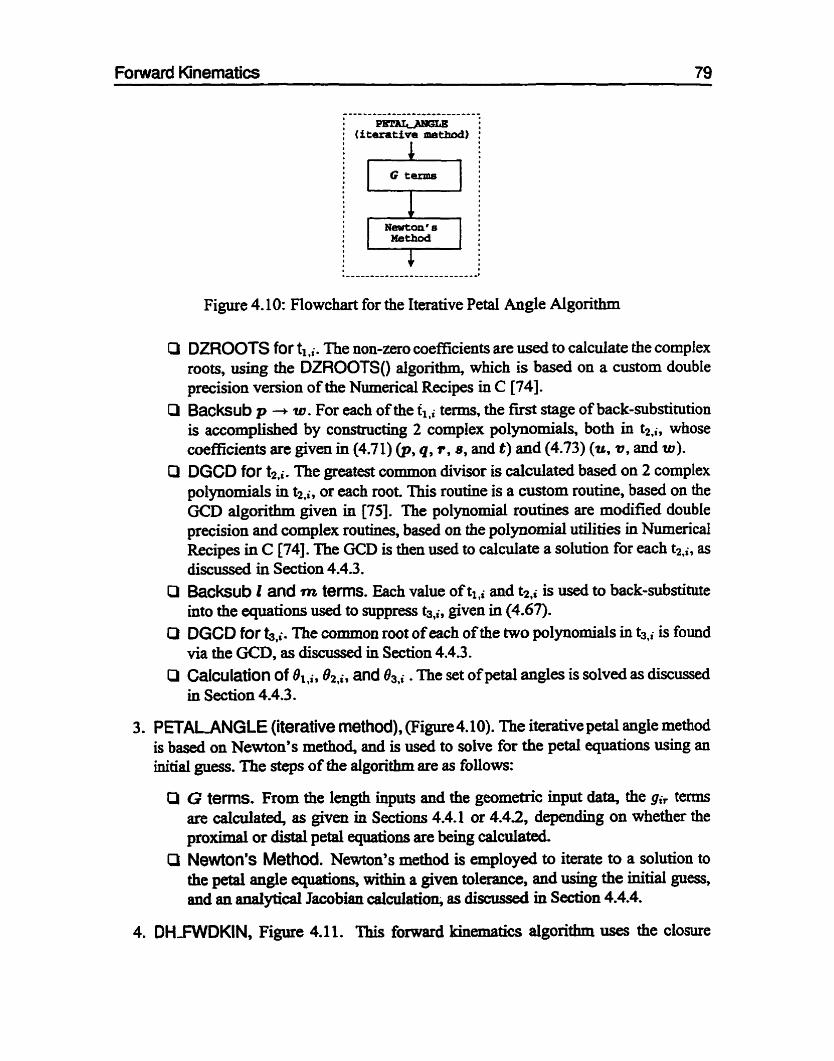
Forward Kinematics 79

Newton' e La Figure 4.10: Flowchart for the Iterative Petal Angle Algorithm

DZROOTS for ti,i. The non-zero coefficients are used to calcuiate the complex roots, using the DZROOTS() algoxithm, which is based on a custom double precision version of the Numerical Recipes in C [74]. Backsub p + W . For each of the fini terms, the first stage of back-substitution is accomplished by constructing 2 complex polynomials, both in t2,;, whose coefficients are given in (4.71) @, q, T , s, and t ) and (4.73) (u, v , and ia). DGCD for tzPi. The greatest common divisor is calculated based on 2 complex polynomials in tz,i, or each rwt. This routine is a custom routine, based on the GCD algorithm given in [75]. The polynomial routines are modified double precision and complex routines, based on the polynomial utilities in Numerid Recipes in C [74]. The GCD is then used to calcuiate a solution for each tz,i, as discussed in Section 4.4.3. b c k ~ u b Z and rn ternis. Each value of tipi and t2,i is used to back-substitute into the equations used to suppress t3j, given in (4.67). DGCD for t,i. The cornmon mot of each of the two polynomials in is fomd via the ûCD, as discussed in Section 4.4.3. Calculation of and . The set of petal angies is solved as discussed in Section 4.4.3.

3. PETALANGLE (iterative method), (Figure 4.1 O). The iterative petal angle method is based on Newton's method, and is used to sulve for the petal equations using an initial guess. The steps of the algorithm are as follows:

P G terms. From the length inputs and the geometrk input data, the gi, terms are calculated, as givm in Sections 4.4.1 or 4.4.2, depending on whether the proximal or distal petal equatiom are being calcdated.

P Newton's Method. Newton's method is employed to iterate to a solution to the petal angle equations, within a given tolerance, and using the initial guess, and an d y t i c a l Jacobian caldation, as discussed in Section 4.4.4.

4. DHIWDKIN, Figure 4.11. This forward kinematics algorithm uses the closure

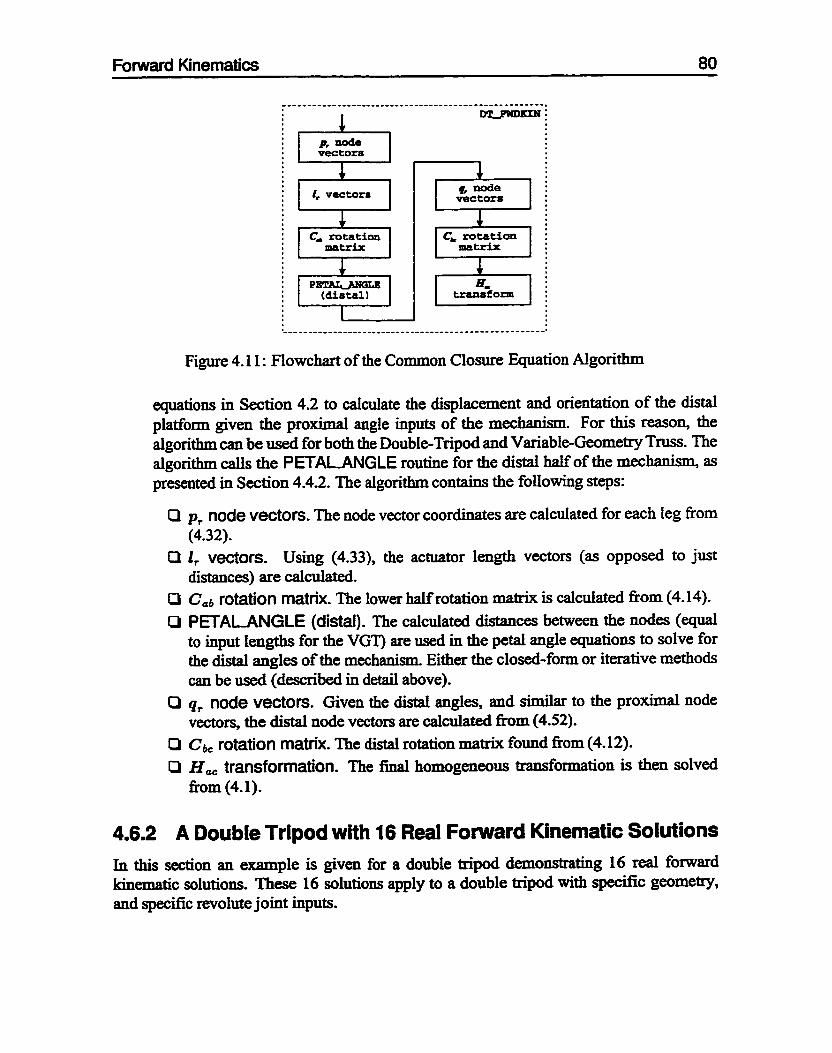
Unematic Inputs

The mode1 was chosen specincally so that it wiii admit 16 real solutions. The parameters where chosen such that the DT is general (class PSR = 000 in Figure 3.1): 1) the distal platform is non-planar (axes do not intersect), 2) the proximal and distal halves of the mechanisn are not symrnetric (reflective) about the midplane, 3) the kinematic chains have irreguiar geometry.

The angular inputs to the kincx.natic mode1 where as follows:

011 = 85 deg = 85 deg

013 = 85 deg

The link parameters for the manipulator are given in Table 4.3. Part (a) of the table indicates which of the available DH parameters were used for the legs, and part (b) of Table 4.3 indicates what the specific parameters were for the base platfonn, distal platform, and legs.

As shown in Table 4.3(a), the legs of the manipulator in this example are modeied with DH twist parameters set to 90 degrees in links 1, 2, 3, and 4 for each leg, given by alr = a 2 + = CL^^ = alr = 90. Because of these specific choices for twist angles, the offset parameter in link 1 is zero (dlr = O), and the length parameter for link 4 is zero as well (a4r = O). With these assumptions, each leg cm be modeled with 2 DH parameters: 1) link 1 length al,, and 2) link 4 offset dl,.

These link parameters, as well as specific platform geometry Uifonnation that is used in the example mechanism, are provided in detail in part @) of Table 4.3. These parameters were defined in the previous Chapter (Kinematic Models), Section 3.3. Note: angies in Table 4.3 are in degrees.

The kinematic parameters, together with the angular inputs, give the mechanian the following notable characteristics:

The proximal platfonn is plma-, due to the consistent zero z dimension in b,,, and coplanar axes vectors, due to the consistent yaw sethg in fi,.

a The distal platform is non-plmua, due to the varying z dimension 4,. Zero petal angles configuration occur in the proximal platform when each of the arms lay "flat", and the spherical joints are in the same plane as the platform2. The direction of rotation is defhed so that arms will "rise" for positive angular displacement, as indicated by Br.

'This a- âuc to the definition of both the G* (given from the platfonn pmmctm and Pr), and the 21, axiS locaitd at the spherical joint. Accoding to DH convention, the zero angle for the ith Iink is denned when the and Si axis art paralltl.

1 Length 1 Offset 1 Twist 1 al d4r 90

5, (a) DH Parameter Assumptions

1 . - - , 1 1

d4r 1 0.8600 1 0.8500 1 0.8400 1 (b) Platform and DH Parameters

panuneter

Table 4.3: Kinematic Parametem for the Rational Double Tripod: (a) Denavit-Hartenberg Variables used in an rth k g , (b) Platfonn and Leg Parameters for the Rational Double Tripod

a The distal platform's zero angle configuration aiso occurs when each of the arms is outstretched. The direction of rotation is defined such that the distal anns will "drop" for positive angular displacement, as indicated by r), .

Kinematic Chain

0 A . Sm (third aaxis of the proximal platfonn) and ZS3 (third z-axis of the distal platfom) are defineci parailel to I axes of their respective proximal and distai reference fiames, Fa and Fc.

'

The mechanisn possesses unequol leg iengfhs, as indicated by al, and 4,. 0 The mechanism can be classifie& accordhg to the taxonomy introduced in Sec-

tion 3.1, as a general double tripod, since its it possesses an non-planar platfonn, its geomttry is ireguIar7 and its geometry arymmehic with respect its midplane through the spherical joints.

2

-0.2500 0.1443

0.2500 0.1443

I brz

Forward Wnematics Solution

3 0.0000 -0.2887 b,

The z; coefficients for i = 16..0 that resuIt for the given input geometry are shown in Table 4.4. The resulting 16 solutions for BSr are given in Table 4.5.

In order to graphicaily represent each solution, an output file was created of pertinent geometry data The data was then 4 by an AutoCAD routine (programmeci in Auto-Lisp). which created a solid mode1 representation for each asscmbly. These assemblies, grouped

bru

-- - -

I XII I -7715.61 II ~ r , 1 -73995.70 I

1 Coefficient Zr6

1 1 5

slrl

513

112

Table 4.4: Polynomial Coefficients for Double Tnpod Example

Table 4.5: 1 6 Real Petal Angle Sorted with Respect to 851

Vahie 1 5.84

- 18.54 -230.72 617.24

3492.30

in fours, are presented in the following figures:

Figure 4.12 + Solution Roots 1,2,3, and 4.

Figure 4.1 3 + Solution Roots 5,6,7, and 8.

Figure 4-14 + Solution Roots 9,10,11, and 12.

Figure 4.15 Solution Rwts 13,14, 15, and 16.

Each figure contains the petal angle solutions, as well as the respective homogeneous transformation II, for that partidar cese.

Coefficient 1 Value 2 7

5 s

X4

23

- 128291.36 -171061.91 163063.73 159509.27 -91314.69

Solution

Solution 2: 6 5 =

Solution 3: =

Figure 4.12: Double Tripod Solutions 1 Through 4

Solution

0.9961 -0.0060 0 .O880

O

Solution 6: =

Solution 7:

-72.39 8, = [ 151.851

-101.26

0.4872 0.8383 0.2447 -0.4649 0.8348 -0.5293 0.1515 -0.2567

= [ U t 6 6 0.1:05 -0.r77 1 1.3FI 1 Figure 4.13: Double Tripod Solutions 5 Through 8

Solution

O .3228 0.8114

-0.4873 O

Hoc =

Solution

108.8 1 Solution 12: =

Figure 4.14: Double Tripod Solutions 9 Through 12

Hoc

Solution 14: O5 =

Solution 16: =

Figure 4.15: Double Tnpod Solutions 13 Though 16

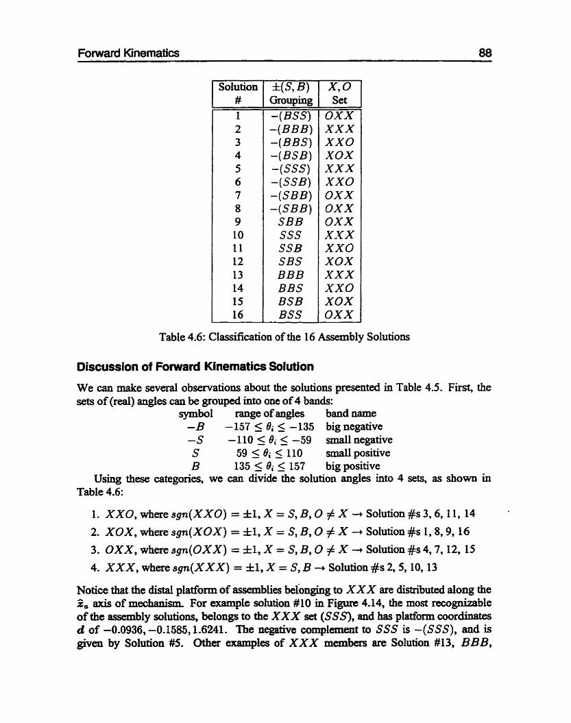
Forward Kinematics 88

Solution CI r f (S, B) Grouping -(BSS) -(BBB) -(BBS) - (BSB) -(SSS) -(SSB) - (SBB) - (SBB) SBB SSS SSB SBS BBB BBS BSB BSS

x, 0 Set

OXX XXX XXO XOX XXX XXO OXX OXX O X X xxx XXO XOX XXX X X O XOX O X X

Table 4.6: Classification of the 16 Assembly Solutions

Discussion of Forward Kinematics Solution

We can make several obsenrations about the solutions presented in Table 4.5. First, the sets of (real) angies can be grouped into one of 4 bands:

symbol range of angles band name -B -157S&<-135 bignegative -S -110 5 Bi 5 -59 d negative S 59 5 Bi 5 110 snall positive B 135 5 8; 5 157 big positive

Using these categories, we can divide the solution angles into 4 sets, as shown in Table 4.6:

1. XXO, wheresgn(XX0) = f 1, X = S,B, O # X -, Solution#s 3,6,11, 14

2. XOX, wheresgn(X0X) = f 1, X = S, B, O # X -, Solution#s 1,8,9,16

3. OXX, where s g n ( 0 X X ) = f 1, X = S, B, O # X -r Solution #s 4,7, 12, 15

4. XXX, where sgn(XXX) = f 1, X = S, B + Solution #s 2,5,10,13

Notice that the distal platfonn of assemblies belonging to XXX are distributed dong the 2. axis of mechaniau For example solution #10 in Figure 4.14, the most recognizable of the assembly solutions, belongs to the XXX set (SSS), and has platform coordinates d of -0.0936, -0.1585,1.6241. The negative cornplexnent to SSS is -(SSS), and is given by Solution #5. Other examples of XXX members are Solution #13, BB B,

Forward Kinematics 89

Sphere 2

Figure 4.16: Assernbly Conditions for the Double Tripod Example

whose platfonn coordinates are d = col{-0.0711, -0.1018,1.3332}, and its negative complement: - ( B B B), Solution #2.

The members of other X, O sets are distributed vertical planes, rather than the 4, axis. For example the members of the X X O are distributed in the neighborhood the @, 2, plane, with each of their platform dz coordinates close to zero. Likewise the X O X solutions are distributed along a vertical plane -120 degrees (about 5.) nom the gai, plane, and the OXX solutions are distributeci dong a similar vertical plane + 120 degrees fiom the gaza plane.

The reason for this distribution of assembly solutions is clear when we examine the assembly conditions of the upper pladorm. If we discomect the revolute joints fiom the upper platfonn, the farnily of points they could occupy are descrîbed by 3 spheres of radius ddr, each centered on spherical joint points Pr, since the r-th distal link would be allowed to spin and rotate fieely about Pr. Thest spheres are depicted and labeled in Figure 4.16, superimposeci upon assembly solution #IO. The assembly conditions of the mechanian are satisfied when each revolute axis is tangent to its respective sphere at the revolute joint location constrained by the distal platform. 'Lhis "simultaneous tangency" condition can be seen inFigure4.16.

Now if d but one of the revolute joints are comected, we can visuahze that the distal platform will be allowed to rotate in a close-to-circular faShion, all the while satismg a twin tangency condition, dong a path descri'bed by the intersection of two spheres. This gives a visualization of why the XXO set, for example, occupies the neighborhood of the.% 2. plane: the intersection of sphere 1 and sphere 2 in Figure 4.16 is parallel to the 9,s. plane. Similady, the XOX and O X X sets are distributed along the intersections of spheres 1 and 3, and spheres 2 and 3, respectively.

4.6.3 A VGT with 64 Fomrard Kinematic Solutions From the previous example, we know that the maximum numba of real solutions for the petai angle equations is 16. It follows, therefore, that the maximum number of unique assemblies for the VGT is 16* = 256. In this example, a case is danonstrated where the petal solutions have a mixture of real and complex solutions, for each the proximal and distai halves of the mechanism, giving rise to 8 real solutions for each petal system, with a totd of B2 = 64 real solutions.

The example provided here is similar to the numerical example provided by the author in [Ml, in that that the petal angle geometnes and r d solutions are eqyivdent-

Kinematic lnputs

The generai geometrïc characteristics of the kinematic parameters for this example:

a planar platform geometry

regular geometry

O asymmetric geometry with respect to midplane, (i.e. the mechanism possesses tapered geometry

Similar DH assumptions are made for the VGT exampIe as previously (see Table 4.3(a)). The specific geometric parameters are given in Table 4.7.

The prismatic joint inputs for the VGT are as follows:

Forward Kinernatics 91

Table 4.7: Kinematic Parameters for the VGT Numerid Example

parameter Kinematic Chain

b, 0.1875 0.1083 0.0000

bTz bw b,,

2 -0.1875 0.1083 0.0000

3 0.0000 -0.2165 0.0000

Forward fûnematics 92

Table 4.8: Distal Polynomial Coefficients for the VGT Example

Coefficient 516

215

514

x13 x12

2 1 1

XIO

59

28

Forward Kinematics Solution

The xi coefficients for i = 16 ... 0 that result for the given input geomew are shown in Table 4.8. The resulting 16 solutions for each BI, and dSr are given in Table 4.8.

Only a subset 4 solutions of the 64 are shown graphidy. The four plotted solutions are given in Figure 4.17, and possess the following combinations of soluti011~:

1. Proximal Solution #14, Distai Solution #12 Solution (14: 12)

Value 1 0.0000

- 19407.3447 0.000~

14065-2618 0.0000

-1795.5913 0.0000 53 .9286

Value 1 O. 1076 0.0000

-9.1414 0.0000

23 1.5025 0.0000

7037.1615 0-0000

2. Proximal Solution #14, Distal Solution #4 * Solution (l4:4)

Coefficient 2 7

56

X S

3 4

t 3

22

XI

50

3. Proximal Solution #2, Distal Solution #12 + Solution (2: 12)

-36360.6582

4. Proximal Solution #3, Distal Solution #12 + Solution (3: 12)

&.

Discussion of Solution

We note the odd-numbered polynomial coefficients in Table 4.8 are zero, such that (4.76) can be written as

8

C xlitlai = O (4.9 1) i=O

which confirms the resuit obtained in [64]. This structure of the polynomial causes sets of nflected solutions, as shown in Table 4.9, for both the real and i m a m casa.

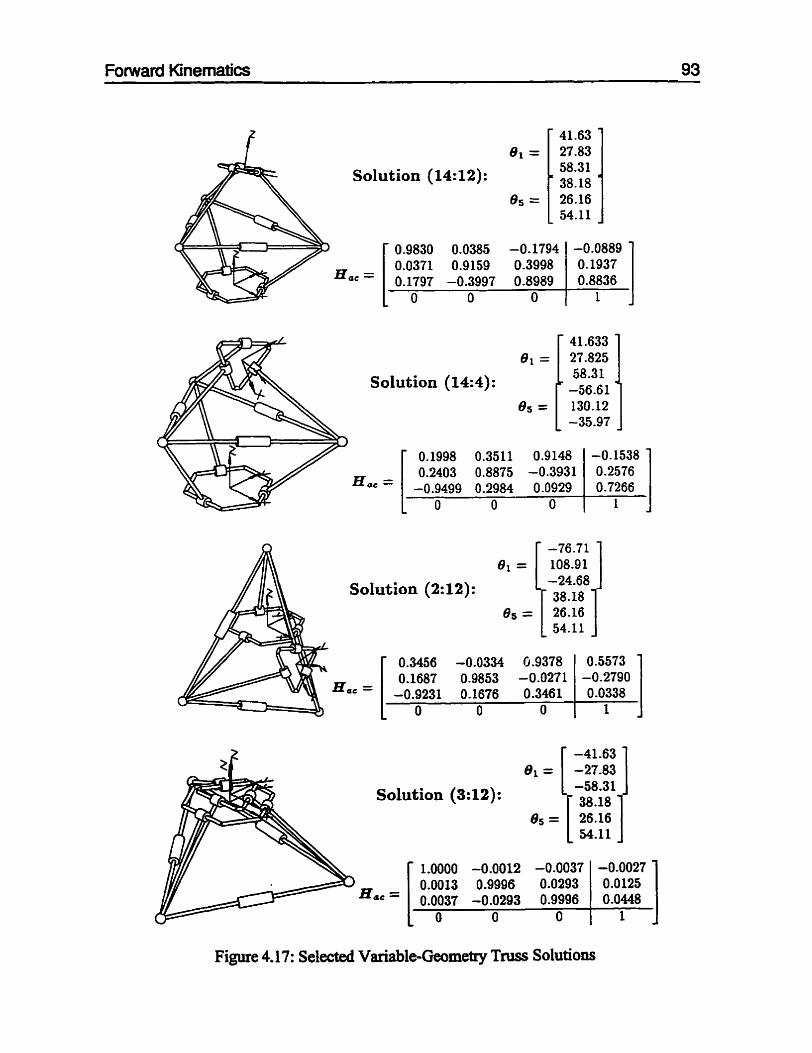
Sol

Hoc =

Solution (2:

Sol

Hoc =

Figure 4.17: Selected Variable-Geometry TM Solutions

Solution #

1 2 3 4 5 6 7 8 9 10 11 12 13 14 15 16

Soiution #

1 2 3 4 5 6 7 8 9 10 11 12 13 14 15 16

Forward Kinematic Sotutions to the Proximal Petal Equations

( 76.706, 0.000) (-108.9 13, 0.000) ( 24.680, 0.000) ( 107.556, 0.000) ( -83.429, 0.000) ( -4.2 10, 0.000)

Forward Kinematic Solutions to the Distal Petai E ~ ~ t i o n s

Table 4.9: Petai Angle Solutions for the VGT Example

Chapter 5

Inverse Kinematics

We state the inverse kinematics problem as solving for the independent joint vanables given the position of an arbitrary point on the distal platfonn. The joint variables are defined as either the angle of revolute joints adjacent to the proximal platform, in the case of the double tripod

81 = f ~ K , D T ( ~ )

or the Iengths of the prisnatic joints, in the case of the variable-geometry tniss

The end-effector vector coordinates, expressed in the reference fnune Fa of the (fmed) prox- imal platfoxm, are given by e, while 8, denotes the revolute joint angles, col{Bi *, 0i2, &J}, and 1 denotes the prismatic joint dispIacement v~ables . col{ll, 12, h } .

5.1 Ovewiew It is evident h m the stated inverse kinematics problems in (5.1) and (5.2) that we are only interested in solving the joint variables of the mechanisn for a three-dimensional displacement input. The orientation of the distal pladorm does not enter into this problem, but rather is dependent on the position of the platfonn, as was s h o w in the forward kinematics in the previous chapter. Although the mechanism is spatial, and has both positioning and orientation capabilities, ody three W F can be independently controlled Analyzes such as the "gimbal problem" [76], where combinations of one or more orientations are substituted for the positionhg DOF, do contain merit, but are of Little practical interest if the mechanisxn is to be used as a positioning device.

Out seemingly ahitrary choice of the independent variabIe e is centered on the fact that the DT and VGT are weil suited for gross positioning tasks, much Wre a more conventional R-R-R mechanilzm comrnonly used for positioning in articulated robot manipulators. Here as weU, the orientation of the mechanhm is not controlled, but is dependent on the controlled position of the device.

Inverse Kinematics 96

For tasks with higher degrees-of-freeciom repuirements, it is proposed that an orientation mechanian (wrist) can be added in series with the DT or VGT mechanism, giving the new device hybnd characteristics. The wrist couid comprise either serial or parallel elements. In such a case, the inverse kinematics algorithms given in (5.1) and (5.2) provide adequate scope for solWig the inverse kinematics of the hybrid mechanism, especidly if the wrist allows the position and orientation problems to be decouplecl (which is the case for the majonty of robot wrists used in industrial settings).

Two solutions are presented to the inverse kinematics problem for the "general" mechanisms, both of which resort to numerical methods The iterative solution is used because a closed-form solution is not readily avdable.

For both methods, the nonlinear equatiom for the inverse kinematics derive fiom a set of closure equations for the manipulator. Once the foregoing nonlinear relationships are established, iterative techniques can be employed for obtaining a solution using the Newton-Raphson method. With a first order truncation of Taylor's senes expansion about an initial position, the Jacobian matrix of the system can be i o v d and used to iterate to the unlaiowns within a r-ed accuracy. The Jacobian mat& cm be calculated fkom either an analytical expression, or a numerical approximation if the analytical form is not readily available.

Two distinct methods of establishing nonlinear system of equations are presented next, namely : the " fornard displacement" and ' ' cIosure equation" methods:

Forward Displacement Method. This method uses the forward kinematics algorithm directly to formulate a system of equations with 3 equations and 3 unlmowns, for which the Jacobian is estirnated numerically.

Closure Equation Method. This iterative method is based on the closure equations of the mec* The orientation of the distd platform is represented by a parameter set of iInknown angular displaceznents, dong with the iinknown petal angles of the closure equations. The resuiting system has 9 equations and 9 unknowm, for which the analytical Jacobian can be computed

For the special case of symmetric geometry, however, a closed-form solution is presented to the inverse kinematics problems. This closed form, symmetric solution applies to b t h the VGT and DT.

5.2 Forward Displacement Method The endeffector position e is expressed as a fuoction of the input variables 6,. This forward kinematic fiinction is taken (4.13), when combined with (4.1) in (4.5) gives the following vector hction:

e = ~ I ( f l 1 1 ) - Cac(81) - t ) (5-3)

Note that p,(Bll) arises nom the node eqyation in (4.32) for r = 1 (dependent ody on 41 mther than 81). Now ql (B1) functionality in ( 5 3 ) can be shown from (4.52), since

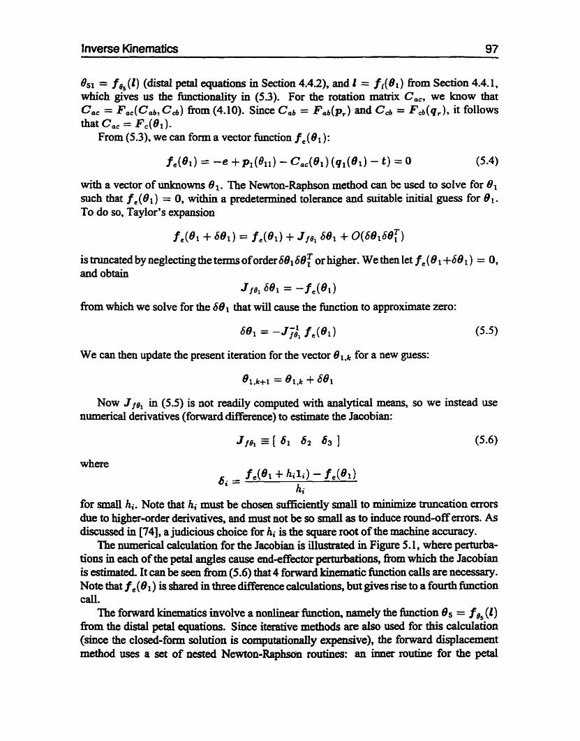
inverse Kinematics 97

es, = f (1) (distal petal equations in Section 4.44, and 1 = f , (B I ) from Section 4.4.1, which gives us the bctionality in (5.3). For the rotation matrk Ca,, we know that Ca, = F.,(C.b, Cd) fkom (4.10). Since Cab = F.b(p,) and C d = Fd(q,) , it follows that Ca, = Fc(B1).

From (5.3), we can form a vector function f, (8 1 ) :

with a vector of unknowns e l . The Newton-Raphson method can be used to solve for 81 such that f , (81 ) = O, withh a predetermined tolemce and suitable initial guess for 0 1 .

To do so, Taylor's expansion

is truncated by neglecting the ternis of order 6e1 68; or higher. We then let f, (0 1 +68 1 ) = 0, and obtain

Jre, 691 = -f,(01)

fkom which we solve for the 681 that wiil cause the fùnction to approximate zero:

We can then update the present iteration for the vector 81,k for a new gum:

Now JIBl in (5.5) is not readily computed with analytical means, so we instead use n u d c a l derivatives (forward difference) to estimate the Jacobian:

where 6; = f .(el + hili) - f ,(BI)

hi for snall hi. Note that hi must be chosai suniciently small to trunation due to higher-order derivatives7 and must not be so small as to induce roundsff mors. AS discussed in [74], a judicious choice for hi is the square root of the machine accuracy.

The numerid calculation for the Jacobian is illustrateci in Figure 5.1, where perturba- tions in each of the petal angles cause end-effector perturbations, from which the Jacobian is estimated. It caa be seen fiom (5.6) that 4 forward kinematic fiinction calls are necessaiy. Note that f ,(O1) is shared in three difference dcuIations7 but gives rise to a fourth hction call.

The forward kinematics involve a nonlinear fhction, namely the hction B5 = f ( l ) from the distal petd equations. Since itexaîive methods are also used for this calculation (since the closed-form solution is computationally expensive), the forward displacement method uses a set of nested Newton-Raphson routines: an inner routine for the petai

Inverse Kinernatics 98

Figure 5.1 : Forward Displacement Method. A perturbation of hi in each input angle cause respective 6 ia displacement, which are then used to estimate the Jacobian for the system.

equaûom solving for given the input actuator lengths 1, and an outer routine as descn'bed above.

For an initiai guess, it is effective to assign the to an average value throughout the expected range of motion. The method works well in practice for the folIowing reasons:

The end-effector displacement can be solved reliably for areas in the workspace away f b n a singularity. Even with this Limitation, the algorithm is useful, since sinpuiarities are avoided in practice.

The forward kinematics petal equations can be solved quickly and reliably, since 0s angle ciifferences are d. O h one iteration for each forward kinematics solution is all that is necessary for the inna iteration Ioop.

The method is well suited for imbedded applications, since it possesses low memory (especially code executable size) requirements due to "recycling" of forward kinematics code.

Closure Equation Method For the closure equation method, we chwse to express (5.3) in temis of more âirect udmowns. To do so, we first defme Ca, as a fiinction of a set of iInknom angular displacements We wilI employ the 3-24 Euler set of angular displacements 91, <pz and

Inverse Kinematics 99

Figure 5.2: Closure Equation Method. A Set of Three Equatioos are Fomulated For Each of the r Closures in the Mechanism.

where Wpi = COS <pi and Spi = sin pi. Furthemore, as shom in Figure 5 2 , we express p, and q, as fiuictions of el, and Os,, respectively. W e a n therefore write the closure equation in (4.13) for each leg:

for r = { 1,2,3}, where (p = col{<pl, ch, p3). R d that the functionali~ @en by the n d e vectors pr(Olr) is declared in (4.32), while q,(&,) is given in (4.52). we cari

formulate the following vector of 9 unltnowns:

We c m obtain 9 scalar etpatioas by evaluating (5.8) for each closure eqyation r = {1,2,3}. Subtracting the rhs of (5.8) nom both sides of the equation gives us the following vector valued function

f = col{f 13 f 23 f 3) (5.10)

Inverse Kinematics 100 -

Again, with the Newton-Raphson method, we soive numericaiiy for r such that f ( x ) = 0, with a predetermined tolerance and a suitable initial guess. We use a truncation of the Taylor expansion to solve for the iteration in x that wili d t in f ( x + 62) = 0:

a 8 = - JT; f ( x ) (5.12)

where the i, j component of Jr, is a f i / a x j . Now since the vector hct ion in (5.1 1) has relatively straightfomard functionality, the analytical computation of J I , is used in (5.12). The 9 x 9 Jacobian mtrix can be found analytidy as follows:

J I = [ Jpei Jqes Jc,<p I where

The partial derivatives for (5.14) are computed by differentiating (4.32) with respect to BI,:

apr -- ~ O I T

- (& sin al, COS 64, - al , sin BI,) SO, + (alr COS + d2r sin al, sin BI,) Ge (5- 17)

while similady for (5.15) the partial derivatives are calcuiated by differentiating (4.52) with respect to Os,:

Inverse KÏnematics 1 O1

The expressions in (5.16) for Jc,, are given as

where

The scalars rn,,, m,, and narx denote the coordinates of the vector mr = (q, - t) (refer to Figure 52).

5.4 Special Case: Symmetric Geometry For the general revolute-sphdcal-revolute mechanism, the solution of the inverse kinematic problem requins simultanwus solution of the orientation and position of the end-effector on the moving platform. For the symmetric mechanisn, the orientation and displacernent of the end-effector can be solved independently, which afCords a closed-form solution.

Assuming the points O and D are located at the centroid of each of their respective spatial trian&%, &etric geometry in the mechanism will cause lO&l = IDV& The midplane point & can therefore be expresseci as a fiinction ofmoving plaaormdisplacement O. From (4.24),

d vd = - (5.2 1)

2 Since point Vd on the midplane of the double tripod can be found, each of the node points Pr can be detennined using the perpendicuiar constraint below:

Moremer, using the position vector of point E of the end-effector (defined in (4.4)), we cm define a new vector u = f (e, t ) that is parallel to d. To do so, the following relation is used to express the components of the vector t in the base reference frame 7.:

Inverse Kinematics 1 02

t~ is the reflection of t expressed in Fa, and 3& is the reflection of Fc across the midplane of the mechanism. The ma& a, is known, because it is a property of the mechanism platforms. Thus, we can write

u = e - t ~ (5.25)

Vector u, as defined above, is orthogonal to the midplaoe of the mechanism and can be used in place of d (5.22):

T O = ( p , - U) u (5 -26)

Substitution of p, nom (4.32) into (5.26) leads to the following relationship for the rth Ieg:

where

The solution of (5.27) is given by

From (528) , it is evident that 8 solutions exist for the inverse kinematics of the double tripod-two for each of the three angles BI , OZ and 03.

Chapter 6

Design and Control

The design and control of practicd laboratory prototypes are discussed in this chapter. These prototypes were used to ver@ the kinematics algorithms developed in the previous chapters.

6.1 Ovewiew: Laboratory Prototypes

6.1.1 Clem-A Double-Tripod Manipulator CIem k afirst-of-ris-Rindproto fype of a doub le-tr@od for roboticapplicutions.

A double-tripod manipulator has been constructed at the University of Toronto Institute for Aerospace Studies. The 3-DOF Inanipdator, named CIem after Melville Clemeas [4q, was developed as a first-of-its-kind test-bed for the kin-tics and robotic applications of the doible-tri@ mechanism. Tht kinematics of Clem is unique in that it has a tapered geometry. The manipulator serves multiple purposes:

1. To v w the kinematics algorithms developed for the double tripod, specifically with revolute actuators and tapered geometry.

2. To ver@ the double tnpod as a viable component in industrial manipulators.

3. To ver@ ptacticai mechanical designs for double-tripods.

A block diagram depicting the system layout of Clem is shown in Figure 6.1. The system comprises the following elements:

1. Pmonal Computer. The PC contahed the RobComm user interface for the robot contro11a. as weli as kinematics and sen10 code development tooikit interface.

2. CS00 Controller. The CS0 controller is an industrial robot controiler mrinilfactured by CRS Robotics Corporation. It contains

(a) a high-level prognimming language named RAPL (Robot Application Ro- IPmming L~guage).

Design and Control 1 04

-Robcomm Interface -KinfServo TooUcit

C500 Controller

- W L -Motion Engine -Kinematics -Servo Control (up to 8 axes)

Figure 6.1 : System Diagram of Clem: A Double-Tripod Manipulator System

@) a Motion Engine which produces rd-time trajectories for the robot joints to follow based on RAPL inputs,

(c) a set of kinematics algorithms, which is embedded into a tramputer processor in the C500, and

(d) capability to control up to 8 motors simultaneously, although 3 where only used for Clem

3. Motor Power Amplifier. Electronics for 3 axes of motor current amplification, via pulse-width modulation (PWM) driving techniques.

4. Clem. A double-trîpod mechanism, placed in an "inverted configuration. The mechanian has asymmetric geometry (or tapered geometry).

As shown in Figure 6.2, Clem is a double-tripod mechankm in an inverted configuration, with the proximal platform (or fixeci base) held from above, and the distai (or moving platform) located below. The proximal platform contains mountbg provisions for three sets of geared motors. The geared motor possesses a DC motor, an optical encoder, and a spur gear drive train. The output of the geared motor &es up the shoulder joints of the double tripod, as depicted in Figure 6.2. Each a m of the mechankm contains a shoulder joint, proximal arm, sphericai elbow joint, distal arm, and a wrist joint. The distal (or moving) platform is placed at the common termination of the three amis, and possesses a m e for mounting an end-effector.

6.1.2 Trussarm-A Variable-Geometry-Truss Manipulato r A variable-geometry-tniss mmipuiator, named Tnissarm (Mark I) has been constructed at the University of Toronto Institute for Aerospace Studies. It was originalIy built in conjunctio11 with s e v d Mester's theses. Published theses include Gtocotî [77] and SaIlmen [78]. The mechrinism is a 3-DOF variable-geometry truss, possessing refected double- octahedron geometry. The system diagram is depicted in Figure 6.3. The manipulator serves several purposes:

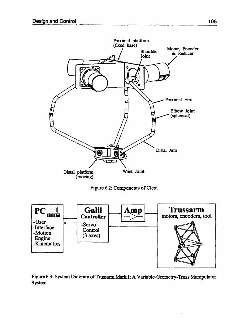
Desian and Control 105

Figure 6.2: Components of Clem

-User Interface -Motion 1 -Sem0

Control (3 axes)

Trussarm 1 motors, encoders, tool 1

Figure 6.3: System Diagram of Tnissami Mark 1: A Variable-Geometry-Tniss Manipuiator SY-

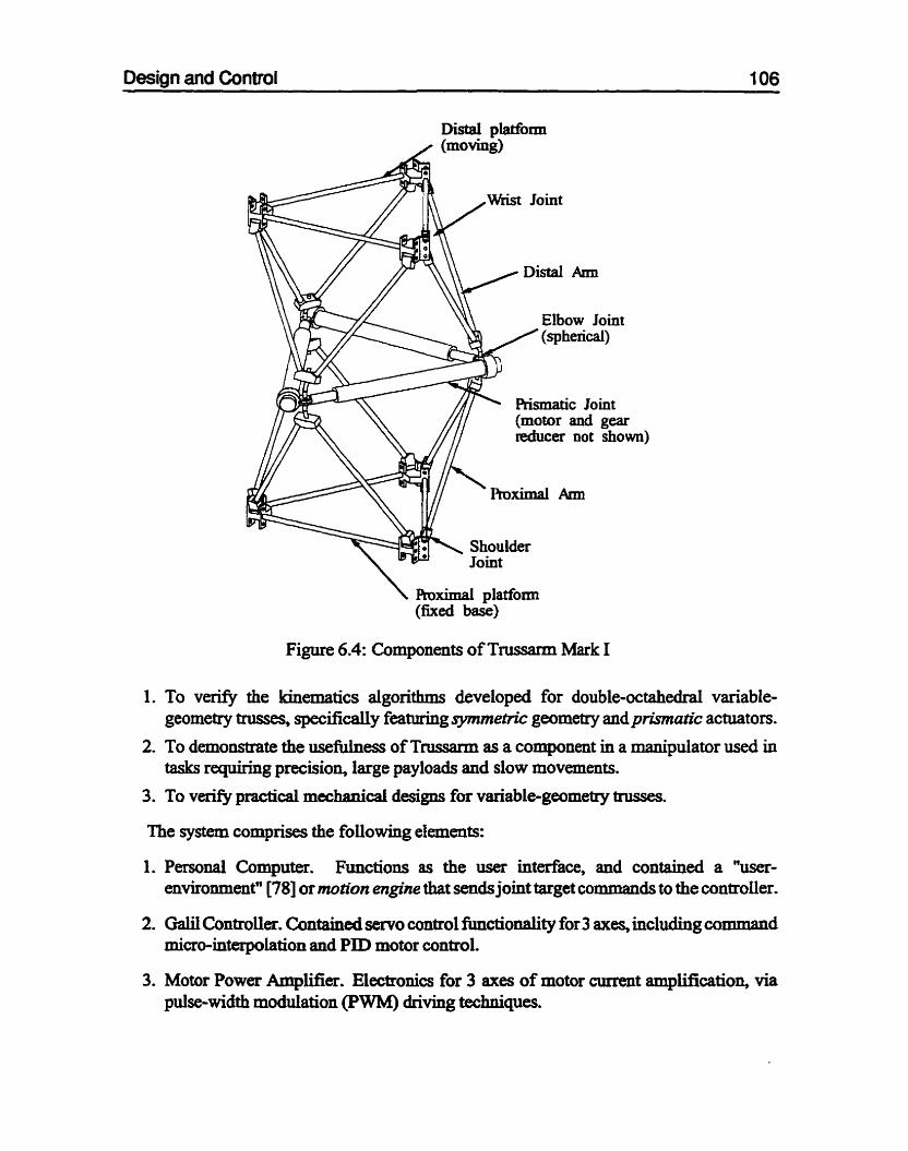
Design and Control 1 06

Rismatic Joint (motor and gear reducer not shown)

Figure 6.4: Components of Tnissami Mark I

1. To ver@ the kinematics algorithms developed for double-octahedral variable- geometry tnisses, specifxdy feanuing symmehic geometry and prismutic achüitors.

2. To demonstrate the usefbhess of Trussaxm as a component in a manipdator used in tasks requiring precision, large payloads and slow movements.

3. To v e pmcticai mechanid designs for variable-geomeîry trusses.

The system comprises the following elements:

1. Personal Cornputer. Functions as the user interface, and containeci a "user- environment" [78] or motion engine that sen& joint target CO-& to the controiier.

2. Galil Controller. Contained servo control functionaiity for 3 axes, including command micro-interpolation and PID motor mntrol.

3. Motor P o w a Amplifier. Electronics for 3 axes of motor current amplification, via pulse-width modulation (PWM) driving techniques.

Desisln and Controf 1 07

4. Trussarm Mark 1. The VGT manipulator structure contains 3 prismatic joints (linear actuators), and the associateci motors and gear reduccn.

The components of Trussann Mark 1 are shown in Figure 6.4. The manipulator is placed in an upright configuration, with the distai platfonn (moving platforni) facing up. Both the proximal and distal platfonns comprise ngid triangular tniss assemblies. The proximal and distal arms are rigid tniss assemblies as weU. The prismatic joints are made up of linear actuator components, which are offset fkom the "spherical" elbow joints. The q h k d joints are not ideal, but contain 4 degrees of fieedom, in order to facilitate the comection of the linear actuators. The prisnatic joints each comprise a DC motor, worm-gea. gear reducer, and reciprocating bali screw.

6.2 Design of a Double Tripod Manipulator

6.2.1 System Design System Design Goals

The design of the Clem system was approached with the following design goals:

1. The system should be designed to be a testbed for induistn'al maniplator applications of the double hipod manipulator, meaning, where possible system components should be chosen that are applicable and demonstrable for industrial applications.

2. The mechanid structure should possess tapered geometry so as to provide a test-bed for new kinematics algorithms.

3. The developmeht project of the prototype should focus on new technologies of double tnpod desigri mid kinematics, rather than robot programming environmen&, and user interface.

4. The system should be a cost-&ectiveproof of concept of the double tripod manipu- lator.

Based on these goals, an industrial robot conîroller was selected for the system design. Such a controuer would satisf4r the goal of king applicable to industrial manipulator applications. An indusfrial controllex also provided an existing user interface and robot programming environment, which allowed the development project to be focused on the core technoIogy developments: mechanism design and kinematics.

A robot programming environment hcludes a high-level programming language and red-tirne operathg system suitable for coorninated control of multi-DOF systems. The highest level gives the user the ability to provide robot motion commands (xeferred to as Elementary Move CO-& in [79]) in the form of interactive commsinds or a set of programS. These commands are input into a Motion Engine, which translates robot

Desian and Cantrol

O MOVE points angle 1 Motion Engiae

; "Kwt"p0intS / Servo Control Trajectory

time

Figure 6.5: A Variable-Geometry-Tm Manipulator with a Serial Wrist

motion coxnmands into real-time trajectories. Dependhg on the coordinate system of input commands and desired output motion, the Motion Engine has the capability to cal1 on either forward or inverse kinematics. The iowest fevel of controi is Servo Control, where the inputs are trajectories generated nom the Motion Engine. The function of Servo Control is to regdate the servo motors via closed-loop feedback control. These levels of control can be illustrateci in a trajectory plot of one axis (Figure 6.5). The highest level of cornman& are the MOVE commands, foilowed by a trajectory of Motion Engine "Knot" points, which then the Servo Control trajectory interpolates between for motor control inputs.

The altemative would be to use a PC-bas& controller, for example, a Galii controller as with the Tnissarm Mark 1 system. Although a PC-based controlier contains Senro Control fiinctiodity (provided either in a card or stand-alone controller), it does not provide either the hi&-level robot command environment and Motion Engine suitable for robot rnanipdators. Some of these controllers provide the capability to coordinate motion, but these are typ idy not tightly integrated with kinernatics a l g o r i h , and this fimctiondity must be developed wholly in the PC emironrnent. The PC-based controlla is the approach taken in the Tnissann Mark 1 system (=fer to Figure 63). For more information about the dems of the implementation of the Trussarm Motion Engine, refet to Sallmen's Master's thesis [78].

An industrial controllex therefore provides the following fhctionality in a tightly- integrated, d - t i m e enviro~ment:

P High-Level Robot Language and Programming Environment, P Motion Enpine O Sem0 Control

whereas a PC based controlier provides only Servo Control functionaliity. The Control Environment designed for T~ssarm Mark 1 contained a Motion Engine, but not a High-

Design and Control 1 09

Level Robot Programming Language. The Motion Engine was implemented on the PC controller, whereas the Servo Control was implmiented on the Galil Controller, show in Figure 6.3, with communication over a serial link.

One disadvantage of an industrial robot controiler is that they are typically difficult to interface with and use in a custom manipulator system, Several newer controllers, however, offer a more "open" architecture, which allow researchers a Limited amount of customisrsrtion, and are programmable in 'C'. Examples of these controllers are:

1. C500 Industrial Robot Controller from CRS Robotics Corporation. 1s a multi- processor 32-bit based controuer implemented with a network of tramputers- Developrnent software includes RobComm (standard Robot communication and user-interface for prognmiming), and the Transputer Development TooIkit, where the traasputer network can be both programrned for custom kinematics and servo code, as well as expanded to additional tramputer computational power.

2. Open Architecture Controller from Cimetrix Incorporated. These controllers are PC-architecture based, and are designed specificaily to be interfaced to various robots.

The CRS CS00 controiler was chosen because of availability (the Cimetrix controller was still under development at that time), and the close proximity of CRS Robotics (Burhgton, Ontario) to the University of Toronto. The C500 has the following interface specifications [80]:

O motion engine command update rate of 10 ms O servo control up&te rate of 1 ms O encoder update nite of 70 ps per axis

a Y 0 scanniiig update rate of 20 ms

0 it 1 O VDC motor amplifier control

12 bit motor command resolution

differential or single ended incremental aicoder feedback

The controuer hardware includes a set of Intel 80286180287 ploce~sofs, an Inmos 20 MHz T4ûû transputer (for servo control), and an Inmos 30 MHz T805 transputer (for kinematics). For expansion, there are 4 on-board Transputer Module (TRAM) sites avaiiable, as well as extenial TRAM net access. Controlier software includes ôoth imbedded RAPL-II progmmmhg language and mukitasking operating system, and PC based RobComm-II and the Transputa Development Tooikit.

6.2.2- Mechanical Design Robot Interface Requirements

Based on the ampliner and controller selection, the following interfie requhements were placed on the physical robot system:

Desian and Controi 110

O M= brush-type motors for the PWM ampiifiers

O différentid or single ended incremental enders

O switches (limit or proximity type) for calibration and homing of incranentai encoders

0 digital end-effector actuation

In order to facilitate industrial style pick-and-place taies, an inverted configuration was chosen for the manipulator. In order to minimize costs, off-the-sheif components were used when possible, ratha than nistorn b d t components. Since the mechanism was designeci to serve as a proof-of-concept manipuiator, there was no explicit design task and an associated required workspace. The only constraint on the mechanian design was that it: a) possess tapered geornetry, b) be inverted, and c) interfaces with the CS00 industrial robot controller.

The following methodology was employed in the mechanism design:

1. Actuator Selection

2. Kinematic Parameter Selection

3. Arm and Joint Design

4. Platform Design

Actuator Sefection

Given the interface criteria, a DC-brush type electric motor was chosen with optical enCoders. A motor was chosen that had 24 V input voltage, and was cment rated for around 5.0 Amps. A geared motor was chosen, because it was availabie directly h m a supplier. The motor had a 12.5-to-1 gear reduction, and a spaedltorque m e with envelope of 3 10 max rpm, and 2.37 Nm staU toque, as shown in Figure 6.6. n e encoder resolution for the motor is 100 counts per revolution.

Kinematic Parameter Selection

A simplified kinemafic mode1 was used to design the link-lengths of the prototype. The input angles were assumeci aqual, which &ts in a mode1 shown in Figure 6.7. From the figure, we let BI and B2 denote the proximal and distal platform kdii, and LI and Lz the proximal and distai arm lengrbs, respective1y. Asslrming that each of the input arms is at the same angle, we arrive at the foiiowing simplifieci geometric relationships:

d, = L 1 ~ i . 0 + L 2 ~ i n t f (62)

once simpl&ed geometric nlationships were identifid, design targets for relative mass distn'bution among the Links were used in order to choose both the payload and reach capability of the links. The mess distriiution was expressed relative to the m a s of the

Design and Control

Toque vs. Speed for Matsushita Geamtor 2.5 t 1 t t 1 n 1

Figure 6.6: Speedflorque Curve for Clern's revolute Actuators

spherical joint m, as shown in Figure 6.7. This mass distribution was then used to size the relative s k e of the components. Note that the m a s of the payload will be shared by each of the three a m , giving an effective mass of only m.

An additional simplification can be made by assuming that the mass of each link is distributed equally into two masses at each joint. If the same assumption is made for the moving platform, the d t i n g masses are mi = gm, and rnz = :m., at the elbow and wrist joints, nspectively. The resdting mass distribution is shown in Figure 6.8. Using this m a s distri'bution, the static torque requited to hold the leg can be calculated as a function of input angle, h m which the maximum angle can be solved. From Figure 6.8, the static torque required at the shodder joint can be expressed as the following function of the mgles 8 and C, normalized mass m, and the force in the distal a m f:

and = cos-' (& - 82; Li MS @

Desirrn and Control 112

sphericd joint

-- - -

Figure 6.7: Geometry Relationships and Target Masses Distribution for Clem (assuming each a m has the same input angle)

K -

Payload (including proximal plat£onn) ProximaI Ann Spherical Joint Distal A m

fkom (6.1). We cm define the torque of the manipulator as the product of characteristic Iength Lc and characteristic weight WC:

3 mc mc/3

MC

mc/2

where WC = md. We can obtain L. by factoring rnd from the (6.3). But firsf the foilowing ratios are defineci:

P l = mt/mc

r2 = m2/mc

which ailow us to factor WC fiom (6.31, giving us an expression for &(el C):

L&t) = &cos6 sin

Desi~n and Control 113

Figure 6.8: Simplifiai Mass Distribution for Clem

With this simplifieci torque analysis, the kinematic parameters of Clem were chosen. Since one of the overail goals of building Clem was to examine tapered geometry, the ratio of the proximal and distal platfom (otherwise known as the taper ratio) was set to

Arm lengths were chosen so the mmipulator wouid at least be collapsible, for equal acniator input angles. This relatioaship occurs when 0 is zero, and is expressed as

From the motor characteristics in Figure 6.6, the maximum stall torque of the motor is 2.37 Nm. To size the motor for contuiuous torque, we set the maximum static torque to a target of r = 0.706 Nm The relatively high peak/continuous torque ratio of 3.4 gives us good "headroom" for the following factors:

1. cases when the input angles are not equal, and one ami must support comparatively more torque

2. dynamic torque for acceleration and deceleration

Desi~n and Contfol 114

O 50 input angle [deg]

Figure 6.9: Chanrcteristic Lengths for Two Design Cases: 1) Onginal Design Case, 2) Acîuai Manufactured Case

Two design cases are shown in Figure 6.9: 1) the original design case, and 2) the achial manuf8CfUCed lengths of the ana The figure depicts the chanictenstic length of each case as fùnction of input angle. The maximum characteristic length can be used to calculate the maximum characteristic weight for a specific static design torque for the motors. For case 1, for example, the specific weight is WC = r / L , = 0.706 Nml0.494 mm = 1.13 N, and for case 2 the specifïc weight is WC = 0.706 Nm/0.403 mm = 1.75 N. These resuLtiag weight distribution for the each design case is Rd in the Table 6.1.

max L d m ) 493.8 403.1

A m and Joint Design

&(mm) 38.1 38.1

1. Use off-the-sheif components where possible, in order to mhhke manuf8ctUring costs.

L~(mm) 203.2 193.0

Design Case 1 2

BI (mm) 76.2 76.2

LI (mm) 152.4 131.6

Oesinn and Control 115

Table 6.1 : Weight Distribution for Two Design Cases of Clem

Design

2. Spherical joint with enough range of motion to allow Clem's input angles to V a r y from O to 90 degrees.

Weight Distnniton 0 Char. Weight ( PayIoad 1 Individual Arm 1 Total Manipulator

The mgie pitch joint is given by the following sum

assuming equal input angles for the rnanipulator. For angular 0 inputs of -30 and 90, the range of motion for design case I is 166.0 degrees, with a minimum of 3 2 degrees and a maximum of 169.2 degrees. Case 2 has a range of 160.6 degrees, with a minimum of 8.0 degrees a maximum of 168.6 degrees. The ranges of motion for both design cases are depicted in Figure 6.10.

In order to obtah adequate range of motion, an RRR set of revolute joints was chosen for the spherical joint. The revolute axes intersect at a conmion point. As with robotic spherîd wrist designs, the design choices vary, but can be grouped into two common styles of arrangements:

9 RuIl-piich-ru22 sphencai joint.

The roll-pitch-roil arrangment is shown in Figure 6.11(a). Reinholtz and his cokagues in [8 11 presented a design for a reflected-tri@ constant velocity couphg that featured a roll-pitch-yaw spherical joint.

The roll-pitch-roll joint contains a singularity for pitch angles O and 180 degrees, which can be avoided by a m layout. A good design range of motion is therefore 10 to 170 de-. For this reason, the joint cannot be used in situations where the links are aligned, and the mechsnism design must take this into accomt. One potential problan with using this joint is that with mgles of 170 de- typically cause the roll joints to interfere with each other, and t'us can reduce its operating range even fiirther. Another inconvenience with this joint is that it is not readily available as an osthe-shelf component, and must be fabricami fkom individual cornponents, thus inmasing the cost of its design.

0 Roll-pitciyaw sphericai joint.

The roll-pitch-yaw sphaicai joint layout in Figure 6.1 1@) is sirnilar to the roll-pitch- roll, except that the pitch joint is offset by 90 degrees. The singularity therefore

Desian and Controt 116

Spherical P i i Joint: Orsplacement vs. Input 180 1 I I I 1 I

160 -

140 -

120 - CI V1

g 100 - - 8 e, 4 80- (2) range = 160.6 deg - a

60 -

40- (1) range = 166 deg

20 -

O 1

-40 -20 O 20 40 60 80 1 O0 theta [degrees]

Figure 6.10: Spherical Pitch Joint Required Ranges of Motion

(a) roll-pitch-roll (b) roll-pitch-yaw

Figure 6.1 1: Sphencal Joint Arrangments:(a) RoU-Pitch-Roll, and (b) Roll-Pitch-Yaw

occurs at -90 and 90 degres, gMng a practical design range of motion nom -80 to 80 degrees. In order to incoqerate this joint into the design, a '%nt a m " design can be employed., when the linlcs are fabricated so that the joint is centered about zero pitch in the arm's mid-motion range.

The roll-pitch-yawjoint can be coIlStNcted using a modified U-joint as the pitch-yaw revolutes, which is a popular off-the-shelf machine component Not only does this simplify the tnanufacturing wsts, it also gives greater design flexibility. The

Desi~n and Control 117

components are readily avdable, corne in various sizes and styles (roller bearing or bushing bearing), and are relatively compact

6.2.3 Kinematic Modeling ui the prwious section, the mechanical design methodology used for the synthesis of Clem was presented. This methodology used a simplified kinematic and mass disfi'bution model in orda to choose the Link lm@ for the manipuiator. In this section, a detaiIed kinematic model is discussed, with which the resulthg design could be malyzed.

The general DH model presented in Chapter 3 was adopted for the kinematic andysis of Clem. The parameters of the geornetric model reflect the fact that Clem is both plana and regdar. (The classification of Clem, therefore, according to the taxonomy presented in Section 3.1 is planar, regular, with PSR = 101.) In situations where the DH method was not specific to frame placement ("base" and "distalm h e s , for example), the following criteria were used:

1. The "petal angles," or angles of the revolute joints adjacent to the proximal and distal platfom, should be measured with respect to their respective planes. Petai angles of zero should locate the spherical joints in the respective plane of the proximal and distal plat$orrns.

2. Positive rotation of the petal angles (in the range O to 90 degrexs) should cause increasing distance between the proximal and distal platfonns.

With these criteria, the kinematics could be easily visuahd Furthemore, the angle meaSUTernents were simüar to kinematic models presented elsewhere in the literature, both by earlier researchers [43,63] and the author [64,47].

The DH panmeters used for Clem are both depicted and summarized in tabuiar formats in Figure 6.12. The figure depicts one of the three kinematic chains for Clem, with each of the Bn angles equal to zero. The familiar DH table inset into Figure 6.12 contains the physical parameters in millimetem. To differentiate between those parameters not included in the general DH model, and those parameters included but specifically set to zero, the parameters not included in the general model are denoted with an x , while the zero length and offset parameters that are a part of the kinematic model are shown as 0.000.

The DH parameters for the kinematic chah can best be undersfood when the fiame placement on the proximal and distai platforms are presented, since the fnune placement on these platfoms influence the DH parameters for each arxn, and vise versa Figure 6.13 depicts proximal pla.tform (wmmon link O), together with tabulated data of the displacemmt parmeters and yaw-pitch-roll panmeten for each kinamtic ch& AIthough the data is given for each kinematic chain, only one reference âame is depicted. The displacement parameters and yaw-pitch-roll parameters are givm in an inset table. Likewise, the corresponding parmeters for the disÉal platform (wmmon link 5) are show11 in Figure 6.14.

From DH parameters in Figure 6.12, the foiiowing points are aiso noteworthy:

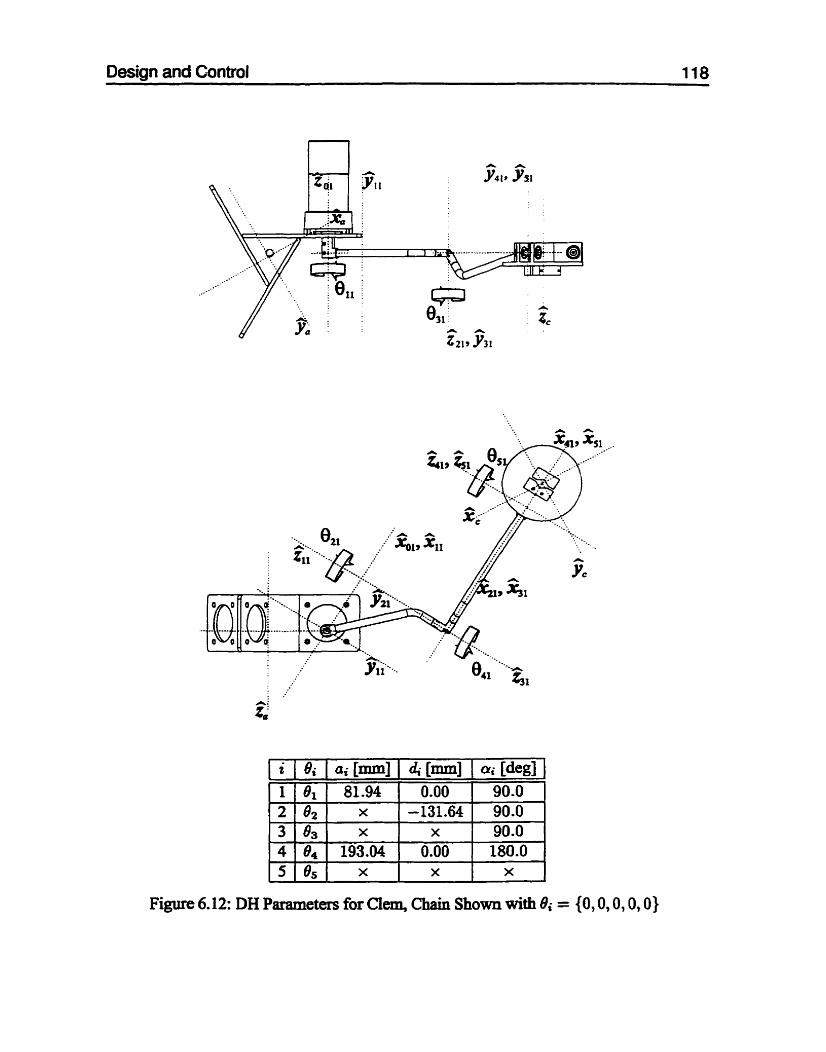
Design and Control 118

Figure 6.12: DH Parameters for Cl- Cham Shown with Bi = {O, 0,0,0,0)

Design and Control 119

Figure 6.13: Frame Placements for Link O: Proximal Platform (ody first ami's fiame shown)

Desian and Controf 120

Figure 6.14: Frame Piacement for Link 5: Distal Platform (only first am's frstmes shom)

0 The offset of both link 1 and link 4 are zero.

4 The distance fkom the finit revolute joint to the spherical joint is made up of two perpendicular components al and d2, and is given by = 155.07 mm.

0 The "bend anangle" joint 2 forms on the end of link 1 is &ai as ab = tan -' (01 /d2) = 31.9.

The fiame placement for each link of the arms is depicted in the remaining following figures:

1. Figure6.15: proximalarm(link 1)

2. Figure 6.16: U-joint yoke ( M c 2)

Desisin and Control 121

Figure 6.1 5: Frame Placement for Link 1 : Proximal Arm

Figure 6.16: Frame Placement for Link 2: U-Joint Yoke

3. Figure 6.17: U-joint centex block (link 3)

4. Figure6.18: distalann(Link4)

Figure 6.19 depicts the kiaematic chah in a more "naRiral" position, with the mgies of each joint set to 45,90, -90, -63, and 40 de- for joints 1-5, respectively.

Desicln and Control 1 22

Figure 6.17: Fnune Placement for Link 3: U-Joint Center

Figure 6.18: Fnune Placement for Link 4: DisFal Ami

6.2.4 Workspace Analysis The reachable workspace of a 3-DOF nmipulator is dcfined as the set of Cartesian locations, givem a range of input angles, that is reachable by the device. For Clem, this 3 dimensional workspace can be v h a k d by viewing the lines and surf'' traced by the end-&&%or. FÎrst the workspace "cube" is traced. The cube is defined as the set of points the mruiipulator can reach when any two of the joints are at their limits. The workspace cube for Clem with joint limits of O and 90 degrees is shown in Figure 6.20. The plot is essentially a line trajectory that the end-effector traces in space, one joint at a tirne,

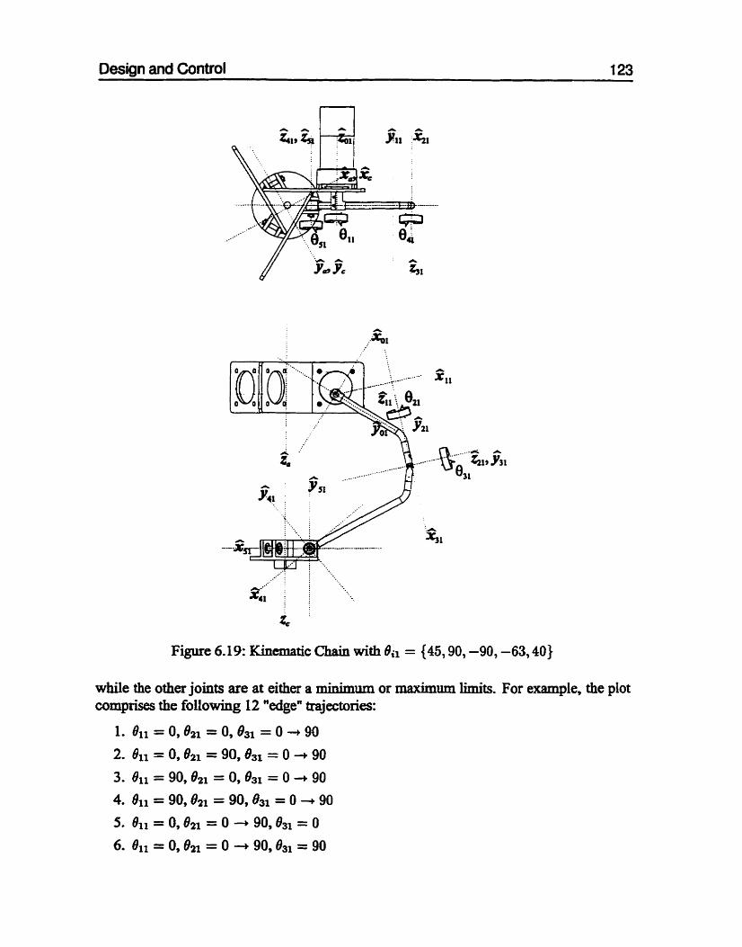
Design and Control 1 23

Figure 6.19: Kinematic Chain with 0, = {45,90, -90, -63,40}

while the other joints are at either a minimum or maximum lùnits. For example, the plot comprises the foilowing 12 "edge" trajectories:

Design and Control 1 24

Workspace Cube for Clern

-500 300 0 200 300

i O0 200 O 1 O0

-100 O -1 O0 -200 -200

y direction [mm] x direction [mm]

Figure 620: Workspace Cube Visualization for Clem

The plot in Figure 6.20 depicts the shape of the workpace edge limits in 3-dimensions, as weli as projections of these trajectories onto the three orthogonal planes. Note that the workspace forms a warped cube, with 12 edges, and 6 faces. The intersection of the three proximal, or upper, &ces forms an apex on the centerline of the mechanisa The intersection of the three di& faces forms motfier apex on the centerline of the mechanisn.

The second mettiod for workspace visualization is to examine the shape of the workspace S U r f h x s . The workspace surface is defined as the set of points that the end-effector reaches whai at least one joint variable is at a k t . For visualization purposes, the worwace is

Design and Control 1 25

Proximal Workçpace Boundary for Clem

x axis [mm] y axis [mm]

Figure 6.21: Proximal Workspace

viewed in two halves: 1) the 3 proximal workspace d a c e s from the top, and 2 ) the 3 distal workspace d a c e s fiom the bottom. These d a c e s are shown in Figures 6.21 and 6.22. Note that the proximal workspace d a c e s are concave, while the distal workspace surfaces are convex.

In addition to workspace visualization, the volume of the workspace was dculated using finite tetrehedron element d y s k

where the volume of the 2-th tetrehdron element is:

where At is the teûahedron base area and h is the height of the tetrehedron. The workspace volume of Clem, using the joint limits of O and 90 degrees, is 6633 cm3.

Design and Control 1 26

Distaî WoMpace Boundary for Clem

x axis [mm] 1 O0 y axis [mm]

Figure 622: Diseal Workspace

6.3 Control of a Double Tripod Manipulator

6.3.1 Klnematic Algorithms An Overview of the Kinematics interface

The foilowing custom kinematics routines where implemented on the C500:

O user~ointto-worfd( joint, world ). This is the forward kinematics algorithm, which converts an input anay of joint coordinates (joint) to an output Cartesian coorninates (~orld), expressed in the current user's reference m e . The kinematics algorithm was designeci to have the foilowing rem code specifications

Design and Control 1 27

O - OK - 1 - Singuiar jacobian encountered in forward kinematics -2 - Forward Kinematics did not successfully iterate within

the required tolerance

user-world_tojoint( world, joint, oldpint, pose ) . The inverse kinematics algorithm converts a Cartesian coordinate (world) into an array of joint angles Qoint). The variables old-joint and pose are not used, but are provided in cases where singularities and multiple solutions are present in the algorithm, respectively. The r e m code for the ïmplemented algorithm was as follows:

O - OK - 1 - Ill-conditioned Jacobian matrix encountered in forward kinematics -2 - Forward kinematics did not successfhlly iterate within

the required tolerance -3 - Joint angles out of range compareci to p r d b e d limits 4 - Inverse kinematics Jacobian mat* is ill-conditioned -5 - Inverse kinematics did not successfbily iterate within

the required tolerance

userdepart( world, dis placement, joint, old joint, pose). A more general inverse kinematics hction, this algorithm calculates inverse kinematics for an input relative displacement from world Cartesian coordinate, and outputs the joint angles. As with user-worldfo joint, the old joint and pose input variables are provided as inputs for the handling of singularies and multiple solutions. The retum code is the same as with user-wo rld foioint . userjoinUomotor( motor, joint ). This algorithm pedonns a unit conversion between encoder pulse counts and joint angle mearurement.

usermotor_toJoint( joint, motor ). This algorithm @omis a unit conversion between encoder pulse counts and joint angle measmement.

user_ManualJointCheck( joint, sense ). This algorithm perfom a check if the robot is moving towards a joint limit, given the cment joint angle and sense. The retum code speciflcation is as foilows: +i - Joint i is moving in a positive direction, and has violated

its positive joint limit. O OK

-i - Joint i is moving in a negative direction and has violated its negative joint Mt.

Global variable inputs for the algorithm include:

1. Joint L i ts (PosJointlimits, NegJointLimits) 2. Cumnt Tm1 Coordinates, t (Tool-Tr~~fomi) 3. Gern Reducer Transmission Ratios (TransmissionRatio)

Design and Control 128

5. User-defineci base offset (baseshift) 6. Kinematic Parameter Information (linfdength) 7. Number of ControW Axes (numberofaxes)

These algorithms were implemented on the CS00 with the "Traosputer Development Toolkit," which incuded hooks for kinematics algorithms, the Logical-Systems 'C' compiler and Windows communication software for downloading the kinematics uito the transputm of the C500.

Algorithm Benchmarks

The "forward displacement method" for inverse kinematics, presented in Section 5 2 , was implemented on the CS00 for the i n v a kinematics algorithm. This algorithm was iterative, employed multiple d s of the fornard kinernatics algorithm, which itself was iterative. The "closure equation method" for inverse kinematics was not implemented on the C500, because it was beyond the scope of this work

Two kinematics algorithm were benchmarked on the PC: the forward kinematics jointto-world routine, and the inverse kinernatics worldfojoint routine. Average t h e s were calcuiated based on the following tolenuice specifications for the iterative portion of

lator (controlled by the opticai encoder resolution). For example, a forward kinematics (joint&-world) with inputs set to = cd(3O .O, 60.0,90.0) give the end-effector output of e = col(5.352, -0.475,11.911). When this md-effector was supplied to the inverse h e - matics routine world-to joint, the output joint angles el = co1{29.991,59.977,89.959). Note thaî the "previous joint" input for this example was 10 degrees from each joint. This gives a joint iteration-induced em>r of col{-0.009, -0.023, -0.0411, smder than the encoder resolution of O. 144 degrees.

Each of the above algoritbms was simuiated on the PC so that they could be debugged and benchmked. A &bit compiler was used on the PC to simulate the embedded code, which was compiled for the tramputers using a 32-bit compiler. DHermces between the 2 compilas, such as 1- of integers, function cal1 naming convention, etc, were haodled by conditional compiler define statements. This design feature made the code cross-compilable, and therefore &y simulatecl in the PC environment.

The PC used for the benchmarks containecl an Intel 486-DX 66 MHz m i c r o p r ~ ~ e ~ ~ ~ r . The spsed specifications of the Tl305 transputer are given as 30 M ï P S (million instructions per second) and 4.3 Mflops (million floating-point operations per second). Similar speed specifidons could not be obtained for the PC, so the following approach was usbd in

each algorithm: Initial Guess

0.5 rad previous joint

'Ihese talerances proved r d t s that were accuate within the resohtion of the manipu-

Function Tolerance "t~lf"

6.45 mm2 2.54 mm

' Algorithm Name jointto-worid world _toioint

Variable Tolerance "tolx"

0.003 rad 0.01 rad

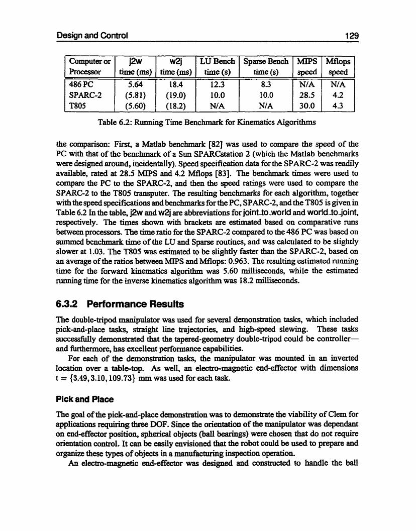
Design and Control 1 29

1 Cornputer or 1 j2w 1 w2j 1 LU Bench 1 Sparse Bench 1 MIPS 1 Mflops 1

- - - -- -- -

Table 6.2: Running Time Benchmark for Kinematics Algorithm';

1 Processor r

486 PC SPARC-2 T805

the cornparison: F h t , a Matlab benchmark 1821 was used to compare the speed of the PC with that of the benchmsrk of a Sun SPARCstation 2 (which the MatIab benchmarks were designed arounk incidentally). Speed specification data for the SPARC-2 was readily available, rated at 28.5 MIPS and 4.2 Mflops [83]. The benchmark times were used to compare the PC to the SPARC-2, and then the speed ratings were used to compare the SPARC-2 to the T805 transputer. The resulting benchmarks for each algorithm, together with the speed specifications and benchmarks for the PC, SPARC-2, and the T805 is given in Table 6.2 In the table, j2w and w2j are abbreviations for jointto-world and worldfo joint, respectively. The times shown with brackets are estimated based on comparative runs between procesSom. The time ratio for the SPARC-2 comparai to the 486 PC was based on summed benchmark tirne of the LU and Sparse routines, and was calculated to be slightly slower at 1.03. The T805 was estimated to be slightly faster than the SPARC-2, based on an average of the ratios between MIPS and Mflops: 0.963. The resulting estimateci d g thne for the forward hematics algorithm was 5.60 millisecon&, while the estimated ninning time for the inverse kinematics algorithm was 18.2 miIIiseconds.

6.3.2 Performance Results

time (ms) 5.64 (5.8 1) (5.60)

The double-ûipod nmipuiator was used for several dew>IlStration tasks, which included pick-and-place tasks, straight line trajectories, and high-speed slewing. These tasks successfbliy demo~l~ttated that the tapered-geometry double-tripod could be controller- and furthermore, has excellent performance capabilities.

For each of the demonstration tasks, the manipulator was mounted in an inverted location over a table-top. As well, an electro-magnetic end-effector with dimensions t = {3.49,3.10,109.73) mm was wed for each task.

Pick and Place

tune (m) 1 8.4

(1 9.0) (18-2)

The goal of the pick-and-place demonstration was to demonstrate the viability of Clem for applications requiring three DOF. Since the orientation of the manipulator was dependant on end-effector position, spherical objects (bali bearings) were chosen that do not require orientation wntrol. It cm be easily envisioned that the robot could be used to prepare and organize these types of objects in a manufkdmhg inspection o p t i o n .

An electro-mgnetic end-effector was designed and constructed to handle the ball

tirne (s) 12.3 10.0 NIA

time (s)

8.3 10.0 NIA

speed N/A 28.5 30.0

speed NIA 4.2 4.3

Desian and Control 130

Figure 6.23: Pattern for Pick-and-Place Demonstration

bearings. This end-effector was attached to the center of the distal platform of the robot The end-effector was intafaceci to the CS00 controller so that it could be energized and de-energized with the native CLOSE and OPEN comm~nds in RAPL-II.

A pick-and-place ta& was pedormed on the 177.8 mm square pattern show in Figure 6.23. The objective of the cycle was to simply rearrange the bail bearings. At the start of the cycle, 4 balî bearings were placed at locations S 1, S2, S3, and S4. The spare location, S5 served as a transfer station A RAPL-II program, called ARRANGE, was used to perfonn one rearrange sequence. The program listing is given here:

; ARRANGE ! cDLONGI241 =O ; RESET BUFFER ! @LONG[24] = 77999 ; 0130AF (ALL AXES, lOMS STEP) QACCEL 0, 0.07 ONLINE OFF SPEED 50 10 MOVE #UP DELAY 0.5 MOVE #NEAR GOSUB GET S Ci] ,50.8 GOSUB PUT S CS) ,5O. 8 GOSUB G E T S [2] ,5O -8 GOSUB PUT S Cl] ,5O . 8 GOSUB G E T S C33 ,50.8 GOSUB PüT S C2] ,5O .8 GOSUE GET S [4] ,50 - 8 GOSUB PUT S [3] ,50.8 GOSUB GET S [5] ,50 .8 GOSUB PUT S [4] ,5O. 8 MOVE #UP RETURN $

Note that at the beginning of the program, a long integer variable is used to control a

Design and Control 131

Save buffer on the sewo transputer. This ffeture was added to the hctionality of the -0-system through custom 'C' programs with the transputta deveiopment toollcit. The control variable, LONG[24] was bit encoded to control which states of the servo controller to record, and at what time resolution to record it. In ARRANGE (shown above) the hexadecimal number O l3AF (77999 in decimal) was used to start saving encoder position, encoder =or, and cornmanded encoder vdocity data for d l three axes. For each tra.jectory in between the taught points, the motion was interpolated with respect to the joint variables, as opposed to Cartesian variables.

In addition, to the pick-and-pIace locatiom, two "precision" (defined with respect to joints) locations were defined: #UP and #NEAR to begin and end the sequence. The pick-and-place sequence comprises the GET and PUT cycles show in Figure 6.23. Each location was approached and departed to a distance of 50.8 mm, in the direction of the tool axis. The subroutines for these bctions are as follows:

; CET AN OBJECT APPRO X O , % 1 MOVE %O FINISH CLOSE DEPART %1 !iEmmN $

; PUT AN OBJECT APPRO %O ,%1 MOVE %O FINISH OPEN DEPART %1 RETURN $

where %O denotes the passed location argument, and %1 denotes the passed approach and depart distance.

The data stored in the Save bmer of the snvo transputer was downloaded in a batch nom the controller after the run was completed. The data depicting the acnial motor position (in encoder pulses) is shown in Figure 624. Note that the 5 pi&-and-place cycles were performed in approximately 7.0 seconds. This gives an average pickdplace time (for a pattem of slightly more than 7 inches, due to the diagonals) of 1.4 seconds.

The motor data was processed using a forevard kinematics simulation of the manipuiator to obtain an estimate of the-Çaaesian motion of the end-effecf~r. These results are depicted in Figure 625. This figure depicts each coordiiiate as a function of time, as well as a 3-D plot showing the end-effector motion in space. Note that the Cartesian coordinates are dehed with respect to the base reference fiame, the z-8XiS of which was pointhg dom

Design and Control 132

Figure 6.24: Pick-and-Place Test: Motor Coordintes vs. time

towards the table-top. For this reason the pick-and-place cycle is oriented upwards, even though the sequene was perfonned with respect to the table.

Staight Une Trajectory

The goal of this demonstration was to show that the inverse kinematics algorithms developed were in fact efficient enough to wntrol the robot in real time.

Using data-logging techniques sWar to the previous section, a portion of a straight line trajectory was recorded and download h m the CS00 controller. With this nui, data was saved during a coordinated motion fiom one point to another. The RAPGII program used for ttiis run was as foilows:

; STAIGHT-LINE RUN ! QLONG [24]=0 ; RESET BüFFER ! QLONG[24]=12319 ; Triggers data recording 301F (Al1 axes)

Design and Control 133

Figure 6.25: Pick-and-Place Test Cartesian Coordintes:(a) vs. T i e , and @) 3D Plot

Design and Control 1 34

StraigM Une: Motor Setpoints vs. Tirne 500 I 1 1 1 1 1 1 8 1

n

8400- - a a. Y

,300- E

ml time (s) 1 1 1 1 1 1 I I 1 1

500 time (s)

1 r 1 I 1 I 1 1 L I - A

Q1

$400- - - z z 3 0 0 - - ç

2000 1 1 1 1 1 1 t 1 I 1

0-02 0.04 0.06 0.08 0.1 0.12 0.14 0.16 0.18 0.2 time (s)

Figure 6.26: Straight Line Test: Motor Coordintes vs. t h e

SPEED 30 MOVE #UP SPEED 50 MOVE S [2] FINISH ONLINE ON MOVE S C41, S FINISH FtETmN $

The motion between the points was interpolated with respect to Cartesian variables, due to the selection of the ",Sn in the RAPLAI motion commsinci. As descfl'bed previousIy, servo data was downloaded fkom thc controkr after the nui was cumpleted. The data depicting the actual motor position (in encoder pulses) is shown in Fi- 6.26. The corresponding endeffetor Cartesian motion is shown in Figure 627. This figure depicts both each coordinate as a function of time, as weil as a 3-D plot showing the end-effector motion in sp--

Desian and Control

(a) Straight Line: Cartesian Coordinates vs. Time

O 0.02 0.04 0.06 0.08 0.1 0.12 0.14 0.16 0.18 0.2 time (s)

I 1 L I 1 1 1 1 1 1 i 1

O 0.02 0.04 0.06 0.08 0.1 0.12 0.14 0.16 0.18 0.2 time (s)

(b) StraigM Line: Cartesian Path in Space

Figure 6.27: Straight Line Test: Cartesian Coorninates:(a) vs. t h e , and (b) 3d plot

Design and Control 136

The goal for high-speed slewing tests was to demonstrate the maximum speed and acceleration capabilities of the rnanipulator. Two points were taught in the workspace, each at opposite extremes of the workspace envelope. The robot was commanded to move fiom point to point, with the motion in joint cooràinates. The following RAPL-II program was used for the runs:

; HIGH SPEED SLEW TEST MOVE #ONEUP FINISH ! QLONG [24] =O ; RESET BUFFER ! QLONG [24] =12319 ; Triggers data recording 301F ( ~ l l axes) ONLINE OFF SPEED 100 MOVE #ï ï iOUP ; 100,610,610 FINISH MOVE #ONEUP ; 610,100,100 FINISH RETURN $

This prognun moved the robot between the two defined locations with a parabolic velocity profile (defined by non-shaight moves with ONLINE mode OFF in RAPL-II). The encoder data, saved in 1 ms time intervals, is given in Figure 6.28. The maximum motor speed for the run was set to 2500 tpm. With the 12.5/1 gear reducer, the corresponding maximum output speed was 1200 degis. It can be seen fkom Figure 628 that each slew twk approximately 0 2 seconds. The encoder error during the high-speed slew is shown on Figure 6.29. We expect some encoder error to be present during the slew, due to the high torques necessary to drive each joint, and the fact that a feedback PID controkr was used on the joints. The maximum error magnitude* accordhg to Figure 629 was -38 encoder pulses on axis 1, and 15 pulses on axes 2 and 3. The Merence between the encoder errors is attributed to the fact that joints 2 and 3 are slewing togethex, wherieas joint 1 is slewing on its own.

The corresponding Cartesian position for the stew can be calculated using the encoder data. This data is shown both with respect to time, and in space in Figure 6.30. Although @valent paths are commanded to and from the slew points, the end-effector travels on slightiy diffimmt paths. The reason for fis, and the relatively high encoder pulse emor on joint 1 (see Figure 6.291, are due to differences in path mature, rnanipdator configuration, and subsequent torque requirments on each motor. This effect could be better understood through an analysis of the dynamics of the manipulator, but represents work beyond the scope of this thesis.

From the Cartesian position data in Figure 6.30, the velocity and acceleration profiles for the motion can be estimateci. For velocity estimation, a sewnd-order forward/reverse Butterworth low-pass filter (HLTFILT [82]) was used to smooth the first derivative. The

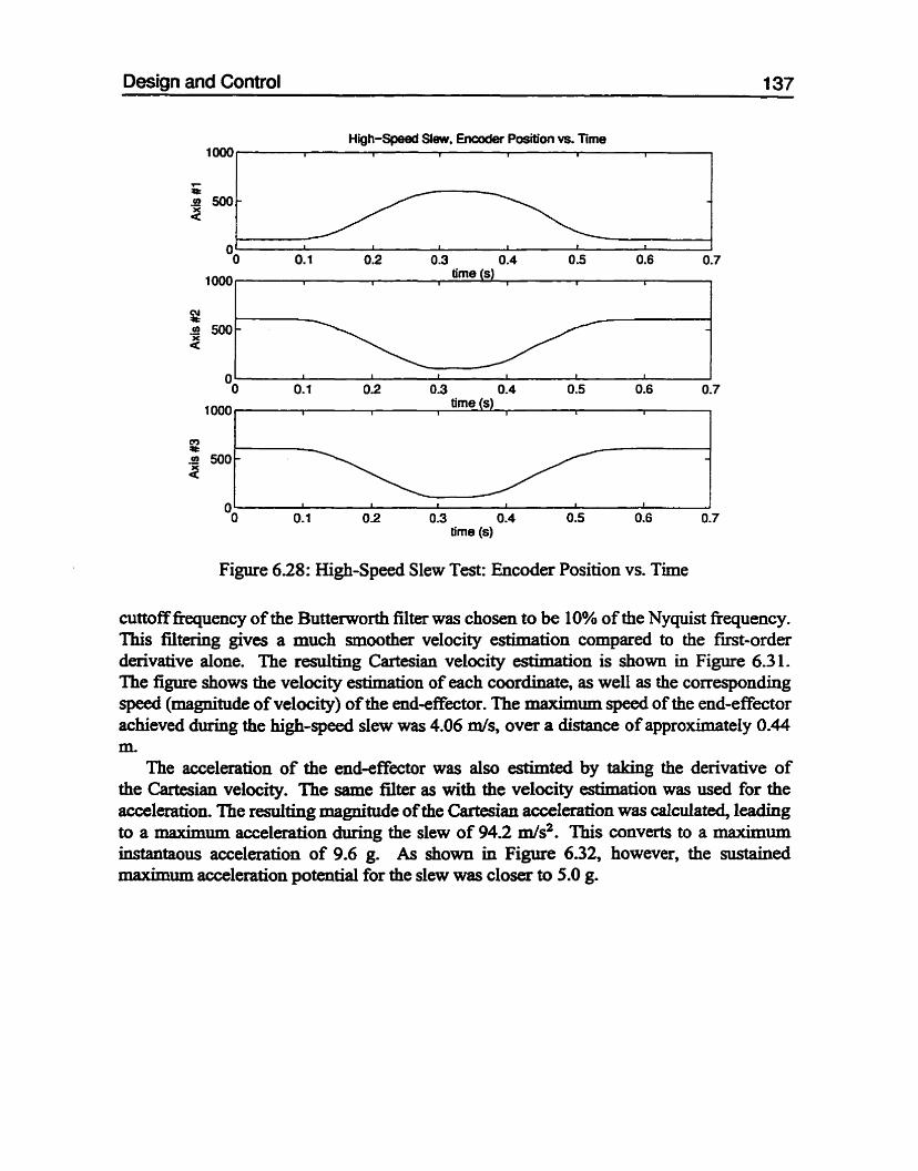
Design and Control 1 37

High-Speed Slew. Encoder Posia'on vs. Time I I I 1 t 1 1

P O

a 01 1 I 1 I 1

1

O O. 1 0.2 0.3 0.4 0.5 0.6 0.7

1000 time (s) I I I I 6 6

O; 1 1 t I 1 I f

0.1 02 0.3 0.4 0.5 0.6 0.7 tirne (s)

CU O 3 500- a

Figure 628: High-Speed Slew Test: Encoder Position vs. Time

-

cuttoff fkequency of the Butterworth filter was chosen to be 10% of the Nyquist frequency. This filtering gives a much smoother velocity estimation cornpareci to the fïrst-order denvative alone. The r d t i n g Cartesian velocity estimation is shown in Figure 6.3 1. The figure shows the velocity estimation of each coordinate, as weli as the corresponding speed (magnitude of velocity) of the end-effector. The maximum speed of the end-effector achieved during the high-speed slew was 4.06 mis, over a distance of approximately 0.44 m.

The acceleration of the end-effector was also estimted by taking the derivative of the Cartesian velacity. The same filter as with the velocity estimation was used for the accelemtioa The d t i n g magnitude of the Cartesian acceleration was dculated, lading to a maximum acceleration during the slew of 94.2 m/s2. This converts to a maximum instantaous acceleration of 9.6 g. As shown in Figure 6.32, however, the susfaineci maximum acceleration potential for the slew was closer to 5.0 g.

Oii 1 1 I 1 I I

O. 1 0 2 0.3 0.4 0.5 0.6 0.7

1 O00 tirne (s)

l 1 1 1 1 I I

Design and Control 138

High-Speed Slew, Encoder Position Emr vs. Time mi 1 1 1 b 1 I

20 1 time (s)

I I I I I I 1

I I I I I I I 0.1 0.2 0.3 0.4 0.5 0.6 0.7

tirne (s)

Figure 6.29: Hi@-Speed Slew Test Encoder Position k o r vs. Time

Desian and Control 1 39

(a) High-Speed Slew, Cartesian Position us. Time

-

h

E E -300 - w

N

-0 1 1 1 1 1 1

0.1 0 2 0.3 0-4 0.5 0.6 0.7 üme (s)

(b) High-Speed Slew, Cartesian Position in Spaçe

Figure 6.30: High-Speed Slew Test: Cartesian Coordintes:(a) vs. Tirne, and (b) 3D Plot

Design and Control

High-Speed Slew, Cartesian Velocity and Speed vs. Time A 2000- b

2 E € O - rn >

* -2000 1 1 i

O 0.1 0.2 0.3 0.4 0.5 0.6 0.7

A 5000- 1 1 1 1 1 i r E E - 0- - a > -5000. 1 I 1 1 I 1

O 0.1 0.2 0.3 0.4 0.5 0.6 0.7 - 5 O f -CZ 1 1 I 1 I 1

E E Y

O al a

3- O 2

O 0.1 0.2 0.3 0.4 0.5 0.6 0.7 time (s)

Figure 6.3 1: High-Speed Slew Test: Cartesian Velocity Estimation

Desian and Control 141

High-Speed Slew, Cartesian Acceleration vs. Time

Figure 6.32: High-Speed Slew Test: Cartekan Acceleration Estimation

Chapter 7

Conclusions, Contributions, and Suggestions for Future Work

7.1 Conclusions In this thesis, the kinematics and design of the revolute-spherical-revolute (RSR) class of manipulators has been studied. These manipulators consist of spatial, palle1 mechanisns with three degrees of fiadom The two members of the class examined include the double tripod PT) and the double octahedral variable-geometry tniss (VGT).

By introducing the RSR class, the DT and VGT have been identified as common mechaaisms. This has been accomplished by recognizing their common set of three RSR joints adjoining two platforms (proximal and distal). By doing so, the kinematics and design principles for both mechanhm has been unif id

In this work, the doubletripod mechanian has been introduced. The mechsurism is a more generalized and non-reflective form of Hunt's original '"reflected tripod". The name "double tripod" has been thus coined, acknow1edging the hidoncal significance of the mechaism.

The historical root of the RSR class has been researched, with the conclusion that it traces its roots to a patent by Clemens in 1869 for a constant speed coupling. This is important because it identifies that the RSR class of mechanisms has a long and rich history-begiiming with DT predecessors, continuhg later with the VGT, and joining together in this work

The detaiied anaiysis begins with the introduction of the general kïnematic model for the RSR class of mechanismn- The general model contains platforms with g e n d geometiy, and legs with a general RSR chah. The well-lmown Denavit-Hartenberg convention has been adopted to model each leg. The general kinematic model is valuable because it gives rise to new design and analysis tools for the DT and VGT. The Denavit-Hartenberg convention also aids specifically in the design and analysis of pmtical spherical joints.

As part of the kinematic modeling, a new classification scheme has been introduced for the RSR mechaaisns. This taxonomy is based on three geometric properties of the mechanisms, and gives rise to 8 distinctive sub-classes. This classification method provides

Conclusions, Contributions, and Suggestions for Future Work 1 43

an important insight in the andysis and design of both the DT and VGT mechanisms. The forward kinematics has been solved using the general kinematic model. The

soIutions have been given for both the DT and VGT. An algorithm that uses common elements to solve both the DT and VGT has been presented. The algorithm is important because it highlights the commonalities and ciifferences between the mechanism.

The grnerd forward bernatics algorithm, more specifically, begins with the solution of the unknown revolute joints in the mechankm using a set of petai (closure) quations. The DT forward kinematics employ one petai equation, while the VGT involves two. Two methods have been used to solve the petal equations: direct solution, and itmative solution. The direct solution for the petal equations has been accomplished through polynomial etimination methods. The result of this procedure was a 16th degree polynomial, showing that a maximum of 16 and 256 forward kinematic solutions exists for a general DT and VGT, respectively. Although the final equations are very large, they are important in order to confirm the existence of 16 solutions for the DT. As weU, the development dso shows that the VGT has a maximum of 256 unique forward kinematic solutions.

An example has been shown for a DT mechanism where al1 16 solutions forward kinematics polynomial are real. This r d t is important because it shows that no extraneous solutions exist, and that al1 16 solutions can be practically obtained The example is also sigaificant because it exercises al1 equatiom developed in the forward kinematics dgorihm.

The iterative solution method for the petal equations has been shown to be computa- tionally efficient and suitable for real-time implementation. The iterative algorithm uses the Newton-Raphson method, and successfulIy iterates to a hnal solution given an initial guess. This r d t is useful because it ailows the forward kinematics algorithm to be implemented in d - t h e trajectory control applications.

Although the general case is solved in the forward kinematics algorithm, the specific cases of the DT were shown to admit closed-form solutions. These cases occur when the geometry is symmetric (reflective). This is significant because it relates the generd solution to the more simplified solution, and also shows that special forms of the DT have closed-form forward kinematics.

The forward kinematics algorithm also solves for the angles of the spherical joints of in the RSR mechanian This is possible because the kinematic model includes these joints explicitly (as mmtioned previously). This is an important tool for the analysis and design of practical spherical joints

The invase bematics problem has been solved with iterative methods for the g e n d model of RSR class of manipulator. Two alternative methods have been presented: the fkst iterated using the mechaaiSm closure equations, and the second using the fornard kinematics. These methods have been shown to be pracfical for real-the applications- This is important because without inverse kinematics, the mmïpulator would have only limited pxwtical utility*

The inverse kinematics greatly simplifies for the inverse kinematics when the kinematic madel is symmetric. For this specid case, the inverse kinematics is solved in closed-fom for both the DT and VGT.

Conclusions, Contributions. and Suggestions for Future Work 144

The experimental portion of this work centered around the design, construction, and control of a tapered (asymmetric) DT manipulator. This mmipulator is named " C l d after Clemens. The goals of the design were to test kinematics on a DT with tapered geornetry, and to demonstrate the mechanisms applicability to industrial maipulators. This design concept is important because it represents the first time a tapered DT has been proposed for robot mmipulator applications.

Forward and inverse kinematics dgorithms have been implemented on an induSanai robot controller. The iterative version of the forward kinematics algorithm has been implernented, while the latter (forward-kinematics-based) version of the iterative inverse kinematics has been implemented. AU algorithms have been implemented in 'C', and are proven suitable for real-the control.

The resulting performance of Clem demonstrates that the DT is a suitable component for industrial manipulator applications. The combination of readily avdable components, simple design, and high speed have been achieved with Clem, making it an excellent candidate for industnal applications.

7.2 Original Contributions 1. Introduced the general variable-geometry tniss (VGT) and double tripod @T),

coining double bipod to describe the revolute-spherical-revolute (RSR) parallel mechanisn without prismatic actuators.

2. Developed a general mode1 for the RSR class using the Denavit-Hartenberg conven- tion.

3. For the general DT and VGT, solved the forward kinematics polynomial coefficients that arise from the direct solution of the petal equations.

4. As an example, rendered al1 16 forward bernatics solutions for a general DT.

5. Demonstrated simplified forward and inverse kinematics solutions for the RSR class of mechanisns, and showed how they relate to the general kinematics solutions.

6. Designed and b d t a fmt-of-its-kind DT manipulator-possessing tapered (w- meîric) geometry.

7. Interfaced the DT manipulator to an industrial manipulator controkr, using the DT kinematics algorithms developed in this thesis.

7.3 Suggestions for Future Work 1. Design and control of a non-planar-platfonn VGT or DT. The non-planar-platform

s u ~ l a s s of the RSR mechmism may possess some interesting and practical mech-

Conclusions, Contributions. and Suaaestions for Future Work 1 45

anisrn design. Although algorithms have been developed for general models, only pianar-platform prototypes have been comûucted for the DT and VGT.

2. Closeci-fonn solution for the inverse bernatics for the asyrnmeaic subciass of RSR mechanisms. A closed-fonn solution fias not been found for this sub-class, but iterative algorithms have been used. A closed-form solution could shed more light on the maximum nimiber of inverse kinematics solutions, and provide more efficient algorithms.

3. Design of a higher performance (with respect to both speed and precision) DT, equipped with a sphexical wrist, to serve as an industrial manipulator prototype. Clem has been designed with only three-DOF, to serve as a prototype manipulator. Given the favorable performance results, the next step in its development would be to mount a wrist mechanism on the device so that a fidl six-DOF manipulator could be obtained.

4. Design and control of a t a p e d terratrial tnissarm, using algorithms developed in this thesis. The asymmetric sub-class of VGT's opens the possibility to have a continum2y tapered tmssam (multiple Sefially stacked VGT bays). Such a design element could be employed to strengthen the base while milintainhg a light tip in a terrestrial gravity environment.

References

[ 11 K. H. Hunt, Kinematic Geometry of Mechunisms. Mor& England: Oxford University Press, 1978.

[2] T. Leinonen et al., "International Federation for the Theory of Machines and Mechanisns @;ToMM): Terminology for the theory of machines and mechanians," MechanLsm and Machine Theory, vol. 26, no. 5,199 1.

[3] R P. Paul, Robot Manipulators: mathemutics, programrning, and C Q ~ @ O ~ - Cambridge, Mass.: MIT Press, 1982.

[4] J. J. Craig, Introduction to Robotics MechanUms & Control. Reading, M A : Addison- Wesley Publishing Co., 1986.

[5] C. Y. Ho and J. Sriwattanathemma, Robot Kinematics: S'ymbolic Automation and N ~ r n ~ c a l S'th&. Norwood, New Jersey: Ablex Publishing Corporation, 1 990.

[6] J. Angeles, Spatial Kinematic Chaim: AnaIysis-Synthesis-Optim~ution. New York: Sp~ger-Verlag, 1 982.

[7] K H. Hunt, ' ' Structural kinematics of in-parallel-actuated robot-amis," Journul of MechaniSm, Trairsmissions, and Automation in Design, vol. 105, pp. 705-7 12,1983.

[8] D. Stewart, " A platform with six degrees o f keedom," hceedings of the Institution of Mechunicul Engrneers, vol. 180, no. 15, pp. 37 1386,1965-66.

[9] V. Gough and S. Wtehall, "Universal tyre test machine," in Proceedings, I't. of Mechanical Engineers Ninth Int. Tech. Congress, May 1962.

[IO] V. E. Gough, "CommU1Ulcation RE: A plaîfkorm with six degrees of fieedom (d. sîewarî)," Proceedings of the Institution of Mechanical Enginem, vol. 180, no. 15, pp. 379-38 1,1965-66.

[Il] K. Etexnadi-Zanganeh and J. Angeles, "Instantaneous bernatics o f modular par- allel manipuiators," in Design Engineerîng: Robotics: Kinematics, -mi- and Controls, vol. 72, pp. 27 1-277, ASME, 1994.

[ 121 W. L. V. Pollard, Position Controlling Apparatus. US. Patent #2 f 86,57 1, June 16, 1942.

REFERENCES 1 47

[13] H. Asada and K. Youcef-Toumi, Direct M e Robotr. ï7ieory und Procrice. MIT Press, 1987.

[14] V. E. Gough, "Contriion to discussion to papers on research in automibile stability and control and in tyre performance, by CorneIl staff," in Proceedings, Automotive Division, Imtitution of Mecchannical Engineers, 1956-57.

[lS] H. Inoue, Y. Tsusaka, and T. Fukuinimi, "ParaHel manipulator," in Robotics Rtserch: The Third international Symposium, pp. 32 1-327, October 1 986.

[16 ] K. Lee and D. Shah, "Kinematic analysis iof a three-degrees-of-freedom in-parallel actuated manipulator," LEEE Journal of Robotics and Automation, vol. 4, no. 3, pp. 354-360,1988.

[17] C. M. Gosselin and J. Angeles, "The optimal kinematic design of a sphencal three- degree-of-keedom paralle1 manipulator," ASME Journal of Mechanical Design, VOL 1 1 1, no. 2, pp. 202--207, 1989.

[18] D. J. Cox and D. Tesar, "The dynamic mode1 of a three-degree-of-fieedom parailel robotic shoulder module," in Proceedings, Fourth International Conference on Advanced Robotics, (Columbus, Ohio), 1989.

[ 191 J. M. Herne, "Group mathematics and parallel link mechanians," Un Proceedings, WCS/SICE Interational Symposium on Robotia, Mechaironics and Manufacturing Systems, vol. 1, (Kobe, Japan), pp. 459-464, September 1992.

[20] H. Mccallion and P. D. Truong, "The analysis of a six-degree-of-fietdom work station for mechaniseci assembly," in Proceedings, FijZh World Congres on m e o ~ of Machines and Mechanimrï, pp. 61 1-6 16, ASME, 1979.

[2 11 1. L. Powell, "The parallel topology manipulator, kinematics analysis and simula- tion," tech. rep., Marconi Research Laboratories, GEC Marconi ELectronics Limited, 1981. MTR81/30,

[22] D. C. H. Yang and T. W. Lee, "Feasibility study of a platforni type of robotic manipulator fiom a kinematic viewpoint," Trmactions of the ASm, Journal of MechanLns, Tramnissions and Automation in Design, vol. 180, no. 1, pp. 19 1 - 198, 1984.

[23] E. F. Fichter, "A Stewart platform-based manipulator: General theory and practicd construction," in Kinematia of Robot Maniplators (J. M. McCarthy, HL), pp. 165- 190, MIT Press, 1987.

[24] M. Cwiakala and N. A. Langrana, "On the feasibiiity of platform manipulators using cable legs," in T r d ami Developments in Mechanimu* Machines. md Robotia, VOL 3, p ~ . 97-103, ASME, Swtembcr 1988.

REFERENCES 1 48

J. C. Hudgens and D. Tesar, "A My-paralel six degree-of-fkeedorn micromanip datoc Kinematic analysis and dynamic model," in Trendr and Developments in MechanlsmF, Machines, and Rohtics, vol. 3, pp. 29-37, ASME, September 1988.

W. F. Smith, III and C. C. Nguyen, "On the mechanical design of a Stewart platform- based robotic end-effector," in Proceedings, Southe~con, vol. 2, pp. 875-879, IEEE, 1991.

V. Kumar, "Characterization of workspaces of p d e l manipulators," J o u d of Mechanicd Design, vol. 1 14, pp. 368-375,1992.

S. E. Landsberger and T. B. Sheridan, "A minimiil, minimal linkage: The tension- compression parallel link rnanipulator," in Proceedings, M C S / S K E International Symposium on Robotics, Mechatronicr and Manufacr~ring System, vol. 1, pp. 493- 500, September 1992.

O. Ma and J. Angeles, "Architecture singuiarities of paralle1 manipulators," Interna- tional Journal of Robotim and Automation, vol. 7, no. 1, pp. 23-29,1992.

K Cleary and T. Brooks, "Kinematic analysis of a novel6-DOF paralle1 manipula- tor," in Proceedings, IEEE Inremational Conference on Robotics and Automation, pp. 708-713,1993.

S. Dubowsicy, W. Durfée, A. Kuklinski, U. Muller, 1. Paul, and J. Pennington, 'The design and implementatioon of a laboratory test bed for space robotics: The VES MOD II," in Design Engineering: Robotics: fiematics, Dynamics and Controls, vol. 72, pp. 99-108, ASME, 1994.

R Clavel Disposiitifpour le dkplacement et le positinnement d'un element dam l'espace. Swiss Patent CH 672089A5, reqyested: 1985, gtanted: 1989.

F. Pierrot, A. Fournier, and P. Dauchez, "Toward a M y paralle16 DOF robot for high-speed applications," Intentational Jmmal of Robotics and Aufornation, vol. 7, no. 1, pp. 15-22,1992.

R Clavel, "A prototype of thc P o h d manipuiator." Personal demonstration during a visit to the laboratory, ûctober, 1993.

"Motoman series-ail-electnc indusirial robot.' ' Yaskawa Electric Corporation Prod- uct Brochure CHE-C945-OG, Japan, 1993.

G. S. Thomton, "The GEC Tetrabot - a new serial-pdel assembly robot," in Proceedings of the he Intemtionnal Conference on Robotics and Automation, pp. 437-439, IEEE, 1988.

M. H& and K J. Waldson, "Position kinematics of a mixed mechanïsm," in Robotia. Spatial Mechanisnts, a d Mechunical Systems: Design Engineering, vol. 45, pp. 4147, MME, Septesdm 1992.

REFERENCES 149

[38] K. Maeda, K. Fujirnoto, S. Tadokoro, and T. Takamori, "An analysis of passive impedance of 6-DOF direct-drive wrist joint," in Proceedings, IMACSXSICE Inter- national Symposium on Robotia, Mechatronics and Mmiufacturing System, vol. 1 , (Kobe, Japan), pp. 433-438, September 1992.

[39] C. C. Nguyen, S. S. AntraZi, and 2.-L. Zhou, "Analysis and implementation of a 6 DOF stewart platform-based force sensor for passive cornpliant robotic assembly," in Proceedings, Southeastcon, vol. 2, pp. 880-884, IEEE, 199 1.

[40] C. Reboulet and R Pigeyre, "Hybnd control of a 6-DOF in-pardlel actuated micro- manipulator mounted on a scara robot," International Journal of Robotics and Automation, vol. 7, no. 1, pp. 10-14, 1992.

[4 11 M. Lambert, Mecunhe PoWicule Retractile. French Patent #2,542,4 1 9, Septem- ber 1984.

[42] M. Lambert, P~L'ya~c~cZcstted Retructiile Midianism. U.S. Patent W,65 1,589, March 24, 1987.

[43] K Miura, H. Furuya, and K. Suaiki, "Variable geometry truss and its application to [a] deployable truss and space Crane am," in 35th Congress of the International RFrronauticol Federation, (Lausame, Swiaerland), October 1984. IAF-84-394.

[44] G. S. Chirilcjian and J. W. Burdick, "Parallel formulation of the inverse kinemat- ics of modular hyper-redundant manipulators," in Proceedings of the 1991 IEEE Intentational Conference on Roborics and Automation, pp. 708-7 13,199 1.

(451 M. Shahinpoor, "Kinematics of a parallel-serial (hybrid) manipulator," Journal of Robotic Systems, vol. 9, no. 1, pp. 17-36.1992.

[46] M. Clemens, Impnvement in Apparatus for Tronmiiting Rotary Motion. U.S. Patent #96,395, November 1869.

[471 R B. Hertz and P. C. Hughes, "Kinematic analysis of a class of spatial parallel manipulators with three degrees of freedom," in Design Engineering: Robotics: fiematics, Dynamics mrd ConfroIs, vol. 72, pp. 279-284, ASM, 1994.

[48] W. Steeds, Mechanism and the finematics ofMochines. London, England: Longmans, 1940.

[49] D. M Wailace and F. Freudenskin, "The displacement analysis of the generalized tracta coupling," J o d of Appled Mechanics, pp. 7 l3-7l9, Septenibex 1970.

[SOI S. L. M e I d , R J. Salerno, and C. F. Reinholtz, "Kinexmtic design of a large- angiuiar-motion constant-velocity tupiing," in D&gn Engiheen'rtg: MechaniSm Synthesis and Analysis, vol. 70, ASME, 1994.

REFERENCES 150

[5 11 M. R Bricard, "Sin la théorie de l'octaèdre articulé," J o d Mathématiques Pures et Appliquées, vol. 3, pp. 113-148,1897.

1521 M. D. Rhodes and M. M. Mürulas, Jr., "Deployable controllable geometry t m beam," technical memorandum, Langley Research Center, NASA, 1985. #86388.

[53] W. G. Sincarsin and P. C. Hughes, "Trussarm candidate geometries," tech. rep., Dynacon Enterprises Ltd., 1987. Report 28-61 110401.

[54] C. F. Reinholtz and D. Gokhale, "Design and analysis of variable geometry ûuss robots," in 10th Applied Mechunhs Confeence, 1987.

[55] K. Miura and H. Furuya, "Adaptive structure concept for future Wace applications," AuL4 Journal, vol. 26, no. 8, pp. 995-1002, 1988.

[56] H. H. Robcashaw, R H. Wynn, Jr., H. F. Kun& S. L. Hendricks, and W. W. Clark, "Dynarnics 'and control of a spatial active tniss actuator," in Proceedings, 30th Stncctures, Sn~cturaZ Dynomics and Muteriuls Confeence, pp. 1473- 1479, AbU, 1989.

[57] P. C. Hughes, W. G. Sincarsin, and K A. Carroll, "Tnissami - a variable-geometry- tniss manipdator," Jorunal of Intelligent Materials. Systents and Structures, vol. 3, pp. 148-160, 1991.

[58] K. H. Robertshaw and C. F. Reinholtz, "Grant review: Vibration control of flexible structures (NASA gant NAG-1-570, LaRC)." not published, January 1989.

[59] C. Innocenti and V. Parenti-CasteIli, "Direct position analysis of the Stewart platform mechankm," Mechanikm und Machine Theory, vol. 25, no. 6, pp. 6 1 1-62 1,1990.

[60] P. H Tidwell, C. F. ReinhoItz, H. H. Robertshaw, and C. G. Horner, "Kinematic analysis of general adaptive ûusses," in Proceedings of the Fimt Joint U.S./Japan Conference on Adaptive $tnu:tures, pp. 772-79 1,1990.

1611 V. Anin, C. F. Reiaholtz, and L. T. Watson, "Application of new homotopy continuation techniques to variable geometry tnisses," J o d of Mechaniml Design, vol. 114, no. 3, pp. 422427.1992.

[62] M. Gr* and J. Duffy, "A forward displacement analysis of a class of stewart platforms," JmmI of Robotic Systems, vol. 6, no. 6, pp. 703-720,1989.

[63] F. Naccarato and P. C. Hughes, "Redundancy rcsolution in variable-geometry tniss manipulators using reference shape curves," in Proceedings, SecondJoint Jopan/U.S. Conference on Adrptive Sttucfrrtes, pp. 539-555,199 1.

[64] R B. Hertz and P. C. Hughes, "Forward kinematics of a 3-DOF variabk-geometry- trus~ mmipuiator," in Computational Kinematics (J. Angeles, G. Hommel, and P. Kovacs, eds.), pp. 241-250, Kluwer Academic Publishers, 1993.

REFERENCES 151

1651 B. Padmanabhan, V. Anm, and C. F. Remholtz, "Closed-form inverse kinematic analysis of a variable geometry tniss manipulator," in Proceedngs of the 2Ist Biennial MeciuuiismF Confwence: Cam, Gems. Robots, und Mechanimrî, vol. 26, pp. 99-105, ASME Design Enpineexhg Division, 1990.

[66] V. Anui, B. Padmanabhan, K. Kolady, and C. F. Reùiholtz, "Detemination of the workspace of the 3-dof double-octahedral variable-geometry-tnrss manipulator,' ' in Robotics, Spatial Mechanism. and Mechanical Systems: Design Enginemg, vol. 45, pp. 493-500, ASME, September 1992.

[67] S. O. Oikawa, "Design and construction of a Cbay variable-geometry-tniss manipu- lator am,'' Master's thesis, University of Toronto, 1995. Aerospace Engineering.

[68] P. C . Hughes, Spacecrafl Attitude Dynumicr. John Wiley and Sons, 1986.

[69] F. Naccarato, finematics of Variable Geometry Twses. PhD thesis, University of Toronto, Toronto, Ontario, 1994. Aerospace Engineering.

[70] J. Denavit and R S. Hartenberg, ''A kinemaîic notation for lower-pair mechanisns based on matrices," Journal of AppZied MechanrmLF, pp. 215-221, June 1955.

[7 11 K. Kendig, Elementmy Algebruic Geometry. New York: Springer-Verlag, 1976.

[72] Wolfiam Research Inc, 4'Mathemati~ version 2 2 for SGI." Software Package, 1993.

[73] Waterloo Maple Software, "Maple V release 3.0 for Microsofl Windows.' ' Software Program, 1994.

[74] Nurnenkd Recipes in C: The A n of Scientrpc Computing. Cambridge University Press, 1988- 1992.

[75] D. Cox, J. Little, and D. O'Shea, Ideah, Varieties, and Algo&hms. Undergraduate Texts in Mathematics, New York: Springer-Verlag, 1992.

[76] B. Parimanababn, V. Anin, and C. F. Reinholtz, "Closed-fom inverse kinematic analysis of variable-geometry truss manipulators," Jownd of Mechanical Design, vol. 114, pp. 438443, September 1992.

[77l S. Grocott, "Control of tmswm," Bachelor's thesis, University of Toronto, 1991. Aerospace Engineeriag.

[78] J. P. Sallmen, ''T~ssarm control environment," Master's thesis, Universi@ of Toronto, 1993. Aerospace Engineering.

[79] J. Albris, "NASA/NBS standard refetence model for telaobot control systern archi- tecture (NASREM)," technid report, NASA, March 13,1987. SS-GSFC-00027.

1801 "CS00 industrial robot cuntrolier." CRS Plus Inc. Product Literature, 1995.

REFERENCES 152

[81] S. L. CanfieId, R J. Salerno, and C. F. Reinboitz, "Kinematic design of a large- mgular-motion constant-velocity muphg," in Design Engineering: Mechanimm Synthesis and Ana&&, vol. 70, pp. 167- 173, MM, 1994.

[82] The Mathworks Inc., "Matlab for windows benchmark demo." Online Help File, 1994.

[83] J. W. Burdsall, "The sun hardware reference m-4 models l i ~ " http://sun- www.picarefL.com/~~r~-~/rnodels-4h~, 1997.

Appendix A

Forward Kinematics Coefficients

A.l Background The fomard bernatics of the rotary-sphdcal-rotary mecbanism involves the solution of a set of nonlinear equations given in (4.53, (4.56), and (4.57). The development of these eqyations are covered in Chapter 4. To solve for the system of equations explicitly, polynomial elimination is employed. This appendix contains coefficients that result fkom the eIimination process.

Tnese equafions have been dewloped wittr the use of symboiic foniula rnm@uIafr*on somme,

This has been accompiished with a symbolic math package named Mathematica [72], on a Silicon Graphics Challenge L multiprocessor wmputer (skuIe.ecf.utoronto.ca) with 5 12 hWytes of RAM. Mathematica has bcm chosen for this partidar reduction step because of memory capabilities As weil, the SOI cornputer has been chosen on the basis of its relatively large memory size.

The complete Iisting of terms has been translated automatically in to "Latex" by Mathematica. It is provided here to demontitrate the complexity of the terms. The example given in Section 4.6.2 has been chosen to exercise every term of the final polynomial.

The ex~unpb I Sedion 4.62 d e s aü B e equatbns in ihis Appendk

A.2 Pseudo-Univariate Polynomial The second suppression step of the polynomial elimination process involves writing (4.69) as a pseudo-univariate polynomial in t2. The coefficients for the d t i n g tl matrk in (4.7 1) are as foilows:

Forward Kinernatics Coefficients

(hl3h33 - h12h23) (h72b3 - h92h23) + (hl3h72 - h2h23) (h32hl3 - hb2h23) + (hi3h52 - h n h ) (h52h13 - ha2hu) + 2 (h13h02 - h 2 h 3 ) (hi3hoz - hi2h43 ) + (hi3 h82 - h22 hr3 l2 (h33h32 ' h12hS3) ( h t l h 3 - h92h23) + (h13h32 - h12h23) (h72h73 ' h92h53)

+2 (h33he2 - b h 7 3 ) (h13h52 - h12hr3) + 2 (hi3he2 - h 2 h ) (h33hd2 - h12h73 + (hmhs2 - h n h s ) (hs2hl3 - h d u ) + ( h 1 3 b - h22h23) (h52h73 - ha2h53

f 2 (h33 h82 - hnh73 ) (hl3 ha2 - h22 h43 ) + (A33 hm - h2 hm ) (h32 b3 - h 6 2 h ) + (h13h72 - h2h23) ( h h t 3 - hb2hm)

2 (h63he2 - k 2 b 3 ) (h13hol - h12hl3) + 2 (h33hBZ - h2h73) (hJ3hb2 - hl~h73)

+2 (h13b2 - h12h3) (hbJAb2 - h12b3) + 2 ( k h 8 2 - h22b3) (h13h12 ' h22h43)

+ ( h a h m - h n h ~ 3 ) ~ + ( k h 3 2 - h12ha3) (h72h3 - he2h23) + (h33h32 - h12h53)

(h72hn - h h ~ ) + (h13h32 - hi2hlS) (h72ho3 - b 2 k ) + ( k h n - hr2ha3 1 (h32h3 - hb2 h23) + (h h72 - h2h53) (h32h73 - hd2h53 ) + (h13h72 - h2h23 ) (h32h93 - bah=) + (hahs2 - hnhm) (h52hl3 - hmhzs) + ( h ~ h s 2 - hmh= 1 (hs2hn - ha2hs) + (hi3h52 - h n h ) (hs2b3 - h 2 h m ) 2 (hss ha2 - h n he3) (hm ha2 - hm h73) + ( h a h72 - hhs) ( A d 7 3 - hd2hs ) + (h33h72 - k2h53) (h32h93 - hd2hm) + 2 ( k h 9 2 - khOJ)(h3,3hd~ - htzht3) +2 ( h 3 3 h - 142 h73) (h h s 2 - h l 2 h ) + ( b h 5 2 - h 2 2 h ) (h52h73 - hblh53 ) + ( h m k - h n h s ) ( k h 9 3 - b2hu3) + (b A32 - h12ha) (h72h73 - h02h53 + (ki h32 - hi2 h ~ ) (h72hs3 - h02hu3)

( b h n - k 2 h ) (h32h03 - b 2 h ) + ( h h 5 2 - h m k ) (hs2h03 - h82h63)

+2 (hh - ka&) ( h a A s 2 - h 1 2 h ) + (kh - h ~ 2 h e 3 ) ~ + (h63h32 - h12h63)

(hnhes - hk)

Fonrvard Kinernatics Coefficients 1 55

A.3 Univariate Polynomial The finai univariate polynomial kom (4.76) is as follows:

whae ti = tan (Oilw) and zi are the coefficients. The coefficients SC through ZIG for the polynomial in ( k 6 ) are provided here and in the following pages:

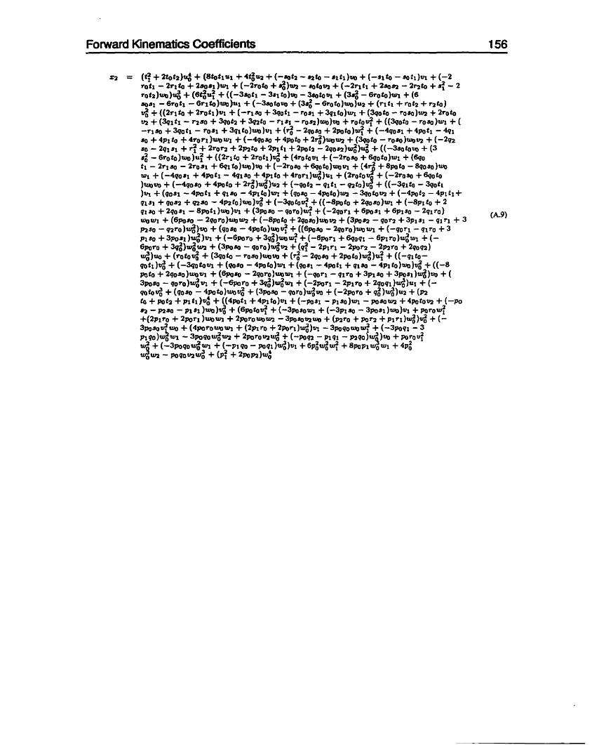
Forwarû Kinemab'cs Coefficients

Forward Kinematics Coefficients

Forward Kinematics Coefficients

F o rward Kinematics Coefficients

Fo ward Kinematics Coefficients

Forward Kinernatics Coefficients

Forward Kinematics Coefficients

Forward Kinematics Coefficients

Foward Kinematics Coefficients

Forward Kinematics Coefficients

Forward Kinematics Coefficients

Forward Kinernatics Coefficients

Fo rward Kinematics Coefficients

Forward Kinematics Coefficients

Forward Kinematics Coefficients

Forward Kinernatics Coefficients

Foward Kinematics Coefficients

Fonnrard Kinematics Coefficients 1 77

Forward Kinernatics Coefficients

Forward Kinematics Coefficients 1 79

Foruuard Kinematics Coefficients

Forward Kinematics Coefficients 1 84

Fo rward Kinematics Coefficients

Forward Kinematics Coefficients

Forward Kinematics Coefficients

Fotward Kinematics Coefficients

Fonnrard Kinernatics Coefficients

Forward Kinematics Coefficients

IMAGE NALUATION TEST TARGET (QA-3)

APPLIED 1 INIAGE . lnc 1653 East Main Street - -. - Rochester. NY 14609 USA -- ,==> Phone: 71 61482-0300 -- --= Fax: 716/28&5989