Marine Ecology Spatial Distribution of Oceanographic Properties, Phytoplankton, Nutrients and...
315
Transcript of Marine Ecology Spatial Distribution of Oceanographic Properties, Phytoplankton, Nutrients and...


Marine Ecology

Spatial Distribution of Oceanographic Properties,Phytoplankton, Nutrients and Coloured DissolvedOrganic Matter (CDOM) in the Boka KotorskaBay (Adriatic Sea)
A. Campanelli1, M. Cabrini2, F. Grilli1, Z. Kljajic3, E. Paschini1, P.Penna1, M. Marini11, Institute of Marine Sciences, CNR, Ancona, Italy2, National Institute of Oceanography and Experimental Geophysics, Trieste, Italy3, Institute of Marine Biology Kotor Dobrota, Kotor, [email protected]
Abstract
The temporal variations of temperature, salinity, fluorescence, dissolved oxygenconcentration, Coloured Dissolved Organic Matter (CDOM) and of chemical (nu-trients, chlorophyll a) and biological (phytoplankton composition) parameters in theBoka Kotorska Bay were observed during two periods (May and June 2008). CDOMregulates the penetration of UV light into the sea and therefore plays an importantrole in many hydrological and biogeochemical processes on the sea surface layer in-cluding primary productivity.In the framework ADRICOSM-STAR it was possible to investigate the Boka Ko-torska Bay during May and June 2008 in order to increase the understanding of opti-cal and chemical characteristics and their evolution through these periods.Owing to the Karst river inputs and the reduced water exchange with the open sea,in both periods station KO (located furthest from the open sea) presented differentphysical, chemical and biological characteristics with respect to the other stationsinside the Boka Kotorska Bay.A positive correlation was found between CDOM and chlorophyll a (R=0.7, P<0.001,n=15) and this implies that in this area, similarly to the open sea, the primary sourceof CDOM should be the biological production from phytoplankton. This is proba-bly due to the fact that the rivers entering the Boka Kotorska Bay are not severelyimpacted by man.
1 Introduction
Light entering the ocean is absorbed bywater, living and detrital particles, anddissolved materials (< 0.2 µm). Ab-sorption by the latter component, alsoknown as coloured dissolved organic mat-
ter (CDOM), is mostly attributable to hu-mic substances.It is well known, that the abundance anddistribution of CDOM for many coastalwaters is dominated by terrestrial inputsfrom rivers and runoff as decompositionof terrestrial organic matter yields light-

Marine Ecology
absorbing compounds such as, humic andfulvic acids [1, 2, 3]. In particular, CDOMis produced near the surface of the openocean as a result of a heterotrophic pro-cess [4, 5, 6, 7] and is destroyed by so-lar bleaching in stratified waters [8, 9, 10,11, 3]. The optical properties of CDOMare (almost) never completely eliminatedby solar bleaching or other natural pro-cesses, suggesting a pool of CDOM that isat least partially resistant to solar bleach-ing and microbial degradation. CDOMregulates the penetration of UV light intothe sea and mediates photochemical reac-tions, therefore playing an important rolein many biogeochemical processes on theocean surface including primary produc-tivity and the air-sea exchange of radia-tively important trace gases (e.g. [12, 13,14, 15]). The absorption of blue light byCDOM overlaps the phytoplankton absorp-tion peak near 440 nm, resulting in a com-petition between CDOM and phytoplank-ton for light in this region of visible spec-trum [16, 17, 18]. To better character-ize the relationship between phytoplanktonbiomass and the absorption by dissolvedmaterials, CDOM absorption coefficientsaCDOM (λ) have been compared withchlorophyll concentrations [19, 17]. Sig-nificant correlations between chlorophyll aand aCDOM (λ) have been observed in eu-trophic waters [20]. Generally, however,aCDOM (λ) does not covary linearly withinstantaneous estimates of pigment con-centrations or phytoplankton productivityin coastal regions [4]. Bricaud et al. [19]hypothesized that such a covariation mightexist if biological activity was averagedover a seasonal time period.The Boka Kotorska bay is a semi-enclosedbasin situated in the south-eastern Adri-atic sea (Mediterrean Sea - Montenegro),sometimes called Europe’s southernmost
fjord. Boka Kotorska bay represents adrowned valley shaped during the Plioceneperiod continued later by tectonic down-warping. Kotor and Risan bays are char-acterized by karstic rivers and undergroundsprings, which influence temperature, den-sity and salinity of sea water ([21] Klja-jic, personal data). The freshwater runofffrom these rivers probably modifies the op-tical and biochemical properties of seawa-ter during the different seasons.The enrichment of water with nutrientsprimarily nitrogen, silicate and phospho-rus might result in algal biomass growth.In particular, light and nutrient levels inthe surface layer were sufficient to sus-tain active phytoplankton growth in simi-lar basins, but if there is a short residencetime of the surface water this means thatmost of this production can be exportedto the outer basin [22]. The nutrients cancome from land surface runoff within awatershed (rivers and underground waterdischarges) and from direct urban inputs(sewage treatment plant outflows, indus-trial and storm water drains).Variations in the stratification regimes andmixing depths in basins of this type haveinteresting effect on phytoplankton growth.However, Mikee et al. [22] found that highCDOM content in fresh water runoff wasthe most obvious factor limiting productionin a fjord situated on the west coast of Scot-land. They found that if CDOM concen-trations in the surface layer were reducedthen the euphotic zone would extend to thebottom and conditions would be favourablefor substantial growth of the phytoplanktonpopulation.The aim of the present study is to under-stand and assess the optical biochemicaland biological characteristics and their evo-lutions throughout May and June in theBoka Kotorska bay characterized by fresh
4
Marine research at CNR
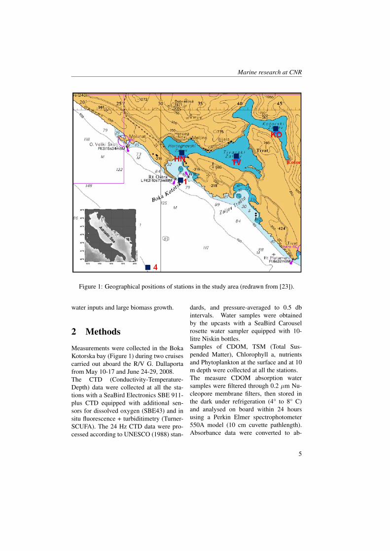
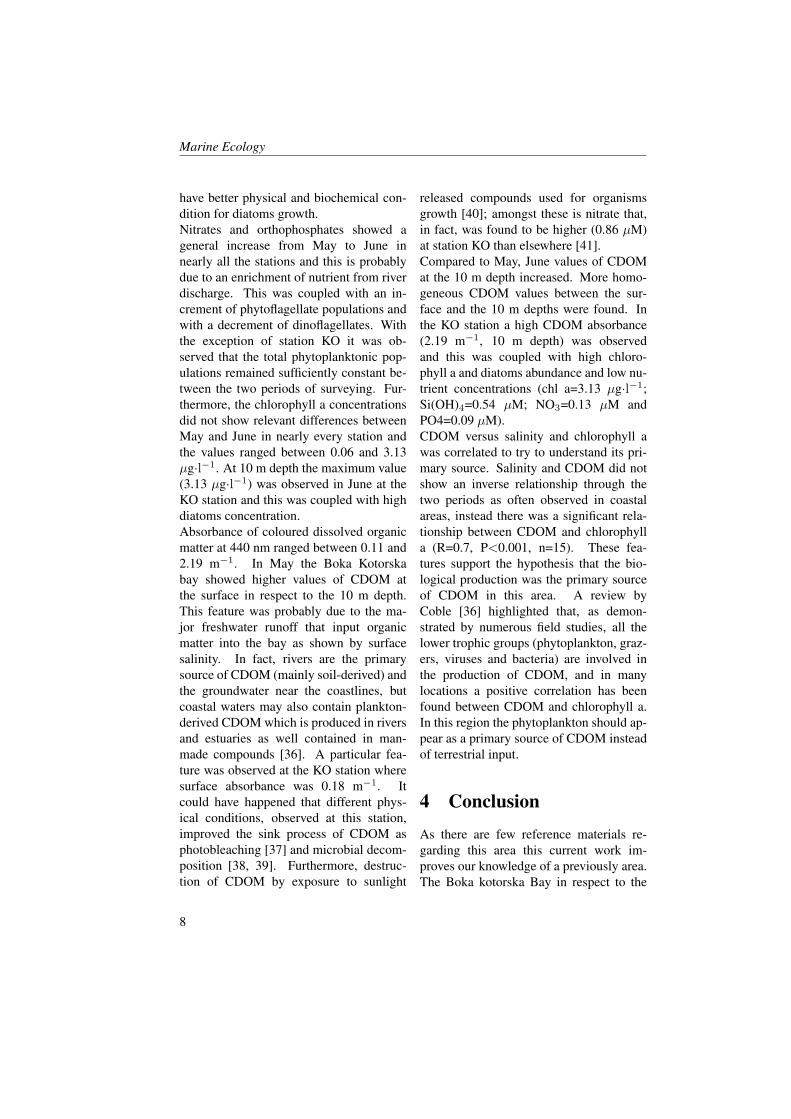
Figure 1: Geographical positions of stations in the study area (redrawn from [23]).
water inputs and large biomass growth.
2 Methods
Measurements were collected in the BokaKotorska bay (Figure 1) during two cruisescarried out aboard the R/V G. Dallaportafrom May 10-17 and June 24-29, 2008.The CTD (Conductivity-Temperature-Depth) data were collected at all the sta-tions with a SeaBird Electronics SBE 911-plus CTD equipped with additional sen-sors for dissolved oxygen (SBE43) and insitu fluorescence + turbiditimetry (Turner-SCUFA). The 24 Hz CTD data were pro-cessed according to UNESCO (1988) stan-
dards, and pressure-averaged to 0.5 dbintervals. Water samples were obtainedby the upcasts with a SeaBird Carouselrosette water sampler equipped with 10-litre Niskin bottles.Samples of CDOM, TSM (Total Sus-pended Matter), Chlorophyll a, nutrientsand Phytoplankton at the surface and at 10m depth were collected at all the stations.The measure CDOM absorption watersamples were filtered through 0.2 µm Nu-cleopore membrane filters, then stored inthe dark under refrigeration (4° to 8° C)and analysed on board within 24 hoursusing a Perkin Elmer spectrophotometer550A model (10 cm cuvette pathlength).Absorbance data were converted to ab-
5
Marine Ecology
sorption coefficient (aCDOM) accordingto Mitchell et al. [24]:
aCDOM(λ) = (2.303 · l−1)·
·[ABs(λ) − ABbs(λ) − ABnull(λ)],
where l is the cuvette pathlength, ABs(λ)is the optical density of the filtrate samplerelative to purified water, ABbs(λ) is opti-cal density of a purified water blank treatedlike a sample relative to purified water, andABnull(λ) is the apparent residual opticaldensity at a long visible or near infraredwavelength where absorption by dissolvedmaterial is assumed to be zero.For TSM measurements, 1litre of theseawater sample was filtered into a pre-weighed 47 mm GF/F Whatman filter (0.7µm). The filter was rinsed with 25-30 mlof deionised water to remove salt crystals,then dried at 60°C and weighed [25].Chlorophyll a was measured by filtering3l samples through 47 mm GF/F filters andimmediately extracted with 5 ml of acetoneat –22 °C. The analysis were made, in theISMAR-CNR laboratory, with a DionexHPLC equipped with a gradient pumpGP50, Photodiode Array Detector PDA100(wavelength range: 190–800 nm), C18 re-versed phase column (4.6 mm x 250 mm, 5µm particle size), AS50 Autosampler and300 µl sample injection loop. Pigment con-centrations were determined employing amodification of the procedure developedby Wrighit et al. [26].Nutrient samples were filtered (GF/FWhatman), stored at -20 °C in polyethy-lene vials and analysed in the ISMAR-CNR laboratory. The nutrients (nitrate-NO3, orthophosphate-PO4 and silicicacid-Si(OH)4) were analysed with aBran+Luebbe Autoanalyzer QUAATROsystem, and the resulting data processedwith AACE 6.0 (Automated Analyzer Con-
trol and Evaluation) software. Nutrientconcentrations were determined employ-ing a modification of procedures developedby Strickland and Parsons [25].Microphytoplankton samples (250 ml)were fixed with Ca(HCO3)2 bufferedformaldehyde (4% final concentra-tion). Samples were processed usingsedi-mentation chambers according toUtermohl [27, 28] and observed with alight inverted microscope in order to deter-mine and count all the cells.
3 Results and Discussion
3.1 Hydrography
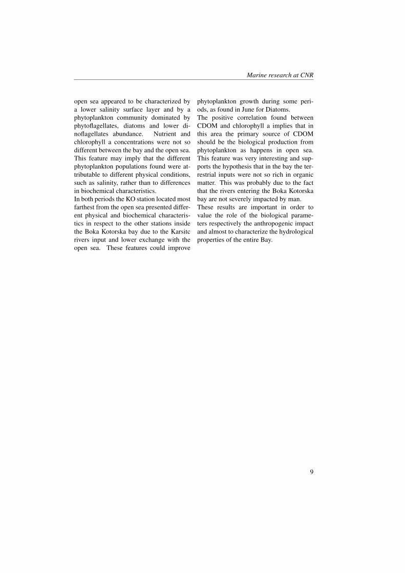
Figures 2 and 3 show profiles of the tem-perature, salinity, dissolved oxygen andfluorescence concentrations for the fourstations inside the Boka Kotorska bay (KO,TV, HN and 1) and for one station (station4) in the open sea during the two cruises. InMay, temperature and salinity levels, in allfour sites inside the bay, were comparable.However, the KO station compared to theother stations showed a higher temperature(18 °C) and less salinity water (28.5) in thefirst five metres. The KO station was influ-enced by river runoff, as the other stationsinside the bay, but it was the station fur-thest from the open sea and this probablyinfluenced mixing processes along the wa-ter column. Furthermore, the fluorescenceand oxygen concentrations showed manymore differences between KO station andall the other stations.TV, HN and 1 stations showed nearly thesame oxygen saturation and fluorescenceconcentration profiles. Fluorescence washomogeneous in the entire water column(0.7-0.8 A.U.) with a slight increase on thebottom layer (0.9-1 A.U.). However the
6
Marine research at CNR
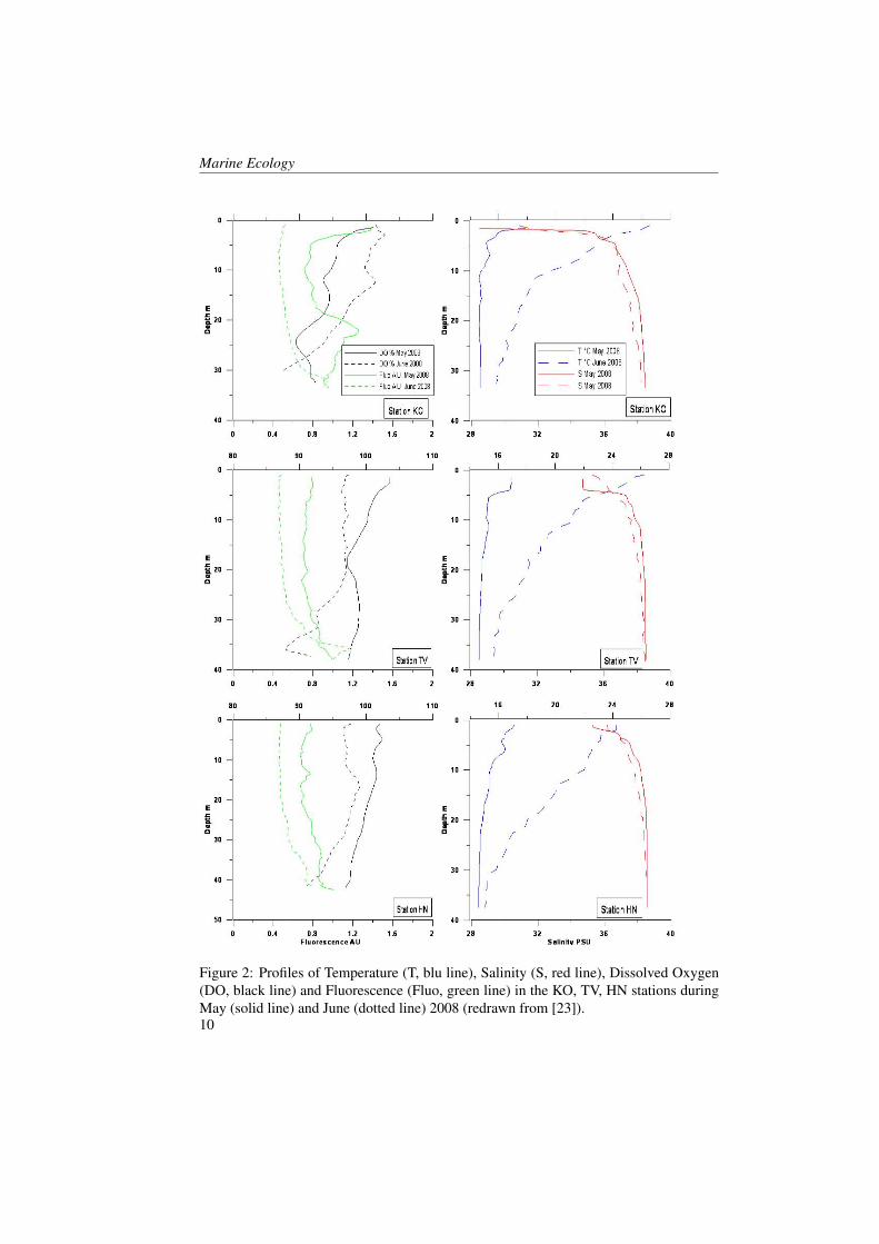
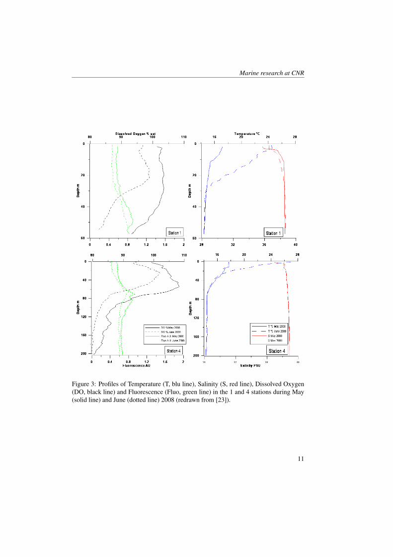
oxygen saturation showed an opposite pat-tern by decreasing near the bottom.KO station was the only one that showedhigh values of fluorescence at the surface(1.4 A.U.) in correspondence to the maxi-mum of oxygen (101 %), and in the middlelayer (1.2 A.U. at 22 m depth) coupled withthe minimum oxygen values (89.4 % at 25m depth). The minimum of oxygen satura-tion below the layer of the maximum of thefluorescence indicated a probable predomi-nance of mineralization process rather thana primary production process and the ab-sence of important vertical mixing.The waters occurring in station 4 (Figure3) showed the same charateristics of theAdriatic coastal waters. Salinity was con-stant enough from the surface to the bot-tom with a slight increase along the watercolumn (from 38 to 38.8). A surface layerbegan warming as expected in this period[29, 30, 31]. Fluorescence and oxygen pro-files showed the maximum values at 50-80m where light conditions were good for theprimary production [32, 33].In June, the temperature increased in all thefive stations in particular the 30 m layerfrom the surface. This increase in respectto previous period was around 7 °C (in HNand 1 station) and 9 °C (in TV and 4 sta-tion). The salinity increased at the sur-face by only 1-2 points in all the stationsand this was probably due to the poor riverrunoff in the summer period.The oxygen saturation presented lower val-ues (less than 5-10 %) compared to Maybecause during the summer period the ver-tical mixing was normally reduced [34].The KO station showed some differencesin respect to the other ones. Oxygen satu-ration increased to 7-8 % in respect to May.This increment was coupled with the fluo-rescence concentration decrease and it wasnot probably imputable to the primary pro-
duction.In respect of May, more changed were ob-served in fluorescence and oxygen satura-tion at the KO, TV and HN stations. Inparticular, the KO station showed, as ob-served in May, major differences in respectto the other stations.
3.2 CDOM, Biochemical andBiological characteristics
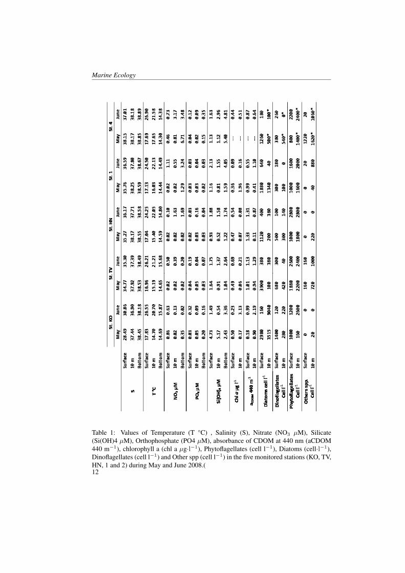
Table 1 shows the values of CDOM andbiochemical parameters (nutrients, chloro-phyll a) and phytoplankton (phytoflagel-lates, diatoms, dinoflagellates and othersnanoflagellates) in the two months.Microplankton community was dominatedby diatoms, nanoflagellates both au-totrophic and heterotrophic and dinoflag-ellates with lower abundances but highspecific diversity, as previous observa-tions documented by Vuksanovich and Kri-vokapic [35] in Boka Kotorska Bay.The nutrient and phytoplankton concentra-tions showed a different distribution at theKO station compared to the others. Inparticular, orthosilicate concentrations anddiatom abundances showed different pat-terns. In May, the silicate concentrationswere about 5 µM at the KO station cou-pled with a diatom abundance of about3000-3500 cell·l−1. In June an incrementof cell number of diatoms at the 10 mdepth (9040 cell·l−1) and an uptake of or-thosilicates that reduced to 0.54 µM wasobserved. The other stations inside thebay and in open sea showed opposite be-haviour. In these stations, the orthosilicateconcentrations increased by about 1 µM inrespect to May and the diatom concentra-tions reduced drastically (e.g. from 3900cell·l−1to 380 cell·l−1 at the surface of theTV station). In June the Kotor bay seems to
7
Marine Ecology
have better physical and biochemical con-dition for diatoms growth.Nitrates and orthophosphates showed ageneral increase from May to June innearly all the stations and this is probablydue to an enrichment of nutrient from riverdischarge. This was coupled with an in-crement of phytoflagellate populations andwith a decrement of dinoflagellates. Withthe exception of station KO it was ob-served that the total phytoplanktonic pop-ulations remained sufficiently constant be-tween the two periods of surveying. Fur-thermore, the chlorophyll a concentrationsdid not show relevant differences betweenMay and June in nearly every station andthe values ranged between 0.06 and 3.13µg·l−1. At 10 m depth the maximum value(3.13 µg·l−1) was observed in June at theKO station and this was coupled with highdiatoms concentration.Absorbance of coloured dissolved organicmatter at 440 nm ranged between 0.11 and2.19 m−1. In May the Boka Kotorskabay showed higher values of CDOM atthe surface in respect to the 10 m depth.This feature was probably due to the ma-jor freshwater runoff that input organicmatter into the bay as shown by surfacesalinity. In fact, rivers are the primarysource of CDOM (mainly soil-derived) andthe groundwater near the coastlines, butcoastal waters may also contain plankton-derived CDOM which is produced in riversand estuaries as well contained in man-made compounds [36]. A particular fea-ture was observed at the KO station wheresurface absorbance was 0.18 m−1. Itcould have happened that different phys-ical conditions, observed at this station,improved the sink process of CDOM asphotobleaching [37] and microbial decom-position [38, 39]. Furthermore, destruc-tion of CDOM by exposure to sunlight
released compounds used for organismsgrowth [40]; amongst these is nitrate that,in fact, was found to be higher (0.86 µM)at station KO than elsewhere [41].Compared to May, June values of CDOMat the 10 m depth increased. More homo-geneous CDOM values between the sur-face and the 10 m depths were found. Inthe KO station a high CDOM absorbance(2.19 m−1, 10 m depth) was observedand this was coupled with high chloro-phyll a and diatoms abundance and low nu-trient concentrations (chl a=3.13 µg·l−1;Si(OH)4=0.54 µM; NO3=0.13 µM andPO4=0.09 µM).CDOM versus salinity and chlorophyll awas correlated to try to understand its pri-mary source. Salinity and CDOM did notshow an inverse relationship through thetwo periods as often observed in coastalareas, instead there was a significant rela-tionship between CDOM and chlorophylla (R=0.7, P<0.001, n=15). These fea-tures support the hypothesis that the bio-logical production was the primary sourceof CDOM in this area. A review byCoble [36] highlighted that, as demon-strated by numerous field studies, all thelower trophic groups (phytoplankton, graz-ers, viruses and bacteria) are involved inthe production of CDOM, and in manylocations a positive correlation has beenfound between CDOM and chlorophyll a.In this region the phytoplankton should ap-pear as a primary source of CDOM insteadof terrestrial input.
4 Conclusion
As there are few reference materials re-garding this area this current work im-proves our knowledge of a previously area.The Boka kotorska Bay in respect to the
8
Marine research at CNR
open sea appeared to be characterized bya lower salinity surface layer and by aphytoplankton community dominated byphytoflagellates, diatoms and lower di-noflagellates abundance. Nutrient andchlorophyll a concentrations were not sodifferent between the bay and the open sea.This feature may imply that the differentphytoplankton populations found were at-tributable to different physical conditions,such as salinity, rather than to differencesin biochemical characteristics.In both periods the KO station located mostfarthest from the open sea presented differ-ent physical and biochemical characteris-tics in respect to the other stations insidethe Boka Kotorska bay due to the Karsitcrivers input and lower exchange with theopen sea. These features could improve
phytoplankton growth during some peri-ods, as found in June for Diatoms.The positive correlation found betweenCDOM and chlorophyll a implies that inthis area the primary source of CDOMshould be the biological production fromphytoplankton as happens in open sea.This feature was very interesting and sup-ports the hypothesis that in the bay the ter-restrial inputs were not so rich in organicmatter. This was probably due to the factthat the rivers entering the Boka Kotorskabay are not severely impacted by man.These results are important in order tovalue the role of the biological parame-ters respectively the anthropogenic impactand almost to characterize the hydrologicalproperties of the entire Bay.
9
Marine Ecology
Figure 2: Profiles of Temperature (T, blu line), Salinity (S, red line), Dissolved Oxygen(DO, black line) and Fluorescence (Fluo, green line) in the KO, TV, HN stations duringMay (solid line) and June (dotted line) 2008 (redrawn from [23]).10
Marine research at CNR
Figure 3: Profiles of Temperature (T, blu line), Salinity (S, red line), Dissolved Oxygen(DO, black line) and Fluorescence (Fluo, green line) in the 1 and 4 stations during May(solid line) and June (dotted line) 2008 (redrawn from [23]).
11
Marine Ecology
Table 1: Values of Temperature (T °C) , Salinity (S), Nitrate (NO3 µM), Silicate(Si(OH)4 µM), Orthophosphate (PO4 µM), absorbance of CDOM at 440 nm (aCDOM440 m−1), chlorophyll a (chl a µg·l−1), Phytoflagellates (cell l−1), Diatoms (cell·l−1),Dinoflagellates (cell l−1) and Other spp (cell l−1) in the five monitored stations (KO, TV,HN, 1 and 2) during May and June 2008.(12
Marine research at CNR
References[1] N.K. Højerslev. Yellow substance in the Sea. The Role of Solar Ultraviolet Radia-
tion in Marine Ecosystems, pages 263–281, 1982.
[2] K.L. Carder, R.G. Steward, G.R. Harvey, and P.B. Ortner. Marine humic and fulvicacids: Their effects on remote sensing of ocean chlorophyll. Limnol. Oceanogr.,34:68–81, 1989.
[3] R. Del Vecchio, N.V., and Blough. Spatial and seasonal distribution oh chro-mophoric dissolved organic matter (CDOM) and dissolved organic carbon (DOC)in the Middle Atlantic Bight. Mar. Chem., 66:35–51, 2004.
[4] N.B. Nelson, D.A. Siegel, and A.F. Michaels. Seasonal dynamics of coloured dis-solved organic material in the Sargasso Sea. Deep Sea Res. I, 45:931–957, 1998.
[5] N.B. Nelson, C.A. Carlson, and D.K. Steinberg. Production of chromophoric dis-solved organic matter by Sargasso Sea microbes. Mar. Chem., 89:273–287, 2004.
[6] D.K. Steinberg, N.B. Nelson, and C.A. Carlson. Production of dissolved chro-mophoric dissolved organic matter (CDOM) in the open ocean by zooplankton andthe colonial cyanobacterium Tricodesmium spp. Mar. Ecol. Prog. Ser., 267:45–56,2004.
[7] Y. Yamaschita and E. Tanoue. In situ production of chromophoric dissolved organicmatter in coastal environment. Geophys. Res. Lett., 31(L24302), 2004.
[8] S. Determan, R. Reuter, and R. Willkomm. Fluorescent matter in the eastern At-lantic Ocean. Part. 2: vertical profiles and relation to water masses. Deep Sea Res.I, 43:345–360, 1996.
[9] A. Vodacek, N.V. Blough, M.D. DeGrandpre, E.T. Peltzer, and R.K. Nelson. Sea-sonal variation of CDOM and DOC in the Middle Atlantic Bight: Terrestrial inputsand photooxidation. Limnol. Oceanogr., 42:674–686, 1997.
[10] D.A. Siegel, S. Maritorema, N.B. Nelson, D.A. Hansell, and M. Lorenzi-Kayser.Global distribution and dynamics of colored dissolved and detrital organic materi-als. J. Geophys. Res., 107(C12):3228, 2002.
[11] D.A. Siegel, S. Maritorema, N.B. Nelson, and M.J. Behrenfeld. Independence andinterdependencies among global ocean color properties: Reassessing the bio-opticalassumption. J. Geophys. Res., 110(C07011), 2005.
[12] K. Mopper, X.L. Zhou, R.J. Kieber, D.J. Kieber, R.J. Sikorski, and R.D. Jones. Pho-tochemical degradation of dissolved organic carbon and its impact on the oceaniccarbon cycle. Nature, 353:60–62, 1991.
13
Marine Ecology
[13] K.R. Arrigo and C.W. Brown. The impact of chromophoric dissolved organic matteron UV inhibition of primary productivity in the open ocean. Mar. Ecol. Prog. Ser.,140:207–216, 1996.
[14] R.G. Zepp, T.V. Callaghan, and D.J. Erickson. Effect of enhanced ultraviolet radi-ation on biogeochemical cycles. J. Photoch. Photobio. B, 46:69–82, 1998.
[15] D.A. Toole and D.A. Siegel. Light-driven cycling of dimethilsulfide (DMS) in theSargasso Sea: closing the loop. Geophys. Res. Lett., 31(L09308), 2004.
[16] T.J. Wrigley, J.M. Chambers, and A.J. McComb. Nutrient and gilvin levels in wa-ters of coastal-plain wetlands in an agricultural area of western Australia. Aust. J.Mar. Freshwater Res., 39:685–694, 1988.
[17] R.J. Davies-Colley. Yellow substance in coastal and marine waters round the southisland, New Zealand, N. Z. J. Mar. Freshwater Res., 26:311–322, 1992.
[18] J.T.O. Kirk. Light and Photosynthesis in Aquatic Ecosystems. pages 1–508, 1994.
[19] A. Bricaud, A. Morel, , and L. Prieur. Aborpion by dissolved organic matter in thesea (yellow substance in the UV and visible domains. Limnol. Oceanogr., 28:45–53,1981.
[20] O.V. Kopelevich, Burenkov, and V.I. Relation between the spectral values of thelight absorption coefficients of sea water, phytoplankton pigments, and the yellowsubstance. Oceanology, 17:278–282, 1977.
[21] V. Lepetic. Composition and seasonal dynamics of ichthyobenthos and edible in-vertebrata in bay of Boka Kotorska and possibilities of their exploitation. StudiaMarina, 1:1–128, 1965.
[22] D. Mickee, A. Cunningham, and K.J. Jones. Optical and hydrographic conse-quences of freshwater run-off during spring phytoplankton growth in a Scottishfjord. J. Plankton Res., 24(11):1163–1171, 2002.
[23] A. Campanelli, A. Bulatovic, M. Cabrini, F. Grilli, Z. Kljajic, R. Mosetti, E. Pas-chini, P. Penna, and M. Marini. Spatial distribution of physical, chemical and bio-logical oceanograohic properties, Phytoplankton, nutrients and Coloured DissolvedOrganic Matter (CDOM) in the Boha Kotorska Bay (Adriatic Sea). Geofizika, 26,2009.
[24] B.G. Mitchell, M. Kahru, J. Wieland, , and M. Stramska. Determination of spec-tral absorption coefficient of particles, dissolved material and phytoplankton fordiscrete water samples. pages 39–64, 2003.
[25] D.H. Strickland and T.R. Parsons. A practical handbook of seawater analysis. Bull.Fish. Res., 167:1–310, 1972.
14
Marine research at CNR
[26] S.W. Wrighit, S.W. Jeffrey, R.F.C. Mantoura, C.A. Llewellyn, T. Bjornland,D. Repeta, and N. Welschmeyer. Improved HPLC method for the analysis ofchlorophylls and carotenoids from marine phytoplankton. Mar. Ecol. Prog. Ser.,77:183–196, 1991.
[27] H. Uternohl. Zur Vervolikommunung der quantitative Phytoplankton. Methodik.Mitt. Int. Ver. Theor. Angew. Limnol., 9:1–38, 1958.
[28] A. Zingone, G. Honsell, D. Marino, M. Montresor, and G. Socal. Nova Thalassia.pages 183–198, 1990.
[29] A. Russo and A. Artegiani. Adriatic Sea Hydrography. Sci. Mar., 60(2):33–43,1996.
[30] A. Artegiani, D. Bregant, E. Paschini, N. Pinardi, F. Raicich, and A. Russo. TheAdriatic Sea General circulation. Part I: Air-Sea Interactions and Water Mass Struc-ture. J. Phys. Oceanogr., 27:1515–1532, 1997.
[31] A. Artegiani, D. Bregant, E. Paschini, N. Pinardi, F. Raicich, and A. Russo. TheAdriatic Sea General circulation. Part II: Baroclinic Circulation Structure. J. Phys.Oceanogr., 27:1492–1514, 1997.
[32] G. Socal, A. Boldrin, F. Bianchi, G. Civitarese, A. De Lazzari, S. Rabitti, C. Totti,and M.M. Turchetto. Nutrient, parti culate matter and phytoplankton variabilita inthe photic layer of the Otranto strait. J. Mar. Syst., 20:381–398, 1999.
[33] M. Zavatarelli, F. Raicich, D. Bregant, A. Russo, and A. Artegiani. Climatologicalbiogeochemical caracteristics of the Adriatic Sea. J. Mar. Syst., 18:227–263, 1998.
[34] M. Olsen, C. Laundsgaard, and A. Andrushaitis. Influence of nutrients and mixingon the primary production and community respiration in the Gulf of Riga. J. Mar.Sys., 23:127–143, 1998.
[35] N. Vuksanovic and S. Krivokapic. Prilog poznavaviv fitoplaktona Kotorskog zalivau zimskoi sezoni 2004. Zbornik Radova, pages 347–350, 2005.
[36] P.G. Coble. Marine Optical Biochemistry: the Chemistry of Ocean Color. Chem.Rev., 107(2):402–418, 2007.
[37] K. Mopper and D.J. Kieber. Marine Photochemistry and its impact on CarbonCycling. 2000.
[38] M.A. Moran, W.M. Sheldon, and R.G. Zepp. Carbon loss and optical propertychanges during long-term photochemical and biological degradation of estuarinedissolved organic matter. Limnol. Oceanogr., 45(6):1254–1264, 2000.
[39] T.J. Boyd and C.L. Osburn. Changes in CDOM fluorescence from allochthonousand autochthonous sources during tidal mixing and bacterial degradation in twocoastal estuaries. 89(1-4):189–210, 2004.
15
Marine Ecology
[40] W.L. Miller and M.A. Moran. Interaction of photochemical and microbial processesin the degradation of refractory dissolved organic matter from a coastal marineenvironment. Limnol. Oceanogr., 42(6):1317–1324, 1997.
[41] K. Mopper and D.J. Kieber. Photochemistry and the Cycling of Carbon Sulfur,Nitrogen and Phosphorus. 2002.
16
Coupled Analytical-Numerical Model of Fish Re-sponse to Environmental Changes
A. Cucco1, M. Sinerchia1, C. Le Francois2, P. Domenici1, P. Magni1, M.Ghezzo3, G. Umgiesser3, A. Perilli11, Institute for Coastal Marine Environment, CNR, Oristano, Italy2, University of La Rochelle, La Rochelle, France3, Institute of Marine Sciences, CNR, Venezia, [email protected]
Abstract
Eco-physiology studies, performed in laboratory under controlled conditions,provide an essential tool for quantifying the impact of environmental changes on themetabolism and behavior of individual fish. One way of quantifying such impact isby measuring the Metabolic Scope (MS) of a fish. Laboratory experiments were per-formed to calculate the MS of, textitMugil cephalus, under different environmentalconditions (temperature and oxygen). The equations derived were introduced intoan ecological model, which was then coupled to a high resolution hydrodynamicmodel. The model was calibrated for reproducing the environmental variability inthe Cabras lagoon and Gulf of Oristano (Italy). We used the model to reproduce thetemporal and spatial variation in MS of a textitM. cephalus fish population to inves-tigate the relationship between changes in MS and the observed seasonal migrationpattern between the gulf and lagoon. Results shows that during the spring-beginningof summer period Cabras lagoon provides a higher MS for textitM. cephalus than theGulf of Oristano. During the rest of the year, apart from some transitional phases, theGulf provides more suitable conditions (higher MS) for textitM. cephalus. Resultswere compared to fisheries data, showing that textitM. cephalus catches are highestduring the end-July to August period. This period was characterized by fish werecaught migrating from the lagoon into the Gulf and coincides with the reproduceddrop of MS for textitM. cephalus in the lagoon.
1 Introduction
Several studies show the potential ofchanges in the physical and chemical en-vironment in causing serious modifica-tions in marine and coastal ecosystems [1].Such changes influence directly the eco-physiological response of different levelsof the ecosystem [2]. In particular, the pro-gressive rise in temperature is thought to bea critical factor responsible for the migra-
tion of several fish species towards higherlatitudes [3], for the changes in the ecosys-tem trophic structure due to the reductionor total lack of food, for the sub-optimalgrowth rate and lower reproductive poten-tial [4]. In particular, the combined effectof the rise in temperature and reduction indissolved oxygen has the potential to causeserious changes in the ecosystem dynam-ics. The effect of environmental changeson the ecosystem status and dynamics (e.g.

Marine Ecology
biodiversity, productivity, trophic cascade,etc.) is amplified in shallow water environ-ments, such as coastal and lagoon areas, inparticular those characterized by slow wa-ter renewal [5]. A typical example of suchenvironments is represented by Mediter-ranean lagoons, rich in biodiversity and im-portant nurseries for several fish species,many of which having commercial valueand playing a fundamental role in the localeconomy [6]. The physical and chemicalcharacteristics of the water in these envi-ronments fluctuate in an irregular fashion,due to sea storms, intense rainfall or riveroverflows [7]. Eco-physiology studies, per-formed in laboratory under controlled con-ditions, provide the perfect tool for quanti-fying the impact, in terms of energetic bud-geting and fish behavior, of such changes.Quantification of the impact of environ-mental changes on the energetic budgetof a fish was performed by measuring itsMetabolic Scope, hereafter MS, [8]. TheMS of a fish represents its energetic poten-tial available to fuel all its activities (e.g.motion, digestion, reproduction, etc.), andprovides a way of estimating the energeticcost fish have to pay for adapting to en-vironmental changes. Results from stud-ies on the MS of individual fish providedthe bio-energetic basis for the constructionof a numerical model projecting the im-pact observed at individual level to popu-lation level. In particular, the model wasused to investigate how seasonal changesin temperature and oxygen concentration intwo adjacent shallow water environments,the Cabras lagoon and Oristano gulf, affecttextitmugil cephalus MS, which may ex-plain the observed migration between thetwo areas.
2 Site description
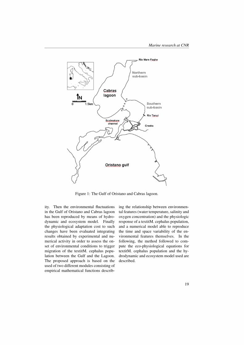
The Cabras lagoon is a shallow water body(mean depth 1.7 m) located on the westcoast of Sardinia, western MediterraneanSea (39 57’ N, 008 29’ E), and is oneof the largest brackish water basins in theMediterranean region with a surface of 22km2 (Figure 1). It is connected to theGulf of Oristano by a series of small creeksflowing into a main open channel, the Scol-matore. The lagoon is connected to twosmall rivers: Rio Mare Foghe, in the Northrepresenting the major source of freshwa-ter, and Rio Tanui in the South. River dis-charge is rather limited due to a low rain-fall regime in the region (about 10-100 mmfrom July to December, respectively). Thelagoon salinity may drop to less than 10psu during rainfall periods and rise to morethan 30 psu, especially in summer. Thetidal amplitude is less than 20 cm, mak-ing a very limited contribution to water ex-change between the lagoon and the gulf.The lagoon is subdivided into 2 sub-basins,a northern one and a southern one, with adifferent water circulation pattern and wa-ter residence time. Cabras Lagoon interactsdirectly with the Gulf of Oristano, which initself has a great economic value becauseis a nursery area for the most valuable fishspecies in the Lagoon [6].
3 Methods
In order to represent accurately the ef-fects of environmental changes on the eco-physiological response of fish several taskshave been performed. First of all the rela-tionship between changes in environmentalvariables, temperature and dissolved oxy-gen, and textitM. cephalus MS have beenestimated by means of experimental activ-
18
Marine research at CNR
Figure 1: The Gulf of Oristano and Cabras lagoon.
ity. Then the environmental fluctuationsin the Gulf of Oristano and Cabras lagoonhas been reproduced by means of hydro-dynamic and ecosystem model. Finallythe physiological adaptation cost to suchchanges have been evaluated integratingresults obtained by experimental and nu-merical activity in order to assess the on-set of environmental conditions to triggermigration of the textitM. cephalus popu-lation between the Gulf and the Lagoon.The proposed approach is based on theused of two different modules consisting ofempirical mathematical functions describ-
ing the relationship between environmen-tal features (water temperature, salinity andoxygen concentration) and the physiologicresponse of a textitM. cephalus population,and a numerical model able to reproducethe time and space variability of the en-vironmental features themselves. In thefollowing, the method followed to com-pute the eco-physiological equations fortextitM. cephalus population and the hy-drodynamic and ecosystem model used aredescribed.
19
Marine Ecology
3.1 Laboratory experiments
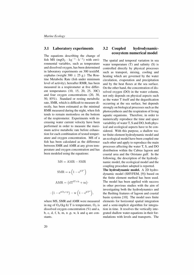
The equations describing the change offish MS (mgO2 · kg−1 · h−1) with envi-ronmental variables, such as temperatureand dissolved oxygen, has been determinedin laboratory experiments on 300 textitM.cephalus (weight 300 ± 25 g.) The Rou-tine Metabolic Rate (fish under minimumlevel of activity), hereafter RMR, has beenmeasured in a respirometer at five differ-ent temperatures (10, 15, 20, 25, 30C)and four oxygen concentrations (20, 30,50, 85%). Standard or resting metabolicrate, SMR, which is difficult to measure di-rectly, has been estimated as the minimalRMR measured during the night, when fishtends to remain motionless on the bottomof the respirometer. Experiments with in-creasing water current velocity have beenperformed in order to measure the maxi-mum active metabolic rate before exhaus-tion for each combination of tested temper-ature and oxygen concentration. MS of afish has been calculated as the differencebetween SMR and AMR at any given tem-perature and oxygen concentration and hasbeen modeled using the equations:
MS = AMR− SMR
SMR = a(1− ebTc
)AMR =
(dTfT+h + m
)·
·(1− enO2+p
)− w
(1− ekTq
),
where MS, SMR and AMR were measuredin mg of O2/(kg·h) T is temperature, O2 isdissolved oxygen concentration (%) and a,b, c, d, f, h, m, n ,p, w, k and q are con-stants.
3.2 Coupled hydrodynamic-ecosystem numerical model
The spatial and temporal variation in seawater temperature (T) and salinity (S) iscontrolled directly by physical processessuch as transport, mixing, cooling andheating which are governed by the watercirculation, evaporation and precipitationand by the heat fluxes at the sea surface.On the other hand, the concentration of dis-solved oxygen (DO) in the water column,not only depends on physical aspects suchas the water T itself and the degasificationoccurring at the sea surface, but dependsstrongly on biological processes such as thephotosynthesis and the respiration of livingaquatic organisms. Therefore, in order tonumerically reproduce the time and spacevariability of water T, S and DO, both phys-ical and ecological aspects have to be con-sidered. With this purpose, a shallow wa-ter finite element hydrodynamic model andan ecological model have been coupled oneeach other and apply to reproduce the mainprocesses affecting the water T, S, and DOdistribution within the Cabras lagoon andcoastal area and the Oristano gulf. In thefollowing, the description of the hydrody-namic model, the ecological model and thecoupling procedure adopted is reported.The hydrodynamic model. A 2D hydro-dynamic model (SHYFEM, [9]) based onthe finite element method has been used.The model has been applied with successin other previous studies with the aim ofinvestigating both the hydrodynamics andthe flushing features of lagoon and coastalbasin systems [10]. The model uses finiteelements for horizontal spatial integrationand a semi-implicit algorithm for integra-tion in time. It resolves the vertically inte-grated shallow water equations in their for-mulations with levels and transports. The
20

Marine research at CNR
Figure 2: MS as a function of temperature (T) and dissolved oxygen concentration (DO).Open circles represent observations, while the surface of the plot represents MS predictedby the model.
horizontal diffusion, the baroclinic pres-sure gradient and the advective terms inthe momentum equation are fully explic-itly treated. The Coriolis force and thebarotropic pressure gradient terms in themomentum equation and the divergenceterm in the continuity equation are semi-implicitly treated. The friction term istreated fully implicitly for stability reasons.The model is unconditionally stable whatconcerns the fast gravity waves, the bottomfriction and the Coriolis acceleration [9].The ecological model. The base eco-logical model used was the Biogeochem-ical Flux Model (hereafter BFM, [11], abiomass-based differential equation model.The model is built with respect to massconservation following a top-down ap-proach. The food web consists of func-tional groups. Each group is expressed bya set of state variables expressing chemi-cal content (C, N, P and SI), or molecules(Chl-a). The food-web was constitutedby primary producers (diatoms, 20-200 mESD, picophytoplankton, 2 m ESD, flagel-lates, 2-20 m ESD, and dinoflagellates, 20-200 m ESD), zooplankton (microzooplank-ton, heterotrophic nanoflagellates, carniv-
orous mesozooplankton and omnivororusmesozooplankton), bacteria, nutrients anddissolved chemical species for oxygen andthe carbonate system. Bacterioplanktonrepresent free-living, non-colonial bacte-ria that can switch from aerobic to anaer-obic metabolism according to the pelagicoxygen conditions. The nutrients includedin the model were: nitrite, nitrate, am-monium, orthophosphate and silicate, dis-solved bioavailable iron, oxygen, carbondioxide, dissolved and particulate (non-living) organic matter. The model simu-lates the evolution of up to 44 state vari-ables in the water column describing boththe main metabolic processes within eachfunctional group and the trophic interac-tions between functional groups. In par-ticular, carbon assimilation, nutrient up-take, lysis of primary producers, grazingby and of secondary producers, respira-tion, mortality excretion and exudation ofall organisms are modeled. We refer toVichi [11] for a detailed description of themodel structure and the adopted numericalmethod.
21
Marine Ecology
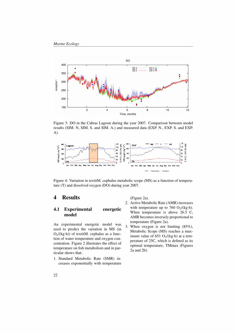
Figure 3: DO in the Cabras Lagoon during the year 2007. Comparison between modelresults (SIM. N, SIM. S. and SIM. A.) and measured data (EXP. N., EXP. S. and EXP.A).
Figure 4: Variation in textitM. cephalus metabolic scope (MS) as a function of tempera-ture (T) and dissolved oxygen (DO) during year 2007.
4 Results
4.1 Experimental energeticmodel
An experimental energetic model wasused to predict the variation in MS (inO2/(kg·h)) of textitM. cephalus as a func-tion of water temperature and oxygen con-centration. Figure 2 illustrates the effect oftemperature on fish metabolism and in par-ticular shows that:1. Standard Metabolic Rate (SMR) in-
creases exponentially with temperature
(Figure 2a).2. Active Metabolic Rate (AMR) increases
with temperature up to 760 O2/(kg·h).When temperature is above 26.5 C,AMR becomes inversely proportional totemperature (Figure 2a).
3. When oxygen is not limiting (85%),Metabolic Scope (MS) reaches a max-imum value of 651 O2/(kg·h) at a tem-perature of 25C, which is defined as itsoptimal temperature, TMmax (Figures2a and 2b).
22
Marine research at CNR
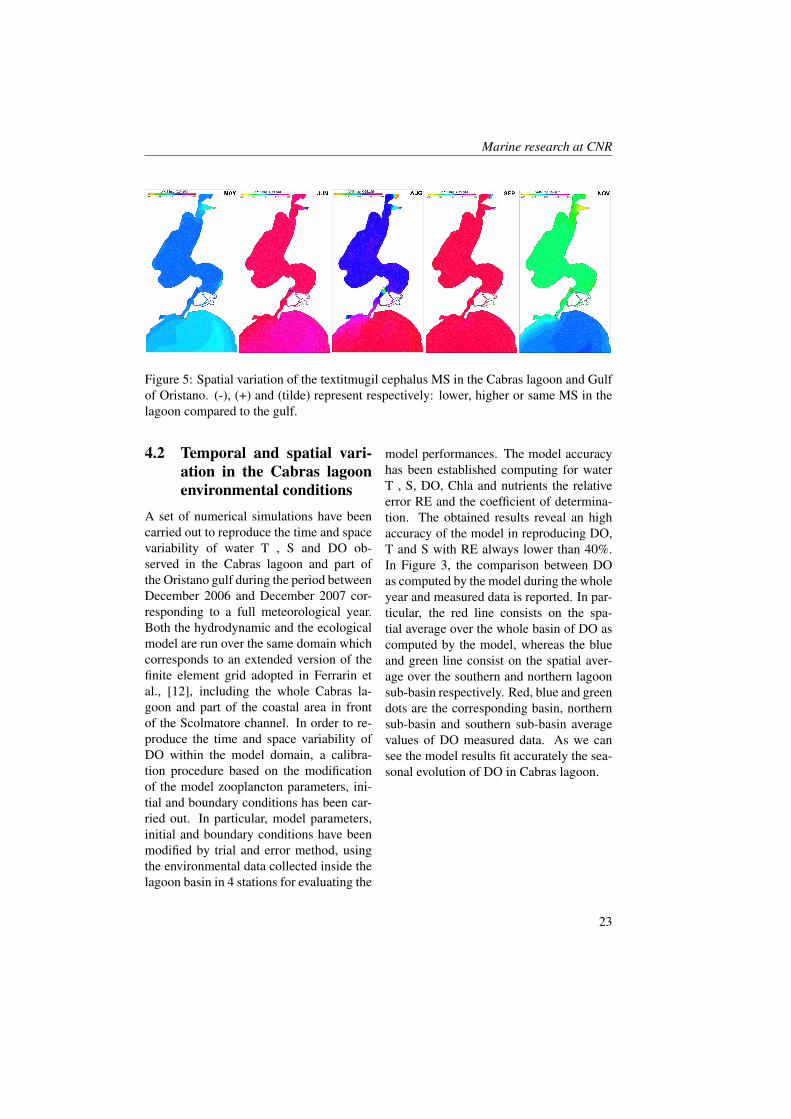
Figure 5: Spatial variation of the textitmugil cephalus MS in the Cabras lagoon and Gulfof Oristano. (-), (+) and (tilde) represent respectively: lower, higher or same MS in thelagoon compared to the gulf.
4.2 Temporal and spatial vari-ation in the Cabras lagoonenvironmental conditions
A set of numerical simulations have beencarried out to reproduce the time and spacevariability of water T , S and DO ob-served in the Cabras lagoon and part ofthe Oristano gulf during the period betweenDecember 2006 and December 2007 cor-responding to a full meteorological year.Both the hydrodynamic and the ecologicalmodel are run over the same domain whichcorresponds to an extended version of thefinite element grid adopted in Ferrarin etal., [12], including the whole Cabras la-goon and part of the coastal area in frontof the Scolmatore channel. In order to re-produce the time and space variability ofDO within the model domain, a calibra-tion procedure based on the modificationof the model zooplancton parameters, ini-tial and boundary conditions has been car-ried out. In particular, model parameters,initial and boundary conditions have beenmodified by trial and error method, usingthe environmental data collected inside thelagoon basin in 4 stations for evaluating the
model performances. The model accuracyhas been established computing for waterT , S, DO, Chla and nutrients the relativeerror RE and the coefficient of determina-tion. The obtained results reveal an highaccuracy of the model in reproducing DO,T and S with RE always lower than 40%.In Figure 3, the comparison between DOas computed by the model during the wholeyear and measured data is reported. In par-ticular, the red line consists on the spa-tial average over the whole basin of DO ascomputed by the model, whereas the blueand green line consist on the spatial aver-age over the southern and northern lagoonsub-basin respectively. Red, blue and greendots are the corresponding basin, northernsub-basin and southern sub-basin averagevalues of DO measured data. As we cansee the model results fit accurately the sea-sonal evolution of DO in Cabras lagoon.
23
Marine Ecology
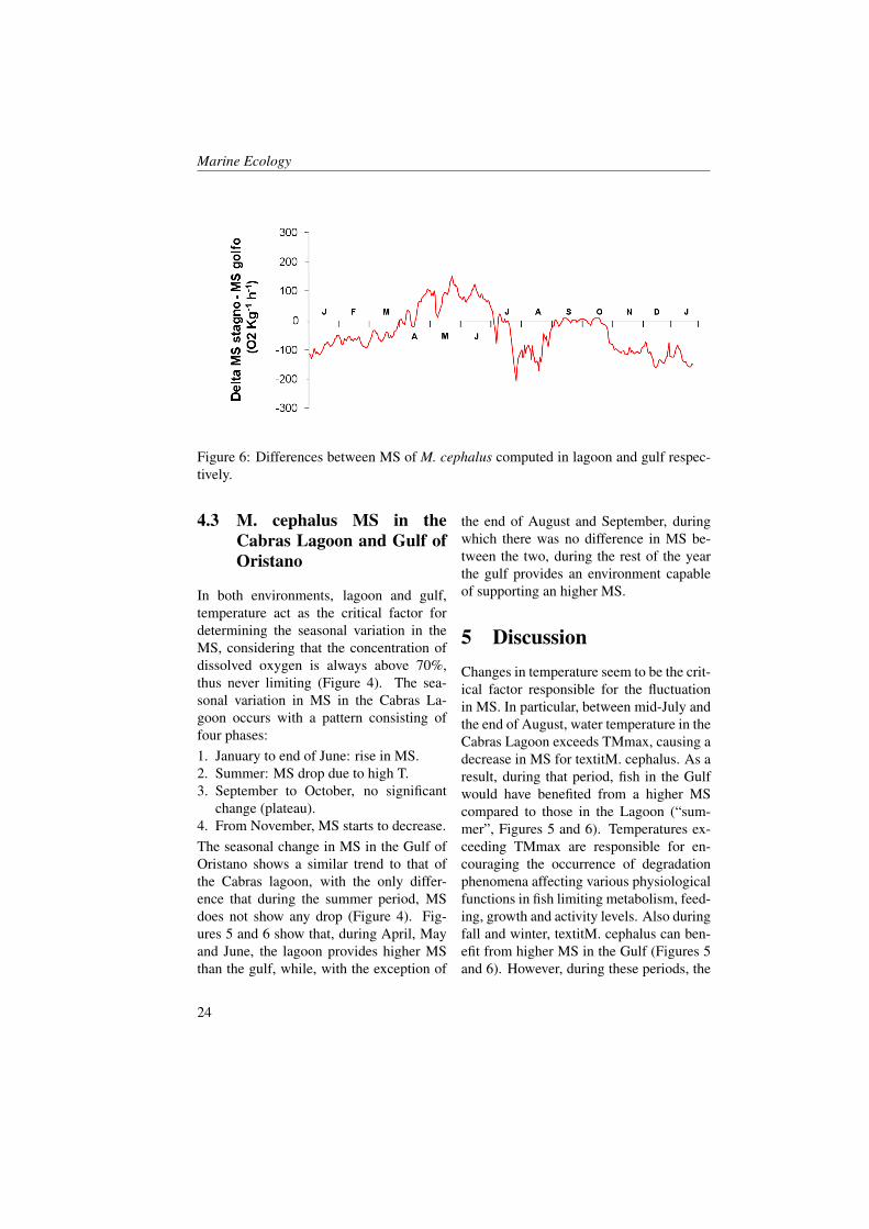
Figure 6: Differences between MS of M. cephalus computed in lagoon and gulf respec-tively.
4.3 M. cephalus MS in theCabras Lagoon and Gulf ofOristano
In both environments, lagoon and gulf,temperature act as the critical factor fordetermining the seasonal variation in theMS, considering that the concentration ofdissolved oxygen is always above 70%,thus never limiting (Figure 4). The sea-sonal variation in MS in the Cabras La-goon occurs with a pattern consisting offour phases:1. January to end of June: rise in MS.2. Summer: MS drop due to high T.3. September to October, no significant
change (plateau).4. From November, MS starts to decrease.The seasonal change in MS in the Gulf ofOristano shows a similar trend to that ofthe Cabras lagoon, with the only differ-ence that during the summer period, MSdoes not show any drop (Figure 4). Fig-ures 5 and 6 show that, during April, Mayand June, the lagoon provides higher MSthan the gulf, while, with the exception of
the end of August and September, duringwhich there was no difference in MS be-tween the two, during the rest of the yearthe gulf provides an environment capableof supporting an higher MS.
5 DiscussionChanges in temperature seem to be the crit-ical factor responsible for the fluctuationin MS. In particular, between mid-July andthe end of August, water temperature in theCabras Lagoon exceeds TMmax, causing adecrease in MS for textitM. cephalus. As aresult, during that period, fish in the Gulfwould have benefited from a higher MScompared to those in the Lagoon (“sum-mer”, Figures 5 and 6). Temperatures ex-ceeding TMmax are responsible for en-couraging the occurrence of degradationphenomena affecting various physiologicalfunctions in fish limiting metabolism, feed-ing, growth and activity levels. Also duringfall and winter, textitM. cephalus can ben-efit from higher MS in the Gulf (Figures 5and 6). However, during these periods, the
24
Marine research at CNR
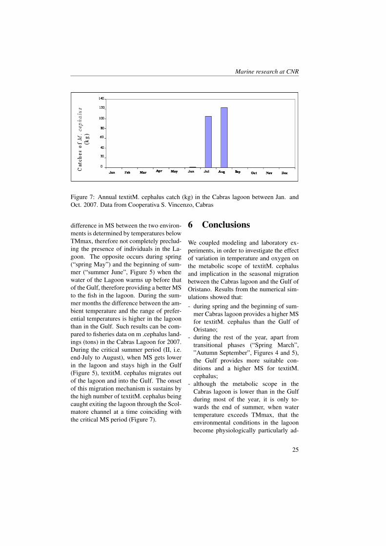
Figure 7: Annual textitM. cephalus catch (kg) in the Cabras lagoon between Jan. andOct. 2007. Data from Cooperativa S. Vincenzo, Cabras
difference in MS between the two environ-ments is determined by temperatures belowTMmax, therefore not completely preclud-ing the presence of individuals in the La-goon. The opposite occurs during spring(“spring May”) and the beginning of sum-mer (“summer June”, Figure 5) when thewater of the Lagoon warms up before thatof the Gulf, therefore providing a better MSto the fish in the lagoon. During the sum-mer months the difference between the am-bient temperature and the range of prefer-ential temperatures is higher in the lagoonthan in the Gulf. Such results can be com-pared to fisheries data on m .cephalus land-ings (tons) in the Cabras Lagoon for 2007.During the critical summer period (II, i.e.end-July to August), when MS gets lowerin the lagoon and stays high in the Gulf(Figure 5), textitM. cephalus migrates outof the lagoon and into the Gulf. The onsetof this migration mechanism is sustains bythe high number of textitM. cephalus beingcaught exiting the lagoon through the Scol-matore channel at a time coinciding withthe critical MS period (Figure 7).
6 Conclusions
We coupled modeling and laboratory ex-periments, in order to investigate the effectof variation in temperature and oxygen onthe metabolic scope of textitM. cephalusand implication in the seasonal migrationbetween the Cabras lagoon and the Gulf ofOristano. Results from the numerical sim-ulations showed that:- during spring and the beginning of sum-
mer Cabras lagoon provides a higher MSfor textitM. cephalus than the Gulf ofOristano;
- during the rest of the year, apart fromtransitional phases (“Spring March”,”Autumn September”, Figures 4 and 5),the Gulf provides more suitable con-ditions and a higher MS for textitM.cephalus;
- although the metabolic scope in theCabras lagoon is lower than in the Gulfduring most of the year, it is only to-wards the end of summer, when watertemperature exceeds TMmax, that theenvironmental conditions in the lagoonbecome physiologically particularly ad-
25
Marine Ecology
verse to fish;- changes in MS related to the seasonal
variation in temperature and oxygencould be a factor responsible for trigger-ing the onset of seasonal migration be-tween the two different environments.
7 Acknowledgements
This research was funded by the SIGLAproject funded by the Italian Minister ofUniversity and Research.
References[1] C. Rosenzweig, D. Karoly, M. Vicarell, P. Neofotis, Q. Wu, et al. The warming
trend at Helgoland Roads, North Sea: phytoplankton response. Helgoland marineresearch 58:269-273., 58:269–273, 2004.
[2] P. Domenici, G. Claireaux, and D.J. McKenzie. Environmental constraints upon lo-comotion and predator-prey interactions in aquatic organisms. Philosophical Trans-actions of the Royal Society B, (362):1929–1936, 2007.
[3] J.M. Grebmeier, J.E. Overland, S.E. Moore, E.V. Farley, et al. A Major EcosystemShift in the Northern Bering Sea. Science, 5766(311):1461–1464, 2006.
[4] P.L. Munday, M.J. Kingsford, M. Callaghan, and J.M. Donelson. Elevated temper-ature restricts growth potential of the coral reef fish Acanthochromis polyacanthus.Coral Reef 27(4): 927-931, 4(27):927–931, 2009.
[5] A. Cucco, A. Perilli, G. De Falco, M. Ghezzo, and G. Umgiesser. Water circulationand transport timescales in the Gulf of Oristano. Chemistry and Ecology, (22):307–331, 2006.
[6] M. Murenu, A. Olita, A. Sabatini, M.C. Follesa, and A. Cau. Dystrophy effects onthe Liza ramada (Risso, 1826) (Pisces, Mugilidae) population in the Cabras lagoon(central-western Sardinia). Chemistry and Ecology, 20, 2004.
[7] X.D. Quintana, R. Moreno-Amich, and F.A. Comın. Nutrient and plankton dy-namics in a Mediterranean salt marsh dominated by incidents of flooding. Part. 2:Response of the zooplankton community to disturbances. Journal of Plankton Re-search, (20:):2109–2127, 1998.
[8] G. Claireaux and C. Lefrancois. Linking environmental variability and fish perfor-mance: integration through the concept of scope for activity. Phil. Trans. R. Soc.B., 362(1487):2031–2041, 2007.
[9] G. Umgiesser, D. Melaku Canu, A. Cucco, and C. Solidoro. A finite element modelfor the Venice Lagoon. Development, set up, calibration and validation. Journal ofMarine Systems, 51:123–145, 2004.
26
Marine research at CNR
[10] A. Cucco, G. Umgiesser, C. Ferrarin, A. Perilli, D.M. Canu, and C. Solidoro. Eule-rian and lagrangian transport time scales of a tidal active coastal basin. EcologicalModelling, 28(6):797–812, 2009.
[11] M. Vichi, N. Pinardi, and S. Masina. A generalized model of pelagic biogeochem-istry for the global ocean ecosystem. Part I: Theory. Journal Marine Systems, 64(1-4): 89-109., 61:89–109, 2007.
[12] C. Ferrarin and G. Umgiesser. Hydrodynamic modeling of a coastal lagoon: TheCabras lagoon in Sardinia, Italy. Ecological Modelling, (188):340–357, 2005.
27

Marine Ecology
28
Mercury and Cadmium in Tissues and Organs ofTwo Cetacean Species (Stenella Coeruleoalba andTursiops Truncatus) Stranded Along the ItalianCoasts
A. Bellante1, M. Sprovieri1, G. Buscaino1, D. Salvagio Manta1, G. Buffa1,V. Di Stefano1, F. Filiciotto1, A. Bonanno1, M. Barra2, B. Patti11, Institute for Coastal Marine Environment, CNR, Capo Granitola (TP), Italy2, Institute for Coastal Marine Environment, CNR, Napoli, [email protected]
Abstract
Distribution of mercury and cadmium in tissues and organs of two differentcetacean species (Stenella coeruleoalba and Tursiops truncatus) stranded along theItalian coasts between 2000 and 2009 are here presented. According to previousauthors mercury and cadmium accumulate preferentially in liver and kidney, respec-tively. All organs and tissues show a positive correlation of mercury and cadmiumwith length thus suggesting the effect of bioaccumulation processes over time. Spec-imens of S. coeruleoalba exhibit higher mercury and cadmium concentrations withrespect to specimens of T. truncatus. This suggests the existence of different mecha-nisms of bioaccumulation, through different diet patterns and/or uniqueness in phys-iological and/or biological control of Hg and Cd incorporation, for the two groupsof populations. Comparison among mercury concentration levels measured in liversamples of S. coeruleoalba from different Mediterranean and ocean areas, shows thatsouthern Adriatic sea and Sicily channel are the areas at lowest risk of Hg pollutionin the Mediterranean basin as a result of reduced industrial impact compared to thehighly contaminated French marine areas.
1 Introduction
Large amounts of organic and inorganicchemicals enter estuarine and coastal ma-rine environments from natural and an-thropogenic sources. Human activitieshave increased the flux of many naturallyoccurring chemicals, such as metals andpetroleum hydrocarbons, to the ocean [1].Thus, marine ecosystems degradation andpollution are considered as a global prob-lem [2]. Several metals, such as cad-
mium and mercury are considered highlytoxic [1]. Those do not normally partic-ipate in metabolism and, at least in toppredators, are accumulated throughout theentire life of an individual [1]. Due totheir lengthy persistence and high mobil-ity in the marine ecosystem, mercury andcadmium show a high level of bioaccu-mulation in the upper levels of the foodweb. Dolphins are at the top of the foodchain and therefore accumulate high mer-cury and cadmium loads from their prey
Marine Ecology
[3]. A lot of study were carried out ontrace metals concentrations in tissues ofStenella coeruleoalba. On the other sidea limited number of data on trace metalsis available for other species such as Tur-siops truncatus. All of these studies pointto the high variability found in mercury andcadmium levels. According to Thompson[4], the variation is likely to reflect bothinterspecies dietary differences with corre-sponding differing mercury and cadmiumlevels, and age-accumulation trends. In thepresent study, the distribution and the con-centration of mercury and cadmium wereexamined in the organs and tissues of spec-imens of S. coeruleoalba and T. truncatusstranded along the Italian coasts. Moreoverwe compare our results with mercury con-centrations previously reported by otherauthors in different marine areas withinMediterranean sea. The main aims of thisresearch are at attempting to: (1) verify, onthe basis of a new and larger dataset, previ-ously reported mercury and cadmium dis-tribution patterns in cetaceans, (2) inves-tigate differential bioaccumulation mecha-nisms for different organs and species, (3)assess the importance of cetaceans tissuesas indicators of marine pollution.
2 Materials and methods
2.1 Analytical methods
Samples of muscle, liver, lung, kidney andheart were collected from specimens ofS. coeruleoalba (n=12) and T. truncatus(n=12) stranded along Italian coasts dur-ing the period 2000-2009. Samples werestored at -20°C after collection. Sam-ples were dried at 60 °C for 48h and ho-mogenised in a agate mortar. About 0.25gof each air-dried and homogenised sam-
ple were digested under pressure in 10mlof ultra-grade HNO3 in Teflon liners us-ing a microwave equipment (CEM MARS-5), for 4h at 200W and at T=160±5°C.Metal concentrations were measured byICP-AES Varian Vista MPX.
2.2 Statistical methods
Mercury concentration in livers and mus-cles of S. coeruleoalba from the FrenchMediterranean coasts [5], Israeli coasts [6],Ligurian sea [3], Adriatic sea [7] are hereconsidered and compared to our datasetfrom the Sicily Channel. Because vari-ables were not normally distributed, non-parametric tests were used to compare dif-ferent groups in the present study. Spear-man’s rank correlation coefficient was usedto measure the proportionality betweenlength and metals concentration in the stud-ied specimens. Krustal Wallis test was usedto compare metal concentrations betweenthe different tissues analyzed. Analysis ofcovariance (ANCOVA) was used to com-pare the concentrations of metals betweendifferent species and sampling areas. Inthis study we use length as covariate.
3 Results
3.1 Mercury distribution
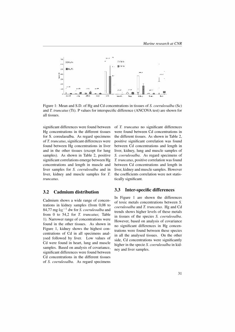
Mercury shows a wide range of con-centrations, especially in liver samples(from 8,48 to 1752 mg·kg−1 dw for S.coeruleoalba and from 9,6 to 1404 for T.truncatus; Table 1). As shown in Figure1, liver shows the highest concentrationsof Hg in all specimens analysed, followedby samples of kidney and lung. The low-est values were found in samples of mus-cle and heart. Based on ANCOVA test, no
30
Marine research at CNR
Figure 1: Mean and S.D. of Hg and Cd concentrations in tissues of S. coeruleoalba (Sc)and T. truncatus (Tt). P values for interspecific difference (ANCOVA test) are shown forall tissues.
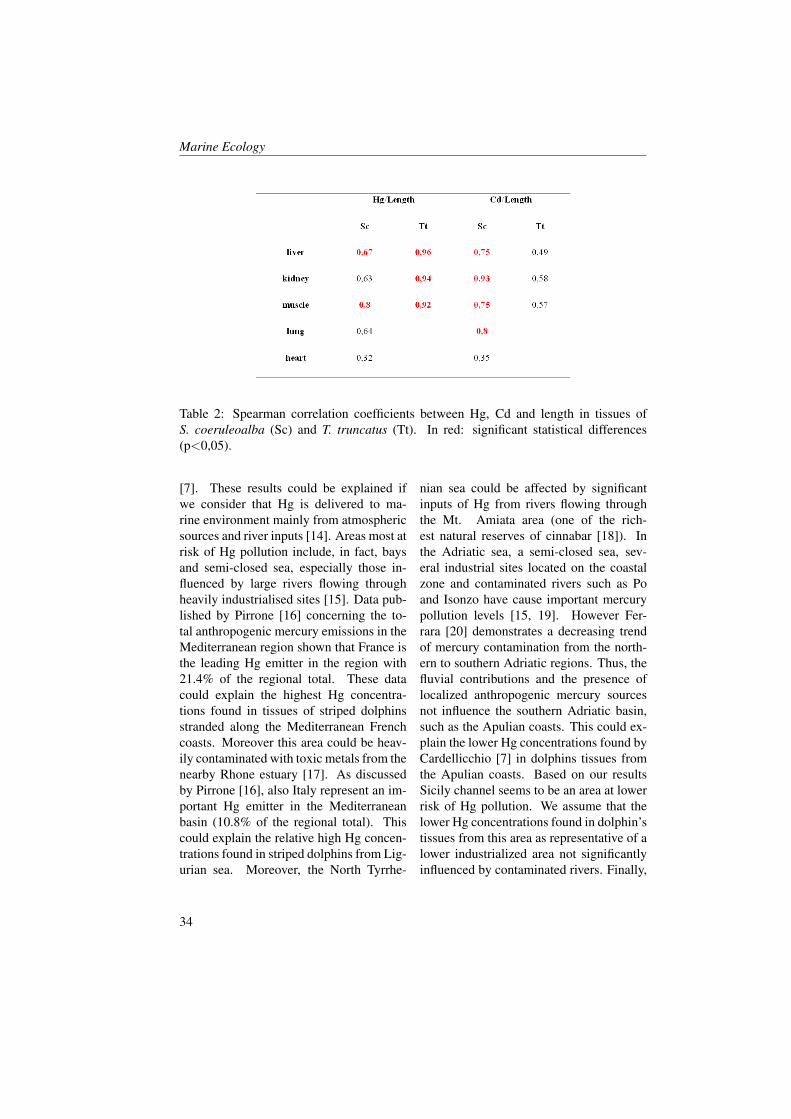
significant differences were found betweenHg concentrations in the different tissuesfor S. coreulaoalba. As regard specimensof T. truncatus, significant differences werefound between Hg concentrations in liverand in the other tissues (except for lungsamples). As shown in Table 2, positivesignificant correlations emerge between Hgconcentrations and length in muscle andliver samples for S. coeruleoalba and inliver, kidney and muscle samples for T.truncatus.
3.2 Cadmium distribution
Cadmium shows a wide range of concen-trations in kidney samples (from 0,08 to84,77 mg·kg−1 dw for S. coeruleoalba andfrom 0 to 54,2 for T. truncatus; Table1). Narrower range of concentrations werefound in the other tissues. As shown inFigure 1, kidney shows the highest con-centrations of Cd in all specimens anal-ysed followed by liver. Low values ofCd were found in heart, lung and musclesamples. Based on analysis of covariance,significant differences were found betweenCd concentrations in the different tissuesof S. coeruleoalba. As regard specimens
of T. truncatus no significant differenceswere found between Cd concentrations inthe different tissues. As shown in Table 2,positive significant correlation was foundbetween Cd concentrations and length inliver, kidney, lung and muscle samples ofS. coeruleoalba. As regard specimens ofT. truncatus, positive correlation was foundbetween Cd concentrations and length inliver, kidney and muscle samples. Howeverthe coefficients correlation were not statis-tically significant.
3.3 Inter-specific differencesIn Figure 1 are shown the differencesof toxic metals concentrations between S.coeruleoalba and T. truncatus. Hg and Cdtrends shows higher levels of these metalsin tissues of the species S. coeruleoalba.However, based on analysis of covarianceno significant differences in Hg concen-trations were found between these speciesin all the analysed tissues. On the otherside, Cd concentrations were significantlyhigher in the specie S. coeruleoalba in kid-ney and liver samples.
31
Marine Ecology
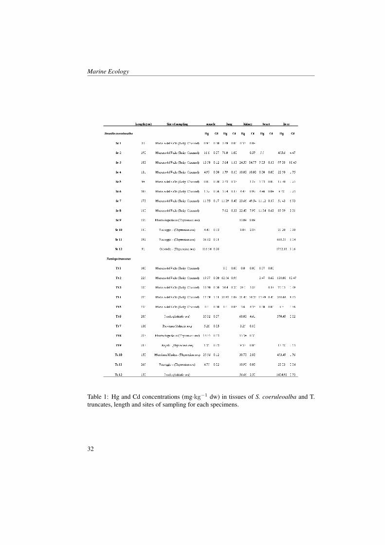
Table 1: Hg and Cd concentrations (mg·kg−1 dw) in tissues of S. coeruleoalba and T.truncates, length and sites of sampling for each specimens.
32
Marine research at CNR
4 Discussions
4.1 Mercury and cadmium dis-tribution
The highest concentrations of Hg werefound in the liver samples of all thespecimens analysed. This suggests thatdemethylation, namely the transformationof organic mercury into the less toxic in-organic form, occurs in this organ. Therewere significant correlations of Hg con-centrations in both liver, muscle and kid-ney with length for both species analysed.Thus, a relatively constant input of mercuryover time can be assumed. As shown inFigure 1, Cd accumulated preferentially inthe kidney of all species analysed. This isin accordance with results of previous au-thors [5, 8] and suggests a storage of Cd inthis organ possibly associated to effects ofcomplexation with metallothioneins (MT)and an excretory function of this organ.Also, significant correlations were foundbetween Cd concentrations and length inall tissues of S. coeruleoalba (except forheart samples). This may confirm the ex-istence of bioaccumulation process of Cdwith age for this species. Positive corre-lation with age were found also in tissuesof T. truncatus although at not statisticallysignificant levels. This can be explained bya lower accumulation of Cd in tissues ofthis species. These hypothesis seems to beconfirmed by Figure 1.
4.2 Inter-specific differencesNo significant differences in Hg concentra-tions were found between the two speciesin all the analysed tissues. However, asshown in Figure 1, it seems to be evi-dent that S. coeruleoalba exhibits higherHg and Cd concentrations than T. trun-
catus (in liver and kidney samples, re-spectively). Dolphins accumulate mercuryand cadmium mainly through the diet. T.truncatus can feed on fishes and squids,which make up 60 and 20% of its diet,respectively, while S. coeruleoalba have agreat proportion of squids in her diet [9].Squids are well-known toxic metal accu-mulators and a source of these metals totheir predators [10, 11, 12]. As a result,species or populations that consume an im-portant proportion of cephalopods can beexpected to exhibit higher Cd and Hg lev-els in their tissues than piscivorous preda-tors [13]. Moreover the analysed specieshave a similar trophic level [9] (4.2 for T.truncatus and S. coeruleoalba). Thus, thehigher Hg and Cd concentrations found inliver and kidney of S. coeruleoalba can beexplained by a great proportion of squidsin the diet composition of both groups oforganisms.
4.3 Cetaceans as indicators ofmercury marine pollution
A large number of data is available formercury concentrations in liver samplesof striped dolphin. The datasets of mer-cury concentrations in liver of striped dol-phin from Mediterranean French coasts[5], Israel coasts [6], Ligurian sea [3],Adriatic sea [7] and Sicily Channel (thisstudy) are here compared. Based on re-sults of ANCOVA test, significant differ-ences were found between Hg concentra-tions in liver samples of specimens fromdifferent marine areas. The highest Hgconcentrations were found in liver of spec-imens of S. coeruleoalba from the Frenchcoasts [5] followed by liver of specimensfrom Ligurian sea [3], Israel coasts [6],Sicily channel (this study) and Adriatic sea
33
Marine Ecology
Table 2: Spearman correlation coefficients between Hg, Cd and length in tissues ofS. coeruleoalba (Sc) and T. truncatus (Tt). In red: significant statistical differences(p<0,05).
[7]. These results could be explained ifwe consider that Hg is delivered to ma-rine environment mainly from atmosphericsources and river inputs [14]. Areas most atrisk of Hg pollution include, in fact, baysand semi-closed sea, especially those in-fluenced by large rivers flowing throughheavily industrialised sites [15]. Data pub-lished by Pirrone [16] concerning the to-tal anthropogenic mercury emissions in theMediterranean region shown that France isthe leading Hg emitter in the region with21.4% of the regional total. These datacould explain the highest Hg concentra-tions found in tissues of striped dolphinsstranded along the Mediterranean Frenchcoasts. Moreover this area could be heav-ily contaminated with toxic metals from thenearby Rhone estuary [17]. As discussedby Pirrone [16], also Italy represent an im-portant Hg emitter in the Mediterraneanbasin (10.8% of the regional total). Thiscould explain the relative high Hg concen-trations found in striped dolphins from Lig-urian sea. Moreover, the North Tyrrhe-
nian sea could be affected by significantinputs of Hg from rivers flowing throughthe Mt. Amiata area (one of the rich-est natural reserves of cinnabar [18]). Inthe Adriatic sea, a semi-closed sea, sev-eral industrial sites located on the coastalzone and contaminated rivers such as Poand Isonzo have cause important mercurypollution levels [15, 19]. However Fer-rara [20] demonstrates a decreasing trendof mercury contamination from the north-ern to southern Adriatic regions. Thus, thefluvial contributions and the presence oflocalized anthropogenic mercury sourcesnot influence the southern Adriatic basin,such as the Apulian coasts. This could ex-plain the lower Hg concentrations found byCardellicchio [7] in dolphins tissues fromthe Apulian coasts. Based on our resultsSicily channel seems to be an area at lowerrisk of Hg pollution. We assume that thelower Hg concentrations found in dolphin’stissues from this area as representative of alower industrialized area not significantlyinfluenced by contaminated rivers. Finally,
34

Marine research at CNR
as reported by Pirrone [16], Israel repre-sents a minor Hg emitter in Mediterraneanbasin (0,8% of the regional total) with re-duced impact from contaminated rivers.These data well reflect the lower Hg con-centrations in tissues of striped dolphinfound in this area by Roditi-Elasar [6].
5 ConclusionsConcentration and distribution ranges ofHg and Cd in the reported dataset are sub-stantially comparable with those reportedby other authors worldwide. In particu-lar, the liver systematically shows the high-est concentrations of Hg while the kid-ney shows the highest concentrations of Cdwith evident high potential for toxic ele-ments accumulation of these two organs.According with previous authors we reportthe existence of bioaccumulation processover time of these toxic elements. Thereported dataset well documents the ex-istence of different mechanisms of bioac-
cumulation, through different diet patternsand/or uniqueness in physiological and/orbiological control of Hg and Cd incorpora-tion for S. coeruleoalba and T. truncatus.Particularly seems to be evident the bioac-cumulation of an higher amounts of Hgand Cd in target organs of S. coeruleoalba.Last but not least, Hg concentrations in tis-sues of striped dolphin show clear differ-ence of concentrations of this toxic ele-ment within Mediterranean seawater. Par-ticularly, it seems to be clear that differ-ences of environment Hg contaminationscan occur at regional scale due to differ-ences of anthropogenic impacts in differ-ent Mediterranean areas. These differencesmay reflect the existence of different andseparated populations of S. coeruleoalba inMediterranean basin with different feedinghabitats and exposition to different anthro-pogenic impact. This implies that migra-tory movements of the studied groups ofcetaceans in the Mediterranean sea are de-cidedly limited.
References[1] J.M. Neff. Bioaccumulation in Marine Organisms: Effect of Contaminants from
Oil Well Produced Water. 2002.
[2] J.O. Nriagu. Human influence on the global cycling of trace metals. 1991.
[3] R. Capelli, G. Drava, R. De Pellegrini, V. Minganti, and R. Poggi. Study of traceelements in organs and tissues of striped dolphins (Stenella coeruleoalba) founddead along the Ligurian coasts (Italy). 2000.
[4] D.R. Thompson. Metal levels in marine vertebrates. 1990.
[5] J.M. Andre, A. Boudou, F. Ribeyre, and M. Bernhard. Comparative study of mer-cury accumulation in dolphins (Stenella coeruleoalba) from French Atlantic andMediterranean coasts. Sci. Total Environ., 1991.
[6] M. Roditi-Elasar, D. Kerem, H. Hornung, N. Kress, E. Shoham-Frider, and O. Goff-man. Heavy Metal levels in bottlenose and striped dolphins off the Mediterraneancoast of Israel. Marine Pollution Bulletin, (46):503–12, 2003.
35
Marine Ecology
[7] N. Cardellicchio, A. Decataldo, A. Di Leo, and A. Misino. Accumulationand tissue distribution of mercury and selenium in striped dolphins (Stenellacoeruleoalba) from the Mediterranean Sea (southern Italy). Environmental Pol-lution, (116):265–271, 2002.
[8] T. J. Lavery, N. Butterfield, C. M. Kemper, R. J. Reid, and K. Sanderson. Metalsand selenium in the liver and bone of three dolphin species from South Australia,1988–2004. 2008.
[9] D.A. Pauly, W. Trites, E. Capuli, and V. Christensen. Diet composition and trophiclevels of marine mammals. 1998.
[10] R.J. Law. Metals in marine mammals. 1996.
[11] J. Koyama, N. Nanamori, and S. Segawa. Bioaccumulation of waterborne anddietary cadmium by oval squid, Sepioteuthis lessoniana, and its distribution amongorgans. Marine Pollution Bulletin, (40):961–967, 2000.
[12] D. Bowles. An overview of the concentrations and effects of metals in cetaceanspecies. 1999.
[13] V. Lahaye, P. Bustamante, W. Dabin, O. Van Canneyt, F. Dhermain, C. Cesarini,G.J. Pierce, and F. Cauran. New insights from age determination on toxic elementaccumulation in striped and bottlenose dolphins from Atlantic and Mediterraneanwaters. 2006.
[14] D. Cossa, J.M. Martin, K. Takayanagi, and J. Sanjuan. The distribution and cyclingof mercury species in the western Mediterranean. Deep-sea Research II, (44):721–740, 1997.
[15] F. Sprovieri and N. Pirrone. Spatial and temporal distribution of atmospheric mer-cury species over the Adriatic Sea. 2007.
[16] N. Pirrone, P. Costa, J.M. Pacyna, and R. Ferrara. Mercury emissions to the atmo-sphere from natural and anthropogenic sources in the Mediterranean region. Atmo-spheric Environment, (35):2997–3006, 2001.
[17] A. Renzoni, S. Focardi, C. Fossi, C. Leonzio, and J. Mayol. Comparison betweenconcentration of mercury and other contaminants in eggs and tissues of Cory’sShearwater (Calonectris diomedea) collected on Atlantic and Mediterranean Is-lands. Environmental Pollution, (40):17–37, 1986.
[18] E. Bacci. Mercury in the Mediterranean. Marine Pollution Bullettin, (22):59–63,1989.
[19] S. Covelli, R. Piani, A. Acquavita, S. Predonzani, and J. Faganali. Transport anddispersion of particulate Hg associated with a river plume in coastal Northern Adri-atic environments. Marine Pollution Bulletin, (55):436–450, 2007.
36

Marine research at CNR
[20] R. Ferrara, B.E. Maserti, and C. Zanaboni. Mercury levels in total sospende matterand in the plankton of the Mediterranean basin. Science of the Total Environment,(84):129–134, 1989.
37

Marine Ecology
38
Food Web Reconstruction Gives Evidence of In-creased Trophic Levels in No-Trawl Areas: theRed Mullet, Mullus barbatus L. Case in NorthernSicily
F. Badalamenti1, F. Andaloro2, D. Campo3, M. Coppola1, G. D’Anna1,G. Di Stefano1, A. Mazzola4, C. Pipitone1, C. Romano1, M. Sinopoli1, S.Vizzini41, Institute for Coastal Marine Environment, CNR, Castellammare del Golfo (TP), Italy2, Institute for Environmental Protection and Research, Palermo, Italy3, CEA LABTER Ragusa, Ragusa, Italy4, Department of Ecology, University of Palermo, [email protected]
Abstract
This study was aimed at identifying the food web of the red mullet, Mullus bar-batus in order to understand how it is affected by trawling disturbance. To achievethis objective: a) the main features of the red mullet habitat were investigated; b) thefood web of this habitat was studied in two no-trawl areas and in two areas open totrawling.The working hypothesis is that trawling affects the biochemistry of the sediment andthe trophic structure of the benthic assemblage. It was predicted: a) less biomass,smaller size and higher production rate in the benthic assemblages of protected gulfs;b) higher average trophic level for both the red mullet and its predators in protectedgulfs; c) a diet shift driven by the mechanical disturbance of trawling.The results achieved confirmed our hypotheses and allowed us to characterize forthe first time the trophic web structure in the red mullet habitat in the study area.Results also allowed us to compare the trophic level of red mullet of different sizesusing two independent techniques, stable isotopes of nitrogen and gut contents. Theaverage trophic level of the red mullet was higher and the energy consumption perunit of biomass larger in the protected gulfs. Species with a trophic level higher thanthe red mullet and therefore its potential predators were few and the most importantwere the white grouper, Epinephelus aeneus, the pandora, Pagellus erythrinus andthe common torpedo, Torpedo torpedo.
1 Introduction
The Gulfs of Castellammare and Patti canbe considered marine protected areas dueto a trawl ban imposed in 1990 (Regional
Act n. 25/1990). Studies carried out in thetwo gulfs [1, 2, 3, 4] showed a strong in-crease of groundfish biomass as a result ofthe ban. The red mullet, Mullus barbatushad one of the highest increase rates among
Marine Ecology
commercial finfish species. This species,which accounts for about 25% of the to-tal groundfish biomass in both gulfs, has anadult diet based on benthic organisms likepolychaetes, molluscs and crustaceans [5].Such huge “new” red mullet biomass mostlikely has a strong impact on the benthicfood web - and also on the pelagic foodweb on which pre-benthic juveniles rely -which is poorly known. Badalamenti et al.[6] showed that the red mullet has a veryhigh trophic level and speculated that bot-tom food webs are longer than hitherto ex-pected, because many invertebrates couldbe actually omnivorous instead of simplydeposit feeders or carnivorous.In 2005 the Italian Ministry for Agricul-ture and Forest Policy funded the coordi-nated project “Evaluation of the efficacyof no-trawl areas through the study of thepredators and prey of the red mullet, Mul-lus barbatus L.”. This project evaluatedthe effect of the establishment of a trawl-ing exclusion zone on the coastal marineecosystem and in particular on the benthicfood web. The study was aimed at identify-ing the predators and prey of the red mul-let, M. barbatus to better understand howa disturbance, in this case the trawling ban,may affect the trophic structure. To achievethis objective (a) the main biological andsediment features of the red mullet habi-tat (i.e., muddy bottoms between 40 and80 m depth) were investigated, and (b) thefood web of this habitat was studied and thefood web of the red mullet reconstructed.The study area included four gulfs alongthe northern Sicily coast, two under a no-trawl regime (Castellammare and Patti) andtwo open to trawl fishing (Termini Imereseand Sant’Agata).The working hypothesis was that besidesthe well documented difference in fishbiomass between protected and unpro-
tected gulfs there were also differences inthe benthic assemblage structure and pro-duction, in the biochemistry of the sedi-ment and in the food web structure. Itwas predicted: (a) less biomass, smallersize and higher production rate in the ben-thic assemblages of protected gulfs be-cause of larger groundfish biomass andhence higher feeding pressure on the ben-thos; (b) higher average trophic level forboth the red mullet and its predators dueto the extension of the food web and the in-crease in the number of omnivorous organ-isms at the base of the food web, and (c) adiet shift driven by the mechanical distur-bance of trawling.The study was carried out by a coordinatedgroup that included three teams: CNR-IAMC (team 1 and project coordinator),ISPRA (team 2) and the Department ofEcology (formerly: Animal Biology) of theUniversity of Palermo (team 3).
2 Materials and methods
The study area (Figures 1-3) included fourlocations off the northern Sicily coast:two no-trawl areas (Gulf of Castellam-mare, GCAST and Gulf of Patti, GPATT),and two trawled areas (Gulf of TerminiImerese, GTERM and Gulf of S. Agata,GSANT).An experimental design based on protectedand unprotected areas, each with two repli-cate locations (i.e., the gulfs), was adopted.Each location was divided in three equiva-lent surface sectors: West (W), Centre (C)and East (E). The design included threefactors: Protection (fixed with two levels:protected PR and unprotected UPR), Gulf(random and nested in the Protection factorwith two levels: GCAST and GPATT forPR and GTERM and GSANT for UPR),
40
Marine research at CNR
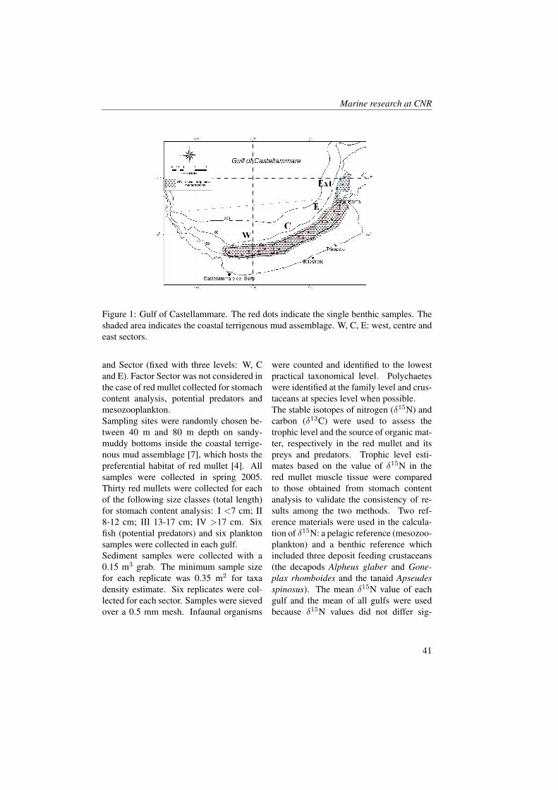
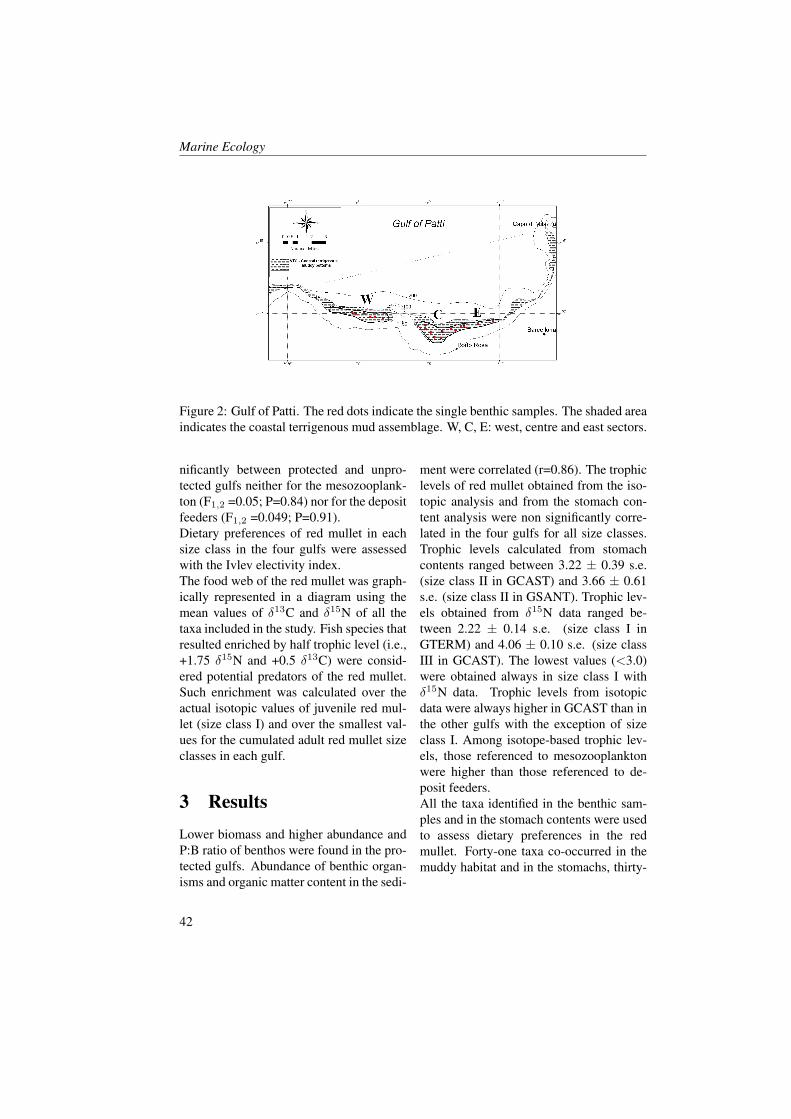
Figure 1: Gulf of Castellammare. The red dots indicate the single benthic samples. Theshaded area indicates the coastal terrigenous mud assemblage. W, C, E: west, centre andeast sectors.
and Sector (fixed with three levels: W, Cand E). Factor Sector was not considered inthe case of red mullet collected for stomachcontent analysis, potential predators andmesozooplankton.Sampling sites were randomly chosen be-tween 40 m and 80 m depth on sandy-muddy bottoms inside the coastal terrige-nous mud assemblage [7], which hosts thepreferential habitat of red mullet [4]. Allsamples were collected in spring 2005.Thirty red mullets were collected for eachof the following size classes (total length)for stomach content analysis: I <7 cm; II8-12 cm; III 13-17 cm; IV >17 cm. Sixfish (potential predators) and six planktonsamples were collected in each gulf.Sediment samples were collected with a0.15 m3 grab. The minimum sample sizefor each replicate was 0.35 m2 for taxadensity estimate. Six replicates were col-lected for each sector. Samples were sievedover a 0.5 mm mesh. Infaunal organisms
were counted and identified to the lowestpractical taxonomical level. Polychaeteswere identified at the family level and crus-taceans at species level when possible.The stable isotopes of nitrogen (δ15N) andcarbon (δ13C) were used to assess thetrophic level and the source of organic mat-ter, respectively in the red mullet and itspreys and predators. Trophic level esti-mates based on the value of δ15N in thered mullet muscle tissue were comparedto those obtained from stomach contentanalysis to validate the consistency of re-sults among the two methods. Two ref-erence materials were used in the calcula-tion of δ15N: a pelagic reference (mesozoo-plankton) and a benthic reference whichincluded three deposit feeding crustaceans(the decapods Alpheus glaber and Gone-plax rhomboides and the tanaid Apseudesspinosus). The mean δ15N value of eachgulf and the mean of all gulfs were usedbecause δ15N values did not differ sig-
41
Marine Ecology
Figure 2: Gulf of Patti. The red dots indicate the single benthic samples. The shaded areaindicates the coastal terrigenous mud assemblage. W, C, E: west, centre and east sectors.
nificantly between protected and unpro-tected gulfs neither for the mesozooplank-ton (F1,2 =0.05; P=0.84) nor for the depositfeeders (F1,2 =0.049; P=0.91).Dietary preferences of red mullet in eachsize class in the four gulfs were assessedwith the Ivlev electivity index.The food web of the red mullet was graph-ically represented in a diagram using themean values of δ13C and δ15N of all thetaxa included in the study. Fish species thatresulted enriched by half trophic level (i.e.,+1.75 δ15N and +0.5 δ13C) were consid-ered potential predators of the red mullet.Such enrichment was calculated over theactual isotopic values of juvenile red mul-let (size class I) and over the smallest val-ues for the cumulated adult red mullet sizeclasses in each gulf.
3 ResultsLower biomass and higher abundance andP:B ratio of benthos were found in the pro-tected gulfs. Abundance of benthic organ-isms and organic matter content in the sedi-
ment were correlated (r=0.86). The trophiclevels of red mullet obtained from the iso-topic analysis and from the stomach con-tent analysis were non significantly corre-lated in the four gulfs for all size classes.Trophic levels calculated from stomachcontents ranged between 3.22 ± 0.39 s.e.(size class II in GCAST) and 3.66 ± 0.61s.e. (size class II in GSANT). Trophic lev-els obtained from δ15N data ranged be-tween 2.22 ± 0.14 s.e. (size class I inGTERM) and 4.06 ± 0.10 s.e. (size classIII in GCAST). The lowest values (<3.0)were obtained always in size class I withδ15N data. Trophic levels from isotopicdata were always higher in GCAST than inthe other gulfs with the exception of sizeclass I. Among isotope-based trophic lev-els, those referenced to mesozooplanktonwere higher than those referenced to de-posit feeders.All the taxa identified in the benthic sam-ples and in the stomach contents were usedto assess dietary preferences in the redmullet. Forty-one taxa co-occurred in themuddy habitat and in the stomachs, thirty-
42
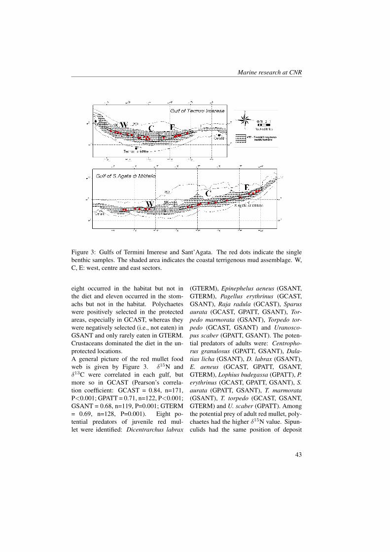
Marine research at CNR
Figure 3: Gulfs of Termini Imerese and Sant’Agata. The red dots indicate the singlebenthic samples. The shaded area indicates the coastal terrigenous mud assemblage. W,C, E: west, centre and east sectors.
eight occurred in the habitat but not inthe diet and eleven occurred in the stom-achs but not in the habitat. Polychaeteswere positively selected in the protectedareas, especially in GCAST, whereas theywere negatively selected (i.e., not eaten) inGSANT and only rarely eaten in GTERM.Crustaceans dominated the diet in the un-protected locations.A general picture of the red mullet foodweb is given by Figure 3. δ15N andδ13C were correlated in each gulf, butmore so in GCAST (Pearson’s correla-tion coefficient: GCAST = 0.84, n=171,P<0.001; GPATT = 0.71, n=122, P<0.001;GSANT = 0.68, n=119, P=0.001; GTERM= 0.69, n=128, P=0.001). Eight po-tential predators of juvenile red mul-let were identified: Dicentrarchus labrax
(GTERM), Epinephelus aeneus (GSANT,GTERM), Pagellus erythrinus (GCAST,GSANT), Raja radula (GCAST), Sparusaurata (GCAST, GPATT, GSANT), Tor-pedo marmorata (GSANT), Torpedo tor-pedo (GCAST, GSANT) and Uranosco-pus scaber (GPATT, GSANT). The poten-tial predators of adults were: Centropho-rus granulosus (GPATT, GSANT), Dala-tias licha (GSANT), D. labrax (GSANT),E. aeneus (GCAST, GPATT, GSANT,GTERM), Lophius budegassa (GPATT), P.erythrinus (GCAST, GPATT, GSANT), S.aurata (GPATT, GSANT), T. marmorata(GSANT), T. torpedo (GCAST, GSANT,GTERM) and U. scaber (GPATT). Amongthe potential prey of adult red mullet, poly-chaetes had the higher δ15N value. Sipun-culids had the same position of deposit
43
Marine Ecology
feeding polychaetes, whereas holothurianshad a δ15N value close to deposit feedingpolychaetes but a much higher δ13C, whichexcluded them from the group of potentialprey. Crustaceans in all gulfs fell withintwo trophic guilds: omnivores (or large-sized deposit feeders) and deposit feeders;according to their isotopic values, they arepotential prey of adult red mullet in allgulfs.
4 Discussion and conclu-sions
The abundance and biomass of the benthicassemblage differ among locations, withhigher abundance and lower biomass inthe protected gulfs (especially GCAST).The lower benthic biomass in the protectedgulfs - which is compensated by higherP:B, especially in GCAST - could be dueto the much higher groundfish biomass(red mullet biomass up to 47-fold higher[2, 3, 4] as a result of the trawl ban, anda consequent higher predation on the ben-thos.In the unprotected gulfs the red mulletprefers suprabenthic prey, whereas in theprotected gulfs (particularly in GCAST)they prefer infaunal prey, especially poly-chaetes. This difference, which is consis-tent across protected and unprotected lo-cations, could be a result of adaptation tothe level of trawling impact on the benthiccommunity rather than due to natural vari-ability.This study clearly shows that the two meth-ods used to calculate the trophic level ofred mullet (i.e., stomach contents and sta-ble isotope analysis) are not comparable.The isotope method seems to underesti-mate the trophic level of juveniles, whereas
the stomach content method seems to un-derestimate that of adults. The result of theisotopic study of juveniles based on the de-posit feeders is expected, because the refer-ence material was not collected in the habi-tat of juvenile red mullet (which is coastalpelagic). What is unexpected is the resultobtained with the mesozooplankton refer-ence, which could be due to the differenthabitat (offshore pelagic) of the planktonsamples. As a conclusion it is not advisableto collect the reference material in habitatsdifferent or far away from the habitat of theconsumer, and this should be taken into ac-count in future studies.The mean isotope-based trophic level ofred mullet is higher in the protected gulfs.At least two possible causes can be directlyrelated to the trawl ban, that is (a) the ab-sence of physical disturb on the bottom,and (b) the increased groundfish biomass.The absence of disturbance could havemade new and different food sources avail-able to the red mullet, as suggested bythe higher number of positively selectedprey items (e.g., polychaetes) in protectedgulfs. A higher trophic level of polychaeteswould explain the higher trophic level ofred mullet in the protected locations (1/3to 1/2 higher than unprotected), which inturn means that more energy is subtractedto the ecosystem by a unit biomass of redmullet. Most likely the ceased trawling im-pact has caused an increase in the trophiclevel of primary consumers (i.e., benthicinvertebrates) and hence of their predators.Post and Takimoto [8] proposed a few pos-sible ecological mechanisms that might ap-ply to our case. The addition of a newintermediate species amid two species al-ready linked by a prey-predator relation-ship might have increased the connectivity- and hence trophic level - in our protectedgulfs [8].
44

Marine research at CNR
The food web is similar in the four gulfs.The number of potential predators is smalland basically only one species, the whitegrouper E. aeneus, is common to all gulfs.Less important are the pandora P. erythri-nus, and the common torpedo T. torpedo.Remarkable is the absence of the hake Mer-luccius merluccius from the list of preda-tors while the monkfish Lophius spp. ap-pears only in GPATT. The stargazer U.scaber and the sea bass D. labrax could beoccasional predators of juvenile red mullet.The observed differences between the fourgulfs are consistent for all of the stud-ied variables. A clear pattern is recog-nizable, with GCAST different from theunprotected gulfs (which are similar eachother), and GPATT in an intermediate posi-tion between these two extremes. This pat-tern is similar to what has been observedfor the red mullet CPUE in the four gulfs(authors’ unpublished data), thus it seemscorrelated to the effect of protection. Onone hand GSANT and GTERM are un-protected areas subjected to heavy trawlingimpact, while on the other hand GCASTand GPATT differ each other because theyare subjected to a different degree of en-forcement of the trawl ban. In GCAST,a major role in contrasting illegal fishinghas been played by the presence of: (a) ahuge system of artificial reefs within the -50 m isobath, (b) the CNR marine ecology
laboratory who has contributed to developthe awareness among the different fisherystakeholders, (c) a great activism of the lo-cal Consortium for fish replenishment and(d) an effective enforcement of the trawlban provided by the bodies in charge forpatrolling the area.The trawl ban in the Sicilian gulfs canbe described as a successful managementchoice. It has contributed to reconstruct thebenthic trophic food web and to increasethe trawlable biomass, notwithstanding thehigher average trophic level gained by sec-ondary consumers. Due to the results ob-tained, the exclusion of trawl fishing fromvast areas of the continental shelf has po-tential for application to other geographi-cal areas in the context of an ecosystem ap-proach to fishery. The data gathered in thisstudy show the results of a true protectionmade possible by effective enforcement,especially in the earlier period. However,since fishermen are aware that trawlableresources are scarce and dramatically lessabundant outside the protected areas, ille-gal trawling inside the protected area hasincreased recently [9]. For this reason strictenforcement is needed if gains are not tobe lost, keeping in mind that the trawl banin the Sicilian gulfs has allowed major en-hancements from an ecosystem and fisherypoint of view, as well as new achievementsin the field of marine ecology.
45
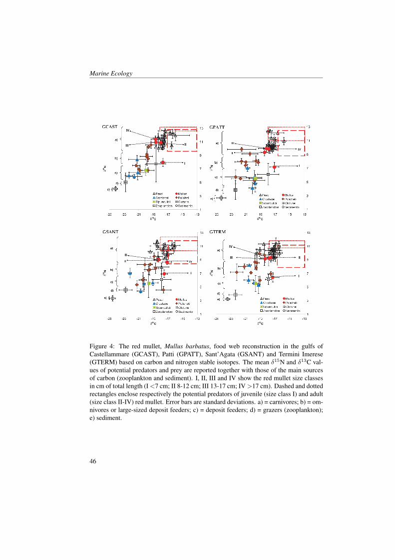
Marine Ecology
Figure 4: The red mullet, Mullus barbatus, food web reconstruction in the gulfs ofCastellammare (GCAST), Patti (GPATT), Sant’Agata (GSANT) and Termini Imerese(GTERM) based on carbon and nitrogen stable isotopes. The mean δ15N and δ13C val-ues of potential predators and prey are reported together with those of the main sourcesof carbon (zooplankton and sediment). I, II, III and IV show the red mullet size classesin cm of total length (I<7 cm; II 8-12 cm; III 13-17 cm; IV>17 cm). Dashed and dottedrectangles enclose respectively the potential predators of juvenile (size class I) and adult(size class II-IV) red mullet. Error bars are standard deviations. a) = carnivores; b) = om-nivores or large-sized deposit feeders; c) = deposit feeders; d) = grazers (zooplankton);e) sediment.
46
Marine research at CNR
References[1] G. D’Anna, F. Badalamenti, C. Pipitone, D. Patti, A. Cuttitta, and R. Lipari. Structure
of the populations and assessment of the biomass of the coastal demersal resourcesin the Golfo di Castellammare. Final report of Study MED 92/011. Commission ofthe European Communities, DG XIV. pages 1–60, 1994.
[2] A. Potoschi, G. Cavallaro, P. Sturiale, and G. Lo Duca. Effetti del decreto regionaledel 31/5/90 sui rendimenti di pesca di Mullus barbatus (L., 1758) catturato con retea strascico nel Golfo di Patti (ME). Biol. Mar. Medit., 2(2):505–507, 1995.
[3] C. Pipitone, F. Badalamenti, G. D’Anna, and B. Patti. Fish biomass increase after afour-year trawl ban in the Gulf of Castellammare (NW Sicily, Mediterranean Sea).Fish. Res., 48(1):23–30, 2000a.
[4] C. Pipitone, F. Badalamenti, G. D’Anna, D. Whitmarsh, C. James, and H. Pickering.Trawling ban in the Gulf of Castellammare: effects on the small scale fishery eco-nomics and on the abundance of fish. Final report of Study No. 97/063 Commissionof the European Communities, DG XIV, page 120, 2000.
[5] R. Lipari, F. Badalamenti, and G. D’Anna. Relazioni trofiche e selezione alimentaredi Mullus barbatus L. (1758) nella comunita a sabbie fini del Golfo di Castellammare(Sicilia N/O). Biol. Mar. Medit., 5(1):354–356, 1998.
[6] F. Badalamenti, G. D’Anna, J.K. Pinnegar, and N.V.C. Polunin. Size-related tropho-dynamic changes in three target fish species recovering from intensive trawling. Mar.Biol., 141:561–570, 2002.
[7] J.M. Peres. Major benthic assemblages. Mar. Ecol. 5, 5:373–522, 1982.
[8] D.M. Post and G. Takimoto. Proximate structural mechanisms for variation in food-chain length. Oikos, 116:775–782, 2007.
[9] S. Stefanoni, G. D’Anna, C. Pipitone, and F. Badalamenti. Analisi economica dellepolitiche di gestione della pesca nel Golfo di Castellammare. La valutazione dellerisorse ambientali: approcci multidisciplinari al Golfo di Castellammare, pages178–201, 2008.
47

Marine Ecology
48
Inter-Annual Variability of the Trace ElementContent in Seawater from the Western Ross Sea,Antarctica
C. Turetta1, C. Barbante1,2, G. Capodaglio1,2, P. Cescon1,2
1, Institute for the Dynamics of Environmental Processes, CNR, Venezia, Italy2, Department of Environmental Sciences, University “Ca’ Foscari”, Venezia, [email protected]
Abstract
Total dissolved content of some trace elements (Cd, Cr, Cu, Mn, Pb, Zn), nu-trients (nitrate, phosphate and silicate), fluorescence, salinity, dissolved oxygen andtemperature were measured on several samples collected during 2 oceanographic sur-veys from 2001 to 2003 within the framework of the Italian expedition in Antarcticaon board the R.V. Italica. The mean concentrations measured are consistent with lit-erature data for seawater at high latitude. The concentration value of some elements,never detected in high latitude seawater before, were compared with the expectedvalues for oceanic water: the results are in agreement with literature data. As forall the oceans, also in the Ross sea the relationship between Cd and phosphate isevident. Some trace elements like copper, cadmium and zinc may have the doublerole of micronutrient and toxicant. The geochemical cycle of some trace elements,like manganese, is principally controlled by the oxidation-reduction reaction. Theobtained results were discussed taking in account the distribution of such trace ele-ments as a function of the different water masses present during the austral summerin the western sector of the Ross Sea.
1 Introduction
The importance of trace elements as en-vironmental contaminants and their diffu-sion at a planetary level has already beenhighlighted in various paper. Trace ele-ments are released into the environment bya large number of natural processes, and,during the last few centuries, also by anumber of uncontrolled human activities[1, 2, 3, 4, 5, 6]. With the aim to bet-ter understand the mechanisms that con-trol the distribution of trace elements, wehave focussed our attention on seawaterbecause of the importance of this matrix
in the global transport of chemicals. TheSouthern Ocean, plays a key role in the cir-culation of the world’s ocean, since the An-tartic Circumpolar Current (ACC) extendsaround the globe, flowing eastwardly anddriven by the world’s strongest westerlywinds, being a unique global link whichjoins all major oceans [7], and the RossSea has an important role in the forma-tion of Antarctic Bottom Water (AABW)which re-oxygenate all the oceans [8, 9].Geochemical, physical and biological pro-cesses may control trace metals concen-tration in the various areas of the worldocean. Hence, the study of the distribu-
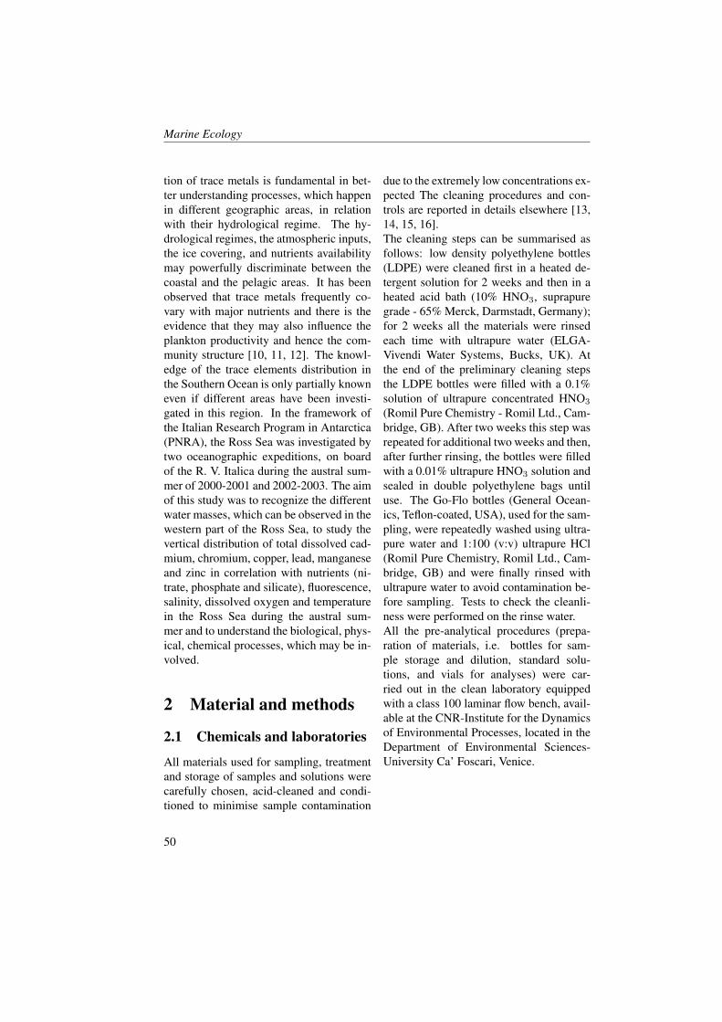
Marine Ecology
tion of trace metals is fundamental in bet-ter understanding processes, which happenin different geographic areas, in relationwith their hydrological regime. The hy-drological regimes, the atmospheric inputs,the ice covering, and nutrients availabilitymay powerfully discriminate between thecoastal and the pelagic areas. It has beenobserved that trace metals frequently co-vary with major nutrients and there is theevidence that they may also influence theplankton productivity and hence the com-munity structure [10, 11, 12]. The knowl-edge of the trace elements distribution inthe Southern Ocean is only partially knowneven if different areas have been investi-gated in this region. In the framework ofthe Italian Research Program in Antarctica(PNRA), the Ross Sea was investigated bytwo oceanographic expeditions, on boardof the R. V. Italica during the austral sum-mer of 2000-2001 and 2002-2003. The aimof this study was to recognize the differentwater masses, which can be observed in thewestern part of the Ross Sea, to study thevertical distribution of total dissolved cad-mium, chromium, copper, lead, manganeseand zinc in correlation with nutrients (ni-trate, phosphate and silicate), fluorescence,salinity, dissolved oxygen and temperaturein the Ross Sea during the austral sum-mer and to understand the biological, phys-ical, chemical processes, which may be in-volved.
2 Material and methods
2.1 Chemicals and laboratories
All materials used for sampling, treatmentand storage of samples and solutions werecarefully chosen, acid-cleaned and condi-tioned to minimise sample contamination
due to the extremely low concentrations ex-pected The cleaning procedures and con-trols are reported in details elsewhere [13,14, 15, 16].The cleaning steps can be summarised asfollows: low density polyethylene bottles(LDPE) were cleaned first in a heated de-tergent solution for 2 weeks and then in aheated acid bath (10% HNO3, suprapuregrade - 65% Merck, Darmstadt, Germany);for 2 weeks all the materials were rinsedeach time with ultrapure water (ELGA-Vivendi Water Systems, Bucks, UK). Atthe end of the preliminary cleaning stepsthe LDPE bottles were filled with a 0.1%solution of ultrapure concentrated HNO3
(Romil Pure Chemistry - Romil Ltd., Cam-bridge, GB). After two weeks this step wasrepeated for additional two weeks and then,after further rinsing, the bottles were filledwith a 0.01% ultrapure HNO3 solution andsealed in double polyethylene bags untiluse. The Go-Flo bottles (General Ocean-ics, Teflon-coated, USA), used for the sam-pling, were repeatedly washed using ultra-pure water and 1:100 (v:v) ultrapure HCl(Romil Pure Chemistry, Romil Ltd., Cam-bridge, GB) and were finally rinsed withultrapure water to avoid contamination be-fore sampling. Tests to check the cleanli-ness were performed on the rinse water.All the pre-analytical procedures (prepa-ration of materials, i.e. bottles for sam-ple storage and dilution, standard solu-tions, and vials for analyses) were car-ried out in the clean laboratory equippedwith a class 100 laminar flow bench, avail-able at the CNR-Institute for the Dynamicsof Environmental Processes, located in theDepartment of Environmental Sciences-University Ca’ Foscari, Venice.
50
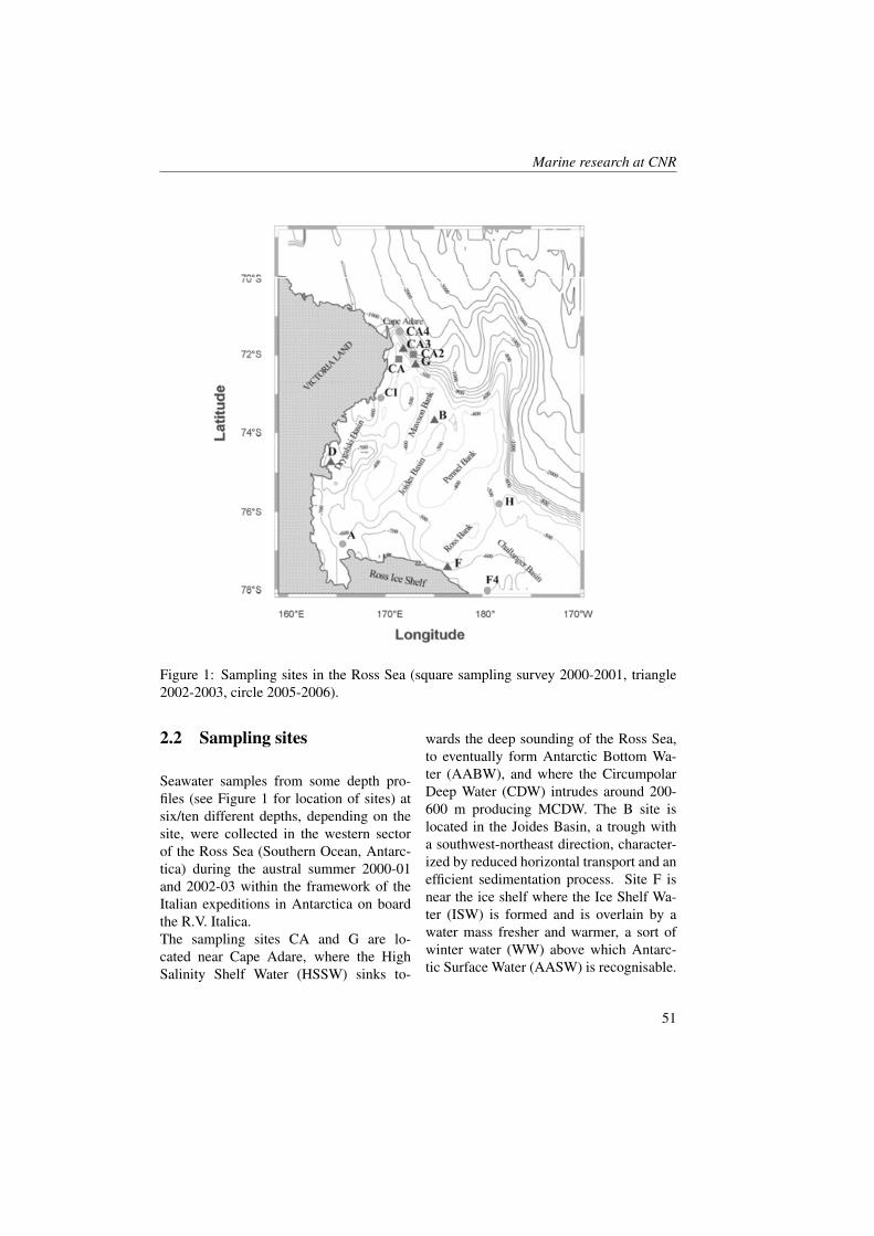
Marine research at CNR
Figure 1: Sampling sites in the Ross Sea (square sampling survey 2000-2001, triangle2002-2003, circle 2005-2006).
2.2 Sampling sites
Seawater samples from some depth pro-files (see Figure 1 for location of sites) atsix/ten different depths, depending on thesite, were collected in the western sectorof the Ross Sea (Southern Ocean, Antarc-tica) during the austral summer 2000-01and 2002-03 within the framework of theItalian expeditions in Antarctica on boardthe R.V. Italica.The sampling sites CA and G are lo-cated near Cape Adare, where the HighSalinity Shelf Water (HSSW) sinks to-
wards the deep sounding of the Ross Sea,to eventually form Antarctic Bottom Wa-ter (AABW), and where the CircumpolarDeep Water (CDW) intrudes around 200-600 m producing MCDW. The B site islocated in the Joides Basin, a trough witha southwest-northeast direction, character-ized by reduced horizontal transport and anefficient sedimentation process. Site F isnear the ice shelf where the Ice Shelf Wa-ter (ISW) is formed and is overlain by awater mass fresher and warmer, a sort ofwinter water (WW) above which Antarc-tic Surface Water (AASW) is recognisable.
51
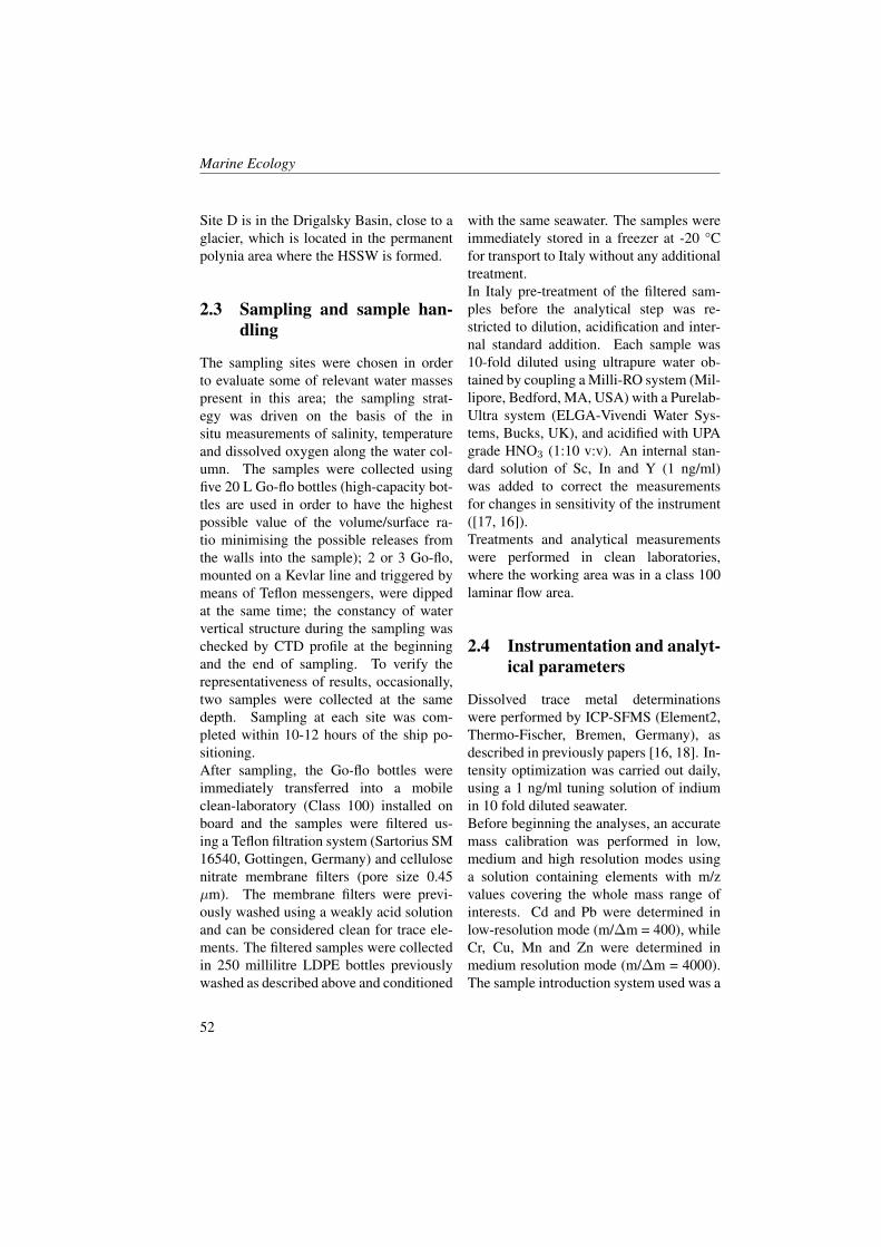
Marine Ecology
Site D is in the Drigalsky Basin, close to aglacier, which is located in the permanentpolynia area where the HSSW is formed.
2.3 Sampling and sample han-dling
The sampling sites were chosen in orderto evaluate some of relevant water massespresent in this area; the sampling strat-egy was driven on the basis of the insitu measurements of salinity, temperatureand dissolved oxygen along the water col-umn. The samples were collected usingfive 20 L Go-flo bottles (high-capacity bot-tles are used in order to have the highestpossible value of the volume/surface ra-tio minimising the possible releases fromthe walls into the sample); 2 or 3 Go-flo,mounted on a Kevlar line and triggered bymeans of Teflon messengers, were dippedat the same time; the constancy of watervertical structure during the sampling waschecked by CTD profile at the beginningand the end of sampling. To verify therepresentativeness of results, occasionally,two samples were collected at the samedepth. Sampling at each site was com-pleted within 10-12 hours of the ship po-sitioning.After sampling, the Go-flo bottles wereimmediately transferred into a mobileclean-laboratory (Class 100) installed onboard and the samples were filtered us-ing a Teflon filtration system (Sartorius SM16540, Gottingen, Germany) and cellulosenitrate membrane filters (pore size 0.45µm). The membrane filters were previ-ously washed using a weakly acid solutionand can be considered clean for trace ele-ments. The filtered samples were collectedin 250 millilitre LDPE bottles previouslywashed as described above and conditioned
with the same seawater. The samples wereimmediately stored in a freezer at -20 °Cfor transport to Italy without any additionaltreatment.In Italy pre-treatment of the filtered sam-ples before the analytical step was re-stricted to dilution, acidification and inter-nal standard addition. Each sample was10-fold diluted using ultrapure water ob-tained by coupling a Milli-RO system (Mil-lipore, Bedford, MA, USA) with a Purelab-Ultra system (ELGA-Vivendi Water Sys-tems, Bucks, UK), and acidified with UPAgrade HNO3 (1:10 v:v). An internal stan-dard solution of Sc, In and Y (1 ng/ml)was added to correct the measurementsfor changes in sensitivity of the instrument([17, 16]).Treatments and analytical measurementswere performed in clean laboratories,where the working area was in a class 100laminar flow area.
2.4 Instrumentation and analyt-ical parameters
Dissolved trace metal determinationswere performed by ICP-SFMS (Element2,Thermo-Fischer, Bremen, Germany), asdescribed in previously papers [16, 18]. In-tensity optimization was carried out daily,using a 1 ng/ml tuning solution of indiumin 10 fold diluted seawater.Before beginning the analyses, an accuratemass calibration was performed in low,medium and high resolution modes usinga solution containing elements with m/zvalues covering the whole mass range ofinterests. Cd and Pb were determined inlow-resolution mode (m/∆m = 400), whileCr, Cu, Mn and Zn were determined inmedium resolution mode (m/∆m = 4000).The sample introduction system used was a
52
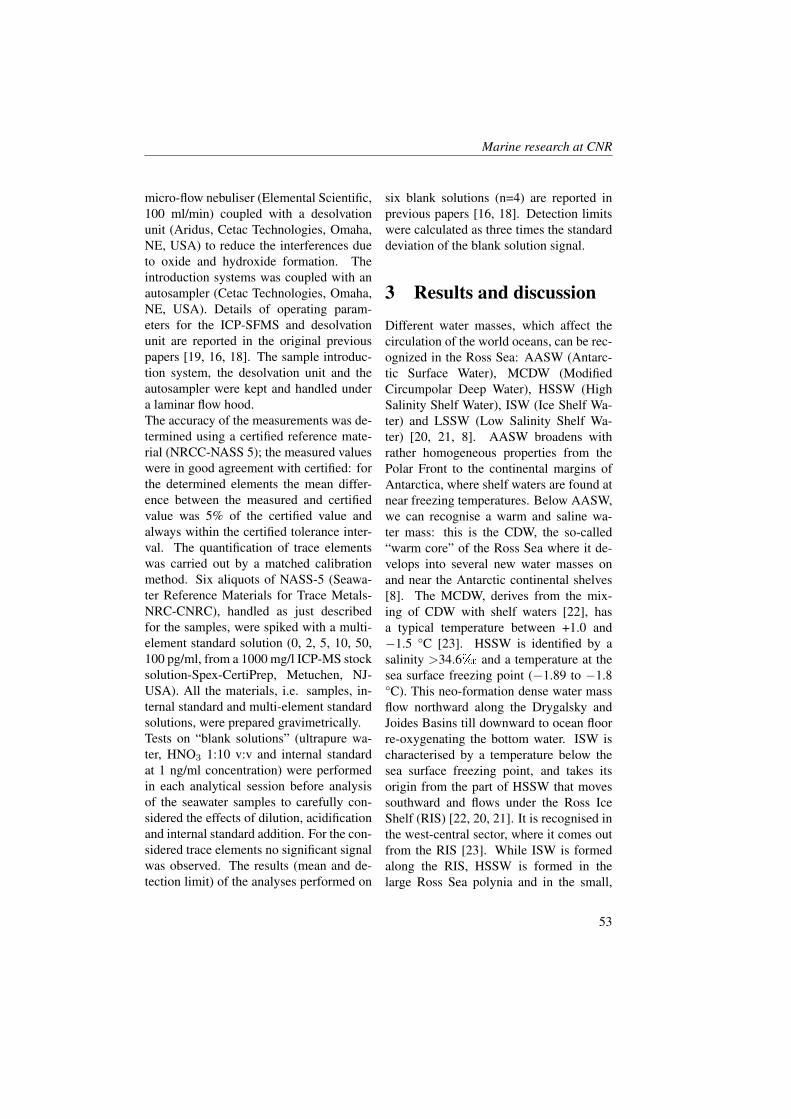
Marine research at CNR
micro-flow nebuliser (Elemental Scientific,100 ml/min) coupled with a desolvationunit (Aridus, Cetac Technologies, Omaha,NE, USA) to reduce the interferences dueto oxide and hydroxide formation. Theintroduction systems was coupled with anautosampler (Cetac Technologies, Omaha,NE, USA). Details of operating param-eters for the ICP-SFMS and desolvationunit are reported in the original previouspapers [19, 16, 18]. The sample introduc-tion system, the desolvation unit and theautosampler were kept and handled undera laminar flow hood.The accuracy of the measurements was de-termined using a certified reference mate-rial (NRCC-NASS 5); the measured valueswere in good agreement with certified: forthe determined elements the mean differ-ence between the measured and certifiedvalue was 5% of the certified value andalways within the certified tolerance inter-val. The quantification of trace elementswas carried out by a matched calibrationmethod. Six aliquots of NASS-5 (Seawa-ter Reference Materials for Trace Metals-NRC-CNRC), handled as just describedfor the samples, were spiked with a multi-element standard solution (0, 2, 5, 10, 50,100 pg/ml, from a 1000 mg/l ICP-MS stocksolution-Spex-CertiPrep, Metuchen, NJ-USA). All the materials, i.e. samples, in-ternal standard and multi-element standardsolutions, were prepared gravimetrically.Tests on “blank solutions” (ultrapure wa-ter, HNO3 1:10 v:v and internal standardat 1 ng/ml concentration) were performedin each analytical session before analysisof the seawater samples to carefully con-sidered the effects of dilution, acidificationand internal standard addition. For the con-sidered trace elements no significant signalwas observed. The results (mean and de-tection limit) of the analyses performed on
six blank solutions (n=4) are reported inprevious papers [16, 18]. Detection limitswere calculated as three times the standarddeviation of the blank solution signal.
3 Results and discussion
Different water masses, which affect thecirculation of the world oceans, can be rec-ognized in the Ross Sea: AASW (Antarc-tic Surface Water), MCDW (ModifiedCircumpolar Deep Water), HSSW (HighSalinity Shelf Water), ISW (Ice Shelf Wa-ter) and LSSW (Low Salinity Shelf Wa-ter) [20, 21, 8]. AASW broadens withrather homogeneous properties from thePolar Front to the continental margins ofAntarctica, where shelf waters are found atnear freezing temperatures. Below AASW,we can recognise a warm and saline wa-ter mass: this is the CDW, the so-called“warm core” of the Ross Sea where it de-velops into several new water masses onand near the Antarctic continental shelves[8]. The MCDW, derives from the mix-ing of CDW with shelf waters [22], hasa typical temperature between +1.0 and−1.5 °C [23]. HSSW is identified by asalinity >34.6� and a temperature at thesea surface freezing point (−1.89 to −1.8°C). This neo-formation dense water massflow northward along the Drygalsky andJoides Basins till downward to ocean floorre-oxygenating the bottom water. ISW ischaracterised by a temperature below thesea surface freezing point, and takes itsorigin from the part of HSSW that movessouthward and flows under the Ross IceShelf (RIS) [22, 20, 21]. It is recognised inthe west-central sector, where it comes outfrom the RIS [23]. While ISW is formedalong the RIS, HSSW is formed in thelarge Ross Sea polynia and in the small,
53
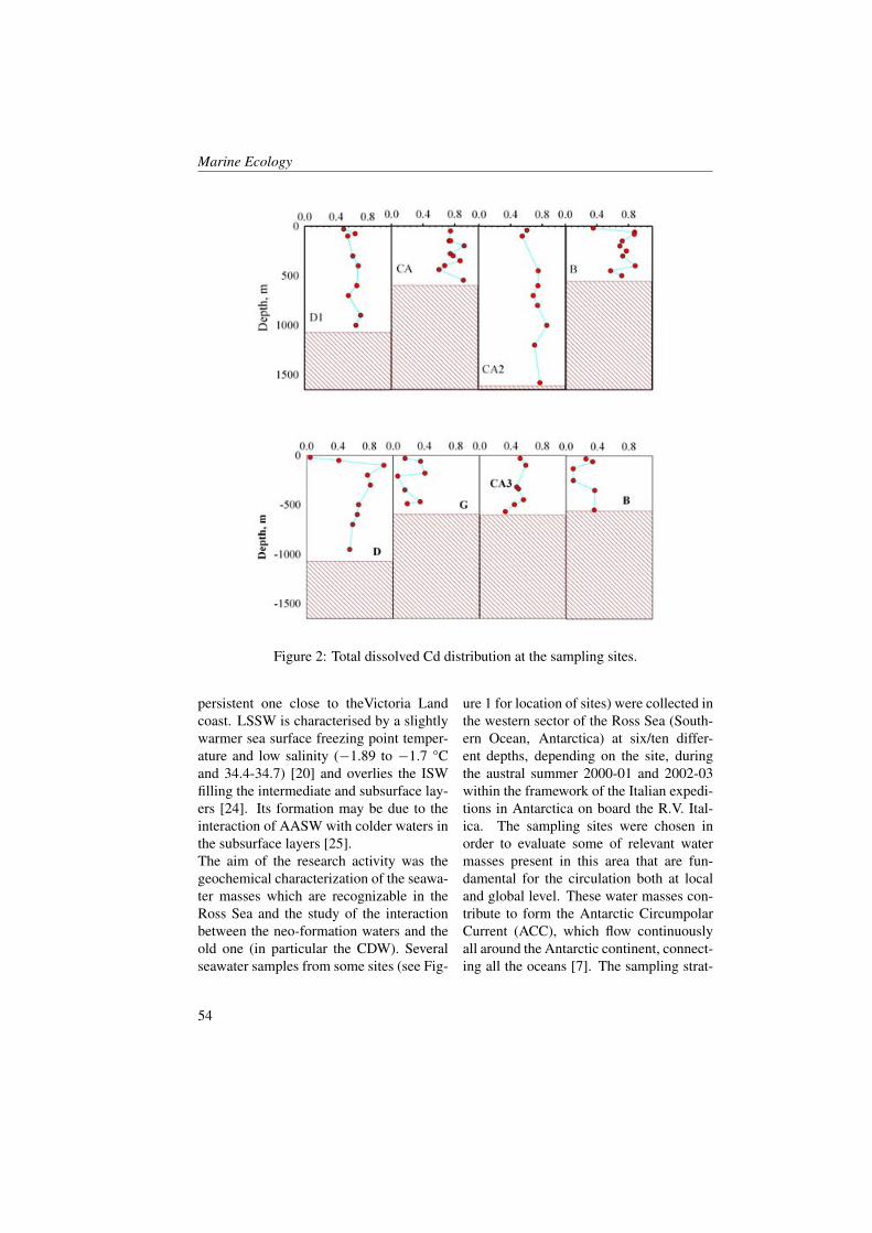
Marine Ecology
Figure 2: Total dissolved Cd distribution at the sampling sites (from Corami, 2005 modified).
Figure 2: Total dissolved Cd distribution at the sampling sites.
persistent one close to theVictoria Landcoast. LSSW is characterised by a slightlywarmer sea surface freezing point temper-ature and low salinity (−1.89 to −1.7 °Cand 34.4-34.7) [20] and overlies the ISWfilling the intermediate and subsurface lay-ers [24]. Its formation may be due to theinteraction of AASW with colder waters inthe subsurface layers [25].The aim of the research activity was thegeochemical characterization of the seawa-ter masses which are recognizable in theRoss Sea and the study of the interactionbetween the neo-formation waters and theold one (in particular the CDW). Severalseawater samples from some sites (see Fig-
ure 1 for location of sites) were collected inthe western sector of the Ross Sea (South-ern Ocean, Antarctica) at six/ten differ-ent depths, depending on the site, duringthe austral summer 2000-01 and 2002-03within the framework of the Italian expedi-tions in Antarctica on board the R.V. Ital-ica. The sampling sites were chosen inorder to evaluate some of relevant watermasses present in this area that are fun-damental for the circulation both at localand global level. These water masses con-tribute to form the Antarctic CircumpolarCurrent (ACC), which flow continuouslyall around the Antarctic continent, connect-ing all the oceans [7]. The sampling strat-
54

Marine research at CNR
Figure 3: Total dissolved Pb distribution at the sampling sites (from Corami, 2005 modified).
Figure 3: Total dissolved Pb distribution at the sampling sites.
egy was driven on the basis of the in situmeasurements of salinity, temperature anddissolved oxygen along the water column.The sampled sites represent areas of newwater formation (HSSW and ISW), or mix-ing area (shelf water and CDW), or sinkarea (where new waters flow downward toocean floor re-oxygenating the bottom wa-ter) [26, 18].The obtained results have highlighted theexisting differences between the variousseawater masses recognizable in the RossSea.The dissolved cadmium concentrationranged between 0.1 and 0.9 nmol/L show-ing a general agreement with the concen-
trations reported in literature for the Wed-del Sea and the Ross Sea [27, 28].A variability on surface concentration ofcadmium in the Ross Sea was observed; itseem to be related to similar and dishomo-geneous distribution of phytoplankton, ashighlighted in previous works [29], andwith differences also in the major nutri-ent concentration and all the trace elementswhose distribution is related to biologicalactivity. Studies performed on the coastalareas of the Ross Sea have highlighted thestrong relationship between cadmium andphytoplanktonic bloom along the verticalprofile, expecially during the summer pe-riod, when the concentration vary from 0.8
55
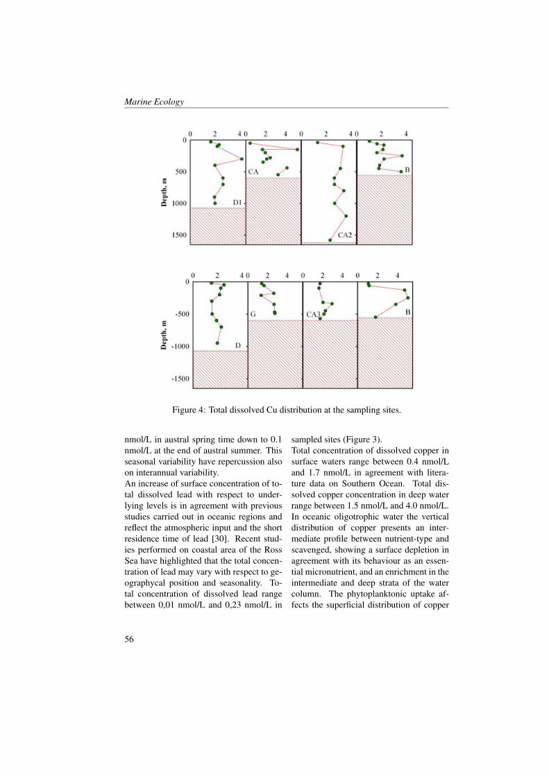
Marine Ecology
Figure 4: Total dissolved Cu distribution at the sampling sites (from Corami, 2005 modified).
Figure 4: Total dissolved Cu distribution at the sampling sites.
nmol/L in austral spring time down to 0.1nmol/L at the end of austral summer. Thisseasonal variability have repercussion alsoon interannual variability.An increase of surface concentration of to-tal dissolved lead with respect to under-lying levels is in agreement with previousstudies carried out in oceanic regions andreflect the atmospheric input and the shortresidence time of lead [30]. Recent stud-ies performed on coastal area of the RossSea have highlighted that the total concen-tration of lead may vary with respect to ge-ographycal position and seasonality. To-tal concentration of dissolved lead rangebetween 0,01 nmol/L and 0,23 nmol/L in
sampled sites (Figure 3).Total concentration of dissolved copper insurface waters range between 0.4 nmol/Land 1.7 nmol/L in agreement with litera-ture data on Southern Ocean. Total dis-solved copper concentration in deep waterrange between 1.5 nmol/L and 4.0 nmol/L.In oceanic oligotrophic water the verticaldistribution of copper presents an inter-mediate profile between nutrient-type andscavenged, showing a surface depletion inagreement with its behaviour as an essen-tial micronutrient, and an enrichment in theintermediate and deep strata of the watercolumn. The phytoplanktonic uptake af-fects the superficial distribution of copper
56
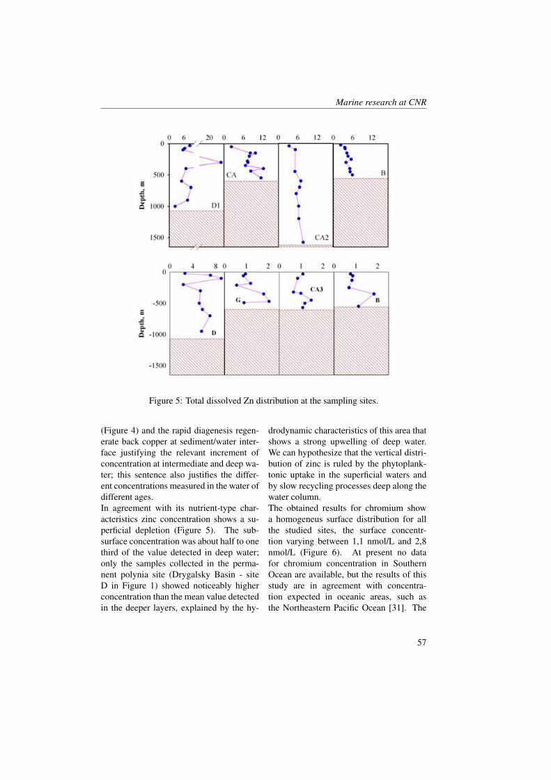
Marine research at CNR
Figure 5: Total dissolved Zn distribution at the sampling sites (from Corami, 2005 modified).
Figure 5: Total dissolved Zn distribution at the sampling sites.
(Figure 4) and the rapid diagenesis regen-erate back copper at sediment/water inter-face justifying the relevant increment ofconcentration at intermediate and deep wa-ter; this sentence also justifies the differ-ent concentrations measured in the water ofdifferent ages.In agreement with its nutrient-type char-acteristics zinc concentration shows a su-perficial depletion (Figure 5). The sub-surface concentration was about half to onethird of the value detected in deep water;only the samples collected in the perma-nent polynia site (Drygalsky Basin - siteD in Figure 1) showed noticeably higherconcentration than the mean value detectedin the deeper layers, explained by the hy-
drodynamic characteristics of this area thatshows a strong upwelling of deep water.We can hypothesize that the vertical distri-bution of zinc is ruled by the phytoplank-tonic uptake in the superficial waters andby slow recycling processes deep along thewater column.The obtained results for chromium showa homogeneus surface distribution for allthe studied sites, the surface concentr-tion varying between 1,1 nmol/L and 2,8nmol/L (Figure 6). At present no datafor chromium concentration in SouthernOcean are available, but the results of thisstudy are in agreement with concentra-tion expected in oceanic areas, such asthe Northeastern Pacific Ocean [31]. The
57

Marine Ecology
Figure 6: Total dissolved Cr distribution at the sampling sites (from Corami, 2005 modified).
Figure 6: Total dissolved Cr distribution at the sampling sites.
expected oceanic distribution for this el-ement is in correlation with the biologi-cal activity recognized in this area; it alsoseem to be complicated by the oxidation-reduction processes in anoxic waters. Themeasured performed on our samples showthat the total concentration increase withdepth. In oxigenated water Cr (IV) is thedominant species: due to the oxigenationof the studied area chromium should as-sume this state. Therefore the slow oxida-tion rate of Cr(III) could permit the coexis-tence of the two species in oxigenated wa-ters, while we cannot exclude the presenceof the reduced form close to the sediment.The concentration distribution of total dis-solved manganese is quite homogeneous in
the studied sites (Figure 7), the total con-centration varying in the mixlayer between1.3 nmol/L and 2.0 nmol/L and between1.4 nmol/L and 3.6 nmol/L in the interme-diate water. A homogeneous distribution inthe superficial and intermediate layers wasunderlined also in the Indian sector of theSouthern Ocean; moreover, in the Ross Seathe concentration and the vertical distribu-tion of manganese may vary with the sea-sonality, in particular between spring andaustral summer. The obtained value of bot-tom water are in agreement with the valueof polynia area in the spring time [32].
58

Marine research at CNR
Figure 7: Total dissolved Mn distribution at the sampling sites (from Corami, 2005 modified).
Figure 7: Total dissolved Mn distribution at the sampling sites.
4 Conclusion and futureperspective
The vertical distribution of trace elementsseems to be related not only to their geo-chemical property but also to other factors:seasonality, various local input, biologicalactivity and to the different characteristicsof the water masses recognizable in thewestern sector of the Ross Sea. On thebasis of the acquired knowledge we maytry to better understand the complex systemof the Southern Ocean and to contribute todeeper known the role of the Ross Sea onthe evolution of our environment.
In the framework of the Italian expedi-tions in Antarctica on board the R.V. Ital-ica during the austral summer 2005-2006we have collected numerous samples alongfive depth profile in different sites of theRoss Sea to have confirmation of our pre-vious data and to evaluate the evolution ofnew-formation waters; we’ll try to followtheir movements till the mixing area of newand old waters and to quantify their inter-annual variability.It will be necessary to deeply study theAntarctic waters, in particular in the ar-eas of polynia, of formation of icewaterand of sink from shelf to abyssal zone to
59
Marine Ecology
better understand the mechanisms, the ex-change entity between the water massesand the geochemical cycles of trace ele-ments. The studies should be extended todifferent areas of all our planet to followthe exchanges between the different oceanstill the Arctic Ocean.
5 AcknowledgementsThis work was financially supported by theItalian National Antarctic Research Pro-gramme (PNRA). We are indebted to allthe crew of “R/V Italica” for their help insampling operations. We are also gratefulto the scientists of the Sector 8 “Oceanog-raphy” for physical parameter measure-ments.
References[1] L.Y. Alleman, T.M.Church, P. Ganguli, A.J.Veron, B. Hamelin, , and A.R. Flegal.
Role of oceanic circulation on contaminant lead distribution in the South Atlantic.Deep Sea Research Part II: Topical Studies in Oceanography, 48(2855):2876, 2001.
[2] C. Barbante, C. Turetta, G. Capodaglio, P. Cescon, S.M. Hong, J.P. Candelone,K. van de Velde, and C.F. Boutron. Trace element determination in polar snow andice. An overview of the analytical process and application in environmental andpaleoclimatic studies. (55):86, 2001.
[3] J.R.Mc Connell, G.W. Lamorey, , and M.A. Hutterli. A 250-year high-resolutionrecord of Pb flux and crustal enrichment in central Greenland. Geophysical Re-search Letters, 29, 2002.
[4] J.O. Nriagu and J.M. Pacyna. Quantitative assessment of worldwide contaminationof air, water and soils by trace metals. Nature, 333(134):139, 1988.
[5] J.M.Pacyna and E.G.Pacyna. An assessment of global and regional emissions oftrace metals to the atmosphere from anthropogenic sources worldwide. Environ-mental Reviews, 9, 2001.
[6] F.A.M.Planchon, C.F. Boutron, C. Barbante, G. Cozzi, V. Gaspari, E.W. Wolff, C.P.Ferrari, , and P. Cescon. Changes in heavy metals in Antarctic snow from CoatsLand since the mid-19th to the late-20th century. Earth and Planetary ScienceLetters, 200, 2002.
[7] A.H. Orsi, T. Whitworth III, and W.D. Nowlin Jr. On the meridional extent andfronts of the Antarctic Circumpolar Current. Deep Sea Research Part I: Oceano-graphic Research Papers, 42(641):673, 1995.
[8] S.S. Jacobs and C.F. Giulivi. Thermohaline data and ocean circulation on the Rosssea. (3):16, 1999.
60
Marine research at CNR
[9] A.H. Orsi, G.C. Johnson, , and J.L. Bullister. Circulation, mixing, and productionof Antarctic Bottom Water. Progress In Oceanography, 43, 1999.
[10] K.W. Bruland, J.R. Donat, , and D.A. Hutchins. Interactive influences of bioactivetrace metals on biological production in oceanic waters. Limnology and Oceanog-raphy, 36, 1991.
[11] J. Smith, J. Marra, M.R. Hiscock, and R.T. Barber. The seasonal cycle of phyto-plankton biomass and primary productivity in the Ross Sea, Antarctica. Deep SeaResearch Part II: Topical Studies in Oceanography, 47(3119):3140, 2000.
[12] S. Westerlund and P. Ohman. Cadmium, copper, cobalt, nickel, lead, and zinc in thewater column of the Weddell Sea, Antarctica. Geochimica e Cosmochimica Acta,55, 1991.
[13] G. Capodaglio, G. Toscano, P. Cescon, G. Scarponi, and H. Muntau. Collabora-tive sampling error assessment of trace metal determination in seawater. Annali diChimica - Rome, 84, 1994.
[14] G. Capodaglio, C. Barbante, and P. Cescon. Trace metals in Antarctic sea water.(107):154, 2001.
[15] G. Capodaglio, C. Barbante, C. Turetta, G. Scarponi, , and P. Cescon. Analyti-cal quality control: sampling procedures to detect trace metals in environmentalmatrices. Mikrochimica Acta, 123, 1996.
[16] C. Turetta, G. Cozzi, C. Barbante, G. Capodaglio, and P. Cescon. Trace ele-ments determination in seawater by ICP-SFMS coupled with a micro-flow nebu-lization/desolvation. Analytical and Bioanalytical Chemistry, 380(258):268, 2004.
[17] I. Rodushkin and T. Ruth. Determination of Trace Metals in Estuarine and Sea-water Reference Materials by High Resolution Inductively Coupled Plasma MassSpectrometry. Journal of Analytical Atomic Spectrometry, 12(1181):1185, 1997.
[18] C. Turetta, C. Barbante, G. Capodaglio, A. Gambaro, , and P.Cescon. The dis-tribution of dissolved thallium in the different water masses of the western sectorof the Ross Sea (Antarctica) during the austral summer. Microchemical Journal,96(2):194–202, 2010.
[19] C. Turetta, G. Cozzi, A. Varga, C. Barbante, G. Capodaglio, and P. Cescon. Plat-inum group elements determination in seawater by ICP-SFMS: initial results. Jour-nal de Physique IV, 107(2):1321–1324, 2003.
[20] L.I. Gordon, L.A. Codispoti, J.C. Jennings Jr., F.J. Millero, J.M. Morrison, andC. Sweeney. Seasonal evolution of hydrographic properties in the Ross Sea, Antarc-tica. Deep Sea Research Part II: Topical Studies in Oceanography, 47(3095):3117,2000.
61
Marine Ecology
[21] D.M. Holland, S.S. Jacobs, , and A. Jenkins. Modelling the ocean circulation be-neath the Ross Ice Shelf. Antarctic Science, 15(13):23, 2003.
[22] G. Budillon, S. Gremes Cordero, , and E. Salusti. On the dense water spreadingoff the Ross Sea shelf (Southern Ocean). Journal of Marine Systems, 35(207):227,2002.
[23] M.S. Dinniman, J.M. Klinck, , and J. Smith. Cross-shelf exchange in a model ofthe Ross Sea circulation and biogeochemistry. Deep Sea Research Part II: TopicalStudies in Oceanography, 50, 2003.
[24] S.S. Jacobs, R.G. Fairbanks, and Y. Horibe. Origin and evolution of water massesnear the antarctic continental margin: evidence from H2 18O/H2 16O ratios inseawater. Oceanology of the Antarctic Continental Shelf, 43(59):85, 1985.
[25] G. Budillon, M. Pacciaroni, S. Cozzi, P. Rivaro, G. Catalano, C. Ianni, , and C. Can-toni. An Optimum Multiparameter Mixing Analysis Of The Shelf Waters In TheRoss Sea. Antarctic Science, 15, 2003.
[26] F. Corami, G. Capodaglio, C. Turetta, F. Soggia, E. Magi, , and M. Grotti. Sum-mer distribution of trace metals in the western sector of the Ross Sea, Antarctica.Journal of Environmental Monitoring, 7(1256):1264, 2005.
[27] M. Grotti, F. Soggia, M.L. Abelmoschi, P. Rivaro, E. Magi, and R. Frache. Tempo-ral distribution of trace metals in Antarctic coastal waters. Marine Chemistry, 76,2001.
[28] R.F. Nolting and H.J.W. De Baar. Behaviour of nickel, copper, zinc and cadmiumin the upper 300 m of a transect in the Southern Ocean (57°–62°S, 49°W). MarineChemistry, 45, 1994.
[29] W.O. Smith and V.L. Asper. The influence of phytoplankton assemblage com-position on biogeochemical characteristics and cycles in the southern Ross Sea,Antarctica. Deep Sea Research Part I: Oceanographic Research Papers, 48, 2001.
[30] C.E. Jones, A.N. Halliday, D.K. Rea, and R.M. Owen. Eolian inputs of lead to theNorth Pacific. Geochimica et Cosmochimica Acta, 64, 2000.
[31] W. Sirinawin, D.R. Turner, and S. Westerlund. Chromium(VI) distributions in theArctic and the Atlantic Oceans and a reassessment of the oceanic Cr cycle. MarineChemistry, 71, 2000.
[32] P.N. Sedwick and G.R. Di Tullio. Regulation of algal blooms in Antarctic shelfwaters by the release of iron from melting sea ice. Geophysical Research Letters,24, 1997.
62

Effect of Sea Surface Temperature and Wind Forc-ing on the Potential Spawning Habitat of EuropeanAnchovy (Engraulis encrasicolus) in the Strait ofSicily
G. Basilone1, A. Bonanno1, B. Patti1, R. Grammauta2, A. Cuttitta1, S.Aronica1, G. Giacalone1, I. Fontana1, G. Buscaino1, B. De Luca1, C.Patti1, E.M. Quinci1, F. Falco1
1, Institute for Coastal Marine Environment, CNR, Capo Granitola (TP), Italy2, Faculty of Mathematical, Physical and Natural Sciences, University of Palermo, Palermo,[email protected]
Abstract
The European anchovy (Engraulis encrasicolus) represents one of the most im-portant fishery resources of the Mediterranean. Because of its short living nature andits recruitment variability, associated to high environmental variability, this speciesundergo large interannual fluctuactions in the biomass levels. The aim of presentstudy is to characterize the anchovy spawning habitat in terms of satellite-derivedand in situ measurements of sea surface temperature (SST), and wind mixing andsurface wind stress. This research work has been performed on the data collectedduring three oceanographic surveys carried in the Strait of Sicily out on board theR/V Urania in summer 2004, 2005 and 2006. The main spawning ground during2004 survey was located in the coastal waters between Sciacca and Gela; duringthe 2005 survey the egg density spatial distribution pattern was complementary tothe one observed in the previous year, with two main spawning areas located on theAdventure Bank and on the northern part of the Maltese shelf; the spatial pattern in2006 was similar to 2005 but with lower densities. The results showed the existenceof preferred values in the examined physical variables, associated to anchovy spawn-ing areas. The analysis on SST indicates that the spawning habitat is characterizedby a main peak at 23°C, while the optimal spawning conditions obtained by analysison wind mixing and wind stress show a main peak in the range 300-500 m3 · s−3andat 0.10 N/m2.
1 Introduction
The European anchovy (Engraulis encra-sicolus) constitutes one of the most impor-tant fishery resource in the central Mediter-ranean sea. Because of its short liv-
ing nature and of its recruitment variabil-ity, associated to high environmental vari-ability, this small pelagic species under-goes high interannual fluctuations in thebiomass level [1]. The population abun-dance is determined especially by the high
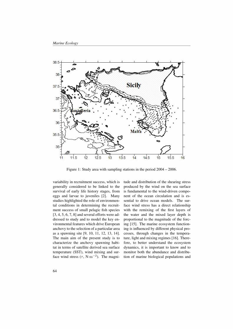
Marine Ecology
Figure 1: Study area with sampling stations in the period 2004 – 2006.
variability in recruitment success, which isgenerally considered to be linked to thesurvival of early life history stages, fromeggs and larvae to juveniles [2]. Manystudies highlighted the role of environmen-tal conditions in determining the recruit-ment success of small pelagic fish species[3, 4, 5, 6, 7, 8] and several efforts were ad-dressed to study and to model the key en-vironmental features which drive Europeananchovy to the selection of a particular areaas a spawning site [9, 10, 11, 12, 13, 14].The main aim of the present study is tocharacterize the anchovy spawning habi-tat in terms of satellite derived sea surfacetemperature (SST), wind mixing and sur-face wind stress (τ , N·m−2). The magni-
tude and distribution of the shearing stressproduced by the wind on the sea surfaceis fundamental to the wind-driven compo-nent of the ocean circulation and is es-sential to drive ocean models. The sur-face wind stress has a direct relationshipwith the remixing of the first layers ofthe water and the mixed layer depth isproportional to the magnitude of the forc-ing [15]. The marine ecosystem function-ing is influenced by different physical pro-cesses, through changes in the tempera-ture, light and mixing regimes [16]. There-fore, to better understand the ecosystemdynamics, it is important to know and tomonitor both the abundance and distribu-tion of marine biological populations and
64
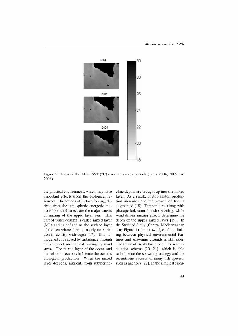
Marine research at CNR
Figure 2: Maps of the Mean SST (°C) over the survey periods (years 2004, 2005 and2006).
the physical environment, which may haveimportant effects upon the biological re-sources. The actions of surface forcing, de-rived from the atmospheric energetic mo-tions like wind stress, are the major causesof mixing of the upper layer sea. Thispart of water column is called mixed layer(ML) and is defined as the surface layerof the sea where there is nearly no varia-tion in density with depth [17]. This ho-mogeneity is caused by turbulence throughthe action of mechanical mixing by windstress. The mixed layer of the ocean andthe related processes influence the ocean’sbiological production. When the mixedlayer deepens, nutrients from subthermo-
cline depths are brought up into the mixedlayer. As a result, phytoplankton produc-tion increases and the growth of fish isaugmented [18]. Temperature, along withphotoperiod, controls fish spawning, whilewind-driven mixing effects determine thedepth of the upper mixed layer [19]. Inthe Strait of Sicily (Central Mediterraneansea; Figure 1) the knowledge of the link-ing between physical environmental fea-tures and spawning grounds is still poor.The Strait of Sicily has a complex sea cir-culation scheme [20, 21], which is ableto influence the spawning strategy and therecruitment success of many fish species,such as anchovy [22]. In the simplest circu-
65
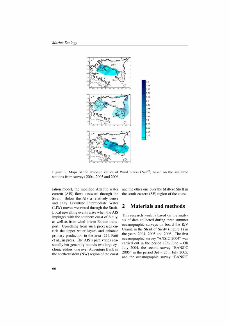
Marine Ecology
Figure 3: Maps of the absolute values of Wind Stress (N/m2) based on the availablestations from surveys 2004, 2005 and 2006.
lation model, the modified Atlantic watercurrent (AIS) flows eastward through theStrait. Below the AIS a relatively denseand salty Levantine Intermediate Water(LIW) moves westward through the Strait.Local upwelling events arise when the AISimpinges with the southern coast of Sicily,as well as from wind-driven Ekman trans-port. Upwelling from such processes en-rich the upper water layers and enhanceprimary production in the area [22], Pattiet al., in press. The AIS’s path varies sea-sonally but generally bounds two large cy-clonic eddies, one over Adventure Bank inthe north-western (NW) region of the coast
and the other one over the Maltese Shelf inthe south-eastern (SE) region of the coast.
2 Materials and methodsThis research work is based on the analy-sis of data collected during three summeroceanographic surveys on board the R/VUrania in the Strait of Sicily (Figure 1) inthe years 2004, 2005 and 2006. The firstoceanographic survey “ANSIC 2004” wascarried out in the period 17th June – 6thJuly 2004, the second survey “BANSIC2005” in the period 3rd – 25th July 2005,and the oceanographic survey “BANSIC
66
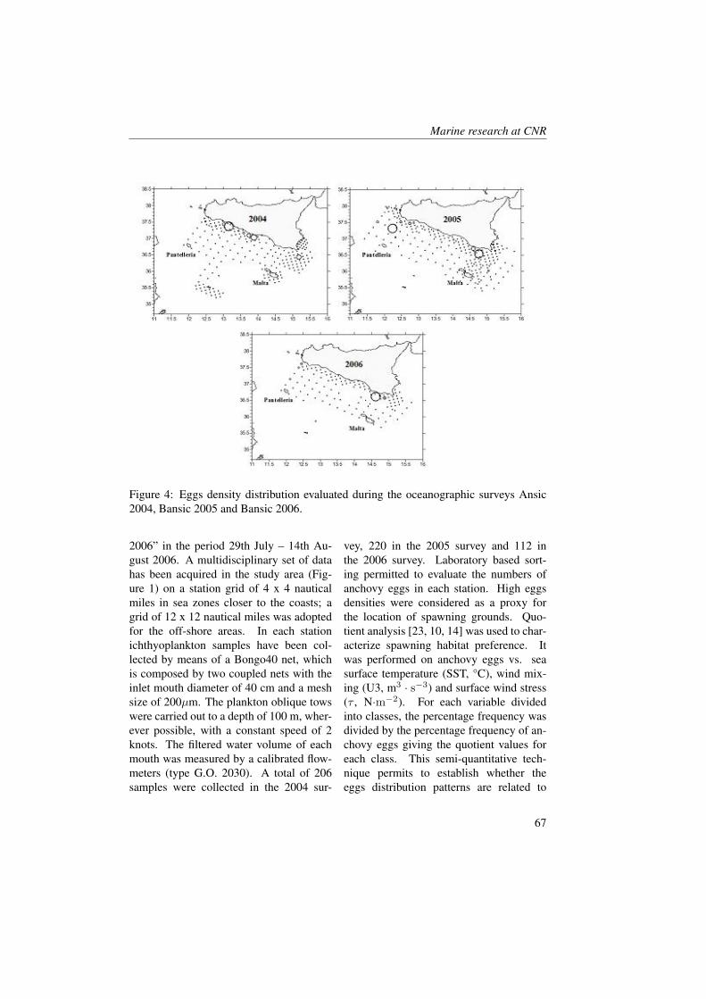
Marine research at CNR
Figure 4: Eggs density distribution evaluated during the oceanographic surveys Ansic2004, Bansic 2005 and Bansic 2006.
2006” in the period 29th July – 14th Au-gust 2006. A multidisciplinary set of datahas been acquired in the study area (Fig-ure 1) on a station grid of 4 x 4 nauticalmiles in sea zones closer to the coasts; agrid of 12 x 12 nautical miles was adoptedfor the off-shore areas. In each stationichthyoplankton samples have been col-lected by means of a Bongo40 net, whichis composed by two coupled nets with theinlet mouth diameter of 40 cm and a meshsize of 200µm. The plankton oblique towswere carried out to a depth of 100 m, wher-ever possible, with a constant speed of 2knots. The filtered water volume of eachmouth was measured by a calibrated flow-meters (type G.O. 2030). A total of 206samples were collected in the 2004 sur-
vey, 220 in the 2005 survey and 112 inthe 2006 survey. Laboratory based sort-ing permitted to evaluate the numbers ofanchovy eggs in each station. High eggsdensities were considered as a proxy forthe location of spawning grounds. Quo-tient analysis [23, 10, 14] was used to char-acterize spawning habitat preference. Itwas performed on anchovy eggs vs. seasurface temperature (SST, °C), wind mix-ing (U3, m3 · s−3) and surface wind stress(τ , N·m−2). For each variable dividedinto classes, the percentage frequency wasdivided by the percentage frequency of an-chovy eggs giving the quotient values foreach class. This semi-quantitative tech-nique permits to establish whether theeggs distribution patterns are related to
67
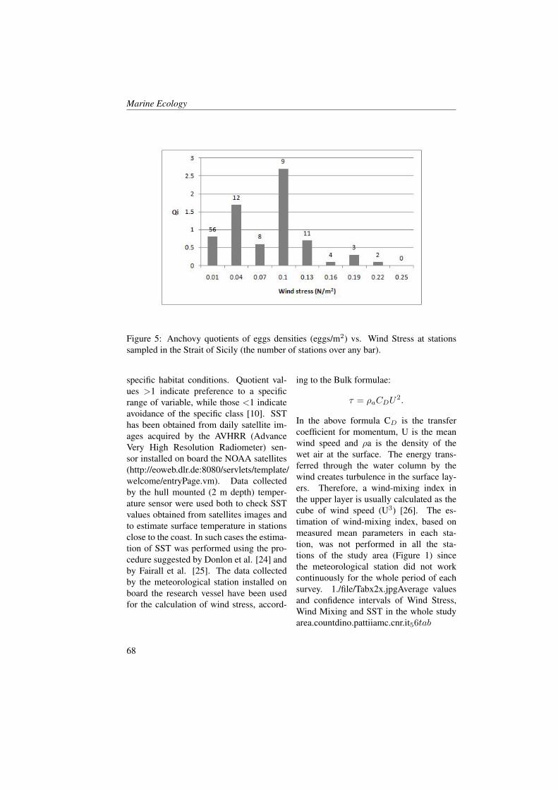
Marine Ecology
Figure 5: Anchovy quotients of eggs densities (eggs/m2) vs. Wind Stress at stationssampled in the Strait of Sicily (the number of stations over any bar).
specific habitat conditions. Quotient val-ues >1 indicate preference to a specificrange of variable, while those <1 indicateavoidance of the specific class [10]. SSThas been obtained from daily satellite im-ages acquired by the AVHRR (AdvanceVery High Resolution Radiometer) sen-sor installed on board the NOAA satellites(http://eoweb.dlr.de:8080/servlets/template/welcome/entryPage.vm). Data collectedby the hull mounted (2 m depth) temper-ature sensor were used both to check SSTvalues obtained from satellites images andto estimate surface temperature in stationsclose to the coast. In such cases the estima-tion of SST was performed using the pro-cedure suggested by Donlon et al. [24] andby Fairall et al. [25]. The data collectedby the meteorological station installed onboard the research vessel have been usedfor the calculation of wind stress, accord-
ing to the Bulk formulae:
τ = ρaCDU2.
In the above formula CD is the transfercoefficient for momentum, U is the meanwind speed and ρa is the density of thewet air at the surface. The energy trans-ferred through the water column by thewind creates turbulence in the surface lay-ers. Therefore, a wind-mixing index inthe upper layer is usually calculated as thecube of wind speed (U3) [26]. The es-timation of wind-mixing index, based onmeasured mean parameters in each sta-tion, was not performed in all the sta-tions of the study area (Figure 1) sincethe meteorological station did not workcontinuously for the whole period of eachsurvey. 1./file/Tabx2x.jpgAverage valuesand confidence intervals of Wind Stress,Wind Mixing and SST in the whole studyarea.countdino.pattiiamc.cnr.it56tab
68
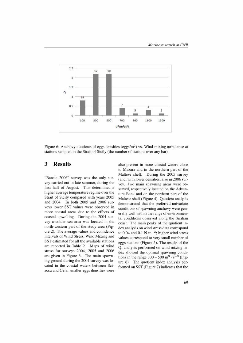
Marine research at CNR
Figure 6: Anchovy quotients of eggs densities (eggs/m2) vs. Wind-mixing turbulence atstations sampled in the Strait of Sicily (the number of stations over any bar).
3 Results
“Bansic 2006” survey was the only sur-vey carried out in late summer, during thefirst half of August. This determined ahigher average temperature regime over theStrait of Sicily compared with years 2005and 2004. In both 2005 and 2006 sur-veys lower SST values were observed inmore coastal areas due to the effects ofcoastal upwelling. During the 2004 sur-vey a colder sea area was located in thenorth-western part of the study area (Fig-ure 2). The average values and confidenceintervals of Wind Stress, Wind Mixing andSST estimated for all the available stationsare reported in Table 2. Maps of windstress for surveys 2004, 2005 and 2006are given in Figure 3. The main spawn-ing ground during the 2004 survey was lo-cated in the coastal waters between Sci-acca and Gela; smaller eggs densities were
also present in more coastal waters closeto Mazara and in the northern part of theMaltese shelf. During the 2005 survey(and, with lower densities, also in 2006 sur-vey), two main spawning areas were ob-served, respectively located on the Adven-ture Bank and on the northern part of theMaltese shelf (Figure 4). Quotient analysisdemonstrated that the preferred univariateconditions of spawning anchovy were gen-erally well within the range of environmen-tal conditions observed along the Siciliancoast. The main peaks of the quotient in-dex analysis on wind stress data correspondto 0.04 and 0.1 N·m−2; higher wind stressvalues correspond to very small number ofeggs stations (Figure 5). The results of theQI analysis performed on wind mixing in-dex showed the optimal spawning condi-tions in the range 300 – 500 m3 · s−3 (Fig-ure 6). The quotient index analysis per-formed on SST (Figure 7) indicates that the
69
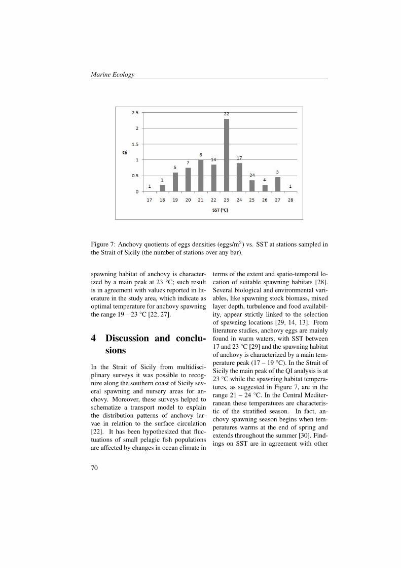
Marine Ecology
Figure 7: Anchovy quotients of eggs densities (eggs/m2) vs. SST at stations sampled inthe Strait of Sicily (the number of stations over any bar).
spawning habitat of anchovy is character-ized by a main peak at 23 °C; such resultis in agreement with values reported in lit-erature in the study area, which indicate asoptimal temperature for anchovy spawningthe range 19 – 23 °C [22, 27].
4 Discussion and conclu-sions
In the Strait of Sicily from multidisci-plinary surveys it was possible to recog-nize along the southern coast of Sicily sev-eral spawning and nursery areas for an-chovy. Moreover, these surveys helped toschematize a transport model to explainthe distribution patterns of anchovy lar-vae in relation to the surface circulation[22]. It has been hypothesized that fluc-tuations of small pelagic fish populationsare affected by changes in ocean climate in
terms of the extent and spatio-temporal lo-cation of suitable spawning habitats [28].Several biological and environmental vari-ables, like spawning stock biomass, mixedlayer depth, turbulence and food availabil-ity, appear strictly linked to the selectionof spawning locations [29, 14, 13]. Fromliterature studies, anchovy eggs are mainlyfound in warm waters, with SST between17 and 23 °C [29] and the spawning habitatof anchovy is characterized by a main tem-perature peak (17 – 19 °C). In the Strait ofSicily the main peak of the QI analysis is at23 °C while the spawning habitat tempera-tures, as suggested in Figure 7, are in therange 21 – 24 °C. In the Central Mediter-ranean these temperatures are characteris-tic of the stratified season. In fact, an-chovy spawning season begins when tem-peratures warms at the end of spring andextends throughout the summer [30]. Find-ings on SST are in agreement with other
70
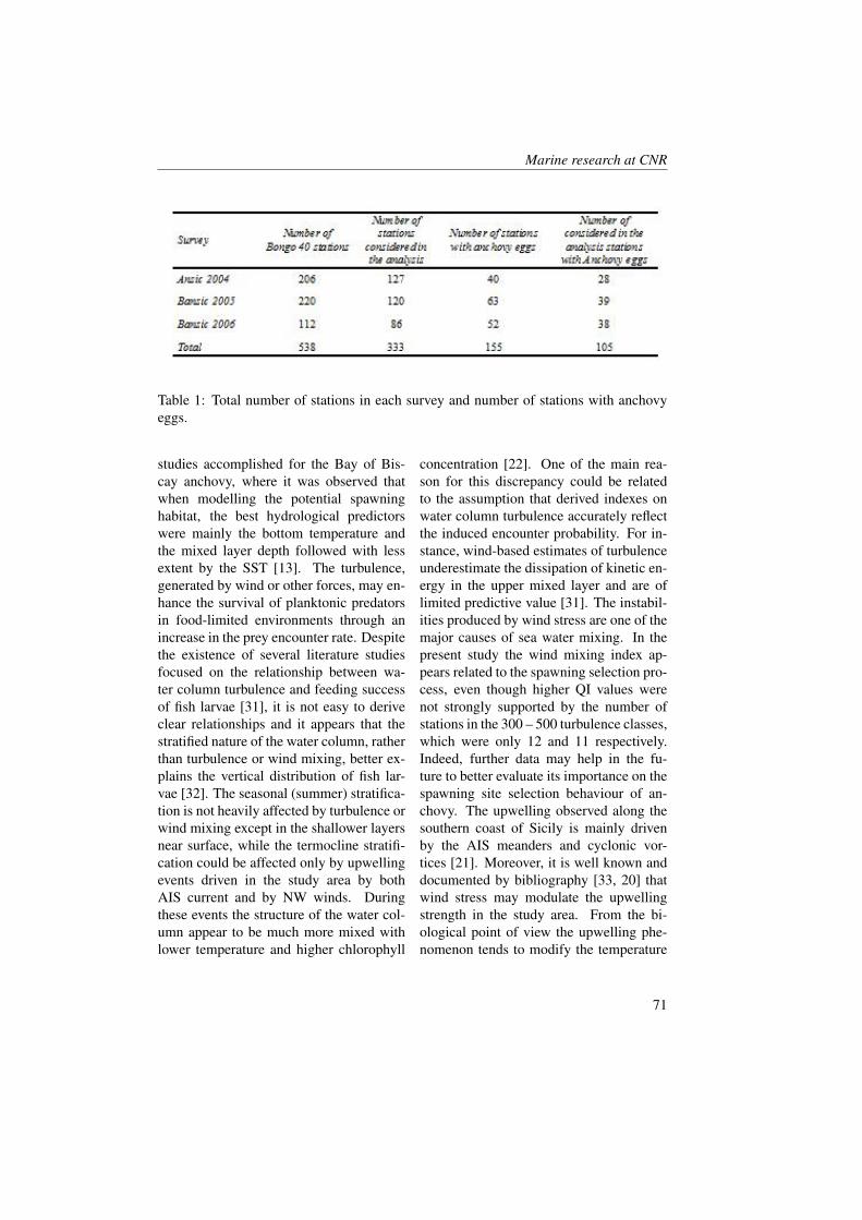
Marine research at CNR
Table 1: Total number of stations in each survey and number of stations with anchovyeggs.
studies accomplished for the Bay of Bis-cay anchovy, where it was observed thatwhen modelling the potential spawninghabitat, the best hydrological predictorswere mainly the bottom temperature andthe mixed layer depth followed with lessextent by the SST [13]. The turbulence,generated by wind or other forces, may en-hance the survival of planktonic predatorsin food-limited environments through anincrease in the prey encounter rate. Despitethe existence of several literature studiesfocused on the relationship between wa-ter column turbulence and feeding successof fish larvae [31], it is not easy to deriveclear relationships and it appears that thestratified nature of the water column, ratherthan turbulence or wind mixing, better ex-plains the vertical distribution of fish lar-vae [32]. The seasonal (summer) stratifica-tion is not heavily affected by turbulence orwind mixing except in the shallower layersnear surface, while the termocline stratifi-cation could be affected only by upwellingevents driven in the study area by bothAIS current and by NW winds. Duringthese events the structure of the water col-umn appear to be much more mixed withlower temperature and higher chlorophyll
concentration [22]. One of the main rea-son for this discrepancy could be relatedto the assumption that derived indexes onwater column turbulence accurately reflectthe induced encounter probability. For in-stance, wind-based estimates of turbulenceunderestimate the dissipation of kinetic en-ergy in the upper mixed layer and are oflimited predictive value [31]. The instabil-ities produced by wind stress are one of themajor causes of sea water mixing. In thepresent study the wind mixing index ap-pears related to the spawning selection pro-cess, even though higher QI values werenot strongly supported by the number ofstations in the 300 – 500 turbulence classes,which were only 12 and 11 respectively.Indeed, further data may help in the fu-ture to better evaluate its importance on thespawning site selection behaviour of an-chovy. The upwelling observed along thesouthern coast of Sicily is mainly drivenby the AIS meanders and cyclonic vor-tices [21]. Moreover, it is well known anddocumented by bibliography [33, 20] thatwind stress may modulate the upwellingstrength in the study area. From the bi-ological point of view the upwelling phe-nomenon tends to modify the temperature
71
Marine Ecology
regime of surface waters, cooling them be-low the optimal temperatures for anchovyspawning [22, 27]. Therefore, in this paperthe major effects of wind stress were takeninto account by analysing both sea watermixing (wind mixing index) and temper-ature regime. The preliminary results ob-tained in this work suggest that SST andthe wind induced turbulence may be con-
sidered proxies of a favourable anchovyspawning sites, where adult specimens maymeet optimal environmental features for re-ducing the mortality of the spawning prod-ucts. Further investigations and surveys fordata collection are necessary in order tounderstand how the biological variabilitycan be coupled with water column stabil-ity/turbulence.
References[1] R.A. Schwartzlose, J. Alheit, A. Bakun, et al. South African Journal of Marine
Science. (21):289, 1999.
[2] R. Lasker. Fish. Bull. (73):453, 1975.
[3] D.H. Cushing. Climate and Fisheries. Academic Press, London, 1982.
[4] M.P. Sissenwine. Sciences Research Report 32. Berlin: Springer-Verlag. (59),1984.
[5] W.S. Wooster and K.M. Bailey. Can. Spec. Publishers Fish. Aquat. Sci. (108):153,1989.
[6] R.J. Beamish. Can. Spec. Publishers Fish. Aquat. Sci. 121:739, 1995.
[7] A. Borja, A. Uriarte, V. Valencia, and L. Motos. Sci. Mar. 60:179, 1996.
[8] A. Borja, A. Uriarte, J. Egana, L. Motos, and V. Valencia. Fish Oceanogr. 7:375,1998.
[9] V. Agostini and A. Bakun. Fish. Oceanogr. 11:129, 2002.
[10] N.M. Twatwa, C.D. Van Der Lingen, L. Drapeau, et al. African Journal of MarineScience. 27:487, 2005.
[11] P. Petitgas, S. Magri, and P. Lazure. Fish. Oceanogr. (15):413, 2006.
[12] E. Bellier, B. Planque, and P. Petitgas. Fish. Oceanogr. doi:10.1111/j.1365-2419.2006.00410.x. 2006.
[13] B. Planque, E. Bellier, and P. Lazure. Fish. Oceanogr. (16):16, 2007.
[14] S. Somarakis and N. Nikolioudakis. Mar. Bio. (152):1147, 2007.
[15] J.E.Ø. Nilsen and E. Falck. Progress in Oceanography. (70):58, 2006.
72
Marine research at CNR
[16] R. Margalef. Sci. Mar. 61:109–123, 1997.
[17] L.H. Kantha and C.A. Clayson. Small Scale Processes in Geophysical Fluid Flows.International Geophysics Series, 67, 2000.
[18] I. Yasuda, T. Tozuka, M. Noto, and S. Kouketsu. Progress in Oceanography.(47):257, 2000.
[19] J.J. Govoni. Scientia Marina. 69(suppl. 1):125, 2005.
[20] P.F.J. Lermusiaux and A. R. Robinson. Deep Sea Research I. (48):1953, 2001.
[21] A.R. Robinson, J. Sellschopp, A. Warn-Varnas, W.G. Leslie, et al. J. Marine Syst.(20):113, 1999.
[22] J. Garcıa Lafuente, A. Garcıa, S. Mazzola, et al. Fish. Oceanogr. (11):31–44, 2002.
[23] C.D. van der Lingen, L. Hutchings, D. Merkle, et al. Alaska Sea Grant CollegeProgram, AK-SG-01-02. pages 185–209, 2001.
[24] C. J. Donlon, P. J. Minnett, I. J. Barton, T. J. Nightngale, and C. Gentemann. .http://www.soc.soton.ac.uk/JRD/MET/WGASF/workshop/PDF/45Donlon.doc.pdf,2002.
[25] C.W. Fairall, E.F. Bradley, J.S. Godfrey, and G.A. Wick. Geophys. Res. (101):1295,1996.
[26] R.L. Elsberry and R.W Garwood. Bull. Am. Meteor. Soc. 59:786–789, 1978.
[27] J. Garcıa Lafuente, J.M. Vargas, and F. Criado. Fish. Oceanogr. 14:32–46, 2005.
[28] J.R. Hunter and J. Alheit. . GLOBEC Report No. 8, 1995.
[29] I. Palomera, M.P. Olivar, J. Salat, A. Sabates, M. Coll., et al. Progress in Oceanog-raphy. (74):377, 2007.
[30] G. Basilone, C. Guisande, B. Patti, S. Mazzola, et al. Fisheries Oceanography.15:271, 2006.
[31] B.R. Mackenzie. Ocean. Acta. (23):357, 2000.
[32] C.S. Reiss, A. Anis, C.T. Taggart, J.F. Dower, and B. Ruddick. Fish. Oceanogr.11(3):156, 2002.
[33] A. Warn-Varnas, J. Sellschopp, P.J. Haley Jr., et al. Dynam. Atmos. Oceans.(29):437, 1999.
73

Marine Ecology
74
Identification of a Novel Helitron Transposon inthe Genome of Antarctic Fish
E. Cocca1, M.A. Morescalchi2, S. De Iorio3, T. Capriglione3
1, Institute of Protein Biochemistry, CNR, Napoli, Italy2, Department of Life Sciences, Second University of Naples, Caserta, Italy3, Department of Biological Sciences, University of Napoli “Federico II”, Napoli, [email protected]
Abstract
Rolling-circle eukaryotic transposons, known as Helitrons, are widely distributed,from protist to mammal species. Autonomous Helitrons show a peculiar open read-ing frame, encoding for a polypeptide that contains typical domains for the rollingcircle replication: the Rep (rolling-circle replication initiatior) and the DNA helicasedomains. These elements are believed to have an important role in the evolutionof the host genomes, owing to their frequent capture of host genes, some of whichcan evolve into novel genes or become essential for Helitron transposition. In thiswork, we performed a molecular analysis on the suborder of the Notothenioidei, aPerciformes group of species that nowadays dominate the Antarctic waters, due totheir remarkable ability in achieving cold-adaptation. We isolated and characteriseda novel Helitron element, that we named HeliNoto (8.9 kb), from the genome of theicefish species Chionodraco hamatus, belonging to the Channichthyidae, the mostderived family of the Notothenioids. The unique open reading frame obtained wasanalysed and compared to homologous sequences present in the genome of differentspecies. The distribution of this element among Notothenioids was finally discussed.
1 Introduction
Rolling-circle eukaryotic transposons,known as Helitrons, are widely distributed,from protist to mammal species [1]. Au-tonomous Helitrons encode the so-calledRep/Hel protein, composed of the repli-cation initiator (Rep) and helicase (Hel)domains. The Rep domain contains threemotifs that are conserved in Rep proteins,which are encoded by plasmids and sin-gle stranded DNA viruses replicating byrolling circle mechanism (RCR). The Reps,such as transposases, perform both cleav-age and ligation of DNA during rolling-circle replication. The Hel domain is a heli-
case that belongs to the SF1 superfamily ofDNA helicases. In some species, Helitronscontain additional domains: apurinic en-donuclease, cysteine protease, zinc fingermotifs and replication protein A (RPA).Helitron is the only known class of trans-posons in eukaryotes that integrates intothe genome without introducing target siteduplications (TSDs). These elements arebelieved to have an important role in theevolution of the host genomes, owing totheir frequent capture of host genes, someof which can evolve into novel genes orbecome essential for Helitron transposi-tion. Therefore, Helitrons may function asa powerful tool of evolution, by mediat-
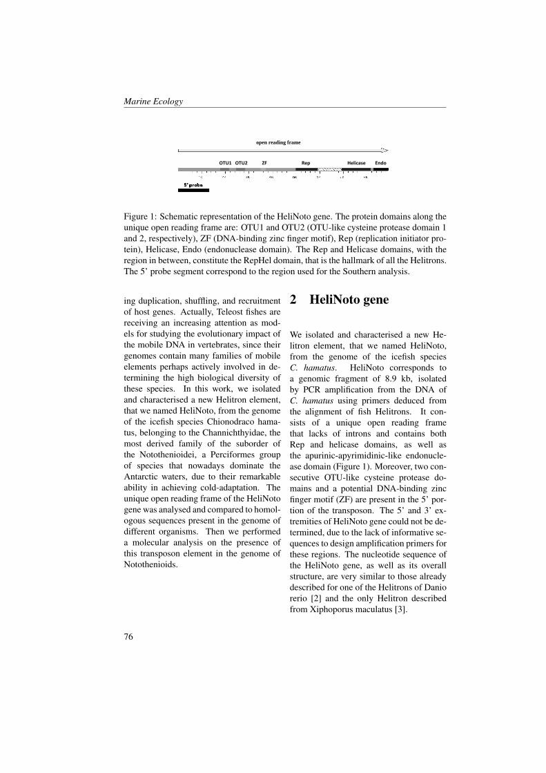
Marine Ecology
open reading frame
OTU1 OTU2 ZF Rep Helicase Endo
5’ probe
Figure 1: Schematic representation of the HeliNoto gene. The protein domains along theunique open reading frame are: OTU1 and OTU2 (OTU-like cysteine protease domain 1and 2, respectively), ZF (DNA-binding zinc finger motif), Rep (replication initiator pro-tein), Helicase, Endo (endonuclease domain). The Rep and Helicase domains, with theregion in between, constitute the RepHel domain, that is the hallmark of all the Helitrons.The 5’ probe segment correspond to the region used for the Southern analysis.
ing duplication, shuffling, and recruitmentof host genes. Actually, Teleost fishes arereceiving an increasing attention as mod-els for studying the evolutionary impact ofthe mobile DNA in vertebrates, since theirgenomes contain many families of mobileelements perhaps actively involved in de-termining the high biological diversity ofthese species. In this work, we isolatedand characterised a new Helitron element,that we named HeliNoto, from the genomeof the icefish species Chionodraco hama-tus, belonging to the Channichthyidae, themost derived family of the suborder ofthe Notothenioidei, a Perciformes groupof species that nowadays dominate theAntarctic waters, due to their remarkableability in achieving cold-adaptation. Theunique open reading frame of the HeliNotogene was analysed and compared to homol-ogous sequences present in the genome ofdifferent organisms. Then we performeda molecular analysis on the presence ofthis transposon element in the genome ofNotothenioids.
2 HeliNoto gene
We isolated and characterised a new He-litron element, that we named HeliNoto,from the genome of the icefish speciesC. hamatus. HeliNoto corresponds toa genomic fragment of 8.9 kb, isolatedby PCR amplification from the DNA ofC. hamatus using primers deduced fromthe alignment of fish Helitrons. It con-sists of a unique open reading framethat lacks of introns and contains bothRep and helicase domains, as well asthe apurinic-apyrimidinic-like endonucle-ase domain (Figure 1). Moreover, two con-secutive OTU-like cysteine protease do-mains and a potential DNA-binding zincfinger motif (ZF) are present in the 5’ por-tion of the transposon. The 5’ and 3’ ex-tremities of HeliNoto gene could not be de-termined, due to the lack of informative se-quences to design amplification primers forthese regions. The nucleotide sequence ofthe HeliNoto gene, as well as its overallstructure, are very similar to those alreadydescribed for one of the Helitrons of Daniorerio [2] and the only Helitron describedfrom Xiphoporus maculatus [3].
76
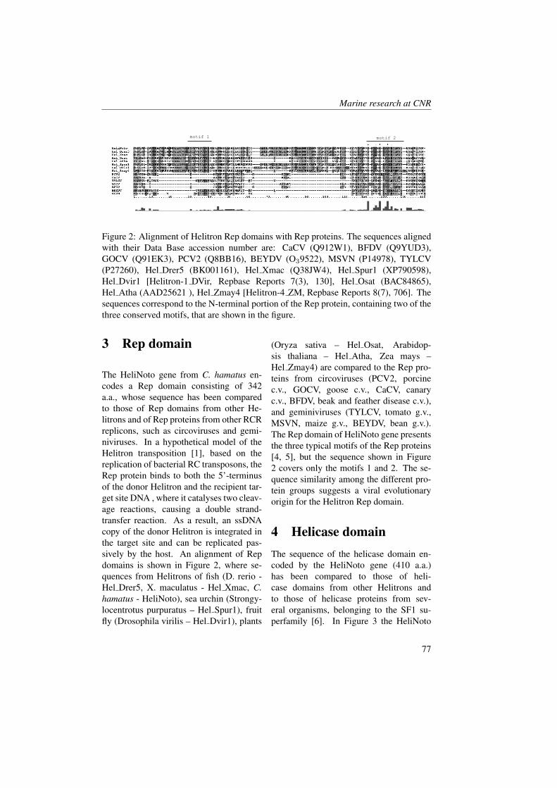
Marine research at CNR
motif 1 motif 2
Figure 2: Alignment of Helitron Rep domains with Rep proteins. The sequences alignedwith their Data Base accession number are: CaCV (Q912W1), BFDV (Q9YUD3),GOCV (Q91EK3), PCV2 (Q8BB16), BEYDV (O39522), MSVN (P14978), TYLCV(P27260), Hel Drer5 (BK001161), Hel Xmac (Q38JW4), Hel Spur1 (XP790598),Hel Dvir1 [Helitron-1 DVir, Repbase Reports 7(3), 130], Hel Osat (BAC84865),Hel Atha (AAD25621 ), Hel Zmay4 [Helitron-4 ZM, Repbase Reports 8(7), 706]. Thesequences correspond to the N-terminal portion of the Rep protein, containing two of thethree conserved motifs, that are shown in the figure.
3 Rep domain
The HeliNoto gene from C. hamatus en-codes a Rep domain consisting of 342a.a., whose sequence has been comparedto those of Rep domains from other He-litrons and of Rep proteins from other RCRreplicons, such as circoviruses and gemi-niviruses. In a hypothetical model of theHelitron transposition [1], based on thereplication of bacterial RC transposons, theRep protein binds to both the 5’-terminusof the donor Helitron and the recipient tar-get site DNA , where it catalyses two cleav-age reactions, causing a double strand-transfer reaction. As a result, an ssDNAcopy of the donor Helitron is integrated inthe target site and can be replicated pas-sively by the host. An alignment of Repdomains is shown in Figure 2, where se-quences from Helitrons of fish (D. rerio -Hel Drer5, X. maculatus - Hel Xmac, C.hamatus - HeliNoto), sea urchin (Strongy-locentrotus purpuratus – Hel Spur1), fruitfly (Drosophila virilis – Hel Dvir1), plants
(Oryza sativa – Hel Osat, Arabidop-sis thaliana – Hel Atha, Zea mays –Hel Zmay4) are compared to the Rep pro-teins from circoviruses (PCV2, porcinec.v., GOCV, goose c.v., CaCV, canaryc.v., BFDV, beak and feather disease c.v.),and geminiviruses (TYLCV, tomato g.v.,MSVN, maize g.v., BEYDV, bean g.v.).The Rep domain of HeliNoto gene presentsthe three typical motifs of the Rep proteins[4, 5], but the sequence shown in Figure2 covers only the motifs 1 and 2. The se-quence similarity among the different pro-tein groups suggests a viral evolutionaryorigin for the Helitron Rep domain.
4 Helicase domainThe sequence of the helicase domain en-coded by the HeliNoto gene (410 a.a.)has been compared to those of heli-case domains from other Helitrons andto those of helicase proteins from sev-eral organisms, belonging to the SF1 su-perfamily [6]. In Figure 3 the HeliNoto
77
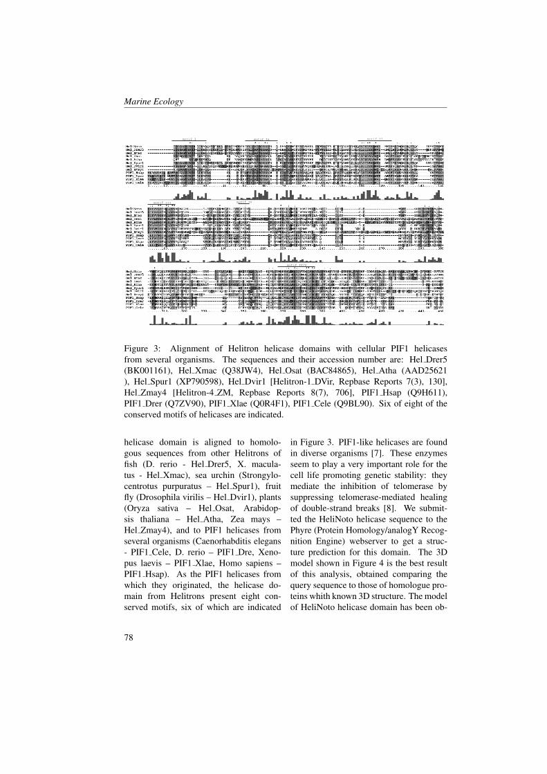
Marine Ecology
motif I motif Ia motif II
motif III motif IV
motif IV/V
Figure 3: Alignment of Helitron helicase domains with cellular PIF1 helicasesfrom several organisms. The sequences and their accession number are: Hel Drer5(BK001161), Hel Xmac (Q38JW4), Hel Osat (BAC84865), Hel Atha (AAD25621), Hel Spur1 (XP790598), Hel Dvir1 [Helitron-1 DVir, Repbase Reports 7(3), 130],Hel Zmay4 [Helitron-4 ZM, Repbase Reports 8(7), 706], PIF1 Hsap (Q9H611),PIF1 Drer (Q7ZV90), PIF1 Xlae (Q0R4F1), PIF1 Cele (Q9BL90). Six of eight of theconserved motifs of helicases are indicated.
helicase domain is aligned to homolo-gous sequences from other Helitrons offish (D. rerio - Hel Drer5, X. macula-tus - Hel Xmac), sea urchin (Strongylo-centrotus purpuratus – Hel Spur1), fruitfly (Drosophila virilis – Hel Dvir1), plants(Oryza sativa – Hel Osat, Arabidop-sis thaliana – Hel Atha, Zea mays –Hel Zmay4), and to PIF1 helicases fromseveral organisms (Caenorhabditis elegans- PIF1 Cele, D. rerio – PIF1 Dre, Xeno-pus laevis – PIF1 Xlae, Homo sapiens –PIF1 Hsap). As the PIF1 helicases fromwhich they originated, the helicase do-main from Helitrons present eight con-served motifs, six of which are indicated
in Figure 3. PIF1-like helicases are foundin diverse organisms [7]. These enzymesseem to play a very important role for thecell life promoting genetic stability: theymediate the inhibition of telomerase bysuppressing telomerase-mediated healingof double-strand breaks [8]. We submit-ted the HeliNoto helicase sequence to thePhyre (Protein Homology/analogY Recog-nition Engine) webserver to get a struc-ture prediction for this domain. The 3Dmodel shown in Figure 4 is the best resultof this analysis, obtained comparing thequery sequence to those of homologue pro-teins whith known 3D structure. The modelof HeliNoto helicase domain has been ob-
78
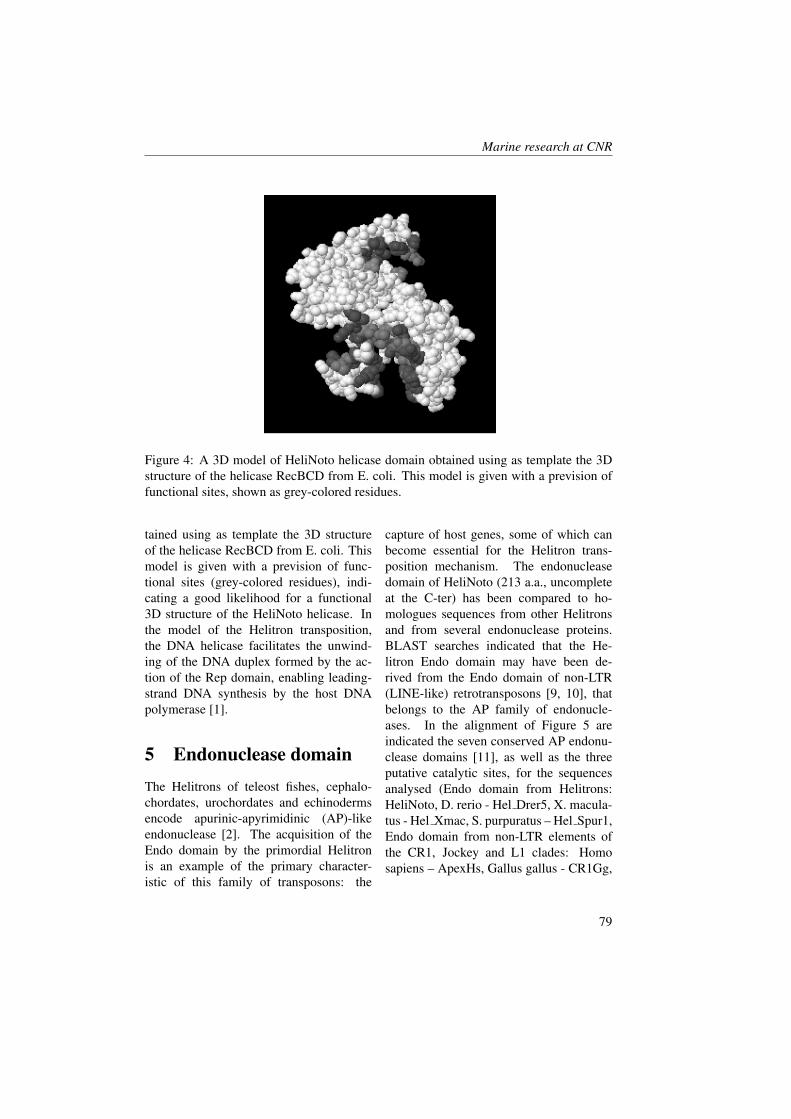
Marine research at CNR
Figure 4: A 3D model of HeliNoto helicase domain obtained using as template the 3Dstructure of the helicase RecBCD from E. coli. This model is given with a prevision offunctional sites, shown as grey-colored residues.
tained using as template the 3D structureof the helicase RecBCD from E. coli. Thismodel is given with a prevision of func-tional sites (grey-colored residues), indi-cating a good likelihood for a functional3D structure of the HeliNoto helicase. Inthe model of the Helitron transposition,the DNA helicase facilitates the unwind-ing of the DNA duplex formed by the ac-tion of the Rep domain, enabling leading-strand DNA synthesis by the host DNApolymerase [1].
5 Endonuclease domainThe Helitrons of teleost fishes, cephalo-chordates, urochordates and echinodermsencode apurinic-apyrimidinic (AP)-likeendonuclease [2]. The acquisition of theEndo domain by the primordial Helitronis an example of the primary character-istic of this family of transposons: the
capture of host genes, some of which canbecome essential for the Helitron trans-position mechanism. The endonucleasedomain of HeliNoto (213 a.a., uncompleteat the C-ter) has been compared to ho-mologues sequences from other Helitronsand from several endonuclease proteins.BLAST searches indicated that the He-litron Endo domain may have been de-rived from the Endo domain of non-LTR(LINE-like) retrotransposons [9, 10], thatbelongs to the AP family of endonucle-ases. In the alignment of Figure 5 areindicated the seven conserved AP endonu-clease domains [11], as well as the threeputative catalytic sites, for the sequencesanalysed (Endo domain from Helitrons:HeliNoto, D. rerio - Hel Drer5, X. macula-tus - Hel Xmac, S. purpuratus – Hel Spur1,Endo domain from non-LTR elements ofthe CR1, Jockey and L1 clades: Homosapiens – ApexHs, Gallus gallus - CR1Gg,
79
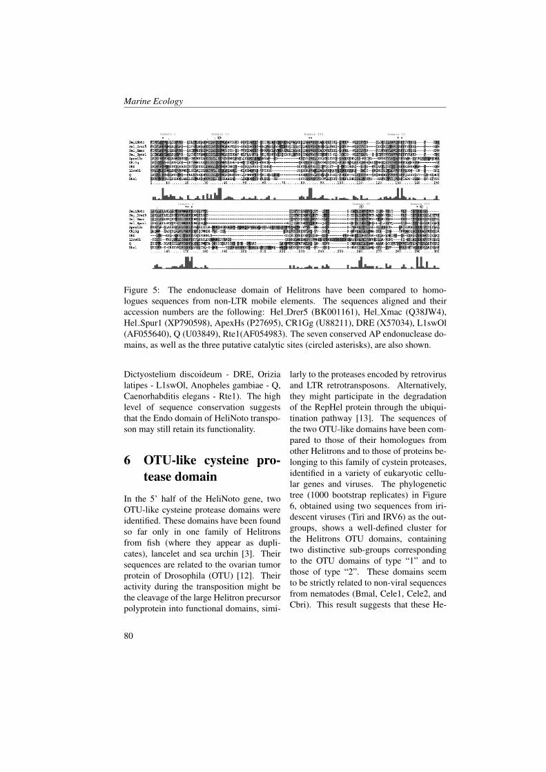
Marine Ecology
Domain I Domain II Domain III Domain IV
Domain V Domain VI Domain VII
Figure 5: The endonuclease domain of Helitrons have been compared to homo-logues sequences from non-LTR mobile elements. The sequences aligned and theiraccession numbers are the following: Hel Drer5 (BK001161), Hel Xmac (Q38JW4),Hel Spur1 (XP790598), ApexHs (P27695), CR1Gg (U88211), DRE (X57034), L1swOl(AF055640), Q (U03849), Rte1(AF054983). The seven conserved AP endonuclease do-mains, as well as the three putative catalytic sites (circled asterisks), are also shown.
Dictyostelium discoideum - DRE, Orizialatipes - L1swOl, Anopheles gambiae - Q,Caenorhabditis elegans - Rte1). The highlevel of sequence conservation suggeststhat the Endo domain of HeliNoto transpo-son may still retain its functionality.
6 OTU-like cysteine pro-tease domain
In the 5’ half of the HeliNoto gene, twoOTU-like cysteine protease domains wereidentified. These domains have been foundso far only in one family of Helitronsfrom fish (where they appear as dupli-cates), lancelet and sea urchin [3]. Theirsequences are related to the ovarian tumorprotein of Drosophila (OTU) [12]. Theiractivity during the transposition might bethe cleavage of the large Helitron precursorpolyprotein into functional domains, simi-
larly to the proteases encoded by retrovirusand LTR retrotransposons. Alternatively,they might participate in the degradationof the RepHel protein through the ubiqui-tination pathway [13]. The sequences ofthe two OTU-like domains have been com-pared to those of their homologues fromother Helitrons and to those of proteins be-longing to this family of cystein proteases,identified in a variety of eukaryotic cellu-lar genes and viruses. The phylogenetictree (1000 bootstrap replicates) in Figure6, obtained using two sequences from iri-descent viruses (Tiri and IRV6) as the out-groups, shows a well-defined cluster forthe Helitrons OTU domains, containingtwo distinctive sub-groups correspondingto the OTU domains of type “1” and tothose of type “2”. These domains seemto be strictly related to non-viral sequencesfrom nematodes (Bmal, Cele1, Cele2, andCbri). This result suggests that these He-
80
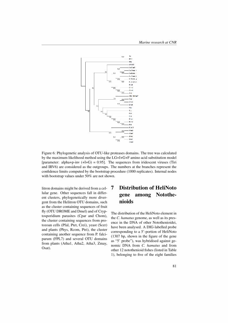
Marine research at CNR
Figure 6: Phylogenetic analysis of OTU-like proteases domains. The tree was calculatedby the maximum likelihood method using the LG+I+G+F amino acid substitution model[parameter: alpha+p-inv (+I+G) = 0.95]. The sequences from iridescent viruses (Tiriand IRV6) are considered as the outgroups. The numbers at the branches represent theconfidence limits computed by the bootstrap procedure (1000 replicates). Internal nodeswith bootstrap values under 50% are not shown.
litron domains might be derived from a cel-lular gene. Other sequences fall in differ-ent clusters, phylogenetically more diver-gent from the Helitron OTU domains, suchas the cluster containing sequences of fruitfly (OTU DROME and Dmel) and of Cryp-tosporidium parasites (Cpar and Chom),the cluster containing sequences from pro-tozoan cells (Pfal, Ptet, Crei), yeast (Scer)and plants (Phys, Rcom, Ptri), the clustercontaining another sequence from P. falci-parum (FPL7) and several OTU domainsfrom plants (Atha1, Atha2, Atha3, Zmay,Osat).
7 Distribution of HeliNotogene among Notothe-nioids
The distribution of the HeliNoto element inthe C. hamatus genome, as well as its pres-ence in the DNA of other Notothenioidei,have been analysed. A DIG-labelled probecorresponding to a 5’-portion of HeliNoto(1307 bp, shown in the figure of the geneas “5’ probe”), was hybridised against ge-nomic DNA from C. hamatus and fromother 12 notothenioid fishes (listed in Table1), belonging to five of the eight families
81
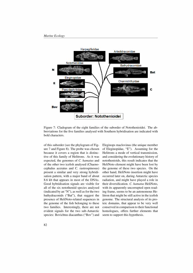
Marine Ecology
Figure 7: Cladogram of the eight families of the suborder of Notothenioidei. The ab-breviations for the five families analysed with Southern hybridisation are indicated withbold characters.
of this suborder (see the phylogram of Fig-ure 7 and Figure 8). The probe was chosenbecause it covers a region that is distinc-tive of this family of Helitrons. As it wasexpected, the genomes of C. hamatus andof the other two icefish analysed (Chaeno-cephalus aceratus and C. rastrospinosus)present a similar and very strong hybridi-sation pattern, with a major band of about8.6 kb that appears in most of the DNAs.Good hybridisation signals are visible forall of the six nototheniid species analysed(indicated by an “N”), as well as for the twobathydraconids (“Bat”), that suggest thepresence of HeliNoto-related sequences inthe genome of the fish belonging to thesetwo families. Interestingly, there are notevident signals for the two sub-Antarcticspecies: Bovichtus diacanthus (“Bov”) and
Eleginops maclovinus (the unique memberof Eleginopidae, “E”). Assuming for theHelitrons a mode of vertical transmission,and considering the evolutionary history ofnotothenioids, this result indicates that theHeliNoto element might have been lost bythe genome of these two species. On theother hand, HeliNoto insertion might haveoccurred later on, during Antarctic speciesradiation, and might have played a role intheir diversification. C. hamatus HeliNoto,with its apparently uncorrupted open read-ing frame, seems to be an autonomous He-litron that might be still active in the icefishgenome. The structural analysis of its pro-teic domains, that appear to be very wellconserved in comparison to their functionalhomologues, offers further elements thatseem to support this hypothesis.
82
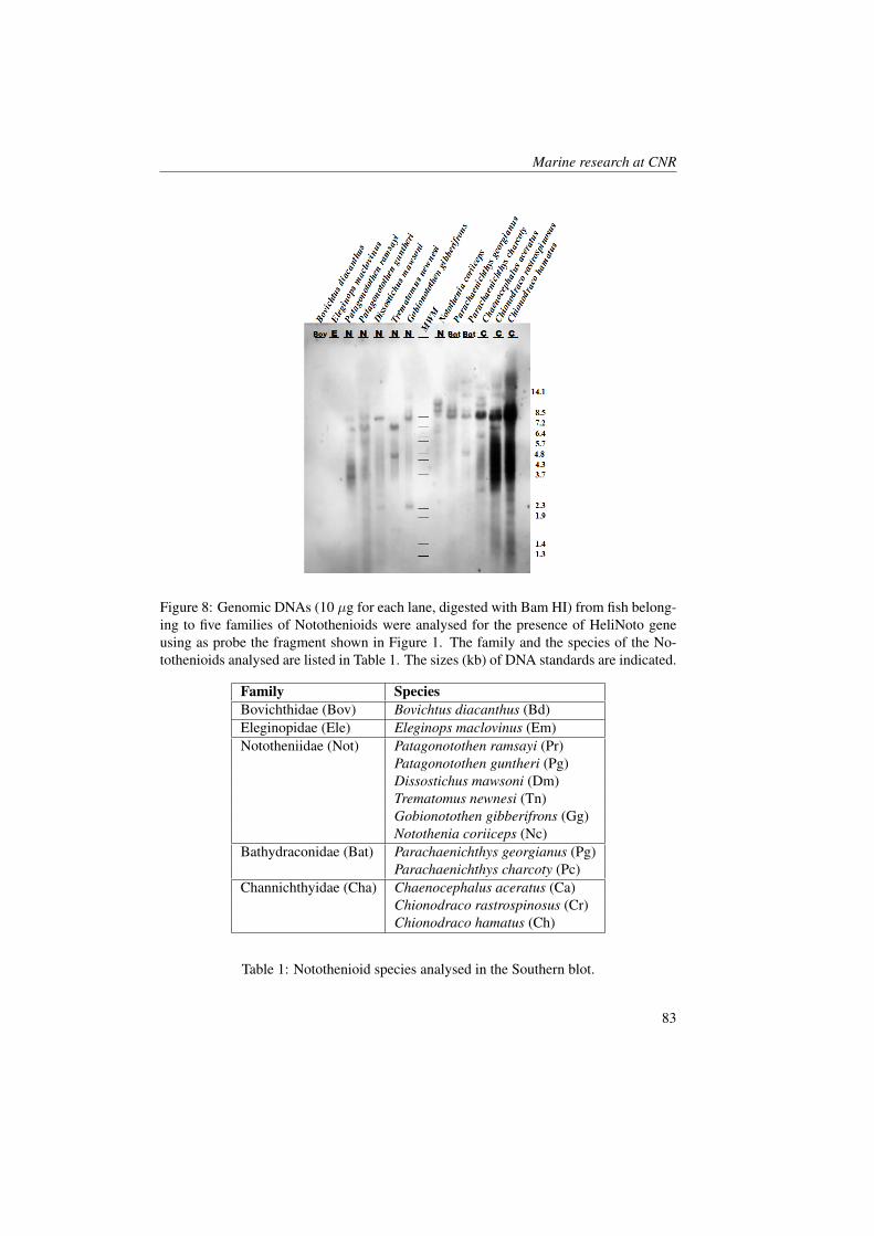
Marine research at CNR
Figure 8: Genomic DNAs (10 µg for each lane, digested with Bam HI) from fish belong-ing to five families of Notothenioids were analysed for the presence of HeliNoto geneusing as probe the fragment shown in Figure 1. The family and the species of the No-tothenioids analysed are listed in Table 1. The sizes (kb) of DNA standards are indicated.
Family SpeciesBovichthidae (Bov) Bovichtus diacanthus (Bd)Eleginopidae (Ele) Eleginops maclovinus (Em)Nototheniidae (Not) Patagonotothen ramsayi (Pr)
Patagonotothen guntheri (Pg)Dissostichus mawsoni (Dm)Trematomus newnesi (Tn)Gobionotothen gibberifrons (Gg)Notothenia coriiceps (Nc)
Bathydraconidae (Bat) Parachaenichthys georgianus (Pg)Parachaenichthys charcoty (Pc)
Channichthyidae (Cha) Chaenocephalus aceratus (Ca)Chionodraco rastrospinosus (Cr)Chionodraco hamatus (Ch)
Table 1: Notothenioid species analysed in the Southern blot.
83
Marine Ecology
References[1] V.V. Kapitonov and J. Jurka. Helitrons on a roll: eukaryotic rolling-circle trans-
posons. Trends Genet., 23(521-9), 2007.
[2] R.T.M. Poulter, T.J.D. Goodwin, and M.I. Butler. Vertebrate helentrons and othernovel Helitrons. Gene 313, 201–212., 313:201–12, 2003.
[3] Q. Zhou, A. Froschauer, C. Schultheis, C. Schmidt, G.P. Bienert, M. Wenning,A. Dettai, and J.-N. Volff. Helitron transposons on the sex chromosomes of theplatyfish Xiphophorus maculatus and their evolution in animal genomes. Zebrafish,3:39–52, 2006.
[4] T.V. Ilyina and E.V. Koonin. Conserved sequence motifs in the initiator proteinsfor rolling circle DNA replication encoded by diverse replicons from eubacteria,eucaryotes and archaebacteria. Nucleic Acids Res., 20:3279–85, 1992.
[5] B.M. Orozco and L. Hanley-Bowdoin. Conserved Sequence and Structural MotifsContribute to the DNA Binding and Cleavage Activities of a Geminivirus Replica-tion Protein. . J. Biol. Chem., 273:24448–56, 1998.
[6] M.C. Hall and S.W. Matson. Helicase motifs: the engine that powers DNA unwind-ing. Mol. Microbiol., 34:867–77, 1999.
[7] J.B. Bessler, J.Z. Torredagger, and V.A. Zakian. The Pif1p subfamily of helicases:region-specific DNA helicases? Trends Cell Biol., 11:60–65, 2001.
[8] J.-Q. Zhou, E.K. Monson, S.-C. Teng, V.P. Schulz, and V.A. Zakian. Pif1p helicase,a catalytic inhibitor of telomerase in yeast. Science, 289:771–4, 2000.
[9] H.S. Malik, W.D. Burke, and T.H. Eickbush. The age and evolution of non-LTRretrotransposable elements. Mol. Biol. Evol., 16:793–805, 1999.
[10] J.N. Volff, C. Korting, and M. Schartl. Multiple lineages of the non-LTR retro-transposon Rex1 with varying success in invading fish genomes. Mol. Biol. Evol.,17(1673-84), 2000.
[11] B. Demple, T. Herman, and D.S. Chen. Cloning and expression of APE,the cDNAencoding the major human apurinic endonuclease: definition of a family of DNArepair enzymes. Proc. Natl. Acad. Sci. USA, 88:11450–4, 1991.
[12] K.S. Makarova, L. Aravind, and E.V. Koonin. A novel superfamily of predictedcysteine proteases from eukaryotes, viruses and Chlamydia pneumoniae. TrendsBiochem. Sci., 25:50–2, 2000.
[13] M.Y. Balakirev, S.O. Tcherniuk, M. Jaquinod, and J. Chroboczek. Otubains: a newfamily of cysteine proteases in the ubiquitin pathway. EMBO Rep., 4:517–522,2003.
84

Mucilage Monitoring Program in the NorthernAdriatic Sea (Oceanographic Parameters)
F. Grilli, E. Paschini, M. MariniInstitute of Marine Sciences, CNR, Ancona, [email protected]
Abstract
A research program MAT, supported by the Italian Ministry of the Environmentand Protection of the Territory, has been devoted to monitor for four years the en-vironmental conditions of the northern Adriatic Sea, with the main aim to study themucilage phenomenon. These phenomena increased since the late eighties. Meteoro-logical conditions, circulation patterns and water column stratification can affect thedevelopment and spreading of mucilage. Starting from June 1999, a monthly moni-toring along three transects located in the northern Adriatic was carried out for threeyears. CTD casts were performed from the Italian to the Croatian coast, with watercolumn sampling for a subset of stations. Some unusual oceanographic situations,heating of the sea surface in May–June and domination of eastwards transport offreshened waters formed in the Po Delta area, were observed during the investigatedperiod in the years with more intense mucilage events (2000 and 2002).
1 Introduction
The northern Adriatic (NA) is a very shal-low continental sub-basin extending ap-proximately to the 100 m depth and char-acterized by a mean depth of about 35 mand by strong river runoff [2]. This sub-basin identifies distinct physical [3] andbiological [4] oceanographic characteris-tics. The western coastal area has a differ-ent dynamical regime compared to the off-shore zone. The coastal area north of thePo delta is dominated by the fresh waterplumes of many rivers, while the circula-tion south of the Po delta is dominated bya boundary intensified current, the WesternAdriatic Coastal Current (WACC) which isa wind and fresh water input driven cur-rent. The southward spreading of this sur-face water mass along the Italian shore iscompensate by a northward current along
the eastern coast, the Eastern Adriatic Cur-rent [5, 6, 3, 7]. The NA is an impor-tant shelf area where the occurrence of crit-ical environmental issues such as exten-sive algal blooms, sea water anoxia and inparticular mucilage events may affect theeconomic activities of the area. The mu-cilage phenomenon is represented by theappearance of suspended gelatinous ma-terial in marine waters horizontally trans-ported by currents and subjected to verti-cal movements due to water temperatureand salinity changes. There is a generalconsensus that the mucilage phenomenonis generated by synergic combination ofseveral factors [8]. Among these, sig-nificant changes of nutrient concentrationcan increase the phytoplankton excretionrate of polysaccharide mucus that com-prises the matrix of the mucilaginous ma-terial [9]. Moreover various perturbation
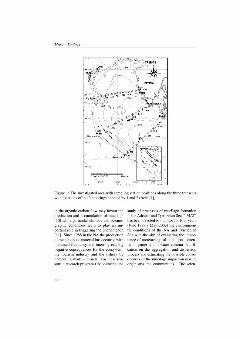
Marine Ecology
Figure 1: The investigated area with sampling station positions along the three transectswith locations of the 2 moorings denoted by 1 and 2 (from [1]).
in the organic carbon flow may favour theproduction and accumulation of mucilage[10] while particular climatic and oceano-graphic conditions seem to play an im-portant role in triggering the phenomenon[11]. Since 1988 in the NA the productionof mucilaginous material has occurred withincreased frequency and intensity causingnegative consequences for the ecosystem,the tourism industry and the fishery byhampering work with nets. For these rea-sons a research program (“Monitoring and
study of processes of mucilage formationin the Adriatic and Tyrrhenian Seas”-MAT)has been devoted to monitor for four years(June 1999 - May 2003) the environmen-tal conditions of the NA and TyrrhenianSea with the aim of evaluating the impor-tance of meteorological conditions, circu-lation patterns and water column stratifi-cation on the aggregation and dispersionprocess and estimating the possible conse-quences of the mucilage impact on marineorganisms and communities. The scien-
86
Marine research at CNR
Table 1: Description of the aggregate types observed in the northern Adriatic Sea.
tific activities were performed by 150 sci-entists and technicians belonging to 24 Ital-ian and two Croatian institutions. Duringthe first three years (June 1999 - July 2002)oceanographic cruises were monthly per-formed in the NA. In addition, several lab-oratory and in situ experiments were con-ducted to explain mechanisms and evaluateprocesses observed in the field. The me-teorological, physical, chemical, biogeo-chemical, planktonic, benthonic parame-ters and visible mucilaginous aggregates
have been monitored. In this paper some ofthe results obtained in the framework of theproject concerning physical and chemicaloceanographic conditions during the mu-cilage events and the spatial distribution ofthe mucilaginous aggregates are analysed.
2 Methods
Enviromental monitoring was taken placeover a network of 43 stations, spaced by
87
Marine Ecology
Table 2: Scale for the semi-quantitative estimation of flocs abundance.
about 10 km, situated along three tran-sects in the NA, (A) Po Delta-Rovinj(Rovigno), (B) Cesenatico-Cape Kamen-jak (Promontore), and (C) Senigallia-SusakIsland (Sansego; Figure 1) where monthly,in the period June 1999 - July 2002 dur-ing 39 cruises, oceanographic data werecollected. The Conductivity-Temperature-Depth (CTD) data were collected with aSeaBird Electronic and processed accord-ing to UNESCO [12] standards, obtain-ing pressure-averaged data (0.5 db inter-val). During the period of study, two cur-rentmeter moorings were deployed (Fig-ure 1 in the NA). The first one (sta-tion 1) was located mid-way along tran-sect C (bottom depth 68 m), and the sec-ond (station 2) 4.2 km offshore from Ce-senatico (bottom depth 9 m). The sam-pling interval was 10 min. Recovered datawere qualitatively checked, and hourly anddaily averages were calculated after remov-ing tidal components. Nutrient concen-trations (ammonium—NH4, nitrite—NO2,nitrate— NO3, orthophosphate—PO4 andorthosilicate—SiO4,) were determined at20 stations (bottom depths 9–71 m) alongall three transects. Water samples werecollected with 5 L Niskin bottles at 2–5oceanographic depths (surface, 5, 10, 20,30, 40 and 2 m above the bottom), depend-ing on station sonic depths. The samples
were filtered (HA Millipore, 0.45 µm) andstored at -22 °C in polyethylene vials (tran-sect B and C), or analysed immediatelyaboard after collection (transect A). Dis-solved inorganic nitrogen (DIN) was cal-culated as the sum of the NH4, NO2 andNO3 concentrations. The nutrient concen-trations and geostrophic velocities (calcu-lated using a standard dynamical method[13]) estimated across transects A, B andC were interpolated on a regular grid (dis-tances between grid points: 2 km in hori-zontal and 2 m in vertical) using the Krig-ing method [14]. Nutrient transports werecomputed by multiplying nutrient concen-tration by water transport (calculated byintegrating geostrophic velocities over thecross-sectional area). Net transports rep-resent the difference between northward(positive values) and southward transports(negative values). The distribution of visi-ble aggregations in the water column wasmonitored using underwater video cam-eras. The identification of the typologyof the aggregates (Table 1) was based onthe morphologic differences as defined byStachowitsch et al. [15] while the abun-dance (Table 2) was determined on a semi-quantitative scale from 0 to 5 on the ba-sis of the average distance between aggre-gates. The observations along transect Aare presented for stations A05, A07 and
88
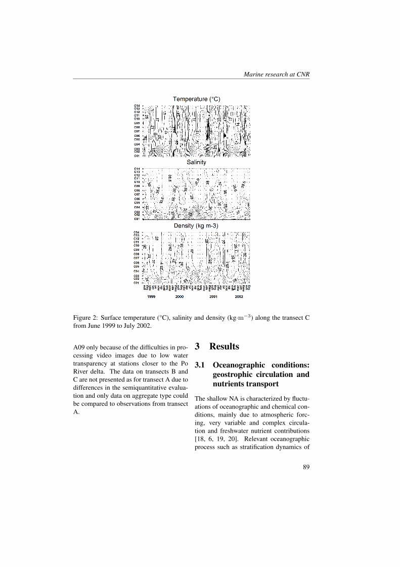
Marine research at CNR
Figure 2: Surface temperature (°C), salinity and density (kg·m−3) along the transect Cfrom June 1999 to July 2002.
A09 only because of the difficulties in pro-cessing video images due to low watertransparency at stations closer to the PoRiver delta. The data on transects B andC are not presented as for transect A due todifferences in the semiquantitative evalua-tion and only data on aggregate type couldbe compared to observations from transectA.
3 Results
3.1 Oceanographic conditions:geostrophic circulation andnutrients transport
The shallow NA is characterized by fluctu-ations of oceanographic and chemical con-ditions, mainly due to atmospheric forc-ing, very variable and complex circula-tion and freshwater nutrient contributions[18, 6, 19, 20]. Relevant oceanographicprocess such as stratification dynamics of
89
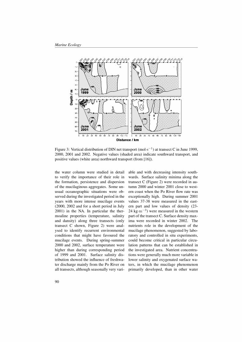
Marine Ecology
Figure 3: Vertical distribution of DIN net transport (mol·s−1) at transect C in June 1999,2000, 2001 and 2002. Negative values (shaded area) indicate southward transport, andpositive values (white area) northward transport (from [16]).
the water column were studied in detailto verify the importance of their role inthe formation, persistence and dispersionof the mucilaginous aggregates. Some un-usual oceanographic situations were ob-served during the investigated period in theyears with more intense mucilage events(2000, 2002 and for a short period in July2001) in the NA. In particular the ther-moaline properties (temperature, salinityand dansity) along three transects (onlytransect C shown, Figure 2) were anal-ysed to identify recurrent environmentalconditions that might have favoured themucilage events. During spring-summer2000 and 2002, surface temperature werehigher than during corresponding periodof 1999 and 2001. Surface salinity dis-tribution showed the influence of freshwa-ter discharge mainly from the Po River onall transects, although seasonally very vari-
able and with decreasing intensity south-wards. Surface salinity minima along thetransect C (Figure 2) were recorded in au-tumn 2000 and winter 2001 close to west-ern coast when the Po River flow rate wasexceptionally high. During summer 2001values 37-38 were measured in the east-ern part and low values of density (23-24 kg·m−3) were measured in the westernpart of the transect C. Surface density max-ima were recorded in winter 2002. Thenutrients role in the development of themucilage phenomenon, suggested by labo-ratory and controlled in situ experiments,could become critical in particular circu-lation patterns that can be established inthe investigated area. Nutrient concentra-tions were generally much more variable inlower salinity and oxygenated surface wa-ters, in which the mucilage phenomenonprimarily developed, than in other water
90

Marine research at CNR
types of the northern Adriatic [21]. Dur-ing the mucilage events (2000, 2001 and2002) the nutrients transport (in particularDIN, Figure 3) on the westernmost transectC was principally northward indicating asemi-enclosed circulation of a major partof the nutrient-rich water that forms in thearea off the Po Delta and along the west-ern coastal belt within the investigated area[22]. This circulation pattern mainly co-incided with a very weak or even reversedWACC, the principal mechanism of nutri-ent export from the northern Adriatic.
3.2 Typology and distribution ofmucilaginous aggregates
Mucilaginous aggregates formed duringspring/summer of 2000, 2002 and for abriefer period in July 2001, but were absentduring the first year of investigation (1999).The distribution of visible aggregates ontransect A according to Table 2 is presentedin Figure 4. Smaller aggregates (flocs; <1 cm) were present through the entire in-vestigated period. The maximal particleconcentration was roughly correlated withincreases of the Po River flow, stimulat-ing phytoplankton growth [1]. In generalthe flocs appearance was more accentu-ated when the circulation was weak andtransversal currents were favoured [16]. Inthese conditions the residence time of wa-ters originated from the Po River in the NAmay be longer (e.g. in 2000 and 2002).The flocs appearance was also more accen-tuated in the western part of the transect,where they accumulated in a marked py-
cnocline layer. Macroflocs (1–5 cm) andfilaments (2–25 cm) mainly appeared aftera maximum abundance of flocs. The firstsign of the upcoming mucilage aggregationwere noted at the end of May 2000 (29-31)and in the last 10 days of May 2002 when arise in the abundance of filaments (up to 50cm long) was observed in the entire watercolumn together with the maximal abun-dances of flocs [17]. This indicates thatduring the mucilage events all types of ag-gregates were formed. The appearance oflarger aggregates (ribbons and clouds) aswell as complex structures (cobwebs andfalse bottoms) were again mainly locatedin the upper water column, below the py-cnocline. Their accumulation on the sur-face was dependent on oceanographic con-ditions such as freshwater discharge, tem-perature and turbulence.
4 ConclusionThe results of Project MAT represented asignificant contribution to the knowledgeof the mucilage phenomenon. The mon-itoring activities aimed at recognising theinception of the phenomenon in order toactivate system of prevention and controlat an early stage of its development. Ex-tremely important have been investigationson the oceanographic process, principallywater dynamics and nutrient fluxes, to ex-plain mechanisms and evaluate processesobserved in the field as well as to esti-mate possible consequences of the forma-tion, persistence and dispersion of the mu-cilaginous aggregates.
91
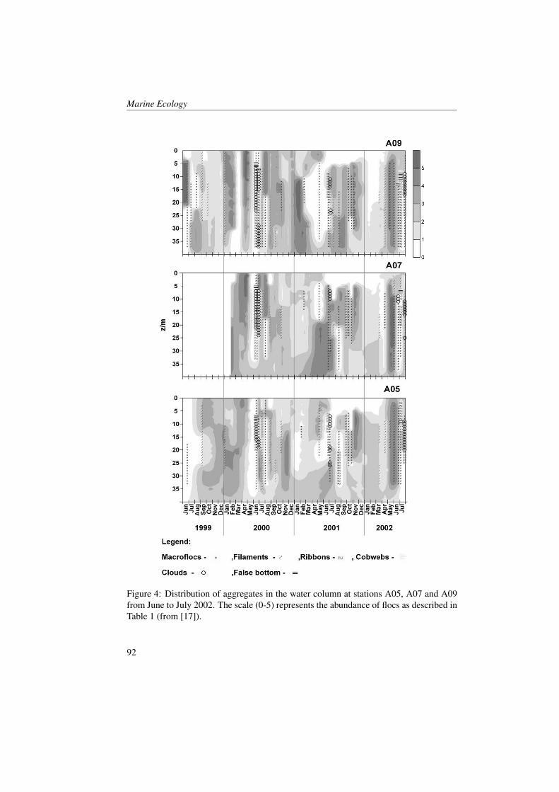
Marine Ecology
Figure 4: Distribution of aggregates in the water column at stations A05, A07 and A09from June to July 2002. The scale (0-5) represents the abundance of flocs as described inTable 1 (from [17]).
92
Marine research at CNR
References[1] A. Russo, S. Maccaferri, T. Djakovac, P. Precali, et al. Meteorological and oceano-
graphic conditions in the northern Adriatic Sea during the period June 1999–July2002: influence on the mucilage phenomenon. 2005.
[2] A. Artegiani, D. Bregant, E. Paschini, N. Pinardi, F. Raicich, and A. Russo. TheAdriatic Sea general circulation. Part I: Air–sea interactions and water mass struc-ture. 1997.
[3] A. Artegiani, D. Bregant, E. Paschini, N. Pinardi, F. Raicich, and A. Russo. TheAdriatic Sea general circulation. Part II: Baroclinic circulation structure. 1997.
[4] M. Zavatarelli, F. Raicich, A. Artegiani, D Bregant, and A. Russo. Climatologicalbiogeochemical characteristics of the Adriatic Sea. J. Mar. Syst., 1998.
[5] P. Franco and A. Michelato. Northern Adriatic Sea: oceanography of the basinproper and of the western coastal zone. 1992.
[6] M. Orlic, M. Gacic, and P.E. La Violette. The currents and circulation of the Adri-atic Sea. 1992.
[7] B. Cushman-Roisin, M. Gacic, P.M. Poulain, and A. Artegiani. Physical oceanog-raphy of the Adriatic Sea. Past, present and future. 2001.
[8] D. Degobbis, A. Malej, and S. Fonda Umani. The mucilage phenomenon in thenorthern Adriatic Sea. A critical review of the present scientific hypotheses. 1999.
[9] C. Fajon, G. Cauwet, P. Lebaron, S. Terzic, et al. The accumulation and releaseof polysaccharides by planktonic cells and subsequent bacterial response during acontrolled axperiment. 1999.
[10] F. Azam, S. Fonda Umani, and E. Funari. Significance of bacteriain the mucilagephenomenon in the northern Adriatic Sea. 1999.
[11] D. Degobbis, S. Fonda Umani, P. Franco, A. Malej, R. Precali, and N. Smodlaka.Changes in the northern Adriatic ecosystem and appearance of hypertrophic gelati-nous aggregates. 1995.
[12] UNESCO. The acquisition, calibration and analysis of CTD data. 1988.
[13] N. Supic, M. Orlic, and D. Degobbis. Istrian coastal countercurrent and its year toyear variability. 2000.
[14] N.A.C. Cressie. Statistics for spatial data. 1991.
[15] M. Stachowitsch, N. Fanuko, and M. Richter. Mucous aggregates in the AdriaticSea: an overview of types and occurrences. 1990.
93
Marine Ecology
[16] F. Grilli, E. Paschini, A. Russo, R. Precali, and N. Supic. Circulation and horizontalfluxes in the Northern Adriatic (June 1999-July 2002). 2005.
[17] R. Precali, M. Giani, M. Marini, F. Grilli, O. Pecar, and E. Paschini. Mucilageevents in the northern Adriatic in the period 1999–2002. Science of the Total Envi-roment, 2005.
[18] P. Franco. Oceanography of Northern Adriatic Sea Data from the cruises of theyears 1978 and 1979. 1982.
[19] D. Degobbis, R. Precali, I. Ivancic, N. Smodlaka, et al. Long-term changes in thenorthern Adriatic ecosystem related to anthropogenic eutrophication. 2000.
[20] P.M. Poulain, V.H. Kourafalou, and B. Cushman-Roisin. Northern Adriatic sea.Physical oceanography of the Adriatic Sea Past, present and future., 2001.
[21] D. Degobbis, R. Precali, C.R. Ferrari, T. Djakovac, A. Rinaldi, et al. Changes innutrient concentrations and ratios during mucilage event in the period 1999-2002.2005.
[22] F. Grilli, M. Marini, D. Degobbis, C. Ferrari, P. Fornasiero, et al. Circulation andhorizontal fluxes in the Northern Adriatic Sea in the period June 1999-July 2002.2005.
94
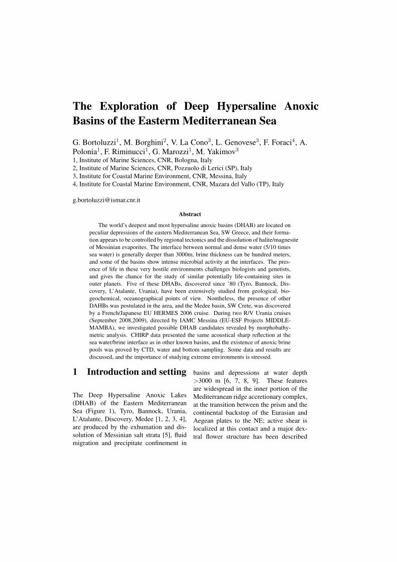
The Exploration of Deep Hypersaline AnoxicBasins of the Easterm Mediterranean Sea
G. Bortoluzzi1, M. Borghini2, V. La Cono3, L. Genovese3, F. Foraci4, A.Polonia1, F. Riminucci1, G. Marozzi1, M. Yakimov3
1, Institute of Marine Sciences, CNR, Bologna, Italy2, Institute of Marine Sciences, CNR, Pozzuolo di Lerici (SP), Italy3, Institute for Coastal Marine Environment, CNR, Messina, Italy4, Institute for Coastal Marine Environment, CNR, Mazara del Vallo (TP), Italy
Abstract
The world’s deepest and most hypersaline anoxic basins (DHAB) are located onpeculiar depressions of the eastern Mediterranean Sea, SW Greece, and their forma-tion appears to be controlled by regional tectonics and the dissolution of halite/magnesiteof Messinian evaporites. The interface between normal and dense water (5/10 timessea water) is generally deeper than 3000m, brine thickness can be hundred meters,and some of the basins show intense microbial activity at the interfaces. The pres-ence of life in these very hostile environments challenges biologists and genetists,and gives the chance for the study of similar potentially life-containing sites inouter planets. Five of these DHABs, discovered since ’80 (Tyro, Bannock, Dis-covery, L’Atalante, Urania), have been extensively studied from geological, bio-geochemical, oceanographical points of view. Nontheless, the presence of otherDAHBs was postulated in the area, and the Medee basin, SW Crete, was discoveredby a French/Japanese EU HERMES 2006 cruise. During two R/V Urania cruises(September 2008,2009), directed by IAMC Messina (EU-ESF Projects MIDDLE-MAMBA), we investigated possible DHAB candidates revealed by morphobathy-metric analysis. CHIRP data presented the same acoustical sharp reflection at thesea water/brine interface as in other known basins, and the existence of anoxic brinepools was proved by CTD, water and bottom sampling. Some data and results arediscussed, and the importance of studying extreme environments is stressed.
1 Introduction and setting
The Deep Hypersaline Anoxic Lakes(DHAB) of the Eastern MediterraneanSea (Figure 1), Tyro, Bannock, Urania,L’Atalante, Discovery, Medee [1, 2, 3, 4],are produced by the exhumation and dis-solution of Messinian salt strata [5], fluidmigration and precipitate confinement in
basins and depressions at water depth>3000 m [6, 7, 8, 9]. These featuresare widespread in the inner portion of theMediterranean ridge accretionary complex,at the transition between the prism and thecontinental backstop of the Eurasian andAegean plates to the NE; active shear islocalized at this contact and a major dex-tral flower structure has been described
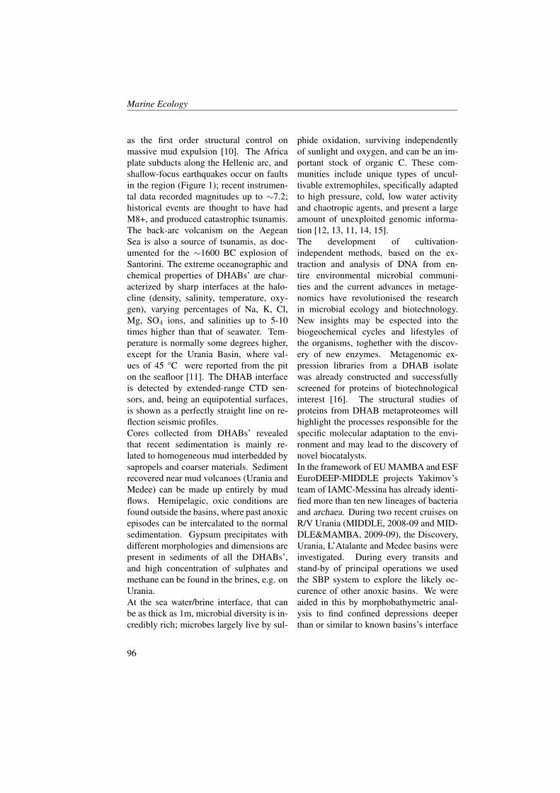
Marine Ecology
as the first order structural control onmassive mud expulsion [10]. The Africaplate subducts along the Hellenic arc, andshallow-focus earthquakes occur on faultsin the region (Figure 1); recent instrumen-tal data recorded magnitudes up to ∼7.2;historical events are thought to have hadM8+, and produced catastrophic tsunamis.The back-arc volcanism on the AegeanSea is also a source of tsunamis, as doc-umented for the ∼1600 BC explosion ofSantorini. The extreme oceanographic andchemical properties of DHABs’ are char-acterized by sharp interfaces at the halo-cline (density, salinity, temperature, oxy-gen), varying percentages of Na, K, Cl,Mg, SO4 ions, and salinities up to 5-10times higher than that of seawater. Tem-perature is normally some degrees higher,except for the Urania Basin, where val-ues of 45 °C were reported from the piton the seafloor [11]. The DHAB interfaceis detected by extended-range CTD sen-sors, and, being an equipotential surfaces,is shown as a perfectly straight line on re-flection seismic profiles.Cores collected from DHABs’ revealedthat recent sedimentation is mainly re-lated to homogeneous mud interbedded bysapropels and coarser materials. Sedimentrecovered near mud volcanoes (Urania andMedee) can be made up entirely by mudflows. Hemipelagic, oxic conditions arefound outside the basins, where past anoxicepisodes can be intercalated to the normalsedimentation. Gypsum precipitates withdifferent morphologies and dimensions arepresent in sediments of all the DHABs’,and high concentration of sulphates andmethane can be found in the brines, e.g. onUrania.At the sea water/brine interface, that canbe as thick as 1m, microbial diversity is in-credibly rich; microbes largely live by sul-
phide oxidation, surviving independentlyof sunlight and oxygen, and can be an im-portant stock of organic C. These com-munities include unique types of uncul-tivable extremophiles, specifically adaptedto high pressure, cold, low water activityand chaotropic agents, and present a largeamount of unexploited genomic informa-tion [12, 13, 11, 14, 15].The development of cultivation-independent methods, based on the ex-traction and analysis of DNA from en-tire environmental microbial communi-ties and the current advances in metage-nomics have revolutionised the researchin microbial ecology and biotechnology.New insights may be espected into thebiogeochemical cycles and lifestyles ofthe organisms, toghether with the discov-ery of new enzymes. Metagenomic ex-pression libraries from a DHAB isolatewas already constructed and successfullyscreened for proteins of biotechnologicalinterest [16]. The structural studies ofproteins from DHAB metaproteomes willhighlight the processes responsible for thespecific molecular adaptation to the envi-ronment and may lead to the discovery ofnovel biocatalysts.In the framework of EU MAMBA and ESFEuroDEEP-MIDDLE projects Yakimov’steam of IAMC-Messina has already identi-fied more than ten new lineages of bacteriaand archaea. During two recent cruises onR/V Urania (MIDDLE, 2008-09 and MID-DLE&MAMBA, 2009-09), the Discovery,Urania, L’Atalante and Medee basins wereinvestigated. During every transits andstand-by of principal operations we usedthe SBP system to explore the likely oc-curence of other anoxic basins. We wereaided in this by morphobathymetric anal-ysis to find confined depressions deeperthan or similar to known basins’s interface
96
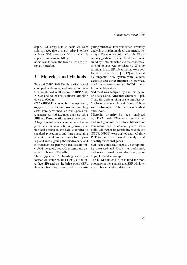
Marine research at CNR
depth. On every studied basin we wereable to recognize a sharp, crisp interfacewith the SBP, except on Medee, where itappeared to be more diffuse.Some results from the two cruises are pre-sented hereafter.
2 Materials and MethodsWe used CNR’s R/V Urania, a 61 m vesselequipped with integrated navigation sys-tem, single and multi-beam, CHIRP SBP,ADCP, and water and sediment samplingdown to 6000m.CTD (SBE-911, conductivity, temperature,oxygen, pressure) and rosette samplingcasts were performed; on brine pools ex-tended range, high accuracy and resolutionSBE and Paroscientific sensors were used.A large amount of water and sediment sam-ples, their immediate filtering, manipula-tion and storing in the field according tostandard procedures, and time-consuminglaboratory work are necessary for explor-ing and investigating the biodiversity andbiogeochemical pathways that sustain mi-crobial metabolic network systems and ge-nomic richness of DHABs’.Three types of CTD-casting were per-formed on water column (WC), at the in-terface (IF) and on the brine pools (BP).Samples from WC were used for investi-
gating microbial dark production, diversityanalysis at maximum depth and metabolic-arrays. On samples collected at the IF thesalinity gradient for each bottle was mea-sured by Refractometer and the concentra-tion of oxygen was checked by Winklertitration. IF and BP sub-sampling were per-formed as described in [13, 12] and filteredby tangential flow system with Pelliconcassettes and direct filtration on Sterivex;the filtrates were stored at -20°Ctill trans-fer to the laboratory.Sediment was sampled by a 60 cm cylin-dric Box-Corer. After measurement of pH,T and Eh, and sampling of the interface, 3-5 sub-cores were collected. Some of themwere subsampled. The bulk was washedand sieved.Microbial diversity has been analysedby DNA and RNA-based techniquesand metagenomic and clone libraries oftaxonomic and functional genes werebuilt. Molecular fingerprinting techniques(SSCP, DGGE) were applied and real-timePCR technique performed to analyse andquantify functional genes.Sediment cores had magnetic susceptibil-ity measured and X-ray was performed,and once opened, were described, pho-tographed and subsampled.The DTM data of [17] was used for mor-phobathymetric analysis and SBP window-ing for brine interface detection.
97
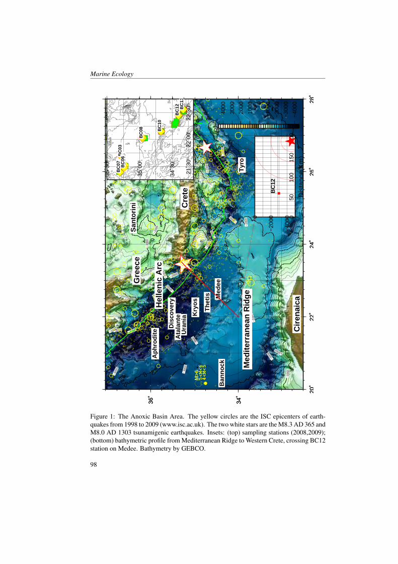
Marine Ecology
20˚
22˚
24˚
26˚
28˚
34˚
36˚
−4000
−4000
−300
0
−300
0
−300
0
−300
0
−300
0
−300
0
−30
00
−3000
−2000
−20
00−2
000
−2000
−2000
−20
00
−20
00
−200
0 −2000
−20
00
−200
0
−100
0
−1000
−100
0
−1000
−10
00
−100
0
−1000
−1000
−100
0
−1000
−100
0
20˚
22˚
24˚
26˚
28˚
34˚
36˚
M>6
5<M<6
4<M<5 M
edit
erra
nea
n R
idg
e
Hel
len
ic A
rc
Gre
ece
Cre
te
San
tori
ni
Cir
enai
ca
Ura
nia
Dis
cove
ryA
tala
nte
Kry
os
Th
etis
Ban
no
ck
Tyr
o
Med
ee
Ap
hro
dit
e
21˚3
0'22
˚00'
22˚3
0'
34˚3
0'
35˚0
0'
35˚3
0'
BC
01
BC
02
BC
03
BC
05
BC
06
BC
07
BC
08
BC
10
BC
12
BC
13
−40
00
−30
00
−20
00
−10
000
1000
2000
3000
4000
−40
00
−20
000 050
100
150
200
Dis
tanc
e(K
m)
BC
12
Figure 1: The Anoxic Basin Area. The yellow circles are the ISC epicenters of earth-quakes from 1998 to 2009 (www.isc.ac.uk). The two white stars are the M8.3 AD 365 andM8.0 AD 1303 tsunamigenic earthquakes. Insets: (top) sampling stations (2008,2009);(bottom) bathymetric profile from Mediterranean Ridge to Western Crete, crossing BC12station on Medee. Bathymetry by GEBCO.
98
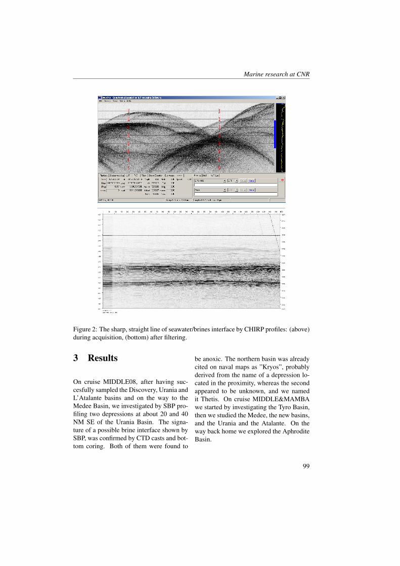
Marine research at CNR
Figure 2: The sharp, straight line of seawater/brines interface by CHIRP profiles: (above)during acquisition, (bottom) after filtering.
3 Results
On cruise MIDDLE08, after having suc-cesfully sampled the Discovery, Urania andL’Atalante basins and on the way to theMedee Basin, we investigated by SBP pro-filing two depressions at about 20 and 40NM SE of the Urania Basin. The signa-ture of a possible brine interface shown bySBP, was confirmed by CTD casts and bot-tom coring. Both of them were found to
be anoxic. The northern basin was alreadycited on naval maps as ”Kryos”, probablyderived from the name of a depression lo-cated in the proximity, whereas the secondappeared to be unknown, and we namedit Thetis. On cruise MIDDLE&MAMBAwe started by investigating the Tyro Basin,then we studied the Medee, the new basins,and the Urania and the Atalante. On theway back home we explored the AphroditeBasin.
99
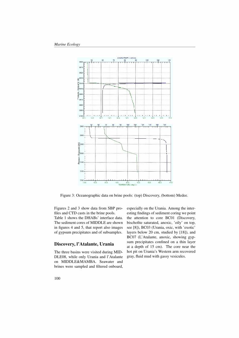
Marine Ecology
Figure 3: Oceanographic data on brine pools: (top) Discovery, (bottom) Medee.
Figures 2 and 3 show data from SBP pro-files and CTD casts in the brine pools.Table 1 shows the DHABs’ interface data.The sediment cores of MIDDLE are shownin figures 4 and 5, that report also imagesof gypsum precipitates and of subsamples.
Discovery, l’Atalante, UraniaThe three basins were visited during MID-DLE08, while only Urania and l’Atalanteon MIDDLE&MAMBA. Seawater andbrines were sampled and filtered onboard,
especially on the Urania. Among the inter-esting findings of sediment coring we pointthe attention to core BC01 (Discovery,bischofite saturated, anoxic, ’oily’ on top,see [8]), BC03 (Urania, oxic, with ’exotic’layers below 20 cm, studied by [18]), andBC07 (L’Atalante, anoxic, showing gyp-sum precipitates confined on a thin layerat a depth of 15 cm). The core near thehot pit on Urania’s Western arm recoveredgray, fluid mud with gassy vesicules.
100

Marine research at CNR
LON LAT DATE STATION BRINE INTERF. INTERF. BOT. BOT.
ddmm ddmm dB m dB m
02141.41 3516.60 2008-09-26 Discovery YES 3638.5 3581.4 3694.5 3636.0
02131.24 3513.28 2008-09-28 Urania YES 3523.0 3466.6 3609.5 3553.1
02123.98 3519.00 2008-09-29 L'Atalante YES 3638.5 3581.4 3558.0 3502.8
02209.12 3440.25 2008-10-01 Thetis YES 3307.5 3258.0 3414.5 3467.5
02226.43 3423.14 2008-10-01 Medee YES 2967.6 2925.0 3063.5 3019.6
02602.32 3352.70 2009-09-12 Tyro YES 3378.0 3327.5 3576.9 3521.6
02051.08 3551.43 2009-09-19 Aphrodite NO - - 3261.5 3212.9
Table 1: CTD Stations interface data.
New basinsThe Kryos Basin, is a narrow, N-S elon-gated fracture. The brine composition,bischofite saturated, and the recoveredblack, ’oily’ at top, sediment, were foundto be similar to that of the Discovery Basin.This transparent and water soluble ’oily’fraction is likely a polymer of biogenic ori-gin (C.Ferreri, personal communication).The bottom core revealed an undisturbed,laminated, gray to black muddy sediment[19].The Thetis Basin as depicted bybathymetry and halocline depth [20] showsan elliptical shape, oriented WNW-ESE,with a bulge to the S. Its morphology showsa linear trough or valley, bending to NE andE as a semicircular ring around a relief, andpointing to the S toward the Medee areaThe brine is halite saturated, with valuesclose to that of the L’Atalante’s composi-tion. The bottom core revealed an undis-turbed, laminated, gray-greenish muddysediment [19]. During the 2009 cruise theNE basin was sampled and was found to beoxic.
Medee BasinThe Medee brines fill a trench at the baseof a 1800 m relief, SW of the westernside of Crete. Box corer BC12 (MID-
DLE, Figure 1), recovered an ∼8 cmlayer, characterized by a coarse, fining up-wards, sandy basal unit located at ∼23cm from top (Figure 5). This base standsover compact gray mud and is composedmainly by foraminifera, rounded white andgray grains, with some black aggregates,green crystals, and less abundant orange tored crystals; the top shows two levels ofslightly coarser, silty sediment. Sedimentabove and below is gray mud.In the absence of additional samples anddata, we interpret it as a turbidite fromthe NE flanks of the ridge driven byearthquake-triggered slope instabilities.Local seismicity in the area is low, al-though some M5+ events were recorded tothe South and East. The 365 AD earth-quake [21], epicenter 150 km NE (Figure1), and related tsunami may be good can-didates (according to [22] the average sedi-mentation rates on DHABs’ is∼14 cm/ka).The mechanism for the turbidite triggeringcan be the passage of the tsunami wave,the shaking of the earthquake itself, orboth. This reconstruction is higly ques-tionable, especially without accurate dat-ings and knowledge of local sedimentationrate, and needs further analysis and datingof carbonatic materials sampled from key-layers. Weiss [23] argues that the tsunamiamplitude in deep water should not be able
101
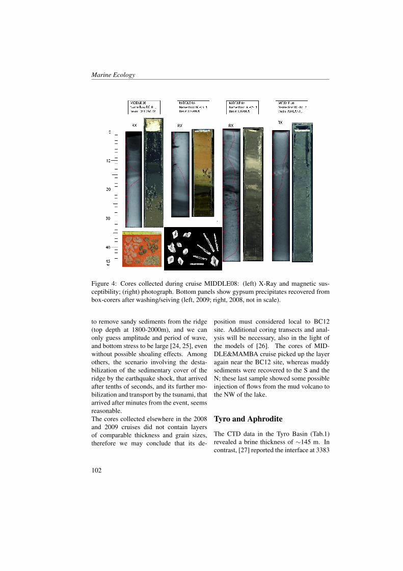
Marine Ecology
Figure 4: Cores collected during cruise MIDDLE08: (left) X-Ray and magnetic sus-ceptibility; (right) photograph. Bottom panels show gypsum precipitates recovered frombox-corers after washing/seiving (left, 2009; right, 2008, not in scale).
to remove sandy sediments from the ridge(top depth at 1800-2000m), and we canonly guess amplitude and period of wave,and bottom stress to be large [24, 25], evenwithout possible shoaling effects. Amongothers, the scenario involving the desta-bilization of the sedimentary cover of theridge by the earthquake shock, that arrivedafter tenths of seconds, and its further mo-bilization and transport by the tsunami, thatarrived after minutes from the event, seemsreasonable.The cores collected elsewhere in the 2008and 2009 cruises did not contain layersof comparable thickness and grain sizes,therefore we may conclude that its de-
position must considered local to BC12site. Additional coring transects and anal-ysis will be necessary, also in the light ofthe models of [26]. The cores of MID-DLE&MAMBA cruise picked up the layeragain near the BC12 site, whereas muddysediments were recovered to the S and theN; these last sample showed some possibleinjection of flows from the mud volcano tothe NW of the lake.
Tyro and Aphrodite
The CTD data in the Tyro Basin (Tab.1)revealed a brine thickness of ∼145 m. Incontrast, [27] reported the interface at 3383
102
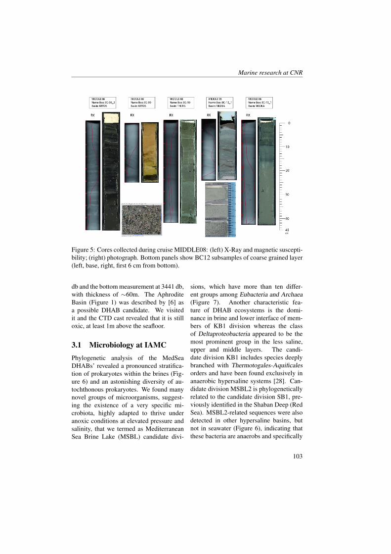
Marine research at CNR
Figure 5: Cores collected during cruise MIDDLE08: (left) X-Ray and magnetic suscepti-bility; (right) photograph. Bottom panels show BC12 subsamples of coarse grained layer(left, base, right, first 6 cm from bottom).
db and the bottom measurement at 3441 db,with thickness of ∼60m. The AphroditeBasin (Figure 1) was described by [6] asa possible DHAB candidate. We visitedit and the CTD cast revealed that it is stilloxic, at least 1m above the seafloor.
3.1 Microbiology at IAMCPhylogenetic analysis of the MedSeaDHABs’ revealed a pronounced stratifica-tion of prokaryotes within the brines (Fig-ure 6) and an astonishing diversity of au-tochthonous prokaryotes. We found manynovel groups of microorganisms, suggest-ing the existence of a very specific mi-crobiota, highly adapted to thrive underanoxic conditions at elevated pressure andsalinity, that we termed as MediterraneanSea Brine Lake (MSBL) candidate divi-
sions, which have more than ten differ-ent groups among Eubacteria and Archaea(Figure 7). Another characteristic fea-ture of DHAB ecosystems is the domi-nance in brine and lower interface of mem-bers of KB1 division whereas the classof Deltaproteobacteria appeared to be themost prominent group in the less saline,upper and middle layers. The candi-date division KB1 includes species deeplybranched with Thermotogales-Aquificalesorders and have been found exclusively inanaerobic hypersaline systems [28]. Can-didate division MSBL2 is phylogeneticallyrelated to the candidate division SB1, pre-viously identified in the Shaban Deep (RedSea). MSBL2-related sequences were alsodetected in other hypersaline basins, butnot in seawater (Figure 6), indicating thatthese bacteria are anaerobs and specifically
103
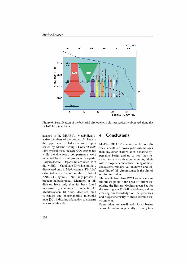
Marine Ecology
Figure 6: Stratification of the bacterial phylogenetic clusters typically observed along theDHAB lake interfaces.
adapted to the DHABs’. Metabolically-active members of the domain Archaea inthe upper level of halocline were repre-sented by Marine Group I Crenarchaeota[29], typical meso-pelagic CO2 scavenger,while the downward compartments wereinhabited by different groups of halophilicEuryarchaeota. Organisms affiliated withthe MSBL-1 Candidate Division initiallydiscovered only in Mediterranean DHABs’exhibited a distribution similar to that ofANME-1 (Figure 7), but likely possess abroader halotolerance. Members of thisdivision have only thus far been foundin anoxic, hypersaline environments, likeMediterranean DHABs’, deep-sea mudvolcanoes and endoevaporitic microbialmats [30], indicating adaptation to extremeanaerobic lifestyle.
4 Conclusions
MedSea DHABs’ contain much more di-verse uncultured prokaryotic assemblagesthan any other shallow anoxic marine hy-persaline basin, and up to now they re-sisted to any cultivation attempts; theirrole in biogeochemical functioning of theseecosystems remains yet unknown and un-ravelling of this circumstance is the aim ofour future studies.The results from two R/V Urania success-ful cruises point to the need of further ex-ploring the Eastern Mediterranean Sea fordiscovering new DHAB candidates, and in-creasing our knowledge on life processesand biogeochemistry of these extreme en-vironments.Brine lakes are small and closed basinswhose formation is generally driven by tec-
104
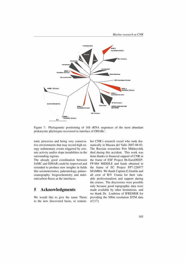
Marine research at CNR
Figure 7: Phylogenetic positioning of 16S rRNA sequences of the most abundantprokaryotic phylotypes recovered in interface of DHABs’.
tonic processes and being very conserva-tive environments that may record high en-ergy sedimentary events triggered by seis-mic activity and/or slope instabilities in thesurrounding regions.The already good coordination betweenIAMC and ISMAR could be improved andextended to produce new insights in fieldslike seismotectonics, paleontology, palaeo-ceanography, biogeochemistry and nutri-ent/carbon fluxes at the interfaces.
5 AcknowledgmentsWe would like to give the name Thetisto the new discovered basin, to remem-
ber CNR’s research vessel who sunk dra-matically in Mazara del Vallo 2007-08-03.The Russian researcher Petr Mikheychikdied during this accident. This work wasdone thanks to financial support of CNR inthe frame of ESF Project 06-EuroDEEP-FP-004 MIDDLE and funds obtained inthe frame of EC Project FP7-226977MAMBA. We thank Captain E.Gentile andall crew of R/V Urania for their valu-able professionalism and support duringthe cruises. The discoveries were possibleonly because good topographic data weremade available by other Institutions, andwe thank Dr. Loubrieu of IFREMER forproviding the 500m resolution DTM dataof [17].
105
Marine Ecology
References[1] M.B. Cita, K.A. Kastens, F.W. McCoy, F. Aghib, A. Cambi, A. Camerlenghi,
C. Corselli, E. Erba, M. Giambastiani, T. Herbert, C. Leoni, P. Malinverno,A. Nosetto, and E. Parisi. Scientific staff of cruise bannock 1984-12: Gypsum pre-cipitation from cold brines in an anoxic basin in the eastern mediterranean. Nature,314:152–154, 1985.
[2] C. Corselli, D. Basso, G.J. De Lange, and J. Thomson. Mediterranean ridge accre-tionary complex yields rich surprises. Eos Trans. AGU, 77(24):227, 1996.
[3] K. Wallmann, E. Suess, G.H. Westbrook, G. Winckler, M.B. Cita, and MEDRIFFConsortium. Salty brines in the mediterranean sea floor. Nature, 387:31–32, 1997.
[4] Hermes-EU. Hermes news issue8 spring07.pdf. http://www.noc.soton.ac.uk,2007.
[5] K.J. Hsu, M.B. Cita, and W.B.F. Ryan. The origin of the mediterranean evaporites.Init. Repts. DSDP, U.S. Govt.Printing Office, 13:1203–1231, 1973.
[6] A. Camerlenghi and M.B Cita. Setting and tectonic evolution of some easternmediterranean deep-sea basins. Mar.Geol., 75:31–55, 1987.
[7] MEDRIFF-Consortium. Three brine lakes discovered in the seafloor of the easternmediterranean. Eos Trans. AGU, 76:313, 1995.
[8] N. Fusi, G. Aloisi de Larderel, A. Borello, O. Amelio, D. Castradori, A. Negri,B. Rimoldi, R. Sanvoisin, P. Tarbini, and M.B. Cita. Marine geology of the medriffcorridor, mediterranean ridge. Island Arc, 5:420–439, 1996.
[9] B.M. Cita. Exhumation of messinian evaporites in the deep-sea and creation ofdeep anoxic brine-filled collapsed basins. Sedim.Geol., 188–189:357–378, 2006.
[10] N. Chamot-Rooke, A. Rabaute, , and C. Kreemer. Western mediterranean ridge mudbelt correlates with active shear strain at the prism-backstop geological contact.Geology, 33:861–864, 2005.
[11] M.M. Yakimov, V. La Cono, R. Denaro, G. D’Auria, F. Decembrini, K.N. Timmis,P.G. Golyshin, and Giuliano L. Primary producing prokaryotic communities ofbrine, interface and seawater above the halocline of deep anoxic lake l’atalante,eastern mediterranean sea. ISME Journ., 1:743–755, 2007,a.
[12] P.W.J.J. van der Wielen, H. Bolhuis, S. Borin, D. Daffonchio, C. Corselli, L. Giu-liano, G. D’Auria, G.J. de Lange, A. Huebner, S.P. Varnavas, J. Thomson, C. Tam-burini, D. Marty, T.J. McGenity, K.N. Timmis, and Scientific-Party BioDeep.The enigma of prokaryotic life in deep hypersaline anoxic basins. Science,307(5706):121–123, 2005.
106
Marine research at CNR
[13] D. Daffonchio, S. Borin, T. Brusa, L. Brusetti, P.W.J.J. Van der Wielen, H. Bol-huis, M.M. Yakimov, G. D’Auria, L. Giuliano, D. Marty, C. Tamburini, T.J. Mc-Genity, J.E Hallsworth, A.M. Sass, K.N. Timmis, A. Tselepides, G.J. de Lange,A. Huebner, J. Thomson, S.P. Varnavas, F. Gasparoni, H. W. Gerber, E. Malin-verno, C. Corselli, and Scientific-Party BioDeep. Stratified prokaryote network inthe oxic-anoxic transition of a deep sea halocline. Nature, 440:203–207, 2006.
[14] M.M. Yakimov, L. Giuliano, S. Cappello, R. Denaro, and P.N. Golyshin. Microbialcommunity of hydrothermal mud vent underneath the deep-sea anoxic brine lakeurania (eastern mediterranean). Orig. of life and evolut. of the Biosphere, 37:177–188, 2007,b.
[15] S. Borin, L. Brusetti, F. Mapelli, G. D’Auria, T. Brusa, M. Marzorati, A. Rizzi,M. Yakimov, D. Marty, G.J. De Lange, P. Van der Wielen, H. Bolhuis, T.J. McGen-ity, P.N. Polymenakou, E. Malinverno, L. Giuliano, C. Corselli, and D. Daffonchio.Sulfur cycling and methanogenesis primarily drives microbial colonization of thehighly sulfidic urania deep hypersaline basin. Proc.Nat.Acad.Sci.USA, June 2009.
[16] M. Ferrer, O.V. Golyshina, T.N. Chernikova, A.N. Khachane, V.A.P. Matrins dosSantos, M.M. Yakimov, K.N. Timmis, and P.N. Golyshin. Microbial enzymesmined from the urania deep-sea hypersaline anoxic basin. Chem.Biol., 12:895–904,2005.
[17] B. Loubrieu, J. Mascle, and Medimap-Group. Morpho-bathymetry of the mediter-ranean sea. CIESM, 2008.
[18] R. Hubner, G.J. De Lange, J. Ditter, and P. Halbach. Geochemistry of an exoticsediment layer above sapropel s-1: mud expulsion from the urania basin, easternmediterranean? Mar.Geol., 197:49–61, 2003.
[19] E. Oliveri, M. Sprovieri, D. Salvagio Manta, G. Tranchida, V. La Cono, M. Yaki-mov, and S. Mazzola. Biogeochemical dynamics in superficial sediments collectedfrom the new anoxic hypersaline lake Thetis. Geophysical Research Abstracts, 13,2011. EGU2011-8073, 2011, EGU General Assembly 2011.
[20] V. La Cono, F. Smedile, G. Bortoluzzi, E. Arcadi, G. Maimone, E. Messina,M. Borghini, E. Oliveri, S. Mazzola, S. L’haridon, L. Toffin, L. Genovese, M. Fer-rer, L. Giuliano, P.N. Golyshin, and M.M. Yakimov. Unveiling microbial life in newdeep-sea hypersaline Lake Thetis. Part I: Prokaryotes and environmental settings.Environ. Microbiol., 13, 2011. doi: 10.1111/j.1462-2920.2011.02478.x.
[21] B. Shaw, N.N. Ambraseys, P.C. England, M.A. Floyd, G.J. Gorman, T.F.G. Higham,J.A. Jackson, J.M. Nocquet, C.C. Pain, and M.D. Piggott. Eastern mediterraneantectonics and tsunami hazard inferred from the ad 365 earthquake. Nature Geosc.,1:268–276, 2008.
107
Marine Ecology
[22] P. Maffioli, M.S. Principato, and C. Corselli. Are anoxic basins of the easternmediterranean important recorder of paleoclimatic reconstructions? EGS- AGU-EUG Assembly, Nice, France:6945, 2003.
[23] R. Weiss. Sediment grains moved by passing tsunami waves: tsunami deposits indeep water. Mar.Geol., 250:252–257, 2008.
[24] S. Tinti, A. Armigliato, G. Pagnoni, and F. Zaniboni. Scenarios of giants tsunamiof tectonic origin in the mediterranean sea. ISET J.Earth.Technol., 42(4):171–188,2005.
[25] S. Lorito, M.M. Tiberti, R. Basili, A. Piatanesi, and G. Valensise. Earthquake-generated tsunamis in the mediterranean sea: Scenarios of potential threats to south-ern italy. J. geophys. Res., pages 113,B01301, 2008.
[26] B. Rimoldi and B.M Cita. Deep sea turbidites in brine-filled anoxic basins of themediterranean ridge. depositional models based on sedimentological and geochem-ical characterization. Rend.Fis.Acad.Lincei, 18:27–47, 2007.
[27] A. Boldrin and S. Rabitti. Hydrography of the brines in the bannock and tyro anoxicbasins (eastern mediterranean). Mar.Chem., 31:21–33, 1990.
[28] W. Eder, M. Schmidt, M. Koch, D. Garbe-Schonberg, and R. Hubner. Prokaryoticphylogenetic diversity and corresponding geochemical data of the brine-seawaterinterface of the shaban deep, red sea. Environ.Microbiol., 4:758–763, 2002.
[29] E.F. DeLong. Everything in moderation: Archaea as non-extremophiles.Curr.Opin.Genet.Dev., 8:649–654, 1998.
[30] K.B. Sorensen, D.E. Canfield, A.P. Teske, and A. Oren. Community compositionof a hypersaline endoevaporitic microbial mat. Appl. Environ. Microbiol, 71:7352–7365, 2005.
108
High Efficiency Feeding Strategy of Tursiops trun-catus During Fishing Gear Depredation
G. Buffa, G. Buscaino, F. Filiciotto, A. Bellante, V. Maccarrone, G.Basilone, C. Angela, B. Patti, M. SprovieriInstitute for Coastal Marine Environment, CNR, Capo Granitola (TP), [email protected]
Abstract
It is well known that the Bottlenose dolphin (Tursiops truncatus) has a diet madeup by a great variety of preys, including many fish that are also target species of thesmall scale fisheries activities. Previous studies has showed that this dolphin speciesoften interacts with fishing activities feeding on the entangled fishes in order to catchpreys at a low energetic cost.The Bottlenose dolphin’s depredation on artisanal fisheries is a serious problem be-cause it represents a real economic threat to fishermen damaging the nets and reduc-ing the fish catch.In order to better characterize the foraging strategies of Tursiops truncatus, a com-parative study on two different artisanal typologies of nets was carried out duringthe depredation activities in the South-Eastern coast of Sicily. Two multifilamentgillnets named “Palamitara” and one Trammel net were used. For each haul (29),data on damage, weight and species composition of the catch were collected. CPUE(Capture Per Unit Effort) and Damage Factor, as indicator of depredation level, werecalculated for the three nets in order to asses the feeding strategies in relation to thenet efficiencies. The analysis of results (ANOVA) shows that the Palamitara net withthe highest CPUE has also the highest value of Damage factor. These results sug-gest that the Tursiops truncatus is able to discriminate among different opportunities,choosing those providing greater benefits.
1 Introduction
Diet and feeding behavior of marine preda-tors, such as Bottlenose dolphins (Tursiopstruncatus), are the result of the combina-tion of the availability of resources andforaging strategies [1]. It is well knownthat this species has a diet made up bya great variety of preys, mainly teleostsand cephalopods [2, 3]. Furthermore, thedistribution of Bottlenose Dolphin popu-lations can be often linked to the distri-bution of their preferred preys [4, 5, 6].
Preys’ patch sizes and their spatial andtemporal distributions are important fac-tors that influence the predator’s foragingdecisions and strategies [7, 8, 9]. Some for-aging behaviours are associated with habi-tats or specific conditions [10, 11] whileother ones may depend on human activitiesand can be related to fishing performance[12, 13, 14]. The fishing exploitation bydolphins represents a new source of foodthat plus allows to foresee the availabilityof resource.The Bottlenose dolphin’s behaviour can
Marine Ecology
vary according to the type and distributionof preys [15, 16]. Moreover, the behavior,habitat and distribution of mammals mayalso change in response to the fishing effort[17, 13]. Previous studies showed that theBottlenose dolphin interacts with fishingactivities feeding on the entangled fishes[14].The analysis of dolphin behaviour, dur-ing the interaction with the net, suggeststhat there is a complex feeding strategy.This species was observed directly en-gaged in the depredation of gillnet, witha “common strategy” in which specimensremoved fishes from the net [18, 19]. An-other strategy could consist in the use ofthe net as a “supermarket” [20] in whichit is possible to select the preferred preyand the most nutritious portion [21]. Par-ticularly, this behavioural was evident inthe trammel net for red mullet (Mullussurmuletus) that was considered the mostaffected trammel net by depredation events[22, 23]. In her studies, Shane [15] listed27 different feeding behaviours exhibitedby Bottlenose dolphins, including herdingfish into a net. The net may act as a wallby which prey cannot escape [24], makingit beneficial for dolphins that use it as fishsafety. Understanding the breadth of Tur-siops truncatus foraging behavior duringinteraction with fishing activities, it is im-portant to answer questions on behaviouralflexibility in this social species and theirsurvival.The competitive interaction betweencetaceans and fisheries is probably as oldas the first human attempts to catch fishwith a net [13]. Today, the Bottlenose dol-phin is a species involved in many cases ofinteractions with coastal fisheries, but notalways it benefits from them. In fact, it iswell-known that the biggest problem forthe dolphins is the risk of by-catch in the
nets, considered the main threat to the con-servation of different species of cetaceans[25, 26]. Although different studies re-port frequent interactions, other ones showfew or none entanglements of dolphin[27, 19, 28], concluding that dolphins areentrapped when they are unaware of the netor are distracted by other stimuli [25]. Itwas also assessed that this species is able toidentify the fishing net (Kastelein, 2002).However, we must also consider that thedepredation strategies of artisanal fisheriesis a serious problem since it represents areal economic threat to fishermen damag-ing the nets and reducing the fishing catch[17, 22, 28]. Based on this assumption,data were analysed in the past in order toquantify the impacts of dolphin depreda-tion on artisanal fisheries [13, 20, 23, 28].To better characterize the foraging strate-gies of Tursiops truncatus, a comparativestudy on two different artisanal typologiesof net, through the analysis of damagesand fished during dolphin depredation, wascarried out.
2 Materials and methodsThe study was carried out in autumn2005 inside the Ognina bay (South-Eastof Sicily, 36°59.826’ N; 15°17.231’ E)(Figure 1), where a family of fishermenclaimed frequent Tursiops truncatus depre-dation raids in the nets.
2.1 Fishing gearsThe Palamitara is a multifilament gillnet ofsmall-scale fisheries of Sicily. This fishingtechnique is inspired to the strategies usedin Tuna traps [29] and its fishing efficiencydepend on the fisherman’s ability to plac-ing the gear in the area where there is a
110
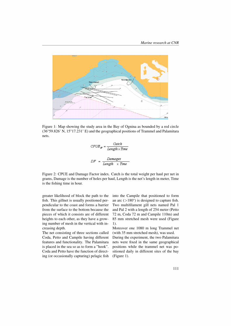
Marine research at CNR
Figure 1: Map showing the study area in the Bay of Ognina as bounded by a red circle(36°59.826’ N, 15°17.231’ E) and the geographical positions of Trammel and Palamitaranets.
Figure 2: CPUE and Damage Factor index. Catch is the total weight per haul per net ingrams, Damage is the number of holes per haul, Length is the net’s length in meter, Timeis the fishing time in hour.
greater likelihood of block the path to thefish. This gillnet is usually positioned per-pendicular to the coast and forms a barrierfrom the surface to the bottom because thepieces of which it consists are of differentheights to each other, as they have a grow-ing number of mesh in the vertical with in-creasing depth.The net consisting of three sections calledCoda, Petto and Campile having differentfeatures and functionality. The Palamitarais placed in the sea so as to form a ”hook”.Coda and Petto have the function of direct-ing (or occasionally capturing) pelagic fish
into the Campile that positioned to forman arc (>180°) is designed to capture fish.Two multifilament gill nets named Pal 1and Pal 2 with a length of 254 meter (Petto72 m, Coda 72 m and Campile 110m) and85 mm stretched mesh were used (Figure1).Moreover one 1080 m long Trammel net(with 35 mm stretched mesh), was used.During the experiment, the two Palamitaranets were fixed in the same geographicalpositions while the trammel net was po-sitioned daily in different sites of the bay(Figure 1).
111
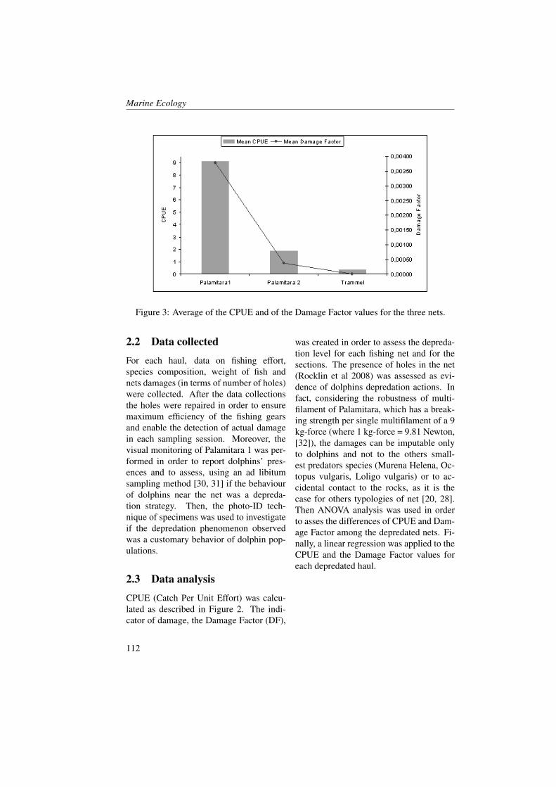
Marine Ecology
Figure 3: Average of the CPUE and of the Damage Factor values for the three nets.
2.2 Data collected
For each haul, data on fishing effort,species composition, weight of fish andnets damages (in terms of number of holes)were collected. After the data collectionsthe holes were repaired in order to ensuremaximum efficiency of the fishing gearsand enable the detection of actual damagein each sampling session. Moreover, thevisual monitoring of Palamitara 1 was per-formed in order to report dolphins’ pres-ences and to assess, using an ad libitumsampling method [30, 31] if the behaviourof dolphins near the net was a depreda-tion strategy. Then, the photo-ID tech-nique of specimens was used to investigateif the depredation phenomenon observedwas a customary behavior of dolphin pop-ulations.
2.3 Data analysis
CPUE (Catch Per Unit Effort) was calcu-lated as described in Figure 2. The indi-cator of damage, the Damage Factor (DF),
was created in order to assess the depreda-tion level for each fishing net and for thesections. The presence of holes in the net(Rocklin et al 2008) was assessed as evi-dence of dolphins depredation actions. Infact, considering the robustness of multi-filament of Palamitara, which has a break-ing strength per single multifilament of a 9kg-force (where 1 kg-force = 9.81 Newton,[32]), the damages can be imputable onlyto dolphins and not to the others small-est predators species (Murena Helena, Oc-topus vulgaris, Loligo vulgaris) or to ac-cidental contact to the rocks, as it is thecase for others typologies of net [20, 28].Then ANOVA analysis was used in orderto asses the differences of CPUE and Dam-age Factor among the depredated nets. Fi-nally, a linear regression was applied to theCPUE and the Damage Factor values foreach depredated haul.
112
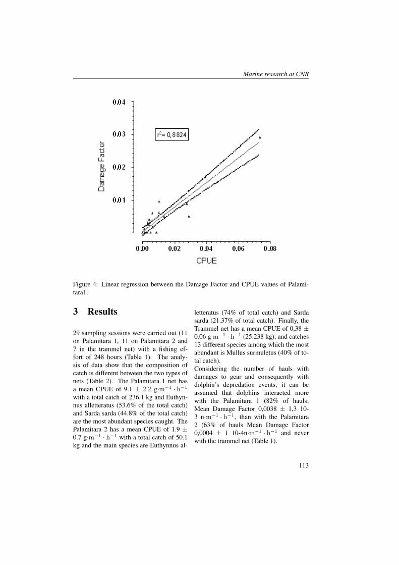
Marine research at CNR
Figure 4: Linear regression between the Damage Factor and CPUE values of Palami-tara1.
3 Results
29 sampling sessions were carried out (11on Palamitara 1, 11 on Palamitara 2 and7 in the trammel net) with a fishing ef-fort of 248 hours (Table 1). The analy-sis of data show that the composition ofcatch is different between the two types ofnets (Table 2). The Palamitara 1 net hasa mean CPUE of 9.1 ± 2.2 g·m−1 · h−1
with a total catch of 236.1 kg and Euthyn-nus alletteratus (53.6% of the total catch)and Sarda sarda (44.8% of the total catch)are the most abundant species caught. ThePalamitara 2 has a mean CPUE of 1.9 ±0.7 g·m−1 · h−1 with a total catch of 50.1kg and the main species are Euthynnus al-
letteratus (74% of total catch) and Sardasarda (21.37% of total catch). Finally, theTrammel net has a mean CPUE of 0,38 ±0.06 g·m−1 · h−1 (25.238 kg), and catches13 different species among which the mostabundant is Mullus surmuletus (40% of to-tal catch).Considering the number of hauls withdamages to gear and consequently withdolphin’s depredation events, it can beassumed that dolphins interacted morewith the Palamitara 1 (82% of hauls;Mean Damage Factor 0,0038 ± 1,3 10-3 n·m−1 · h−1, than with the Palamitara2 (63% of hauls Mean Damage Factor0,0004 ± 1 10-4n·m−1 · h−1 and neverwith the trammel net (Table 1).
113
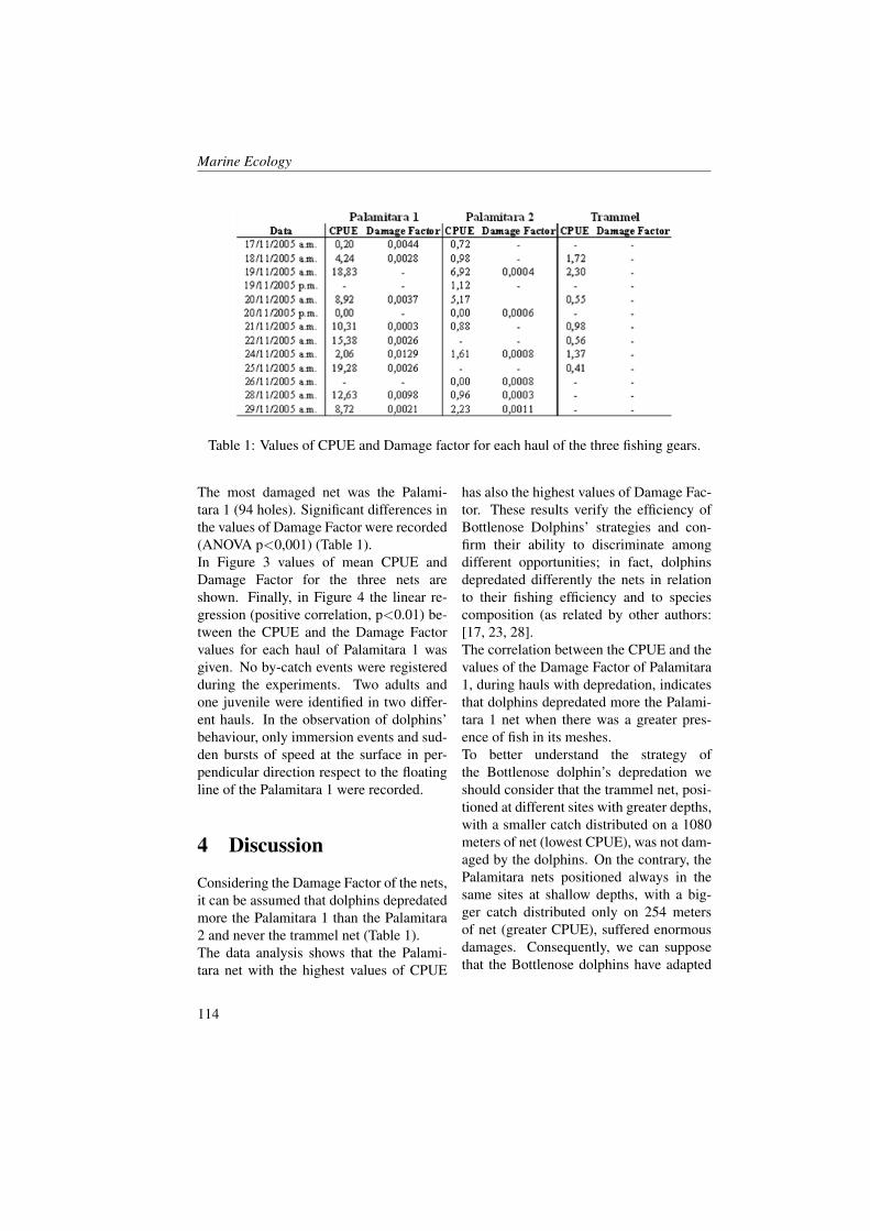
Marine Ecology
Table 1: Values of CPUE and Damage factor for each haul of the three fishing gears.
The most damaged net was the Palami-tara 1 (94 holes). Significant differences inthe values of Damage Factor were recorded(ANOVA p<0,001) (Table 1).In Figure 3 values of mean CPUE andDamage Factor for the three nets areshown. Finally, in Figure 4 the linear re-gression (positive correlation, p<0.01) be-tween the CPUE and the Damage Factorvalues for each haul of Palamitara 1 wasgiven. No by-catch events were registeredduring the experiments. Two adults andone juvenile were identified in two differ-ent hauls. In the observation of dolphins’behaviour, only immersion events and sud-den bursts of speed at the surface in per-pendicular direction respect to the floatingline of the Palamitara 1 were recorded.
4 Discussion
Considering the Damage Factor of the nets,it can be assumed that dolphins depredatedmore the Palamitara 1 than the Palamitara2 and never the trammel net (Table 1).The data analysis shows that the Palami-tara net with the highest values of CPUE
has also the highest values of Damage Fac-tor. These results verify the efficiency ofBottlenose Dolphins’ strategies and con-firm their ability to discriminate amongdifferent opportunities; in fact, dolphinsdepredated differently the nets in relationto their fishing efficiency and to speciescomposition (as related by other authors:[17, 23, 28].The correlation between the CPUE and thevalues of the Damage Factor of Palamitara1, during hauls with depredation, indicatesthat dolphins depredated more the Palami-tara 1 net when there was a greater pres-ence of fish in its meshes.To better understand the strategy ofthe Bottlenose dolphin’s depredation weshould consider that the trammel net, posi-tioned at different sites with greater depths,with a smaller catch distributed on a 1080meters of net (lowest CPUE), was not dam-aged by the dolphins. On the contrary, thePalamitara nets positioned always in thesame sites at shallow depths, with a big-ger catch distributed only on 254 metersof net (greater CPUE), suffered enormousdamages. Consequently, we can supposethat the Bottlenose dolphins have adapted
114
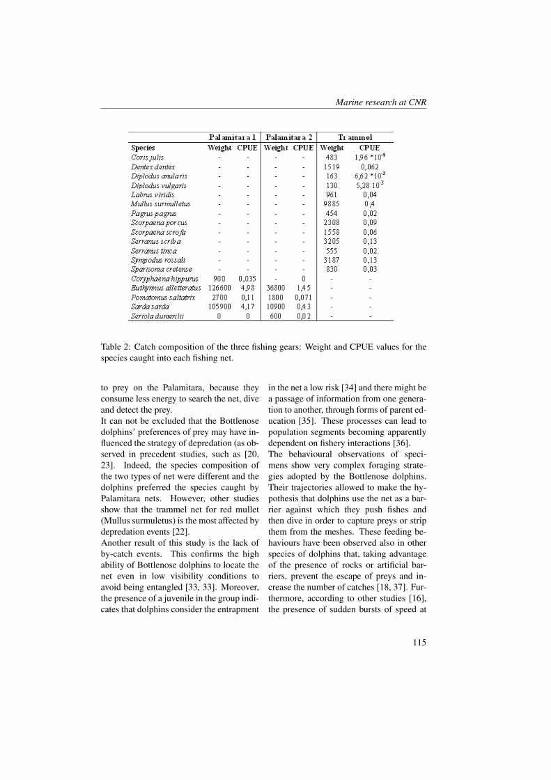
Marine research at CNR
Table 2: Catch composition of the three fishing gears: Weight and CPUE values for thespecies caught into each fishing net.
to prey on the Palamitara, because theyconsume less energy to search the net, diveand detect the prey.It can not be excluded that the Bottlenosedolphins’ preferences of prey may have in-fluenced the strategy of depredation (as ob-served in precedent studies, such as [20,23]. Indeed, the species composition ofthe two types of net were different and thedolphins preferred the species caught byPalamitara nets. However, other studiesshow that the trammel net for red mullet(Mullus surmuletus) is the most affected bydepredation events [22].Another result of this study is the lack ofby-catch events. This confirms the highability of Bottlenose dolphins to locate thenet even in low visibility conditions toavoid being entangled [33, 33]. Moreover,the presence of a juvenile in the group indi-cates that dolphins consider the entrapment
in the net a low risk [34] and there might bea passage of information from one genera-tion to another, through forms of parent ed-ucation [35]. These processes can lead topopulation segments becoming apparentlydependent on fishery interactions [36].The behavioural observations of speci-mens show very complex foraging strate-gies adopted by the Bottlenose dolphins.Their trajectories allowed to make the hy-pothesis that dolphins use the net as a bar-rier against which they push fishes andthen dive in order to capture preys or stripthem from the meshes. These feeding be-haviours have been observed also in otherspecies of dolphins that, taking advantageof the presence of rocks or artificial bar-riers, prevent the escape of preys and in-crease the number of catches [18, 37]. Fur-thermore, according to other studies [16],the presence of sudden bursts of speed at
115

Marine Ecology
the surface by dolphins was used as indica-tor of prey chasing.The results highlight the opportunistic be-haviour of Tursiops truncatus and his abil-
ity to discriminate among different feed-ing opportunities, exploiting the ones fromwhich obtain the greatest benefits and gen-erating strong competition with fishermen.
References[1] J. Spitz, Y. Rousseau, and V. Ridoux. Diet overlap between harbour porpoise and
bottlenose dolphin: an argument in favour of interference competition for food?Estuarine, Coastal and Shelf Science, 70:259–270, 2006.
[2] V.G. Cockcroft and G.J.B. Ross. Food and feeding of the Indian Ocean BottlenoseDolphin off Southern Natal, South Africa. Academic Press, NewYork, 1990.
[3] C. Blanco, O. Salomon, and J.A Raga. Diet of the bottlenose dolphin (Tursiopstruncatus) in the western Mediterranean Sea. Journal of the Marine Biology Asso-ciation UK, 81:1053, 2001.
[4] D.E. Gaskin. The ecology of whales and dolphins. page 459, 1982.
[5] N.B. Barrows and D.K. Odell. Food habits of bottlenose dolphins in the southeastern United States. page 309–328, 1990.
[6] N.B. Barrows, E.C.M. Parsons, and T.A. Jefferson. Prey of offshore bottlenosedolphins from the South China Sea. Aquat. Mamm., 26(1):2–6, 2000.
[7] Y. Iwasa, M. Higashi, and N. Yamamura. Prey distribution as a factor determiningthe choice of optimal foraging strategy. Am. Nat., 117:710–723, 1981.
[8] J.R. Krebs and R.H. Mc Cleery. Optimization in behavioural ecology. page 91/121.,1984.
[9] T. Caraco. Foraging games in a random environment. Foraging Behavior, pages389–441, 1987.
[10] R.O. Petricig. Bottlenose dolphins (Tursiops truncatus) in Bull Creek, South Car-olina. 1995.
[11] K.A. Rossbach and D.L. Herzing. Underwater observations of benthic-feeding bot-tlenose dolphins (Tursiops truncatus) near Grand Bahama Island, Bahamas. Mar.Mamm. Sci., 13:49–50, 1997.
[12] D. Fertl. Fisheries, Interference with. Academic Press, New York, page 438–44,2002.
[13] G. Bearzi. Interactions between cetacean and fisheries in the Mediterranean Sea. Areport to the Accobams Secretariat, Monaco, February, 9:20, 2002.
116
Marine research at CNR
[14] E.A. Zollet and A.J. Read. Depredation of catch by bottlenose dolphins (Tursiopstruncatus) in the Florida king mackerel (Scomberomorus cavalla) troll fishery. FishBull., 104:343–349, 2006.
[15] S.H. Shane. Comparison of Bottlenose dolphin behavior in Texas and Florida, witha critique of methods for studying dolphin behavior. (b). pages 541–558, 1990.
[16] A. Acevedo-Gutierrez and N. Parker. Surface behavior of bottlenose dolphins isrelated to spatial arrangement of prey. Marine Mammal Science, 16:287–298, 2000.
[17] R.R. Reeves, A.J. Read, and G. Notarbartolo di Sciara. Report of the workshopon interactions between dolphins and fisheries in the Mediterranean: Evaluation ofmitigation alternatives. Report of ICRAM, Rome, Italy, page 44, 2001.
[18] R.G. Busnel. Symbiotic relationship between man and dolphins. N.X Acad. Sci.,235:112–131, 1973.
[19] A.J. Read, K.W. Urian D.M. Waples, and D. Swanner. Fine-scale behaviour ofbottlenose dolphin around gillnets. Proc. R. Soc. Lond. B. suppl., 270:90–92, 2003.
[20] G. Lauriano, C. Fortuna, G. Moltedo, and G. Notarbartolo di Sciara. Interactionsbetween common bottlenose dolphins (Tursiops truncatus) and the artisanal fish-ery in Asinara Island National Park (Sardinia): Assessment of catch damage andeconomic loss. Journal of Cetacean Research and Management, 6:165–173, 2004.
[21] J. Harwood. Assessing the competitive effects of marine mammal predation ofcommercial fisheries. Afr. J. mar. Sci., 12:689–693, 1992.
[22] M. Gazo, J. Gonzalvo, and A. Aguilar. Pingers as deterrents of bottlenose dolphinsinteracting with trammel nets. Fisheries Research, 92:70–75, 2008.
[23] J.M. Brotons, Z. Munilla, A.M. Grau, and L. Rendell. Do pingers reduce interac-tions between bottlenose dolphins and nets around the Balearic Islands? Endan-gered Species Research, 5:1–8, 2008.
[24] B. Wursig and M. Wursig. Behavior and ecology of the dusky dolphinLagenorhynchus obscurus, in the South Atlantic. Fish Bull, 77(4):871–890, 1980.
[25] W.F. Perrin, G.P. Donovan, and Barlow. Report of the International Whaling Com-mission (Special Issue 15). Gillnets and Cetaceans. page 629, 1994.
[26] M.A. Hall and G.P. Donovan. Environmentalists, fishermen, cetaceans and fish:is there a balance and can science find it? In: Marine Mammals: Biology andConservation. pages 491–521, 2002.
[27] S.C. Hagedorn. Depredation by Bottlenose Dolphins on Gill Nets in Dare County,North Carolina. Masters Project, Nicholas School of the Environment and EarthSciences, Duke University, Durham, NC, 2002.
117
Marine Ecology
[28] G. Buscaino, G. Buffa, G. Sara, A. Bellante, A.J. Tonello Junior, F.A.S. Hardt, M.J.Cremer, A. Bonanno, A. Cuttitta, and S. Mazzola. Pinger affects efficiency anddamages of bottom gill nets by bottlenose dolphins. Fisheries Science, 75(3):537,2009.
[29] R. Sara. From the myth to the hydrofoil. Migration, biology, legends, tradition andsocio-behaviour aspects of tunas in Mediterranean. page 271, 1998.
[30] J. Altman. Observational study of behaviour: sampling methods. Behaviour, Lei-den, 494:227–26, 1974.
[31] J. Mann. Behavioural sampling methods for cetaceans: a review and critique. Ma-rine Mammal Science, 15:102–112, 1999.
[32] J. Prado, P.Y. Dremiere, and M. Ferretti. GUIDA PRATICA DEL PESCATOREFAO. 2010.
[33] R.A. Kastelein, W.W.L. Au, and D. de Haan. . Detection of bottom-set gillnets byharbour porpoises (Phocoena phocoena) and bottlenose dolphins (Tursiops trunca-tus). Marine Environmental Research, 49:359–437, 2000.
[34] Ashford, Rubilar, and A. R. Martin. Interactions between cetaceans and long linefishery operations around South Georgia. Marine Mammal Science, 12:452–456,1996.
[35] H. Whitehead, L. Rendell, R.W. Osborne, and B. Wursig. Culture and conservationof non-humans with reference to whales and dolphins: Review and new directions.Biological Conservation, 120(427-437), 2004.
[36] B.L. Chilvers, P.J. Corkeron, and M.L. Puotinin. The influence of trawling onthe behaviour and spatial distribution of Indo-Pacific bottlenose dolphins, Tursiopsaduncus, in Moreton Bay, Australia. Canadian Journal of Zoology., 81:1947–1,2003.
[37] T. Simila and F. Ugarte. Surface and underwater observations of cooperativelyfeeding killer whales in northern Norway. Can. J. Zool., 71(1):494, 1993.
118
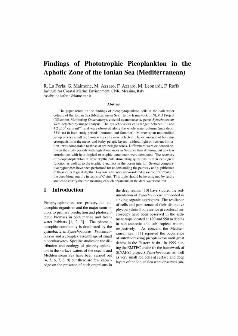
Findings of Phototrophic Picoplankton in theAphotic Zone of the Ionian Sea (Mediterranean)
R. La Ferla, G. Maimone, M. Azzaro, F. Azzaro, M. Leonardi, F. RaffaInstitute for Coastal Marine Environment, CNR, Messina, [email protected]
Abstract
The paper refers on the findings of picophytoplankton cells in the dark watercolumn of the Ionian Sea (Mediterranean Sea). In the framework of NEMO Project(NEutrinos Monitoring Observatory), coccoid cyanobacteria, genus Synechococcuswere detected by image analysis. The Synechococcus cells ranged between 0.1 and4.2 x103 cells ml−1 and were observed along the whole water column (max depth3331 m) in both study periods (Autumn and Summer). Moreover, an unidentifiedgroup of very small red fluorescing cells were detected. The occurrence of both mi-croorganisms at the meso- and bathy-pelagic layers - without light or nutrient limita-tion - was comparable to those at epi-pelagic zones. Differences were evidenced be-tween the study periods with high abundances in Summer than Autumn, but no clearcorrelations with hydrological or trophic parameters were computed. The recoveryof picophytoplankton at great depths puts stimulating questions to their ecologicalfunction as well as to the trophic dynamics in the ocean interior. Several compara-tive hypotheses have been performed for understanding the pathway and significanceof these cells at great depths. Anyhow, a till now unconsidered resource of C exists inthe deep biota, mainly in terms of C sink. This topic should be investigated by futurestudies to clarify the true meaning of such organisms in the dark water column.
1 Introduction
Picophytoplankton are prokaryotic au-totrophic organisms and the major contrib-utors to primary production and photosyn-thetic biomass in both marine and fresh-water habitats [1, 2, 3]. The photoau-totrophic community is dominated by thecyanobacteria Synechococcus, Prochloro-coccus and a complex assemblage of smallpicoeukaryotes. Specific studies on the dis-tribution and ecology of picophytoplank-ton in the surface waters of the oceans andMediterranean Sea have been carried out[4, 5, 6, 7, 8, 9] but there are few knowl-edge on the presence of such organisms in
the deep realm. [10] have studied the sed-imentation of Synechococcus embedded insinking organic aggregates. The resilienceof cells and persistence of their distinctivephycoerythrin fluorescence at confocal mi-croscopy have been observed in the sedi-ment traps located at 120 and 550 m depthsin sub-antarctic and sub-tropical waters,respectively. As concern the Mediter-ranean sea, [11] reported the occurrenceof autofluorescing picoplankton until greatdepths in the Eastern basin. In 1999 dur-ing the EMTEC cruise (in the framework ofSINAPSI project) Synechococcus as wellas very small red cells at surface and deeplayers of the Ionian Sea were observed (un-
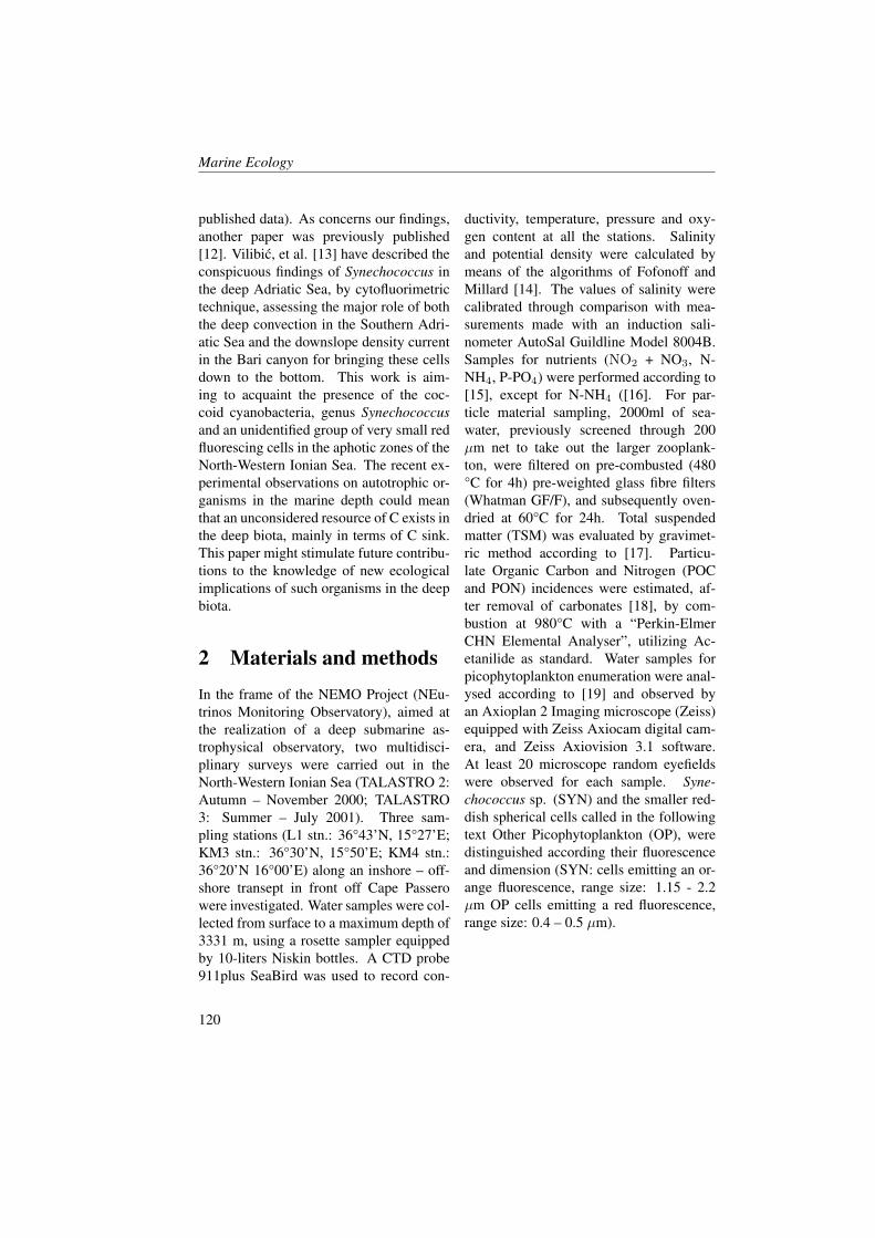
Marine Ecology
published data). As concerns our findings,another paper was previously published[12]. Vilibic, et al. [13] have described theconspicuous findings of Synechococcus inthe deep Adriatic Sea, by cytofluorimetrictechnique, assessing the major role of boththe deep convection in the Southern Adri-atic Sea and the downslope density currentin the Bari canyon for bringing these cellsdown to the bottom. This work is aim-ing to acquaint the presence of the coc-coid cyanobacteria, genus Synechococcusand an unidentified group of very small redfluorescing cells in the aphotic zones of theNorth-Western Ionian Sea. The recent ex-perimental observations on autotrophic or-ganisms in the marine depth could meanthat an unconsidered resource of C exists inthe deep biota, mainly in terms of C sink.This paper might stimulate future contribu-tions to the knowledge of new ecologicalimplications of such organisms in the deepbiota.
2 Materials and methods
In the frame of the NEMO Project (NEu-trinos Monitoring Observatory), aimed atthe realization of a deep submarine as-trophysical observatory, two multidisci-plinary surveys were carried out in theNorth-Western Ionian Sea (TALASTRO 2:Autumn – November 2000; TALASTRO3: Summer – July 2001). Three sam-pling stations (L1 stn.: 36°43’N, 15°27’E;KM3 stn.: 36°30’N, 15°50’E; KM4 stn.:36°20’N 16°00’E) along an inshore – off-shore transept in front off Cape Passerowere investigated. Water samples were col-lected from surface to a maximum depth of3331 m, using a rosette sampler equippedby 10-liters Niskin bottles. A CTD probe911plus SeaBird was used to record con-
ductivity, temperature, pressure and oxy-gen content at all the stations. Salinityand potential density were calculated bymeans of the algorithms of Fofonoff andMillard [14]. The values of salinity werecalibrated through comparison with mea-surements made with an induction sali-nometer AutoSal Guildline Model 8004B.Samples for nutrients (NO2 + NO3, N-NH4, P-PO4) were performed according to[15], except for N-NH4 ([16]. For par-ticle material sampling, 2000ml of sea-water, previously screened through 200µm net to take out the larger zooplank-ton, were filtered on pre-combusted (480°C for 4h) pre-weighted glass fibre filters(Whatman GF/F), and subsequently oven-dried at 60°C for 24h. Total suspendedmatter (TSM) was evaluated by gravimet-ric method according to [17]. Particu-late Organic Carbon and Nitrogen (POCand PON) incidences were estimated, af-ter removal of carbonates [18], by com-bustion at 980°C with a “Perkin-ElmerCHN Elemental Analyser”, utilizing Ac-etanilide as standard. Water samples forpicophytoplankton enumeration were anal-ysed according to [19] and observed byan Axioplan 2 Imaging microscope (Zeiss)equipped with Zeiss Axiocam digital cam-era, and Zeiss Axiovision 3.1 software.At least 20 microscope random eyefieldswere observed for each sample. Syne-chococcus sp. (SYN) and the smaller red-dish spherical cells called in the followingtext Other Picophytoplankton (OP), weredistinguished according their fluorescenceand dimension (SYN: cells emitting an or-ange fluorescence, range size: 1.15 - 2.2µm OP cells emitting a red fluorescence,range size: 0.4 – 0.5 µm).
120
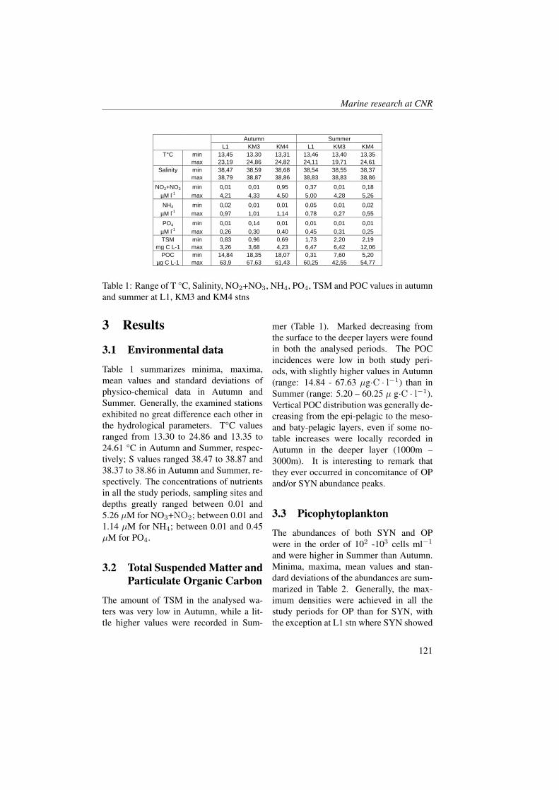
Marine research at CNR
Autumn Summer
L1 KM3 KM4 L1 KM3 KM4
T°C min 13,45 13,30 13,31 13,46 13,40 13,35
max 23,19 24,86 24,82 24,11 19,71 24,61
Salinity min 38,47 38,59 38,68 38,54 38,55 38,37
max 38,79 38,87 38,86 38,83 38,83 38,86
NO2+NO3 min 0,01 0,01 0,95 0,37 0,01 0,18
µM l-1
max 4,21 4,33 4,50 5,00 4,28 5,26
NH4 min 0,02 0,01 0,01 0,05 0,01 0,02
µM l-1
max 0,97 1,01 1,14 0,78 0,27 0,55
PO4 min 0,01 0,14 0,01 0,01 0,01 0,01
µM l-1
max 0,26 0,30 0,40 0,45 0,31 0,25
TSM min 0,83 0,96 0,69 1,73 2,20 2,19
mg C L-1 max 3,26 3,68 4,23 6,47 6,42 12,06
POC min 14,84 18,35 18,07 0,31 7,60 5,20
µg C L-1 max 63,9 67,63 61,43 60,25 42,55 54,77
Table 1: Range of T °C, Salinity, NO2+NO3, NH4, PO4, TSM and POC values in autumnand summer at L1, KM3 and KM4 stns
3 Results
3.1 Environmental data
Table 1 summarizes minima, maxima,mean values and standard deviations ofphysico-chemical data in Autumn andSummer. Generally, the examined stationsexhibited no great difference each other inthe hydrological parameters. T°C valuesranged from 13.30 to 24.86 and 13.35 to24.61 °C in Autumn and Summer, respec-tively; S values ranged 38.47 to 38.87 and38.37 to 38.86 in Autumn and Summer, re-spectively. The concentrations of nutrientsin all the study periods, sampling sites anddepths greatly ranged between 0.01 and5.26 µM for NO3+NO2; between 0.01 and1.14 µM for NH4; between 0.01 and 0.45µM for PO4.
3.2 Total Suspended Matter andParticulate Organic Carbon
The amount of TSM in the analysed wa-ters was very low in Autumn, while a lit-tle higher values were recorded in Sum-
mer (Table 1). Marked decreasing fromthe surface to the deeper layers were foundin both the analysed periods. The POCincidences were low in both study peri-ods, with slightly higher values in Autumn(range: 14.84 - 67.63 µg·C · l−1) than inSummer (range: 5.20 – 60.25 µ g·C · l−1).Vertical POC distribution was generally de-creasing from the epi-pelagic to the meso-and baty-pelagic layers, even if some no-table increases were locally recorded inAutumn in the deeper layer (1000m –3000m). It is interesting to remark thatthey ever occurred in concomitance of OPand/or SYN abundance peaks.
3.3 Picophytoplankton
The abundances of both SYN and OPwere in the order of 102 -103 cells ml−1
and were higher in Summer than Autumn.Minima, maxima, mean values and stan-dard deviations of the abundances are sum-marized in Table 2. Generally, the max-imum densities were achieved in all thestudy periods for OP than for SYN, withthe exception at L1 stn where SYN showed
121
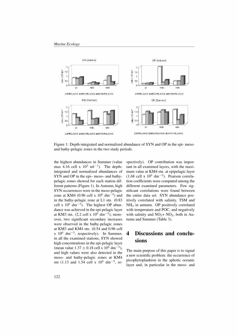
Marine Ecology
Figure 1: Depth-integrated and normalized abundance of SYN and OP in the epi- meso-and bathy-pelagic zones in the two study periods.
the highest abundances in Summer (valuemax 4.16 cell x 103 ml−1). The depth-integrated and normalized abundances ofSYN and OP in the epi– meso– and bathy-pelagic zones showed for each station dif-ferent patterns (Figure 1). In Autumn, highSYN occurrences were in the meso-pelagiczone at KM4 (0.96 cell x 106 dm−3) andin the bathy-pelagic zone at L1 stn. (0.83cell x 106 dm−3). The highest OP abun-dance was achieved in the epi-pelagic layerat KM3 stn. (2.2 cell x 106 dm−3); more-over, two significant secondary increaseswere observed in the bathy-pelagic zonesat KM3 and KM4 stn. (0.54 and 0.96 cellx 106 dm−3, respectively). In Summer,in all the examined stations, SYN showedhigh concentrations in the epi-pelagic layer(mean value 1.37 ± 0.18 cell x 106 dm−3),and high values were also detected in themeso- and bathy-pelagic zones at KM4stn (1.13 and 1.54 cell x 106 dm−3, re-
spectively). OP contribution was impor-tant in all examined layers, with the maxi-mum value at KM4 stn. at epipelagic layer(1.68 cell x 106 dm−3). Pearson correla-tion coefficients were computed among thedifferent examined parameters. Few sig-nificant correlations were found betweenthe entire data set: SYN abundance pos-itively correlated with salinity, TSM andNH4 in autumn. OP positively correlatedwith temperature and POC, and negativelywith salinity and NO3+ NO2, both in Au-tumn and Summer (Table 3).
4 Discussions and conclu-sions
The main purpose of this paper is to signala new scientific problem: the occurrence ofpicophytoplankton in the aphotic oceaniclayer and, in particular in the meso- and
122
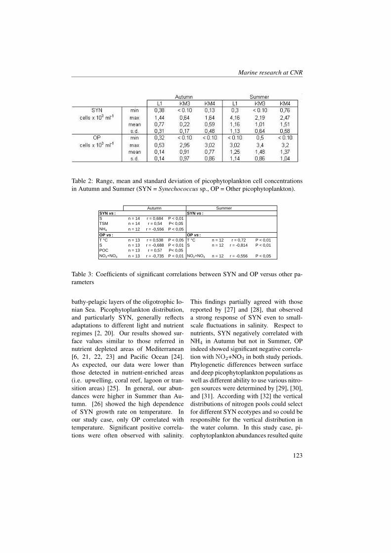
Marine research at CNR
Table 2: Range, mean and standard deviation of picophytoplankton cell concentrationsin Autumn and Summer (SYN = Synechococcus sp., OP = Other picophytoplankton).
Summer
S n = 14 r = 0,684 P < 0,01TSM n = 14 r = 0,54 P< 0,05NH4 n = 12 r = -0,556 P < 0,05
T °C n = 13 r = 0,538 P < 0,05 T °C n = 12 r = 0,72 P < 0,01S n = 13 r = -0,688 P < 0,01 S n = 12 r = -0,814 P < 0,01POC n = 13 r = 0,57 P< 0,05NO2+NO3 n = 13 r = -0,735 P < 0,01 NO2+NO3 n = 12 r = -0,556 P < 0,05
OP vs : OP vs :
Table 3. Coefficients of significant correlations between SYN and OP versus other parameters.
Autumn SYN vs : SYN vs :
Table 3: Coefficients of significant correlations between SYN and OP versus other pa-rameters
bathy-pelagic layers of the oligotrophic Io-nian Sea. Picophytoplankton distribution,and particularly SYN, generally reflectsadaptations to different light and nutrientregimes [2, 20]. Our results showed sur-face values similar to those referred innutrient depleted areas of Mediterranean[6, 21, 22, 23] and Pacific Ocean [24].As expected, our data were lower thanthose detected in nutrient-enriched areas(i.e. upwelling, coral reef, lagoon or tran-sition areas) [25]. In general, our abun-dances were higher in Summer than Au-tumn. [26] showed the high dependenceof SYN growth rate on temperature. Inour study case, only OP correlated withtemperature. Significant positive correla-tions were often observed with salinity.
This findings partially agreed with thosereported by [27] and [28], that observeda strong response of SYN even to small-scale fluctuations in salinity. Respect tonutrients, SYN negatively correlated withNH4 in Autumn but not in Summer, OPindeed showed significant negative correla-tion with NO2+NO3 in both study periods.Phylogenetic differences between surfaceand deep picophytoplankton populations aswell as different ability to use various nitro-gen sources were determined by [29], [30],and [31]. According with [32] the verticaldistributions of nitrogen pools could selectfor different SYN ecotypes and so could beresponsible for the vertical distribution inthe water column. In this study case, pi-cophytoplankton abundances resulted quite
123
Marine Ecology
low and might have been underestimated.In fact, the use of fluorescent microscopyinstead of flow citometry had probably ne-glected the counts of Prochlorococcus andpicoeukaryotic cells [8]. However, in ouropinion, the repeated microscopic obser-vations of the small red cells (OP) consti-tute an important topic, since such pico-sized cells showed characteristics similarto the marine prochlorophytes. As regardsthe novelty of this paper, namely the oc-currence of SYN and OP in the meso-and bathy-pelagic layers of the Ionian Sea,the majority of researchers consider unex-pected their presence in the “dark watercolumn”. As a consequence, most of thestudies on picophytoplankton are restrictedto the upper ocean. Formerly, [33] at-tributed the measurements of deep maximain-situ fluorescent profiles in the deep Pa-cific Ocean (500 and 1000m) to biologicalcauses, like as the occurrence of cyanobac-teria or nitryfing bacteria or purple non sul-fur bacteria. They associated these find-ings with the transport of faecal pellets, ofwhich cyanobacteria constitute one of themain vital components [34]. This hypotesishas been confirmed by [10] that observedthe accumulation of Synechococcus cells insediment traps located at 150 and 550 min sub-antarctic and sub-tropical waters, re-spectively. Recently, [35] emphasized thepossibility to find picophytoplankton in thedeep biota as a consequence of differentpathways including indirect export throughthe consumption of picoplankton aggre-gates by organisms at higher trophic lev-els, and direct routes such as aggregationand incorporation into settling detritus. Asa consequence the contribution of picophy-toplankton to export could be proportionalto their production rates. Our findings con-firm the possibility that the aggregation ofpicophytoplankton cells into larger detri-
tal particles determines their vertical set-tling and export fluxes from the upper lay-ers. In fact, significant correlations be-tween SYN and TSM as well as OP withwere detected. Moreover, aggregate cellsor cells adhering to detritus of OP were of-ten observed, above all in the deep samples.Unfortunately, they were discarded fromthe enumerations because of the difficul-ties in counting. A different intriguing hy-pothesis by [13] showed that Synechococ-cus could be a tracer for deep water ven-tilation. A significant vertical transport ofSynechococcus to oceanic depths was im-puted in winter 2006 to the convective pro-cesses of water masses, like the deep wa-ter formation in the Southern Adriatic Sea(AdDW, Adriatic Deep Water) as well as tothe downslope density current of NAdDW(North Adriatic Dense Water) through theBari canyon for bringing these cells downto the bottom. The authors found the max-imum abundance at subsurface layer and at800 m depth (3.5 x 10⁵ cells ml−1). Nev-ertheless, in our study case the picophyto-planktonic cells occurred along the wholewater column in an almost constant wayand the circulatory patterns of the studyarea were not as strong as in the South-ern Adriatic Sea. However, the importanceof SYN in carbon cycling and fixation isstill a novel topic also assessed by using hi-erarchical model, genomic and proteomicstudies [36]. We don’t exclude that themore and more frequent experimental ob-servations of picophytoplankton in the ma-rine depth could mean that an unconsid-ered additional resource of C exists in thedeep biota. The weight of picophytoplank-ton biomass in the aphotic water layers, assuggested by depth-integrated data, open anew scenario about the C sink in oceans.These populations need to be better knownbecause their true role in deep marine habi-
124
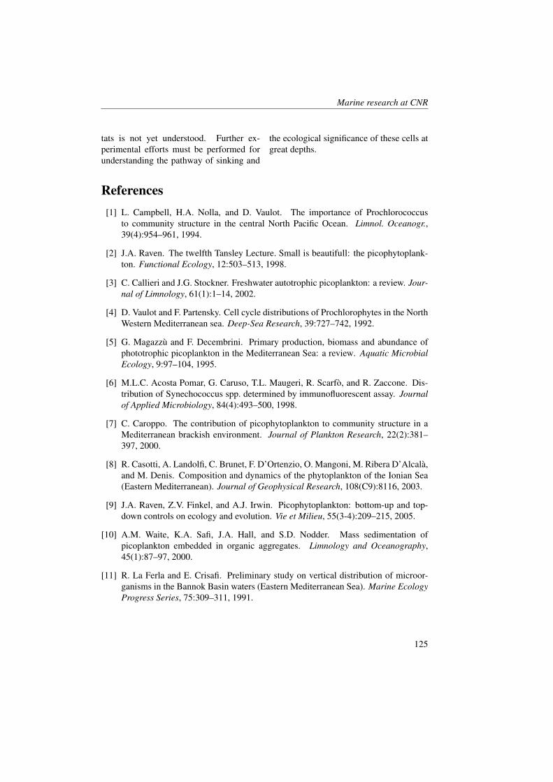
Marine research at CNR
tats is not yet understood. Further ex-perimental efforts must be performed forunderstanding the pathway of sinking and
the ecological significance of these cells atgreat depths.
References[1] L. Campbell, H.A. Nolla, and D. Vaulot. The importance of Prochlorococcus
to community structure in the central North Pacific Ocean. Limnol. Oceanogr.,39(4):954–961, 1994.
[2] J.A. Raven. The twelfth Tansley Lecture. Small is beautifull: the picophytoplank-ton. Functional Ecology, 12:503–513, 1998.
[3] C. Callieri and J.G. Stockner. Freshwater autotrophic picoplankton: a review. Jour-nal of Limnology, 61(1):1–14, 2002.
[4] D. Vaulot and F. Partensky. Cell cycle distributions of Prochlorophytes in the NorthWestern Mediterranean sea. Deep-Sea Research, 39:727–742, 1992.
[5] G. Magazzu and F. Decembrini. Primary production, biomass and abundance ofphototrophic picoplankton in the Mediterranean Sea: a review. Aquatic MicrobialEcology, 9:97–104, 1995.
[6] M.L.C. Acosta Pomar, G. Caruso, T.L. Maugeri, R. Scarfo, and R. Zaccone. Dis-tribution of Synechococcus spp. determined by immunofluorescent assay. Journalof Applied Microbiology, 84(4):493–500, 1998.
[7] C. Caroppo. The contribution of picophytoplankton to community structure in aMediterranean brackish environment. Journal of Plankton Research, 22(2):381–397, 2000.
[8] R. Casotti, A. Landolfi, C. Brunet, F. D’Ortenzio, O. Mangoni, M. Ribera D’Alcala,and M. Denis. Composition and dynamics of the phytoplankton of the Ionian Sea(Eastern Mediterranean). Journal of Geophysical Research, 108(C9):8116, 2003.
[9] J.A. Raven, Z.V. Finkel, and A.J. Irwin. Picophytoplankton: bottom-up and top-down controls on ecology and evolution. Vie et Milieu, 55(3-4):209–215, 2005.
[10] A.M. Waite, K.A. Safi, J.A. Hall, and S.D. Nodder. Mass sedimentation ofpicoplankton embedded in organic aggregates. Limnology and Oceanography,45(1):87–97, 2000.
[11] R. La Ferla and E. Crisafi. Preliminary study on vertical distribution of microor-ganisms in the Bannok Basin waters (Eastern Mediterranean Sea). Marine EcologyProgress Series, 75:309–311, 1991.
125
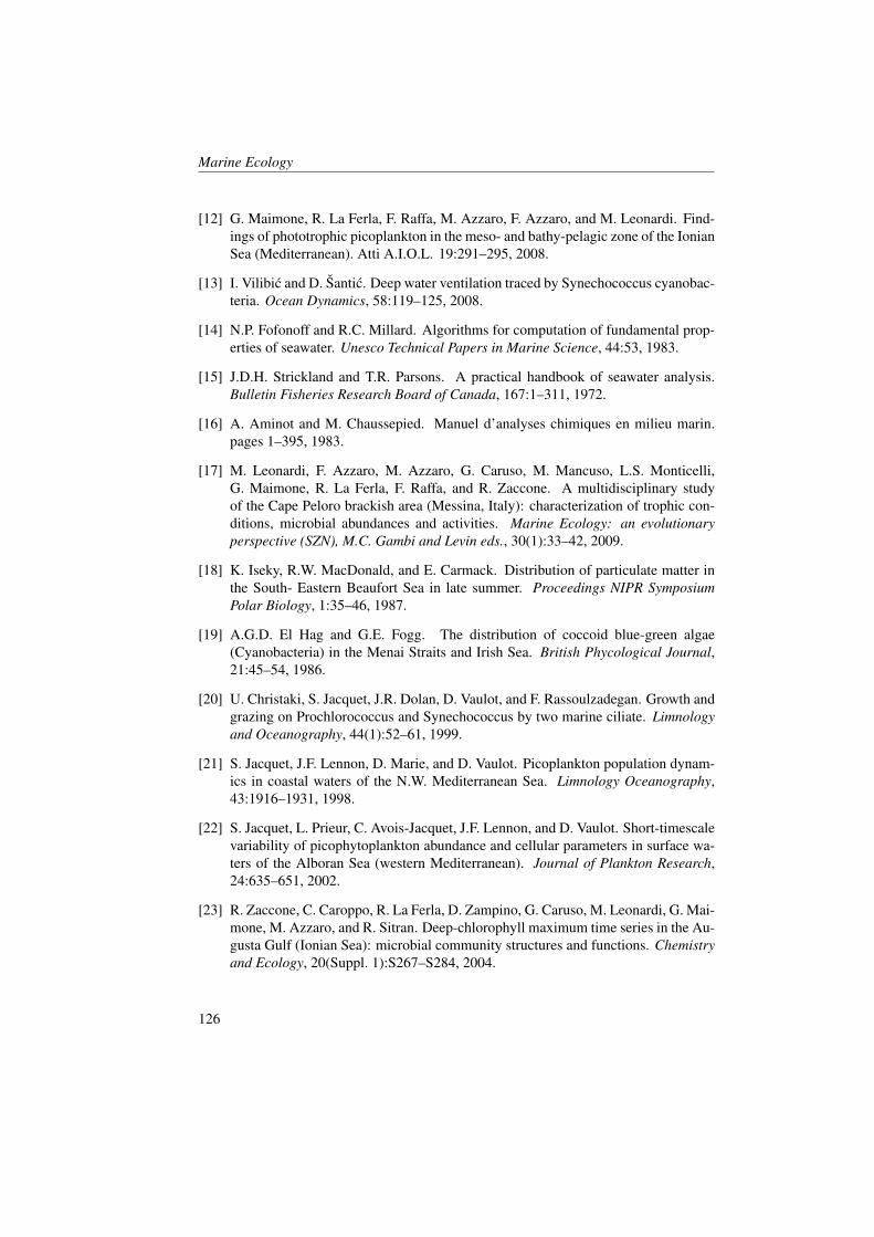
Marine Ecology
[12] G. Maimone, R. La Ferla, F. Raffa, M. Azzaro, F. Azzaro, and M. Leonardi. Find-ings of phototrophic picoplankton in the meso- and bathy-pelagic zone of the IonianSea (Mediterranean). Atti A.I.O.L. 19:291–295, 2008.
[13] I. Vilibic and D. Santic. Deep water ventilation traced by Synechococcus cyanobac-teria. Ocean Dynamics, 58:119–125, 2008.
[14] N.P. Fofonoff and R.C. Millard. Algorithms for computation of fundamental prop-erties of seawater. Unesco Technical Papers in Marine Science, 44:53, 1983.
[15] J.D.H. Strickland and T.R. Parsons. A practical handbook of seawater analysis.Bulletin Fisheries Research Board of Canada, 167:1–311, 1972.
[16] A. Aminot and M. Chaussepied. Manuel d’analyses chimiques en milieu marin.pages 1–395, 1983.
[17] M. Leonardi, F. Azzaro, M. Azzaro, G. Caruso, M. Mancuso, L.S. Monticelli,G. Maimone, R. La Ferla, F. Raffa, and R. Zaccone. A multidisciplinary studyof the Cape Peloro brackish area (Messina, Italy): characterization of trophic con-ditions, microbial abundances and activities. Marine Ecology: an evolutionaryperspective (SZN), M.C. Gambi and Levin eds., 30(1):33–42, 2009.
[18] K. Iseky, R.W. MacDonald, and E. Carmack. Distribution of particulate matter inthe South- Eastern Beaufort Sea in late summer. Proceedings NIPR SymposiumPolar Biology, 1:35–46, 1987.
[19] A.G.D. El Hag and G.E. Fogg. The distribution of coccoid blue-green algae(Cyanobacteria) in the Menai Straits and Irish Sea. British Phycological Journal,21:45–54, 1986.
[20] U. Christaki, S. Jacquet, J.R. Dolan, D. Vaulot, and F. Rassoulzadegan. Growth andgrazing on Prochlorococcus and Synechococcus by two marine ciliate. Limnologyand Oceanography, 44(1):52–61, 1999.
[21] S. Jacquet, J.F. Lennon, D. Marie, and D. Vaulot. Picoplankton population dynam-ics in coastal waters of the N.W. Mediterranean Sea. Limnology Oceanography,43:1916–1931, 1998.
[22] S. Jacquet, L. Prieur, C. Avois-Jacquet, J.F. Lennon, and D. Vaulot. Short-timescalevariability of picophytoplankton abundance and cellular parameters in surface wa-ters of the Alboran Sea (western Mediterranean). Journal of Plankton Research,24:635–651, 2002.
[23] R. Zaccone, C. Caroppo, R. La Ferla, D. Zampino, G. Caruso, M. Leonardi, G. Mai-mone, M. Azzaro, and R. Sitran. Deep-chlorophyll maximum time series in the Au-gusta Gulf (Ionian Sea): microbial community structures and functions. Chemistryand Ecology, 20(Suppl. 1):S267–S284, 2004.
126
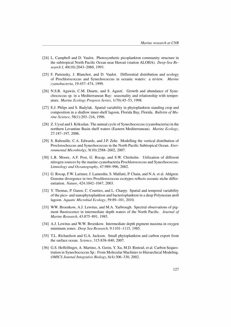
Marine research at CNR
[24] L. Campbell and D. Vaulot. Photosynthetic picoplankton community structure inthe subtropical North Pacific Ocean near Hawaii (station ALOHA). Deep-Sea Re-search I, 40(10):2043–2060, 1993.
[25] F. Partensky, J. Blanchot, and D. Vaulot. Differential distribution and ecologyof Prochlorococcus and Synechococcus in oceanic waters: a review. Marinecyanobacteria, 19:457–474, 1999.
[26] N.S.R. Agawin, C.M. Duarte, and S. Agustı. Growth and abundance of Syne-chococcus sp. in a Mediterranean Bay: seasonality and relationship with temper-ature. Marine Ecology Progress Series, 1(70):45–53, 1998.
[27] E.J. Phlips and S. Badylak. Spatial variability in phytoplankton standing crop andcomposition in a shallow inner-shelf lagoon, Florida Bay, Florida. Bulletin of Ma-rine Science, 58(1):203–216, 1996.
[28] Z. Uysal and I. Koksalan. The annual cycle of Synechococcus (cyanobacteria) in thenorthern Levantine Basin shelf waters (Eastern Mediterranean). Marine Ecology,27:187–197, 2006.
[29] S. Rabouille, C.A. Edwards, and J.P. Zehr. Modelling the vertical distribution ofProclorochoccus and Synechococcus in the North Pacific Subtropical Ocean. Envi-ronmental Microbiolgy, 9(10):2588–2602, 2007.
[30] L.R. Moore, A.F. Post, G. Rocap, and S.W. Chisholm. Utilization of differentnitrogen sources by the marine cyanobacteria Prochlorococcus and Synechococcus.Limnology and Oceanography, 47:989–996, 2002.
[31] G. Rocap, F.W. Larimer, J. Lamerdin, S. Malfatti, P. Chain, and N.A. et al. Ahlgren.Genome divergence in two Prochlorococcus ecotypes reflects oceanic niche differ-entiation. Nature, 424:1042–1047, 2003.
[32] Y. Thomas, P. Garen, C. Courties, and L. Charpy. Spatial and temporal variabilityof the pico- and nanophytoplankton and bacterioplankton in a deep Polynesian atolllagoon. Aquatic Microbial Ecology, 59:89–101, 2010.
[33] WW. Broenkow, A.J. Lewitus, and M.A. Yarbrough. Spectral observations of pig-ment fluorescence in intermediate depth waters of the North Pacific. Journal ofMarine Research, 43:875–891, 1985.
[34] A.J. Lewitus and W.W. Broenkow. Intermediate depth pigment maxima in oxygenminimum zones. Deep Sea Research, 9:1101–1115, 1985.
[35] T.L. Richardson and G.A. Jackson. Small phytoplankton and carbon export fromthe surface ocean. Science, 315:838–840, 2007.
[36] G.S. Heffelfinger, A. Martino, A. Gorin, Y. Xu, M.D. Rintoul, et al. Carbon Seques-tration in Synechococcus Sp.: From Molecular Machines to Hierarchical Modeling.OMICS Journal Integrative Biology, 6(4):306–330, 2002.
127

Marine Ecology
128
Study of the Decomposition of Organic Polymersin Mediterranean Basins Through the Measure-ments of Microbial Enzymatic Activities
G. Caruso, R. ZacconeInstitute for Coastal Marine Environment, CNR, Messina, [email protected]
Abstract
Knowledge of the processes involved in the turnover of organic matter is ofutmost importance to understand ecosystem functioning. In most of the aquaticecosystems, microorganisms are major players in the cycling of biogeochemical nu-trients (Nitrogen, Phosphorus) and Carbon through their enzymatic activities (leucineaminopeptidase, alkaline phosphatase and beta-glucosidase) on organic polymers(proteins, organic phosphates and polysaccharides, respectively). The small monomersreleased by decomposition may be used by microbes themselves for their growth.Estimates of the decomposition rates of organic polymers are performed using fluo-rogenic compounds, analogues to natural substrates, whose hydrolysis rate allow usto obtain information on the potential metabolic activity of the prokaryotic commu-nity.This note refers some of the results obtained during recent oceanographic cruises per-formed in the Tyrrhenian and Ionian Seas, with the aim of evaluating the contributionof the prokaryotic community to organic matter decomposition and the changes inmicrobial activity patterns during different seasonal conditions. Enzyme measure-ments revealed significant variations in the rates of hydrolytic activities in relation tospace and time, with the highest levels generally found during summer and in upperepipelagic layer; sporadic peaks (hot spots) of enzyme activity are also detected inmeso- and bathypelagic layers, due to the presence of different water masses.
1 IntroductionProkaryotes are an important componentof the planktonic community of aquaticecosystems. Other than producers, someof them, such as heterotrophic bacteria, arealso the main consumers of dissolved or-ganic matter (DOM) and therefore they aremajor players in organic matter turnoverwithin the “microbial loop” [1]. Microor-ganisms contribute significantly to the reg-ulation of the flux of organic matter andenergy from the biotic to abiotic compart-
ment, acting in both decomposition (byDOM hydrolysis and nutrient release) andproduction processes (new living biomassproduction). Enzymatic hydrolysis of or-ganic matter, which is mostly composedof both dissolved and particulate poly-mers, is recognised as a critical processfor organic matter utilization. In fact,heterotrophic microorganisms may uptakedirectly only low molecular weight sub-strates, such as amino-acids, simple sug-ars, fatty acids [2]. Many microorgan-
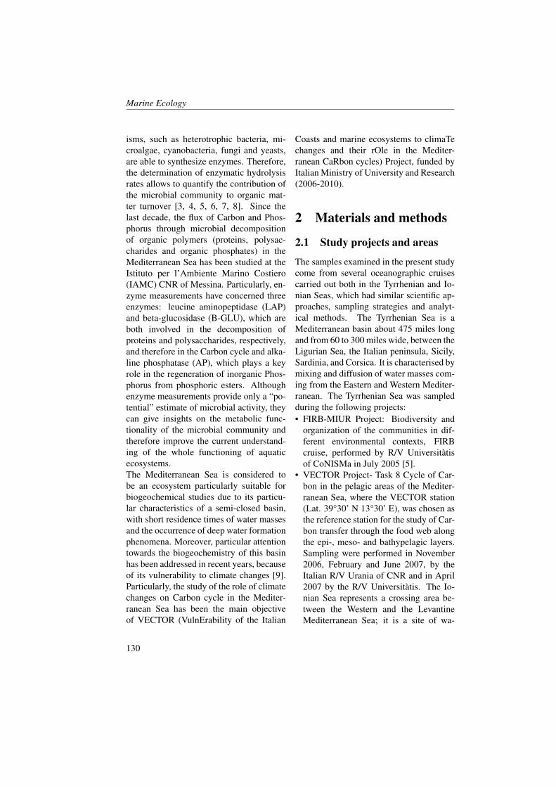
Marine Ecology
isms, such as heterotrophic bacteria, mi-croalgae, cyanobacteria, fungi and yeasts,are able to synthesize enzymes. Therefore,the determination of enzymatic hydrolysisrates allows to quantify the contribution ofthe microbial community to organic mat-ter turnover [3, 4, 5, 6, 7, 8]. Since thelast decade, the flux of Carbon and Phos-phorus through microbial decompositionof organic polymers (proteins, polysac-charides and organic phosphates) in theMediterranean Sea has been studied at theIstituto per l’Ambiente Marino Costiero(IAMC) CNR of Messina. Particularly, en-zyme measurements have concerned threeenzymes: leucine aminopeptidase (LAP)and beta-glucosidase (B-GLU), which areboth involved in the decomposition ofproteins and polysaccharides, respectively,and therefore in the Carbon cycle and alka-line phosphatase (AP), which plays a keyrole in the regeneration of inorganic Phos-phorus from phosphoric esters. Althoughenzyme measurements provide only a “po-tential” estimate of microbial activity, theycan give insights on the metabolic func-tionality of the microbial community andtherefore improve the current understand-ing of the whole functioning of aquaticecosystems.The Mediterranean Sea is considered tobe an ecosystem particularly suitable forbiogeochemical studies due to its particu-lar characteristics of a semi-closed basin,with short residence times of water massesand the occurrence of deep water formationphenomena. Moreover, particular attentiontowards the biogeochemistry of this basinhas been addressed in recent years, becauseof its vulnerability to climate changes [9].Particularly, the study of the role of climatechanges on Carbon cycle in the Mediter-ranean Sea has been the main objectiveof VECTOR (VulnErability of the Italian
Coasts and marine ecosystems to climaTechanges and their rOle in the Mediter-ranean CaRbon cycles) Project, funded byItalian Ministry of University and Research(2006-2010).
2 Materials and methods
2.1 Study projects and areas
The samples examined in the present studycome from several oceanographic cruisescarried out both in the Tyrrhenian and Io-nian Seas, which had similar scientific ap-proaches, sampling strategies and analyt-ical methods. The Tyrrhenian Sea is aMediterranean basin about 475 miles longand from 60 to 300 miles wide, between theLigurian Sea, the Italian peninsula, Sicily,Sardinia, and Corsica. It is characterised bymixing and diffusion of water masses com-ing from the Eastern and Western Mediter-ranean. The Tyrrhenian Sea was sampledduring the following projects:• FIRB-MIUR Project: Biodiversity and
organization of the communities in dif-ferent environmental contexts, FIRBcruise, performed by R/V Universitatisof CoNISMa in July 2005 [5].
• VECTOR Project- Task 8 Cycle of Car-bon in the pelagic areas of the Mediter-ranean Sea, where the VECTOR station(Lat. 39°30’ N 13°30’ E), was chosen asthe reference station for the study of Car-bon transfer through the food web alongthe epi-, meso- and bathypelagic layers.Sampling were performed in November2006, February and June 2007, by theItalian R/V Urania of CNR and in April2007 by the R/V Universitatis. The Io-nian Sea represents a crossing area be-tween the Western and the LevantineMediterranean Sea; it is a site of wa-
130
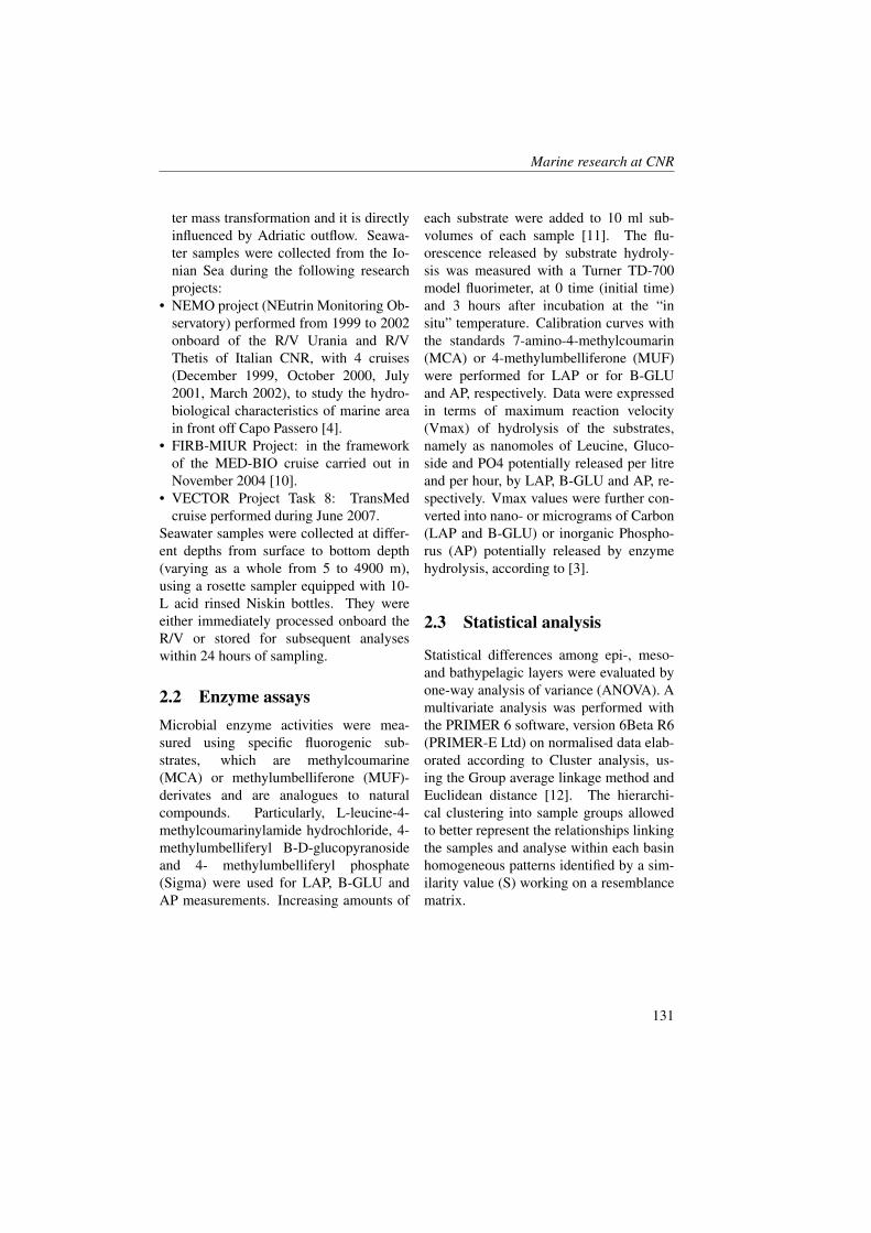
Marine research at CNR
ter mass transformation and it is directlyinfluenced by Adriatic outflow. Seawa-ter samples were collected from the Io-nian Sea during the following researchprojects:
• NEMO project (NEutrin Monitoring Ob-servatory) performed from 1999 to 2002onboard of the R/V Urania and R/VThetis of Italian CNR, with 4 cruises(December 1999, October 2000, July2001, March 2002), to study the hydro-biological characteristics of marine areain front off Capo Passero [4].
• FIRB-MIUR Project: in the frameworkof the MED-BIO cruise carried out inNovember 2004 [10].
• VECTOR Project Task 8: TransMedcruise performed during June 2007.
Seawater samples were collected at differ-ent depths from surface to bottom depth(varying as a whole from 5 to 4900 m),using a rosette sampler equipped with 10-L acid rinsed Niskin bottles. They wereeither immediately processed onboard theR/V or stored for subsequent analyseswithin 24 hours of sampling.
2.2 Enzyme assaysMicrobial enzyme activities were mea-sured using specific fluorogenic sub-strates, which are methylcoumarine(MCA) or methylumbelliferone (MUF)-derivates and are analogues to naturalcompounds. Particularly, L-leucine-4-methylcoumarinylamide hydrochloride, 4-methylumbelliferyl B-D-glucopyranosideand 4- methylumbelliferyl phosphate(Sigma) were used for LAP, B-GLU andAP measurements. Increasing amounts of
each substrate were added to 10 ml sub-volumes of each sample [11]. The flu-orescence released by substrate hydroly-sis was measured with a Turner TD-700model fluorimeter, at 0 time (initial time)and 3 hours after incubation at the “insitu” temperature. Calibration curves withthe standards 7-amino-4-methylcoumarin(MCA) or 4-methylumbelliferone (MUF)were performed for LAP or for B-GLUand AP, respectively. Data were expressedin terms of maximum reaction velocity(Vmax) of hydrolysis of the substrates,namely as nanomoles of Leucine, Gluco-side and PO4 potentially released per litreand per hour, by LAP, B-GLU and AP, re-spectively. Vmax values were further con-verted into nano- or micrograms of Carbon(LAP and B-GLU) or inorganic Phospho-rus (AP) potentially released by enzymehydrolysis, according to [3].
2.3 Statistical analysis
Statistical differences among epi-, meso-and bathypelagic layers were evaluated byone-way analysis of variance (ANOVA). Amultivariate analysis was performed withthe PRIMER 6 software, version 6Beta R6(PRIMER-E Ltd) on normalised data elab-orated according to Cluster analysis, us-ing the Group average linkage method andEuclidean distance [12]. The hierarchi-cal clustering into sample groups allowedto better represent the relationships linkingthe samples and analyse within each basinhomogeneous patterns identified by a sim-ilarity value (S) working on a resemblancematrix.
131
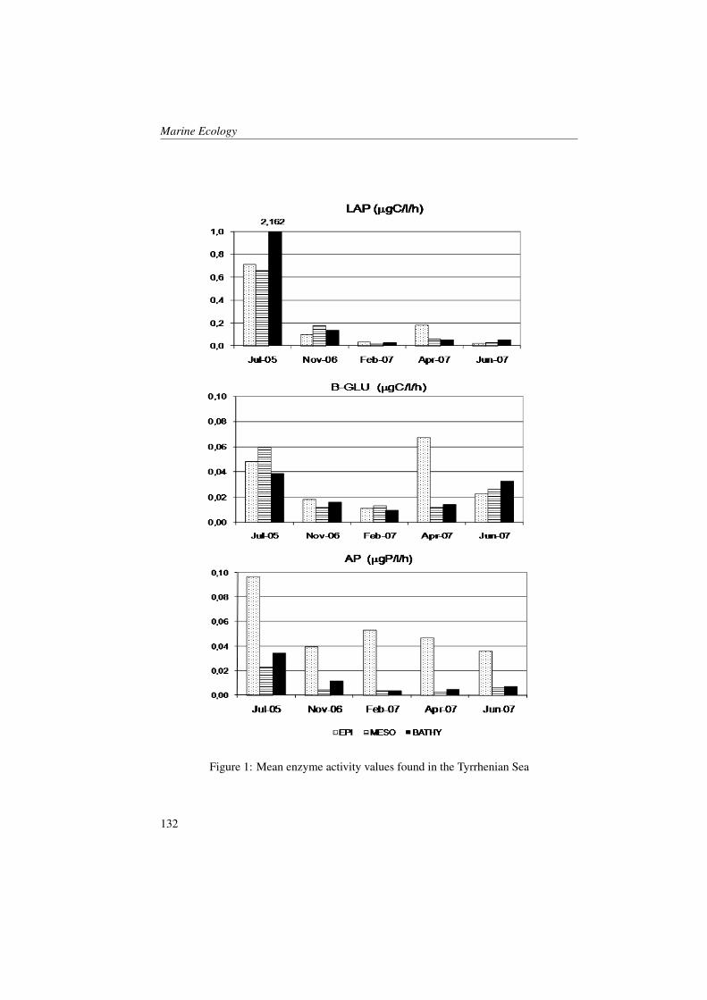
Marine Ecology
Figure 1: Mean enzyme activity values found in the Tyrrhenian Sea
132
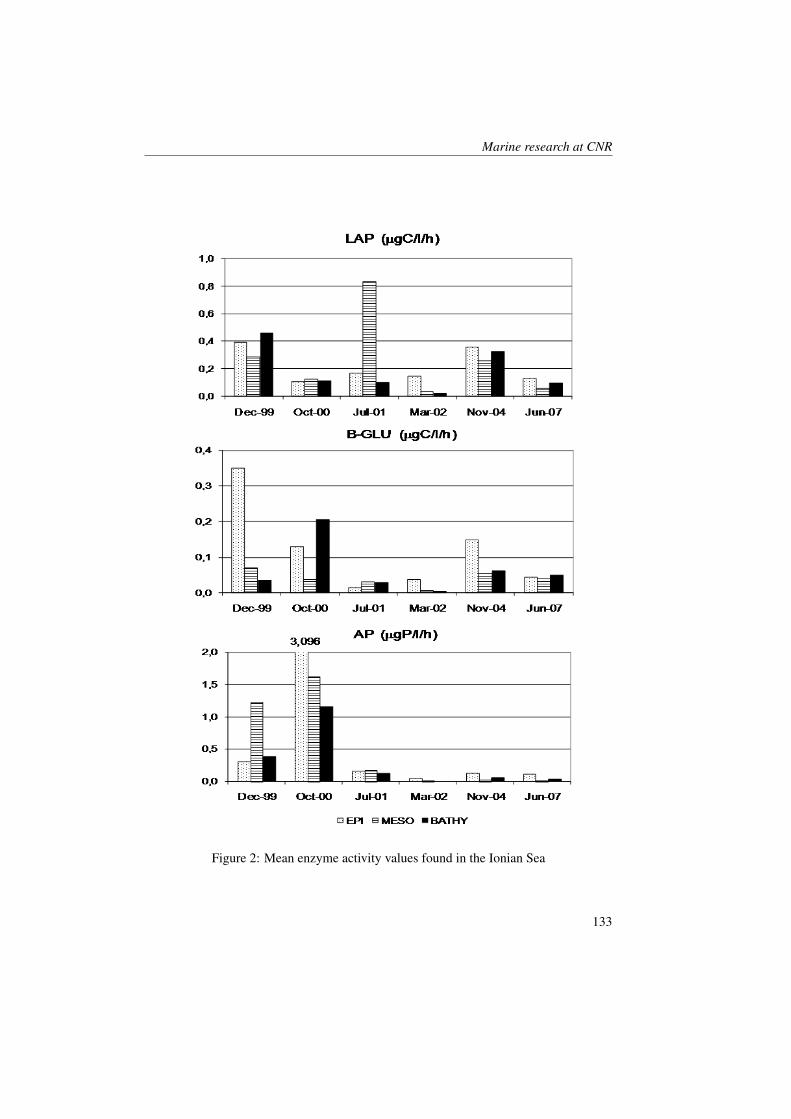
Marine research at CNR
Figure 2: Mean enzyme activity values found in the Ionian Sea
133
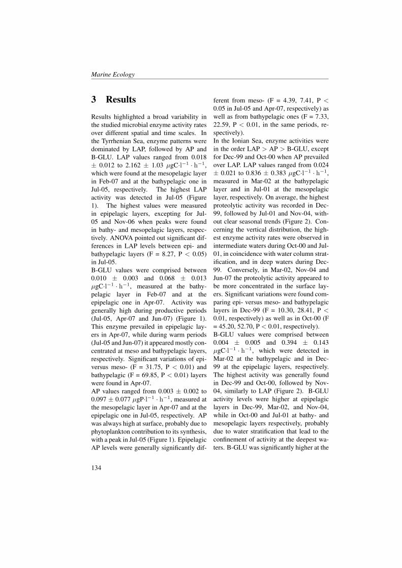
Marine Ecology
3 Results
Results highlighted a broad variability inthe studied microbial enzyme activity ratesover different spatial and time scales. Inthe Tyrrhenian Sea, enzyme patterns weredominated by LAP, followed by AP andB-GLU. LAP values ranged from 0.018± 0.012 to 2.162 ± 1.03 µgC·l−1 · h−1,which were found at the mesopelagic layerin Feb-07 and at the bathypelagic one inJul-05, respectively. The highest LAPactivity was detected in Jul-05 (Figure1). The highest values were measuredin epipelagic layers, excepting for Jul-05 and Nov-06 when peaks were foundin bathy- and mesopelagic layers, respec-tively. ANOVA pointed out significant dif-ferences in LAP levels between epi- andbathypelagic layers (F = 8.27, P < 0.05)in Jul-05.B-GLU values were comprised between0.010 ± 0.003 and 0.068 ± 0.013µgC·l−1 · h−1, measured at the bathy-pelagic layer in Feb-07 and at theepipelagic one in Apr-07. Activity wasgenerally high during productive periods(Jul-05, Apr-07 and Jun-07) (Figure 1).This enzyme prevailed in epipelagic lay-ers in Apr-07, while during warm periods(Jul-05 and Jun-07) it appeared mostly con-centrated at meso and bathypelagic layers,respectively. Significant variations of epi-versus meso- (F = 31.75, P < 0.01) andbathypelagic (F = 69.85, P < 0.01) layerswere found in Apr-07.AP values ranged from 0.003 ± 0.002 to0.097 ± 0.077 µgP·l−1 · h−1, measured atthe mesopelagic layer in Apr-07 and at theepipelagic one in Jul-05, respectively. APwas always high at surface, probably due tophytoplankton contribution to its synthesis,with a peak in Jul-05 (Figure 1). EpipelagicAP levels were generally significantly dif-
ferent from meso- (F = 4.39, 7.41, P <0.05 in Jul-05 and Apr-07, respectively) aswell as from bathypelagic ones (F = 7.33,22.59, P < 0.01, in the same periods, re-spectively).In the Ionian Sea, enzyme activities werein the order LAP > AP > B-GLU, exceptfor Dec-99 and Oct-00 when AP prevailedover LAP. LAP values ranged from 0.024± 0.021 to 0.836 ± 0.383 µgC·l−1 · h−1,measured in Mar-02 at the bathypelagiclayer and in Jul-01 at the mesopelagiclayer, respectively. On average, the highestproteolytic activity was recorded in Dec-99, followed by Jul-01 and Nov-04, with-out clear seasonal trends (Figure 2). Con-cerning the vertical distribution, the high-est enzyme activity rates were observed inintermediate waters during Oct-00 and Jul-01, in coincidence with water column strat-ification, and in deep waters during Dec-99. Conversely, in Mar-02, Nov-04 andJun-07 the proteolytic activity appeared tobe more concentrated in the surface lay-ers. Significant variations were found com-paring epi- versus meso- and bathypelagiclayers in Dec-99 (F = 10.30, 28.41, P <0.01, respectively) as well as in Oct-00 (F= 45.20, 52.70, P < 0.01, respectively).B-GLU values were comprised between0.004 ± 0.005 and 0.394 ± 0.143µgC·l−1 · h−1, which were detected inMar-02 at the bathypelagic and in Dec-99 at the epipelagic layers, respectively.The highest activity was generally foundin Dec-99 and Oct-00, followed by Nov-04, similarly to LAP (Figure 2). B-GLUactivity levels were higher at epipelagiclayers in Dec-99, Mar-02, and Nov-04,while in Oct-00 and Jul-01 at bathy- andmesopelagic layers respectively, probablydue to water stratification that lead to theconfinement of activity at the deepest wa-ters. B-GLU was significantly higher at the
134
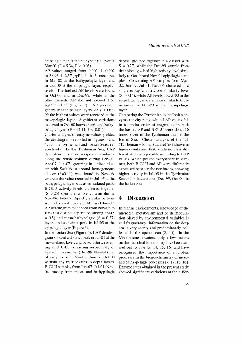
Marine research at CNR
epipelagic than at the bathypelagic layer inMar-02 (F = 5.34, P < 0.05).AP values ranged from 0.003 ± 0.002to 3.096 ± 2.57 µgP·l−1 · h−1, measuredin Mar-02 at the bathypelagic layer andin Oct-00 at the epipelagic layer, respec-tively. The highest AP levels were foundin Oct-00 and in Dec-99, while in theother periods AP did not exceed 1.62µgP·l−1 · h−1 (Figure 2). AP prevailedgenerally at epipelagic layers; only in Dec-99 the highest values were recorded at themesopelagic layer. Significant variationsoccurred in Oct-00 between epi- and bathy-pelagic layers (F = 12.11, P < 0.01).Cluster analysis of enzyme values yieldedthe dendrograms reported in Figures 3 and4, for the Tyrrhenian and Ionian Seas, re-spectively. In the Tyrrhenian Sea, LAPdata showed a close reciprocal similarityalong the whole column during Feb-07,Apr-07, Jun-07, grouping in a close clus-ter with S=0.06; a second homogeneouscluster (S=0.11) was found in Nov-06,whereas the value recorded in Jul-05 at thebathypelagic layer was as an isolated peak.B-GLU activity levels clustered together(S=0.26) over the whole column duringNov-06, Feb-07, Apr-07; similar patternswere observed during Jul-05 and Jun-07.AP dendrogram evidenced from Nov-06 toJun-07 a distinct separation among epi-(S= 0.5) and meso-bathypelagic (S = 0.27)layers and a distinct peak in Jul-05 at theepipelagic layer (Figure 3).In the Ionian Sea (Figure 4), LAP dendro-gram showed a distinct peak in Jul-01 at themesopelagic layer, and two clusters, group-ing at S=0.43, consisting respectively oflate autumn samples (Dec-99, Nov-04) andof samples from Mar-02, Jun-07, Oct-00without any relationships to depth layers.B-GLU samples from Jun-07, Jul-01, Nov-04, mostly from meso- and bathypelagic
depths, grouped together in a cluster withS = 0.27, while the Dec-99 sample fromthe epipelagos had high activity level simi-larly to Oct-00 and Nov-04 epipelagic sam-ples. Concerning AP, samples from Mar-02, Jun-07, Jul-01, Nov-04 clustered in asingle group with a close similarity level(S = 0.14), while AP levels in Oct-00 in theepipelagic layer were more similar to thosemeasured in Dec-99 in the mesopelagiclayer.Comparing the Tyrrhenian to the Ionian en-zyme activity rates, while LAP values fellin a similar order of magnitude in boththe basins, AP and B-GLU were about 10times lower in the Tyrrhenian than in theIonian Sea. Cluster analysis of the full(Tyrrhenian + Ionian) dataset (not shown infigure) confirmed that, while no clear dif-ferentiation was possible according to LAPvalues, which peaked everywhere in sum-mer, both B-GLU and AP were differentlyexpressed between the two basins, showinghigher activity in Jul-05 in the TyrrhenianSea and in late autumn (Dec-99, Oct-00) inthe Ionian Sea.
4 Discussion
In marine environments, knowledge of themicrobial metabolism and of its modula-tion played by environmental variables isstill fragmentary; information on the deepsea is very scanty and predominantly col-lected in the open ocean [2, 13]. In theMediterranean waters, only a few studieson the microbial functioning have been car-ried out to date [5, 14, 15, 16] and haverecognised the importance of microbialprocesses in the biogeochemistry of meso-and bathy-pelagic processes [7, 17, 18, 16].Enzyme rates obtained in the present studyshowed significant variations at the differ-
135
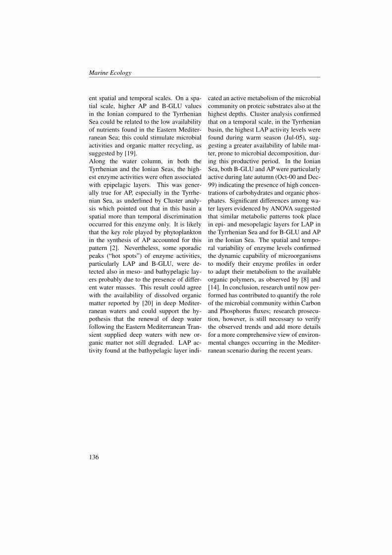
Marine Ecology
ent spatial and temporal scales. On a spa-tial scale, higher AP and B-GLU valuesin the Ionian compared to the TyrrhenianSea could be related to the low availabilityof nutrients found in the Eastern Mediter-ranean Sea; this could stimulate microbialactivities and organic matter recycling, assuggested by [19].Along the water column, in both theTyrrhenian and the Ionian Seas, the high-est enzyme activities were often associatedwith epipelagic layers. This was gener-ally true for AP, especially in the Tyrrhe-nian Sea, as underlined by Cluster analy-sis which pointed out that in this basin aspatial more than temporal discriminationoccurred for this enzyme only. It is likelythat the key role played by phytoplanktonin the synthesis of AP accounted for thispattern [2]. Nevertheless, some sporadicpeaks (“hot spots”) of enzyme activities,particularly LAP and B-GLU, were de-tected also in meso- and bathypelagic lay-ers probably due to the presence of differ-ent water masses. This result could agreewith the availability of dissolved organicmatter reported by [20] in deep Mediter-ranean waters and could support the hy-pothesis that the renewal of deep waterfollowing the Eastern Mediterranean Tran-sient supplied deep waters with new or-ganic matter not still degraded. LAP ac-tivity found at the bathypelagic layer indi-
cated an active metabolism of the microbialcommunity on proteic substrates also at thehighest depths. Cluster analysis confirmedthat on a temporal scale, in the Tyrrhenianbasin, the highest LAP activity levels werefound during warm season (Jul-05), sug-gesting a greater availability of labile mat-ter, prone to microbial decomposition, dur-ing this productive period. In the IonianSea, both B-GLU and AP were particularlyactive during late autumn (Oct-00 and Dec-99) indicating the presence of high concen-trations of carbohydrates and organic phos-phates. Significant differences among wa-ter layers evidenced by ANOVA suggestedthat similar metabolic patterns took placein epi- and mesopelagic layers for LAP inthe Tyrrhenian Sea and for B-GLU and APin the Ionian Sea. The spatial and tempo-ral variability of enzyme levels confirmedthe dynamic capability of microorganismsto modify their enzyme profiles in orderto adapt their metabolism to the availableorganic polymers, as observed by [8] and[14]. In conclusion, research until now per-formed has contributed to quantify the roleof the microbial community within Carbonand Phosphorus fluxes; research prosecu-tion, however, is still necessary to verifythe observed trends and add more detailsfor a more comprehensive view of environ-mental changes occurring in the Mediter-ranean scenario during the recent years.
136
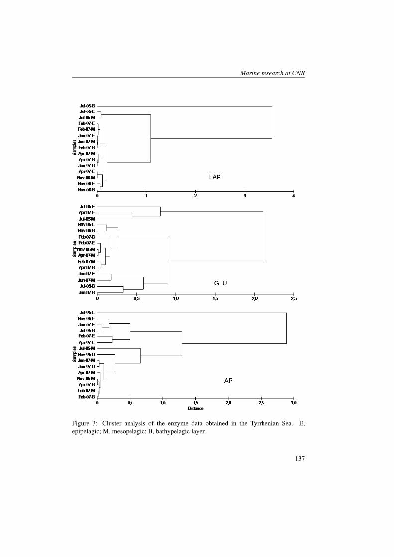
Marine research at CNR
Figure 3: Cluster analysis of the enzyme data obtained in the Tyrrhenian Sea. E,epipelagic; M, mesopelagic; B, bathypelagic layer.
137
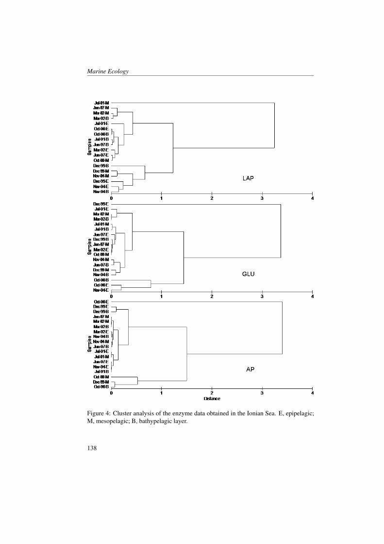
Marine Ecology
Figure 4: Cluster analysis of the enzyme data obtained in the Ionian Sea. E, epipelagic;M, mesopelagic; B, bathypelagic layer.
138
Marine research at CNR
References[1] F. Azam, D.C. Smith, G.F. Steward, and A. Hagstrom. Bacteria-organic matter
coupling and its significance for oceanic carbon cycling. Microb. Ecol., 28:167–179, 1993.
[2] H.G. Hoppe, C. Arnosti, and G.J. Herndl. Ecological significance of bacterial en-zymes in the marine environment. Enzymes in the environment: activity, ecologyand applications, pages 73–108, 2002.
[3] G. Caruso and R. Zaccone. Estimates of leucine aminopeptidase activity in differentmarine and brackish environments. J. Appl. Microbiol., 89(6):951–959, 2000.
[4] G. Caruso, R. Zaccone, M. Azzaro, M. Mancuso, and M. Leonardi. Stime di abbon-danza ed attivita microbiche in un’area oligotrofica del mar Ionio: studio stagionale.Atti Associazione Italiana Oceanologia e Limnologia, 16:67–77, 2003.
[5] G. Caruso, L. Monticelli, R. La Ferla, G. Maimone, M. Azzaro, F. Azzaro, F. De-cembrini, M. Leonardi, and E. De Domenico. Microbial distribution and activitywithin the epi-, meso- and bathypelagic layers of the southern Tyrrhenian Sea. 3rdInternational Conference Enzymes in the Environment. Viterbo, July 15-19,, page302, 2007.
[6] R. La Ferla, R. Zaccone, M. Azzaro, and G. Caruso. Microbial respiratory andectoenzymatic activities in the Northern Adriatic Sea. Chem. Ecol., 18(1-2):75–84,2002.
[7] R. La Ferla, F. Azzaro, M. Azzaro, G. Caruso, F. Decembrini, M. Leonardi, G. Mai-mone, L.S. Monticelli, F. Raffa, C. Santinelli, R. Zaccone, and M. Ribera d’Alcala.Microbial contribution to carbon biogeochemistry in the Mediterranean Sea: vari-ability of activities and biomass. J. Mar. Syst., 57(1-2):146–166, 2005.
[8] R. Zaccone, G. Caruso, and C. Cali’. Heterotrophic bacteria in the Northern Adri-atic Sea: seasonal changes and enzyme profile. Mar. Environ. Res., 54(1):1–19,2002.
[9] C.M. Turley. The changing Mediterranean Sea - a sensitive ecosystem? Progr.Oceanogr., 44:387–400, 1999.
[10] L.S. Monticelli, E. De Domenico, G. Caruso, F. Azzaro, M. Azzaro, R. La Ferla,M. Leonardi, G. Maimone, and F. Decembrini. Attivita e biomasse microbichenelle acque superficiali del mar Ionio. Atti Associazione Italiana Oceanologia eLimnologia, 19:349–359, 2008.
[11] H.G. Hoppe. Use of fluorogenic model substrates for extracellular enzyme activ-ity (EEA) measurement of bacteria. Handbook of methods in aquatic microbialecology, pages 423–432, 1993.
139
Marine Ecology
[12] K.R. Clarke and R.M. Warwick. Change in marine communities: an approach tostatistical analysis and interpretation. pages 1–144, 1994.
[13] F. Baltar, J. Aristegui, E. Sintes, H.M. van Aken, J.M. Gasol, and G.J. Herndl.Prokaryotic extracellular enzymatic activity in relation to biomass production andrespiration in the meso- and bathypelagic waters of the (sub)tropical Atlantic. Env-iron. Microbiol., 11(8):1998–2014, 2009.
[14] C. Misic, M. Castellano, N. Ruggieri, and A. Covazzi Harriague. Variations in ec-toenzymatic hydrolytic activity in a oligotrophic environment (Southern TyrrhenianSea, W Mediterranean). J. Mar. Syst., 73:123–137, 2008.
[15] C. Tamburini, J. Garcin, M. Ragot, and A. Bianchi. Biopolymer hydrolysis andbacterial production under ambient hydrostatic pressure through a 2000 m watercolumn in the NW Mediterranean. Deep-Sea Res. Part II, 49:2109–2123, 2002.
[16] C. Tamburini, M. Garel, B. Al Ali, B. Merigot, P. Kriwy, B. Charriere, and G. Budil-lon. Distribution and activity of Bacteria and Archaea in the different water massesof the Tyrrhenian Sea. Deep-Sea Res. Part II, 56:700–712, 2009.
[17] R. La Ferla, M. Azzaro, G. Caruso, L.S. Monticelli, G. Maimone, R. Zaccone, andT.T. Packard. Prokaryotic abundance and heterotrophic metabolism in the deepMediterranean Sea. Adv. Oceanogr. Limnol., 1:143–166, 2010.
[18] J. Aristegui, G.M. Gasol, C.M. Duarte, and G.J. Herndl. Microbial oceanographyof the dark ocean’s pelagic realm. Limnol. Oceanogr., 54(5):1501–1529, 2009.
[19] F. van Wambeke, U. Christaki, A. Giannakourou, T. Moutin, and K. Souvemer-zoglou. Longitudinal and vertical trends of bacterial limitation by phosphorus andcarbon in the Mediterranean Sea. Microb. Ecol., 43(1):119–133, 2002.
[20] A. Seritti, B.B. Manca, C. Santinelli, E. Murru, A. Boldrin, and L. Nannicini. Rela-tionships between dissolved organic carbon (DOC) and water mass structure in theIonian Sea (winter 1999). J. Geophys. Res., 108(C9):1–13, 2003.
140
The Impact of Plankton Communities over theNorthern Adriatic Pelagic Ecosystem
G. Socal1, F. Acri1, M. Bastianini1, F. Bernardi Aubry1, F. Bianchi1, E.Camatti1, A. Conversi2, A. De Lazzari1, A. Pugnetti11, Institute of Marine Sciences, CNR, Venezia, Italy2, Institute of Marine Sciences, CNR, Pozzuolo di Lerici (SP), [email protected]
Abstract
The research activity of ISMAR on plankton communities of the Northern Adri-atic Sea is described here. The results derive from data that have been gathered in40 years of oceanographic cruises. Spatial and temporal variations of abundanceand species composition of phytoplankton and zooplankton communities have beenstudied in relation with meteorological forcings and hydrochemical conditions, e.g.water column structure, chlorophyll a concentrations and nutrient availability, withthe aim of: i) highlighting the dominant scales of variability in biomass and speciescomposition, ii) recognizing the possible relationships between environmental pa-rameters, plankton biomass and specific changes, iii) identifying long-term signals ofvariability. The link between plankton communities and some environmental emer-gencies (mucilage events, discoloured waters, presence of potentially toxic algae) isalso evaluated.
1 IntroductionIn this paper we report and review the re-search activity of ISMAR in the study ofphytoplankton and zooplankton communi-ties of the Northern Adriatic Sea (NAS)during the last 40 years. This area is lo-cated between the Gulf of Trieste (46°N)and the imaginary line from Ancona, inItaly, to Zadar, in Croatia (approx. 44°N),and it is characterized by overall shallowdepth (average = ÷ 35 m). In the Mediter-ranean context, these features make theNAS as the northernmost area as well asthe most extensive region of shallow wa-ter in the Mediterranean Sea: consequently,the hydrography of this basin is stronglyaffected by the atmospheric regime. Thelargest Italian river, the Po river, discharges
its waters in this sub-basin (1918-2006 av-erage flux = 1492 m3 · s−1), after havingcrossed the most developed region in Italyin terms of inhabitants and industrial andagricultural activities. For this reason, theNAS is a site of intense biological activ-ity and a good example of how the marineecosystem copes with pollution, eutroph-ication, climate change and other humanmediated activities [1]. Since the ‘1960s,ISMAR carried out several oceanographiccruises in this basin, in the framework ofseveral national and international projects.Spatial and temporal variations of plank-ton community structures have been stud-ied in relation to meteorological forcingand hydrochemical conditions, such as wa-ter column structure, nutrient availability
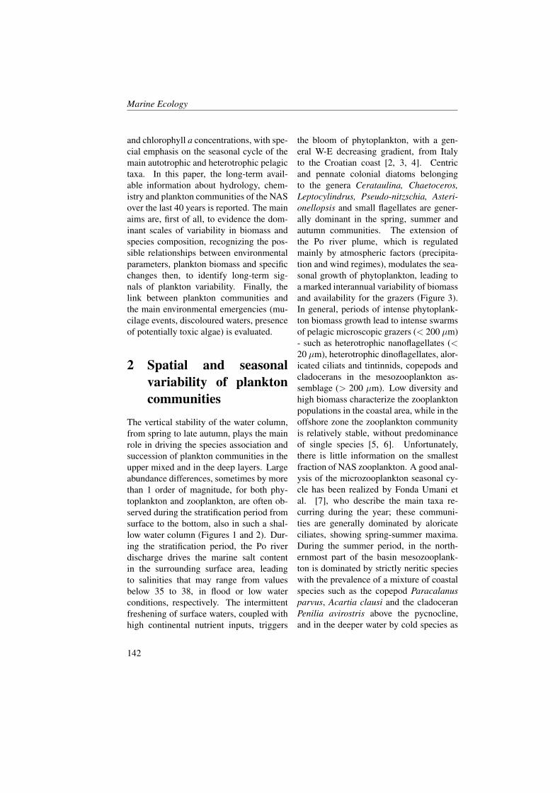
Marine Ecology
and chlorophyll a concentrations, with spe-cial emphasis on the seasonal cycle of themain autotrophic and heterotrophic pelagictaxa. In this paper, the long-term avail-able information about hydrology, chem-istry and plankton communities of the NASover the last 40 years is reported. The mainaims are, first of all, to evidence the dom-inant scales of variability in biomass andspecies composition, recognizing the pos-sible relationships between environmentalparameters, plankton biomass and specificchanges then, to identify long-term sig-nals of plankton variability. Finally, thelink between plankton communities andthe main environmental emergencies (mu-cilage events, discoloured waters, presenceof potentially toxic algae) is evaluated.
2 Spatial and seasonalvariability of planktoncommunities
The vertical stability of the water column,from spring to late autumn, plays the mainrole in driving the species association andsuccession of plankton communities in theupper mixed and in the deep layers. Largeabundance differences, sometimes by morethan 1 order of magnitude, for both phy-toplankton and zooplankton, are often ob-served during the stratification period fromsurface to the bottom, also in such a shal-low water column (Figures 1 and 2). Dur-ing the stratification period, the Po riverdischarge drives the marine salt contentin the surrounding surface area, leadingto salinities that may range from valuesbelow 35 to 38, in flood or low waterconditions, respectively. The intermittentfreshening of surface waters, coupled withhigh continental nutrient inputs, triggers
the bloom of phytoplankton, with a gen-eral W-E decreasing gradient, from Italyto the Croatian coast [2, 3, 4]. Centricand pennate colonial diatoms belongingto the genera Cerataulina, Chaetoceros,Leptocylindrus, Pseudo-nitzschia, Asteri-onellopsis and small flagellates are gener-ally dominant in the spring, summer andautumn communities. The extension ofthe Po river plume, which is regulatedmainly by atmospheric factors (precipita-tion and wind regimes), modulates the sea-sonal growth of phytoplankton, leading toa marked interannual variability of biomassand availability for the grazers (Figure 3).In general, periods of intense phytoplank-ton biomass growth lead to intense swarmsof pelagic microscopic grazers (< 200 µm)- such as heterotrophic nanoflagellates (<20 µm), heterotrophic dinoflagellates, alor-icated ciliats and tintinnids, copepods andcladocerans in the mesozooplankton as-semblage (> 200 µm). Low diversity andhigh biomass characterize the zooplanktonpopulations in the coastal area, while in theoffshore zone the zooplankton communityis relatively stable, without predominanceof single species [5, 6]. Unfortunately,there is little information on the smallestfraction of NAS zooplankton. A good anal-ysis of the microzooplankton seasonal cy-cle has been realized by Fonda Umani etal. [7], who describe the main taxa re-curring during the year; these communi-ties are generally dominated by aloricateciliates, showing spring-summer maxima.During the summer period, in the north-ernmost part of the basin mesozooplank-ton is dominated by strictly neritic specieswith the prevalence of a mixture of coastalspecies such as the copepod Paracalanusparvus, Acartia clausi and the cladoceranPenilia avirostris above the pycnocline,and in the deeper water by cold species as
142
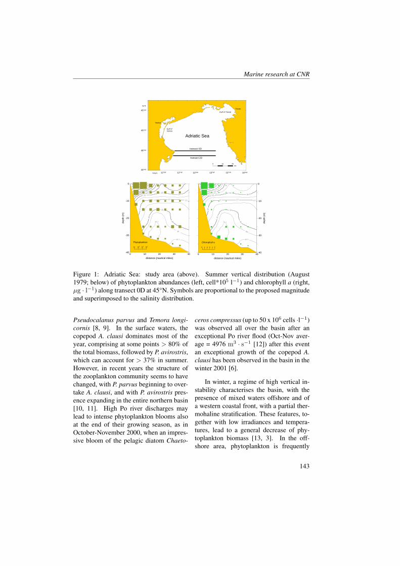
Marine research at CNR
0 10 20 30 40
distance (nautical miles)
-40
-30
-20
-10
0
depth
(m
)
10 10 10 10
Phytoplankton
2 3 4
0 10 20 30 40
distance (nautical miles)
-40
-30
-20
-10
0
depth
(m
)
0 1 2 5
Chlorophyll a
3 4
45°00'
13°00' 14°00'
Adriatic Sea
44°40'
45°20'
45°40'
12°20' 12°40' 13°20' 13°40'
0.00.30.50.81.00 10 20nm
Venice
Trieste
Gulf of Trieste
Gulf ofVenice
transect 0D
transect 2D
lat N
long E
Figure 1: Adriatic Sea: study area (above). Summer vertical distribution (August1979; below) of phytoplankton abundances (left, cell*105 l−1) and chlorophyll a (right,µg · l−1) along transect 0D at 45°N. Symbols are proportional to the proposed magnitudeand superimposed to the salinity distribution.
Pseudocalanus parvus and Temora longi-cornis [8, 9]. In the surface waters, thecopepod A. clausi dominates most of theyear, comprising at some points > 80% ofthe total biomass, followed by P. avirostris,which can account for > 37% in summer.However, in recent years the structure ofthe zooplankton community seems to havechanged, with P. parvus beginning to over-take A. clausi, and with P. avirostris pres-ence expanding in the entire northern basin[10, 11]. High Po river discharges maylead to intense phytoplankton blooms alsoat the end of their growing season, as inOctober-November 2000, when an impres-sive bloom of the pelagic diatom Chaeto-
ceros compressus (up to 50 x 106 cells ·l−1)was observed all over the basin after anexceptional Po river flood (Oct-Nov aver-age = 4976 m3 · s−1 [12]) after this eventan exceptional growth of the copepod A.clausi has been observed in the basin in thewinter 2001 [6].
In winter, a regime of high vertical in-stability characterises the basin, with thepresence of mixed waters offshore and ofa western coastal front, with a partial ther-mohaline stratification. These features, to-gether with low irradiances and tempera-tures, lead to a general decrease of phy-toplankton biomass [13, 3]. In the off-shore area, phytoplankton is frequently
143
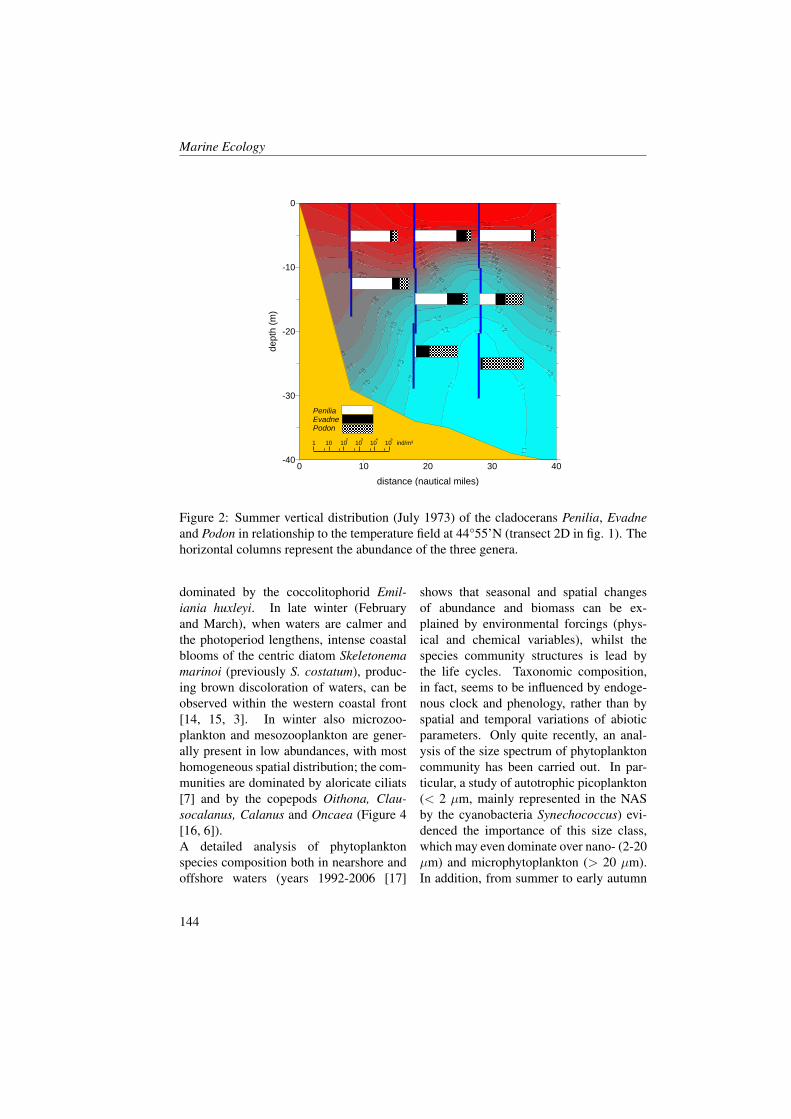
Marine Ecology
0 10 20 30 40
distance (nautical miles)
-40
-30
-20
-10
0
depth
(m
)
1 10 10 10 10 10 ind/m³2 3 4 5
PeniliaEvadnePodon
Figure 2: Summer vertical distribution (July 1973) of the cladocerans Penilia, Evadneand Podon in relationship to the temperature field at 44°55’N (transect 2D in fig. 1). Thehorizontal columns represent the abundance of the three genera.
dominated by the coccolitophorid Emil-iania huxleyi. In late winter (Februaryand March), when waters are calmer andthe photoperiod lengthens, intense coastalblooms of the centric diatom Skeletonemamarinoi (previously S. costatum), produc-ing brown discoloration of waters, can beobserved within the western coastal front[14, 15, 3]. In winter also microzoo-plankton and mesozooplankton are gener-ally present in low abundances, with mosthomogeneous spatial distribution; the com-munities are dominated by aloricate ciliats[7] and by the copepods Oithona, Clau-socalanus, Calanus and Oncaea (Figure 4[16, 6]).A detailed analysis of phytoplanktonspecies composition both in nearshore andoffshore waters (years 1992-2006 [17]
shows that seasonal and spatial changesof abundance and biomass can be ex-plained by environmental forcings (phys-ical and chemical variables), whilst thespecies community structures is lead bythe life cycles. Taxonomic composition,in fact, seems to be influenced by endoge-nous clock and phenology, rather than byspatial and temporal variations of abioticparameters. Only quite recently, an anal-ysis of the size spectrum of phytoplanktoncommunity has been carried out. In par-ticular, a study of autotrophic picoplankton(< 2 µm, mainly represented in the NASby the cyanobacteria Synechococcus) evi-denced the importance of this size class,which may even dominate over nano- (2-20µm) and microphytoplankton (> 20 µm).In addition, from summer to early autumn
144
Marine research at CNR
5
10
15
20
25
30
°C
a)
0
1
2
3
4
5
6
feb
apr
jun
aug
oct
dec
feb
apr
jun
aug
oct
dec
feb
apr
jun
aug
oct
dec
cell
s d
m-3
* 1
06
0
50
100
150
200
250
300
µg
Cd
m-3
abundance biomass
b)
1999 2000 2001
Figure 3: Temporal evolution of (a) surface temperature and (b) total phytoplanktonabundance and biomass, 1999-2001: values represent the averages for the whole sam-pling area.
a shift from large to small cells is often ob-served in oligotrophic areas (characterizedby high temperature and salinity and lownutrient concentration [18]). Pugnetti et al.[19] perform an analysis of the carbon par-titioning in plankton biomass, demonstrat-ing that nutrients, charged by the rivers,can impose a large interannual variabilityon the autotrophic/heterotrophic biomassratio; when oligotrophy prevails, planktoncommunity shows heterotrophic biomass(including bacteria) exceeding that of au-totrophs, leading to a reversed trophic pyra-mid.
3 Long term trend ofplankton communities
An analysis of the chlorophyll variationsin the years from 1970 to 2007 at basinscale [20], with the help of satellite-derivedinformation, demonstrates a generally de-
clining trend of phytoplankton biomassconcentration, reaching a decreasing valueof about 0.11 µg l-1 per year in the lastdecade. The authors attribute this to a cor-responding reduce in nutrient concentra-tions in the basin, indicating that the stillcommon perception of the Adriatic Sea asa very eutrophic basin is no longer appro-priate, at least for its northern part and inrecent years. Through the analysis of timeseries, with regard to mesozooplankton weobserve significant changes in communitycomposition at the time scale of approx.40 years, mostly due to a general decreaseof Acartia clausi, as dominant species, be-ing replaced by Paracalanus parvus. Whencompared to past records, Penilia avirostrisswarms appear to have extended their tem-poral occurrence too. These changes mightbe related to the observed general in-crease of the average sea water tempera-ture and the reduction of phosphate in theNAS [21, 6, 10]. Copepod time series
145
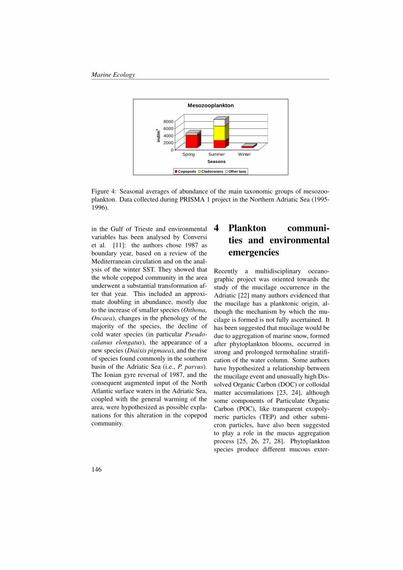
Marine Ecology
0
2000
4000
6000
8000
ind
/m3
Spring Summer Winter
Seasons
Mesozooplankton
Copepods Cladocerans Other taxa
Figure 4: Seasonal averages of abundance of the main taxonomic groups of mesozoo-plankton. Data collected during PRISMA 1 project in the Northern Adriatic Sea (1995-1996).
in the Gulf of Trieste and environmentalvariables has been analysed by Conversiet al. [11]: the authors chose 1987 asboundary year, based on a review of theMediterranean circulation and on the anal-ysis of the winter SST. They showed thatthe whole copepod community in the areaunderwent a substantial transformation af-ter that year. This included an approxi-mate doubling in abundance, mostly dueto the increase of smaller species (Oithona,Oncaea), changes in the phenology of themajority of the species, the decline ofcold water species (in particular Pseudo-calanus elongatus), the appearance of anew species (Diaixis pigmaea), and the riseof species found commonly in the southernbasin of the Adriatic Sea (i.e., P. parvus).The Ionian gyre reversal of 1987, and theconsequent augmented input of the NorthAtlantic surface waters in the Adriatic Sea,coupled with the general warming of thearea, were hypothesized as possible expla-nations for this alteration in the copepodcommunity.
4 Plankton communi-ties and environmentalemergencies
Recently a multidisciplinary oceano-graphic project was oriented towards thestudy of the mucilage occurrence in theAdriatic [22] many authors evidenced thatthe mucilage has a planktonic origin, al-though the mechanism by which the mu-cilage is formed is not fully ascertained. Ithas been suggested that mucilage would bedue to aggregation of marine snow, formedafter phytoplankton blooms, occurred instrong and prolonged termohaline stratifi-cation of the water column. Some authorshave hypothesized a relationship betweenthe mucilage event and unusually high Dis-solved Organic Carbon (DOC) or colloidalmatter accumulations [23, 24], althoughsome components of Particulate OrganicCarbon (POC), like transparent exopoly-meric particles (TEP) and other submi-cron particles, have also been suggestedto play a role in the mucus aggregationprocess [25, 26, 27, 28]. Phytoplanktonspecies produce different mucous exter-
146
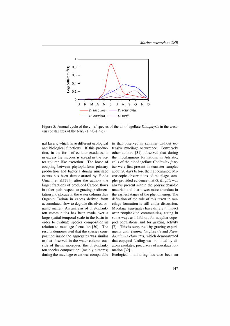
Marine research at CNR
0
0,2
0,4
0,6
0,8
1
J F M A M J J A S O N D
Lo
g(c
ells/d
m3+1)
D.sacculus D. rotundata
D. caudata D. fortii
Figure 5: Annual cycle of the chief species of the dinoflagellate Dinophysis in the west-ern coastal area of the NAS (1990-1996).
nal layers, which have different ecologicaland biological functions. If this produc-tion, in the form of cellular exudates, isin excess the mucous is spread in the wa-ter column like excretion. The loose ofcoupling between phytoplankton primaryproduction and bacteria during mucilageevents has been demonstrated by FondaUmani et al.[29]: after the authors thelarger fractions of produced Carbon flowsin other path respect to grazing, sedimen-tation and storage in the water column thusOrganic Carbon in excess derived formaccumulated slow to degrade dissolved or-ganic matter. An analysis of phytoplank-ton communities has been made over alarge spatial-temporal scale in the basin inorder to evaluate species composition inrelation to mucilage formation [30]. Theresults demonstrated that the species com-position inside the aggregates was similarto that observed in the water column out-side of them; moreover, the phytoplank-ton species composition, (mainly diatoms)during the mucilage-event was comparable
to that observed in summer without ex-tensive mucilage occurrence. Converselyother authors [31], observed that duringthe mucilaginous formations in Adriatic,cells of the dinoflagellate Goniaulax frag-ilis were first present in seawater samplesabout 20 days before their appearance. Mi-croscopic observations of mucilage sam-ples provided evidence that G. fragilis wasalways present within the polysaccharidicmaterial, and that it was more abundant inthe earliest stages of the phenomenon. Thedefinition of the role of this taxon in mu-cilage formation is still under discussion.Mucilage aggregates have different impactover zooplankton communities, acting insome ways as inhibitors for naupliar cope-pod populations and for grazing activity[7]. This is supported by grazing experi-ments with Temora longicornis and Pseu-docalanus elongatus, which demonstratedthat copepod feeding was inhibited by di-atom exudates, precursors of mucilage for-mation [32].Ecological monitoring has also been an
147
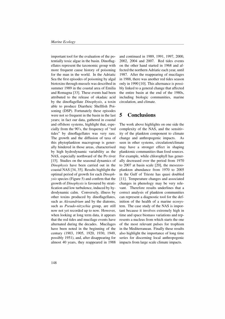
Marine Ecology
important tool for the evaluation of the po-tentially toxic algae in the basin. Dinoflag-ellates represent the taxonomic group withmore frequent cause history of poisoningfor the man in the world. In the AdriaticSea the first episodes of poisoning by algalbiotoxins through mussels was described insummer 1989 in the coastal area of Emiliaand Romagna [33]. These events had beenattributed to the release of okadaic acidby the dinoflagellate Dinophysis, a toxinable to produce Diarrheic Shellfish Poi-soning (DSP). Fortunately these episodeswere not so frequent in the basin in the lastyears; in fact our data, gathered in coastaland offshore systems, highlight that, espe-cially from the 90’s, the frequency of “redtides” by dinoflagellates was very rare.The growth and the diffusion of taxa ofthis phytoplankton macrogroup is gener-ally hindered in those areas, characterisedby high hydrodynamic variability as theNAS, especially northward of the Po river[15]. Studies on the seasonal dynamics ofDinophysis have been carried out in thecoastal NAS [34, 35]. Results highlight theoptimal period of growth for each Dinoph-ysis species (Figure 5) and confirm that thegrowth of Dinophysis is favoured by strati-fication and low turbulence, induced by hy-drodynamic calm. Conversely, illness byother toxins produced by dinoflagellates,such as Alexandrium and by the diatoms,such as Pseudo-nitzschia group, are stillnow not yet recorded up to now. However,when looking at long term data, it appearsthat the red tides and mucilage events havealternated during the decades. Mucilageshave been noted in the beginning of thecentury (1903, 1905, 1920, 1930, 1949,possibly 1951), and, after disappearing foralmost 40 years, they reappeared in 1988
and continued in 1989, 1991, 1997, 2000,2002, 2004 and 2007. Red tides eventson the other hand started in 1968 and af-fected the northern Adriatic each year, until1987. After the reappearing of mucilagesin 1988, there was another red tides seasononly in 1990 [10]. This alternance is possi-bly linked to a general change that affectedthe entire basin at the end of the 1980s,including biologic communities, marinecirculation, and climate.
5 ConclusionsThe work above highlights on one side thecomplexity of the NAS, and the sensitiv-ity of the plankton component to climatechange and anthropogenic impacts. Asseen in other systems, circulation/climatemay have a stronger effect in shapingplanktonic communities than food sources.For example, while chlorophyll has gener-ally decreased over the period from 1970to 2007 at basin scale [20], the mesozoo-plankton abundance from 1970 to 2005in the Gulf of Trieste has quasi doubled[11]. Temperature changes and associatedchanges in phenology may be very rele-vant. Therefore results underlines that acorrect analysis of plankton communitiescan represent a diagnostic tool for the def-inition of the health of a marine ecosys-tem. The case study of the NAS is impor-tant because it involves extremely high intime and space biomass variations and rep-resents a nucleus from which starts the oneof the most relevant pulses for trophismin the Mediterranean. Finally these resultsalso highlight the importance of long timeseries for discerning local anthropogenicimpacts from large scale climate impacts.
148
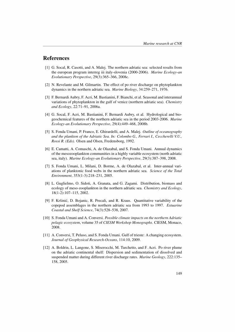
Marine research at CNR
References[1] G. Socal, R. Casotti, and A. Malej. The northern adriatic sea: selected results from
the european program interreg iii italy-slovenia (2000-2006). Marine Ecology-anEvolutionary Perspective, 29(3):365–366, 2008c.
[2] N. Revelante and M. Gilmartin. The effect of po river discharge on phytoplanktondynamics in the northern adriatic sea. Marine Biology, 34:259–271, 1976.
[3] F. Bernardi Aubry, F. Acri, M. Bastianini, F. Bianchi, et al. Seasonal and interannualvariations of phytoplankton in the gulf of venice (northern adriatic sea). Chemistryand Ecology, 22:71–91, 2006a.
[4] G. Socal, F. Acri, M. Bastianini, F. Bernardi Aubry, et al. Hydrological and bio-geochemical features of the northern adriatic sea in the period 2003-2006. MarineEcology-an Evolutionary Perspective, 29(4):449–468, 2008b.
[5] S. Fonda Umani, P. Franco, E. Ghirardelli, and A. Malej. Outline of oceanographyand the plankton of the Adriatic Sea. In: Colombo G., Ferrari I., Ceccherelli V.U.,Rossi R. (Eds). Olsen and Olsen, Fredensborg, 1992.
[6] E. Camatti, A. Comaschi, A. de Olazabal, and S. Fonda Umani. Annual dynamicsof the mesozooplankton communities in a highly variable ecosystem (north adriaticsea, italy). Marine Ecology-an Evolutionary Perspective, 29(3):387–398, 2008.
[7] S. Fonda Umani, L. Milani, D. Borme, A. de Olazabal, et al. Inter-annual vari-ations of planktonic food webs in the northern adriatic sea. Science of the TotalEnvironment, 353(1-3):218–231, 2005.
[8] L. Guglielmo, O. Sidoti, A. Granata, and G. Zagami. Distribution, biomass andecology of meso-zooplankton in the northern adriatic sea. Chemistry and Ecology,18(1-2):107–115, 2002.
[9] F. Krsinic, D. Bojanic, R. Precali, and R. Kraus. Quantitative variability of thecopepod assemblages in the northern adriatic sea from 1993 to 1997. EstuarineCoastal and Shelf Science, 74(3):528–538, 2007.
[10] S. Fonda Umani and A. Conversi. Possible climate impacts on the northern Adriaticpelagic ecosystem, volume 35 of CIESM Workshop Monographs. CIESM, Monaco,2008.
[11] A. Conversi, T. Peluso, and S. Fonda Umani. Gulf of trieste: A changing ecosystem.Journal of Geophysical Research-Oceans, 114:10, 2009.
[12] A. Boldrin, L. Langone, S. Miserocchi, M. Turchetto, and F. Acri. Po river plumeon the adriatic continental shelf: Dispersion and sedimentation of dissolved andsuspended matter during different river discharge rates. Marine Geology, 222:135–158, 2005.
149
Marine Ecology
[13] P. Franco, G. Socal, and F. Bianchi. Fitoplancton nell’adriatico settentrionale.crociere 1978. Naturalista sicil., 6(Suppl.):29–38, 1982.
[14] M. Bastianini, F. Acri, F. Bernardi Aubry, R. Casotti, et al. Environmental factorstriggering the late-winter diatom bloom in the north adriatic sea. Rapports Com-mission Internationale pour l’Exploration Scientifique de la Mer Mediterranee,37:487, 2004.
[15] F. Bernardi Aubry, A. Berton, M. Bastianini, G. Socal, and F. Acri. Phytoplanktonsuccession in a coastal area of the nw adriatic, over a 10-year sampling period(1990–1999). Continental Shelf Research, 24:97–115, 2004.
[16] A. Comaschi, F. Acri, B. Cavalloni, and G. Socal. Andamento temporale dipopolazioni zooplanctoniche in tre stazioni dell’adriatico settentrionale e loro dis-tribuzione verticale in relazione alla struttura della colonna d’acqua. Biol. Mar.Mediterr., 5(1):223–231, 1998.
[17] G. Socal, F. Acri, V. Bandelj, M. Bastianini, et al. Condizioni ambientali, ciclo vi-tale ed orologio endogeno nella dinamica del fitoplancton. evidenze da osservazionisperimentali nell’adriatico nord occidentale. Biol. Mar. Mediterr., 15(1):396–397,2008a.
[18] F. Bernardi Aubry, F. Acri, M. Bastianini, A. Pugnetti, and G. Socal. Picophyto-plankton contribution to phytoplankton community structure in the gulf of venice(nw adriatic sea). International Reviews of Hydrobiology, 91:51–70, 2006b.
[19] A. Pugnetti, A. Bazzoni, A. Beran, F. Bernardi Aubry, et al. Changes in biomassstructure and trophic status of the plankton communities in a highly dynamicecosystem (gulf of venice, northern adriatic sea). Marine Ecology-an Evolution-ary PerspectIve, 29(3):367–374, 2008.
[20] P. Mozetic, C. Solidoro, G. Cossarini, G. Socal, et al. Recent trends towards olig-otrophication of the northern adriatic: Evidence from chlorophyll a time series.Estuaries and Coasts, 2009.
[21] L Kamburska and S. Fonda Umani. Long-term copepod dynamics in the gulf of tri-este (northern adriatic sea): recent changes and trends. Climate Res., 31(2-3):195–203, 2006.
[22] M. Giani, D. Berto, V. Zangrando, S. Castelli, P. Sist, and R. Urbani. Chemicalcharacterization of different typologies of mucilaginous aggregates in the northernadriatic sea. Science of the Total Environment, 353(1-3):232–246, 2005a.
[23] V. Vojvodic and B. Cosovic. Fractionation of surface active substances on the xad-8resin: Adriatic sea samples and phytoplankton culture media. Marine Chemistry,54(1-2):119–133, 1996.
150
Marine research at CNR
[24] M. Pettine, L. Patrolecco, M. Camuso, and S. Crescenzio. Transport of carbon andnitrogen to the northern adriatic sea by the po river. Estuarine Coastal and ShelfScience, 46:127–142, 1998.
[25] V. Zutic, V. Svetlicic, N. Ivosevic, A. Hozic, and O. Pecar. Northern adriatic meso-cosm experiment rovinj 2003: Dynamics of organic microparticles studied by theelectrochemical technique. Periodicum Biologorum, 106(1):67–74, 2004.
[26] M. Giani, A. Rinaldi, and D. Degobbis. Mucilages in the adriatic and tyrrheniansea: An introduction. Science of the Total Environment, 353(1-3):3–9, 2005b.
[27] T. Radic, R. Kraus, D. Fuks, J. Radic, and O. Pecar. Transparent exopolymeric par-ticles’ distribution in the northern adriatic and their relation to microphytoplanktonbiomass and composition. Science of the Total Environment, 353(1-3):151–161,2005.
[28] A. De Lazzari, D. Berto, D. Cassin, A. Boldrin, and M. Giani. Influence of windsand oceanographic conditions on the mucilage aggregation in the northern adriaticsea in 2003-2006. Marine Ecology-an Evolutionary Perspective, 29(4):469–482,2008.
[29] S. Fonda Umani, P. Del Negro, C. Larato, C. De Vittor, et al. Major inter-annualvariations in microbial dynamics in the gulf of trieste (northern adriatic sea) andtheir ecosystem implications. Aquatic Microbial Ecology, 46:163–175, 2007.
[30] C. Totti, M. Cangini, C. Ferrari, R. Kraus, et al. Phytoplankton size-distributionand community structure in relation to mucilage occurrence in the northern adriaticsea. Science of the Total Environment, 353:1–3, 2005.
[31] M. Pompei, C. Mazziotti, F. Guerrini, M. Cangini, et al. Correlation between thepresence of Gonyaulax fragilis (Dinophyceae) and the mucilage phenomena of theemilia-romagna coast (northern adriatic sea). Harmful Algae, 2(4):301–316, 2003.
[32] A. Malej and R.P. Harris. Inhibition of copepod grazing by diatom exudates - afactor in the development of mucus aggregates. Marine Ecology Progress Series,96(1):33–42, 1993.
[33] L. Boni, L. Mancini, A. Milandri, R. Poletti, M. Pompei, and R. Viviani. First casesof diarrhoetic shellfish poisoning in the Northen Adriatic Sea. In: (R. A. Vollenwei-der, R.Marchetti and R. Viviani, eds). Marine Coastal Eutrophication. Elsevier,Amsterdam, 1992.
[34] F. Bernardi Aubry, A. Berton, M. Bastianini, R. Bertaggia, A. Baroni, and G. Socal.Seasonal dynamics of dinophysis in coastal waters of the nw adriatic sea (1990-1996). Botanica Marina, 43:423–430, 2000.
151

Marine Ecology
[35] J. France and P. Mozetic. Ecological characterization of toxic phytoplanktonspecies (/dinophysis/ spp., dinophyceae) in slovenian mariculture areas (gulf of tri-este, adriatic sea) and the implications for monitoring. Marine Pollution Bulletin,52(11):1504–1516, 2006.
152
Impact of an Acoustic Stimulus on the Motilityand Blood Parameters of European Sea Bass (Di-centrarchus labrax L.) and Gilthead Sea Bream(Sparus aurata L.)
G. Buscaino1, F. Filiciotto1, G. Buffa1, A. Bellante1, V. Di Stefano1, A.Assenza2, F. Fazio2, G. Caola2, S. Aronica1, C. Buscaino1
1, Institute for Coastal Marine Environment, CNR, Capo Granitola (TP), Italy2, Department of Experimental and Applied Biotechnology, University of Messina, Messina,[email protected]
Abstract
The physiological responses of fish to underwater noise are poorly understoodand further information is needed to evaluate any possible negative effects of soundexposure. We exposed European sea bass and gilthead sea bream to a 0.1–1 kHz lin-ear sweep (150 dBrms re 1 µPa). This band frequency is perceptible by many speciesof fish and is mainly produced by vessel traffic. We assessed the noise-induced motil-ity reaction (analysing the movements) and the haematological responses (measuringblood lactate, and haematocrit levels). The noise exposure produced a significant in-crease in motility as well as an increase in lactate and haematocrit levels in sea breamand sea bass. A linear correlation between blood parameters and motility in fish ex-posed to the noise was observed. The acoustic stimulus produced intense muscleactivity.
1 Introduction
The impact of human activity on marinehabitats can produce adaptive alterationsand other significant changes in animals[1, 2, 3]. In recent years, many studieshave been carried out with the aim of evalu-ating the effects of anthropogenic acousticdisturbance on marine organisms [4, 5, 6],thus increasing the awareness of the dam-age done to animals exposed to humanrelated underwater sounds [7, 8]. Thesesounds are associated with shipping, seis-mic surveys, sonar, recreational boatingand many other anthropogenic sources that
are known to induce several types of re-sponses in fishes [9, 10, 2, 11, 12, 13, 14].Pacific herring (Harengus pallasi) exhib-ited alarm responses in reaction to motor-boat noise [13]. Engas et al. [10] foundthat seismic shooting has effects on the lo-cal abundance and distribution of Gadusmorhua and haddock (Melanogrammus ae-glefinus). Smith et al. [14] examined theshort- and long-term effects of increasedambient noise on the behaviour and hear-ing of goldfish (Carassius auratus). Theynoted that goldfish exhibited an initial star-tle response with a rapid burst of erraticswimming followed by general increased
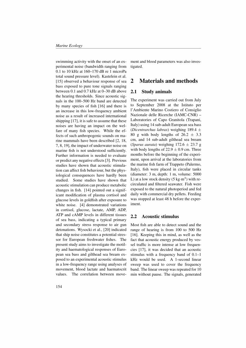
Marine Ecology
swimming activity with the onset of an ex-perimental noise (bandwidth ranging from0.1 to 10 kHz at 160–170 dB re 1 microPatotal sound pressure level). Kastelein et al.[15] observed a behaviour response of seabass exposed to pure tone signals rangingbetween 0.1 and 0.7 kHz at 0–30 dB abovethe hearing thresholds. Since acoustic sig-nals in the 100–500 Hz band are detectedby many species of fish [16] and there isan increase in this low-frequency ambientnoise as a result of increased internationalshipping [17], it is safe to assume that thesenoises are having an impact on the wel-fare of many fish species. While the ef-fects of such anthropogenic sounds on ma-rine mammals have been described [2, 18,7, 8, 19], the impact of underwater noise onmarine fish is not understood sufficiently.Further information is needed to evaluateor predict any negative effects [3]. Previousstudies have shown that acoustic stimula-tion can affect fish behaviour, but the phys-iological consequences have hardly beenstudied. Some studies have shown thatacoustic stimulation can produce metabolicchanges in fish. [14] pointed out a signif-icant modification of plasma cortisol andglucose levels in goldfish after exposure towhite noise. [4] demonstrated variationsin cortisol, glucose, lactate, AMP, ADP,ATP and cAMP levels in different tissuesof sea bass, indicating a typical primaryand secondary stress response to air gundetonations. Wysocki et al., [20] indicatedthat ship noise constitutes a potential stres-sor for European freshwater fishes. Thepresent study aims to investigate the motil-ity and haematological responses of Euro-pean sea bass and gilthead sea bream ex-posed to an experimental acoustic stimulusin a low-frequency range using analyses ofmovement, blood lactate and haematocritvalues. The correlation between move-
ment and blood parameters was also inves-tigated.
2 Materials and methods
2.1 Study animals
The experiment was carried out from Julyto September 2008 at the Istituto perl’Ambiente Marino Costiero of ConsiglioNazionale delle Ricerche (IAMC-CNR) –Laboratories of Capo Granitola (Trapani,Italy) using 14 sub-adult European sea bass(Dicentrarchus labrax) weighing 189.4 ±80 g with body lengths of 26.2 ± 3.3cm, and 14 sub-adult gilthead sea bream(Sparus aurata) weighing 172.6 ± 23.7 gwith body lengths of 22.9 ± 0.9 cm. Threemonths before the beginning of the experi-ment, upon arrival at the laboratories fromthe marine fish farm of Trappeto (Palermo,Italy), fish were placed in circular tanks(diameter: 3 m, depth: 1 m, volume: 5000L) at a low stock density (5 kg·m3) with re-circulated and filtered seawater. Fish wereexposed to the natural photoperiod and feddaily with commercial dry pellets. Feedingwas stopped at least 48 h before the exper-iment.
2.2 Acoustic stimulus
Most fish are able to detect sound and therange of hearing is from 100 to 500 Hz[16]. Keeping this in mind, as well as thefact that acoustic energy produced by ves-sel traffic is more intense at low frequen-cies [17], it was decided that an acousticstimulus with a frequency band of 0.1–1kHz would be used. A 1-second linearsweep was used to cover the frequencyband. The linear sweep was repeated for 10min without pause. The signals, generated
154
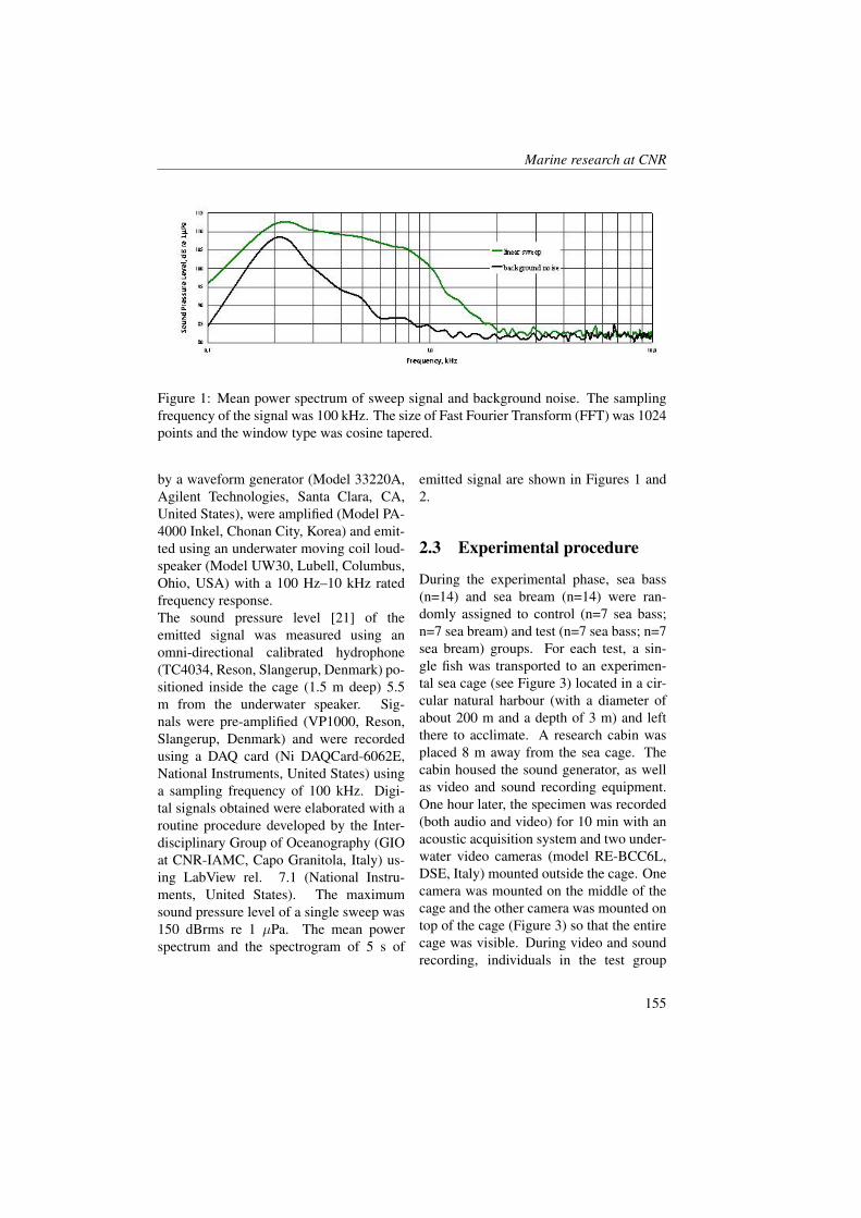
Marine research at CNR
Figure 1: Mean power spectrum of sweep signal and background noise. The samplingfrequency of the signal was 100 kHz. The size of Fast Fourier Transform (FFT) was 1024points and the window type was cosine tapered.
by a waveform generator (Model 33220A,Agilent Technologies, Santa Clara, CA,United States), were amplified (Model PA-4000 Inkel, Chonan City, Korea) and emit-ted using an underwater moving coil loud-speaker (Model UW30, Lubell, Columbus,Ohio, USA) with a 100 Hz–10 kHz ratedfrequency response.The sound pressure level [21] of theemitted signal was measured using anomni-directional calibrated hydrophone(TC4034, Reson, Slangerup, Denmark) po-sitioned inside the cage (1.5 m deep) 5.5m from the underwater speaker. Sig-nals were pre-amplified (VP1000, Reson,Slangerup, Denmark) and were recordedusing a DAQ card (Ni DAQCard-6062E,National Instruments, United States) usinga sampling frequency of 100 kHz. Digi-tal signals obtained were elaborated with aroutine procedure developed by the Inter-disciplinary Group of Oceanography (GIOat CNR-IAMC, Capo Granitola, Italy) us-ing LabView rel. 7.1 (National Instru-ments, United States). The maximumsound pressure level of a single sweep was150 dBrms re 1 µPa. The mean powerspectrum and the spectrogram of 5 s of
emitted signal are shown in Figures 1 and2.
2.3 Experimental procedure
During the experimental phase, sea bass(n=14) and sea bream (n=14) were ran-domly assigned to control (n=7 sea bass;n=7 sea bream) and test (n=7 sea bass; n=7sea bream) groups. For each test, a sin-gle fish was transported to an experimen-tal sea cage (see Figure 3) located in a cir-cular natural harbour (with a diameter ofabout 200 m and a depth of 3 m) and leftthere to acclimate. A research cabin wasplaced 8 m away from the sea cage. Thecabin housed the sound generator, as wellas video and sound recording equipment.One hour later, the specimen was recorded(both audio and video) for 10 min with anacoustic acquisition system and two under-water video cameras (model RE-BCC6L,DSE, Italy) mounted outside the cage. Onecamera was mounted on the middle of thecage and the other camera was mounted ontop of the cage (Figure 3) so that the entirecage was visible. During video and soundrecording, individuals in the test group
155
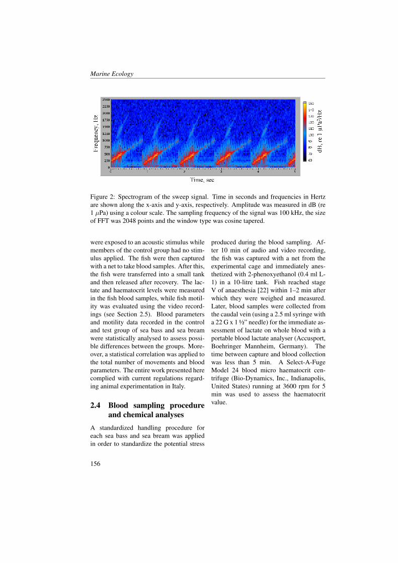
Marine Ecology
Figure 2: Spectrogram of the sweep signal. Time in seconds and frequencies in Hertzare shown along the x-axis and y-axis, respectively. Amplitude was measured in dB (re1 µPa) using a colour scale. The sampling frequency of the signal was 100 kHz, the sizeof FFT was 2048 points and the window type was cosine tapered.
were exposed to an acoustic stimulus whilemembers of the control group had no stim-ulus applied. The fish were then capturedwith a net to take blood samples. After this,the fish were transferred into a small tankand then released after recovery. The lac-tate and haematocrit levels were measuredin the fish blood samples, while fish motil-ity was evaluated using the video record-ings (see Section 2.5). Blood parametersand motility data recorded in the controland test group of sea bass and sea breamwere statistically analysed to assess possi-ble differences between the groups. More-over, a statistical correlation was applied tothe total number of movements and bloodparameters. The entire work presented herecomplied with current regulations regard-ing animal experimentation in Italy.
2.4 Blood sampling procedureand chemical analyses
A standardized handling procedure foreach sea bass and sea bream was appliedin order to standardize the potential stress
produced during the blood sampling. Af-ter 10 min of audio and video recording,the fish was captured with a net from theexperimental cage and immediately anes-thetized with 2-phenoxyethanol (0.4 ml L-1) in a 10-litre tank. Fish reached stageV of anaesthesia [22] within 1–2 min afterwhich they were weighed and measured.Later, blood samples were collected fromthe caudal vein (using a 2.5 ml syringe witha 22 G x 1 ½” needle) for the immediate as-sessment of lactate on whole blood with aportable blood lactate analyser (Accusport,Boehringer Mannheim, Germany). Thetime between capture and blood collectionwas less than 5 min. A Select-A-FugeModel 24 blood micro haematocrit cen-trifuge (Bio-Dynamics, Inc., Indianapolis,United States) running at 3600 rpm for 5min was used to assess the haematocritvalue.
156
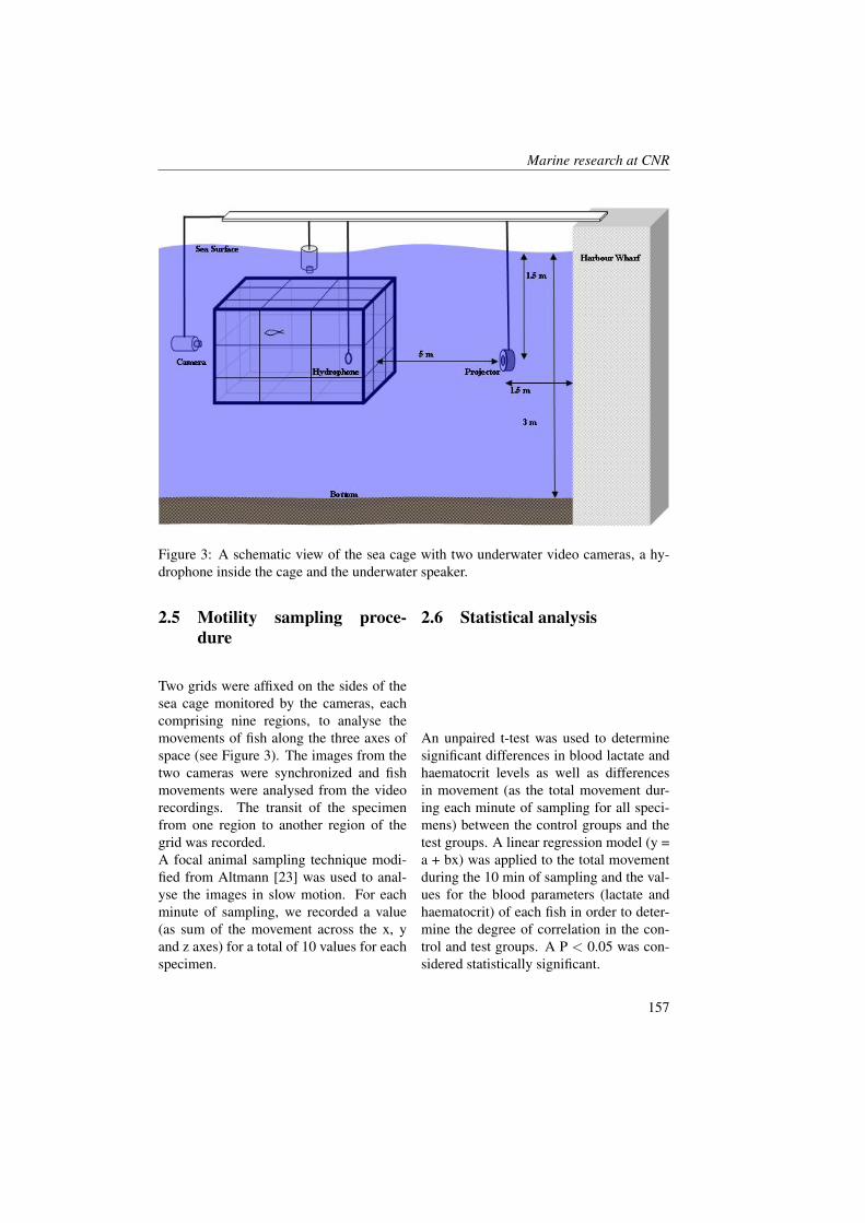
Marine research at CNR
Figure 3: A schematic view of the sea cage with two underwater video cameras, a hy-drophone inside the cage and the underwater speaker.
2.5 Motility sampling proce-dure
Two grids were affixed on the sides of thesea cage monitored by the cameras, eachcomprising nine regions, to analyse themovements of fish along the three axes ofspace (see Figure 3). The images from thetwo cameras were synchronized and fishmovements were analysed from the videorecordings. The transit of the specimenfrom one region to another region of thegrid was recorded.A focal animal sampling technique modi-fied from Altmann [23] was used to anal-yse the images in slow motion. For eachminute of sampling, we recorded a value(as sum of the movement across the x, yand z axes) for a total of 10 values for eachspecimen.
2.6 Statistical analysis
An unpaired t-test was used to determinesignificant differences in blood lactate andhaematocrit levels as well as differencesin movement (as the total movement dur-ing each minute of sampling for all speci-mens) between the control groups and thetest groups. A linear regression model (y =a + bx) was applied to the total movementduring the 10 min of sampling and the val-ues for the blood parameters (lactate andhaematocrit) of each fish in order to deter-mine the degree of correlation in the con-trol and test groups. A P < 0.05 was con-sidered statistically significant.
157
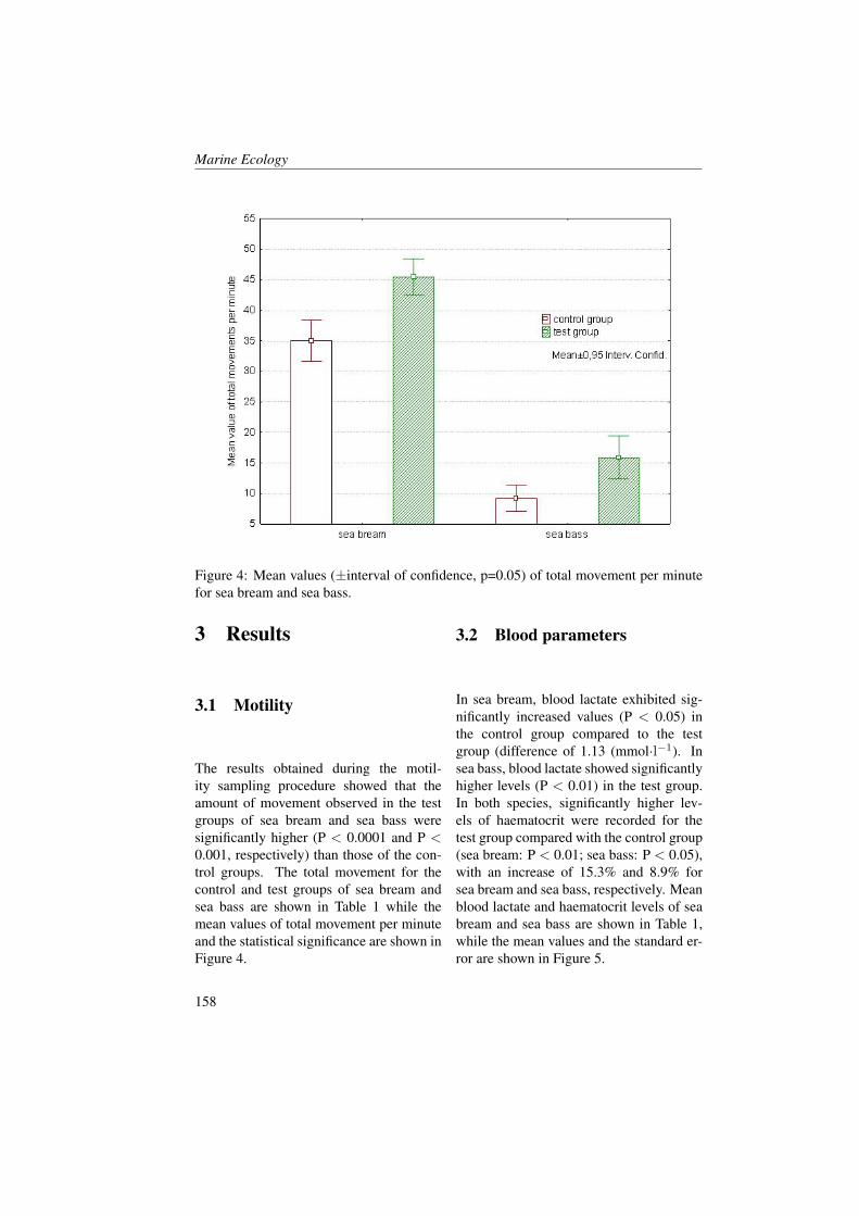
Marine Ecology
Figure 4: Mean values (±interval of confidence, p=0.05) of total movement per minutefor sea bream and sea bass.
3 Results
3.1 Motility
The results obtained during the motil-ity sampling procedure showed that theamount of movement observed in the testgroups of sea bream and sea bass weresignificantly higher (P < 0.0001 and P <0.001, respectively) than those of the con-trol groups. The total movement for thecontrol and test groups of sea bream andsea bass are shown in Table 1 while themean values of total movement per minuteand the statistical significance are shown inFigure 4.
3.2 Blood parameters
In sea bream, blood lactate exhibited sig-nificantly increased values (P < 0.05) inthe control group compared to the testgroup (difference of 1.13 (mmol·l−1). Insea bass, blood lactate showed significantlyhigher levels (P < 0.01) in the test group.In both species, significantly higher lev-els of haematocrit were recorded for thetest group compared with the control group(sea bream: P < 0.01; sea bass: P < 0.05),with an increase of 15.3% and 8.9% forsea bream and sea bass, respectively. Meanblood lactate and haematocrit levels of seabream and sea bass are shown in Table 1,while the mean values and the standard er-ror are shown in Figure 5.
158
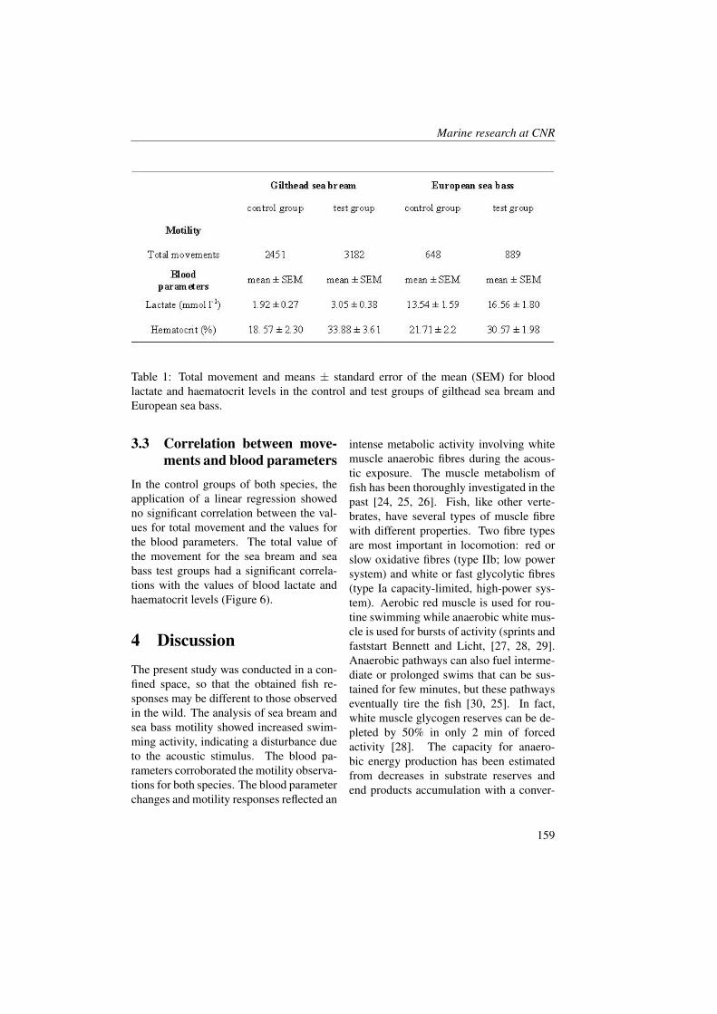
Marine research at CNR
Table 1: Total movement and means ± standard error of the mean (SEM) for bloodlactate and haematocrit levels in the control and test groups of gilthead sea bream andEuropean sea bass.
3.3 Correlation between move-ments and blood parameters
In the control groups of both species, theapplication of a linear regression showedno significant correlation between the val-ues for total movement and the values forthe blood parameters. The total value ofthe movement for the sea bream and seabass test groups had a significant correla-tions with the values of blood lactate andhaematocrit levels (Figure 6).
4 DiscussionThe present study was conducted in a con-fined space, so that the obtained fish re-sponses may be different to those observedin the wild. The analysis of sea bream andsea bass motility showed increased swim-ming activity, indicating a disturbance dueto the acoustic stimulus. The blood pa-rameters corroborated the motility observa-tions for both species. The blood parameterchanges and motility responses reflected an
intense metabolic activity involving whitemuscle anaerobic fibres during the acous-tic exposure. The muscle metabolism offish has been thoroughly investigated in thepast [24, 25, 26]. Fish, like other verte-brates, have several types of muscle fibrewith different properties. Two fibre typesare most important in locomotion: red orslow oxidative fibres (type IIb; low powersystem) and white or fast glycolytic fibres(type Ia capacity-limited, high-power sys-tem). Aerobic red muscle is used for rou-tine swimming while anaerobic white mus-cle is used for bursts of activity (sprints andfaststart Bennett and Licht, [27, 28, 29].Anaerobic pathways can also fuel interme-diate or prolonged swims that can be sus-tained for few minutes, but these pathwayseventually tire the fish [30, 25]. In fact,white muscle glycogen reserves can be de-pleted by 50% in only 2 min of forcedactivity [28]. The capacity for anaero-bic energy production has been estimatedfrom decreases in substrate reserves andend products accumulation with a conver-
159

Marine Ecology
sion of glucose to lactate followed by stim-ulation of pyruvate metabolism and oxy-gen debt [28, 31, 32, 33, 29]. Lactateproduced in the myotome is released intothe circulatory system following bursts ofanaerobic activity. In the present study, thestatistically significant responses in motil-ity and blood lactate observed in both seabass and sea bream exposed to the acous-tic stimulus indicate increased muscle ac-tivity using anaerobic Ia fibres. Further-more, the increase of metabolic muscle ac-tivity implies a higher demand for oxygen,which is increased by increasing the respi-ratory rate. During this adaptive response,fish experience the haemopoietic activityof the spleen that encourages the produc-tion of red blood cells for oxygen transport[34]. This condition leads to an increasein the levels of blood corpuscular compo-nents such haematocrit, one of the mostreliable indexes. This increase was alsofound in the present study (Figure 5). Thesignificant correlation between the move-ment values and the selected blood param-eters (Figure 6) supports what has been de-scribed above.
5 ConclusionsIn conclusion, the results from this studyshowed that anthropogenic noise at lowfrequencies can influence the swimmingactivity of fish. Moreover, many previ-ous studies have shown that muscle ac-tivity rates can be a very large part ofthe fish energy budget [35, 36]. Conse-quently, increased swimming activity andthe associated metabolic costs could com-promise other biological activities, such as
food acquisition, regulation due to envi-ronmental perturbation, migration and re-production. Banner and Hyatt [37] andLagardere [38] observed a drastic reduc-tion of egg survival and reproductive andgrowth rates in farmed fish species exposedto high sound levels. The present studyshows the relationship between behaviourand haematological parameters in relationto noise exposure. It also shows that theuse of different study approaches (physi-ological or behavioural) can lead to sim-ilar results. Moreover, our results indi-cate that our real-time field assays wereappropriate for measuring the physiologi-cal impact of the acoustic stimulus in seabass and sea bream. Although this short-term noise experiment showed an increasein fish motility, lactate and haematocrit val-ues, it would be useful to carry out fu-ture tests with a similar experimental pro-cedure on other fish species using longer-term noise exposure to better understandthe impact of anthropogenic noise on fishbehaviour and physiology.
6 AcknowledgmentsThis investigation was financially sup-ported by the detached branch of the CapoGranitola of the IAMC-CNR, throughfunds made available from the “Acous-tic Dispositive for the Reduction of Fish-ery and Marine Mammals Interaction –DAIMAR” project. The authors wouldlike to thank Dr. Paolo Domenici for hisvaluable comments on the manuscript andDr. Antonino Adamo for his assistancewith language revision.
160
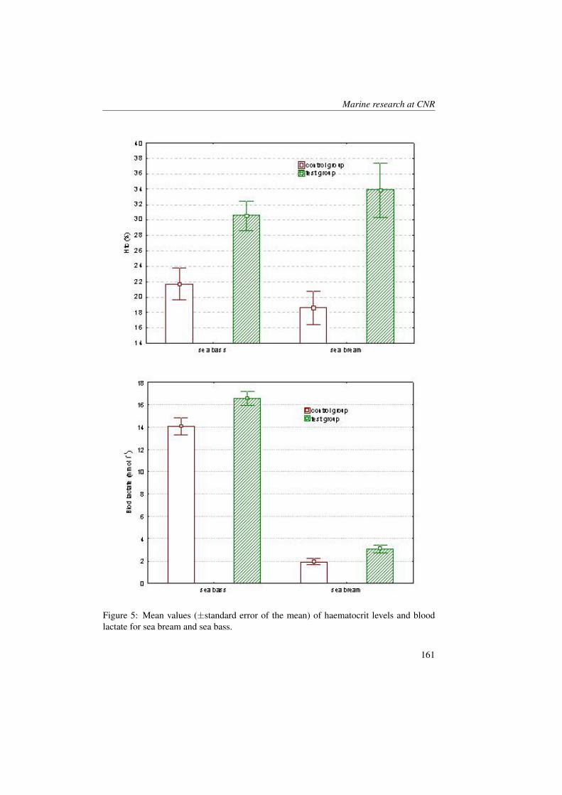
Marine research at CNR
Figure 5: Mean values (±standard error of the mean) of haematocrit levels and bloodlactate for sea bream and sea bass.
161
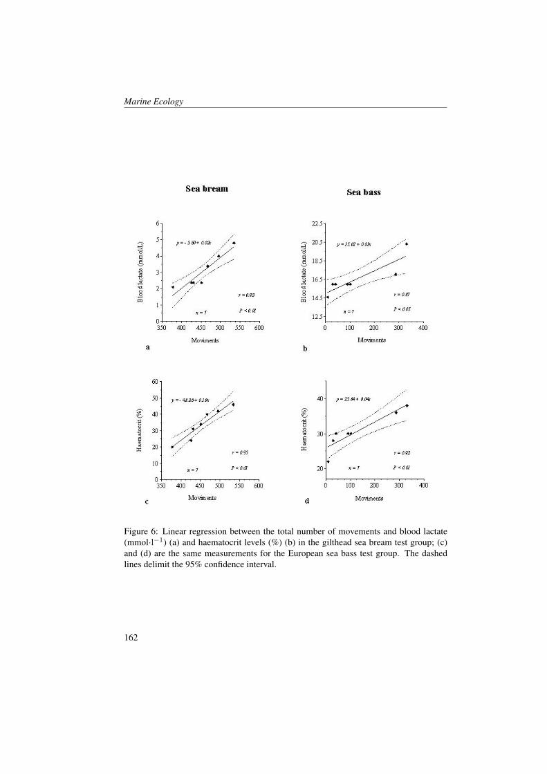
Marine Ecology
Figure 6: Linear regression between the total number of movements and blood lactate(mmol·l−1) (a) and haematocrit levels (%) (b) in the gilthead sea bream test group; (c)and (d) are the same measurements for the European sea bass test group. The dashedlines delimit the 95% confidence interval.
162

Marine research at CNR
References[1] A.D. McIntyre. Human impact on the oceans: the 1990s and beyond. Marine
Pollution Bulletin, 31:147–151, 1995.
[2] A.A. Myrberg. The effects of man-made noise on the behaviour of marine animals.Environment International, 16:575–586, 1980.
[3] A.N. Popper, J. Fewtrell, M.E. Smith, and R.D. McCauley. Anthropogenic sound:effects on the behaviour and physiology of fishes. Marine Technology Society Jour-nal, 37:35–40, 2004.
[4] A. Santulli, A. Modica, C. Messina, L. Ceffa, A. Curatolo, G. Rivas, G. Fabi,and V. D’Amelio. Biochemical responses of European sea bass (Dicentrarchuslabrax L.) to the stress induced by offshore experimental seismic prospecting in theMediterranean Sea. Marine Pollution Bulletin, 38:105–1114, 1999.
[5] G. Sara, J.M. Dean, D. D’Amato, G. Buscaino, A. Oliveri, S. Genovese, S. Ferro,G. Buffa, M. Lo Martire, and S. Mazzola. Effect of shipping traffic on behaviourof bluefin tuna Thunnus thynnus. Marine Ecology Progress Series, 331:243–253,2007.
[6] A.R. Scholik and Y. Hong Yan. Effects of underwater noise on auditory sensitivityof a cyprinid fish. Hearing Research, 152:17–24, 2001.
[7] National Research Council. Ocean Noise and Marine Mammals. National AcademyPress, Washington, DC, 2003.
[8] National Research Council. Marine Mammal Populations and Ocean Noise, De-termining When Noise Causes Biologically Significant Effects. National AcademyPress, Washington, DC, 2005.
[9] A.N. Bart, J. Clark, J. Young, and Y. Zohar. Underwater ambient noise measure-ments in aquaculture systems: a survey. Aquacultural Engineering, (25):99–110,2001.
[10] A. Engas, S. Loıkkeborg, E. Ona, and A.V. Soldal. Effects of seismic shooting onlocal abundance and catch rates of cod (Gadus morhua) and haddock (Melanogram-mus aeglefinus). Canadian Journal of Fisheries and Aquatic Science, 53:2238–2249, 1996.
[11] A.N. Popper, M.E. Smith, P.A. Cott, B.W. Hanna, A.O. MacGillivray, M.E. Austin,and D.A. Mann. Effects of exposure to seismic airgun use on hearing of 3 fishspecies. Journal of the Acoustical Society of America, 117:3958–3971, 2005.
[12] A. Sandstrom, B.K. Eriksson, P. Karas, M. Isæus, and H. Schreiber. Boating andnavigation activities influence the recruitment of fish in a Baltic Sea archipelagoarea. A Journal of the Human Environment, 34:125–130, 2005.
163
Marine Ecology
[13] A.L. Schwarz and G.L. Greer. Responses of Pacific herring, Clupea harengus pal-lasi, to some underwater sounds. Canadian Journal of Fisheries and Aquatic Sci-ence, 41:1183–1192, 1984.
[14] M.E. Smith, A.S. Kane, and A.N. Popper. Noise-induced stress response and hear-ing loss in goldfish (Carassius auratus). Journal of Experimental Biology, page427–435, 2004.
[15] R.A. Kastelein, S. van der Heul, W.C. Verboom, N. Jennings, J. van der Veen, andD. de Haan. Startle response of captive North Sea fish species to underwater tonesbetween 0.1 and 64 kHz. Marine Environmental Research, 65:369–377, 2008.
[16] A.N. Popper, R.R Fay, C. Platt, and O. Sand. Sound detection mechanism and capa-bilities of teleost fishes. In: Collin, S.P., Marshall, N.J. (Eds.), Sensory Processingin Aquatic Environments. Springer, New York, (3-38), 2003.
[17] D. Ross. Ship sources of ambient noise. Journal of Oceanic Engineering,30:257–261, 2005.
[18] National Research Council. Marine Mammals and Low Frequency Sound: ProgressSince 1944. National Academy Press, Washington, DC, 2000.
[19] W.J. Richardson, C.R. Greene, C.I. Malme, and D.H. Thomson. Marine Mammalsand Noise. Academic Press, London, 1995.
[20] L.E. Wysocki, J.P. Dittami, and F. Ladich. Ship noise and cortisol secretion inEuropean freshwater fishes. Biological Conservation, 128:501–508, 2006.
[21] American Acoustical Society. American National Standard Acoustical Terminol-ogy. American Acoustical Society, Melville, New York, page 1–1994, 1994.
[22] R.C. Summerfelt and L.S. Smith. Anaesthesia, surgery and related techniques. In:Schreck, C.B., Moyle, P.B. (Eds.), Methods in Fish Biology. American FisheriesSociety, Bethesda, page 213–272, 1990.
[23] J. Altmann. Observational study of behaviour: sampling methods. Behaviour,(49):227–265, 1974.
[24] F.W.H. Beamish. Swimming capacity. In: Hoar, W.S., Randall, D.J. (Eds.), FishPhysiology. Academic Press, New York, page 101–187, 1978.
[25] J.R. Brett and T.D.D. Groves. Physiological energetics. In: Hoar, W.S., Randall,D.J., Brett, J.R. (Eds.), Fish Physiology. Academic Press, New York, page 279, 1979.
[26] F.E.J. Fry. The effect of environmental factors on the physiology of fish. In: Hoar,W.S., Randall, D.J. (Eds.), Fish Physiology. Academic Press, Orlando, pages 1–98,1971.
164
Marine research at CNR
[27] A.F. Bennett and P. Licht. Anaerobic metabolism during activity in lizards. Journalof Comparative Physiology, 81:277–288, 1972.
[28] E.M. Goolish. Aerobic and anaerobic scaling in fish. Biological Reviews, 66(33),1991.
[29] W. Weiser, U. Platzer, and S. Hinterleitner. Anaerobic and aerobic energy produc-tion of young rainbow trout (Salmo gairdneri) during and after bursts of activity.Journal of Comparative Physiology, 155:485–492, 1985.
[30] Q. Bone. Muscular and energetic aspects of fish swimming. In: Wu, T.Y., Brocaw,C.J., Brennen, C. (Eds.), Swimming and Flying in Nature. Plenum Press, New York,page 493, 1975.
[31] R. Kauffman. Respiratory cost of swimming in larval and juvenile cyprinids. heJournal of Experimental Biology, 150:343–366, 1990.
[32] K.J. Puckett and L.M. Dill. Cost of sustained and burst swimming to juvenilecoho salmon (Oncorhynchus kisutch). Canadian Journal of Fisheries and AquaticScience, 41:1546–1551, 1984.
[33] K.J. Puckett and L.M. Dill. The energetics of feeding territorially in juvenile cohosalmon (Oncorhynchus kisutch). Behaviour, 92:97–111, 1985.
[34] C.E. Franklin, W. Davison, and J.C. Mckenzie. The role of the spleen during ex-ercise in the antarctic teleost, pagothenia borchgrevinki. Journal of ExperimentalBiology, 174:381–386, 1993.
[35] D. Boisclair and P. Sirois. Testing assumptions of fish bioenergetics models bydirect estimation of growth, consumption, and activity rates. Transactions of theAmerican Fisheries Society, 122:784–796, 1993.
[36] F. Koch and W. Wieser. Partitioning of energy in fish: can reduction of swim-ming activity compensate for the cost of production? The Journal of ExperimentalBiology, 107:141–146, 1983.
[37] A. Banner and M. Hyatt. Effects of noise on eggs and larvae of two estuarine fishes.Transactions of the American Fisheries Society, 1:134–136, 1973.
[38] J.P Lagardere. Effects of noise on growth and reproduction of Crangon crangon inrearing tanks. Marine Biology, 71:177–185, 1982.
165

Marine Ecology
166
Acoustic Characterization of Middle TrophicLevel Species in the Ross Sea Ecosystem (Antarc-tica)
I. Leonori, A. De Felice, I. Biagiotti, F. Campanella, M. AzzaliInstitute of Marine Sciences, CNR, Ancona, [email protected]
Abstract
By far the largest components of the Ross Sea Middle Trophic Level are theoceanic (E. superba) and the shelf (E. crystallorophias) krill species. In spite oftheir abundance and key role in Ross Sea trophic chain, they have received very littleattention from the scientific community before the six large scale acoustic surveysconducted during the Italian expeditions to Antarctica of 1989-90, 1994, 1997-98,2000, 2003-04. The region sampled acoustically is roughly a rectangle of 131000nm2, 64% of the Ross Sea. A three frequency method, adequate to the biological andenvironmental situation of the Ross Sea, much more complex than that of Atlanticsector areas, was developed. The estimation of E. superba biomass was around 2.5millions of tons in Nov. 1994, around 2 millions of tons in Dec. 1997 and 1 million oftons in Jan. 2000. The decreasing of E. superba biomass in the Ross Sea from Nov.to Feb. occurred in parallel with the movement northwards of the polynya ice edge.This suggests that E. superba habitat enlarges to the Pacific Ocean, and portions ofthis population of the Ross Sea spread into the Pacific waters, beginning from thesecond half of Dec. On the other hand the total biomass of E. crystallorophias wasrather stable (∼200000 t) in the five surveys. It suggests that ice krill population issegregated within the Ross Sea.
1 Introduction
Ross Sea is the last marine ecosystem notyet exploited by man. It is covered by icefor nearly nine months in a year and thedistribution, abundance and behaviour ofall the species in this region are regulatedonly by natural factors. The sea ice ex-pands from late February onwards, and re-treats from late October. Both processesstart near the front of the Ross Ice Shelf.The water properties and circulation in theRoss Sea are well known from extensivesurveys over the last few decades.
The circulation separates the Ross Sea intwo regions: (1) the inshore region withdepth < 500 m and extension around 30%of the entire region, it is dominated by awind driven gyre [1, 2]; (2) the offshoreregion that is dominated by processes inthe wider Southern Ocean. This circulationmeans that Ross Sea is somewhat separatedfrom the rest of the Southern Ocean. TheRoss Sea is bounded to the North by the3000 m depth around 69° S latitude and160° W longitude. The extension of thetotal region is calculated in 205000 nm2.The area of this study is the East part of the
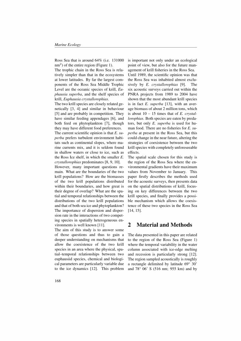
Marine Ecology
Ross Sea that is around 64% (i.e. 131000nm2) of the entire region (Figure 1).The trophic chain in the Ross Sea is rela-tively simpler than that in the ecosystemsat lower latitudes. By far the largest com-ponents of the Ross Sea Middle TrophicLevel are the oceanic species of krill, Eu-phausia superba, and the shelf species ofkrill, Euphausia crystallorophias.The two krill species are closely related ge-netically [3, 4] and similar in behaviour[5] and are probably in competition. Theyhave similar feeding appendages [6], andboth feed on phytoplankton [7], thoughthey may have different food preferences.The current scientific opinion is that E. su-perba prefers turbulent environment habi-tats such as continental slopes, where ma-rine currents mix, and it is seldom foundin shallow waters or close to ice, such asthe Ross Ice shelf, in which the smaller E.crystallorophias predominates [8, 9, 10].However, many important questions re-main. What are the boundaries of the twokrill populations? How are the biomassesof the two krill populations distributedwithin their boundaries, and how great istheir degree of overlap? What are the spa-tial and temporal relationships between thedistributions of the two krill populationsand that of both sea ice and phytoplankton?The importance of dispersion and disper-sion rate in the interactions of two compet-ing species in spatially heterogeneous en-vironments is well known [11].The aim of this study is to answer someof those questions and thus to gain adeeper understanding on mechanisms thatallow the coexistence of the two krillspecies in an area where the physical, spa-tial–temporal relationships between twoeuphausiid species, chemical and biologi-cal parameters are particularly variable dueto the ice dynamics [12]. This problem
is important not only under an ecologicalpoint of view, but also for the future man-agement of krill fisheries in the Ross Sea.Until 1989, the scientific opinion was thatthe Ross Sea was inhabited almost exclu-sively by E. crystallorophias [9]. Thesix acoustic surveys carried out within thePNRA projects from 1989 to 2004 haveshown that the most abundant krill speciesis in fact E. superba [13], with an aver-age biomass of about 2 million tons, whichis about 10 – 15 times that of E. crystal-lorophias. Both species are eaten by preda-tors, but only E. superba is used for hu-man food. There are no fisheries for E. su-perba at present in the Ross Sea, but thiscould change in the near future, altering thestrategies of coexistence between the twokrill species with completely unforeseeableeffects.The spatial scale chosen for this study isthe region of the Ross Sea where the en-vironmental gradients have their maximumvalues from November to January. Thispaper firstly describes the methods usedfor the acoustic surveys, then presents dataon the spatial distributions of krill, focus-ing on key differences between the twokrill species, and finally provides a possi-ble mechanism which allows the coexis-tence of these two species in the Ross Sea[14, 15].
2 Material and Methods
The data presented in this paper are relatedto the region of the Ross Sea (Figure 1)where the temporal variability in the watercolumn associated with ice-edge meltingand recession is particularly strong [12].The region sampled acoustically is roughlya rectangle delimited by latitude 69° 30’and 78° 06’ S (516 nm; 955 km) and by
168
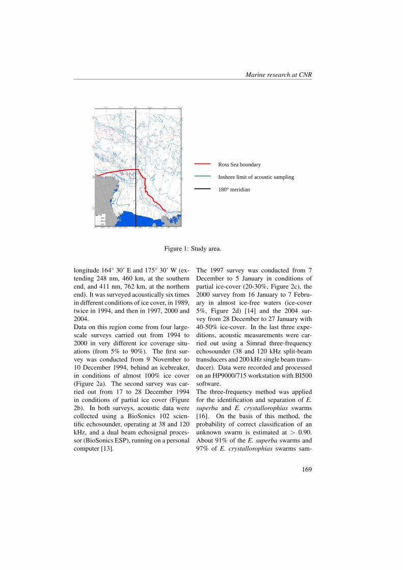
Marine research at CNR
Ross Sea boundary
Inshore limit of acoustic sampling
180° meridian
Figure 1: Study area.
longitude 164° 30’ E and 175° 30’ W (ex-tending 248 nm, 460 km, at the southernend, and 411 nm, 762 km, at the northernend). It was surveyed acoustically six timesin different conditions of ice cover, in 1989,twice in 1994, and then in 1997, 2000 and2004.Data on this region come from four large-scale surveys carried out from 1994 to2000 in very different ice coverage situ-ations (from 5% to 90%). The first sur-vey was conducted from 9 November to10 December 1994, behind an icebreaker,in conditions of almost 100% ice cover(Figure 2a). The second survey was car-ried out from 17 to 28 December 1994in conditions of partial ice cover (Figure2b). In both surveys, acoustic data werecollected using a BioSonics 102 scien-tific echosounder, operating at 38 and 120kHz, and a dual beam echosignal proces-sor (BioSonics ESP), running on a personalcomputer [13].
The 1997 survey was conducted from 7December to 5 January in conditions ofpartial ice-cover (20-30%, Figure 2c), the2000 survey from 16 January to 7 Febru-ary in almost ice-free waters (ice-cover5%, Figure 2d) [14] and the 2004 sur-vey from 28 December to 27 January with40-50% ice-cover. In the last three expe-ditions, acoustic measurements were car-ried out using a Simrad three-frequencyechosounder (38 and 120 kHz split-beamtransducers and 200 kHz single beam trans-ducer). Data were recorded and processedon an HP9000/715 workstation with BI500software.The three-frequency method was appliedfor the identification and separation of E.superba and E. crystallorophias swarms[16]. On the basis of this method, theprobability of correct classification of anunknown swarm is estimated at > 0.90.About 91% of the E. superba swarms and97% of E. crystallorophias swarms sam-
169
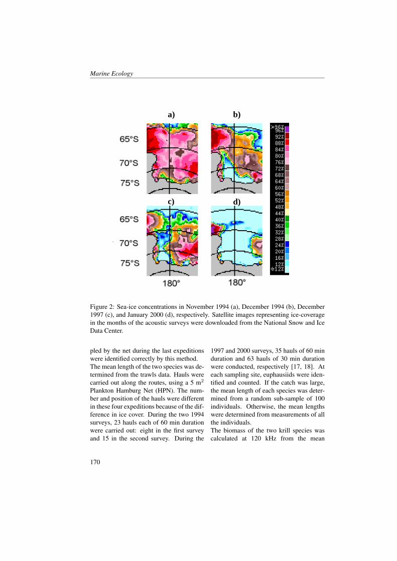
Marine Ecology
a) b)
c) d)
Figure 2: Sea-ice concentrations in November 1994 (a), December 1994 (b), December1997 (c), and January 2000 (d), respectively. Satellite images representing ice-coveragein the months of the acoustic surveys were downloaded from the National Snow and IceData Center.
pled by the net during the last expeditionswere identified correctly by this method.The mean length of the two species was de-termined from the trawls data. Hauls werecarried out along the routes, using a 5 m2
Plankton Hamburg Net (HPN). The num-ber and position of the hauls were differentin these four expeditions because of the dif-ference in ice cover. During the two 1994surveys, 23 hauls each of 60 min durationwere carried out: eight in the first surveyand 15 in the second survey. During the
1997 and 2000 surveys, 35 hauls of 60 minduration and 63 hauls of 30 min durationwere conducted, respectively [17, 18]. Ateach sampling site, euphausiids were iden-tified and counted. If the catch was large,the mean length of each species was deter-mined from a random sub-sample of 100individuals. Otherwise, the mean lengthswere determined from measurements of allthe individuals.The biomass of the two krill species wascalculated at 120 kHz from the mean
170
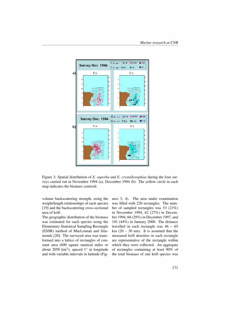
Marine research at CNR
a)
b)
Figure 3: Spatial distribution of E. superba and E. crystallorophias during the four sur-veys carried out in November 1994 (a), December 1994 (b). The yellow circle in eachmap indicates the biomass centroid.
volume backscattering strength, using theweight/length relationships of each species[19] and the backscattering cross-sectionalarea of krill.The geographic distribution of the biomasswas estimated for each species using theElementary Statistical Sampling Rectangle(ESSR) method of MacLennan and Sim-monds [20]. The surveyed area was trans-formed into a lattice of rectangles of con-stant area (600 square nautical miles orabout 2058 km2), spaced 1° in longitudeand with variable intervals in latitude (Fig-
ures 3, 4). The area under examinationwas filled with 220 rectangles. The num-ber of sampled rectangles was 53 (23%)in November 1994, 62 (27%) in Decem-ber 1994, 66 (29%) in December 1997, and101 (44%) in January 2000. The distancetravelled in each rectangle was 46 – 65km (20 – 30 nm). It is assumed that themeasured krill densities in each rectangleare representative of the rectangle withinwhich they were collected. An aggregateof rectangles containing at least 90% ofthe total biomass of one krill species was
171
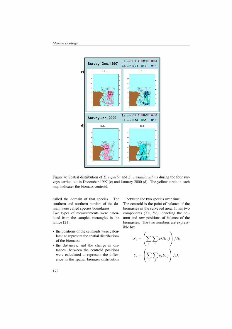
Marine Ecology
c)
d)
Figure 4: Spatial distribution of E. superba and E. crystallorophias during the four sur-veys carried out in December 1997 (c) and January 2000 (d). The yellow circle in eachmap indicates the biomass centroid.
called the domain of that species. Thesouthern and northern borders of the do-main were called species boundaries.Two types of measurements were calcu-lated from the sampled rectangles in thelattice [21]:
• the positions of the centroids were calcu-lated to represent the spatial distributionsof the biomass;
• the distances, and the change in dis-tances, between the centroid positionswere calculated to represent the differ-ence in the spatial biomass distribution
between the two species over time.The centroid is the point of balance of thebiomasses in the surveyed area. It has twocomponents (Xc, Yc), denoting the col-umn and row positions of balance of thebiomasses. The two numbers are express-ible by:
Xc =
∑j
∑i
xiBi, j
/B;
Yc =
∑i
∑j
yjBi,j
/B;
172

Marine research at CNR
i = 1, 2, · · · , 20(column);
j = 1, 2, · · · , 14, (row),
where Bi,j is the biomass in the rectangle(i, j), B is the total biomass in the surveyedarea, and (xi, yj) are the coordinates of thecentre of the rectangle (i, j).The centroid is determined only by the mu-tual locations of the rectangles and theirbiomasses. When the set of biomasses isin motion, the centroid is also in motion.Therefore, the spatial biomass patterns andmovements can be studied using the cen-troid techniques.In this paper, the coordinates of the cen-troids are expressed in terms of longitude(x-axis, increasing from 164°30’ E and175°30’ W) and latitude (y-axis increasingfrom 69°30’ S (0 km) and 78°06’ S (955km)), while the distances and the changesof distances in the distribution of centroidsare expressed in terms of kilometres. Threedistances are calculated: along latitude,along longitude, and in total.
3 ResultsThe geographical distribution and biomassdensity (t/nm2) of the two euphausiidspecies in the seasons and years are shownin:• Figure 3a: late spring (November 1994)
when polynya ice edge is in the southernpart of the Ross Sea;
• Figure 3b and 4c: early summer (Decem-ber 1994 and 1997), when polynya iceedge is moving north;
• Figure 4d: full summer (January 2000)when polynya and Pacific waters mix.
3.1 November 1994The spatial distribution of the biomass ofthe two krill species in November 1994 is
shown in Figure 3a. The total biomassof E. superba was estimated in 2.4 mil-lion tonnes (mean density: 21.9 tkm−2),which is almost 11 times higher than thebiomass of E. crystallorophias (0.2 mil-lion tonnes; mean density: 1.8 tkm−2).More than 95% of E. superba biomasswas distributed between latitude 71°00’ S(northern species boundary) and 75° 08’S (southern species boundary) and longi-tude 171° E and 177° 30’ W. Three rect-angles had high concentrations of E. su-perba, containing 77.6% of the total E.superba biomass while representing only5.7% of the surveyed area. The centroidof E. superba biomass (latitude 74°09.6’ Slongitude 175°53’ E) was 108 km north ofits southern species boundary and close tothe three rectangles of highest concentra-tions. E. crystallorophias mainly occurredin the areas south of latitude 74°28.6’ S(northern species boundary). This area in-cluded 58.5% of the surveyed region andcontained 92.1% of the E. crystallorophiasbiomass. The centroid of the E. crystal-lorophias population (latitude 75°08.1’ Slongitude 170°38.4’ E) was close to itsnorthern border. It was 108 km south and147 km east of the centroid of the E. su-perba population. Even though the do-mains of the two krill species slightly over-lapped, their centroids were separated by185 km. In November 1994, the catch ofboth species comprised only adults. Fromall samples, the average E. superba lengthwas 42.51 mm TL (range 42.4 – 45.0 mm),and the average E. crystallorophias lengthwas 25.58 mm TL (range 25 – 30 mm).
3.2 December 1994The average densities of both krill speciesfound in December 1994 were approxi-mately the same as those 1 month be-
173
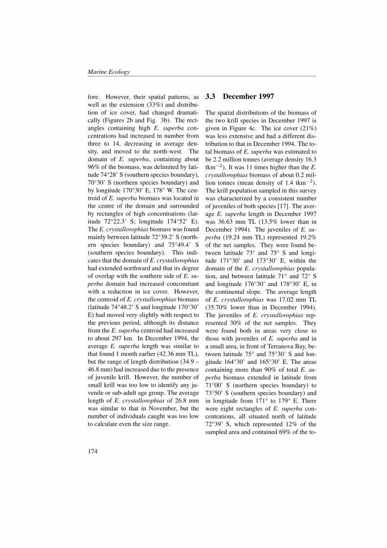
Marine Ecology
fore. However, their spatial patterns, aswell as the extension (33%) and distribu-tion of ice cover, had changed dramati-cally (Figures 2b and Fig. 3b). The rect-angles containing high E. superba con-centrations had increased in number fromthree to 14, decreasing in average den-sity, and moved to the north-west. Thedomain of E. superba, containing about96% of the biomass, was delimited by lati-tude 74°28’ S (southern species boundary),70°30’ S (northern species boundary) andby longitude 170°30’ E, 178° W. The cen-troid of E. superba biomass was located inthe centre of the domain and surroundedby rectangles of high concentrations (lat-itude 72°22.3’ S; longitude 174°52’ E).The E. crystallorophias biomass was foundmainly between latitude 72°39.2’ S (north-ern species boundary) and 75°49.4’ S(southern species boundary). This indi-cates that the domain of E. crystallorophiashad extended northward and that its degreeof overlap with the southern side of E. su-perba domain had increased concomitantwith a reduction in ice cover. However,the centroid of E. crystallorophias biomass(latitude 74°48.2’ S and longitude 170°30’E) had moved very slightly with respect tothe previous period, although its distancefrom the E. superba centroid had increasedto about 297 km. In December 1994, theaverage E. superba length was similar tothat found 1 month earlier (42.36 mm TL),but the range of length distribution (34.9 –46.8 mm) had increased due to the presenceof juvenile krill. However, the number ofsmall krill was too low to identify any ju-venile or sub-adult age group. The averagelength of E. crystallorophias of 26.8 mmwas similar to that in November, but thenumber of individuals caught was too lowto calculate even the size range.
3.3 December 1997
The spatial distributions of the biomass ofthe two krill species in December 1997 isgiven in Figure 4c. The ice cover (21%)was less extensive and had a different dis-tribution to that in December 1994. The to-tal biomass of E. superba was estimated tobe 2.2 million tonnes (average density 16.3tkm−2). It was 11 times higher than the E.crystallorophias biomass of about 0.2 mil-lion tonnes (mean density of 1.4 tkm−2).The krill population sampled in this surveywas characterized by a consistent numberof juveniles of both species [17]. The aver-age E. superba length in December 1997was 36.63 mm TL (13.5% lower than inDecember 1994). The juveniles of E. su-perba (19.24 mm TL) represented 19.2%of the net samples. They were found be-tween latitude 73° and 75° S and longi-tude 171°30’ and 173°30’ E, within thedomain of the E. crystallorophias popula-tion, and between latitude 71° and 72° Sand longitude 176°30’ and 178°30’ E, inthe continental slope. The average lengthof E. crystallorophias was 17.02 mm TL(35.70% lower than in December 1994).The juveniles of E. crystallorophias rep-resented 30% of the net samples. Theywere found both in areas very close tothose with juveniles of E. superba and ina small area, in front of Terranova Bay, be-tween latitude 75° and 75°30’ S and lon-gitude 164°30’ and 165°30’ E. The areascontaining more than 90% of total E. su-perba biomass extended in latitude from71°00’ S (northern species boundary) to73°50’ S (southern species boundary) andin longitude from 171° to 179° E. Therewere eight rectangles of E. superba con-centrations, all situated north of latitude72°39’ S, which represented 12% of thesampled area and contained 69% of the to-
174
Marine research at CNR
tal E. superba biomass. The centroid of E.superba biomass (latitude 72°05.3’ S; lon-gitude 175°18’ E) was shifted slightly tothe northeast of that obtained in Decem-ber 1994. Over half (57%) of the E. crys-tallorophias biomass was found betweenlatitude 71° and 73° S, mixed with E. su-perba biomass. The remaining 43% wasdistributed between 73° and 77° S, in rect-angles with very few E. superba. Althoughthe domains of the two krill populationsoverlapped to a large extent in this sur-vey, the centroids were still far apart. TheE. crystallorophias centroid was found 196km to the southeast of the E. superba cen-troid. Comparison between these resultsand those obtained under similar ice condi-tions in December 1994 indicates that thesouthern boundary of E. superba biomassmoved northward in December 1997, butits centroid remained similar to that foundin 1994. In contrast, in December 1997, thenorthern E. crystallorophias boundary wasmuch further north, the biomass centroidhad moved to the northeast, and the por-tion of E. crystallorophias biomass foundwithin the E. superba domain was muchhigher than in December 1994. It is pos-sible that krill distribution is influenced byage structure, and the consistent number ofjuveniles of both species, found in Decem-ber 1997, had facilitated their mixing.
3.4 January 2000Figure 4d represents the spatial distribu-tions of the two krill populations in Jan-uary 2000, when the waters of Ross Seawere virtually ice-free (Figure 2d). Thetotal E. superba biomass was estimated tobe 1.2 million tonnes (average density 11tkm−2), 8.6 times higher than E. crystal-lorophias biomass of 0.14 million tonnes(average density 0.7 tkm−2). In ice-free
conditions, the domain of E. superba com-prising 93.4% of the biomass was dis-tributed in an area between latitude 70° S(northern species boundary) and 73°14’ S(southern species boundary). There wereseven rectangles of high E. superba con-centrations representing 6.9% of the sam-pled area and containing 49.7% of the to-tal E. superba biomass. The centroid ofE. superba biomass (latitude 71°47.6’ S;longitude 173°18’ E) was found at themost north-western position of all previ-ous surveys. The domain of E. crystal-lorophias, containing more than 90% of thebiomass, was delimited by latitude 72°39’S (northern species boundary) and 77°18’S (southern species boundary). The ar-eas south of latitude 73°14’ S were dom-inated by the E. crystallorophias popula-tion. They contained 87.2% of E. crystal-lorophias biomass and only 6.6% of E. su-perba biomass. The centroid of E. crys-tallorophias biomass (latitude 74°28.6’ S;longitude 174°30’ E) was located morethan 300 km south of the E. superba cen-troid. This is the largest distance betweencentroids in all the surveys, albeit simi-lar to the distance in December 1994. Itseems that in ice-free conditions, the E.superba biomass distribution may extendnorthwards beyond the edge of the RossSea in parallel with the progression andmelting of the sea-ice. In contrast, mostof the E. crystallorophias biomass remainsconfined within the southern part of theRoss Sea in all ice-cover situations. Theaverage E. superba length in January 2000was 44.8 mm TL (range 32.2 – 54.5 mm),but the number of small krill was too lowto identify any juvenile or sub-adult agegroup. The average length of E. crystal-lorophias was 20.4 mm TL (range 7.9 –40.41 mm). The number of juveniles rep-resented 35.9%, and the number of sub-
175

Marine Ecology
adults 31.5% of all the catches [18].
4 ConclusionsThe results of the acoustic surveys are thefollowing:1. Biomass level. In average the biomass
density of E. superba is around an or-der of magnitude higher than that of E.crystallorophias.
2. Biomass distribution. The northern andnorth-western areas of the Ross Sea areparticularly suitable for the E. superbapopulation, the southern and south-western areas are more suitable for theE. crystallorophias population, while inthe central area of the Ross Sea thereis a variation in the two species relatedwith ice cover and perhaps with theirage structure. This general distribu-tion seems consistent with that of phy-toplanktonic communities of the RossSea, with diatoms dominating to thenorth and west and Phaeocystis to thesouth along the ice shelf. This distri-bution is probably also reflected in thedifferent diets of the two krill species.
3. Biomass dynamics. The progressivemovement northward of the ice edgefrom November to January seems to in-fluence the apparent movement of bothkrill species. The centroid of E. su-perba biomass moves markedly north-ward from lat. 74° S (November) to theRoss Sea border (January: around 71°S) [22]. Also the centroid of E. crys-tallorophias moves Northward from lat.75°, but it does not go beyond 73° S.This suggests that the spatial extent ofthe E. superba population may enlargeup to the Pacific Ocean and spread intothe open ocean waters beginning fromJanuary, while E. crystallorophias pop-
ulation seems to be segregated withinthe Ross Sea.
The acoustic surveys have produced someevidence on the relation between the dy-namics of krill biomass distribution and icecover and on the spatial segregation of thetwo krill species.The progressive movement northward ofthe ice edge from November to Januaryseems to influence the apparent movementof both krill species as measured by theirbiomass centroids. However, the centroidof the E. superba biomass moved differ-ently with respect to that of the E. crys-tallorophias biomass. The E. superba cen-troid moved almost 265 km from latitude74° 09’ S to an area close to the Ross Seaborder (around 71° 41’ S). The E. crystal-lorophias centroid moved northeast, had amaximum displacement of 141 km to thenorth, and did not extend north of 73° 50’S. This suggests that portions of the RossSea population of E. superba may spreadinto the open ocean waters of the South-ern Ocean beginning in January. On theother hand, the E. crystallorophias popula-tion seems to be confined within the RossSea.All the results seem to indicate that thetwo krill populations occupy only partiallyoverlapping domains, move at differentspatial scales, and react differently to icecover. Thus, it seems that the two krillpopulations generally tend to be confinedto separate areas and to avoid substantialmixing through migration. This mecha-nism is probably activated by some exter-nal biological and physical factors causedby ice melting and retreating, but may alsoinclude some active internal factors such asinter-specific competition and age effects.However, the acoustic surveys in the RossSea occurred in different years, seasonsand environmental conditions that may
176
Marine research at CNR
have introduced some bias into the estima-tion of biomasses and their spatial distribu-tions. Further experimental and theoreticalwork is necessary to understand the physi-cal, biological, and behavioural factors thatgovern the spatial distributions of the twokrill species, how those distributions influ-
ence the trophic level above and are influ-enced by the trophic level below, and howmuch the fluctuations of the biomasses andtheir spatial distributions depend on sea-sons, years, environmental conditions andunusual events.
References[1] R.A. Locarnini. Water masses and circulation in the Ross gyre and environs. Ph.D.
Dissertation, 1994.
[2] W.O. Smith Jr, D.G. Ainley, and R. Cattaneo-Vietti. Trophic interactions within theRoss Sea continental shelf ecosystem. Phil. Trans. R. Soc. B, 362:95–111, 2007.
[3] S.N. Jarman, N.G. Elliott, S. Nicol, and A. McMinn. Molecular phylogenetics ofcircumglobal Euphausia species (Euphausiacea: Crustacea). Can. J. Fish. Aquat.Sci., 57((Suppl. 3)):51–67, 2000.
[4] L. Zane and T. Patarnello. Krill: a possible model for investigating the effect ofocean current on the genetic structure of a pelagic invertebrate. Can. J. Fish. Aquat.Sci., 57((Suppl. 3)):16–23, 2000.
[5] V. Siegel. Krill (Euphausiacea) life history and aspects of population dynamics.Can. J. Fish. Aquat. Sci., 57(Suppl. 3):130 – 150, 2000.
[6] J. Mauchline. Feeding appendages of the Euphausiacea (Crustacea). J. Zool. Lond.,153:1–43, 1967.
[7] W. Hagen and H. Auel. Seasonal adaptations and the role of lipids in oceaniczooplankton. Zoology, 104:313–326, 2001.
[8] S. Nicol. Krill, currents, and sea ice: Euphausia superba and its changing environ-ment. BioScience, 56(2):111–120, 2006.
[9] J.W.S. Marr. The natural history and geography of the Antarctic krill (Euphausiasuperba Dana). ‘Discovery’ Rep., 32:33–464, 1962.
[10] S.A. Harrington and P.G. Thomas. Observations on spawning by Euphausia crystal-lorophias from waters adjacent to Enderby Land (East Antarctica) and speculationson the early ontogenetic ecology of neritic euphausiids. Polar Biology, 7:93–95,1987.
[11] K. Gopalsamy. Competition and coexistence in spatially heterogeneous environ-ments. Math. Biosci., 36:229–242, 1977.
177
Marine Ecology
[12] J.H. Hecq, Guglielmo L., Goffart A., Catalano G., and Goosse H. A modellingapproach to the Ross Sea plankton ecosystem. Ross Sea Ecology. Ross Sea Ecology,page 395–411, 1999.
[13] M. Azzali and J. Kalinowski. Spatial and temporal distribution of krill E. superbabiomass in the Ross Sea (1989 – 1990 and 1994). Ross Sea Ecology, page 433–455,1999.
[14] M. Azzali, I. Leonori, A. De Felice, and A. Russo. Spatial–temporal relationshipsbetween two euphausiid species in the Ross Sea. Chemistry and Ecology, 22(Suppl.1):219 – 233, 2006.
[15] M. La Mesa, M. Azzali, and I. Leonori. Incidenza dei cambiamenti climaticisull’ecosistema pelagico del Mare di Ross (Antartide). Clima e Cambiamenti Cli-matici: le attivita di ricerca del CNR, pages 267–270, 2007.
[16] M. Azzali, I. Leonori, and G. Lanciani. A hybrid approach to acoustical classifica-tion and length estimation of krill. CCAMLR Sci., 11:33–58, 2004.
[17] M. Azzali, J. Kalinowski, G. Lanciani, and I. Leonori. Comparative studies onthe biological and acoustical properties of krill (Euphausia superba, Dana) sampledduring the XIII Italian Expedition to the Ross Sea (December 1997–January 1998).Document WG-EMM-00/39. CCAMLR, Hobart, Australia, 2000.
[18] A. Sala, M. Azzali, and A. Russo. Krill of the Ross Sea: distribution, abundance anddemography of Euphausia superba and Euphausia crystallorophias during the Ital-ian Antarctic Expedition (January–February 2000). Sci. Mar., 66:123–133, 2002.
[19] V. Siegel. Review of length–weight relationships for Antarctic krill. CCAMLRSelect. Sci. Paper, 9:145–155, 1992.
[20] E.J. Simmonds and D.N. MacLennan. Fishery Acoustics. 2005.
[21] C.A. Glasbey and G.W. Horgan. Image Analysis for the Biological Sciences. page156–161, 1995.
[22] M. Azzali, I. Leonori, A. De Felice, S. De Pasqualis, I. Biagiotti, and A. Russo.Interactions between the behaviour of an Euphausia superba superswarm, observedin November 1994 in the Ross Sea, and its physical and pelagic environment. Pro-ceeding of Joint AIOL-SItE Meeting, pages 201–206, 2009.
178
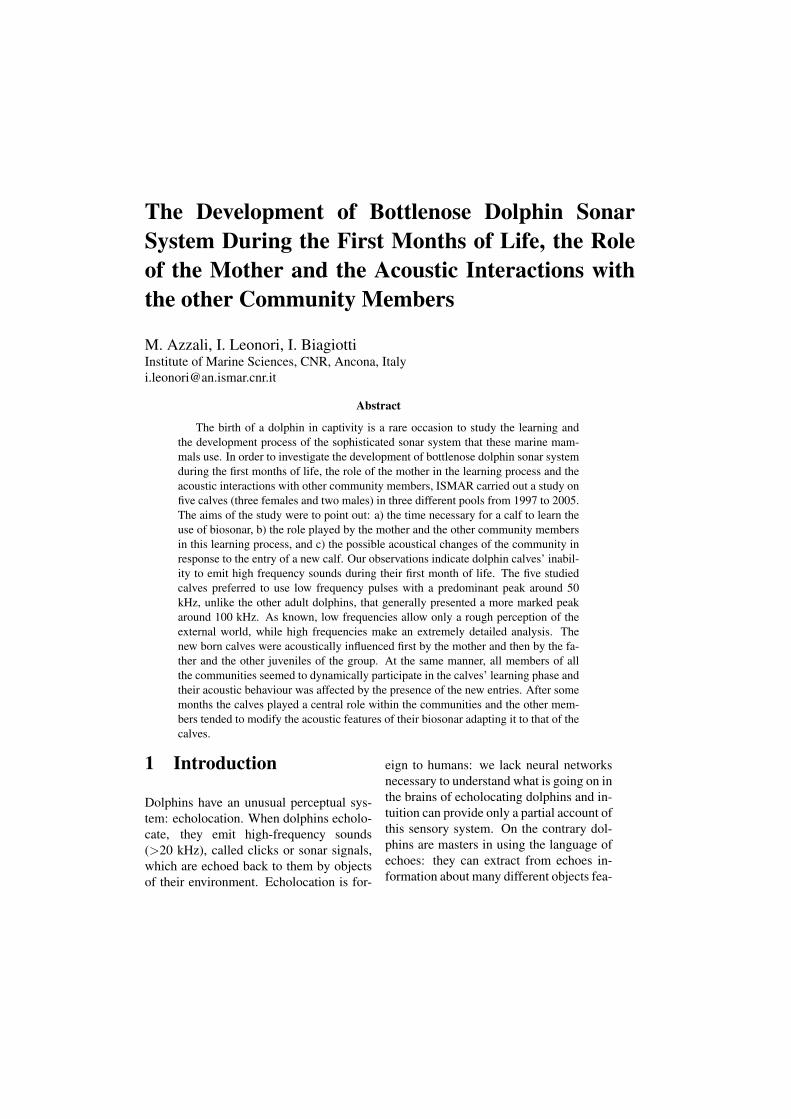
The Development of Bottlenose Dolphin SonarSystem During the First Months of Life, the Roleof the Mother and the Acoustic Interactions withthe other Community Members
M. Azzali, I. Leonori, I. BiagiottiInstitute of Marine Sciences, CNR, Ancona, [email protected]
Abstract
The birth of a dolphin in captivity is a rare occasion to study the learning andthe development process of the sophisticated sonar system that these marine mam-mals use. In order to investigate the development of bottlenose dolphin sonar systemduring the first months of life, the role of the mother in the learning process and theacoustic interactions with other community members, ISMAR carried out a study onfive calves (three females and two males) in three different pools from 1997 to 2005.The aims of the study were to point out: a) the time necessary for a calf to learn theuse of biosonar, b) the role played by the mother and the other community membersin this learning process, and c) the possible acoustical changes of the community inresponse to the entry of a new calf. Our observations indicate dolphin calves’ inabil-ity to emit high frequency sounds during their first month of life. The five studiedcalves preferred to use low frequency pulses with a predominant peak around 50kHz, unlike the other adult dolphins, that generally presented a more marked peakaround 100 kHz. As known, low frequencies allow only a rough perception of theexternal world, while high frequencies make an extremely detailed analysis. Thenew born calves were acoustically influenced first by the mother and then by the fa-ther and the other juveniles of the group. At the same manner, all members of allthe communities seemed to dynamically participate in the calves’ learning phase andtheir acoustic behaviour was affected by the presence of the new entries. After somemonths the calves played a central role within the communities and the other mem-bers tended to modify the acoustic features of their biosonar adapting it to that of thecalves.
1 Introduction
Dolphins have an unusual perceptual sys-tem: echolocation. When dolphins echolo-cate, they emit high-frequency sounds(>20 kHz), called clicks or sonar signals,which are echoed back to them by objectsof their environment. Echolocation is for-
eign to humans: we lack neural networksnecessary to understand what is going on inthe brains of echolocating dolphins and in-tuition can provide only a partial account ofthis sensory system. On the contrary dol-phins are masters in using the language ofechoes: they can extract from echoes in-formation about many different objects fea-

Marine Ecology
tures, which even the sharpest sight willnever be able to perceive. For example dol-phins gather data about the material fromwhich an object is made [1, 2], object wallthickness [3], object size and distance [4],object three-dimensional shape [5, 6] andobject aspect-dependent shape [7]. It isgeneral opinion that dolphins use sonar sig-nals only for representing objects of theirenvironment, while for social interactionsthey use low-frequency sounds (<20 kHz),called vocalizations. However several au-thors have supported the idea that sonarsignals may be an additional and sophis-ticated method of communication amongmembers of the same community [8, 9, 10].A fact that suggests there is an additionalfunction for clicks other than echoloca-tion is that dolphins use clicks also whenthe objects of their environments are wellknown and echolocation information arenot needed. These clicks, unlike echo lo-cating ones, have a very high repetitionrate that does not follow the two-way tran-sit (TWT) time rule (i.e. the interclickintervals of echolocating dolphins dependon and increase with the distance of tar-get, see [11]) and in some social situationsare emitted in couples [10]. Double clicksand clicks with high repetition rate arenot believed to have an echolocation func-tion, according to current sonar theory. Infact such click trains were detected duringcourtship, mother-infant interaction, dis-cipline, exhibition, play, aggression, fear,danger when sonar use seems to have noutility at all. The threshold of dolphin’ssomatic pressure receptors was estimatedby Kolchin an Bel’kovich [12] around 160-170 dB re 1µPa, well below (40-50 dB) thesound pressure of sonar signals, rangingbetween 228 and 210 dB re 1µPa [10]. Thegenital and mammary regions are the areasmost sensitive to sound pressure, followed
by the upper rostrum, lower jaw, forehead,flukes and pectoral and dorsal fins. So,when a dolphin is hit by a click train emit-ted by another dolphin, it receives not onlyauditory information but also tactile sensa-tions. It is very probable that acoustic andtactile information are intimately related indolphins and if one cue is partially maskedthe other cue can complete it. This sug-gests that a dolphin can transfer through apacket of clicks its emotive state (as dan-ger, aggressiveness, courtship, fear, ago-nistic or playful state) into another indi-vidual, who must have enough knowledgeabout the structure of clicks and the en-vironmental context for assigning the cor-rect emotional interpretation to the tactile-acoustical message.Some other aspects of the existing knowl-edge on echolocation signals may havepeculiarities and functions not yet under-stood.An hydrophone lowered among a dolphingroup picks up only chaotic fluctuations inthe pressure of the medium. However eachecholocating dolphin can recognize, in thiscomplex network of sounds, its own clicksand the returned echoes so as we can easilyattend to the voice of a single person, evenwhile many people around us are simul-taneously speaking. Therefore both sonarsignals and echoes must carry also infor-mation concerning the identity of the echo-locating dolphin [8], as for us the voiceidentifies a person.In a group only some dolphins echolo-cate, the others move silently, but be-have synchronously with the echolocat-ing ones. Experiments in controlled en-vironment [13] demonstrated that passivelistening dolphins can identify the objectthat their neighbours are echo-locating byeavesdropping on its echoes, so imaginingthe same auditory scene and sharing the
180
Marine research at CNR
same knowledge. Shared knowledge en-hances group effectiveness and might beone of the mechanisms that allows dol-phins in groups to cooperate closely inhunting the prey or in defending them-selves from enemies. If it so, each dolphinmust be capable of recognising a dolphinof its group by click features and of deci-phering perceptual information containedin the continuously varying click echoes,even if distorted by noise or at times oblit-erated. This mechanism is basically sim-ilar to that of human speech perception,except it seems to be used by dolphinsmostly in the immediate context of events.A human listener, as a dolphin, convertswith little conscious effort the continuouslyvarying acoustic stimulus produced by aspeaker into an internal representation ofa sequence of events, even in presence oflarge distortions in the signal. This appearto be so because the listener has an exten-sive knowledge of both the speaker’s lan-guage and slang and the speech context. Ifthe substrate of understanding echoes bypassive listening dolphins and speech byhumans is similar, then it is of crucial im-portance for a young dolphin to learn boththe language of echoes and the individualacoustic characteristics of each member ofits group.One could speculate if dolphins could usesonar signals as metaphors of a state, ac-tion or thing out of the context of events,to transfer or evoke perceptual experiencesof past events into other individuals of thesame group and influence their behaviour.We know that various social mammalsuse metaphorical signals as their most ad-vanced mean of communication [14]. Forexample the howling of wild dogs, occur-ring before the hunt [15] may be metaphorsof the chase, but without the prey present.It was demonstrated that dolphins that have
been given human language training canrespond to symbols representing variousparts of speech [16]. Therefore dolphins,who live in a foggy, vast and open en-vironment as ocean and then need subtleforms of acoustic signals to assure socialcohesion in their complex societies basedon mutual altruism, have certainly enoughcognitive capabilities to learn metaphoricalsignals and perhaps to use them for ma-nipulating the relationships among mem-bers of the same group or for preparing afuture event. However at moment there isno experimental evidence that dolphins useecholocation out of event context, althoughvery little is known about how dolphins useecholocation in their natural environment.In conclusion information carried by sonarsignals may regard, in order of increasinglevels of complexity: 1) the objects of dol-phin’s environment; 2) dolphin emotionalstate; 3) objects that dolphin’s neighboursare echolocating; 4) things, state and actionout of the context of events.The acoustic signal is characterized in eachinstant only by one quantity the pressure onthe auditory apparatus. How can a mono-dimensional quantity so poor as the pres-sure carry so many types and pieces of in-formation? Only learning and a complex.brain properly programmed from birth canallow to perceive a dimensionality muchhigher than that strictly physical in veryrapid pressure amplitude fluctuations thatoccur within short (some tenths of mi-croseconds),and often weak and distortedechoes. Dolphins have the most highlyspecialized auditory systems known in anyanimal group, including humans and pro-duce and process the sounds with a pecu-liar mechanisms not yet understood fully.Young dolphins, animals with one of thelongest period of dependence on mother (≈4-6 years), learn during this period large
181
Marine Ecology
part of their acoustic behaviour. Etholo-gists and their opponents have attempted toclarify in many ways the dichotomy “na-ture/nurture” or “instinct/learning” in dol-phins with contrasting conclusions. Insteadof debating or taking up extreme positionsabout whether the acoustic ability of dol-phins is predominately innate or learned,the question that here we attempt to answeris how does this ability develop in youngdolphins.The optimal strategy should be to studyhow the acoustic behaviour develops in aninfant dolphin free swimming in the sea to-gether with its mother and adults. Unfor-tunately, if the experiments are carried outin natural conditions on wild dolphins, thetechniques which are needed still presentenormous difficulties and uncertainties. Itis a big problem even to establish howmany dolphins are echolocating and whichdolphin is producing the recorded signals,because dolphins produce sounds withoutmoving any muscle and remaining quiteimperturbable. To our knowledge system-atic measurements in wild on the devel-opment of echolocation in young dolphinshave never been done. On other hand thebirth of a dolphin in captivity is a rareevent. We were fortunate to have occa-sions to study the learning and the develop-ment process in five young dolphins, bornin three different facilities and from fourdifferent mothers. The aim of this workis to point out: a) the possible existenceof an infant language, not linked to exter-nal factors, included calf mothers and theircommunities; b) the time necessary for acalf to learn the use of biosonar; c) the roleplayed by the mother and the other com-munity members in this learning process.
2 Material and methods
The study of the infant language regardedfive calves and their mothers, held in threedifferent facilities. They are Dafne, bornon 26th September 1992 in Cattolica Del-phinarium from Bonnie and Clide; Blueborn on 26th June 1997 from Beta andSpeedy and Rocco born on 27th Septem-ber 1999 from Alfa and Speedy housed inRimini Delphinarium, Nau born on 28th
October 2001 and Tango born 31st March2005 both generated by Betty and Robinand housed in Palablu of Gardaland (VR).The data presented in this work are basedon weekly 1 hour long recording sessionsfrom birth through 15th postnatal week andthen every two or three weeks until 20th
or 26th week of age of the calves, depend-ing on years and the pools. Sonar signalswere recorded using a Bruel & Kjær Type8105 hydrophone, a charge amplifier (Type2626 Bruel & Kjær) and a custom-builtwide band (30 Hz – 300 kHz) analogicalrecorder (a Sony U-Matic video recorder,in which the video band was adapted towork as an audio broadband). The hy-drophone was placed 2 m below the wa-ter surface and 3 m away from the poolwall. The signals produced by dolphinswere monitored on a HP 54520-A digi-tal recorder. The comments of a skilledresearcher, who was observing both themonitor and the animals and especiallywhich dolphin was pointing towards thehydrophone, were contextually recordedinto the low band (< 20kHz) channel ofthe same recorder. Unidentified, uncer-tain and not well shaped signals were dis-carded, the others were digitalized at an ef-fective sampling rate of 5.12 µs and pro-cessed using Matlab m-file language [8].In each session, six adimensional statis-tic parameters were extracted from the sets
182
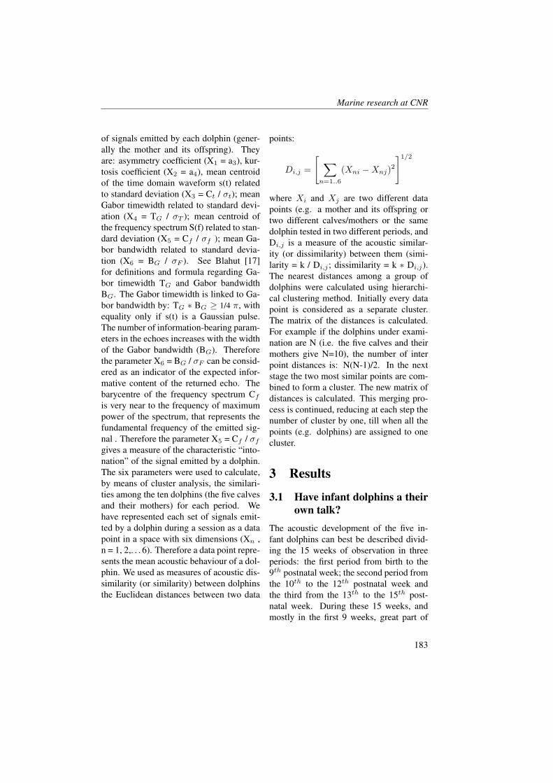
Marine research at CNR
of signals emitted by each dolphin (gener-ally the mother and its offspring). Theyare: asymmetry coefficient (X1 = a3), kur-tosis coefficient (X2 = a4), mean centroidof the time domain waveform s(t) relatedto standard deviation (X3 = Ct / σt); meanGabor timewidth related to standard devi-ation (X4 = TG / σT ); mean centroid ofthe frequency spectrum S(f) related to stan-dard deviation (X5 = Cf / σf ); mean Ga-bor bandwidth related to standard devia-tion (X6 = BG / σF ). See Blahut [17]for definitions and formula regarding Ga-bor timewidth TG and Gabor bandwidthBG. The Gabor timewidth is linked to Ga-bor bandwidth by: TG ∗ BG ≥ 1/4 π, withequality only if s(t) is a Gaussian pulse.The number of information-bearing param-eters in the echoes increases with the widthof the Gabor bandwidth (BG). Thereforethe parameter X6 = BG / σF can be consid-ered as an indicator of the expected infor-mative content of the returned echo. Thebarycentre of the frequency spectrum Cf
is very near to the frequency of maximumpower of the spectrum, that represents thefundamental frequency of the emitted sig-nal . Therefore the parameter X5 = Cf / σf
gives a measure of the characteristic “into-nation” of the signal emitted by a dolphin.The six parameters were used to calculate,by means of cluster analysis, the similari-ties among the ten dolphins (the five calvesand their mothers) for each period. Wehave represented each set of signals emit-ted by a dolphin during a session as a datapoint in a space with six dimensions (Xn ,n = 1, 2,. . . 6). Therefore a data point repre-sents the mean acoustic behaviour of a dol-phin. We used as measures of acoustic dis-similarity (or similarity) between dolphinsthe Euclidean distances between two data
points:
Di,j =
[ ∑n=1..6
(Xni −Xnj)2]1/2
where Xi and Xj are two different datapoints (e.g. a mother and its offspring ortwo different calves/mothers or the samedolphin tested in two different periods, andDi,j is a measure of the acoustic similar-ity (or dissimilarity) between them (simi-larity = k / Di,j ; dissimilarity = k ∗ Di,j).The nearest distances among a group ofdolphins were calculated using hierarchi-cal clustering method. Initially every datapoint is considered as a separate cluster.The matrix of the distances is calculated.For example if the dolphins under exami-nation are N (i.e. the five calves and theirmothers give N=10), the number of interpoint distances is: N(N-1)/2. In the nextstage the two most similar points are com-bined to form a cluster. The new matrix ofdistances is calculated. This merging pro-cess is continued, reducing at each step thenumber of cluster by one, till when all thepoints (e.g. dolphins) are assigned to onecluster.
3 Results
3.1 Have infant dolphins a theirown talk?
The acoustic development of the five in-fant dolphins can best be described divid-ing the 15 weeks of observation in threeperiods: the first period from birth to the9th postnatal week; the second period fromthe 10th to the 12th postnatal week andthe third from the 13th to the 15th post-natal week. During these 15 weeks, andmostly in the first 9 weeks, great part of
183
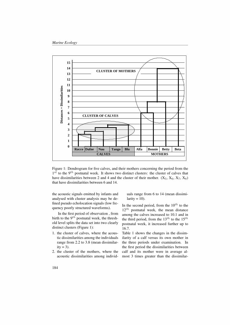
Marine Ecology
Dis
tan
ces
= D
issi
mil
ari
ties
CLUSTER OF CALVES
Dafne Nau
CLUSTER OF MOTHERS
0
1
2
Alfa
4
5
Blu
3
Tango
6
Bonnie Betty
MOTHERS
Beta
CALVES
Rocco
15
7
8
9
10
11
12
13
14
Figure 1: Dendrogram for five calves, and their mothers concerning the period from the1st to the 9th postnatal week. It shows two distinct clusters: the cluster of calves thathave dissimilarities between 2 and 4 and the cluster of their mother. (X5, X6, X7, X8)that have dissimilarities between 6 and 14.
the acoustic signals emitted by infants andanalysed with cluster analysis may be de-fined pseudo echolocation signals (low fre-quency poorly structured waveforms).
In the first period of observation , frombirth to the 9th postnatal week, the thresh-old level splits the data set into two clearlydistinct clusters (Figure 1):1. the cluster of calves, where the acous-
tic dissimilarities among the individualsrange from 2.2 to 3.8 (mean dissimilar-ity = 3).
2. the cluster of the mothers, where theacoustic dissimilarities among individ-
uals range from 6 to 14 (mean dissimi-larity = 10).
In the second period, from the 10th to the12th postnatal week, the mean distanceamong the calves increased to 10.1 and inthe third period, from the 13th to the 15th
postnatal week, it increased further up to16.7.Table 1 shows the changes in the dissim-ilarity of a calf versus its own mother inthe three periods under examination. Inthe first period the dissimilarities betweencalf and its mother were in average al-most 3 times greater than the dissimilar-
184
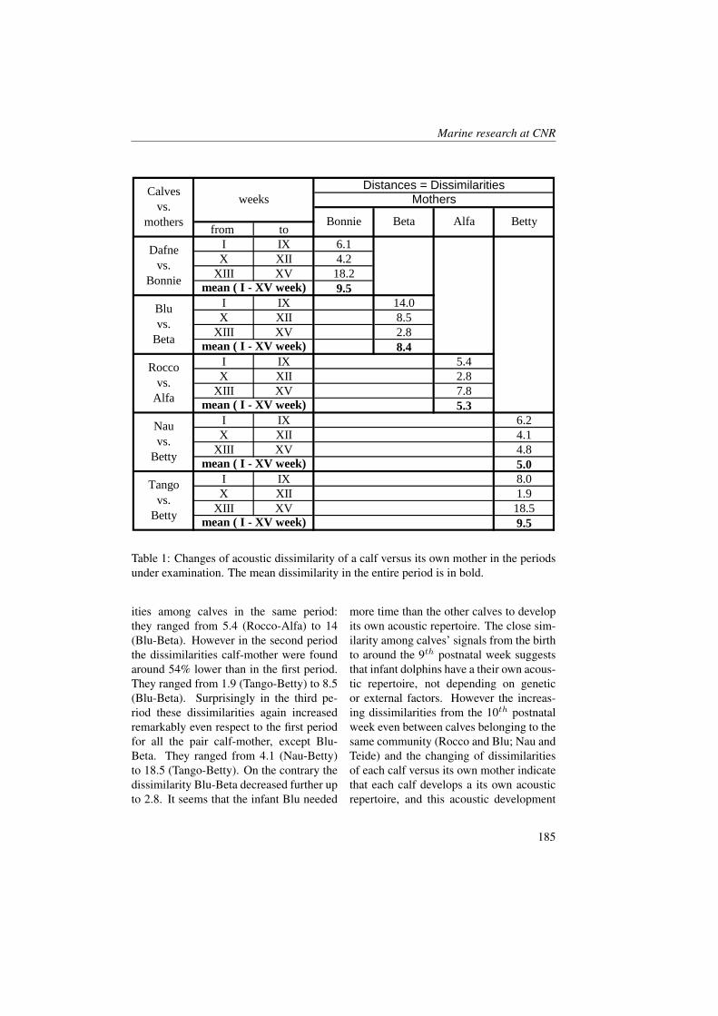
Marine research at CNR
from to
I IX 6.1
X XII 4.2
XIII XV 18.2
9.5
I IX 14.0
X XII 8.5
XIII XV 2.8
8.4
I IX 5.4
X XII 2.8
XIII XV 7.8
5.3
I IX 6.2
X XII 4.1
XIII XV 4.8
5.0
I IX 8.0
X XII 1.9
XIII XV 18.5
9.5
Distances = DissimilaritiesMothers
Calves
vs.
mothers
weeks
Betty
Tango
vs.
Betty
mean ( I - XV week)
mean ( I - XV week)
mean ( I - XV week)
mean ( I - XV week)
mean ( I - XV week)
Beta
Blu
vs.
Beta
Nau
vs.
Betty
Dafne
vs.
Bonnie
Rocco
vs.
Alfa
AlfaBonnie
Table 1: Changes of acoustic dissimilarity of a calf versus its own mother in the periodsunder examination. The mean dissimilarity in the entire period is in bold.
ities among calves in the same period:they ranged from 5.4 (Rocco-Alfa) to 14(Blu-Beta). However in the second periodthe dissimilarities calf-mother were foundaround 54% lower than in the first period.They ranged from 1.9 (Tango-Betty) to 8.5(Blu-Beta). Surprisingly in the third pe-riod these dissimilarities again increasedremarkably even respect to the first periodfor all the pair calf-mother, except Blu-Beta. They ranged from 4.1 (Nau-Betty)to 18.5 (Tango-Betty). On the contrary thedissimilarity Blu-Beta decreased further upto 2.8. It seems that the infant Blu needed
more time than the other calves to developits own acoustic repertoire. The close sim-ilarity among calves’ signals from the birthto around the 9th postnatal week suggeststhat infant dolphins have a their own acous-tic repertoire, not depending on geneticor external factors. However the increas-ing dissimilarities from the 10th postnatalweek even between calves belonging to thesame community (Rocco and Blu; Nau andTeide) and the changing of dissimilaritiesof each calf versus its own mother indicatethat each calf develops a its own acousticrepertoire, and this acoustic development
185
Marine Ecology
is influenced not only by its mother, butalso by other factors as genetic factors andperhaps experience. Similar results werefound by Iannessa [18] in her dissertationon the acoustic evolution of four calves ofTursiops truncatus.
3.2 How much time need a calfto learn the use of biosonar?
The infant Blue, from birth to the 15th
postnatal week, emitted no clicks, but onlyshort, low frequency and little modulatedsignals. Her first echolocation pulse wasrecorded approximately 16 weeks after herbirth [19], while Rocco, housed in the sameRimini Delphinarium, needed about a halftime (≈ 7 weeks) to learn the use of thebiosonar.The time necessary for the infant namedNau to learn the use of biosonar was in-vestigated in detail with weekly observa-tions and recordings from its birth to the26th postnatal week [20]. See Figure 2 fora summary of the results. In this period thecalf and its mother resided separately fromthe other dolphins of Palablu. The infantfrom birth to 10th postnatal week emittedno clicks, but only low frequency wave-forms similar to those of Blue, and it swamprevalently in resting position. From 11 to20 weeks Nau was able to produce clickswith only one peak at 50 kHz (Figure 2Band 2C) . At 21 weeks Nau produced morestructured waveforms with two peaks at 40and 60 kHz (Figure 2D). This trend seemsto reflect the parallel improvement in themotor control from the young dolphin, ob-served in the same period.The isolation of Nau from the communitycould have delayed its acoustic and motordevelopment. However Tango, who alsoresided in Palablu and as Nau remained
for six months from its birth only withits mother and Nau was particularly pre-cocious: it emitted its first sonar pulses 7weeks after its birth [21].The first echolocation pulse of Daphne,housed in Cattolica Delphinarium, wasrecorded approximately 9 weeks after herbirth [19].In conclusion the studied calves neededfrom 7 to 16 weeks to produce their firstsonar pulse. These observations find a con-firmation in Lindhard [22] that illustratedthe dolphin calves’ inability to emit highfrequency sounds (>20 kHz) during theirfirst month of life. Moreover, all stud-ied calves preferred to use pulses with fewcycles and a predominant peak around 50kHz, unlike the adult dolphins, that gener-ally presented a more marked peak around90-100 kHz. As known, low frequenciesallow only a rough perception of the exter-nal world, while high frequencies make anextremely detailed analysis. It is unclear ifthese first simple signals with poorly struc-tured spectra were emitted by the dolphinsintentionally to obtain environmental in-formation or in imitation on mother andif they were related with the changes ofmother-infant swimming positions occur-ring at these ages.With growth, calves produced more struc-tured waveforms (bimodal spectra) show-ing several cycles, but at 26 weeks frombirth the signals emitted by the calves wereyet lacking of frequency components above100 kHz. The bimodal clicks became morefrequent with the longer departures of thecalves from their mothers. This seems tosuggest that young dolphins intentionallyuse more structured signals to move in thepool without maternal aid [23].
186
Marine research at CNR
3.3 The role of the mother
It is difficult to analyse the role the motherplays in providing echolocation model andinstructions to its offspring. For examplesince when the calf Nau emitted its firstclicks (11 week), Betty seemed to sim-plify her own typical clicks and to adaptthem to the acoustic characteristics of Nau(Figure 2C). A similar acoustic behaviourwas observed in Alfa and Betty. It is in-teresting to speculate if this may reflectthe intention of mothers to share the sameenvironmental information with their off-springs or provide them a model to imi-tate. The trend of acoustic dissimilaritiesmother calf showed in Table 1 seems to in-dicate that the mother plays an importantrole in providing echolocation models to itsoffspring mostly between the 10th to the12th postnatal week. Finally it is unclearthe function of the two almost simultane-ous pulse emissions from mother – infant,recorded without any significant changesin all our experiments. These signals mayhave been used by the two dolphins tomaintain acoustic contact or the mothermay have produced standard echolocation
signals as models, expecting that its off-spring could imitate them.
3.4 Possible acoustical changesof the community in re-sponse to the entry of a newcalf
The study on the possible acousticalchanges of the community in response tothe entry of a new calf was done in Pal-ablu on the calf Nau. The calf resided sep-arately from the other two adult dolphinsof the community and lived only with itsmother for six months. The calf and itsmother were reintegrated, first gradually(May-June 2002) then completely (sinceJuly 2002), into the community. Cal-giago, in her dissertation [24], has found aprogressive decrease of the acoustical dis-tances, measured with the cluster analysis,between the calf and the other membersof the community, and mostly between thecalf and its father. This decrease seems duenot only to changes in the characteristics ofthe calf click structure, but also to acousti-cal changes of the community after the en-try of the calf in it.
187
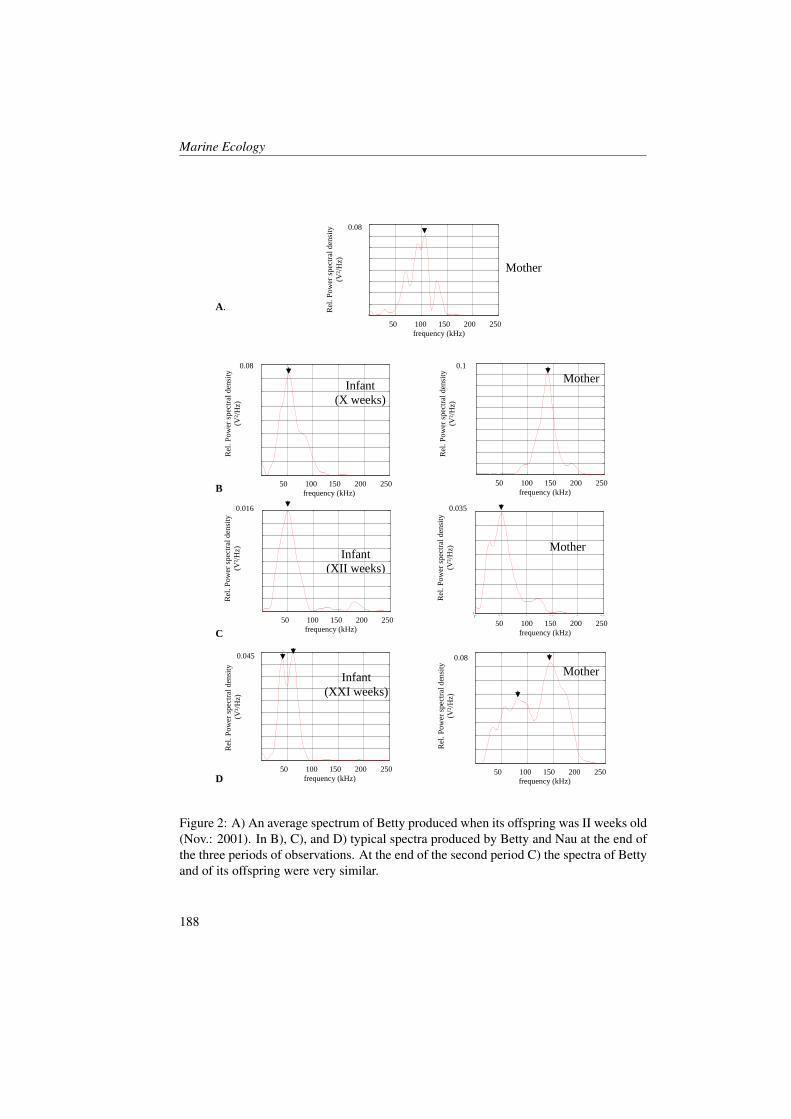
Marine Ecology
0 0.5 1 1.5 2 2.5
x 105
0
0.01
0.02
0.03
0.04
0.05
0.06
0.07
0.08
0.09
0.1
frequency (Hz)
po
we
r sp
ectr
al d
en
sity (
V2/H
z)
50 100 150 200 250
frequency (kHz)
0.1
Rel
. P
ow
er s
pec
tral
den
sity
(V²/
Hz)
Mother
0 0.5 1 1.5 2 2.5
x 105
0
0.01
0.02
0.03
0.04
0.05
0.06
0.07
0.08
frequency (Hz)
po
we
r sp
ectr
al d
en
sity (
V2/H
z)
50 100 150 200 250
frequency (kHz)
0.08
Rel
. P
ow
er s
pec
tral
den
sity
(V²/
Hz)
Infant
(X weeks)
A.
B
C
D
0 0.5 1 1.5 2 2.5
x 105
0
0.01
0.02
0.03
0.04
0.05
0.06
0.07
0.08
frequency (Hz)
po
we
r sp
ect
ral d
en
sity
(V
2/H
z)
50 100 150 200 250
frequency (kHz)
0.08
Rel
. P
ow
er s
pec
tral
den
sity
(V²/
Hz)
Mother
0 0.5 1 1.5 2 2.5
x 105
0
0.002
0.004
0.006
0.008
0.01
0.012
0.014
0.016
frequency (Hz)
pow
er
spectr
al dencsity (
V2/H
z)
50 100 150 200 250
frequency (kHz)
0.016
Rel
. P
ow
er s
pec
tral
den
sity
(V²/
Hz)
Infant
(XII weeks)
0 0.5 1 1.5 2 2.5
x 105
0
0.005
0.01
0.015
0.02
0.025
0.03
0.035
frequency (Hz)
po
we
r sp
ectr
al d
en
sity (
V2/H
z)
50 100 150 200 250
frequency (kHz)
0.035
Rel
. P
ow
er s
pec
tral
den
sity
(V²/
Hz)
Mother
0 0.5 1 1.5 2 2.5
x 105
0
0.005
0.01
0.015
0.02
0.025
0.03
0.035
0.04
0.045
frequency (Hz)
po
we
r sp
ectr
al d
en
sity (
V2/H
z)
50 100 150 200 250
frequency (kHz)
0.045
Rel
. P
ow
er s
pec
tral
den
sity
(V
²/H
z)
Infant
(XXI weeks)
0 0.5 1 1.5 2 2.5
x 105
0
0.01
0.02
0.03
0.04
0.05
0.06
0.07
0.08
frequency (Hz)
po
we
r sp
ectr
al d
en
sity (
V2/H
z)
50 100 150 200 250
frequency (kHz)
0.08
Rel
. P
ow
er s
pec
tral
den
sity
(V²/
Hz)
Mother
Figure 2: A) An average spectrum of Betty produced when its offspring was II weeks old(Nov.: 2001). In B), C), and D) typical spectra produced by Betty and Nau at the end ofthe three periods of observations. At the end of the second period C) the spectra of Bettyand of its offspring were very similar.
188
Marine research at CNR
4 Conclusion
Although the acoustics of the bottlenosedolphin’s echolocation system is well re-searched, the studies on the developmentof echolocation in young dolphins has re-ceived much less focus.Our observations, done in controlled exper-iments, indicate that:• Infant dolphins till about 9th postnatal
week from birth seem to have a their ownacoustic repertoire, not depending on ge-netic or external factors (Figure 1).
• From the 10th postnatal week the dissim-ilarities among calves’ signals increasedprogressively. Then since the 10th post-natal week each calf seems to develop aits own acoustic repertoire.
• The five studied calves needed from 7 to15 weeks from birth to produce their firstsonar pulses.
• The same calves till the 26th postnatalweek used low frequency pulses with apredominant peak around 50 kHz, unlikethe other adult dolphins, that generallypresented the most marked peak around100 kHz.
• With growth the acoustic dissimilari-ties calf-mother first decreased remark-ably (second period) then (third period)tended to increase again (except Blu-Beta, Table 1). This trend could indicate
that the mother plays an important rolein providing echolocation models to itsoffspring mostly around the X-XII post-natal week. Figure 2C shows that whenthe calf Nau was able to emit sonar sig-nals, her mother seemed to adapt somefeatures of its typical signals to thoseof Nau. It may reflect the intention ofmother to share the same environmentalinformation with its offspring or providea model to imitate. Moreover it is un-clear the function of the two almost si-multaneous pulse emissions from mother– infant, recorded without any significantchanges in all our experiments.
• The calf Nau studied in Palablu ofGardaland who lived only with itsmother for the first six months, whenreintegrated in its community was acous-tically influenced mostly by the fatherand then by the other members of thegroup. On the other hand, the acousticbehaviour of all members of the commu-nity seemed to be affected by the pres-ence of the new entry.
Although the experiments in controlledconditions are of great importance, wemust consider, as future research, similarmeasurements in the wild. Other criticalareas for future research are the social, pas-sive and metaphorical uses of echolocationboth in captivity and in the wild.
References[1] C.E. Hammer. Echo - recognition in the porpoise (Tursiops truncatus): an exper-
imental analysis of salient target characteristics. Naval Ocean System Center, SanDiego, San Diego Technical Report, 192, 1978.
[2] C.E. Hammer and W.W.L. Au. Porpoise echo - recognition: an analysis ofcontrolling target characteristics. Journal of the Acoustical Society Of America,68(5):1285–1293, 1980.
189
Marine Ecology
[3] W.W.L. Au and D.A. Pawloski. Cylinder and thickness discrimination by an echolo-cating dolphin. Journal of Comparative Physiology, 172:41 – 47, 1992.
[4] V.M. Bel’kovich, I.V. Borisov, V.S. Gurevich, and N.L. Krushinskaya. Echolocatingcapabilities of the common dolphin (Delphinus delphis). Zool. Zhurn, 48:876 – 883,1969.
[5] W.W.L. Au, Shusterman, R.J., Kersting, and D.A. Sphere-cylinder discriminationvia echolocation by Tursiops truncatus. In: Animal Sonar System, Eds. R.G. Bus-nel, J.F. Fish, Plenum Press, New York. pages 859 – 862, 1980.
[6] M. Azzali, A. Manzini, and G. Buracchi. Acoustic recognition by a dolphinof shapes. In: Sensory Systems of Aquatic Mammals, Eds R.A. Kastelein, J.A.Thomas, P.E. Nachtigal, De Spil Publishers, Woerden, The Netherlands. pages137–156, 1995.
[7] D.A. Helweg. Recognition of aspect-dependent geometric solids by an echolocat-ing Atlantic bottlenosed dolphin. Unpublished doctoral dissertation. University ofHawaii, Honolulu, 1993.
[8] M. Azzali, P. Garbati, and A. Impetuoso. Similarity among sonar signals collectedfrom communities of dolphins (Tursiops truncatus). 4th Europ. Conf. UnderwaterAcoustics, 1:137–156, 1998.
[9] E.M. Dos Santos and V.C. Almada. A case for Passive Sonar: Analysis of Clicktrain production Patterns by Bottlenose Dolphins. In: Echolocation in Bats andDolphins. Eds. J.A Thomas, C.F. Moss, and M. Vater, The University of ChicagoPress, Chicago and London. pages 400–403, 2004.
[10] D.L. Herzig and M.E. Dos Santos. Functional Aspect of Echolocation in Dolphins.In: Echolocation in Bats and Dolphins, Eds. J.A Thomas, C.F. Moss, and M. Vater,The University of Chicago Press, Chicago and London. pages 386–393, 2004.
[11] W.W.L. Au. Echolocation signals of the Atlantic bottlenose (Tursiops truncatus)in open water. In: Animal sonar: Processes and performances. Eds. P.E. Nachtigalland P.W.B. Moore. Plenum Press, New York. pages 251–282, 1980.
[12] A. Kolchin and V.M. Bel’kovich. Tactile sensitivity in Delphinus delphis. Zoolo-gishesky Zhurnal, 53:620–622, 1973.
[13] M.J. Jr Xitco and H.L. Roitblat. Object recognition through eavesdropping: Passiveecholocation in bottlenose dolphins. Animal Learning and Behavior, 24(4):355–365, 1996.
[14] K.S. Norris and E.C. Evans. On the evolution of acoustic communication in verte-brates. In: Animal Sonar Processes and Performance. Eds. P. E. Nachtigall, P. W.B. Moore, New York, Plenum Press. 156:655–681, 1988.
190
Marine research at CNR
[15] R.D. Estes and J. Goddard. Prey selection and hunting behaviour of the Africanwild dog. Jour. Wildl. Mgt., 31:52–70, 1967.
[16] L.M. Hermann, D.G. Richards, and J.P. Wolz. Comprehension of sentences bybottlenosed dolphins. Cognition, 16(2):129 – 219, 1984.
[17] E.R. Blahut. Theory of remote surveillance algorithms. Radar and Sonar. Part I TheIMA Volumes in Mathematics and its Applications. Eds. R.E. Blahut, W.Jr. Miller,C.H. Wilcox. 32:1–66, 1991.
[18] F. Iannessa. Evoluzione del linguaggio in quattro cuccioli di Tursiops truncatuscomparata tra loro e le rispettive madri. Unpublished doctoral dissertation, MarchePolytechnic University, Italy, page 120, 2004.
[19] S. Manoukian, M. Azzali, C. Farchi, and R. Tizzi. Development of Tursiops trunca-tus Sonar System During First Months of Life in Captivity: Acoustic Interactionswith other Community Members. Acta Acustica united with Acustica, 88:743 –747, 2002.
[20] F. Ricciardo, M. Azzali, and S. Manoukian. Development of the acoustic and loco-motor behaviour of an infant bottlenose dolphin (Tursiops truncatus). Proceedingsof the 17th European Cetacean Society Annual Conference, Las Palmas de GranCanaria, Spain, March 9-13 2003, 2003.
[21] I. Biagiotti, S. Catacchio, R. Simoni, and M. Azzali. Acoustic evolution of a coupleof captive bottlenoses, mother and calf. Proceedings of the 34th Annual Symposiumof the European Association for Aquatic Mammals, Riccione, Italy, 17-20 March,2006.
[22] M. Lindhard. Apparent sonar click from a captive bottlenose dolphin Tursiops trun-catus when 2, 7 and 38 weeks old. In: Animal Sonar Processes and PerformanceEds. P. E. Nachtigal, P. W. B. Moore, , New York, Plenum Press. 156:109 – 113,1988.
[23] D. Reiss. Observations on the development of echolocation in young bottlenosedolphins. In: Animal Sonar Processes and Performances. Eds. Paul E. Nachtigall,Patrick W.B. Moore,. Plenum Press, New York. pages 121–127, 1988.
[24] I. Calciago. Studio dell’evoluzione acustica di un cucciolo di Tursiops truncatus(Montagu, 1821) dai sei mesi ai quattordici mesi di vita, in relazione al comporta-mento acustico e sociale della madre e della sua comunita. Unpublished DoctoralDissertation, Universita degli studi di Milano, Italy, page 148, 2003.
191

Marine Ecology
192
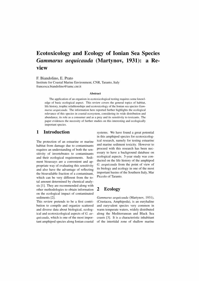
Ecotoxicology and Ecology of Ionian Sea SpeciesGammarus aequicauda (Martynov, 1931): a Re-view
F. Biandolino, E. PratoInstitute for Coastal Marine Environment, CNR, Taranto, [email protected]
Abstract
The application of an organism in ecotoxicological testing requires some knowl-edge of basic ecological aspect. This review covers the general topics of habitat,life history, trophic relathionships and ecotoxicology of the Ionian sea species Gam-marus aequicauda. The information here reported further highlights the ecologicalrelevance of this species in coastal ecosystem, considering its wide distribution andabundance, its role as a consumer and as a prey and its sensitivity to toxicants. Thepaper evidences the necessity of further studies on this interesting and ecologicallyimportant species.
1 Introduction
The protection of an estuarine or marinehabitat from damage due to contaminantsrequires an understanding of both the sen-sitivity of invertebrates to contaminantsand their ecological requirements. Sedi-ment bioassays are a convenient and ap-propriate way of evaluating this sensitivityand also have the advantage of reflectingthe bioavailable fraction of a contaminant,which can be very different from the to-tal amount determined by chemical analy-sis [1]. They are recommended along withother methodologies to obtain informationon the ecological impact of contaminatedsediments [2].This review pretends to be a first contri-bution to compile and organize scatteredand diverse data about biological, ecolog-ical and ecotoxicological aspects of G. ae-quicauda, which is one of the most impor-tant amphipod species along Ionian coastal
systems. We have found a great potentialin this amphipod species for ecotoxicolog-ical research, namely for testing estuarineand marine sediment toxicity. However toproceed with this research has been nec-essary to have a background database onecological aspects. 5-year study was con-ducted on the life history of the amphipodG. aequicauda from the point of view ofits biology and ecology in one of the mostimportant basins of the Southern Italy, MarPiccolo of Taranto.
2 Ecology
Gammarus aequicauda (Martynov, 1931),(Crustacea, Amphipoda), is an euryhalineand euryvalent species very common inwarm temperate waters, widely distributedalong the Mediterranean and Black Seacoasts [3]. It is a characteristic inhabitantof the intertidal zone of shallow marine
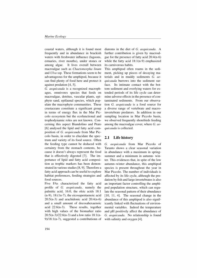
Marine Ecology
coastal waters, although it is found mostfrequently and in abundance in brackishwaters with freshwater influence (lagoons,estuaries, river mouths), under stones oramong algae. It lives overall betweenmacroalgae such as Chaetomorpha linumand Ulva ssp. These formations seem to beadvantageous for the amphipod, because itcan find plenty of food here and protect itagainst predation [4, 5].G. aequicauda is a recognized macroph-agus, omnivores species that feeds onmacroalgae, detritus, vascular plants, epi-phyte sand, epifaunal species, which pop-ulate the macrophyte communities. Thesecrustaceans constitute a significant groupin terms of energy flux in the Mar Pic-colo ecosystem but the ecofunctional andtrophodynamic roles are not known. Con-cerning this aspect Biandolino and Prato[6] analysed the lipid and fatty acid com-position of G. aequicauda from Mar Pic-colo basin, in order to elucidate the spec-trum and variety of its food source. Oftenthe feeding type cannot be deduced withcertainty from the stomach contents, be-cause it doesn’t always represent the foodthat is effectively digested [7]. The im-portance of lipid and fatty acid composi-tion as trophic markers has been demon-strated in various studies [8, 9]. Therefore afatty acid approach can be useful to explorehabitat preferences, feeding strategies andfood sources.Five FAs characterized the fatty acidprofile of G. aequicauda, namely thepalmitic acid, 16:0, the oleic acids 18:1(n-9), 18:(1n-7), the eicosapentaenoic acid20:5(n-3) and arachidonic acid 20:4(n-6)and a small amount of docosahexaenoicacid 22:6(n-3). These results, togetherwith high values of the biomarker ratio20:5(n-3)/22:6(n-3) and a low ratio 18:1(n-9)/18:1(n-7), suggested a contributionn of
diatoms in the diet of G. aequicauda. Afurther contribution is given by macroal-gae for the presence of fatty acid 20:4(n-6)while the fatty acid 18:1(n-9) emphasizedits carnivorous habits.This amphipod often roams in the sedi-ment, picking up pieces of decaying ma-terials and in muddy sediments G. ae-quicauda burrows into the sediment sur-face. Its intimate contact with the bot-tom sediment and overlying waters for ex-tended periods of its life cycle can deter-mine adverse effects in the presence of con-taminated sediments. From our observa-tion G. aequicauda is a food source fora diverse range of vertebrate and macro-invertebrate predators. In addition in oursampling location in Mar Piccolo basin,we observed frequently shorebirds feedingamong the macroalgae cover, where G. ae-quicauda is collected.
2.1 Life historyG. aequicauda from Mar Piccolo ofTaranto shows a clear seasonal variationin abundance with a maximum in spring-summer and a minimum in autumn- win-ter. This evidences that, in spite of the lowautumn–winter abundance, this amphipodspecies is present throughout the year inMar Piccolo. The number of individuals isaffected by its life cycle, although the pre-dation by fish and large invertebrates is alsoan important factor controlling the amphi-pod population structure, which can regu-late the seasonal pattern of their abundance[10, 11, 4]. The seasonal change in theabundance of this amphipod is also signif-icantly linked with fluctuations of environ-mental variables. Indeed the temperatureand pH positively affect the abundance ofG. aequicauda. No relationship is foundwith salinity and oxygen [4].
194

Marine research at CNR
G. aequicauda reproduces continuously inthe Mar Piccolo estuary, as can be con-cluded by the presence of ovigerous fe-males throughout the year. This is observedalso in other populations of this species,studied by Greze [12], Janssen et al. [13],Porcu and Tagliasacchi Masala [14] andKevrekidis and Koukouras [15]. Two gen-erations each year are recorded: juvenilesborn in the spring, grow, mature, and be-come reproductively active during the sum-mer months, giving rise to the next input ofrecruits in autumn. Although our observa-tions from laboratory cultures indicate thatthe population probably produces severalgenerations per year [16]. Therefore, cou-pled field and culture data indicate that G.aequicauda population of the Mar Piccoloestuary reproduces several times in the yearand has a multivoltine life cycle, that is,produces several generations per year.The sex ratio (number of males/number offemales) vary considerably over the yearwith the mean value of 1.12 (± 0.1 stan-dard error), however, females were moreabundant than males during winter months.Regarding size-class structure, the popula-tion of G. aequicauda consists in spring ofadult individuals and few juveniles. Sizedifferences between males and females oc-cur throughout the year because the malesgrow faster than females and reach a longersize.In the summer months most of the last gen-eration seem to die and the population ismainly constituted by juveniles and smallindividuals. This tendency is kept rela-tively constant during early autumn untilDecember being mainly made up of small-sized adults.The recruitment quantification, particularlyof the animals with total length (TL) < 2mm is hard to do, since these animal’s den-sities show pronounced variations between
monthly replicates. The presence of juve-niles throughout the year evidences a con-tinuous recruitment. Although in the pe-riod spring-summer the number of juve-niles is too small to account for adults ofthe next months. This may be a samplingdeficiency, as mentioned by Anger [17] forother small-sized amphipod species. An in-crease in juveniles number occurs in au-tumn–winter. Furthermore, it is possiblethat, the decrease in the adult population inautumn-winter months maybe due to somemigration of adults between different habi-tat types related to the breeding periods[18, 10]. The size of the brood is positivelycorrelated to the cephalic length of the fe-male. Indeed in summer and early autumnis registered the lowest fecundity when themean ovigerous females size is the small-est. G. aequicauda females become oviger-ous when they reach a size of about 5mm,producing more than 20 eggs only when fe-males exceed 8mm.
2.2 Gammarus aequicauda rear-ing in the laboratory at dif-ferent environmental vari-ables
On the basis of field data alone, it is dif-ficult to come to any conclusion about theprocesses governing the life history traits.A combination of field and laboratory ex-periments may provide adequate estimatesand improve our understanding of popula-tion dynamics and biological traits that canbe difficult to follow in the field. Findingsfrom this study have implications in devel-opments of ecotoxicological testing withG. aequicauda. In order to fully under-stand the effects of pollutants in acute andespecially chronic toxicity investigations,G. aequicauda’s life history in the labo-
195
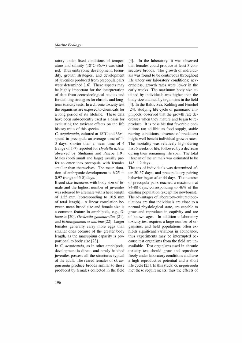
Marine Ecology
ratory under fixed conditions of temper-ature and salinity (18°C-36�) was stud-ied. Thus embryonic development, fecun-dity, growth strategies, and developmentof juveniles produced from precopula pairswere determined [16]. These aspects maybe highly important for the interpretationof data from ecotoxicological studies andfor defining strategies for chronic and long-term toxicity tests. In a chronic toxicity testthe organisms are exposed to chemicals fora long period of its lifetime. These datahave been subsequently used as a basis forevaluating the toxicant effects on the lifehistory traits of this species.G. aequicauda, cultured at 18°C and 36�spend in precopula an average time of 1-3 days, shorter than a mean time of 4(range of 1-7) reported for Hyalella aztecaobserved by Shuhaimi and Pascoe [19].Males (both small and large) usually pre-fer to enter into precopula with femalessmaller than themselves. The mean dura-tion of embryonic development is 6.25 ±0.97 (range of 5-8) days.Brood size increases with body size of fe-male and the highest number of juvenileswas released by a female with a head lengthof 1.25 mm (corresponding to 10.9 mmof total length). A linear correlation be-tween mean brood size and female size isa common feature in amphipods, e.g., G.locusta [20], Orchestia gammarellus [21],and Echinogammarus marinus[22]. Largerfemales generally carry more eggs thansmaller ones because of the greater bodylength, as the marsupium capacity is pro-portional to body size [23].In G. aequicauda, as in other amphipods,development is direct, and newly hatchedjuveniles possess all the structures typicalof the adult. The reared females of G. ae-quicauda produce broods similar to thoseproduced by females collected in the field
[4]. In the laboratory, it was observedthat females could produce at least 3 con-secutive broods. The growth of individu-als was found to be continuous throughoutlife under our laboratory conditions; nev-ertheless, growth rates were lower in theearly weeks. The maximum body size at-tained by individuals was higher than thebody size attained by organisms in the field[4]. In the Baltic Sea, Kolding and Fenchel[24], studying life cycle of gammarid am-phipods, observed that the growth rate de-creases when they mature and begin to re-produce. It is possible that favorable con-ditions (an ad libitum food supply, stablerearing conditions, absence of predators)might well benefit individual growth rates.The mortality was relatively high duringfirst 6 weeks of life, followed by a decreaseduring their remaining life span. The totallifespan of the animals was estimated to be145 ± 2 days.The sex of individuals was determined af-ter 30-37 days, and precopulatory pairingbehavior began after 44 days. The numberof precopula pairs reached a maximum at84-88 days, corresponding to 46% of theexisting population (except for newborns).The advantages of laboratory-cultured pop-ulations are that individuals are close to anormal physiological state, are capable togrow and reproduce in captivity and areof known ages. In addition a laboratorytoxicity test requires a large number of or-ganisms, and field populations often ex-hibits significant variations in abundance,thus experiments may be interrupted be-cause test organisms from the field are un-available. Test organisms used in chronictoxicity test should grow and reproducefreely under laboratory conditions and havea high reproductive potential and a shortlife cycle [25]. In this study, G. aequicaudamet these requirements, thus the effects of
196
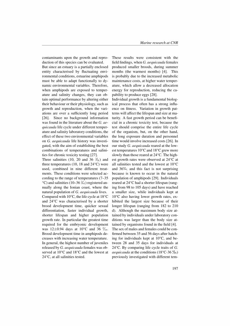
Marine research at CNR
contaminants upon the growth and repro-duction of this species can be evaluated.But since an estuary is a partially enclosedentity characterised by fluctuating envi-ronmental conditions, estuarine amphipodsmust be able to adapt functionally to dy-namic environmental variables. Therefore,when amphipods are exposed to temper-ature and salinity changes, they can ob-tain optimal performance by altering eithertheir behaviour or their physiology, such asgrowth and reproduction, when the vari-ations are over a sufficiently long period[26]. Since no background informationwas found in the literature about the G. ae-quicauda life cycle under different temper-ature and salinity laboratory conditions, theeffect of these two environmental variableson G. aequicauda life history was investi-gated, with the aim of establishing the bestcombinations of temperatures and salini-ties for chronic toxicity testing [27].Three salinities (10, 20 and 36 �) andthree temperatures (10, 18 and 24°C) wereused, combined in nine different treat-ments. These conditions were selected ac-cording to the range of temperatures (7–35°C) and salinities (10–36�) registered an-nually along the Ionian coast, where thenatural population of G. aequicauda lives.Compared with 10°C, the life cycle at 18°Cand 24°C was characterised by a shorterbrood development time, quicker sexualdifferentiation, faster individual growth,shorter lifespan and higher populationgrowth rate. In particular the greatest timerequired for the embryonic developmentwas 12±0.94 days at 10°C and 36 �.Brood development time in amphipods de-creases with increasing water temperature.In general, the highest number of juvenilesreleased by G. aequicauda females was ob-served at 10°C and 18°C and the lowest at24°C, at all salinities tested.
These results were consistent with thefield findings, when G. aequicauda femalesproduced smaller broods, during summermonths (the warmest months) [4]. Thisis probably due to the increased metabolicmaintenance costs, at higher water temper-ature, which allow a decreased allocationenergy for reproduction, reducing the ca-pability to produce eggs [28].Individual growth is a fundamental biolog-ical process that often has a strong influ-ence on fitness. Variation in growth pat-terns will affect the lifespan and size at ma-turity. A fast growth period can be benefi-cial in a chronic toxicity test, because thetest should comprise the entire life cycleof the organism, but, on the other hand,the long exposure duration and personneltime would involve increased costs [26]. Inour study G. aequicauda reared at the low-est temperatures 10°C and 18°C grew moreslowly than those reared at 24°C. The high-est growth rates were observed at 24°C atall salinities tested and the lowest at 10°Cand 36� and this fact is not surprisingbecause is known to occur in the naturalpopulation of amphipods [29]. Individualsreared at 24°C had a shorter lifespan (rang-ing from 98 to 105 days) and have reacheda smaller size, while individuals kept at10°C also having lower growth rates, ex-hibited the largest size because of theirlonger lifespan (ranging from 182 to 210d). Although the maximum body size at-tained by individuals under laboratory con-ditions was larger than the body size at-tained by organisms found in the field [4].The sex of males and females could be con-firmed between 35 and 56 days after hatch-ing for individuals kept at 10°C, and be-tween 28 and 35 days for individuals at24°C. By comparing life cycle traits of G.aequicauda at the conditions (18°C-36�)previously investigated with different tem-
197
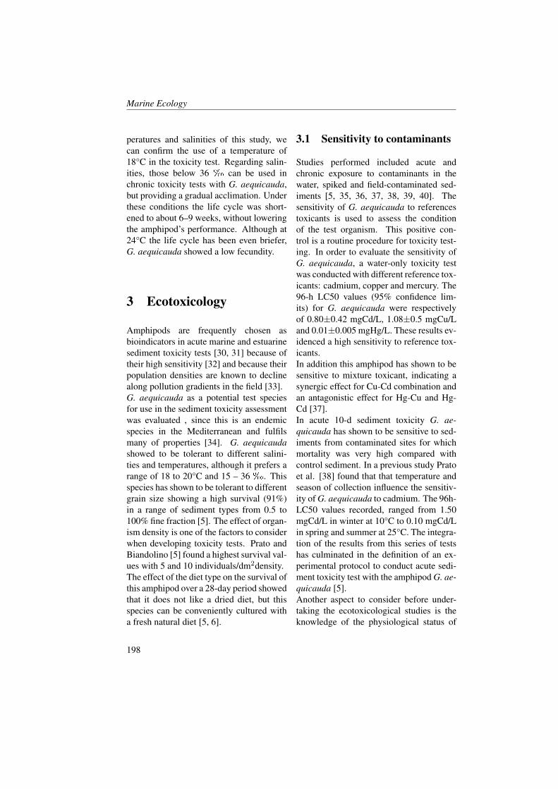
Marine Ecology
peratures and salinities of this study, wecan confirm the use of a temperature of18°C in the toxicity test. Regarding salin-ities, those below 36 � can be used inchronic toxicity tests with G. aequicauda,but providing a gradual acclimation. Underthese conditions the life cycle was short-ened to about 6–9 weeks, without loweringthe amphipod’s performance. Although at24°C the life cycle has been even briefer,G. aequicauda showed a low fecundity.
3 Ecotoxicology
Amphipods are frequently chosen asbioindicators in acute marine and estuarinesediment toxicity tests [30, 31] because oftheir high sensitivity [32] and because theirpopulation densities are known to declinealong pollution gradients in the field [33].G. aequicauda as a potential test speciesfor use in the sediment toxicity assessmentwas evaluated , since this is an endemicspecies in the Mediterranean and fulfilsmany of properties [34]. G. aequicaudashowed to be tolerant to different salini-ties and temperatures, although it prefers arange of 18 to 20°C and 15 – 36�. Thisspecies has shown to be tolerant to differentgrain size showing a high survival (91%)in a range of sediment types from 0.5 to100% fine fraction [5]. The effect of organ-ism density is one of the factors to considerwhen developing toxicity tests. Prato andBiandolino [5] found a highest survival val-ues with 5 and 10 individuals/dm2density.The effect of the diet type on the survival ofthis amphipod over a 28-day period showedthat it does not like a dried diet, but thisspecies can be conveniently cultured witha fresh natural diet [5, 6].
3.1 Sensitivity to contaminants
Studies performed included acute andchronic exposure to contaminants in thewater, spiked and field-contaminated sed-iments [5, 35, 36, 37, 38, 39, 40]. Thesensitivity of G. aequicauda to referencestoxicants is used to assess the conditionof the test organism. This positive con-trol is a routine procedure for toxicity test-ing. In order to evaluate the sensitivity ofG. aequicauda, a water-only toxicity testwas conducted with different reference tox-icants: cadmium, copper and mercury. The96-h LC50 values (95% confidence lim-its) for G. aequicauda were respectivelyof 0.80±0.42 mgCd/L, 1.08±0.5 mgCu/Land 0.01±0.005 mgHg/L. These results ev-idenced a high sensitivity to reference tox-icants.In addition this amphipod has shown to besensitive to mixture toxicant, indicating asynergic effect for Cu-Cd combination andan antagonistic effect for Hg-Cu and Hg-Cd [37].In acute 10-d sediment toxicity G. ae-quicauda has shown to be sensitive to sed-iments from contaminated sites for whichmortality was very high compared withcontrol sediment. In a previous study Pratoet al. [38] found that that temperature andseason of collection influence the sensitiv-ity of G. aequicauda to cadmium. The 96h-LC50 values recorded, ranged from 1.50mgCd/L in winter at 10°C to 0.10 mgCd/Lin spring and summer at 25°C. The integra-tion of the results from this series of testshas culminated in the definition of an ex-perimental protocol to conduct acute sedi-ment toxicity test with the amphipod G. ae-quicauda [5].Another aspect to consider before under-taking the ecotoxicological studies is theknowledge of the physiological status of
198
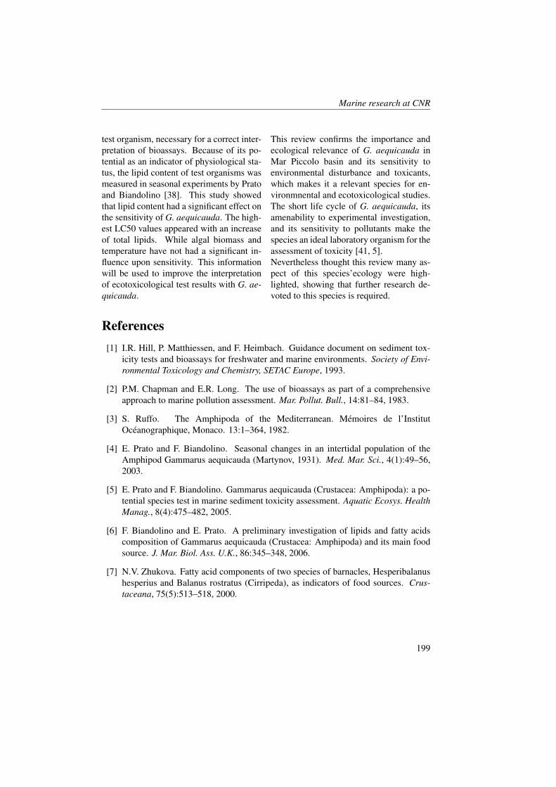
Marine research at CNR
test organism, necessary for a correct inter-pretation of bioassays. Because of its po-tential as an indicator of physiological sta-tus, the lipid content of test organisms wasmeasured in seasonal experiments by Pratoand Biandolino [38]. This study showedthat lipid content had a significant effect onthe sensitivity of G. aequicauda. The high-est LC50 values appeared with an increaseof total lipids. While algal biomass andtemperature have not had a significant in-fluence upon sensitivity. This informationwill be used to improve the interpretationof ecotoxicological test results with G. ae-quicauda.
This review confirms the importance andecological relevance of G. aequicauda inMar Piccolo basin and its sensitivity toenvironmental disturbance and toxicants,which makes it a relevant species for en-vironmnental and ecotoxicological studies.The short life cycle of G. aequicauda, itsamenability to experimental investigation,and its sensitivity to pollutants make thespecies an ideal laboratory organism for theassessment of toxicity [41, 5].Nevertheless thought this review many as-pect of this species’ecology were high-lighted, showing that further research de-voted to this species is required.
References[1] I.R. Hill, P. Matthiessen, and F. Heimbach. Guidance document on sediment tox-
icity tests and bioassays for freshwater and marine environments. Society of Envi-ronmental Toxicology and Chemistry, SETAC Europe, 1993.
[2] P.M. Chapman and E.R. Long. The use of bioassays as part of a comprehensiveapproach to marine pollution assessment. Mar. Pollut. Bull., 14:81–84, 1983.
[3] S. Ruffo. The Amphipoda of the Mediterranean. Memoires de l’InstitutOceanographique, Monaco. 13:1–364, 1982.
[4] E. Prato and F. Biandolino. Seasonal changes in an intertidal population of theAmphipod Gammarus aequicauda (Martynov, 1931). Med. Mar. Sci., 4(1):49–56,2003.
[5] E. Prato and F. Biandolino. Gammarus aequicauda (Crustacea: Amphipoda): a po-tential species test in marine sediment toxicity assessment. Aquatic Ecosys. HealthManag., 8(4):475–482, 2005.
[6] F. Biandolino and E. Prato. A preliminary investigation of lipids and fatty acidscomposition of Gammarus aequicauda (Crustacea: Amphipoda) and its main foodsource. J. Mar. Biol. Ass. U.K., 86:345–348, 2006.
[7] N.V. Zhukova. Fatty acid components of two species of barnacles, Hesperibalanushesperius and Balanus rostratus (Cirripeda), as indicators of food sources. Crus-taceana, 75(5):513–518, 2000.
199
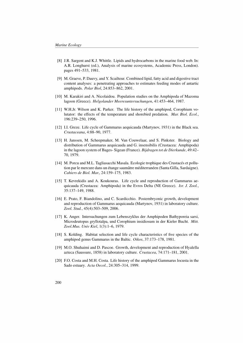
Marine Ecology
[8] J.R. Sargent and K.J. Whittle. Lipids and hydrocarbons in the marine food web. In:A.R. Longhurst (ed.), Analysis of marine ecosystems, Academic Press, London).pages 491–533, 1981.
[9] M. Graeve, P. Dauvy, and Y. Scailteur. Combined lipid, fatty acid and digestive tractcontent analyses: a penetrating approaches to estimates feeding modes of antarticamphipods. Polar Biol, 24:853–862, 2001.
[10] M. Karakiri and A. Nicolaidou. Population studies on the Amphipoda of Mazomalagoon (Greece). Helgolander Meeresuntersuchungen, 41:453–464, 1987.
[11] W.H.Jr. Wilson and K. Parker. The life history of the amphipod, Corophium vo-lutator: the effects of the temperature and shorebird predation. Mar. Biol. Ecol.,196:239–250, 1996.
[12] I.I. Greze. Life cycle of Gammarus aequicauda (Martynov, 1931) in the Black sea.Crustaceana, 4:88–90, 1977.
[13] H. Janssen, M. Scheepmaker, M. Van Couwelaar, and S. Pinkster. Biology anddistribution of Gammarus aequicauda and G. insensibilis (Crustacea: Amphipoda)in the lagoon system of Bages- Sigean (France). Bijdragen tot de Dierkunde, 49:42–70, 1979.
[14] M. Porcu and M.L. Tagliasacchi Masala. Ecologie trophique des Crustaces et pollu-tion par le mercure dans un etange saumatre mediterraneen (Santa Gilla, Sardaigne).Cahiers de Biol. Mar., 24:159–175, 1983.
[15] T. Kevrekidis and A. Koukouras. Life cycle and reproduction of Gammarus ae-quicauda (Crustacea: Amphipoda) in the Evros Delta (NE Greece). Isr. J. Zool.,35:137–149, 1988.
[16] E. Prato, F. Biandolino, and C. Scardicchio. Postembryonic growth, developmentand reproduction of Gammarus aequicauda (Martynov, 1931) in laboratory culture.Zool. Stud., 45(4):503–509, 2006.
[17] K. Anger. Intersuchungen zum Lebenszyklus der Amphipoden Bathyporeia sarsi,Microdeutopus gryllotalpa, und Corophium insidiosum in der Kieler Bucht. Mitt.Zool.Mus. Univ Kiel, 1(3):1–6, 1979.
[18] S. Kolding. Habitat selection and life cycle characteristics of five species of theamphipod genus Gammarus in the Baltic. Oikos, 37:173–178, 1981.
[19] M.O. Shuhaimi and D. Pascoe. Growth, development and reproduction of Hyalellaazteca (Saussure, 1858) in laboratory culture. Crustacea, 74:171–181, 2001.
[20] F.O. Costa and M.H. Costa. Life history of the amphipod Gammarus locusta in theSado estuary. Acta Oecol., 24:305–314, 1999.
200
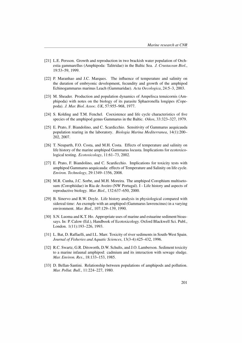
Marine research at CNR
[21] L.E. Persson. Growth and reproduction in two brackish water population of Orch-estia gammarellus (Amphipoda: Talitridae) in the Baltic Sea. J. Crustacean Biol.,19:53–59, 1999.
[22] P. Maranhao and J.C. Marques. The influence of temperature and salinity onthe duration of embryonic development, fecundity and growth of the amphipodEchinogammarus marinus Leach (Gammaridae). Acta Oecologica, 24:5–3, 2003.
[23] M. Sheader. Production and population dynamics of Ampelisca tenuicornis (Am-phipoda) with notes on the biology of its parasite Sphaeronella longipes (Cope-poda). J. Mar. Biol. Assoc. UK, 57:955–968, 1977.
[24] S. Kolding and T.M. Fenchel. Coexistence and life cycle characteristics of fivespecies of the amphipod genus Gammarus in the Baltic. Oikos, 33:323–327, 1979.
[25] E. Prato, F. Biandolino, and C. Scardicchio. Sensitivity of Gammarus aequicaudapopulation rearing in the laboratory. Biologia Marina Mediterranea, 14(1):200–202, 2007.
[26] T. Neuparth, F.O. Costa, and M.H. Costa. Effects of temperature and salinity onlife history of the marine amphipod Gammarus locusta. Implications for ecotoxico-logical testing. Ecotoxicology, 11:61–73, 2002.
[27] E. Prato, F. Biandolino, and C. Scardicchio. Implications for toxicity tests withamphipod Gammarus aequicauda: effects of Temperature and Salinity on life cycle.Environ. Technology, 29:1349–1356, 2008.
[28] M.R. Cunha, J.C. Sorbe, and M.H. Moreira. The amphipod Corophium multiseto-sum (Corophiidae) in Ria de Aveiro (NW Portugal). I - Life history and aspects ofreproductive biology. Mar. Biol., 132:637–650, 2000.
[29] B. Sinervo and R.W. Doyle. Life history analysis in physiological compared withsidereal time: An exemple with an amphipod (Gammarus lawrencinus) in a varyingenvironment. Mar. Biol., 107:129–139, 1990.
[30] S.N. Luoma and K.T. Ho. Appropriate uses of marine and estuarine sediment bioas-says. In: P. Calow (Ed.), Handbook of Ecotoxicology. Oxford Blackwell Sci. Publ.,London. 1(11):193–226, 1993.
[31] L. Bat, D. Raffaelli, and I.L. Marr. Toxicity of river sediments in South-West Spain.Journal of Fisheries and Aquatic Sciences, 13(3-4):425–432, 1996.
[32] R.C. Swartz, G.R. Ditsworth, D.W. Schults, and J.O. Lamberson. Sediment toxicityto a marine infaunal amphipod: cadmium and its interaction with sewage sludge.Mar. Environ. Res., 18:133–153, 1985.
[33] D. Bellan-Santini. Relationship between populations of amphipods and pollution.Mar. Pollut. Bull., 11:224–227, 1980.
201
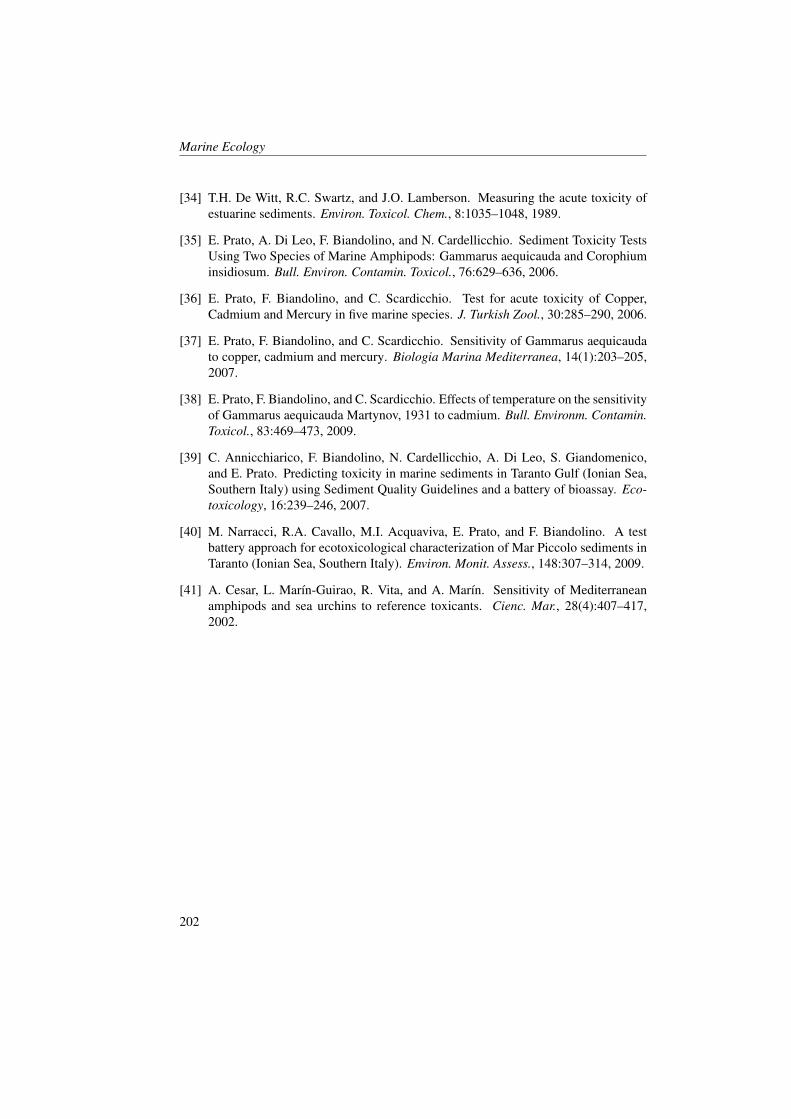
Marine Ecology
[34] T.H. De Witt, R.C. Swartz, and J.O. Lamberson. Measuring the acute toxicity ofestuarine sediments. Environ. Toxicol. Chem., 8:1035–1048, 1989.
[35] E. Prato, A. Di Leo, F. Biandolino, and N. Cardellicchio. Sediment Toxicity TestsUsing Two Species of Marine Amphipods: Gammarus aequicauda and Corophiuminsidiosum. Bull. Environ. Contamin. Toxicol., 76:629–636, 2006.
[36] E. Prato, F. Biandolino, and C. Scardicchio. Test for acute toxicity of Copper,Cadmium and Mercury in five marine species. J. Turkish Zool., 30:285–290, 2006.
[37] E. Prato, F. Biandolino, and C. Scardicchio. Sensitivity of Gammarus aequicaudato copper, cadmium and mercury. Biologia Marina Mediterranea, 14(1):203–205,2007.
[38] E. Prato, F. Biandolino, and C. Scardicchio. Effects of temperature on the sensitivityof Gammarus aequicauda Martynov, 1931 to cadmium. Bull. Environm. Contamin.Toxicol., 83:469–473, 2009.
[39] C. Annicchiarico, F. Biandolino, N. Cardellicchio, A. Di Leo, S. Giandomenico,and E. Prato. Predicting toxicity in marine sediments in Taranto Gulf (Ionian Sea,Southern Italy) using Sediment Quality Guidelines and a battery of bioassay. Eco-toxicology, 16:239–246, 2007.
[40] M. Narracci, R.A. Cavallo, M.I. Acquaviva, E. Prato, and F. Biandolino. A testbattery approach for ecotoxicological characterization of Mar Piccolo sediments inTaranto (Ionian Sea, Southern Italy). Environ. Monit. Assess., 148:307–314, 2009.
[41] A. Cesar, L. Marın-Guirao, R. Vita, and A. Marın. Sensitivity of Mediterraneanamphipods and sea urchins to reference toxicants. Cienc. Mar., 28(4):407–417,2002.
202
The Effect of Heavy Metals on BenthicForaminifera in the Gulf of Gela (SicilianChannel)
M. Musco1, A. Cuttitta1, S. Bonomo1, G. Tranchida1, A. Mazzola2, S.Vizzini2, C. Tramati2, A. Bonanno1, B. Patti1, G. Basilone1
1, Institute for Coastal Marine Environment, CNR, Capo Granitola (TP), Italy2, Department of Ecology, University of Palermo, [email protected]
Abstract
Benthic foraminifera are very sensitive to oceanographic parameter variations,to which they rapidly response through changes in the abundance and/or richnessof their associations and in morphological variations of their shell. Many stud-ies have used benthic foraminifera as bioindicators. We investigated recent benthicforaminiferal assemblages in the Gulf of Gela (Sicilian Channel, Mediterranean Sea),examining their relative abundance, specific richness and morphological abnormali-ties, to highlight a possible correlation with oceanographic features and the concen-tration of heavy metals in sediments. Sediment was sampled in summer 2006 usingbox corers in four stations at increasing distances from a point-source of industrialpollution. We performed hydrological characterization of the study area, grain sizeanalysis and heavy metal determinations in sediments, and quantitative and qualita-tive analyses of benthic foraminifera. Heavy metal analyses highlighted very highmercury and cadmium concentrations in the station nearest the pollution source, inwhich the Dominance index showed the minimum of population density. In conclu-sion, a positive correlation seems to exist between the abundance of foraminifera andthe concentration of cadmium and mercury in the sediment.
1 Introduction
The Gulf of Gela is located in the southerncoast of the island. Since 1962 the Petro-chemical Industry has been active in themiddle of the gulf, close to the city of Gela,where about five million tons of crude oilper year are refined, to produce LPG, gaso-line, diesel and pet-coke.At the end of the refining process, manyhighly dangerous substances, which in-clude mercury, cadmium, arsenic, etc, arereleased in the marine environment as
waste products.The other main pollutants of the area comefrom the massive presence of greenhouseson the coastal dunes of the Gela’s Plain [1].
Benthic foraminifera are one of the groupsof marine microorganisms often usedas bioindicators of pollution in marineecosystems. These marine protozoa canlive in different microhabitats and many ofthem have a mineralized shell.The peculiarity of benthic foraminifera istheir sensitivity to environmental varia-tion, to which they rapidly respond through

Marine Ecology
Figure 1: The Gulf of Gela and the sampling stations. P.I.G.: Petrochemical Industryof Gela; AIS: Atlantic Ionian Stream; ABV and ISV: Adventure Bank and Ionian SlopeVortexes.
changes in the abundance and/or richnessof their associations and in morphologicalvariations of their shell.Studies on the effects of pollution on ben-thic foraminifera began in the second halfof the last century: the innovative worksby Zalesny [2], Resig [3] and Watkins [4]were followed by several other studies thatused benthic foraminifera as indicators ofmarine pollution, particularly in coastal ar-eas [5, 6, 7, 8, 9, 10, 11, 12, 13, 14, 15, 16].Similar works were conducted in Italy in
coastal marine areas and in transition en-vironments [17, 18, 19, 20]. There aredifferent ways to use benthic foraminiferaas bioindicators of pollution: Frontalini &Coccioni [21], Samir & El-Din [15], andTriantaphillou et al. [22] corroborated theuse of shell deformation as biomarker ofheavy metals pollution, while Bergin etal. [23] and Geslin et al. [16] showedthe correspondence between distribution ofbenthic foraminifera and the concentrationof heavy metals in sediment. The princi-
204
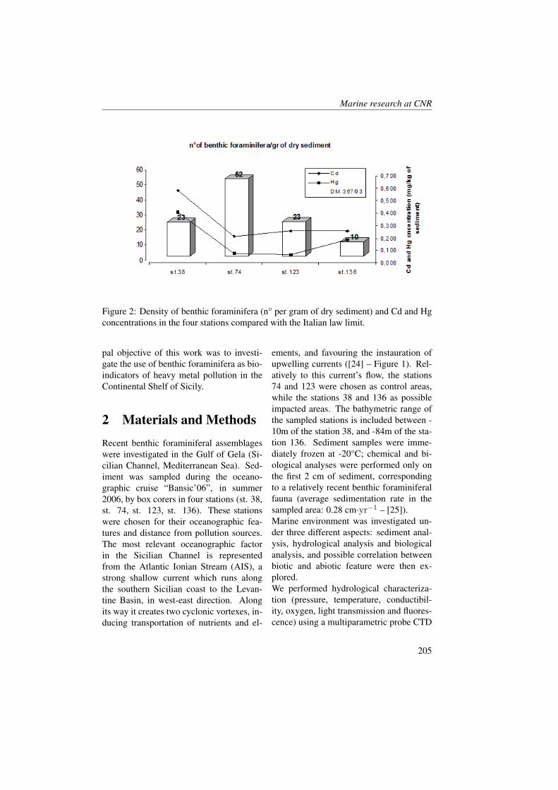
Marine research at CNR
Figure 2: Density of benthic foraminifera (n° per gram of dry sediment) and Cd and Hgconcentrations in the four stations compared with the Italian law limit.
pal objective of this work was to investi-gate the use of benthic foraminifera as bio-indicators of heavy metal pollution in theContinental Shelf of Sicily.
2 Materials and Methods
Recent benthic foraminiferal assemblageswere investigated in the Gulf of Gela (Si-cilian Channel, Mediterranean Sea). Sed-iment was sampled during the oceano-graphic cruise “Bansic’06”, in summer2006, by box corers in four stations (st. 38,st. 74, st. 123, st. 136). These stationswere chosen for their oceanographic fea-tures and distance from pollution sources.The most relevant oceanographic factorin the Sicilian Channel is representedfrom the Atlantic Ionian Stream (AIS), astrong shallow current which runs alongthe southern Sicilian coast to the Levan-tine Basin, in west-east direction. Alongits way it creates two cyclonic vortexes, in-ducing transportation of nutrients and el-
ements, and favouring the instauration ofupwelling currents ([24] – Figure 1). Rel-atively to this current’s flow, the stations74 and 123 were chosen as control areas,while the stations 38 and 136 as possibleimpacted areas. The bathymetric range ofthe sampled stations is included between -10m of the station 38, and -84m of the sta-tion 136. Sediment samples were imme-diately frozen at -20°C; chemical and bi-ological analyses were performed only onthe first 2 cm of sediment, correspondingto a relatively recent benthic foraminiferalfauna (average sedimentation rate in thesampled area: 0.28 cm·yr−1 – [25]).Marine environment was investigated un-der three different aspects: sediment anal-ysis, hydrological analysis and biologicalanalysis, and possible correlation betweenbiotic and abiotic feature were then ex-plored.We performed hydrological characteriza-tion (pressure, temperature, conductibil-ity, oxygen, light transmission and fluores-cence) using a multiparametric probe CTD
205
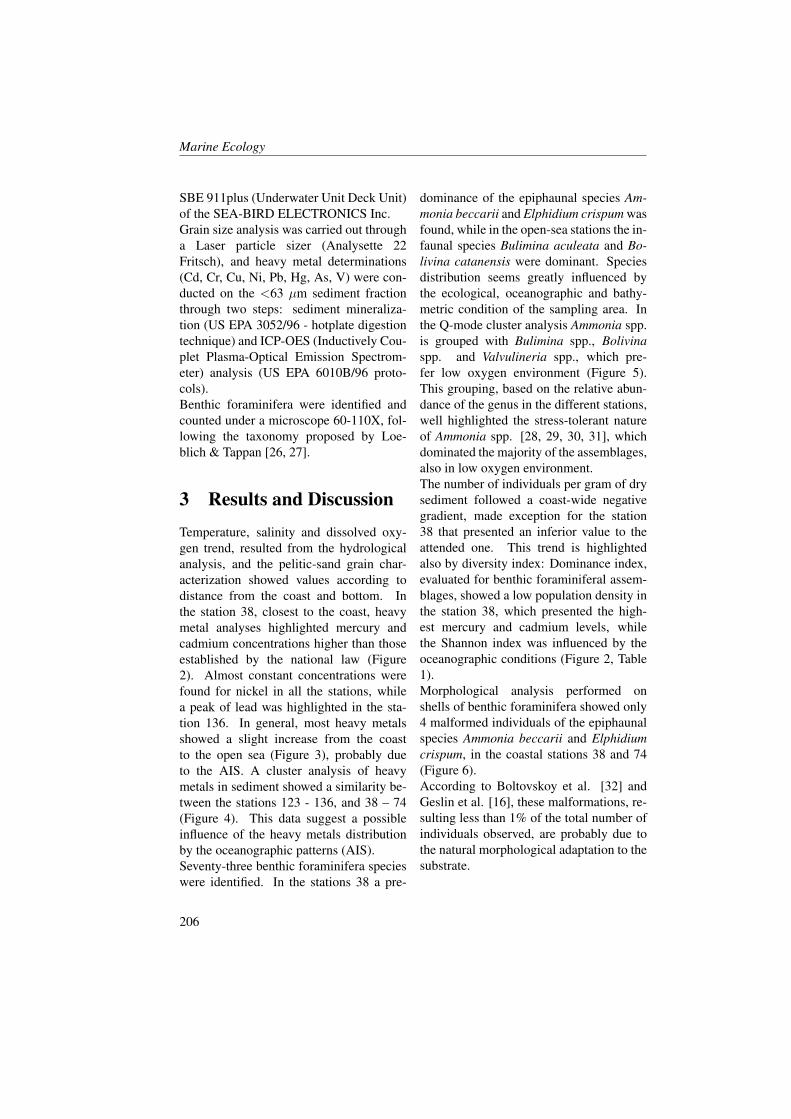
Marine Ecology
SBE 911plus (Underwater Unit Deck Unit)of the SEA-BIRD ELECTRONICS Inc.Grain size analysis was carried out througha Laser particle sizer (Analysette 22Fritsch), and heavy metal determinations(Cd, Cr, Cu, Ni, Pb, Hg, As, V) were con-ducted on the <63 µm sediment fractionthrough two steps: sediment mineraliza-tion (US EPA 3052/96 - hotplate digestiontechnique) and ICP-OES (Inductively Cou-plet Plasma-Optical Emission Spectrom-eter) analysis (US EPA 6010B/96 proto-cols).Benthic foraminifera were identified andcounted under a microscope 60-110X, fol-lowing the taxonomy proposed by Loe-blich & Tappan [26, 27].
3 Results and Discussion
Temperature, salinity and dissolved oxy-gen trend, resulted from the hydrologicalanalysis, and the pelitic-sand grain char-acterization showed values according todistance from the coast and bottom. Inthe station 38, closest to the coast, heavymetal analyses highlighted mercury andcadmium concentrations higher than thoseestablished by the national law (Figure2). Almost constant concentrations werefound for nickel in all the stations, whilea peak of lead was highlighted in the sta-tion 136. In general, most heavy metalsshowed a slight increase from the coastto the open sea (Figure 3), probably dueto the AIS. A cluster analysis of heavymetals in sediment showed a similarity be-tween the stations 123 - 136, and 38 – 74(Figure 4). This data suggest a possibleinfluence of the heavy metals distributionby the oceanographic patterns (AIS).Seventy-three benthic foraminifera specieswere identified. In the stations 38 a pre-
dominance of the epiphaunal species Am-monia beccarii and Elphidium crispum wasfound, while in the open-sea stations the in-faunal species Bulimina aculeata and Bo-livina catanensis were dominant. Speciesdistribution seems greatly influenced bythe ecological, oceanographic and bathy-metric condition of the sampling area. Inthe Q-mode cluster analysis Ammonia spp.is grouped with Bulimina spp., Bolivinaspp. and Valvulineria spp., which pre-fer low oxygen environment (Figure 5).This grouping, based on the relative abun-dance of the genus in the different stations,well highlighted the stress-tolerant natureof Ammonia spp. [28, 29, 30, 31], whichdominated the majority of the assemblages,also in low oxygen environment.The number of individuals per gram of drysediment followed a coast-wide negativegradient, made exception for the station38 that presented an inferior value to theattended one. This trend is highlightedalso by diversity index: Dominance index,evaluated for benthic foraminiferal assem-blages, showed a low population density inthe station 38, which presented the high-est mercury and cadmium levels, whilethe Shannon index was influenced by theoceanographic conditions (Figure 2, Table1).Morphological analysis performed onshells of benthic foraminifera showed only4 malformed individuals of the epiphaunalspecies Ammonia beccarii and Elphidiumcrispum, in the coastal stations 38 and 74(Figure 6).According to Boltovskoy et al. [32] andGeslin et al. [16], these malformations, re-sulting less than 1% of the total number ofindividuals observed, are probably due tothe natural morphological adaptation to thesubstrate.
206
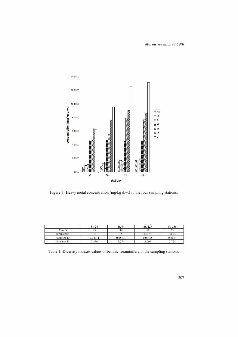
Marine research at CNR
Figure 3: Heavy metal concentration (mg/kg d.w.) in the four sampling stations.
Table 1: Diversity indexes values of benthic foraminifera in the sampling stations.
207
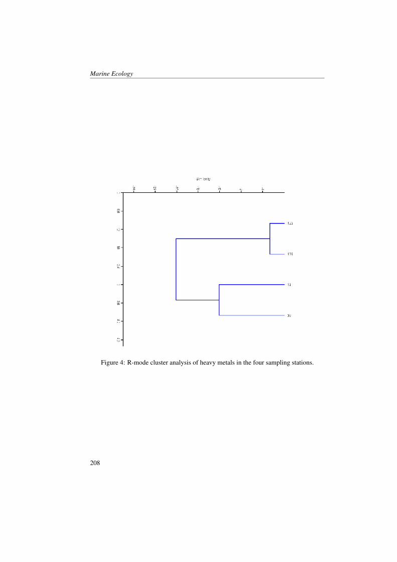
Marine Ecology
Figure 4: R-mode cluster analysis of heavy metals in the four sampling stations.
208
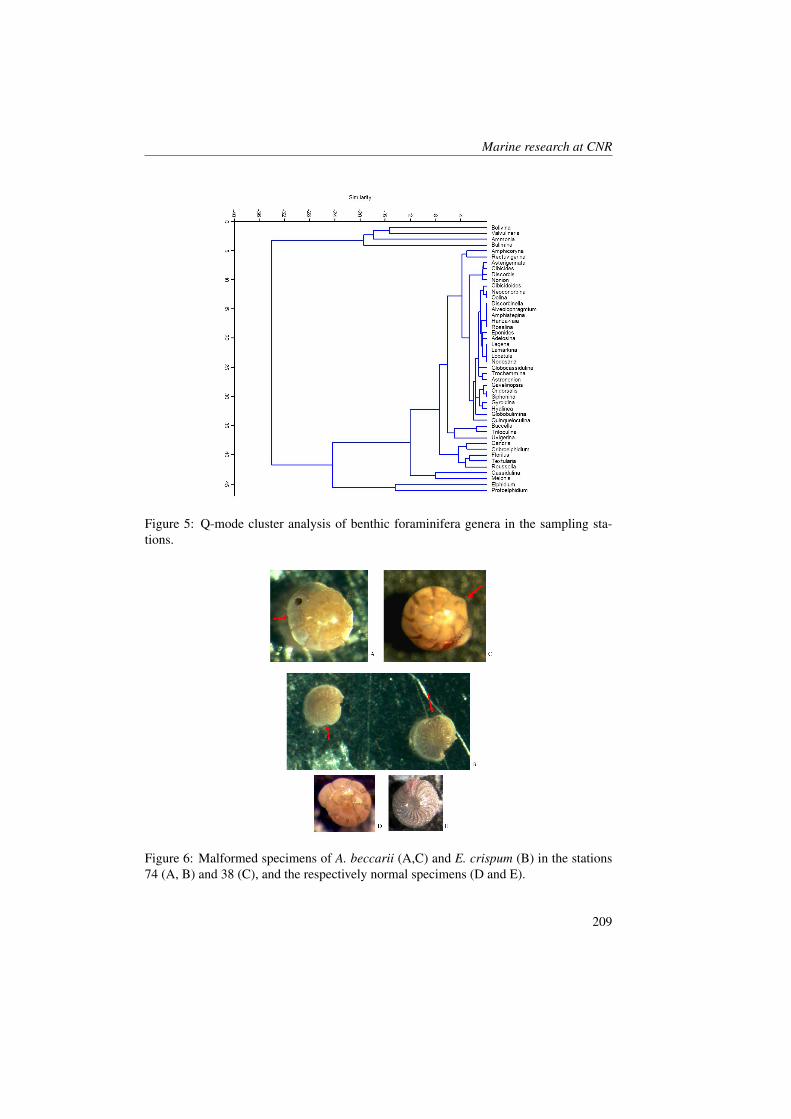
Marine research at CNR
Figure 5: Q-mode cluster analysis of benthic foraminifera genera in the sampling sta-tions.
Figure 6: Malformed specimens of A. beccarii (A,C) and E. crispum (B) in the stations74 (A, B) and 38 (C), and the respectively normal specimens (D and E).
209
Marine Ecology
4 Conclusions
Considering the results obtained in thisstudy, it seems that the high concentra-tion of the more toxic heavy metals (i.e.mercury and cadmium) in the sediment,
has a negative influence on the abundanceof benthic foraminifera, while distribu-tion and genera richness, as well as shellmalformations, seem to be due to natural(oceanographic, ecological and bathymet-ric) condition.
References[1] P. Russo, L. Carullo, and G. Tomaselli. Analisi del paesaggio rurale delle aree
“Natura 2000” di Gela per la comprensione delle dinamiche storiche di trasfor-mazione. IX Convegno Nazionale dell’Associazione Italiana di Ingegneria Agraria,memoria, pages 6–22, 2009.
[2] E.R. Zalesny. Foraminiferal ecology of Santa Monica Bay, California. Micropale-ontology, 5:101–126, 1959.
[3] J.M. Resig. Foraminiferal ecology around ocean outfalls off southern California.In: Pearson, P.A. (Ed.). Waste disposal in the marine environment. Pergamon press,London, page 104 – 121, 1960.
[4] J.G. Watkins. Foraminiferal ecology around the Orange Country, California, oceansewer outfall. Micropaleontology, 7:199–206, 1961.
[5] M.T. Venec-Peyre. Les foraminiferes et la pollution: etude de la microfaune dela Cale du Dourduff (embrouchure de la riviere de Morlaix). Cahiers de BiologieMarine, 22:25–33, 1981.
[6] R.L. Ellison, R. Broome, and R. Ogilvie. Foraminiferal response to trace metalcontamination in the Patapsco River and Baltimore Harbour, Maryland. PollutionBulletin, 17:419–423, 1986.
[7] J. Nagy and E. Alve. Temporal changes in foraminiferal faunas and impact of pol-lution in Sandebucta, Oslo Fjord. Marine Micropaleontology, 12:109–128, 1987.
[8] M.H. Caralp. Size and morphology of the benthic foraminifer Melonis barleeanumrelationships with marine oceanic matter. Journal of Foraminiferal Research,19:235–245, 1989.
[9] E. Alve. Benthic foraminifera in sediment cores reflecting heavy metal pollution inSørfjord, Western Norway. Journal of Foraminiferal Research, 21:1–19, 1991.
[10] A.R. Sharifi, I.W. Croudace, and R.L. Austin. Benthic foraminiferids as pollutionindicators in Southampton Water, southern England, UK. Journal of Micropaleon-tology, 10:109–113, 1991.
210
Marine research at CNR
[11] V. Yanko, J. Kronfeld, and A. Flexer. Response of benthic foraminifera to variouspollution sources: implications for pollution monitoring. Journal of ForaminiferalResearch, 24:1–17, 1994.
[12] V. Yanko, M. Ahmad, and M. Kaminski. Morphological deformities of benthicforaminiferal tests in response to pollution byheavymetals: implications for pollu-tion monitoring. Journal of Foraminiferal Research, 28:177–200, 1998.
[13] A.M. Samir. The response of benthic foraminifera and ostracods to various pol-lution sources: a study from two lagoons in Egypt. Journal of Foraminiferal Re-search, 30:83–98, 2000.
[14] J.P. Debenay, E. Tsakiridis, R. Soulard, and H. Grossel. Factor determining the dis-tribution of foraminiferal assemblages in port Joinville Harbour (Ile d’Yeu, France):the influence of pollution. Marine Micropaleontology, 43:75–118, 2001.
[15] A.M. Samir and A.B. El-Din. Benthic foraminiferal assemblages and morphologi-cal abnormalities as pollution proxies in two Egyptian bays. Marine Micropaleon-tology, 41:193–227, 2001.
[16] E. Geslin, J.P. Debenay, W. Duleba, and C. Bonetti. Morphological abnormalitiesof foraminiferal tests in Brazilian environments: comparison between polluted andnon-polluted areas. Marine Micropaleontology, 45:151–168, 2002.
[17] R. Coccioni. Benthic foraminifera as bioindicators of heavy metal pollution. A casestudy from the Goro Lagoon (Italy). Environmental Micropaleontology, Topics inGeobiology. Kluwer Academic/Plenum Publishers. NewYork, 15:71–103, 2000.
[18] R. Coccioni, A. Marsili, and A. Venturati. Foraminiferi e stress ambientale. In:R. Coccioni (2003) Verso la gestione integrata della costa del Monte San Bartolo:risultati di un progetto pilota. Quaderni del Centro di Geobiologia, 1:99–118, 2003.
[19] R. Coccioni, F. Frontalini, A. Marsili, and F. Troiani. Foraminiferi bentonici emetalli in traccia: implicazioni ambientali. In: R. Coccioni (2005) La dinamicaevolutiva della fascia costiera tra le foci dei fiumi Foglia e Metauro: verso la ges-tione integrata di una costa di elevato pregio ambientale. . Quaderni del Centro diGeobiologia, 3:57–92, 2005.
[20] R. Coccioni and A. Marsili. Monitoring in polluted transitional marine environ-ments using foraminifera bioindicators: a case study from the Venice lagoon (Italy).Abstract volume Geoitalia. Spoleto (Italy)., pages 327–328, 2005.
[21] F. Frontalini and R. Coccioni. Benthic foraminifera for heavy metal pollution moni-toring: A case study from the central Adriatic Sea coast of Italy. Estuarine, Coastaland Shelf Science, 76:404–417, 2008.
211
Marine Ecology
[22] M.V. Triantaphyllou, T. Tsourou, O. Koukousioura, and M.D. Dermitzakis.Foraminiferal and ostracod ecological patterns in coastal environments of SE An-dros Island (Middle Aegean Sea, Greece). Revue de micropaleontology, 48:279 –302, 2005.
[23] F. Bergin, F. Kucuksezgin, E. Uluturhan, I.F. Barut, E. Meric, N. Avsar, andA. Nazik. The response of benthic foraminifera and ostracoda to heavy metal pol-lution in Gulf of Izmir (Eastern Aegean Sea). Estuarine, Coastal and Shelf Science,66:368–386, 2006.
[24] A.R. Robinson, J. Sellschopp, A. Warn-Varnas, W.G. Leslie, C.J. Lozano, P.J. Ha-ley, L.A. Anderson, and P.F.J. Lermusiaux. The Atlantic Ionian Stream. Journal ofMarine Systems, 20:113–128, 1999.
[25] G. Tranchida, A. Bellanca, M. Angelone, A. Bonanno, L. Langone, S. Mazzola,R. Neri, and B. Patti. Chronological records of metal deposition in sediments fromthe Strait of Sicily, central Mediterranean: Assessing natural fluxes and anthro-pogenic alteration. Journal of Marine Systems, 79:157–152, 2010.
[26] A.R. Loeblich and H. Tappan. Foraminiferal Classification and Evolution. Journalof the Geological Society of India, 5:5–39, 1964.
[27] A.R. Loeblich and H. Tappan. Foraminiferal genera and their classification. VanNostrand Reinold Ed., New York, 1988.
[28] J.P. Debenay, J.J. Guillou, F. Redois, and E. Geslin. Distribution trends offoraminiferal assemblages in paralic environments: a base for using foraminiferaas bioindicators, in Martin, R. E. (ed.). Environmental Micropaleontology: TheApplication of Microfossils to Environmental Geology. Kluwer Academic/PlenumPublishers, New York, page 39–67, 2000.
[29] J.P. Debenay, L. Della Patrona, and H. Goguenheim. Colonization of coastal en-vironments by foraminifera: insight from shrimp ponds in New Caledonia (sw Pa-cific). The Journal of Foraminiferal Research, 39(4):249–266, 2009.
[30] J.P. Debenay and J.J. Guillou. Ecological transitions indicated by foraminiferalassemblages in paralic environments. Estuaries, 25:1107–1120, 2002.
[31] V. Yanko, A.J. Arnold, and W.C. Parker. Effects of marine pollution on benthicforaminifera. In: Modern Foraminifera, B. K. SEN GUPTA (Ed.), Kluwer Acad.Publ., New York, page 217, 1999.
[32] E. Boltovskoy, D.B. Scott, and F.S. Medioli. Morphological variations of benthicforaminiferal tests in response to changes in ecological parameters: a review. Jour-nal of Paleontology, 65:175–185, 1991.
212
A 20-Year Time-Series Analysis of Carbon Oxida-tion Rates in the Dark Waters of the Ionian Sea:the Microbial Response to the Global Changes
M. Azzaro, R. La FerlaInstitute for Coastal Marine Environment, CNR, Messina, [email protected]
Abstract
In the marine ecosystem the biological pump controls the export of biogenic car-bon from the surface layers down to the depth. In brief, through photosynthesisprocesses in the euphotic zone, this mechanism transforms the carbon dioxide intoorganic matter, the latter sinks to the waters below and at the same time is consumedby respiration with the production of metabolic CO2. However, during the formationof dense waters, a significant quantity of organic products is conveyed from the sur-face within the water mass and remineralized inside it, thereby altering the normalflow of the biological pump.In 1990 a transitional climatic event (EMT, Eastern Mediterranean Transient) haschanged not only the physical characteristics of the Mediterranean Sea but the micro-biological, too. The organic load advected from Aegean Sea has fuelled the deep-seabiota that has utilized most of the oxygen carried by the new water masses for thebiological oxidation. In this study the evolution of carbon dioxide production rates inthe deep Ionian Sea, before and during the Eastern Mediterranean Transient (EMT),is reported. The check of the carbon oxidation evolution has shown that EMT eventhas constituted a natural test for a different approach to the oceanic carbon sequestra-tion. Biogeochemical implications of accelerated rates of oxygen consumption andthen of CO2 sequestration in the Ionian Sea will be analysed and discussed in thetext.
1 IntroductionDuring the last 150 years, the global in-crease in the consumption of fossil fuels to-gether with the reduced capacity to removeCO2 due to deforestation, have caused adramatic input of carbon dioxide into theatmosphere [1]. The atmospheric carbondioxide levels increased by nearly 40%,from preindustrial levels to 2007 [2] andthis increase, is at least an order of mag-nitude faster than has occurred for millionsof years [3]. The resulting enhancement of
the natural Greenhouse Effect is temperedby oceanic uptake by sequestration of CO2
in the deep oceanic waters, which accountsfor nearly a third of anthropogenic carbonadded to the atmosphere [4, 5]. In fact, top-ical studies have supported the significantrole of the oceanic biological pump [6, 7]and continental shelf pump [8] with respectto the atmospheric CO2 build-up (Figure1).Option to store carbon dioxide in the oceanis a potential climate change mitigation that
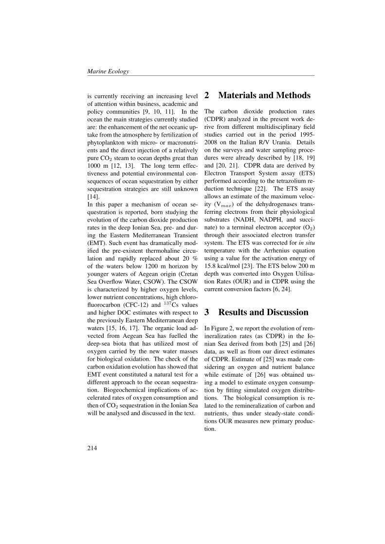
Marine Ecology
is currently receiving an increasing levelof attention within business, academic andpolicy communities [9, 10, 11]. In theocean the main strategies currently studiedare: the enhancement of the net oceanic up-take from the atmosphere by fertilization ofphytoplankton with micro- or macronutri-ents and the direct injection of a relativelypure CO2 steam to ocean depths great than1000 m [12, 13]. The long term effec-tiveness and potential environmental con-sequences of ocean sequestration by eithersequestration strategies are still unknown[14].In this paper a mechanism of ocean se-questration is reported, born studying theevolution of the carbon dioxide productionrates in the deep Ionian Sea, pre- and dur-ing the Eastern Mediterranean Transient(EMT). Such event has dramatically mod-ified the pre-existent thermohaline circu-lation and rapidly replaced about 20 %of the waters below 1200 m horizon byyounger waters of Aegean origin (CretanSea Overflow Water, CSOW). The CSOWis characterized by higher oxygen levels,lower nutrient concentrations, high chloro-fluorocarbon (CFC-12) and 137Cs valuesand higher DOC estimates with respect tothe previously Eastern Mediterranean deepwaters [15, 16, 17]. The organic load ad-vected from Aegean Sea has fuelled thedeep-sea biota that has utilized most ofoxygen carried by the new water massesfor biological oxidation. The check of thecarbon oxidation evolution has showed thatEMT event constituted a natural test for adifferent approach to the ocean sequestra-tion. Biogeochemical implications of ac-celerated rates of oxygen consumption andthen of CO2 sequestration in the Ionian Seawill be analysed and discussed in the text.
2 Materials and Methods
The carbon dioxide production rates(CDPR) analyzed in the present work de-rive from different multidisciplinary fieldstudies carried out in the period 1995-2008 on the Italian R/V Urania. Detailson the surveys and water sampling proce-dures were already described by [18, 19]and [20, 21]. CDPR data are derived byElectron Transport System assay (ETS)performed according to the tetrazolium re-duction technique [22]. The ETS assayallows an estimate of the maximum veloc-ity (Vmax) of the dehydrogenases trans-ferring electrons from their physiologicalsubstrates (NADH, NADPH, and succi-nate) to a terminal electron acceptor (O2)through their associated electron transfersystem. The ETS was corrected for in situtemperature with the Arrhenius equationusing a value for the activation energy of15.8 kcal/mol [23]. The ETS below 200 mdepth was converted into Oxygen Utilisa-tion Rates (OUR) and in CDPR using thecurrent conversion factors [6, 24].
3 Results and Discussion
In Figure 2, we report the evolution of rem-ineralization rates (as CDPR) in the Io-nian Sea derived from both [25] and [26]data, as well as from our direct estimatesof CDPR. Estimate of [25] was made con-sidering an oxygen and nutrient balancewhile estimate of [26] was obtained us-ing a model to estimate oxygen consump-tion by fitting simulated oxygen distribu-tions. The biological consumption is re-lated to the remineralization of carbon andnutrients, thus under steady-state condi-tions OUR measures new primary produc-tion.
214
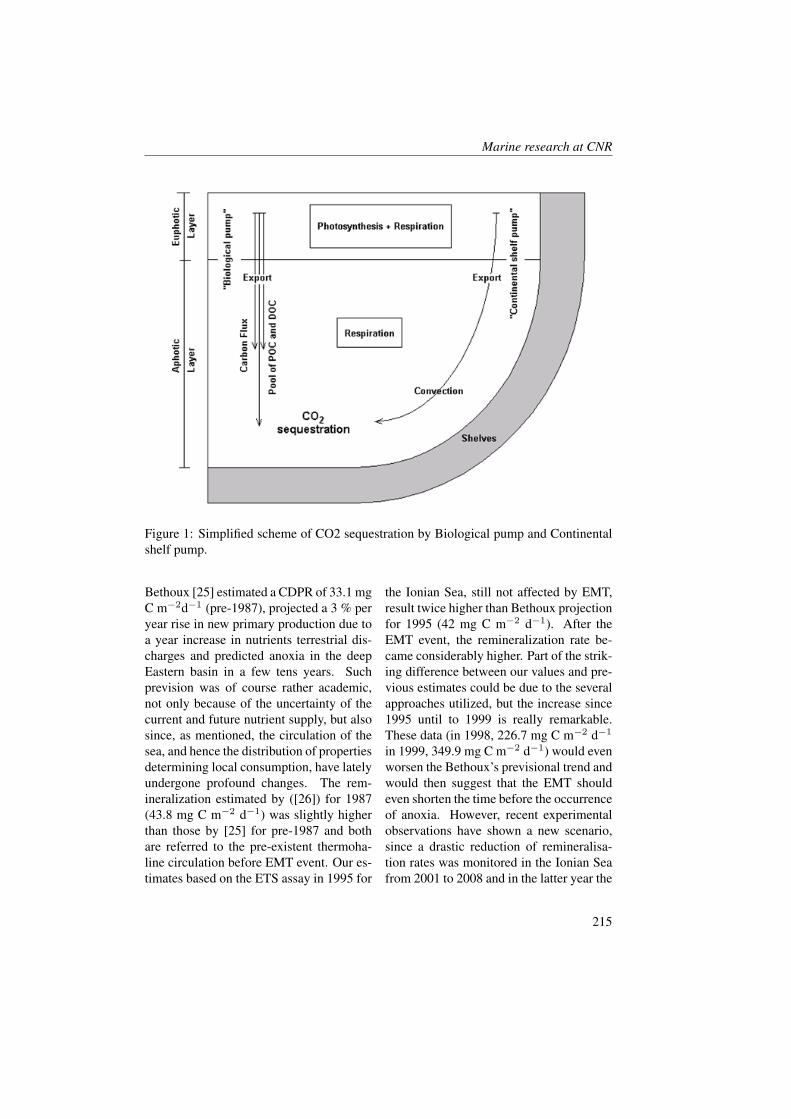
Marine research at CNR
Figure 1: Simplified scheme of CO2 sequestration by Biological pump and Continentalshelf pump.
Bethoux [25] estimated a CDPR of 33.1 mgC m−2d−1 (pre-1987), projected a 3 % peryear rise in new primary production due toa year increase in nutrients terrestrial dis-charges and predicted anoxia in the deepEastern basin in a few tens years. Suchprevision was of course rather academic,not only because of the uncertainty of thecurrent and future nutrient supply, but alsosince, as mentioned, the circulation of thesea, and hence the distribution of propertiesdetermining local consumption, have latelyundergone profound changes. The rem-ineralization estimated by ([26]) for 1987(43.8 mg C m−2 d−1) was slightly higherthan those by [25] for pre-1987 and bothare referred to the pre-existent thermoha-line circulation before EMT event. Our es-timates based on the ETS assay in 1995 for
the Ionian Sea, still not affected by EMT,result twice higher than Bethoux projectionfor 1995 (42 mg C m−2 d−1). After theEMT event, the remineralization rate be-came considerably higher. Part of the strik-ing difference between our values and pre-vious estimates could be due to the severalapproaches utilized, but the increase since1995 until to 1999 is really remarkable.These data (in 1998, 226.7 mg C m−2 d−1
in 1999, 349.9 mg C m−2 d−1) would evenworsen the Bethoux’s previsional trend andwould then suggest that the EMT shouldeven shorten the time before the occurrenceof anoxia. However, recent experimentalobservations have shown a new scenario,since a drastic reduction of remineralisa-tion rates was monitored in the Ionian Seafrom 2001 to 2008 and in the latter year the
215
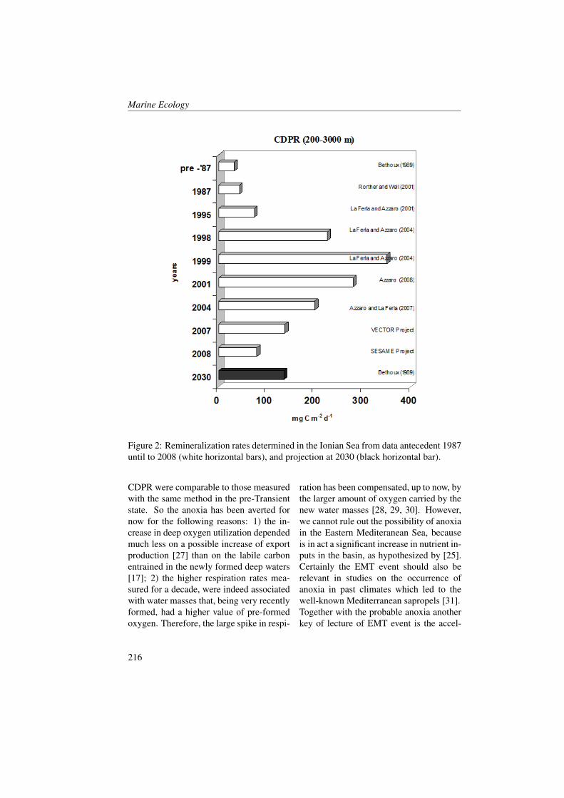
Marine Ecology
Figure 2: Remineralization rates determined in the Ionian Sea from data antecedent 1987until to 2008 (white horizontal bars), and projection at 2030 (black horizontal bar).
CDPR were comparable to those measuredwith the same method in the pre-Transientstate. So the anoxia has been averted fornow for the following reasons: 1) the in-crease in deep oxygen utilization dependedmuch less on a possible increase of exportproduction [27] than on the labile carbonentrained in the newly formed deep waters[17]; 2) the higher respiration rates mea-sured for a decade, were indeed associatedwith water masses that, being very recentlyformed, had a higher value of pre-formedoxygen. Therefore, the large spike in respi-
ration has been compensated, up to now, bythe larger amount of oxygen carried by thenew water masses [28, 29, 30]. However,we cannot rule out the possibility of anoxiain the Eastern Mediteranean Sea, becauseis in act a significant increase in nutrient in-puts in the basin, as hypothesized by [25].Certainly the EMT event should also berelevant in studies on the occurrence ofanoxia in past climates which led to thewell-known Mediterranean sapropels [31].Together with the probable anoxia anotherkey of lecture of EMT event is the accel-
216

Marine research at CNR
erated carbon dioxide sequestration regis-tered in the deep water of Ionian Sea. Onecontributing factor to the accelerated deep-water CDPR might be the untypically hightemperature in the deep Mediterranean Sea(> 12 °C) that is not a limit to the micro-bial metabolism. Precedent studies has al-ready evidenced the importance of carbonsequestration in the deepest with respect tothe shallowest layers in the MediterraneanSea in comparison to oceans [32, 18].The unusual CO2 sequestration registeredduring EMT event highlighted that deepbasins do not constitute only an inert sinksof carbon dioxide but could act quickly incarbon sequestration mitigating effect ofthe climate changes on regional scale.Extension on a global scale of the EMT ex-periment is conceptually feasible but needat least the control of three main factors:water temperature, available organic sub-strates, oxygen levels. Deep-water tem-perature in the oceans is lower than in theMediterranean Sea and could affect the mi-crobial carbon sequestration for about 40% [30]. It is well known that the ma-jority of dissolved organic matter in thedeep ocean is refractory, then a naturalevent (e.g. EMT) or anthropogenic activityshould consider the injection of labile eas-ily oxidable DOC. During the EMT event,pre-formed oxygen was driven by CSOWin the Eastern Mediterranean depth. Hencea constant balance between oxidable or-
ganic substrate and oxygen level must bemaintain with the aim of avoiding anoxia.
4 ConclusionsThe occurrence of changing patterns in mi-crobial biogeochemistry has emphasizedthe Mediterranean vulnerability to climatechanges, confirming that the export of bio-genic carbon is partially driven by the bi-ological pump and enhanced by lateral ad-vection.The EMT event resulted a particular caseof continental shelf pump that has signifi-cantly affected the deep respiration in theIonan Sea. Nevertheless the occurrence ofanoxia in a shorter time than Bethoux pre-vision is removed by the larger amount ofoxygen carried by the younger Aegean wa-ter masses.In the context of ocean sequestration, theEMT resulted a natural test which focusedthe possible role of oceanic depths in mit-igating the climate changes and then con-tributing to dump atmospheric CO2 build-up.
5 AcknowledgementsThe research has been supported by theItalian VECTOR Project, by the EUSESAME Project and by the funds ofRSTL-CNR cod.483.
References[1] E.T. Sundquist. Geological perspectives on carbon doxide and the carbon cycle. In:
The carbon cycle and atmospheric CO2: Natural variations archean to present. Eds.E.T. Sundquist, W.S. Broecker. 32:89–98, 1985.
[2] S. Solomon, D. Quin, M. Manning, Z. Chen, and M. Marquis. Climate Change
217
Marine Ecology
2007: The Physical ScienceBasis: Contribution of Working Group I to the FourthAssessment Report of the Intergovernmental Panel on Climate Change. 2007.
[3] S.C. Doney and D.S. Schimel. Carbon and climate system coupling on timescalesfrom the Precambrian to the Anthropocene. Annual Review of Environment andResources, 32:31–66, 2007.
[4] C.L. Sabine and R.A. Feely. The oceanic sink for carbon dioxide. In: GreenhouseGas Sinks, Eds. D. Reay, N. Hewitt, J. Grace, K. Smith. pages 31–49, 2007.
[5] C.L. Sabine, R.A. Feely, N. Gruber, R.M. Key, and K. Lee. The oceanic sink foranthropogenic CO2. Science, 305:367–371, 2004.
[6] T.T. Packard, M. Denis, M. Rodier, and P. Garfield. Deep-ocean metabolic CO2
production: calculations from ETS activity. Deep-Sea Research Part I, 35:371–382, 1988.
[7] K. L. Smith Jr., H. A. Ruhl, B. J. Bett, D. S. M. Billett, R. S. Lampitt, andR. S. Kaufmann. Climate, carbon cycling, and deep-ocean ecosystems. PNAS,106(46):19211–1921, 2009.
[8] H. Thomas, Y. Bozec, K. Elkalay, and H. J. W. De Baar. Enhanced open oceanstorage of CO2 from shelf sea pumping. Science, 304:1005–1008, 2004.
[9] Y. Fujioka, M. Ozaki, K. Takeuchi, Y. Shindi, and H. Herzog. Cost comparison invarious CO2 ocean disposal options. Energy conversion and management, 38:273–277, 1997.
[10] H. Herzog, E. Adams, D. Auerbach, and J. Caulfield. Environmental impacts ofocean disposal of CO2. Energy conversion and management, 37(6-8):999–1005,1996.
[11] G.H. Rau and K. Caldeira. Enhanced carbonate dissolution: A means of seques-tering waste CO2 as ocean bicarbonate. Energy Conversion and Management,40:1803–1813, 1999.
[12] P. G. Brewer, E. T. Peltzer, G. Friederich, I. Aya, and K. Yamane. Experiments onthe ocean sequestration of fossil fuel CO2: pH measurements and hydrate forma-tion. Marine Chemistry, 72:83–93, 2000.
[13] P.W. Boyd, T. Jickells, C.S. Law, S. Blain, E. A. Boyle, K.O. Buesseler, K.H.Coale, J.J. Cullen, H.J.W. de Baar, M. Follows, M. Harvey, C. Lancelot, M. Lev-asseur, N.P.J. Owens, R. Pollard, R.B. Rivkin, J. Sarmiento, V. Schoemann, andV. Smetace. Mesoscale Iron Enrichment Experiments 1993-2005: Synthesis andFuture Directions. Science, 315(5812):612–617, 2007.
218
Marine research at CNR
[14] K.O. Buesseler, S.C. Doney, D.M. Karl, P.W. Boyd, K. Caldeira, F. Chai, K.H.Coale, H.J.W. de Baar, P.G. Falkowski, K.S. Johnson, R.S. Lampitt, A.F. Michaels,S.W.A. Naqvi, V. Smetacek, S. Takeda, and A.J. Watson. Ocean iron fertilization:Moving forward in a sea of uncertainty. Science, 319:162–163, 2008.
[15] W. Roether and B. Klein. The great Eastern Mediterranean deep-water transient.Rapport Commission internationale Mer Mediterranee, 35:12–15, 1998.
[16] C. Papucci and P. Delfanti. 137Cs distribution in the eastern Mediterranean Sea:recent changes and future trends. Science of Total Environment, 237:67–75, 1999.
[17] A. Seritti, B.B. Manca, C. Santinelli, E. Murru, A. Boldrin, and L. Nannicini. Re-lationships between dissolved organic carbon (DOC) and water mass structures inthe Ionian Sea (winter 1999). Journal Geophysical Research, 108(C9):8112, 2003.
[18] R. La Ferla and M. Azzaro. Microbial respiration in the Levantine Sea: evolution ofthe oxidative processes in relation to the main Mediterranean water masses. Deep-Sea Research Part I, 48:2147–2159, 2001.
[19] R. La Ferla and M. Azzaro. Metabolic CO2 production in the Mediterranean Sea:a study basin for estimating carbon budget in the sea. Scientia Marina, 68:57–64,2004.
[20] R. La Ferla, F. Azzaro, M. Azzaro, G. Caruso, F. Decembrini, M. Leonardi, G. Mai-mone, L.S. Monticelli, F. Raffa, C. Santinelli, R. Zaccone, and M. Ribera d’Alcala.Microbial contribution to carbon biogeochemistry in the Central MediterraneanSea: Variability of activities and biomass. Journal of Marine Systems, 57:146–166,2005.
[21] M. Azzaro and R. La Ferla. Accelerati tassi di sequestro di anidride carbonicanelle acque profonde del Mediterraneo Orientale durante il Transiente. In: Clima eCambiamenti Climatici le attivita di ricerca del CNR. Eds. B. Carli, G. Cavarretta,M. Colacino, S. Fuzzi. pages 505–508, 2007.
[22] T.T. Packard and P.J.-LeB Williams. Rates of respiratory oxygen consumption andelectron transport in surface sea water from the Northwest Atlantic. OceanologicaActa, 4:351–358, 1981.
[23] T.T. Packard, A.H. Devol, and F.D. King. The effect of temperature on the respira-tory electron transport system in marine plankton. Deep-Sea Research, 22:237–249,1975.
[24] M. Azzaro, R. La Ferla, and F. Azzaro. Microbial respiration in the aphotic zone ofthe Ross Sea (Antarctica). Marine Chemistry, 99(1-4):199–209, 2006.
[25] J.P. Bethoux. Oxygen consumption, new production, vertical advection and en-vironmental evolution in the Mediterranean Sea. Deep-Sea Research Part I,36(5):769–781, 1989.
219

Marine Ecology
[26] W. Roether and R. Well. Oxygen consumption in the Eastern Mediterranean. Deep-Sea Research Part I, 48:1535–1551, 2001.
[27] K. Stratford and K. Haines. Modelling nutrient cycling during the Eastern Mediter-ranean transient event 1987-1995 and beyond. Geophysical Research Letters, 33-34:51–62, 2002.
[28] W. Roether, B.B. Manca, B. Klein, D. Bregant, D. Georgopoulos, V. Beitzel, V. Ko-vacevic, and A. Luchetta. Recent changes in the Eastern Mediterranean deep water.Science, 271:333–335, 1996.
[29] B. Klein, W. Roether, N. Kress, B.B. Manca, M. Ribera d’Alcala, E. Souverme-zoglou, A. Teocharis, G. Civitarese, and A. Luchetta. Accelerated oxygen con-sumption in eastern Mediterranean deep waters following the recent changes inthermohaline circulation. Journal Geophysical Research, 108(C9):8107, 2003.
[30] R. La Ferla, M. Azzaro, G. Civitarese, and M. Ribera d’Alcala. Distribution patternsof carbon oxidation in the Eastern Mediterranean Sea: evidence of changes in theremineralization processes. Journal of Geophysical Research, 108(C9):8111, 2003.
[31] E.J. Rohling. Review and new aspects concerning the formation of Eastern Mediter-ranean sapropels. Marine Geology, 122:1–28, 1994.
[32] J.P. Christensen, T.T. Packard, F.Q. Dortch, H.J. Minas, J.C. Gascard, C. Richez,and P.C. Garfield. Carbon oxidation in the deep Mediterranean Sea: evidence fordissolved organic carbon source. Global Biogeochemical Cycles, 3:315–335, 1989.
220

Settlement and Habitat of Juvenile EuropeanSpiny Lobster Palinurus Elephas (Fabricius, 1787)(Crustacea Decapoda) in the North Western Sicil-ian Coasts
M. Gristina1, G. Garofalo2, F. Fiorentino1
1, Institute for Coastal Marine Environment, CNR, Mazara del Vallo (TP), Italy2, Institute for Applied Mathematics “Mauro Picone”, CNR, Roma, [email protected]
Abstract
The ecological and commercial value of species of the genera Palinuridae is nowwidely recognized throughout the European continent. These species present a com-plex life cycle, with slow growth rate and a high size at maturity. As a consequence,these species are particularly susceptible to fishing pressure and the management andconservation of this resource requires specific attention. P. elephas is considered avulnerable species mainly due to the high age-dependent mortality of adults and sub-adults individuals, which consequently reduces fishing recruitment and that mightlead to an ecological bottleneck for this species limiting population growth.With these notions in mind, this study aimed to identify the settlement stage of Pal-inurus elephas and to describe the preferred microhabitat for juveniles (Fabricius,1787), along the north-western coast of Sicily (Isola delle Femmine – Palermo).Furthermore, on the basis of field observations, we tested in a controlled environ-ment, the geometric features of the substrate needed for P. elephas settlement, Thiswas done to propose suitable artificial structures that might favor or facilitate the set-tlement of P. elephas and that might protect juveniles during their benthic life stageas well as reducing natural mortality.
1 Introduction
Due to their important commercial value,lobsters represent one of the main target forartisanal fisheries and, even if catches aresporadic and reduced, this fishery has beenactive over the years. Thus, almost all P.elephas populations in the MediterraneanSea are evidently overexploited [1, 2]. De-spite its important economical and ecolog-ical value, the ecology of P. elephas stockspresents large knowledge gaps and veryfew attempts have been made to achieve
a sustainable exploitation of this resource.Lobsters are generally characterized by pe-culiar life cycle which involves a longpelagic larval stage (from 5 to 12 monthsdepending on the species), with two de-velopment stages (namely Phlyllosoma andPuerulus), a juvenile benthic stage (post-puerulus) and an adult benthic stage. Inaddition, lobsters present a slow growthrate and they reach a late size at matu-rity (4/5years) [3]. Consequently, lobstersare particularly susceptible to fishing ac-tivities that are not managed or regulated.
Marine Ecology
Furthermore, the high natural mortalityexperienced in the post-pueruli stage re-duces dramatically recruitment, hence cre-ating a bottleneck which prevents popula-tion growth.Experiments carried out in situ and in thelaboratory on Palinuridae, both in the trop-ical and temperate regions, demonstratedthe importance of appropriate artificial sub-strates to increase larval settlement andfor the survival of juveniles. However,at present such experiments are not avail-able for P. elephas. Only recently Diaz etal. [4] provided some indications on habi-tat preference by P. elephas in the SpanishMediterranean.This study aims at filling the present gapson the ecology of P. elephas and to providenew insights on the biology and ecology ofthe juvenile’s stage of this species.Specifically, this study has the followingobjectives:1. to identify the season during which
occurs the transition from the pelagicstage (phyllosoma) to the benthic stage(post-puerulus)
2. to describe the features of the preferredhabitat of P. elephas juveniles (substratetype, shape and slope)
3. to assess the depth range where thehighest number of juveniles is recorded.
2 MethodsField Studies - Evaluation of habitat char-acteristics and settlement period for P. ele-phas A visual census was carried out onP. elephas juveniles in the two study ar-eas (Isola and Barcarello). Visual censuswas done by scuba diving every 15 daysbetween May and October 2005 and aftera short break during the winter (November2005 to February 2006), scuba activities
were resumed (March to November 2006).For each area, sampling was performed atfour depth ranges (5-10, 10-15, 15-20 and20-25m). At each depth range, each of thetwo divers carried out 2 transect for 5 min-utes, with a interval of ½ a minute in be-tween.Thus, for each depth range, 4 transectswere run, of 5 mins. each, for an ap-proximate area of 25 m2. data was ex-pressed in n of individuals/m2 and averagefor the 4 transects were obtained. To iden-tify the preferred substrate for P. elephasjuveniles, when an individual was founddivers recorded slope and orientation ofrefuge, type of refuge, distance from thebottom, habitat type (rocks, cliffs, detri-tus). We compared the preferred schel-ter features by the log-likelihood ratio testfor goodness of fit (G-test) to reveal anypositional bias. The shelter preference oflobsters was compared to expected valuesfrom a Poisson distribution by the G-test[5] with Williams’ correction.
3 Mesocosm studies
Individuals used in the experiment werecaptured with seine nets from local fisher-men, handled and transported carefully tothe laboratory facility as soon as possibleafter landing. For the experiment, we useda number of seawater tanks with a recircu-lation system (water flow 56±7,3 l min-1),with a water residency time of 12 hours.Temperature and salinity in the seawatersystem was monitored daily during thewhole length of the experiment. Tem-perature and salinity values never differedamong tanks (17,9 – 18,3 °C; 37,5 ppt).Each individual of P. elephas was mea-sured prior to be introduced in the tanks;carapace length (LC), width (LargC), total
222
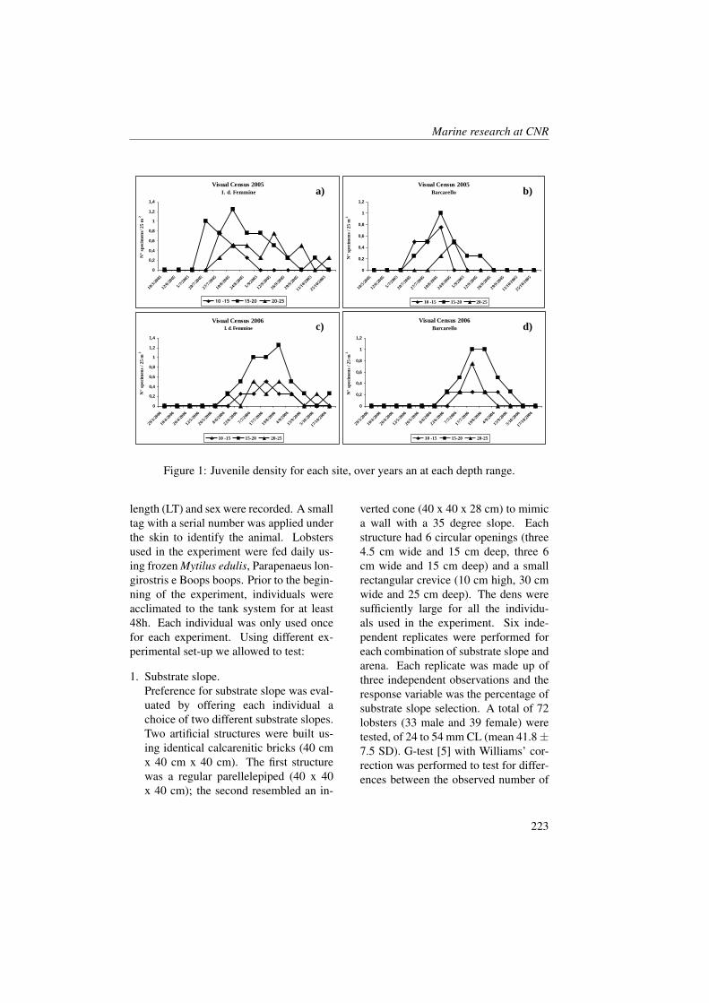
Marine research at CNR
Visual Census 2005
I. d. Femmine
0
0,2
0,4
0,6
0,8
1
1,2
1,4
10/3/2
005
12/6/2
005
5/7/2
005
20/7/2
005
27/7/2
005
10/8/2
005
24/8/2
005
5/9/2
005
12/9/2
005
26/9/2
005
29/9/2
005
11/10/
2005
25/10/
2005
N°
spec
imen
s/ 2
5 m
2
10 -15 15-20 20-25
Visual Census 2005
Barcarello
0
0,2
0,4
0,6
0,8
1
1,2
10/5/2
005
12/6/2
005
5/7/2
005
20/7/2
005
27/7/2
005
10/8/2
005
24/8/2
005
5/9/2
005
12/9/2
005
26/9/2
005
29/9/2
005
11/10/
2005
25/10/
2005
N°
spec
imen
s / 2
5 m
2
10 -15 15-20 20-25
Visual Census 2006
I. d. Femmine
0
0,2
0,4
0,6
0,8
1
1,2
1,4
29/3/2
006
10/4/2
006
26/4/2
006
12/5/2
006
26/5/2
006
8/6/2
006
22/6/2
006
7/7/2
006
17/7/2
006
19/8/2
006
4/9/2
006
15/9/2
006
5/10/2
006
17/10/
2006
N°
spec
imen
s / 2
5 m
2
10 -15 15-20 20-25
Visual Census 2006
Barcarello
0
0,2
0,4
0,6
0,8
1
1,2
29/3/2
006
10/4/2
006
26/4/2
006
12/5/2
006
26/5/2
006
8/6/2
006
22/6/2
006
7/7/2
006
17/7/2
006
19/8/2
006
4/9/2
006
15/9/2
006
5/10/2
006
17/10/
2006
N°
spec
imen
s / 2
5 m
2
10 -15 15-20 20-25
a) b)
c) d)
Figure 1: Juvenile density for each site, over years an at each depth range.
length (LT) and sex were recorded. A smalltag with a serial number was applied underthe skin to identify the animal. Lobstersused in the experiment were fed daily us-ing frozen Mytilus edulis, Parapenaeus lon-girostris e Boops boops. Prior to the begin-ning of the experiment, individuals wereacclimated to the tank system for at least48h. Each individual was only used oncefor each experiment. Using different ex-perimental set-up we allowed to test:
1. Substrate slope.Preference for substrate slope was eval-uated by offering each individual achoice of two different substrate slopes.Two artificial structures were built us-ing identical calcarenitic bricks (40 cmx 40 cm x 40 cm). The first structurewas a regular parellelepiped (40 x 40x 40 cm); the second resembled an in-
verted cone (40 x 40 x 28 cm) to mimica wall with a 35 degree slope. Eachstructure had 6 circular openings (three4.5 cm wide and 15 cm deep, three 6cm wide and 15 cm deep) and a smallrectangular crevice (10 cm high, 30 cmwide and 25 cm deep). The dens weresufficiently large for all the individu-als used in the experiment. Six inde-pendent replicates were performed foreach combination of substrate slope andarena. Each replicate was made up ofthree independent observations and theresponse variable was the percentage ofsubstrate slope selection. A total of 72lobsters (33 male and 39 female) weretested, of 24 to 54 mm CL (mean 41.8±7.5 SD). G-test [5] with Williams’ cor-rection was performed to test for differ-ences between the observed number of
223
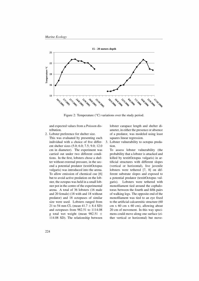
Marine Ecology
15 - 20 meters depth
13
16
19
22
25
10/5/2005
5/7/2005
27/7/2005
24/8/2005
12/9/2005
29/9/2005
25/10/2005
18/3/2006
10/4/2006
12/5/2006
8/6/2006
7/7/2006
19/8/2006
15/9/2006
17/10/2006
Tem
per
atu
re °
C
Figure 2: Temperature (°C) variations over the study period.
and expected values from a Poisson dis-tribution.
2. Lobster preference for shelter size.This was evaluated by presenting eachindividual with a choice of five differ-ent shelter sizes (5.0; 6.0; 7.5; 9.0; 12.0cm in diameter). The experiment wascarried out under two different condi-tions. In the first, lobsters chose a shel-ter without external pressure, in the sec-ond a potential predator (textitOctopusvulgaris) was introduced into the arena.To allow emission of chemical cue [6]but to avoid active predation on the lob-ster, the octopus was held in a small lob-ster pot in the centre of the experimentalarena. A total of 36 lobsters (16 maleand 20 female) (18 with and 18 withoutpredator) and 18 octopuses of similarsize were used. Lobsters ranged from21 to 54 mm CL (mean 41.7 ± 8.4 SD)and octopuses from 982.51 to 1114.08g total wet weight (mean 982.51 ±114.08 SD). The relationship between
lobster carapace length and shelter di-ameter, in either the presence or absenceof a predator, was modeled using leastsquares linear regression.
3. Lobster vulnerability to octopus preda-tion.To assess lobster vulnerability (theprobability that a lobster is attacked andkilled by textitOctopus vulgaris) in ar-tificial structures with different slopes(vertical or horizontal), live juvenilelobsters were tethered [7, 8] on dif-ferent substrate slopes and exposed toa potential predator (textitOctopus vul-garis). Lobsters were tethered withmonofilament tied around the cephalo-torax between the fourth and fifth pairsof walking legs. The opposite end of themonofilament was tied to an eye fixedto the artificial calcarenitic structure (60cm x 60 cm x 60 cm), allowing about20 cm of movement. In this way speci-mens could move along one surface (ei-ther vertical or horizontal) but move-
224
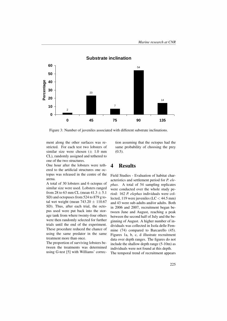
Marine research at CNR
Substrate inclination
2
23
7
54
14
0
10
20
30
40
50
60
0 45 75 90 135
Pe
rce
nta
ge
Figure 3: Number of juveniles associated with different substrate inclinations.
ment along the other surfaces was re-stricted. For each test two lobsters ofsimilar size were chosen (± 1.0 mmCL), randomly assigned and tethered toone of the two structures.One hour after the lobsters were teth-ered to the artificial structures one oc-topus was released in the centre of thearena.A total of 30 lobsters and 6 octopus ofsimilar size were used. Lobsters rangedfrom 28 to 63 mm CL (mean 41.3± 5.1SD) and octopuses from 524 to 879 g to-tal wet weight (mean 743.20 ± 110.67SD). Thus, after each trial, the octo-pus used were put back into the stor-age tank from where twenty-four otherswere then randomly selected for furthertrials until the end of the experiment.These procedure reduced the chance ofusing the same predator in the sametreatment more than once.The proportion of surviving lobsters be-tween the treatments was determinedusing G-test [5] with Williams’ correc-
tion assuming that the octopus had thesame probability of choosing the prey(0.5).
4 Results
Field Studies - Evaluation of habitat char-acteristics and settlement period for P. ele-phas. A total of 54 sampling replicateswere conducted over the whole study pe-riod: 162 P. elephas individuals were col-lected, 119 were juveniles (LC < 44.5 mm)and 43 were sub-adults and/or adults. Bothin 2006 and 2007, recruitment began be-tween June and August, reaching a peakbetween the second half of July and the be-ginning of August. A higher number of in-dividuals was collected in Isola delle Fem-mine (74) compared to Barcarello (45).Figures 1a, b, c, d illustrate recruitmentdata over depth ranges. The figures do notinclude the shallow depth range (5-10m) asindividuals were not found at this depth.The temporal trend of recruitment appears
225
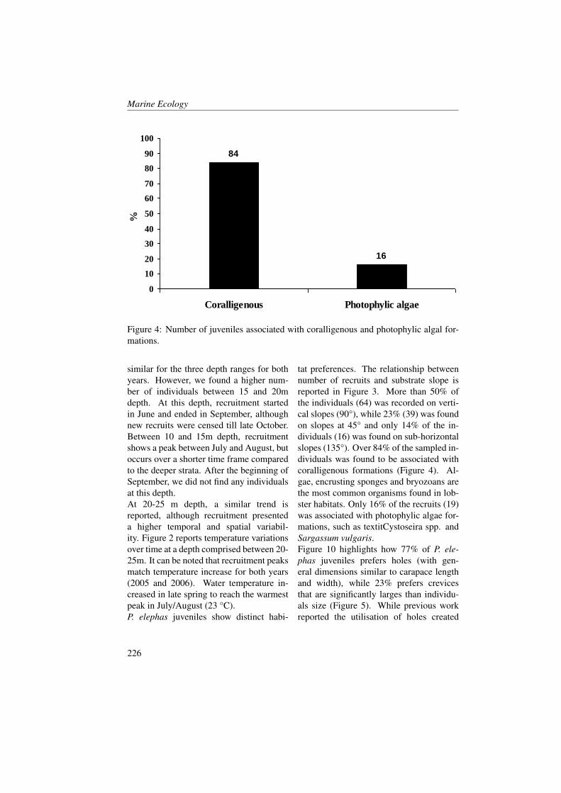
Marine Ecology
84
16
0
10
20
30
40
50
60
70
80
90
100
Coralligenous Photophylic algae
%
Figure 4: Number of juveniles associated with coralligenous and photophylic algal for-mations.
similar for the three depth ranges for bothyears. However, we found a higher num-ber of individuals between 15 and 20mdepth. At this depth, recruitment startedin June and ended in September, althoughnew recruits were censed till late October.Between 10 and 15m depth, recruitmentshows a peak between July and August, butoccurs over a shorter time frame comparedto the deeper strata. After the beginning ofSeptember, we did not find any individualsat this depth.At 20-25 m depth, a similar trend isreported, although recruitment presenteda higher temporal and spatial variabil-ity. Figure 2 reports temperature variationsover time at a depth comprised between 20-25m. It can be noted that recruitment peaksmatch temperature increase for both years(2005 and 2006). Water temperature in-creased in late spring to reach the warmestpeak in July/August (23 °C).P. elephas juveniles show distinct habi-
tat preferences. The relationship betweennumber of recruits and substrate slope isreported in Figure 3. More than 50% ofthe individuals (64) was recorded on verti-cal slopes (90°), while 23% (39) was foundon slopes at 45° and only 14% of the in-dividuals (16) was found on sub-horizontalslopes (135°). Over 84% of the sampled in-dividuals was found to be associated withcoralligenous formations (Figure 4). Al-gae, encrusting sponges and bryozoans arethe most common organisms found in lob-ster habitats. Only 16% of the recruits (19)was associated with photophylic algae for-mations, such as textitCystoseira spp. andSargassum vulgaris.Figure 10 highlights how 77% of P. ele-phas juveniles prefers holes (with gen-eral dimensions similar to carapace lengthand width), while 23% prefers crevicesthat are significantly larges than individu-als size (Figure 5). While previous workreported the utilisation of holes created
226
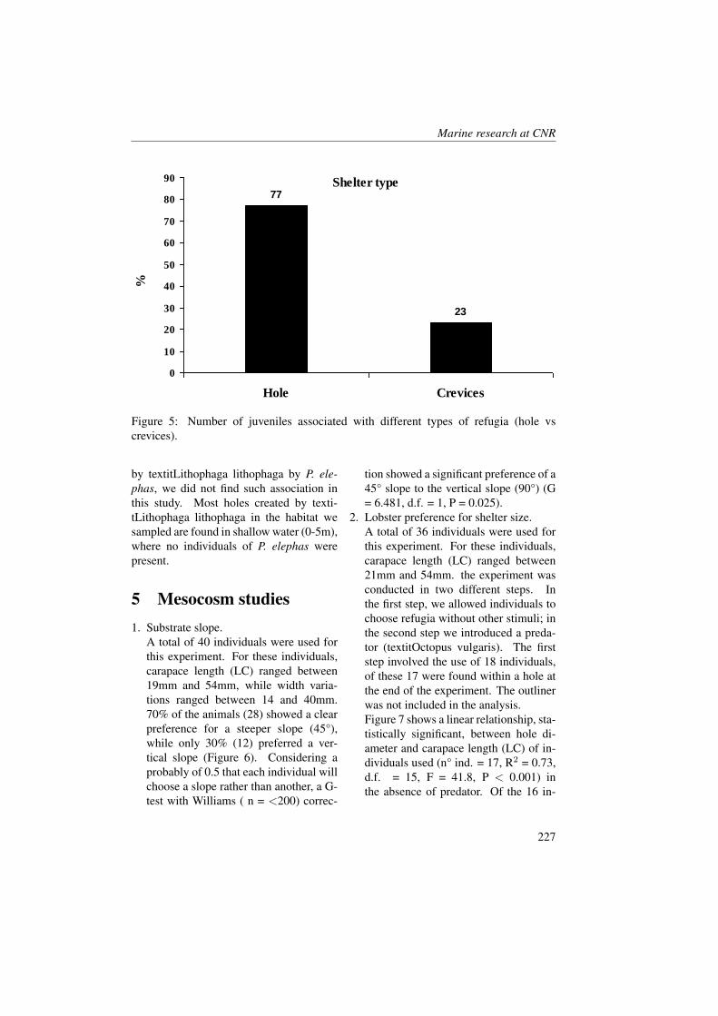
Marine research at CNR
77
23
0
10
20
30
40
50
60
70
80
90
Hole Crevices
Shelter type
%
Figure 5: Number of juveniles associated with different types of refugia (hole vs
crevices).
by textitLithophaga lithophaga by P. ele-phas, we did not find such association inthis study. Most holes created by texti-tLithophaga lithophaga in the habitat wesampled are found in shallow water (0-5m),where no individuals of P. elephas werepresent.
5 Mesocosm studies1. Substrate slope.
A total of 40 individuals were used forthis experiment. For these individuals,carapace length (LC) ranged between19mm and 54mm, while width varia-tions ranged between 14 and 40mm.70% of the animals (28) showed a clearpreference for a steeper slope (45°),while only 30% (12) preferred a ver-tical slope (Figure 6). Considering aprobably of 0.5 that each individual willchoose a slope rather than another, a G-test with Williams ( n = <200) correc-
tion showed a significant preference of a45° slope to the vertical slope (90°) (G= 6.481, d.f. = 1, P = 0.025).
2. Lobster preference for shelter size.A total of 36 individuals were used forthis experiment. For these individuals,carapace length (LC) ranged between21mm and 54mm. the experiment wasconducted in two different steps. Inthe first step, we allowed individuals tochoose refugia without other stimuli; inthe second step we introduced a preda-tor (textitOctopus vulgaris). The firststep involved the use of 18 individuals,of these 17 were found within a hole atthe end of the experiment. The outlinerwas not included in the analysis.Figure 7 shows a linear relationship, sta-tistically significant, between hole di-ameter and carapace length (LC) of in-dividuals used (n° ind. = 17, R2 = 0.73,d.f. = 15, F = 41.8, P < 0.001) inthe absence of predator. Of the 16 in-
227
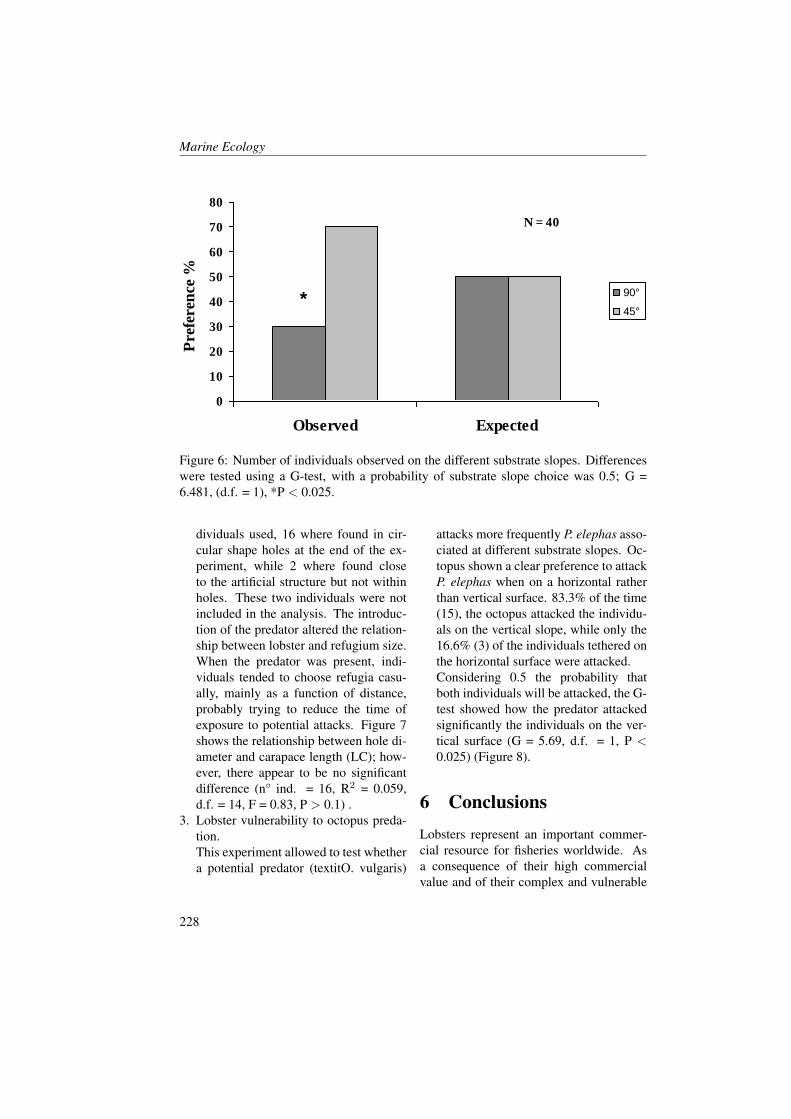
Marine Ecology
0
10
20
30
40
50
60
70
80
Observed Expected
Pre
fere
nce
%
90°
45°
N = 40
*
Figure 6: Number of individuals observed on the different substrate slopes. Differenceswere tested using a G-test, with a probability of substrate slope choice was 0.5; G =6.481, (d.f. = 1), *P < 0.025.
dividuals used, 16 where found in cir-cular shape holes at the end of the ex-periment, while 2 where found closeto the artificial structure but not withinholes. These two individuals were notincluded in the analysis. The introduc-tion of the predator altered the relation-ship between lobster and refugium size.When the predator was present, indi-viduals tended to choose refugia casu-ally, mainly as a function of distance,probably trying to reduce the time ofexposure to potential attacks. Figure 7shows the relationship between hole di-ameter and carapace length (LC); how-ever, there appear to be no significantdifference (n° ind. = 16, R2 = 0.059,d.f. = 14, F = 0.83, P > 0.1) .
3. Lobster vulnerability to octopus preda-tion.This experiment allowed to test whethera potential predator (textitO. vulgaris)
attacks more frequently P. elephas asso-ciated at different substrate slopes. Oc-topus shown a clear preference to attackP. elephas when on a horizontal ratherthan vertical surface. 83.3% of the time(15), the octopus attacked the individu-als on the vertical slope, while only the16.6% (3) of the individuals tethered onthe horizontal surface were attacked.Considering 0.5 the probability thatboth individuals will be attacked, the G-test showed how the predator attackedsignificantly the individuals on the ver-tical surface (G = 5.69, d.f. = 1, P <0.025) (Figure 8).
6 ConclusionsLobsters represent an important commer-cial resource for fisheries worldwide. Asa consequence of their high commercialvalue and of their complex and vulnerable
228
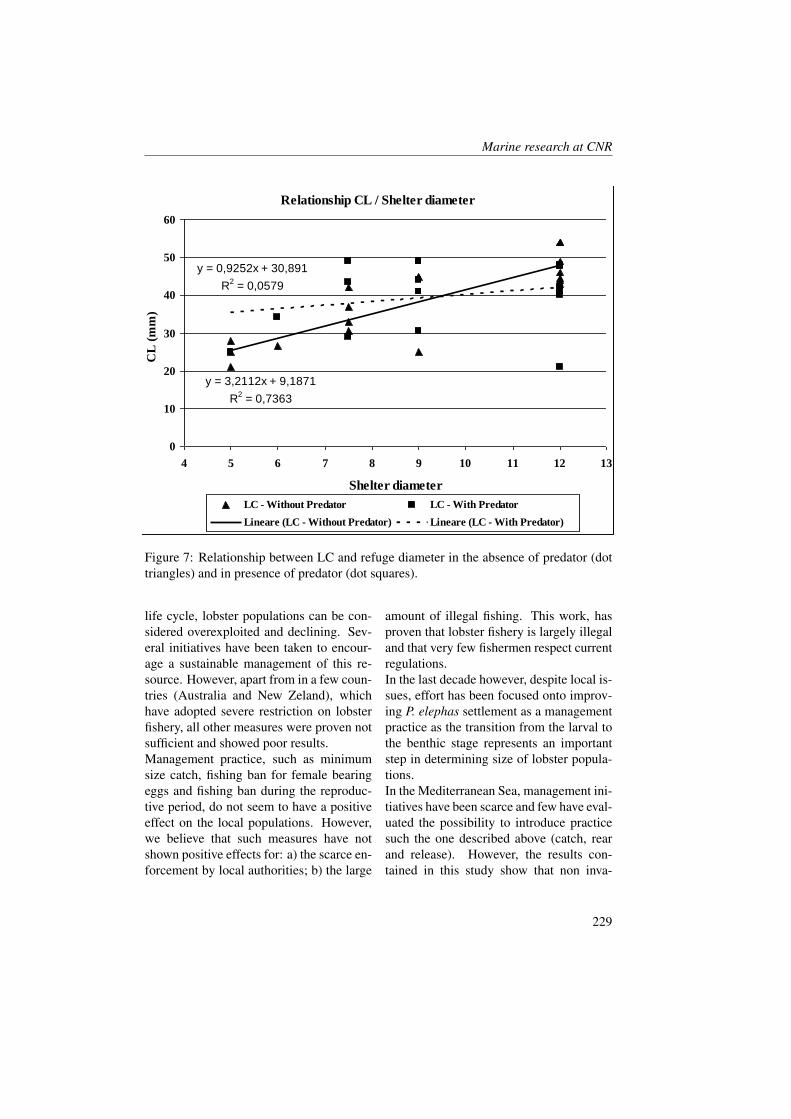
Marine research at CNR
Relationship CL / Shelter diameter
y = 3,2112x + 9,1871
R2 = 0,7363
y = 0,9252x + 30,891
R2 = 0,0579
0
10
20
30
40
50
60
4 5 6 7 8 9 10 11 12 13
Shelter diameter
CL
(m
m)
LC - Without Predator LC - With Predator
Lineare (LC - Without Predator) Lineare (LC - With Predator)
Figure 7: Relationship between LC and refuge diameter in the absence of predator (dot
triangles) and in presence of predator (dot squares).
life cycle, lobster populations can be con-sidered overexploited and declining. Sev-eral initiatives have been taken to encour-age a sustainable management of this re-source. However, apart from in a few coun-tries (Australia and New Zeland), whichhave adopted severe restriction on lobsterfishery, all other measures were proven notsufficient and showed poor results.Management practice, such as minimumsize catch, fishing ban for female bearingeggs and fishing ban during the reproduc-tive period, do not seem to have a positiveeffect on the local populations. However,we believe that such measures have notshown positive effects for: a) the scarce en-forcement by local authorities; b) the large
amount of illegal fishing. This work, hasproven that lobster fishery is largely illegaland that very few fishermen respect currentregulations.In the last decade however, despite local is-sues, effort has been focused onto improv-ing P. elephas settlement as a managementpractice as the transition from the larval tothe benthic stage represents an importantstep in determining size of lobster popula-tions.In the Mediterranean Sea, management ini-tiatives have been scarce and few have eval-uated the possibility to introduce practicesuch the one described above (catch, rearand release). However, the results con-tained in this study show that non inva-
229
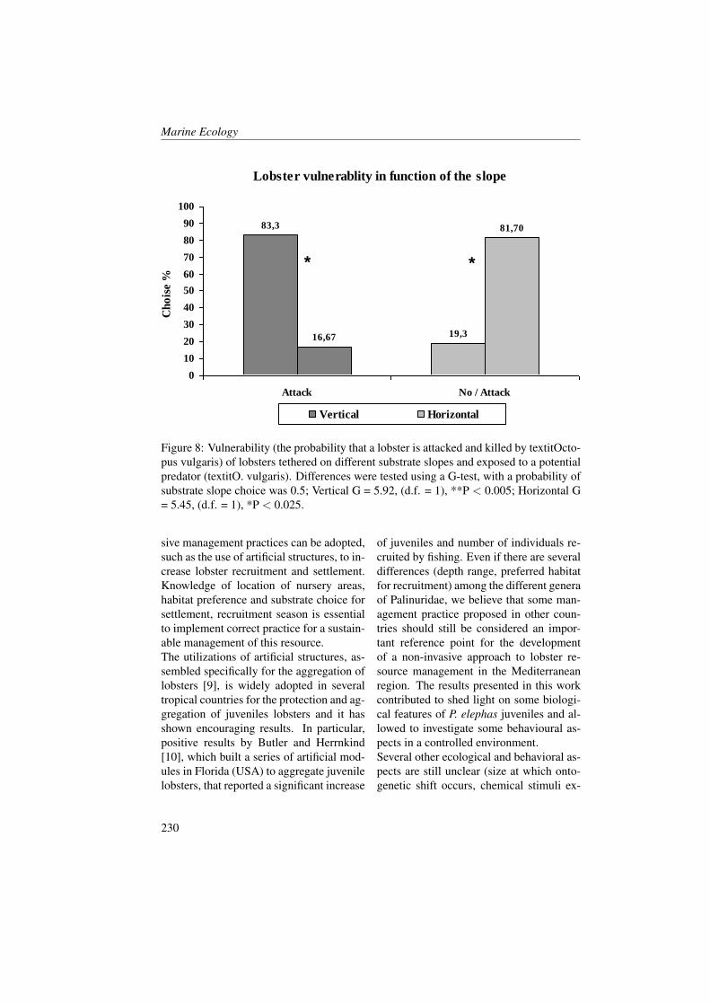
Marine Ecology
Lobster vulnerablity in function of the slope
83,3
19,316,67
81,70
0
10
20
30
40
50
60
70
80
90
100
Attack No / Attack
Ch
ois
e %
Vertical Horizontal
* *
Figure 8: Vulnerability (the probability that a lobster is attacked and killed by textitOcto-pus vulgaris) of lobsters tethered on different substrate slopes and exposed to a potentialpredator (textitO. vulgaris). Differences were tested using a G-test, with a probability ofsubstrate slope choice was 0.5; Vertical G = 5.92, (d.f. = 1), **P < 0.005; Horizontal G= 5.45, (d.f. = 1), *P < 0.025.
sive management practices can be adopted,such as the use of artificial structures, to in-crease lobster recruitment and settlement.Knowledge of location of nursery areas,habitat preference and substrate choice forsettlement, recruitment season is essentialto implement correct practice for a sustain-able management of this resource.The utilizations of artificial structures, as-sembled specifically for the aggregation oflobsters [9], is widely adopted in severaltropical countries for the protection and ag-gregation of juveniles lobsters and it hasshown encouraging results. In particular,positive results by Butler and Herrnkind[10], which built a series of artificial mod-ules in Florida (USA) to aggregate juvenilelobsters, that reported a significant increase
of juveniles and number of individuals re-cruited by fishing. Even if there are severaldifferences (depth range, preferred habitatfor recruitment) among the different generaof Palinuridae, we believe that some man-agement practice proposed in other coun-tries should still be considered an impor-tant reference point for the developmentof a non-invasive approach to lobster re-source management in the Mediterraneanregion. The results presented in this workcontributed to shed light on some biologi-cal features of P. elephas juveniles and al-lowed to investigate some behavioural as-pects in a controlled environment.Several other ecological and behavioral as-pects are still unclear (size at which onto-genetic shift occurs, chemical stimuli ex-
230
Marine research at CNR
change, MPA effects, etc.). However, acomparison between in situ and controlledexperiments, can represent a fair compro-mise to approach ecological and behavioralaspects. The development of specific andtargeted artificial modules, planned follow-ing the results presented here and the bib-
liography we included here, and coupledwith other management practice (see nextchapter), could represent an important toolfor the recovery of P. elephas and to pre-serve and promote traditional and artisanalfishery, by guaranteeing a high and con-stant commercial yield.
References[1] H.J. Ceccaldi and D. Latrouite. Spiny lobster management. 1994.
[2] R. Goni and D. Latrouite. Review of the biology, ecology and fisheries of Palinurusspp. species of European waters: Palinurus elephas (Fabricius, 1787) and Palinurusmauritanicus (Gruvel, 1911). Cah. Biol. Mar., 46:127–142, 2005.
[3] E. Hunter. Biology of the European spiny lobster Palinurus elephas (Fabricius,1787) (Decapoda, Palinuridea). Crustaceana, 72:545 565, 1999.
[4] D. Diaz, M. Marı, P. Abello, and M. Semestre. Settlement and juvenile habitat ofthe European spiny lobster Palinurus elephas (Crustacea: Decapoda: Paluniridae)in the western Mediterranean Sea. Scientia Marina, 65(4):347 356, 2001.
[5] R.R. Sokal and F.J. Rohlf. Biometry. 1981.
[6] S.G. Ratchford and D.G. Eggleston. Size and scale-dependent chemical attractioncontribute to an ontogenetic shift in sociality. Animal Behaviour, 56:1027 1034,1998.
[7] K.N. Smith and W.F. Herrnkind. Predation on early juvenile spiny lobsters Pan-ulirus argus (Latreille): influence of size and shelter. J Exp Mar Biol Ecol, 157:196205, 1992.
[8] D.E. Barshaw, K.L. Lavalli, and E. Spanier. Offense versus defense: responses ofthree morphological types f lobsters to predation. Mar Ecol Prog Ser, 256:171–182,2003.
[9] E. Lozano-Alvarez, P.Briones-Fourzan, L. Alvarez Filip, H.M. Weiss, et al. Influ-ence of shelter availability on interactions between Caribbean spiny lobsters andmoray eels: implications for artificial lobster enhancement. Mar. Ecol. Prog. Ser.,400:175–185, 2010.
[10] M.J. Butler and W.F. Herrnkind. A test of recruitment limitation and the potentialfor artificial enhancement of spiny lobster (Panulirus argus) populations in Florida.Canadian Journal of Fisheries and Acquatic Science, 54:452 463, 1996.
231

Marine Ecology
232

Fish Parasites in Polar Seas
M.R. Coscia, U. OresteInstitute of Protein Biochemistry, CNR, Napoli, [email protected]
Abstract
Parasitism is a very frequent event in the marine ecosystem. Nematodes (Nema-toda) are the most common parasites in demersal and pelagic fishes throughout theworld. This phenomenon has either human health or economic costs implications. Infact the ingestion of uncooked parasitized fishes causes the gastric Anisakidosis dis-ease. Although the present knowledge remained incomplete, studies about parasitebiology, phylogeny and ecology in Atlantic, Pacific, Mediterranean and polar areasachieved important results. The life-cycle of nematode parasites includes differentvertebrate and invertebrate hosts, fish being only intermediate host, birds and mam-mals being the final one. The most common nematode larvae found in Arctic andAntarctic regions belong to the Anisakis, Contracaecum, and Pseudoterranova gen-era; in Antarctic and sub-Antarctic areas the nematode infection intensity is higherthan in Arctic and sub-Arctic regions.During three expeditions to Antarctica we verified a high incidence of parasitic infec-tions in fish, particularly in the species of the families Channichthyidae and Bathy-draconidae. We carried out some experiments to analyze the immune response ofhost to nematodes: we separated proteins of Contracaecum osculatum and Pseu-doterranova decipiens larvae extracts and demonstrated the presence of nematode-specific antibodies in fish plasma and secretions. The antigenic proteins were identi-fied and the antibody specificity in plasma and bile was compared.
1 Fish parasitism
Parasitism is a very frequent event in themarine ecosystem. Although the presentknowledge remains incomplete, studiesabout parasite biology, phylogeny andecology, but also taxonomy, and zoogeog-raphy in Atlantic, Pacific, Mediterraneanand polar areas achieved important re-sults. This phenomenon has either hu-man health or economic costs implications.Nematodes (Nematoda) are the most com-mon endoparasites in demersal and pelagicfishes throughout the world. The acciden-tal ingestion of larval nematodes in raw or
insufficiently pickled, salted, smoked, orcooked wild marine fish causes a gastricdisease known as Anisakidosis [1]. Mostof patients complain of acute symptomssuch as epigastric pain, occlusion, diffuseabdominal pain, and appendicitis. Larvaeare attached to the gastric mucosa elicit-ing an inflammatory response. The first hu-man case of Anisakidosis was diagnozed inHolland and in 1960 van Thiel establishedthe relationship between the human diseaseand eating infested raw herring. Infestationrate is high in fish: 80-90% in cod rock fish,herring, salmon, and mackerel.There is a need to create a new classifi-
Marine Ecology
cation system of these parasites; for thispurpose, genetic differentiation and phy-logenetic relationships of different groupsbased on detailed studies of individualspecies were revised and compared. Sig-nificant contributions to the study of par-asite systematics, evolution and ecologyhave been provided by molecular methods,such as isozyme analysis, restriction frag-ment length polymorphisms, random am-plified DNA analysis, mini and microsatel-lite DNA polymorphisms, mitochondrialmarkers, etc. However, a certain progressin the research of fish nematodes has beenachieved during recent years, thanks to theuse of some new methods, in particularScanning Electron Micrographs and DNAstudies.Over the first two decades, the applicationof molecular systematics to the anisakidnematodes of the genera Anisakis, Pseu-doterranova and Contracaecum, parasitesof aquatic organisms, has advanced the un-derstanding of their systematic, taxonomy,ecology and phylogeny. Different patternsof distribution of anisakid nematodes invarious definitive and intermediate hostshave been proposed. Differences in the lifehistory of related species can be due both todifferential host-parasite coadaptation andcoevolution, and/or to interspecific compe-tition.
2 Fish immune responseto parasite antigens
Interest in defence mechanisms of fish de-rives from the need to develop health man-agement tools to support the aquacultureindustry, and, at the same time, to clarifythe evolution and origins of immunity invertebrates.
The host-parasite relationship is based onfine balance between parasite survival andhost defense. In this context, parasites of-ten use the same or similar immune sig-naling molecules and molecular mimicryto escape host immunosurveillance. Bothprocesses represent an adaptive strategyto ensure host immunocompatibility. Inimmunocompetent hosts, parasites evadethe immune response mainly through twomechanisms: i) expression of appropri-ate antigens, either by antigen variationthat is changing the expressed antigens fastenough to prevent any efficient immune re-sponse or by antigen mimicry that is ex-pressing epitopes similar to those of hostmolecules; ii) modification of the host im-mune response either directly by its ownmolecules, or indirectly by disregulatingthe host effector cells. In vivo, antigenshedding in nematodes could be a para-site defence mechanism against antibody-mediated immune effector processes [2].In an attempt to understand the molecu-lar mechanisms of the host-parasite rela-tionship, Politz and Philipp [3] conducteda biochemical study of the structure of thenematode cuticle. They defined three cat-egories of protein components: 1) Sur-face associated proteins and glycoproteins,characterized by their ability to be solu-bilized from the cuticle by mild extrac-tion procedures without reducing agents.They are expressed as the parasite colo-nizes a new host environment, and canelicit host immune response; 2) Colla-gens, hydrolyzed by collagenase, solubi-lized only with the aid of reducing agents;3) The so-called cuticlins, cross linkedby non-reducible bonds involving tyrosineresidues [4].Innate immunity plays greater role in resis-tance in fish compared to that in poikilo-therm vertebrates [5]. The limited reper-
234
Marine research at CNR
toire of adaptive immune mechanisms inpoikilotherms has conferred a selective ad-vantage on individuals or species possess-ing natural mechanisms of disease resis-tance. Models of innate immunity againstparasites in teleosts are particularly inter-esting because of the life history, biochem-ical and genetic complexity of the eukary-otic parasites compared with viral or bacte-rial pathogens and because of the potentialfor greater diversity in anti-parasitic mech-anisms [6]. A clearer understanding of themechanisms of resistance may provide anovel perspective of host-parasite coevolu-tion. Similarly, the survival of parasites inthe host environment suggests that adapta-tion by parasite is a distinct feature.Recent studies have begun to clarify therole of innate and adaptive immunityagainst parasitic infestation in teleosts. Theskin and gills are common sites of par-asite infestation despite the barrier func-tions associated with mucosal epithelia offish. Parasites inhabiting the skin and gillsare frequent causes of mortality, partic-ularly among fish reared in aquaculture.The physico-chemical characteristics ofskin mucus, the presence of haemolysins,lysozyme, C-reactive protein, complement,and lectins and the epidermal migrationof inflammatory cells and their secretionsmay affect the proliferation of ectopara-sites.Many studies have noted that the level andnature of the immune response of fish is de-termined by a range of parameters includ-ing the duration of infection and environ-mental conditions such as temperature [7]and pollution [8].The role of humoral factors such as com-plement and antibody in the immune re-sponse of fish to parasites has not beencompletely clarified. Although there havebeen several investigations on the associ-
ation between complement and viral andbacterial pathogens in fish, there has beena limited number of studies on the anti-parasitic activity of teleost complement. Incontrast, there have been several studiesthat have also highlighted the involvementof antibodies in the host-parasite relation-ship in fish.
3 Antarctic fish para-sitism
The study of Antarctic fish parasitism bynematodes is particularly interesting be-cause a natural immune response (notelicited by immunization) has been foundin fish living at an extremely low constanttemperature (-1.8 °C). Many authors haveinvestigated the effects of environmentaltemperature on fish antibody production.Le Morvan et al. [9] suggested that thedecreased antibody production observed incarp maintained at low water temperaturewas a direct effect of temperature on cel-lular immune function modulated by mem-brane fluidity. Collazos et al. [10] foundthe proliferative response of lymphocytesof Tinca tinca to be lower at 12 °C thanat 22 °C. Bly and Clem [11] attributedthe low temperature-mediated immunosup-pression of Ictalurus punctatus to the rigidnature of the T cell membranes; further-more, they supposed that losses associatedwith the ‘winter kill’ syndrome may beattributable to a low temperature-inducedimmuno-deficient state [12].Among the environmental antigenic stim-uli of the fish immune system, parasitemolecules play a major role. Parasites canbe distinguished into ectoparasite and en-doparasites. There have been very few re-search projects focusing on ectoparasites
235
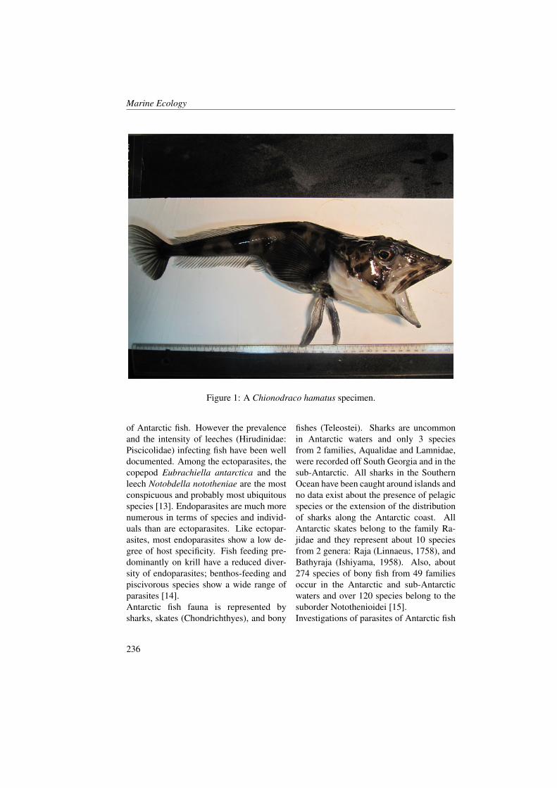
Marine Ecology
Figure 1: A Chionodraco hamatus specimen.
of Antarctic fish. However the prevalenceand the intensity of leeches (Hirudinidae:Piscicolidae) infecting fish have been welldocumented. Among the ectoparasites, thecopepod Eubrachiella antarctica and theleech Notobdella nototheniae are the mostconspicuous and probably most ubiquitousspecies [13]. Endoparasites are much morenumerous in terms of species and individ-uals than are ectoparasites. Like ectopar-asites, most endoparasites show a low de-gree of host specificity. Fish feeding pre-dominantly on krill have a reduced diver-sity of endoparasites; benthos-feeding andpiscivorous species show a wide range ofparasites [14].Antarctic fish fauna is represented bysharks, skates (Chondrichthyes), and bony
fishes (Teleostei). Sharks are uncommonin Antarctic waters and only 3 speciesfrom 2 families, Aqualidae and Lamnidae,were recorded off South Georgia and in thesub-Antarctic. All sharks in the SouthernOcean have been caught around islands andno data exist about the presence of pelagicspecies or the extension of the distributionof sharks along the Antarctic coast. AllAntarctic skates belong to the family Ra-jidae and they represent about 10 speciesfrom 2 genera: Raja (Linnaeus, 1758), andBathyraja (Ishiyama, 1958). Also, about274 species of bony fish from 49 familiesoccur in the Antarctic and sub-Antarcticwaters and over 120 species belong to thesuborder Notothenioidei [15].Investigations of parasites of Antarctic fish
236
Marine research at CNR
Positive
%
Negative
%
C. aceratus 100
C. hamatus 83 17
N. gibberifrons 50 50
N. coriiceps 100
P. georgianus 100
T. bernacchii 20 80
Table 1: Summary of positive and negative results obtained by double immunodiffusionassay in six Antarctic fish species
have been mostly systemic studies. Inven-tories of parasites now exist for a num-ber of notothenioids, primarily nototheni-ids and channichthyids, despite the taxon-omy of some groups of parasites is still in-determinate. Infestation rates and infesta-tion intensities of most fish species, as wellas the life cycles of most parasites and re-lationships with their hosts, still await elu-cidation. Teleosts play an important role inthe completion of life cycles of many para-sites species. They serve as either definitiveor intermediate hosts. Chondrichthyes aredefinitive hosts only. Trematodes, monoge-neans, nematodes, and cestodes, which areknown to represent a major component ofthe parasite fauna in fish living in temper-ate water [16, 17], are also found infestingAntarctic fish.Seventy-three helminth species occur asthe adult stage in fishes: Digea (45), Ces-toda (14), Nematoda (6), Acantocephala(8). Also, 11 larval stages of Cestodaand Nematoda are known. One digenean
species, Otodistomum cestoides, maturesin skates. Antarctic Chondrichthyes arenot infested with nematodes and acantho-cephalans. Larval nematodes representAnisakidae, parasites of fish, birds andmammals. All acanthocephalans, almostall digeneans, the majority of cestodes, andsome nematodes occur mainly or exclu-sively in benthic fishes. Among parasitesusing fishes as definitive hosts, all Cestoda,most Digenea and Nematoda, and almostall Acanthocephala have a range of hostsrestricted to one order or even to 1-2 hostspecies [18].In Antarctic fish, the parasitic fauna ap-pears to be impoverished in terms ofspecies. Infestation rates and infesta-tion intensities varied considerably be-tween species, being 100% in some speciessuch as Pseudochaenichthys georgianusand Notothenia rossii at South Georgia.Acanthocephalans show pronounced sitefidelity in that each species settles in adefinitive section of the digestive tract of
237
Marine Ecology
the host. Digean trematodes are found pre-dominantly in the esophagus and in thestomach.The first report on the occurrence of adultcestodes in the Antarctic fishes was givenby Linstow (1907) who described a newspecies, Phyllobothrium dentatum, fromunidentified shark which was found on thecoast of South Georgia. Cestodes foundare primarily larvae and hence unidentifi-able to genus or species level. Cestode lar-vae probably use planktonic copepods asfirst hosts whereas fish are the second in-termediate host. Adults have been foundin Bathyraja species and only occasionallyin nototheniids, but seals are consideredas prime candidates for potential definitivehost [19]. Infestation rates in some no-totheniids and channichthyids in the Sco-tia Arc region and the Weddell Sea rangedfrom 20% to 100%.Nematode parasites of Antarctic fish areprimarily third-stage larvae of the anisakidgenera Contracaecum [20] and Pseudoter-ranova [21]. Fish are the paratenic hostsof the larvae, which mature after being in-gested by the final host, seals or seabirds. Apositive relationship between sea eutroph-ication and fish parasitism by nematodeshas also been suggested, the parasite faunabeing the result of the feeding habitat andthe trophic level of the host [22]. More-over, the infection levels of anisakid nema-todes from various areas of the Boreal andAustral regions have been used as biolog-ical indicators of fish stocks and food-webintegrity in areas at high versus low levelsof habitat disturbance (pollution, overfish-ing, by-catch) [23].Nematode larvae may live in fish for acouple of years. The main target sites ofContracaecum larvae in the fish host in-clude liver, mesenteries and stomach wall[24]. The parasitic load of the liver
of some species of Antarctic fish is of-ten very high. Infestation intensities areup to 60-150 nematode larvae in piscivo-rous species, such as Chaenocephalus ac-eratus and Chionodraco rastrospinosus inthe Antarctic Peninsula region and Chion-odraco myersi and Chionodraco antarcti-cus in the Weddell Sea [25]. Their parasiticload is positively correlated with the size ofthe fish. This is likely to be due to the accu-mulation of larvae with age of the host, andto size-specific change of its diet. Acan-thocephalans and larvae of the nematodePseudoterranova are primarily found in fishfeeding on benthic crustaceans. Larvae ofContracaecum species use both planktonicand benthic transmission pathways. Thisclose relationship of feeding to the extentof parasitic infestation is also evident insome channichthyids, which shift their dietconsiderably when changing from pelagicto demersal life. As a result, infectionrates with Contracaecum larvae increasesharply from 0-20% to 90-100% [25]. Pis-civorous fish, such as channichthyids, playan important role as accumulators of acan-thocephalan larvae [26] and Contracaecumlarvae [20].The genus Pseudoterranova consists ofthree species: P. kogiae, P. ceticolaandP. decipiens. The life cycle of thelatter, the only cosmopolitan species, hasbeen described by McClelland [27]: thethird larval stage occurs in benthic fishand the main sites of infestation are theliver, mesenteries and stomach walls.P. de-cipiens larvae have been recorded alsoin the Antarctic notothenioid species bymany authors and the Weddell seal (Lep-tonychotes weddellii) is known to be animportant final host [21]. P. decipienswas first found in T. bernacchii by John-ston [28]. Other fish species infestedbyP. decipiens are Notothenia coriiceps,
238
Marine research at CNR
Champsocephalus gunnari, Chionodracokathleenae, Notothenia gibberifrons, Pseu-dochaenichthys georgianus and Notothe-nia neglecta living in the Antarctic Ocean.Also, in the North Atlantic Ocean, com-mercially important species, including At-lantic cod (Gadus morhua), are infestedbyP. decipiens. Based on the results ofmultilocus electrophoresis,P. decipiens lar-vae recovered from North Atlantic fishhave been separated into three sibling, mor-phologically indistinguishable species, A,B and C [29].
4 Genetic diversity ofanisakid nematodes
In order to test for a correlation existingbetween the genetic diversity of anisakidnematodes and habitat disturbance, thegenetic variability, estimated by nuclearmarkers (19 allozyme loci), was evaluatedamong several anisakid populations fromfish and marine mammals in various areasof the Boreal and Austral regions. Antarc-tic and sub-Antarctic populations showedsignificantly higher levels of genetic diver-sity than those from the Arctic and sub-Arctic species. Analysis between the de-gree of genetic variability and the levelsof parasitic infections within their hosts re-vealed higher intensities in anisakid infec-tions in Antarctic and sub-Antarctic hosts,presumably resulting from a lower degreeof habitat disturbance in less stressed areas.The absence of disturbance presumably al-lowed anisakid species to reach a largerpopulation size, with a reduced probabil-ity of genetic drift in their gene pools. Thissuggests that anisakid nematodes, and theirlevels of genetic diversity may be suitableindicators of the integrity of marine food
webs and of the general biodiversity of amarine ecosystem [30].
5 Antibody response to C.osculatum antigens
To investigate the presence of antibodiesto Contracaecum osculatum antigens in theplasma of several Antarctic fish, first theimmunoglobulin fraction was purified froma plasma pool of Chionodraco hamatusspecimens (Figure 1): 25.9% of the plasmaproteins were bound by the thiophilic ad-sorbent [31]. The bound fraction was re-solved into three peaks by size-exclusionFPLC; the relative molecular mass of themost representative peak (81%) was esti-mated to be 780 kDa. The serum concen-tration of this fraction was calculated tobe 12.6 mg/ml. It was analyzed by SDS-PAGE under reducing conditions. Twobands were obtained: the higher (75 kDa)was suggested to be the IgH chain, thelower (27 kDa) the IgL chain. To investi-gate the specificity of C. hamatus antibody,we tested for the presence of anti-nematodeantibodies in the purified Ig fraction. C.osculatum somatic proteins (Co SP) weresubjected to gel electrophoresis. At least14 separated bands of relative molecularmass ranging between 21 and 200 kDawere identified. The most representativebands were those with relative molecularmass of about 200, 91, 47, and 36 kDa.To identify the antigenic components ofCo SP, SDS-PAGE separated bands wereelectroblotted onto nitrocellulose sheet andthen incubated in sequence with Ig purifiedfrom plasma of C. hamatus or from Boopssalpa, as uninfested fish, and 125I rabbitIgG anti-C. hamatus plasma. Only someprotein components were identified as anti-
239
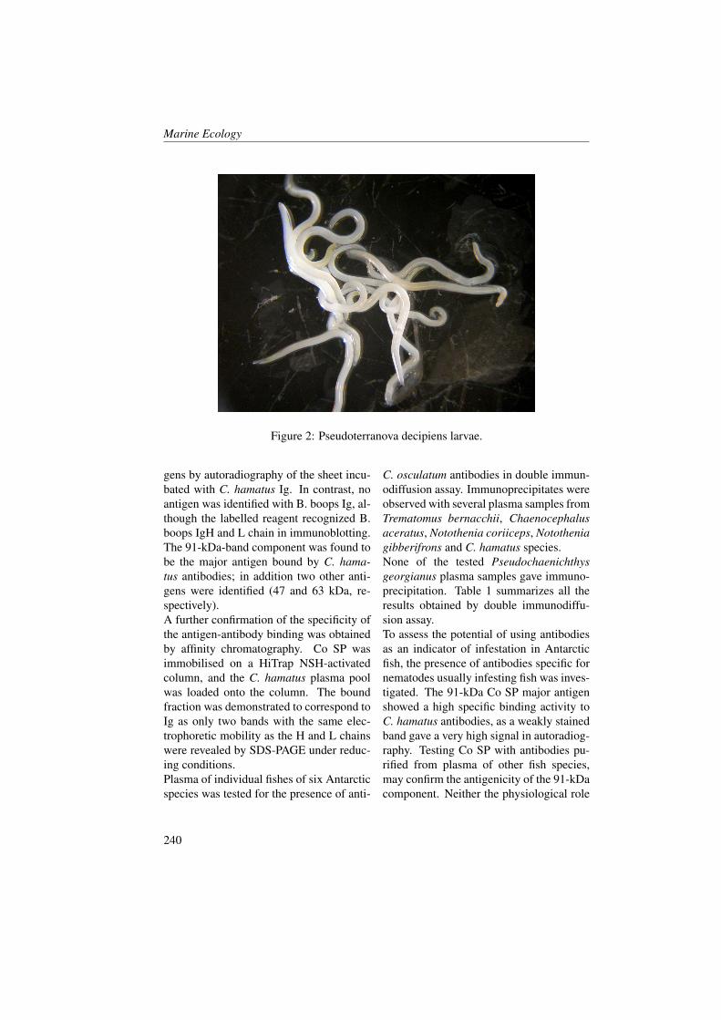
Marine Ecology
Figure 2: Pseudoterranova decipiens larvae.
gens by autoradiography of the sheet incu-bated with C. hamatus Ig. In contrast, noantigen was identified with B. boops Ig, al-though the labelled reagent recognized B.boops IgH and L chain in immunoblotting.The 91-kDa-band component was found tobe the major antigen bound by C. hama-tus antibodies; in addition two other anti-gens were identified (47 and 63 kDa, re-spectively).A further confirmation of the specificity ofthe antigen-antibody binding was obtainedby affinity chromatography. Co SP wasimmobilised on a HiTrap NSH-activatedcolumn, and the C. hamatus plasma poolwas loaded onto the column. The boundfraction was demonstrated to correspond toIg as only two bands with the same elec-trophoretic mobility as the H and L chainswere revealed by SDS-PAGE under reduc-ing conditions.Plasma of individual fishes of six Antarcticspecies was tested for the presence of anti-
C. osculatum antibodies in double immun-odiffusion assay. Immunoprecipitates wereobserved with several plasma samples fromTrematomus bernacchii, Chaenocephalusaceratus, Notothenia coriiceps, Nototheniagibberifrons and C. hamatus species.None of the tested Pseudochaenichthysgeorgianus plasma samples gave immuno-precipitation. Table 1 summarizes all theresults obtained by double immunodiffu-sion assay.To assess the potential of using antibodiesas an indicator of infestation in Antarcticfish, the presence of antibodies specific fornematodes usually infesting fish was inves-tigated. The 91-kDa Co SP major antigenshowed a high specific binding activity toC. hamatus antibodies, as a weakly stainedband gave a very high signal in autoradiog-raphy. Testing Co SP with antibodies pu-rified from plasma of other fish species,may confirm the antigenicity of the 91-kDacomponent. Neither the physiological role
240
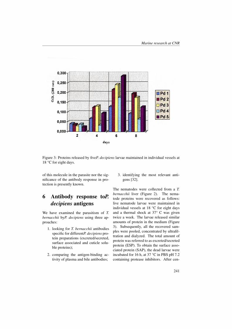
Marine research at CNR
Figure 3: Proteins released by fiveP. decipiens larvae maintained in individual vessels at18 °C for eight days.
of this molecule in the parasite nor the sig-nificance of the antibody response in pro-tection is presently known.
6 Antibody response toP.decipiens antigens
We have examined the parasitism of T.bernacchii byP. decipiens using three ap-proaches:
1. looking for T. bernacchii antibodiesspecific for differentP. decipiens pro-tein preparations (excreted/secreted,surface associated and cuticle solu-ble proteins);
2. comparing the antigen-binding ac-tivity of plasma and bile antibodies;
3. identifying the most relevant anti-gens [32].
The nematodes were collected from a T.bernacchii liver (Figure 2). The nema-tode proteins were recovered as follows:live nematode larvae were maintained inindividual vessels at 18 °C for eight daysand a thermal shock at 37° C was giventwice a week. The larvae released similaramounts of protein in the medium (Figure3). Subsequently, all the recovered sam-ples were pooled, concentrated by ultrafil-tration and dialyzed. The total amount ofprotein was referred to as excreted/secretedprotein (ESP). To obtain the surface asso-ciated protein (SAP), the dead larvae wereincubated for 16 h, at 37 °C in PBS pH 7.2containing protease inhibitors. After cen-
241
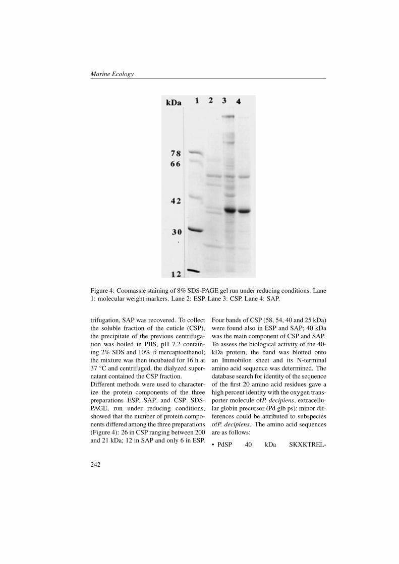
Marine Ecology
Figure 4: Coomassie staining of 8% SDS-PAGE gel run under reducing conditions. Lane1: molecular weight markers. Lane 2: ESP. Lane 3: CSP. Lane 4: SAP.
trifugation, SAP was recovered. To collectthe soluble fraction of the cuticle (CSP),the precipitate of the previous centrifuga-tion was boiled in PBS, pH 7.2 contain-ing 2% SDS and 10% β mercaptoethanol;the mixture was then incubated for 16 h at37 °C and centrifuged, the dialyzed super-natant contained the CSP fraction.Different methods were used to character-ize the protein components of the threepreparations ESP, SAP, and CSP. SDS-PAGE, run under reducing conditions,showed that the number of protein compo-nents differed among the three preparations(Figure 4): 26 in CSP ranging between 200and 21 kDa; 12 in SAP and only 6 in ESP.
Four bands of CSP (58, 54, 40 and 25 kDa)were found also in ESP and SAP; 40 kDawas the main component of CSP and SAP.To assess the biological activity of the 40-kDa protein, the band was blotted ontoan Immobilon sheet and its N-terminalamino acid sequence was determined. Thedatabase search for identity of the sequenceof the first 20 amino acid residues gave ahigh percent identity with the oxygen trans-porter molecule ofP. decipiens, extracellu-lar globin precursor (Pd glb ps); minor dif-ferences could be attributed to subspeciesofP. decipiens. The amino acid sequencesare as follows:
• PdSP 40 kDa SKXKTREL-
242
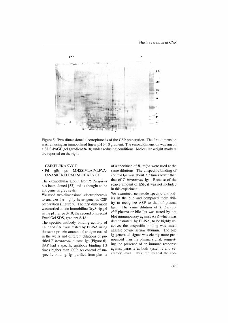
Marine research at CNR
Figure 5: Two-dimensional electrophoresis of the CSP preparation. The first dimensionwas run using an immobilized linear pH 3-10 gradient. The second dimension was run ona SDS-PAGE gel (gradient 8-18) under reducing conditions. Molecular weight markersare reported on the right.
GMKELEKAKVGT,• Pd glb ps MHSSIVLAIVLFVA-
IASASKTRELCMKSLEHAKVGT.
The extracellular globin fromP. decipienshas been cloned [33] and is thought to beantigenic in grey seals.We used two-dimensional electrophoresisto analyze the highly heterogeneous CSPpreparation (Figure 5). The first dimensionwas carried out on Immobiline DryStrip gelin the pH range 3-10, the second on precastExcelGel SDS, gradient 8-18.The specific antibody binding activity ofCSP and SAP was tested by ELISA usingthe same protein amount of antigen coatedin the wells and different dilutions of pu-rified T. bernacchii plasma Igs (Figure 6).SAP had a specific antibody binding 1.3times higher than CSP. As control of un-specific binding, Igs purified from plasma
of a specimen of B. salpa were used at thesame dilutions. The unspecific binding ofcontrol Igs was about 7.7 times lower thanthat of T. bernacchii Igs. Because of thescarce amount of ESP, it was not includedin this experiment.We examined nematode specific antibod-ies in the bile and compared their abil-ity to recognize ASP to that of plasmaIgs. The same dilution of T. bernac-chii plasma or bile Igs was tested by dotblot immunoassay against ASP, which wasdemonstrated, by ELISA, to be highly re-active; the unspecific binding was testedagainst bovine serum albumin. The bileIg-generated signal was clearly more pro-nounced than the plasma signal, suggest-ing the presence of an immune responseagainst parasite at both systemic and se-cretory level. This implies that the spe-
243
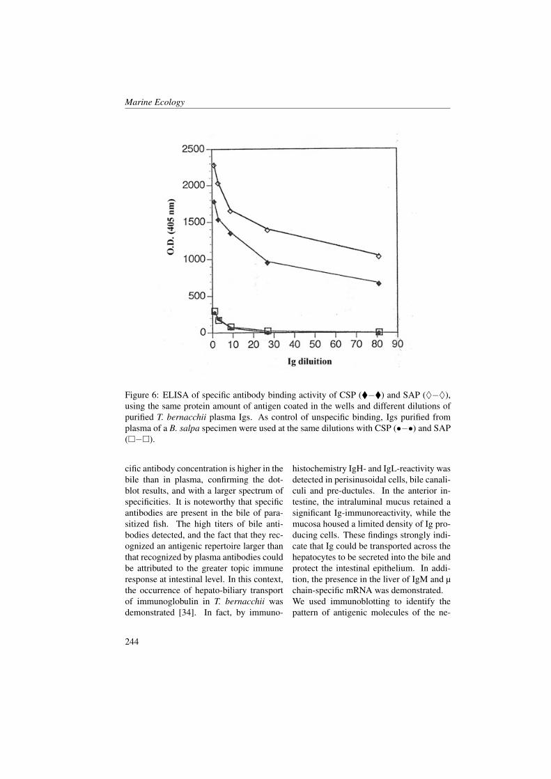
Marine Ecology
Figure 6: ELISA of specific antibody binding activity of CSP (�−�) and SAP (♦−♦),using the same protein amount of antigen coated in the wells and different dilutions ofpurified T. bernacchii plasma Igs. As control of unspecific binding, Igs purified fromplasma of a B. salpa specimen were used at the same dilutions with CSP (•−•) and SAP(�−�).
cific antibody concentration is higher in thebile than in plasma, confirming the dot-blot results, and with a larger spectrum ofspecificities. It is noteworthy that specificantibodies are present in the bile of para-sitized fish. The high titers of bile anti-bodies detected, and the fact that they rec-ognized an antigenic repertoire larger thanthat recognized by plasma antibodies couldbe attributed to the greater topic immuneresponse at intestinal level. In this context,the occurrence of hepato-biliary transportof immunoglobulin in T. bernacchii wasdemonstrated [34]. In fact, by immuno-
histochemistry IgH- and IgL-reactivity wasdetected in perisinusoidal cells, bile canali-culi and pre-ductules. In the anterior in-testine, the intraluminal mucus retained asignificant Ig-immunoreactivity, while themucosa housed a limited density of Ig pro-ducing cells. These findings strongly indi-cate that Ig could be transported across thehepatocytes to be secreted into the bile andprotect the intestinal epithelium. In addi-tion, the presence in the liver of IgM and µchain-specific mRNA was demonstrated.We used immunoblotting to identify thepattern of antigenic molecules of the ne-
244
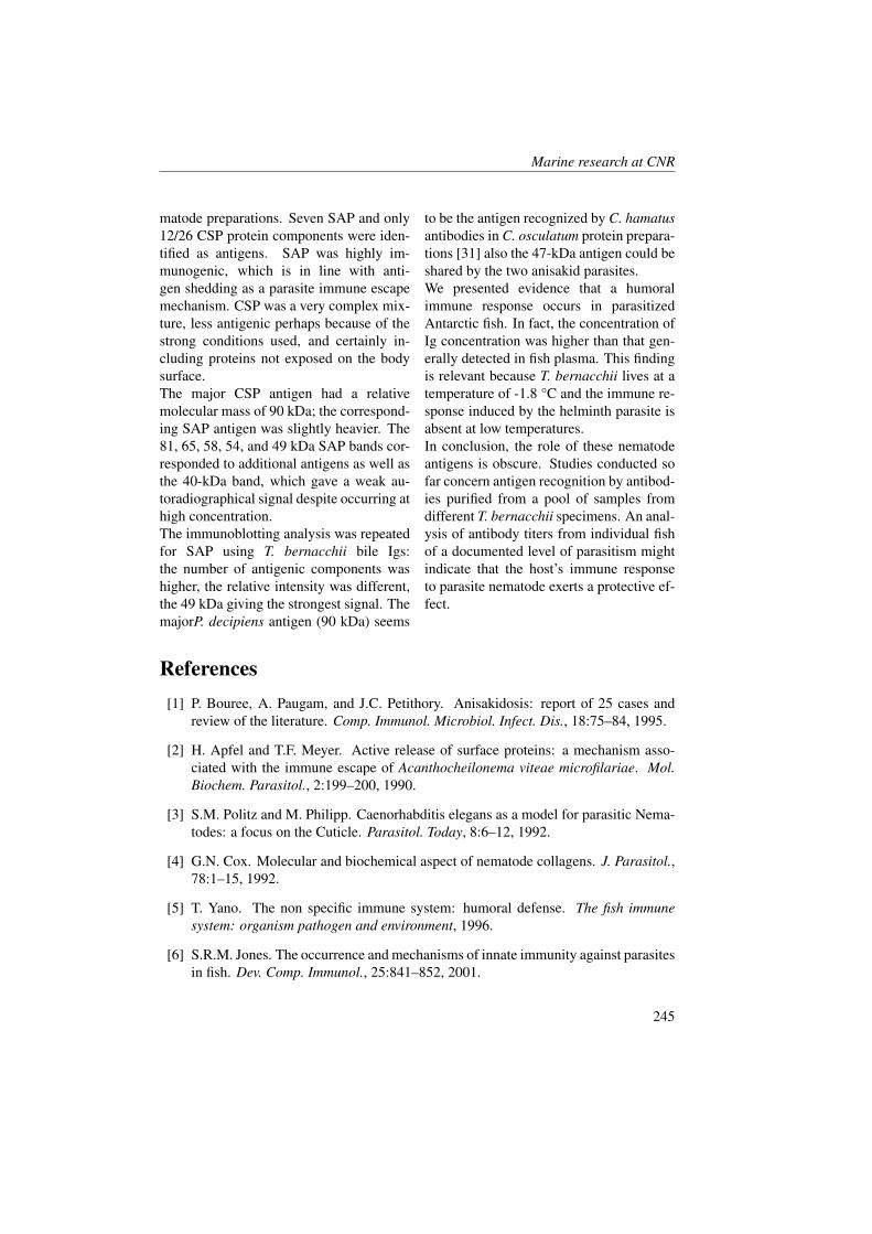
Marine research at CNR
matode preparations. Seven SAP and only12/26 CSP protein components were iden-tified as antigens. SAP was highly im-munogenic, which is in line with anti-gen shedding as a parasite immune escapemechanism. CSP was a very complex mix-ture, less antigenic perhaps because of thestrong conditions used, and certainly in-cluding proteins not exposed on the bodysurface.The major CSP antigen had a relativemolecular mass of 90 kDa; the correspond-ing SAP antigen was slightly heavier. The81, 65, 58, 54, and 49 kDa SAP bands cor-responded to additional antigens as well asthe 40-kDa band, which gave a weak au-toradiographical signal despite occurring athigh concentration.The immunoblotting analysis was repeatedfor SAP using T. bernacchii bile Igs:the number of antigenic components washigher, the relative intensity was different,the 49 kDa giving the strongest signal. ThemajorP. decipiens antigen (90 kDa) seems
to be the antigen recognized by C. hamatusantibodies in C. osculatum protein prepara-tions [31] also the 47-kDa antigen could beshared by the two anisakid parasites.We presented evidence that a humoralimmune response occurs in parasitizedAntarctic fish. In fact, the concentration ofIg concentration was higher than that gen-erally detected in fish plasma. This findingis relevant because T. bernacchii lives at atemperature of -1.8 °C and the immune re-sponse induced by the helminth parasite isabsent at low temperatures.In conclusion, the role of these nematodeantigens is obscure. Studies conducted sofar concern antigen recognition by antibod-ies purified from a pool of samples fromdifferent T. bernacchii specimens. An anal-ysis of antibody titers from individual fishof a documented level of parasitism mightindicate that the host’s immune responseto parasite nematode exerts a protective ef-fect.
References[1] P. Bouree, A. Paugam, and J.C. Petithory. Anisakidosis: report of 25 cases and
review of the literature. Comp. Immunol. Microbiol. Infect. Dis., 18:75–84, 1995.
[2] H. Apfel and T.F. Meyer. Active release of surface proteins: a mechanism asso-ciated with the immune escape of Acanthocheilonema viteae microfilariae. Mol.Biochem. Parasitol., 2:199–200, 1990.
[3] S.M. Politz and M. Philipp. Caenorhabditis elegans as a model for parasitic Nema-todes: a focus on the Cuticle. Parasitol. Today, 8:6–12, 1992.
[4] G.N. Cox. Molecular and biochemical aspect of nematode collagens. J. Parasitol.,78:1–15, 1992.
[5] T. Yano. The non specific immune system: humoral defense. The fish immunesystem: organism pathogen and environment, 1996.
[6] S.R.M. Jones. The occurrence and mechanisms of innate immunity against parasitesin fish. Dev. Comp. Immunol., 25:841–852, 2001.
245
Marine Ecology
[7] D.T. Richards, D. Hoole, J.W. Lewis, E. Ewens, and C. Arme. Stimulation ofcarp Cyprinus carpio lymphocytes in vitro by the blood fluke Sanguinicola inermis(Trematoda: Sanguinicolidae). Dis. Aquat. Org., 25:97–93, 1996.
[8] D. Hoole, J.W. Lewis, P.M. Schuwerack, C. Chakravarthy, et al. Inflammatoryinteractions in fish exposed to pollutants and parasites: a role for apoptosis and Creactive protein. Parasitol., 126:71–85, 2003.
[9] C. Le Morvan, P. Deschaux, and D. Troutaud. Effects and mechanisms of envi-ronmental temperature on carp (Cyprinus carpio) anti-DNP antibody response andnon-specific cytotoxic cell activity: a kinetic study. Dev. Comp. Immunol., 20:331–340, 1996.
[10] M.E. Collazos, E. Ortega, and C. Barriga. Influence of the temperature upon theproliferative response of lymphocytes of tench (Tinca tinca) during winter and sum-mer. Comp. Immunol., Microbiol. Infect. Dis., 18:209–214, 1995.
[11] J.E. Bly and L.W. Clem. Temperature-mediated processes in teleost immu-nity: homeoviscous adaptation by channel catfish peripheral blood cells. Comp.Biochem. Physiol., 91:481–485, 1988.
[12] J.E. Bly and L.W. Clem. Temperature-mediated processes in teleosts immunity: invitro immunosuppression induced by in vivo low temperature in channel catfish.Vet. Immunol. Immunopathol., 28:365–377, 1991.
[13] K.H. Kock. Antarctic fish and fisheries. 1992.
[14] J.N. Hoogester and M. White. Notes on parasite infestation of inshore fish at SignyIsland, South Orkney Islands. Br. Antarct. Surv. Bull., 54:23–31, 1981.
[15] J.T. Eastman and A. Clarke. A comparison of adaptive radiations of Antarctic fishwith those of Non-Antarctic fish. In: Fishes of Antarctica. A biological overview,pages 3–26, 1998.
[16] P. Orecchia and L. Paggi. Systematic and ecological aspects of helminth parasitesof marine fish studied at the Institute of Parasitology of the University of Rome.Parassitologia, 20:73–89, 1978.
[17] C.R. Kennedy and A.O. Bush. The relationship between pattern and scale in para-site communities: a stranger in a strange land. Parasitology, 109:187–196, 1994.
[18] A. Rocka. Helminths of Antarctic fishes. Wiad Parazytol., 54:47–48, 2008.
[19] J.G. O’Neill, M.G. White, T.A. Sims, and D.L. Barber. An inflammatory responseof the Antarctic silverfish, Pleuragramma antarcticum Boulanger, 1902 (Teleostei:Notothenioidei) to infestation by plerocercoid of a pseudophyllidean cestode (Di-phyllobothrium sp.). British Antarctic Survey Bulletin, 79:51–63, 1988.
246
Marine research at CNR
[20] H. Kloser and J. Plotz. Morphological distinction between adult Contracaecumradiatum and Contracaecum osculatum (Nematoda, Anisakidae) from the Weddellseal (Leptonychotes weddelli). Zoologica Scripta, 21:129–132, 1992.
[21] H. Palm, K. Andersen, H. Kloser, and J. Plotz. Occurrence of Pseudoterranovadecipiens (Nematoda) in fish from the southeastern Weddell Sea (Antarctic). PolarBiol., 14:539–544, 1994.
[22] M. Moser and R.K. Cowen. The effect of periodic eutrophication on parasitism andstock identification of Trematomus bernacchii (Pisces, Nototheniidae) in McMurdoSound, Antarctica. J. Parasitol., 77:551–556, 1992.
[23] S. Mattiucci and G. Nascetti. Advances and trends in the molecular systematicsof anisakid nematodes, with implications for their evolutionary ecology and host-parasite co-evolutionary processes. Adv. Parasitol., 66:47–148, 2008.
[24] M. Køie and H.P. Fagerholm. The life cycle of Contracaecum osculatum (Rudolphi,1802) sensu stricto (Nematoda, Ascaridoidea, Anisakidae) in view of experimentalinfections. Parasitol. Res., 81:481–489, 1995.
[25] V. Siegel. Quantitative investigations on parasites of Antarctic channichthyid andnototheniid fishes. Meeresforschung, 28:146–156, 1980.
[26] K. Zdzitowiecki. Prevalence of acanthocephalans in fishes of South Shetlands(Antarctic). I. Juvenile Corynosoma spp. Acta Parasitol. Polonica, 30:143–160,1986.
[27] G. McClelland. Larval sealworm (Pseudoterranova decipiens) infections in benthicmicrofauna. Can. Bull. Fish Aquat. Sci., 222:47–65, 1990.
[28] T.H. Johnston. Parasitic Nematoda. Sci. Rep. Austral Antarct. Exped. [Ser C],10:3–31, 1938.
[29] L. Paggi, G. Nascetti, R. Cianchi, P. Orecchia, et al. Genetic evidence for threespecies within Pseudoterranova decipiens (Nematoda, Ascaridida, Ascaridoidea) inthe North Atlantic and Norwegian and Barents seas. Int. J. Parasitol., 21:195–212,1991.
[30] S. Mattiucci and G. Nascetti. Genetic diversity and infection levels of anisakidnematodes parasitic in fish and marine mammals from Boreal and Austral hemi-spheres. Vet. Parasitol., 148:43–57, 2007.
[31] M.R. Coscia and U. Oreste. Presence of antibodies specific for proteins of Contra-caecum osculatum (Rudolphi, 1908) in plasma of several Antarctic teleosts. FishShellfish Immunol., 8:295–302, 1998.
[32] M.R. Coscia and U. Oreste. Plasma and bile antibodies of the teleost Trematomusbernacchii specific for the nematode Pseudoterranova decipiens. Dis. Aquat. Org.,41:37–42, 2000.
247

Marine Ecology
[33] B. Dixon, B. Walker, W. Kimmins, and B. Pohajdak. Isolation and sequencing ofa cDNA for an unusual hemoglobin from the parasitic nematode Pseudoterranovadecipiens. Proc. Natl. Acad. Sci. USA, 88:5655–5659, 1991.
[34] L. Abelli, M.R. Coscia, A. De Santis, C. Zeni, and U. Oreste. Evidence for hepato-biliary trasport of immunoglobulin in the Antarctic teleost fish Trematomus bernac-chii. Dev. Comp. Immunol., 29:431–442, 2005.
248

Benthic Communities as Indicators of HabitatSaprobity
D. Tagliapietra1, M. Sigovini2,3, P. Magni1,3
1, Institute of Marine Sciences, CNR, Venezia, Italy2, Department of Environmental Sciences, University “Ca’ Foscari”, Venezia, Italy3, Institute for Coastal Marine Environment, CNR, Oristano, Italy
Abstract
We delineate the concept of saprobity as a state of an ecosystem resulting fromorganic matter (OM) metabolism processes. An overview is given on conceptualmodels describing the succession of benthic communities along a gradient of or-ganic enrichment. Similarities between different models, e.g. between the Pearson-Rosenberg [1] and the Guelorget-Perthuisot [2] models, are highlighted. Based ona critical analysis of existing models and indices, we propose a general frameworkwhere the processes of OM metabolism are a major structuring factor the benthiccommunities in microtidal lagoons, and saprobity is used as a state descriptor ofthese process. We assume that saprobity cannot be quantified by considering onlythe amount of OM. In fact, saprobity is the result of both input of OM and otherprocesses, such as mineralization, sinking, dilution and export of OM. The sameorganic input can, therefore, generate different degrees of saprobity in different sys-tems/areas. Saprobity acts on benthic communities together with other componentsof the transitional gradient, such as salinity but, in coastal lagoons, the effect of thelatter is primarily in oligohaline and hyperhaline areas. Due to difficulties to quan-tify saprobity itself, we are developing a numerical index of saprobity which takesinto account the memberships of benthic species to different saprobic groups. Maincharacteristics of this index are described in this paper and a zonal approach is alsoforeseen.
1 The concept of Sapro-bity
Saprobity (from the Greek: σαπρoς ,Sapros = rotten, putrid, putrefaction, decayand βιoσ, Bios = life) is the expression ofthe metabolism of organic matter subjectedto microbial degradation and of its ecosys-temic balance. It was first developed forrivers in relation to the occurrence of or-ganic waste discharges [3, 4, 5].
A definition of saprobity was accepted atthe Symposium CMEA on “Questions ofSaprobity” (Prague, 26-28 April 1966):”Within the bioactivity of a body of wa-ter, saprobity is the sum total of all thosemetabolic processes, which are the antithe-sis of primary production. It is there-fore the sum total of all those processeswhich are accompanied by a loss of poten-tial energy. In combination with the bio-genic and physical oxygen component, it
Marine Ecology
determines the saprobity level of a bodyof water. This level can be ascertainedboth by metabolic-dynamic measurementsand by analysis of the living communi-ties” [6, 7]. This definition points out thatsaprobity is not the result of the mere pres-ence of organic matter but involves ecosys-temic processes. The saprobity is there-fore the state an ecosystem assumes as aconsequence of the decomposition of or-ganic matter. In general terms, saprobityis given by the balance between an inputof catabolites generated by the metabolismof the organic matter, and their removalfrom the medium. The removal of catabo-lites from the medium depends mainlyon their utilization by microorganisms (re-mineralization or self-depuration), on thedilution into the water column and on theexport from the system. The sum of allremoval processes can be regarded as the“clearance” of the ecosystem. As result ofa metabolic processes, saprobity is strictlydependent on oxygen availability and tem-perature.Saprobic processes in sedimentary en-vironments, such as coastal transitionalecosystems (CTE), occur mostly close tothe sediment surface. Benthic micro-bial metabolism generates oxygen demand(Sediment Oxygen Demand) subtractingthe gas from the overlying water. Oftenjust few centimeters of sediment and waterare affected by oxygen deficiency but thisis sufficient to shape the benthic biota [8].The texture of sediments and bioturbationaffect the oxygen penetration in the sub-strate (as can be evidenced by the depth ofthe Redox discontinuity layer RPD) and theflux of reduced and toxic products. Hydrol-ogy and physical mechanisms plays a keyrole in the clearance process. For instance,tides act both on the dilution of catabolitesbringing new seawater and to the physi-
cal export toward the sea. The marine wa-ter supply usually conveys dissolved oxy-gen to the system. Re-mineralization pro-cesses can be enhanced by water mixingthrough oxygenation and increased contactof catabolites with various kind of surfacessuch as the bottom, suspended matter andother physical and biological supports (e.g.shells, cobbles, plant stems). The differ-ent components of the clearance (i.e. self-depuration, sinking, dilution, export) havedifferent influence in different zones of thesame lagoon depending on the hydrody-namics. In outer areas, close to the inlets,(lotic areas) the export play a major rolein the clearance process, whereas in the in-nermost areas (lentic areas) self-depurationand burrowing can have a dominant role.Similarly, different types of lagoons natu-rally express different saprobity a shallowlagoon with reduced hydrodynamics, lit-tle oxygenated waters and fine sedimentsis likely to have a higher saprobity thana sandy leaky lagoon. The same organicinput can, therefore, generate different de-gree of saprobity in different habitats.
2 Effects of saprobity onbenthic communities
The main effect of saprobity on macro-scopic biocoenosis is that the number ofspecies that can cope with it decreasesprogressively as the saprobity increases,leading to a reduction of species richnessand diversity. Species change along asaprobity gradient gives rise to a succes-sion/seriation according to species-specifictolerance levels to saprobity. Along thisgradient, the density and biomass of an in-dividual species, as well as the total densityand biomass of the community, show char-
250
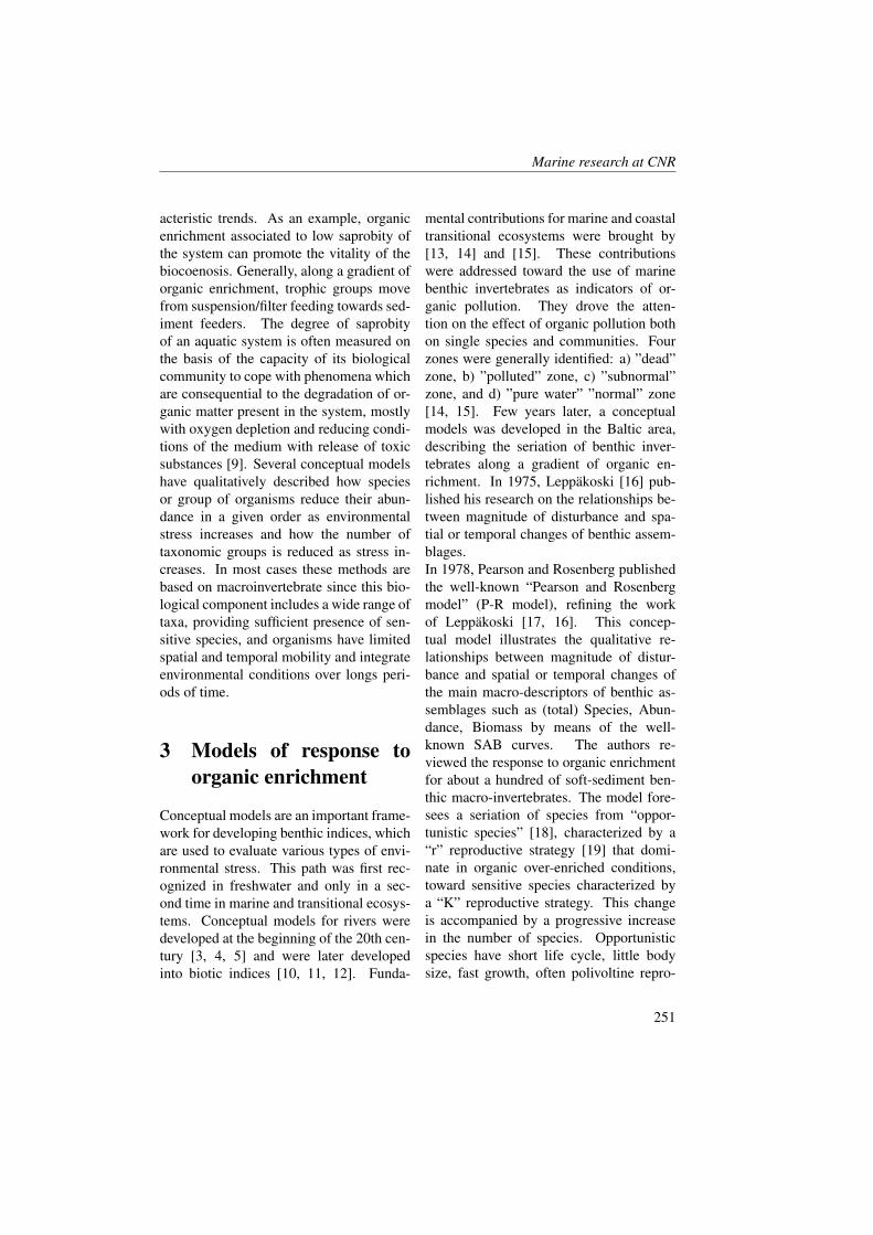
Marine research at CNR
acteristic trends. As an example, organicenrichment associated to low saprobity ofthe system can promote the vitality of thebiocoenosis. Generally, along a gradient oforganic enrichment, trophic groups movefrom suspension/filter feeding towards sed-iment feeders. The degree of saprobityof an aquatic system is often measured onthe basis of the capacity of its biologicalcommunity to cope with phenomena whichare consequential to the degradation of or-ganic matter present in the system, mostlywith oxygen depletion and reducing condi-tions of the medium with release of toxicsubstances [9]. Several conceptual modelshave qualitatively described how speciesor group of organisms reduce their abun-dance in a given order as environmentalstress increases and how the number oftaxonomic groups is reduced as stress in-creases. In most cases these methods arebased on macroinvertebrate since this bio-logical component includes a wide range oftaxa, providing sufficient presence of sen-sitive species, and organisms have limitedspatial and temporal mobility and integrateenvironmental conditions over longs peri-ods of time.
3 Models of response toorganic enrichment
Conceptual models are an important frame-work for developing benthic indices, whichare used to evaluate various types of envi-ronmental stress. This path was first rec-ognized in freshwater and only in a sec-ond time in marine and transitional ecosys-tems. Conceptual models for rivers weredeveloped at the beginning of the 20th cen-tury [3, 4, 5] and were later developedinto biotic indices [10, 11, 12]. Funda-
mental contributions for marine and coastaltransitional ecosystems were brought by[13, 14] and [15]. These contributionswere addressed toward the use of marinebenthic invertebrates as indicators of or-ganic pollution. They drove the atten-tion on the effect of organic pollution bothon single species and communities. Fourzones were generally identified: a) ”dead”zone, b) ”polluted” zone, c) ”subnormal”zone, and d) ”pure water” ”normal” zone[14, 15]. Few years later, a conceptualmodels was developed in the Baltic area,describing the seriation of benthic inver-tebrates along a gradient of organic en-richment. In 1975, Leppakoski [16] pub-lished his research on the relationships be-tween magnitude of disturbance and spa-tial or temporal changes of benthic assem-blages.In 1978, Pearson and Rosenberg publishedthe well-known “Pearson and Rosenbergmodel” (P-R model), refining the workof Leppakoski [17, 16]. This concep-tual model illustrates the qualitative re-lationships between magnitude of distur-bance and spatial or temporal changes ofthe main macro-descriptors of benthic as-semblages such as (total) Species, Abun-dance, Biomass by means of the well-known SAB curves. The authors re-viewed the response to organic enrichmentfor about a hundred of soft-sediment ben-thic macro-invertebrates. The model fore-sees a seriation of species from “oppor-tunistic species” [18], characterized by a“r” reproductive strategy [19] that domi-nate in organic over-enriched conditions,toward sensitive species characterized bya “K” reproductive strategy. This changeis accompanied by a progressive increasein the number of species. Opportunisticspecies have short life cycle, little bodysize, fast growth, often polivoltine repro-
251
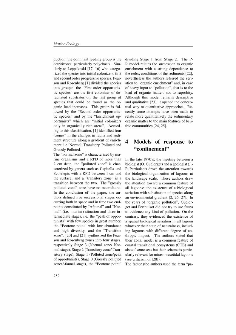
Marine Ecology
duction, the dominant feeding group is thedetritivores, particularly polychaets. Sim-ilarly to Leppakoski [17, 16] who catego-rized the species into initial colonizers, firstand second order progressive species, Pear-son and Rosenberg [1] divided the speciesinto groups: the “First-order opportunis-tic species” are the first colonizer of de-faunated substrates or, the last group ofspecies that could be found as the or-ganic load increases. This group is fol-lowed by the “Second-order opportunis-tic species” and by the “Enrichment op-portunists” which are “initial colonizersonly in organically rich areas”. Accord-ing to this classification, [1] identified four”zones” in the changes in fauna and sedi-ment structure along a gradient of enrich-ment, i.e. Normal, Transitory, Polluted andGrossly Polluted.The ”normal zone” is characterized by ma-rine organisms and a RPD of more than2 cm deep, the ”polluted zone” is char-acterized by genera such as Capitella andScolelepis with a RPD between 1 cm andthe surface, and a ”transitory zone” is atransition between the two. The ”grosslypolluted zone” zone have no macrofauna.In the conclusion of the paper, the au-thors defined five successional stages oc-curring both in space and in time two end-points constituted by “Afaunal” and “Nor-mal” (i.e. marine) situation and three in-termediate stages, i.e. the “peak of oppor-tunists” with few species in great number,the “Ecotone point” with low abundanceand high diversity, and the “Transitionzone”. [20] and [21] synthesized the Pear-son and Rosenberg zones into four stages,respectively Stage 3 (Normal zone/ Nor-mal stage), Stage 2 (Transitory zone/ Tran-sitory stage), Stage 1 (Polluted zone/peakof opportunists), Stage 0 (Grossly pollutedzone/Afaunal stage), the “Ecotone point”
dividing Stage 1 from Stage 2. The P-R model relates the succession to organicenrichment with a strong dependence tothe redox conditions of the sediments [22],nevertheless the authors referred the seri-ation to “organic enrichment” and, in caseof heavy input to “pollution”, that is to theload of organic matter, not to saprobity.Although this model remains descriptiveand qualitative [23], it opened the concep-tual way to quantitative approaches. Re-cently some attempts have been made torelate more quantitatively the sedimentaryorganic matter to the main features of ben-thic communities [24, 25].
4 Models of response to“confinement”
In the late 1970’s, the meeting between abiologist (O. Guelorget) and a geologist (J.-P. Perthuisot) drove the attention towardsthe biological organization of lagoons atthe landscape scale. These authors drawthe attention toward a common feature ofall lagoons: the existence of a biologicalseriation with substitution of species alongan environmental gradient [2, 26, 27]. Inthe years of “organic pollution”, Guelor-get and Perthuisot did not try to use faunato evidence any kind of pollution. On thecontrary, they evidenced the existence ofa spatial biological seriation in all lagoonwhatever their state of naturalness, includ-ing lagoons with different degree of an-thropic impact. The authors stated thattheir zonal model is a common feature ofcoastal transitional ecosystems (CTE) andalso of some seas but their scheme is partic-ularly relevant for micro-mesotidal lagoons(see criticism of [28]).The factor (the authors used the term “pa-
252
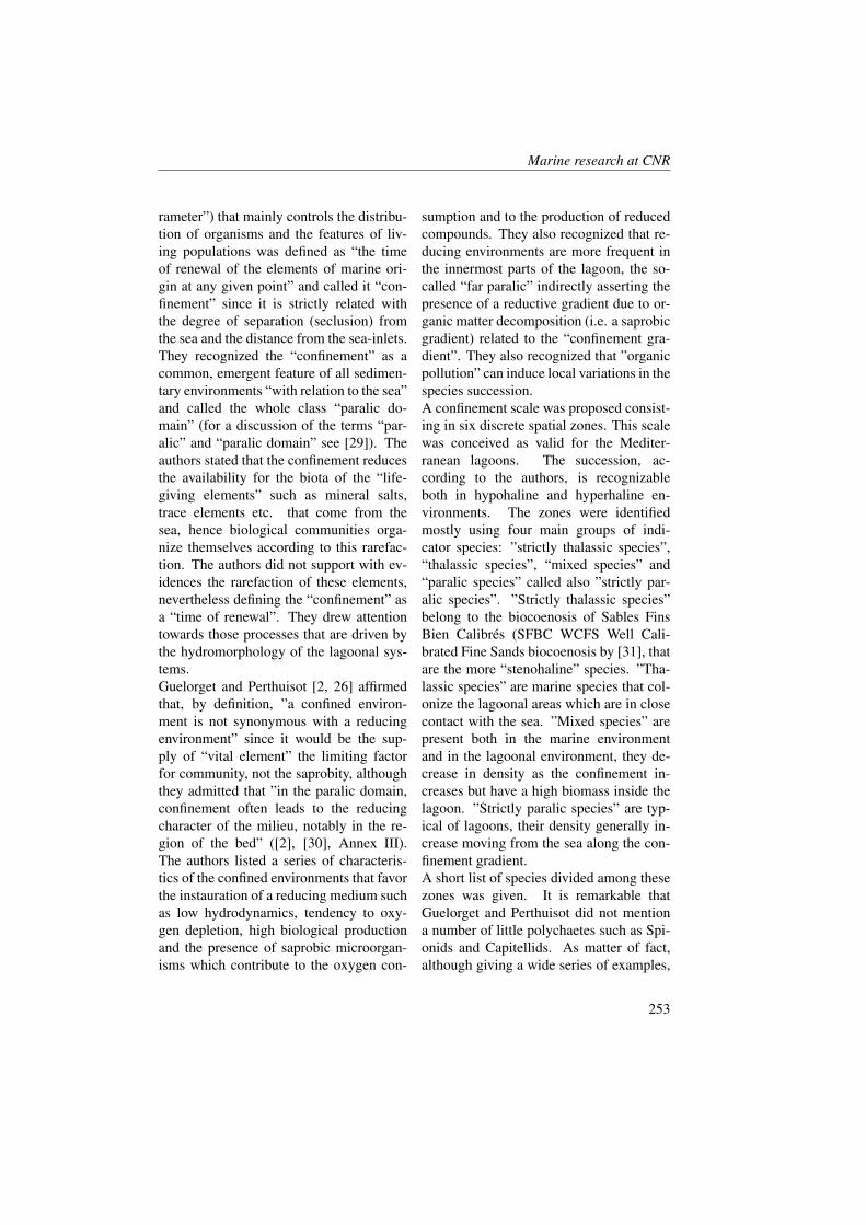
Marine research at CNR
rameter”) that mainly controls the distribu-tion of organisms and the features of liv-ing populations was defined as “the timeof renewal of the elements of marine ori-gin at any given point” and called it “con-finement” since it is strictly related withthe degree of separation (seclusion) fromthe sea and the distance from the sea-inlets.They recognized the “confinement” as acommon, emergent feature of all sedimen-tary environments “with relation to the sea”and called the whole class “paralic do-main” (for a discussion of the terms “par-alic” and “paralic domain” see [29]). Theauthors stated that the confinement reducesthe availability for the biota of the “life-giving elements” such as mineral salts,trace elements etc. that come from thesea, hence biological communities orga-nize themselves according to this rarefac-tion. The authors did not support with ev-idences the rarefaction of these elements,nevertheless defining the “confinement” asa “time of renewal”. They drew attentiontowards those processes that are driven bythe hydromorphology of the lagoonal sys-tems.Guelorget and Perthuisot [2, 26] affirmedthat, by definition, ”a confined environ-ment is not synonymous with a reducingenvironment” since it would be the sup-ply of “vital element” the limiting factorfor community, not the saprobity, althoughthey admitted that ”in the paralic domain,confinement often leads to the reducingcharacter of the milieu, notably in the re-gion of the bed” ([2], [30], Annex III).The authors listed a series of characteris-tics of the confined environments that favorthe instauration of a reducing medium suchas low hydrodynamics, tendency to oxy-gen depletion, high biological productionand the presence of saprobic microorgan-isms which contribute to the oxygen con-
sumption and to the production of reducedcompounds. They also recognized that re-ducing environments are more frequent inthe innermost parts of the lagoon, the so-called “far paralic” indirectly asserting thepresence of a reductive gradient due to or-ganic matter decomposition (i.e. a saprobicgradient) related to the “confinement gra-dient”. They also recognized that ”organicpollution” can induce local variations in thespecies succession.A confinement scale was proposed consist-ing in six discrete spatial zones. This scalewas conceived as valid for the Mediter-ranean lagoons. The succession, ac-cording to the authors, is recognizableboth in hypohaline and hyperhaline en-vironments. The zones were identifiedmostly using four main groups of indi-cator species: ”strictly thalassic species”,“thalassic species”, “mixed species” and“paralic species” called also ”strictly par-alic species”. ”Strictly thalassic species”belong to the biocoenosis of Sables FinsBien Calibres (SFBC WCFS Well Cali-brated Fine Sands biocoenosis by [31], thatare the more “stenohaline” species. ”Tha-lassic species” are marine species that col-onize the lagoonal areas which are in closecontact with the sea. ”Mixed species” arepresent both in the marine environmentand in the lagoonal environment, they de-crease in density as the confinement in-creases but have a high biomass inside thelagoon. ”Strictly paralic species” are typ-ical of lagoons, their density generally in-crease moving from the sea along the con-finement gradient.A short list of species divided among thesezones was given. It is remarkable thatGuelorget and Perthuisot did not mentiona number of little polychaetes such as Spi-onids and Capitellids. As matter of fact,although giving a wide series of examples,
253

Marine Ecology
Guelorget and Perthuisot did not give asystematic and quantitative description ofthe distribution of species along the ”par-alic” seriation, leaving room for many crit-icisms. [28], criticized the possibility ofapplication of the ”confinement” species toestuaries and tidal-flat habitats of the north-ern macrotidal Europe, characterized by astrong hydrodynamics and water renewal.This author also recognized the non directdependence of the distribution of ”brackishfauna” on salinity. He pointed out that themajority of the species listed by Guelor-get and Perthuisot can be considered aseuryhaline, or particularly euryhaline, ma-rine species that penetrated also estuaries.However, most importantly, he stressedthe existence of ”lagoonal species”, i.e.species that lives in nanotidal or microti-dal lagoons but are usually absent frommacrotidal estuaries and tidal-flat habitats,that are coincident with the ”strictly par-alic species” of Guelorget and Perthuisot.These ”lagoonal species” are adapted tolentic, little flushed CTE, the environmentsthat are more subjected to develop sapro-bic conditions. The G-P model was notfollowed by indices that quantify the “con-finement”, with the exception of a bioticindex proposed by [32, 33] conceived toassess environmental quality in Mediter-ranean lagoons.
5 Convergence of the P-Rand G-P models
Applying the P-R model to lagoons, we no-tice that there is an evident parallelism withthe biological succession foreseen by theG-P model. In fact, both the P-R and G-P models foresee a shift in trophic habitsfrom a dominance of filter feeders and sus-
pension feeders towards an almost com-plete dominance of deposit feeders, firstsurface deposit feeders and then subsur-face deposit feeders. This roughly cor-responds, in terms of systematic groups,to a passage from a bivalve-dominated as-semblage toward a polychaetes-dominatedone. Also, it seems there is a strong par-allelism between the “ecological groups”as defined by the P-R model (and thesubsequent derived indices) and the G-Pgroups of species. The seriation startsfrom the sea with ”sensitive species” the“thalassic species” of G-P model, con-tinue with ”mixed species” defined also”coastal/estuarine species” by [28], ”tol-erant species” or “strictly paralic” or “la-goonal” in Barnes. These evidences sug-gest that the P-R and G-P models describesubstantially the same phenomenon: thesuccession of macrobenthic species in re-lation to a gradient of saprobity. How-ever community would not be structured bya general input of ”vital elements of ma-rine origin”, but by processes linked to themetabolism of organic mater as for the P-R model. Therefore both models describethe effects accumulation, metabolism andclearance of organic matter catabolites andthe related subtraction of oxygen from thesystem. In this regard, the two models ac-knowledge the fundamental importance ofhydrodynamics both in the genesis of theorganic enrichment gradient and in clear-ance processes. Descriptions differ be-cause of the habitat investigated, coastalmarine, estuarine or lagoonal character-ized by different hydrodynamics and sed-imentology and because of the nature ofthe organic input, anthropogenic or morenatural. The application of the G-P con-ceptual model, however, suffered from thesame drawbacks as the P-R model, thatis poor quantification and formalization.
254
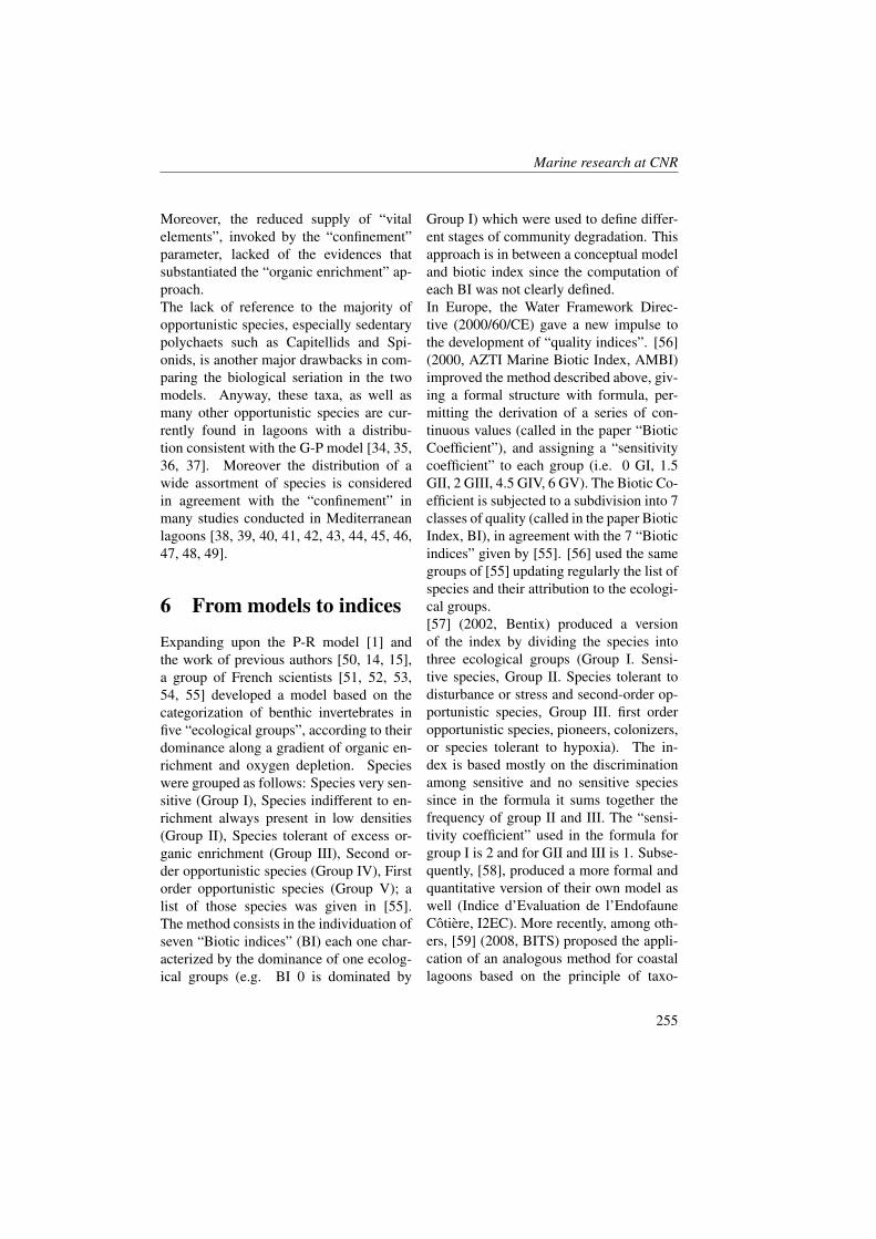
Marine research at CNR
Moreover, the reduced supply of “vitalelements”, invoked by the “confinement”parameter, lacked of the evidences thatsubstantiated the “organic enrichment” ap-proach.The lack of reference to the majority ofopportunistic species, especially sedentarypolychaets such as Capitellids and Spi-onids, is another major drawbacks in com-paring the biological seriation in the twomodels. Anyway, these taxa, as well asmany other opportunistic species are cur-rently found in lagoons with a distribu-tion consistent with the G-P model [34, 35,36, 37]. Moreover the distribution of awide assortment of species is consideredin agreement with the “confinement” inmany studies conducted in Mediterraneanlagoons [38, 39, 40, 41, 42, 43, 44, 45, 46,47, 48, 49].
6 From models to indices
Expanding upon the P-R model [1] andthe work of previous authors [50, 14, 15],a group of French scientists [51, 52, 53,54, 55] developed a model based on thecategorization of benthic invertebrates infive “ecological groups”, according to theirdominance along a gradient of organic en-richment and oxygen depletion. Specieswere grouped as follows: Species very sen-sitive (Group I), Species indifferent to en-richment always present in low densities(Group II), Species tolerant of excess or-ganic enrichment (Group III), Second or-der opportunistic species (Group IV), Firstorder opportunistic species (Group V); alist of those species was given in [55].The method consists in the individuation ofseven “Biotic indices” (BI) each one char-acterized by the dominance of one ecolog-ical groups (e.g. BI 0 is dominated by
Group I) which were used to define differ-ent stages of community degradation. Thisapproach is in between a conceptual modeland biotic index since the computation ofeach BI was not clearly defined.In Europe, the Water Framework Direc-tive (2000/60/CE) gave a new impulse tothe development of “quality indices”. [56](2000, AZTI Marine Biotic Index, AMBI)improved the method described above, giv-ing a formal structure with formula, per-mitting the derivation of a series of con-tinuous values (called in the paper “BioticCoefficient”), and assigning a “sensitivitycoefficient” to each group (i.e. 0 GI, 1.5GII, 2 GIII, 4.5 GIV, 6 GV). The Biotic Co-efficient is subjected to a subdivision into 7classes of quality (called in the paper BioticIndex, BI), in agreement with the 7 “Bioticindices” given by [55]. [56] used the samegroups of [55] updating regularly the list ofspecies and their attribution to the ecologi-cal groups.[57] (2002, Bentix) produced a versionof the index by dividing the species intothree ecological groups (Group I. Sensi-tive species, Group II. Species tolerant todisturbance or stress and second-order op-portunistic species, Group III. first orderopportunistic species, pioneers, colonizers,or species tolerant to hypoxia). The in-dex is based mostly on the discriminationamong sensitive and no sensitive speciessince in the formula it sums together thefrequency of group II and III. The “sensi-tivity coefficient” used in the formula forgroup I is 2 and for GII and III is 1. Subse-quently, [58], produced a more formal andquantitative version of their own model aswell (Indice d’Evaluation de l’EndofauneCotiere, I2EC). More recently, among oth-ers, [59] (2008, BITS) proposed the appli-cation of an analogous method for coastallagoons based on the principle of taxo-
255
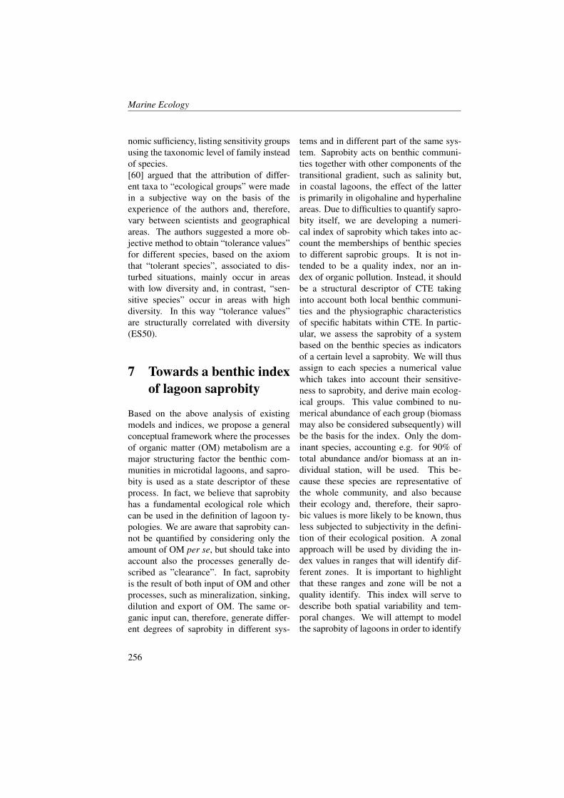
Marine Ecology
nomic sufficiency, listing sensitivity groupsusing the taxonomic level of family insteadof species.[60] argued that the attribution of differ-ent taxa to “ecological groups” were madein a subjective way on the basis of theexperience of the authors and, therefore,vary between scientists and geographicalareas. The authors suggested a more ob-jective method to obtain “tolerance values”for different species, based on the axiomthat “tolerant species”, associated to dis-turbed situations, mainly occur in areaswith low diversity and, in contrast, “sen-sitive species” occur in areas with highdiversity. In this way “tolerance values”are structurally correlated with diversity(ES50).
7 Towards a benthic indexof lagoon saprobity
Based on the above analysis of existingmodels and indices, we propose a generalconceptual framework where the processesof organic matter (OM) metabolism are amajor structuring factor the benthic com-munities in microtidal lagoons, and sapro-bity is used as a state descriptor of theseprocess. In fact, we believe that saprobityhas a fundamental ecological role whichcan be used in the definition of lagoon ty-pologies. We are aware that saprobity can-not be quantified by considering only theamount of OM per se, but should take intoaccount also the processes generally de-scribed as ”clearance”. In fact, saprobityis the result of both input of OM and otherprocesses, such as mineralization, sinking,dilution and export of OM. The same or-ganic input can, therefore, generate differ-ent degrees of saprobity in different sys-
tems and in different part of the same sys-tem. Saprobity acts on benthic communi-ties together with other components of thetransitional gradient, such as salinity but,in coastal lagoons, the effect of the latteris primarily in oligohaline and hyperhalineareas. Due to difficulties to quantify sapro-bity itself, we are developing a numeri-cal index of saprobity which takes into ac-count the memberships of benthic speciesto different saprobic groups. It is not in-tended to be a quality index, nor an in-dex of organic pollution. Instead, it shouldbe a structural descriptor of CTE takinginto account both local benthic communi-ties and the physiographic characteristicsof specific habitats within CTE. In partic-ular, we assess the saprobity of a systembased on the benthic species as indicatorsof a certain level a saprobity. We will thusassign to each species a numerical valuewhich takes into account their sensitive-ness to saprobity, and derive main ecolog-ical groups. This value combined to nu-merical abundance of each group (biomassmay also be considered subsequently) willbe the basis for the index. Only the dom-inant species, accounting e.g. for 90% oftotal abundance and/or biomass at an in-dividual station, will be used. This be-cause these species are representative ofthe whole community, and also becausetheir ecology and, therefore, their sapro-bic values is more likely to be known, thusless subjected to subjectivity in the defini-tion of their ecological position. A zonalapproach will be used by dividing the in-dex values in ranges that will identify dif-ferent zones. It is important to highlightthat these ranges and zone will be not aquality identify. This index will serve todescribe both spatial variability and tem-poral changes. We will attempt to modelthe saprobity of lagoons in order to identify
256

Marine research at CNR
reference values for each lagoon typology.The index should thus be used to identify
saprobic zones inside CTE landscapes.
References[1] T. Pearson and R. Rosenberg. Macrobenthic succession in relation to organic en-
richment and pollution of the marine environment. Oceanography and Marine Bi-ology Annual Review, 16:229–311, 1978.
[2] O. Guelorget and J.-P. Perthuisot. Le domain paralique. Expressions geologiques,biologiques et economiques du confinement, volume 16 of Travaux du Laboratoirede Geologie. Presses de l’Ecole Normale Superieure de Paris, Paris, 1983. 136 pp.In French.
[3] R. Kolkwitz and M. Marsson. Grundsatze fur die biologische Beurteilungdes Wassers nach seiner Flora und Fauna. Mitteilungen aus dem KoniglichePrufungsanstalt fur Wasserversorgung und Abwasserbeseitigung Berlin, 1:33–72,1902. In German.
[4] R. Kolkwitz and M. Marsson. Okologie der tierischen Saprobien. Berichte derDeutschen Botanischen Gesellschaft, 26a:505–519, 1908. In German.
[5] R. Kolkwitz and M. Marsson. Okologie der tierischen Saprobien. Beitragezur Lehre von der biologischen Gewasserbeurteilung. Internationale Revue derGesamten Hydrobiologie und Hydrographie, 2:126–152, 1909. In German.
[6] H. Caspers and L. Karbe. Proposals for a saprobiological classification of waters.Report WHO/EBL/66.80, World Health Organization, Geneva, 1966.
[7] V. Sladecek. The ecological and physiological trends in the saprobiology. Hydro-biologia, 30(3-4):513–526, 1967.
[8] M. Bartoli, D. Longhi, D. Nizzoli, S. Como, P. Magni, and P. Viaroli. Short termeffects of hypoxia and bioturbation on solute fluxes, denitrification and bufferingcapacity in a shallow dystrophic pond. Journal of Experimental Marine Biologyand Ecology, 381(2):105–113, 2009.
[9] M.A. Best, A.W. Wither, and S. Coates. Dissolved oxygen as a physico-chemicalsupporting element in the Water Framework Directive. Marine Pollution Bulletin,55(1-6):53–64, 2007.
[10] R. Pantle and H. Buck. Die biologische Uberwachung der Gewasser und dieDarstellung der Ergebnisse. Gas- und Wasserfach. Wasser und Abwasser, 96:604–607, 1955.
257
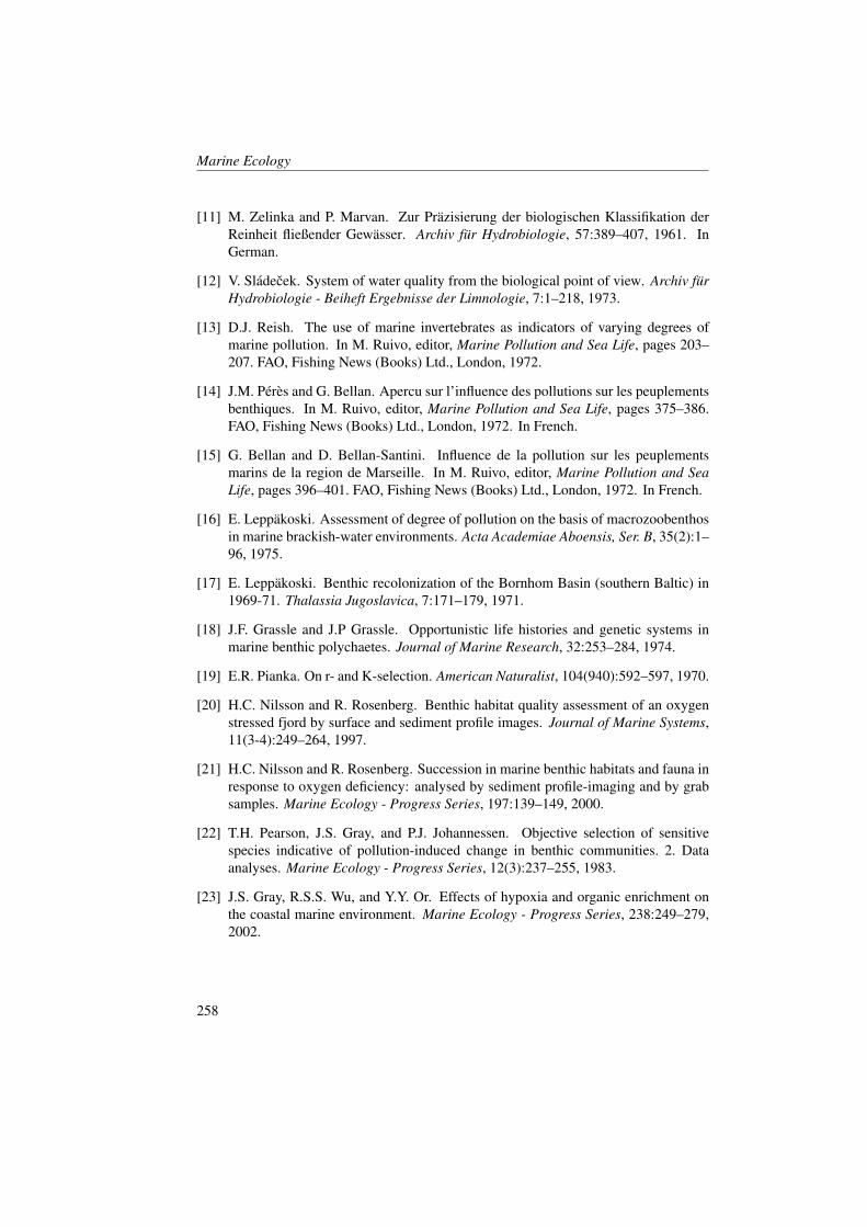
Marine Ecology
[11] M. Zelinka and P. Marvan. Zur Prazisierung der biologischen Klassifikation derReinheit fließender Gewasser. Archiv fur Hydrobiologie, 57:389–407, 1961. InGerman.
[12] V. Sladecek. System of water quality from the biological point of view. Archiv furHydrobiologie - Beiheft Ergebnisse der Limnologie, 7:1–218, 1973.
[13] D.J. Reish. The use of marine invertebrates as indicators of varying degrees ofmarine pollution. In M. Ruivo, editor, Marine Pollution and Sea Life, pages 203–207. FAO, Fishing News (Books) Ltd., London, 1972.
[14] J.M. Peres and G. Bellan. Apercu sur l’influence des pollutions sur les peuplementsbenthiques. In M. Ruivo, editor, Marine Pollution and Sea Life, pages 375–386.FAO, Fishing News (Books) Ltd., London, 1972. In French.
[15] G. Bellan and D. Bellan-Santini. Influence de la pollution sur les peuplementsmarins de la region de Marseille. In M. Ruivo, editor, Marine Pollution and SeaLife, pages 396–401. FAO, Fishing News (Books) Ltd., London, 1972. In French.
[16] E. Leppakoski. Assessment of degree of pollution on the basis of macrozoobenthosin marine brackish-water environments. Acta Academiae Aboensis, Ser. B, 35(2):1–96, 1975.
[17] E. Leppakoski. Benthic recolonization of the Bornhom Basin (southern Baltic) in1969-71. Thalassia Jugoslavica, 7:171–179, 1971.
[18] J.F. Grassle and J.P Grassle. Opportunistic life histories and genetic systems inmarine benthic polychaetes. Journal of Marine Research, 32:253–284, 1974.
[19] E.R. Pianka. On r- and K-selection. American Naturalist, 104(940):592–597, 1970.
[20] H.C. Nilsson and R. Rosenberg. Benthic habitat quality assessment of an oxygenstressed fjord by surface and sediment profile images. Journal of Marine Systems,11(3-4):249–264, 1997.
[21] H.C. Nilsson and R. Rosenberg. Succession in marine benthic habitats and fauna inresponse to oxygen deficiency: analysed by sediment profile-imaging and by grabsamples. Marine Ecology - Progress Series, 197:139–149, 2000.
[22] T.H. Pearson, J.S. Gray, and P.J. Johannessen. Objective selection of sensitivespecies indicative of pollution-induced change in benthic communities. 2. Dataanalyses. Marine Ecology - Progress Series, 12(3):237–255, 1983.
[23] J.S. Gray, R.S.S. Wu, and Y.Y. Or. Effects of hypoxia and organic enrichment onthe coastal marine environment. Marine Ecology - Progress Series, 238:249–279,2002.
258
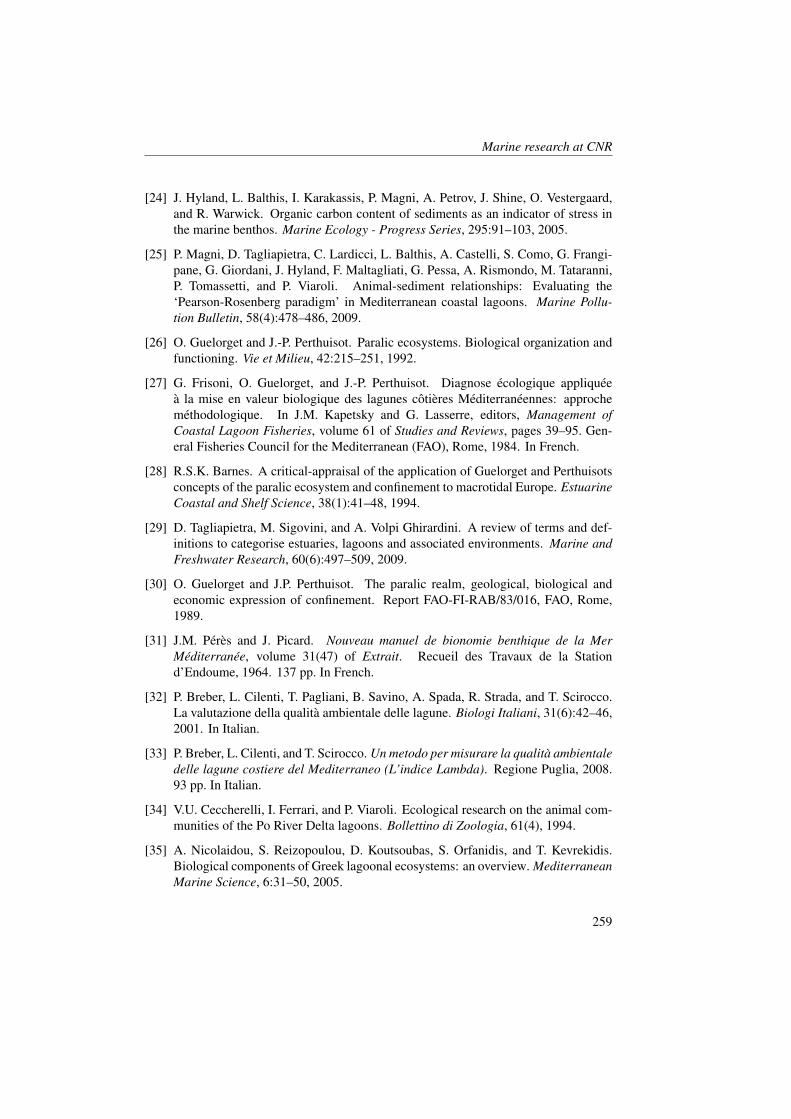
Marine research at CNR
[24] J. Hyland, L. Balthis, I. Karakassis, P. Magni, A. Petrov, J. Shine, O. Vestergaard,and R. Warwick. Organic carbon content of sediments as an indicator of stress inthe marine benthos. Marine Ecology - Progress Series, 295:91–103, 2005.
[25] P. Magni, D. Tagliapietra, C. Lardicci, L. Balthis, A. Castelli, S. Como, G. Frangi-pane, G. Giordani, J. Hyland, F. Maltagliati, G. Pessa, A. Rismondo, M. Tataranni,P. Tomassetti, and P. Viaroli. Animal-sediment relationships: Evaluating the‘Pearson-Rosenberg paradigm’ in Mediterranean coastal lagoons. Marine Pollu-tion Bulletin, 58(4):478–486, 2009.
[26] O. Guelorget and J.-P. Perthuisot. Paralic ecosystems. Biological organization andfunctioning. Vie et Milieu, 42:215–251, 1992.
[27] G. Frisoni, O. Guelorget, and J.-P. Perthuisot. Diagnose ecologique appliqueea la mise en valeur biologique des lagunes cotieres Mediterraneennes: approchemethodologique. In J.M. Kapetsky and G. Lasserre, editors, Management ofCoastal Lagoon Fisheries, volume 61 of Studies and Reviews, pages 39–95. Gen-eral Fisheries Council for the Mediterranean (FAO), Rome, 1984. In French.
[28] R.S.K. Barnes. A critical-appraisal of the application of Guelorget and Perthuisotsconcepts of the paralic ecosystem and confinement to macrotidal Europe. EstuarineCoastal and Shelf Science, 38(1):41–48, 1994.
[29] D. Tagliapietra, M. Sigovini, and A. Volpi Ghirardini. A review of terms and def-initions to categorise estuaries, lagoons and associated environments. Marine andFreshwater Research, 60(6):497–509, 2009.
[30] O. Guelorget and J.P. Perthuisot. The paralic realm, geological, biological andeconomic expression of confinement. Report FAO-FI-RAB/83/016, FAO, Rome,1989.
[31] J.M. Peres and J. Picard. Nouveau manuel de bionomie benthique de la MerMediterranee, volume 31(47) of Extrait. Recueil des Travaux de la Stationd’Endoume, 1964. 137 pp. In French.
[32] P. Breber, L. Cilenti, T. Pagliani, B. Savino, A. Spada, R. Strada, and T. Scirocco.La valutazione della qualita ambientale delle lagune. Biologi Italiani, 31(6):42–46,2001. In Italian.
[33] P. Breber, L. Cilenti, and T. Scirocco. Un metodo per misurare la qualita ambientaledelle lagune costiere del Mediterraneo (L’indice Lambda). Regione Puglia, 2008.93 pp. In Italian.
[34] V.U. Ceccherelli, I. Ferrari, and P. Viaroli. Ecological research on the animal com-munities of the Po River Delta lagoons. Bollettino di Zoologia, 61(4), 1994.
[35] A. Nicolaidou, S. Reizopoulou, D. Koutsoubas, S. Orfanidis, and T. Kevrekidis.Biological components of Greek lagoonal ecosystems: an overview. MediterraneanMarine Science, 6:31–50, 2005.
259
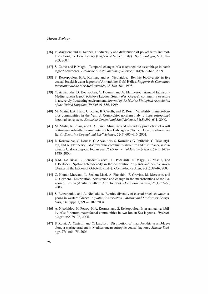
Marine Ecology
[36] F. Maggiore and E. Keppel. Biodiversity and distribution of polychaetes and mol-luscs along the Dese estuary (Lagoon of Venice, Italy). Hydrobiologia, 588:189–203, 2007.
[37] S. Como and P. Magni. Temporal changes of a macrobenthic assemblage in harshlagoon sediments. Estuarine Coastal and Shelf Science, 83(4):638–646, 2009.
[38] S. Reizopoulou, K.A. Kormas, and A. Nicolaidou. Benthic biodiversity in fivecoastal brackish water lagoons of Amvrakikos Gulf, Hellas. Rapports de CommitteeInternationale de Mer Mediterranee, 35:580–581, 1998.
[39] C. Arvanitidis, D. Koutsoubas, C. Dounas, and A. Eleftheriou. Annelid fauna of aMediterranean lagoon (Gialova Lagoon, South-West Greece): community structurein a severely fluctuating environment. Journal of the Marine Biological Associationof the United Kingdom, 79(5):849–856, 1999.
[40] M. Mistri, E.A. Fano, G. Rossi, K. Caselli, and R. Rossi. Variability in macroben-thos communities in the Valli di Comacchio, northern Italy, a hypereutrophizedlagoonal ecosystem. Estuarine Coastal and Shelf Science, 51(5):599–611, 2000.
[41] M. Mistri, R. Rossi, and E.A. Fano. Structure and secondary production of a softbottom macrobenthic community in a brackish lagoon (Sacca di Goro, north-easternItaly). Estuarine Coastal and Shelf Science, 52(5):605–616, 2001.
[42] D. Koutsoubas, C. Dounas, C. Arvanitidis, S. Kornilios, G. Petihakis, G. Triantafyl-lou, and A. Eleftheriou. Macrobenthic community structure and disturbance assess-ment in Gialova Lagoon, Ionian Sea. ICES Journal of Marine Science, 57(5):1472–1480, 2000.
[43] A.M. De Biasi, L. Benedetti-Cecchi, L. Pacciardi, E. Maggi, S. Vaselli, andI. Bertocci. Spatial heterogeneity in the distribution of plants and benthic inver-tebrates in the lagoon of Orbetello (Italy). Oceanologica Acta, 26(1):39–46, 2003.
[44] C. Nonnis Marzano, L. Scalera Liaci, A. Fianchini, F. Gravina, M. Mercurio, andG. Corriero. Distribution, persistence and change in the macrobenthos of the La-goon of Lesina (Apulia, southern Adriatic Sea). Oceanologica Acta, 26(1):57–66,2003.
[45] S. Reizopoulou and A. Nicolaidou. Benthic diversity of coastal brackish-water la-goons in western Greece. Aquatic Conservation - Marine and Freshwater Ecosys-tems, 14(Suppl. 1):S93–S102, 2004.
[46] A. Nicolaidou, K. Petrou, K.A. Kormas, and S. Reizopoulou. Inter-annual variabil-ity of soft bottom macrofaunal communities in two Ionian Sea lagoons. Hydrobi-ologia, 555:89–98, 2006.
[47] F. Rossi, A. Castelli, and C. Lardicci. Distribution of macrobenthic assemblagesalong a marine gradient in Mediterranean eutrophic coastal lagoons. Marine Ecol-ogy, 27(1):66–75, 2006.
260
Marine research at CNR
[48] M.F. Gravina, G.D. Ardizzone, F. Scaletta, and C. Chimenz. Descriptive analysisand classification of benthic communities in some Mediterranean coastal lagoons(Central Italy). Marine Ecology, 10(2):141–166, 2008.
[49] S. Tlig-Zouari, T. Mami, and F. Maamouri. Structure of benthic macroinvertebratesand dynamics in the northern lagoon of Tunis. Journal of the Marine BiologicalAssociation of the United Kingdom, 89(7):1305–1318, 2009.
[50] G. Bellan. Pollution et peuplements benthiques des substrats meubles de la regionde Marseille. Revue Internationale d’Oceanographie Medical, 6-7:53–87, 1967. InFrench.
[51] M. Glemarec and C. Hily. Perturbations apportees a la macrofaune benthique dela baie de Concarneau par les effluents urbains et portuaires. Acta Oecologica Oe-cologia Applicata, 2:139–150, 1981. In French.
[52] C. Hily. Variabilite de la macrofaune benthique dans les milieux hypertrophiquesde la Rade de Brest, 1984. Vol. 1: 359 pp., Vol. 2: 337 pp. In French.
[53] C. Hily, H. Le Bris, and M. Glemarec. Impacts biologiques des emissaires urbainssur les ecosystemes benthiques. Oceanis, 12:419–426, 1986. In French.
[54] S.A. Majeed. Organic-matter and biotic indexes on the beaches of North Brittany.Marine Pollution Bulletin, 18(9):490–495, 1987.
[55] J. Grall and M. Glemarec. Using biotic indices to estimate macrobenthic commu-nity perturbations in the Bay of Brest. Estuarine Coastal and Shelf Science, 44(suppl. A):43–53, 1997.
[56] A. Borja, J. Franco, and V. Perez. A marine Biotic Index to establish the ecologicalquality of soft-bottom benthos within European estuarine and coastal environments.Marine Pollution Bulletin, 40(12):1100–1114, 2000.
[57] N. Simboura and A. Zenetos. Benthic indicators to use in ecological quality clas-sification of Mediterranean soft bottom marine ecosystems including a new BioticIndex. Mediterranean Marine Science, 3(2):77–111, 2002.
[58] J. Grall and M. Glemarec. L’indice d’evaluation de l’endofaune cotiere. InC. Alzieu, editor, Bioevaluation de la qualite environnementale des sedimentsportuaires et des zones d’immersion, pages 51–85. Edition IFREMER, 2003. InFrench.
[59] M. Mistri and C. Munari. BITS: A SMART indicator for soft-bottom, non-tidallagoons. Marine Pollution Bulletin, 56(3):587–599, 2008.
[60] R. Rosenberg, M. Blomqvist, H.C. Nilsson, H. Cederwall, and A. Dimming. Marinequality assessment by use of benthic species-abundance distributions: a proposednew protocol within the European Union Water Framework Directive. Marine Pol-lution Bulletin, 49(9-10):728–739, 2004.
261

Marine Ecology
262
Benthic Diversity in Oligotrophic Waters: the CaseStudy of Is Arenas (Western Sardinia, Italy)
G.A. Fenzi1, P. Magni1,2
1, Institute for Coastal Marine Environment, CNR, Oristano, Italy2, Institute of Marine Sciences, CNR, Venezia, [email protected]
Abstract
We report the distribution of benthic assemblages in Is Arenas Bay, a coastalmarine area of western Sardinia characterized by oligotrophic waters and the pres-ence of different habitats, including the seagrass Posidonia oceanica and unvegetatedsediments. Gammarids tended to dominate in proximity of the seagrass meadow,while nematods, polychaetes (Lumbrineridae) and bivalves (Tellinidae) increased inwell-sorted fine-sand sediments. Among these benthic communities, a wide rangeof taxonomic groups included as the polychaetes Phyllodocidae, Nuculanidae andGliceridae, the crustaceans Ostracoda, Caprellidae, Processidae, Isopoda and Por-tunidae, the mollusks Nuculanidae, Glycymeridae, Naticidae, Eulimidae, and theechinoderms Astropectinidae, Ophiuroidea, Holoturoidea. Overall, the benthic com-munities of Is Arenas were dominated by taxa sensitive to anthropogenic impact,indicating a high biodiverse and healthy coastal marine ecosystem.
1 Introduction
Coastal marine ecosystems play a key roleon the whole marine environment, pro-viding a variety of ecological functions[1]. As an example, physical [2], chemi-cal [3, 4] and biological processes take partin the gas regulation and nutrient cyclingat different spatial and temporal scales[5]. These environments are also essentialfor many organisms, providing essentialhabitats as a nursery ground for juvenilesof many marine, estuarine and freshwaterfishes [6]. Moreover, coastal areas have di-rect or indirect junctions with different eco-nomical services and human values. Thesenatural resources should be considered asrenewable and preserved through the con-servation of biodiversity and the mitigationof climate change effects [1] to maintain
constant their productivity in the future.The spatial and temporal distributionof macrozoobenthic assemblages and themain features of sediments provide valu-able information of the ecological statusof the system [7, 8]. Indeed, benthic dy-namics are tightly related with processesoccurring both in the water column andsediments. Distributional changes, alteredabundance and reduced diversity in thebenthos can be used as biological toolsof past and present disturbances [9, 10].Because of the sedentary lifestyle and thelongevity (several months to a few years)of benthic organisms, they can be a directevidence of environmental changes in themarine habitats [11, 12].Several aspects of benthic communities canbe described by their functional diversity.Tilman [13] defined it as “the number of
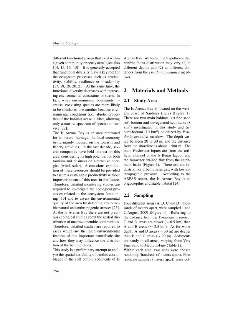
Marine Ecology
different functional groups that exist withina given community or ecosystem” (see also[14, 15, 16, 13]). It is generally acceptedthat functional diversity plays a key role forthe ecosystem processes such as produc-tivity, stability, resilience or invadability[17, 18, 19, 20, 21]. At the same time, thefunctional diversity decreases with increas-ing environmental constraints or stress. Infact, when environmental constraints in-crease, coexisting species are more likelyto be similar to one another because envi-ronmental conditions (i.e. abiotic proper-ties of the habitat) act as a filter, allowingonly a narrow spectrum of species to sur-vive [22].The Is Arenas Bay is an area renownedfor its natural heritage, the local economybeing mainly focused on the tourism andfishery activities. In the last decade, sev-eral companies have held interest on thisarea, considering its high potential for bothtourism and business on alternative ener-gies (wind, solar). A conscious exploita-tion of these resources should be providedto assure a sustainable productivity withoutimpoverishment of this area in the future.Therefore, detailed monitoring studies arerequired to investigate the ecological pro-cesses related to the ecosystem function-ing [13] and to assess the environmentalquality of the area by detecting any possi-ble natural and anthropogenic stresses [23].At the Is Arenas Bay there are not previ-ous ecological studies about the spatial dis-tribution of macrozoobenthic communities.Therefore, detailed studies are required toasses which are the main environmentalfeatures of this important naturalistic siteand how they may influence the distribu-tion of the benthic fauna.This study is a preliminary attempt to anal-yse the spatial variability of benthic assem-blages in the soft bottom sediments of Is
Arenas Bay. We tested the hypotheses thatbenthic fauna distribution may vary (1) atdifferent depths and (2) at different dis-tances from the Posidonia oceanica mead-ows.
2 Materials and Methods
2.1 Study Area
The Is Arenas Bay is located on the west-ern coast of Sardinia (Italy) (Figure 1).There are two main habitats: (i) fine sandsoft bottom and unvegetated sediments (8km2) investigated in this study and (ii)hard-bottom (10 km2) colonized by Posi-donia oceanica meadow. The depth var-ied between 20 to 30 m, and the distancefrom the shoreline is about 1.500 m. Themain freshwater inputs are from the arti-ficial channel of the Is Benas lagoon andthe rainwater drained flux from the catch-ment basin (Figure 1). There are not in-dustrial nor urban discharges, with low an-thropogenic pressure. According to theARPAS report, the Is Arenas Bay is anoligotropthic and stable habitat [24].
2.2 Sampling
Four different areas (A, B, C and D), thou-sands of meters apart, were sampled 1 and2 August 2009 (Figure 1). Referring tothe distance from the Posidonia oceanica,C and D areas are closer (∼ 0.5 km) thanA and B areas (∼ 2.5 km). As for waterdepth, A and D areas (∼ 30 m) are deeperthnn B and C areas (∼ 20 m). Sedimentsare sandy in all areas, varying from VeryFine Sand to Medium-Fine (Table 1).Within each area, two sites were chosenrandomly (hundreds of meters apart). Fourreplicate samples (meters apart) were col-
264
Marine research at CNR
Figure 1: Location of Is Arenas Bay, western Sardinia (Italy). The four study areas (A,B, C and D) are circled.
lected per site for a total of 32 samples.Macrozoobenthic samples were collectedby means of a van Veen grab with a sam-pling area of 360 cm2. The samples weresieved through a 0.5 mm mesh and thenpreserved in 4% formaldehyde. In the lab-oratory, all organisms were identified to thefamily level.
2.3 AnalysisFor each sample and each taxonomic levelthe number of taxa and the Shannon diver-sity index (H’ log2 based, [25]) were cal-
culated. Non-parametric multivariate anal-ysis of community structure was performedusing the software package PRIMER v.6[26]. The abundance data (no transfor-mation) were used to detect the differ-ences between sampling areas, using testANOSIM (Analysis of Similarities) basedon the Bray-Curtis (dis)similarity measureswith no transformation [27]. A non-metricmultidimensional-scaling (nmMDS) wasused to plot the differences between areasin the macrobenthic assemblage. The SIM-PER procedure was used to identify speciescontribution to similarity between samples.
265
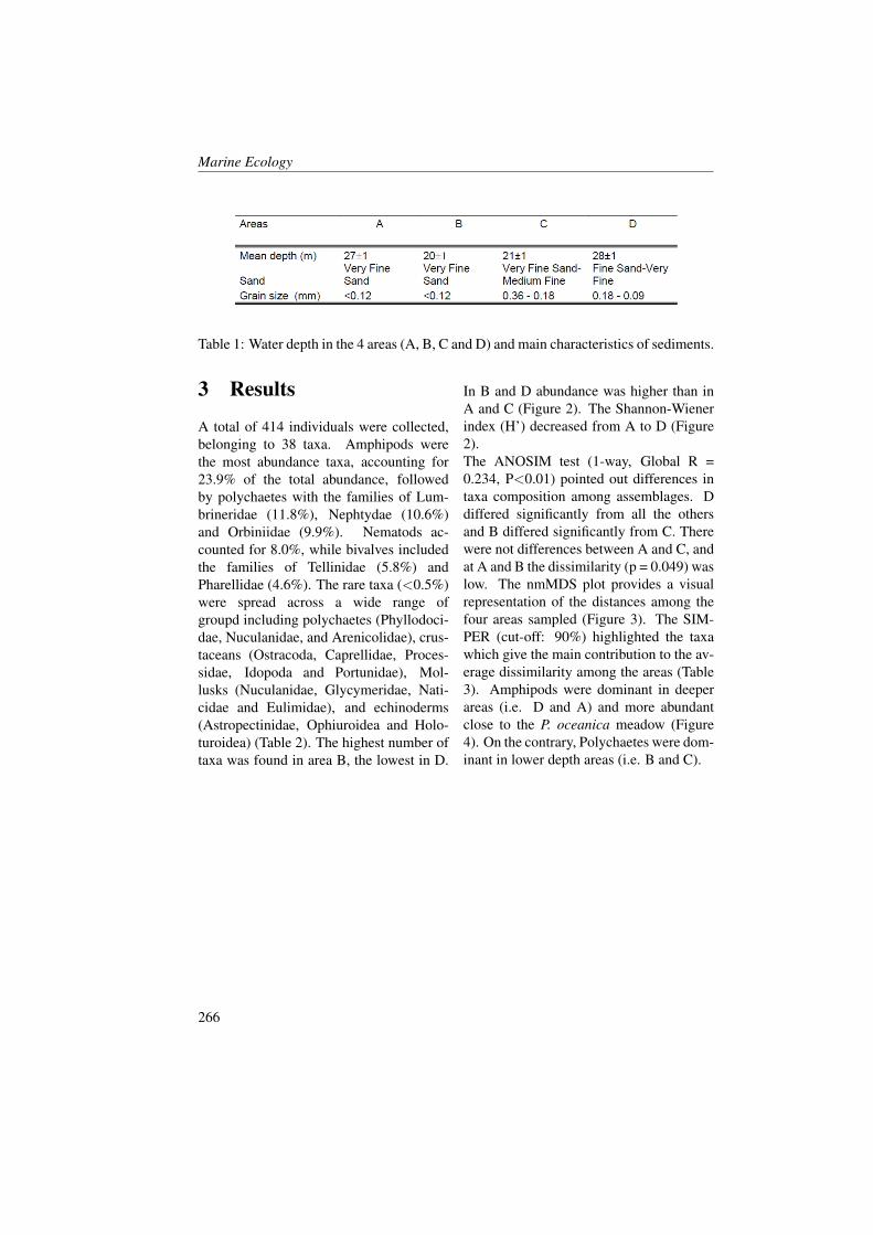
Marine Ecology
Table 1: Water depth in the 4 areas (A, B, C and D) and main characteristics of sediments.
3 Results
A total of 414 individuals were collected,belonging to 38 taxa. Amphipods werethe most abundance taxa, accounting for23.9% of the total abundance, followedby polychaetes with the families of Lum-brineridae (11.8%), Nephtydae (10.6%)and Orbiniidae (9.9%). Nematods ac-counted for 8.0%, while bivalves includedthe families of Tellinidae (5.8%) andPharellidae (4.6%). The rare taxa (<0.5%)were spread across a wide range ofgroupd including polychaetes (Phyllodoci-dae, Nuculanidae, and Arenicolidae), crus-taceans (Ostracoda, Caprellidae, Proces-sidae, Idopoda and Portunidae), Mol-lusks (Nuculanidae, Glycymeridae, Nati-cidae and Eulimidae), and echinoderms(Astropectinidae, Ophiuroidea and Holo-turoidea) (Table 2). The highest number oftaxa was found in area B, the lowest in D.
In B and D abundance was higher than inA and C (Figure 2). The Shannon-Wienerindex (H’) decreased from A to D (Figure2).The ANOSIM test (1-way, Global R =0.234, P<0.01) pointed out differences intaxa composition among assemblages. Ddiffered significantly from all the othersand B differed significantly from C. Therewere not differences between A and C, andat A and B the dissimilarity (p = 0.049) waslow. The nmMDS plot provides a visualrepresentation of the distances among thefour areas sampled (Figure 3). The SIM-PER (cut-off: 90%) highlighted the taxawhich give the main contribution to the av-erage dissimilarity among the areas (Table3). Amphipods were dominant in deeperareas (i.e. D and A) and more abundantclose to the P. oceanica meadow (Figure4). On the contrary, Polychaetes were dom-inant in lower depth areas (i.e. B and C).
266
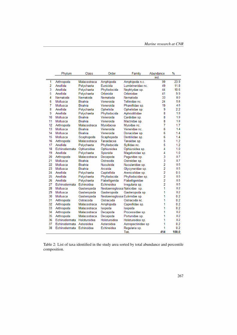
Marine research at CNR
Table 2: List of taxa identified in the study area sorted by total abundance and percentile composition.
Table 2: List of taxa identified in the study area sorted by total abundance and percentilecomposition.
267
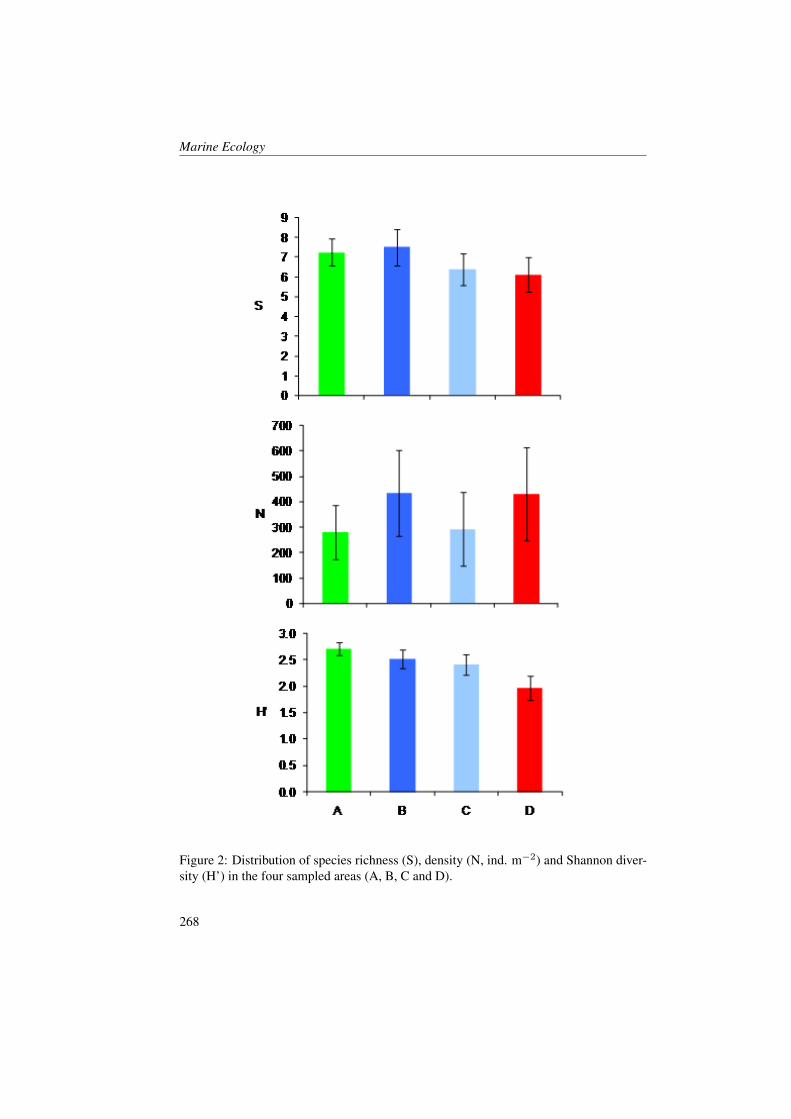
Marine Ecology
Figure 2: Distribution of species richness (S), density (N, ind. m−2) and Shannon diver-sity (H’) in the four sampled areas (A, B, C and D).
268
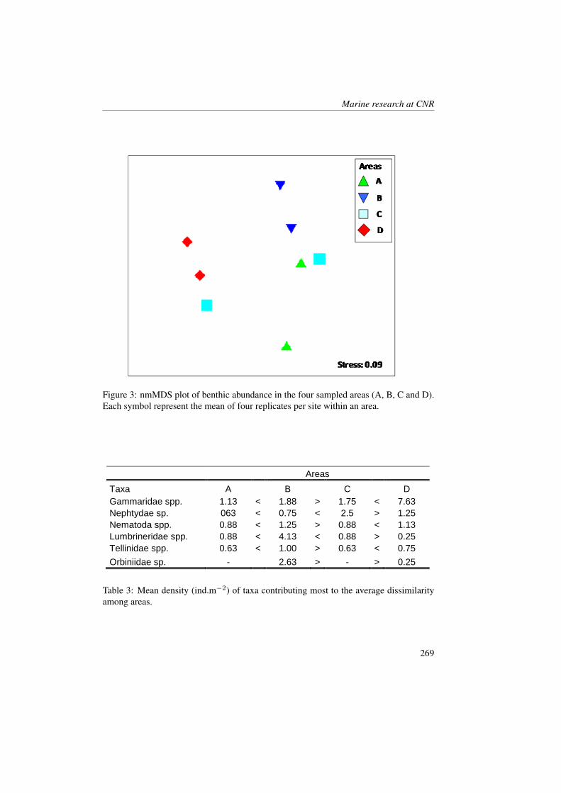
Marine research at CNR
Figure 3: nmMDS plot of benthic abundance in the four sampled areas (A, B, C and D).Each symbol represent the mean of four replicates per site within an area.
Areas
Taxa A B C D
Gammaridae spp. 1.13 < 1.88 > 1.75 < 7.63
Nephtydae sp. 063 < 0.75 < 2.5 > 1.25
Nematoda spp. 0.88 < 1.25 > 0.88 < 1.13
Lumbrineridae spp. 0.88 < 4.13 < 0.88 > 0.25
Tellinidae spp. 0.63 < 1.00 > 0.63 < 0.75
Orbiniidae sp. - 2.63 > - > 0.25
Table 3. Mean density (ind.m-2
) of taxa contributing most to the average dissimilarity among
areas.
Table 3: Mean density (ind.m−2) of taxa contributing most to the average dissimilarityamong areas.
269
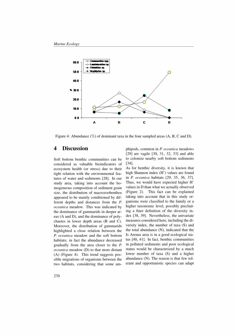
Marine Ecology
Figure 4: Abundance (%) of dominant taxa in the four sampled areas (A, B, C and D).
4 Discussion
Soft bottom benthic communities can beconsidered as valuable bioindicators ofecosystem health (or stress) due to theirtight relation with the environmental fea-tures of water and sediments [28]. In ourstudy area, taking into account the ho-mogeneous composition of sediment grainsize, the distribution of macrozoobenthosappeared to be mainly conditioned by dif-ferent depths and distances from the P.oceanica meadow. This was indicated bythe dominance of gammarids in deeper ar-eas (A and D), and the dominance of poly-chaetes in lower depth areas (B and C).Moreover, the distribution of gammaridshighlighted a close relation between theP. oceanica meadow and the soft bottomhabitats; in fact the abundance decreasedgradually from the area closer to the P.oceanica meadow (D) to that more distant(A) (Figure 4). This trend suggests pos-sible migrations of organisms between thetwo habitats, considering that some am-
phipods, common in P. oceanica meadows[29] are vagile [30, 31, 32, 33] and ableto colonize nearby soft bottom sediments[34].As for benthic diversity, it is known thathigh Shannon index (H’) values are foundin P. oceanica habitats [29, 35, 36, 37].Thus, we would have expected higher H’values in D than what we actually observed(Figure 2). This fact can be explainedtaking into account that in this study or-ganisms were classified to the family or ahigher taxonomic level, possibly preclud-ing a finer definition of the diversity in-dex [38, 39]. Nevertheless, the univariatemeasures considered here, including the di-versity index, the number of taxa (S) andthe total abundance (N), indicated that theIs Arenas area is in a good ecological sta-tus [40, 41]. In fact, benthic communitiesin polluted sediments and poor ecologicalstatus would be characterized by a muchlower number of taxa (S) and a higherabundance (N). The reason is that few tol-erant and opportunistic species can adapt
270
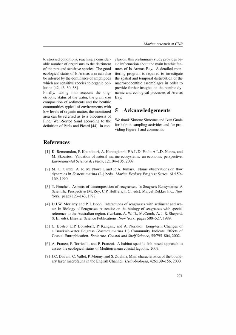
Marine research at CNR
to stressed conditions, reaching a consider-able number of organisms to the detrimentof the rare and sensitive species. The goodecological status of Is Arenas area can alsobe inferred by the dominance of amphipodswhich are sensitive species to organic pol-lution [42, 43, 30, 38].Finally, taking into account the olig-otrophic status of the water, the grain sizecomposition of sediments and the benthiccommunities typical of environments withlow levels of organic matter, the monitoredarea can be referred as to a biocenosis ofFine, Well-Sorted Sand according to thedefinition of Peres and Picard [44]. In con-
clusion, this preliminary study provides ba-sic information about the main benthic fea-tures of Is Arenas Bay. A detailed mon-itoring program is required to investigatethe spatial and temporal distribution of themacrozoobenthic assemblages in order toprovide further insights on the benthic dy-namic and ecological processes of ArenasBay.
5 AcknowledgementsWe thank Simone Simeone and Ivan Gualafor help in sampling activities and for pro-viding Figure 1 and comments.
References[1] K. Remoundou, P. Koundouri, A. Kontogianni, P.A.L.D. Paulo A.L.D. Nunes, and
M. Skourtos. Valuation of natural marine ecosystems: an economic perspective.Environmental Science & Policy, 12:104–105, 2009.
[2] M. C. Gambi, A. R. M. Nowell, and P. A. Jumars. Flume observations on flowdynamics in Zostera marina (L.) beds. Marine Ecology Progress Series, 61:159–169, 1990.
[3] T. Fenchel. Aspects of decomposition of seagrasses. In Seagrass Ecosystems: AScientific Perspective (McRoy, C.P. Helfferich, C., eds). Marcel Dekker Inc., NewYork. pages 123–143, 1977.
[4] D.J.W. Moriarty and P. I. Boon. Interactions of seagrasses with sediment and wa-ter. In Biology of Seagrasses-A treatise on the biology of seagrasses with specialreference to the Australian region. (Larkum, A. W. D., McComb, A. J. & Sheperd,S. E., eds). Elsevier Science Publications, New York. pages 500–527, 1989.
[5] C. Bostro, E.P. Bonsdorff, P. Kangas., and A. Norkko. Long-term Changes ofa Brackish-water Eelgrass (Zostera marina L.) Community Indicate Effects ofCoastal Eutrophication. Estuarine, Coastal and Shelf Science, 55:795–804, 2002.
[6] A. Franco, P. Torricelli, and P. Franzoi. A habitat-specific fish-based approach toassess the ecological status of Mediterranean coastal lagoons. 2009.
[7] J.C. Dauvin, C. Vallet, P. Mouny, and S. Zouhiri. Main characteristics of the bound-ary layer macrofauna in the English Channel. Hydrobiologia, 426:139–156, 2000.
271
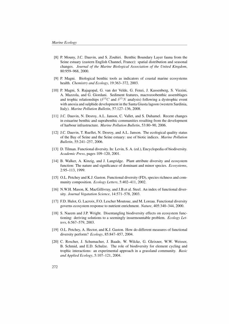
Marine Ecology
[8] P. Mouny, J.C. Dauvin, and S. Zouhiri. Benthic Boundary Layer fauna from theSeine estuary (eastern English Channel, France): spatial distribution and seasonalchanges. Journal of the Marine Biological Association of the United Kingdom,80:959–968, 2000.
[9] P. Magni. Biological benthic tools as indicators of coastal marine ecosystemshealth. Chemistry and Ecology, 19:363–372, 2003.
[10] P. Magni, S. Rajagopal, G. van der Velde, G. Fenzi, J. Kassenberg, S. Vizzini,A. Mazzola, and G. Giordani. Sediment features, macrozoobenthic assemblagesand trophic relationships (δ13C and δ15N analysis) following a dystrophic eventwith anoxia and sulphide development in the Santa Giusta lagoon (western Sardinia,Italy). Marine Pollution Bulletin, 57:127–136, 2008.
[11] J.C. Dauvin, N. Desroy, A.L. Janson, C. Vallet, and S. Duhamel. Recent changesin estuarine benthic and suprabenthic communities resulting from the developmentof harbour infrastructure. Marine Pollution Bulletin, 53:80–90, 2006.
[12] J.C. Dauvin, T. Ruellet, N. Desroy, and A.L. Janson. The ecological quality statusof the Bay of Seine and the Seine estuary: use of biotic indices. Marine PollutionBulletin, 55:241–257, 2006.
[13] D. Tilman. Functional diversity. In: Levin, S. A. (ed.), Encyclopedia of biodiversity.Academic Press, pages 109–120, 2001.
[14] B. Walker, A. Kinzig, and J. Langridge. Plant attribute diversity and ecosystemfunction: The nature and significance of dominant and minor species. Ecosystems,2:95–113, 1999.
[15] O.L. Petchey and K.J. Gaston. Functional diversity (FD), species richness and com-munity composition. Ecology Letters, 5:402–411, 2002.
[16] N.W.H. Mason, K. MacGillivray, and J.B.et al. Steel. An index of functional diver-sity. Journal Vegatation Science, 14:571–578, 2003.
[17] F.D. Hulot, G. Lacroix, F.O. Lescher Moutoue, and M. Loreau. Functional diversitygoverns ecosystem response to nutrient enrichment. Nature, 405:340–344, 2000.
[18] S. Naeem and J.P. Wright. Disentangling biodiversity effects on ecosystem func-tioning: deriving solutions to a seemingly insurmountable problem. Ecology Let-ters, 6:567–579, 2003.
[19] O.L. Petchey, A. Hector, and K.J. Gaston. How do different measures of functionaldiversity perform? Ecology, 85:847–857, 2004.
[20] C. Roscher, J. Schumacher, J. Baade, W. Wilcke, G. Gleixner, W.W. Weisser,B. Schmid, and E.D. Schulze. The role of biodiversity for element cycling andtrophic interactions: an experimental approach in a grassland community. Basicand Applied Ecology, 5:107–121, 2004.
272
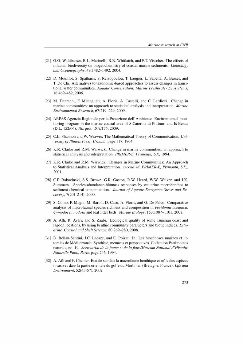
Marine research at CNR
[21] G.G. Waldbusser, R.L. Marinelli, R.B. Whitlatch, and P.T. Visscher. The effects ofinfaunal biodiversity on biogeochemistry of coastal marine sediments. Limnologyand Oceanography, 49:1482–1492, 2004.
[22] D. Mouillot, S. Spatharis, S. Reizopoulou, T. Laugier, L. Sabetta, A. Basset, andT. Do Chi. Alternatives to taxonomic-based approaches to assess changes in transi-tional water communities. Aquatic Conservation: Marine Freshwater Ecosystems,16:469–482, 2006.
[23] M. Tataranni, F. Maltagliati, A. Floris, A. Castelli, and C. Lardicci. Change inmarine communities: an approach to statistical analysis and interpretation. MarineEnvironmental Research, 67:219–229, 2009.
[24] ARPAS Agenzia Regionale per la Protezione dell’Ambiente. Environmental mon-itoring program in the marine coastal area of S.Caterina di Pittinuri and Is Benas(D.L. 152/06). Ns. prot. D09/175, 2009.
[25] C.E. Shannon and W. Weawer. The Mathematical Theory of Communication. Uni-versity of Illinois Press, Urbana, page 117, 1964.
[26] K.R. Clarke and R.M. Warwick. Change in marine communities: an approach tostatistical analysis and interpretation. PRIMER-E, Plymouth, UK, 1994.
[27] K.R. Clarke and R.M. Warwick. Changes in Marine Communities: An Approachto Statistical Analysis and Interpretation. second ed. PRIMER-E, Plymouth, UK,,2001.
[28] C.F. Rakocinski, S.S. Brown, G.R. Gaston, R.W. Heard, W.W. Walker, and J.K.Summers. Species-abundance-biomass responses by estuarine macrobenthos tosediment chemical contamination. Journal of Aquatic Ecosystem Stress and Re-covery, 7(201-214), 2000.
[29] S. Como, P. Magni, M. Baroli, D. Casu, A. Floris, and G. De Falco. Comparativeanalysis of macrofaunal species richness and composition in Posidonia oceanica,Cymodocea nodosa and leaf litter beds. Marine Biology, 153:1087–1101, 2008.
[30] A. Afli, R. Ayari, and S. Zaabi. Ecological quality of some Tunisian coast andlagoon locations, by using benthic community parameters and biotic indices. Estu-arine, Coastal and Shelf Science, 80:269–280, 2008.
[31] D. Bellan-Santini, J.C. Lacaze, and C. Poizat. In: Les biocenoses marines et lit-torales de Mediterranee. Synthese, menaces et perspectives. Collection Patrimoinesnaturels, no. 19. Secretariat de la faune et de la flore/Museum National d’HistoireNaturelle Publ., Paris, page 246, 1994.
[32] A. Afli and F. Chenier. Etat de santede la macrofaune benthique et roˆle des especesinvasives dans la partie orientale du golfe du Morbihan (Bretagne, France). Life andEnvironment, 52(43-57), 2002.
273

Marine Ecology
[33] F. Bioret, M. Glemarec, and J.M. Gehu. Identification des habitats cotiers de laDirective Habitats presents en France. Fitosociologia, 41:43–51, 2004.
[34] C. MacNeil, T. A. Dick Jaimie, and P. J. Mark. A species invasion mediated throughhabitat structure, intraguild predation, and parasitism. Limnolology and Oceanog-raphy, 49:1848–1856, 2004.
[35] G. Bachelet, X. de Montaudouin, I. Auby, and P.J. Labourg. Seasonal changesin macrophyte and macrozoobenthos assemblages in three coastal lagoons undervarying degrees of eutrophication. Journal of Marine Science, 57:1495–1506, 2000.
[36] J.D. Ros, J. Romero, E. Ballesteros, and J.M. Gili. Diving in blue water. The ben-thos. In: Western Mediterranean (Ed. R. Margalef). Pergamon Press, Oxford. pages233–295, 1985.
[37] C. Chimenz Gusso, M.F. Gravina, and F.R. Maggiore. Temporal variations in softbottom benthic communities in central Tyrrhenian sea (Italy). Arch. Oceanogr.Limnol., 22:175–182, 2001.
[38] R. Pinto, J. Patrıcio, A. Baeta, B.D. Fath, J.M. Neto, and J.C. Marques. Review ofestuarine biotic indices to assess benthic condition. Ecological Indicators, 9:1–25,2009.
[39] S. Beqiraj, M. Pinna, A. Basset, E. Nikleka, B. Fetahu, E. Doka, M. Ismailaj, E. Bar-bone, F. Sangiorgio, and M. Fedele. Preliminary data on the macrozoobenthos ofthe Albanian coastal lagoons (lagoons of Patok, Karavasta, Narta). TransitionalWaters Bulletin, 3:37–43, 2007.
[40] A. Bakalem, J.C. Dauvin, and T. Ruellet. Benthic indices and ecological quality ofshallow Algeria fine sand community. Ecological Indicators, 9:395–408, 2009.
[41] M. Tataranni and C. Lardicci. Performance of some biotic indices in the real vari-able world: A case study at different spatial scales in North-Western MediterraneanSea. Environmental Pollution, 158:26–34, 2009.
[42] J.A. de la Ossa-Carretero, Y. del Pilar Ruso, F. Gimenez Casalduero, and J.L.Sanchez Lizaso. Testing BOPA index in sewage affected soft-bottom communi-ties in the north-western Mediterranean. Marine Pollution Bulletin, 58:332–340,2009.
[43] J.L. Gomez Gesteira and J.C. Dauvin. Amphipods are good bioindicators of theimpact of oil spills on softbottom macrobenthic communities. 2000.
[44] J.M. Peres and J. Picard. Nouveau manuel de bionomie benthique de la merMediterranee. Bulletin Travaux Station Marine d’Endoume, 31:1–138, 1964.
274
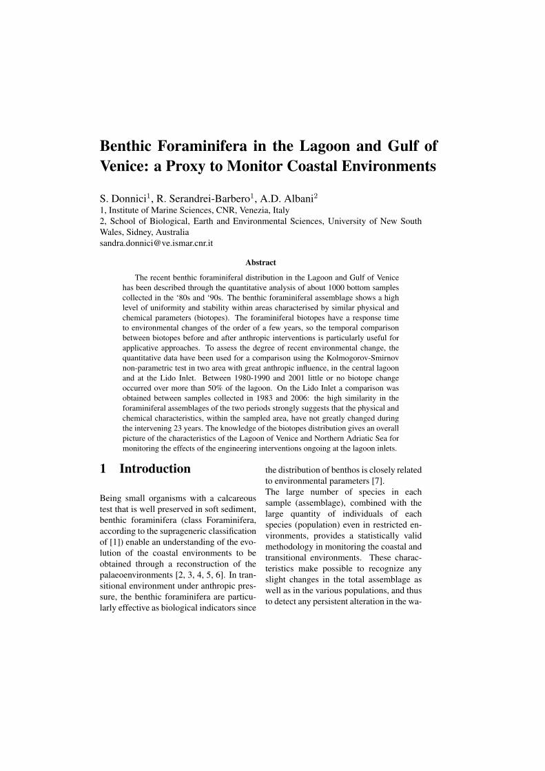
Benthic Foraminifera in the Lagoon and Gulf ofVenice: a Proxy to Monitor Coastal Environments
S. Donnici1, R. Serandrei-Barbero1, A.D. Albani21, Institute of Marine Sciences, CNR, Venezia, Italy2, School of Biological, Earth and Environmental Sciences, University of New SouthWales, Sidney, [email protected]
Abstract
The recent benthic foraminiferal distribution in the Lagoon and Gulf of Venicehas been described through the quantitative analysis of about 1000 bottom samplescollected in the ‘80s and ‘90s. The benthic foraminiferal assemblage shows a highlevel of uniformity and stability within areas characterised by similar physical andchemical parameters (biotopes). The foraminiferal biotopes have a response timeto environmental changes of the order of a few years, so the temporal comparisonbetween biotopes before and after anthropic interventions is particularly useful forapplicative approaches. To assess the degree of recent environmental change, thequantitative data have been used for a comparison using the Kolmogorov-Smirnovnon-parametric test in two area with great anthropic influence, in the central lagoonand at the Lido Inlet. Between 1980-1990 and 2001 little or no biotope changeoccurred over more than 50% of the lagoon. On the Lido Inlet a comparison wasobtained between samples collected in 1983 and 2006: the high similarity in theforaminiferal assemblages of the two periods strongly suggests that the physical andchemical characteristics, within the sampled area, have not greatly changed duringthe intervening 23 years. The knowledge of the biotopes distribution gives an overallpicture of the characteristics of the Lagoon of Venice and Northern Adriatic Sea formonitoring the effects of the engineering interventions ongoing at the lagoon inlets.
1 Introduction
Being small organisms with a calcareoustest that is well preserved in soft sediment,benthic foraminifera (class Foraminifera,according to the suprageneric classificationof [1]) enable an understanding of the evo-lution of the coastal environments to beobtained through a reconstruction of thepalaeoenvironments [2, 3, 4, 5, 6]. In tran-sitional environment under anthropic pres-sure, the benthic foraminifera are particu-larly effective as biological indicators since
the distribution of benthos is closely relatedto environmental parameters [7].The large number of species in eachsample (assemblage), combined with thelarge quantity of individuals of eachspecies (population) even in restricted en-vironments, provides a statistically validmethodology in monitoring the coastal andtransitional environments. These charac-teristics make possible to recognize anyslight changes in the total assemblage aswell as in the various populations, and thusto detect any persistent alteration in the wa-

Marine Ecology
ter qualities.In the biological investigations a speciesis considered an environmental indicatorwhen its presence-absence-abundance re-lates to biotic processes that often co-vary with natural and anthropogenic envi-ronmental gradients, in particular in a la-goon environment given the great variabil-ity of the physical and chemical parame-ters. However, the species as indicator isless efficient and reliable than the whole as-semblage [8] as the totality of the speciespresent reflects the physical-chemical pa-rameters prevailing.The foraminifera of the Lagoon of Venicewere described for the first time by Sil-vestri [9] and later in the earlier studieson the lagoon [10, 11, 12, 13, 14]. Theirsensitivity to environmental changes makesthem a proxy to identify future changes.
2 The recent foraminiferaof the Venice coastalarea
In the ’80s a systematic sampling of theLagoon of Venice and Northern Adriaticseabed was initiated and over 700 sed-iment samples were collected. The to-tal foraminiferal fauna was identified andcounted in each sample and the abundanceand distribution of 80 benthic specieswithin the lagoon and the Gulf of Venicehas been established [15, 16].Numerical analyses were based on the to-tal assemblage of both living and dead in-dividuals as that gives an integrated viewof the assemblage [17]. The short-termvariations of the living assemblage, be-ing mainly due to the availability of phy-toplankton and biotic interactions, resultmore irregular with respect to the total as-
sociation [18].The average assemblage of benthicforaminifera in the lagoon is composedof 11 species; the assemblages reach 37species in the vicinity of the marine in-lets and reduce to 5-6 species in the moreconfined areas. Ammonia beccarii, Hay-nesina paucilocula, Aubignyna perlucidaand Cribrononion granosum are distributedover 90% of the area and appear to bethe most tolerant species; other 57 speciesare present in sediment covering less than10% of the lagoon. The foraminiferal as-semblages show a high level of unifor-mity and stability within an area (biotope)that is characterised by similar physicaland chemical parameters, hence allowingbiotopes to be identified by Q-mode clus-ter analysis [19, 20]. A percent matrixusing the Pearson correlation coefficient[19] is obtained from the percentage dataset and cluster analysis is performed onsuch correlation matrix. The output ofthe cluster is generally presented in theform of a dendrogram. Cluster analysisis a metod for linking stations accordingto their similarity in faunal content, thecloser the foraminiferal assemblages are,the higher is the similarity between sta-tions.The foraminiferal biotopes [21, 22, 23, 24]reflect the characteristics of the lagoonaland coastal environment during the years1980 - 1990. Each biotope is charac-terised by the association of a numberof key species that are more tolerant tothe extremes conditions of the different ar-eas (Table 1). The distribution of benthicforaminifera in the Lagoon of Venice to-day appear to be largely controlled by res-idence time, pollution, fresh water inputsand presence of intertidal morphologies(Figure 1), parameter well tolerated respec-tively by Ammonia beccarii, Haynesina
276
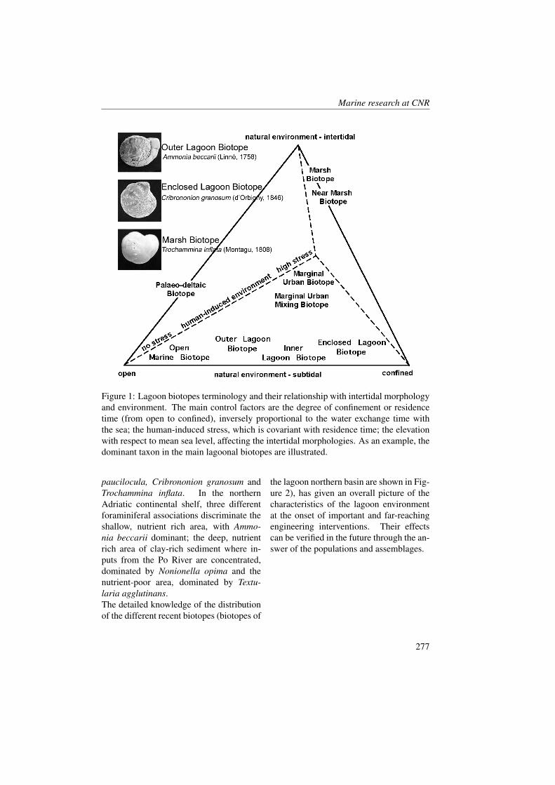
Marine research at CNR
Figure 1: Lagoon biotopes terminology and their relationship with intertidal morphologyand environment. The main control factors are the degree of confinement or residencetime (from open to confined), inversely proportional to the water exchange time withthe sea; the human-induced stress, which is covariant with residence time; the elevationwith respect to mean sea level, affecting the intertidal morphologies. As an example, thedominant taxon in the main lagoonal biotopes are illustrated.
paucilocula, Cribrononion granosum andTrochammina inflata. In the northernAdriatic continental shelf, three differentforaminiferal associations discriminate theshallow, nutrient rich area, with Ammo-nia beccarii dominant; the deep, nutrientrich area of clay-rich sediment where in-puts from the Po River are concentrated,dominated by Nonionella opima and thenutrient-poor area, dominated by Textu-laria agglutinans.The detailed knowledge of the distributionof the different recent biotopes (biotopes of
the lagoon northern basin are shown in Fig-ure 2), has given an overall picture of thecharacteristics of the lagoon environmentat the onset of important and far-reachingengineering interventions. Their effectscan be verified in the future through the an-swer of the populations and assemblages.
277
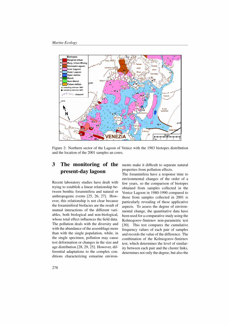
Marine Ecology
Figure 2: Northern sector of the Lagoon of Venice with the 1983 biotopes distributionand the location of the 2001 samples an cores.
3 The monitoring of thepresent-day lagoon
Recent laboratory studies have dealt withtrying to establish a linear relationship be-tween benthic foraminifera and natural oranthropogenic events [25, 26, 27]. How-ever, this relationship is not clear becausethe foraminiferal biofacies are the result ofmutual interactions of the different vari-ables, both biological and non-biological,whose total effect influences the field data.The pollution deals with the diversity andwith the abundance of the assemblage morethan with the single population, while, inthe single specimen, pollution may causetest deformation or changes in the size andage distribution [28, 29, 25]. However, dif-ferential adaptations to the complex con-ditions characterizing estuarine environ-
ments make it difficult to separate naturalproperties from pollution effects.The foraminifera have a response time toenvironmental changes of the order of afew years, so the comparison of biotopesobtained from samples collected in theVenice Lagoon in 1980-1990 compared tothose from samples collected in 2001 isparticularly revealing of these applicativeaspects. To assess the degree of environ-mental change, the quantitative data havebeen used for a comparative study using theKolmogorov-Smirnov non-parametric test[30]. This test compares the cumulativefrequency values of each pair of samplesand records the value of the difference. Thecombination of the Kolmogorov-Smirnovtest, which determines the level of similar-ity between each pair and the cluster links,determines not only the degree, but also the
278
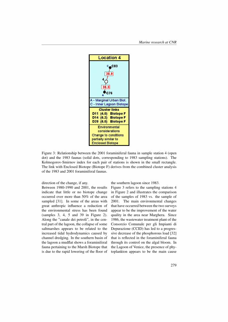
Marine research at CNR
Figure 3: Relationship between the 2001 foraminiferal fauna in sample station 4 (opendot) and the 1983 faunas (solid dots, corresponding to 1983 sampling stations). TheKolmogorov-Smirnov index for each pair of stations is shown in the small rectangle.The link with Enclosed Biotope (Biotope F) derives from the combined cluster analysisof the 1983 and 2001 foraminiferal faunas.
direction of the change, if any.Between 1980-1990 and 2001, the resultsindicate that little or no biotope changeoccurred over more than 50% of the areasampled [31]. In some of the areas withgreat anthropic influence a reduction ofthe environmental stress has been found(samples 3, 4, 5 and 39 in Figure 2).Along the ”canale dei petroli”, in the cen-tral part of the lagoon, the collapse of somesaltmarshes appears to be related to theincreased tidal hydrodynamics caused bychannel dredging. In the southern basin ofthe lagoon a mudflat shows a foraminiferalfauna pertaining to the Marsh Biotope thatis due to the rapid lowering of the floor of
the southern lagoon since 1983.Figure 3 refers to the sampling stations 4in Figure 2 and illustrates the comparisonof the samples of 1983 vs. the sample of2001. The main environmental changesthat have occurred between the two surveysappear to be the improvement of the waterquality in the area near Marghera. Since1986, the wastewater treatment plant of theConsorzio Comunale per gli Impianti diDepurazione (CCID) has led to a progres-sive decrease of the phosphorous load [32]that is reflected in the foraminiferal faunathrough its control on the algal bloom. Inthe Lagoon of Venice, the presence of phy-toplankton appears to be the main cause
279
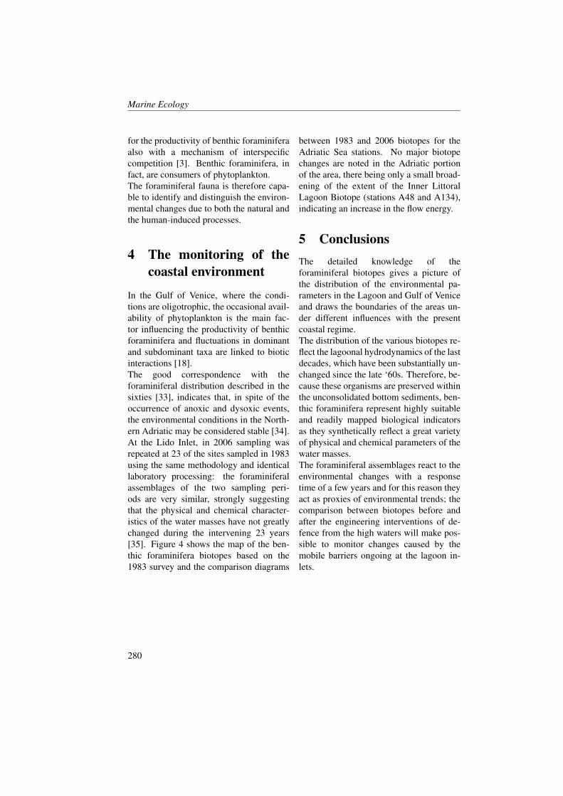
Marine Ecology
for the productivity of benthic foraminiferaalso with a mechanism of interspecificcompetition [3]. Benthic foraminifera, infact, are consumers of phytoplankton.The foraminiferal fauna is therefore capa-ble to identify and distinguish the environ-mental changes due to both the natural andthe human-induced processes.
4 The monitoring of thecoastal environment
In the Gulf of Venice, where the condi-tions are oligotrophic, the occasional avail-ability of phytoplankton is the main fac-tor influencing the productivity of benthicforaminifera and fluctuations in dominantand subdominant taxa are linked to bioticinteractions [18].The good correspondence with theforaminiferal distribution described in thesixties [33], indicates that, in spite of theoccurrence of anoxic and dysoxic events,the environmental conditions in the North-ern Adriatic may be considered stable [34].At the Lido Inlet, in 2006 sampling wasrepeated at 23 of the sites sampled in 1983using the same methodology and identicallaboratory processing: the foraminiferalassemblages of the two sampling peri-ods are very similar, strongly suggestingthat the physical and chemical character-istics of the water masses have not greatlychanged during the intervening 23 years[35]. Figure 4 shows the map of the ben-thic foraminifera biotopes based on the1983 survey and the comparison diagrams
between 1983 and 2006 biotopes for theAdriatic Sea stations. No major biotopechanges are noted in the Adriatic portionof the area, there being only a small broad-ening of the extent of the Inner LittoralLagoon Biotope (stations A48 and A134),indicating an increase in the flow energy.
5 ConclusionsThe detailed knowledge of theforaminiferal biotopes gives a picture ofthe distribution of the environmental pa-rameters in the Lagoon and Gulf of Veniceand draws the boundaries of the areas un-der different influences with the presentcoastal regime.The distribution of the various biotopes re-flect the lagoonal hydrodynamics of the lastdecades, which have been substantially un-changed since the late ‘60s. Therefore, be-cause these organisms are preserved withinthe unconsolidated bottom sediments, ben-thic foraminifera represent highly suitableand readily mapped biological indicatorsas they synthetically reflect a great varietyof physical and chemical parameters of thewater masses.The foraminiferal assemblages react to theenvironmental changes with a responsetime of a few years and for this reason theyact as proxies of environmental trends; thecomparison between biotopes before andafter the engineering interventions of de-fence from the high waters will make pos-sible to monitor changes caused by themobile barriers ongoing at the lagoon in-lets.
280
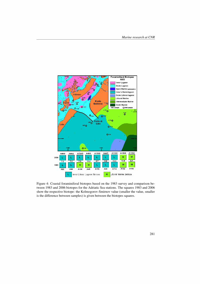
Marine research at CNR
Figure 4: Coastal foraminiferal biotopes based on the 1983 survey and comparison be-tween 1983 and 2006 biotopes for the Adriatic Sea stations. The squares 1983 and 2006show the respective biotope: the Kolmogorov-Smirnov value (smaller the value, smalleris the difference between samples) is given between the biotopes squares.
281

Marine Ecology
BiotopeMajor foraminiferal species average median average medianTrochammina inflata (Montagu) 0,8 0,6 0,2 - 1,6 1,9 1,1 0,2 - 6,9Eggerella scabra (Williamson) Quinqueloculina seminulum (Linné) 2,9 1,9 0,4 - 12,3 2,8 1,6 0,2 - 12,2Aubignyana perlucida (Heron-Allen & Earland) 3,9 2,4 0,5 - 17,4 4,3 3,1 0,8 - 13,7Haynesina paucilocula (Cushman) 47,3 46,9 30,9 - 66,0 24,9 25,6 16,3 - 37,1Nonion politum (d'Orbigny) 0,2 0,2 0,2 - 0,2 6,2 6,2 4,0 - 8,3Ammonia beccarii (Linné) 38,6 38,3 27,7 - 51,0 54,2 53,8 43,0 - 62,6Elphidium granosum (d'Orbigny) 6,8 5,2 1,1 - 20,6 9,8 10,1 1,7 - 16,2
stationsspeciesBiotope
Major foraminiferal species average median average medianTrochammina inflata (Montagu) 1,7 0,5 0,2 - 13,4 0,5 0,3 0,2 - 5,3Eggerella scabra (Williamson) 3,4 0,6 0,2 - 17,2 1,9 0,7 0,2 - 8,7Quinqueloculina seminulum (Linné) 3,2 2,3 0,1 - 23,7 1,9 1,3 0,2 - 14,8Aubignyana perlucida (Heron-Allen & Earland) 6,6 6,2 0,3 - 17,7 6,6 6,3 0,3 - 16,2Haynesina paucilocula (Cushman) 11,5 9,7 1,3 - 38,6 6,7 6,3 0,3 - 18,1Nonion politum (d'Orbigny) 1,8 1,0 0,2 - 7,7 1,8 1,3 0,2 - 7,7Ammonia beccarii (Linné) 62,0 62,6 28,0 - 81,7 71,7 72,4 43,0 - 93,0Elphidium granosum (d'Orbigny) 11,7 10,2 0,3 - 43,0 7,7 6,7 0,3 - 25,2
stationsspeciesBiotope
Major foraminiferal species average median average medianTrochammina inflata (Montagu) 0,3 0,3 0,3 - 0,3Eggerella scabra (Williamson) 12,3 12,3 7,5 - 17,0Quinqueloculina seminulum (Linné) 15,3 15,4 6,0 - 23,3 0,8 0,3 0,3 - 2,3Aubignyana perlucida (Heron-Allen & Earland) 1,7 1,7 1,2 - 2,5 2,8 3,2 0,8 - 4,5Haynesina paucilocula (Cushman) 3,4 3,7 0,7 - 5,3 12,8 13,7 0,7 - 20,3Nonion politum (d'Orbigny) 0,7 0,7 0,4 - 1,0 8,8 11,7 0,3 - 15,7Ammonia beccarii (Linné) 46,9 50,2 35,0 - 58,7 69,3 70,6 57,1 - 78,0Elphidium granosum (d'Orbigny) 13,6 10,3 5,4 - 34,2 2,8 1,6 0,8 - 6,0
stationsspeciesBiotope
Major foraminiferal species average median average medianTrochammina inflata (Montagu) 0,3 0,2 0,1 - 0,5 26,4 24,1 17,7 - 39,8Eggerella scabra (Williamson) 0,5 0,5 0,3 - 0,7Quinqueloculina seminulum (Linné) 2,9 1,2 0,2 - 13,3 0,3 0,3 0,3 - 0,3Aubignyana perlucida (Heron-Allen & Earland) 5,7 5,9 2,8 - 7,4 4,9 4,8 3,3 - 6,7Haynesina paucilocula (Cushman) 17,1 19,7 6,3 - 27,3 5,7 5,5 4,0 - 7,7Nonion politum (d'Orbigny) 6,7 6,7 5,3 - 8,0Ammonia beccarii (Linné) 33,2 33,7 20,8 - 43,8 54,1 53,3 49,4 - 60,3Elphidium granosum (d'Orbigny) 39,2 40,6 18,7 - 56,1 1,8 1,8 0,7 - 2,9
stationsspeciesBiotope
Major foraminiferal species average medianTrochammina inflata (Montagu) 8,3 8,8 1,4 - 13,4Eggerella scabra (Williamson) Quinqueloculina seminulum (Linné) 2,7 1,5 0,3 - 11,4Aubignyana perlucida (Heron-Allen & Earland) 4,1 3,8 0,3 - 8,2Haynesina paucilocula (Cushman) 11,8 9,4 5,2 - 21,0Nonion politum (d'Orbigny) 1,5 0,6 0,3 - 3,7Ammonia beccarii (Linné) 67,7 68,1 64,1 - 71,7Elphidium granosum (d'Orbigny) 3,4 3,2 0,7 - 8,1
stationsspecies
A- Marginal Urban B-Marginal Urban Mixing
C- Inner Lagoon
H-Near Marsh
G-MarshF-Enclosed Lagoon
D-Outer Lagoon
I-Open Marine J-Palaeo-deltaic
range
range
range
range
6 = 1.01%41 = 55.41%
11 = 1.84%14 = 18.92%
rangerange
range
range
12 = 2.01%18 = 24.32%
317 = 53.10%72 = 97.30%
17 = 2.85%25 = 33.78%
The % values are calculated based on 74 total species and 559 stations
7 = 1.17%25 = 33.78%
4 = 0.67%19 = 25.68%
186 = 31.16%68 = 91.89%
8 = 1.34%16 = 21.62%
range
Table 1: Biotopes faunal composition, as relative abundance of each species in the to-tal assemblages of about 300 individuals, based on the 1983 survey. Only significativespecies are represented with their range of relative abundance, average, median value andoccurrence expressed as number of stations and percentages of total stations (areas).
282
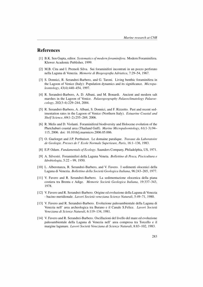
Marine research at CNR
References[1] B.K. Sen Gupta, editor. Systematics of modern foraminifera. Modern Foraminifera.
Kluwer Academic Publisher, 1999.
[2] M.B. Cita and I. Premoli Silva. Sui foraminiferi incontrati in un pozzo perforatonella Laguna di Venezia. Memorie di Biogeografia Adriatica, 7:29–54, 1967.
[3] S. Donnici, R. Serandrei-Barbero, and G. Taroni. Living benthic foraminifera inthe Lagoon of Venice (Italy): Population dynamics and its significance. Micropa-leontology, 43(4):440–454, 1997.
[4] R. Serandrei-Barbero, A. D. Albani, and M. Bonardi. Ancient and modern saltmarshes in the Lagoon of Venice. Palaeogeography Palaeoclimatology Palaeoe-cology, 202(3-4):229–244, 2004.
[5] R. Serandrei-Barbero, A. Albani, S. Donnici, and F. Rizzetto. Past and recent sed-imentation rates in the Lagoon of Venice (Northern Italy). Estuarine Coastal andShelf Science, 69(1-2):255–269, 2006.
[6] R. Melis and D. Violanti. Foraminiferal biodiversity and Holocene evolution of thePhetchaburi coastal area (Thailand Gulf). Marine Micropaleontology, 61(1-3):94–115, 2006. doi: 10.1016/j.marmicro.2006.05.006.
[7] O. Guelorget and J.P. Perthuisot. Le domaine paralique. Travaux du Laboratoirede Geologie. Presses de l’ Ecole Normale Superieure, Paris, 16:1–136, 1983.
[8] E.P. Odum. Fundamentals of Ecology. Saunders Company, Philadelphia, US, 1971.
[9] A. Silvestri. Foraminiferi della Laguna Veneta. Bollettino di Pesca, Piscicultura eIdrobiologia, 5:22 – 99, 1950.
[10] L. Alberotanza, R. Serandrei-Barbero, and V. Favero. I sedimenti olocenici dellaLaguna di Venezia. Bollettino della Societa Geologica Italiana, 96:243–265, 1977.
[11] V. Favero and R. Serandrei-Barbero. La sedimentazione olocenica della pianacostiera tra Brenta e Adige. Memorie Societa Geologica Italiana, 19:337–343,1978.
[12] V. Favero and R. Serandrei-Barbero. Origine ed evoluzione della Laguna di Venezia- bacino meridionale. Lavori Societa veneziana Scienze Naturali, 5:49–71, 1980.
[13] V. Favero and R. Serandrei-Barbero. Evoluzione paleoambientale della Laguna diVenezia nell’ area archeologica tra Burano e il Canale S.Felice. Lavori SocietaVeneziana di Scienze Naturali, 6:119–134, 1981.
[14] V. Favero and R. Serandrei-Barbero. Oscillazioni del livello del mare ed evoluzionepaleoambientale della Laguna di Venezia nell’ area compresa tra Torcello e ilmargine lagunare. Lavori Societa Veneziana di Scienze Naturali, 8:83–102, 1983.
283
Marine Ecology
[15] D. Albani and R. Serandrei-Barbero. I foraminiferi della Laguna e del Golfo diVenezia. Universita di Padova, Memorie di Scienze Geologiche, 42:271–341, 1990.
[16] R. Serandrei-Barbero, A. Albani, and S. Donnici. Atlante dei Foraminiferi dellaLaguna di Venezia. Istituto Veneto di Scienze, Lettere ed Arti, Venice, 2008.
[17] D.B. Scott and F.S. Medioli. Living vs. total foraminiferal populations; their relativeusefulness in paleoecology. Journal of Paleontology, 54(4):814–831, 1980.
[18] R. Serandrei-Barbero, M. Morisieri, L. Carbognin, and S. Donnici. An innershelf foraminiferal fauna and its response to environmental processes (Adriatic Sea,Italy). Revista Espanola Micropaleontologia, 35:1 – 24, 2003.
[19] P.H.A. Sneath and R.R. Sokal. Numerical taxonomy. W.H. Freeman and Company,S. Francisco, US, 1981.
[20] A. D. Albani. Use of benthonic foraminifera to evaluate the environmental charac-teristics of Port Hacking; significance for coastal engineering works and pollution.In G. McNally, M. Knight, and R. Smith, editors, Collected Case Studies in Engi-neering Geology, Hydrogeology and Environmental Geology, page 134. GeologicalSociety of Australia, Sydney, 1993.
[21] R. Serandrei-Barbero, L. Carbognin, G. Taroni, and E. Cova. Distribution of recentbenthic foraminifera in the southern basin of the Venice lagoon (Italy): Statisticalevaluation of taxa significance. Micropaleontology, 45(1):99–111, 1999.
[22] R. Serandrei-Barbero, A.D. Albani, and V. Favero. Distribuzione dei foraminiferirecenti nella Laguna a Nord di Venezia. Bollettino Societa Geologica Italiana,108:279–288, 1989.
[23] A.D. Albani, V. Favero, and R. Serandrei-Barbero. The distribution and ecologicalsignigicance of recent foraminifera in the lagoon South of Venice (Italy). RevistaEspanola Micropaleontologia, 23:29–45, 1991.
[24] A.D. Albani, V. Favero, and R. Serandrei-Barbero. Distribution of Sediment andBenthic Foraminifera in the Gulf of Venice, Italy. Estuarine, Coastal and ShelfScience, 46:251–265, 1998.
[25] A.M. Samir. The response of benthic foraminifera and ostracods to variouspollution sources: A study from two lagoons in Egypt”, Journal = ”Journal ofForaminiferal Research. 30(2):83–98, 2000.
[26] J. Morvan, V. Le Cadre, F. Jorissen, and J.P. Debenay. Foraminifera as potential bio-indicators of the ”Erika” oil spill in the Bay of Bourgneuf: Field and experimentalstudies. Aquatic Living Resources, 17(3):317–322, 2004.
[27] R. Saraswat, S.R. Kurtarkar, A. Mazumder, and R. Nigam. Foraminifers as indica-tors of marine pollution: a culture experiment with Rosalina leei. Marine PollutionBulletin, 48(1-2):91–96, 2004.
284
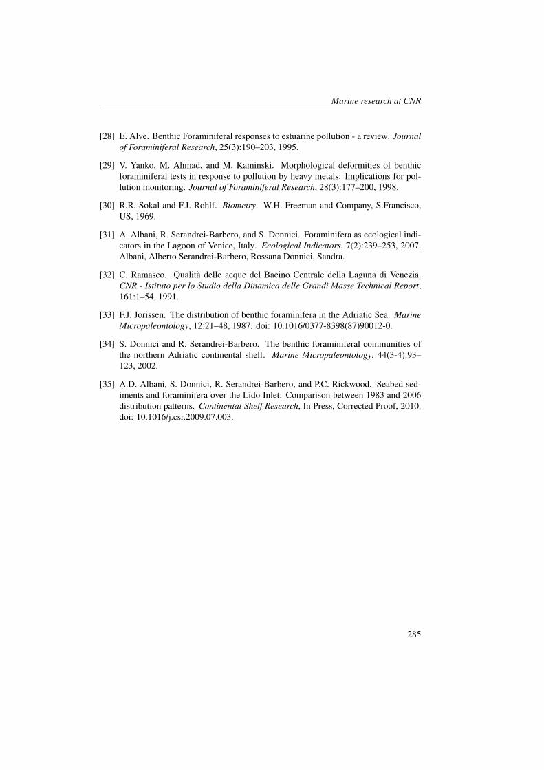
Marine research at CNR
[28] E. Alve. Benthic Foraminiferal responses to estuarine pollution - a review. Journalof Foraminiferal Research, 25(3):190–203, 1995.
[29] V. Yanko, M. Ahmad, and M. Kaminski. Morphological deformities of benthicforaminiferal tests in response to pollution by heavy metals: Implications for pol-lution monitoring. Journal of Foraminiferal Research, 28(3):177–200, 1998.
[30] R.R. Sokal and F.J. Rohlf. Biometry. W.H. Freeman and Company, S.Francisco,US, 1969.
[31] A. Albani, R. Serandrei-Barbero, and S. Donnici. Foraminifera as ecological indi-cators in the Lagoon of Venice, Italy. Ecological Indicators, 7(2):239–253, 2007.Albani, Alberto Serandrei-Barbero, Rossana Donnici, Sandra.
[32] C. Ramasco. Qualita delle acque del Bacino Centrale della Laguna di Venezia.CNR - Istituto per lo Studio della Dinamica delle Grandi Masse Technical Report,161:1–54, 1991.
[33] F.J. Jorissen. The distribution of benthic foraminifera in the Adriatic Sea. MarineMicropaleontology, 12:21–48, 1987. doi: 10.1016/0377-8398(87)90012-0.
[34] S. Donnici and R. Serandrei-Barbero. The benthic foraminiferal communities ofthe northern Adriatic continental shelf. Marine Micropaleontology, 44(3-4):93–123, 2002.
[35] A.D. Albani, S. Donnici, R. Serandrei-Barbero, and P.C. Rickwood. Seabed sed-iments and foraminifera over the Lido Inlet: Comparison between 1983 and 2006distribution patterns. Continental Shelf Research, In Press, Corrected Proof, 2010.doi: 10.1016/j.csr.2009.07.003.
285

Marine Ecology
286
Study of the Biomass and Spatial Distribution ofDeep Pelagic Fish Larvae of the Sicilian Channelin Relationships to the Physical and Chemical Pa-rameters of the Water Column
A. Cuttitta, L. Caruana, B. Patti, A. Bonanno, C. Patti, B. De Luca, S.Bonomo, E. Quinci, G. Tranchida, M. Musco, T. Masullo, M. Borghi, G.BuscainoInstitute for Coastal Marine Environment, CNR, Capo Granitola (TP), [email protected]
Abstract
Mesopelagic fish represent one of the most important links in the food chain ofthe marine ecosystem. Their abundance in the Mediterranean sea makes them themost important members of the deep water fauna and a potential resource for fu-ture fisheries. The aim of this work is the study of the spatial distribution, com-position and biomass of mesopelagic fish larvae species in relationship with theoceanographic parameters of the Sicilian Channel. This area is characterized bydifferent water masses associated with the typical hydro graphic structures of theChannel (Atlantic Ionian Stream-AIS), influencing the presence and distribution offish species larval stages. Samples were collected during oceanographic surveys, onboard of URANIA O/V in years 2005, 2006 and 2007. Distribution maps of thehauls, grouped in clusters, showed similar patterns during all analyzed years. Themost common spots we found were located under Pozzallo, Cape Passero and Sir-acusa, though there were small spots along the central shelf of the western coast.These results would be influenced by the existence of different water masses on thesurface, associated with the AIS path and with the hydrographic structures. Theoccurrence of these species in shelf areas would be associated with the coastal up-welling characterizing the northern part of the study area. In addition, the accumu-lation of larvae on the south-eastern edge could be related to the strong salinity frontoff Cape Passero.
1 Introduction
Spatiotemporal patterns of ichthyoplank-ton communities, with respect to abun-dance, distribution and species composi-tion, have been traditionally a basic topicof scientific research in fisheries oceanog-raphy [1]. Ichthyoplankton surveys pro-vide useful data for the assessment of im-
portant parameters of commercially impor-tant fish populations (i.e. spawning stockbiomass, recruitment), but can also im-prove our knowledge on the agents struc-turing larval assemblages [2]. A large num-ber of biological and physical factors con-tribute to the formation, maintenance anddisruption of larval fish assemblages as ithas been pointed out for several coastal
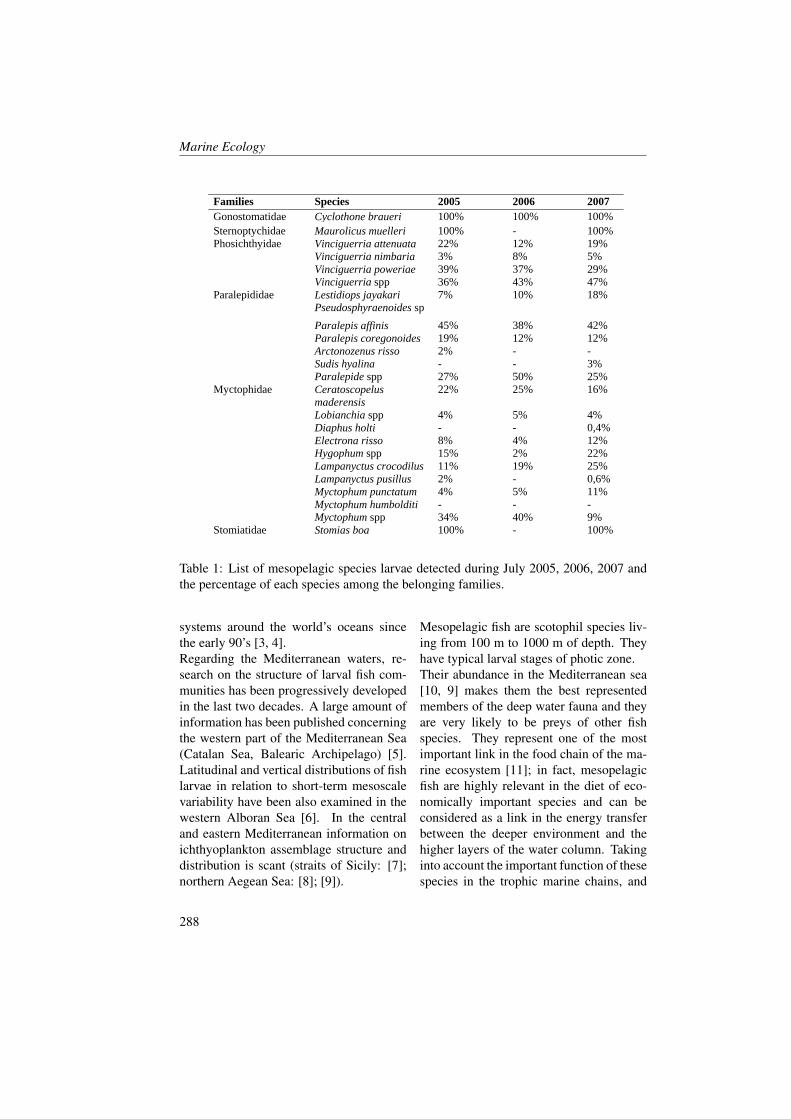
Marine Ecology
Families Species 2005 2006 2007 Gonostomatidae Cyclothone braueri 100% 100% 100% Sternoptychidae Maurolicus muelleri 100% - 100% Phosichthyidae Vinciguerria attenuata 22% 12% 19% Vinciguerria nimbaria 3% 8% 5% Vinciguerria poweriae 39% 37% 29% Vinciguerria spp 36% 43% 47% Paralepididae Lestidiops jayakari
Pseudosphyraenoides sp 7% 10% 18%
Paralepis affinis 45% 38% 42% Paralepis coregonoides 19% 12% 12% Arctonozenus risso 2% - - Sudis hyalina - - 3% Paralepide spp 27% 50% 25% Myctophidae Ceratoscopelus
maderensis 22% 25% 16%
Lobianchia spp 4% 5% 4% Diaphus holti - - 0,4% Electrona risso 8% 4% 12% Hygophum spp 15% 2% 22% Lampanyctus crocodilus 11% 19% 25% Lampanyctus pusillus 2% - 0,6% Myctophum punctatum 4% 5% 11% Myctophum humbolditi - - - Myctophum spp 34% 40% 9% Stomiatidae Stomias boa 100% - 100%
Table 1: List of mesopelagic species larvae detected during July 2005, 2006, 2007 andthe percentage of each species among the belonging families.
systems around the world’s oceans sincethe early 90’s [3, 4].Regarding the Mediterranean waters, re-search on the structure of larval fish com-munities has been progressively developedin the last two decades. A large amount ofinformation has been published concerningthe western part of the Mediterranean Sea(Catalan Sea, Balearic Archipelago) [5].Latitudinal and vertical distributions of fishlarvae in relation to short-term mesoscalevariability have been also examined in thewestern Alboran Sea [6]. In the centraland eastern Mediterranean information onichthyoplankton assemblage structure anddistribution is scant (straits of Sicily: [7];northern Aegean Sea: [8]; [9]).
Mesopelagic fish are scotophil species liv-ing from 100 m to 1000 m of depth. Theyhave typical larval stages of photic zone.Their abundance in the Mediterranean sea[10, 9] makes them the best representedmembers of the deep water fauna and theyare very likely to be preys of other fishspecies. They represent one of the mostimportant link in the food chain of the ma-rine ecosystem [11]; in fact, mesopelagicfish are highly relevant in the diet of eco-nomically important species and can beconsidered as a link in the energy transferbetween the deeper environment and thehigher layers of the water column. Takinginto account the important function of thesespecies in the trophic marine chains, and
288
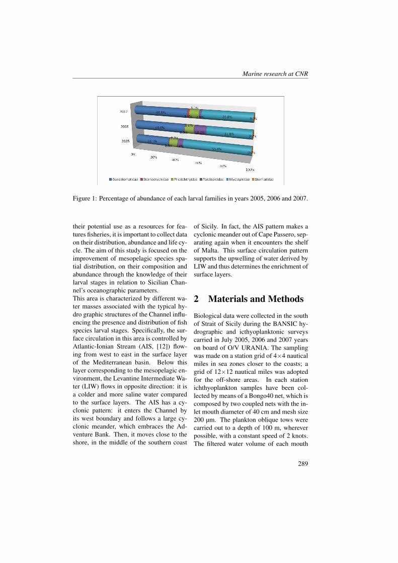
Marine research at CNR
Figure 1: Percentage of abundance of each larval families in years 2005, 2006 and 2007.
their potential use as a resources for fea-tures fisheries, it is important to collect dataon their distribution, abundance and life cy-cle. The aim of this study is focused on theimprovement of mesopelagic species spa-tial distribution, on their composition andabundance through the knowledge of theirlarval stages in relation to Sicilian Chan-nel’s oceanographic parameters.This area is characterized by different wa-ter masses associated with the typical hy-dro graphic structures of the Channel influ-encing the presence and distribution of fishspecies larval stages. Specifically, the sur-face circulation in this area is controlled byAtlantic-Ionian Stream (AIS, [12]) flow-ing from west to east in the surface layerof the Mediterranean basin. Below thislayer corresponding to the mesopelagic en-vironment, the Levantine Intermediate Wa-ter (LIW) flows in opposite direction: it isa colder and more saline water comparedto the surface layers. The AIS has a cy-clonic pattern: it enters the Channel byits west boundary and follows a large cy-clonic meander, which embraces the Ad-venture Bank. Then, it moves close to theshore, in the middle of the southern coast
of Sicily. In fact, the AIS pattern makes acyclonic meander out of Cape Passero, sep-arating again when it encounters the shelfof Malta. This surface circulation patternsupports the upwelling of water derived byLIW and thus determines the enrichment ofsurface layers.
2 Materials and Methods
Biological data were collected in the southof Strait of Sicily during the BANSIC hy-drographic and icthyoplanktonic surveyscarried in July 2005, 2006 and 2007 yearson board of O/V URANIA. The samplingwas made on a station grid of 4×4 nauticalmiles in sea zones closer to the coasts; agrid of 12×12 nautical miles was adoptedfor the off-shore areas. In each stationichthyoplankton samples have been col-lected by means of a Bongo40 net, which iscomposed by two coupled nets with the in-let mouth diameter of 40 cm and mesh size200 µm. The plankton oblique tows werecarried out to a depth of 100 m, whereverpossible, with a constant speed of 2 knots.The filtered water volume of each mouth
289
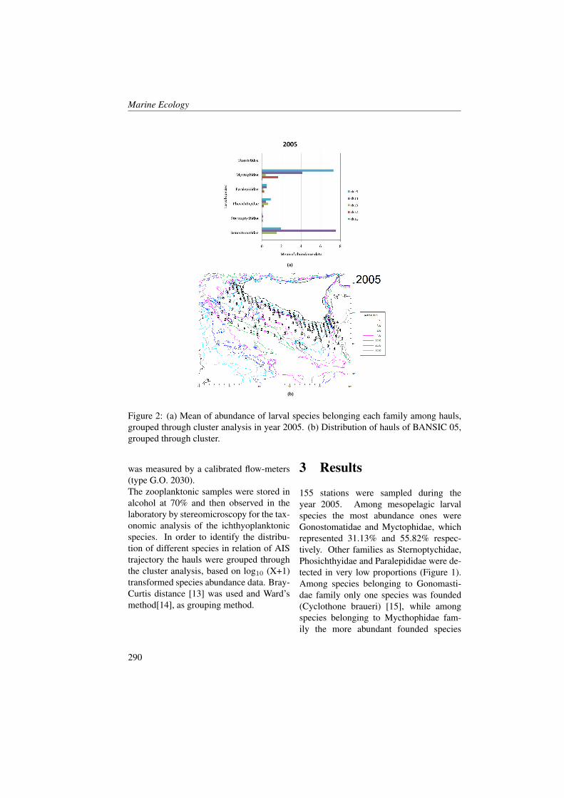
Marine Ecology
(a)
(b)
Figure 2: (a) Mean of abundance of larval species belonging each family among hauls,grouped through cluster analysis in year 2005. (b) Distribution of hauls of BANSIC 05,grouped through cluster.
was measured by a calibrated flow-meters(type G.O. 2030).The zooplanktonic samples were stored inalcohol at 70% and then observed in thelaboratory by stereomicroscopy for the tax-onomic analysis of the ichthyoplanktonicspecies. In order to identify the distribu-tion of different species in relation of AIStrajectory the hauls were grouped throughthe cluster analysis, based on log10 (X+1)transformed species abundance data. Bray-Curtis distance [13] was used and Ward’smethod[14], as grouping method.
3 Results
155 stations were sampled during theyear 2005. Among mesopelagic larvalspecies the most abundance ones wereGonostomatidae and Myctophidae, whichrepresented 31.13% and 55.82% respec-tively. Other families as Sternoptychidae,Phosichthyidae and Paralepididae were de-tected in very low proportions (Figure 1).Among species belonging to Gonomasti-dae family only one species was founded(Cyclothone braueri) [15], while amongspecies belonging to Mycthophidae fam-ily the more abundant founded species
290
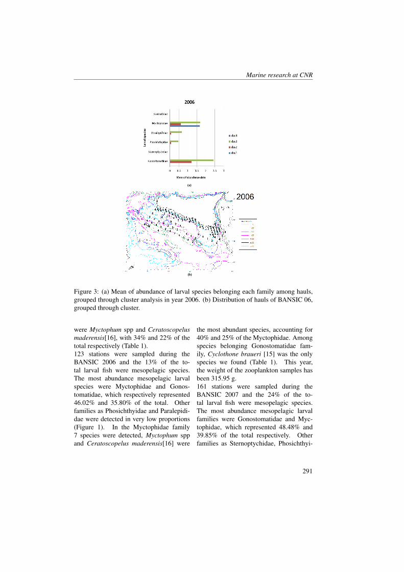
Marine research at CNR
(a)
(b)
Figure 3: (a) Mean of abundance of larval species belonging each family among hauls,grouped through cluster analysis in year 2006. (b) Distribution of hauls of BANSIC 06,grouped through cluster.
were Myctophum spp and Ceratoscopelusmaderensis[16], with 34% and 22% of thetotal respectively (Table 1).123 stations were sampled during theBANSIC 2006 and the 13% of the to-tal larval fish were mesopelagic species.The most abundance mesopelagic larvalspecies were Myctophidae and Gonos-tomatidae, which respectively represented46.02% and 35.80% of the total. Otherfamilies as Phosichthyidae and Paralepidi-dae were detected in very low proportions(Figure 1). In the Myctophidae family7 species were detected, Myctophum sppand Ceratoscopelus maderensis[16] were
the most abundant species, accounting for40% and 25% of the Myctophidae. Amongspecies belonging Gonostomatidae fam-ily, Cyclothone braueri [15] was the onlyspecies we found (Table 1). This year,the weight of the zooplankton samples hasbeen 315.95 g.161 stations were sampled during theBANSIC 2007 and the 24% of the to-tal larval fish were mesopelagic species.The most abundance mesopelagic larvalfamilies were Gonostomatidae and Myc-tophidae, which represented 48.48% and39.85% of the total respectively. Otherfamilies as Sternoptychidae, Phosichthyi-
291
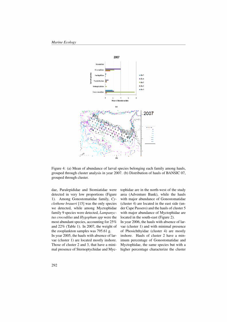
Marine Ecology
(a)
(b)
Figure 4: (a) Mean of abundance of larval species belonging each family among hauls,grouped through cluster analysis in year 2007. (b) Distribution of hauls of BANSIC 07,grouped through cluster.
dae, Paralepididae and Stomiatidae weredetected in very low proportions (Figure1). Among Gonostomatidae family, Cy-clothone braueri [15] was the only specieswe detected, while among Myctophidaefamily 9 species were detected, Lampanyc-tus crocodilus and Hygophum spp were themost abundant species, accounting for 25%and 22% (Table 1). In 2007, the weight ofthe zooplankton samples was 795.61 g.In year 2005, the hauls with absence of lar-vae (cluster 1) are located mostly inshore.Those of cluster 2 and 3, that have a mini-mal presence of Sternoptychidae and Myc-
tophidae are in the north-west of the studyarea (Adventure Bank), while the haulswith major abundance of Gonostomatidae(cluster 4) are located in the east side (un-der Cape Passero) and the hauls of cluster 5with major abundance of Myctophidae arelocated in the south-east (Figure 2).In year 2006, the hauls with absence of lar-vae (cluster 1) and with minimal presenceof Phosichthyidae (cluster 4) are mostlyinshore. Hauls of cluster 2 have a min-imum percentage of Gonostomatidae andMyctophidae, the same species but with ahigher percentage characterize the cluster
292
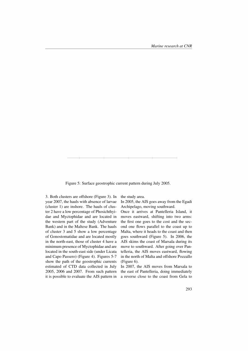
Marine research at CNR
12° 13° 14° 15° 16°
36°
37°
38°
N
S
W E
Current speed (m/s)
0.001 0.8
Figure 5: Surface geostrophic current pattern during July 2005.
3. Both clusters are offshore (Figure 3). Inyear 2007, the hauls with absence of larvae(cluster 1) are inshore. The hauls of clus-ter 2 have a low percentage of Phosichthyi-dae and Myctophidae and are located inthe western part of the study (AdventureBank) and in the Maltese Bank. The haulsof cluster 3 and 5 show a low percentageof Gonostomatidae and are located mostlyin the north-east, those of cluster 4 have aminimum presence of Myctophidae and arelocated in the south-east side (under Licataand Capo Passero) (Figure 4). Figures 5-7show the path of the geostrophic currentsestimated of CTD data collected in July2005, 2006 and 2007. From such patternit is possible to evaluate the AIS pattern in
the study area.In 2005, the AIS goes away from the EgadiArchipelago, moving southward.Once it arrives at Pantelleria Island, itmoves eastward, shifting into two arms:the first one goes to the cost and the sec-ond one flows parallel to the coast up toMalta, where it heads to the coast and thengoes southward (Figure 5). In 2006, theAIS skims the coast of Marsala during itsmove to southward. After going over Pan-telleria, the AIS moves eastward, flowingin the north of Malta and offshore Pozzallo(Figure 6).In 2007, the AIS moves from Marsala tothe east of Pantelleria, doing immediatelya reverse close to the coast from Gela to
293
Marine Ecology
12° 13° 14° 15° 16°
36°
37°
38°
N
S
W E
Current speed (m/s)
0.001 0.8
Figure 6: Surface geostrophic current pattern during July 2006.
Pozzallo, then heading southward (Figure7).
4 DiscussionDistribution maps of the hauls, groupedin clusters showed similar patterns dur-ing all analyzed years. In fact, the mostcommon spots we found were located un-der Pozzallo, Cape Passero and Siracusa,though there were small spots along thecentral shelf of the western coast. Distribu-tion maps for the cluster with major abun-dance of Gonomastodae basically showedthe presence of spots along the Egadi Is-lands and in the same sites where we found
the Myctophidae. The distribution of clus-ter with presence of Phosichthyidae wasalong the central shelf of the western coast(from Porto Empedocle to Pozzallo) andunder Cape Passero. During the sampling(July), the AIS skims along the Siciliancoasts only in the neighbours of Egadi Is-lands and Cape Passero, while there is ashift of the tide in the central part of thesouth-western coast. The trajectory of theidentified AIS core suggests that the AISwas flowing offshore and only approachedthe shore near the edge of Sicily, over theMaltese Shelf. Path irregularities in thesouthern part of the Sicilian Channel mightbe caused by the very small differences in
294
Marine research at CNR
12° 13° 14° 15° 16°
36°
37°
38°
N
S
W E
Current speed (m/s)
0.001 0.8
Figure 7: Surface geostrophic current pattern during July 2007.
the numerical value of the minimum salin-ity found in the different offshore legs, butalso by interference with other small-scaleoceanographic features that may be gen-erated in the neighbourhood with a strongsalinity front of Cape Passero. The highersalinity values along the south-eastern Si-cilian coast reveal the presence of a well-developed coastal upwelling event. This isalso confirmed by the temperature distri-bution, which exhibits a very large spatialvariability.
5 Conclusions
Results showed the existence of differentwater masses on the surface, associatedwith the AIS path and with the hydro-graphic structures. AIS path presents year-to-year variability that has consequenceson the predominant hydrological phenom-ena occurring in the region, such as theextent of upwelling and the formation offrontal structures [17].These appear in turn to affect the distri-bution of mesopelagic species larvae ob-served. In fact, the presence of thesefamilies offshore would testify the bathy-
295
Marine Ecology
pelagic environment of the adult fractionin their respective populations, whereas theoccurrence of these species in shelf areaswould be associated with the coastal up-welling characterizing the northern part ofthe study area.In addition, the accumulation of larvae onthe south-eastern edge could be related tothe strong salinity front of Cape Passero.The higher larval concentration of Cape
Passero raises the question of whether thereare physical reasons for defining it as a re-tention area. There, the presence of a sur-face thermohaline front linked to the Io-nian slope fronts (ISFs) [18] would be ableto provide a suitable scenario of enrich-ment, concentration and retention (the fun-damental triad; [19, 20]), thus forming afavourable nursery habitat for larvae [21].
References[1] J.J. Govoni. Fisheries Oceanography and the ecology of the early life histories of
fishes: a perspective over fifty years. Scientia Marina, 69(1):125–137, 2005.
[2] S. Isari, N. Fragopoulu, and S. Somarakis. Interranual variability in horizontal pat-terns of larval fish assemblages in the northeastern Aegean Sea (eastern Mediter-ranean) during early summer. Estuarine, Coastal and Shelf Science, 79:607–619,2008.
[3] G.W. Boehlert and B.C. Mundy. Ichthyoplankton assemblages at seamounts andoceanic islands. Bull. Mar. Sci., 53(2):336–361, 1993.
[4] M.J. Doyle, W.W. Morse, and A.W. Kendal. A comparison of larval fish assem-blages in the temperate zone of the northeast Pacific and northwest Atlantic oceans.Bulletin of Marine Science, 53:588–644, 1993.
[5] A. Sabates, M.P. Olivar, and J. Salat. Physical and biological processes controllingthe distribution of fish larvae in the NW Mediterranean. Prog. Oceanogr., pages355–376, 2007.
[6] M. Vargas Yanez and A. Sabates. High frequeny variability of fish larvae distribu-tions in the Alboran Sea : The influence of mesoscale processes. J. Marine Systems,68:421– 438, 2007.
[7] A. Cuttitta, A. Arigo, G. Basilone, A. Bonanno, G. Buscaino, L. Rollandi, J. Gar-cia Lafuente, A. Garcia, S. Mazzola, and B. Patti. Mesopelagic fish larvae speciesin the Strait of Sicily and their relationships to main oceanographic events. Hydro-biologia, 527(1):177–182, 2004.
[8] S. Somarakis, E. Maraveya, and N. Tsimenides. Multispecies ichtyoplankton as-sociations in epipelagic species: is there any intrinsic adaptive function? BelgianJournal of Zoology, 130:129–133, 2000.
296
Marine research at CNR
[9] S. Somarakis, P. Drakopoulos, and V. Filippou. Distribution and abundance oflarval fishes in the northern Aegean Sea -eastern Mediterranean in relation to earlysummer oceanographic conditions. Journal of Plankton Research, 24:339–357,2002.
[10] M.P. Olivar, A. Sabates, P. Abello, and M. Garcia. Transitory hydrographic struc-tures and distribution of fish larvae and neustonic crustaceans in the north-westernMediterranean. Oceanologica Acta, 21:95–114, 1998.
[11] E. Tortonese. Fauna d’Italia. Vol. X, Osteichthyes, part 1. Calderini, Bologna. page565, 1970.
[12] A.R. Robinson, J. Sellschopp, A. Warn-Varnas, W.G. Leslie, C.J. Lozano, P.J. Ha-ley, L.A. Anderson, and P.F.J. Lermusiaux. Patterns in the Ocean: Ocean Processesand Marine Population Dynamics. Journal of Marine systems, 20:113–128, 1999.
[13] J.R. Bray and J.T. Curtis. An ordination of the upland forest communities of south-ern Wisconsin. Ecological Monographs, 27:325–349, 1957.
[14] Everitt B.S. Cluster Analysis. London: Edward Arnold., 1993.
[15] Jespersen. On the halibut in Icelandic waters. Rapp. P.-V. Reun., Cons. Perm. Int.Explor. Mer, 39:103–113, 1926.
[16] R.L. Bolin. Iniomi (Myctophidae). Report on the Scientific Results of the ”MichaelSars” North Atlantic Deep-sea Exped. 1910. 4(2):1–45, 1959.
[17] P.F.J. Lermusiaux and A.R. Robinson. Features of dominant mesoscale variability,circulation patterns and dynamics in the Strait of Sicily. Deep-Sea Research I,48:1953–1997, 2001.
[18] P.F.J. Lermusiaux. Estimation and Study of Mesoscale Variability in the Strait ofSicily. Dynamics of Atmospheres and Oceans, 29:255–303, 1999.
[19] A. Bakun. Patterns in the Ocean: Ocean Processes and Marine Population Dynam-ics. Univ. of Calif., La Jolla: Calif. Sea Grant College System. page 323, 1996.
[20] A. Bakun. Ocean triads and radical interdecadal stock variability: bane and boon forfishery management science. In: Reinventing Fisheries Management. T.J. Pitcher,P.J.B. Hart and D. Pauly (eds) London: Chapman & Hall. page 331–358, 1998.
[21] S. Mazzola, B. Patti, A. Bonanno, A. Cuttitta, G. Basilone, L. Calise, G. Bus-caino, S. Goncharov, G. Cosimi, V. Palombo, A. Garcıa, L.F. Quintanilla, D. Cortes,J. Baro, A. Carpena, J.M. Serna, J. Garcıa Lafuente, J.M. Vargas, F. Criado,T. Sarhan, and F. Plaza. The Sicilian Channel anchovy fishery and the underlyingoceanographic and biological processes conditioning their inter-annual fluctuations.DG XIV, MED 98-070 Final Report. 2002.
297

Marine Ecology
298
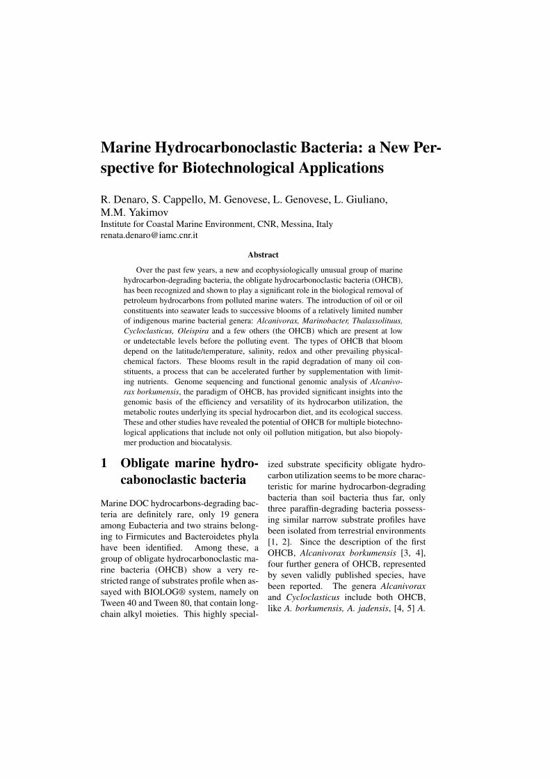
Marine Hydrocarbonoclastic Bacteria: a New Per-spective for Biotechnological Applications
R. Denaro, S. Cappello, M. Genovese, L. Genovese, L. Giuliano,M.M. YakimovInstitute for Coastal Marine Environment, CNR, Messina, [email protected]
Abstract
Over the past few years, a new and ecophysiologically unusual group of marinehydrocarbon-degrading bacteria, the obligate hydrocarbonoclastic bacteria (OHCB),has been recognized and shown to play a significant role in the biological removal ofpetroleum hydrocarbons from polluted marine waters. The introduction of oil or oilconstituents into seawater leads to successive blooms of a relatively limited numberof indigenous marine bacterial genera: Alcanivorax, Marinobacter, Thalassolituus,Cycloclasticus, Oleispira and a few others (the OHCB) which are present at lowor undetectable levels before the polluting event. The types of OHCB that bloomdepend on the latitude/temperature, salinity, redox and other prevailing physical-chemical factors. These blooms result in the rapid degradation of many oil con-stituents, a process that can be accelerated further by supplementation with limit-ing nutrients. Genome sequencing and functional genomic analysis of Alcanivo-rax borkumensis, the paradigm of OHCB, has provided significant insights into thegenomic basis of the efficiency and versatility of its hydrocarbon utilization, themetabolic routes underlying its special hydrocarbon diet, and its ecological success.These and other studies have revealed the potential of OHCB for multiple biotechno-logical applications that include not only oil pollution mitigation, but also biopoly-mer production and biocatalysis.
1 Obligate marine hydro-cabonoclastic bacteria
Marine DOC hydrocarbons-degrading bac-teria are definitely rare, only 19 generaamong Eubacteria and two strains belong-ing to Firmicutes and Bacteroidetes phylahave been identified. Among these, agroup of obligate hydrocarbonoclastic ma-rine bacteria (OHCB) show a very re-stricted range of substrates profile when as-sayed with BIOLOG® system, namely onTween 40 and Tween 80, that contain long-chain alkyl moieties. This highly special-
ized substrate specificity obligate hydro-carbon utilization seems to be more charac-teristic for marine hydrocarbon-degradingbacteria than soil bacteria thus far, onlythree paraffin-degrading bacteria possess-ing similar narrow substrate profiles havebeen isolated from terrestrial environments[1, 2]. Since the description of the firstOHCB, Alcanivorax borkumensis [3, 4],four further genera of OHCB, representedby seven validly published species, havebeen reported. The genera Alcanivoraxand Cycloclasticus include both OHCB,like A. borkumensis, A. jadensis, [4, 5] A.
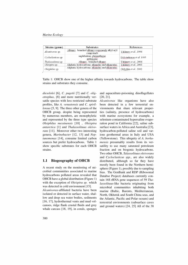
Marine Ecology
Table 1: OHCB show one of the higher affinity towards hydrocarbons. The table showstrains and substrates they consume.
dieselolei [6], C. pugetii [7] and C. olig-otrophus, [8] and more nutritionally ver-satile species with less restricted substrateprofiles, like A. venustensis and C. spiril-lensus [5, 9]. The three other genera of theOHCB group, despite being representedby numerous members, are monophyleticand represented by the three type speciesOleiphilus messinensis [10] , Oleispiraantarctica [1] and Thalassolituus oleivo-rans [11]. Moreover other two interestinggenera, Marinobacter [12, 13] and Nep-tunomonas [14], consume limited carbonsources but prefer hydrocarbons. Table 1show specific substrates for each OHCBstrains.
1.1 Biogeography of OHCB
A recent study on the monitoring of mi-crobial communities associated to marinehydrocarbons polluted areas revealed thatOHCB have a global distribution (Figure 1)with the exception of Oleispira sp. whichwas detected in cold environment [15].Alcanivorax-affiliated bacteria have beenisolated or detected in surface water, shal-low and deep sea water bodies, sediments[16, 17], hydrothermal vents and mud vol-canoes, ridge flank crustal fluids and greywhale carcass [18, 19], in corals, sponges
and aquaculture-poisoning dinoflagellates[20, 21].Alcanivorax like organisms have alsobeen detected in a few terrestrial en-vironments that share relevant proper-ties (salinity, presence of hydrocarbons)with marine ecosystems for example, aselenium-contaminated hypersaline evapo-ration pond in California [22], saline sub-surface waters in Africa and Australia [23],hydrocarbon-polluted saline soil and var-ious geothermal areas in Italy and USA(Yellowstone). This ubiquity of A. borku-mensis presumably results from its ver-satility to use many saturated petroleumfraction and on biogenic hydrocarbons.Two other OHCB, Talassolituus oleivoransand Cycloclasticus spp., are also widelydistributed, although so far they havemostly been found in the Northern hemi-sphere (Figure 1), possibly due to samplingbias. The GenBank and RDP (RibosomalDatabse Project) databases currently con-tain 16S rRNA gene sequences of 59 Tha-lassolituus-like bacteria originating frommicrobial communities inhabiting bothmarine (Baltic, Barents, Mediterranean,North, Okhotsk and South China seas, andthe Atlantic, Pacific and Polar oceans) andterrestrial environments (subsurface cavesand ground waters) [24, 25] All of the 38
300

Marine research at CNR
Figure 1: The marine areas where OHCB have been detected is represented by rectan-gles, namely, yellow sector is referred to Cycloclasticus sp. Red to Alcanivorax sp. BlueThalassolituus sp. In Artic and Antarctica regions was retrieved Oleispira antarctica(green sectors).
sequences in the databases assigned to thegenus Cycloclasticus were retrieved ex-clusively from marine microbial commu-nities, or PAH-supplemented enrichments[26, 27]. In contrast, the distribution of thepsychrophilic OHCB Oleispira antarctica(55 sequences to date) is thus far limitedto the colder waters found at high latitudes[28, 29]: the least cold sites at which O.antarctica has been found are Cape Cod(MA, USA GenBank AM117931), andSouth Tasmania [30].The most enigmatic marine OHCB,Oleiphilus messinensis [10], initially iso-lated from harbor sediments (Messina,Italy) seems to thrive elsewhere as a sponge
symbiont, as Oleiphilus-like 16S rRNAgene fragments have been recovered frombryozoan and dictyoceratid sponges sam-pled in North Atlantic and equatorial Pa-cific oceans.[31, 32].
1.2 Genomic basis of OHCBecophysiology
Marine OHCB occupy a special trophicniche among marine heterotrophic bacte-ria participating in the global carbon cy-cle, as they mediate degradation of chem-ically stable saturated and aromatic hydro-carbon species that are not substrates formost bacteria. However, a few studies
301
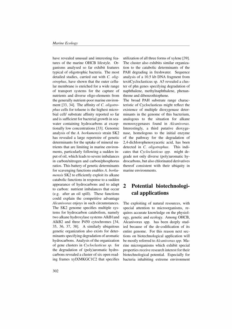
Marine Ecology
have revealed unusual and interesting fea-tures of the marine OHCB lifestyle. Or-ganisms analysed so far exhibit featurestypical of oligotrophic bacteria. The mostdetailed studies, carried out with C. olig-otrophus, have shown that the outer cellu-lar membrane is enriched for a wide rangeof transport systems for the capture ofnutrients and diverse oligo-elements fromthe generally nutrient-poor marine environ-ment [33, 34]. The affinity of C. oligotro-phus cells for toluene is the highest micro-bial cell/ substrate affinity reported so farand is sufficient for bacterial growth in sea-water containing hydrocarbons at excep-tionally low concentrations [33]. Genomicanalysis of the A. borkumensis strain SK2has revealed a large repertoire of geneticdeterminants for the uptake of mineral nu-trients that are limiting in marine environ-ments, particularly following a sudden in-put of oil, which leads to severe imbalancesin carbon/nitrogen and carbon/phosphorusratios. This battery of genetic determinantsfor scavenging functions enables A. borku-mensis SK2 to efficiently exploit its alkanecatabolic functions in response to a suddenappearance of hydrocarbons and to adaptto carbon: nutrient imbalances that occur(e.g. after an oil spill). These functionscould explain the competitive advantageAlcanivorax enjoys in such circumstances.The SK2 genome specifies multiple sys-tems for hydrocarbon catabolism, namelytwo alkane hydroxylase systems AlkB1andAlkB2 and three P450 cytochromes [34,35, 36, 37, 38]. A similarly ubiquitousgenetic organization also exists for deter-minants specifying degradation of aromatichydrocarbons. Analysis of the organizationof gene clusters in Cycloclasticus sp. forthe degradation of (poly)aromatic hydro-carbons revealed a cluster of six open read-ing frames xylXMKGC1C2 that specifies
utilization of all three forms of xylene [39].The cluster also exhibits similar organiza-tion to the catabolic determinants of thePAH degrading in freshwater. Sequenceanalysis of a 10.5 kb DNA fragment fromtexitCycloclasticus sp. A5 revealed a clus-ter of phn genes specifying degradation ofnaphthalene, methylnaphthalene, phenan-threne and dibenzothiophene.The broad PAH substrate range charac-teristic of Cycloclasticus might reflect theexistence of multiple dioxygenase deter-minants in the genome of this bacterium,analogous to the situation for alkanemonooxygenases found in Alcanivorax.Interestingly, a third putative dioxyge-nase, homologous to the initial enzymeof the pathway for the degradation of2,4-dichlorophenoxyacetic acid, has beendetected in C. oligotrophus. This indi-cates that Cycloclasticus spp. might de-grade not only diverse (poly)aromatic hy-drocarbons, but also chlorinated derivativesthereof consistent with their ubiquity inmarine environments.
2 Potential biotechnologi-cal applications
The exploiting of natural resources, withspecial attention to microorganisms, re-quires accurate knowledge on the physiol-ogy, genetic and ecology. Among OHCB,Alcanivorax spp. has been deeply stud-ied because of the de-codification of itsentire genome. For this reason next sec-tions on biotechnological application willbe mostly referred to Alcanivorax spp. Ma-rine microrganisms which exhibit specialproperties receive research interest for theirbiotechnological potential. Especially forbacteria inhabiting extreme environment
302
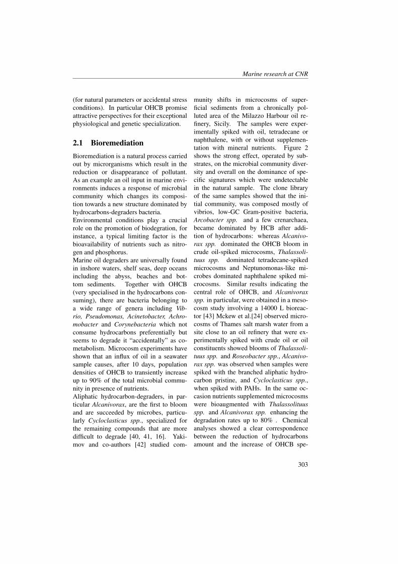
Marine research at CNR
(for natural parameters or accidental stressconditions). In particular OHCB promiseattractive perspectives for their exceptionalphysiological and genetic specialization.
2.1 BioremediationBioremediation is a natural process carriedout by microrganisms which result in thereduction or disappearance of pollutant.As an example an oil input in marine envi-ronments induces a response of microbialcommunity which changes its composi-tion towards a new structure dominated byhydrocarbons-degraders bacteria.Environmental conditions play a crucialrole on the promotion of biodegration, forinstance, a typical limiting factor is thebioavailability of nutrients such as nitro-gen and phosphorus.Marine oil degraders are universally foundin inshore waters, shelf seas, deep oceansincluding the abyss, beaches and bot-tom sediments. Together with OHCB(very specialised in the hydrocarbons con-suming), there are bacteria belonging toa wide range of genera including Vib-rio, Pseudomonas, Acinetobacter, Achro-mobacter and Corynebacteria which notconsume hydrocarbons preferentially butseems to degrade it “accidentally” as co-metabolism. Microcosm experiments haveshown that an influx of oil in a seawatersample causes, after 10 days, populationdensities of OHCB to transiently increaseup to 90% of the total microbial commu-nity in presence of nutrients.Aliphatic hydrocarbon-degraders, in par-ticular Alcanivorax, are the first to bloomand are succeeded by microbes, particu-larly Cycloclasticus spp., specialized forthe remaining compounds that are moredifficult to degrade [40, 41, 16]. Yaki-mov and co-authors [42] studied com-
munity shifts in microcosms of super-ficial sediments from a chronically pol-luted area of the Milazzo Harbour oil re-finery, Sicily. The samples were exper-imentally spiked with oil, tetradecane ornaphthalene, with or without supplemen-tation with mineral nutrients. Figure 2shows the strong effect, operated by sub-strates, on the microbial community diver-sity and overall on the dominance of spe-cific signatures which were undetectablein the natural sample. The clone libraryof the same samples showed that the ini-tial community, was composed mostly ofvibrios, low-GC Gram-positive bacteria,Arcobacter spp. and a few crenarchaea,became dominated by HCB after addi-tion of hydrocarbons: whereas Alcanivo-rax spp. dominated the OHCB bloom incrude oil-spiked microcosms, Thalassoli-tuus spp. dominated tetradecane-spikedmicrocosms and Neptunomonas-like mi-crobes dominated naphthalene spiked mi-crocosms. Similar results indicating thecentral role of OHCB, and Alcanivoraxspp. in particular, were obtained in a meso-cosm study involving a 14000 L bioreac-tor [43] Mckew et al.[24] observed micro-cosms of Thames salt marsh water from asite close to an oil refinery that were ex-perimentally spiked with crude oil or oilconstituents showed blooms of Thalassoli-tuus spp. and Roseobacter spp., Alcanivo-rax spp. was observed when samples werespiked with the branched aliphatic hydro-carbon pristine, and Cycloclasticus spp.,when spiked with PAHs. In the same oc-casion nutrients supplemented microcosmswere bioaugmented with Thalassolituusspp. and Alcanivorax spp. enhancing thedegradation rates up to 80% . Chemicalanalyses showed a clear correspondencebetween the reduction of hydrocarbonsamount and the increase of OHCB spe-
303
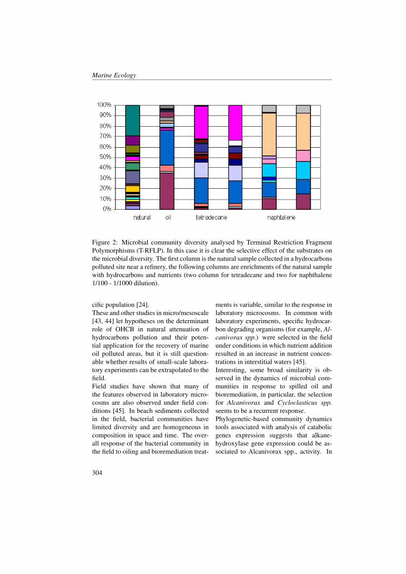
Marine Ecology
Figure 2: Microbial community diversity analysed by Terminal Restriction FragmentPolymorphisms (T-RFLP). In this case it is clear the selective effect of the substrates onthe microbial diversity. The first column is the natural sample collected in a hydrocarbonspolluted site near a refinery, the following columns are enrichments of the natural samplewith hydrocarbons and nutrients (two column for tetradecane and two for naphthalene1/100 - 1/1000 dilution).
cific population [24].These and other studies in micro/mesoscale[43, 44] let hypotheses on the determinantrole of OHCB in natural attenuation ofhydrocarbons pollution and their poten-tial application for the recovery of marineoil polluted areas, but it is still question-able whether results of small-scale labora-tory experiments can be extrapolated to thefield.Field studies have shown that many ofthe features observed in laboratory micro-cosms are also observed under field con-ditions [45]. In beach sediments collectedin the field, bacterial communities havelimited diversity and are homogeneous incomposition in space and time. The over-all response of the bacterial community inthe field to oiling and bioremediation treat-
ments is variable, similar to the response inlaboratory microcosms. In common withlaboratory experiments, specific hydrocar-bon degrading organisms (for example, Al-canivorax spp.) were selected in the fieldunder conditions in which nutrient additionresulted in an increase in nutrient concen-trations in interstitial waters [45].Interesting, some broad similarity is ob-served in the dynamics of microbial com-munities in response to spilled oil andbioremediation, in particular, the selectionfor Alcanivorax and Cycloclasticus spp.seems to be a recurrent response.Phylogenetic-based community dynamicstools associated with analysis of catabolicgenes expression suggests that alkane-hydroxylase gene expression could be as-sociated to Alcanivorax spp., activity. In
304
Marine research at CNR
fact there is some indication that differ-ent genotypes of Alcanivorax can becomeprevalent under conditions of high and lownutrient input [16]. Two distinct Alcanivo-rax genotypes were identified in laboratoryand field oil-spill bioremediation experi-ments, and the patterns of the relative abun-dance of 16S-rRNA sequences in clonelibraries from sediments that were treatedwith different amounts of nutrients indicatethat the different genotypes are adapted tohigher or lower concentrations of nutrients.Different Alcanivorax spp. have differentphysiological properties [3, 6], and the se-lection of different Alcanivorax genotypesduring bioremediation might affect the ki-netics and patterns of biodegradation thatoccur.Although the pivotal role of OHCB inbioremediation in marine environment isconfirmed by several studies, in nature,biodegradation is the results of cooperationand interaction within microbial commu-nity acting in concert or sequence, ratherthan as single strains. For example, Taggeret al.[46] point out that of 9 oil-degradingisolates from marine sediments, only 2strains were able to grow on napthaleneas sole carbon source, but the remaining7 used metabolic intermediates. The im-portance of such trophic interactions andsuccession have to be interpreted not onlyfor environmental recovery but also as amethod for organic carbon balance andrecycling. On this bases it is noticeablethe effect of hydrocarbon-degrading preda-tors. Studies in mesocosms revealed thepresence of nanoflagelates which, not onlytolerate the presence of oil, but seemed tofeed in Alcanivorax spp. dominated micro-bial community.Predators indirectly affect contaminantbiodegradation, owing to their ability to se-lectively graze on, and control the biomass
of bacteria. The influence of protozoa onbiodegradation is often negative, becauseit decreases the number of degrading bac-teria in comparison to the situation in theabsence of predators [47]). However, pre-dation has been shown to stimulate bac-terial degradation of toluene and benzeneconsiderably on a per-cell basis [48, 49].In addition, predation creates a nutritionalloop, because predators can re-mineralizenutrients, which in turn increases bacterialgrowth.The knowledge on the use ofhydrocarbons-degraders as an alternativeintervention to the chemical one lacksof theoretical basis to underpin and pre-dict the behaviour and interactions ofhydrocarbon-degrading bacteria in situ.Further studies are required to elucidatethe biochemistry, genetic basis and regula-tion of hydrocarbon-degrading pathways.Nevertheless experiments carried out inmicro-meso/scales simulate the natural re-sponses of the marine microbial commu-nity to an oil spill event, many questions re-main about the dynamic of hydrocarbons-degraders and their predators, the succes-sion of degradation pathways, how bacte-ria compete for substrate utilization (spe-cial capturing and transport systems, toxicmetabolic intermediates, antibiotic produc-tion).The needs on bioremediation studies are re-lated to field application of OHCB in con-sortium with other hydrocarbons degradersand the optimization of intervention strat-egy in terms of quantity of biomass, nutri-ents, surfactant monitoring environmentalparameters also.
305
Marine Ecology
2.2 Bioproducts: Biosurfac-tant applications to increasebioavailability
Biosurfactants are surface-active microbialproducts that have numerous industrial ap-plications.The production of biosurfactants facili-tates emulsification of hydrophobic or-ganic substrates, enhances their bioavail-ability and increases the degradation.Many microorganisms, especially bacte-ria, produce biosurfactants when grown onwater-immiscible substrates (Rhodococ-cus, Acinetobacter, P. aeruginosa). Mostcommon biosurfactants are glycolipids inwhich carbohydrates are attached to along-chain aliphatic acid, while others,like lipopeptides, lipoproteins and het-eropolysaccharides, are more complex.The most promising applications of bio-surfactants are in the cleaning of oil-contaminated tankers, oil-spill manage-ment, transportation of heavy crude, en-hanced oil recovery, recovery of oil fromsludge and bioremediation of sites contam-inated with hydrocarbons, heavy metalsand other pollutants [50, 51]. Rhodococ-cus sp. 094 can oxidize alkanes incrude oil emulsified by nonionic chemi-cal and biological surfactants Iwabuchi etal. [52] observed that in oil-polluted seawater supplemented with nitrogen, phos-phorus and iron, significant biodegradationof an aromatic fraction of crude oil oc-curred only when extracellular polysaccha-rides from Rhodococcus rhodochrous werepresent. The extracellular polysaccharidesresulted in emulsification of oil, followedby changes in the composition of the bac-terial community, with Cycloclasticus spp.becoming dominant [53]. A. borkumen-sis forms stable emulsions of hydrocar-bon in water and produces biosurfactants
[54]. These biosurfactants are anionic glu-colipids carrying four fatty acids of vary-ing chain lengths. The genetic organizationof the glucolipid biosynthesis remains un-clear in A. borkumensis SK2, but genomeannotation revealed candidate genes po-tentially involved in biosurfactant produc-tion. ABO 1783 and ABO 2215 encodeglycosyltransferases, exhibiting significanthomology with RhlB from Pseudomonasaeruginosa and glycosyltransferase proteinfamily, respectively. These gene prod-ucts possibly provide the sugar moiety ofthe glucolipids, yielding glucose lipid sur-factants. A. borkumensis SK2 also ex-presses an OprF/OmpA protein encodedby ABO 0822, which is upregulated whengrown on alkane
2.3 Bioproducts: Polyhydrox-yalkanoic acids (PHAs)
One of the currently overcome of modernsociety is the production of environmen-tally friendly materials. This is particu-larly thru for the plastic objects which havea deleterious environmental impact. Poly-hydroxyalkanoic acids (PHAs), are naturalpolymers whose production/degradationcycle reduces undesirable wastes and emis-sions.PHAs are extremely versatile polymers astheir crystalline aspect can be manipulatedto provide a broad range of mechanical andbarrier properties, in some cases matchingthe performance of engineered thermoplas-tics. PHA biodegradable polymers are stilllargely at the development stage of marketdevelopment, although there a few com-mercial applications available.These polymers are synthesised as storagesubstances by bacteria in specific condi-tions of nutrients and carbon source. For
306
Marine research at CNR
carbon-limited microbes, an increase incarbon allows an increase in growth rateuntil another growth limitation is reached.The first survey of PHA was observedon Bacillus megaterium which producedan intracellular polymer of hydroxybu-tyrate monomers. In the followingyears biopolyesters with longer side chains(medium-chain-lengthPHAs [mcl-PHAs])were also described in Pseudomonasputida GPo1 growing on alkanes [55].Moreover has been detected in some ar-chaea and a wide range of gram-positiveand gram-negative bacteria in aerobic andanaerobic environments. Although thereare many microorganisms that are ableto produce PHA, mcl-PHA productionhad been repetitively restricted to Pseu-domonas strains [55, 56, 57, 58, 59].The appearance of alkanes in oligotrophicenvironments like most marine habitats al-lows Alcanivorax to ”bloom” initially un-til nitrogen limitation is experienced. Un-der conditions of high C/N ratios, manymicrobes synthesize carbon storage mate-rials, like polyhydroxyalkanoates (PHAs).ABO 1418, one of two A. borkumensisphaC PHA synthase genes, was solely ex-pressed in alkane-grown cells, whereas an-other, ABO 2214, was not expressed at de-tectable levels in such cells. Since PHA isalso produced at high C/N ratios in cellsgrown on non-alkane substrates (Sabirovaet al., unpublished), it seems that A. borku-mensis produces one of two distinct PhaCPHA synthases in response to differentgrowth substrates, probably having differ-ent substrate specificities that reflect dis-tinct metabolites produced from the differ-ent growth substrates.A recent functional genomics study of A.borkumensis SK2 revealed that inactivationof a ‘TesB’-like hydroxyacyl-coenzyme A-specific thioesterase leads to hyperproduc-
tion and extracellular localization of PHAs, even though the normal food storagecompounds found in this strain and otherOHCB (Marinobacter and Thalassolituus)are triacylglycerols and wax esters. The ex-tracellular localization of PHA is an excep-tional novelty both because of the extrac-tion technique and the amount of the pro-duction.Currently, other potential applications arebeing assessed, including environmentaland medical applications, such as the use ofPHAs in wastewater denitrification biore-actors, in which they serve as both thesource of reducing equivalents for denitrifi-cation and asthe matrix for biofilm forma-tion [60], and as biocompatible materialsfor implants, scaffolds for tissue engineer-ing, and drug carriers [61, 62].
2.4 Bioproducts: EnzymesMetabolic specialization and biotechnolog-ical potential A. borkumensis SK2, likeother hydrocarbonoclastic bacteria, has alimited substrate range for its growth. Theabsence of a functional PEP-dependentsugar/phosphotransferase system or othertypes of sugar transporters, as well as thelack of several determinants for key en-zymes of the glycolytic, pentose phos-phate shunt and Entner-Doudoroff path-ways, is consistent with the inabilityof A. borkumensis SK2 to utilize sim-ple hexoses and other simple carbohy-drates for growth. The A. borkumensisSK2 genome encodes a number of pro-teins putatively involved in metabolic re-actions of potential biotechnological in-terest, including eight hydrolases of thehaloacid dehydrogenase/epoxide family,two determinants for dienelactone hydro-lases(ABO 1618 and ABO 1886), threefor deacylases, 36 for variouscytochrome
307
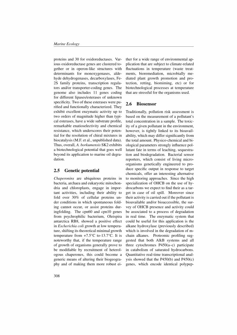
Marine Ecology
proteins and 30 for oxidoreductases. Var-ious oxidoreductase genes are clustered to-gether or in operon-like structures withdeterminants for monoxygenases, alde-hyde dehydrogenases, decarboxylases, Fe-2S family proteins, transcription regula-tors and/or transporter-coding genes. Thegenome also includes 11 genes codingfor different lipases/esterases of unknownspecificity. Two of these esterases were pu-rified and functionally characterized. Theyexhibit excellent enzymatic activity up totwo orders of magnitude higher than typi-cal esterases, have a wide substrate profile,remarkable enatioselectivity and chemicalresistance, which underscores their poten-tial for the resolution of chiral mixtures inbiocatalysis (M.F. et al., unpublished data).Thus, overall, A. borkumensis SK2 exhibitsa biotechnological potential that goes wellbeyond its application to marine oil degra-dation.
2.5 Genetic potentialChaperonins are ubiquitous proteins inbacteria, archaea and eukaryotic mitochon-dria and chloroplasts, engage in impor-tant activities, including their ability tofold over 30% of cellular proteins un-der conditions in which spontaneous fold-ing cannot occur, or assist proteins dur-ingfolding. The cpn60 and cpn10 genesfrom psychrophilic bacterium, Oleispiraantarctica RB8, showed a positive effectin Escherichia coli growth at low tempera-ture, shifting its theoretical minimal growthtemperature from +7.5°C to-13.7°C. It isnoteworthy that, if the temperature rangeof growth of organisms generally prove tobe modifiable by recruitment of heterol-ogous chaperones, this could become ageneric means of altering their biogeogra-phy and of making them more robust ei-
ther for a wide range of environmental ap-plication that are subject to climate-relatedfluctuations in temperature (waste treat-ments, bioremediation, microbially me-diated plant growth promotion and pro-tection, retting, biomiming, etc) or forbiotechnological processes at temperaturethat are stressful for the organisms used.
2.6 BiosensorTraditionally, pollution risk assessment isbased on the measurement of a pollutant’stotal concentration in a sample. The toxic-ity of a given pollutant in the environment,however, is tightly linked to its bioavail-ability, which may differ significantly fromthe total amount. Physico-chemical and bi-ological parameters strongly influence pol-lutant fate in terms of leaching, sequestra-tion and biodegradation. Bacterial sensorreporters, which consist of living micro-organisms genetically engineered to pro-duce specific output in response to targetchemicals, offer an interesting alternativeto monitoring approaches. Since the highspecialization of OHCB on the use of hy-drocarbons we expect to find their as a tar-get in case of oil spill. Moreover sincetheir activity is carried out if the pollutant isbioavailable and/or bioaccessible, the sur-vey of OHCB presence and activity couldbe associated to a process of degradationin real time. The enzymatic system thatcould be useful for this application is thealkane hydroxylase (previously described)which is involved in the degradation of m-chain alkanes. Proteomic profiling sug-gested that both AlkB systems and allthree cytochromes P450(a–c) participatein catabolism of saturated hydrocarbons.Quantitative real-time transcriptional anal-ysis showed that the P450(b) and P450(c)genes, which encode identical polypep-
308
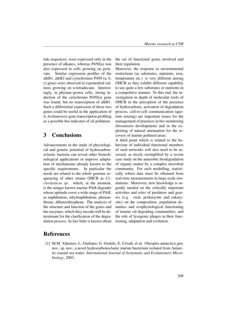
Marine research at CNR
tide sequences, were expressed only in thepresence of alkanes, whereas P450(a) wasalso expressed in cells growing on pyru-vate. Similar expression profiles of thealkB1, alkB2 and cytochromes P450 (a, b,c) genes were observed in exponential cul-tures growing on n-tetradecane. Interest-ingly, in phytane-grown cells, strong in-duction of the cytochrome P450(a) genewas found, but no transcription of alkB1.Such a differential expression of these twogenes could be useful in the application ofA. borkumensis gene transcription profilingas a possible bio-indicator of oil pollution.
3 ConclusionsAdvancements in the study of physiologi-cal and genetic potential of hydrocarbon-oclastic bacteria can reveal other biotech-nological applications or improve adapta-tion of mechanisms already known to thespecific requirements. In particular theneeds are related to the whole genome se-quencing of other strains OHCB as Cy-cloclasticus sp. which, at the moment,is the unique known marine PAH-degraderwhose aptitude cover a wide range of PAH,as naphthalene, ethylnaphthalene, phenan-threne, dibenzothiophene. The analysis ofthe structure and function of the genes andthe enzymes, which they encode will be de-terminant for the clarification of the degra-dation process. In fact little is known about
the set of functional genes involved andtheir regulation.Moreover, the response to environmentalrestrictions (as substrates, nutrients, iron,temperature etc.) is very different amongOHCB as they exhibit different capabilityto use quite a few substrates or nutrients ina competitive manner. To this end, the in-vestigation in depth of molecular tools ofOHCB in the perception of the presenceof hydrocarbons, activation of degradationprocess, cell-to-cell communication (quo-rum sensing) are important issues for themanagement of practices in bio-monitoring(biosensors development) and in the ex-ploiting of natural attenuation for the re-covery of marine polluted areas.A third point which is related to the be-haviour of individual functional membersof such networks will also need to be as-sessed, as nicely exemplified by a recentcase study on the anaerobic biodegradationof organic matter by a complex microbialcommunity. For such modelling, statisti-cally robust data must be obtained fromreal-time measurements in large-scale sim-ulations. Moreover, new knowledge is ur-gently needed on the critically importantactivities and roles of predators and graz-ers (e.g. viral, prokaryotic and eukary-otic) on the composition, population dy-namics and ecophysiological functioningof marine oil-degrading communities, andthe role of lysogenic phages in their func-tioning, adaptation and evolution.
References[1] M.M. Yakimov, L. Giuliano, G. Gentile, E. Crisafi, et al. Oleispira antarctica gen.
nov., sp. nov., a novel hydrocarbonoclastic marine bacterium isolated from Antarc-tic coastal sea water. International Journal of Systematic and Evolutionary Micro-biology, 2003.
309
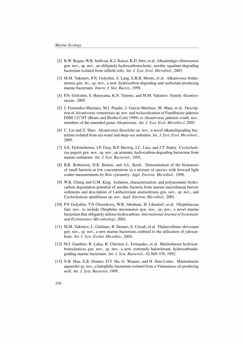
Marine Ecology
[2] B.W. Bogan, W.R. Sullivan, K.J. Kaiser, K.D. Derr, et al. Alkanindiges illinoisensisgen. nov., sp. nov., an obligately hydrocarbonoclastic, aerobic squalane-degradingbacterium isolated from oilfield soils. Int. J. Syst. Evol. Microbiol., 2003.
[3] M.M. Yakimov, P.N. Golyshin, S. Lang, E.R.B. Moore, et al. Alkanivorax borku-mensis gen. no., sp. nov., a new, hydrocarbon-degrading and surfactant-producingmarine bacterium. Intern. J. Sist. Bacter., 1998.
[4] P.N. Golyshin, S. Harayama, K.N. Timmis, and M.M. Yakimov. Family Alcanivo-raceae. 2005.
[5] J. Fernandez-Martinez, M.J. Pujalte, J. Garcia-Martinez, M. Mata, et al. Descrip-tion of Alcanivorax venustensis sp. nov. and reclassification of Fundibacter jadensisDSM 12178T (Bruns and Berthe-Corti 1999) as Alcanivorax jadensis comb. nov.,members of the emended genus Alcanivorax. Int. J. Syst. Evol. Microbio.l, 2003.
[6] C. Liu and Z. Shao. Alcanivorax dieselolei sp. nov., a novel alkanedegrading bac-terium isolated from sea water and deep-sea sediment. Int. J. Syst. Evol. Microbiol.,2005.
[7] S.E. Dyksterhouse, J.P. Gray, R.P. Herwig, J.C. Lara, and J.T. Staley. Cycloclasti-cus pugetii gen. nov., sp. nov., an aromatic hydrocarbon-degrading bacterium frommarine sediments. Int. J. Syst. Bacteriol., 1995.
[8] B.R. Robertson, D.K. Button, and A.L. Koch. Determination of the biomassesof small bacteria at low concentrations in a mixture of species with forward lightscatter measurements by flow cytometry. Appl. Environ. Microbiol., 1998.
[9] W.K. Chung and G.M. King. Isolation, characterization, and polyaromatic hydro-carbon degradation potential of aerobic bacteria from marine macrofaunal burrowsediments and description of Lutibacterium anuloederans gen. nov., sp. nov., andCycloclasticus spirillensus sp. nov. Appl. Environ. Microbiol., 2001.
[10] P.N Golyshin, T.N Chernikova, W.R. Abraham, H. Lunsdorf, et al. Oleiphilaceaefam. nov., to include Oleiphilus messinensis gen. nov., sp. nov., a novel marinebacterium that obligately utilizes hydrocarbons. International Journal of Systematicand Evolutionary Microbiology, 2002.
[11] M.M. Yakimov, L. Giuliano, R. Denaro, E. Crisafi, et al. Thalassolituus oleivoransgen. nov., sp. nov., a new marine bacterium confined to the utilization of ydrocar-bons. Int. J. Syst. Evolut. Microbio., 2004.
[12] M.J. Gauthier, B. Lafay, R. Christen, L. Fernandez, et al. Marinobacter hydrocar-bonoclasticus gen. nov., sp. nov., a new, extremely halotolerant, hydrocarbonde-grading marine bacterium. Int. J. Syst. Bacteriol., 42:568–576, 1992.
[13] N.B. Huu, E.B. Denner, D.T. Ha, G. Wanner, and H. Stan-Lotter. Marinobacteraquaeolei sp. nov., a halophilic bacterium isolated from a Vietnamese oil producingwell. Int. J. Syst. Bacteriol, 1999.
310
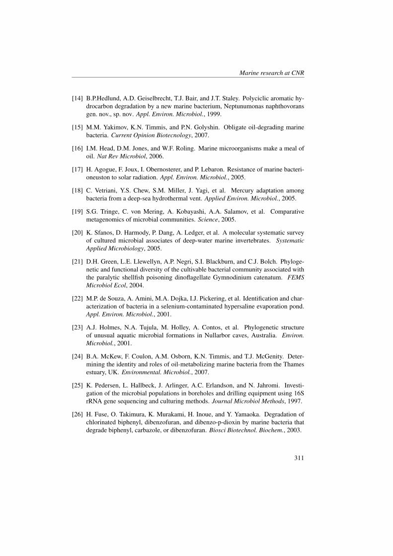
Marine research at CNR
[14] B.P.Hedlund, A.D. Geiselbrecht, T.J. Bair, and J.T. Staley. Polyciclic aromatic hy-drocarbon degradation by a new marine bacterium, Neptunumonas naphthovoransgen. nov., sp. nov. Appl. Environ. Microbiol., 1999.
[15] M.M. Yakimov, K.N. Timmis, and P.N. Golyshin. Obligate oil-degrading marinebacteria. Current Opinion Biotecnology, 2007.
[16] I.M. Head, D.M. Jones, and W.F. Roling. Marine microorganisms make a meal ofoil. Nat Rev Microbiol, 2006.
[17] H. Agogue, F. Joux, I. Obernosterer, and P. Lebaron. Resistance of marine bacteri-oneuston to solar radiation. Appl. Environ. Microbiol., 2005.
[18] C. Vetriani, Y.S. Chew, S.M. Miller, J. Yagi, et al. Mercury adaptation amongbacteria from a deep-sea hydrothermal vent. Applied Environ. Microbiol., 2005.
[19] S.G. Tringe, C. von Mering, A. Kobayashi, A.A. Salamov, et al. Comparativemetagenomics of microbial communities. Science, 2005.
[20] K. Sfanos, D. Harmody, P. Dang, A. Ledger, et al. A molecular systematic surveyof cultured microbial associates of deep-water marine invertebrates. SystematicApplied Microbiology, 2005.
[21] D.H. Green, L.E. Llewellyn, A.P. Negri, S.I. Blackburn, and C.J. Bolch. Phyloge-netic and functional diversity of the cultivable bacterial community associated withthe paralytic shellfish poisoning dinoflagellate Gymnodinium catenatum. FEMSMicrobiol Ecol, 2004.
[22] M.P. de Souza, A. Amini, M.A. Dojka, I.J. Pickering, et al. Identification and char-acterization of bacteria in a selenium-contaminated hypersaline evaporation pond.Appl. Environ. Microbiol., 2001.
[23] A.J. Holmes, N.A. Tujula, M. Holley, A. Contos, et al. Phylogenetic structureof unusual aquatic microbial formations in Nullarbor caves, Australia. Environ.Microbiol., 2001.
[24] B.A. McKew, F. Coulon, A.M. Osborn, K.N. Timmis, and T.J. McGenity. Deter-mining the identity and roles of oil-metabolizing marine bacteria from the Thamesestuary, UK. Environmental. Microbiol., 2007.
[25] K. Pedersen, L. Hallbeck, J. Arlinger, A.C. Erlandson, and N. Jahromi. Investi-gation of the microbial populations in boreholes and drilling equipment using 16SrRNA gene sequencing and culturing methods. Journal Microbiol Methods, 1997.
[26] H. Fuse, O. Takimura, K. Murakami, H. Inoue, and Y. Yamaoka. Degradation ofchlorinated biphenyl, dibenzofuran, and dibenzo-p-dioxin by marine bacteria thatdegrade biphenyl, carbazole, or dibenzofuran. Biosci Biotechnol. Biochem., 2003.
311
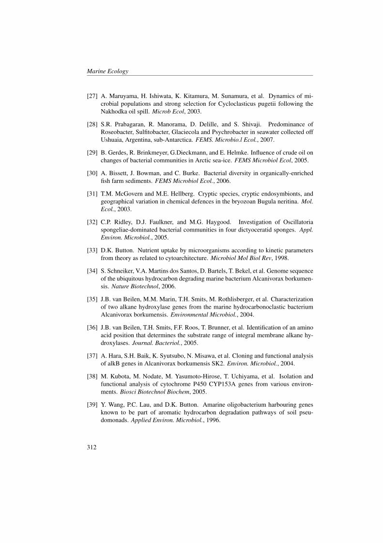
Marine Ecology
[27] A. Maruyama, H. Ishiwata, K. Kitamura, M. Sunamura, et al. Dynamics of mi-crobial populations and strong selection for Cycloclasticus pugetii following theNakhodka oil spill. Microb Ecol, 2003.
[28] S.R. Prabagaran, R. Manorama, D. Delille, and S. Shivaji. Predominance ofRoseobacter, Sulfitobacter, Glaciecola and Psychrobacter in seawater collected offUshuaia, Argentina, sub-Antarctica. FEMS. Microbio.l Ecol., 2007.
[29] B. Gerdes, R. Brinkmeyer, G.Dieckmann, and E. Helmke. Influence of crude oil onchanges of bacterial communities in Arctic sea-ice. FEMS Microbiol Ecol, 2005.
[30] A. Bissett, J. Bowman, and C. Burke. Bacterial diversity in organically-enrichedfish farm sediments. FEMS Microbiol Ecol., 2006.
[31] T.M. McGovern and M.E. Hellberg. Cryptic species, cryptic endosymbionts, andgeographical variation in chemical defences in the bryozoan Bugula neritina. Mol.Ecol., 2003.
[32] C.P. Ridley, D.J. Faulkner, and M.G. Haygood. Investigation of Oscillatoriaspongeliae-dominated bacterial communities in four dictyoceratid sponges. Appl.Environ. Microbiol., 2005.
[33] D.K. Button. Nutrient uptake by microorganisms according to kinetic parametersfrom theory as related to cytoarchitecture. Microbiol Mol Biol Rev, 1998.
[34] S. Schneiker, V.A. Martins dos Santos, D. Bartels, T. Bekel, et al. Genome sequenceof the ubiquitous hydrocarbon degrading marine bacterium Alcanivorax borkumen-sis. Nature Biotechnol, 2006.
[35] J.B. van Beilen, M.M. Marin, T.H. Smits, M. Rothlisberger, et al. Characterizationof two alkane hydroxylase genes from the marine hydrocarbonoclastic bacteriumAlcanivorax borkumensis. Environmental Microbiol., 2004.
[36] J.B. van Beilen, T.H. Smits, F.F. Roos, T. Brunner, et al. Identification of an aminoacid position that determines the substrate range of integral membrane alkane hy-droxylases. Journal. Bacteriol., 2005.
[37] A. Hara, S.H. Baik, K. Syutsubo, N. Misawa, et al. Cloning and functional analysisof alkB genes in Alcanivorax borkumensis SK2. Environ. Microbiol., 2004.
[38] M. Kubota, M. Nodate, M. Yasumoto-Hirose, T. Uchiyama, et al. Isolation andfunctional analysis of cytochrome P450 CYP153A genes from various environ-ments. Biosci Biotechnol Biochem, 2005.
[39] Y. Wang, P.C. Lau, and D.K. Button. Amarine oligobacterium harbouring genesknown to be part of aromatic hydrocarbon degradation pathways of soil pseu-domonads. Applied Environ. Microbiol., 1996.
312
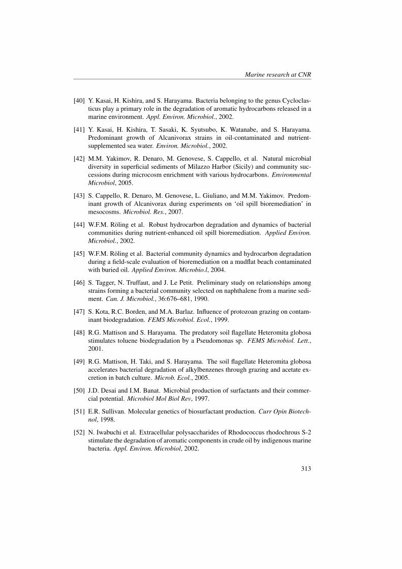
Marine research at CNR
[40] Y. Kasai, H. Kishira, and S. Harayama. Bacteria belonging to the genus Cycloclas-ticus play a primary role in the degradation of aromatic hydrocarbons released in amarine environment. Appl. Environ. Microbiol., 2002.
[41] Y. Kasai, H. Kishira, T. Sasaki, K. Syutsubo, K. Watanabe, and S. Harayama.Predominant growth of Alcanivorax strains in oil-contaminated and nutrient-supplemented sea water. Environ. Microbiol., 2002.
[42] M.M. Yakimov, R. Denaro, M. Genovese, S. Cappello, et al. Natural microbialdiversity in superficial sediments of Milazzo Harbor (Sicily) and community suc-cessions during microcosm enrichment with various hydrocarbons. EnvironmentalMicrobiol, 2005.
[43] S. Cappello, R. Denaro, M. Genovese, L. Giuliano, and M.M. Yakimov. Predom-inant growth of Alcanivorax during experiments on ‘oil spill bioremediation’ inmesocosms. Microbiol. Res., 2007.
[44] W.F.M. Roling et al. Robust hydrocarbon degradation and dynamics of bacterialcommunities during nutrient-enhanced oil spill bioremediation. Applied Environ.Microbiol., 2002.
[45] W.F.M. Roling et al. Bacterial community dynamics and hydrocarbon degradationduring a field-scale evaluation of bioremediation on a mudflat beach contaminatedwith buried oil. Applied Environ. Microbio.l, 2004.
[46] S. Tagger, N. Truffaut, and J. Le Petit. Preliminary study on relationships amongstrains forming a bacterial community selected on naphthalene from a marine sedi-ment. Can. J. Microbiol., 36:676–681, 1990.
[47] S. Kota, R.C. Borden, and M.A. Barlaz. Influence of protozoan grazing on contam-inant biodegradation. FEMS Microbiol. Ecol., 1999.
[48] R.G. Mattison and S. Harayama. The predatory soil flagellate Heteromita globosastimulates toluene biodegradation by a Pseudomonas sp. FEMS Microbiol. Lett.,2001.
[49] R.G. Mattison, H. Taki, and S. Harayama. The soil flagellate Heteromita globosaaccelerates bacterial degradation of alkylbenzenes through grazing and acetate ex-cretion in batch culture. Microb. Ecol., 2005.
[50] J.D. Desai and I.M. Banat. Microbial production of surfactants and their commer-cial potential. Microbiol Mol Biol Rev, 1997.
[51] E.R. Sullivan. Molecular genetics of biosurfactant production. Curr Opin Biotech-nol, 1998.
[52] N. Iwabuchi et al. Extracellular polysaccharides of Rhodococcus rhodochrous S-2stimulate the degradation of aromatic components in crude oil by indigenous marinebacteria. Appl. Environ. Microbiol, 2002.
313

Marine Ecology
[53] P. Bruheim, H. Bredholt, and K. Eimhjellen. Bacterial degradation of emulsifiedcrude oil and the effect of various surfactants. Can. J. Microbiol., 1997.
[54] W.R. Abraham and H. Meyer & M.M. Yakimov. Novel glycine containing glucol-ipids from the alkane using bacterium Alcanivorax borkumensis. 1393, 1998.
[55] M. de Smet, G. Eggink, B. Witholt, J. Kingma, and H. Wynberg. Characterizationof intracellular inclusions formed by Pseudomonas oleovorans during growth onoctane. Journal. Bacteriol., 1983.
[56] G.W. Huisman, O. de Leeuw, G. Eggink, and B. Witholt. Synthesis of poly-3-hydroxyalkanoates is a common feature of fluorescent pseudomonads. Appl. Envi-ron. Microbiol., 1989.
[57] J.M. Luengo, B. Garcıa, A. Sandoval, G. Naharro, and E.R. Olivera. Bioplasticsfrom microorganisms. Curr. Opin. Microbiol., 2003.
[58] M. Zinn, B. Witholt, and T. Egli. Occurrence, synthesis and medical application ofbacterial polyhydroxyalkanoate. Adv. Drug Deliv. Rev, 2001.
[59] J.S. Sabirova, M. Ferrer, H. Lunsdorf, V. Wray, et al. Mutation in a “tesB-like”hydroxyacyl-coenzyme A specific thioesterase gene causes hyperproduction of ex-tracellular polyhydroxyalkanoates by Alcanivorax borkumensis SK2. Journal Bac-teriol, 2006.
[60] A. Hiraishi and S.T. Khan. Application of polyhydroxyalkanoates for denitrifica-tion in water and wastewater treatment. Appl. Microbiol. Biotechnol., 61:103–109,2003.
[61] C.H. Rivard, T. C. Chapu, S. Rhalmi, and A. Selmani. Bio-adsorbable syntheticpolyesters and tissue regeneration: a study of three-dimensional proliferation ofovine chondrocytes and osteoblasts. Ann. Chirl., 50:658–751, 1996.
[62] B. Nebe, C. Forster, H. Pommerenke, G. Fulda, et al. Structural alterations of ad-hesion mediating components in cells cultured on poly-beta-hydroxy butyric acid.Biomaterials, 22:2425–2434, 2001.
314