Economia Internazionale n. 3 - 2012FINALE
128
ECONOMIA INTERNAZIONALE INTERNATIONAL ECONOMICS
-
Upload
independent -
Category
Documents
-
view
0 -
download
0
Transcript of Economia Internazionale n. 3 - 2012FINALE

ECONOMIA INTERNAZIONALE
INTERNATIONAL ECONOMICS


ECONOMIA INTERNAZIONALE / INTERNATIONAL ECONOMICS is published quarterly.
Manuscripts to be considered for publication, books for review, periodicals in exchange, correspondence and subscription orders should be sent to the Managing Editor, Istituto di Economia Internazionale, Via Garibaldi 4 ‑ 16124 Genova (Italy).
Submission is free. All papers submitted will be forwarded to the anony‑mous referees of this Journal without indication of the author’s name. The‑refore contributors are kindly requested not to include their names on the typescript, but in an accompanying letter together with their address for correspondence. Contributors will receive 30 free reprints of each published paper and may order additional copies when returning the corrected proofs.
Neither the Publisher nor the Editors take any responsibility for opinions or facts stated by contributors. Papers published in this Journal may not be reproduced without the prior permission in writing of the Editors.
si pubblica in fascicoli trimestrali.
Gli articoli sottoposti per la pubblicazione, le opere per recensione, i perio‑dici in cambio, la corrispondenza e le richieste di abbonamento vanno inviati al seguente indirizzo: Direttore, Istituto di Economia Internazionale, Via Garibaldi, 4 ‑ 16124 Genova (Italia).
Gli articoli proposti per la pubblicazione saranno esaminati in forma ano‑nima dai referees anonimi della Rivista. Pertanto nome e indirizzo dell’autore devono essere riportati separatamente in un foglio allegato. L’autore riceverà gratuitamente 30 estratti dell’articolo pubblicato. Ulteriori copie possono es‑sere ordinate all’atto della restituzione delle bozze corrette.
Per gli articoli firmati la Direzione assume solo le responsabilità di legge. È vietata la riproduzione degli articoli pubblicati in questa Rivista salvo espres‑sa autorizzazione della Direzione.
ECONOMIA INTERNAZIONALE / INTERNATIONAL ECONOMICS


ECONOMIA INTERNAZIONALEINTERNATIONAL ECONOMICS
Volume LXV, No. 3 August 2012
F. Aiello, F. DemAriA ‑ “Do Trade Preferential Agreements Enhance the Exports of Developing Countries? Evidence from the EU GSP” ................................................ 371
m.G. Fikru ‑ “Do Strict Environmental Regulations in the OECD Discourage Foreign Firms?” . 405
F. GAzzo, e. SeGhezzA ‑ “Bretton Woods and the Legalization of International Monetary Affairs” ... 415
r.k. Goel, i. korhonen ‑ “Economic Growth in BRIC Countries and Comparisons with Rest of the World” ........................... 447
i. mooSA, k. BurnS ‑ “Can Exchange Rate Models Outperform the Random Walk? Magnitude, Direction and Profitability as Criteria” ....................................... 473
CONTENTS


DO TRADE PREFERENTIAL AGREEMENTS ENHANCE THE EXPORTS OF DEVELOPING COUNTRIES?
EVIDENCE FROM THE EU GSP∗
1. introDuction
The EU is an important market for the exports from developing countries because of its size and trade policies. It is the biggest agricultural market in the world with approximately 20% of total exports and imports of agricultural products during the last twenty years (FAOSTAT online database). Furthermore, the Preferential Trade Agreements (PTAs) implemented by the EU are a valuable opportunity for developing countries to increase market access to EU markets. Indeed PTAs offer duty free or low tariff rate to EU imports from developing countries.
An important PTA adopted by the EU is the Generalised System of Preferences (GSP), which is a set of unilateral trade concessions exclusively granted to DCs. GSP is a multiregional arrangement covering numerous criteria and levels of differentiation between the beneficiary countries. This preferential scheme dates back to 1968 when the United Nations Conference on Trade and Development (UNCTAD) recommended the creation of a “Generalised System of Tariff Preferences” under which developed countries would grant trade preferences to all DCs. It was adopted by the EU in 1971 for a period of ten years and has been renewed several times, with
* The authors thank Giovanni Anania, Paola Cardamone, Anne Celia Disdier, Valentina Raimondi for their suggestions and comments on an earlier version of the paper. Financial support received from the “New Issues in Agricultural, Food and Bio‑energy Trade (AGRFOODTRADE)” (Small and Medium‑scale Focused Research Project, Grant Agreement n° 212036) research project funded the European Commission, and from the Italian Ministry of Education, University and Research (Scientific Research Program of National Relevance 2007 on “European Union policies, economic and trade integration processes and WTO negotiations”) is gratefully acknowledged. The views expressed in this paper are the sole responsibility of the authors and not necessarily reflect those of the European Commission.

372 F. Aiello - F. Demaria
revisions involving product coverage, quotas, ceilings and their administration, as well as the lists of beneficiaries and of tariff cuts for agricultural products.
The impact of the EU GSP has been analysed in some details and much research has been conducted using the gravity model. This approach posits that export flows are positively influenced by the economic masses of trading countries, negatively influenced by the distance between them (Tinbergen, 1962) and, within this analytical framework, that preferential treatment extended to exporters will increase their exports to the preference‑giving countries. This is because countries which benefit from GSP tariff reductions face more favourable access to EU markets than exporters who are not eligible for GSP support do. Looking at the gravity empirics, the main outcome is that the EU GSP does not achieve its objectives in terms of enhancing the export flows of beneficiaries towards EU markets (see Aiello et al., 2010; Cardamone, 2011; Cipollina and Salvatici, 2010; Nilsson, 2002; Persson and Wilhelmsonn, 2007; Pishbahar and Huchet‑Bourdon, 2008; Subramanian and Wei, 2007; Verdeja, 2006). This is mainly due to the size of trade preferences, to the high administrative costs, the restrictive Rules of Origin (RoO) and other conditions that undermine the full potential of the preferential treatment1.
While the EU GSP has received a great deal of attention, research has mainly focused on the impact on total trade by using the dummy variable approach to measure the effect of the preferential treatment. In other words, assessment of the trade effects induced by the GSP has not been made by exploiting data on tariffs which would allow precise gauging of the margin of preferences enjoyed by DCs and the analyses have been rarely made by referring to sectoral data.
This paper attempts to fill this gap in the literature by providing new empirical evidence of the impact of the EU GSP, the evaluation of which is based on the estimation of a gravity model using trade data at a very high level of disaggregation. With respect to the related literature on the impact of the EU GSP, the distinguishing features of the study are threefold.
1 The GSP is governed by strict RoO to ensure that benefits only go to the GSP countries. In fact, products originate in a country if they were wholly obtained in the country or sufficiently worked upon or processed within it. However, cumulation rules enable production processes to take place in certain other countries without affecting the exporter’s entitlement to GSP benefits.

Do trade preferential agreements enhance the exports of developing countries? 373
Firstly, as far as the measure of PTAs is concerned, instead of considering a dummy variable, we use a quantitative measure of the preferential treatment granted by the EU to the exports of DCs involved in a trade agreement (GSP, Cotonou Agreement, European Mediterranean Agreements). This measure is defined as the ratio between the margin of preference and the Most‑Favoured Nation (MFN) duty, where the margin of preference is the difference between the MFN tariff and the preferential tariff to be applied, under a given trade agreement, to any specific trade flow.
Secondly, we shall focus on agricultural exports using disaggregated data extracted from the Harmonized System (HS). To be more precise, we shall analyse the export flows towards EU markets of fourteen groups of agricultural products2 over the period 2001‑2004. We use agricultural data at HS6‑digit level because trade preferences granted to DCs are substantial in agriculture, whereas the trade restrictions applied by the EU to its non‑agricultural imports are modest. Furthermore, by using the sectoral data we intend to limit the aggregation bias which characterises, for instance, the indicators meant to reveal the trade protection of all imports (Anderson and Neary, 2005; Cipollina and Salvatici, 2008). Finally, GSP trade preferences, like those of any other trade agreement, are conceived of as being applied at product level and are extremely heterogeneous across sectors. Therefore, it seems reasonable to evaluate their impact at disaggregated level.
Thirdly, the methods used in the estimations deal with several issues which are common when using a gravity equation to analyse trade flows. Indeed, we shall use a fixed effect model to check for country non‑observable heterogeneity. Again, following the method adopted by Burger et al. (2009) we shall apply the Zero Inflated Poisson (ZIP) procedure, in order to overcome the questions posed by zero‑trade flows, the frequency of which is severe when a study is based on disaggregated data. This method considers the non‑multiplicative form of the gravity equation and leads to more reliable results than the estimations do based on the log‑linear specification
2 At first we worked at 6-digit level by considering 763 agricultural products lines, then we grouped into 14 groups of homogeneous groups defined at 4-digit level. The fourteen 4-digit agricultural products included in the analysis are the following: live animals, fisheries, fruits, lacs and gums, oils and fats, products of animal origin, sugar, vegetables, beverages and spirits, tobacco, tropical fruits, residues of the food industry, dairy products and products of animal origin.

374 F. Aiello - F. Demaria
of the model carried out using the standard methods (i.e., OLS or Fixed Effect Models). This is because the ZIP captures zero‑trade flows and, therefore, can shed light on why countries do not trade with each other.
The sample on which the econometric section of the present study is based consists of 169 countries and 763 agricultural product lines. The period under consideration is 2001‑2004. This choice is brought about by the fact that data on tariffs for such a large number of commodities are easily available only from DBTAR (Gallezot, 2005).
The chapter is divided into eight sections. The second section describes the GSP scheme; the third summarises the literature on the effectiveness of the EU GSP scheme. The fourth section presents a descriptive analysis of DC agricultural exports to the EU market, while the fifth paragraph gives a breakdown of preferential tariffs implemented through the EU GSP in 2004 and 2006. The sixth section focuses on the gravity equation, while the empirical results are discussed in section seven. Section eight concludes.
2. the EU GSP Scheme
Since 1971, when the GSP was initially adopted by the EU, almost all DCs have enjoyed non‑reciprocal preferential trading terms for exporting to the EU market. The first GSP was in force for a period of ten years. The 1981 GSP revision involved product coverage, quotas, ceilings and their administration, as well as the list of beneficiaries and the tariff cuts for agricultural products. From 1981 to 1995, there were no substantial changes in the operating rules of the EU GSP, whereas in January, 1995 a new 10‑year EU GSP scheme was introduced. Within this broad system of trade preferences, the ordinary GSP remained the main part of the arrangement because it covered about 7,000 products classified in four groups according to the tariff cuts they received3. Besides the ordinary GSP, since 1990 the EU had granted additional market access to Andean Community members under the GSP Drug (Bolivia, Colombia,
3 There were 3,000 non‑sensitive products entering the EU market duty free, whereas the duty applicable was 85% of the MFN rate for 3,700 products classified as “very sensitive”. Another group of products comprised a subset of sensitive products which had an applicable duty of 70% of the MFN rate and, finally, there was a group of semi-sensitive products, which had an applicable duty of 35% of the MFN rate.

Do trade preferential agreements enhance the exports of developing countries? 375
Ecuador, Peru and Venezuela), which was extended to Costa Rica, Guatemala, Honduras, Nicaragua, El Salvador and Panama in 1998. A revision of GSP was made in June 2001, where the duty‑free access was maintained for all non‑sensitive products, while all other goods were classified as sensitive products and benefited from a flat rate reduction of 3.5 percentage points from the MFN duty. In 2001 GSP revision, the EU launched the EBA initiative4. With the 2006 GSP revision, the EU maintained the ordinary GSP and the EBA initiative and launched the GSP‑Plus, which was designed to sustain the exports of the poorest and most vulnerable countries. Again, in 2006 the EU incorporated the GSP Drug into the GSP Plus. The current operating rules of GSP were established by regulation 732/2008 which was applied until the 31st December, 2011 (European Commission 2009). In order to guarantee stability, predictability and transparency within the operation of the scheme, the new GSP has not changed the structure or the substance of the old scheme and has renewed the ordinary GSP, the GSP‑Plus and the EBA initiative for a period of three years5.
In 2009, the ordinary GSP extended trade preferences to 6,244 products divided into one group of 3,200 non‑sensitive products
4 EBA provides duty‑free and quota‑free treatment for all products originating in LDCs, except for arms and ammunition. Within this initiative, a special regulation has been introduced for three sensitive products (bananas, sugar and rice), where duty free access was given to bananas in January, 2006, to sugar in January, 2009 and to rice in September, 2009.
5 One of the distinguishing feature of the new GSP regulations is the graduation mechanism according to which the preferential tariffs may be either suspended or re‑established when each country’s exports to EU markets exceed or fall below a certain threshold over a three‑year period. As a result of the graduation mechanism applied to trade statistics covering the years 2004‑2006, GSP preferences will be re‑established for Algeria (mineral products), India (jewellery, pearls, precious metals and stones), Indonesia (wood and articles of wood), Russia (products of the chemical or allied industries and base metals), South Africa (transport equipment) and Thailand (transport equipment) and will be suspended for Vietnam (footwear, headgear, umbrellas, parasols, artificial flowers). Finally, it is worth noticing a general rule, which has been applied since 1971 and regards the possibility of removing a country from the GSP. This removal occurs when a country becomes competitive in its exporting of a particular product or range of products, when a country is classified as a high-income country by the World Bank for three consecutive years, or when exports of the five major GSP products account for less than 75 % of total GSP‑covered exports to the EU market.

376 F. Aiello - F. Demaria
and another group of 3,044 sensitive products. The first group has duty free access, whereas the sensitive products receive, when an ad valorem duty is applied, a tariff cut of 3.5% with respect to MFN tariff rates (the tariff cut is 20% for textiles and clothing, 15% for ethyl alcohol and 30% when specific duties are applied). The GSP‑Plus essentially offers duty free access to 6,336 products in order to help vulnerable countries in their ratification and implementation of relevant international conventions, whereas the EBA initiative provides duty‑free and quota‑free access to all products (except for arms and ammunitions) exported by 49 LDCs to EU markets. Within each scheme there are 2,405 products which do not enjoy any preferential treatment, because the MFN tariffs are already zero. Again in each scheme there are products entering the EU at MFN rates (these goods are 919 in the case of the ordinary GSP, 827 for the GSP‑Drug and 23 in the case of EBA).
3. the literAture on the impAct oF the EU GSP: A very BrieF review
There is a substantial literature analysing the role of preferential trade agreements and some of it has specifically evaluated the impact of the EU GSP scheme (for a review see Nielsen, 2003; Cardamone, 2007). In what follows, we simply refer to some papers which use the gravitational approach (Aiello et al., 2010; Cardamone, 2011; Cipollina and Salvatici, 2010; Nilsson, 2002; Oguledo and MacPhee, 1994; Persson and Wilhelmsson, 2007; Pishbahar and Huchet‑Bourdon, 2008; Sapir, 1981; Subramanian and Wei, 2007; Verdeja, 2006). These studies do not converge towards a common result with regard to the effectiveness of the scheme. However, Sapir (1981), Oguledo and MacPhee (1994), Nilsson (2002), Verdeja, (2006) and Aiello et al. (2010) show that the GSP scheme has a positive effect, albeit smaller than that of other preferential schemes. On the other, Subramanian and Wei (2007) find a significant and positive impact of the EU GSP on total trade, although the effect is negative for the agro‑food sector. Cardamone (2011) restricts the evaluation to five products (oranges, mandarins, apples, pears and fresh grapes) by using monthly data at HS8 level. She shows that the GSP has a positive impact in increasing the exports to the EU only for apples and fresh grapes. Persson and Wilhelmsson (2007) argue that eligible countries for GSP did not gain any advantage from the scheme over the period 1960‑2002. The same result can be found for the year 2004 in Cipollina and Salvatici (2010). Further evidence of the

Do trade preferential agreements enhance the exports of developing countries? 377
negative impact of the EBA preferences is provided by Pishbahar and Huchet‑Bourdon (2008).
The mixed results regarding the actual effectiveness of the EU GSP may be better understood if we briefly refer to the conclusions obtained by other authors who have studied the structure and the utilisation of GSP preferences. When dealing with the structure of the GSP trade preferences, some authors (Brenton, 2003; Hoekman and Olarreaga, 2002; Stevens and Kennan, 2005; Tangermann, 2002) observe that the preferential treatment of GSP is only generous with regard to a few products. Indeed, not every product benefits from trade preferences, and many goods receive a preference only within tight quotas. For instance, the MFN tariffs applied to EU imports of tropical products are zero or negligible and so GSP preferences are of little or no use. Moreover, other products (e.g., temperate raw products or processed food products) are still excluded from any preferences (Bureau et al., 2007). Finally, the same protectionist motives that prompt the EU to erect high trade barriers in many agricultural sectors (fruits, tropical fruits) also provide the ground for not granting generous trade preferences in favour of DCs. This also holds true for the EBA initiative which, since its entering into force, has not allowed immediate free access to the EU market of three particularly important products for LDCs (rice, sugar and bananas) (cfr. footnote 4).
Another important issue is the utilisation of trade preferences, which is defined as the ratio between the value of the imports actually receiving preferential treatment and the value of total imports eligible for a preference. On the one hand some studies suggest under‑utilisation of trade preferences (Brenton, 2003; Bureau et al., 2007; Manchin, 2006; Stevens and Kennan, 2005), on the other hand Bureau and Gallezot (2004) and Brenton and Ikezuki (2005) show that preferential regimes considered as a whole are largely utilised and some regimes tend to be preferred to others (for instance, the Cotonou agreement instead of GSP and EBA). Based on this literature, a general conclusion that can be drawn is that the EU trade preferences, in particular those granted through the GSP, are under‑utilised and this is due to different reasons. First of all, if one considers exports of a product to the EU, the Cotonou agreement generally offers the same, or greater, tariff advantages to an ACP country as the GSP does, and, if a country only benefits from the GSP, it will tend to be relatively discriminated rather than preferred (Brenton, 2003). In addition, the RoO explain the low utilisation of the EU GSP. Finally, the costs and complexity of implementing the

378 F. Aiello - F. Demaria
terms required by a preference are principally due to the cost of compliance with administrative or technical requirements (Candau and Jean 2009; Manchin, 2006)6.
To sum up, studies of the GSP scheme focus on the agricultural sector, as it both plays a crucial role in DC economies and is highly protected in the European market. The literature agrees that the GSP scheme appeared rather generous, when compared to similar schemes implemented by other developed countries (Japan, USA), albeit only for a limited number of economic sectors. At the same time, the literature review clearly shows that there are many doubts about the actual effectiveness of GSP preferences in enhancing DC exports to EU markets.
4. A DeScriptive AnAlySiS oF EU AGriculturAl importS From GSP countrieS
In this section we present a breakdown of EU imports, by focusing on agro‑food imports from the countries eligible for a preferential treatment (ordinary GSP, GSP‑Drug, EBA Cotonou agreement and Euro‑Mediterranean arrangement). In order to read the data, we aggregate the 763 product lines at HS2‑digit level by considering both EU agricultural imports as a whole and imports by group of products. Moreover, while the econometric section focuses on the period 2001‑2004, here the descriptive analysis is extended until 2008, because all the information over 2001‑2008 is meant to be helpful to understand the capabilities and main role of EU GSP.
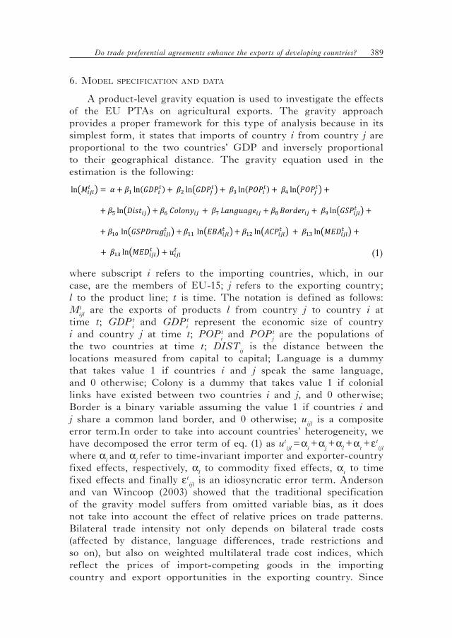
From figure 1, it emerges that EU agricultural imports increased over the period 2001‑2008: in 2008, they were worth about US$ 148 billion, that is twice the value (US$ 65 billion) observed in 2001 (data
6 A recent report commissioned by the EU Commission (CARIS, 2010) confirms that the share of EU imports entered in EU market by preferential regime is low. From 2002 to 2004, the share imports entering EU markets under MFN regime increased about 9.86%. In more detail, in 2002 76,2% of EU imports entered under MFN rates (53% under MFN=0 and 23% under MFN>0). This share was 81.18% in 2004 (58% under MFN=0 and 23% under MFN>0). GSP, GSP‑Drug and EBA account 5.04%, 0.32% and 0.28% of total EU imports respectively in 2002 and 3.55%, 0.27% and 0.34% respectively in 2004. With regard to the use of preferences, the same report points out that in 2002 56% of exports from GSP countries to EU entered, on average, at zero MFN tariff. This proportion is 60% in the case of exports from GSP‑Drug countries and 50% for EBA countries. The same applies in 2004 (CARIS, 2010).

Do trade preferential agreements enhance the exports of developing countries? 379
are expressed at 2001 constant prices). In 2004 these imports were US$ 93.74 billion. While this trend is in line with that observed for world imports, the comparison between the two time series suggests that a stable trend is exhibited by EU imports as a share of world imports (this share is about 14%‑15% for each year of the period 2001‑2008). Another interesting detail from figure 1 is the role of DCs in EU agricultural markets. On the one hand, data indicate that DCs are the largest suppliers to the EU, with a share of about 2/3 of total EU agricultural imports. On the other hand, it emerges that DCs’ share of these imports slightly declined over time, with a shift from 66.8% in 2001 to 65.8% in 2008 (this share was 67% in 2004).
Source: UN COMTRADE database.
FiGure 1 - Eu Agricultural Imports and World Agricultural Imports (2001-2008)
Data in Billions uS$ at 2001 Costant Prices
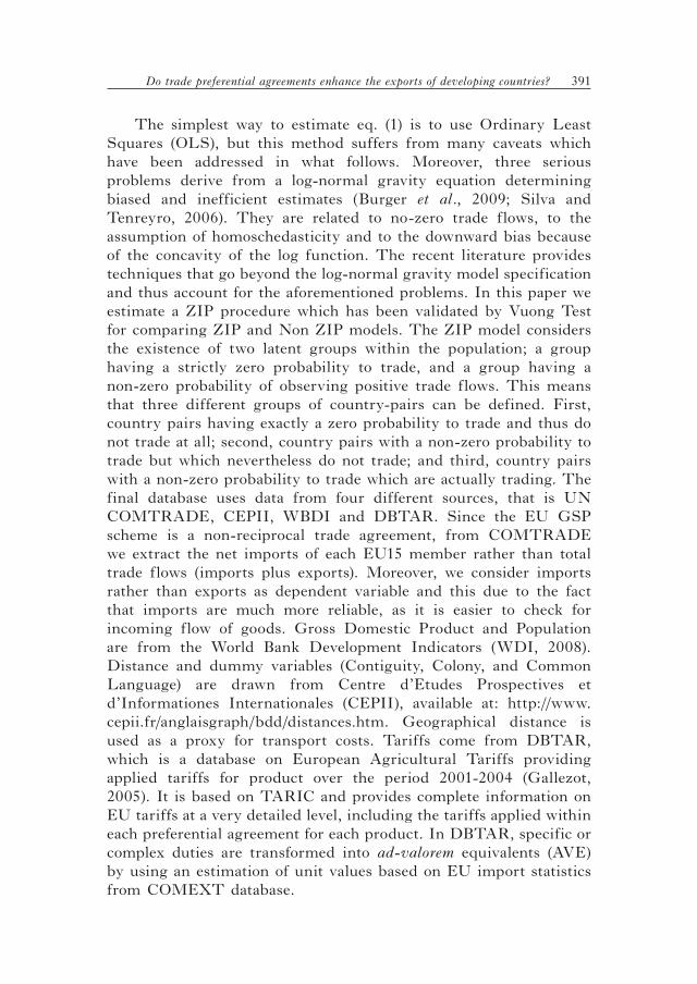
In figure 2 we present trends for EU agricultural imports from six group of countries. The first five groups are composed by those countries which are eligible for the trade preferences established under the GSP, GSP‑Drug, EBA, the Cotonou agreement and the EuroMed agreements7, while the latter group (Rest of the World,
7 The EBA, the GSP‑Drug and the EuroMed agreements include 49, 15 and 12 countries respectively, while the ACP group we consider is formed by
a

380 F. Aiello - F. Demaria
RoW) is comprised of all other exporters. We want to ascertain whether EU imports of agro‑food products from DCs and LDCs had increased and if their growth was uniform or not. Most EU agricultural imports come from countries eligible for GSP treatment and from the RoW. The exports of GSP countries to the EU doubled over the period considered (from US$ 27.2 billion in 2001 to more than US$ 61 billion in 2008). In 2004 they were 39.3 billion of US$. The same increases are found for the EU’s imports from RoW (they amount to US$ 21.5 billion in 2001, US$ 30.9 and US$ 51 billion in 2004 and 2008 respectively) as well as for Mediterranean countries and for DCs eligible for GSP‑Drug. The value of agricultural exports from LDCs to EU shows an increasing trend, but at a lesser rate than that observed for the other group of countries. All these trends imply that the composition of EU agricultural imports has not changed over time and that GSP countries maintained a dominant position, followed by the RoW. In this context, the EBA and the ACP countries register a decrease of their shares in the EU agricultural market; in the case of EBA countries, shifting from 3.05% in 2001 to 2.7% in 2004 and to 2.5% in 2008, and, dropping from 7.2% in 2001 to 6.69% in 2004 and to 5.3% in 2008 for ACP countries (Figure 2).
FiGure 2 - Eu Agricultural Imports by Country-Groups (2001-2008)Data in Billions uS$ at 2001 Constant Prices
Source: UN COMTRADE database.
all ACPs non‑LDCs and the GSP group comprises all DCs, other than those of ACP, EBA, GSP‑Drug and EuroMed samples (cfr. Appendix A).
ACPs
EBA
MEDCountries
GSP-Drug
RoW
OrdinaryGSP

Do trade preferential agreements enhance the exports of developing countries? 381
Another issue is the composition of exports by product. Table 1 highlights the structure of agricultural exports from GSP countries to the EU market from 2001 to 2008, while tables 2 and 3 refer to countries eligible for GSP‑Drug and EBA respectively. Among the total EU agricultural imports from GSP countries, just four group of products (fisheries; edible fruits and nuts; residues and waste from the food industry; oil seeds and oleaginous fruits) accounted for about 50% of GSP’s exports in 2001 and more than 43% in 2008. On the one hand, if these data indicate that the GSP agricultural exports have, over time, tended to become less concentrated, on the other hand, it emerges that the shares of each sector appear quite stable, except for animal or vegetables fats and oils whose quota increases from 4.78% in 2001 to 10.36% in 2008. The concentration is higher when considering GSP‑Drug (Table 2). In such a case, the exports of only two group of products alone (edible vegetables, roots and tubers; coffee, tea, mate and spices) make up more than 60% of total EU agricultural imports from GSP‑Drug countries and the increases in market shares which can be quoted as being significant with regard to animal or vegetables fats and oils (from less than 1% in 2001‑2003 to more than 4% in 2008), preparations of meat (from 3.68% in 2001 to more than 6% at the end of the period) and beverages, spirit and vinegar (from 1% in 2001 to about 2% in 2008). Finally, moving to EU agro‑food imports from EBA countries, we find different and conflicting results (Table 3). Indeed, fishery is the most important sector for EBA countries, although the market share shows a regular, marked, declining trend (from 43.27% in 2001 to 36.13% in 2007 and 29.82% in 2008). The exports of coffee, tea, mate and spices account for about 15% of total EBA agricultural exports to the EU and those of tobacco for about 10%. In contrast with the analysis of export composition under the ordinary GSP and the GSP‑Drug, the picture coming from the EBA initiative indicates a certain increase in the diversification of EBA agricultural exports. Indeed, the export structure of EBA changed in favour of several products (e.g., sugar, cocoa, live trees, edible fruits) whose weight increased over the period 2001‑2008, while, at the same time, the share of a few products (preparations of meat, animal or vegetable fats and oils; oil seeds and oleaginous fruits) decreased slightly.
To sum up, vegetable products (fruits, vegetables, cereals, coffee etc.) and fisheries were the largest group of EU imports from DCs eligible for GSP preferential treatment, followed by prepared foodstuffs (preparations of meat, cereal based foods, sugar confections, beer, wine, spirits, and tobacco). The relative importance of these sectors

382 F. Aiello - F. Demaria
in the export basket of DCs may be, ceteris paribus, a mirror of the protection in the EU market for agricultural and food products. An issue which will be addressed in the following section.
tABle 1 - Quota of Eu Agricultural Imports from Countries Eligible for the Ordinary GSP by Chapter, from 2001 to 2008 (%)
Group of products 2001 2002 2003 2004 2005 2006 2007 2008
Live Animals 0.63 0.64 0.66 0.65 0.62 0.42 0.40 0.39
Meat and edible meat offal 4.59 4.19 4.15 4.04 4.39 4.46 4.95 3.80
Fisheries 15.23 13.83 14.29 13.10 13.47 14.60 12.56 8.62
Dairy produce 0.51 0.64 0.76 0.72 0.52 0.48 0.42 0.54
Products of animal origin 1.46 1.42 1.31 1.42 1.41 1.31 1.11 1.32
Live trees and other plants 1.62 1.71 1.70 1.67 1.63 1.63 1.46 1.52
Edible vegetables, roots & tubers 4.53 4.57 4.32 4.87 4.72 4.83 5.62 4.49
Edible fruits & nuts 13.29 13.00 13.72 13.70 14.80 14.15 13.12 12.98
Coffee, tea, mate & spices 5.87 5.14 4.83 4.67 5.40 5.63 5.23 5.82
Cereals 2.16 3.21 2.90 2.59 1.97 2.55 5.35 4.44
Products of the milling industry 0.07 0.08 0.08 0.08 0.10 0.09 0.12 0.10
Oil seeds & oleaginous fruits 9.08 8.43 8.82 8.83 7.93 7.07 7.59 8.30
Lacs, gums, resins & other veg. saps
0.57 0.53 0.47 0.51 0.55 0.57 0.51 0.50
Vegetable products n.e.s. 0.26 0.19 0.18 0.17 0.18 0.16 0.17 0.15
Animal or vegetable fats & oils 4.78 5.76 6.16 7.02 7.32 8.28 7.90 10.36
Preparations of meat 4.59 4.46 4.51 4.48 4.95 5.14 4.92 5.68
Sugars 2.79 2.81 2.67 2.65 2.64 2.44 2.15 2.20
Cocoa & cocoa preparations 2.06 2.77 3.33 2.84 3.08 2.80 2.94 3.15
Preps. of cereals, flour, starch, etc. 0.48 0.54 0.56 0.59 0.62 0.66 0.64 0.76
Preps. of vegetables, fruits, nuts & plants
6.39 6.80 6.43 6.56 6.73 6.62 6.27 6.16
Miscellaneous edible preparations 0.79 0.85 0.84 0.86 0.97 1.12 1.18 1.24
Beverages, spirits & vinegar 3.86 4.10 3.97 4.14 4.16 4.00 3.95 4.05
Residues and waste from food in‑dustry
11.25 11.09 10.54 11.33 9.55 8.84 9.41 11.25
Tobacco & tobacco products 3.14 3.22 2.80 2.50 2.27 2.15 2.05 2.17
100% 100% 100% 100% 100% 100% 100% 100%
Source: Own calculations of data from UN COMTRADE database.

Do trade preferential agreements enhance the exports of developing countries? 383
tABle 2 - Quota of Eu Agricultural Imports from Countries Eligible for the GSP Plus (Drug) by Chapter, from 2001 to 2008 (%)
Group of products 2001 2002 2003 2004 2005 2006 2007 2008
Live Animals 0,03 0,03 0,03 0,02 0,02 0,01 0,01 0,01
Meat and edible meat offal 0,01 0,04 0,03 0,04 0,01 0,00 0,01 0,00
Fisheries 8,75 7,54 7,67 7,77 8,68 9,27 8,40 5,44
Dairy produce 0,07 0,08 0,16 0,13 0,05 0,06 0,04 0,06
Products of animal origin 0,13 0,15 0,11 0,14 0,13 0,08 0,07 0,08
Live trees and other plants 6,65 6,49 5,64 5,15 4,73 4,59 4,35 3,97
Edible vegetables, roots & tubers 2,00 2,16 2,03 2,34 2,46 2,53 2,52 2,31
Edible fruits & nuts 42,38 46,34 47,98 49,64 46,14 44,10 44,72 48,18
Coffee, tea, mate & spices 21,96 17,73 15,73 15,01 17,09 18,27 16,70 18,80
Cereals 0,10 0,45 0,10 0,12 0,13 0,23 0,26 0,13
Products of the milling industry 0,06 0,06 0,06 0,05 0,07 0,06 0,08 0,08
Oil seeds & oleaginous fruits 0,62 0,54 0,47 0,53 0,82 0,58 0,51 0,83
Lacs, gums, resins & other veg. saps
0,09 0,14 0,06 0,15 0,08 0,13 0,13 0,09
Vegetable products n.e.s. 0,09 0,11 0,09 0,05 0,05 0,05 0,07 0,09
Animal or vegetable fats & oils 0,77 0,68 0,87 1,74 2,30 1,84 3,14 4,12
Preparations of meat 3,68 4,84 5,82 5,49 6,00 6,05 6,20 5,15
Sugars 0,18 0,17 0,17 0,23 0,20 0,32 0,32 0,25
Cocoa & cocoa preparations 0,92 1,49 1,89 1,62 1,52 1,34 1,58 1,80
Preps. of cereals, flour, starch, etc. 0,04 0,04 0,05 0,06 0,10 0,07 0,08 0,05
Preps. of vegetables, fruits, nuts & plants
4,37 4,31 4,01 3,83 3,37 3,72 4,39 3,54
Miscellaneous edible preparations 1,17 1,07 0,88 0,79 0,85 0,79 0,81 0,85
Beverages, spirits & vinegar 0,94 1,20 1,60 1,88 2,03 2,13 1,83 1,83
Residues and waste from food industry
3,79 3,35 3,60 2,34 2,52 3,20 3,16 1,83
Tobacco & tobacco products 1,19 1,00 0,96 0,89 0,61 0,56 0,64 0,49
100% 100% 100% 100% 100% 100% 100% 100%
Source: Own calculations of data from UN COMTRADE database.

384 F. Aiello - F. Demaria
tABle 3 - Quota of Eu Agricultural Imports from Countries Eligible for the EBA by Chapter, from 2001 to 2008 (%)
Group of products 2001 2002 2003 2004 2005 2006 2007 2008
Live Animals 0.15 0.13 0.13 0.13 0.12 0.04 0.05 0.05
Meat and edible meat offal 0.19 0.05 0.05 0.03 0.05 0.07 0.05 0.02
Fisheries 43.27 43.75 41.83 39.99 37.70 39.90 36.13 29.82
Dairy produce 0.04 0.05 0.14 0.12 0.05 0.05 0.04 0.05
Products of animal origin 0.15 0.15 0.11 0.10 0.10 0.09 0.08 0.06
Live trees and other plants 2.10 2.04 1.81 1.85 2.13 2.71 3.66 5.18
Edible vegetables, roots & tubers 3.24 3.66 3.45 3.93 3.92 3.94 3.64 3.84
Edible fruits & nuts 2.66 2.63 3.14 5.04 3.00 3.01 4.14 3.82
Coffee, tea, mate & spices 17.31 16.22 16.35 14.90 17.68 16.35 14.99 17.75
Cereals 0.11 0.21 0.22 0.37 0.19 0.27 1.01 0.59
Products of the milling industry 0.09 0.09 0.11 0.13 0.10 0.08 0.10 0.06
Oil seeds & oleaginous fruits 3.78 3.27 3.24 3.36 2.66 2.50 2.22 3.99
Lacs, gums, resins & other veg. saps
2.10 1.98 1.97 3.11 4.90 2.40 2.38 2.75
Vegetable products n.e.s. 0.38 0.36 0.39 0.38 0.28 0.26 0.25 0.25
Animal or vegetable fats & oils 4.22 3.82 2.63 2.20 1.95 1.76 2.89 2.38
Preparations of meat 3.74 3.84 4.56 5.07 4.15 3.34 2.50 2.44
Sugars 3.04 4.25 5.56 5.30 5.98 6.28 7.02 8.50
Cocoa & cocoa preparations 1.07 1.91 2.30 2.36 4.15 5.26 5.44 7.59
Preps. of cereals, flour, starch, etc. 0.04 0.04 0.04 0.07 0.08 0.14 0.14 0.18
Preps. of vegetables, fruits, nuts & plants
0.33 0.49 0.51 0.59 0.59 0.61 0.50 0.53
Miscellaneous edible preparations 0.51 0.47 0.44 0.37 0.53 0.57 0.50 0.76
Beverages, spirits & vinegar 0.12 0.45 0.45 0.08 0.10 0.18 0.15 0.18
Residues and waste from food industry
1.55 1.45 0.84 0.64 0.20 0.52 0.48 0.17
Tobacco & tobacco products 9.81 8.70 9.73 9.89 9.40 9.68 11.65 9.04
100% 100% 100% 100% 100% 100% 100% 100%
Source: Own calculations of data from UN COMTRADE database.

Do trade preferential agreements enhance the exports of developing countries? 385
5. Some DeScriptive StAtiSticS on GSP tAriFFS
This section provides a comparison between tariffs under GSP in 2006 and 2004. In 2004, 1,658 tariff lines were eligible for a tariff reduction under the ordinary GSP, i.e. 48% of the total of 3,453 product lines covered by the scheme. This proportion increased to 69% (2,489 preferred goods out of 3,603 total lines) when considering the GSP‑Drug and to approximately 98% (3,631 out of 3,683 lines) for the EBA initiative. In 2006, the coverage of products benefiting from trade preferences was 57% for the GSP, 63% for the GSP‑Drug and 98% for the EBA scheme. In terms of the absolute incidence of GSP coverage, it is interesting to note that the number of products enjoying a preference under the ordinary GSP increased from 1,658 in 2004 to 1,998 in 2006 and that there was an analogous increase under the GSP‑Drug from 2,489 products in 2004 to 2,178 in 2006. In 2006, there were 3,390 products eligible for EBA preferences, which was fewer than the 3,631 preferred lines in 2004. The sum effect, combining the coverage of the schemes and the number of products with zero‑duty in each agreement (columns 5 and 6 of table 4), represents the average tariff faced by exporting countries and the resulting margin of preference. As expected, the average tariff was high for products exported under MFN conditions (more than 19% in 2004 and 2006) and decreased to around 17% in the case of the ordinary GSP. The applied tariff for GSP‑Drug was 14% and it was very low for the EBA initiative (1.36% in 2004 and 0.38% in 2006). Finally, we can see that the preferential margin was significantly high only for EBA schemes (around 18%), while it was 5% for the GSP‑Drug and just around 2% for the ordinary GSP (Table 4). In conclusion, it can be said that even if the average rate for GSP tariffs did not change much between the old and the new GSP schemes, the number of tariff lines involved increased. This is particularly true when considering the ordinary GSP.
Based on these results, on the one hand, one would expect the GSP scheme to have a generally modest impact, as the trade preferences it gives to DCs are, on average, very low. However, by analysing EU imports from preferred countries (cfr. figures 2 and 3), it emerges, on the other hand, that there was an increase in trade even though the preferential margin in percentage points slightly changed over time. All this suggests that export flows depend not only on other variables, but, in some ways, also on the structure of trade preferences granted by the EU. In order to look at this issue in detail, table 5 shows the number of products by the level of GSP applied duties. In 2004, 973 products faced a duty greater than

386 F. Aiello - F. Demaria
20%, while the tariff applied to a further 958 goods ranged between 10% and 20%. These products faced a tariff of more than 10% and represented more than 50% of the products covered by the GSP. In contrast, the tariff applied to 602 products ranged from 1% to 5% and was less than 1% for the other 547 goods.
Table 6 compares the level of GSP tariffs and the margin of preferences for each group of HS2‑digit agricultural products for the years 2004 and 20068. The data allows us to observe whether, and to what extent, tariffs differed across sectors, trade arrangements and from one year to another. By limiting the discussion to the margin of preferences, it can be noticed that, as expected, there were relevant differences between the ordinary GSP and the GSP‑Drug. Furthermore, the preferential margin was found to be quite stable from 2004 to 2006: the major changes occurred in fisheries (from 3.99% to 2.01%), vegetables (3.1%; 2.25%), preparations of meat (5.22%; 4.19%). The agricultural sectors with the highest margin of preferences under the ordinary GSP regime were tobacco (about 8.16% in 2006), preparations of meat (5.22% in 2006), preparations of fruits and vegetables (4.98% in 2006) and fisheries (3.99% in 2006). The average margin was modest in the chapters of livestock, meat, dairy products, other animal products, cereals, products of the milling industry, oilseeds, sugar, and residues and waste from the food industry. To sum up, the level of the preferential tariff granted by the GSP did not change much as a result of the introduction of the 2006 GSP scheme (on average, less than one percentage point between 2004 and 2006), nor did all chapters benefit from the reductions.
8 This data is based on the DBTAR database built up by Gallezot (2005). From this source, we have extracted and computed EU ad valorem equivalents of the MFN and GSP tariffs for agri‑food products for 2006 in order to assess the size of preference margin offered by GSP. The 2006 AVE has been computed with the 2004 unit value in order to be compared with the 2004 AVE; in other words, any differences in the preference margin between the two years are due to changes in the GSP tariff, not because of differences in world prices. The HS2 average tariffs faced by the beneficiaries of the GSP have been computed using a simple average of the AVEs calculated at the NC10 level. When a line was excluded from preferences, the MFN AVE has been used for the computation. When the tariff evolved during the year (due to seasonal changes, for example), a simple average over the year has been used.

Do trade preferential agreements enhance the exports of developing countries? 387
tA
Bl
e 4
- C
ompa
riso
n of
som
e In
dica
tors
und
er M
FN
and
GS
P R
egim
es i
n 20
04 a
nd 2
006
Reg
ime
No.
of
line
s 20
04N
o. o
f li
nes
2006
No.
of
pref
erre
d li
nes
2004
No.
of
pref
erre
d li
nes
2006
No.
of
zero
line
s 20
04
No.
of
zero
line
s 20
06
Ave
rage
tari
ff
face
d by
be
nefic
iari
es
2004
Ave
rage
ta
riff
face
d by
be
nefic
iari
es
2006
Pref
eren
tial
M
argi
n (%
poi
nts)
20
04
Pref
eren
tial
M
argi
n (%
poi
nts)
20
06
MF
N3,
677
3,44
70
040
538
819
.61%
19.0
4%0
0
GS
P3,
683
3,45
31,
658
1,99
852
255
317
.68%
16.9
5%1.
932.
1
GS
P+
3,68
33,
453
2,48
92,
178
2,23
62,
161
14.5
8%13
.97%
5.03
5.0
7
EB
A3,
683
3,45
33,
631
3,39
03,
629
3,38
9 1
.36%
0.38
% 1
8.25
18.
66
Sou
rce:
Dem
aria
et
al.
(20
08).
tA
Bl
e 5
‑ D
uty,
Num
ber
of L
ines
and
Pre
fere
ntia
l M
argi
n un
der
the
GS
P S
chem
es i
n 20
04
Lev
el o
f th
e du
tyN
um
ber
of t
ar-
iff
line
s%
Pre
fere
ntia
l M
argi
n u
nde
r G
SP
(min
-Max
)
Pre
fere
ntia
l M
argi
n u
nde
r G
SP-D
rug
(min
-Max
)
Pre
fere
ntia
l M
argi
n u
nde
r E
BA
(m
in-M
ax)
Tot
al
3,68
310
0
0 <
mar
g <
175
.22
0
< m
arg
< 1
84.7
6
0 <
mar
g <
184
.76
> 2
0%97
326
0
< m
arg
< 1
75.2
20.
14 <
mar
g <
184
.76
0
< m
arg
< 1
84.7
6
10‑2
0%95
826
1
< m
arg
< 1
6.97
1.3
< m
arg
< 1
9.97
1.68
< m
arg
< 1
9.97
5‑10
%60
316
0.5
< m
arg
< 9
.71
0.16
< m
arg
< 9
.94
3.84
< m
arg
< 9
.94
1‑5%
602
160.
09 <
mar
g <
4.3
6 0
.6 <
mar
g <
4.9
61.
15 <
mar
g <
4.1
6
< 1
%54
715
0
< m
arg
< 0
.97
0
< m
arg
< 0
.97
0
< m
arg
< 0
.97
Sou
rce:
Ow
n c
omp
uta
tion
bas
ed o
n d
ata
from
DB
TA
R (
Gal
lezo
t, 2
005
) an
d T
aric
.

388 F. Aiello - F. Demaria
tABle 6 ‑ Tariffs and Preferential Margins under GSP, by HS02-Digit Agricultural Products (in %) (2004 and 2006)
Ordinary GSP tariffs
(%)
GSP Plus (Drug in
2004)Tariffs (%)
MFN tariffs (%)
Ordinary GSP:
Margin of Preferences
(%)
GSP Plus (Drug)
Margin of Preferences
(%)
Groups of products at HS2-digit level
2006 2004 2006 2004 2006 2004 2006 2004 2006 2004
01‑ Live animals 40.17 40.17 40.04 40.04 40.49 40.49 0.33 0.33 0.45 0.45
02‑ Meat 43.85 43.45 43.47 43.31 43.97 43.71 0.12 0.25 0.50 0.40
03‑ Fisheries 6.51 8.73 0.03 0.03 10.51 10.74 4.00 2.02 10.47 10.71
04‑ Dairies 52.40 50.23 51.92 50.12 52.70 50.68 0.30 0.45 0.79 0.56
05‑ Other animal products 0.08 0.08 0.00 0.00 0.24 0.24 0.17 0.17 0.24 0.24
06‑ Live trees and plants 3.33 3.56 0.00 0.00 6.40 6.79 3.08 3.23 6.40 6.79
07‑ Vegetables 38.79 37.67 37.76 36.15 41.89 39.92 3.10 2.25 4.13 3.77
08‑ Fruits 18.54 19.08 17.38 17.71 20.26 20.64 1.72 1.56 2.88 2.94
09‑ Coffee, tea, spices 1.09 1.09 0.00 0.12 3.05 3.05 1.96 1.96 3.05 2.93
10‑ Cereals 18.85 36.60 18.84 36.58 18.86 36.60 0.01 0.00 0.02 0.02
11‑ Products of the milling ind. 22.29 22.22 21.89 21.78 22.55 22.51 0.26 0.29 0.66 0.73
12‑ Oilseeds 1.66 1.31 0.87 0.86 2.38 2.35 0.72 1.04 1.51 1.49
13‑ Lac, gums, resins 5.11 5.24 0.00 0.00 7.93 7.89 2.82 2.65 7.93 7.89
14‑ Other vegetable products 0 0 0 0 0 0 0 0 0 0
15‑ Oils and fats 5.61 5.73 2.78 2.86 8.54 8.60 2.94 2.87 5.76 5.75
16- Preparations of meat, fish 12.80 13.75 4.21 4.34 18.03 17.94 5.23 4.19 13.82 13.60
17‑ Sugar 19.94 21.18 18.78 20.19 20.57 21.74 0.63 0.56 1.80 1.55
18‑ Cocoa 22.99 22.92 21.27 21.37 24.16 23.96 1.17 1.05 2.89 2.59
19‑ Preparations of cereals 26.34 27.67 23.45 24.35 29.45 30.86 3.11 3.19 6.00 6.51
20‑ Preparations of fruits and veg. 18.19 18.18 4.25 3.98 23.16 22.55 4.98 4.37 18.92 18.57
21‑ Miscellaneous edible preparations 11.03 11.46 5.97 6.28 14.33 14.85 3.29 3.39 8.36 8.57
22‑ Beverages 11.98 11.16 7.74 7.42 13.34 12.64 1.36 1.49 5.60 5.23
23‑ Waste from food industry 15.01 12.76 14.71 12.51 15.92 13.60 0.91 0.84 1.21 1.09
24‑ Tobacco 10.15 10.15 0 0 18.31 18.31 8.16 8.16 18.31 18.31
Source: Own computation on data from DBTAR (Gallezot 2005) and Taric.
Do trade preferential agreements enhance the exports of developing countries? 389
6. moDel SpeciFicAtion AnD DAtA
A product‑level gravity equation is used to investigate the effects of the EU PTAs on agricultural exports. The gravity approach provides a proper framework for this type of analysis because in its simplest form, it states that imports of country i from country j are proportional to the two countries’ GDP and inversely proportional to their geographical distance. The gravity equation used in the estimation is the following:
21
6. MODEL SOECIFICATION AND DATA
A product-level gravity equation is used to investigate the effects of the EU PTAs on agricultural
exports. The gravity approach provides a proper framework for this type of analysis because in
its simplest form, it states that imports of country i from country j are proportional to two
countries’ GDP and inversely proportional to their geographical distance. The gravity equation
used in the estimation is the following:
ln������ � � � � �� ln(�����) ��� ln������� ��� ln(�����) ��� ln������� �
��� ln�������� � ���������� � ������������ � ���������� ��� ln�������� � �
���� ln������������ � ���� ln�������� ����� ln�������� � ���� ln�������� � �
������ (1)
where subscript i refers to the importing countries, which, in our case, are the members of EU-
15; j refers to the exporting country; l to the product line; t is time. The notation is defined as
follows: tijlM are the exports of products l from country j to country i at time t; t
iGDP and
ti
GDP represent the economic size of country i and country j at time t; ti
POP and tjPOP are the
populations of the two countries at time t; ijDIST is the distance between the locations measured
from capital to capital; Language is a dummy that takes value 1 if countries i and j speak the
same language, and 0 otherwise; Colony is a dummy that takes value 1 if colonial links have
existed) between two countries i and j, and 0 otherwise; Border is a binary variable assuming the
value 1 if countries i and j share a common land border, and 0 otherwise; ijlu is a composite error
term.In order to take into account countries’ heterogeneity, we have decomposed the error term
of eq. (1) as ijlt
tljiijltu εαααα ++++= where αi and αj refer to time-invariant importer and
exporter-country fixed effects, respectively, lα to commodity fixed effects, tα to time fixed
21
6. MODEL SOECIFICATION AND DATA
A product-level gravity equation is used to investigate the effects of the EU PTAs on agricultural
exports. The gravity approach provides a proper framework for this type of analysis because in
its simplest form, it states that imports of country i from country j are proportional to two
countries’ GDP and inversely proportional to their geographical distance. The gravity equation
used in the estimation is the following:
ln������ � � � � �� ln(�����) ��� ln������� ��� ln(�����) ��� ln������� �
��� ln�������� � ���������� � ������������ � ���������� ��� ln�������� � �
���� ln������������ � ���� ln�������� ����� ln�������� � ���� ln�������� � �
������ (1)
where subscript i refers to the importing countries, which, in our case, are the members of EU-
15; j refers to the exporting country; l to the product line; t is time. The notation is defined as
follows: tijlM are the exports of products l from country j to country i at time t; t
iGDP and
ti
GDP represent the economic size of country i and country j at time t; ti
POP and tjPOP are the
populations of the two countries at time t; ijDIST is the distance between the locations measured
from capital to capital; Language is a dummy that takes value 1 if countries i and j speak the
same language, and 0 otherwise; Colony is a dummy that takes value 1 if colonial links have
existed) between two countries i and j, and 0 otherwise; Border is a binary variable assuming the
value 1 if countries i and j share a common land border, and 0 otherwise; ijlu is a composite error
term.In order to take into account countries’ heterogeneity, we have decomposed the error term
of eq. (1) as ijlt
tljiijltu εαααα ++++= where αi and αj refer to time-invariant importer and
exporter-country fixed effects, respectively, lα to commodity fixed effects, tα to time fixed 21
6. MODEL SOECIFICATION AND DATA
A product-level gravity equation is used to investigate the effects of the EU PTAs on agricultural
exports. The gravity approach provides a proper framework for this type of analysis because in
its simplest form, it states that imports of country i from country j are proportional to two
countries’ GDP and inversely proportional to their geographical distance. The gravity equation
used in the estimation is the following:
ln������ � � � � �� ln(�����) ��� ln������� ��� ln(�����) ��� ln������� �
��� ln�������� � ���������� � ������������ � ���������� ��� ln�������� � �
���� ln������������ � ���� ln�������� ����� ln�������� � ���� ln�������� � �
������ (1)
where subscript i refers to the importing countries, which, in our case, are the members of EU-
15; j refers to the exporting country; l to the product line; t is time. The notation is defined as
follows: tijlM are the exports of products l from country j to country i at time t; t
iGDP and
ti
GDP represent the economic size of country i and country j at time t; ti
POP and tjPOP are the
populations of the two countries at time t; ijDIST is the distance between the locations measured
from capital to capital; Language is a dummy that takes value 1 if countries i and j speak the
same language, and 0 otherwise; Colony is a dummy that takes value 1 if colonial links have
existed) between two countries i and j, and 0 otherwise; Border is a binary variable assuming the
value 1 if countries i and j share a common land border, and 0 otherwise; ijlu is a composite error
term.In order to take into account countries’ heterogeneity, we have decomposed the error term
of eq. (1) as ijlt
tljiijltu εαααα ++++= where αi and αj refer to time-invariant importer and
exporter-country fixed effects, respectively, lα to commodity fixed effects, tα to time fixed
21
6. MODEL SOECIFICATION AND DATA
A product-level gravity equation is used to investigate the effects of the EU PTAs on agricultural
exports. The gravity approach provides a proper framework for this type of analysis because in
its simplest form, it states that imports of country i from country j are proportional to two
countries’ GDP and inversely proportional to their geographical distance. The gravity equation
used in the estimation is the following:
ln������ � � � � �� ln(�����) ��� ln������� ��� ln(�����) ��� ln������� �
��� ln�������� � ���������� � ������������ � ���������� ��� ln�������� � �
���� ln������������ � ���� ln�������� ����� ln�������� � ���� ln�������� � �
������ (1)
where subscript i refers to the importing countries, which, in our case, are the members of EU-
15; j refers to the exporting country; l to the product line; t is time. The notation is defined as
follows: tijlM are the exports of products l from country j to country i at time t; t
iGDP and
ti
GDP represent the economic size of country i and country j at time t; ti
POP and tjPOP are the
populations of the two countries at time t; ijDIST is the distance between the locations measured
from capital to capital; Language is a dummy that takes value 1 if countries i and j speak the
same language, and 0 otherwise; Colony is a dummy that takes value 1 if colonial links have
existed) between two countries i and j, and 0 otherwise; Border is a binary variable assuming the
value 1 if countries i and j share a common land border, and 0 otherwise; ijlu is a composite error
term.In order to take into account countries’ heterogeneity, we have decomposed the error term
of eq. (1) as ijlt
tljiijltu εαααα ++++= where αi and αj refer to time-invariant importer and
exporter-country fixed effects, respectively, lα to commodity fixed effects, tα to time fixed
(1)
where subscript i refers to the importing countries, which, in our case, are the members of EU‑15; j refers to the exporting country; l to the product line; t is time. The notation is defined as follows: Mt
ijl are the exports of products l from country j to country i at
time t; GDPti and GDPt
i represent the economic size of country i and country j at time t; POPt
i and POPtj are the populations of
the two countries at time t; DISTij is the distance between the locations measured from capital to capital; Language is a dummy that takes value 1 if countries i and j speak the same language, and 0 otherwise; Colony is a dummy that takes value 1 if colonial links have existed between two countries i and j, and 0 otherwise; Border is a binary variable assuming the value 1 if countries i and j share a common land border, and 0 otherwise; uijl is a composite error term.In order to take into account countries’ heterogeneity, we have decomposed the error term of eq. (1) as ut
ijl = αi + αj + αl + αt + εtijl
where αi and αj refer to time‑invariant importer and exporter‑country fixed effects, respectively, αl to commodity fixed effects, αt to time fixed effects and finally εt
ijl is an idiosyncratic error term. Anderson and van Wincoop (2003) showed that the traditional specification of the gravity model suffers from omitted variable bias, as it does not take into account the effect of relative prices on trade patterns. Bilateral trade intensity not only depends on bilateral trade costs (affected by distance, language differences, trade restrictions and so on), but also on weighted multilateral trade cost indices, which reflect the prices of import‑competing goods in the importing country and export opportunities in the exporting country. Since

390 F. Aiello - F. Demaria
the latter are unobservable it is possible to include dummy variables to take into account all the variations in the same dimension as the Multilateral Resistance Terms (MRT). We control for this term by using fixed effects. We employ an explicit measure of the trade preferences and, in this sense, the variables GSP, GSP‑Drug, EBA, ACP, MED become the key elements of our analysis. They represent the preferential margin in favor of a given country when it exports certain commodities to EU. For instance, GSP t
ijl is the preferential margin under the ordinary GSP that the j-th country enjoys when exporting product line l to country i. The same applies for the other preference variables GSP‑Drug, EBA, ACP and MED.
For each trade agreement, the preferential margin is defined as the ratio between the preferential margin (the difference between the MFN and the preferential duties at each tariff line) and the MFN tariff. The formula is:
22
effects and finally ijltε is an idiosyncratic error term. Anderson and van Wincoop (2003) showed
that the traditional specification of the gravity model suffers from omitted variable bias, as it
does not take into account the effect of relative prices on trade patterns. Bilateral trade intensity
not only depends on bilateral trade costs (affected by distance, language differences, trade
restrictions and so on), but also on weighted multilateral trade cost indices, which reflect the
prices of import-competing goods in the importing country and export opportunities in the
exporting country. Since the latter are unobservable it is possible include dummy variables to
take account of all variation in the same dimensions as the Multilateral Resistance Terms (MRT).
We control for this term by using fixed effects. We employ an explicit measure of the trade
preferences and, in this sense, the variables GSP, GSP-Drug, EBA, ACP, MED become the key
elements of our analysis. They represent the preferential margin in favor of a given country when
it exports certain commodities to EU. For instance, tijlGSP is the preferential margin under the
ordinary GSP that the j-th country enjoys when exporting product line l to country i. The same
applies for the other preference variables GSP-Drug, EBA, ACP and MED.
For each trade agreement, the preferential margin is defined as the ratio between the
preferential margin (the difference between the MFN and the preferential duties at each tariff
line) and the MFN tariff. The formula is:
���������������������� = ������� � ����������������������
(2)
where i refers to the 15 EU importers, j indicates the exporting countries, l is the tariff line and t
is time. PREF_TARIFF is the preferential tariffs applied under any specific trade arrangement
(GSP, GSP-Drug, EBA, ACP, MED). This measure allows us to take into account the size of the
actual tariff preference for a particular product9. The overlapping of preferences has been solved
9 The MFN and the preferential tariffs come from the DBTAR database, which has enabled us to identify the tariffs
applied by the EU under the different preferential regimes. We have extracted tariff data at the 10-digit level and
(2)
where i refers to the 15 EU importers, j indicates the exporting countries, l is the tariff line and t is time. PREF_TARIFF is the preferential tariffs applied under any specific trade arrangement (GSP, GSP‑Drug, EBA, ACP, MED). This measure allows us to take into account the size of the actual tariff preference for a particular product9. The overlapping of preferences has been solved by taking, for a given trade flow, the maximum margin of preference as that which has been used by the beneficiary country. For instance, if a country is eligible for preferential treatment under both the GSP and the Cotonou agreement, and the preferential margins are, respectively, 3% and 5%, we assume that country will export under the Cotonou agreement.
9 The MFN and the preferential tariffs come from the DBTAR database, which has enabled us to identify the tariffs applied by the EU under the different preferential regimes. We have extracted tariff data at the 10‑digit level and consolidated it at the 6‑digit level for each partner and each year, by averaging (simple average) the data of 10‑digit lines. For each preferential scheme, each product line and each year, we have generated the simple average of preferential tariffs and computed the preferential margin. To assign the preferential margin to country groups, we used dummies for the country groups belonging to different preferential schemes. For each country and each preferential scheme, we have constructed a dummy that takes a value of 1 if the country benefits from a particular scheme and zero otherwise.
Do trade preferential agreements enhance the exports of developing countries? 391
The simplest way to estimate eq. (1) is to use Ordinary Least Squares (OLS), but this method suffers from many caveats which have been addressed in what follows. Moreover, three serious problems derive from a log‑normal gravity equation determining biased and inefficient estimates (Burger et al., 2009; Silva and Tenreyro, 2006). They are related to no‑zero trade flows, to the assumption of homoschedasticity and to the downward bias because of the concavity of the log function. The recent literature provides techniques that go beyond the log‑normal gravity model specification and thus account for the aforementioned problems. In this paper we estimate a ZIP procedure which has been validated by Vuong Test for comparing ZIP and Non ZIP models. The ZIP model considers the existence of two latent groups within the population; a group having a strictly zero probability to trade, and a group having a non‑zero probability of observing positive trade flows. This means that three different groups of country‑pairs can be defined. First, country pairs having exactly a zero probability to trade and thus do not trade at all; second, country pairs with a non‑zero probability to trade but which nevertheless do not trade; and third, country pairs with a non‑zero probability to trade which are actually trading. The final database uses data from four different sources, that is UN COMTRADE, CEPII, WBDI and DBTAR. Since the EU GSP scheme is a non‑reciprocal trade agreement, from COMTRADE we extract the net imports of each EU15 member rather than total trade flows (imports plus exports). Moreover, we consider imports rather than exports as dependent variable and this due to the fact that imports are much more reliable, as it is easier to check for incoming flow of goods. Gross Domestic Product and Population are from the World Bank Development Indicators (WDI, 2008). Distance and dummy variables (Contiguity, Colony, and Common Language) are drawn from Centre d’Etudes Prospectives et d’Informationes Internationales (CEPII), available at: http://www.cepii.fr/anglaisgraph/bdd/distances.htm. Geographical distance is used as a proxy for transport costs. Tariffs come from DBTAR, which is a database on European Agricultural Tariffs providing applied tariffs for product over the period 2001‑2004 (Gallezot, 2005). It is based on TARIC and provides complete information on EU tariffs at a very detailed level, including the tariffs applied within each preferential agreement for each product. In DBTAR, specific or complex duties are transformed into ad-valorem equivalents (AVE) by using an estimation of unit values based on EU import statistics from COMEXT database.

392 F. Aiello - F. Demaria
7. reSultS
In this section, we have summarised the results obtained when estimating eq. (1) with the LSDV (Least Squares Dummy Variables) and the ZIP methods. LSDV results are just used as initial estimates in order to obtain detail about the role of zero‑trade flows which we have treated by using the ZIP procedure. Differently from the Pseudo Quasi Maximum Likelihood Method (PQML) (i.e. see Santos Silva and Tenreyro, 2009), the ZIP estimator is not vulnerable to problems such as over‑dispersion and excess of zero trade flows (on this issue see, Burger et al., 2009). In both models (OLS and ZIP procedure), fixed effects are included and the inference is based on robust‑cluster standard errors.
Results show that PTAs appear to have different effects across sectors. Of course results depend on sector specificities, such as the structure of demand and supply and the specificity of the agricultural products. The first regression we ran regarded the pooled data of all agricultural exports to the EU. Afterwards we ran separate regressions for the following homogenous groups of products: livestock, fisheries, products of animal origin, fruits, lacs and gums, oils and fats, dairy products, live trees, sugar, vegetables, beverages and spirits, tobacco, tropical fruits and residues from the food industry. Whatever the level of aggregation, the trade statistics used in the estimations are identified at HS6‑ digit level. The results for the pooled data are presented in table 7, while those obtained sector‑by‑sector are presented in table 8.
When considering the outcomes of pooled regressions10, it emerges that results differ in sign and magnitude. Briefly, as regards gravity standard variables, we found that the elasticity of importing and exporting country GDP is positive and statistically significant in ZIP estimates. Distance, Colonial Ties and Common Language showed the expected signs (Table 7, column 2).
As for the goal of this work we found mixed evidence. Above all, the main result is that the GSP preferential scheme exerted a positive and significant impact on beneficiary countries in both regressions. Its estimated value ranged from 0,108 (LSDV regression) to 0.265 (ZIP estimates). In other words, in case of ZIP results a 1% increase of GSP preferential margin induces an increase of 0.265% of the probability
10 We have ran the RESET test to verify the specification of our model. We find that the gravity model estimated using the ZIP method passes the RESET test (the p‑value is 0.699), while it fails in the LSDV estimator (the p‑value is 0.0010).

Do trade preferential agreements enhance the exports of developing countries? 393
to trade. The GSP‑Drug reports a positive and significant coefficient in LSDV estimates (0.050), while it turned out to be positive but not significant in ZIP regression (0.062). The EBA initiative displayed non‑significant parameters both in ZIP procedure, where its sign is positive, and in LSDV estimates, when the sign is even negative. Un‑conclusive evidence was found for the impact of the EuroMed agreement as well, which, at best, was positive but not significant in LSDV regression. Finally, from LSDV estimates it emerges that the preferential margin granted under the Cotonou Agreement in favour of ACPs positively affected the agricultural exports of beneficiaries. The ACP coefficient becomes not significant in ZIP regression.
In the pooled results presented so far, the role of trade preferential treatment is measured as an average impact across the agricultural sectors covered by the study. Therefore, the resulting estimates summarise the role that preferential policies exert in all sectors. As it is well known agricultural exports enter EU market at very different level of tariffs and preferential margins even under the same trade arrangement. These facts legitimate the use of more disaggregated analyses and, hence, we next present the results obtained when running the gravity regression for each agricultural sector. For ease of exposition we limit the presentation to the ZIP estimates which are displayed in table 8.
When looking at results across agricultural groups, we observe that the GDP coefficient for importing countries is positive and statistically significant in two cases (live animals and fisheries), while it is negative and not significant in the following groups of products: sugar, residues from food industry, tropical fruits and dairy products. The GDP coefficient for exporting countries is negative and significant in the sector of spirit and vinegar, and it is positive and significant just in the case of fruits. The population coefficient of importing countries has an ambiguous sign, the population coefficient of exporting countries as well. Distance is negative and significant in two cases, it reports negative but not significant coefficient in seven group of products, while it is positive but not significant in the remaining groups. Border is positive and significant in tropical fruits, colony reports a positive and significant coefficient in fruits and live animals, while language has a positive and significant coefficient in beverages and spirits, oils and fats and tropical fruits. In the other cases these indicators show ambiguous signs (Table 8).
With respect to the preferential margin, the coefficient for the GSP is positive and significant for the following groups of agricultural products: live animals (0.315), fisheries (4.326), fruits (0.881), oils and

394 F. Aiello - F. Demaria
fats (1.984), dairy products (0.318). GSP parameter is positive but not significant in vegetables, live trees, lac and gums, sugar, tropical fruits, vinegar and spirits and tobacco, while it is negative but not significant for residues from food industry (‑0.083). The GSP‑Drug shows a positive and significant coefficient in live animal regression (0.741); it turns out to be negative and significant in oils‑fats sector (‑0.603). We find a positive but not significant effect of EBA in all sub groups regressions except for dairy products where it is negative but not significant. The ACP coefficient is positive and significant for live animal (12.740), oils and fats (7.247), tropical fruits (3.156) and beverages‑spirits (6.560). The Mediterranean preferential margin reports a negative but not significant coefficient in fisheries, live trees, lac and gums and dairy products and it is positive but not significant in tropical fruits, vegetable, oils and fats and live animals. Nothing can be said with regard to products of animal origin since the ZIP regression does not converge.
We employ several estimators (Pseudo Maximum Likelihood Method, Negative Binomial Regression Model, Hurdle Double Model and Zero Negative Binomial Poisson Model) to ensure the robustness of our analysis. Our main conclusions are substantially unaltered when we estimate the gravity equation by using Poisson and modified Poisson estimation techniques. Moreover we perform the RESET test to check the adequacy of our model. As already specified (cfr. footnote 10) the ZIP procedure is the most appropriate model. Our results report marked differences among agricultural sectors and group of countries with respect to their access to the EU market. As specified in section III, preferential margins vary among countries and sectors implying that each agricultural sector has its own specific rules which may limit the effects of preferential schemes. We know that most GSP countries enjoy preferences not for all agricultural products, but only for a subset of products. The preferences are not fully used because of RoOs, cumulation rules and cost of compliance, so that the impact of preferential treatment could be overestimated/underestimated. Having data on each flow according to the trade regime used we could get more precise estimates. Additionally, results suggest that sectors with a significant preferential margin are live animals, fisheries, fruits, products of animal origins and fats. In the case of live animal, there is also a clear increase in trade across preferential schemes: the ACP agreement gives the largest effect followed by GSP‑Drug and GSP. Thus, the evidence indicates that the GSP exerts a positive impact on EU imports from developing countries in several sectors and the estimated GSP parameter is highly significant in many regressions.

Do trade preferential agreements enhance the exports of developing countries? 395
The same applies for trade preferences granted under the Cotonou agreement. No clear indication comes from the role of GSP‑Drug, Mediterranean agreement and EBA initiative. This suggests that further research is needed to deeply understand the role of entire architecture of EU trade preferences.
tABle 7 ‑ uE-15 Agricultural Imports and Impact of the Eu GSP Scheme. Estimates of a Gravity Equation when using
the LSDV and the ZIP Methods (2001-2004)
LSDV ZIP
GDPi
0.07 0.1372**
[0.444] [0.476]
GDPj
0.092 0.136**
[0.061] [0.078]
POPi
‑7.307** ‑2.914
[1.937] [2.041]
POPj
0.354 2.35
[0.668] [1.765]
Dist 0.418** ‑0.323
[0.026] [0.175]
Border 0.349** 0.483**
[0.042] [0.137]
Language ‑0.052 ‑0.028
[0.030] [0.132]
Colony 0.086** 0.112
[0.029] [0.131]
GSP 0.108** ‑0.265*
[0.006] [0.119]
GSP-Drug 0.050** 0.062
[0.012] [0.063]
EBA ‑0.025 0.239
[0.051] [0248]
ACP ‑0.387** 0.033
[0.045] [0.254]
MED ‑0.009 ‑0.011
[0.009] [0.020]
Country Pairs FE YES YES
Time FE YES YES
OBSERVATIONS 140,948 2,889,954
R-squared 0.094
Standard Errors in Brackets **p<0.01, *p<0.05

396 F. Aiello - F. Demaria
tA
Bl
e 8
‑ R
esul
ts f
rom
Zer
o In
flat
ed P
oiss
on R
egre
ssio
n by
Gro
up o
f P
rodu
cts
(200
1-20
04)
Liv
e A
nim
alF
ish
erie
sL
ive
Tre
esFr
uit
sL
ac &
G
um
sO
ils
&
Fat
sSu
gar
Dai
ry
Pro
du
cts
Tro
pica
l Fr
uit
sVe
geta
-bl
esSp
irit
&
Vin
egar
Res
idu
es
from
F.I
.T
obac
co
GD
Pi
7.36
6**
1.43
4***
1,34
91.
718*
*1,
627
1,20
3‑0
,46
‑3,3
24‑0
,197
0,39
44,
178
‑2,4
241,
038
[3
.089
][0
.465
][0
.000
][0
.756
][0
.000
][1
.318
][0
.000
][2
.695
][1
.847
][0
.000
][3
.017
][0
.000
][0
.000
]
GD
Pj
‑0,0
020,
076
0,04
80.
219*
*‑0
,351
‑0,1
590,
485
0,03
50,
536
0,39
5‑2
.262
*0,
108
0,37
1
[0
.369
][0
.099
][0
.000
][0
.098
][0
.000
][0
.390
][0
.000
][1
.074
][0
.430
][0
.000
][1
.228
][0
.000
][0
.000
]
PO
Pi
‑11,
39‑2
,38
‑2,4
73‑6
,003
‑2,6
49‑4
0,73
33,
411
‑0,4
63‑1
,069
‑5,4
9414
,349
‑5,9
02
[1
0.18
9][2
.460
][0
.000
][6
.659
][0
.000
][2
.754
][0
.000
][1
2.37
2][1
1.12
2][0
.000
][1
7.39
1][0
.000
][0
.000
]
PO
Pj
0,81
20,
721
0,33
73,
396
0,27
63,
086
‑0,1
125,
882
‑0,3
02‑0
,139
4,20
3‑7
,989
0,57
1
[7
.899
][2
.408
][0
.000
][2
.083
][0
.000
][3
.776
][0
.000
][1
5.69
7][7
.107
][0
.000
][1
4.21
7][0
.000
][0
.000
]
Dis
t‑0
.723
**‑1
.290
***
‑0,1
67‑0
,496
0,26
10,
078
‑1,2
790,
341
0,02
2‑0
,004
‑0,5
76‑0
,529
‑0,1
87
[0
.336
][0
.325
][0
.000
][0
.333
][0
.000
][0
.256
][0
.000
][0
.618
][0
.265
][0
.000
][0
.885
][0
.000
][0
.000
]
Bor
der
‑0,1
30,
045
1,32
20,
025
0,09
20,
461
‑0,8
690,
910.
710*
*0,
938
0,08
40,
67‑0
,198
[0
.589
][0
.378
][0
.000
][0
.295
][0
.000
][0
.429
][0
.000
][0
.772
][0
.309
][0
.000
][1
.331
][0
.000
][0
.000
]
Lan
guag
e‑0
,222
0,02
40,
347
0,07
40,
741
0.68
8**
1,54
1‑1
,766
0.80
3***
1,17
40.
515*
**0,
592
0,02
4
[0
.492
][0
.307
][0
.000
][0
.177
][0
.000
][0
.310
][0
.000
][1
.346
][0
.226
][0
.000
][0
.170
][0
.000
][0
.000
]
Col
ony
0.90
6***
0,08
5‑0
,088
0.88
1***
0,02
‑0,0
03‑0
,332
‑0,0
74‑0
,05
0,40
10,
104
‑0,3
25‑0
,124

Do trade preferential agreements enhance the exports of developing countries? 397
Liv
e A
nim
alF
ish
erie
sL
ive
Tre
esFr
uit
sL
ac &
G
um
sO
ils
&
Fat
sSu
gar
Dai
ry
Pro
du
cts
Tro
pica
l Fr
uit
sVe
geta
-bl
esSp
irit
&
Vin
egar
Res
idu
es
from
F.I
.T
obac
co
[0
.193
][0
.111
][0
.000
][0
.251
][0
.000
][0
.126
][0
.000
][0
.952
][0
.129
][0
.000
][0
.405
][0
.000
][0
.000
]
GS
P0.
315*
**4.
326*
**0,
119
1.58
5***
0,42
1.98
4***
0,70
40.
318*
**0,
166
0,09
20,
424
‑0,0
837,
819
[0
.121
][1
.425
][0
.000
][0
.453
][0
.000
][0
.740
][0
.000
][0
.108
][0
.122
][0
.000
][0
.460
][0
.000
][0
.000
]
DR
uG
0.74
1***
‑0,1
790,
147
31,5
961,
423
‑0.6
03**
*0,
595
‑0,1
16
[0
.158
][0
.199
][0
.000
][3
4.52
0][0
.000
][0
.198
][1
.150
][0
.000
]
EB
A0,
002
0,51
20,
604
1,22
5‑0
,21
0,40
30,
432
0,62
[0
.242
][1
.155
][5
.643
][0
.000
][1
.053
][0
.369
][0
.000
][0
.000
]
AC
P12
.740
***
0,13
97.
247*
**2,
848
3,66
83.
156*
**0,
949
6.56
0***
0,78
4
[3
.113
][0
.352
][2
.290
][0
.000
][4
.509
][0
.940
][0
.000
][0
.164
][0
.000
]
ME
D0,
128
‑0,0
03‑0
,226
‑0,0
06‑0
,003
0,04
4‑0
,001
0,04
51,
023
[0
.080
][0
.080
][0
.000
][0
.053
][0
.000
][0
.125
][0
.059
][0
.034
][0
.000
]
Con
stan
t‑7
,753
1,54
41,
503
‑10,
204
3,85
4‑1
9,48
24,
002
‑83,
906
8,37
20,
951
‑23,
365
‑2,9
9255
,725
[0
.000
][4
4.30
3][0
.000
][1
19.1
61]
[0.0
00]
[76.
226]
[0.0
00]
[196
.695
][2
51.4
69]
[0.0
00]
[333
.388
][0
.000
][0
.000
]
Obs
.80
.805
59.7
0725
.182
243.
488
8.37
114
8.26
111
.834
32.8
6810
8.95
256
.929
51.3
9823
.712
23.7
12
Rob
ust
Sta
nd
ard
Err
ors
in B
rack
ets,
* s
ign
ifica
nt
at 1
0%; *
* si
gnifi
can
t at
5%
; ***
sig
nifi
can
t at
1%
.

398 F. Aiello - F. Demaria
8. DiScuSSion AnD concluDinG remArkS
The purpose of this work is to provide an empirical assessment of the impact that the EU GSP exerts on the exports of those developing countries that are eligible for this preferential treatment.
Previous research investigating the effectiveness of the EU GSP concludes that this preferential trade agreement does not achieve its objectives in terms of enhancing the export flows of beneficiaries towards EU markets. This is due to the magnitude of the granted margin of preference as well as to the high administrative costs, the restrictive RoO, and other conditions which undermine the potential of the preferential treatment.
While research on the EU GSP has focused mainly on its impact on total trade by using dummies to measure the extent of the preferential treatment, assessment of trade effects brought about by the GSP has not been made by referring to sectoral data or by exploiting data on tariffs which would allow us to gauge the margin of preferences enjoyed by developing countries precisely.
Our work aims at contributing to this literature by providing further evidence based on disaggregated data of agricultural products and introducing into the estimations a quantitative measure for five different trade agreements: ordinary GSP, GSP‑Drug, EBA, Cotonou Agreement, and European Mediterranean Agreement. Furthermore, besides a standard estimator – the LSDV – we employed the ZIP procedure, in order to cope with the existence of many zero trade values in trade statistics.
The analysis was carried out by considering a large sample of agricultural exports from 169 exporting countries to the EU over the period 2001‑2004. The sample of products is comprised of 763 agricultural goods.
The main findings of our analysis may be summarised as follows: the EU GSP has a positive and significant impact on the agricultural exports of preferred countries. This evidence is quite robust, being confirmed in the two pooled regressions we estimated by using the abovementioned estimating techniques. Yet, on the one hand, positive effects were recorded in the case of Cotonou agreement; on the other hand, the findings on the role of EBA, GSP Drug and the EuroMed were puzzling. Although findings at sectoral level are much more mixed than those obtained when pooling the data, the impact of the ordinary GSP is positive for many agricultural sectors confirming that, for a large proportion of DCs, the gains to be preferred when entering to EU agricultural markets are considerable. However, the

Do trade preferential agreements enhance the exports of developing countries? 399
advantages of the preferential treatment granted by EU under the GSP are not fully reaped by eligible countries. In this sense the analysis presented in this chapter does not permit to deeply understand why this is the case, but it directly proves that there is room to enhance the exports of GSP eligible countries by increasing the preferential margin they enjoy when exporting to EU. Indeed, as we have shown, there is a scope in eliminating imports tariffs in several agricultural sectors (for instance, live animals, meat, dairies, vegetables, cocoa, cereals), on which many developing countries still depend for their economic growth. Of course, in order to be effective, the increase of preferential margin requires a parallel reduction of costs to meet the eligibility criteria and a sharp simplification of rules‑of‑origins.
FrAnceSco Aiello
university of Calabria, Department of Economics and Statistics, Cosenza, Italy
FeDericA DemAriA university of Calabria, Department of Economics and Statistics,
Cosenza, Italy
R E F E R E N C E S
Aiello, F., P. Cardamone and M.R. Agostino (2010), “Evaluating the Impact of Non‑Reciprocal Trade Preferences Using Gravity Models”, Applied Economics, 42(29), 3745‑3760.
Anderson, J.E and J.P. Neary (2005), Measuring the Restrictiveness of International Trade Policy, MIT Press: Cambridge and London.
Anderson, J.E. and E. van Wincoop (2003), “Gravity with Gravitas: A Solution to the Border Puzzle”, American Economic Review, 93(1), 170‑192.
Brenton, P. (2003), “Integrating the Least Developed Countries into the World Trade System: The Current Impact of EU Preferences under Everything But Arms”, World Bank Policy Research Working Paper No. 3018.
Brenton, P. and T. Ikezuki (2005), The Impact of Agricultural Trade Preferences, with Particular Attention to the Least-Developed Countries, in: M. Ataman Aksoy, J.C. Beghin (Eds), “Global Agricultural Trade and Developing Countries”, World Bank: Washington, DC.
Bureau, J.C., R. Chakir and J. Gallezot (2007), “The Utilisation of Trade Preferences for Developing Countries in the Agri‑Food Sector”, Journal of Agricultural Economics, 58(2), 175‑198.

400 F. Aiello - F. Demaria
Bureau, J.C. and J. Gallezot (2004), Assessment of Utilisation and Motives for Under‑Utilisation of Preferences in Selected Least Developed Countries, OECD Publications: Paris.
Burger, M., F. Van Oort and G.J. Linders (2009), “On the Specification of the Gravity Model of Trade: Zeros, Excess Zeros and Zero-inflated Estimation”, Spatial Economic Analysis, 4(2), 167‑190.
Candau, F. and S. Jean (2009), What are Eu Trade Preferences Worth for Sub-Saharan Africa and Other Developing Countries?, in: B. Hoekman, W. Martin, C.A. Primo Braga (Eds), “Trade Preference Erosion: Measurement and Policy Response”, Palgrave‑McMillan and World Bank: Washington, DC.
Cardamone, P. (2007), “A Survey of the Assessments of the Effectiveness of Preferential Trade Agreements Using Gravity Models, Economia Internazionale/International Economics, 60(4), 421‑473.
Cardamone, P. (2011), Preferential Trade Agreements Granted by the European union: An Application of the Gravity Model using Monthly Data, in: L. De Benedictis, L. Salvatici (Eds) “The Trade Impact of European Union Preferential Policies: An Analysis Through Gravity Models”, Springer: Berlin and Heidelberg.
CARIS (2010), “Mid‑term Evaluation of the EU’s Generalised System of Preferences”, Report commissioned by the Commission of the European Communities, Centre for the Analysis of Regional Integration of Sussex, Sussex University.
Cipollina, M. and L. Salvatici (2008), “Measuring Protection: Mission Impossible?”, Journal of Economic Survey, 22(3), 577‑616.
Cipollina, M. and L. Salvatici (2010), “The Trade Impact of European Union Agricultural Preferences”, Journal of Economic Policy Reform, 13(1), 87‑106.
Demaria, F., S. Droguè and A. Matthews (2008), “Agro‑food Preferences in the EU’s GSP Scheme: An Analysis of Changes Between 2004 and 2006”, Development Policy Review, 26(6), 693‑712.
European Commission (2009), The EU Scheme of Generalized System of Preferences, New EC Regulation No.732/2008, Brussels: Belgium.
Gallezot, J. (2005), “Database on European Agricultural Tariffs DBTAR”, TradeAg Project, Working Paper No. 05/07.
Hoekman, B., F. Ng and M. Olarreaga (2002), “Eliminating Excessive Tariffs on Exports of Least Developed Countries”, The World Bank Economic Review, 16(1), 1‑21.
Manchin, M. (2006), “Preferences Utilization and Tariff Reduction in EU Imports from ACP Countries”, The World Economy, 29(9), 1243‑1266.
Nielsen, C.P. (2003), Regional and Preferential Trade Agreements: A Literature Review and Identification of Future Steps, Fødevareøkonomisk Institut, Copenhagen, Report 155.

Do trade preferential agreements enhance the exports of developing countries? 401
Nilsson, L. (2002), “Is The Roadmap from Lomé to Cotonou Correct?”, Applied Economics, 34(4), 439‑452.
Oguledo, V.I. and C.R. MacPhee (1994), “Gravity Models: a Reformulation and an Application to Discriminatory Trade Arrangements”, Applied Economics, 26(2), 107‑120.
Persson, M. and F. Wilhelmsson (2007), Assessing the Effects of Eu Trade Preferences for Developing Countries, in: Y. Bourdet, J. Gullstrand, K. Olofsdotter (Eds), “The European Union and Developing Countries. Trade, Aid and Growth in an Integrating World”, Edward Elgar Publishing: Cheltenham and Northhampton.
Pishbahar, E. and M. Huchet‑Bourdon (2008), “European Union’s Preferential Trade Agreements in Agricultural Sector: a Gravity Approach”, Journal of International Agricultural Trade and Development, 5(1), 93‑114.
Santos Silva, J. and S. Tenreyro (2006), “The Log of Gravity“, The Review of Economics and Statistics, 88(4), 641‑658.
Santos Silva, J. and S. Tenreyro (2009), “Further Simulation Evidence of the Performance of the Poisson Pseudo Maximum Likelihood Estimator”, LSE, CEP Discussion Paper No. 0933.
Sapir, A. (1981), “Trade Benefits under the EEC Generalized System of Preferences”, European Economic Review, 15(3), 339‑355.
Stevens, C. and J. Kennan (2005), “Comparative Study of G8 Preferential Access Schemes for Africa”, University of Sussex Institute of Development Studies, Report on a DFID‑commissioned study.
Subramanian, A. and S.J. Wei (2007), “The WTO Promotes Trade, Strongly but Unevenly”, Journal of International Economics, 72(1), 151‑175.
Tangermann, S. (2002), “The Future of Preferential Trade Agreements for Developing Countries and the Current Round of WTO Negotiations on Agriculture”, FAO Geneva Round, Discussion Paper No. 3.
TARIC Database, Taxation and Customs Union, EU Commission: Brussels.
Tinbergen, J. (1962), Shaping the World Economy: Suggestions for and International Economic Policy, The Twentieth Century Fund: New York.
UN COMTRADE, United Nations Commodity Trade Statistics Database.
Verdeja, L. (2006), “EU’s Preferential Trade Agreements with Developing Countries Revisited”, Unpublished, University of Nottingham, School of Economics.
World Bank (2008), World Bank Development Indicators, World Bank: Washington, DC.

402 F. Aiello - F. Demaria
ABSTRACT
The EU grants preferential access to its imports from developing countries under several trade agreements. The widest arrangement, in terms of country and product coverage, is the Generalised System of Preferences (GSP) through which, since 1971, virtually all developing countries have received preferential treatment when exporting to EU. This paper evaluates the impact of GSP in enhancing developing countries’ exports to EU markets. It is based on the estimation of a gravity model for a sample of 769 products exported from 169 countries to EU over the period 2001‑2004. From an econometric point of view, the estimation methods take into account unobservable country heterogeneity and the potential selection bias which zero‑trade values pose. Moreover, the empirical setting considers an explicit measure of trade preferences, the margin of preferences. The analysis offers new empirical evidence that the impact of GSP on developing countries’ agricultural exports to the EU is, on average, positive.
Keywords: Trade Preferences, Agricultural Trade, Gravity ModelJEL Classification: C23, F13, O19, Q17
RIASSUNTOGli accordi di preferenza commerciale promuovono
le esportazioni dei paesi in via di sviluppo? un’analisi del sistema di preferenze generalizzate
Sin dagli anni settanta l’Unione Europea (UE) garantisce accesso preferenziale alle sue importazioni provenienti dai paesi in via di sviluppo (PVS) attraverso una serie di accordi di preferenza commerciale. Tra questi, il più importante è il Sistema di Preferenze Generalizzate (SPG), che è adottato dall’UE su base unilaterale e garantisce ai paesi beneficiari la concessione di preferenze commerciali, tariffarie e non, alle esportazioni sul mercato comunitario. Lo scopo di questo articolo è di valutare se il SPG ha stimolato le esportazioni agricole dei PVS verso l’UE nel periodo 2001‑2004. L’analisi empirica è effettuata utilizzando un modello gravitazionale e considera i flussi commerciali di 769 prodotti agricoli provenienti da 169 paesi. Per valutare l’impatto delle preferenze garantite da tale accordo si utilizza una misura quantitativa del margine di preferenza commerciale e, da un punto di vista econometrico, si utilizza uno stimatore che permette di tener conto degli effetti sulle stime determinati dalla presenza di flussi commerciali nulli. Se da un lato i risultati mostrano che il SPG esercita, in media, un impatto positivo sulle esportazioni dei paesi beneficiari, dall’altro lato l’analisi evidenzia l’esistenza di sostanziali differenze di impatto da un settore all’altro.

Do trade preferential agreements enhance the exports of developing countries? 403
APPENDIX A
THE LIST OF EXPORTING COUNTRIES INCLUDED IN THE ANALYSIS
GSP: Albania (AL), Andorra (AD), Anguilla (AI), Argentina (AR), Armenia (AM), Aruba (AW), Azerbaijan (AZ), Bahrain (BH), Belarus (BY), Bermuda (BM), Bosnia and Herzegovina (BA), Brazil (BR), British Indian Territory (IO), Brunei Darussalam (BN), Bulgaria (BG), Cayman Islands (KY), Chile (CL), China, People’s Republic of (CN), Christmas Island (CX), Cocos Islands or Keeling Islands (CC), Cook Islands (CK), Croatia (HR), Cuba (CU), Democratic Republic of Korea (KP), Falklands Islands (FK), Republic of Korea (KR), Faeroe Islands (FO), French Polynesia (PF), French Southern territories (TF), Gibraltar (GI), Greenland (GL), India (IN), Indonesia (ID), Iran, Islamic Republic of (IR), Iraq (IQ), Kazakhstan (KZ), Kuwait (KW), Libyan Arab Jamahiriya (LY), Malaysia (MY), Mayotte (YT), Mexico (MX), Micronesia, Federated States of (FM), Montserrat (MS), Netherlands Antilles (AN), New‑Caledonia (NC), Norfolk Island (NF), Northern Mariana Islands (MP), Oman (OM), Pakistan (PK), Palau (PW), Paraguay (PY), Philippines (PH), Pitcairn (PN), Qatar (QA), Romania (RO), Russian Federation (RU), Santa Helena (SH), Saudi Arabia (SA), Singapore (SG), South Africa (ZA), South Georgia and South Sandwich Islands (GS), Tajikistan (TJ), Thailand (TH), Tokelau (TK), Turkmenistan (TM), Turks and Caicos Islands (TC), Uganda (UG), United Arab Emirates (AE), United States Minor outlying Islands (UM), Uruguay (UY), Uzbekistan (UZ), Wallis and Futuna (WF).
ACP: Antigua and Barbuda (AG), Bahamas (BS), Barbados (BB), Belize (BZ), Botswana (BW), Cook Islands (CK), Cameroon (CM), Côte d’Ivoire (CI), Dominica (DM), Dominican Republic (DO), Fiji (FJ), Gabon (GA), Grenada (GD), Ghana (GH), Grenada (GD), Republic of Guinea (GN), Guyana (GY), Jamaica (JM), Kenya (KE), Marshall Islands (MH), Mauritius (MU), Namibia (MA), Nauru (NR), Nigeria (NG), Niue (NU), Papua New Guinea (PG), St. Kitts and Nevis (KN), St. Lucia (LC), St. Vincent and the Grenadines (VC), Seychelles (SC), Suriname (SR), Swaziland (SZ), Tonga (TO), Trinidad and Tobago (TT), Zimbabwe (ZW).
GSP-Drug11: Bolivia (BO), Colombia (CO), Costa Rica (CR), Ecuador
11 COMMISSION DECISION of 21st December, 2005 regarding the list of beneficiary countries which qualify for the special incentive

404 F. Aiello - F. Demaria
(EC), Georgia (GE), Guatemala (GT), Honduras (HN), Sri Lanka (LK), Moldova, Republic of (MD), Mongolia (MN), Nicaragua (NI), Panama (PA), Peru (PE), El Salvador (SV), Venezuela (VE).
EBA: Afghanistan (AF), Angola (AO), Bangladesh (BD), Burkina Faso (BF), Burundi (BI), Benin (BJ), Bhutan (BT), Congo, Democratic Republic of (CD), Central African Republic (CF), Cape Verde (CV), Djibouti (DJ), Eritrea (ER), Ethiopia (ET), Gambia (GM), Guinea (GN), Equatorial Guinea (GQ), Guinea‑Bissau (GW), Haiti (HT), Cambodia (KH), Kiribati (KI), Comoros (KM), Laos People’s Democratic Republic (LA), Liberia (LR), Lesotho (LS), Madagascar (MG), Mali (ML), Myanmar (MM), Mauritania (MR), Maldives (MV), Malawi (MW), Mozambique (MZ), Niger (NE), Nepal (NP), Rwanda (RW), Solomon Islands (SB), Sudan (SD), Sierra Leone (SL), Senegal (SN), Somalia (SO), São Tomé and Príncipe (ST), Chad (TD), Togo (TG), Timor‑Leste (TL), Tuvalu (TV), Tanzania, United Republic of (TZ), Uganda (UG), Vanuatu (VU), Samoa (WS), Yemen (YE), Zambia (ZM).
EuroMed: Algeria (DZ), Cyprus (CY), Egypt (EG), Israel (IL), Jordan (JO), Lebanon (LB), Malta (MT), Morocco (MA), Palestinian Territory, occupied (PS), Syria (SY), Tunisia (TN), Turkey (TR).
Developed countries: USA (US), Norway (NO) Japan (JP), New Zealand (NZ) Australia (AU), Canada (CA), Switzerland (CH).
arrangement for sustainable development and good governance, provided for by Article 26(e) of Council Regulation (EC) No 980/2005 which applied a scheme of generalised tariff preferences (2005/924/EC). Moldova and Sri Lanka were added to the list while Pakistan was removed.

DO STRICT ENVIRONMENTAL REGULATIONS IN THE OECD DISCOURAGE FOREIGN FIRMS?
1. introDuction
The pollution haven hypothesis predicts that lax environmental policies attract polluting industries whereas strict regulation drives out firms to other locations. Empirical studies examining the relationship between environmental regulation and the location decision of polluting firms yield mixed results (Cave and Blomquist, 2008). Earlier studies find a support for the pollution haven hypothesis where stricter regulation in developed countries drives out firms to developing countries which usually have weaker environmental standards (Lucas et al., 1992; Low and Yeats, 1992; Levinson, 1996; Stafford, 2000; Xing and Kolstad, 2002). Others find no strong evidence to support the hypothesis; firm location decision is either not affected by environmental policies at all or has a very small effect (Eskeland and Harrison, 2003; Kahn, 2003). A recent study by Kellenberg (2009) found a
“robust confirmation of the pollution haven hypothesis by accounting for strategically determined environmental policies”.
A major challenge in the empirical test for the pollution haven hypothesis is finding appropriate data to measure environmental regulation in different sectors and countries. Eskeland and Harrison (2003), Ederington and Minier (2003), Xing and Kolstad (2002) and several others use pollution abatement expenditure to proxy for environmental regulation. Lucas et al. (1992), Cave and Blomquist (2008) and Kahn (2003) use toxic intensity of sectors whereas Stafford (2000) uses the number of environmental regulations passed in US states. However, abatement expenditure and toxic intensities are not perfect measures of environmental regulation. In fact, when regulation is flexible so as to allow firms in the same industry to apply different abatement technologies to meet a given standard, abatement expenditures may fail to capture the real stringency of policies. This is because there are many options for achieving compliance and firms

406 M. Fikru
facing a given standard may adopt different abatement technologies and hence incur different abatement expenditures not related to the stringency of policy (OECD, 2009). Furthermore, given a fixed environmental regulation requiring certain expenditure, some firms may view it as stricter and respond differently from others. In addition, about 30% of all pollution abatement expenditures in the OECD are not attributed to environmental regulation (OECD, 1996). At times, the increase in pollution abatement expenditures may be due to the inclusion of existing investments in integrated abatement technologies rather than only end‑of‑the‑pipe techniques (OECD, 1996). Similarly, the use of toxic intensity of sectors does not capture the stringency of regulation at the firm level. Toxic intensity allows us to identify which sectors are more likely to face higher regulation, but ignores firm heterogeneity.
This paper uses the actual perception of individual firms towards the stringency of environmental policy to test the pollution haven hypothesis. The study is based on a survey which asks Chief Executive Officers (CEOs) how they perceive the stringency of environmental regulations affecting the firm. The CEO responds based on how environmental policy affects decision making in the facility. Different firms in a given sector with similar abatement cost (and same pollution intensity) may face similar regulations, but the effect of the regulation on the firm’s decision‑making may differ across firms. Some firms may view the policy as less stringent in that they meet the obligations with relative ease whereas others view the policy as stringent requiring a managerial and technological response. Hence, the use of the actual perception of firms towards the stringency of environmental policy has advantages over using toxic intensities or abatement costs.
In a similar study, Kellenberg (2009) uses the actual firm perception of environmental stringency in a country and its enforceability. But this measure expresses the firm’s perception towards a country’s environmental regulation and not necessarily those regulations that affect decision‑making in the individual firm. A firm may view the regulation of a country as stringent but if the firm has not taken actions to accommodate for such stricter policies, then effectively the regulation is not stringent for that individual firm.
Thus, the contribution of this study is in the use of an appropriate measure of the stringency of environmental policy which measures the extent to which policies affect major decision making of firms. We address the question of what determines the decision of firms to

Do strict environmental regulations in the OECD discourage foreign firms? 407
invest in a foreign country. The role of environmental policies and characteristics of firms are examined as possible determinants of the location decision of firms. We use a sample of 3,785 firms operating in 7 OECD countries (Organization for Economic Co‑operation and Development) to test the pollution haven hypothesis.
The result of the study suggests that strict environmental regulation may not necessarily discourage foreign firms operating in the OECD. Rather, foreign owned firms perceive environmental regulations in the OECD as stricter when comparing to other non‑OECD markets in which they operate in. We also find that firms which decide to invest in foreign countries are relatively newer and tend to be global companies. These foreign‑owned firms also have a positive business performance and their shares are sold in a stock market.
In the next section we present the data source and explain the empirical methodology used to test the pollution haven hypothesis. In section 3 empirical results are presented and finally section 4 concludes the discussion.
2. methoDoloGy AnD DAtA iSSueS
The basic regression equation used to test the effect of the perceived stringency of environmental policy on the location decision of firms is a Probit model:
Pr(foreigni,j,k = 1) = F(a0 + a
1POLICYi + a
2Zi)
where F is the cdf of a normal distribution, Pr(foreigni,j,k = 1) is the probability that firm i in sector j operating in country k has a foreign headquarter. POLICY represents the perceived stringency of environmental policy by the individual firm and Z is a vector of firm specific characters such as firm size, firm age, etc.
Data is obtained from a survey conducted by the Environmental Directorate of the OECD in 2003 as part of the OECD’s “Environmental Policy and Firm‑Level Management” project (www.oecd.org/env/cpe/firms). About 4,200 manufacturing firms participated in the survey, but this study is based on 3,785 firms who have provided information on their perception of the stringency of environmental policy. The firms are located in 7 OECD countries namely; Japan, USA, Germany, Hungary, Norway, Canada and France. About 35% of the firms are located in Japan whereas 22% operate in Germany. Table 1 provides a country distribution of firms.

408 M. Fikru
The firms are engaged in 24 different pollution‑intensive activities in the manufacturing sector where activities include the production of fabricated metals, machinery, food and beverages, rubber and plastics, chemicals, etc. About 56% of firms are engaged in the top 25 highly polluting activities defined by Hettige et al. (1995) and these include fabricated metals, basic metals, textiles, printing and publishing, paper, chemicals, non‑metallic minerals, rubber and plastic, wood and furniture, etc. (see Table 2).
tABle 1 ‑ Country Distribution
COUNTRY FIRMS
Japan 1,318
Germany 817
USA 462
Hungary 422
Norway 291
Canada 242
France 233
Total 3,785
tABle 2 ‑ Sector Distribution
SECTOR FIRMS
Fabricated metals 503
Machinery and equipment 385
Food and beverage 373
Electrical machinery and apparatus 331
Rubber and plastic 290
Chemicals 272
Basic metals 251
Transport equipment 175
Publishing and printing 160
Non‑metallic minerals 139

Do strict environmental regulations in the OECD discourage foreign firms? 409
The dependent variable is one for firms operating in one of the 7 OECD countries but whose headquarter is located in a foreign country and zero otherwise. About 12% of the firms in the sample have their headquarters in a foreign country. These firms represent a capital flow to the host country (or OECD) either in the form of a foreign direct investment or a cross border merger. The firms are asked how they perceive the stringency of environmental regulation they face and the answer is reported in a scale where the firm gives a value 1 if it does not perceive the policy as stringent, 2 if it perceives the policy as moderately stringent and requires some managerial and technological response, and finally 3 if the firm perceives the policy as very stringent so as to greatly affect several decision making of the facility. This scaled value represents the perceived stringency of environmental policy (POLICY). About 17% of the firms have reported that the environmental policy is very stringent whereas 45% reported it is moderately stringent.
tABle 3 ‑ Descriptive Statistics
VARIABLES OBS. MEAN STD. MIN MAX
Stringency of environmental policy 3,785 1.78 0.71 1 3
Scope of firm 3,785 2.81 1.05 1 4
Age of firm (years) 3,432 36.15 21.68 0 99
Average number full time employees 3,747 333.77 865.95 2 28,618
Stock exchange listing (yes/no) 3,767 0.17 0.38 0 1
Headquarter in a foreign country (yes/no) 3,785 0.12 0.33 0 1
Overall business performance 3,689 3.46 0.98 1 5
Firm specific controls are age of the firm, the average number of full time employees which is used to control for a size effect and a dummy variable used to control for firms listed on a stock exchange market. The overall business performance of firms is also used to control for profitable firms. The overall business performance is reported based on comparing revenues to costs over the past three years. The variable ranges from 1 to 5 where 1 represents firms with low revenue and large losses, whereas 5 represents firms whose revenue is well in excess of costs. Firms are also required to report the scope of their market as 1 for local, 2 for national, 3 for regional (including

410 M. Fikru
neighboring countries) and 4 for global. Country dummies and sector dummies are included to control for between‑countries and between‑sectors effect. See Table 3 for a descriptive statistics of variables.
3. empiricAl reSultS
Regression results are reported in Table 4. We find that the probability that firms have a foreign headquarter significantly increases as the perceived environmental policy is stricter. At first instance, it may seem that strict environmental policies do attract foreign firms to a host country and that foreign firms do face more stringent regulations than locally owned firms. However, it may be the case that foreign owned firms in the 7 OECD countries are comparing OECD regulations to those in other markets in which they operate, particularly non‑OECD countries. In spite of strict regulations, foreign firms continue to invest in OECD countries and hence there is not enough evidence to support the pollution haven hypothesis.
Firms which are relatively younger tend to be multi‑nationals and invest in foreign lands. This could be an aggressive strategy followed by new firms to gain market power. It could also be because older firms are already established, and are not attracted by new markets in foreign countries. Firms which are listed in a stock exchange and have a positive overall business performance tend to invest in foreign countries.
tABle 4 ‑ Regression Results
Dependent Variable: Pr(foreigni = 1), dy/dx is marginal effect
(1) (2) (3) (4) (5) dy/dx
Stringency of environment policy 0.3378a 0.2707a 0.3076a 0.3051a 0.2381a 0.0372a
Scope of firm 0.3304a 0.3425a 0.3449a 0.3221a 0.0503a
Age of firm ‑0.0069a ‑0.0072a ‑0.0067a ‑0.0010a
Number of employees ‑0.00 ‑0.00 ‑0.00
Stock market listing 0.8002a 0.1747a
Overall business performance
0.1226a 0.0191a
Constant ‑1.7922a ‑2.6703a ‑2.5219a ‑2.5310a ‑2.9933a
Obs. 3,785 3,785 3,432 3,407 3,314 3,314
a Significant at 1% level.

Do strict environmental regulations in the OECD discourage foreign firms? 411
Finally, we find that the probability that firms enter a foreign market increases with the scope of their market. As is to be expected, firms which are located in foreign lands are global firms and foreign direct investment comes more from global than regional or local firms. Country dummies for USA and Japan have significant negative signs which suggest that these host countries may not be preferred by foreign firms relative to Europe and Canada. All sector dummies have insignificant coefficients suggesting that the between‑sector variation is less important to explain the location decision of firms. Similarly, the size of firms as measured by the number of employees is not a significant determinant of the location decision of firms.
4. concluSion
This study forms a relationship between the stringency of environmental policies and the location decision of firms. Unlike other studies, the stringency of environmental policies is measured by how a firm perceives the policy to affect its major decision making. Data based on a survey of 3,785 manufacturing firms operating in 7 OECD countries is used to examine the major determinants of the location decision of firms. Our result shows that in spite of stricter regulations in the OECD, foreign firms choose to invest in these countries especially in Europe and Canada. We also find that firms who have foreign headquarters are relatively newer, are listed on a stock exchange and tend to have a better business performance.
mAhelet G. Fikru
Missouri university of Science and Technology, Department of Economics, Rolla, MO, uSA

412 M. Fikru
R E F E R E N C E S
Cave, L.A. and G.C. Blomquist (2008), “Environmental Policy in European Union: Fostering the Development of Pollution Havens?”, Ecological Economics, 65(2), 253‑261.
Ederington, J. and J. Minier (2003), “Is Environmental Policy a Secondary Trade Barrier? An Empirical Analysis”, Canadian Journal of Economics, 36(1), 137‑154.
Eskeland, G.S. and A.E. Harrison (2003), “Moving to Greener Pastures? Multinationals and the Pollution Haven Hypothesis”, Journal of Development Economics, 70(1), 1‑23.
Hettige, H., P. Martin, M. Singh and D. Wheller (1995), “The Industrial Pollution Projection System”, The World Bank, Policy Research Working Paper No. 1431.
Kahn, M.E. (2003), “The Geography of US Pollution Intensive Trade: Evidence from 1958 to 1994”, Regional Science and urban Economics, 33(4), 383‑400.
Kellenberg, D.K. (2009), “An Empirical Investigation of the Pollution Haven Effect with Strategic Environment and Trade Policy”, Journal of International Economics, 78(2), 242‑255.
Levinson, A. (1996), “Environmental Regulations and Manufacturers’ Location Choices: Evidence from the Census of Manufacturers”, Journal of Public Economics, 62(1‑2), 5‑29.
Low, P. and A. Yeats (1992), Do Dirty Industries Migrate?, in: P. Low (Ed.), “International Trade and the Environment”, The World Bank: Washington, DC.
Lucas, R.E.B., D. Wheller and H. Hettige (1992), “Economic Development, Environmental Regulation and the International Migration of Toxic Industrial Pollution: 1960‑1988”, The World Bank, Policy Research Working Paper No. 1062.
OECD (1996), Pollution Abatement and Control Expenditure in OECD Countries, Environment Monograph: Paris.
Stafford, S.L. (2000), “The Impact of Environmental Regulations on Location of Firms in the Hazardous Waste Management Industry”, Land Economics, 76(4), 569‑589.
Xing, Y. and C.D. Kolstad (2002), “Do Lax Environmental Regulations Attract Foreign Investment?”, Environmental and Resource Economics, 21(1), 1‑22.

Do strict environmental regulations in the OECD discourage foreign firms? 413
ABSTRACT
The study forms a relationship between the perceived stringency of environmental policy and the location decision of firms. We use data from 3,785 firms operating in 7 OECD countries to show that strict environmental regulation in the OECD may not necessarily discourage foreign firms. Rather, foreign owned firms perceive environmental regulations in the OECD as stricter when comparing to other non‑OECD markets in which they operate in. We also find that firms who have foreign headquarters are relatively newer, are listed on a stock exchange and tend to have a better business performance.
Keywords: Environmental Policy, Foreign Firms, OECD, Pollution Haven Hypothesis
JEL Classification: F2, Q5
RIASSUNTO
Le imprese straniere sono scoraggiate dal rigore della legislazione ambientale nei paesi OCSE?
Questo studio esamina la relazione esistente tra il rigore delle politiche ambientali – percepito dalle imprese – e le decisioni di localizzazione delle imprese. I dati utilizzati si riferiscono a 3785 imprese in 7 paesi OCSE e mostrano come una legislazione ambientale severa in quest’area non necessariamente scoraggia le imprese straniere. Piuttosto, le società a capitale estero percepiscono le leggi ambientali nell’area OCSE come maggiormente restrittive rispetto a quelle di altri paesi dell’area non‑OCSE nei quali esse già operano. Viene inoltre trovata evidenza che società aventi sede all’estero sono relativamente più giovani, sono quotate in borsa e tendono ad avere migliori performance economiche.


BRETTON WOODS AND THE LEGALIZATION OF INTERNATIONAL MONETARY AFFAIRS
1. introDuction1
The Bretton Woods Agreements were signed by a total of 44 countries on the evening of July 22, 1944, after three years of negotiations. The agreements sought, on the one hand, to promote the growth of international trade by adopting a regime of fixed exchange rates, and, on the other, to continue to allow individual states margins of discretionality in managing monetary policy. These two objectives were made compatible by limiting international movements of capital.
This is not the place to illustrate in detail the content of the agreements or to describe the different original positions taken by White and Keynes and the development of the negotiations; there is already a vast literature on these matters.
Aside from their ‘real’ effects, in particular on the growth of international trade, an important aspect of the Bretton Woods agreements lies in the fact that, for the first time, they brought about the ‘legalization’ of international monetary affairs: in short, a framework of rules and institutions which ensured the proper functioning of the system of international payments was shared and accepted by a large number of countries. This also made possible at an international level the introduction of innovative payment technologies, based not on commodity money, as was the gold standard, but on convertible money, in other words on money with high fiduciary content. In the Bretton Woods system maintenance of trust in the stability of the future value of this type of money was made into a question of respect for the ‘legislation’ laid down in the Agreements.
Section 1 in this paper attempts to highlight the specific nature of the monetary system introduced with the Bretton Woods agreements
1 Although this study is the result of a joint project, Fabrizio Gazzo was responsible for sections 1 and 2, and Elena Seghezza for sections 3, 4 and 5.

416 F. Gazzo - E. Seghezza
by making a comparison between the fundamental characteristics of this system, based as it was on a convertible currency, and those of the classic gold standard, based instead on a commodity money. The comparison makes it clear that while the proper functioning of the former depended on largely impersonal and automatic mechanisms, the latter was founded on respect for the rules and the institutions accepted by the countries that signed the Agreements.
The main interpretations of these agreements are illustrated in Section 2. These interpretations insist exclusively on the discontinuity between the interwar period and the period after the Second World War. However, there were also undeniable elements of continuity between these two periods which are illustrated in Section 3. On a national level, the 1920s and 1930s saw important monetary innovations which signaled the transition from commodity money to a convertible currency. On an international level, these years were marked by a demand for payment technologies compatible with the changes that were occurring on a national level. This demand remained unsatisfied. The attempt to construct an international monetary system based on a convertible currency failed.
Section 4 develops a theoretical model which explains the origin and evolution of an international money by taking account both of the demand for innovative payment technologies and the supply of an institutional framework which over time protects the property rights of money holders. This model enables us to understand when the demand for monetary innovations is satisfied and what happens if it is not. The model offers an alternative interpretation of the Bretton Woods agreements and the system based on them. According to this interpretation, set forth in Section 5, this system was not the outcome of an act of coercion by a hegemonic country or the result of a cooperative agreement between states. It was the outcome of a political exchange between countries with (at least partly) different objectives. Finally, the Conclusions go back over the subjects discussed in the paper and make some suggestions about future research developments.
2. the Bretton wooDS AGreementS AnD the ‘leGAlizAtion’ oF internAtionAl monetAry AFFAirS
After the breakdown of the gold‑exchange standard, the Bretton Woods system represented a return to an international currency as there had been under the classic gold standard. However, while the

Bretton Woods and the legalization of international monetary affairs 417
latter was based on a commodity money, the Bretton Woods system was based on a convertible currency.
A commodity money, once adopted, is self-enforcing2: it has an intrinsic value that corresponds to its face value. If a convertible currency is to be accepted, there must be trust in the stability of its future value in terms of goods. Such trust can be produced only by an adequate institutional framework.
The different nature of the means of payment on which the two systems were based also explains the various ways in which they came into being. At the origin of the classic gold standard there was no international agreement that required participating states to abide by the rules. Each country joined the system by unilateral decision, without having to agree with the other countries as to their intention to join or with regard to the conversion rate of their currency.
A country’s participation in the gold standard was normally accompanied by the laying down of a set of national rules (laws or statutes) designed to guarantee that its national currency would be able to participate in the system. These rules generally assumed the form of limits placed on the quantity of banknotes issued3 and the imposition of the constraint of convertibility.
Underlying the gold standard there were not even agreements between states on its functioning. There was an unwritten law in the system according to which if a state, for some reason, suspended convertibility, it would have to re‑establish it as soon as possible. This meant that in the long term governments could expand the quantity of money in line with the growth of gold reserves. In fact, between 1870 and 1914, on a world level, the total quantity of money increased to the same extent as gold reserves.
Cooperation between the central banks almost always took on the form of occasional bilateral relations designed to deal with any situation in which a central bank may have suffered from a liquidity shortage.
Equally, the hegemonic role of Great Britain and the Bank of England – described by Keynes as the ‘conductor of the international
2 As highlighted by Menger (1892) and repeated in search‑theoretic models, this is the outcome of a process whereby the market selects the various means of payment.
3 The most obvious example of this praxis is the 1944 Bank Charter Act, imitated later by many other countries. Cf. Giannini (2004).

418 F. Gazzo - E. Seghezza
orchestra’ – needs to be defined more clearly. In particular, it is to be excluded that Great Britain and its central bank exercised political leadership – in other words, forms of coercion, pressure or persuasion over other countries and their central banks to join the gold standard and to abide by its rules4.
The classic gold standard, given the payment technology underlying it, was able to function with impersonal automatic mechanisms, that is to say, without an institutional framework to safeguard the property rights of money holders.
Unlike the classic gold standard, the Bretton Woods system was not based on the unilateral adherence of individual countries but on the agreements signed on 6 July 1944 by 44 countries in the small New Hampshire mountain resort. The signatories to these agreements pledged themselves to guaranteeing the functioning of the system and respecting the rules and institutions laid down in them. In this way they gave up part of their monetary sovereignty. Moreover, by becoming members of the IMF, they committed themselves to acknowledging its authority.
The rules of conduct the participating states had to follow can be summed up as follows:
1. the member countries of the Fund were required to remove all restrictions on current account transactions within five years. After that, they had to consult the Fund to keep the restrictions in effect;
2. the member countries committed themselves to keeping the exchange rate of their currency fixed against others. Variations of parity were allowed; however, if they exceeded 10 per cent, the approval of the Fund was necessary;
3. the member countries were allowed to introduce and maintain restrictions on the movement of capital. The Fund was entitled to carry out controls;
4. countries with current account deficits had to cover these deficits in part by using their reserves and in part by purchasing the
4 The minutes of the parliamentary debates show that the British political classes gave only marginal importance to international monetary questions. The Bank of England itself exercised no hegemonic role under the gold standard: it neither promoted negotiations for the laying down of rules that participating countries in the system had to follow nor encouraged the setting up of forms of institutionalized cooperation between central banks. Cf. Gallarotti (1995).

Bretton Woods and the legalization of international monetary affairs 419
necessary currencies from the Fund. The position of these countries with respect to the Fund had to be restored to the initial level once the economic situation of the country had improved;
5. countries with chronic current account surpluses were denied the right to use the Fund and their currency had to be declared scarce by the Fund and thus subject to discrimination by other countries.
These are the distinctive features of the Bretton Woods agreements. Firstly, the system did not arise spontaneously, like the classic gold standard, but resulted from an agreement signed by states. Secondly, the states, by signing the agreement, committed themselves to abiding by the rules of conduct it laid down. Respect for such rules was designed to achieve the main objectives of the agreements:
“The essential purpose of the international monetary system is to provide a framework that facilitates the exchange of goods, services, and capital among countries”5.
Point 2 (see above) demonstrates that signing the agreements implied adhering to a system of fixed exchange rates. Each country was called upon to fix its exchange rate and to inform the Fund of any possible subsequent variations. Member countries were absolutely forbidden to adopt a multiplicity of exchange rates. This praxis was seen as similar to other forms of foreign exchange discrimination, which were absolutely banned (see Point 1). What has just been explained shows that the agreements accorded the exchange rate the rank of a question of international interest6. So none of the participating countries were allowed to use discretionality in managing it.
In order to maintain the fixity of the exchange rate countries could have recourse to controls of movements of capital (Point 3). Granting states this possibility was a way of avoiding the stability of exchange rates being compromised by the volatility of short‑term inflows and outflows of capital, as had happened in the interwar period.
5 See Article IV, Section I, of the Articles of Agreement of the International Monetary Fund, adopted at the United Nations Monetary and Financial Conference, Bretton Woods.
6 The drawing up of the agreements reflected “… a general recognition that measures of national economic policy affect other countries and that such consequences should be taken into account before national policies are adopted”. Cf. Cox (1987).

420 F. Gazzo - E. Seghezza
In this way the macroeconomic trilemma was respected, preserving monetary sovereignty without compromising the convertibility of currencies with fixed exchange rates. These were protected, not only by imposing constraints on the movements of capital, but also by demanding compliance with some rules of behavior.
The rule explained under Point 5 was designed to avoid too much asymmetry between creditor countries and debtor countries, in other words, in the world distribution of reserves. For the first time, an international organization, the IMF, would be able to intervene to force a particular country to put either positive or negative corrective maneuvers into effect. The fact that also countries in chronic surplus could be subject to sanctions indicates the demand to favor forms of symmetric adjustments; in other words, not only countries with a current deficit were affected. The prescription described under Point 5 evidently arose out of the conviction that one of the main causes of the collapse of the gold‑exchange standard was the growing concentration of most of the gold reserves in the hands of two countries: the United States and France.
Nevertheless, the possibility of revising exchange rates (Point 2), albeit in certain cases subject to the approval of the Fund, and the borrowing limits from the Fund (Point 4), constituted incentives for countries with a structural deficit to introduce corrective maneuvers. This favored the graduality of the adjustment measures, while at the same time conditions were laid down for these measures to be adopted.
Unlike the classic gold standard, the Bretton Woods system, based as it was on a convertible money, could only work when there was an institutional apparatus that ensured the maintenance of trust in the key currency, the dollar, and in the functioning of the system as a whole. Such an apparatus was laid down in the Bretton Woods agreements and accepted by the countries that signed them. The Bretton Woods system came into effect in the ten‑year period following the signing of the agreements. At least in some respects, however, it did not represent a full implementation of these agreements. There can be no doubt that the dollar took on a role which the agreements did not give it. It is equally beyond question that, contrary to what was contemplated in the agreements, the Bretton Woods system increasingly conformed with a system of exchanges that was almost irrevocably fixed. However, this system not only conformed with the ultimate goals of the agreements (the convertibility of currency and freedom of exchanges), but also consolidated the institutional apparatus designed to preserve trust in the system of international payments.

Bretton Woods and the legalization of international monetary affairs 421
3. current interpretAtionS oF the Bretton wooDS AGreementS
In the previous section it was pointed out that the crucial aspect of the Bretton Woods agreements was that payment technologies based on a fiduciary currency could only function if there was a set of rules and institutions designed to protect the property rights of money holders. It is therefore no surprise that the literature on international relations has put forward varying hypotheses to explain the origin of these institutions.
The realists attribute the Bretton Woods system to the hegemony of America as it emerged after the Second World War. This interpretative hypothesis is based, albeit with considerable modifications, on Kindleberger (1973) explanation of the breakdown of the gold‑exchange standard. In this perspective an orderly international monetary system can only exist if there is a hegemonic country ready to guarantee its proper functioning.
On the basis of this thesis the realists tend to make a distinction between the content and the implementation of the Bretton Woods agreements. The agreements and their signature by numerous states reflect the optimistic and cooperative climate that reigned between the allies at the end of the war. The actual implementation of the agreements, however, occurred some time after they were drawn up: indeed, it was not until 1958, much later than predicted, that most participating countries declared the convertibility of their currencies.
Over this long period of time the framework of international relations had changed radically; in particular, the grave economic situation of Europe and Japan had further reinforced the international power of the United States. In this context, according to the realists, the international monetary system was molded by America whose main focus was on its own interests7, which meant that there were important divergences from the content of the Bretton Woods agreements8. In particular, the high demand for international liquidity which accompanied the intensive growth of the industrialized countries in the 1950s revealed the limitations of
7 “The role of the dollar in the postwar monetary regime, in short, conferred upon the united States a greater degree of freedom in domestic and foreign security policy than was available to other states participating in the regime”. Gowa (1983; p. 44).
8 Cf., among others, Gilpin (2002): “In subsequent years the original Bretton Woods system has been significantly modified in response to economic and political realities beginnning immediately after the end of World War Two”.

422 F. Gazzo - E. Seghezza
the IMF as a creator of liquidity. In this context, the dollar had the upper hand over alternative forms of international currency, starting from gold. Consequently, the United States took on the role of the country issuing the international currency, and thus acquired the privilege of international seigniorage9.
The discrepancies between the monetary system actually set up after the Second World War and the crucial role played by the United States in its construction lead the realists to attribute a secondary role to the Bretton Woods agreements10: events, after all, confirm the thesis of these scholars, who see international institutions (including the monetary systems) as nothing other than the instruments of the hegemonic country to consolidate its power11.
The realists’ interpretation of the Bretton Woods agreements and system tends to insist exclusively on the role of supply: it is the hegemonic country which creates the institutions, and thus the monetary system, most favorable to it. This hypothesis, however, fails to explain the evolution of the system of international payments, in particular the reason why over time currencies were established which had ever lower intrinsic value and ever higher elasticity of supply.
This aspect can only be understood by taking into account the demand for monetary innovations. On an international level this demand is driven both by private individuals and by states. On the one hand, the firm growth of international trade between countries makes them more aware of the costs of low elasticity of supply of the currency and thus more inclined to ask for monetary innovations12. On the other hand, governments and states are induced to ask for technologies which are in line with their national system of payments13.
9 Cf., on this aspect, Gowa (1983; p. 37): “... Over time, the member states of the Bretton Woods regime came to rely not only on the Fund and gold but also on a variety of ad hoc arrangements and, incresingly, on U.S. payment deficits for supplies of international liquidity. Thus, the system evolved into a full-fledged gold-dollar standard; the united States was its key currency country”.
10 On this point, cf. Block (1977).11 Dornbusch (1993; p. 99) writes: “…[the] Bretton Woods system may not
have come to an end in 1971 – it is alive and well. We might think of the Bretton Woods system as a narrowly defined system of fixed exchange rates and current account convertibility. In that case, it lasted only from 1958 to 1971. But if we take the broader purpose of an exchange rate system that supports open trade and the financing of imbalances, the system is still functioning”.
12 Cf. Giannini (2004; p. 72).13 Cf. Kirshner (1995).

Bretton Woods and the legalization of international monetary affairs 423
The role of demand in determining the origin and evolution of international institutions, and thus also of international monetary systems, is emphasized by neo‑liberal institutionalism and constructivism. From the institutionalist perspective14 the Bretton Woods agreements are seen as the first successful attempt by a broad range of states to direct and control the development of their economic interrelations15. This attempt, based on cooperation between states16, was promoted in the awareness that the monetary disorder of the interwar period had been the outcome of mistakes in behavior17 and in policy choices by governments, mistakes which needed to be avoided in the future. It was above all necessary to eliminate the uncertainty generated by the volatility of exchange rates and the recourse to beggar-thy-neighbor type policies, to avoid permanent imbalances in current accounts, and to limit as far as possible the volatility of capital movement. All this was set out in the agreements: the signatory states committed themselves to keeping to these rules in a cooperative way18.
However appealing it may be, the institutionalist interpretation, which is founded on the hypothesis that states are rational agents that behave in a cooperative manner, is open to at least two objections. Historically it is difficult to understand why on some occasions, as for example in the interwar period, states did not behave cooperatively even though that meant a significant increase in transaction costs. Theoretically, however, one has to ask whether in the anarchic context of the international community cooperation is in all situations compatible with the objective of national security. On this latter
14 More in general, within the framework of this approach international institutions make it possible to reduce the transaction costs of economic relations between states and, as such, they are created by states, seen as rational agents whose goal is to maximize the well‑being of their citizens. Cf. Axelrod (1984).
15 See Van Dormael (1978; p. 28).16 Departing somewhat from the scheme suggested by Axelrod, Keohane
(1993) maintains that the Bretton Woods agreements arose out of the closely complementary relationship between the hegemony of one country, the United States, and the cooperative behavior of the others.
17 Such policy mistakes were documented in the important paper by Nurkse (1944), commissioned by the League of Nations and distribuited to the participants at the Bretton Woods Conference in July 1944. On this point, cf., among others, Eichengreen (1996; pp. 93‑94).
18 Keohane (1993; p. 2).

424 F. Gazzo - E. Seghezza
point, two observations appear important. Firstly, one cannot ignore the fact that states, in evaluating the effects of agreements and cooperative behavior, tend to give importance not only to absolute gains but also to relative gains that partners can obtain from them19. Secondly, engaging in cooperative behavior can bind a country to certain policy choices and compromise its degree of independence and inevitably weaken its position on the international scene. These observations show how the institutionalist interpretation of Bretton Woods, which insists primarily on the demand for institutions, ultimately becomes a form of functionalism and fails to explain why in the period between the two wars they did not cooperate.
The crucial role of the demand for institutions is emphasized not only by the institutionalists but also in the interpretation of the Bretton Woods agreements offered by the constructivist hypothesis. According to this hypothesis, after the First World War there was a strong cultural tendency to reject the laissez‑faire approach of the 19th century and to subordinate international economic policy to domestic economic and social policy20. The Bretton Woods Conference can be considered the culmination of this tendency. The objective of the Agreements according to Ruggie (1982; p. 393) was
“… to devise a framework which would safeguard and even aid the quest for domestic stability without, at the same time, triggering the mutually destructive external consequences that had plagued the interwar period”,
in other words, to establish an ‘embedded liberalism’, that is to say, a liberalism tempered by the pursuit of full employment and high levels of social well‑being (Polanyi, 1944)21.
19 Waltz writes (1979; p. 105): “The condition of security at least, the uncertainty of each about the other’s future intentions and actions, works against their cooperation. … A state worries about a division of possible gains that may favour another more than itself”. This concern results from the fact that today’s friends can become tomorrow’s enemies.
20 Cf. Helleiner (1995).21 Taking a similar point of view, Ikenberry holds that the Bretton Woods
agreements were the outcome of the work of economists and experts with a shared ideological orientation, namely Keynesianism. “… a set of policy ideas inspired by Keynesianism and embraced by a group of well-placed British and American economists and policy specialists was crucial in defining government conceptions of postwar interests, building coalitions in support of the postwar settlement, and legitimating the exercise of American power”. Cf. Ikenberry (1993; p. 157).

Bretton Woods and the legalization of international monetary affairs 425
Nevertheless, the rejection of the 19th‑century belief in laissez-faire and the demand for a tempered liberalism had already emerged towards the end of the 1920s and become even more forceful after the Great Depression. The question then arises: why, if these ‘social laws’ were established in the interwar period, was it not possible during that period to construct a monetary system that was, to use the words of Ruggie (1982; p. 408) referring to the Bretton Woods agreements, “the compromise of embedded liberalism”. In short, the constructivist interpretation comes up against the limits of any socio‑centric position. It leaves out the role of the political classes in translating society’s preferences into a political project, in stimulating them and pointing them in the right direction. Likewise, on the international level it neglects the supply of institutions. In the case of fiduciary money it fails to clarify which agents are supposed to produce trust in the stability of its future value.
The limitations of the current interpretations of the Bretton Woods agreements and system lie in their failure to explain the aspects of both continuity and discontinuity between the interwar period and the period immediately after the Second World War. As a result, the realists, insisting only on supply, are unable to explain the fact that various institutions created in the 1920s appear to anticipate institutions that are at the basis of the Bretton Woods system.
Conversely, constructivists and institutionalists are unable to explain the reasons for discontinuity. To say, as institutionalists do, that no international currency emerged in the interwar period because there was a lack of cooperation between the central banks amounts to disregarding the basic problem: why do states not cooperate even to the detriment of the well‑being of their citizens? For these reasons it is useful to investigate the reasons for the failure of the gold‑exchange standard and to look at the institutions that came into being with it. This will be the subject of the next section.
4. the DemAnD For internAtionAl monetAry innovAtionS in the interwAr perioD
Unlike the period under the classic gold standard and the period under Bretton Woods, the years between the two wars were characterized by the absence of an international money. In the 1920s the attempt to create an international monetary system in the form of the gold‑exchange standard failed: the system lasted barely six years, from 1925 to 1931. The 1930s saw a return to a regime of fluctuating

426 F. Gazzo - E. Seghezza
exchange rates. Monetary blocks formed around some Great Powers. In the absence of an international currency clearing agreements were put in place, in other words, forms of barter between states.
What were the ultimate causes of the failure of the gold‑exchange standard? The most commonly held interpretation attributes this failure to the absence of cooperation between central banks and between states. What was lacking was the awareness that a monetary regime constructed on the basis of cooperation would have benefited everyone. Such an awareness did, however, exist after the Second World War and led to the Bretton Woods agreements. We find, then, a radical discontinuity between the interwar years and the period following the Second World War due essentially to the different behavior of governments and states.
This interpretation suffers from the main vices of the institutionalist neo‑liberal approach. Firstly, if states are rational agents, it is difficult to understand why they did not cooperate in the period between the two wars, given the advantages this would have given them. Secondly, the interpretation in question, like the neo‑liberal institutionalist approach, disregards the problem of the relative gains that flow from cooperation. Focus on such gains could be important in a phase during which there were serious tensions in relations between Great Powers whose political‑military strength was more or less equivalent.
The discontinuity between the interwar period and that following the Second World War seems to be explicable not so much in terms of the irrational behavior of states as the different balance of power between the Great Powers. Indeed, in the period between the two wars, given the prevalence worldwide of a multipolar equilibrium, no country was able to promote – or saw profit in promoting – the creation of rules and institutions that produce trust in a convertible currency and to ensure compliance with them. In the period after the Second World War the emergence of the United States as a political leader served to overcome the absence of this supply of institutions.
On the side of demand for monetary innovations, there is great continuity between the interwar period and the years following the Second World War. The 1920s and 1930s were marked by attempts to introduce institutions and organizations that might produce trust in a new monetary system based on convertible money. This process of institution building was completed with the Bretton Woods system. In the monetary field, the interwar period was dominated by the need to make the existence of an international currency compatible with the evolution of national payment technologies. After the First World

Bretton Woods and the legalization of international monetary affairs 427
War there were many radical innovations in this sphere, designed to increase the elasticity of money supply. The introduction of these innovations was favored by various factors, including the awareness governments acquired during the war that they could manage their money supply discretionally.
At the Conferences of Brussels (1920) and Genoa (1922) a monetary system was set up, the gold‑exchange standard, which, thanks to its pyramidal nature, allowed broader discretionality in managing the money supply. This implied an increase in the fiduciary content of money. In particular, the Genoa Conference promoted the introduction of important monetary innovations on a national level22. Firstly, the central banks were given the possibility to cover issued banknotes and sight deposits, not only with gold, but also with financial assets in the major currencies (pound sterling and dollar). Secondly, the Genoa Conference encouraged states to reduce their demand for gold, to take gold‑based currencies from circulation and to allow convertibility only for high‑denomination banknotes. Thirdly, the Genoa conference also encouraged states to set up central banks where they did not exist and to consolidate them where they did. Overall, these measures favored the lowering of the gold cover of the currencies issued by the central banks (Table 1). This meant a significant increase in the fiduciary nature of money.
This was also driven by the changes in the political‑social equilibrium that occurred after the First World War. Indeed, with the widespread introduction of universal suffrage and the strengthening of unions, the political weight of workers increased significantly. The severe measures of adjusting possible macroeconomic imbalances imposed by the classic gold standard were now difficult to sustain politically.
The monetary innovations introduced at the national level would have been compatible with the gold‑exchange standard if the states had abided by the rules laid down in the resolutions adopted at the Genoa Conference. These resolutions were not, however, binding. They constituted a kind of soft law; no international agreement obliged countries to abide by the resolutions.
In order to encourage respect for the rules set out in the resolutions various institutional innovations were introduced. The international monetary conferences held in Brussels in 1920, Genoa in 1922, Geneva in 1927 and London in 1931 represented the first
22 Cf. Eichengreen (1989).

428 F. Gazzo - E. Seghezza
type of innovation. The calling of these Conferences, which were always disappointing, showed that there was now an awareness that managing the money supply could not be left to impersonal mechanisms (as had been the case under the classic gold standard) but was up to governments and politics23.
The second type of institutional innovation was the creation of international monetary and financial organizations. The most important of these was the Financial Commission of the League of Nations. The most significant function performed by these organizations was ‘surveillance’. This took on two main forms. The first consisted mainly in the publication of data and reports on the economies of the individual countries. In this way it was possible to identify situations of serious macroeconomic imbalance, prevent cases of default and propose realignment policies. This information base enabled the League to recommend to governments virtuous behavior in managing public finances, monetary policy and the balance of payments. The second form of surveillance introduced by the League consisted in interventions to support countries with serious
23 Cf. Pauly (1997).
tABle 1 ‑ Banknotes in Circulation and Sight Deposits of Central Banks Compared to the World Stock of Gold*
YEAR
BANKNOTES IN CIR‑
CULATION AND SIGHT
DEPOSITS OF CENTRAL
BANKS (A)
WORLD STOCK
OF GOLD (B)
B/A
(IN %)
1913 10,208 8,560 83.9
1925 22,036 10,057 45.6
1927 23,668 10,407 44.0
1929 22,601 11,125 49.2
1931 21,546 about 12,000 55.7
1933 29,297 20,883 71.3
1935 34,205 24,586 71.9
1936 34,964 25,959 74.2
* The totals for the years after 1928 do not include Russia. Source: Hayek (1999).

Bretton Woods and the legalization of international monetary affairs 429
economic imbalances through conditional financing, analogous to similar arrangements offered today by the IMF24. In the 1920s, Austria, Hungary and Greece and other minor states benefited from interventions of this type.
Also the problem of Germany’s reparations pressed governments to create international bodies which, by taking a position super partes, would offer solutions to the problem. To this end the Reparations Commission was set up, in other words, an international agency whose decisions the individual states would have to abide by. This Commission’s lack of success and the failure to solve the problem of reparations were behind the setting up of the BIS in 193125. This institution was supposed to enable Germany to pay its debts and strengthen cooperation between central banks. The conflicts between France and Great Britain over the basic aims of the BIS, however, undermined its operating efficiency.
One can conclude from the above that the launch of the gold‑exchange standard, that is to say, a system based on convertible money, was accompanied by the creation of various types of institutions. The purpose of these was to help maintain trust in an international monetary system.
The operating efficiency of these institutions was limited. The multipolar equilibrium that prevailed between the two wars meant that countries gave more importance to ‘relative gains’ and were thus not inclined to behave in a cooperative manner.
Despite their poor operating efficiency, many of the institutions created in the 1920s anticipate familiar institutions of the period after the Second World War. The activity and the modus operandi of the League of Nations Financial Commission anticipate the measures introduced by the IMF. It is a fact that this Commission contributed decisively to the stabilization of certain countries in the 1920s using procedures very similar to the conditioned loans granted by the IMF.
Similarly, the international conferences and the informal meetings between the governors of the central banks of the main countries reflected the need that was felt for coordination between countries in running the system of international payments. Finally,
24 On this analogy, cf., among others, Santaella (1993) and Pauly (1997).25 On the origins of the BIS and, in particular, on the role played by
private individuals, cf. Simmons (1993).

430 F. Gazzo - E. Seghezza
the setting up of agencies and of the BIS is an indication of the awareness that some international monetary problems could only be resolved if countries gave up some of their monetary sovereignty.
The institutional innovations introduced in the international monetary sphere in the 1920s proved to be not very effective. They were unable to maintain the credibility of the gold‑exchange standard.
The historical experience of the period between the two wars raises two questions which the current interpretations of the Bretton Woods agreements fail to explain adequately: why was it not possible to adopt a payment technology based on convertible money at an international level until after the Second World War? Why did the system of international payments in the interwar period regress so far as to return to forms of barter? The next section attempts a reply to these questions.
5. oriGin AnD evolution oF the internAtionAl currency: A theoreticAl FrAmework
Currently, the literature on the origins of money is based mainly on search-theoretic models26. In the extensions of these models to international money27, and in particular to fiat money28, the probability of meeting an exchange partner with foreign money increases in proportion to the size of the country and its degree of openness. It follows that in international exchanges the currency of the larger and more open country tends to prevail as a means of payment.
Search-theoretic models have a high heuristic value when applied to forms of commodity money. They suffer from two main limits when applied to fiduciary money.
On the one hand, they neglect the problem of trust in the stability of the value of the various means of payment. This aspect can be disregarded only in the case of commodity money, whose amount is given exogenously and which is therefore not subject to the risk of over‑issue, as is the case with convertible or fiat money.
On the other hand, search-theoretic models fail to explain how
26 See Kiyotaki and Wright (1989; 1993).27 See Matsuyama et al. (1993) and Trejos and Wright (1996). 28 See Li and Matsui (2005).

Bretton Woods and the legalization of international monetary affairs 431
payment technologies evolve and do not describe the conditions under which an innovative payment technology becomes established.
As observed by North (1990), changes in institutions are driven by two forces. On the one hand, the incentive to create new institutions stems from ‘economic development’; on the other, the ‘institutional environment’ limits the set of institutions that can actually be set up.
In relation to fiduciary money, the two forces just mentioned are, respectively, demand for (innovative) payment technologies and the supply of institutions designed to guarantee the property rights of money holders. The former is driven mainly by the increase in the number of exchanges between private individuals, whilst the latter takes the form of an authority capable of exercising forms of coercion and persuasion.
On a national level this authority is represented by the state. The problem is more difficult to solve in a context where anarchy reigns, such as the international context.
In this latter context the demand for monetary innovation was not always satisfied on the supply side. Hence the need to clarify two aspects: under what conditions is the demand for monetary innovations in the international context satisfied? What happens if the demand for innovations remains unsatisfied?
We use an analytic model to provide an answer to these questions. The model that we develop in this section hinges on three factors. The first is the different institutional framework needed by a payments technology based on fiat money rather than on commodity-money. The second factor we intend to emphasize is that the acceptance of a currency as international money requires a particular equilibrium in international relations. The third is connected to the conditions that make it financially advantageous for a country to produce confidence in the future value of the money it emits. These factors are both economic and of international politics: the point is that economic factors alone cannot explain how a national currency can be accepted as international money.
What has been expressed intuitively in the previous section can be modelled analytically by starting from traditional search-theoretic models, whose main characteristics have been described shortly in section 1. Accordingly, we consider a situation with an infinite temporal horizon in which time is measured in a discrete manner. Such an economy is inhabited by individuals who live forever. The totality of the population is normalized to 1. These individuals belong to two different countries: Home and Foreign. The population of

432 F. Gazzo - E. Seghezza
Home is defined by n ∈ (0,1). There are k (k ≥ 3) types of goods. The proportion of type k individuals is the same in each country. A type i individual derives utility only from the consumption of good i, but can only produce good i+1. Therefore forms of direct barter are not possible. Each individual may take from one period to the next only one unit of the good s/he produces, or one monetary unit. u>0 is the utility the individual derives from the consumption of his/her favourite good, and δ is the discount rate.
Each country issues a fiat currency. The supply of Home (Foreign) currency per citizen is m (m*) ∈ (0.1). And m
h (m
f) is the proportion
of Home citizens who hold a unit of Home (Foreign) currency. The individuals living in a country can be subdivided according
to what they possess. X is the distribution of Home citizens, X=(1‑m
h‑m
f, m
h, m
f). If the population of Home equals 1, a share equal
to mh holds local currency, a share equal to m
f holds currency of
the other country, and a share equal to (1‑mh‑m
f) holds goods.
Similarly, m*h (m*
f) is the proportion of Foreign citizens who hold
Home (Foreign) currency. The distribution of Foreign citizens is X*= (1‑m*
h‑m*
f, m*
h, m*
f), that is, a m*
f share holds local currency,
a share equal to m*h holds Home currency, and the remainder of
the population holds goods. In search-theoretic models there is no centralized market; only bilateral exchanges are possible. Individuals are matched in a random way.
The government of each country mints fiat currency and taxes the holding of that currency via a tax that we could describe as an inflation tax. The revenue from this tax finances the acquisition of a public good. To introduce an inflation tax we assume, as in Li and Matsui (2005), that an individual who holds currency from the Home (Foreign) country is subject to the possibility that his/her currency may be confiscated by the Home (Foreign) government. The probability that this may happen, t
h (t
f), can be interpreted as
the inflation tax. When an individual with Home currency and an individual with a good that the former wishes to buy meet, and are about to exchange what they possess, there is a probability equal to t
h that an agent of the Home government may appear. This person
confiscates the currency and with it buys the good. The same applies in the case of Foreign currency. The government transforms the good acquired into a public good from which each citizen enjoys utility equal to φ(G), where G is the total of goods acquired by the government in the unit of time.
We are now ready to consider the expected benefit for a Home

Bretton Woods and the legalization of international monetary affairs 433
citizen of holding a good that s/he produces, local currency, and foreign currency. V
G, V
H, V
F are these benefits and P
a,b the probability
that s/he will exchange a for b. Bellman’s equations are:
18
currency may be confiscated by the Home (Foreign) government. The probability that this may
happen, h (f), can be interpreted as the inflation tax. When an individual with Home currency and
an individual with a good that the former wishes to buy meet, and are about to exchange what they
possess, there is a probability equal to h that an agent of the Home government may appear. This
person confiscates the currency and with it buys the good. The same applies in the case of Foreign
currency. The government transforms the good acquired into a public good from which each citizen
enjoys utility equal to (G), where G is the total of goods acquired by the government in the unit of
time.
We are now ready to consider the expected benefit for a Home citizen of holding a good that s/he
produces, local currency, and foreign currency. VG, VH, VF are these benefits and Pa,b the
probability that s/he will exchange a for b. Bellman’s equations are:
1)V� = [�1 − P��� − P����V� + P���V� + P���V�] (1 + δ)⁄
2)V� = [τ�P��V� + (1 − τ�)P��(u + V�) + (1 − P��)V�]/(1 + δ)
3) V� = [τ�P��V� + (1 − τ�)P��(u + V�) + (1 − P��)V�]/(1 + δ)
Equation (1) shows that the benefit expected by a Home citizen who holds the good s/he produces is
equal to the weighted average of the benefit of holding the good s/he produces, the benefit of
holding local currency, and the benefit of holding currency from the Foreign country. Equation (2)
and eq. (3) are similar to eq. (1). In equations (1)--(3) we have assumed that it is not possible for an
individual to exchange local currency with Foreign currency and vice versa. From equations (1)--(3)
we obtain the benefit functions VG, VH, VF:
4) V� = [(δ+ P��)(1 − τ�)P��P�� + (δ+ P��)(1 − τ�)P��P��]u P⁄
5) V� = [(1 − τ�)[(δ+ P��)(δ+ P��) + δP��] + (1 − τ�)P��P��]P��u P⁄
6) V� = [(1 − τ�)[(δ+ P��)(δ+ P��) + δP��] + (1 − τ�)P��P��]P��u P⁄
where � = �[(δ+ P�� + P��)(δ+ P��) + P��(δ+ P��)]
(1)
18
currency may be confiscated by the Home (Foreign) government. The probability that this may
happen, h (f), can be interpreted as the inflation tax. When an individual with Home currency and
an individual with a good that the former wishes to buy meet, and are about to exchange what they
possess, there is a probability equal to h that an agent of the Home government may appear. This
person confiscates the currency and with it buys the good. The same applies in the case of Foreign
currency. The government transforms the good acquired into a public good from which each citizen
enjoys utility equal to (G), where G is the total of goods acquired by the government in the unit of
time.
We are now ready to consider the expected benefit for a Home citizen of holding a good that s/he
produces, local currency, and foreign currency. VG, VH, VF are these benefits and Pa,b the
probability that s/he will exchange a for b. Bellman’s equations are:
1)V� = [�1 − P��� − P����V� + P���V� + P���V�] (1 + δ)⁄
2)V� = [τ�P��V� + (1 − τ�)P��(u + V�) + (1 − P��)V�]/(1 + δ)
3) V� = [τ�P��V� + (1 − τ�)P��(u + V�) + (1 − P��)V�]/(1 + δ)
Equation (1) shows that the benefit expected by a Home citizen who holds the good s/he produces is
equal to the weighted average of the benefit of holding the good s/he produces, the benefit of
holding local currency, and the benefit of holding currency from the Foreign country. Equation (2)
and eq. (3) are similar to eq. (1). In equations (1)--(3) we have assumed that it is not possible for an
individual to exchange local currency with Foreign currency and vice versa. From equations (1)--(3)
we obtain the benefit functions VG, VH, VF:
4) V� = [(δ+ P��)(1 − τ�)P��P�� + (δ+ P��)(1 − τ�)P��P��]u P⁄
5) V� = [(1 − τ�)[(δ+ P��)(δ+ P��) + δP��] + (1 − τ�)P��P��]P��u P⁄
6) V� = [(1 − τ�)[(δ+ P��)(δ+ P��) + δP��] + (1 − τ�)P��P��]P��u P⁄
where � = �[(δ+ P�� + P��)(δ+ P��) + P��(δ+ P��)]
(2)
18
currency may be confiscated by the Home (Foreign) government. The probability that this may
happen, h (f), can be interpreted as the inflation tax. When an individual with Home currency and
an individual with a good that the former wishes to buy meet, and are about to exchange what they
possess, there is a probability equal to h that an agent of the Home government may appear. This
person confiscates the currency and with it buys the good. The same applies in the case of Foreign
currency. The government transforms the good acquired into a public good from which each citizen
enjoys utility equal to (G), where G is the total of goods acquired by the government in the unit of
time.
We are now ready to consider the expected benefit for a Home citizen of holding a good that s/he
produces, local currency, and foreign currency. VG, VH, VF are these benefits and Pa,b the
probability that s/he will exchange a for b. Bellman’s equations are:
1)V� = [�1 − P��� − P����V� + P���V� + P���V�] (1 + δ)⁄
2)V� = [τ�P��V� + (1 − τ�)P��(u + V�) + (1 − P��)V�]/(1 + δ)
3) V� = [τ�P��V� + (1 − τ�)P��(u + V�) + (1 − P��)V�]/(1 + δ)
Equation (1) shows that the benefit expected by a Home citizen who holds the good s/he produces is
equal to the weighted average of the benefit of holding the good s/he produces, the benefit of
holding local currency, and the benefit of holding currency from the Foreign country. Equation (2)
and eq. (3) are similar to eq. (1). In equations (1)--(3) we have assumed that it is not possible for an
individual to exchange local currency with Foreign currency and vice versa. From equations (1)--(3)
we obtain the benefit functions VG, VH, VF:
4) V� = [(δ+ P��)(1 − τ�)P��P�� + (δ+ P��)(1 − τ�)P��P��]u P⁄
5) V� = [(1 − τ�)[(δ+ P��)(δ+ P��) + δP��] + (1 − τ�)P��P��]P��u P⁄
6) V� = [(1 − τ�)[(δ+ P��)(δ+ P��) + δP��] + (1 − τ�)P��P��]P��u P⁄
where � = �[(δ+ P�� + P��)(δ+ P��) + P��(δ+ P��)]
(3)
Equation (1) shows that the benefit expected by a Home citizen who holds the good s/he produces is equal to the weighted average of the benefit of holding the good s/he produces, the benefit of holding local currency, and the benefit of holding currency from the Foreign country. Equation (2) and eq. (3) are similar to eq. (1). In equations (1)‑(3) we have assumed that it is not possible for an individual to exchange local currency with Foreign currency and vice versa. From equations (1)‑(3) we obtain the benefit functions V
G, V
H, V
F:
18
currency may be confiscated by the Home (Foreign) government. The probability that this may
happen, h (f), can be interpreted as the inflation tax. When an individual with Home currency and
an individual with a good that the former wishes to buy meet, and are about to exchange what they
possess, there is a probability equal to h that an agent of the Home government may appear. This
person confiscates the currency and with it buys the good. The same applies in the case of Foreign
currency. The government transforms the good acquired into a public good from which each citizen
enjoys utility equal to (G), where G is the total of goods acquired by the government in the unit of
time.
We are now ready to consider the expected benefit for a Home citizen of holding a good that s/he
produces, local currency, and foreign currency. VG, VH, VF are these benefits and Pa,b the
probability that s/he will exchange a for b. Bellman’s equations are:
1)V� = [�1 − P��� − P����V� + P���V� + P���V�] (1 + δ)⁄
2)V� = [τ�P��V� + (1 − τ�)P��(u + V�) + (1 − P��)V�]/(1 + δ)
3) V� = [τ�P��V� + (1 − τ�)P��(u + V�) + (1 − P��)V�]/(1 + δ)
Equation (1) shows that the benefit expected by a Home citizen who holds the good s/he produces is
equal to the weighted average of the benefit of holding the good s/he produces, the benefit of
holding local currency, and the benefit of holding currency from the Foreign country. Equation (2)
and eq. (3) are similar to eq. (1). In equations (1)--(3) we have assumed that it is not possible for an
individual to exchange local currency with Foreign currency and vice versa. From equations (1)--(3)
we obtain the benefit functions VG, VH, VF:
4) V� = [(δ+ P��)(1 − τ�)P��P�� + (δ+ P��)(1 − τ�)P��P��]u P⁄
5) V� = [(1 − τ�)[(δ+ P��)(δ+ P��) + δP��] + (1 − τ�)P��P��]P��u P⁄
6) V� = [(1 − τ�)[(δ+ P��)(δ+ P��) + δP��] + (1 − τ�)P��P��]P��u P⁄
where � = �[(δ+ P�� + P��)(δ+ P��) + P��(δ+ P��)]
(4)
18
currency may be confiscated by the Home (Foreign) government. The probability that this may
happen, h (f), can be interpreted as the inflation tax. When an individual with Home currency and
an individual with a good that the former wishes to buy meet, and are about to exchange what they
possess, there is a probability equal to h that an agent of the Home government may appear. This
person confiscates the currency and with it buys the good. The same applies in the case of Foreign
currency. The government transforms the good acquired into a public good from which each citizen
enjoys utility equal to (G), where G is the total of goods acquired by the government in the unit of
time.
We are now ready to consider the expected benefit for a Home citizen of holding a good that s/he
produces, local currency, and foreign currency. VG, VH, VF are these benefits and Pa,b the
probability that s/he will exchange a for b. Bellman’s equations are:
1)V� = [�1 − P��� − P����V� + P���V� + P���V�] (1 + δ)⁄
2)V� = [τ�P��V� + (1 − τ�)P��(u + V�) + (1 − P��)V�]/(1 + δ)
3) V� = [τ�P��V� + (1 − τ�)P��(u + V�) + (1 − P��)V�]/(1 + δ)
Equation (1) shows that the benefit expected by a Home citizen who holds the good s/he produces is
equal to the weighted average of the benefit of holding the good s/he produces, the benefit of
holding local currency, and the benefit of holding currency from the Foreign country. Equation (2)
and eq. (3) are similar to eq. (1). In equations (1)--(3) we have assumed that it is not possible for an
individual to exchange local currency with Foreign currency and vice versa. From equations (1)--(3)
we obtain the benefit functions VG, VH, VF:
4) V� = [(δ+ P��)(1 − τ�)P��P�� + (δ+ P��)(1 − τ�)P��P��]u P⁄
5) V� = [(1 − τ�)[(δ+ P��)(δ+ P��) + δP��] + (1 − τ�)P��P��]P��u P⁄
6) V� = [(1 − τ�)[(δ+ P��)(δ+ P��) + δP��] + (1 − τ�)P��P��]P��u P⁄
where � = �[(δ+ P�� + P��)(δ+ P��) + P��(δ+ P��)]
(5)
18
currency may be confiscated by the Home (Foreign) government. The probability that this may
happen, h (f), can be interpreted as the inflation tax. When an individual with Home currency and
an individual with a good that the former wishes to buy meet, and are about to exchange what they
possess, there is a probability equal to h that an agent of the Home government may appear. This
person confiscates the currency and with it buys the good. The same applies in the case of Foreign
currency. The government transforms the good acquired into a public good from which each citizen
enjoys utility equal to (G), where G is the total of goods acquired by the government in the unit of
time.
We are now ready to consider the expected benefit for a Home citizen of holding a good that s/he
produces, local currency, and foreign currency. VG, VH, VF are these benefits and Pa,b the
probability that s/he will exchange a for b. Bellman’s equations are:
1)V� = [�1 − P��� − P����V� + P���V� + P���V�] (1 + δ)⁄
2)V� = [τ�P��V� + (1 − τ�)P��(u + V�) + (1 − P��)V�]/(1 + δ)
3) V� = [τ�P��V� + (1 − τ�)P��(u + V�) + (1 − P��)V�]/(1 + δ)
Equation (1) shows that the benefit expected by a Home citizen who holds the good s/he produces is
equal to the weighted average of the benefit of holding the good s/he produces, the benefit of
holding local currency, and the benefit of holding currency from the Foreign country. Equation (2)
and eq. (3) are similar to eq. (1). In equations (1)--(3) we have assumed that it is not possible for an
individual to exchange local currency with Foreign currency and vice versa. From equations (1)--(3)
we obtain the benefit functions VG, VH, VF:
4) V� = [(δ+ P��)(1 − τ�)P��P�� + (δ+ P��)(1 − τ�)P��P��]u P⁄
5) V� = [(1 − τ�)[(δ+ P��)(δ+ P��) + δP��] + (1 − τ�)P��P��]P��u P⁄
6) V� = [(1 − τ�)[(δ+ P��)(δ+ P��) + δP��] + (1 − τ�)P��P��]P��u P⁄
where � = �[(δ+ P�� + P��)(δ+ P��) + P��(δ+ P��)]
(6)
where
18
currency may be confiscated by the Home (Foreign) government. The probability that this may
happen, h (f), can be interpreted as the inflation tax. When an individual with Home currency and
an individual with a good that the former wishes to buy meet, and are about to exchange what they
possess, there is a probability equal to h that an agent of the Home government may appear. This
person confiscates the currency and with it buys the good. The same applies in the case of Foreign
currency. The government transforms the good acquired into a public good from which each citizen
enjoys utility equal to (G), where G is the total of goods acquired by the government in the unit of
time.
We are now ready to consider the expected benefit for a Home citizen of holding a good that s/he
produces, local currency, and foreign currency. VG, VH, VF are these benefits and Pa,b the
probability that s/he will exchange a for b. Bellman’s equations are:
1)V� = [�1 − P��� − P����V� + P���V� + P���V�] (1 + δ)⁄
2)V� = [τ�P��V� + (1 − τ�)P��(u + V�) + (1 − P��)V�]/(1 + δ)
3) V� = [τ�P��V� + (1 − τ�)P��(u + V�) + (1 − P��)V�]/(1 + δ)
Equation (1) shows that the benefit expected by a Home citizen who holds the good s/he produces is
equal to the weighted average of the benefit of holding the good s/he produces, the benefit of
holding local currency, and the benefit of holding currency from the Foreign country. Equation (2)
and eq. (3) are similar to eq. (1). In equations (1)--(3) we have assumed that it is not possible for an
individual to exchange local currency with Foreign currency and vice versa. From equations (1)--(3)
we obtain the benefit functions VG, VH, VF:
4) V� = [(δ+ P��)(1 − τ�)P��P�� + (δ+ P��)(1 − τ�)P��P��]u P⁄
5) V� = [(1 − τ�)[(δ+ P��)(δ+ P��) + δP��] + (1 − τ�)P��P��]P��u P⁄
6) V� = [(1 − τ�)[(δ+ P��)(δ+ P��) + δP��] + (1 − τ�)P��P��]P��u P⁄
where � = �[(δ+ P�� + P��)(δ+ P��) + P��(δ+ P��)] Let us consider the case where Foreign currency is used as an
international currency. In this situation Home currency is accepted only by Home citizens, whereas Foreign currency circulates in both countries.
An important characteristic of fiat money is its degree of acceptability. It not only depends on the probability that it will be used in the exchanges but also on the trust individuals have in it.
Regarding the probability of using it in the exchanges, we assume, as in traditional search theoretic models, that the probability of meeting a person from one’s own country is greater than that of meeting a person from the other country. In particular, the probability of meeting a person from the other country depends on the degree of economic integration, defined by the parameter β ∈(0,1).
As regards trust in the currency, we assume that the leader country can foster a degree of monetary integration between countries. Indeed, if a fiat money is to be accepted there need to be some institutional safeguards of money holders’ claims. A leader country can, by resorting to its influence capacity, create and maintain these

434 F. Gazzo - E. Seghezza
institutions and consequently enhance the monetary integration of countries29.
We model the acceptability of a currency assuming that an individual accepts the currency of the other country only if, at the moment of the exchange, there is a third person that certifies the value of the currency. An agent that certifies the currency of the Foreign country is present at exchanges with probability C
F.
We assume that the degree of monetary integration, CF ∈ (0.1),
depends on the degree of influence exercised by the leader country30: the more influence capacity this country has, the greater the degree of monetary integration.
In this context the probabilities of exchange for a Home citizen are31:
20
7) ��� = �� ���� ������������������������������������������������������� = �(� ��)(� � ��∗ ) ��
8) ����� = [�(� ��) + �(� � �)] ��∗ ��� ��� = [�(� � �) + �(� � �)](� ���∗ ) ���
Analogously, the probabilities of exchange for a Foreign citizen are:
�)�������∗ = [��(� � �) + (� � �)] ��∗
� ���∗ = [��(� � �)(� � ��∗ )] ��
10) ���∗ = [��(� � �)C� + (� � �)](� � ��∗ ) �� ���∗ = ���∗ = ���∗ = 0
This equilibrium exists when Home citizens accept the currency of their own country, i.e., VG < VH,
and that of the Foreign country, i.e., VG < VF, while the citizens of Foreign do not accept Home
currency, i.e. V*G > V*
H.
For the sake of simplicity, we only consider the case when the two countries have the same
dimension. Home citizens accept Home currency if:
11) �� < ��������
�����∗ (�����)
If the influence capacity of Foreign is very high, Home citizens prefer not to use local currency and
only use the foreign currency. The higher the degree of economic integration the less influence
capacity is necessary for Home to lose the use of its own currency. Finally, the higher the local rate
of inflation compared with the foreign rate of inflation, the more probable is the loss of its own
currency.
Home citizens accept Foreign currency if:
12) �� > ��������
�(���)(�����)�(���)�����∗����
From the above inequality we can see that as the degree of economic integration, increases, the
influence level needed for Home countries citizens to accept Foreign currency diminishes. It is
state the relationship between holders of goods and holders of Foreign currency in the two countries must equal ��∗
����∗= ��
������. 20
7) ��� = �� ���� ������������������������������������������������������� = �(� ��)(� � ��∗ ) ��
8) ����� = [�(� ��) + �(� � �)] ��∗ ��� ��� = [�(� � �) + �(� � �)](� ���∗ ) ���
Analogously, the probabilities of exchange for a Foreign citizen are:
�)�������∗ = [��(� � �) + (� � �)] ��∗
� ���∗ = [��(� � �)(� � ��∗ )] ��
10) ���∗ = [��(� � �)C� + (� � �)](� � ��∗ ) �� ���∗ = ���∗ = ���∗ = 0
This equilibrium exists when Home citizens accept the currency of their own country, i.e., VG < VH,
and that of the Foreign country, i.e., VG < VF, while the citizens of Foreign do not accept Home
currency, i.e. V*G > V*
H.
For the sake of simplicity, we only consider the case when the two countries have the same
dimension. Home citizens accept Home currency if:
11) �� < ��������
�����∗ (�����)
If the influence capacity of Foreign is very high, Home citizens prefer not to use local currency and
only use the foreign currency. The higher the degree of economic integration the less influence
capacity is necessary for Home to lose the use of its own currency. Finally, the higher the local rate
of inflation compared with the foreign rate of inflation, the more probable is the loss of its own
currency.
Home citizens accept Foreign currency if:
12) �� > ��������
�(���)(�����)�(���)�����∗����
From the above inequality we can see that as the degree of economic integration, increases, the
influence level needed for Home countries citizens to accept Foreign currency diminishes. It is
state the relationship between holders of goods and holders of Foreign currency in the two countries must equal ��∗
����∗= ��
������.
(7)
20
7) ��� = �� ���� ������������������������������������������������������� = �(� ��)(� � ��∗ ) ��
8) ����� = [�(� ��) + �(� � �)] ��∗ ��� ��� = [�(� � �) + �(� � �)](� ���∗ ) ���
Analogously, the probabilities of exchange for a Foreign citizen are:
�)�������∗ = [��(� � �) + (� � �)] ��∗
� ���∗ = [��(� � �)(� � ��∗ )] ��
10) ���∗ = [��(� � �)C� + (� � �)](� � ��∗ ) �� ���∗ = ���∗ = ���∗ = 0
This equilibrium exists when Home citizens accept the currency of their own country, i.e., VG < VH,
and that of the Foreign country, i.e., VG < VF, while the citizens of Foreign do not accept Home
currency, i.e. V*G > V*
H.
For the sake of simplicity, we only consider the case when the two countries have the same
dimension. Home citizens accept Home currency if:
11) �� < ��������
�����∗ (�����)
If the influence capacity of Foreign is very high, Home citizens prefer not to use local currency and
only use the foreign currency. The higher the degree of economic integration the less influence
capacity is necessary for Home to lose the use of its own currency. Finally, the higher the local rate
of inflation compared with the foreign rate of inflation, the more probable is the loss of its own
currency.
Home citizens accept Foreign currency if:
12) �� > ��������
�(���)(�����)�(���)�����∗����
From the above inequality we can see that as the degree of economic integration, increases, the
influence level needed for Home countries citizens to accept Foreign currency diminishes. It is
state the relationship between holders of goods and holders of Foreign currency in the two countries must equal ��∗
����∗= ��
������.
(8)
Analogously, the probabilities of exchange for a Foreign citizen are:
20
7) ��� = �� ���� ������������������������������������������������������� = �(� ��)(� � ��∗ ) ��
8) ����� = [�(� ��) + �(� � �)] ��∗ ��� ��� = [�(� � �) + �(� � �)](� ���∗ ) ���
Analogously, the probabilities of exchange for a Foreign citizen are:
�)�������∗ = [��(� � �) + (� � �)] ��∗
� ���∗ = [��(� � �)(� � ��∗ )] ��
10) ���∗ = [��(� � �)C� + (� � �)](� � ��∗ ) �� ���∗ = ���∗ = ���∗ = 0
This equilibrium exists when Home citizens accept the currency of their own country, i.e., VG < VH,
and that of the Foreign country, i.e., VG < VF, while the citizens of Foreign do not accept Home
currency, i.e. V*G > V*
H.
For the sake of simplicity, we only consider the case when the two countries have the same
dimension. Home citizens accept Home currency if:
11) �� < ��������
�����∗ (�����)
If the influence capacity of Foreign is very high, Home citizens prefer not to use local currency and
only use the foreign currency. The higher the degree of economic integration the less influence
capacity is necessary for Home to lose the use of its own currency. Finally, the higher the local rate
of inflation compared with the foreign rate of inflation, the more probable is the loss of its own
currency.
Home citizens accept Foreign currency if:
12) �� > ��������
�(���)(�����)�(���)�����∗����
From the above inequality we can see that as the degree of economic integration, increases, the
influence level needed for Home countries citizens to accept Foreign currency diminishes. It is
state the relationship between holders of goods and holders of Foreign currency in the two countries must equal ��∗
����∗= ��
������.
(9)
20
7) ��� = �� ���� ������������������������������������������������������� = �(� ��)(� � ��∗ ) ��
8) ����� = [�(� ��) + �(� � �)] ��∗ ��� ��� = [�(� � �) + �(� � �)](� ���∗ ) ���
Analogously, the probabilities of exchange for a Foreign citizen are:
�)�������∗ = [��(� � �) + (� � �)] ��∗
� ���∗ = [��(� � �)(� � ��∗ )] ��
10) ���∗ = [��(� � �)C� + (� � �)](� � ��∗ ) �� ���∗ = ���∗ = ���∗ = 0
This equilibrium exists when Home citizens accept the currency of their own country, i.e., VG < VH,
and that of the Foreign country, i.e., VG < VF, while the citizens of Foreign do not accept Home
currency, i.e. V*G > V*
H.
For the sake of simplicity, we only consider the case when the two countries have the same
dimension. Home citizens accept Home currency if:
11) �� < ��������
�����∗ (�����)
If the influence capacity of Foreign is very high, Home citizens prefer not to use local currency and
only use the foreign currency. The higher the degree of economic integration the less influence
capacity is necessary for Home to lose the use of its own currency. Finally, the higher the local rate
of inflation compared with the foreign rate of inflation, the more probable is the loss of its own
currency.
Home citizens accept Foreign currency if:
12) �� > ��������
�(���)(�����)�(���)�����∗����
From the above inequality we can see that as the degree of economic integration, increases, the
influence level needed for Home countries citizens to accept Foreign currency diminishes. It is
state the relationship between holders of goods and holders of Foreign currency in the two countries must equal ��∗
����∗= ��
������.
(10)
This equilibrium exists when Home citizens accept the currency of their own country, i.e., V
G < V
H, and that of the Foreign country,
i.e., VG
< VF, while the citizens of Foreign do not accept Home
currency, i.e. V*G
> V*H.
For the sake of simplicity, we only consider the case when the two countries have the same dimension. Home citizens accept Home currency if:
29 With reference to national currencies, Klein et al. (1978) trace the high correlation between the rise of inconvertible money and the increasing intervention of the state in money matters back to the high costs of producing confidence. In our opinion, states guarantee the acceptability of fiat money not through size but through political authority.
30 By this term we mean the ability of a country to exercise leverage or enforce compliance.
31 In this situation the distribution of resources of Home citizens is X=(1‑m‑m
F, m, m
F), where it has been taken into account that m
H=m, and that of
Foreign is X*= (1‑m*F, 0, m*
F). We must, moreover, consider the fact that in
a stationary state the relationship between holders of goods and holders of
Foreign currency in the two countries must equal
20
7) ��� = �� ���� ������������������������������������������������������� = �(� ��)(� � ��∗ ) ��
8) ����� = [�(� ��) + �(� � �)] ��∗ ��� ��� = [�(� � �) + �(� � �)](� ���∗ ) ���
Analogously, the probabilities of exchange for a Foreign citizen are:
�)�������∗ = [��(� � �) + (� � �)] ��∗
� ���∗ = [��(� � �)(� � ��∗ )] ��
10) ���∗ = [��(� � �)C� + (� � �)](� � ��∗ ) �� ���∗ = ���∗ = ���∗ = 0
This equilibrium exists when Home citizens accept the currency of their own country, i.e., VG < VH,
and that of the Foreign country, i.e., VG < VF, while the citizens of Foreign do not accept Home
currency, i.e. V*G > V*
H.
For the sake of simplicity, we only consider the case when the two countries have the same
dimension. Home citizens accept Home currency if:
11) �� < ��������
�����∗ (�����)
If the influence capacity of Foreign is very high, Home citizens prefer not to use local currency and
only use the foreign currency. The higher the degree of economic integration the less influence
capacity is necessary for Home to lose the use of its own currency. Finally, the higher the local rate
of inflation compared with the foreign rate of inflation, the more probable is the loss of its own
currency.
Home citizens accept Foreign currency if:
12) �� > ��������
�(���)(�����)�(���)�����∗����
From the above inequality we can see that as the degree of economic integration, increases, the
influence level needed for Home countries citizens to accept Foreign currency diminishes. It is
state the relationship between holders of goods and holders of Foreign currency in the two countries must equal ��∗
����∗= ��
������.
Bretton Woods and the legalization of international monetary affairs 435
20
7) ��� = �� ���� ������������������������������������������������������� = �(� ��)(� � ��∗ ) ��
8) ����� = [�(� ��) + �(� � �)] ��∗ ��� ��� = [�(� � �) + �(� � �)](� ���∗ ) ���
Analogously, the probabilities of exchange for a Foreign citizen are:
�)�������∗ = [��(� � �) + (� � �)] ��∗
� ���∗ = [��(� � �)(� � ��∗ )] ��
10) ���∗ = [��(� � �)C� + (� � �)](� � ��∗ ) �� ���∗ = ���∗ = ���∗ = 0
This equilibrium exists when Home citizens accept the currency of their own country, i.e., VG < VH,
and that of the Foreign country, i.e., VG < VF, while the citizens of Foreign do not accept Home
currency, i.e. V*G > V*
H.
For the sake of simplicity, we only consider the case when the two countries have the same
dimension. Home citizens accept Home currency if:
11) �� < ��������
�����∗ (�����)
If the influence capacity of Foreign is very high, Home citizens prefer not to use local currency and
only use the foreign currency. The higher the degree of economic integration the less influence
capacity is necessary for Home to lose the use of its own currency. Finally, the higher the local rate
of inflation compared with the foreign rate of inflation, the more probable is the loss of its own
currency.
Home citizens accept Foreign currency if:
12) �� > ��������
�(���)(�����)�(���)�����∗����
From the above inequality we can see that as the degree of economic integration, increases, the
influence level needed for Home countries citizens to accept Foreign currency diminishes. It is
state the relationship between holders of goods and holders of Foreign currency in the two countries must equal ��∗
����∗= ��
������.
(11)
If the influence capacity of Foreign is very high, Home citizens prefer not to use local currency and only use the foreign currency. The higher the degree of economic integration the less influence capacity is necessary for Home to lose the use of its own currency. Finally, the higher the local rate of inflation compared with the foreign rate of inflation, the more probable is the loss of its own currency.
Home citizens accept Foreign currency if:
20
7) ��� = �� ���� ������������������������������������������������������� = �(� ��)(� � ��∗ ) ��
8) ����� = [�(� ��) + �(� � �)] ��∗ ��� ��� = [�(� � �) + �(� � �)](� ���∗ ) ���
Analogously, the probabilities of exchange for a Foreign citizen are:
�)�������∗ = [��(� � �) + (� � �)] ��∗
� ���∗ = [��(� � �)(� � ��∗ )] ��
10) ���∗ = [��(� � �)C� + (� � �)](� � ��∗ ) �� ���∗ = ���∗ = ���∗ = 0
This equilibrium exists when Home citizens accept the currency of their own country, i.e., VG < VH,
and that of the Foreign country, i.e., VG < VF, while the citizens of Foreign do not accept Home
currency, i.e. V*G > V*
H.
For the sake of simplicity, we only consider the case when the two countries have the same
dimension. Home citizens accept Home currency if:
11) �� < ��������
�����∗ (�����)
If the influence capacity of Foreign is very high, Home citizens prefer not to use local currency and
only use the foreign currency. The higher the degree of economic integration the less influence
capacity is necessary for Home to lose the use of its own currency. Finally, the higher the local rate
of inflation compared with the foreign rate of inflation, the more probable is the loss of its own
currency.
Home citizens accept Foreign currency if:
12) �� > ��������
�(���)(�����)�(���)�����∗����
From the above inequality we can see that as the degree of economic integration, increases, the
influence level needed for Home countries citizens to accept Foreign currency diminishes. It is
state the relationship between holders of goods and holders of Foreign currency in the two countries must equal ��∗
����∗= ��
������.
(12)
From the above inequality we can see that as the degree of economic integration, β, increases, the influence level needed for Home countries citizens to accept Foreign currency diminishes. It is important to note, however, that also in the event of perfect economic integration, i.e., when β = 1, Foreign currency is accepted by Home citizens only if the Foreign country exercises some degree of influence.
Lastly, Foreign citizens do not accept Home currency if32:
21
important to note, however, that also in the event of perfect economic integration, i.e., when =1,
Foreign currency is accepted by Home citizens only if the Foreign country exercises some degree of
influence.
Lastly, Foreign citizens do not accept Home currency if 32:
13) �� > ��(���) �
�����
�������(���)�����∗
��∗ [�(���)��]− 1�
The higher Home’s relative rate of inflation is compared to Foreign’s, the greater the probability
that the citizens of Foreign will not accept Home currency.
From the above inequalities it becomes clear that the likelihood of an international monetary system
based on the currency of Foreign is greater the higher Foreign’s degree of influence. The level of
influence needed decreases with the degree of economic integration. However, even in the case of
perfect economic integration, an international monetary system based on a fiat money can exist only
if the leader country exercises a certain degree of influence.
The utility of Home, W, consists of the expected value of all Home individuals utilities derived by
their transactions and by the flow of the public good obtained through seigniorage. The utility of
each country, moreover, depends upon the differential in seigniorage obtained by the two
countries33. We assume that the weight given to the differential in seigniorage depends on the two
countries’ relative influence capacity: if the discrepancy of power between the two countries is
substantial, the countries do not worry about relative gains; conversely, when the difference in
power is minimal, the countries pay maximum attention to relative gains.
The utility of the Home country is:
14)��� � (1 − �)��[(1 − �� −��)�� ����� �����] � ��(�)� − �[(1 − �)�∗(�∗) −���
and that of the Foreign country is:
32 We are assuming that: (1 − ��)���∗ > (1 − ��)���∗ . 33 See Grieco (1988) for modelling relative gains.
(13)
The higher Home’s relative rate of inflation is compared to Foreign’s, the greater the probability that the citizens of Foreign will not accept Home currency.
From the above inequalities it becomes clear that the likelihood of an international monetary system based on the currency of Foreign is greater the higher Foreign’s degree of influence. The level of influence needed decreases with the degree of economic integration. However, even in the case of perfect economic integration, an international monetary system based on a fiat money can exist only if the leader country exercises a certain degree of influence.
The utility of Home, W, consists of the expected value of all Home individuals utilities derived by their transactions and by the flow of the public good obtained through seigniorage. The utility of each country, moreover, depends upon the differential in seigniorage
32 We are assuming that: (1 – τF)P*GF > (1 – τH)P*
HG.

436 F. Gazzo - E. Seghezza
obtained by the two countries33. We assume that the weight given to the differential in seigniorage depends on the two countries’ relative influence capacity: if the discrepancy of power between the two countries is substantial, the countries do not worry about relative gains; conversely, when the difference in power is minimal, the countries pay maximum attention to relative gains.
The utility of the Home country is:
21
important to note, however, that also in the event of perfect economic integration, i.e., when =1,
Foreign currency is accepted by Home citizens only if the Foreign country exercises some degree of
influence.
Lastly, Foreign citizens do not accept Home currency if 32:
13) �� > ��(���) �
�����
�������(���)�����∗
��∗ [�(���)��]− 1�
The higher Home’s relative rate of inflation is compared to Foreign’s, the greater the probability
that the citizens of Foreign will not accept Home currency.
From the above inequalities it becomes clear that the likelihood of an international monetary system
based on the currency of Foreign is greater the higher Foreign’s degree of influence. The level of
influence needed decreases with the degree of economic integration. However, even in the case of
perfect economic integration, an international monetary system based on a fiat money can exist only
if the leader country exercises a certain degree of influence.
The utility of Home, W, consists of the expected value of all Home individuals utilities derived by
their transactions and by the flow of the public good obtained through seigniorage. The utility of
each country, moreover, depends upon the differential in seigniorage obtained by the two
countries33. We assume that the weight given to the differential in seigniorage depends on the two
countries’ relative influence capacity: if the discrepancy of power between the two countries is
substantial, the countries do not worry about relative gains; conversely, when the difference in
power is minimal, the countries pay maximum attention to relative gains.
The utility of the Home country is:
14)��� � (1 − �)��[(1 − �� −��)�� ����� �����] � ��(�)� − �[(1 − �)�∗(�∗) −���
and that of the Foreign country is:
32 We are assuming that: (1 − ��)���∗ > (1 − ��)���∗ . 33 See Grieco (1988) for modelling relative gains. 21
important to note, however, that also in the event of perfect economic integration, i.e., when =1,
Foreign currency is accepted by Home citizens only if the Foreign country exercises some degree of
influence.
Lastly, Foreign citizens do not accept Home currency if 32:
13) �� > ��(���) �
�����
�������(���)�����∗
��∗ [�(���)��]− 1�
The higher Home’s relative rate of inflation is compared to Foreign’s, the greater the probability
that the citizens of Foreign will not accept Home currency.
From the above inequalities it becomes clear that the likelihood of an international monetary system
based on the currency of Foreign is greater the higher Foreign’s degree of influence. The level of
influence needed decreases with the degree of economic integration. However, even in the case of
perfect economic integration, an international monetary system based on a fiat money can exist only
if the leader country exercises a certain degree of influence.
The utility of Home, W, consists of the expected value of all Home individuals utilities derived by
their transactions and by the flow of the public good obtained through seigniorage. The utility of
each country, moreover, depends upon the differential in seigniorage obtained by the two
countries33. We assume that the weight given to the differential in seigniorage depends on the two
countries’ relative influence capacity: if the discrepancy of power between the two countries is
substantial, the countries do not worry about relative gains; conversely, when the difference in
power is minimal, the countries pay maximum attention to relative gains.
The utility of the Home country is:
14)��� � (1 − �)��[(1 − �� −��)�� ����� �����] � ��(�)� − �[(1 − �)�∗(�∗) −���
and that of the Foreign country is:
32 We are assuming that: (1 − ��)���∗ > (1 − ��)���∗ . 33 See Grieco (1988) for modelling relative gains.
21
important to note, however, that also in the event of perfect economic integration, i.e., when =1,
Foreign currency is accepted by Home citizens only if the Foreign country exercises some degree of
influence.
Lastly, Foreign citizens do not accept Home currency if 32:
13) �� > ��(���) �
�����
�������(���)�����∗
��∗ [�(���)��]− 1�
The higher Home’s relative rate of inflation is compared to Foreign’s, the greater the probability
that the citizens of Foreign will not accept Home currency.
From the above inequalities it becomes clear that the likelihood of an international monetary system
based on the currency of Foreign is greater the higher Foreign’s degree of influence. The level of
influence needed decreases with the degree of economic integration. However, even in the case of
perfect economic integration, an international monetary system based on a fiat money can exist only
if the leader country exercises a certain degree of influence.
The utility of Home, W, consists of the expected value of all Home individuals utilities derived by
their transactions and by the flow of the public good obtained through seigniorage. The utility of
each country, moreover, depends upon the differential in seigniorage obtained by the two
countries33. We assume that the weight given to the differential in seigniorage depends on the two
countries’ relative influence capacity: if the discrepancy of power between the two countries is
substantial, the countries do not worry about relative gains; conversely, when the difference in
power is minimal, the countries pay maximum attention to relative gains.
The utility of the Home country is:
14)��� � (1 − �)��[(1 − �� −��)�� ����� �����] � ��(�)� − �[(1 − �)�∗(�∗) −���
and that of the Foreign country is:
32 We are assuming that: (1 − ��)���∗ > (1 − ��)���∗ . 33 See Grieco (1988) for modelling relative gains.
(14)
and that of the Foreign country is:
22
15) �∗ = (� − �)��[(� − ��∗ − ��∗ )��∗ + ��∗ ��∗ + ��∗��∗] + (� − �)�∗(�∗)�
�������������������−�[��(�) − (� − �)�∗(�∗)] − �
Where F is a fixed cost paid to be the leader country. The payment of the fixed cost F allows the
country to acquire a level of influence capacity, CF, and a level of relative influence, , where the
coefficient � � (���) is the ratio between influence capacity in the weaker country and that in the
leader country.
We consider the case in which the two countries have the same dimensions and the same rate of
inflation. The choice variable is the quantity of money to issue. In the case of autarchy the optimal
policy for the two countries is to set m=m*=1/2. In the case of an international currency, on the
other hand, from maximization of the utility functions of the two countries we get the optimal level
of money supply for the two countries. Given the high level of non-linearity of the two functions, in
order to study how international money supply varies, that is, the amount of Foreign currency held
by Home citizens, ��, we linearized them around the situation of autarchy, that is, around m=��∗ = �
� . Once the expressions for m and ��∗ had been obtained, in turn non-linear functions of the
relative degree of influence capacity, �, we calculate the amount of international currency held by
citizens of Home, equal to �� = (� −�)��∗ , for given values of �. Table 2 reports the results of
some numerical simulations34.
[insert here Table 2]
This Table shows that when is low, that is, when there is a dominant country, the amount of
international currency and therefore international seigniorage for the dominant country is wide. As
increases, the strength of the two countries becomes more similar and the amount of international
seignorage diminishes. The higher the degree of leadership, therefore, the higher the possibility that
international seignorage is greater than the fixed cost F that the dominant country has to pay to have
its currency an international currency.
34The simulations above have been carried out assuming the following values for parameters: n’=’=1;H=F=0,2; u=1, cF=0.6.
(15)
where F is a fixed cost paid to be the leader country. The payment of the fixed cost F allows the country to acquire a level of influence capacity, C
F, and a level of relative influence, γ, where the coefficient
γ is the ratio between influence capacity in the weaker country and that in the leader country.
We consider the case in which the two countries have the same dimensions and the same rate of inflation. The choice variable is the quantity of money to issue. In the case of autarchy the optimal policy for the two countries is to set m=m*=1/2. In the case of an international currency, on the other hand, from maximization of the utility functions of the two countries we get the optimal level of money supply for the two countries. Given the high level of non‑linearity of the two functions, in order to study how international money supply varies, that is, the amount of Foreign currency held by Home citizens, mF, we linearized them around the situation of autarchy, that is, around m = m*F = 1–
2. Once the expressions for m
and m*F had been obtained, in turn non‑linear functions of the relative degree of influence capacity, γ, we calculate the amount of international currency held by citizens of Home, equal to mF = (1 – m)m*
F, for given values of γ. Table 2 reports the results of some numerical simulations34.
This Table shows that when γ is low, that is, when there is a dominant country, the amount of international currency and
33 See Grieco (1988) for modelling relative gains. 34 The simulations above have been carried out assuming the following
values for parameters: n=0,5; κ=3 φ’= φ∗’=1;τH= τF=0,2; u=1, β=0.7, cF=0.6.

Bretton Woods and the legalization of international monetary affairs 437
therefore international seigniorage for the dominant country is wide. As γ increases, the strength of the two countries becomes more similar and the amount of international seignorage diminishes. The higher the degree of leadership, therefore, the higher the possibility that international seignorage is greater than the fixed cost F that the dominant country has to pay to have its currency an international currency.
The model described above allows us to draw the following conclusions. The first conclusion of the model relates to the fact that the degree of acceptability of a country’s currency as an international money depends on the weight other countries attribute to the relative gains arising from its seignorage: in the case of a country which enjoys political leadership, the weight attributed by other countries to relative gains is virtually nil.
If we take account of the previous conclusions and of the different importance attributed to relative gains, according to the prevailing international political equilibrium, we can reach a second conclusion.
When a fiat money circulates in individual countries, the international monetary system can take on two extreme forms:a. a situation in which the degree of influence capacity of one
tABle 2 - Numerical Simulations of the Amount of International Currency Held by Residents of the Weaker Country
when its Relative Coercion Varies
γ m m*F
mF
INTERNATIONAL SEIGNIORAGE
0.1 .20 .50 .40 .080
0.2 .21 .50 .40 .079
0.3 .22 .50 .39 .078
0.4 .24 .51 .38 .077
0.5 .27 .51 .37 .075
0.6 .30 .51 .36 .072
0.7 .35 .52 .34 .068
0.8 .43 .53 .30 .060
0.9 .60 .56 .23 .045
1.0 1.0 .74 .00 .000

438 F. Gazzo - E. Seghezza
country is similar to that of the other. In this context there can be no international money of a fiat kind. In this context the two countries make an autarchic choice or adopt as a means of payment commodity money, i.e. a means of payment which has an intrinsic value.
b. a situation in which there is a political leader country whose currency becomes an international money. In such a context the political leader country has an economic interest in producing trust in its currency because the costs it bears by producing trust are rewarded by the privilege of international seignorage it enjoys35. In a few words, the rise of an international fiat money is a joint product36. At the same time, the other countries, on the one hand, given the power gap in relation to the hegemonic country, they do not attribute importance to relative gains, and, on the other hand, obtain benefits from the lower transaction costs that result from an international money.
These conclusions would not differ if one considered a convertible money instead of a fiat money, since the latter has high fiduciary content.
6. the Bretton wooDS AGreementS AS A politicAl exchAnGe
To fully understand the differences between traditional search‑theoretic models and the model presented in the previous section, it is necessary to take into account not only the differences between commodity money and fiduciary or fiat money, but also the distinction between economic and political hegemony. This is a necessary distinction if we want to adequately clarify the various forms of production of trust which underlie the forms of money that are fiduciary in nature and void of intrinsic value.
In reality, economic and political hegemony, despite their strictly complementary nature, are not always synonymous. In the latter decades of the 19th century, for example, the undisputed economic
35 Walter (1991) observes that the hegemonic country could overissue money. This predatory behaviour, however, would be in conflict with the aim of intertemporal maximization of its interests that a rational state should pursue.
36 See Broz (1997).

Bretton Woods and the legalization of international monetary affairs 439
hegemony of Great Britain was not matched by any political‑military hegemony: in 1870, Britain was responsible for 33.0 per cent of exports from the Great Powers of the time and only 17.8 per cent of their military expenditure (Table 3). Conversely, this Table also shows that, in the 1920s, while the United States held overwhelming military (and thus also political) hegemony, its exports share was little higher than Germany.
tABle 3 ‑ Exports and Defense Expenditure of the Great Powers(Percentage Shares of the Total of these Countries)
DEFENSE EXPENDITURE EXPORTS
1870 1913 1950 1965 2009 1870 1913 1950 1965 2009
Austria‑
Hungary10.3 6.8 ‑ ‑ ‑ 5.6 5.2 ‑ ‑ ‑
France 16.3 13.8 10.9 5.6 6.6 18.4 12.2 13.0 13.9 10.6
Germany 17.3 11.2 0.7 6.1 4.7 14.4 22.6 8.3 25.5 26.6
Italy 6.3 7.8 2.6 2.1 3.7 7.1 4.5 5.1 8.4 9.1
Japan 2.7 6.7 1.8 1.1 5.3 0.5 2.9 3.5 14.0 14.7
Russia 19.2 22.7 ‑ ‑ 5.5 7.3 7.2 ‑ ‑ 6.0
United
Kingdom17.8 16.7 11.5 8.4 6.0 33.0 23.5 26.7 11.2 8.1
United
States10.1 14.3 72.5 76.7 68.2 13.7 21.9 43.3 27.0 25.3
Total 100.0 100.0 100.0 100.0 100.0 100.0 100.0 100.0 100.0 100.0
Source: Banks (1971), IMF (2010), Sipri (2011).
Bearing in mind the distinction between economic and political hegemony and between different types of currency, we are able to draw up a classification of the prevailing international monetary systems in the recent period (Table 4).
Thus the classic gold standard was a system in which Great Britain found itself exercising primarily economic hegemony.
As Table 4 shows, the gold‑exchange standard was a politically inconsistent system. On the one hand, there was no leading country able to produce trust in a system of payments based on a convertible money; on the other, the multipolar equilibrium between the

440 F. Gazzo - E. Seghezza
European Great Powers made them little inclined to abide by the rules and the institutions of the gold‑exchange standard.
The experience of the interwar period shows that when the structure of international relations is inconsistent with the demand for innovations in the international payments system, there is a regressive process towards non‑monetary forms of exchange.
The demand for an international money whose supply was elastic with regard to output and was thus to be handled with discretionality was satisfied only after the Second World War with the signing of the Bretton Woods agreements.
These agreements represented an exchange between states with objective functions, at least in part, different: they were not, therefore, the outcome of a cooperative game.
On the one hand, it was the follower states (in other words, the countries of western Europe together with Japan) which, wishing to increase their international trade and to attenuate fluctuations in output, demanded a system of payments based on a highly elastic money supply and agreed to allow the hegemonic country (that is, the United States) to enjoy the privileges of the right of seigniorage. On the other, it was the leading country that asked to be able to maintain and increase its power by exploiting the right
tABle 4 - Types of Monetary Systems and Structure of International Relations
INTERNATIONAL FINANCIAL
ARCHITECTURE
SYSTEM OF INTERNATIONAL
RELATIONS
TYPES OF CURRENCY
THE INTERNATIONAL
MONETARY SYSTEM IS
POLITICALLY
Classic Gold Standard 1870‑1914
hegemonic‑economiccommodity
moneycoherent
Monetary experimentation 1919‑1939 (gold‑exchange standard 1925‑1931)
multipolar
commodity money and fractional currency
incoherent
Bretton Woods system 1944‑1971
hegemonic‑politicalfractional currency
coherent
Post‑Bretton Woods system
hegemonic‑political with a tendency to become multipolar
fiduciary currency
coherent with a tendency to become incoherent

Bretton Woods and the legalization of international monetary affairs 441
of seigniorage, although at the same time it offered to establish an institutional framework which made possible the existence of a convertible international money.
7. concluSionS
The Bretton Woods agreements once again enabled states to use an international money. The traditional interpretations of these agreements emphasize the extreme discontinuity between the period after the Second World War and the interwar period. Some interpretations insist on the fact that after the Second World War, unlike what happened in the 1920s and 1930s, states continued to behave in a cooperative manner. Other interpretations ascribe the drawing up of the Bretton Woods agreements to the absence of a hegemonic country.
Aside from these radical differences, the traditional interpretations all treat money as an economic institution which – on a par with others (such as customs tariffs) – did not evolve over time. The fact is, however, that historically money did change. On the one hand, it took on increasingly abstract forms, while on the other, it was characterized by an increasing elasticity of supply. Money whose fiduciary content increased and which could be managed politically replaced commodity money, the quantity of which is not subject to the risk of over‑issue as it is given exogenously. The problem thus arose of how to produce trust in the future value of money.
On a national level this task is performed by the state. Internationally, however, when there is no supranational authority, the supply of institutions to protect the property rights of money’s holders with a high fiduciary content becomes more problematic. This is only the case under certain circumstances; under others it can be missing. In this case the demand for monetary innovations remains unsatisfied.
What happened in the period between the two wars is emblematic. During that period, on the national level states introduced innovations which significantly increased both the fiduciary content of the currency and elasticity of supply. States felt the need to make the international system of payments consistent with domestic monetary innovations. In this context we see attempts to create a two‑level system such as the gold‑exchange standard. The creation of this system accompanied the introduction of institutional innovations such as the League of Nations Financial Commission, which was meant to produce trust in the international currency and protect the property rights of its holders.

442 F. Gazzo - E. Seghezza
The lack of incentives and constraints which would force countries to abide by the rules and the institutions of the gold‑exchange standard led to the collapse of this system and to a situation of extreme monetary disorder.
Essentially, in the period between the two wars the conditions were lacking whereby a country with authority replaced the functions which the state performed at a national level by offering to produce trust.
Internationally speaking, the encounter between demand for monetary innovations and the supply of trust which makes them acceptable appears easier when there is a hegemonic country. There are two main reasons for this.
Firstly, when there is a marked difference in political‑military strength between one country and the others, the latter are less interested in the asymmetric relative gains that may flow from the fact that the hegemonic country can enjoy the right of seigniorage.
Secondly, a hegemonic country may have an interest in producing trust in an international money (convertible or fiat), since the costs it incurs from producing trust are lower than for the other countries and it can cover these costs by benefiting from the right of seigniorage.
The production of trust in a convertible international currency by the politically hegemonic country presents itself as a joint product: the hegemon bears the costs of producing the public good of trust when it sees a ‘private’ interest, in other words the gains that it makes from exploiting the right of seigniorage.
The exchange hypothesis set out in this paper offers a way of overcoming certain limitations of traditional interpretations. It enables us to understand both how and under what conditions monetary innovations were introduced at an international level and for what reasons, in certain periods, the system of international payments witnessed outright regression.
According to the perspective outlined in this paper, the existence of an international money void of any intrinsic value is not the outcome of an act of coercion by a hegemonic country or the outcome of a cooperative agreement.
It is rather the result of an exchange between countries with at least partly diverse objectives. An example of such an exchange was the Bretton Woods agreements.
The demand for international monetary innovations as manifested in the period between the two wars only met with an adequate supply in these agreements. On the one hand, the hegemonic country, the United States, given the opportunity to exploit the right of

Bretton Woods and the legalization of international monetary affairs 443
seigniorage, committed itself to producing trust in an international system of payments based on a convertible money; on the other hand, the other countries requested an international money with high elasticity of supply and, given the predominance of the United States, were willing to accept that the USA exploited its right of seigniorage and further reinforced its political‑military strength.
FABrizio GAzzo università di Genova, Dipartimento di Scienze Politiche, Genova, Italia
elenA SeGhezzA
università di Genova, Dipartimento di Economia e Metodi Quantitativi, Genova, Italia
R E F E R E N C E S
Axelrod, R. (1984), The Evolution of Cooperation, Penguin Books: New York.
Block, F. (1977), The Origins of International Economic Disorder, University of California Press: Berkeley.
Broz, J.L. (1997), The International Origins of the Federal Reserve System, Cornell University Press: Ithaca, New York.
Cox, R. (1987), Production, Power, and World Order, Columbia University Press: New York.
Dornbusch, R. (1993), Comment on M.D. Bordo “The Bretton Woods International Monetary System: A Historical Overview”, in: M.D. Bordo, B. Eichengreen (Eds), “A Retrospective on the Bretton Woods System”, University of Chicago Press: Chicago.
Eichengreen, B. (1989), Hegemonic Stability Theories of the International Monetary System, in: N. Cooper, B. Eichengreen, G. Holtham, R.D. Putnam, C.R. Henning (Eds), “Can Nations Agree? Issues in International Economic Cooperation”, The Brookings Institution: Washington.
Eichengreen, B. (1996), Globalizing Capital. A History of the International Monetary System, Princeton University Press: Princeton.
Gallarotti, G. (1995), The Anatomy of an International Monetary Regime: The Classical Gold Standard, 1880‑1914, Oxford University Press: Oxford.
Giannini, C. (2004), L’età delle banche centrali, il Mulino: Bologna.
Gilpin, R. (2002), The Rise of American Hegemony, in: P.K. O’Brien, A. Clesse (Eds), “Two Hegemonies: Britain 1846‑1914 and the United States 1941‑2001”, Ashgate Publishing Ltd.: Aldershot.
Gowa, J. (1983), Closing the Gold Window, Cornell University Press: Ithaca.

444 F. Gazzo - E. Seghezza
Grieco, J.M. (1988), “Anarchy and the Limits of Cooperation: A Realist Critique of the Newest Liberal Institutionalism”, International Organization, 42(3), 485‑507.
Helleiner, E. (1995), “Great Transformations: A Polanyian Perspective on the Contemporary Global Financial Order”, Studies in Political Economy, Vol. 48, 149‑164.
Ikenberry, G.J. (1993), The Political Origins of Bretton Woods, in: M.D. Bordo, B. Eichengreen (Eds), “A Retrospective on the Bretton Woods System: Lessons from International Monetary Reform”, University of Chicago Press: Chicago.
IMF (2010), International Financial Statistics, International Monetary Fund: Washington, DC.
Keohane, R. (1993), The Analysis of International Regimes: Towards a European-American Research Programme, in: V. Rittberger (Ed.), “Regime Theory and International Relations”, Clarendon Press: Oxford.
Kindleberger, C. (1973), The World in Depression, 1929‑1939, University of California Press: Berkeley.
Kirshner, J. (1995), Currency and Coercion, Princeton University Press: Princeton.
Kiyotaki, N. and R. Wright (1989), “On Money as a Medium of Exchange”, Journal of Political Economy, 97(4), 927‑954.
Kiyotaki, N. and R. Wright (1993), “A Search‑Theoretic Approach to Monetary Economics”, American Economic Review, 83(1), 63‑77.
Klein, B., R.G. Crawford and A.A. Alchian (1978), “Vertical Integration, Appropriable Rents and the Competitive Contracting Process”, Journal of Law and Economics, 21(2), 297‑326.
Li, Y. and A. Matsui (2005), A Theory of International Currency and Seigniorage Competition, CIRJE F‑Series No. F‑363, University of Kyoto, Faculty of Economics.
Matsuyama, K., N. Kyotaki and A. Matsui (1993), “Toward a Theory of International Currency”, Review of Economic Studies, 60(2), 283‑307.
Menger, K. (1892), “On the Origin of Money”, Economic Journal, Vol. 2, 239‑255.
North, D. (1990), Institutions, Institutional Change and Economic Performance, Cambridge University Press: New York.
Nurkse, R. (1944), International Currency Experience, League of Nations: Geneva.
Pauly, L.W. (1997), Who Elected the Bankers?, Cornell University Press: Ithaca.
Polanyi, K. (1944), The Great Transformation, Rinehart: New York.
Ruggie, J.G. (1982), “International Regimes, Transactions and Change: Embedded Liberalism in the Post‑war Economic Order”, International Organization, 36(2), 379‑415.

Bretton Woods and the legalization of international monetary affairs 445
Santaella, J.A. (1993), Stabilization Programs and External Enforcements: Experience from the 1920s, IMF Working Paper No. WP/93/3.
Simmons, B.A. (1993), “Why Innovate? Founding the Bank of International Settlements”, World Politics, 45(3), 361‑405.
SIPRI (2011), Military Expenditure 1988‑2010, Stockholm International Peace Research Institute: Stockholm.
Trejos, A. and R. Wright (1996), “Search‑theoretic Models of International Currency”, Federal Reserve Bank of St. Louis Review, 78(3), 117‑132.
Van Dormael, A. (1978), Bretton Woods. Birth of a Monetary System, MacMillan: London.
Walter, A. (1991), World Power and World Money: The Role of Hegemony and International Monetary Order, Harvester Wheatsheaf: London.
Waltz, K.N. (1979), Theory of International Politics, Addison‑Wesley: Reading, MA.
ABSTRACT
The Bretton Woods Agreement once again enabled states to use an international money. The traditional interpretations of this Agreement emphasize the extreme discontinuity between the period after the Second World War and the interwar period. Some interpretations insist on the fact that after the Second World War, unlike what happened in the 1920s and 1930s, states continued to behave in a cooperative manner. Other interpretations ascribe the drawing up of the Bretton Woods Agreement to the presence of a hegemonic country. These interpretations neglect the fact that different types of money are associated with different ways of protecting money holders’ claim. This causes these interpretations to emphasize only the discontinuity between the Gold Exchange Standard and the monetary system based on the Bretton Woods Agreements, and to miss the continuities.
Keywords: Bretton Woods, Gold‑Exchange Standard, Continuities and Discontinuities
JEL Classification: F33

446 F. Gazzo - E. Seghezza
RIASSUNTO
Bretton Woods e la legalizzazione delle questioni monetarie internazionali
Gli accordi di Bretton Woods hanno consentito agli stati di avere una moneta internazionale. Le interpretazioni tradizionali di questo accordo sottolineano l’estrema discontinuità tra il periodo immediatamente successivo alla seconda guerra mondiale e il periodo tra le due guerre. Alcune interpretazioni insistono sul fatto che dopo la seconda guerra mondiale, a differenza di quanto accaduto negli anni ‘20 e ‘30, gli stati si comportarono in modo cooperativo. Altre interpretazioni attribuiscono la stesura degli accordi di Bretton Woods alla presenza di un paese egemone. Queste interpretazioni trascurano il fatto che diversi tipi di moneta sono associati a diversi modi di proteggere i diritti dei detentori della moneta. Questo fa sì che queste interpretazioni enfatizzino solo le discontinuità tra il gold-exchange standard e il sistema monetario basato sugli accordi di Bretton Woods, e non ne considerino le continuità.

ECONOMIC GROWTH IN BRIC COUNTRIES ANDCOMPARISONS WITH REST OF THE WORLD*
1. introDuction
The causes of economic growth have intrigued economists and policymakers for quite some time. Over time, numerous theories and empirical studies have been generated examining different aspects (for examples, see Solow, 1956; Barro, 1991; Mankiw et al., 1992; Romer, 1990; Aghion and Howitt, 1997; and Barro and Sala‑i‑Martin, 2004 for review of the related literature). Increased globalization in recent times has led to complex cross‑country linkages affecting growth that are not easily captured. Overall, while there is some consensus, numerous issues remain either contentious or unexplored (see Levine and Renelt, 1992).
The present research focuses on the growth behavior of four leading emerging economies – Brazil, Russia, India, and China (BRIC). These nations are interesting studies due to their unique attributes. Their growth success, especially of China, and growth potential have received considerable interest in recent years (see Wilson and Purushothaman, 2003; Bird, 2007; Fischer, 2006; Herd and Dougherty, 2007; Hölscher et al., 2010; and Russian Analytical Digest, 2011). Policymakers in other nations are interested in identifying components of growth in BRIC nations so that the success of BRIC nations can be replicated elsewhere. BRIC nations are themselves interested in maintaining or even accelerating their growth. However, formal growth investigations of BRIC countries have been few and the present research attempts to make a contribution in this regard.
Even though the four countries in the BRIC group are clubbed, they are quite dissimilar in many respects. There are significant
* An earlier version of this paper was presented at Bank of Finland’s International Conference on Long‑term Growth Potential of Russia and China, Estonian Business School and at INESAD, Bolivia. We would like to thank Vladimir Miklashevsky for help with data collection.

448 R.K. Goel - I. Korhonen
differences in resource endowments and comparative advantages within the BRIC group. For instance, China has been a huge growth success over the past two decades and significant causes of its growth can provide useful lessons for nations trying to emulate its growth success (see Maddison, 2009). Brazil and Russia, on the other hand, are uniquely endowed with numerous natural resources which provide them useful growth ingredients. Some research has focused on the resource‑growth nexus (Leite and Weidmann, 1999; Stevens, 2003; and Kalyuzhnova et al., 2009), although the context in which growth in the present study is being considered appears somewhat unique. Russia is also a transition country and there are some unique issues associated with transition (Havrylyshyn and van Rooden, 2000; Roland, 2000; and Falcetti et al., 2005). Further, China, India and Russia have strong education systems ensuring a quality labor force and this can translate into higher economic growth. India has comparative advantage in terms of a relatively large pool of English‑speaking workforce that has translated into its success in information technology. Further, geographically, all BRIC nations are among the largest nations in the world in terms of land area and are also the ones with many bordering neighbors. Whereas, on the one hand, the geographic proximity can encourage trade, there can be potentially adverse effects due to illegal migration etc.
We examine the differing growth determinants in BRIC countries in the context of a cross‑national study involving more than 100 nations. We also move beyond the BRIC group by examining a broader set of highly growing nations and compare whether factors driving growth in these nations are substantially different from those for low growth nations. Thus, besides the primary focus of this study mentioned above, the size and the recent nature of the underlying data may be viewed as secondary contributions of this work. As part of the exercise, a number of aspects are studied:
(i) determinants of economic growth – medium‑term versus short‑term growth;
(ii) the role of exports, both aggregated and disaggregated, in fostering economic growth, especially in BRIC countries (Feder, 1983; Gylfason et al., 1999; Auty, 2001; and Karras, 2003);
(iii) the role of institutions in growth (Mauro, 1995; Knack and Keefer, 2003; Glaeser et al., 2004; Boschini et al., 2007);
(iv) determinants of growth across countries with different growth rates; and

Economic growth in BRIC countries and comparisons with rest of the world 449
(v) possible reverse linkage between institutional quality and growth (Chong and Calderón, 2000)1.
Within the context of the overall framework and focusing on BRIC countries, the following key questions will be answered:
(a) How do determinants of medium‑term economic growth differ from those of short‑term growth?
(b) What are the differences between the effects of aggregate versus disaggregated exports on growth?
(c) Is lower institutional quality necessarily an impediment to growth? and
(d) Do various growth factors consistently promote growth across low growth and high growth countries? The formal model follows.
2. moDel AnD DAtA
To arrive at a growth equation and to illustrate the theoretical background, one can start with a simple two‑factor aggregate production function with capital (K) and labor (L), with Q denoting the aggregate output or GDP of a country (see Goel and Ram, 1994; Goel et al., 2008)
Q = g(K, L) (1) Taking the total differential of both sides of (1) and rearranging,
one can obtain a growth equation of the form: (dQ/Q) = (∂Q/∂K)(1/Q)dK + [(∂Q/∂L)(L/Q)](dL/L) (2)Here (dQ/Q) and (dL/L) are, respectively, the rates of growth
in output and labor, [(∂Q/∂L)(L/Q)] is the elasticity of output with respect to labor, (∂Q/∂K) is the marginal product of capital and dK is investment. The labor and capital factors in (2) will be augmented by other factors in the estimated equations below. Two significant aspects of this research deal with examining the linkage between various exports and growth and that between institutional quality and growth.
The data include annual cross‑country observations for more than one hundred countries for the year 2007 (or the closest year
1 The Boschini et al. (2007) study, examining resource curse across 80 countries, may be viewed as complementary to present research. The authors do not focus on BRIC nations nor examine the variations across different growth levels.

450 R.K. Goel - I. Korhonen
available). Some of the right‑hand side variables are taken with lagged values to make them somewhat predetermined and alleviate concerns about reverse feedbacks2. Within the context of this large sample, we try to determine if economic growth in BRIC countries has been somewhat unique. We primarily focus on medium‑term growth over 2000‑2007 because this is the period that has mainly brought the BRIC nations’ growth in focus. The results for determinants of medium‑term growth (GDPgr) are compared to those for short‑term growth dealing with a single year (2007), (GDPgrSR).
The growth equations estimated in this section facilitate comparisons with the extant literature, albeit with recent and somewhat different data. Using the theoretical underpinnings of (2), we arrive at our estimation equation for medium‑term growth baseline models
GDPgri = f(GDPpci, GDIi, LABgri, EFi, EXPij,
Brazil, China, India, Russia) (3) i =1,2,3… j = AGexp, FLexp, MNexp, ORexpThe growth relation in (3) is a variant of the endogenous growth
theory. The endogenous growth theory, due mainly to Romer (1990), states that nations might be able to affect their growth and that initial resource endowments matter (also see Aghion and Howitt, 1997).
The dependent variable is the percentage growth in the per capita GDP of a country. The primary focus is on examining growth in the medium‑term from 2000 to 2007 (GDPgr). This period roughly begins with the accelerated growth in the BRIC group and ends before the current financial crisis. A one‑year growth over 2006‑2007 (GDPgrSR) is also taken to capture short‑term growth as a robustness check.
Here GDI captures the investment mentioned in equation (2) above and LABgr is the growth in labor (annual average over 2000‑2006). GDI has generally been found to be a strong determinant of growth, whereas the effect of LABgr has been less clear. There was considerable variation in GDI (for 2005; as % of GDP) within BRIC countries. GDI in China and India (44% and 34.8%, respectively)
2 The main reason for conducting a cross‑sectional analysis is that some of the variables employed, most notably the available indices of cross‑country corruption perceptions, are not readily amenable to time series interpretation.

Economic growth in BRIC countries and comparisons with rest of the world 451
was substantially greater than that in Russia and Brazil (20.1% and 16.2%, respectively).
EF is an index of economic freedom in a country. Other things being the same, more economically free nations would be better able to use resources and exploit comparative advantages (de Haan and Sturm, 2000). While all BRIC nations were about 50% economically free, they were below the average of the countries in our sample (about 63%).
The effect of initial GDP (GDPpc00) might be difficult to pinpoint a priori. On the one hand, more prosperous nations might have the infrastructure in place to boost future growth; on the other hand, it might be relatively difficult to generate a higher percentage growth of an already substantial base. The initial GDP also captures whether there is any trend towards economic convergence (see Barro and Sala‑i‑Martin, 2004, pp. 44‑50; also see Aghion and Howitt, 1997).
The role of exports (EXP) in growth has been well recognized in the literature (see for example, Feder, 1983). Further, the composition of exports might affect growth differently. For example, nations uniquely endowed with natural resources do not necessarily face similar competition in international export markets as nations with manufacturing exports do. These differences could affect the relative growth impacts of the different export types. To account for these issues, we include total exports as percentage of GDP (EXP); and a country’s share of exports in four major categories: agricultural exports (AGexp), fuel exports (FLexp), manufacturing exports (MNexp) and ore exports (ORexp).
This issue is especially interesting in the case of the BRIC group as these countries have different but significant export capabilities. Whereas the overall exports in both China and Russia (37.4% and 35.2%, respectively) and those in Brazil and India (15.1% and 19.9%, respectively) were similar in 2005, the composition of exports varies considerably. For instance, China has emerged as a world power in manufacturing exports in recent decades, while Russia is a major player in a number of fuel export markets. In 2005, fuel exports were merely 2.3% of merchandise exports in China, 6% in Brazil and 11.5% in India, while they were 61.8% in Russia. On the other hand, in the same year, manufacturing exports ranged from 91.9% of merchandise exports in China to 18.9% in Russia. Therefore, the relative growth effects of decomposed exports would be illustrative, especially in a study focusing on the BRIC group.

452 R.K. Goel - I. Korhonen
A version of the baseline model adds institutional quality and literacy (LIT) as additional growth determinants. Other things being the same, higher quality labor, proxied by the literacy rate, would enhance growth (Barro, 2001).
The quality of institutions in a country is crucial to economic growth. Effective institutions correct market failures and lower transactions costs (see Mehlum et al., 2006). Recognizing the difficulties with empirically measuring institutional quality, we employ three measures of institutional quality. One is an index of corruption perceptions from the Transparency International (www.transparency.org), (CORR). A high level of corruption would imply underdeveloped or inefficient institutions. However, higher levels of corruption can have positive growth effects when it promotes efficiency (Lui, 1985). As an alternate measure of institutional quality, we include an index of property or patent rights protection (IPP), due to Park (2008). Other things being the same, a strong property right protection would imply good institutional quality that would bolster economic growth. Finally, the effect of democracy (DEM) on economic growth is examined. Democratic nations have freedom of press and other civil liberties. These factors might enhance growth by protecting rights; on the other hand, growth in more democratic nations might go down as the equity‑efficiency tradeoff is bent more towards equity. In addition to the primary focus on BRIC nations, the relative comparison of alternate institutional quality measures may be viewed as a contribution of this research.
Turning to the main focus of this study, dummy variables identifying Brazil, China, India and Russia are included to identify BRIC countries. We also include a BRIC group dummy variable to see if as a group the BRIC countries performed differently from rest of the world. A positive sign on the resulting coefficient would imply that, holding other factors constant, growth in these countries was greater3. In other words, in the sample of countries considered, growth in BRIC nations was somewhat unique. Details about the variables used, summary statistics and data sources are provided in Table 1.
3 While we are conducting a cross‑country study, one could alternately conduct a growth study of BRIC countries based on time series data for these countries.

Economic growth in BRIC countries and comparisons with rest of the world 453
TABle 1 ‑ Variable Definitions, Summary Statistics and Data Sources
VariableDefinition
(Mean; Std. dev.)Source
GDPgrGDP per capita growth, annual average 2000‑2007, (3.73%; 2.64)
World Development Indicators
GDPgrSR GDP per capita growth, 2007, (4.76%; 3.78) World Development Indicators
GDIGross domestic investment (% of GDP), 2005, (23.53%; 6.42)
World Development Indicators
LABgrGrowth in labor force, annual average 2000‑2006, (1.76%; 1.49)
ILO LABORSTA Internet EAPEP v5 Economically Active Population Estimates and Projections
EFEconomic Freedom in a country, (percent free), 2007, (62.95%; 9.78)
www.heritage.org
CORR
Corruption Perceptions Index (CPI), Transparency International, (higher value more corrupt), 2007, CORR=log((10-CPI)/CPI), (0.18; 1.09)
www.transparency.org
LITLiteracy rate (percent of literate population above age 15), 2006, (82.65%; 18.87)
World Development Indicators
GDPpc00GDP per capita in 2000 (PPP, in current intl. dollar units), ($10812.56; 10869.45)
IMF World Economic Outlook Database, 2007
EXP Exports/GDP ratio , 2005, (46.44%; 32.41) World Development Indicators
AGexpAgricultural exports (percent of merchandise exports), 2005, (3.84%; 7.07)
World Development Indicators
FLexpFuel exports (percent of merchandise exports), 2005, (14.26%; 22.69)
World Development Indicators
MNexpManufacturing exports (percent of merchandise exports), 2005, (49.23%; 30.56)
World Development Indicators
ORexpOre and metal exports (percent of merchandise exports), 2005, (8.17%; 14.00)
World Development Indicators
DEMSum of a country’s political rights and civil liberties scores, 2007, (higher score, more democratic), (‑5.72; 3.36)
Freedom House
IPPIndex of intellectual property (patent) rights, in natural logs, 2005, (higher value greater protection), (1.24; 0.26)
Park (2008)
Brazil Dummy variable identifying Brazil
China Dummy variable identifying China
India Dummy variable identifying India
Russia Dummy variable identifying Russia
BRIC Dummy variable identifying the BRIC group
ETHNICEthnic fractionalization(0.42; 0.25)
Alesina et al. (2003)
LANGLanguage fractionalization (0.36; 0.28)
Alesina et al. (2003)
RELIGReligious fractionalization(0.44; 0.23)
Alesina et al. (2003)
GCONSGeneral government final consumption expenditure (% of GDP), 2005, (15.64%; 5.52)
World Development Indicators
Note: all data are by country and by year.
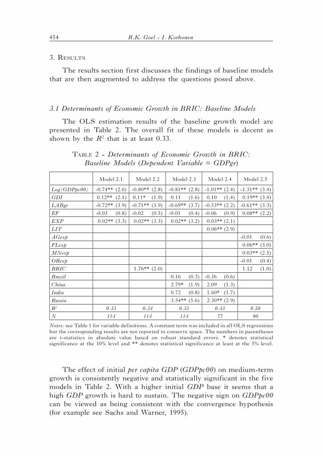
454 R.K. Goel - I. Korhonen
3. reSultS
The results section first discusses the findings of baseline models that are then augmented to address the questions posed above.
3.1 Determinants of Economic Growth in BRIC: Baseline Models
The OLS estimation results of the baseline growth model are presented in Table 2. The overall fit of these models is decent as shown by the R2 that is at least 0.33.
tABle 2 - Determinants of Economic Growth in BRIC: Baseline Models (Dependent Variable = GDPgr)
Model 2.1 Model 2.2 Model 2.3 Model 2.4 Model 2.5
Log(GDPpc00) ‑0.74** (2.6) ‑0.80** (2.8) ‑0.81** (2.8) ‑1.01** (2.4) ‑1.31** (3.4)
GDI 0.12** (2.1) 0.11* (1.9) 0.11 (1.6) 0.10 (1.4) 0.19** (3.4)
LABgr ‑0.72** (3.9) ‑0.71** (3.9) ‑0.69** (3.7) ‑0.53** (2.2) ‑0.61** (3.3)
EF ‑0.03 (0.8) ‑0.02 (0.5) ‑0.01 (0.4) ‑0.06 (0.9) 0.08** (2.2)
EXP 0.02** (3.3) 0.02** (3.3) 0.02** (3.2) 0.03** (2.1)
LIT 0.06** (2.9)
AGexp ‑0.01 (0.6)
FLexp 0.06** (3.0)
MNexp 0.03** (2.5)
ORexp ‑0.01 (0.4)
BRIC 1.76** (2.0) 1.12 (1.0)
Brazil 0.16 (0.3) ‑0.36 (0.6)
China 2.79* (1.9) 2.09 (1.3)
India 0.72 (0.8) 1.60* (1.7)
Russia 3.54** (5.6) 2.30** (2.9)
R2 0.33 0.34 0.35 0.43 0.50
N 114 114 114 77 90
Notes: see Table 1 for variable definitions. A constant term was included in all OLS regressions but the corresponding results are not reported to conserve space. The numbers in parentheses are t‑statistics in absolute value based on robust standard errors. * denotes statistical significance at the 10% level and ** denotes statistical significance at least at the 5% level.
The effect of initial per capita GDP (GDPpc00) on medium‑term growth is consistently negative and statistically significant in the five models in Table 2. With a higher initial GDP base it seems that a high GDP growth is hard to sustain. The negative sign on GDPpc00 can be viewed as being consistent with the convergence hypothesis (for example see Sachs and Warner, 1995).

Economic growth in BRIC countries and comparisons with rest of the world 455
As in other growth studies (see for example, Goel and Ram, 1994; and Barro and Sala‑i‑Martin, 2004, pp. 531‑32), the effect of investment (GDI) on growth is positive and significant in a majority of cases. In all models 2.1‑2.4, a one percent increase in GDI (as percent of GDP), has a greater impact on growth than a one percent increase in overall exports. Labor growth (LABgr) has a growth‑retarding effect, as there might be issues with gainfully employing additional workers. The effect of economic freedom (EF) is generally insignificant, but positive and statistically significant in Model 2.54.
Aggregate exports (EXP) are shown to have a positive and significant growth effect throughout models 2.1‑2.45. This supports the notion that a country’s exports enable better resource utilization through comparative advantage exploitation and realization of scale economies.
Upon disaggregating exports into four categories in Model 2.5, only manufacturing exports (MNexp) and fuel exports (FLexp) have positive and significant growth effects. In terms of relative magnitudes, fuel exports have a larger positive impact on growth than a corresponding increase in manufacturing exports. Unique resource endowments provide nations with comparative advantages and possibly larger markups that contribute significantly to growth. However, this is not consistently true across all exports, as the effects of agricultural (AGexp) and ore exports (ORexp) are statistically insignificant.
To account for labor quality, Model 2.4 adds the degree of literacy (LIT) as an additional regressor. The sample size in this case shrinks due to missing observations. The resulting coefficient on literacy is positive and significant – as expected, better labor quality boosts growth. Interestingly, a one percent increase in the literacy rates has the potential to boost medium‑term economic growth by twice a one percent increase in the aggregate exports (Model 2.4).
4 Economic freedom may alternately be captured by a nation’s degree of openness to trade (measured as the ratio of exports and imports to GDP). Prior research including openness as an explanatory variable in growth regressions has found the corresponding effect to be statistically insignificant (Barro and Sala‑i‑Martin, 2004, pp. 529‑530).
5 To account for possible complementarities between exports and economic freedom, a variation of Model 2.3 adding an interaction term between the two variables was also run. The resulting coefficient was positive and statistically significant, confirming that economic freedom might be influencing exports. The effects of other variables were generally in line with what is reported above. Details are available upon request.

456 R.K. Goel - I. Korhonen
Turning to BRIC countries, two variations are considered: using a group dummy variable (BRIC in Models 2.2 and 2.5) and individual country dummies (Models 2.3 and 2.4). The sign on the group dummy, BRIC, is positive in both instances suggesting that, other things being the same, economic growth in the BRIC group was higher over the 2000‑2007 period. However, the resulting coefficient is statistically significant only when aggregate exports are included (Model 2.2).
Of the BRIC countries, the coefficient on Russia was consistently positive and statistically significant. China and India also showed positive growth effects, although the statistical significance was weak in one of the two instances in each case. Interesting, the coefficient on India attains statistical significance in the model that takes labor quality into account (Model 2.4). On the other hand, Brazil did not show significant growth differences from the rest of the sample over the period 2000‑2007. Thus, while overall the BRIC group might seem to have grown significantly higher than rest of the world over the medium term, important within‑group differences persist.
3.2 Institutional Quality and BRIC Economic Growth
In this section we examine the role of institutions in fostering economic growth. While it has been recognized for quite a long time that institutional quality can play a crucial role in economic growth, measurement of institutional quality remains a challenge. To somewhat address this issue, we employ three different measures of institutional quality: the degree of corruption (CORR), the strength of patent rights (IPP) and the degree of democracy (DEM)6. Since these cross‑country measures each come from a single source, they provide comparable benchmarks.
Beginning with the seminal work of Mauro (1995), researchers have been drawn to the connection between cross‑country growth and corruption (Bardhan, 1997; Jain, 2001; and Lambsdorff, 2006; for related literature surveys; also see Mo, 2001; Blackburn et al.,
6 There are many proxies for institutions that one can choose from (see Knack and Keefer, 2003; also Williams and Siddique, 2008). In line with the focus of the present study on BRIC nations, we limit our choice to three measures.

Economic growth in BRIC countries and comparisons with rest of the world 457
tABle 3 ‑ Institutional Quality and BRIC Economic Growth(Dependent Variable = GDPgr)
Model 3.1 Model 3.2 Model 3.3 Model 3.4 Model 3.5 Model 3.6
Log(GDPpc00) ‑0.31 (1.1) ‑0.18 (0.6) ‑0.27 (0.7) ‑0.04 (0.1) ‑0.35 (1.22) ‑0.16 (0.5)
GDI 0.09 (1.4) 0.10 (1.4) 0.01 (0.1) 0.01 (0.3) 0.10* (1.6) 0.11* (1.7)
LABgr ‑0.72** (4.1) ‑0.66** (3.7) ‑0.49** (2.6) ‑0.46** (2.3) ‑0.82** (4.4) ‑0.82** (4.3)
EF 0.06 (1.2) 0.09* (1.9) ‑0.05* (1.8) ‑0.22 (0.7) 0.004 (0.1) 0.02 (0.8)
EXP 0.02** (3.3) 0.02** (4.2) 0.02** (2.0)
CORR 1.18** (3.1) 1.25** (3.3)
IPP 0.14 (0.1) ‑0.98 (0.5)
DEM ‑0.29** (2.5) ‑0.37** (3.3)
Brazil ‑0.19 (0.4) ‑0.70 (1.2) ‑0.66 (1.5) ‑1.05** (2.1) 0.33 (0.6) 0.07 (0.1)
China 3.58** (2.5) 3.54** (2.3) 5.30** (4.6) 5.68** (4.4) 0.93 (0.5) 0.35 (0.2)
India 1.49 (1.6) 1.11 (1.2) 2.39** (3.0) 2.38** (2.7) 1.35 (1.6) 1.25 (1.5)
Russia 3.04** (5.0) 3.18** (5.0) 3.26** (5.6) 3.57** (5.5) 1.81** (2.1) 1.45 (1.5)
R2 0.40 0.34 0.38 0.26 0.40 0.37
N 114 114 94 94 114 114
Notes: see Table 1 for variable definitions. A constant term was included in all OLS regressions but the corresponding results are not reported to conserve space. The numbers in parentheses are t‑statistics in absolute value based on robust standard errors. * denotes statistical significance at the 10% level and ** denotes statistical significance at least at the 5% level.
2006; Méndez and Sepúlveda, 2006; and Aidt et al., 2008)7. The main premise is that corrupt acts create bottlenecks and are associated with unproductive transfers (Aidt, 2009; Shleifer and Vishny; 1993). Both of these factors retard growth and corruption control has been espoused by cross‑national organizations as a condition for rapid economic growth. However, the efficiency aspects of corruption, whereby corruption expedites governmental procedures, have also been recognized (Lui, 1985; Méon and Sekkat, 2005; Méon and Weill, 2008). Thus the overall effect of corruption on growth would be determined by the relative strength of each effect. In his authoritative review of the literature, Lambsdorff (2006) concludes that the
7 See Becker (1968) for background on the economics of criminal behavior.

458 R.K. Goel - I. Korhonen
“link between corruption and GDP or the growth of GDP has its empirical and theoretical weaknesses”, (p. 27) and that some results were “ambiguous”, (p. 25).
We contribute to the ongoing debate in this context by focusing on BRIC countries.
We add the cross‑country index of corruption perceptions (CORR) from the Transparency International to the estimated equation (3). This index has been widely used in cross‑country studies over the past decade and a half and provides fairly consistent data8. In our sample, Russia fared relatively worse in terms of corruption perceptions than other BRIC countries. However, all nations in the group fared worse than the sample average, suggesting that corruption was a significant problem.
The degree of patent protection can be seen as capturing the role of institutions surrounding the protection of property rights. The protection of intellectual property rights in BRIC nations has been the subject of some debate (Bird, 2007) and the present research will shed light on this aspect in the context of economic growth. Democracy is related to institutions covering the freedom of press and civil liberties. As discussed above, greater democracy would enhance growth when it fosters efficiency at the expense of equity and vice versa. In the BRIC group, India has a longstanding tradition of democracy, while democratic institutions are in their infancy in Russia. China is currently the least democratic nation of the BRIC group.
Results from Table 3 show that, when institutional quality is taken into account, unlike Table 2, initial GDP and GDI do not have an appreciable impact on economic growth; while the results with respect to LABgr are similar. Further, the effect of economic freedom is mixed. Aggregate exports again consistently boost economic growth and this finding is robust across alternate measures of institutional quality9.
With regard to institutional quality, greater corruption is shown to boost economic growth in both the models where it appears.
8 We performed a logarithmic transformation on the corruption index to unbind and to facilitate interpretation (see Table 1).
9 In consideration of some potential multicollinearity between exports and institutional quality (Leite and Weidmann, 1999; Stevens, 2003; Bulte and Damania, 2008), Models 3.2 and 3.4 in Table 3 were run without EXP. The main findings from Models 3.1 and 3.3 remained essentially unchanged.

Economic growth in BRIC countries and comparisons with rest of the world 459
The resulting coefficient is positive and significant. This result is consistent with the notion that corrupt practices might be boosting efficiency by acting as a grease to speed procedures and circumvent bottlenecks (see Méon and Weill, 2008). Thus, on efficiency grounds, corruption seems to fare well. Whether such corruption turns out to be equitable is a different issue.
When institutional quality is alternately measured by the degree of patent protection (IPP), the resulting coefficient fails to show any statistically significant effects. Further, greater democracy (DEM) somewhat retarded economic growth. Greater debate and attention to due processes in democracies tend to lower growth relative to instances where solely efficiency aspects are emphasized. This finding provides some justification for differences in the Chinese and Indian growth rates.
Of the BRIC group, growth in China and Russia was higher in all instances whether institutional quality was measured by the degree of corruption or by the degree of patent protection. The coefficient on India was positive in all cases, and statistically significant when patent protection was taken into account (Models 3.3 and 3.4). Finally, the coefficient on Brazil was negative and statistically significant in one instance.
3.3 Growth Determinants across Different Growth Levels
In this section we address the question of whether similar influences significantly bear on growth across nations with high and low growth rates. Thus, we are able to move beyond strictly the four nations in the BRIC group. The answer to this question goes to the heart of the design of growth policies and recommendations across nations – can uniform growth recommendations work well across nations with different growth rates? Recognizing the limitations of dichotomous variables, the quantile regression procedure also enables us to alternately examine the determinants of economic growth across nations with different growth rates. For this purpose we employ with quantile regression to Models 2.2 and 2.5, without the BRIC group dummy variable10. This focus across different growth rates is unique in the present study. Section 4.1 deals with aggregate exports, while section 4.2 addresses disaggregated exports.
10 See Koenker and Hallock (2001) for background on the quantile regression.

460 R.K. Goel - I. Korhonen
tABle 4 - Determinants of Economic Growth across Different Growth Rates (Dependent Variable = GDPgr)
4.1 (N=114) (q0.10) (q0.25) (q0.50) (q0.75) (q0.90)Log(GDPpc00) 0.14 (0.4) ‑0.29 (0.8) ‑0.88** (2.7) ‑0.91** (2.4) ‑1.60** (2.4)GDI 0.04 (0.8) 0.12** (2.3) 0.10** (2.1) 0.14** (2.2) 0.11 (1.0)LABgr 0.10 (0.3) ‑0.40 (1.3) ‑0.66** (3.1) ‑0.89** (4.2) ‑1.32** (3.6)EF 0.04 (0.9) ‑0.01 (0.3) ‑0.01 (0.3) ‑0.04 (1.2) ‑0.03 (0.5)EXP 0.01 (1.0) 0.01** (2.3) 0.02** (2.7) 0.03** (2.0) 0.07** (2.8)Pseudo-R2
0.05 0.10 0.21 0.29 0.34
4.2 (N=90) (q0.10) (q0.25) (q0.50) (q0.75) (q0.90)
Log(GDPpc00) 0.10 (0.2) ‑0.93* (1.7) ‑1.04* (1.7) ‑1.11** (2.2) ‑2.10** (3.0)GDI 0.03 (0.4) 0.14** (2.8) 0.18** (3.4) 0.16** (2.4) 0.25** (3.0)LABgr ‑0.01 (0.04) ‑0.14 (0.4) ‑0.57* (1.9) ‑0.57** (2.5) ‑0.71** (2.3)EF ‑0.01 (0.2) 0.04 (0.8) 0.07** (1.2) 0.09** (2.2) 0.09* (1.8)AGexp ‑0.01 (0.2) 0.02 (0.5) ‑0.01 (0.3) ‑0.02 (0.6) ‑0.03 (0.5)FLexp 0.02 (1.0) 0.04* (1.9) 0.04 (1.5) 0.07** (2.4) 0.06** (2.4)MNexp 0.01 (0.2) 0.03* (1.9) 0.02 (1.4) 0.02 (1.3) 0.02 (1.1)ORexp ‑0.02 (0.7) 0.001 (0.02) ‑0.03 (0.9) 0.001 (0.1) ‑0.03 (1.3)Pseudo-R2
0.10 0.15 0.21 0.37 0.50
Notes: details about the variables are provided in Table 1. Absolute values of t‑statistics based on 200 bootstrap standard errors of simultaneous quantile regression are in parentheses. A constant term was included in all models but the corresponding results are not presented to conserve space. Lower quantiles (e.g., q0.10) imply countries with low economic growth. ** denotes statistically significant at the 5% level, and * at the 10% level.
In Section 4.1, GDPpc00 generally has a negative and significant effect, except in the least growth countries (q0.10). Not unexpectedly, the least growing countries fail to show significant trends towards economic convergence. GDI seems effective in most cases, except in the least growth nations, and in the highest growing nations in the case of aggregate exports (Section 4.1). It could be the case that underdeveloped or undeveloped institutions might be behind the ineffectiveness of many growth factors in these low growth countries.
LABgr generally has a negative effect, which becomes significant in higher growth nations (median growth or higher). The effect of economic freedom (EF) is consistently insignificant with aggregate exports (Section 4.1), and positive and significant in higher growth nations (Section 4.2). High growth nations might be competitors in

Economic growth in BRIC countries and comparisons with rest of the world 461
many international markets and fewer bottlenecks might fuel growth in such instances.
The role of aggregate exports is positive and significant in most cases, except the least growing countries. Interesting results emerge, however, when agricultural, ore, fuel and manufacturing exports are separately considered. Like Table 2 (Model 2.5), both ORexp and AGexp fail to show growth dividends. This is true across nations with different levels of economic growth. Fuel exports positively and significantly contribute to growth in most cases, except in the least and most growing nations; while the effect of manufacturing exports is mostly insignificant, except for moderate growth nations (q0.25). Consistent with the findings in Table 2, the magnitude of the growth contribution of fuel exports is greater than that of manufacturing exports.
A key overall finding from this section is that no single growth determinant consistently contributes to growth across nations with different growth levels. The effectiveness of various factors in affecting growth is partly dictated by the stage of a country’s growth. This revelation is a key contribution of the present research and also provides an alternate way (other than dummy variables) to capture the relative differences across slow and fast growing (BRIC) nations. This calls for a move away from blanket growth recommendations across nations and calls for a country or region‑specific approach.
In closing, it is possible that there is some reverse causality between institutional quality and growth (Chong and Calderón, 2000; Glaeser et al., 2004). For instance, rapidly growing nations might have higher corruption. In other words, bigger potential rents in fast growing economies might encourage bribe seekers. Also, the degree of patent protection might be higher in high growth countries. Finally economic growth might lead to development of democratic institutions. This issue is addressed in section 3.4 below.
3.4 Possible Simultaneity between Institutional Quality and Economic Growth
As mentioned above, there might be simultaneity between institutional quality and growth whereby high growth countries might (i) invite more corrupt practices due to a bigger set of potential rents to be had; or (ii) have stronger patent protection. Conversely, it is possible that low level corruption might be more prevalent in low growth nations due to poor monitoring systems and underdeveloped institutions.

462 R.K. Goel - I. Korhonen
tABle 5 ‑ Allowing for Endogeneity of Institutional Quality: IV Regressions (Dependent variable = GDPgr)
Model 5.1 Model 5.2 Model 5.3
Log(GDPpc00) 0.22 (0.5) ‑0.38 (0.3) ‑0.39 (0.4)
GDI 0.09** (2.4) 0.002 (0.1) 0.10** (2.8)
LABgr ‑0.74** (4.4) ‑0.47* (1.9) ‑0.81** (2.6)
EF 0.16** (2.6) ‑0.06 (1.0) 0.004 (0.1)
EXP 0.02** (2.5) 0.02* (1.8) 0.02 (1.1)
CORR 2.49** (2.9)
IPP 0.84 (0.1)
DEM ‑0.28 (0.5)
Brazil ‑0.33 (0.2) ‑0.69 (0.4) 0.31 (0.1)
China 4.19* (1.8) 5.19* (1.9) 1.06 (0.2)
India 2.15 (1.0) 2.25 (0.9) 1.33 (0.5)
Russia 2.90 (1.3) 3.21* (1.8) 1.91 (0.5)
F-value 6.9** 4.9** 5.9**
N 112 93 113
First-stage F-value 39.2** 12.7** 15.1**
Sargan overidentification test (p-value)
6.15 (0.10) 0.45 (0.80) 1.52 (0.47)
Notes: see Table 1 for variable definitions. A constant term was included in all 2SLS regressions but the corresponding results are not reported to conserve space. CORR was instrumented by ETHNIC, LANG, RELIG, and GCONS in Model 5.1; while IPP and DEM were instrumented by ETHNIC, LANG and RELIG in Models 5.2 and 5.3, respectively. The numbers in parentheses are (absolute) z‑statistics of second‑stage results. * denotes statistical significance at the 10% level and ** denotes statistical significance at least at the 5% level.
A two‑stage least squares regression was estimated with CORR instrumented by the additional variables shown in relation (4)11.
CORRi = h(ETHNICi, LANGi, RELIGi, GCONSi) (4) i =1,2,3… The instruments for IPP and DEM, on the other hand, were
11 Justifications for determinants of corruption can be found in Jain (2001), Lambsdorff (2006) and Treisman (2000).

Economic growth in BRIC countries and comparisons with rest of the world 463
IPPi, DEMi = h(ETHNICi, LANGi, RELIGi) (5) i =1,2,3…ETHNIC, LANG, and RELIG are, respectively, indices of
ethnic, linguistic and religious fractionalizations (see Paldam, 2002 for study of their effect on corruption and Mauro, 1995 for a related choice of instruments; also Alesina et al., 2003 for background on the calculation of fractionalization indices). These socio‑cultural differences might crucially affect attitudes towards corruption.
Finally, GCONS is government size, capturing the size of the bureaucracy as well as the enforcement machinery (Rose‑Ackerman, 1999; also see Budak and Goel, 2004). More regulatory barriers provide opportunities for rent seeking, while stronger enforcement machinery increases the probability of detection.
Table 5 reports (second‑stage) 2SLS estimation results allowing for the endogeneity of the corruption, DEM and IPP variables in (5). The Sargan overidentification test confirmed our choice of instruments. The first‑stage F‑tests were also statistically significant.
The overall fit of Model 5.1, endogenizing corruption, seems relatively better than Models 5.2 and 5.3. The effect of initial GDPpc is statistically insignificant, that of LABgr is negative and significant, and that of exports is positive and significant in both cases. Both economic freedom and GDI positively impact growth in Model 5.1, but the corresponding coefficients are not consistently statistically significant in the other two cases.
Turning to the influence of institutions after allowing for possible endogeneity, the results from Table 3 are reinforced. Namely, greater corruption positively and significantly affects growth while the effects of patent protection and democracy are statistically insignificant. The efficiency effect of corruption dominates the bottleneck effect in this case as well. Finally, with respect to BRIC countries, China shows consistently positive and statistically significant effects, while that of Russia is positive and significant in one instance. The coefficients on Brazil and India fail to attain statistical significance. This shows that growth in China, and to some extent in Russia, has been remarkable.
In sum, when possible reverse causality from corruption to growth is taken into account, the previous results regarding the relation between institutional quality and growth hold, while the effects of other influences are similar to earlier findings. In addition to the robustness of our results across three measures of institutional quality and the inclusion of BRIC group versus individual country dummies, we consider two robustness checks.

464 R.K. Goel - I. Korhonen
3.5 Robustness Checks
We perform two robustness checks to analyze the validity of our findings. These deal with examining growth over a shorter time period and checking the influence of outlying observations on the key results.
3.5a Short-Term versus Long-Term Growth
As a robustness check of our medium‑term growth model estimated in Table 2, we also examine determinants of short‑term growth12. The general pattern of findings is similar when a short‑term growth model, explaining economic growth over 2006‑2007 period is estimated. Two versions, with and without labor quality, are considered. The corresponding results are presented in the Appendix. As expected, the explanatory power is lower as many influences on growth take some time to have an effect. In Model A.1 exports show a positive growth impact, while LABgr exhibits a negative effect. The effects of other variables, while similar in signs to those in Table 2, were statistically insignificant. In Model A.2, greater literacy is shown to pay growth dividends even over the short term, while GDPpc00 is now statistically significant. The other variables failed to achieve statistical significance.
Of the BRIC nations, China stood out, even more so than it did in Table 2. It seems that Chinese growth might be even more remarkable over the short term. The results for Brazil and India echoed those from earlier and Russia was statistically significant in one of the two cases.
3.5b Sensitivity of Findings to Outliers
Another robustness check was performed to check the effect of outliers on our results. For this purpose, Hadi’s procedure was applied to GDPgr and CORR and only one country in the sample (Azerbaijan) emerged as an outlier. Models 3.1 and 3.2 were rerun after dropping the outlier and the results were very similar to what is reported in Table 313.
12 Admittedly, our characterization of the time periods for short‑term and long‑term growth is somewhat arbitrary. However, the term BRIC gained prominence only in the new millennium.
13 Details are available upon request.
Economic growth in BRIC countries and comparisons with rest of the world 465
4. concluDinG remArkS
Using data for over 100 nations and employing a fairly standard growth model, this paper examines the determinants of economic growth in BRIC countries relative to rest of the world. The growth success of BRIC nations in recent years has intrigued policymakers and researchers in recent years. However, little formal research exists that focuses on these countries, and this work makes a contribution in that regard. A number of questions are addressed:
(a) How do determinants of medium‑term economic growth differ from those of short‑term growth?
We find that the general pattern of findings is unchanged over the medium and short term (Table 2 and Appendix). Exports and literacy boost growth, while there is support for convergence and labor growth has perverse effects. GDI has generally positive effects, while greater economic freedom shows little statistical significance. The convergence hypothesis was supported. BRIC countries as a group showed better growth than rest of the world. However, important within‑group differences were found, with China and Russia mostly showing remarkable growth, India sometime showing positive growth and Brazil almost never standing out.
(b) What are the differences between the effects of aggregate versus disaggregated exports on growth?
While aggregate exports in most cases showed positive growth effects, the story was somewhat mixed when exports were disaggregated into four key categories: agricultural exports, fuel exports, manufacturing exports and ore exports (Tables 2 and 4). Both agricultural and ore exports consistently failed to show any statistically significant impacts on growth. On the other hand, fuel and manufacturing exports exhibited positive growth effects. We further find that the growth dividends from fuel exports were almost double those from manufacturing exports. These findings were robust to a nonparametric analysis that enabled evaluation of growth determinants across countries with different growth rates. The patterns for BRIC nations were similar to those discussed above. Finally, our findings were unable to find support for the resource curse hypothesis (see Stevens, 2003; Boschini et al., 2007; Bulte and Damania, 2008).
(c) Is lower institutional quality necessarily an impediment to growth?
We employed three measures of institutional quality: the degree of corruption, the degree of cross‑country patent protection and the extent of democracy (Tables 3 and 5). With respect to corruption,

466 R.K. Goel - I. Korhonen
it turns out that the efficiency aspects of corruption overpowered any negative consequences resulting in positive association between growth rates and corruption. In other words, the greasing effects are supported over the sanding aspects of corruption (see Méon and Sekkat, 2005; Aidt, 2009). Greater democracy lowered growth, suggesting that that efficiency considerations were somewhat compromised at the expense of equity issues. The degree of patent protection, on the other hand, failed to exert any appreciable effect on growth. Only corruption effect was significant after allowance was made for possible reverse linkages from economic growth to institutional quality.
(d) Do various growth factors consistently promote growth across low growth and high growth countries?
The answer to this question is negative – the factors driving growth in high growth and low growth nations are not necessarily similar (Table 4). Our findings exclusively show that the determinants of growth were sensitive to prevailing growth rates. Not surprisingly, no effective growth‑promoting strategy seemed to work in the lowest growth nations (i.e., bottom 10 percent of our sample). For instance, the contribution of aggregate exports is positive and significant in most cases, except the least growing countries. A key overall finding from this section is that no single growth determinant consistently contributes to growth across nations with different growth levels. This revelation is a key contribution of the present research and also provides an alternate way (other than dummy variables) to capture the relative differences across slow and fast growing (BRIC) nations. This calls for a move away from blanket growth recommendations across nations and calls for a country or region‑specific approach.
To sum up, while as a group the BRIC nations have shown higher growth than rest of the world, there are significant within‑group differences. China and Russia mostly showed higher growth, ceteris paribus, while India showed positive growth in some cases. On the other hand, we were unable to find Brazil performing better than the rest. The main policy lesson from this is that, given the dissimilar composition of the BRIC group, the lessons for other nations looking to boost growth by emulating BRIC nations might be limited. Such nations would have to pay careful attention to their own comparative advantages.
rAjeev k. Goel Illinois State university, Department of Economics, Normal, Illinois, uSA
iikkA korhonen Bank of Finland, Helsinki, Finland

Economic growth in BRIC countries and comparisons with rest of the world 467
R E F E R E N C E S
Aghion, P. and P. Howitt (1997), Endogenous Growth Theory, MIT Press: Cambridge, MA.
Aidt, T.S. (2009), “Corruption, Institutions, and Economic Development”, Oxford Review of Economic Policy, 25(2), 271‑291.
Aidt, T., J. Dutta and V. Sena (2008), “Governance Regimes, Corruption and Growth: Theory and Evidence”, Journal of Comparative Economics, 36(2), 195‑220.
Alesina, A., A. Devleeschauwer, W. Easterly, S. Kurlat, and R. Wacziarg (2003), “Fractionalization”, Journal of Economic Growth, 8(2), 155‑194.
Auty, R.M. (2001), “The Political Economy of Resource‑Driven Growth”, European Economic Review, 45(4‑6), 839‑846.
Bardhan, P. (1997), “Corruption and Development: A Review of Issues”, Journal of Economic Literature, 35(3), 1320‑1346.
Barro, R.J. (1991), “Economic Growth in a Cross Section of Countries”, Quarterly Journal of Economics, 106(2), 407‑443.
Barro, R.J. (2001), “Human Capital and Growth”, American Economic Review, 91(2), 12‑17.
Barro, R.J. and X. Sala‑i‑Martin (2004), Economic Growth, 2nd edition, MIT Press: Cambridge, MA.
Becker, G.S. (1968), “Crime and Punishment: An Economic Approach”, Journal of Political Economy, 76(2), 169‑217.
Bird, R.C. (2007), “Defending Intellectual Property Rights in the BRIC Economies”, <http://papers.ssrn.com/sol3/papers.cfm?abstract_id=807844>.
Blackburn, K., N. Bose and M.E. Haque (2006), “The Incidence and Persistence of Corruption in Economic Development”, Journal of Economic Dynamics and Control, 30(12), 2447‑2467.
Boschini, A., J. Pettersson and J. Roine (2007), “Resource Curse or Not: A Question of Appropriability”, Scandinavian Journal of Economics, 109(3), 593‑617.
Budak, J. and R.K. Goel (2004), “Transition, Governance and Corruption”, Economia Internazionale/International Economics, 57(4), 395‑406.
Bulte, E. and R. Damania (2008), “Resources for Sale: Corruption, Democracy and the Natural Resource Curse”, The B.E. Journal of Economic Analysis & Policy, 8(1), Article 5.
Chong, A. and C. Calderón (2000), “Causality and Feedback between Institutional Measures and Growth”, Economics and Politics, 12(1), 69‑81.
de Haan, J. and J‑E. Sturm (2000), “On the Relationship between Economic Freedom and Economic Growth”, European Journal of Political Economy, 16(2), 215‑241.

468 R.K. Goel - I. Korhonen
Falcetti, E., T. Lysenko and P. Sanfey (2005), “Reforms and Growth in Transition: Re‑examining the Evidence”, European Bank for Reconstruction and Development Working Paper No. 90.
Feder, G. (1983), “On Exports and Economic Growth”, Journal of Development Economics, 12(1‑2), 59‑73.
Fischer, S. (2006), “The New Global Economic Geography”, mimeo, <http://www.kc.frb.org/PUBLICAT/SYMPOS/2006/PDF/14Fischer.pdf>.
Glaeser, E.L., R. La Porta, F. Lopez de Silanes and A. Shleifer (2004), “Do Institutions Cause Growth?”, Journal of Economic Growth, 9(3), 271‑303.
Goel, R.K., J.E. Payne and R. Ram (2008), “R&D Expenditures and U.S. Economic Growth: A Disaggregated Approach”, Journal of Policy Modeling, 30(2), 237‑250.
Goel, R.K. and R. Ram (1994), “Research and Development Expenditures and Economic Growth: A Cross‑Country Study”, Economic Development and Cultural Change, 42(2), 403‑411.
Gylfason, T., T.T. Herbertson and G. Zoega (1999), “A Mixed Blessing: Natural Resources and Economic Growth”, Macroeconomic Dynamics, 3(02), 204‑225.
Havrylyshyn, O. and R. van Rooden (2000), “Institutions Matter in Transition, but so do Policies”, International Monetary Fund Working Paper No. 00/70.
Herd, R. and S. Dougherty (2007) “Growth Prospects in China and India Compared”, European Journal of Comparative Economics, 4(1), 65‑89.
Hölscher, J., E. Marelli and M. Signorelli (2010), “China and India in the Global Economy”, Economic Systems, 34(3), 212‑217.
Jain, A.K. (2001), “Corruption: A Review”, Journal of Economic Surveys, 15(1), 71‑121.
Kalyuzhnova, Y., A.M. Kutan and T. Yigit (2009), “Corruption and Economic Development in Energy‑Rich Economies”, Comparative Economic Studies, 51(2), 165‑180.
Karras, G. (2003), “Trade Openness and Economic Growth: Can we Estimate the Precise Effect?”, Applied Econometrics and International Development, 3(1), 7‑26.
Knack, S. and P. Keefer (2003), Institutions and Economic Performance: Cross-country Tests using Alternative Institutional Measures, in: S. Knack (Ed.), “Democracy, Governance and Growth”, University of Michigan Press: Ann Arbor.
Koenker, R. and K.F. Hallock (2001), “Quantile Regression”, Journal of Economic Perspectives, 15(4), 143‑156.
Lambsdorff, J.G. (2006), Causes and Consequences of Corruption: What do we Know from a Cross-section of Countries?, in: S. Rose‑Ackerman (Ed.), “International Handbook on the Economics of Corruption”, Edward Elgar: Cheltenham, UK.

Economic growth in BRIC countries and comparisons with rest of the world 469
Leite, C. and J. Weidmann (1999), “Does Mother Nature Corrupt? Natural Resources, Corruption, and Economic Growth”, IMF Working Paper WP/99/85.
Levine, R. and D. Renelt (1992), “A Sensitivity Analysis of Cross‑Country Growth Regressions”, American Economic Review, 82(4), 942‑963.
Lui, F.T. (1985), “An Equilibrium Queuing Model of Bribery”, Journal of Political Economy, 93(4), 760‑781.
Maddison, A. (2009), “Measuring the Economic Performance of Transition Economies: Some Lessons from Chinese Experience”, Review of Income and Wealth, 55(s1), 423‑441.
Mankiw, N.G., D. Romer and D.N. Weill (1992), “A Contribution to the Empirics of Economic Growth”, Quarterly Journal of Economics, 107(2), 407‑437.
Mauro, P. (1995), “Corruption and Growth”, Quarterly Journal of Economics, 110(3), 681‑712.
Mehlum, H., K. Moene and R. Torvik (2006), “Institutions and the Resource Curse”, Economic Journal, 116(508), 1‑20.
Méndez, F. and F. Sepúlveda (2006), “Corruption, Growth and Political Regimes: Cross‑Country Evidence”, European Journal of Political Economy, 22(1), 82‑98.
Méon, P‑G. and K. Sekkat (2005) “Does Corruption Grease or Sand the Wheels of Growth?” Public Choice, 122(1‑2), 69‑97.
Méon, P-G. and L. Weill (2008), “Is Corruption an Efficient Grease?”, BOFIT Discussion Paper No. 20/2008.
Mo, P.H. (2001), “Corruption and Economic Growth”, Journal of Comparative Economics, 29(1), 66‑79.
Paldam, M. (2002), “The Cross‑Country Pattern of Corruption: Economics, Culture and the Seesaw Dynamics”, European Journal of Political Economy, 18(2), 215‑240.
Park, W.G. (2008), “International Patent Protection: 1960‑2005”, Research Policy, 37(4), 761‑766.
Roland, G. (2000), Transition and Economics, MIT Press: Cambridge, MA.
Romer, P.M. (1990), “Human Capital and Growth: Theory and Evidence”, Carnegie-Rochester Series on Public Policy, 32(1), 251‑286.
Rose‑Ackerman, S. (1999), Corruption and Government, Cambridge University Press: Cambridge, MA.
Russian Analytical Digest (2011), “Russia and BRIC”, No. 91, February 14.
Sachs, J.D. and A.M. Warner (1995), “Economic Convergence and Economic Policies”, Harvard Institute of Economic Research Working Papers 1715.
Shleifer, A. and R.W. Vishny (1993), “Corruption”, Quarterly Journal of Economics, 108(3), 599‑617.

470 R.K. Goel - I. Korhonen
Solow, R.M. (1956), “A Contribution to the Theory of Economic Growth”, Quarterly Journal of Economics, 70(1), 65‑94.
Stevens, P. (2003), “Resource Impact: Curse or Blessing? A Literature Survey”, Journal of Energy Literature, 9(1), 1‑42.
Treisman, D. (2000), “The Causes of Corruption: A Cross‑National Study”, Journal of Public Economics, 76(3), 399‑457.
Williams, A. and A. Siddique (2008), “The Use (and Abuse) of Governance Indicators in Economics: A Review”, Economics of Governance, 9(2), 131‑175.
Wilson, D. and R. Purushothaman (2003), “Dreaming with BRICs: The Path to 2050”, Goldman Sachs, Global Economics Paper No. 99.
ABSTRACT
We study economic growth in four emerging economies – Brazil, Russia, India, and China (BRIC). Questions addressed are: (a) How do medium‑term growth determinants differ from short term determinants? (b) What are differences between growth effects of aggregate versus disaggregated exports? (c) Does lower institutional quality hinder growth? and (d) Do similar factors promote growth across low growth and high growth countries? Results show that while BRIC nations have higher growth, there are significant within-group differences. China and Russia mostly showed higher growth, while India sometimes showed positive growth, and Brazil did not outperform the rest. A nonparametric analysis with a broader set of high‑growth nations provides some novel insights. Policy implications are discussed.
Keywords: Economic Growth, BRIC Countries, Exports, Institutions, Corruption, World
JEL Classification: O40, O57, P52
RIASSUNTO
Crescita economica nei paesi BRIC e confronti con il resto del mondo
In questo lavoro si studiano quattro economie emergenti: Brasile, Russia, India e Cina (BRIC). I problemi affrontati sono: (a) le determinanti della crescita nel medio periodo sono diverse da quelle della crescita nel breve periodo?; (b) quali differenze ci sono fra gli effetti della crescita delle esportazioni aggregate e delle esportazioni disaggregate?; (c) una qualità istituzionale scadente può rallentare la crescita?; (d) la crescita è stimolata da fattori simili sia nei paesi a crescita lenta che in quelli a crescita elevata? I risultati mostrano che, sebbene i paesi dell’area BRIC presentino tutti tassi di crescita elevata, vi sono differenze significative all’interno dell’area stessa. Alcuni risultati nuovi sono forniti dall’analisi non‑parametrica su un più ampio set di paesi ad alta crescita economica. Inoltre vengono discusse le relative implicazioni politiche.

Economic growth in BRIC countries and comparisons with rest of the world 471
APPENDIX
Determinants of Economic Growth in BRIC: Short‑Term Growth (Dependent variable = GDPgrSR)
Model A.1 Model A.2
Log(GDPpc00) ‑0.59 (1.3) ‑1.14** (2.1)
GDI 0.05 (0.5) 0.03 (0.2)
LABgr ‑0.54* (1.9) 0.07 (0.2)
EF ‑0.08 (1.4) ‑0.09 (0.9)
EXP 0.03** (2.4) 0.03 (1.2)
LIT 0.13** (4.4)
Brazil 0.52 (0.6) ‑0.24 (0.2)
China 5.41** (2.2) 5.21* (1.9)
India 2.03 (1.3) 4.67** (3.2)
Russia 2.65** (2.8) 1.30 (1.0)
R2 0.18 0.33
N 114 77
Notes: see Table 1 for variable definitions. A constant term was included in all OLS regressions but the corresponding results are not reported to conserve space. The numbers in parentheses are t‑statistics in absolute value based on robust standard errors. * denotes statistical significance at the 10% level and ** denotes statistical significance at least at the 5% level.


CAN EXCHANGE RATE MODELS OUTPERFORM THE RANDOM WALK? MAGNITUDE, DIRECTION AND
PROFITABILITY AS CRITERIA
1. introDuction
Since the publication of the highly‑cited paper of Meese and Rogoff (1983), it has become something like an undisputable fact of life that exchange rate determination models cannot outperform the naïve random walk model in out‑of‑sample forecasting. Several explanations have been put forward for this empirical regularity. In their original paper, Meese and Rogoff (1983) attributed their findings to some econometric problems, including simultaneous equations bias, sampling errors, stochastic movements in the true underlying parameters, model misspecification and failure to account for nonlinearities. Meese (1990) adds other explanations such as improper modelling of expectations and over‑reliance on the representative agent paradigm – hence it appears that Meese questions the theoretical pillars of exchange rate models. As a matter of fact the majority of economists attribute the apparent failure to outperform the random walk to model inadequacy, in the sense that exchange rate models do not provide a valid representation of exchange rate behaviour (for example, Cheung and Chinn, 1999).
An important reason for the failure of these models to beat the random walk is typically, but not universally, overlooked. It is the use of quantitative measures of forecasting accuracy that are calculated from the forecasting errors, such as the root mean square error (which was used by Meese and Rogoff). It has been suggested that relying entirely on these measures may not be appropriate because a correct prediction of the direction of change may be more important than the magnitude of the error (for example, Engel, 1994). Others have suggested that the ultimate test of forecasting power is the ability to make profit by trading on the basis of the forecasts – hence the appropriate criterion would be profitability (for example, Leitch and Tanner, 1991). Cheung et al. (2005) argue that using criteria other than the mean square error does not boil down to “changing

474 I. Moosa - K. Burns
the rules of the game” while advocating the use of other criteria by suggesting that minimising the mean square error may not be important from an economic standpoint. They argue against the use of the mean square error on the grounds that it may miss out on important aspects of prediction, particularly at long horizons. Christofferson and Diebold (1998) point out that the mean square error indicates no improvement in predictions that take into account cointegrating relationships vis-a-vis univariate prediction. Leitch and Tanner (1991) argue that the direction of change may be more relevant for profitability and economic concerns, while Cumby and Modest (1987) suggest that direction accuracy is also related to tests for market timing ability. Engel (1994) advocates the use of direction accuracy, which he describes as “not a bad proxy for a utility‑based measure of forecasting performance”. He also argues that it is impossible to think of important circumstances under which the direction of change is exactly the right criterion for maximising the welfare of the forecaster, citing as an example the case of central banks under a fixed exchange rate system.
Profitability, or in general utility, is another criterion that can be used to test predictive power. Abhyankar et al. (2005) propose a utility‑based criterion pertaining to the portfolio allocation problem, as they find that the relative performance of the structural model improves when this criterion is used. Likewise, West et al. (1993) suggest a utility‑based evaluation of exchange rate predictability. Li (2011) evaluates the effectiveness of economic fundamentals in enhancing carry trade. He finds that the profitability of carry trade and risk‑return measures can be enhanced by using forecasts. Likewise, Boothe and Glassman (1987) compare the rankings of alternative exchange rate forecasting models using two different criteria: accuracy (measured by the root mean square error) and profitability.
Leitch and Tanner (1991) note that economists are puzzled by the observation that profit‑maximising firms buy professional forecasts when measures of forecasting accuracy indicate that a naïve (random walk) model provides free forecasts that are just as good (or as bad) as those provided by fee‑charging forecasters. The explanation they present is that these measures bear very weak relation to the profit generated by acting on the basis of the forecasts, suggesting that the only substitute criterion for profit is a measure of direction accuracy. They find the relation between direction accuracy and profit to be almost as close as the relation between other measures (for example, between the root mean

Can exchange rate models outperform the random walk? Magnitude, direction and profitability as criteria 475
square error and the mean absolute error). They further suggest that if profits are not observable, direction accuracy of the forecasts may be used as the evaluation criterion.
The objective of this paper is to examine these propositions by using simulated data, generated specifically to cover the two extremes of being good at predicting magnitude but not direction, and vice versa. The use of simulated data to represent models with extreme abilities is also motivated by the desire to determine whether the ability to forecast direction is more or less strongly related to profitability than the ability to forecast the magnitude of the error. A contribution of this paper is the development of a new measure of forecasting accuracy that takes into account errors of magnitude and direction by adjusting the conventional root mean square error. It is demonstrated that random walk forecasts are not as good as they typically appear when forecasting accuracy is measured in terms of direction accuracy and profitability.
2. the SimulAteD DAtA AnD conventionAl meASureS oF ForecAStinG power
For the purpose of this exercise we generated 100 observations randomly on the actual percentage change in a hypothetical exchange rate. Then we generated eight sets of forecasts to represent a variety of models with various abilities to forecast magnitude and direction. The forecasting power of these hypothetical models (A, B, C, …, H) is represented by their prediction‑realisation diagrams, which are plots of the actual on the predicted percentage changes in the exchange rate. The prediction‑realisation diagrams, which are displayed in Figure 1, show that the best model in predicting the direction accurately is Model A because most of the points fall in the first and third quadrants. On the other hand, it seems that the best model in terms of the magnitude of the forecasting error is Model H, as the points cluster close to the 45 degree lines (not shown in the graphs).
To confirm these observations we calculate the root mean square error (RMSE) and the confusion rate (CR). The root mean square error in percentage terms is calculated as
4
2. THE SIMULATED DATA AND CONVENTIONAL MEASURES OF FORECASTING POWER
For the purpose of this exercise we generated 100 observations randomly on the actual
percentage change in a hypothetical exchange rate. Then we generated eight sets of
forecasts to represent a variety of models with various abilities to forecast magnitude
and direction. The forecasting power of these hypothetical models (A, B, C, …, H) is
represented by their prediction-realisation diagrams, which are plots of the actual on
the predicted percentage changes in the exchange rate. The prediction-realisation
diagrams, which are displayed in Figure 1, show that the best model in predicting the
direction accurately is Model A because most of the points fall in the first and third
quadrants. On the other hand, it seems that the best model in terms of the magnitude
of the forecasting error is Model H, as the points cluster close to the 45 degree lines
(not shown in the graphs).
[INSERT FIGURE 1]
To confirm these observations we calculate the root mean square error (RMSE) and
the confusion rate (CR). The root mean square error in percentage terms is calculated
as
n
tte
nRMSE
1
21 (1)
where e is the percentage forecasting error, which is defined as
t
ttt S
SSe
ˆ (2)
where tS and tS are the actual and predicted values of the exchange rate,
respectively.
(1)
where e is the percentage forecasting error, which is defined as

476 I. Moosa - K. Burns
FiGure 1 - Prediction-realisation Diagrams of the Models
20
FIGURE 1 - Prediction-realisation Diagrams of the Models
Model A
-30
-20
-10
0
10
20
30
-15 -10 -5 0 5 10 15
Model B
-30
-20
-10
0
10
20
30
-15 -10 -5 0 5 10 15
Model C
-30
-20
-10
0
10
20
30
-15 -10 -5 0 5 10 15
Model D
-30
-20
-10
0
10
20
30
-15 -10 -5 0 5 10 15
40
-40
40
-40
40
-40
40
-40

Can exchange rate models outperform the random walk? Magnitude, direction and profitability as criteria 477 21
FIGURE 1: Continued
Model E
-30
-20
-10
0
10
20
30
-15 -10 -5 0 5 10 15
Model F
-30
-20
-10
0
10
20
30
-15 -10 -5 0 5 10 15
Model G
-30
-20
-10
0
10
20
30
-15 -10 -5 0 5 10 15
Model H
-30
-20
-10
0
10
20
30
-15 -10 -5 0 5 10 15
40
-40
40
-40
40
-40
40
-40

478 I. Moosa - K. Burns
4
2. THE SIMULATED DATA AND CONVENTIONAL MEASURES OF FORECASTING POWER
For the purpose of this exercise we generated 100 observations randomly on the actual
percentage change in a hypothetical exchange rate. Then we generated eight sets of
forecasts to represent a variety of models with various abilities to forecast magnitude
and direction. The forecasting power of these hypothetical models (A, B, C, …, H) is
represented by their prediction-realisation diagrams, which are plots of the actual on
the predicted percentage changes in the exchange rate. The prediction-realisation
diagrams, which are displayed in Figure 1, show that the best model in predicting the
direction accurately is Model A because most of the points fall in the first and third
quadrants. On the other hand, it seems that the best model in terms of the magnitude
of the forecasting error is Model H, as the points cluster close to the 45 degree lines
(not shown in the graphs).
[INSERT FIGURE 1]
To confirm these observations we calculate the root mean square error (RMSE) and
the confusion rate (CR). The root mean square error in percentage terms is calculated
as
n
tte
nRMSE
1
21 (1)
where e is the percentage forecasting error, which is defined as
t
ttt S
SSe
ˆ (2)
where tS and tS are the actual and predicted values of the exchange rate,
respectively.
(2)
where St and St are the actual and predicted values of the exchange rate, respectively.
The confusion rate is the percentage of occasions on which the model predicts the direction of change incorrectly. It is calculated as CR = 1 – DA (3) where DA is direction accuracy, which is calculated as
5
The confusion rate is the percentage of occasions on which the model predicts the
direction of change incorrectly. It is calculated as
DACR 1 (3)
where DA is direction accuracy, which is calculated as
n
ta
nDA
1
2
11 (4)
where
01
a if
0))(ˆ(
0))(ˆ(
11
11
tttt
tttt
SSSS
SSSS (5)
Table 1 shows the RMSE and CR of each of the eight models as well as their rankings
according to the two criteria. According to the RMSE the best model is H (ranked 1)
and the worst is F (ranked 8). By using CR as a criterion, the best model is A (ranked
1) and the worst is B (ranked 8). Hence, different criteria produce different rankings.
Consider now the rank correlations resulting from the use of the two criteria. The rank
correlation between RMSE and CR is -0.21. Negative correlation between RMSE and
CR is not necessarily the case – it is due to the particular characteristics of the
simulated data set. This result does not mean that a model that is good in predicting
direction is necessarily bad in predicting magnitude, and vice versa. This result is
obtained here by construction.
[INSERT TABLE 1]
Consider now the performance of the eight models against the random walk without
drift, which always predicts zero change in the exchange rate, and the random walk
with drift, which consistently predicts a positive or a negative change in the exchange
rate (depending on the sign of the drift factor). Following Meese and Rogoff (1983),
(4)
where
5
The confusion rate is the percentage of occasions on which the model predicts the
direction of change incorrectly. It is calculated as
DACR 1 (3)
where DA is direction accuracy, which is calculated as
n
ta
nDA
1
2
11 (4)
where
01
a if
0))(ˆ(
0))(ˆ(
11
11
tttt
tttt
SSSS
SSSS (5)
Table 1 shows the RMSE and CR of each of the eight models as well as their rankings
according to the two criteria. According to the RMSE the best model is H (ranked 1)
and the worst is F (ranked 8). By using CR as a criterion, the best model is A (ranked
1) and the worst is B (ranked 8). Hence, different criteria produce different rankings.
Consider now the rank correlations resulting from the use of the two criteria. The rank
correlation between RMSE and CR is -0.21. Negative correlation between RMSE and
CR is not necessarily the case – it is due to the particular characteristics of the
simulated data set. This result does not mean that a model that is good in predicting
direction is necessarily bad in predicting magnitude, and vice versa. This result is
obtained here by construction.
[INSERT TABLE 1]
Consider now the performance of the eight models against the random walk without
drift, which always predicts zero change in the exchange rate, and the random walk
with drift, which consistently predicts a positive or a negative change in the exchange
rate (depending on the sign of the drift factor). Following Meese and Rogoff (1983),
if
5
The confusion rate is the percentage of occasions on which the model predicts the
direction of change incorrectly. It is calculated as
DACR 1 (3)
where DA is direction accuracy, which is calculated as
n
ta
nDA
1
2
11 (4)
where
01
a if
0))(ˆ(
0))(ˆ(
11
11
tttt
tttt
SSSS
SSSS (5)
Table 1 shows the RMSE and CR of each of the eight models as well as their rankings
according to the two criteria. According to the RMSE the best model is H (ranked 1)
and the worst is F (ranked 8). By using CR as a criterion, the best model is A (ranked
1) and the worst is B (ranked 8). Hence, different criteria produce different rankings.
Consider now the rank correlations resulting from the use of the two criteria. The rank
correlation between RMSE and CR is -0.21. Negative correlation between RMSE and
CR is not necessarily the case – it is due to the particular characteristics of the
simulated data set. This result does not mean that a model that is good in predicting
direction is necessarily bad in predicting magnitude, and vice versa. This result is
obtained here by construction.
[INSERT TABLE 1]
Consider now the performance of the eight models against the random walk without
drift, which always predicts zero change in the exchange rate, and the random walk
with drift, which consistently predicts a positive or a negative change in the exchange
rate (depending on the sign of the drift factor). Following Meese and Rogoff (1983),
(5)
Table 1 shows the RMSE and CR of each of the eight models as well as their rankings according to the two criteria. According to the RMSE the best model is H (ranked 1) and the worst is F (ranked 8). By using CR as a criterion, the best model is A (ranked 1) and the worst is B (ranked 8). Hence, different criteria produce different rankings. Consider now the rank correlations resulting from the use of the two criteria. The rank correlation between RMSE and CR is ‑0.21. Negative correlation between RMSE and CR is not necessarily the case – it is due to the particular characteristics of the simulated data set. This result does not mean that a model that is good in predicting direction is necessarily bad in predicting magnitude, and vice versa. This result is obtained here by construction.
tABle 1 - Ranking of Models by Measures of Magnitude and Direction
Model RMSE Ranking CR Ranking
A 8.30 5 0.09 1
B 7.38 4 0.77 8
C 5.70 2 0.26 3
D 11.16 7 0.74 7
E 10.04 6 0.30 4
F 11.31 8 0.22 2
G 6.95 3 0.41 5
H 2.33 1 0.66 6

Can exchange rate models outperform the random walk? Magnitude, direction and profitability as criteria 479
Consider now the performance of the eight models against the random walk without drift, which always predicts zero change in the exchange rate, and the random walk with drift, which consistently predicts a positive or a negative change in the exchange rate (depending on the sign of the drift factor). Following Meese and Rogoff (1983), the drift factor is estimated as the average value of the percentage change in the exchange rate, which turns out to be 0.07 per cent. The results are presented graphically in Figure 2 and Figure 3, which display the ratios of the RMSEs and CRs to those of the random walk with drift (RWD) and without drift (RWN). In Figure 2 we can readily observe that only two models (C and H) outperform the random walk. The reason why the results are identical whether we use the random walk with or without drift is simple: the drift factor is numerically small and statistically insignificant, which makes the RMSE of the random walk with drift equal to that of the random walk without drift. 22
FIGURE 2 - Ratio of RMSE Relative to Random Walk
0.00
0.25
0.50
0.75
1.00
1.25
1.50
1.75
2.00
A B C D E F G H
RWN RWD
FiGure 2 - Ratio of RMSE Relative to Random Walk
According to CR, on the other hand, all models outperform the random walk without drift and five of the eight models outperform the random walk with drift (only B, D and H fail to do so). The reason why the random walk without drift appears at the bottom of the league is simple: it always predicts no change, so it has a

480 I. Moosa - K. Burns
CR of 1 – that is, it fails to predict the direction of change on each occasion. Since the drift factor has a positive sign, the random walk with drift always predicts a positive change – this is why it has a CR of 0.49 rather than 1. If, however, we consider the significance, rather than the value, of the drift factor we reach the conclusion that all models outperform the random walk with drift. Actually in this case there is no drift factor, which is quite consistent with the empirical observation that exchange rates move as random walk with little or no drift (see, for example, Moosa, 2000). 23
FIGURE 3 - Ratio of CR Relative to Random Walk
0.00
0.25
0.50
0.75
1.00
1.25
1.50
1.75
A B C D E F G H
RWN RWD
FiGure 3 - Ratio of CR Relative to Random Walk
It seems therefore that it is justifiable to advocate the use of direction accuracy as a criterion. It also seems plausible to speculate that had Meese and Rogoff used direction accuracy as a criterion they might have been able to outperform the random walk.
3. the ADjuSteD root meAn SquAre error (ArmSe)
As we argued earlier, the relative importance of magnitude and direction depends on the underlying decision making situation. For example, Moosa (2006) demonstrates that the notion of forecasting

Can exchange rate models outperform the random walk? Magnitude, direction and profitability as criteria 481
accuracy is not unique and that it should be defined and measured depending on the underlying decision rule. Specifically he shows that in some situations what matters entirely is the direction of change (for example, intra‑day trading where the interest rate factor is negligible). In other situations what matters is the magnitude of change (for example, betting on market volatility by using straddles and strangles). There are also situations where both the magnitude and direction do matter (for example, carry trade). Thus we may emphasise measures of forecasting accuracy that are based on magnitude or direction or both, depending on the underlying situation – using the RMSE in some cases, the CR in others and both when the underlying situation requires the prediction of magnitude and direction.
In an exercise (such as the Meese‑Rogoff exercise) where the objective is to assess the forecasting power of various models without reference to the underlying situation, it may be useful to devise a measure of forecasting accuracy that takes into account both magnitude and direction without bias to either. Such a measure would also be useful for situations requiring the prediction of both magnitude and direction. The following is a proposal to come up with such a measure, which we call the adjusted root mean square error (ARMSE).
The ARMSE can be constructed simply by adjusting the conventional RMSE to take into account the ability or otherwise to predict the direction of change. If two models have equal RMSEs, the model with the higher CR should have a higher ARMSE. Thus a possible formula for the adjusted RMSE is the following:
8
n
tte
nCRARMSE
1
2 (6)
A nice property of ARMSE as defined by equation (6) is that it is not biased towards
measures of either magnitude (RMSE) or direction (CR). The rank correlation between
ARMSE and RMSE and between ARMSE and CR are close in value at 0.571 and
0.551, respectively1. The ARMSE can be modified to assign more weight to the
prediction of direction or the magnitude of change (see appendix).
Figure 4 shows the ranking of the eight models according to the three criteria (RMSE,
CR and ARMSE). The best models (ranked 1) are H, A and H, respectively whereas
the worst models (ranked 8) are F, B and D, respectively. The RMSE and ARMSE
produce the same ranking once only, selecting model H as the best. Likewise, the CR
and ARMSE produce the same ranking once, putting model D at number 7 in the
ranking.
[INSERT FIGURE 4]
Figure 5 shows the ratio of the ARMSE of the model relative to that of the random
walk with and without drift. Only models B and D fail to outperform the random walk
without drift while five models fail to outperform the random walk with drift (B, D, E,
F and G). If, however, we consider the statistical significance of the drift factor rather
than its numerical value, the random walk with drift will turn out to be as inferior as
the random walk without drift (in fact they become identical). These results suggest
that Meese and Rogoff could have outperformed the random walk by evaluating
1 The models are ranked in terms of RMSE, CR and ARMSE. Rank correlations are then calculated as the correlation coefficients between the RMSE and CR, on one hand, and the ARMSE, on the other.
(6)
A nice property of ARMSE as defined by equation (6) is that it is not biased towards measures of either magnitude (RMSE) or direction (CR). The rank correlation between ARMSE and RMSE and between ARMSE and CR are close in value at 0.571 and 0.551, respectively1. The ARMSE can be modified to assign more weight to the prediction of direction or the magnitude of change (see appendix).
1 The models are ranked in terms of RMSE, CR and ARMSE. Rank correlations are then calculated as the correlation coefficients between the RMSE and CR, on one hand, and the ARMSE, on the other.

482 I. Moosa - K. Burns
Figure 4 shows the ranking of the eight models according to the three criteria (RMSE, CR and ARMSE). The best models (ranked 1) are H, A and H, respectively whereas the worst models (ranked 8) are F, B and D, respectively. The RMSE and ARMSE produce the same ranking once only, selecting model H as the best. Likewise, the CR and ARMSE produce the same ranking once, putting model D at number 7 in the ranking. 24
FIGURE 4 - Ranking of Models by the three Criteria (1: the Best, 8: the Worst)
0
1
2
3
4
5
6
7
8
9
A B C D E F G H
RMSE CR ARMSE
FiGure 4 - Ranking of Models by the three Criteria (1: the Best, 8: the Worst)
Figure 5 shows the ratio of the ARMSE of the model relative to that of the random walk with and without drift. Only models B and D fail to outperform the random walk without drift while five models fail to outperform the random walk with drift (B, D, E, F and G). If, however, we consider the statistical significance of the drift factor rather than its numerical value, the random walk with drift will turn out to be as inferior as the random walk without drift (in fact they become identical). These results suggest that Meese and Rogoff could have outperformed the random walk by evaluating forecasting power according a criterion that takes into account both magnitude and direction.

Can exchange rate models outperform the random walk? Magnitude, direction and profitability as criteria 483
4. proFitABility AS A criterion
Leitch and Tanner (1991) use profitability to explain the apparent puzzle as to why profit‑maximising firms pay for forecasts when the measures of forecasting accuracy based on the magnitude of the error are so poor and when these forecasters cannot outperform the random walk. They argue that measures of forecasting accuracy based on the magnitude of the error bear no predictable relation to the profitability of operations based on the forecasts, which means that these criteria are “unpredictable indicators of profits”.
To use profitability as a criterion we simulate the interest rate differential such that it assumes values falling between two and four percentage points. Profitability is measured on the basis of the rate of return on an investment strategy that involves taking a short position on one currency and a long position on the other. The decision rule works as follows. First define the expected return, p e , based on the forecast percentage change in the exchange rate as
p e=(iy,t– ix,t) + Set+1
(7)where Se is the expected percentage change in the exchange rate, iy is the interest rate on currency y and ix is the interest rate on currency x, hence iy – ix is the interest rate differential. The decision rule is to
25
FIGURE 5 - Ratio of ARMSE Relative to Random Walk
0.00
0.25
0.50
0.75
1.00
1.25
1.50
1.75
2.00
2.25
2.50
A B C D E F G H
RWN RWD
FiGure 5 - Ratio of ARMSE Relative to Random Walk

484 I. Moosa - K. Burns
take a short position on x and a long position on y if the expected return is positive, and vice versa. Hence the realised return is given by
10
1,,
1,,
ˆ)(
ˆ)(
ttytx
ttxty
Sii
Sii if
00
e
e
(8)
To evaluate the forecasting performance of the random walk (without drift) we
basically conduct a carry trade operation, taking a long position on the high interest
currency and a short position on the low intrest currency since the random walk
implies that 01 etS . A carry trade operation is implicitly based on the assumption of
random walk without drift (see, for example, Moosa, 2004). The return on carry trade
is therefore given by
1,,
1,,
ˆ)(
ˆ)(
ttytx
ttxty
Sii
Sii if
txty
txty
ii
ii
,,
,,
(9)
Once the period-to-period rates of return have been calculated, we can quantify the
mean return, the standard deviation and the Sharpe ratio (the ratio of the mean to the
standard deviation as a measure of risk-adjusted return).
Table 2 displays the ranking of models by profitability, using the Sharpe ratio as a
measure of risk-adjusted return. The results show that four models (A, C, D and F)
provide forecasts that enhance the profitability of carry trade, which means that the
four models outperform the random walk in terms of profitability. The results also
show that the rank correlation between SR and CR (0.76) is higher than that between
SR and either RMSE (-0.19) or ARMSE (0.17). This means that the ability to predict
the direction of change is more strongly related to profitability than the ability to
predict the magnitude. This, however, is not a general result. It is dependent on the
nature of the trading operation and the simulated data – in this case giving more
weight to the percentage change in the exchange rate and hence to the ability to
predict the direction of change. Still, by using profitability as a criterion, it can be
demonstrated that the random walk can be outperformed.
if
10
1,,
1,,
ˆ)(
ˆ)(
ttytx
ttxty
Sii
Sii if
00
e
e
(8)
To evaluate the forecasting performance of the random walk (without drift) we
basically conduct a carry trade operation, taking a long position on the high interest
currency and a short position on the low intrest currency since the random walk
implies that 01 etS . A carry trade operation is implicitly based on the assumption of
random walk without drift (see, for example, Moosa, 2004). The return on carry trade
is therefore given by
1,,
1,,
ˆ)(
ˆ)(
ttytx
ttxty
Sii
Sii if
txty
txty
ii
ii
,,
,,
(9)
Once the period-to-period rates of return have been calculated, we can quantify the
mean return, the standard deviation and the Sharpe ratio (the ratio of the mean to the
standard deviation as a measure of risk-adjusted return).
Table 2 displays the ranking of models by profitability, using the Sharpe ratio as a
measure of risk-adjusted return. The results show that four models (A, C, D and F)
provide forecasts that enhance the profitability of carry trade, which means that the
four models outperform the random walk in terms of profitability. The results also
show that the rank correlation between SR and CR (0.76) is higher than that between
SR and either RMSE (-0.19) or ARMSE (0.17). This means that the ability to predict
the direction of change is more strongly related to profitability than the ability to
predict the magnitude. This, however, is not a general result. It is dependent on the
nature of the trading operation and the simulated data – in this case giving more
weight to the percentage change in the exchange rate and hence to the ability to
predict the direction of change. Still, by using profitability as a criterion, it can be
demonstrated that the random walk can be outperformed.
(8)
To evaluate the forecasting performance of the random walk (without drift) we basically conduct a carry trade operation, taking a long position on the high interest currency and a short position on the low intrest currency since the random walk implies that Se
t+1=0.
A carry trade operation is implicitly based on the assumption of random walk without drift (see, for example, Moosa, 2004). The return on carry trade is therefore given by
10
1,,
1,,
ˆ)(
ˆ)(
ttytx
ttxty
Sii
Sii if
00
e
e
(8)
To evaluate the forecasting performance of the random walk (without drift) we
basically conduct a carry trade operation, taking a long position on the high interest
currency and a short position on the low intrest currency since the random walk
implies that 01 etS . A carry trade operation is implicitly based on the assumption of
random walk without drift (see, for example, Moosa, 2004). The return on carry trade
is therefore given by
1,,
1,,
ˆ)(
ˆ)(
ttytx
ttxty
Sii
Sii if
txty
txty
ii
ii
,,
,,
(9)
Once the period-to-period rates of return have been calculated, we can quantify the
mean return, the standard deviation and the Sharpe ratio (the ratio of the mean to the
standard deviation as a measure of risk-adjusted return).
Table 2 displays the ranking of models by profitability, using the Sharpe ratio as a
measure of risk-adjusted return. The results show that four models (A, C, D and F)
provide forecasts that enhance the profitability of carry trade, which means that the
four models outperform the random walk in terms of profitability. The results also
show that the rank correlation between SR and CR (0.76) is higher than that between
SR and either RMSE (-0.19) or ARMSE (0.17). This means that the ability to predict
the direction of change is more strongly related to profitability than the ability to
predict the magnitude. This, however, is not a general result. It is dependent on the
nature of the trading operation and the simulated data – in this case giving more
weight to the percentage change in the exchange rate and hence to the ability to
predict the direction of change. Still, by using profitability as a criterion, it can be
demonstrated that the random walk can be outperformed.
if
10
1,,
1,,
ˆ)(
ˆ)(
ttytx
ttxty
Sii
Sii if
00
e
e
(8)
To evaluate the forecasting performance of the random walk (without drift) we
basically conduct a carry trade operation, taking a long position on the high interest
currency and a short position on the low intrest currency since the random walk
implies that 01 etS . A carry trade operation is implicitly based on the assumption of
random walk without drift (see, for example, Moosa, 2004). The return on carry trade
is therefore given by
1,,
1,,
ˆ)(
ˆ)(
ttytx
ttxty
Sii
Sii if
txty
txty
ii
ii
,,
,,
(9)
Once the period-to-period rates of return have been calculated, we can quantify the
mean return, the standard deviation and the Sharpe ratio (the ratio of the mean to the
standard deviation as a measure of risk-adjusted return).
Table 2 displays the ranking of models by profitability, using the Sharpe ratio as a
measure of risk-adjusted return. The results show that four models (A, C, D and F)
provide forecasts that enhance the profitability of carry trade, which means that the
four models outperform the random walk in terms of profitability. The results also
show that the rank correlation between SR and CR (0.76) is higher than that between
SR and either RMSE (-0.19) or ARMSE (0.17). This means that the ability to predict
the direction of change is more strongly related to profitability than the ability to
predict the magnitude. This, however, is not a general result. It is dependent on the
nature of the trading operation and the simulated data – in this case giving more
weight to the percentage change in the exchange rate and hence to the ability to
predict the direction of change. Still, by using profitability as a criterion, it can be
demonstrated that the random walk can be outperformed.
(9)
Once the period‑to‑period rates of return have been calculated, we can quantify the mean return, the standard deviation and the Sharpe ratio (the ratio of the mean to the standard deviation as a measure of risk‑adjusted return).
Table 2 displays the ranking of models by profitability, using the Sharpe ratio as a measure of risk‑adjusted return. The results show that four models (A, C, D and F) provide forecasts that enhance the profitability of carry trade, which means that the four models outperform the random walk in terms of profitability. The results also show that the rank correlation between SR and CR (0.76) is
tABle 2 - Ranking by Profitability
Model Mean SD SR Ranking (SR)
A 4.89 5.12 0.96 1
B 2.72 6.52 0.42 6
C 3.79 5.95 0.64 2
D 0.18 7.14 0.02 8
E 3.73 6.02 0.62 3
F 3.54 6.03 0.59 4
G 2.02 6.82 0.30 7
H ‑0.20 6.97 ‑0.03 9
RW 3.10 6.37 0.49 5

Can exchange rate models outperform the random walk? Magnitude, direction and profitability as criteria 485
higher than that between SR and either RMSE (‑0.19) or ARMSE (0.17). This means that the ability to predict the direction of change is more strongly related to profitability than the ability to predict the magnitude. This, however, is not a general result. It is dependent on the nature of the trading operation and the simulated data – in this case giving more weight to the percentage change in the exchange rate and hence to the ability to predict the direction of change. Still, by using profitability as a criterion, it can be demonstrated that the random walk can be outperformed.
5. concluDinG remArkS
Failure to outperform the random walk in out‑of‑sample forecasting has been accepted as something like an undisputed fact of life following the work of Meese and Rogoff (1983) who were the first to reveal this finding. While many reasons have been presented to explain this failure, a simple explanation is the use of measures of forecasting accuracy, such as the root mean square error, that depend entirely on the magnitude of the forecasting error. By using simulated data representing the forecasts of eight models with varying ability to forecast the magnitude and direction of change, it was demonstrated that it is possible to outperform the random walk (with and without drift). The results show that the random walk can be outperformed if the forecasting power is judged by measures of direction accuracy, by adjusting the root mean square error to take into account direction accuracy, and by using measures of the risk‑adjusted return obtained from a trading strategy based on the forecasts.
Even the seemingly better performance of the random walk with drift (when CR and ARMSE are used as criteria) is due to the use of the numerical value of the estimated drift factor, which makes it better than the random walk without drift in predicting direction. Engel and Hamilton (1990) argue that (in theory) the random walk with drift is a more reasonable standard of comparison when the drift factor is significantly different from zero. If we follow this proposition, and given that the drift factor estimated in this study is not statistically significant, the results for the random walk with drift and without drift are identical. Because the drift factor invariably turns out to be insignificant, Engel and Hamilton suggest (based on their results) that it does not make much difference whether the random walk with or without drift is used as the standard for out‑of‑sample forecasting.

486 I. Moosa - K. Burns
If this consideration is taken into account, our results are even stronger in refuting the proposition of the unbeatable random walk. It seems that Meese and Rogoff (1983) could have outperformed the random walk, had they judged forecasting accuracy by criteria other than the root mean square error.
imAD mooSA
RMIT university, School of Economics, Finance and Marketing, Melbourne, Australia
kelly BurnS
RMIT university, School of Economics, Finance and Marketing, Melbourne, Australia

Can exchange rate models outperform the random walk? Magnitude, direction and profitability as criteria 487
AppenDix
A General Formula for the ARMSE
A general formula for the adjusted root men square error can be written as:
13
APPENDIX
A General Formula for the Armse
A general formula for the adjusted root men square error can be written as:
n
tt
m
en
CRARMSE1
2 (10)
In our calculations we set 1m , which gives us a measure of forecasting accuracy
that is not biased to either the ability to forecast the magnitude of the error or the
direction of change. However, there are some circumstances under which the decision
maker is more concerned with forecasting the direction rather than the magnitude or
vice versa (see, for example, Moosa, 2006). It is possible to modify the measure in
such a way as to favour either magnitude or the direction by changing the value of m.
To emphasise the ability of the model to predict the direction of change (hence
making the ARMSE more biased towards direction), we increase the value of m, and
vice versa.
In the following exercise we try values for m ranging from 0.30 to 1.75 at intervals of
0.05. As we change the value of m, we calculate the corresponding rank correlation of
the ARMSE, on the one hand, and the RMSE and CR, on the other. It turns out that
rank correlations are related to m by the nonlinear relations:
1267.15563.00804.0),( 2 mmRMSEARMSE (11)
and
279.00831.12926.0),( 2 mmCRARMSE (12)
where ),( RMSEARMSE is the rank correlation between ARMSE and RMSE, while
),( CRARMSE is the rank correlation between ARMSE and CR. These curves are
plotted in Figure 6, which shows that the rank correlation is a decreasing function of
(10)
In our calculations we set m = 1, which gives us a measure of forecasting accuracy that is not biased to either the ability to forecast the magnitude of the error or the direction of change. However, there are some circumstances under which the decision maker is more concerned with forecasting the direction rather than the magnitude or vice versa (see, for example, Moosa, 2006). It is possible to modify the measure in such a way as to favour either magnitude or the direction by changing the value of m. To emphasise the ability of the model to predict the direction of change (hence making the ARMSE more biased towards direction), we increase the value of m, and vice versa.
In the following exercise we try values for m ranging from 0.30 to 1.75 at intervals of 0.05. As we change the value of m, we
FiGure 6 - Rank Correlation as a Function of m
26
FIGURE 6 - Rank Correlation as a Function of m
0.0
0.2
0.4
0.6
0.8
1.0
0.0 0.2 0.4 0.6 0.8 1.0 1.2 1.4 1.6 1.8 2.0
m
Corr
elat
ion
RMSE CR

488 I. Moosa - K. Burns
calculate the corresponding rank correlation of the ARMSE, on the one hand, and the RMSE and CR, on the other. It turns out that rank correlations are related to m by the nonlinear relations:
r(ARMSE, RMSE) = 0.0804m2 – 0.5563m + 1.1267 (11)and r(ARMSE, CR) = –0.2926m2 + 1.0831m – 0.279 (12)
where r(ARMSE, RMSE) is the rank correlation between ARMSE and RMSE, while r(ARMSE, CR) is the rank correlation between ARMSE and CR. These curves are plotted in Figure 6, which shows that the rank correlation is a decreasing function of m for RMSE and an increasing function of m for CR. The point of intersection of the two curves represents the value of m that gives exactly no bias towards either magnitude or direction. If equations (10) and (11) are solved for m, we obtain m = 1.164567, which is the exact value that makes the ARMSE not biased to either magnitude or direction.

Can exchange rate models outperform the random walk? Magnitude, direction and profitability as criteria 489
r e F e r e n c e S
Abhyankar, A., L. Sarno and G. Valente (2005), “Exchange Rates and Fundamentals: Evidence on the Economic Value of Predictability”, Journal of International Economics, 66(2), 325‑348.
Boothe, P. and D. Glassman (1987), “Comparing Exchange Rate Forecasting Models: Accuracy versus Profitability”, International Journal of Forecasting, 3(1), 65‑79.
Cheung, Y‑W. and M.D. Chinn (1999), “Macroeconomic Implications of the Beliefs and Behavior of Foreign Exchange Traders”, NBER Working Paper No. 7417.
Cheung, Y‑W., M.D. Chinn and A.G. Pascual (2005), “Empirical Exchange Rate Models of the Nineties: Are any Fit to Survive?”, Journal of International Money and Finance, 24(7), 1150‑1175.
Christoffersen, P.F. and F.X. Diebold (1998), “Cointegration and Long‑Horizon Forecasting”, Journal of Business and Economic Statistics, 16(4), 450‑458.
Cumby, R.E. and D.M. Modest (1987), “Testing for Market Timing Ability: A Framework for Forecast Evaluation”, Journal of Financial Economics, 19(1), 169‑189.
Engel, C. (1994), “Can the Markov Switching Model Forecast Exchange Rates?”, Journal of International Economics, 36(1‑2), 151‑165.
Engel, C. and J.D. Hamilton (1990), “Long Swings in the Dollar: Are they in the Data and do Markets Know it?”, American Economic Review, 80(4), 689‑713.
Leitch, G. and J.E. Tanner (1991), “Economic Forecast Evaluation: Profits versus the Conventional Error Measures”, American Economic Review, 81(3), 580‑590.
Li, M. (2011), “An Evaluation of Exchange Rate Models by Carry Trade”, Journal of Economics and International Finance, 3(2), 72‑87.
Meese, R.A. (1990), “Currency Fluctuations in the post Bretton Woods Era”, Journal of Economic Perspectives, 4(1), 117‑134.
Meese, R.A. and K. Rogoff (1983), “Empirical Exchange Rate Models of the Seventies: Do they Fit out of Sample?”, Journal of International Economics, 14(1‑2), 3‑24.
Moosa, I.A. (2000), Exchange Rate Forecasting: Techniques and Applications, Macmillan: London.
Moosa, I.A. (2004), “What is Wrong with Market‑Based Forecasting of Exchange Rates?”, International Journal of Business and Economics, 3(2), 107‑121.
Moosa, I.A. (2006), “On the Notion of Forecasting Accuracy as Applied to Financial Decision Rules Involving Exchange Rates”, Forecasting Letters, 1(2), 5‑9.

490 I. Moosa - K. Burns
West, K.D., H. Edison and D. Cho (1993), “A Utility Based Comparison of Some Models of Exchange Rate Volatility”, Journal of International Economics, 35(1‑2), 23‑45.
ABSTRACT
While many explanations have been put forward for the failure of exchange rate models to outperform the random walk in out‑of‑sample forecasting, a simple explanation is the use of measures of forecasting accuracy that depend entirely on the magnitude of the forecasting error. By using simulated data representing the forecasts of eight models, it is demonstrated that the random walk can be outperformed if forecasting power is judged by measures of direction accuracy, by adjusting the root mean square error to take into account direction accuracy, and by using the risk‑adjusted return obtained from a trading strategy based on the forecasts.
Keywords: Direction Accuracy, Exchange Rate Models, Forecasting, Random Walk
JEL Classification: C53, F31, F37
riASSunto
I modelli di tasso cambio possono battere la “random walk”? Grandezza, direzione e profittabilità come criteri di comparazione
Sono state proposte diverse spiegazioni della incapacità dei modelli di previsione dei tassi di cambio di battere la random walk. Qui si avanza l’ipotesi di considerare come unica metodologia valida di comparazione la dimensione dell’errore di previsione. Utilizzando le previsioni di otto modelli si dimostra che la random walk può essere superata se la capacità di previsione è valutata attraverso misure di accuratezza direzionale, tramite lo scarto quadratico medio dell’errore e il risk-adjusted return ottenuto da una strategia di trading basata sulle previsioni.


Direttore responsabile: Prof. AMEDEO AMATO
Autorizzazione del Tribunale Civile di Genova N. 334 del 17 marzo 1955
FINITO DI STAMPARE NEL MESE DI SETTEMBRE 2012