Ear recognition using principal component analysis
71
Ear recognition system Using Principal component analysis Author: Supervisor: Avijit Mathur Dr. Richard Conway 12110132 Submitted to the University of Limerick in part fulfillment of the requirements for the Master of Engineering in Information and Network Security on 26 th August 2013
Transcript of Ear recognition using principal component analysis

Ear recognition system
Using
Principal component analysis
Author: Supervisor:
Avijit Mathur Dr. Richard Conway
12110132
Submitted to the University of Limerick in part fulfillment of the requirements for the
Master of Engineering in Information and Network Security on 26th
August 2013

i
Abstract
The use of biometrics in everyday life has increased progressively. Research has been
going on with an interest of finding best biometric features to be employed for the purpose of
increasing security. My research emphasizes on the use of ear biometrics for recognition systems
with the goal of user enrollment and deriving the system performance under different conditions.
The program has made use of principal component analysis method to reduce the
dimensionality of the image for improvement in the processing stage with the utilization of haar-
like features for object recognition purpose thereby assisting in enrollment of the user. The initial
step was the detection of ear followed by normalization and equalization of the acquired image.
This image was then processed through the steps of principal component analysis, resulting in a
matrix of weights. Simultaneously the weights of the probes were calculated and used along with
the original matrix for the purpose of deriving genuine and imposter scores.
The results were viewed on a receiver operating characteristic curve thus defining the
overall performance of the system under different conditions. Moreover, each genuine and
imposter score implies that the system had verified or rejected that particular user. The learning
acquired from this thesis was the simplicity of the principal component analysis being an
important factor in the implementation of ear recognition when considering smaller scale
models.

ii
Table of Contents Chapter 1: Background ................................................................................................................... 1
Debrief ......................................................................................................................................... 1
Overview ..................................................................................................................................... 1
Problems associated ................................................................................................................. 2
Scope ........................................................................................................................................... 3
Biometrics ................................................................................................................................... 3
Terminologies .......................................................................................................................... 4
Ear recognition ............................................................................................................................ 9
Chapter 2: Principal Component Analysis .................................................................................... 14
A By-hand PCA Interpretation .................................................................................................. 17
Chapter 3 ....................................................................................................................................... 23
Implementation.......................................................................................................................... 23
Ear Detection ............................................................................................................................. 26
First observations – Detection ................................................................................................... 27
Principal Component Analysis .................................................................................................. 30
Observations: ......................................................................................................................... 31
Obtain the weight matrix ........................................................................................................... 31
Euclidean distance calculation .................................................................................................. 32
Implementing ROC curve ......................................................................................................... 34
Chapter 4: Current Context ........................................................................................................... 35
Chapter 5: Results ......................................................................................................................... 39
ROC Curve ................................................................................................................................ 41
Discussion ..................................................................................................................................... 45
Conclusions ................................................................................................................................... 46
References ..................................................................................................................................... 47
Source code overview ................................................................................................................. A-1
File: detect_new.h ................................................................................................................... A-1
File: pc_new.cpp ..................................................................................................................... A-7

iii
List of Figures
FIGURE 1: ENROLMENT .................................................................................................................... 4
FIGURE 2: VERIFICATION ................................................................................................................. 5
FIGURE 3: IDENTIFICATION .............................................................................................................. 6
FIGURE 4: ANATOMY OF AN EAR ...................................................................................................... 9
FIGURE 5: REDRAWN FROM (ROSS, ADVANCES IN EAR BIOMETRICS, 2011) .................................. 11
FIGURE 6: EXAMPLE ROC CURVE WITH EER FOR A FIXED NUMBER OF GENUINE USERS AND
IMPOSTERS .............................................................................................................................. 13
FIGURE 7: BASIC STEPS IN PCA REDRAWN FROM (LAMMI, 2003) .................................................. 14
FIGURE 8: PCA OVERVIEW ............................................................................................................ 16
FIGURE 9: SAMPLE CHELSEA‟S PLOT WITH * => ACTUAL DATA AND + => ADJUSTED DATA. .......... 18
FIGURE 10: PLOT OF NORMALISED CHELSEA‟S DATA WITH RESPECT TO THE 4 EIGENVECTORS
SEPARATELY. .......................................................................................................................... 20
FIGURE 11: CHELSEA TRANSFORMED DATA USING EIGENVECTOR 2 .............................................. 22
FIGURE 12: EXAMPLE OF HAAR-LIKE FEATURES ON A SAMPLE IMAGE ........................................... 23
FIGURE 13: LOW CONTRAST IMAGE................................................................................................ 25
FIGURE 14: EQUALIZED IMAGE ...................................................................................................... 25
FIGURE 15: EAR DETECTION........................................................................................................... 27
FIGURE 16: DETECTED EAR ........................................................................................................... 27
FIGURE 17: ENROLMENT ................................................................................................................ 28
FIGURE 18: THE PRINCIPAL COMPONENTS ...................................................................................... 29
FIGURE 19: PART OF THE WEIGHT MATRIX ..................................................................................... 29
FIGURE 20: ORIGINAL EARS ........................................................................................................... 31
FIGURE 21: TOP FOUR EIGENVECTORS ........................................................................................... 31
FIGURE 22: WEIGHT MATRIX CALCULATION .................................................................................. 32
FIGURE 23: WEIGHT MATRIX ......................................................................................................... 32
FIGURE 24 EAR IMAGES (IIT DATABASE) ........................................................................................ 37
FIGURE 25: ORIGINAL EARS 1-10 .................................................................................................. 39
FIGURE 26: RECONSTRUCTED EARS 1-10 ....................................................................................... 39
FIGURE 27: ROC CURVE WITH 30 EIGENVECTORS ......................................................................... 41
FIGURE 28: ROC CURVE WITH 50 EIGENVECTORS ......................................................................... 42
FIGURE 29: FMR VS FNMR CURVE WITH ASSISTANCE FROM (CONWAY, BIOMETRIC ERRORS FOR
VERIFICATION HANDOUT(WEEK 2), 2013) .............................................................................. 43
FIGURE 30: ROC CURVE WITH 55 EIGENVECTORS ......................................................................... 44

1
Chapter 1: Background
Debrief The human body is an entity with amazing features that run from head to toe. The
uniqueness that surrounds it has mystified experts not only in the field of biology but also in
other fields like biometric recognition. With a rise in the area of security it gets more
competitive because the counter-measures are increasing probably at an exponential rate
therefore there is a need to come up with methods that will help improve security by reducing
chances of circumvention. The randomness of the structure or features of different parts of
body or different behavioral characteristics has helped form a framework that is used in
modern recognition systems for the purpose of identification or verification of an individual.
This leads to a question that scientists around the world are trying to answer i.e. which
biometric is accurate and has the underlying system more efficient when compared to others.
As every entity or process in the world has merits and demerits, in the same fashion it is
currently not possible to determine a biometric which is both highly accurate and highly
efficient. But considering the simplicity and good performance with permanence of features
over time, I have selected the ear for the purpose of constructing a biometric recognition
system.
The paper addresses the usage of a method used to reduce dimensions of the image
(Principal component analysis) in order to determine genuine users and imposters which are
further used for the construction of a curve that provides the performance levels of this
method applied onto the ears.
Overview In the modern world there is a need to stay secure due to the vast number of techniques
and methodologies being employed into the technical field. From airports, train stations and
public areas to offices, banks and government facilities, there has been an increase for the
need of security due to several reasons:
• Increased automation of everyday tasks like attendance, banking.
• Watch-list screening at the airport to identify malicious individuals.
• Protection of sensitive data (personal details, financial records, vital database).
• Identification in different fields.
• Assuring that information is not lost in a critical situation.
As suggested by (Wikipedia, 2001) the key features that should be provided by a security
methodology are:
• Confidentiality

2
• Integrity
• Availability
• Non-repudiation
• Authenticity
• Information security
Confidentiality: The data or information transmitted must be for the destination it was meant
to be and must not fall in the wrong hands under any circumstances.
Integrity: Transmitted data or information must not be altered i.e. receiving party must acquire
the same entity which was sent by the sender.
Availability: Services and system must be available to the concerned party i.e. prevent attacks
on the system that would render it useless.
Non-repudiation: (of source & origin) implies that the party sending or receiving information
should not be in a state of denial.
Authenticity: Proves that the parties involved are valid and who they claim to be.
Information security: a task force must be appointed for proper functioning and maintenance
of all the components of a security system.
The above factors combine in a dynamic way to form the requirements for a security system
which may be employed in any of the following 3 ways:
• Knowledge of sensitive information (passwords or PIN)
• Possession of secure entity (smart cards)
• Personal traits (biometrics)
Problems associated
Knowledge of sensitive information: People often forget this entity and the system is entirely
dependent upon the possession of the secret which may be compromised if found in the wrong
hands.
Possession of secure entity: In this case, security is invalidated if the card is possessed by a
nefarious person. But since this kind of authentication uses PIN/passwords in association,
therefore it is one step more secure than the previous method.
Biometrics: Comparatively more secure than others due to the fact of low circumvention
possibility as it is difficult to forge a biometric. Moreover, security depends upon degree of
natural randomness. The main problem, however, is that it‟s a nascent technology and is not
as accurate as others when it comes to differentiating between genuine and imposter users.

3
Scope The enrollment phase details the capturing of the left ear of an individual from a live
video stream with the help of haar-like features only and does not take into account occlusions
by hair, spectacles or piercing. It then moves onto implementation of equalization and
normalization methods before saving it onto the disk. The program does not include alignment
of the ear at a vertical axis; this feature is adjusted manually at the time of image capture.
The method employed for the detailed study of ear biometrics is Principal Component
Analysis (PCA) which pre-loads the normalized, equalized and aligned database of images
thus generating principal components which may be referred to as Eigen ears. It does not use
the image captured from the camera for the purpose of filling up the whole database.
Since the processing power available is limited therefore the number of eigenvectors used has
been limited to 55 as matrix multiplications and PCA can exhaust the memory.
Finally, the system is capable of being expanded to a verification system in which the
alignment of ear images during acquisition is done automatically.
Biometrics The field of biometrics deals with the identification of a person based on their physical
(face, fingerprint etc.) or behavioral (voice and signature) traits.
Static biometrics (Physical):
• Face biometrics
• Ear biometrics
• Iris biometrics
• Retina biometrics
• Fingerprint
• Hand geometry
Dynamic biometrics (Behavioral):
• Hand writing
• Signature
• Voice patterns/rhythm
The main advantage of biometrics is the fact that the person only needs to present
themselves unlike in other systems where the user must remember various entities like
usernames, passwords or carry identification cards with themselves.

4
The disadvantage of biometric systems lies in the false accepting mechanism. The system
may accept an imposter if their scores are in the acceptable region which usually happens for a
small amount of the population.
Terminologies
According to (Conway, Week 1 intro handout, 2013) following are some of the basic definitions:
Biometric sample: An electronic projection of a biometric trait for an individual; obtained
through a sensor.
Feature: a set of patterns extracted from a biometric trait in order to form the second part
in the comparison pair with the biometric template.
Template: Feature extracted at the time of enrolment and made persistent by storing in the
database for future verification/identification purposes.
The different type of methods implemented in a standard biometric system:
Identification: Comparison of feature extracted at the time of identification with all the
templates in the database in order to identify the user.
Verification: Verification process involves matching the feature extracted with a particular
template from the database fetched using some form of identification (PIN or name).
Enrolment:
Figure 1: Enrolment
• The process of registering an individual with the biometric system.
• A PIN is generated, stored in database and supplied to the user.
• This PIN is essential for later authentication mechanism.

5
• The process of enrolment takes place only once per individual.
• It is possible a person may not be able to enroll themselves due to non-universality of
the biometric trait. In such cases, FTE (failure to enroll) rate goes high and indirectly
affects the ROC curve (Receiver operating characteristic).
Verification:
Figure 2: Verification
• Process of authenticating an individual based on an ID or PIN provided by them.
• The ID or PIN is matched against the database of templates and corresponding
template T‟ is extracted.
• The feature matcher matches live query (T) against T‟ resulting in a score.
• The score is then used to decide whether the user is accepted or rejected (usually based
on threshold values).

6
Identification:
Figure 3: Identification
• The user provides his/her biometric sample to the sensor.
• Extracted template (T) is then matched against a whole database of „N‟ Templates.
• Score or rank based identification systems may be used according to the requirements.
Main methods for storing data relating to biometrics as described in (Hawkes, 2003)
Centralized database: In this method, templates of all the individuals are stored in a common
location along with a PIN or ID (for only verification systems). This PIN or ID is supplied by
the user at the time of authentication and is used to extract the corresponding template from
the database.
Card based system: Every individual possesses a card which during enrolment is registered
with a template. This template is extracted during authentication and matched against the live
query.
Biometric Properties
Universality: Relates to the fact that every individual must be in possession of the biometric
trait.
Uniqueness: The biometric trait must be unique enough to differentiate and distinguish
between individuals.
Permanence: A biometric must not vary over a certain limit during the lifetime of the
individual.

7
Acceptability: The process of acquiring and the system itself must be trustworthy so that the
users are willing to provide their biometric sample.
Collectability: The biometric should be easy to acquire
Circumvention: How probable is the biometric towards being bypassed using forgery.
The ear however possesses universality, uniqueness, permanence and collectability.
Applications
• Identification of a person in sensitive areas (with combination of other biometrics
or/and a password) like banks or government facilities.
• In immigration for comparing a suspicious person against the watch-list.
• Covert video surveillance (without permission of the person) may be in violation of the
person‟s privacy.
• In small scale facilities it may be used for attendance or monitoring a particular area
for record keeping.
• Iris recognition may be used for identification purposes due to its higher accuracy
compared to other biometrics.
Government Personal Crime zone
Driver‟s license Mobile phone Missing person
Biometric passport ATM Autopsy
Visa/Border control Security login Watch-list identification
Parliament Safe-box Investigation
Table 1: Applications redrawn from (Jain, 2004).
Privacy issues
According to (Gurchiek, 2012):
• Acquiring face image may be considered as acquiring the person‟s identity as it can
lead to extraction of information such as name or address which may compromise their
personal security.

8
• Fingerprint impressions may be persistent on the sensor after the user has left the
premises and therefore can be used by a malicious person for invading the user‟s
privacy.
• Fake fingerprints using rubber stamps or wafer thin plastic sheets can be used to
bypass the security system.
• Voice recognition systems may be more vulnerable as this biometric trait is fairly easy
to acquire and replay, leading to problems for the user and the authorities.
• Furthermore, even if the database is kept confidential there are chances of information
getting leaked or hacked leading to problems for the public.
Information leaked can be used in several ways. In the least harmful way, it may be used to
forge attendance in the office or in classes. But when it comes to the magnitude of breaking
into a government facility or stealing sensitive information and framing an individual, the
consequences can be severe and thus the topic of biometric is much debated.
Moreover, there are many legal issues regarding the use of biometrics as people have
fundamental human rights and are therefore protected by the Data Protection Act. It is
necessary for any organization to conduct an in-depth assessment as to why be there a need to
implement biometric system and if implemented will it give an added advantage compared to
current systems.
Overall, (Prabhakar, Pankati, & Jain, 2003) defines the three main issues that arise relating to
automated recognition systems using biometrics:
• When acquiring the biometric, chances are that additional medical information may
slip through the administrator. This information can be used to form a medical profile
which can be used against the individual at many levels. For example, spots on the
hand imply the person is suffering from etrecharea; a malicious individual can
manipulate the dosages to harm that particular person.
• Fingerprints may reveal more about the person than any other biometric. It can be
used to detail where the person works, which bank they use or any legal aliases that
they may maintain.
• Privacy is denied by covert recognition systems which analyze the person‟s face for
identification purposes (for example on a street) without the knowledge, let alone the
consent of the individual.
Therefore, this data that may be used to test the biometric devices is capable of improving
the performance of identification systems, enhancing the robustness of the devices and
increase the efficiency of systems.
Furthermore, the error rates defined in direct relation to identification and verification due to
several environmental and social factors are TPR & FPR (True positive Rate & False Positive
Rate). Which are used in later stages of the project for the construction of the ROC curve
(Receiver operating characteristic).

9
Ear recognition The usage of ears in biometrics seems peculiar at first; however, it is a good
anatomical feature for identifying a person as it is unique to every person and rarely changes
its shape and characteristics over time. The structure of outer ear (pinna) is not complex when
compared to other physiological biometrics. Moreover, it is highly stable and does not vary
according to facial expressions of a person.
As quoted in (Iannarelli, 1989) , “Next to fingerprints, the external ear constitutes the most
unique design, characteristic features and peculiarities for the purpose of identification. On no
other part of human body do we have flesh lines with such a unique design”.
The question that arises is what separates ear from other biometrics. The presence of
hills, valleys and other structural patterns can be used to implement multiple methods for ear
recognition system as the probability of two ears having similar patterns is very low.
Due to constant and uniform distribution of color levels, conversion to gray-scale image does
not alter patterns or structural information.
Figure 4: Anatomy of an ear
There are several methods defined in (Antakis, 2009) capable of recognizing ears and putting
them into use for recognition purposes:
Iannarelli‟s system:
• Foundation for ear recognition systems.
• The system defines measuring 12 specific points on a 2D image of the ear.
• The measurements were based on a normalized ear image.

10
• Due to the difficulty of locating anatomical points it is not suitable for
computer vision.
• Classification: Based on the shape of ear as observed by the naked eye e.g.,
round, triangle, rectangle and oval.
Voronoi diagrams:
• It comes up with a solution around the problem of localizing anatomical points
in the Iannarelli‟s system.
• It is a 5 step algorithm which involves: Acquiring, Localizing, Extracting edges
and curves, Graph modeling.
Compression networks:
• Usage of a compression network classifier based on a method which treats the
ear images as common images by circumventing the use of feature extraction.
• The recognition system incorporated made use of neural networks.
Force field transformations:
• Makes good use of laws from physics: each particle exerts a certain force on
surrounding particles.
• The image is converted into a force field with potential energy wells and
channels.
• These wells and channels are used in the identification of the ear.
Acoustic ear recognition:
• Uses the structure of ear.
• A particular sound is send into the ears and the received signal is then
analyzed.
• The received signal forms the basis of the ear signature.
Principal component analysis:
• Contrasts the similarities and differences from any other information.
• Used for both ear and faces.
Image ray transform:
• A relatively new study and is 99.6% accurate.
• Retrieves curved features of the ear using a ray-producing algorithm.
Modified Snake algorithm:
• Able to detect the shape of the „triangular fossa‟
• Still in research phase.

11
Ear Biometrics (Yuan, Mu, & Xu, 2005): advantages
• Robust structure preserved throughout the lifetime of the individual.
• Unlike facial expressions, ear structure does not alter.
• The size of the acquiring image is small under similar resolution which is an added
advantage when using a portable media like a cellphone.
• Can be used in negative identification systems and covert operations.
Ear Classification
There is a possibility to divide the ear images into one of several fixed classes based
on dominant parts of the ear as explained in (Ross, Advances in Ear Biometrics, 2011).
Figure 5: redrawn from (Ross, Advances in Ear Biometrics, 2011)
The aim of this project is to detect and extract ear from a video stream, followed by
equalization and normalization of the images in database for efficient implementation of the
principal component analysis (PCA) which is further used in enrolment and verification of
users using the Receiver operating characteristic (ROC) curve.
Ear Marks
Conventionally, (Lammi, 2003) describes ear identification using either a live video feed
or an image. However, there is another possibility, the usage of ear impression on a piece of
glass. At first a few people were judged according to their earmarks but later these were ruled

12
out as they carry insufficient details and therefore are not reliable enough to judge an
individual on criminal grounds.
Thermal Imaging
The prime usage of thermal imaging in ear recognition systems is to work around the
occlusions caused due to hair or/and spectacles of the individual. The variation in colors and
textures form the basis of differentiating between different parts of an ear.
System Performance
In the open world it is very difficult for two samples of the same ear to be exactly
same due to factors like hair or spectacles obtrusion, environment, alignment, scaling and
quality of sensor. To accommodate these factors it is important to understand the rate at which
they reduce the performance of the biometric system. Therefore, a matching algorithm (say
PCA) can be used to obtain a similarity score i.e. the degree of similarity between the live
query template (T) and database template (T‟).
The basic error rates covering the underlying performance of the biometric system are:
• False Accept Rate (FAR)
• False Reject Rate (FRR)
• Equal Error Rate (EER)
Sometimes False Match Rate (FMR) and False Non-Match rate (FNMR) are used in place of
FAR and FRR respectively. However, there is a minute difference between the two entities.
Note that FAR and FRR correspond to „system‟ failure rates while FMR and FNMR are
„comparison‟ failure rates. The reason for interchanged terminology is that the „comparison‟
failure rates are easier to process.
Terminology
False Accept Rate (FAR): Rate at which the biometric system accepts an imposter „falsely‟.
False Reject Rate (FRR): Rate at which the biometric system „falsely‟ rejects a genuine user.
Equal Error Rate (EER): Measure of the quality of matching or classification mechanism for
the biometric system. It is the point at which FMR is equal to FNMR and is very useful in
comparing ROC curves.
True Positive Rate (TPR): Rate at which the biometric system „correctly‟ accepts a genuine
user.

13
ROC curve: Gives the measure of system performance by variation of a certain quantity
(threshold). It is formed with TPR as the y-axis and FPR as the x-axis.
Figure 6: Example ROC curve with EER for a fixed number of genuine users and imposters

14
Chapter 2: Principal Component Analysis
It is a statistical technique employed to reduce the dimensions of the image in order to
make it more searchable or comparable to other images thus making it apt for use in
identification or verification biometrics. In this technique reduction of the variables in data is
accomplished where it is believed that the absence of some variables does not make the data
unrecognizable. For example, Eigen ears are the eigenvectors of the ear images with less
information but a human eye can still distinguish and identify between different Eigen ears
similar to the process with which it can do the same with original ear images.
PCA requires linear data with large variances and orthogonal principal components
otherwise the PCA might not perform very well especially with a non- Gaussian distribution.
Terminology
Variance: The measure of the amount of variation of the data in the dataset.
Covariance: Measure of how much one dimension varies with the other dimension.
Covariance Matrix: A matrix representation of covariance between different dimensions
where the main-diagonal forms the variance of the dimensions. If a particular quantity in the
matrix is positive then the two dimensions move with each other i.e. if one increases/decreases
then the other dimension also increases/decreases respectively. While for a negative quantity
the relationship is inversely proportional.
Principal components: Variables exhibit linearity and are not correlated i.e. are independent of
each other.
Figure 7: Basic steps in PCA redrawn from (Lammi, 2003)
The process of dimensionality reduction may incur information loss; therefore it is important
to carefully select the correct dimension to be dropped.

15
Eigenvectors:
According to (Smith, 2002) matrix multiplication has some rules without which it is not
feasible to multiply two matrices. Eigenvectors arise as a special case from the rules tying
matrix multiplication.
If a transformation matrix (T) is multiplied with a certain quantity (V) and the resulting matrix
is an exact integral multiple of that quantity (E=V) then the particular quantity (E) is referred
to as an eigenvector and the integral multiple (λ) is the corresponding eigenvalue.
T x V = λ x E
The vector E is the representation of an arrow with beginning point as (0,0) i.e. origin towards
the point defined by E, say (x,y). All the points lying on this line will be eigenvectors as it
does not matter how long the vector is stretched in the same direction.
Eigenvectors can be found only for square matrices, although not all of the square matrices
bear eigenvectors. For example, a square matrix with dimensions m x m and is capable of
producing eigenvectors, results in m eigenvectors.
Moreover, if the vector V is multiplied by any integral quantity before multiplication with T
then the eigenvalue remains the same as in previous case because the direction of the vector
remains unchanged.
Finally, the eigenvectors are always orthogonal to each other i.e. at right angles to each other
regardless of the number of dimensions. This property helps in representing data in terms of
eigenvectors instead of the absolute horizontal and vertical axes. For the purpose of making
calculations easier and standard all eigenvectors are scaled down to a length of 1 as they must
be of same length with respect to each other.
PCA Process:
• Acquiring initial set of data (in this case images form the data).
• The efficiency of PCA is improved by subtracting the average or mean of the
particular dimension from its components. E.g., dimension x becomes x – x‟, where x‟
is the mean.
• The next step involves calculating the covariance matrix which is a representation of
the relations between two dimensions.
• Finally, calculate the eigenvector and eigenvalues from the covariance matrix. The
eigenvectors are then arranged according to descending eigenvalues and usually the
top few eigenvectors are chosen as principal components.
The process proceeds as follows:
• Subtract the mean of the image dimensions from themselves.

16
• Scalar multiplication of the images matrix with the matrix comprising of the principal
components resulting in the weight matrix.
• Now, to match two images (one test image with another from the database) the
Euclidean distance between the two weight matrices of the images is calculated.
• The above mentioned distance is known as the score. Lower the score more are the
similarities between the two images.
• A test run of the system is used to set a threshold below which the person is accepted
as a valid user. This is combined with variation in threshold to obtain genuine and
imposter scores resulting in the ROC curve.
CameraPrincipal component
analysis(PCA)
Matcher
Weight Matrix (W)
From databaseIf score < Threshold
ACCEPT
Figure 8: PCA Overview
Dimensionality reduction
Matrix of eigenvectors with size (mxm) implies that m eigenvectors are present and a
PCA transformation will result in m dimensional space. In the next step the top k eigenvectors
with highest eigenvalues are chosen to form the transformation matrix, (Saleh, 2007). Finally, the
eigenvectors are sorted according to descending order of the eigenvalues.

17
The reasons for dimensionality reduction are to visualize the data from a different
angle, to reduce the noise (if any) which helps in better identification of patterns, features and
classification.
In my research the maximum number of eigenvectors chosen was 55, the prime reason for this
move is the fact that usage of more eigenvectors implies accurate results.
Normalization
• In this research extraction of left ear is facilitated with the assumption that the
alignment during the acquiring stages is performed manually.
• The ear detection algorithm takes care of cropping tightly around the ear.
• Scaling to a fixed image with gray scale pixel values is performed using the normalize
function in opencv.
• Image size of the extracted and normalized ear is 48 x 80 pixels.
• In the research the experiments are performed on the ears using the IIT database with
dimensions 50 x 180 pixels.
A By-hand PCA Interpretation
With assistance from (Smith, 2002) the method of PCA is interpreted using custom
example. The First PC (principal component) usually reflects the overall size of the entities
following that all the PCs are used for comparing and contrasting, . An example of what PCA
achieves by using 10 different players to join 4 different clubs of the English premier league:
The 10 players are considered to be the variables and the 4 clubs are the observations.
Step 1 & 2: Get the data and subtract the mean.
Chelsea
Data adj Data
Manchester City
Data adj Data
Newcastle
Data adj Data
Tottenham
Data adj Data
Lampard 110 -107 45 -93 102 -70 100 -160
Cole 300 83 200 62 209 37 205 -55
Demba
Ba
300 83 100 -38 306 134 299 39
Davids 100 -117 101 -37 109 -63 456 196

18
Terry 90 -127 40 -98 40 -132 39 -221
Persie 330 113 330 192 400 228 326 66
Podolski 120 -97 123 -15 119 -53 400 140
Messi 140 -77 141 03 144 -28 200 -60
Rooney 200 -17 200 62 201 29 480 220
Hazard 480 263 100 -38 90 -82 95 - 165
Mean: 217 138 172 260
Figure 9: sample Chelsea’s plot with * => actual data and + => adjusted data.
Step 3: calculate the covariance matrix
Cov(Chelsea,Chelsea) = (dataadjusted Chelseai )2/(n-1)= 152610/(10-1) = 16956.666667
Cov(Chelsea,ManC) = (dataadjusted Chelseai * dataadjusted ManCi)/(n-1) = 40590/9 =
4510

19
Cov(Chelsea, NewCastle) = (dataadjusted Chelseai * dataadjusted NewCastlei )/(n-1)=
56820/9 = 6313.3334
Covariance Matrix[4x4]:-
16956.7 4510 6313.33 -3078.89
4510 7477.33 7597.78 6077.33
6313.33 7597.78 12084.4 6714.78
-3078.89 6077.33 6714.78 24509.3
Since the non-diagonal elements are not positive i.e. (Tottenham, Chelsea) & (Chelsea,
Tottenham) which are essentially the same => the relationship between the transfers in these
two clubs is inversely proportional.
All the other relationships increase with each other as their coefficients are positive!
Step 4: Calculate the eigenvalues and eigenvectors of the covariance matrix
SciLab code:
Z=[16956.7, 4510, 6313.33, -3078.89; 4510, 7477.33, 7597.78, 6077.33; 6313.33,
7597.78, 12084.4, 6714.78; -3078.89, 6077.33, 6714.78, 24509.3]
[val,vec] = bdiag(Z)
//vec are the eigen vectors
//val are the eigen values
vec =
0.7915460 0.5859747 0.1711188 - 0.0284073
0.2045886 - 0.3487159 0.3854600 0.8294344
0.3189907 - 0.5985939 0.4822082 - 0.5544417
- 0.4794199 0.4203763 0.7678635 - 0.0618553

20
val =
22531.448 0. 0. 0.
0. 5614.7057 0. 0.
0. 0. 31090.722 0.
0. 0. 0. 1790.8549
Figure 10: Plot of normalised Chelsea’s data with respect to the 4 eigenvectors separately.
Step 5: Choosing components and forming a feature vector
Here one can choose all eigenvectors or leave out the eigenvectors with smaller
eigenvalues. The second eigenvector is chosen due to corresponding higher eigenvalue than
others: 5614.7057
Eig2 =
0.5859747
- 0.3487159

21
- 0.5985939
0.4203763
Step 6: Deriving the new data set
WeightMatrix = FeatureVectorr’ x AdjustedDatar
FeatureVectorr’ = [Eig2]’ = [ 0.5859747 - 0.3487159 - 0.5985939 0.4203763 ];
AdjuistedDatar = [AdjustedData]’ =
[ -107 83 83 -117 -127 113 -97 -77 -17 263]
[ -93 62 -38 -37 -98 192 -15 03 62 -38]
[ -70 37 134 -63 -132 228 -53 -28 29 -82]
[ -160 -55 39 196 -221 66 140 -60 220 -165]
WeightMatrix =
- 146.62421 - 149.1521 76.493326 - 31.650667
109.92255 - 35.996404 37.6994 18.084468
65.253307 114.23163 92.215463 44.715198
- 130.64026 127.25078 - 154.22362 - 19.960827
- 174.26152 - 225.9943 77.030518 - 67.998513
239.09204 98.792599 - 5.5337699 197.52822
- 98.615903 81.07708 - 125.14206 - 9.1584169
- 62.278001 - 77.35841 - 6.5933928 20.387599
21.586981 168.55551 - 150.5288 42.873349
176.56502 - 101.40639 158.58293 - 194.82041
Chelsea Transformed data:-
- 146.62421
109.92255
65.253307

22
- 130.64026
- 174.26152
239.09204
- 98.615903
- 62.278001
21.586981
176.56502
Figure 11: Chelsea transformed data using Eigenvector 2
The next step requires obtaining another data sample for Chelsea parameter and following the
same steps above to obtain the new weight matrix. This matrix is then compared with the
original matrix to find the Euclidean distance between them.

23
Chapter 3
Implementation
Ear detection is the acknowledgement of an ear from a live video stream. The
underlying technique used to successfully perform this task is named 'Haar-like features'.
These encompass digital features which have a striking similarity when compared to „Haar
wavelets‟ and imply discontinuous functions which form the shape of a square and
collectively form the wavelets as proposed by Alfred Haar in 1909.
A brief process from (Viola & Jones, 2001):
• In the output window, adjacent rectangular regions are taken into consideration.
• Next, pixel intensities for the whole region are added to form a mathematical sum.
• Finally difference between the sums of different regions is calculated. This difference
forms the basis of distinguishing between structural categories of the ear.
• Thus transforming the image to wavelet space.
• It is a requirement that numerous features be present in the object (Ear in this case) so
that it can be distinguished from non-objects with higher accuracy.
Figure 12: Example of Haar-like features on a sample image
In the above figure, it is clear that the difference in intensities is used as a category to form
rectangular regions which then follow the same process as outlined above.

24
Computing sum
The process as detailed in (Viola & Jones, 2001):
Sum, S = A-B-C+D
Advantage:
• Minimal additions for varying size of rectangles.
• Summation is relatively easier and faster than any other mathematical computation.
Therefore, detection is at a faster rate.
• Uses Integral images for feature calculation in constant time.
Integral images: It calculates values at a specific position (a,b) which is the sum of the
pixel values up to that point in the image.
Cascade classifier
• The use of cascade classifier has been implemented in the detection of ears.
• Cascade classifiers are implemented by using multiple classifiers with the output of
one feeding into the input of other
•
• In the above figure it can be deduced that the False Positive Rate (FPR) decreases
with every classifier thereby improving the performance of the system.
• The output of a cascade classifier is binary i.e. 1 or 0. Where 1 implies that the
object is detected and 0 means that it is not.

25
The algorithm employed in the program or ear recognition uses the following haar-like
features, (opencv dev team, 2013):
• Edge features
• Line features
• Center-surround features
Histogram Equalization
Adjust the contrast of an image with the help of its histogram. This is to un-
compress the intensity range.
Figure 13: Low contrast image
Figure 14: Equalized Image

26
Ear Detection
Detection of an object is not a trivial task in the field of programming. In a video
stream the coordinates of a particular object might change every millisecond. Moreover, the
shape of the object may appear different from different viewpoints of the camera. To
circumvent the problem of detecting the indefinite shape of an ear, the usage of an open-
source library (OpenCV) is required for progressing through the milestones of this project.
This particular library includes computer vision algorithms which assist in the detection of ear
and performing principal component analysis (PCA).
The following are basic requirements for completing this objective:
• The environment of the live video should have good brightness and contrast
parameters.
• Person‟s ear must not be partially or completely hidden by their hair.
• Prior to ear detection the frame captured is converted to gray scale and the histogram is
equalized for better processing in the later stages of the system.
The reason for histogram equalization is to reduce the reflections and varying contrasts
resulting from the conversion of a 3D ear image into a 2D image.

27
First observations – Detection
Figure 15: Ear detection
Sample:
Figure 16: Detected Ear

28
Enrolment
• Name of the user is taken as input
• The program generates a unique PIN (identification number) and stores the mapping
onto a configuration file.
Figure 17: Enrolment
• The user is informed about the PIN.
• Samples of ear are then recorded for the purpose of Principal Component Analysis
Verification
• User enters their PIN (acquired during enrolment stage).
• The PIN is used to extract the corresponding stored weight matrix (W‟) from the disk.
• A sample query of ear is registered during verification stage.
• This is used to calculate a new weight matrix (W) using a single live query image.
• If the Euclidean distance between W and W‟ is minimum (less than threshold) then the
user is termed as genuine else they are called imposters.
29
Sample result with database consisting of same person's ear deriving principal components
and a mean vector.
Principal components
Figure 18: The principal components
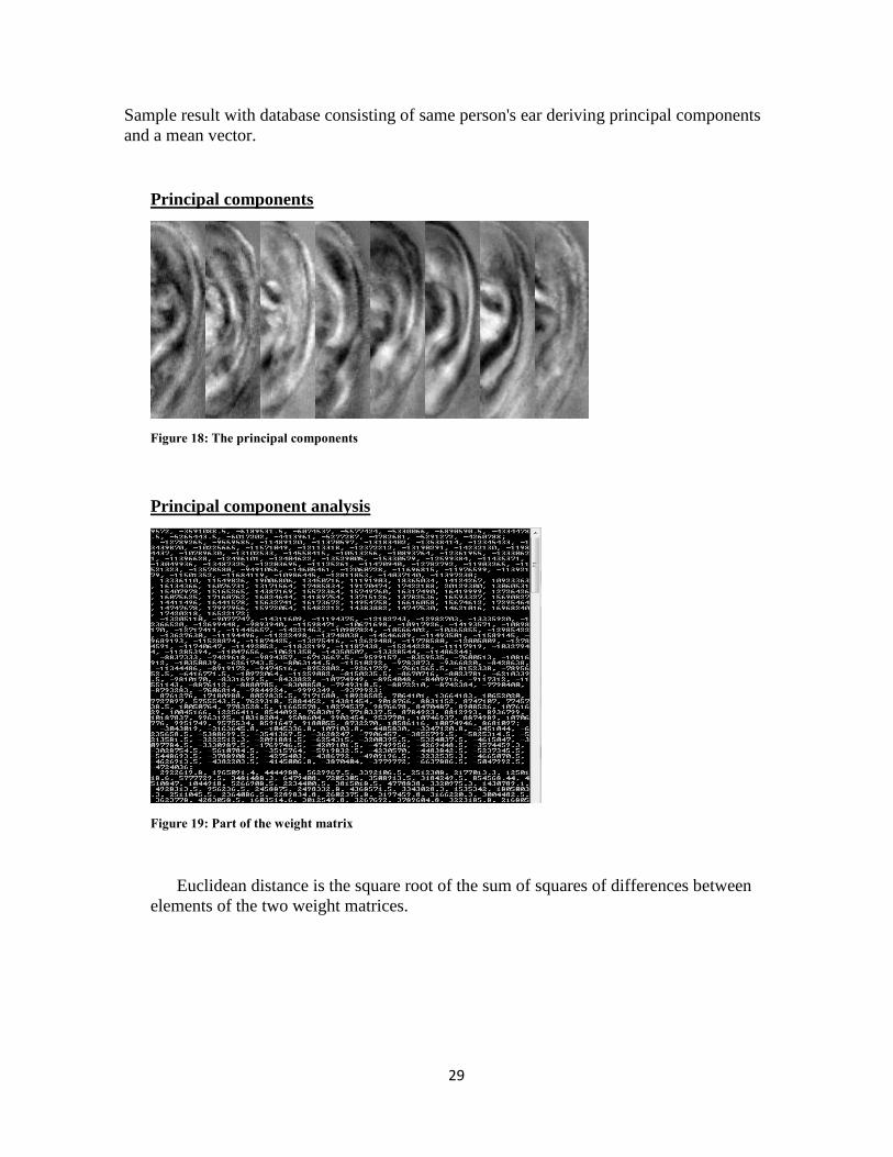
Principal component analysis
Figure 19: Part of the weight matrix
Euclidean distance is the square root of the sum of squares of differences between
elements of the two weight matrices.

30
Principal Component Analysis
Calculate the principal components of the ear images of different people.
Documentation defines the basic usage of PCA in opencv.
• Open the images in gray scale and push them into a vector of matrices.
• Create a function which returns the vector content as a row matrix. (This is
required because the PCA class of OpenCV does not accept the images in
vector form).
• Retrieve the number of images (n) in the vector and the dimensionality
of images (d).
• Create a new matrix with „n‟ as the number of rows and „d‟ as number
of columns equivalent to type of the vector. E.g., the following matrix
has n = 2 rows and d = 10 dimensions. i.e. 2 images with 10 dimension
each.
• Errors are checked to make sure the vector is not empty or there is no
mismatch of dimensions between images.
• The current row of this matrix is filled with the pixel values from the
images residing in the vector.
• Perform the principal component analysis (PCA) on the returned matrix with
customizable number of components.
• Calculate the eigenvectors and eigenvalues.

31
Observations:
The following images are used from the IIT Delhi ear database for testing purposes.
The ears belong to 5 different people of varied ethnicity.
Figure 20: Original ears
Principal components after running the code:
PC1 PC2 PC3 PC4
Figure 21: Top four eigenvectors
Obtain the weight matrix
The next step is involving particular steps of matrix multiplication, which is used in
order to calculate an entity named weight matrix.
The weight matrix is used as
• A machine understandable representation of the images and the principal components
acquired in the previous stages.

32
• In addition to comparing images, the weight matrix is useful in estimating the
threshold that will be used as an error margin when accepting or rejecting a person
during their biometric scan.
(Scalar Weight Matrix
Multiplication) of each image
Euclidean distance calculation
Calculate the Euclidean distance between two weight matrices to verify if the two
images (one current scan of the ear and one from the database) are equal within a certain
allowed limit (threshold). The scalar multiplication in the previous stage will result in a matrix
with weights for each of the image i.e.
Image 1
Image 2
.
.
.
Image n-1
Image n
PC1a PC2a ….. PCna
PC1b PC2b ….. PCnb
PC1c PC2c ….. PCnc
.
.
.
PC1n PC2n ….. PCnn
Figure 22: Weight matrix calculation
W.M 1
W.M 2
.
.
.
W.M n-1
W.M n
Figure 23: Weight Matrix

33
W.M x:- weight matrix of the corresponding image.
• These matrices are stored in the database.
• When a person is to be verified, the corresponding weight matrix of the image from
database is retrieved and then matched against the weight matrix of the current
scanned image.
• Euclidean distance = square root( |a1 – a‟1|2 + |b1 – b‟1|
2 +…+ |n1 – n‟1|
2);
The storage of weight matrices for every individual is kept separately on the disk using a
„.yaml‟ file. YAML is a hybrid format combining features from XML (machine readable) and
programming languages like C++.
Every enrolled person has an associated weight matrix and a PIN to distinguish them from
other individuals. Hence, the weight matrix corresponding to an individual is stored in a
„.yaml‟ file with their PIN as the name of that particular file. This technique helps in easy
retrieval of the weight matrices during different phases of the system.
Post-PCA
The matrix that contains the initial set of images, say (alpha) α, e is the matrix
containing eigenvectors stored in column major form, ρ holds the probe images stored in one
row.
λ = α‟ //lambda is the transpose of alpha
ψ = Mean (λ) //row wise mean is stored in a single column
ω = λ – ψ //subtract each row‟s mean
weight_matrix = ω‟ * e
ψ = Mean (ρ) //row wise mean is stored in a single column
t = ρ – ψ //subtract each row‟s mean
weightprobes_matrix = t * e
The matrices weight_matrix and weightprobes_matrix are used for score generation in the
ROC curve.

34
Implementing ROC curve
Running sample verifications for agreeing on a point which is used as a threshold for
the purpose of matching 2D images of the person‟s ear. Thereby, resulting in True positive
rate and False positive rate and giving rise to the ROC (Receiver operating characteristic
curve) which represents the overall performance of the system under investigation by variance
of the threshold. The threshold will be agreed upon this stage accommodating an acceptable
amount of error rate during the verification of a person.
Moving on, the following work will involve creating a database of images for the purpose
of enrolling a person into the system.
• One image per person will be taken during the initial stages of the process.
• This image will go through principal component analysis and then the resulting weight
matrix (W) will be stored in the database.
• The storage will include the person‟s personal identifier in the filename for future
referencing.
• When the person wants to verify themselves, the personal identifier is matched against
the filenames to retrieve the correct data image.
• The new image produces another weight matrix (W‟).
• If the Euclidean distance between W and W‟ matrices lies in the acceptable zone it is a
genuine score, else it results in an imposter score.

35
Chapter 4: Current Context
Ear biometrics play a vital role in many sectors of immigrations, for example,
according to (Yuan, Mu, & Xu, 2005) the US Immigrations require an applicant to submit their
photographs according to a particular specification which allows them to view part of the right
ear. This is used for the purposes of biometric verification or watch-list identification. In
context to an investigation ear forms a good method of identification when other biometric
either fails or is unavailable. In the field of criminology, investigators have recognized the
usage of ear as a vital role in the identification of criminals. Alphonse Bertillon realized the
path of identification through ears, (Bertillon, 1890). Moreover, Ear biometrics was used in
recognition of humans even before the birth of fingerprinting technology. Alfred Victor
Iannarelli describes in his book a clear analysis of the various aspects of ear which are used
for the purpose of identification of people.
Furthermore, the people in law enforcement make use of Iannarelli‟s ear biometrics method
and analyze the ears when trying to identify criminals because some of them might have
undergone plastic surgery on their faces, but ears rarely change and are hardly modified using
surgery therefore they form a more solid form of identification than facial features. Moreover,
they are helpful in identification when other biometrics are either not available or are very less
accurate, (Steele, 2011).
In addition, (Steele, 2011) describes the growth of ear with age. According to research conducted
by Iannarelli, the human ear forms its basic features completely at 4 months of age, from this
point onwards its size increases without alteration in shape till the person is 20 years of age.
Moving on, the length of the ear increases from 7mm to 13mm by the age of 60-70.
Another research by James A. Heathcote points to the fact that human ears grow at 0.22mm
per year on an average. But since this growth does not affect the structure, design and form of
the ear, therefore it is possible to use it for the purpose of human recognition with individuals
of varying age.
According to a 1995 British study with several other physicians and hundreds of subjects aged
30-93, James A. Heathcote, MD concluded that our ears grow at an average rate of about
.22mm (.01 inches) per year. This study was confirmed by a Japanese study of 400 people in
1996. While average growth rates vary from person to person and may vary during different
stages in a person's life, we can assume that an individual with a 2" long ear at age 30 would,
by age 80, have achieved about a 25% growth rate, resulting in about a 2-1/2" long ear.
Taking it another direction as described in (News Staff, 2010), the latest development in the field
of ear recognition comes from scientists of the University‟s School of Electronics and
Computer Science (ECS). They claim to have highlighted a technique named image ray
transform which is capable of contrasting tubular structures (ears) for the purpose of
identification. This technique makes use of the elliptical shape of a particular part of the ear
like the helix with a success rate of astonishing 99.6% during enrollment phase consisting of
252 images and taking into account the errors due to hair and/or glasses, this study provides a
great platform for the future of ear biometrics in numerous fields.

36
According to me, this study is a path towards integrating ears into the world of security with
more confidence as the success rate is very high compared to any other technique employed
for the purpose of enrollment even though the complexity is quite high.
3D ear recognition systems
Research has been going on in the 3D section of ear recognition systems, (Paug & Busch,
2012). A three dimensional image provides more information (structural or behavioral) as it can
be rotated, scaled and translated which is not feasible in 2D systems. Moreover, the extra
information in three dimensions can be used to improve the accuracy of the system by
reducing the error rates (FAR or FRR). Although the system might incorporate several
components leading to an expensive investment it has a bright future due to its accuracy.
As described in (Islam, Davies, Bennamoun, & Mian, 2011), the algorithm for 3D ear recognition system
is the Iterative Closest Point (ICP) which deploys local feature matching and can be used in
tandem with 2D AdaBoost detector to procreate an accurate and fast system. The 2D detector
makes use of 2D images for the purpose of ear detection. The next step involves extraction of
the 3-dimensional ear data (structural) from the image while showing the local 3D features.
These features form the basis of the rejection classifier used in the system. With a 99.9%
detection rate and 95.4% identification rate the ICP algorithm marks the beginning of a new
era in 3D recognition systems.
Usage
In the United States of America, immigration has employed fingerprint recognition
system for the purpose of watch-list identification (i.e. negative identification). While in the
United Arab Emirates they are using an Iris recognition system for the purpose of identifying
deported individuals attempting to re-enter the country, (Ross & Abaza, Human Ear Recognition, 2011).
Study has begun for the integration of different characteristics such as height, body shape,
scars or marks with the traditional physical biometric. This multi-modal system will reduce
the inaccuracies of the physical biometric by improving the error rates.

37
Figure 24 Ear images (IIT database)
The above figures represent the static and dynamic differences between ears of
separate individuals. For example, the pinna, triangular fossa and the crus of helix are
different in size, color and/or texture.
At the (University of Science and Technology Beijing, 2007) work has been going on ear
recognition for the past few years. This work encompasses certain processes namely,
detection, normalization, feature extraction and recognition. In 2003, using the method of
kernel PCA, the university was able to achieve an ear identification rate of 94%. In the
following ears, they included rates arising from pose and lighting variations. Furthermore, it
was proposed to use a modified algorithm of AdaBoost for the purpose of real-time detection
and take into account occlusions. With advances in other sectors (normalization, feature
extraction and recognition) it is clear that ample amount of effort is being put worldwide to
make ear a popular biometric by mitigating its weaknesses and thus improving the security in
sensitive facilities where the recognition system can be employed.
Challenge
Public face identification can be difficult as cameras mounted in public places may not
be able to acquire the complete face image of a person, however at this point it would be an
advantage if the camera was able to pick up the ear from a distance for the purpose of
identification as it has lesser inter-class and intra-class variations when compared to face. It
may also use the technique of fusing face and ear identification at different levels like feature,
sample or decision level, (Paug & Busch, 2012).
Symmetry
As of now, there have been no studies on the relationship of symmetry between the
two ears of an individual. Iannarelli has shown that the two factors that remotely affect the
outer ear appearance are inheritance and ageing.
In the near future it is possible to study the symmetric relationships along with effects of
inheritance leading to a complex but more precise ear recognition system.

38
Future considerations
According to a conference paper edited by (Sun, Tan, Lai, & Chen, 2011), when it comes to 2D
ear recognition systems it is important to consider the effects of ear registration and its
alignment as they can render a very good algorithm useless due to higher error rates relating to
spatial positions. Therefore, for advancement in 2D ear recognition systems the following
factors must be dealt with:
• Illumination: 2D images of the ear require the right amount of illumination for the
purpose of extracting local features efficiently.
• Pose variations: Currently, there are few algorithms that are efficient enough to handle
pose variation. This factor can be a tedious problem in Principal component analysis as
the method depends upon the alignment of the ear.
• Occlusions: Algorithms can take into account occlusions like hair and/or spectacles,
for example, by using segmentation of ear image and then applying separate classifiers
to each segment.

39
Chapter 5: Results
Reconstruction
The ear can be reconstructed by applying back-projection from the PCA subspace in
the principal component analysis method. The ears are reconstructed using the normalized
matrix (which has its mean subtracted from it) of the images in the database and the
eigenvectors computed from the PCA method.
The following figure gives an example of the reconstructed ear from images 001 to
010 of the 50 images in the database using 50 eigenvectors.
Figure 25: Original Ears 1-10
Figure 26: Reconstructed Ears 1-10
Errors
The error rate between the original ear (O) and the reconstructed ear (R) is found using the
following formula:
Error rate = ∑ ∑ –
2 / O(i,j)
2]

40
Ear Pair (Original & Reconstructed) Error rate
001 0.494423
002 0.415781
003 0.472347
004 0.343564
005 0.488391
006 0.47529
007 0.479895
008 0.428305
009 0.473665
010 0.313577 Table 2: Error rates of first 10 samples and their reconstructed image.

41
ROC Curve
For the given curve 30 Eigenvectors were used in conjunction with 30 images in the
database.
Figure 27: ROC curve with 30 Eigenvectors

42
For the following curve 50 samples were used in addition to 2 samples each for the
same individual.
Figure 28: ROC Curve with 50 Eigenvectors
The green line in the above figure is „y=1-x‟ and the intersection of this line with the curve
results in the Equal error rate (EER) with False positive rate (FPR) = 0.2 and True positive
rate (TPR) = 0.8

43
FMR: False Match Rate = False Positive Rate (FPR)
FNMR: False Non-Match Rate = 1 – True Positive Rate (TPR)
Figure 29: FMR Vs FNMR curve with assistance from (Conway, Biometric Errors for Verification Handout(week 2),
2013)
Low False Match rate implies more security while convenience is achieved by
reducing the False Non-Match rate.

44
Figure 30: ROC Curve with 55 Eigenvectors
Verification
The system is enrolled with images 01 to 50 in the database. The following table
contains samples of scores used in the ROC curve.
Genuine scores Imposter score
1.4232e+006 2.16749e+008
4.0441e+006 2.79522e+008
2.76344e+007 9.67247e+007
2.04753e+006 2.22609e+008
3.12499e+007 1.92432e+008

45
Discussion
The sections of an ROC curve define the abstract performance of the system under
observation. The line x-y=0 in fig. 27 represents the natural random process of guessing while
any system falling beneath it is considered to be worse than random guessing. According to
the ROC curve in the previous section it can be observed that the system‟s performance is
well above the x-y=0 line indicating the fact that the classifier is better than random guessing.
From the above fig. 27, 28 and 30 it can be observed that the curve moving towards the upper
left corner of the graph which signifies that the performance of the system is better with the
involvement of more eigenvectors. fig. 28 and 30 show better performance of the system
compared to fig 27. as it contains 30 eigenvectors only. The instances that produced figures 28
and 30 use 50 and 55 eigenvectors respectively. Therefore it can be inferred from the
observations that the system performance increases with more number of eigenvectors.
The error rates derived in the ear reconstruction phase give an average rate of 0.469251 i.e.
46.9251% for 50 samples in the database. Therefore it can be inferred that the performance of
the system on an average is 53.0749%.
From the performance of the system under average conditions it can also be inferred that
principal component analysis of the ear is an apt method for usage in 2D recognition systems
as it gives above average performance with ease of implementation and is comparatively less
expensive than other biometrics like iris. Moreover, it can also be considered that since the
structure of the ear remains consistent throughout the lifetime of an individual it preserves the
timeliness.
After getting insights in the working of the biometric it is observed to probably have the
following properties:
Universality: Every individual possesses ears except in some cases where it may be
damaged in accident. Nevertheless the probability of damaging both the ears is
expected to be low.
Uniqueness: No two ears are same even for the same person.
Permanence: The structure of the ear hardly alters over time.
Circumvention: is low as it is difficult to replicate the trait.

46
Conclusions
In my research for the usage of biometrics in security I have used the method of
principal component analysis followed by score generation which yields a good result. It was
found that ear possesses many of the biometric properties which make it apt for usage in
security sensitive areas.
According to the observations from the ROC curve it can be concluded that the system
performs above average under the conditions that the ear image is equalized, normalized and
is aligned at a right angle with respect to the horizontal axis. These requirements form the base
nature for the method implemented i.e. Principal Component Analysis (PCA). Moreover, the
ROC curve is generated by varying the threshold in the range defined by computed genuine
and imposter scores thus giving rise to a dynamic set of points which portray system
performance with varied conditions. Moreover, the ear reconstruction results in system
performance of approximately 53%.
Finally, the PCA has helped in forming a simple system which is capable of detecting the ear
from a live video stream, analyzing the images and reducing its dimensions leading to easier
calculations of the Euclidean distance. This distance acts as a comparison framework for
images to be verified using ROC curve, as lesser is the distance between two matrices then
closer they are to each other, mathematically.
Future work
In future research relating to ear biometrics, it is possible to add a multimodal
approach in conjunction with face using the algorithm of Eigen faces. The first approach is
combining the face and ear images pre-PCA and applying the process of principal component
analysis on the resulting image. These images can be combined horizontally or vertically with
minute variation in recognition rates. The second approach utilizes post-PCA combination of
the images where the Eigen face and Eigen ear methods are applied separately and the
resulting transformed matrix is combined to form the final entity.
Moreover, the system has been built such that it is capable of upgrading to single verification
mode, where each person is capable of verifying themselves using their PIN and live query.
Finally, the capturing of ear requires human intervention for the need of image alignment. The
orientation of the ear must be kept vertical at 90 degrees with respect to the horizontal axis.
This feature, in the future, can be set up automatically for increasing the speed and accuracy.

47
References
Antakis, S. (2009, Feburary 23). A Survey on Ear Recognition. Enschede, The Netherlands.
Bertillon, A. (1890). La Photographie Judiciaire: Avec Un Appendice Sur La Classification Et
L'Identification Anthropometriques. Paris: Gauthier-Villars.
Conway, R. (2013, April 29). Biometric Errors for Verification Handout(week 2). Limerick,
Ireland.
Conway, R. (2013, Feburary 15). Week 1 intro handout. Limerick, Ireland`.
Gurchiek, K. (2012, September 14). Facial Recognition Technology Raises Privacy Issues.
Technology.
Hawkes, B. (2003). Biometrics in Schools, Colleges and other Educational Institutions.
Retrieved June 25, 2013, from Data Protection Commissioner:
http://www.dataprotection.ie/docs/FAQ/1236.htm
Iannarelli, A. V. (1989). Ear Identification, Forensic Identification series. California:
Paramont Pub.
Islam, S. M., Davies, R., Bennamoun, M., & Mian, A. S. (2011). Efficient Detection and
Recognition of 3D Ears. Int Journal of Computer Vision manuscript No.
Jain, A. K. (2004). Biometric Authentication How do I know who you are? Michigan, United
States of America.
Lammi, H.-K. (2003, November 19). Ear Biometrics. Lappeenranta, Finland.
News Staff. (2010, October 10). Biometrics: Identifying People By Their Ears. Retrieved July
21, 2013, from Scientific Blogging:
http://www.science20.com/news_articles/biometrics_identifying_people_their_ears
opencv dev team. (2013, July 1). Cascade Classification. Retrieved July 19, 2013, from
OpenCV: http://docs.opencv.org/modules/objdetect/doc/cascade_classification.html
Paug, A., & Busch, C. (2012, July 2). Ear Biometrics: A Survey of Detection, Feature
Extraction and Recognition Methods.
Prabhakar, S., Pankati, S., & Jain, A. K. (2003). Biometric Recognition: Security and Privacy
concerns. Denton: IEEE Computer Society.
Ross, A. (2011). Advances in Ear Biometrics. Virginia, United States of America.
Ross, A., & Abaza, A. (2011, November). Human Ear Recognition. Identity Sciences. IEEE
Computer Society.

48
Saleh, M. I. (2007, May 7). Using Ears for Human Identification. Blacksburg, Virginia,
United States of America.
Smith, L. I. (2002, Feburary 26). A tutorial on Principal Component Analysis. Otago, New
Zealand.
Steele, J. (2011, November 5). Ears Don't Lie. Olympia, Washington, United States of
America.
Sun, Z., Tan, T., Lai, J., & Chen, X. (2011). 3D Ear Recognition Based on 2D Images.
Biometric Recognition: 6th Chinese Conference (p. 257). Beijing: Springer-Verlag.
University of Science and Technology Beijing. (2007). Ear Recognition Laboratory. Beijing,
China.
Viola, & Jones. (2001). Rapid object detection using boosted cascade of simple features.
Computer Vision and Pattern Recognition.
Wikipedia. (2001). Information Security. Retrieved June 25, 2013, from Wikipedia:
http://en.wikipedia.org/wiki/Information_security
Yuan, L., Mu, Z., & Xu, Z. (2005). Using Ear Biometrics for Personal Recognition. Beijing,
China.

A-1
Appendix
Source code overview
The source code is split into two parts, a header file containing the main class and the main c plus plus file
in which the main function resides.
File: detect_new.h
The header file contains the main class which has the following functions defined
forming the basic foundation of the program:
detect_new(): Constructor loads the haar cascade xml file for ear detection
pre: none
post: xml file loaded for use in program
ear_detection(Mat, int, int): detects the ear in live video stream.
pre: requires the frame of video, identification number of user and option 0 or 1 for enrollment
and verification respectively.
post: ear is detected, captured and a rectangle is displayed surrounding it in the live feed.
error_checking(): checks whether xml file loaded correctly or not.
pre: none
post: returns true or false if the file is loaded correctly or incorrectly respectively.
load_images(int, int): loads the images onto an array of Matrices (Mat).
pre: requires identification number of the user and option 0 or 1 for enrollment and verification
respectively.
post: the images are loaded onto the corresponding array
load_probes(int &): loads the probes i.e. different samples for each image in the database onto
an array of Matrices (Mat).
pre: requires identification number of the user
post: probes are loaded onto an array of Matrices (Mat) and then pushed into a vector forming a
vector of images.
Matrix_change_form(const vector<Mat>&, int, char, double alpha, double beta): changes
the images in a vector of matrices into a single matrix with each row occupying a single image.
pre: requires vector of images with the type of matrices (i.e. float in this case), an option to
select row major or coloumn major form
and default values for the inbuilt function convertTo; alpha is the scale factor and beta is the
delta added to this scale factor.
post: returns the reshaped matrix.

A-2
normalize_img(Mat &): returns the normalized image.
pre: the original image is passed by reference to avoid conflict of local updating of the image in
the function.
post: the image is normalized and returned
push_img_vector(int, int): returns a vector of equalized images.
pre: requires option for enrollment or verification and the identification number of the user.
post: the images are equalized, pushed into the vector which is then returned.
#pragma once
#include <map>
int capture_count = 0; //for counting no. of samples per person
Mat probes[100]; //holds probe images for the users in database
Mat e; //holds the eigenvectors generated from PCA
Mat psi; //used to hold average of row in a matrix
class detect_new
{
private:
char* file; //stores name of the haar cascade classifier file
CascadeClassifier ear; //CascadeClassifier class object to detect ear in a live video stream
Mat image[143]; //stores the images as they are from the disk during enrolment stage
Mat img[143]; //stores the images from image with an equalized Histogram during enrolment stage
Mat ver; //stores the images as they are from the disk during verification stage
Mat ver2; //stores the images from image with an equalized Histogram during verification stage
public:
detect_new();
void ear_detection(Mat, int,int);
void load_images(int,int);
bool error_checking();
Mat normalize_img(Mat&);
Mat Matrix_change_form(const vector<Mat>&, int ,char op, double alpha , double beta );
Mat Matrix_mult(Mat ,Mat);
vector<cv::Mat> push_img_vector(int, int);
vector<cv::Mat> load_probes(int &);
};
Mat detect_new::Matrix_mult(Mat pic, Mat eign)
{
if(pic.cols == eign.rows) //matrix multiplication condition
return (pic * eign); //return the matrix multiplication
else
return Mat(); //else return empty matrix
}
vector<cv::Mat> detect_new::push_img_vector(int op, int PIN)
{
vector<cv::Mat> images_v;
if(op == 0) //enrolment

A-3
{
for(int i=1; i<=PIN; i++)
{
equalizeHist(image[i-1], img[i-1]); //equalize histogram
images_v.push_back(img[i-1]); //push the image into the vector
}
}
else if(op == 1) //verification
{
equalizeHist(ver, ver2);
images_v.push_back(ver2);
}
return images_v;
}
Mat detect_new::Matrix_change_form(const vector<Mat>& orig, int rtype , char op, double alpha=1 , double
beta=0)
{
Mat new_mat; //new matrix
Mat c; //temporary row matrix
size_t d;
size_t s = orig.size(); // acquire the Number of images in the vector
// return an empty matrix if error
if(s == 0)
return Mat();
// dimensionality of (reshaped) or modified samples
d = orig[0].total();
//equal to pixels of 1st image as all images must be of same dimensions
// Create resulting data matrix and copy data:
for(int i = 0; i < s; i++) {
//
if(orig[i].empty()) {
std::cerr<<"Error the image "<<i<<" is empty!!!";
}
if(orig[i].total() != d) {
std::cerr<<"Error, matrix contains the wrong number of elements!!! please check
dimension (no. of pixels of any 1 image)";
}
if(op == 'r')
{// Get the current row:
new_mat.create(s, d, rtype);
c = new_mat.row(i);
if(orig[i].isContinuous()) {
orig[i].reshape(1, 1).convertTo(c, rtype, alpha, beta);
// reshape to 1 channel and 1 row
} else {

A-4
orig[i].clone().reshape(1, 1).convertTo(c, rtype, alpha, beta);
//since clone does not copy the gaps
}
}
else if(op == 'c'){ // Get the current column
new_mat.create(d, s, rtype);
//since s=> numbor of PCs which should be in seperate columns
c = new_mat.col(i);
}
if(orig[i].isContinuous()){
orig[i].reshape(1, d).convertTo(c, rtype, alpha, beta);
// reshape to 1 channel, d rows where d is number of pixels in the PC
} else {
orig[i].clone().reshape(1, d).convertTo(c, rtype, alpha, beta);
//since clone does not copy the gaps
}
// reshape by cloning for non-continuous matrices
}
return new_mat;
}
vector<cv::Mat> detect_new::load_probes(int &PIN)
{
//load 5 other samples not used for eigenvectors for each PIN
char buffer[53];
vector<cv::Mat> vec;
for(int i=1; i<=50; i++)
{
for(int k=0;k<2;k++)
{ //load the probes
if(i>=10)
probes[(i-1)*2+k] = imread("E:/ear_images/ear/processed/221/0" +
string(itoa(i,buffer,10)) + "_"+string(itoa(k+2,buffer,10))+".bmp",0);
else
probes[(i-1)*2+k] = imread("E:/ear_images/ear/processed/221/00" +
string(itoa(i,buffer,10)) + "_"+string(itoa(k+2,buffer,10))+".bmp",0);
vec.push_back(probes[(i-1)*2+k]); //push the images into the vector
}
}
return vec;
}
void detect_new::load_images(int PIN, int op)
{
char buffer[33]; //used for integer to alphabet conversion
Mat check;
if(op == 0) //enrolment
{
for(int i=1;i<=PIN;i++)
{//load the probes
if(i>9)

A-5
{
image[i-1] = imread("E:/ear_images/ear/processed/221/0" +
string(itoa(i,buffer,10)) + "_1.bmp",0);
}
else
{
image[i-1] = imread("E:/ear_images/ear/processed/221/00" +
string(itoa(i,buffer,10)) + "_1.bmp",0);
}
}
}
else if(op == 1)
{//verification
ver = imread("E:/ear_images/ear/processed/221/0" + string(itoa(PIN,buffer,10)) + "_1.bmp",0);
}
}
Mat detect_new::normalize_img(Mat& orig)
{
//orig: original image
// Create and return normalized image
Mat modified;
case 1:
normalize(orig, modified, 0, 255, NORM_MINMAX, CV_8UC1);
break;
case 3:
normalize(orig, modified, 0, 255, NORM_MINMAX, CV_8UC3);
break;
default:
orig.copyTo(modified);
break;
}
return modified;
}
detect_new::detect_new()
{
file= "haarcascade_mcs_rightear.xml";
//the xml file describing to the compiler how does the ear appear
}
bool detect_new::error_checking()
{
//error checking
if(ear.load(file) == false)
{
return false; //error
}
else
{
return true;
}
}
int index=0;

A-6
void detect_new::ear_detection(Mat frame, int PIN, int op)
{
char buffer[33]; //for itoa
std::vector<Rect> ears; //stores ear images (type Rect) in a vector
Mat frame_graysc; //grayscale frame
int c,fi=0;
cvtColor( frame, frame_graysc, CV_BGR2GRAY ); //convert frame to grayscale frame
equalizeHist( frame_graysc, frame_graysc ); //equalized histogram of the image
//Detect ears
ear.detectMultiScale( frame_graysc, ears, 2.0, 0, 0|CV_HAAR_SCALE_IMAGE,Size(35,35));
for( size_t i = 0; i < ears.size(); i++ )
{
fi++;
//save the file with pin name
Mat cropped = frame_graysc(ears[i]); // to crop the image in a later stage
//Draw the ears
rectangle(frame,Point(ears[0].x,ears[0].y) ,Point(ears[ears.size()-1].x+ears[ears.size()-
1].width,ears[ears.size()-1].y+ears[ears.size()-1].height),Scalar(255,0,255),1,8,0);
imshow( "Captured Ear Image", cropped);
c = cvWaitKey(10);
if(c==32)
//if space bar is pressed write the image of ear onto the disk location specified.
{
//assumming program runs 1nce for 1 person
if(op == 0)
{
imwrite("E:/ear_images/sample" + string(itoa(PIN,buffer,10)) + "_" +
string(itoa(capture_count,buffer,15)) + string(".jpg"), cropped);
capture_count++; //1 shot taken
}
else if(op == 1) //verification
{
imwrite("E:/ear_images/sample" + string(itoa(PIN,buffer,10)) + "_v" + string(".jpg"),
cropped);
}
}
}
//Show the result
imshow( "Ear Detection", frame );
}

A-7
File: pc_new.cpp
The cpp file contains the main function which drives the program and the header file
previously mentioned.
calc_vm_verf(Mat): returns a single row weight matrix of a single image
pre: requires the matrix omega which is calculated in the function omega_calc(Mat).
post: calculates the row weight matrix by multiplying omega with e (eigenvectors matrix).
capture_from_CAM_v(int): captures the ear image from live feed during verification stage.
pre: requires the identification number of the user.
post: the ear image is captured and stored for future purposes.
capture_from_CAM1(string, map<int, string>): Captures from ear image and works with
database handler to generate a pin
pre: requires name of user and a map which is capable of storing the names along with the
identification numbers.
post: returns the identification number (PIN) for the corresponding user.
database_handler(string, map<int, string>): generates the PIN and returns it to
capture_from_CAM1.
pre: requires name of user and a map which is capable of storing the names along with the
identification numbers.
post: writes the map to the file.
load_weight_mat(int): loads the weight matrix from the disk into the program.
pre: requires the identification number of user
post: returns the loaded matrix
omega_calc(Mat): returns omega.
pre: requires the original matrix of images.
post: omega is calculated by rotating the original matrix to lambda and then subtracting mean.
perform_pca(detect_new, vector<Mat>, Mat, int): performs principal component analysis
(PCA) and returns the weight matrix.
pre: requires the class object to access its public functions, vector of images, omega and PIN.
post: generates eigenvectors during the PCA process.
reconstruct_ears(Mat, int): reconstructs a particular ear sample.
pre: requires backprojected matrix from pca which is calculated in perform_pca method.
post: reconstructs the ear into correct dimensions.
score_generator_new(Mat, Mat): generates the genuine and imposter scores for
implementation in ROC curves.
pre: requres the original weight matrix and weightprobes matrix.
post: the scores are generated are written onto the disk.

A-8
weightprobes_calc(int &): generates the weightprobes matrix i.e which contains different
samples for every user.
pre: requres the identification number of the user.
post: returns the weightprobes matrix.
write_weight_mat(Mat, int): writes the weight matrix onto the disk.
pre: requires the original weight matrix and the identification number of the user.
post: none
rec_error_calc(): calculates the error rates for reconstructed ear.
pre: ears must be reconstructed prior to calling this function.
post: the error rates are calculated accoriding to a pre-defined formula.
void capture_from_CAM_v(int PIN)
{
CvCapture* click;
Mat frame;
detect_new object;
bool check;
check = object.error_checking();
if(check == false)
{
std::cout<<"Error capturing from video stream!";
_getch();
exit(-1);
}
//capture from camera
click = cvCaptureFromCAM(1); //capture from in-built camera
if(click)
{
while(1) //infinite loop
{
frame = cvQueryFrame(click) //extract the frame from video
//now use the classifier
if(frame.empty() == false)
{
object.ear_detection(frame, PIN,1);
//go to the function to detect the ear
}
else
{
std::cout<<"Error in capturing from video stream!!!\n";
break;

A-9
}
int wait = cvWaitKey(10);
if( (char)wait == 'c' )
{
break;
}
}
}
}
int capture_from_CAM1(string name, map<int,string> m)
{
int PIN;
CvCapture* click;
Mat frame;
detect_new object;
bool check;
check = object.error_checking();
if(check == false)
{
std::cout<<"Error capturing from video stream!";
_getch();
exit(-1);
}
click = cvCaptureFromCAM(1); //capture from in-built camera
if(click)
{
//insert values in m
m[0] = name;
cout<<"name: "<<m[0];
PIN = database_handler(name,m);
//make map persistent by writing it to file
while(1) //infinite loop
{
frame = cvQueryFrame(click); //extract the frame from video
//now use the classifier
if(frame.empty() == false)
{
object.ear_detection(frame, PIN,0);
//go to the function to detect the ear
}
else
{
std::cout<<"Error in capturing from video stream!!!\n";
break;
}

A-10
int wait = cvWaitKey(10);
if( (char)wait == 'c' )
{
break;
}
}
}
return PIN;
}
int database_handler(string name, map<int,string> m)
{
int ret=1; //return value
ofstream outputFile; //to write to a file
ifstream inputFile; //to read from a file
string value;
outputFile.open("E:/ear_images/config_0.txt", ios::out | ios::app);
//write map m to file
outputFile << "\n";
for (map<int,string>::const_iterator i = m.begin(); i != m.end(); ++i)
{
outputFile << i->second;
}
//close file in write mode before reading it
outputFile.close();
//read
inputFile.open("E:/ear_images/config_0.txt", ios::in | ios::beg );
//read from configuration file
std::map<int, string> myMap;
while (getline(inputFile, value,'\n'))
myMap[index++] = value;
cout<<"Read from file: ";
for( map<int,string>::iterator ii=myMap.begin(); ii!=myMap.end(); ++ii)
{
cout << (*ii).first << ": " << (*ii).second << endl;
if((*ii).second == name) //i.e the person being enrolled!
{
ret =(*ii).first;
//corresponding PIN generated (to be used later during verification stage)
}
}
//close file
inputFile.close();
return ret;
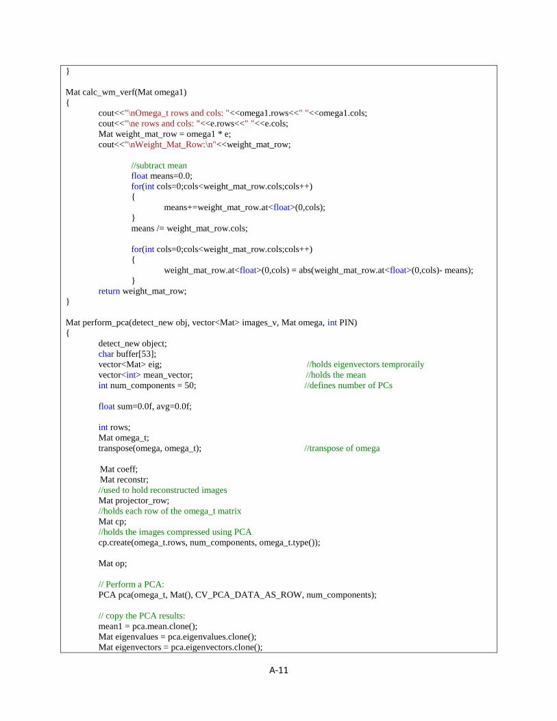
A-11
}
Mat calc_wm_verf(Mat omega1)
{
cout<<"\nOmega_t rows and cols: "<<omega1.rows<<" "<<omega1.cols;
cout<<"\ne rows and cols: "<<e.rows<<" "<<e.cols;
Mat weight_mat_row = omega1 * e;
cout<<"\nWeight_Mat_Row:\n"<<weight_mat_row;
//subtract mean
float means=0.0;
for(int cols=0;cols<weight_mat_row.cols;cols++)
{
means+=weight_mat_row.at<float>(0,cols);
}
means /= weight_mat_row.cols;
for(int cols=0;cols<weight_mat_row.cols;cols++)
{
weight_mat_row.at<float>(0,cols) = abs(weight_mat_row.at<float>(0,cols)- means);
}
return weight_mat_row;
}
Mat perform_pca(detect_new obj, vector<Mat> images_v, Mat omega, int PIN)
{
detect_new object;
char buffer[53];
vector<Mat> eig; //holds eigenvectors temproraily
vector<int> mean_vector; //holds the mean
int num_components = 50; //defines number of PCs
float sum=0.0f, avg=0.0f;
int rows;
Mat omega_t;
transpose(omega, omega_t); //transpose of omega
Mat coeff;
Mat reconstr;
//used to hold reconstructed images
Mat projector_row;
//holds each row of the omega_t matrix
Mat cp;
//holds the images compressed using PCA
cp.create(omega_t.rows, num_components, omega_t.type());
Mat op;
// Perform a PCA:
PCA pca(omega_t, Mat(), CV_PCA_DATA_AS_ROW, num_components);
// copy the PCA results:
mean1 = pca.mean.clone();
Mat eigenvalues = pca.eigenvalues.clone();
Mat eigenvectors = pca.eigenvectors.clone();

A-12
// The mean ear:
imshow("Mean", obj.normalize_img(mean1.reshape(1, images_v[0].rows)));
//do not forget the mean component!
PC[0] = obj.normalize_img(mean1.reshape(1, images_v[0].rows));
eig.push_back(PC[0]);
// The eigenears:
for(int i=1;i<50;i++)
{
PC[i] = obj.normalize_img(pca.eigenvectors.row(i)).reshape(1, images_v[0].rows);
//store PCs. in a column matrix form
eig.push_back(PC[i]);
}
//change to column matrix i.e each PC is stored in seperate columns
e = obj.Matrix_change_form(eig, CV_32FC1,'c');
int cnt=1;
//counter
for(int i=0; i<omega_t.rows;i++)
{
projector_row = omega_t.row(i);
coeff = cp.row(i);
pca.project(projector_row, coeff);
//each row of omega_t containing modified images is projected into pca space
pca.backProject(coeff,reconstr); //reconstruction
reconstruct_ears(reconstr,cnt);
cnt++;
}
//subtract mean from every col of omega
for(int rows=0; rows<omega_t.rows; rows++)
{
for(int cols=0; cols<omega_t.cols; cols++)
{
omega_t.at<float>(rows,cols) -= mean1.at<float>(0,cols);
}
}
//weight matrix is the product of omega_t and e(eigenvector matrix)
Mat weight_mat = omega_t*e;
//store the principal components onto the disk
for(int i=0; i<10; i++)
{
//store the images on the drive
imwrite("E:/ear_images/PCs/PC" + string(itoa(i, buffer, 10))+ ".jpg", PC[i]);
}
return weight_mat;
}

A-13
void write_weight_mat(Mat weight_mat, int PIN)
{
char buffer[33];
//store weight matrix in a yaml file
FileStorage fs("E:/ear_images/weight_matrices/test"+ string(itoa(PIN,buffer,10)) + string(".yml"),
FileStorage::WRITE);
fs << "Matrix"<< weight_mat;
fs.release();
}
Mat load_weight_mat(int PIN)
{
char buffer[33];
//retrieve the weight matrix from the corresponding yaml file
FileStorage fs("E:/ear_images/weight_matrices/test"+ string(itoa(50,buffer,10)) + string(".yml"),
FileStorage::READ);
Mat cameraMatrixFromFile;
fs["Matrix"] >> cameraMatrixFromFile;
fs.release();
return cameraMatrixFromFile;
}
Mat omega_calc(Mat obs_mat)
{
//lambda should be just 1 row and no. of images in images_v columns
Mat lambda;
transpose(obs_mat, lambda);
cout<<"cols and rows: "<<lambda.cols<<" "<<lambda.rows;
float sum;
psi.create(lambda.rows, 1, CV_32FC1);
//now calculate mean for every row in obs_mat
for(int rows=0; rows < lambda.rows; rows++)
{
sum = 0.0;
for(int cols=0; cols < lambda.cols; cols++)
{
sum += lambda.at<float>(rows,cols);
}
psi.at<float>(rows, 0) = sum/(lambda.cols);
//assign the mean value of that particular row
}
//now from every row of lambda we must subtract the average i.e in psi.
Mat omega;
omega.create(lambda.rows, lambda.cols, CV_32FC1);
for(int rows=0; rows < lambda.rows; rows++)
{
for(int cols=0; cols < lambda.cols; cols++)
{

A-14
omega.at<float>(rows,cols) = abs(lambda.at<float>(rows,cols) -
psi.at<float>(rows,0));
//subtract the average of that row from itself
}
}
return omega;
}
void reconstruct_ears(Mat wtprobes, int cnt)
{
char buffer[33];
//translate it into image form 50 by 180
Mat rec;
rec.create(180,50,CV_32FC1);
int recrows=0;
for(int rows=0; rows<180; rows++)
{
for(int cols=0; cols<50; cols++)
{
rec.at<float>(rows,cols) = result.at<float>(0, recrows++);
}
}
imwrite("D:/reconstructed/reconstructed_ear"+string(itoa(cnt,buffer,10))+string(".bmp"),rec);
}
Mat weightprobes_calc(int &PIN)
{
//loads the 2nd and 3rd images for the sample and subtracts mean from every row
detect_new d;
vector<cv::Mat> vec;
vec = d.load_probes(PIN);
Mat probez = d.Matrix_change_form(vec, CV_32FC1, 'r'); //change the
probez matrix containing the probes into row matrix form
cout<<"probez rows : "<<probez.rows<<" probez cols: "<<probez.cols;
Mat weightprobes, tempprobes;
tempprobes.create(probez.rows, probez.cols, CV_32FC1);
Mat psi2;
float sum=0.0;
psi2.create(probez.rows, 1, CV_32FC1);
//has rows equal to probez matrix rows and 1 column
//now calculate mean for every row in obs_mat
for(int rows=0; rows < probez.rows; rows++)
{
sum = 0.0;
for(int cols=0; cols < probez.cols; cols++)
{

A-15
sum += probez.at<float>(rows,cols);
}
psi2.at<float>(rows, 0) = sum/(probez.cols);
//assign the mean value of that particular row
}
for(int rows = 0; rows < probez.rows; rows++)
{
for(int cols = 0; cols < probez.cols; cols++)
{
//subtract the average from the array probes
tempprobes.at<float>(rows, cols) = probez.at<float>(rows,cols) - psi2.at<float>(rows,0);
}
}
cout<<"temprobes row and col :"<<tempprobes.rows<<" " <<tempprobes.cols;
cout<<"e row and col :"<<e.rows<<" " <<e.cols;
weightprobes = tempprobes*e;
return weightprobes;
}
void score_generator_new(Mat wt_mat, Mat weightprobes)
{
float score[150];
float sum;
int index=0;
cout<<"\nwt_mat rows and cols: "<<wt_mat.rows<<" "<<wt_mat.cols;
cout<<"\nweightprobes rows and cols: "<<weightprobes.rows<<" "<<weightprobes.cols;
int temprows;
int wt_matrows=0;
//----------------GENUINE SCORES------------------
//distance between gallery and probes
for(int rows=0; rows<weightprobes.rows; rows=rows+2)
{
temprows=rows;
sum=0.0;
for(int x=0; x<2; x++)
{
for(int cols=0; cols<weightprobes.cols; cols++)
{
sum+=((wt_mat.at<float>(wt_matrows, cols) -
weightprobes.at<float>(temprows,cols) )*(wt_mat.at<float>(wt_matrows, cols) - weightprobes.at<float>(temprows,
cols)));
}
temprows++;
score[index++] = std::sqrt(sum);
}

A-16
wt_matrows++;
}
temprows=0; //reinitialize
//now calc distance between probes 1 and 2
//subtract row 0 and 1 , 0 and 2 and soon
for(int rows=0; rows<weightprobes.rows; rows=rows+2)
{
temprows=rows+1;
sum=0.0;
for(int cols=0; cols<weightprobes.cols; cols++)
{
sum+=((weightprobes.at<float>(rows, cols) - weightprobes.at<float>(temprows,cols)
)*(weightprobes.at<float>(rows, cols) - weightprobes.at<float>(temprows,cols)));
}
score[index++] = std::sqrt(sum);
}
ofstream fout;
fout.open("G:/gscores.dat", ios::app);
//display
cout<<"\nGenuine SCORES\n";
for(int i=0; i< 150; i++)
{
cout<<score[i]<<"\n";
fout<<score[i]<<"\n";
}
fout.close();
//-------------Imposter scores-------------
float iscores[1225];
index=0;
for(int rows=0; rows<wt_mat.rows-1; rows++)
{
sum=0.0;
for(int j=rows+1; j<wt_mat.rows; j++)
{
for(int cols=0; cols<wt_mat.cols; cols++)
{
sum+=((wt_mat.at<float>(rows, cols) -
wt_mat.at<float>(j,cols))*(wt_mat.at<float>(rows, cols) - wt_mat.at<float>(j,cols)));
}
iscores[index++] = std::sqrt(sum);
}
}
fout.open("G:/iscores.dat", ios::app);
cout<<"\nimposter SCORES\n";
for(int i=0; i< 1225; i++)
{
cout<<iscores[i]<<"\n";

A-17
fout<<iscores[i]<<"\n";
}
fout.close();
}
void rec_error_calc()
{
Mat imagey[51], image6[51], recy[51], rec6[51];
char buffer[33];
for(int i=1; i<=50; i++)
{
if(i<10)
imagey[i] =
imread("E:/ear_images/ear/processed/221/00"+string(itoa(i,buffer,10))+"_1.bmp",CV_LOAD_IMAGE_GRAYSCA
LE);
else
imagey[i] =
imread("E:/ear_images/ear/processed/221/0"+string(itoa(i,buffer,10))+"_1.bmp",CV_LOAD_IMAGE_GRAYSCA
LE);
//convert format of image to float with 1 channel and 32 bit
image6[i] = Mat(imagey[i].rows,imagey[i].cols,CV_32FC1,Scalar(0));
imagey[i].convertTo(image6[i],CV_32FC1, 1,0);
//rec
recy[i] =
imread("D:/reconstructed/reconstructed_ear"+string(itoa(i,buffer,10))+".bmp",CV_LOAD_IMAGE_GRAYSCALE
);
rec6[i] = Mat(recy[i].rows,recy[i].cols,CV_32FC1,Scalar(0));
recy[i].convertTo(rec6[i],CV_32FC1, 1,0);
}
float denom;
float num;
float error_r[50];
int cnt=1;
while(cnt<=50)
{
for(int rows = 0; rows < image6[cnt].rows; rows++)
{
denom=0.0;
num=0.0;
for(int cols = 0; cols < image6[cnt].cols; cols++)
{
denom += (float)(image6[cnt].at<float>(rows,cols)*image6[cnt].at<float>(rows,cols));
num += (float)((rec6[cnt].at<float>(rows,cols)-
image6[cnt].at<float>(rows,cols))*(rec6[cnt].at<float>(rows,cols)-image6[cnt].at<float>(rows,cols)));
}

A-18
}
error_r[cnt]=num/denom; //calculate error for that image
cnt++;
}
float sum=0.0;
cout<<"\nAverage error rate: ";
for(int i=1;i<=50;i++)
{
sum+=error_r[i];
}
cout<<sum/50;
}
Scilab code (for Curve generation only)
True positive rate generator
g=0 ;i=0 ; t = 1.025+06; count=0 ;index=1;
while t <= 3.75D+08;
i=0;
g=0;
index = 1;
while index <= 150
if valuearray0(index) <= t then
g = g + 1;
end,
index = index + 1;
end
count = count + 1;
TPR(count) =g/150;
t = t + 0.25D+07;
end
False positive rate generator
g=0 ;i=0 ; t =1.14D+07; count=0 ;index=1;
while t <= 8.12D+08;
i=0;
g=0;

A-19
index = 1;
while index <= 1225
if valuearray1(index) < t then
i = i + 1;
end,
index = index + 1;
end
count = count + 1;
FPR(count) =i/1225;
t = t + 0.55D+07;
end