ASSESSMENT OF PRINCIPAL COMPONENT ANALYSIS ...

http://fenbil.trakya.edu.tr/tujs Trakya Univ J Sci, 6(2):39-58 , 2005 ISSN 1305- 6468 DIC: 192LGCT620512050106 Research Article/Araştırma Makalesi

ASSESSMENT OF PRINCIPAL COMPONENT ANALYSIS (PCA) FOR MODERATE AND HIGH RESOLUTION SATELLITE DATA Levent Genç1* , Scot Smith2

1 College of Agriculture, Canakkale Onsekiz Mart University 17020 Canakkale TURKEY- 2 Geomatics / School of Forest Resources and Conservation 345 Weil Hall P. O Box 116580 University of Florida Gainesville * Corresponding Author: E-mail: [email protected],

Alınış : 04.07.2005 Kabul Ediliş : 26.10.2005

Abstract : The objective of this study was to determine and compare the principal components for different satellite imagery in the same study area. Five different remote sensing data sources were tested. They are: (a) (i) the moderate resolution satellite images from the Landsat Enhanced Thematic Mapper Plus (ETM+), (ii) the Indian Remote Sensing Satellite (IRS), and (iii) French Satellite Pour l'Observation de la Terre (SPOT) and (b) (iv) high-resolution satellite images from IKONOS and (v) airborne hyperspectral images taken by the Compact Airborne Spectral Imaging system (CASI). Among all the principle components (PCs) for all the datasets, the first three PCs contain most of the variance of the original datasets and all the other PC bands contain noise for both moderate and high-resolution images. From these results, it was concluded that instead of original images the first three PCs could be used for classifications in agricultural and wetland areas.

Key words: CASI, Landsat TM, IRS, SPOT, IKONOS, Principal Component Ana Bileşenler Analizi Yardımıyla Orta ve Yüksek Çözünürlükteki Uydu Görüntülerinin İncelenmesi

Özet: Çalışmanin amacı, aynı çalışma alanında farklı uydu görüntüleri için ana bileşenlerin (PCs) belirlenmesi ve karşılaştırılmasıdır. Bu amaçla beş değişik uydu görüntüsü test edildi. Bunlar: (a) orta çözünürlükteki (20-30m) uydu görüntüleri: (1) Amerikan Landsat Enhanced Thematic Mapper Plus (ETM+), (2) Hindistan Remote Sensing Satellite (IRS), ve (3)Fransız Satellite Pour l'Observation de la Terre (SPOT) ve (b) yüksek çözünürlükteki uydu görüntüleri (1) (4m) Amerikan IKONOS ve (2) Kanada teknoloji yüksek çözünürlükteki çok kanallı hava görüntüsüdür (1m) (CASI). Orta ve yüksek çözünürlükteki görüntülerin ana bileşenler analizi (PCA) sonuçları karşılaştırıldığında, ilk üç bileşenlerinin orijinal uydu görüntüsünün % 99.9’unu temsil ettiği tespit edilmiştir, geri kalan kanalların ise gürültü sinyallerinden oluştuğu görülmüştür. Bu veriler doğrultusunda, tarım ve ıslak alanlar için yapılacak bitki örtüsü sınıflandırmalarında ilk üç bileşenin, orijinal görüntülerin yerine kullanılmasının tercih edilebileceği belirlenmiştir.

Anahtar kelimeler: CASI, Landsat ETM+, IRS, SPOT, IKONOS, Temel Element Analizi

mailto:[email protected]

Levent Genç ,Scot Smith

40

Introduction Principle Components Analysis (PCA) has proven to be of great value in the analysis of multi-spectral remotely sensed data (Gonzalez and Woods, 1993; Jensen, 1996; Richards and Jia, 1999, Genc et al., 2005). The transformation of the raw remote sensor data using PCA can result in new principle component images that may be more interpretable than the original data (Singh and Harrison, 1985). PCA may also be used to compress the information content of n number of bands of imagery into fewer than n number of bands transformed principle component images (Richards and Jia, 1999). PCA has been used in remote sensing for different purposes. Mathematical derivation of PCA and its applications have been demonstrated by many researchers including Gonzalez and Woods (1993), Jensen (1996), Richard and Jia (1999), and Lilesand and Kiefer (2000). PCA has been used to correlate Landsat (TM) imagery for prediction of land cover change (Mather, 1999). PCA was used with SPOT multispectral images and its applications dealing with vegetation were studied by Carr and Matanawi (1999). Vani et al. (2001) applied PCA to Indian Remote Sensing satellite (IRS) imagery to describe data fusion. Hunter and Power (2002) applied PCA to Compact Airborne Spectral Imaging system (CASI) data and found that combination of PC2, PC3, and PC4 produced the best vegetation and sediment classification results. However, there are no published results that compare all five images and this is what was tested in this study. The objectives of this study were to determine the PCs for moderate resolution remote sensing dataset (ETM+, IRS, and SPOT) and high resolution remote sensing datasets (IKONOS and CASI) and compare the first three PCs in terms of representation of original datasets in wetland and agricultural regions. This is the first part of an environmental project supported by the Florida Environment Protection Department. Material and Methods Study Area and Data Description Four satellite based datasets: ETM+, IRS, SPOT, and IKONOS and one airborne sensor: CASI were used to produce PCs for this study. The study area was approximately 75 hectares located on the western shore of Lake Hatchineha in central Florida. A map of the study area location is shown in Figure 1. The names and characteristics of the sensors used in this study are given in Table 1 as found in Jensen (1996), Mather (1999), and Richards and Jia (1999).

Figure 1. Location of Study Area. Table 1. Sensor Characteristics.

Assessment of Principal Component Analysis (Pca) for Moderate and High Resolution Satellite Data

41

Data Date Image Taken No of Bands Ground Cell Size

Landsat ETM+(visible) October 23, 1999 6 band 28.5m *

IRS(visible) December 4, 1999 4 band 23.5m

SPOT(visible) March 2, 1993 3 band 20m

IKONOS (visible) March 29, 2000 4 band 4m

CASI Hyper spectral March 20, 2002 12 band 1m

* generally Landsat ETM resampled to 30 m Description of PCA PCA is a technique for representing an image using basic functions derived from eigen value decomposition of the data autocorrelation matrix. PCA is a common technique for finding patterns in data of high dimension (Lilesand and Kiefer 2000; Rogerson 2001). Mathematical and statistical concepts used to calculate PCA are: standard deviation, covariance, eigenvalues, eigenvectors and linear transformations as shown in Figure 2 through Figure 5. Detailed discussions on properties and applications of PCA in multispectral images may be found in: Jensen (1996), Mather (1999), and Richards and Jia (1999).

Principal Component Transformation (PCT) Transformation was performed using ERDAS Imagine 8.5 software program. After transformation was done the results were investigated based on Richard and Jia (1999). They explained that it is possible to represent X space dataset in new space (Y) for better representation of data by removing the correlation between bands (equation 1). Jensen (1996), Mather (1999), and Richards and Jia (1999) demonstrated the PCA as follows: Vector component (the individual spectral response in each band) can describe the position of a pixel in multi-spectral space. Consider a multispectral space with six pixels plotted in Figure 3 with each pixel in space defined by an expected value of pixel vector X.

⎥⎥⎥⎥⎥⎥

⎦

⎤

⎢⎢⎢⎢⎢⎢

⎣

⎡

=

⎥⎥⎥⎥⎥⎥

⎦

⎤

⎢⎢⎢⎢⎢⎢

⎣

⎡

=

NN x

xx

DNBandN

DNBandDNBand

Xi........

_......................................_2_1

2

1

1,

1,1

1,1

(1) In Figure 4, two-dimensional vector space, such a new coordinate system is described (PC1 and PC2). In the new coordinates, if the vectors describing the pixel are represented as Y, a linear transformation of original co-ordinates, G, can be found by equation 2.

GXY =

(2) The co-variance matrix of the pixel data in Y space is diagonal and the co-variance matrix for Y space can be defined by equation 3.

Trakya Univ J Sci, 6(2), 39-58, 2005


42

B2

Figure 2. Two-dimensional multispectral space showing the individual pixel vectors and their mean position, as

defined by M, mean vector (adapted from Richard and Jia, 1999).

Figure 3. Modified coordinate system in which the pixel vector has no correlated components ( Adopted from

Richards and Jia 1999).

• XN

PC 1

• X1

B1

B1 and B2 in X space.

• X2

• X4

• X3

• X5 PC1 and PC2 in Y space.

PC 2 • Mx

Y1

• X, Y

Y2

X2

X1 B1

B2 PC1

Highly correlated in X space

Y space

No correlation in Y space

PC2

X space


43

∑ −−=Y

tMyYMyY )))(((ς (3)

∑ =Y

Co-variance matrix in Y space

My = Data mean vector in Y space Y = Individual pixel vector t = Vector transpose My is expressed by equation 4:

∑=

====N

nXn

NGGMxGXYMy

1

1)()( ςς (4)

Then the co-variance matrix in Y space becomes:

{∑ −−=Y

tGMxGXGMxGX ))((ς } (5)

It can be re-organized as equation 6 and 7.

∑ −−=Y

tGMxXMxXG ))))(((( ς (6)

∑ ∑=Y X

tGG (7)

∑ =Y

Co-variance of the pixel data in Y space

By arranging, must be diagonal and G can be recognized as the transposed matrix of eigenvectors

of , provided G is an orthogonal matrix. Finally,

∑ Y

∑ X ∑ Y can be then identified as the diagonal

matrix of eigenvalues of (Equation 8). ∑ X

⎟⎟⎟⎟⎟⎟⎟⎟

⎠

⎞

⎜⎜⎜⎜⎜⎜⎜⎜

⎝

⎛

=

−

∑

N

N

Y

λλ

λλ

................................

1

2

1

(8)

Trakya Univ J Sci, 6(2), 39-58, 2005


44

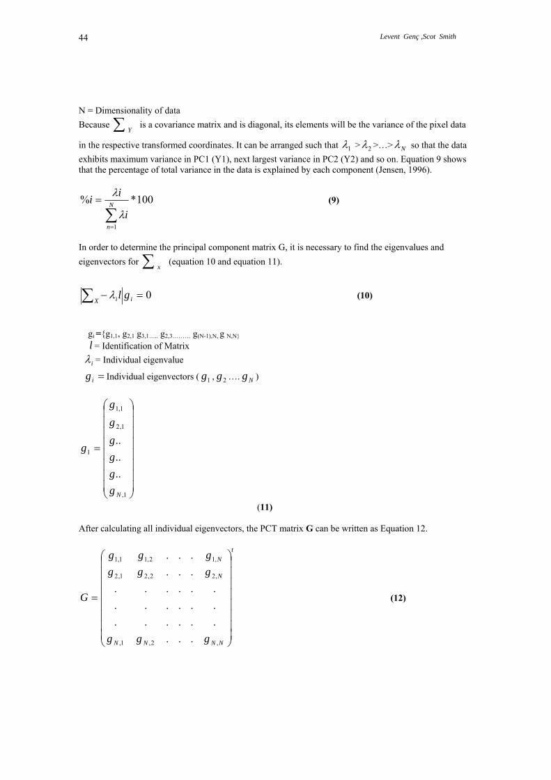
N = Dimensionality of data Because is a covariance matrix and is diagonal, its elements will be the variance of the pixel data

in the respective transformed coordinates. It can be arranged such that

∑ Y

1λ > 2λ >…> Nλ so that the data exhibits maximum variance in PC1 (Y1), next largest variance in PC2 (Y2) and so on. Equation 9 shows that the percentage of total variance in the data is explained by each component (Jensen, 1996).

100*%

1∑=

= N

n

i

iiλ

λ (9)

In order to determine the principal component matrix G, it is necessary to find the eigenvalues and eigenvectors for ∑ (equation 10 and equation 11).

x

0=−∑ iX i glλ (10)

gi ={g1,1, g2,1 g3,1….. g2,3……… g(N-1),N, g N,N} l = Identification of Matrix iλ = Individual eigenvalue

Individual eigenvectors ( , …. ) =ig 1g 2g Ng

⎟⎟⎟⎟⎟⎟⎟⎟

⎠

⎞

⎜⎜⎜⎜⎜⎜⎜⎜

⎝

⎛

=

1,

1,2

1,1

1

..

..

..

Ngggggg

g

(11) After calculating all individual eigenvectors, the PCT matrix G can be written as Equation 12.

t

NNNN

N

N

ggg

gggggg

G

⎟⎟⎟⎟⎟⎟⎟⎟

⎠

⎞

⎜⎜⎜⎜⎜⎜⎜⎜

⎝

⎛

=

,2,1,

,22,21,2

,12,11,1

.....................

...

...

(12)


45

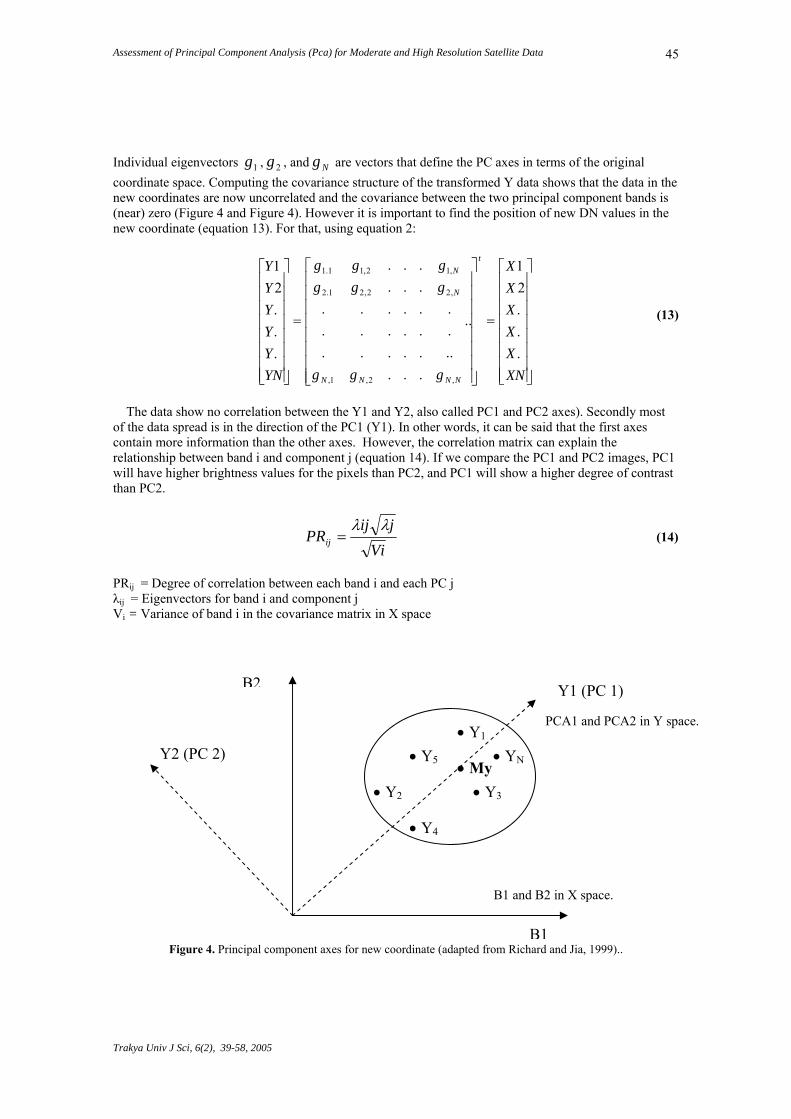
Individual eigenvectors , , and are vectors that define the PC axes in terms of the original coordinate space. Computing the covariance structure of the transformed Y data shows that the data in the new coordinates are now uncorrelated and the covariance between the two principal component bands is (near) zero (Figure 4 and Figure 4). However it is important to find the position of new DN values in the new coordinate (equation 13). For that, using equation 2:

1g 2g Ng

⎥⎥⎥⎥⎥⎥⎥⎥

⎦

⎤

⎢⎢⎢⎢⎢⎢⎢⎢

⎣

⎡

=

⎥⎥⎥⎥⎥⎥⎥⎥

⎦

⎤

⎢⎢⎢⎢⎢⎢⎢⎢

⎣

⎡

=

⎥⎥⎥⎥⎥⎥⎥⎥

⎦

⎤

⎢⎢⎢⎢⎢⎢⎢⎢

⎣

⎡

XNXXXXX

ggg

gggggg

YNYYYYY

t

NNNN

N

N

.

.

.21

..

......................

...

...

.

.

.21

,2,1,

,22,21.2

,12,11.1

(13)

The data show no correlation between the Y1 and Y2, also called PC1 and PC2 axes). Secondly most of the data spread is in the direction of the PC1 (Y1). In other words, it can be said that the first axes contain more information than the other axes. However, the correlation matrix can explain the relationship between band i and component j (equation 14). If we compare the PC1 and PC2 images, PC1 will have higher brightness values for the pixels than PC2, and PC1 will show a higher degree of contrast than PC2.

Vi

jijPRij

λλ= (14)

PRij = Degree of correlation between each band i and each PC j λij = Eigenvectors for band i and component j Vi = Variance of band i in the covariance matrix in X space B2

Figure 4. Principal component axes for new coordinate (adapted from Richard and Jia, 1999)..

B1

B1 and B2 in X space.

• Y2

• Y4

• Y3

• Y1 • Y5 • YN

Y1 (PC 1)

Y2 (PC 2) • My

PCA1 and PCA2 in Y space.

Trakya Univ J Sci, 6(2), 39-58, 2005


46

Figure 5. Mathematical and statistical concepts of PCA (ERDAS, 1999).

Results and Discussion Co-variance matrices, correlation matrices, eigenvalues and eigenvectors were computed for all datasets and are shown in Table 2 through 26. The software (ERDAS Imagine Ver. 8.5) is capable of calculating eigenvalues based on all datasets. The software then calculated the co-variance of the pixel data in X space (∑ ) and Y space. In addition, the degree of correlation was calculated for both X and

Y space as shown in Figure 6 through Figure 10. First, three components for all datasets were plotted and compared as in Figure 11.

X

Table 2. Covariance Matrix for the ETM+.Scene Statistics Used in Principal Component Calculation.

BANDS 1 2 3 4 5 6

1 1034.638

2 706.0478 485.2357

3 577.3981 397.6535 329.2088

4 936.2192 658.5568 543.5296 989.359

5 638.5779 452.0443 376.8172 687.7266 489.5947

6 372.3631 261.165 217.7285 382.2958 270.9989 152.9949


47

Table 3. Correlation Matrix for ETM+.Scene Statistics Used in Principal Component Calculation.

BANDS 1 2 3 4 5 6

1 1.000

2 0.996 1.000

3 0.989 0.995 1.000

4 0.925 0.950 0.952 1.000

5 0.897 0.927 0.939 0.988 1.000

6 0.936 0.959 0.970 0.983 0.990 1.000

Table 4. Eigenvalues Computed for ETM+ .Scene Statistics Used in Principal Component Calculation.

PC1 PC2 PC3 PC4 PC5 PC6 Eigenvalues 1095.807 16.497 5.281 1.056 1.023 0.816 % of Variance 97.798 1.472 0.471 0.094 0.091 0.073

Table 5. Eigenvector for the ETM+.Scene Statistics Used in Principal Component Calculation.

BANDS PC1 PC2 PC3 PC4 PC5 PC6 1 0.053 -0.139 0.253 0.659 -0.650 0.240 2 0.135 -0.073 0.246 0.152 -0.072 -0.942 3 0.151 -0.361 0.762 0.006 0.470 0.213 4 0.742 0.640 0.158 -0.062 -0.044 0.092 5 0.586 -0.512 -0.513 0.273 0.240 0.016 6 0.250 -0.417 0.086 -0.681 -0.541 0.022

Table 6. Degree of Correlation between each band and each principal component for the ETM+.

BANDS PC1 PC2 PC3 PC4 PC5 PC6

1 0.055 -0.018 0.018 0.021 -0.020 0.007 2 0.203 -0.013 0.026 0.007 -0.003 -0.039 3 0.275 -0.081 0.097 0.000 0.026 0.011 4 0.781 -0.083 0.012 -0.020 -0.001 0.003 5 0.877 -0.094 -0.053 0.013 0.011 0.001 6 0.671 -0.137 0.016 -0.057 -0.044 0.002

Trakya Univ J Sci, 6(2), 39-58, 2005


48

Figure 6. Comparison of PCs and original bands for ETM+ dataset.

Table 7. Covariance Matrix for IRS Scene Statistics Used in Principal

Component Calculation.

BANDS 1 2 3 4

1 559.798

2 322.072 187.571

3 473.498 279.411 447.234

4 653.607 382.157 591.985 821.778

Table 8. Correlation Matrix IRS Scene Statistics Used in Principal Component Calculation.

BANDS 1 2 3 4

1 1.000

2 0.994 1.000

3 0.946 0.965 1.000

4 0.964 0.973 0.976 1.000


49

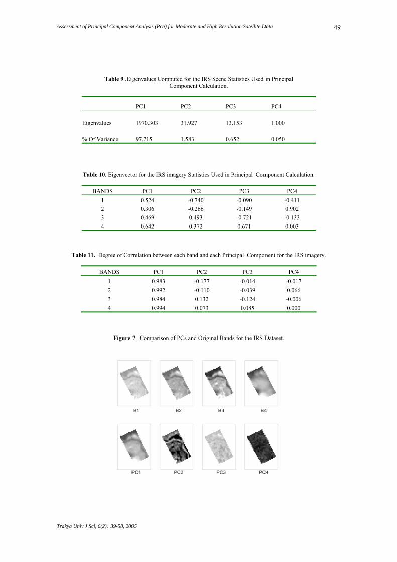
Table 9 .Eigenvalues Computed for the IRS Scene Statistics Used in Principal Component Calculation.

PC1 PC2 PC3 PC4

Eigenvalues 1970.303 31.927 13.153 1.000

% Of Variance 97.715 1.583 0.652 0.050

Table 10. Eigenvector for the IRS imagery Statistics Used in Principal Component Calculation.

BANDS PC1 PC2 PC3 PC4

1 0.524 -0.740 -0.090 -0.411 2 0.306 -0.266 -0.149 0.902 3 0.469 0.493 -0.721 -0.133 4 0.642 0.372 0.671 0.003

Table 11. Degree of Correlation between each band and each Principal Component for the IRS imagery.

BANDS PC1 PC2 PC3 PC4 1 0.983 -0.177 -0.014 -0.017 2 0.992 -0.110 -0.039 0.066 3 0.984 0.132 -0.124 -0.006 4 0.994 0.073 0.085 0.000

Figure 7. Comparison of PCs and Original Bands for the IRS Dataset.

Trakya Univ J Sci, 6(2), 39-58, 2005


50

Table 12. Covariance Matrix for SPOT Scene Statistics Used in Principal Component Calculation.

BANDS 1 2 3

1 327.558

2 213.531 141.368 3 313.514 209.408 318.524

Table 13. Correlation Matrix SPOT Scene Statistics Used in Principal Component Calculation.

BANDS 1 2 3

1 1.000

2 0.992 1.000

3 0.971 0.987 1.000

Table 14. Eigenvalues Computed for the Covariance Matrix SPOT Scene Statistics Used in Principal Component

Calculation.

PC1 PC2 PC3

Eigenvalues 777.254 9.5477 0.649

% Of Variance 98.7050 1.213 0.082

Table 15. Eigenvector for the Covariance Matrix SPOT Scene Statistics Used in Principal Component Calculation.

BANDS PC1 PC2 PC3

1 0.645 -0.676 0.357 2 0.426 -0.070 -0.902 3 0.635 0.733 0.243

Table 16. Degree of Correlation between each band and each Principal Component for SPOT imagery.

BANDS PC1 PC2 PC3

1 0.994 -0.115 0.016

2 0.999 -0.018 -0.061

3 0.992 0.127 0.011


51

Figure 8. Comparison of PCs and Original Bands for SPOT Dataset

Table 17. Covariance Matrix IKONOS Scene Statistics Used in Principal


BANDS 1 2 3 4

1 292.774

2 292.805 295.693

3 197.394 200.668 141.425

4 609.390 625.343 411.325 1481.741

Table 18 . Correlation Matrix IKONOS Scene Statistics Used in Principal


BANDS 1 2 3 4

1 1.000

2 0.995 1.000

3 0.970 0.981 1.000

4 0.925 0.945 0.899 1.000

Trakya Univ J Sci, 6(2), 39-58, 2005


52

Table 19 .Eigenvalues Computed for IKONOS Scene Statistics Used in Principal Component Calculation.

PC1 PC2 PC3 PC4

Eigenvalues % of 2139.487 66.354 5.504 0.287

Variance 96.738 3.000 0.249 0.013

Table 20. Eigenvector for the IKONOS Scene Statistics Used in Principal Component Calculation


1 0.356 -0.542 -0.589 0.482

2 0.363 -0.449 -0.035 -0.816

3 0.242 -0.439 0.806 0.315

4 0.826 0.559 0.033 0.059

Table 21. Degree of Correlation between each band and each Principal Component (IKONOS).


1 0.962 -0.258 -0.081 0.015

2 0.976 -0.213 -0.005 -0.025

3 0.941 -0.301 0.159 0.014

4 0.993 0.118 0.002 0.001

Figure 9. Comparison of PCs and Original Bands for IKONOS Dataset.


53

Table 22. Covariance Matrix for CASI Scene Statistics Used in Principal Component Calculation

BANDS 1 2 3 4 5 6 7 8 9 10 11 12

1 746481.5

2 1171381.1 2011287.3

3 1195620.9 2052084.9 2096176.0

4 1137972.0 1938617.1 1979944.0 1874621.9

5 875870.6 1403363.1 1435464.6 1372639.8 1089172.1

6 757972.7 1185221.7 1212880.0 1164151.6 950144.5 838940.6

7 874339.6 1401608.2 1433594.9 1370505.6 1087706.2 950107.0 1091583.8

8 1364799.7 2316819.0 2367213.9 2242707.1 1663021.5 1415808.3 1670635.9 2724876.4

9 2663991.2 4810857.6 4906086.3 4593543.4 3124633.6 2580254.7 3152799.4 5556695.0 12697322.1

10 2999979.3 5403234.3 5510706.2 5161485.0 3518860.3 2908492.9 3548862.1 6242995.7 14240727.0 15984117

11 2881646.2 5181414.1 5284378.9 4950148.1 3379335.4 2794947.2 3408944.1 5989424.3 13653710.5 15324277 14696868

12 2375410.4 4252102.7 4336368.1 4063489.9 2783969.1 2306598.6 2809878.6 4919955.4 11196400.6 12568815 12056702 9902414

Table 23. Correlation Matrix for CASI Scene Statistics Used in Principal Component Calculation.

BANDS 1 2 3 4 5 6 7 8 9 10 11 12

1 1.000 2 0.956 1.000 3 0.956 0.999 1.000 4 0.962 0.998 0.999 1.000 5 0.971 0.948 0.950 0.961 1.000 6 0.958 0.912 0.915 0.928 0.994 1.000 7 0.969 0.946 0.948 0.958 0.998 0.993 1.000 8 0.957 0.990 0.990 0.992 0.965 0.936 0.969 1.000 9 0.865 0.952 0.951 0.942 0.840 0.791 0.847 0.945 1.000 10 0.868 0.953 0.952 0.943 0.843 0.794 0.850 0.946 1.000 1.000 11 0.870 0.953 0.952 0.943 0.845 0.796 0.851 0.946 0.999 1.000 1.000 12 0.874 0.953 0.952 0.943 0.848 0.800 0.855 0.947 0.999 0.999 0.999 1.000

Table 24. Eigenvalues Computed for the CASI Scene Statistics Used in Principal Component Calculation

PC1 PC2 PC3 PC4 PC5 PC6 PC7 PC8 PC9 PC10 PC11 PC12 Eigenvalues 64027330 1564020 89725 39072 12536 10534 4918 1768 1331 1049 948 628.1 % of Variance 97.37 2.38 0.14 0.06 0.02 0.02 0.01 0.00 0.00 0.00 0.00 0.00

Trakya Univ J Sci, 6(2), 39-58, 2005


54

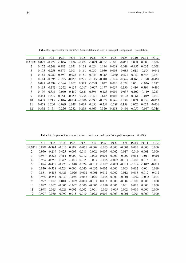
Table 25. Eigenvector for the CASI Scene Statistics Used in Principal Component Calculation

PC1 PC2 PC3 PC4 PC5 PC6 PC7 PC8 PC9 PC10 PC11 PC12 BAND1 0.097 -0.272 -0.036 0.826 -0.472 -0.079 -0.035 -0.001 -0.051 0.008 0.000 0.006

2 0.172 -0.248 0.482 0.051 0.138 0.024 0.144 0.058 0.649 -0.457 0.032 0.008 3 0.175 -0.258 0.479 0.001 0.161 0.030 0.030 0.003 -0.083 0.618 -0.504 -0.0414 0.165 -0.280 0.390 -0.023 0.181 0.044 -0.088 -0.060 -0.521 -0.050 0.646 0.067 5 0.114 -0.396 -0.225 -0.055 0.225 -0.145 -0.101 -0.064 -0.326 -0.463 -0.390 -0.4676 0.095 -0.394 -0.384 0.002 0.329 -0.288 0.022 0.010 0.079 0.061 -0.036 0.697 7 0.115 -0.383 -0.352 -0.137 -0.017 -0.007 0.177 0.059 0.330 0.410 0.394 -0.4808 0.199 -0.331 -0.040 -0.459 -0.621 0.396 -0.123 0.001 -0.037 -0.102 -0.119 0.233 9 0.444 0.205 0.051 -0.155 -0.254 -0.471 0.642 0.007 -0.178 -0.061 -0.019 0.013

10 0.498 0.215 -0.016 -0.034 -0.006 -0.241 -0.577 0.548 0.080 0.039 0.038 -0.05311 0.478 0.200 -0.089 0.048 0.069 0.050 -0.254 -0.788 0.158 0.052 0.023 -0.01612 0.392 0.151 -0.226 0.232 0.293 0.669 0.320 0.253 -0.110 -0.050 -0.047 0.046

Table 26. Degree of Correlation between each band and each Principal Component (CASI)

PC1 PC2 PC3 PC4 PC5 PC6 PC7 PC8 PC9 PC10 PC11 PC12 BAND1 0.898 -0.394 -0.012 0.189 -0.061 -0.009 -0.003 0.000 -0.002 0.000 0.000 0.000

2 0.970 -0.219 0.425 0.007 0.011 0.002 0.007 0.002 0.017 -0.010 0.001 0.000 3 0.967 -0.223 0.414 0.000 0.012 0.002 0.001 0.000 -0.002 0.014 -0.011 -0.0014 0.964 -0.256 0.347 -0.003 0.015 0.003 -0.005 -0.002 -0.014 -0.001 0.015 0.001 5 0.874 -0.475 -0.270 -0.010 0.024 -0.014 -0.007 -0.003 -0.011 -0.014 -0.012 -0.0116 0.830 -0.538 -0.524 0.000 0.040 -0.032 0.002 0.000 0.003 0.002 -0.001 0.019 7 0.881 -0.458 -0.421 -0.026 -0.002 -0.001 0.012 0.002 0.012 0.013 0.012 -0.0128 0.965 -0.251 -0.030 -0.055 -0.042 0.025 -0.005 0.000 -0.001 -0.002 -0.002 0.004 9 0.997 0.072 0.018 -0.009 -0.008 -0.014 0.013 0.000 -0.002 -0.001 0.000 0.000

10 0.997 0.067 -0.005 -0.002 0.000 -0.006 -0.010 0.006 0.001 0.000 0.000 0.000 11 0.998 0.065 -0.029 0.002 0.002 0.001 -0.005 -0.009 0.002 0.000 0.000 0.000 12 0.997 0.060 -0.090 0.015 0.010 0.022 0.007 0.003 -0.001 -0.001 0.000 0.000


55

Figure 10. Comparison of PCs and Original Bands for CASI Dataset.

The first three PC’s of all datasets are compared in Figure 11. The first three PC’s of the original Landsat ETM+ described 99.7 % of the original Landsat ETM+ dataset, the first three PC’s of the original IRS represented 99.95 % of the original IRS dataset, the first three PC’s of the original SPOT represented 100% of the original SPOT, the first three PC’s of the original IKONOS represented 99.99 % of the original IKONOS, and the first three PC’s of the original CASI represented 99.90 % of the original CASI dataset. PC2 accounted for 1.42%, 1.58%, 1.21%, 3.0%, and 2.38% of the remaining variance respectively as shown in Figure 11. Likewise, PC3 had little variance for all datasets. Cumulatively the first three components for each dataset, Landsat ETM+ , IRS, SPOT , IKONOS , and CASI, explained approximately 99.74%, 99.95%, 100%, 99.98%, and 99.89% of the total variance for the datasets, respectively. These results show that the six band Landsat ETM+ dataset, the four band IRS dataset, the three band SPOT dataset, the four band IKONOS dataset, and the twelve band CASI dataset, compressed into just three or fewer new PC datasets, could describe most of the original datasets.

Trakya Univ J Sci, 6(2), 39-58, 2005


56

Figure 11. Comparison of the first 3 PCs for all datasets.

0

10

20

30

40

50

60

70

80

90

100

Perc

ent o

f Var

ianc

e

PC1 % 97.798 97.715 98.705 96.738 97.37PC2 % 1.472 1.583 1.213 3 2.38PC3 % 0.471 0.652 0.082 0.249 0.14

ETM+ IRS SPOT IKONOS CASI

In addition, Table 6 (ETM+), Table 11 (IRS), Table 16 (SPOT), Table 21 (IKONOS), and Table 26 (CASI) show the correlation between the original dataset (bands) and PC datasets (bands). In other words, computing the correlation for each band i with component j can explain how individual bands associate with principal components. Moderate resolution (30x30) image, Landsat ETM+ band 4, 5, 6 have a higher correlation with PC1 (Table 6). Correlation between PC1 and band 4, 5, and 6 are 0.781, 0.877, and 0.671, respectively. These three bands are mainly the near infrared and mid infrared reflectance bands. Because the study area is located in a wetland area, these results are reasonable in terms of vegetation reflectance. Figure 5 supports the idea that, except for the first two PC’s, all the PC bands contain noise. Jensen (1996) stated the same results for the TM 5 image. Another moderate resolution image is the IRS. PC1 of IRS is correlated highly with all bands. These bands represent green, red, and near and mid infrared bands. Because the IRS image had been taken earlier than the ETM+ image, temporal resolution may be significant in terms of reflectance when compared to the IRS dataset with Landsat ETM+ dataset. When the IRS image was taken, the area was undergoing a severe drought. Because of the drought, visible bands (green and red) also load to PC1 (Table 11). The PC2 of IRS contains some information, but not as much as PC1. Vegetation, for example, began to be shown as dark areas. PC3 and PC4 are essentially noise of the original IRS image (Figure 6). The SPOT image was taken in the spring of 1993. It has visible green, red and near infrared bands with a 20x20m spatial resolution. All three bands load PC1 images (Table 16). As with Figure 7, the first two PC bands represented 99% of the total variance. PC3 contains noise from the original image. The high-resolution IKONOS satellite image (Table 21) showed that all bands correlated with PC1. This was due to the fact that the image was taken in the spring when vegetation growth was relatively high. Figure 8 also shows that most of the information was compressed into PC1 and vegetation in PC2 started to reflect less. PC3 and PC4 contained mostly noise.


57

Correlation between PCs and the original CASI bands is shown in Table 26. The last 4 bands of CASI dataset are near infrared bands that load most of the original data into PC1. Also, the blue band (first 4 bands) has almost the same impact as the near infrared bands. Red bands have relatively less impact on PC1. Other than the first PCs, all the PC bands contain mostly noise (Figure 9). Hunter and Power (2002) stated that PCA has the effect of condensing most of the variance (99.8% variance into PCs 1, 2, 3 and 4) in the CASI image into a few bands. A similar result was found in this study. PC1 and PC2 contain 99% of the variance in the CASI image. Even moderate resolution or high-resolution images have almost the same effect when PCA takes place. If PC1, PC2 and PC3 account for most of the variance in the dataset, classification can be performed using these three PC images. Conclusion This research showed that the PCA approach was a useful image pre-processing technique to compress data for both moderate and high-resolution datasets for the study site. Among the all the PC bands for all datasets using this research, the first three PCs contain most of the information of the original data for each dataset. Furthermore, it was found that other than the first three PC bands, all other PCs contained noise for both moderate and high-resolution images. Using the first three PC results in better classifications than the original dataset (without noise). Fewer bands take less time to process when image processing takes place. It was found that the PCA analysis in this study supports the previous research done by Jensen (1996), and Hunter and Power (2002). However, the questions that should be answered in future studies are: does the size of the study site matter when we produce the PCs and, would the PCs results change when temporal resolution differs. Further this results will help to understand PCA for common satellite images that using in remote sensing studies.

Acknowledgements The author thanks Florida Environment Protection Ministry for funding this project and Dr. Dewitt, B., Geomatics program director, in University of Florida for encouragement and critical discussions. References

1. CARR, J., and K. MATANAWI. 1999. Correspondence analysis for principal components transformation of multispectral and hyperspectral digital images. Photogrammetry Engineering and Remote Sensing 65(8):909-914.

2. ERDAS Imagine, 1999, Field Guide. Copyright 1982 - 1999 by ERDAS, Inc. Atlanta, Georgia. 3. GENC, L. SMITH, S, DEWITT, B, 2005. Using Satellite Imagery and LIDAR Data to

Corroborate an Adjudicated Ordinary High Water Line. International Journal of Remote Sensing (accepted for publication February 2005)

4. GONZALEZ, R. and WOODS, R., 1993. Digital Image Processing, Addison—Wesley Publishing Company, Menlo Park, CA pp. 148-156.

5. HUNTER, E. L. and POWER, C. H., 2002. An assessment of two classification methods for mapping Thames Estuary inertial habitat using CASI data. International Journal of Remote Sensing 23: 2989-3008.

6. JENSEN, J. R., 1996. Introductory digital image processing: a remote sensing perspective London: Prentice-Hall Inc., 2nd edition pp. 172-176.

7. LILESAND, T.M., and KIEFER, R.W. 2000. Remote Sensing and Image interpretation. 4th Edition. John Wiley & Sons. New York. Pp. 572-596.

8. MATHER P. 1999. Computer Processing of Remotely Sensed Images, John Wiley & Sons,Inc. New York, NY, USA pp.126-137.

Trakya Univ J Sci, 6(2), 39-58, 2005


58

9. RICHARDS, J.A. and JIA, X., 1999. Digital Image Processing, Springer-Verlag: NewYork. pp. 133-143.

10. ROGERSON, A. P, 2001. Statistical Methods for Geography, SAGE Publication, Thousand Oaks, California pp. 194-197.

11. SINGH, A. and HARRISON A., 1985, Standardized Principal Components. International Journal of Remote Sensing 6: 883-896.

12. VANI, K., SHAMMUGAYEL, S., and MARRUTHACHALAM, M., 2001. Fusion of IRS-LISS III and Pan Images Using Different Resolution Ratio. The 22nd Asian Conference on Remote Sensing 5-9 November 2001, Singapore.

ASSESSMENT OF PRINCIPAL COMPONENT ANALYSIS ...

Documents

Transcript of ASSESSMENT OF PRINCIPAL COMPONENT ANALYSIS ...