Direct Importance Estimation with a Mixture of Probabilistic Principal Component Analyzers

1IEICE Transactions on Information and Systems,vol.E93-D, no.10, pp.2846–2849, 2010.

Direct Importance Estimation with A Mixture ofProbabilistic Principal Component Analyzers

Makoto Yamada ([email protected])Tokyo Institute of Technology

Masashi Sugiyama ([email protected])Tokyo Institute of Technology

andJapan Science and Technology Agency

Gordon WichernMIT Lincoln Lab, Lexington, MA 02420-9108, U.S.A.

Jaak SimmTokyo Institute of Technology

Abstract

Estimating the ratio of two probability density functions (a.k.a. the importance)has recently gathered a great deal of attention since importance estimators can beused for solving various machine learning and data mining problems. In this paper,we propose a new importance estimation method using a mixture of probabilisticprincipal component analyzers. The proposed method is more flexible than existingapproaches, and is expected to work well when the target importance function iscorrelated and rank-deficient. Through experiments, we illustrate the validity of theproposed approach.

Keywords

Importance, Kullback-Leibler importance estimation procedure, Mixture of proba-bilistic principal component analyzers, Expectation-maximization algorithm

1 Introduction

Recently, the ratio of two probability density functions (a.k.a. the importance function)has been shown to be useful for solving various data processing tasks [1], including non-stationarity adaptation [2, 3], transfer learning [4], multi-task learning [5], outlier de-tection [6], change detection [7], feature selection [8], feature extraction [9], independent

Direct Importance Estimation with A Mixture of PPCAs 2

component analysis [10], causal inference [11], conditional density estimation [12], andprobabilistic classification [13]. For this reason, importance estimation has attracted con-siderable attention these days.

A naive approach to approximating the importance function is to separately estimatethe densities corresponding to the numerator and denominator of the ratio, and thentake the ratio of the estimated densities. However, density estimation itself is a difficultproblem and taking the ratio of estimated densities can magnify the estimation error.To overcome this problem, a direct importance estimator called the Kullback-Leibler im-portance estimation procedure (KLIEP) was proposed [14]. A typical implementationof KLIEP employs a linear combination of spherical Gaussian kernels for modeling theimportance function, and the (common) Gaussian width is chosen by cross-validation.

Although KLIEP was shown to work well in experiments, using ellipsoidal Gaussiankernels would be more suitable when the true importance function has a correlated pro-file. Following this idea, an extension of KLIEP using a Gaussian mixture model calledGaussian-mixture KLIEP (GM-KLIEP) was proposed [15]. In GM-KLIEP, the Gaus-sian mixture model is efficiently trained using an expectation-maximization algorithm,in which the covariance matrices of Gaussian kernels are adaptively adjusted. AlthoughGM-KLIEP was shown to be promising in experiments, its training algorithm involvesestimation of inverse covariance matrices, which makes GM-KLIEP numerically unstablewhen data samples are (locally) rank-deficient.

A standard approach to coping with rank deficiency would be to use dimensional-ity reduction methods such as principal component analysis (PCA). Following this idea,we propose to combine GM-KLIEP with PCA, resulting in a new direct importanceestimation procedure using a mixture of probabilistic principal component analyzers (PP-CAs) [16]. We illustrate the usefulness of the proposed approach called PPCA-mixtureKLIEP (PM-KLIEP) through experiments.

2 Background

In this section, we formulate the problem of importance estimation, and briefly reviewthe KLIEP method.

2.1 Problem Formulation

Let D ∈ Rd be the data domain and suppose we are given i.i.d. samples {xdei }nde

i=1 froma “denominator” data distribution with density pde(x) and i.i.d. samples {xnu

j }nnuj=1 from

a “numerator” data distribution with density pnu(x). We assume that pde(x) > 0 forall x ∈ D. The goal of this paper is to develop a method of estimating the importancefunction w(x) from {xde

i }ndei=1 and {xnu

j }nnuj=1:

w(x) =pnu(x)

pde(x).


Our key restriction is that we avoid estimating densities pde(x) and pnu(x) when estimatingw(x).

2.2 Kullback-Leibler Importance Estimation Procedure(KLIEP)

KLIEP allows one to directly estimate w(x) without going through density estimation [14].In KLIEP, the following linear importance model is used:

w(x) =b∑

l=1

αlφl(x), (1)

where {αl}bl=1 are parameters, b is the number of parameters, and φl(x) is a basis function.In the original KLIEP paper [14], the Gaussian kernel was used as the basis function:

φl(x) = exp

(−∥x− cl∥2

2τ 2

),

where τ > 0 is the Gaussian width and cl is the Gaussian center randomly chosen from{xi}nnu

i=1. Using the model w(x), one may estimate pnu(x) as

pnu(x) = w(x)pde(x).

Based on this, {αl}bl=1 is determined so that the Kullback-Leibler divergence from pnu(x)to pnu(x) is minimized:

KL[pnu(x)∥pnu(x)] =∫

pnu(x) lnpnu(x)

pde(x)w(x)dx

=

∫pnu(x) ln

pnu(x)

pde(x)dx−

∫pnu(x) ln w(x)dx.

The first term in the last equation is independent of {αl}bl=1, so it can be ignored. Let usdefine the second term as KL′:

KL′ =

∫pnu(x) ln w(x)dx ≈ 1

nnu

nnu∑j=1

ln w(xnuj ),

where the expectation over pnu(x) is approximated by the average over its i.i.d. samples{xnu

j }nnuj=1. Since pnu(x) is a probability density, the following normalization constraint

should be satisfied:

1 =

∫pnu(x)dx =

∫pde(x)w(x)dx ≈ 1

nde

nde∑i=1

w(xdei ),


where the expectation over pde(x) is approximated by the average over its i.i.d. samples{xde

i }ndei=1. Then the KLIEP optimization problem is given as follows:

max{αl}bl=1

[nnu∑j=1

ln

(b∑

l=1

αlφl(xnuj )

)]

s.t.1

nde

nde∑i=1

b∑l=1

αlφl(xdei ) = 1 and α1, . . . , αb ≥ 0.

2.3 Model Selection by Likelihood Cross-validation

In the KLIEP algorithm, the choice of the Gaussian width τ is critical. Since KLIEP isbased on the maximization of the score KL′, it would be natural to determine τ so thatKL′ is maximized.

The expectation over pnu(x) involved in KL′ can be approximated by likelihood cross-validation (LCV) as follows [14]: First divide the “numerator” samples X nu = {xnu

j }nnuj=1

into K disjoint subsets {X nuj }Kj=1 of (approximately) the same size. Then obtain an

importance estimator wk(x) from {X nuj }j =k (i.e., without X nu

k ) and approximate the scoreKL′ using X nu

k as

KL′k =

1

|X nuk |

∑x∈Xnu

k

ln wk(x).

This procedure is repeated for k = 1, . . . , K and the average of KL′k over all k is used as

an estimate of KL′:

KL′=

1

K

K∑k=1

KL′k.

For model selection, KL′is computed for all model candidates (the Gaussian width τ in

the current setting) and the candidate that maximizes KL′is chosen.

3 KLIEP with A Mixture of Probabilistic Principal

Component Analyzers (PPCAs)

In this section, we propose a new method, PPCA-mixture KLIEP (PM-KLIEP).Instead of the linear model (1), we use a mixture of PPCAs as the importance model:

w(x) =b∑

l=1

πlpl(x),


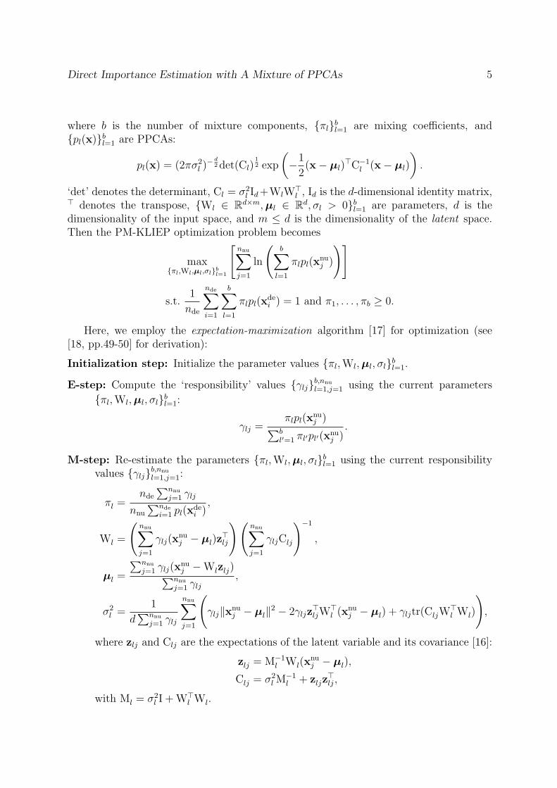
where b is the number of mixture components, {πl}bl=1 are mixing coefficients, and{pl(x)}bl=1 are PPCAs:

pl(x) = (2πσ2l )

− d2det(Cl)

12 exp

(−1

2(x− µl)

⊤C−1l (x− µl)

).

‘det’ denotes the determinant, Cl = σ2l Id+WlW

⊤l , Id is the d-dimensional identity matrix,

⊤ denotes the transpose, {Wl ∈ Rd×m,µl ∈ Rd, σl > 0}bl=1 are parameters, d is thedimensionality of the input space, and m ≤ d is the dimensionality of the latent space.Then the PM-KLIEP optimization problem becomes

max{πl,Wl,µl,σl}bl=1

[nnu∑j=1

ln

(b∑

l=1

πlpl(xnuj )

)]

s.t.1

nde

nde∑i=1

b∑l=1

πlpl(xdei ) = 1 and π1, . . . , πb ≥ 0.

Here, we employ the expectation-maximization algorithm [17] for optimization (see[18, pp.49-50] for derivation):

Initialization step: Initialize the parameter values {πl,Wl,µl, σl}bl=1.

E-step: Compute the ‘responsibility’ values {γlj}b,nnu

l=1,j=1 using the current parameters

{πl,Wl,µl, σl}bl=1:

γlj =πlpl(x

nuj )∑b

l′=1 πl′pl′(xnuj )

.

M-step: Re-estimate the parameters {πl,Wl,µl, σl}bl=1 using the current responsibilityvalues {γlj}b,nnu

l=1,j=1:

πl =nde

∑nnu

j=1 γlj

nnu

∑nde

i=1 pl(xdei )

,

Wl =

(nnu∑j=1

γlj(xnuj − µl)z

⊤lj

)(nnu∑j=1

γljClj

)−1

,

µl =

∑nnu

j=1 γlj(xnuj −Wlzlj)∑nnu

j=1 γlj,

σ2l =

1

d∑nnu

j=1 γlj

nnu∑j=1

(γlj∥xnu

j − µl∥2 − 2γljz⊤ljW

⊤l (x

nuj − µl) + γljtr(CljW

⊤l Wl)

),

where zlj and Clj are the expectations of the latent variable and its covariance [16]:

zlj = M−1l Wl(x

nuj − µl),

Clj = σ2l M

−1l + zljz

⊤lj ,

with Ml = σ2l I +W⊤

l Wl.


Evaluation step: Repeat the E- and M-steps until the log-likelihood converges:

nnu∑j=1

ln

(b∑

l=1

πlpl(xnuj )

).

When the dimensionality of the latent space, m, is equal to the entire dimensionality d,the proposed PM-KLIEP is reduced to the Gaussian-mixture KLIEP (GM-KLIEP) [15].Thus PM-KLIEP can be regarded as an extension of GM-KLIEP to (locally) rank-deficientdata.

4 Experiments

In this section, we compare the performance of PM-KLIEP with the original KLIEP andGM-KLIEP.

4.1 Illustrative Example

Let us first consider a locally rank-deficient two-dimensional importance estimation prob-lem. The “denominator” and “numerator” densities are defined as

pde(x) =1

2N(x;

[10

],

[2 00 ϵ

])+1

2N(x;

[01

],

[ϵ 00 2

]),

pnu(x) =1

2N(x;

[20

],

[1 00 ϵ

])+1

2N(x;

[02

],

[ϵ 00 1

]),

where N (·;µ,Σ) denotes the Gaussian density with mean µ and covariance matrix Σ,and ϵ = 10−15. We set nde = 100 and nnu = 1000. In KLIEP, we set b = 100 and use theGaussian kernel as the basis function; the kernel width is chosen based on 5-fold LCV.In GM-KLIEP and PM-KLIEP, we use the k-means clustering algorithm for parameterinitialization [17], and we choose the number of mixture components based on 5-fold LCV.In PM-KLIEP, the dimension of the latent space is also chosen based on 5-fold LCV.

Figure 1 depicts the true importance function, along with the importance functionsestimated by KLIEP, GM-KLIEP, and PM-KLIEP, respectively. As can be seen, PM-KLIEP can approximate the true importance function more favorably than KLIEP andGM-KLIEP for this rank-deficient example.

4.2 Application to Inlier-based Outlier Detection

Next, we compare the performance of the proposed PM-KLIEP method with KLIEP andGM-KLIEP in inlier-based outlier detection [6].

The problem of inlier-based outlier detection is to identify outliers in an “evaluation”dataset based on a “model” dataset that only contains inliers. If the density ratio of twodatasets is considered, the importance values for inliers are close to one, while those for


−4 −2 0 2 4 6−4

−2

0

2

4

6

−4 −2 0 2 4 6−4

−2

0

2

4

6

(a) True importance (b) KLIEP

−4 −2 0 2 4 6−4

−2

0

2

4

6

−4 −2 0 2 4 6−4

−2

0

2

4

6

(c) GM-KLIEP (d) PM-KLIEP

Figure 1: Contours of the true importance and its estimates obtained by KLIEP, GM-KLIEP (b = 1 is chosen by LCV), and PM-KLIEP (b = 2 is chosen by LCV).

outliers tend to significantly deviate from one. Thus, the values of the importance maybe used as an outlier score.

The IDA benchmark datasets [19] are used for performance evaluation; we exclude the“splice” dataset since it is discrete. The original datasets are binary classification andeach set consists of positive/negative and training/test samples. We regard the positivesamples as inliers and the negative samples as outliers. We form the model dataset byincluding all the positive training samples, and the evaluation dataset by including all thepositive test samples and the first 5% of the negative test samples in the database. Weassign the evaluation dataset to the denominator of the ratio and the model dataset tothe numerator of the ratio. Thus, a sample with the importance value significantly lessthan one is likely to be an outlier.

In the evaluation of outlier detection performance, it is important to take into accountboth the detection rate (the amount of true outliers that an outlier detection algorithmcan find) and the detection accuracy (the amount of true inliers that an outlier detectionalgorithm misjudges as outliers). Since there is a trade-off between the detection rateand the detection accuracy, we adopt the area under the ROC curve (AUC) as our error


Table 1: Mean AUC values (and the standard deviation in brackets) over 20 trials in theoutlier detection experiments. If GM- or PM-KLIEP significantly outperforms KLIEP bythe t-test at a significance level of 5%, we indicate it by ‘◦’. Similarly, we use ‘+’ whenKLIEP or PM-KLIEP outperforms GM-KLIEP, and ‘⋆’ when KLIEP or GM-KLIEPoutperforms PM-KLIEP.

Datasets KLIEP GM-KLIEP PM-KLIEPbanana 55.9 (5.0) ◦⋆70.6 (2.3) ◦60.3 (1.2)

brestcancer 71.1 (8.8) 69.7(13.0) 65.0(11.8)diabetes +⋆63.0 (9.0) 53.1 (7.3) 55.6 (4.0)flaresolar 57.5 (6.7) 60.1 (6.4) 59.4 (6.7)german 58.8 (7.9) 56.2 (7.8) 56.9 (6.7)heart 69.0(15.1) 73.1(15.6) 73.6(15.0)image 55.1 (6.6) ◦69.8(14.3) ◦72.7 (6.5)thyroid 57.8 (9.8) ◦78.0 (9.1) ◦76.9(14.8)titanic 63.7 (9.1) 63.2 (2.1) 63.6 (2.4)twonorm 70.1 (8.4) 70.6 (3.3) ◦+85.1 (1.5)waveform 63.5 (8.0) ◦76.1 (2.7) ◦+81.6 (1.3)Average 62.3 — 67.3 — 68.2 —

metric.The results are summarized in Table 1, showing that PM-KLIEP clearly outperforms

KLIEP and compares favorably with GM-KLIEP with a small margin.

5 Conclusions

In this paper, we proposed a new importance estimation method using a mixture of proba-bilistic principal component analyzers (PPCAs). Optimization of the proposed algorithm,PM-KLIEP, can be efficiently carried out by the expectation-maximization algorithm.The usefulness of the proposed approach was illustrated through experiments.

We thank SCAT, AOARD, the JST PRESTO program, and Monbukagakusho Schol-arship.

References[1] M. Sugiyama, T. Kanamori, T. Suzuki, S. Hido, J. Sese, I. Takeuchi, and L. Wang, “A

density-ratio framework for statistical data processing,” IPSJ Trans. on Computer Visionand Applications, vol.1, pp.183–208, 2009.

[2] H. Shimodaira, “Improving predictive inference under covariate shift by weighting the log-likelihood function,” J. of Statistical Planning and Inference, vol.90, no.2, pp.227–244, 2000.

[3] M. Sugiyama, M. Krauledat, and K.-R. Muller, “Covariate shift adaptation by importanceweighted cross validation,” J. of Machine Learning Research, vol.8, pp.985–1005, 2007.


[4] Y. Tsuboi, H. Kashima, S. Hido, S. Bickel, and M. Sugiyama, “Direct density ratio es-timation for large-scale covariate shift adaptation,” J. of Information Processing, vol.17,pp.138–155, 2009.

[5] S. Bickel, J. Bogojeska, T. Lengauer, and T. Scheffer, “Multi-task learning for HIV therapyscreening,” Intl. Conf. on Machine Learning, pp.56–63, 2008.

[6] S. Hido, Y. Tsuboi, H. Kashima, M. Sugiyama, and T. Kanamori, “Statistical outlierdetection using direct density ratio estimation,” Knowledge and Information Systems, toappear.

[7] Y. Kawahara and M. Sugiyama, “Change-point detection in time-series data by directdensity-ratio estimation,” SIAM Intl. Conf. on Data Mining, pp.389–400, 2009.

[8] T. Suzuki, M. Sugiyama, T. Kanamori, and J. Sese, “Mutual information estimation revealsglobal associations between stimuli and biological processes,” BMC Bioinformatics, vol.10,no.1, p.S52, 2009.

[9] T. Suzuki and M. Sugiyama, “Sufficient dimension reduction via squared-loss mutual infor-mation estimation,” Intl. Conf. on Artificial Intelligence and Statistics, pp.804–811, 2010.

[10] T. Suzuki and M. Sugiyama, “Least-squares independent component analysis,” NeuralComputation, to appear.

[11] M. Yamada and M. Sugiyama, “Dependence minimizing regression with model selectionfor non-linear causal inference under non-Gaussian noise,” AAAI Conf. on Artificial Intel-ligence, 2010, to appear.

[12] M. Sugiyama, I. Takeuchi, T. Suzuki, T. Kanamori, H. Hachiya, and D. Okanohara,“Least-squares conditional density estimation,” IEICE Trans. on Information and Systems,vol.E93-D, no.3, pp.583–594, 2010.

[13] M. Sugiyama, “Superfast-trainable multi-class probabilistic classifier by least-squares pos-terior fitting,” IEICE Trans. on Information and Systems, to appear.

[14] M. Sugiyama, T. Suzuki, S. Nakajima, H. Kashima, P. von Bunau, and M. Kawanabe,“Direct importance estimation for covariate shift adaptation,” Annals of the Institute ofStatistical Mathematics, vol.60, no.4, pp.699–746, 2008.

[15] M. Yamada and M. Sugiyama, “Direct importance estimation with Gaussian mixture mod-els,” IEICE Trans. on Information and Systems, vol.E92-D, no.10, pp.2159–2162, 2009.

[16] M.E. Tipping and C.M. Bishop, “Mixtures of probabilistic principal component analyzers,”Neural Computation, vol.11, no.2, pp.443–482, 1999.

[17] C.M. Bishop, Pattern recognition and machine learning, Springer-Verlag, New York, USA,2006.

[18] M. Yamada, Kernel Methods and Frequency Domain Independent Component Anal-ysis for Robust Speaker Identification, Ph.D. Dissertation, The Graduate Universityfor Advanced Studies, Japan, http://sugiyama-www.cs.titech.ac.jp/∼yamada/pdf/thesis myamada.pdf


[19] G. Ratsch, T. Onoda, and K.R. Muller, “Soft margins for adaboost,” Machine Learning,vol.42, pp.287–320, 2001.

Direct Importance Estimation with a Mixture of Probabilistic Principal Component Analyzers

Documents

Transcript of Direct Importance Estimation with a Mixture of Probabilistic Principal Component Analyzers