Hindawi Publishing CorporationEURASIP Journal on Advances in Signal ProcessingVolume 2009, Article ID 783194, 14 pagesdoi:10.1155/2009/783194

Research Article

Kernel Principal Component Analysis for the Classification ofHyperspectral Remote Sensing Data over Urban Areas

Mathieu Fauvel,1, 2 Jocelyn Chanussot,1 and Jon Atli Benediktsson2

1 GIPSA-lab, Grenoble INP, BP 46, 38402 Saint Martin d’Heres, France2 Faculty of Electrical and Computer Engineering, University of Iceland, Hjardarhagi 2-6, 107 Reykjavik, Iceland

Correspondence should be addressed to Mathieu Fauvel, mathieu.fauvel@inrialpes.fr

Received 2 September 2008; Revised 19 December 2008; Accepted 4 February 2009

Recommended by Mark Liao

Kernel principal component analysis (KPCA) is investigated for feature extraction from hyperspectral remote sensing data.Features extracted using KPCA are classified using linear support vector machines. In one experiment, it is shown that kernelprincipal component features are more linearly separable than features extracted with conventional principal componentanalysis. In a second experiment, kernel principal components are used to construct the extended morphological profile (EMP).Classification results, in terms of accuracy, are improved in comparison to original approach which used conventional principalcomponent analysis for constructing the EMP. Experimental results presented in this paper confirm the usefulness of the KPCAfor the analysis of hyperspectral data. For the one data set, the overall classification accuracy increases from 79% to 96% with theproposed approach.

Copyright © 2009 Mathieu Fauvel et al. This is an open access article distributed under the Creative Commons AttributionLicense, which permits unrestricted use, distribution, and reproduction in any medium, provided the original work is properlycited.

1. Introduction

Classification of hyperspectral data from urban areas usingkernel methods is investigated in this article. Thanks torecent advances in hyperspectral sensors, it is now possibleto collect more than one hundred bands at a high-spatial res-olution [1]. Consequently, in the spectral domain, pixels arevectors where each component contains specific wavelengthinformation provided by a particular channel [2]. The size ofthe vector is related to the number of bands the sensor cancollect. With hyperspectral data, vectors belong to a high-dimensional vector space, for example, the 100-dimensionalvector space R100.

With increasing resolution of the data, in the spec-tral or spatial domain, theoretical and practical problemsappear. For example, in a high-dimensional space, normallydistributed data have a tendency to concentrate in thetails, which seems contradictory with a bell-shaped densityfunction [3, 4]. For the purpose of classification, theseproblems are related to the curse of dimensionality. Inparticular, Hughes showed that with a limited training set,classification accuracy decreases as the number of featuresincreases beyond a certain limit [5]. This is paradoxical, since

with a higher spectral resolution one can discriminate moreclasses and have a finer description of each class—but thedata complexity leads to poorer classification.

To mitigate this phenomenon, feature selection/extractionis usually performed as preprocessing to hyperspectral dataanalysis [6]. Such processing can also be performed formultispectral images in order to enhance class separabilityor to remove a certain amount of noise.

Transformations based on statistical analysis have alreadyproved to be useful for classification, detection, identifica-tion, or visualization of remote sensing data [2, 7–10]. Twomain approaches can be defined.

(1) Unsupervised Feature Extraction. The algorithm worksdirectly on the data without any ground truth. Its goal is tofind another space of lower dimension for representing thedata.

(2) Supervised Feature Extraction. Training set data areavailable, and the transformation is performed according tothe properties of the training set. Its goal is to improve classseparability by projecting the data onto a lower-dimensionalspace.

2 EURASIP Journal on Advances in Signal Processing

Supervised transformation is in general well suited topreprocessing for the task of classification, since the transfor-mation improves class separation. However, its effectivenesscorrelates with how well the training set represents thedata set as a whole. Moreover, this transformation can beextremely time consuming. Examples of supervised featuresextraction algorithms are

(i) sequential forward/backward selection methods andthe improved versions of them. These methods selectsome bands from the original data set [11–13];

(ii) band selection using information theory. A collectionof bands are selected according to their mutualinformation [14];

(iii) discriminant analysis, decision boundary, and non-weighted feature extraction (DAFE, DBFE, andNWFE) [6]. These methods are linear and usesecond-order information for feature extraction.They are “state-of-the-art” methods within theremote sensing community.

The unsupervised case does not focus on class discrimi-nation, but looks for another representation of the data in alower-dimensional space, satisfying some given criterion. Forprincipal component analysis (PCA), the data are projectedinto a subspace that minimizes the reconstruction error inthe mean squared sense. Note that both the unsupervised andsupervised cases can also be divided into linear and nonlinearalgorithms [15].

PCA plays an important role in the processing of remotesensing images. Even though its theoretical limitations forhyperspectral data analysis have been pointed out [6, 16],in a practical situation, the results obtained using PCA arestill competitive for the purpose of classification [17, 18]. Theadvantages of PCA are its low complexity and the absence ofparameters. However, PCA only considers the second-orderstatistic, which can limit the effectiveness of the method.

A nonlinear version of the PCA has been shown to becapable of capturing a part of higher-order statistics, thusbetter representing the information from the original data set[19, 20]. The first objective of this article is the applicationof the nonlinear PCA to high-dimensional spaces, suchas hyperspectral images, and to assess influence of usingnonlinear PCA on classification accuracy. In particular,kernel PCA (KPCA) [20] has attracted our attention. Itsrelation to a powerful classifier, support vector machines, andits low-computational complexity make it suitable for theanalysis of remote sensing data.

Despite the favorable performance of KPCA in manyapplication, no investigation has been carried out in thefield of remote sensing. In this paper, the first contribu-tion concerns the comparison of extracting features usingconventional PCA and using KPCA for the classificationof hyperspectral remote sensing data. In our very firstinvestigation in [21], we found that the use of kernelprincipal components as input to a neural network classifierleads to an improvement in classification accuracy. However,a neural network is a nonlinear classifier, and the conclusionswere difficult to generalize to other classifiers. In the present

study, we make use of a linear classifier (support vectormachine) to draw more general conclusions.

The second objective of the paper concerns an importantissue in the classification of remote sensing data: the useof spatial information. High-resolution hyperspectral datafrom urban areas provide both detailed spatial and spectralinformation. Any complete analysis of such data needs toinclude both types of information. However, conventionalmethods use the spectral information only. An approach hasbeen proposed for panchromatic data (one spectral band)using mathematical morphology [22, 23]. The idea was toconstruct a feature vector, the morphological profile, thatincludes spatial information. Despite good results in termsof classification accuracy, an extension to hyperspectral datawas not straightforward. In fact, due to the multivaluednature of pixels, standard image-processing tools whichrequire a total ordering relation, such as mathematicalmorphology [24], cannot be applied. Plaza et al. haveproposed an extension to the morphological transformationin order to integrate spectral and spatial information fromthe hyperspectral data [25]. In [26], Benediktsson et al.have proposed a simpler approach, that is, to use the PCAto extract representative images from the data and applymorphological processing on each first principal componentindependently. A stacked vector, the extended morphologicalprofile, is constructed from all the morphological profiles.Good classification accuracies were achieved, but it wasfound that too much spectral information were lost duringby the PCA transformation [27, 28].

Motivated by the favorable results obtained using theKPCA in comparison with conventional PCA, the secondcontribution of this paper is the analysis of the pertinenceof the features extracted with the KPCA in the constructionof the extended morphological profile.

The article is organized as follows. The EMP is presentedin Section 2. The KPCA is detailed in Section 3. The supportvector machines for the purpose of classification are brieflyreviewed in Section 4. Experiments are presented on real datasets in Section 5. Finally, conclusion are drawn in Section 6.

2. The Extended Morphological Profile

In this section, we briefly introduce the concept of themorphological profile for the classification of remote sensingimages.

Mathematical morphology provides high level operatorsto analyze spatial interpixel dependency [29]. One widelyused approach is the morphological profile (MP) [30] whichis a strategy to extract spatial information from high spatialresolution images [22]. It has been successfully used forthe classification of IKONOS data from urban areas usinga neural network [23]. Based on the granulometry principle[24], the MP consists of the successive application of geodesicclosing/opening transformations of increasing size. An MP iscomposed of the opening profile (OP) and the closing profile(CP). The OP at pixel x of the image f is defined as a p-dimensional vector:

OPi(x) = γ(i)R (x), ∀i ∈ [0, p], (1)

EURASIP Journal on Advances in Signal Processing 3

Closings Original Openings

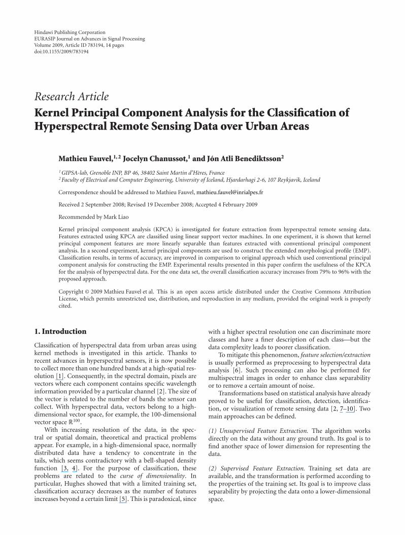
Figure 1: Simple morphological profile with 2 openings and 2closings. In the profile shown, circular structuring elements are usedwith radius increment 4 (r = 4, 8 pixels). The image processed ispart of Figure 4(a).

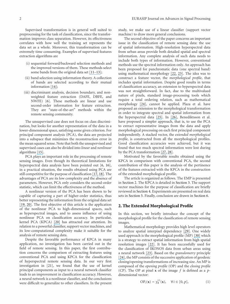
Profile from PC1 Profile from PC2

Combined profile

Figure 2: Extended morphological profile of two images. Eachof the original profiles has 2 openings and 2 closings. A circularstructuring element with radius increment 4 was used (r = 4, 8).The image processed is part of Figure 4(a).

where γ(i)R is the opening by reconstruction with a structuring

element (SE) of size i, and p is the total number of openings.Also, the CP at pixel x of image f is defined as a p-dimensional vector:

CPi(x) = φ(i)R (x), ∀i ∈ [0, p], (2)

where φ(i)R is the closing by reconstruction with an SE of size

i. Clearly, we have CP0(x) = OP0(x) = f (x). By collating theOP and the CP, the MP of image f is defined as a 2p + 1-dimensional vector:

MP(x) = {CPp(x), . . . , f (x), . . . , OPp(x)}. (3)

An example of MP is shown in Figure 1. Thus, from asingle image a multivalued image results. The dimension ofthis image corresponds to the number of transformations.For application to hyperspectral data, characteristic imagesneed to be extracted. In [26], it was suggested to use severalprincipal components (PCs) of the hyperspectral data forsuch a purpose. Hence, the MP is applied on the firstPCs, corresponding to a certain amount of the cumulativevariance, and a stacked vector is built using the MP on eachPC. This yields the extended morphological profile (EMP).Following the previous notation, the EMP is a q(2p + 1)-dimensional vector:

EMP(x) = {MPPC1 (x), . . . , MPPCq(x)}

, (4)

where q is the number of retaining PCs. An example of anEMP is shown in Figure 2.

As stated in the introduction, PCA does not fully handlethe spectral information. Previous works using alternativefeature reduction algorithms, such as independent compo-nent analysis (ICA), have led to equivalent results in termsof classification accuracy [31]. In this article, we proposethe use of the KPCA rather than PCA for the construction

of the EMP, that is, the first kernel PCs (KPCs) are used tobuild the EMP. The assumption is that much more spectralinformation will be captured by the KPCA than with thePCA. The next section presents the KPCA and how the KPCAis applied to hyperspectral remote sensing images.

3. Kernel Principal Component Analysis

3.1. Kernel PCA Problem. In this section, a brief descriptionis given of kernel principal component analysis for featurereduction on remote sensing data. The theoretical founda-tion may be found in [20, 32, 33].

The starting point is a set of pixel vectors xi ∈ Rn, i ∈[1, . . . , �]. Conventional PCA solves the eigenvalue problem:

λv = Σxv, subject to ‖v‖2 = 1, (5)

where Σx = E[xcxTc ] ≈ (1/(� − 1))∑�

i=1(xi −mx)(xi −mx)T

,and xc is the centered vector x. A projection onto the first mprincipal components is performed as xpc = [v1| · · · |vm]Tx.

To capture higher-order statistics, the data can bemapped onto another space H (from now on, Rn is calledthe input space and H the feature space):

Φ : Rn −→H

x �−→ Φ(x),(6)

where Φ is a function that may be nonlinear, and the onlyrestriction on H is that it must have the structure of areproducing kernel Hilbert space (RKHS), not necessarily offinite dimension. PCA in H can be performed as in the inputspace, but thanks to the kernel trick [34], it can be performeddirectly in the input space. The kernel PCA (KPCA) solvesthe following eigenvalue problem:

λα = Kα, subject to ‖α‖2 = 1λ

, (7)

where K is the kernel matrix constructed as follows:

K =

⎛

⎜⎜⎜⎜⎜⎜⎜⎝

k(

x1, x1) · · · k

(x1, x�

)

k(

x2, x1) · · · k

(x2, x�

)

.... . .

...

k(

x� , x1) · · · k

(x� , x�

)

⎞

⎟⎟⎟⎟⎟⎟⎟⎠

. (8)

The function k is the core of the KPCA. It is a positivesemidefinite function on Rn that introduces nonlinearityinto the processing. This is usually called a kernel. Classickernels are the polynomial kernel, q ∈ R+ and p ∈ N+,

k(x, y) = (〈x, y〉R + q)p

, (9)

and the Gaussian kernel, σ ∈ R+,

k(x, y) = exp

(

− ‖x− y‖2

2σ2

)

. (10)

4 EURASIP Journal on Advances in Signal Processing

−0.2

0

0.2

0.4

0.6

0.8

−0.2 0 0.2 0.4 0.6 0.8

(a)

−0.8

−0.6

−0.4

−0.2

0

0.2

0.4

0.6

−0.8 −0.6 −0.4 −0.2 0 0.2 0.4 0.6 0.8

(b)

−0.5

0

0.5

−0.8 −0.6 −0.4 −0.2 0 0.2 0.4 0.6 0.8

(c)

−0.2

0

0.2

0.4

0.6

0.8

−0.2 0 0.2 0.4 0.6 0.8

(d)

−0.2

0

0.2

0.4

0.6

0.8

−0.2 0 0.2 0.4 0.6 0.8

(e)

−0.2

0

0.2

0.4

0.6

0.8

−0.2 0 0.2 0.4 0.6 0.8

(f)

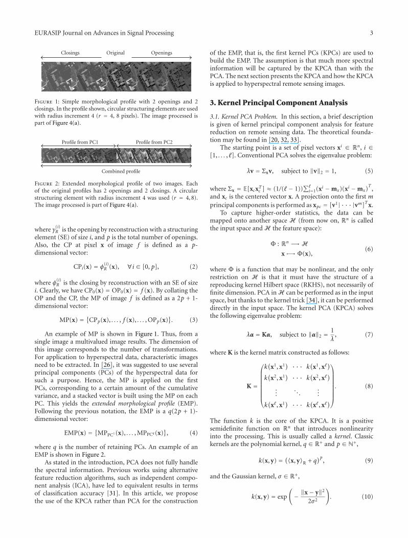
Figure 3: PCA versus KPCA. (a) Three Gaussian clusters, and their projection onto the first two kernel principal components with (b)a Gaussian kernel and (c) a polynomial kernel. (d), (e), and (f) represent, respectively, the contour plot of the projection onto the firstcomponent for the PCA, the KPCA with Gaussian kernel, and the KPCA with a polynomial kernel. Note how with the Gaussian kernel thefirst component “picks out” the individual clusters [20]. The intensity of the contour plot is proportional to the value of the projection, thatis, light gray indicates that Φ1

kpc(x) has a high value.

As with conventional PCA, once (7) has been solved,projection is then performed:

Φmkpc(x) =

�∑

i=1

αmi k(

xi, x). (11)

Note it is assumed that K is centered, otherwise it can becentered as [35]

Kc = K− 1�K−K1� + 1�K1� (12)

where 1� is a square matrix such as (1�)i j = 1/�.

3.2. PCA versus KPCA. Let us start by recalling that thePCA relies on a simple generative model. The n observedvariables result from a linear transformation of mGaussianlydistributed latent variables, and thus it is possible to recoverthe latent variable from the observed one by solving (5).

To better understand the link and the difference betweenPCA and KPCA, one must note that the eigenvectors ofΣx can be obtained from those of XXT , where X =[x1, x2, . . . , x�]

T [36]. Consider the eigenvalue problem:

γu = XXTu, subject to ‖u‖2 = 1. (13)

The left part is multiplied by XT giving

γXTu = XTXXTu,

γXTu = (� − 1)ΣxXTu,

γ′XTu = ΣxXTu,

(14)

which is the eigenvalue problem (5): v = XTu. But ‖v‖2 =uTXXTu = γuTu = γ /= 1. Therefore, the eigenvectors of Σx

can be computed from eigenvectors of XXT as v = γ−0.5XTu.

The matrix XXT is equal to

⎛

⎜⎜⎜⎜⎜⎜⎜⎝

⟨x1, x1

⟩ · · · ⟨x1, x�

⟩

⟨x2, x1

⟩ · · · ⟨x2, x�

⟩

.... . .

...⟨

x� , x1⟩ · · · ⟨

x� , x�⟩

⎞

⎟⎟⎟⎟⎟⎟⎟⎠

, (15)

which is the kernel matrix with a linear kernel: k(xi, x j) =〈xi, x j〉Rn . Using the kernel trick k(xi, x j) = 〈Φ(xi),Φ(x j)〉H ,K can be rewritten in a similar form as (15)

⎛

⎜⎜⎜⎜⎜⎜⎜⎝

⟨Φ(

x1),Φ(

x1)⟩

H · · · ⟨Φ(

x1),Φ(

x�)⟩

H⟨Φ(

x2),Φ(

x1)⟩

H · · · ⟨Φ(

x2),Φ(

x�)⟩

H

.... . .

...⟨Φ(

x�),Φ(

x1)⟩

H · · · ⟨Φ(

x�),Φ(

x�)⟩

H

⎞

⎟⎟⎟⎟⎟⎟⎟⎠

. (16)

From (15) and (16), the advantage of using KPCA comesfrom an appropriate projection Φ of Rn onto H . In thisspace, the data should better match the PCA model. It is clearthat the KPCA shares the same properties as the PCA, but indifferent space.

To illustrate how the KPCA works, a short example isgiven here. Figure 3(a) represents three Gaussian clusters.The conventional PCA would result in a rotation of thespace, that is, the three clusters would not be identified.Figures 3(b) and 3(c) represent the projection onto the firsttwo kernel principal components (KPCs). Using a Gaussiankernel, the structure of the data is better captured than withPCA: a cluster can be clearly identified on the first KPC

EURASIP Journal on Advances in Signal Processing 5

(a) (b)

(c)

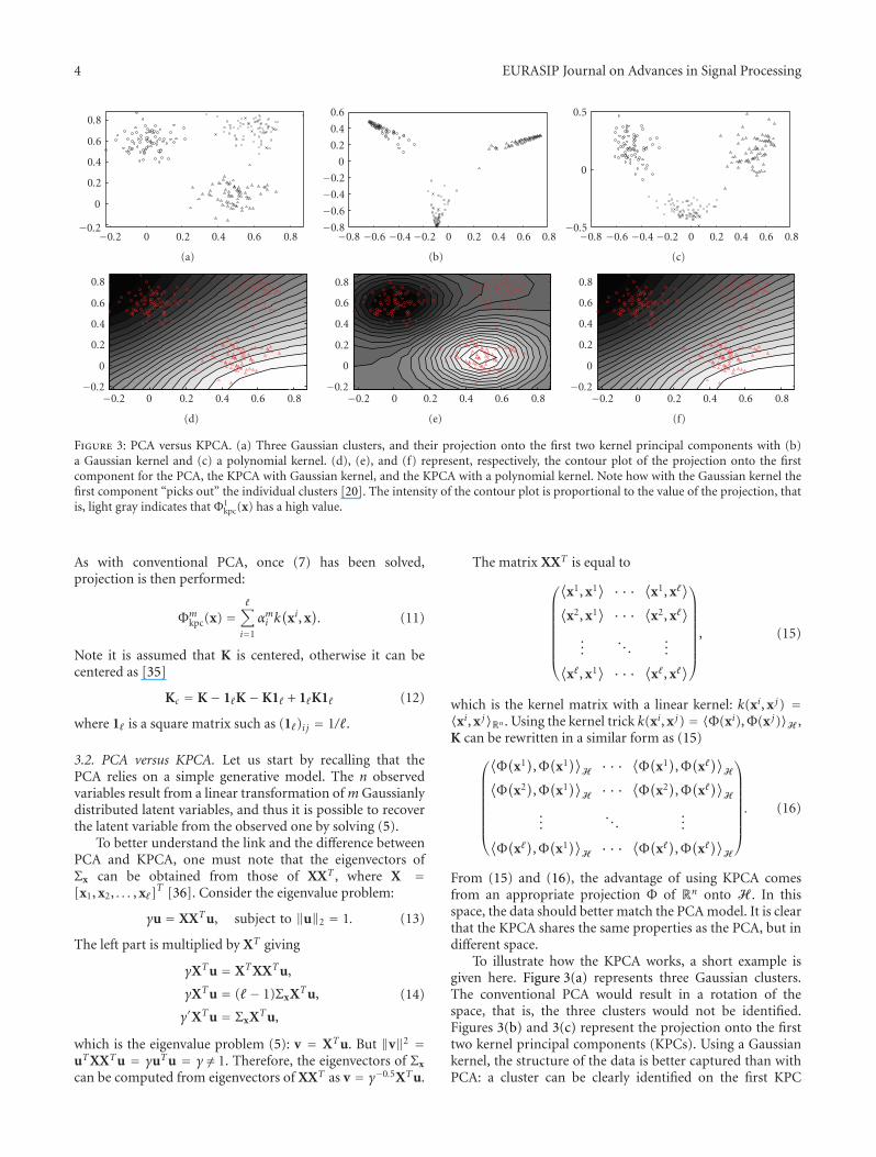
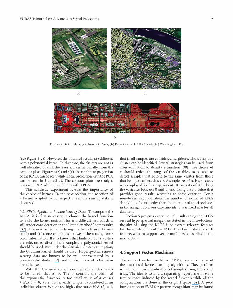
Figure 4: ROSIS data. (a) University Area, (b) Pavia Center. HYDICE data: (c) Washington DC.

(see Figure 3(e)). However, the obtained results are differentwith a polynomial kernel. In that case, the clusters are not aswell identified as with the Gaussian kernel. Finally, from thecontour plots, Figures 3(e) and 3(f), the nonlinear projectionof the KPCA can be seen while linear projection with the PCAcan be seen in Figure 3(d). The contour plots are straightlines with PCA while curved lines with KPCA.

This synthetic experiment reveals the importance ofthe choice of kernels. In the next section, the selection ofa kernel adapted to hyperspectral remote sensing data isdiscussed.

3.3. KPCA Applied to Remote Sensing Data. To compute theKPCA, it is first necessary to choose the kernel functionto build the kernel matrix. This is a difficult task which isstill under consideration in the “kernel method” community[37]. However, when considering the two classical kernelsin (9) and (10), one can choose between them using someprior information. If it is known that higher-order statisticsare relevant to discriminate samples, a polynomial kernelshould be used. But under the Gaussian cluster assumption,the Gaussian kernel should be used. Hyperspectral remotesensing data are known to be well approximated by aGaussian distribution [7], and thus in this work a Gaussiankernel is used.

With the Gaussian kernel, one hyperparameter needsto be tuned, that is, σ . The σ controls the width ofthe exponential function. A too small value of σ causesk(xi, x j) = 0, i /= j, that is, each sample is considered as anindividual cluster. While a too high value causes k(xi, x j) = 1,

that is, all samples are considered neighbors. Thus, only onecluster can be identified. Several strategies can be used, fromcross-validation to density estimation [38]. The choice ofσ should reflect the range of the variables, to be able todetect samples that belong to the same cluster from thosethat belong to others clusters. A simple, yet effective, strategywas employed in this experiment. It consists of stretchingthe variables between 0 and 1, and fixing σ to a value thatprovides good results according to some criterion. For aremote sensing application, the number of extracted KPCsshould be of same order than the number of species/classesin the image. From our experiments, σ was fixed at 4 for alldata sets.

Section 5 presents experimental results using the KPCAon real hyperspectral images. As stated in the introduction,the aim of using the KPCA is to extract relevant featuresfor the construction of the EMP. The classification of suchfeatures with the support vector machines is described in thenext section.

4. Support Vector Machines

The support vector machines (SVMs) are surely one ofthe most used kernel learning algorithms. They performrobust nonlinear classification of samples using the kerneltrick. The idea is to find a separating hyperplane in somefeature space induced by the kernel function while all thecomputations are done in the original space [39]. A goodintroduction to SVM for pattern recognition may be found

6 EURASIP Journal on Advances in Signal Processing

in [40]. Given a training set S = {(x1, y1), . . . , (x� , y�)} ∈Rn × {−1; 1}, the decision function is found by solving theconvex optimization problem:

maxa

g(a) =�∑

i=1

αi − 12

�∑

i, j=1

αiαj yi y jk(

xi, x j)

subject to 0 ≤ αi ≤ C and�∑

i=1

αi yi = 0,

(17)

where α are the Lagrange coefficients, C a constant thatis used to penalize the training errors, and k the kernelfunction. Same than KPCA, classic effective kernels are (9)and (10). A short comparison of kernels for remotely sensedimage classification may be found in [41]. Advanced kernelfunctions can be constructed using some prior [42].

When the optimal solution of (17) is found, that is, αi,the classification of a sample x is achieved by observing towhich side of the hyperplane it belongs:

y = sgn

( �∑

i=1

αi yik(

xi, x)

+ b

)

. (18)

SVMs are designed to solve binary problems where theclass labels can only take two values: ±1. For a remote-sensing application, several species/classes are usually ofinterest. Various approaches have been proposed to addressthis problem. They usually combine a set of binary classifiers.Two main approaches were originally proposed for C-classproblems [35].

(i) One-versus-the-Rest. C binary classifiers are applied oneach class against all the others. Each sample is assigned tothe class with the maximum output.

(ii) Pairwise Classification. C(C − 1)/2 binary classifiers areapplied on each pair of classes. Each sample is assigned tothe class getting the highest number of votes. A vote for agiven class is defined as a classifier assigning the pattern tothat class.

Pairwise classification has proved more suitable for largeproblems [43]. Even though the number of classifiers used islarger than for the one-versus-the-rest approach, the wholeclassification problem is decomposed into much simplerones. Therefore, the pairwise approach was used in ourexperiments. More advanced approaches applied to remotesensing data can be found in [44].

SVMs are primarily a nonparametric method, yet somehyperparameters do need to be tuned before optimization.In the Gaussian kernel case, there are two hyperparameters:C the penalty term and σ the width of the exponential. This isusually done by a cross-validation step, where several valuesare tested. In our experiments, C is fixed to 200 and σ2 ∈{0.5, 1, 2, 4} is selected using 5-fold cross validation. TheSVM optimization problem was solved using the LIBSVM[45]. The range of each feature was stretched between 0 and1.

5. Experiments

Three real data sets were used in the experiments. They aredetailed in the following. The original hyperspectral data aretermed “Raw” in the rest of the paper.

5.1. Data Set. Airborne data from the reflective optics systemimaging spectrometer (ROSIS-03) optical sensor are used forthe first two experiments. The flight over the city of Pavia,Italy was operated by the Deutschen Zentrum fur Luft- undRaumfahrt (DLR, the German Aerospace Agency) withinthe context of the HySens project, managed and sponsoredby the European Union. According to specifications, theROSIS-03 sensor provides 115 bands with a spectral coverageranging from 0.43 to 0.86 μm. The spatial resolution is 1.3 mper pixel. The two data sets are:

(1) university Area: the first test set is around theEngineering School at the University of Pavia. Itis 610 × 340 pixels. Twelve channels have beenremoved due to noise. The remaining 103 spectralchannels are processed. Nine classes of interest areconsidered: tree, asphalt, bitumen, gravel, metalsheet, shadow, bricks, meadow, and soil;

(2) Pavia center: the second test set is the center of Pavia.The Pavia center image was originally 1096 × 1096pixels. A 381 pixel wide black band in the left-hand part of image was removed, resulting in a “twopart” image of 1096 × 715 pixels. Thirteen channelshave been removed due to noise. The remaining102 spectral channels are processed. Nine classes ofinterest are considered: water, tree, meadow, brick,soil, asphalt, bitumen, tile, and shadow.

Airborne data from the hyperspectral digital imagery col-lection experiment (HYDICE) sensor was used for thethird experiments. The HYDICE was used to collect datafrom flightline over the Washington DC Mall. Hyper-spectral HYDICE data originally contained 210 bands inthe 0.4–2.4 μm region. Channels from near-infrared andinfrared wavelengths are known to contained more noisethan channel from visible wavelengths. Noisy channels dueto water absorption have been removed, and the set consistsof 191 spectral channels. The data were collected in August1995, and each channel has 1280 lines with 307 pixels each.Seven information classes were defined, namely, roof, road,grass, tree, trail, water, and shadow. Figure 4 shows false colorimages for all the data sets.

Available training and test sets for each data set are givenin Tables 1, 2, and 3. These are selected pixels from the databy an expert, corresponding to a predefined species/classes.Pixels from the training set are excluded from the test set ineach case and vice versa.

The classification accuracy was assessed with

(i) an overall accuracy (OA) which is the number ofwell-classified samples divided by the number of testsamples,

(ii) an average accuracy (AA) which represents theaverage of class classification accuracy,

EURASIP Journal on Advances in Signal Processing 7

Table 1: Information classes and training/test samples for theUniversity Area data set.

Class Samples

No Name Train Test

1 Asphalt 548 6641

2 Meadow 540 18649

3 Gravel 392 2099

4 Tree 524 3064

5 Metal Sheet 265 1345

6 Bare Soil 532 5029

7 Bitumen 375 1330

8 Brick 514 3682

9 Shadow 231 947

Total 3921 42776

Table 2: Information classes and training/test samples for the PaviaCenter data set.

Class Samples

No Name Train Test

1 Water 824 65971

2 Tree 820 7598

3 Meadow 824 3090

4 Brick 808 2685

5 Bare soil 820 6584

6 Asphalt 816 9248

7 Bitumen 808 7287

8 Tile 1260 42826

9 Shadow 476 2863

Total 7456 148152

Table 3: Information classes and training/test samples for theWashington DC Mall data set.

Class Samples

No. Name Train Test

1 Roof 40 3794

2 Road 40 376

3 Trail 40 135

4 Grass 40 1888

5 Tree 40 365

6 Water 40 1184

7 Shadow 40 57

Total 280 6929

(iii) a kappa coefficient of agreement (κ) which is thepercentage of agreement corrected by the amount ofagreement that could be expected due to chance alone[7],

(iv) a class accuracy which is the percentage of correctlyclassified samples for a given class.

These criteria were used to compare classification resultsand were computed using a confusion matrix. Furthermore,the statistical significance of differences was computed using

McNemar’s test, which is based upon the standardizednormal test statistic [46]:

Z = f12 − f21√f12 + f21

, (19)

where f12 indicates the number of samples classified correctlyby classifier 1 and incorrectly by classifier 2. The difference inaccuracy between classifiers 1 and 2 is said to be statisticallysignificant if |Z| > 1.96. The sign of Z indicates whetherclassifier 1 is more accurate than classifier 2 (Z > 0) or viceversa (Z < 0). This test assumes that the training and the testsamples are related and is thus adapted to the analysis sincethe training and test sets were the same for each experimentfor a given data set.

5.2. Spectral Feature Extraction. Solving the eigenvaluesproblem (5) for each data set yields the results reportedin Table 4. Looking at the cumulative eigenvalues, in eachROSIS case, three principal components (PCs) reach 95% oftotal variance. After the PCA transformation, the dimension-ality of the new representation of the University Area dataset and the Pavia Center is 3, if the threshold is set to 95%of the cumulative variance. The results for the third dataset are somewhat different. Acquired from a higher rangeof wavelengths, more noise is contained in the data andmore bands were removed by comparison to the ROSIS data.That explains why more PCs are needed, that is, 40 PCs, toreach 95% of the cumulative variance. But from the table,it can be clearly seen that the first two PCs contain mostof the information. This means that by using second-orderinformation, the hyperspectral data can be reduced to a two-or three-dimensional space. But, as experiments will show,hyperspectral richness is not fully handled using only themean and variance/covariance of the data.

Table 5 shows the variance and the cumulative variancefor the three data sets when KPCA is applied. The kernelmatrix in each case was constructed using 5000 randomlyselected samples. From the table, it can be seen that morekernel principal components (KPCs) are needed to achievethe same amount of variance as for the conventional PCA.For the University data set, the first 12 KPCs are neededto achieve 95% of the cumulative variance, 11 for theWashington DC data set and only 10 for the Pavia Centerdata set. That may be an indication that more informationis extracted and the KPCA is more robust to the noise,since a reasonable number of features are extracted from theWashington DC data set.

To test this assumption, the mutual information (MI)between each (K)PC has been computed. The classicalcorrelation coefficient was not used since the PCA is optimalfor that criterion. For comparison, the normalized MI was

computed: In(x, y) = I(x, y)/(√I(x, x)

√I(y, y)). The MI

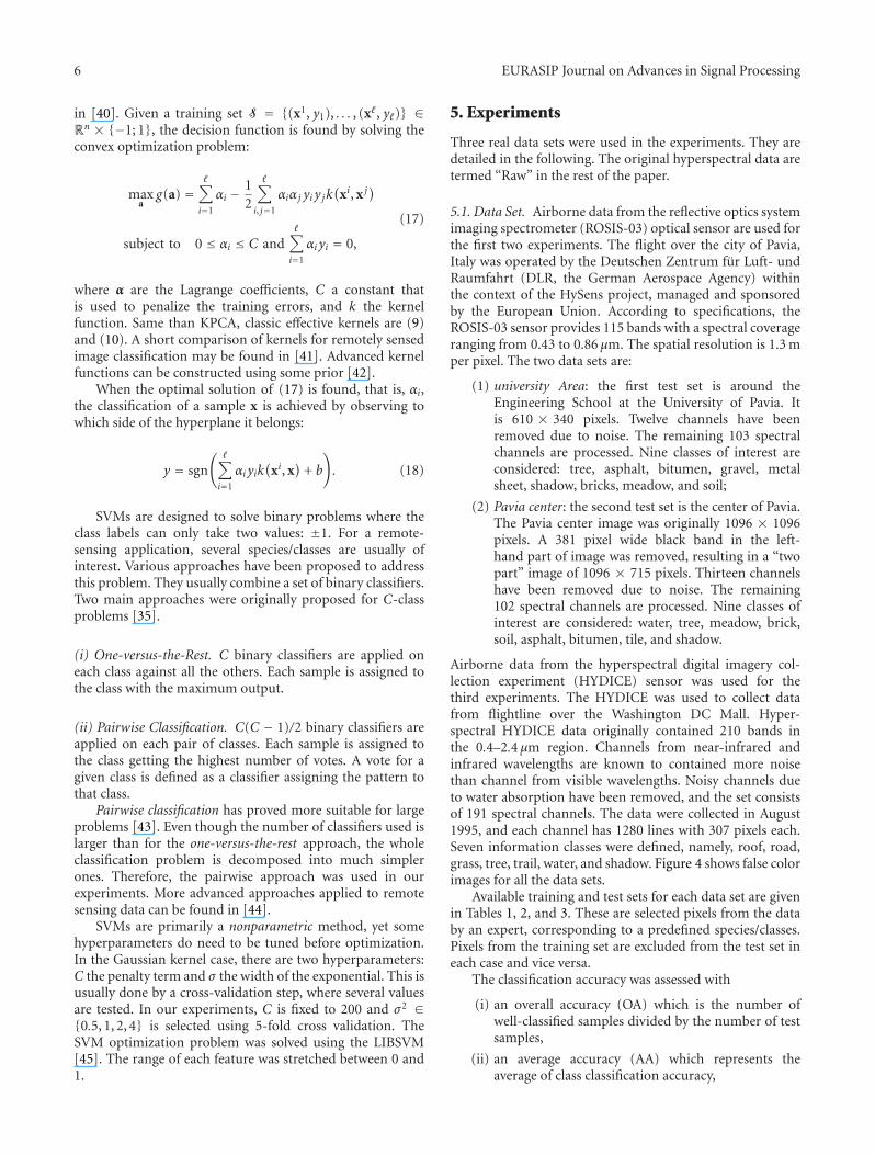
is used to test independence between two variables, andintuitively the MI measures the information that the twovariables share. An MI close to 0 indicates independence,while a high MI indicates dependence and consequentlysimilar information. Figure 5 presents the MI matrices,which represents the MI for each pair of extracted features

8 EURASIP Journal on Advances in Signal Processing

Table 4: PCA: Eigenvalues and cumulative variance in percentages for the three hyperspectral data sets.

Pavia center University area Washington DC

Component % Cum. % % Cum. % % Cum. %

1 72.85 72.85 64.85 64.85 53.38 53.38

2 21.03 93.88 28.41 93.26 18.65 72.03

3 04.23 98.11 05.14 98.40 03.83 75.87

4 00.89 99.00 00.51 98.91 02.00 77.87

5 00.30 99.30 00.25 99.20 00.66 78.00

Table 5: KPCA: Eigenvalues and cumulative variance in percent for the two hyperspectral data sets (KPCA).

Pavia center University area Washington DC

Component % Cum. % % Cum. % % Cum. %

1 43.94 43.94 31.72 31.72 40.99 40.99

2 21.00 64.94 26.04 57.76 20.18 61.17

3 15.47 80.41 19.36 75.12 13.77 74.95

4 05.23 85.64 06.76 81.88 05.99 80.94

5 03.88 89.52 04.31 86.19 05.22 86.16

with both PCA and KPCA, for the Washington DC data set.From Figure 5(a), PCs number 4 to 40 contain more or lessthe same information since they correspond to a high MI.Although uncorrelated, these features are still dependent.This phenomenon is due to the noise contained in the datawhich is not Gaussian [6] and is distributed over several PCs.From Figure 5(a), KPCA is less sensitive to the noise, that is,in the feature space the data match better the PCA model andthe noise tends to be Gaussian. Note that with KPCA, onlythe first 11 KPCs are retained against 40 with conventionalPCA.

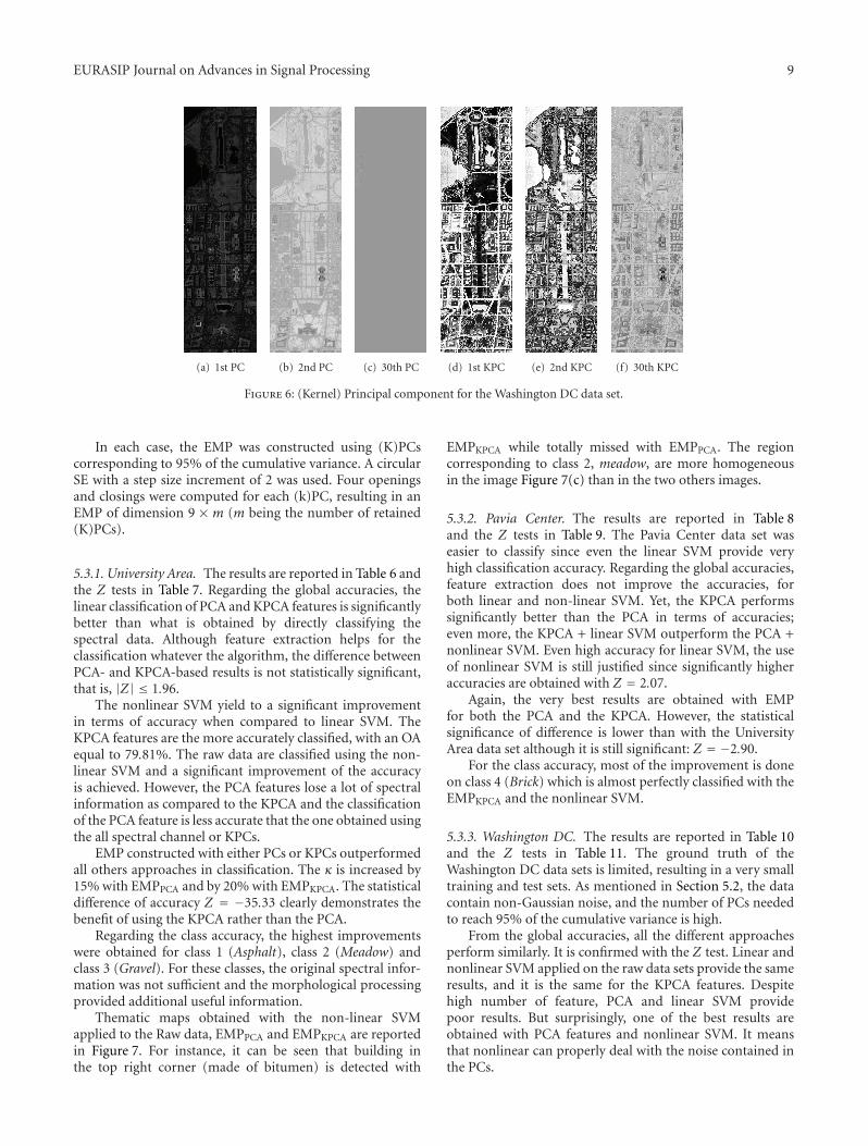
To visually assess what is contained in each different(K)PC, Figure 6 represents the first, second, and thirtieth PCfor both the PCA and the KPCA. It can be seen that

(1) the extracted PCs are different (all the images havebeen linearly stretched between 0 and 255 for thepurpose of visualization),

(2) the thirtieth PC contains only noise, while thethirtieth KPC still contains some information andspatial structure can be detected with the EMP.

In conclusion of this section, the KPCA can extractmore information from the hyperspectral data than theconventional PCA, and is robust to the noise that canaffect remote sensing data. The next question is: Is thisinformation useful for the purpose of classification? Inthe next section, experiments are conducted using featuresextracted by the PCA and the KPCA, for the classification orfor the construction of the EMP.

5.3. Classification of Remote Sensing Data. Several experi-ments were conducted to evaluate KPCs as a suitable featurefor (1) the classification of remote sensing images and (2)the construction of the EMP. For the first item, linearSVM are used to perform the classification. The aim is toinvestigate whether the data are easily classified after the PCA

40

35

30

25

20

15

10

5

5 10 15 20 25 30 35 40

0.2

0.4

0.6

0.8

1

(a) PCA

40

35

30

25

20

15

10

5

5 10 15 20 25 30 35 40

0.2

0.4

0.6

0.8

1

(b) KPCA

Figure 5: Mutual Information matrices for the Washington DC dataset.

or the KPCA. Therefore a linear classifier is used to limitits influence on the results. For the EMP, as state in theintroduction, too much information are lost during the PCA,and experiments should confirm that the KPCA extractsmore information. In the following, an analysis of the resultsfor each data sets is provided.

EURASIP Journal on Advances in Signal Processing 9

(a) 1st PC (b) 2nd PC (c) 30th PC (d) 1st KPC (e) 2nd KPC (f) 30th KPC

Figure 6: (Kernel) Principal component for the Washington DC data set.

In each case, the EMP was constructed using (K)PCscorresponding to 95% of the cumulative variance. A circularSE with a step size increment of 2 was used. Four openingsand closings were computed for each (k)PC, resulting in anEMP of dimension 9 × m (m being the number of retained(K)PCs).

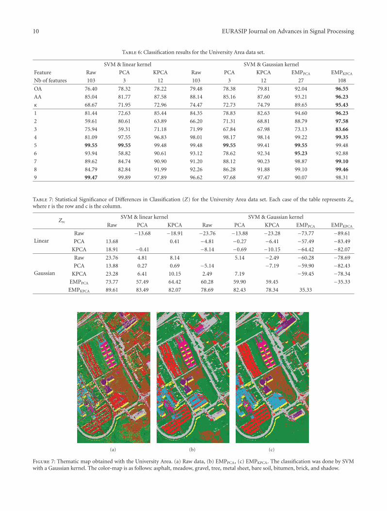
5.3.1. University Area. The results are reported in Table 6 andthe Z tests in Table 7. Regarding the global accuracies, thelinear classification of PCA and KPCA features is significantlybetter than what is obtained by directly classifying thespectral data. Although feature extraction helps for theclassification whatever the algorithm, the difference betweenPCA- and KPCA-based results is not statistically significant,that is, |Z| ≤ 1.96.

The nonlinear SVM yield to a significant improvementin terms of accuracy when compared to linear SVM. TheKPCA features are the more accurately classified, with an OAequal to 79.81%. The raw data are classified using the non-linear SVM and a significant improvement of the accuracyis achieved. However, the PCA features lose a lot of spectralinformation as compared to the KPCA and the classificationof the PCA feature is less accurate that the one obtained usingthe all spectral channel or KPCs.

EMP constructed with either PCs or KPCs outperformedall others approaches in classification. The κ is increased by15% with EMPPCA and by 20% with EMPKPCA. The statisticaldifference of accuracy Z = −35.33 clearly demonstrates thebenefit of using the KPCA rather than the PCA.

Regarding the class accuracy, the highest improvementswere obtained for class 1 (Asphalt), class 2 (Meadow) andclass 3 (Gravel). For these classes, the original spectral infor-mation was not sufficient and the morphological processingprovided additional useful information.

Thematic maps obtained with the non-linear SVMapplied to the Raw data, EMPPCA and EMPKPCA are reportedin Figure 7. For instance, it can be seen that building inthe top right corner (made of bitumen) is detected with

EMPKPCA while totally missed with EMPPCA. The regioncorresponding to class 2, meadow, are more homogeneousin the image Figure 7(c) than in the two others images.

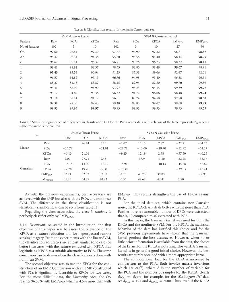
5.3.2. Pavia Center. The results are reported in Table 8and the Z tests in Table 9. The Pavia Center data set waseasier to classify since even the linear SVM provide veryhigh classification accuracy. Regarding the global accuracies,feature extraction does not improve the accuracies, forboth linear and non-linear SVM. Yet, the KPCA performssignificantly better than the PCA in terms of accuracies;even more, the KPCA + linear SVM outperform the PCA +nonlinear SVM. Even high accuracy for linear SVM, the useof nonlinear SVM is still justified since significantly higheraccuracies are obtained with Z = 2.07.

Again, the very best results are obtained with EMPfor both the PCA and the KPCA. However, the statisticalsignificance of difference is lower than with the UniversityArea data set although it is still significant: Z = −2.90.

For the class accuracy, most of the improvement is doneon class 4 (Brick) which is almost perfectly classified with theEMPKPCA and the nonlinear SVM.

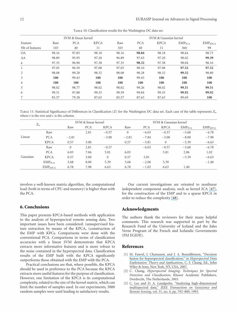
5.3.3. Washington DC. The results are reported in Table 10and the Z tests in Table 11. The ground truth of theWashington DC data sets is limited, resulting in a very smalltraining and test sets. As mentioned in Section 5.2, the datacontain non-Gaussian noise, and the number of PCs neededto reach 95% of the cumulative variance is high.

From the global accuracies, all the different approachesperform similarly. It is confirmed with the Z test. Linear andnonlinear SVM applied on the raw data sets provide the sameresults, and it is the same for the KPCA features. Despitehigh number of feature, PCA and linear SVM providepoor results. But surprisingly, one of the best results areobtained with PCA features and nonlinear SVM. It meansthat nonlinear can properly deal with the noise contained inthe PCs.

10 EURASIP Journal on Advances in Signal Processing

Table 6: Classification results for the University Area data set.

SVM & linear kernel SVM & Gaussian kernel

Feature Raw PCA KPCA Raw PCA KPCA EMPPCA EMPKPCA

Nb of features 103 3 12 103 3 12 27 108

OA 76.40 78.32 78.22 79.48 78.38 79.81 92.04 96.55

AA 85.04 81.77 87.58 88.14 85.16 87.60 93.21 96.23

κ 68.67 71.95 72.96 74.47 72.73 74.79 89.65 95.43

1 81.44 72.63 85.44 84.35 78.83 82.63 94.60 96.23

2 59.61 80.61 63.89 66.20 71.31 68.81 88.79 97.58

3 75.94 59.31 71.18 71.99 67.84 67.98 73.13 83.66

4 81.09 97.55 96.83 98.01 98.17 98.14 99.22 99.35

5 99.55 99.55 99.48 99.48 99.55 99.41 99.55 99.48

6 93.94 58.82 90.61 93.12 78.62 92.34 95.23 92.88

7 89.62 84.74 90.90 91.20 88.12 90.23 98.87 99.10

8 84.79 82.84 91.99 92.26 86.28 91.88 99.10 99.46

9 99.47 99.89 97.89 96.62 97.68 97.47 90.07 98.31

Table 7: Statistical Significance of Differences in Classification (Z) for the University Area data set. Each case of the table represents Zrc

where r is the row and c is the column.

ZrcSVM & linear kernel SVM & Gaussian kernel

Raw PCA KPCA Raw PCA KPCA EMPPCA EMPKPCA

LinearRaw −13.68 −18.91 −23.76 −13.88 −23.28 −73.77 −89.61

PCA 13.68 0.41 −4.81 −0.27 −6.41 −57.49 −83.49

KPCA 18.91 −0.41 −8.14 −0.69 −10.15 −64.42 −82.07

Gaussian

Raw 23.76 4.81 8.14 5.14 −2.49 −60.28 −78.69

PCA 13.88 0.27 0.69 −5.14 −7.19 −59.90 −82.43

KPCA 23.28 6.41 10.15 2.49 7.19 −59.45 −78.34

EMPPCA 73.77 57.49 64.42 60.28 59.90 59.45 −35.33

EMPKPCA 89.61 83.49 82.07 78.69 82.43 78.34 35.33

(a) (b) (c)

Figure 7: Thematic map obtained with the University Area. (a) Raw data, (b) EMPPCA, (c) EMPKPCA. The classification was done by SVMwith a Gaussian kernel. The color-map is as follows: asphalt, meadow, gravel, tree, metal sheet, bare soil, bitumen, brick, and shadow.

EURASIP Journal on Advances in Signal Processing 11

Table 8: Classification results for the Pavia Center data set.

SVM & linear kernel SVM & Gaussian kernel

Feature Raw PCA KPCA Raw PCA KPCA EMPPCA EMPKPCA

Nb of features 102 3 10 102 3 10 27 90

OA 97.60 96.54 97.39 97.67 96.99 97.32 98.81 98.87

AA 95.42 92.34 94.38 95.60 93.56 94.40 98.14 98.25

κ 96.62 95.14 96.32 96.71 95.76 96.23 98.32 98.41

1 98.41 98.82 98.57 98.35 98.80 98.49 99.07 98.91

2 93.43 85.56 90.94 91.23 87.33 89.06 92.67 92.01

3 96.57 94.82 95.15 96.76 94.98 95.40 96.38 96.31

4 88.27 81.15 83.87 88.45 82.94 82.50 99.70 99.59

5 94.41 88.97 94.99 93.97 95.23 94.55 99.39 99.77

6 95.17 94.82 95.36 96.32 94.72 96.06 98.48 99.24

7 93.18 88.14 91.12 96.01 89.24 94.50 97.98 98.58

8 99.38 98.30 99.43 99.40 98.83 99.07 99.68 99.89

9 99.93 99.93 99.97 99.93 99.93 99.93 99.93 99.55

Table 9: Statistical significance of differences in classification (Z) for the Pavia center data set. Each case of the table represents Zrc where ris the row and c is the column.

ZrcSVM & linear kernel SVM & Gaussian kernel

Raw PCA KPCA Raw PCA KPCA EMPPCA EMPKPCA

Linear

Raw 26.74 6.13 −2.07 15.15 7.87 −32.71 −34.26

PCA −26.74 −21.01 −27.71 −13.00 −19.70 −52.92 −54.27

KPCA −6.13 21.01 −9.45 12.19 2.38 −37.30 −40.23

Gaussian

Raw 2.07 27.71 9.45 18.9 13.30 −32.25 −35.36

PCA −15.15 13.00 −12.19 −18.91 −10.13 −45.78 −47.67

KPCA −7.78 19.70 −2.38 −13.30 10.13 −39.03 −42.41

EMPPCA 32.71 52.92 37.30 32.25 45.78 39.03 −2.90

EMPKPCA 35.26 54.27 40.23 35.36 47.67 42.41 2.90

As with the previous experiments, best accuracies areachieved with the EMP, but also with the PCA, and nonlinearSVM. The difference in the three classification is notstatistically significant, as can be seen from Table 11.

Regarding the class accuracies, the class 7, shadow, isperfectly classifier only by EMPKPCA.

5.3.4. Discussion. As stated in the introduction, the firstobjective of this paper was to assess the relevance of theKPCA as a feature reduction tool for hyperspectral remotesensing imagery. From the experiments with the linear SVM,the classification accuracies are at least similar (one case) orbetter (two cases) with the features extracted with KPCA thuslegitimizing KPCA as a suitable alternative to PCA. The sameconclusion can be drawn when the classification is done withnonlinear SVM.

The second objective was to use the KPCs for the con-struction of an EMP. Comparison with an EMP constructedwith PCs is significantly favorable to KPCA for two cases.For the most difficult data, the University Area, the OAreaches 96.55% with EMPKPCA which is 4.5% more than with

EMPPCA. This results strengthen the use of KPCA againstPCA.

For the third data set, which contains non-Gaussiannoise, the KPCA clearly deals better with the noise than PCA.Furthermore, a reasonable number of KPCs were extracted,that is, 10 compared to 40 extracted with PCA.

In this paper, the Gaussian kernel was used for both theKPCA and the nonlinear SVM. For the KPCA, the statisticalbehavior of the data has justified this choice and for theSVM previous experiments have shown that the Gaussiankernel produce the best accuracies. However, when no orlittle prior information is available from the data, the choiceof the kernel for the KPCA is not straightforward. A Gaussiankernel is in general a good initial choice. However, the bestresults are surely obtained with a more appropriate kernel.

The computational load for the KCPA is increased bycomparison to the PCA. Both involve matrix inversionswhich are o(d3), where d is the number of variable forthe PCA and the number of samples for the KPCA; clearlydPCA � dKPCA, for example, for the Washington DC dataset dPCA = 191 and dKPCA = 5000. Thus, even if the KPCA

12 EURASIP Journal on Advances in Signal Processing

Table 10: Classification results for the Washington DC data set.

SVM & linear kernel SVM & Gaussian kernel

Feature Raw PCA KPCA Raw PCA KPCA EMPPCA EMPKPCA

Nb of features 103 40 11 103 40 11 360 99

OA 98.16 97.85 98.18 98.16 98.84 98.18 98.64 98.73

AA 98.89 95.95 97.20 96.89 97.65 97.20 98.02 99.39

κ 97.35 96.90 97.38 97.35 98.32 97.38 98.04 98.16

1 97.05 96.50 97.08 97.05 98.10 97.08 97.52 97.52

2 98.08 99.28 98.32 98.08 98.28 98.32 99.52 98.80

3 100 99.43 100 100 99.43 100 100 100

4 100 100 100 100 100 100 100 100

5 98.02 98.77 98.02 98.02 99.26 98.02 99.51 99.51

6 99.51 97.88 99.35 99.59 99.84 99.35 99.92 99.92

7 85.57 79.38 87.65 85.57 87.63 87.63 89.69 100

Table 11: Statistical Significance of Differences in Classification (Z) for the Washington DC data set. Each case of the table represents Zrc

where r is the row and c is the column.

ZrcSVM & linear kernel SVM & Gaussian kernel

Raw PCA KPCA Raw PCA KPCA EMPPCA EMPKPCA

LinearRaw 2.81 −0.57 0 −6.03 −0.57 −5.68 −6.78

PCA −2.81 −3.00 −2.81 −7.84 −3.00 −8.00 −7.98

KPCA 0.57 3.00 0.57 −5.81 0 −5.39 −6.63

Gaussian

Raw 0 2.81 −0.57 −6.03 −0.57 −5.68 −6.78

PCA 6.03 7.84 5.81 6.03 5.81 2.06 1.02

KPCA 0.57 3.00 0 0.57 5.81 −5.39 −6.63

EMPPCA 5.68 8.00 5.39 5.68 −2.06 5.39 −1.40

EMPKPCA 6.78 7.98 6.63 6.78 −1.02 6.63 1.40

involves a well-known matrix algorithm, the computationalload (both in terms of CPU and memory) is higher than withthe PCA.

6. Conclusions

This paper presents KPCA-based methods with applicationto the analysis of hyperspectral remote sensing data. Twoimportant issues have been considered: (unsupervised fea-ture extraction by means of the KPCA, (construction ofthe EMP with KPCs. Comparisons were done with theconventional PCA. Comparisons in terms of classificationaccuracies with a linear SVM demonstrate that KPCAextracts more informative features and is more robust tothe noise contained in the hyperspectral data. Classificationresults of the EMP built with the KPCA significantlyoutperforms those obtained with the EMP with the PCA.

Practical conclusions are that, where possible, the KPCAshould be used in preference to the PCA because the KPCAextracts more useful features for the purpose of classification.However, one limitation of the KPCA is its computationalcomplexity, related to the size of the kernel matrix, which canlimit the number of samples used. In our experiments, 5000random samples were used leading to satisfactory results.

Our current investigations are oriented to nonlinearindependent component analysis, such as kernel ICA [47],for the construction of the EMP and to a sparse KPCA inorder to reduce the complexity [48].

Acknowledgments

The authors thank the reviewers for their many helpfulcomments. This research was supported in part by theResearch Fund of the University of Iceland and the JulesVerne Program of the French and Icelandic Governments(PAI EGIDE).

References

[1] M. Fauvel, J. Chanussot, and J. A. Benediktsson, “Decisionfusion for hyperspectral classification,” in Hyperspectral DataExploitation: Theory and Applications, C.-I. Chang, Ed., JohnWiley & Sons, New York, NY, USA, 2007.

[2] C. Chang, Hyperspectral Imaging: Techniques for SpectralDetection and Classification, Kluwer Academic Publishers,Dordrecht, The Netherlands, 2003.

[3] C. Lee and D. A. Landgrebe, “Analyzing high-dimensionalmultispectral data,” IEEE Transactions on Geoscience andRemote Sensing, vol. 31, no. 4, pp. 792–800, 1993.

EURASIP Journal on Advances in Signal Processing 13

[4] L. Jimenez and D. A. Landgrebe, “Supervised classification inhigh dimensional space: geometrical, statistical and asymp-totical properties of multivariate data,” IEEE Transactions onSystems, Man, and Cybernetics, Part B, vol. 28, no. 1, pp. 39–54, 1993.

[5] G. Hughes, “On the mean accuracy of statistical patternrecognizers,” IEEE Transactions on Information Theory, vol. 14,no. 1, pp. 55–63, 1968.

[6] D. A. Landgrebe, Signal Theory Methods in MultispectralRemote Sensing, John Wiley & Sons, Hoboken, NJ, USA, 2003.

[7] J. A. Richards and X. Jia, Remote Sensing Digital Image Analysis:An Introduction, Springer, New York, NY, USA, 1999.

[8] N. Keshava, “Distance metrics and band selection in hyper-spectral processing with applications to material identificationand spectral libraries,” IEEE Transactions on Geoscience andRemote Sensing, vol. 42, no. 7, pp. 1552–1565, 2004.

[9] C. Unsalan and K. L. Boyer, “Linearized vegetation indicesbased on a formal statistical framework,” IEEE Transactions onGeoscience and Remote Sensing, vol. 42, no. 7, pp. 1575–1585,2004.

[10] K.-S. Park, S. Hong, P. Park, and W.-D. Cho, “Spectral con-tent characterization for efficient image detection algorithmdesign,” EURASIP Journal on Advances in Signal Processing,vol. 2007, Article ID 82874, 14 pages, 2007.

[11] A. Jain and D. Zongker, “Feature selection: evaluation, appli-cation, and small sample performance,” IEEE Transactions onPattern Analysis and Machine Intelligence, vol. 19, no. 2, pp.153–158, 1997.

[12] P. Somol, P. Pudil, J. Novovicova, and P. Paclık, “Adaptive float-ing search methods in feature selection,” Pattern RecognitionLetters, vol. 20, no. 11–13, pp. 1157–1163, 1999.

[13] S. B. Serpico and L. Bruzzone, “A new search algorithm forfeature selection in hyperspectral remote sensing images,”IEEE Transactions on Geoscience and Remote Sensing, vol. 39,no. 7, pp. 1360–1367, 2001.

[14] B. Guo, S. R. Gunn, R. I. Damper, and J. D. B. Nelson, “Bandselection for hyperspectral image classification using mutualinformation,” IEEE Geoscience and Remote Sensing Letters, vol.3, no. 4, pp. 522–526, 2006.

[15] H. Kwon and N. M. Nasrabadi, “A comparative analysis ofkernel subspace target detectors for hyperspectral imagery,”EURASIP Journal on Advances in Signal Processing, vol. 2007,Article ID 29250, 13 pages, 2007.

[16] M. Lennon, Methodes d’analyse d’images hyperspectrales,exploitation du capteur aeroporte CASI pour des applicationsde cartographies agro-environnementale en Bretagne, Ph.D.dissertation, Universite de Rennes, Rennes, France, 2002.

[17] L. Journaux, X. Tizon, I. Foucherot, and P. Gouton, “Dimen-sionality reduction techniques: an operational comparison onmultispectral satellite images using unsupervised clustering,”in Proceedings of the 7th Nordic Signal Processing Symposium(NORSIG ’06), pp. 242–245, Reykjavik, Iceland, June 2006.

[18] M. Lennon, G. Mercier, M. C. Mouchot, and L. Hubert-Moy,“Curvilinear component analysis for nonlinear dimensionalityreduction of hyperspectral images,” in Image and SignalProcessing for Remote Sensing VII, vol. 4541 of Proceedings ofSPIE, pp. 157–168, Toulouse, France, September 2002.

[19] A. Hyvarinen, J. Karhunen, and E. Oja, Independent Compo-nent Analysis, John Wiley & Sons, New York, NY, USA, 2001.

[20] B. Scholkopf, A. Smola, and K.-R. Muller, “Nonlinear com-ponent analysis as a Kernel eigenvalue problem,” NeuralComputation, vol. 10, no. 5, pp. 1299–1319, 1998.

[21] M. Fauvel, J. Chanussot, and J. A. Benediktsson, “Kernelprincipal component analysis for feature reduction in hyper-spectrale images analysis,” in Proceedings of the 7th NordicSignal Processing Symposium (NORSIG ’06), pp. 238–241,Reykjavik, Iceland, June 2006.

[22] M. Pesaresi and J. A. Benediktsson, “A new approach forthe morphological segmentation of high-resolution satelliteimagery,” IEEE Transactions on Geoscience and Remote Sensing,vol. 39, no. 2, pp. 309–320, 2001.

[23] J. A. Benediktsson, M. Pesaresi, and K. Arnason, “Classifica-tion and feature extraction for remote sensing images fromurban areas based on morphological transformations,” IEEETransactions on Geoscience and Remote Sensing, vol. 41, no. 9,part 1, pp. 1940–1949, 2003.

[24] P. Soille, Morphological Image Analysis: Principles and Applica-tions, Springer, New York, NY, USA, 2nd edition, 2003.

[25] A. Plaza, P. Martınez, J. Plaza, and R. Perez, “Dimensionalityreduction and classification of hyperspectral image data usingsequences of extended morphological transformations,” IEEETransactions on Geoscience and Remote Sensing, vol. 43, no. 3,pp. 466–479, 2005.

[26] J. A. Benediktsson, J. A. Palmason, and J. R. Sveinsson,“Classification of hyperspectral data from urban areas basedon extended morphological profiles,” IEEE Transactions onGeoscience and Remote Sensing, vol. 43, no. 3, pp. 480–491,2005.

[27] J. A. Palmason, J. A. Benediktsson, J. R. Sveinsson, and J.Chanussot, “Fusion of morphological and spectral informa-tion for classification of hyperspectal urban remote sensingdata,” in Proceedings of IEEE International Conference onGeoscience and Remote Sensing Symposium (IGARSS ’06), pp.2506–2509, Denver, Colo, USA, July-August 2006.

[28] M. Fauvel, J. Chanussot, J. A. Benediktsson, and J. R.Sveinsson, “Spectral and spatial classification of hyperspectraldata using SVMs and morphological profiles,” in Proceedingsof IEEE International Conference on Geoscience and RemoteSensing Symposium (IGARSS ’07), pp. 1–12, Barcelona, Spain,October 2008.

[29] T. Geraud and J.-B. Mouret, “Fast road network extraction insatellite images using mathematical morphology and Markovrandom fields,” EURASIP Journal on Applied Signal Processing,vol. 2004, no. 16, pp. 2503–2514, 2004.

[30] X. Jin and C. H. Davis, “Automated building extractionfrom high-resolution satellite imagery in urban areas usingstructural, contextual, and spectral information,” EURASIPJournal on Applied Signal Processing, vol. 2005, no. 14, pp.2196–2206, 2005.

[31] J. A. Palmason, Classification of hyperspectral data from urbanareas, M.S. thesis, Faculty of Engineering, University ofIceland, Reykjavik, Iceland, 2005.

[32] B. Scholkopf, S. Mika, C. J. C. Burges, et al., “Input space ver-sus feature space in kernel-based methods,” IEEE Transactionson Neural Networks, vol. 10, no. 5, pp. 1000–1017, 1999.

[33] K.-R. Muller, S. Mika, G. Ratsch, K. Tsuda, and B. Scholkopf,“An introduction to kernel-based learning algorithms,” IEEETransactions on Neural Networks, vol. 12, no. 2, pp. 181–201,2001.

[34] N. Aronszajn, “Theory of reprodusing kernel,” Tech. Rep.11, Division of Engineering Sciences, Harvard University,Cambridge, Mass, USA, 1950.

[35] B. Scholkopf and A. J. Smola, Learning with Kernels: SupportVector Machines, Regularization, Optimization, and Beyond,MIT Press, Cambridge, Mass, USA, 2002.

14 EURASIP Journal on Advances in Signal Processing

[36] J. A. Lee and M. Verleysen, Nonlinear Dimensionality Reduc-tion, Springer, New York, NY, USA, 2007.

[37] J. Shawe-Taylor and N. Cristianini, Kernel Methods for PatternAnalysis, Cambridge University Press, Cambridge, UK, 2004.

[38] M. Fauvel, Spectral and spatial methods for the classification ofurban remote sensing data, Ph.D. dissertation, Institut NationalPolytechnique de Grenoble, Reykjavik, Iceland, 2007.

[39] V. Vapnik, Statistical Learning Theory, John Wiley & Sons, NewYork, NY, USA, 1998.

[40] C. J. C. Burges, “A tutorial on support vector machines forpattern recognition,” Data Mining and Knowledge Discovery,vol. 2, no. 2, pp. 121–167, 1998.

[41] M. Fauvel, J. Chanussot, and J. A. Benediktsson, “Evaluationof kernels for multiclass classification of hyperspectral remotesensing data,” in Proceedings of IEEE International Conferenceon Acoustics, Speech, and Signal Processing (ICASSP ’06), vol. 2,pp. 813–816, Toulouse, France, May 2006.

[42] Q. Yong and Y. Jie, “Modified kernel functions by geodesicdistance,” EURASIP Journal on Applied Signal Processing, vol.2004, no. 16, pp. 2515–2521, 2004.

[43] C.-W. Hsu and C.-J. Lin, “A comparison of methods formulticlass support vector machines,” IEEE Transactions onNeural Networks, vol. 13, no. 2, pp. 415–425, 2002.

[44] F. Melgani and L. Bruzzone, “Classification of hyperspectralremote sensing images with support vector machines,” IEEETransactions on Geoscience and Remote Sensing, vol. 42, no. 8,pp. 1778–1790, 2004.

[45] C.-C. Chang and C.-J. Lin, “LIBSVM: a library for supportvector machines,” 2001, http://www.csie.ntu.edu.tw/∼cjlin/libsvm.

[46] G. M. Foody, “Thematic map comparison: evaluating thestatistical significance of differences in classification accuracy,”Photogrammetric Engineering & Remote Sensing, vol. 70, no. 5,pp. 627–633, 2004.

[47] F. R. Bach and M. I. Jordan, “Kernel independent componentanalysis,” The Journal of Machine Learning Research, vol. 3, pp.1–48, 2002.

[48] L. K. Saul and J. B. Allen, “Periodic component analysis:an eigenvalue method for representing periodic structure inspeech,” in Advances in Neural Information Processing Systems13, T. K. Leen, T. G. Dietterich, and V. Tresp, Eds., pp. 807–813,MIT Press, Cambridge, Mass, USA, 2001.

Photograph © Turisme de Barcelona / J. Trullàs

Preliminary call for papers

The 2011 European Signal Processing Conference (EUSIPCO 2011) is thenineteenth in a series of conferences promoted by the European Association forSignal Processing (EURASIP, www.eurasip.org). This year edition will take placein Barcelona, capital city of Catalonia (Spain), and will be jointly organized by theCentre Tecnològic de Telecomunicacions de Catalunya (CTTC) and theUniversitat Politècnica de Catalunya (UPC).EUSIPCO 2011 will focus on key aspects of signal processing theory and

li ti li t d b l A t f b i i ill b b d lit

Organizing Committee

Honorary ChairMiguel A. Lagunas (CTTC)

General ChairAna I. Pérez Neira (UPC)

General Vice ChairCarles Antón Haro (CTTC)

Technical Program ChairXavier Mestre (CTTC)

Technical Program Co Chairsapplications as listed below. Acceptance of submissions will be based on quality,relevance and originality. Accepted papers will be published in the EUSIPCOproceedings and presented during the conference. Paper submissions, proposalsfor tutorials and proposals for special sessions are invited in, but not limited to,the following areas of interest.

Areas of Interest

• Audio and electro acoustics.• Design, implementation, and applications of signal processing systems.

l d l d d

Technical Program Co ChairsJavier Hernando (UPC)Montserrat Pardàs (UPC)

Plenary TalksFerran Marqués (UPC)Yonina Eldar (Technion)

Special SessionsIgnacio Santamaría (Unversidadde Cantabria)Mats Bengtsson (KTH)

FinancesMontserrat Nájar (UPC)• Multimedia signal processing and coding.

• Image and multidimensional signal processing.• Signal detection and estimation.• Sensor array and multi channel signal processing.• Sensor fusion in networked systems.• Signal processing for communications.• Medical imaging and image analysis.• Non stationary, non linear and non Gaussian signal processing.

Submissions

Montserrat Nájar (UPC)

TutorialsDaniel P. Palomar(Hong Kong UST)Beatrice Pesquet Popescu (ENST)

PublicityStephan Pfletschinger (CTTC)Mònica Navarro (CTTC)

PublicationsAntonio Pascual (UPC)Carles Fernández (CTTC)

I d i l Li i & E hibiSubmissions

Procedures to submit a paper and proposals for special sessions and tutorials willbe detailed at www.eusipco2011.org. Submitted papers must be camera ready, nomore than 5 pages long, and conforming to the standard specified on theEUSIPCO 2011 web site. First authors who are registered students can participatein the best student paper competition.

Important Deadlines:

P l f i l i 15 D 2010

Industrial Liaison & ExhibitsAngeliki Alexiou(University of Piraeus)Albert Sitjà (CTTC)

International LiaisonJu Liu (Shandong University China)Jinhong Yuan (UNSW Australia)Tamas Sziranyi (SZTAKI Hungary)Rich Stern (CMU USA)Ricardo L. de Queiroz (UNB Brazil)

Webpage: www.eusipco2011.org

Proposals for special sessions 15 Dec 2010Proposals for tutorials 18 Feb 2011Electronic submission of full papers 21 Feb 2011Notification of acceptance 23 May 2011Submission of camera ready papers 6 Jun 2011