DEPARTEMENT AEROELASTICITE ETDYNAMIQUE DES STRUCTURES

Rapport Technique

Discontinuous finite elements with highdegree polynomial interpolation for transportequations

Daniel del Pozo Galan

Septembre 2013

– 1 –

SEPTEMBRE 2013

CONTENTS

1. LE STAGE . . . . . . . . . . . . . . . . . . . . . . . . . . . . . . . . . . . . . . . . . . . . . . 31.1. Definition initiale du contrat . . . . . . . . . . . . . . . . . . . . . . . . . . . . . . . . . 31.2. Vecu de l’eleve . . . . . . . . . . . . . . . . . . . . . . . . . . . . . . . . . . . . . . . . 31.3. Resituation de l’ entreprise dans son contexte socio-economique . . . . . . . . . . . . . 3

1.3.1. Historique et presentation . . . . . . . . . . . . . . . . . . . . . . . . . . . . . . 31.3.2. Organisation . . . . . . . . . . . . . . . . . . . . . . . . . . . . . . . . . . . . . 4

2. PHYSICAL MODEL . . . . . . . . . . . . . . . . . . . . . . . . . . . . . . . . . . . . . . . . 5

3. NUMERICAL METHODS . . . . . . . . . . . . . . . . . . . . . . . . . . . . . . . . . . . . . 63.1. Introduction . . . . . . . . . . . . . . . . . . . . . . . . . . . . . . . . . . . . . . . . . . 63.2. Basic principle of discontinuous galerkin finte element method . . . . . . . . . . . . . 63.3. Formulation and implementation of the DG method . . . . . . . . . . . . . . . . . . . 73.4. Basis of polynomial interpolation . . . . . . . . . . . . . . . . . . . . . . . . . . . . . . 8

3.4.1. Orthonormal basis on a triangle . . . . . . . . . . . . . . . . . . . . . . . . . . 103.4.2. Interpolation points on a triangle . . . . . . . . . . . . . . . . . . . . . . . . . . 12

4. DG METHOD FOR THE TRANSPORT EQUATION . . . . . . . . . . . . . . . . . . . . . . 144.1. Solving problem in one direction with nodal method . . . . . . . . . . . . . . . . . . . 14

4.1.1. Mass matrix . . . . . . . . . . . . . . . . . . . . . . . . . . . . . . . . . . . . . 154.1.2. Stiffness matrix . . . . . . . . . . . . . . . . . . . . . . . . . . . . . . . . . . . 154.1.3. Flux matrices . . . . . . . . . . . . . . . . . . . . . . . . . . . . . . . . . . . . 17

4.2. Solving the problem in all directions with the nodal method . . . . . . . . . . . . . . . 204.2.1. Mass matrix . . . . . . . . . . . . . . . . . . . . . . . . . . . . . . . . . . . . . 204.2.2. Stiffness matrix . . . . . . . . . . . . . . . . . . . . . . . . . . . . . . . . . . . 204.2.3. Flux matrices . . . . . . . . . . . . . . . . . . . . . . . . . . . . . . . . . . . . 214.2.4. Boundary flux matrices for reflection phenomena . . . . . . . . . . . . . . . . . 224.2.5. Fourier basis . . . . . . . . . . . . . . . . . . . . . . . . . . . . . . . . . . . . . 244.2.6. Complex basis . . . . . . . . . . . . . . . . . . . . . . . . . . . . . . . . . . . . 25

4.3. Assembling the mesh . . . . . . . . . . . . . . . . . . . . . . . . . . . . . . . . . . . . . 284.4. Time discretization . . . . . . . . . . . . . . . . . . . . . . . . . . . . . . . . . . . . . . 28

5. NUMERICAL RESULTS . . . . . . . . . . . . . . . . . . . . . . . . . . . . . . . . . . . . . . 285.1. Numerical results in one direction with nodal method . . . . . . . . . . . . . . . . . . . 28

5.1.1. Numerical analysis . . . . . . . . . . . . . . . . . . . . . . . . . . . . . . . . . 285.1.2. Simulation . . . . . . . . . . . . . . . . . . . . . . . . . . . . . . . . . . . . . . 29

5.2. Numerical results in all directions with nodal method . . . . . . . . . . . . . . . . . . . 30

– 2 –

SEPTEMBRE 2013

5.2.1. Numerical analysis . . . . . . . . . . . . . . . . . . . . . . . . . . . . . . . . . 305.2.2. Simulation . . . . . . . . . . . . . . . . . . . . . . . . . . . . . . . . . . . . . . 30

6. CONCLUSIONS . . . . . . . . . . . . . . . . . . . . . . . . . . . . . . . . . . . . . . . . . . . 31

7. SYNTHESE . . . . . . . . . . . . . . . . . . . . . . . . . . . . . . . . . . . . . . . . . . . . . . 32

8. BIBLIOGRAPHY . . . . . . . . . . . . . . . . . . . . . . . . . . . . . . . . . . . . . . . . . . 34

APPENDIX I. JACOBI POLYNOMIALS . . . . . . . . . . . . . . . . . . . . . . . . . . . . . . 35I.1. Introduction . . . . . . . . . . . . . . . . . . . . . . . . . . . . . . . . . . . . . . . . . . 35I.2. Definition . . . . . . . . . . . . . . . . . . . . . . . . . . . . . . . . . . . . . . . . . . . 35I.3. Basic properties . . . . . . . . . . . . . . . . . . . . . . . . . . . . . . . . . . . . . . . . 35

I.3.1. Orthogonality . . . . . . . . . . . . . . . . . . . . . . . . . . . . . . . . . . . . 35I.3.2. Symmetry relation . . . . . . . . . . . . . . . . . . . . . . . . . . . . . . . . . . 35I.3.3. Differential equation . . . . . . . . . . . . . . . . . . . . . . . . . . . . . . . . 35

– 3 –

SEPTEMBRE 2013

1. LE STAGE

1.1. Definition initiale du contrat

Intitule: Methodes d’ordre eleve pour la propagation d’ondes elastiques dans des plaques com-positesLes schemas de discretisation spatiale des EDP de la mecanique des structures peuvent se classer en deuxcategories principales: les methodes globales, pour lesquelles le calcul de la solution approchee en un pointdepend non seulement de l’information relative aux points voisins, mais aussi de l’information relative a toutle domaine; et les methodes locales, qui ne font appel qu’a l’information portee par le voisinage du pointconsidere. En regime transitoire on privilegiera une approche locale qui permet de traiter efficacement les con-ditions aux limites et les geometries complexes, et reste precise aux temps longs. Ces differentes contraintesexcluent a priori les methodes d’elements finis continus classiques. Le developpement de methodes localesde haute precision et de haute performance, telle que les approches Galerkin discontinues (GD), constitue unealternative prometteuse pour les simulations en regime transitoire.L’objectif de ce stage est de mettre en oeuvre une methode GD pour des equations de transport scalairesmodelisant la propagation d’energie vibratoire dans une coque par exemple. Le travail propose sera plusparticulierement consacre au developpement de schemas de discretisation spatiale d’ordre eleve sur des mail-lages bidimensionnels non structures. Il comportera a la fois un volet theorique de developpement d’unemodelisation adaptee, et un volet d’analyse et de validation numeriques de la methode. Les applications viseesconcernent la propagation d’ondes dans des structures composites pour la vibro-acoustique ou le controle santepar ondes ultrasonores.

1.2. Vecu de l’eleve

Dans ce stage d’une duree de six mois, j’ai ete charge de creer un code en Matlab qui comporte laresolution de l’equation de transport avec la methode Galerkin discontinue.Lors de cette experience professionnelle j’ai pu profiter d’une grande autonomie, neanmoins en etant mene achaque nouvelle etape du stage par M.SAVIN qui m’a carrement aide. L’ambience conviviale retrouvee dansl’equipe ainsi que son aide m’a permis de travailler tres a l’aise et pouvoir y mettre toutes mes energies.

1.3. Resituation de l’ entreprise dans son contexte socio-economique

1.3.1. Historique et presentation

L’Onera a ete cree en 1946 autour de six missions cles:•Orienter et conduire les recherches dans le domaine aerospatial•Valoriser ces recherches pour l’industrie nationale et europeenne•Realiser et mettre en oeuvre les moyens d’experimentation associes•Fournir a l’industrie des prestations et des expertises de haut niveau•Conduire des actions d’expertise au benefice de l’Etat•Former des chercheurs et des ingenieurs

– 4 –

SEPTEMBRE 2013

Premier acteur francais de la R&T aeronautique, spatiale et de defense, l’Office National d’Etudes etRecherches Aerospatiales compte 2000 salaries, dont 1500 chercheurs, ingenieurs et techniciens, repartis surhuit sites en France. Sa contribution fut determinante au succes technologique du Concorde et des Mirage,puis des Airbus, des helicopteres et des lanceurs Ariane.L’Onera dispose de moyens technologiques a l’hauteur de ses ambitions. Parmi ceux-ci, on trouve notammentdes souffleries qui simulent plusieurs types d’ecoulement ainsi que des calculateurs tres performants.Depuis sa creation, l’Onera represente la France dans la plupart des cooperations scientifiques internationales,notamment avec les laboratoires de recherche americains (NASA, US Air-Force, etc.), asiatiques et surtoutavec ses homologues europeens, maintenant reunis au sein de l’EREA (Association des Etablissements deRecherche Europeens de l’Aeronaurtique).

1.3.2. Organisation

A l’Onera la diversite des disciplines, qui vont de la modelisation theorique, a la manipulation experimentale,implique une diversite des metiers (employes, ouvriers, techniciens, ingenieurs, chercheurs, cadres adminis-tratifs). On distingue cependant quatre branches:•Mecanique des fluides et energetiques,•Physique,•Materiaux et structures,•Traitement de l’information et systemes.Chaque branche se subdivise elle meme en plusieurs departements. La branche materiaux et structures, lo-calisee en partie a Chatillon, contient le departement Aeroelasticite et dynamique des structures DADS auquelj’ai ete affecte.Le departement DADS s’attache d’une part a creer et valider des methodes theoriques en modelisation et sim-ulations numeriques destinees a decrire la dynamique des structures dans leur environnement, et d’autre part aproduire des moyens experimentaux necessaires a la mise en place de nouveaux concepts.Plusieurs themes sont ensuite approfondis a l’interieur de chaque departement. Par exemple, la dynamique etla vibration des structures constituent des axes de recherche developpes a DADS.

– 5 –

SEPTEMBRE 2013

2. PHYSICAL MODEL

Engineering structures exhibit typical transport and diffusive behaviors in the higher frequency rangeof vibration. These regimes are describes by linear transport equations for the energy density associated tothe oscillating solutions of the Navier equation for elastic wave propagation. In this section we summarizethe results obtained for the transport properties of high-frequency waves in random media, and in visco-elasticmaterials with memory effect [1].

For an heterogeneous, visco-elastic medium with statistically isotropic random perturbations of itsmechanical parameters, such as the density and the Young or shear modulus, and embedded in the domainΩ ⊆ Rd (R is the set of all real numbers and d = 1, 2 or 3), the evolution of the high-frequency energy densityfollows the multigroup radiative transfer equations (MRTE) [2–4]

∂twα +Hαwα =M∑β=1

∫Sd−1

σαβ(x, |k|, k · k′)(wβ(x,k′, t)− wα(x,k, t))dµ(k′) , (2.1)

which couple M different energy propagation modes, or rays. Here Hα is the Hamiltonian associated tothe eigenfrequency λα(x,k) = cα(x)|k| of the mode α of which energy celerity is cα, Hαf ≡ λα, f =∇kλα ·∇xf −∇xλα ·∇kf is the usual Poisson’s bracket, Sd−1 is the unit sphere of Rd with the uniformprobability measure µ, and σαβ ≥ 0 is the scattering cross-section which gives the rate of conversion of anenergy ray β in the direction k′ to another ray α in the direction k, at position x and wavenumber |k|. Thestandard notation k = |k|k is used throughout this report. In a deterministic medium all scattering cross-sections are zero and right-hand-sides vanish in Eq. (2.1), which reduces to Liouville transport equations:

∂twα + λα, wα = 0 . (2.2)

Plugging λα into Eq. (2.2), the latter also reads:

∂twα + ck ·∇xwα − |k|∇xc ·∇kwα = 0 . (2.3)

Note that the scalar Wigner measures wα1≤α≤M (see [1]), hereafter called phase-space energy densities orspecific intensities, are non-negative. The space-time energy density of this medium is given by:

E(x, t) =1

2

M∑α=1

∫Rd

wα(x,k, t) dk (2.4)

and the space-time power flow density is given by:

π(x, t) =1

2

M∑α=1

cα(x)

∫Rd

wα(x,k, t)k dk . (2.5)

These results are adapted to elastic waves in slender structures or porous media in [5, 6], but they also applyto acoustic waves, electromagnetic waves, or the Schrodinger equation [2, 3, 7, 8].

– 6 –

SEPTEMBRE 2013

Our goal in this report is to solve numerically Eq. (2.2) in order to compute E(x, t). Indeed, no ana-lytical solution exists for this equation in the presence of edges that will reflect the waves and therefore theenergy.

3. NUMERICAL METHODS

3.1. Introduction

Numerical methods with low numerical dispersion and dissipation errors are needed to perform long-time simulations of the MRTE for engineering applications. Monte-Carlo methods and discontinuous finiteelement methods both have these properties. Monte-Carlo methods are easy to implement since they are basedon an intuitive interpretation of radiative transfer equations. They also allow to compute local solutions, adecisive advantage over energetic methods (such as finite elements) for large-scale computations. They con-verge slowly, but it is always possible to control their accuracy. Their main drawback is their lack of versatilityfor complex geometries as typically encountered in structural dynamics and acoustics. Finite element meth-ods are, on the contrary, much more flexible and can be applied to truly complex geometries. Among thesemethods, the discontinuous ”Galerkin” (DG) finite element method is well adapted to the integration of theMRTE. In the DG method, boundary fluxes at the edges or faces of the elements maintain the consistency ofthe numerical solution with the continuous, non-discretized MRTE, wich are otherwise discretized on eachelement without any continuity relation between elements.

3.2. Basic principle of discontinuous galerkin finte element method

The discontinuous Galerkin finite element method (DG-FEM) appears to have first been proposed in1973 as a way of solving the steady-state neutron transport equation [9]

σu+∇ · (au) = f, (3.1)

where σ is a real constant, a(x) is a velocity field, and u is the unknown. Much like the continuous Galerkin(CG) method, the DG method is a finite element method formulated relative to a weak variational formulationof a particular model system. Unlike traditional CG methods that are conforming, the DG method works overa trial function space that can be piecewise discontinuous, and thus often comprises more inclusive functionspaces than the finite dimensional inner product subspaces utilized in conforming methods (see Fig. 3.1).

Figure 3.1 –: Mesh with non-common nodes between elements.

– 7 –

SEPTEMBRE 2013

3.3. Formulation and implementation of the DG method

We first focus on solving the equation (2.3) in only one direction, thus v = ck is a constant velocityfield. We also consider that we only have one mode of propagation α, so wα ≡ w. Finally the wavenumber|k| = 1 is constant throughout the spreading process. Therefore one has to solve the transport equation inΩ ⊂ Rd:

∂tw +∇ · (vw) = 0 . (3.2)

In this work we consider a two-dimensional medium such that d = 2. We assume Ω can be triangulated usingK elements where DkKk=1 are straight-sided triangles and the triangulation is assumed to be geometricallyconforming:

Ω ' Ωh =K⋃k=1

Dk . (3.3)

Now let us approximate w with k constant (meaning that w(x,k, t) ≡ w(x, t)) by:

w(x, t) ' wh(x, t) =K⊕k=1

wkh(x, t) ∈ Vh =K⊕k=1

ϕn(Dk)Np

n=1 , (3.4)

with Vh =⊕K

k=1ϕn(Dk)Npn=1 the set of basis functions defined as the space of piecewise polynomial func-tions. Here ϕn(Dk) is a two-dimensional polynomial basis defined on the element Dk, and Np is the numberof retained basis functions. Then with this approximation wh(x, t) we define the residualR(x, t) as:

R(x, t) =∂wkh(x, t)

∂t+∇ · (vwkh) . (3.5)

Clearly,R(x, t) is not zero, as in that case, wh(x, t) would satisfy Eq. (3.2) exactly and would be the solutionw(x, t). Thus, we need to specify in which way wh must satisfy this equation, which amounts to a statementabout the residual R(x, t). So we define a space of test functions, chosen as the space of trial functions Vh,and require that the residual is orthogonal to all test functions in this space:∫

Dk

vk (∂wkh(x, t)

∂t+∇ · (vwkh)) dx = 0 ∀vk ∈ Vh . (3.6)

From Green’s formula, one obtains the following weak form of the discontinuous Galerkin method:∫Dk

vk∂wkh(x, t)

∂tdx−

∫Dk

wkh(x, t)v · ∇vk dx +

∫∂Dk

vkwkh(x, t)v · n dσ(x) = 0 , (3.7)

where ∂Dk is the boundary of Dk and n the unit outward normal along that boundary. We must stress hereon the importance of the third term of Eq. (3.7), which is the flux that ensures the connection between ele-ments. Because continuity does not hold between elements due to the discontinuous approximation (3.4), letus approach that real flux wkh v · n by a numerical flux Fnum taking into account the right-hand side and theleft-hand side values of wkh on the triangle faces. For example, we can choose an upwind flux as:

Fnum(wkh, wlh,nkl) = w k

h max(v · nkl , 0) + w lh min(v · nkl , 0) , (3.8)

where nkl is the unit normal along an edge of the triangle Dk pointing to a neighbouring triangle Dl (seeFig. 3.2).

– 8 –

SEPTEMBRE 2013

Figure 3.2 –: normal nkl .

3.4. Basis of polynomial interpolation

We continue to develop the tools needed for the polynomial interpolation on triangles, by assumingthat the local solution is expressed as either a nodal expansion (assuming again that k is constant):

x ∈ Dk : wkh(x, t) =

Np∑i=1

wkh(xki , t)l

ki (x) , (3.9)

or a modal expansion:

x ∈ Dk : wkh(x, t) =

Np∑n=1

wkn(t)ψn(x) . (3.10)

Here lki (x)Np

i=1 are the multidimensional Lagrange polynomials based on the interpolation points xiNp

i=1,and ψ(x)Np

n=1 is a genuine two-dimensional orthonormal polynomial basis of order N . We first notice thatNp does not represent the order N of the polynomial wkh, but rather the number of terms in the local expansion.These two parameters are related by:

Np =(N + 1)(N + 2)

2, (3.11)

for a polynomial of order N in two variables. As sketched in Fig. 3.3, we introduce a mapping Ψ connectingthe general straight-sided triangle x ∈ Dk with the reference triangle I, defined as:

I = r = (r , s) | (r , s) ≥ −1 ; r + s ≤ 0 . (3.12)

– 9 –

SEPTEMBRE 2013

Figure 3.3 –: Mapping from the straight-sided triangle D onto the reference triangle I; after [9].

The direct mapping with (v1,v2,v3) the three vertices of the actual element counted counterclockwise, is:

x = −r + s

2v1 +

r + 1

2v2 +

s + 1

2v3 = Ψ(r) . (3.13)

It is important to observe that this mapping is linear in r. This has the consequence that any two straight-sidedtriangles are connected through an affine mapping; that is, it has a constant transformation Jacobian. FromEq. (3.13) we have:

(xr, yr) =v2 − v1

2, (xs, ys) =

v3 − v1

2, (3.14)

yielding:rx =

ysJ, ry = −xs

J, sx = −yr

J, sy =

xrJ, (3.15)

where the Jacobian is given byJ = xrys − xsyr . (3.16)

Here we have used the standard notation of ab to mean a differentiated with respect to b. Through this mapping,we are back in the position where we can focus on the development of polynomials and operators defined onthe reference triangle. Let us thus consider the local polynomial approximation:

wh(r, t) =

Np∑i=1

wh(ri, t)li(r) =

Np∑n=1

wn(t)ψn(r) , (3.17)

where the expansion coefficients wn are:

wn(t) =

∫I

w(r, t)ψn(r) dr . (3.18)

To avoid problems with having to evaluate multidimensional integrals, they are computed through an interpo-lation using the interpolation points riNp

i=1. This yields the expression:

Vw = w , (3.19)

where w = (w1 , ..., wNp)T are the Np expansion coefficients and w = (w(r1), ...,w(rNp))T represents the Np

interpolation point values. To ensure a stable numerical behavior of the generalized Vandermonde matrix Vhaving the entries:

Vij = ψj(ri) , (3.20)

we need to adress two issues:

– 10 –

SEPTEMBRE 2013

– Identify an orthonormal polynomial basis ψj(r) defined on the triangle I;– Identify families of points riNp

i=1 that lead to a good behavior of the interpolating Lagrange polynomialsdefined on I. Such points can be viewed as a multidimensional generalization of the Legendre-Gauss-Lobatto (LGL) points although they do not need to have a quadrature formula associated with them.

The first issue is, at least in principle, easy to solve. It is addressed in the subsequent subsection, whereas theinterpolation points are introduced in Sect. 3.4.2.

3.4.1. Orthonormal basis on a triangle

Consider the canonical basis:

ψm(r) = risj, (i, j) ≥ 0; i+ j ≤ N,

m = j + (N + 1)i+ 1− i

2(i− 1), (i, j) ≥ 0; i+ j ≤ N .

This means that, for example for N = 3, we have a polynomial basis ψm10m=1 which spans the space of third-

order polynomials in two variables r = (r, s); See the table 3.1 for the correspondance between the indicesi, j and the index m. It is a complete polynomial basis and it can be orthonormalized through a Gram-Schmidt

N i j m3 0 0 1

0 1 20 2 30 3 41 0 51 1 61 2 72 0 82 1 93 0 10

Table 3.1 –: Polynomials index table.

process. The resulting basis of Eq. (3.21) below is defined on a square (a, b) ∈ [−1, 1]2:

ψm(r) =√

2P(0,0)i (a)P

(2i+1,0)j (b)(1− b)i (3.21)

whith:a = 2

1 + r

1− s− 1, b = s , (3.22)

and P (α,β)n (x) is the n-th order Jacobi polynomial (see the appendix I). By substituting Eq. (3.22) into Eq. (3.21),

we indeed obtain a basis on the reference triangle I [9, 10]; see the figure 3.4. We point out that the caseα = β = 0 corresponds to the Legendre polynomials.

– 11 –

SEPTEMBRE 2013

Figure 3.4 –: Mapping transforming of Eq. (3.22).

To get an idea of how this basis behaves, we show the shape of the basis functions for a few choices of(i, j), i+ j ≤ 4. As expected, the basis resembles Legendre polynomials along the edges and is also, naturally,oscillatory inside the triangle.

(a) m=1 (b) m=2 (c) m=3 (d) m=4 (e) m=5 (f) m=6 (g) m=7 (h) m=8 (i) m=9 (j) m=10 (k) m=11 (l) m=12 (m) m=13 (n) m=14 (o) m=15

Figure 3.5 –: Behavior of the first few orthonormal basis functions defined on I.

– 12 –

SEPTEMBRE 2013

3.4.2. Interpolation points on a triangle

With the identification of an orthonormal polynomial basis, we are left with the task of having toidentify Np interpolation points on I , leading to well-behaved interpolations. The challenge now is to find asuitable set of nodes. For the interpolation nodes, several optimal configurations have been proposed in recentyears, Fekete nodes is one of the most popular choices [11]. These points are determined by minimizing theinterpolation error inside the element. The nodes on the sides of the triangle coincide with the LGL nodeson the sides of the rectangle, which has the advantage of allowing to combine triangular and quadrilateralelements. Fig. 3.6 shows how the Fekete nodes are distributed in a triangle for the first order to the fourthorder. Fig. 3.7 shows an example of a higher-order distribution N = 10.

(a) N=1 (b) N=2 (c) N=3 (d) N=4

Figure 3.6 –: The different node configurations for Fekete nodes in a triangle.

Figure 3.7 –: Configuration for the tenth order.

This now completes the required developments: that is, we have identified an orthonormal basis and away to construct nodal sets (Fekete nodes) which are adapted to an interpolation on the triangle. This allows forthe construction of a well-behaved Vandermonde matrix for operations on the triangle and extends to generaltriangles by an affine mapping. We can construct the local approximations as:

w(r, t) ' wh(r, t) =

Np∑i=1

w(ri, t)li(r) =

Np∑n=1

wn(t)ψn(r) ,

where ri is a two-dimensional nodal set and ψn(r) is the orthonormal two-dimensional polynomial basis. Werecall that the number of terms in the expansion is

Np =(N + 1)(N + 2)

2,

– 13 –

SEPTEMBRE 2013

for an N -th-order polynomial in two variables. A central result of all this work is the stable construction of theVandermonde matrix, V, which establishes the connections:

Vw = w .

Also we can find a connection between the orthogonal polynomials and the Lagrange polynomials onthe triangle. Indeed, using a linear combination of the latter in terms of the orthonormal functions:

lk(r) =

Np∑n=1

ankψn(r) , (3.23)

one obtains by verifying the conditions which define the Lagrange polynomials at the Fekete points:

lk(rk) = 1 =

Np∑n=1

ankψn(rk) ,

lk(ri) = 0 =

Np∑n=1

ankψn(ri) , i 6= k .

We then have: 1 0 · · ·0 1... . . .

= VA , (3.24)

where A = V−1 is the matrix of coefficients ank. We thus obtain the connection between L = (l1 (r), . . . , lNp(r))T

and Ψ = (ψ1(r), . . . , ψNp(r))T by the equation:

L = V−TΨ . (3.25)

– 14 –

SEPTEMBRE 2013

As an example, let us plot the multidimensional Lagrange polynomials of fourth-order based on Fekete nodesin Fig. 3.8.

(a) i=1 (b) i=2 (c) i=3 (d) i=4 (e) i=5 (f) i=6 (g) i=7 (h) i=8 (i) i=9 (j) i=10 (k) i=11 (l) i=12 (m) i=13 (n) i=14 (o) i=15

Figure 3.8 –: Example of multidimensional Lagrange polynomials of fourth-order based on the nodes inFig. 3.6 (d).

4. DG METHOD FOR THE TRANSPORT EQUATION

4.1. Solving problem in one direction with nodal method

Since w does not depend on k in this section, it only has one spreading direction. Consequently, asshown previously in Eq. (3.7), we have a weak form with three different terms that yield three different globalmatrices called respectively the ”mass matrix” M, the ”stiffness matrix” B, and the ”flux matrix” F oncethe interpolation of Eq. (3.4) has been used. The construction of these matrices is detailed in the subsequentsubsections.

4.1.1. Mass matrix

The mass matrix M is given as the sum of local mass matrices as:

M =K⊕k=1

Mk . (4.1)

With the local approximation in place, the first term of Eq. (3.7):∫Dk

vk · ∂wkh(x, t)

∂tdx

gives rise to the local mass matrix Mk. A classical choice leading to a Galerkin scheme is to require that thespaces spanned by the basis functions and test functions are the same. This is what is done in this work. Thusif we use a nodal expansion (3.9), we obtain:∫

Dk

vk · ∂wkh(x, t)

∂tdx =

∫Dk

lkj (x)

Np∑i=1

wkh(xki , t)l

ki (x) dx . (4.2)

– 15 –

SEPTEMBRE 2013

So the local mass matrix has elements:

Mkij =

∫Dk

lki (x)lkj (x) dx = J

∫I

li(r)lj(r) dr ,

where J is the Jacobian of Eq. (3.16). In matrix form, taking into account the orthonormality of ψm, we have:

Mk =

∫Dk

L · LT dx = J

∫I

V−TΨΨTV−1 dr = JV−T (

∫I

ΨΨT dr)V−1 = J (VVT )−1 . (4.3)

Also we define MI as:M I

ij =

∫I

li(r)lj(r) dr . (4.4)

4.1.2. Stiffness matrix

First of all, let us introduce the Vandermonde gradients as:

Vr =

∂ψ1(r1)∂r

∂ψ2(r1)∂r

· · ·∂ψ1(r2)∂r

∂ψ2(r2)∂r

... . . .

, Vs =

∂ψ1(r1)∂s

∂ψ2(r1)∂s

· · ·∂ψ1(r2)∂s

∂ψ2(r2)∂s

... . . .

.

The so-called differentiation matrices, defined by:

Dr =

∂l1(r1)∂r

∂l2(r1)∂r

· · ·∂l1(r2)∂r

∂l2(r2)∂r

... . . .

, Ds =

∂l1(r1)∂s

∂l2(r1)∂s

· · ·∂l1(r2)∂s

∂l2(r2)∂s

... . . .

,

are constructed with the values of the derivatives of the Lagrange functions at the Fekete nodes. Their expres-sions follow directly taking into account Eq. (3.23):

Dr = VrV−1 , Ds = VsV

−1 .

If we take the second term of Eq. (3.7), it reads:

Bkij =

∫Dk

vx∂lki∂x

lkj dx +

∫Dk

vx∂lki∂y

lkj dx , (4.5)

with (vx, vy) the vector components of v. By developping the first term of Eq. (4.5), we have:

(Bkij)

(1) =

∫I

vx∂li∂r

∂r

∂xljJ dr +

∫I

vx∂li∂s

∂s

∂yljJ dr ,

or with Eq. (3.15):

(Bkij)

(1) =

∫I

vx∂li∂r

ysJljJ dr−

∫I

vx∂li∂s

yrJljJ dr .

– 16 –

SEPTEMBRE 2013

But:

(MIDr)ij =

Np∑n=1

(MI)in(Dr)nj

=

Np∑n=1

(

∫I

li(r)ln(r) dr)∂lj∂r|rn

=

Np∑n=1

(

∫I

li(r)ln(r)∂lj∂r|rn dr)

=

∫I

li(r)

Np∑n=1

∂lj∂r|rnln(r) dr

=

∫I

li(r)∂lj(r)

∂rdr .

As a result of the above mathematical development, one has:

(Bk)(1) = vxysMIDr − vxyrMIDs .

In the same way for the second term of Eq. (4.5) we have:

(Bk)(2) = −vyxsMIDr + vyxrMIDs .

We finally obtain:Bk = vxysM

IDr − vxyrMIDs − vyxsMIDr + vyxrMIDs , (4.6)

and the global stiffness matrix is:

B =K⊕k=1

Bk . (4.7)

4.1.3. Flux matrices

Finally the third term of Eq. (3.7) is:∫∂Dk

vkwkh(x, t)v · n dσ(x) .

Because we do not have the same values of wkh(x, t) on the right-hand side and the left-hand side of thetriangles, we introduce a numerical flux Fnum(w−, w+) with w− the boundary trace of the energy density inthe actual element Dk, and w+ the boundary trace of the energy density in the neighbouring elements; see thefigure 4.1 below. We choose and upwind flux as in Eq. (3.8) that yields on each edge:– If v · n > 0:

(Fkedge)ij =

∫edge

Fnum(w−, w+)l ki (x) ds(x) =N+1∑j=1

w−(xkj , t)

∫edge

(v · n)l kj (x)l ki (x)ds(x) .

– 17 –

SEPTEMBRE 2013

Figure 4.1 –: Values of the energy density w on each side of the actual element Dk.

Here x runs along the edge edge of the boundary ∂Dk of the actual element Dk where there are exactlyN + 1 interpolation points (see Fig. 3.6) when Np interpolation points are used on the triangle. Since alltriangles are assumed to be straight-sided, the outward unit normal n is constant along edge so that:∫

edge

(v · n)l kj (x)l ki (x)ds(x) = (v · n)

∫edge

l kj (x)l ki (x) ds(x) . (4.8)

At first, this appears to be a full matrix of size Np× (N + 1). However, we recall that li(x) is a polynomialof order N , as well as its trace along the edge edge. Thus, if xi (the particular interpolation point whereli(xi) = 1) does not reside on the edge, li(x) is an N -th-order polynomial, taking the value zero at N + 1interpolation points; that is, it is exactly zero along the edge. Therefore the mass-like matrices of Eq. (4.8)only have nonzero entries in those rows i where xi resides on the edge. If we define the Vandermondematrix V1D corresponding to the one-dimensional interpolation along the edge edge by:

V1D = ψj(ri) i, j = 1..(N + 1) | ri ∈ edge , (4.9)

we have:Fkedge = (v · n)J 1 (V1D(V1D)T )−1 , (4.10)

where J1 is the transformation Jacobian along the edge edge – the ratio between the length of that face inDk and in I, respectively.

– If v · n < 0:

(Fkedge)ij =

∫edge

Fnum(w−, w+)lki (x) ds(x) =N+1∑j=1

w+(xkj , t)

∫edge

(v · n)l k′

j (x)l ki (x)ds(x) ,

where k′ is the index of the element Dk′ sharing the same edge edge with the actual element Dk. Again wehave: ∫

edge

(v · n)l k′

j (x)l ki (x)ds(x) = (v · n)

∫edge

l k′

j (x)l ki (x) ds(x) (4.11)

for straight-sided elements.Until now, the developments were quite straightforward, but for the flux matrices above the formulation

becomes slightly more complex because we have the product of Lagrange functions supported on Dk and Dk′

respectively. This raises some computational and programming difficulties which are briefly outlined now.Indeed, we have to take into account the fact that different local numberings of the triangle edges are used. Asillustrated on figure 4.2, the edges are numbered counterclockwise with the local numbering increasing in thedirection of the yellow arrows. So on a triangular mesh we may encounter two situations of edge junction.

– 18 –

SEPTEMBRE 2013

Figure 4.2 –: Case for N = 2.

Figure 4.3 –: An edge with different local numberings in the triangles sharing it.

– The first situation is when the local numberings on a common edge are inverted from one side to the other,as we can see it on the Fig. 4.3. In that case the computation of the mass-like matrix (4.11) mapped ontothe reference triangle requires the computation of the following (N + 1)× (N + 1) matrix of inner productson the edge edgeI: ∫

edgeI

lI1...

lIN+1

(lI′1 · · · lI′N+1

)ds(r) ,

where the superscript I′ is introduced to point out the different numbering for the neighbouring elementDk′ . Because of this inversion the above matrix shall be computed as:

∫edgeI

lI1...

lIN+1

(lIN+1 · · · lI1)ds(r) . (4.12)

As we saw, we can obtain the Lagrange function vector from the orthonormal basis by Eq. (3.25). For thecase of the vector L′ = (lN+1 (r), . . . , l1 (r))T, this requires a permutation of the rows of the matrix V−T

such that the last one becomes the first one, the last-but-one becomes the second one, etc. This reads:

L′ = SΨ ,

with:S = TV−T ,

– 19 –

SEPTEMBRE 2013

where T is:

T =

· · · 0 1· · · 1 0...

......

.

Comming back to Eq. (4.12), we can express it as:∫edgeI

L(L′)T ds(r) =

∫edgeI

V−TΨ(SΨ)T ds(r) .

Finally, the flux matrix is:Fkedge = (v · n)J 1((V1D)−TST) .

– Now for the second situation (see Fig. 4.4) we see that the local nodes on the edge edge are in front of thesame nodes with the same numbering on the neighbouring Dk′ . Thus the flux matrix is as in Eq. (4.10).

Figure 4.4 –: An edge with identical local numberings in the triangles sharing it.

Finally, the global flux matrix is:

F =K⊕k=1

3⊕edge=1

Fkedge .

4.2. Solving the problem in all directions with the nodal method

In that case, wave spreads in all directions so the wave vector is now k = (cos θ, sin θ), ∀θ ∈ [0, 2π].Thus let us represent w(x,k, t) ≡ w(x, θ, t) in Dk × [0, 2π] by:

x ∈ Dk, θ ∈ [0, 2π] : wkh(x, θ, t) =

Np∑j=1

M∑m=0

χjk(t)fm(θ)lkj (x) , (4.13)

where fmMm=0 is a set of orthonormal basis functions on [0, 2π]. In that case things are slightly more complexbecause we have a non-constant velocity field, now v = c(cos θ, sin θ), and the test basis functions will be:

vk ∈ fm(θ)lkj (x) , j = 1 . . . Np ; m = 0 . . .M . (4.14)

Similarly as we have done in Sect. 3.3, we require that the residualR(x, θ, t) is orthogonal to all test functions,yielding:∫Dk×[0,2π]

vk∂wkh(x, θ, t)

∂tdxdθ−

∫Dk×[0,2π]

wkh(x, θ, t)v·∇vk dxdθ+∫∂Dk×[0,2π]

vkwkh(x, θ, t)v·n dσ(x)dθ = 0 .

(4.15)

– 20 –

SEPTEMBRE 2013

4.2.1. Mass matrix

Within this framework, the first term of Eq. (4.15) reads:

Mkjm,j′m′ =

∫Dk

lkj (x)lkj′(x) dx ·∫ 2π

0

fm(θ)fm′(θ) dθ , (4.16)

with ∫ 2π

0

fm(θ)fm′(θ) dθ = δmm′ . (4.17)

4.2.2. Stiffness matrix

The second term of Eq. (4.15) will be:

Bkjm,j′m′ =

∫Dk×[0,2π]

cos θ ∂x(lkj′(x)fm′(θ))l

kj (x)fm(θ) dxdθ︸ ︷︷ ︸

Bk−xjm,j′m′

+

∫Dk×[0,2π]

sin θ ∂y(lkj′(x)fm′(θ))l

kj (x)fm(θ) dxdθ︸ ︷︷ ︸

Bk−y

jm,j′m′

,

(4.18)with:

Bk−xjm,j′m′ =

∫Dk

lkj (x)∂xlkj′(x) dx ·

∫ 2π

0

cos θfm(θ)fm′(θ) dθ , (4.19)

Bk−yjm,j′m′ =

∫Dk

lkj (x)∂ylkj′(x) dx ·

∫ 2π

0

sin θfm(θ)fm′(θ) dθ . (4.20)

From the results of Sect. 4.1.2 we see how to compute the polynomial integral matrices.

4.2.3. Flux matrices

We now need to compute integrals of the form:∫∂Dk×[0,2π]

vkwkh(x, θ, t)(v · n) dσ(x)dθ. (4.21)

Because v runs on the full circle of R2 we will have on each edge of the triangle a region where the innerproduct of the velocity and the outward unit normal will be positive and another region where it will benegative. We denote γ+ the interval of θ where the inner product v · n is positive and γ− the interval ofθ where the inner product v · n is negative such that γ+ ∪ γ− ≡ γ ≡ [0, 2π]. Denote by θn the angle ofthe unit outward normal to Dk with respect to the horizontal axis x, and let us introduce (θi = θn − π

2) and

(θf = θn + π2). Then:

γ+ ≡ [θi, θf ] ,

γ− ≡ [θf , θi] ,

So let us separate Eq. (4.21) into two regions, taking into account the fact that we have to introduce differentnumerical fluxes due to the discontinuities:∫∂Dk×γ

vkFnum(w−, w+) dσ(x)dθ =

∫∂Dk×γ+

v kFnum(w−,w+) dσ(x)dθ+

∫∂Dk×γ−

v kFnum(w−,w+) dσ(x)dθ ;

(4.22)

– 21 –

SEPTEMBRE 2013

Figure 4.5 –: Two different regions.

then with Eq. (3.8), Eq. (4.13) and Eq. (4.14) on each edge one has:

(Fkedge)jm,j′m′ =

∫edge

lkj (x)lkj′(x) ds(x) ·∫ θf

θi

(v · n)fm(θ)fm ′(θ) dθ

+

∫edge

lkj (x)lk′

j′ (x) ds(x) ·∫ θi

θf

(v · n)fm(θ)fm ′(θ) dθ , (4.23)

and we know how to compute the polynomial integrals thanks to the results of Sect. 4.1.3.So far, we have computed all that is necessary for propagation in all directions on an infinite plate.

We now want to simulate that propagation phenomena on a finite plate taking into account some reflectioneffects at its boundaries. We will consider that the latter act as perfect mirrors reflecting all waves. For thatpurpose we need to take into consideration the Snell-Descartes reflection laws, which state that the angles ofthe incoming and outgoing wave vectors with respect to the unit outward normal are the same, and celeritiesare kept constant. This conditions are integrated through the numerical flux matrices for the elements sharingone edge with the boundary of the plate ∂Ω, as expounded in the subsequent section.

4.2.4. Boundary flux matrices for reflection phenomena

Figure 4.6 –: Reflected wave vector kr for an incident wave vector kinc according to Snell-Descartes laws.

The general expression for an incoming flux k·n < 0 on an element edge with reflection, transmission,

– 22 –

SEPTEMBRE 2013

mode conversion β α for α, β = 1 . . .M and discontinuous celerities across γ, such that c−α 6= c+α , reads:

c−αw−α (x,k, t)k · n =

M∑β=1

(∫k′·n<0

τ+αβ(x, k, k′)c+

β w+β (x,k′, t)k′ · n dµ(k′)

−∫k′·n>0

ρ−αβ(x, k, k′)c−βw−β (x,k′, t)k′ · n dµ(k′)

)(4.24)

with τ+αβ and ρ−αβ are the right (+) and left (-) transmissivity/reflectivity coefficients, respectively (see Fig. 4.7).

Figure 4.7 –: Resultant wave vector k for mode α with a transmission/reflection of an incident wave vector k′

for mode β .

– 23 –

SEPTEMBRE 2013

Because we compute flux on extrenal edges, it means the boundary of the plate ∂Ω, there is no possibletransmissivity from right-hand side (+), τ+

αβ = 0 , also with just one wave modeM = 1, Eq. (4.24) yields:

Fnum(w−, w+) = c−w−(x,k, t)k · n = −∫k′·n>0

ρ−(x, k, k′)c−w−(x,k′, t)k′ · n dµ(k′) , (4.25)

Eq. (4.22) without outgoing flux, no transmission on the boundary of the plate ∂Ω, reads:∫∂Dk×γ

vkFnum(w−, w+) dσ(x)dµ(k) =

∫∂Dk×γ−

v kFnum(w−,w+) dσ(x)dµ(k) , (4.26)

recall γ− also can be defined as k · n < 0 and γ+ as k · n > 0 , thus with Eq. (4.25) the Eq. (4.26) reads:

−∫∂Dk×γ−

vk(∫

k′·n>0

ρ−(x, k, k′)c−w−(x,k′, t)k′ · n dµ(k′)

)dσ(x)dµ(k) , (4.27)

where ρ−(x, k, k′) is defined as:

ρ−(x, k, k′) = R−(x)δ(k′ − R(k)) ,

and δ is the Dirac delta function and R(k) is the function that results the kinc that reflects as k, it meansR(k) = kinc . Properties of Dirac delta function in Eq. (4.27) yields:

−∫∂Dk×γ−

vk(x, k, t)R−(x)c−w−(x, R(k), t)R(k) · n dσ(x)dµ(k) , (4.28)

As we have done previously we can represent k = (cos θ, sin θ), ∀θ ∈ [0, 2π] therefore c− = c, constant alongthe plate, and R−(x) = 1, which means complet reflection, thus with Eq. (4.13) and Eq. (4.14) the flux matrixon each edge reads:

(Fkedge)jm,j′m′ = −

∫edge

lkj (x)lkj′(x) ds(x) ·∫ θi

θf

(c(cos(θinc(θ)), sin(θinc(θ))) · n)fm(θ)fm ′(θinc(θ)) dθ ,

Finally we obtain θinc(θ) from Snell-Descartes law as:

θinc(θ) = θf − ξ

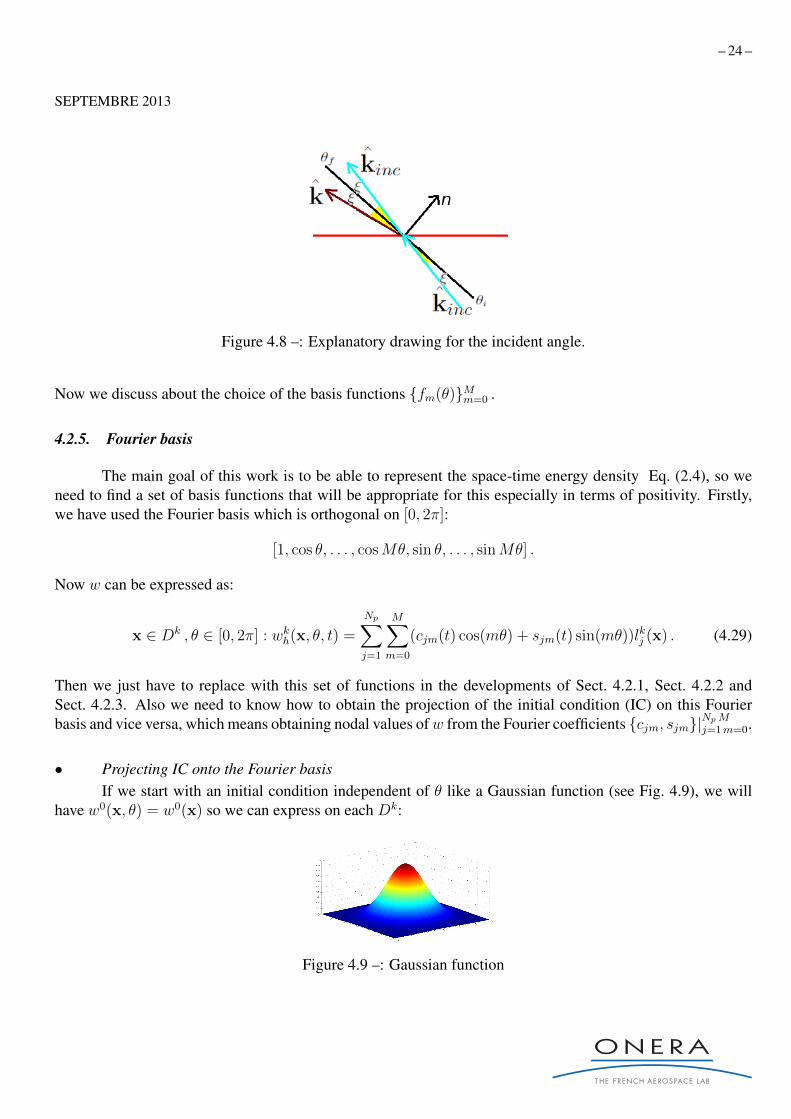
with ξ = θ − θf , thus θinc(θ) = 2θf − θ (see Fig. 4.8).

– 24 –

SEPTEMBRE 2013

Figure 4.8 –: Explanatory drawing for the incident angle.

Now we discuss about the choice of the basis functions fm(θ)Mm=0 .

4.2.5. Fourier basis

The main goal of this work is to be able to represent the space-time energy density Eq. (2.4), so weneed to find a set of basis functions that will be appropriate for this especially in terms of positivity. Firstly,we have used the Fourier basis which is orthogonal on [0, 2π]:

[1, cos θ, . . . , cosMθ, sin θ, . . . , sinMθ] .

Now w can be expressed as:

x ∈ Dk , θ ∈ [0, 2π] : wkh(x, θ, t) =

Np∑j=1

M∑m=0

(cjm(t) cos(mθ) + sjm(t) sin(mθ))lkj (x) . (4.29)

Then we just have to replace with this set of functions in the developments of Sect. 4.2.1, Sect. 4.2.2 andSect. 4.2.3. Also we need to know how to obtain the projection of the initial condition (IC) on this Fourierbasis and vice versa, which means obtaining nodal values ofw from the Fourier coefficients cjm, sjm|NpM

j=1m=0.

• Projecting IC onto the Fourier basisIf we start with an initial condition independent of θ like a Gaussian function (see Fig. 4.9), we will

have w0(x, θ) = w0(x) so we can express on each Dk:

Figure 4.9 –: Gaussian function

– 25 –

SEPTEMBRE 2013

w0(x, θ) = w0(x) =

Np∑j=1

w0j lkj (x) .

In comparaison with Eq. (4.29), it yields:

w0j =

M∑m=0

(c0jm cos(mθ) + s0

jm sin(mθ)) .

Because we are working with an orthogonal basis, we finally have:∫ 2π

0

w0j cos(mθ) dθ =

∫ 2π

0

cos2(mθ)c0jm dθ =

c0jm = w0

j if m = 0c0jm = 0 if m ≥ 1∫ 2π

0

w0j sin(mθ) dθ =

∫ 2π

0

sin2(mθ)s0jm dθ ⇒

s0jm = 0 ∀m.

• Computing the energy density E with the Fourier basisAfterwards we plug Eq. (4.29) into Eq. (2.4) to obtain the energy density as:

E(x, t) =1

2

Np∑j=1

M∑m=0

(cjm(t)

∫ 2π

0

cos(mθ) dθ + sjm(t)

∫ 2π

0

sin(mθ) dθ

)lkj (x) .

Because of orthogonal function’s properties it yields:

E(x, t) = π

Np∑j=1

cj0(t)lkj (x) ,

thus the nodal expansion of E yields:

E(xj, t) = cj0(t)π; j = 1 . . . Np .

4.2.6. Complex basis

Secondly, we have used an orthonormal complex basis on the unit disc [12] but in some ways this basisremains a sinusoidal basis considering its trace on the unit circle, as we can see it on Fig. 4.10. Neverthelessthis basis allows us tu use a more compact and simple notation. Let us introduce:

[g0(eiθ), . . . , gm(eiθ)] |m ∈ N ,

where:

gm(eiθ) =

√m! Γ(1)√

Γ(m+ 1)gm(eiθ) , θ ∈ [0, 2π] ,

and gm(eiθ)∞m=0 is the set of orthogonal basis functions where gm(eiθ) ≡ gm(z) / |z| = 1 is defined by:

gm(z) =(1)mm!

F (−m, 1, 1, 1− z) ,

– 26 –

SEPTEMBRE 2013

with:(a)m = a(a+ 1)(a+ 2) . . . (a+m− 1) ,

F (a, b, c, d) =n∑k=0

(a)k(b)k(c)kk!

dk ,

and Γ is the usual Gamma function defined by Γ(z) =∫ +∞

0tz−1e−t dt. Then we have:∫ 2π

0

gm(eiθ)gn(eiθ) dθ = δmn ,

where δmn is the Kronecker delta, so that gm(eiθ)∞m=0 is a set of orthonormal basis functions on the unitcircle. To get an idea how this basis behaves, we have plotted the first five real part functions in Fig. 4.10. Now

(a) m=0 (b) m=1 (c) m=2 (d) m=3

(e) m=4 (f) m=5

Figure 4.10 –: Example of the real parts of multidimensional complex basis functions on the unit disc.

the solution can be expanded as:

x ∈ Dk , θ ∈ [0, 2π] : wkh(x, θ, t) =

Np∑j=1

M∑m=0

χjm(t)gm(eiθ)lkj (x) . (4.30)

• Projecting IC onto the complex basisWith an initial condition such as in Fig. 4.9 we have:

w0(x, θ) = w0(x) =

Np∑j=1

w0j lkj (x) ,

which in comparison with Eq. (4.30) yields:

w0j =

M∑m=0

χjm(0)gm(z) ,

– 27 –

SEPTEMBRE 2013

where, because of the orthogonality property, one has:

χjm(0) =

∫ 2π

0

w0j gm(eiθ) dθ .

Since w0j ∈ R and g0(z) = cte ∈ R on the unit disc, all the gm′(z) such that m′ 6= 0 are orthogonal to w0

j ,because w0

j is proportional to g0(z). Thus :

χjm(0) =

∫ 2π

0w0j gm(eiθ) dθ if m = 0

0 if m 6= 0 .

• Computing the energy density E with the complex basisAfterwards we plug Eq. (4.30) into Eq. (2.4) to obtain the energy density as:

E(x, t) =1

2

Np∑j=1

M∑m=0

χjm(t)lkj (x)

∫ 2π

0

gm(eiθ) dθ =

Np∑j=1

Ej(t)lkj (x) ,

where:

Ej(t) =1

2

M∑m=0

χjm(t)

∫ 2π

0

gm(eiθ) dθ .

Again, all integrals of gm(z) are zero except g0(z), so that:

Ej(t) =χj0(t)

2

∫ 2π

0

g0(eiθ) dθ .

– 28 –

SEPTEMBRE 2013

4.3. Assembling the mesh

With all local operations in place, we now need to connect all local matrices in the global matricesM,B,F. This is done by a connectivity matrix that relates the local numbering of each element with a globalnumbering. After that, we obtain the following matrix ordinary differential equation:

Mdw

dt= (B− F)w , (4.31)

where w is a vector containing all projection coefficients on the local bases. Because M,B,F are constantmatrices, one has:

dw

dt= M−1(B− F)w = Gw . (4.32)

4.4. Time discretization

The differential equation (4.32) has as solution:

w(t) = etGw0 , (4.33)

where w0 is the vector containing all projection coefficients of the IC on the local bases. We can approach theexponential solution by plenty of methods as for example the descomposition in Taylor’s series, which for atime step dt reads:

w(t + dt) = (I + Gdt + G2dt2

2!+ G3dt

3

3!+ . . .)w(t) . (4.34)

So for each time step, we obtain an updated increment of w on the left-hand side of Eq. (4.34) that will beintroduced on the right-hand side of this very equation in order to compute the solution at the next time step.This allows us to construct the evolution of w(t) over time.

5. NUMERICAL RESULTS

5.1. Numerical results in one direction with nodal method

5.1.1. Numerical analysis

We must verify that our scheme is energy-conserving, so we have to compute the total energy E:

E(t) =

∫Ω

E(x, t) dΩ (5.1)

over the domain Ω, and verify that it is kept constant by our numerical scheme. This is verified on Fig. 5.1,with a maximal gap between the estimated average energy and instant energy of 3.6 % of the estimated averageenergy. The numerical parameters for this computation are N = 5 and h = 0, 08 where h is the average sizeof the elements meshing the domain Ω = [−1, 1]2.

Next, let us characterize the dispersion of our scheme. For that we have to check if the true physicalcelerity c = 1m/s is conserved by the simulation. As we can see on Fig. 5.2, the GD method allows to achievegood dispersion properties because the numerical velocity approaches the true physical velocity. However wehave some large oscillations at earlier times which are quickly damped at later times.

– 29 –

SEPTEMBRE 2013

Figure 5.1 –: Energy evolution for a computation in the domain Ω = [−1, 1]2 with N = 5 and h = 0, 08.

Figure 5.2 –: Velocity evolution for a computation in the domain Ω = [−1, 1]2 with N = 5 and h = 0, 08.

5.1.2. Simulation

We can see on the pictures below in Fig.5.3 the propagation of a Gaussian-shaped IC without anydistortion of this pulse as time increases.

– 30 –

SEPTEMBRE 2013

(a) t=0.06 s (b) t=0.352 s

Figure 5.3 –: Propagation of the gaussian function in the domain Ω = [−1, 1]2 with N = 5 and h = 0, 08 .

5.2. Numerical results in all directions with nodal method

5.2.1. Numerical analysis

By measuring the time for the wave front to reach the external edges of the plate we can observe thatthis scheme is rather dispersive due to its low resolution with respect to the phase variable θ.

(a) t=0.0006 s (b) t=0.6636 s

Figure 5.4 –: Centering propagation of the gaussian function for and N = 20 and h = 0, 2.

Indeed, we obtain a spreading velocity of c = 0.7m/s by our scheme, whereas the true physical velocity isc = 1m/s. Increasing the Fourier order M reduces significantly this dispersion error. Finally, let us plot theenergy overall integrating time for this scheme (see Fig. 5.5).

5.2.2. Simulation

We can see on Fig. 5.6 that our scheme does not preserve the positivity of the energy density, which isundesirable because an energy must always be positive. Negative values are indeed observed just behind thewave front. On Fig. 5.7 we have reproduced the same results now filtering the negative values

– 31 –

SEPTEMBRE 2013

Figure 5.5 –: Energy evolution for a computation in the domain Ω = [−1, 1]2 with N = 5 and h = 0, 2 .

(a) t=0.0126 s (b) t=0.1776 s (c) t=0.3942 s

(d) t=0.4614 s (e) t=0.6438 s (f) t=0.7698 s

Figure 5.6 –: Wave propagation and reflection with Fourier basis functions. The negative values are not filtered.

– 32 –

SEPTEMBRE 2013

(a) t=0.0126 s (b) t=0.1776 s (c) t=0.3942 s

(d) t=0.4614 s (e) t=0.6438 s (f) t=0.7698 s

Figure 5.7 –: Wave propagation and reflection with Fourier basis functions. The negative values are filtered.

6. CONCLUSIONS

We have developed a GD method for the transport equation in 2D to simulate the propagation of thevibrational energy within a plate. This method gives us a high accuracy without the need of a fine mesh thanksto the possibilty of increasing the number of nodes on each finite element. We have obtained good resultsfor one propagation direction with a very good dispersive and conservative behavior. Nevertheless solving theproblem for all directions, shows an increase in dispersion and the loss of the positivity-preserving propertiesof the scheme. Indeed, the various bases used for the approximation of the angular variable introduce spuriousoscillations. Further investigations are needed to improve the discretization schemes in order to enforce somepositivity-preserving condition. These issues are the subject of ongoing research.

7. SYNTHESE

Concernant ce qui a ete propose au depart de ce projet, il faut dire que les objectifs ont ete atteintsd’une maniere satisfaisante parce qu’on a reussi a implementer les polynomes d’ordre eleve dans la methode(GD) et developper le code pour la propagation dans tous les sens avec des conditions aux frontieres dereflexion speculaire. Au meme temps, pendant la duree de ce stage j’ai pu apprendre comment est le metier

– 33 –

SEPTEMBRE 2013

de l’ingenieur charge de la modelisation numerique et l’importance d’ailleurs de cette etape en amont de toutnouveau projet dans le domaine industriel.

– 34 –

SEPTEMBRE 2013

8. BIBLIOGRAPHY

[1] E.Savin,Transient vibrational power flows in slender random structures:theoretical modelling and numericalsolutions.,Probabilistic Engineering Mechanics, 28 (2011), pp. 194–205.

[2] M. Guo and X.-P. Wang,Transport equations for a general class of evolution equations with random perturbations,Journal of Mathematical Physics, 40 (10) (1999), pp. 4828–4858.

[3] G. C. Papanicolaou and L. V. Ryzhik,Waves and transport,In Hyperbolic Equations and Frequency Interactions, edited by L. Caffarelli and W. E, vol. 5 of IAS/ParkCity Mathematics Series, pp. 305–382. American Mathematical Society, Providence RI (1999).

[4] J.-L. Akian,Wigner measures for high-frequency energy propagation in visco-elastic media,Technical Report ONERA no RT 2/07950 DDSS, Chatillon (December 2003).

[5] E.Savin,Transient transport equations for high-frequency power flow in heterogeneous cylindrical shells,Waves in Random Media, 14 (3) (2004), pp. 303–325.

[6] E.Savin,High-frequency vibrational power flows in randomly heterogeneous structures,In In Proceedings of the 9th International Conference on Structural Safety and Reliability ICOSSAR2005, pp. 2467–2474, Rotterdam, Millpress Science Publishers (2005).

[7] L.Erdos and H.T.Yau,Linear Boltzman equation as the weak coupling limit of a random Schrodinger equation,Communications on Pure and Applied Mathematics, (6) (2000), pp. 667–735.

[8] J.Lukkarinen and H.Spohn,Kinetic limit for wave propagation in a random medium,Archive for Rational Mechanics and Analysis, 183 (1) (2007), pp. 93–162.

[9] J. S. Hesthaven and Tim Warburton,Nodal Discontinuous Galerkin Methods Algorithms, Analysis and Applications,Springer, Berlin (2008).

[10] T. Liu, Mrinal K.Sen, Tianyue Hu, Jonas D.De Basabe and Lin Li,Dispersion analysis of the spectral element method using a triangular mesh,Wave Motion, 49 (2012), pp. 474–483.

[11] F. R. Laura Lazar Richard Pasquetti,Fekete-Gauss Spectral Elements for Incompressible Navier-Stokes Flows: The Two-Dimensional Case,Communications in Computational Physics, 13 (5) (2013), pp. 1309–1329.

[12] L. Chien Shen,Orthogonal polynomials on the unit circle associated with the Laguerre polynomials,American Mathematical Society, 129 (3) (October 2000), pp. 873–879.

– 35 –

SEPTEMBRE 2013

APPENDIX I. JACOBI POLYNOMIALS

I.1. Introduction

Jacobi polynomials (occasionally called hypergeometric polynomials) are a class of classical orthogo-nal polynomials. They are orthogonal with respect to the weight

(1− x)α(1 + x)β ,

on the interval [−1, 1].

I.2. Definition

One of its definitions, via the hypergeometric functions is:

P (α,β)n (z) =

Γ(α + n+ 1)

n!Γ(α + β + n+ 1)

n∑m=0

(n

m

)Γ(α + β + n+m+ 1)

Γ(α +m+ 1)

(z − 1

2

)m. (I.1)

I.3. Basic properties

I.3.1. Orthogonality

The Jacobi polynomials satisfy the orthogonality condition∫ 1

−1

(1−x)α(1 +x)βP (α,β)m (x)P (α,β)

n (x) dx =2α+β+1

2n+ α + β + 1

Γ(n+ α + 1)Γ(n+ β + 1)

Γ(n+ α + β + 1)n!δnm ∀α, β > −1 .

I.3.2. Symmetry relation

The polynomials have the symmetry relation

P (α,β)n (−z) = (−1)nP (β,α)

n (z) .

I.3.3. Differential equation

The Jacobi polynomial P (α,β)n is a solution of the second order linear homogeneous differential equation

(1− x2)y′′ + (β − α− (α + β + 2)x)y′ + n(n+ α + β + 1)y = 0 .