Flash-evaporation printing methodology for perovskite thin films
Upload
independentCategory
view
4download
0
Direct Numerical Simulation of Sprays: Turbulent Dispersion, Evaporation and Combustion
Julien Reveillon CORIA CNRS, University of Rouen, Rouen, France
Abstract Numerical procedures to describe the dispersion, evaporation and combustion of a polydisperse liquid fuel in a turbulent oxidizer are presented. Direct Numerical Simulation (DNS) allows one to describe accurately the evolution of the fully compressible gas-phase coupled with a Lagrangian description in order to describe two-phase flows. Standard coupling is used for the Eulerian/Lagrangian system while some practical issues related to the reactive source terms are addressed by suggesting a fast single-step Arrhenius law allowing one to capture the main fundamental properties of the flame whatever the local equivalence ratio. Then some basic procedures to describe spray preferential segregation in a turbulent reactor are described. Eventually spray combustion is addressed by first demonstrating the complex interactions caused by the presence of an evaporating liquid phase: definition of various equivalence ratios, apparition of flame instabilities for a unit Lewis number, etc. Then a history of the development of the existing spray combustion diagrams is presented to display the possible flame structures and combustion regimes encountered in spray combustion.
1 Introduction
It is generally admitted that the Navier-Stokes (NS) equations offer an accurate description of fluid motion. The basis for these equations is that the fluid under consideration is a continuum. Numerical resolution of the NS equations on a fine computational mesh allows one to capture all the macroscopic structures since all the considered length scales are considerably larger than the molecular length and time scales. Such NS resolution is defined as Direct Numerical Simulation (DNS). DNS solves all the characteristic scales of a turbulent flow^ from the Kolmogorov 'dissi-pative' length scale up to the integral 'energy-containing' length scale. However, if a two-phase flow is considered (gas/liquid for example), the apparition of an interface and a strong variation of density jeopardizes the possibility to achieve a complete DNS of the flow. It is especially true if fundamental physical phenomena, like evaporation or heat transfer, are present at the interface. Then the computational cost of the DNS of the whole flow, including both phases, would sky rocket unless some major assumptions were made.
A first possibility is to adopt an interface-tracking approach like the 'volume of fluid' (VOF) method developed by Hirt and Nichols (1981). It is based on the reconstruction of the gas/liquid interface from the time and space evolution of the local volume fraction of liquid. This mass-conservative procedure is complex and time consuming as far as the interface reconstruction is concerned. Another possibility is to use the level-set procedure of Osher and Sethian (1988),
230 Julien Reveillon
which follows the motion of an iso-surface of a specific scalar function that maintains algebraic distances. Even if these simulations are still designed as DNS because no turbulence model is used, from a strict point of view, the results are not an exact resolution of the complete NS equations and some approximations are often necessary. For example, an incompressible formulation is generally used. Then evaporation, heat transfer or even combustion phenomena are difficult to account for. Nevertheless, these methods are very promising as demonstrated very recently by Tanguy and Berlemont (2005) who simulated for the first time the complete atomization of a liquid jet.
A second possibility is to give up the idea of a complete DNS of the flow while trying to maintain highly accurate results. This objective seems rather difficult to reach as far as dense flows are concerned. On the other hand, when a dispersed liquid or solid phase is embedded in a gaseous carrier phase, some solutions exist. The principle is to carry out a DNS of the gaseous continuous phase and to model the dispersion of the liquid phase through a Lagrangian or an Eulerian formulation (Gouesbet and Berlemont, 1999). In the framework of DNS, where accurate results are more important than computational cost, Lagrangian modeling of the spray is preferable because every particle (or group of particles) is followed in space and time by the solver, whereas statistical integration of the information is obtained when a Eulerian model is used. It appears however that both procedures are complementary: Lagrangian formulations have to be used for the accurate description the dispersion of few (some millions per processor) particles while, on the other hand, an Eulerian formulation seems to be particularly adapted to complex dispersed or dense flows involving large-scale computations.
DNS was first introduced 35 years ago by Orszag and Patterson (1972) and then Rogallo (1981) and Lee et al. (1991) for the simulation of inert gaseous flows. It has since been used in a large range of applications. During the last two decades, DNS of reactive flows has been carried out to study non-premixed, partially premixed and premixed turbulent combustion of purely gaseous fluids (Givi, 1989; Poinsot et al., 1996; Vervisch and Poinsot, 1998; Poinsot and Veynante, 2001; Pantano et al., 2003). DNS has been extended to two-phase flows starting with the pioneering work of Riley and Patterson (1974). Most of the first numerical studies were dedicated to solid particle dispersion (see for instance Samimy and Lele, 1991; Squires and Eaton, 1991; Elgobashi and Truesdell, 1992; Wang and Maxey, 1993, and Ling et al., 1998). More recently, Mashayek et al. (1997), Reveillon et al. (1998) and Miller and Bellan (1999) conducted the first DNS with evaporating droplets in turbulent flows. Since then, DNS of two-phase flows have been extended to incorporate two-way coupling effects, multicomponent fuels, etc., and to deal with spray evaporation and combustion phenomena (Mashayek, 1998; Miller and Bellan, 1999,2000; Reveillon and Vervisch, 2005).
The objective of this text is to offer a full description of the numerical procedures used to carry out DNS of two-phase dispersed flows. Note that a similar methodology may be used for large-eddy simulations if subgrid turbulence, mixing and dispersion models are added to the general balance equations. Starting from the classical NS equations, specific source terms are added to account for the presence of a dispersed liquid phase whose evolution is described by a Lagrangian solver. The modeling of the liquid phase embedded in a full DNS of the gas phase implies that the droplets are not resolved by the Eulerian solver. They are considered as local point sources of mass, momentum and energy. On the other hand, these source terms are obtained thanks to a fine-scale description of the evolution of droplets that are considered individually by the Lagrangian solver. Another major task concerns the chemical source terms describing
Direct Numerical Simulation of Sprays 231
chemical reactions between the various components. Two major solutions emerge: first, detailed chemistry may be used and leads to an accurate description of the combustion phenomena and the flame structures; however, it increases significantly the computational cost. The other possibility, often adopted in single-phase DNS as well, is to use a one-step Arrhenius law to describe the impact of combustion kinetics from a global point of view. In that case, two major conditions have to be respected: an accurate resolution of the basic features of the flame (propagation velocity, thickness, heat release) with respect to the local properties of the flow (equivalence ratio, stretch). However, basic single-step Arrhenius laws show major drawbacks especially when partially premixed combustion is concerned, which is mainly the case with turbulent two-phase flows. Thus, an adapted single-step kinetics has to be used.
In the following, two major parts are developed: first, details concerning the coupling of a complete DNS of a gaseous turbulent flow with a Lagrangian model of the dispersed phase are given. This association is especially useful to study fundamental physical phenomena and to carry out the preliminary development of two-phase flow models. Coupling with the dispersed spray is detailed as well as the specific Arrhenius law allowing one to capture properly the combustion phenomena whatever the local equivalence ratio. Then some applications and analysis procedures are briefly described to demonstrate the ability of DNS to capture every major phenomena present in two-phase flows: dispersion, evaporation and combustion.
2 Direct Numerical Simulation
DNS is a powerful way to study turbulent flows. Indeed, the NS equations are resolved with highly accurate and non-dissipative numerical methods that are able to capture all the time and length scales of the flow. No models are necessary to observe the development and the evolution of turbulent structures and all results may be considered to be as close as possible to reality (if the simulations are conducted properly). Occasionally, DNS is even referred to as a 'numerical experiment'. The grid mesh has to be fine enough to capture the smallest scales of the flow. This leads to severe conditions based on the turbulent Reynolds number and the Damkohler number, which is the ratio of the fluid motion time scale to the characteristic reaction time. A large Damkohler number indicates a rapid chemical reaction compared to all other processes. DNS is thus very limited from a technological point of view by the capacity of the current supercomputers. Only configurations with very small dimensions and small turbulent Reynolds numbers may be considered at the present time. Nevertheless, because of the accuracy of the results, it is a useful tool to analyze some specific physical phenomena.
One has to be careful as far as the 'DNS' term is concerned. Indeed in many works what is called DNS is a 'direct numerical resolution' of the considered equations without any model but not necessarily with adapted numerical methods and grids. This may lead to severe numerical dissipation and approximations, in which case speaking of DNS is abusive because the results are not a direct outcome of the equations for the physics. Indeed, an implicit numerical filtering exists in between the two. For a complete introduction to DNS of turbulent reactive single-phase flows and the resolved equations, readers may refer to the recent book of Poinsot and Veynante (2005).
Many formulations may be derived for the NS equations. The fully compressible equations allow for a complete description of the physics including acoustic phenomena. Apart from having a very small time step mainly based on the sound velocity, the main difficulties lie in a
232 Julien Reveillon
good formulation of the initial and boundary conditions that must account for entering and exiting acoustic waves. If acoustic phenomena are negligible, it is possible to select a low Mach number (LMN) formulation with either a constant- or variable-density flow. Then, boundary conditions are straightforward to prescribe. However, an elliptic solver is needed to close the momentum balance equation. For non-reactive flow or by using an implicit scheme for the temperature/species equations, the computational cost may be reduced by a factor of five to ten compared to the corresponding compressible formulation.
In the next section the complete compressible equations are given, and then a low Mach number formulation is derived. These sets of equations describe the evolution of the gas phase. They are rapidly introduced because they are widely documented in the CFD literature. Then a derivation of the Lagrangian solver to be resolved simultaneously with the DNS is proposed with a detailed description of the coupling between the carrier phase and the dispersed evaporating droplets. This part ends with a detailed description of a single-step Arrhenius law adapted to the full range of fuel and equivalence ratios.
2.1 Compressible formulation
The carrier phase is a compressible Newtonian fluid following the equation of state for an ideal gas. The instantaneous balance equations describe the evolution of mass p, momentum pU, total (except chemical) energy E^ and species mass fraction. Fp denotes the mass fraction of gaseous fuel resulting from spray evaporation and YQ is the oxidizer mass fraction. The following set of balance equations are solved where the usual notation is adopted:
dp dpUk . ,^ . . ot axk
H 7{ = - T ; \- T; h vt , (2.2) dt dxk dxi dxk
dxk V dxk J
dpE, , d(pE, + P)Uk d (,^T\ doikUk . ^ . , . . , ^ 7 " + ~" 5 " F ~ ^ J ~ + ^ + pcoe+e, (2.3)
ot OXk OXfc V d^k J (J^i apFp , dpYj^Uk
H :\ = T;— pD-— + p^o , (2.5)
with
dpYj^Uk 9 / 9 F F \ . .
dxk OXk V OXk J
V ^^k)
V 9- 7 dxi ) 3 dxk '
dt dxk dxk
Jij , i J J OXk
together with the equation of state for ideal gases:
P=prT.
Source terms are present, the coi terms are related to the chemical reaction processes and m, v and e result from a two-way coupling between the carrier phase and the spray. These terms will be discussed in detail later.
The sixth-order Fade scheme from Lele (1992) and the Navier-Stokes characteristics boundary conditions (NSCBC) of Poinsot and Lele (1992) or Baum et al. (1994) are usually employed
Direct Numerical Simulation of Sprays 233
to solve the gas-phase transport equations on a regular mesh. The time integration of both the spray and gas-phase equations is done with a third-order explicit Runge-Kutta scheme with a minimal data storage method (Wray, 1990). A third-order interpolation is employed when gas-phase properties are needed at the droplet positions.
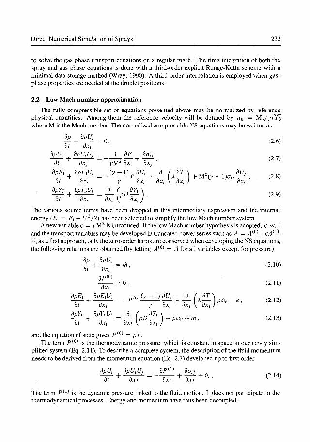
2.2 Low Mach number approximation
The fully compressible set of equations presented above may be normalized by reference physical quantities. Among them the reference velocity will be defined by wo = M^y/yrTo where M is the Mach number. The normalized compressible NS equations may be written as
1 + 1 ^ = 0 , (2.6) ot dxi
+ ^ ^ = - ^ ^ + ^ , (2.7) dpUj dpUiUj _ _]_dP_ dGij
dt dxj yM^ dxi dxj
ot axi y oxi oxf \ oxi J oxi
dpY^ ^ dpYM ^ d f^dy?\ (2.9) dt dXi dxi \ dxi J
The various source terms have been dropped in this intermediary expression and the internal energy {Ei = E^ — U^/2) has been selected to simplify the low Mach number system.
A new variable 6 = yM' is introduced. If the low Mach number hypothesis is adopted, 6 <^ 1 and the transport variables may be developed in truncated power series such as A = A^^^-\-€A^^\ If, as a first approach, only the zero-order terms are conserved when developing the NS equations, the following relations are obtained (by letting A^^^ = A for all variables except for pressure):
'£+'i^=rn, (2.10) dt axi
9P(0) ^ — = 0, (2.11)
M i + ^ _ p ( o ) ( K z : i ) ^ + A A | I ) , ^ , + , , (2.12) at oXi y oxi axi \ oXi J
and the equation of state gives P^^^ = pT. The term P ^^ is the thermodynamic pressure, which is constant in space in our newly sim
plified system (Eq. 2.11). To describe a complete system, the description of the fluid momentum needs to be derived from the momentum equation (Eq. 2.7) developed up to first order.
^ + = - 5 ^ + 1 ^ + 0,. a,4, at axj OXi axj
The term P^^^ is the dynamic pressure linked to the fluid motion. It does not participate in the thermodynamical processes. Energy and momentum have thus been decoupled.

234 Julien Reveillon
Note that if an open system is considered the pressure P^^^ is equal to the external pressure. On the other hand, if the system is closed (periodical or adiabatic boundaries) it is possible to show that
3P(0) -Jfl pycbedv, (2.15) dt
where the integral is over the volume of the domain. Spatial derivative and temporal integrations schemes similar to the ones used for the compressible formulation may be used. Boundary conditions are straightforward: a given value or gradient is prescribed on all the domain boundaries for the considered variables. The major stumbling block of the LMN formulation concerns the determination of the first-order pressure term P^^\ If a derivative operator is applied to Eq. (2.14), a Poisson equation appears with P^^^ as the unknown. By using an adapted elliptic solver, the pressure gradient may be determined and Eq. (2.14) is closed. For more details about the low Mach number formulation for reacting single- and two-phase flows, readers may consult the works of McMurtry et al. (1986) or Wang and Rutland (2005) and references therein.
3 Dispersed-Phase Lagrangian Description
As described by Reeks (1991), is it possible to account for many forces to characterize the droplet dynamics. However, the purpose of this text is to present a basis to carry out DNS of two-phase flows. Because of the high density ratio between the liquid and gas phases, only the drag force, which is prevalent, has been selected. Moreover, several usual assumptions have to be formulated. First, the spray is dispersed and each droplet is unaware of the existence of the others. Any internal liquid circulation or droplet rotations are neglected and an infinite heat conduction coefficient is assumed. Therefore, the liquid core temperature remains uniform in every droplet, although it may vary as a function of time. The spray is then composed of local sources of mass following the saturation law and modifying the momentum and gaseous fuel topology, depending on the local temperature, pressure and vapor mass fraction.
3.1 Position and velocity
By letting V : and X^ denote the velocity and position vectors of droplet k, the relations
^ = ^ ^ U ( X , , 0 - V . ) , (3.1)
^ = V . , (3.2) at
are used to track their evolution throughout the computational domain. The vector U (Xjt, 0 represents the gas velocity at the droplet position X^. The right-hand side of Eq. (3.1) represents a drag force applied to the droplet and ^^ Ms a kinetic relaxation time. It may be obtained from the k droplet dynamics:
m—— = Dk , (3.3) d
where D is the drag force applied to a sphere. A summation of all the forces on the droplet surface gives
D^ = 3nakfiCk (U (Xk, t) - \k) , (3.4)

Direct Numerical Simulation of Sprays 235
where ajc is the diameter of droplet k. A corrective coefficient Cjc = I -{- Re^^ /6 (Crowe et al., 1998) is introduced to allow for the variation of the drag factor according to the value of the droplet Reynolds number Re^ = p|U (X^, t) — ykWh/l^- Thus from Eqs. (3.3) and (3.4) and with ruk = pd7tal/6, the following relation is obtained:
dV^ _ (U(XkJ)-\k)lSfiCk
dt al pd
and leads directly to the kinetic relaxation time of droplet k\
^ ( v ) ^ ^ d ^ (3.6) ^^ 18Q/X ^ ^
3.2 Heating and evaporation
The heating and evaporation of each droplet in the flow may be described through a normalized quantity Bk, called the "mass-transfer number". B^ is the normalized flux of gaseous fuel between the droplet surface, where the fuel mass fraction takes the value Y^, and the surrounding gas at the droplet position, where the fuel mass fraction is 7F(XA:). It may be written
Yl - Y^iXk) Bj. = J£ iLJLi . (3.7)
By solving the mass and energy balances at the surface of a vaporizing droplet in a quiescent atmosphere (Kuo, 1986), the following relations for the surface and temperature evolution of the kih droplet are found:
da? al
dTk 1 / BkLy\
^-;^(^(x.)-^.--^j. (3.9)
Again, characteristic relaxation times appear and are defined by
f = ^ - ^ i _ , (3.10) ^^ 4Shc/x ln(l-f 5^) ' ^ ^
(T) ^ Pr Capgal Bj, ^^ 6Nuc Cp /x ln(l -hBk)' ^ ' ^
Normalized gas and liquid heat capacities are denoted by Cp and Cd, respectively, and as Lv is the latent heat of evaporation; all of which are considered as constant in the present set of equations. Sc and Pr are the Schmidt and Prandtl numbers, respectively. She and Nuc are the convective Sherwood and Nusselt numbers, respectively. They are both equal to 2 in a quiescent atmosphere, but a correction has to be applied in a convective environment. In this context, the empirical expression of Faeth and Fendell (Kuo, 1986), identical either for She or Nuc (She I Nuc), may be

236 Julien Reveillon
used: ( S h . | N u A = 2 + 0.55R,><Sc|Pr). _ ^ , 3 , ^ ^
(l.232 + Re^(Sc|Pr)2/'j
One of the most accurate models to describe the evaporation process is to consider a phase equihbrium at the interface thanks to the Clausius-Clapeyron relation:
dln(P^) Lv
where rp is the ideal gas constant in the gaseous fuel. This leads to the following expression for the partial pressure P^ of fuel vapor at the surface of a droplet:
where / ref and Tref are two reference parameters. A fuel boiling temperature Tref corresponding to a reference pressure Pref has been introduced. T^ is the gas temperature at the droplet surface. The liquid temperature is uniform in all droplets. Thus, it is equal to the temperature of the gas at the interface T^ = T^.
The gaseous fuel mass fraction at the surface of the droplet may be determined from
ys _ 1 + Wo rpjXq) Y ^ F V PI J
- 1
(3.15)
where WQ and Wp are the molecular weights of the considered oxidizer and fuel, respectively. Once the gaseous fuel mixture fraction at the droplet surface is known, the mass-transfer number Bk is determined by introducing relation (3.15) into Eq. (3.7). Consequently, Eqs. (3.8) and (3.9) describing the evolution of droplet surface are and temperature are closed.
4 Eulerian/Lagrangian Coupling
The terms m, v and e modify the gas-phase mass, momentum and temperature owing to a distribution of the Lagrangian quantities on the Eulerian grid. Every droplet has positive or negative source terms to be distributed over the Eulerian nodes and the specification of an accurate projection of these Lagrangian sources onto the Eulerian mesh is not an easy task. In real spray flows, this distribution is not instantaneous and further assumptions are needed to perform simulations. Every Lagrangian source has to be distributed over the Eulerian nodes by adding the volumetric contributions from droplets. This induces a numerical dispersion that remains weak because of the small size of the DNS grid (Reveillon and Vervisch, 2000). This procedure is not really satisfactory but this stumbling block remains an open problem at the present time.
For every Eulerian node, a control volume V is defined by the mid-distance between the neighboring nodes. If an isotropic Cartesian grid is considered ( zl = x^+i — xt = Ax = Ay = Az), then V = A^. The mass source term applied to an Eulerian node n is denoted Wy\
v = - ; ^ L ^ r - ^ ' (4.1) k
Direct Numerical Simulation of Sprays 237
0), (3)
Control volume of droplet k\ V
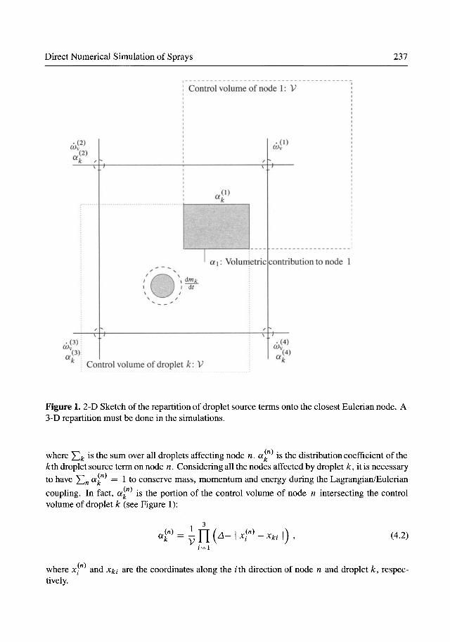
Figure 1. 2-D Sketch of the repartition of droplet source terms onto the closest Eulerian node. A 3-D repartition must be done in the simulations.
where ^j^ is the sum over all droplets affecting node n. af is the distribution coefficient of the kih droplet source term on node n. Considering all the nodes affected by droplet /:, it is necessary to have Yin ^k " ^ to conserve mass, momentum and energy during the Lagrangian/Eulerian
M"^ coupling. In fact, a^ is the portion of the control volume of node n intersecting the control volume of droplet k (see Figure 1):
:"'=in(^-i.!"'-*i). / = 1
(4.2)
where x\ and Xkt are the coordinates along the /th direction of node n and droplet k, respectively.

238 Julien Reveillon
The mass of the considered droplet k in the neighborhood of node n is rrik = Pd^^l/^ and using Eqs. (3.8) and (4.1) one may write
k
Similarly, the following relation:
""'"-lyE"!"'"?/^?- <«)
k
leads to the expression for the momentum source term:
The energy variation of the gaseous flow induced by the droplets inside volume V may be written as
(n)^kCdTk (4.6) k
and it can be rewritten as
'"'=-c.p-f^i:«r«j(r •(«) /- ^ 1 v ^ (n) 3 (2T{Xd,t)-Tk- BkLy/Cp Tk \
This last equation details how energy fluxes reaching the droplet surface are distributed (evaporation and liquid core heating) and the loss of energy due to the loss of liquid mass.
5 Reaction Rates
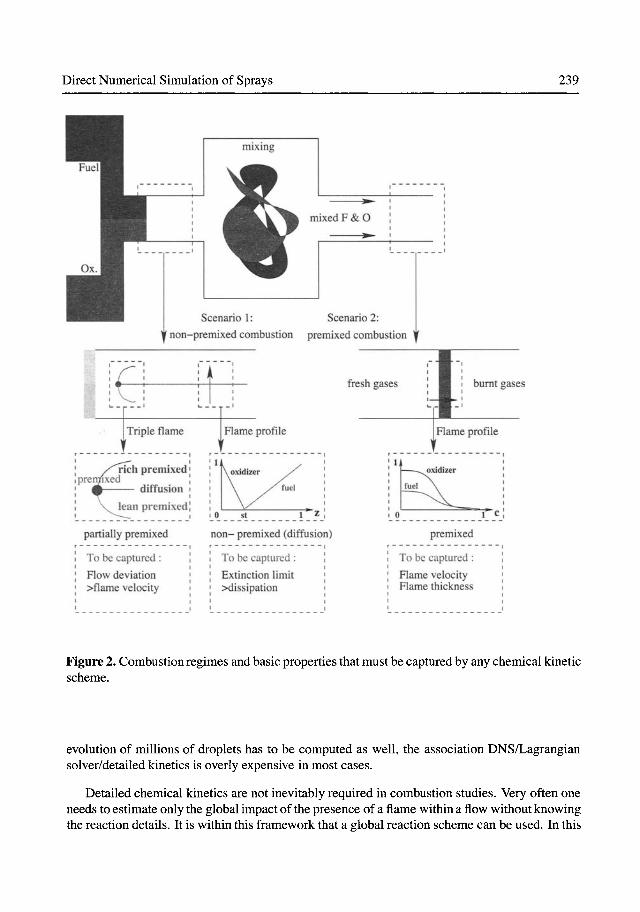
First it may be useful to sketch the usual combustion regimes. Initially segregated gaseous fuel and oxidizer streams are injected into the combustion chamber. Two possible combustion scenarios are shown in Figure 2. In the first case, reaction takes place before any mixing between fuel and oxidizer occurs. Then a diffusion flame emerges piloted by a triple flame. Otherwise if fuel and oxidizer are mixed before ignition takes place, a premixed flame propagates in the domain. These premixed and diffusion flames have very different structures and behaviors, but they are characterized through the same chemical law. Indeed, it is possible to consider their common origin in the chemical kinetics resulting from the presence in the same region of molecules of each species.
As mentioned in the Introduction, detailed chemistry may be used to determine the chemical source terms d>e and coy appearing in the energy and species balance equations, respectively. The Eulerian/Lagrangian procedure may be coupled with a solver dedicated to the computation of detailed chemistry. An open-source package like Cantera from Caltech (Goodwin, 2003) is an ideal candidate. However detailed kinetics are time consuming. Added to the fact that the
Direct Numerical Simulation of Sprays 239
mixed F & O
Scenario 1: Scenario 2: f non-premixed combustion premixed combustion W
fresh gases
lean, premixed
partially premixed
To be captured:
Flow deviation >flame velocity
0 St 1 Z J
non- premixed (diffusion)
To be captured :
Extinction limit >dissipation
premixed
To be captured :
Flame velocity Flame thickness
Figure 2. Combustion regimes and basic properties that must be captured by any chemical kinetic scheme.
evolution of millions of droplets has to be computed as well, the association DNS/Lagrangian solver/detailed kinetics is overly expensive in most cases.
Detailed chemical kinetics are not inevitably required in combustion studies. Very often one needs to estimate only the global impact of the presence of a flame within a flow without knowing the reaction details. It is within this framework that a global reaction scheme can be used. In this
240 Julien Re veillon
case, chemical kinetics are reduced to a unique irreversible single-step reaction:
Fuel + Oxidizer —> Products. (5.1)
If the reaction rate resulting from this reaction captures the basic properties of the real flames, then the global effects of the combustion on the gas flow will be taken into account. It is possible to briefly enumerate some of these fundamental properties:
• Combustion heat release to account for gas dilatation in the flow motion and to determine the correct output temperature,
• Flame velocity to capture the burning rate corresponding to the local equivalence ratio, • Flame thickness to estimate correctly the scale of the vortices able to cross the flame front in
combustion/turbulence studies and thus the flame wrinkling and turbulent velocity, • Extinction limit to establish local extinction of the flame because of the local dissipation rate, • Ignition delay/lift-off height to capture the flame ignition delay or the distance between the
injector and the flame. Single-step chemistry can not capture ignition delays, which are directly linked to the rate of creation of intermediate species.
The most basic model for global kinetics concerns non-premixed combustion. An infinitely fast reaction between fuel and oxidizer occurs because both of them react instantaneously as soon as they meet and the flame is then controlled by the mixing of the flow. Only the heat release (first property) is captured by this model that considers only very high Damk bhler numbers. However, even if its global properties and behavior are wrong, this instantaneous and simple method may be useful as a development procedure to test the ability of numerical and physical models to cope with combustion heat release and gas dilatation.
On the other hand, the Arrhenius law, which is commonly used to describe global kinetics, proved to be able to capture most of the fundamental properties. However, as it will be developed later, problems appear as far as realistic stoichiometric coefficients and non-stoichiometric (or partially premixed) combustion are concerned. To overcome this issue, which is fundamental for two-phase flows, a pre-exponential correction for the Arrhenius law is proposed in the following, which takes into account a significant number of the fundamental properties and phenomena resulting from the combustion. This method may be used for any stoichiometric ratio between the fuel and the oxidizer without the usual numerical and physical problems met with standard methods. Moreover, it allows for a proper computation of the velocity and the thickness of the flame, the heat release and the extinction limit whatever the local or global equivalence ratio. The method is called GKAS (Global Kinetics, Any Stoichiometry) in this work.
The evolution of a chemical system is usually described by the quantities of fuel and oxidizer present in the domain. It is possible to add to this conventional representation a new phase space based on the intensity and the progress of any reaction. The definition of the conventional parameters (mixture fraction, reaction rate, etc.) will help us to introduce a new set of parameters allowing us to modify the Arrhenius law.
5.1 Definitions
As it has been mentioned above, it is possible to study two initially segregated gaseous flows injected into the same domain (see Figure 2). It is possible to consider diluted fuel and oxidizer; however, for the sake of clarity, we will not do so here. The first flow consists of a pure fuel
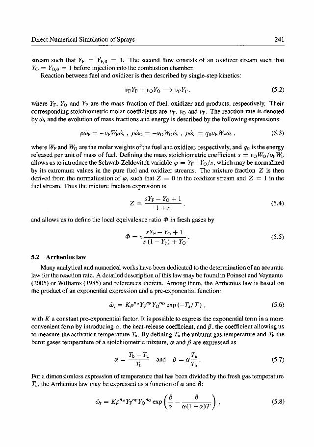
Direct Numerical Simulation of Sprays 241
stream such that Ip = ^F,O = 1- The second flow consists of an oxidizer stream such that YQ = YQ^O = 1 before injection into the combustion chamber.
Reaction between fuel and oxidizer is then described by single-step kinetics:
vpFp + voYo -^ ypFp . (5.2)
where 7p, YQ and Yp are the mass fraction of fuel, oxidizer and products, respectively. Their corresponding stoichiometric molar coefficients are vp, VQ and vp. The reaction rate is denoted by (br and the evolution of mass fractions and energy is described by the following expressions:
pCOp = - y p T F p d ) r , pcbo = -VoWoCbr , pcbe = ^O^FW^F<^r , (5.3)
where VFp and WQ are the molar weights of the fuel and oxidizer, respectively, and qo is the energy released per unit of mass of fuel. Defining the mass stoichiometric coefficient s = VQWO/V^WP
allows us to introduce the Schwab-Zeldovitch variable (p = Y^^—YQ/S, which may be normalized by its extremum values in the pure fuel and oxidizer streams. The mixture fraction Z is then derived from the normalization of cp, such that Z = 0 in the oxidizer stream and Z = 1 in the fuel stream. Thus the mixture fraction expression is
1 -\- s
and allows us to define the local equivalence ratio 0 in fresh gases by
^ r p - F o + l 0=s-- . (5.5)
^ ( i - 7 p ) + ro
5.2 Arrheniuslaw
Many analytical and numerical works have been dedicated to the determination of an accurate law for the reaction rate. A detailed description of this law may be found in Poinsot and Veynante (2005) or Williams (1985) and references therein. Among them, the Arrhenius law is based on the product of an exponential expression and a pre-exponential function:
cbr = Kp""^ Fp"^ Fo' ^ exp {-TJ T) , (5.6)
with K a constant pre-exponential factor. It is possible to express the exponential term in a more convenient form by introducing a, the heat-release coefficient, and j6, the coefficient allowing us to measure the activation temperature Ta. By defining T^ the unbumt gas temperature and 7b the burnt gases temperature of a stoichiometric mixture, a and fi are expressed as
Of = ^ and ^ = Qf-^. (5.7) ^b ^b
For a dimensionless expression of temperature that has been divided by the fresh gas temperature Tu, the Arrhenius law may be expressed as a function of a and S:
d)r = ii:p"^rp"^Fo'^^ exp (^ - -—1-—] , (5.8) \a a(\ —ot)T J

242 Julien Reveillon
where the term exp (—P/a) has been included in the K constant to balance the orders of magnitude. The reaction exponents «F and no are not necessarily equal to vp and VQ, and Hp is set to ftp = «F + ^o- Equation (5.8) allows us to model the kinetics of a single-step reaction. It is widely used to determine asymptotically or numerically the reaction rate. However a lot of physical or numerical restrictions may appear. As summarized by Poinsot and Veynante (2005), with reaction exponents «F and no of the order of unity, asymptotic and numerical estimations of the flame speed as a function of the equivalence ratio provide good estimates on the lean side (0 < 1), but fail on the rich side ( 0 > 1). In fact, a constant growth of the velocity may be observed even for equivalence ratios greater than unity, whereas it should reach a maximum value in the vicinity of <P = 1. This problem is linked to the pre-exponential function defined by
PeC^F, Yo, «F, no) = V^Fo"« . (5.9)
By looking for the maximum value of the pre-exponential function PQ for a varying equivalence ratio (9Pe/9^ = 0), it is possible to show that the maximum value of the pre-exponential function PQ for a stoichiometric mixture 0 = 1, is obtained only for the following ratio:
^ = 5 . (5.10) «F
For combustion of classical fuels (methane, propane, any hydrocarbon, etc.) with air, the stoichiometric coefficient s is greater than 10 and often close to 15. In this last case, exponents between 0.0625 and 15 appear if the standard pre-exponential function is utilized. For example, if «F = 0.0626 and no = 0.9375, numerical noise may be burnt ((lAQ-^'^f'^^^^ = 0.13) and numerical difficulties exist as soon as high values of no/njj are prescribed. Therefore using a realistic value for s is not possible. Otherwise, if other exponents are used, the bell-shape curve (BSC) will not be maximum for a stoichiometric mixture.
For analytical studies based on heat release analysis, this problem may be circumvented by working with a non-realistic fuel such as 5" = 1. In this case, no/n^ is equal to unity, and a maximum value of the flame velocity is found for 0 = 1. However, even in this simplified case, another problem remains. Experiments show that the flame speed as a function of the equivalence ratio is almost symmetrical in the vicinity of its maximum value. But the numerical estimation of this curve shows a substantial asymmetry. This is due to the fact that the amount of burnt fuel as a function of the equivalence ratio is not symmetrical around 0 = 1. Therefore, the heat release and flame velocity are more sustained on the rich side.
The new method will have to override two major stumbling blocks: first, the flame velocity as a function of the equivalence ratio has to be maximum in the vicinity of 0 = 1, for all values of 5". Second, the (BSC) has to be symmetrical around stoichiometry.
5.3 GKAS procedure
The GKAS procedure may be divided into two parts: 1. Remapping: The first stage consists of modifying the expression for the pre-exponential
factor so that the new function has a maximum value at 0 = 1 whatever the value oi s. This new pre-exponential factor will induce 'naturally' a correct global shape for the BSC.
2. Scaling: A correction factor depending on the mixture fraction <P is added to the Arrhenius law so that the numerical BSC matches the experimental one.

Direct Numerical Simulation of Sprays 243
A ^o, Y^
P, = pM ^ Y^Yo'Z'^^^l {SYF+YOV
data projection
pM y M y M ^e — ^F ^O
FF, Y^
Figure 3. Sketch of the projection parameters for the remapping procedure. ^ is the slope factor and data are sliding along the iso- p line from the ^ = 1 pre-exponential function to be mapped onto any s pre-exponential function.
Remapping As mentioned in the previous section, working with a non-realistic pre-exponential function such as >y = 1 leads to a ratio no/n^ = 1 and then
P,{Y^,Yo) = Y^Yo. (5.11)
This pre-exponential function is numerically stable and quick. However our objective is to work with higher values of s, which leads to unstable expressions for P^.
As sketched in Figure 3 the general procedure consists of projecting the values of the stable pre-exponential function (Eq. 5.11) defined for 5* = 1 onto any s pre-exponential function along constant p lines such as /> = Yp + ^o- This procedure allows one to impose the correct shape of the flame velocity curve with respect to the equivalence ratio, while all numerical difficulties linked to the exponents have been avoided. Thus the flame velocity will be at its maximum value when 0 = 1. The mapped pre-exponential function P^ is written:
>M y M y M ^F ^O (5.12)
244 Julien Reveillon
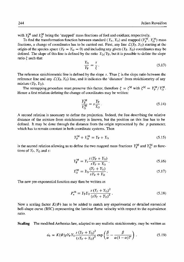
with Y^ and Y^ being the 'mapped' mass fractions of fuel and oxidizer, respectively. To find the transformation function between standard (Fp, ^o) and mapped (Y^, Y^) mass
fractions, a change of coordinates has to be carried out. First, any line £ ( F F , ^G) starting at the origin of the species space (Yj: = YQ = 0) and including any given (Fp, FQ) coordinates may be defined. The slope of this line is defined by the ratio F O / ^ F , but it is possible to define the slope ratio f such that
The reference stoichiometric line is defined by the slope s. Thus ^ is the slope ratio between the reference line and any C(Yf;, YQ) line, and it indicates the 'distance' from stoichiometry of any mixture (Yp,Yo).
The remapping procedure must preserve this factor, therefore ^ = ^^ with ^^ = Y^/Y^. Hence a first relation defining the change of coordinates may be written:
Y^^ I F
Y^ Vo M - ^ ^ - (5.14)
A second relation is necessary to define the projection. Indeed, the line describing the relative distance of the mixture from stoichiometry is known, but the position on this line has to be defined. It may be done through the distance from the origin represented by the p parameter, which has to remain constant in both coordinate systems. Then
yp^ + 7 ^ = yp + yo (5.15)
is the second relation allowing us to define the two mapped mass fractions Y^ and Y^ as functions of Fp, YQ and s:
^ ( I F + FQ)
^Fp + Fo ' Fp^ = F p ^ \ 7 ; ; / \ (5.16)
VM _Y (^F + YQ)
The new pre-exponential function may then be written as
pM^Y.Yo'-^^^-^. (5.18) >M = ivin
(sY^-^YoY Now a scaling factor K(0) has to be added to match any experimental or detailed numerical bell-shape curve (BSC) representing the laminar flame velocity with respect to the equivalence ratio.
Scaling The modified Arrhenius law, adapted to any realistic stoichiometry, may be written as
a, = K(0)pY,Yo'-^^^ exp ( ^ - - ^ ) , (5.19) (^Fp + Fo)^ \oi a(l-a)Tj

Direct Numerical Simulation of Sprays 245
• Analytic • Methane • Ethyne A Propane . O K =cte fl
' ' \
\
\ ' ^ '^
Equivalence ratio
(a) Flame velocity versus equivalence ratio (BSC). Symbols: Experimental results. Lines:
GKAS procedure.
2 4 6 Inverse of normalized scalar dissipation rate
(b) Propane extinction limit. Temperature and reaction rates have been normalized by their
maximum value along the profile. Scalar dissipation rate is normalized by its asymptotic
extinction limit. Figure 4. Characteristics of flames found from the KGKAS procedure.
where K(^^ is a pre-exponential coefficient, which allows one to tune the BSC to a prescribed shape. A first approximation would be to use a constant pre-exponential coefficient K = K{^. But even if a maximum value is found when the equivalence ratio <t> equals unity thanks to the remapping procedure, the response velocity of the flame (see Figure 4a, open circles) is not entirely satisfactory. The evolution of the lean side of the BSC is correctly determined with a constant K (as for a classical Arrhenius law). However, the rich-side velocities are overestimated even if there is a distinct improvement compared to the classical Arrhenius law that leads to an unceasingly growing velocity after the unity equivalence ratio. In fact, the reaction rate is decomposed into a pre-exponential and an exponential factor. The imbalance between the lean side and the rich side of the global Arrhenius law is directly due to the imbalance of heat release due to the exponential term.
Another solution is to add a 0-dependence to the pre-exponential factor K. This can be done according to two procedures. If an extremely accurate determination of the BSC is necessary, it is suggested to use a 1-D code able to compute stabilized premixed flames (Cantera or Chemkin for example), or to use a BSC obtained from experiments. Then, using a root-finding procedure, the coefficient A'(0) may be determined according to the correct BSC that gives the velocity reached by the flame for any value of the equivalence ratio. A second procedure, less accurate but more direct, consists of determining K(^^ as a generic function with some adjustable parameters. Figure 4a shows various BSC curves obtained with the new Arrhenius law calibrated with experimental BSC for methane, ethane and propane. The analytical result, very close to the first three, has been obtained with an empirical function based on two second-order polynomial expressions: one for the lean side, and one for the rich side. Coefficients of the polynomial have to be adapted to a synthetic fuel or retrieved from a prescribed BSC with a root-finding method
246 Julien Reveillon
(a) Methane. (b) Ethane. (c) Propane. (d) Analytic.
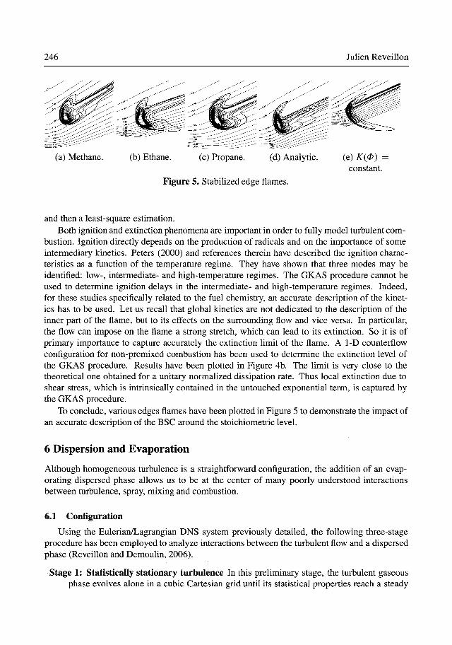
Figure 5. StabiHzed edge flames.
(e) K(0) = constant.
and then a least-square estimation. Both ignition and extinction phenomena are important in order to fully model turbulent com
bustion. Ignition directly depends on the production of radicals and on the importance of some intermediary kinetics. Peters (2000) and references therein have described the ignition characteristics as a function of the temperature regime. They have shown that three modes may be identified: low-, intermediate- and high-temperature regimes. The GKAS procedure cannot be used to determine ignition delays in the intermediate- and high-temperature regimes. Indeed, for these studies specifically related to the fuel chemistry, an accurate description of the kinetics has to be used. Let us recall that global kinetics are not dedicated to the description of the inner part of the flame, but to its effects on the surrounding flow and vice versa. In particular, the flow can impose on the flame a strong stretch, which can lead to its extinction. So it is of primary importance to capture accurately the extinction limit of the flame. A 1-D counterflow configuration for non-premixed combustion has been used to determine the extinction level of the GKAS procedure. Results have been plotted in Figure 4b. The limit is very close to the theoretical one obtained for a unitary normalized dissipation rate. Thus local extinction due to shear stress, which is intrinsically contained in the untouched exponential term, is captured by the GKAS procedure.
To conclude, various edges flames have been plotted in Figure 5 to demonstrate the impact of an accurate description of the BSC around the stoichiometric level.
6 Dispersion and Evaporation
Although homogeneous turbulence is a straightforward configuration, the addition of an evaporating dispersed phase allows us to be at the center of many poorly understood interactions between turbulence, spray, mixing and combustion.
6.1 Configuration
Using the Eulerian/Lagrangian DNS system previously detailed, the following three-stage procedure has been employed to analyze interactions between the turbulent flow and a dispersed phase (Reveillon and Demoulin, 2006).
Stage 1: Statistically stationary turbulence In this preliminary stage, the turbulent gaseous phase evolves alone in a cubic Cartesian grid until its statistical properties reach a steady
Direct Numerical Simulation of Sprays 247
E
^ 0.5
J . 0.4
0.3 E'
w' /u'
• St = 0.35 •St =1.05
- St = 2.8
. , . . r ^ _ ^ > X . . . . ; \
:--.'*^CW
A. St = 0.17 1 B, St = 1.05 -est = 5.6 1
) :
\ > 5 *
10 15 20 25 30 35
Normalized Vorticity
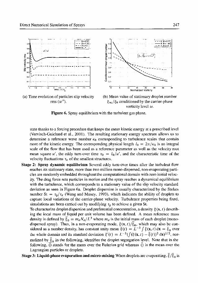
(a) Time evolution of particles slip velocity (b) Mean value of stationary droplet number rms ( K; '0 • OD / f o conditioned by the carrier-phase
vorticity level co.
Figure 6. Spray equilibrium with the turbulent gas phase.
state thanks to a forcing procedure that keeps the mean kinetic energy at a prescribed level (Vervisch-Guichard et al., 2001). The resulting stationary energy spectrum allows us to determine a reference wave number KQ corresponding to turbulence scales that contain most of the kinetic energy. The corresponding physical length /Q = 2n/Ko is an integral scale of the flow that has been used as a reference parameter as well as the velocity root mean square u\ the eddy turn-over time to = /o/w^ and the characteristic time of the velocity fluctuations z^ of the smallest structures.
Stage 2: Spray dynamic equilibrium Several eddy turn-over times after the turbulent flow reaches its stationary state, more than two million mono-dispersed, non-evaporating particles are randomly embedded throughout the computational domain with zero initial velocity. The drag force sets particles in motion and the spray reaches a dynamical equilibrium with the turbulence, which corresponds to a stationary value of the slip velocity standard deviation as seen in Figure 6a. Droplet dispersion is usually characterized by the Stokes number St = Tp/r^ (Wang and Maxey, 1993), which indicates the ability of droplets to capture local variations of the carrier-phase velocity. Turbulence properties being fixed, simulations are been carried out by modifying rp to achieve a given St. To characterize droplet dispersion and preferential concentration, a density ^(x, t) describing the local mass of liquid per unit volume has been defined. A mean reference mass density is defined by f Q = m^N^/L^ where m^ is the initial mass of each droplet (mono-dispersed spray). Thus, in a non-evaporating mode, J x, 0 /?0 ' which may also be considered as a number density, has constant unity mean ^{t) = L~^ J ^(x, t) dx = f Q over the whole domain and its standard deviation ^\t) = L~^(/(^(x, t) — ^{t))^ dx)^/^, normalized by Q in the following, identifies the droplet segregation level. Note that in the following, 0 stands for the mean over the Eulerian grid whereas () is the mean over the Lagrangian particles or droplets.
Stage 3: Liquid-phase evaporation and micro-mixing When droplets are evaporating, ^ /^Q is
248 Julien Reveillon
(a) (b)
(c) (d)
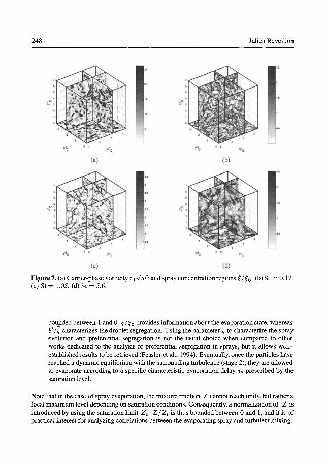
Figure 7. (a) Carrier-phase vorticity TQ V CD and spray concentration regions ^/f o- (b) St = 0.17. ( c )S t= 1.05. (d) St =5 .6 .
bounded between 1 and 0. f/^Q provides information about the evaporation state, whereas f 7 ? characterizes the droplet segregation. Using the parameter ^ to characterize the spray evolution and preferential segregation is not the usual choice when compared to other works dedicated to the analysis of preferential segregation in sprays, but it allows well-established results to be retrieved (Fessler et al., 1994). Eventually, once the particles have reached a dynamic equilibrium with the surrounding turbulence (stage 2), they are allowed to evaporate according to a specific characteristic evaporation delay tv prescribed by the saturation level.
Note that in the case of spray evaporation, the mixture fraction Z cannot reach unity, but rather a local maximum level depending on saturation conditions. Consequently, a normalization of Z is introduced by using the saturation limit Zg. Z /Zs is thus bounded between 0 and 1, and it is of practical interest for analyzing correlations between the evaporating spray and turbulent mixing.

Direct Numerical Simulation of Sprays 249
6.2 Preferential segregation of non-evaporating droplets
To study the preferential concentration of discrete particles in turbulent flows, several approaches exist (see for instance Squires and Eaton, 1991; Wang and Maxey, 1993; Fessler et al., 1994; Simonin et al., 1993, and Aliseda et al., 2002). If a statistically homogeneously distributed spray is randomly injected, i.e. if there is no preferential segregation, the distribution of the number of particles per control volume (CV) of a given size must follow a binomial distribution, which may be approximated by a Poisson distribution. Hence, the study of preferential concentration is usually based (Fessler et al., 1994) on the difference between the actual segregated distribution and the Poisson distribution. Thus it is characterized by
H = (o>-Vx)/X, (6.1)
where A is the average number of particles per cell, whereas a and VA are the standard deviations of the particle distribution and the Poisson distribution, respectively. For a given Lagrangian distribution of the particles, U depends strongly on the size of the CV. However, according to Fessler et al. (1994), the length scale corresponding to the characteristic cluster size is equal to ^i:max, which is the size of the CV when U reaches a maximum value.
In the case considered in this configuration, particles are liquid droplets of fuel that are evaporated to prepare the reactive mixture. Preferential concentration of particles is potentially important when describing flow-induced heterogeneities that could appear in the mixture-fraction field. Following such considerations, another parameter, more representative of the evaporation and turbulent mixing processes, has been considered to describe preferential-segregation effects.
Droplet dispersion and preferential segregation are analyzed from a Eulerian point of view thanks to the local Eulerian liquid density ^ (x, t). Instantaneous fields of f are plotted in Figure 7 for three Stokes numbers (St = 0.17, St = 1.05 and St = 5.6), along with the corresponding vorticity field. These four fields have been captured at exactly the same time after droplet dispersion has reached a stationary value (t > too). Even without any quantitative analysis, it is possible to see the dramatic impact of the particles' inertia on their dispersion properties. Indeed, even with a small Stokes number, particles tend to leave the vortex cores and segregate in weak vorticity areas. This phenomenon may be seen in Figures 7b and 7c where f is represented for St = 0.17 and St = 1.05, respectively. This last case shows a normalized liquid density ^/f Q ranging between 0 (no droplets) and 5 (five times the mean density). As will be shown later, density fluctuations reach a maximum when St = 1.
When St = 0.17, segregation is already clearly visible (maximum deviation: 2.5), although there are more intermediates density areas (see Figure 7b). When the St = 1 limit is surpassed, the droplet distribution tends to be totally different than for St < 1 (see Figure 7d). Indeed, kinetic times become large enough for the droplets to cross high vorticity areas, leading to a less segregated spray (maximum deviation: 2.5). This result is confirmed in Figure 6b where the mean liquid density conditioned by the local vorticity level has been plotted for various Stokes numbers. For highly^segregated sprays (St = 1.05), high vorticity areas are_almost empty, with an average value of ^ /^Q ^q^^l to 0.2, whereas when vorticity tends to 0, ^ /^Q converges toward 2. Figure 6b is in accordance with classical results such as the work of Squires and Eaton (1991). They found a maximum correlation between the number of particles and the vorticity level for a Stokes number equal to 0.15. However they used a Stokes number based on the integral time scale of the turbulence. By swapping it with the Kolmogorov time scale, the peak of correlation occurs
250 Julien Reveillon
stokes St
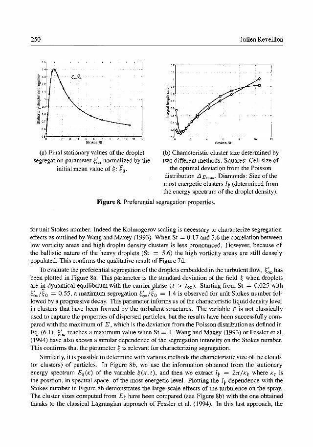
(a) Final stationary values of the droplet segregation parameter ^^ normalized by the
initial mean value of ^: ^Q.
stokes St
(b) Characteristic cluster size determined by two different methods. Squares: Cell size of
the optimal deviation from the Poisson distribution AzimsLx- Diamonds: Size of the most energetic clusters / (determined from the energy spectrum of the droplet density).
Figure 8. Preferential segregation properties.
for unit Stokes number. Indeed the Kolmogorov scaling is necessary to characterize segregation effects as outlined by Wang and Maxey (1993). When St = 0.17 and 5.6 the correlation between low vorticity areas and high droplet density clusters is less pronounced. However, because of the ballistic nature of the heavy droplets (St = 5.6) the high vorticity areas are still densely populated. This confirms the qualitative result of Figure 7d.
To evaluate the preferential segregation of the droplets embedded in the turbulent flow, ^^ has been plotted in Figure 8a. This parameter is the standard deviation of the field f when droplets are in dynamical equilibrium with the carrier phase ( > ?oo)- Starting from St = 0.025 with t ^ / ? o = 0.55, a maximum segregation f^/^o = 1-4 is observed for unit Stokes number followed by a progressive decay. This parameter informs us of the characteristic liquid density level in clusters that have been formed by the turbulent structures. The variable ^ is not classically used to capture the properties of dispersed particles, but the results have been successfully compared with the maximum of U, which is the deviation from the Poisson distribution as defined in Eq. (6.1). ^ ^ reaches a maximum value when St = 1. Wang and Maxey (1993) or Fessler et al. (1994) have also shown a similar dependence of the segregation intensity on the Stokes number. This confirms that the parameter ^ is relevant for characterizing segregation.
Similarly, it is possible to determine with various methods the characteristic size of the clouds (or clusters) of particles. In Figure 8b, we use the information obtained from the stationary energy spectrum E^(K) of the variable ^{x,t), and then we extract / = ITV/K^ where K^ is the position, in spectral space, of the most energetic level. Plotting the / dependence with the Stokes number in Figure 8b demonstrates the large-scale effects of the turbulence on the spray. The cluster sizes computed from E^ have been compared (see Figure 8b) with the one obtained thanks to the classical Lagrangian approach of Fessler et al. (1994). In this last approach, the
Direct Numerical Simulation of Sprays 251
cluster size denoted by A^msix is the width of the CV when U reaches a maximum value. Both / and Z\i:max show a similar evolution with a minimum size for St = 1. In their experiment Aliseda et al. (2002) compared the characteristic cluster size Asmax to the length scale found using a method proposed by Wang and Maxey (1993). In this last approach, the change between the actual distribution to the binomial distribution is measured as the square of the difference of probabilities given by the two distributions summed over all possible values. Aliseda et al. found that both methods lead to the same characteristic length scale for the clusters. Thus using the Eulerian f parameter is in accordance with the classical Lagrangian approach for the analysis of preferential segregation. Notice that for the measurement of the characteristic cluster length scale, Aliseda et al. (2002) use all of the droplet class sizes. Therefore, it is not possible to determine the Stokes number dependency of the clusters' characteristic length scale. The two methods they used to find the cluster length scale agree globally when considering all of the droplet sizes. It is still possible that some differences may appear for specific values of Stokes as we found when comparing Ajjmsix to f.
Fessler et al. (1994) conducted experiments with various sets of particles corresponding to Stokes numbers ranging from 1.7 up to 130. Their study does not extend to Stokes numbers smaller than unity. It appears that Asm&x is dependent on the Stokes number, starting with a value of the order of the Kolmogorov length scale, it increases as the Stokes number increases. For Stokes numbers greater than unity, the parameter ^ allows this trend to be recovered. In our DNS, when St < 1 the evolution of the cluster size obtained with both U and f is similar, although the length scales are different (Figure 8b). However, using ^ as a reference parameter offers a new range of possible analysis.
From a phenomenological point of view, the cluster-size evolution results from the competition between three physical phenomena: the ejection of the droplets from the vortex cores by the turbulence, the turbulent micro-mixing (prevalent when St < 1) and the ballistic effects (prevalent when St > 1). Indeed, droplets tend to be ejected from the turbulent structures to form clusters concentrated in low vorticity areas. However, for droplets with a small Stokes number, turbulent micro-mixing counteracts the segregation process and 'diffuse' clouds are obtained (as seen in Figure 7b): the lighter the droplets, the more effective the mixing and the larger the characteristic size of the clusters. When St = 1, an optimal segregation is obtained because micro-mixing's impact is weak and the droplets are not heavy enough to leave low vorticity areas where they are trapped. However, as soon as inertia is prevalent (St > 1) the particles are able to cross turbulent structures no matter what their vorticity is and then the characteristic size of the clusters increases again. In Figure 8b, it is clear that both / and ^ijmax capture this natural dependence on the Stokes number.
To conclude on the non-evaporating dispersion aspect, this first DNS application shows that preferential segregation in sprays cannot be characterized using only the mean segregation parameter ^^ and the mean density ^. Indeed, for two sprays with the same mean density and whose Stokes numbers are 0.17 and 5.6, a similar mean segregation level equal to 0.85 is found in Figure 8a. However, the corresponding topologies of spray density are distinct, as may be seen in Figures 7b and 7d where ^ is plotted for St = 0.17 and 5.6, respectively. Consequently, for two fields with identical first moments of ^, different mixture fraction topologies can be obtained from droplet evaporation and different combustion regimes might be observed if the ignition delay is short compared to the turbulent mixing time. Thus, in addition to ^ and f^, a third parameter, which has to depend on the droplet's Stokes number, is necessary to describe accurately

252 Julien Reveillon
» 0.16
i I 0.14 I
I 0.12
A | / 'NV jl \
li V
\'\ \ I \ \ f \ 1 \ 1 \ 1 \
\
A,,St = 0.17|
B,,St=1.05 -
C,,St = 5.6
Z'/Zs
(a)
O 1
•O 0.8
I °H §•0.4 >
UJ 0.2
"*
V :C'/4o :
N ^ " > e k
" " ^ ^ ^
A3,St = 0.17 1
63,31 = 1.05 .
C3,St = 5.6
• «. ^ c: .^: ,^^^^^
(b) (c)
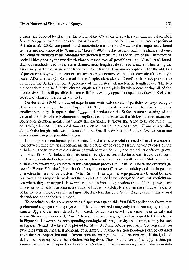
Figure 9. Evaporating spray: (a) Time evolution of spray segregation, (b) Liquid density, (c) Mean droplet surface.
the preferential segregation of the spray and the subsequent mixture-fraction field.
6.3 Evaporation
Once dynamical equilibrium is reached between the turbulent gaseous flow and the dispersed phase, evaporation is activated. A very different behavior may be observed in Figure 9a where the evolution of the standard deviation of the mixture fraction, Z' , has been plotted for various Stokes numbers {A\,B\ and C\ correspond to TV/TO = 1/2). From a general point of view, the global shape of the curves is the same: starting from Z' jZ^ = 0 where evaporation starts, the curves reach a maximum value long before the characteristic evaporation delay (when ^/TQ ^ 0.2). At this point, dissipation effects on the mixture-fraction fluctuations become greater than the evaporation effect. Then mixture-fraction fluctuations decrease continuously. Details of the competition between evaporation and dissipation may be found in Reveillon and Vervisch (2000).
A more detailed analysis shows different local evolutions of the mixture fraction. First, the

Direct Numerical Simulation of Sprays 253
most segregated spray generates the most fluctuating mixture-fraction field (case Bl, St = 1.05). Indeed, droplets accumulate in small clusters and when evaporation starts, high levels of mixture fraction are obtained in small control volumes leading to a strong deviation Z', Another important point to notice is the evolution of the deviation Z' of case CI that initially evolves like case Al because of the initial similar droplet segregation level. However, it exceeds very quickly (more than 30%) the maximum value of Z^j before joining, almost exactly, the curve Z^j corresponding to the highly segregated case. This behavior is due to the decrease of the mean Stokes number of the spray that leads to a very quick segregation of the initially ballistic droplets of case C1. On the other hand, there is no change in segregation for case A1 (St = 0.17) as the Stokes number becomes smaller and smaller.
This interpretation is confirmed in Figure 9b where the evolution of the droplet segregation parameter ^' has been plotted for cases A3, B3 and C3 (TV = 2TO), which shows this behavior more clearly. The general trend of cases A and B is a decrease of the segregation because of the diminution of the corresponding Stokes number. The turbulent micro-mixing becomes more and more effective leading to a less segregated spray. When the Stokes number is initially greater than unity (cases C) the segregation first increases before following the general decay. The initial elevation of the segregation level corresponds to an evolution of the droplet dynamics to a level that is more efficient (unit Stokes number) at creating clusters and, therefore, to increase %' momentarily. This modification of the evaporating droplet dynamics has a direct impact on the mixture-fraction evolution as seen in Figure 9b.
The evolution of the mean droplet surface divided by its initial value is shown in Figure 9c for various Stokes numbers and various evaporation delays. Additional curves, represented by circles, represent the mean droplet surface evolution that would be obtained if there were no preferential segregation (homogeneous droplet distribution). Figure 9c demonstrates the dramatic effect of the segregation of the dispersed phase on the evaporation process. Two distinct stages may be observed. First, when evaporation starts far from the saturation limit, the decrease in the mean droplet surface area calculated from the DNS is similar to the results obtained with the analytical model that neglects segregation phenomena. Then, depending on the Stokes number (i.e. on the droplet segregation level), a second evaporating stage controlled by saturation may be observed with a slower rate.
7 Laminar Spray Combustion
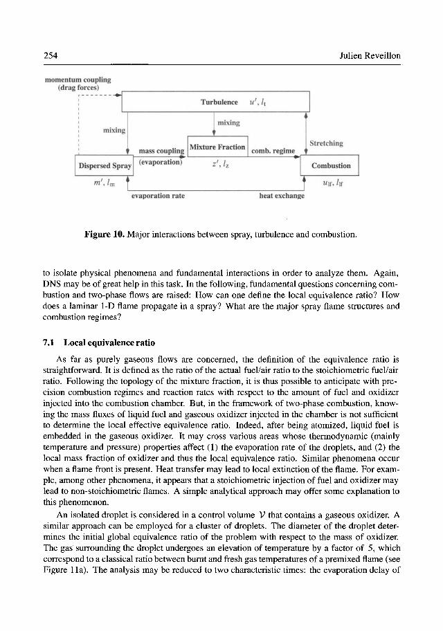
Depending on the configuration of the studied system, combustion may take place either after the full evaporation of the liquid fuel, or within the evaporating dispersed phase. In the first case, even if classical gaseous combustion models can be utilized, the mixture-fraction topology issued from the spray evaporation is completely different from the one obtained with gaseous fuel injection. As described by the preceding example concerning spray preferential segregation or in Reveillon et al. (1998), partially premixed areas appear and consequently, depending on the dynamics of the droplets, various flame structures may be generated. On the other hand, if flames propagate in the mixture where evaporating droplets are still present, numerous complex interactions appear between combustion, droplet evaporation and turbulence (see Figure 10).
Indeed, the spray modifies local heat transfer, momentum, and dissipation rate and, of course, the mixture-fraction level. All these variables affect deeply not only the flame ignition and propagation, but also the characteristic properties of the turbulence. It is then particularly difficult
254 Julien Reveillon
momentum coupling (drag forces)
Turbulence u\ k
mixmg
f mass coupling
Dispersed Spray
mixmg
Mixture Fraction comb, regime j
(evaporation) z\k
Stretching
Combustion
U]f, /if
evaporation rate heat exchange
Figure 10. Major interactions between spray, turbulence and combustion.
to isolate physical phenomena and fundamental interactions in order to analyze them. Again, DNS may be of great help in this task. In the following, fundamental questions concerning combustion and two-phase flows are raised: How can one define the local equivalence ratio? How does a laminar 1-D flame propagate in a spray? What are the major spray flame structures and combustion regimes?
7.1 Local equivalence ratio
As far as purely gaseous flows are concerned, the definition of the equivalence ratio is straightforward. It is defined as the ratio of the actual fuel/air ratio to the stoichiometric fuel/air ratio. Following the topology of the mixture fraction, it is thus possible to anticipate with precision combustion regimes and reaction rates with respect to the amount of fuel and oxidizer injected into the combustion chamber. But, in the framework of two-phase combustion, knowing the mass fluxes of liquid fuel and gaseous oxidizer injected in the chamber is not sufficient to determine the local effective equivalence ratio. Indeed, after being atomized, liquid fuel is embedded in the gaseous oxidizer. It may cross various areas whose thermodynamic (mainly temperature and pressure) properties affect (1) the evaporation rate of the droplets, and (2) the local mass fraction of oxidizer and thus the local equivalence ratio. Similar phenomena occur when a flame front is present. Heat transfer may lead to local extinction of the flame. For example, among other phenomena, it appears that a stoichiometric injection of fuel and oxidizer may lead to non-stoichiometric flames. A simple analytical approach may offer some explanation to this phenomenon.
An isolated droplet is considered in a control volume V that contains a gaseous oxidizer. A similar approach can be employed for a cluster of droplets. The diameter of the droplet determines the initial global equivalence ratio of the problem with respect to the mass of oxidizer. The gas surrounding the droplet undergoes an elevation of temperature by a factor of 5, which correspond to a classical ratio between burnt and fresh gas temperatures of a premixed flame (see Figure 11a). The analysis may be reduced to two characteristic times: the evaporation delay of

Direct Numerical Simulation of Sprays 255
5
44-
3
2
• • time
tv
(a) Sketch of the configuration: Droplet is surrounded by a quiescent atmosphere. A sudden temperature growth (1) expands the gas and (2) evaporates the droplet.
Figure 11. Analysis of the impact of evaporation dynamics on the gaseous equivalence ratio
(b) Ratio of the final gaseous equivalence ratio to the initial liquid equivalence ratio with respect to Dy.
the droplet Ty, and the heating delay of the gas phase XQ. An open domain is considered and the pressure remains constant and equal to the atmospheric pressure. The increase of temperature leads to a dilatation of the gas phase. Then the amount of oxidizer in the control volume diminishes. During this process the droplet is evaporating. Consequently, the final equivalence ratio in the volume depends on the ratio of the evaporation delay to the heating delay: Dy = tv/tc. Indeed, a very small evaporation delay (Dy <^ 1) leads to the quick disappearance of the droplet before the dilatation of the whole gas mixture. The final equivalence ratio is then very close to the initial global equivalence ratio determined from the mass of the liquid droplet. On the contrary, if Dy ^ 1 the mass of oxidizer diminishes before the full evaporation of the droplet. This leads to an increase in the final equivalence ratio. These remarks are summarized in Figure 1 lb, which shows the ratio of the final gas-phase equivalence ratio 0g to the initial liquid equivalence ratio 01 with respect to the parameter Dy. Theoretically, this ratio may reach the ratio of the burnt gas temperature to the fresh gas temperature (7b/Tu = 5). From a practical point of view, the Dy parameter remains small. However, it concerns the area with the strongest variation of 0^/<P\, and we know from Figure 4a that only a slight variation of 0g may lead to strong variations of the flame structure.
This analysis has been oversimplified and numerous effects have been neglected. Nevertheless, a major point has been put forward: it is necessary to clearly differentiate between the global equivalence ratio of the chamber and the effective local equivalence ratio, which determines the flame structure and the combustion regime. This is one of the reasons that has led us to develop an Arrhenius law capable of determining the local properties of the flame regardless of the equivalence ratio.
256 Julien Reveillon
7.2 Laminar spray combustion
The second stage, dealing with two-phase flow combustion, is the analysis of the propagation and the structure of 1-D laminar premixed spray flames. Numerous researchers have worked on this subject. One of the first studies was carried out by Williams (1960). He derived an analytical solution for two distinct cases: either all the droplets are evaporated before reaching the flame front, or each droplet bums with a diffusion flame around it. Afterwards, various studies were dedicated to mono- or poly-dispersed spray combustion (Patil and NicoUs, 1978; Richards and Sojka, 1990; Lin et al., 1988; Lin and Sheu, 1991). Most often, in theses studies, the carrier phase contains initially some fuel vapor to stabilize the flame. Then the presence of droplets leads to a modification of the local equivalence ratio. Silverman et al. (1991, 1993) worked on the derivation of an analytical expression for the laminar flame speed in a spray. Nevertheless, in all of these studies, which are mostly numerical, the dilatation of the gas phase is not accounted for. As pointed out above, this phenomenon may lead to some dramatic modifications in the local properties of the mixing and, thus, on the flame structure. However, thanks to DNS, it is possible to carry out a basic 1-D configuration with a compressible formulation for the gas phase. It is a complex study with a lot of different flame behaviors and combustion regimes. In the following, we illustrate with a one simple example the complex behavior of spray flames. Monodisperse droplets are regularly spaced in the 3-D space that may be considered only along the direction of propagation of the planar flame. In this simple configuration, the droplets are anchored in the domain. They may be seen as local sources of fuel that follow the evaporation law, which depends on the local temperature, pressure and vapor mass fraction. The gas phase is initially at rest and the initial liquid equivalence ratio 0\ is equal to 1.48. Initially, there is no vapor mixed with the oxidizer.
The sketch of the configuration is shown in Figure 12a. Note that the flame propagates from right to left whereas the axis is oriented from left to right. A gaseous premixed flame profile is utilized to initialize the computation (1). The gaseous fuel is removed upstream of the flame front to be replaced by the droplets. The flame evolves within the spray and after a while an equilibrium appears between evaporation and combustion phenomena, and a time-periodic pattern appears (3). The Lewis number of this configuration is equal to 1. In a purely gaseous situation, the flame would be perfectly stationary. But, as far as spray combustion is concerned, oscillations appear. The results (flame thickness, flame speed, maximum reaction rate) have been normalized by the corresponding properties of the stationary gaseous stoichiometric flame obtained with the same fuel.
Flame index Spray combustion involves generally partially premixed and non-premixed combustion regimes. In order to differentiate between heat release due to premixed and diffusion flames, Yamashita et al. (1996) suggested to use a flame index based on the scalar product of the fuel and oxidizer normalized gradients. This flame index has been utilized also by Mizobuchi et al. (2002) to analyze a lifted hydrogen flame. The flame index may be written as
GFo = VrF-V7o (7.1)

Direct Numerical Simulation of Sprays 257
Gaseous fuel Temperature
^ ' ' I • • . •• • • • . . ' • — . • •• • • - •. • • • • — — . • . - . . . . . - . • . • . . . - . — i z . ' ^ . . • • •. 1
computational domain
Caseous fuel Temperature
Droplets
# # # # / Temperature
\Gaseous fuel
B
I A I fi I front de flamme
front d'evaporation
• • Premier front de flamme
associe au front d'evaporatioi
D J. (a) Sketch of the configuration. (1) Purely gaseous flame is generated. (2) Gaseous fuel is replaced by droplets. (3) Spray flame propagates.
Figure 12. 1-D spray flame.
Un second front de flamme suit le premier
(b) Dynamics of the double-flame front.
It is positive for a premixed flame and negative for a non-premixed one. From this definition, ^p, a normalized construction of the flame index, is derived:
?p K - V F F VFo (7.2)
When p vanishes, diffusion flames are observed, while premixed combustion is found when it reaches unity. More or less partially premixed reaction zones develop for values of p ranging between zero to unity, p has a sense only where the reaction rate is non-null. To evaluate the amount of burning in premixed and partially premixed regimes and to compare it to the overall heat release rate, a premixed fraction of the burning rate W p(x) must be introduced. W^(x) is defined for any control volume V as the average of the amount of fuel burning in premixed modes normalized by the total burning rate:
W^(x) = (7.3)
This quantity and other flame parameters are now used to seek out combustion regimes observed in the laminar cases.
Flame structure and dynamics Time evolution of the maximum of the reaction rate is plotted in Figure 13a. It appears that the flame follows a periodical pulsating behavior with two maximum reaction peaks over a period of eight flame times. First it is necessary to point out the fact
258 Julien Reveillon
that the interdrop spacing is equal to one-tenth of the reference flame thickness. Thus pulsations do not originate from the possible combustion of isolated droplets (an impossible task to resolve with our DNS formulation), but from the global flame dynamics. Even if initially the mixture is fuel rich, the maximum reaction rate corresponds to the one of the reference stoichiometric flame. To understand what is happening in the core of the flame, five positions: A, B, C, D and E (periodically equivalent to A) have been marked in Figure 13 a. The time evolution of the maximum evaporation rate is plotted in Figure 13b. It appears that this data is maximum for position B, which corresponds to the first reaction rate peak. At B the maximum reaction rate and maximum evaporation rate are at the same spatial location (see Figure 13d). (Note that a diminution of the position value corresponds to a propagation of the flame.) The first maximum reaction rate peak corresponds thus to the burning of the vapor that just left the droplet surface. But concerning the second maximum reaction rate peak (position D in Figure 13a), there is no evaporation in the domain (see Figure 13b) and the maximum reaction rate repositions itself downstream (in the burnt gases) the first front (see Figure 13c).
It appears that combustion occurs following two stages summarized in Figures 12b and 13d, which represents the flame trajectory in the (maximum reaction rate/maximum evaporation rate) space. Starting from point A where the maximum reaction and evaporation rates are weak, evaporation begins. As soon as the vapor and oxidizer mixture reach an ideal state, a first flame front propagates strongly (point B) and drives the evaporation front. However, characteristic delays of the flame are shorter than evaporation delays and the first flame front depletes quickly the vapor and extinction occurs (point C). Meanwhile downstream from this flame front, liquid fuel finished to evaporate. A mixture of burnt gases and vapor has been formed because of the originally rich configuration. When the first flame front disappears (point C), oxidizer is able to diffuse backwards into the burnt gases. Then a second flame front appears and follows the path of the first one to reach the cloud of droplets that needed this delay to generate a new evaporation front. This process is periodic and it starts over at point A.
This single example shows the complexity of spray combustion. Indeed, many characteristic parameters are involved: the flame velocity, thickness and heat release, the droplet size, interspacing, evaporation delay, etc. By modifying only one of these parameters, the flame dynamics may be dramatically changed. The next section offers a glimpse of the combustion diagrams that have been already developed in the literature.
8 Spray Combustion Diagrams
Two pioneering works have envisioned classifications of spray-flame morphology. The first diagram (see Figure 14), developed by Chiu and coworkers (Suzuki and Chiu, 1971; Chiu and Liu, 1977; Chiu and Croke, 1981; Chiu et al., 1982) consisted of the determination of the structure of flames propagating through a cloud of droplets plunged into a preheated oxidizer. Spray combustion regimes were classified according to a group combustion number G. This dimensionless number may be seen as the ratio between the characteristic evaporation speed and the molecular diffusion speed, or the convective speed of the hot gases inside the cloud. When the Peclet number is large, Candel et al. (1999) showed that in most cases the relation G ^ SN-^^^/S is verified between the group number G, the total number of droplets in the cloud N and the separation parameter S. This last number S = 8s/S^ is the ratio between (5s, the mean droplet inter-spacing, and 8rf, a characteristic diffusion-flame radius (Kerstein and Law, 1982).
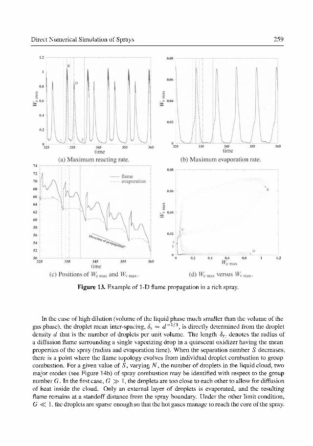
Direct Numerical Simulation of Sprays 259
^u 0.6
11
B
:
u u vJ^
1 ll 1
345
time (a) Maximum reacting rate. (b) Maximum evaporation rate.
^> 0.04 ^
' f/ -
:i 0.2 0.4 0.6 0.8
*^e max
(c) Positions of W^ max and W^ max- (d) WQ max vcrsus Wy
Figure 13. Example of 1-D flame propagation in a rich spray.
In the case of high dilution (volume of the liquid phase much smaller than the volume of the gas phase), the droplet mean inter-spacing, 8^ = d~^^^,is directly determined from the droplet density d that is the number of droplets per unit volume. The length Sr^ denotes the radius of a diffusion flame surrounding a single vaporizing drop in a quiescent oxidizer having the mean properties of the spray (radius and evaporation time). When the separation number S decreases, there is a point where the flame topology evolves from individual droplet combustion to group combustion. For a given value of S, varying N, the number of droplets in the liquid cloud, two major modes (see Figure 14b) of spray combustion may be identified with respect to the group number G. In the first case, G ^ 1, the droplets are too close to each other to allow for diffusion of heat inside the cloud. Only an external layer of droplets is evaporated, and the resulting flame remains at a standoff distance from the spray boundary. Under the other limit condition, G <$C 1, the droplets are sparse enough so that the hot gases manage to reach the core of the spray.

260 Julien Reveillon
lO^i
s
External Sheath Combustion
Single Droplet Combustion
S : separation a Interdrop spacing droplet radius
(a) Group combustion diagram (Chigier, 1983; Kuo, 1986).
External sheath combustion External group combustiot
^^ ^ ^ External flame
^-£>_-?-' V non-vaponzmi / droplets
G « l
I ® ® - 0 ^©^
'^.® ^® ®X
\ ®Q® 0 ® ® ;
Individual droplet burning
Internal group combustion single droplet combustion
(b) Combustion modes for a droplet cloud (Chiu et al., 1982; Kuo, 1986).
multi-droplet combustion
internal group combustion
external group combustion
diffusion flame
turbulent brush flam^
(c) Sketch of spray group combustion (Chiu and Croke, 1981; Kuo, 1986).
Figure 14. Combustion modes defined by Chiu.
Hence evaporation and combustion processes take place around every individual droplets. Those conditions delineate the so-called "external" combustion regime expected for G ^ 1, which is complemented by the "internal" combustion regime, observed for G <$C 1 (see Figure 14b). A smooth transition between these limiting regimes was anticipated by Chiu et al. (1982), leading to intermediate submodes depending on the magnitude of G. When G is slightly above unity, the flame stays around the droplet group with a temperature rise of the liquid phase affecting the core of the cloud. For G smaller than unity, a first ring of individual burning droplets is centered on a droplet cloud surrounded by a diffusion flame.
Later on, Chang and also Borghi and coworkers (Chang, 1996; Borghi, 1996b,a; Borghi and Champion, 2000) added to the analysis the control parameters of the reaction zone itself, namely the characteristic flame time tf and its thickness 8f. The corresponding diagram may be seen in Figure 15. In addition, the mean evaporation delay ry was introduced. When ty <^ tf, the mixture may be locally premixed and a propagating premixed flame develops (see Figure 16a). This regime should be observed for all values of mean droplets inter-spacing Ss and flame thickness
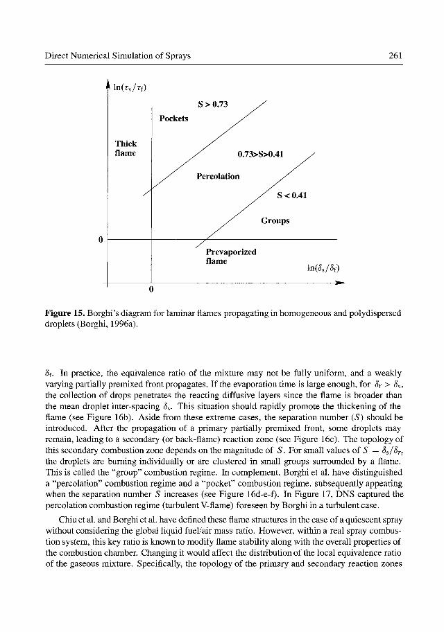
Direct Numerical Simulation of Sprays 261
A ln(rv/rf)
Figure 15. Borghi's diagram for laminar flames propagating in homogeneous and poly dispersed droplets (Borghi, 1996a).
Sf. In practice, the equivalence ratio of the mixture may not be fully uniform, and a weakly varying partially premixed front propagates. If the evaporation time is large enough, for Sf > 8^, the collection of drops penetrates the reacting diffusive layers since the flame is broader than the mean droplet inter-spacing 5s. This situation should rapidly promote the thickening of the flame (see Figure 16b). Aside from these extreme cases, the separation number (S) should be introduced. After the propagation of a primary partially premixed front, some droplets may remain, leading to a secondary (or back-flame) reaction zone (see Figure 16c). The topology of this secondary combustion zone depends on the magnitude of S. For small values of S = Ss/8rf the droplets are burning individually or are clustered in small groups surrounded by a flame. This is called the "group" combustion regime. In complement, Borghi et al. have distinguished a "percolation" combustion regime and a "pocket" combustion regime, subsequently appearing when the separation number S increases (see Figure 16d-e-f). In Figure 17, DNS captured the percolation combustion regime (turbulent V-flame) foreseen by Borghi in a turbulent case.
Chiu et al. and Borghi et al. have defined these flame structures in the case of a quiescent spray without considering the global liquid fuel/air mass ratio. However, within a real spray combustion system, this key ratio is known to modify flame stability along with the overall properties of the combustion chamber. Changing it would affect the distribution of the local equivalence ratio of the gaseous mixture. Specifically, the topology of the primary and secondary reaction zones
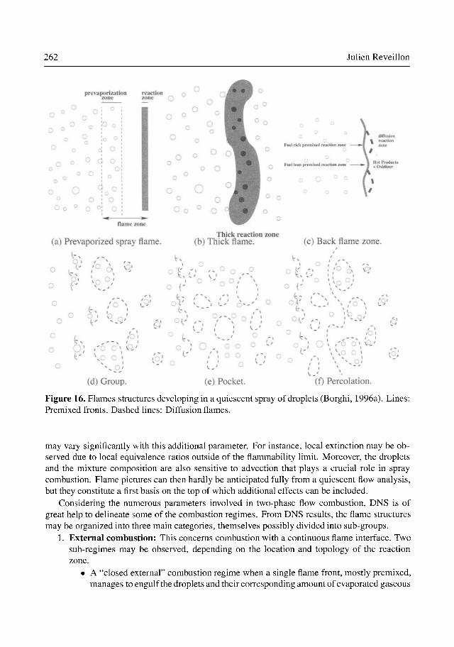
262 Julien Reveillon
pre vaporization reaction Q r^ j zone ynnp r^ ^^m
o
o
o
o o
o
O o
O
o 0
o 0 o
o
o
o o
O
o °
o ; ° o
o ;0 o
°o i° ° Q O
o 6 o I o
O ' n 1 O
c o 1 O
O ; O
0 ^ 0
flame zone
(a) Prevaporized spray flc
o
o
o
o
o
o
o
o»
o
0
/ o ^ c ks ' o 1 o ^ ;
/ ' o o ^ ^Q.' \ o o »
(d) Grouf ).
ime.
2'
&
(2^
O o o
O
O o
o o
O o
O o
oV^ ( - S
Oi^'
o ,
o
o • • i O o H o •H o aHft o VHI
0 O o ^
0 O •
O ' fl o fli
° o °fl|
o Q
o
Thick reaction (b) Thick flame.
o
' o ' - ' o o /
O . / o o ,' ' o o
(e) Pocket.
s \ V
/ -
/ 1
o Q
o
o
o
o o
o
o
o
o zone
o
1
\ 1
o
o
° r ° o \ O f diffusion
O i % reaction Fuel rich premixed reaction zone * - i zone
Fuel lean premixed reaction zone » - I ^ Oxidizer*^ *
h o O ° o 1 1
o o o 1^ 1
(c) Back flame zone.
o ' r ; ; / ° o^ ' ;
o {^^ ^ \\^ y
oV ;7^^^^^ /o^\ ,'Q' (- s ~ ' S ' ' "
1 O ' O ,^ /
o ; o ' -'o o>, a' <-' \ \ o 0 1 ,b;
(f) Percolation.
Figure 16. Flames structures developing in a quiescent spray of droplets (Borghi, 1996a). Lines: Premixed fronts. Dashed lines: Diffusion flames.
may vary significantly with this additional parameter. For instance, local extinction may be observed due to local equivalence ratios outside of the flammability limit. Moreover, the droplets and the mixture composition are also sensitive to advection that plays a crucial role in spray combustion. Flame pictures can then hardly be anticipated fully from a quiescent flow analysis, but they constitute a first basis on the top of which additional effects can be included.
Considering the numerous parameters involved in two-phase flow combustion, DNS is of great help to delineate some of the combustion regimes. From DNS results, the flame structures may be organized into three main categories, themselves possibly divided into sub-groups.
1. External combustion: This concerns combustion with a continuous flame interface. Two sub-regimes may be observed, depending on the location and topology of the reaction zone.
• A "closed external" combustion regime when a single flame front, mostly premixed, manages to engulf the droplets and their corresponding amount of evaporated gaseous

Direct Numerical Simulation of Sprays 263
>- 0
Figure 17. Example of percolating flames obtained from DNS of a turbulent V-shape flame.
2.
3.
fuel to transform it into products (Figure 18a). • An "open external" combustion regime when two reaction zones develop on each
side of the central jet (see Figure 18b). ^Group" combustion: The droplets are organized in several groups, with flames independently consuming each cluster. Both rich premixed and diffusion flames are observed (see Figure 18c).
'Hybrid" combustion: This regime is a combination of the two previous ones. The premixed flames are burning in a group combustion mode, whereas the diffusion flames cannot percolate between the clusters of droplets because of the overly rich environment. The leftover fuel is burnt with the co-flowing oxidizer in an additional external diffusion flame (see Figure 18d).
These regimes, and others not detailed here, may be organized into a combustion diagram, and at least three directions are necessary to classify them. The first concerns the ratio ty/rf between the characteristic evaporation and flame times. Another important ratio, S^/Sf, is built from the mean distance between the droplets and the flame thickness, the droplet interspace s being inversely related to J \ the spray dilution. Finally, 0LO ^^^ equivalence ratio measured within the spray jet, is also needed to account for the amount of oxidizer entrained in the core of the central jet.
To start the classification, the pioneering analysis of Borghi (1996a) is followed. If the evaporation delay of injected droplets is very small compared to the flame characteristic time (Ty/rf <^ 1), then purely gaseous combustion occurs. Therefore, when Tv/tf <^ 1 the droplets are vaporized far away from the flame front and combustion develops in a fully gaseous mode.

264 Julien Reveillon
oo 0 o r o o o /'
o / o o y>
(a) Closed-external.
oo 8 o o o
o <rrr :
(b) Open-external.
o o 0 ^ ' - - - . ' )
(c) Group.
°o o o n C y ^ r \ Q
^
(a') Closed-external from DNS.
-v - -
' ^ f
(b') Open-external from DNS.
(c') Group from DNS.
(d) Hybrid structure. (d'): Hybrid from DNS.
Figure 18. Summary of generic flames structures. Orange: Premixed burning. Blue: Diffusion burning.
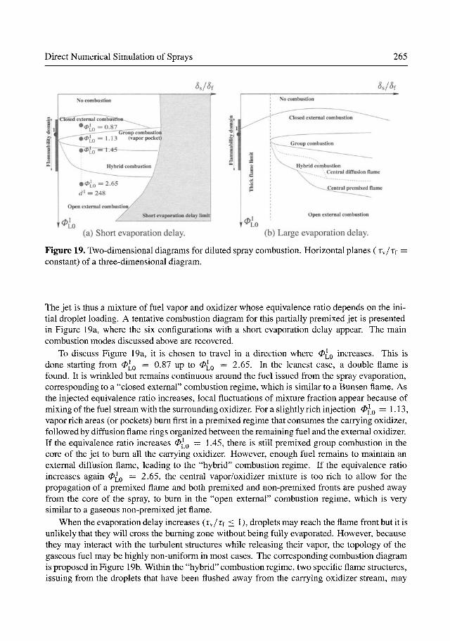
Direct Numerical Simulation of Sprays 265
(a) Short evaporation delay.
Open external combustion
(b) Large evaporation delay.
Figure 19. Two-dimensional diagrams for diluted spray combustion. Horizontal planes ( Ty/tf = constant) of a three-dimensional diagram.
The jet is thus a mixture of fuel vapor and oxidizer whose equivalence ratio depends on the initial droplet loading. A tentative combustion diagram for this partially premixed jet is presented in Figure 19a, where the six configurations with a short evaporation delay appear. The main combustion modes discussed above are recovered.
To discuss Figure 19a, it is chosen to travel in a direction where ^LO increases. This is done starting from 0LO — ^-^^ ^P ^ ^LO — 2.65. In the leanest case, a double flame is found. It is wrinkled but remains continuous around the fuel issued from the spray evaporation, corresponding to a "closed external" combustion regime, which is similar to a Bunsen flame. As the injected equivalence ratio increases, local fluctuations of mixture fraction appear because of mixing of the fuel stream with the surrounding oxidizer. For a slightly rich injection ^LO ~ ^ • • ' vapor rich areas (or pockets) bum first in a premixed regime that consumes the carrying oxidizer, followed by diffusion flame rings organized between the remaining fuel and the external oxidizer. If the equivalence ratio increases 0^0 ~ ^-45, there is still premixed group combustion in the core of the jet to bum all the carrying oxidizer. However, enough fuel remains to maintain an extemal diffusion flame, leading to the "hybrid" combustion regime. If the equivalence ratio increases again 0^0 ~ 2.65, the central vapor/oxidizer mixture is too rich to allow for the propagation of a premixed flame and both premixed and non-premixed fronts are pushed away from the core of the spray, to bum in the "open extemal" combustion regime, which is very similar to a gaseous non-premixed jet flame.
When the evaporation delay increases (tv/rf < 1), droplets may reach the flame front but it is unlikely that they will cross the buming zone without being fully evaporated. However, because they may interact with the turbulent stmctures while releasing their vapor, the topology of the gaseous fuel may be highly non-uniform in most cases. The corresponding combustion diagram is proposed in Figure 19b. Within the "hybrid" combustion regime, two specific flame stmctures, issuing from the droplets that have been flushed away from the carrying oxidizer stream, may
266 Julien Reveillon
be observed with either central diffusion flames or even, for richer mixtures, central premixed flames.
9 Acknowledgments
Numerous reflections, procedures and results presented in this text are the outcome of work carried out in collaboration with other researchers whom I would like to thank deeply and, in particular, F. X. Demoulin, M. Massot and C. Pera for their collaboration and their patience. I also wish to express my full gratitude to R. O. Fox and D. L. Marchisio for their support, encouragement and efficiency.
Bibliography
A. Aliseda, A. Cartellier, F. Hainaux, and J. C. Lasheras (2002). Effect of preferential concentration on the settling velocity of heavy particles in homogeneous isotropic turbulence. Journal of Fluid Mechanics, 468:77-105.
M. Baum, T. J. Poinsot, and D. Thevenin (1994). Accurate boundary conditions for multicom-ponent reactive flows. Journal of Computational Physics, 116:247-261.
R. Borghi (1996a). Background on droplets and sprays. In Combustion and Turbulence in Two-Phase Flowsy Lecture Series 1996-02. Von Karman Institute for Fluid Dynamics.
R. Borghi (1996b). The links between turbulent combustion and spray combustion and their modelling, pages 1-18. In , Chang (1996). ISBN 1560324562.
R. Borghi and M. Champion, editors (2000). Modelisation et theorie des flammes. Technip. ISBN 2-7108-0758-0.
S. Candel, F. Lacas, N. Darabiha, and C. Rolon (1999). Group combustion in spray flames. Multiphase Science and Technology, 11:1-18.
S. H. Chang, editor (1996). Transport Phenomena in Combustion. Taylor and Francis. ISBN 1560324562.
N. Chigier (1983). Group combustion models and laser diagnostic methods in sprays: a review. Combustion and Flame ,51:127-139.
H. H. Chiu and E. J. Croke (1981). Group combustion of liquid fuel sprays. Technical report. Energy Technology Lab Report 81-2, University of Illinois at Chicago.
H. H. Chiu, H. Y. Kim, and E. J. Croke (1982). Internal group combustion of liquid droplets. In The Combustion Institute, editor. Proceedings of the Nineteenth Symposium (International) on Combustion.
H. H. Chiu and T. M. Liu (1977). Group combustion of liquid droplets. Combustion Science and
Technology, 17:127-131. C. Crowe, M. Sommerfeld, and Y. Tsuji, editors (1998). Multiphase Flows with Droplets and
Particles. CRC Press. ISBN 0-8493-9469-4. S. Elgobashi and G. C, Truesdell (1992). Direct numerical simulation of particle dispersion in a
decaying isotropic turbulence. Journal of Fluid Mechanics, 242:655-700. J. R. Fessler, J. D. Kulick, and J. K. Eaton (1994). Prefereiitial concentration of heavy particles
in turbulent channel flow. Physics of Fluids, (6): 3742-^3749.

Direct Numerical Simulation of Sprays 267
P. Givi (1989). Model free simulations of turbulent reactive flows. Progress in Energy and Combustion Science, 15:1-107.
D. G. Goodwin (2003). An open source, extensible software suite for CVD process simulation. In Proceedings of CVD XVI and EuroCVD Fourteen. Electrochemical Society, 155-162.
G. Gouesbet and A. Berlemont (1999). Eulerian and Lagrangian appfdaches for predicting the behaviour of discrete particles in turbulent flows. Progress in Energy and Combustion Science, 25:133-159.
C. W. Hirt and B. D. Nichols (1981). Volume of fluid (VOF) - method for the dynamics of free boundaries. Journal of Computational Physics, 3 9:201 -225.
A. R. Kerstein and C. K. Law (1982). Percolation in combustion sprays. I: Transition from cluster combustion to percolate combustion in non-premixed sprays. In The Combustion Institute, editor. Proceedings of the Nineteenth Symposium (International) oh Combustion .
K. K. Kuo, editor (1986). Principles of Combustion. John Wiley and Sons. ISBN 0-471-62605-8. S. Lee, K. Lele, and P. Moin (1991). Numerical simulations of spatially evolving compressible
turbulence. Center for Turbulence Research, Annual Research Briefs, Stanford, (126). S. K. Lele (1992). Compact finite difference schemes with spectral like resolution. Journal of
Computational Physics, (103): 16-42. T. H. Lin, C. K. Law, and S. H. Chung (1988). Theory of laminar flame propagation in off-
stoichiometric dilute spray. International Journal of Heat and Mass Transfer, 31(5): 1023-1034.
T. H. Lin and Y. Y. Sheu (1991). Theory of laminar flame propagation in near stoichiometric dilute spray. Combustion and Flame, ^4:333-342.
W. Ling, J. N. Chung, T. R. Troutt, and C. T Crowe (1998). Direct numerical simulation of a three-dimensional temporal mixing layer with particle dispersion. Journal of Fluids Mechanics, {35S):6l-S5.
F. Mashayek (1998). Direct numerical simulations of evaporating droplet dispersion in forced low Mach number turbulence. International Journal of Heat and Mass Transfer, 41(17):2601-2617.
R Mashayek, F. A. Jaberi, R. S. Miller, and P. GiVi (1997). Dispersion and polydispersity of droplets in stationary isotropic turbulence. International Journal of Multiphase Flow, 23(2): 337-355.
P. A. McMurtry, W. H. Jou, J. J. Riley, and R. W. Metcalfe (1986). Direct numerical simulation of a reacting mixing layer with chemical heat release. AJAA Journal, 24(6):962-970.
R. S. Miller and J. Bellan (1999). Direct numerical simulation of a confined three-dimensional gas mixing layer with one evaporating hydrocarbon-droplet-laden stream. Journal of Fluids Mechanics, 384:293-338.
R. S. Miller and J. Bellan (2000). Direct numerical simulation and subgrid analysis of a transitional droplet laden mixing layer. Physics of Fluids, 12(3):650-671.
Y. Mizobuchi, S. Tachibaha, L Shinjo, S. Ogawa, and T. Takeno (2002). A numerical analysis on structure of turbulent hydrogen jet lifted flame. Proceedings of the Combustion Institute, 29.
S. A. Orszag and G. S. Patterson (1972). Numerical simulation of three-dimensional homogeneous isotropic turbulence. Physical Review. Letters, 28(2):76-79..
Osher and Sethian (1988)., Fronts propagating with-cufvatiite-dependent speed: Algorithms based on Hamilton-fecobi formulations; Journal of Computational Physics, 79:12-49.

268 Julien Reveillon
C. Pantano, S. Sarkar, and F. A. Williams (2003). Mixing of a conserved scalar in a turbulent reacting shear layer. Journal of Fluid Mechanics, 481:291-328.
M. Sichel P. B. Patil and J. A. Nicolls (1978). Analysis of spray combustion in a research turbine combustor. Combustion Science and Technology, 18:21-31.
N. Peters (2000). Turbulent Combustion. Cambridge University Press. T. Poinsot, S. Candel, and A. Trouve (1996). Direct numerical simulation of premixed turbulent
combustion. Progress in Energy and Combustion Science, 12:531-576. T. Poinsot and S. K. Lele (1992). Boundary conditions for direct simulations of compressible
viscous flows. Journal of Computational Physics, 1(101): 104-129. T. Poinsot and D. Veynante (2001). Theoretical and Numerical Combustion, Edwards. ISBN
1-930217-05-6. T. Poinsot and D. Veynante (2005). Theoretical and Numerical Combustion, second edition.
Edwards. ISBN 978-1930217102. M. W. Reeks (1991). On a kinetic equation for the transport of particles in turbulent flows.
Physics of Fluids, 3(3):446-456. J. Reveillon, K. N. C. Bray, and L. Vervisch (1998). Dns study of spray vaporization and turbulent
micro-mixing. In AIAA 98-1028, 36th Aerospace Sciences Meeting and Exhibit, January 12-15, Reno NV.
J. Reveillon and F. X. Demoulin (2006). Evaporating droplets in turbulent reacting flows. In Proceedings of the 31th International Symposium on Combustion , Heidelberg, Germany.
J. Reveillon and L. Vervisch (2000). Accounting for spray vaporization in non-premixed turbulent combustion modeling: A single droplet model (sdm). Combustion and Flame, 1(121): 75-90.
J. Reveillon and L. Vervisch (2005). Analysis of weakly turbulent diluted-spray flames and spray combustion regimes. Journal of Fluid Mechanics, (537):317-347.
G. A. Richards and P. E. Sojka (1990). A model of H2-enhanced spray combustion. Combustion
and Flame, 19:319-332.
J. J. Riley and G. S. Patterson (1974). Diffusion experiments with numerically integrated isotropic turbulence. Physics of Fluids, 17:292-297.
R. S. Rogallo (1981). Numerical experiments in homogeneous turbulence. Technical Report,
NASA. Technical Memorandum No. 81315.
M. Samimy and S. K. Lele (1991). Motion of particles with inertia in a compressible free shear layer. Physics of Fluids, 8(3): 1915-1923.
I. Silverman, J. B. Greenberg, and Y. Tambour (1991). Asymptotic analysis of a premixed poly-dispersed spray flame. SIAM Journal of Applied Mathematics, 51(5): 1284-1303.
I. Silverman, J. B. Greenberg, and Y. Tambour (1993). Stoichiometry and polydisperse effects in premixed spray flames. Combustion and Flame, 118:97-118.
O. Simonin, P. Fevrier, and J. Lavieville (1993). On the spatial distribution of heavy-particle velocities in turbulent flow: from continuous field to particulate chaos. Journal of Turbulence, 118:97-118.
K. D. Squires and J. K. Eaton (1991). Preferential concentration of particles by turbulence. Physics of Fluids, 3(5): 1169-1178.
Direct Numerical Simulation of Sprays 269
T. Suzuki and H. H. Chiu (1971). Multi droplet combustion on liquid propellants. In Proceedings of the Ninth International Symposium on Space Technology Science, pages 145-154, Tokyo, Japan, AGNE.
S. Tanguy and A. Berlemont (2005). Application of a level set method for simulation of droplet collisions. International]our nal of Multiphase Flow, 31(9): 1015-1035.
L. Vervisch and T. Poinsot (1998). Direct numerical simulation of non-premixed turbulent flame. Annual Reviews of Fluid Mechanics, (30):655-692.
L. Vervisch-Guichard, J. Reveillon, and R. Hauguel (2001). Stabilization of a turbulent pre-mixed flame. In TSFP, editor. Proceedings of the Second Symposium on Turbulent Shear Flow Phenomena, Stockholm.
L. P. Wang and M. R. Maxey (1993). Settling velocity and concentration distribution of heavy particles in homogeneous isotropic turbulence. Journal of Fluid Mechanics, 256:27-68.
Y. Wang and C. J. Rutland (2005). Effects of temperature and equivalence ratio on the ignition of n-heptane fuel droplets in turbulent flows. Proceedings of the Combustion Institute, 30.
F. A. Williams (1960). Progress in spray combustion analysis. In The Combustion Institute, editor, Proceedings of the 8th Symposium (International) on Combustion .
F. A. Williams (1985). Combustion Theory. Addison Wesley Publishing Company; 2nd edition. A. A. Wray (1990). Minimal storage time-advancement schemes for spectral methods. Technical
report. Center for Turbulence Research Report, Stanford University. H. Yamashita, M. Shimada, and T. Takeno (1996). A numerical study on flame stability at the
transition point of jet diffusion flames. Proceedings of the Combustion Institute, 26:27-34.
Copyright © 2022 FDOKUMEN