Direct Numerical Simulation of inertial particle accelerations in near-wall turbulence: effect of...
32
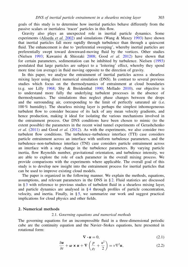
J. Fluid Mech. (2012), vol. 704, pp. 301–332. c Cambridge University Press 2012 301 doi:10.1017/jfm.2012.241 Direct numerical simulation of inertial particle entrainment in a shearless mixing layer Peter J. Ireland and Lance R. Collins† Sibley School of Mechanical and Aerospace Engineering, Cornell University, Ithaca, NY 14853, USA International Collaboration for Turbulence Research (Received 3 November 2011; revised 12 May 2012; accepted 20 May 2012; first published online 2 July 2012) We present the first computational study of the dynamics of inertial particles in a shearless turbulence mixing layer. We parametrize our direct numerical simulations to isolate the effects of turbulence, Reynolds number, particle inertia, and gravity on the entrainment process. By analysing particle concentrations, particle and fluid velocities, particle size distributions, and higher-order velocity moments, we explore the impact of particle inertia and gravity on the mechanism of turbulent mixing. We neglect thermodynamic processes, including phase changes between the drops and surrounding air, which is equivalent to assuming the air is saturated (i.e. 100 % humidity). Entrainment is found to be governed by the large scales of the flow and is relatively insensitive to the Reynolds number over the range considered. Our results show that both fluid and particle velocities exhibit intermittency and that gravity and turbulent diffusion interact in unexpected ways to dictate particle dynamics. An analysis of the temporal evolution of fluid and particle statistics suggests that particle concentration profiles and velocities are self-similar under certain circumstances. We also observe large fluctuations in particle concentrations resulting from entrainment and introduce a model to estimate the impact these fluctuations have on the radial distribution function, a statistic that is often used to quantify inertial particle clustering. Our study is both a computational counterpart to and an extension of the wind tunnel experiments by Gerashchenko, Good & Warhaft (J. Fluid Mech., vol. 668, 2011, pp. 293–303) and Good, Gerashchenko, & Warhaft (J. Fluid Mech., vol. 694, 2012, pp. 371–398). We find good agreement between these experimental studies and our computational results. We anticipate that a better understanding of the role of gravity and turbulence in inertial particle entrainment will lead to improved cloud evolution predictions. Key words: particle/fluid flow, turbulent mixing, turbulence simulation 1. Introduction Entrainment, the drawing in of external fluid by a turbulent flow, is ubiquitous in both industrial and natural turbulent processes. In jets, plumes, and mixing layers, entrainment results from the turbulent diffusion of momentum from a central core region (Pope 2000). There have been a number of experimental and numerical investigations of the fluid mechanics and mixing characteristics of tracer species convected by these flows (Dahm & Dimotakis 1987; Veeravalli & Warhaft 1990; † Email address for correspondence: [email protected]
-
Upload
independent -
Category
Documents
-
view
0 -
download
0
Transcript of Direct Numerical Simulation of inertial particle accelerations in near-wall turbulence: effect of...
J. Fluid Mech. (2012), vol. 704, pp. 301–332. c© Cambridge University Press 2012 301doi:10.1017/jfm.2012.241
Direct numerical simulation of inertial particleentrainment in a shearless mixing layer
Peter J. Ireland and Lance R. Collins†
Sibley School of Mechanical and Aerospace Engineering, Cornell University, Ithaca, NY 14853, USAInternational Collaboration for Turbulence Research
(Received 3 November 2011; revised 12 May 2012; accepted 20 May 2012;first published online 2 July 2012)
We present the first computational study of the dynamics of inertial particles in ashearless turbulence mixing layer. We parametrize our direct numerical simulationsto isolate the effects of turbulence, Reynolds number, particle inertia, and gravityon the entrainment process. By analysing particle concentrations, particle and fluidvelocities, particle size distributions, and higher-order velocity moments, we explorethe impact of particle inertia and gravity on the mechanism of turbulent mixing.We neglect thermodynamic processes, including phase changes between the dropsand surrounding air, which is equivalent to assuming the air is saturated (i.e. 100 %humidity). Entrainment is found to be governed by the large scales of the flow andis relatively insensitive to the Reynolds number over the range considered. Our resultsshow that both fluid and particle velocities exhibit intermittency and that gravityand turbulent diffusion interact in unexpected ways to dictate particle dynamics. Ananalysis of the temporal evolution of fluid and particle statistics suggests that particleconcentration profiles and velocities are self-similar under certain circumstances. Wealso observe large fluctuations in particle concentrations resulting from entrainmentand introduce a model to estimate the impact these fluctuations have on the radialdistribution function, a statistic that is often used to quantify inertial particle clustering.Our study is both a computational counterpart to and an extension of the wind tunnelexperiments by Gerashchenko, Good & Warhaft (J. Fluid Mech., vol. 668, 2011,pp. 293–303) and Good, Gerashchenko, & Warhaft (J. Fluid Mech., vol. 694, 2012,pp. 371–398). We find good agreement between these experimental studies and ourcomputational results. We anticipate that a better understanding of the role of gravityand turbulence in inertial particle entrainment will lead to improved cloud evolutionpredictions.
Key words: particle/fluid flow, turbulent mixing, turbulence simulation
1. IntroductionEntrainment, the drawing in of external fluid by a turbulent flow, is ubiquitous in
both industrial and natural turbulent processes. In jets, plumes, and mixing layers,entrainment results from the turbulent diffusion of momentum from a central coreregion (Pope 2000). There have been a number of experimental and numericalinvestigations of the fluid mechanics and mixing characteristics of tracer speciesconvected by these flows (Dahm & Dimotakis 1987; Veeravalli & Warhaft 1990;
† Email address for correspondence: [email protected]

302 P. J. Ireland and L. R. Collins
Bisset, Hunt & Rogers 2002; Mathew & Basu 2002; Westerweel et al. 2002, 2005;Holzner et al. 2007, 2008). In particular, the connection of tracer species to awide range of combustion processes has led to a broad literature on the mixingcharacteristics of entraining flows (Batt 1977; Breidenthal 1981; Broadwell &Breidenthal 1982; Mungal & Dimotakis 1984; Koochesfahani & Dimotakis 1986;Poulain et al. 2004).
Entrainment has also been recognized as an important process in atmospheric clouds.In particular, entrainment of dry air near cloud boundaries by turbulence can affectprecipitation mechanisms, but little is yet known about the fundamental parametersand mechanisms that control the entrainment process (Pruppacher & Klett 1997; Shaw2003). Indeed, Blyth’s (1993) observation still remains relevant today: ‘It is evenpossible that if cumulus clouds did not entrain, many problems in cloud physicswould have been more-or-less solved.’ Clouds, aside from their role in weather,are responsible for the greatest uncertainty in global climate models (Shaw 2003;Stratmann et al. 2009).
In the meantime, our understanding of the motion of inertial particles in turbulencehas advanced considerably. A number of numerical studies demonstrate inertial particleclustering outside vortices due to a centrifugal effect (Maxey 1987; Squires & Eaton1991b; Eaton & Fessler 1994; Reade & Collins 2000a; Wang, Wexler & Zhou 2000;Fung & Vassilicos 2003; Bec et al. 2007). Recent experimental measurements withsufficient precision show clustering levels that are similar to the numerical simulations(Wood, Hwang & Eaton 2005; Salazar et al. 2008; Saw et al. 2008; de Jonget al. 2010). Clustering has been shown to affect aerosol processes such as particlecollisions and coalescence (Sundaram & Collins 1997; Wang et al. 2000; Reade& Collins 2000b; Zhou, Wexler & Wang 2001), particle sedimentation (Maxey &Corrsin 1986; Maxey 1987; Wang & Maxey 1993; Nielsen 1993; Aliseda et al. 2002;Kawanisi & Shiozaki 2008), the modulation of turbulence by particles (Squires &Eaton 1990; Elghobashi & Truesdell 1993; Sundaram & Collins 1999; Druzhinin& Elghobashi 1999; Hwang & Eaton 2006), and particle acceleration statistics (Becet al. 2006; Ayyalasomayajula et al. 2006; Ayyalasomayajula, Warhaft & Collins 2008;Gerashchenko et al. 2008; Lavezzo et al. 2010).
That understanding, however, has not been extended to the entrainment of inertialparticles across interfaces by turbulence, as is found at the boundaries of atmosphericclouds; that is, the impact of inertia and gravity on the mixing process is not wellunderstood. In two recent studies, Gerashchenko, Good & Warhaft (2011) and Good,Gerashchenko & Warhaft (2012) investigated this issue by examining the motion ofdroplets across a ‘shearless mixing layer’, which is simply an interface between flowswith the same mean velocity but different turbulence levels (Veeravalli & Warhaft1989; Briggs et al. 1996; Knaepen, Debliquy & Carati 2004; Tordella & Iovieno 2006;Kang & Meneveau 2008; Tordella & Iovieno 2011). These studies are particularlyrelevant to entrainment in cumulus clouds, where a sharp interface exists between thehighly turbulent cloud and the less turbulent ambient air (Shaw 2003). By eliminatingmean shear in their flow, they were able to focus on the intrinsic turbulence effects.Both experiments (Veeravalli & Warhaft 1989; Kang & Meneveau 2008; Gerashchenkoet al. 2011; Good et al. 2012) and simulations (Briggs et al. 1996; Knaepen et al.2004; Tordella & Iovieno 2006; Kang & Meneveau 2008) show that the fluid velocityfield is marked by high intermittency near the interface, characteristic of turbulentbursts penetrating the low-turbulence region. Prior numerical studies of the shearlessmixing layer have not considered the effect of particle inertia, and thus one of the
DNS of inertial particle entrainment in a shearless mixing layer 303
goals of this study is to determine how inertial particles behave differently from thepassive scalars or inertialess ‘tracer’ particles in this flow.
Gravity also plays an unexpected role in inertial particle dynamics. Someexperiments (Aliseda et al. 2002) and simulations (Wang & Maxey 1993) have shownthat inertial particles fall more rapidly through turbulence than through a quiescentfluid. The enhancement is due to ‘preferential sweeping’, whereby inertial particles arepreferentially swept toward downward-moving fluid by the vortices. Other studies(Nielsen 1993; Kawanisi & Shiozaki 2008; Good et al. 2012) have shown thatfor certain parameters, sedimentation can be inhibited by turbulence. Nielsen (1993)postulated that large particles are subject to a ‘loitering’ effect, whereby they spendmore time (on average) in fluid moving opposite to the direction of gravity.
In this paper, we analyse the entrainment of inertial particles across a shearlessmixing layer using direct numerical simulation (DNS). In contrast to several previousstudies which focus on the thermodynamics of entrainment at cloud boundaries(e.g. see Lilly 1968; Shy & Breidenthal 1990; Mellado 2010), our objective isto understand more fully the underlying turbulent processes in the absence ofthermodynamics. The simulations thus neglect phase changes between the dropsand the surrounding air, corresponding to the limit of perfectly saturated air (i.e.100 % humidity). The shearless mixing layer is perhaps the simplest inhomogeneousturbulent flow to consider because of its lack of any mean velocity gradients, andhence production, making it ideal for isolating the various mechanisms involved inthe entrainment process. Our DNS conditions have been chosen to mimic (to theextent possible) the parameters in the recent wind tunnel experiments of Gerashchenkoet al. (2011) and Good et al. (2012). As with the experiments, we also consider twoturbulent flow conditions. The turbulence–turbulence interface (TTI) case considersparticle entrainment across an interface with uniform turbulence parameters, and theturbulence–non-turbulence interface (TNI) case considers particle entrainment acrossan interface with a step change in the turbulence parameters. By varying particleinertia, flow Reynolds number, gravitational orientation, and turbulence intensity, weare able to explore the role of each parameter in the overall mixing process. Weprovide comparisons with the experiments where applicable. The overall goal of thisstudy is to develop new insight into the entrainment process for inertial particles thatcan be used to improve existing cloud models.
The paper is organized in the following manner. We explain the methods, equations,assumptions, and relevant parameters in the DNS in § 2. Fluid statistics are discussedin § 3 with reference to previous studies of turbulent fluid in a shearless mixing layer,and particle dynamics are analysed in § 4 through profiles of particle concentration,velocity, and inertia. Finally, in § 5, we summarize our work and suggest practicalimplications for cloud physics and other fields.
2. Numerical methods2.1. Governing equations and numerical methods
The governing equations for an incompressible fluid in a three-dimensional periodiccube are the continuity equation and the Navier–Stokes equations, here presented inrotational form:
∇ ·u= 0, (2.1)∂u∂t+ ω × u+∇
(p
ρf+ u2
2
)= ν∇2u, (2.2)

304 P. J. Ireland and L. R. Collins
where u is the fluid velocity, ω ≡ ∇ × u is the vorticity, p is the pressure, ρf isthe fluid density, and ν is the kinematic viscosity. We employ a pseudospectralmethod to advance these equations on a 5123 grid using a second-order, explicitRunge–Kutta scheme with aliasing errors removed by means of a combination ofspherical truncation and phase-shifting. Further details of the fluid update are givenin Brucker et al. (2007).
Non-evaporating, solid particles in the flow field are advanced according to theMaxey & Riley (1983) equation, which in the limit of small, heavy particles (i.e.d/η� 1, where d is the particle diameter and η is the Kolmogorov length scale, andρp/ρf � 1, where ρp is the particle density) reduces to the following set of linearordinary differential equations for the ith particle:
dXi
dt={u(Xi) passive tracers,vi inertial particles,
(2.3)
dvi
dt= u(Xi)− vi
τpi
+ (1− ρf /ρp)g, (2.4)
where Xi and vi are the instantaneous position and velocity of the ith particlerespectively, u(Xi) is the undisturbed fluid velocity at the particle centre, τpi ≡d2
i ρp/(18ρfν) is the particle response time, and g is the gravitational acceleration.Equations (2.3) and (2.4) have the additional restriction that the particle Reynoldsnumber must be small, i.e. Rep ≡ ‖u(X) − v‖d/ν < 0.5 (Elghobashi & Truesdell1992). This condition is met by over 99.8 % of the particles at a given time inthe simulation. To obtain u(Xi), we employ an eighth-order Lagrange polynomialinterpolation in three dimensions. The influence of particles on the continuity andmomentum equations is negligible for low volume (Φv ∼ 10−6) and mass (Φm ∼ 10−3)loadings (e.g. see Elghobashi & Truesdell 1993; Sundaram & Collins 1999), and wetherefore consider only one-way coupling between the flow field and the particles.All particles are represented as point particles, and collisions are neglected (Reade &Collins 2000a).
2.2. InitializationFor the isotropic velocity field, we first generate a random phase velocity withcomponents that are scaled to match the following prescribed energy spectrum (Isaza& Collins 2009):
E0(k)= Cκε2/30 k−5/3
(k/κ0)
2 k < κ0,
(k/κ0)−5/3 κ0 6 k 6 κη,
0 k > κη,(2.5)
where k is the wavenumber, Cκ ≈ 1.5 is the Kolmogorov constant, ε0 is the initialenergy dissipation rate, κ0 is the initial location of the peak in the energy spectrum,and κη is the maximum energy-containing wavenumber. We select these parametersto give good resolution of both large- and small-scale motions. For adequate large-scale resolution, we require that L /` & 8, where L = 2π is the length of one sideof the computational domain, and ` is the longitudinal integral length scale (Pope2000). Small-scale resolution is maintained by ensuring that kmaxη > 1, where kmaxis the maximum resolved wavenumber (Eswaran & Pope 1988). After generating arandom phase velocity field, we let the flow evolve according to (2.1) and (2.2) untilthe skewness of the velocity derivatives 〈(∂u/∂x)3〉/[〈(∂u/∂x)2〉3/2] converged to the
DNS of inertial particle entrainment in a shearless mixing layer 305
accepted value of ∼ − 0.4 (Tavoularis, Bennett & Corrsin 1978). This then was theinitial velocity field for all of the turbulence–turbulence interface (TTI) studies.
The turbulence–non-turbulence interface (TNI) simulations require that we generateturbulence with strong spatial variation (i.e. the ‘shearless’ mixing layer). Ourapproach is based on the initialization procedure used by Briggs et al. (1996),Knaepen et al. (2004), and Tordella & Iovieno (2006). We first create two separateisotropic velocity fields according to the algorithm described above, each with differentturbulence characteristics. We shall refer to the low- and high-turbulence velocityfields, respectively, as ulow and uhigh. The two velocities are combined to generate aprovisional mixing layer velocity u as follows,
u(x)= [1− G (x)]ulow(x)+ G (x)uhigh(x), (2.6)
where the smoothing function G (x) is defined as (Knaepen et al. 2004):
G (x)=
0 if 0 6 y< 5π/12,12
(sin(
6(
y− π2
))+ 1)
if 5π/12 6 y< 7π/12,
1 if 7π/12 6 y< 17π/12,12
(sin(
6(
y− 4π3
))+ 1)
if 17π/12 6 y< 19π/12,
0 if 19π/12 6 y 6 2π.
(2.7)
In this way, we establish variation of the turbulence intensity in the y-direction, with aslab of high-intensity turbulence in the centre of the cube surrounded by low-intensityturbulence on either side. The blending region between high and low turbulenceintensities comprises 1/6 of the total width of the periodic cube.
The resulting velocity u(x) has the correct turbulence levels; however, as aconsequence of the filter, it no longer satisfies continuity (i.e. ∇ · u 6= 0). To correctthis, we take the Fourier transform of u(x), say ˆu(k), and form the inner product withthe ‘projection tensor’ Pij(ki)= δij − kikj/k2 (Pope 2000):
u(k)≡ P(k) · ˆu(k). (2.8)
The resulting velocity field u(k) in Fourier space or u(x) in physical space is,by definition, divergence-free. This procedure, however, diminishes the ratio of theintensity of the high- and low-turbulence regions. By iteratively rescaling the velocitycomponents and projecting to satisfy continuity, we can converge the divergence-freevelocity field arbitrarily close to the intended turbulence intensity ratio.
The particles are placed randomly throughout the central slab of the cube (theone corresponding to the high-turbulence region in the TNI simulations). They areinitialized with the fluid velocity at their location plus a Stokes’ drift term to accountfor gravitational settling. It should be noted that other simulations performed withthe Stokes’ drift omitted at initialization showed no discernible difference in particlestatistics at later times, suggesting that the effect of the initial velocity is quicklyforgotten.
The periodic boundary conditions require that we use this slab configuration, wherethe two interfaces are statistically equivalent and can be analysed together. We definey = 0 as the location of the initial interfaces, with the particle injection side (theinitial high-energy side for the TNI) given by y < 0 and the non-injection side (theinitial low-energy side for the TNI) given by y > 0. Thus, by our sign convention,
306 P. J. Ireland and L. R. Collins
10–3
10–2
10–1
100
101
102
10–2 10–1 10010–2 10–1 100
10–2
10–1
100
IIIIII
10–3 101 10–3 10110–4
103(a) (b)
10–3
101
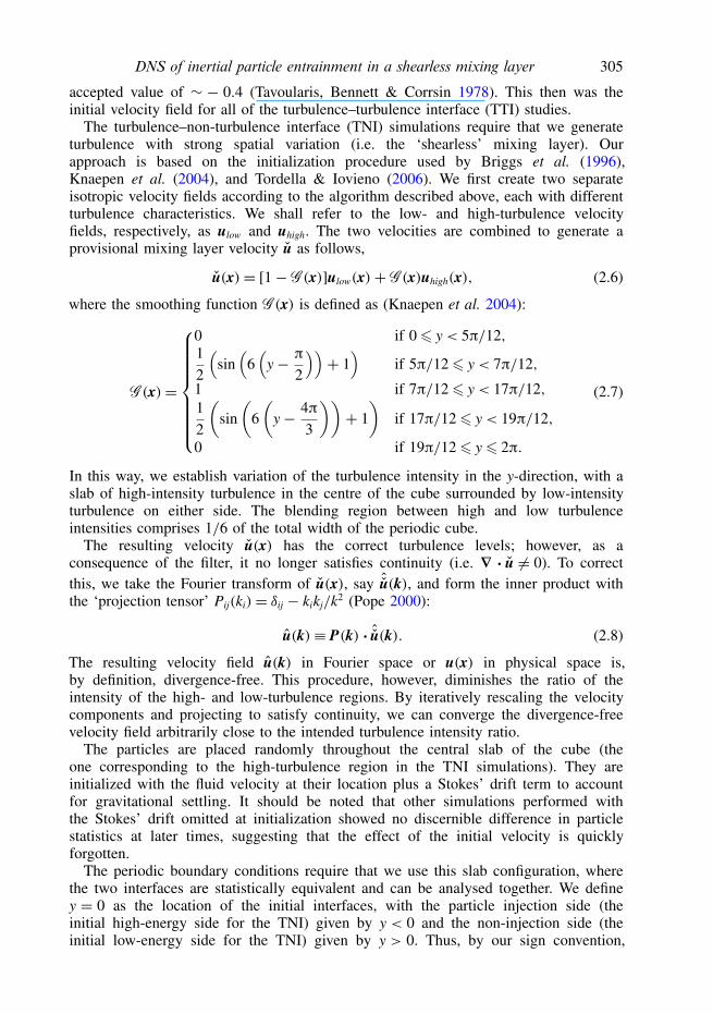
FIGURE 1. Normalized (a) energy and (b) dissipation spectra at 0.7 large-eddy turnovertimes for the three TTI cases defined in table 2.
particle velocities directed toward the non-injection side are positive. All statistics arepresented as a function of the inhomogeneous coordinate y and are averaged overthe statistically homogeneous x–z plane corresponding to that value of y. Propertiessuch as the energy and dissipation spectra, the large-eddy turnover time, the Stokesnumbers, and the settling velocities, which are presented without regard to their spatiallocation, are defined based on fluid properties in the centre of the high-energy region,where the flow is approximately isotropic.
2.3. ParametersThe parameters in the simulations are chosen to match those of the wind tunnelexperiments described in Gerashchenko et al. (2011) and Good et al. (2012). Onecomplication is our inability in the simulations to match the Reynolds numbersin the experiments. On a 5123 grid the Taylor microscale Reynolds numberRλ ≡ 2K
√5/(3νε) is less than half that of Gerashchenko et al. (2011) and Good
et al. (2012) (Rλ = 275), where K is the turbulent kinetic energy and ε is the turbulentenergy dissipation rate. We perform three different simulations at Reynolds numbersRλ ranging from 75 to 111 at initialization and from 54 to 71 at t/τ = 0.7, whereτ ≡ K0/ε0 is the initial large-eddy turnover time (as defined in previous studies ofthe shearless mixing layer, e.g. Briggs et al. 1996; Knaepen et al. 2004; Tordella &Iovieno 2006; Kang & Meneveau 2008), to study the effect of the Reynolds numberon fluid and particle statistics over the range we could access. As is evident fromtable 1, the three flow fields corresponding to the three different Reynolds numbersare created to have similar large scales, but different dissipation (small) scales.Normalized energy and dissipation spectra for the TTI for the three fields are shownin figure 1.
Because we are unable to match the Reynolds number in the experiment, we areforced to choose whether to match the large or small scales to the experiments (sinceboth could not be matched simultaneously). As we will demonstrate, the overall fluidand particle dynamics are a strong function of the large-scale turbulence, and hence wechoose to match those statistics.
We attempt to match the turbulent energy ratio between the high- and low-turbulence sides to the TNI wind tunnel experiments. Their initial energy ratio wasestimated to be 27; however, the uncertainty is large due to the large error in theintensity measurement on the low turbulence side. The energy ratio was approximately
DNS of inertial particle entrainment in a shearless mixing layer 307
Parameter High-turbulence side Low-turbulence sideI II III I II III
ν 0.001 0.0012 0.002 0.001 0.0012 0.002ε0 6 6 6 0.048 0.048 0.048κ0 4 4 4 4 4 4κη 152 152 152 152 152 152
TABLE 1. Initialization parameters for the DNS for the high-turbulence side (TTI andTNI) and low-turbulence side (TNI only). The initial fields are created according to theprocedure given in § 2.2. Parameters are in arbitrary units.
27 at the test section, corresponding to t/τ = 0.7. This ratio in the simulation wasapproximately 33 initially and 17 at t/τ = 0.7. We attribute the difference in energydecay rates between the experiment and DNS to the discrepancy in the Reynoldsnumbers and the large uncertainties in the experiment at the entrance. Nevertheless, inboth cases the turbulent energy ratio is sufficiently large that the turbulence dynamicsare controlled by the high-turbulence side of the flow.
To avoid additional complexities in the mixing process, we match the integral lengthscales ` in the high- and low-turbulence regions. These scales differ by no more than20 % at the start of the simulations. Accurate measurements of ` in the low-turbulenceside in Gerashchenko et al. (2011) and Good et al. (2012) were not available. To learnmore about the effect of the length scale ratio, the interested reader is referred to thestudy by Tordella & Iovieno (2006) which varied the length scale ratio `high/`low.
Following convention (e.g. see Squires & Eaton 1991a,b), we define the particleStokes number as St` ≡ τp/τ`, where τ` ≡ `/u′ is the large-eddy turnover time,and u′ ≡ √2K/3 is the turbulence intensity. τ` was defined in Gerashchenko et al.(2011) based on the the homogeneous velocity component u, i.e. τ` = `/urms. However,turbulence in the wind tunnel is inherently anisotropic as compared to the DNS, andconsequently, τ`/τ is larger in the experiment than in the DNS. As there is no uniqueway to reconcile this discrepancy, we adopt the convention of using τ to define thedimensionless time (i.e. t/τ ) and τ` to define the particle Stokes number.
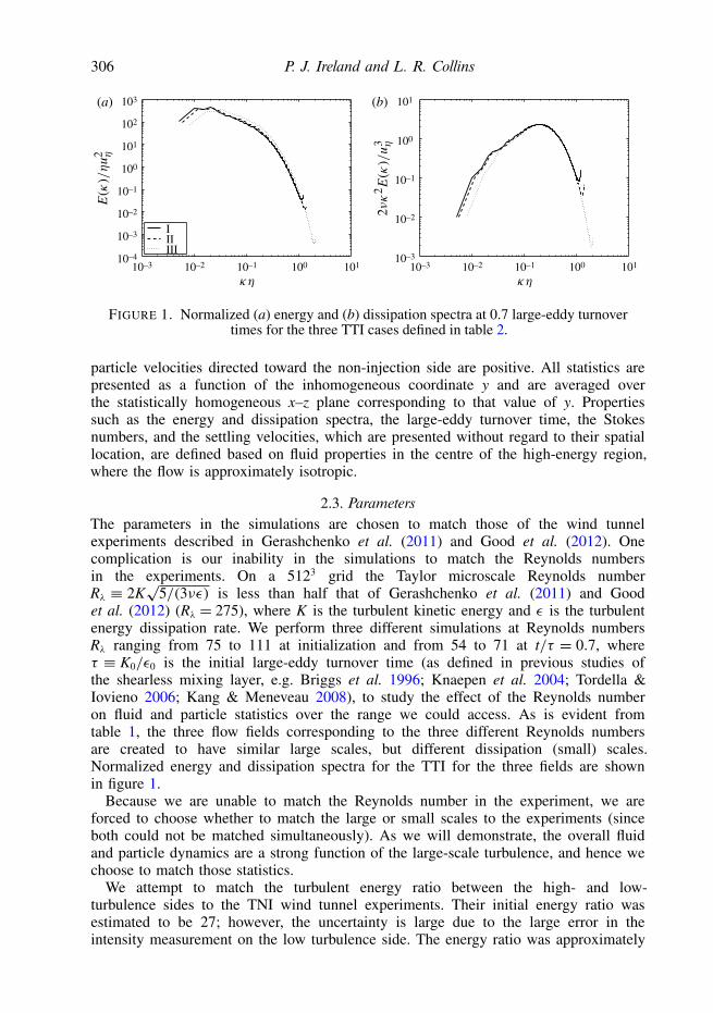
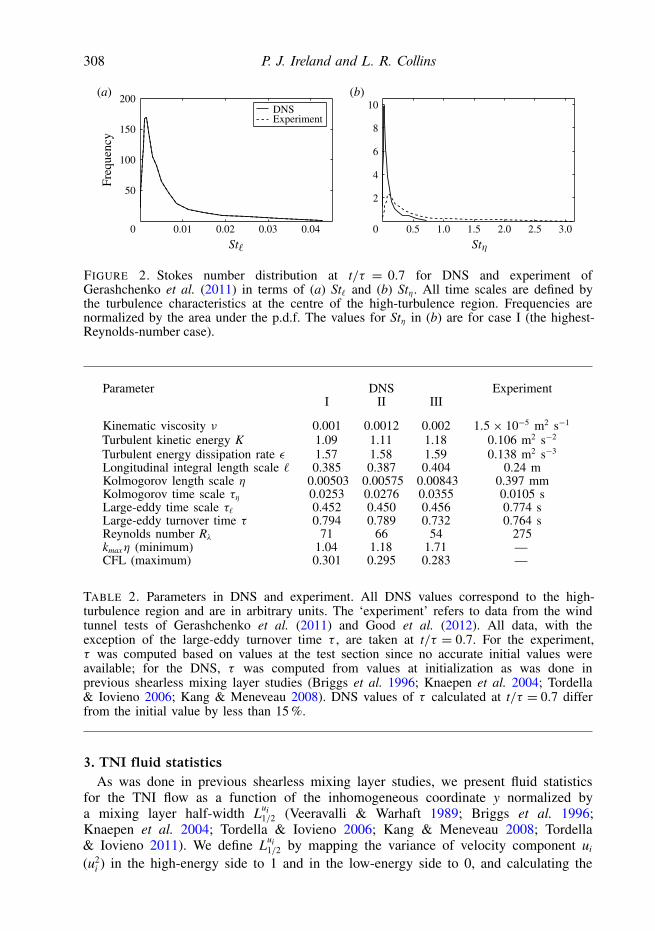
The parameters in the simulations and the corresponding values in the experiment(where applicable) are given in table 2. The particle Stokes number distributions att/τ = 0.7 are shown in figure 2 for both (a) St` and (b) Stη. As you can see, there isvery close agreement in St` but not in Stη due to the difference in Reynolds numbers.
For the cases with gravity, a key dimensionless number is the settling parameterSv` ≡ τpg/u′, which is the ratio of the particle terminal velocity τpg to the turbulenceintensity u′ (e.g. see Yang & Lei 1998). Note that for given values of St` and Sv`we can form a large-scale Froude number (Fr` ≡ Sv`/St` = g/(u′/τ`)) which dependsonly on fluid parameters. Fr` can be viewed as the ratio between the gravitationalacceleration g and the large-eddy acceleration u′/τ`.
We set the gravitational acceleration in the DNS to g = 50 (arbitrary units) so thatthe settling parameters for the particles in the DNS match those of the experiment(and hence Fr` ≈ 25 is the same in both the experiment and DNS). Since there is littlevariation in the large scales among the three Reynolds number cases, g was fixed forall three flow fields.
308 P. J. Ireland and L. R. Collins
DNSExperiment
50
100
150
0.01 0.02 0.03 0.04
Freq
uenc
y200
0 0.5 1.0 1.5 2.0 2.5 3.00
(a) (b)
2
4
6
8
10
FIGURE 2. Stokes number distribution at t/τ = 0.7 for DNS and experiment ofGerashchenko et al. (2011) in terms of (a) St` and (b) Stη. All time scales are defined bythe turbulence characteristics at the centre of the high-turbulence region. Frequencies arenormalized by the area under the p.d.f. The values for Stη in (b) are for case I (the highest-Reynolds-number case).
Parameter DNS ExperimentI II III
Kinematic viscosity ν 0.001 0.0012 0.002 1.5× 10⁻⁵ m2 s−1
Turbulent kinetic energy K 1.09 1.11 1.18 0.106 m2 s−2
Turbulent energy dissipation rate ε 1.57 1.58 1.59 0.138 m2 s−3
Longitudinal integral length scale ` 0.385 0.387 0.404 0.24 mKolmogorov length scale η 0.00503 0.00575 0.00843 0.397 mmKolmogorov time scale τη 0.0253 0.0276 0.0355 0.0105 sLarge-eddy time scale τ` 0.452 0.450 0.456 0.774 sLarge-eddy turnover time τ 0.794 0.789 0.732 0.764 sReynolds number Rλ 71 66 54 275kmaxη (minimum) 1.04 1.18 1.71 —CFL (maximum) 0.301 0.295 0.283 —
TABLE 2. Parameters in DNS and experiment. All DNS values correspond to the high-turbulence region and are in arbitrary units. The ‘experiment’ refers to data from the windtunnel tests of Gerashchenko et al. (2011) and Good et al. (2012). All data, with theexception of the large-eddy turnover time τ , are taken at t/τ = 0.7. For the experiment,τ was computed based on values at the test section since no accurate initial values wereavailable; for the DNS, τ was computed from values at initialization as was done inprevious shearless mixing layer studies (Briggs et al. 1996; Knaepen et al. 2004; Tordella& Iovieno 2006; Kang & Meneveau 2008). DNS values of τ calculated at t/τ = 0.7 differfrom the initial value by less than 15 %.
3. TNI fluid statisticsAs was done in previous shearless mixing layer studies, we present fluid statistics
for the TNI flow as a function of the inhomogeneous coordinate y normalized bya mixing layer half-width Lui
1/2 (Veeravalli & Warhaft 1989; Briggs et al. 1996;Knaepen et al. 2004; Tordella & Iovieno 2006; Kang & Meneveau 2008; Tordella& Iovieno 2011). We define Lui
1/2 by mapping the variance of velocity component ui
(u2i ) in the high-energy side to 1 and in the low-energy side to 0, and calculating the
DNS of inertial particle entrainment in a shearless mixing layer 309
IIIIIIExperiment
0.25
0.50
0.75
1.00
–2 0 20
1.25
–4 4
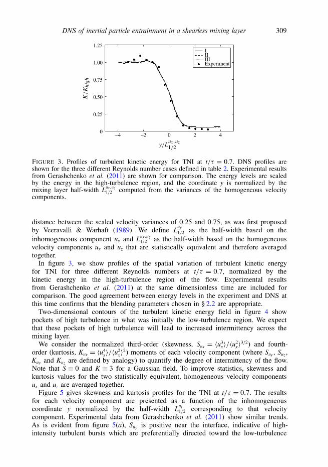
FIGURE 3. Profiles of turbulent kinetic energy for TNI at t/τ = 0.7. DNS profiles areshown for the three different Reynolds number cases defined in table 2. Experimental resultsfrom Gerashchenko et al. (2011) are shown for comparison. The energy levels are scaledby the energy in the high-turbulence region, and the coordinate y is normalized by themixing layer half-width Lux,uz
1/2 computed from the variances of the homogeneous velocitycomponents.
distance between the scaled velocity variances of 0.25 and 0.75, as was first proposedby Veeravalli & Warhaft (1989). We define L
uy1/2 as the half-width based on the
inhomogeneous component uy and Lux,uz1/2 as the half-width based on the homogeneous
velocity components ux and uz that are statistically equivalent and therefore averagedtogether.
In figure 3, we show profiles of the spatial variation of turbulent kinetic energyfor TNI for three different Reynolds numbers at t/τ = 0.7, normalized by thekinetic energy in the high-turbulence region of the flow. Experimental resultsfrom Gerashchenko et al. (2011) at the same dimensionless time are included forcomparison. The good agreement between energy levels in the experiment and DNS atthis time confirms that the blending parameters chosen in § 2.2 are appropriate.
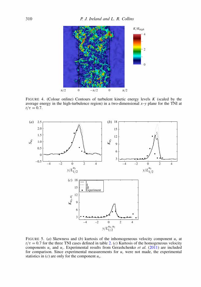
Two-dimensional contours of the turbulent kinetic energy field in figure 4 showpockets of high turbulence in what was initially the low-turbulence region. We expectthat these pockets of high turbulence will lead to increased intermittency across themixing layer.
We consider the normalized third-order (skewness, Sux = 〈u3x〉/〈u2
x〉3/2) and fourth-order (kurtosis, Kux = 〈u4
x〉/〈u2x〉2) moments of each velocity component (where Suy , Suz ,
Kuy and Kuz are defined by analogy) to quantify the degree of intermittency of the flow.Note that S ≡ 0 and K ≡ 3 for a Gaussian field. To improve statistics, skewness andkurtosis values for the two statistically equivalent, homogeneous velocity componentsux and uz are averaged together.
Figure 5 gives skewness and kurtosis profiles for the TNI at t/τ = 0.7. The resultsfor each velocity component are presented as a function of the inhomogeneouscoordinate y normalized by the half-width Lui
1/2 corresponding to that velocitycomponent. Experimental data from Gerashchenko et al. (2011) show similar trends.As is evident from figure 5(a), Suy is positive near the interface, indicative of high-intensity turbulent bursts which are preferentially directed toward the low-turbulence
310 P. J. Ireland and L. R. Collins
0
2
4
0 0
FIGURE 4. (Colour online) Contours of turbulent kinetic energy levels K (scaled by theaverage energy in the high-turbulence region) in a two-dimensional x–y plane for the TNI att/τ = 0.7.
IIIIIIExperiment
0
0.5
1.0
1.5
2.0
–2 0 2 –2 0 2
–2 0 2
3
6
9
12
15
18
3
6
9
12
15
18
–0.5
2.5
–4 4 –4 4
–4 4
(c)
(a) (b)
FIGURE 5. (a) Skewness and (b) kurtosis of the inhomogeneous velocity component uy att/τ = 0.7 for the three TNI cases defined in table 2. (c) Kurtosis of the homogeneous velocitycomponents ux and uz. Experimental results from Gerashchenko et al. (2011) are includedfor comparison. Since experimental measurements for uz were not made, the experimentalstatistics in (c) are only for the component ux.

DNS of inertial particle entrainment in a shearless mixing layer 311
StepGradual
0.2
0.4
0.6
0.8
–2 0 2
0
1.0
–4 4
FIGURE 6. Two initial mean concentration profiles for the particle field. The solid line is astep change at the interface and the dashed line uses the smoothing function G (x) as definedin (2.7) to provide a more gradual transition between the high- and low-concentration regions.
region. The skewness of the homogeneous velocity components (not shown) is close tozero throughout the entire domain.
Figure 5 indicates strong departures from Gaussian behaviour in the mixing region.Notice that Kuy > Kux,uz , which implies that uy is the most highly intermittentcomponent of the fluid velocity. The reason for this stronger intermittency is explainedin detail in Veeravalli & Warhaft (1989). Again, we see similar trends between ourDNS and Gerashchenko et al. (2011). The location and magnitude of the Kuy peaks areslightly different, possibly due to differences in the Reynolds numbers or the imperfectmatch of the initial conditions of the two flows. All velocity components for the TTIare nearly Gaussian throughout the entire domain.
4. Particle statisticsWe now consider the motion of inertial particles that are convected by both the TTI
and TNI flow fields. The particles are initially seeded randomly throughout the centreslab (for the TNI, this corresponds to the high-turbulence region) with two differentmean concentration profiles between the particle-rich and particle-lean regions (seefigure 6). The first is a step change and the second has a gradual transition basedon the smoothing function G (x) defined in (2.7). We advance the particle positionsand velocities according to (2.3) and (2.4). Statistics are gathered by averaging overthe homogeneous x–z plane and are treated as a function of the inhomogeneouscoordinate, y.
4.1. Mean particle concentrationsFigure 7 plots the number of particles at a given y-coordinate normalized by thenumber of particles in the particle injection side (here taken to be the initialconcentration in the central slab) at a dimensionless time t/τ = 0.7 equal to thetime in the experiment that corresponds to the test section and for both initial particleconcentration profiles. It is evident that the initial particle distribution only weaklyaffects the particle distributions at later times for both the TTI and TNI. Moreover, thechoice of the initial distribution does not resolve the discrepancies between the DNSand experimental measurements presented later in the paper (cf. figure 12). As the

312 P. J. Ireland and L. R. Collins
TTI, stepTTI, gradualTNI, stepTNI, gradual
0
0.2
0.4
0.6
0.8
1.0
–2 0 2–2 0 210–5
10–4
10–3
10–2
10–1
100
–4 4 –4 4
(a) (b)
FIGURE 7. Particle concentration profiles at t/τ = 0.7 for the TTI and TNI for the twodifferent initial particle distributions shown in figure 6 on (a) a semilog scale and (b) a linearscale. The results are for the highest-Reynolds-number case (I).
0
1.5
0.4 0.6 1.0
100
0.2 0.8
0.5
1.0
10–1
101(a) (b)
10–1 100
FIGURE 8. Time evolution of the mixing layer half-width. Different measures of L1/2 areshown in (a), and power-law fits for L1/2 are given in (b). All measures of L1/2 are normalizedby `, the integral length scale at t/τ = 0.7. We observe very similar results when L1/2 isnormalized by the instantaneous integral length scale.
gradual distribution introduces parameters that were not measured in the experiments(Gerashchenko et al. 2011; Good et al. 2012), and the impact on the results isrelatively weak, we hereafter present only the results from the step distribution.
Figure 8(a) shows the velocity measures of the half-width for the TNI (Lux,uz1/2 and
Luy1/2) and L1/2 for both the TNI and the TTI. Notice that all measures of the half-width
are of the same order of magnitude for the duration of the simulation. The half-widthL1/2 is greater for the TTI case than that for the TNI case at all times, indicatingthat the TTI mixes more quickly than the TNI. In figure 8(b), we plot least-squarespower-law fits for L1/2 of the form L1/2/` = c0 (t/τ)
c1 , where ` is the integral lengthscale at t/τ = 0.7. (We are unable to simulate past t/τ ≈ 0.7 for the TTI and t/τ ≈ 0.9for the TNI, because after this point the particles will reach the y-boundary of ourdomain and periodic boundary conditions in y will contaminate the results.) For theTTI, we calculate c0 = 2.03 ± 0.16 and c1 = 0.774 ± 0.064, while for the TNI, weobtain c0 = 1.47 ± 0.071 and c1 = 0.854 ± 0.045. Due to the uncertainties on thepower-law fits for c1 (which represent 95 % confidence intervals), we cannot determine

DNS of inertial particle entrainment in a shearless mixing layer 313
10–4
10–3
10–2
10–1
0
0.2
0.4
0.6
0.8
1.0
–2 0 2 –2 0 2–4 4 –4 410–5
100(a) (b)
FIGURE 9. Particle concentration profiles for the TTI and TNI at the three indicatedReynolds numbers and t/τ = 0.7 on (a) a semilog scale and (b) a linear scale. Negativevalues of y correspond to regions initially laden with particles, while positive values of ycorrespond to regions initially void of particles.
whether the L1/2 grows more quickly for the TTI or the TNI; c1 in our DNS agreeswell with the value of 0.83 presented in Veeravalli & Warhaft (1990), which wascomputed from the mean concentration profiles of a passive scalar line source mixingin a TNI.
Figure 9 shows the particle concentration profiles for the case without gravity(hereafter referred to as ‘g0’). As we are interested in making an absolute comparisonbetween the TTI and TNI which have different values of L1/2, we normalizethe inhomogeneous coordinate by the longitudinal integral length scale ` in thehomogeneous region of the flow, which is identical for both cases. From theseprofiles, we again see that the TTI is much more effective at transporting the particlesthan the TNI. This finding is consistent with the observation that the boundariesbetween cumulus clouds (generally more turbulent) and the ambient air (generallyless turbulent) are sharp and well-defined (e.g. see Shaw 2003). From figure 9(b), wealso note the symmetry in the TTI profile but the asymmetry in the TNI profile, aconsequence of the gradient in mean turbulent kinetic energy in the TNI. SymmetricTTI profiles and asymmetric TNI profiles were observed by Veeravalli & Warhaft(1990) for passive scalar dispersion and are discussed in detail there.
This difference between the TTI and TNI cases can be explained by a simple eddydiffusivity argument. If we approximate the transport of particles as that of passivescalars, we expect the particle concentration plots to take the form of error functions,and the turbulent diffusivity to scale with u′ (LaRue & Libby 1981; Ma & Warhaft1986; Speziale 1991). Since u′ is smaller in the low-turbulence region, we expect alower diffusivity there and fewer particles to be mixed. Gerashchenko et al. (2011)and Good et al. (2012) showed that the particle concentration profiles can be wellrepresented by an error function with a diffusivity that varies based on the localturbulence intensity u′, which is consistent with our findings.
Figure 9 also shows the variation in the mean particle concentration with Reynoldsnumber (see § 2.3 for the description of the three cases). Over the limited rangeof Reynolds numbers achieved in our simulations (Rλ = 54–71 at t/τ = 0.7), weobserve no discernible Reynolds number dependence in these profiles. We similarlyfind no Reynolds number dependence when gravitational effects are included. Hencefor the remaining figures we only show the highest-Reynolds-number case (I). (Wealso found no Reynolds number dependence in the statistics of particle concentration

314 P. J. Ireland and L. R. Collins
0.230.450.68
TTI 0.230.450.680.91
TNI
10–4
10–3
10–2
10–1
100
10–4
10–3
10–2
10–1
100
–2 –1 0 1 2 –1 0 1–3 3 –2 2
(a) (b)
FIGURE 10. Particle concentration plots for the (a) TTI and (b) TNI at the indicated times,t/τ .
TTI
TNI10–4
10–3
10–2
10–1
100
–1 0 110–4
10–3
10–2
10–1
100
–1 0 1
LargeSmallTracers
–2 2 –2 2
(a) (b)
FIGURE 11. Effect of particle inertia on the (a) TTI and (b) TNI concentration profiles att/τ = 0.7 and without gravity.
fluctuations, mean velocities, and higher-order velocity moments presented in thefollowing sections.)
Figure 10 shows the temporal evolution of the TTI and TNI mean particleconcentration profiles using the half-width L1/2 to normalize the y coordinate. In thesecoordinates, the TTI profiles appear to be self-similar, with only a slight deviationfar into the non-injection side of the first profile at t/τ = 0.23. The TNI profiles alsoapproach self-similarity after an initial transient period indicated by the first profile.The approximate self-similarity of these profiles, combined with the power-law relationfor L1/2, suggests that particle concentration profiles at different times can be estimatedfrom data at a given time, at least for t/τ . 1.
We examine the role of particle inertia in the mean concentration profiles att/τ = 0.7 by splitting the particles into two classes. Following the binning procedureof Good et al. (2012), we define ‘large’ particles as those with a response timeτp greater than 2.4τp (where τp is the arithmetic mean response time), and ‘small’particles as those with a response time τp less than 0.6τp. Concentration profiles forlarge and small particles, without gravity, are compared in figure 11. Also shownare concentration profiles for inertialess (tracer) particles. Figure 11 shows that in theabsence of gravity, particle inertia plays a negligible role in the mean concentrationprofiles. From figure 2(b) we see that the particles span a relatively large range of
DNS of inertial particle entrainment in a shearless mixing layer 315
TTI
TNI
–1 0 1
(a) (b)
10–4
10–3
10–2
10–1
100
–2 2 –1 0 110–4
10–3
10–2
10–1
100
–2 2
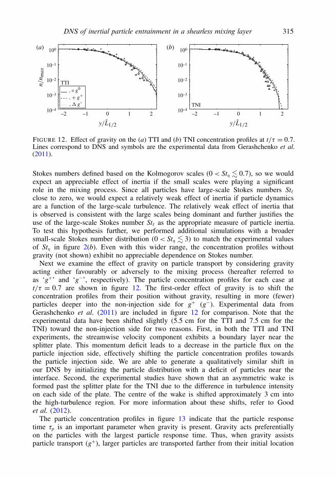
FIGURE 12. Effect of gravity on the (a) TTI and (b) TNI concentration profiles at t/τ = 0.7.Lines correspond to DNS and symbols are the experimental data from Gerashchenko et al.(2011).
Stokes numbers defined based on the Kolmogorov scales (0< Stη . 0.7), so we wouldexpect an appreciable effect of inertia if the small scales were playing a significantrole in the mixing process. Since all particles have large-scale Stokes numbers St`close to zero, we would expect a relatively weak effect of inertia if particle dynamicsare a function of the large-scale turbulence. The relatively weak effect of inertia thatis observed is consistent with the large scales being dominant and further justifies theuse of the large-scale Stokes number St` as the appropriate measure of particle inertia.To test this hypothesis further, we performed additional simulations with a broadersmall-scale Stokes number distribution (0 < Stη . 3) to match the experimental valuesof Stη in figure 2(b). Even with this wider range, the concentration profiles withoutgravity (not shown) exhibit no appreciable dependence on Stokes number.
Next we examine the effect of gravity on particle transport by considering gravityacting either favourably or adversely to the mixing process (hereafter referred toas ‘g+’ and ‘g−’, respectively). The particle concentration profiles for each case att/τ = 0.7 are shown in figure 12. The first-order effect of gravity is to shift theconcentration profiles from their position without gravity, resulting in more (fewer)particles deeper into the non-injection side for g+ (g−). Experimental data fromGerashchenko et al. (2011) are included in figure 12 for comparison. Note that theexperimental data have been shifted slightly (5.5 cm for the TTI and 7.5 cm for theTNI) toward the non-injection side for two reasons. First, in both the TTI and TNIexperiments, the streamwise velocity component exhibits a boundary layer near thesplitter plate. This momentum deficit leads to a decrease in the particle flux on theparticle injection side, effectively shifting the particle concentration profiles towardsthe particle injection side. We are able to generate a qualitatively similar shift inour DNS by initializing the particle distribution with a deficit of particles near theinterface. Second, the experimental studies have shown that an asymmetric wake isformed past the splitter plate for the TNI due to the difference in turbulence intensityon each side of the plate. The centre of the wake is shifted approximately 3 cm intothe high-turbulence region. For more information about these shifts, refer to Goodet al. (2012).
The particle concentration profiles in figure 13 indicate that the particle responsetime τp is an important parameter when gravity is present. Gravity acts preferentiallyon the particles with the largest particle response time. Thus, when gravity assistsparticle transport (g+), larger particles are transported farther from their initial location

316 P. J. Ireland and L. R. Collins
TTI
TNI
–1 0 1
(a)
10–4
10–3
10–2
10–1
100
–2 2 –1 0 110–4
10–3
10–2
10–1
100
–2 2
(b)
largesmalllargesmall
FIGURE 13. Effect of particle inertia on the (a) TTI and (b) TNI concentration profiles att/τ = 0.7, with the indicated particle size and direction of gravity. Experimental data fromGood et al. (2012) are shown for comparison, where + corresponds to g+ and × to g−. Largesymbols are for large particles, and small symbols are for small particles.
than smaller particles; the reverse is true when gravity hinders particle transport (g−).These trends can be observed in the visualizations of particles in the non-injection sidein figure 14, where we see that the g+ case has larger particles in the non-injectionside than the g0 case. Our data in figure 13 agree well with the results of Good et al.(2012) (shown for comparison).
The results presented thus far have been focused on the mean particle concentration.In the next section, we look more closely at the impact of gravity and particle inertiaon particle concentration fluctuations.
4.2. Apparent ‘clustering’ due to particle entrainmentAs discussed in § 1, inertia can cause an initially uniform distribution of particlesto cluster outside the vortices of the flow. The mechanism responsible for inertialclustering is completely unrelated to the entrainment process that is the focus ofthis study. Inertial clustering occurs when inertial particles are ‘centrifuged’ out ofregions of high vorticity and accumulate in regions of high strain (e.g. Balachandar& Eaton 2010). The non-uniform particle concentrations we observe, however, aredue to the mixing of particles from one region of flow to the other. This is apparentin figure 14, which shows particle positions in the non-injection side of the TTIand TNI flows, with and without gravity. The non-uniform particle concentrationfield is present in both flows, with the degree of the fluctuations being higher forthe TNI. Note that this non-uniform distribution occurs even for inertialess (tracer)particles. The connection between the large eddies and high-concentration regions isapparent in figure 15, which shows isocontours of the turbulent kinetic energy (left)and particle concentrations (right) along an x–y slice. From these figures, we seethat highly turbulent regions are particularly effective at transporting particles. Forexample, the turbulent patch in the upper right corner of the mixing layer drives aprotrusion of particle-rich fluid that advances into the non-injection side of the boxwith time. We believe intermittent ‘bursts’ such as these play a critical role in mixingthe particles, particularly for the TNI case. As a consequence, we see that regions ofhigh turbulence and high particle flux are closely correlated. The spatial coherence andintermittency of the turbulence (and hence the flux) leads to high-concentration regionson scales of the order of the integral length scale.

DNS of inertial particle entrainment in a shearless mixing layer 317
2 5 10 15 2 5 10 15
x
y
0 1 2 3 4
TTI TNI
(a) (b)
(c) (d )
FIGURE 14. (Colour online) Instantaneous particle field on the non-injection side (positive y)at t/τ = 0.7 for the (a) TTI with g0, (b) TNI with g0, (c) TTI with g+, and (d) TNI with g+.
Both inertial clustering and particle entrainment affect statistical measures of theparticle concentration fluctuations. For example, the statistic most commonly used toquantify inertial clustering is the radial distribution function (RDF, e.g. see Sundaram& Collins 1997). As noted in the experimental study by Saw et al. (2008), spatialinhomogeneities resulting from incomplete mixing affect the RDF. In particular, theyobserved an extended ‘shoulder’ at separation distances well into the inertial range (i.e.beyond the separation distance where inertial clustering is expected to be important).To investigate this phenomenon in the present system, we evaluate the two-dimensionalRDF (2D RDF) measured along the x–z plane for a fixed value of y. We define the 2DRDF as follows:
g2D(ri)≡ Ni/Ai
N/A, (4.1)
where Ni is the number of particle pairs that lie within a shell with an average radiusof ri and radial width 1r, Ai is the area of the shell, and N is the total number ofparticle pairs located in the total cross-sectional area, A. Note that the 2D RDF is notequivalent to the 3D RDF, but instead involves a projection of the 3D RDF onto the

318 P. J. Ireland and L. R. Collins
(a)
(b)
(c)
(d )
3
2
1
0
1.0
0
0.5
FIGURE 15. (Colour online) Isocontours of normalized turbulent kinetic energy (left) andparticle concentration (right) in a two-dimensional x–y plane for the TNI case with g0 at theindicated times.
2D plane, introducing a loss of information (Holtzer & Collins 2002). Nevertheless, itis the highest measure we can consider in this inhomogeneous particle field.
Figure 16 shows the 2D RDF at t/τ = 0.7 for g0, g+, and g− at y/` = −1, 0,and +1. We observe that the degree of non-uniformity is consistently greater for theTNI than for the TTI, increases with distance towards the non-injection side, and isenhanced for g− and suppressed for g+. To better understand the competing processescontrolling the particle concentration fluctuations, we plot the temporal evolution ofg2D(ri) in figure 17. At y/` = 0 and y/` = 1, the degree of non-uniformity decreaseswith time, while at y/` = −1 it increases slightly with time. Turbulent transport of

DNS of inertial particle entrainment in a shearless mixing layer 319
TTI TNI
10–1 100 101 102
100
101
102
10–3 10–2 10–1 100
10–1 100 101 102
100
101
102
10–3 10–2 10–1 100
(a) (b)
FIGURE 16. 2D RDFs for the (a) TTI and (b) TNI at t/τ = 0.7 and at the indicated y-location(line type) and direction of gravity (symbol).
TTI TNI
10–1 100 101 102
100
101
102
10–3 10–2 10–1 100
10–1 100 101 102
100
101
102
10–3 10–2 10–1 100
(a) (b)
FIGURE 17. Temporal evolution of the 2D RDFs for the (a) TTI and (b) TNI at the indicatedy-location (line type) and time (symbol). Note that some curves are not shown due toinadequate statistics.
particles from regions of higher concentration to regions of lower concentration formsapparent ‘clusters’ of variable sizes that scale with the integral length scale of theturbulence, causing g2D(ri) to increase. Turbulent mixing within the x–z plane tendsto break up these ‘clusters’, reducing g2D(ri). The lower turbulence levels on thenon-injection side in the TNI flow weaken the homogenization process, leading tolarger values of g2D(ri) than for the TTI flow. Particles that reach deeper into thenon-injection side must necessarily be transported by the most energetic turbulentfluctuations, and therefore they are the most densely concentrated. When gravityassists transport (g+), the particles are less dependent on the turbulent fluctuation,and therefore they exhibit lower levels of non-uniformity relative to the g− case.
As already noted, the apparent ‘clustering’ observed in this mixing study isqualitatively different from inertial clustering. For example, the length scale of inertialclustering is of order 10η (Aliseda et al. 2002), whereas the non-uniformity in theparticle distribution here scales with the integral length scale. Additionally, inertialclustering is very sensitive to the particle Stokes number, whereas mixing-driven
320 P. J. Ireland and L. R. Collins
TTI TNI
10–1 100 101 102
10–3 10–2 10–1 100
10–1 100 101 102
10–3 10–2 10–1 10010–2
10–1
100
10–2
10–1
100
(a) (b)
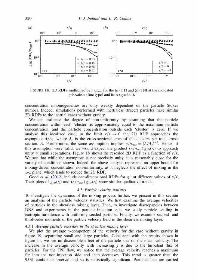
FIGURE 18. 2D RDFs multiplied by n/nmax for the (a) TTI and (b) TNI at the indicatedy-location (line type) and time (symbol).
concentration inhomogeneities are only weakly dependent on the particle Stokesnumber. Indeed, simulations performed with inertialess (tracer) particles have similar2D RDFs to the inertial cases without gravity.
We can estimate the degree of non-uniformity by assuming that the particleconcentration within each ‘cluster’ is approximately equal to the maximum particleconcentration, and the particle concentration outside each ‘cluster’ is zero. If weanalyse this idealized case, in the limit r/`→ 0 the 2D RDF approaches theasymptote A/Ac, where Ac is the cross-sectional area of the clusters per total cross-section, A. Furthermore, the same assumption implies n/nmax = (A/Ac)
−1. Hence, ifthis assumption were valid, we would expect the product (n/nmax) g2D(ri) to approachunity at small separations. Figure 18 shows the rescaled 2D RDF as a function of r/`.We see that while the asymptote is not precisely unity, it is reasonably close for thevariety of conditions shown. Indeed, the above analysis represents an upper bound formixing-driven concentration non-uniformity, as it neglects the effect of mixing in thex–z plane, which tends to reduce the 2D RDF.
Good et al. (2012) include one-dimensional RDFs for g+ at different values of y/`.Their plots of g1D(ri) and (n/nmax) g1D(ri) show similar qualitative trends.
4.3. Particle velocity statisticsTo investigate the dynamics of the mixing process further, we present in this sectionan analysis of the particle velocity statistics. We first examine the average velocitiesof particles in the shearless mixing layer. Then, to investigate discrepancies betweenDNS and experiments in the particle injection side, we study particle settling inisotropic turbulence with uniformly seeded particles. Finally, we examine second- andthird-order moments of the particle velocity field in the shearless mixing layer.
4.3.1. Average particle velocities in the shearless mixing layerWe plot the average y-component of the velocity for the case without gravity in
figure 19, separating small and large particles. Consistent with the results shown infigure 11, we see no discernible effect of the particle size on the mean velocity. Theincrease in the average velocity with increasing y is due to the turbulent flux ofparticles. For the TNI flow, we notice that the average velocity reaches a maximumfar into the non-injection side and then decreases. This trend is greater than the95 % confidence interval and so is statistically significant. Particles that are carried

DNS of inertial particle entrainment in a shearless mixing layer 321
TTI
LargeSmall
TNI
0
0.5
1.0
1.5
–1.0 –0.5 0 0.5 1.0–0.5
0
0.5
1.0
1.5
2.0
–1.0 –0.5 0 0.5 1.0–1.5 1.5 –1.5 1.5
(a) (b)
–0.5
2.0
FIGURE 19. Profiles of the average particle velocity 〈vy〉 for the (a) TTI and (b) TNI att/τ = 0.7, g0, and the indicated particle size. Error bars are 95 % confidence intervals.
0.230.450.68TTI
0.230.450.680.91TNI
0
0.5
1.0
1.5
2.0
2.5
–1 0 1
0
0.5
1.0
1.5
2.0
2.5
–1 0 1–2 2 –2 2
(a) (b)
FIGURE 20. Evolution of the average particle velocity 〈vy〉 profiles for the (a) TTI and(b) TNI with g0, and the indicated dimensionless times t/τ .
the farthest into the non-injection side are generally carried by fluid experiencing thelargest turbulent fluctuations. As this fluid penetrates the low-turbulence region of theTNI flow, its kinetic energy is diminished by the surrounding fluid, causing the meanparticle velocity to decrease far into the non-injection side.
Figure 20 gives the temporal evolution of the average particle transport velocitiesfor the case without gravity. For the TTI, this scaling does not produce a self-similarbehaviour, suggesting that the average particle velocity spreads more quickly than doesthe half-width L1/2. For the TNI, in contrast, we see that the four lines collapse wellin these coordinates, up to y/L1/2 ≈ 1. Therefore, as with the particle concentrationprofiles, there is good potential for a model for the TNI case based on the turbulenceintensity of the carrier fluid u′, the half-width L1/2, and a velocity profile at a giventime t/τ .
We consider gravitational effects on the mean particle velocity in figure 21.Experimental data from Good et al. (2012) are shown for comparison. We expectboth turbulent diffusion and gravity to contribute to particle transport velocities for g+
and g−. As expected, when gravity acts in the same direction as turbulent diffusion, wehave larger transport velocities, and when gravity acts opposite to turbulent diffusion,we have smaller transport velocities. Both the experiment and DNS indicate that the

322 P. J. Ireland and L. R. Collins
TTI TNI
largesmalllargesmall
0
0.5
1.0
1.5
–1.0 0 0.5 1.0–0.5–0.5
0
0.5
1.0
1.5
2.0
–1.0 0 0.5 1.0–0.5–1.5 1.5 –1.5 1.5
(a) (b)
–0.5
2.0
FIGURE 21. Profiles of the average particle velocity 〈vy〉 for the (a) TTI and (b) TNI att/τ = 0.7 and the indicated particle size and direction of gravity. Experimental data fromGood et al. (2012) are shown for comparison, where + corresponds to g+ and × to g−. Largesymbols are for large particles, and small symbols are for small particles.
TTI TNI
largesmalllargesmall
0
0.5
1.0
1.5
–1.0 –0.5 0 0.5 1.0–0.5
0
0.5
1.0
1.5
2.0
–1.0 –0.5 0 0.5 1.0–1.5 1.5 –1.5 1.5
(a) (b)
–0.5
2.0
FIGURE 22. Average fluid velocity 〈uy〉 at the particle centres for the (a) TTI and (b) TNI att/τ = 0.7, and the indicated particle size and direction of gravity.
large particles are more strongly affected by gravity than the small particles. In theDNS, however, the particle velocity is a much stronger function of particle size than inthe experiment, particularly in the injection side (y< 0). We will discuss this further in§ 4.3.2.
We also see in figure 21 that the g+ and g− curves for the large particles convergewith increased y, particularly for the TNI. This convergence is essentially a samplingeffect. Far into the non-injection side, for a given value of y, the sample only containsparticles that have transport velocities 〈vy〉 above a certain threshold, as particles withvelocities below this threshold will not reach this value of y. Therefore for g−, theparticles sampled at a given location on the non-injection side generally come fromturbulent fluid with an even larger velocity fluctuation than for g+, since this fluid isacting in opposition to gravity. Plots of the average fluid velocity at the particle centres〈uy〉 in figure 22 confirm this hypothesis. This trend in 〈uy〉 is strongest for the largestparticles, which experience the largest gravitational effect. The increased values of〈uy〉 in the non-injection side for g− counter the decrease due to gravitational settling,causing the g+ and g− particle transport velocity curves in figure 21 to converge. Thisconvergence is more pronounced for the TNI than for the TTI, since gravitational
DNS of inertial particle entrainment in a shearless mixing layer 323
DNS, linear dragDNS, nonlinear drag
ExperimentDNS, linear dragDNS, nonlinear drag
10–3 10–2 10–1 100 101
10–2
100
10–4 10–3 10–2 10–1
0
0.05
0.10
10–4 10–3 10–2 10–110–5 100 10–5 100–0.05
0.15
(a) (b)
10–4
102
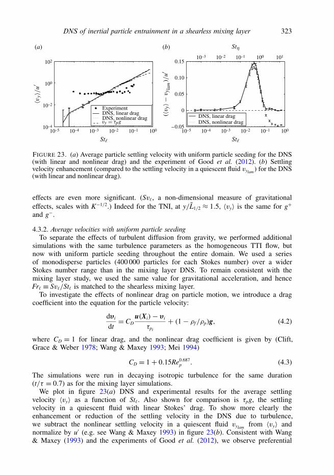
FIGURE 23. (a) Average particle settling velocity with uniform particle seeding for the DNS(with linear and nonlinear drag) and the experiment of Good et al. (2012). (b) Settlingvelocity enhancement (compared to the settling velocity in a quiescent fluid vylam) for the DNS(with linear and nonlinear drag).
effects are even more significant. (Sv`, a non-dimensional measure of gravitationaleffects, scales with K−1/2.) Indeed for the TNI, at y/L1/2 ≈ 1.5, 〈vy〉 is the same for g+
and g−.
4.3.2. Average velocities with uniform particle seedingTo separate the effects of turbulent diffusion from gravity, we performed additional
simulations with the same turbulence parameters as the homogeneous TTI flow, butnow with uniform particle seeding throughout the entire domain. We used a seriesof monodisperse particles (400 000 particles for each Stokes number) over a widerStokes number range than in the mixing layer DNS. To remain consistent with themixing layer study, we used the same value for gravitational acceleration, and henceFr` ≡ Sv`/St` is matched to the shearless mixing layer.
To investigate the effects of nonlinear drag on particle motion, we introduce a dragcoefficient into the equation for the particle velocity:
dvi
dt= CD
u(Xi)− vi
τpi
+ (1− ρf /ρp)g, (4.2)
where CD = 1 for linear drag, and the nonlinear drag coefficient is given by (Clift,Grace & Weber 1978; Wang & Maxey 1993; Mei 1994)
CD = 1+ 0.15Re0.687p . (4.3)
The simulations were run in decaying isotropic turbulence for the same duration(t/τ = 0.7) as for the mixing layer simulations.
We plot in figure 23(a) DNS and experimental results for the average settlingvelocity 〈vy〉 as a function of St`. Also shown for comparison is τpg, the settlingvelocity in a quiescent fluid with linear Stokes’ drag. To show more clearly theenhancement or reduction of the settling velocity in the DNS due to turbulence,we subtract the nonlinear settling velocity in a quiescent fluid vylam from 〈vy〉 andnormalize by u′ (e.g. see Wang & Maxey 1993) in figure 23(b). Consistent with Wang& Maxey (1993) and the experiments of Good et al. (2012), we observe preferential
324 P. J. Ireland and L. R. Collins
sweeping at modest Stokes numbers and loitering at high Stokes numbers, but themagnitudes of the two effects differ significantly from the experiment.
For the smallest St` particles, Good et al. (2012) show settling speeds in excess ofτpg. They attribute this velocity enhancement to the ‘preferential sweeping’ mechanismidentified by Nielsen (1993) and Wang & Maxey (1993), whereby a particle is morelikely to reside in fluid travelling in the same direction of gravity. The findings inGood et al. (2012) are consistent with the experimental results of Nielsen (1993)and Kawanisi & Shiozaki (2008), which also show preferential sweeping at very lowStokes numbers. For the DNS, we observe preferential sweeping only at much largerStokes numbers, consistent with earlier DNS (Wang & Maxey 1993; Yang & Lei 1998;Bosse, Kleiser & Meiburg 2006) and some experiments (Aliseda et al. 2002; Yang &Shy 2003, 2005). Since we would expect inertial particles with St`→ 0 to behave liketracers (with vy→ 0), the reason for this deviation in the experiment is unclear.
For the largest St` particles, Good et al. (2012) show settling speeds considerablyslower than predicted by Stokes’ drag. They argue that this reduction is not causedby nonlinear drag, since the majority of the particles with reduced settling speeds arestill in the linear drag regime. Citing Nielsen (1993), Good et al. (2012) attribute thisreduction to the ‘loitering effect’. Nielsen (1993) reasoned that heavy particles bisectturbulent eddies and spend more time (on average) in fluid that is moving opposite tothe direction of gravity. He argued that loitering still could occur even in the lineardrag regime. Our DNS (figure 23b) shows only a modest loitering with nonlineardrag. The explanation for loitering due to nonlinear drag is given by Wang & Maxey(1993). Particles falling in the nonlinear drag regime will experience higher drag whentravelling in fluid that is moving opposite to gravity (due to higher slip velocities) andlower drag in fluid that is moving in the same direction as gravity (due to lower slipvelocities). Hence, on average, particles will loiter in fluid that is travelling opposite togravity. This loitering, however, is relatively modest in our DNS: ∼5 % for the largestparticles.
In summary, while the direct numerical simulations with nonlinear drag show bothpreferential sweeping and loitering at moderate and high Stokes numbers, respectively,the magnitude of the deviations are considerably smaller than those observed in theexperiments of Good et al. (2012). This deviation cannot be explained by nonlineardrag. Turbulence modulation by the particles in the experiment and other collectiveeffects are also unlikely due to the low volume and mass loadings (e.g. Elghobashi& Truesdell 1993; Sundaram & Collins 1999; Aliseda et al. 2002). Some possibleexplanations are the difference in Reynolds numbers between the experiment andsimulations, and possible effects due to the mean flow and anisotropy of the turbulencein the wind tunnel, but this is purely speculative since none of these effects havebeen systematically explored in the literature. Finally, we note that while there aresignificant differences in the settling speeds as a function of Stokes number, thetrends with respect to particle concentrations, particle concentration fluctuations, andhigher-order particle velocity moments (presented below) agree well.
4.3.3. Higher-order particle velocity momentsReturning to the shearless mixing layer with non-uniform particle seeding, we
consider the variance of particle velocities across the mixing layer. The higher-ordermoments for the small particles are very weak functions of gravity, and therefore weshow g0 for all particles and g+ and g− only for the large particles. Figure 24 showsthe particle velocity variance of the x- and z-components (homogeneous direction)and y-component (inhomogeneous direction) as a function of position for the TTI
DNS of inertial particle entrainment in a shearless mixing layer 325
TTI TNI
TTI TNI
g0
Fluid
largelarge
0.5
1.0
1.5
–1.5 –1.0 –0.5 0 0.5 1.0 1.5
0.5
1.0
1.5
–1.0 –0.5 0 0.5 1.0
0
0.5
1.0
1.5
2.0
–1.5 –1.0 –0.5 0 0.5 1.0 1.5
0
0.5
1.0
1.5
2.0
–1.0 –0.5 0 0.5 1.0–1.5 1.5 –1.5 1.50
2.0
0
2.0(a) (b)
(c) (d )
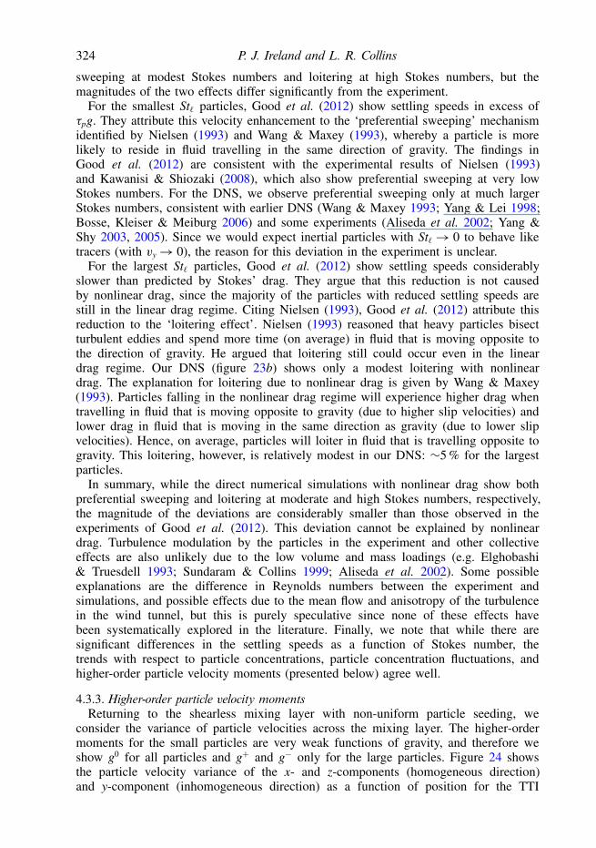
FIGURE 24. Profiles of the particle velocity variance of the components in the homogeneousdirections for the (a) TTI and (b) TNI, and component in the inhomogeneous direction forthe (c) TTI and (d) TNI, at t/τ = 0.7. As indicated in the legend, we consider all particlesfor g0 and only large particles for g+ and g−. The variances are scaled by the average fluidvelocity variance of that component in the injection side, 〈u2
i 〉. Experimental data from Goodet al. (2012) for large particles are shown for comparison, where + corresponds to g+ and ×to g−.
and TNI, scaled by the average fluid velocity variance of that component in theinjection side 〈u2
i 〉. The variance for the fluid field (dotted line) as well as experimentaldata from Good et al. (2012) (symbols) are shown for comparison. The variances ofthe homogeneous velocity components for the TTI (figure 24a) are nearly identicalto those of the underlying fluid velocity, suggesting that the particles in thosedirections are simply responding to the fluid. On the other hand, σ 2
vydecreases in
the non-injection side of the TTI (figure 24c), relative to the underlying fluid velocity.Moreover, we observe a slightly higher variance for g+ than for g0 or g− over most ofthe domain. The experiments of Good et al. (2012) show the same qualitative trend,although their spatial variation is much greater than the DNS. We hypothesize thatfor g0 and g−, particles are transported by relatively large, intermittent fluctuationsthat are comparatively coherent and strongly correlated. These fluctuations lead tolarge mean fluxes of particles, but somewhat less variance because of their coherence.In contrast, g+ allows somewhat weaker fluctuations to carry the particles the samedistance, and these weaker events are more randomized, leading to a slightly highervariance. Farther into the non-injection side, however, this effect disappears as thememory of the fluid from which the particles originated decays and the variances forall three cases approach each other.
For the TNI cases (figure 24b,d), we observe a much stronger spatial variation inthe velocity variance of all three velocity components, reflecting the spatial variation
326 P. J. Ireland and L. R. Collins
TTI TNI
g0
Tracers
largelarge
–0.5
0
0.5
–1.0 –0.5 0 0.5 1.0
–1.0
–0.5
0
0.5
1.0
–1.0 –0.5 0 0.5 1.0
(a) (b)
–1.5 1.5 –1.5 1.5
–1.0
1.0
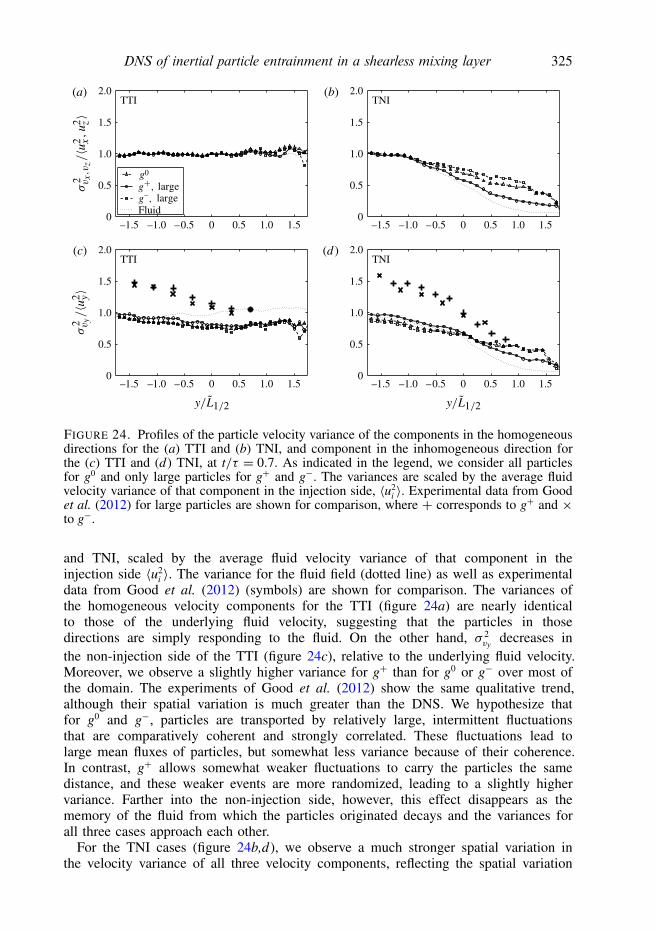
FIGURE 25. Profiles of skewness of the particle velocity component in the inhomogeneousdirection for the (a) TTI and (b) TNI at t/τ = 0.7. As indicated in the legend, we considerall particles for g0 and only large particles for g+ and g−. Experimental data from Good et al.(2012) for large particles are shown for comparison, where + corresponds to g+ and × to g−.
in the underlying fluid. In addition to the physics described above for the TTI, theparticles on the non-injection side are also equilibrating with surrounding fluid that isat a lower turbulent kinetic energy. We observe that the dependences on the injectionside are qualitatively the same as for the TTI; however, on the non-injection side thereis a reversal, with the variances for g0 and g− exceeding that for g+. We believe thisresults from a memory effect, whereby particles overcoming gravity (g−) must initiallyhave larger velocity fluctuations, relative to the g+ case, to overcome gravity. As theparticles equilibrate their energy with the surrounding fluid, they retain some memoryof the fluctuation that brought them there, causing the g− case to achieve a highervariance than the g+ case.
Our trends are qualitatively consistent with those of Good et al. (2012), althoughthe magnitudes differ. One surprising experimental result in figure 24(c,d) is the highparticle y-velocity variances for y< 0. We observe particle velocity variances from theexperiment which are ∼50 % greater than the corresponding fluid velocity variances. Arecent DNS study in isotropic turbulence (Salazar & Collins 2012) yielded the sameunexpected trend over a range of Stokes numbers, and attributed it to biased samplingof the fluid flow due to particle inertia. However, the relative amount of the overshootby the particles was well below 5 % and hence cannot explain the experiment. Themuch larger discrepancy in the particle statistics in the experiment may be due to theinherent difference in the underlying flows, which is caused, at least in part, by theanisotropy in the wind tunnel flow and the difference in Reynolds numbers.
The final higher-order moment we consider is the standardized third-order moment,or skewness, of the velocity fluctuations. Skewness provides information about theasymmetry of the underlying velocity p.d.f., which is indirectly related to itsintermittency. Note that the homogeneous velocity components (not shown) haveessentially no skewness, and so we focus our attention on the y-component ofvelocity. Figure 25 shows the skewness profiles for (a) the TTI and (b) the TNI.On the injection side of the TTI, the skewness values are negligible; however, onthe non-injection side, we see strongly negative skewness, with the largest magnitudeassociated with g− and smallest magnitude associated with g+. The skewness in thevelocity of the underlying fluid is approximately zero throughout, suggesting that thiseffect must be related to the particle flux, particle inertia, or both. The effect of thebiased sampling is observed by considering the fluid skewness along tracer particle
DNS of inertial particle entrainment in a shearless mixing layer 327
trajectories (dotted line). We see almost identical results for tracer particles and inertialparticles without gravity, indicating that the negative skewness results almost entirelyfrom the biased sampling introduced by the particle flux. Gravity acting in the adversedirection (g−) further enhances negative velocity fluctuations, which decreases theskewness even further, while the opposite is true for favourable gravity (g+).
In contrast to the TTI, we observe positive skewness for the TNI over nearly theentire mixing region (cf. figure 25b). Recall that the underlying fluid velocity isalso highly positively skewed due to the inhomogeneous turbulent kinetic energy (cf.figure 5a). Undoubtedly the particle velocity is responding to this forcing from thefluid velocity field. However, the degree of skewness of the particle velocity is lessthan that for the fluid for the same reasons described above for the TTI. That is, biasedsampling and adverse gravity tend to reduce the skewness. The qualitative trends forthe TNI are the same as for the TTI, but shifted due to the underlying skewness in thefluid velocity.
All of these trends are qualitatively consistent with the experimental results of Goodet al. (2012), which are shown for comparison in figure 25. Again, the differences inmagnitudes are likely an effect (at least in part) of anisotropy and differences in theReynolds numbers.
5. ConclusionsWe investigated the entrainment of inertial, non-evaporating particles across a
shearless mixing layer in the absence of thermodynamic processes with the goal ofunderstanding the fundamental turbulence mechanisms involved and their dependenceon parameters such as particle inertia (Stokes number), gravity (acting in both afavourable and adverse direction) and the Reynolds number. The studies were carriedout with two flow configurations, the turbulence–turbulence interface (TTI) and theturbulence–non-turbulence interface (TNI), so that the effect of the inhomogeneousturbulent field in the latter could be isolated. The entire study was motivated by recentexperiments by Gerashchenko et al. (2011) and Good et al. (2012) of the equivalentsystem carried out in a wind tunnel that arose from earlier experiments of the shearlessmixing layer (Veeravalli & Warhaft 1989).
Consistent with the experiments, we find that the TTI is more effective at mixing theinertial particles than the TNI. Over the limited range of Reynolds numbers we couldachieve in these 5123 direct numerical simulations (Rλ = 54–71 at t/τ = 0.7), we findlittle dependence on Reynolds number, and moreover clear evidence that the inertialparticle mixing is dominated by the largest scales of the turbulence, confirming our useof St` as the appropriate measure of inertia. Note that St` . 0.04 for all the particlesand hence in general inertial effects are negligible, in the absence of gravity. Withgravity present, however, the mixing process is either enhanced (favourable gravity,g+) or inhibited (adverse gravity, g−), with larger particles experiencing the strongereffect. Gravity therefore causes the distribution of particle response times across thelayer to go from uniform for no gravity to an enrichment (favourable) or depletion(adverse) of larger particles deep into the non-injection side. The explanation for theseeffects could be found from a simple analysis of the settling speed of the particles foreach condition, and hence the mean concentration statistics resemble those of a passivetracer with gravitational settling superimposed.
One contribution of this work is to demonstrate the impact of mixing on the 2DRDF. To gain a further understanding of the non-uniform particle concentrations, weexamined the 2D RDF computed along x–z planes at fixed y. Both visual evidence

328 P. J. Ireland and L. R. Collins
and the 2D RDF show evidence of apparent ‘clustering’ resulting from the mixingprocess. Particles swept into a particular plane would be locally concentrated by thecoherent bursts of turbulence that carried them. Mixing along the plane would tendto break up the high-concentration regions and hence diminish the 2D RDF. The2D RDFs increase with decreasing r/`, approaching a constant for r/`� 1. Thisconstant is found to be related to the ratio A/Ac, where Ac is the cross-sectionalarea of the ‘clusters’ within the total cross-section, A. This analysis assumes theconcentration within the ‘cluster’ is fixed to the maximum particle concentration, andhence represents an upper bound. Under the assumptions of this model, we expectthe product (n/nmax) g2D(ri) to approach unity as r/`→ 0. Plots of this rescaled 2DRDF approach constants that are at or below unity most likely because of mixing inthe homogeneous directions. This part of the study highlights the role inhomogeneousmixing plays in the ‘clustering’ process. Note that these issues have previously beenraised by Saw et al. (2008), who found evidence of apparent ‘clustering’ due to spatialinhomogeneities in the particle concentration field in their wind tunnel measurements.
We then went on to study different moments of the particle velocity statistics acrossthe mixing layer. Our findings show that when gravity assists particle transport (g+),particles are less dependent on the highly turbulent fluid for transport, and particlevelocities have higher-order moments that are closer to the underlying flow. For g−
the opposite is true (though the differences are not simply monotonic), as particleshave higher-order moments farther from the underlying flow due to an increaseddependence on the high-turbulence fluid for transport. We observe good qualitativeagreement between the experiments of Good et al. (2012) and our DNS with regard tohigher-order moments. The intermittency of the particle velocity distributions and non-monotonic trends in particle velocity moments with gravity show that inertial particlesundergoing entrainment exhibit much more complex and unexpected dynamics than isfound for a passive tracer with superimposed gravitational settling.
An important discrepancy between our DNS and Good et al. (2012) involves thegravitational settling velocity of the particles. In simulations with uniform particleseeding and both linear and nonlinear drag forces on the particles, we find enhancedsettling for moderate Stokes numbers, consistent with the ‘preferential sweeping’mechanism described by Wang & Maxey (1993). Good et al. (2012), however,observed enhanced settling for particles with very small Stokes numbers. They alsofound reduced settling for large-Stokes-number particles that they claim were still inthe linear drag regime. We only observe reduced settling in our DNS for large-Stokes-number particles with nonlinear drag, consistent with Wang & Maxey (1993). Thereason for these discrepancies is unclear, and further experimental and computationalstudies which analyse the effect of scale separation, anisotropy, and the mean flow onparticle settling are needed.
This study is relevant for industrial and environmental processes with inertialparticles that are subject to entrainment, including exhaust plumes, the atmosphericboundary layer, and the oceanic thermocline. In particular, we are interested in betterunderstanding the impact of entrainment on cloud growth and evolution. Our particleparameters are all within the range of those in cumulus clouds, though the flowReynolds number is considerably lower (Siebert, Shaw & Warhaft 2010). Since muchof our results show a very weak dependence on the Reynolds number (though thishypothesis remains to be tested at the higher Reynolds numbers characteristic ofenvironmental flows), computational simulations may be able to predict the dynamicsof particle entrainment accurately in cumulus clouds. Furthermore, since particledynamics are dependent mostly on the large scales of the flow, it is possible that
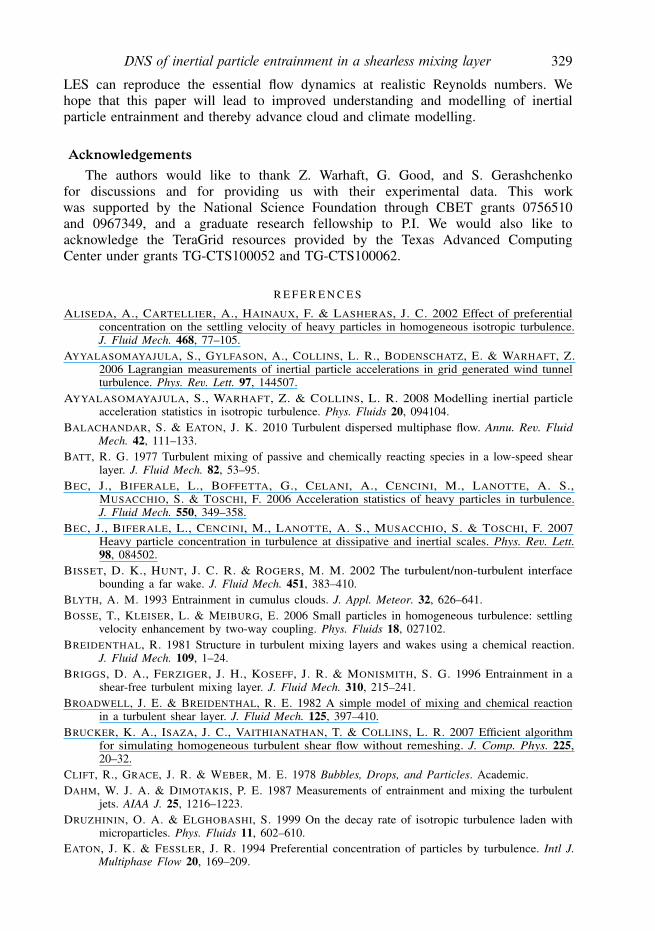
DNS of inertial particle entrainment in a shearless mixing layer 329
LES can reproduce the essential flow dynamics at realistic Reynolds numbers. Wehope that this paper will lead to improved understanding and modelling of inertialparticle entrainment and thereby advance cloud and climate modelling.
AcknowledgementsThe authors would like to thank Z. Warhaft, G. Good, and S. Gerashchenko
for discussions and for providing us with their experimental data. This workwas supported by the National Science Foundation through CBET grants 0756510and 0967349, and a graduate research fellowship to P.I. We would also like toacknowledge the TeraGrid resources provided by the Texas Advanced ComputingCenter under grants TG-CTS100052 and TG-CTS100062.
R E F E R E N C E S
ALISEDA, A., CARTELLIER, A., HAINAUX, F. & LASHERAS, J. C. 2002 Effect of preferentialconcentration on the settling velocity of heavy particles in homogeneous isotropic turbulence.J. Fluid Mech. 468, 77–105.
AYYALASOMAYAJULA, S., GYLFASON, A., COLLINS, L. R., BODENSCHATZ, E. & WARHAFT, Z.2006 Lagrangian measurements of inertial particle accelerations in grid generated wind tunnelturbulence. Phys. Rev. Lett. 97, 144507.
AYYALASOMAYAJULA, S., WARHAFT, Z. & COLLINS, L. R. 2008 Modelling inertial particleacceleration statistics in isotropic turbulence. Phys. Fluids 20, 094104.
BALACHANDAR, S. & EATON, J. K. 2010 Turbulent dispersed multiphase flow. Annu. Rev. FluidMech. 42, 111–133.
BATT, R. G. 1977 Turbulent mixing of passive and chemically reacting species in a low-speed shearlayer. J. Fluid Mech. 82, 53–95.
BEC, J., BIFERALE, L., BOFFETTA, G., CELANI, A., CENCINI, M., LANOTTE, A. S.,MUSACCHIO, S. & TOSCHI, F. 2006 Acceleration statistics of heavy particles in turbulence.J. Fluid Mech. 550, 349–358.
BEC, J., BIFERALE, L., CENCINI, M., LANOTTE, A. S., MUSACCHIO, S. & TOSCHI, F. 2007Heavy particle concentration in turbulence at dissipative and inertial scales. Phys. Rev. Lett.98, 084502.
BISSET, D. K., HUNT, J. C. R. & ROGERS, M. M. 2002 The turbulent/non-turbulent interfacebounding a far wake. J. Fluid Mech. 451, 383–410.
BLYTH, A. M. 1993 Entrainment in cumulus clouds. J. Appl. Meteor. 32, 626–641.BOSSE, T., KLEISER, L. & MEIBURG, E. 2006 Small particles in homogeneous turbulence: settling
velocity enhancement by two-way coupling. Phys. Fluids 18, 027102.BREIDENTHAL, R. 1981 Structure in turbulent mixing layers and wakes using a chemical reaction.
J. Fluid Mech. 109, 1–24.BRIGGS, D. A., FERZIGER, J. H., KOSEFF, J. R. & MONISMITH, S. G. 1996 Entrainment in a
shear-free turbulent mixing layer. J. Fluid Mech. 310, 215–241.BROADWELL, J. E. & BREIDENTHAL, R. E. 1982 A simple model of mixing and chemical reaction
in a turbulent shear layer. J. Fluid Mech. 125, 397–410.BRUCKER, K. A., ISAZA, J. C., VAITHIANATHAN, T. & COLLINS, L. R. 2007 Efficient algorithm
for simulating homogeneous turbulent shear flow without remeshing. J. Comp. Phys. 225,20–32.
CLIFT, R., GRACE, J. R. & WEBER, M. E. 1978 Bubbles, Drops, and Particles. Academic.DAHM, W. J. A. & DIMOTAKIS, P. E. 1987 Measurements of entrainment and mixing the turbulent
jets. AIAA J. 25, 1216–1223.DRUZHININ, O. A. & ELGHOBASHI, S. 1999 On the decay rate of isotropic turbulence laden with
microparticles. Phys. Fluids 11, 602–610.EATON, J. K. & FESSLER, J. R. 1994 Preferential concentration of particles by turbulence. Intl J.
Multiphase Flow 20, 169–209.
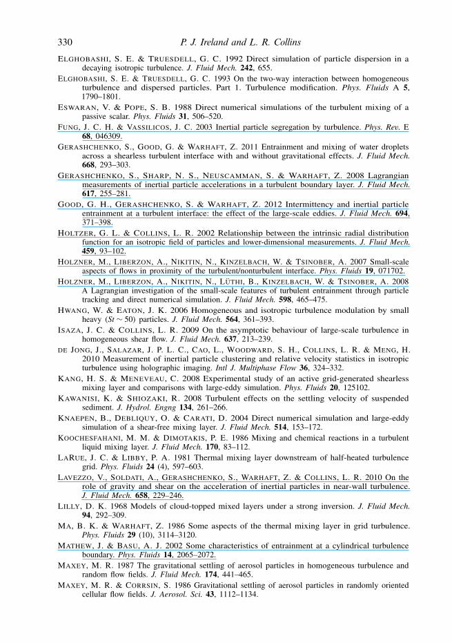
330 P. J. Ireland and L. R. Collins
ELGHOBASHI, S. E. & TRUESDELL, G. C. 1992 Direct simulation of particle dispersion in adecaying isotropic turbulence. J. Fluid Mech. 242, 655.
ELGHOBASHI, S. E. & TRUESDELL, G. C. 1993 On the two-way interaction between homogeneousturbulence and dispersed particles. Part 1. Turbulence modification. Phys. Fluids A 5,1790–1801.
ESWARAN, V. & POPE, S. B. 1988 Direct numerical simulations of the turbulent mixing of apassive scalar. Phys. Fluids 31, 506–520.
FUNG, J. C. H. & VASSILICOS, J. C. 2003 Inertial particle segregation by turbulence. Phys. Rev. E68, 046309.
GERASHCHENKO, S., GOOD, G. & WARHAFT, Z. 2011 Entrainment and mixing of water dropletsacross a shearless turbulent interface with and without gravitational effects. J. Fluid Mech.668, 293–303.
GERASHCHENKO, S., SHARP, N. S., NEUSCAMMAN, S. & WARHAFT, Z. 2008 Lagrangianmeasurements of inertial particle accelerations in a turbulent boundary layer. J. Fluid Mech.617, 255–281.
GOOD, G. H., GERASHCHENKO, S. & WARHAFT, Z. 2012 Intermittency and inertial particleentrainment at a turbulent interface: the effect of the large-scale eddies. J. Fluid Mech. 694,371–398.
HOLTZER, G. L. & COLLINS, L. R. 2002 Relationship between the intrinsic radial distributionfunction for an isotropic field of particles and lower-dimensional measurements. J. Fluid Mech.459, 93–102.
HOLZNER, M., LIBERZON, A., NIKITIN, N., KINZELBACH, W. & TSINOBER, A. 2007 Small-scaleaspects of flows in proximity of the turbulent/nonturbulent interface. Phys. Fluids 19, 071702.
HOLZNER, M., LIBERZON, A., NIKITIN, N., LUTHI, B., KINZELBACH, W. & TSINOBER, A. 2008A Lagrangian investigation of the small-scale features of turbulent entrainment through particletracking and direct numerical simulation. J. Fluid Mech. 598, 465–475.
HWANG, W. & EATON, J. K. 2006 Homogeneous and isotropic turbulence modulation by smallheavy (St ∼ 50) particles. J. Fluid Mech. 564, 361–393.
ISAZA, J. C. & COLLINS, L. R. 2009 On the asymptotic behaviour of large-scale turbulence inhomogeneous shear flow. J. Fluid Mech. 637, 213–239.
DE JONG, J., SALAZAR, J. P. L. C., CAO, L., WOODWARD, S. H., COLLINS, L. R. & MENG, H.2010 Measurement of inertial particle clustering and relative velocity statistics in isotropicturbulence using holographic imaging. Intl J. Multiphase Flow 36, 324–332.
KANG, H. S. & MENEVEAU, C. 2008 Experimental study of an active grid-generated shearlessmixing layer and comparisons with large-eddy simulation. Phys. Fluids 20, 125102.
KAWANISI, K. & SHIOZAKI, R. 2008 Turbulent effects on the settling velocity of suspendedsediment. J. Hydrol. Engng 134, 261–266.
KNAEPEN, B., DEBLIQUY, O. & CARATI, D. 2004 Direct numerical simulation and large-eddysimulation of a shear-free mixing layer. J. Fluid Mech. 514, 153–172.
KOOCHESFAHANI, M. M. & DIMOTAKIS, P. E. 1986 Mixing and chemical reactions in a turbulentliquid mixing layer. J. Fluid Mech. 170, 83–112.
LARUE, J. C. & LIBBY, P. A. 1981 Thermal mixing layer downstream of half-heated turbulencegrid. Phys. Fluids 24 (4), 597–603.
LAVEZZO, V., SOLDATI, A., GERASHCHENKO, S., WARHAFT, Z. & COLLINS, L. R. 2010 On therole of gravity and shear on the acceleration of inertial particles in near-wall turbulence.J. Fluid Mech. 658, 229–246.
LILLY, D. K. 1968 Models of cloud-topped mixed layers under a strong inversion. J. Fluid Mech.94, 292–309.
MA, B. K. & WARHAFT, Z. 1986 Some aspects of the thermal mixing layer in grid turbulence.Phys. Fluids 29 (10), 3114–3120.
MATHEW, J. & BASU, A. J. 2002 Some characteristics of entrainment at a cylindrical turbulenceboundary. Phys. Fluids 14, 2065–2072.
MAXEY, M. R. 1987 The gravitational settling of aerosol particles in homogeneous turbulence andrandom flow fields. J. Fluid Mech. 174, 441–465.
MAXEY, M. R. & CORRSIN, S. 1986 Gravitational settling of aerosol particles in randomly orientedcellular flow fields. J. Aerosol. Sci. 43, 1112–1134.
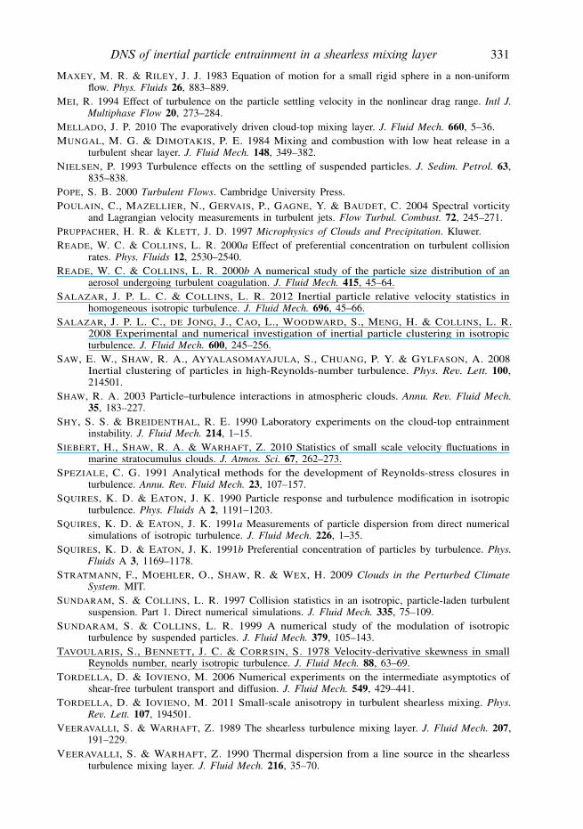
DNS of inertial particle entrainment in a shearless mixing layer 331
MAXEY, M. R. & RILEY, J. J. 1983 Equation of motion for a small rigid sphere in a non-uniformflow. Phys. Fluids 26, 883–889.
MEI, R. 1994 Effect of turbulence on the particle settling velocity in the nonlinear drag range. Intl J.Multiphase Flow 20, 273–284.
MELLADO, J. P. 2010 The evaporatively driven cloud-top mixing layer. J. Fluid Mech. 660, 5–36.MUNGAL, M. G. & DIMOTAKIS, P. E. 1984 Mixing and combustion with low heat release in a
turbulent shear layer. J. Fluid Mech. 148, 349–382.NIELSEN, P. 1993 Turbulence effects on the settling of suspended particles. J. Sedim. Petrol. 63,
835–838.POPE, S. B. 2000 Turbulent Flows. Cambridge University Press.POULAIN, C., MAZELLIER, N., GERVAIS, P., GAGNE, Y. & BAUDET, C. 2004 Spectral vorticity
and Lagrangian velocity measurements in turbulent jets. Flow Turbul. Combust. 72, 245–271.PRUPPACHER, H. R. & KLETT, J. D. 1997 Microphysics of Clouds and Precipitation. Kluwer.READE, W. C. & COLLINS, L. R. 2000a Effect of preferential concentration on turbulent collision
rates. Phys. Fluids 12, 2530–2540.READE, W. C. & COLLINS, L. R. 2000b A numerical study of the particle size distribution of an
aerosol undergoing turbulent coagulation. J. Fluid Mech. 415, 45–64.SALAZAR, J. P. L. C. & COLLINS, L. R. 2012 Inertial particle relative velocity statistics in
homogeneous isotropic turbulence. J. Fluid Mech. 696, 45–66.SALAZAR, J. P. L. C., DE JONG, J., CAO, L., WOODWARD, S., MENG, H. & COLLINS, L. R.
2008 Experimental and numerical investigation of inertial particle clustering in isotropicturbulence. J. Fluid Mech. 600, 245–256.
SAW, E. W., SHAW, R. A., AYYALASOMAYAJULA, S., CHUANG, P. Y. & GYLFASON, A. 2008Inertial clustering of particles in high-Reynolds-number turbulence. Phys. Rev. Lett. 100,214501.
SHAW, R. A. 2003 Particle–turbulence interactions in atmospheric clouds. Annu. Rev. Fluid Mech.35, 183–227.
SHY, S. S. & BREIDENTHAL, R. E. 1990 Laboratory experiments on the cloud-top entrainmentinstability. J. Fluid Mech. 214, 1–15.
SIEBERT, H., SHAW, R. A. & WARHAFT, Z. 2010 Statistics of small scale velocity fluctuations inmarine stratocumulus clouds. J. Atmos. Sci. 67, 262–273.
SPEZIALE, C. G. 1991 Analytical methods for the development of Reynolds-stress closures inturbulence. Annu. Rev. Fluid Mech. 23, 107–157.
SQUIRES, K. D. & EATON, J. K. 1990 Particle response and turbulence modification in isotropicturbulence. Phys. Fluids A 2, 1191–1203.
SQUIRES, K. D. & EATON, J. K. 1991a Measurements of particle dispersion from direct numericalsimulations of isotropic turbulence. J. Fluid Mech. 226, 1–35.
SQUIRES, K. D. & EATON, J. K. 1991b Preferential concentration of particles by turbulence. Phys.Fluids A 3, 1169–1178.
STRATMANN, F., MOEHLER, O., SHAW, R. & WEX, H. 2009 Clouds in the Perturbed ClimateSystem. MIT.
SUNDARAM, S. & COLLINS, L. R. 1997 Collision statistics in an isotropic, particle-laden turbulentsuspension. Part 1. Direct numerical simulations. J. Fluid Mech. 335, 75–109.
SUNDARAM, S. & COLLINS, L. R. 1999 A numerical study of the modulation of isotropicturbulence by suspended particles. J. Fluid Mech. 379, 105–143.
TAVOULARIS, S., BENNETT, J. C. & CORRSIN, S. 1978 Velocity-derivative skewness in smallReynolds number, nearly isotropic turbulence. J. Fluid Mech. 88, 63–69.
TORDELLA, D. & IOVIENO, M. 2006 Numerical experiments on the intermediate asymptotics ofshear-free turbulent transport and diffusion. J. Fluid Mech. 549, 429–441.
TORDELLA, D. & IOVIENO, M. 2011 Small-scale anisotropy in turbulent shearless mixing. Phys.Rev. Lett. 107, 194501.
VEERAVALLI, S. & WARHAFT, Z. 1989 The shearless turbulence mixing layer. J. Fluid Mech. 207,191–229.
VEERAVALLI, S. & WARHAFT, Z. 1990 Thermal dispersion from a line source in the shearlessturbulence mixing layer. J. Fluid Mech. 216, 35–70.

332 P. J. Ireland and L. R. Collins
WANG, L. P. & MAXEY, M. R. 1993 Settling velocity and concentration distribution of heavyparticles in homogeneous isotropic turbulence. J. Fluid Mech. 256, 27–68.
WANG, L.-P., WEXLER, A. S. & ZHOU, Y. 2000 Statistical mechanical description and modellingof turbulent collision of inertial particles. J. Fluid Mech. 415, 117–153.
WESTERWEEL, J., FUKUSHIMA, C., PEDERSEN, J. M. & HUNT, J. C. R. 2005 Mechanics of theturbulent–nonturbulent interface of a jet. Phys. Rev. Lett. 95, 174501.
WESTERWEEL, J., HOFMANN, T., FUKUSHIMA, C. & HUNT, J. C. R. 2002 The turbulent/non-turbulent interface at the outer boundary of a self-similar turbulent jet. Exp. Fluids 33,873–878.
WOOD, A. M., HWANG, W. & EATON, J. K. 2005 Preferential concentration of particles inhomogeneous and isotropic turbulence. Intl J. Multiphase Flow 31, 1220–1230.
YANG, C. Y. & LEI, U. 1998 The role of turbulent scales in the settling velocity of heavy particlesin homogeneous isotropic turbulence. J. Fluid Mech. 20, 179–205.
YANG, T. S. & SHY, S. S. 2003 The settling velocity of heavy particles in an aqueousnear-isotropic turbulence. Phys. Fluids 15, 868–880.
YANG, T. S. & SHY, S. S. 2005 Two-way interaction between solid particles and homogeneous airturbulence: particle settling rate and turbulence modification measurements. J. Fluid Mech.526, 171–216.
ZHOU, Y., WEXLER, A. S. & WANG, L.-P. 2001 Modelling turbulent collision of bidisperse inertialparticles. J. Fluid Mech. 433, 77–104.