Evaluation of Rigid and Non-rigid Motion Compensation of Cardiac Perfusion MRI
Upload
khangminh22Category
view
0download
0
Vector Mechanics For Engineers: Dynamics
Twelfth Edition
PROPRIETARY MATERIAL © 2020 The McGraw Hill Inc. All rights reserved. No part of this PowerPoint slide may be displayed, reproduced or distributed in any formor by any means, without the prior written permission of the publisher, or used beyond the limited distribution to teachers and educators permitted by McGraw Hill for theirindividual course preparation. If you are a student using this PowerPoint slide, you are using it without permission.
Copyright © 2020 McGraw Hill , All Rights Reserved.
Chapter 16Chapter 16
Plane Motion of Rigid Bodies: Forces and Accelerations
© 2019 McGraw-Hill Education.
ContentsIntroduction
Equations of Motion of a Rigid Body
Angular Momentum of a Rigid Body in Plane Motion
Plane Motion of a Rigid Body
A Remark on the Axioms of the Mechanics of Rigid Bodies
Problems Involving the Motion of a Rigid Body
Sample Problem 16.1
Sample Problem 16.3
Sample Problem 16.4
Sample Problem 16.5
Sample Problem 16.6
Constrained Plane Motion
Constrained Plane Motion: Noncentroidal Rotation
Constrained Plane Motion: Rolling Motion
Sample Problem 16.7
Sample Problem 16.9
Sample Problem 16.10
Sample Problem 16.12
© 2019 McGraw-Hill Education.
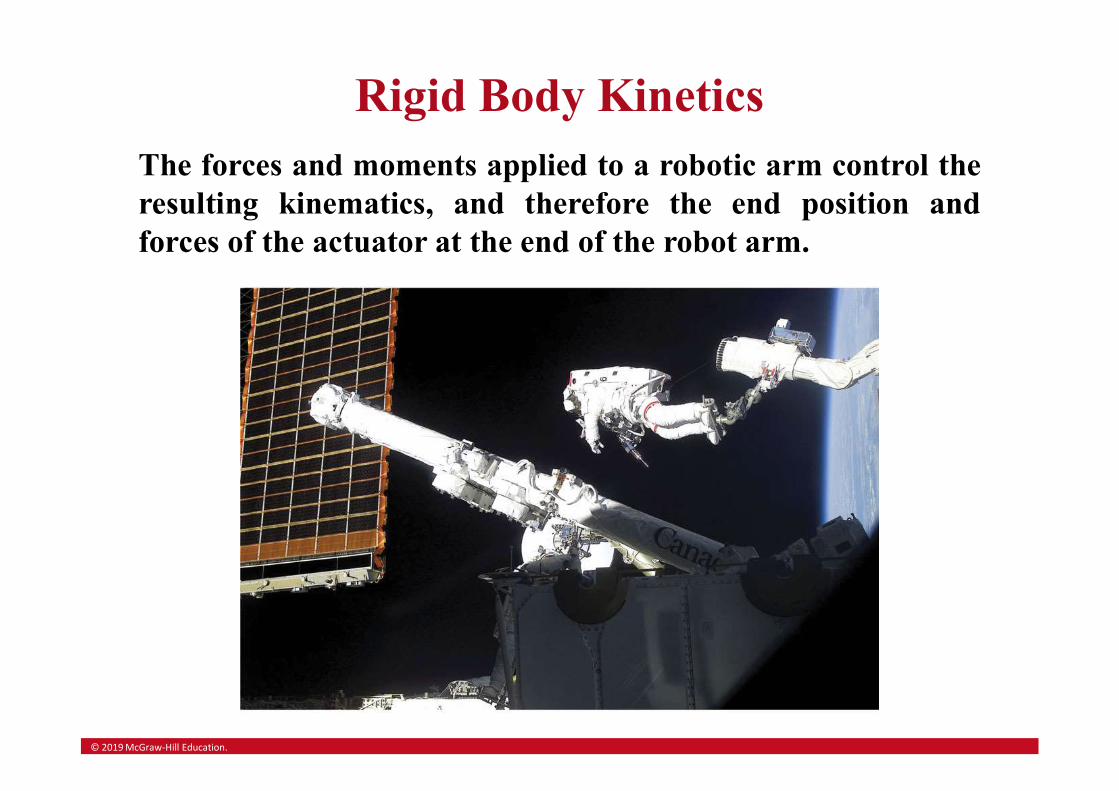
Rigid Body KineticsThe forces and moments applied to a robotic arm control theresulting kinematics, and therefore the end position andforces of the actuator at the end of the robot arm.
© 2019 McGraw-Hill Education.
Introduction• In this chapter and in Chapters 17 and 18, we will be concerned
with the kinetics of rigid bodies, that is relations between the forces acting on a rigid body, the shape and mass of the body, and the motion produced.
Results of this chapter will be restricted to:
• plane motion of rigid bodies, and
• rigid bodies consisting of plane slabs or bodies which are symmetrical with respect to the reference plane.
• Our approach will be to consider rigid bodies as made of large numbers of particles and to use the results of Chapter 14 for the motion of systems of particles. Specifically,
GG HMamF and
© 2019 McGraw-Hill Education.
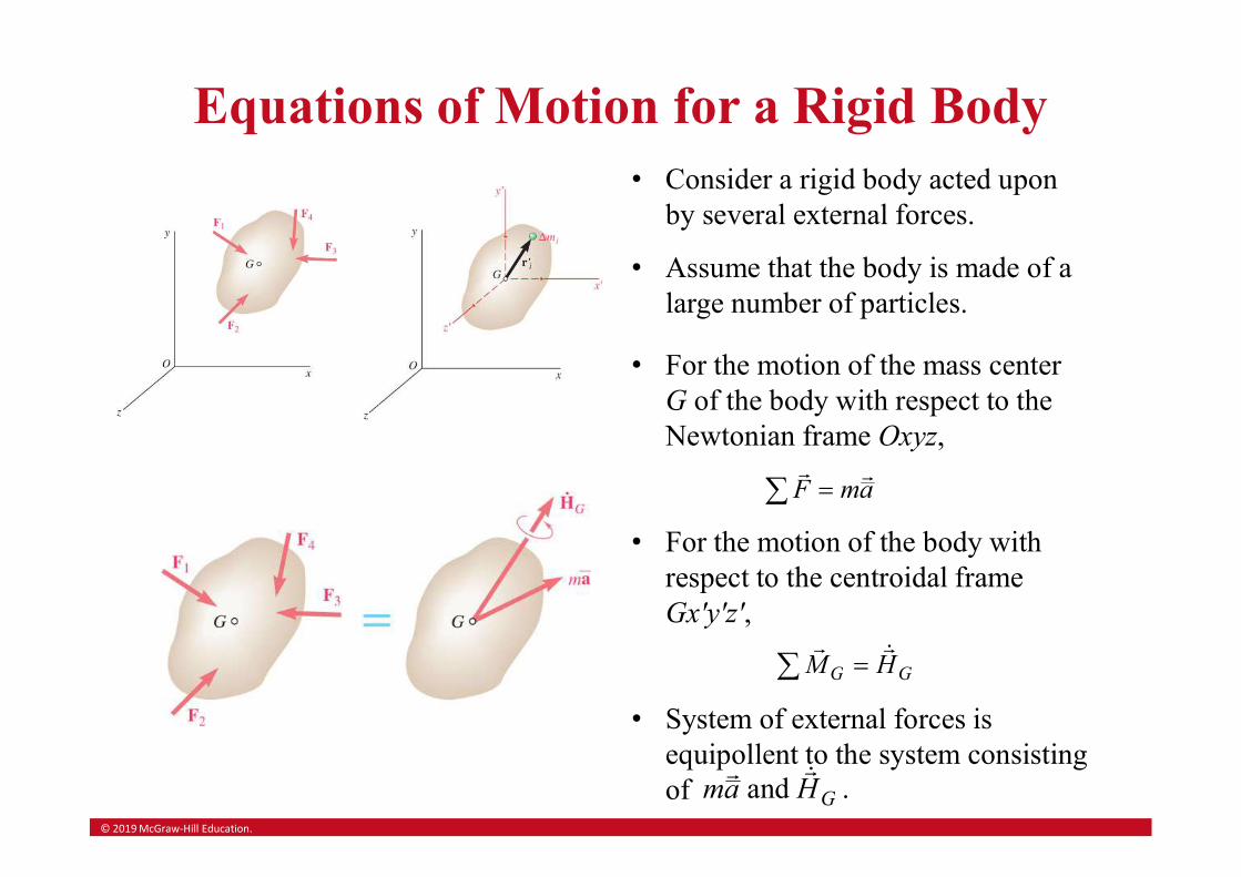
Equations of Motion for a Rigid Body• Consider a rigid body acted upon
by several external forces.
• Assume that the body is made of a large number of particles.
• For the motion of the mass center G of the body with respect to the Newtonian frame Oxyz,
amF
• For the motion of the body with respect to the centroidal frame Gx′y′z′,
GG HM
• System of external forces is equipollent to the system consisting of . and GHam
© 2019 McGraw-Hill Education.
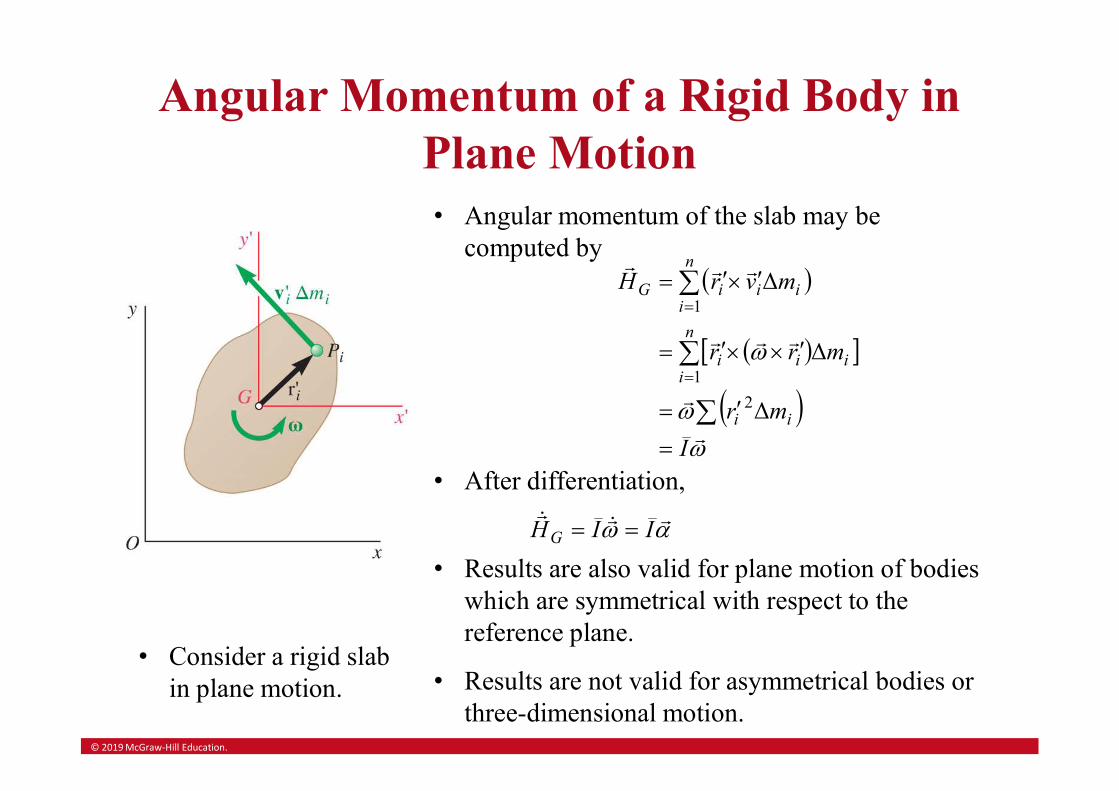
Angular Momentum of a Rigid Body in Plane Motion
• Consider a rigid slab in plane motion.
• Angular momentum of the slab may be computed by
I
mr
mrr
mvrH
ii
n
iiii
n
iiiiG
Δ
Δ
Δ
2
1
1
• After differentiation,
IIHG
• Results are also valid for plane motion of bodies which are symmetrical with respect to the reference plane.
• Results are not valid for asymmetrical bodies or three-dimensional motion.
© 2019 McGraw-Hill Education.
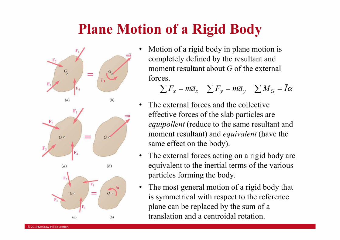
Plane Motion of a Rigid Body• Motion of a rigid body in plane motion is
completely defined by the resultant and moment resultant about G of the external forces.
IMamFamF Gyyxx
• The external forces and the collective effective forces of the slab particles are equipollent (reduce to the same resultant and moment resultant) and equivalent (have the same effect on the body).
• The external forces acting on a rigid body are equivalent to the inertial terms of the various particles forming the body.
• The most general motion of a rigid body that is symmetrical with respect to the reference plane can be replaced by the sum of a translation and a centroidal rotation.
© 2019 McGraw-Hill Education.
A Remark on the Axioms of the Mechanics of Rigid Bodies
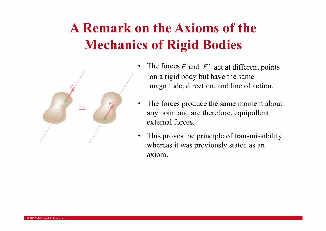
• The forces FF and act at different points
on a rigid body but have the same magnitude, direction, and line of action.
• The forces produce the same moment about any point and are therefore, equipollent external forces.
• This proves the principle of transmissibility whereas it was previously stated as an axiom.
© 2019 McGraw-Hill Education.
Problems Involving the Motion of a Rigid Body
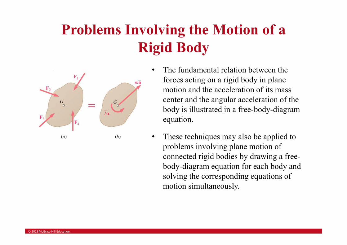
• The fundamental relation between the forces acting on a rigid body in plane motion and the acceleration of its mass center and the angular acceleration of the body is illustrated in a free-body-diagram equation.
• These techniques may also be applied to problems involving plane motion of connected rigid bodies by drawing a free-body-diagram equation for each body and solving the corresponding equations of motion simultaneously.
© 2019 McGraw-Hill Education.
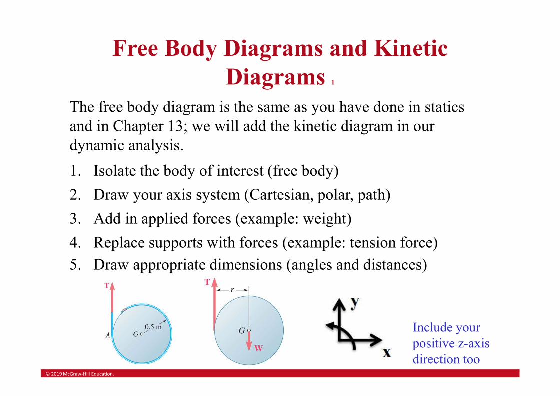
Free Body Diagrams and Kinetic Diagrams 1
Include your positive z-axis direction too
The free body diagram is the same as you have done in statics and in Chapter 13; we will add the kinetic diagram in our dynamic analysis.
1. Isolate the body of interest (free body)
2. Draw your axis system (Cartesian, polar, path)
3. Add in applied forces (example: weight)
4. Replace supports with forces (example: tension force)
5. Draw appropriate dimensions (angles and distances)
© 2019 McGraw-Hill Education.
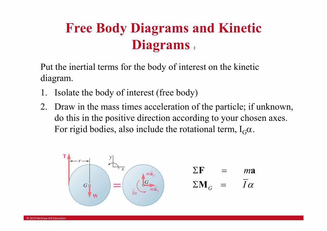
Free Body Diagrams and Kinetic Diagrams 2
Put the inertial terms for the body of interest on the kinetic diagram.
1. Isolate the body of interest (free body)
2. Draw in the mass times acceleration of the particle; if unknown, do this in the positive direction according to your chosen axes. For rigid bodies, also include the rotational term, IG.
m F a
G I M
© 2019 McGraw-Hill Education.
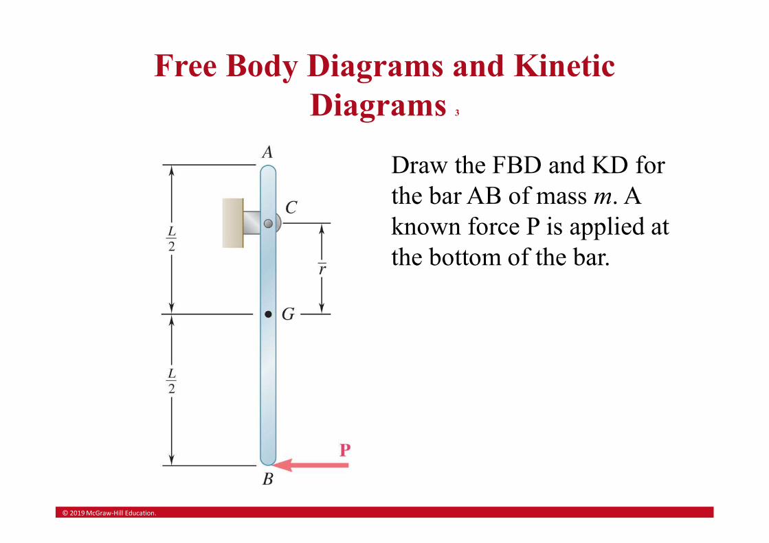
Free Body Diagrams and Kinetic Diagrams 3
Draw the FBD and KD for the bar AB of mass m. A known force P is applied at the bottom of the bar.
© 2019 McGraw-Hill Education.
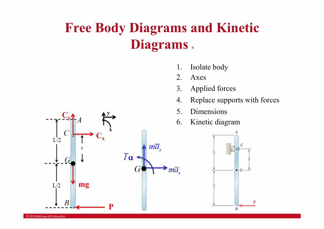
Free Body Diagrams and Kinetic Diagrams 4
1. Isolate body2. Axes
3. Applied forces
4. Replace supports with forces
5. Dimensions6. Kinetic diagram

© 2019 McGraw-Hill Education.
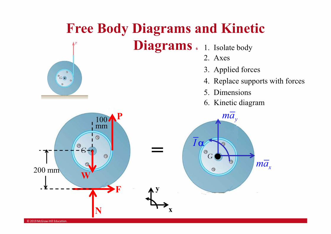
Free Body Diagrams and Kinetic Diagrams 5
A drum of 100 mm radius is attached to a disk of 200 mm radius. The combined drum and disk had a combined mass of 5 kg. A cord is attached as shown, and a force of magnitude P=25 N is applied. The coefficients of static and kinetic friction between the wheel and ground are ms= 0.25 and mk= 0.20, respectively. Draw the FBD and KD for the wheel.
© 2019 McGraw-Hill Education.
Free Body Diagrams and Kinetic Diagrams 6
xma
yma
I
P
F
W
N x
y
=
1. Isolate body2. Axes
3. Applied forces
4. Replace supports with forces
5. Dimensions6. Kinetic diagram
100 mm
200 mm

© 2019 McGraw-Hill Education.
Free Body Diagrams and Kinetic Diagrams 7
The ladder AB slides down the wall as shown. The wall and floor are both rough. Draw the FBD and KD for the ladder.
© 2019 McGraw-Hill Education.
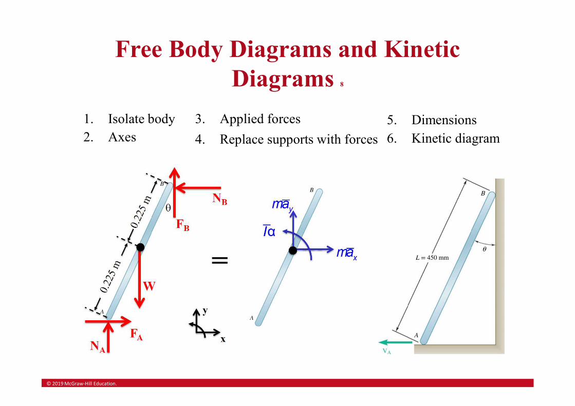
Free Body Diagrams and Kinetic Diagrams 8
1. Isolate body2. Axes
3. Applied forces
4. Replace supports with forces
5. Dimensions6. Kinetic diagram
© 2019 McGraw-Hill Education.
Sample Problem 16.1 1
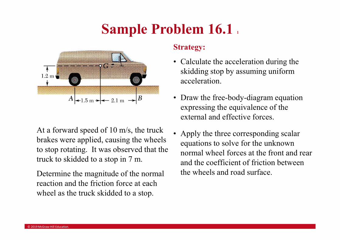
At a forward speed of 10 m/s, the truck brakes were applied, causing the wheels to stop rotating. It was observed that the truck to skidded to a stop in 7 m.
Determine the magnitude of the normal reaction and the friction force at each wheel as the truck skidded to a stop.
Strategy:
• Calculate the acceleration during the skidding stop by assuming uniform acceleration.
• Apply the three corresponding scalar equations to solve for the unknown normal wheel forces at the front and rear and the coefficient of friction between the wheels and road surface.
• Draw the free-body-diagram equation expressing the equivalence of the external and effective forces.
© 2019 McGraw-Hill Education.
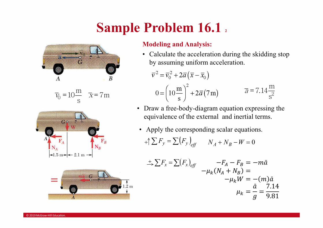
Sample Problem 16.1 2
0
m10 7m
sv x= =
Modeling and Analysis:
• Calculate the acceleration during the skidding stop by assuming uniform acceleration.
2
m7.14
sa =
• Draw a free-body-diagram equation expressing the equivalence of the external and inertial terms.
• Apply the corresponding scalar equations.
0 WNN BA
effyy FF
effxx FF

© 2019 McGraw-Hill Education.
Sample Problem 16.1 3
𝑁 = 𝑊 − 𝑁 = 0.341𝑊
𝑁 =1
2𝑁 =
1
20.341𝑊 𝑁 = 0.1705𝑊
𝑁 =1
2𝑁 =
1
20.659𝑊 𝑁 = 0.3295𝑊
𝐹 = 𝜇 𝑁 = 0.728 0.1705𝑊
𝐹 = 0.1241𝑊
𝐹 = 𝜇 𝑁 = 0.728 0.3295𝑊
𝐹 = 0.240𝑊
effAA MM
© 2019 McGraw-Hill Education.
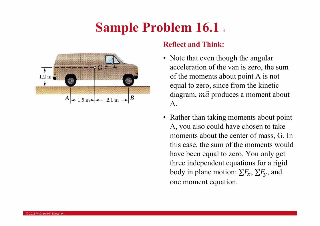
Sample Problem 16.1 4
Reflect and Think:
• Note that even though the angular acceleration of the van is zero, the sum of the moments about point A is not equal to zero, since from the kinetic diagram, produces a moment about A.
• Rather than taking moments about point A, you also could have chosen to take moments about the center of mass, G. In this case, the sum of the moments would have been equal to zero. You only get three independent equations for a rigid body in plane motion: , , and one moment equation.
© 2019 McGraw-Hill Education.
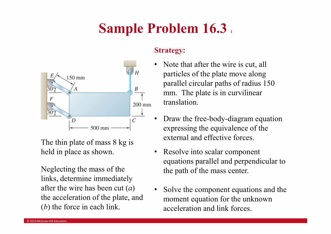
Sample Problem 16.3 1
The thin plate of mass 8 kg is held in place as shown.
Neglecting the mass of the links, determine immediately after the wire has been cut (a) the acceleration of the plate, and (b) the force in each link.
Strategy:
• Note that after the wire is cut, all particles of the plate move along parallel circular paths of radius 150 mm. The plate is in curvilinear translation.
• Draw the free-body-diagram equation expressing the equivalence of the external and effective forces.
• Resolve into scalar component equations parallel and perpendicular to the path of the mass center.
• Solve the component equations and the moment equation for the unknown acceleration and link forces.
© 2019 McGraw-Hill Education.
Sample Problem 16.3 2
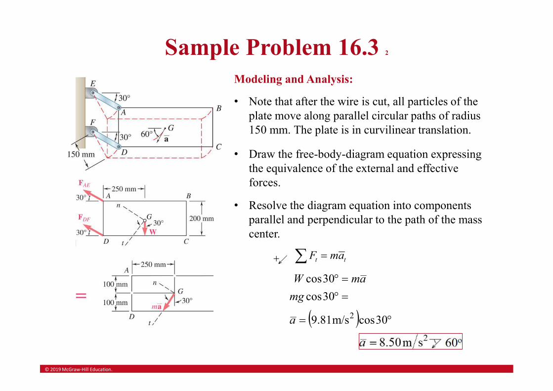
Modeling and Analysis:
• Note that after the wire is cut, all particles of the plate move along parallel circular paths of radius 150 mm. The plate is in curvilinear translation.
• Draw the free-body-diagram equation expressing the equivalence of the external and effective forces.
• Resolve the diagram equation into components parallel and perpendicular to the path of the mass center.
tt amF
30cos
30cos
mg
amW
30cosm/s81.9 2a
© 2019 McGraw-Hill Education.
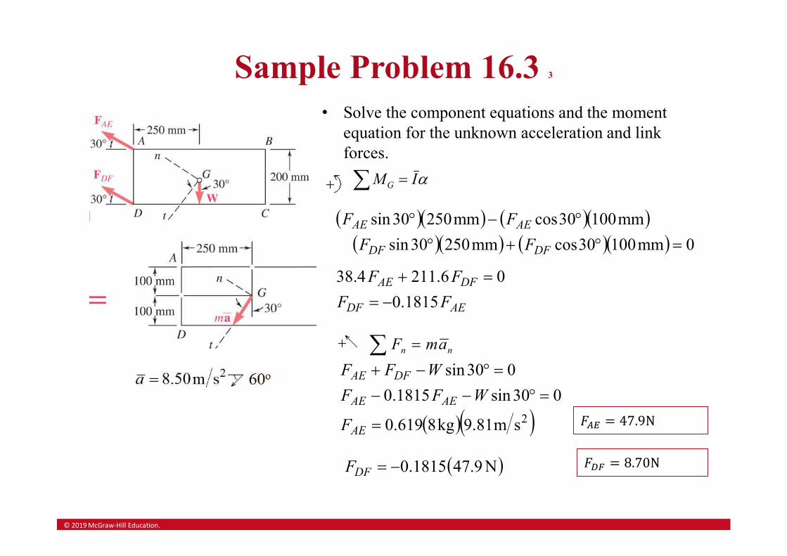
Sample Problem 16.3 3
• Solve the component equations and the moment equation for the unknown acceleration and link forces.
IMG 0mm10030cosmm25030sin
mm10030cosmm25030sin
DFDF
AEAE
FF
FF
AEDF
DFAE
FF
FF
1815.0
06.2114.38
nn amF
2sm81.9kg8619.0
030sin1815.0
030sin
AE
AEAE
DFAE
F
WFF
WFF
𝐹 = 47.9N
N9.471815.0DFF 𝐹 = 8.70N
© 2019 McGraw-Hill Education.
Sample Problem 16.3 4
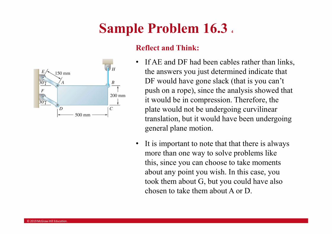
Reflect and Think:
• If AE and DF had been cables rather than links, the answers you just determined indicate that DF would have gone slack (that is you can’t push on a rope), since the analysis showed that it would be in compression. Therefore, the plate would not be undergoing curvilinear translation, but it would have been undergoing general plane motion.
• It is important to note that that there is always more than one way to solve problems like this, since you can choose to take moments about any point you wish. In this case, you took them about G, but you could have also chosen to take them about A or D.

© 2019 McGraw-Hill Education.
Sample Problem 16.4 1
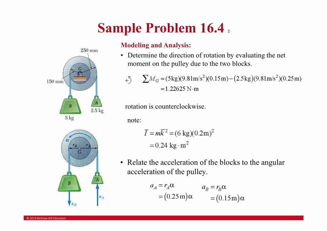
A pulley of mass 6 kg and having a radius of gyration of 200 mm is connected to two blocks as shown.
Assuming no axle friction, determine the angular acceleration of the pulley and the acceleration of each block.
Strategy:
• Determine the direction of rotation by evaluating the net moment on the pulley due to the two blocks.
• Relate the acceleration of the blocks to the angular acceleration of the pulley.
• Draw the free-body-diagram equation expressing the equivalence of the external and effective forces on the complete pulley plus blocks system.
• Solve the corresponding moment equation for the pulley angular acceleration.
© 2019 McGraw-Hill Education.
Sample Problem 16.4 2
• Relate the acceleration of the blocks to the angular acceleration of the pulley.
note:
Modeling and Analysis:
• Determine the direction of rotation by evaluating the net moment on the pulley due to the two blocks.
rotation is counterclockwise.
© 2019 McGraw-Hill Education.
Sample Problem 16.4 3
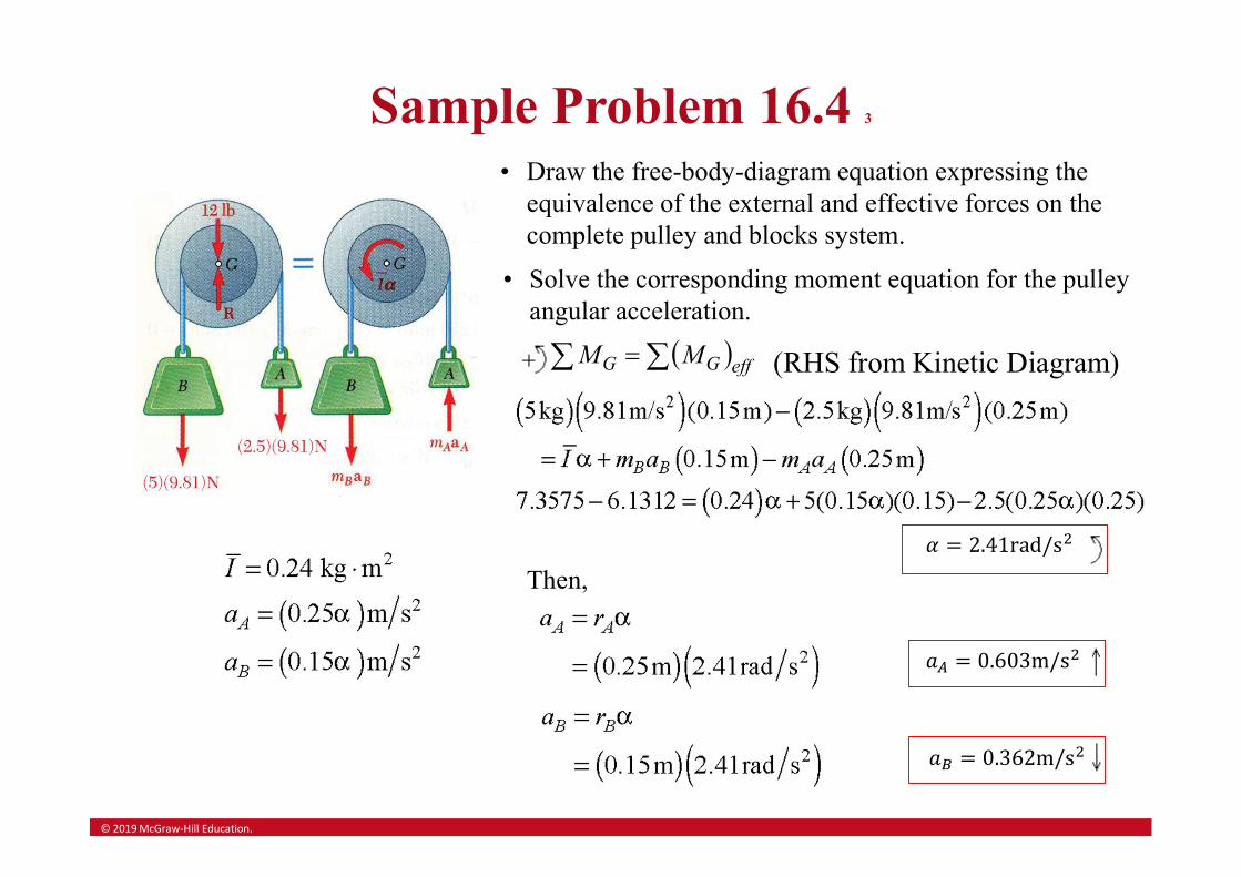
• Draw the free-body-diagram equation expressing the equivalence of the external and effective forces on the complete pulley and blocks system.
effGG MM
• Solve the corresponding moment equation for the pulley angular acceleration.
𝛼 = 2.41rad/s
Then,
(RHS from Kinetic Diagram)
𝑎 = 0.603m/s
𝑎 = 0.362m/s
© 2019 McGraw-Hill Education.
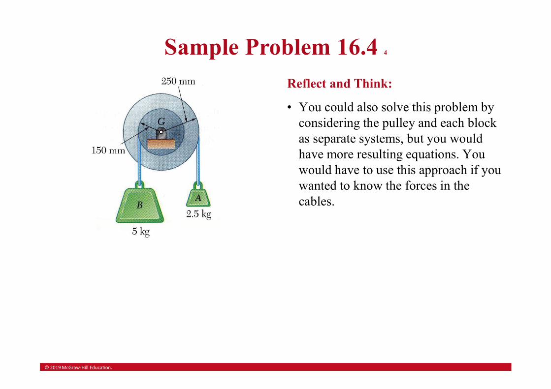
Sample Problem 16.4 4
Reflect and Think:
• You could also solve this problem by considering the pulley and each block as separate systems, but you would have more resulting equations. You would have to use this approach if you wanted to know the forces in the cables.
© 2019 McGraw-Hill Education.
Sample Problem 16.5 1
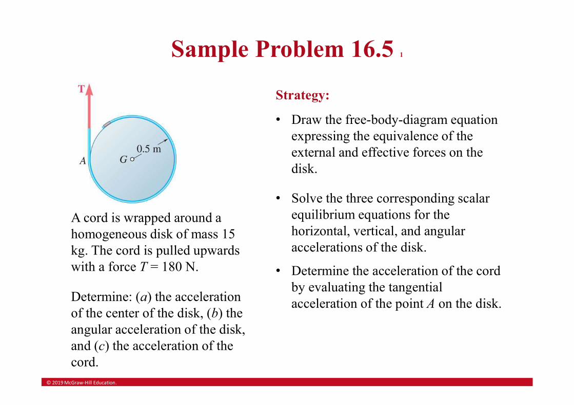
A cord is wrapped around a homogeneous disk of mass 15 kg. The cord is pulled upwards with a force T = 180 N.
Determine: (a) the acceleration of the center of the disk, (b) the angular acceleration of the disk, and (c) the acceleration of the cord.
Strategy:
• Draw the free-body-diagram equation expressing the equivalence of the external and effective forces on the disk.
• Solve the three corresponding scalar equilibrium equations for the horizontal, vertical, and angular accelerations of the disk.
• Determine the acceleration of the cord by evaluating the tangential acceleration of the point A on the disk.
© 2019 McGraw-Hill Education.
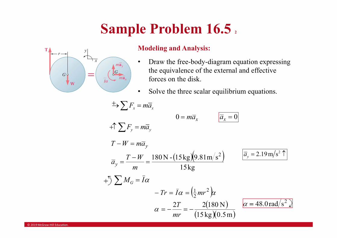
Sample Problem 16.5 2
Modeling and Analysis:
• Draw the free-body-diagram equation expressing the equivalence of the external and effective forces on the disk.
• Solve the three scalar equilibrium equations.
x xF ma xam0 0xa
y yF ma
kg15
sm81.9kg15-N180 2
m
WTa
amWT
y
y22.19m sya
IMG
m5.0kg15
N18022
221
mr
T
mrITr
© 2019 McGraw-Hill Education.
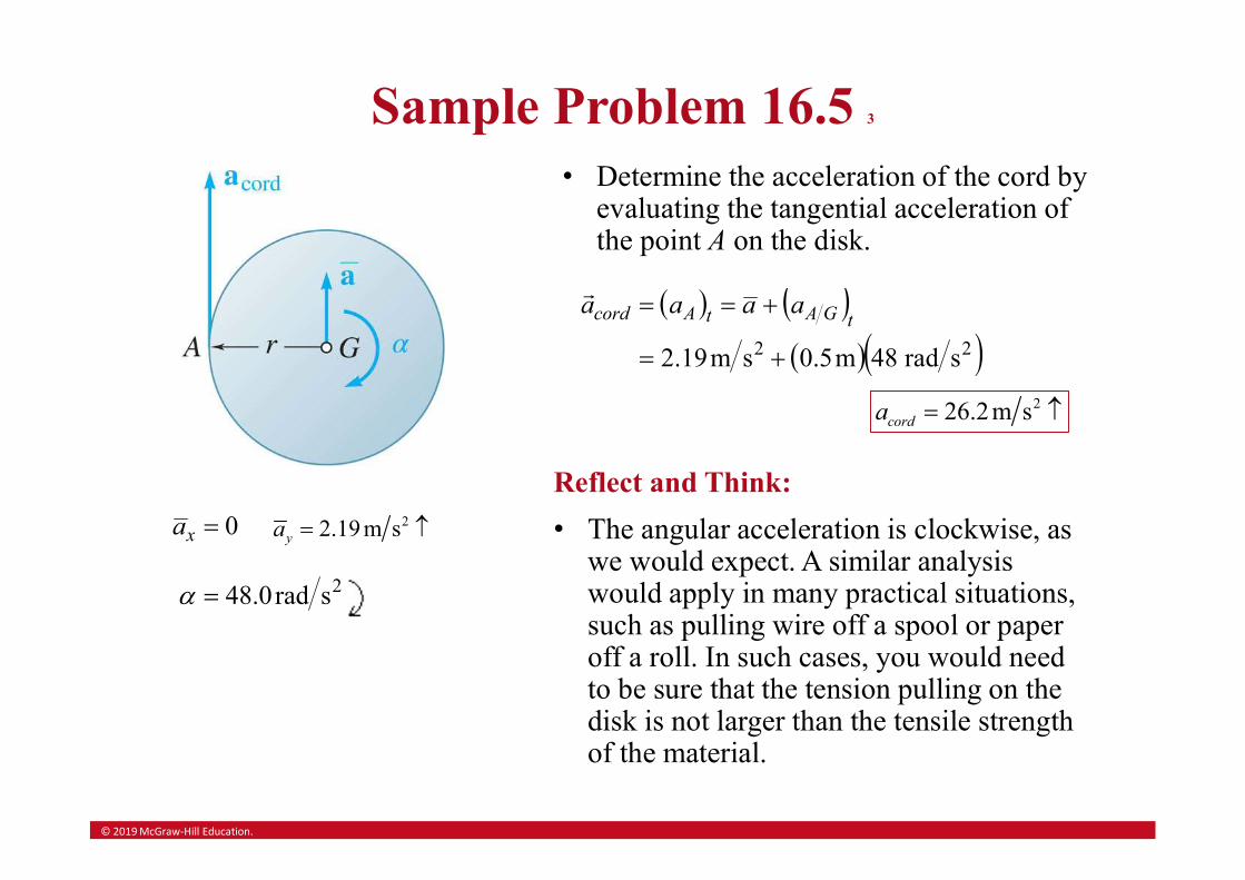
Sample Problem 16.5 3
0xa 22.19 m sya
2srad0.48
• Determine the acceleration of the cord by evaluating the tangential acceleration of the point A on the disk.
22 srad48m5.0sm19.2
tGAtAcord aaaa
226.2m scorda
Reflect and Think:
• The angular acceleration is clockwise, as we would expect. A similar analysis would apply in many practical situations, such as pulling wire off a spool or paper off a roll. In such cases, you would need to be sure that the tension pulling on the disk is not larger than the tensile strength of the material.
© 2019 McGraw-Hill Education.
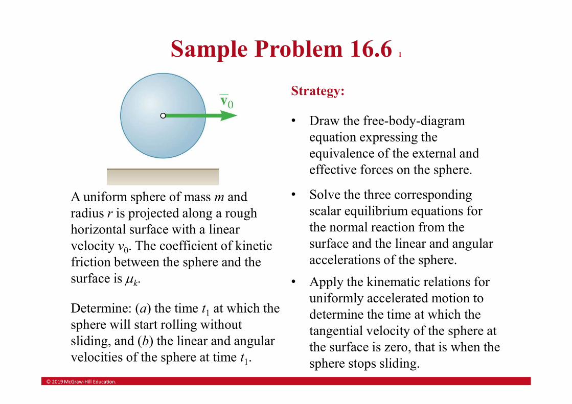
Sample Problem 16.6 1
A uniform sphere of mass m and radius r is projected along a rough horizontal surface with a linear velocity v0. The coefficient of kinetic friction between the sphere and the surface is mk.
Determine: (a) the time t1 at which the sphere will start rolling without sliding, and (b) the linear and angular velocities of the sphere at time t1.
Strategy:
• Draw the free-body-diagram equation expressing the equivalence of the external and effective forces on the sphere.
• Solve the three corresponding scalar equilibrium equations for the normal reaction from the surface and the linear and angular accelerations of the sphere.
• Apply the kinematic relations for uniformly accelerated motion to determine the time at which the tangential velocity of the sphere at the surface is zero, that is when the sphere stops sliding.
© 2019 McGraw-Hill Education.
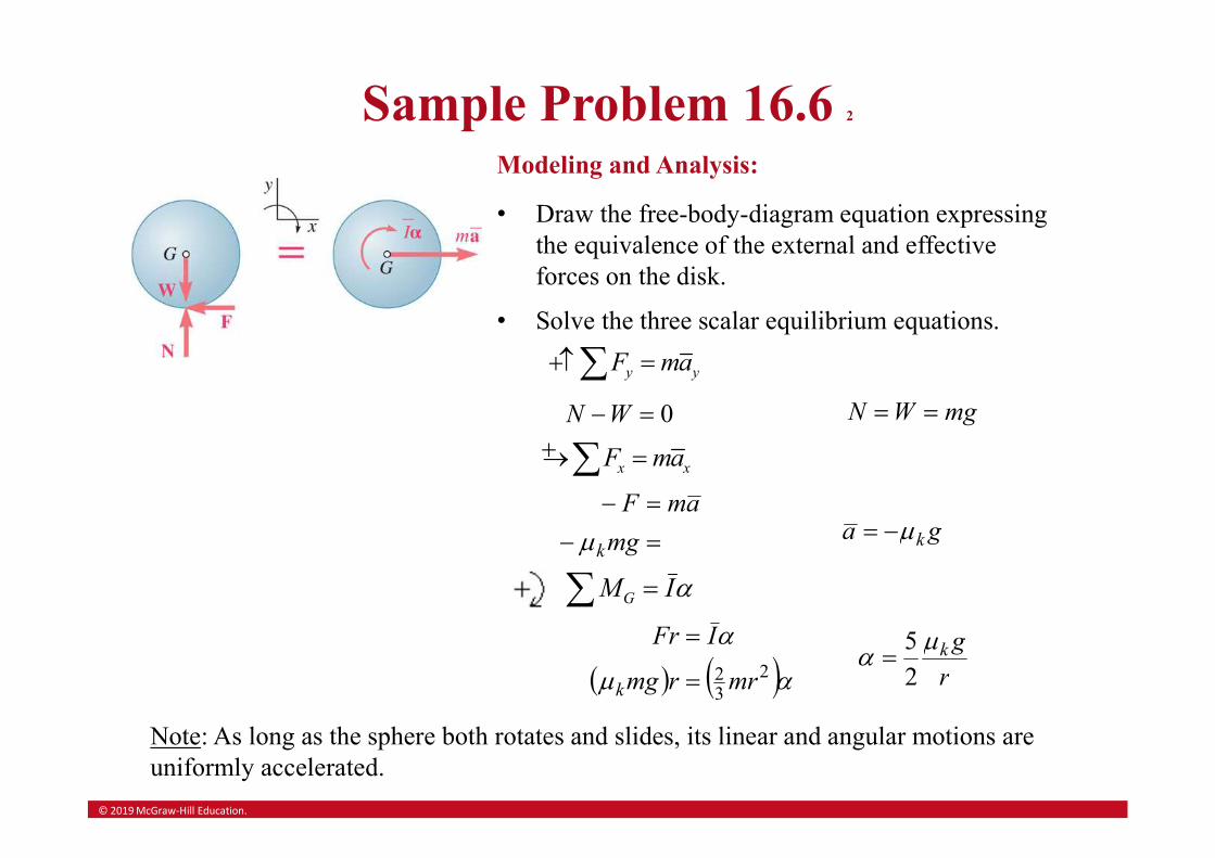
Sample Problem 16.6 2
Modeling and Analysis:
• Draw the free-body-diagram equation expressing the equivalence of the external and effective forces on the disk.
• Solve the three scalar equilibrium equations.
y yF ma 0WN mgWN
x xF ma
mg
amF
kmga km
IMG
m
2
32 mrrmg
IFr
k
r
gkm2
5
Note: As long as the sphere both rotates and slides, its linear and angular motions are uniformly accelerated.
© 2019 McGraw-Hill Education.
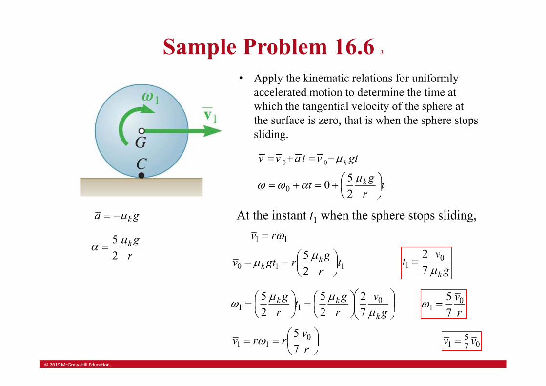
Sample Problem 16.6 3
ga km
r
gkm2
5
• Apply the kinematic relations for uniformly accelerated motion to determine the time at which the tangential velocity of the sphere at the surface is zero, that is when the sphere stops sliding.
gtvtavv km 00
tr
gt k
m2
500
At the instant t1 when the sphere stops sliding,
11 rv
110 2
5t
r
grgtv k
k
mmg
vt
km0
1 7
2
g
v
r
gt
r
g
k
kk
mmm 0
11 7
2
2
5
2
5
r
v01 7
5
r
vrrv 0
11 7
5 075
1 vv
© 2019 McGraw-Hill Education.
Sample Problem 16.6 4
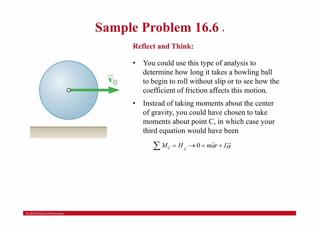
Reflect and Think:
• You could use this type of analysis to determine how long it takes a bowling ball to begin to roll without slip or to see how the coefficient of friction affects this motion.
• Instead of taking moments about the center of gravity, you could have chosen to take moments about point C, in which case your third equation would have been
0C CM H mar I
© 2019 McGraw-Hill Education.
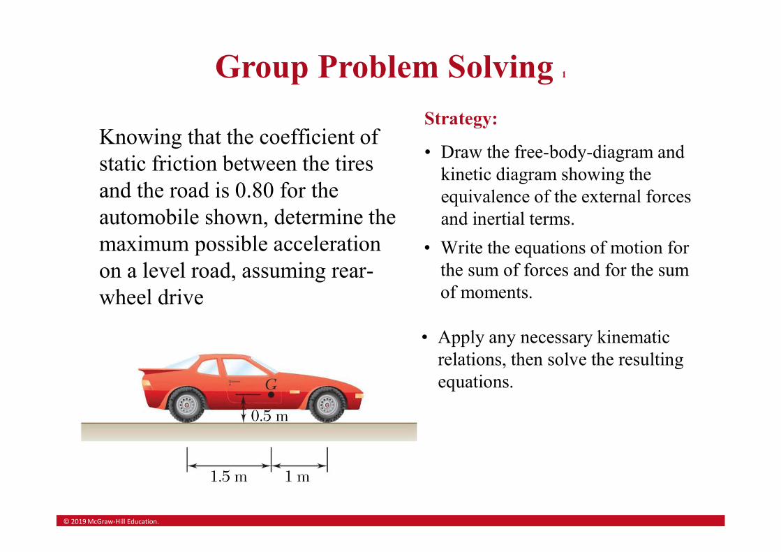
Group Problem Solving 1
Knowing that the coefficient of static friction between the tires and the road is 0.80 for the automobile shown, determine the maximum possible acceleration on a level road, assuming rear-wheel drive
Strategy:
• Draw the free-body-diagram and kinetic diagram showing the equivalence of the external forces and inertial terms.
• Write the equations of motion for the sum of forces and for the sum of moments.
• Apply any necessary kinematic relations, then solve the resulting equations.
© 2019 McGraw-Hill Education.
Group Problem Solving 2
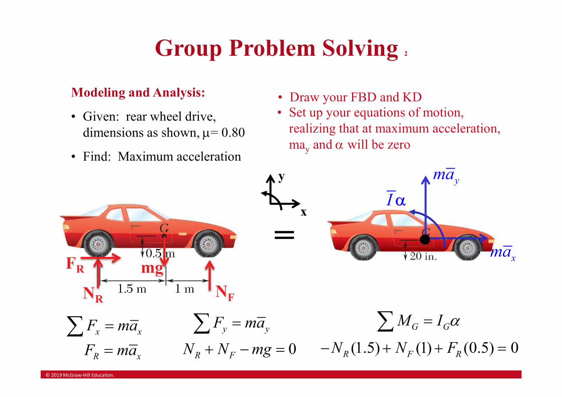
Modeling and Analysis:
• Given: rear wheel drive, dimensions as shown, m= 0.80
• Find: Maximum acceleration
• Draw your FBD and KD
x
y
xma
I yma
=
x xF ma y yF maR xF ma 0R FN N mg
• Set up your equations of motion, realizing that at maximum acceleration, may and will be zero
G GM I (1.5) (1) (0.5) 0R F RN N F
© 2019 McGraw-Hill Education.
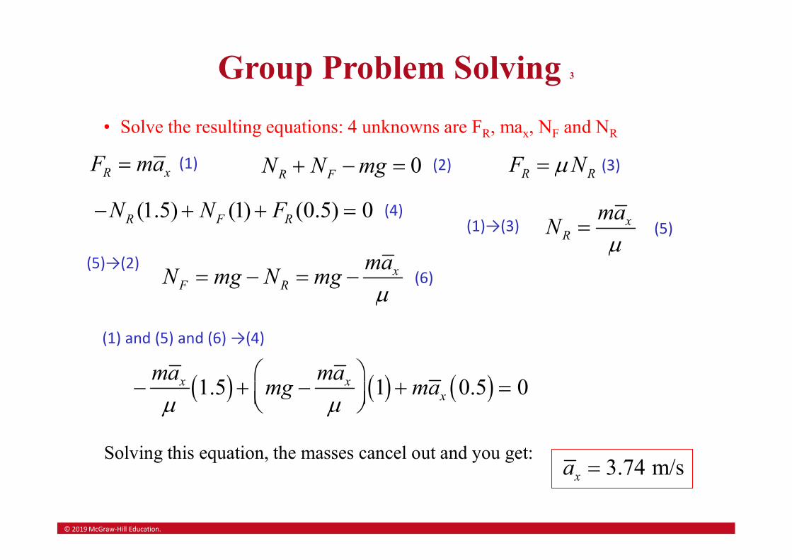
Group Problem Solving 3
• Solve the resulting equations: 4 unknowns are FR, max, NF and NR
(1) (2) (3)
(4)
Solving this equation, the masses cancel out and you get:
(1.5) (1) (0.5) 0R F RN N F
0R FN N mg R xF ma R RF Nm
xR
maN
m(1)→(3) (5)
xF R
maN mg N mg
m (6)
(5)→(2)
(1) and (5) and (6) →(4)
1.5 1 0.5 0x xx
ma mamg ma
m m
3.74 m/sxa
© 2019 McGraw-Hill Education.
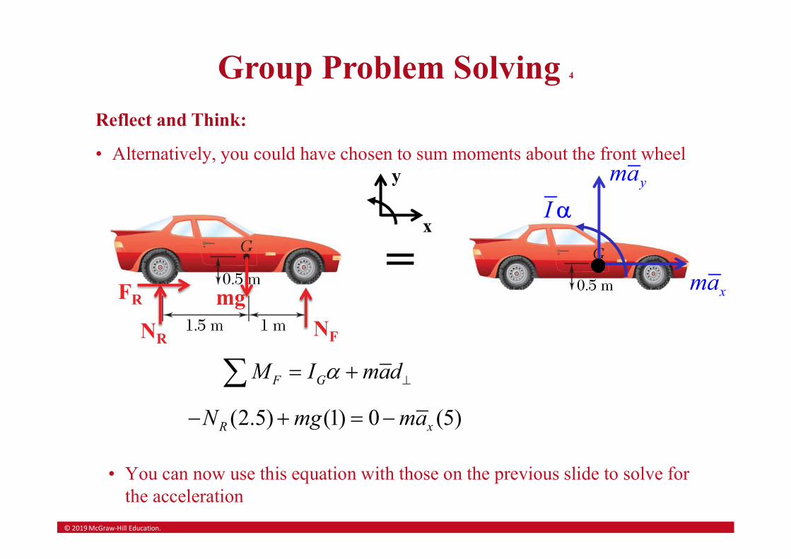
Group Problem Solving 4
Reflect and Think:
• Alternatively, you could have chosen to sum moments about the front wheel
x
y
xma
I yma
=
F GM I mad (2.5) (1) 0 (5)R xN mg ma
• You can now use this equation with those on the previous slide to solve for the acceleration
© 2019 McGraw-Hill Education.
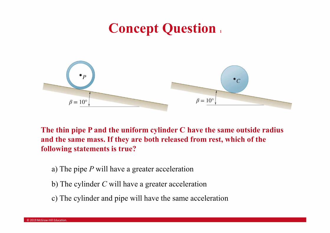
Concept Question 1
The thin pipe P and the uniform cylinder C have the same outside radius and the same mass. If they are both released from rest, which of the following statements is true?
a) The pipe P will have a greater acceleration
b) The cylinder C will have a greater acceleration
c) The cylinder and pipe will have the same acceleration
© 2019 McGraw-Hill Education.
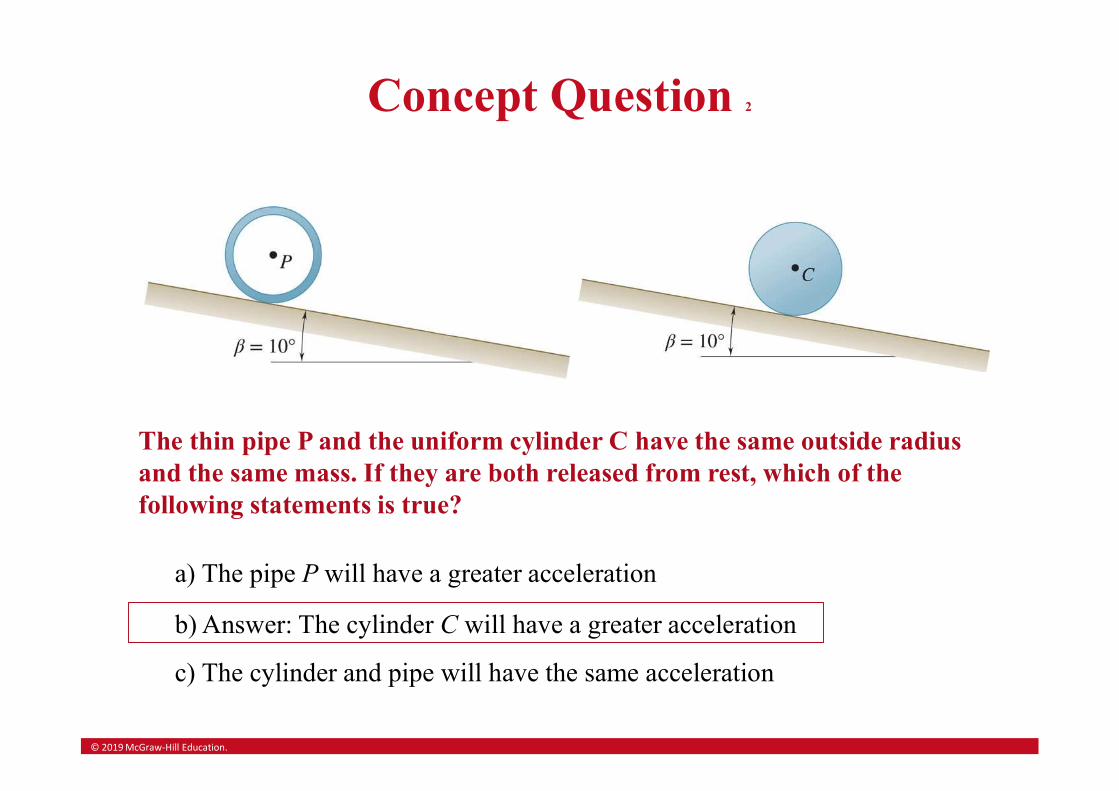
Concept Question 2
The thin pipe P and the uniform cylinder C have the same outside radius and the same mass. If they are both released from rest, which of the following statements is true?
a) The pipe P will have a greater acceleration
b) Answer: The cylinder C will have a greater acceleration
c) The cylinder and pipe will have the same acceleration

© 2019 McGraw-Hill Education.
Constrained Plane Motion 1
The reactions of the automobile crankshaft bearings depend on the mass, mass moment of inertia, and the kinematics of the crankshaft.
The forces one the wind turbine blades are also dependent on mass, mass moment of inertia, and kinematics.
©Loraks/ Getty Images RF

© 2019 McGraw-Hill Education.
Constrained Plane Motion 2
Most engineering applications involve rigid bodies which are moving under given constraints, example: cranks, connecting rods, and non-slipping wheels.
Constrained plane motion: motions with definite relations between the components of acceleration of the mass center and the angular acceleration of the body.
Solution of a problem involving constrained plane motion begins with a kinematic analysis.
Example: given q, ω, and α, find P, NA, and NB.• kinematic analysis yield . and yx aa
• We can then find P, NA, and NB by solving the appropriate equations.

© 2019 McGraw-Hill Education.
Constrained Motion: Noncentroidal Rotation• Noncentroidal rotation: motion of a body
is constrained to rotate about a fixed axis that does not pass through its mass center.
• Kinematic relation between the motion of the mass center G and the motion of the body about G,
2 rara nt
• The kinematic relations are used to eliminate nt aa and from the method of dynamic equilibrium.
© 2019 McGraw-Hill Education.
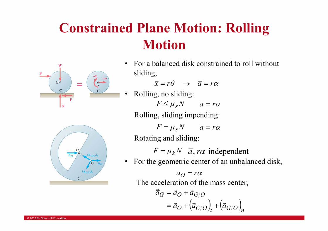
Constrained Plane Motion: Rolling Motion
• For a balanced disk constrained to roll without sliding,
q rarx • Rolling, no sliding:
NF sm ra Rolling, sliding impending:
NF sm ra Rotating and sliding:
NF km , independenta r• For the geometric center of an unbalanced disk,
raO The acceleration of the mass center,
nOGtOGO
OGOG
aaa
aaa
© 2019 McGraw-Hill Education.
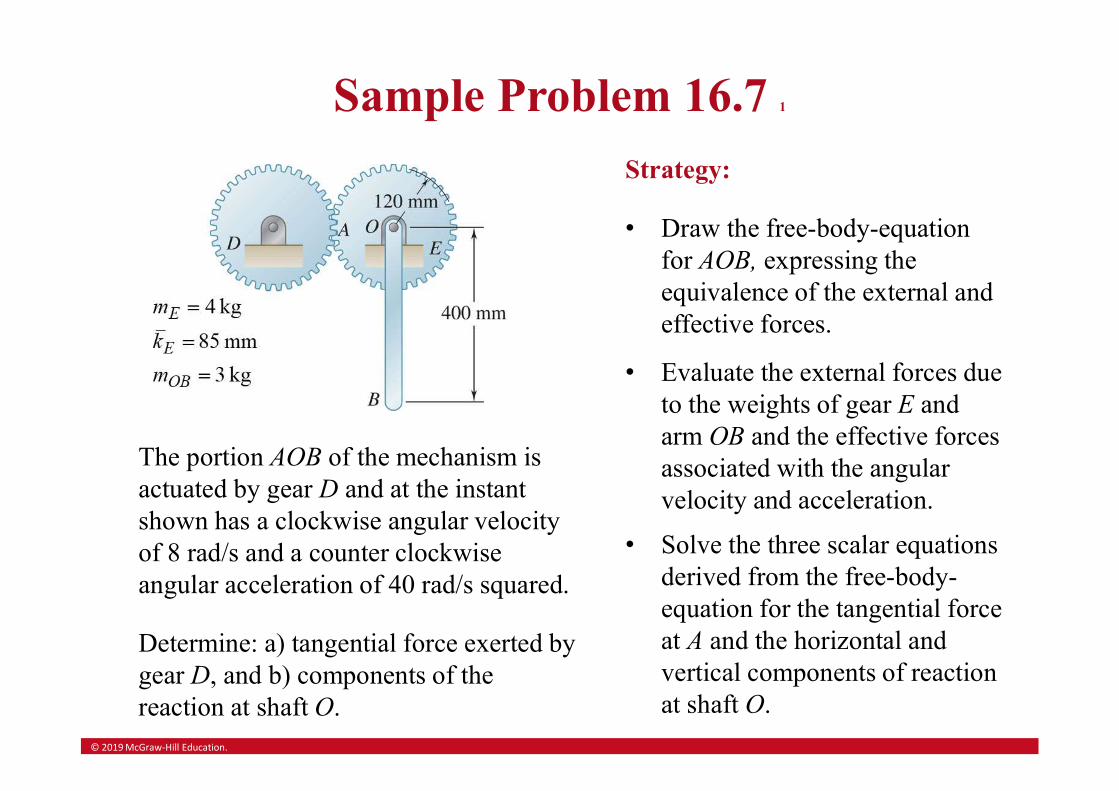
Sample Problem 16.7 1
The portion AOB of the mechanism is actuated by gear D and at the instant shown has a clockwise angular velocity of 8 rad/s and a counter clockwise angular acceleration of 40 rad/s squared.
Determine: a) tangential force exerted by gear D, and b) components of the reaction at shaft O.
Strategy:
• Draw the free-body-equation for AOB, expressing the equivalence of the external and effective forces.
• Evaluate the external forces due to the weights of gear E and arm OB and the effective forces associated with the angular velocity and acceleration.
• Solve the three scalar equations derived from the free-body-equation for the tangential force at A and the horizontal and vertical components of reaction at shaft O.

© 2019 McGraw-Hill Education.
Sample Problem 16.7 2
kg 3
mm 85
kg 4
OB
E
E
m
k
m 2srad40
rad/s 8
22 /8)/40)(200.0()( smsradmra tOB 222 /8.12)/8)(200.0()( smsradmra nOB
Modeling and Analysis:• Draw the free-body-equation for AOB.
• Evaluate the external forces due to the weights of gear E and arm OB and the effective forces.
N4.29sm81.9kg3
N2.39sm81.9kg42
2
OB
E
W
W
mN156.1
srad40m085.0kg4 222
EEE kmI
N0.24
srad40m200.0kg3 2
rmam OBtOBOB
N4.38
srad8m200.0kg3 22
rmam OBnOBOB
mN600.1
srad40m.4000kg3 221212
121
LmI OBOB
© 2019 McGraw-Hill Education.
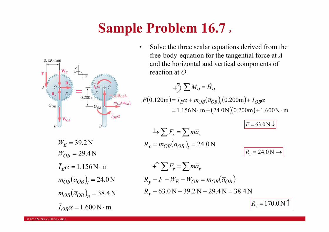
Sample Problem 16.7 3
N4.29
N2.39
OB
E
W
W
mN156.1 EI
N0.24tOBOB am
N4.38nOBOB am
mN600.1 OBI
• Solve the three scalar equations derived from the free-body-equation for the tangential force at Aand the horizontal and vertical components of reaction at O.
OO HM
mN600.1m200.0N0.24mN156.1
m200.0m120.0
OBtOBOBE IamIF
63.0 NF
x xF ma N0.24 tOBOBx amR
24.0 NxR
y yF ma
N4.38N4.29N2.39N0.63
y
OBOBOBEy
R
amWWFR
170.0 NyR
© 2019 McGraw-Hill Education.
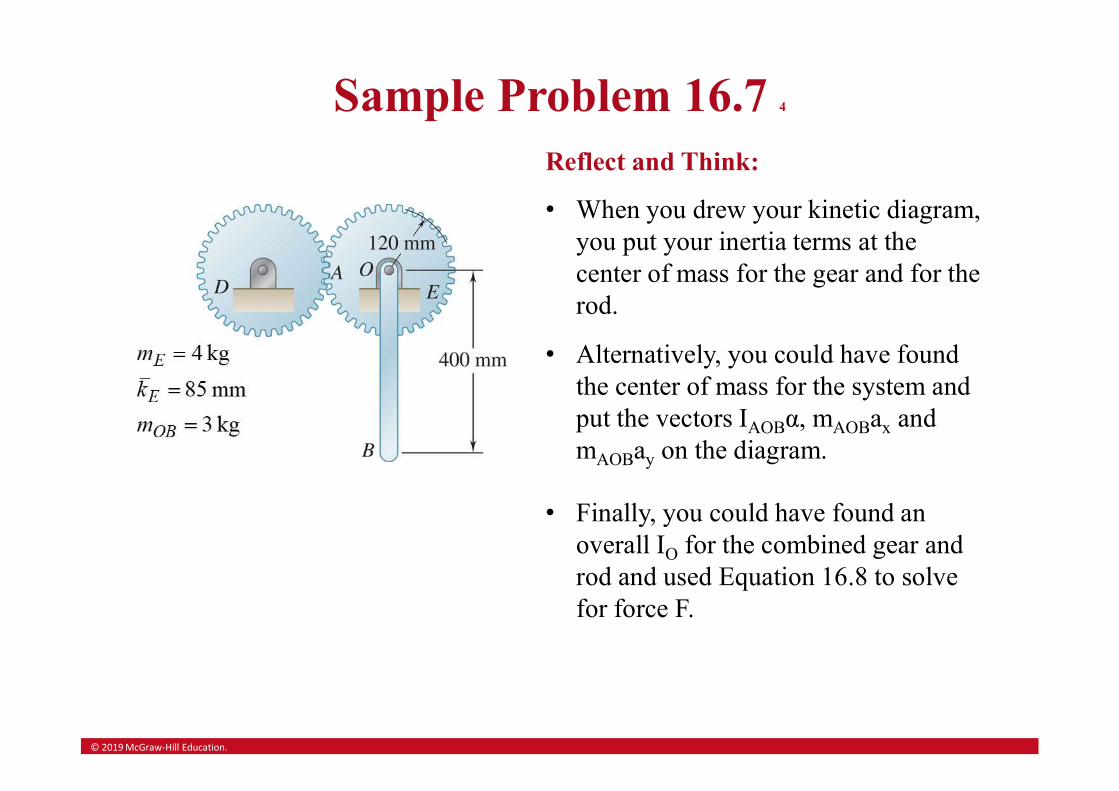
Sample Problem 16.7 4
Reflect and Think:
• When you drew your kinetic diagram, you put your inertia terms at the center of mass for the gear and for the rod.
• Alternatively, you could have found the center of mass for the system and put the vectors IAOBα, mAOBax and mAOBay on the diagram.
• Finally, you could have found an overall IO for the combined gear and rod and used Equation 16.8 to solve for force F.
© 2019 McGraw-Hill Education.
Sample Problem 16.9 1
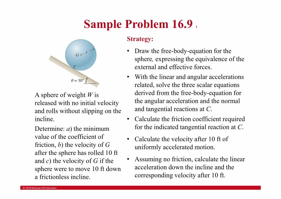
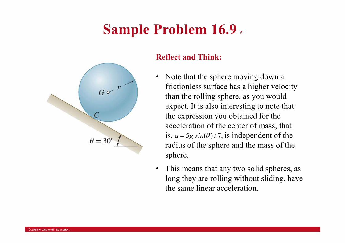
A sphere of weight W is released with no initial velocity and rolls without slipping on the incline.
Determine: a) the minimum value of the coefficient of friction, b) the velocity of Gafter the sphere has rolled 10 ftand c) the velocity of G if the sphere were to move 10 ft down a frictionless incline.
Strategy:
• Draw the free-body-equation for the sphere, expressing the equivalence of the external and effective forces.
• With the linear and angular accelerations related, solve the three scalar equations derived from the free-body-equation for the angular acceleration and the normal and tangential reactions at C.
• Calculate the friction coefficient required for the indicated tangential reaction at C.
• Calculate the velocity after 10 ft of uniformly accelerated motion.
• Assuming no friction, calculate the linear acceleration down the incline and the corresponding velocity after 10 ft.
© 2019 McGraw-Hill Education.
Sample Problem 16.9 2
ra
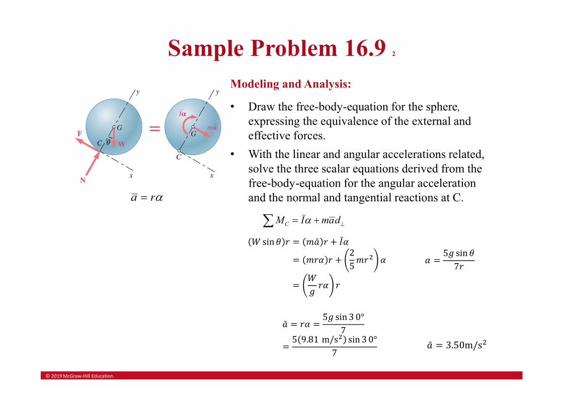
Modeling and Analysis:
• Draw the free-body-equation for the sphere,expressing the equivalence of the external and effective forces.
• With the linear and angular accelerations related, solve the three scalar equations derived from the free-body-equation for the angular acceleration and the normal and tangential reactions at C.
𝑊 sin 𝜃 𝑟 = 𝑚�̄� 𝑟 + 𝐼𝛼
= 𝑚𝑟𝛼 𝑟 +2
5𝑚𝑟 𝛼
=𝑊
𝑔𝑟𝛼 𝑟
𝛼 =5𝑔 sin 𝜃
7𝑟
�̄� = 𝑟𝛼 =5𝑔 sin 3 0°
7
=5 9.81 m/s sin 3 0°
7�̄� = 3.50m/s
damIMC
© 2019 McGraw-Hill Education.
Sample Problem 16.9 3
r
g
7
sin5 q
2sft50.11 ra
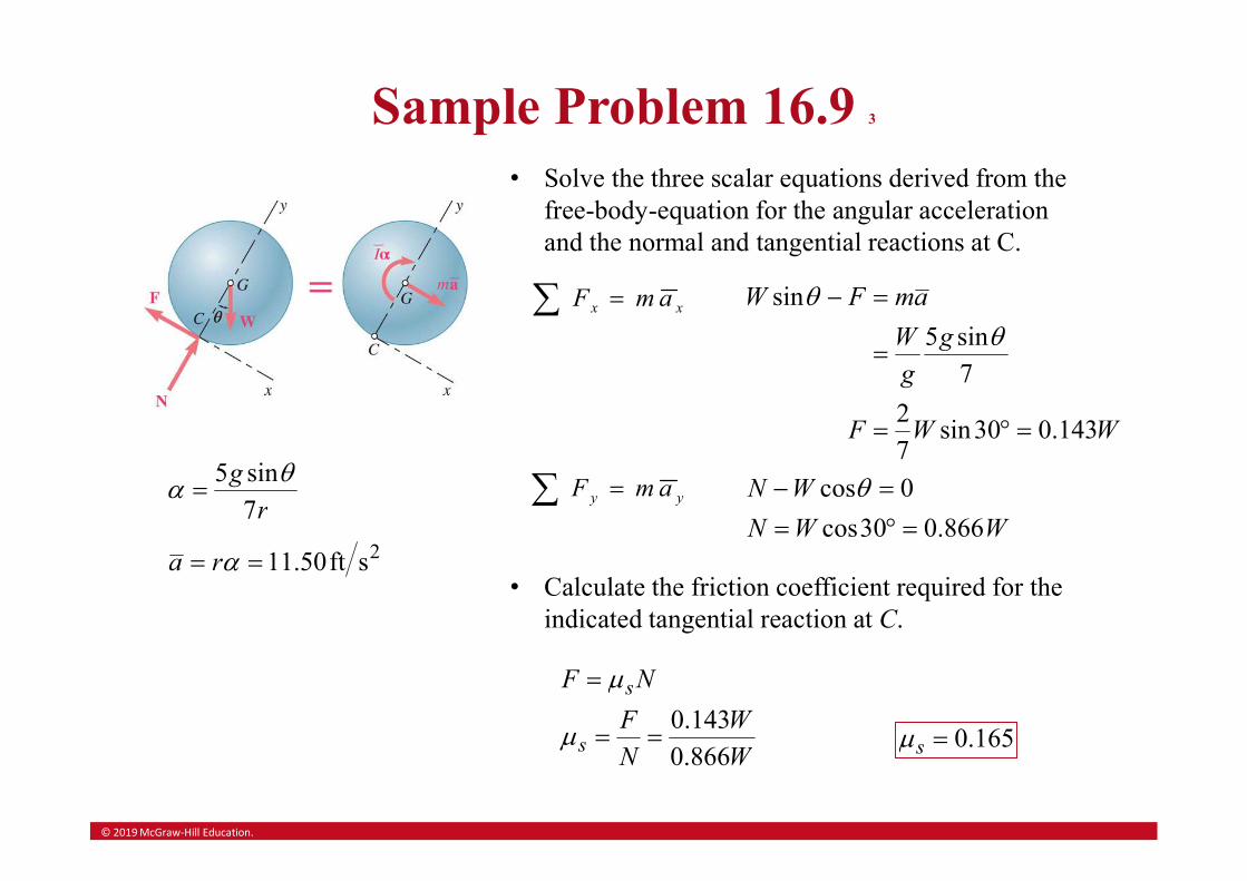
• Solve the three scalar equations derived from the free-body-equation for the angular acceleration and the normal and tangential reactions at C.
xx amF
WWF
g
g
W
amFW
143.030sin7
2
7
sin5
sin
q
q
yy amF WWN
WN
866.030cos
0cos
q
• Calculate the friction coefficient required for the indicated tangential reaction at C.
W
W
N
F
NF
s
s
866.0
143.0
m
m
165.0sm
© 2019 McGraw-Hill Education.
Sample Problem 16.9 4
r
g
7
sin5 q
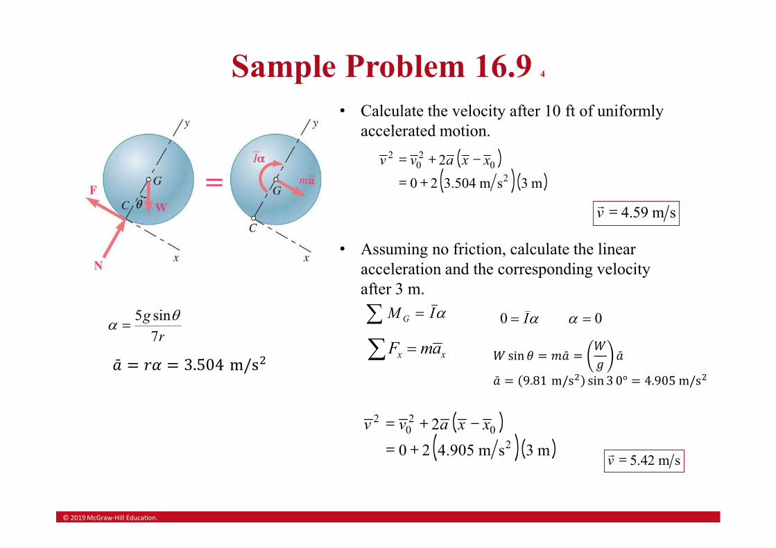
• Calculate the velocity after 10 ft of uniformly accelerated motion.
( )( )( )
2 20 0
2
2
0 2 3.504 m s 3 m
v v a x x= + -
= +
4.59 m sv =
• Assuming no friction, calculate the linear acceleration and the corresponding velocity after 3 m.
IM G 00 I
xx amF 𝑊 sin 𝜃 = 𝑚�̄� =𝑊
𝑔�̄�
�̄� = 9.81 m/s sin 3 0° = 4.905 m/s
( )( )( )
2 20 0
2
2
0 2 4.905 m s 3 m
v v a x x= + -
= +5.42 m sv =
© 2019 McGraw-Hill Education.
Sample Problem 16.9 5
Reflect and Think:
• Note that the sphere moving down a frictionless surface has a higher velocity than the rolling sphere, as you would expect. It is also interesting to note that the expression you obtained for the acceleration of the center of mass, that is, 5 ( ) / 7,a g sin q is independent of the radius of the sphere and the mass of the sphere.
• This means that any two solid spheres, as long they are rolling without sliding, have the same linear acceleration.
© 2019 McGraw-Hill Education.
Sample Problem 16.10 1
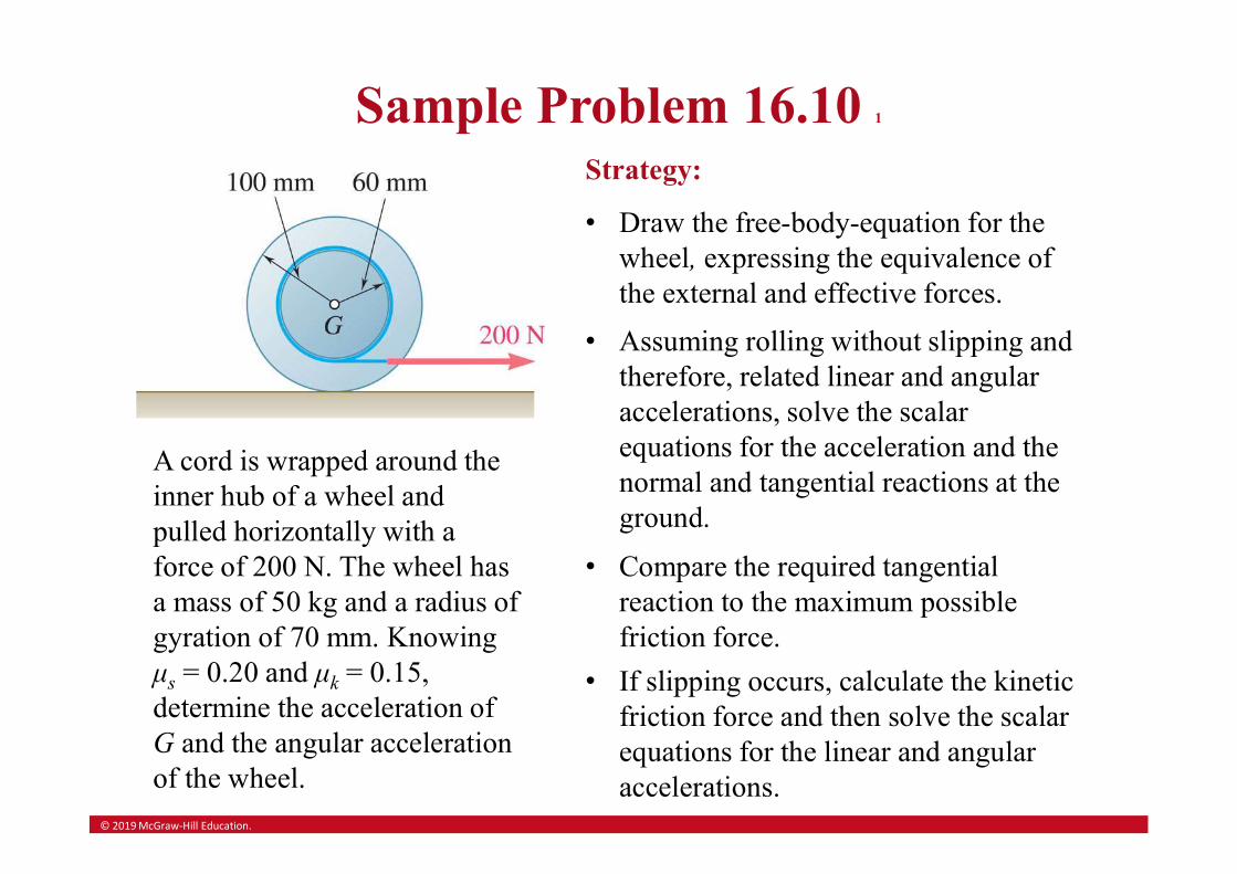
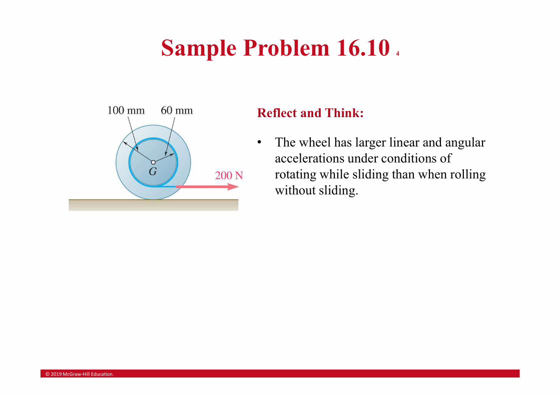
A cord is wrapped around the inner hub of a wheel and pulled horizontally with a force of 200 N. The wheel has a mass of 50 kg and a radius of gyration of 70 mm. Knowing μs = 0.20 and μk = 0.15, determine the acceleration of G and the angular acceleration of the wheel.
Strategy:
• Draw the free-body-equation for the wheel, expressing the equivalence of the external and effective forces.
• Assuming rolling without slipping and therefore, related linear and angular accelerations, solve the scalar equations for the acceleration and the normal and tangential reactions at the ground.
• Compare the required tangential reaction to the maximum possible friction force.
• If slipping occurs, calculate the kinetic friction force and then solve the scalar equations for the linear and angular accelerations.
© 2019 McGraw-Hill Education.
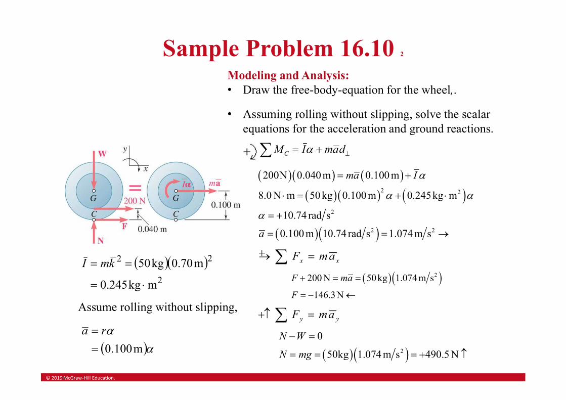
Sample Problem 16.10 2
2
22
mkg245.0
m70.0kg50
kmI
Assume rolling without slipping,
m100.0 ra
Modeling and Analysis:• Draw the free-body-equation for the wheel,.
• Assuming rolling without slipping, solve the scalar equations for the acceleration and ground reactions.
damIMC
2 2
2
2 2
200N 0.040 m 0.100 m
8.0 N m 50 kg 0.100 m 0.245kg m
10.74 rad s
0.100 m 10.74 rad s 1.074 m s
ma I
a
x xF m a 2200 N 50kg 1.074m s
146.3N
F ma
F
y yF ma
2
0
50kg 1.074 m s 490.5 N
N W
N mg
© 2019 McGraw-Hill Education.
Sample Problem 16.10 3
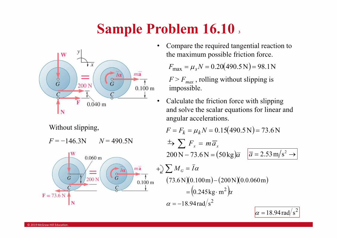
Without slipping,
F = −146.3N N = 490.5N
• Compare the required tangential reaction to the maximum possible friction force.
N1.98N5.49020.0max NF sm
F > Fmax , rolling without slipping is impossible.
• Calculate the friction force with slipping and solve the scalar equations for linear and angular accelerations.
N6.73N5.49015.0 NFF kk m
x xF m a akg50N6.73N200 22.53m sa
IM G
2
2
srad94.18
mkg245.0
m060.0.0N200m100.0N6.73
2srad94.18
© 2019 McGraw-Hill Education.
Sample Problem 16.10 4
Reflect and Think:
• The wheel has larger linear and angular accelerations under conditions of rotating while sliding than when rolling without sliding.
© 2019 McGraw-Hill Education.
Sample Problem 16.12 1
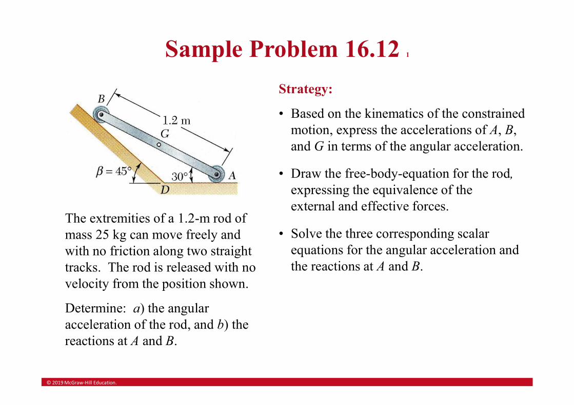
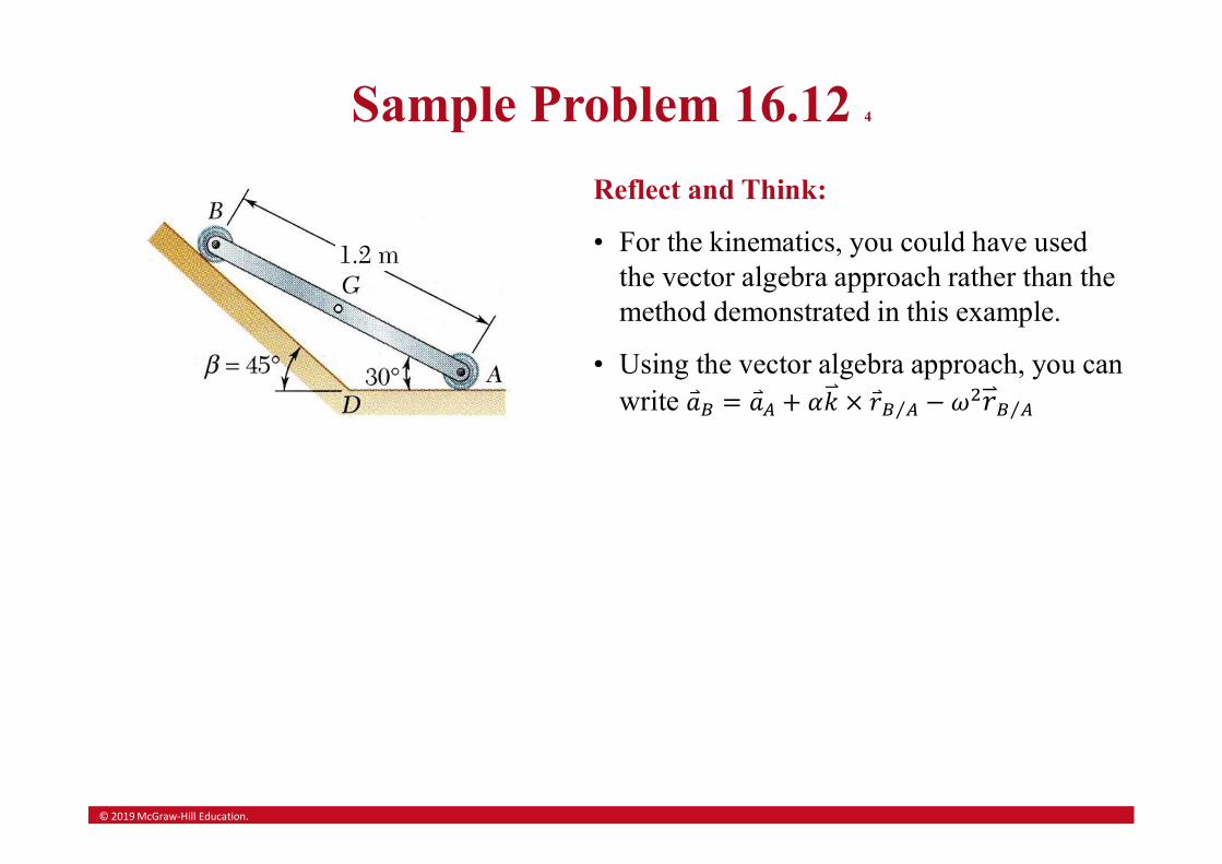
The extremities of a 1.2-m rod of mass 25 kg can move freely and with no friction along two straight tracks. The rod is released with no velocity from the position shown.
Determine: a) the angular acceleration of the rod, and b) the reactions at A and B.
Strategy:
• Based on the kinematics of the constrained motion, express the accelerations of A, B, and G in terms of the angular acceleration.
• Draw the free-body-equation for the rod,expressing the equivalence of the external and effective forces.
• Solve the three corresponding scalar equations for the angular acceleration and the reactions at A and B.
© 2019 McGraw-Hill Education.
Sample Problem 16.12 2
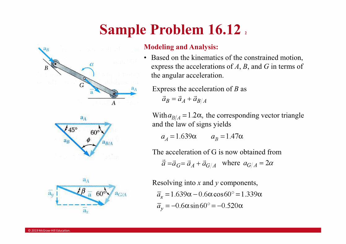
Modeling and Analysis:
• Based on the kinematics of the constrained motion, express the accelerations of A, B, and G in terms of the angular acceleration.
Express the acceleration of B as
ABAB aaa
With the corresponding vector triangle and the law of signs yields
The acceleration of G is now obtained from
AGAG aaaa
2 where AGa
Resolving into x and y components,
© 2019 McGraw-Hill Education.
Sample Problem 16.12 3
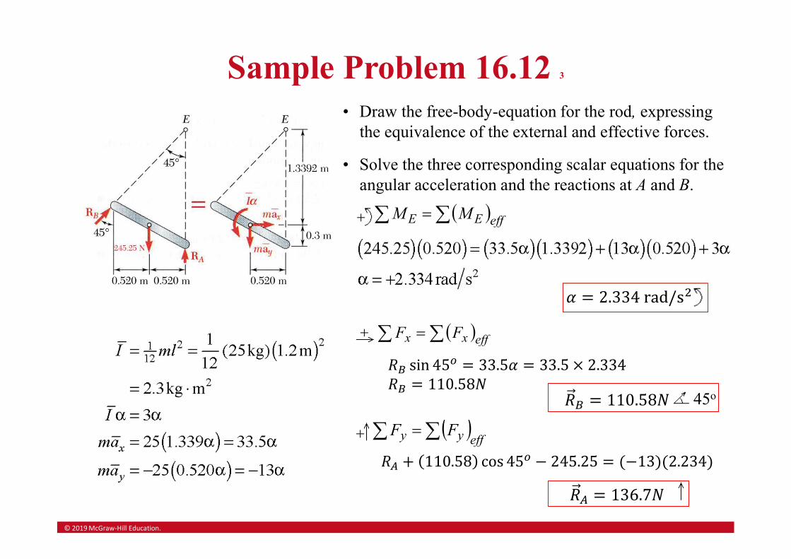
• Draw the free-body-equation for the rod, expressing the equivalence of the external and effective forces.
• Solve the three corresponding scalar equations for the angular acceleration and the reactions at A and B.
effEE MM
effxx FF
45o
effyy FF
𝑅 sin 45 = 33.5𝛼 = 33.5 × 2.334𝑅 = 110.58𝑁
𝑅 + 110.58 cos 45 − 245.25 = (−13)(2.234)
© 2019 McGraw-Hill Education.
Sample Problem 16.12 4
Reflect and Think:
• For the kinematics, you could have used the vector algebra approach rather than the method demonstrated in this example.
• Using the vector algebra approach, you can write ⁄ ⁄

© 2019 McGraw-Hill Education.
Group Problem Solving 5
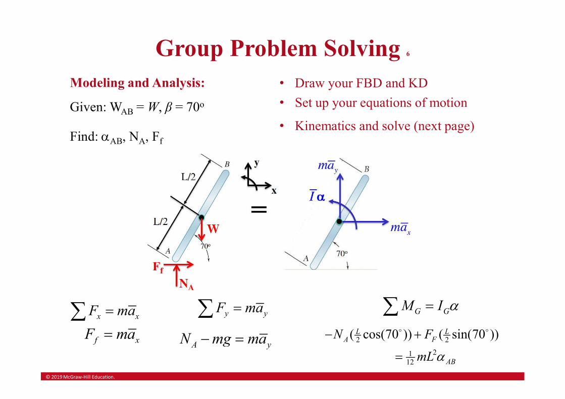
The uniform rod AB of weight W is released from rest when β = 70o. Assuming that the friction force between end A and the surface is large enough to prevent sliding, determine immediately after release (a) the angular acceleration of the rod, (b) the normal reaction at A, (c) the friction force at A.
Strategy:
• Draw the free-body-diagram and kinetic diagram showing the equivalence of the external forces and inertial terms.
• Write the equations of motion for the sum of forces and for the sum of moments.
• Apply any necessary kinematic relations, then solve the resulting equations.
© 2019 McGraw-Hill Education.
Group Problem Solving 6
Modeling and Analysis:
Given: WAB = W, β = 70o
Find: AB, NA, Ff
• Draw your FBD and KD
• Set up your equations of motion
x xF maf xF ma
y yF maA yN mg ma
G GM I 2 2
2112
( cos(70 )) ( sin(70 ))
L LA F
AB
N F
mL
• Kinematics and solve (next page)
© 2019 McGraw-Hill Education.
Group Problem Solving 7
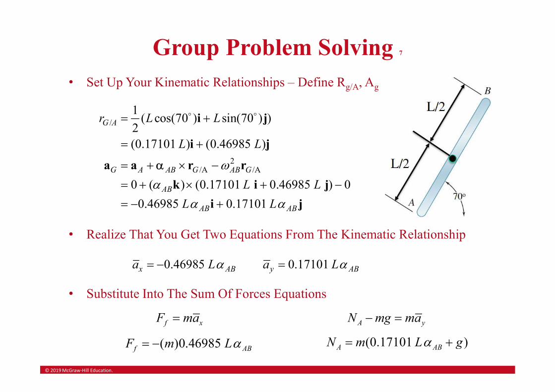
• Set Up Your Kinematic Relationships – Define Rg/A, Ag
/
2/A /A
1( cos(70 ) sin(70 ) )
2(0.17101 ) (0.46985 )
0 ( ) (0.17101 0.46985 ) 0
0.46985 0.17101
G A
G A AB G AB G
AB
AB AB
r L L
L L
L L
L L
i j
i j
a a r r
k i j
i j
• Realize That You Get Two Equations From The Kinematic Relationship
0.46985 0.17101 x AB y ABa L a L
• Substitute Into The Sum Of Forces Equations
f xF ma
( )0.46985 f ABF m L
A yN mg ma
(0.17101 )A ABN m L g
© 2019 McGraw-Hill Education.
Group Problem Solving 8
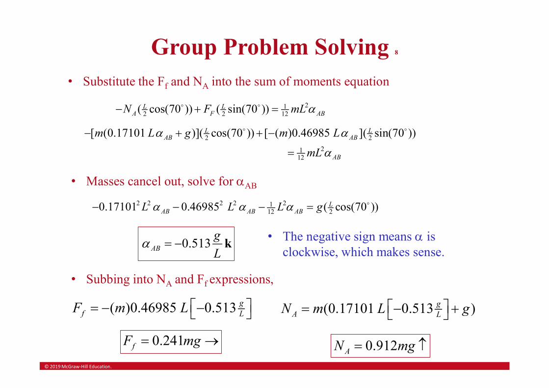
• Substitute the Ff and NA into the sum of moments equation
212 2 12( cos(70 )) ( sin(70 ))L L
A F ABN F mL
2 2
2112
[ (0.17101 )]( cos(70 )) [ ( )0.46985 ]( sin(70 ))
L LAB AB
AB
m L g m L
mL
• Masses cancel out, solve for AB
2 2 2 2 2112 20.17101 0.46985 ( cos(70 ))L
AB AB ABL L L g
0.513AB
g
L k • The negative sign means is
clockwise, which makes sense.
• Subbing into NA and Ff expressions,
( )0.46985 0.513 gf LF m L
0.241fF mg
(0.17101 0.513 )gA LN m L g
0.912AN mg
© 2019 McGraw-Hill Education.
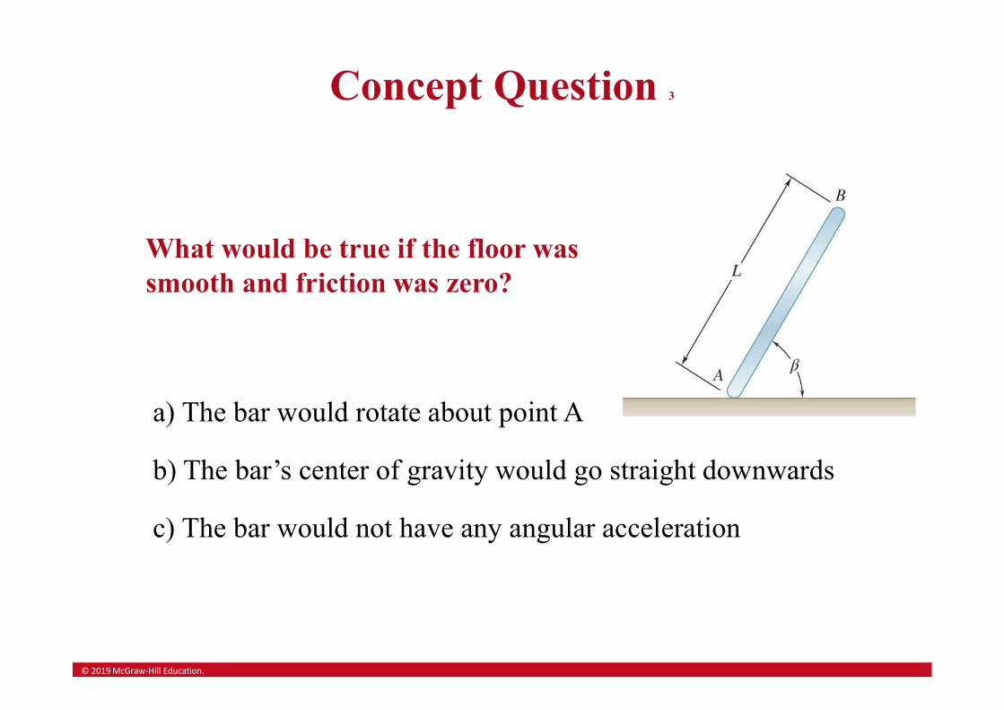
Concept Question 3
What would be true if the floor was smooth and friction was zero?
a) The bar would rotate about point A
b) The bar’s center of gravity would go straight downwards
c) The bar would not have any angular acceleration
© 2019 McGraw-Hill Education.
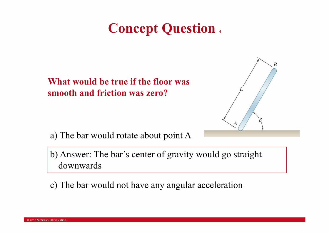
Concept Question 4
What would be true if the floor was smooth and friction was zero?
a) The bar would rotate about point A
b) Answer: The bar’s center of gravity would go straight downwards
c) The bar would not have any angular acceleration
© 2019 McGraw-Hill Education.
End of Chapter 16
Copyright © 2022 FDOKUMEN


![4.1.1] plane waves](https://static.fdokumen.com/doc/165x107/6322513728c445989105b845/411-plane-waves.jpg)