Citation: Zhou, Q.; Lo, L.-Y.; Jiang, B.;

Chang, C.-W.; Wen, C.-Y.; Chen, C.-K.;

Zhou, W. Development of

Fixed-Wing UAV 3D Coverage Paths

for Urban Air Quality Profiling.

Sensors 2022, 22, 3630. https://

doi.org/10.3390/s22103630

Academic Editor:

Sergio Toral Marín

Received: 5 April 2022

Accepted: 7 May 2022

Published: 10 May 2022

Publisher’s Note: MDPI stays neutral

with regard to jurisdictional claims in

published maps and institutional affil-

iations.

Copyright: © 2022 by the authors.

Licensee MDPI, Basel, Switzerland.

This article is an open access article

distributed under the terms and

conditions of the Creative Commons

Attribution (CC BY) license (https://

creativecommons.org/licenses/by/

4.0/).

sensors

Article

Development of Fixed-Wing UAV 3D Coverage Paths for UrbanAir Quality ProfilingQianyu Zhou 1 , Li-Yu Lo 1 , Bailun Jiang 1 , Ching-Wei Chang 2 , Chih-Yung Wen 1 , Chih-Keng Chen 3

and Weifeng Zhou 4,*

1 Department of Aeronautical and Aviation Engineering, The Hong Kong Polytechnic University, Kowloon,Hong Kong; q1zhou@polyu.edu.hk (Q.Z.); liyu.lo@connect.polyu.hk (L.-Y.L.);bailun-robin.jiang@connect.polyu.hk (B.J.); chihyung.wen@polyu.edu.hk (C.-Y.W.)

2 Department of Mechanical Engineering, The Hong Kong Polytechnic University, Kowloon, Hong Kong;chingwei.chang@connect.polyu.hk

3 Department of Vehicle Engineering, National Taipei University of Technology, Taipei 10608, Taiwan;ckchen@ntut.edu.tw

4 School of Professional Education and Executive Development, The Hong Kong Polytechnic University,Kowloon, Hong Kong

* Correspondence: chandler.zhou@cpce-polyu.edu.hk; Tel.: +852-3746-0127

Abstract: Due to the ever-increasing industrial activity, humans and the environment suffer fromdeteriorating air quality, making the long-term monitoring of air particle indicators essential. Theadvances in unmanned aerial vehicles (UAVs) offer the potential to utilize UAVs for various forms ofmonitoring, of which air quality data acquisition is one. Nevertheless, most current UAV-based airmonitoring suffers from a low payload, short endurance, and limited range, as they are primarilydependent on rotary aerial vehicles. In contrast, a fixed-wing UAV may be a better alternative.Additionally, one of the most critical modules for 3D profiling of a UAV system is path planning, as itdirectly impacts the final results of the spatial coverage and temporal efficiency. Therefore, this workfocused on developing 3D coverage path planning based upon current commercial ground controlsoftware, where the method mainly depends on the Boustrophedon and Dubins paths. Furthermore, auser interface was also designed for easy accessibility, which provides a generalized tool module thatlinks up the proposed algorithm, the ground control software, and the flight controller. Simulationswere conducted to assess the proposed methods. The result showed that the proposed methodsoutperformed the existing coverage paths generated by ground control software, as it showed a bettercoverage rate with a sampling density of 50 m.

Keywords: air quality; monitoring; fixed-wing UAV; coverage path planning

1. Introduction

Over the past few decades, rapid economic growth has resulted in skyrocketed pop-ulation growth and industrialization in many major metropolitan areas. The increase inurbanization has led to a series of environmental consequences, with the drastic increase inatmospheric pollutants being one of them. Undoubtedly, the deterioration in air qualityhas become a global issue and has caused adverse impacts on both the environment andsociety, demanding immediate resolutions. Li et al. [1] further advocated that the globalair pollution issue requires different means to resolve depending on the location sincethe causes vary; for instance, the PM 2.5 particles in Asian countries are mainly causedby heating and cooking, whereas agriculture is the culprit in European countries. Thishence makes monitoring the pollutant concentration and distribution essential so that thecomposition of toxicities can be further quantified [2].

Currently, environmental authorities around the globe have established methods tomeasure and monitor atmospheric indicators. For instance, the Environment Protection

Sensors 2022, 22, 3630. https://doi.org/10.3390/s22103630 https://www.mdpi.com/journal/sensors

Sensors 2022, 22, 3630 2 of 23

Department (EPD) of the Hong Kong Special Administrative Region (HKSAR) has beentracking street-level pollution as well as the regional smog problem through the installationof ground monitoring stations and publishing the measured data [3]. The method has gener-ally been applicable with high robustness and could be seen in various places; nevertheless,such a conventional method is deemed spatio-temporally inflexible, as the sampling pointsare stationary and limited, while skilled personnel are required to conduct measurementswith higher accuracy [4]. Therefore, many research and governmental institutions furtheremploy crewed aircraft or satellites for larger-scale monitoring activities [4], such as thework proposed or mentioned by [5–8]. Although it is considered that satellites and aerialsensors can cover more sampling points and provide complete profiling information, thehigher deployment and maintenance cost of those technologies also brings inaccessibilityto the general public, making the task operationally difficult [4].

In recent years, with the advances in unmanned aerial vehicles (UAVs), many re-searchers have proposed to utilize the technology to carry out monitoring jobs, as theyhave lower cost, higher autonomy, and easier availability [9]. Gu et al. [10] developedan end-to-end quadrotor-based air pollution profiling system. They tried to reach fullautonomy by integrating the drone, the ground station software, the sensors, and thedata acquisition and fusion modules. Similarly, the authors in [11] attempted to track andanalyze the SO2 and NO2 of ship plumes by exploiting a rotary unmanned aerial vehicleand embedded air quality sensors. Based on a similar configuration, Araujo et al. [12]programmed different flight patterns for a commercial drone to evaluate the efficacy ofmeasuring air pollutants. Jumaah et al. [13] also developed a UAV-based air monitoringsystem, where a hex-rotor was utilized to assess PM2.5 particles. Similar work applyingUAVs for air quality surveying can also be found in [14–18]. Furthermore, among theaforementioned projects, many adopt coverage path planning (CPP) methods to ensure ahigh coverage rate of a certain region of interest (ROI). The method can be frequently seenin several robotic applications, such as vacuum robots [19], photogrammetry drones [20],or automatic lawnmowers [21], in which paths are searched and determined to visit allinterest points within the ROI [22]. In specific, to acquire such a path, CPP can be modeledas a traveling salesman problem (TSP) [22], in which the NP-hard problem is then solvedwith heuristic or complete methods [23]; the final output then allows the agent to travelall points on the network without duplicated visits. For a deeper understanding of thetraveling salesman problem, we refer readers to [23,24].

Despite a considerable body of research on air quality monitoring rotary dronesutilizing coverage path planning methods, we argue that the practicality of such a systemdesign is still discounted. Particularly, due to the size, weight, and power (SWaP) limitationsof most currently commercialized drones, the payload, range, and endurance are usuallyrestricted [25], making large-scale air quality monitoring missions temporally and spatiallyunsustainable [4]. In contrast, fixed-wing-based UAVs provide a plausible alternative; inrecent years, several research studies on fixed-wing aircraft for remote sensing applicationshave been published. For instance, Simon et al. [26] utilized a tail-sitter configurationUAV to conduct 3D mapping of the terrain of a specific region, in which they tried todirectly acquire photogrammetric information via a lightweight VTOL aerial vehicle. Workconducted by Coombes et al. [27–30], on the other hand, developed coverage path planningmethods through geometry decomposition, Boustrophedon paths, etc., and meanwhile,different scenarios were addressed, including utilization in agriculture activities and windysituations. Paull et al. [31] also proposed a path planner that attempted to achieve acoverage path without a priori understanding of the workspace, in which a camera sensorwas equipped, and an in situ path planning module was included for the aircraft tomake control decisions. In addition to all of the above, Yu et al. [32] utilized the knee-guided differential evolution algorithm [33] to construct a path planning problem forUAVs for disaster scenarios within 3D terrain situations. In particular, the work aimed tosolve the problem by utilizing B-spline paths and modeling the task with multi-objectiveoptimization, where distance and risk are mainly considered as the objective functions;

Sensors 2022, 22, 3630 3 of 23

such a method could then offer an optimal solution and allow the vehicle to follow asmooth path.

Therefore, motivated by the pioneering works, this study utilized a vertical takeoffand landing (VTOL) configuration UAV to conduct a 3D air quality profiling task, as it isdeemed to have a higher range and longer endurance than rotary UAV, as well as a lowercost and easier deployment (requires no open area or takeoff runway) than crewed aircraft.Particularly, this research aimed to develop an easy-access coverage path planning module,which automatically generates a kinematic feasible path for a VTOL UAV of quad-planeconfiguration for 3D air quality profiling. In addition, to make the proposed system moreaccessible to the public, a user interface was added for all users from different fields todeploy the VTOL UAV. Therefore, the objectives were as follows:

1. To design a 3D coverage path planning algorithm that outputs a path aligning withthe quad-plane physical feasibilities based upon a 3D voxel region of interest (ROI) inGPS coordinates, which are inputted according to user specifications;

2. In addition to the planner, design an easy-access user interface written in pythonscript for users to interact with the module;

3. To carry out simulations within the software-in-the-loop platform, in which theefficiency of our method is assessed by comparing it with the default software paths.

To address the above, the remainder of this article is organized as follows. Section 2outlines the significant materials and methodologies of the coverage path planning for 3Dprofiling. Then, Section 3 discusses the simulation results. Lastly, Section 4 projects possiblefuture work and improvements.

2. Materials and Methods

In order to perform a 3D air quality profiling of an ROI, the proposed work consists ofthe following modules: (1) coverage path generation for 3D air quality profiling, (2) securereturn to launch path generation, (3) an easy-access user interface, and (4) ground controlstation software.

2.1. Coverage Path Generation for 3D Air Quality Profiling

As mentioned in Section 1, currently, there is no optimal coverage path planningmethod for fixed-wing UAVs; most flight missions are either generated manually by humaninput or by the default photogrammetric purpose auto-grid method from ground controlsoftware. Currently, ArduPilot Mission Planner [34] and QGroundControl [35] are two ofthe most widespread open-source software. These methods, when being applied to fixed-wing aircraft, have disadvantages of the following: (1) low efficiency, as the waypoints arerequired to be manually inputted through ground control software [34,35]; (2) empiricismdependency, where operators should be equipped with basic knowledge of coverage pathsso that the ROI can be completely surveyed; and (3) lack of compliance with the dynamicfeasibilities of fixed-wing vehicles, as in photogrammetric purpose auto-grid paths [20], themethodology is mainly designed for rotary UAVs, and applicability on fixed-wing planescan be suboptimal. Hence, this study asserts the importance of an automatic calculation-and theory-based coverage path planning algorithm, in particular for air quality sensingmissions. The following further elucidates the methodologies of the proposed coveragepath planner.

2.1.1. Coverage Path Planning Constraints for Fixed-Wing Aircrafts

To perform 3D ROI air quality profiling, the coverage path should be designed to coverall the voxels or sampling points within an ROI as densely as possible, i.e., maximizing thecoverage rate. For the common coverage path planning of an ROI in quadrotor applications,many adopt the Boustrophedon path [36,37], in which the vehicle follows an iterating backand forth path to cover the ROI, as shown in Figure 1.

Sensors 2022, 22, 3630 4 of 23

Figure 1. An instance of a Boustrophedon path.

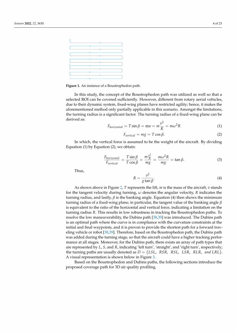
In this study, the concept of the Boustrophedon path was utilized as well so that aselected ROI can be covered sufficiently. However, different from rotary aerial vehicles,due to their dynamic system, fixed-wing planes have restricted agility; hence, it makes theaforementioned method only partially applicable in this scenario. Amongst the limitations,the turning radius is a significant factor. The turning radius of a fixed-wing plane can bederived as:

Fhorizontal = T sin β = ma = mv2

R= mω2R (1)

Fvertical = mg = T cos β. (2)

In which, the vertical force is assumed to be the weight of the aircraft. By dividingEquation (1) by Equation (2), we obtain:

FhorizontalFvertical

=T sin β

T cos β=

m v2

Rmg

=mω2R

mg= tan β. (3)

Thus,

R =v2

g tan β. (4)

As shown above in Figure 2, T represents the lift, m is the mass of the aircraft, v standsfor the tangent velocity during turning, ω denotes the angular velocity, R indicates theturning radius, and lastly, β is the banking angle. Equation (4) then shows the minimumturning radius of a fixed-wing plane; in particular, the tangent value of the banking angle βis equivalent to the ratio of the horizontal and vertical force, indicating a limitation on theturning radius R. This results in low robustness in tracking the Boustrophedon paths. Toresolve the low maneuverability, the Dubins path [38,39] was introduced. The Dubins pathis an optimal path where the curve is in compliance with the curvature constraints at theinitial and final waypoints, and it is proven to provide the shortest path for a forward trav-eling vehicle or robot [38,39]. Therefore, based on the Boustrophedon path, the Dubins pathwas added during the turning stage, so that the aircraft could have a higher tracking perfor-mance at all stages. Moreover, for the Dubins path, there exists an array of path types thatare represented by L, S, and R, indicating ‘left turn’, ‘straight’, and ‘right turn’, respectively;the turning paths are usually denoted as D = {LSL, RSR, RSL, LSR, RLR, and LRL}.A visual representation is shown below in Figure 3.

Based on the Boustrophedon and Dubins paths, the following sections introduce theproposed coverage path for 3D air quality profiling.

Sensors 2022, 22, 3630 5 of 23

Figure 2. The force diagram of a turning plane with a banking angle of β.

Figure 3. Classification of Dubins paths.

2.1.2. Cycle-Boustrophedon Path Planning

Given a specified cubic ROI with vertices v = {v1, v2, v3, v4} in GPS coordinates andaltitude boundaries of hmax and hmin in meters, a coverage path was planned to completean air quality profiling task with a predefined sampling density d (all notations d in thismanuscript stand for the sampling density as described here). To perform the calculation,coordination transformation (illustrated in Figure 4) was first conducted:

vθ =

[cos θ − sin θsin θ cos θ

]v (5)

where θ is calculated via the relative rotation angle of the ROI to the global frame. The pathwas then planned within the local frame and rotated back afterward.

Sensors 2022, 22, 3630 6 of 23

Figure 4. Coordination transformation from GPS coordinates frame to local frame; in which, the xaxis and the y axis of the local frame are defined leftward and downward, respectively.

For a conventional Boustrophedon path, each parallel track is executed in seriesadjacently; however, in this scenario, to have a smoother turn for fixed-wing planes, wefirst segregated the tracks into two sub-Boustrophedon groups, even and odd orders, wherethey would be followed consecutively. Consequently, each level of altitude was required tocomplete two ‘cycles’ of paths, hence the name ‘cycle-Boustrophedon’. Figure 5a shows theoriginal Boustrophedon method, whilst the illustration on the right (Figure 5b) displaysthe proposed method. Specifically, the blue, which is the ‘even order’, is first implemented,and then the paths in orange, which are the ‘odd order’, are followed. Notably, the “odd”and “even” orders refer to the horizontal path orders from top to bottom in Figure 5b.Furthermore, to fulfill the profiling density, the distance between the abutting tracks shouldbe d, making the distance between the tracks in the sub-Boustrophedon group 2d. Theproposed planning was duplicated vertically in layers, with the number of layers beingn = hmax−hmin

d + 1. We believed that this addition to the conventional Boustrophedon pathswould allow the fixed-wing aircraft to have a more optimal performance, since the majorityof the sampling density possesses a smaller scale than the minimum radius of the UAV.

Figure 5. (a) Conventional Boustrophedon path and (b) the proposed cycle-Boustrophedon path.

After setting the main tracks of the proposed cycle-Boustrophedon paths, Dubinspaths were then added at the turning points for further path optimization. As thereexists a minimum turning radius (which is defined as r1 below) for a fixed-wing plane,and since for each turning point, the aircraft is required to make a 180-degree turn, anLRL/RLR or LSL/RSR type Dubins path was added to the sub-Boustrophedon path. The

Sensors 2022, 22, 3630 7 of 23

determination of using either the LRL/RLR or LSL/RSR type Dubins path depended onthe user predefined sampling density, as:{

d < R, Ddubins ∈ LRL/RLRd ≥ R, Ddubins ∈ LSL/RSR

(6)

Figure 6a,b above illustrate the two aforementioned types. To perform the above,waypoints were further defined. For the LRL/RLR with the RLR, for instance as shown inFigure 7, for each turning, the following points (from a bird’s eye view) were first defined:

assume point A = {a1, a2}, & α = arccos(

r1 + d2r1

), r1 = R =

V2

g tan β. (7)

Hence, A = (a1, a2)

B = (a1 + r1 sinα, a2 + r1 (cos α− 1))C = (a1 + r1(2 sin α + 1), a2 + d)

B′ = (a1 + r1(sin α), a2 + r1(1− cos α) + 2d)A′ = (a1, a2 + 2d)

. (8)

Figure 6. (a) illustrates the Dubins path (an RLR instance) when d < R, whereas (b) shows the Dubinspath (an LSL instance) when d ≥ R.

Figure 7. Dubins path (RLR) when d < R, where the aircraft first turns right, then left, and lastlyright to complete the Dubins path.

Sensors 2022, 22, 3630 8 of 23

The waypoint radius was further considered to obtain better performance, apart fromthe above-listed waypoints. The waypoint radius is a default parameter for flight controllersto justify whether the system has reached the desired waypoint; for most fixed-wing aircraft,as they have lower maneuverability, the waypoint radius is usually set at a large scale(compared to rotary vehicles). Therefore, in this scenario, where each waypoint is relativelyclose to another, the waypoint radius r2 was further considered when conducting pathplanning. Figure 8 shows the final waypoints.

Figure 8. Dubins path (RLR) with the waypoint radius taken into consideration, which is deemed toincrease the turning performance, resulting in a better trajectory.

The coordinates are:A = (a1, a2)

B1 = (a1 + r1 sinα, a2 + r1 (cos α− 1)− r2)C1 = (a1 + r1(2 sin α + 1) + r2, a2 + d)

B’1 = (a1 + r1(sin α), a2 + r1(1− cos α) + 2d + r2)

A′ = (a1, a2 + 2d)

. (9)

Therefore, to complete one iteration of the cycle-Boustrophedon path, there were bothRLR and LRL Dubins paths and 10 waypoints in total, as shown in Figure 9 (A→B→C→B’→A’→D→E→F→E’→D’).

Figure 9. Dubins path (RLR + LRL) for each iteration.

Sensors 2022, 22, 3630 9 of 23

For the LSL/RSR, as shown in Figure 6b, taking LSL for instance, fewer waypointswere needed; these waypoints are defined as:

A = (a1, a2)B = (a1 + r, a2 + r)

B′ = (a1 + r, a2 + 2d− r)A′ = (a1, a2 + 2d)

. (10)

Similarly, as the waypoints were relatively close to each other, the waypoint radiusshould also be considered, making the final waypoints:

A = (a1, a2)B1 = (a1 + r1 + r2, a2 + r1)

B′1 = (a1 + r1 + r2, a2 + 2d− r1)A′ = (a1, a2 + 2d)

. (11)

Therefore, for each iteration, there were both LSL and RSR Dubins paths and 8 way-points in total in the proposed method (shown in Figure 10, A→B→B’→A’→C→D→D’→C’).

Figure 10. Dubins path (LSL + RSR) when d ≥ R for one iteration.

The following pseudo-code shows the overall cycle-Boustrophedon path planningAlgorithm 1:

Sensors 2022, 22, 3630 10 of 23

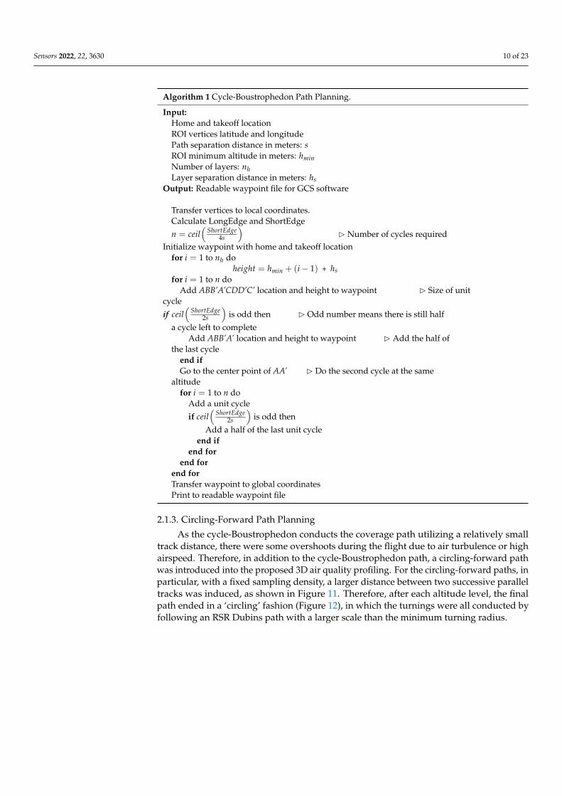
Algorithm 1 Cycle-Boustrophedon Path Planning.

Input:Home and takeoff locationROI vertices latitude and longitudePath separation distance in meters: sROI minimum altitude in meters: hminNumber of layers: nhLayer separation distance in meters: hs

Output: Readable waypoint file for GCS software

Transfer vertices to local coordinates.Calculate LongEdge and ShortEdge

n = ceil(

ShortEdge4s

)B Number of cycles required

Initialize waypoint with home and takeoff locationfor i = 1 to nh do

height = hmin + (i− 1) ∗ hsfor i = 1 to n do

Add ABB’A’CDD’C’ location and height to waypoint B Size of unitcycle

if ceil(

ShortEdge2s

)is odd then B Odd number means there is still half

a cycle left to completeAdd ABB’A’ location and height to waypoint B Add the half of

the last cycleend ifGo to the center point of AA’ B Do the second cycle at the same

altitudefor i = 1 to n do

Add a unit cycle

if ceil(

ShortEdge2s

)is odd then

Add a half of the last unit cycleend if

end forend for

end forTransfer waypoint to global coordinatesPrint to readable waypoint file

2.1.3. Circling-Forward Path Planning

As the cycle-Boustrophedon conducts the coverage path utilizing a relatively smalltrack distance, there were some overshoots during the flight due to air turbulence or highairspeed. Therefore, in addition to the cycle-Boustrophedon path, a circling-forward pathwas introduced into the proposed 3D air quality profiling. For the circling-forward paths, inparticular, with a fixed sampling density, a larger distance between two successive paralleltracks was induced, as shown in Figure 11. Therefore, after each altitude level, the finalpath ended in a ‘circling’ fashion (Figure 12), in which the turnings were all conducted byfollowing an RSR Dubins path with a larger scale than the minimum turning radius.

Sensors 2022, 22, 3630 11 of 23

Figure 11. One iteration of the circling-forward path.

Figure 12. The final circling-forward path.

Moreover, for the waypoints at each iteration, as the distances between them were ona relatively large scale, the effect induced by the waypoint radius could be neglected in thiscase, whilst the Dubins path could be simply defined by the corner waypoints; this meansthe final waypoints were the following:

A = (a1, a2)B = (a1 − r1, a2)

C = (a1 − r1, a2 + 0.5ShortEdge + d)D =

(a1 + LongEdge + r1, a2 +

12 ShortEdge + d

)E = (a1 + LongEdge + r1, a2 + d)

(12)

where point A is the starting position of each circling iteration, and ‘ShortEdge’ and‘LongEdge’, respectively, stand for the shorter edge and longer edge of the ROI rectangle.

The following pseudo-code shows the overall circling-forward path planning Algorithm 2:

Sensors 2022, 22, 3630 12 of 23

Algorithm 2 Circling-forward Path Planning.

Input:Home and takeoff locationROI vertices latitude and longitudePath separation distance in meters: sROI minimum altitude in meters: hminNumber of layers: nhLayer separation distance in meters: hs

Output: Readable waypoint file for GCS software

Transfer vertices to local coordinates.Calculate LongEdge and ShortEdge

n = ceil(

ShortEdge2s

)B Number of cycles required

if n is odd then B Odd n results in an uncovered path at middle of ROIn = n + 1 B Round n up to even number

end ifBC = s ∗ (n + 1) B Size of unit cycle

DE = s ∗ nCD = CD + 2r1 B Expand LongEdge for full coverageInitialize waypoint with home and takeoff location

for i = 1 to nh doheight = hmin + (i− 1) ∗ hs

for i = 1 to n doAdd BCDE location and height to waypoint

Move unit cycle along BC by send for

end forTransfer waypoint to global coordinatesPrint to readable waypoint file

2.2. Secure Return to Launch Path Generation

After the coverage path planning, it is considered that the landing path is also essentialto ensure the aircraft chooses a safe and proper route. The two key factors of this return tolaunch path are the controlled descent rate and turn rate. This study proposes an alternateapproach for a landing strategy, in which the aircraft circles along the edge of the ROI witha constant and secure descent rate rather than return toward the home position directly.After the UAV descends to a safe altitude, which in our case was 100 above ground, theUAV then flies toward the launch point and switches to the multi-rotor mode to land. Thefollowing pseudo-code shows the overall return to launch path generation Algorithm 3:

Algorithm 3 Return to Launch Path Generation.

Cycling path completed.while height ≥ 100 do

height = height− EdgeLength ∗ tan(θ) B θ is fixed glide angleAdd next ROI vertex location and height to waypoint

end whileAdd launch location to waypointTransfer to quadrotor mode and land

2.3. Easy-Access User Interface

For general utilization, an easy-access user interface was further designed. The useris only requested to input the required ROI for 3D air quality profiling in terms of GPScoordinates while defining the grid dimension, i.e., the profiling density; the applicationthen passes the parameters to the algorithm elaborated in Section 2.1. In addition, thedesigned module acts as the application programming interface (API) between the pro-

Sensors 2022, 22, 3630 13 of 23

posed algorithm and ground control station software, as it passes the generated waypointsfile to the software (‘.waypoints’ file for Mission Planner and ‘.plan’ file for QGroundCon-trol). Figure 13 shows the screenshot of the application’s appearance in which users areallowed to define the vertices (v = {v1, v2, v3, v4}) of the ROI in the first four entry bracketsand the desired altitudes of the ROI in the fifth and sixth entry brackets, as well as thesampling density.

Figure 13. The designed GUI for air quality profiling coverage path planning.

2.4. Ground Control Station Software

Ground control station software usually refers to the software platform for launchingand retracting aerial vehicles, which usually acts as a communication module between thepilot and the unmanned aircraft. For most commercial or open-source software, detailedinformation about a flight mission can be predefined, such as the waypoint coordinates,airspeed at each stage, takeoff and landing methods, and so forth. The software then,either through physical wire or wireless telemetry, sets up the flight commands of the flightcontroller. As described in Section 2.2, after the user inputs the profiling ROI, the designedmodule generates a suitable flight path. The flight path then further acts as the waypointsfor the ground control station software, and in this study, our application worked well withboth QGroundControl and MissionPlanner.

3. Simulation Experiment

Both Sections 2.1 and 2.2 were implemented in Python 3.8.10, in which the U/I wasdesigned with wx-python 4.1.1 library. To validate the proposed coverage path planner,simulations were conducted to compare the auto-grid paths generated by the groundcontrol software and those proposed in this study. In particular, two different simulationplatforms were adopted, whose setups are shown in Table 1.

Table 1. Simulation setup.

Simulation Platform 1 Simulation Platform 2

Software Platform Mission Planner SITL (software in theloop) Simulation [34] Gazebo [40]

Firmware ArduPilot PX4Compared Paths Auto-grid paths by Mission Planner Auto-grid paths by QGroundControl

Sensors 2022, 22, 3630 14 of 23

The reason for applying two different platforms was to confirm the applicability of ourproposed API with different ground control station software. In short, instead of outputtingthe flight plan to a physical controller, this experiment was set to run the simulation directlyafter receiving the waypoint files from the proposed path planner. Then, the result wasanalyzed in MATLAB after the emulated 3D air quality profiling flight mission. First, thepredefined parameters for the simulations are shown in Table 2.

Table 2. Predefined parameters.

Parameters Value

Vmax (max. air speed) 30 m/sVmin (min. air speed) 10 m/s

β (banking angle) 25◦

r1(turning radius, assumed) 87.5 mr2 (waypoint radius) 90 md (sampling density) 50 m

v1 (vertex 1) (113.9250, 22.3736)v2 (vertex 2) (113.9202, 22.3705)v3 (vertex 3) (113.9163, 22.3768)v4 (vertex 4) (113.9211, 22.3798)

hmax (max. altitude) 600 mhmin (min. altitude) 300 m

For the rest of this section, as two different platforms were employed, all simulationsfor the different methods are first presented separately, followed by discussion.

3.1. Auto-Grid Paths3.1.1. Auto-Grid Paths in Simulation Platform 1

By defining the same parameters as presented in Table 2, an auto-grid coveragepath was generated in Mission Planner (compared path with Table 1). However, as suchfunctions in most software are mainly designed for photogrammetric purposes, only a2D coverage path could be acquired. Therefore, after an auto-grid coverage path wasgenerated by Mission Planner (which was based upon the configuration of the FLIR VUE336 13 mm camera), the path was extended to 3D, where multiple extra layers were added.Additionally, the distance between the tracks was set to the predefined air sampling size,voxel dimension d = 50 m. The final generated waypoints are shown in green below inFigure 14.

Figure 14. Auto-grid coverage paths generated by Mission Planner.

Sensors 2022, 22, 3630 15 of 23

Figure 15a show the final simulated flight in 2D bird’s eye view. The flight took4144.7 s to complete the mission, while the total traveling distance was 89, 110 m.

Figure 15. Bird’s eye view of the trajectory result of auto-grid paths in simulation platform 1 (a) andplatform 2 (b).

3.1.2. Auto-Grid Paths in Simulation Platform 2

Similar to Mission Planner, an auto-grid coverage path was generated based on thesame configuration. The final results show that the simulation flight took 4715.5 s tocomplete the mission, and the traveling distance was measured to be 94,310 m in total.Below is the bird’s eye view of the simulated flight in Figure 15b.

3.2. Cycle-Boustrophedon Path3.2.1. Cycle-Boustrophedon Path in Simulation Platform 1

By setting all the parameters according to Table 2, the simulation utilizing the proposedcycle-Boustrophedon path planner was carried out. Figure 16 displays the generatedwaypoints in both 2D and 3D views.

Figure 16. (a) Bird’s eye view of the cycle-Boustrophedon waypoints and (b) the 3D visualization.

The 2D simulated result is presented in Figure 17a. In this simulation, the flightduration was 5671.8 s, and the flight distance was 110,600 m.

Sensors 2022, 22, 3630 16 of 23

Figure 17. Bird’s eye view of the final trajectory result of cycle-Boustrophedon path in simulationplatform 1 (a) and platform 2 (b).

3.2.2. Cycle-Boustrophedon Path in Simulation Platform 2

By applying the same waypoints and the same parameters, the simulation was furtherconducted in QGroundControl. Similar results were acquired, and Figure 17b shows thefinal simulation results. The flight duration was 5317.3 s, and the flight distance was109,300 m.

3.3. Circling-Forward Path Planner3.3.1. Circling-Forward Path Planner in Simulation Platform 1

Applying the same flight parameters shown in Table 2, the proposed circling-forwardpath planner was simulated under the same scenario. Figure 18 shows the generatedwaypoints in both 2D and 3D.

Figure 18. (a) Bird’s eye view of the circling-forward waypoints and (b) the 3D visualization.

The simulation results from Mission Planner are presented in Figure 19a. The totalflight duration was calculated to be 6168.2 s, and the flight path distance was 120,095 m.

Sensors 2022, 22, 3630 17 of 23

Figure 19. Bird’s eye view of the final trajectory result of circling-forward path in simulation platform1 (a) and platform 2 (b).

3.3.2. Circling-Forward Path Planner in Simulation Platform 2

A similar result was acquired by conducting the same mission in QGroundControl,where the flight duration and distance were, respectively, 5802.8 s and 119,280 m. Figure 19bshows the results generated by the QGroundControl simulation platform.

3.4. Results and Discussion

From the above, it can be easily observed that with the same user-defined ROI, thereexisted differences between each method. As seen in Figure 15, the auto-grid path oftendrifted away from the ROI, especially during the turning points, whereas the proposedmethods had better coverage (Figures 17 and 19).

In order to make the discussion of the results more rigorous and credible, a secondscenario set was simulated with the same path planners to ensure the repeatability of thesimulation results. Table 3 shows the parameters of the two scenarios. The two cubes’length, width, and height were 600, 800, 300, and 400, 400, 400, respectively.

Table 3. Parameters of the simulation scenarios.

Scenario 1 Scenario 2

Vertex 1 coordinates (113.9250, 22.3736) (114.2672861, 22.34372)Vertex 2 coordinates (113.9202, 22.3705) (114.2711671, 22.3439472)Vertex 3 coordinates (113.9163, 22.3768) (114.2713736, 22.3403549)Vertex 4 coordinates (113.9211, 22.3798) (114.2674926, 22.3401327)

hmax 600 500hmin 300 100

3.4.1. Coverage Rate of ROI

With two sets of experiments being conducted and to further evaluate the performanceof our proposed methods, a few metrics were selected for a more in-depth comparison. Itis well known that for a 3D air quality profiling mission, the coverage rate is deemed themost critical aspect of a path design. Therefore, to conduct the numerical appraisement,sampling waypoints were defined. By setting a threshold radius, 15 m in this case, thewaypoints could be categorized as “approached” or “bypassed”, based on whether their

Sensors 2022, 22, 3630 18 of 23

shortest distances were smaller or equal to or larger than 15 m with the simulated trajectory,respectively. The coverage rate was defined accordingly by:

rc =NANs

(13)

where NC is the number of the ‘approached’ sampling points, while NS is the number ofthe total sampling points.

Thus, the coverage rate of the two scenarios was calculated, and Table 4 shows thecoverage rate of different methods in different simulation software. We can also referto Figure 20 for visualization, which shows the 3D trajectory with the misapproachedsampling points (circled in red). As observed, the missed sampling points were mainlyconcentrated near the short edges of the ROI, which are the sections where the UAV makesits turns. Thus, it was concluded that our proposed paths, which considered the dynamicsof a fixed-wing UAV, improved the trajectory tracking performance. From Table 4, it can befurther seen quantitatively that the proposed methods outperformed the auto-grid methodin terms of the coverage rate.

Table 4. Comparison of the coverage rate between different methods on different platforms.

Scenario 1 Scenario 2MP SITL QGC-Gazebo MP SITL QGC-Gazebo

Auto-grid 53.78% 90.99% 50.97% 71.43%

Cycle-Boustrophedon 89.69% 93.89% 83.07% 87.65%

Circling-forward 100% 100% 100% 100%

3.4.2. Comparison between Cycle-Boustrophedon and Circling-Forward

Additionally, we can refer to Figure 21 for a closer look at the comparison of the twoproposed algorithms. In Figure 21a, which shows the track of the cycle-Boustrophedonmethod, it can be observed that between every parallel track, the UAV had to rotate itsheading angle for 180 degrees, which caused the loose tracking at the short edges of ROI. Onthe contrary, the circling-forward method, as shown in Figure 21b, had a more considerabledistance between every parallel track, in which the heading angle only swung for 90 degreesduring every turn. Hence, its tracking performance between every turn outperformedthe cycle-Boustrophedon, leading to the best coverage rate amongst all methods in bothMission Planner SITL and QGroundControl-Gazebo simulations. However, it was alsodeemed that the coverage rate of the cycle-Boustrophedon can be improved by furtherbroadening the size of the short edge extended area. By such a process, not only are theflying distance and duration increased, but it also leads to an expanded area, which resultsin a lower airspace efficiency (the airspace usage of cycle-Boustrophedon was already largerthan cycle-Boustrophedon, which can be observed in Figure 21). On the other hand, thecircling-forward method secured a high coverage rate by only containing increased flyingdistance and duration, which is hence considered the best path planning method in thisfixed-wing 3D coverage planning scenario.

Sensors 2022, 22, 3630 19 of 23

Figure 20. The 3D trajectory results of scenario 1 in blue lines, the not approached sampling points inred circles, and returning route in orange bold lines of (a) auto-grid paths, (b) cycle-Boustrophedon,and (c) circling-forward in simulation platform 1, and (d) auto-grid paths, (e) cycle-Boustrophedon,and (f) circling-forward in simulation platform 2.

3.4.3. Duration and Distance of Different Paths

Engineering analysis for practicality is discussed. To appraise the flying performancein terms of efficiency, the total flying distance and duration are compared in Table 5.Additionally, the discrepancies of the results in terms of percentage are also presented forreaders to have a more intuitive understanding of the difference between each method.From the flight duration and distance data, it is obvious that both metrics were significantlylarger than the auto-grid method. This trend was caused by the extended flying pathout of the ROI from the proposed method. Hence, the extended duration and distancewere the trade-offs for coverage rate accuracy. Notably, the long endurance of a fixed-wing VTOL UAVs with a quad-plane configuration should be able to absorb the cost oflong flight duration. Furthermore, between the two proposed methods, users can also

Sensors 2022, 22, 3630 20 of 23

select different methods between cycle-Boustrophedon and circling-forward based on thetrade-off between accuracy and a time requirement.

Figure 21. The 2D trajectory results of scenario 1 in blue lines, the not approached sampling pointsin red circles, and the turning route between first two parallel tracks in bold lines of (a) cycle-Boustrophedon (b) circling-forward in simulation platform 1.

Table 5. Comparison of the flight duration and distance between different methods ondifferent platforms.

Scenario 1

MP SITL QGC-Gazebo

Flight duration Flight distance Flight duration Flight distanceAuto-grid 4145 (s) 89.11 (km) 4716 (s) 94.31 (km)

Cycle-Boustrophedon 5672 (s) +36.84% 110.6 (km) +24.11% 5317 (s) +12.76% 109.3 (km) 15.89%Circling-forward 6168 (s) +8.75% 120.1 (km) +8.58% 5803 (s) +9.13% 119.3 (km) 9.13%

Scenario 2

MP SITL QGC-Gazebo

Flight duration Flight distance Flight duration Flight distanceAuto-grid 2291 (s) 38.44 (km) 2842 (s) 48.30 (km)

Cycle-Boustrophedon 3527 (s) +53.95% 54.82 (km) +42.61% 3077 (s) +8.27% 57.73 (km) +19.52%Circling-forward 3768 (s) +6.84% 59.57 (km) +8.67% 3342 (s) +8.61% 62.85 (km) +8.87%

3.4.4. Return to Launch Paths

Last but not least, Figure 20 also presents the returning routes (colored in orange) ofthe inspection mission. In Figure 20a,d, it can be observed that different landing strategieswere adopted by different firmware. With the ArduPilot firmware in platform 1, the planeflew in fixed-wing mode and spiraled down with a small radius above the home position.In platform 2, which is the PX4 firmware, the fixed-wing UAV transited into the multi-rotormode and landed above the home position vertically. For a quad-plane configuration UAV,such design of paths could cause instability, whereas it is also propounded that such aUAV application should have a generalized landing method. Therefore, in Figure 20b–f,instead of utilizing the automated returning paths, the proposed return to launch methodwas integrated and showed similar results. Applying the proposed landing approach, boththe descent rate and turning rate were pre-determined and secured, which also preventeddivergence between different firmware. This also avoided the confusion of operatorswhile launching UAVs in different firmware platforms and hence reduced operating errorand hazard.

Sensors 2022, 22, 3630 21 of 23

4. Conclusions

In this study, based on a quad-plane configuration, two path planning methods werestudied and proposed to conduct 3D air quality profiling missions, where the objectiveswere to reach a high coverage rate of a chosen ROI. To achieve this, in particular, theBoustrophedon paths were utilized and extended to 3D, whilst the Dubins paths were alsoincluded to ensure the dynamic feasibility. To have a higher coverage rate, the circling-forward planner was proposed additionally to observe the difference in the aforementionedmetric. Furthermore, the landing strategy was also included to ensure the robustness ofthe system; a user interface was embedded with the proposed algorithms, in which thedesigned module also provided an API to support some of the most popular ground controlsoftware platforms. Simulations were then conducted, and by calculating the coverage rateof the sampling points, it was validated that there exists an improvement from the software-generated auto-grid paths to the proposed method’s paths. In addition, the comparisonbetween the two proposed methods was also included, and the duration and distance of allmethods were discussed.

With the emphasis on the engineering practicality of this research, it is consideredthat this study may potentially benefit various parties in both the academic community aswell as governmental institutions. Specifically, for the former, researchers in the field of airquality and pollution can harness such a system to collect 3D data to perform profiling andmodeling tasks, which were not able to be achieved by conventional methods at such lowcost and convenience. Researchers can then use the collected data to conduct further dataanalysis or learning-based predictions. As for the latter, authorities can have deeper andmore thorough monitoring of the environmental condition in both urban and suburbanareas; thus, strategic policies can be made, while situational awareness of the climatetrend can be grasped. We believe that such a system can not only bridge the gap betweentheoretical methods and real-world applications but also, to some extent, help with thedevelopment of automated environmental protection.

In the near future, a modularized air quality sensor will be equipped on the proposedUAV, i.e., a VTOL quad-plane, while the developed planner will be utilized for the gener-ation of paths. Additionally, a GPS-based synchronization module will also be added sothat a complete air quality profile can be established in an efficient fashion. In addition,for extended work, optimization can be considered, where the path planner can be furtheradvanced by minimizing the power consumption in terms of acceleration. Sensor allocationcan also be discussed, in which sensitivity analysis between the measurement accuraciesand airflow speed can be conducted.

Author Contributions: Conceptualization, Q.Z., B.J. and C.-W.C.; methodology, Q.Z., L.-Y.L. and B.J.;software, Q.Z. and L.-Y.L.; validation, Q.Z., L.-Y.L. and C.-W.C.; formal analysis, B.J. and C.-W.C.;investigation, Q.Z. and B.J.; data curation, Q.Z. and B.J.; writing—original draft preparation, Q.Z.and L.-Y.L.; writing—review and editing, C.-Y.W., C.-K.C. and W.Z.; project administration, C.-Y.W.,C.-K.C. and W.Z.; funding acquisition, C.-Y.W. and W.Z. All authors have read and agreed to thepublished version of the manuscript.

Funding: This work was supported by the Innovation and Technology Commission of Hong Kongunder grant number ITT/027/19GP, and the Research Committee of College of Professional and Con-tinuing Education, The Hong Kong Polytechnic University under reference number SEHS-2021-238(I).

Institutional Review Board Statement: Not applicable.

Informed Consent Statement: Not applicable.

Data Availability Statement: Not applicable.

Conflicts of Interest: The authors declare no conflict of interest.

Sensors 2022, 22, 3630 22 of 23

References1. Li, X.; Jin, L.; Kan, H. Air pollution: A global problem needs local fixes. Nature 2019, 570, 437–439. [CrossRef] [PubMed]2. Villa, T.F.; Gonzalez, F.; Miljievic, B.; Ristovski, Z.D.; Morawska, L. An overview of small unmanned aerial vehicles for air quality

measurements: Present applications and future prospectives. Sensors 2016, 16, 1072. [CrossRef] [PubMed]3. Environmental Protection Department. Environmental Protection Interactive Centre. Available online: https://cd.epic.epd.gov.

hk/EPICDI/air/station/?lang=en (accessed on 2 March 2022).4. Lambey, V.; Prasad, A. A review on air quality measurement using an unmanned aerial vehicle. Water Air Soil Pollut. 2021,

232, 109. [CrossRef]5. Karion, A.; Sweeney, C.; Wolter, S.; Newberger, T.; Chen, H.; Andrews, A.; Kofler, J.; Neff, D.; Tans, P. Long-term greenhouse gas

measurements from aircraft. Atmos. Meas. Tech. 2013, 6, 511–526.6. Wich, S.; Koh, L.P. Conservation drones. GIM Int. 2012, 26, 29–33.7. Li, C.; Hsu, N.C.; Tsay, S.-C. A study on the potential applications of satellite data in air quality monitoring and forecasting.

Atmos. Environ. 2011, 45, 3663–3675. [CrossRef]8. Engel-Cox, J.A.; Hoff, R.M.; Haymet, A. Recommendations on the use of satellite remote-sensing data for urban air quality. J. Air

Waste Manag. Assoc. 2004, 54, 1360–1371. [CrossRef]9. Barnhart, R.K.; Marshall, D.M.; Shappee, E. Introduction to Unmanned Aircraft Systems; CRC Press: Boca Raton, FL, USA, 2021.10. Gu, Q.; Michanowicz, D.R.; Jia, C. Developing a modular unmanned aerial vehicle (UAV) platform for air pollution profiling.

Sensors 2018, 18, 4363.11. Zhou, F.; Gu, J.; Chen, W.; Ni, X. Measurement of SO2 and NO2 in ship plumes using rotary unmanned aerial system. Atmosphere

2019, 10, 657. [CrossRef]12. Araujo, J.O.; Valente, J.; Kooistra, L.; Munniks, S.; Peters, R.J. Experimental flight patterns evaluation for a UAV-based air pollutant

sensor. Micromachines 2020, 11, 768. [CrossRef]13. Jumaah, H.J.; Kalantar, B.; Halin, A.A.; Mansor, S.; Ueda, N.; Jumaah, S.J. Development of UAV-based PM2.5 monitoring system.

Drones 2021, 5, 60. [CrossRef]14. Alvarado, M.; Gonzalez, F.; Fletcher, A.; Doshi, A. Towards the development of a low cost airborne sensing system to monitor

dust particles after blasting at open-pit mine sites. Sensors 2015, 15, 19667–19687. [CrossRef] [PubMed]15. Roldán, J.J.; Joossen, G.; Sanz, D.; Del Cerro, J.; Barrientos, A. Mini-UAV based sensory system for measuring environmental

variables in greenhouses. Sensors 2015, 15, 3334–3350. [CrossRef] [PubMed]16. Neumann, P.P. Gas Source Localization and Gas Distribution Mapping with a Micro-Drone; Bundesanstalt für Materialforschung

und-Prüfung (BAM): Berlin, Germany, 2013.17. Gerhardt, N.; Clothier, R.; Wild, G.; Mohamed, A.; Petersen, P.; Watkins, S. Analysis of inlet flow structures for the integration of a

remote gas sensor on a multi-rotor unmanned aircraft system. In Proceedings of the Fourth Australasian Unmanned SystemsConference (ACUS), Melbourne, Australia, 15–16 December 2014; pp. 1–6.

18. Xu, A.; Viriyasuthee, C.; Rekleitis, I. Optimal complete terrain coverage using an unmanned aerial vehicle. In Proceedings of theInternational Conference on Robotics and Automation, Shanghai, China, 9–13 May 2011; pp. 2513–2519.

19. Yasutomi, F.; Yamada, M.; Tsukamoto, K. Cleaning robot control. In Proceedings of the International Conference on Robotics andAutomation, Philadelphia, PA, USA, 24–29 April 1988; pp. 1839–1841.

20. Di Franco, C.; Buttazzo, G. Coverage path planning for UAVs photogrammetry with energy and resolution constraints. J. Intell.Robot. Syst. 2016, 83, 445–462. [CrossRef]

21. Bosse, M.; Nourani-Vatani, N.; Roberts, J. Coverage algorithms for an under-actuated car-like vehicle in an uncertain environment.In Proceedings of the International Conference on Robotics and Automation, Roma. Italy, 10–14 April 2007; pp. 698–703.

22. Galceran, E.; Carreras, M. A survey on coverage path planning for robotics. Robot. Auton. Syst. 2013, 61, 1258–1276. [CrossRef]23. Arkin, E.M.; Hassin, R. Approximation algorithms for the geometric covering salesman problem. Discret. Appl. Math. 1994, 55,

197–218. [CrossRef]24. Arkin, E.M.; Fekete, S.P.; Mitchell, J.S. Approximation algorithms for lawn mowing and milling. Comput. Geom. 2000, 17, 25–50.

[CrossRef]25. Chung, S.-J.; Paranjape, A.A.; Dames, P.; Shen, S.; Kumar, V. A survey on aerial swarm robotics. IEEE Trans. Robot. 2018, 34,

837–855. [CrossRef]26. Simon, M.; Copăcean, L.; Popescu, C.; Cojocariu, L. 3D mapping of a village with a wingtraone vtol tailsiter drone using pix4d

mapper. Res. J. Agric. Sci. 2021, 53, 228–237.27. Coombes, M.; Chen, W.-H.; Liu, C. Boustrophedon coverage path planning for UAV aerial surveys in wind. In Proceedings of the

International Conference on Unmanned Aircraft Systems (ICUAS), Miami, FL, USA, 13–16 June 2017; pp. 1563–1571.28. Coombes, M.; Chen, W.-H.; Liu, C. Fixed wing UAV survey coverage path planning in wind for improving existing ground

control station software. In Proceedings of the 37th Chinese Control Conference (CCC), Wuhan, China, 25–27 July 2018; pp.9820–9825.

29. Coombes, M.; Fletcher, T.; Chen, W.-H.; Liu, C. Optimal polygon decomposition for UAV survey coverage path planning in wind.Sensors 2018, 18, 2132. [CrossRef]

Sensors 2022, 22, 3630 23 of 23

30. Coombes, M.; Chen, W.-H.; Liu, C. Flight testing Boustrophedon coverage path planning for fixed wing UAVs in wind. InProceedings of the International Conference on Robotics and Automation (ICRA), Montreal, QC, Canada, 20–24 May 2019;pp. 711–717.

31. Paull, L.; Thibault, C.; Nagaty, A.; Seto, M.; Li, H. Sensor-driven area coverage for an autonomous fixed-wing unmanned aerialvehicle. IEEE Trans. Cybern. 2013, 44, 1605–1618. [CrossRef] [PubMed]

32. Yu, X.; Li, C.; Yen, G.G. A knee-guided differential evolution algorithm for unmanned aerial vehicle path planning in disastermanagement. Appl. Soft Comput. 2021, 98, 106857. [CrossRef]

33. Zhang, X.; Tian, Y.; Jin, Y. A knee point-driven evolutionary algorithm for many-objective optimization. IEEE Trans. Evol. Comput.2014, 19, 761–776. [CrossRef]

34. Ardupilot. ArduPilot Open Source Autopilot. 2018. Available online: https://ardupilot.org/ardupilot/index.html (accessed on 2May 2022).

35. Meier, L. MAVLink Micro Air Vehicle Communication Protocol; QGroundControl: 2017. Available online: http://qgroundcontrol.com (accessed on 2 May 2022).

36. Rekleitis, I.; New, A.P.; Rankin, E.S.; Choset, H. Efficient boustrophedon multi-robot coverage: An algorithmic approach. Ann.Math. Artif. Intell. 2008, 52, 109–142. [CrossRef]

37. Choset, H. Coverage of known spaces: The boustrophedon cellular decomposition. Auton. Robot. 2000, 9, 247–253. [CrossRef]38. Bui, X.-N.; Boissonnat, J.-D.; Soueres, P.; Laumond, J.-P. Shortest path synthesis for Dubins non-holonomic robot. In Proceedings

of the International Conference on Robotics and Automation, San Diego, CA, USA, 8–13 May 1994; pp. 2–7.39. Lugo-Cárdenas, I.; Flores, G.; Salazar, S.; Lozano, R. Dubins path generation for a fixed wing UAV. In Proceedings of the

International Conference on Unmanned Aircraft Systems (ICUAS), Orlando, FL, USA, 27–30 May 2014; pp. 339–346.40. Nguyen, K.D.; Ha, C. Development of hardware-in-the-loop simulation based on gazebo and pixhawk for unmanned aerial

vehicles. Int. J. Aeronaut. Space Sci. 2018, 19, 238–249. [CrossRef]