Computer Vision in Target Pursuit

Using a UAV

Feng (Teddy) Su

A thesis submitted in partial fulfilment of requirements

for the degree of

Doctor of Philosophy

Supervisors

A/Prof. Gu Fang

Dr. Ju Jia (Jeffrey) Zou

School of Computing, Engineering and Mathematics

Western Sydney University

July 2018

II

Statement of Authentication

I hereby declare that this submission is my own work and that this report contains no

material that has been accepted for the award of any other degree or diploma, and to

the best of my knowledge and belief, this report contains no material previously

published or written by another person, except where due reference is made in the

text of the report.

Signed

....................................

Date

07/01/19

III

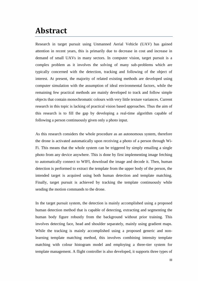
Abstract

Research in target pursuit using Unmanned Aerial Vehicle (UAV) has gained

attention in recent years, this is primarily due to decrease in cost and increase in

demand of small UAVs in many sectors. In computer vision, target pursuit is a

complex problem as it involves the solving of many sub-problems which are

typically concerned with the detection, tracking and following of the object of

interest. At present, the majority of related existing methods are developed using

computer simulation with the assumption of ideal environmental factors, while the

remaining few practical methods are mainly developed to track and follow simple

objects that contain monochromatic colours with very little texture variances. Current

research in this topic is lacking of practical vision based approaches. Thus the aim of

this research is to fill the gap by developing a real-time algorithm capable of

following a person continuously given only a photo input.

As this research considers the whole procedure as an autonomous system, therefore

the drone is activated automatically upon receiving a photo of a person through Wi-

Fi. This means that the whole system can be triggered by simply emailing a single

photo from any device anywhere. This is done by first implementing image fetching

to automatically connect to WIFI, download the image and decode it. Then, human

detection is performed to extract the template from the upper body of the person, the

intended target is acquired using both human detection and template matching.

Finally, target pursuit is achieved by tracking the template continuously while

sending the motion commands to the drone.

In the target pursuit system, the detection is mainly accomplished using a proposed

human detection method that is capable of detecting, extracting and segmenting the

human body figure robustly from the background without prior training. This

involves detecting face, head and shoulder separately, mainly using gradient maps.

While the tracking is mainly accomplished using a proposed generic and non-

learning template matching method, this involves combining intensity template

matching with colour histogram model and employing a three-tier system for

template management. A flight controller is also developed, it supports three types of

IV

controls: keyboard, mouse and text messages. Furthermore, the drone is programmed

with three different modes: standby, sentry and search.

To improve the detection and tracking of colour objects, this research has also

proposed several colour related methods. One of them is a colour model for colour

detection which consists of three colour components: hue, purity and brightness. Hue

represents the colour angle, purity represents the colourfulness and brightness

represents intensity. It can be represented in three different geometric shapes: sphere,

hemisphere and cylinder, each of these shapes also contains two variations.

Experimental results have shown that the target pursuit algorithm is capable of

identifying and following the target person robustly given only a photo input. This

can be evidenced by the live tracking and mapping of the intended targets with

different clothing in both indoor and outdoor environments. Additionally, the various

methods developed in this research could enhance the performance of practical

vision based applications especially in detecting and tracking of objects.

V

Acknowledgements

I would like to express my gratitude to my supervisor panel: principal supervisor

A/Prof. Gu Fang and co-supervisor Dr. Ju Jia (Jeffrey) Zou for their support,

especially Gu for his constant encouragement and guidance throughout the research

which enabled me to develop a better understanding of the subjects involved.

I am also grateful and honoured to the scholarship committee for providing financial

support by selecting me for the Australian Postgraduate Award and WSU Top-Up

Award, the latter is only offered to the highest ranked applicant.

I would like to thank the Western Sydney University especially the School of

Computing, Engineering and Mathematics for providing me the opportunity and

resources to undergo research and conduct experiments in this field.

Finally, I would like to thank my parents for their encouragement and patience

throughout the journey of my study.

VI

Table of Contents

Statement of Authentication........................................................................................ II

Abstract ....................................................................................................................... III

Acknowledgements ...................................................................................................... V

List of Figures ............................................................................................................... IX

List of Tables ................................................................................................................ XI

List of Abbreviations ................................................................................................... XII

Chapter 1 Introduction ........................................................................................ 1

1.1 Statement of the Problem ........................................................................................ 1

1.2 Aims and Objectives ................................................................................................. 3

1.3 Summary of Contributions ....................................................................................... 4

1.4 List of Publications (Resulting from this Research) .................................................. 5

1.5 Outline of the Thesis ................................................................................................ 6

Chapter 2 Literature Review ................................................................................ 7

2.1 Computer Vision ....................................................................................................... 7

2.2 Edge Features ......................................................................................................... 12

2.2.1 Roberts ....................................................................................................................... 13

2.2.2 Prewitt ........................................................................................................................ 13

2.2.3 Sobel ........................................................................................................................... 14

2.2.4 LOG ............................................................................................................................. 14

2.2.5 Canny .......................................................................................................................... 15

2.3 Colour Features ...................................................................................................... 18

2.3.1 Simple Thresholding ................................................................................................... 18

2.3.2 Histogram Binning ...................................................................................................... 19

2.3.3 Otsu ............................................................................................................................ 20

2.3.4 K-means ...................................................................................................................... 22

VII

2.3.5 Mean Shift .................................................................................................................. 22

2.4 Motion Features ..................................................................................................... 25

2.4.1 Background Subtraction ............................................................................................. 25

2.4.2 Optical Flow ................................................................................................................ 28

2.5 Colour Models ........................................................................................................ 31

2.5.1 RGB ............................................................................................................................. 32

2.5.2 HCV, HCL, HSV and HSL ............................................................................................... 33

2.5.3 YUV, YIQ, LUV and LAB ............................................................................................... 36

2.6 Machine Learning ................................................................................................... 39

2.6.1 SVM ............................................................................................................................. 40

2.6.2 ANN ............................................................................................................................. 41

2.6.3 CNN ............................................................................................................................. 43

2.7 Human Detection ................................................................................................... 44

2.8 Object Tracking ....................................................................................................... 48

2.9 Target Pursuit Using UAV ....................................................................................... 51

2.10 Motion Control of Quadrotor ................................................................................. 53

Chapter 3 Proposed Methods in Colour Based Feature Detection ................... 57

3.1 A Colour Enhancement Method for Colour Segmentation .................................... 57

3.2 A Colour Identification Method .............................................................................. 63

3.3 A Colour Model ....................................................................................................... 72

3.3.1 HPB Sphere ................................................................................................................. 73

3.3.2 HPB Hemisphere ......................................................................................................... 79

3.3.3 HPB Cylinder ............................................................................................................... 82

Chapter 4 Proposed Methods in Object Detection and Tracking ..................... 88

4.1 A Human Detection Method .................................................................................. 88

4.1.1 Scaled Gradient Mapping ........................................................................................... 89

4.1.2 Blob Filtering ............................................................................................................... 91

4.1.3 Body Estimation .......................................................................................................... 96

VIII

4.1.4 Figure Extraction ......................................................................................................... 99

4.2 An Object Tracking Method.................................................................................. 103

4.2.1 Detection .................................................................................................................. 103

4.2.2 Update ...................................................................................................................... 105

4.2.3 Tracking .................................................................................................................... 107

Chapter 5 Vision Based Target Pursuit Using a UAV ....................................... 115

5.1 Depth Estimation Using the Onboard Monocular Vision ..................................... 115

5.2 Trajectory Mapping .............................................................................................. 123

5.3 The Flight Controller ............................................................................................. 126

5.3.1 Keyboard ................................................................................................................... 127

5.3.2 Mouse ....................................................................................................................... 128

5.3.3 Text Messages .......................................................................................................... 128

5.4 Autopilot Modes ................................................................................................... 129

5.4.1 The Standby Mode .................................................................................................... 135

5.4.2 The Sentry Mode ...................................................................................................... 138

5.4.3 The Search Mode ...................................................................................................... 139

Chapter 6 Discussions and Conclusions........................................................... 142

6.1 Colour Based Feature Detection .......................................................................... 142

6.2 Object Detection and Tracking ............................................................................. 143

6.3 Target Pursuit Using a UAV .................................................................................. 144

6.4 Future Work ......................................................................................................... 145

References ................................................................................................................ 147

IX

List of Figures

Figure 1 Some examples of UAVs and their applications ......................................................... 2

Figure 2 Example problem in computer vision: tiger + deer + wilderness + chasing = hunting

? ................................................................................................................................................ 8

Figure 3 Photoreceptor layer in human vision ......................................................................... 9

Figure 4 Bayer filter in computer vision ................................................................................. 10

Figure 5 Timeline of computer vision ..................................................................................... 11

Figure 6 Gradient based edge features .................................................................................. 12

Figure 7 Example results of edge detection ........................................................................... 17

Figure 8 Colours in visible spectrum based on wavelength (nanometres) ............................ 18

Figure 9 Example results of colour segmentation .................................................................. 24

Figure 10 Example results of motion detection ..................................................................... 31

Figure 11 RGB cube ................................................................................................................ 32

Figure 12 Hue based colour models ....................................................................................... 35

Figure 13 Luminance based colour models ............................................................................ 38

Figure 14 CIE colour models ................................................................................................... 38

Figure 15 Example ANN setup: 1 input, 2 hidden and 1 output layers .................................. 41

Figure 16 Example CNN setup: it contains 1 input, 4 convolutional, 7 activation, 2 pooling, 3

hidden and 1 output layers .................................................................................................... 44

Figure 17 Example result of HOG ........................................................................................... 46

Figure 18 Example results of object tracking ......................................................................... 51

Figure 19 Example tracking frames of existing practical approaches .................................... 53

Figure 20 Spatial movements of a quadrotor: pitch, roll, yaw, heave, surge and sway ........ 54

Figure 21 Typical rotor configuration of quadrotor ............................................................... 54

Figure 22 The motion control of quadrotor ........................................................................... 56

Figure 23 Original and enhanced images using TCE and CCE ................................................. 61

Figure 24 Colour segmentation using the original and the enhanced images (TCE and CCE) 63

Figure 25 Colour identification using AMT with benchmark images ..................................... 69

Figure 26 Colour identification using AMT with various other images .................................. 72

Figure 27 HPB spherical colour models .................................................................................. 79

Figure 28 HPB hemispherical colour models .......................................................................... 81

Figure 29 HPB cylindrical colour models ................................................................................ 83

Figure 30 Colour identification with HPB model .................................................................... 85

Figure 31 Flowchart of the proposed human detection method ........................................... 89

Figure 32 Original input and gradient orientation map ......................................................... 91

Figure 33 Estimated human body proportions using golden ratio (head to knee) ................ 93

Figure 34 Face, head and shoulder detections ....................................................................... 96

Figure 35 Estimated human body regions (head to knee) ..................................................... 97

Figure 36 Estimated body regions .......................................................................................... 98

Figure 37 Unfilled body outlines and final segmented body regions ................................... 100

Figure 38 Human detection using GHD with various images ............................................... 102

Figure 39 Object tracking using GHD with various benchmark videos ................................ 112

X

Figure 40 Mean overlap scores with all thresholds .............................................................. 114

Figure 41 Depth estimation template .................................................................................. 118

Figure 42 Basic principle of the proposed depth estimation procedure .............................. 119

Figure 43 Example frame of the focal length recovery procedure....................................... 120

Figure 44 Depth estimation results and errors .................................................................... 123

Figure 45 Example trajectory during target pursuit ............................................................. 126

Figure 46 Example third person view of the drone in standby mode .................................. 129

Figure 47 Flowchart of the target pursuit system ................................................................ 130

Figure 48 POP dialog for image fetching .............................................................................. 131

Figure 49 Human detection and template extraction .......................................................... 133

Figure 50 Target pursuit in standby mode – case 1 ............................................................. 136

Figure 51 Target pursuit in standby mode – case 2 ............................................................. 137

Figure 52 Target acquisition in sentry mode ........................................................................ 138

Figure 53 Target pursuit in search mode .............................................................................. 140

Figure 54 More target pursuit results .................................................................................. 141

XI

List of Tables

TABLE I SIMPLE 8 COLOURS CLASSIFICATION ................................................................................... 19

TABLE II 4-BIN 64 COLOURS CLASSIFICATION .................................................................................. 20

TABLE III F1 SCORES OF AMT WITH BENCHMARK IMAGES.................................................................. 70

TABLE IV F1 SCORES OF COLOUR IDENTIFICATION WITH HPB MODEL .................................................. 86

TABLE V RANKINGS OF COLOUR MODELS BASED ON F1 SCORES .......................................................... 86

TABLE VI CONFIDENCE MEASURES FOR THE FACE AND SHOULDER, AND THE HEAD AND SHOULDER CASES 95

TABLE VII POSITION AND SIZE OF THE ESTIMATED HUMAN BODY REGIONS .......................................... 98

TABLE VIII UPDATE POLICY ......................................................................................................... 106

TABLE IX TRACKING POLICY ........................................................................................................ 107

TABLE X HYPERPARAMETERS ...................................................................................................... 108

TABLE XI FOCAL LENGTH ESTIMATION BASED ON IMAGE HEIGHT...................................................... 121

TABLE XII KEYBOARD CONTROLS ................................................................................................. 127

TABLE XIII TEXT COMMANDS ...................................................................................................... 129

TABLE XIV BASE64 CHARACTERS................................................................................................. 131

XII

List of Abbreviations

2D Two-Dimensional

3D Three-Dimensional

AMT Adaptive Multi-channel Thresholding

ANN Artificial Neural Network

AT Attention

CCD Charge Coupled Device

CCE Chroma based Colour Enhancement

CMOS Complementary Metal Oxide Semiconductor

CNN Convolutional Neural Network

CPU Central Processing Unit

FRG Fragment based Tracking

GHD Gradient based Human Detection

GMM Gaussian Mixture Model

GPS Global Positioning System

GPU Graphics Processing Unit

HCL Hue-Chroma-Lightness

HCV Hue-Chroma-Value

HOG Histogram of Oriented Gradients

HPB Hue-Purity-Brightness

HSL Hue-Saturation-Lightness

HSV Hue-Saturation-Value

IGMM Improved Gaussian Mixture Model

INS Inertial Navigation System

KNL Kernel based Tracking

LGN Lateral Geniculate Nucleus

LOG Laplacian of Gaussian

LSH Locality Sensitive Histogram based Tracking

LSK Local Sparse Appearance Model and K-selection based Tracking

NBP Normalised Back Projection

NCC Normalised Cross Correlation

NETSH Network Shell

OAB Online AdaBoost Tracking

POP Post Office Protocol

XIII

RGB Red-Green-Blue

ROI Region of Interest

SIFT Scale-Invariant Feature Transform

SVM Support Vector Machine

TCE Traditional Contrast Enhancement

TLD Tracking-Learning-Detection

TPU Tensor Processing Unit

TTT Tiered Template based Tracking

UAV Unmanned Aerial Vehicle

1

Chapter 1 Introduction

1.1 Statement of the Problem

Mobile robotics has always been an attractive field of research that combines many

different ideas and approaches to build mechatronic systems, an example is the

Unmanned Aerial Vehicle (UAV). A UAV can be defined as a generic aircraft

designed to operate with no human pilot onboard. Although, the motivation of the

development of early UAV was primarily due to military needs, nowadays, UAV has

become a popular platform for many different applications due to its low cost and

high flexibility. They are mainly used for tasks that are usually labour intensive, dull,

time consuming or dangerous for humans to operate, such tasks can include

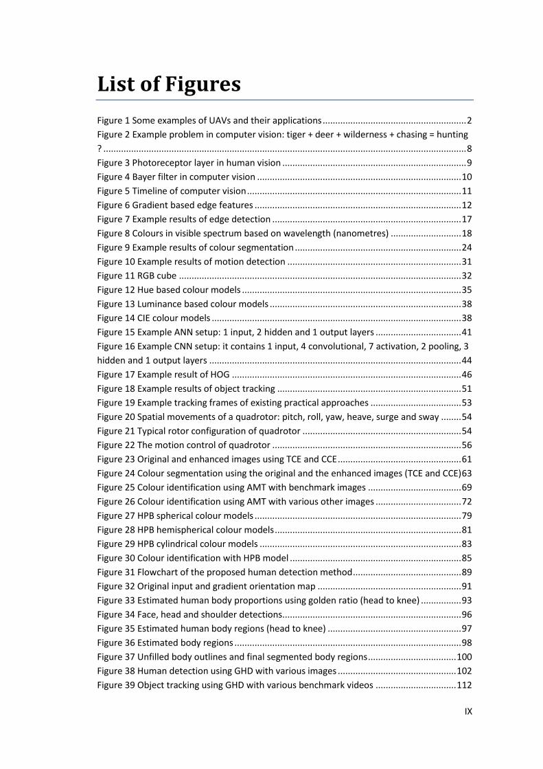
surveillance, mapping, inspection, rescue and target pursuit, some examples of

UAVs and their applications are shown in Fig. 1.

Among the applications, target pursuit using UAV is an innovative but problematic

area of research [1–10]. Target pursuit can be defined as the task of following an

object of interest continuously and autonomously. This is done through data fusion

based on the sensors of the UAV, typical sensors include but are not limited to:

Inertial Navigation System (INS), Global Positioning System (GPS), rangefinders

and cameras. INS and GPS tend to be used together for localisation and navigation,

INS provides higher accuracy at the local level but suffers from integration drift,

while GPS is reliable at global level but suffers from signal inconsistency, the two

systems collaborate with each other to eliminate drift and signal errors [11].

Rangefinders such as radar and sonar sensors are typically used to avoid obstacles

and locate objects from afar. And, vision sensors such as traditional and thermal

imaging cameras are mainly used to locate objects at close range through image

processing. This research focuses on the task of target pursuit using primarily

monocular vision.

2

(a) MQ-9 Reaper for military operation (b) Amazon Prime Air for commercial

delivery*

(c) Little Ripper Lifesaver for ocean rescue†

(d) DJI Phantom with GoPro camera for

recreational use‡

(e) Nano Hummingbird for surveillance and

reconnaissance (f) The Parrot AR Drone for this research

Figure 1 Some examples of UAVs and their applications

*https://www.flickr.com/photos/135518748@N08/37078925214

†https://www.engadget.com/2018/01/18/little-ripper-lifeguard-drone-rescue

‡https://commons.wikimedia.org/wiki/File:Drone_with_GoPro_digital_camera_mounted_underneat

h_-_22_April_2013.jpg

3

In computer vision, target pursuit is a complex problem as it involves the solving of

many sub-problems which are typically concerned with the detection, tracking and

following of the object of interest. Moreover, issues such as localisation, path

planning, obstacle avoidance and multi-robot cooperation can also be included.

Despite these hurdles, interest of target pursuit using UAV is rising. Many methods

have been proposed through the years, but the majority of them are developed using

computer simulation with the assumption of ideal environmental factors [1–5].

Despite a thorough search of the relevant literature, only a few practical vision based

methods that focused on target pursuit (such as human following) can be found [6–

10], but these methods tend to be designed for tracking and following simple objects.

Current research in this topic is clearly lacking of reliable practical vision based

approaches.

Furthermore, to the best of author’s knowledge, all existing methods require manual

selection of the object of interest, this is typically done through the use of pre-defined

Region of Interest (ROI). This means that at the beginning of each tracking sequence,

the user needs to setup a target ROI which is usually represented by a bounding box

of the object. In this research, the object of interest is considered to be unknown at

the start, the only input required is a photo of the object, the actual ROI of the object

in the image is acquired automatically.

1.2 Aims and Objectives

At present, the majority of related existing methods are developed using computer

simulation with the assumption of ideal environmental factors, while the remaining

few practical methods are mainly developed to track and follow simple objects that

contain monochromatic colours with very little texture variances. Current research in

this topic is lacking of practical vision based approaches. Thus, the aim of this

research is to fill the gap by developing a real-time algorithm capable of following a

person continuously given only a photo input. As this research considers the whole

procedure as an autonomous system, the drone should activate automatically upon

receiving a photo of a person through Wi-Fi, this means that whole system can be

triggered by simply emailing a single photo from any device anywhere. For example,

4

taking a photo of a person and emailing to the drone 30 kilometres away should

activate it and it should start searching for that person. Additionally, this research is

aimed to contribute in practical applications using computer vision especially in

detecting and tracking of objects.

To achieve the aims, the major objectives of this research have been set out as

follows:

To improve the detection and tracking of objects by studying existing colour

models.

To develop human detection methods capable of extracting the human figure

from a given image.

To develop object tracking methods capable of tracking the target object

continuously.

1.3 Summary of Contributions

Given the stated aims and objectives, the contributions of this thesis include:

A colour enhancement method for improved colour segmentation which

focused on boosting the saliency level of the critical regions in the image by

maximising chroma while preserving the hue angle.

A colour identification method for improved colour extraction which relied

on a colour space selection scheme to find the most suitable hue based colour

space, the required colour is then identified through a multi-channel filtering

process.

A colour model for improved colour detection which consists of three colour

components: hue, purity and brightness. It can be represented in three

different geometric shapes: sphere, hemisphere and cylinder, each of these

shapes also contains two variations.

A human detection method to identify a person from a photo, then extract

and segment the human figure into three key parts: head, upper body and

5

lower body. The proposed method works by detecting face, head and

shoulder separately, mainly using gradient maps.

An object tracking method to track an object continuously and robustly in

real time. The key strategies of the proposed method are: combining intensity

template matching with colour histogram model to increase tracking

robustness, employing a three-tier system to store templates, applying update

and tracking policies for template management.

1.4 List of Publications (Resulting from this

Research)

The publications consist of five conference papers and one journal article, the list is

shown below from latest to earliest:

F. Su, G. Fang, and J. J. Zou, “Robust real-time object tracking using tiered

templates,” The 13th

World Congress on Intelligent Control and Automation,

Changsha, China, July 2018 (to appear).

F. Su, G. Fang, and J. J. Zou, “A novel colour model for colour detection,”

Journal of Modern Optics, vol. 64, no. 8, pp. 819–829, November 2016.

F. Su, G. Fang, and J. J. Zou, “Human detection using a combination of face,

head and shoulder detectors,” IEEE Region 10 Conference (TENCON),

Singapore, pp. 842–845, November 2016.

F. Su, and G. Fang, “Chroma based colour enhancement for improved colour

segmentation,” The 9th

International Conference on Sensing Technology,

Auckland, New Zealand, pp. 162–167, December 2015.

F. Su, and G. Fang, “Colour identification using an adaptive colour model,”

The 6th

International conference on Automation, Robotics and Applications,

Queenstown, New Zealand, pp. 466–471, February 2015.

F. Su, and G. Fang, “Human detection using gradient maps and golden ratio,”

The 31st International Symposium on Automation and Robotics in

Construction and Mining, Sydney, Australia, pp. 890–896, July 2014.

6

1.5 Outline of the Thesis

After the introduction, the rest of the thesis is organised as follows:

Chapter 2 reviews the existing research in the related literature which

include computer vision, feature detection, colour models, machine learning,

human detection, object tracking, target pursuit using UAV and motion

control of quadrotor.

Chapter 3 details the proposed methods in colour based feature detection

which include a colour enhancement method for colour segmentation, a

colour identification method and a colour model for improved colour

detection.

Chapter 4 presents the proposed methods in object detection and tracking, in

which a human detection method using gradient maps and an object tracking

method using tiered templates are introduced.

Chapter 5 provides the results of the target pursuit experiment with three

different modes: standby, sentry and search. Other related topics including

depth estimation and trajectory mapping are also explained.

Chapter 6 discusses the effectiveness of the proposed methods and

concludes the completed work with suggestions for potential future work.

7

Chapter 2 Literature Review

This chapter provides a detailed analysis of related literature in computer vision.

Section 2.1 presents an overview of computer vision. Sections 2.2, 2.3 and 2.4

examine three main types of features: edge based, colour based and motion based,

respectively. Section 2.5 analyses the currently known colour models. Section 2.6

details the concept of machine learning. Sections 2.7 and 2.8 review existing human

detection and object tracking methods, respectively. Section 2.9 provides the

background information about UAV and its usage in vision based target pursuit and

Section 2.10 explains the motion control of quadrotor.

2.1 Computer Vision

A picture is worth a thousand words, this can be true for humans as we are able to

convey the meaning or essence very effectively by identifying or at least guessing the

objects, events and locations within an image. However, this can be a complex

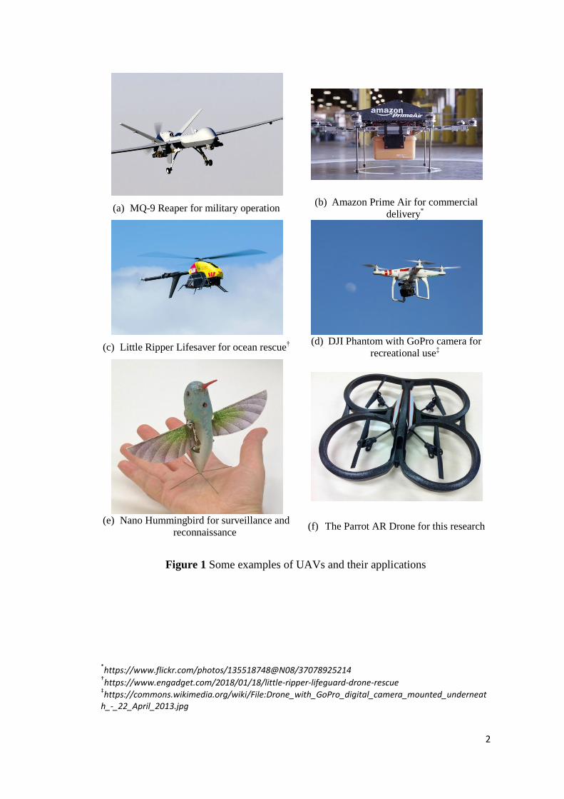
problem for a computer to solve, for example, given the photo in Fig. 2, if the

question is “What is happening in the photo?”, this will be a very simple and

straightforward question for a human to answer. On the other hand, in order for a

computer to truly answer this question, it needs to identify the deer and the tiger,

recognise they are both running in the wildness and the tiger is chasing the deer, or

perhaps even detect the mood of the deer as desperate and scared, therefore

concludes the meaning of the photo as tiger hunting deer in wildness or simply as

hunting.

Since a digital image is really a large Two-Dimensional (2D) matrix captured of a

Three-Dimensional (3D) scene, so the actual problem for the computer to solve is to

describe a 3D scene by extracting meaningful elements from a 2D matrix, this can be

done through image processing and pattern recognition which are the two most

common procedures in computer vision. Image processing is the study of techniques

that involves transforming, improving and analysing digital images to obtain specific

meaningful information [12]. While pattern recognition is a branch that is concerned

8

with the classification of data based either on a prior knowledge or statistical

information extracted from patterns [13].

Figure 2 Example problem in computer vision: tiger + deer + wilderness + chasing =

hunting ?*

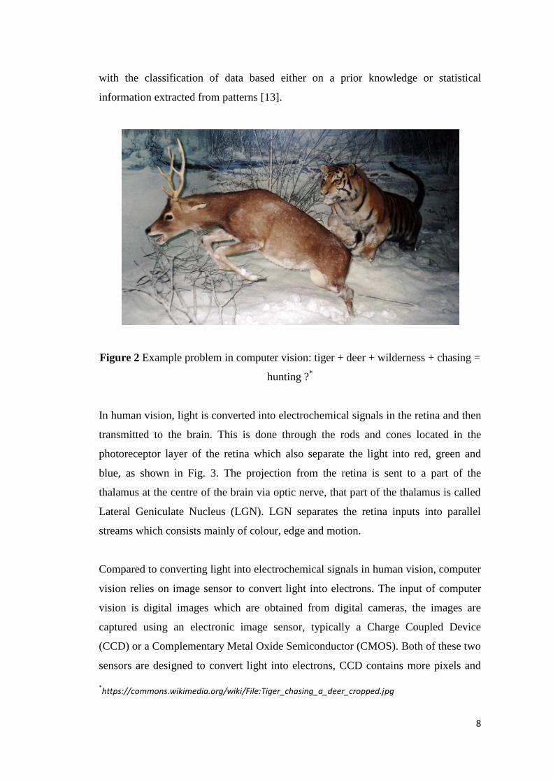
In human vision, light is converted into electrochemical signals in the retina and then

transmitted to the brain. This is done through the rods and cones located in the

photoreceptor layer of the retina which also separate the light into red, green and

blue, as shown in Fig. 3. The projection from the retina is sent to a part of the

thalamus at the centre of the brain via optic nerve, that part of the thalamus is called

Lateral Geniculate Nucleus (LGN). LGN separates the retina inputs into parallel

streams which consists mainly of colour, edge and motion.

Compared to converting light into electrochemical signals in human vision, computer

vision relies on image sensor to convert light into electrons. The input of computer

vision is digital images which are obtained from digital cameras, the images are

captured using an electronic image sensor, typically a Charge Coupled Device

(CCD) or a Complementary Metal Oxide Semiconductor (CMOS). Both of these two

sensors are designed to convert light into electrons, CCD contains more pixels and

*https://commons.wikimedia.org/wiki/File:Tiger_chasing_a_deer_cropped.jpg

9

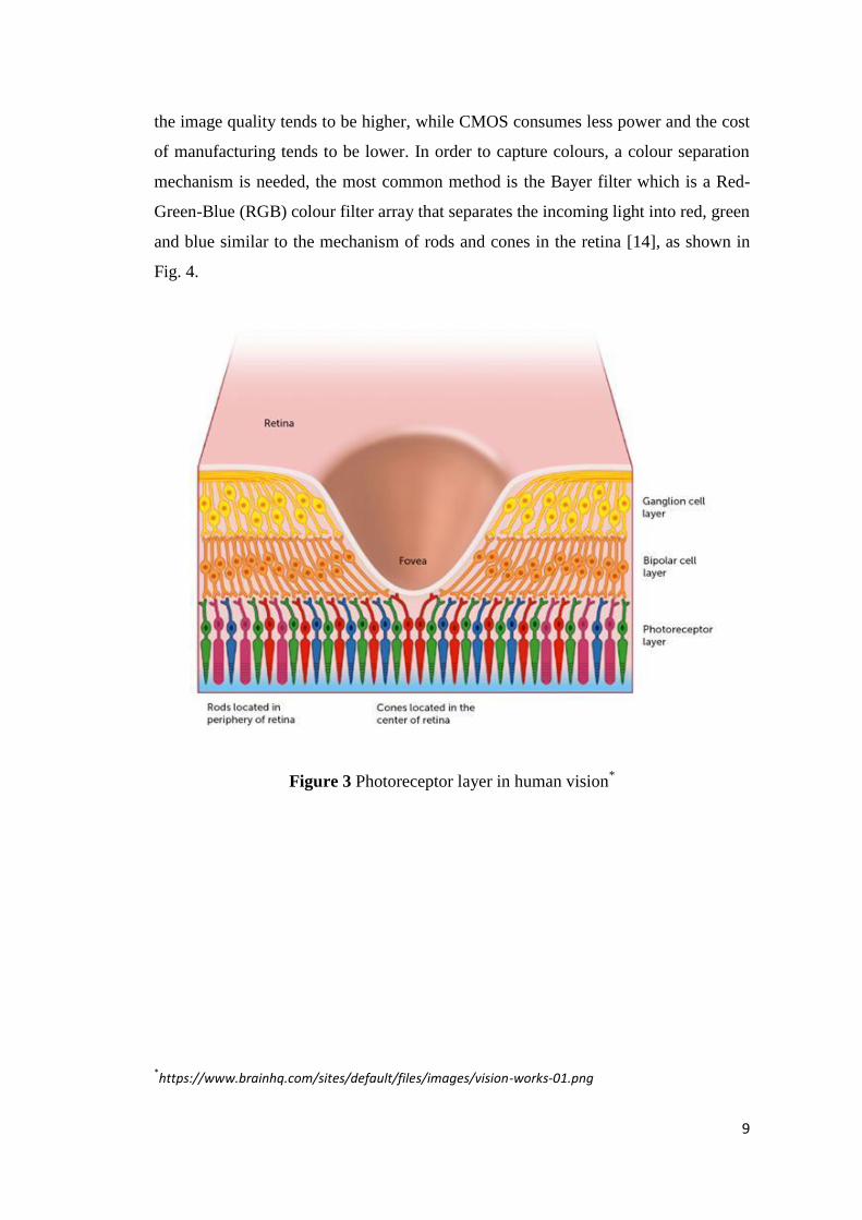
the image quality tends to be higher, while CMOS consumes less power and the cost

of manufacturing tends to be lower. In order to capture colours, a colour separation

mechanism is needed, the most common method is the Bayer filter which is a Red-

Green-Blue (RGB) colour filter array that separates the incoming light into red, green

and blue similar to the mechanism of rods and cones in the retina [14], as shown in

Fig. 4.

Figure 3 Photoreceptor layer in human vision*

*https://www.brainhq.com/sites/default/files/images/vision-works-01.png

10

Figure 4 Bayer filter in computer vision*

Computer vision is also the core component of artificial intelligence, it can be

described as the visual perception component of an ambitious agenda to mimic

human intelligence and to endow robots with intelligent behaviour [15]. It is a

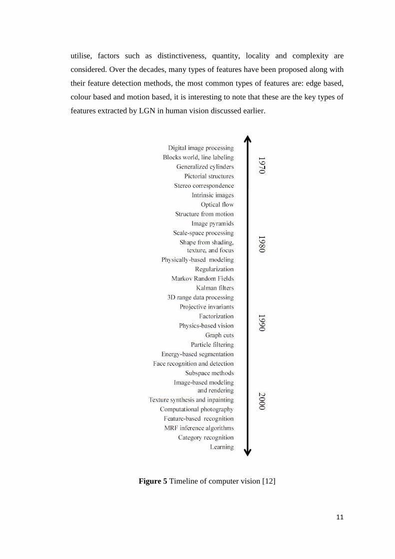
relatively young field of study that started out in the early 1970s, a timeline of some

of the most active research topics in computer vision is shown in Fig. 5. The output

of computer vision is a structure of quantitative measurements that describes the

scene. Computer vision can therefore be defined as the construction of explicit and

meaningful descriptions of physical objects from images [16]. The applications of

computer vision can include surveillance such as traffic monitoring [17] and hazard

detection [18], navigation such as mapping [19] and autonomous driving [20], object

recognitions such as face [21] and gesture [22].

The most crucial part in computer vision is the feature detection. No vision based

system can work until good features can be identified and tracked [23]. A feature is

typically a small and salient part of an image which can be included as an identifier

and descriptor of an object, event or location. When deciding the type of features to

*https://commons.wikimedia.org/wiki/File:Bayer_pattern_on_sensor_profile.svg

11

utilise, factors such as distinctiveness, quantity, locality and complexity are

considered. Over the decades, many types of features have been proposed along with

their feature detection methods, the most common types of features are: edge based,

colour based and motion based, it is interesting to note that these are the key types of

features extracted by LGN in human vision discussed earlier.

Figure 5 Timeline of computer vision [12]

12

2.2 Edge Features

Edges can be defined as significant local changes of intensity [24]. In computer

vision, they usually occur on the boundary between two different regions in an image

due to discontinuities. These discontinuities are the products created by different

objects, surfaces, reflections and shadows. Edge detection is the process of finding

meaningful transitions caused by local intensity differences in an image, because of

this, the majority of edge detectors are gradient based, that is measuring the intensity

gradients pixel by pixel, as given in Fig. 6. The origin is proposed to be the top left

corner of the image with positive directions of x and y axes to the right and the

bottom, respectively. There is a great deal of diversity in the applications of edge

detection, these can include barcode scanner [25], text detection [26], defect

detection [27], face recognition [28], autonomous driving [29] and 3D modelling

[30].

Figure 6 Gradient based edge features

13

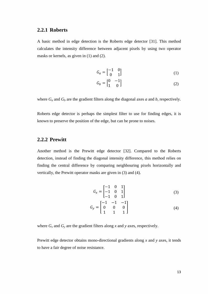
2.2.1 Roberts

A basic method in edge detection is the Roberts edge detector [31]. This method

calculates the intensity difference between adjacent pixels by using two operator

masks or kernels, as given in (1) and (2).

(1)

(2)

where Ga and Gb are the gradient filters along the diagonal axes a and b, respectively.

Roberts edge detector is perhaps the simplest filter to use for finding edges, it is

known to preserve the position of the edge, but can be prone to noises.

2.2.2 Prewitt

Another method is the Prewitt edge detector [32]. Compared to the Roberts

detection, instead of finding the diagonal intensity difference, this method relies on

finding the central difference by comparing neighbouring pixels horizontally and

vertically, the Prewitt operator masks are given in (3) and (4).

(3)

(4)

where Gx and Gy are the gradient filters along x and y axes, respectively.

Prewitt edge detector obtains mono-directional gradients along x and y axes, it tends

to have a fair degree of noise resistance.

14

2.2.3 Sobel

Another method is the Sobel edge detector [33]. Sobel is similar to the Prewitt, the

only difference is Sobel emphasises more on the importance of the central pixels by

assigning more weight, the Sobel operator masks are given in (5) and (6).

(5)

(6)

where Gx and Gy are the gradient filters along x and y axes, respectively.

Since the distribution of weight is less at the corners, Sobel is thought to possess

slightly better noise suppression when compared to Prewitt, but it may produce more

edge discontinuities.

2.2.4 LOG

The methods described so far are all first order derivative based, but it is not the only

tool to extract gradient based edge features. Second order derivatives can also be

used, an example is the Laplacian of Gaussian (LOG) edge detector [34]. Gaussian

filter is first implemented to reduce the noise level by smoothing the image, this is

the same procedure employed in Canny. Laplacian is then applied to obtain edge

features by finding zero crossings of the second order derivative. Only one Laplacian

operator mask is required, the most commonly used kernel is given in (7).

(7)

where L is the Laplacian filter.

15

Because of the second order derivative nature of the LOG edge detector, it tends to

yield better results with clustered objects when compared to the first order

approaches. However, LOG is known to be relatively prone to background noise and

it has an inclination to generate closed contours which do not always represent actual

edges.

2.2.5 Canny

A more advanced and well known method is the Canny edge detector [35]. Canny

implements a multi-staged algorithm to detect a wide range of edges in images, it is

aimed to achieve minimum detection error while maintaining good edge localisation.

The first step of the Canny method involves filtering out noise using a Gaussian

filter, as given in (8).

(8)

where x and y are the distances from the specific pixel of consideration in the

horizontal and vertical axes, respectively, a is the scale factor with overall magnitude

equal to 1 and σ is the standard deviation of the Gaussian distribution.

Commonly, a Gaussian kernel with a dimension of 5×5 and σ = 1.4 is used, as given

in (9).

(9)

where g is the Gaussian filter.

The second step involves finding the gradient magnitude and orientation, gradient

can be computed with any of the previously mentioned masks, Sobel is commonly

16

selected due to its resemblances to a Gaussian kernel. The equations for calculating

the magnitude and orientation are given in (10) and (11).

(10)

(11)

where Gx and Gy are the gradient components along x and y axes, respectively. θ is

rounded to one of four main directions: horizontal (0° or 180°), vertical (90° or 270°)

and two diagonals (45° or 225, and 135° or 315°).

The third step is a non-maximum suppression procedure, in which any pixel along

the direction of the gradient of a ridge with non-peak value is removed. This results

in an edge thinning effect by removing pixels that are not considered to be part of an

edge.

The final step is a hysteresis thresholding procedure, in which two values (upper and

lower) are used for thresholding. If the gradient of a pixel is higher than the upper

threshold, the pixel is accepted as an edge. If the value is below the lower threshold,

then the pixel is removed. If the value is in between the two thresholds, then it is

accepted only if the pixel itself is connected to another pixel that is above the upper

threshold. It is commonly recommended to select the two thresholds with an upper to

lower ratio between 2 and 3.

Due to its low computational cost and high robustness, Canny edge detector is

widely used for many different applications. However it has some limitations [36]:

firstly, because of its dual-threshold nature, the optimal window of the upper and

lower thresholds is difficult to adjust. Secondly, corner pixels tend to search in the

wrong directions of their neighbours, which frequently causing open ended edges.

Furthermore, positions of the edges are usually shifted due to the blurring effect of

the Gaussian filter.

17

Examples of results using different edge detectors are illustrated in Fig. 7. The results

are generated by computing gradient magnitude maps based on the kernels described

earlier, they are also normalised for visualisation and comparison purposes. For first

order derivative based methods that compute gradients along both x and y axes, the

overall magnitudes are obtained using (10). For Canny, rather than choose the upper

and lower thresholds manually, they are obtained based on the mean magnitude of

Sobel. This automatic threshold selection approach proves to be effective for most

images, the mean value is linked to the lower threshold and the upper threshold is

simply two times the mean.

(a) Original

* (b) Roberts

(c) Prewitt (d) Sobel

(e) LOG (f) Canny

Figure 7 Example results of edge detection

*https://peopledotcom.files.wordpress.com/2017/10/obama-oval-office.jpg

18

2.3 Colour Features

Colour is an important feature in both human vision and computer vision, it can be

defined as the perceptual sensation of the spectral distribution of visible light [37].

Visible light is basically electromagnetic radiation with typical wavelength ranging

from 400 to 700 nanometres, as shown in Fig. 8. Therefore it can be said that the

colour of an object depends on the wavelength of the light leaving its surface.

Figure 8 Colours in visible spectrum based on wavelength (nanometres)*

In computer vision, colour segmentation is the process of partitioning an image into

meaningful regions based on colour properties. Because each person perceives the

boundaries of colours differently, this means that the ground truth of colour regions

varies depending on the observer. Furthermore, environment factors such as lighting,

shadow and viewing angle can also greatly influence the perception of colours, thus

colour segmentation can be a challenging task. It can be commonly found in

applications that rely on the detection and tracking of various colours, these can

include remote sensing [38], object tracking [39], skin segmentation [40], tumour

detection [41], road lane detection [42] and 3D modelling [43].

Colour features can be defined subject to particular colour spaces [44], a number of

colour spaces have been proposed in the literature and are to be discussed in detail in

Section 2.5. For simplicity, only the RGB colour space is considered for colour

segmentation methods discussed in this section.

2.3.1 Simple Thresholding

A simple method to separate the colours is thresholding based on Euclidean distance

[45]. An example approach is to divide the RGB colour space into 8 colours then

*https://en.wikipedia.org/wiki/File:Rendered_Spectrum.png

19

classify the pixels based on minimum squared Euclidean distance to the absolute

values of these colours, as listed in Table I. For a typical 8-bit colour image, RGB

values are in range of 0 to 255.

TABLE I SIMPLE 8 COLOURS CLASSIFICATION

Colours Red Green Blue

Red 255 0 0

Green 0 255 0

Blue 0 0 255

Yellow 255 255 0

Cyan 0 255 255

Magenta 255 0 255

Black 0 0 0

White 255 255 255

The squared Euclidean distance of individual pixels to the absolute colours (defined

as 8 vertices of the RGB cube) is computed using (12).

(12)

where d is the distance, a and i are the absolute and pixel colours, respectively, R, G

and B are the RGB positions or pixel values, respectively.

Thresholding based methods are built based on the principle that different regions of

the image can be separated by identifying important characteristics such as local

maxima and minima, they are simple to implement but can be sensitive to noise.

2.3.2 Histogram Binning

A common feature in colour segmentation is colour histogram which is basically a

representation of colour distributions in an image. In the RGB colour space, a colour

histogram represents the count of number of pixels in an image belonging to a

particular RGB bin, these histogram bins are used to quantise the pixels into different

20

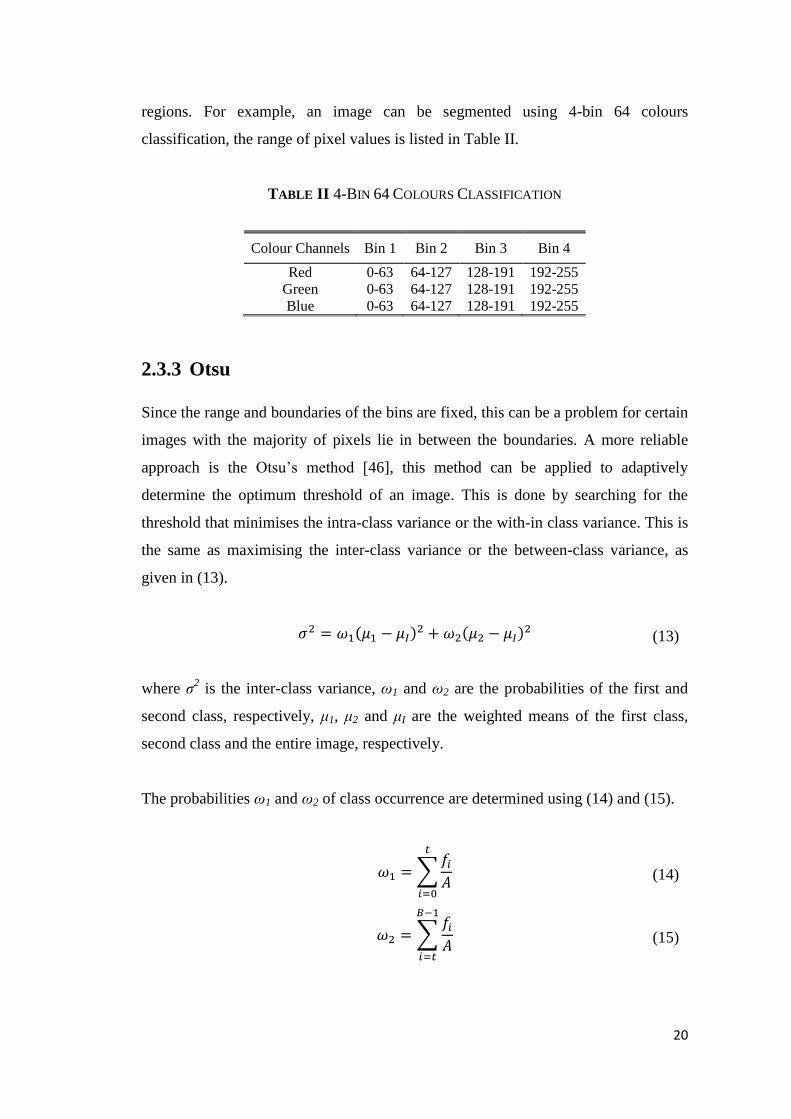
regions. For example, an image can be segmented using 4-bin 64 colours

classification, the range of pixel values is listed in Table II.

TABLE II 4-BIN 64 COLOURS CLASSIFICATION

Colour Channels Bin 1 Bin 2 Bin 3 Bin 4

Red 0-63 64-127 128-191 192-255

Green 0-63 64-127 128-191 192-255

Blue 0-63 64-127 128-191 192-255

2.3.3 Otsu

Since the range and boundaries of the bins are fixed, this can be a problem for certain

images with the majority of pixels lie in between the boundaries. A more reliable

approach is the Otsu’s method [46], this method can be applied to adaptively

determine the optimum threshold of an image. This is done by searching for the

threshold that minimises the intra-class variance or the with-in class variance. This is

the same as maximising the inter-class variance or the between-class variance, as

given in (13).

(13)

where σ2 is the inter-class variance, ω1 and ω2 are the probabilities of the first and

second class, respectively, μ1, μ2 and μI are the weighted means of the first class,

second class and the entire image, respectively.

The probabilities ω1 and ω2 of class occurrence are determined using (14) and (15).

(14)

(15)

21

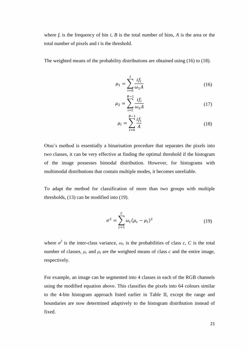
where fi is the frequency of bin i, B is the total number of bins, A is the area or the

total number of pixels and t is the threshold.

The weighted means of the probability distributions are obtained using (16) to (18).

(16)

(17)

(18)

Otsu’s method is essentially a binarisation procedure that separates the pixels into

two classes, it can be very effective at finding the optimal threshold if the histogram

of the image possesses bimodal distribution. However, for histograms with

multimodal distributions that contain multiple modes, it becomes unreliable.

To adapt the method for classification of more than two groups with multiple

thresholds, (13) can be modified into (19).

(19)

where σ2 is the inter-class variance, ωc is the probabilities of class c, C is the total

number of classes, μc and μI are the weighted means of class c and the entire image,

respectively.

For example, an image can be segmented into 4 classes in each of the RGB channels

using the modified equation above. This classifies the pixels into 64 colours similar

to the 4-bin histogram approach listed earlier in Table II, except the range and

boundaries are now determined adaptively to the histogram distribution instead of

fixed.

22

For a given image, histogram based methods exhibit relatively good performance if

the variance of the foreground is small and the mean difference compared to the

background is high. However, it has limited usage against images that contain no

obvious valley and peak regions.

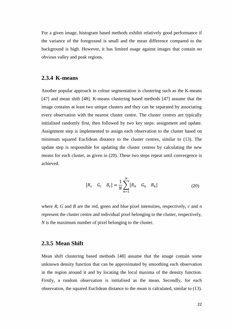
2.3.4 K-means

Another popular approach in colour segmentation is clustering such as the K-means

[47] and mean shift [48]. K-means clustering based methods [47] assume that the

image contains at least two unique clusters and they can be separated by associating

every observation with the nearest cluster centre. The cluster centres are typically

initialised randomly first, then followed by two key steps: assignment and update.

Assignment step is implemented to assign each observation to the cluster based on

minimum squared Euclidean distance to the cluster centres, similar to (13). The

update step is responsible for updating the cluster centres by calculating the new

means for each cluster, as given in (20). These two steps repeat until convergence is

achieved.

(20)

where R, G and B are the red, green and blue pixel intensities, respectively, c and n

represent the cluster centre and individual pixel belonging to the cluster, respectively,

N is the maximum number of pixel belonging to the cluster.

2.3.5 Mean Shift

Mean shift clustering based methods [48] assume that the image contain some

unknown density function that can be approximated by smoothing each observation

in the region around it and by locating the local maxima of the density function.

Firstly, a random observation is initialised as the mean. Secondly, for each

observation, the squared Euclidean distance to the mean is calculated, similar to (13).

23

Thirdly, a vote is added to the observation if it is deemed close to the mean, this is

determined if the distance to the mean is smaller than a radius threshold. Finally, the

mean is updated based on all the observations close to the mean, this is basically a

gradient descent process which shifts the mean towards a local minimum, similar to

(20). These steps repeat until convergence is achieved. The cluster and its votes are

merged into another cluster if it is found within half of the radius threshold of any

existing clusters, else it is regarded as a new cluster. For the merging case, the

combined mean of the two clusters is determined based on the maximum of the

cluster votes, as given in (21) and (22). An unvisited observation is then initialised as

the new mean and whole procedure repeats until all observations have been visited.

(21)

(22)

where V and μ are the votes (of the pixels) and means belonging to the clusters,

respectively, i and m are the current and merging clusters, respectively.

Both K-means and mean shift require only a single input, but the inputs for both

methods are difficult to set. They are typically determined empirically depending on

the applications. For K-means the input is the total number of clusters, while for

mean shift, the input is the radius of the Region of Interest (ROI). K-means is usually

computationally inexpensive, but can be sensitive to outliers and requires pre-

knowledge of the number of segmentations needed. On the other hand, mean shift

automatically determines the number of segmentations based on the radius input.

However, it does not scale well with more than one dimension of feature space as it

is computationally expensive.

Examples of results using different colour segmentation methods described earlier

are illustrated in Fig. 9. The results are normalised for visualisation and comparison

purposes. Two cases have been considered: 8 segments and 27 segments. For

histogram, 8 and 27 segments are the results of quantisation using 2-bin and 3-bin in

each channel of the RGB colour space, respectively. For Otsu’s method, 8 and 27

24

segments are the results of thresholding by finding one and two optimal thresholds

per RGB channel, respectively. For mean shift, the specific numbers of segments are

generated through trial and error since mean shift does not guarantee number of

segments in the outcome.

(a) Original

*

(b) Histogram – 8 segments (c) Otsu – 8 segments

(d) K-means – 8 segments (e) Mean shift – 8 segments

(f) Histogram – 27 segments (g) Otsu – 27 segments

(h) K-means – 27 segments (i) Mean shift – 27 segments

Figure 9 Example results of colour segmentation

*http://www.maxtheknife.com/marshax3/marsha36.jpg

25

2.4 Motion Features

In physics, motion is defined as the change in position of an object over time relative

to a frame of reference. In computer vision, motion is detected by comparing two

consecutive image frames in a sequence. Motion features are extracted to analyse the

objects for advanced purposes or simply to detect and track the objects in the first

place. Basic analysis can be performed to obtain important characteristics about the

objects, these can include shape, posture, centre of mass, velocity and trajectory.

Further advanced analysis can lead to action recognition [49], behaviour recognition

[50], object recognition [51] and object reconstruction [52]. There are two well

known motion detection methods that have been used extensively throughout the

years: background subtraction [53] and optical flow [54].

2.4.1 Background Subtraction

Background subtraction [53] is typically used to separate moving foreground objects

from static background. The fundamental assumption of the algorithm is that the

background remains relatively stable when compared to foreground objects. When

objects move in a set of video frames, the regions that differ significantly from the

background model can be considered to be the foreground. In other words, when

assuming a statistical model of the scene, an intruding object can be detected by

spotting the parts of the image that don't belong to the model.

A vast amount of research has been conducted with many algorithms proposed. The

simplest way of achieving background subtraction is the frame difference method, in

which the background is estimated from the previous frame according to an intensity

difference threshold, as given in (23).

(23)

where It is the intensity of frame t, Δ is the intensity difference threshold.

26

This basic method only relies on a single threshold which controls the sensitivity of

the separation between the foreground and background, this threshold is linked to the

speed of the moment so that a high threshold is required for fast movement. This

method is only suited for a particular moment in the scene and is very sensitive to

noise.

A more refined and renowned method is the Gaussian Mixture Model (GMM) [55].

GMM models each background pixel by a mixture of Gaussian distributions (a small

number usually from 3 to 5). The probability of observing the current pixel value is

given in (24).

(24)

where P(Xt) is the probability of observing pixel value X at time t, K is the number of

Gaussians in the model, ωi is the weight parameter of Gaussian i, η(Xt,μi,Σi) is the

normal distribution of Gaussian i with mean μi and covariance Σi.

Gaussians are employed to indicate different colours. The weight parameter is used

to represent the time that those colours stay in the scene and is updated at every new

frame. The mean value and covariance matrix are needed to compute Gaussian

probability density function.

To find the foreground, background pixels can be assumed to have high weight

values and low variance values because they remain longer and are more static when

compared to the foreground objects. A fitness value is introduced to measure the

formation of the clusters, in which static single colour objects tend to form tight

clusters, while moving ones tend to form wide clusters caused by reflections from

different surfaces due to the movement. During the update, every new pixel is

checked against existing model for fitness measure and is updated according to a

specific learning rate.

27

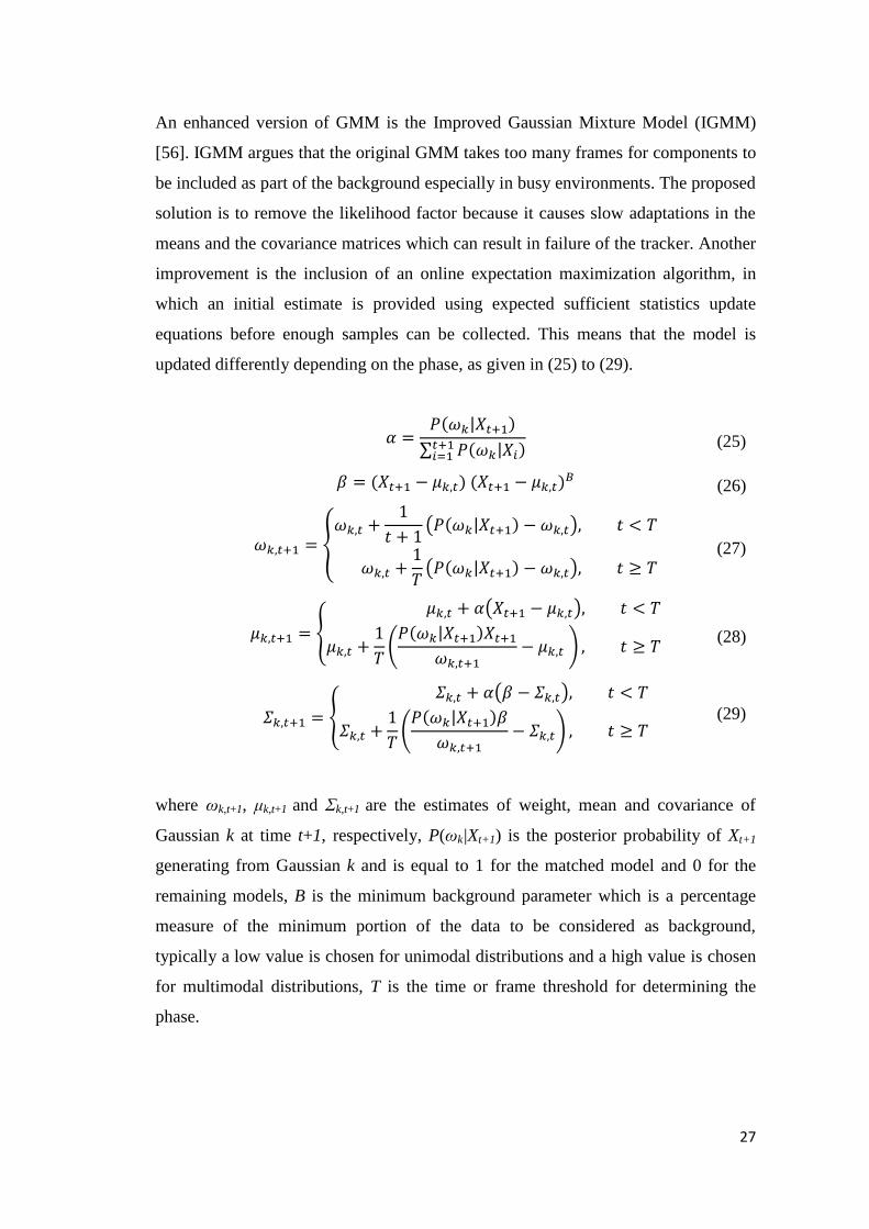
An enhanced version of GMM is the Improved Gaussian Mixture Model (IGMM)

[56]. IGMM argues that the original GMM takes too many frames for components to

be included as part of the background especially in busy environments. The proposed

solution is to remove the likelihood factor because it causes slow adaptations in the

means and the covariance matrices which can result in failure of the tracker. Another

improvement is the inclusion of an online expectation maximization algorithm, in

which an initial estimate is provided using expected sufficient statistics update

equations before enough samples can be collected. This means that the model is

updated differently depending on the phase, as given in (25) to (29).

(25)

(26)

(27)

(28)

(29)

where ωk,t+1, μk,t+1 and Σk,t+1 are the estimates of weight, mean and covariance of

Gaussian k at time t+1, respectively, P(ωk|Xt+1) is the posterior probability of Xt+1

generating from Gaussian k and is equal to 1 for the matched model and 0 for the

remaining models, B is the minimum background parameter which is a percentage

measure of the minimum portion of the data to be considered as background,

typically a low value is chosen for unimodal distributions and a high value is chosen

for multimodal distributions, T is the time or frame threshold for determining the

phase.

28

Initially, when the number of frames is smaller than T, the model is updated

according to the expected sufficient statistics update equations. Later, when the first

T samples are processed, the update equations of the model are switched to the T-

recent window version. The expected sufficient statistics update equations allow

faster convergences while still providing a good overall estimation during the initial

phase, while the T-recent window equations gives priority over recent data, this

increases the adaptiveness of the model. Thus, IGMM is able to reduce the

computational cost while maintaining accuracy of the model.

In general, with a stationary camera, background subtraction can be an effective tool

for motion detection. However, when the camera itself starts moving, background

subtraction tends to become unreliable and problematic to implement. This is

because with a moving camera, the background of the image is constantly changing,

this results in abnormally high variances which leads to failure of the separation as

the majority of the image are highly likely to be falsely classified as foreground.

2.4.2 Optical Flow

Optical flow [54] is an alternative and well known method for motion detection. The

key idea is to measure the relative motion between the objects and the viewer similar

to movement awareness from human vision. This is achieved by analysing the

distribution of observed velocity in brightness patterns. Optical flow can also be used

to find other important characteristics of the scene, these can include the rate of

change which is utilised to estimate the structures of the 3D scenes and the

discontinuities which is extracted to distinguish between objects by segmenting

images into different regions.

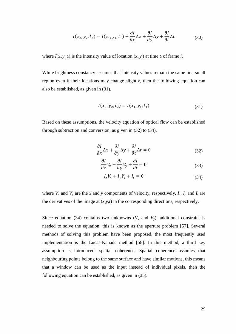
There are two key assumptions for optical flow: temporal persistence and brightness

constancy. Temporal persistence assumes that the image motion of a surface path is

small and any movement results consistent changes of coordinates, then the

following equation can be established, as given in (30).

29

(30)

where I(xi,yi,ti) is the intensity value of location (xi,yi) at time ti of frame i.

While brightness constancy assumes that intensity values remain the same in a small

region even if their locations may change slightly, then the following equation can

also be established, as given in (31).

(31)

Based on these assumptions, the velocity equation of optical flow can be established

through subtraction and conversion, as given in (32) to (34).

(32)

(33)

(34)

where Vx and Vy are the x and y components of velocity, respectively, Ix, Iy and It are

the derivatives of the image at (x,y,t) in the corresponding directions, respectively.

Since equation (34) contains two unknowns (Vx and Vy), additional constraint is

needed to solve the equation, this is known as the aperture problem [57]. Several

methods of solving this problem have been proposed, the most frequently used

implementation is the Lucas-Kanade method [58]. In this method, a third key

assumption is introduced: spatial coherence. Spatial coherence assumes that

neighbouring points belong to the same surface and have similar motions, this means

that a window can be used as the input instead of individual pixels, then the

following equation can be established, as given in (35).

30

(35)

where n is the total number of pixels inside the window, Vx and Vy are the x and y

components of velocity, respectively, Ix, Iy and It are the derivatives of the image at

(x,y,t) in the corresponding directions, respectively.

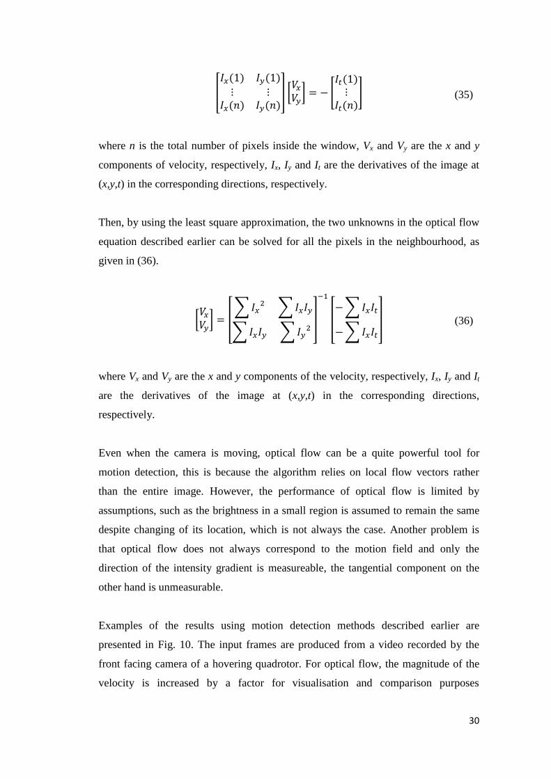
Then, by using the least square approximation, the two unknowns in the optical flow

equation described earlier can be solved for all the pixels in the neighbourhood, as

given in (36).

(36)

where Vx and Vy are the x and y components of the velocity, respectively, Ix, Iy and It

are the derivatives of the image at (x,y,t) in the corresponding directions,

respectively.

Even when the camera is moving, optical flow can be a quite powerful tool for

motion detection, this is because the algorithm relies on local flow vectors rather

than the entire image. However, the performance of optical flow is limited by

assumptions, such as the brightness in a small region is assumed to remain the same

despite changing of its location, which is not always the case. Another problem is

that optical flow does not always correspond to the motion field and only the

direction of the intensity gradient is measureable, the tangential component on the

other hand is unmeasurable.

Examples of the results using motion detection methods described earlier are

presented in Fig. 10. The input frames are produced from a video recorded by the

front facing camera of a hovering quadrotor. For optical flow, the magnitude of the

velocity is increased by a factor for visualisation and comparison purposes

31

(represented by the green vectors), this factor is equal to 5% of the maximum length

(width and height) of the image.

(a) Frame 1 (b) Frame 2

(c) Background subtraction (IGMM) (d) Optical flow (Lukas-Kanade)

Figure 10 Example results of motion detection

2.5 Colour Models

Colour model can be defined as a digital representation of possible contained colours

[59]. Many different colour models have been proposed in the literature, each with

their own strengths and weaknesses. The most commonly used colour model for

capturing images is the RGB model, while hue based colour models such as Hue-

Saturation-Value (HSV) are frequently chosen for colour related tasks such as the

detection, segmentation and enhancement of colours. Others colour models include

luminance based colour models such as YUV and the CIE colour models such as

LUV. Existing literature tends to present and discuss the colour models based on 2D

cross sections, this can be sometimes misleading especially for colour models with

irregular gamuts, therefore in this section, complete 3D models are provided along

with their conversions from RGB and vise versa.

32

2.5.1 RGB

RGB is the most common and fundamental colour model, in which each channel

corresponds to the intensity of one of the primary colours: red, green and blue. The

standard RGB colour model can be represented as a 3D Cartesian space using three

mutually perpendicular axes, as shown in Fig. 11.

Due to its simplicity and its additive property, RGB colour model is very easy to

store, configure and display the images [60]. However, as important colour

properties, such as purity and brightness, are embedded within the RGB colour

channels and any effect or change on one of the channels also affects the other

channels, it can be difficult to extract specific colours and to determine their reliable

working ranges [61]. Thus, modern methods typically rely on other colour models

for colour related tasks.

Figure 11 RGB cube

33

2.5.2 HCV, HCL, HSV and HSL

The most frequently used colour models for colour related applications are the hue

based colour models [62]. These can include Hue-Chroma-Value (HCV), Hue-

Chroma-Lightness (HCL), Hue-Saturation-Value (HSV) and Hue-Saturation-

Lightness (HSL), as shown in Fig. 12 (a) to (d), respectively. In the models, hue

represents colour angle, chroma or saturation represents colour purity, value or

lightness represents colour brightness.

The conversions from RGB to HCV, HCL, HSV and HSL are given in (37) to (43).

(37)

(38)

(39)

(40)

(41)

(42)

(43)

where r, g, b are the red, green and blue intensities, respectively, V is value, C is

chroma, L is lightness, H is hue, SV and SL are saturations based on value and

lightness, respectively.

34

The inverse conversions from HCV, HCL, HSV and HSL to RGB are given in (44)

to (48).

(44)

(45)

(46)

(47)

(48)

where r, g and b are the red, green and blue intensities, respectively, V (value), M and

U are the maximum, middle and minimum intensities among r, g and b, respectively,

C is chroma, L is lightness, H is hue and S is saturation.

Hue based colour models tend to be the preferred choices for colour detection

applications [63], this is because they separate important properties such as purity

and brightness from the image and their various colour regions can be easily

recognised by human perception.

35

(a) HCV cone

(b) HCL double cone

(c) HSV cylinder

(d) HSL cylinder

Figure 12 Hue based colour models

36

2.5.3 YUV, YIQ, LUV and LAB

Other colour models include luminance based colour models such as YUV and YIQ

[64], and the CIE colour models such as LUV and LAB [65], as shown in Fig. 13 and

Fig. 14, respectively. The luminance based colour models are comprised of one

luminance channel and two chrominance channels, this separates the image into

greyscale and colour sets. While the CIE colour models consist of one lightness

channel and two correlated chrominance channels of either cyan-red and blue-yellow

(LUV) or green-red and blue-yellow (LAB).

The conversions from RGB to YUV and YIQ are given in (49) and (50),

respectively.

(49)

(50)

The inverse conversions from YUV and YUQ to RGB are given in (51) and (52),

respectively.

(51)

(52)

The conversions from RGB to LUV and LAB are given in (53) to (61).

(53)

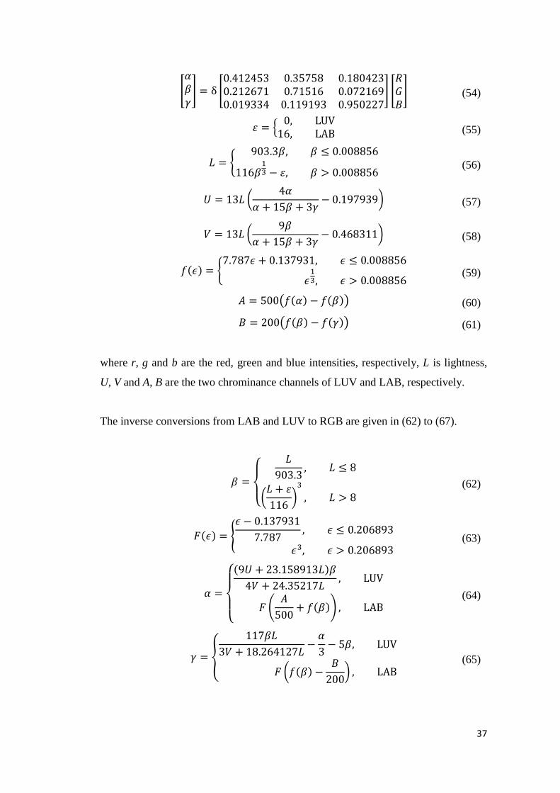
37

(54)

(55)

(56)

(57)

(58)

(59)

(60)

(61)

where r, g and b are the red, green and blue intensities, respectively, L is lightness,

U, V and A, B are the two chrominance channels of LUV and LAB, respectively.

The inverse conversions from LAB and LUV to RGB are given in (62) to (67).

(62)

(63)

(64)

(65)

38

(66)

(67)

where r, g and b are the red, green and blue intensities, respectively, L is lightness,

U, V and A, B are the two chrominance channels of LUV and LAB, respectively.

(a) YUV cuboid

(b) YIQ cuboid

Figure 13 Luminance based colour models

(a) LUV irregular gamut

(b) Lab irregular gamut

Figure 14 CIE colour models

39

Luminance is regarded as the dominant channel as human perception is more

sensitive to changes in overall light intensity (luminance) than differences among

each colour channels (chrominance). This means that the bandwidth in the

chrominance channels (U and V) can be reduced when necessary without

significantly damaging the image quality, thus luminance based colour models are

typically used for colour TV broadcasting.

On the other hand, the CIE colour models are designed to be perceptually uniform,

they rely on a set of colour matching functions to resemble the responses of red,

green and blue cones in human vision, thus CIE colour models can be regarded as the

closest models to human perception. However, since the correlations are non-linear,

the structure of these models is difficult to visualise and manipulate. More

conversions from RGB can be found in the colour model survey paper [66].

2.6 Machine Learning

Machine learning has become a trending topic in computer science and computer

vision in recent years due to its capability of solving complex tasks. Its applications

can include gesture recognition [22], activity recognition [67], scene recognition

[68], cancer classification [69], cyber security [70] and face recognition [71].

In general terms, the goal of machine learning is to enable a system to learn from the

past or present and use that knowledge to make predictions or decisions regarding

unknown future events [72]. In terms of image processing and data analysing,

machine learning is about learning the related features associated with different

classes without explicitly program these features. This is usually done through

reinforced training with huge amount of data that contain positive and negative

examples.

The concept of machine learning is not new, in fact, it has been used as early as

1950s, in which a computer has been successfully trained to play checkers

competitively given only the rules of the game [73]. The revival of machine learning

in recent years is primarily due to two reasons: the first major reason is the

40

advancements in hardware especially the Graphics Processing Unit (GPU) and the

Tensor Processing Unit (TPU), while the second minor reason is due to the increased

availability of many datasets that can now be accessed easily online.

GPU is originally designed for fast displaying of images, it has become the top

choice for machine learning because when comparing to the Central Processing Unit

(CPU), GPU is simply faster at computing multi-dimensional data such as images.

This is due to the architecture differences between CPU and GPU, CPU is built with

several powerful cores for sequential processing while GPU is built with thousands

of tiny but efficient cores for parallel processing. TPU on the other hand is even

faster than GPU, it consists of matrix multiplier unit designed specifically for matrix

computations. However, currently TPU is extremely expensive to build due to its

custom designed chips.

2.6.1 SVM

A well known and widely used method for analysing data through classification and

regression is Support Vector Machine (SVM) [74]. SVM is a two-group classifier,

the goal is to separate the training data into two classes with the largest possible

difference between them. In a 2D linearly separable situation, this is equivalent of

finding a line with the maximum possible margin, as given in (68).

(68)

where x is the training data, w is the normal vector, b is the bias.

Learning the SVM is then become an optimisation problem of finding the minimum

value of ||w||2 that satisfies (69).

(69)

41

where x is the training data, w is the normal vector, b is the bias, y is the indicator to

separate the data into two classes, in which y is equal to 1 for one class and -1 for the

other class.

SVM is proven to be effective for most two-group classification problems. However,

it can be unreliable when there are more than two classes, it also assumes that the

inputs are linearly separable which is not always the case.

2.6.2 ANN

An advanced method is the Artificial Neural Network (ANN) [75]. ANN is inspired

from the biological neural network in the brain, it typically consists of three types of

layers: input, hidden and output, as shown in Fig. 15. Each layer is made of fully

connected neurons, the numbers of neurons in the input and output layers are linked

to the actual sizes of the input and output, respectively, while the number of layers

and the number of neurons in each of the hidden layers are usually chosen arbitrarily

depending on the difficulty of the task (typically 2 hidden layer with number of

neurons between the sizes of input and output layers).

Figure 15 Example ANN setup: 1 input, 2 hidden and 1 output layers

42

For a typical object classification problem, the image itself can be regarded as the

input layer, in which each neuron represents the intensity value of each pixel. While

the results of classification can be regarded as the output layer, in which each neuron

represents a separate class. For the two hidden layers, the output of the first layer can

be thought of as the basic features such as edges belonging to the objects, while the

output of the second layer can be thought of as the advanced features such as small

parts belonging to the objects.

For each neuron, the network function can be defined as (70).

(70)

where I and O are the input and output of the neuron, respectively, w and b are the

weight and bias in the neuron, respectively, F is the activation function (usually a

rectifier that resets all negative outputs to zero).

For each iteration during the training of the network, the performance of the network

is computed using a cost function. The most commonly used method is mean squared

error, as given in (71).

(71)

where Od and Oa are the desired and actual output of the network, respectively, n is

the number of training examples, E is the error (cost) of the network.

The learning or the training of the network can then be described as the process of

finding the optimal weight w and bias b that minimising the error E. This is done

through backpropagation via gradient descent, in which all w and b are readjusted

based on the gradient of the cost function and learning rate, as given in (72).

(72)

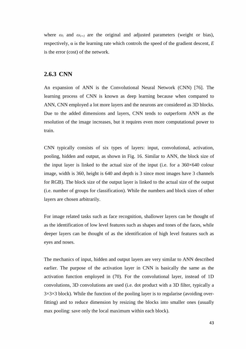
43

where ωi and ωi+1 are the original and adjusted parameters (weight or bias),

respectively, α is the learning rate which controls the speed of the gradient descent, E

is the error (cost) of the network.

2.6.3 CNN

An expansion of ANN is the Convolutional Neural Network (CNN) [76]. The

learning process of CNN is known as deep learning because when compared to

ANN, CNN employed a lot more layers and the neurons are considered as 3D blocks.

Due to the added dimensions and layers, CNN tends to outperform ANN as the

resolution of the image increases, but it requires even more computational power to

train.

CNN typically consists of six types of layers: input, convolutional, activation,

pooling, hidden and output, as shown in Fig. 16. Similar to ANN, the block size of

the input layer is linked to the actual size of the input (i.e. for a 360×640 colour

image, width is 360, height is 640 and depth is 3 since most images have 3 channels

for RGB). The block size of the output layer is linked to the actual size of the output

(i.e. number of groups for classification). While the numbers and block sizes of other

layers are chosen arbitrarily.

For image related tasks such as face recognition, shallower layers can be thought of

as the identification of low level features such as shapes and tones of the faces, while

deeper layers can be thought of as the identification of high level features such as

eyes and noses.

The mechanics of input, hidden and output layers are very similar to ANN described

earlier. The purpose of the activation layer in CNN is basically the same as the

activation function employed in (70). For the convolutional layer, instead of 1D

convolutions, 3D convolutions are used (i.e. dot product with a 3D filter, typically a

3×3×3 block). While the function of the pooling layer is to regularise (avoiding over-

fitting) and to reduce dimension by resizing the blocks into smaller ones (usually

max pooling: save only the local maximum within each block).

44

Figure 16 Example CNN setup: it contains 1 input, 4 convolutional, 7 activation, 2

pooling, 3 hidden and 1 output layers

Machine learning, especially CNN, is quickly becoming a new tool for solving many

complex problems. However, it requires huge amount of samples for the network to

learn adequately, the computational cost is also enormous and the training time can

be long and highly unpredictable. Additionally, it is widely known that the results of

the training can be sometimes puzzling, for example, when feeding a random

generated image that doesn’t look like anything into a trained network, it tends to

response with a very confident output.

2.7 Human Detection

Human detection can be defined as a process of detecting the presence of human

features from images or videos. Its applications are mainly found in the area of

surveillance [77], these may include the recognition [78], following [79] and

counting [80] of different people. The goal of human detection is to separate the

human from the background in a given image or video by identifying common

human-like features. As different people tend to have different features which are

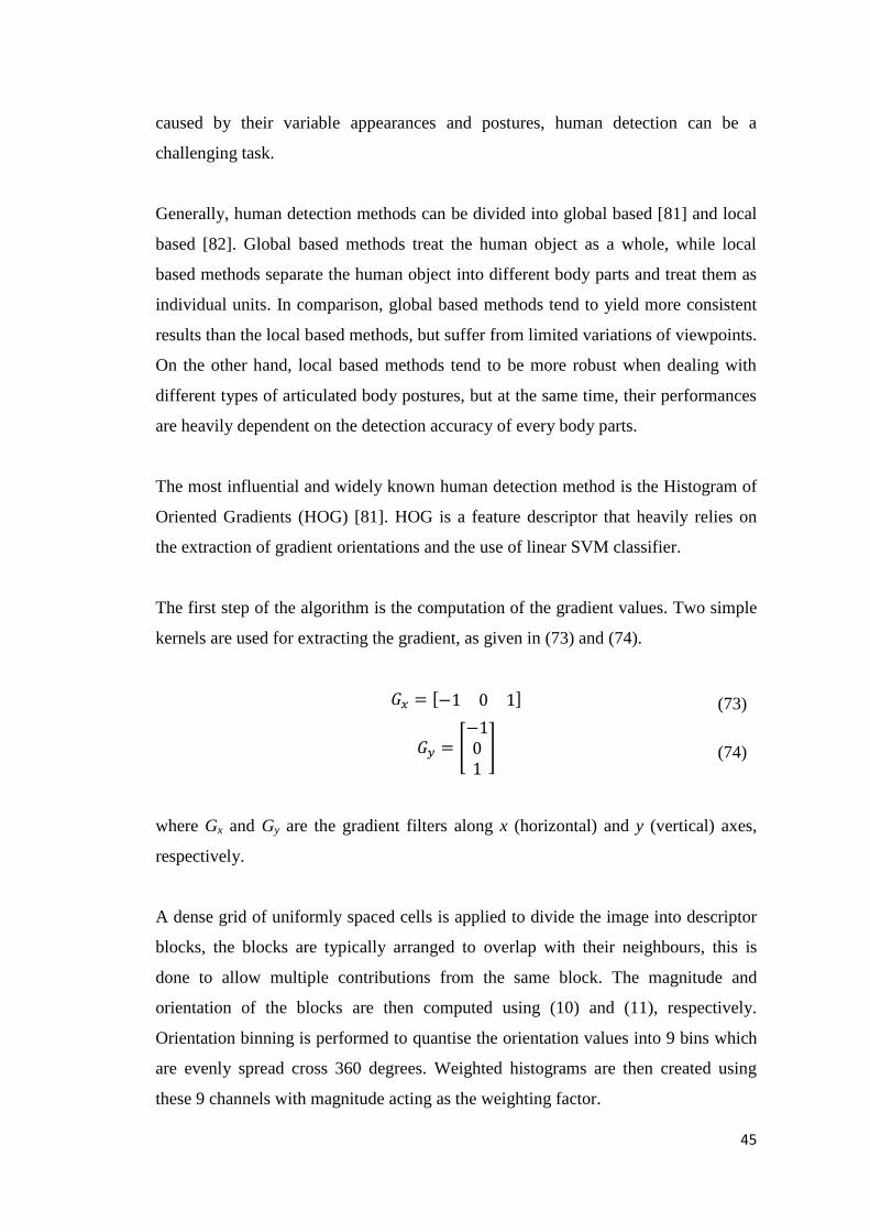
45

caused by their variable appearances and postures, human detection can be a

challenging task.

Generally, human detection methods can be divided into global based [81] and local

based [82]. Global based methods treat the human object as a whole, while local

based methods separate the human object into different body parts and treat them as

individual units. In comparison, global based methods tend to yield more consistent

results than the local based methods, but suffer from limited variations of viewpoints.

On the other hand, local based methods tend to be more robust when dealing with

different types of articulated body postures, but at the same time, their performances

are heavily dependent on the detection accuracy of every body parts.

The most influential and widely known human detection method is the Histogram of

Oriented Gradients (HOG) [81]. HOG is a feature descriptor that heavily relies on

the extraction of gradient orientations and the use of linear SVM classifier.

The first step of the algorithm is the computation of the gradient values. Two simple

kernels are used for extracting the gradient, as given in (73) and (74).

(73)

(74)

where Gx and Gy are the gradient filters along x (horizontal) and y (vertical) axes,

respectively.

A dense grid of uniformly spaced cells is applied to divide the image into descriptor

blocks, the blocks are typically arranged to overlap with their neighbours, this is

done to allow multiple contributions from the same block. The magnitude and

orientation of the blocks are then computed using (10) and (11), respectively.

Orientation binning is performed to quantise the orientation values into 9 bins which

are evenly spread cross 360 degrees. Weighted histograms are then created using

these 9 channels with magnitude acting as the weighting factor.

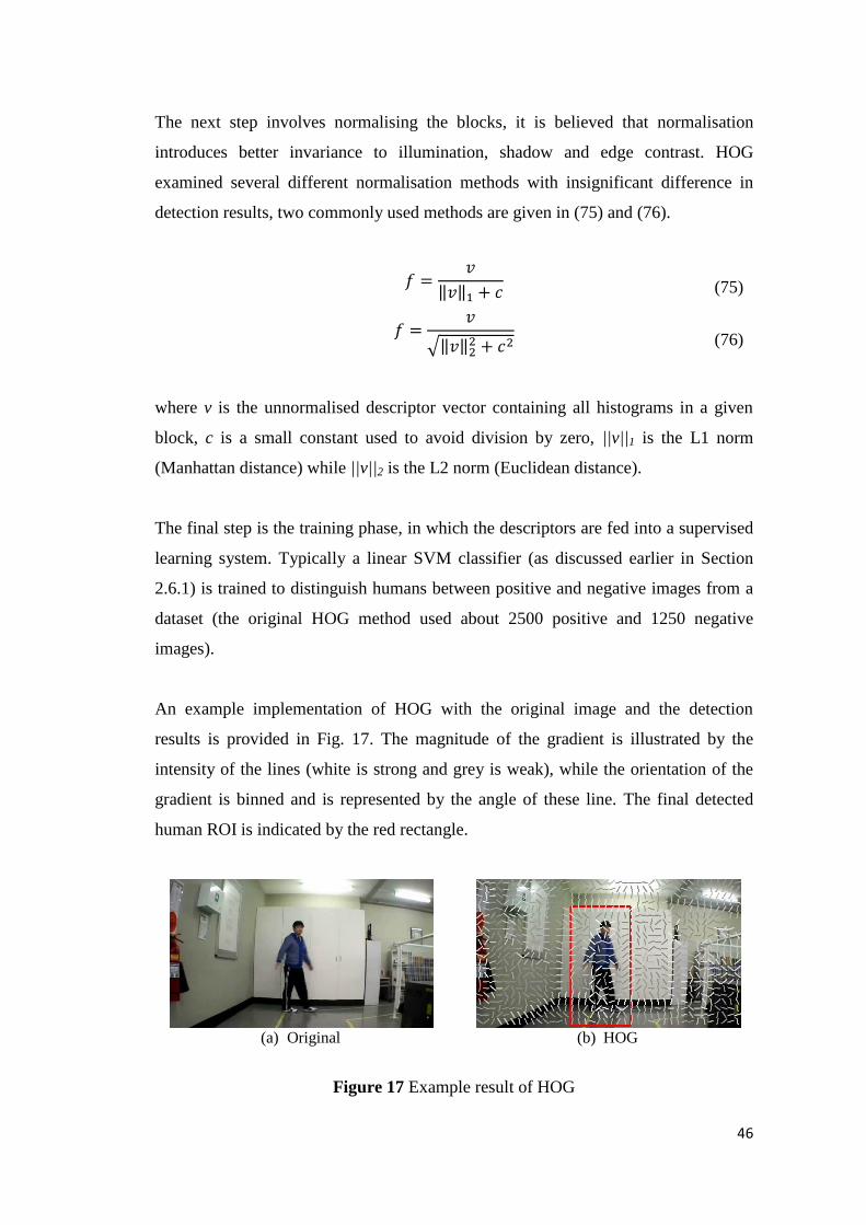
46

The next step involves normalising the blocks, it is believed that normalisation

introduces better invariance to illumination, shadow and edge contrast. HOG

examined several different normalisation methods with insignificant difference in

detection results, two commonly used methods are given in (75) and (76).

(75)

(76)

where v is the unnormalised descriptor vector containing all histograms in a given

block, c is a small constant used to avoid division by zero, ||v||1 is the L1 norm

(Manhattan distance) while ||v||2 is the L2 norm (Euclidean distance).

The final step is the training phase, in which the descriptors are fed into a supervised

learning system. Typically a linear SVM classifier (as discussed earlier in Section

2.6.1) is trained to distinguish humans between positive and negative images from a

dataset (the original HOG method used about 2500 positive and 1250 negative

images).

An example implementation of HOG with the original image and the detection

results is provided in Fig. 17. The magnitude of the gradient is illustrated by the

intensity of the lines (white is strong and grey is weak), while the orientation of the

gradient is binned and is represented by the angle of these line. The final detected

human ROI is indicated by the red rectangle.

(a) Original (b) HOG

Figure 17 Example result of HOG

47

HOG is renowned for its human detection ability by utilising a large amount of

training images. However, the accuracy of HOG is heavily influenced by the quality

and quantity of these training images. This is because, in order to train a classifier

successfully, it requires continuously recurring shape events in the given blocks of

the training images [83]. HOG generally suffers from speed issues due to its energy

intensive feature computations and the training itself can be a time consuming task.

Many existing methods tend to design their approaches based on HOG or utilise it as

an additional tool for their algorithms.

One method states that humans in standing positions tend to have distinguishing

colour characteristics [84], therefore addition colour information can be utilised with

HOG descriptors. This is done by extracting colour frequency and co-occurrence

features in each channel of the converted HSV colour space. It also employed the

partial least square regression analysis [85] onto the descriptors. These additional

elements improved the accuracy of HOG, however at the same time the

computational cost is also increased.

Another method utilises the omega shaped features of human heads [86]. This

approach argues that the HOG feature based classifier is generally accurate but very

slow to work with, while Haar feature based classifiers [87] are typically fast but

prone to noises. Thus, it is believed greater robustness can be achieved by combining

these two classifiers. This is done by employing Haar feature classifier to filter out

obvious negative image patches and then rely on HOG for the detection using the

remaining image patches. This approach greatly increased the computational speed

with only a small drop in accuracy. However, only the head of a person is

considered, the rest of the body are completely ignored.

Scale-Invariant Feature Transform (SIFT) can also be used for human detection [88].

SIFT [89] is an algorithm designed to detect and describe local features by extracting

distinctive invariant features. SIFT descriptors are similar to HOG in the sense that

both descriptors utilise gradient features. The difference is that HOG is computed in

dense grids while SIFT is computed in sparse grids with orientation alignment. By

combining HOG and SIFT descriptors, higher detection rate can be achieved.

48

However, the robustness of these methods tends to suffer significantly with online

processing, since both descriptors require reasonably high computational cost.

You Only Look Once (YOLO) is a general purpose object detector which can be

tuned for human detection [90]. By converting the detection problem to a fixed grid

regression problem, YOLO is able to minimise the computational cost required

during run-time. This is done by dividing the image into sparse grids in which each

grid detects only one object. A 24-layered CNN network is employed for the

detection, the first 20 layers are employed for pre-training purposes, the detection

layers are followed by 2 fully connected layers, while an average pooling and a

single fully connected layers are attached to the end of training layers. Because of its

fast detection speed, YOLO is regarded as a real-time detector, however the

precision level of the detection results tends to be low, this is mostly due to its fixed

grid nature.

2.8 Object Tracking

In computer vision, object tracking is about keeping track of the position of the target

object on the image continuously through a period of time. This may seem like a

straightforward task, but it remains a challenging problem due to several

complications such as occlusion, out of view, illumination, shadow, motion blur and

change of viewpoint [91]. Its applications can include surveillance [92], mapping

[93], medical imaging [94], automated manufacturing [95], gesture [22] and

behaviour recognitions [96].

Object tracking methods can be generally divided into two groups: learning based

and non-learning based. Learning based methods focus on the training of feature

classifiers to distinguish between the foreground object and the background noise,

while non-learning based methods usually concerned with the tracking of specific

features using pre-determined parameters. Learning based methods tend to be

relatively more resistant against background interference but require large pools of

training samples that contain relevant features to achieve satisfactory results. On the

49

contrary, non-learning based methods do not require any training, their results may

be prone to noise.

Learning based methods have gained traction in recent years mostly due to the

advancements in hardware, as the training and simulation time have been reduced

significantly compared to a decade ago. One of the well known methods in this topic

is Tracking-Learning-Detection (TLD) [97]. TLD proposes that the object tracking

task can be decomposed into three components: tracking, learning and detection.

These components work independently of each other as median flow is used to track

objects between frames, detection in a single frame is done based on template

matching and nearest neighbour classifier, growing and pruning are achieved through

learning of false positive and negative errors. Another widely known method is

Online AdaBoost Tracking (OAB) [98]. OAB allows feature updates during tracking

by utilising fast computable features such as Haar-like wavelets, orientation

histograms and local binary patterns. It also employs two types of classifiers: weak

classifier that corresponds to a single feature and strong classifier that represents a set

of weak classifiers. Local Sparse Appearance Model and K-selection based Tracking

(LSK) [99] is a method focus on the learning of the target appearance. LSK relies on

a static sparse dictionary and a dynamic basis distribution to limit the drifting of the

tracking. The object appearance is also modelled using a sparse coding histogram

based on a learned dictionary that improved detection.

Non-learning based methods tend to work with specific features. An example of such

methods is Kernel based Tracking (KNL) [100]. KNL regularises the feature

histogram based object representation by using spatial masking with an isotropic

kernel. It employs mean shift to perform gradient based optimisation with metrics

derived from the Bhattacharyya coefficient acting as the similarity measurement.

Fragment based Tracking (FRG) [101] is another method, it is based on histogram

tracking. For each frame, FRG introduces arbitrary patches to vote on possible

positions and scales of the object, the voting is performed by comparing intensity and

colour histogram with the corresponding patch. The vote maps are then combined

using the minimum sum method. Locality Sensitive Histogram based Tracking

(LSH) [102] also relies on histogram for tracking. However, unlike the conventional

50

histogram, LSH computes a weighted histogram at each pixel location with distance

as the weight, such that boundary pixels have minimum impact to the corresponding

histogram bin values. It also introduces a method of extracting illumination invariant

features.

Examples of the results using object tracking methods described earlier are presented

in Fig. 18. In the figure, the input image with original ROI and the test image with

detected ROIs using different methods are given in (a) and (b), respectively. The

original ROI and the detected ROIs are also provided separately, as shown in (c) to

(i). The size of these ROIs is increased by a factor for visualisation and comparison

purposes, their actual sizes are illustrated by the different rectangular ROIs in (a) and

(b).

(a) Input image with original ROI (b) Test image with detected ROIs

(c) Original

(d) TLD (e) OAB

51

(f) LSK (g) KNL

(h) FRG (i) LSH

Figure 18 Example results of object tracking

2.9 Target Pursuit Using UAV

Although UAV is initially designed for military purposes which can be traced back

to as early as the World War I [103], nowadays, UAV is mainly used for

photogrammetric applications such as surveillance and remote sensing. In recent

times, there is an evidenced increase in popularity of using UAV for various

applications such as target pursuit, this is because when compared to manned

systems, UAV is cheaper, faster and safer [104]. Additionally, most UAVs tend to be

small since there is no need for human pilots onboard. This allows them to operate in

tight spaces and rather close to the object, thus acquiring more images with higher

quality. Another important reason of the increased demand can be explained by the

spreading of low cost GPS and INS combined systems. The combination of GPS and

INS is known to provide reliable velocity and position estimations, which are

necessary for high precision navigations [105].

Among the applications of UAV, vision based target pursuit is a challenging and

complex problem, this is because it consists of many sub-problems which are

typically concerned with the detection, tracking and following of the object of

interest. Other issues such as localisation, path planning, obstacle avoidance and

52

multi-robot cooperation can also be considered which further increase the difficulty.

Until recent years, there are very few practical approaches related to this to topic [6–

10], as the majority of the related existing methods are developed using computer

simulation with the assumption of ideal environmental factors [1–5]. This is mostly

due to advancements in both hardware and software of small UAVs such as

quadrotors during the past decade. Among the few methods developed, one method

approached the pursuit problem by focusing on tracking the colour of the target [6],

this is done by employing a colour based probabilistic tracking scheme based on

Camshift [106]. This method is experimented with the tracking of a balloon using a

drone at close range. Another method [7] working on the tracking of the entire body

of a standing person also chose Camshift. This approach relied on Camshift to detect

candidate ROIs, the most suitable ROI is then determined by comparing the

corresponding sizes and histogram. Kalman filter [107] is employed for the

localisation of both the drone and target person with respect to a common reference

frame. Other approaches, such as the one presented in [8] employed TLD [97] to

track a human target. This is done by tracking gradient based and greyscale intensity

features belonging to the torso of a person, the drone is then programmed to follow

the person.

While most methods relied on front facing cameras for tracking the target, downward

facing ones can also be used. An example is this implementation [9], in which a

drone is programmed to pursuit a remotely controlled toy car using a downward

pointing camera. It employs a colour tracking approach based on the particle filter

[108] with considerations of noise and occlusion. A similar experiment is performed

with a moving landing platform [10]. This is done by tracking the platform using

rectangle detection and optical flow [54]. The position of the platform is computed

based on centroid of image moments.

Based on the results provided in these practical methods, such as the example

tracking frames shown in Fig. 19, it can be seen that the methods are able to track

their designed targets within their test environments. However, their targets tend to

be simple objects that contain monochromatic colours with very little texture

variances, these targets also appear highly salient when compared to the

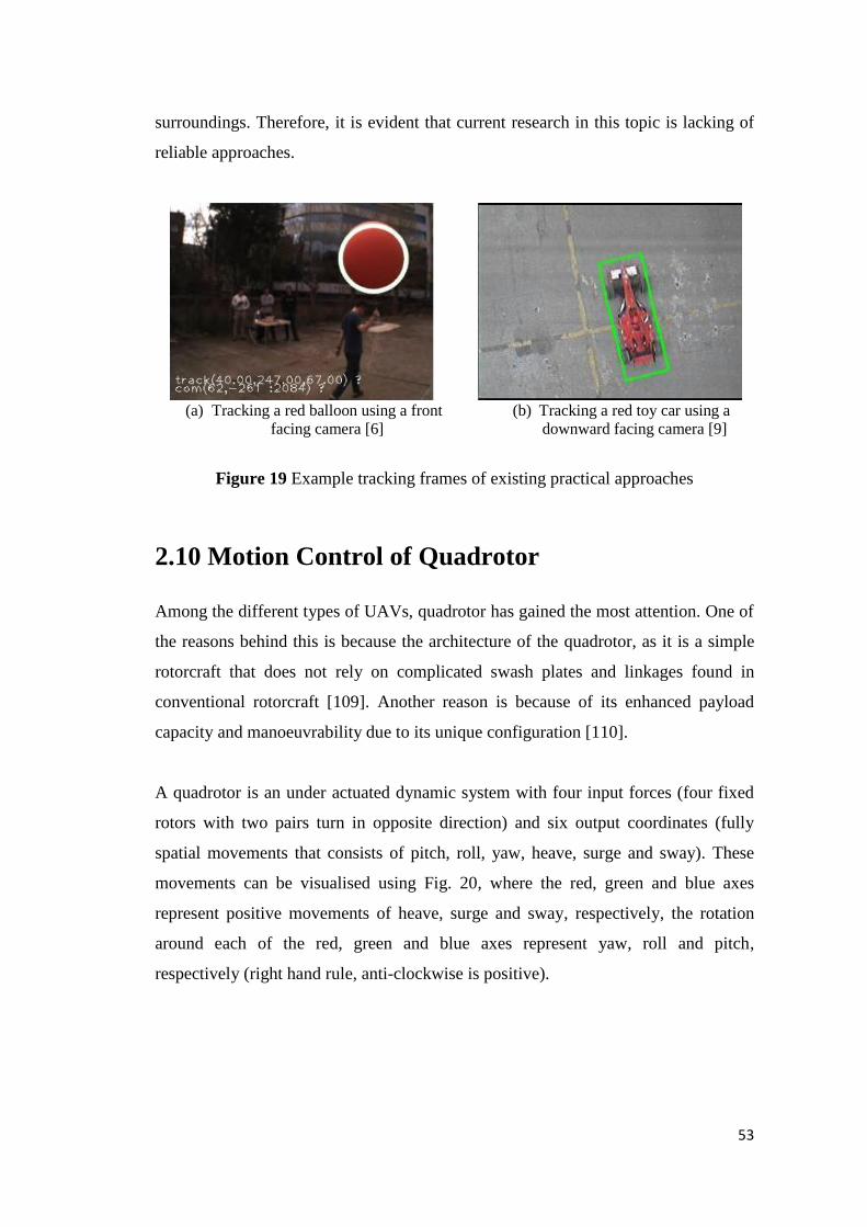
53

surroundings. Therefore, it is evident that current research in this topic is lacking of

reliable approaches.

(a) Tracking a red balloon using a front

facing camera [6]

(b) Tracking a red toy car using a

downward facing camera [9]

Figure 19 Example tracking frames of existing practical approaches

2.10 Motion Control of Quadrotor

Among the different types of UAVs, quadrotor has gained the most attention. One of

the reasons behind this is because the architecture of the quadrotor, as it is a simple

rotorcraft that does not rely on complicated swash plates and linkages found in

conventional rotorcraft [109]. Another reason is because of its enhanced payload

capacity and manoeuvrability due to its unique configuration [110].

A quadrotor is an under actuated dynamic system with four input forces (four fixed

rotors with two pairs turn in opposite direction) and six output coordinates (fully

spatial movements that consists of pitch, roll, yaw, heave, surge and sway). These

movements can be visualised using Fig. 20, where the red, green and blue axes

represent positive movements of heave, surge and sway, respectively, the rotation

around each of the red, green and blue axes represent yaw, roll and pitch,

respectively (right hand rule, anti-clockwise is positive).

54

Figure 20 Spatial movements of a quadrotor: pitch, roll, yaw, heave, surge and sway

Since one pair of opposite propellers rotates in clockwise direction while the other

pair rotates in anti-clockwise direction, this causes the net aerodynamic torque to be

exactly zero, thus eliminates the need of a yaw stabilising rotor found in

conventional helicopters. Typical rotor configuration of quadrotor with its rotation

directions is given in Fig. 21, where C and A represent clockwise and anti-clockwise

rotations, respectively.

Figure 21 Typical rotor configuration of quadrotor

Various motions of quadrotor can be produced by controlling the individual rotor

speeds of all four motors, as given in Fig. 22, where + and – represent increasing and

55

decreasing rotor speeds, respectively, O represents equilibrium rotor speed that keeps

the quadrotor stable when hovering (thrust equals to weight, i.e. 4×O causes the

quadrotor to hover over a fixed point). Pitch, roll and yaw rotations are achieved by

creating speed variations between different pairs of propellers: pitch is affected by

front and back pairs, roll is affected by left and right pairs, yaw is affected by

diagonal pairs. Heave translation is achieved by varying the speed of all propellers

evenly, while surge and sway translations are achieved by maintaining non-zero

pitch and roll angles, respectively.

(a) Hover

(b) Surge

(c) Sway

(d) Heave

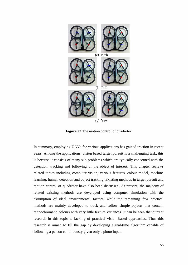
56

(e) Pitch

(f) Roll

(g) Yaw

Figure 22 The motion control of quadrotor

In summary, employing UAVs for various applications has gained traction in recent

years. Among the applications, vision based target pursuit is a challenging task, this

is because it consists of many sub-problems which are typically concerned with the

detection, tracking and following of the object of interest. This chapter reviews

related topics including computer vision, various features, colour model, machine

learning, human detection and object tracking. Existing methods in target pursuit and

motion control of quadrotor have also been discussed. At present, the majority of

related existing methods are developed using computer simulation with the

assumption of ideal environmental factors, while the remaining few practical

methods are mainly developed to track and follow simple objects that contain

monochromatic colours with very little texture variances. It can be seen that current

research in this topic is lacking of practical vision based approaches. Thus this

research is aimed to fill the gap by developing a real-time algorithm capable of

following a person continuously given only a photo input.

57

Chapter 3 Proposed Methods in Colour Based Feature Detection

This chapter proposes three methods in colour based feature detection. Section 3.1

introduces a colour enhancement method for colour segmentation. Section 3.2

discusses a colour identification method and Section 3.3 details the concept of a

colour model for improved colour detection. The contents of this chapter are based

on revised versions of author’s publications resulting from this research [111–113].

These publications can also be found in the list of publications in Section 1.4.

3.1 A Colour Enhancement Method for Colour

Segmentation

Existing colour segmentation methods tend to be designed for a specific colour

space, they also tend to focus on the segmentation stage alone and employ little to

none for pre-processing. In this section, a colour enhancement method that is capable

of improving the results of colour segmentation is presented. The proposed colour

enhancement method is named Chroma based Colour Enhancement (CCE), chroma

can be defined as the colourfulness property relative to brightness, the goal of the

enhancement is to boost the colour saliency of critical regions and to improve the

consistency of segmentation results by maximizing chroma while preserving the hue

angle. The enhancement procedure is efficient and easy to implement as it is

designed to operate on raw RGB inputs and only requires one pass of the original

image for filtering.

The proposed CCE method starts by finding the optimal threshold for colour

enhancement. This is determined according to the colourfulness of the given image

based on the mean chroma level. Critical colour regions of the image are then

enhanced by maximizing the chroma while preserving the hue angle, this is done by

58

filtering through all three channels of the raw RGB inputs using the determined

threshold. The detailed approach is described below.

Chroma is calculated based on common knowledge using (77) to (79). Mean chroma

level can be interpreted as an indicator of the colourfulness of the image and is

computed using (80). The optimal threshold is then obtained based on the mean

chroma level using (81).

(77)

(78)

(79)

(80)

(81)

where i represents individual pixel, r, g, b are the red, green and blue intensity

values, U and V are the minimum and maximum intensity values, respectively, n is

the total number of pixels in the image, C is chroma, is the mean chroma level and

CT is the optimal threshold for colour enhancement. CT is employed to differentiate

grey from ordinary colours. A colourful image tends to have less grey pixels than a

colourless one, therefore threshold decreases when the mean chroma level increases

and vise versa. The limits of CT are determined empirically based on mean chroma

level of typical photos (which tend to be medium to low levels).

Once the optimal threshold is determined, all three RGB channels of the image are

filtered, in which the chroma level of every pixel is checked against the threshold. If

its chroma level is greater or equal to the threshold, the pixel is assigned to the

critical colour regions and colour enhancement is applied by maximising chroma

while preserving the hue angle. Otherwise it is regarded as noise and the colour

content of the pixel will be removed by converting it to greyscale.

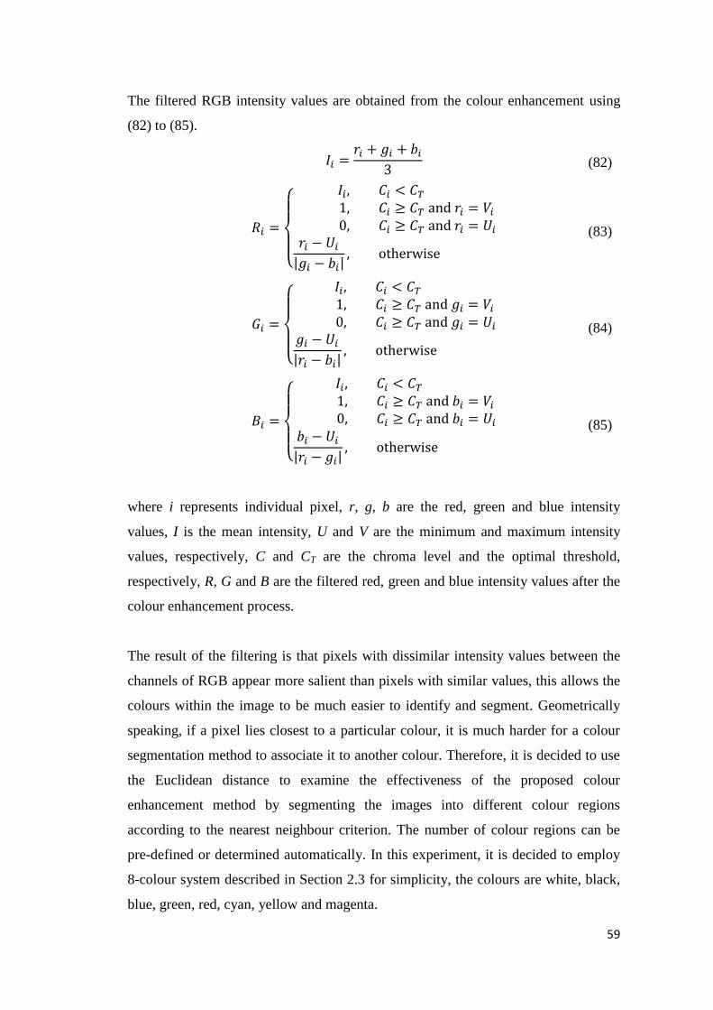
59

The filtered RGB intensity values are obtained from the colour enhancement using

(82) to (85).

(82)

(83)

(84)

(85)

where i represents individual pixel, r, g, b are the red, green and blue intensity

values, I is the mean intensity, U and V are the minimum and maximum intensity

values, respectively, C and CT are the chroma level and the optimal threshold,

respectively, R, G and B are the filtered red, green and blue intensity values after the

colour enhancement process.

The result of the filtering is that pixels with dissimilar intensity values between the

channels of RGB appear more salient than pixels with similar values, this allows the

colours within the image to be much easier to identify and segment. Geometrically

speaking, if a pixel lies closest to a particular colour, it is much harder for a colour

segmentation method to associate it to another colour. Therefore, it is decided to use

the Euclidean distance to examine the effectiveness of the proposed colour

enhancement method by segmenting the images into different colour regions

according to the nearest neighbour criterion. The number of colour regions can be

pre-defined or determined automatically. In this experiment, it is decided to employ

8-colour system described in Section 2.3 for simplicity, the colours are white, black,

blue, green, red, cyan, yellow and magenta.

60

To fully present the effectiveness of the proposed colour enhancement method, the

proposed approach is compared with one of the traditional contrast based approaches

[114] (referred to as traditional contrast enhancement or TCE). The original image,

and the enhanced images using TCE and the proposed CCE methods are shown in

Fig. 23, while the results of colour segmentation in RGB colour space using these

three type of images are provided in Fig. 24. The original images are collected from

various sources and have different sizes, intensity and quality, from the top to the

bottom: the first three images are captured by the front facing camera of the

quadrotor used in this research, the next two images are obtained from the INRIA

person dataset and the rest are randomly selected from Google images.

1(a) 1(b) 1(c)

2(a) 2(b) 2(c)

3(a) 3(b) 3(c)

4(a) 4(b) 4(c)

5(a) 5(b) 5(c)

6(a) 6(b) 6(c)

61

7(a) 7(b) 7(c)

8(a) 8(b) 8(c)

9(a) 9(b) 9(c)

10(a) 10(b) 10(c)

11(a) 11(b) 11(c)

12(a) 12(b) 12(c)

(a) Original* (b) TCE (c) CCE

Figure 23 Original and enhanced images using TCE and CCE

*Original images (based on case number):

3 to 5: http://pascal.inrialpes.fr/data/human 6: https://www.youtube.com/watch?v=woag8p2aEaE 7: http://geekongadgets.com/wp-content/uploads/2014/06/702325779.jpg 8: https://dirghakala.files.wordpress.com/2012/11/obama.jpg 9: https://exampundit.in/wp-content/uploads/2014/08/IBPSFIFANOTES.jpg 10: http://i.dailymail.co.uk/i/pix/2015/01/15/24BCA07300000578-2912489-image-a-25_1421364595463.jpg 11: http://www.maxtheknife.com/marshax3/marsha36.jpg 12: https://www.sneakerfiles.com/wp-content/uploads/2009/04/nike-terminator-low-pink-blue-turquoise-purple-4.jpg

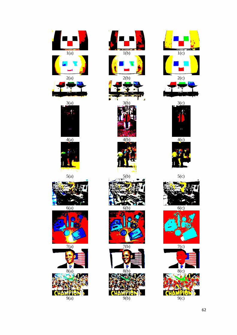
62

1(a) 1(b) 1(c)

2(a) 2(b) 2(c)

3(a) 3(b) 3(c)

4(a) 4(b) 4(c)

5(a) 5(b) 5(c)

6(a) 6(b) 6(c)

7(a) 7(b) 7(c)

8(a) 8(b) 8(c)

9(a) 9(b) 9(c)

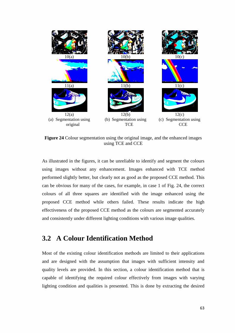
63

10(a) 10(b) 10(c)

11(a) 11(b) 11(c)

12(a) 12(b) 12(c)

(a) Segmentation using

original

(b) Segmentation using

TCE

(c) Segmentation using

CCE

Figure 24 Colour segmentation using the original image, and the enhanced images

using TCE and CCE

As illustrated in the figures, it can be unreliable to identify and segment the colours

using images without any enhancement. Images enhanced with TCE method

performed slightly better, but clearly not as good as the proposed CCE method. This

can be obvious for many of the cases, for example, in case 1 of Fig. 24, the correct

colours of all three squares are identified with the image enhanced using the

proposed CCE method while others failed. These results indicate the high

effectiveness of the proposed CCE method as the colours are segmented accurately

and consistently under different lighting conditions with various image qualities.

3.2 A Colour Identification Method

Most of the existing colour identification methods are limited to their applications

and are designed with the assumption that images with sufficient intensity and

quality levels are provided. In this section, a colour identification method that is

capable of identifying the required colour effectively from images with varying

lighting condition and qualities is presented. This is done by extracting the desired

64

colour through adaptively determining the thresholds and the colour space that

produce the best outcome.

The proposed colour identification method is named Adaptive Multi-channel

Thresholding (AMT), it consists of three stages: image analysis, colour space

selection and adaptive filtering. The proposed AMT method firstly analyses the

image by collecting a variety of information, this is employed to determine the key

properties of the image. The colour space selection scheme is then applied to find the

most suitable hue based colour space by using the key properties obtained earlier.

Finally, to extract the target colour, the image is filtered through all the channels of

the selected colour space. The detailed approach is described below.

The first stage is image analysis, in which key properties of the image are

determined. The obtained image properties include: value, chroma, lightness,

saturation, hue, entropy (of hue), mean intensity and its standard deviation (of the

foreground, the background and the entire image). The equations for value, chroma,

lightness, saturation and hue are described earlier in Section 2.5, mean intensity is

determined using (86) and (87), standard deviation and entropy are calculated based

on common knowledge using (88) and (89), respectively.

(86)

(87)

(88)

(89)

where i represents individual pixel, r, g, b are the red, green and blue intensities,

respectively, n is the total number of pixels in the image, H is the hue, I and are the

65

mean intensity of the pixel and the entire image, respectively, σ and E are the

standard deviation and the entropy, respectively.

Additionally, the pixels are roughly classified into foreground and background

through a simple hue filtering procedure, as given in (90).

(90)

where α is the class identifier in which 1 and 0 represent foreground and background,

respectively, H and Hd are the actual and desired hue values, respectively. The

desired value can be determined based on a pre-defined colour or it can be obtained

automatically from a ROI. The absolute difference threshold is selected empirically

as the shifting of hue due to lighting condition is common to occur but unlikely to be

more than 30°.

By finding these properties, the main characteristic of the image can be determined.

For example, an image with low entropy and standard deviation levels tends to

indicate the colour consistency is high and the image quality is low.

The second stage is the colour space selection, in which the most suitable colour

space is selected based on properties obtained through image analysis. Generally, in

hue based colour models there are four commonly used colour spaces: HSV, HSL,

HCV and HCL. The selection of these colour spaces is important because each

colour space has its own measures of colour purity and brightness under different

lighting conditions. The key in the selection is to differentiate between the lightness

with the value in the colour brightness channel, and between the chroma with the

saturation in the colour purity channel.

When the foreground has a wider spread of intensity than the background, it can be

said that the foreground has a higher variance in the brightness channel than the

background. Therefore both the maximum and minimum values of the RGB should

be considered and hence L is selected to represent the brightness of the image,

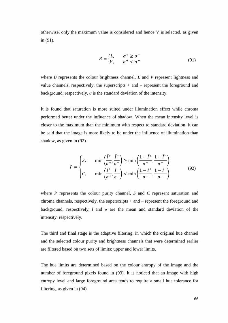
66

otherwise, only the maximum value is considered and hence V is selected, as given

in (91).

(91)

where B represents the colour brightness channel, L and V represent lightness and

value channels, respectively, the superscripts + and – represent the foreground and

background, respectively, σ is the standard deviation of the intensity.

It is found that saturation is more suited under illumination effect while chroma

performed better under the influence of shadow. When the mean intensity level is

closer to the maximum than the minimum with respect to standard deviation, it can

be said that the image is more likely to be under the influence of illumination than

shadow, as given in (92).

(92)

where P represents the colour purity channel, S and C represent saturation and

chroma channels, respectively, the superscripts + and – represent the foreground and

background, respectively, and σ are the mean and standard deviation of the

intensity, respectively.

The third and final stage is the adaptive filtering, in which the original hue channel

and the selected colour purity and brightness channels that were determined earlier

are filtered based on two sets of limits: upper and lower limits.

The hue limits are determined based on the colour entropy of the image and the

number of foreground pixels found in (93). It is noticed that an image with high

entropy level and large foreground area tends to require a small hue tolerance for

filtering, as given in (94).

67

(93)

(94)

where H1 and H2 are the lower and upper hue limits, respectively, n+ and n are the

numbers of foreground and total pixels in the image, respectively, Hd is the desired

hue value, E is the entropy. Note: log2 360° is the maximum entropy and 30° is the

absolute difference threshold used in (90).

The brightness limits are computed based on foreground intensity, background

intensity and standard deviation of intensity. An image with low background and

foreground intensities but large standard deviation tends to favour a small brightness

tolerance for filtering, as given in (95) and (96).

(95)

(96)

where B1 and B2 are the lower and upper brightness limits, respectively, the

superscripts + and – represent the foreground and background, respectively, and σ

are the mean and standard deviation of the intensity, respectively. As colour regions

located next to absolute white (maximum) and absolute black (minimum) are

difficult to differentiate, a brightness threshold BT of 1% is applied to each of the

limits to filter out those regions.

The purity limits are obtained based on the brightness limits. However, the upper

limit is adjusted to the maximum, this is done because colour purity is a reliable

measure of the strength of the colours presented in the image, as given in (97) and

(98).

68

(97)

(98)

where P1 and P2 are the lower and upper purity limits, respectively, B1 is the lower

brightness limit.

Based on these selections, the required colour can then be obtained through multi-

channel filtering. To fully present the effectiveness of the proposed AMT method,

the method is firstly examined with the detection of red square in the five benchmark

images, as shown in Fig. 25.

These five images are captured by the front facing camera of the quadrotor used in

this research under very different lighting conditions, from the top to the bottom: the

first image is captured under normal lighting conditions, the next two images are

captured under shadow effects and the last two images are capture under illumination

effects. In the figure, the original benchmark images are shown in (a), results using

the simple hue filter are given in (b), results using AMT (without adaptive colour

space selection) in HCV, HCL, HSV and HSL are provided in (c) to (f), respectively,

results using AMT with adaptive colour space selection are presented in (g).

1(b) 1(c) 1(d)

1(a) 1(e) 1(f) 1(g)

2(b) 2(c) 2(d)

2(a) 2(e) 2(f) 2(g)

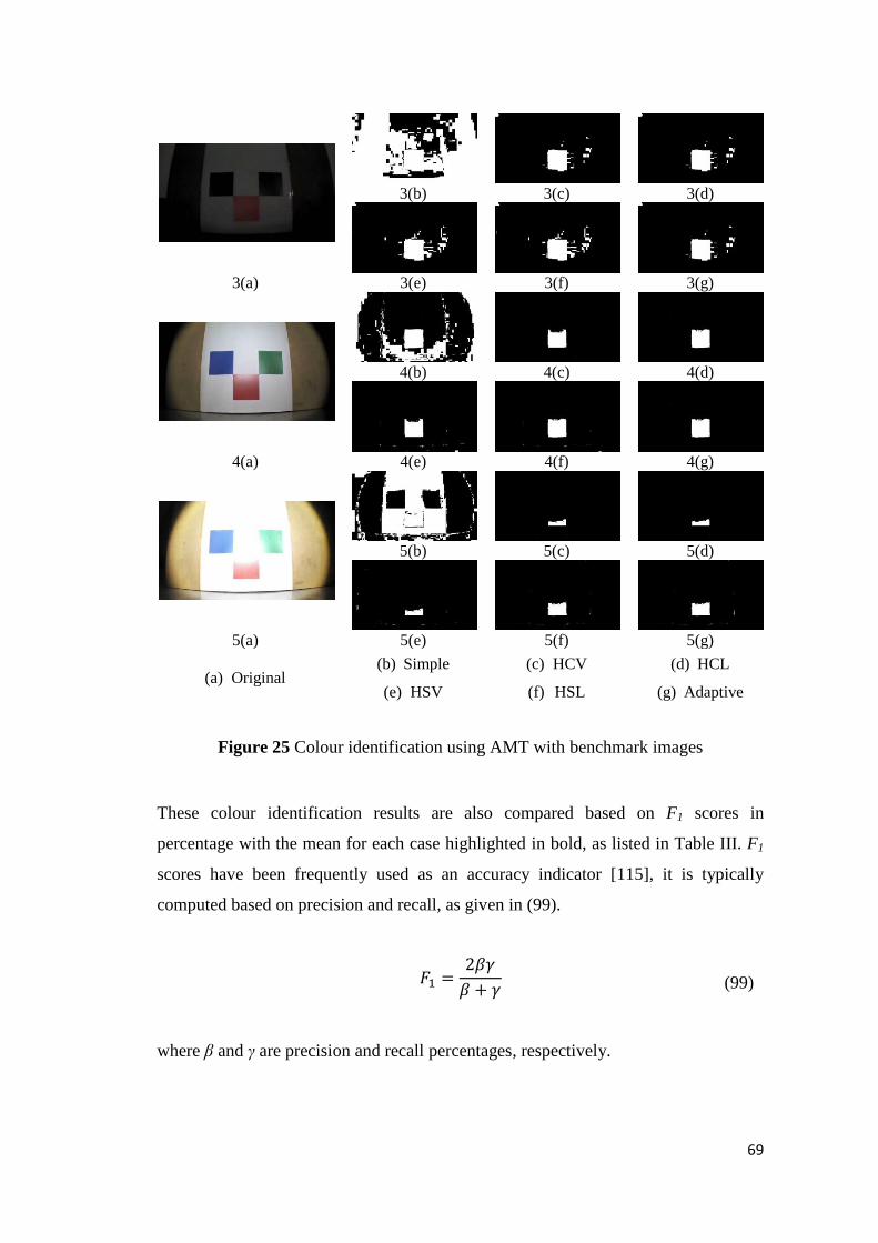
69

3(b) 3(c) 3(d)

3(a) 3(e) 3(f) 3(g)

4(b) 4(c) 4(d)

4(a) 4(e) 4(f) 4(g)

5(b) 5(c) 5(d)

5(a) 5(e) 5(f) 5(g)

(a) Original (b) Simple (c) HCV (d) HCL

(e) HSV (f) HSL (g) Adaptive

Figure 25 Colour identification using AMT with benchmark images

These colour identification results are also compared based on F1 scores in

percentage with the mean for each case highlighted in bold, as listed in Table III. F1

scores have been frequently used as an accuracy indicator [115], it is typically

computed based on precision and recall, as given in (99).

(99)

where β and γ are precision and recall percentages, respectively.

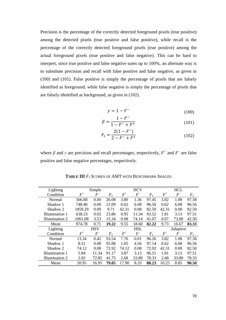
70

Precision is the percentage of the correctly detected foreground pixels (true positive)

among the detected pixels (true positive and false positive), while recall is the

percentage of the correctly detected foreground pixels (true positive) among the

actual foreground pixels (true positive and false negative). This can be hard to

interpret, since true positive and false negative sums up to 100%, an alternate way is

to substitute precision and recall with false positive and false negative, as given in

(100) and (101). False positive is simply the percentage of pixels that are falsely

identified as foreground, while false negative is simply the percentage of pixels that

are falsely identified as background, as given in (102).

(100)

(101)

(102)

where β and γ are precision and recall percentages, respectively, F+ and F

– are false

positive and false negative percentages, respectively.

TABLE III F1 SCORES OF AMT WITH BENCHMARK IMAGES

Lighting

Condition

Simple HCV HCL

F+ F

– F1 F

+ F

– F1 F

+ F

– F1

Normal 566.88 0.00 26.08 3.80 1.36 97.45 3.82 1.08 97.58

Shadow 1 748.40 0.00 21.09 0.62 6.08 96.56 0.62 6.08 96.56

Shadow 2 1859.29 0.00 9.71 42.31 0.08 82.50 42.31 0.08 82.50

Illumination 1 638.23 0.02 23.86 0.95 11.34 93.52 1.81 3.13 97.51

Illumination 2 1061.08 3.53 15.34 0.08 74.14 41.07 0.07 73.00 42.50

Mean 974.78 0.71 19.22 9.55 18.60 82.22 9.73 16.67 83.33

Lighting

Condition

HSV HSL Adaptive

F+ F

– F1 F

+ F

– F1 F

+ F

– F1

Normal 13.34 0.42 93.54 7.76 0.01 96.26 3.82 1.08 97.58

Shadow 1 8.51 0.08 95.88 1.05 4.56 97.14 0.62 6.08 96.56

Shadow 2 74.12 0.08 72.92 74.12 0.08 72.92 42.31 0.08 82.50

Illumination 1 5.84 11.34 91.17 3.87 3.13 96.51 1.81 3.13 97.51

Illumination 2 2.92 72.85 41.75 2.68 33.89 78.33 2.68 33.89 78.33

Mean 20.95 16.95 79.05 17.90 8.33 88.23 10.25 8.85 90.50

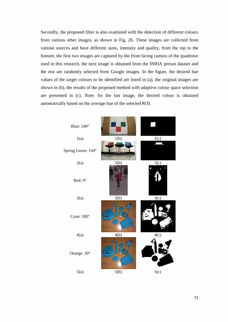
71

Secondly, the proposed filter is also examined with the detection of different colours

from various other images, as shown in Fig. 26. These images are collected from

various sources and have different sizes, intensity and quality, from the top to the

bottom: the first two images are captured by the front facing camera of the quadrotor

used in this research, the next image is obtained from the INRIA person dataset and

the rest are randomly selected from Google images. In the figure, the desired hue

values of the target colours to be identified are listed in (a), the original images are

shown in (b), the results of the proposed method with adaptive colour space selection

are presented in (c). Note: for the last image, the desired colour is obtained

automatically based on the average hue of the selected ROI.

Blue: 240°

1(a) 1(b) 1(c)

Spring Green: 150°

2(a) 2(b) 2(c)

Red: 0°

3(a) 3(b) 3(c)

Cyan: 180°

4(a) 4(b) 4(c)

Orange: 30°

5(a) 5(b) 5(c)

72

Cyan: 180°

6(a) 6(b) 6(c)

Orange: 30°

7(a) 7(b) 7(c)

ROI: 157°

8(a) 8(b) 8(c)

(a) Hue (b) Original* (c) Adaptive

Figure 26 Colour identification using AMT with various other images

These results indicate the high effectiveness of the proposed AMT method as the

required colours are extracted successfully under different lighting conditions and

image qualities. In Table III, the mean F1 score for the five benchmark images is

90.50% which is relatively high considered that four out of five cases are under the

effects of illumination or shadow. In the case when the required colour is unknown,

the proposed method can still be applied as long as a ROI is selected to indicate the

desired colour, as demonstrated in case 8 of Fig. 26.

3.3 A Colour Model

Currently, approaches working with colour based features tend to rely on a specific

colour model (typically hue based colour spaces). However, exiting colour models

are known to be environment dependent in which slight changes of environmental

factors such as lighting could greatly reduce the reliability. In this section, a colour *Original images (based on case number):

3: http://pascal.inrialpes.fr/data/human 4 & 5: http://geekongadgets.com/wp-content/uploads/2014/06/702325779.jpg 6 & 7: http://www.maxtheknife.com/marshax3/marsha36.jpg 8: https://www.sneakerfiles.com/wp-content/uploads/2009/04/nike-terminator-low-pink-blue-turquoise-purple-4.jpg

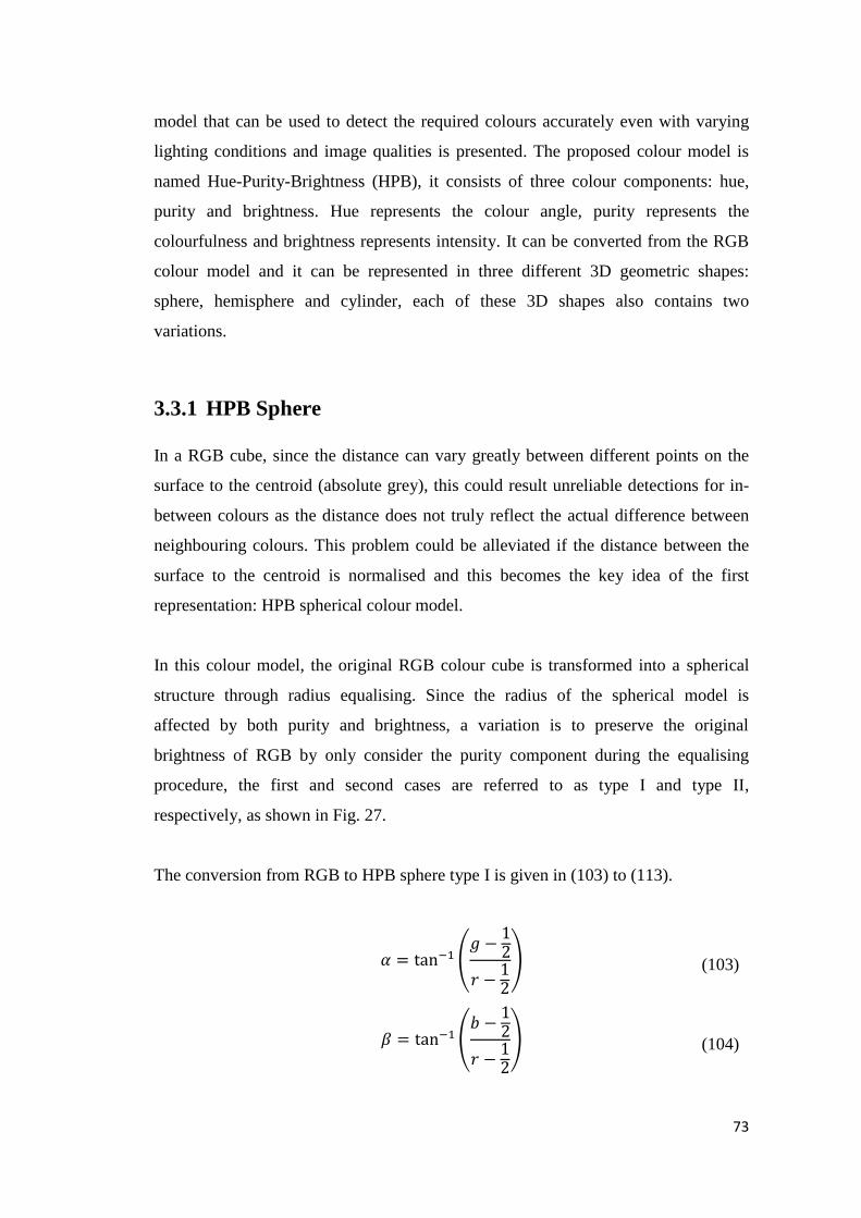
73

model that can be used to detect the required colours accurately even with varying

lighting conditions and image qualities is presented. The proposed colour model is

named Hue-Purity-Brightness (HPB), it consists of three colour components: hue,

purity and brightness. Hue represents the colour angle, purity represents the

colourfulness and brightness represents intensity. It can be converted from the RGB

colour model and it can be represented in three different 3D geometric shapes:

sphere, hemisphere and cylinder, each of these 3D shapes also contains two

variations.

3.3.1 HPB Sphere

In a RGB cube, since the distance can vary greatly between different points on the

surface to the centroid (absolute grey), this could result unreliable detections for in-

between colours as the distance does not truly reflect the actual difference between

neighbouring colours. This problem could be alleviated if the distance between the

surface to the centroid is normalised and this becomes the key idea of the first

representation: HPB spherical colour model.

In this colour model, the original RGB colour cube is transformed into a spherical

structure through radius equalising. Since the radius of the spherical model is

affected by both purity and brightness, a variation is to preserve the original

brightness of RGB by only consider the purity component during the equalising

procedure, the first and second cases are referred to as type I and type II,

respectively, as shown in Fig. 27.

The conversion from RGB to HPB sphere type I is given in (103) to (113).

(103)

(104)

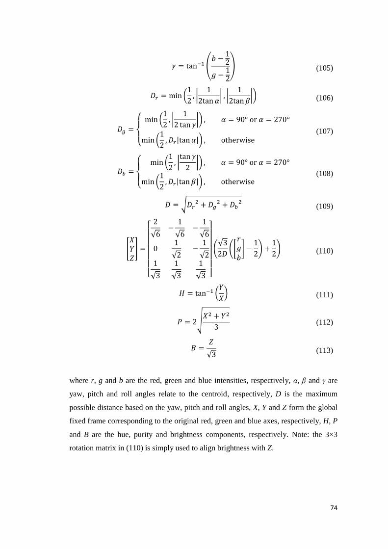
74

(105)

(106)

(107)

(108)

(109)

(110)

(111)

(112)

(113)

where r, g and b are the red, green and blue intensities, respectively, α, β and γ are

yaw, pitch and roll angles relate to the centroid, respectively, D is the maximum

possible distance based on the yaw, pitch and roll angles, X, Y and Z form the global

fixed frame corresponding to the original red, green and blue axes, respectively, H, P

and B are the hue, purity and brightness components, respectively. Note: the 3×3

rotation matrix in (110) is simply used to align brightness with Z.

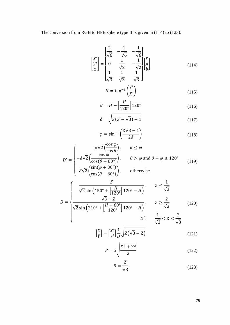
75

The conversion from RGB to HPB sphere type II is given in (114) to (123).

(114)

(115)

(116)

(117)

(118)

(119)

(120)

(121)

(122)

(123)

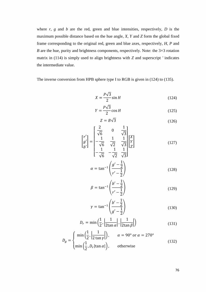
76

where r, g and b are the red, green and blue intensities, respectively, D is the

maximum possible distance based on the hue angle, X, Y and Z form the global fixed

frame corresponding to the original red, green and blue axes, respectively, H, P and

B are the hue, purity and brightness components, respectively. Note: the 3×3 rotation

matrix in (114) is simply used to align brightness with Z and superscript ' indicates

the intermediate value.

The inverse conversion from HPB sphere type I to RGB is given in (124) to (135).

(124)

(125)

(126)

(127)

(128)

(129)

(130)

(131)

(132)

77

(133)

(134)

(135)

where r, g and b are the red, green and blue intensities, respectively, α, β and γ are

yaw, pitch and roll angles relate to the centroid, respectively, D is the maximum

possible distance based on the yaw, pitch and roll angles, X, Y and Z form the global

fixed frame corresponding to the original red, green and blue axes, respectively, H, P

and B are the hue, purity and brightness components, respectively. Note: the 3×3

rotation matrix in (127) is simply the inverse (and transpose due to orthogonality) of

the rotation matrix in (110). Superscript ' indicates the intermediate value.

The inverse conversion from HPB sphere type II to RGB is given in (136) to (145).

(136)

(137)

(138)

(139)

(140)

(141)

(142)

78

(143)

(144)

(145)

where r, g and b are the red, green and blue intensities, respectively, D is the

maximum possible distance based on the hue angle, X, Y and Z form the global fixed

frame corresponding to the original red, green and blue axes, respectively, H, P and

B are the hue, purity and brightness components, respectively. Note: the 3×3 rotation

matrix in (145) is simply the inverse (and transpose due to orthogonality) of the

rotation matrix in (110). Superscript ' indicates the intermediate value.

79

(a) HPB sphere I

(b) HPB sphere II

Figure 27 HPB spherical colour models

3.3.2 HPB Hemisphere

In the first representation, the original RGB cube is transformed into HPB sphere so

that the distance between any point on the surface to the centroid (absolute grey)

stays the same. However, since the lengths of the brightness and the purity

components are different (brightness is exactly twice as long as purity), another

model is proposed in the second representation: HPB hemispherical colour model.

The purity and brightness components of the two spheres (type I and type II) in the

first representation are normalised in the new model, as shown in Fig. 28.

The conversion from RGB to HPB hemisphere type I is very similar to the spherical

conversion (type I) in the first representation except an additional step (146) is

inserted after (110).

(146)

80

where X, Y and Z form the global fixed frame corresponding to the original red, green

and blue axes, respectively, h and s represent hemisphere and sphere, respectively.

The conversion from RGB to HPB hemisphere type II is very similar to the spherical

conversion (type II) in the first representation except (128) is replaced with (147).

(147)

where X, Y and Z form the global fixed frame corresponding to the original red, green

and blue axes, respectively, D is the maximum possible distance based on the hue

angle. Note: superscript ‘ indicates the intermediate value.

Furthermore, since the lengths of purity and brightness component are now equal (for

both type I and type II), purity computation needs to be updated by replacing (112)

and (122) with (148).

(148)

where X and Y are the global fixed axes corresponding to the original red and green

axes, respectively, P is the purity component.

Correspondingly, during the inverse conversion (for both type I and type II), X and Y

computations need to be updated by replacing (124) and (125), (136) and (137) with

(149) and (150).

(149)

(150)

where X and Y are the global fixed axes corresponding to the original red and green

axes, respectively, H and P are the hue and purity components, respectively.

81

Then, the only difference between the inverse conversion from HPB hemisphere type

I to RGB and the spherical inverse (type I) in the first representation is the additional

step (151) which is inserted before (127).

(151)

where X, Y and Z form the global fixed frame corresponding to the original red, green

and blue axes, respectively, h and s represent hemisphere and sphere, respectively.

The only difference between the inverse conversion from HPB hemisphere type II to

RGB and the spherical inverse (type II) in the first representation is the replacement

of (144) with (152).

(152)

where X, Y and Z form the global fixed frame corresponding to the original red, green

and blue axes, respectively, D is the maximum possible distance based on the hue

angle. Note: superscript ‘ indicates the intermediate value.

(a) HPB hemisphere I

(b) HPB hemisphere II

Figure 28 HPB hemispherical colour models

82

3.3.3 HPB Cylinder

Since the length of the purity component of the spherical model in the first

representation is not constant, an alternative model is proposed in the third

representation: HPBr cylindrical colour model. The cylindrical structure is the result

of replacing the absolute distance with relative distance in the purity component

(equalising purity along brightness) of the spherical model in the first representation,

as shown in Fig. 29.

Again, the conversion from RGB to HPB cylinder type I is very similar to the

spherical conversion (type I) except an additional step (153) is inserted after (110).

(153)

where X, Y and Z form the global fixed frame corresponding to the original red, green

and blue axes, respectively, c and s represent cylinder and sphere, respectively.

The conversion from RGB to HPB cylinder type II is very similar to the spherical

conversion (type II) except (121) is replaced with (154).

(154)

where X, Y and Z form the global fixed frame corresponding to the original red, green

and blue axes, respectively, D is the maximum possible distance based on the hue

angle. Note: superscript ‘ indicates the intermediate value.

Correspondingly, the only difference between the inverse conversion from HPB

cylinder type I to RGB and the spherical inverse (type I) is the additional step (155)

which is inserted before (127).

83

(155)

where X, Y and Z form the global fixed frame corresponding to the original red, green

and blue axes, respectively, c and s represent cylinder and sphere, respectively.

The only difference between the inverse conversion from HPB cylinder type II to

RGB and the spherical inverse (type II) is the replacement of (144) with (156).

(156)

where X, Y and Z form the global fixed frame corresponding to the original red, green

and blue axes, respectively, D is the maximum possible distance based on the hue

angle. Note: superscript ' indicates the intermediate value.

(a) HPB cylinder I

(b) HPB cylinder II

Figure 29 HPB cylindrical colour models

84

To assess the effectiveness of the proposed HPB model, the model is examined with

the detection of red square in the five benchmark images using AMT (describe

earlier in Section 3.2), as shown in Fig. 30. AMT is selected since it is designed for

hue based colour filtering and the results can be compared with existing hue based

colour models such as HCV, HSV, HSV and HSL.

These five images are captured by the front facing camera of the quadrotor used in

this research under very different lighting conditions, from the top to the bottom: the

first image is captured under normal lighting conditions, the next two images are

captured under shadow effects and the last two images are capture under illumination

effects. In the figure, the original benchmark images are shown in (a), colour

identification results with sphere type I, hemisphere type I, cylinder type I, sphere

type II, hemisphere type II and cylinder type II models are presented, respectively.

These colour identification results are also compared based on F1 scores in

percentage with the mean for each case highlighted in bold, as listed in Table IV. In

the table, F+ and F

– are false positive and false negative percentages, respectively, F1

scores are computed based on false positive and false negative percentages using

(109). Additionally, the overall and individual rankings of colour models based on F1

scores are provided with the mean highlighted in bold, as listed in Table V. Note: F1

scores of existing hue based colour models are listed earlier in Table III.

As demonstrated in the results using benchmark images, compared to existing hue

based colour models, the proposed HPB model is relatively more effective at

determining the correct colours. Among all the cases, the hemisphere type I model

has achieved the highest individual F1 score (98.30%), while cylinder type I model

has produced the best overall outcome (89.00%).

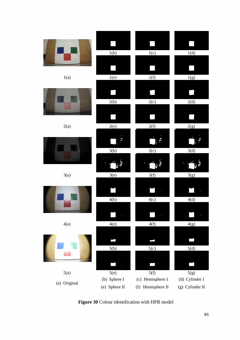
85

1(b) 1(c) 1(d)

1(a) 1(e) 1(f) 1(g)

2(b) 2(c) 2(d)

2(a) 2(e) 2(f) 2(g)

3(b) 3(c) 3(d)

3(a) 3(e) 3(f) 3(g)

4(b) 4(c) 4(d)

4(a) 4(e) 4(f) 4(g)

5(b) 5(c) 5(d)

5(a) 5(e) 5(f) 5(g)

(a) Original (b) Sphere I (c) Hemisphere I (d) Cylinder I

(e) Sphere II (f) Hemisphere II (g) Cylinder II

Figure 30 Colour identification with HPB model

86

TABLE IV F1 SCORES OF COLOUR IDENTIFICATION WITH HPB MODEL

Lighting Condition Sphere I Hemisphere I Cylinder I

F+ F

– F1 F

+ F

– F1 F

+ F

– F1

Normal 3.76 0.12 98.09 3.03 0.42 98.30 3.99 0.11 97.99

Shadow 1 2.31 3.58 97.04 1.25 7.42 95.53 2.33 3.58 97.03

Shadow 2 31.93 0.00 86.23 44.75 0.00 81.72 47.31 0.00 80.87

Illumination 1 1.88 7.78 95.02 1.76 7.82 95.06 2.05 7.78 94.94

Illumination 2 0.00 60.58 56.55 0.00 72.64 42.96 0.22 40.92 74.17

Mean 7.98 14.41 86.59 10.16 17.66 82.71 11.18 10.48 89.00

Lighting Condition Sphere II Hemisphere II Cylinder II

F+ F

– F1 F

+ F

– F1 F

+ F

– F1

Normal 6.25 0.02 96.96 4.41 0.04 97.82 7.41 0.02 96.42

Shadow 1 2.24 1.91 97.93 0.68 4.73 97.24 2.24 1.75 98.01

Shadow 2 75.94 0.00 72.48 75.95 0.00 72.48 75.95 0.00 72.48

Illumination 1 4.30 2.42 96.67 4.00 2.45 96.80 4.69 2.41 96.49

Illumination 2 1.23 36.51 77.09 0.29 41.41 73.75 3.00 32.85 78.93

Mean 17.99 8.17 88.23 17.07 9.73 87.62 18.66 7.41 88.46

TABLE V RANKINGS OF COLOUR MODELS BASED ON F1 SCORES

Rank Normal Shadow 1 Shadow 2

Model F1 Model F1 Model F1

1st Hemisphere I 98.30 Cylinder II 98.01 Sphere I 86.23

2nd

Sphere I 98.09 Sphere II 97.93 HCV 82.50

3rd

Cylinder I 97.99 Hemisphere II 97.24 HCL 82.50

4th Hemisphere II 97.82 HSL 97.14 Hemisphere I 81.72

5th HCL 97.58 Sphere I 97.04 Cylinder I 80.87

6th HCV 97.45 Cylinder I 97.03 HSV 72.92

7th Sphere II 96.96 HCV 96.56 HSL 72.92

8th Cylinder II 96.42 HCL 96.56 Sphere II 72.48

9th HSL 96.26 HSV 95.88 Hemisphere II 72.48

10th HSV 93.54 Hemisphere I 95.83 Cylinder II 72.48

Rank Illumination 1 Illumination 2 Overall

Model F1 Model F1 Model F1

1st HCL 97.51 Cylinder II 78.93 Cylinder I 89.00

2nd

Hemisphere II 96.80 HSL 78.33 Cyldiner II 88.46

3rd

Sphere II 96.67 Sphere II 77.09 Sphere II 88.23

4th HSL 96.51 Cylinder I 74.17 HSL 88.23

5th Cylinder II 96.49 Hemisphere II 73.75 Hemisphere II 87.62

6th Hemisphere I 95.06 Sphere I 56.55 Sphere I 86.59

7th Sphere I 95.02 Hemisphere I 42.96 HCL 83.33

8th Cylinder I 94.94 HCL 42.5 Hemisphere I 82.71

9th HCV 93.52 HSV 41.75 HCV 82.22

10th HSV 91.17 HCV 41.07 HSV 79.05

87

In summary, this chapter proposed three methods in colour based feature detection: a

colour enhancement method for colour segmentation (CCE), a colour identification

method (AMT) and a colour model (HPB) for improved colour detection. CCE is an

efficient and simple filtering tool to boost the colour saliency level of the image, the

drawback of this procedure is the loss of texture detail. AMT is an adaptive multi-

channel colour identification method that can be applied even when the image is

heavily affected by effects such as illumination and shadow. However, the colour

space selection scheme employed by this approach is currently limited to hue based

colour spaces. HPB is a novel colour model that consists of three colour components:

hue, purity and brightness. Compared to existing hue based colour models, HPB

model allows enhanced colour detection from images. However, the computation

required to convert between the model and RGB is relatively more expensive than

traditional hue based models. These methods have not been implemented into the

real-time tracking and pursuit system (Chapter 5) primarily due to the limited

computational power.

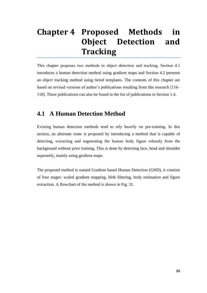
88

Chapter 4 Proposed Methods in Object Detection and Tracking

This chapter proposes two methods in object detection and tracking. Section 4.1

introduces a human detection method using gradient maps and Section 4.2 presents

an object tracking method using tiered templates. The contents of this chapter are

based on revised versions of author’s publications resulting from this research [116–

118]. These publications can also be found in the list of publications in Section 1.4.

4.1 A Human Detection Method

Existing human detection methods tend to rely heavily on pre-training. In this

section, an alternate route is proposed by introducing a method that is capable of

detecting, extracting and segmenting the human body figure robustly from the

background without prior training. This is done by detecting face, head and shoulder

separately, mainly using gradient maps.

The proposed method is named Gradient based Human Detection (GHD), it consists

of four stages: scaled gradient mapping, blob filtering, body estimation and figure

extraction. A flowchart of the method is shown in Fig. 31.

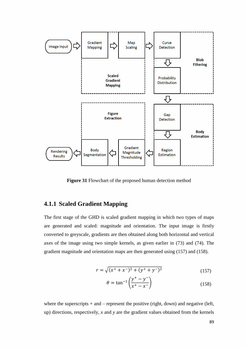
89

Figure 31 Flowchart of the proposed human detection method

4.1.1 Scaled Gradient Mapping

The first stage of the GHD is scaled gradient mapping in which two types of maps

are generated and scaled: magnitude and orientation. The input image is firstly

converted to greyscale, gradients are then obtained along both horizontal and vertical

axes of the image using two simple kernels, as given earlier in (73) and (74). The

gradient magnitude and orientation maps are then generated using (157) and (158).

(157)

(158)

where the superscripts + and – represent the positive (right, down) and negative (left,

up) directions, respectively, x and y are the gradient values obtained from the kernels

90

along horizontal and vertical axes, respectively, r and θ are magnitude and

orientation of the gradient, respectively.

Finally, both gradient maps are scaled into 8 smaller sizes by a set of scaling factors,

as given in (159).

(159)

where α represents the set of scaling factors. The values are selected empirically to

accommodate various sizes of human in the image.

During the scaling procedure, max pooling is applied for the magnitude maps in

which only the local maximum within each block is saved. The size of the block is

related to the scaling factor and is simply 1/α. For the orientation maps, both positive

and negative directions of the gradient along horizontal and vertical axes are

considered, as given in (160).

(160)

where θα is the scaled orientation, the superscripts + and – represent the positive

(right, down) and negative (left, up) directions, respectively, X and Y are the

maximum gradient within the block along horizontal and vertical axes, respectively.

The original image and gradient orientation map are shown in Fig. 32 (a) and (b),

respectively.

91

(a) Original input (b) Gradient orientation map

Figure 32 Original input and gradient orientation map

4.1.2 Blob Filtering

The second stage of the GHD is blob filtering in which blobs are formed and filtered

based on the results of face, head and shoulder detectors. Firstly, as both head and

shoulder have distinctive curvatures, curve detection is employed to detect possible

head and shoulder regions. This is done via two curve templates which can be

represented as two 3 by 3 kernels, as given in (161) and (162).

(161)

(162)

where C1 and C2 are the two curve templates, represents null (element not

considered). The values are determined based on their relative angles from each of

the bottom corners in the kernels.

Using sliding window approach, the scaled gradient maps are then searched for

patches that contain similar gradient features with the templates. The similarity level

between the patch and the template can be determined by computing the weighted

difference using (163).

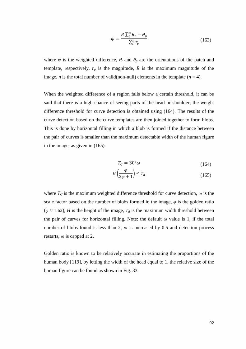
92

(163)

where ψ is the weighted difference, θt and θp are the orientations of the patch and

template, respectively, rp is the magnitude, R is the maximum magnitude of the

image, n is the total number of valid(non-null) elements in the template (n = 4).

When the weighted difference of a region falls below a certain threshold, it can be

said that there is a high chance of seeing parts of the head or shoulder, the weight

difference threshold for curve detection is obtained using (164). The results of the

curve detection based on the curve templates are then joined together to form blobs.

This is done by horizontal filling in which a blob is formed if the distance between

the pair of curves is smaller than the maximum detectable width of the human figure

in the image, as given in (165).

(164)

(165)

where TC is the maximum weighted difference threshold for curve detection, ω is the

scale factor based on the number of blobs formed in the image, φ is the golden ratio

(φ ≈ 1.62), H is the height of the image, Td is the maximum width threshold between

the pair of curves for horizontal filling. Note: the default ω value is 1, if the total

number of blobs found is less than 2, ω is increased by 0.5 and detection process

restarts, ω is capped at 2.

Golden ratio is known to be relatively accurate in estimating the proportions of the

human body [119], by letting the width of the head equal to 1, the relative size of the

human figure can be found as shown in Fig. 33.

93

Figure 33 Estimated human body proportions using golden ratio (head to knee)

For face detection, a simple feature based Haar classifier [120] is implemented. Since

the method is prioritised on head and shoulder detections, the parameters of the face

classifier are tuned towards high precision rather than high recall. As Haar classifiers

tend to yield clusters of ROIs around the detected faces, the number of overlaps at

the cluster centre is used as the confidence measure for the face detector. Two cut-off

thresholds have been established based on the size of the image to describe the

confidence of the detected ROI as low, medium or high, as given in (166) to (168).

(166)

(167)

(168)

where fl and fh are the two thresholds for low and high confidences, t is a size

parameter determined based on the image width W and height H.

At this stage, several (or no) blobs may form depending on the level of background

noise. To identify the true head and shoulder blobs, a probability model based on

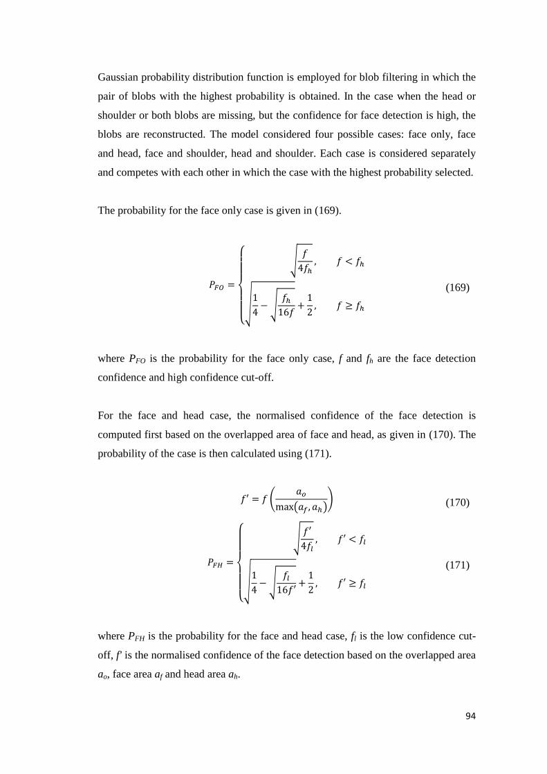
94

Gaussian probability distribution function is employed for blob filtering in which the

pair of blobs with the highest probability is obtained. In the case when the head or

shoulder or both blobs are missing, but the confidence for face detection is high, the

blobs are reconstructed. The model considered four possible cases: face only, face

and head, face and shoulder, head and shoulder. Each case is considered separately

and competes with each other in which the case with the highest probability selected.

The probability for the face only case is given in (169).

(169)

where PFO is the probability for the face only case, f and fh are the face detection

confidence and high confidence cut-off.

For the face and head case, the normalised confidence of the face detection is

computed first based on the overlapped area of face and head, as given in (170). The

probability of the case is then calculated using (171).

(170)

(171)

where PFH is the probability for the face and head case, fl is the low confidence cut-

off, f' is the normalised confidence of the face detection based on the overlapped area

ao, face area af and head area ah.

95

For the face and shoulder, and the head and shoulder cases, Gaussian probability

distribution function is applied to find the best pair of blobs. This is done by

examining all pairs with five types of confidence measures, as list in Table VI, where

δ and σ are the desired output and standard deviation for each of the confidence

measures, respectively, x and y are the horizontal and vertical centroid positions,

respectively, w and h are the width and height of the blob, respectively, a is area, φ is

the golden ratio, H is the height of the image. Note: δ and σ are selected based on the

maximum detectable human size in the image and golden ratio.

TABLE VI CONFIDENCE MEASURES FOR THE FACE AND SHOULDER, AND THE HEAD

AND SHOULDER CASES

Type Confidence Measures Algebraic Expression δ σ

A Horizontal centroid difference

B Vertical centroid difference over width

C Height over width

D Width ratio

E Area sum

The overall probability is then calculated using (172).

(172)

where PFS and PHS are the probabilities for the face and shoulder, and the head and

shoulder cases, respectively, η and δ are the actual and desired outputs, respectively,

σ is the standard deviation, n is the total number of types.

The results of face, head and shoulder detections are illustrated in Fig. 34 using

white, red and yellow rectangles, respectively.

96

Figure 34 Face, head and shoulder detections

4.1.3 Body Estimation

The third stage of the GHD is the body estimation in which the human body regions

are estimated. Firstly, gap detection is performed to locate possible gaps below the

armpit and between the legs, these gaps can be assumed as regions with multiple

edges and significant orientation changes. This is done similar to the curve detection

described earlier in which a gap template is used and it can be represented as a 3 by 3

kernel using (173).

(173)

where G is the gap template, represents null (element not considered). The values

are determined based on their relative angles to an element lays below the kernel.

Correspondingly, the weighted difference between the patch and the template can be

determined using (163). The results of the gap detection based on the gap template

are then fused together by vertical filling. The weight difference threshold for gap

detection is obtained using (174).

(174)

where TG is the maximum weighted difference threshold for gap detection, ω is the

scale factor based on the number of blobs formed in the image. Note: the default ω

97

value is 1, if the total number of blobs found is less than 2, ω is increased by 0.5 and

the detection process restarts, ω is capped at 2.

The human body region can then be estimated using eleven overlapping blocks, as

shown in Fig. 35. The filled areas in the figure represent detected head and shoulder

blobs, the three red blocks (1–3) are the estimated gap regions, while the eight blue

blocks (4–11) are the estimated body regions based on Fig. 33. Each block overlaps

at least one other region to ensure maximum coverage of the human body.

Figure 35 Estimated human body regions (head to knee)

The position and size of the blocks are listed in Table VII, where φ is the golden

ratio, i is the block number, X and Y are the horizontal and vertical centroid positions,

respectively, w and h are the width and height, respectively, h and s represent head

and shoulder, respectively, G1 represents the minimum horizontal position of the gap

regions detected in block 1, G2 represents the maximum horizontal position of the

gap regions detected in block 2, G3 represents the horizontal centroid position of the

gap regions detected in block 3. Note: the origin of the image is located at top left

corner.

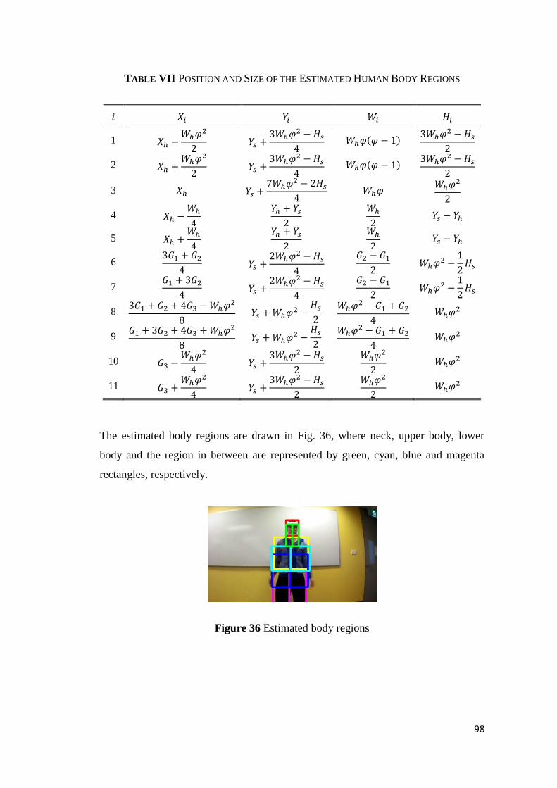
98

TABLE VII POSITION AND SIZE OF THE ESTIMATED HUMAN BODY REGIONS

1

2

3

4

5

6

7

8

9

10

11

The estimated body regions are drawn in Fig. 36, where neck, upper body, lower

body and the region in between are represented by green, cyan, blue and magenta

rectangles, respectively.

Figure 36 Estimated body regions

99

4.1.4 Figure Extraction

The fourth and the final stage of the GHD is the figure extraction in which the human

figure is extracted and segmented into three parts: head, upper body and lower body.

Firstly, The outline of the human body is generated by applying gradient magnitude

thresholding with the block regions defined earlier, in which the bottom 75 percentile

of the pixels in the block that belong to the gradient magnitude is removed. This is

done to preserve key edge features while removing the texture and background

noises.

Additional body outlines are also inserted to ensure minimum amount of outlines are

available for filling the human figure. This is done by placing hollow circles at the

centroids of the head (head blob), neck (blocks 4 and 5), shoulder (shoulder blob),

upper body (blocks 6 and 7), lower body (blocks 10 and 11) and the regions in

between (blocks 8 and 9). The radii of the circles are determined using (175).

(175)

where R is the radius, φ is the golden ratio, W and H are the width and height of the

regions.

Horizontal filling is then performed by filling the space between the outlines. The

human figure is generated by adding the head and shoulder blobs detected earlier

while removing the filled gap regions. Finally, based on the estimated human body

regions, body segmentation is applied to divide the human figure into three parts:

head (head blob, blocks 4 and 5), upper body (shoulder blob, blocks 6 and 7), and

lower body (blocks 10 and 11).

The unfilled body outlines and the final segmented body regions are provided in Fig.

37 (a) and (b), respectively. The final segmented results are rendered using red, green

and blue colours, representing head, upper body and lower body, respectively.

100

(a) Unfilled body outlines (b) Final segmented body regions

Figure 37 Unfilled body outlines and final segmented body regions

To assess the effectiveness of the proposed GHD method, the method is examined

with various images, as shown in Fig. 38. These images are collected from various

sources and have different sizes, intensity and quality, from the top to the bottom: the

first two images are captured by the front facing camera of the quadrotor used in this

research, the next two images are obtained from the INRIA person dataset and the

last two images are selected from Google images. In the figure, the original images

are shown in (a), the gradient orientation maps are presented in (b), the results of

face, head and shoulder detections are illustrated in (c) using white, red and yellow

rectangles, respectively, the estimated body regions are drawn in (d), where neck,

upper body, lower body and the region in between are represented by green, cyan,

blue and magenta rectangles, respectively, the unfilled body outlines are provided in

(e) and the final segmented body regions are rendered in (f) with red, green and blue

representing head, upper body and lower body, respectively.

As it can be seen from the figures, face detection (white rectangles) has failed to find

the correct face regions when the person is not facing towards the camera (cases 2

and 5). Despite this, the method is still capable of detecting the person correctly

using head and shoulder detections. These results indicate the high effectiveness of

the proposed GHD method as the human figure is detected, extracted and segmented

accurately.

101

1(a) 1(b) 1(c)

1(d) 1(e) 1(f)

2(a) 2(b) 2(c)

2(d) 2(e) 2(f)

3(a) 3(b) 3(c)

3(d) 3(e) 3(f)

4(a) 4(b) 4(c)

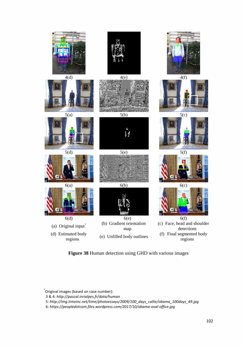
102

4(d) 4(e) 4(f)

5(a) 5(b) 5(c)

5(d) 5(e) 5(f)

6(a) 6(b) 6(c)

6(d) 6(e) 6(f)

(a) Original input*

(b) Gradient orientation

map

(c) Face, head and shoulder

detections

(d) Estimated body

regions (e) Unfilled body outlines

(f) Final segmented body

regions

Figure 38 Human detection using GHD with various images

*Original images (based on case number):

3 & 4: http://pascal.inrialpes.fr/data/human 5: http://img.timeinc.net/time/photoessays/2009/100_days_callie/obama_100days_49.jpg 6: https://peopledotcom.files.wordpress.com/2017/10/obama-oval-office.jpg

103

4.2 An Object Tracking Method

Currently, object tracking can be divided into two groups: learning based and non-

learning based, learning based methods tend to yield better results in noisy

conditions, but suffer from high computational cost. On the other hand, non-learning

methods usually perform well in constrained environments, but tend to be application

specific. In this section, a generic and non-learning approach is proposed to track an

object continuously and robustly in real time without prior training. This is done by

combining intensity template matching with colour histogram model and employing

a three-tier system for template management.

The proposed object tracking method is named the Tiered Template based Tracking

(TTT). It involves three key stages: detection, update and tracking. Templates are

used for all the stages to store and compare ROIs. They are organised into three tiers:

tier 1 represents stable templates (usually large ROIs that contain the full object),

they are rarely updated, tier 2 represents unstable templates (usually medium ROIs

that contain part of the object), they are frequently updated and tier 3 represents

temporary templates (usually small ROIs that may or may not contain part of the

object), they are updated every frame. Initially, when the target ROI is provided

manually or acquired automatically (for example, through human detection), it is

immediately saved into tier 1. Detection checks for similar ROIs based on the

templates, update policy decides the inclusion of templates based on the detected

ROIs and tracking policy chooses the most suitable ROI to track.

4.2.1 Detection

The first stage of TTT is detection, for each frame, detection is called first to find

similar ROIs based on the templates. All the templates in the three tiers are checked

against the image using sliding window approach. Tiers are checked from the top to

the bottom, for each tier, templates are checked in the order of time, when a template

is found, any remaining templates are skipped and the checking procedure restarts

from the next tier. Similarity is determined based on intensity template matching

104

using Normalised Cross Correlation (NCC) [121] and colour histogram model using

Normalised Back Projection (NBP) [122].

For each template, NCC is applied to produce an intensity probability map by

computing similarity in the intensity channel between the current template and the

ROI in the current search window, as given in (176) to (178).

(176)

(177)

(178)

where I is the intensity probability of template t matches with the ROI in the current

search window w, (x, y) is the global position within the image and (u, v) is the local

position within the current template and search window, and are the mean

intensity values of the template and the ROI in the current search window,

respectively.

Colour probability maps are also obtained, this is done by computing similarity in the

RGB channels using NBP, as given in (179).

(179)

where C is the colour probability, (x, y) is the global position within the image and

(u, v) is the local position within the current template and search window, (R, G, B)

and (r, g, b) are the corresponding RGB bin positions of the image and the template,

respectively, f is the corresponding RGB bin value of the template based on the bin

position.

105

The combined intensity and colour probability map is then determined, as given in

(180) and (181).

(180)

(181)

where P is the combined probability, I and C are the intensity and colour

probabilities, respectively, is the mean of the corresponding RGB bin values based

on the bin positions of the template, T1 is a colour weight constant.

A good match requires a high similarity between the currently compared ROIs and

low similarity with other ROIs. Therefore, detection is counted as successful if the

maximum combined probability of a ROI is high and salient compared to the rest of

the image, this is represented using two conditions, as given in (182) and (183).

(182)

(183)

where P1 and P2 are the maximum and second maximum combined probabilities,

respectively, I1 and C1 are the intensity and colour components of the first maximum,

respectively, T2 is a probability threshold constant, while T3 is a saliency threshold

constant. When finding the second maximum, neighbouring regions connected to the

first maximum are excluded by masking out the surrounding ROIs and itself (a 3 by

3 ROI mask centred on the first maximum).

4.2.2 Update

The second stage of the TTT is update. Update is performed after the detection stage

to include new templates and to replace old ones in the three tiers when necessary.

During the update, if the detected ROI is deemed suitable for template inclusion, it is

added into the corresponding tier. Similarity checks are performed between the ROI

and all the templates in the current tier using (176) to (182). If any of the checks

106

returns a probability less than T2, then the least similar one is replaced, if all the

templates passed the similar check and the tier is full, the corresponding template

found in the detection stage is replaced, else the ROI is added as a new template.

Templates in the tier are then rearranged in the order of time. Tier 1 is regarded as

the stable tier, it is rarely updated. Tier 2 is regarded as the unstable tier, in which

whenever a template is updated, its size is also checked and readjusted if a larger or

smaller template produces a more reliable result. Tier 3 is regarded as the temporary

tier, in which if none of the templates in tier 3 are updated, all of them are removed.

An update policy is used to decide the inclusion of templates, the conditions are

listed in Table VIII. These conditions are established based on general observations.

For example, template in tier 2 is updated when detection is found in tier 1 but not in

tier 2.

TABLE VIII UPDATE POLICY

Update Tier Detected Tier Additional Conditions

1 1&2 !O1,2&(Q2≥Q1)&(p2>p1)

2 1&2 !O1,2&!(Q2≥Q1&p2>p1)

2 1&!2

2 2 (Qm≥Q1T3)&(2pm 1≥T2)

3 !1&2&!3 S1,2

3 !1&2&3 O2,3

where & and ! represent the AND and NOT logic operations, respectively, p is the

probability of the detected ROI based on the corresponding template, S is the

similarity check explained previously to compare between the detected ROIs, O is an

overlap check which is used to determine if the detected ROIs overlap with each

other and is given in (184), Q is a colour quality measurement based on hue and

chroma which is given in (185) and (186), pm is the maximum probability given in

(187), Qm is the colour quality measurements using the template with the maximum

probability.

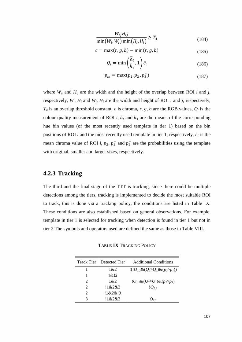
107

(184)

(185)

(186)

(187)

where Wij and Hij are the width and the height of the overlap between ROI i and j,

respectively, Wi, Hi and Wj, Hj are the width and height of ROI i and j, respectively,

T4 is an overlap threshold constant, c is chroma, r, g, b are the RGB values, Qi is the

colour quality measurement of ROI i, and are the means of the corresponding

hue bin values (of the most recently used template in tier 1) based on the bin

positions of ROI i and the most recently used template in tier 1, respectively, is the

mean chroma value of ROI i, , and

are the probabilities using the template

with original, smaller and larger sizes, respectively.

4.2.3 Tracking

The third and the final stage of the TTT is tracking, since there could be multiple

detections among the tiers, tracking is implemented to decide the most suitable ROI

to track, this is done via a tracking policy, the conditions are listed in Table IX.

These conditions are also established based on general observations. For example,

template in tier 1 is selected for tracking when detection is found in tier 1 but not in

tier 2.The symbols and operators used are defined the same as those in Table VIII.

TABLE IX TRACKING POLICY

Track Tier Detected Tier Additional Conditions

1 1&2 !(!O1,2&(Q2≥Q1)&(p2>p1))

1 1&!2

2 1&2 !O1,2&(Q2≥Q1)&(p2>p1)

2 !1&2&3 !O2,3

2 !1&2&!3

3 !1&2&3 O2,3

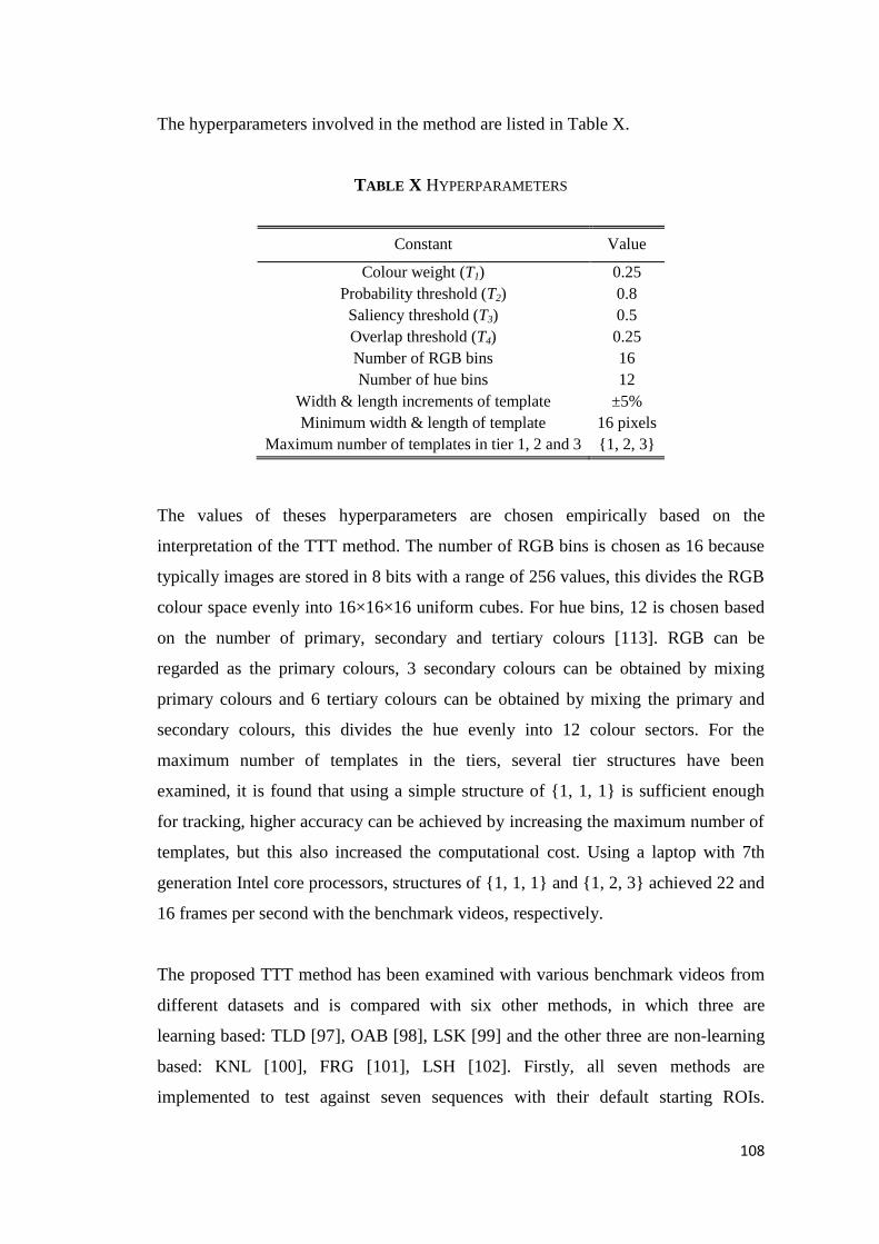
108

The hyperparameters involved in the method are listed in Table X.

TABLE X HYPERPARAMETERS

Constant Value

Colour weight (T1) 0.25

Probability threshold (T2) 0.8

Saliency threshold (T3) 0.5

Overlap threshold (T4) 0.25

Number of RGB bins 16

Number of hue bins 12

Width & length increments of template ±5%

Minimum width & length of template 16 pixels

Maximum number of templates in tier 1, 2 and 3 {1, 2, 3}

The values of theses hyperparameters are chosen empirically based on the

interpretation of the TTT method. The number of RGB bins is chosen as 16 because

typically images are stored in 8 bits with a range of 256 values, this divides the RGB

colour space evenly into 16×16×16 uniform cubes. For hue bins, 12 is chosen based

on the number of primary, secondary and tertiary colours [113]. RGB can be

regarded as the primary colours, 3 secondary colours can be obtained by mixing

primary colours and 6 tertiary colours can be obtained by mixing the primary and

secondary colours, this divides the hue evenly into 12 colour sectors. For the

maximum number of templates in the tiers, several tier structures have been

examined, it is found that using a simple structure of {1, 1, 1} is sufficient enough

for tracking, higher accuracy can be achieved by increasing the maximum number of

templates, but this also increased the computational cost. Using a laptop with 7th

generation Intel core processors, structures of {1, 1, 1} and {1, 2, 3} achieved 22 and

16 frames per second with the benchmark videos, respectively.

The proposed TTT method has been examined with various benchmark videos from

different datasets and is compared with six other methods, in which three are

learning based: TLD [97], OAB [98], LSK [99] and the other three are non-learning

based: KNL [100], FRG [101], LSH [102]. Firstly, all seven methods are

implemented to test against seven sequences with their default starting ROIs.

109

Secondly, since an object’s ROI can be perceived differently depending on the

person, another test is performed with the same sequences but with alternate starting

ROIs (of the same objects). Furthermore, to compare the robustness of those

methods, additional tests are conducted with the starting ROIs shifted by one pixel

(eight tests: one for each direction based on both default and alternate ROIs).

The sequences with their default and alternate starting ROIs along with the tracking

frames are shown in Fig. 39, from the top to the bottom: the first four sequences are

produced by the author using the front facing camera of the quadrotor used in this

research. The next two sequences are listed in the reference [123], the last sequence

is obtained from reference [124]. Information about the implementation of these

methods can be found in reference [125].

1(a) 1(b)

1(c) 1(d)

2(a) 2(b)

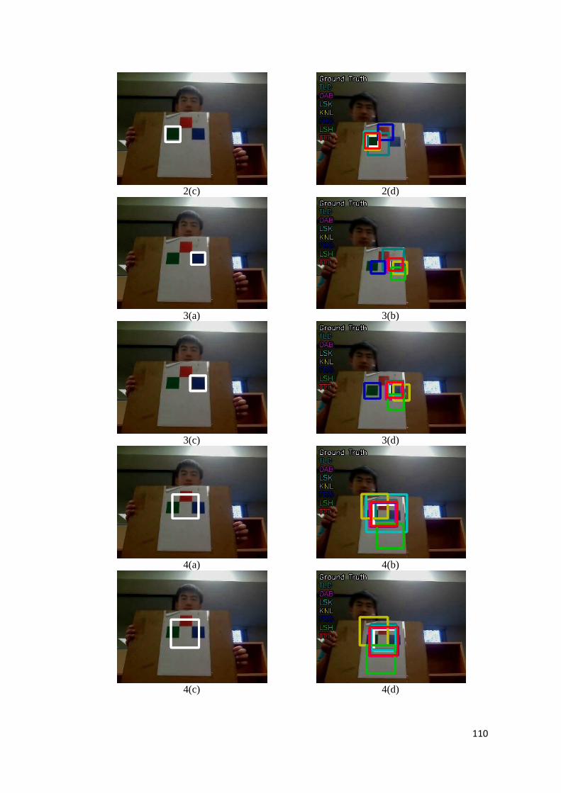
110

2(c) 2(d)

3(a) 3(b)

3(c) 3(d)

4(a) 4(b)

4(c) 4(d)

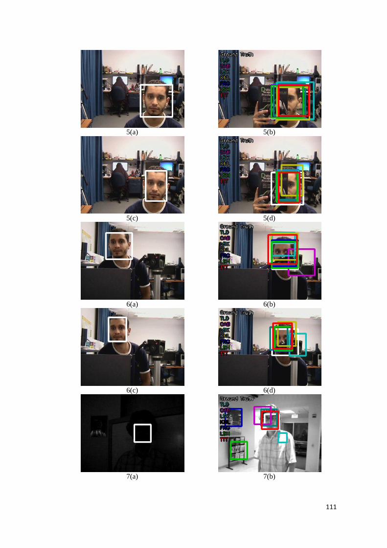
111

5(a) 5(b)

5(c) 5(d)

6(a) 6(b)

6(c) 6(d)

7(a) 7(b)

112

7(c) 7(d)

(a) Initial frame with default starting ROI (b) Tracking frame with default starting ROI

(c) Initial frame with alternate starting ROI (d) Tracking frame with alternate starting ROI

Figure 39 Object tracking using GHD with various benchmark videos

Overlap performance evaluation [126] is a common technique to compare the

tracking capabilities among different methods. For each frame, the overlap ratio is

computed based on intersection over union between the tracked ROI and the ground

truth ROI. A percentage threshold (typically 25% or 50%) is then applied to classify

the frame into positive (successful) and negative (unsuccessful) groups. The overall

performance score is simply the percentage of positive frames.

To illustrate the effectiveness of the methods, resultant curves of all the thresholds

with the default, alternate and shifted starting ROIs are shown in Fig. 40. In the

figure, the circles represent the most common choices of 25% and 50% threshold

values. Note: a threshold of 0 (left most case) means the results is positive as long as

an overlapped region exists, while a threshold of 1 (right most case) means the two

ROIs need to be identical in order for the results to be counted as positive.

From the results, it can be clearly seen that the proposed TTT method performs

superiorly over the existing methods in vast majority of the cases (thresholds of 10%

to 90%).

113

(a) Default starting ROI

(b) Alternate starting ROI

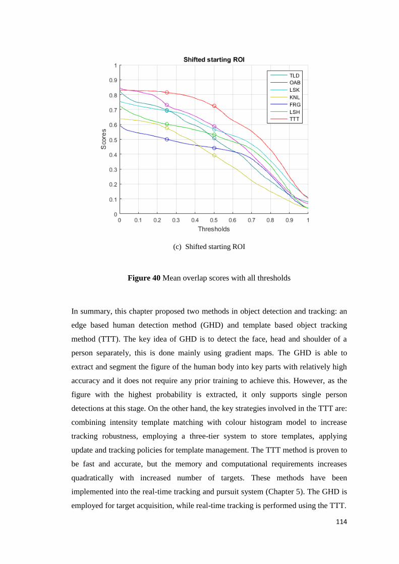
114

(c) Shifted starting ROI

Figure 40 Mean overlap scores with all thresholds

In summary, this chapter proposed two methods in object detection and tracking: an

edge based human detection method (GHD) and template based object tracking

method (TTT). The key idea of GHD is to detect the face, head and shoulder of a

person separately, this is done mainly using gradient maps. The GHD is able to

extract and segment the figure of the human body into key parts with relatively high

accuracy and it does not require any prior training to achieve this. However, as the

figure with the highest probability is extracted, it only supports single person

detections at this stage. On the other hand, the key strategies involved in the TTT are:

combining intensity template matching with colour histogram model to increase

tracking robustness, employing a three-tier system to store templates, applying

update and tracking policies for template management. The TTT method is proven to

be fast and accurate, but the memory and computational requirements increases

quadratically with increased number of targets. These methods have been

implemented into the real-time tracking and pursuit system (Chapter 5). The GHD is

employed for target acquisition, while real-time tracking is performed using the TTT.

115

Chapter 5 Vision Based Target Pursuit Using a UAV

This chapter discusses the proposed target pursuit methods and its related topics.

Section 5.1 explains the depth estimation method using the onboard monocular

vision. Section 5.2 describes the trajectory mapping method using the onboard

sensors of the drone and Section 5.3 provides the results of the target pursuit

experiment with three different modes: standby, sentry and search.

5.1 Depth Estimation Using the Onboard

Monocular Vision

Depth is an important feature for many practical applications. It is typically obtained

through the use of rangefinders such as a sonar sensor, it can also be estimated using

cameras. In computer vision, depth estimation is a procedure to recover the depth

information from 2D images, this is commonly done using stereovision. However,

for small UAVs such as quadrotors, monocular vision based approach is more

relevant. This is because compared to monocular vision, the configuration of dual

cameras can be inflexible and inconvenient [127]. When a stereo pair is calibrated, it

can only work if the target is within certain range of the calibration block, the

geometry of the stereo pair also needs to be fixed at all time. Another factor is the

limit of payload, most quadrotors can only carry a single camera. Furthermore,

stereovision based approaches tend to suffer in operation speed due to high

computational cost [128].

Generally, camera needs to be calibrated in order to recover the depth information.

Camera calibration is the process of finding the true parameters of the camera used,

these parameters can be divided into intrinsic and extrinsic parameters [129]. The

intrinsic parameters consist of the focal length, location of the image centre, the skew

and distortions, while the extrinsic parameters consist of the rotation and translation

matrices, as given in (188) to (196).

116

(188)

(189)

(190)

(191)

(192)

(193)

(194)

(195)

(196)

where I and E are the intrinsic and extrinsic matrices, respectively, (u,v) and (x,y,z)

are the locations of the points in the image plane and the Cartesian space,

respectively, R and T are the rotation and translation matrices, respectively, R1,1 to

R3,3 are the rotation parameters, Tx, Ty and Tz are the translation parameters with

respect to x, y and z axes, s is the arbitrary scale factor, γ is the skew factor, αx and αy

are the focal lengths along x and y components, respectively, cx and cy are the x and y

locations of image centre, respectively, f represents the distortion function,

superscript ‘ represents components of undistorted coordinate vector, while

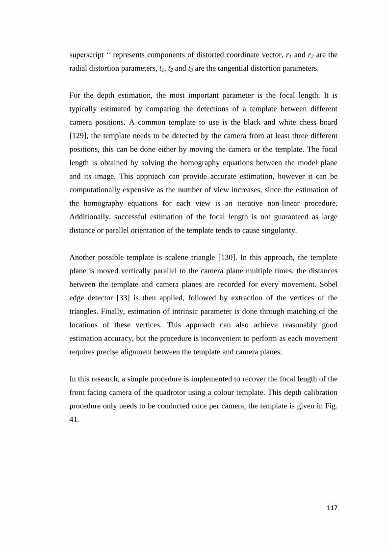
117

superscript ‘' represents components of distorted coordinate vector, r1 and r2 are the

radial distortion parameters, t1, t2 and t3 are the tangential distortion parameters.

For the depth estimation, the most important parameter is the focal length. It is

typically estimated by comparing the detections of a template between different

camera positions. A common template to use is the black and white chess board

[129], the template needs to be detected by the camera from at least three different

positions, this can be done either by moving the camera or the template. The focal

length is obtained by solving the homography equations between the model plane

and its image. This approach can provide accurate estimation, however it can be

computationally expensive as the number of view increases, since the estimation of

the homography equations for each view is an iterative non-linear procedure.

Additionally, successful estimation of the focal length is not guaranteed as large

distance or parallel orientation of the template tends to cause singularity.

Another possible template is scalene triangle [130]. In this approach, the template

plane is moved vertically parallel to the camera plane multiple times, the distances

between the template and camera planes are recorded for every movement. Sobel

edge detector [33] is then applied, followed by extraction of the vertices of the

triangles. Finally, estimation of intrinsic parameter is done through matching of the

locations of these vertices. This approach can also achieve reasonably good

estimation accuracy, but the procedure is inconvenient to perform as each movement

requires precise alignment between the template and camera planes.

In this research, a simple procedure is implemented to recover the focal length of the

front facing camera of the quadrotor using a colour template. This depth calibration

procedure only needs to be conducted once per camera, the template is given in Fig.

41.

118

Figure 41 Depth estimation template

As shown in the figure, this is a very simple template that can be easily created and

printed on a paper. For the three squares in the template, red square is the intended

target, blue and green squares are employed for alignment purpose only, so that the

image plane is parallel to the template plane. The size of each square should be the

same, but their combined area can vary. In the experiment, the template is printed on

an A4 paper, the actual physical size of each square is 55×55 millimetres.

The procedure involves facing the camera to the template (aim at the centre of the

red square) and moving the drone some distance to the template (either towards or

away from the template). After the movement, simply record the height of the red

square appeared in the image in pixels. The focal length can be recovered by

repeating the steps several times. The basic principle of the proposed depth

estimation approach is given in Fig. 42, where C1 and C2 are the two different camera

positions, respectively, h1 and h2 are the detected heights in pixels of the target,

respectively, D is the depth, H is the actual physical width, f is the focal length.

119

Figure 42 Basic principle of the proposed depth estimation procedure

By using the properties of similar triangles, two equations can be established for a

single movement, as given in (197) and (198).

(197)

(198)

By rearranging the equations and adding more measurements, a single equation can

be obtained to recover the focal length, as given in (199).

(199)

where hi is the image height in pixels of the ith

measurement, H is the actual physical

height, f is the focal length, n is the total number of movements, D is the depth.

120

An example frame of the focal length recovery procedure is given in Fig. 43. In the

figure, r, g and b represent the red, green and blue squares, respectively, x and y are

the image width and height of the squares in pixels. Note: the original resolution of

the frame is 360×640. For best results, the height of the red square should only be

recorded if the camera is aligned with the template, in which the width and height of

green and blue squares match with each other (i.e. gx = bx and gy = by).

Figure 43 Example frame of the focal length recovery procedure

In the experiment, the drone is moved 20 times (21 measurements recorded). The

image height of the red square detected using the camera is listed in Table XI, where

hi is the image height of the red square for ith

measurement. The distance of every

movement is 50 millimetres, focal length is estimated to be approximately 557 pixels

after 20 movements with 18 out of 20 applicable computations using (199). The two

non-applicable cases are produced because the detected image height did not change

during these two movements (division by zero error), this could be due to human

error and the fact that the actual physical size of the square might be too small for the

camera to detect.

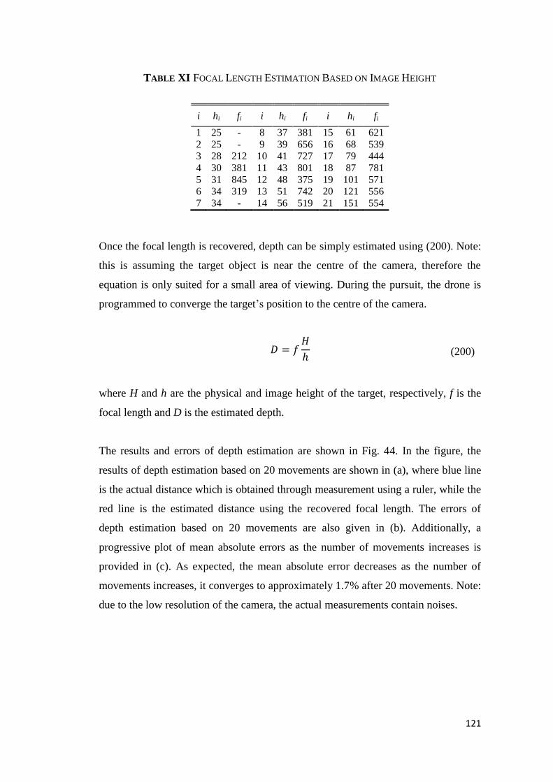
121

TABLE XI FOCAL LENGTH ESTIMATION BASED ON IMAGE HEIGHT

i hi fi i hi fi i hi fi

1 25 - 8 37 381 15 61 621

2 25 - 9 39 656 16 68 539

3 28 212 10 41 727 17 79 444

4 30 381 11 43 801 18 87 781

5 31 845 12 48 375 19 101 571

6 34 319 13 51 742 20 121 556

7 34 - 14 56 519 21 151 554

Once the focal length is recovered, depth can be simply estimated using (200). Note:

this is assuming the target object is near the centre of the camera, therefore the

equation is only suited for a small area of viewing. During the pursuit, the drone is

programmed to converge the target’s position to the centre of the camera.

(200)

where H and h are the physical and image height of the target, respectively, f is the

focal length and D is the estimated depth.

The results and errors of depth estimation are shown in Fig. 44. In the figure, the

results of depth estimation based on 20 movements are shown in (a), where blue line

is the actual distance which is obtained through measurement using a ruler, while the

red line is the estimated distance using the recovered focal length. The errors of

depth estimation based on 20 movements are also given in (b). Additionally, a

progressive plot of mean absolute errors as the number of movements increases is

provided in (c). As expected, the mean absolute error decreases as the number of

movements increases, it converges to approximately 1.7% after 20 movements. Note:

due to the low resolution of the camera, the actual measurements contain noises.

122

(a) Results based on 20 movements

(b) Errors based on 20 movements

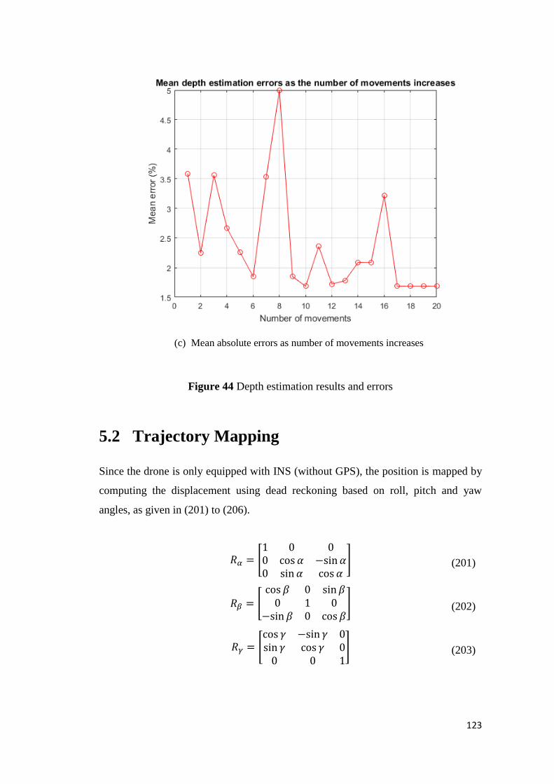
123

(c) Mean absolute errors as number of movements increases

Figure 44 Depth estimation results and errors

5.2 Trajectory Mapping

Since the drone is only equipped with INS (without GPS), the position is mapped by

computing the displacement using dead reckoning based on roll, pitch and yaw

angles, as given in (201) to (206).

(201)

(202)

(203)

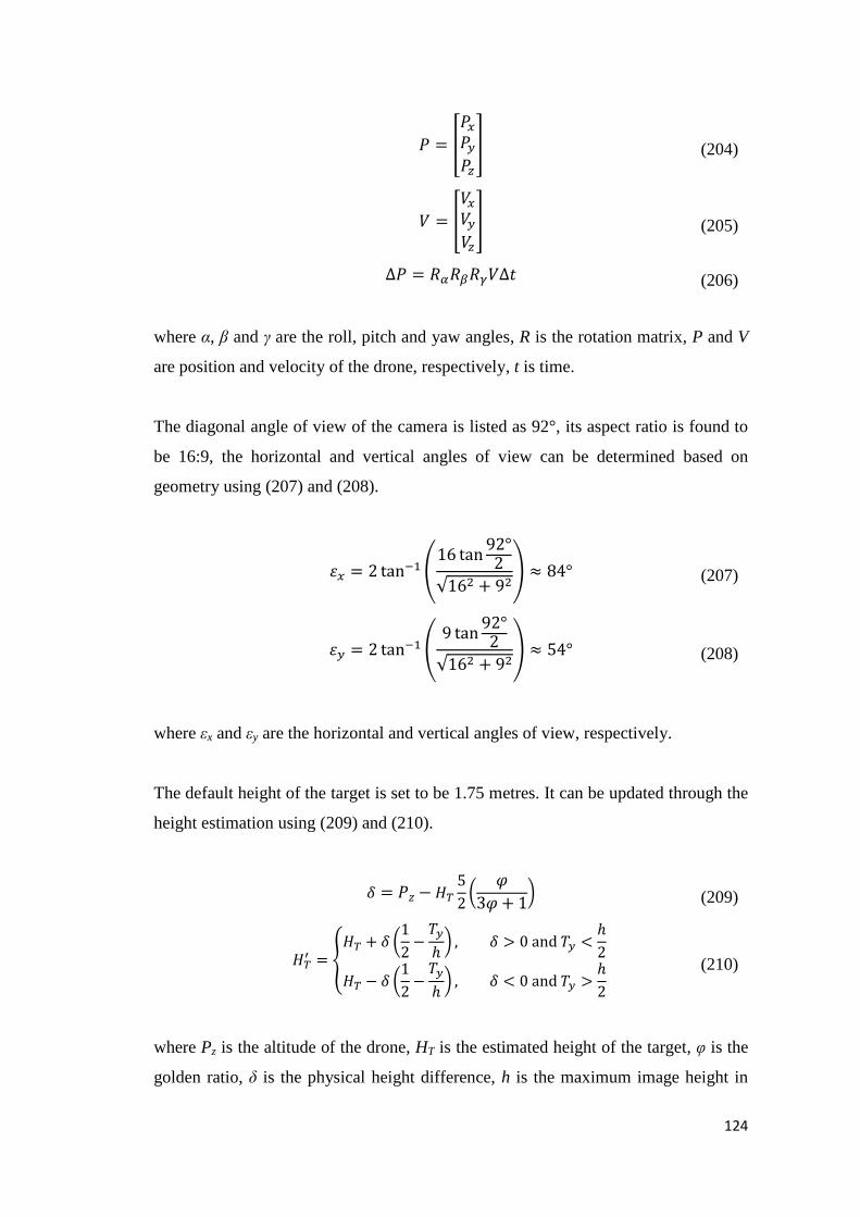
124

(204)

(205)

(206)

where α, β and γ are the roll, pitch and yaw angles, R is the rotation matrix, P and V

are position and velocity of the drone, respectively, t is time.

The diagonal angle of view of the camera is listed as 92°, its aspect ratio is found to

be 16:9, the horizontal and vertical angles of view can be determined based on

geometry using (207) and (208).

(207)

(208)

where εx and εy are the horizontal and vertical angles of view, respectively.

The default height of the target is set to be 1.75 metres. It can be updated through the

height estimation using (209) and (210).

(209)

(210)

where Pz is the altitude of the drone, HT is the estimated height of the target, φ is the

golden ratio, δ is the physical height difference, h is the maximum image height in

125

pixel, Ty is the vertical centroid position of the upper body belonging to the target in

the image. Superscript ' indicates the updated value. Note: the origin of the image at

top left corner.

The distance to the target is determined based on the depth estimation obtained in

(200) and is given in (211).

(211)

where HT is the estimated height of the target, hT is the image height of the upper

body belonging to the target, φ is the golden ratio, f is the focal length and D is the

estimated distance to the target.

The desired clearance to follow the target is also computed which is based on the

maximum detectable human size, this is to ensure the key parts of the target are

visible to the drone during pursuit, as given in (212).

(212)

where HT is the estimated height of the target, φ is the golden ratio, δ is the physical

height difference, εy is the vertical angle of view and C is the clearance. The

clearance is about 1.25 metres for a 1.75 metres tall person.

Finally, the trajectory of the drone is plotted onto a 250×250 image representing a

10×10 metres map, as shown in Fig. 45. In the figure, the white vertical line from the

centre of the map is north, green path is the trajectory of the drone, the white filled

circle is the target in pursuit, the red and white unfilled circles are the current and

intended positions, respectively, the lines attached to the circles represent visible

range of the drone based on the angle of view.

126

Figure 45 Example trajectory during target pursuit

5.3 The Flight Controller

The quadrotor used in this research is a Parrot AR Drone 2, the drone is originally

designed to be controlled only via mobile applications such as FreeFlight* on iOS.

However, since it does not support advanced capabilities such as image processing, a

custom flight controller is built with Microsoft Visual Studio using C++, additional

libraries installed are: OpenCV†, CVDrone

‡, CVBlob

§ and CURL

**. OpenCV is

essential for image processing, CVDrone is necessary for communicating with the

drone, CVBlob is helpful for filtering and rendering ROIs, CURL is useful for image

fetching and remote control. The drone is controlled through WIFI, in which live

video captured using the front facing camera of the drone is sent to a laptop for

online processing and the actual controls are then sent back to the drone. The video

*https://itunes.apple.com/app/id373065271

†https://opencv.org

‡https://github.com/puku0x/cvdrone

§https://github.com/emgucv/cvblob

**https://curl.haxx.se/

127

can be streamed at 30 frames per second with 720×1280 resolution, for the tracking

and pursuit experiment, the resolution has to be compressed into 180×320 in order to

maintain 30 frames per second for online processing. This is due to the fact that the

WIFI connection available is not suitable for high resolution video streaming and the

laptop is only equipped with a low speed CPU (Intel core 2 Duo).

The flight controller supports three types of controls: keyboard, mouse and text

messages. Since the drone itself is a WIFI access point, the actual motion of the

drone is controlled by sending specific Attention (AT) commands, AT commands are

typically used for communicating with modems. An example of using AT command

to control the drone to take-off is:

sockCommand.sendf("AT*REF=%d,290718208\r", ++seq);

5.3.1 Keyboard

The easiest way to control the drone is via a keyboard, the keyboard controls are

listed in Table XII. Note: the autopilot modes listed in the table are to be discussed in

detail in Section 5.6.

TABLE XII KEYBOARD CONTROLS

Key Function Note

W Go forward (surge) Maximum: about 3 metres per second

S Go backward (surge) Maximum: about 3 metres per second

A Shift left (sway) Maximum: about 3 metres per second

D Shift right (sway) Maximum: about 3 metres per second

Z Climb up (heave) Maximum: about 1 metre per second

C Climb down (heave) Maximum: about 1 metre per second

Q Rotate anti-clockwise (Yaw) Maximum: about 120° per second

E Rotate clockwise (Yaw) Maximum: about 120° per second

X Switch between cameras Cameras: front and downward facing

V Record video: On / Off

B Record trajectory: On / Off

F Activate autopilot Deactivate by pressing any other keys

G Switch between autopilot modes Modes: standby, sentry and search

Space Take-off / Land

Escape Emergency stop Send landing command then exit controller

128

5.3.2 Mouse

The drone can also be controlled via a mouse, this is done by clicking anywhere on

the trajectory map which is described earlier in Section 5.4. Mouse control is

designed to only output surge translation and yaw rotation, this simplify the required

motions to reach the target position, as given in (213) and (217).

(213)

(214)

(215)

(216)

(217)

where T and D represent the target and the drone, respectively, X and Y are the

horizontal and vertical positions on the trajectory map, γ is yaw, V and R are

translation and rotation motions, respectively. Note: for safety reason, surge

translation is capped at 75 centimetres per second, while yaw rotation is capped at

60° per second. Rγ is included in Vx so that yaw rotation has higher priority than

surge translation. Superscript ' indicates the intermediate value.

5.3.3 Text Messages

Furthermore, the drone can be controlled remotely via text messages, this is achieved

by sending specific text to an email address linked with the controller. In this

approach, the email is automatically downloaded and read, in which all the texts are

scanned for control commands that can trigger the drone to activate and move to a

nearby location. However, since the controller also relies on WIFI to communicate

with the drone, this means that the text commands can only be received when the

drone is not active in which the controller automatically switch WIFI to connect to

129

the internet. The specific text commands are listed in Table XIII, where each ?

represents an input character.

TABLE XIII TEXT COMMANDS

Text Function

ACTD Activate drone, must be included first before all other commands

MOVX??Y?? Move (P / N: positive or negative) (0–9) meters along X and Y directions,

only outputs Vx and Rγ, similar to mouse control

RECV Record video

RECB Record trajectory

AUTO? Activate autopilot with mode (1–3: standby, sentry and search)

5.4 Autopilot Modes

The flight controller is built with three autopilot modes: standby, sentry and search.

In standby mode, the drone takes-off immediately upon receiving a photo of a person

and simply hovers until the intended target appears. In sentry mode, the drone is used

to monitor an area and is only triggered when the target is detected through its

camera. In search mode, the drone patrols in a fixed path continuously while

searching for the target. An example third person view of the drone in standby mode

is provided in Fig. 46.

Figure 46 Example third person view of the drone in standby mode

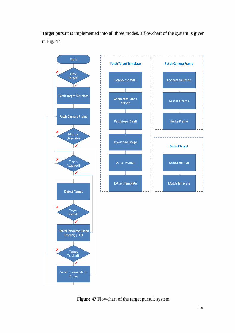
130

Target pursuit is implemented into all three modes, a flowchart of the system is given

in Fig. 47.

Figure 47 Flowchart of the target pursuit system

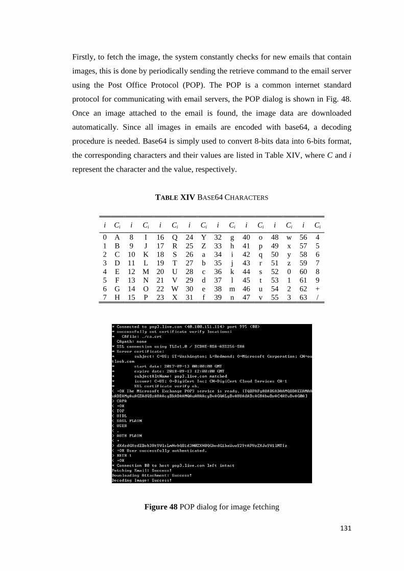
131

Firstly, to fetch the image, the system constantly checks for new emails that contain

images, this is done by periodically sending the retrieve command to the email server

using the Post Office Protocol (POP). The POP is a common internet standard

protocol for communicating with email servers, the POP dialog is shown in Fig. 48.

Once an image attached to the email is found, the image data are downloaded

automatically. Since all images in emails are encoded with base64, a decoding

procedure is needed. Base64 is simply used to convert 8-bits data into 6-bits format,

the corresponding characters and their values are listed in Table XIV, where C and i

represent the character and the value, respectively.

TABLE XIV BASE64 CHARACTERS

i Ci i Ci i Ci i Ci i Ci i Ci i Ci i Ci

0 A 8 I 16 Q 24 Y 32 g 40 o 48 w 56 4

1 B 9 J 17 R 25 Z 33 h 41 p 49 x 57 5

2 C 10 K 18 S 26 a 34 i 42 q 50 y 58 6

3 D 11 L 19 T 27 b 35 j 43 r 51 z 59 7

4 E 12 M 20 U 28 c 36 k 44 s 52 0 60 8

5 F 13 N 21 V 29 d 37 l 45 t 53 1 61 9

6 G 14 O 22 W 30 e 38 m 46 u 54 2 62 +

7 H 15 P 23 X 31 f 39 n 47 v 55 3 63 /

Figure 48 POP dialog for image fetching

132

Human detection using the proposed GHD method described earlier in Section 4.1 is

then employed to find the possible human presented in the image. If detection is

found, human segmentation is applied to divide the body figure into head, upper

body and lower body. The final template is then extracted based on the largest square

region centred in the upper body. Two cases with different clothing and background

are presented in Fig. 49. In the figure, the original images downloaded from the

email is shown in (a), the results of the GHD are provided in (b) to (f), the extracted

upper body region is presented in (g) and the extracted template for tracking and

pursuit is given in (h).

1(a) 1(b)

1(c) 1(d)

1(e) 1(f)

133

1(g) 1(h)

2(a) 2(b)

2(c) 2(d)

2(e) 2(f)

2(g) 2(h)

(a) Original fetched image (b) Gradient orientation map

(c) Face, head and shoulder detections (d) Estimated body regions

(e) Unfilled body outlines (f) Segmented body regions

(g) Extracted upper body region (h) Extracted template

Figure 49 Human detection and template extraction

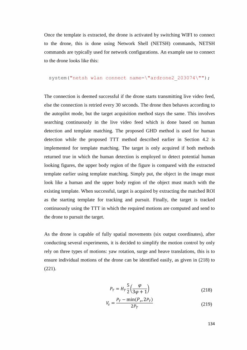
134

Once the template is extracted, the drone is activated by switching WIFI to connect

to the drone, this is done using Network Shell (NETSH) commands, NETSH

commands are typically used for network configurations. An example use to connect

to the drone looks like this:

system("netsh wlan connect name=\"ardrone2_203074\"");

The connection is deemed successful if the drone starts transmitting live video feed,

else the connection is retried every 30 seconds. The drone then behaves according to

the autopilot mode, but the target acquisition method stays the same. This involves

searching continuously in the live video feed which is done based on human

detection and template matching. The proposed GHD method is used for human

detection while the proposed TTT method described earlier in Section 4.2 is

implemented for template matching. The target is only acquired if both methods

returned true in which the human detection is employed to detect potential human

looking figures, the upper body region of the figure is compared with the extracted

template earlier using template matching. Simply put, the object in the image must

look like a human and the upper body region of the object must match with the

existing template. When successful, target is acquired by extracting the matched ROI

as the starting template for tracking and pursuit. Finally, the target is tracked

continuously using the TTT in which the required motions are computed and send to

the drone to pursuit the target.

As the drone is capable of fully spatial movements (six output coordinates), after

conducting several experiments, it is decided to simplify the motion control by only

rely on three types of motions: yaw rotation, surge and heave translations, this is to

ensure individual motions of the drone can be identified easily, as given in (218) to

(221).

(218)

(219)

135

(220)

(221)

where PT and Pz are the desired and actual altitude of the drone, respectively, HT is

the estimated height of the target, φ is the golden ratio, w is the maximum image

width, Tx is the horizontal centroid position of the upper body belonging to the target

in the image, Vx and Vz are surge and heave translations, respectively, Rγ is yaw

rotation. Note: for safety reason, during the experiment, surge and heave translations

are capped at 75 and 50 centimetres per second, respectively, while yaw rotation is

capped at 60° per second. Vx, Vz and Rγ are chained together (Vz is included in Rγ,

while Rγ is included in Vx), this means that heave translation has the highest priority

between the three motions, while surge translation has the lowest priority, this is to

ensure the drone is flying at the desired altitude and facing the desired direction

before moving forward.

5.4.1 The Standby Mode

In the standby mode, the drone simply stays hovering after it takes-off. Two example

tracking and pursuit sequences are shown in Fig. 50 and Fig. 51. In the figures, the

live pursuit sequences are presented in (a), while the trajectory maps are provided in

(b). The motion control of Vz (heave translation), Vx (surge translation) and Rγ (yaw

rotation) are displayed at the top left corner in the liver pursuit sequences, where 1

and –1 represent the positive and negative maximum velocities. The green ROI is the

results of human detection using the GHD, blue and yellow ROIs are the results of

tracking using the TTT. Furthermore, a demonstration video of the tracking and

pursuit sequence shown in Fig. 51 can also be viewed online at:

https://youtu.be/4r19bvS9K5U.

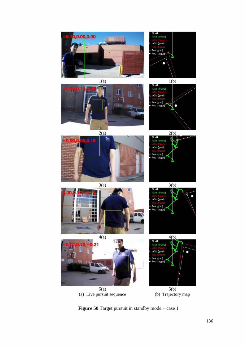
136

1(a) 1(b)

2(a) 2(b)

3(a) 3(b)

4(a) 4(b)

5(a) 5(b)

(a) Live pursuit sequence (b) Trajectory map

Figure 50 Target pursuit in standby mode – case 1

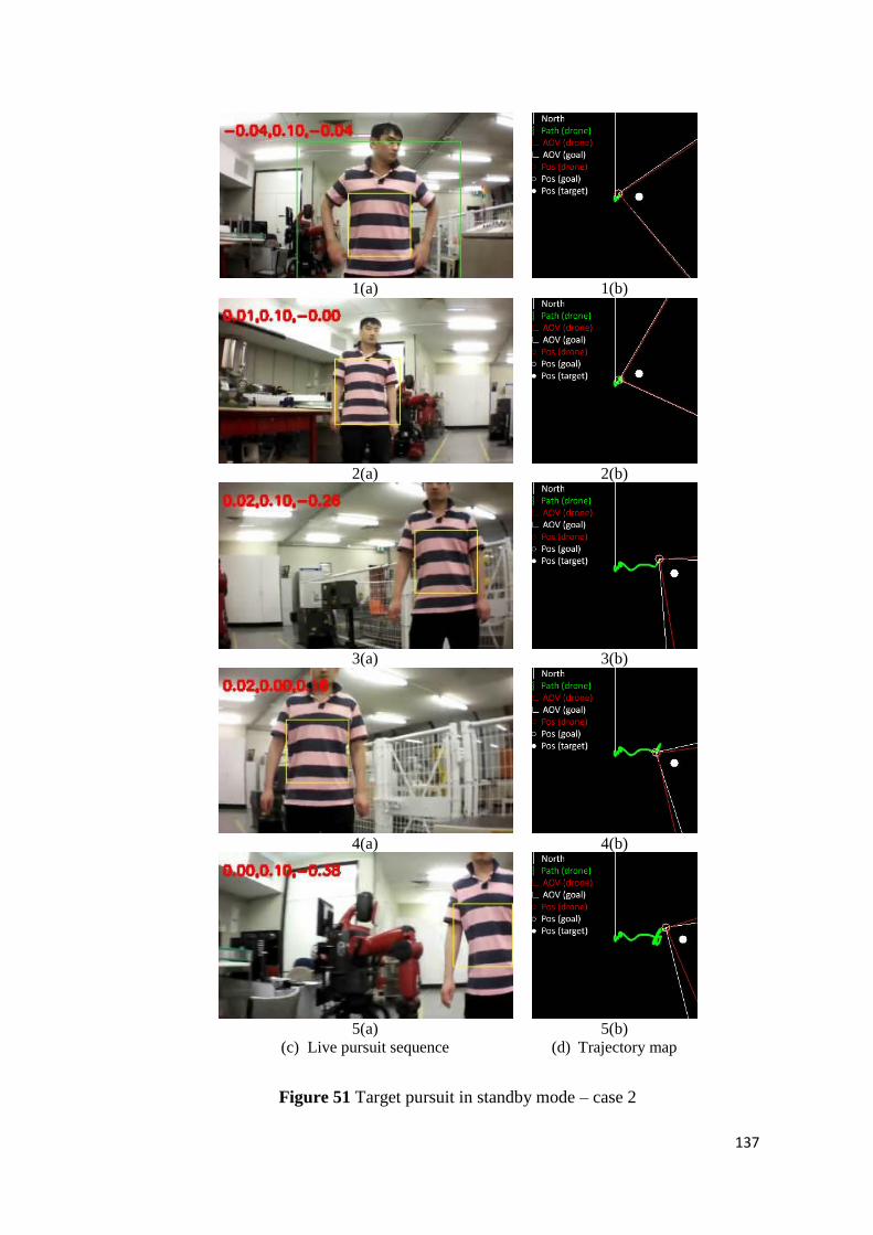
137

1(a) 1(b)

2(a) 2(b)

3(a) 3(b)

4(a) 4(b)

5(a) 5(b)

(c) Live pursuit sequence (d) Trajectory map

Figure 51 Target pursuit in standby mode – case 2

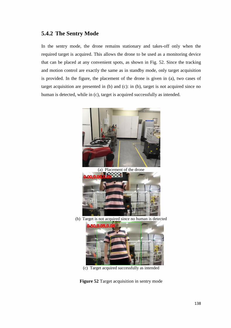
138

5.4.2 The Sentry Mode

In the sentry mode, the drone remains stationary and takes-off only when the

required target is acquired. This allows the drone to be used as a monitoring device

that can be placed at any convenient spots, as shown in Fig. 52. Since the tracking

and motion control are exactly the same as in standby mode, only target acquisition

is provided. In the figure, the placement of the drone is given in (a), two cases of

target acquisition are presented in (b) and (c): in (b), target is not acquired since no

human is detected, while in (c), target is acquired successfully as intended.

(a) Placement of the drone

(b) Target is not acquired since no human is detected

(c) Target acquired successfully as intended

Figure 52 Target acquisition in sentry mode

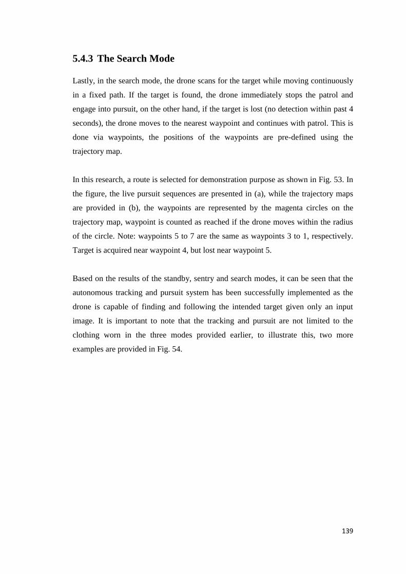
139

5.4.3 The Search Mode

Lastly, in the search mode, the drone scans for the target while moving continuously

in a fixed path. If the target is found, the drone immediately stops the patrol and

engage into pursuit, on the other hand, if the target is lost (no detection within past 4

seconds), the drone moves to the nearest waypoint and continues with patrol. This is

done via waypoints, the positions of the waypoints are pre-defined using the

trajectory map.

In this research, a route is selected for demonstration purpose as shown in Fig. 53. In

the figure, the live pursuit sequences are presented in (a), while the trajectory maps

are provided in (b), the waypoints are represented by the magenta circles on the

trajectory map, waypoint is counted as reached if the drone moves within the radius

of the circle. Note: waypoints 5 to 7 are the same as waypoints 3 to 1, respectively.

Target is acquired near waypoint 4, but lost near waypoint 5.

Based on the results of the standby, sentry and search modes, it can be seen that the

autonomous tracking and pursuit system has been successfully implemented as the

drone is capable of finding and following the intended target given only an input

image. It is important to note that the tracking and pursuit are not limited to the

clothing worn in the three modes provided earlier, to illustrate this, two more

examples are provided in Fig. 54.

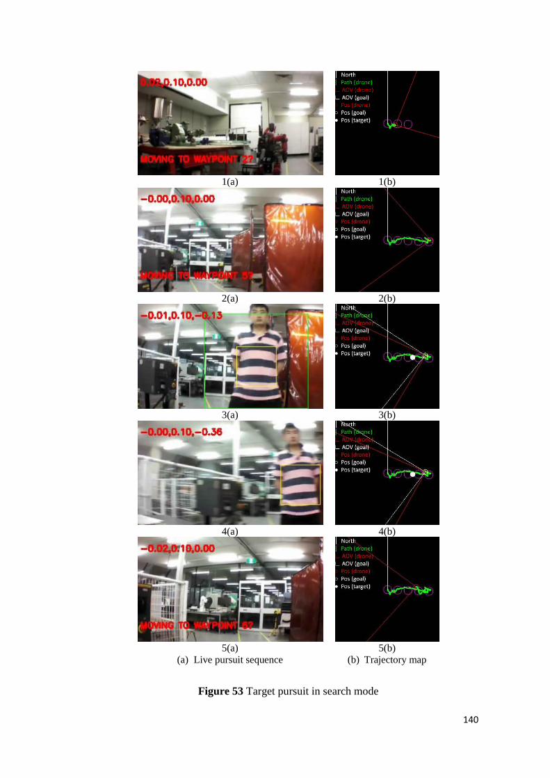
140

1(a) 1(b)

2(a) 2(b)

3(a) 3(b)

4(a) 4(b)

5(a) 5(b)

(a) Live pursuit sequence (b) Trajectory map

Figure 53 Target pursuit in search mode

141

1(a) 1(b)

1(c) 1(d)

1(e) 1(f)

2(a) 2(b)

2(c) 2(d)

2(e) 2(f)

(a) Original fetched image (b) Gradient orientation map

(c) Estimated body regions (d) Extracted template

(e) Live pursuit sequence (f) Trajectory map

Figure 54 More target pursuit results

142

Chapter 6 Discussions and Conclusions

This chapter discusses the effectiveness of the methods proposed in this thesis and

concludes the completed work. Section 6.1 examines the novelties related to colour

based feature detection. Section 6.2 considers the novelties related to object detection

and tracking, Section 6.3 reviews the target pursuit experiment and potential future

work are provided in Section 6.4.

6.1 Colour Based Feature Detection

A novel colour enhancement method named CCE is introduced. The proposed CCE

method is an efficient and simple filtering tool to boost the saliency level of the

critical regions in the image by maximising the chroma while preserving the hue

angle. As evidenced by the experimental results, it is much easier to identify colours

with images pre-processed with CCE. It is worth mentioning that the drawback of

CCE is the loss of texture detail, therefore it is not recommended for edge based

detections.

A novel colour identification method named AMT is also proposed. The proposed

method firstly analyses the image to determine important properties of the image. It

is then followed by a colour space selection scheme in which the most suitable hue

based colour space is selected based on properties obtained through image analysis.

Finally, the image is filtered through the channels of the selected colour model to

identify the required colour. As illustrated in the experimental results using

benchmark images, this method is able to identify the colour even when the image is

heavily affected by effects such as illumination and shadow. However, the colour

space selection scheme employed by this approach is currently limited to hue based

colour spaces.

Additionally, a novel colour model named HPB is created. The proposed HPB colour

model is converted from the RGB colour model and it consists of three colour

143

components: hue, purity and brightness. HPB model can be represented in three

different geometric shapes: sphere, hemisphere and cylinder. Compared to existing

hue based colour models, HPB model allows enhanced colour detection from images,

even with significantly different lighting conditions. However, the computation

required to convert between the model and RGB is relatively more expensive than

the traditional hue based models.

6.2 Object Detection and Tracking

A novel human detection method named GHD is introduced. The proposed GHD

method works by detecting the face, head and shoulder separately, mainly using

gradient maps. Compared to existing methods, the advantages of the GHD is that

firstly rather than detecting the human and display the results into a rectangular ROI,

the figure of the human body is detected, extracted and segmented into key parts with

relatively high accuracy. Secondly, the GHD does not require any prior training

about the image, as it does not rely on pre-training. However, as the proposed

method is designed to extract the figure with the highest probability, currently it is

only suited for single person detection.

A novel object tracking method named TTT is also proposed. The key strategies

involved in the proposed TTT method are: combining intensity template matching

with colour histogram model to increase tracking robustness, employing a three-tier

system to store templates, applying update and tracking policies for template

management. Using the benchmark videos and overlap performance evaluation,

experimental results have shown that TTT produced the highest score among exiting

methods. TTT is also relatively fast to support real time tracking as evidenced from

the target pursuit experiment. The limitation of the TTT is perhaps the memory and

computational requirements when dealing with multiple targets, as each target

requires its own set of templates and these templates need to be compared against all

existing ones, this means that the cost increases quadratically with increased number

of targets.

144

6.3 Target Pursuit Using a UAV

A novel autopilot flight controller with manual override capability is introduced. The

controller provides three autopilot modes: standby, sentry and search. Experimental

results have shown that the autonomous tracking and pursuit system has been

successfully implemented as the drone is capable of finding and following the

intended target given only an input image. This is done by first implementing image

fetching to automatically connect to WIFI, download the image and decode it. Then,

human detection is performed to extract the template from the upper body of the

person. The intended target is acquired using both human detection and template

matching. Finally, target pursuit is achieved by tracking the template continuously

while sending the motion commands to the drone. Only greyscale input is considered

for human detection, while for template matching, both greyscale and RGB are

considered for improved tracking accuracy and template management. A novel

monocular vision based depth estimation method through recovering the focal length

is also proposed, and by combining with the onboard sensors, the positions of the

drone and the target can be mapped.

Despite satisfactory results from the experiment, there are several problems with the

current system. Firstly, as the human detection and object tracking methods have

consumed the vast majority of the available computational power, the colour based

feature detection methods have not been implemented into the real-time tracking and

pursuit system. Secondly, the drone used in this research occasionally experiences

drift which causes it to wander out of the intended path, this is mostly caused by

noise of the accelerometer on the drone. Thirdly, since the drone is not equipped with

a GPS, sensor reading and integration errors can build up quickly, this cause the

trajectory mapping to be less reliable as flight time goes on.

In summary, the majority of the existing related methods are developed using

computer simulation with the assumption of ideal environmental factors, while the

remaining few practical methods are mainly developed to track and follow simple

objects that contain monochromatic colours with very little texture variances. Current

research in this topic is lacking of practical vision based approaches. Therefore, the

145

work conducted in this research is intended to fill the gap by designing an

autonomous system for vision based target pursuit using a UAV. Although vision

based target pursuit is a complex problem, it can be concluded that the target pursuit

experiment conducted in this research is successful. This can be evidenced by the

live tracking and mapping of the intended targets with different clothing in both

indoor and outdoor environments. Additionally, the various methods developed in

this research could enhance the performance of practical vision based applications

especially in detecting and tracking of objects.

6.4 Future Work

There are some interesting possibilities for future work with the various methods

developed in this research.

As the proposed colour enhancement method (CCE) is designed to boost colour

saliency at the cost of texture detail, a potential improvement of the method is to

introduce a control parameter that influences the effect level of the enhancement.

Two possible improvements can be considered for the proposed colour identification

method (AMT): training the colour space selection scheme using machine learning

might produce better outcomes in certain scenarios, including more colour models

into the selection pool to increase its overall performance.

Since the proposed colour model (HPB) can be represented in six different structures

(three shapes: sphere, hemisphere and cylinder, each consists of two variations) and

each structure has its own strength and weakness, a possible next step is to adaptively

select the optimal colour structure that produces the best colour identification results

based on the existing lighting condition.

Considered that the proposed human detection method (GHD) is designed to extract

the figure with the highest probability in the image, multi-person detection is

certainly a possibility for future work. Besides human detection, another potential

146

application for GHD is human recognition, as the GHD separates the human figure

into head, upper body and lower body, face and clothing recognitions can be applied

to identified the person.

For the proposed object tracking method (TTT), it will be intriguing to see if better

results can be achieved by replacing the update and tracking policies with learning

based selections. With increased computational power, tracking multiple objects is

certainly another possible improvement.

Despite the limitations of the target pursuit experiment, there are several exciting

ideas for future considerations. Firstly, face and person recognition could be

implemented with the drone for improved tracking accuracy. Secondly, the drone

could also map the surrounding areas during the pursuit, ideally with a depth sensor.

Thirdly, multiple drones could work together for cooperative tasks such as tracking a

group of people.

147

References

[1] A. Kashyap, and D. Ghose, “Pursuing a time varying and moving source signal

using a sensor equipped UAV,” Unmanned Aircraft Systems, Miami, USA, pp. 506–

515, June 2017.

[2] R. Lima, and D. Ghost, “Target localization and pursuit by sensor-equipped UAVs

using distance information,” Unmanned Aircraft Systems, Miami, USA, pp. 383–

392, June 2017.

[3] X. W. Fu, H. C. Feng, and X. G. Gao, “UAV mobile ground target pursuit

algorithm,” Intelligent and Robotic Systems, vol. 68, no. 3–4, pp. 359–371,

December 2012.

[4] U. Zengin, and A. Dogan, “Cooperative target pursuit by multiple UAVs in an

adversarial environment,” Robotics and Autonomous Systems, vol. 59, no. 12, pp.

1049–1059, December 2011.

[5] P. Theodorakopoulos, and S. Lacroix, “UAV target tracking using an adversarial

iterative prediction,” Robotics and Automation, Kobe, Japan, pp. 2866–2871, May

2009.

[6] I. F. Mondragón, P. Campoy, M. A. O. Mendez, and C. Martinez, “3D object

following based on visual information for unmanned aerial vehicles,” Automatic

Control and Industry Applications, Bogota, Colombia, October 2011.

[7] A. Basit, W. S. Qureshi, M. N. Dailey, and T. Krajník, “Joint localization of pursuit

quadcopters and target using monocular cues,” Intelligent and Robotic Systems, vol.

78, no. 3–4, pp. 613–630, June 2015.

[8] K. Haag, S. Dotenco, and F. Gallwitz, “Correlation filter based visual trackers for

person pursuit using a low-cost quadrotor,” Innovations for Community Services,

Nuremberg, Germany, July 2015.

[9] J. E. G. Balderas, G. Flores, L. R. G. Carrillo, and R. Lozano, “Tracking a ground

moving target with a quadrotor using switching control,” Intelligent and Robotic

Systems, vol. 70, no. 1–4, pp. 65–78, April 2013.

[10] C. Teuliere, L. Eck, and E. Marchand, “Chasing a moving target from a flying

UAV,” Intelligent Robotic and Systems, San Francisco, USA, pp. 4929–4934,

September 2011.

[11] X. Zhang, Y. Li, P. Mumford, and C. Rizos, “Allan variance analysis on error

characters of MEMS inertial sensors for an FPGA-based GPS/INS system,”

GPS/GNNS, Tokyo, Japan, pp. 127–133, November 2008.

148

[12] H. C. Webber, Image Processing and Transputers, Ios Pr Inc, 1992.

[13] B. Waske, and J. Benediktsson, “Pattern recognition and classification,”

Encyclopedia of Remote Sensing, Springer, pp. 503–509, 2014.

[14] S. Kawada, S. Sakai, N. Akahane, K. Mizobuchi, and S. Sugawa, “A color-

independent saturation, linear response, wide dynamic range CMOS image sensor

with retinal rod- and cone-like color pixels,” VLSI Circuits, Kyoto, Japan, pp. 180–

181, June 2009.

[15] R. Szeliski, Computer Vision: Algorithms and Applications, Springer, 2010.

[16] D. H. Ballard, and C. M. Brown, Computer Vision, Prentice Hall, 1982.

[17] S. R. E. Datondji, Y. Dupuis, P. Subirats, and P. Vasseur, “A survey of vision-based

traffic monitoring of road intersections,” Intelligent Transportation Systems, vol. 17,

no. 10, pp. 2681–2698, October 2016.

[18] H. Salmante, L. Khoudour, and Y. Ruichek, “A video-analysis-based railway-road

safety system for detecting hazard situations at level crossings,” Intelligent

Transportation Systems, vol. 16, no. 2, pp. 596–609, April 2015.

[19] M. J. Roberson, M. Bryson, A. Friedman, O. Pizarro, G. Troni, P. Ozog, and J. C.

Henderson, “High-resolution underwater robotic vision-based mapping and three-

dimensional reconstruction for archaeology,” Field Robotics, vol. 34, no. 4, pp. 625–

643, June 2017.

[20] G. Ros, S. Ramos, M. Granados, A. Bakhtiary, D. Vazquez, and A. M. Lopez,

“Vision-based offline-online perception paradigm for autonomous driving,”

Applications of Computer Vision, Waikoloa, USA, pp. 231–238, January 2015.

[21] F. Schroff, D. Kalenichenko, and J. Philbin, “FaceNet: a unified embedding for face

recognition and clustering,” Computer Vision and Pattern Recognition, pp. 815–823,

2015.

[22] S. S. Rautaray, and A. Agrawal, “Vision based hand gesture recognition for human

computer interaction: a survey,” Artificial Intelligence Review, vol. 43, no. 1, pp. 1–

54, January 2015.

[23] J. B. Shi, and C. Tomasi, “Good features to track,” Computer Vision and Pattern

Recognition, Seattle, USA, pp. 593–600, June 1994.

[24] S. Jayaraman, S. Esakkirajan, and T. Veerakumar, Digital Image Processing, Tata

McGraw Hill Education, 2009.

[25] P. Gaur, and S. Tiwari, “Recognition of 2D barcode images using edge detection and

morphological operation,”, Computer Science and Mobile Computing, vol. 3, no. 4,

pp. 1277–1282, April 2014.

149

[26] C. Yu, Y. H. Song, Q. Meng, Y. L. Zhang, and Y. Liu, “Text detection and

recognition in natural scene with edge analysis,” Computer Vision, vol. 9, no. 4, pp.

603–613, August 2015.

[27] Q. Ding, J. H. Ji, F. Gao, and Y. T. Yang, “Machine-vision-based defect detection

using circular Hough transform in laser welding,” Machinery, Materials and

Computing Technology, pp. 730–733, 2016.

[28] K. J. Karande, and S. N. Talbar, Independent Component Analysis of Edge

Information for Face Recognition, Springer, 2014.

[29] J. Merkow, Z. W. Tu, D. Kriegman, and A. Marsden, “Structural edge detection for

cardiovascular modeling,” Medical Image Computing and Computer-Assisted

Intervention, pp. 735–742, November 2015.

[30] T. Sugawara, H. Altmannshofer, and S. Kakegawa, “Applications of road edge

information for advanced driver assistance systems and autonomous driving,”

Advanced Microsystems for Automotive Applications, pp. 71–86, August 2017.

[31] L. G. Roberts, “Machine perception of three-dimensional solids,” Optical and

Electro-Optical Information Processing, MIT Press, pp. 159–197, May 1965.

[32] J. M. S. Prewitt, “Object enhancement and extraction,” Picture Processing and

Psychopictorics, New York Academic Press, pp. 75–149, 1970.

[33] I. Sobel, “Camera models and machine perception,” PhD Thesis, Stanford

University, May 1970.

[34] D. Marr, and E. Hildreth, “Theory of edge detection,” Biological Sciences, vol. 207,

no. 1167, pp. 187–217, February 1980.

[35] J. Canny, “A computational approach to edge detection,” Pattern Analysis and

Machine Intelligence, vol. 8, no. 6, pp. 679–698, November 1986.

[36] M. P. Tran, “3D image analysis with variational methods and wavelets - applications

to medical image processing,” PhD Thesis, University of Orléans, September 2012.

[37] N. K. Myshkin, H. Kong, A. Y. Grigoriev, and E. S. Yoon, “The use of color in wear

debris analysis,” Wear, vol. 251, no. 1–12, pp. 1218–1226, October 2001.

[38] R. Trias-Sanz, G. Stamon , and J. Louchet, “Using colour, texture, and hierarchial

segmentation for high-resolution remote sensing,” Photogrammetry and Remote

Sensing, vol. 63, no. 2, pp. 156–168, March 2008.

[39] K. H. Seo, J. H. Shin, W. Kim, and J. J. Lee, “Real-time object tracking and

segmentation using adaptive color snake model,” Control, Automation, and Systems,

vol. 4, no. 2, pp. 236–246, April 2006.

150

[40] S. L. Phung, A. Bouzerdoum, and D. Chai, “Skin segmentation using color pixel

classification: analysis and comparison,” Pattern Analysis and Machine Intelligence,

vol. 27, no. 1, pp. 148–154, January 2005.

[41] M. N. Wu, C. C. Lin, and C. C. Chang, “Brain tumor detection using color-based k-

means clustering segmentation,” Intelligent Information Hiding and Multimedia

Signal Processing, Kaohsiung, Taiwan, pp. 245–250, November 2007.

[42] A. B. Hillel, R. Lerner, D. Levi, and G. Raz, “Recent progress in road and lane

detection: a survey,” Machine Vision and Applications, vol. 25, no. 3, pp. 727–745,

April 2014.

[43] G. Alenya, B. Dellen, and C. Torras, “3D modelling of leaves from color and ToF

data for robotized plant measuring,” Robotics and Automation, Shanghai, China, pp.

3408–3414, May 2011.

[44] D. P. Tian, “A review on image feature extraction and representation techniques,”

Multimedia and Ubiquitous Engineering, vol. 8, no. 4, pp. 385–396, July 2013.

[45] P. Soille, and P. Vogt, “Morphological segmentation of binary patterns,” Pattern

Recognition Letters, vol. 30, no. 4, pp. 456–459, March 2009.

[46] N. Otsu, “A threshold selection method from gray-level histograms,” System, Man,

and Cybernetics, vol. 9, no. 1, pp. 62–66, January 1979.

[47] S. P. Lloyd, “Least squares quantization in PCM,” Information Theory, vol. 28, no.

2, pp. 129–137, March 1982.

[48] K. Fukunaga, and L. D. Hostetler, “The estimation of the gradient of a density

function, with applications in pattern recognition,” Information Theory, vol. 21, no.

1, pp. 32–40, January 1975.

[49] A. Fathi, and G. Mori, “Action recognition by learning mid-level motion,” Computer

Vision and Pattern Recognition, Anchorage, USA, June 2008.

[50] S. Khalid, U. Akram, and S. Razzaq, “Behaviour recognition using multivariate m-

mediod based modelling of motion trajectories,” Multimedia Systems, vol. 21, no. 5,

pp. 485–505, September 2014.

[51] I. Bogun, A. Angelova, and N. Jaitly, “Object recognition from short videos for

robotic perception,” arXiv: 1509.01602, September 2015.

[52] Y. Pekelny, and C. Gotsman, “Articulated object reconstruction and markerless

motion capture from depth video,” Eurographics, vol. 27, no. 2, pp. 399–408, 2008.

[53] A. Sobral, and A. Vacavant, “A comprehensive review of background subtraction

algorithms evaluated with synthetic and real videos,” Computer Vision and Image

Understanding, vol. 122, pp. 4–21, May 2014.

151

[54] D. Fortun, P. Bouthemy, and C. Kervrann, “Optical flow modeling and computation:

a survey,” Computer Vision and Image Understanding, vol. 134, pp. 1–21, May

2015.

[55] C. Stauffer, and W. E. L. Grimson, “Adaptive background mixture models for real-

time tracking,” Computer Vision and Pattern Recognition, Ft. Collins, USA, pp.

246–252, June 1999.

[56] P. KaewTraKulPong, and R. Bowden, “An improved adaptive background mixture

model for real-time tracking with shadow detection,” Advanced Video Based

Surveillance Systems, London, UK, pp. 1–5, September 2001.

[57] R. Mann, and M. S. Langer, “Optical snow and the aperture problem,” Pattern

Recognition, Quebec City, Canada, pp. 264–267, August 2002.

[58] B. D. Lucas, and T. Kanade, “An iterative image registration technique with an

application to stereo vision,” Artificial Intelligence, Vancouver, Canada, pp.674–

679, August 1981.

[59] P. A. Kumar, and B. Anuradha, “Estimating reflectivity of DWR images by

analysing different colour spaces through distance measures,” Advances in

Computational Sciences and Technology, vol. 10, no. 8, pp. 2191–2200, 2017.

[60] N. A. Ibraheem, M. M. Hasan, R. Z. Khan, and P. K. Mishra, “Understanding color

models: a review,” Science and Technology, vol. 2, no. 3, pp. 265–275, 2012.

[61] P. Sebastian, Y. V. Voon, and R. Comley, “Colour space effect on tracking in video

surveillance,” Electrical Engineering and Informatics, vol. 2, no. 4, pp. 298–312,

2010.

[62] H. D. Cheng, X. H. Jiang, Y. Sun, J. L. Wang, “Color image segmentation: advances

and prospects,” Pattern Recognition, vol. 34, no. 12, pp. 2259–2281, 2001.

[63] P. Sebastian, Y. V. Voon, and R. Comley, “The effect of colour space on tracking

robustness,” Industrial Electronics and Applications, Singapore, pp. 2512–2516,

June 2008.

[64] N. M. Kwok, Q. P. Ha, and G. Fang, “Effect of color space on color image

segmentation,” Image and Signal Processing, Tianjin, China, October 2009.

[65] K. N. Plataniotis, and A. N. Konstantinos, Color Image Processing and Applications,

Springer, 2000.

[66] A. Ford, and A. Roberts, Colour Space Conversions, Westminster University,

London, August 1998.

[67] N. Y. Hammerla, S. Halloran, and T. Ploetz, “Deep, convolutional, and recurrent

models for human activity recognition using wearables,” arXiv: 1604.08880, April

2016.

152

[68] B. Zhou, A. Lapedriza, J. Xiao, A. Torralba, and A. Oliva, “Learning deep features

for scene recognition using places database,” Advances in Neural Information

Processing Systems, pp. 487–495, 2014.

[69] A. Esteva, B. Kuprel, R. A. Novoa, J. Ko, S. M. Swetter, H. M. Blau, and S. Thrun,

“Dermatologist-level classification of skin cancer with deep neural networks,”

Nature, vol. 542, pp. 115–118, February 2017.

[70] A. L. Buczak, and E. Guven, “A survey of data mining and machine learning

methods for cyber security intrusion detection,” Communications Surveys and

Tutorials, vol. 18, no. 2, 2016.

[71] R. D. Findling, and R. Mayrhofer, “Towards face unlock: on the difficulty of

reliably detecting faces on mobile phones,” Advances in Mobile Computing and

Multimedia, Bali, Indonesia, pp. 275–280, December 2012.

[72] S. Landset, T. M. Khoshgoftaar, A. N. Richter, and T. Hasanin, “A survey of open

source tools for machine learning with big data in the Hadoop ecosystem,” Big Data,

vol. 2, no. 24, December 2015.

[73] A. L. Samuel, “Some studies in machine learning using the game of checkers,”

Research and Development, vol. 3, no. 3, pp. 210–229, July 1959.

[74] C. Cortes, and V. Vapnik, “Support-vector networks,” Machine Learning, vol. 20,

no. 3, pp. 273–297, September 1995.

[75] F. Rosenblatt, “The perceptron: a probabilistic model for information storage and

organization in the brain,” Psychological Review, vol. 65, no. 6, pp. 386–408,

November 1958.

[76] Y. LeCun, P. Haffner, L. Bottou, and Y. Bengio, “Object recognition with gradient-

based learning,” Shape, Contour and Grouping in Computing Vision, Springer, pp.

319–345, 1999.

[77] M. Paul, S. M. Haque, and S. Chakraborty, “Human detection in surveillance videos

and its applications – a review,” Advances in Signal Processing, vol. 2013, no. 176,

November 2013.

[78] A. Bialkowski, S. Denman, S. Sridharan, and C. Fookes, “A database for person re-

identification in multi-camera surveillance networks,” Digital Image Computing

Techniques and Applications, Fremantle, Australia, December 2012.

[79] F. Su, G. Fang, and N. M. Kwok, “Adaptive colour feature identification in image

for object tracking,” Mathematical Problems in Engineering, vol. 2012, November

2012.

153

[80] Y. L. Hou, and G. K. H. Pang, “People counting and human detection in a

challenging situation,” Systems, Man and Cybernetics, vol. 41, no. 1, pp. 24–33, Jan

2011.

[81] N. Dalal, and B. Triggs, “Histograms of oriented gradients for human detection,”

Computer Vision and Pattern Recognition, San Diego, USA, pp.886–893, June

2005.

[82] M. Andriluka, S. Roth, and B. Schiele, “Pictorial structures revisited: people

detection and articulated pose estimation,” Computer Vision and Pattern

Recognition, Miami, USA, pp.1014–1021, June 2009.

[83] N. Dalal, “Finding People in Images and Videos,” PhD Thesis, Grenoble Institute of

Technology, July 2006.

[84] W. R. Schwartz, A. Kembhavi, D. Harwood, and L. S. Davis, “Human detection

using partial least squares analysis,” Computer Vision, Kyoto, Japan, pp. 24–31,

September 2009.

[85] H. World, “Partial least squares,” Encyclopedia of Statistical Sciences, Wiley, vol. 6,

pp. 581–591, 1985.

[86] M. Li, Z. X. Zhang, K. Q. Huang, and T. N. Tan, “Rapid and robust human detection

and tracking based on omega-shape features,” Image Processing, Cairo, Egypt, pp.

2545–2548, November 2009.

[87] P. Viola, and M. Jones, “Rapid object detection using a boosted cascade of simple

features,” Computer Vision and Pattern Recognition, Kauai, USA, pp. 511–518,

December 2001.

[88] B. Ammar, N. Rokbani, and A. M. Alimi, “Learning system for standing human

detection,” Computer Science and Automation Engineering, Shanghai, China, pp.

300–304, June 2011.

[89] D. G. Lowe, “Distinctive image features from scale-invariant interest points,”

Computer Vision, vol. 60, no. 2, pp. 91–110, November 2004.

[90] J. Redmon, S. Divvala, R. Girshick, and A. Farhadi, “You Only Look Once: Unified,

Real-Time Object Detection,” Computer Vision and Pattern Recognition, Las Vegas,

USA, pp. 779–788, Jun 2016.

[91] F. Su, and G. Fang, “Moving object tracking using an adaptive colour filter,”

Control Automation Robotics & Vision, Guangzhou, China, pp. 1048–1052,

December 2012.

[92] M. Keck, L. Galup, and C. Stauffer, “Real-time tracking of low-resolution vehicles

for wide-area persistent surveillance,” Applications of Computer Vision, Tampa,

USA, pp. 441–448, January 2013.

154

[93] D. Moratuwage, B. N. Vo, and D. W. Wang, “Collaborative multi-vehicle SLAM

with moving object tracking,” Robotics and Automation, Karlsruhe, Germany, pp.

5702–5708, May 2013.

[94] I. Smal, K. Draegestein, N. Galjart, W. Niessen, and E. Meijering, “Particle filtering

for multiple object tracking in dynamic fluorescence microscopy images:

Application to microtubule growth analysis,” Medical Imaging, vol. 27, no. 6, pp.

789–804, June 2008.

[95] F. Šuligoj, B. Šekoranja, M. Švaco, and B. Jerbić, “Object tracking with a multiagent

robot system and a stereo vision camera,” Procedia Engineering, vol. 69, pp. 968–

973, 2014.

[96] O. P. Popoola, and K. J. Wang, “Video-based abnormal human behavior

recognition—A review,” Systems, Man, and Cybernetics, Part C (Applications and

Reviews), vol. 42, no. 6, pp. 865–878, November 2012.

[97] Z. Kalal, K. Mikolajczyk, and J. Matas, “Tracking-learning-detection,” Pattern

Analysis and Machine Intelligence, vol. 34, no. 7, pp. 1409–1422, July 2012.

[98] H. Grabner, M. Grabner, and H. Bischof, “Real-time tracking via on-line boosting,”

British Machine Vision Conference, vol. 1, pp. 47–56, 2006.

[99] B. Y. Liu, J. Z. Huang, L. Yang, and C. Kulikowski, “Robust visual tracking using

local sparse appearance model and k-selection,” Pattern Analysis and Machine

Intelligence, vol. 35, no. 12, pp. 2968–2981, December 2013.

[100] D. Comaniciu, V. Ramesh, and P. Meer, “Kernel-based object tracking,” Pattern

Analysis and Machine Intelligence, vol. 25, no. 5, pp. 564–577, May 2003.

[101] A. Adam, E. Rivlin, and I. Shimshoni, “Robust fragments-based tracking using the

integral histogram,” Computer vision and Pattern Recognition, New York, USA, pp.

798–805, June 2006.

[102] S. F. He, Q. X. Yang, R. W. H. Lau, J. Wang, and M. H. Yang, “Visual tracking via

locality sensitive histograms,” Computer Vision and Pattern Recognition, pp. 2427–

2434, 2013.

[103] W. R. Dufrene, “AI techniques in uninhabited aerial vehicle flight,” Aerospace and

Electronic Systems Magazine, vol.19, no.8, pp.8–12, August 2004.

[104] A. V. Gheorghe, “Unmanned aerial systems integration to national airspace system,”

Infrastructure Systems and Services, Malahide, Ireland, pp.1–5, November 2008.

[105] H. Eisenbeiss, “A mini unmanned aerial vehicle (UAV): system overview and image

acquisition,” Processing and Visualization Using High Resolution Imagery,

Phitsanulok, Thailand, vol. 36, no. 5, pp.1–7, November 2004.

155

[106] G. R. Bradski, “Computer vision face tracking for use in a perceptual user interface,”

Intel Technology Journal, vol. 2, pp.214–219, January 1998.

[107] R. E. Kalman, “A new approach to linear filtering and prediction problems,” Basic

Engineering, vol. 82, no. 1, pp.35–45, March 1960.

[108] P. D. Moral, “Nonlinear filtering: interacting particle resolution,” Markov Processes

and Related Fields, vol. 2, no. 4, pp.555–580, October 1996.

[109] P. Pounds, R. Mahony, and P. Corke, “Modelling and control of a quad-rotor robot,”

Australasian Conference on Robotics and Automation, Auckland, New Zealand,

pp.1–10, December 2006.

[110] J. C. Raimundes, and A. F. Villaverde, “Adaptive tracking control for a quad-rotor,”

Nonlinear Dynamics, Saint Petersburg, Russia, June 2008.

[111] F. Su, and G. Fang, “Chroma based colour enhancement for improved colour

segmentation,” Sensing Technology, Auckland, New Zealand, pp. 162–167,

December 2015.

[112] F. Su, and G. Fang, “Colour identification using an adaptive colour model,”

Automation, Robotics and Applications, Queenstown, New Zealand, pp. 466–471,

February 2015.

[113] F. Su, G. Fang, and J. J. Zou, “A novel colour model for colour detection,” Modern

Optics, vol. 64, no. 8, pp. 819–829, 2017.

[114] N. M. Kwok, G. Fang, and Q. P. Ha, “Intensity-based gain adaptive unsharp

masking for image contrast enhancement,” Image and Signal Processing, Chongqin,

China, pp. 529–533, October 2012.

[115] A. W. M. Smeulders, D. M. Chu, R. Cucchiara, S. Calderara, A. Dehghan, and M.

Shah, “Visual tracking: an experimental survey,” Pattern Analysis and Machine

Intelligence, vol. 36, no. 7, pp. 1442–1468, July 2014.

[116] F. Su, and G. Fang, “Human detection using gradient maps and golden ratio,”

Automation and Robotics in Construction, vol. 31, 2014.

[117] F. Su, G. Fang, and J. J. Zou, “Human detection using a combination of face, head

and shoulder detectors,” IEEE Region 10 (TENCON), Singapore, pp. 842–845,

November 2016.

[118] F. Su, G. Fang, and J. J. Zou, “Robust real-time object tracking using tiered

templates,” World Congress on Intelligent Control and Automation, Changsha,

China, July 2018 (accepted).

[119] M. Spira, “On the golden ratio,” Mathematical Education, Seoul, Korea, pp. 1–16,

July 2012.

156

[120] R. Lienhart, A. Kuranov, and V. Pisarevsky, “Empirical analysis of detection

cascades of boosted classifiers for rapid object detection,” Pattern Recognition, vol.

2781, pp. 297–304, May 2002.

[121] J. P. Lewis, “Fast normalized cross-correlation,” Vision Interface, vol. 10, pp. 120–

123, 1995.

[122] M. J. Swain, and D. H. Ballard, “Indexing via color histograms,” Active Perception

and Robot Vision, pp. 261–273, Springer, Berlin, Heidelberg, 1992.

[123] W. Bouachir, and G. A. Bilodeau, “Structure-aware keypoint tracking for partial

occlusion handling,” Applications of Computer Vision, Steamboat Springs, USA,

pp. 877–884, March 2014.

[124] B. Babenko, M. H. Yang, and S. Belongie, “Robust object tracking with online

multiple instance learning,” Pattern Analysis and Machine Intelligence, vol. 33, no.

8, pp. 1619–1632, August 2011.

[125] Y. Wu, J. W. Lim, and M. H. Yang, “Object tracking benchmark,” Pattern Analysis

and Machine Intelligence, vol. 37, no. 9, pp. 1834–1848, September 2015.

[126] M. Everingham, L. V. Gool, C. K. I. Williams, J. Winn, and A. Zisserman, “The

pascal visual object classes (VOC) challenge,” Computer Vision, vol. 88, no. 2, pp.

303–338, June 2010.

[127] J. Smit, R. Kleihorst, A. Abbo, J. Meuleman, and G. V. Willigenburg, “Real time

depth mapping performed on an autonomous stereo vision module,” Integrated

Systems and Circuits, Veldhoven, Netherlands, pp. 306–310, November 2004.

[128] N. Lazaros, G. C. Sirakoulis, and A. Gasteratos, “Review of stereo vision

algorithms: from software to hardware,” Optomechatronics, vol. 2, no. 4, pp. 435–

462, November 2008.

[129] Z. Zhang, “A flexible new technique for camera calibration,” Pattern Analysis and

Machine Intelligence, vol. 22, no. 11, pp. 1330–1334, November 2000.

[130] Q. Z. Wang, and X. Y Cheng, “The simple camera calibration approach based on a

triangle and depth estimation from monocular vision,” Intelligent Robots and

Systems, St. Louis, USA, pp. 316–320, October 2009.