Development of a LiDAR Derived Digital Elevation Model

(DEM) as Input to a METRANS Geographic Information System (GIS)

METRANS Project AR 05-04

May 2011

Suzanne P. Wechsler, Ph.D.

Principal Investigator

Department of Geography, College of Liberal Arts

California State University Long Beach

Long Beach, CA 90840

-i-

Disclaimer

The contents of this report reflect the views of the authors, who are responsible for the facts and the accuracy of the information presented herein. This document is disseminated under the sponsorship of the Department of Transportation, University Transportation Centers Program, and California Department of Transportation in the interest of information exchange. The U.S. Government and California Department of Transportation assume no liability for the contents or use thereof. The contents do not necessarily reflect the official views or policies of the State of California or the Department of Transportation. This report does not constitute a standard, specification, or regulation.

-ii-

Abstract

This report describes an assessment of digital elevation models (DEMs) derived from LiDAR data for a subset of the Ports of Los Angeles and Long Beach. A methodology based on Monte Carlo simulation was applied to investigate the accuracy of DEMs derived from the LiDAR data using different interpolation methods (inverse distance weighted, spline and Kriging) at different grid cell resolutions (0.25m2, and 0.50m2, 1m2 and 2m2). Results indicate that elevation accuracy and the accuracy of a building feature derived from the interpolated elevations are not correlated. Inverse Distance Weighed at 0.25m2 resolution produced the most accurate surfaces and ranked second in its ability to capture the shape of the building. However, this interpolation method and grid cell resolution pair took the longest time to compute (over three weeks for the accuracy simulation). The methodology provides Port personnel and LiDAR users with an approach to determine an appropriate grid cell resolution and interpolation method for generating DEMs and extracting building features from LiDAR data. Results indicate that compromises between surface accuracy, shape representation and the time required to process the data are required.

-iii-

Table of Contents

Disclaimer ....................................................................................................................... i

Abstract .......................................................................................................................... ii

List of Figures .............................................................................................................. iv

List of Tables ................................................................................................................ iv

Disclosure ...................................................................................................................... v

Acknowledgements ...................................................................................................... vi

Introduction ................................................................................................................... 1

Significance ................................................................................................................... 2

Background ................................................................................................................... 3

Digital Elevation Models ................................................................................................. 3

LiDAR DEMs .................................................................................................................. 3

DEM Error ...................................................................................................................... 4

DEM Accuracy Assessment ........................................................................................... 4

LiDAR Accuracy ............................................................................................................. 4

DEM Creation through Interpolation ............................................................................... 5

Grid Cell Resolution and Interpolation ............................................................................ 5

Study Area ..................................................................................................................... 6

Data Acquisition and Description ................................................................................ 8

Data Acquisition ............................................................................................................. 8

Data Description ............................................................................................................. 8

Airborne1 Quality Assurance/Quality Control (QA/QC) ................................................... 9

Data Processing ............................................................................................................10

Analysis Methodology ................................................................................................ 11

Interpolation Accuracy Procedure ..................................................................................11

Building Extraction Procedure .......................................................................................12

Analyses, Results and Discussion ............................................................................ 15

Interpolation Accuracy ...................................................................................................18

Interpolation Accuracy versus Interpolation Time ..........................................................19

Building Extraction Assessment.....................................................................................21

Conclusions ................................................................................................................. 26

Implementation ............................................................................................................ 27

References ................................................................................................................... 28

-iv-

List of Figures

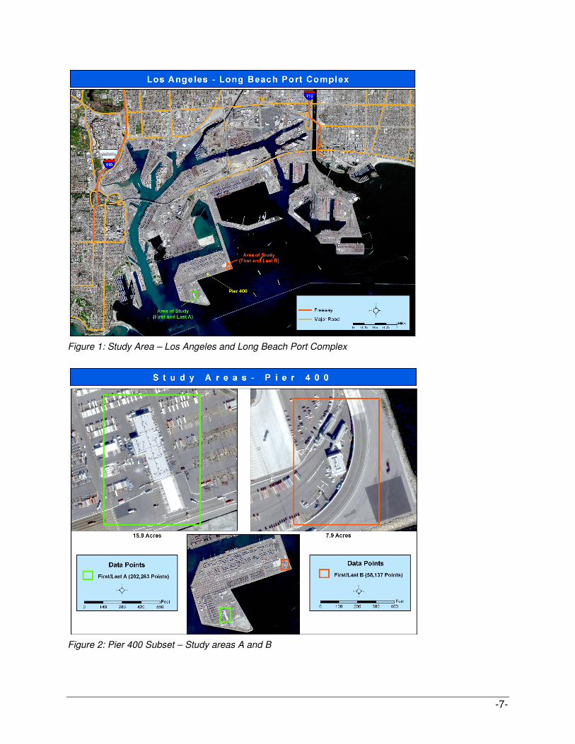
Figure 1: Study Area – Los Angeles and Long Beach Port Complex .......................................... 7

Figure 2: Pier 400 Subset – Study areas A and B ...................................................................... 7

Figure 3: LiDAR Data collection boundary .................................................................................. 8

Figure 4: Airborne1 QA/QC data collection a: Entire area; b: Zoom to roads .............................. 9

Figure 5: Validation points extracted for a simulation in Study Area A .......................................12

Figure 6: Spatial Model of Methodology ....................................................................................13

Figure 7: Sample Output text file with summary statistics ..........................................................14

Figure 8: Visualization of IDW Interpolations – First A ...............................................................16

Figure 9: Visualization of spline interpolation – First A ..............................................................17

Figure 10: Visualization of Kriging interpolation – First A ...........................................................18

Figure 11: Interpolation Accuracy Results .................................................................................19

Figure 12: Building shape reproduction 0.25m resolution ..........................................................21

Figure 13: Building shape reproduction 0.5m resolution ............................................................22

Figure 14: Building shape reproduction 1m resolution ...............................................................22

Figure 15: Building shape reproduction 2m resolution ...............................................................23

Figure 16: Ranks of RMSE, Interpolation Time, CAC and Area Deviation .................................25

List of Tables

Table 1: DEM Accuracy Statistics .............................................................................................. 4

Table 2: LiDAR data for Subsets of the Port Study Area ........................................................... 9

Table 3: Interpolation Parameters used in Monte Carlo Simulations .........................................13

Table 4: Summary of Interpolations ...........................................................................................15

Table 5: Interpolation Accuracy Results ....................................................................................19

Table 6: Interpolation Accuracy (RMSE) and Simulation Time ..................................................20

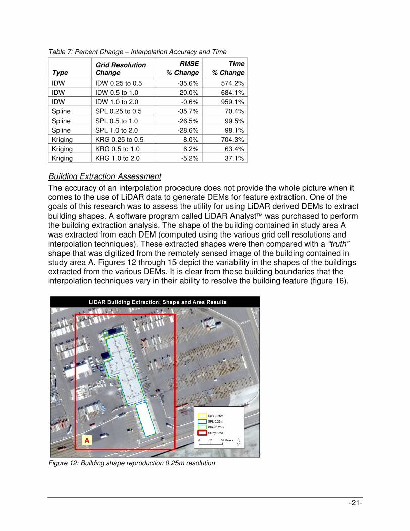
Table 7: Percent Change – Interpolation Accuracy and Time ....................................................21

Table 8: Building Shape Analysis – Area Deviation and RMSE .................................................23

Table 9: Coefficient of Areal Correspondence (CAC), Area Deviation, RMSE & Time ...............24

-v-

Disclosure

This project was funded in entirety under this contract to California Department of Transportation.

-vi-

Acknowledgements

Funding for this project was made possible through the support of METRANS. Graduate student researcher Cesar Espinosa was instrumental in the undertaking and completion of this project. Graduate Student Michael Inman assisted in the data preparation. The following personnel at the Port of Los Angeles collaborated on study area selection and the focus of this study: Rich Riingen, David Malin, Stanley Yon and Daryl Raasch. We greatly appreciate the support and consideration of Dr. Tom O’Brien METRANS Associate Director of CSULB Programs, METRANS Director Dr. Genevieve Giuliano and METRANS Executive Director, Dr. Marianne Venieris. Anonymous Reviewer(s) comments significantly improved this document and are greatly appreciated.

-1-

Introduction

The purpose of this project was to obtain, process, and develop a high-resolution highly accurate elevation data set of the Port complex using Light Detection and Ranging (LiDAR) technology. The applicability of the data set for feature extraction and GIS functionality was investigated for a subset of the Port area. This METRANS applied research project fell under the METRANS directive of “data gathering, description and documentation” to achieve the stated purpose of investigating, and developing a highly accurate elevation data set for use in a Geographic Information System that encompasses the Port complex.

This research focused on the acquisition and processing of a highly detailed elevation dataset using Light Detection and Ranging (LiDAR) technology. LiDAR data are frequently used within geographic information systems (GISs) to obtain surface elevation values and to refine the boundaries of manmade surface features. A spatial database that incorporates the data acquired and investigated under this proposal, combined with features extracted from remotely sensed imagery (please refer to the companion project by Dr. C. Lee, AR05-02) could serve as inputs to sophisticated GIS analyses. Such analyses could be used for a variety of applications such as monitoring and modeling goods movement and their associated impacts. This research constitutes a proof of concept, to demonstrate the value and applicability of LiDAR data layers to address Port-related spatial questions.

LiDAR elevation data is a highly accurate elevation data source (with suggested vertical elevation accuracies of up to 17 cm). A typical procedure for developing a digital elevation models (DEMs) from LiDAR data is to use the LiDAR elevation points and interpolate them onto a gridded surface using common “off the shelf” interpolation algorithms. These derived digital elevation models (DEMs) are models of the surface and contain inaccuracies. Both the selection of an interpolation algorithm, and the grid cell resolution selected for a particular interpolation, affect the accuracy of the resulting surface. In addition, interpolating a DEM from LiDAR data can be extremely time intensive. This research sought to determine the most appropriate grid cell resolution and interpolation algorithm for a selected subset of the Port Complex. A methodology developed specifically for this purpose was implemented within a GIS to assess the accuracy of DEMs derived using different commonly used interpolation algorithms at varying grid cell resolutions. The results can be used to guide Port GIS personnel and other researchers in selecting an appropriate grid cell resolution and interpolation technique. Results from this analysis could assist LiDAR users with a mechanism to assess the accuracy of DEMs created using a particular interpolation method and grid cell resolution, and evaluate the time efficiency of an interpolation procedure based on the time required to process the data.

-2-

Significance

Geography, via its representation in a GIS, is the underlying integrator of data capable of addressing complex Port-related issues ranging from environmental impacts to homeland security. The complex analytic capability of geographic information systems (GISs) make this technology extremely useful not just for visualization but for analyses and informed decision making. The Port’s infrastructure (such as roadways, railroads, ships and buildings) is complex and constantly changing. A georeferenced, spatially based information system could provide the Port with the ability to visualize an assess port operations (in near real time).

An integrated and organized spatial database could be used for a range of activities including but not limited to: planning; development; infrastructure maintenance; change assessment and detection; environmental monitoring and impact assessment (such as air and water quality); tsunami planning and preparation; and managing information to assist in port-related and homeland security planning and assessment.

Elevation datasets provide the underlying baseline data upon which Port infrastructure is built and represented in a GIS. Understanding where features are in relation to each other in the x-y horizontal plane is extremely important and generally easy to assess in a GIS. However, where objects are in relation to each other is influenced not only by its underlying surface elevation, but also by the elevation of each feature (i.e. a building, road or bridge). Therefore an accurate elevation surface is an extremely important underlying component of any spatial database.

This applied research proposal focused on the acquisition and processing of highly accurate LiDAR-acuired data. This research constituted a “proof of concept” to demonstrate the value and applicability of LiDAR data. The accuracy of surfaces generated from LiDAR, as well as the accuracy of building features extracted from the LiDAR surfaces were investigated. A bias in the QA/QC provided by the LiDAR vendor was revealed indicating questions about the “true” accuracy of the delivered dataset. The derived elevation surfaces were actually less accurate than the stated accuracy of the LiDAR data (17 cm); accuracy ranged from 0.56 meters to 3.13 meters.

It is imperative that decision makers are provided with as accurate a dataset as possible, as well as an understanding that there is uncertainty and fuzziness associated with results derived from spatial analyses. It is important for LiDAR data users to understand how accuracy varied based on the surface interpolation technique. Elevation data are frequently used to derive surface products such as slope, and flow direction. The propagation of this “fuzziness” through spatial analyses is poorly understood and rarely quantified. However it is essential that decision makers understand the uncertainty associated with results from spatial analyses. This research provides a start in the quantification and assessment of LiDAR derived data products.

-3-

At the time of this analysis, no studies have explicitly addressed the impact that different interpolation methods have on DEMs interpolated from LiDAR data, and the time required to interpolate these. Although a general understanding of the accuracy of DEMs is known, there have been few empirical studies to assess the accuracy of DEMs derived from LiDAR data. In fact, as we have seen with the LiDAR data used in this research, the accuracy of the LiDAR data delivered is based on a QA/QC procedure that does not sufficiently encompass the entire area of coverage, or the features contained in that area. Thus the stated accuracy of a LiDAR data product cannot be transferred to the DEM interpolated from the dataset. It is therefore imperative that DEM users have available a methodology that can be used to assess the accuracy of DEMs interpolated from LiDAR data. The results of this research project will inform GIS data users such as Port personnel regarding the appropriate grid cell resolution and interpolation algorithm to select when extracting urban features from DEM datasets. This methodology had previously not been applied to LiDAR data.

Background

Digital Elevation Models

A Geographic Information Systems (GIS) is defined as a combination of computer hardware and software that enables complex analyses of geographic data. GISs are frequently used in spatial analyses of natural and urban resources. Data that represent elevation in a GIS are termed digital elevation models (DEMs). The term “DEM” is a generic term for digital topographic (or bathymetric) data. DEM data generally represents the surface as “bare earth”, void of vegetation and urban features. However, digital elevation data may also include surface features such as trees, and buildings. These datasets are referred to as digital surface models or DSMs. DEMs and DSMs provide the basis for characterization of both natural and manmade surface features. For the purposes of this research, the elevation datasets generated are referred to as DEMs and elevation data are represented in a GIS using the raster grid cell structure. LiDAR DEMs

Highly detailed digital elevation data can be generated using a technology called Light Detection and Ranging (LiDAR). Elevation information is captured from an aircraft using special lasers that are not affected by cloud cover or other atmospheric interference. The results are extremely accurate (10-20cm) and highly detailed DEMs. Because the surface is captured so precisely, surface features such as buildings, trees and power lines can be extracted from the data. LiDAR data is obtained by mounting a scanner and an Inertial Measuring Unit and Airborne Global Positioning System (GPS) to an aircraft (Gross 2007). GPS satellites and GPS receivers inside the aircraft are used to indicate the LiDAR unit’s location as it collects the data. A significant amount of data storage is required to process the return time for each pulse returned back to the sensor and calculate the variable distances from the sensor, or changes in terrain/land cover surfaces. One of the most attractive characteristics of LiDAR is that it has very high vertical accuracy, which enables it to capture and represent features on the Earth’s surface (Ma 2005).

-4-

Researchers are actively applying LiDAR technology and reporting on methods used to extract information from the data (Priestnall, Jaafar et al. 2000; Akel, Zilberstein et al. 2003; Brovelli, Cannata et al. 2004; Clode, Kootsookos et al. 2004). DEM Error

DEMs are models of the elevation surface. Like all spatial data, they contain errors. Often the nature and extent of these errors are unknown. Sources of errors are related to production methods such as the equipment used for data collection, man-made, accuracy of the data source, errors introduced in the transformation of control points, and errors transmitted from the data source (Zhu, Shi et al. 2005). The following errors have been associated with LiDAR data (Airborne1 2005).

• System accuracy specifications associated with published vendor specifications;

• Laser rangefinder errors which are caused either by calibration or atmospheric circumstances.

• Inertial measurement unit (IMU) error associated with the airplane’s pitch and roll measurements.

DEM Accuracy Assessment

DEM Accuracy is defined as the closeness of a single measured elevation point to a standard or accepted correct value based on a known vertical datum (Maune 2001). Accuracy is referred to as “high” or “low” depending on the size of the differences the estimated and the standard value”. DEM accuracy is most commonly quantified using the Root Mean Square Error (RMSE) and for the purposes of this research was also quantified using the Mean Absolute Difference (MAD) statistic (Table 1). The MAD is similar to the RMSE, however it incorporates the absolute value of the difference between an observation and the “truth” value. The RMSE squares this difference, which tends to provide more weight to values that are farther off from each other (Wechsler 2000). Table 1: DEM Accuracy Statistics

Root Mean Square Error [RMSE]

( )

N

N

i

∑=1

2

)truth(ited)(interpola i Z-Z

Mean Absolute Difference (MAD)

N

N

i

∑

= 1

Z-Z)truth(ited)(interpola i

LiDAR Accuracy

LiDAR analysts report Root Square Mean Errors (RSME) of up to 12 cm (Blundell, Opitz et al. 2006). Others report that aerospace companies quote LiDAR accuracies of 15 cm

-5-

RMSE. However, this is only achievable under the most ideal circumstances (Hodgson 2004). Some studies suggest LiDAR accuracies of 26 cm to 153 cm RSME in large scale mapping applications (Adams and Chandler 2002; Bowen and Waltermire 2002; Hodgson 2004). Other studies focus on the effect of pulse repetition frequency (PRF) on the accuracy of LiDAR, and suggest that elevation errors are smaller with 33 kHz PRF and larger with 70 kHz PRF (Csanyi and Toth 2006).

DEM Creation through Interpolation

DEM users often generate their own DEMs for areas that might not have one readily available at a resolution sufficient for analysis (Wechsler 2003). DEMs are often created through interpolation processes whereby known elevations are used to predict elevations in areas where elevations are unknown. Many algorithms have been developed to perform sophisticated types of interpolations (Bindlish and Barros 1996; Doytsher and Hall 1997; Shi and Tian 2006). The three interpolation techniques applied in this research include Inverse Distance Weighted (IDW), spline and Kriging. A brief review of these methods is provided. A detailed review of several interpolation techniques can be found elsewhere (Burrough 1986; Wood 1996; Burrough and McDonnell 1998; ESRI 1998; Maune 2001). Inverse Distance Weighted (IDW) interpolation implements the concept of spatial autocorrelation, often referred to as Tobler’s first law of geography – objects in nature that are close to one another are more alike than things that are far apart. Measured values closest to the prediction location have more influence on the predicted value than those that are farther away. The spline interpolation technique is frequently described as a “rubber sheeting” technique. Imagine a sheet of rubber pulled through a set of points. The result is smooth, gently varying surface, that passes through each point (ESRI 1998; Maune 2001). Geostatistical interpolation methods, such as Kriging, are probabilistic statistical models that also incorporate spatial autocorrelation. The strength of similarity between measured sample points accounts for distance and direction. Kriging creates a surface that minimizes the error between the predicted values and a statistical model of the surface (Maune 2001). Grid Cell Resolution and Interpolation

In a GIS, DEMs are commonly represented in a grid format, referred to as a raster data structure. Each grid cell value represents the elevation in a square area on the ground. The size of a grid cell is commonly referred to as the grid cell’s resolution, with a smaller grid cell indicating a higher resolution. A grid cell resolution must be selected as part of the interpolation process; each interpolation technique is implemented using a user-selected grid cell resolution. DEM interpolation results have been shown to be sensitive to the grid cell resolution selected. Researchers continue to be uncertain about a precise methodology for selecting an appropriate resolution for DEM generation. No consensus has been agreed upon, however, the selected resolution should be fine enough to resolve the criteria for the analysis that the DEM is intended for (Wechsler 2007).

-6-

Study Area

The Los Angeles and Long Beach Port complex is the largest in the U.S. and fifth in the world. Together they handle one third of all U.S. container traffic with 60.5% imports and 39.7% exports (SCAG 2005). Because of the two port’s huge economic impact in the U.S., stakeholders have a special interest in assuring that geographic data are up to date and as accurate as possible to be able to respond quickly and efficiently to any emergency. Figure 1 depicts the area where LiDAR data was purchased for this research. The sample points used in our study are from a subset of Pier 400 (Figure 2), which is a man-made addition to the Port of Los Angeles created using material dredged from the channels in and around the port. A subset of the LiDAR dataset was required due to the enormous size of the dataset and processing requirements. Pier 400 was chosen for this study because management personnel at the Los Angeles Port were interested in developing a dataset for this area. Pier 400 is an ideal study area for this type of urban elevation analysis because it contains a fairly flat surface with features such as buildings, containers, and portions of a road that should be well defined using LiDAR data. Two smaller areas on Pier 400 were selected for the analysis, referred to as areas A and B (Figure 2). The urban features of interest in study area A (15.2 acres, 0.062 km2) consist of a building, freight cranes, and containers. Features in study area B (7.0, 0.028 km2acres) consist of a building, freight cranes, containers, a bridge and road.

-7-

Figure 1: Study Area – Los Angeles and Long Beach Port Complex

Figure 2: Pier 400 Subset – Study areas A and B

-8-

Data Acquisition and Description

Data Acquisition

LiDAR data was collected for a 100 km2 area that encompasses the entire Los Angeles-Long Beach Port Complex (Figure 3). LiDAR data acquisition was contracted with Airborne1 Corporation (El Segundo, CA). The data was collected on October 4, 2005. An aircraft was flown at 3000 feet above the ports. According to the vendor, there were no flight restrictions at this elevation; restrictions for the Port area exist for flights below 2,500 and above 8,000 feet (personal communication with Airborne1, 3/17/05). The LiDAR data was initially delivered on November 18, 2005. Upon processing the data, discrepancies and errors were identified. Airborne1 was notified on February 7, 2006 and a replacement data set was received on February 13, 2006. The LiDAR data product has a horizontal accuracy of 30cm and a vertical accuracy of <18.5 cm. Data was delivered as raw point (x, y, and z) data in ASCII file format.

Figure 3: LiDAR Data collection boundary

Data Description

The LiDAR dataset purchased from Airborne1 covers the port complex in its entirety (Figure 3). The area was divided into 99 tiles. Each tile contained a text file in the form of “x, y, z” data where x is longitude, y is latitude, and z is elevation. The complete

-9-

dataset has close to 121 million points, was fifty-seven (57) gigabytes in size and was delivered on eight (8) DVDs. The dataset consists of both first return and last return points. First return constitutes x, y, z readings for points that LiDAR hits first (i.e. tree canopy, buildings, etc.), while last return constitute last hits of LiDAR (i.e. bare earth). The dataset required a detailed pre-processing procedure so that the data could be accessed and processed using a GIS. The LiDAR dataset was delivered in a file format not recognized by the GIS or database software. To enable further processing files were converted into a text file format. This process required considerable time due to the high density of the LiDAR data. The samples for this project were taken from two areas of Pier 400 (Figure 2). Each study area, A and B, consists of four GIS shapefiles (two first returns and two last returns) with different numbers of points (Table 2).

Table 2: LiDAR data for Subsets of the Port Study Area

ID Area First Return Last Return

A 15.9 acres 202,263 points 202,173 points

B 7.9 acres 58,137 points 58,097 points

Airborne1 Quality Assurance/Quality Control (QA/QC)

As part of the Contract, Airborne1 conducted a Quality Assurance/Quality Control (QA/QC) assessment of the data collection. This was based on comparison of the LiDAR data with a set of points collected in the study area (Figures 4a and 4b). Their QA/QC was based on 175 points collected along accessible surfaces (roads) in the study area. The data they collected for this analysis represents 0.00015% of the study area and was collected for one type of feature (roads).

It is evident from the nature of the QA/QC report provided by this vendor that the data used to quantify the delivered LiDAR data’s accuracy is insufficient in capturing the accuracy of the entire area of coverage.

a. b.

Figure 4: Airborne1 QA/QC data collection a: Entire area; b: Zoom to roads

-10-

Data Processing

Raw LiDAR datasets are delivered as a dense network of elevation postings (x,y,z) in an ENZI file format that contains millions of data points. The enormous amount of information in this dataset was processed by the student research assistants employed on this project. Because of the huge amount of data feature extraction and validation was focused on a study area(s) (Figure 2). Pier 400 was selected as an area of interest after consultation with Port Personnel. The students applied various methods identified from the literature review to extract and differentiate manmade features from natural terrain elevations in these areas. This time consuming data processing included testing and evaluation of the various interpolation methods. This process and methods used are described in this section.

The dataset was processed before it could be analyzed using four different types of software; Notepad, Microsoft Access 2003, ArcGIS 9.2, and Surfer 7. The steps described below were followed to process the sample dataset.

(1) The study area was identified.

(2) The sample raw LiDAR data (delivered in an .enz format) were extracted from the dataset.

(3) Each text file, from the first and last returns, was converted into a text file. Each file (approximately 300 files) was opened using Notepad and saved as a text file.

(4) Using all the newly created text files four separate databases were created in Access.

(5) Once the databases were completed they were converted into a dBASEIV file format in Access.

(6) Each dBASEIV file was imported into ArcMap separately and four separate point shapefiles (First/Last for areas A and B) were created for mapping.

(7) In ArcMap, the point shapefiles were assigned the appropriate projection and coordinate system (UTM NAD 83 Zone 11N), providing a spatial reference.

(8) Using the point shapefiles a grid was created using Surfer 7. The grids and the point-shapefiles were used in ArcView 3.2 to perform the validation procedure.

-11-

Analysis Methodology

The raw Airborne1 LiDAR data consisted of a collection of points with spatial coordinates (latitude, longitude and elevation – x,y,z). To generate an elevation surface (DEM), these points must be interpolated onto a regular grid. Numerous techniques exist for interpolating raw point data onto a regular grid for use in a GIS. Selection of an appropriate and accurate technique is an iterative process that involves testing and validation of a number of different interpolation methods. Surfaces were developed from the LiDAR data by applying various interpolation techniques to selected areas of the dataset and assessing their accuracy using ground control validation points.

The analysis approach was designed to enable those who interpolate digital surfaces to assess the accuracy of the resulting surface, and select an appropriate interpolator and grid cell resolution that will provide a result with the highest level of accuracy as well as best building extraction results. The approach assumes that interpolated surface quality can be assessed by comparing an interpolated elevation surface with validation points extracted from the original set of data points (and not used as part of the interpolation). Points extracted from the original data set are termed “validation” data points and considered "truth" values. A Monte Carlo simulation was applied to assess the accuracy of the interpolation method and grid cell resolution. A GIS extension designed to assess interpolation accuracy was used to perform the analyses (Wechsler 2002). Interpolation Accuracy Procedure

The first step taken to perform the interpolation accuracy was to randomly extract validation points from the elevation point shapefiles created. These validation points were randomly extracted and saved as a validation data file. The number of randomly selected validation points varied based on the number of data points available within the dataset to be analyzed. About 0.1% of the total number of points was extracted as validation points for study areas “A” and “B”.

The number of points selected as validation points in each interpolation represented 0.1% of the entire dataset -- 202,263 in study area A (~13 points per acre) and 58,097 points in study area B (~8.3 points per acre). Selection of these values was based on the following justification: (a) The US Geological Survey uses 24 validation points to compute the RMSE accuracy statistic for its 7.5 minute quadrangle maps (scale of 1:24,000, roughly 64 mi2 or 40960 acres). This represents approximately 0.024% of the dataset for a typical 1/3 arc second, 10 meter resolution DEM, or roughly 0.0005 points per acre. (b) Statistically, values greater than 30 represent a large sample size. The values were used to compute accuracy statistics (RMSE and MAD) for each simulation. The process of surface generation was repeated 10 times. The resulting RMSE and MAD for each simulation was computed and averaged. Therefore the results do not represent just one simulation, but the average of 10 simulations per interpolation type and grid cell resolution.

Sampling statistics provide measures for selecting sample sizes based on non-spatial populations. According to these measures, the recommended sample size for a population of 202,263 at the 95% confidence level and a confidence interval of 5 is 383.

-12-

The recommended sample size for a population of 58,097 at the 95% confidence level and a confidence interval of 5 is 382 (Creative Research Systems, 2011). These statistical approaches do not include spatial organization of a study area or the purpose of the sample. The purpose of this sample was to extract actual data from the dataset to generate a surface. Extracting too many points from the input dataset would adversely impact the resulting interpolation, contributing to lower accuracy in the resulting surfaces. The method selected for this research, which is based on a randomly distributed percentage of the population, adequately incorporates this consideration. Increasing the sample size in study area B would adversely impact results.

For each simulation 202 points were randomly extracted from study area A, and 58 validation points randomly extracted from study area B. The remaining points were saved to another file, and used to interpolate surfaces using IDW, spline and Kriging for increasing grid cell resolutions (0.25m, 0.5m, 1m and 2m). A sample of the validation points extracted for one simulation is depicted in Figure 5. The validation points were randomly selected and changed for each simulation. Building Extraction Procedure

A software program called LiDAR Analyst (VLS 2008) was purchased to extract the building feature in Study Area A from the LiDAR data.

Figure 5: Validation points extracted for a simulation in Study Area A

A flowchart of this methodology is provided in Figure 6, and parameters used in the various interpolations presented in Table 3. The methodology applied in this research was programmed into an extension for the ArcView 3.x software.

-13-

Point File

Interpolation

Points

Validation

Points

Save remaining points to an

interpolation file

Interpolate grid

IDW, Spline or Kriging

select cell size

Interpolated Grid

Randomly select N

validation points

Compare collocated

interpolated values

with Validation points. Compute:• RMSE

• Mean Absolute Difference • Standard Deviation

Save values to a file.

REPEAT N TIMES

Figure 6: Spatial Model of Methodology

Table 3: Interpolation Parameters used in Monte Carlo Simulations

Simulation Parameters

Number of validation points Area A: 202; Area B: 58

Number of simulations 10

Grid Cell Size (m) Either 0.25, 0.5, 1 or 2 IDW Parameters

Power 2

Search Radius 10

Radius Fixed

Sample Count 10 Spline Parameters

Type Regularized

Number of Points 10

Weight 0 Kriging Parameters

Type Universal

Barrier No Barrier

Radius Fixed

Search Distance 10

Sample Count 10

Lag Distance 0.5

Once the interpolation simulations were competed for a particular interpolation technique and grid cell resolution, summary statistics associated with each simulation were exported to a text file (Figure 7). These text files were then imported into an Excel Spreadsheet for analysis.

-14-

Figure 7: Sample Output text file with summary statistics

-15-

Analyses, Results and Discussion

Three different interpolations algorithms (IDW, spline, and Kriging) were applied to study areas A and B using four different grid cell resolutions (0.25, 0.5, 1 and 2 meters). Several attempts were made to successfully run the simulation software for both the first and last return datasets for each subarea (A and B) using these interpolators and grid cell resolutions. We were successful in interpolating first and last returns for IDW in each subarea, first returns for each subarea A and B using spline and first returns for study area A using Kriging (Table 4). Table 4: Summary of Interpolations

Cell Size (m) IDW: First A IDW: First B IDW: Last A IDW: Last B

0.25 � � � �

0.5 � � � �

1.0 � � � �

2.0 � � � �

Cell Size Spline: First A Spline: First B Spline: Last A Spline: Last B

0.25 � � �

0.5 � � �

1.0 � � �

2.0 � � �

Cell Size Kriging: First A Kriging: First B Kriging: Last A Kriging: Last B

0.25 �

0.5 �

1.0 �

2.0 �

� indicates a successful simulation

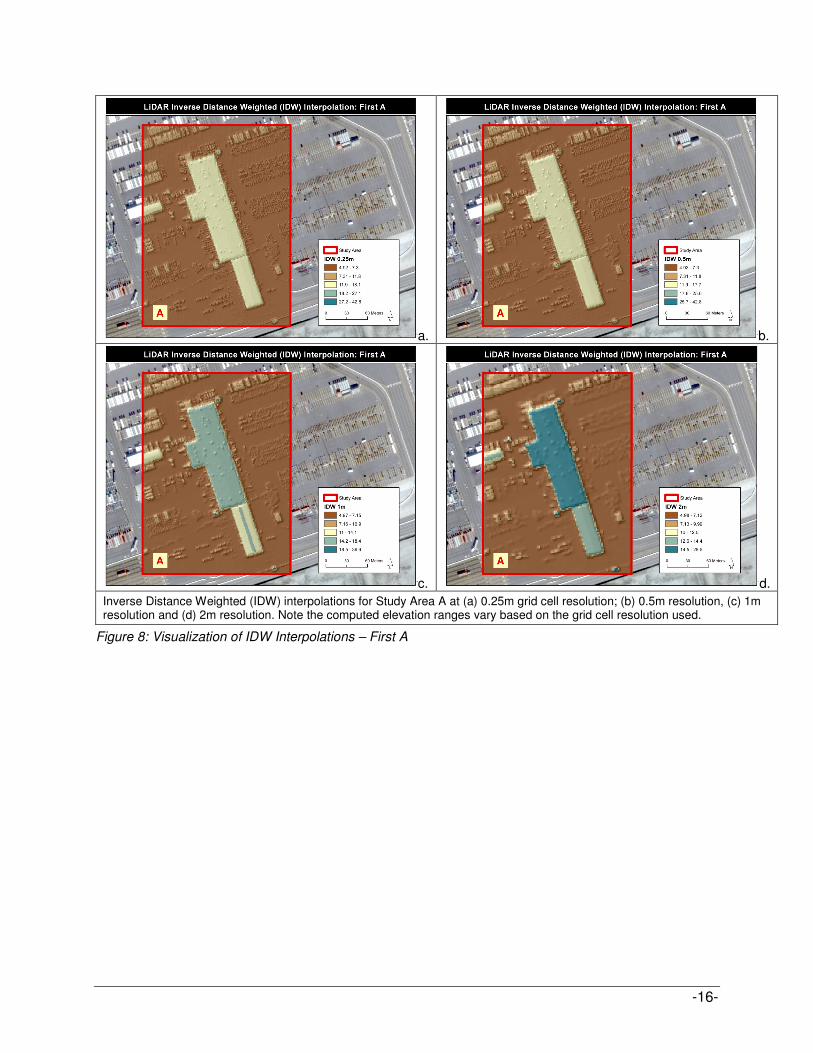
Simulations were successful for each interpolator and grid cell resolution in study area A using the first return LiDAR data. Results for study area A (first return) are presented in this report. Figures 8, 9 and 10 depict the results of the interpolations for study area A. Please note the variation in the elevation ranges resulting form the different interpolation methods and grid cell resolutions. The legend for these figures is based on the Jenks’ natural breaks classification scheme, whereby data are classified based on categories that minimize differences within the classes (ESRI 2008).

-16-

a. b.

c. d.

Inverse Distance Weighted (IDW) interpolations for Study Area A at (a) 0.25m grid cell resolution; (b) 0.5m resolution, (c) 1m resolution and (d) 2m resolution. Note the computed elevation ranges vary based on the grid cell resolution used.

Figure 8: Visualization of IDW Interpolations – First A

-17-

a. b.

c. d.

Spline interpolations for Study Area A at (a) 0.25m grid cell resolution; (b) 0.5m resolution, (c) 1m resolution and (d) 2m resolution. Note the computed elevation ranges vary based on the grid cell resolution used.

Figure 9: Visualization of spline interpolation – First A

-18-

a. b.

c. d.

Kriging interpolations for Study Area A at (a) 0.25m grid cell resolution; (b) 0.5m resolution, (c) 1m resolution and (d) 2m resolution. Note the computed elevation ranges vary based on the grid cell resolution used.

Figure 10: Visualization of Kriging interpolation – First A

Interpolation Accuracy

Interpolation accuracy for each interpolator and grid cell resolution was assessed using the RMSE and MAD statistics (Table 5; Figure 11). The average RMSE and MAD for the N=10 simulations per interpolation-grid cell resolution “pair” were ranked (lowest values indicate highest accuracies) and are provided in Table 5. As expected, the RMSE decreased as the grid cell size decreased (accuracy increases with smaller grid cell sizes). We would expect to see a lower average RMSE in the smaller grid cell resolutions for these interpolations (the 0.25, and 0.5 meter cell sizes) because the higher resolutions (smaller grid cell sizes) better preserve the original LiDAR data values; more point values are averaged to populate at the coarser grid cell resolutions. These results indicate that overall, DEMs generated using the Inverse Distance Weighted algorithm were most accurate. DEMs generated using the Kriging algorithm were least accurate.

-19-

Table 5: Interpolation Accuracy Results

Interpolation RMSE (m)

Mean Absolute Difference

RMSE Rank

MAD Rank

IDW 0.25m 0.56 0.15 1 1

SPL 0.25m 0.59 0.19 2 2

IDW 0.5m 0.86 0.21 3 3

SPL 0.5m 0.92 0.25 4 4

IDW 1m 1.08 0.26 5 5

IDW 2m 1.08 0.32 6 6

SPL 1m 1.25 0.33 7 7

SPL 2m 1.75 0.50 8 8

KRG 0.25m 2.88 1.33 9 9

KRG 1m 2.95 1.39 10 10

KRG 2m 3.11 1.47 11 12

KRG 0.5m 3.13 1.39 12 11

Values represent the average of N=10 simulations per interpolation and grid cell resolution pair. Data represent study area A, first return LiDAR points.

0.0

0.5

1.0

1.5

2.0

2.5

3.0

3.5

IDW RMSE KRG RMSE SPL RMSE IDW MAD KRG MAD SPL MAD

2m

1m

0.5m

0.25m

Figure 11: Interpolation Accuracy Results

Interpolation Accuracy versus Interpolation Time

Each interpolation simulation required a considerable amount of time to process the data (Table 6). In fact, the interpolation with the highest accuracy (IDW at 0.25m resolution) took the longest time to compute (123 hours and 17 minutes – close to three straight weeks of processing time for this small study area).

-20-

Table 6: Interpolation Accuracy (RMSE) and Simulation Time

Interpolation Cell Size Average

RMSE

Interpolation Time

(Hrs.Min)

RMSE Rank

Time Rank

IDW 0.25 0.555 123.17 1 11

IDW 0.5 0.862 18.27 3 9

IDW 1 1.078 2.33 5 4

IDW 2 1.084 0.22 6 1

Kriging 0.25 2.878 162.30 9 12

Kriging 0.5 3.127 20.18 12 10

Kriging 1 2.945 12.35 10 8

Kriging 2 3.107 9.01 11 7

Spline 0.25 0.592 7.07 2 6

Spline 0.5 0.921 4.15 4 5

Spline 1 1.253 2.08 7 3

Spline 2 1.754 1.05 8 2

The percent change was used to measure the change in DEM accuracy and processing time required by moving from a coarser grid cell resolution to a higher grid cell resolution (and vice-versa). Percent change is computed as [(new value-original value)/original value)*100]. This computation provides an indication of the percent improvement in accuracy (based on the average RMSE) and the percent change in time required to run the simulations for each interpolation and grid cell resolution (Table 7). Going from finer to coarser grid cell resolutions the percent accuracy decreased, and the percent change in time required to run a simulation increased. For example, the IDW 0.25 grid cell resolution provided the highest accuracy simulation based on the average RMSE. However, the simulation required approximately 127 hours of processing time. Should someone wish to use a coarser grid cell resolution for an interpolation, for example the 0.5 meter resolution, the accuracy achieved decreases by 35.6%, but the time required to run the simulation improved by 574%. The highest accuracy of the First A interpolation was IDW at 0.25 meter cell size resolution with an RMSE of 0.56m. However, the time required to run this simulation was a little over three weeks (123 hours and 17 minutes). On the other hand, Spline with the same grid cell size resolution had an RMSE of .59m and an interpolation time of only seven hours. The accuracy varied by only 3cm (a change of only -6.3%) however the time required to compute the DEMs in this simulation decreased by 94.3%. Overall, the best value for the First A study area based on accuracy and interpolation time appears to be Spline at 0.25 meter cell size resolution. That is, spline at 0.25m resolution appears to be the most efficient method when effort (as measured by simulation time) is considered.

-21-

Table 7: Percent Change – Interpolation Accuracy and Time

Type Grid Resolution Change

RMSE

% Change

Time

% Change

IDW IDW 0.25 to 0.5 -35.6% 574.2%

IDW IDW 0.5 to 1.0 -20.0% 684.1%

IDW IDW 1.0 to 2.0 -0.6% 959.1%

Spline SPL 0.25 to 0.5 -35.7% 70.4%

Spline SPL 0.5 to 1.0 -26.5% 99.5%

Spline SPL 1.0 to 2.0 -28.6% 98.1%

Kriging KRG 0.25 to 0.5 -8.0% 704.3%

Kriging KRG 0.5 to 1.0 6.2% 63.4%

Kriging KRG 1.0 to 2.0 -5.2% 37.1%

Building Extraction Assessment

The accuracy of an interpolation procedure does not provide the whole picture when it comes to the use of LiDAR data to generate DEMs for feature extraction. One of the goals of this research was to assess the utility for using LiDAR derived DEMs to extract

building shapes. A software program called LiDAR Analyst was purchased to perform the building extraction analysis. The shape of the building contained in study area A was extracted from each DEM (computed using the various grid cell resolutions and interpolation techniques). These extracted shapes were then compared with a “truth” shape that was digitized from the remotely sensed image of the building contained in study area A. Figures 12 through 15 depict the variability in the shapes of the buildings extracted from the various DEMs. It is clear from these building boundaries that the interpolation techniques vary in their ability to resolve the building feature (figure 16).

Figure 12: Building shape reproduction 0.25m resolution

-22-

Figure 13: Building shape reproduction 0.5m resolution

Figure 14: Building shape reproduction 1m resolution

-23-

Figure 15: Building shape reproduction 2m resolution

One method of assessing the quality of the extracted feature is to simply compare the areas of the buildings extracted from the LiDAR-derived DEMs with the area of the “truth” building, and deviations were calculated (Table 8). Although the spline interpolation at 0.25m resolution was ranked 2nd in accuracy, it underestimated the area of the building by 580 m2, thus ranking 6th in its approximation of the building area.

Table 8: Building Shape Analysis – Area Deviation and RMSE

Interpolation Area

Deviation Area Rank RMSE RMSE Rank

IDW 0.5 -93.88 1 0.86 3

KRG 0.25 -145.91 2 2.88 9

IDW 1.0 -223.65 3 1.08 5

IDW 0.25 -234.73 4 0.56 1

SPL 0.5 -447.01 5 0.92 4

SPL 0.25 -580.79 6 0.59 2

IDW 2.0 -684.38 7 1.08 6

SPL 2.0 -980.44 8 1.75 8

SPL 1.0 -1191.87 9 1.25 7

KRG 2.0 -1550.09 10 3.11 11

KRG 1.0 -3068.69 11 2.95 10

KRG 0.5 -3138.98 12 3.13 12

Values are listed in order of their rank in comparison of area between the derived building and the true building area. IDW refers to the Inverse Distance Squared interpolation method, SPL refers to the Spline interpolation method and KRG refers to the Kriging interpolation method. Numbers represent the grid cell resolution applied.

-24-

However, straight comparison of building areas is not a robust method for comparing the data output. Two polygons can have similar areas but not overlap in space. Therefore the coefficient of areal correspondence (CAC) statistic was calculated to compare the building extracted for each interpolation/grid cell resolution with the truth building shape (Table 9). The CAC for any two associated areas is computed as the area of intersection divided by the area of union. The CAC is a measure of areal association that ranges from 0 to where 0 indicates no correspondence and 1 indicates that the two distributions correspond exactly (Taylor 1977; Stanislawski, Finn et al. 2007). Spline at 0.5m resolution exhibited the highest degree of areal correspondence with the truth building, followed by Inverse Distance Weighted at .25m and Inverse Distance Weighted at 1m. These interpolation methods-grid cell resolutions ranked 4th. 1st and 5th respectively, with average RMSE values of 1.25m, 0.56m and 1.08m.

Table 9: Coefficient of Areal Correspondence (CAC), Area Deviation, RMSE & Time

Interpolation CAC CAC

Rank Area

Deviation Area Rank

RMSE RMSE Rank

Time (Hrs.Min)

Time Rank

SPL 0.5 98.72% 1 -447.01 5 0.921 4 4.15 5

IDW 0.25 91.46% 2 -234.73 4 0.555 1 123.17 11

IDW 1.0 90.96% 3 -223.65 3 1.078 5 2.33 4

IDW 0.5 90.89% 4 -93.88 1 0.862 3 18.27 9

IDW 2.0 89.99% 5 -684.38 7 1.084 6 0.22 1

SPL 0.25 89.97% 6 -580.79 6 0.592 2 7.07 6

KRG 0.25 87.87% 7 -145.91 2 2.878 9 162.3 12

KRG 2.0 82.28% 8 -1550.09 10 3.107 11 9.01 7

SPL 1.0 78.42% 9 -1191.87 9 1.253 7 2.08 3

SPL 2.0 73.67% 10 -980.44 8 1.754 8 1.05 2

KRG 0.5 59.23% 11 -3138.98 12 3.127 12 20.18 10

KRG 1.0 51.03% 12 -3068.69 11 2.945 10 12.35 8

Values are listed in order of their rank based on the CAC statistic. IDW refers to the Inverse Distance Squared interpolation method, SPL refers to the Spline interpolation method and KRG refers to the Kriging interpolation method. Numbers represent the grid cell resolution applied.

Spline at 0.25m resolution was ranked 2nd in accuracy and deemed the best compromise when considering the accuracy of a LiDAR derived DEM, since the time to process the data using this method was much less than that required by the first place method – IDW at 0.25m resolution. However, this method generated a building with a CAC of 91%, indicating that 9% of the area did not correspond to the truth building. Figure 19 provides a comparison of the ranking in each of the assessment areas: accuracy (RMSE), interpolation time, CAC and Area deviation. Figure 16 demonstrate the tradeoffs between interpolation methods. The most accurate surface was derived using IDW on a 0.25m grid cell resolution. However this interpolation was the most time intensive and did not produce the highest accuracy building derivation. The method that produced the most accurate building extraction, as measured by the CAC statistic, was derived using spline on a 0.5m resolution grid; however the accuracy of this surface was ranked 5th.

-25-

0

1

2

3

4

5

6

7

8

9

10

11

12

IDW

0.25

IDW

0.5

IDW

1.0

IDW

2.0

SPL

0.25

SPL

0.5

SPL

1.0

SPL

2.0

KRG

0.25

KRG

0.5

KRG

1.0

KRG

2.0

RMSE Rank

Time Rank

CAC Rank

Area Rank

Figure 16: Ranks of RMSE, Interpolation Time, CAC and Area Deviation

-26-

Conclusions

Although DEMs are ubiquitous, rarely is their accuracy and utility for specific applications evaluated and quantified systematically. This research implemented a methodology to investigate the accuracy of LiDAR derived digital elevation models (DEMs), and the accuracy of a building feature extracted from the derived surfaces, for a subset of the Port Complex. Three different interpolation methods (inverse distance weighted, spline and Kriging) using four different grid cell resolutions (0.25m2, 0.5m2, 1m2 and 2m2) were investigated.

The interpolation method that produced the highest accuracy DEM – Inverse Distance Weighted at 0.25m resolution – required a significant amount of time (the accuracy simulation using ten grids required over three weeks to process the data for study area A). The interpolation that was deemed the best compromise between accuracy and tome – spline at 0.25m resolution – ranked 6th in its ability to capture the shape of the building located in the study area.

In selecting an appropriate method for generating surfaces from the DEM, Port Personnel and other LiDAR users must consider three factors – interpolation accuracy, interpolation time and the accuracy of features extrapolated from the derived surfaces. Prioritization of each of these factors is required, and in doing so compromises are made. The methodology presented provides Port personnel and LiDAR data users in general with a mechanism for selecting an interpolation method and grid cell resolution. Identification of a method will depend on the ultimate use of the derived surfaces, and how much time is available to get the work done.

LiDAR data are expensive, in terms of base costs for acquisition and time associated with processing and surface derivation. However, freely available DEMs, such as those available from the USGS, are limited in functionality because they are dated, have a coarse grid cell resolution and much higher RMSEs (generally 2 meters). LiDAR data therefore do provide the best solution for Port-related purposes due to their accuracy and currency. However, newer, lower cost technologies are emerging, such as those that enable DEMs to be derived from images (structure from motion). Such technology may provide viable alternatives to the time and cost associated with LiDAR data. Regardless of the elevation dataset used, an understanding of its accuracy and limitations is imperative for responsible use of the technology and responsible communication of results from analyses to decision makers.

-27-

Implementation

As a result of this project LiDAR data collected in October 2005 for the Port Complex are available. This data was used to explore the usefulness of LiDAR data in deriving digital elevation models for a subset of the Port Complex, and in extracting a building from those derived surfaces. The accuracy of interpolation methods in generating digital elevation models form the LiDAR data was explored. The accuracy of a building footprint extracted from the derived surfaces was also investigated.

The data acquired, processed and presented through this project provide a foundation that, when used in the context of deriving elevation models from LiDAR data, could directly contribute to an understanding of issues confronted by the Port Complex. DEMs provide the foundation for spatial GIS models such as those used to evaluate and develop networks for goods movement and trade transportation. Digital elevation models are used in hazard assessment and hazard mitigation and assessment such as tsunami modeling. Buildings derived from LiDAR-based DEMs can be used for emergency response planning and homeland security exercises. Using the LiDAR data to its fullest potential and with the greatest accuracy is imperative for many of these applications.

Our experience with this large dataset suggests that LiDAR data is currently too unwieldy to work with in an effective manner for deriving and extracting building footprints for an area the size of the entire Port Complex. The data management and processing requirements exceed current computer processing capabilities. The data is rich in elevation values and provides high accuracy point data. The Port could certainly use this dataset to provide elevation for a site-specific case. However it is currently not useful for deriving “on-the-fly” representations of the elevation surface and built environment for the entire area of data coverage.

The methodology and results presented in this report provide Port Personnel with a procedure for working with the data set and an understanding of the accuracy and limitations of LiDAR-derived DEMs. This research also provides Port Management with a rationale for establishing priorities for the DEMs they wish to derive from LiDAR data. The following questions should be considered by Port Management in their use of the surfaces derived from this valuable data set:

• How will the DEMs be used?

• Based on their use, what level of accuracy can be tolerated?

• How much time (person hours and computer processing) can be dedicated to the task?

By addressing these questions in the context of the results presented here, the LiDAR data can be used most efficiently and applied with the maximum benefit.

-28-

References

Adams, J. C. and J. H. Chandler (2002). "Evaluation of LiDAR and Medium Scale Photogrammetry for Detecting Soft-Cliff Coastal Change." Photogrammetric Record 17(99): 405-418.

Airborne1 (2005). Technical Considerations: Error Budget for LiDAR. El Segundo, CA. Briefing Note #BN01.

Akel, N. A., O. Zilberstein, et al. (2003). "Automatic DTM Extraction from Dense Raw LIDAR Data in Urban Areas." Proceedings: FIG Working Week, from http://www.fig.net/pub/fig_2003/TS_26/PP26_1_AboAkel_et_al.pdf.

Bindlish, R. and P. Barros (1996). "Aggregation of Digital Terrain Data Using a Modified Fractal Interpolation Scheme." Computers & Geosciences 22(8): 907-917.

Blundell, S., D. Opitz, et al. (2006). Automated feature extraction from terrestrial and airborne LiDAR. Proceedings of the International LiDAR Mapping Forum.

Bowen, Z. H. and R. G. Waltermire (2002). "Evaluation of light detection and ranging (LiDAR) for measuring river corridor topography." Journal of the American Water Resources Association 38(1): 33-41.

Brovelli, M. A., M. Cannata, et al. (2004). "LIDAR Data Filtering and DTM Interpolation Within GRASS." Transactions in GIS 8(2): 155-174.

Burrough, P. and R. McDonnell (1998). Principles of Geographic Information Systems. New York, NY, Oxford University Press.

Burrough, P. A. (1986). Principles of Geographical Information Systems for Land Resources Assessment. New York, NY, Oxford University Press.

Clode, S. P., P. Kootsookos, et al. (2004). "The Automatic Extraction of Roads from LiDAR Data." International Archives of Photogrammetry, Remote Sensing and Spatial Information Sciences 35: 231-236.

Creative Research Systems, 411 B Street, Petaluma CA 94952, http://www.surveysystem.com/sscalc.htm, last accessed May 27, 2011.

Csanyi, N. and K. C. Toth (2006). LiDAR accuracy: The impact of pulse repetition rate. Proceedings of the MAPPS/ASPRS Conference, San Antonio, Texas.

Doytsher, Y. and J. K. Hall (1997). "Interpolation of DTM Using Bi-Directional Third-Degree Parabolic Equations, With Fortran Subroutines." Computers & Geosciences 23(9): 1013-1020.

ESRI (1998). ArcView Spatial Analyst. Redlands, CA, Environmental Systems Research Institute.

ESRI (2008). ArcGIS Version 9.2. Redlands, CA, Environmental Systems Research Institute.

Gross, S. B. (2007). "LIDAR (Light Detection and Ranging)." How LiDAR Works Retrieved January 26, 2007, from http://www.sbgmaps.com/lidar.htm.

Hodgson, M. E., Bresnahan, P. (2004). "Accuracy of airborne Lidar-Derived Elevation: Empirical Assessment and Error Budget." Photogrammetric Engineering and Remote Sensing 70(3): 331-39.

-29-

Ma, R. (2005). "DEM Generation and Building Detection from Lidar Data." Photogrammetric Engineering and Remote Sensing 71(7): 847-54.

Maune, D. F. (2001). Digital Elevation Model Technologies and Applications: The DEM Users Manual. Bethesda, Maryland, The American Society for Photogrammetry and Remote Sensing.

Priestnall, G., J. Jaafar, et al. (2000). "Extracting urban features from LiDAR digital surface models." Computers Environment and Urban Systems 24: 65-78.

SCAG (2005). Goods movement in Southern California: the challenge, the opportunity, and the solution. . White Paper. Los Angeles, Southern California Association of Governments (SCAG): 12.

Shi, W. Z. and Y. Tian (2006). "A hybrid interpolation method for the refinement of a Regular Grid Digital Elevation Model." International Journal of Geographical Information Science 20(1): 53-67.

Stanislawski, L., M. Finn, et al. (2007). Assessment of a Rapid Approach for Estimating Catchment Areas for Surface Drainage Lines. ACSM-IPLSA-MSPS, St. Louis, MO.

Taylor, P. J. (1977). Quantitative Methods in Geography: An Introduction to Spatial Analysis. Boston, MA, Houghton Mifflin Company.

VLS. (2008). "Visual Learning Systems Software: LiDAR Analyst." Retrieved August 11, 2008, from http://www.featureanalyst.com/lidar_analyst.htm.

Wechsler, S. P. (2000). Effect of DEM Uncertainty on Topographic Parameters, DEM Scale and Terrain Evaluation. Syracuse, NY, State University of New York College of Environmental Science and Forestry. Ph.D. Dissertation: 380.

Wechsler, S. P. (2002). Effect of interpolation method & grid cell resolution on DEM Accuracy…a methodology. Association of American Geographers Annual Conference, Los Angeles, CA.

Wechsler, S. P. (2003). "Perceptions of Digital Elevation Model Uncertainty by DEM Users." URISA Journal 15(2): 57-64.

Wechsler, S. P. (2007). "Uncertainties associated with digital elevation models for hydrologic applications: a review." Hydrol. Earth Syst. Sci. 11: 1481-1500.

Wood, J. (1996). The Geomorphological Characterization of Digital Elevation Models. Department of Geography. Leicester, UK, University of Leicester.

Zhu, C., W. Shi, et al. (2005). "Estimation of average DEM accuracy under linear interpolation consideration random error at the nodes of TIN Model." International Journal of Remote Sensing 26(24): 5509-5523.