
Translating data between geographic information systems
141
Translating Data Between Geographic Information Systems A thesis submitted in partial fulfillment of the requirements for the Degree of Master of Science in Computer Science in the University of Canterbury by RichardT. Pascoe University of Canterbury 1989
-
Upload
khangminh22 -
Category
Documents
-
view
5 -
download
0
Transcript of Translating data between geographic information systems

Translating Data Between
Geographic Information Systems
A thesis
submitted in partial fulfillment
of the requirements for the Degree of
Master of Science in Computer Science
in the
University of Canterbury
by
RichardT. Pascoe
University of Canterbury
1989


SCIENCES LIBRARY'
THESIS
1
2 2.1. 2.2. 2.3.
3 3.1. 3.2.
4 4.1. 4.2. 4.3. 4.4.
5
6 6.1 6.1.1 6.1.2 6.2 6.2.1 6.2.2
7 7.1. 7.2. 7.3. 7.3.1. 7.3.2. 7.4.
Table of Contents
Abstract .. , ................................................... iii
Introduction ................................................ . 1
Geographic Data Translation ••...•...•••.•••.........•....• 5 Geographic Data Representation .............................. 5 Notation of Data Translation ................................... 7 The Goals of Data Translation ................................. 9
Interfacing Strategies .................................. ... 13 Comparison of Interfacing Strategies ........................ 15 Interchange Formats ........................................... 16
General Data Translation ..........•••....•...•........... 19 Language Translation .......................................... 19 Electronic Manuscript Translation ........................... 21 Database Translation ........................................... 22 Geographic Data Translation ................................. 25
The Translation Process ................... ................ 2 9
Translation Specification ........................•..•..... 3 3 Format Specification ........................................... 33
Geographic Data Model Specification ............. 34 Implementation Method Specification ............. 37
Specifying the Source to Target Format Mapping ......... 40 The Relational Data Model ......................... 40 Extending the Relational Model.. ................. .41
The Decode Phase .. ................ '• ...................... 4 3 Parser Generators .............................................. 44 Simplified Ingres Interface ................................... .46 Decoding Techniques .......................................... 47
Repeating Groups ................................... 47 Lexical Analysis of Dataflles ....................... 49
Processing Large Data Volumes ............................. 51
8 The Translate Phase ................... · .................... 53 8.1. QUEL ...................... ~ .......................................... 53 8.2. Translation Algorithms ........................................ 54
9 9.1. 9.1.1. 9.3. 9.4.
10
The Encode Phase . ........................................ 59 EQUEL .................... : ........................................ 59
Nested Retrieve Statements ........................ 61 Generating Format Encoders ................................. 65 The Structure of Format Encoders ........................... 67
Conclusions ............................................... 69
Acknowledgemet:t~s ................................................ 71

Page ii Data Translation between Geographic Injonnation Systems
Bibliography ........................................................ 7 3
A Format Implementation Specifications ......••....••.... 7 7 A.1 The GeoVision GINA Format. ............................... 77 A.1.1 BNF Specification ................................... 77 A.1.2 uxicon ................................................ 82 A.2 The BIF Format ................................................ 83 A.2.1 BNF Specification ................................... 83 A.2.2 uxicon ................................................. 83 A.3 The Colourmap Format ....................................... 84 A.3.1 BNF Specification ................................... 84 A.3.2 uxicon ......... , ... , .. ~ ................................... 85
B Format Decoders ........ "' ................................. 8 7 B .1 The Colormap Format Decoder .............................. 87 B .1.1 Y ace Definition file .................................. 87 B .1. 2 Lex defmition File ................................... 96 B.2 The GINA Format Decoder ................................... 98 B.2.1 Yacc Definition file .................................. 98 B.2.2 Lex Defmition File ................................ 100 B.3 The BIF Decoder ............................................. 102 B. 3 .1 Y ace Definition file ................................ 102 B. 3. 2 Lex Definition File ................................ 106
C A Simplified INGRES Interface ........................ 107 C.1. eql.h ........................................................... 107 C.2. hash.h .......................................................... 107 C.3. eqlappend() ................................................... 108 C.4. eqlreplace() ................................................... 109 C.5. atctrl() ......................................................... 111 C.6. getattype() ..................................................... 111 C. 7. hash functions ................................................ 112
D Lexical Analysis of Repeating Groups .•......•...•.... 117
E Example Translation Algorithm ......................... 119 E.l BIF Format Relational Data Model ........................ 119 E.2 Research Relational Data ModeL. .......................... 119 E.3 Translation Algorithm ....................................... 120
F Format Encoder Generator .............................. 125 F .1 Y ace Definition file ......................... ;, ............... 125 F.2 Lex defmition File ........................................... 129
G An Example of a Format Encoder ....................... 131 G .1 tre .. h. .. .. . .. . . .. . . .. . . .. . . . .. . . . . . . . . . . . . . . . . . . .. . . . . . . . . .. . . . . . . . . . . . . . . 131 0.2 tre.c., ........ ................................................... 131 G.3 enc.qc ......................................................... 132

Abstract
Transferring data from one geographic information system (GIS) to another is difficult
because of the diverse, and often complex, structure of transfer file formats.
Accordingly, the design and implementation of an interface for transferring data from
one format to another is time consuming and difficult. The translation may be performed
by an interface constructed for the two formats (the individual interfacing strategy), by
two interfaces through an interchange format (the interchange format interfacing
strategy), or by a number of interfaces through a series of formats (the ring interfacing
strategy).
The interchange format interfacing strategy is widely adopted because it offers an
acceptable compromise between the quality of the data translation and number of
interfaces required. In contrast, the individual interfacing strategy achieves the best
quality of translation but is generally rejected because of the impracticality of
constructing a large number of interfaces.
The goal pursued in this thesis is to maximise the quality of the translation by
overcoming the impracticality of the individual interfacing strategy. This is achieved in
the following way. An interface is divided into three phases: the decode phase, in which
the source format decoder places data from the source format into a relational data base;
the translate phase, in which the data is restructured according to a translation algorithm
written in a relational query language; and the encode phase, in which the target format
encoder places data from the relational data base into the target format.
The time and effort involved in implementing these phases of data translation is
minimised with the assistance of the following software tools: parser generators and
lexical analysers which are used for generating format decoders; a relational data base
management system which is used for implementing translation algorithms; and an
encoder generator which is used for generating format encoders. The encoder generator
is a new tool developed in this thesis. The efficacy of these tools is demonstrated, and a
significant reduction in the effort of constructing interfaces is achieved, making the
individual interfacing strategy a practical approach.


Chapter One
Introduction
Many organisations require the same gev5J..:tphic data. Organisations responsible for
supplying electricity, tel nnmunications, and drainage, for example, have a common
need for a digital representation of data such as coastal outlines, roads, and house
boundaries. Data acquisition is achieved most frequently through the laborious
procedure of hand digitising existing maps and editing this digital representation to
achieve the desired quality of data.
It is wasteful for many organisations to capture the same data in this way; rather, the
data should be digitised once and then made available to any organisation requiring it. In
doing so, the enormous effort in capturing data by digitisation is performed once for all
organisations. Furthermore, designating one source for shared data sets will result in a
more consistent collection of data across organisations, and making this data readily
available will reduce the time, effort, and cost of installing a new Geographic
Information System (GIS).
Exchanging data is complicated because organisations use different geographic
information systems, and these systems 'represent geographic data in different ways.
For example, Colourmap, Geo Vision, and GDS are three geographic information
systems that have individual external data representations, or transfer file formats. A
transfer file format (TFF) defines the structure of a set of files that may act as the
import/export gateway for data that is being transferred in or out of a GIS; data exported
from the system will be made available, and data to be imported into the system must be
provided, in this format. To achieve the transfer of data from one type of GIS to
another, the data must be translated from the transfer file format of the source GIS into
the format of the target GIS.
This translation from one format to another is performed by a geographic inteiface
which has been defined as "a mechanism by which one data structure can be directly
converted into another data structure for the purpose of communication between
systems or sub-systems, [van Roessel et al1986]. The data structures referred to in the
definition are taken to be transfer file formats.

Page2 Data Translation between Geographic Information Systems
Some formats are not associated with a specific GIS. Instead, these intermediate or
interchange formats are used in conjunction with a particular type of interfacing strategy
that defines the way in which data is exchanged between geographic information
systems. Two examples of an interfacing strategy are: the individual interfacing
strategy, where all GI Systems exchange data betWeen each other directly; and the
interchange format interfacing strategy, where all GI systems exchange data between
each other indirectly through an interchange format. Interfacing strategies such as these
have evolved in an attempt to reduce the number of interfaces necessary for translating
data from one format into another.
The theme of this thesis is to reduce the effort of implementing a geographic interface to
such an extent that the more desirable individual interfacing strategy can be applied.
Employing this strategy allows the advantage of providing the optimum translation from
one format to another to be gained. This theme is developed as follows.
In Chapter 2, a description is presented of the underlying data models that are the basis
for the majority of the formats. A format is divided into two parts: a geographic data
model, and a method of encoding this model into the transfer media. The geographic
data model is further subdivided into a spatial model, and a descriptor data model. A
notation is presented, and used throughout this thesis, for describing the various stages
of the data translation process. A discussion is given of the goals to be achieved when
considering translating geographic data.
In Chapter 3, a comparison is made of three interfacing strategies: the individual
interfacing strategy; the ring interfacing strategy; and the interchange format interfacing
strategy. Although the last of these strategies is widely adopted, it is shown by the
author that the effectiveness of this strategy is reduced by the definition of many
different interchange formats. In showing this weakness, the importance of being able
to minimise the effort necessary for implementing an interface, regardless of the
interfacing strategy adopted, is emphasized.
In Chapter 4, a description is given of schemes for translating data in the fields of
electronic publishing, database exchange, and computer languages, as well as
geography. The purpose of examining these schemes is to look for solutions to
problems that are similar in nature to those to be found in translating geographic data.
Particularly useful solutions have been incorporated into the author's method of
designing, specifying or implementing a translation.
Introduction Page3
In Chapter 5, a structure is presented of a translation process for geographic data. The
structure consists of three phases: the decode phase, the translate phase, and the encode
phase. An explanation is given of how this structure serves the purpose of this thesis.
In Chapter 6, the specification of a data translation is described with the intention of
processing this specification to implement the desired translation. In particular, a
discussion is presented on the use of: various diagramming techniques to specify the
geographic data model of a format; a BNF notation to specify the syntactic structure of
files in a format; an extended relational query language to specify the translation
algorithm.
Implementation is discussed of the decode, translate, and encode phases in Chapters 7,
8, and 9, respectively. These discussions centre on the use of software tools such as
Yacc and Lex for constructing format decoders, and the use of relational data base
management systems, such as INGRES, for storing and manipulating geographic data.


Chapter Two
Geographic Data Translation
The process of geographic data translation has many aspects that must be understood
before a successful translation can be achieved. These aspects are: the different
representations of geographic features used in various transfer file formats; the
interfacing strategies that may be used; the steps needed to accomplish a translation; and
the problems in implementing each of these steps. Each of these aspects is examined 'in
detail in the following sections.
2 .1. Geographic Data Representation
Geographic data consists of features: a feature is "a defined entity and its object
representation" [ DCDSTF 1988 ], with an entity being "a real world phenomenon that
is not subdivided into phenomena of the same kind11, and an object being "a digital
representation of all or part of an entity".
Data associated with real world entities is divided into two categories: the spatial data,
which "portray the spatial locations and configurations of individual entities" [ Peuquet
1984] , and the non-spatial, attribute, or descriptor data which describe the non-spatial
characteristics of the entities. For example, consider an object representing an oil well.
The spatial data may describe the object as a point at some latitude and longitude. The
descriptor data may define that point as an oil well with a name and rate of production.
Accordingly, the objects that represent the entities are defined by a geographic data
model that is composed of: a model for spatial data, which defines the topological
structures and geometry of the objects; and a model for descriptor data, which defines
the attributes of, and the relationships between, the objects. A transfer file format
consists of a geographic data model that is encoded by some implementation method.
The implementation method is "a method of encoding data content and data structure to
accomplish a transfer between dissimilar computer systems, without loss of content,
meaning, or structure." [ DCDSTF 1988].
Page6 Translating Data Between Geographic lnfonnation Systems
Topology deals with the spatial configuration of an object, and conveys information
about its spatial relationship, such as incidence and adjacency, with other objects. In the
recently published Spatial Data Transfer Specification [ DCDSTF 1988] the following
set of cartographic objects are defined: 0-dimensional objects, points and nodes; !
dimensional objects, lines, line segments, strings, arcs, links, directed links, chains,
and rings; 2-dimensional objects: areas, interior areas, polygons, pixels, and grid cells.
Geometry deals with the location, size, shape, and orientation, of the objects within
some coordinate system. The geometry is frequently specified using one of the
following coordinate systems: Geographical (longitude and latitude), Universal
Transverse Mercator, Lambert and, in New Zealand, the New Zealand Map Grid.
Geometric data such as the area of a polygon, length of a line, and the shortest path
between two nodes of a graph, are computed using the locations of objects within the
coordinate system.
Because, in both their topology and geometry, spatial data models can be complex [van
Roessel et al 1986, Peuquet 1984] there is a wide variety of spatial models. These
models, however, derive from either the vector model, or the tessellation model
[ Peuquet 1984 ].
A connected sequence of x,y coordinates is the .basic logical unit of a vector data model
and it is used to construct more complex spatial objects such as polygon boundaries, or
networks. Points are regarded as a special case where there is only one set of
coordinates in the sequence. For example, in the Geo Vision GINA transfer file format.
[ Geo Vision 1986 ] the linear feature type, commonly defined by a sequence of
coordinates, also "includes single-point features". Peuquet points out that the following
are all examples of the vector model: the spaghetti model, the topologic model, the
GBF/DIME model, and the POLYVRT model.
The basic logical unit of a regular tessellation model is a pixel, or a grid cell. Peuquet
notes that:
" .... tessellation, or polygonal mesh models, represent the logical
dual of the vector approach. Individual entities become the basic data
units for which spatial information is explicitly recorded in vector
models. With tessellation models, on the other hand, the basic data
unit is a unit of space for which entity information is explicitly
recorded."

Geographic Data Translation Pagel
Peuquet identifies five forms of the tessellation model:
1) Grid and other regular tessellations. These are based around the
three differing geometries of the square, triangular, and hexagonal
meshes.
2) Nested tessallation models. These are based on subdividing the
elemental polygon of the grid into polygons of the same shape. The
most recognised of these models is the quadtree [Samet 1984].
3) Irregular tessellations. These differ from grid and other regular
tessellation models in that the elemental polygons within a mesh are
not necessarily of the same size. The most commonly used model of
this form is called the triangulated irregular network (TIN).
4) Scan-line models. These are a special case of the square mesh where
the cells of a mesh are organised into single, contiguous rows across
the data surface, usually parallel to the x axis.
5) Peano scans. These scans are based on mappings of n-dimensional
space on to lines and vice versa. Peano scans are found to be useful
for image processing applications [Stevens et al, 1983]
For real world entities represented by objects in the geographic data model, a descriptor
data model defines the attributes of, and the relationships between, those entities.
Research into descriptor data models has, to a large extent, received less attention than
research into spatial data models.
The problem of particular interest in this thesis is that of translating geographic data
represented by a vector spatial data model and some form of a descn'ptor data model.
2. 2. Notation of Data Translation
Geographic data translation can be described as follows: Data represented in some
source transfer file format Fs is to be translated into some target transfer file format Fr,
that is:

Page8 Translating Data Between Geographic Information Systems
When the interlace is implemented, the data may be translated through a series of
temporary formats, denoted by f1, that are internal to the interlace. These temporary
formats are of interest only to someone wanting a detailed understanding of the
interlace, perhaps with a view to modifying it for use in a different translation. The
notation emphasises this limited interest by using lower-case f inside braces, that is
The translation process may also involve one or more interchange transfer file formats
(Chapter 3), denoted by I. For example, a translation involving interchange transfer file
format j can be described as:
The source to interchange format translation is perlormed by an export interface;
correspondingly the interchange to target format translation is perlormed by an import
interface.
Consider now the use of the notation developed above to describe a translation process
to convert data provided by the Department of Survey Land and Information (DOSLI)
for display on a system owned by the Christchurch Drainage Board. Source data was in
the Geo Vision GINA transfer file format [ Geo Vision 1986], and the target format was
the BIF transfer file format of the ODS system [ODS 1984]. The translation from
GINA format to BIF format was made through the interchange transfer file format SIF
[Intergraph 1986]; that is:
This translation was achieved using the import interface IsiF-+ FmF that was already
available on the Christchurch Drainage Boards system, and the export interlace FoiNA ->
IsiF which was implemented by the author to demonstrate the techniques described in
Chapters 7, 8 and 9 of this thesis. The export interlace consisted of three phases and
two temporary formats:
FoiNA-} {foRM-} fsRM}-} IsiF
In Chapter 5, an explanation is given of these phases and the temporary formats.

Geographic Data Translation Page9
2. 3. The Goals of Data Translation
Deciding on the priority of the goals when developing a translation process depends on
the user's perspective. The geographic database administrator will expect the translation
to produce data of the highest possible quality; designers who have to construct a large
number of different translations wish to minimise the effort required to develop each
translation; users who frequently employ interfaces will expect the interface to operate
efficiently without placing an excessively high demand on computing resources.
Any data translation is achieved, therefore, with a compromise between the following
conflicting goals:
1) To minimise the time and effort involv~d in constructing interfaces.
2) To maximise the quality of the translation.
3) To maximise the performance of the interface.
It is not possible to achieve all three goals simultaneously. The complexity of transfer
file formats, and the goal of achieving a translation of high quality, results in a complex
interface; accordingly, the time and effort necessary to implement the interface, and the
amount of computing resources used by the interface while translating the data, will
increase.
The goal of minimising the time and effort involved in the construction of an interlace
may be pursued by adopting methods to automate the construction of individual
interfaces. The automatic generation of many types of programs has been a long term
goal of computer science and three types of automatic programming systems have been
described by Rich and Waters [ 1988 ]:
1) Bottom up. Programs are constructed using very high level
languages which consist of powerful abstract data types and
operations.
2) Narrow Domain. Programs are automatically generated by a
program generator that is constructed for a specific type of program
domain.
3) Assistant. Programs are constructed using powerful software tools
such as: intelligent editors, on-line documentation aids, and program
analyzers.

Page 10 Translating Data Between Geographic Information Systems
The goal of maximising the quality of the translation is approached by developing
improved methods of specifying and implementing the mapping of the source data into
the target format. In doing so, issues that determine the quality of translation may be
addressed.
Examples of these issues are:
1) Can all that is represented in the source format be represented in the
target format ?
2) Can cartographic objects from the source format be mapped onto
equivalent cartographic objects in the target format ?
3) Can all data required in the target format be derived from that
contained in the source format ?
4) If there are alternative representations in the target format, which is
most suitable for the data being translated ?
For example, consider the translation
In the BI Format, a circle is represented by its centre point, and radius. In the SI
Format, a circle is represented by its centre point and radius, with the optional
specification of a transformation matrix, and whether the circle is a solid, or a hole. It
can be seen, therefore, that an accurate translation can be achieved from the BI Format
representation of a circle to the SI Format representation. If the translation had of been
FBIF ---+ FoiNA
the translation would have been almost impossible because there is no representation for
a circle in the GINA format (some other representation such as a hexagon may be an
acceptable substitution). Other examples can be given where a target format cannot
represent data in some other format.
An important factor in the quality of data translation is the mapping of cartographic data
objects from the source format onto objects of the target format. If the source system is
designed for engineering or draughting, and the target is a geographic information
system, then the mapping between the two .may be difficult, as in the previous example
involving the representation of a circle. The BI Format and the SI Format deal with
precisely defined geometric shapes found in drawings, whereas the GINA Format deals
with less precise geometric representations of natural phenomena.

Geographic Data Translation Pagell
In many cases, the target format may explicitly represent data that is implicit within the
source format. For example, in the Colourmap format [ CSIRONET 1986] the number
of lines that define the boundary of a polygon is explicitly stored for each polygon in the
polygon partition of a geographic map file. In the BI Format, however, this information
is implicitly represented by the occurrence of the line primitive definitions associated
with an object, and has to be calculated (see § 8.2, Example 1) for inclusion in the
Colourmap format.
In some cases, data necessary for the target format is absent from the source format.
For example, in the Colourmap format there is no record that specifies the coordinate
system used for the data. This information is contained within the definition of the
format, therefore, it has to be provided by whoever implements the translation. The
coordinate system in use for the data within a GINA format is explicitly stated by the
coordinate system record of the database header file.
An interchange format may have alternative representations for data. For example, the
SDTS offers three representations, or transfer forms: the Vector form, the Relational
form, and the Raster form. In some cases, these representations may be incompatible
with those of the target format, consequently, either the translation cannot be done, or
there is a loss of data quality because of the mapping from one representation to
another.
The goal of maximising the performance of an interface is considered is probably of
much less importance than the other two because [Penny 1986]:
... the conversion is a once-only .operation for data that may be used
hundreds of times. Simplicity of the transfer, rather than its
efficiency, is the key factor .
The emphasis in this thesis is, therefore, on the goals of reducing the time and effort
taken to construct interfaces, and of achieving a high quality data translation.


Chapter Three
Interfacing Strategies
In an attempt to reduce the effort required to allow geographic information systems to
communicate with each other, a number of different interfacing strategies can be
considered. In general, an interfacing strategy specifies the way in which interfaces are
organised to transfer data between geographic information systems. Three types of
interfacing strategies (Figure 3.1) are described by Fosnight and van Roessel [1985]:
1) The individual interfacing strategy
2) The ring interfacing strategy
3) The interchange format interfacing strategy
Figure 3.1
Interfacing Strategies
Individual interfacing strategy
Intennediate interfacing strategy
Ring interfacing strategy
Legend
-)1- An interface
e Afonnat
tJ) An intennediate fonnat

Page14 Translating Data between Geographic Information Systems·
The individual interlacing strategy employs an interlace for each source-to-target format
translation. Data in the source format is translated directly into the target format. The
translation process is described as:
The ring interfacing strategy organises the use of interlaces in a way that connects all
formats in series with the the last format in the series connected to the first. The best
situation is when the target format is the next in the series after the source format, in
which case the process is described as above. Otherwise, data in the source format is
translated into the target format through one or more intervening formats; that is:
The interchange format strategy revolves around the use of one interchange format. Data
in the source format is translated into an interchange format by the export interlace, and
then into the target format by the import interlace. The translation process is described
as:
All those geographic information systems that have a pair of import and export
interlaces for a particular interchange format will be referred to h~re as an interchange
group (Figure 3.2). For example, all geographic information systems that have import
and export interlaces for the SIF interchange format belong to one interchange group,
and all those with import and export interlaces for the SDTS will belong to another.
Figure 3.2
An Interchange Group
Legend
---).- An interface
41 Aformat
(I} An intermediate format
Q An interchange group

Interfacing Strategies PagelS
3 .1. Comparison of Interfacing Strategies
To compare the three strategies, suppose that there are N geographic information
systems that exchange data with each other. Figure 3.3 presents the number of
interfaces, T, that would have to be constructed for each of the three strategies. If an
interfacing strategy were to be selected on the basis of minimising the total number of
interfaces constructed, then the ring interfacing strategy would be the best. This basis is
unsatisfactory for deciding on an interfacing strategy because it ignores the number of
interfaces required to perform a translation for any pair of source and target formats.
Figure 3.3
The number of interfaces required according to each interfacing strategy
Interfacing strategy Total number of interfaces
Individual Interfaces T= N(N-1)
Ring Interfacing T=N
Interchange format T 2N
There are two reasons for reducing the number of interfaces involved in any source-to
target format translation: fewer interfaces mean a quicker translation; and, more
important, fewer intervening formats make it less likely that information will be lost.
Information present in the source format and representable in the target format, may be
lost because the intervening formats are unable to represent that information. For each
interfacing strategy, Figure 3.4 presents the for any pair of source and target formats.
Figure 3.4
The number of interfaces required to perform a translation from one format to another
Interfacing strategy Number of interfaces
in a translation
Individual Interfaces 1
Ring Interfacing up to N-1
Interchange format 2

Page 16 Translating Data between Geographic Information Systems
The number of interfaces required for a translation when operating under the ring
interface strategy may be very high, up to N-1. The potential loss of information,
therefore, makes the strategy undesirable. With the individual interface strategy, no
information representable in both the source and target formats need be lost. If the
interchange format strategy is used, no information representable in both the source and
target formats will be lost, provided that the interchange format can represent data that
may be represented in any format of that interchange group.
Use of the interchange format strategy is wide-spread because an acceptable
compromise is reached between the total number of interfaces constructed, and the
number of interfaces used in a data translation. The use of the interchange format
strategy does leave some problems unresolved and these are examined in the next
section.
3. 2. Interchange Formats
Many interchange formats have been defined [Penny 1986]. During research for this
thesis, the author has become familiar with three: the Standard Interchange Format
(SIP) [ Intergraph 1986 ], the Spatial Data Transfer Specification (SDTS) [ DCDSTF
1988 ], and the proposed New Zealand Transfer File Format (NZTFF) [van Berkel
1987].
Without specifying the rules governing how many interface groups a format may belong
to, the number of interfaces, T, which guarantees that data in one format, can be
translated to and from any other, is given by the following formula:
T=2NM
where there are N formats and M interchange formats.
If an interfacing strategy is introduced between the different interfacing groups, each
format need only belong to one interchange group. Depending on which interfacing
strategy is used, the number of interfaces, T, can be given by any of the following
formulae:
1) the individual interfacing strategy,
T=2N+M(M-1)
2) the ring interfacing strategy,
T=2N+M

I nteifacing Strategies Page 17
3) The interchange format interfacing strategy,
T=2N +2M
With, or without an interfacing strategy, the definition of many interchange formats has
resulted in an increase in the number of interlaces necessary to guarantee that data in one
format can be translated to and from any other. In short, the initial interchange format
interfacing strategy is undermined by the definition of many interchange formats.
Another problem with an interchange format is the consequences of modifying its
definition. It is conceivable, and to be expected, that the definition of any interchange
format will alter over a period of time. A new representation for geographic data may be
developed, or changes to current representations used within the interchange format
may be required. For example, another transfer form of the SDTS may be specified for
a hybrid data model such as the vaster data model proposed by Peuquet [1984]. When
the SDTS was published, the US Geological Survey was made "the designated
maintenance organisation" responsible for any revisions or modifications to the SDTS.
Once an interchange format becomes established and a pair of error-free import and
export interfaces is implemented for each format operating under the interfacing
strategy, data may be transferred between any of the formats. If, after a period of time,
the interchange standard were to change possibly all interfaces would have to be
modified. Emphasis should, therefore, be placed on designing interfaces in a way that
facilitates their redesign after any possible change to the interchange, or transfer file
format of a geographic information system.


Chapter Four
General Data Translation
The problem of data translation occurs in many areas other than geographic information
· systems, and many of the techniques developed in these areas may be adapted for
geographic data translation. In the following sections, a description is presented of the
techniques used to achieve language translation, electronic manuscript translation, and
database translation. The Chapter ends with a description of research into geographic
data translation by van Roessel eta! at the EROS data center.
4 .1. Language Translation
The problem of translating geographic data from one format to another is analogous to
the problem of translating a computer program from one language to another. The
translation of a program is performed by a compiler which translates from a high level
language, say LHLL, into a machine code, denoted LMC· The notation of §2.2 described
geographic data translation from a source format, Fs to a target format FT, as:
Similarly, the translation of a program can be described as:
Steel [1960] introduced the idea of an intermediate language, denoted here as LJ.
Incorporating this into the description of the translation of a program results in the
following:
The translation is divided into two parts: the front end of a compilation translates the
program written in the target language into the functionally equivalent program written
in an intermediate language; the back end of a compilation translates a program written
in the intermediate language into a functionally equivalent program in machine code. An
example of this type of translating environment is that provided by the Amsterdam
Compiler Kit [Tanenbaum et all983] which uses the EM intermediate language.

Page20 Translating Data between Geographic Information Systems
_ Suppose it is necessary to translate any one of N higher level languages into any one of
M machine code languages. Figure 4.1 presents a comparison on the number of
translators (compilers or front ends and back ends) necessary with, and without, the use
of an intermediate language. It is apparent from Figure 4.1 that the use of an
intermediate language reduces the programing effort from N*M compilers down toN
front ends and M back ends. Furthermore, if another higher level language is
developed then with the use of an intermediate language only one front for the new
language woul~ have to be implemented because all of the existing back ends can be
used to complete the translations. Without the intermediate language, however, another
M compilers, one for each of the available machine code languages, would have to be
developed.
Figure 4.1
Translation method Nwnber of translators
Without intermediate language N * M compilers
With an intermediate language N front ends + M back ends
The drawback to the use of an intermediate language is that it is not possible to design a
single intermediate language that provides a suitably small range of instructions for
every combination of high level language and machine code language. The EM
intermediate language [Tanenbuam 1978] is designed for use with block structured high
level languages such as Algol and Pascal.
In the area of geographic data translation, the use of an intermediate format is analogous
to the use of an intermediate language. The front end, and back end of a compiler, are
equivalent to the export interface and the import interface, respectively. The same
drawback that occurs with intermediate languages also occurs with intermediate
formats. To avoid restricting the translation of data from the source format to the target
format, an intermediate format must provide a wide range of data representations. The
SDT Specification illustrates this by incorporating three transfer forms to cater for a
wide a range of source and target format combinations.
The construction of compilers, including front ends and back ends, has been
extensively studied, and a number of software tools have been developed to assist in
this construction. In particular, the use of parser generators, such as Yacc and its
companion lexical analyser Lex, is widely established in compiler construction.

General Data Translation. Page21
Parser generators generate programs based upon the grammar of the high level
language. The author has applied a parser generator to the construction of a class of
programs, called format decoders, that decode the implementation method of the source
format and place the data into a temporary data structure. The way in which this type of
program is used, and implemented, is described in Chapter 7.
4. 2. Electronic Manuscript Translation
The exchange of electronic manuscripts is a problem similar to that of exchanging
geographic data. In an article describing the Chameleon research project at the Ohio
State University, Mamrak et al [ 1987 ] makes the point that: "the wide variety of
electronic-manuscript representations presents an obstacle to widespread exchange".
The same problem applies for the exchange of geographic data.
In an attempt to reduce the problem of different representations for electronic
manuscripts, many standard forms have been introduced. It is recognised, however,
that standard forms "only reduce the number of translations required", and that "there
are many different standards being proposed within the domain of electronic
manuscripts, both nationally and internationally ... Thus the support of translation among
standard forms themselves may become necessary." [op cit]. There is an obvious
similarity between this problem and that created by the occurrence of many intermediate
formats for geographic data. The formation of interchange groups due to the many
different intermediate formats for geographic data was discussed in § 3.1.
The primary goal of the Chameleon research project is to "develop a software system
that will (1) support programmers in building software tools to do translations, and (2)
provide assistance in the use of these tools while translating manuscripts into and from
standard-form representations." In short, the objectives are to design and implement a
comprehensive translation architecture that supports both the building and use of
translation tools.
The Standard Generalized Markup Language [ISO 1986] is used to specify the
translation from a standard to a nonstandard form. The ·software for electronic
manuscript translation is constructed by processing this specification, using a set of
tools that:
1) produce an attribute grammar that formally specifies the translation,
2) inverts the formal translation grammar of 1) to produce the translation
from a nonstandard to a standard form,
3) generates scanners for the standard and nonstandard forms,

Page 22 Translating Data between Geographic Information Systems
4) generates the software to implement the translation from a standard to
a nonstandard form, and from a nonstandard to a standard form.
The method taken to the automatic generation of software for electronic manuscript
translation is an example of the assistant approach,. described in §2.3. This approach
has been taken by Mamrak et al because, in both the construction and the use of
electronic manuscript translation software, there are aspects which are not readily
automated. Mamrak et al found that, "the intent of the author ....... cannot be derived
automatically". Consequently, experienced users are required to apply effectively the
software tools that assist in the construction of the translation software, and to oversee
the use of translation software. As explained in Chapter 5, the author has taken the
assistant approach to the construction of software for geographic data translation.
4. 3. Database Translation
In the area of database translation, the bottom up approach (§2.3) to the generation of
data translation software has been researched in the development of the Extraction,
Processing, and Restructuring System EXPRESS [Shu eta!, 1977 ]. EXPRESS was
"originally developed as a research prototype in order to test the generality and
applicability of applying high-level data description and high-level data manipulation
techniques-to the data translation problem." [Taylor 1982]. For specifying the desired
translation, the system provides two nonprocedural languages: DEFINE for data
description, and CONVERT for data manipulation.
The DEFINE language is used to specify the, usually hierarchical, structure of data
files. According to this specification, a program is generated that either reads data from
the source files, or writes data into the target files. As well as describing the structure of
files, the language provides facilities for: editing data, checking of data integrity, and
incorporating user defined error detection and correction procedures.
The CONVERT language is used to manipulate hierarchically structured data that, for
convenience, may be viewed as a form. Figure 4.2 is an example of a form taken from
Shu et al [1977]. In a relational data model, a form would correspond to an
unnormalised relation.

General Data Translation Page23
Figure 4.2
(Department)
(EMP) (Proj) DNO MGR Budget (Equip)
FNO Job PJNO Leader Item No Description
D1 OOE 40000 19 ENG J6 RAE 221 Computer
41 SEC J8 MEW 46 Scope
52 TECH 317 Laser
77 ENG Ill FAR 271 Computer
D4 so 20000 60 CHEM J9 lA 47 Microscope
The CONVERT language provides nine high level operators for manipulating the data.
To illustrate the language, a brief description of three of these operations is provided
here. The SLICE operator is used to transform hierarchical data into a flat file. For
example, the following SLICE operation on the form in Figure 4.2 produces the form
presented in Figure 4.3(a):
A= SLICE (DNO, MGR, PJNO, LEADER, DESC, FROM DEPT);
The SELECT operation selects part of a form which satisfies specified criteria. For
example, the following applied to Figure 4.2 would produce the form shown in Figure
4.3(b):
B = SELECI'(DNO, MGR, PROJ(PJNO, LEADER) FROM DEPT WHERE DESC EQ 'COMPUTER};
Figure 4.3
A B DNO MGR PJNO Leader Description
DNO MGR (Proj)
Dl OOE J6 RAE Computer PJNO Leader
Dl OOE J8 MEW Scope D1 OOE J6 RAE
Dl DOE J8 MEW Laser Jll FAR
Dl OOE Jll FAR Computer D4 so J9 lA Microscope
Figure 4.3(a) Figure 4.3(b)
The GRAFT operation is used to attach data to a hierarchical tree. For example (based
on one from Shu et al [1977]), the form shown in Figure 4.4(a) is grafted onto (b) to
create the form shown in Figure 4.4(c) by the following operation:
T =GRAFT (DSDP ONTO T BEFORE PJNO WHERE T.DNO = DSUP.DNO);

Page24 Translating Data between Geographic Information Systems
Figure 4.4
An illustration of a GRAFf operation
DSUP
DNO DNO
COMP Dl
SNAME LOC
DS
Figure 4.4(a)
T
T
EMP PROJ DNO MGR BUDGET
ENO JOB PJNO LEADER
Dl DOE 40000 19 ENG J6 RAE
41 SEC J8 MEE
52 TECH
77 ENG J11 ~ Figure 4.4(b)
T
I DNO I MGR I BUDGET)
EMP COMP PRO!
I ENO JOB l ISNAME LocJ I PJNO LEADER I
T
,~EMP COMP PROJ DNO MGR BUDGET
SNAME 0 JOB LOC PJNO LEADER
Dl DOE 40000 19 ENG ACME SF J6 RAE
41 SEC EMCO MV J8 MEE
52 TECH
77 ENG J1l FAR
Figure 4.4(c)

General Data Translation Page25
From the specification of the translation using the languages DEFINE and CONVERT,
EXPRESS generates a set of PL/1 programs which, collectively, achieve the desired
translation. The translation process consists of three major steps: the read step where
the data in the source format is read, checked for errors, and organised into an internal
form; the restructuring step where the data"is structured into the target files; and the load
step where the target files are loaded into the target database.
The idea of manipulating data using high level operators is sound, and the idea of using
relational operators available with relational DBM Systems has been discussed [Penny
1986, van Roessel and Fosnight 1985 ]. The author stores and manipulates geographic
data within a relational database management system called INGRES [Held et al 1975,
Date 1986 ].
4. 4. Geographic Data Translation
The EROS Data Center has been working on a project called the Spatial Data Research
and Support System (SDRSS) with a goal to providing "an integrated set of system
resources to support data acquisition, storage, processing, analysis, and product
generation requirements of a broad research program directed toward the integration and
application of disparate spatial data types". During the development of SDRSS, research
has been performed into the design and implementation of geographic interfaces to
enable the transfer of vector data between geographic processing systems [van Roessel
et al, 1986].
The I2 intermediate data structure developed by van Roessel eta/ is an implementation
of the intermediate structure used in the interfacing model proposed by the Working
Group on Data Organisation of the National Committee for Digital Cartographic Data
Standards ( NCDCDS ) [ Nyerges, 1984 ]. The proposed model ( Figure 4.5 ) is the
same as the interchange format interfacing.strategy described in § 3. The model,
however, only describes the translation from the source to the intermediate format; the
translation from the intermediate format to the target transfer file format is similar.
Figure 4.5
The interfacing model proposed by the Working Group on Data Organisation
of the National Committee for Digital Cartographic Data Standards.
Source Format
Translation Tools (Tl) I1
Translation Tools (T2)

Page26 Translating Data between Geographic Infonnation Systems
According to the NCDCDS workgroup model, there are two categories of tools, Tl and
T2. Tools in category Tl are used to translate data into the "intermediate" intermediate
(sic) data structure Il. Tools in category T2 are used to translate data from the I1
structure into the intermediate structure, I2.
If data is to be exchanged by employing the interfacing model proposed by the
NCDCDS, two interfaces are required: the export interface, to translate from the source
GIS format into the intermediate format, and the import interface, to translate data from
the intermediate format into the target GIS format. When supplying data, the source
system provides the data in the standard interchange format using the export interface.
The data is then translated by the import interface of the target system into the native
transfer file format.
van Roessel et al have implemented this interfacing model, using the relational data
model for three reasons:
1) elegance and simplicity of the data representation
2) the availability of the relational algebra and its unique relational
operators
3) -the"availability of a number of different software systems on different
hardware configurations
The I2 intermediate data structure is defined as an interchange format, and the data is
maintained in a relational database management system; the RIM relational database
management system was used at the EROS Data Center. The 12 data structure consists
of six core relations containing spatial data:
regpol: region number, polygon number
polarc: polygon number, arc number
archdr: arc number, start node, end node, left region, right region
arcxy: arc number, x, y
nodearc: node number, arc number
nodexy: node number, x, y
and a set of nested relations containing primary and secondary non-spatial data:
attprime: element number, attribute 1, attribute 2, attribute 3, .....
attsec: attribute 1, secondary attribute 1, secondary attribute 2, ....

General Data Translation Page27
The thrust of the research by van Roessel et al was to minimise the time taken to
construct an interface, through the application of the relational operators in the
translation process. In particular, the operators were considered useful as T2 tools.
Tools in category Tl, such as the program RIMNET developed at the EROS Data
Center, are used to translate data into the Il data structure. The function of RIMNET is
to transform an unnormalised data representation into a normalised representation. The
transformation is specified using a free-format syntax that defines the desired tracking
sequence of data elements through the unnormalised form.
Van Roessel et al also introduced the idea of using Backus Naur Form (BNF) to
describe the syntactic structure of a format. A discussion on this method of specifying
the structure of a format is deferred until Chapter 6. The approach taken in this thesis,
which is described in the next Chapter, improves on that of van Roessel et al. by
extending the use of BNF, and using it to generate software that extracts data from the
source format and place it into a relational data base.


Chapter Five
The Translation Process
The translation process is defined here as the method used to restructure data from the
source format into the target format. The author's model of the translation process
consists of three phases (Figure 5.1 ):
1) the decode phase, which extracts data from the source transfer file,
and places it into an equivalent relational data model
2) the translate phase, which reorganises data from the source relational
data model into the target relational data model
3) the encode phase, which retrieves data from the relational data model
and encodes it for the target transfer file.
Source fonnat
data files
The Decode Phase
Source format
data model
Figure 5.1
The Translate Phase
Target fonnat
data model
The Encode Phase
The translation of data from the GeoVision GINA format to the SIF format has been
described (§2.2) as
FmNA-r {faRM -r fsRM} -r IsiF
In the decode phase, the data is transferred from the GINA format FaiNA into this
format's relational data model faRM:
FGINA -r faRM

Page30 Translating Data between Geographic Information Systems
In the translate phase, the data is mapped from the GINA relational data model foRM
into the SIF relational data model fsRM:
faRM-+ fsRM
In the encode phase, the SIF relational data model is encoded into the SIF interchange
format IsiF:
fsRM-+ IsiF
Each phase is to be performed by the user of the translation system. The user, most
likely a technician, would have to be familiar with at least geographic data structures and
computer storage media such as tape and floppy disk.
Three software tools are used in the translation process, each in one particular phase of
this process. In Chapter 7, the use of parser generators and lexical analysers is
described for implementing the decode phase of the translation process. In Chapter 8,
the use of a relational DBMS is described for storing and manipulating the data into the
target data model. In Chapter 9, a description is given of a new software tool, designed
by the author, for implementing the encode phase of this process.
To use thes~to()ls effectively, the technicians who translate the data will have to develop
expertise in using· relational database management systems, and parser generators.
Experience gained with EXPRESS (§4.3) revealed the problem of achieving a balance
between developing a translation system that is sufficiently general to be useful, and
developing one that is easy to use [Taylor, 1982 ]. In the Chameleon Project (§4.2), it
is acknowledged by Mamrak et al [1987] that only users who are "experts in the theory
and practice of formal languages" can effectively use the translation system which was
developed. To gain the maximum benefit from translation systems that require
experienced users, Taylor [ 1982] suggested that "a designated center of conversion
expertise" could be set up.
The rationale behind this three phase translation process is primarily to develop software
modules that can be used for many different translations, thereby reducing the effort of
implementing any future interfaces. For example, if the GINA to SIF translation
F GINA-+ {foRM -+ fsRM} -+ IsiF
had been implemented and, later, data in the Colourmap format was to be translated into
the SIF interchange format, that is

The Translation Process Page31
then only the decode phase, FcMP---+ fcRM, and the translate phase, fCRM ---+ fsRM• would
have to be implemented because the encoder phase, fsRM---+ IsiF, used in the GINA to
SIP translation could be used again. For any further translation from the Colourmap
format, the decode phase, FCMP---+ fcRM• could be used.
Other advantages of the approach taken are that the modular architecture will minimise
the impact of modifications to a format, and the division of the translation process into
phases reduces the task into smaller problems that can be solved with the assistance of
software tools. It can be classified, therefore, as an assistant approach to the automatic
generation of interfaces.
In Chapter 3, the advantages and disadvantages were discussed of three different
interfacing strategies: the individual interfacing strategy, the ring interfacing strategy,
and the interchange format interfacing strategy. The translation process described here
can be used to provide an interface for use in any of these three interfacing strategies.
The individual interfacing strategy, however, is favoured by the author because:
1) the effort required to implement the greater number of interfaces
required for that strategy is reduced through the repeated use of the
encode and decode phase implementations for each format and the
use of relational database·management systems in the translate phase
of the translation process
2) the use of the individual inte1facing strategy increases the quality of
the translation for the reasons described in Chapter 3.
The next Chapter describes how to specify a particular source to target format
translation in a form that facilitates the implementation of each of the three phases of the
translation process.

Chapter Six
Translation ·Specification
According to van Roessel et al [1986], "one of the first steps for developing a
conversion methodology is to obtain a consistent description" of a translation process.
In this Chapter the form is given of the specification for a translation process which is to
be implemented using the approach described in Chapter 5.
The description of a translation process should be in a form that is suitable for its
intended use. To automate the implementation of a translation process, much of the
specification should be in a form that can be used by software tools which are employed
to implement the process.
Corresponding to the three phases of the translation process described in Chapter 5,
there are three parts to specifying a particular translation process:
··1) A description of the source format
2) A description of the steps to be taken when translating data form the
source format to the target format
3) A description of the target format.
In section 6.1, the way in which the description of a source format, used in the decode
phase, and the description of the target format, used in the encode phase, is discussed.
The specification of the source to target format translation, used in the translation
phase, is discused in section 6.2.
6.1 Format Specification
In section 2.1, a transfer file format was defined as consisting of a geographic data
model encoded into flies according to some implementation method. In the defmition of
the SDTS [DCDSTF 1988], for example, the geographic data model is referred to as the
conceptual data model and the ISO 8211 [1985] (the equivalent British standard is BS
6690 [1986]), entitled "A data descriptive file for information interchange", is specified
as the implementation method.

Page34 Translating Data between Geographic Information Systems
To encode and decode a format, specification is required of the geographic data model
and the implementation method. The next two sub-sections describe the way in which
the data model and the implementation method are to be specified when using the
method of translating geographic data suggested here.
6.1.1 Geographic Data Model Specification
The geographic data model of a format defines the topological structures and geometry
of the objects, and the attributes of, and the relationships between, these objects. The
definition of a geographic data model is used in the design of a relational structure for
storing the data from a format. Two techniques for specifying the geographic data
model of a format will be discussed here: dependency diagrams as used by Smith
[ 1985 ], and entity-relationship diagrams [Martin and McClure, 1986 ].
Smith [ 1985] defines a procedure that enables fully normalized relations to be directly
composed from a completed dependency list and dependency diagram. The list and
diagram are used to specify the single-valued and multivalued dependencies between
data fields. For a single-valued dependency to exist from data field A to data field B,
one fact about A must determine a single fact about B. Each value of A must be nonnull
and unique and any value of B may be null or duplicated. For a multivalued dependency
to exist froniA to B, one fact about A must determine a set of facts about B.
Each data field of the data base is pictorially represented in a dependency diagram by
enclosing the field's name within an ellipse. There may be more than one field within an
ellipse. These ellipses are interconnected by lines with one or two arrow heads
depending on whether they represent single-valued, or multivalued dependencies. A set
of rules for the construction of a dependency diagram is given in a paper by van Roessel
[ 1987] that describes the application of Smith's method to the design of a spatial data
structure for a relational data base. In Figure 6.1, a dependency diagram is presented
for the character form of the Binary Interface File format.
Entity-relationship diagrams provide an alternative technique for specifying the
geographic data model of a format. In the context of entity-relationship diagrams, an
entity is something "(real or abstract) about which we store data" [ Martin and
McClure, 1986 ]. An entity type is "a named class of entities which have the same set
of attribute types"[op cit]. An attribute of an entity type describes a property of an
entity. For example the entity type Chain may have the attributes Chain_id,
Left_polygon_id, Right_polygon_id, Start_node_id, and End_node_id.

Translation Specification Page35
Figure 6.1
Dependency diagram for the character form of the BIF format geographic data model
In an entity-relationship diagram, an entity type is represented by a named box and the
attributes of an entity type are represented by an ellipse containing the attribute names.
The entity type is connected to its attributes by a line and the associations between
different entity types are represented by links. There are four types of associations
[Martin and McClure, 1986] :
1) Basic associations, which indicate how many instances of one entity
can be associated with another entity,
2) Labeled associations, which are basic associations with text that
describe what the association represents,
3) Looped associations, which indicate basic, or labeled associations
within the same entity type,

Page 36 Translating Data between Geographic Infonnation Systems
4) Linked associations, which indicate that there is some type of
connection between the associations made; for example, associations
may be linked together to indicate that all must exist for an occurrence
of the entity types involved.
Three types of notation are used for entity-relationship diagrams: Crow's-foot notation,
Arrow notation, and Bachman notation. In Figure 6.2, an entity-relationship diagram
for the geographic data model of the character form of the BIF format is presented using
Crow's-foot notation.
Figure 6.2
An Entity-Relationship diagram for the character BIF geographic data model
Consists of Chain
Consists of
Consists of

Translation Specification Page37
To compare the two techniques for specifying a geographic data model, consider the
specification of the model for the character form of the Binary Interface File format
using a dependency diagram (Figure 6.1) and an entity-relationship diagram (Figure
6.2).
In an Entity-Relationship diagram, the individual entities such as objects, chains, and
circles, are explicitly represented whereas in a dependency diagram, entities are
implicitly represented by the occurrence of the attributes associated with these entities.
Because of this implicit representation in the dependency diagram, it can be difficult to
specify structures such as the line and arc entity subclasses shown in the entity
relationship diagram of Figure 6.2. Another advantage of using entity-relationship
diagrams is that associations, such as linked associations, between entities can be
specified.
In conclusion, either a dependency or an entity-relationship diagramming technique can
be used to document the geographic data model of a format. Entity-relationship
diagrams are preferred by the author because they can be used to provide more detail on
the relationships between entities represented in a format.
6.1.2 Implementation Method Specification
The specification of a format's implementation method will defrne at least the following:
1) the file structure, that is, what records occur within a file and the
order in which these records occur,
2) the record structure, that is, what fields occur in a record, whether
this occurrence is compulsory or optional, and whether the field
repeatedly occurs in the record,
3) the field structure, that is, what type of values are found in each field.
Van Roessel et al [1986] suggested the use of a notation based on Backus Naur Form
( BNF ) as a method for concisely specifying the implementation method of a format.
BNF, as used by Naur [1963] to define the syntax of ALGOL 60, consisted of
metalinguistic formulae such as
<unsigned integer>::== <digit> I <unsigned integer> <digit>
<digit> ::== 0 11 I 21 3 I 4 I 5 I 6 I 7 I 8 I 9

Page38 Translating Data between Geographic Information Systems
Characters enclosed in the brackets<> represent metalinguistic variables whose values
are sequences of symbols. A metalinguistic formula consists of two parts: the left hand
side, which specifies the variable being defmed; and the right hand side, which specifies
the valid sequences of symbols either directly, by listing the symbols themselves, or
indirectly, through the use of variables. The two parts of a formula are separated by the
connective symbol::=, and alternative sequences on the right hand side of a formula are
separated by the connective symbol!. The order in which a symbol, or a variable occurs
in a formula indicates the order in which they occur in the sequence of symbols being defined.
In addition to the::= and I metalinguistic connectives used by Naur [op cit], van Roessel
et al [1986] used an ampersand to indicate that both metalinguistic variables either side
of the ampersand occur in the sequence, although not necessarily in the specified order.
Curly brackets are used by van Roessel eta/ to indicate that the enclosed variables may
be repeated an unspecified number of times and square brackets are used to indicate that
the enclosed variables are optional.
In this thesis, BNF as defined by Naur [op cit] is augmented by the use of a lexicon for
defining those metalinguistic variables that consist of a sequence of symbols. An entry
in a lexicon consists of: a token name, which is used in the BNF specification where
the sequence of symbols would be expected to occur; and the regular expression that
defines the sequence of symbols that the token name refers to. In Figure 6.3, a BNF
specification and a lexicon is given for the implementation method of the character form
of the Binary Interface File format, and the specification of the implementation method
for other fonnats are given in Appendix A.
A regular expression is a method of defining a regular set that consists of character
sequences. In general, a regular expression is defined over a character set using
operators that indicate repetition, and alternatives. There are various notations, and
operators for defining regular expressions; the following examples are defined
according to the requirements of the lexical analyser lex[ Lesk and Schmidt 1979]:
[0-9]+ denotes all sequences of digits of length 1
(ablcd) denotes either the character sequence ab, or the sequence cd
(ab?c) denotes either the character sequence ac, or the sequence abc
(ablcd+)?(ef)* denotes character sequences such as abefef, efef, cdef, or cddd

Translation Specification Page39
Figure 6.3
Specification of the Implementation method of the character form of the BIF format
«datafile» : := <<empty» I «drawing» «object list>>
«empty» ::= (that is, the null string of symbols)
«drawing» ::=DRAWING REAL REAL REAL REAL
«object list» ::= «empty» I «objeet list>> «object»
«object» := <<name» «hook» «primitive list>>
«name»::= NAME «ocd value»
«ocd value» ::= «compound value» I «ocd value» COLON «compound value»
«compound value» ::= «a value» I «compound value» «a value>>
«a value» ::= INTEGER I REAL I STRING
«hook» ::=HOOK REAL REAL
«primitive list>> ::= «primitive» I «primitive list» «primitive»
«primitive» ::= «line» «segment list» I «circle» I «text» «text line list>> I «points» «point list>>
«line» ::=LINE REAL REAL «compound value»
«segment list» ::= «to» I «arc» I «segment list» «to>> I «segment list» «arc»
«to» ::= TO REAL REAL
«arc» ::= ARC REAL REAL REAL
«circle>> :::::: CIRCLE REAL REAL REAL STRING
«text» ::= TEXT REAL REAL REAL REAL REAL REAL STRING «a value»
«text line list>> ::= «chars» I «text line list» «chars»
«chars» ::= CHARS STRING
«points» ::=POINT STRING
«point list» ::= «at» I <<point list>> «at»
«at» ::= AT REAL REAL
Figure 6.3(a): the BNF specification
Lexical Symbol ReRular Expression Lexical Symbol ARC "arc" NEWLINE AT "at" POINT CHARS "chars" REAL CIRCLE "circle" COLON tt.tt
DRAWING "drawing'' HOOK "hook" STRING
INTEGER [+-]?[0-9]+ LINE "Line" TEXT
NAME "Name" TO
Figure 6.3(b): the lexicon
Re~ular Expression "\n" "point" ([ +-]?[0-9]+" ."[0-9]* ([E][+-][0-9][0-9))*) I ([+-]?[0-9]*" ."[0-9]+ (IE1[+-lf0-9Jf0-91)*) ([\ \ \-A-Za-z'$#! %A& -?/]+[0-9]*)+ "text" "to"

Page40 Translating Data between Geographic Infonnation Systems
BNF has become an established method for describing the syntax of computer
languages after it was used to describe the syntax of ALGOL 60 [Naur 1963].
Consequently, software tools for processing these BNF descriptions have been
developed for use in the construction of compilers. In Chapter 7, a description is
presented of how the software tools Yacc and Lex, primarily intended to be used in the
construction of parsers, are used to implement a format decoder for the decode phase.
6. 2 Specifying the Source to Target Format Mapping
A translation algorithm defmes a procedure for reorganising data from the source format
into the target format. This procedure may involve:
1) reorganising data from the source format into the structure of the
target format
2) deriving data not contained explicitly within the source format
The use of high-level operators for concisely defining this procedure has been found to
be successful [Taylor 1982, van Roessel et al [1986], Penny 1986 ]. As suggested by
van Roessel et al (see§ 4.4), and Penny [1986], a translation is specified here using the
structures and operators of the relational data model defined by Codd [ 1970].
6.2.1 The Relational Data Model
At the core of the relational data model are relations, and a set of operations for
manipulating these relations. Relations are two dimensional tables where a column of a
table is referred to as an attribute, and the rows of a table are referred to as tuples.
Codd [1972] originally defined eight operators, which can be divided into two groups
[Date 1986 ]: the traditional set operations union, intersection, difference, and cartesian
product where the interpretation of these have been modified for use with relations; and
the special relational operations select, project, join, and divide.
Expressions for manipulating relations using these operators can be formulated in two
functionally equivalent ways: relational algebra, and relational calculus. A solution
formulated using relational algebra explicitly specifies a sequence of relational operators
that will construct the desired relation. Using relational calculus, the necessary
operations to construct the desired relation is derived from a description of this relation.

Translation Specification Page41
To illustrate the difference between relational algebra and relational calculus, a data base
consisting of the following relations is defined: the polygon relation , consisting of the
attributes polygon_name, and ring_name; and the ring relation, consisting of the
attributes ring_name, sequence_number, and chain_name. Consider the formulation of
an expression for constructing the relation poly _chain, which contains the set of chains
that define the boundary of a polygon called "POLY2". Using relational algebra, the
relational expression would be:
Join relations polygon and ring on the attribute ring_name;
From the result of that join, select tuples whose polygon_name
attribute has a value of "POL Y2";
From those tuples selected, project on the attributes polygon_name,
and chain_name
Using relational calculus, the relational expression would be:
Get polygon_name and chain_name for polygons such that there
exists a polygon and a ring with the same ring_name value and the
polygon_name attribute has a value of "POL Y2"
The INGRES relational DBM System provides a query language QUEL, which is an
implementation of relational calculus [ Date 1986 ]. The use of this language for
specifying a translation algorithm is discussed in Chapter 8.
In an article describing the use of a relational query language for specifying a
"conversion algorithm" to reorganise data from the source format into the target format,
Penny [1986] concluded that a set of spatial operators, in addition to the relational
operators, would have to be provided by a query language. Systems that provide, or
are designed to facilitate the provision of, such operators are described next.
6.2.2 Extending the Relational Model
As a consequence of applying the relational data model to the storage and manipulation
of geographic data, new data base management systems are being designed and
implemented with this application in mind. Two examples of this evolution are:
POSTGRES [Stonebraker and Rowe 1986], and a model built around Gee-Relational
Algebra [Outing 1988].

Page42 Translating Data between Geographic Information Systems
POSTGRES (POST inGRES) is a new relational data base management system designed
and implemented to incorporate new functions that are difficult to integrate with the
existing data base management system INGRES. Of particular interest here are the design
goals of:
1) supporting complex objects such as polygons, lines, and circles,
2) masking it easier to extend the data base management system to
provide: specialized data types such as a latitude and longitude
position data type for mapping applications; and new operators for
manipulating these data types.
Guting [1988] has proposed a model and query language for geometric data base
systems based on relational algebra. The new language, geo-relational algebra,
introduces the following into relational algebra:
1) attributes of relations may have geometric data values such as points,
line, or regions, and new operators such as inside, outside,
intersects, is_neighbour_of, and perimeter, are defined to manipulate
these data values,
2) a tuple of a relation describes an object as a combination of geometric
and non-geometric attribute values, and a relation consists of a
homogeneous collection of geometric objects.
These advances in relational data base technology provide an ideal environment for
reorganising geographic data from one format into another. The specification of this
reorganisation is given as an algorithm written using a relational query language that has
been extended to include spatial operators. In Chapter 8, a discussion is presented on
. specifying these translation algorithms using the INGRES relational calculus query
language QUEL.

Chapter Seven
.The Decode Phase
The purpose of the decode phase of a translation process is to decode the data from the
implementation method of the format, and to place this data into a relational data base.
Implementation methods for encoding the geographic data model of a format may be
divided into those methods that encode the model in a binary file representation, and
those that encode the model in a text file representation. In a binary file representation
the smallest unit of storage in a file is the bit whereas in the text file representation the
smallest unit is a character from a character set such as the American Standard Code for
Information Interchange (ASCIT).
The primary advantage of a binary file representation is that less space is required to
represent data than that of a text file representation. The disadvantage is that the binary
representation of integer and real values vary for different computers, and purpose built
software must be used to access the files. A text file representation is that it can be
stored on any machine that uses the same character set as that of the representation.
The method of implementing the decode phase that is discussed in the following
sections is applicable for implementation methods that use text file representations. For
data encoded in a binary file representation a different approach to implementing the
decode phase would have to be taken. For example, in the case of the Binary Interface
File format (BIF) a utility for converting the binary representation into a text
representation was used by the author. The resultant text representation was processed
by software that was constructed using the method described in the following sections.
In section 7.1 a description is given of how the software tools Yacc [Johnson 1979]
and Lex [ Lesk and Schmidt 1979] are used to generate a-format decoder. The interface
between the format decoder and the relational data base management system INGRES is
discussed in § 7.2 where a set of functions for simplifying the interface is described.
Techniques to solve specific problems raised when implementing decoder modules are
given in § 7.3. Finally, in § 7.4 a few comments are made on the importance of
efficient memory management when dealing with very large volumes of data.

Page44 Translating Data between Geographic lnfonnation Systems
7 .1. Parser Generators
In Chapter 4 (§ 4.1), an analogy between geographic data translation and language
translation was made. The function of a parser in a compiler is analogous to that of a
format decoder: a parser recreates the structure of the source .program in the form of a
parse tree; a format decoder recreates the structure of the source format in a relational
data base. This similarity is exploited to implement a format decoder using the same
software tools that are used to generate a parser.
A parser generator, of which Yacc is an example, is a software tool for generating the
parser of a compiler according to a BNF description of the language to be parsed. A
lexical analyser such as Lex is used to generate a routine for breaking a sequence of
characters into tokens according to regular expressions and passing these tokens onto
the parser. These tools are used to generate a format decoder by processing the BNF
and lexical components of a format specification(§ 6.1).
Although the Unix parser generating tools Yacc (Yet Another Compiler Compiler) and
Lex are used here, any software which is functionally equivalent to Yacc and Lex can be
substituted for these tools.
Grammars J:h.at. are to be processed by Yacc use a notation which differs from that used
by Naur (§ 6.1.2) in the following ways:
1) A different connective symbol is used for separating the meta
linguistic variable from its definition; the symbol":" is used instead
of the symbol"::="
2) A token name is substituted for the sequence of characters that define
the metalinguistic variable; consequently, the variables are not
enclosed by the symbols"<" and">" because there is no distinction
to be made between those symbols that form the variable names, and
those symbols that occur in the data being parsed.
The token names used in the grammar are defined by regular expressions (see § 6.1.2),
and these definitions are processed by Lex to generate the lexical analyser. When a
sequence of characters is matched with a regular expression, the lexical analyser signals
to the parser that the token associated with the expression has been read.

The Decode Phase Page45
Actions to be performed by the parser are associated with formulae in a Yacc grammar.
These actions are written using the C programming language [Kernighan and Richie
1978] and are enclosed by the symbols"{" and 'T'. When using Yacc to generate a
parser, these actions usually construct the parse tree. When using Yacc to generate a
fonnat decoder, these actions place the data into a relational data base. A set of routines
for accessing data in a data base that is managed by INGRES is described in § 7 .3.
To illustrate the use of the tools Y ace and Lex, the syntactic specification and associated
actions are given in Figure 7.1 for the headerrecord of an attribute file in the Colourmap
format. In Appendix B the Y ace and Lex definition files are given for the Colourmap
and BIF format decoders.
Figure 7.1 Syntactic specification and associated actions for the header record of an attribute
flle in the Colourmap format
header {
: num.attr num.names missing.dat.val NEWLINE
eqlappend("cm attrdss","nattributes",itv($1),"nnames", itv($2)-; "missdatval", dtv($3), EOAL);
} ;
num.attr : INTEGER - ($$-$1;};
num.names : INTEGER { $$ ;;;; $1; } ;
missing.dat.val REAL - { $$ $1; };
Lexical Symbol
INTEGER
NEWLINE
REAL
Regular Expression
[+-]?[0-9]+
"\n"
([+-]?[0-9]+"."[0-9]* ([E][+-][0-9][0-9])*) I ([+-]?[0-9]*"."[0-91+ (!E]f+-]f0-91[0-9])*)
In Figure 7.1, the header record is defined to consist of three data elements: num. attr,
an integer value which specifies the number of attributes in the file; num. names, an
integer value which specifies the number of names, or objects that are included in the
file; and missing. dat. val, a real value used to indicate that there is no attribute value
available for this combination of name and attribute. When this record is found, the
action performed by the decoder is to call the C function, eqlappend (), that is
provided for appending data to a relation.

Page46 Translating Data between Geographic Information Systems
In § 7 .3, a discussion is presented on two techniques for solving problems encountered
while constructing format decoders for the GINA format, the Colourmap format, and
the text representation of the BIF format. A complete listing is given of the definition
files for these format decoders in Appendix D. In the next sub-section, a description is
given of a set of function calls for placing data into a data base managed by the relational
data base system INGRES.
7. 2. Simplified INGRES Interface
t'
The relational data base INGRES provides an embedded query language, called EQUEL,
which allows customised user interfaces to be constructed using a combination of the
general programming language C and the QUEL query language of INGRES. A
preprocessor translates the EQUEL statements embedded in an application into library
calls. The application is then compiled, and the INGRES libraries are linked in to resolve
these library calls.
To illustrate EQUEL syntax, the following example appends the value "Christchurch" to
the map attribute of the relation mapname in the data base called examplel:
main()
## ingres examplel
## append mapname (map "Christchurch")
## exit
}
As the format decoder processes the source format, it either appends data to relations, or
replaces existing data in relations. To remove the necessity of using the pre-processor,
and to provide some independence between the decoder and the source relational data
model, the author developed two functions, eqlappend(), and eqlreplace(). These
functions construct parametrized QUEL statements at run-time by retrieving from the
INGRES data base a description of the attributes involved in the query. Thus, if the size
of an attribute is changed, the decoder will continue to operate because the description
of the attribute is not specified at compile time.

The Decode Phase Page47
The following BNF grammar defines the argument structure for these two functions:
«eql append arg list»
«eql replace arg list»
«element list»:
«relation name» «element list»
«EOAL constant>>-
«relation name» «element list»
«EOAL constant>>- <<qualification»
«EOQL constant»
«attribute name»"," «attribute value»
«element list» "," «element list»
The following calls to these functions illustrate the use of these functions:
eqlappend( "relation", "attributel", attr:l_value, "attribute2",
attr2_value, EOAL);
eqlreplace( "relation", "attribute2", new_attr2_value, EOAL,
"relation.attributel 200", EOQL);
A listing of these two functions, and others that are used to implement them is given in
~ppendix C.
7. 3. Decoding Techniques
Two readily identified tasks of a format decoder are the introduction of sequence
numbers ( § 7.3.1 ), and the introduction of default values where they are omitted in
the format ( § 7.3.2 ). Techniques to fulfill these tasks are likely to be useful when
implementing many format decoders; therefore, a description of these techniques are
given in the following sub-sections.
7. 3 .1. Repeating Groups
A particular problem with transferring data from a sequential structure such as a file into
a relational data base management system is that of processing enumerated repeating
groups (ERG). An enumerated repeating group consists of a list of data objects
preceded by the number of objects in the list. Within the Colourmap transfer file format,
for example, part of the definition of a segment consists of an enumerated repeating
group which specifies the connected sequence of points that form the segment.

Page48 Translating Data between Geographic Information Systems
To illustrate an ERG,. consider the BNF specification of an enumerated list of coordinate
pairs as follows:
«coordinate list» ::=
«coordinates» : :=
«coordinate pair>> : :=
«number of coordinates» «coordinates»
«coordinate pair» «coordinates» «coordinate pair»
«X» «y»
The relationship between the data element «number. of. coordinates» and the number
of coordinate pairs in the list cannot be explicitly defined using a BNF grammar.
Therefore, to incorporate this relationship into a format decoder generated by Y ace and
Lex, the author has used the following technique.
Y ace permits an action to be performed before parsing of a production in the grammar is
completed. The author uses this facility to set a counter to the number of data objects in
the repeating group. The BNF grammar for the Colourmap transfer file format is
augmented with an End Of Repeating Group (BORG ) token. Using the notation
required for processing by Yacc, the above illustration of an enumerated group of
coordinate pairs is specified as follows:
coor9.;i..nate.list: number.of.coordinates {
INITRG(number.of.coordinates);
coordinates EORG
coordinates: coordinate.pair coordinates coordinate.pai~
coordinate.pair: x y { DECRG; }
Each time the lexical analyser is called to supply a token to the parser, the lexical
analyser checks to see if a repeating group is being parsed and, if so, whether the last
data object in the group has been found. If the last data object in the group has been
recognised, then the lexical analyser generates an BORG token. Otherwise it continues
reading the datafile and generating tokens in the usual manner. Each time the parser
recognises a data object, the counter is decremented. Appendix D lists the data
structures, macros, and alterations needed to the definition of the lexical analyser to
implement this technique. Examples of its use can be found in the definition files for the
Colourmap source decoder (Appendix B).

The Decode Phase Page49
When decoding an enumerated repeating group and placing the data objects into the
source relational data model, the format decoder may have to provide an explicit
sequence number for each data object in the repeating group. The sequence number
may be required to comply with the non-ordering property of the relational model as
specified by Codd [ 1970 ].
Generating the sequence number for each data object in an enumerated group can be
achieved through the use of the facility, provided by Yacc, for associating a value with a
symbol in a grammar. This value is calculated by the actions defined for the alternative
definitions for the symbol defined. Consider the ERG of coordinate pairs used above.
To sequence explicitly the coordinate pairs, the following set of Yacc rules would be
used:
1) coordinate.list:
2) coordinates:
3)
4) coordinate.pair:
number.of.coordinates { INITRG(number.of.coordinates);
coordinates EORG
coordinate.pair { $$ = 0; }
coordinates coordinate.pair { $$ = $1 + 1 }
X y { DECRG; }
The non-terminal symbol coordinates is defined by rules 2 and 3. Associated with
this symbol is a value which is the sequence number of the most recently seen
coordinate pair. To ensure that the coordinate pairs are correctly sequenced in ascending
order from left to right, rules 2 and 3 are "left recursive" grammar rules. Rule 2 will be
reduced for the first coordinate pair only; therefore, the first coordinate pair will always
have a sequence number of 0. The second and all succeeding coordinate pairs are taken
care of by rule 3. The sequence number for rule 3 is calculated by incrementing the
sequence number associated with the coordinates symbol.
7. 3 .2. Lexical Analysis of Datafiles
In the Colourmap transfer file format specification, some data elements are character
strings. Because a character string may contain alphabetic characters, spaces, and digits
without being enclosed by quotation marks, the length of a character string is the only
way of ensuring that the correct number of characters are associated with a data element.

Page 50 Translating Data between Geographic Information Systems
Character strings in the Colourmap format have different lengths depending on what the
data element is: a comment is 80 characters long, a zone name is 10 characters long, and
the site name or annotation for a point is 40 characters long. A technique for enabling
the format decoder to instruct the lexical analyser on the length of the next character
string ( a STRING token ) is as follows.
Yacc provides the facility of performing an action before a rule is completely
recognised; therefore, the length of the required character string can be specified in front
of the character string in a rule. For example, a rule for the zone identifier with a
character string length of 10 is:
_zone.id_: datasize = 10;} string
The lexical analyser uses the value assigned to the variable datasize to determine
how long the expected string token will be. There is a complication with this technique:
before the action is performed, the next token must have been returned by the lexical
analyser, that is the string token would have to be read in before the action setting its
length is performed.
To solve this problem, the rule
string: SETSIZE STRING
for character strings is defined. Then the token ( SETSIZE) following the action which
sets the length of the character string will always be generated by the lexical analyser
before the STRING token with its associated character string is returned. In effect, the
lexical analyser sends a message ( the SETSIZE token ) to the format decoder
requesting more information before returning a STRING token. Incorporating the rule
for character strings with the above example using the zone identifier would result in
zone.id : - - datasize = 10; } SETSIZE STRING
When the lexical analyser recognises a sequence of characters that match the regular
expression for a STRING token, it checks to see whether the size of the character string
has been set by the parser. If it has been set, the lexical analyser takes the number of
characters required leaving any excess characters for the next token. Otherwise, the
lexical analyser leaves all of the matched characters for the next call and generates a
SETSIZE token.

The Decode Phase Page 51
7.4. Processing Large Data Volumes
Because of the potentially large volumes of data being processed, the performance of
the decoder can be adversely effected if insufficient care is taken towards memory
management. From the outset, the goal of maximising the performance of software used
in the translation process has been of secondary importance to the goals of minimising
the construction time for interfaces, and maximising the quality of the translation
(§ 2.3 ). The issue of efficient memory management was, however, considered of
significance in the construction of a format decoder.
A decoder primarily uses memory as temporary storage locations for data that is being
transferred from the source format into the relational data base. If this memory is not
relinquished for future use, the large volume of data uses large amounts of virtual
memory. As a result of this high demand on memory, the decoder takes longer to
complete its task because it is suspended with increased frequency while its request for
memory is processed. Experience with a format decoder processing a source format
indicated that the memory required by the decoder was modest, and reached a stable
level provided that memory was relinquished after having been used.


Chapter Eight
The Translate Phase
During the translate phase of the translation process, data from the source format is
reorganised into the relational data model of the target format. As discussed in § 6.2,
this reorganisation is to be specified by a translation algorithm written in an extended
relational query language. In this thesis, the example algorithms are written in the
INGRES query language QUEL, which is described in§ 8.1.
In section 8.2, a discussion is presented on implementing the translation algorithm
using QUEL and finally, in section 8.3, an explanation is given on how the choice of
interfacing method is influenced by use of a relational query language to specify the
translation algorithm.
8.1. QUEL
QUEL is a calculus-based language for data manipulation within data bases that are
managed by INGRES. A brief description of this language follows, and a more detailed
description can be found in the INGRES Reference Manual [ Kalash et al 1986 ] , and
Date [1986]. A QUEL interaction consists of at least one range statement, and one or
more command statements. A range statement of the form
RANGE OF variable-list IS relation-name
defines a set of tuple variables that range over a relation. These variables are used in
command statements to identify tuples of relations. Command statements of the form
Command [result-name] (target-list) [WHERE Qualification]
can be grouped into: update commands, such as APPEND, DELETE, or REPLACE, which
append or delete tuples in relations, or replace attribute values in tuples of a relation; and
the RETRIEVE command, which is used to inquire about data contained within the data
base.

Page 54 Data Translation between Geographic Information Systems
To illustrate the difference between relational algebra and calculus, in § 6.2.1 the
following example query was formulated:
Get polygon_name and chain_name for polygons such that there
exists a polygon and a ring with the same ring_name value and the
polygon_name attribute has a value of "POL Y2,
As an example of the RETRIEVE command, this query would be written in QUEL as:
RANGE OF plygn IS polygon
RANGE OF mg IS ring
RETRIEVE poly_chn(polygon_name = plygn.polygon_name,
chain_name = mg.chain_name)
WHERE plygn.ring_name = mg.ring_name and plygn.polygon_name = "POL Y2"
QUEL does not provide spatial operators such as those provided in the gee-relational
algebra proposed by Gutting (see § 6.2.2). Instead of modifying the query language, a
filter for providing these operators was implemented by the author. The filter intercepts
operations of the form
&operator( argument_list)
and maps them onto functions provided by the filter. For example, the operator
&impbif(source_f:tlename)
results in the execution of the BIF source decoder, which takes data from the named
BIF file and places it into the data base.
8. 2. Translation Algorithms
When implementing translation algorithms using a programming language such as C
[Kernighan and Ritchie 1978 ], the specification of the mapping from the source
format to the target format is intertwined with other statements for maintaining the data
structures, or controlling the flow of program execution. Translation algorithms can be
implemented more concisely, clearly, and with less effort, by using an augmented
relational query language, such as the combination of QUEL and a filter, as described
above for providing spatial operators.

The Translate Phase Page 55
To illustrate the use of QUEL for specifying translation algorithms, the following
examples are taken from algorithms written by the author.
Example 1: calculating the number of objects that collectively define another object.
When performing the translation phase from the BIF format to the Colourmap format,
the number of lines that define the boundary of a polygon has to be calculated for a
polygon definition in the Colourmap format. This can be achieved by counting the
number of graphic primitives associated with an object representing a polygon in the
BIF format. QUEL provides the aggregate operator COUNTO for counting the number of
tuples that meet a specific qualification and it can be used in the following way.
Consider a relational model of the BIF format that includes the relation obj_prm with
attributes object_name, prm_name, and prm_type. Each tuple in this relation links the
definition of a graphic primitive with an object definition. To create a relation
obj_nmbr_prm that contains the attributes object_name, and nmbr_prm, the following
QUEL query would be used:
· RANGE OF objpnn IS obj_pnn
RETRIEVE obj_nmber_pnn( object_name = objpnn.object_name,
nmbr_pnn = COUNT(objpnn.pnn_name by objpnn.object_name))
Applying this query on the relation shown in Figure 8.1(a) results in the relation shown
in Figure 8.1(b).
Figure 8.1 Calculating the number of line primitives that define a polygon in the BIF format
obi prm obi nmbr prm
object name prm name prm type object name nmbr prm
A 1 line A 2
A 2 line B 3
B 3 line
B 4 line
B 5 line
Figure 8.1(a) Figure 8.1(b)

Page 56 Data Translation between Geographic Information Systems
Example 2: calculating the spatial extent of an object.
When translating from the GINA format to the Colounnap format, it is necessary, as part
of the Colounnap format, to calculate the minimum bounding rectangle of each polygon
(Figure 8.2). The minimum bounding rectangle delimits the spatial extent of an object
and is specified by its diagonally opposing comers. The edges of the rectangle are
parallel to the coordinate system axis.
Figure 8.2
Minimum Bounding Rectangle
The minimum bounding rectangle for an object is calculated by retrieving the minimum
and maximum x, and y coordinate values of the object. For this example, the following
relations are defined: poly_line, with attributes poly_name, line_name, direction, and
edge; and feat_xy with attributes feat_name, feat_type, seq, x, and y; and the relation
poly_mbr, with attributes poly _name, min_x, min_y, max_x, and max_y.
To construct the desired relation poly _mbr, the following sequence of QUEL statements
is used:
RANGE OF pol_ln IS poly _line
RANGE OF feat IS feat_xy
RETRIEVE tmp(poly_name = pol_ln.poly_name, x = feat.x, y = feat.y)
WHERE pol_ln.line_name = feat.feat_name and feat.feat_type = "line"
RANGE OF tIS tmp
RETRIEVE poly_mbr( poly_name = t.poly_name, min_x = .MIN(t.x by t.poly_name),
min_y = MIN(t.y by t.poly_name); max_x = MAX(t.x by t.poly_name),
max._y = MAX(t.y by t.poly_name))
Applying the above sequence of QUEL statements to the relations shown in Figure
8.3(a) results in the relations presented in Figure 8.3(b).

The Translate Phase Page 57
Figure 8.3
Calculating the minimum bounding rectangle of objects in the BIF fonnat
poly line featxy
poly name line name direction edRe ifeat name type seq X y
1 1 left e 1 line 0 1.4 2.3
1 2 right e 1 line 1 2.2 3.4
2 3 left e 1 line 2 3.1 1.3
2 4 left . e 2 line 0 3.1 1.3
2 5 right e 2 line 1 1.4 2.3
Figure 8.3(a)
tmp poly mbr
poly name X y !poly name minx min y max x max y
1 1.4 2.3 1 1.4 1.3 3.1 3.4
1 2.2 3.4
1 3.1 1.3
1 3.1 1.3
1 1.4 2.3
Figure 8.3(b)
Another aspect to the design of translation algorithms is that of coordinate
transformations. Geometric data can be specified using a variety of projections and
when transferring data from one GIS to another, it may be necessary to transform this
data from one projection onto another. These projection transfonnations [Hutchinson
1981 ] are mathematically complex and not easily specified using a relational query
language. The specification of projection transformations would be made easier by
including in a query language a set of mathematical operators that assist in these
transformations.
During the research for this thesis, the author has translated data from Christchurch
Drainage Board ( in the BIF format ), into a relational data structure that is being used
for the development of a map browsing facility (Penny et a/1989]. The algorithm used
for this translation is given in Appendix E.

Page 58 Data Translation between Geographic Information Systems
In summary, the author found that the specification of a translation algorithm to be easy
using a query language such as QUEL because of the powerful operators, and the higher
level of data abstraction, provided by the INGRES data base management system.

Chapter Nine . . .
The Encode Phase
The purpose of a format encoder is to fetch data from the relational data base and encode
it into the file structure of the desired target format. To automate the construction of
interfaces, a new software tool is proposed that generates an encoder by processing a
BNF specification of the file structure. This method of generating a program is similar
to using Yacc to generate a format decoder (Chapter 7) and one specification of the file
structure for a format should serve both tools.
In section 9.1 a discussion is presented on how the INGRES programing interface EQUEL
influences the structure of encoders. In section 9.2 a prototype software tool for
generating encoders is described and in section 9.3 the generation of an encoder for the
character form of the BIF format is described.
9.1. EQUEL
A program written in the C programing language can retrieve information from a data
base managed by INGRES through an embedded query language called EQUEL. EQUEL
statements are QUEL statements (see§ 8.1) preceded by the symbol"##". The facilities
provided by EQUEL are identical to those of QUEL, except for the syntax and meaning of
an EQUEL retrieve statement with no result relation specified. This form of EQUEL
retrieve statement gives the C program access to the data retrieved. Its syntax is as
follows [ Kalash et al 1986]:
##retrieve (C-variable = aJcn {, C-variable = aJcn))
optionally followed by:
## [where qualification ]
##{ /** C program statements**/
##)
The C program statements are executed for each tuple that is returned by the retrieve
statement.

Page60 Translating Data between Geographic Information Systems
The use of such a retrieve statement is illustrated in Figure 9.1. The output shown in
Figure 9.1(c) is generated by applying Figure 9.1(a) to the relation given in Figure
9.1 (b).
Figure 9.1 Illustration of the EQUEL embedded query language
print_objectxy_relation()
I** ** variables object_id, x and y are previously defined and ** tuples are sorted by objectxy.objid and objectid.seq **I
{ ## retrieve (object id ~ objectxy.objid, x ~ objectxy.xcrd, H y ~ ob:fectxy. ycrd) H
H }
printf("%s %1£ %lf\n", object_id, x, y);
Figure 9.1(a)
ob'ectxy
ob-jid seq xcrd ycrd
A 1.1 1.5
A 2.5 2.3
B 2.2 3.4
B 3.1 3.2
B 1.5 1.9
A 0 1.1 1.5
A 1 2.5 2.3
B 0 2.2 3.4
B 1 3.1 3.2
B 2 1.5 1.9
Figure 9.1(b) Figure 9.1(c)
A parametrized retrieve statement is used when the structure of the retrieve statement is
unknown at compile-time of an EQUEL program. The syntax of a parametrized retrieve
statement for the commercially available INGRES is as follows [ INGRES 1986 ]:
##retrieve ( param(target string, varaddr ))
optionally followed by:
## [where qualification]
## { /** C program statements**/
##}

The Encode Phase Page61
A parametrized retrieve statement uses a function param() to process a target string and
an array of pointers to variables. The target string is of the form
"%variable_type a_fcn {, %variable_type = a_fcn}"
where the variable type may be one of the following:
i2 - two-byte integer
i4 - four-byte integer ("int" or "long")
f4 - four-byte floating point number ("float")
f8 - eight-byte floating point number ("double")
c - character string
When executing the parametrized retrieve statement, the INGRES run time system
substitutes each variable type with its corresponding variable pointer taken from the
varaddr array. Thus the sequence of pointers in the array, starting with varaddr[O],
should correspond to the order of appearance of the variable types in the target string.
The following fragment of code illustrates the form of a parametrized retrieve statement:
!** variable declarations **/
## char *tlist, char *varaddr[lO];
## int int_var;
## double double_var;
tlist = "%£8 = r.coll, %i2 r.col2";
varaddr(O]
varaddr[l]
&double_var;
&int_var;
## retrieve (param(tlist, varaddr))
printf("%1£ %d\n", double_var, int_var);
9 .1.1. Nested Retrieve Statements
A retrieve statement is referred to as a nested retrieve statement when it occurs inside the
body of another retrieve statement, as in the case of the italicised retrieve statement in
Figure 9.2. The nested retrieve statement uses, as part of its qualification clause, data
that is fetched by the outer retrieve statement. In Figure 9 .2, data retrieved into the
variable C-variablel is subsequently used to restrict the tuples fetched by the nested
retrieve statement.

Page62 Translating Data between Geographic Information Systems
Figure 9.2
An example of a nested retrieve statement
##retrieve (C-variablel = rell.attrl , C-variable2 = rell.attr2)
##{
/** C- program statements**/
## retrieve (C-variable3 = rel2.attrl, C-variable4 = rel2.attr2)
## where rel2.attr3 = C-variablel
## { !** C- program statements **I
## }
##}
Unfortunately, nested retrieve statements are unavailable in EQUEL. If they were
available, they would be used frequently when encoding data from a data base into a
format. For example, consider the format specification given in Figure 9.3, and the
corresponding encoder given in Figure 9.4(a) which would have been constructed using
a nested retrieve statement.
«file»
«object list»
«line list»
«object»
«line segment»
Figure 9.3
«object list»
«object» «line list»
«object list» «object» «line list»
«line segment» I «line list» «line segment»
OBJECT «object name» «newline»
LINE «line xl» «line yl» «line x2» «line y2»
«newline»
Figure 9.3(a) : BNF specification of a format file
Consists of
Relation Attributes
object objname, line name
line seg line name, xl, yl, x2, and y2
Figure 9.3(b) :Entity- Relationship model and relations

The Encode Phase Page63
Applying the encoder given in Figure 9.4(a) to the relations in Figure 9.4(b) would
produce the file shown in Figure 9.4(c).
Figure 9.4
gen_file ()
I** ** ** **I
variables object name, ln name, ln_x1, ln_y1, ln_x2, and ln_y2 are previously defined
{ ## retrieve (object_name = object.objname, ## ln_name = object.line_name)
##{ printf("OBJECT %s\n", object_name);
## retrieve (ln_x1 ~ line_seg.x1, ln_yl = line_seg.y1, ## ln x2 = line seg.x2, ln y2 ~ line_seg.y) ## where line~eg.line_name ~ ln_name
printf("LINE %d %lf %lf\n", ln_x1,ln_y1,ln_x2, ln_y2);
Figure 9.4(a): format encoder
object
objname In name
ObjA LnA
ObjA LnB
ObjA LnC
OBJECT ObjA LINE 2.2 1.3 1.1 1.4 LINE 1.1 1.4 1.7 2.1 LINE 1.7 2.1 2.2 1.3
In name xi
LnA 2.2
LnB 1.1
LnC 1.7
Figure 9 .4(b)
Figure 9 .4( c)
line
yl
1.3
1.4
2.1
x2 y2
1.1 1.4
1.7 2.1
2.2 1.3
Because the nested retrieve statement is an illegal EQUEL construct, the o~ter retrieve
statement must be completed before the nested retrieve statement can be executed. Data
retrieved by the outer statement must, therefore, be stored in a temporary data structure.
Data in this structure is used by what was the second, nested, retrieve statement to fetch
data from the data base.

Page64 Translating Data between Geographic Information Systems
Thus, a nested retrieve statement can be replaced with the following fragment of code:
##retrieve (C-variablel = rell.attrl , C-variable2 = rell.attr2 )
##{
store(C-variablel)
##}
For each stored value of C-variablel do {
## retrieve (C-variable3 = rel2.attrl, C-variable4 = rel2.attr2)
## where rel2.attr3 = C-variablel
## {
##
}
/** C- program statements**/
The relationship between tuples retrieved by the first statement and tuples retrieved by
statements nested within this statement can be represented by a multi-way tree,
accommodating an arbitrary level of nesting. A tree structure is defined as[ Horowitz
and Sahni 1983 ]:
a finite set of one or more nodes such that: (i) there is a specially
designated node called the root; (ii) the remaining nodes are
partitioned into n ;;:: 0 disjoint sets TJ .... T n where each of these sets is
a tree. TJ .... Tn are called subtrees of the root.
In Figure 9.5, many tuples are fetched by the second retrieve statement for each tuple
fetched by the first, and with a third retrieve statement nested within the second, many
tuples may be retrieved for each tuple fetched by the second retrieve statement.
Figure. 9.5
Retrieve Statement 2
)1\ A A)l\ Tuple Tuple Tuple Tuple Tuple Tuple
Retrieve Statement 1
AA~ AA A
Retrieve Statement 3 Tuple Tuple Tuple

The Encode Phase Page65
9. 3. Generating Format Encoders
In Chapter 7, a description is given of how to generate format decoders according to the
BNF specification of the file structure using the Y ace software tool. In this section a
description is given of an encoder generator that processes the same, or a similar, BNF
specification to generate format encoders. An implementation of this tool has been
started, although limited time has prevented a working system from being completed.
The specification of the encoder to be generated is given using a BNF notation that is
purposely similar to that processed by Y ace for generating format decoders. The reason
for this similarity is to enable the same specification to be used by both tools, or for one
specification to be easily derived from the other. To simplify implementation of the
prototype encoder generator, however, specification of a list of items uses a different
notation for to that employed by Y ace which is illustrated as follows. In the left hand
column is a Yacc rule for specifying a list of items, and in the right hand column the
equivalent notation used by the encoder generator:
list list {item}
list item
The Yacc BNF notation is also expanded to include the following features. A
metalinguistic variable of the form
relation.attribute
indicates that at that point in the file structure, a value of the specified attribute is to be
substituted in much the same way as a token in a Yacc grammar indicates that a
particular sequence of symbols is expected at that point in the file. For example, the
encoder specification:
file { rell.attrl } ;
indicates that the desired file consists of a list of values taken from attribute attrl of
relation rell. The second feature introduced to the BNF specification processed by the
new tool is that of directly specifying a sequence of symbols to be placed in the file.
Extending the previous example so that each value of attribute occurs on individual
lines, with each line being tagged with the symbols "DATN', the encoder specification
would be:
file { "DATA" rell.attrl "\n" }

Page66 Translating Data between Geographic Information Systems
The EQUEL program generated for the above rule consists of a parametrized retrieve
statement, with a sequence of calls to the standard output routine printf() to print a line
of the desired form. An example is given in Figure 9.7 of a BNF description and the
corresponding program generated by the encoder generator.
Figure 9.7
file "OBJECT " rell.attrl " " , rell.attr2 "\n"
Figure 9.7(a) : BNF of desired file structure
main() {
## ## ## ## ##
char *argv[20]; double dvar; long ivar; float fvar; char svar[255];
## ingres "kiwi: :enctest"
argv[O] = (char *)&ivar; argv[l] = svar;
## retrieve ( param( "%i4 = rell. attrl, %c rell. attr2", argv)) ##{
##} }
printf("OBJECT "); printf("%d", ivar); printf(","); printf("%s",svar); printf("\n");
Figure 9.7(b): Output of encoder generator
Rell
Attrl Attr2
1012 Line
1013 Circle
Figure 9.7(c): Relation to be encoded
OBJECT 1012,Line
OBJECT 1013,Circle
Figure 9.7(d): File produced by encoder
The translation from BNF specification to an EQUEL program is performed by a
translator that is generated by Y ace and Lex according to the specification files given in
Appendix F. The next section discusses the structure of format encoders that would
have been generated by a full working version of the encoder generator.
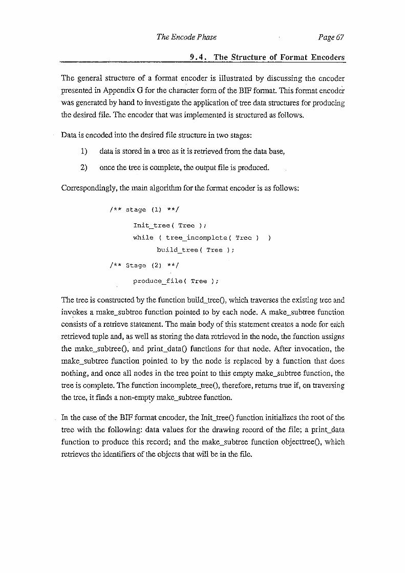
The Encode Phase Page67
9. 4. The Structure of Format Encoders
The general structure of a format encoder is illustrated by discussing the encoder
presented in Appendix G for the character form of the BIF format. This format encoder
was generated by hand to investigate the application of tree data structures for producing
the desired file. The encoder that was implemented is structured as follows.
Data is encoded into the desired file structure in two stages:
1) data is stored in a tree as it is retrieved from the data base,
2) once the tree is complete, the output file is produced.
Correspondingly, the main algorithm for the format encoder is as follows:
I** stage (1) **/
Init_tree( Tree);
while ( tree_incomplete( Tree
build_tree( Tree);
/** Stage (2) **/
produce_file( Tree);
The tree is constructed by the function build_tree(), which traverses the existing tree and
inv?kes a make_subtree function pointed to by each node. A make_subtree function
consists of a retrieve statement. The main body of this statement creates a node for each
retrieved tuple and, as well as storing the data retrieved in the node, the function assigns
the make_subtree(), and print_data() functions for that node. After invocation, the
make_subtree function pointed to by the node is replaced by a function that does
nothing, and once all nodes in the tree point to this empty make_subtree function, the
tree is complete. The function incomplete_tree(), therefore, returns true if, on traversing
the tree, it finds a non-emp~y make_subtree function.
In the case of the BIF format encoder, the Init_tree() function initializes the root of the
tree with the following: data values for the drawing record of the file; a print_data
function to produce this record; and the make_subtree function objecttree(), which
retrieves the identifiers of the objects that will be in the file.

Page68 Translating Data between Geographic lnfonnation Systems
The build_tree function traverses the tree and invokes the objecttree() function which
generates a subtree consisting of nodes that are individually assigned: an object
identifier; a pointer to the make_subtree function called prmtree(); and a pointer to the
print_ data function called object(). After invocation, the objecttree() function is replaced
by the empty() function so that in future traversals of the tree by the build_tree()
function, the objecttree() function is not invoked.
Because of the existence of the prmtree function in the tree, the incomplete_ tree function
returns true and the build_tree() is invoked again. On this traversal of the tree, each
occurrence of the prmtree() function results in the construction of a subtree that consists
of nodes containing: the identifier and type of the primitives that defme the object; and a
make_subtree function and a print_data function that is appropriate for the type of the
primitive.
The above sequence of function invocations continues until all the necessary data is
retrieved from the data base and stored in the tree. Once the construction of the tree is
complete, the produce_file() function is invoked. This function traverses the tree,
invoking the print_data function pointed to by each node. The output from the
print_ data functions is the data from the data base structured in the 11?-anner required by
the target format.
In practice, the use of a tree to implement nested retrieve statements is unnecessarily
inefficient, and because the data set being processed is potentially large, it is impractical
to build the entire tree in memory and then produce the file. A more space-efficient
implementation strategy is needed. Fortunately, it is possible to integrate the construc
tion of the tree and production of the file in such a way that only those branches of the
tree necessary for producing the next part of the flle are kept in memory. Thus a stack of
retrieved data pending processing is kept, using at most the storage of one node for each
level of the tree. Due to insufficient time, this strategy was not incorporated in the
prototype.

Chapter Ten
Conclusions
There are many diverse and complex transfer file formats for geographic data. The
translation of data from one format to another may be difficult and require considerable
effort. The objectives set in this thesis were:
1) To minimise the effort involved in achieving a data translation, and
2) To maximise the quality of the translation that is achieved.
The extent to which these objectives are attainable with the following three strategies
was discussed:
1) the ring interfacing strategy,
2) the interchange format interfacing strategy,
3) the individual interfacing strategy.
The ring interface was discarded because of the high potential for translating data
inaccurately. The interchange format interfacing strategy has become widely
established, but the value of this strategy is undermined by the definition of several
different interchange formats. The individual interfacing strategy is the ideal solution,
but an efficient method of implementing any interface is required for this strategy to be
practical.
The author has defined a model of data translation that consists of three phases:
1) the decode phase, which extracts data from the source format, and
places it into an equivalent relational data model,
2) the translate phase, which reorganises data from the source relational
data model into the target relational data model,
3) the encode phase, which retrieves data from the relational data model
and encodes it into the target format.

Page 70 Translating Data between Geographic Information Systems
The modular construction of a translation process allows the development of re-useable
software modules. After implementing a decoder and encoder for a format, they are
used in any data translation irrespective of the other format involved. In this way,
implementing the individual interfacing strategy has been reduced to implementing a
translation algorithm for the translate phase of any' source to target format translation
pair.
The translation algorithm is specified using a relational query language provided by a
relational data base management system such as INGRES, and the author's experience
with INGRES indicates that specifying algorithms using QUEL can be achieved easily.
Use of a system such as POSTGRES, where the standard relational data model is
extended to include spatial data types and operators, will facilitate the concise definition
of translation algorithms.
The effort of implementing a translation process is further reduced by generating some
of the necessary software modules directly from the specification of the translation
process. The syntactic structure of an implementation method for a format was specified
using BNF which is processed, using software construction tools such as Yacc and
Lex, to generate the format decoder and encoder. All three phftses were implemented
and tested for a variety of formats, although the automation of encoder generation is
incomplete due to time constraints.
This thesis has shown that it is practical, and desirable, to implement the individual
interfacing strategy through the use of: a three phase translation process; software tools
such as Yacc and Lex; and a relational data base management system such as INGRES.
In doing so, a reduction can be achieved in the effort needed to provide geographic
interfaces for geographic data exchange. Further, the quality of the data translation is
improved as a consequence of being able to use the individual interfacing strategy.

Acknowledgements
I wish to thank my supervisor Prof. John Penny whose interest and enthusiasm in my
research, and my writing style, was greatly valued. I would also like to thank other staff
of the Computer Science department at Canterbury who have offered advice during the
preparation of this thesis. Bruce Mckenzie for discussion on generating parsers with
Yacc and Lex, Neville Churcher for discussion on the use of relational data base
management systems, and in particular Tim Bell who assisted in the final draft of this
thesis.
Finally, I would like to express deep gratitude for the love and concern of my Parents
who supported me while I was studying.


Bibliography
BS 6690 : 1986 I ISO 8211-1985 (1986) A data descriptive file for information
interchange. British Standards Institution.
Codd E. F. (1970) A Relational Model of Data for Large Shared Data Banks.
Communications of the ACM,13, 377-387.
Codd E. F. (1972) Relational Completeness of Data Base Sublanguages. Data Base
Systems, Courant Computer Science Symposia Series, 6.
CSIRONET (1986) Command Driven Colourmap, User's Guide. CSIRONET
Reference Manual No 19, Version 1, Graphics System Section, CSIRONET.
Data Interchange Standards. AURISA news, June 1985.
Date, C. J. (1986) An Introduction to Database Systems.1 (Fourth Ed.)
DCDSTF (Digital Cartographic Data Standards Task Force) (1988) Spatial Data
- -- -Transfer Specification, Volume 1 -The Standard. The American Cartographer,
15,21-144. Volume 2- Initial Entity and Attribute Definitions. The American
. Cartographer, 15, 143 (microfiche).
Fosnight, E. A. and J. W. van Roessel (1985) Vector Data Interfacing at the EROS
Data Center; RIM to ARC/INFO and Related Interfaces. EROS Data Center, Sioux
Falls, South Dakota 57198
GDS (1984) Binary Interface File (BIF) Format. ODS Reference Manual.
GeoVision (1986) Data Translation Guide. GeoVision Reference Manual.
Goldschlager, L. and A. Lister (1988) Computer Science A Modern Introduction.
Second Ed.
Outing, R. H. (1988) Gee-Relational Algebra: A Model and Query Language for
Geometric Database Systems. Computational Geomerty and its Applications,
Lecture Notes in Computer Science, 333.
Held G.D., M. R. Stonebraker and E. Wong (1975) INGRES- A relational data base
system. AFIPS conference proceedings, 44, 409-416
Page74 Translating Data Between Geographic Information Systems
Horowitz, E. and S. Sahni (1983) Fundamentals of Data Structures
Hutchinson, M. F. (1981) MAPROJ- A computer map projection system, Division of
land use research technical paper No. 39. Commonwealth scientific and industrial
research organization, Australia.
INGRES (1986) INGRES Release 5.0 for the UNIX Operating System Volume 3,
Relational Technology
Intergraph (1986) Standard Interchange Format (SIF) Command Language
Implementation Guide (8.8.2).
International Organization for Standardization (ISO) 1986. Information processing -
Text and office systems- Standard Generalized Markup Language (SGML). ISO
8879-1986 (E), International Organization for Standardization Oct 1986.
International Organization for Standardization (ISO) 1986. Information processing -
Specification for a Data Descriptive File for Information Interchange. ISO 8211-
1985.
Johnson, S. C. (1979) Yacc: Yet Another Compiler-Compiler. Unix Time-Sharing
System: Unix Programmer's Manual, Seventh Edition, Volume 2B.
Kalash, J. L. Rodgin, Z. Pong, J. Anton (1986) INGRES - Reference manual (
Version 8)
Kernighan, B. W. and D. M. Richie (1978) The C Programming Language
Lesk, M. E. and E. Schmidt (1979) Lex- A Lexical Analyzer Generator. Unix Time
Sharing System: Unix Programmer's Manual, Seventh Edition, Volume 2B.
Mamrak, S. A., M. J. Kaelbling, C. K. Nicholas, and M. Share (1987) A Software
Architecture for Supporting the Exchange of Electronic Manuscripts.
Communications of the ACM, 30, 408 - 414.
Martin, J. and C. McClure (1986) Diagramming Techniques for Analysts and
Programmers.
Naur, P. (Editor) (1963) Revised report on the algorithmic language ALGOL 60.
Communications of the ACM, 6, 1-17.

Bibliogr,aphy Page75
Nyerges, T. (Editor) (1984) Digital Cartographic Data Standards: Alternatives in Data
Organization. Progress Report of the Workgroup on Data Organization of the
National Committe for Digital Cartographic Data Standards, Report 4, January.
Penny J. P. (1986) Relational methods for format conversion of map data.
Cartography, 15, 26-34.
Penny, J. P., G. C. Ewing and R. T. Pascoe (1989) Aspects of Interactive Systems for
Computer Mapping. Twelth Australian Computer Science Conference,
Wollongong
Peuquet, D. (1984) A Conceptual Framework and Comparison of Spatial Data Models.
Carto graphica, 21, 66-113
Rich, C. and R. C. Waters (1988) Automatic Programming: Myths and Prospects.
Computer lEEE.
Samet (1984) The Quadtree and related Hierarchical Data Structures. ACM Computing
Surveys, 16, 187-260
Shu N. C., B. C. Housel, R. E. Taylor, S. P. Ghosh, and V. Y. Lum (1977)
.EXPRESS: A Data EXtraction, Processing, and REStructuring System. ACM
Trans. on Database Systems, 2, 134-174.
Smith, H. C. (1985) Database design: composing fully normalized tables from a
rigorous dependency diagram. Communications of the ACM, 28, 826.
Steel T. B. Jr. (1960) UNCOL: The myth and the fact. Annual Review in Automatic
Programming, 2, 325-344.
Stevens, R.J., A.F.Lehar, and F. H. Preston (198.3) Manipulation and presentation of
multidimensional image data using the Peano scan. IEEE Trans. on Pattern
Analysis and Machine Intelligence, 5, 520-526.
Stonebraker, M. and L.A. Rowe (1986) The Design ofPOSTGRES. Proceedings ACM
SIGMOD 1986, International Conference on Management of Data, Washington
D.C.
Stonebraker, M., C. Williams (1975) An approach to implementing a geodata system,
· proceedings of the workshop on databases for interactive design, 67-77

Page 76 Translating Data Between Geographic Information Systems
Stonebraker, M., E. Wong, P. Kreps, and G. Held (1976) The design and
implementation of INGRES. ACM Transactions on Database Systems, 1, 189-
222.
Tanenbaum, A. S. (1978) Implications of Structured Programming for Machine
Architecture, Communications of the ACM, 21, 237 - 246.
Tanenbaum, A. S., H. van Straveren, E. G. Keizer, and J. W. Stevenson (1983) A
Practical Tool Kit for Making Portable Compilers. Communications of the ACM,
26, 654 - 660.
Taylor, R. W. 1982 Experiences Using Generalized Data Translation Techniques for
Database Interchange. Computers & Standards 1, 111-118
van Berkel, P. (1987) Proposal for a Standard for the Interchange of Digital Land Data.
A Discussion Document, Land Information New Zealand (LINZ) Support Group.
van Roessel, J. W. (1987) Design of a spatial data structure using the relational normal
forms. Int. J. Geographical Information Systems, 1,33-50.
van Roessel, J. W. and Fosnight, E. A. (1985) A relational Approach to vector data
structure conversion. Proc. Auto-carto 7 Conf. Washington
van Roessel, J., D. Bankers, V. Connochioli, S. Doescher, G. Fosnight, M. Wehde,
and D.Taylor (1986) Vector Data Structure Conversion at the EROS Data Center.
Final Report (Draft), Phase I, EROS Data Center.

Appendix A
Format Implementation Specifications
This appendix contains an implementation specification for the Geo Vision GINA
format, the charac~er form of the BIF format, and the Colourmap format. Throughout
this Appendix the metalinguistic variable «empty» indicates the null string, that is:
«empty» ::=
A.l The GeoVision GINA Format
A.l.l BNF Specification
«GINA file» ::=«physical format file» «database header file» «primary schema file» «feature file» «polygon relationship file» «indirect attributes file» «data base trailer file»
«physical format file» ::= UDB-START «block format>> «block length» «max block size»
«block format>> := BLOCKED I UNBLOCKED
«block length» := F I VARIABLE
«max block size»::= UNSIGNED_INT
«database header flle» ::= «dbf header record>> «description record>> «coordinate system record» «extent record>> «layer record list>> «network record list>>
«dbf header record>> ::= UDB-HEADER «GINA version number>> «database name» «database description»
«GINA version number>> ::=REAL
«database name» ::= CHAR
«database description»::= STRING
«description record»::= «empty» I DESCR DATE TIME «GINA user name» «comment>>
«GINA user name» ::=CHARACTER
«comment» ::= «empty» I STRING

Page78 Data Translation between Geographic Information Systems
Note:: The question marks in the following indicate that the structure was not clearly defmed at this
point of the format description.
«coordinate system record» ::=«empty» I COORD-SYS «mercator crds» «coordinate units» «spheroid defmition» «scale factor
at central meridian» «zone width» «central meridian>> «false easting>> «false northing» COORD-SYS GEOG DEGREES .. COORD-SYS GEOG DEGREES OVERRIDE «semi_major axis>>«semi_minor axis» COORD-SYS RECT «coordinate units» COORD-SYS MERC «coordinate units» ?? COORD-SYS LAMBERT «coordinate units» ?? COORD-SYS NC_STATE «coordinate units»??
«mercatorcrds» ::;;: TM I UTM
«coordinate units»::= «empty» I FEET I METRES I MILLIMETRE$ I JNCBES I KILOMETRES
«spheroid definition» ::= CLARK I IAU I OVERRIDE «semi_major axis» «semi_minor axis»
«semi_major axis»::= REAL
«semi_minor axis»::= REAL
«scale factor at central meridian» ::=REAL
«zone widlh» ::;;: UNSIGNED_INT
«Central meridian»::;;: INTEGER
«false eastin&?> .. ::=.«empty» I UNSIGNED_INT
«false northing»::= «empty» I UNSIGNED_INT
«extent record»::::::: «empty» I EXTENT «min x or long coordinate» «min y or lat coordinate» «max x or long
coordinate» «max y or lat coordinate»
«min x or long coordinate» ::= REAL I JNTEGER
«min y or lat coordinate» ::=REAL I JNTEGER
«max x or long coordinate» ::=REAL I INTEGER
«max y or lat coordinate» ::=REAL I JNTEGER
«layer record list>> : := «empty» I «layer record list>> «layer record»
«layer record» ::=LAYER «layer number» «layer name» «layer description»
«layer number» ::= UNSIGNED _INT
«layer name» ::==CHARACTER
«layer description» ::= S'IRJNG
«network record list>> ::= «empty I «network record list>> «network record»

Format Implementation Specifications Page79
«network record» ::= NE1WORK «network number» «network name» «network type» «layer number» <<network description»
«network number»::""' UNSIGNED_INT
«network name»::""' CHAR
«network type» ::== PLGN I L
«network description» ::== S'IRING
«primary schema file» ::= UDB-PRIMARY «table definition list»
«table definition list» ::= «table definition» I «table definition list>> «table definition»
«table definition» ::=«fixed table record» «fixed field definition list» «feature code list>> I «free table record» «free field definition list>> «feature code list>>
«fixed table record» ::==TABLE «table name» FIXED
«free table record»::= TABLE «table name» FREE
«table name» ::= CHAR
«fixed field definition list» ::= «fixed field record» l «flxed fleld definition list» «fixed field record»
«fixed field record»::= FJELD «field name» «field description» «index flag» «unique flag» «null flag» «description of attribute» «start column of field» «number of columns field occupies»
«free field definition list>> ::= «free field record» I «free field definition list>> «free field record»
«iree field record» ::=FJELD «field name» «field description» «index flag» «unique flag» <<null flag» «description of attribute»
«field name» ::= CHAR
<<field description» ::= CHR «number of characters» I NUM «number of digits» COMMA <<number of decimal digits»
«number of characters» ::=UNSIGNED _INT
«number of digits» ::= UNSIGNED _INT
«number of decimal digits» ::= UNSIGNED_INT
«index flag» ::=«empty» I I
«unique flag» ::= «empty» I UNQ
«null flag» ::= «empty» IN
«description of attribute>> ::= S'IRING
«start column of field» ::==UNSIGNED _INT
«number of columns field occupies» ::= UNSIGNED_INT
«feature code list>> ::= «feature code record» I «feature code list>> «feature code record»

Page80 Data Translation between Geographic Information Systems
«feature code record»::= FEAT_CODE «low feature code» «high feature code»
«low feature code» ::=«feature code»
«high feature code» ::=«feature code»
«feature file»::= UDB-FEAT «feature definition list>>
«feature definition list» ::= «feature record» «coordinate list>> «label defmition» «attributes»
«feature record» ::=FEAT «feature sequence number» «feature code» «layer number» «network numben} «type of feature» «coordinate definitiom} «graphic parameter b «graphic parameter 2» «flow direction>}
«feature sequence numbeP} : := UNSIGNED _INT
«feature code>> : := CHAR
«type of feature» ::= PLGN IN I L
«coordinate definition»::= XY I XYZ I XYCZ «Z»
«graphic parameter 1» ::=CHAR
«graphic parameter 2» ::=CHAR
«flow direction»::= INTEGER
«coordinate list» ::= «coordinate record» I «coordinate list>> «coordinate record}>
«coordinate record» : := COOR «coordinate pair list>>
«coordinate pair list» ::= «2d coordinate list» l «3d coordinate list»
«2d coordinate list>> ::= «X» COMMA «y» I «2d coordinate list» «X» COMMA «y»
«3d coordinate list»::= «X» COMMA «y» COMMA «Z» I «3d coordinate list» «X» COMMA «Y» COMMA «Z»
«X» ::= REAL I INTEGER
«y» ::=REAL I INTEGER
«z» ::=REAL I INTEGER.
«label definition» ::= «empty» I «label record» I «text record» I «label record» «text record»
«label record» ::=LABEL «label number» «label x position» «label y positioM «orientation flag» «orientation angle»
«label number»::= UNSIGNBD_INT
«label x position» ::= REAL I INTEGER
«label y positiom> ::=REAL I INTEGER
«orientation flag» ::=«empty» I HORZ I RBL '
«orientation angle»::= «empty>> I REAL

Format Implementation Specifications
«text record» ::=TEXT «text character string»
«text character string» ::= STRING
«attributes» ::= «empty» I «attribute record» «attribute continuation list»
«attribute record» ::= ATTR «attribute value list»
Page81
«attribute continuation list» ::= «empty» I «attribute continuation list» «attribute continuation record»
«attribute continuation record»::= ATCR .«attribute value list»
«attribute value list» ::= «attribute value» I «attribute value list» «attribute value»
«attribute value» ::= as defined by primary schema file
«polygon relationships file»::= UDB-PLGN «relationship record list»
«relationship record list» ::=«relationship record» I «relationship record list» «relationship record»
«relationship record» : := POLY «line sequence numbeD> «left I right flag» «interior I exterior flag»
«line sequence numbeD> ::;::; UNSIGNED_INT
«left I right flag» ::= L I R I QU
«interior I exterior flag» ::=I IE
«indirect attributes flle» ::= UDB-INDRT «table definition list» «attributes»
. «database trailer flle» ::= UDB-END

Page82 Data Translation between Geographic Information Systems
A.l.2 Lexicon
Lexical Symbol ReRular Expression Lexical Symbol ReRular Expression ATCR "atcr" PLGN "pl1
ATTR "attr" POLY "poly" BLOCKED "b" QU· 11?11
CHAR [A-Za-z-1@#$% .. ]+ R "r" CHR "char" RECT "rectangular" CLARK "Clark-1866" REAL ([ +-]?[0-9]+"."[0-9]* COMMA II II
' ([E][+-][0-9](0-9])*) I
COOR "coor" COORD-SYS [Cc][Oo][Oo][Rr][Dd]-
[Ss][Yy][Ss]
([+-]?[0-9]*"."[0-9]+ ([E)f+-]f0-9][0-91)*)
REL "relative" DATE [0-3] [0-9] [0 1] [0-9]
[0-9][0-9][0-91[0-9] STRING \''([A-Za-z-1@#$ .. ]?
[ ])+\" DEGREES "degrees" TABLE "table" DESCR "descr" TEXT "text" E ueu TI:ME [0-2] [0-9] II: II [0-5] [0-9]
EXTENT "extent" ":"[0-5)[0-9]
F "f' TM "tm"
FEAT "feat" UDB-END [Uu][Dd][Bb]-
FEAT CODE "fc" [Ee][Nn)[Dd]
FEET "feet" FIELD "field" FIXED "fixed" FREE "free II GEOG "geographicals" HORZ "horizontal" I ·---- .. "i" I "ill
UDB-HEADER [Uu)[Dd][Bb]-[Hh][Ee][Aa][Dd] [Ee][Rr]
UDB-INDRT [Uu][Dd)[Bb]-[Ii][Nn)[Dd][Ii][Rr] [Ee][Cc][Tt]
UDB-PLGN [Uu][Dd][Bb][-[Pp][Oo][Ll][Yy] [Gg)[Oo)[Nn)
IAU "IAU-1965" UDB-PRIMARY [Uu][Dd][Bb]-INCHES "inches" [Pp] [Rr] [Ii) [Mm] INTEGER [+-]?[0-9]+ [Aa][Rr)[Yy] KILO :METRES "kilometres" UDB-START [Uu)[Dd][Bb]-L ltlH [Ss][TtlfAa l[RrlfTtl LABEL "label" UDB_FEAT [Uu][Dd][Bb]-LAMBERT "Lambert" [Ff)[Ee][Aa][Tt] LAYER "layer" MERC "Mercator"
[Uu][Rr)[Ee] UNBLOCKED "u"
:METRES "metres" UNQ "u"
MILLI:METRES "millimetres" UNSIGNED INT [0-9]+
N "n" UTM "utm"
NC STATE "NC state plane" NETWORK "network"
VARIABLE II VII
XY "xy"
·NUM "num" XYCZ "xycz"
OVERRIDE "override" XYZ "xyz"

Format Implementation Specifications Page83
A. 2 . The BIF Format
A.2.1 BNF Specification
«dataiile» ::= «empty» I «drawing» «object list>>
«empty» ::= (that is, the null string of symbols)
«drawing» ::=DRA WlNG REAL REAL REAL REAL
«object list» : := «empty» I «object list>> «object»
«object» := «name» «hook» «primitive list»
«name» ::= N~ «ocd value»
«ocd value» ::= «compound value» I «ocd value» COLON «compound value»
«compound value» ::=«a value» I «compound value» «a value»
«a value» ::= INTEGER I REAL I STRING
«hook» ::= HOOK REAL REAL
«primitive list» ::= «primitive» I «primitive list>> «primitive»
«primitive» ::= «line» «segment list» I «circle» I «text» «text line list>> I «points» «point list>>
«line»::= LINE REAL REAL «compound value»
«segment list» : := «to» I «arc» I «segment list» «to» I «segment list» «arc»
«to» ::= TO REAL REAL
«arC>> ::= ARC REAL REAL REAL
«circle» ::= CIRCLE REAL REAL REAL STRING
. <<text>>. ::= TEXT REAL REAL REAL REAL REAL REAL STRING «a value»
«text line list>> ::= «chars» I «text line list» «chars»
«chars» ::= CHARS STRING
«points»::= POINT STRING
«point list» ::= «at>> I «point list» «at»
«at»::= ATREALREAL
Lexical Symbol Re!?ular Expression ARC "arc" AT "at" CHARS "chars" CIRCLE "circle" COLON tt.n
DRAWING "drawing" HOOK "hook" INTEGER f+-l?f0-91+ LINE "Line" N~ "Name"
A.2.2 Lexicon
Lexical Symbol Re!?Ular Expression POINT "point" REAL ([+-]?[0-9)+". "[0-9]*
([E)(+-][0-9][0-9])*) I ([+-]?[0-9]*" ."[0-9]+ ([E)[+-][0-9][0-9])*)
STRING ([\ \ \-A-Za-z'$#!%A& -? /]+[0-9] *)+
TEXT "text" TO "to"

Page84 Data Translation between Geographic Information Systems
A. 3 The Colourmap Format
The following specification defines three types of Colourmap data files: zone files, line
overlay files, and standard attribute files.
A.3.1 BNF Specification
«dataflle» ::= «comment>> NEWLINE «headeD> «data»
«data>> ::=«name list» «attribute sectn» I «zone part» «poly part» «seg part>> I «seg part»
«zone part>> ::= ZONES NEWLINE «num zones» NEWLINE «zone defn list»
«poly part» ::= «empty» I POLYGONS NEWLINE «num polygons» NEWLINE «polygon defn list»
«seg part»::= «empty» I SEGMENTS NEWLINE «num segments» NEWLINE «segment defn list»
«zone defn list» ::= «z defn» I «zone defn list» «Z defn»
«polygon defn list» ::=«poly defn» I «polygon defn list>> «poly defn»
«segment defn list» ::=«segment defn» I «segment defn list>> «segment defn»
«z defn» : := «zone id» <<poly in zone» NEWLINE «poly id list>> NEWLINE
«poly defn» ::=«poly defn hdr» «X poly label» «y poly label» <<polygon area>> NEWLINE «seg id list» NEWLINE
I <<poly defn hdr» «X poly label» «y poly label» NEWLINE «seg id list» NEWLINE ·1 ---· «poly defn hdr» «polygon area» NEWLINE «seg id list» NEWLINE
«poly defn hdr» ::=«poly id>> «zone id>> «segs in poly» «dsp level» NEWLINE «X min poly regn» «X max poly regn» «y min poly regn» «Y max poly regn»
«segment defn» ::= «segment id>> «seg left zone» «seg right zone» «points in segment>> NEWLINE «xy defn list>> NEWLINE
«seg id list»::= «empty» I «seg id list» NEWLINE I «seg id list» INTEGER
«poly id list>> ::= «empty» I «poly id list» NEWLINE I «poly id list>> INTEGER
«xy defn list» ::=REAL REAL REAL REAL I «xy defn list>> NEWLINE I «xy defn list>> REAL REAL
«headeD> ::=MAP NEWLINE «map window» «map projection» I «num attr» «num names» «missing dat val» NEWLINE
«map window»::= «X min regn» «X max regn» «Y min regn» «Y max regn» NEWLINE
«map projection»::= «map proj code» «zone type» NEWLINE I «map proj code» NEWLINE
<<name list» : := «empty» I «name list» «name» NEWLINE I «name list» <<name»
«attribute sectn» ::= «attribute list»
«attribute list» : := «empty» I «attribute list» «attribute»
«attribute» : := «attr defn» «attr val list»

Format Implementation Specifications Page85
«attr defn» ::= «description» «units» NEWLINE
«attr val list» ::=«empty» I «attr val list» «attr value» NEWLINE I «attr val list» «attr value»
«attr value»::= REAL «segment id» ::= INTEGER
«comment» ::= «string» «seg left zone» ::= «string»
«polygon area» ::=REAL «seg right zone» ::=«string»
«description» : := «string» «units» ::= «string»
«dsp level» ::=INTEGER «X min regn» ::= REAL
«map proj code»::= INTEGER «X max regn» ::=REAL
«poly in zone» ::= INTEGER «X max poly regn» ::=REAL
«segs in poly» ::= INTEGER «x min poly regn» ::=REAL
«points in segment» ::= INTEGER «X poly label» ::=REAL
«missing dat val» ::=REAL «Y max poly regn» ::=REAL
«name» ::= «string» «Y max regn» ::=REAL
«mnn attr» : := INTEGER «Y min regm> ::=REAL
«num segments» ::= INTEGER «y min poly regn» ::=REAL
«num names» ::=INTEGER <<y poly label» ::=REAL
«num polygons»::= INTEGER «zone id» ::= «string»
«num zones» : := INTEGER «zone type»::= INTEGER
«poly id» ::= INTEGER «string»::= STRING
A.3.2 Lexicon
Lexical Symbol ReRular Exvression INTEGER [\t ]+[+-]?[0-9]+[\t ]* MAP "MAP"[\t ]*\n NEWLINE '"'n" POLYGONS "POLYGONS II ['"'n" REAL [\t ]*(+-]?[0-9]+" ."
[0-9]*([E](-+ ][0-9] [0-9])?[\t ]* I [\t ]*[ +-]?[0-9]*" ." [0-9]+([E](-+ ](0-9] 0-9))?[\t ]*
SEGMENTS "SEGMENTS"!\1 ]* STRING ((!\ \-A-Za-zO-
9'$#fo/oA&.-';?/J (".")?)+1\t 1*)+
ZONES "ZONES" 1\t ]*\n


Appendix B
Format .Decoders
B .1 The Colormap Format Decoder
%{ I** $Header$ **I
#include <stdio.h>
#include "eql.h"
#define maxrgflg 5 #define INITRG(A) rgcnt[++rgflg] A; #define DECRG rgcnt[rgflg]--;
#define newtkn(A) yylval.t.code A; #define itv(A) A.v.ival #define dtv(A) A.v.dval #_d~f_ine stv (A) A. v. sval
int rgcnt[maxrgflg], rgflg 0;
char *sf; I** source datafile name
B .1.1 Y ace Definition file
**I
int datasize **I
80; I** used by lex to determine size of string
I** (initialised for size of comment) **I
extern int eqlappend(), eqlreplace(); extern char *strsave();
double atof();
char *zid; int pid, sid, nattr, nname, attrseq; %}
%start datafile
%union struct TKN {
int code; union val { int ival; double dval; char *sval; }v;
}t;

Page88 Data Translation between Geographic Information Systems
int filetype, itmseq; struct PD {
int pid, sip; double xminregn, xmaxregn, yminregn, ymaxregn; polydefn;
%type <filetype> data %type <polydefn> poly.defn.hdr %type <t> _zone.id _ _poly.in.zone _ _poly.id __ segs.in.poly _ _ num.attr_ %type <t> dsp.level x.min.poly.regn x.max.poly.regn %type <t> -y.min.poly.~egn y.max.poly.- x.poly.label %type <t> =y.poly.label_ - -_polygon.area __ segment.id_ -%type <t> _seg.left. _seg.right.zone_ _points.in.segment_ %type <t> num.zones num.polygons num.segments string %type <t> -num.names- -roissing.dat.~al description %type <t> =units __ attr~value __ comment- - -
%type <itmseq> seg.id.list xy.defn.list name.list attribute.list %type <itmseq> attr.val.list
%token <t> MAP POLYGONS ZONES SEGMENTS LINES POINTS NEWLINE %token <t> INTEGER REAL STRING
I** system tokens **/ %token <t> EORG SETSIZE STRCONT
%% l*--------------------------------------------------------------*1 I* Notation *I I* *I I* *I I* _symbol.name_ => Lexical symbol *I I* TOKEN => a reserved symbol/ data type *I I* symbol.name => yacc non-terminal symbol */ I* *I l*--------------------------------------------------------------*1 datafile
{
i
data
_comment NEWLINE header data
eqlreplace("cm dss","srcfile",sf,"tffkey",$4,EOAL, EOQL); free(stv($1));-
names attribute.sectn
$$ = 10;
zone.part poly.part seg.part
$$ = 0; /** Zone file **I
line.part seg.part
$$ = 2; I** line file **/
seg.part

overlay**/ ) ;
zone.part
poly.part I
Format Decoders
$$ 4; /** line overlay **/
point.part
$$ = 1; /** Either A: site, B: name or, C: marker
ZONES NEWLINE num.zones NEWLINE
{ INITRG(itv($3)); } zone.defn.list EORG
eqlreplace("cm_dss", "nzones", itv($3), EOAL, EOQL);
POLYGONS NEWLINE num.polygons NEWLINE
{ INITRG(itv($3)); I polygon.defn.list EORG
Page89
eqlreplace("cm_dss", "npolygons", itv($3), EOAL, EOQL);
seg.part I
line.part
SEGMENTS NEWLINE num.segments NEWLINE
{ INITRG(itv($3)); } segment.defn.list EORG
eqlreplace("cm_dss", "nareachains", itv($3), EOAL, EOQL);
LINES
point.part POINTS
map.window {
REAL REAL REAL REAL NEWLINE
eqlreplace("cm_dss", "xminregn", dtv($1}, "xmaxregn", dtv ($2),
"yminregn", dtv($3), "ymaxregn", dtv($4), EOAL, EOQL);
map.projection
}
INTEGER INTEGER NEWLINE
eqlreplace("cm_dss","projection",itv($1),"zonetype",itv($2), EOAL, EOQL) ;
I INTEGER NEWLINE {
eqlreplace("cm_dss", "projection", itv($1), EOAL, EOQL);

Page90 Data Translation between Geographic Information Systems
zone.defn.list : z.defn zone.defn.list z.defn
polygon.defn.list poly.defn polygon.defn.list poly.defn
segment.defn.list segment.defn
z.defn :
segment.defn.list segment.defn
_zone.id _ _poly.in.zone_ NEWLINE INITRG(itv($2)); zid strsave(stv($1));} poly.id.list EORG NEWLINE
eqlappend("cm_zone", "zoneid", zid, "cmptpol", itv($2), EOAL);
DECRG; free(stv($1)); free(zid);
poly.defn poly.defn.hdr
dtv ($3),
_x.poly.label __ y.poly.label _ _polygon.area_ NEWLINE { INITRG($1.sip); pid = $1.pid; }
seg.id.list EORG NEWLINE
char *sl;
sl = (char *l malloc(200); *sl sprintf(sl, " cm_polygon.polid
t \0!; %d", $l.pid);
eqlreplace("cm_polygon", "xlabel", dtv($2), "ylabel",
"area", dtv($4), EOAL, sl, EOQL); DECRG; free(sl);
poly.defn.hdr x.poly.label y.poly.label NEWLINE INITRG($1.sip)l } seg.id.list-EORG NEWLINE-
/** ** calculate area **.f
double area; char *sl;
area= ($1.xmaxregn - $1.xminregn) * ($1.ymaxregn- $1.yminregn);
sl (char*) malloc(200); *sl = '\0'; sprintf(sl, "cm_polygon.polid %d", $1.pid); eqlreplace("cm_polygon","xlabel",dtv($2),"ylabel",dtv($3),
"area", area, EOAL, sl, EOQL); DECRG; free(sl);
poly.defn.hdr _polygon.area_ NEWLINE

Format Decoders
INITRG($1.sip); } seg.id.list EORG NEWLINE
I** ** calculate centroid **I
double ex, cy; char *sl;
ex ($1.xminregn + $1.xmaxregn) cy ($1.yminregn + $1.ymaxregn)
I 2; I 2;
sl (char*) malloc(200); *sl = '\0'; sprintf(sl, "cm_polygon.polid"" %d", $1.pid);
eqlreplace("cm_polygon", "xlabel", ex, "ylabel", cy, "area", dtv($2), EOAL, sl, EOQL);
DECRG; free(sl);
Page91
poly.defn.hdr NEWLINE
_poly.id __ zone.id __ segs.in.poly __ dsp.level_
stv($2),
_x.min.poly.regn __ x.max.poly.regn _ _ y.min.poly.regn __ y.max.poly.regn_
eqlappend("cm_polygon", "polid", itv($1), "enclzoneid",
"cmptachain", itv($3),"dsplevel", itv($4), "xminregn", dtv($6), "xmaxregn", dtv($7), "yminregn", dtv($8), "ymaxregn", dtv($9), EOAL);
$$.pid itv($1); $$.s = itv($3}; $$.xminregn dtv($6); $$.xmaxregn $$.yminregn dtv($8); $$.ymaxregn free(stv($2));
dtv($7); dtv($9);
segment.defn segment.id seg.left.zone seg.right.zone _points. in. segment_-NEWLINE - - -INITRG(itv($4)); sid = itv($1); xy.defn.list EORG NEWLINE
int i;
eqlappend("cm areachain", "achainid", itv($1), "leftzoneid", stv($2),-
"rightzoneid", stv($3), "cmptpt", itv($4), EOAL); DECRG; free(stv($2)); free(stv($3)); ,

Page92 Data Translation between Geographic Information Systems
seg.id.list : {
$$ = 0;
seg.id.list NEWLINE
$$ = $1;
seg.id.list INTEGER
eqlappend ( "cm__polachain" 1 "polid" 1 pid, "seq", $1, "achainid" 1
itv($2), EOAL);
$$ $1 + 1; DECRG;
po1y.id.list I poly.id.list NEWLINE
poly.id.list INTEGER
eqlappend("cm_zonepol","zoneid",zid,"polid" 1 itv($2), EOAL); DECRG;
xy.defn.list {
REAL REAL REAL REAL
header I {
- eqlappend ("Cm achainpt n f "achainid" f Sid, "seq" f Q f "X" 1 dtV ( $1) f
"y", dtv($2), EOAL); eqlappend("cm_achainpt" 1 "achainid",sid,"seq",1,"x",dtv($3),
"y", dtv($4), EOAL);
$$ = 2; DECRG; DECRG;
xy.defn.list NEWLINE
$$ = $1;
xy.defn.list REAL REAL
eqlappend("cm_achainpt","achainid",sid,"seq",$1,"x",dtv($2), "y", dtv($3), EOAL);
$$ = $1 + 1; DECRG;
MAP NEWLINE map.window map.p.rojection _num.att.r __ num.names __ missing.dat.val_ NEWLINE
nattr = itv($1); nname = itv($2);
eqlappend("cm_attrdss","nattributes",nattr,"nnames", nname, "missdatval", dtv($3), EOAL);

names
name.list {
Format Decoders Page93
{ INITRG(nname); } name.list EORG
$$ = 0;
name.list name NEWLINE - -eqlappend("cm_objname", "nameseq", $1, "name", stv ($2), EOAL); $$ = $1 + 1; DECRG; free(stv{$2));
name.list name - -eqlappend("cm_objname","nameseq",$1,"name",stv($2), EOAL); $$ = $1 + 1; DECRG; free(stv($2));
attribute.sectn { INITRG(nattr); } attribute.list EORG
attribute.list {
attribute
attr.defn {
$$ = 0;
attribute.list { attrseq $1; datasize 30; } attribute
$$ = $1 + 1; DECRG;
attr.defn { INITRG(nname); } attr.val.list EORG
_description __ units_ NEWLINE
eqlappend ("Cl'r\._attrdefn", "a tid", attrseq, "description", stv($1), "units", stv($3), EOAL);
free(stv($1)); free(stv($3));
attr.val.list {
$$ 0;
attr.val.list _attr.value_ NEWLINE
eqlappend("cm_attrvalue", "atid", attrseq, "nameseq", $1, "value", dtv($2), EOAL);
$$ = $1 + 1; DECRG;
attr.val.list _attr.value_
eqlappend("cm_attrvalue", "atid", attrseq, "nameseq", $1, "value", dtv{$2), EOAL);
$$ = $1 + 1; DECRG;

Page94 Data Translation between Geographic Information Systems
l*----------------------------------------------*1 /* Lexicon definitions */ l*----------------------------------------------*1 attr.value REAL
{ $$ = $1; }
comment - { - datasize 80; } string
eqlappend("cm_dss", "description", stv($2), EOAL);
_polygon.area_ REAL
$$ = $1;
description - f datasize = 30; } string
$$ = $2; }
dsp.level INTEGER - { $$-= $1; }
_poly.in.zone_ INTEGER
$$ = $1; }
_segs.in.poly_ INTEGER
$$ $1; }
_points.in.segment_ INTEGER
$$ $1; }
_missing.dat.val_ REAL
$$ = $1; }
_name_ { datasize = 10; } string $$ = $2 i }
num.attr INTEGER - { $$ = $1; }
_num. segments_ INTEGER
$$ = $1; }

_num.names_ INTEGER
$$ = $1; }
_num.polygqns_ INTEGER
$$ = $1; }
Format Decoders
num.zones INTEGER - { $$-= $1; }
_poly.id_ INTEGER { $$ = $1; }
segment.id INTEGER - { $$ = $1; }
seg.left.zone - { datasize 10; } string
$$ = $2; }
_seg.right.zone_ { datasize 10; } string
$$ = $2; }
_units { datasize 10; } string ( $$ = $2; }
_x.max.poly.regn_ REAL
$$ = $1; }
_x.min.poly.regn_ REAL
$$ = $1; }
_x.poly.label_ REAL
$$ = $1;
_y.max.poly.regn_ REAL
$$ = $1; }
_y.min.poly.regn_ REAL
$$ = $1; }
Page95

Page96 Data Translation between Geographic Information Systems
__ y.poly.label_ : REAL
$$ = $1;
zone.id { datasize - { $$ = $2; }
10;) string
l*----------------------------------------------*1 /* General Constructs */ l*----------------------------------------------*1 string
{
%%
$$ == $2;
#include "lex.c"
yyerror(s) char *s;
SETSIZE STRING
printf("yytext:%s:\n", yytext); } main()
FILE *freopen () ;
sf (char *) malloc (30);
printf("Source data filename ? scanf("%s", sf); getc(stdin);
freopen (sf, "r", stdin);
eqlopen("kiwi: :em", "-clO"); yyparse(); eqlclose();
%a 5000 %o 9000 %{
"); fflush(stdout);
B .1. 2 Lex defmition File
#:define input() ((! (rgcnt [rgflg]) && rgflg) ? (rgflg-- 1 '@') :\ (((yytchar=yysptr>yysbuf?U(*--yysptr) :\ getc(yyin))==10?(yylineno++,yytchar) :yytchar)==EOF?O:yytchar))
#define REAL SIZE 10 #define INT SIZE 10 int sizeset -= 0; %} D E w
( 0-9] [E] [-+] {D} {D} [\t J
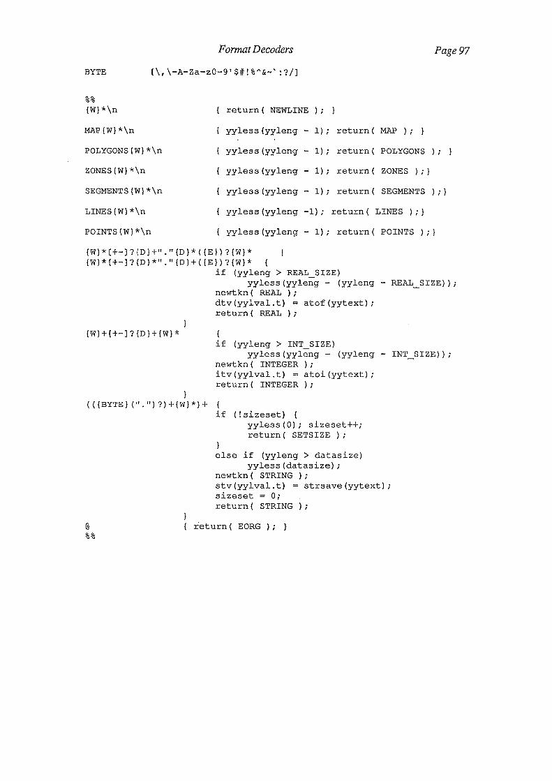
J?or.nu2t1Jecoders Page97
BYTE [\,\-A-Za-z0-9'$#"!%"&-' :?/]
%% {W}*\n return( NEWLINE ) ; }
MAP{W}*\n yyless(yyleng- 1) ; return ( MAP ) ; }
POLYGONS{W}*\n yyless(yyleng- 1) ; return ( POLYGONS ) ;
ZONES{W}*\n yyless(yyleng- 1) ; return( ZONES ) ; }
SEGMENTS{W}*\n yyless(yyleng- 1) i return( SEGMENTS ) ; }
LINES{W}*\n yyless(yyleng -1); return( LINES ) ; }
POINTS{W}*\n yyless(yyleng - 1); return( POINTS ) ; }
{W}*[+-]?{D}+"."{D}*({E})?{W}* {W}*[+-]?{D}*"."{D}+({E})?{W}* {
} {W}+[+-]?{D}+{W}*
}
if (yyleng > REAL_SIZE) yyless(yyleng- (yyleng- REAL_SIZE));
newtkn ( REAL ) ; dtv(yylval.t) = atof(yytext); ret urn ( REAL ) ;
if (yyleng > INT SIZE) yyless(yyleng- (yyleng- INT_SIZE));
newtkn( INTEGER); itv(yylval.t) = atoi(yytext); return( INTEGER);
( ( {BYTE} (" . ") ? ) + { W} *) + {
@
%%
if (! sizeset) { yyless(O); sizeset++; return( SETSIZE ) ;
else if (yyleng > datasize) yyless(datasize);
newtkn( STRING); stv(yylval.t) = strsave(yytext); sizeset = 0; return( STRING);
return( EORG ); }

Page 98 Data Translation between Geographic Information Systems
B. 2 The GINA Format Decoder
The definition files given here only defines the feat, and coor record structures. This
was all that was necessary to achieve the desired translation.
%{ /** $Header$ **/
#include <stdio.h>
#include "eql.h"
#define maxrgflg 5 #define INITRG(A) rgcnt[++rgflg] A; #define DECRG rgcnt[rgflg]--;
#define newtkn(A) yylval.t.code A; #define itv(A) A.v.ival #define dtv(A) A.v.dval #define stv(A) A.v.sval #define qtv(A) A.v.qval
int rgcnt[maxrgflg], rgflg = 0;
char *sf; /** source datafile name **/
%}
int fid, crdseq;
extern int eqlappend(); extern char *strsave();
double atof();
%start datafile
%union struct TKN {
int code; union val { int ival; double dval; char *sval; }v;
}t; int itmseq;
B .2 .1 Y ace Definition file
%type <t> feat.id feat.code layer.nmbr ntwrk.nmbr feat.type crd.type %type <t> grph.paraml grph.param2 flw.drtn x.crd y.crd /** lex tokens **/
%token <t> REAL INTEGER STRING NEWLINE %token <t> UDBFEAT FEAT COOR

Format Decoders Page99
/** system tokens **/ %token <t> EORG SETSIZE STRCONT
%% 1*---------------------------------------·------------------------* I I* Notation *I I* ======== *I I* *I /* symbol.name => Lexical symbol */ /* TOKEN ~> a reserved symbol/data type */ /* symbol.name => yacc non-terminal symbol */ I* *I l*---------------------------------------------------------------*1 datafile
feature.lst
feature
feature.dfn feat.type
stv($6),
crd.dfn
crd.lst
crds
;
UDBFEAT NEWLINE feature.lst
feature feature.lst feature
feature.dfn crd.dfn
FEAT feat.id feat.code layer.nmbr ntwrk.nmbr
crd.type grph.param1 grph.param2 flw.drtn NEWLINE
eqlappend("dosfeat", "fid", itv($2), "fc", stv($3), "layer", itv($4), "network", itv($S), "feattype",
"crdtype", stv($7), "gpl", dtv($8), "gp2", dtv($9), "flw", itv($10), EOAL);
fid = itv($2); crdseq 0;
COOR crd.lst NEWLINE crd.dfn COOR crd.lst NEWLINE
crds crd.lst crds
x.crd y.crd
eqlappend("doscrds", "fid", fid, "seq", crdseq, "x", dtv($1), "y", dtv($2), "z",O.O, EOAL);
crdseq++;
l*---------------------------------------------*1 I* Lexical equivalence */ l*---------------------------------------------*1 feat.id
feat.code
layer.nmbr
INTEGER
STRING
INTEGER
THE LIBRARY UNIVERSITY OF CANTERBURY
CHRISTCHURCH. N.Z.

Page 100 Data Translation between Geographic Information Systems
ntwrk.nmbr
feat.type
crd.type
grph.param1
grph.param2
flw.drtn
x.crd
y.crd
;
INTEGER
STRING
STRING
REAL
REAL
INTEGER
REAL INTEGER
double x; x = itv($1); dtv ($1) = x;
REAL INTEGER
double y; y = itv($1); dtv ($1) = y;
/*--------------------------------------------*1 /* General Constructs */ l*--------------------------------------------*1 %% #include "lex.c"
yyerror(s) char *s;
printf("yytext:%s:\n", yytext); } main()
eqlopen("kiwi: :em", "-c10"); yyparse(); eqlclose();
%o4000 % {
B.2.2 Lex Definition File
#define input() ((! (rgcnt[rgflg]) && rgflg) ? (rgflg--, '@') : (((yytchar=yysptr>yysbuf?U(*--yysptr) :getc(yyin))==lO?(yylineno++,yytchar) :yytchar)==EOF?O:yytchar) )
%}

Format Decoders Page 101
D [0-9] E [E] [-+] {D} {D} w [\t J CHAR {\ 1 \-A-Za-z'$#!%"&~' :?/ J -%% {W}*\n return ( NEWLINE ) i
udb-feature return ( UDBFEAT ) i
feat return ( FEAT ) ; co or return ( COOR ) i
{W}*[+-]?{D}+"."{D}*({E})?{W)* { W} * [ +-] ? { D ) *" . " { D} + ( { E } ) ? { W} *
{W}*[+-]?{D}+{W}*
\ " ( { CHAR} { D ) * { W } * ) * \ "
( {CHAR} { D } * ) +
newtkn ( REAL ) ; dtv(yylval.t) atof(yytext); ret urn ( REAL ) ;
{
newtkn( INTEGER); itv(yylval.t) = atoi(yytext); return( INTEGER);
newtkn( STRING); stv(yylval.t) = strsave(yytext+l); stv(yylval.t) (yyleng-l] = 1 \0'; return( STRING);
newtkn( STRING); stv(yylval.t) strsave(yytext); return( STRING);
@ return( EORG ) ; } %% l*----------------------------------------------------------*1

Page 102 Data Translation between Geographic Information Systems
B . 3 The BIF Decoder
%{ finclude <stdio.h> #include "que.h" #include "yacc.defn.h" #include "eql.h"
B. 3 .1 Y ace Definition file
int cmpobjid=O, objectid= 0, txtlnseq=O, objseq=O, xyseq=O;
extern char *strsave();
double atof () ; char *pntstyle, *malloc();
%} %start datafile
%union QOBJPTR t; int itmseq, ival; double dval; char *sval, *ocd[4];
%type <ival> integer.value %type <dval> real.value %type <sv-al> .. string. value a. value compound. value %type <ocd> ocd.value
%token <t> EORG NEWLINE DRAWING NAME HOOK LINE TO ARC CIRCLE TEXT %token <t> CHARS POINT AT COLON
/** NB: the following must agree with that in que.h **/
%token <t> STRING 1001 INTEGER 1003 REAL 1002
%% datafile
I I I I I I I I I I I
drawing {
datafile drawing NEWLINE datafile name NEWLINE datafile hook NEWLINE datafile line NEWLINE datafile to NEWLINE datafile arc NEWLINE datafile circle NEWLINE datafile text NEWLINE datafile chars NEWLINE datafile points NEWLINE datafile at NEWLINE
DRAWING real.value real.value real.value real.value
eqlappend("drw", "dunit" 1 $2, "dcenx", $3, "dceny", $4, "dsize", $5, EOAL);

name
$2[0),
EOAL);
ocd.value {
Format Decoders Page 103
NAME ocd.value
eqlappend("cmpobjnm", "cmpobjid", ++cmpobjid, "ocd",
"dpso", $2[1], "othrl", $2[2], "othr2", $2[3],
objseq=O;
$$(0] $$(1] $$[2] $$[3]
compound. value
$1; strsave("-"); strsave("-"); strsave("-");
compound.value COLON compound.value
$$[0] $$(1] $$[2] $$[3)
$1; $3; strsave("-"); strsave ("-");
compound.value COLON compound.value COLON compound.value
$$[0] $$ [1] $$[2] $$ [3]
= $1; $3; $5; strsave("-");
compound.value COLON compound.value COLON compound.value COLON compound.value
$$ [0] $1; $$ (1) $3; $$ [2] $5; $$[3] $7;
compound. value a.value
hook
$$ = $1;
compound.value a.value
$$ = (char *)malloc(strlen($1) + strlen($2) + 1); sprint£($$, "%s%s", $1,$2);
HOOK real.value real.value
eqlreplace("cmpobjnm", "hookx", $2, "hooky", $3, EOAL, "cmpobjid", cmpobjid, EOQL) ;

Page 104
line
to
arc
circle : {
text real.value
a.value {
Data Translation between Geographic Information Systems
LINE real.value real.value compound.value
xyseq = 0; . eqlappend("cmpobjdfn", "cmpobjid", cmpobjid, "objectid",
++objectid, "objecttype", 1, "seq", objseq++, "style", $4, EOAL);
eqlappend("curvedfn","curveid", objectid, "seq", xyseq++, "x", $2, "y", $3, "bulge", 0.0, EOAL);
TO real.value real.value
eqlappend("curvedfn", "curveid", objectid,"seq", xyseq++, "x", $2, "y", $3, "bulge", 0.0, EOAL);
ARC real.value real.value real.value
eqlappend("curvedfn", "curveid", objectid,"seq", xyseq++, "x", $2, "y" r $3, "bulge", $4 1 EOAL) i
CIRCLE real.value real.value real.value string.value
eqlappend("cmpobjdfn", "cmpobjid", cmpobjid, "objectid", ++objectid, "objecttype", 2, "seq", objseq++, "style", $5, EOAL);
eqlappend("circledfn", "circleid", objectid, "cntrx", $2, "entry", $3, "radius", $4, EOAL);
TEXT real.value real.value real.value real.value
real.value string.value a.value
eqlappend("cmpobjdfn", "cmpobjid", cmpobjid, "objectid", ++objectid, "objecttype", 3, "seq", objseq++, "style", $9, EOAL);
eqlappend("txtblk", "txtblkid", objectid, "orgnx", $2, "orgny", $3, "width", $4, "height", $5, "sinrot", $6, "cosrot", $7, "just", $8, EOAL);
txtlnseq=O;
integer.value
$$ = (char*) malloc(20); sprintf($$, "%d", $1);
real.value
$$ = (char*) malloc(20); sprintf ($$, "%lf", $1);
string.value
$$ = $1;

chars
, points :
{
at
Format Decoders
CHARS
eqlappend("txtln", "txtblkid", objectid, "seq", txtlnseq++, "line", stv($1), EOAL);
POINT string.value
pntstyle ""' $2;
AT real.value real.value
Page 105
eqlappend("cmpobjdfn", "cmpobjid", cmpobjid, "objectid", ++objectid, "objecttype", O, "seq", objseq++, "style", pntstyle, EOAL);
eqlappend("pntdfn", "pntid", objectid, "x", $2, "y", $3, EOAL); .
integer.value : INTEGER { $$ == itv($1);
real.value { $$
REAL dtv ($1);
string.value STRING { $$ = strsave(stv($1));
#include "lex.c"
yyerror(s) char *s;
printf("ERROR with yytext } main(argc, argv)
int argc; char *argv [];
char *sf; FILE *freopen();
:%s:\n", yytext);
if ( (argc < 3) II (argc > 3)) { fprintf(stderr, "Usage: impbif server::database
filename\n"); exit();
freopen(argv[2), "r", stdin);
eqlopen(argv[l], "-c10"); eqlappend("filename" 1 "file" 1 argv[2), EOAL); yyparse(); eqlclose () ;

Page 106 Data Translation between Geographic Information Systems
%a 5000 %o 9000 % {
B.3.2 Lex Definition File
#define input() ((! (rgcnt[rgflg]) && rgflg) ? (rgflg--, '@') : (((yytchar=yysptr>yysbuf?U(*--yysptr) :getc(yyin))==lO?(yylineno++,yytchar) :yytchar)==EOF?O:yytchar) )
#define REAL SIZE 10 #define INT_SIZE 10
int sizeset = O; %}
D E w ALPHA
%% {W}*\n "• n
drawing name hook line to arc circle· text points at "chars
[0-9] [E)[-+] (D} {D} [\t ] (\.\,\-A-Za-z'$f!%A&-'?/)
{return( NEWLINE); { return( COLON); } {return( DRAWING);} { return( NAME); } { return( HOOK); } { return( LINE ) ; } { return( TO); } { return ( ARC ) ; } { return( CIRCLE); { return( TEXT); } { return( POINT);} { return( AT); }
" ( ( { ALPHA } ) * [ 0 - 9 ] * ) + { newtkn( STRING); stv(yylval.t) = strsave(yytext+6); return( CHARS);
} {W}*[+-]?{D}+"."{D}*({E})?{W}* {W}*(+-]?{D}*"."{D}+({E})?{W}*
newtkn ( REAL ) ;
{W}*[+-]?{D}+
}
(({ALPHA})+[0-9]*)+ newtkn( STRING ) ;
dtv(yylval.t) = atof(yytext); return( REAL);
newtkn( INTEGER); itv(yylval.t) = atoi(yytext); return ( INTEGER ) ; .
stv(yylval.t) = strsave(yytext); return( STRING ) ;
} @ { ret urn ( EORG ) ; } %% l*----------------------------------------------------------*1

Appendix C
A Simplified INGRES Interface
This appendix contains a listing of the functions used by a source decoder to append
and replace data in an INGRES data base. These functions, provide a measure of
independence to a source decoder from changes to the relational data base and generally
enhance the interface between a decoder and it's data base.
Also included with the listing of the eqlappend(), and eqlreplace() functions, is a listing
of other functions that are used to implement these two functions, and a listing of a set
of functions for operating a multi~level hash table. Preceeding these listings is a listing
of two include files that are used by many of the above functions.
I** ** The header file for the EQL functions ** -**/'
#define MAXATTR 30 #define EOAL "@EQLEND" #define EOQL "@EQLQLEND"
struct ATTRDEFN { . char *relid, *attrid, typ; int sz;
} i
#define HASHSIZE 47 #define Hhashtab 0 #define Hattrdefn 1
typedef struct tblentry char *name; union defpart {
struct ATTRDEFN *ad; struct tblentry **ht;
} def; struct tblentry *next;
*TBL_ENTRY, **HASH_TABLE;
C .1. eql.h
C.2. hash.h
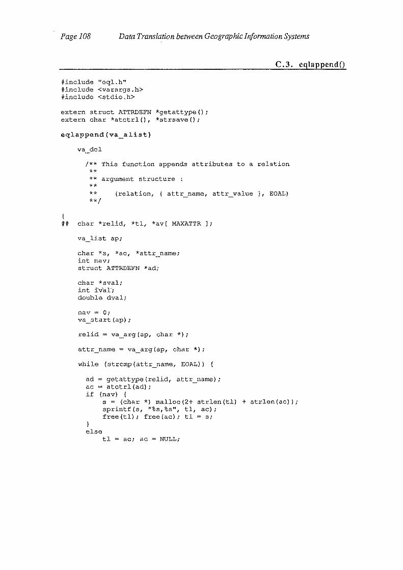
Page 108 Data Translation between Geographic lnfonnation Systems
#include "eql.h" #include <varargs.h> #include <stdio.h>
extern struct ATTRDEFN *getattype(); extern char *atctrl (), *strsave () ;
eqlappend(va_alist)
va del
C.3. eqlappend()
I** This function appends attributes to a relation ** ** argument structure : ** ** (relation, { attr_name, attr value }, EOAL) **I
I ## char *relict, *tl, *av( MAXATTR );
va_list ap;
char *s, *ac, *attr_name; int nav; struct ATTRDEFN *ad;
char *sval; int .tvar; double dval;
nav = 0; va_start (ap) ;
relict= va_arg(ap, char*);
attr_name = va_arg(ap, char*);
while (strcmp(attr_name, EOAL))
ad= getattype(relid, attr_name); ac = atctrl (ad); if (nav) {
s (char*) malloc(2+ strlen(tl) + strlen(ac)); sprintf(s, "%s,%s", tl, ac); free(tl); free(ac); tl = s;
else tl ac; ac NULL;

Simplified INGRES Interface
switch(ad->typ) { case 'c• : {
av[nav++) va_arg(ap, char*); break;
case 'i • : { av[nav++J (char *) &va_arg(ap, int); break;
case 'f' av[nav++J break;
other :;
(char*) &va_arg(ap, double);
attr_name va_arg(ap, char*); }
.Jf# append relid(param(tl, av)) free(tl); }
Page 109
C. 4. eqlreplace()
.Jfinclude "eql.h" #include <varargs.h>
extern struct ATTRDEFN *getattype(); extern char *atctrl(), *strsave();
eqlreplace(va_alist)
{
va del
I** ** This function replaces attribute values in an ingres ** relation according to the given qualification ** ** the argument structure is ** ** (relid, { attr_name, attr_value }+,EOAL, [ qual, ] EOQL) ** ** where { .. }+indicates contents repeated 1 or more times ** and [ ] indicates contents optional. ** ** EOAL, and EOQL are defined in eql.h **I
## char *relid, *tl, *av[ MAXATTR ], *qual;
va_list ap;
char *s, *ac, *attr_name; int nav; struct ATTRDEFN *ad;
char *sval; int ival; double dval;

Page 110 Data Translation between Geographic Information Systems
nav = 0; va_start (ap);
relid =.va_arg(ap, char*); attr_name = va_arg(ap, char*);
while (strcmp(attr_name, EOAL))
ad= getattype(relid, attr_name); ac = atctrl (ad); if (nav) {
else
s = (char*) malloc(2+ strlen(tl) + strlen(ac)); sprintf(s, «%s,%s«, tl, ac); free(tl); free(ac); tl = s;
tl = ac;
switch(ad->typ) case 'c' : {
av[nav++] va_arg(ap, char *); break;
case 'i' : { av[nav++] (char*) &va_arg(ap, int); break;
case 'f' : { av[nav++] (char*) &va_arg(ap, double); break;
other :;
attr name va_arg(ap, char*); }
qual= va_arg(ap, char*);
if (strcmp(qual, EOQL)) ## replace relid(param(tl, av)) where qual
else ## replace relid(param(tl, av))
free(tl);
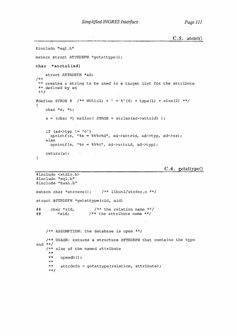
Simplified INGRES Interface Page 111
C.S. atctrl()
tinclude "eql.h"
extern struct ATTRDEFN *getattype();
char *atctr1(ad)
struct ATTRDEFN *ad; /**
** creates a string to be used in a target list for the attribute ** defined by ad **I
.if:define STROH 8 /** NULL(l) + 1
{ %' (4) + type(l) + size(2) **/
char *s, *t;
s (char*) malloc( STROH+ strlen(ad->attrid) );
!= 'c') if (ad->typ sprintf(s,
else sprintf (s,
"%s %%%c%d", ad->attrid, ad->typ, ad->sz);
"%s %%%c", ad->attrid, ad->typ);
return(s);
#include <stdio.h> #include "eql.h" #include "hash.h"
extern char *strsave(); I** libutl/strfns.c **I
struct ATTRDEFN *getattype(rid, aid)
## ##
char *rid, *aid;
I** the relation name **I I** the attribute name **/
I** ASSUMPTION: the database is open **I
C. 6. getattype()
I** USAGE: returns a structure ATTRDEFN that contains the type and **I
/** size of the named attribute ** ** opendb(); ** ** attrdefn = getattype(relation, attribute); **/

Page 112 Data Translation between Geographic Information Systems
## int sz, ty;
static HASH TABLE hashtab; HASH_TABLE newhash(); struct ATTRDEFN *ad, *hlookup(), *hinstall();
if (hashtab ==NULL) hashtab = newhash(); if ((ad= hlookup(hashtab, rid, aid)) !=NULL)
return (ad);
ad= (struct ATTRDEFN *) malloc (sizeof(*ad)); ad->attrid = strsave(aid); ad->relid = strsave(rid);
## retrieve(ty = attribute.attfrmt, sz = attribute.attfrml) ## where attribute.attrelid = rid and attribute.attname = aid
ad->sz = sz;
switch(ty) { case 30
ad->typ 1 i 1 ;
break;
case 31 : ad->typ 1 f 1 ;
break;
case 32 : ad->typ 1 C 1 ;
break;
default : ;
hinstall(hashtab, ad); /**ad
#ifdef GDBG
NULL **/
printf(">>getattype: rid:%s: aid:%s: ty:%c: sz:%d:\n", ad->relid, ad->attrid, ad->typ, ad->sz);
#endif
return(ad);
C. 7. hash functions
The following hash functions implement a hash table. Each entry in this table describes
an attribute that has been used in an eqlreplace or an eqlappend. The performance of
these functions is improved because, if the attribute is used again, it is unnecessary to
retrieve this description a second time from the data base. To find an entry in the hash
table, the relation name is used to find the attributes stored for this relation, then the
attribute name is hashed to find the description of the desired attribute.

Simplified INGRES Interface
#include <varargs.h> #include <stdio.h> #include "eql.h" #include "hash.h"
extern char *strsave();
I**
Page 113
**=~========~===================~========~==================~===
**I
HASH TABLE newhash() {
char* calloc();
return ( (HASH_T.ABLE) calloc ( HASHSIZE, sizeof (TBL_ENTRY))); }
I** **~==================~==========================================
**I
newentry(typ, ht, ad)
int typ; HASH TABLE ht; struct ATTRDEFN *ad;
TBL ENTRY tp, duptp, find(); HASH TABLE newhash(); int hv, hash();
tp = (struct tblentry *) malloc( sizeof( *tp));
switch(typ) {
case Hhashtab : {
tp->name = ad->relid; tp->def.ht = newhash(); newentry(Hattrdefn, tp->def.ht, ad); break;
case Hattrdefn : (
if ((duptp = find(ad->attrid, ht)) ==NULL) { tp->name ad->attrid tp->def.ad ad; ad= NULL;
else { free(tp); duptp->def.ad->sz return(O);
break;
default :; }
hv = hash(tp->name); tp->next = ht(hv]; ht[hv)=tp; return(O);
ad->sz; duptp->def.ad->typ ad->typ;

Page 114 Data Translation between Geographic Information Systems
I** **================~~===================~===============~======== **I
hash(s)
I**
char *s;
I** ** usage **I
int hashval;
hash(keyvalue);
for (hashval Q 0; *s != '\0';) hashval += *s++;
return(hashval% HASHSIZE);
**============================================================== **I
TBL ENTRY find(s, ht)
char *s; HASH TABLE ht;
I** ** Locate an entry in one level of the hash data structure ** /_ ....
TEL ENTRY tp;
if (ht ==NULL) return(NULL);
for (tp = ht[hash(s)]; tp !=NULL; tp = tp->next)
if (strcmp(s, tp->name) return (tp);
0) I** found entry **I
return (NULL); }
I** **===========~================================================== **I
struct ATTRDEFN *hlookup(ht, r, a)
I** look for s in hashtab **I
HASH_TABLE ht; char *r, *a;
I** **usage: hash_tab_entry = lookup(keyvalue);
** ** purpose: Retrieve a pointer to the ATTRDEFN record created ** for attribute a, in relation r **I

I**
Simplified INGRES I nterjace
TBL_ENTRY tel, te2, find();
if ((tel= find(r, ht)) !=NULL)
if ((te2 find(a, tel->def.ht)) !=NULL) return(te2->def.ad);
return (NULL); I** not found **I
Page 115
**========~==~==================================================
**I
struct ATTRDEFN *hinstall(ht, ad)
I** put name,def into hash table **I
HASH_TABLE ht; struct ATTRDEFN *ad;
I** ** usage: ** entry_hash_tab = install(hashtable,keyvalue definition); ** ** purpose: Create a new entry for the attribute defined by ad ** in the hash data structure **I
TBL ENTRY tel, find(); 'int -hash() ;
if ((tel= find(ad->relid, ht))
I** new relation entry **/
newentry(Hhashtab, ht, ad);
else I** new attribute entry **I
NULL)
newentry(Hattrdefn, tel->def.ht, ad); #ifdef HDEBUG
printf(" .•. installed\n"); #endif }
I** **========================================================~=====
**I clearhash(ht)
HASH_TABLE ht;
int i;
for (i =0; i < HASHSIZE; i++) if (ht[i) !=NULL)
clearentry(Hhashtab, ht[i]); free (ht);

Page 116 Data Translation between Geographic Information Systems
clearentry(typ, entry) int typ; TBL ENTRY entry;
int j;
if (entry != NULL) I** ** note that entry -> name is a pointer to either ad->relid or ** ad->attrid. When either of the last two are freed the first is ** implicitly freed. **I
switch(typ) { case Hattrdefn : {
free(entry->def.ad->relid); free(entry->def.ad->attrid); free(entry->def.ad); break;
case Hhashtab : { for ( ; j<HASHSIZE; j++)
if (entry->def.ht[j] ! clearentry(Hattrdefn,
free(entry->def.ht); break;
default : break;
clearentry(typ, entry->next); fre_E;l_( eptry) ;
NULL) entry->def.ht[j]);

Appendix D
Lexical Analysis of Repeating Groups
This appendix contains the variable declarations and data structures used within the
lexical analyser for processing enumerated repeating groups in a format. It is applicable
for lexical analysers that are generated using the Lex software tool [ Lesk and Schmidt
1979 ].
The following variables are declared:
#define maxrgflg 5
#define INITRG(A) rgcnt[++rgflg] =A;
#define DECRG rgcnt[rgflg]--;
int rgcnt[maxrgflg], rgflg = 0;
Table D.l indicates how the analyser can assertain the state of the repeating group
mechanism using the values of rgflg, and rgcnt[rgflg].
TableD.l
Condition Value ofrgflg Value ofrgcnt[rgflg]
Mechanism inactive 0 0
Within incomplete non-zero remaining number of data
repeating group objects to be parsed
Repeating group non-zero 0
completed
The lexical analyser employes the following input macro:
#define input() ( (! (rgcnt [rgflg]) && rgflg) ? (rgflg--, 1 @') :
(((yytchar=yysptr>yysbuf? U(*--yysptr): \
getc(yyin)) == 10? (yylineno++,yytchar): \
yytchar)==EOF? 0 : yytchar))

Page 118 Data Translation between Geographic Information Systems
When the input macro establishes that a repeating group has been completed an '@'
character is inserted into the character stream. A token definition associating the '@'
character to the EORG token is included within the set of token definitions supplied to
Lex. Thus, by inserting the'@' into the character stream the desired EORG token will
be generated by the lexical analyser. To maintain data integrity, the '@' character is
absorbed out of the input character stream by the lexical analyser.

Appendix E
Example Translation Algorithm
To illustrate the use of QUEL, a query language provided by INGRES, a translation
algorithm written in this language is given in§ E.3. The algorithm translates data from
the relational model given in § E.l for the BIF format, into a model given in § E.2
which is used for research in the Department of Computer Science, University of
Canterbury.
E.l BIF Format Relational Data Model
Relations for storing data that is either coming from or going to the BIF format is
created by the following QUEL statements.
create drw(dunit=f8, dcenx=f8, dceny=f8, dsize=f8)
create cmpobjnm(cmpobjid=i4, hookx = f8, hooky
dpso=c15,othrl=c15, othr2=c15)
create hookobj(objectid=i4, hookid=i4)
f8, ocd=clO,
create cmpobjdfn(cmpobjid=i4, objectid=i4, objecttype=i4,
seq=i4, style=c20)
create curvedfn(curveid=i4, seq=i4 1 x=f8, y=f8, bulge=f8)
create circledfn(circleid=i4, cntrx=f8, cntry=f8, radius=f8)
create txtblk(txtblkid=i4, orgnx=f8, orgny=f8, width=f8, height=f8,
sinrot=f8, cosrot=f8, just=c3)
create txtln(txtblkid=i4, seq=i4, line=c250)
create pntdfn(pntid=i4, x=f8, y=f8)
create filename(file = clOO)
\p\g
E. 2 Research Relational Data Model
Relations for storing data that is being used for research is created using the following
QUEL statements.
create layer(layname=c63, layid=i4)
create reps(layid=i4, repid=i4, minlevel=f4, maxlevel=f4)

Page 120 Data Translation between Geographic Information Systems
create object(repid=i4, objid=i4, objtype=i4, minx=f4, maxx=f4,
miny=f4,maxy=f4)
create point(pointid=i4 1 x=f4, y=f4)
create curve(curveid=i4, seq=i4, x=f4, y=f4, bulge=f4)
create circle(circleid=i4, centx=f4 1 centy'=f4, rad=f4)
create textblock(textid=i4, rectx=f4, recty=f4, rectw=f4, recth=f4,
theta=f4, just=c2)
create textline(textid=i4, seq=i4, chars=c255)
\p\g
E. 3 Translation Algorithm
Data in the relations for the BIF format (§ E.l) is translated into the relations being used
for research (§ E.2) by the following translation algorithm.
I** ** ensure objectid to be unique (all objectid > 0)
**I retrieve tmp(maxobjid = max(object.objid)) \p\g
replace cmpobjdfn(objectid = cmpobjdfn.objectid + tmp.maxobjid) \p\g
replace curvedfn(curveid = curvedfn.curveid + tmp.maxobjid) \p\g
replace circledfn( circleid = circledfn.circleid + tmp.maxobjid) \p\g
replace pntdfn( pntid = pntdfn.pntid + tmp.maxobjid) \p\g
replace txtblk( txtblkid txtblk.txtblkid + tmp.maxobjid) \p\g
replace txtln( txtblkid = txtln.txtblkid + tmp.maxobjid) \p\g
destroy tmp
I** ** (temporarily) ensure cmpobjid to be unique
**I retrieve tmp(maxcmpobjid = max{cmpobjlay.cmpobjid))\p\g
replace cmpobjdfn(cmpobjid = cmpobjdfn.cmpobjid + tmp.maxcmpobjid)\p\g
replace cmpobjnm(cmpobjid = cmpobjnm.cmpobjid + tmp.maxcmpobjid) \p\g
destroy tmp
append objsrc(source = "CHCHDB", file = filename.file,
mncmpobjid = min(cmpobjdfn.cmpobjid),
mxcmpobjid = max(cmpobjdfn.cmpobjid))

Example Translation Algon'thm Page 121
I**
** append cmpobj
**/
append to cmpobjlay(cmpobjnm.all) \p\g
append to cmpobj(cmpobjid~cmpobjdfn.cmpobjid,
objid=cmpobjdfn.objectid,
objtype=cmpobjdfn.objecttype, seq=cmpobjdfn.seq, style ~
cmpobjdfn.style) \p\g
I** calculate minimum bounding rectangle of objects
range of cdfn is curvedfn
retrieve tmp(objectid = cdfn.curveid, minx=min(cdfn.x by
cdfn. curveid) ,
maxx = max(cdfn.x by cdfn.curveid), miny
cdfn. curveid) ,
maxy = max(cdfn.y by cdfn.curveid)) \p\g
range of cdfn is circledfn
min(cdfn.y by
**/
a-ppe·:nct tmp (objectid = cdfn. circleid, minx = cdfn. cntrx - cdfn. radius,
maxx cdfn.cntrx + cdfn.radius, miny= cdfn.cntry - cdfn.radius,
maxy cdfn.cntry + cdfn.radius) \p\g
append tmp(objectid = pntdfn.pntid, minx= pntdfn.x, maxx = pntdfn.x,
miny = pntdfn.y, maxy = pntdfn.y) \p\g
range of tb is txtblk
append tmp(objectid tb.txtblkid,
minx = tb.orgnx - tb.height * tb.sinrot,
maxx =tb.orgnx + tb.width * tb.cosrot, miny = tb.orgny,
maxy = tb.orgny + tb.width* tb.sinrot + tb.height * tb.cosrot)
where tb.cosrot >= 0 and tb.sinrot >= 0 \p\g
append tmp(objectid = tb.txtblkid,
minx tb.orgnx + tb.width * tb.cosrot - tb.height * tb.sinrot,
maxx tb.orgnx, miny = tb.orgny + tb.height * tb.cosrot,
maxy tb.orgny + tb.width * tb.sinrot)
where tb.sinrot >=0 and tb.cosrot < 0 \p\g

Page 122 Data Translation between Geographic Information Systems
append tmp(objectid = tb.txtblkid,
minx
maxx
tb.orgnx + tb.width * tb.cosrot,
tb.orgnx - tb.height*tb.sinrot,
miny
maxy
tb.orgny + tb.width*tb.sinrot+tb.height*tb.cosrot,
tb.orgny)
where tb.sinrot < 0 and tb.cosrot < 0 \p\g
append tmp( objectid = tb.txtblkid, minx= tb.orgnx,
naxx
niny
.naxy
tb.orgnx + tb.width * tb.cosrot,
tb.orgny + tb.width * tb.sinrot,
tb.orgny + tb.height * tb.cosrot)
where tb.sinrot < 0 and tb.cosrot >=0 \p\g
/**
** append to object relation
**I
append object(objid = cmpobjdfn.objectid,
objtype = cmpobjdfn.objecttype)
replace object(minx = tmp.minx, maxx=tmp.maxx, miny
tmp .maxy) ____ ··
where object.objid tmp.objectid \p\g
destroy tmp
/**
** append curve definitions to mapbase
**/
append to curve(curvedfn.all)
/**
** append circle definitions to mapbase
**I
append to circle(circleid
centx = circledfn.cntrx,
ci~cledfn.circleid,
centy = circledfn.cntry, rad circledfn.radius)
tmp.miny, maxy

Example Translation Algorithm
I** ** append point definitions to mapbase
**I append to point(pointid pntdfn.pntid, x=pntdfn.x, y
I** ** append text blocks to mapbase
**/
Page 123
pntdfn.y)
appen~ to textblock(textid = txtblk.txtblkid, rectx=txtblk.orgnx,
recty=txtblk.orgny, rectw=txtblk.width, recth=txtblk.height,
just=txtblk.just, theta= 0.0)
I** calculate theta, and replace in mapbase **/
I** pi = 3.141592 **/
replace textblock(theta=3.141592 + atan(txtblk.sinrot/txtblk.cosrot))
where textblock.textid = txtblk.txtblkid and txtblk.cosrot < 0.0
replace textblock(theta=atan(txtblk.sinrot/txtblk.cosrot))
where textblock.textid = txtblk.txtblkid
and txtblk.cosrot >= 0.0 and txtblk.sinrot >= 0.0
repl.ace textblock (theta=2*3 .141592+atan (txtblk. sinrot/txtblk. cos rot))
where textblock.textid = txtblk.txtblkid
and txtblk.sinrot < 0.0 and txtblk.cosrot >= 0.0
append to textline(textid
chars = txtln.line)
\p\g
txtln.txtblkid, seq= txtln.seq,


Appendix F
Format Encoder Generator
The Yacc and Lex files given in this Appendix are used to generate the prototype
generator of fomat encoders.
%{ #include <stdio.h> #include "que.h" #include "yacc.defn.h" #include "eql.h"
%}
int attr_seq = 0;
extern char *strsave(), *retatctrl(); extern struct ATTRDEFN *getattype();
FILE *fp;
.double at of () ; char *dbname, *malloc(); struct PARM_LIST *mkstrprm(), *mkattr();
%start datafile
%union QOBJPTR t; int ival; double dval; char *sval; struct ATTRDEFN *aval; struct PARM LIST {
char *var=list, *target_list, *prf; } *pval;
%type <sval> string.value rule rhs %type <pval> param list %type <aval> attribute
F .1 Yacc Definition file
%token <t> EORG IDENT COLON L BRCK R BRCK DOT SEMI - -/** NB: the following must agree with that in que.h **/
%token <t> STRING 1001 INTEGER 1003 REAL 1002
%% datafile rule
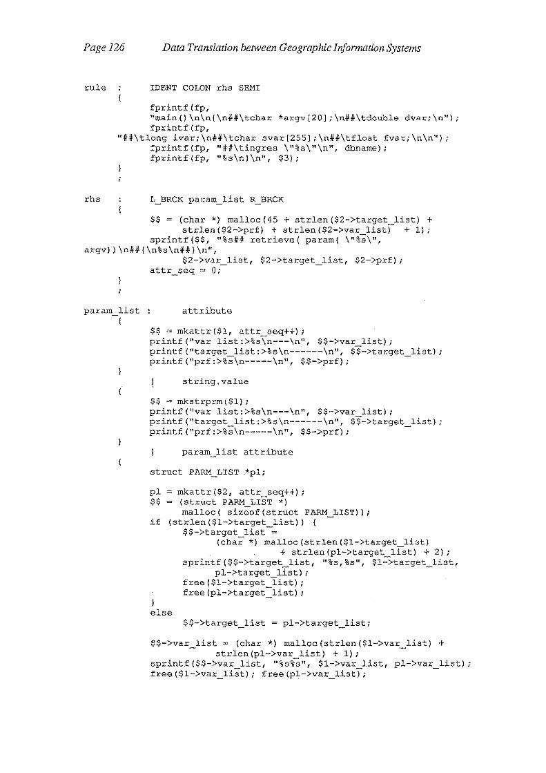
Page 126
rule
Data Translation between Geographic Information Systems
IDENT COLON rhs SEMI
fprintf(fp, "main() \n\n { \n##\tchar *argv [20]; \n##\tdouble dvar; \n") ; fprintf(fp,
"ff\tlong ivar;\n##\tchar svar[255];\nlf\tfloat fvar;\n\n"); fprintf(fp, "##\tingres \"%s\"\n", dbname); fprintf(fp, "%~\n}\n", $3);
rhs L_BRCK param_list R_BRCK
$$ (char *) malloc(45 + strlen($2->target list) + strlen($2->prf) + strlen{$2->var list) + 1);
sprintf($$, "%s## retrieve( param( \"%s\", argv) ) \nff { \n%s \n##} \n",
param_list {
$2->var_list, $2->target_list, $2->prf); attr_seq = 0;
attribute
$$ mkattr($1, attr seq++); printf("var list:>%s\n---\n", $$->var list); printf("target list:>%s\n------\n", $$->target list); printf ("prf :>%s\n-----\n", $$->prf); -
string.value
$$ mkstrprm($1); printf("var list:>%s\n---\n", $$->var list); printf("target list:>%s\n------\n", $$->target list); printf("prf:>%8\n-----\n", $$->prf); -
param_list attribute
struct PARM_LIST .*pl;
pl mkattr($2, attr_seq++); $$ = (struct PARM LIST *)
malloc( sizeof(struct PARM_LIST)); if {strlen ($1->target list)) {
$$->target list-= (char*) malloc(strlen($1->target list)
else
+ strlen(pl->target list) + 2); sprintf($$->target_list, "%s,%s", $1..:S.target_list,
pl->target list); free($1->target list); free(pl->target=list);
$$->target_list = pl->target_list;
$$->var list= (char *) malloc(strlen($1->var_list) + strlen(pl->var list) + 1);
sprintf($$->var list, "%s%s", $1->var list, pl->var list); free($1->var_list); free(pl->var_list);

Format Encoder Generator
$$->prf = (char *) malloc(strlen($1->prf)+strlen(pl->prf) +25);
sprintf($$->prf, "%s%s", $1->prf, pl->prf);
free($1->prf); free($1); free(pl->prf); free(pl);
Page 127
printf("var list:>%s\n---\n", $$->var list); printf("target list:>%3\n------\n", $$->target list); printf("prf:>%s\n-----\n", $$->prf); -
param_list string.value
struct PARM LIST *pl;
pl mkstrprm($2); $$ (struct PARM_LIST *)
malloc( sizeof(struct PARM LIST)); $$->target list = $1->target list; $$->var list = $1->var list;-$$->prf-= (char *) malloc(14 + strlen($1->prf) +
strlen(pl->prf)); sprintf($$->prf, "%s%s", $1->prf, pl->prf);
free($1->prf); free($1); free(pl->prf); free(pl); printf("var list:>%s\n---\n", $$->var_list); printf("target list:>%s\n------\n", $$->target list); printf ("prf: >%s\n-----\n", $$->prf); -
attribute {
IDENT DOT IDENT
$$ getattype(stv($1), stv($3));
string.value STRING { $$ = strsave(stv($1));
%% ifinclude "lex.c"
yyerror (s) char *s;
printf ("ERROR with yytext
main(argc, argv) int argc; char *argv [];
char *sf; FILE *fopen(), *freopen();
:%s:\n", yytext);
if ( (argo < 3) I I (argo > 3) ) { fprintf(stderr,
"Usage: impbif server::database filename\n"); exit() ;
fp = fopen("./encoder.qc", "w"); dbname = argv[l];

Page 128 Data Translation between Geographic Information Systems
freopen(argv[2], "r", stdin); eqlopen(argv[l], "-clO");
yyparse(); eqlclose () ;
struct PARM_LIST *mkattr(ad, n) struct ATTRDEFN *ad; int n;
struct PARM_LIST *pl;
pl = (struct PARM_LIST *) malloc( sizeof(struct PARM_LIST)); pl->target_list = retatctrl(ad); switch(ad->typ) {
case 1 c' : pl->prf = (char*) malloc(26); pl->var list= (char*) malloc(20); sprintf(pl->prf,"\tprintf(\"%%s\",svar);\n"); sprintf(pl->var_list, "\targv[%d] = svar;\n",n); break;
case 1 i 1 :
pl->prf = (char*) malloc(26); sprintf(pl->prf,"\tprintf(\"%%d\", ivar);\n"); pl->var list= (char*) malloc(28); sprintf(pl->var_list,
"\targv[%d] = (char *)&ivar;\n",n); break;
case 'f' if (ad->sz 4) {
else {
break; default . ,
} i return(pl);
pl->prf = (char*) malloc(26); sprintf(pl->prf,
"\tprintf(\"%%f\", fvar);\n"); pl->var_list = (char*) malloc(28); sprintf(pl->var_list,
"\targv[%d] = (char *)&fvar;\n",n);
pl->prf = (char*) malloc(27); sprintf(pl->prf,
"\tprintf(\"%%lf\", dvar);\n"); pl->var list= (char*) malloc(28); sprintf(pl->var_list,
"\targv[%d] = (char *)&dvar;\n",n);
struct PARM LIST *mkstrprm(s) char *s;
struct PARM_LIST *pl;
pl = (struct PARM LIST*) malloc( sizeof(struct PARM_LIST)); pl->prf = (char*) malloc( strlen(s) + 13); sprintf(pl->prf, "\tprintf(\"%s\");\n", s); pl->var list= strsave(""); pl->target_list = strsave(""); return(pl);

Format Encoder Generator Page 129
F. 2 Lex definition File
%o4000 %{
#define input() ((! (rgcnt (rgflg]) && rgflg) ? (rgflg--, '@') : (((yytchar=yysptr>yysbuf?U(*--yysptr) :getc(yyin))==lO?(yylineno++,yytchar) :yytchar)==EOF?O:yytchar))
%}
D [0-9] E [E] [-+] (D} {D} w [\t ) CHAR [A-Za-z]
%% {W}*\n
\ ; ret urn ( SEMI ) ; } \: return( COLON); } \. return( DOT); } \{ return( L_BRCK );
\} return( R BRCK );
\: { return ( COLON ) ; } (W}*[+-]?{D}+"."{D}*({E})?{W}* (W}*[+-]?(D}*"."(D}+((E})?{W}*
} {W}*[+-)?{D}+{W}*
}
newtkn ( REAL ) ; dtv(yylval.t) = atof(yytext); ret urn ( REAL ) ;
newtkn( INTEGER); itv(yylval.t) = atoi(yytext); return( INTEGER);
\ " ( { CHAR } * ( D } * [ \ \ \-\ , ! @ #% " & () ] * { w } * ) * \ II newtkn( STRING); stv(yylval.t) = strsave(yytext+l); st v (yyl val. t) [yyleng-2] • \0' ; return( STRING);
}
( { CHAR } ( D } * ) + newtkn ( IDENT ) ; stv(yylval.t) = strsave(yytext); return ( IDENT ) ;
@ { return( EORG ) ; } %% l*----------------------------------------------------------*1


Appendix G
An Example of a Format Encoder
This appendix contains the listing of a format encoder for the character form of the BIF
format.
struct value { int type; union {
} ;
int ival; double dval; char *sval;
value;
struct tnode {
}_;-. ..
struct value *av[lO]; int (*prntfn) (), (*mksubtree) (); struct tnode *sib; struct tnode *chld;
:jfdefine INT 50 :jfdefine REAL 51 #define CHAR 52 extern struct tnode *nwnd(); extern int prnt_tree();
#include <stdio.h> #include "tre.h" struct tnode *nwnd() {
}
struct tnode *n;
n = (struct tnode *) malloc( sizeof(*n)); n->sib ~ NULL;n->chld = NULL; return(n); ·
incomplete_tree(hd) struct tnode *hd;
int inc; inc = 0;
· if (hd ! = NULL) inc =
G.l tre.h
G.2 tre.c
((hd->mksubtree !=empty) I I incomplete_tree(hd->chld) I I incomplete_tree(hd->sib));
return(inc);

Page 132 Data Translation between Geographic Information Systems
build_tree(hd)
}
struct tnode *hd;
if (hd != NULL) { build_tree(hd->chld); (*hd->mksubtree) (hd); hd->mksubtree = empty; build_tree(hd->sib);
empty (hd) struct tnode *hd;
{} int file gen(hd)
struct tnode *hd;
if (hd NULL) { (*(hd->prntfn)) (hd->av); file_gen(hd->chld); file_gen(hd->sib);
#include <stdio.h> #include "tre.h"
#define POINT 0 #define CURVE 1 #define CTRCLE 2 #define TEXT 3
G.3 enc.qc
int prntdrw(), object(), crv_prm(), ln_seg(), arc_seg(), hook(), empty(), prmtree(), nametree(), objecttree(), crvetree();
## int sq, obj, prm, prmt; ## double xx, yy, blg, r, du, dcx, dey, dsz; ## char *styl, *oc, *ds, *ol, *o2;
struct tnode *init_tree();
main ( argo, argv) int argo;
## char *argv[]; {
struct tnode *tree, *t;
styl (char *) malloc (30); oc (char *}malloc(ll); ds ol = (char *}malloc(l6); o2
## ingres argv[l]
tree= init_tree(}; while (incomplete tree(tree))
build_tree(tree);
file_gen(tree};
(char *)malloc(l6); (char *)malloc(16);

Example Format Encoder
struct tnode *init_tree() {
struct tnode *hd;
hd = nwnd(); hd->mksubtree = objecttree; hd->prntfn = prntdrw;
return (hd);
objecttree(hd) struct tnode *hd;
struct tnode *t;
t = NULL;
retrieve(obj cmpobjnm.cmpobjid)
if (t. == NULL)
else { t = hd->chld nwnd();
t->sib = nwnd(); t = t->sib; }
Page 133
t->av[O] (struct value*) malloc(sizeof (*(t->av[O])));
##} r·-- -·
t->av[O]->type = INT; t->av[O]->value.ival obj; t->prntfn = object; t->mksubtree prmtree;
object(av) struct value *av[];
obj = av[O]->value.ival; retrieve (oc cmpobjnm.ocd, ds
ol = cmpobjnm.othrl, o2 xx cmpobjnm.hookx, yy
where cmpobjnm.cmpobjid= obj printf("name %s\nhook %lf %lf\n",
prmtree (hd) struct tnode *hd;
struct tnode *t;
t NULL;
obj hd->av(OJ->value.ival;
cmpobjnm.dpso, cmpobjnm.othr2, cmpobjnm.hooky)
oc, xx, yy);
## retrieve(prm = cmpobjdfn.objectid, prmt cmpobjdfn.objecttype) ## where cmpobjdfn.cmpobjid = obj ##{
if (t == NULL) t hd->chld = nwnd();
else { t->sib = nwnd(); t = t->sib; }

Pagel34
##}
Data Translation between Geographic Information Systems
t->av[O] = (struct value*) malloc(sizeof (*(t->av[O]))); t->av[O]->type = INT; t->av[O]->value.ival = obj; t->av[l] = (struct value*) malloc(sizeof (*(t->av[O]))); t->av[l]->type = INT; t->av[l]->value.ival = prm; if (prmt == CURVE) {
else
t->prntfn = crv_prm; t->mksubtree = crvetree;
I** Kludge -- incomplete **/ t->prntfn = empty; t->mksubtree = empty;
} crvetree(hd)
struct tnode *hd;
struct tnode *t;
t = NULL; prm = hd->av[l]->value.ival;
/** retrieve should get tuples in order of ascending seq **/
## retrieve (blg = curvedfn.bulge, sq= curvedfn.seq) ## where curvedfn.curveid = prm and curvedfn.seq != 0 ##{
##}
if (t == NULL)
else { t = hd->chld = nwnd();
t->sib = nwnd(); t = t->sib; }
if (blg == 0.0) {
else
}
t->prntfn = ln_seg; t->mksubtree = empty;
t->prntfn = arc_seg; t->mksubtree = empty;
t->av[O] = (struct value*) malloc(sizeof (*(t->av[O]))); t->av[O]->type = INT; t->av[O]->value.ival = prm; t->av[l) = (struct value*) malloc(sizeof (*(t->av[O]))); t->av[l]->type = INT; t->av[l]->value.ival = sq;
} arc_seg(av)
## ## ##
struct value *av[);
prm = av[O]->value.ival; sq = av[l]->value.ival;
retrieve (xx = curvedfn.x, yy = curvedfn.y, blg = curvedfn.bulge)
where curvedfn.curveid = prm and curvedfn.seq printf("arc %lf %lf %lf\n", xx, yy, blg);
sq

Example Format Encoder
ln_seg (av)
u ##
struct value *av[];
prm = av(O]->value.ival; sq = av[l)->value.ival;
retrieve (xx = curvedfn.x,. yy = curvedfn.y) where curvedfn.curveid = prm and curvedfn.seq
printf("to %lf %lf\n", xx, yy);
crv_prm(av)
u ## ## ##
struct value *av[];
obj = av[O]->value.ival; prm = av[l]->value.ival; retrieve (styl = cmpobjdfn.style)
where cmpobjdfn.objectid = obj retrieve (xx = curvedfn.x, yy = curvedfn.y)
where curvedfn.curveid = prm and curvedfn.seq printf("line %lf %lf %s\n",xx, yy, styl);
} prntdrw(av)
struct value *av[]; {
Page 135
sq
0
## retrieve (du = drw.dunit, dcx = drw.dcenx, dey = drw.dceny, ## dsz = drw.size)
printf("drawing %lf %lf %lf %lf\n", du, dcx, dey, dsz);