An evaluation of LIDAR and IFSAR-derived digital elevation models in leaf-on conditions with USGS...

An evaluation of LIDAR- and IFSAR-derived digital elevation models in

leaf-on conditions with USGS Level 1 and Level 2 DEMs

Michael E. Hodgsona,*, John R. Jensena, Laura Schmidtb, Steve Schillc, Bruce Davisd

aDepartment of Geography, University of South Carolina, Columbia, SC 29208, USAbBaruch Marine Science Laboratory, Georgetown, SC 29585, USA

cGeoMetrics, Inc., Columbia, SC 29210, USAdEarth Science Applications Directorate, NASA Stennis Space Center, Stennis, MS 39529, USA

Received 17 July 2001; received in revised form 24 July 2002; accepted 27 July 2002

Abstract

An assessment of four different remote sensing based methods for deriving digital elevation models (DEMs) was conducted in a flood-

prone watershed in North Carolina. New airborne LIDAR (light detecting and ranging) and IFSAR (interferometric synthetic aperture radar

(SAR)) data were collected and corresponding DEMs created. These new sources were compared to two methods: Gestalt Photomapper

(GPM) and contour-to-grid, used by the U.S. Geological Survey (USGS) for creating DEMs. Survey-grade points (1470) for five different

land cover classes were used as reference points. One unique aspect of this study was the LIDAR and IFSAR data were collected during leaf-

on conditions. Analyses of absolute elevation accuracy and terrain slope were conducted. The LIDAR- and contour-to-grid derived DEMs

exhibited the highest overall absolute elevation accuracies. Elevation accuracy was found to vary with land cover categories. Elevation

accuracy also decreased with increasing slopes—but only for the scrub/shrub land cover category. Appreciable terrain slope errors for the

reference points were found with all methods.

D 2002 Elsevier Science Inc. All rights reserved.

Keywords: LIDAR; IFSAR; DEM; Elevation accuracy

1. Introduction

Many hydrologic, vegetation science, and urban planning

applications use digital elevation models (DEMs) to obtain

absolute surface elevation and terrain form (e.g., slope,

aspect) information (Jensen, 2000). The most widely adop-

ted DEMS in the United States are the 30� 30 m Level 1

DEMs produced by the U.S. Geological Survey (USGS)

using photogrammetric techniques (Hodgson, 1998). More

accurate USGS Level 2 DEMs are available for selected

geographic areas. During the past decade, there has been a

significant increase in the production of DEMs using air-

borne LIDAR (light detection and ranging) and IFSAR

(interferometric synthetic aperture radar) remote sensing

techniques (Jensen, 2000). This situation forces scientists

or applied users who want to incorporate a DEM into their

study to carefully consider the source of the DEM. Impor-

tant questions to be addressed when selecting a DEM

include:

1. What is the absolute elevation accuracy of the digital

elevation information that can be extracted from the

DEM using a certain type of technology (e.g., in situ

ground survey, photogrammetry, LIDAR, IFSAR)?

2. What is the accuracy of the surface form (e.g., slope)

derived from the DEM?

3. Does the absolute elevation and/or surface form accuracy

covary with land cover and/or slope?

4. Is the DEM derived using a certain type of technology

more accurate if it is obtained during leaf-on or leaf-off

conditions?

There is considerable conflicting information about

many of these considerations available today. What is

needed is a rigorous comparison of the strengths and

weaknesses of DEMs derived using the various alternative

remote sensing technologies so that the user may know

which is the most appropriate DEM to utilize. To this end,

0034-4257/02/$ - see front matter D 2002 Elsevier Science Inc. All rights reserved.

PII: S0034 -4257 (02 )00114 -1

* Corresponding author.

www.elsevier.com/locate/rse

Remote Sensing of Environment 84 (2003) 295–308

research was conducted in cooperation with the North

Carolina Geodetic Survey. A high priority watershed in

North Carolina susceptible to flooding during hurricanes

was selected for analysis. The geodetic survey collected

1470 in situ x,y,z measurements within the watershed.

Absolute elevation and terrain form derived from USGS

Level 1 and 2 DEMs and from LIDAR and IFSAR-derived

DEMs obtained during leaf-on conditions were compared

with the in situ measurements. The goal of this study was

to obtain an unbiased assessment of the utility of the

various remote sensing-derived DEMS.

2. Methods of creating a digital elevation model

Digital elevation models may be produced using in situ

measurements, photogrammetrically derived measurements

from stereo-correlation, LIDAR laser measurements, and

IFSAR active microwave measurements. The following

sections summarize how the IFSAR, LIDAR, and USGS

Level 1 and 2 DEMs are derived. Previous research con-

ducted on DEM accuracy associated with each of the

technologies is presented wherever available.

2.1. Digital elevation models derived using interferometric

synthetic aperture radar—IFSAR

Elevation has been mapped from both satellite and air-

craft synthetic aperture radars (SARs) since the 1960s

(Jensen, 2000). A SAR synthetically simulates a very long

antenna using the forward movement of the aircraft. Aircraft

or spacecraft carrying SARs also record data from onboard

differentially corrected global positioning systems (GPS)

and an inertial navigation systems (INS) to determine the

location and roll, pitch, and yaw of the craft.

This study focuses on the use of a special type of SAR

called an interferometric synthetic aperture radar (IFSAR) to

derive topographic information. IFSAR exploits the coher-

ent nature of SAR echoes (i.e., the signals are recorded in

both amplitude and phase) to measure difference in the

phase from each patch of the surface when observed from

slightly different locations and/or times. These phase differ-

ences can be attributed to differences in path length between

the two signals. The path-length differences are a function

of: (1) the distance and angles of the radar antennas making

the observations, (2) the topography of the surface, (3) a

change in the position of patches of the surface, and (4)

differences in atmospheric or ionospheric conditions along

the two paths. If the two observations are made simulta-

neously from a pair of radar antennas on a single platform,

item (1) above is well known and the effects of items (3) and

(4) are negligible, leaving item (2), the surface topography,

as the controlling factor (Plaut, Rivard, & D’lorio, 1999).

Therefore, a fixed-baseline dual-antenna interferometric

system is the preferred method for the extraction of DEMs.

The Shuttle Radar Topography Mission (SRTM) is based on

the use of two antennae on the same platform (JPL, 1999) as

is Intermap’s STAR 3i IFSAR used in this investigation.

SAR data have an implicit spatial resolution defined by

the pulse length, flying height, and depression angle (Jen-

sen, 2000). The slant range resolution of SAR data is 1/2

the pulse length. The ground range resolution is defined as

the slant range resolution divided by the cosine of the

depression angle. These two resolutions describe the reso-

lution analogous to the pixel size in remotely sensed

imagery or the ‘‘footprint’’ in LIDAR data (to be dis-

cussed). The more coarse the IFSAR spatial resolution,

the more difficult it is to produce accurate ‘‘bald earth’’

digital elevation models, especially through continuous

forest canopy cover. Directly sensing the earth surface

beneath vegetated canopies requires using a short pulse

length that penetrates through ‘‘holes’’ in the canopy and/or

a longer wavelength. A characteristic of X-band (3 cm

wavelength) radar is that it penetrates only part way into

forest canopy. Longer wavelengths penetrate further, and

there is ongoing research into long-wavelength interferom-

etry. It is not yet clear what accuracies may be achieved,

and under what conditions.

Image data from a fully focused SAR have a limiting

spatial resolution (in the along track direction) determined

by the system bandwidth and the antenna length. Typically,

the resolution is broadened by an averaging process known

as ‘multi-looking,’ which has the effect of reducing

unwanted speckle in the image. The elevation values from

IFSAR are averages from the scatterers within the same

image pixel. Normally the elevation ‘pixels’ are further

averaged over surrounding samples to reduce the random

elevation ‘noise’ in the data set. For example, the image

resolution of the STAR-3i system is f 2.5 m, while the

elevation sample spacing (i.e., the elevation ‘posting’) in the

DEM is usually set at 5 m. The vertical accuracy of the

DEM is determined by several factors associated with

random noise and systematic effects. Many of these error

factors are proportional to the flying height of the IFSAR.

Thus, the lower the flying height, the better the elevation

accuracy, although there is negligible effect on the spatial

resolution of the imagery. It should be noted that each

IFSAR elevation sample corresponds to a ‘cell average’ so

that the DEM is a regular grid of adjacent samples. This is in

contrast to LIDAR, where samples (footprints) are smaller

in size and may be separated from each other by several

meters depending on operational parameters. In either case,

the coarser the DEM, the more difficult it is to correctly

represent topographic expression.

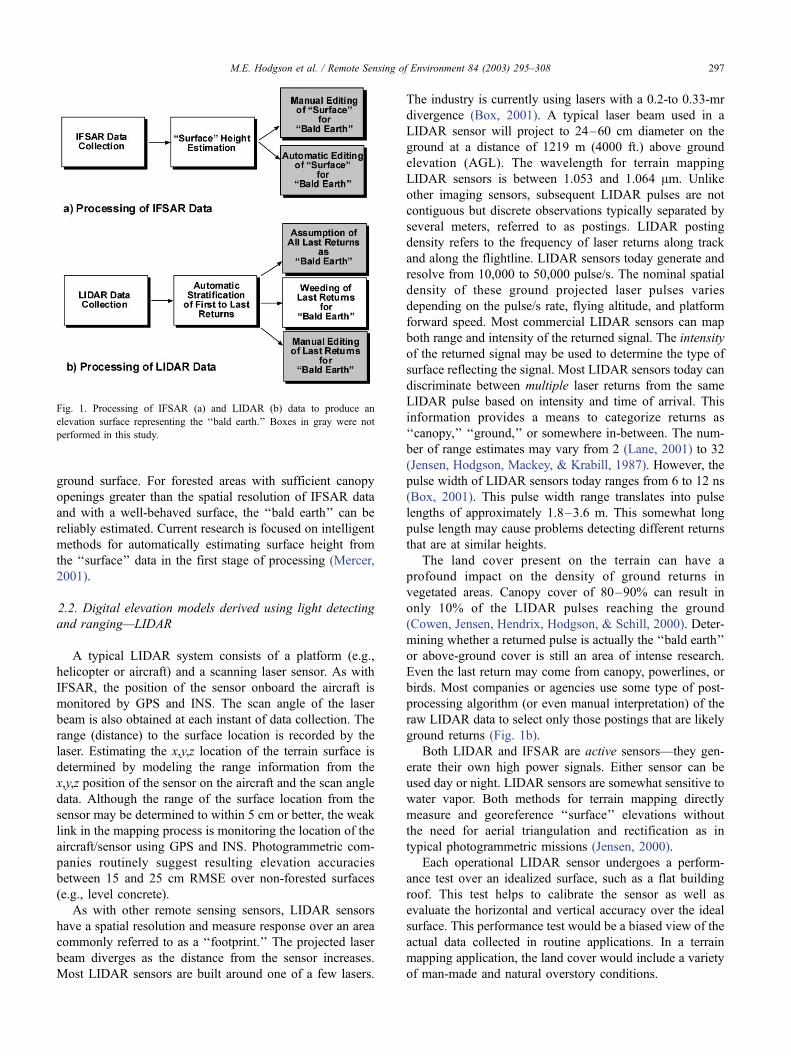
To overcome the canopy cover problem, IFSAR data for

elevation mapping purposes may be processed in stages

(Fig. 1a). The first stage is to collect the IFSAR data and

determine the range of the ‘‘surface.’’ For unforested areas,

this ‘‘surface’’ is at (or very near) the actual ‘‘bald earth’’

(Mercer, 2001). In forested areas, the use of ancillary data

(e.g., aerial photographs or other imagery) may help in

separating the ‘‘expected’’ forest canopy height from the

M.E. Hodgson et al. / Remote Sensing of Environment 84 (2003) 295–308296

ground surface. For forested areas with sufficient canopy

openings greater than the spatial resolution of IFSAR data

and with a well-behaved surface, the ‘‘bald earth’’ can be

reliably estimated. Current research is focused on intelligent

methods for automatically estimating surface height from

the ‘‘surface’’ data in the first stage of processing (Mercer,

2001).

2.2. Digital elevation models derived using light detecting

and ranging—LIDAR

A typical LIDAR system consists of a platform (e.g.,

helicopter or aircraft) and a scanning laser sensor. As with

IFSAR, the position of the sensor onboard the aircraft is

monitored by GPS and INS. The scan angle of the laser

beam is also obtained at each instant of data collection. The

range (distance) to the surface location is recorded by the

laser. Estimating the x,y,z location of the terrain surface is

determined by modeling the range information from the

x,y,z position of the sensor on the aircraft and the scan angle

data. Although the range of the surface location from the

sensor may be determined to within 5 cm or better, the weak

link in the mapping process is monitoring the location of the

aircraft/sensor using GPS and INS. Photogrammetric com-

panies routinely suggest resulting elevation accuracies

between 15 and 25 cm RMSE over non-forested surfaces

(e.g., level concrete).

As with other remote sensing sensors, LIDAR sensors

have a spatial resolution and measure response over an area

commonly referred to as a ‘‘footprint.’’ The projected laser

beam diverges as the distance from the sensor increases.

Most LIDAR sensors are built around one of a few lasers.

The industry is currently using lasers with a 0.2-to 0.33-mr

divergence (Box, 2001). A typical laser beam used in a

LIDAR sensor will project to 24–60 cm diameter on the

ground at a distance of 1219 m (4000 ft.) above ground

elevation (AGL). The wavelength for terrain mapping

LIDAR sensors is between 1.053 and 1.064 Am. Unlike

other imaging sensors, subsequent LIDAR pulses are not

contiguous but discrete observations typically separated by

several meters, referred to as postings. LIDAR posting

density refers to the frequency of laser returns along track

and along the flightline. LIDAR sensors today generate and

resolve from 10,000 to 50,000 pulse/s. The nominal spatial

density of these ground projected laser pulses varies

depending on the pulse/s rate, flying altitude, and platform

forward speed. Most commercial LIDAR sensors can map

both range and intensity of the returned signal. The intensity

of the returned signal may be used to determine the type of

surface reflecting the signal. Most LIDAR sensors today can

discriminate between multiple laser returns from the same

LIDAR pulse based on intensity and time of arrival. This

information provides a means to categorize returns as

‘‘canopy,’’ ‘‘ground,’’ or somewhere in-between. The num-

ber of range estimates may vary from 2 (Lane, 2001) to 32

(Jensen, Hodgson, Mackey, & Krabill, 1987). However, the

pulse width of LIDAR sensors today ranges from 6 to 12 ns

(Box, 2001). This pulse width range translates into pulse

lengths of approximately 1.8–3.6 m. This somewhat long

pulse length may cause problems detecting different returns

that are at similar heights.

The land cover present on the terrain can have a

profound impact on the density of ground returns in

vegetated areas. Canopy cover of 80–90% can result in

only 10% of the LIDAR pulses reaching the ground

(Cowen, Jensen, Hendrix, Hodgson, & Schill, 2000). Deter-

mining whether a returned pulse is actually the ‘‘bald earth’’

or above-ground cover is still an area of intense research.

Even the last return may come from canopy, powerlines, or

birds. Most companies or agencies use some type of post-

processing algorithm (or even manual interpretation) of the

raw LIDAR data to select only those postings that are likely

ground returns (Fig. 1b).

Both LIDAR and IFSAR are active sensors—they gen-

erate their own high power signals. Either sensor can be

used day or night. LIDAR sensors are somewhat sensitive to

water vapor. Both methods for terrain mapping directly

measure and georeference ‘‘surface’’ elevations without

the need for aerial triangulation and rectification as in

typical photogrammetric missions (Jensen, 2000).

Each operational LIDAR sensor undergoes a perform-

ance test over an idealized surface, such as a flat building

roof. This test helps to calibrate the sensor as well as

evaluate the horizontal and vertical accuracy over the ideal

surface. This performance test would be a biased view of the

actual data collected in routine applications. In a terrain

mapping application, the land cover would include a variety

of man-made and natural overstory conditions.

Fig. 1. Processing of IFSAR (a) and LIDAR (b) data to produce an

elevation surface representing the ‘‘bald earth.’’ Boxes in gray were not

performed in this study.

M.E. Hodgson et al. / Remote Sensing of Environment 84 (2003) 295–308 297

As noted earlier, most applications involve weeding the

returns (i.e., the overstory) to select only ‘‘ground’’ points

from which to construct a terrain model. This process is

often called ‘‘vegetation removal’’ when the goal is to map

the terrain surface. The methodologies and algorithms are

proprietary. In general, however, each company will take the

set of LIDAR pulse ‘‘returns’’ categorized by the instrument

and identify those returns that have the characteristics of a

‘‘ground return.’’ Such identification typically involves a

combination of (1) human interpretation of the three-dimen-

sional scatter of points and (2) an automated procedure for

vegetation detection. The automated procedures use a spa-

tial filter to identify locally low elevations under the

assumptions these represent the ground. The methodology

for vegetation removal in this study, for instance, used an

automated procedure first followed by a human operator

further refining the identified ground points.

Pereira and Janssen (1999) evaluated low-altitude (240

m) LIDAR data collected from the Saab TopEye system.

Using very level reference surfaces of bare soil and low

grass, the authors found an RMSE of 10 and 16 cm,

respectively.

2.3. USGS DEMs

The U.S. Geological Survey has long been a major

producer of DEMs for the United States. During the past

25 years, the USGS has used four primary methods for

creating DEMs that are categorized into three levels of

quality—Levels 1, 2, and 3 (Maune, 1996; USGS, 1986).

The four methods for producing these three quality levels

are (1) manual profiling, (2) automatic correlation, (3)

contour-to-grid interpolation, and (4) integrated contour-

to-grid interpolation. Each production method uses a unique

combination of source materials and processing methods

that can result in unique problems or artifacts.

DEMs were a byproduct of the early orthophotoquads

produced by the USGS. The manual profiling method of

DEM production required that the operator view a stereo-

model while keeping the floating and moving ‘‘slit’’ on the

terrain surface. Photographic content in the slit was trans-

ferred to the orthophotoquad while removing the relief

displacement (Thrower & Jensen, 1976). Vertical motions

of the floating slit were recorded as elevation heights

thereby producing the DEM. The classic examples of

artifacts produced from the manual profiler method include

the horizontal striping (erroneous changes in elevation from

north to south) from adjacent slit paths (Garbrecht & Starks,

1995). These artifacts are often so great that cartographic

research has focused on the automated identification and

reduction of the errors (Brown & Bara, 1994).

The automated stereocorrelation technique was used

extensively by the USGS for creating DEMs from black/

white stereopairs of aerial photography. This Gestalt Photo-

mapper (GPM) method (Kelly, McConnell, & Milden-

berger, 1977) was fundamentally based on the same

assumptions as current stereocorrelation techniques. Eleva-

tions are estimated from the relief displacement of areas

within the stereomodel. A USGS 7.5-min DEM was created

from two stereomodels of NHAP (USGS, 1986). Within

each stereomodel, small patches (8 or 9 mm on a side of the

original photo) were correlated at a time (Kok, Blais, &

Rangayyan, 1987). For each point, a smaller kernel of pixels

(e.g., 24� 24 or 40� 40 pixels) centered at the point from

one photograph is matched to its corollary on the opposite

photograph. Any noted horizontal displacement of the

kernel pairs is a measure of the surface height. The set of

mass points produced in this process was not a perfect

lattice so a spatial interpolation of a regular lattice was

performed. The mass points from the two models were

merged and resampled to a 30� 30 m grid. The resultant

DEM was edited for water bodies. In addition, minor errors

identified through visualizing the terrain (i.e., through

shaded-relief, stereomodel, or hypsometric tinting) were

corrected. The obvious deficiency in this DEM production

method was reliance on the photograph image to represent

the ‘‘bald earth.’’ The GPM-derived DEMs represent what-

ever ‘‘surface’’ is apparent on the photographs, including

bare ground, vegetation canopy, man-made construction,

etc. In addition, notable artifacts were produced at the

boundaries of the larger patches and over areas of poor

contrast (e.g., water). Some methods have been developed

to improve the elevation values from GPM-derived DEMs

(Kok et al., 1987).

Two different contour-to-grid interpolation algorithms

(Yoeli, 1986) have been used to create DEMs of higher

quality (i.e., Levels 2 and 3). The CTOG (Zycor, 1983) and

Linetrace algorithms were used to interpolate the regular

spacing of grid points from Digital Line Graph (DLG)

contours. The contour lines typically come from 1:24,000

scale or 1:100,000 scale topographic maps or directly from

the stereomodel of aerial photos. Similar to the evaluation of

Level 1 DEMs, these data are also smoothed for consistency

and any obvious artifacts are removed. The vertical accu-

racy and representation of surface slope in the Level 2

DEMs is typically improved over the Level 1 DEMs. Level

2 DEMs do not suffer from the horizontal striping intro-

duced during the manual profiling method or from edges

between patches produced during stereocorrelation. Some

have noticed, however, that the interpolated grids may have

a bias toward greater frequency of elevations coinciding

with the contour line elevations (Acevedo, 1991; Guth,

1999).

Currently, the highest quality DEMs (i.e., Level 3 DEMs)

from USGS are created by contour-to-grid interpolation

constrained by other planimetric/vertical information. These

other ancillary data sources may include hydrographic

features, breaklines, drainlines, ridgelines, and vertical/hor-

izontal control networks (USGS, 1986). For Level 3 DEMs,

the interpolated elevation values are constrained by all

hydrographic features within a DLG hydrography category

and the cell elevations are ‘‘tilted’’ consistent with the


direction of stream flow (USGS, 1984). Only contour-to-

grid interpolation methods are currently (2001) being used

by the USGS for creating DEMs.

All large-scale DEMs produced by the USGS undergo a

quality analysis that includes computation of accuracy

(USGS, 1986). A minimum of 28 reference points are used

to determine the RMSE for each 7.5-min quad-based DEM.

The outcome of the accuracy assessment is used to establish

whether the DEM meets the target goal of the National Map

Accuracy Standards (NMAS) a 90% threshold level. An

RMSE of 15 m is the maximum allowed for Level 1 DEMs.

The intent is to reserve the Level 1 designation for those

DEMs produced directly from the NHAP/NAPP photogra-

phy (GPM or manual profiler methods). Level 2 and 3

DEMs have a maximum RMSE of 1/2 and 1/3 the contour

interval, respectively. In addition, the RMSE of Level 2 and

3 DEMs should not exceed 7 m, regardless of the contour

interval.

Bolstad and Stowe (1994) evaluated a GPM-derived

DEM in Virginia and found a mean absolute (i.e., unsigned)

elevation error of 4.5 m. The mean signed error was positive

indicating an overprediction of elevation values. This find-

ing was not surprising since the area was predominately

forested and the GPM-derived DEM would model the

canopy surface. Gao (1995) found elevation error increases

with increasing slope. Gong, Li, Zhu, Sui, and Zhou (2000)

noted a general, but inconsistent, relationship between

increasing elevation error and increasing slope angle. Bol-

stad and Stowe also found that slope errors in their GPM-

derived DEM increased with increasing slope. Chang and

Tsai (1991) found that errors in modeled slope angle were

greater in areas of higher slopes.

Using a 7 1/4-min USGS DEM in Virginia, MacEachren

and Davidson (1987) evaluated the relationship between

sampling density and accuracy of interpolated DEMs. As

sampling density increased mean elevation error also

decreased. A positive relationship between elevation accu-

racy and density was empirically derived. Chang and Tsai

(1991) evaluated the relationship between slope/aspect esti-

mations and sampling resolutions (from 20 to 80 m). They

found the accuracy of the estimated slope and aspect angles

increased with increasing data density. Gong et al. (2000)

recently found the elevation accuracy increases with

increasing data density in a linear fashion.

Recent work by Kenward, Lettenmaier, Wood, and

Fielding (2000) with a GPM-based DEM for an area of

moderate topography in Pennsylvania indicates the refer-

ence hydrologic area matches the USGS DEM-derived

hydrologic area well. However, the authors noted a drainage

pattern that suffers from the patch edge problems in the

GPM process.

A seldom recognized observation of the USGS DEMs is

that the values are always represented as integers (i.e., the

whole foot or meter). Because of the use of integers, the

modeled slope for areas of limited relief may show artificial

‘‘jumps’’ in slope over short distances (Carter, 1992).

3. Methodology

No research to date has evaluated the accuracy of U.S.

Geological Survey Level 2 DEMs, and LIDAR and IFSAR-

derived DEMs over a controlled watershed during leaf-on

conditions. One of the main reasons such research has not

taken place is that it is expensive to obtain the LIDAR and

IFSAR data. In addition, there is the added expense of

obtaining unbiased, accurate ground reference information

that is required to perform a rigorous error assessment.

Finally, few studies have examined the influence of land

cover on the accuracy of these remote sensing-derived

DEMs.

3.1. Study area

In the spring of 2000, a joint project between the NASA

Affiliate Research Center at the University of South Caro-

lina and the State of North Carolina was conducted to

evaluate the performance of several remotely sensed sources

for creating digital elevation models. In part, the goal was to

evaluate the derived products for creating a statewide digital

elevation model database. Two areas in the Piedmont and

coastal plain of North Carolina were studied. This paper

reports on the larger area consisting of the Swift and Red

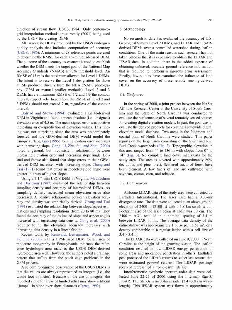
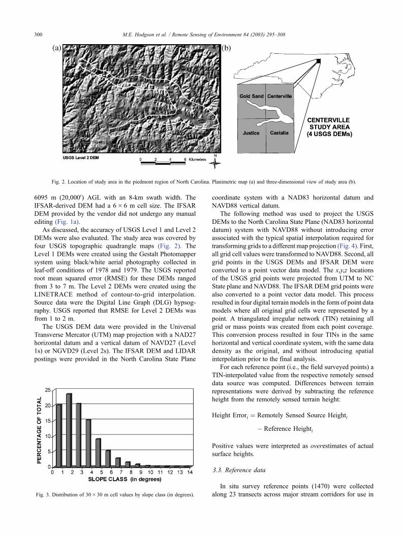
Bud Creek watersheds (Fig. 2). Topographic elevation in

this area ranged from 44 to 136 m with slopes from 0j to

14j (Fig. 3). No complete land cover map exists for the

study area. The area is covered with approximately 60%

deciduous and pine forest. Scattered tracts of forest have

been clearcut. A few tracts of land are cultivated with

soybean, cotton, corn, and tobacco.

3.2. Data sources

Airborne LIDAR data of the study area were collected by

Earthdata International. The laser used had a 0.33-mr

divergence rate. The data were collected at an above ground

elevation of 2400 m (8100 ft) with a 1.8-km swath width.

Footprint size of the laser beam at nadir was 79 cm. The

2400-m AGL resulted in a nominal spacing of 3.4 m

between LIDAR points. The average data density of the

entire dataset was approximately 1 pulse per 11.58 m2, or a

density comparable to a regular lattice with a cell size of

3.4� 3.4 m.

The LIDAR data were collected on June 9, 2000 in North

Carolina at the height of the growing season. The leaf-on

condition resulted in low LIDAR energy penetration in

some areas and no canopy penetration in others. Earthdata

post-processed the LIDAR returns to select last returns that

were estimated ground returns. The LIDAR postings

received represented a ‘‘bald-earth’’ dataset.

Interferometric synthetic aperture radar data were col-

lected June 22-25 of 2000 using the Intermap Star-3i

IFSAR. The Star-3i is an X-band radar (2.4–3.8 cm wave-

length). This IFSAR system was flown at approximately


6095 m (20,000V) AGL with an 8-km swath width. The

IFSAR-derived DEM had a 6� 6 m cell size. The IFSAR

DEM provided by the vendor did not undergo any manual

editing (Fig. 1a).

As discussed, the accuracy of USGS Level 1 and Level 2

DEMs were also evaluated. The study area was covered by

four USGS topographic quadrangle maps (Fig. 2). The

Level 1 DEMs were created using the Gestalt Photomapper

system using black/white aerial photography collected in

leaf-off conditions of 1978 and 1979. The USGS reported

root mean squared error (RMSE) for these DEMs ranged

from 3 to 7 m. The Level 2 DEMs were created using the

LINETRACE method of contour-to-grid interpolation.

Source data were the Digital Line Graph (DLG) hypsog-

raphy. USGS reported that RMSE for Level 2 DEMs was

from 1 to 2 m.

The USGS DEM data were provided in the Universal

Transverse Mercator (UTM) map projection with a NAD27

horizontal datum and a vertical datum of NAVD27 (Level

1s) or NGVD29 (Level 2s). The IFSAR DEM and LIDAR

postings were provided in the North Carolina State Plane

coordinate system with a NAD83 horizontal datum and

NAVD88 vertical datum.

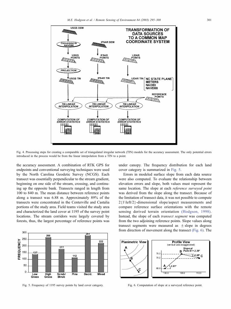
The following method was used to project the USGS

DEMs to the North Carolina State Plane (NAD83 horizontal

datum) system with NAVD88 without introducing error

associated with the typical spatial interpolation required for

transforming grids to a different map projection (Fig. 4). First,

all grid cell values were transformed to NAVD88. Second, all

grid points in the USGS DEMs and IFSAR DEM were

converted to a point vector data model. The x,y,z locations

of the USGS grid points were projected from UTM to NC

State plane and NAVD88. The IFSAR DEM grid points were

also converted to a point vector data model. This process

resulted in four digital terrain models in the form of point data

models where all original grid cells were represented by a

point. A triangulated irregular network (TIN) retaining all

grid or mass points was created from each point coverage.

This conversion process resulted in four TINs in the same

horizontal and vertical coordinate system, with the same data

density as the original, and without introducing spatial

interpolation prior to the final analysis.

For each reference point (i.e., the field surveyed points) a

TIN-interpolated value from the respective remotely sensed

data source was computed. Differences between terrain

representations were derived by subtracting the reference

height from the remotely sensed terrain height:

Height Errori ¼ Remotely Sensed Source Heighti

� Reference Heighti

Positive values were interpreted as overestimates of actual

surface heights.

3.3. Reference data

In situ survey reference points (1470) were collected

along 23 transects across major stream corridors for use inFig. 3. Distribution of 30� 30 m cell values by slope class (in degrees).

Fig. 2. Location of study area in the piedmont region of North Carolina. Planimetric map (a) and three-dimensional view of study area (b).


the accuracy assessment. A combination of RTK GPS for

endpoints and conventional surveying techniques were used

by the North Carolina Geodetic Survey (NCGS). Each

transect was essentially perpendicular to the stream gradient,

beginning on one side of the stream, crossing, and continu-

ing up the opposite bank. Transects ranged in length from

100 to 840 m. The mean distance between reference points

along a transect was 6.88 m. Approximately 89% of the

transects were concentrated in the Centerville and Castalia

portions of the study area. Field teams visited the study area

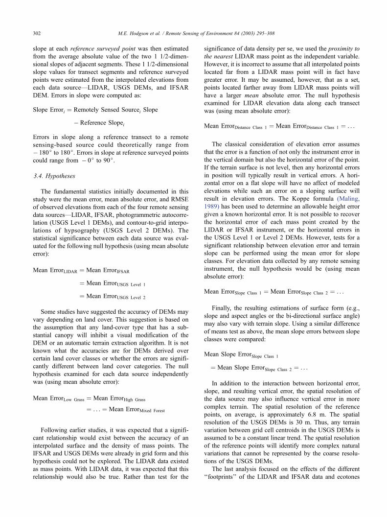
and characterized the land cover at 1195 of the survey point

locations. The stream corridors were largely covered by

forests, thus, the largest percentage of reference points was

under canopy. The frequency distribution for each land

cover category is summarized in Fig. 5.

Errors in modeled surface slope from each data source

were also computed. To evaluate the relationship between

elevation errors and slope, both values must represent the

same location. The slope at each reference surveyed point

was derived from the slope along the transect. Because of

the limitation of transect data, it was not possible to compute

2{1\left/2}-dimensional slope/aspect measurements and

compare reference surface orientations with the remote

sensing derived terrain orientation (Hodgson, 1998).

Instead, the slope of each transect segment was computed

from the two adjoining reference points. Slope values along

transect segments were measured as F slope in degrees

from direction of movement along the transect (Fig. 6). The

Fig. 5. Frequency of 1195 survey points by land cover category. Fig. 6. Computation of slope at a surveyed reference point.

Fig. 4. Processing steps for creating a comparable set of triangulated irregular network (TIN) models for the accuracy assessment. The only potential errors

introduced in the process would be from the linear interpolation from a TIN to a point.


slope at each reference surveyed point was then estimated

from the average absolute value of the two 1 1/2-dimen-

sional slopes of adjacent segments. These 1 1/2-dimensional

slope values for transect segments and reference surveyed

points were estimated from the interpolated elevations from

each data source—LIDAR, USGS DEMs, and IFSAR

DEM. Errors in slope were computed as:

Slope Errori ¼ Remotely Sensed Sourcei Slope

� Reference Slopei

Errors in slope along a reference transect to a remote

sensing-based source could theoretically range from

� 180j to 180j. Errors in slope at reference surveyed points

could range from � 0j to 90j.

3.4. Hypotheses

The fundamental statistics initially documented in this

study were the mean error, mean absolute error, and RMSE

of observed elevations from each of the four remote sensing

data sources—LIDAR, IFSAR, photogrammetric autocorre-

lation (USGS Level 1 DEMs), and contour-to-grid interpo-

lations of hypsography (USGS Level 2 DEMs). The

statistical significance between each data source was eval-

uated for the following null hypothesis (using mean absolute

error):

Mean ErrorLIDAR ¼ Mean ErrorIFSAR

¼ Mean ErrorUSGS Level 1

¼ Mean ErrorUSGS Level 2

Some studies have suggested the accuracy of DEMs may

vary depending on land cover. This suggestion is based on

the assumption that any land-cover type that has a sub-

stantial canopy will inhibit a visual modification of the

DEM or an automatic terrain extraction algorithm. It is not

known what the accuracies are for DEMs derived over

certain land cover classes or whether the errors are signifi-

cantly different between land cover categories. The null

hypothesis examined for each data source independently

was (using mean absolute error):

Mean ErrorLow Grass ¼ Mean ErrorHigh Grass

¼ . . . ¼ Mean ErrorMixed Forest

Following earlier studies, it was expected that a signifi-

cant relationship would exist between the accuracy of an

interpolated surface and the density of mass points. The

IFSAR and USGS DEMs were already in grid form and this

hypothesis could not be explored. The LIDAR data existed

as mass points. With LIDAR data, it was expected that this

relationship would also be true. Rather than test for the

significance of data density per se, we used the proximity to

the nearest LIDAR mass point as the independent variable.

However, it is incorrect to assume that all interpolated points

located far from a LIDAR mass point will in fact have

greater error. It may be assumed, however, that as a set,

points located farther away from LIDAR mass points will

have a larger mean absolute error. The null hypothesis

examined for LIDAR elevation data along each transect

was (using mean absolute error):

Mean ErrorDistance Class 1 ¼ Mean ErrorDistance Class 1 ¼ . . .

The classical consideration of elevation error assumes

that the error is a function of not only the instrument error in

the vertical domain but also the horizontal error of the point.

If the terrain surface is not level, then any horizontal errors

in position will typically result in vertical errors. A hori-

zontal error on a flat slope will have no affect of modeled

elevations while such an error on a sloping surface will

result in elevation errors. The Koppe formula (Maling,

1989) has been used to determine an allowable height error

given a known horizontal error. It is not possible to recover

the horizontal error of each mass point created by the

LIDAR or IFSAR instrument, or the horizontal errors in

the USGS Level 1 or Level 2 DEMs. However, tests for a

significant relationship between elevation error and terrain

slope can be performed using the mean error for slope

classes. For elevation data collected by any remote sensing

instrument, the null hypothesis would be (using mean

absolute error):

Mean ErrorSlope Class 1 ¼ Mean ErrorSlope Class 2 ¼ . . .

Finally, the resulting estimations of surface form (e.g.,

slope and aspect angles or the bi-directional surface angle)

may also vary with terrain slope. Using a similar difference

of means test as above, the mean slope errors between slope

classes were compared:

Mean Slope ErrorSlope Class 1

¼ Mean Slope ErrorSlope Class 2 ¼ . . .

In addition to the interaction between horizontal error,

slope, and resulting vertical error, the spatial resolution of

the data source may also influence vertical error in more

complex terrain. The spatial resolution of the reference

points, on average, is approximately 6.8 m. The spatial

resolution of the USGS DEMs is 30 m. Thus, any terrain

variation between grid cell centroids in the USGS DEMs is

assumed to be a constant linear trend. The spatial resolution

of the reference points will identify more complex natural

variations that cannot be represented by the coarse resolu-

tions of the USGS DEMs.

The last analysis focused on the effects of the different

‘‘footprints’’ of the LIDAR and IFSAR data and ecotones


(i.e., land cover boundaries). As discussed earlier, the

integration within the 5� 5 m IFSAR footprint would be

expected to introduce additional errors along an ecotone.

For the low grass class, the mean absolute error at all

reference points was compared to the error of reference

points located farther than 5 m from a class boundary.

Mean Absolute ErrorLow Grass Class; All

¼ Mean Absolute ErrorLow Grass Class; >5 m

3.5. Analysis methods

Analysis of variances (ANOVAs) were conducted for

each hypothesis tested using the mean absolute error in

elevation. The absolute error in elevation was used rather

than RMSE as this meets the assumptions of the ANOVA

statistical test (i.e., RMSE is a measure of the distribution

about the true location rather than the distribution about the

mean location). A multiple ANOVAwas used to test for the

significance of land cover, slope, and their interaction in

one test.

4. Results

4.1. Elevation error

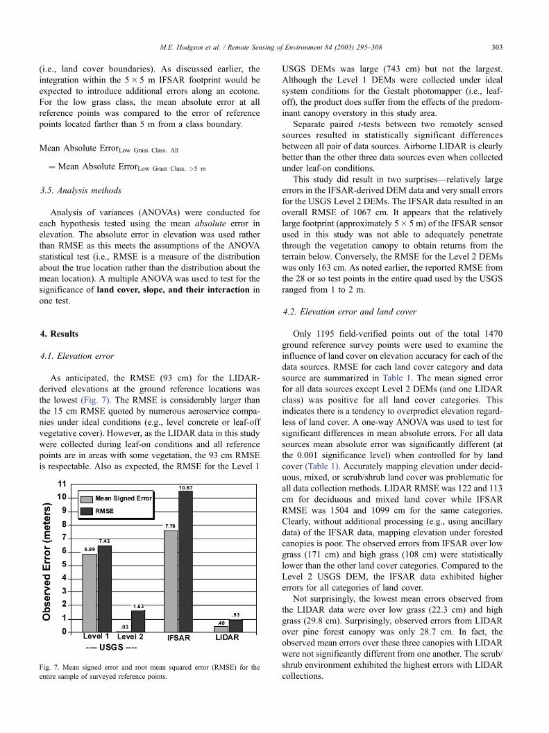
As anticipated, the RMSE (93 cm) for the LIDAR-

derived elevations at the ground reference locations was

the lowest (Fig. 7). The RMSE is considerably larger than

the 15 cm RMSE quoted by numerous aeroservice compa-

nies under ideal conditions (e.g., level concrete or leaf-off

vegetative cover). However, as the LIDAR data in this study

were collected during leaf-on conditions and all reference

points are in areas with some vegetation, the 93 cm RMSE

is respectable. Also as expected, the RMSE for the Level 1

USGS DEMs was large (743 cm) but not the largest.

Although the Level 1 DEMs were collected under ideal

system conditions for the Gestalt photomapper (i.e., leaf-

off), the product does suffer from the effects of the predom-

inant canopy overstory in this study area.

Separate paired t-tests between two remotely sensed

sources resulted in statistically significant differences

between all pair of data sources. Airborne LIDAR is clearly

better than the other three data sources even when collected

under leaf-on conditions.

This study did result in two surprises—relatively large

errors in the IFSAR-derived DEM data and very small errors

for the USGS Level 2 DEMs. The IFSAR data resulted in an

overall RMSE of 1067 cm. It appears that the relatively

large footprint (approximately 5� 5 m) of the IFSAR sensor

used in this study was not able to adequately penetrate

through the vegetation canopy to obtain returns from the

terrain below. Conversely, the RMSE for the Level 2 DEMs

was only 163 cm. As noted earlier, the reported RMSE from

the 28 or so test points in the entire quad used by the USGS

ranged from 1 to 2 m.

4.2. Elevation error and land cover

Only 1195 field-verified points out of the total 1470

ground reference survey points were used to examine the

influence of land cover on elevation accuracy for each of the

data sources. RMSE for each land cover category and data

source are summarized in Table 1. The mean signed error

for all data sources except Level 2 DEMs (and one LIDAR

class) was positive for all land cover categories. This

indicates there is a tendency to overpredict elevation regard-

less of land cover. A one-way ANOVA was used to test for

significant differences in mean absolute errors. For all data

sources mean absolute error was significantly different (at

the 0.001 significance level) when controlled for by land

cover (Table 1). Accurately mapping elevation under decid-

uous, mixed, or scrub/shrub land cover was problematic for

all data collection methods. LIDAR RMSE was 122 and 113

cm for deciduous and mixed land cover while IFSAR

RMSE was 1504 and 1099 cm for the same categories.

Clearly, without additional processing (e.g., using ancillary

data) of the IFSAR data, mapping elevation under forested

canopies is poor. The observed errors from IFSAR over low

grass (171 cm) and high grass (108 cm) were statistically

lower than the other land cover categories. Compared to the

Level 2 USGS DEM, the IFSAR data exhibited higher

errors for all categories of land cover.

Not surprisingly, the lowest mean errors observed from

the LIDAR data were over low grass (22.3 cm) and high

grass (29.8 cm). Surprisingly, observed errors from LIDAR

over pine forest canopy was only 28.7 cm. In fact, the

observed mean errors over these three canopies with LIDAR

were not significantly different from one another. The scrub/

shrub environment exhibited the highest errors with LIDAR

collections.Fig. 7. Mean signed error and root mean squared error (RMSE) for the

entire sample of surveyed reference points.


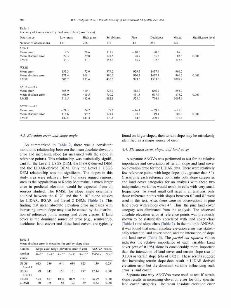
4.3. Elevation error and slope angle

As summarized in Table 2, there was a consistent

monotonic relationship between the mean absolute elevation

error and increasing slope (as measured with the slope at

reference points). This relationship was statistically signifi-

cant for the Level 2 USGS DEM, the IFSAR-derived DEM

and the LIDAR-derived DEM. Only the Level 1 USGS

DEM relationship was not significant. The slopes in this

study area were relatively low. For more rugged regions,

such as the Appalachian or Rocky Mountains, a much larger

error in predicted elevation would be expected from all

sources studied. The RMSE for slope angle essentially

doubled between the 0–2j and the 8–10j slope classes

for LIDAR, IFSAR and Level 2 DEMs (Table 2). This

finding that mean absolute elevation error increases with

increasing terrain slope may also be caused by the distribu-

tion of reference points among land cover classes. If land

cover is the dominant source of error (e.g., scrub/shrub,

deciduous land cover) and these land covers are typically

found on larger slopes, then terrain slope may be mistakenly

identified as a major source of error.

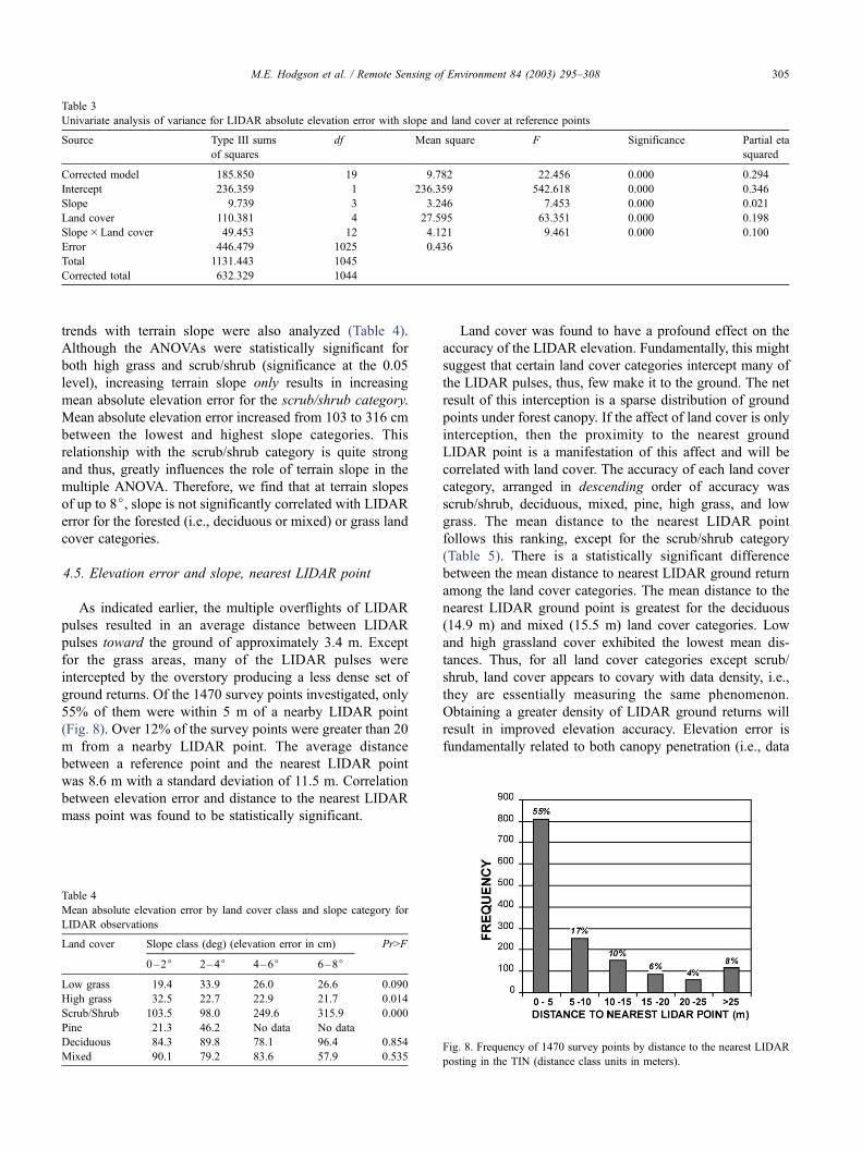
4.4. Elevation error, slope, and land cover

A separate ANOVAwas performed to test for the relative

importance and covariation of terrain slope and land cover

on elevation error for the LIDAR data. There were relatively

few reference points with large slopes (i.e., greater than 8j).Classifying each reference point into both slope categories

and land cover categories for an analysis with these two

independent variables would result in cells with very small

frequencies. To avoid small cell sizes in an analysis, only

those reference points with slopes between 0j and 8j were

used in this test. Also, there were no observations in pine

land cover with slopes over 4j. Thus, the pine land cover

category was eliminated from the analysis. The observed

absolute elevation error at reference points was previously

shown to be statistically correlated with land cover class

(Table 1) and slope class (Table 2). In the multiple ANOVA,

it was found that mean absolute elevation error was statisti-

cally related to land cover, slope, and the interaction of slope

and land cover (Table 3). The partial eta squared values

indicates the relative importance of each variable. Land

cover (eta of 0.198) alone is considerably more important

than the interaction of land cover and terrain slope (eta of

0.100) or terrain slope (eta of 0.021). These results suggest

that increasing terrain slope does result in LIDAR derived

elevation error but the dominant variable influencing such

error is land cover.

Separate one-way ANOVAs were used to test if terrain

slope results in increasing elevation error for only specific

land cover categories. The mean absolute elevation error

Table 2

Mean absolute error in elevation (in cm) by slope class

Remote Slope class (deg) (elevation error in cm) ANOVA results

sensing

source

0–2j 2–4j 4–6j 6–8j 8–10j F-Value Pr>F

USGS

Level 1

613 589 641 634 825 1.39 0.234

USGS

Level 2

99 142 161 161 197 17.44 0.001

IFSAR 574 817 1036 1029 1357 26.79 0.001

LIDAR 60 65 88 93 89 5.32 0.001

Table 1

Accuracy of terrain model by land cover class (error in cm)

Data source Low grass High grass Scrub/shrub Pine Deciduous Mixed Significance level

Number of observations 137 266 177 112 281 222

LIDAR

Mean error 19.5 28.6 111.9 � 10.6 20.6 69.3

Mean absolute error 22.3 29.8 121.5 28.7 85.5 83.8 0.001

RMSE 33.3 37.1 153.4 45.7 122.2 113.4

IFSAR

Mean error 133.3 72.0 379.2 929.5 1437.4 966.2


RMSE 306.2 173.6 435.7 993.5 1503.6 1099.9

USGS Level 1

Mean error 465.9 410.1 722.0 418.2 666.7 854.7


RMSE 519.5 482.6 882.1 528.0 794.6 1005.9

USGS Level 2

Mean error � 21.3 24.7 77.6 � 46.4 � 69.8 � 18.3


RMSE 142.5 141.4 170.6 144.6 200.2 136.4


trends with terrain slope were also analyzed (Table 4).

Although the ANOVAs were statistically significant for

both high grass and scrub/shrub (significance at the 0.05

level), increasing terrain slope only results in increasing

mean absolute elevation error for the scrub/shrub category.

Mean absolute elevation error increased from 103 to 316 cm

between the lowest and highest slope categories. This

relationship with the scrub/shrub category is quite strong

and thus, greatly influences the role of terrain slope in the

multiple ANOVA. Therefore, we find that at terrain slopes

of up to 8j, slope is not significantly correlated with LIDAR

error for the forested (i.e., deciduous or mixed) or grass land

cover categories.

4.5. Elevation error and slope, nearest LIDAR point

As indicated earlier, the multiple overflights of LIDAR

pulses resulted in an average distance between LIDAR

pulses toward the ground of approximately 3.4 m. Except

for the grass areas, many of the LIDAR pulses were

intercepted by the overstory producing a less dense set of

ground returns. Of the 1470 survey points investigated, only

55% of them were within 5 m of a nearby LIDAR point

(Fig. 8). Over 12% of the survey points were greater than 20

m from a nearby LIDAR point. The average distance

between a reference point and the nearest LIDAR point

was 8.6 m with a standard deviation of 11.5 m. Correlation

between elevation error and distance to the nearest LIDAR

mass point was found to be statistically significant.

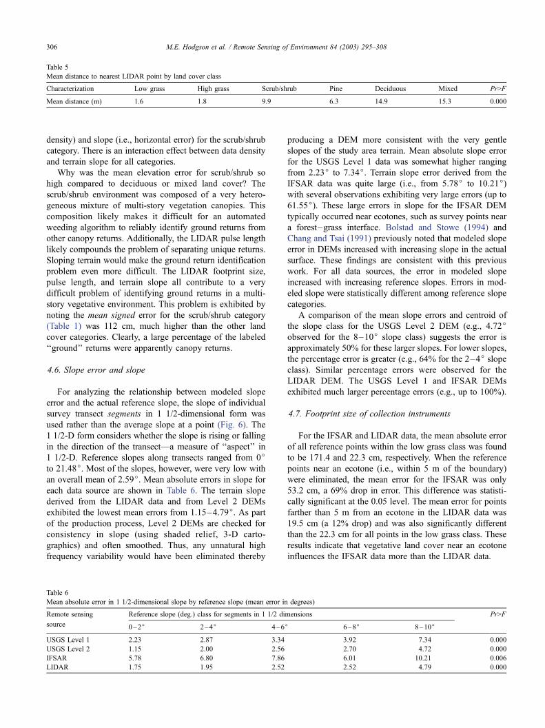
Land cover was found to have a profound effect on the

accuracy of the LIDAR elevation. Fundamentally, this might

suggest that certain land cover categories intercept many of

the LIDAR pulses, thus, few make it to the ground. The net

result of this interception is a sparse distribution of ground

points under forest canopy. If the affect of land cover is only

interception, then the proximity to the nearest ground

LIDAR point is a manifestation of this affect and will be

correlated with land cover. The accuracy of each land cover

category, arranged in descending order of accuracy was

scrub/shrub, deciduous, mixed, pine, high grass, and low

grass. The mean distance to the nearest LIDAR point

follows this ranking, except for the scrub/shrub category

(Table 5). There is a statistically significant difference

between the mean distance to nearest LIDAR ground return

among the land cover categories. The mean distance to the

nearest LIDAR ground point is greatest for the deciduous

(14.9 m) and mixed (15.5 m) land cover categories. Low

and high grassland cover exhibited the lowest mean dis-

tances. Thus, for all land cover categories except scrub/

shrub, land cover appears to covary with data density, i.e.,

they are essentially measuring the same phenomenon.

Obtaining a greater density of LIDAR ground returns will

result in improved elevation accuracy. Elevation error is

fundamentally related to both canopy penetration (i.e., data

Table 4

Mean absolute elevation error by land cover class and slope category for

LIDAR observations

Land cover Slope class (deg) (elevation error in cm) Pr>F

0–2j 2–4j 4–6j 6–8j

Low grass 19.4 33.9 26.0 26.6 0.090

High grass 32.5 22.7 22.9 21.7 0.014

Scrub/Shrub 103.5 98.0 249.6 315.9 0.000

Pine 21.3 46.2 No data No data

Deciduous 84.3 89.8 78.1 96.4 0.854

Mixed 90.1 79.2 83.6 57.9 0.535

Table 3

Univariate analysis of variance for LIDAR absolute elevation error with slope and land cover at reference points

Source Type III sums

of squares

df Mean square F Significance Partial eta

squared

Corrected model 185.850 19 9.782 22.456 0.000 0.294

Intercept 236.359 1 236.359 542.618 0.000 0.346

Slope 9.739 3 3.246 7.453 0.000 0.021

Land cover 110.381 4 27.595 63.351 0.000 0.198

Slope�Land cover 49.453 12 4.121 9.461 0.000 0.100

Error 446.479 1025 0.436

Total 1131.443 1045

Corrected total 632.329 1044

Fig. 8. Frequency of 1470 survey points by distance to the nearest LIDAR

posting in the TIN (distance class units in meters).


density) and slope (i.e., horizontal error) for the scrub/shrub

category. There is an interaction effect between data density

and terrain slope for all categories.

Why was the mean elevation error for scrub/shrub so

high compared to deciduous or mixed land cover? The

scrub/shrub environment was composed of a very hetero-

geneous mixture of multi-story vegetation canopies. This

composition likely makes it difficult for an automated

weeding algorithm to reliably identify ground returns from

other canopy returns. Additionally, the LIDAR pulse length

likely compounds the problem of separating unique returns.

Sloping terrain would make the ground return identification

problem even more difficult. The LIDAR footprint size,

pulse length, and terrain slope all contribute to a very

difficult problem of identifying ground returns in a multi-

story vegetative environment. This problem is exhibited by

noting the mean signed error for the scrub/shrub category

(Table 1) was 112 cm, much higher than the other land

cover categories. Clearly, a large percentage of the labeled

‘‘ground’’ returns were apparently canopy returns.

4.6. Slope error and slope

For analyzing the relationship between modeled slope

error and the actual reference slope, the slope of individual

survey transect segments in 1 1/2-dimensional form was

used rather than the average slope at a point (Fig. 6). The

1 1/2-D form considers whether the slope is rising or falling

in the direction of the transect—a measure of ‘‘aspect’’ in

1 1/2-D. Reference slopes along transects ranged from 0jto 21.48j. Most of the slopes, however, were very low with

an overall mean of 2.59j. Mean absolute errors in slope for

each data source are shown in Table 6. The terrain slope

derived from the LIDAR data and from Level 2 DEMs

exhibited the lowest mean errors from 1.15–4.79j. As partof the production process, Level 2 DEMs are checked for

consistency in slope (using shaded relief, 3-D carto-

graphics) and often smoothed. Thus, any unnatural high

frequency variability would have been eliminated thereby

producing a DEM more consistent with the very gentle

slopes of the study area terrain. Mean absolute slope error

for the USGS Level 1 data was somewhat higher ranging

from 2.23j to 7.34j. Terrain slope error derived from the

IFSAR data was quite large (i.e., from 5.78j to 10.21j)with several observations exhibiting very large errors (up to

61.55j). These large errors in slope for the IFSAR DEM

typically occurred near ecotones, such as survey points near

a forest–grass interface. Bolstad and Stowe (1994) and

Chang and Tsai (1991) previously noted that modeled slope

error in DEMs increased with increasing slope in the actual

surface. These findings are consistent with this previous

work. For all data sources, the error in modeled slope

increased with increasing reference slopes. Errors in mod-

eled slope were statistically different among reference slope

categories.

A comparison of the mean slope errors and centroid of

the slope class for the USGS Level 2 DEM (e.g., 4.72jobserved for the 8–10j slope class) suggests the error is

approximately 50% for these larger slopes. For lower slopes,

the percentage error is greater (e.g., 64% for the 2–4j slope

class). Similar percentage errors were observed for the

LIDAR DEM. The USGS Level 1 and IFSAR DEMs

exhibited much larger percentage errors (e.g., up to 100%).

4.7. Footprint size of collection instruments

For the IFSAR and LIDAR data, the mean absolute error

of all reference points within the low grass class was found

to be 171.4 and 22.3 cm, respectively. When the reference

points near an ecotone (i.e., within 5 m of the boundary)

were eliminated, the mean error for the IFSAR was only

53.2 cm, a 69% drop in error. This difference was statisti-

cally significant at the 0.05 level. The mean error for points

farther than 5 m from an ecotone in the LIDAR data was

19.5 cm (a 12% drop) and was also significantly different

than the 22.3 cm for all points in the low grass class. These

results indicate that vegetative land cover near an ecotone

influences the IFSAR data more than the LIDAR data.

Table 5

Mean distance to nearest LIDAR point by land cover class

Characterization Low grass High grass Scrub/shrub Pine Deciduous Mixed Pr>F

Mean distance (m) 1.6 1.8 9.9 6.3 14.9 15.3 0.000

Table 6

Mean absolute error in 1 1/2-dimensional slope by reference slope (mean error in degrees)

Remote sensing Reference slope (deg.) class for segments in 1 1/2 dimensions Pr>F

source 0–2j 2–4j 4–6j 6–8j 8–10j

USGS Level 1 2.23 2.87 3.34 3.92 7.34 0.000

USGS Level 2 1.15 2.00 2.56 2.70 4.72 0.000

IFSAR 5.78 6.80 7.86 6.01 10.21 0.006

LIDAR 1.75 1.95 2.52 2.52 4.79 0.000


5. Discussion

The distribution of reference points in this study was

very large compared to the checks by the U.S. Geological

Survey using National Map Accuracy Standards. A typical

check by USGS would use 20–30 points well distributed

around the map. Our reference data were concentrated in

riverine and adjacent areas and may not represent the wide

variety of land cover types. Given these differences, it

should be noted that the observed RMSE for the individual

Level 1 DEMS ranged from 4.8 to 10.0 m, while the USGS

reported RMSEs ranging from 3 to 7 m. The USGS reported

RMSE for the four Level 2 DEMs ranged from 1 to 2 m.

The observed Level 2 RMSE for our study varied between

0.78 and 1.90 m for the same four DEMs, consistent with

the USGS observations. While the USGS puts great empha-

sis on modeling surface form (i.e., terrain slope, aspect, and

drainage) in their Level 2 and 3 DEMs, there is no accuracy

standard or attempt to report the accuracy of such parame-

ters. For the Level 1 and 2 DEMs, the error in 1 1/2-

dimensional surface slope is roughly 50%. If this relation-

ship found in slopes ranging from 0j to 10j also holds for

higher slopes then expect to see an average 10j error for

20j slopes, for instance.

All data sources other than the Level 2 DEMs (and one

LIDAR class) overpredicted elevation, on average, regard-

less of land cover. Since the automated stereocorrelation

technique used for the GPM-derived Level 1 DEMs models

the canopy top, this average overprediction in elevations is

not surprising. The IFSAR-derived DEM also suffered from

the canopy problems.

The 113–122 cm RMSE of LIDAR derived elevation in

deciduous/mixed forested areas would be a lower confi-

dence bound for mapping vegetation height (relatively

homogenous canopies) from a single LIDAR overflight.

Estimates of canopy height in a scrub/shrub environment

would be less accurate. Determining vegetation height

requires differencing the estimated canopy elevation from

the estimated surface elevation (Means et al., 2000). The

data collected in leaf-on conditions may be ideal for

determining canopy elevation but not ground elevation.

Conversely, leaf-off conditions may not provide good esti-

mates of canopy height.

Most aeroservice companies advertise LIDAR accuracies

from 15 to 25 cm RMSE, depending on flying height. The

15 cm RMSE is an important threshold for FEMA in

evaluating data sources for mapping floodplains. The find-

ings from this study suggest this 15 cm threshold is not

obtainable with LIDAR during the growing season over any

surface with vegetative cover.

The reported elevation accuracy from the LIDAR or

IFSAR data is strongly related to land cover and to a

somewhat lesser degree is related to slope. Forested land

cover influences the LIDAR penetration rate and multi-story

vegetative cover (e.g., scrub/shrub) confuses the automated

weeding algorithms. Future LIDAR sensors with very high

pulse rates (e.g., 40,000–50,000 pulse/s) may overcome

much of the interception problem in forested areas. Using

lasers with narrower beam divergences and the resulting

smaller footprints would also help in penetrating breaks in

the canopy. Flying at lower altitudes would also reduce the

footprint size. However, more ‘‘intelligent’’ algorithms and

lasers with shorter pulse lengths are needed to map elevation

in multi-story environments, like scrub/shrub. Surprisingly,

pine forests did not dramatically impact LIDAR accuracy.

Not surprisingly, the IFSAR system did not perform well

over the forested surface. Manual editing of the surface (Fig.

1) would be required for this land cover when using IFSAR

data. The Level 2 DEMs from USGS exhibited RMSEs

from 1.4 to 2.0 m with little difference between land cover

categories.

The average slope by land cover class ranged from 1.6jto 3.3j. The Koppe formula demonstrates elevation error

will increase with increasing slope if the data contain any

horizontal errors. As the slopes in this study were relatively

low, the impact of terrain slope on elevation accuracy is

rather minimal. Greater elevation errors may be expected in

areas of more rugged terrain. For those environmental

studies (e.g., hydrologic, biogeographic) requiring either

accurate elevation or terrain slope, either LIDAR or the

USGS Level 2 DEMs are far superior to either the USGS

Level 1 or IFSAR-based DEMs. However, the approxi-

mately 50% errors in terrain slope at about 8–10j slope

should be noted when in applications that require highly

accurate terrain slope estimations for specific sites.

Finally, the integration within the large footprint of the

IFSAR data results in greater errors along ecotones where

the vegetation height of one class is quite different than the

vegetation of a neighboring class (e.g., low grass and

forest). A significant effect of the ecotone was also found

with the LIDAR data although the change in mean errors

was not nearly as pronounced as with the IFSAR data.

Acknowledgements

The authors express their appreciation to Gary Thompson

at the North Carolina Geodetic Survey for the collection of

reference points. Karen Shuckman at Earthdata International

provided the LIDAR data and assisted in the interpretation

of the findings. We also thank George Raber and Jason

Tullis for collection of the land cover information. Bryan

Mercer of Intermap provided useful comments and

interpretation of the IFSAR data and David Box provided

in depth information on LIDAR sensors.

References

Acevedo, W. (1991). First assessment of the U.S. Geological Survey 30-

minute DEM’s: a great improvement over existing 1-degree data. Pro-

ceedings of the Annual Meetings of the ACSM-ASPRS, 1–12.


Bolstad, P. V., & Stowe, T. (1994). An evaluation of DEM accuracy:

elevation, slope, and aspect. Photogrammetric Engineering and Remote

Sensing, 60(11), 1327–1332.

Box, D. (2001). Personal communication.

Brown, D. G., & Bara, T. J. (1994). Recognition and reduction of system-

atic error in elevation and derivative surfaces from 7-1/2 minute DEMs.

Photogrammetric Engineering and Remote Sensing, 60(2), 189–194.

Carter, J. R. (1992). The effect of data precision on the calculation of slope

and aspect using gridded DEMs. Cartographica, 29(1), 22–34.

Chang, K., & Tsai, B. (1991). The effect of DEM resolution on slope and

aspect mapping. Cartography and Geographic Information Systems, 9

(4), 405–419.

Cowen, D. J., Jensen, J. R., Hendrix, C., Hodgson, M. E., & Schill, S. R.

(2000). A GIS-assisted rail construction econometric model that incor-

porates LIDAR data. Photogrammetric Engineering and Remote Sens-

ing, 66(11), 1323–1326.

Gao, J. (1995). Comparison of sampling schemes in constructing DTMs

from topographic maps. The ITC Journal, 1, 18–22.

Garbrecht, J., & Starks, P. (1995). Note on the use of USGS level 7.5-

minute DEM coverages for landscape drainage analyses. Photogram-

metric Engineering and Remote Sensing, 61(5), 519–522.

Gong, J., Li, Z., Zhu, Q., Sui, H., & Zhou, Y. (2000). Effects of various

factors on the accuracy of DEMs: an intensive experimental inves-

tigation. Photogrammetric Engineering and Remote Sensing, 66(9),

1113–1117.

Guth, P. L. (1999). Contour line ‘‘ghosts’’ in USGS level 2 DEMs. Photo-

grammetric Engineering and Remote Sensing., 65(3), 289–296.

Hodgson, M. E. (1998). Comparison of bi-directional angles from surface

slope/aspect algorithms. Cartography and Geographic Information Sys-

tems, 25(3), 173–187.

Jensen, J. R. (2000). Active and passive microwave, and LIDAR remote

sensing. Remote sensing of the environment: an earth resource perspec-

tive (pp. 285–332). NJ: Prentice-Hall, Chap. 9.

Jensen, J. R., Hodgson, M. E., Mackey, H. E., & Krabill, W. (1987).

Correlation between aircraft MSS and LIDAR remotely sensed data

on a forested wetland. Geocarto International, 2(4), 39–54.

JPL (1999). Shuttle radar topography mission. Pasadena: Jet Propulsion

Laboratory, http://www-radar.jpl.nasa.gov/srtm/tech_factsheet.html.

Kelly, R. E., McConnell, P. R. H., & Mildenberger, S. J. (1977). The

Gestalt photomapping system. Photogrammetric Engineering and Re-

mote Sensing, 43(11), 1407–1417.

Kenward, T., Lettenmaier, D. P., Wood, E. F., & Fielding, E. (2000). Effects

of digital elevation model accuracy on hydrologic predictions. Remote

Sensing of Environment, 74, 432–444.

Kok, A. L., Blais, J. A. R., & Rangayyan, R. M. (1987). Filtering of

digitally correlated Gestalt elevation data. Photogrammetric Engineer-

ing and Remote Sensing, 53(5), 535–538.

Lane, T. (2001). Personal communication.

MacEachren, A. M., & Davidson, J. V. (1987). Sampling and isometric

mapping of continuous geographic surfaces. The American Cartogra-

pher, 14(4), 229–320.

Maling, D. H. (1989). Measurements from maps. NY: Pergamon.

Maune, D. F. (1996). Introduction to digital elevation models (DEM).

Digital photogrammetry: an addendum to the manual of photogram-

metry. Bethesda, MD: American Society for Photogrammetry and

Remote Sensing (portion of Chap. 6).

Means, J. E., Acker, S. A., Fitt, B. J., Renslow, M., Emerson, L., &

Hendrix, C. J. (2000). Predicting forest stand characteristics with air-

borne scanning LIDAR. Photogrammetric Engineering and Remote

Sensing, 66(11), 1367–1371.

Mercer, B. (2001). Personal communication.

Pereira, L. M. G., & Janssen, L. L. F. (1999). Suitability of laser data for

DTM generation: a case study in the context of road planning and

design. Photogrammetry and Remote Sensing, 54, 244–253.

Plaut, J. J., Rivard, B., & D’lorio, M. A. (1999). Radar: sensors and case

studies. In A. N. Rencz (Ed.), Remote sensing for the earth sciences:

manual of remote sensing, vol. 3 (3rd ed.) (pp. 613–642). New York:

Wiley.

Thrower, N. J. W., & Jensen, J. R. (1976). The orthophoto and orthopho-

tomap: characteristics, development and application. The American

Cartographer, 3(1), 39–56.

United States Geological Survey (USGS) (1986). Standards for Digital

Elevation Models, Open File Report 86-004.

Yoeli, P. Y. (1986). Computer executed production of a regular grid of

height points from digital contours. The American Cartographer, 13,

219–229.

Zycor (1983). User’s manual for contour-to-grid interpolation. Reston,

VA: U.S. Geological Survey.


http:\\www-radar.jpl.nasa.gov\srtm\tech_factsheet.html

An evaluation of LIDAR and IFSAR-derived digital elevation models in leaf-on conditions with USGS...

Documents

Transcript of An evaluation of LIDAR and IFSAR-derived digital elevation models in leaf-on conditions with USGS...