Marching triangles: Range image fusion for complex object modelling
Upload
khangminh22Category
view
2download
0
&PE RSPPH
OTO
GRA
MM
ETRI
C
HO
TOG
RAM
MET
RIC
EEN
GIN
EERI
NG
&
NG
INEE
RIN
G &
RREM
OTE
EM
OTE
SSEN
SIN
GEN
SIN
G
Th
e o
ffici
al j
ou
rna
l fo
r im
ag
ing
an
d g
eo
spa
tial i
nfo
rma
tion
sci
en
ce a
nd
tech
no
log
y
February 2010 Volume 76, Number 2
Special Issue: Geographic Object-Based Image Analysis (GEOBIA)
Cover.indd 1Cover.indd 1 1/15/2010 2:04:31 PM1/15/2010 2:04:31 PM

Cover.indd 2Cover.indd 2 1/20/2010 10:09:04 AM1/20/2010 10:09:04 AM

February Layout 2.indd 97February Layout 2.indd 97 1/15/2010 1:04:05 PM1/15/2010 1:04:05 PM

Image Processing that delivers fast and accurate results – Because behind every pixel there’s a person.
ITT, the Engineered Blocks, and “Engineered for life” are registered trademarks of ITT Manufacturing Enterprises, Inc., and are used under license. ©2009, ITT Visual Information Solutions
February Layout 2.indd 98February Layout 2.indd 98 1/15/2010 1:04:09 PM1/15/2010 1:04:09 PM

PHOTOGRAMMETRIC ENGINEERING & REMOTE SENSING Februar y 2010 99
PHOTOGRAMMETRIC ENGINEERING & REMOTE SENSINGThe offi cial journal for imaging and geospatial information science and technology
PE&RSFebruary 2010 Volume 76, Number 2
JOURNAL STAFF
Publisher James R. Plasker
Editor Russell G. Congalton
Executive Editor Kimberly A. [email protected]
Technical Editor Michael S. Renslow
Assistant EditorJie Shan
Assistant Director — Publications Rae Kelley
Publications Production Assistant Matthew Austin
Manuscript Coordinator Jeanie Congalton
Circulation Manager Sokhan Hing
Advertising Sales Representative The Townsend Group, Inc.
CONTRIBUTING EDITORS
Grids & Datums Column Clifford J. Mugnier
Book Reviews John Iiames
Mapping Matters Column Qassim Abdullah
Web Site Martin Wills
Immediate electronic access to all peer-reviewed articles in this issue is available to ASPRS members at www.asprs.org. Just log in to the ASPRS web site with your membership ID and password and download the articles you need.
Foreword
121 Special Issue on Geographic Object-Based Image Analysis (GEOBIA) Geoffrey J Hay and Thomas Blaschke
Highlight Article
102 Flood Mapping with Satellite Images and its Web ServiceJie Shan, Ejaz Hussain, KyoHyouk Kim, and Larry Biehl
Columns & Updates
107 Grids and Datums — Federation of Saint Kitts and Nevis
109 Book Review — Assessing the Accuracy of Remotely Sensed Data: Prin-ciples and Practices, 2nd Edition
112 Industry News
115 Headquarters News — The ASPRS Films Committee Coordinates with Oral History Project
Departments
106 Region of the Month 106 ASPRS Member Champions
110 Certifi cation List
111 New Members 116 Who’s Who in ASPRS 117 Sustaining Members 119 Instructions for Authors 150 Forthcoming Articles 172 Calendar 192 Classifi eds 192 Advertiser Index 203 Professional Directory 204 Membership Application
This month’s cover shows light detection and ranging (lidar) data fl own
over Mount Rainier, Washington in September 2007, September
2008 and October 2008 by Watershed Sciences, Inc. for the
National Park Service. The extreme conditions and weather
patterns of Mount Rainier complicated the logistics of the sur-
vey, which resulted in a multi-temporal collection. Acquisition
began in early September 2007, but was suspended due to
early snowfall. Acquisition began again in September of 2008,
but was also delayed until October 2008 due to weather. This
image demonstrates a novel technique of creating multi-band
stacks of lidar derivatives to represent disparate lidar-derived
information in a single RGB image. For this example, we are
demonstrating something we have coined as a Height Above
Ground model, which for our purposes here is a compilation of
various information in the differences between the First Refl ective
Surface models and Bare Earth Surface models. It is our hope
that these multi-band stacks will allow us to take advantage of
the wealth of image processing methods and algorithms that have been developed for passive optical
imagery, such as classifi cation algorithms, and apply them on lidar-derived physical-based information.
This process will be detailed in the March 2010 PE&RS article entitled “Making Lidar More Photogenic”.
For more information, contact Jason Stoker, [email protected].
109109
107107
102102
February Layout 2.indd 99February Layout 2.indd 99 1/15/2010 1:08:36 PM1/15/2010 1:08:36 PM

100 Februar y 2010 PHOTOGRAMMETRIC ENGINEERING & REMOTE SENSING
PHOTOGRAMMETRIC ENGINEERING & REMOTE SENSING is the of-fi cial journal of the American Society for Photogrammetry and Remote Sensing. It is devoted to the exchange of ideas and information about the applications of photogrammetry, remote sensing, and geographic information systems. The technical activities of the Society are conducted through the fol-lowing Technical Divisions: Geographic Information Systems, Photogram-metric Applications, Primary Data Acquisition, Professional Practice, and Remote Sensing Applications. Additional information on the functioning of the Technical Divisions and the Society can be found in the Yearbook issue of PE&RS. Correspondence relating to all business and editorial matters pertaining to this and other Society publications should be directed to the American Society for Photogrammetry and Remote Sensing, 5410 Grosvenor Lane, Suite 210, Bethesda, Maryland 20814-2160, including inquiries, mem-berships, subscriptions, changes in address, manuscripts for publication, advertising, back issues, and publications. The telephone number of the Society Headquarters is 301-493-0290; the fax number is 301-493-0208; email address is [email protected].
PE&RS. PE&RS (ISSN0099-1112) is published monthly by the American Society for Photogrammetry and Remote Sensing, 5410 Grosvenor Lane, Suite 210, Bethesda, Maryland 20814-2160. Periodicals postage paid at Bethesda, Maryland and at additional mailing offi ces.
SUBSCRIPTION. Effective January 1, 2010, the Subscription Rate for non-members per calendar year (companies, libraries) is $330 (USA); $402 for Canada Airmail (includes 5% for Canada’s Goods and Service Tax (GST#135123065); $400 for all other foreign.
POSTMASTER. Send address changes to PE&RS, ASPRS Headquarters, 5410 Grosvenor Lane, Suite 210, Bethesda, Maryland 20814-2160. CDN CPM #(40020812)
MEMBERSHIP. Membership is open to any person actively engaged in the practice of photogrammetry, photointerpretation, remote sensing and geographic information systems; or who by means of education or profession is interested in the application or development of these arts and sciences. Membership is for one year, with renewal based on the anniversary date of the month joined. Membership Dues include a 12-month subscription to PE&RS valued at $68. Subscription is part of membership benefi ts and cannot be deducted from annual dues. Annual dues for Regular members (Active Member) is $135; for Student members it is $45; for Associate Members it is $90 (see description on application in the back of this Journal). An additional postage surcharge is applied to all International memberships: Add $40 for Canada Airmail, and 5% for Canada’s Goods and Service Tax (GST #135123065); all other foreign add $60.00.
COPYRIGHT 2010. Copyright by the American Society for Photogrammetry and Remote Sensing. Reproduction of this issue or any part thereof (except short quotations for use in preparing technical and scientifi c papers) may be made only after obtaining the specifi c approval of the Managing Edi-tor. The Society is not responsible for any statements made or opinions expressed in technical papers, advertisements, or other portions of this publication. Printed in the United States of America.
PERMISSION TO PHOTOCOPY. The appearance of the code at the bottom of the fi rst page of an article in this journal indicates the copyright owner’s consent that copies of the article may be made for personal or internal use or for the personal or internal use of specifi c clients. This consent is given on the condition, however, that the copier pay the stated per copy fee of $3.00 through the Copyright Clearance Center, Inc., 222 Rosewood Drive, Danvers, Massachusetts 01923, for copying beyond that permitted by Sections 107 or 108 of the U.S. Copyright Law. This consent does not extend to other kinds of copying, such as copying for general distribu-tion, for advertising or promotional purposes, for creating new collective works, or for resale.
Peer-Reviewed Articles
123 Comparison of Geo-Object-Based and Pixel-Based Change Detection of Riparian Environments using High Spatial Resolution Multi-Spectral ImageryKasper Johansen, Lara A. Arroyo, Stuart Phinn, and Christian WitteChange maps derived from geo-object based and per-pixel inputs used in three different change detection techniques were compared using QuickBird image data.
137 GEOBIA Vegetation Mapping in Great Smoky Mountains National Park with Spectral and Non-spectral Ancillary InformationMinho Kim, Marguerite Madden, and Bo XuGEOBIA vegetation mapping was conducted with spectral information of VHR remotely sensed images and non-spectral contextual information, including texture, topography and proximity (Euclidean distance) to streams, for Great Smoky Mountains National Park of southeastern U.S.
151 Fuzzy Image Segmentation for Urban Land-Cover Classifi cationIvan Lizarazo and Joana BarrosEvaluation of a new GEOBIA method based on fuzzy image segmentation for land-cover classifi cation in urban landscapes.
163 Real World Objects in GEOBIA through the Exploitation of Existing Digital Cartography and Image SegmentationGeoffrey M. Smith and R. Daniel MortonObject-based image analysis should exploit existing digital cartography to increase its uptake.
173 Automated Image-to-Map Discrepancy Detection using Iterative TrimmingJulien Radoux and Pierre DefournyAn automated geographic object-based image analysis method to detect discrepancies between a forest map and a VHR image.
183 A Geographic Object-based Approach in Cellular Automata Modeling Niandry Moreno, Fang Wang, and Danielle J. MarceauThe optimized implementation of an object-based land-use cellular automata model.
193 Object-based Class Modeling for Cadastre-constrained Delineation of Geo-objectsDirk Tiede, Stefan Lang, Florian Albrecht, and Daniel Hölbling An operational and fully validated approach to the modeling of biotope complexes, integrating SPOT5 data, spatial constraint layers, and a priori knowledge
Is your contact information current?
Contact us at [email protected]
or log on to https://eserv.asprs.org
to update your information.
We value your membership.
February Layout 2.indd 100February Layout 2.indd 100 1/15/2010 1:08:44 PM1/15/2010 1:08:44 PM

PHOTOGRAMMETRIC ENGINEERING & REMOTE SENSING Februar y 2010 101
UltraCam technology creates the most advanced
aerial mapping products for some of the world’s
most sophistica
ted projects, as well as sm
all, single-
craft operations. Each UltraCam is compatible with
the UltraMap state-of-the art workflow software
that allows you to focus on entire projects rather
than just single images or ste
reo pairs.
If you are looking for a cost-effective option
to upgrade or expand your current hardware,
visit microsoft.com/ultracam/pers.
Map the same footprints at lower
altitudes with a new wide-angle lens.
UltraCamXp Wide Angle Largest im
age footprint in the
industry, fewer flight lin
es required.
Ultra
CamXp
Largest footprint fro
m any
medium-format mapping
camera, ideal for smaller craft.
UltraCamLp
Take flight with
advanced UltraCam
technology.
The data you deliver is only as
good as the technology behind it.
Serious tools fo
r serious mapping.
February Layout 2.indd 101February Layout 2.indd 101 1/15/2010 1:04:37 PM1/15/2010 1:04:37 PM

102 Februar y 2010 PHOTOGRAMMETRIC ENGINEERING & REMOTE SENSING
Flood Mapping with Satellite Images and its Web Service
BY Jie Shan, Ejaz Hussain, KyoHyouk Kim, and Larry Biehl
102 February 2010 PHOTOGRAMMETRIC ENGINEERING & REMOTE SENSING
February Layout 2.indd 102February Layout 2.indd 102 1/15/2010 1:09:45 PM1/15/2010 1:09:45 PM

PHOTOGRAMMETRIC ENGINEERING & REMOTE SENSING Februar y 2010 103
IntroductionDuring the 20th century, fl oods were the number-one natural disaster in the United States in terms of number of lives lost and property damage (Charles Perry, http://ks.water.usgs.gov/pubs/fact-sheets/fs.024-00.html). In the U.S., the Midwest is the center of agriculture and bio fuel production. However, it is also the region often subject to record fl ood damages. In central Indiana, for example, four 100-year fl ood events have occurred over the last 15 years (http://in.water.usgs.gov/fl ood/). Recent record fl oods include the ones in Indiana (June 2008 and March 2009), Minnesota and North Dakota (March 2009), and Georgia (September 2009). The damages resulting from these disasters are devastating. Taking the Indiana June 2008 fl ood as an example, the Governor declared a state of emergency in 23 counties, and 39 counties were declared major disaster areas by the President. A total of 51 counties were affected by the fl ood with an initial estimated loss of about $126 million.
Remote sensing images provide a useful data source to detect, determine, and estimate the fl ood extent, damage and impact. Since November 2008, Landsat images have been a free data source. However, two factors limit their broad usage and popularity in fl ood mapping. The revisit time of one Landsat satellite is about two weeks. Despite the combined use of the two operating Landsat satellites, the revisit time of one week may still easily miss the fl ooding events. Besides, the optical nature of Landsat images does not allow for cloud penetration, which considerably hinders their usefulness during the fl ood event.
Recently, we have used temporal optical and synthetic aperture radar images to map the fl ood extents. By using other ancillary data, we were able to estimate the potential damages or impact to major standing crops, roads and streets, and evaluate the designated fl ood-plains. In addition, the fl ood mapping results could be published on
the Web through the Google Earth API with data visualization and query capabilities (Shan et al., 2009). This helps the authorities and the general public to visualize the geospatial distribution and extent of fl oods in a timely way and take any necessary remedial actions.
Satellite Image Sources As one of the most important data sources, the International Char-
ter – Space and Disasters intends to promote cooperation among its member space agencies and industries in the use of disaster related satellite data (Stryker and Jones, 2009). It facilitates the provision of relevant data to the affected countries or regions to enable them to effectively manage the rescue, relief and rehabilitation efforts during and after disasters. As discussed in Stryker and Jones, 2009, when a major disaster occurs, the Charter is activated by the authorized us-ers. In such situations, member space agencies look for archive data or plan for appropriate spacecrafts to take new acquisition over the disaster areas. Satellite data are quickly made available to the project managers, who then make further distribution to the end users and value added data handlers such as universities, government agen-cies and the emergency response centers. The project managers ensure the quick processing of the available data, extraction of the valuable information and its immediate delivery to the end users. As of April 2009, the Charter has been activated more than 135 times in response to various fl ood and hurricane related events (Figure 1), including the recent Indiana fl ood in March 2009 and the Georgia fl ood in September 2009. The Charter provided various SPOT, DMC, Landsat, IRS, CBERS optical images, and ENVISAT, ERS, RADARSAT, ALOS radar images. Some commercial high resolution images were also provided and used during the aforementioned fl oods.
Figure 1. Charter images used for fl ood related mapping (Courtesy Brenda Jones, USGS).
Opposite: Part of QuickBird image collected on June 18, 2008 about one week after the Indiana fl ood (Courtesy DigitalGlobe). The fl ooding water remained in Knox and Gibson counties in southwestern Indiana.
continued on page 104
February Layout 2.indd 103February Layout 2.indd 103 1/15/2010 1:10:02 PM1/15/2010 1:10:02 PM

104 Februar y 2010 PHOTOGRAMMETRIC ENGINEERING & REMOTE SENSING
Data ProcessingData processing involves three steps: registration, fl ood extent determination, and damage assessment.
The Charter provided images are often georeferenced by the data providers. However, such georeference may not be precise enough when they are overlaid with other reference data, such as road maps and high resolution images. Therefore, it is necessary to carefully evaluate the input images with reference to other data sources to ensure their correct geographic reference. When processing the im-ages of the fl oods in Indiana and Georgia, such mis-registration of the input images was determined to be a few meters to as much as a few hundred meters. Google images and road networks were used as reference to rectify the input images before further processing. The rectifi ed images included ALOS PALSAR, ENVISAT, WorldView-1, SPOT, RADARSAT 2, and DMC. The input Landsat images seem to have minimum mis-registration.
Water extent was determined through automated image classifi ca-tion, possibly combined with or followed by some data fusion steps. Object based image classifi cation technique was used (Benz et al., 2004) with two sequential steps: image segmentation and classifi ca-tion of the segmented objects. The image segmentation step divides an image into contiguous, disjoint, and homogeneous regions or objects. At the second step, these objects are classifi ed through fuzzy inference using their spectral, contextual and textural properties. This process needs to repeat for both the during-fl ood images and the pre-fl ood images.
Additional information must be used to fi nd out the fl ood extent. This needs to use priori fl ood images collected at the same season or as close as possible to the fl ood period. The extent of normal water bodies can be identifi ed by using the aforementioned approach. The removal of normal water from the during-fl ood images gives the fl ood extent. This process is straightforward if optical multispectral images, such as Landsat images, are used since detecting water in those images is relatively easy. However, if radar images have to be used due to cloud coverage or limited availability of optical images, certain advanced fusion steps must be involved. Due to the similar refl ectance of water, forestry, grass, and even roads on radar images, the detected water class usually has a lot of false alarms, which must be further removed. In our work, we used available pre-fl ood Landsat images to determine forest and normal water, which were then re-moved from the results obtained from the during-fl ood radar images. The remaining was considered to be the fl ood extent.
Assessment on potential damages is the next task to carry out. One typical interest is crops and road infrastructure. Annual crop data are provided by the United States Department of Agriculture. Every year the National Agricultural Statistics Service, along with the Farm Service Agency and the participating State governments, record and produce the Cropland Data Layer (CDL) for major crops (http://www.nass.usda.gov). The CDL program annually focuses on corn, soybean, and cotton agricultural regions in the participating states to produce digitally categorized, geo-referenced output products for crop acreage estimation. Vector road maps are available from the county or state GIS repository. Such CDL layers and road maps can be used for dam-age assessment through overlaying with the detected fl ood extent to determine the affected crops and roads and their statistics, such as type, area, or length (Shan et al., 2009). Figure 2 shows an example of the Indiana June 2008 fl ood mapping results.
The detected fl ood extent can also be used to evaluate general fl ood plain products, which are often produced based on certain fl ood mod-eling. Such maps are produced by Federal Emergency Management
Agency and often made available through the state GIS repository. Figure 3 shows that most detected fl ood areas using satellite images are within the predicted fl ood plain maps, however, some are indeed outside, which suggests a certain amount of underestimation of the fl ood plain modeling process.
Web Mapping Service The satellite derived fl ood maps can be visualized and accessed on the Internet through web mapping techniques. A prototype tool was developed based on a Google Earth plug-in. Through a web browser, one can visualize the fl ood extent with reference to the background data provided by Google Earth, such as images, roads, boundary, thematic layers, and property map. This way the general public and governments have an easier and more convenient way to evaluate the fl ood situation and can be more informed and updated as to any new developments. Figure 4 illustrates the interface of the prototype tool with detected 2008 Indiana fl ood extent overlaid atop Google Earth reference data. Figure 5 shows the fl ood extent detected from ALOS PALSAR images (blue) during the Georgia fl ood in September 2009. Landsat images prior to the fl ood were used to remove the false water bodies detected on the ALOS images. It should be noted that there was heavy cloud coverage for several weeks during the Georgia fl ood
Figure 2. During fl ood Landsat image (a), fl ood extent map (b), fl ood affected crops (c) and fl ood affected roads (d) for the southwestern Indi-ana June 2008 fl oods. Reprint from Shan et al., 2009 with permission.
(a) (b)
(c) (d)
continued from page 103
February Layout 2.indd 104February Layout 2.indd 104 1/15/2010 1:04:53 PM1/15/2010 1:04:53 PM

PHOTOGRAMMETRIC ENGINEERING & REMOTE SENSING Februar y 2010 105
and the fi rst cloud-free Landsat images were collected about one week after the fl ood, which makes them less useful in this study.
Conclusion The value and usefulness of timely collected and processed satellite images are demonstrated through the mapping activities in recent fl oods in Indiana and Georgia. In addition to the free Landsat images, which have limitations in timely revisits and cloud cover requirements, the other images, such as radar images, from the International Charter are a valuable data source. Archived images and GIS data are needed to detect reliable fl ood extent and estimate potential crop and infra-structure damages. The combined use of temporal optical and radar images is often necessary to achieve this objective. Web mapping capability provides the general public and government agencies with an effective tool for situation awareness and development update.
References Benz, U.C., P. Hofmann, G. Willhauck, I. Lingenfelder, and M. Heynen,
2004. Multi-resolution, object-oriented fuzzy analysis of remote sensing data for GIS ready information. Journal of Photogrammetry and Remote Sensing, Vol. 58, pp. 239–258.
Shan, J., E. Hussain, K. Kim, and L. Biehl, 2009. Chapter 18, Flood Mapping and Damage Assessment — A Case Study in the State of Indiana, pp. 473-495, in Li, D, Shan, J., Gong J., (Eds.), Geospatial Technology for Earth Observation, Springer, 558p.
Stryker, T., and B. Jones, 2009. Disaster response and the International Charter Program, Photogrammetric Engineering and Remote Sens-ing, Vol. 75, No. 12, pp. 1342–1344.
Figure 4. Indiana June 2008 fl ood extents (blue) derived from Landsat images overlaid atop the Google Earth images and the functions for display and damage assessment (the panel to the right) https://engineering.purdue.edu/CE/fl oodmaps/main.htm.
Figure 5. Georgia fl ood extents (blue) derived from ALOS PALSAR images overlaid atop the Google Earth images. Courtesy JAXA for the ALOS images.
AuthorsJie Shan, Ejaz Hussain, Larry Biehland KyoHyouk Kim Terrestrial ObservatorySchool of Civil Engineering Purdue UniversityPurdue University West Lafayette, IN 47907West Lafayette, IN 47907
Figure 3. General fl ood plains (left, light red) and the actual fl ood extents from the Landsat image (right, blue for fl ood water within fl ood plains and dark red for fl ood water outside fl ood plains). Reprint from Shan et al., 2009 with permission.
February Layout 2.indd 105February Layout 2.indd 105 1/15/2010 1:04:54 PM1/15/2010 1:04:54 PM

Thank you to all the
ASPRS regions that
participated in the
Region of the Month
contest.
AND THE
WINNER FOR
THE MONTH
OF DECEMBER
IS THE. . .
POTOMAC REGION
The Potomac Region sponsored 41 new members during the
month of November.
In recognition of their commitment to the Society, they receive the following:
A certifi cate from ASPRS acknowledging their work in membership recruitment.
ASPRS Buck$ vouchers valued at $50 to be used toward merchandise in the ASPRS Bookstore.
This special recognition in this issue of PE&RS of their designation as “Region of the Month,” a true display of their commitment to the Society.
Bravo!! Potomac Region
This is an ongoing
regional recruitment
campaign. We hope other
regions will be listed here
in future months.
BE AN ASPRS MEMBER CHAMPIONASPRS is recruiting new members and YOU benefit from each new member YOU champion. Not only can you contribute to the growth of ASPRS, but you can earn discounts on dues and mer-chandise in the ASPRS Store.
Member Champions by Region from January 1, 2009 – November 30, 2009
REMEMBER! To receive credit for a new member, the CHAMPION’S name and ASPRS membership number must be included on the new member’s application.
CONTACT INFORMATIONFor Membership materials, contact us at: 301-493-0290, ext. 109/104 or email: [email protected] who want to join ASPRS may sign up on-line at https://asprs.org/application.
RECRUIT 1 new member, earn a 10% DISCOUNT off your ASPRS DUES and $5 in ASPRS BUCK$.
5 new members, earn a 50% DISCOUNT off your ASPRS DUES and $25 in ASPRS BUCK$.
10 or more new members in a calendar year and receive the Ford Bartlett Award, one year of complimentary membership, and $50 in ASPRS BUCK$.
All newly recruited members count toward the Region’s tally for the Region of the Month Award given by ASPRS.
Those elibible to be invited to join ASPRS under the Member Champion Program are: Students and/or professionals who have never been ASPRS members. Former ASPRS members are eligible for reinstatement if their membership has
lapsed for at least three years
ASPRS BUCK$ VOUCHERS are worth $5 each toward the purchase of publications or merchandise available through the ASPRS web site, catalog or at ASPRS conferences.
At LargeGeorge Constantinescu
Lalit KumarJonathan Li
Bahram SalehiYun Zhang
Central New York David MessingerJeffrey T. Walton
Columbia River Michelle Kinzel
James E. MeachamBrian Miyake
Erik Strandhagen
Eastern Great Lakes Charles W. Emerson
Ronald W. Henry John E. Lesko IiCarolyn J. Merry
FloridaEvan H. BrownBon A. DewittEkaterina Fitos
Pamela W. NoblesXiaojun Yang
Thomas Jeff Young
IntermountainMr. Keith T. Weber
Mid-SouthRyan Patrick Cody
David L. EvansJason B. JonesBandana KaR
Marguerite MaddenStuart Brian Murchison
Sorin C. PopescuNel Ruffin
Pamela S. Showalter
New EnglandDaniel L. Civco
Russell G. Congalton
North AtlanticTerry Ann ColemanNorthern California
Alan M. MikuniSteven J. SteinbergRandall W. Thomas
PotomacJames B. CampbellBarbara A. Eckstein
Charles J. FinleyRichard B. Gomez
Barry N. HaackMarvin S. Kilbourn
Curtis Musselman, CmsChristopher E. Parrish
Karen L. Schuckman, CpDavid L. Szymanski
Sarah TownsendTim Warner
Randolph H. Wynne
Puget SoundDaVid A. Brown, Rpp, Cp.
Terry CurtisMark Hird-RutterL. Monika Moskal
Rocky MountainSharolyn Anderson
Michaela BuenemannCarol S. Mladinich
Larry T. PerryRamesh Sivanpillai
Stella W. ToddRichard A. Vincent
Saint LouisTimothy M. Bohn, Cp
Ming-Chih HungMaribeth H. Price
James Stanton
Southwest USJoseph M. Bartorelli
Soe W MyintJames D. Morrell
Douglas Stow Cynthia S. A. Wallace
Western Great Lakes Ryan Russell Jensen
Andrew Tillman
Member Champions By number of new members recruited
Recruited From 1 To 4 New MembersSharolyn AndersonJoseph M. Bartorelli
Timothy M. BohnEvan H. Brown
Michaela BuenemannDaniel L. Civco
Ryan Patrick CodyTerry Ann Coleman
Russell G. CongaltonGeorge Constantinescu
Terry A. CurtisCharles W. Emerson
David L. EvansCharles J. Finley Ekaterina FitosBarry N. Haack
Ronald W. HenryMing-Chih HungMark Hird-RutterJason B. Jones
Ryan Russell JensenBandana Kar
Marvin S. Kilbourn Michelle Kinzel
Lalit KumarJohn E. Lesko Ii
Jonathan LiCaRolyn J. Merry
Marguerite MaddenDavid MessingerAlan M. Mikuni
Carol S. MladinichJames D. MorrellL. Monika Moskal
Stuart Brian MurchisonCurtis Musselman, Cms
Soe W MyintPamela W. Nobles
Christopher E. ParrishLarry T. Perry
Maribeth H. PriceNel Ruffin
Bahram Salehi
Pamela S. ShowalterRamesh SivanpillaiSteven J. Steinberg
Douglas StowErik Strandhagen
David L. SzymanskiRandall W. Thomas
Andrew TillmanStella W. Todd
Sarah TownsendRichard A. Vincent
James StantonCynthia S. A. Wallace
Keith T. Weber Randolph H. Wynne Thomas Jeff Young,
Yun Zhang
Recruited 5 Through 26 New Members David A. Brown, Rpp,
Cp.(7)James B. Campbell (10)Barbara A. Eckstein (5)
Bon A. Dewitt (10)Richard B. Gomez (9)
James E. Meacham (8)Brian Miyake (26)
Sorin C. Popescu (7)Karen L. Schuckman, Cp(6)
Steven J. Steinberg (10)Xiaojun Yang (15)
Jeffrey T. Walton (6)
February Layout 2.indd 106February Layout 2.indd 106 1/15/2010 1:05:00 PM1/15/2010 1:05:00 PM

PHOTOGRAMMETRIC ENGINEERING & REMOTE SENSING Februar y 2010 107
Grids & DatumsFEDERATION OF
SAINT KITTS AND NEVISby Clifford J. Mugnier, C.P., C.M.S.
“At the time of European discovery, Carïb Indians inhabited the islands of St. Kitts and Nevis. Christopher Columbus landed on the larger island in 1493 on his second voyage and named it after St. Christopher, his patron saint. Columbus also discovered Nevis on his second voyage, reportedly calling it Nevis because of its resemblance to a snowcapped mountain (in Span-ish, “Nuestra Señora de las Nieves” or Our Lady of the Snows). European settlement did not offi cially begin until 1623–24, when fi rst English, then French settlers arrived on St. Christopher’s Island, whose name the English shortened to St. Kitts Island. As the fi rst English colony in the Caribbean, St. Kitts served as a base for further colonization in the region. The English and French held St. Kitts jointly from 1628 to 1713. During the 17th century, intermittent warfare between French and English settlers ravaged the island’s economy. Meanwhile Nevis, settled by English settlers in 1628, grew prosperous under English rule. St. Kitts was ceded to Great Britain by the Treaty of Utrecht in 1713. The French seized both St. Kitts and Nevis in 1782. The Treaty of Paris in 1783 defi nitively awarded both islands to Britain. They were part of the colony of the Leeward Islands from 1871–1956, and of the West Indies Federation from 1958–62. In 1967, together with Anguilla, they became a self-governing state in association with Great Britain; Anguilla seceded late that year and remains a British dependency. The Federation of St. Kitts and Nevis attained full independence on September 19, 1983” (Background Note, Bureau of Western Hemisphere Affairs, U.S. Dept. of State, 2009). With an area about 1.5 times the size of Washington, D.C., the lowest point is the Caribbean Sea (0 m), and the highest point is Mt. Liamuiga or Mt. Misery (1,156 m). With coastlines in the shape of a baseball bat and ball, the two volcanic islands are separated by a 3-km-wide channel called The Narrows; on the southern tip of long, baseball bat-shaped Saint Kitts lies the Great Salt Pond; Nevis Peak sits in the center of its almost circular namesake island and its ball shape complements that of its sister island (World Factbook, 2009). Although local cadastral surveys of the British West Indies date back to the 19th century, the fi rst known geodetic observations of St. Kitts and Nevis were
in the middle of the 20th century. The origin of the local 1955 datum at Fort Thomas is Station K 12 where: Φo = 17° 17' 17.37" N, Λo = 62° 44' 08.295" W, the azimuth from North to Station Upper Bayford is: αo = 13° 53' 02.7", and the reference ellipsoid is the Clarke 1880 where: a = 6,378,249.145 m and 1/f = 293.465. There is no published relation between the Ft. Thomas Datum of 1955 and WGS 84 Datum, but the U.S. National Geodetic Sur-vey (NGS) did perform a number of high-precision GPS observations on the island of St. Kitts in 1966. Although the NGS indeed occupied one of
the local cadastral control points, they neglected to research the local coordinates of the point. The point occupied was KT 8, and the adjusted NAD83 coordinates observed are: φ = 17° 17' 58.85758" N, λ = 62° 41' 43.83677" W, h = 85.287 m. Once the local BWI ( pronounced “bee-wee” ) coordinates are obtained, the
transformation to WGS 84 will be a trivial computational exercise for local orienteering purposes. The BWI Transverse Mercator Grid for St. Kitts and Nevis is defi ned as: Central Meridian (λo) = 62° W, Scale Factor at Origin (mo) = 0.9995, False Easting = 400 km, False Northing = null. The U.S. Army Map Service, Inter American Geodetic Survey (IAGS) performed cooperative geodetic surveys of all of Latin America and the Caribbean after WWII, and carried the North American Datum of 1927 throughout Central America and the Caribbean Islands. The approximate transformation from NAD 27 to WGS 84 for that area of the Caribbean is: ΔX = –3m ±3m, ΔY = +142m ±9m, and ΔZ = +183m ±12m, and the solution is based on 15 stations in that region of the Caribbean. Thanks go to John W. Hager for the Fort Thomas geodetic reference.
The contents of this column refl ect the views of the author, who is responsible for the facts and accuracy of the data presented herein. The contents do not necessarily refl ect the offi cial views or policies of the American Society for Photogrammetry and Remote Sensing and/or the Louisiana State University Center for GeoInformatics (C4G).
The U.S. Army Map Service, Inter American Geodetic Survey (IAGS) performed cooperative geodetic
surveys of all of Latin America and the Caribbean after WWII, and carried the North American Datum of 1927 throughout Central America and the Caribbean Islands.
ASPRS CONFERENCE INFORMATION· Abstract deadlines · Hotel information · Secure on-line registration
www.asprs.org
February Layout 2.indd 107February Layout 2.indd 107 1/15/2010 1:05:00 PM1/15/2010 1:05:00 PM

108 Februar y 2010 PHOTOGRAMMETRIC ENGINEERING & REMOTE SENSING
GO WHERE GPSHAS NEVER GONEBEFORE.IMPROVEYOURGPS.COM
By coupling GPS and Inertial technologies, NovAtel’s world-leading SPAN™ products enable applications that require continuously-available, highly accurate 3D position and attitude.
SPAN-CPTSingle-enclosure GPS/INS navigation solution is comprised entirely of commercially available parts, minimizing import/export diffi culties.
SPAN-SEPowerful SPAN engine combines with a variety of IMUs to providecontinuous navigation in highly dynamic or challenging conditions.
™
www.novatel.com
February Layout 2.indd 108February Layout 2.indd 108 1/15/2010 1:05:02 PM1/15/2010 1:05:02 PM
PHOTOGRAMMETRIC ENGINEERING & REMOTE SENSING Februar y 2010 109
Assessing the Accuracy of Remotely Sensed Data: Principles and Practices, 2nd EditionRussell G. Congalton and Kass Green
CRC Press: Boca Raton, FL. 2009. xi and 183 pp., diagrams, maps, photographs, images, index
ISBN 978-1-4200-5512
Softcover. $99.95
Reviewed byJohn R. Jensen, Carolina Distinguished Professor, Department of Geography, University of South Carolina, Columbia, South Carolina
Book ReviewBook Review
The 1st edition of Assessing the Accuracy of Remotely Sensed Data: Principles and Practices (1999) contained eight chapters. It was the defi nitive book on the topic for ten years. The 2nd edition in 2009 updates the original information and includes three new chapters that focus on positional accuracy (#2), fuzzy accuracy assessment (#9), and a case study based on NOAA’s C-CAP Pilot Project (#11).
Chapter 1 describes why it is important to assess the positional and thematic accuracy of geospatial information extracted from re-mote sensor data. It carefully identifi es the critical steps in accuracy assessment based upon the use of reference sample data and map accuracy assessment sample data derived from the map product being analyzed.
Chapter 2 provides a history of map positional and thematic ac-curacy assessment. The importance of positional and thematic map accuracy is clearly demonstrated using the example of the Donner Party in 1846 who chose to take Hasting’s Cutoff instead of the established Oregon-California trail. The chapter includes a detailed history of positional accuracy assessment including the American Society of Photogrammetry an Remote Sensing’s (ASPRS) National Map Accuracy Standards (1941, 1947), the Aeronautical Chart and Information Center’s Principles of Error Theory and Cartographic Applications (1962, 1968), the ASPRS’ Interim Accuracy Standards for Large-Scale Maps (1990), the Federal Geographic Data Commit-tee’s National Standard for Spatial Data Accuracy-NSSDA (1998), and current updates. The authors point out that “unlike positional accuracy, there is no government standard for assessing and report-ing thematic accuracy.” Nevertheless, they identify four stages of thematic accuracy assessment culminating in the current “age of the error matrix.” They correctly point out that proper use of the error matrix includes correctly sampling the map and rigorously analyzing the matrix results.
Chapter 3 is a new chapter that delves deeply into positional ac-curacy. It defi nes positional accuracy and then reviews the charac-teristics of the common standards for assessing positional accuracy previously mentioned plus FEMA’s Guidelines and Specifi cations for Flood Hazard Mapping Partners (2003), ASPRS’ Guidelines for Reporting Vertical Accuracy of Lidar Data (2004), and the National Digital Elevation Program’s Guidelines for Digital Elevation Models. The chapter includes information on positional accuracy assessment design and sample selection. It reviews the statistical parameters and equations that should be used to characterize vertical (Table 3.2) and horizontal (Table 3.4) accuracy and corrects “the mistakes in currently used standards” (especially the NSSDA). Congalton and
Green then provide an alternative clarifying standard (page 52). This is a very important contribution to the literature on accuracy assess-ment. I like the suggestion that a minimum of 60 samples stratifi ed by vegetative cover class be obtained when assessing the accuracy of elevation data (page 41).
Chapter 4 describes non-site-specifi c and site-specifi c thematic accuracy assessment. The organizational and mathematical charac-teristics of the error matrix are thoroughly explained.
Chapter 5 provides detailed information on thematic accuracy assessment sample design. The reader should appreciate the sug-gestions about using a mutually exclusive, totally exhaustive, and hierarchical classifi cation scheme. Spatial autocorrelation principles that can violate the assumption of sample independence are re-viewed. Advantages and disadvantages of using single pixel, clusters of pixels, single polygons, and clusters of polygons as sample units are articulated. Recommendations are made concerning how many samples should be collected for each thematic category based on the multinomial distribution. I especially like the recommendation that “a general guideline or good ‘rule of thumb’ suggests planning to collect a minimum of 50 samples for each map class for maps less than 1 million acres in size and fewer than 12 classes. Larger area maps or more complex maps should receive 75 to 100 accuracy assessment sites per class” (page 75). The advantages and disadvantages of the fi ve most common sampling schemes used for collecting reference data are reviewed (Table 5.1).
Chapter 6 focuses on ground reference data collection. Detailed recommendations are made about a) the source of the reference data (e.g., existing maps or other higher resolution imagery, new in situ data), b) the type of reference information to be collected (e.g., quan-titative measurements and/or qualitative observations), c) when the data should be collected (e.g., during the remote sensing overfl ight, after the remote sensing-derived map is prepared), and d) determi-nation of whether or not the samples are unbiased, independent, and collected using consistent methods and calibrated instruments. The use of GPS during ground reference data collection is recommended “to ensure the correct location of fi eld sample sites.”
Chapter 7 reviews the analysis techniques used to perform an accuracy assessment based on an error matrix. There is a detailed review of the discrete multivariate Kappa analysis technique using normal or standardized (using MARGFIT) error matrices. I like the discussion about using the conditional Kappa coeffi cient of agreement when analyzing individual categories within the error matrix and when it might be appropriate (although diffi cult) to use a weighted
continued on page 110
February Layout 2.indd 109February Layout 2.indd 109 1/15/2010 1:11:46 PM1/15/2010 1:11:46 PM

110 Februar y 2010 PHOTOGRAMMETRIC ENGINEERING & REMOTE SENSING
Kappa. I appreciate the authors addressing the objection by some scientists to the use of the Kappa coeffi cient because the degree of chance agreement may be overestimated. They provide references to Kappa-like coeffi cients that compensate for chance agreement in different ways.
Chapter 8 is concerned with analyzing the error matrix to determine why some of the map thematic labels do not match the reference thematic labels. They identify possible reasons why all off-diagonal samples in the error matrix will be the result of one of four possible sources, including: 1) errors in the reference data, 2) sensitivity of the classifi cation scheme to observer variability, 3) the use of inap-propriate remote sensor data to map a specifi c land cover class, and 4) mapping error.
Chapter 9 is an entirely new chapter dealing with the incorporation of fuzzy logic in accuracy assessment. The chapter reviews the history of the use of fuzzy logic in remote sensing and its utility in thematic accuracy assessment. The authors introduce three methods of intro-ducing fuzziness into the accuracy assessment process, including: 1) expanding the major diagonal of the error matrix, 2) measuring map class variability, and 3) using a fuzzy error matrix approach. I like the introduction of the form for labeling accuracy assessment reference sites (Figure 9.1) and how such information is incorporated into a fuzzy error matrix. The examples of deterministic and fuzzy accuracy assessment are very informative (Table 9.4).
Chapter 10 introduces a case study on how NOAA assessed the accuracy of the Next-Generation C-CAP Pilot Projects. The case study describes the classifi cation scheme, sampling unit (polygons), number of samples (>50 per class), sampling design (stratifi ed random), refer-ence data collection (QuickBird 2.4 × 2.4 m data), when the refer-ence data were acquired, the construction of the error matrix, Kappa analysis (deterministic and fuzzy accuracies), and lessons learned. I appreciate seeing the decision rules for the classifi cation scheme found in Appendix 10.1.
Chapter 11 deals with advanced topics such as the accuracy assess-ment of remote sensing-derived change detection maps. The chal-lenges encountered when trying to assess the accuracy of a change detection map are introduced, including: 1) the problem of obtaining ground reference data for two map products, 2) the importance of stratifying the area to focus on change areas, 3) the creation of the complex change error matrix or a simplifi ed ‘change versus no-change’ matrix (Figure 11.2), and 4) change matrix analysis. The authors pro-vide a two-step approach to change detection accuracy assessment along with a case study. I also like the section on multilayer accuracy assessments wherein n (e.g., four) 90%-accurate registered map lay-ers (e.g., land use, vegetation, streams, elevation) may yield a fi nal map (e.g., wildlife habitat suitability) accuracy of only 66% (i.e., 90% × 90% × 90% × 90% = 66%).
This is the most useful book on assessing the positional (vertical and horizontal) and thematic accuracy of remote sensing-derived maps. It is a wonderful contribution to the remote sensing literature and will be used by students, academics, and practitioners for years to come.
Stand out from the rest –earn ASPRS CertificationASPRS congratulates these recently Certified and Re-certified individuals:
Certified PhotogrammetristCarl Christian Moldrup, Jr., Certifi cation #1431, effective 12/17/2009, expires 12/17/2014
Re-certified PhotogrammetristsWade Alexander, Certifi cation # R786, effective 12/14/2009, expires 12/14/2014
Brian L. Blackburn, Certifi cation # R1246, effective 01/11/2010, expires 01/11/2015
Brad Cole, Certifi cation # R772, effective 07/07/2009, expires 07/07/2014
Clifford W. Greve, Certifi cation # R1188, effective 03/31/2010, expires 03/31/2015
Clyde W. Hubbard, Certifi cation # R486, effective 11/09/2009, expires 11/09/2014
David J. Loope, Certifi cation # R990, effective 11/09/2009, expires 11/09/2014
Clifford Lovin, Certifi cation # R934, effective 12/14/2009, expires 12/14/2014
David Maune, Certifi cation # R942, effective 11/09/2009, expires 11/09/2014
Scott Miller, Certifi cation # R948, effective 09/20/2009, expires 09/20/2014
Robert T. Thomason, Certifi cation # R812, effective 01/11/2010, expires 01/11/2015
Mike Tully, Certifi cation # R1181, effective 11/09/2009, expires 11/09/201
Certified Photogrammetric TechnologistLawrence Henry Doidge, Certifi cation # 1432PT, effective 12/10/2009, expires 12/10/2012
Re-certified Photogrammetric TechnologistBradley R. Hille, Certifi cation # R1291PT, effective 03/01/2009, expires 03/01/2012
Certified GIS/LIS TechnologistR. Michael Cousins, Certifi cation #219GST, effective 12/02/2009, expires 12/02/2012
ASPRS certifi cation is available in: Photogrammetrist Mapping Scientist - Remote Sensing Mapping Scientist - GIS/LIS Photogrammetric Technologist Remote Sensing Technologist GIS/LIS Technologist
For more information on ASPRS Certifi cation, visit http://www.asprs.org/membership/certifi cation/
continued from page 109
February Layout 2.indd 110February Layout 2.indd 110 1/15/2010 1:11:49 PM1/15/2010 1:11:49 PM

PHOTOGRAMMETRIC ENGINEERING & REMOTE SENSING Februar y 2010 111
0809PERS
... When Free Just Isn’t Good Enough
Intermap’s uniformly accurate and reliable NEXTMap® USA 3D digital elevation models and images:
Coast-to-coast coverage in early 2010 Precision data for majority of states and counties available TODAY!
USGS 10-meter DTM
Shaded relief models comparing a free USGS DTM and a NEXTMap® USA DTM.
...................
NEXTMap® 5-meter DTM
Visit intermap.com/nextmap-usa to learn moreabout NEXTMap® USA and download sample data.
At LargeJoe Correia
Charles LabergeHaitao Li*
Landra TrevisLe Minh Vinh
Yousif Alghamdi*
Central New YorkVesa Johannes Leppanen
Adam Mathews*Gary Montgomery*
Central_usChristian Armand Stallings*
Columbia RiverJohn TownsendJena Ferrarese*Kari Kimura*Sean Pickner*
Eastern Great LakesGayle Suppa*
FloridaCharles Andre BarrettAdam R. Benjamin*
Robert Collaro*Khaled GebarinAndrew KlaberScott Evans*
James Chris Ogier
IntermountainMalcolm H. Macleod, P. E.
ASPRS would like to welcome the following new members!
Mid-SouthPaul W. Beaty, Jr.
Michael Ray Bender*Steven FarwellRobert E. Ryan
Alan Leslie Stewart*Justin Thornton
Kirk Waters
North AtlanticHyo Jin Ahn
Paul J. DiGiacobbe, P. E.
Northern CaliforniaDaniel Birmingham*Parker Ataru Nogi*
Sharon Eileen Powers*Alex Joel Swanson*
Tyler Woods*
New EnglandGenevieve Bentz*
PotomacDavid Frost Attaway*
Sarah Bergmann*Brad Breslow*
Vaughn Courtney*Upendra Dadi*Keith DePew*Arthur Elmes*Link Elmore*
Kenneth J. Elsner*Caleb Emir Gaw*
Aaron High*
It’s all aIt’s all abbout...out... yourRebecca Lee Hill*Ryan Hippenstiel*
Nader Shahni Karamzadeh*Louis Keddell*Gabriel Lama*
Patrick M. LandonMin Li*
Wenwen Li*Kyle Marion*
Aaron Maxwell*Tara McCloskey*
Samantha McCreery*Michael McCutcheon
Andrew Mendel*Abid Ali Mirza*
Dominique Danielle Norman*Paul O’Keefe*Eric Patwell*
Anthony Phillips*Aaron Ross*
James SalmonsOmri Shafrir
Mukul Sonwalkar*Collin Paul Strine-Zuroski*
Steven Thorp*Harsh G. VanganiWendong WangLarry W. WeisnerBruce WilliamsMarla Yates*
Puget SoundJeff Glickman
Franklin Graham*Knut Olaf Niemann
Rocky MountainNatalie Louise Heberling*Lauren Shugrue Maske*
Christine Tindall*Andrew White*
Saint LouisBrandon W. Banks
Matthew Travis MacDonald*Robert W. Shaw
Southwest USEliza S. Bradley*
Darryl John Colletti*David John Halopoff*
Laura Margaret NormanMatthew E. Terry*
Fred Woods
Western Great LakesBarry Tyler Wilson
*denotes student membership
For more information on ASPRS membership, visit http://www.asprs.org/membership/
working together to advance the practice of geospatial technology
February Layout 2.indd 111February Layout 2.indd 111 1/15/2010 1:05:06 PM1/15/2010 1:05:06 PM

112 Februar y 2010 PHOTOGRAMMETRIC ENGINEERING & REMOTE SENSING
Industry NewsAwardsMerrick & Company’s geospatial tech-nologies business unit (Merrick Geospatial Technologies) received the project of the year award, presented at the Management Association of Private Photogrammetric Surveyors (MAPPS)/ ASPRS specialty con-ference, held in San Antonio, Texas in mid-November. The fi rm’s “Levee Recertifi cation Using Geospatial Technologies” project received the grand award recognition for its utilization of aerial lidar technology and an advanced hydrographic survey. The eleva-tion data generated during the project was in support of the City of Wichita, Kansas’ activities and as part of the process of recer-tifying approximately 100 miles of levees in the fl ood prone area. “The Merrick team did not merely think in terms of what had been done in the past; they actively pursued new ideas and pushed the envelope with new technologies to provide deliverables that would continue to add value for the client long after the immediate project was completed,” said Robert Burch PS, CP, chair of the independent judges panel. Merrick’s project initially won an award in one of fi ve technical categories. The grand award was subsequently selected from those fi ve categories.
BusinessGeoCue Corporation has acquired QCoher-ent™ Software, LLC of Colorado Springs, Colorado for cash and other considerations. The transaction closed on 10 December 2009. GeoCue Corporation develops the GeoCue® line of geospatial integration software and provides integration ser¬vices centered on its product offering. In addition, GeoCue has a lidar vertical business unit that provides end-to-end laser scanning pro-duction software integration and technical support. GeoCue is also the North American Sales and Support center for Terrasolid OY of Finland. Terrasolid is a leading supplier of production lidar software tools. QCoherent Software, LLC produces LP360, reknowned lidar analysis tools for the ESRI® ArcGIS® environment. In addition to these end-user lidar tools, QCoherent also produces LIDAR Server, the fi rst web server aimed specifi cally at lidar dataset visualization, Quality Control and lidar data delivery. QCoherent will be maintained as a wholly owned subsidiary of GeoCue Corporation and will continue its focus on the ArcGIS community, lidar QC tools and lidar web server technology. For information, visit www.geocue.com.
GeoEye, Inc. announced that its Regional Affi liate, King Abdulaziz City for Science and Technology (KACST) has begun directly downlinking high-resolution satellite im-agery from the GeoEye-1 Earth-imaging satellite. In addition to directly acquiring GeoEye-1 imagery, KACST will be able to provide other GeoEye-1 imagery and value-added products to its customers. KACST has the exclusive right to sell GeoEye-1 imagery in Saudi Arabia. For information, visit www.geoeye.com.
ITT Corporation’s Rochester-based Space Systems Division salutes 12 years of admi-rable service from the GOES-10 weather satellite, which NOAA retired in early De-cember 2009, and looks to the future as it helps build the next-generation of NOAA Geostationary Operational Environmen-tal Satellites, GOES-R. GOES-10, which contained an imaging sensor and sounder designed and built by ITT’s Space Systems Division, was launched in April 1997. From its geosynchronous orbit, GOES-10 tracked some of the most infamous tropical cyclones in history, including hurricane Mitch, which devastated parts of Central America in 1998; and hurricane Katrina, which ravaged the Gulf Coast in 2005. NOAA decommissioned the GOES-10 satellite on December 2nd, 2009 after 12 years of service -- seven years longer than its planned fi ve-year mission. GOES-R, scheduled to launch in 2015, will fl y the ITT-designed imager that will provide 48X more data, with twice the spatial resolu-tion, six times the scan rate, and more than three times the number of spectral channels than the current GOES imager.
Optech Incorporated announced Sanborn’s acquisition of Optech’s next-generation Lynx Mobile Mapper. Sanborn is a pioneer in the deployment of mobile mapping technology. As early as 2001, Sanborn was creating digi-tal maps that captured visually and geospa-tially accurate roads, infrastructure, and other assets using VISAT™ (Video Inertial Satellite) video capture and GPS/IMU technology. To-day, Sanborn continues to push the leading edge of technology with the acquisition and deployment of the Optech Lynx V200 Mobile Mapper. This advanced mobile mapping sys-tem combines lidar data with high-resolution video collection to achieve the accuracy required for today’s engineering-grade ap-plications and solutions.The Lynx Mobile Mapper has a new lidar sensor head that leverages Optech’s exten-sive experience in surveying development, in addition to iFLEX to collect survey-grade lidar data at over 200,000 measurements per second with a 360º fi eld-of-view (FOV), while maintaining a Class 1 eye safety rating. For information, visit www.optech.ca or www.sanborn.com.
Vexcel Imaging GmbH has signed a purchase agreement with GeoForce Technologies Co., Ltd. of Taiwan to upgrade an UltraCamD to an UltraCamXp Wide Angle large format digital aerial camera system. The deal was brokered by Imagemaps, Vexcel Imaging’s sales repre-sentative responsible for the People’s Repub-lic of China, Taiwan, Australia, New Zealand and ASEAN (Singapore, Malaysia, Indonesia, Brunei, Thailand, Philippines, Vietnam, Laos, Cambodia and Myanmar).
Merrick & Co. accept award at MAPPS conference.
February Layout 2.indd 112February Layout 2.indd 112 1/15/2010 1:05:15 PM1/15/2010 1:05:15 PM

PHOTOGRAMMETRIC ENGINEERING & REMOTE SENSING Februar y 2010 113
Industry News Vexcel Imaging GmbH also has signed a purchase agreement with Cartográfi ca de Canarias, S.A. (GRAFCAN) for the purchase of an UltraCamXp Wide Angle, a new version of the UltraCam large format digital aerial camera system that features a wide-angle lens with a shorter focal length. The wide-angle lens offers customers with lower-fl ying planes exceptional small-scale mapping capabilities. The UltraCamXp Wide Angle has the largest footprint available and can collect data at a rate of 2.5 Gbits per second. In ad-dition, digital technology removes the need for fi lm/photo processing and scanning, and speeds up geometric processing activities. The combined time and cost savings are an advantage for the digital aerial provider. GRAFCAN offers a full range of GIS, geodesy, basic and thematic cartography, photogram-metry, surveying, and image processing services. For information, visit
The Sidwell Company is opening a new re-gional offi ce in Denver, Colorado. This move will allow the company to meet the needs of their growing client base in the western part of the country, and provide a platform to support future business development op-portunities in the region.
ContractsMerrick & Company is collecting lidar mapping data over a 206-square-mile area located in southern Texas for Rosetta Resources. Rosetta Resources is an indepen-dent oil and gas company engaged in the acquisition, exploration, development, and production of natural gas properties in North America. The data will be used in conjunction with a newly acquired 116-square-mile, 3-D seismic survey to assist Rosetta in its ongo-ing exploration and development activities in South Texas. For information, visit www.merrick.com.
The Sidwell Company has been selected by Dickinson County, Kansas to provide profes-sional GIS services, including migration of their existing cadastral data to an ESRI Geo-database, with a resulting cadastral data set of the highest quality for use in their GIS as their objective. As a result of their satisfaction with the cadastral data received through their 2008 project, the County again looked to Sidwell to help them achieve their accuracy objectives for this important data. Based on Sidwell’s depth of expertise in land use classifi cations and aerial photo interpretation,
the County chose Sidwell’s team to update their land use data accurately, while at the same time meeting the needs and standards of the County. The Garza Central Appraisal District (GCAD) in Garza County, Texas recognized a critical need for a compliant mapping system that would effectively allow their staff to handle the process of GIS-based land records management and keep their maps as current as possible. GCAD turned to The Sidwell Company to provide the professional GIS services to help them achieve these goals. As part of this multi-year project, Sidwell will develop a cadastral GIS with annotation for all parcels within the service area of the Garza Central Appraisal District. GCAD’s existing digital orthophotography will be used as the base map for construction of the new ESRI ArcGIS 9.3 geodatabase. GCAD staff will receive training on the review of the geodatabase, and will support Sidwell as any necessary parcel research and ongoing parcel maintenance is performed. Keya Paha County, Nebraska’s Prop-erty Assessment Division also has selected Sidwell to provide digital conversion of the County’s 2,600 land parcels. Once the conversion process is complete, Sidwell will then use its FARMS™ (Farmland Assessment and Report Management System) solution to provide soil calculations, land use calcula-tions, and database linkages to all parcels to complete the assessment GIS and bring the County’s data into compliance. The resulting cadastral-based GIS is to be delivered to Keya Paha County via a new website which will be designed and hosted by Sidwell. For information, visit www.sidwellco.com.
Grants AvailablePictometry International, Corp. is offering grants totaling $500,000 to State Law En-forcement agencies across the country. The State Police Online Training (SPOT) grant is equivalent to 100% funding for the purchase of up to 200 seats of Pictometry Online™ (POL), Pictometry’s web-based deployment solution, for up to one full year. As part of the SPOT grant offering, Pictometry will provide the seats of POL and up to one year of access to its aerial oblique and orthogo-nal imagery library (where available and to qualifi ed applicants). Pictometry’s extensive national library contains continually-updated imagery captured in portions of 50 states, and representing up to 80% of the populated U.S. SPOT grant recipients are required to utilize POL in mobile units and training sce-
narios, particularly Department of Homeland Security Training Programs. Grants will be awarded as applications from qualifi ed agen-cies are received through July 31, 2010. For information, visit http://www.pictometry.com/government/grants.shtml.
PeopleJoel Campbell has joined the management team at ERDAS Inc. as the new President, reporting to the ERDAS Board of Directors. Campbell is well known and highly regarded throughout the geospatial industry, where he has been a featured speaker, lecturer and trainer for many geospatial organizations around the world. He has over 20 years of experience in the geospatial industry, in a va-riety of senior roles including sales, business development and product management. His previous employers include GeoEye, Defi niens, EarthData and ESRI, along with operating his own consulting fi rm. Most recently, Campbell was the Senior Director of Product Management for GeoEye, where he helped manage the company’s expansion into new commercial markets and supported the launch of products from the GeoEye-1 earth imaging satellite. During more than a decade with ESRI, he held chief leader-ship and management positions in the U.S. sales operation. These included Director of U.S. Sales, supervising regional offi ces and several hundred staff members, as well as expanding the company’s presence in the Washington D.C. area.
Prof. Vic Klemas was awarded the Sci-ence Prize of the Republic of Lithuania last November, for his lifetime achievements in applying remote sensing and other advanced techniques to study coastal ecosystems. Klemas has also been active in helping the Baltic Sea university in Klaipeda to develop advanced coastal oceanography programs by teaching Fulbright courses and inviting other U.S. scientists to do the same. With col-leagues from Denmark, Sweden, Finland and Russia, Klemas has also been a key organizer of the US/EU Baltic Sea symposia in various countries around the Baltic Sea.The award ceremony took place at the Academy of Sciences in Vilnius, the capital, and was attended by cabinet ministers and university presidents. The U.S. ambassador to Lithuania, the Hon. Anne E. Derse, was espe-cially delighted and expressed her gratitude to Klemas for strengthening international ties by collaborating with local scientists and working hard to advance the marine sciences
February Layout 2.indd 113February Layout 2.indd 113 1/15/2010 1:05:16 PM1/15/2010 1:05:16 PM

114 Februar y 2010 PHOTOGRAMMETRIC ENGINEERING & REMOTE SENSING
Industry Newsat Baltic Sea universities. The other two awardees were from Harvard (medicine) and the University of Illinois (linguistics). Klemas’s future plans include several environmental projects in the Baltic Sea and using the prize money to establish a scholarship for students majoring in the marine sciences.
ProductsDeLorme announced the availability of a downloadable trial edition of XMap 7 GIS Enterprise software. This thirty-day evalua-tion copy provides all of the features of the standard Enterprise software version and includes a sample of DeLorme’s topographic base map data. XMap 7 is a three-tiered GIS software suite that has been engineered to extend the reach of GIS to fi eld technicians and mobile professionals through straight-forward two-way data synchronization and form-based data collection and editing. To download a free trial copy of XMap 7 GIS Enterprise, visit www.xmap.com/trial. Also available in the XMap 7 software suite are XMap 7 GIS Editor, a full featured application offering an extensive set of GIS layer import-ing, creating and editing tools, ideally suited for small scale GIS operations; and XMap 7 Professional, which is primarily a GIS data viewing application but, when used in con-junction with XMap GIS Enterprise, becomes a profi cient fi eld data collection and updating tool, ideally suited for fi eld personnel and other mobile professionals.
ERDAS announces LPS eATE, a new module for generating high-resolution terrain infor-mation from stereo imagery. The LPS eATE technology preview provides a sample of the new ERDAS terrain processing solution. LPS eATE is an add-on module to LPS, an integrated suite of workfl ow-oriented pho-togrammetry software tools for production mapping, including the generation of digital terrain models, orthophoto production and 3D feature extraction. Automating precision measurement, maintaining accuracy and including fl exible operations such as image
mosaicking, LPS increases productivity while ensuring high accuracy. ERDAS eATE will be formally released in 2010. For information, visit www.erdas.com.
ERDAS has released IMAGINE Feature Interoperability, a new product extending ERDAS IMAGINE’s native vector support by adding support for additional CAD and GIS formats and tools. IMAGINE Feature Interoperability offers direct support of the DGN format in ERDAS IMAGINE. Powered by Safe Software’s FME technology, IMAGINE Feature Interoperability provides direct read and write support to an expanding number of vector feature formats, starting with Micro-Station’s DGN v7 and v8 format fi les. In ad-dition to direct DGN support available from the Manage Data ribbon in ERDAS IMAGINE, Safe Software’s FME Workbench and Viewer allow for format conversion, as well as data manipulation and analysis. ERDAS has also released LPS 2010. LPS Core now includes ERDAS MosaicPro (as well as IMAGINE Advantage). In addition, this release also provides improved sensor support and increased performance. LPS is a softcopy photogrammetry system for a variety of workfl ows, including defense, remote-area mapping, transportation plan-ning, orthophoto production and close-range applications. It has automated algorithms, fast processing and a tight focus on workfl ow. Finally, ERDAS APOLLO 2010 is now available from ERDAS Inc. A leading en-terprise-class data management, delivery and collaboration solution, ERDAS APOLLO 2010 is equipped to understand, manage and serve large volumes of vector, raster and terrain data. ERDAS APOLLO implements an out-of-the box Service Oriented Architecture (SOA), that provides a publish, fi nd and bind workfl ow for any data type. Integrating ER-DAS Image Web Server and ERDAS TITAN, ERDAS APOLLO is now available in three tiers to cater to any organization’s manage-ment, collaboration and delivery needs. For information, visit www.erdas.com.
Fugro Earth Data has released a new version of FugroViewer™. Available for free down-load at www.fugroviewer.com, upgrades include enhanced memory management; additional lidar format support, including LAS version 2; and, additional image format support, including ERDAS Imagine.
Optech Incorporated has announced ex-panded support of the DiMAC Ultralight+ 60 megapixel medium-format digital mapping camera. With this new camera addition, Optech now supports the widest range of medium-format cameras of any lidar sensor manufacturer. Available for the entire suite of Optech Airborne Laser Terrain Mappers (ALTM™), the new DiMAC cameras will be fully supported by Optech Services, the 24/7 software and hardware support team. For information, visit www.optech.ca.
Vexcel Imaging GmbH began to roll out release 2.0 of its UltraMap photogrammetric software to customers beginning January 25, 2010. UltraMap 2.0 continues the tradition of providing a fl exible and scalable distributed system for managing and processing vast amounts of UltraCam data. The features of Ul-traMap 2.0 are implemented in fi ve modules: Framework, Raw Data Center, Radiometry, Viewer, and Aerial Triangulation. UltraMap includes features for managing data down-load, distributed processing using load balancing and resource management, aerial triangulation, and interactive data visualiza-tion for quality control. Use of Microsoft’s Dragonfl y technology enables smooth and high-resolution image browsing and zoom-ing for very large sets of data content. Drag-onfl y supports multi-channel 16-bit UltraCam imagery for high quality visualization within the complete photogrammetric workfl ow. For information, visit http://www.microsoft.com/ultracam/news/umap20.mspx.
Geospatial Solutions has specialized newsletters to keep you competitive and on top of the latest trends and news in GIS. Get your FREE subscription today!
››› Geospatial Solutions Weekly ››› GeoIntelligence Insiders
To subscribe to Geospatial Solutions’ newsletters, visit www.geospatial-solutions/subscribe.com
February Layout 2.indd 114February Layout 2.indd 114 1/15/2010 1:05:16 PM1/15/2010 1:05:16 PM

PHOTOGRAMMETRIC ENGINEERING & REMOTE SENSING Februar y 2010 115
The ASPRS Films Committee Coordinates with Oral History ProjectThe ASPRS Films Committee develops videos describing the history and work of the Society and its members. How does this work relate to the Oral History Project that has been un-derway for several years? Both have as their foundation a desire to document our shared history, especially with fi rst-hand accounts from those who shaped and lived it. The Oral History Project was initiated in 2004 by Dr. Charles E. Olson, Jr., ASPRS Fellow and its newest Honorary Member. The ASPRS East-ern Great Lakes Region endorsed the project; Olson has been the Project’s driving force and has personally provided all resources (both time and money) for the project. Over the years, Olson has interviewed 56 people, with most of the interviews taking place at ASPRS conferences. Fifteen of the interviews were used as the basis for columns featured in PE&RS under the heading “Refl ections of the Past,” with the interviewee not identifi ed by name until the month after the column appeared.
The interviews are recorded and later tran-scribed. Interviewees are assured that when they review the transcript, anything they want removed will be removed, and only the transcript will be made available to oth-ers, not the cassette tape. This ground rule
is unique to the Oral History Project and was established to help people freely tell their personal stories—even minor incidents—about the people behind the developments in technology and the profession.
When the ASPRS Films Committee was formed Olson became a member; he contrib-utes his extensive interviewing experience to Committee discussions. He also made the transcribed interviews from the Oral History Project available to the Committee for its use. In some cases a snippet of an interview from the audio tape has been combined with a still photo to become part of one of the videos. Plans are to archive appropriate materials from the Oral History Project in the digital archive being developed by the ASPRS Films Committee.
The ASPRS Films Committee submits a proposal to the ASPRS Board of Directors for its activities and the budget needed for those activities. When the Board of Directors approves the planned activities of the Com-mittee, that approval enables the Committee to seek donations; the Board authorizes funds from the Society’s annual operating budget to cover any difference between donations and the approved budget.
To summarize, the Oral History Project has been a sustained effort of one individual, encouraged by his Region, to capture the memories of people involved in the develop-ments of the mapping profession. The ASPRS Films Committee is a relatively young project with a focus on the activities of the Society and its members. It is funded by donations from members, supplemented from the ASPRS operating budget when necessary. The experience and resources of the Oral History Project are available to the ASPRS Films Committee.
If you have suggestions for topics for future video shorts, and people to be interviewed about those topics, contact fi [email protected]. We welcome your input. We plan to conduct more interviews at the Annual Meeting in San Diego in late April.
This column will be carried from time to time in PE&RS to provide updates on progress and to request additional support of various kinds. For more information, see http://www.asprs.org/fi lms/index.html. Contributions of ideas and money are always welcome; contact fi [email protected].
asprsHeadquarters News
February Layout 2.indd 115February Layout 2.indd 115 1/15/2010 1:05:17 PM1/15/2010 1:05:17 PM

116 Februar y 2010 PHOTOGRAMMETRIC ENGINEERING & REMOTE SENSING
Board of Directors
Offi cersPresidentBradley D. Doorn*[email protected]
President-ElectCarolyn J. Merry*The Ohio State [email protected]
Vice PresidentGary Florence*Photo Science, Inc.gfl [email protected]
Past PresidentKass Green*AltaVista [email protected]
TreasurerDonald T. Lauer*U.S. Geological Survey (Emeritus)[email protected]
Board MembersAlaska Region — 2010Paul D. Brooks*AERO-METRIC [email protected]://www.asprs.org/regions/AK_region.html
Central New York Region — 2011John T. BolandITT Industries Space Systems [email protected]://www.asprs.org/regions/CNY_region.html
Central Region — 2011Barry BudzowskiWestern Air [email protected]://www.asprs.org/regions/central_region.html
Columbia River Region — 2011Chris Aldridge, CP*Continental Mapping [email protected]://www.asprs.org/regions/CR_region.html
Eastern Great Lakes Region — 2011Charles K. TothThe Ohio State [email protected]://www.asprs.org/regions/EGL_region.html
Florida Region — 2010Thomas J. YoungPickett & [email protected]://www.asprs.org/regions/FL_region.html
Geographic Information Systems Division — 2011Maribeth PriceSouth Dakota School of Mines and [email protected]://www.asprs.org/divisions/gis.html
Intermountain Region — 2010Lucinda A. [email protected]://www.asprs.org/regions/IM_region.html
Mid-South Region — 2010Lawrence R. Handley*U.S. Geological [email protected]://www.asprs.org/regions/MS_region.html
New England Region — 2012Mark BrennanBAE [email protected]://www.asprs.org/regions/NE_region.html
North Atlantic Region — 2010David [email protected]://www.asprs.org/regions/NA_region.html
Northern California Region—2012Lorraine AmendaTowill, [email protected]://www.asprs.org/regions/NC_region.html
Photogrammetric Applications Division — 2010Rebecca A. MortonTowill, [email protected]://www.asprs.org/divisions/pad.html
Potomac Region — 2011Allan FalconerGeorge Mason [email protected]://www.asprs.org/regions/PT_region.html
Primary Data Acquisition Division — 2011Gregory StensaasU.S. Geological Survey EROS Data [email protected]://www.asprs.org/divisions/pdad.html
Professional Practice Division — 2010Douglas Lee SmithDavid C. Smith and Assoc., [email protected]://www.asprs.org/divisions/ppd.html
Puget Sound Region — 2012Terry A. CurtisWA DNR, Resource Map [email protected]://www.asprs.org/regions/PS_region.html
Remote Sensing Applications Division — 2010John S. Iiames, Jr.US [email protected]://www.asprs.org/divisions/rsad.html
Rocky Mountain Region — 2012Jeffrey M. [email protected]://www.asprs.org/regions/RM_region.html
Southwest U.S. Region — 2011A. Stewart WalkerBAE [email protected]://www.asprs.org/regions/SW_region.html
St. Louis Region — 2012David W. Kreighbaum*US Army Corps of [email protected]://www.asprs.org/regions/SL_region.html
Sustaining Members Council Chair – 2011Mark StantonPixxures, [email protected]://www.asprs.org/committees/sustain-ing_mem.html
Western Great Lakes Region — 2010Qihao WengIndiana State [email protected]://www.asprs.org/regions/WGL_region.html
Division Offi cersPrimary Data AcquisitionDirector: Gregory StensaasAssistant Director: Robert E. RyanStennis Space [email protected]://www.asprs.org/divisions/pdad.html
Remote Sensing ApplicationsDirector: John S. Iiames, Jr.Assistant Director: Joseph F. [email protected]://www.asprs.org/divisions/rsad.html
Professional PracticeDirector: Douglas Lee SmithAssistant Director: Anne K. HillyerBonneville Power Administration (USDOE)[email protected] http://www.asprs.org/divisions/ppd.html
Photogrammetric ApplicationsDirector: Rebecca A. MortonAssistant Director: Lewis N. GrahamGeoCue [email protected]://www.asprs.org/divisions/pad.html
Geographic Information Systems Director: Maribeth PriceAssistant Director: Michael P. FinnU.S. Geological Surveymfi [email protected]://www.asprs.org/divisions/gis.html
Sustaining Members CouncilChair: Mark StantonVice Chair: Jim GreenOptech, [email protected]
*Executive Committee Member
asprsWho’s Who
February Layout 2.indd 116February Layout 2.indd 116 1/15/2010 1:05:17 PM1/15/2010 1:05:17 PM

PHOTOGRAMMETRIC ENGINEERING & REMOTE SENSING Februar y 2010 117
3001, IncFairfax, Virginiawww.3001inc.comMember Since: 12/2004AECOM Technology CorporationCharlotte, North Carolonahttp://www.aecom.comMember Since: 8/2003Aerial Cartographics of America, Inc. (ACA)Orlando, Floridawww.aca-net.com; www.mv-usa.comMember Since: 10/1994Aerial Data Service, Inc.Tulsa, Oklahomawww.aerialdata.comMember Since: 8/1993Aerial Services, Inc.Cedar Falls, Iowawww.AerialServicesInc.comMember Since: 5/2001Aero-Graphics, Inc.Salt Lake City, Utahwww.aero-graphics.comMember Since: 4/2009AERO-METRIC, Inc.Sheboygan, Wisconsinwww.aerometric.comMember Since: 1/1974Aeroquest Optimal (formerly Optimal Geomatics Inc.)Huntsville, Alabamawww.optimalgeo.comMember Since: 2/2006AeroTech Mapping Inc.Las Vegas, Nevadawww.atmlv.comMember Since: 8/2004AGFA CorporationRidgefi eld Park, New Jerseywww.agfa.comMember Since: 1/1990Airborne Hydrography AB Jönköping, Sweden www.airbornehydro.com Member Since: 9/2007 Air Photographics, Inc.Martinsburg, West Virginiawww.airphotographics.comMember Since: 1/1973Airborne 1 CorporationEl Segundo, Californiawww.airborne1.comMember Since: 7/2000American Surveyor MagazineFrederick, Marylandwww.TheAmericanSurveyor.comMember Since: 12/2004Applanix CorporationOntario, Canadawww.applanix.comMember Since: 7/1997Applied ImagerySilver Spring, Marylandwww.appliedimagery.comMember Since: 4/2005ASD Inc. (formally Analytical Spectral Devices)Boulder, Coloradowww.asdi.comMember Since: 1/1998
Axis GeoSpatial, LLCEaston, Marylandwww.axisgeospatial.comMember Since: 1/2005Ayres Associates, Inc.Madison, Wisconsinwww.AyresAssociates.comMember Since: 1/1953BAE SYSTEMSSan Diego, Californiawww.baesystems.com/gxpMember Since: 7/1995Bohannan Huston, Inc.Albuquerque, New Mexicowww.bhinc.comMember Since: 11/1992Booz Allen HamiltonMc Lean, Virginiawww.boozallen.comMember Since: 10/2004Cardinal Systems, LLCFlagler Beach, Floridawww.cardinalsystems.netMember Since: 1/2001CH2M HILLRedding, Californiawww.ch2m.comMember Since: 1/1974Clark Labs/Clark UniversityWorcester, Massachusettswww.clarklabs.orgMember Since: 10/1997COL-EAST, Inc.North Adams, Massachusettswww.coleast.comMember Since: 1/1976CRC Press - Taylor & Francis GroupBoca Raton, Floridawww.crcpress.comMember Since: 9/2006DAT/EM Systems InternationalAnchorage, Alaskawww.datem.comMember Since: 1/1974DEFINIENSBoulder, Coloradowww.defi niens.comMember Since: 12/2005DeLormeYarmouth, Mainewww.delorme.comMember Since: 11/2001DewberryFairfax, Virginiawww.dewberry.comMember Since: 1/1985Digital Aerial Solutions, LLCTampa, Floridawww.digitalaerial.comMember Since: 10/2006Digital Mapping, Inc.Huntington Beach, Californiawww.admap.com; www.admap.comMember Since: 4/2002DigitalGlobeLongmont, Coloradowww.digitalglobe.comMember Since: 7/1996DIMAC Systems s.a.r.l.Longmont, Coloradowww.dimacsystems.comMember Since: 1/2004
DMC International Imaging Ltd.Guildford, Great Britainwww.dmcii.comMember Since: 3/2008Dudley Thompson Mapping Corp. (DTM) Surrey, BC, Canada www.dtm-global.com Member Since: 9/2006 Dynamic Aviation Group, Inc.Bridgewater, Virginiawww.dynamicaviation.comMember Since: 4/2003E. Coyote Enterprises, Inc.Mineral Wells, Texaswww.ecoyote.comMember Since: 1/1978Eagle Mapping, LtdBritish Columbia, Canadawww.eaglemapping.comMember Since: 1/1999Earth Eye, LLCOrlando, Floridawww.eartheye.comMember Since: 7/2009Eastdawn CorporationBeijing, Chinawww.eastdawn.com.cn/englishMember Since: 1/2008Eastern TopographicsWolfeboro, New Hampshirewww.e-topo.comMember Since: 8/1995Environmental Research IncorporatedLinden, Virginiawww.eri.us.comMember Since: 8/2008ERDAS, Inc. (formally Leica Geosystems Geospatial Imaging)Norcross, Georgiawww.erdas.comMember Since: 1/1985ESRI Environmental Systems Research Institute, Inc.Redlands, Californiawww.esri.comMember Since: 1/1987EUROSENSEWemmel, Belgiumwww.eurosense.comMember Since: 1/1982Federal Geographic Data CommitteeReston, Virginiawww.fgdc.govMember Since: 1/1998Fugro EarthData, Inc. (formally EarthData, Inc.)Frederick, Marylandwww.earthdata.comMember Since: 1/1994Fugro Horizons, Inc. (formally Horizons, Inc.)Rapid City, South Dakotawww.fugrohorizons.comMember Since: 1/1974Furnas Centrais Eletricas S/ABotafogo, BrazilMember Since: 1/2007Geo BC, Crown Registry & Geographic Base BranchVictoria, Bristish Columbia, Canadaww.geobc.gov.bc.caMember Since: 12/2008
GeoCue Corporation (formally NIIRS10, Inc.)Madison, [email protected] Since: 10/2003GeoEye (formally ORBIMAGE Inc.)Dulles, Virginiawww.geoeye.com Member Since: 4/1995Geographic Resource SolutionsArcata, Californiawww.grsgis.comMember Since 12/2006Geolas ConsultingPoing, Germanywww.geolas.comMember Since: 1/2002Geospace Inc.Albuquerque, New Mexicowww.geospaceinc.comMember Since: 3/2008Geospatial Systems, Inc.West Henrietta, New Yorkwww.geospatialsystems.comMember Since: 3/2008GRW Aerial Surveys, Inc.Lexington, Kentuckywww.grwinc.comMember Since: 1/1985Groupe ALTASainte-Foy, QC Canadawww.groupealta.comMember Since: 7/1/2003Harris CorporationMelbourne, Floridawww.harris.comMember Since: 6/2008HAS Images, Inc.Dayton, Ohiowww.hasimages.comMember Since: 2/1998HJW GeoSpatial, Inc.Oakland, Californiawww.hjw.comMember Since: 11/1992INPHO GmbHStuttgart, Germanywww.inpho.deMember Since: 4/1994Institute for the Application of Geospatial Technology (IAGT)Auburn, New Yorkwww.iagt.orgMember Since: 3/2001Intergraph Corporation (Z/I Imaging)Madison, Alabamawww.intergraph.comMember Since: 1/1951Intermap Technologies, Inc.Englewood, Coloradowww.intermap.comMember Since: 1/1987International Institute for Geo-Information Science and Earth Observation (ITC)Enschede, Netherlandswww.itc.nlMember Since: 1/1992ITRES Research LimitedCalgary, Canadawww.itres.comMember Since: 1/2003
asprsSustaining Members
February Layout 2.indd 117February Layout 2.indd 117 1/15/2010 1:05:17 PM1/15/2010 1:05:17 PM

118 Februar y 2010 PHOTOGRAMMETRIC ENGINEERING & REMOTE SENSING
ITT (formally RSI)Visual Information Solutions Boulder, Coloradowww.ittvis.comMember Since: 1/1997Kenney Aerial MappingPhoenix, Arizonawww.kam-az.comMember Since: 1/2000Keystone Aerial Surveys, Inc.Philadelphia, Pennsylvaniawww.keystoneaerialsurveys.comMember Since: 1/1985Kim Geomatics Corporation Manotick, Ontario, [email protected] Member Since: 9/2007KLT Associates, Inc.Peabody, Massachusettswww.kltassoc.comMember Since: 11/1993Kucera InternationalWilloughby, Ohiowww.kucerainternational.comMember Since: 1/1992L-3 Communications Titan Group Enterprise Geospatial SolutionsPortland, Oregonwww.L-3com.comMember Since: 11/1999L. Robert Kimball & AssociatesEbensburg, Pennsylvaniawww.lrkimball.comMember Since: 1/1965LaFave, White & McGivern, L.S., P.C.Theresa, New Yorkwww.lwmlspc.comMember Since: 1/1987Land Data Technologies Inc.Edmonton, Canadawww.landdatatech.comMember Since: 1/1987LizardTech, Inc.Seattle, Washingtonwww.lizardtech.comMember Since: 10/1997M.J. Harden Associates, Inc.Mission, Kansaswww.mjharden.comMember since 1/1976Martinez Geospatial, Inc.Minneapolis, Minnesota www.mtzgeo.comMember Since: 1/1979MDA Geospatial Services, Inc.Richmond, Canadawww.mdacorporation.caMember Since: 1/1992Merrick & CompanyAurora, Coloradowww.merrick.com/gisMember Since: 4/1995Michael Baker Jr., Inc.Beaver, Pennsylvaniawww.mbakercorp.comMember Since: 1/1950NavCom Technology, Inc.Torrance, Californiawww.navcomtech.comMember Since: 3/2004
New Tech Services, Inc. Charlotte, North Carolinawww.nts-info.com Member Since: 3/2006 NGA- National Geospatial-Intelligence Agency—BethesdaBethesda, Marylandwww.nga.mil Member Since: 11/2008NOAA National Geodetc SurveySilver Spring, Marylandwww.ngs.noaa.govMember Since: 7/2009North West GroupCalgary, Canadawww.nwgeo.comMember Since: 1/1998Northrop Grumman Information TechnologyChantilly, Virginiawww.northropgrumman.comMember Since: 1/1989NSTec, Remote Sensing Laboratory Las Vegas, Nevadawww.nstec.comMember Since: 7/2005Observera, Inc.Chantilly, Virginiawww.observera.comMember Since: 7/1995Offi ce of Surface MiningDenver, Coloradowww.tips.osmre.govMember Since: 3/2008Optech IncorporatedToronto, Canadawww.optech.caMember Since: 1/1999PAR Government Systems CorporationRome, New Yorkwww.pargovernment.comMember Since: 5/1992PCI GeomaticsOntario, Candawww.pcigeomatics.comMember Since: 1/1989Photo Science, Inc.Lexington, Kentuckywww.photoscience.comMember Since: 7/1997Pickett & Associates, Inc.Bartow, Floridawww.pickett-inc.comMember since: 4/2007Pictometry International Corp.Rochester, New Yorkwww.pictometry.comMember Since: 5/2003Pinnacle Mapping Technologies, Inc. Indianapolis, Indianawww.pinnaclemapping.com Member Since: 7/2002Pixxures, Inc.Arvada, Colorado www.pixxures.comMember Since: 8/2006POB MagazineTroy, Michiganwww.pobonline.comMember Since: 7/2006
QCoherent Software LLCColorado Springs, Coloradowww.qcoherent.comMember Since: 9/2006 Radman Aerial SurveysSacramento, [email protected] Since: 1/1971Reed Business-Geo(formally GITC America, Inc. & GITC bv)Frederick, Marylandwww.reedbusiness-geo.comMember Since: 1/1998Riegl USA, Inc.Orlando, Floridawww.rieglusa.comMember Since: 11/2004Robinson Aerial Survey, Inc. (RAS)Hackettstown, New Jerseywww.robinsonaerial.comMember Since: 1/1954SanbornColorado Springs, Coloradowww.sanborn.comMember Since: 9/1984Science Applications International CorporationMc Lean, Virginiawww.saic.comMember Since: 1/1987The Sidwell CompanySt. Charles, Illinois www.sidwellco.comMember Since: 1/1973SPADAC Inc.Mc Lean, Virginiawww.spadac.comMember since: 2/2008Spatial Data Consultants, Inc.High Point, North Carolinawww.spatialdc.comMember Since: 12/2004Stewart Geo TechnologiesA Division of Property Info CorporationSan Antonio, Texaswww.stewartgeotech.comMember Since: 1/1978Stora Enso OyjVantaa, Finland www.ensomosaic.comMember Since: 1/1999Surdex CorporationChesterfi eld, Missouriwww.surdex.comMember Since: 1/1979Surveying and Mapping (SAM), Inc.Austin, Texaswww.saminc.bizMember Since: 12/2005TerraGo TechnologiesAtlanta, Georgiawww.terragotech.comMember since: 12/2008TerraSim, Inc.Pittsburgh, Pennsylvaniawww.terrasim.comMember Since: 9/2003Terratec ASLysaker, Norwaywww.terratec.noMember Since: 9/2004
Total Aircraft Services, Inc.Van Nuys, Californiawww.tasaircraft.comMember Since: 3/2007Towill, Inc.San Francisco, Californiawww.towill.comMember Since: 1/1952Track’Air BVEj Oldenzaal, Netherlandswww.trackair.comMember Since: 6/2001Trimble Navigation Limited (formerly INPHO GmbH)Westminster, Coloradowww.trimble.comMember Since: 4/1994Trimble Germany GmbH(formerly Trimble Holding GmbH)Braunschweig, Germanywww.rollei-metric.comMember Since: 7/2007U.S. Geological SurveyReston, Virginiawww.usgs.govMember Since: 4/2002Urban Robotics, Inc.Portland, Oregonwww.urbanrobotics.netMember Since: 3/2008USDA/National Agricultural Statistics ServiceFairfax, Virginiawww.nass.usda.govMember Since: 6/2004Vexcel Imaging, GmbH (a Microsoft Company)Graz, Austriawww.microsoft.com/ultracamMember Since: 6/2001Virtual GeomaticsAustin, Texaswww.virtualgeomatics.comMember Since: 2/2008VXServices, LLCLongmont, Coloradowww.vxservices.comMember Since: 6/2001Watershed ConceptsCharlotte, North Carolinawww.watershedconcepts.comMember Since: 8/2003WeoGeoTampa, Floridawww.weogeo.comMember Since: 2/2008Wilson & Company, Inc., Engineers & ArchitectsAlbuquerque, New Mexicowww.wilsonco.comMember Since: 3/2007Wiser Company, LLCMurfreesboro, Tennesseewww.wiserco.comMember Since: 7/1997Woolpert LLPDayton, Ohiowww.woolpert.comMember Since: 1/1985XEOS Imaging Inc.Quebec, Canadawww.xeosimaging.comMember Since: 11/2003
asprsSustaining Members
February Layout 2.indd 118February Layout 2.indd 118 1/15/2010 1:05:17 PM1/15/2010 1:05:17 PM

PHOTOGRAMMETRIC ENGINEERING & REMOTE SENSING Februar y 2010 119
Photogrammetric Engineering and Remote Sensing (PE&RS) Submitting a Manuscript for Peer Review
Instructions for AuthorsAuthors submitting a new manuscript for peer review should follow these instructions.
Failure to do so will result in the manuscript being returned to the author.
INTRODUCTION: The American Society for Photogrammetry and Remote
Sensing (ASPRS) seeks to publish in Photogrammetric Engineering &
Remote Sensing (PE&RS) theoretical and applied papers that address topics
in photogrammetry, remote sensing, geographic information systems (GIS),
the Global Positioning System (GPS) and/or other geospatial information
technologies. Contributions that deal with technical advancements in
instrumentation, novel or improved modes of analysis, or innovative appli-
cations of these technologies in natural and cultural resources assessment,
environmental modeling, or the Earth sciences (atmosphere, hydrosphere,
lithosphere, biosphere, or geosphere) are especially encouraged.
REVIEW PROCEDURES: Manuscripts are peer reviewed and refereed by a
panel of experts selected by the Editor. A double-blind review procedure is
used. The identities and affi liations of authors are not provided to review-
ers, nor are reviewers’ names disclosed to authors. Our goal is to provide
authors with completed reviews within 90 days of receipt of a manuscript
by the Editor. Manuscripts accepted for publication will be returned to the
author(s) for fi nal editing before being placed in the queue for publication.
Manuscripts not accepted will either be (1) rejected or (2) returned to the
author(s) for revision and subsequent reconsideration by the review panel.
Authors who do not revise and return a “to-be-reconsidered” manuscript
within 90 days from receipt of reviews may have their manuscript with-
drawn from the review process.
ENGLISH LANGUAGE: Authors whose fi rst language is not English must have
their manuscripts reviewed by an English-speaking colleague or editor to
refi ne use of the English language (vocabulary, grammar, syntax). At the
discretion of the Editor, manuscripts may be returned for English language
issues before they are sent for review.
COVER LETTER: All submissions must also include a separate cover letter
with the names, complete mailing addresses, and email addresses of all
the authors and any special instructions about the paper. Papers can not be
submitted for review until this information is received by the editor. Also,
please verify in the cover letter that this paper is original work and is cur-
rently not being considered for publication in any other journal. Finally,
the authors should state in the cover letter that they have the funds to pay
for any color fi gures in the manuscript. (Details on color costs can be found
at http://www.asprs.org/publications/pers/submission_review.html.)
PREPARING A MANUSCRIPT FOR REVIEW: Authors must submit papers electroni-
cally in PDF format. Care must be taken to remove the author(s) name(s) from
the electronic document. Please remove all author identifi cation from the
Properties of Microsoft Word before creating the PDF. Verify under Properties
in Adobe Reader that your identity has been removed.
FORMAT REQUIREMENTS: Manuscripts submitted for peer review must
be prepared as outlined below. Manuscripts that do not conform to the
requirements described below will be returned for format revisions before
they are sent for review.
1 TYPING: All pages must be numbered at the bottom of the page. In
addition, manuscripts must be single column and double-spaced. An
11 or 12-point font such as Times New Roman or Arial is preferred.
Authors should use 8.5 by 11-inch or A4 International (210- by 297-
mm) paper size, with 30-mm (1.25 inch) margins all around. For
review purposes every part of the manuscript must be double-spaced,
including title page/abstract, text, footnotes, references, appendices
and fi gure captions. Manuscripts that are single-spaced or have no
page numbers will be returned to authors.
2 PAPER LENGTH: Authors are encouraged to be concise. Published
papers are generally limited to 7-10 journal pages. A 27-page manu-
script (including tables and fi gures), when typed as indicated above,
equals about 7 journal pages. Authors of published papers will be
charged $125/page for each page exceeding 7 journal pages. These
page charges must be paid before publication; without exception.
3 TITLE/ABSTRACT: Authors should strive for titles no longer than eight
to ten words. The fi rst page of the paper should include the title, a
one-sentence description of the paper’s content to accompany the
title in the PE&RS Table of Contents, and the abstract. To facilitate
the blind review process, authors’ names, affi liations, and addresses
must be provided only in a separate cover letter, not on the title page.
Authors should indicate both their current affi liation and, if different,
their affi liation at the time the research was performed. Following
the title and one-sentence and on the same page must be the abstract.
All manuscripts submitted for peer review must include an abstract
of 150 words or less. The abstract should include information on
goals, methods and results of the research reported. The rest of the
paper should begin on the second page.
4 FIGURES AND TABLES: All fi gures and tables must be cited in the text.
Authors should note that fi gures and tables will usually be reduced in
size by the printer to optimize use of space, and should be designed
accordingly. For purposes of peer review, fi gures and tables can be
embedded in the manuscript. However, it should be noted that papers,
once accepted, will require that all fi gures be included as separate
fi les (see instructions for accepted papers) If the manuscript contains
copyrighted imagery, a copyright statement must be included in the
caption (e.g., ©SPOT Image, Copyright [year] CNES).
5 COLOR ILLUSTRATIONS: Authors should use black and white illustra-
tions whenever possible. Authors who include color illustrations
will be charged for the cost of color reproduction. These costs must
be paid before an article is published. Details on color costs can be
found at http://www.asprs.org/publications/pers/submission_review.
html (see Color Order Form). Authors should indicate in the cover
letter that they have the funds to pay for any color fi gures in their
paper.
6 METRIC SYSTEM: The metric system (SI Units) will be employed
throughout a manuscript except in cases where the English System
has special merit stemming from accepted conventional usage (e.g.,
February Layout 2.indd 119February Layout 2.indd 119 1/15/2010 1:05:17 PM1/15/2010 1:05:17 PM

120 Februar y 2010 PHOTOGRAMMETRIC ENGINEERING & REMOTE SENSING
9- by 9-inch photograph, 6-inch focal length). Authors should refer
to “Usage of the International System of Units,” Photogrammetric
Engineering & Remote Sensing, 1978, 44 (7): 923-938.
7 EQUATIONS: Authors should express equations as simply as possible.
They should include only those equations required by an average
reader to understand the technical arguments in the manuscript.
Manuscripts that appear to have excessive mathematical notation
may be returned to the author for revision. Whenever possible,
authors are encouraged to use the Insert and Symbol capabilities of
Microsoft Word to build simple equations. If that is not possible, the
author must indicate in the cover letter which software was used to
create the equations. Microsoft Equation, Microsoft Equation Editor,
or MathType format should be used only if absolutely necessary.
Equations must be numbered, but unlike tables, fi gures, color plates,
and line drawings should be embedded in the text fi le.
8 ELECTRONIC JOURNAL: The ASPRS Journal Policy Committee dis-
courages lengthy appendices, complex mathematical formulations
and software programs. These will ordinarily not be published in
the hardcopy version of PE&RS. However, these materials may be
made available on the ASPRS web site http://www.asprs.org/). Au-
thors wishing to have supplemental material posted on the website
after their paper is published should submit this material along with
their manuscript. All supplemental material must be clearly labeled
as supplemental material.
9 REFERENCES: A complete and accurate reference list is essential.
Only works cited in the text should be included. Cite references
to published literature in the text in alphabetical order by authors’
last names and date, as for example, Jones (1979), Jones and Smith
(1979) or (Jones, 1979; Jones and Smith, 1979), depending on sen-
tence construction. If there are more than two authors, they should
be cited as Jones et al. (1979) or (Jones et al., 1979). Personal com-
munications and unpublished data or reports should not be included
in the reference list but should be shown parenthetically in the text
(Jones, unpublished data, 1979). Format for references will be as
follows:
BOOKS:Falkner, E., 1995. Aerial Mapping: Methods and Applica-tions, Lewis Publishers, Boca Raton, Florida, 322 p.
ARTICLES (OR CHAPTERS) IN A BOOK:Webb, H., 1991. Creation of digital terrain models using analytical photogrammetry and their use in civil engineer-ing, Terrain Modelling in Surveying and Civil Engineering (G. Petrie and T.J.M. Kennie, editors), McGraw-Hill, Inc., New York, N.Y., pp. 73-84.
JOURNAL ARTICLES:Meyer, M.P., 1982. Place of small-format aerial photogra-phy in resource surveys, Journal of Forestry, 80(1):15-17.
PROCEEDINGS (PRINTED):Davidson, J.M., D.M. Rizzo, M. Garbelotto, S. Tjosvold, and G.W. Slaughter, 2002. Phytophthora ramorum and sud-den oak death in California: II. Transmission and survival, Proceedings of the Fifth Symposium on Oak Woodlands: Oaks in California’s Changing Landscape, 23-25 October
2001, San Diego, California (USDA Forest Service, General Technical Report PSW-GTR-184, Pacifi c Southwest Forest and Range Experiment Station, Berkeley, California), pp. 741-749.
PROCEEDINGS (CD-ROM):Cook, J.D., and L.D. Ferdinand, 2001. Geometric fi delity of Ikonos imagery, Proceedings of the ASPRS 2001 Annual Convention, 23- 27 April, St. Louis, Missouri (American Society for Photogrammetry and Remote Sensing, Bethesda, Maryland), unpaginated CD-ROM.
THESIS AND DISSERTATIONS: Yang, W., 1997. Effects of Spatial Resolution and Landscape Structure on Land Cover Characterization, Ph.D. disserta-tion, University of Nebraska-Lincoln, Lincoln, Nebraska, 336 p.
WEBSITE REFERENCES:Diaz, H.F., 1997. Precipitation trends and water consumption in the southwestern United States, USGS Web Conference, URL: http://geochange.er.usgs.gov/sw/changes/natural/diaz/, U.S. Geological Survey, Reston, Virginia (last date accessed: 15 May 2002).
10 ACKNOWLEDGMENTS: In keeping with the process of blind reviews,
authors are asked not to include acknowledgments in manuscripts
submitted for peer review. An acknowledgment may reveal a consid-
erable amount of information for reviewers that is not necessary or
desirable for their evaluation of the manuscript. After a manuscript is
accepted for publication, the lead author will be encouraged to insert
appropriate acknowledgments.
INFORMATION ON MANUSCRIPT REVIEW PROCEDURES: Corresponding authors
of manuscripts submitted for review will receive an e-mail from the Editor
acknowledging receipt of the manuscript. Details on PE&RS Manuscript
Review Procedures can be found at http://www.asprs.org/publications/pers/
submission_review.html .
MANUSCRIPT SUBMISSION: All peer-reviewed manuscripts should be
emailed to:
Dr. Russell G. Congalton, Editor-in-Chief
Photogrammetric Engineering & Remote Sensing
4 Ryan Way
Durham, NH 03824 USA
E-mail: [email protected]; Tel.: (603) 862-4644
NOTE: Authors should NOT MAIL MANUSCRIPTS TO ASPRS HEADQUARTERS. This will cause the review to be delayed.
**Instructions last updated October 2009
February Layout 2.indd 120February Layout 2.indd 120 1/15/2010 1:05:17 PM1/15/2010 1:05:17 PM

PHOTOGRAMMETRIC ENGINEERING & REMOTE SENSING Februar y 2010 121
From global climate change to natural disaster response and national
defense, remote sensing has provided critical information on vast areas of
the Earth’s surface for over 30 years, and continues to do so today. Daily,
terabytes of data are acquired from space- and air-borne platforms, result-
ing in massive archives with incredible information potential; however it
is only recently that we have begun to mine the spatial wealth of these
archives. In essence, we are data rich, but geospatial information poor. In
most cases, data/image access is constrained by technological, national,
and security barriers, and tools for analyzing, visualizing, comparing, and
sharing these data and their extracted information are still in their infancy.
Furthermore, policy, legal, and remuneration issues related to who owns
(and are responsible for) value-added products resulting from the original
data sources, or from products that represent the culmination of many
different users input (i.e., citizen sensors) are not well understood and still
developing. Thus, myriad opportunities exist for improved geospatial in-
formation generation and exploitation.
Over the last decade a quiet paradigm shift in remote sensing image
processing has been taking place that promises to change the way we
think about, analyze and use remote sensing imagery. With it we will have
moved from more than 20 years of a predominantly pixel-spectra based
model to a dynamic multiscale object-based contextual model that at-
tempts to emulate the way humans interpret images (Hay and Castilla,
2008). However, along this new path from pixels, to objects, to (geo-)in-
telligence and the consolidation of this new paradigm, there are numerous
challenges still to be addressed (Hay and Castilla, 2006). In an effort to
better identify these challenges and their potential solutions the interna-
tional conference GEOBIA, 2008 – Pixels, Objects, Intelligence: Geo-
graphic Object Based Image Analysis for the 21st Century was held at the
University of Calgary, Alberta, Canada, 05–08 August, 5–8 in partnership
with the Canadian Space Agency, the American Society for Photogram-
metry and Remote Sensing (ASPRS), and the International Society for
Photogrammetry and Remote Sensing (ISPRS). In total, 137 participants
from 19 different countries attended this conference that included eight
industry led workshops, three keynote addresses, and 65 regular oral pre-
sentations. A special joint session titled “GEOBIA in Support of Govern-
ment of Canada Needs” was also held, as were poster sessions and a stu-
dent award for best paper/presentation. A key objective of the conference
was to facilitate a forum for this growing international community, and to
share in the latest developments of GEOBIA theory, methods, and appli-
cations. Our theme — “Pixels, Objects, Intelligence: GEOgraphic Ob-
ject-Based Image Analysis for the 21st Century” was intended to highlight
this goal, as well as the evolution of this new discipline. GEOBIA (pro-
nounced ge-o-be-ah) is a sub-discipline of GIScience devoted to develop-
ing automated methods to partition remote sensing imagery into mean-
ingful image-objects, and assessing their characteristics through scale
(Hay and Castilla, 2008). Its primary objective is the generation of geo-
graphic information (in GIS-ready format) from which new geo-intelli-
gence can be obtained (Hay, 2008). Here, geo-intelligence is defi ned as
geospatial content in context.
Interest in GEOBIA is worldwide and rapidly evolving. GEOBIA 2008
built upon the success of OBIA 2006 (Lang et al., 2006) — the 1st Inter-
national Conference on Object Based Image Analysis — held in Salzburg
Austria, which was attended by over 120 participants from 24 different
countries. An edited book (Blaschke et al., 2008) was published from
extended peer-reviewed OBIA 2006 conference papers, and OBIA and
GEOBIA Wikis have been developed to facilitate community interaction
with of over 20,000 combined views (Wiki, 2009). More recently, Bl-
aschke (2009) conducted a comprehensive literature review, analyzing
more than 820 OBIA/GEOBIA related articles (comprising 145 journal
papers, 84 book chapters, and nearly 600 conference papers). From this
review, it is evident that the early developmental years of OBIA/GEOBIA
were characterized by a dominance of grey literature; however, over the
last four to fi ve years the number of peer-reviewed journal articles has
increased sharply. This suggests that an image-processing paradigm shift
is indeed taking place within the remote-sensing community. Similarly,
GEOBIA 2008 website statistics (from 12 April 2007–05 August 2008)
revealed 58,623 conference page views from all over the world (Figure
1). Specifi cally, these views represent 17,209 visits from 5,865 individu-
als in 111 different countries/territories spread over 1,647 unique cities.
Figure 1. GEOBIA 2008 web statistics, showing examples of major page-view locations from around the world (source: Google Statistics )
In order to provide greater dissemination of the information shared
during GEOBIA 2008, conference proceedings (Hay et al., 2008) are
freely available from two online sources1. In addition, three new peer-re-
viewed GEOBIA related special journal issues are either underway (Al-
pin and Smith, 2010) or in preparation (Johansen and Bartolo, 2010;
Addink, 2011). We also note that GEOBIA 2010 will be held (29 June–02
July, 2010) in Ghent, Belgium (http://geobia.ugent.be/), with planning
already in-progress for GEOBIA 2012.
In support of the GEOBIA 2008 conference theme, this special issue is
composed of three main areas: We begin with two papers representing the
pixel theme. Johansen et al., present a comparison of geo-object- and pix-
el-based change detection applied to a high-resolution multispectral forest
scene, followed by Kim et al., describing two studies that illustrate the
importance of incorporating both spectral and non-spectral ancillary data
for GEOBIA vegetation classifi cations from very high resolution (VHR)
imagery. Within the object theme, Lizarazo and Barros present a new fuzzy
Foreword
Special Issue: Geographic Object-Based Image Analysis (GEOBIA) by Geoffrey J. Hay and Thomas Blaschke
1. Two online archives of GEOBIA 2008 proceedings may be found at (http://www.ucalgary.ca/geobia/Publishing) and (http://www.isprs.org/publications/archives.aspx) (last date accessed 02 December 2009).
February Layout 2.indd 121February Layout 2.indd 121 1/15/2010 1:05:17 PM1/15/2010 1:05:17 PM

122 Februar y 2010 PHOTOGRAMMETRIC ENGINEERING & REMOTE SENSING
image segmentation method for urban land-cover classifi cation, followed
by Smith, who argues for incorporating and exploiting existing digital car-
tography within the GEOBIA framework. This leads to a related study by
Radoux and Defourny who describe an automated GEOBIA method to
detect discrepancies between an existing (vector) forest map and a VHR
image. The fi nal theme is intelligence — referring to geo-intelligence —
which denotes the “right (geographically referenced) information” (i.e., the
content) in the “right situation” so as to satisfy a specifi c query or queries
within user specifi ed constraints (i.e., the context). The fi rst paper in this
section by Moreno et al., describes a novel geographic object-based vector
approach for cellular automata modeling to simulate land-use change that
incorporates the concept of a dynamic neighborhood. This represents a
very different approach for partitioning a scene, compared to the commonly
used GEOBIA segmentation techniques, while producing a form of tempo-
ral geospatial information with a unique heritage and attributes. The fi nal
paper by Tiede et al., presents a fully operational workfl ow for the model-
ing of 31,698 biotope complexes at the regional level with geo-objects and
a-priori knowledge. It represents one of the few published (to date) meth-
odologically sound, yet operational and transferable, approaches to semi-
automatically delineate biotope complexes.
Due to publication limitations, we regret that a number of very worthy
manuscripts were unable to be included in this special issue. Initially 21
papers were submitted, only seven have been published. Our objective in
selecting these papers is to provide a broad and relatively comprehensive
sample of the many different kinds of research topics that are being ad-
dressed with Geographic Object-Based Image Analysis. We also wish to
thank the 54 reviewers involved in the double- (and sometimes triple-)
blind review process, whose comments have enhanced the high quality
contributions found in this special issue. For those seeking additional re-
sources, we invite you to further peruse the OBIA 2006 and GEOBIA
2008 proceedings, to sample the 43 chapters of the recent book by Bl-
aschke et al., (2008) and to join us in Ghent, Belgium for GEOBIA 2010.
ReferencesAddink, E., (editor), 2011. GEOBIA 2011: Special Issue, Journal of Ap-
plied Earth Observation and Geoinformation (in progress).
Alpine, P., and G. Smith (editors), 2010. Special Issue on Object-Based
Landscape Analysis, International Journal of Geographical Informa-
tion Science (in progress).
Blaschke,T., 2009. Object Based Image Analysis for Remote Sensing, IS-
PRS Journal of Photogrammetry and Remote Sensing, in press, 42 p.
Blaschke,T., S. Lang, and G.J. Hay (editors), 2008. Object-Based Image
Analysis, Spatial concepts for knowledge-drives remote sensing appli-
cations, Series: XVII, Lecture Notes in Geoinformation and Cartogra-
phy, Springer-Verlag, p.818, 304 illustrations with CD-ROM, ISBN:
978-3-540-77057-2, URL: http://www.springer.com/978-3-540-77057-
2 (last date accessed: 02 December 2009).
Hay, G.J., 2009. GEOgraphic Object-Based Image Analysis (GEOBIA),
Developing a new sub-disclipline in GIScience, Oral presentation and
abstract, 20-22 Feb, Spatial Knowledge and Information – Canada, Fer-
nie, B.C., URL: http://rose.geog.mcgill.ca/ski/ (last date accessed: 02
December 2009).
Hay, G.J., T. Blaschke, and D. Marceau (editors), 2008. Proceedings of
GEOBIA 2008 – Pixels, Objects, Intelligence. GEOgraphic Object
Based Image Analysis for the 21st Century, University of Calgary, Cal-
gary, Alberta, Canada, 05–08 August, ISPRS Vol. XXXVIII-4/C1, Ar-
chives ISSN No. 1682-1777, 373 p., URL: http://www.ucalgary.ca/geo-
bia/Publications (last date accessed: 02 December 2009).
Hay, G.J., and G. Castilla, 2008. Geographic Object-Based Image Analy-
sis (GEOBIA): A new name for a new discipline?, in Object-Based Im-
age Analysis – Spatial Concepts for Knowledge-driven Remote Sensing
Applications, T. Blaschke, S. Lang, and G.J. Hay (editors), Springer-
Verlag, Chapter 1.4, pp. 81- 92.
Hay, G.J., and G.C. Castilla, 2006. Object-Based Image Analysis:
Strengths, weaknesses, opportunities and threats (SWOT), Proceedings
from Bridging Remote Sensing and GIS: International Symposium on
Object-based Image Analysis, 04–05 July, Salzburg, Center for Geoin-
formatics, URL:(http://www.commission4.isprs.org/obia06/ (last date
accessed: 02 December 2009).
Johansen, K., and R. Bartolo (editors), 2010. Geographic Object Based Im-
age Analysis - Special Issue, Journal of Spatial Science (in progress).
Lang. S., T. Blaschke, and E. Schöpfer (editors), 2006. Proceedings of the
1st International Conference on Object-Based Image Analysis (OBIA
2006), Salzburg University, Austria, 04–05 July, ISPRS Archieves, Vol.
No. XXXVI–4/C42ISSN 1682–1777, URL: http://www.commission4.
isprs.org/obia06/ (last date accessed: 02 December 2009).
Wiki, 2009. GEOBIA WIKI: University of Calgary, Alberta, Canada,
URL: http://wiki.ucalgary.ca/page/GEOBIA (last date accessed: 02 De-
cember 2009).
Authors
Geoffrey J. Hay
University of Calgary
Department of Geography
2500 University Dr. NW
Calgary, AB, Canada, T2N 1N4
Phone: +1 (403) 220-8761
Fax: +1 (403) 2200-4768
Thomas Blaschke
Z_GIS Centre for Geoinformatics and
Department for Geography and Geology
University of Salzburg
Hellbrunner Str. 34, A-5020
Salzburg, Austria
February Layout 2.indd 122February Layout 2.indd 122 1/15/2010 1:05:18 PM1/15/2010 1:05:18 PM

AbstractThe objectives of this research were to (a) develop a geo-object-based classification system for accurately mappingriparian land-cover classes for two QuickBird images, and(b) compare change maps derived from geo-object-based andper-pixel inputs used in three change detection techniques.The change detection techniques included post-classificationcomparison, image differencing, and the tasseled cap trans-formation. Two QuickBird images, atmospherically correctedto at-surface reflectance, were captured in May and August2007 for a savanna woodlands area along Mimosa Creek inCentral Queensland, Australia. Concurrent in-situ land-coveridentification and lidar data were used for calibration andvalidation. The geo-object-based classification results showedthat the use of class-related features and membershipfunctions could be standardized for classifying the twoQuickBird images. The geo-object-based inputs provided moreaccurate change detection results than those derived from thepixel-based inputs, as the geo-object-based approach reducedmis-registration and shadowing effects and allowed inclusionof context relationships.
IntroductionThe increased use of high spatial resolution image data(pixels �5 m � 5 m) had lead to an increased use of geo-object-based approaches. This is because traditional per-pixelanalyses are hampered by the high reflectance variabilitywithin individual features and land-cover classes present inhigh spatial resolution image data (Arroyo et al., 2006;Desclee et al., 2006). Geographic Object-Based Image Analysis(GEOBIA) is based on the assumption that image geo-objectsprovide a more appropriate scale to map environmentalfeatures. Moreover, image data can be divided into homoge-nous geo-objects at a number of different spatial scales. Geo-object-based image segmentation and classification use thisconcept to divide image data into a hierarchy, where large
PHOTOGRAMMETRIC ENGINEER ING & REMOTE SENS ING Feb r ua r y 2010 123
Kasper Johansen, Lara A. Arroyo, and Stuart Phinn are withthe Centre for Remote Sensing and Spatial InformationScience, School of Geography, Planning and EnvironmentalManagement, The University of Queensland, Brisbane,Queensland, Australia, 4072 ([email protected]).
Christian Witte is with the Department of Environment andResource Management, Climate Building, 80 Meiers Road,Indooroopilly, QLD 4068, Australia.
Photogrammetric Engineering & Remote SensingVol. 76, No. 2, February 2010, pp. 123–136.
0099-1112/10/7602–123/$3.00/0© 2010 American Society for Photogrammetry
and Remote Sensing
Comparison of Geo-Object Based and Pixel-Based Change Detection of Riparian
Environments using High Spatial ResolutionMulti-Spectral Imagery
Kasper Johansen, Lara A. Arroyo, Stuart Phinn, and Christian Witte
geo-objects consist of several smaller geo-objects (Burnett andBlaschke, 2003; Johansen et al., 2008; Muller, 1997). Thismatches up with the widely accepted notion of hierarchytheory and spatial scales of ecological features from plants toglobal scales (Wiens, 1989). GEOBIA typically consists of threemain steps: (a) image segmentation, (b) development of animage object hierarchy based on training geo-objects, and(c) classification (Benz et al., 2004; Blaschke and Hay, 2001;Flanders et al., 2003).
The segmentation of image pixels into homogenousgeo-objects has been explored in several studies throughclustering routines and region-growing algorithms (e.g.,Haralick and Shapiro, 1985; Ketting and Landgrebe, 1976;Ryherd and Woodcock, 1996). The concept of segmentationcan be related to the theory of spatial scale in remotesensing described by Woodcock and Strahler (1987), whoshowed that the local variance of digital image data inrelation to the spatial resolution can be used for selectingthe appropriate image scale for mapping individual land-cover features. Wu (1999) and Hay et al. (2003) exploreddifferent multi-scale image segmentation methods andfound image geo-objects to be hierarchically structured,scale dependent, and with interactions between imagecomponents. The main advantage of using GEOBIA is thecapability to define criteria for image geo-objects at setscales using spectral reflectance characteristics, as well asgeo-object texture, geo-object shape, context relationships,and ancillary spatial data of different spatial resolutions(Bock et al., 2005). The inclusion of context relationshipsand shape features are important sources of additionalinformation because most high spatial resolution imagedatasets consist of only four multi-spectral bands and apanchromatic band (Johansen et al., 2008).
Change detection techniques identify differences in thelandscape occurring over time from two or more imagedatasets (Coppin et al., 2004). The application of highspatial resolution image data for change detection purposespresents a number of challenges: (a) accurate geo-referencing(Wulder et al., 2008), (b) large reflectance variability ofindividual land-cover features (Johansen et al., 2007), and
123-136_GB-610.qxd 1/15/10 6:52 AM Page 123

124 Feb r ua r y 2010 PHOTOGRAMMETRIC ENGINEER ING & REMOTE SENS ING
Figure 1. Location of study area, lidar coverage, and field sites. Photos show the riparian zone alongMimosa Creek.
(c) incorporation of multiple images with different acquisi-tion characteristics (e.g., sensor viewing geometry, shadoweffects, and illumination angles) (Wulder et al., 2008).Research has shown that GEOBIA may reduce the effectstypically encountered in high spatial resolution imageapplications. Some image-based approaches for geo-object-based change detection have been reported (Blaschke, 2005;Bontemps et al., 2008; Conchedda et al., 2008; Desclee etal., 2006; Gamanya et al., 2009; Hall and Hay, 2003; Imet al., 2008, Stow et al., 2008; Walter, 2004). However, therehave been limited attempts to compare geo-object-basedand pixel-based input data used in the change detectionapproaches. Desclee et al. (2006) investigated the utility ofgeo-object-based methods for forest change detection andfound that the change detection accuracies achieved by thegeo-object-based method were higher than pixel-basedmethods regardless of the validation data source. Im et al.(2008) presented a comparison of geo-object-based and pixel-based change classification incorporating neighborhoodcorrelation images and found that the geo-object-basedchange classification produced higher accuracies than per-pixel classification when all other conditions were heldconstant.
The main aim of this research was to compare theresults of change detection maps derived from geo-object-based and pixel-based inputs with focus on three differentchange detection techniques. The change detectionapproaches included post-classification comparison, imagedifferencing, and the tasseled cap transformation. Classi-fied images were first produced from both geo-object-basedand pixel-based techniques and then separately used inthe post-classification comparison routine. The geo-object-based and pixel-based inputs were embedded in thechange analysis for the remaining two change detectionapproaches. The objectives of this research were to: (a)develop a geo-object-based classification system foraccurately mapping riparian land-cover classes for twoQuickBird images, and (b) compare the results of changedetection maps derived from both geo-object-based and
pixel-based inputs used in three change detection tech-niques. The results of this work are considered applicableto other land-cover classes and will therefore provideinformation that can be used to determine the advantages,disadvantages, and the suitability of geo-object-basedversus pixel-based inputs used in different change detec-tion routines.
Study Area and Data
Study Area DescriptionThe study area was located within the Fitzroy Catchment,Queensland, Australia and covered a 19 km stretch ofMimosa Creek and associated riparian vegetation 10 kmupstream of the junction with the Dawson River (24°31�S,149°46�E). Extensive clearing of surrounding woody vegeta-tion has occurred in the past and transformed large areasinto open woodland, here referred to as rangeland (Figure 1).However, patches of remnant woodland vegetation remainand regrowth is common. The major land-use is grazing withsome agriculture also occurring. The area receives on average600 to 700 mm of rain with the majority of rain betweenOctober and March. The stream and riparian zone widths ofMimosa Creek were in most cases between 10 to 30 m and15 to 80 m, respectively.
Land-cover Characteristics in May and August 2007Seasonal patterns of leaf production and leaf fall are com-mon in Australian savanna woodlands, which affect struc-tural properties of woody vegetation (Williams et al., 1997).Assimilation rates and foliar chlorophyll, nitrogen, andphosphorus concentrations also vary throughout the year intropical wet-dry environments (Prior et al., 2004). Hence, toenable interpretation of the change maps derived from thegeo-object-based and pixel-based inputs used in the threechange detection techniques, a visual examination of themain land-cover classes (riparian vegetation, woodlands,rangelands, streambed, and bare ground) within the study
123-136_GB-610.qxd 1/15/10 6:52 AM Page 124

PHOTOGRAMMETRIC ENGINEER ING & REMOTE SENS ING Feb r ua r y 2010 125
Figure 2. Photos of the land-cover classes classified and used for the post-classificationcomparison. Inserts beneath photos show subsets of the QuickBird image data from18 May and 11 August 2007 for the corresponding land-cover classes depicted as agreen, red, near infrared false color composite.
area was conducted (Figure 2). No clearing within the studyarea was detected between the time the two images werecaptured (18 May and 11 August 2007). No changes fromone land-cover class to another were identified althoughchanges occurred in structural and chemical properties ofcanopy, understory, and grass within several of the individ-ual land-cover classes.
Very little rain fell in the three months prior to thefirst image capture in May 2007, while the study areareceived over 100 mm of rain in June 2007, whichincreased the greenness and amount of photosyntheticallyactive grass cover of the rangelands class in August, whenthe second image was captured. However, the rainfall inJune did not appear sufficient to create any water bodieswithin the creek. Hence, no changes in reflectance couldbe observed for the dry streambed. Areas of bare grounddid not change either, although areas with sparse senes-cent grass present in the May image appeared with somesparse photosynthetically active grass cover in the Augustimage. A slight reduction in the near infrared (NIR)reflectance and increase in the red reflectance of theriparian canopy between May and August could beobserved in the images. This was because of an overallreduced water availability in these areas and an assumedassociated lowering of the water table. From visual
examination of the images, a slight thinning of the ripariancanopy could be observed, most likely because of areduction in leaf area index caused by leaf drop (Prioret al., 2004). The woodland areas appeared similar in theMay and August images. However, the groundcover inthese areas showed a slight increase in greenness mostlikely because of the rainfall in June, while a slightreduction in NIR reflectance and an increase in redreflectance were observed for the trees within the wood-land areas as a part of expected seasonal effects on woodyvegetation in savanna woodlands (Williams et al., 1997).
From the review of changes in land-cover characteris-tics between the two image capture dates, some assump-tions were made to help interpret the change maps pro-duced from the geo-object-based and pixel-based inputs. Atthe spatial scale the land-cover classes were mapped, nochange from one land-cover class to another was assumedbetween the two images as no clearing was observed. Thisassumption holds true, as only land-cover classes withinthe riparian zones were accuracy assessed for the post-classification comparison. For the other two change detec-tion techniques (image differencing and the tasseled captransformation) some level of change detection wasexpected for areas covered by riparian vegetation, range-lands, and woodland vegetation. No change was expected in
123-136_GB-610.qxd 1/15/10 6:52 AM Page 125

126 Feb r ua r y 2010 PHOTOGRAMMETRIC ENGINEER ING & REMOTE SENS ING
areas with streambeds and bare ground, although areas withsparse senescent grass in May were expected to appear aschange in some areas because of slight regeneration of asparse grass cover.
DatasetsTwo multi-spectral QuickBird images were captured of thestudy area on 18 May 2007 and 11 August 2007 with off-nadir angles of 20.0° and 14.6°, respectively. The imageswere radiometrically corrected to at-sensor spectralradiance based on pre-launch calibration coefficientsprovided by DigitalGlobe. The FLAASH module in ENVI4.3 was then used to atmospherically correct the Augustimage to at-surface reflectance, with atmospheric parame-ters derived from the MODIS sensor and the AustralianBureau of Meteorology. Four pseudo-invariant features,with dark, moderate, and high reflectance, were used toproduce a linear regression function to normalize the Mayimage to at-surface reflectance (R2 � 0.98 for all bands)(Jensen, 2005). A total of 18 ground control points (GCPs)derived in the field were used to geometrically correct theAugust image (root mean square error (RMSE) � 0.59pixels). Features identifiable in both the field and imageswere used as GCPs. The AutoSync function in ERDASImagine® 9.1 was used to automatically select 300 GCPs togeoreference the two QuickBird images using the nearestneighbor resample algorithm. GCPs with a RMSE �0.8 pixelswere omitted from the rectification. An overall RMSE of0.48 pixels was obtained for the georeferencing of the twoimages.
In-situ land-cover identification was carried out from28 May to 05 June 2007 as part of a more extensive fielddata acquisition campaign also focusing on structuralvegetation parameters within the riparian zone and theareas where riparian vegetation was merging into woodlandvegetation or rangelands (Figure 1). Quantitative fieldmeasurements of ground cover, plant projective cover,vegetation overhang, bank slope, creek width, and riparianzone width were obtained along 25 m wide transectslocated perpendicular to the stream and starting at the toeof the stream bank. The transect lines were extendedthrough the riparian zones and beyond the external perime-ter of the riparian zone to determine the location of land-cover class boundaries, i.e., streambed/riparian zone andriparian zone/woodlands, and rangelands. Ground cover,bank slope, and vegetation structure were measured within5 m � 5 m quadrants within the 25 m wide transects.These measurements were used to identify changes inground and canopy cover and bank slope in the boundaryareas of land-cover classes such as the streambed, riparianzone, and surrounding woodlands and rangelands. Thisinformation was used for rule set development of the geo-object-based image classification. The riparian zone widthwas defined as the Euclidean distance from the toe of thebank to the external perimeter, where an abrupt change invegetation height, structure and density and bank slopeoccurred. In areas without gullies, the external perimeteralso coincided with a flattening of the stream bankslope. This information was used in the Light Detection andRanging (lidar) data assessment to locate the streambed anddiscriminate riparian vegetation from surrounding wood-lands and rangelands (Figure 2).
Lidar data were captured by the Leica ALS50-II on 15July 2007 for a 5 km stretch along Mimosa Creek (Figure1). The lidar data were captured with an average pointspacing of 0.5 m and consisted of four returns with anaverage point density of 3.98 points/m2. The lidar datawere used to locate the streambed, stream banks andriparian zones based on lidar generated raster products,
including: (a) a digital elevation model (DEM) produced at0.5 m pixels using the inverse distance weighted interpola-tion of last returns classified as ground, (b) terrain slope,i.e., rate of change in horizontal and vertical directionsfrom the center pixel of a 3 � 3 moving window, (c)fractional cover counts, defined as one minus the gapfraction probability, and (d) a canopy height modelcalculated by subtracting the ground elevation from thefirst return elevation. The streambed was mapped throughsegmentation of the DEM and variance of the terrain slopeand classified based on low-lying areas surrounded bysteep terrain slope and higher elevation. Riparian zoneswere segmented based on the streambed map, terrainslope, and the canopy height model and classified throughthe use of distance to the streambed, canopy cover andheight, and elevation differences between the streambedand the external perimeter of the riparian zones. A moredetailed description of methods and results of the GEOBIAof the lidar data can be found in Johansen et al. (in press).Because of the high lidar mapping accuracies and as thelidar data covered a larger area than the field measure-ments, the lidar data were used for validation of theQuickBird image classifications to discriminate thestreambed, riparian vegetation, and surrounding land-coverclasses.
MethodsThe two QuickBird images were first segmented and classi-fied into major land-cover classes. The rule sets developedfor the classifications were then compared to assess theirgeneral applicability for classifying different image datasets.The general applicability was determined through compari-son of classification accuracies when using similar rule setsfor the two QuickBird images. The next stage focused oncomparing differences in the change detection results derivedfrom the geo-object-based and pixel-based inputs used in thethree change detection techniques. For the post-classificationcomparison, the best possible classification algorithms for thegeo-object-based and pixel-based approaches were compared.All GEOBIA was carried out in Definiens Developer 7(Definiens, 2007), and all pixel-based image analysis wasconducted in ERDAS Imagine® 9.1. Figure 3 illustrates theinputs, processing of the inputs, and the output products ofthis research.
Image SegmentationThe QuickBird images were segmented in DefiniensDeveloper 7. The green, red, and NIR bands from bothQuickBird images were used together in the segmentationprocess to avoid misalignments of geo-objects betweenimages to reduce erroneous detection of change alongboundaries of land-cover classes (Johansen et al., 2008).A tiling and stitching segmentation routine was used toavoid exceeding the maximum allowable number of geo-objects, which is a current limitation of the DefiniensDeveloper software. The tiling and stitching process breaksthe image into manageable subsets, segments the subsets,and stitches the subsets back together after the segmenta-tion. This is a more efficient computational approach thansegmenting an entire image dataset as one process. Thissegmentation approach involved a number of individualsteps (Figure 4a through 4h). First, the image was seg-mented into large squares consisting of 1000 � 1000 pixels(Figure 4a and 4b). Each of these squares was then seg-mented one at a time using multi-resolution segmentationwith a scale parameter of 30 (Figure 4c and 4d). All geo-objects in contact with the edge of the large squares
123-136_GB-610.qxd 1/15/10 6:52 AM Page 126

PHOTOGRAMMETRIC ENGINEER ING & REMOTE SENS ING Feb r ua r y 2010 127
Figure 3. Flowchart showing the inputs, processing of the inputs, and the derivedoutput products from this research.
(Figure 4e) were re-segmented using a scale parameter of60 to eliminate edge effects caused by the first segmenta-tion (Figure 4f). Those geo-objects that did not touch theedge of the large squares were then re-segmented using ascale parameter of 60 to ensure a consistent spatial scalefor all geo-objects (Figure 4g and 4h). The segmentationdivided the multi-spectral image pixels into a total of51,003 geo-objects. The segmentation developed for theimage classification was employed for all three geo-object-based change detections.
Image Classification
Geo-object-based ClassificationA rule set was developed independently for each of thetwo QuickBird images to classify the following main land-cover classes: (a) riparian vegetation, (b) streambed, (c)woodlands, (d) rangelands, and (e) bare ground (Figure 2).The field-derived information on land-cover classes andlocation of land-cover class boundaries were used fortraining. Both object- and class-related features were usedtogether with different membership functions and associ-ated thresholds set based on the training data. Mean geo-object and standard deviation values were initially usedto classify the land-cover classes. Class-related featuressuch as the relative border and area of geo-objects
classified as one land-cover class in relation to geo-objectsclassified as another land-cover class were used toeliminate geo-objects incorrectly classified. The features,membership functions, and thresholds required for classi-fying the two images were compared to assess the generalapplicability of the rule sets for geo-object-based imageclassification in relation to the derived classificationaccuracies. The geo-object-based classifications wereaccuracy assessed against the lidar-derived information onstreambed and riparian zones. As the streambed andriparian zone widths were mapped from the lidar datawith high accuracies assessed against the field data (RMSE� 1.55 m, n � 11 and RMSE � 3.19 m, n � 10, respec-tively), and covered a much larger area than the fielddata, the lidar data were deemed most appropriate for arobust accuracy assessment. Lidar-derived pixels classi-fied as streambed with less than 20 percent plant projec-tive cover (3,475 pixels at 2.4 m) and pixels classified asriparian zones (98,320 pixels at 2.4 m) were used asreference data.
Pixel-based ClassificationPixel-based image classification of the two QuickBirdimages were all carried out using unsupervised imageclassification of the same land-cover classes. Past experi-ences have shown that the selection of training data for
123-136_GB-610.qxd 1/15/10 6:52 AM Page 127

128 Feb r ua r y 2010 PHOTOGRAMMETRIC ENGINEER ING & REMOTE SENS ING
Figure 4. Tiling and stitching segmentation routineshowing the individual stages of segmenting the originalimage into geo-objects.
pixel-based supervised classification become very difficultfor high spatial resolution image data. This is because ofthe large variability in spectral reflectance of individualland-cover classes in high spatial resolution image data(Johansen et al., 2008). Hence, no single reflectancecharacteristic exists for individual land-cover classes.Because of that and the fact that training data only existedfor parts of the images, an unsupervised approach wasdeemed most appropriate. Three unsupervised pixel-basedapproaches were applied for initial classification of50 classes using the following classifiers: isodata, mini-mum distance to mean, and maximum likelihood. Themaximum likelihood classifier produced the best resultsassessed against the field data on land-cover boundarylocation. In addition, it is one of the most commonly usedclassifiers, because of its simplicity and robustness (Plattand Goetz, 2004). Hence, the remaining two pixel-basedapproaches were excluded from further analyses. For thepixel-based maximum likelihood classification, the corre-sponding distance file was used to identify pixels with alarge distance between the input image and the mean ofthe spectral class it was assigned to. A thresholding
routine was applied to specify the probability thresholdsbelow which pixels were assigned as unclassified. Unclas-sified pixels excluded by the thresholding routine wereseparately re-classified in a second step before integratedwith the already classified pixels to form a final land-cover classification. The field data on land-cover boundarylocation were used for labeling the 50 classes prior torecoding and merging the classes based on the land-coverclass each of the 50 classes most resembled. A majorityfilter of 7 � 7 pixels was used for each image classifica-tion because of the large spatial extent of the five land-cover classes mapped and to reduce the number of mis-classified single pixels prior to post-classificationcomparison. As the within land-cover class reflectancevariability was high in the QuickBird images, not allpixels were correctly classified. Using a majority filterconverted several misclassified pixels to the dominatingsurrounding land-cover class and improved the classifica-tion result prior to post-classification comparison. Thepixel-based classifications were also accuracy assessedagainst the lidar-derived information on streambed andriparian zones.
To avoid any bias in the comparison of the changedetection results based on the geo-object-based and pixel-based inputs, the pixel-based classification was based onthe same bands as the geo-object-based classifications, i.e.,blue, green, red, NIR, normalized difference vegetation index(NDVI), and standard deviation of the NIR band using win-dows of 5 � 5 pixels and 9 � 9 pixels. These window sizeswere set based on the findings of a semi-variogram analysiswithin the streambed and riparian zone (Franklin et al.,1996). However, the standard deviation band was excludedin the pixel-based approach, as it prevented accuratemapping of bare ground.
Post-classification ComparisonThe geo-object-based image classifications of the twoQuickBird images were used for post-classification com-parison. The labeled unsupervised per-pixel classificationswere used as inputs into the pixel-based post-classificationcomparison (Table 1). Minor modifications to the geo-object-based and pixel-based classification approachescould affect the classification accuracies and post-classifi-cation comparison results. For consistency, the sameclassification approach of the two images was used toavoid erroneous detection of change caused by the use ofdifferent classification approaches. Riparian vegetationchanges occurring in the geo-object-based post-classifica-tion comparison were compared to the correspondingpixel-based post-classification comparison and vice versa.As no change from one land-cover class to another wasexpected between the two images, change occurring in thepost-classification comparison was assumed to be causedby misclassification.
Image DifferencingImage differencing was used to subtract the blue, green,red, NIR, and NDVI bands of the May image from those ofthe August image (Lu et al., 2004). The pixel-based imagedifferencing subtracted all image pixel values in the Mayimage from the pixel values at the corresponding locationin the August image for each band. The same approach wasused for the geo-object-based image differencing, where themean value of each geo-object (average value of all pixelswithin each geo-object) in the May image was subtractedfrom the corresponding geo-objects in the August image(Table 1). Thresholds for different levels of change were setbased on trial and error (Lu et al., 2004).
123-136_GB-610.qxd 1/15/10 6:52 AM Page 128

PHOTOGRAMMETRIC ENGINEER ING & REMOTE SENS ING Feb r ua r y 2010 129
TABLE 1. INPUTS OF THE GEO-OBJECT-BASED AND PER-PIXEL APPROACHES USED IN THE THREE CHANGE DETECTION TECHNIQUES
Inputs
Change detection technique Geo-object-based Per-pixel
Post-classification comparison Segmented and classified image based on Classified image based on the following bands:the following bands: blue, green, red, blue, green, red, NIR, and NDVINIR, NDVI, and standard derivation of NIR
Image differencing Segmented image using the following bands: The following bands were used: blue, green,blue, green, red, NIR, and NDVI red, NIR, and NDVI
Tasseled cap transformation The tasseled cap transformation coefficients The tasseled cap transformationwere derived from 70 selected geo-objects. coefficients were derived from 70 selectedThe coefficients were applied to the segmented pixels. The coefficients were applied to theimages to calculate stable brightness, stable original images to calculate stable brightness,greenness, and vegetation change based on stable greenness, and vegetation change basedNDVI differences between the two images. on NDVI differences between the two images.
Tasseled Cap TransformationThe tasseled cap transformation was developed by Kauthand Thomas (1976) to derive brightness and greennessfeatures from multispectral image data. Crist and Cicone(1984) extended the approach to define a wetness featurerelated to canopy and soil moisture. The multitemporalgeneralization of the tasseled cap transformation by Collinsand Woodcock (1994) was used for both the geo-object-basedand pixel-based change detection. This method detectschanges in a particular direction. It can be used to identifychanges along the constructed axis of change, but becauseit is specific, other changes will not be reflected in thechange component. In other words, the axis of change canbe defined in order to identify a particular change (increasein biomass, tree mortality, etc.), and it will only indicate theamount of change that takes place along that direction(Collins and Woodcock, 1994). A rotational transformationwas carried out by applying linear combinations of themultispectral bands. Thus, the original set of axes in themultispectral feature space was redefined in order toincorporate the temporal dimension. As this researchassessed vegetation change, NDVI bands produced from thetwo QuickBird images prior to the tasseled cap transforma-tion and their related NDVI change were used as an indicatorof vegetation change. The tasseled cap transformation resultsin a new set of three axes representing (a) brightness ofstable components, (b) greenness of stable components,and in this case, (c) amount of change in NDVI. The new ori-gin of this set of axes was set as the average of thereflectance values of twenty of the darkest geo-objects/pixels(mainly areas with deep shadow or water) that had notchanged between May and August. Twenty of the brightestunchanged geo-objects/pixels and 20 of the unchanged geo-objects/pixels with the highest NDVI values were used toproduce the first two axes: brightness and greenness ofstable components. The axis amount of change in NDVI wascreated through the origin and perpendicular to the plane ofthe previous two axes. Ten geo-objects/pixels showing thehighest increase in NDVI values between May and Augustwere selected for this transformation. These were visuallyinspected to ensure that changes were not occurring due toimage mis-registration. For the geo-object-based approach,the tasseled cap transformation coefficients were applied inDefiniens Developer 7 by defining three new arithmeticfeatures: unchanged brightness, unchanged greenness, andvegetation changes. The pixel-based transformations wereperformed in the Modeler in ERDAS Imagine® 9.1. Thisproduced images consisting of three bands, where the thirdband represented vegetation change (Table 1). A threshold toidentify change was set at 200 based on visual assessment.
Results
Geo-object-based and Pixel-based Image ClassificationThis section addresses the results of the image classificationsand for developing a classification system for accuratelymapping riparian land-cover classes from two QuickBirdimages. The accuracy assessment showed that open areasof streambed could not be classified from the pixel-basedapproach and were classified mainly as woodland vegetation,whereas most exposed streambed sections were classified asriparian vegetation using GEOBIA. The geo-object-based classifi-cations produced mapping accuracies �90 percent of riparianvegetation for both QuickBird images. The pixel-basedunsupervised classifications of the May and August imagesproduced riparian vegetation accuracies of 50.63 percent and57.88 percent, respectively, with the majority of misclassifiedriparian vegetation pixels assigned to the woodlands land-cover class (Table 2).
The results of the geo-object-based classification of thetwo QuickBird images revealed that similar features andmembership functions could be used for both dates, butdifferent thresholds for the membership functions wererequired for object-related features (Table 3). As indicatedin Table 3, the same membership functions and thresholdscould be used for the class-related contextual features forboth images, which show capacity for rule set standardiza-tion. In the geo-object-based classification, assessing therelative area of riparian vegetation within a local area(10 pixel radius) enabled reclassification of bare ground tostreambed, when more than 55 percent of the local area withbare ground consisted of riparian vegetation. Other contextrelationships such as assessment of the relative border ofclassified image geo-objects were useful for improving thegeo-object-based image classification.
Change Detection ResultsThis section addresses the second research objective, i.e.,to compare change maps derived from geo-object-based andper-pixel inputs used in three change detection techniques.Because of the small time gap (�3 months) and no identi-fied clearing within the study area between the two imageacquisition dates, no change from one land-cover class toanother occurred between the two images. A total of 713,481pixels were classified by the geo-object-based approach asriparian vegetation in the May and August images (Plate 1).The corresponding pixels were evaluated for the pixel-basedpost-classification comparison. Only 38.67 percent of thesepixels were classified as no land-cover change in the pixel-based change detection, while 81.44 percent showed noland-cover change in the geo-object-based change detection
123-136_GB-610.qxd 1/15/10 6:52 AM Page 129
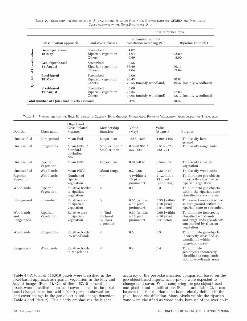
130 Feb r ua r y 2010 PHOTOGRAMMETRIC ENGINEER ING & REMOTE SENS ING
TABLE 3. PARAMETERS FOR THE RULE SETS USED TO CLASSIFY BARE GROUND, RANGELANDS, RIPARIAN VEGETATION, WOODLANDS, AND STREAMBEDS
Object and Class-Related Membership Value Value
Domain Class name Features function (May) (August) Purpose
Unclassified Bare ground Mean Red Larger than 1585–1595 1490–1495 To classify bare ground
Unclassified Rangelands Mean NDVI / Smaller than / 0.39–0.395 / 0.51–0.52 / To classify rangelandsStandard Smaller than 222–224 222–224deviationNIR
Unclassified Riparian Mean NDVI Larger than 0.645–0.65 0.54–0.55 To classify riparianVegetation vegetation
Unclassified Woodlands Mean NDVI About range 0.2–0.66 0.22–0.57 To classify woodlands
Riparian Woodlands Number of �� 4 (within a 4 (within a To eliminate geo-objectsVegetation riparian 15 pixel 15 pixel incorrectly classified as
vegetation perimeter) perimeter) riparian vegetation
Woodlands Riparian Relative border � 0.4 0.3 To eliminate geo-objectsVegetation to riparian within the riparian zone
vegetation classified as woodlands
Bare ground Streambed Relative area � 0.55 (within 0.55 (within To convert areas classifiedof riparian a 10 pixel a 10 pixel as bare ground within thevegetation perimeter) perimeter) riparian zone to streambed.
Woodlands Riparian Relative area � (find 0.60 (within 0.60 (within To eliminate incorrectlyand Vegetation of riparian enclosed a 10 pixel a 10 pixel classified woodlandsRangelands vegetation by class perimeter) perimeter) and rangelands geo-objects
algorithm) surrounded by riparianvegetation
Woodlands Rangelands Relative border � 0.5 0.5 To eliminate geo-objectsto woodlands incorrectly classified as
woodlands withinrangelands areas
Rangelands Woodlands Relative border � 0.4 0.4 To eliminate to rangelands geo-objects incorrectly
classified as rangelandswithin woodlands areas
TABLE 2. CLASSIFICATION ACCURACIES OF STREAMBED AND RIPARIAN VEGETATION DERIVED FROM THE GEOBIA AND PIXEL-BASEDCLASSIFICATIONS OF THE QUICKBIRD IMAGE DATA
Lidar reference data
Streambed withoutClassification approach Land-cover classes vegetation overhang (%) Riparian zone (%)
Geo-object-based Streambed 4.0718 May Riparian vegetation 94.94 92.00
Others 0.99 8.00
Geo-object-based Streambed 6.5611 August Riparian vegetation 86.40 90.11
Others 7.04 9.89
Pixel-based Streambed 0.0018 May Riparian vegetation 20.45 50.63
Others 79.55 (mainly woodland) 49.37 (mainly woodland)
Pixel-based Streambed 0.0011 August Riparian vegetation 22.35 57.88
Others 77.65 (mainly woodland) 42.12 (mainly woodland)
Total number of QuickBird pixels assessed 3,475 98,320
Qu
ick
Bir
d C
lass
ific
atio
n
(Table 4). A total of 418,019 pixels were classified in thepixel-based approach as riparian vegetation in the May andAugust images (Plate 1). Out of these, 57.18 percent ofpixels were classified as no land-cover change in the pixel-based change detection, while 92.49 percent showed noland-cover change in the geo-object-based change detection(Table 4 and Plate 2). This clearly emphasizes the higher
accuracy of the post-classification comparison based on thegeo-object-based inputs, as no pixels were expected tochange land-cover. When comparing the geo-object-basedand pixel-based classifications (Plate 1 and Table 2), it canbe seen that the riparian zone is not clearly defined in thepixel-based classification. Many pixels within the riparianzone were classified as woodlands, because of the overlap in
123-136_GB-610.qxd 1/15/10 6:52 AM Page 130
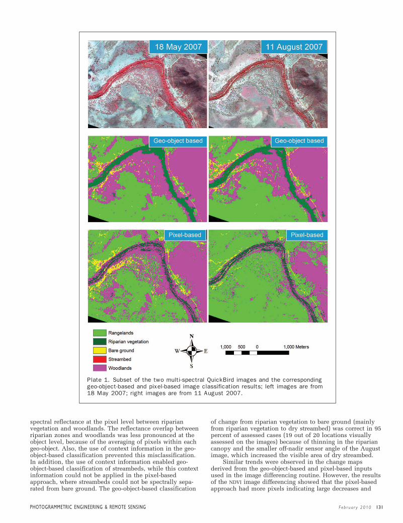
PHOTOGRAMMETRIC ENGINEER ING & REMOTE SENS ING Feb r ua r y 2010 131
Plate 1. Subset of the two multi-spectral QuickBird images and the correspondinggeo-object-based and pixel-based image classification results; left images are from18 May 2007; right images are from 11 August 2007.
spectral reflectance at the pixel level between riparianvegetation and woodlands. The reflectance overlap betweenriparian zones and woodlands was less pronounced at theobject level, because of the averaging of pixels within eachgeo-object. Also, the use of context information in the geo-object-based classification prevented this misclassification.In addition, the use of context information enabled geo-object-based classification of streambeds, while this contextinformation could not be applied in the pixel-basedapproach, where streambeds could not be spectrally sepa-rated from bare ground. The geo-object-based classification
of change from riparian vegetation to bare ground (mainlyfrom riparian vegetation to dry streambed) was correct in 95percent of assessed cases (19 out of 20 locations visuallyassessed on the images) because of thinning in the ripariancanopy and the smaller off-nadir sensor angle of the Augustimage, which increased the visible area of dry streambed.
Similar trends were observed in the change mapsderived from the geo-object-based and pixel-based inputsused in the image differencing routine. However, the resultsof the NDVI image differencing showed that the pixel-basedapproach had more pixels indicating large decreases and
123-136_GB-610.qxd 1/15/10 6:52 AM Page 131

Plate 2. Results of the (a) geo-object-based, and (b) pixel-based post-classificationchange detection presented for a subset of the image data. To simplify the colorcoding of this illustration, the direction of change is not specified, i.e., to-from andfrom-to classes are merged.
132 Feb r ua r y 2010 PHOTOGRAMMETRIC ENGINEER ING & REMOTE SENS ING
TABLE 4. COMPARISON OF THE PERCENTAGE OF PIXELS CLASSIFIED AS CHANGE IN THE GEO-OBJECT-BASED AND PIXEL-BASEDPOST-CLASSIFICATION COMPARISON IN AREAS CLASSIFIED AS RIPARIAN VEGETATION IN EITHER THE MAY OR AUGUST IMAGE
Pixels related to riparian change in Pixels related to riparian change ingeo-object-based post-classification pixel-based post-classificationcomparison comparison
Geo-object-based Pixel-based Geo-object-based Pixel-basedChange classes approach (%) approach (%) approach (%) approach (%)
No change 81.44 38.67 92.49 57.18Non-riparian change 0.00 40.23 1.32 0.00Bare ground - riparian 0.00 0.17 0.00 0.72Rangelands - riparian 0.38 0.09 0.25 1.54Woodlands - riparian 6.64 15.72 2.72 29.22Riparian - bare ground 0.41 0.08 0.19 0.14Riparian - rangelands 0.20 1.01 0.03 4.71Riparian - woodlands 10.93 4.03 3.00 6.49
Total pixels 713,481 713,481 418,019 418,119
increases in NDVI values compared to the geo-object-basedNDVI image differencing (Plate 3).
The transformation coefficients for stable brightness andstable greenness were similar in both the geo-object-basedand pixel-based approaches, whereas the transformationcoefficients for the change axes were different. The tasseledcap transformation worked well using the geo-object-basedapproach, where rangelands with increased grass cover inAugust were clearly identified. However, the pixel-basedtransformation provided very poor results with changes onlyoccurring in the riparian zone (Plate 4), where only a slightreduction in the NIR reflectance and a slight increase in thered reflectance of the riparian canopy could be observedbetween May and August. The transformation coefficientsderived from the geo-object-based approach were tested forthe pixel-based transformation, which significantly improvedthe result. It was found that the 10 pixels selected for
producing the axis representing change in vegetation werenot representative. The 10 geo-objects selected for the geo-object-based approach represented � 1,000 pixels, makingthis approach more robust.
Discussion
Comparison of Change Maps Derived from Geo-object-based and Per-pixel InputsIn general, the change maps derived from the geo-object-basedinputs used in the change detection techniques providedmore accurate results than those derived from the pixel-basedinputs. This was because of the ability of the geo-object-basedapproach to (a) reduce effects of slight mis-registrationbetween the two images, (b) reduce high spatial frequencynoise, (c) include context relationships and geo-object shape
123-136_GB-610.qxd 1/15/10 6:52 AM Page 132

PHOTOGRAMMETRIC ENGINEER ING & REMOTE SENS ING Feb r ua r y 2010 133
Plate 3. Results of the (a) geo-object-based, and (b) pixel-based NDVI imagedifferencing presented for a subset of the image data.
Plate 4. Results of the (a) geo-object-based, and (b) pixel-based multi-temporaltasseled cap transformation presented for a subset of the image data. Increases anddecreases in NDVI values were regarded as vegetation change.
information, (d) reduce effects of shadows from trees, and(e) reduce effects of differences in sensor viewing geometryand illumination angle.
Post-classification ComparisonThe post-classification comparison can provide usefulinformation on changes from one land-cover class toanother. This approach relies on high image classificationaccuracies of the two images. Misclassification and mis-registration errors often result in unsatisfactory results
(Coppin et al., 2004). As no change from one land-coverclass to another occurred between the May and Augustimages, the post-classification comparisons should nothave shown any change. However, a large part of the geo-objects/pixels showing change between riparian vegetationand woodlands occurred in close proximity (within 30 m)to the riparian zone. This misclassification issue wascaused by woodland vegetation next to the riparian zonebeing denser and greener in May than in August. Hence,riparian zone width was overestimated in the May image
123-136_GB-610.qxd 1/25/10 1:26 PM Page 133

134 Feb r ua r y 2010 PHOTOGRAMMETRIC ENGINEER ING & REMOTE SENS ING
(more water available) and more accurately mapped in theAugust image (less water available). This is a commonissue of mapping riparian zone width in wet-dry environ-ments from optical image data (Johansen et al., 2008).Misclassification, caused by changes in structural andchemical properties of canopy, understory, and grasswithin several of the individual land-cover classes, wasmost pronounced in the pixel-based approach. This wasbecause of the overlap in reflectance in the spectral bandsbetween different land-cover classes, e.g., patches ofwoodland and riparian vegetation. Even though a majorityfilter of 7 � 7 pixels were used to reduce the effects ofhigh spatial frequencies in the pixel-based classification,many pixels were still classified as woodlands within theriparian zone. The use of class-related context relationshipsin the geo-object-based approach reduced the misclassifica-tion between woodland and riparian vegetation. Informa-tion on the elongated shape of riparian zones locatedparallel to the streambed also improved the geo-object-based classification.
Mapped changes from rangelands to riparian vegetationin the change detection maps derived from the geo-object-based inputs were in most cases rangelands in both May andAugust, but with greener patches in August resulting inmisclassification as riparian vegetation. Slight mis-registra-tion between the two image datasets resulted in some smallgeo-objects along the edges of the riparian zone and range-lands being classified as rangelands in May and riparianvegetation in August. This was a result of using the samesegmentation for both images. The pixel-based approacheswere affected by slight mis-registrations (�2 pixels) andeffects from the differences in image off-nadir viewing andillumination angle between the two images, which resultedin the boundaries of tree crowns and their associatedshadows appearing as change. The geo-object-basedapproach was in most cases not affected by these effects(dependent on geo-object size), as they were averaged out atthe object level.
High spatial resolution image data are more likely tobe affected by distinct local changes in structural andchemical properties, while local changes may be averagedout at the object level. The results of the post-classifica-tion comparisons implied that changes in structural andchemical properties within individual land-cover classescaused some problems in the pixel-based approach. Thesereflectance changes were not misclassified to the sameextent as land-cover change in the geo-object-based post-classification approach. This was mainly because of theuse of context relationships. Changes in structural andchemical properties affect the spectral characteristics ofland-cover classes, but do not influence the contextrelationships between individual land-cover classes. Thismakes the inclusion of context relationships very power-ful. Rutherford and Rapoza (2008) compared geo-object-based and pixel-based image classification results andfound that segmentation into image geo-objects andintegration of context relationships improved the imageclassification accuracy.
Image DifferencingImage differencing was found useful and easy to interpretbecause of the simplicity of the approach. The critical partof the approach is the definition of thresholds indicatingchange (Coppin et al., 2004). It was found important toinclude more than just one band to identify all changes.
The image differencing based on the per-pixel inputsindicated larger decreases and increases in NDVI values(and other bands) than observed when using the geo-object-based inputs. This can be explained in two ways:
(a) the pixel-based approach identified small distinctchanges and/or misclassified change because of slight mis-registration between the two images, and (b) the geo-object-based approach did not identify small areas ofchange, as these were averaged out at the object level.A more detailed assessment showed that many of thelarge changes in NDVI values in the pixel-based approachoccurred because of slight mis-registration and/or off-nadirviewing differences, which caused small tree crowns to bespatially offset in the two images. This was in particularan issue in the savanna woodlands because of the highlevel of spectral reflectance heterogeneity in these areas.For the geo-object-based approach, small geo-objects werealso affected, but larger geo-objects (�50 pixels) were lessinfluenced as they included multiple tree crowns. Hence,the mean spectral reflectance per geo-object was similarfrom May to August even if the same tree crowns were notincluded in the geo-objects compared. For more homoge-nous land-cover classes such as rangelands, both the pixel-based and geo-object-based approaches correctly identifiedchanges in spectral reflectance between senescent (Mayimage) and regenerated grass (August image). Also forthose parts of the riparian zones with a dense continuouscanopy cover, the pixel- and object-based approaches wereless affected by small geometric offsets. However, forsparser canopies with gaps and influences of reflectancefrom ground cover, the geo-object-based approach per-formed better than the pixel-based approach. Nielsen et al.(2008) explained that while effects on change detectionfrom vegetation phenology can be minimized through theuse of anniversary image data, image differencing isconstrained by the high level of natural temporal variabil-ity in wetlands caused by hydrological variability. Basedon the findings in this paper, the use of geo-object-basedinputs for image differencing may solve the issue outlinedby Nielsen et al. (2008).
Tasseled Cap TransformationThe multi-temporal tasseled cap transformation wasinterpreted based on the new layer representing change inthe image. The main disadvantage of this approach is thatthe construction of the new coordinate system is laboriousand requires previous knowledge of the study area and anaccurate definition of the changes to be identified.
The results of the multitemporal tasseled cap transforma-tion derived from the pixel-based inputs were less accuratethan those produced from the geo-object-based inputs. Whenworking with geo-objects, the size of the sample used forconstruction of the new coordinate system is larger, in thiscase 70 pixels in total for the pixel-based approach againstthousands of pixels in the geo-object-based approach. Thismakes the geo-object-based approach more robust, especiallywhen working with high spatial resolution image data, wherepixels cover very small areas.
ConclusionsThis work focused on the development of a geo-object-basedimage classification system for mapping riparian land-coverclasses, and the comparison of change maps derived fromgeo-object-based and pixel-based inputs from high spatialresolution QuickBird image data used in three changedetection techniques. The geo-object-based classificationaccuracies of riparian vegetation were significantly higherthan those of the pixel-based classifications. The developmentof geo-object-based rule sets for classifying the two imagesshowed that the setup of the rule sets can be standardized butthat different thresholds for the membership functions arerequired. Class-related features showed more potential than
123-136_GB-610.qxd 1/25/10 1:26 PM Page 134

PHOTOGRAMMETRIC ENGINEER ING & REMOTE SENS ING Feb r ua r y 2010 135
the object-related features for rule set standardization betweenmulti-temporal images covering the same area.
In general, the change maps derived from the geo-object-based inputs used in the three change detection techniquesproduced more accurate results than the pixel-based inputs.The geo-object-based post-classification comparison andimage differencing routines provided significantly betterresults than those of the pixel-based routines, because of theability of the geo-object-based approaches to (a) reduceeffects of slight mis-registration between the two images,(b) reduce high spatial frequency noise, (c) include contextrelationships and geo-object shape information, (d) reduceeffects of shadows from trees, and (e) reduce effects ofdifferences in sensor viewing geometry and illuminationangle. The multitemporal tasseled cap transformationprovided inaccurate results for the pixel-based inputsbecause of the small size of the sample used for the calcula-tion of the change coefficient. This research shows theimproved capabilities of using geo-object-based inputs forchange detection analysis of multitemporal high spatialresolution image data.
AcknowledgmentsThanks to Santosh Bhandary (The University of Queens-land, Australia), Andrew Clark (Department of Environ-ment and Resource Management, Queensland, Australia(DERM)), and Joanna Blessing (CSIRO) for help collectingand analyzing the field data. Also, thanks to John Armston(DERM) for help analyzing the lidar data. L.A. Arroyo wasfunded by the Fundacion Alonso Martin Escudero (Spain).K. Johansen was supported by an Australian ResearchCouncil Linkage Grant to K. Mengersen, S. Phinn, andC. Witte.
ReferencesArroyo, L.A., S.P. Healey, W.B. Cohen, D. Cocero, and J.A. Manzanera,
2006. Using object-oriented classification and high-resolutionimagery to map fuel types in a Mediterranean region, Journal ofGeophysical Research, 111:G04S04.
Benz, U.C., P. Hofmann, G. Willhauck, I. Lingenfelder, and M.Heynen, 2004. Multi-resolution, object-oriented fuzzy analysisof remote sensing data for GIS-ready information, ISPRS Journalof Photogrammetry and Remote Sensing, 58:239–258.
Blaschke, T., 2005. A framework for change detection based on imageobjects, Göttinger Geographische Abhandlungen (S. Erasmi,B. Cyffka, and M. Kappas, editors), Göttinger, 113:1–9.
Blaschke, T., and G.J. Hay, 2001. Object-oriented image analysis andscale-space: Theory and methods for modeling and evaluatingmultiscale landscape structure, International Archives ofPhotogrammetry and Remote Sensing, 34:22–29.
Bock, M., P. Xofis, J. Mitchley, G. Rossner, and M. Wissen, 2005.Object-oriented methods for habitat mapping at multiplescales - Case studies from Northern Germany and WyeDowns, UK Journal for Nature Conservation, 13:75–89.
Bontemps, S., P. Bogaert, N. Titeux, and P. Defourny, 2008. Anobject-based change detection method accounting for temporaldependences in time series with medium to coarse spatialresolution, Remote Sensing of Environment, 112:3181–3191.
Burnett, C., and T. Blaschke, 2003. A multi-scale segmentation/objectrelationship modelling methodology for landscape analysis,Ecological Modelling, 168:233–249.
Collins, J.B., and C.E. Woodcock, 1994. Change detection using theGramm-Schmidt transformation applied to mapping forestmortality, Remote Sensing of Environment, 50:267–279.
Conchedda, G., L. Durieux, and P. Mayaux, 2008. An object-basedmethod for mapping and change analysis in mangroveecosystems, ISPRS Journal of Photogrammetry and RemoteSensing, 63:578–589.
Coppin, P., I. Jonckheere, K. Nackaerts, and B. Muys, 2004. Digitalchange detection methods in ecosystem monitoring: A review,International Journal of Remote Sensing, 25(9):1565–1596.
Crist, E.P., and R.C. Cicone, 1984. Application of the tasseled capconcept to simulated Thematic Mapper data, PhotogrammetricEngineering & Remote Sensing, 39:343–352.
Definiens, 2007. Definiens Developer 7: User Guide, Version7.0.1.872, Definiens AG, Munich, Germany, 497 p.
Desclee, B., P. Bogaert, and P. Defourny, 2006. Forest changedetection by statistical object-based method, Remote Sensing ofEnvironment, 102:1–11.
Flanders, D., M. Hall-Beyer, and J. Pereverzoff, 2003. Preliminaryevaluation of eCognition object-oriented software for cut blockdelineation and feature extraction, Canadian Journal of RemoteSensing, 29:441–452.
Franklin, S., M. Wulder, and M. Lavigne, 1996. Automated derivationof geographic windows for use in remote sensing digital imageanalysis, Computers and Geosciences, 22:665–673.
Gamanya, R., P.D. Maeyer, and M.D. Dapper, 2009. Object-orientedchange detection for the city of Harare, Zimbabwe, ExpertSystems with Applications, 36,571–588.
Hall, O., and G. Hay, 2003. A multiscale object-specific approach todigital change detection, International Journal of Applied EarthObservation and Geoinformation, 4:311–327.
Haralick, R.M., and L.G. Shapiro, 1985. Image segmentationtechniques, Computer Vision, Graphics, and Image Processing,29:100–132.
Hay, G.J., T. Blaschke, D.J. Marceau, and A. Bouchard, 2003.A comparison of three image-object methods for the multiscaleanalysis of landscape structure, ISPRS Journal of Photogramme-try and Remote Sensing, 57:327–345.
Im, J., J.R. Jensen, and J.A. Tullis, 2008. Object-based change detectionusing correlation image analysis and image segmentation,International Journal of Remote Sensing, 29(2):399–423.
Jensen, J.R., 2005. Introductory Digital Image Processing: A RemoteSensing Perspective, Third edition, Prentice Hall, Upper SaddleRiver, New Jersey, 526 p.
Johansen, K., N. Coops, S. Gergel, and Y. Stange, 2007. Applicationof high spatial resolution satellite imagery for riparian andforest ecosystem classification, Remote Sensing of Environment,110:29–44.
Johansen, K., S. Phinn, J. Lowry, and M. Douglas, 2008. Quantifyingindicators of riparian condition in Australian tropical savannas:Integrating high spatial resolution imagery and field surveydata, International Journal of Remote Sensing, 29(23)7003–7028.
Johansen, K., C. Roelfsema, and S. Phinn, 2008. Special feature - Highspatial resolution remote sensing for environmental monitoringand management, Journal of Spatial Science, 53(1):43–47.
Johansen, K., L.A. Arroyo, J. Armston, S. Phinn, C. Witte, in press.Mapping riparian condition indicators in a sub-tropicalsavanna environment from discrete return LiDAR data usingobject-oriented image analysis, Ecological Indicators.
Kauth, R.J., and G.S. Thomas, 1976. The tasselled cap - A graphicdescription of spectral-temporal development of agriculturalcrops as seen by Landsat, Proceedings of the 2nd InternationalSymposium on Machine Processing of Remotely Sensed Data,Purdue University, West Lafayette, Indiana.
Ketting, R.L., and D.A. Landgrebe, 1976. Classification of multispectralimage data by extraction and classification of homogeneousobjects, IEEE Transactions on Geoscience Electronics, GE-14(1):19–26.
Lu, D., P. Mausel, E. Brondizio, and E. Moran, 2004. Changedetection techniques, International Journal of Remote Sensing,25:2365–2407.
Muller, F., 1997. State-of-the-art in ecosystem theory, EcologicalModelling, 100:135–161.
Nielsen, E.M., S.D. Price, and G.T. Koeln, 2008. Wetland changemapping for the U.S. mid-Atlantic region using an outlierdetection technique, Remote Sensing of Environment,112:4061–4074.
Platt, R.V., and A.F.H. Goetz, 2004. A comparison of AVIRIS andsynthetic Landsat data for land use classification at the urban
123-136_GB-610.qxd 1/15/10 6:52 AM Page 135

136 Feb r ua r y 2010 PHOTOGRAMMETRIC ENGINEER ING & REMOTE SENS ING
fringe, Photogrammetric Engineering & Remote Sensing,70(7):813–819.
Prior, L.D., D. Eamus, and D.M.J.S. Bowman, 2004. Tree growthrates in north Australian savanna habitats: Seasonal patternsand correlations with leaf attributes, Australian Journal ofBotany, 52:303–314.
Rutherford, V.P., and L. Rapoza, 2008. An evaluation of an object-oriented paradigm for land use/land cover classification, TheProfessional Geographer, 60(1):87–100.
Ryherd, S., and C. Woodcock, 1996. Combining spectral and texturedata in the segmentation of remotely sensed images, Photogram-metric Engineering & Remote Sensing, 62(1):181–194.
Stow, D., Y. Hamada, L. Culter, and Z. Anguelova, 2008. Monitoringshrubland habitat changes through object-based changeidentification with airborne multispectral imagery, RemoteSensing of Environment, 112:1051–1061.
Walter, V., 2004. Object-based classification of remote sensing datafor change detection, ISPRS Journal of Photogrammetry andRemote Sensing, 58:225–238.
Wiens, J.A., 1989. Spatial scaling in ecology, Functional Ecology,3:385–397.
Williams, R.J., B.A. Myers, W.J. Muller, G.A. Duff, and D. Eamus,1997. Leaf phenology of woody species in a north Australiantropical savanna, Ecology, 78:2542–2558.
Woodcock, C.E., and A.H. Strahler, 1987. The factor of scale inremote sensing, Remote Sensing of Environment, 21:311–332.
Wu, J., 1999. Hierarchy and scaling: Extrapolating information along ascaling ladder, Canadian Journal of Remote Sensing, 25:367–380.
Wulder, M.A., S.M. Ortlepp, J.C. White, N.C. Coops, and S.B.Coggins, 2008. Monitoring tree-level insect population dynamicswith multi-scale and multi-source remote sensing, Journal ofSpatial Science, 53:49–61.
SEND COMPLETED FORM WITH YOUR PAYMENT TO:
ASPRS Certifi cation Seals & Stamps, 5410 Grosvenor Lane, Suite 210, Bethesda, MD 20814-2160
NAME: PHONE:
CERTIFICATION #: EXPIRATION DATE:
ADDRESS:
CITY: STATE: POSTAL CODE: COUNTRY:
PLEASE SEND ME: Embossing Seal ..................... $45 Rubber Stamp ............$35
Now that you are certifi ed as a remote sensor, photo grammetrist or GIS/LIS mapping scientist and you have that certifi cate on the wall, make sure everyone knows!
An embossing seal or rubber stamp adds a certifi ed fi nishing touch to your professional product .
You can’t carry around your certifi -cate, but your seal or stamp fi ts in your pocket or briefcase.
To place your order, fi ll out the necessary mailing and certifi cation information. Cost is just $35 for a stamp and $45 for a seal; these pric-es include domestic US shipping. International shipping will be billed at cost . Please allow 3-4 weeks for delivery.
Certifi cation Seals & Stamps
METHOD OF PAYMENT: Check Visa MasterCard American Express
CREDIT CARD ACCOUNT NUMBER EXPIRES
SIGNATURE DATE
February Layout 2.indd 136February Layout 2.indd 136 1/15/2010 1:19:23 PM1/15/2010 1:19:23 PM

AbstractVegetation mapping was performed using geographic object-based image analysis (GEOBIA) and very high spatialresolution (VHR) imagery for two study areas in Great SmokyMountains National Park. This study investigated howaccurately GEOBIA with ancillary data emulates manualinterpretation in rugged mountain areas for multi-levelvegetation classes of the National Vegetation ClassificationSystem (NVCS). It was discovered that the incorporation oftexture and topographic variables with spectral data fromscanned color infrared aerial photographs increased theoverall accuracy of GEOBIA vegetation classification by2.8 percent and 5.0 percent Kappa. In a separate studyusing multispectral Ikonos imagery, the use of elevation,aspect, slope and proximity to streams produced NVCSmacro-group vegetation segmentations that resembledmanual interpretation and significantly improved the overallaccuracy to 76.6 percent, Kappa 0.57. Ancillary informationmay thus aid in GEOBIA vegetation mapping for updatingvegetation inventories in rugged mountain areas.
IntroductionVegetation mapping in regions such as the AppalachianMountains of the southeastern US offers challenges inmapping, photogrammetry, and thematic classification dueto rugged terrain, high diversity and historical land uses,and disturbances that create complex landscapes (Welchet al., 2002). Multiple factors have been considered whenclassifying vegetation communities using remotely sensedimagery. Aerial photographs, for example, have beenemployed for manual interpretation of vegetation resourcesin the US since the 1930s (Spurr and Brown, 1946). Manyapplications focused on forest damage and individual treespecies identification by crown shape and appearance onblack-and-white, color or color infrared (CIR) photos (Colwell, 1950; Sayn-Wittgenstein and Aldred, 1967). Photointerpreters traditionally used basic elements of manual
PHOTOGRAMMETRIC ENGINEER ING & REMOTE SENS ING Feb r ua r y 2010 137
Minho Kim and Marguerite Madden are with the Center forRemote Sensing and Mapping Science (CRMS), Departmentof Geography, University of Georgia, Athens, Georgia([email protected]).
Bo Xu is with the Department of Geography & EnvironmentalStudies, California State University, San Bernardino,California, and formerly with the Center for Remote Sensingand Mapping Science (CRMS), Department of Geography,University of Georgia, Athens, Georgia.
Photogrammetric Engineering & Remote SensingVol. 76, No. 2, February 2009, pp. 137–149.
0099-1112/10/7602–137/$3.00/0© 2010 American Society for Photogrammetry
and Remote Sensing
GEOBIA Vegetation Mapping in Great SmokyMountains National Park with Spectral and
Non-spectral Ancillary InformationMinho Kim, Marguerite Madden, and Bo Xu
interpretation such as size, shape, tone (or color), texture,and association (Teng et al., 1997). These elements providestructural and contextual knowledge used in manualclassification by human interpreters (Blasckhe, 2003).However, manual interpretation is a labor-intensive andcostly procedure that requires a high level of knowledge andexpertise (Heller and Ulliman, 1983).
Automated pixel-based methodologies have been usedextensively for forest classification with moderate-resolutionsatellite imagery since the launch of Landsat-1 in 1972(Hoffer et al., 1978; Jensen et al., 1978). On the other hand,many applications require high spatial resolution images toidentify forest details such as crown morphology, tree heights,and species. Attempts have been made to employ automatedmethodologies to develop natural resource inventories withVHR imagery. However, conventional pixel-based approacheswere found to have limitations with VHR imagery in relationto increased within-class spectral variation of individualground features, which decreases the performance of pixel-based classification (Woodcock and Strahler, 1987; Marceauet al., 1990; Shiewe et al., 2001; Yu et al., 2006; Lu andWeng, 2007). Therefore, remote sensing researchers havedeveloped various methods of utilizing spatial and contextualinformation as well as object-based approaches to meetchallenges associated with VHR imagery (Lu and Weng, 2007).
New image processing procedures show promise forapproximating contextual manual interpretation in a moreefficient and automated manner. Object-based image analysis(OBIA), for example, uses contextual information and facili-tates the use of ancillary data to group similar image pixelsinto geo-objects (also called image objects or segments) thatcan be related to real landscape features using object-basedclassification techniques (Blaschke et al., 2000; Hay et al.,2001). Since OBIA is also used for medical applications, theterm geographic object-based image analysis (GEOBIA) distin-guishes applications in the Earth sciences (Hay et al., 2008).The image segmentation and classification of GEOBIA havebeen considered since the late-1990s as an automatic interpre-tation method that emulates human interpreters’ abilities(Schiewe et al., 2001; Blaschke, 2003). In recent years, GEOBIAhas increasingly gained attention for use with VHR imagery toinclude basic interpretation elements for close coupling ofremote sensing and geographic information systems (GIS) (Hay
137-149_GB-613.qxd 1/15/10 7:53 AM Page 137

138 Feb r ua r y 2010 PHOTOGRAMMETRIC ENGINEER ING & REMOTE SENS ING
and Castilla, 2008). The GEOBIA approach specifically handlesincreased spectral variation inherent in VHR imagery (Burnettand Blaschke, 2003; Yu et al., 2006). In addition, GEOBIA canproduce vector polygons that resemble manual interpretationresults and input directly to GIS (Castilla et al., 2008).
In GEOBIA, the results of image classifications werereported to be influenced by segmentation quality (Dorrenet al., 2003; Meinel and Neubert, 2004; Addink et al., 2007).Blaschke (2003) addressed some important issues in usingGEOBIA: (a) the size of geo-objects, (b) input data, (c) seman-tic model, and (d) relationship building. In vegetation-related GEOBIA, the size of segments was found to affect theresults of image classification (Ryherd and Woodcock,1996; Dorren et al., 2003; Kim et al., 2009). Although thereis no specific guideline to determine the most appropriate(or optimal) size of geo-objects, several attempts have beenmade for this purpose (Wang et al., 2004; Feitosa et al.,2006; Kim et al., 2008).
The spectral information (i.e., multispectral colorinformation) of VHR imagery has been widely utilized inprevious vegetation-related GEOBIA (Heyman et al., 2003;Johansen and Phinn, 2006). GEOBIA approaches with spectraland non-spectral information, however, can possibly disen-tangle within-class spectral variation inherent in VHRimagery and enhance classification results (Lu and Weng,2007). Texture, as a carrier of spatial information, has beenwidely employed in pixel-based remote sensing research(Zhang, 1999; Ferro and Warner, 2002). The calculation oftexture in pixel-based approaches, however, is dependenton the size of a rectangular moving window (or kernel) andbetween-class texture has been reported to degrade theperformance of pixel-based classification (Ferro and Warner,2002). In GEOBIA, object-specific texture is computed basedon pixels within the boundary of a geo-object. The influenceof between-class texture is potentially excluded with reliablesegmentation quality and the incorporation of object-specifictexture with spectral bands often improves forest classifica-tion results (Hay et al., 1996; Kim et al., 2009).
In addition, the incorporation of other ancillary informa-tion, e.g., topographic variables of elevation, aspect and slope,has a potential for producing better classification results sincevegetation distribution is known to be influenced by environ-mental factors that create microhabitat conditions (Parker,1982; Florinsky and Kurakova, 1996; Treitz and Howarth,2000; Boyd and Danson, 2005; Domaç and Süzen, 2006;Chastain et al., 2008). Topographic variables, along with otherinformation from GIS databases, have been employed in pixel-based vegetation and land-cover mapping. Sader et al. (1995)incorporated GIS data sets, including wetland inventory aswell as hydric soils and topographic variables, with LandsatTM spectral bands for the classification of wetland foresttypes. Burrough et al. (2001) also performed forest classifica-tion of Greater Yellowstone National Park area with factorssuch as distance from ridgelines, wetness index, and profilecurvature. In addition, Debeir et al. (2002) also utilized roads,hydrography, and rail networks with topographic variables toconduct land-cover mapping. The topographic variables havebeen adopted in GEOBIA to perform automatic landform unitclassifications (Dragut and Blaschke, 2006). In Great SmokyMountains (GRSM) National Park, specifically, Madden et al.(2004) found that ecological locations of forest communitiesare closely associated with elevation and moisture gradientsfrom field observations in this high relief area. The spatialcoincidence of vegetation and topographic variables was alsoassessed by a GIS overlay analysis to derive topographic-related rule sets appropriate for use in GEOBIA segmentationand classification.
Considering the importance of combining ancillaryinformation with spectral data for vegetation mapping in
rugged areas, this study conducts GEOBIA vegetationclassification using VHR scanned aerial photograph andsatellite imagery. We report two separate GEOBIA studiesassociated with mapping hierarchical vegetation classes thatapproximate the more detailed association (L8) and alliance(L7) levels, and the more general group (L6) and macro-group (L5) levels of the National Vegetation ClassificationStandard (NVCS), version 2.0 (FGDC, 2008). We comparedspectral-only, multi-level classification of VHR imagery to amanually interpreted and progressively generalized vegeta-tion data set of known accuracy. Non-spectral auxiliary dataincluding texture, elevation, aspect, slope, and proximity tostreams were then added to improve the correspondencebetween GEOBIA and manual data sets. The major objectiveof this study, therefore, is to evaluate how accurately GEOBIAclassification resembles manually interpreted vegetationmaps towards a goal of operational monitoring over broadareas. The study specifically investigates:
1. How the aggregation of vegetation classes from detailedfloristic-based association and alliance levels to physiog-nomic-and structural-based group and macro-groups affectsGEOBIA spectral-only vegetation classification results;
2. what potential effects are made on GEOBIA vegetationclassification with the addition of texture and topographicvariables to spectral information; and
3. how GIS-derived data can influence the segmentation qualityof macro-group vegetation classes associated with GEOBIAspectral and contextual classification results.
Study Area and Data SourcesThis study was conducted in Great Smoky MountainsNational Park (GRSM) that was established in 1934 to protectnatural and cultural resources threatened by extensivelogging. This park, located along the North Carolina-Tennessee border in southeastern US, is one of the mostdiverse temperate forests in the world with over 100 speciesof native trees (Kaiser, 1999). Over 95 percent of the park isforested and includes some of the most extensive remainingdeciduous old-growth forest in North America (NPS, 2008).Two study areas, corresponding to U.S. Geological Survey(USGS) 1:24 000-scale Thunderhead Mountain and Smoke-mont 7.5’ quadrangles, were selected to perform GEOBIAvegetation classifications (Figure 1). The total areas of thestudy sites are 7.6 km2 and 40 km2 for Thunderhead Moun-tain and Smokemont, respectively.
Figure 1. Locator map of Thunderhead Mountainand Smokemont USGS quadrangles in Great SmokyMountains National Park.
137-149_GB-613.qxd 1/15/10 7:53 AM Page 138

PHOTOGRAMMETRIC ENGINEER ING & REMOTE SENS ING Feb r ua r y 2010 139
A CIR aerial photograph acquired on 27 October 1997, bythe US Forest Service at 1:12 000 scale, was scanned at 600dots per inch (dpi) to create a digital image of 0.5 m spatialresolution with green, red, and near-infrared (NIR) bands(Figure 2a). The image was subsequently orthorectified usingthe R-WEL, Inc., Desktop Mapping System (DMS) with
horizontal control points from USGS Digital OrthoimageryQuadrangles (DOQs) and vertical control points from the USGSNational Elevation Dataset (NED) digital elevation model(DEM) to a root-mean-square-error (RMSE) of � 5 to 10 m(Jordan, 2002; Welch et al., 2002). The orthorectified imagewas then utilized for GEOBIA vegetation mapping of Thunder-head Mountain and a multispectral Ikonos image, acquiredon 30 October 2003, was used for GEOBIA of the Smokemontarea (Figure 2b). The fall color and leaf-on condition of thevegetation in the two sites exhibited a color diversity thatwas ideal for mapping overstory vegetation communities(Welch et al., 2002). In addition, USGS 30 m and 10 m DEMswere utilized to derive topographic variables of elevation,aspect and slope for the two study sites.
The Center for Remote Sensing and Mapping Science(CRMS), Department of Geography at the University ofGeorgia (UGA) previously created GIS databases of vegetationfor the GRSM park by manual interpretation of 1:12 000 scaleCIR aerial photographs (Welch et al., 2002; Madden et al.,2004). Performed in conjunction with the National ParkService (NPS) and NatureServe as a part of the USGS-NPSNational Vegetation Inventory Program, the GIS databasesinclude vegetation as well as non-vegetation classes suchas homesites and roads. According to an independent andfield-verified accuracy evaluation by NPS, vegetation inter-pretation was conducted with an overall accuracy of80.4 percent and a Kappa of 0.80 for 40 NVCS association-level classes (Jenkins, 2007). The accuracy of an aggregatedalliance or group-level interpretation of the CRMS-NPSvegetation is expected to be even higher. Association-levelvegetation classes were aggregated to NVCS alliance, groupand macro-group levels in ArcGIS® 9.3 and each hierarchicallevel of vegetation was utilized to evaluate GEOBIA classifica-tion results. For instance, an aggregated vegetation interpre-tation to the alliance level was compared to GEOBIA vegeta-tion classification at the alliance level.
In the Thunderhead Mountain area, 15 association-level vegetation classes were identified and manuallyinterpreted from the CIR air photo in conjunction withground truth data collection. These association-level classeswere aggregated into nine alliance classes, seven groupclasses, and five macro group classes, as shown in Table 1,to examine the effects of vegetation attribute generalizationand non-spectral ancillary data, i.e., texture and topo-graphic variables, on GEOBIA classification accuracies. Asfor the Smokemont area, 60 association-level vegetationclasses were collapsed into five macro groups includingbroadleaf deciduous forest (DF), coniferous evergreen forest(EF), mixed broadleaf deciduous and coniferous evergreenforest (MF), shrub (SB), and grass (GR). In the Smokemontarea, mixed forests associated with eastern hemlock (Tsugacanadensis) and southern Appalachian cove hardwoodforests are often found in narrow strips along streamcourses, while pine forests (e.g., Pinus echinata) dominateevergreen forests on dry southern slopes and along ridges(Jackson, 2004). We examined the effect of adding topo-graphic variables and proximity to stream channels on thequality and accuracy of segmenting/classifying vegetationclasses at the macro-group level. The generalized CRMS-NPSGIS databases were utilized as reference data sets to assessthe emulation of GEOBIA vegetation classification to manualinterpretation.
MethodsTwo separate GEOBIA studies were performed using theMultiresolution Segmentation algorithm, implemented inDefiniens Developer, version 7.0. Vegetation classificationresults were evaluated with CRMS-NPS manual interpretation
Figure 2. Panchromatic versions of images used in thisstudy: (a) orthorectified CIR imagery for ThunderheadMountain, and (b) orthorectified multispectral Ikonosimagery of Smokemont with masked non-vegetationfeatures.
137-149_GB-613.qxd 1/15/10 7:53 AM Page 139

140 Feb r ua r y 2010 PHOTOGRAMMETRIC ENGINEER ING & REMOTE SENS ING
TABLE 1. HIERARCHICAL LEVELS OF VEGETATION CLASSES IN THUNDERHEAD MOUNTAIN AREA THAT CORRESPOND TO MULTIPLE LEVELS OF THE NATIONAL VEGETATION CLASSIFICATION SYSTEM (NVCS)
Macro group Group Alliance Association level (L5) level (L6) level (L7) level (L8) Association description
Coniferous forest T T T/NHxA Eastern hemlock (T) and northernT/HxA hardwood acid type (NHxA) or
mixed acidic (HxA)
Deciduous forest NHx NHx NHxBe Northern hardwoodsMOr NHxA NHxA yellow birch type (NHxB)Hx NHxR NHxR Beech gap (NHxBe)
MOr MOr/R-K Acid type (NHxA)Hx MOr/Hth Rich type (NHxR)
MOr/G Montane northern red oak (MOr)HxA with rhododendron kalmia (R-K),HxA/T heath (Hth) or graminoid (G)
Mixed hardwoods acid type (HxA)with eastern hemlock (T)
Mixed forest CHx CHxR CHxR Cove hardwoods (CHx)CHxR/T Rich type (CHxR)
Shrub Hth Hth Hth/NHx Heath bald/northern hardwoods Hth/Sb Heath bald/shrub (Sb)
Grass P P G Graminoid pasture
and the assessment results were addressed with overallaccuracy, Kappa coefficient and producer’s and user’saccuracies. The detailed descriptions of procedures areprovided in subsequent sections.
GEOBIA Vegetation Mapping of Thunderhead Mountain with CIR OrthoimageA series of image segmentations was conducted using threespectral bands of the CIR orthoimage across segmentationscales, i.e., scale parameters in Definiens, of 50 to 300 insteps of 50. In these segmentations, default values wereemployed for other parameters. The vegetation classificationsof each NVCS level were then performed with supervisednearest neighbor classifier using only spectral information ofthe image across all segmentations, and the overall accuraciesof the classifications were graphed as a function of scales.Depending on classification results, we selected appropriatesegmentation scale and NVCS level that most closely resem-bled manual interpretation of a higher level of detail.
With the selected level of vegetation, non-spectralancillary data of texture and topographic variables were nextutilized in subsequent classification procedures. We computedobject-specific texture measures in Definiens with grey-level co-occurrence matrix (GLCM) using the segmentationscale that produced the highest classification accuracy. ThreeGLCM texture measures of contrast, correlation and entropywere calculated from the NIR band of the orthorectified CIRimage since they were reported to produce preferred classifica-tion results (Clausi, 2002). In addition, Kayitakire et al. (2006)and Kim et al. (2009) discovered that the inclusion of contrastand correlation provided a good estimation of forest structurevariables and improved the accuracies of GEOBIA forest typeclassification with VHR satellite imagery. Each texture wasacquired as a directionally invariance measure by computingthe mean of results in all four directions (0°, 45°, 90°, and135°) in Definiens. Supervised nearest neighbor classificationswere conducted with individual texture measures as well asspectral bands and classification results were evaluated todecide the most appropriate texture measure.
A USGS 30 m DEM was then utilized to extract elevationranges and slope using ERDAS Imagine® (version 9.2) andthe two topographic variables were employed to develop
rule sets for vegetation classification. Although Jackson(2004) and Madden (2004) observed spatial coincidence oftopographic variables with vegetation in Great SmokyMountains National Park, the development of rule setsbased on field verification would be a labor-intensive andtime-consuming procedure. Therefore, we performed GISoverlay analysis to compute minimum and maximumvalues of elevation and slope that corresponded to eachvegetation class at the selected NVCS levels. These rangesdefined membership functions of Definiens rule sets foradding non-spectral ancillary data to improve the resultsof supervised classification with spectral bands only.Lastly, GLCM texture measures and topographic variablecombinations that produced the highest classificationaccuracies were identified. The CRMS-NPS manually inter-preted vegetation database was used to assess theaccuracy of classification results at random sample points.GEOBIA classification of the Thunderhead Mountain areawas evaluated with overall accuracy, Kappa coefficient,producer’s, and user’s accuracies.
GEOBIA Vegetation Mapping of Smokemont with Multispectral IkonosImageryThe multispectral Ikonos imagery was obtained as aStandard GeoProduct from GeoEye, Inc. An orthorectifica-tion procedure was required to remove positional dis-placements caused by high relief terrain (Carleer andWolff, 2004). In general, the procedure can be facilitatedwith rational polynomial coefficients (RPCs) that areaccompanied by Ikonos imagery (Tao et al., 2004). How-ever, since RPCs are not provided for the Ikonos GeoProd-uct, a satellite orbital math model implemented in PCIGeomatica® 9.1 was adopted to orthorectify the multispec-tral Ikonos imagery. The math model can produce anaccurate orthorectification result with more than 20control points (PCI, 2003). We selected a total of 24control points, corresponding to buildings and roads for asmall developed area and tree tops for most vegetatedareas to conduct an image-to-image orthorectification ofthe multispectral Ikonos image. These points were locatedin a horizontal reference data set created by the UGA-CRMS
137-149_GB-613.qxd 1/15/10 7:53 AM Page 140
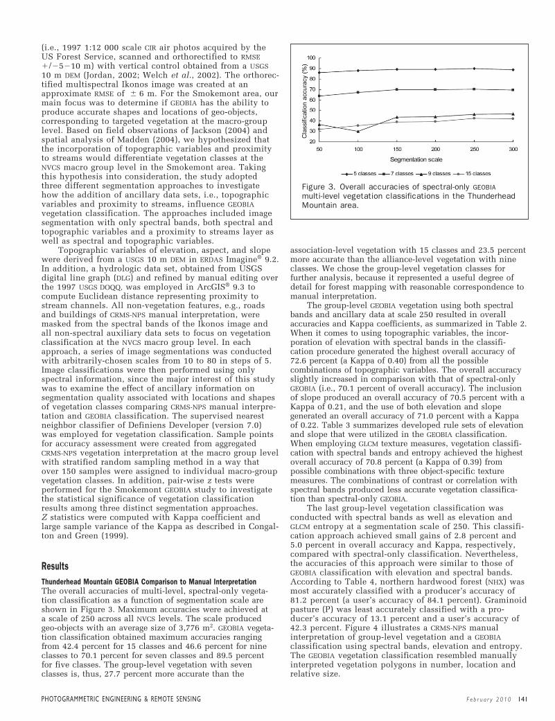
PHOTOGRAMMETRIC ENGINEER ING & REMOTE SENS ING Feb r ua r y 2010 141
(i.e., 1997 1:12 000 scale CIR air photos acquired by theUS Forest Service, scanned and orthorectified to RMSE�/�5�10 m) with vertical control obtained from a USGS10 m DEM (Jordan, 2002; Welch et al., 2002). The orthorec-tified multispectral Ikonos image was created at anapproximate RMSE of � 6 m. For the Smokemont area, ourmain focus was to determine if GEOBIA has the ability toproduce accurate shapes and locations of geo-objects,corresponding to targeted vegetation at the macro-grouplevel. Based on field observations of Jackson (2004) andspatial analysis of Madden (2004), we hypothesized thatthe incorporation of topographic variables and proximityto streams would differentiate vegetation classes at theNVCS macro group level in the Smokemont area. Takingthis hypothesis into consideration, the study adoptedthree different segmentation approaches to investigatehow the addition of ancillary data sets, i.e., topographicvariables and proximity to streams, influence GEOBIAvegetation classification. The approaches included imagesegmentation with only spectral bands, both spectral andtopographic variables and a proximity to streams layer aswell as spectral and topographic variables.
Topographic variables of elevation, aspect, and slopewere derived from a USGS 10 m DEM in ERDAS Imagine® 9.2.In addition, a hydrologic data set, obtained from USGSdigital line graph (DLG) and refined by manual editing overthe 1997 USGS DOQQ, was employed in ArcGIS® 9.3 tocompute Euclidean distance representing proximity tostream channels. All non-vegetation features, e.g., roadsand buildings of CRMS-NPS manual interpretation, weremasked from the spectral bands of the Ikonos image andall non-spectral auxiliary data sets to focus on vegetationclassification at the NVCS macro group level. In eachapproach, a series of image segmentations was conductedwith arbitrarily-chosen scales from 10 to 80 in steps of 5.Image classifications were then performed using onlyspectral information, since the major interest of this studywas to examine the effect of ancillary information onsegmentation quality associated with locations and shapesof vegetation classes comparing CRMS-NPS manual interpre-tation and GEOBIA classification. The supervised nearestneighbor classifier of Definiens Developer (version 7.0)was employed for vegetation classification. Sample pointsfor accuracy assessment were created from aggregated CRMS-NPS vegetation interpretation at the macro group levelwith stratified random sampling method in a way thatover 150 samples were assigned to individual macro-groupvegetation classes. In addition, pair-wise z tests wereperformed for the Smokemont GEOBIA study to investigatethe statistical significance of vegetation classificationresults among three distinct segmentation approaches.Z statistics were computed with Kappa coefficient andlarge sample variance of the Kappa as described in Congal-ton and Green (1999).
ResultsThunderhead Mountain GEOBIA Comparison to Manual InterpretationThe overall accuracies of multi-level, spectral-only vegeta-tion classification as a function of segmentation scale areshown in Figure 3. Maximum accuracies were achieved ata scale of 250 across all NVCS levels. The scale producedgeo-objects with an average size of 3,776 m2. GEOBIA vegeta-tion classification obtained maximum accuracies rangingfrom 42.4 percent for 15 classes and 46.6 percent for nineclasses to 70.1 percent for seven classes and 89.5 percentfor five classes. The group-level vegetation with sevenclasses is, thus, 27.7 percent more accurate than the
association-level vegetation with 15 classes and 23.5 percentmore accurate than the alliance-level vegetation with nineclasses. We chose the group-level vegetation classes forfurther analysis, because it represented a useful degree ofdetail for forest mapping with reasonable correspondence tomanual interpretation.
The group-level GEOBIA vegetation using both spectralbands and ancillary data at scale 250 resulted in overallaccuracies and Kappa coefficients, as summarized in Table 2.When it comes to using topographic variables, the incor-poration of elevation with spectral bands in the classifi-cation procedure generated the highest overall accuracy of 72.6 percent (a Kappa of 0.40) from all the possiblecombinations of topographic variables. The overall accuracyslightly increased in comparison with that of spectral-onlyGEOBIA (i.e., 70.1 percent of overall accuracy). The inclusionof slope produced an overall accuracy of 70.5 percent with aKappa of 0.21, and the use of both elevation and slopegenerated an overall accuracy of 71.0 percent with a Kappaof 0.22. Table 3 summarizes developed rule sets of elevationand slope that were utilized in the GEOBIA classification.When employing GLCM texture measures, vegetation classifi-cation with spectral bands and entropy achieved the highestoverall accuracy of 70.8 percent (a Kappa of 0.39) frompossible combinations with three object-specific texturemeasures. The combinations of contrast or correlation withspectral bands produced less accurate vegetation classifica-tion than spectral-only GEOBIA.
The last group-level vegetation classification wasconducted with spectral bands as well as elevation andGLCM entropy at a segmentation scale of 250. This classifi-cation approach achieved small gains of 2.8 percent and5.0 percent in overall accuracy and Kappa, respectively,compared with spectral-only classification. Nevertheless,the accuracies of this approach were similar to those ofGEOBIA classification with elevation and spectral bands.According to Table 4, northern hardwood forest (NHX) wasmost accurately classified with a producer’s accuracy of81.2 percent (a user’s accuracy of 84.1 percent). Graminoidpasture (P) was least accurately classified with a pro-ducer’s accuracy of 13.1 percent and a user’s accuracy of42.3 percent. Figure 4 illustrates a CRMS-NPS manualinterpretation of group-level vegetation and a GEOBIAclassification using spectral bands, elevation and entropy.The GEOBIA vegetation classification resembled manuallyinterpreted vegetation polygons in number, location andrelative size.
Figure 3. Overall accuracies of spectral-only GEOBIAmulti-level vegetation classifications in the ThunderheadMountain area.
137-149_GB-613.qxd 1/15/10 7:53 AM Page 141
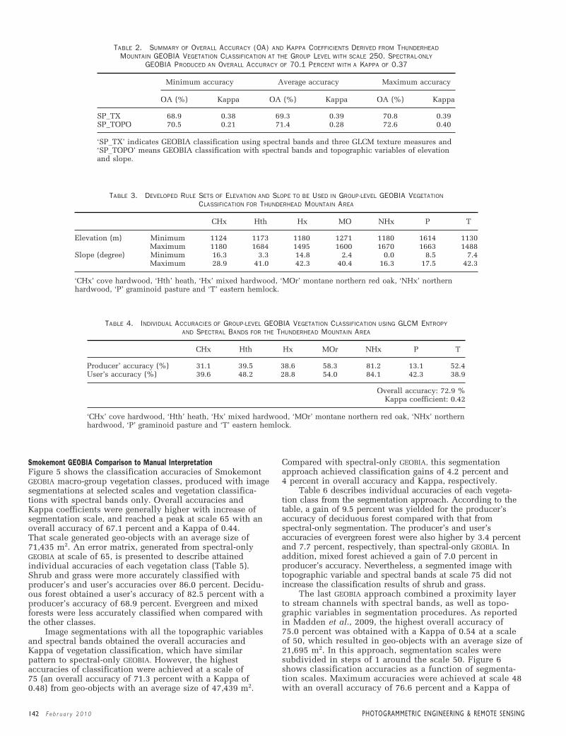
142 Feb r ua r y 2010 PHOTOGRAMMETRIC ENGINEER ING & REMOTE SENS ING
TABLE 4. INDIVIDUAL ACCURACIES OF GROUP-LEVEL GEOBIA VEGETATION CLASSIFICATION USING GLCM ENTROPY AND SPECTRAL BANDS FOR THE THUNDERHEAD MOUNTAIN AREA
CHx Hth Hx MOr NHx P T
Producer’ accuracy (%) 31.1 39.5 38.6 58.3 81.2 13.1 52.4User’s accuracy (%) 39.6 48.2 28.8 54.0 84.1 42.3 38.9
Overall accuracy: 72.9 %Kappa coefficient: 0.42
‘CHx’ cove hardwood, ‘Hth’ heath, ‘Hx’ mixed hardwood, ‘MOr’ montane northern red oak, ‘NHx’ northernhardwood, ‘P’ graminoid pasture and ‘T’ eastern hemlock.
TABLE 2. SUMMARY OF OVERALL ACCURACY (OA) AND KAPPA COEFFICIENTS DERIVED FROM THUNDERHEADMOUNTAIN GEOBIA VEGETATION CLASSIFICATION AT THE GROUP LEVEL WITH SCALE 250. SPECTRAL-ONLY
GEOBIA PRODUCED AN OVERALL ACCURACY OF 70.1 PERCENT WITH A KAPPA OF 0.37
Minimum accuracy Average accuracy Maximum accuracy
OA (%) Kappa OA (%) Kappa OA (%) Kappa
SP_TX 68.9 0.38 69.3 0.39 70.8 0.39SP_TOPO 70.5 0.21 71.4 0.28 72.6 0.40
‘SP_TX’ indicates GEOBIA classification using spectral bands and three GLCM texture measures and‘SP_TOPO’ means GEOBIA classification with spectral bands and topographic variables of elevationand slope.
Smokemont GEOBIA Comparison to Manual InterpretationFigure 5 shows the classification accuracies of SmokemontGEOBIA macro-group vegetation classes, produced with imagesegmentations at selected scales and vegetation classifica-tions with spectral bands only. Overall accuracies andKappa coefficients were generally higher with increase ofsegmentation scale, and reached a peak at scale 65 with anoverall accuracy of 67.1 percent and a Kappa of 0.44.That scale generated geo-objects with an average size of71,435 m2. An error matrix, generated from spectral-onlyGEOBIA at scale of 65, is presented to describe attainedindividual accuracies of each vegetation class (Table 5).Shrub and grass were more accurately classified withproducer’s and user’s accuracies over 86.0 percent. Decidu-ous forest obtained a user’s accuracy of 82.5 percent with aproducer’s accuracy of 68.9 percent. Evergreen and mixedforests were less accurately classified when compared withthe other classes.
Image segmentations with all the topographic variablesand spectral bands obtained the overall accuracies andKappa of vegetation classification, which have similarpattern to spectral-only GEOBIA. However, the highestaccuracies of classification were achieved at a scale of75 (an overall accuracy of 71.3 percent with a Kappa of0.48) from geo-objects with an average size of 47,439 m2.
Compared with spectral-only GEOBIA, this segmentationapproach achieved classification gains of 4.2 percent and4 percent in overall accuracy and Kappa, respectively.
Table 6 describes individual accuracies of each vegeta-tion class from the segmentation approach. According to thetable, a gain of 9.5 percent was yielded for the producer’saccuracy of deciduous forest compared with that fromspectral-only segmentation. The producer’s and user’saccuracies of evergreen forest were also higher by 3.4 percentand 7.7 percent, respectively, than spectral-only GEOBIA. Inaddition, mixed forest achieved a gain of 7.0 percent inproducer’s accuracy. Nevertheless, a segmented image withtopographic variable and spectral bands at scale 75 did notincrease the classification results of shrub and grass.
The last GEOBIA approach combined a proximity layerto stream channels with spectral bands, as well as topo-graphic variables in segmentation procedures. As reportedin Madden et al., 2009, the highest overall accuracy of75.0 percent was obtained with a Kappa of 0.54 at a scaleof 50, which resulted in geo-objects with an average size of21,695 m2. In this approach, segmentation scales weresubdivided in steps of 1 around the scale 50. Figure 6shows classification accuracies as a function of segmenta-tion scales. Maximum accuracies were achieved at scale 48with an overall accuracy of 76.6 percent and a Kappa of
TABLE 3. DEVELOPED RULE SETS OF ELEVATION AND SLOPE TO BE USED IN GROUP-LEVEL GEOBIA VEGETATIONCLASSIFICATION FOR THUNDERHEAD MOUNTAIN AREA
CHx Hth Hx MO NHx P T
Elevation (m) Minimum 1124 1173 1180 1271 1180 1614 1130Maximum 1180 1684 1495 1600 1670 1663 1488
Slope (degree) Minimum 16.3 3.3 14.8 2.4 0.0 8.5 7.4Maximum 28.9 41.0 42.3 40.4 16.3 17.5 42.3
‘CHx’ cove hardwood, ‘Hth’ heath, ‘Hx’ mixed hardwood, ‘MOr’ montane northern red oak, ‘NHx’ northernhardwood, ‘P’ graminoid pasture and ‘T’ eastern hemlock.
137-149_GB-613.qxd 1/15/10 7:53 AM Page 142

PHOTOGRAMMETRIC ENGINEER ING & REMOTE SENS ING Feb r ua r y 2010 143
those from image segmentation with spectral bands andtopographic variables only.
Table 7 is an error matrix produced from a segmentation atscale 48 with spectral bands, topographic variables, andproximity layer. Geo-objects with an average size of 20,523 m2
were produced at that scale. When compared with spectral-onlyGEOBIA (see Table 5), this approach acquired a gain of 15.5percent in producer’s accuracy with that of 2.0 percent in user’saccuracy for deciduous forest. Mixed forest also gained largeincreases of 14.3 percent and 5.6 percent in user’s and pro-ducer’s accuracies, respectively. In addition, a notable gain of15.5 percent in user’s accuracy was achieved for evergreenforest and the user’s accuracy of grass was increased by5.6 percent. Nevertheless, there were slight decreases inproducer’s accuracies of evergreen and grass, i.e., 1.7 percentand 2.1 percent, respectively. The individual accuracies ofshrub also decreased by 3.3 percent and 6.5 percent comparedwith spectral-only GEOBIA.
Figure 7 illustrates CRMS-NPS manual interpretation andGEOBIA vegetation classification results with three differentsegmentation approaches. With a visual examination, asegmentation with proximity layer, topographic variables,and spectral bands produced a GEOBIA classification resultmuch resembling manual interpretation in terms of locationand shapes of vegetation classes. Considering pair-wise ztests, described in Table 8, the image segmentation with allnon-spectral ancillary data sets yielded a classification resultthat was significantly different from the other two segmenta-tion approaches at a confidence level of 99 percent.
DiscussionThis study addressed GEOBIA results of two studies withinGreat Smoky Mountains National Park that tested itspotential to emulate manual interpretation with VHRremotely sensed imagery and non-spectral ancillary data.The study areas, corresponding to two USGS quadrangles ofThunderhead Mountain and Smokemont, representedchallenging landscapes for vegetation mapping using GEOBIAapproaches due to the nearly continuous forest cover,gradual transitions between some forest types, and lack ofcultural features within the National Park with clearlydefined geo-objects.
The spatial resolution of remotely sensed images waspreviously reported to have an effect on the classificationaccuracies of forest classes at multiple hierarchical levels
Figure 4. Thunderhead Mountain vegetation at grouplevel: (a) CRMS-NPS manual interpretation, and (b) GEOBIAclassification with GLCM entropy, elevation and spectralbands at scale 250. ‘CHx’ means cove hardwood, ‘Hx’mixed hardwood, ‘Hth’ heath, ‘MOr’ montane northernred oak, ‘NHx’ northern hardwood, ‘P’ graminoidpasture, and ‘T’ eastern hemlock
0.57 that were higher by 9.5 percent and 13.0 percent,respectively, compared with spectral-only GEOBIA. Theclassification accuracies of the last segmentation approachwere also higher by 5.3 percent and 9.0 percent in overallaccuracy and Kappa, respectively, in comparison with
Figure 5. Classification accuracies of Smokemontmacro-group vegetation derived from segmentedimages with spectral bands only.
137-149_GB-613.qxd 1/15/10 7:53 AM Page 143

144 Feb r ua r y 2010 PHOTOGRAMMETRIC ENGINEER ING & REMOTE SENS ING
(Marceau et al., 1994). The spectral information content of aremotely sensed image was found to be sufficient for acertain level of vegetation classes, but insufficient for theother levels. This study also demonstrated that GEOBIAvegetation classification produced a large difference of
47.1 percent in overall accuracy between association (fine)and macro-group (coarse) vegetation levels. To obtainappropriate spectral information for each hierarchical levelof vegetation, multiple remotely sensed images in variousspatial and/or spectral resolutions would be required interms of data fusion for GEOBIA (Marceau et al., 1994;Marceau and Hay, 1999; Blaschke, 2003).
Non-spectral contextual information was found toinfluence GEOBIA vegetation classification results in thisstudy. GEOBIA classification with GLCM texture, topographicvariables, and spectral bands produced slightly higher overallaccuracy with improvements of 2.8 percent with a Kappa of5.0 percent, compared with spectral-only classification. Inaddition, segmented images with proximity layer, topographicvariables and spectral bands generated higher overall accu-racy and Kappa by 9.5 percent and 13.0 percent, respectively,than a segmented image with spectral bands only.
Pair-wise z tests for Smokemont area indicated that theinclusion of non-spectral ancillary data in segmentationprocedures produced a significantly different vegetationclassification from that of spectral-only segmentation at aconfidence level of a � 0.99. When visually compared withmanual interpretation (Figure 7a), a spectral-only segmenta-tion generated approximate location of macro-level vegeta-tion with forest patches more round in shape, particularlyfor evergreen and mixed forests (Figure 7b). In the Thunder-head Mountain area, a segmentation with spectral bandsalone also resulted in more round vegetation shapes thanmanual interpretation at NVCS group level (see Figure 4).
TABLE 5. ERROR MATRIX OF INDIVIDUAL VEGETATION CLASSES PRODUCED WITH SPECTRAL-ONLY SEGMENTATION AT SCALE 65 FOR SMOKEMONT AREA
Reference
DF EF MF SB GR
Classification DF 1554 144 154 13 18 82.5EF 253 215 37 0 2 42.4MF 431 49 237 8 0 32.7SB 8 0 3 132 0 92.3GR 11 0 0 0 166 93.8
Producer’s accuracy (%) 68.9 52.7 55.0 86.3 89.3
Overall accuracy: 67.1 %Kappa coefficient: 0.44
‘DF’ deciduous forest, ‘EF’ evergreen forest, ‘MF’ mixed forest, ‘SB’ shrub and ‘GR’ grass.
TABLE 6. ERROR MATRIX OF INDIVIDUAL VEGETATION CLASSES DERIVED FROM A SEGMENTED IMAGE WITH TOPOGRAPHICVARIABLES AND SPECTRAL BANDS AT SCALE 75 FOR SMOKEMONT AREA
Reference
DF EF MF SB GR
Classification DF 1768 157 163 14 27 83.0EF 150 201 45 4 1 50.1MF 329 50 207 9 10 34.2SB 8 0 16 126 0 84.0GR 2 0 0 0 148 98.67
Producer’s accuracy (%) 78.3 49.3 48.0 82.4 79.6
Overall accuracy: 71.3 %Kappa coefficient: 0.48
‘DF’ deciduous forest, ‘EF’ evergreen forest, ‘MF’ mixed forest, ‘SB’ shrub and ‘GR’ grass.
Figure 6. Classification accuracies of Smokemontmacro-group vegetation generated from segmentedimages with Euclidean distance to stream channels,topographic variables, and spectral bands. Used withpermission (Madden et al. 2009).
User’s accuracy (%)
User’s accuracy (%)
137-149_GB-613.qxd 1/15/10 7:53 AM Page 144
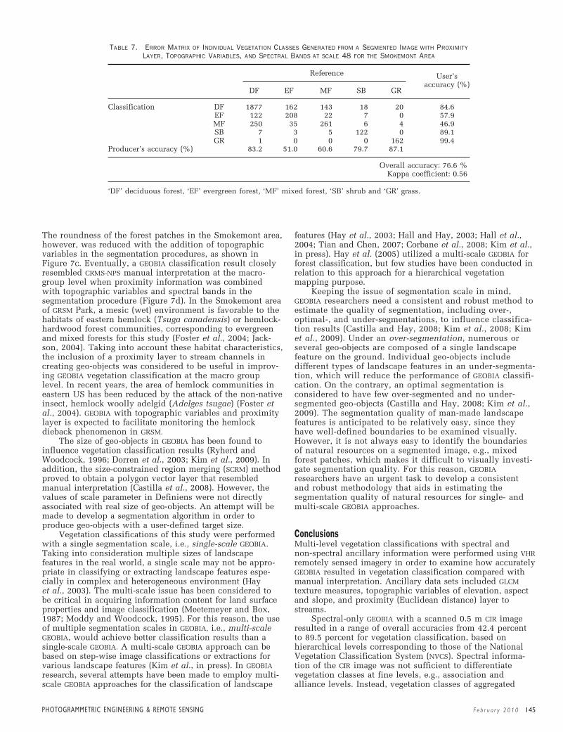
PHOTOGRAMMETRIC ENGINEER ING & REMOTE SENS ING Feb r ua r y 2010 145
TABLE 7. ERROR MATRIX OF INDIVIDUAL VEGETATION CLASSES GENERATED FROM A SEGMENTED IMAGE WITH PROXIMITYLAYER, TOPOGRAPHIC VARIABLES, AND SPECTRAL BANDS AT SCALE 48 FOR THE SMOKEMONT AREA
Reference
DF EF MF SB GR
Classification DF 1877 162 143 18 20 84.6EF 122 208 22 7 0 57.9MF 250 35 261 6 4 46.9SB 7 3 5 122 0 89.1GR 1 0 0 0 162 99.4
Producer’s accuracy (%) 83.2 51.0 60.6 79.7 87.1
Overall accuracy: 76.6 %Kappa coefficient: 0.56
‘DF’ deciduous forest, ‘EF’ evergreen forest, ‘MF’ mixed forest, ‘SB’ shrub and ‘GR’ grass.
The roundness of the forest patches in the Smokemont area,however, was reduced with the addition of topographicvariables in the segmentation procedures, as shown inFigure 7c. Eventually, a GEOBIA classification result closelyresembled CRMS-NPS manual interpretation at the macro-group level when proximity information was combinedwith topographic variables and spectral bands in thesegmentation procedure (Figure 7d). In the Smokemont areaof GRSM Park, a mesic (wet) environment is favorable to thehabitats of eastern hemlock (Tsuga canadensis) or hemlock-hardwood forest communities, corresponding to evergreenand mixed forests for this study (Foster et al., 2004; Jack-son, 2004). Taking into account these habitat characteristics,the inclusion of a proximity layer to stream channels increating geo-objects was considered to be useful in improv-ing GEOBIA vegetation classification at the macro grouplevel. In recent years, the area of hemlock communities ineastern US has been reduced by the attack of the non-nativeinsect, hemlock woolly adelgid (Adelges tsugae) (Foster etal., 2004). GEOBIA with topographic variables and proximitylayer is expected to facilitate monitoring the hemlockdieback phenomenon in GRSM.
The size of geo-objects in GEOBIA has been found toinfluence vegetation classification results (Ryherd andWoodcock, 1996; Dorren et al., 2003; Kim et al., 2009). Inaddition, the size-constrained region merging (SCRM) methodproved to obtain a polygon vector layer that resembledmanual interpretation (Castilla et al., 2008). However, thevalues of scale parameter in Definiens were not directlyassociated with real size of geo-objects. An attempt will bemade to develop a segmentation algorithm in order toproduce geo-objects with a user-defined target size.
Vegetation classifications of this study were performedwith a single segmentation scale, i.e., single-scale GEOBIA.Taking into consideration multiple sizes of landscapefeatures in the real world, a single scale may not be appro-priate in classifying or extracting landscape features espe-cially in complex and heterogeneous environment (Hayet al., 2003). The multi-scale issue has been considered tobe critical in acquiring information content for land surfaceproperties and image classification (Meetemeyer and Box,1987; Moddy and Woodcock, 1995). For this reason, the useof multiple segmentation scales in GEOBIA, i.e., multi-scaleGEOBIA, would achieve better classification results than asingle-scale GEOBIA. A multi-scale GEOBIA approach can bebased on step-wise image classifications or extractions forvarious landscape features (Kim et al., in press). In GEOBIAresearch, several attempts have been made to employ multi-scale GEOBIA approaches for the classification of landscape
features (Hay et al., 2003; Hall and Hay, 2003; Hall et al.,2004; Tian and Chen, 2007; Corbane et al., 2008; Kim et al.,in press). Hay et al. (2005) utilized a multi-scale GEOBIA forforest classification, but few studies have been conducted inrelation to this approach for a hierarchical vegetationmapping purpose.
Keeping the issue of segmentation scale in mind,GEOBIA researchers need a consistent and robust method toestimate the quality of segmentation, including over-,optimal-, and under-segmentations, to influence classifica-tion results (Castilla and Hay, 2008; Kim et al., 2008; Kimet al., 2009). Under an over-segmentation, numerous orseveral geo-objects are composed of a single landscapefeature on the ground. Individual geo-objects includedifferent types of landscape features in an under-segmenta-tion, which will reduce the performance of GEOBIA classifi-cation. On the contrary, an optimal segmentation isconsidered to have few over-segmented and no under-segmented geo-objects (Castilla and Hay, 2008; Kim et al.,2009). The segmentation quality of man-made landscapefeatures is anticipated to be relatively easy, since theyhave well-defined boundaries to be examined visually.However, it is not always easy to identify the boundariesof natural resources on a segmented image, e.g., mixedforest patches, which makes it difficult to visually investi-gate segmentation quality. For this reason, GEOBIAresearchers have an urgent task to develop a consistentand robust methodology that aids in estimating thesegmentation quality of natural resources for single- andmulti-scale GEOBIA approaches.
ConclusionsMulti-level vegetation classifications with spectral and non-spectral ancillary information were performed using VHRremotely sensed imagery in order to examine how accuratelyGEOBIA resulted in vegetation classification compared withmanual interpretation. Ancillary data sets included GLCMtexture measures, topographic variables of elevation, aspectand slope, and proximity (Euclidean distance) layer tostreams.
Spectral-only GEOBIA with a scanned 0.5 m CIR imageresulted in a range of overall accuracies from 42.4 percentto 89.5 percent for vegetation classification, based onhierarchical levels corresponding to those of the NationalVegetation Classification System (NVCS). Spectral informa-tion of the CIR image was not sufficient to differentiatevegetation classes at fine levels, e.g., association andalliance levels. Instead, vegetation classes of aggregated
User’s accuracy (%)
137-149_GB-613.qxd 1/15/10 7:53 AM Page 145

146 Feb r ua r y 2010 PHOTOGRAMMETRIC ENGINEER ING & REMOTE SENS ING
levels, e.g., group and macro-group, achieved improvedresults with higher overall accuracies over 70.0 percent.
This study demonstrated the importance of using non-spectral ancillary information in GEOBIA segmentation andclassification for natural vegetation features in mountain-ous areas. When GLCM texture and topographic variableswere added to classification procedures, the overallaccuracy and Kappa of vegetation classification werehigher by 2.8 percent and 5.0 percent, respectively, thanspectral-only GEOBIA at NVCS group level. It was found
that a segmentation with spectral bands and topographicvariables yielded a statistically improved vegetationclassification result of NVCS macro group level at a confi-dence level of 95 percent, compared with spectral-onlyGEOBIA. In addition, a segmented image with proximitylayer, topographic variables and spectral bands generateda vegetation classification that was significantly enhancedat a confidence level of 99 percent when compared withspectral-only GEOBIA. With spectral bands and allancillary data sets, GEOBIA achieved an overall accuracy
Figure 7. Macro group vegetation of Smokemont area: (a) CRMS-NPS manual interpretation, (b) aclassification result from a segmented image with spectral bands only at scale 65, (c) a classificationresult from a segmented image with topographic variables and spectral bands at scale 75, and (d) aclassification result from a segmented image with proximity layer, topographic variables and spectralbands at scale 48. ‘DF’ indicates deciduous forest, ‘EF’ evergreen forest, ‘MF’ mixed forest, ‘SB/GR’shrub and grass. Used with permission (Madden et al. 2009).
137-149_GB-613.qxd 1/15/10 7:53 AM Page 146

of 76.6 percent and a Kappa of 0.57 that were higher by 9.5percent and 13.0 percent for overall accuracy and Kappa,respectively, than GEOBIA with spectral bands alone.
In future research, we plan to utilize non-spectralancillary data sets in both segmentation and classificationprocedures for GEOBIA vegetation mapping at finer hierarchi-cal levels. We also plan to develop a multi-scale GEOBIAapproach, related to multi-level vegetation classes of NVCS,with VHR remotely sensed imagery and non-spectral auxil-iary information. These attempts are anticipated to con-tribute to the development of new vegetation inventoriesand facilitate the update and revision of existing vegetationdatabases in terms of natural resources management forNational Parks.
AcknowledgmentsThis study was sponsored by the US Department ofInterior, National Park Service under (Cooperative Agree-ments No. 1443-CA-5460-98-019, H5028 01 0651 andH5000 03 5040). The authors wish to express their appre-ciation for the devoted efforts of Dr. Thomas Jordan andthe staff at the Center for Remote Sensing and MappingScience, The University of Georgia, the staff of Nature-Serve and the National Park Service, especially KeithLangdon, Michael Jenkins, Teresa Leibfreid and RobertEmmott.
ReferencesAddink, E.A., S.M. de Jong, and E.J. Pebesma, 2007. The importance
of scale in object-based mapping of vegetation parameters withhyperspectral imagery, Photogramemtric Engineering & RemoteSensing, 72(8):905–912.
Blaschke, T., S. Lang, E. Lorup, J. Strobl, and P. Zeil, 2000. Object-oriented image processing in an integrated GIS/remote sensingenvironment and perspectives for environmental applications,Environmental Information for Planning, Politics and the Public(A. Cremers and K. Greve, editors), Metropolis Verlag, Marburg,pp. 555–570.
Blaschke, T., 2003. Object-based contextual image classificationbuilt on image segmentation, Proceedings of the 2003 IEEEWorkshop on Advances in Techniques for Analysis ofRemotely Sensed Data, 27–28 October, Washington D.C.,pp. 113–119.
Boyd, D.S., and F.M. Danson, 2005. Satellite remote sensing forforest resources: Three decades of research development,Progress in Physical Geography, 29(1):1–26.
Burnett, C., and T. Blaschke, 2003. A multi-scalesegmentation/object relationship modeling methodology forlandscape analysis, Ecological Modelling, 168:233–249.
Burrough, P.A., J.P. Wilson, P.F.M. Gaans, and A.J. Hansen, 2001.Fuzzy k-means classification of topo-climatic data as an aidto forest mapping in the Greater Yellowstone Area, USA,Landscape Ecology, 36:523–546.
Carleer, A., and E. Wolff, 2004. Exploitation of very high resolutionsatellite data for tree species identification, PhotogrammetricEngineering & Remote Sensing, 70(1):135–140.
Castilla, G., G.J. Hay, and J.R. Ruiz, 2008. Size-controlled regionmerging (SCRM): An automated delineation tool for assistedphotointerpretation, Photogrammetric Engineering & RemoteSensing, 74(4):409–419.
Chastain, R.A., A.S. Matthew, H.S. He, and D.R. Larsen, 2008.Mapping vegetation communities using statistical data fusionin the Ozark National Scenic Riverways, Missouri, USA,Photogrammetric Engineering & Remote Sensing,74(2):247–264.
Clausi, D.A., 2002. An analysis of co-occurrence texture statistics asa function of gray level quantization, Canadian Journal ofRemote Sensing, 1:45–62.
Congalton, R.G., and K. Green, 1999. Assessing the Accuracy ofRemotely Sensed Data: Principles and Practices, CRC/LewisPress, Boca Raton, Florida, 137 p.
Colwell, R.N., 1950, New technique for interpreting aerial colorphotography, Journal of Forestry, 48:204–205.
Corbane, C., D. Raclot, F. Jacob, J. Albergel, and P. Andrieux, 2008.Remote sensing of soil surface characteristics from a multiscaleclassification approach, Catena, 75(3):308–318.
Debeir, O., I.V. den Steen, P. Latinne, P.V. Ham, and E. Wolff, 2002.Textural and contextual land-cover classification using singleand multiple classifier systems, Photogrammetric Engineering& Remote Sensing, 68(6):597–605.
Domaç, A., and M.L. Süzen, 2006. Integration of environmentalvariables with satellite images in regional scale vegetationclassification, International Journal of Remote Sensing,27(7):1329–1350.
Dorren, L.K.A., B. Maier, and A.C. Seijmonsbergen, 2003.Improved Landsat-based forest mapping in steep mountainousterrain using object-based classification, Forest Ecology andManagement, 183:31–46.
Dragut, L., and T. Blaschke, 2006. Automated classification oflandform elements using object-based image analysis,Geomorphology, 81:330–344.
Federal Geographic Data Committee (FGDC), 2008. NationalVegetation Classification Standard, version 2, FGDC-STD-005-2008, Vegetation Subcommittee, Federal Geographic DataCommittee, FGDC Secretariat, U.S. Geological Survey, Reston,Virginia, 119 p.
Feitosa, C.U., G.A.O.P. Costa, and T.B. Cazes, 2006. A geneticapproach for the automatic adaptation of segmentation parame-ters, Commission IV, WG IV/4 on Proceeding of 1st OBIAConference, 04–05 July, Salzburg, Austria (International Societyfor Photogrammetry and Remote Sensing), unpaginated CD-ROM.
Ferro, C.J.S., and T.A. Warner, 2002. Scale and texture in digitalimage classification, Photogrammetric Engineering & RemoteSensing, 68(1):51–63.
Florinsky, I.V., and G.A. Kurykova, 1996. Influence of topographyon some vegetation cover properties, Catena, 27:123–141.
Foster, D., G. Motzkin, J. O’Keefe, E. Boose, D. Orwig, J. Fuller, andB. Hall, 2004. The environmental and human history of NewEngland, Forests in Time: The Environmental Consequences of1000 Years of Change in New England (D. Foster and J.D. Aber,editors), Yale University, pp. 43–100.
Hall, O., and G.J. Hay, 2003. A multiscale object-specific approachto digital change detection, International Journal of AppliedEarth Observation and Geoinformation, 4(4):311–327.
Hall, O., G.J. Hay, A. Bouchard, and D.J. Marceau, 2004. Detectingdominant landscape objects through multiple scales: Anintegration of object-specific methods and watershed segmenta-tion, Landscape Ecology, 19:59–76.
Hay, G.J., K.O. Niemann, and G.F. McLean, 1996. An object-specificimage-texture analysis of H-resolution forest imagery, RemoteSensing of Environment, 55:108–122.
PHOTOGRAMMETRIC ENGINEER ING & REMOTE SENS ING Feb r ua r y 2010 147
TABLE 8. PAIR-WISE Z TEST RESULTS OF SMOKEMONT GEOBIAVEGETATION CLASSIFICATIONS AT THE MACRO-GROUP LEVEL WITH DIFFERENTIMAGE SEGMENTATION APPROACHES. THE CRITICAL VALUES OF SELECTED
LEVELS ARE 1.96 AND 2.58 FOR CONFIDENCE LEVELS OF 95 PERCENTAND 99 PERCENT, RESPECTIVELY
SP_TOPO SP_TOPO_PR
SP 2.08 6.31SP_TOPO 4.18
‘SP’ indicates a vegetation classification derived from a spectral-onlysegmentation at scale 65, ‘SP_TOPO’ denotes vegetation classificationproduced from a segmentation with topographic variables andspectral bands at scale 75 and ‘SP_TOPO_PR’ means a vegetationclassification generated from a segmentation with proximity layer,topographic variables and spectral bands at scale 48.
137-149_GB-613.qxd 1/15/10 7:53 AM Page 147

148 Feb r ua r y 2010 PHOTOGRAMMETRIC ENGINEER ING & REMOTE SENS ING
Hay, G.J., D.J. Marceau, A. Bouchard, and P. Dube, 2001. A multi-scale framework for landscape analysis: Object-specificupscaling, Landscape Ecology, 16:471–490.
Hay, G.J., T. Blaschke, D.J. Marceau, and A. Bouchard, 2003. Acomparison of three image-object methods for the multiscaleanalysis of landscape structure, ISPRS Journal of Photogrammetryand Remote Sensing, 57:327–345.
Hay, G.J., G. Castilla, M.A. Wulder, and J.R. Ruiz, 2005. Anautomated object-based approach for the multiscale imagesegmentation of forest scenes, International Journal of AppliedEarth Observation and Geoinformation, 7:339–359.
Hay, G.J., T. Blaschke, and D.J. Marceau, 2008. GEOBIA 2008 - Pixels,objects, intelligence, Proceedings of the GEOgraphic Object BasedImage Analysis for the 21st Century Conference, University ofCalgary, Calgary, Alberta, Canada, 05–08 August, ISPRS Archives,XXXVIII-4/C1, 373 p.
Hay, G.J., and G. Castilla, 2008. Geographic object-based imageanalysis (GEOBIA): A new name for a new discipline, Object-Based Image Analysis - Spatial Concepts for Knowledge-drivenRemote Sensing Applications (T. Blaschke, S. Lang, and G.J.Hay, editors), Springer-Verlag, Berlin, pp. 75–89.
Heller, R.C., and J.J. Ulliman, 1983. Forest resources assessments,Manual of Remote Sensing, (R.N. Colwell, editor), Vol II,Second edition, American Society of Photogrammetry, FallsChurch, Virginia, pp. 2229–2324.
Heyman, O., G.G. Gaston, A.J. Kimerling, and J.T. Campbell, 2003.A per-segment approach to improving aspen mapping fromhigh-resolution remote sensing imagery, Journal of Forestry,101(4):29–33.
Hoffer, R.M., S.C. Noyer, and R.P. Mroczynski, 1978. A compari-son of Landsat and forest survey estimates of forest cover,Proceedings of the Fall Technical Meeting of the AmericanSociety of Photogrammetry, Albuquerque, New Mexico,pp. 221–231.
Jackson, P., 2004. Notes on the overstory vegetation classificationsystem for Great Smoky Mountains National Park, DigitalVegetation Maps for the Great Smoky Mountains National Park(by M. Madden, R. Welch, T. Jordan, P. Jackson, R. Seavey, andJ. Seavey), Final Report to the U.S. Dept. of Interior, NationalPark Service, 1443-CA-5460-98-019, Center for Remote Sensingand Mapping Science, The University of Georgia, Athens,Georgia, Attachment C, 30 p.
Jenkins, M., 2007. Thematic Accuracy Assessment: Great SmokyMountains National Park Vegetation Map, National ParkService, Great Smoky Mountains National Park, Gatlinburg,Tennessee, 26 p.
Jensen, J.R., J.E. Estes, and L.R. Tinney, 1978. Evaluation of highaltitude photography and Landsat imagery for digital cropidentification, Photogrammetric Engineering & Remote Sensing,44(6):723–733.
Johansen, K., and S. Phinn, 2006. Mapping structural parametersand species composition of riparian vegetation using Ikonosand Landsat ETM� data in Australian tropical Savannahs,Photogrammetric Engineering & Remote Sensing, 2(1):71–80.
Jordan, T.R., 2002. Softcopy Photogrammetric Techniques forMapping Mountainous Terrain: Great Smoky MountainsNational Park, Ph.D. Dissertation, Department of Geography,The University of Georgia, Athens, Georgia, 193 p.
Kaiser, J., 1999. Great Smokies species census under way, Science,284(5421):1747–1748.
Kayitakire, F., C. Hamel, and P. Defourny, 2006. Retrieving foreststructure variables based on image texture analysis and Ikonos-2imagery, Remote Sensing of Environment, 102:390–401.
Kim, M., M. Madden, and T. Warner, 2008. Estimation of optimalimage object size for the segmentation of forest stands withmultispectral Ikonos imagery, Object-based Image Analysis -Spatial Concepts for Knowledge-driven Remote SensingApplications (T. Blaschke, S. Lang, and G.J. Hay, editors),Springer-Verlag, Berlin, pp. 291–307.
Kim, M., M. Madden, and T. Warner, 2009. Forest type mappingusing object-specific texture measures from multispectral Ikonosimagery: Segmentation quality and image classification issues,Photogrammetric Engineering & Remote Sensing, 75(7):819–830.
Kim, M., J.B. Holt, C.Y. Ku, and M. Madden, in press. GEOBIAbuilding extraction of Mae La refugee camp, Thailand: Step-wise multi-scale feature classification approach, LandscapeAnalysis using Geospatial Tools: Community to the Globe(M. Madden and E. Allen, editors), Springer-Verlag, New York,in press.
Lu, D., and Q. Weng, 2007. Survey of image classification methodsand techniques for improving classification performance,International Journal of Remote Sensing, 28(5):823–870.
Madden, M., 2004. Visualization and analysis of vegetation patternsin National Parks of the southeastern United States, Proceedingsof Challenges in Geospatial Analysis, Integration and Visualiza-tion II (J. Schiewe, M. Hahn, M. Madden, and M. Sester,editors), International Society for Photogrammetry and RemoteSensing Commission IV Joint Workshop, Stuttgart, Germany,pp. 143–146.
Madden, M., T. Jordan, M. Kim, H. Allen, and B. Xu, 2009. Integrat-ing remote sensing and GIS: From overlays to GEOBIA and geo-visualization, Manual of Geographic Information Systems (M.Madden, editor-in-chief), American Society for Photogrammetryand Remote Sensing, Bethesda, Maryland, pp. 701–720.
Madden, M., R. Welch, T. Jordan, P. Jackson, R. Seavey, and J.Seavey, 2004. Digital Vegetation Maps for the Great SmokyMountains National Park, Final Report to the U.S. Departmentof Interior, National Park Service, 1443-CA-5460-98-019, Centerfor Remote Sensing and Mapping Science, The University ofGeorgia, Athens, Georgia, 112 p.
Marceau, D.J., P.J. Howarth, J.M.M. Dubois, and D.J. Gratton, 1990.Evaluation of grey-level co-occurrence matrix method for land-cover classification using SPOT imagery, IEEE Transac-tions on Geoscience and Remote Sensing, 28(4):513–519.
Marceau, D.J., P.J. Howarth, and D.J. Gratton, 1994. Remote sensingand the measurement of geographical entities in a forestedenvironment - 1.:The scale and spatial aggregation problem,Remote Sensing of Environment, 49:93–104.
Marceau, D.J., and G.J. Hay, 1999. Remote sensing contributions tothe scale issue, Canadian Journal of Remote Sensing,25(4):357–366.
Meetemeyer, V., and E.O. Box, 1987. Scale effects in landscapestudies, Landscape Heterogeneity and Disturbance (M. Turner,editor), Springer-Verlag, New York, pp. 15–34.
Meinel, G., and M. Neubert, 2004. A comparison of segmentationprograms for high resolution remote sensing data, Proceedingsof Commission VI, Proceeding of XXth ISPRS Congress, 12–23July, Istanbul, Turkey (International Society for Photogrammetryand Remote Sensing), unpaginated CD-ROM.
Moody, A., and C.E. Woodcock, 1995. The influence of scale andthe spatial characteristics of landscapes on land-cover mappingusing remote sensing, Landscape Ecology, 10(6):363–379.
National Park Service (NPS), 2008. Great Smoky MountainsNational Park. URL: http://www.nps.gov/grsm/naturescience/index.htm (last date accessed: 01 December 2009).
Parker, A. J., 1982. The topographic relative moisture index: Anapproach to soil-moisture assessment in mountain terrain,Physical Geography, 3(2):160–168.
PCI, 2003. Geomatica OrthoEngine User Guide, PCI GeomaticsEnterprises, Inc.
Ryherd, S., and C. Woodcock, 1996. Combining spectral andtexture data in the segmentation of remotely sensed images,Photogrammetric Engineering & Remote Sensing,62(2):181–194.
Sader, S.A., D. Ahl, and W. Liou, 1995. Accuracy of Landsat-TMand GIS rule-based methods for forest wetland classification inMaine, Remote Sensing of Environment, 53:133–144.
Sayn-Wittgenstein, L., and A.H. Aldred, 1967. Tree volumes fromlarge-scale photos, Photogrammetric Engineering & RemoteSensing, 33(1):69–73.
Schiewe, J., L. Tufte, and E. Ehlers, 2001. Potential and problemsof multi-scale segmentation methods in remote sensing, GIS-Zeitschrift für Geoinformationssysteme, 6:34–39.
Spurr, S.H., and C.T. Brown Jr., 1946. Specifications for aerialphotographs used in forest management, PhotogrammetricEngineering & Remote Sensing, 12(1):131–141.
137-149_GB-613.qxd 1/15/10 7:53 AM Page 148

Tao, C.V., Y. Hu, and W. Jiang, 2004. Photogrammetric exploitationof Ikonos imagery for mapping applications, InternationalJournal of Remote Sensing, 25(14):2833–2853.
Teng, W.T., E.R. Loew, D.I. Ross, V.G. Zsilinsky, C.P. Lo, W.R.Philipson, W.D. Philpot, and S.A. Morain, 1997. Fundamentalsof photographic interpretation, Manual of PhotographicInterpretation (W.R. Philipson, editor), American Society ofPhotogrammetry and Remote Sensing, pp. 49–110.
Tian, J., and D.M. Chen, 2007. Optimization in multi-scale segmen-tation of high-resolution satellite images for artificial featurerecognition, International Journal of Remote Sensing,28(20):4625–4644.
Treitz, P., and P. Howarth, 2000. Integrating spectral, spatial andterrain variables for forest ecosystem classification, Photogram-metric Engineering & Remote Sensing, 66(3):305–317.
Wang, L., W.P. Sousa, and P. Gong, 2004. Integration of object-basedand pixel-based classification for mapping mangroves with
PHOTOGRAMMETRIC ENGINEER ING & REMOTE SENS ING Feb r ua r y 2010 149
Ikonos imagery, International Journal of Remote Sensing,25(24):5655–5668.
Welch, R., M. Madden, and T. Jordan, 2002. Photogrammetric andGIS techniques for the development of vegetation databases ofmountainous areas: Great Smoky Mountains National Park,ISPRS Journal of Photogrammetry & Remote Sensing,57(1–2):53–68.
Woodcock, C.E., and A.H. Strahler, 1987. The factor of scale inremote sensing, Remote Sensing of Environment, 25:349–379.
Yu, Q., P. Gong, N. Clinton, G. Biging, M. Kelly, and D. Shirokauer,2006. Object-based detailed vegetation classification withairborne high spatial resolution remote sensing imagery,Photogrammetric Engineering & Remote Sensing,72(7):799–811.
Zhang, Y., 1999. Optimization of building detection in satelliteimages by combining multispectral classification and texturefiltering, International Journal of Remote Sensing, 54:50–60.
February Layout 2.indd 149February Layout 2.indd 149 1/15/2010 1:21:28 PM1/15/2010 1:21:28 PM

150 Februar y 2010 PHOTOGRAMMETRIC ENGINEERING & REMOTE SENSING
Ryan R. Jensen, Perry J. Hardin, and Mark W. Jackson, Spectral Modeling of Population Density: A Study of Utah’s Wasatch Front.
Stefaan Lhermitte, Jan Verbesselt, Willem W. Verstraeten, and Pol Coppin, A Pixel-based Regeneration Index Using Time Series Similarity and Spatial Context.
Benjamin E. Wilkinson, Ahmed H. Mohamed, Bon A. Dewitt, and Gamal H. Seedahmed, A Novel Approach to Terrestrial Lidar Geo-referencing.
Libin Zhou and Xiaojun Yang, Training Algorithm Performance for Image Classifi cation by Neural Networks.
Subhashni Taylor, Lalit Kumar, and Nick Reid, Mapping Lantana ca-mara: Accuracy Comparison of Various Fusion Techniques.
Marc Linderman, Yu Zeng, and Pedram Rowhani, Climate and Land-use Effects on Interannual fAPAR Variability from MODIS 250 m Data.
Qinghua Guo, Wenkai Li, Hong Yu, and Otto Alvarez, Effects of Top-ographic Variability and Lidar Sampling Density on Several DEM Interpolation Methods.
Toshihiro Sakamoto, Michio Shibayama, Eiji Takada, Akihiro Inoue, Kazuhiro Morita, Wataru Takahashi, Shigenori Miura, and Akihiko Kimura, Detecting Seasonal Changes in Crop Community Struc-ture using Day and Night Digital Images.
Thomas B. Pollard, Ibrahim Eden, Joseph L. Mundy, and David B. Coo-per, A Volumetric Approach to Change Detection in Satellite Images.
Xiaodong Na, Shuqing Zhang, Xiaofeng Li, Huan Yu, and Chunyue Liu, Improved Land Cover Mapping using Random Forests Com-bined with Landsat Thematic Mapper Imagery and Ancillary Geo-graphic Data.
Guo Zhang, Wen-bo Fei, Zhen Li, Xiaoyong Zhu, and De-ren Li, Eval-uation of the RPC Model for Spaceborne SAR Imagery.
M. Mokhtarzade, M.J. Valadan Zoej, H. Ebadi, and M.R. Sahebi, An Innovative Image Space Clustering Technique for Automatic Road Network Vectorization.
Cristina Vega-García, Jamie Tatay-Nieto, Ricardo Blanco, and Emilio Chuvieco, Evaluation of the Infl uence of Local Fuel Homogeneity on Fire Hazard through Landsat-5 TM Texture Measures.
Francisco Javier Ariza López, Alan David Atkinson Gordo, José Luis García Balboa, and José Rodríguez Avi, Analysis of User and Produc-er Risk when Applying the ASPRS Standards for Large Scale Maps.
Douglas A. Stow, Christopher D. Lippitt, and John R. Weeks, Geo-graphic Object-based Delineation of Neighborhoods af Accra, Ghana using QuickBird Satellite Imagery.
Andrew Ashworth, David L. Evans, William H. Cooke, Andrew Londo, Curtis Collins, and Amy Neuenschwander, Predicting Southeastern Forest Canopy Heights and Fire Fuel Models using GLAS Data.
Gang Qiao, Weian Wang, Bo Wu, Chun Liu, and Rongxing Li, Assess-ment of Geopositioning Capability of High Resolution Satellite Im-agery for Densely Populated High Buildings in Metropolitan Areas.
John Dolloff and Reuben Settergren, An Assessment of Worldview-1 Po-sitional Accuracy Based on Fifty Contiguous Stereo Pairs of Imagery.
Simon J. Buckley, Ernesto Schwarz, Viktor Terlaky, John A. Howell, and W.C. Arnott, Combining Aerial Photogrammetry and Terres-trial Lidar for Reservoir Analog Modeling.
Zhangyan Jiang and Alfredo R. Huete, Linearization of NDVI based on Its Relationship with Vegetation Fraction.
In-seong Jeong and James Bethel, A Study of Trajectory Models for Satellite Image Triangulation.
Peijun Li and Haiqing Xu, Land Cover Change Detection using One Class Support Vector Machine.
Humberto Rosas, Watson Vargas, and Alexander Cerón, A Mathemati-cal Expression for Stereoscopic Depth Perception.
Nicholas Clinton, Ashley Holt, James Scarborough, Li Yan, and Peng Gong, Accuracy Assessment Measures for Object-based Image Segmentation Goodness.
Yu-Ching Lin and Jon P. Mills, Factors Infl uencing Pulse Width of Small Footprint, Full Waveform Airborne Laser Scanning Data.
Devrim Akca, Co-registration of Surfaces by 3D Least Squares Matching.
Andrew Niccolai, Melissa Niccolai, and Chadwick Dearing Oliver, Point Set Topology for Branch and Crown-level Species Classifi cation.
Ru An, Peng Gong, Huilin Wang, Xuezhi Feng, Pengfeng Xiao, Qi Chen, Qing Zhang, Chunye Chen, and Peng Yan, A Modifi ed PSO Algorithm for Remote Sensing Image Template Matching.
Yichang (James) Tsai, Zhaozheng Hu, and Chris Alberti, Detection of Roadway Sigh Condition Changes using Multi-scale Sign Image Matching and Statistical Color Model.
Dimitri Bulatov and John E. Lavery, Reconstruction and Texturing of 3D Urban Terrain from Uncalibrated Monocular Images using L1 Splines.
Adam P. Young, M.J. Olsen, N. Driscoll, R.E. Flick, R. Gutierrez, R.T Guza, E. Johnstone, and F. Kuester, Comparison of Airborne and Terrestrial Lidar Estimates of Seacliff Erosion in Southern California.
Yichang (James) Tsai, Zhaozheng Hu, and Chris Alberti, Detection of Roadway Sign Condition Changes using Multi-scale Sign Image Matching (M-SIM) and Statistical Color Model (SCM).
Tapas R. Martha, Norman Kerle, Cees J. van Westen, Victor Jetten, and K. Vinod Kumar, Effect of Sun Elevation Angle on DSMs De-rived from Cartosat-1 Data.
Shannon L. Savage and Rick L. Lawrence, Vegetation Dynamics in Yellowstone’s Northern Range: 1985 to 1999.
Hanqiu Xu, Analysis of Impervious Surface and Its Impact on Urban Heat Environment Using the Normalized Difference Impervious Surface Index (NDISI).
Cuizhen Wang, Diego J. Bentivegna, Reid J. Smeda, and Randy E. Swanigan, Comparing Classifi cation Approaches for Mapping Cut-level Teasel in Highway Environments.
Sagi Filin and Amit Baruch, Detection of Sinkhole Hazards Using Airborne Laser Scanning Data.
Tristan Goulden and Chris Hopkinson, The Forward Propagation of Integrated System Component Errors within Airborne Lidar Data.
Arzhan Surazakov and Vladimir Aizen, Positional Accuracy Evalua-tion of Declassifi ed Hexagon KH-9 Mapping Camera Imagery.
Ayman F. Habib, Ruifang Zhai, and Changjae Kim, Generation of Complex Polyhedral Building Models by Integrating Stereo Aerial Imagery and Lidar Data.
Andrea S. Laliberete, Jeffery E. Herrick, Albert Rango, and Craig Winters, Acquisition, Orthorectifi cation, and Object-based Classifi -cation on Unmanned Aerial Vehicle (UAV) Imagery for Rangeland Monitoring.
Forthcoming Articles
February Layout 2.indd 150February Layout 2.indd 150 1/15/2010 1:25:08 PM1/15/2010 1:25:08 PM

AbstractA main problem of hard image segmentation is that, incomplex landscapes, such as urban areas, it is very hard toproduce meaningful crisp image-objects. This paper proposesa fuzzy approach for image segmentation aimed to producefuzzy image-regions expressing degrees of membership ofpixels to different target classes. This approach, called FuzzyImage-Regions Method (FIRME), is a natural way to deal withthe inherent ambiguity of remotely sensed images. The FIRMEapproach comprises three main stages: (a) image segmenta-tion which creates fuzzy image-regions, (b) feature analysiswhich measures properties of fuzzy image regions, and(c) classification which produces the intended land-coverclasses. The FIRME method was evaluated in a land-coverclassification experiment using high spectral resolutionimagery in an urban zone in Bogota, Colombia. Resultssuggest that in complex environments, fuzzy image segmen-tation may be a suitable alternative for GEOBIA as it produceshigher thematic accuracy than the hard image segmentationand other traditional classifiers.
IntroductionAn appropriate characterization of urban land-cover isuseful for a variety of applications including climate andhydrological modeling, environmental management, andland-use zoning. However, over the past decades, themajority of remote sensing applications focused on naturalenvironments mainly due to the limited spatial resolutionof the available satellite imagery. Traditional pixel-wiseclassifiers did not perform very well to classify urbanland-cover from images with pixel sizes coarser than thesize of the objects of interest. Although the availability offiner resolution data since the beginning of this centurydid not solve the problem, it suggested the convenience ofincluding the spatial domain into the image analysisprocess (Jensen, 2006).
An emerging paradigm for dealing with high spatialresolution imagery is object-based image analysis, alsoreferred to as geographic object-based image analysis(Hay and Castilla, 2008), which uses segmentation tech-niques to group pixels into discrete image objects as a firststep to extracting real world classes or objects. By usingimage objects instead of pixels, it is possible to includespatial and/or textural properties of image objects in orderto improve the classification process (Blaschke et al., 2006;
PHOTOGRAMMETRIC ENGINEER ING & REMOTE SENS ING Feb r ua r y 2010 151
Ivan Lizarazo is with the Engineering Faculty at Universidad Distrital Francisco José de Caldas, Bogotá, Colombia ([email protected]).
Joana Barros is at Birkbeck University of London, Malet St,London, WC1E 7HX.
Photogrammetric Engineering & Remote SensingVol. 76, No. 2, February 2010, pp. 151–162.
0099-1112/10/7602–151/$3.00/0© 2010 American Society for Photogrammetry
and Remote Sensing
Fuzzy Image Segmentation for Urban Land-Cover Classification
Ivan Lizarazo and Joana Barros
Kux and Pinho, 2006; Lang et al., 2006; Thomas et al.,2003).
While the GEOBIA paradigm has proven valuable in anumber of urban applications (see for example, Shackelfordand Davis, 2003; Wei et al., 2005; Zhou et al., 2007), it cannot be considered a magic bullet: when classes overlapspectrally, high classification accuracy is still difficult toachieve (Platt and Rapoza, 2008). In particular, the creationof discrete image objects usually requires considerableparameterization effort looking to find the right sizes andhomogeneity criteria able to produce a suitable segmentationfor a given scene and application. In many situations, imagesegmentation become a time consuming task which requiresiterative processing, and may not always succeed (Schieweet al., 2001; Lang et al., 2006). Depending on the complexityof the landscape, the quality of the image and user skills,image segmentation may produce image objects that repre-sent real-world objects, part of an object or just noise.
A successful segmentation produces image objectswhich can be unambiguously linked to the geographicobjects of interest. However, the aim of creating uniformand homogeneous image regions may be affected by sensornoise, shading and highlights (Bezdek et al., 1999). This isaggravated in urban landscapes which usually includeobjects of different sizes which may exhibit within-classheterogeneity (Herold et al., 2003). Moreover, differentland-cover types may be composed by similar materialsand do not have crisp boundaries to discriminate betweenthem (e.g., asphalt roads and dark-colored tar-and-gravelrooftops). Hard segmentation cannot account for suchuncertainties as the image regions are crisp and unambigu-ous as pixels have only one of two memberships, 0 being anonmember of an image object and 1 being a full memberof the image object.
As an alternative approach to the traditional discreteimage segmentation, Prewitt (1970) suggested that theresults of image segmentation should be fuzzy sets ratherthan crisp sets. While, in a discrete segmentation, eachpixel belongs only to one image object, in a fuzzy segmen-tation, each pixel is allowed to belong to one or moreimage regions. Bezdek et al. (1999) suggested that the resultof a fuzzy segmentation is a partition of the image intofuzzy image regions in which each pixel may have mem-bership values in the continuous range of values between0 and 1 (Bezdek et al., 1999). This notion of supervisedfuzzy segmentation seems similar to the concept of fuzzy
151-162_GB-604.qxd 1/15/10 10:33 AM Page 151

152 Feb r ua r y 2010 PHOTOGRAMMETRIC ENGINEER ING & REMOTE SENS ING
classification in remote sensing (Wang, 1990). In bothcases, it is recognized that a pixel has partial and multiplememberships to classes. However, fuzzy segmentation aimsat measuring properties of groups of pixels rather thanthose of individual pixels.
In order to take full advantage of the potential value offuzzy segmentation, a clarification of the differences betweena hard segmentation and a fuzzy segmentation is required. Onthe one hand, a hard segmentation produces well bounded(crisp), discrete, contiguous, non-intersecting image objects.On the other hand, a fuzzy segmentation starts by a fuzzyclassification which produces a c number of images, i.e., agrey-level image for every class c, where pixels have thepossibility of belonging to one or more of the target classes.Each output image is a thematic grouping of pixels based ontheir degrees of similarity to the training samples. However,this is not a discrete grouping, where pixels are allocatedto one or another image-object and contiguous pixels areaggregated to create polygons. The result of a fuzzy classifica-tion can be interpreted as a set of fuzzy-fuzzy (FF) imageregions where the first F represents an uncertain spatialextent, and the second F an uncertain thematic description(Cheng et al., 2001).
A fuzzy-fuzzy image-region is a fuzzy set of pixels overa two-dimensional domain. A membership value of 1indicates it belongs fully to the region. A membership grade0 indicates that a pixel does not belong to the region.However, a FF image region is essentially a pixel-basedprocess. In order for going from fuzzy classification to fuzzysegmentation, two basic options can be followed: (a) aconditional boundary is set to define explicitly the spatialextent of the fuzzy regions and allocate each pixel to aspecific image region, or (b) a clear boundary cannot bedefined but there might be transition zones between imageregions. In the first option, the initial set of FF objects istransformed into crisp-fuzzy (CF) objects. In the secondoption, the output are converted into fuzzy-crisp (FC)objects. While CF objects have crisp boundaries and fuzzyinteriors (i.e., memberships must be kept within a certainrange in order to avoid overlap between classes), FC objectshave uncertain boundaries and certain cores (i.e., zones inwhich membership equals 1) (Cheng et al., 2001).
Figures 1a and 1b illustrate the main difference betweenhard and fuzzy image segmentation. While hard segmenta-tion produces one single image composed of crisp imageobjects, fuzzy image segmentation creates fuzzy-fuzzy image
Imageobject
1
2
3
4
(a)
(b)
Figure 1. Two approaches for image segmentation: (a) Traditional image segmentationproduces image-objects with well defined boundaries, and (b) Fuzzy image segmentationproduces a set of image-regions with indeterminate boundaries and uncertain thematiccontent. These fuzzy-fuzzy image regions can be further transformed into other types ofimage regions.
151-162_GB-604.qxd 1/15/10 10:33 AM Page 152

PHOTOGRAMMETRIC ENGINEER ING & REMOTE SENS ING Feb r ua r y 2010 153
regions which may be transformed into fuzzy-crisp imageregions or crisp-fuzzy image regions. Moreover, FF imageregions can be hardened and converted to crisp imageobjects by fully allocation of every pixel to the class withthe maximum membership value.
ObjectivesThis paper aims to investigate whether a generic fuzzyimage segmentation approach is an appropriate and desir-able means of extracting land-cover information in thecontext of complex environments such as urban landscapes.Two main reasons have been stated above to justify thisresearch: (a) urban geographic objects, both natural and man-made, often appear blurred in images because of sensornoise, highlights and shadows, and (b) crisp image objects,produced by discrete image segmentation are not alwaysmeaningful as intended. In the present study, we used fuzzyimage segmentation as alternative method for producingobject-based classification from remotely sensed images. Theproposed method, named Fuzzy Image Regions Method(FIRME), is implemented using open source software andapplied to classify land-cover in an experiment where theperformance of the proposed method is compared to hardsegmentation, fuzzy classification, and maximum likelihoodclassification. In particular, our contribution is the applica-tion of generalized additive models for conducting the fuzzyclassification and support vector machines for the finaldefuzzification. In addition, we developed methods for fuzzysegmentation and measurement of properties of both fuzzyimage regions and crisp image objects which are combinedto produce the final classification.
MethodsStudy AreaThe study area is a small urban zone in Bogota (Colombia).The study area measures approximately 842 m by 825 m andencompasses seven land-cover classes: roads, two types ofrooftops, grass, trees, water, and soil (Figure 2). The terrain is
flat with elevation 2,600 m ASL. Land-use is residentialhousing for small buildings, and recreational for largebuildings and open spaces (i.e., grass, trees, and water).
DataThe image used is a QuickBird multispectral datasetacquired by DigitalGlobe in four bands with the followingnames and middle wavelengths: blue (479.5 nm), green(546.5 nm), red (654 nm), and near-infrared (814.5 nm). Theinput data set is 352 columns � 344 rows. Spatial resolutionis 2.44 m and radiometric resolution is 11 bits. Spectralbands are referred here to as b1 (blue), b2 (green), b3 (red),and b4 (near-infrared). Figure 3 shows the four bands of theQuickBird dataset.
Land-cover classes follow the classification schemapresented in Table 1 which uses class codes modified fromthe USGS classification system (Anderson et al., 1976).
FIRME’s Functional ModelFigure 4 shows the workflow of our method FIRME, a genericframework for implementing land-cover classification usingfuzzy image-regions. It depicts the sequential developmentof three main stages: (a) fuzzy segmentation in FF imageregions obtained by a fuzzy classification are transformedinto CF and FC image objects, (b) feature analysis in whichproperties of image regions are evaluated, and (c) categori-cal classification in which image objects are allocated toland-cover classes. The overall process of image classifica-tion is formulated as a problem of supervised patternrecognition, that is, that given a certain number of classes,it is necessary to allocate a new individual to one of theseclasses (Duda et al., 2001). Typically, the classes of acertain number of individuals are known. These individu-als, often referred to as a training set, are used for selectingthe relevant features or attributes of the individuals and thealgorithms for the class recognition task. The next sectiondiscusses the general approach of the FIRME method forimage classification. Then, the specific implementationfollowed in the study case is described.
Figure 2. The study area, a small urban zone located in Bogota, Colombia covers thesmall white rectangle drawn on the center of a Landsat TM image (left side).
151-162_GB-604.qxd 1/15/10 10:33 AM Page 153

154 Feb r ua r y 2010 PHOTOGRAMMETRIC ENGINEER ING & REMOTE SENS ING
(a) (b)
(c) (d)
Figure 3. QuickBird multispectral imagery: (a) Band 1, (b) Band 2, and (c) Band 3with training sites overlaid, and (d) Band 4 with testing sites overlaid.
Fuzzy SegmentationThe input to this stage is a fuzzy classification in whichfuzzy image-regions are created from raw or pre-processedpixels. As explained above, the fuzzy image-regions havevalues restricted to the range [0, 1]. Such values represent
degrees of belonging of every pixel to the classes understudy. In pattern recognition applications, a number oftechniques for inferring fuzzy memberships from labeledtraining samples to new data are available (e.g., inference,rank ordering, neural networks, genetic algorithms, and
TABLE 1. LAND-COVER CLASSIFICATION SYSTEM
Code Name Training pixels Testing Pixels Observations
148 Road 145 154 Asphalt and concrete180 Rooftop1 162 89 Medium reflectance (asphalt, concrete and bricks)183 Rooftop2 10 61 High reflectance (metal, fiber glass)311 Grass 59 62325 Tree 23 49521 Water 25 34731 Soil 17 29
441 478
151-162_GB-604.qxd 1/15/10 10:33 AM Page 154

PHOTOGRAMMETRIC ENGINEER ING & REMOTE SENS ING Feb r ua r y 2010 155
Fuzzy-Fuzzy Image Regions
GroundTruth
SamplingTraining Sites
Fuzzy Classification
1
2
QuickBirdImage
Feature Analysis
Training Sites
Categorical Classification
Land Cover Classes
Fuzzy Segmentation
Fuzzy-Crisp & Crisp-Fuzzy Image Regions
3
Fuzzy Image Regions Properties
Figure 4. Land-cover classification workflow usingthe FIRME method.
inductive reasoning) (Ross, 2004). Many of these techniqueshave been used for remote sensing image classification (Luand Weng, 2007) and provide a range of capabilities to dealwith imperfect or imprecise data. We understand fuzzyclassification as a regression task in which, training samplesare used to infer membership values to classes for the wholeimage. Thus, in our method, any statistical technique able tofit a supervised regression model may be used to producefuzzy image-regions. Once a set of membership grey-levelimages has been produced, there will be one fuzzy image-region available for each target class and the subsequentsegmentation may continue.
The aim of the fuzzy segmentation stage is to transformthe FF image regions previously obtained into CF and FCimage regions. The crisp boundary of CF image regions isobtained by allocating every pixel to one of the target classesusing the fuzzy t-conorm MAX operator, a logical unionoperator defined in Equation 1 (Ross, 2004):
MAX � mi1 U �i2 . . . U mic � max (mi1, mi2, . . . , mic) (1)
where max() indicates the largest membership value of theith pixel or neighborhood to the class c. Once the MAXvalue has been calculated, contiguous pixels belonging to
the same class are clumped and sieved (clumps smallerthan a given minimum size can be removed) in order toproduce crisp image regions. The fuzzy interior of CFimage regions can be obtained by replacing the largestmembership value with the original membership value ofpixels or using an average of the original window in asmall window.
On the other hand, the fuzzy boundary of FC imageregions can be obtained by defining a conditional boundaryas expressed by the confusion index (CI) according toEquation 2 (Burrough et al., 1997):
CI � 1 � [mmaxi � m(max�1)i ] (2)
where mmaxi and m(max�1)i are, respectively, the first andsecond largest membership value of the ith pixel. The CImeasures the classification uncertainty at any point andprovides insight for further investigating the sites with highmembership values to more than one class (Bragato, 2004).CI values are in the range [0,1], values closer to 1 describezones of classification uncertainty.
Different layers of FC image regions can be created bythe union of a crisp interior (defined using a given thresholdof membership) and a conditional boundary represented bythe CI, as defined in Equation 3:
IF MAX �� THRESHOLD, THEN FC1 � MAX, OTHERWISE FC1 � CI. (3)
Feature AnalysisThis stage aims to define, select, and extract a relevantset of image-region’s properties and relationships suitableto infer appropriate decision rules and resolve the spectralambiguity of land-cover classes. By default, the member-ship values of CF image regions to target classes, and thefuzzy boundaries of FC image regions are considered aspart of the attributes to take into account. In addition,intersection of FF image-regions can be measured to detectproblematic zones. A metric potentially useful is theabsolute normalized difference index (ANDI) defined inEquation 4:
ANDI � ƒmiA � miBƒ / (�iA � �iB) (4)
where miA and miB are the membership values of the ith pixelto the classes A and B, respectively. The ANDI value is anindicator of the overlap existing between two specific FFimage-regions.
In addition, there are a number of properties that can bemeasured within crisp image regions, including:
• region geometry (e.g., area, perimeter, or fractal dimension)• region statistics (e.g., mean, majority, or range of spectral
values).
Categorical ClassificationThis stage aims to infer (and apply) appropriate decisionrules to assign full membership of the fuzzy image regionsto the target land-cover classes. Common defuzzificationtechniques used in fuzzy applications include: max member-ship value, centroid method, weighted average method, andmean max membership (Ross, 2004). However, all thesetechniques do not conduct feature analysis and hence do notake advantage of the potential richness of informationcarried by fuzzy image regions.
The MAX membership defuzzification method has beenused for land-cover classification in the last two decades(Wang, 1990). However, in the FIRME method proposed here,following the GEOBIA approach, the basic idea is to enrich
151-162_GB-604.qxd 1/15/10 10:33 AM Page 155

156 Feb r ua r y 2010 PHOTOGRAMMETRIC ENGINEER ING & REMOTE SENS ING
TABLE 2. GAM MODELS’ QUALITY INDICATORS
Residual Akaike InformationCode Null deviance Deviance Criteria
148 390.23 100.23 74180 377.69 121.69 67183 88.93 0 100311 305.48 0 100325 165.26 0 100521 175.30 0 100731 132.76 0 100
the feature vector of memberships with additional attributesof the fuzzy image-regions. This means that the process ofdefuzzification is considered again as a problem of super-vised learning, and that a variety of classification techniquesmay be applied (Lizarazo, 2008).
FIRME’s Implementation in the Study CaseThe FIRME implementation in this paper relies on twostatistical inferential methods for conducting the regres-sion and classification tasks: generalized additive models(GAM) and support vector machines (SVM). GAMs andSVMs are generalizations of linear models (LM) which areused widely in most branches of science (Hastie et al.,2001). While these methods have been extensively usedfor per-pixel classification, its application in the context offuzzy segmentation is recent (Lizarazo and Elsner, 2009).These methods were selected in this study because theydo not demand time consuming procedures for modelparameterization.
Linear models are statistic models in which a univari-ate response is modeled as the combination of a linearpredictor and a zero mean random error term. In thefollowing example, a variable response datum, yi, istreated as an observation on a random variable, Yi , withE(Yi) as expectation, the i represent zero mean randomvariables, and the bi are model parameters, the values ofwhich are unknown and need to be estimated usingtraining data. In Equation 5:
E(Yi) � b0 � xi b1 � zi b2; (5)
Yi � E(Yi) � i is a linear model in which y depends onpredictor variables x and z.
A key feature of a linear model is that the linearpredictor depends linearly on the parameters. Statisticalinference with such models is usually based on the assump-tion that the response variable has a normal distribution(Wood, 2006).
Generalized linear models (GLMs) allow the expectedvalue of the response to depend on a smooth monotonicfunction of the linear predictor. Similarly, the assumptionthat the response is normally distributed is relaxed byallowing it to follow any distribution from the exponentialfamily (i.e., normal, Poisson, binomial, gamma). Moreover,a GAM is a GLM in which part of the linear predictor isspecified in terms of a sum of smooth functions of predictorvariables. The exact parametric form of these functions isunknown, as is the degree of smoothness appropriate foreach of them. Statisticians state that, by going from linearmodels through GLMs to GAMs, such models describe betterthe reality and the methods for inference become moreconsistent but less precise (Wood, ,2006).
For the fuzzy segmentation stage, a GAM model wasfitted to produce a fuzzy classification using a trainingsample, shown in Figure 3c, comprising 441 pixels whichaccount for less than 0.5 percent of the image size. We usedan additive approach to model the presence/absence ofevery land-cover class ci, according to Equation 6:
logit (E(Yi)) � f (b1i , b2i , b3i , b4i) (6)
where logit (E(Yi)) � log(E(Yi) / (1 � E(Yi))), f is a smoothfunction of the multi-spectral bands, b1, b2, b3, and b4, andci � binomial (1, E(Yi)).
Quality indicators of the GAM classification can bequantified by measuring the goodness-of-fit of the model,such as null deviance, residual deviance and AkaikeInformation Criteria (AIC) of each predictor variable, whichare shown in Table 2. Note that model fitting quality for
natural classes (grass, tree, water, and soil) outperformsquality for artificial classes (road and rooftop).
Fuzzy-fuzzy image regions obtained for every targetland-cover class are shown in Figure 5: (a) road,(b) rooftop1, (c) rooftop2, (d) grass, (e) tree, (f) water, and(g) soil. Light tone represents high degrees of membership.
Using the procedures explained in the previous section,the FF image regions were transformed into one CF imageregion, three FC image regions (using membership values of0.60, 0.70, and 0.80 as thresholds), and one crisp imageregion. Figure 6 shows a selected number of the imageregions obtained in the fuzzy segmentation stage.
In the feature analysis stage, the ANDI index wascalculated for the following pairs of spectrally similarclasses: road and rooftop1, and road and rooftop2. Figures7a and 7b depict these two ANDI indices. Darker values ofANDI indicate zones of confusion between a given pair ofFF image regions. In addition, the mean value of spectralbands b1 and b2 within crisp image regions is shown inFigures 7c and 7d.
For the final categorical classification stage, a supportvector machine (SVM) was used to discriminate final crispobjects. SVM is a robust classifier which transforms theoriginal feature space into a new one using a kernel func-tion, and then uses a selected number of samples (located inthe boundaries of classes) as support vectors to discriminatetarget classes. Available kernels for SVM include: linear,polynomial, radial basis function, and sigmoid. The kerneltransformation (or kernel trick as many authors refers to it)allows finding a new feature space in which linear hyper-planes are appropriate for class separation. Separatingboundaries are non-linear in the original feature space(Hastie et al., 2001).
We used a radial basis function to transform from theoriginal feature space to a new one linear space, to beable to assign a crisp land-cover class ci using the fuzzypredictors, as indicated in the model defined byEquation 7:
E(Yi) � SVM (K(f1, f2, . . . , fn )) (7)
where K is a radial basis kernel applied to n predictors fi,in order to find SVM vectors able to classify ci as amultinomial function of E(Yi). Ten predictor variableswere used as follows:
f1 � CF image regionf2 � FC image region at threshold 0.80f3 � FC image region at threshold 0.70f4 � FC image region at threshold 0.60f5 � ANDI index between road and rooftop1f6 � ANDI index between road and rooftop2f7 � Mean of band b1 within crisp image regionsf8 � Mean of band b2 within crisp image regionsf9 � Mean of band b3 within crisp image regionsf10 � Mean of band b4 within crisp image regions
151-162_GB-604.qxd 1/15/10 10:33 AM Page 156

PHOTOGRAMMETRIC ENGINEER ING & REMOTE SENS ING Feb r ua r y 2010 157
(a) (b) (c)
(d) (e) (f)
(g) (h)
Figure 5. Fuzzy-Fuzzy Image-Regions obtained by fuzzy classification represent membership of pixels toland-cover classes: (a) road, (b) rooftop1, (c) rooftop2 (d) grass, (e) trees, (f) water, and (g) soil. Lighttones represent high degrees of membership. A panchromatic image is shown in (h) for visual reference.
The training sample comprised the same set of pointsused for the fuzzification stage. The SVM model was automat-ically fitted using 129 support vectors and a gamma value of0.071. The SVM parameterization procedure was explained ina recent paper by Lizarazo (2008).
As a final step, an evaluation of thematic accuracy wasconducted using a testing sample, shown in Figure 3d,accounting for 0.5 percent of the image size.
FIRME’s implementation was done using R, a freesoftware environment for statistical computing and graphics(R Development Core Team, 2008). Besides the R basepackage which provides basic statistical and programmingcapabilities, the additional packages rgdal, sp, and maptools,RSAGA, gam, and e1071 were used. They provide, respec-tively, functions for reading and writing images in standard
formats, creating and manipulating spatial classes, calculat-ing raster statistics, building generalized additive models,and applying support vector machines.
Land-cover Classification using Traditional Hard SegmentationIn order to compare the performance of the FIRME methodwith more established methods, a traditional GEOBIA imageclassification was conducted using the ERDAS Imagine®
Objective tool which exploits both pixel and object levels inorder to automate the interpretation of digital imagery(ERDAS, 2008). In the study case, a pixel-wise classificationof the QuickBird imagery was conducted applying a Bayesiannetwork and using the same training sample previouslydescribed. The output of the pixel classifier was a pixelprobability layer in which each pixel value represented the
151-162_GB-604.qxd 1/15/10 10:33 AM Page 157

158 Feb r ua r y 2010 PHOTOGRAMMETRIC ENGINEER ING & REMOTE SENS ING
(a) (b)
(c) (d)
Figure 6. Image-Regions obtained in the fuzzy segmentation stage comprise differenttypes of image objects: (a) crisp-fuzzy image regions, (b) crisp image objects,(c) fuzzy-crisp image regions with threshold at 0.80 membership, and (d) fuzzy-crispimage regions with threshold at 0.70 membership values.
probability of being the feature of interest. Using differentparameter values, the multispectral image was partitionedinto crisp image objects. By default, the resulting imageobjects have the zonal mean probabilities as attributes. Usingthe best segmentation, as visually assessed, image objectswere converted to vector format, and their following proper-ties were measured:
• Geometry (Perimeter square / Area , Axis 2 / Axis 1,Orientation)
• Zonal Mean and Zonal standard deviation of every spectralband
Finally, representative samples of image objects wereselected to train the object classifier and produce the finalland-cover classification.
Results and DiscussionPlate 1a shows the final land-cover classification obtainedusing FIRME. As reference, the best classification obtainedafter trying hard image segmentation and different objectmetrics is shown in Plate 1b. In addition, the result of atraditional fuzzy classification is shown in Plate 1c, and
the image classified using the maximum likelihood algo-rithm is shown in Plate 1d. In these two cases, the classifi-cation was conducted using the software IDRISI. It isapparent that FIRME results look cleaner than the hardsegmentation output and the other results. Overall accu-racy, measured as Percentage of Correct Classification (PCC)is 83 percent. The error matrix of the fuzzy segmentationmethod is shown in Table 3. The error matrix for each ofthe reference methods is shown in Tables 4, 5, and 6.While the fuzzy segmentation performed better than theother methods, the confusion between roads and rooftopswas not completely solved. This issue can be explained bythe fact that many objects from these land-cover classescontain asphalt and concrete in similar proportions.Unexpectedly, the degree of confusion between rooftop1and rooftop2 was high. This problem may be caused by thesmall size of the training sample for the rooftop2 class,both for hard and fuzzy segmentation.
Results show that the FIRME approach leads to goodthematic accuracy for urban land-cover classes. Hence, it issuggested that fuzzy image-regions provide informationwhich is potentially useful to enhance the classification ofremotely-sensed images covering complex landscapes.
151-162_GB-604.qxd 1/15/10 10:33 AM Page 158
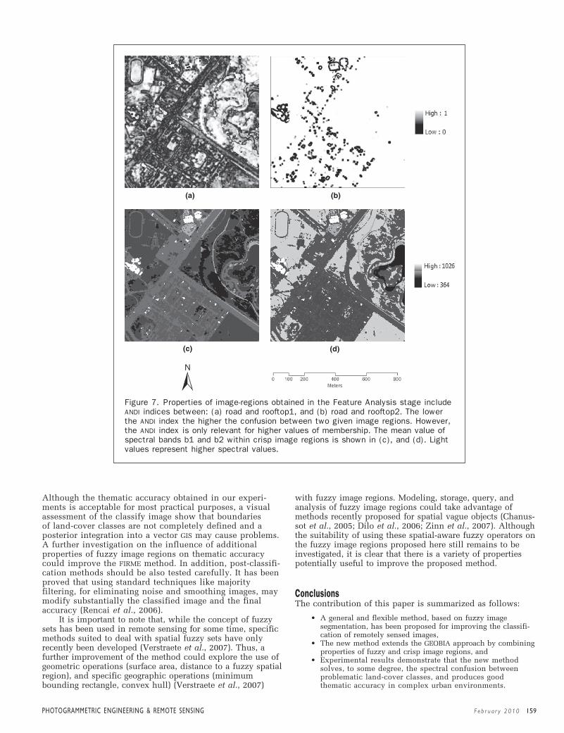
PHOTOGRAMMETRIC ENGINEER ING & REMOTE SENS ING Feb r ua r y 2010 159
(a) (b)
(c) (d)
Figure 7. Properties of image-regions obtained in the Feature Analysis stage includeANDI indices between: (a) road and rooftop1, and (b) road and rooftop2. The lowerthe ANDI index the higher the confusion between two given image regions. However,the ANDI index is only relevant for higher values of membership. The mean value ofspectral bands b1 and b2 within crisp image regions is shown in (c), and (d). Lightvalues represent higher spectral values.
Although the thematic accuracy obtained in our experi-ments is acceptable for most practical purposes, a visualassessment of the classify image show that boundariesof land-cover classes are not completely defined and aposterior integration into a vector GIS may cause problems.A further investigation on the influence of additionalproperties of fuzzy image regions on thematic accuracycould improve the FIRME method. In addition, post-classifi-cation methods should be also tested carefully. It has beenproved that using standard techniques like majorityfiltering, for eliminating noise and smoothing images, maymodify substantially the classified image and the finalaccuracy (Rencai et al., 2006).
It is important to note that, while the concept of fuzzysets has been used in remote sensing for some time, specificmethods suited to deal with spatial fuzzy sets have onlyrecently been developed (Verstraete et al., 2007). Thus, afurther improvement of the method could explore the use ofgeometric operations (surface area, distance to a fuzzy spatialregion), and specific geographic operations (minimumbounding rectangle, convex hull) (Verstraete et al., 2007)
with fuzzy image regions. Modeling, storage, query, andanalysis of fuzzy image regions could take advantage ofmethods recently proposed for spatial vague objects (Chanus-sot et al., 2005; Dilo et al., 2006; Zinn et al., 2007). Althoughthe suitability of using these spatial-aware fuzzy operators onthe fuzzy image regions proposed here still remains to beinvestigated, it is clear that there is a variety of propertiespotentially useful to improve the proposed method.
ConclusionsThe contribution of this paper is summarized as follows:
• A general and flexible method, based on fuzzy imagesegmentation, has been proposed for improving the classifi-cation of remotely sensed images,
• The new method extends the GEOBIA approach by combiningproperties of fuzzy and crisp image regions, and
• Experimental results demonstrate that the new methodsolves, to some degree, the spectral confusion betweenproblematic land-cover classes, and produces goodthematic accuracy in complex urban environments.
151-162_GB-604.qxd 1/15/10 10:33 AM Page 159

160 Feb r ua r y 2010 PHOTOGRAMMETRIC ENGINEER ING & REMOTE SENS ING
(a) (b)
(c) (d)
Plate 1. Final land-cover classification using: (a) fuzzy segmentation(PCC � 0.83), (b) crisp image-objects (PCC � 0.64), (c) fuzzy classification(PCC � 0.75), and (d) maximum likelihood (PCC � 0.66). Classified imagesshow road in gray, rooftop1 in orange, rooftop2 in cyan, grass in lightgreen, tree in dark green, water in blue, and soil in yellow.
TABLE 3 ACCURACY OF LAND-COVER CLASSIFICATION USING FUZZY SEGMENTATION ASIMPLEMENTED IN THE FIRME METHOD
Class Road Rooftop1 Rooftop2 Grass Tree Water Soil Totals
Road 131 12 2 1 2 0 1 149Rooftop1 21 76 23 0 4 0 6 130Rooftop2 0 0 32 0 0 0 1 33Grass 2 0 1 61 0 0 0 64Tree 0 0 0 0 43 0 0 43Water 0 0 0 0 0 34 0 34Soil 0 1 3 0 0 0 21 25Totals 154 89 61 62 49 34 29 478Producer’s 0.85 0.85 0.52 0.98 0.88 1.00 0.72User’s 0.88 0.58 0.97 0.95 1.00 1.00 0.84
Overall Accuracy 0.83
151-162_GB-604.qxd 1/15/10 10:33 AM Page 160

PHOTOGRAMMETRIC ENGINEER ING & REMOTE SENS ING Feb r ua r y 2010 161
TABLE 4. ACCURACY OF LAND-COVER CLASSIFICATION USING CRISP SEGMENTATION AS IMPLEMENTED IN IMAGINE® OBJECTIVE
Class Road Rooftop1 Rooftop2 Grass Tree Water Soil Totals
Road 87 10 4 0 4 9 0 114Rooftop1 66 79 44 1 1 0 7 198Rooftop2 0 0 13 0 0 0 0 13Grass 1 0 0 42 0 0 4 47Tree 0 0 0 0 44 0 2 46Water 0 0 0 0 0 25 0 25Soil 0 0 0 19 0 0 16 35Total 154 89 61 62 49 34 29 478Producer’s 0.56 0.89 0.21 0.68 0.90 0.74 0.55User’s 0.76 0.40 1.00 0.89 0.96 1.00 0.46
Overall Accuracy 0.64
The implementation of FIRME, tested in the experi-ments reported in this paper, used spectral and contextualproperties of fuzzy image regions as basis for land-coverclassification. Fuzzy-Fuzzy image-regions are generic typesof image objects which represent degrees of membershipsto competing land-cover classes. By solving the spatialand/or the thematic ambiguity of these image regions, apotential rich amount of information can be used toimprove the separation of spectrally mixed classes.
While two specific statistical learning methods havebeen used for the preliminary implementation of FIRME inthis study, the method can be applied using other super-vised methods. It is important to note that all stages of theproposed method have been programmed using R an opensource statistical language and environment.
The proposed method has the following advantagescompared to object-based image classification using commer-cial software: (a) Simplicity: Except for providing a trainingsample, users do not need to tweak scale or shape parameters,(b) Flexibility: Users can choose any learning statistic methodfor conducting the fuzzy segmentation and/or categoricalclassification stages, and (c) Low cost: Users may use freeopen source software tools for conducting accurate remotesensing classification.
A further development of FIRME is to explore additionalrelationships and properties of fuzzy image-regions; only afew of them were used in the presented experiments. Hence,our future work will integrate additional attributes whichprove be relevant for improving the thematic accuracy of theimage classification process. It will also include testing the
TABLE 5. ACCURACY OF LAND-COVER CLASSIFICATION USING FUZZY CLASSIFICATION AS IMPLEMENTED IN IDRISI
Class Road Rooftop1 Rooftop2 Grass Tree Water Soil Totals
Road 136 45 0 0 0 0 0 181Rooftop1 17 37 2 0 1 0 0 57Rooftop2 0 5 59 0 0 14 6 84Grass 0 0 0 36 1 0 0 37Tree 0 0 0 2 46 0 0 48Water 0 0 0 0 0 20 0 20Soil 1 2 0 24 1 0 23 51Total 154 89 61 62 49 34 29 478Producer’s 0.88 0.42 0.97 0.58 0.94 0.59 0.79User’s 0.75 0.65 0.70 0.97 0.96 1.00 0.45
Overall Accuracy 0.75
TABLE 6. ACCURACY OF LAND-COVER CLASSIFICATION USING MAXIMUM LIKELIHOOD AS IMPLEMENTED IN IDRISI
Class Road Rooftop1 Rooftop2 Grass Tree Water Soil Totals
Road 46 8 0 0 0 0 0 54Rooftop1 106 72 0 2 2 14 1 197Rooftop2 1 9 61 4 0 0 11 86Grass 1 0 0 56 1 0 4 62Tree 0 0 0 0 46 1 0 47Water 0 0 0 0 0 19 0 19Soil 0 0 0 0 0 0 13 13Total 154 89 61 62 49 34 29 478Producer’s 0.30 0.81 1.00 0.90 0.94 0.56 0.45User’s 0.85 0.37 0.71 0.90 0.98 1.00 1.00
Overall Accuracy 0.66
151-162_GB-604.qxd 1/15/10 10:33 AM Page 161

162 Feb r ua r y 2010 PHOTOGRAMMETRIC ENGINEER ING & REMOTE SENS ING
performance of machine learning techniques, like randomforest or decision trees, which are able to produce human-readable classification rules.
AcknowledgmentsThe authors would like to thank the Universidad DistritalFrancisco Jose de Caldas (UDFJC) at Bogota, Colombia and theSchool of Geography, Birkbeck College, University of Londonfor their support. The multispectral image used in ourexperiments was provided by UDFJC. The authors acknowl-edge valuable comments from three anonymous reviewers.
ReferencesAnderson, J., E. Hardy, J. Roach, and R. Witmer, 1976. A Land Use
and Land Cover Classification System for use with RemoteSensor Data, Technical Report, U.S. Geological Survey.
Bezdek, J., M.P.J. Keller, and R. Krisnauram, 1999. Fuzzy Modelsand Algorithms for Pattern Recognition and Image Processing,Springer, New York.
Blaschke, T., Ch. Burnett, and A. Pekkarinen, 2006, ImageSegmentation Methods for Object-based Analysis andClassification, Remote Sensing Image Analysis: Including theSpatial Domain (S.M. de Jong and F.D. van der Meer, editors),Springer, pp. 211–236.
Bragato, G., 2004. Fuzzy continuous classification and spatialinterpolation in conventional soil survey for soil mapping of thelower Piave plain, Geoderma, 118(1–2):1–16.
Burrough, P.A., P.F.M. van Gaans, and R. Hoostmans, 1997.Continuous classification in soil survey: Spatial correlation,confusion and boundaries, Geoderma, 77(2–4):115–135.
Chanussot, J., I. Nystrom, and N. Sladoje, 2005. Shape signatures of fuzzy star-shaped sets based on distance from the centroid,
Pattern Recognition Letters, 26(6):735–746.Cheng, T., M. Molenaar, and H.S. Lin, 2001. Formalizing fuzzy
objects from uncertain classification results, InternationalJournal of Geographical Information Science, 15(1):27–42.
Dilo, A., P. Bos, P. Kraipeerapun, and R. de By, 2006. Storage andmanipulation of vague spatial objects using existing GISfunctionality, Flexible Databases Supporting Imprecision andUncertainty (G. Bordogna and G. Psaila, editors), Springer-Verlag, Berlin, pp. 293–321.
Duda, R., P. Hart, and D. Stork, 2001. Pattern Classification, JohnWiley and Sons, New York.
ERDAS, 2008. Automating Feature Extraction with IMAGINEObjective, White Paper, URL: http://gi.leica-geosystems.com/documents/pdf/IMAGINEObjectivebrochure.pdf (last dateaccessed: 10 November 2009).
Hastie, T., R. Tibshirani, and J. Friedman, 2001. The Elements ofStatistical Learning: Data Mining, Inference and Prediction,Springer-Verlag, New York.
Hay, G., and G. Castilla, 2008. Geographic Object-Based ImageAnalysis (GEOBIA): Paradigm shift or new methods?, Object-Based Image Analysis - Spatial Concepts for Knowledge-drivenRemote Sensing Applications (T. Blaschke, S. Lang, and G. J. Hay,editors). Springer-Verlag., pp. 20.
Herold, M., M.E. Gardner, and D.A. Roberts, 2003, Spectral resolutionrequirements for mapping urban areas, IEEE Transactions onGeoscience and Remote Sensing, 41:1907–1919.
Jensen, J., 2006. Introductory Digital Image Processing, PrenticeHall, Upper Saddle River, New Jersey.
Kux, H., and C. Pinho, 2006. Object-oriented analysis of high-resolution satellite images for intra-urban land cover classifica-tion: Case study in Sao Jose dos Campos, Sao Paulo State,Brazil, Proceedings of the First International Conference onObject-Based Image Analysis.
Lang, S., F. Albretch, and T. Blaschke, 2006. Tutorial: Introduc-tion to Object-based Image Analysis, Centre for Geoinformatics - Z-GIS.
Lizarazo, I., 2008. SVM-based segmentation and classification ofremotely sensed data, International Journal of Remote Sensing,29(24):7277–7283.
Lizarazo, I., and P. Elsner, 2009. Fuzzy segmentation for object-based image classification, International Journal of RemoteSensing, 30(6):1643–1649.
Lu, D., and Q. Weng, 2007. A survey of image classification methodsand techniques for improving classification performance,International Journal of Remote Sensing, 28:823–870.
Platt, R.V., and L. Rapoza, 2008. An evaluation of an object-orientedparadigm for land use/land cover classification, The ProfessionalGeographer, 60(1):87–100.
Prewitt, J.M., 1970. Object Enhancement and Extraction, PictureProcessing and Psychopictorics (B.S. Lipkin and A. Rosenfeld,editors), Academic Press, New York, pp. 75–149.
R Development Core Team, 2008. R: A Language and Environmentfor Statistical Computing, R Foundation for Statistical Computing,Vienna, Austria. ISBN 3-900051-07-0, URL http://www.R-project.org (last date accessed: 10 November 2009).
Rencai, D., D. Jiajia, W. Gand, and D. Hongbing, 2006. Optimizationof post-classification processing of high-resolution satelliteimage: A case study, Science en China Series E: TechnologicalSciences, 49(1):98–107.
Ross, T., 2004. Fuzzy Logic with Engineering Applications, Wiley.Shackelford, A.K., and C.H. Davis, 2003. A combined fuzzy pixel-
based and object-based approach for classification of high-resolution multispectral data over urban areas, IEEE Transac-tions on Geoscience and Remote Sensing, 41(10):2354–2363.
Schiewe, J., L. Tufte, and M. Ehlers, 2001. Potential and problemsof multi-scale segmentation methods in remote sensing, GIS,Geo-Informations-System, 6(9):34–39.
Thomas, N., C. Hendrix, and R. Congalton, 2003. A comparisonof urban mapping methods using high-resolution digitaldmagery, Photogrammetric Engineering & Remote Sensing,69(9):963–972.
Verstraete, J., A. Hallex, and G. De Tré, 2007. Fuzzy Regions: Theoryand Applications, Geographic Uncertainty in EnvironmentalSecurity (A. Morris and S. Kokhan, editors), Springer, pp. 1–17.
Wang, F., 1990. Fuzzy supervised classification of remote sensingimages, IEEE Transactions on Geoscience and Remote Sensing,28(2):194–201.
Wei, W., X. Chen, and A. Ma, 2005. Object-oriented informationextraction and application in high resolution remote sensingimage, Proceedings of the International Geoscience and RemoteSensing Symposium(IGARSS), 6:3803–3806.
Wood, S., 2006. Generalized Additive Models: An Introduction withR, Chapman and Hall.
Zinn, D., J. Bosch, and M. Gertz, 2007. Modeling and queryingvague spatial objects using shapelets, Proceedings of the 33rd
International Conference on Very Large Databases, University ofVienna.
Zhou, C., P. Wang, Z. Zhang, C. Qi, and Y. Wang, 2007. Object-oriented information extraction technology from QuickBirdpan-sharpened images, Proceedings of SPIE -The InternationalSociety for Optical Engineering, 6279(2):62793L.
151-162_GB-604.qxd 1/15/10 10:33 AM Page 162

AbstractDescriptions of Geographic Object-Based Image Analysis(GEOBIA) often identify image segmentation as the initialstep. This may be reasonable in some cases, but segmenta-tion might also be considered a “black art,” due to its imagedependence and the limited amount control available tousers. The resulting segments reflect the spectral structure ofthe image rather than the physical structure of the land-scape with no one-to-one relationship between real worldobjects and segments. Geographic analysis often begins inthe context of existing mapping. In regions with high qualitylarge scale cartography, an obvious question is why is thisinformation not used in the GEOBIA process? It is thereforeproposed that GEOBIA be redefined to use the best existingreal world feature datasets as the starting point beforesegmentation is considered. Such an approach wouldincrease opportunities for integration, improve map updateinitiatives, and widen uptake by end user communities.
IntroductionGeographic Object-Based Image Analysis (GEOBIA) isdescribed as “a sub-discipline of Geographic InformationScience (GIScience) devoted to developing automatedmethods to partition remote sensing imagery into meaning-ful image-objects, and assessing their characteristics throughspatial, spectral and temporal scales, so as to generate newgeographic information in GIS-ready format,” (Hay andCastilla, 2008a). This definition makes no suggestion as tothe source of the image-object boundaries and the term‘meaningful’ would suppose that they should be related asclosely as possible to real world objects.
However, much of the published material on GEOBIAand its applications begin with the assertion that imagesegmentation is the vital first stage of the process. Asthe field of GEOBIA has developed over the last few years,many of the review papers that have come out to developthe theory (for example, Lang and Blaschke, 2006) havefailed to identify any other source for the image-objectsthan segmentation. It can then be assumed that featureextraction from images appears to be a major driver behindGEOBIA.
PHOTOGRAMMETRIC ENGINEER ING & REMOTE SENS ING Feb r ua r y 2010 163
Geoffrey M. Smith, Specto Natura Ltd., Impington, Cambridge, CB24 9PL, United Kingdom, ([email protected]).
Dr R. Daniel Morton, Centre for Ecology and Hydrology,Lancaster Environment Centre, Library Avenue, Bailrigg,Lancaster, LA1 4AP, United Kingdom.
Photogrammetric Engineering & Remote Sensing Vol. 76, No. 2, February 2010, pp. 163–171.
0099-1112/10/7602–163/$3.00/0© 2010 American Society for Photogrammetry
and Remote Sensing
Real World Objects in GEOBIA through theExploitation of Existing Digital Cartography
and Image SegmentationGeoffrey M. Smith and R. Daniel Morton
In their work on the strengths, weaknesses, opportunities,and threat associated with GEOBIA, Hay and Castilla (2008a)followed the conventional definitions and understanding, butidentified an interesting set of key issues which GEOBIAshould be addressing. The first is a driver from the usercommunity regarding the sophistication of their needs andtheir expectations regarding products. Another key driver wasseen as the need for greater integration with vector GIS dataand applications. Finally, a key weakness of GEOBIA was seenas the segmentation approach itself, its uncertainties, and thelack of repeatability.
In this paper we hope to address some of these issuesand propose a broader definition of GEOBIA to exploit itsstrengths and minimize its weaknesses. The keys to this arethe selection of meaningful image-objects and the appropriateand effective use of image segmentation. An example will begiven for operational national-level land-cover mapping inthe UK. The end result of adopting a broad definition will beto maximize the exploitation of GEOBIA products and tech-nologies by the end user community.
Spatial FrameworksThe majority of geo-information activity and market inthe commercial/operational sector is centered on the useof map-like and vector-based products. Raster-based imageproducts play a more minor role and in a significantproportion of these cases are used only to guide the useror place a vector-based analysis in context. For example,aerial photographs are extensively used in GIS applicationsas a contextual backdrop over which to display theinformation of interest, for instance utility networks.Vector-based products are what most end users feelcomfortable with and provide a straight forward link toexisting data, conventional mapping and their spatialperceptions.
Even though GEOBIA generates a vector-based product,the dominance of image segmentation as a major compo-nent of many of its applications confers raster characteris-tics on the end product, and creates a barrier to useracceptance. To really exploit the benefits of GEOBIA, theobject structures adopted must align themselves as closelyas possible to what is already known, what is already in
163-171_GB-601.qxd 1/15/10 10:27 AM Page 163

164 Feb r ua r y 2010 PHOTOGRAMMETRIC ENGINEER ING & REMOTE SENS ING
(a) (b)
Figure 1. Examples of (a) over, and (b) under segmentation when generating landparcel objects. In (a) the group of five segments in the center should have been mergedinto a single field. In (b) the large segment in the center should have been subdividedinto at least two separate fields. The images also show the inherent image characteris-tics transferred to the segments.
use, and what fits with the users’ perception. From aremote sensing point of view image segmentation mayseem a sensible first step in developing object-basedapproaches to a particular analysis, but when users haveexisting land parcel objects or clear perceptions of land-scape structure the power and benefits of GEOBIA may getundersold or ignored.
Image segmentation has obviously an important role toplay in monitoring and assessment of landscape characteris-tics, but it may be better deployed as part of a multi-sourceobject definition solution. The crucial first step in GEOBIAshould be more generically defined as obtaining a set ofmeaningful land parcel objects which represent the featuresof interest to the user in the landscape, whether or not theyhave a spectral distinction in the image.
Use of SegmentationThe use of segmentation algorithms to identify relativelyhomogeneous areas in images has been around for decadesin experimental and semi-operational forms (Haralick andShapiro, 1985). Recent developments in computer powerand software technology have now brought segmentationand GEOBIA to the mainstream. Even so, the applicationof image segmentation algorithms might still be considereda “black art,” due to the dependence of the results onthe image data and the limited, and often vaguely speci-fied, control parameters available to the user. In the caseof segmenting a complete Landsat Thematic Mapper (TM)scene three or four parameters may be the only controlover the generation of in excess of 300,000 land parcelscovering a broad range of land-cover and landscape types.
Once a suitable set of parameters have been selected,often by trial and error, the resulting segments reflect thespectral structure of the image rather than the true struc-ture of the landscape (Figure 1). For instance, two adjacentfields with the same crop could be combined into a singleobject even though they may be owned by differentfarmers. Even if a boundary feature existed between them,it would need to be spatially and spectrally significant atthe spatial resolution of the image data to cause the
segmentation algorithm to initiate a new object.Conversely, single fields that contain natural and accept-able variability may give multiple objects per field. Forinstance, a crop may progressively come into flower acrossa field, and the pattern of flowering could be captured bythe image data and then recorded as spurious objects.Segments and their boundaries also retain the inherentarea sampling, raster structure, of the original imageresulting in an unnatural stepped appearance. This causesproblems when comparing with other data sets, especiallywhere they represented diagonal boundaries in a moreconventional manner (Kampouraki et al., 2008), if linegeneralization has not been applied.
The results of image segmentation therefore representthe sensors view of the surface rather than the user’s. Asdescribed by Hay and Castilla (2008b), segmentationproduces image objects which often have complex relation-ships to the geographic objects which are of interest to theuser. Unfortunately, the segmentation view of the surfacehas limited repeatability over time due to changes in thesurface and atmospheric characteristics caused by seasonal-ity (Walter, 2004), illumination (Kampouraki et al., 2008),and climate. Also, at different times of year the combina-tions of land-cover types within a scene will have differentrelative spectral and textural separabilities, and thusgenerate different sets of segments. For instance, in earlyMay in the UK, grass and wheat fields may appear verysimilar, and only later in the growing season can they bereliably distinguished. The same can be said for differentpreprocessing methodologies, different segmentationalgorithms (Carleer et al., 2005; Neubert et al., 2006), anddifferent parameter selections (for example, Figure 2).
It could be suggested that this lack of a direct one-to-one relationship between real world objects and imagesegments and their limited temporal coherence, has pre-vented GEOBIA reaching its full potential. The currentsituation is not too surprising as much of the earlier GEOBIAwork was within the raster processing domain and onlyrecently have fully structured digital vector cartographydatasets and the necessary software tools become availableto explore other approaches effectively.
163-171_GB-601.qxd 1/15/10 10:27 AM Page 164

PHOTOGRAMMETRIC ENGINEER ING & REMOTE SENS ING Feb r ua r y 2010 165
(a)
(c) (d)
(b)
Figure 2. Examples of different segmentation algorithms applied to the same imagedata set and aimed at delivering a field by field scale segmentation: (a) Definiens,(b) LCM2000, (c) experimental, and (d) original Landsat TM scene).
Utilization of External LineworkRarely today is any environmental or geographic analysisbegun on a blank canvas, but begins in the context ofexisting mapping of some form, which is often availabledigitally. In regions of the world with high quality largescale cartographic mapping, an obvious question is why isthis information not used to control the GEOBIA process?
Even in the less cartographically developed parts of theworld, there will be some form of line work with which toat least begin the process of creating a landscape structureand thus a land parcel object data set. At the lowest level,even national boundaries have been seen as controls onland-cover type or condition due to, for instance, landmanagement regimes or conflict. There may be differencesbetween the cartography and EO data used in GEOBIA due totemporal changes, but the majority of key landscape features(e.g., roads, field boundaries, forest compartments, etc.) arerelatively stable up to at least decadal intervals.
Many countries with formalized systems of landownership already have land parcel data sets in the form
of cadastral systems (Cadastral Template Project, 2009).Due to the nature of the development of cadastre, themeans employed for marking ownership on the surface,and the consequent differences in land management, thecadastral dataset can form a significant part of the requiredland parcel object set for a GEOBIA approach. Some cadas-tre also carry basic land-cover information. Finally, in themost cartographically developed regions not only isownership mapped, but also many of the key landscapefeatures related to policy and land management. Theremay be access issues due to privacy concerns, but oftenthese datasets are produced by public bodies and arebeginning to fall under open access agreements such as theEuropean INSPIRE directive (INSPIRE, 2009).
In the context of national land-cover mapping, the landparcel objects required for the spatial framework will befields, lakes, and patches of woodland, etc. In urban map-ping, the objects may be buildings, roads, gardens, etc. Thespecific requirements will be related to the actual land-coverclasses or features present in a region, and the specification
163-171_GB-601.qxd 1/15/10 10:27 AM Page 165

166 Feb r ua r y 2010 PHOTOGRAMMETRIC ENGINEER ING & REMOTE SENS ING
of the final product required by the end user. Any differ-ences between cartography and EO data can identify areasfor improvement in the process, the data used, or thepresence of a real change.
It should be noted that any digital cartography availableis rarely acquired for the same purpose as the GEOBIAapplication, and there will be a need to tailor it. This mayinclude the sub-setting of selected features, the generalizationof spatial detail, and the addition of further linework.
Use of Digital Cartography in Object-based ApproachesCompared to the amount of reported work driven solely byimage segmentation, the number of projects which haveused external line work is very limited. However, even workdating back to the 1980s (e.g., Mason et al., 1988) saw thevalue of external line work to support image segmentation,even though the developments were hindered by technologi-cal limitations, leading to the approaches being rathersimplistic.
More recent work has in the main been focused onsmall scale studies. Dean and Smith (2003) mapped a naturereserve and surrounding areas to demonstrate the value ofexploiting land parcel data sets when extracting and aggre-gating spectral information from images for classification.They assessed the differences in performance when dealingwith homogeneous agricultural fields and heterogeneoussemi-natural areas within the nature reserve. A similarapproach was adopted by Walter (2004) using cadastreinformation as the spatial framework and a maximumlikelihood algorithm to classify objects on a per-parcel basis.A slightly different implementation was employed by Aplinet al. (1999) who first classified pixels individually usingconventional means, and then grouped the classified pixelsper land parcel to derive a representative class (e.g., bycalculating the modal class per object) for each land parcel.This implementation was also used by Raclot et al. (2005)when updating a land-cover classification product using arule-based decision system. A further extension of this workwas to locate fuzzy (sub-pixel) land-cover class proportionsspatially by segmenting the actual pixels (4 m spatialresolution) according to polygon boundaries (Aplin andAtkinson, 2001), while Shackleford and Davis (2003) usedsub-pixel class proportions to derive new land-cover classesat the land parcel object level. The problem of classifyingvery high spatial resolution images has been addressed byusing unsupervised clustering approaches to identifyspectral image components, and then assessing the propor-tions of the components within a set of established landparcels (Hoffmann et al., 2000).
A number of projects have exploited agricultural landparcels data sets to improve crop mapping (e.g., Arikan,2004; Ozdarici and Turker, 2006) and the agricultural landparcels have been enhanced by identifying within parcelboundaries (Turker and Kok, 2006). Wu et al. (2007) used acombination of GIS and Earth Observation (EO) data topopulate and analyze a set of tax parcel boundaries for land-use classification.
A relatively large scale object-based land-cover mappingexercise was undertaken while producing a land-cover mapfor the island of Jersey in 1997 (Smith and Fuller, 2001).The island government had digital cartography available foran area of approximately 215 km2, but this cartography wastoo detailed to generate land parcels for integration directlywith standard EO data sets (�10 m spatial resolution). It wastherefore necessary to generalize the digital cartographybefore the object-based classification could be applied.Unfortunately, at the time, the only means of doing thisgeneralization was by manually editing the line work and
building objects from the disconnected lines. This processtook around two person months and was therefore impracti-cal for larger areas. At a larger level, the use of agriculturalland parcels has been integrated as part of the land-covermapping initiatives of The Netherlands (Hazeu, 2006; DeWit and Clevers, 2004).
Finally, some work has been done combining existingdigital cartography with segmentation results as a check onthe acceptability of the digital cartography. Tiede et al.(2007) segmented and classified SPOT5 data, and thencompared the results to existing cartography and transferredthe classification result as appropriate. Where the segmenta-tion provided additional boundaries, these were added tothe existing boundaries, and where the existing cartographywas found to be too detailed compared to the segmentation,boundaries were removed. This later case is useful to reducedata volumes and complexity, but the existing boundariesthat have been removed may have significance beyondspectral separability.
It can be seen from the above description that the use ofexisting cartography has not been all together absent fromGEOBIA developments. The dominance of segmentation is inthe main due to the software tools in widespread use andthe poor availability of suitably structured digital cartogra-phy. As these deficiencies are now beginning to be over-come, the GEOBIA community should respond and incorpo-rate digital cartography into their analysis whereappropriate.
Implementation in the United KingdomThe United Kingdom (UK) undertakes an assessment of itslandscape at intervals of eight to ten years known as theCountryside Survey (CS). The main component of the CS is aground-based field survey of sample sites, but the last two CSshave included national land-cover maps derived from EO data.
Introduction to the UK Land Cover MapsThe first of these, the Land Cover Map of Great Britain(LCMGB) in 1990, was a relatively simple pixel-based classifi-cation using Landsat Thematic Mapper (TM) data (Fuller etal., 1994). An update and upgrade of LCMGB was producedbetween 1998 and 2001, referred to as Land Cover Map 2000(LCM2000), which adopted an object-based approach (Fulleret al., 2002; 2005). The production of the UK land-covermaps has closely tracked methodological and technicaldevelopments in GEOBIA, but within a national operationalcontext attempting to address a broad spectrum of end users.
LCM2000 used image segmentation to deliver an object-based product with a final dataset containing around6.6 million segmented land parcels with a minimummappable unit (MMU) of 0.5 ha (Figure 3). Although consid-ered extremely successful from an EO point-of-view and alsowhen undertaking regional assessments, the relationshipbetween the segmented land parcels and the real worldfeatures in LCM2000 as seen by end-users did receive somecriticism. The key issues were the differences between thesegments and existing products and mapping, the need torepeat the production at regular intervals, and the difficul-ties of downstream integration.
Improvements for LCM2007Production is now underway on a further update of the UKnational land-cover product which had a target summer forEO data collection of 2007 (thus to be known as LCM2007)and a completion date of late-2009. This product will againbe object-based, but this time digital cartography will beadapted to give an object structure which more accuratelyreflects the true structure of the UK landscape (Smith, 2008).
163-171_GB-601.qxd 1/15/10 10:27 AM Page 166

PHOTOGRAMMETRIC ENGINEER ING & REMOTE SENS ING Feb r ua r y 2010 167
Figure 3. An example of LCM2000 data showing the landparcel object structure and the impact of the pixelatedsegments on the overall result.
In 2001 the Ordnance Survey (OS), the national mappingagency of Great Britain, released MasterMap (MM) a topologi-cally structured digital cartography layer for the wholecountry. The structured nature of the data provides acomprehensive cover of land parcel objects and theirassociated attribution allows the use of efficient, costeffective generalization to provide land parcels suitable forintegration with EO data that has a spatial resolution ofapproximately 20 to 30 m (see Smith et al., 2007 for details).The MMU for the LCM2007 was set to 0.5 ha, and the mini-mum feature width (MFW) was set to 20 m. In comparisonwith a Landsat TM image (Figure 4), it can be seen that thegeneralized OS MM is fully aligned with the needs of anobject-based analysis procedure at this scale. Assessment of
the land parcel objects by aerial photography interpreters(Figure 5) has confirmed the quality and utility of the resultswith the correspondence to the underlying aerial photogra-phy being exceptionally good. In the example in Figure 5,there is arguably one missed field boundary, and in practice,the plantation woodland should be divided up into blocksthat could be allocated to deciduous and coniferous (distinc-tions not necessarily recorded in the cartography) or clearfelling (which may post date the cartography).
Challenges for Integrating Additional Data SetsWhen the generalized OS MM for LCM2007 was compared tocontemporary EO data for a wider area, two particularlandscape types were lacking boundaries required forGEOBIA; agricultural areas due to changing land managementand semi-natural area due to subtle habitat patches. Thegeneralization of OS MM worked best in urban areas andrural areas dominated by pasture farming. The urban areaswere well defined as changes in land-cover were virtuallyalways accompanied by some form of boundary which wasmapped by the OS.
In the agricultural landscape, issues related to thepresence of actual boundary features or just the operationof different land management practices come into play. Aspasture farming requires that all boundaries are stockproof, all land parcel boundaries will be mapped by the OSin this case. The generalized digital cartography appearedto be slightly less successful for deriving land parcelobjects in the arable landscape where land-cover bound-aries appeared to be missing. Some of these missingboundaries were related to the “open gate” problem wherethe original OS LandLine, a “spaghetti” data set whichformed MM, could not be built into complete area objectsrelated to fields. Other missing boundary features wererelated to different farming practices being applied todifferent parts of the same field with no physical boundarypresent for the OS to map. In the UK, for farmers to join
Figure 4. A comparison of generalized OS MM and LandsatThematic Mapper data with a spatial resolution of 25 m.
Figure 5. A comparison of generalized OS MM andconventional aerial photography with a spatialresolution of less than 1 m.
163-171_GB-601.qxd 1/15/10 10:27 AM Page 167

168 Feb r ua r y 2010 PHOTOGRAMMETRIC ENGINEER ING & REMOTE SENS ING
and receive grants from government schemes, there is aneed to map the extent of different cropped areas, andthus additional and complimentary land parcel boundarydata sets are available. The Rural Land Register (RLR) heldby the Rural Payments Agency (RLA) captures and main-tains permanent field boundaries to create a spatialboundary layer and produces an accurate digital map ofdeclared agricultural land parcels in England. Similar datasets are held by agencies in Scotland, Wales, and NorthernIreland. The second stage of the construction of the spatialframework for LCM2007 is therefore the integration ofagricultural land parcel boundary information with thegeneralized OS MM where appropriate within the spatialspecification and in a hierarchical fashion. Many bound-aries in the generalized OS MM and the agricultural landparcel data sets will represent the same real world fea-tures, even if they do not appear in exactly the samespatial location. For instance, the generalization processmay have moved a boundary to remove a feature belowthe MFW, but agricultural land parcel data set may have itin the correct location (Figure 6). Therefore, the integra-tion process is not a simple merging of the two input datasets, but a more complex spatial processing operation.Figure 7 shows an example of the generalized OS MM dataand RLR data.
The other problematic area when building the spatialframework for LCM2007 concerned environments associated
with semi-natural and upland land-cover types. In theseareas the total extents are mapped well by the OS MM data,such as the area delineated by the “high wall mark” in theuplands, but the internal divisions caused by habitatpatches were poorly mapped. These internal divisions wereoften indistinct, complex, and dynamic, and the lack ofpermanent physical boundary features, walls, hedges, roads,etc. in upland areas generates large land parcels that do not
Figure 6. An example of generalized OS MM (solid), theagricultural land parcel data (dashed), and the resultingintegrated data set showing the contribution from theagricultural land parcel data set.
Figure 7. A comparison of generalized OSMM (dark grey) and the additional boundaryinformation available in arable areas from the agricultural land parcel datasets(light grey).
163-171_GB-601.qxd 1/15/10 10:27 AM Page 168

PHOTOGRAMMETRIC ENGINEER ING & REMOTE SENS ING Feb r ua r y 2010 169
adequately record the semi-natural vegetation structurewithin these landscapes. To complete the final part of theLCM2007 spatial structure, large upland land parcel objectswere segmented based on EO data to generate the necessaryinternal boundaries (Figure 8). Landscape knowledge andthe examination of within parcel variation of the EO datawill limit the need for segmentation to only the areas whereit is necessary.
A key component of the UK land-cover maps and animportant feature for the later reuse of the information is theretention of land parcel level metadata (Smith and Fuller,2002). The source of the input data for the spatial frame-work is recorded in construction metadata so that users willbe aware of how the objects have been produced and canuse this information to guide their analyses.
The production of the LCM2007 uses a number of carto-graphic and EO input datasets and a complex set ofprocesses to generate a consistent and objective landscapestructure for the UK prior to the classification of land-covertypes by GEOBIA. This is therefore a multi-source solution tothe need to produce land parcels for the later stages of theGEOBIA process, but that still contains image segmentation,although applied in an effective and realistic manner.
The example from LCM2007 has highlighted the opportuni-ties offered by the incorporation of existing digital cartography
but also the challenges that it introduces. Spatial frameworksbuilt on cartography are in the main more closely aligned tothe real world and fit user perceptions. However, existingcartography will often require preprocessing of some form andis likely to be incomplete compared to user requirementsnecessitating the use of supplementary data from other sourcessuch as segmentation.
ConclusionsOne data source or one approach to the generation of landparcels for GEOBIA will rarely provide all of the necessaryboundary information to a level of quality acceptable to allend users. Various sources of boundary information need tobe combined in such a way as to maximize the quality of thefinal spatial structure and retain a level of traceability so thatend users can effectively interpret the results. The details ofthis approach will obviously be application specific, but theuse of existing linework as a first step, if appropriate andavailable, would seem to represent an initial rule for GEOBIA.
The use of external linework in land-cover mappingremoves the constraints imposed by the image specifica-tion and characteristics from the spatial framework part ofthe process and allows the strength of the GEOBIA approachto be exploited. Segmentation is used for deriving addi-
Figure 8. An example of a generalized OSMM objects (black) subdivided by imagesegmentation of EO data (white) applied within the land parcel object only.
163-171_GB-601.qxd 1/15/10 10:27 AM Page 169

170 Feb r ua r y 2010 PHOTOGRAMMETRIC ENGINEER ING & REMOTE SENS ING
tional boundaries within existing land parcel objectswhich are either not mapped at all or are too subtle ordynamic to be mapped by conventional cartographicupdate. Tests during the development stages of LCM2007have identified a further benefit of using land parcelobjects derived from externally validated datasets, ascoarse spatial resolution data sets can be integrated intothe classification process without affecting the quality ofthe spatial structure. The segmentation step can thereforebe used where it is most needed and most effective, orexcluded when sufficiently spatially detailed EO data arenot available.
It is proposed that the GEOBIA process be made moregeneric so as to use the best existing real world featuredatasets as the starting point for the process before seg-mentation is considered. Such an approach wouldincrease opportunities for integration with other datasetsand improve the results of map update initiatives. Theadoption of such approaches should result in greateruptake of GEOBIA products and technologies by the enduser community.
AcknowledgmentsDigital cartography reproduced by permission of OrdnanceSurvey of behalf of HMSO © Crown copyright and databaseright 2007; all rights reserved. The development work forthe object-based analyses associated with the UK land-covermaps has been funded by the Natural Environment ResearchCouncil and a consortium of government departments andagencies led by the Department for Environment, Food andRural Affairs. Much of the work has been undertaken as partof the Countryside Survey (http://www.countrysidesurvey.org.uk/) program. The technology behind the generalizationof the digital cartography and land-cover classification isbased on the Gothic core technology of 1Spatial Limited(http://www.1spatial.com/).
ReferencesAplin, P., and P.M. Atkinson, 2001. Sub-pixel land cover mapping
for per-field classification, International Journal of RemoteSensing, 22:2853–2858.
Aplin, P., P.M. Atkinson, and P.J. Curran, 1999. Fine spatialresolution simulated satellite imagery for land cover mapping inthe UK, Remote Sensing of Environment, 68:206–216.
Arikan, M., 2004. Parcel-based crop mapping through multi-temporalmasking classification of Landsat 7 images in Karacabey, Turkey,Proceedings of the XXth ISPRS Congress, Istanbul, Turkey, 12–23July, pp. 1085.
Cadastral Template Project, 2009. Cadastral Template: A World-wide Comparison of Cadastral Systems, URL: http://www.cadastraltemplate.org/, Department of Geomatics,University of Melbourne, Victoria (last date accessed: 09November 2009).
Carleer, A.P., O. Debeir, and E. Wolff, 2005. Assessment of very highspatial resolution satellite image segmentations PhotogrammetricEngineering & Remote Sensing, 71(11):1285–1294.
Dean, A.M., and G.M. Smith, 2003. An evaluation of per-parcel landcover mapping using maximum likelihood class probabilities,International Journal of Remote Sensing, 24:2905–2920.
De Wit, A.J.W., and J.G.P.W. Clevers, 2004. Efficiency and accuracyof per-field classification for operational crop mapping,International Journal of Remote Sensing, 25:4091–4112.
Fuller, R.M., G.B. Groom, and A.R. Jones, 1994. The Land CoverMap of Great Britain: An automated classification of LandsatThematic Mapper data, Photogrammetric Engineering & RemoteSensing, 60(5):553–562.
Fuller, R.M., G.M. Smith, J.M. Sanderson, R.A. Hill, A.G. Thomson,R. Cox, N.J. Brown, R.T. Clarke, P. Rothery, and F.F. Gerard,
2002. The UK Land Cover Map 2000: Construction of a parcel-based vector map from satellite images, Cartographic Journal,39:15–25.
Fuller, R.M., R. Cox, R.T. Clarke, P. Rothery, R.A. Hill, G.M. Smith,A.G. Thomson, N.J. Brown, D.C. Howard, and A.P. Stott, 2005.The UK Land Cover Map 2000: Planning, construction andcalibration of a remotely sensed, user-oriented map of broadhabitats, International Journal of Applied Earth Observation andGeoinformation, 7:202–216.
Haralick, R.M., and L. Shapiro, 1985. Image segmentation techniques,Computer Vision Graphics and Image Processing, 29:100–132.
Hay, G.J., and G. Castilla, 2008a. Geographic Object-Based ImageAnalysis (GEOBIA): A new name for a new discipline, Object-Based Image Analysis: Spatial Concepts for Knowledge-DrivenRemote Sensing Applications (Th. Blaschke, S. Lang, andG.J. Hay, editors), Springer-Verlag, Berlin, pp. 75–89.
Hay, G.J., and G. Castilla, 2008b. Image objects and geographic objects,Object-Based Image Analysis: Spatial Concepts for Knowledge-Driven Remote Sensing Applications (Th. Blaschke, S. Lang, andG.J. Hay, editors), Springer-Verlag, Berlin, pp. 91–110.
Hazeu, G.W., 2006. Land-use mapping and monitoring in theNetherlands (LGN5), Proceedings of the 2nd EARSeLWorkshop on Land Use and Land Cover, Bonn, Germany, 28–30 September.
Hoffmann, A., G.M. Smith, and F. Lehmann, 2000. The classifica-tion of fine spatial resolution imagery: Parcel-based approachesusing HRSC-A data, Proceedings of the Geoscience and RemoteSensing Symposium, IGARSS 2000. 7:3009–3011.
INSPIRE, 2008. INSPIRE Directive, http://inspire.jrc.ec.europa.eu/,European Commission, Brussels (last date accessed: 09 November 2009)
Kampouraki, M., G.A. Wood, and T.R. Brewer, 2008. Opportunitiesand limitations of object-based image analysis for detecting urbanimpervious and vegetated surfaces using true-colour aerialphotography, Object-Based Image Analysis: Spatial Concepts forKnowledge-Driven Remote Sensing Applications (Th. Blaschke,S. Lang, and G.J. Hay, editors), Springer-Verlag, Berlin,pp. 555–569.
Lang, S., and T. Blaschke, 2006. Bridging remote sensing and GIS - What are the main supportive pillars?, Proceedings of the1st International Conference on Object-based Image Analysis(OBIA 2006), Salzburg University, Austria, July 04–05.
Mason, D.C., D.G. Corr, A. Cross, D.C. Hogg, D.H. Lawrence,M. Petrou, and A.M. Tailor, 1988. The use of digital map datain the segmentation and classification of remotely-sensedimages, International Journal of Geographical InformationSystems, 2:195–215.
Neubert, M., H. Herold, and G. Meinel, 2006. Evaluation of remotesensing image segmentation quality - Further results andconcepts, Proceedings of the 1st International Conference onObject-based Image Analysis (OBIA 2006), Salzburg University,Austria, July 04–05.
Ozdarici, A., and M. Turker, 2006. Field-based classification ofagricultural crops using multi-scale images, Proceedings of the1st International Conference on Object-based Image Analysis(OBIA 2006), Salzburg University, Austria, July 04–05.
Raclot, D., F. Colin, and C. Puech, 2005. Updating land coverclassification using a rule-based decision system, InternationalJournal of Remote Sensing, 26:1309–1321.
Shackelford, A.K., and C.H. Davis, 2003. A hierarchical fuzzyclassification approach for high-resolution multispectral dataover urban areas, IEEE Transactions on Geoscience and RemoteSensing, 41:1920–1932.
Smith, G.M., 2008. The development of integrated object-basedanalysis of EO data within the UK national land coverproducts, Object-Based Image Analysis: Spatial Concepts forKnowledge-Driven Remote Sensing Applications (Th. Blaschke,S. Lang, and G.J. Hay, editors), Springer-Verlag, Berlin,pp. 513–528.
Smith, G., M. Beare, M. Boyd, T. Downs, M. Gregory, D. Morton,N. Brown, and A. Thomson, 2007. UK Land Cover Mapproduction through the generalisation of OS MasterMap,Cartographic Journal, 44:276–283.
163-171_GB-601.qxd 1/15/10 10:27 AM Page 170

PHOTOGRAMMETRIC ENGINEER ING & REMOTE SENS ING Feb r ua r y 2010 171
Smith, G.M., and R.M. Fuller, 2001. An integrated approach toland-cover classification: An example in the Island of Jersey,International Journal of Remote Sensing, 22:3123–3142.
Smith, G.M., and R.M. Fuller, 2002. Land Cover Map 2000 andmeta-data at the land parcel level, Uncertainty in RemoteSensing and GIS (G.M. Foody and P.M. Atkinson editors), JohnWiley and Sons, London, pp 143–153.
Tiede, D., M. Möller, S. Lang, and D. Hölbling, 2007. Adapting,splitting and merging cadastral boundaries according tohomogenous LULC types derived from SPOT 5 data, PIA07 -International Archives of Photogrammetry, Remote Sensingand Spatial Information Sciences (U. Stilla, H. Mayer,
F. Rottensteiner, C. Heipke, and S. Hinz, editors), 36 (3/W49A), München, pp. 99–104.
Turker, M., and E.H. Kok, 2006. Developing an integrated systemfor extracting the sub-fields within agricultural parcels fromremote sensing images, Proceedings of the 1st InternationalConference on Object-based Image Analysis (OBIA 2006),Salzburg University, Austria, July 04–05.
Walter, V., 2004. Object-based classification of remote sensing datafor change detection, ISPRS Journal of Photogrammetry andRemote Sensing, 58(3–4):225–238.
Wu, S., J. Silvan-Cardenas, and L. Wang, 2007. Per-field urban landuse classification based on tax parcel boundaries, InternationalJournal of Remote Sensing, 28:2777–2800.
February Layout 2.indd 171February Layout 2.indd 171 1/15/2010 1:24:36 PM1/15/2010 1:24:36 PM

172 Februar y 2010 PHOTOGRAMMETRIC ENGINEERING & REMOTE SENSING
CalendarFEBRUARY
2–4, 6th Gi4DM Conference on Geomatics
for Crisis Management, Torino, Italy. For more information, visit www.gi4dm-2010.org.
10–12, CuroCOW 2010: The Calibration and
Orientation Workshop, Institute of Geomat-ics on behalf of the EuroSDR (European Spatial Data Research) Commission I and, ISPRS (International Society for Photogrammetry and Remote Sensing) Working Group 1.5: Integrated Systems for Sensor Georeferenc-ing and Navigation, Castelldefels, Spain. For more information, visit www.ideg.es/page.php?id=787.
23–25, Art, Science and Applications of
Refl ectance Spectroscopy, ASD and IEEE, Boulder, Colorado. For more information, visit www.Refl ectanceSpectroscopySympo-sium.com
MARCH
3–5, ILMF 2010, The International LIDAR Mapping Forum, Denver, Colorado. For more information, visit www.lidarmap.org.
15–17, Core Spatial Databases – Updat-
ing, Maintenance and Services – from
Theory to Practice, ISPRS, Haifa, Israel. For more information, visit http://geo.haifa.ac.il/~isprs/HaifaJointWS .
22–25, CARIS 2010 — Stronger Together
– People, Products, Infrastructure, Miami, Florida. For more information, visit www.caris.com/caris2010.
APRIL
5–9, SPIE Defense, Security, and Sens-
ing 2010, SPIE, Orlando, Florida. For more information, visit http://spie.org/defense-security.xml?WT.mc_id=Cal-DSS.
26–30, ASPRS 2010 Annual Conference, ASPRS, San Diego, California. For more information, visit www.asprs.org.
MAY
12–15, Representing Reality: Imagery in
the Cognitive, Social and Natural Sciences, Presented by the University at Buffalo IGERT in GIScience, Buffalo, New York. For more information, visit http://www.ncgia.buffalo.edu/Conference/index.htm
26–28, 14th International Symposium on
Spatial Data Handling — Theory, Model-
ing and concepts in Geospatial Informa-
tion Science, Commission II on Theory and Concepts of Spatial Information Science of International Society of Photogrammetry and Remote Sensing (ISPRS), Commission on Geographic Information Science of Interna-tional Geographical Union (IGU), and Com-mission on Modelling Geographical Systems of IGU, Hong Kong. For more information, visit http://isgis.lsgi.polyu.edu.hk.
JUNE
20–25, 10th International Multidisciplinary
Scientifi c Geo-Conference and Expo –
SGEM 2010, Albena, Bulgaria. For more information, visit www.sgem.org.
22–24, ISPRS Commission on V Mid-Term
Symposium Close Range Image Measure-
ment Techniques, ISPRS, Remote Sensing and Photogrammetry Society, Newcastle Univer-sity, and Civil Engineering and Geosciences, Newcastle upon Tyne, UK. For more informa-tion, visit www.isprs-newcastle2010.org.
29–July 2, GEOBIA 2010 — GEOgraphi-
cal Object-Based Image Analysis, Ghent University, ITC and ISPRS, Utrecht University, Ghent, Belgium. For more information, visit http://geobia.ugent.be.
JULY
5–7, ISPRS Symposium Technical Commis-
sion VII, ISPRS, Vienna Austria. For more information visit, www.isprs100vienna.org.
6-9, GI Forum 2010, Salzburg, Austria. For more information, visit www.gi-forum.org.
18–25, COSPAR 2010 — 38th Scientifi c
Assembly of the Committee on Space Re-
search, COSPAR, Bremen, Germany. For more information, visit www.cospar2010.org/.
AUGUST
1–5, SPIE Optics+Photonics 2010, SPIE, San Diego Convention Center San Diego, Cali-fornia, USA. For more information, visit http://spie.org/optics-photonics.xml?WT.mc_id=Cal-OP.
SEPTEMBER
1–3, Photogrammetric Computer Vision
and Image Analysis Conference, ISPRS Technical Commission III, Paris, France. For more information, visit pcv2010.ign.fr.
OCTOBER
19–21, IX Seminar on Remote Sensing
and GIS Applied to Forest Engineering, Curitiba, Paraná Sate, Brazil. For more infor-mation, visit9seminariofl orestal.com.br.
NOVEMBER
15–18, ASPRS 2010 Fall Conference, ASPRS, Orlando, Florida. For more informa-tion, visit www.asprs.org.
MAY 2011
1–5, ASPRS 2011 Annual Conference, ASPRS, Milwaukee, Wisconsin. For more information, visit www.asprs.org.
= indicates a new listing
Who Do I Contact to Advertise with ASPRS?
5410 Grosvenor Lane, Suite 210 Bethesda, MD 20814
301-493-0290, 301-493-0208 (fax)www.asprs.org
Calendar x107 [email protected]
Exhibit Sales 410-788-1735 [email protected]
Meeting Information x106 [email protected]
PE&RS Advertising 410-788-1735 [email protected]
February Layout 2.indd 172February Layout 2.indd 172 1/15/2010 1:25:26 PM1/15/2010 1:25:26 PM

AbstractKeeping existing vector databases up to date is a real chal-lenge for GIS data providers. This study directly compares amap with a more recent image in order to detect the discrep-ancies between them. An automatic workflow was designed toprocess the image based on existing information extractedfrom the vector database. First, geographic object-based imageanalysis provided automatically labeled image segments aftermatching the vector database to the image. Then, discrepan-cies were detected using a statistical iterative trimming, whereoutliers were excluded based on a likelihood threshold.Applied on forest map updating, the proposed workflow wasable to detect about 75 percent of the forest regeneration, and100 percent of the clear cuts with less than 10 percent ofcommission errors. This discrepancy detection approachassumes that discrepancy corresponds to small proportion ofthe map area and is very promising in diverse applicationsthanks to its flexibility.
IntroductionThanks to remote sensing and field surveys, many countrieshold high quality cartographic vector databases. Thesedatabases are the main input for Geographic InformationSystem (GIS) in many applications such as land-use planning,ecological modeling, disaster response, and resource manage-ment. Updating the existing cartographic databases is thereforea major requirement in a context of rapid change.
In the particular case of forest management, variousforestry applications rely on cartographic vector database,e.g., logging management, forest pest models (White, 1986),or fire management (Lowell and Astroth, 1989). Keepingthese databases up to date is a real challenge because of thecost of the field surveys in remote areas and the frequencyof change due to exploitation and natural hazards (storms,insects, etc.). Very high resolution remote sensing providesthe opportunity to update forest maps at lower costs.Nevertheless, semi-automated processes are still to bedeveloped in order to provide operational tools for changedetection.
Change detection algorithms provide valuable toolstoward the automation of map update. The two mainapproaches for change detection are (a) post-classificationcomparison, and (b) multi-temporal classification. In the firstcase, two images are classified independently with the samelegend, and the resulting maps are crossed with specificdecision rules. This approach suffers from error propagationand mis-registration but gives straightforward information
PHOTOGRAMMETRIC ENGINEER ING & REMOTE SENS ING Feb r ua r y 2010 173
Unit of Environmetrics and Geomatics,Université catholiquede Louvain, Croix du Sud, 2/16, B-1348 Belgium([email protected]).
Photogrammetric Engineering & Remote Sensing Vol. 76, No. 2, February 2010, pp. 173–181.
0099-1112/10/7602–173/$3.00/0© 2010 American Society for Photogrammetry
and Remote Sensing
Automated Image-to-Map DiscrepancyDetection using Iterative Trimming
Julien Radoux and Pierre Defourny
about the type of change. In the second case, correspondingpixels, or image segments of different dates, are processedtogether in order to produce a change mask, most of thetime without information about the type of change. For moredetails, see Coppin et al. (2004) or Lu et al. (2004).
Different image-to-image change detection algorithmshave been applied successfully on forest/non-forest change.Recent studies (Stow et al., 2007; Hyvönen and Anttila,2006) used geographic object-based classification (respec-tively, nearest-neighbor and discriminant analysis) with bi-temporal aerial photographs. These methods showed goodperformance on the dataset, but relied on training sampleswhich may be costly. The TDA-SVM algorithm (Huang et al.,2008) used support vector machine (SVM) with training dataautomation (TDA) assuming that forests were the darkestvegetation type. Unfortunately, this method, appropriate forLandsat imagery, cannot be applied on very high spatialresolution images because sun-facing tree crown pixels havethe same intensity as other vegetation types. Another image-to-image approach used iterative trimming on multitemporalimage segments with the assumption that outliers in thedistribution were likely to be forest change (Desclée et al.,2006; Duveiller et al., 2008). The sensitivity of this methodrelied on a tuning parameter.
Ancillary data have been used to improve the automationof change detection workflows, for instance, using machinelearning to build a knowledge base (Huang and Jensen, 1997).Nevertheless, image-to-vector land-cover change detectionalgorithms are still uncommon, even if there is a greatpotential coming from conflation or integration methods.In this case, the information from two digital maps arecombined to produce a third map that is better than eachcomponent sources (Cobb et al.,1998). Based on matchingalgorithms, these methods are used for reducing boundaryconflicts (Butenuth et al., 2007) and network registration(Chen et al., 2006) using, e.g., an edge detection filter andsnakes. Other applications used both image and vectors todetect the change (Schardt et al., 1998; Knudsen, 2003), butimage classification often remained a necessary intermediatestep for conflation. Nevertheless, recent studies achievedautomated detection of new buildings based on color informa-tion (chrominance) extracted from matching buildingsbetween a vector database and an aerial photograph (Ceresolaet al., 2005). A similar approach was used to classify land-cover with training areas extracted from the vector database(Walter, 1998 and 2004), but in this case, the presence of
173-181_GB-609.qxd 1/15/10 10:30 AM Page 173
174 Feb r ua r y 2010 PHOTOGRAMMETRIC ENGINEER ING & REMOTE SENS ING
discrepancies inside the training dataset and the spectralheterogeneity of the land-cover classes reduced the accuracyof the classification.
This study proposes a hybrid method combining imageprocessing and GIS analysis in order to detect discrepanciesbetween a single satellite image and a vector database. Thesediscrepancies may include land-cover change, land-usechange, geolocation errors and artifacts. The proposedworkflow is tested in managed temperate forests, where itcan be reasonably assumed that the discrepancies areeffective land-cover change.
Data and Study AreaThe study area is located in Southern Belgium and covers40 km2 of a rural landscape including forests, agriculturalland, and small villages. The forests in this area are veryfragmented temperate forests including dozens of differentconiferous and deciduous species ranging from regenerationto mature (up to 100 years old) stands. This area is coveredby a QuickBird image and a vector database based on theBelgian National Geographic Institute (NGI) data.
The multispectral QuickBird image was recorded insummer 2006 and was provided as a ortho-ready product.It was orthorectified using the Rapid Polynomial Coeffi-cient provided with the product and a 1:50 000 scaledigital elevation model. The ground control points werelocated from the vector database, and the RMSE of theorthorectification model was around 2 m at ground level.According to the viewing angles and the sensor resolution,the image was then resampled at 2.8 m using cubicconvolution.
The vector database was composed of a 1:10 000 scalereference map from the NGI and was complemented by afield survey in 2005. The NGI map achieved 1 m accuracy onnon-generalized objects. The forested areas were labeled inthree classes, i.e., coniferous forests, deciduous forests, anda mixed forest class composed of the three different mixedforest types.
All the forests in this area are exploited. Most of thetime, the logging is performed by the clear cutting of smallpatches (1 to 3 hectares) that are followed by natural orartificial regeneration. Most of the changes in this region arethus land-cover changes due to human activities rather thanpermanent land-use change such as conversion from forestto agriculture.
MethodIn order to automate image-to-map discrepancy detection,let us assume that the vector database is a reliable sourceof information and that changes occurred on limitedspatial extents. As a matter of fact, the information con-tained in a vector database is different from the content ofa satellite image. The former is composed of photogram-metrically-derived objects with crisp boundaries andthematic attributes, while the latter is a grid of pixelsstoring measurements of electromagnetic radiation for agiven sun-object-sensor configuration. The reformatting ofthe two data types is presented in the first subsections andoutlined in Figure 1. The next subsection is about modify-ing the vector database so that it fits with a view from theEarth observation satellite followed by an explanation ofhow geographic object-based image analysis could be usedto create image-segments combining vector attributes andimage characteristics. Next, the cornerstone of the method,that is the discrepancy detection itself, is described,followed by the accuracy assessment.
Secondary GIS DatabaseThe large scale vector database from the NGI was producedfrom the photo-interpretation of aerial photographs completedby field surveys. Each land-cover type is clearly described interms of actual content and delineation characteristics. Therepresentation of the objects in the database is also con-strained with some cartographic rules such as minimummapping unit and edge generalization.
Remote sensing imagery gives a snapshot of the realitythat differs from a categorical map in several aspects: (a)boundaries are not generalized and are sometimes fuzzy,(b) a given class may have different phenology due tovegetation seasonality or composite classes, and (c) someobjects are hidden by others, and some edges suffer apparentshift due to parallax and shade effects. Parallax effects canbe corrected on the image when the orthorectification uses adigital surface model (DSM), but this creates gaps wherethere was no visibility, which are commonly filled withneighboring pixel values.
The image to map comparison was performed based ona modified vector database. The goal of this modified vectordatabase is to mimic remote sensing artifacts (e.g., shadows)and to remove objects that should not be visible on theimage (e.g., a road under trees). The residual parallax shift isprocessed at the same time to predict the most likelylocation of boundaries observed on the image.
The residual parallax shifts and the shadows weremodeled based on the sun-object-sensor geometry availablein the image metadata. The apparent shift (S) was calculatedin the direction of viewing azimuth angle based on meanstand height (H) and viewing zenith angle (VZA):
S � tan(VZA)*H. (1)
This simplified trigonometric model (Equation 1) wasused in this study as it was compatible with the precision ofthe multispectral QuickBird image (2.8 m). Shadows weremodeled the same way using the solar angles. Spatial deci-sion rules were then used to combine the different layersconsistently with the sensor viewing. For instance, shadowswere hidden by the shifted tree crowns due to parallax butoccluded land covers at ground level. This created a second-ary GIS database.
Geographic Object Extraction and LabelingWhile the proposed outlier detection method could also workin a pixel-based framework, geographic object-based imageanalysis was preferred in this study. Indeed, it is easier tohandle the high spectral heterogeneity of forests with objectsbecause values averaged at object level reduce the variabilitywithin a class. Furthermore, the image-segment structure iscloser to the GIS object structure than pixels. It is also impor-tant to note that working with objects helped to markedlyreduce the processing time of the discrepancy detection, asthe number of objects was 100 times smaller than the numberof pixels.
Image-segments were produced using the variance-based region merging segmentation algorithm fromDefiniens software (Baatz and Schäpe, 2000). This algo-rithm was successfully used in many recent studies (e.g.,Niemeyer et al., 2008) even if creating spectrally homoge-neous objects may not properly delineate heterogeneousforest stands (Van Coillie et al., 2008). This effect could bereduced by adding a shape constraint on the objects, butthe quality of their boundary was then reduced, especiallyalong the edges between deciduous and coniferous stands(Radoux and Defourny, 2008).
In this study, a smoothing filter was chosen to reducethe spectral heterogeneity of the forest areas. A median filter
173-181_GB-609.qxd 1/15/10 10:30 AM Page 174

PHOTOGRAMMETRIC ENGINEER ING & REMOTE SENS ING Feb r ua r y 2010 175
Figure 1. Outline of the automatic labeling process. Left figures aresubsets of the image preprocessing, and right figures show thecreation of the secondary GIS database. The resulting majority map isshown at the bottom.
was selected because of its ability to preserve sharp edgesand to maintain their position. A 5 � 5 window size wasselected because the shaded gaps between tree crowns wereof 2 to 4 pixels wide. Only the red and NIR bands were usedfor the segmentation. The former provided a good contrastbetween areas with or without vegetation, and the latter wasuseful to isolate shadows areas and to distinguish differenttypes of vegetation, such as coniferous and deciduous. Thefiltered image was then segmented with a scale parameteradapted to the scale of the map. A scale parameter of 30 anda shape parameter of 0.3 were chosen by trial and error.
This parameter was a good compromise between the spectralcoherence and the representation of the image-segmentswithin each land-cover class. Nevertheless, this choice wasof little impact on the overall result. Scale parametersranging from 20 to 50 were still performing well, but this isout of the scope of this study.
After segmentation, each image-segment was labeledbased on the class from the secondary GIS database coveringthe largest proportion of its area. Small position differencebetween the vector boundaries and the image edges werethus tolerated. In addition, the mean spectral values of the
173-181_GB-609.qxd 1/15/10 10:30 AM Page 175

176 Feb r ua r y 2010 PHOTOGRAMMETRIC ENGINEER ING & REMOTE SENS ING
200 300 400 500 600 700 800 9000
100
200
300
400
NIR
Red
Figure 2. Observed mean spectral values of forest standobjects. X and Y axes correspond to the NIR and Redintensities in Digital Number, respectively.
unfiltered multispectral QuickBird image were computed foreach band inside each image-segment.
Multivariate Iterative TrimmingIn a generic discrepancy detection framework, the values ofthe discrepancies and their total area are unknown a priori.Supervised classification could be used to classify thediscrepancies, but it requires the selection of trainingsamples for each discrepancy type. The proposed methodonly relied on the information automatically extracted fromthe vector database as explained in the previous subsection.This method is based on the concept of trimming.
Trimming consists in truncating a distribution from itsleast likely values that behave like outliers. The initialpurpose of this procedure is to improve the estimates ofthe parameter characterizing a given distribution, such assample mean and variance in the case of Gaussian distribu-tion. As this study aims at identifying discrepanciesbetween the map and the image, trimming was used todetect the outliers in each population of image segmentswith the same initial label. Outliers were thus associatedwith the discrepancies, which is a reasonable assumptionas the image segments from the same class should sharesimilar characteristics.
In order to be widely applicable, the outlier detectionwas based on a user-defined probability threshold, �. Thethreshold values to detect outliers can then be measuredbased on the probability density function (pdf). The first stepof the trimming therefore consists in estimating the class pdf.However, the estimates of the class pdf may be stronglyinfluenced by the outliers, which are often creating tails onthe distributions. The outliers are detected and then removedfrom the distribution to compute the pdf again. This runsiteratively until no more outliers were detected.
Contrary to the distribution of image differences, asused by Desclée et al.(2006), we found that the distributionof spectral values corresponding to land-cover classes couldnot be parameterized with only a few parameters. The classpatterns can indeed be more complex than a multinomialdistribution for several reasons. First, a single class maycontain several sub-classes. For instance, Picea sp. andLarix sp. stands are both labeled as “coniferous” but do nothave the same reflectance. This is even more obvious in thecase of mixed forests. Second, temperate forests appeartextured at the resolution of QuickBird multispectralsensors (2.4 to 2.8 m) and darker or lighter patches stillremain after filtering and segmentation, due to alternatingsunlit and shaded areas. Additionally, some values seemedto be truncated due to sensor calibration, as can be seen onFigure 2. With such a priori unknown distributions, the useof a parametric model would require testing a large number
of different models without guarantee that the appropriateone actually exists.
A non-parametric probability density estimate wasselected because it did not require any assumption on theshape of the distribution and is thus adaptive. The chosenmethod was the widely used kernel density estimate(Silverman, 1986). Kernel density estimates are constructedby replacing each observation with the same kernel andadding them together. The most efficient kernel is theEpanechnikov kernel. However, Gaussian kernels wereselected in this study for their better smoothing propertiesdue to their unbounded support.
The kernel density estimate can be tuned to fit to theobservation based on the bandwidth of its kernels. The largerthe bandwidth, the smoother the curve. For each trimmingiteration, the data were normalized and the kernel bandwidthwas optimized using the Fukunaga method (Fukunaga, 1972)(Equation 2):
(2)
(3)
where S is the covariance matrix of the data, d the numberof dimensions, n the number of observations, and k(xTx) aGaussian kernel; hopt is the optimal bandwidth given byEquation 3. The chosen kernel smoothing method is theleast expensive in terms of computation time, and its maindisadvantage is a risk of over-smoothing in case of largedistribution tails. It therefore suits an iterative trimming,which requires several calculations of the optimal band-width and removes distribution tails.
The selection of outliers then relied on a probabilitythreshold a, which is the only parameter that users need totune. Small a values may not be sensitive enough to detectoutliers. On the other hand, large � values remove manyobservations at once based on inaccurate pdf estimates,which may increase the rate of false outlier detection.Values between 2 and 12 percent were tested in this casestudy based on the results of Desclée et al. (2006) withGaussian pdf. The density values out of which the integralof the pdf was smaller than � were considered as outliers.Because the function was not parametric, the integral wasreplaced by a sum of small bins so that the density thresh-old was calculated at the zero of Equation 4 for t, the valueof the pdf below which the trimming is to be performed:
(4)
Accuracy AssessmentEach step of the workflow induced its own errors withregards to the global objective of image-to-map discrepancydetection.
The reference dataset was built from a comprehensivevisual interpretation of the image-segments labeled as forestby the NGI vector database. The interpretation was per-formed with the help of aerial photographs, for a total of4,000� objects covering a total surface of 10 km2. Theseobjects were visually labeled as discrepancies or in agree-ment with regards to their initial label. In order to supporta further analysis of the results, discrepancies between themap and the image were discriminated in four categories:clear cuts, regeneration, wrong forest type, and shadows.
In addition, labeling and segmentation errors wereevaluated. The main problem came from pixels of contrast-ing spectral values embedded in single image segments after
e a{x��d|f(x) Ú t}
f(x)¢x f � (1 � a)
hopt � {4/n(d � 2)}1/(d�4)
f (x) �(det S)�1/2
nhoptd a
n
i�1k{hopt
�2(x � Xi)TS�1(x � Xi)}
173-181_GB-609.qxd 1/15/10 10:30 AM Page 176

PHOTOGRAMMETRIC ENGINEER ING & REMOTE SENS ING Feb r ua r y 2010 177
(a)
(b)
Figure 3. Subset of a deciduous forest in NIR overlaid by the segmentation result(a) with or (b) without median filtering. The arrows point out the main issue in eachcase. Image segmentation after median filtering creates unwanted composite objects,while it is unable to group sunlit and shaded area in the same “forest” object whenno filtering is applied.
segmentation. These image segments were labeled as“composite” when the proportion of the dominant class wassmaller than 75 percent.
Image-to-map discrepancy detection was performedbased on labeled image segments. The iterative trimmingwas performed with values of the � parameter in [0.02 0.12]in order to assess its efficiency. The results were quantifiedbased on the area correctly detected as discrepancies andthe area of the contamination errors. The true detection (TD)was the ratio between the area of the discrepancies detectedby the iterative trimming algorithm and the area of thediscrepancies based on the reference dataset. On the otherhand, false detection (FD) was the ratio between the area ofobjects mistakenly detected as discrepancies and the totalarea of consistently labeled objects.
Receiver Operating Characteristic (ROC) curves, plottingTD against FD were derived from this accuracy assessment inorder to evaluate the performance of the trimming and theperformance of the overall method. Furthermore, theefficiency (E) of the discrepancy detection method wasdefined as the difference between TD and FD.
Due to the small proportion of discrepancies in themap, using the overall accuracy as a global index wouldlead to over-optimistic results. However, it is interesting tocompare the overall accuracy of the discrepancy detectionwith the overall accuracy of the original forest classification,if the changed area were neglected.
ResultsImage segmentation after median filtering provided meaning-ful objects for subsequent classification. Edge accuracy wasmaintained on straight lines, and the intra-class variancewas reduced compared with an equivalent segmentation onthe original image. Figure 3 illustrates the effect of themedian filtering in a deciduous forest stand. Due to the highcontrast between sunlit and shaded areas in deciduousforest, the multi-resolution segmentation algorithm did notmerge these dark and bright areas, even with relatively large
shape parameter (up to 0.4). After smoothing with a windowsize larger than these areas, the contrast was reduced for thesegmentation, leading to more meaningful forest objects.
As a result of the increased spectral variability withinobjects, the intra-class variability was reduced. The classseparability was therefore improved. This was confirmedwith the increased Mahalanobis distance between deciduousand coniferous forests in the spectral space. It yielded abetter class separability with the median filtering prior tothe segmentation (1.29) than without it (1.01). On the otherhand, the percentage of composite objects was larger afterthe median filtering. There was no significant difference inthe coniferous class, but the segmentation after medianfiltering produced 4 percent in area of mixed objects against2 percent in the case of segmentation on the non-filteredimage. These objects were rarely associated with land-coverchange as they often consisted in typical forest objectsincluding small canopy gaps. However, they also includeddelineation errors where the median filter failed to preservethe edges, e.g., near sharp corners. These problems arepointed out in Figure 3.
Image-segments resulting from image segmentation wereautomatically labeled based on the secondary vector data-base. This labeling was very consistent in terms of objectdelineation, and all the forest objects were properly includedin one of the three forest classes. Figure 4 shows the match-ing between the GIS database and the labeled image seg-ments. These good results were due to the high quality of theGIS database, the good co-registration of the two datasets andthe appropriate delineation of the image segments. Some ofobjects such as small buildings or linear elements were notproperly detected due to inappropriate spatial resolution.However, the large objects were properly delineated exceptfor the confusion between similar land-cover correspondingwith different land-use. For instance, coniferous trees (land-cover) belonged to either coniferous or mixed forest in termsof management units (land-use).
The detection accuracy was computed for each foresttype (Tables 1, 2, and 3). By design, the number of removed
173-181_GB-609.qxd 1/15/10 10:30 AM Page 177

178 Feb r ua r y 2010 PHOTOGRAMMETRIC ENGINEER ING & REMOTE SENS ING
TABLE 1. DETECTION ACCURACY (TD IN PERCENT) FOR IMAGESEGMENTS LABELED AS CONIFEROUS FORESTS.
FD REPRESENTS THE COMMISSION ERRORS
a � 0.03 a � 0.06 a � 0.1
Fd 0.7 3.9 7.9Td (Clear cut) 89.4 100.0 100.0Td (Regeneration) 11.5 71.3 86.5Td (Deciduous) 0.0 0.0 5.2
Td (Composite objects) 31.7 69.0 71.0
TABLE 2. DETECTION ACCURACY (TD IN PERCENT) FOR IMAGESEGMENTS LABELED AS DECIDUOUS FORESTS. FD REPRESENTS
THE COMMISSION ERRORS
a � 0.03 a � 0.06 a � 0.1
Fd 1.7 7.3 16.8Td (Clear cut) 97.3 99.4 100.0Td (Regeneration) 13.6 62.9 96.3Td (Coniferous) 11.0 81.4 90.5Td (Shadows) 100.0 100.0 100.0
Td (Composite objects) 35.2 76.9 96.3
Figure 4. Vector database overlaid on the automatically labeled image-segments.
outliers increased when the � values increased. Conse-quently, the detection accuracy of discrepancies was betterwhen � was large; however this created more false detec-tion (FD), i.e., more commission errors. Plate 1 shows the
different categories of discrepancies identified by iterativetrimming.
Iterative trimming was first assessed for its ability todistinguish clear cuts from typical forest objects. As shownon the ROC curves (Figure 5) and illustrated on Plate 1, theunsupervised discrepancy detection was very efficient.Indeed, the discrepancy detection quickly climbed to100 percent while the commission errors remained below10 percent. However, the results were better in the case ofthe deciduous stands than in the case of coniferous stands.The best efficiency E value was 97.8 for the deciduousstand against 92.0 in the coniferous. In terms of overallaccuracy, it was very sensitive to the commission errorsdue to the small proportion of changed areas in the map.Only a values smaller than 0.05 for the deciduous standsand smaller than 0.07 for the coniferous stands lead to animproved accuracy.
While only clear cuts were detected at first, regenerationand composite objects, being closer to the mature forestobjects in terms of spectral values, were properly detected asoutliers for larger � values. The detection of composite
TABLE 3. DETECTION ACCURACY (TD IN PERCENT) FOR IMAGESEGMENTS LABELED AS MIXED FORESTS. FD REPRESENTS THE
COMMISSION ERRORS
a � 0.03 a � 0.06 a � 0.1
Fd 0.2 5.6 6.7Td (Clear cut) 100.0 100.0 100.0Td (Regeneration) 5.3 37.0 77.3
Td (Composite objects) 4.6 62.8 71.3
173-181_GB-609.qxd 1/15/10 10:30 AM Page 178

PHOTOGRAMMETRIC ENGINEER ING & REMOTE SENS ING Feb r ua r y 2010 179
The latter was only present with the deciduous stands,where it was perfectly detected.
DiscussionThis study demonstrates that it is possible to compare animage with a map without interactive training sampleselection. Geographic object-based image analysis indeed
Plate 1. Results of the automatic discrepancy detection for different a values.Green for a detection at a � 0.03, yellow for a � 0.06, and red for a � 0.1.The white boundaries delineate the consistently labeled image-segments.
objects and regeneration areas ranged between 75 percentand 95 percent. The remaining objects could be detectedwith larger � values, but this caused larger commissionvalues. Nevertheless, the efficiency E of the iterative trim-ming was still quite high.
The other object types were the misclassification andthe shadows. The former was well detected inside decidu-ous stands but poorly identified in the coniferous stands.
173-181_GB-609.qxd 1/15/10 10:30 AM Page 179

180 Feb r ua r y 2010 PHOTOGRAMMETRIC ENGINEER ING & REMOTE SENS ING
0 0.05 0.1 0.15 0.20.2
0.4
0.6
0.8
1
Proportion of false positive
Pro
port
ion
of tr
ue p
ositi
veConiferous forests
0 0.05 0.1 0.15 0.20.2
0.4
0.6
0.8
1
Proportion of false positive
Pro
port
ion
of tr
ue p
ositi
ve
Deciduous forests
(a)
(b)
Figure 5. Performance of the discrepancydetection (using ROC curves) for the (a)coniferous stands, and (b) and deciduous.The dotted line represents clear cutdetection only, and the plain line standsfor overall discrepancy detection.
provided a good framework to directly extract the informationfrom an existing GIS database in order to feed the imageanalysis. Iterative trimming was then able to detect discrepan-cies related to different processes providing that their spectralvalues were different from the spectral values of the imagesegments belonging to the same class.
The segmentation algorithm is a bottleneck because ofthe composite objects misleading the edge delineation orembedding small changed areas inside the forest stands.The interpretation of these partially changed objects isdifficult and information about the context and the relevantminimum mapping unit would be necessary to processthem properly. Nevertheless, the majority of the mixedobjects were accurately detected as discrepancies, and theundetected ones were those with the smallest proportion ofchanged pixels (less than 50 percent). Image-segmentsdetected as discrepancies with large a values could there-fore be further processed with a smaller scale parameter inorder to screen out the composite ones. On the other hand,working with image-segments improved the class separabil-ity and tremendously reduced the processing time. The
overall balance of the object-based approach was thereforepositive.
The non-parametric iterative trimming is promisingbecause of its ability to adjust on different land cover typesin order to automatically detect discrepancies with highdetection accuracy and acceptable commission errors. Byconstruction, it is mainly limited by the fact that discrepan-cies must be scarce. If the frequency of a given discrepancytype is too high, it becomes impossible to decide if thecorresponding subgroup of the distribution is an outlierwithout external information.
Red and NIR wavelengths were chosen for the detectionof outliers in forest because of their relevancy to character-ize vegetation patterns. However, it proved to be not appro-priate for detecting deciduous forest within the coniferousobjects. This is mainly due to the fact that a large proportionof young coniferous stands had reflectance values close tothose of deciduous stands. In this case, other image segmentcharacteristics (e.g., texture, shape) could be of greaterinterest to detect discrepancies. However, as the computa-tion time and the sample size needed for good pdf estimatesincrease geometrically with the number of dimensions, anoptimized workflow for other land-cover types should alsoinclude a step for the selection of the most meaningfulcharacteristics (e.g., texture or shape) to discriminate eachclass from the rest of the image.
Producing a crisp classification of discrepancies withtypical forests is useful for decision making and easy tointerpret but does not correspond to the field complexity.Whereas clear cuts are unambiguously defined on the field,there are different types of regeneration, and there is agradual change between clear cut and mature forest stands.The outlier detection also gives additional information onthe reliability of the detection, namely the probabilitydensity and the number of iterations before the object wasexcluded, which could improve the interpretation of theresults.
The main advantage of this method is that it is auto-mated as it relies on existing information. However, usershave to adjust its sensitivity according to their requirements.It was shown that the optimal � value could vary fordifferent land-cover classes and for different applications.For instance, accurate clear cut detection can be performedwith a in [0.02; 0.03]. In this case, only the most contrastingdiscrepancies (e.g., clouds or clear cuts in forests) aredetected and the percentage of false detection is very low.On the other hand, trimming can also be used for theunsupervised selection of training samples. In this case,false detection is not a problem, but it is important toremove all types of discrepancies. Larger � values (between0.1 and 0.15) can then be used as more than 90 percent ofthe discrepancies can be removed this way. Next to thesestraightforward cases, the optimal detection of discrepanciesfor vector map updating requires appropriate tuning fromthe user. It is not possible to extrapolate the results of thissingle case study, but it is worth noting that � values closeto 0.5 were appropriate both in the case of deciduous andconiferous.
ConclusionsIn this study, the gap between image processing and GISdata editing has been reduced. It was shown that image-to-map discrepancies could be successfully detected withoutprior image classification. By using probabilistic iterativetrimming, an automated image-to-map workflow wasdesigned, where the information was automaticallyextracted from a GIS database. The range of applications ofiterative trimming was improved by adopting the new non-
173-181_GB-609.qxd 1/15/10 10:30 AM Page 180

PHOTOGRAMMETRIC ENGINEER ING & REMOTE SENS ING Feb r ua r y 2010 181
parametric approach, which was successfully applied toforest change detection with high precision data. The mainadvantage of this method is its flexibility regarding thepattern of the processed land-cover class. Furthermore, itssensitivity could be tuned depending on the application.However, the scope of this automated method is limited byconstruction to relatively small percentages (10 to 20percent) of discrepancies between the remote sensing dataand the map.
Discrepancy detection is only a first step toward theupdate of existing GIS database. Further work is necessaryto classify the discrepancy type, which could be doneusing existing classification algorithms trained by automati-cally selected samples. In the end, decision rules have tobe developed in order to assimilate the change informationinto the vector database. Nevertheless, detecting andlocating changed areas is already a very valuable step tofocus the update effort and to reduce the costs of regularmap updating.
AcknowledgmentsThe authors thank the Belgian Scientific Policy for providingthe QuickBird images and for funding through the BelgianORFEO-PLEIADE accompaniment program. Our thanks alsogo to the Belgian National Geographic Institute for theirdiscount price on the TOPO10V-GIS vector database. Last, butnot least, thank you to the guest editor and the reviewers fortheir valuable comments.
ReferencesBaatz, M., and A. Schäpe, 2000. Multiresolution segmentation - An
optimization approach for high quality multi-scale imagesegmentation, Angewandte Geographische Informationsverar-beitung XII (J. Strobl, T. Blaschke, and G. Griesebner, editors),Wichmann-Verlag, Heidelberg, pp. 12–23.
Butenuth, M., G. Gösseln, M. Tiedge, C. Heipke, U. Lipeck, andM. Sester, 2007. Integration of heterogeneous geospatial data ina federated database, Journal of Photogrammetry and RemoteSensing, 62(1):328–346.
Ceresola, S., A. Fusiello, M. Bicego, A. Belussi, and V. Murino,2005. Automatic updating of urban vector maps, Proceedings ofICIAP 2005, LNCS 3617 (F. Roli and S. Vitulano, editors),pp. 1133–1139.
Chen, C.-C., C. Knoblock, and C. Shahabi, 2006. Automaticallyconflating road vector data with orthoimagery, GeoInformatica,10(1):495–530.
Cobb, M., M. Chung, H. Foley, F. Petry, K. Shaw, and V. Miller,1998. A rule-based approach for the conflation of attributedvector data, GeoInformatics, 2(1):7–35.
Coppin, P., I. Jonckheere, K. Nackaerts, B. Muys, and E. Lambin, 2004.Digital change detection methods in ecosystem monitoring: Areview, International Journal of Remote Sensing, 25(9):1565–1596.
Desclée, B., P. Bogaert, and P. Defourny, 2006. Forest changedetection by statistical object-based method, Remote Sensing ofEnvironment, 102(1–2):1–11.
Duveiller, G., P. Defourny, B. Desclée, and P. Mayaux, 2008.Tropical deforestation in the Congo basin: National and
ecosystem-specific estimates by advanced processing ofsystematically-distributed Landsat extracts, Remote Sensing ofEnvironment, 112(5):1969–1981.
Fukunaga, K., 1972. Introduction to Statistical Pattern Recognition,Academic Press: New York, London.
Huang, C., K. Song, S. Kim, J. Townshend, P. Davis, J. Masek, andS. Goward, 2008. Use of a dark object concept and supportvector machines to automate forest cover change analysis,Remote Sensing of Environment, 112:970–985.
Huang, X., and J. Jensen, 1997. A machine-learning approach toautomated knowledge-base building for remote sensing imageanalysis with GIS data, Photogrammetric Engineering & RemoteSensing, 63(10):1185–1194.
Hyvönen, P., and P. Anttila, 2006. Change detection in borealforests using bi-temporal aerial photographs, Silva Fennica,40(2):303–314.
Knudsen, T.O.B., 2003. Automated change detection for updates ofdigital map databases, Photogrammetric Engineering & RemoteSensing, 69(11):1289–1296.
Lowell, K., and J. Astroth, 1989. Vegetative succession and controlledfire in a glades ecosystem: Geographic information systemapproach, International Journal of Geographic InformationSystems, 3(1):69{81.
Lu, D., P. Mausel, E. Brondizio, and E. Moran, 2004. Changedetection techniques, International Journal of Remote Sensing,25(12):2365–2407
Niemeyer, I., P. Marpu, and S. Nussbaum, 2008. Change detectionusing object features, Object-based Image Analysis (Th. Blaschke,L. Lang, and G.J. Hay, editors) Springer, Verlag Berlin Heidelberg,pp. 185–201.
Radoux, J., and P. Defourny, 2008. Quality assessment of segmenta-tion devoted to object-based classification, Object-based ImageAnalysis, (Th. Blaschke, L. Lang, and G.J. Hay, editors),Springer, Verlag Berlin Heidelberg, pp. 257–272
Schardt, M., H. Kenneweg, L. Faber, and H. Sagischewski, 1998.Fusion of different data-level in geographic information system,Proceedings of ISPRS Commission IV Symposium on GIS -Between Visions and Applications (D. Fritsch, M. Englich, andM. Sester, editors), unpaginated CD-ROM.
Silverman, B., 1986. Density Estimation for Statistics and DataAnalysis, Chapman & Hall.
Stow, D., Y. Hamada, L. Coulter, and Z. Anguelova, 2008. Monitoringshrubland habitat changes through object-based change identifica-tion with airborne multispectral imagery, Remote Sensing ofEnvironment, 112:1051–1061.
Van Coillie, F., L. Verbeke, and R. De Wulf, 2008. Semi-automatedforest stand delineation using wavelet based segmentation ofvery high resolution optical image, Object-based Image Analysis,(Th. Blaschke, L. Lang, and G.J. Hay, editors) Springer, VerlagBerlin Heidelberg, pp. 237–256.
Walter, V., 1998. Automatic revision of remote sensing data for GISdatabase revision, Proceedings of ISPRS Commission IV Sympo-sium on GIS - Between Visions and Applications. (D. Fritsch,M. Englich, and M. Sester, editors), unpaginated CD-ROM.
Walter, V., 2004. Object-based classification of remote sensing datafor change detection, ISPRS Journal of Photogrammetry andRemote Sensing, 58:225–238.
White, M., 1986. Modelling forest pest impacts aided by a GISdecision support system framework, Proceedings of the ThirdNational MOSS Users Workshop, US Bureau of Land Manage-ment, Denver, Colorado.
173-181_GB-609.qxd 1/15/10 10:30 AM Page 181

182 Februar y 2010 PHOTOGRAMMETRIC ENGINEERING & REMOTE SENSING
NEW FROM ASPRS!
Manual of Geographic Information SystemsMarguerite Madden, PhD, editor
Foreword by Jack Dangermond, ESRI
ISBN: 1-57083-086-XHardcover1352 pages + DVDJuly 2009
Publication Prices:List Price: $135ASPRS Member Price: $110.00Student Price: $80.00
INSTRUCTORS MAY REQUEST AN EXAMINA-TION COPY FOR THIS TITLE.*
DESCRIPTIONThe Manual of Geographic Information Systems is the latest addition to the rich collection of ASPRS manuals. Until now; however, there has never been a manual devoted to geographic information systems (GIS). This volume is designed to be a comprehensive resource on GIS for students, researchers and practioners who are interested in asking spatial questions, assessing landscapes, building geodatabases and envisioning a world of integrated geospatial technologies.
The book has been organized in eight major sections: Background and Overview; Data Models, Metadata and Ontology; GIS Data Quality and Uncertainty; Spatio-Temporal Aspects of GIS; Analysis and Modeling; Blending GIS with Remote Sensing, GPS and Visualization; GIS and the World Wide Web and GIS Applications. Top researchers in GIS from around the world, along with emerging scholars, have told the story of a discipline that originated alongside advances in computer technology and is increasingly incorporated into our daily lives. The wide range of top-ics covered in the 62 chapters of this volume attest to the role GIS plays in blurring the boundaries between traditional photogrammetry, remote sensing, land surveying, geodesy, cartography, and computer science. The Manual of Geographic Information Systems provides a conceptual framework for data connected to location, the language needed for spatial conversation and analysis tools for discovery of geographic place, proxim-ity, dimensions, trends and correlations.
The DVD that accompanies this book contains more than 300 color fi gures plus digital content contributed by leading GIS companies, agencies and institutions including, ESRI; ERDAS; SAIC; IVS 3D; NOAA; USGS; San Diego State University; University of California, Santa Barbara; Universi-ty of Plymouth; Florida State University; University of Georgia; and, State University of New York College of Environmental Science and Forestry.
To order, go online at www.asprs.org and click on the ASPRS Bookstore tab, call 301-206-9789 or email [email protected]
* Examination CopiesExamination copies are available on a 45-day-on-approval basis. To request an examination copy for course adoption consideration, please fax your request, including the name of your course, the estimated class size, and the adop-tion decision date, on school letterhead to the ASPRS Distribution Center at [email protected] or 301-206-9789. An invoice will accompany your examination copy. If you decide to adopt the book (a minimum order of 5 cop-ies of the book is required), keep the examination copy and return the original invoice with a copy of your request to the ASPRS Distribution Center. If you do not adopt the book, you may either pay the invoiced amount and keep the book for your personal library or return it, unmarked and in salable condition (books must not have a broken spine or bent covers), to the Distribution Cen-ter. To ensure proper credit, please enclose the original invoice. Schools that do not resolve invoices within the 45-day examination period will be required to prepay future orders.
February Layout 2.indd 182February Layout 2.indd 182 1/15/2010 1:25:46 PM1/15/2010 1:25:46 PM

AbstractThis paper describes an optimized implementation of anobject-based cellular automata (CA) model recently developedto overcome the sensitivity of standard raster CA models tocell size and neighborhood configuration. In this CA model,space is partitioned using a vector structure in which thepolygons correspond to meaningful geographical entities. Themodel allows the geometric transformation of each objectbased on the influence of its respective neighbors. In addi-tion, it incorporates the concept of dynamic neighborhoodwhere the neighborhood relationships among objects areexpressed semantically, removing any restriction of distancein the neighborhood definition. The optimized implementa-tion described in this paper makes use of a spatial databaseand spatial indexes to handle several spatial operations,which considerably reduces the computation time requiredfor the simulations. The model is simple, flexible and robust,and can be easily adapted to various geographic areas atdifferent scales.
IntroductionCellular automata (CA) are individual-based, dynamic modelsoriginally conceived by Ulam and Von Neumann in the1940s to study self-reproducing artificial structures andinvestigate the behavior of complex systems (Von Neumannand Burks, 1966). Wolfram (1984) has further provided aformal definition of CA that encompasses five components:(a) a space on which the model acts, composed of a regulardiscrete lattice of cells in one or two dimensions, (b) a finiteset of possible states associated to every cell, (c) a neighbor-hood composed of adjacent cells whose state influence thecentral cell, (d) transition rules applied uniformly throughtime and space, and (e) a discrete time at which the state ofthe system is updated. CA models are designed to simulatesystems in which the global properties emerge from thespatial local interactions of the system basic entities (Wu andWebster, 2000). These five components distinguish CA fromother bottom-up, dynamic modeling approaches, such asindividual-based models as referred to in Ecology (Grimm,1999), and multi-agent systems (Marceau, 2008).
PHOTOGRAMMETRIC ENGINEER ING & REMOTE SENS ING Feb r ua r y 2010 183
Niandry Moreno is with Alberta Environment, 2938 - 11 St,NE, Calgary, AB, Canada, T2E 7L7, and formerly with theGeocomputing Laboratory, Department of Geomatics Engineering, University of Calgary, 2500 University DriveN.W., Calgary, AB, Canada, T2N 1N4([email protected]).
Fang Wang and Danielle J. Marceau are with the Geocomputing Laboratory, Department of Geomatics Engineering, University of Calgary, 2500 University DriveN.W, Calgary, AB, Canada, T2N 1N4.
Photogrammetric Engineering & Remote Sensing Vol. 76, No. 2, February 2010, pp. 183–191.
0099-1112/10/7602–183/$3.00/0© 2010 American Society for Photogrammetry
and Remote Sensing
A Geographic Object-based Approach inCellular Automata Modeling
Niandry Moreno, Fang Wang, and Danielle J. Marceau
In the 1990s, scientists from various disciplines haverealized the potential of CA models for environmental applica-tions and have adapted the original formalism to simulatereal-world phenomena. Circular and extended neighborhoodsare now commonly used to reduce directional bias and bettercapture the spatial influence of surrounding cells on thecentral one (White et al., 1997; Torrens and Benenson, 2005).Distance functions are applied within a neighborhood to takeinto account the spatially dependent attractiveness or repul-siveness of a cell state over another (Liu and Phinn, 2003).CA models can be constrained to reflect real-world conditionsimposed on the system, such as population growth thatdetermines the need for residential space (Ward et al., 2000;White and Engelen, 2000, He et al., 2008). In addition todeterministic transition rules, stochastic rules are commonlyapplied to capture the intrinsic variability of natural andhuman systems. Such rule combinations are empiricallyderived from historical datasets using different techniques,including linear extrapolation (Jenerette and Wu, 2001),neural networks (Li and Yeh, 2002), data mining (Li and Yeh,2004), genetic algorithms (Shan et al., 2008), and automaticcalibration (Straatman et al., 2004; Dietzel and Clarke, 2007;Hasbani and Marceau, 2007, 2009).
While traditional modeling techniques tend to ignorespatial details, CA models make explicit use of the spatialcomplexity. They can reproduce realistic global behaviorand patterns from simple local interactions of individualcells. The system dynamics being modeled is encapsulatedwithin the transition rules allowing the link between theobserved patterns and the underlying processes governingthem. For these reasons, CA models are increasinglydesigned for simulating various spatial phenomena includ-ing land-use/land-cover changes (Wu and Webster, 1998;Wu, 2002; Almeida et al., 2003; Soares-Filho et al., 2002;Ménard and Marceau, 2007), urban growth (Couclelis, 1997;Clarke and Gaydos, 1998; Batty et al., 1999; Li and Yeh,2000; Torrens and Sullivan, 2001; Barredo et al., 2003;Cheng and Masser, 2004; Liu and Phinn, 2003; Lau andKam, 2005; Batty, 2005; Almeida et al., 2008; Van Vlietet al., 2009), forest fire propagation and deforestation(Berjak and Hearne, 2002; Yassemi et al., 2008; Morenoet al., 2007), species competition (Arii and Parrot, 2006),and traffic flow (Sun and Wang, 2007).
In these applications, space is typically representedas a grid of regular cells, and the neighborhood is definedas a collection of cells based on physical adjacency. This
183-191_GB-605.qxd 1/15/10 10:34 AM Page 183
184 Feb r ua r y 2010 PHOTOGRAMMETRIC ENGINEER ING & REMOTE SENS ING
configuration is referred to as the standard raster-basedCA model. However, recent studies have demonstrated thatthese raster-based CA are sensitive to the modifiable spatialunits used in the model, and that the modeling resultsmay vary according to the cell size and the neighborhoodconfiguration. Jenerette and Wu (2001) tested two cell sizesin their CA model designed to simulate the urbanizationprocess in Phoenix, Arizona. They only obtained reliableresults with the coarser spatial resolution. In their CA-basedprey-predator model, Chen and Mynett (2003) revealedthat the choice of a particular cell size and neighborhoodconfiguration has a clear effect on the resulting spatialpatterns and the system stability. Jantz and Goetz (2005)examined the modeling results of a widely used CA-basedurban model, SLEUTH, and showed that the model is ableto reliably capture the growth rate across different cellsizes, but differences in the ability to simulate growthpatterns were substantial. Similar studies have also con-firmed that raster-based land-use and urban growth CAmodels are sensitive to cell resolutions and neighborhoodconfigurations (Ménard and Marceau, 2005; Kocabas andDragicevic, 2006; Samat, 2006).
The impact of scale variations on spatial analysis andmodeling results is known to scientists for several decades. Ithas been shown that the number and size of spatial units overwhich data have been collected can greatly affect statisticalanalysis (Clark and Avery, 1976; Fotheringham and Wong,1991), classification of remote sensing imagery (Marceau et al.,1994a and 1994b; Cao and Lam, 1997; Marceau and Hay,1999), landscape pattern analysis (Kok and Veldkamp, 2001;Wu, 2004), and environmental modeling results (Bruneauet al., 1995; Turner et al., 1996; Lin et al., 2008). This effectis known as the Modifiable Areal Unit Problem (MAUP), whichstates that since a large number of different ways exist bywhich a geographic region can be partitioned into non-overlapping areal units for the purpose of spatial analysis, thedata collected from these units and the value of any workbased upon them may not possess any validity independent ofthe units that are used (Openshaw, 1984). It has been advo-cated that an object-based approach is the answer to overcomesome aspects of scale sensitivity (Fotheringham, 1989; Hayand Marceau, 2004; Hay and Castilla, 2008). In the specificcase of CA modeling, the model should rely on elementaryunits of the landscape being investigated (Benenson, 2007)rather than on cells which size might not fit these units ofinterest.
In CA modeling, space definition using an irregulartessellation rather than the traditional grid has been pro-posed. Space has been partitioned into Voronoi polygonsusing elementary spatial objects as generators and by defin-ing neighbors as polygons sharing common Voronoi bound-aries (Flache and Hegselmann, 2001; Shi and Pang, 2000; Huand Li, 2004). Similar approaches where space is subdividedusing a Delaunay triangle network (Semboloni, 2000) and aplanar graph (O’Sullivan, 2001a and 2001b) have been tested.However, these early models have limitations. First, thepolygons and the neighborhood are generated automatically.The polygons might not correspond to real-world entitiescomposing the landscape, and the neighborhood definition isrigid and limited since it only relies on topology (Whiteand Engelen, 2000). An improvement to these tessellationsis an entity-based approach where space is defined basedon elements composing a landscape such as land parcels.Benenson et al. (2002) applied this approach to simulateurban residential dynamics, but still defined the neighbor-hood using Voronoi polygons. Recently, Stevens et al. (2007)partitioned space in their CA model using irregular cadastralland parcels, and defined the neighborhood using criteriasuch as geographic distance and accessibility. Although this
progress in space representation contributes to the develop-ment of more flexible and spatially realistic CA models, thegeometry of the objects remains invariant, that is, the modelsdo not allow irregular growth or decrease as would beindicated by the change of shape and size of the objects. Thisis an important limitation since such changes are prevalentin the real world. To address this issue, Hammam et al.(2007) proposed the concept of vector agents, which allowsreal-world entities to control their geometry, including theirlocation. Their model was able to simulate realistic spatialpatterns of land use; however the vector agents are stillpredominately driven by geometry.
A new object-based CA model was recently presented byMarceau and Moreno (2008) and Moreno et al. (2008 and2009) to overcome the sensitivity of the raster-based CAmodels to both cell size and neighborhood configuration.In its last version (Moreno et al., 2009), this new modelencompasses the following characteristics. First, space isdefined as a collection of geographic objects of irregularshape and size corresponding to meaningful real-worldentities composing the system of interest. Second, theneighborhood is not rigid and restricted to a set of adjacentpolygons; rather, it is dynamic, it includes the wholegeographic space, and it is specific to each object. Theneighborhood relationships among objects are definedsemantically, that is two objects are neighbors if they areseparated by 0, 1 or more objects whose states favor thestate transition between them, therefore removing anyrestriction of distance in the neighborhood definition.Finally, the model allows the geometric transformation ofeach object, expressed as a change of state in part or intotality of its surface, according to a transition function thatincorporates the influence of its neighbors. Simulationresults obtained with this model revealed that it generatesan adequate evolution of the geometry of the objects, andproduces more realistic spatial patterns than the onesgenerated by a raster-based CA model (Figure 1). Thelandscape simulated by the object-based model is composedof large patches of well-defined boundaries, compared withthe more fragmented landscape produced by the raster-basedmodel where patches have diffuse, staircase-like boundaries(Moreno et al., 2008).
However, this object-based CA model is computationallyintensive due to the large amount of geometric operationsthat must be performed to identify the neighbors of eachgeographic object composing a study area and to executetheir change of shape. This considerably limits the applica-bility of the model, specifically in the context of decisionmaking where testing alternative scenarios in a relativelyshort period of time is highly desirable. In this paper, anoptimized implementation to improve the performance ofthe model is presented. This new implementation involvesthe use of a spatial database along with spatial indexes tohandle the geographic space and the geometry of theobjects. The conceptual model is presented in the nextsection, followed by the description of its optimizedimplementation.
Conceptual Model of the Object-based CAIn this object-based CA model, the components of space,neighborhood, and transition rules of the traditional raster-based CA model are redefined. Space is represented as acollection of interconnected irregular geographic objects,corresponding to real-word entities such as a city, a lake, oran agricultural area. Each object is represented as a polygonand evolves through time according to a transition functionthat determines its change of state and shape due to itsneighbors’ influence. This change is produced in the area
183-191_GB-605.qxd 1/15/10 10:34 AM Page 184

PHOTOGRAMMETRIC ENGINEER ING & REMOTE SENS ING Feb r ua r y 2010 185
(a)
(b)
Figure 1. (a) Simulation outcomes from araster-based CA model, and (b) Simulationoutcomes from the original implementation ofthe object-based CA model.
that is closest to the neighbor that exerts an influence higherthan a threshold value (�), which represents the resistanceof the object to change state.
The neighborhood is dynamic and specific to eachgeographic object. It includes the whole geographic space,and the neighborhood relationships depend on the proper-ties of each object. Two objects A and B are neighborsif they are adjacent or separated by one or more objects,which state is favorable to the transition from the state ofA to the state of B. For example, let’s suppose a geographicspace composed of six objects as illustrated in Figure 2.Each geographic object represents a patch of different land-use/land-cover (Undeveloped land, Residential land, Park,Commercial land, and Industrial land). Let’s suppose thatthe possible transitions are Undeveloped to Residentialland, Undeveloped to Commercial land, Undeveloped landto Park, Undeveloped to Industrial land, Park to Residentialland, Park to Commercial land, and Park to Industrialland. Let’s suppose that Residential land is favorable to thetransition Park to Commercial land; Commercial land isfavorable to the transition’s Undeveloped land to Parkand Park to Commercial land, and Park is favorable to thetransition’s Undeveloped to Residential land and Undevel-oped to Commercial land. This is represented in the matrixM, where a value of 1 indicates that a state X is favorable tothe transition, while a value of 0 indicates the opposite(Equation 1). This n � m binary matrix is built from theanalysis of historical land-use maps to identify if a state Xis favorable to the transition from the state Y to the state Z(n is the number of possible states of a geographic object,and m is the number of possible transitions in the model).The number of intermediate objects between two objects Aand B can be 0, 1 or any number. Using this description,the neighbors of object A are the adjacent objects B, E and Fand the non-adjacent object C, because A and C are sepa-rated by B and E, both favorable to the transition fromUndeveloped to Residential land.
R C P U I
(1)
The geometric change of the geographic objects isperformed when a neighbor exerts an influence on thisobject that is higher than a threshold value (l), whichrepresents the resistance of this object to change state for the
M �
U : R 0 1 1 0 0U : C 0 0 1 0 0U : P 0 1 0 0 0U : I ≥ 0 0 0 0 0P : R 0 0 0 0 0P : C 1 1 0 0 0P : I 0 0 0 0 0
¥
Figure 2. Geographic space composed of six objects;the object A has four neighbors: the adjacent objects B,E, and F, and the non-adjacent object C.
183-191_GB-605.qxd 1/15/10 10:34 AM Page 185

186 Feb r ua r y 2010 PHOTOGRAMMETRIC ENGINEER ING & REMOTE SENS ING
state of its neighbor. This influence function is delimitedbetween 0 and 1 (Equation 2). The influence value isvariable on the surface of the geographic object; it increaseswhen the neighbor gets closer to the geographic object; itreaches its maximum value on the object’s border, anddecreases inside the object. An exponential function is usedto define the influence function; the parameter � dependson the factors that determine the influence of a neighbor ona geographic object.
(2)
where gAB is the influence of A on B, �AB is defined inEquation 3, and �AB
� is the value �AB on the border of B.
(3)
where p is the transition probability from B’s state to A’sstate, aA is the area of object A, aB is the area of object B, cbis the common border between A and B, bB is the perimeterof object B, dmin is the minimum distance between A and B,amax is the largest object’s area within the whole geographicspace, and amin is the smallest object’s area.
The value 3 is used as a threshold to ensure that theinfluence function remains between 0 and 0.999999.
The threshold value is calculated as the probabilitythat a geographic object does not change its state to state Xalthough all its neighbors are in state X. When the influenceof a neighbor is higher than the threshold value, a bufferaround the neighbor is built and intersected with thegeographic object. The intersection area is then removedfrom the geographic object and joined to the neighbor. Ifthe neighbor is a non-adjacent object, a new object is createdhaving the same state of the neighbor that produced thechange of geometry (Figure 3).
The transition function defines the size of the bufferthat is built around the neighbor. As the influence of aneighbor on a geographic object decreases inside the object,the transition function is defined as the distance from thegeographic object’s border to any point inside the objectwhere the influence value is equal to the threshold value.That is, the transition function calculates the value of dminfor which the influence value is equal to the thresholdvalue (l) when �AB is higher than �AB
� (Equation 4). Details
0 … a … 3
aAB � p1/2P
aA
aB
a max
a min
� cbbB
� e�d min Q
gAB � e1 � eaAB if 0 … a … aœ
e�1aAB�aABœ2 if a 7 aœ
on the influence and transition functions can be found inMoreno et al. (2008).
(4)
where fAB is the transition function that determines the sizeof the buffer that is built around A to take a portion of B. is a random variable limited between 0 and 1 to introducestochasticity in the model.
This model was implemented as a library of componentswritten in Java (Moreno et al., 2008). Two main classesrepresented the system under study: the GeograficObjectclass and the VecGCA class. The former was a general classthat allowed the definition of each object composing thegeographic space, its behavior, its neighborhood, and thetransition function. The second class defined the systemitself, including its name, the time step of the simulation,the list of the geographic objects, and the simulation process(system evolution). Two additional libraries, namely Open-Map library (OpenMap, 2005) and JTS Topology Suite (JTS,2004) were respectively used for the handling and display ofthe shape files, and the handling of the geometric objects andthe execution of the geometric operations. All the numerousgeometric operations that had to be executed when thegeographic objects interacted with their neighborhood andchanged shape were executed on the flight during thesimulation process. Spatial operations such as intersection,difference and union were executed on runtime each timethe neighbors’ list of an object had to be updated or when anobject had to change shape.
Optimized Implementation of the ModelIn this optimized implementation of the model, to reduce thecomputation time associated with the handling of the geomet-ric operations, a spatial database is used as support to defineand store the objects composing the geographic space. TheGeographicObject class of the previous version of the modelis replaced by the VecGCA database (Figure 4). This databaseis composed of a set of tables that store the properties of eachgeographic object (GeographicObject table), the list of neigh-bors of each geographic object (Neighborhood table), the listof intermediate objects between two neighboring objects(IntermediateObjects table), and the list of geometric transfor-mations to be executed (GeometricTransformations table). Thedatabase is implemented in Microsoft SQL Server 2008Express Edition (SQL Server, 2008a and 2008b), which is afree version of Microsoft SQL Server 2008. The spatial datatype geometry is used to store the geometry associated to eachobject. This spatial data type supports the representation ofpoints, lines, and polygons as defined in a Euclidian coordi-nate system. A spatial index is defined on the GeographicOb-ject table using the geometry column. SQL Server 2008defines spatial indexes using the B-tree architecture: that is,the index represents the two-dimensional spatial data in thelinear order of B-trees (SQL Server, 2008a and 2008b).
Procedures to update the neighbors’ table and to executethe geometric transformations are added to the VecGCAclass. To minimize the computation time, all the spatialoperations that are supported by the spatial indexationprocedure in SQL Server 2008 are implemented as a query tothe database while the other operations are executed on theflight using the JTS procedures to reduce the access to thephysical memory. For example, in the original version of themodel, the procedure to search all the adjacent neighbors of
fAB � �b*LnJ 1p1/2 1aAB¿ � Ln(l)2�
aA
aB
amax
amin
� cbbB
K
Figure 3. Creation of a new object during the geometrictransformation procedure.
183-191_GB-605.qxd 1/15/10 10:34 AM Page 186

PHOTOGRAMMETRIC ENGINEER ING & REMOTE SENS ING Feb r ua r y 2010 187
Figure 4. Database used to support the geographic space in the new implementationof the object-based CA model.
a geographic object performed n-1 calls to the intersectionmethod of the JTS library, where n is the total number ofobjects composing the geographic space. In the new imple-mentation, the same procedure performs only one simpleSQL query to the database using the where condition and theintersect function of SQL Server that is supported by thespatial index. A list of the spatial operations supported bythe spatial index is available on the SQL Server 2008documentation (SQL Server 2008a and 2008b).
Testing the Optimized ImplementationThe optimized implementation of the model was testedto simulate land-use changes in the eastern portion of theElbow River watershed, a dynamic area adjacent to theCity of Calgary, located in southern Alberta, Canada thatcovers approximately 731 km2. Three land-use maps withan average accuracy of 80 to 85 percent were generatedby a remote sensing specialist from Landsat ThematicMapper images acquired in the summer of 1996, 2001, and2006. They revealed that the landscape is fragmented andcomposed of numerous polygons of small extent. Threedominant land uses were identified in the region: forest,agriculture, and urban. A portion of the watershed corre-sponds to the Tsuu T’ina Nation Reserve; since the land-usedynamics inside this area is very limited, it has not beensimulated in this project. These land-use maps were used tocalibrate the model and establish the initial conditions ofthe simulations. A comparison of the 1996 and 2001 land-use maps was done to build the transition matrix andcalculate the transition probabilities. The former wasperformed by identifying when a change of state of an objecthas occurred due to the influence of its non-adjacentneighbors and the states of these intermediate objects.Transition probabilities were calculated as the area thatchanges from the state X at time t to the state Y at t�1divided by the total area that changes from the state X to allother states at t�1 (including Y). The probabilities for a oneyear temporal resolution needed for the simulation werecalculated using an exponential method where the transitionprobability P calculated for a time step t is substituted by Pn
for a time step T where T � n*t (Yeh and Li, 2006).
Simulations were performed from 1996 to 2016, witha temporal increment of one year, and the results obtainedwere compared with the 2001 and 2006 land-use/land-cover reference maps. Three metrics were used for thecomparison: the proportion of each land-use in the studyarea, the percentage of spatial coincidence between thesimulated and the reference maps obtained from an overlayanalysis, and the Moran spatial autocorrelation index.Since a pseudo-random number generator was used toimplement the random variable (b) in the transitionfunction, five replicates of each simulation were performedand the mean was calculated.
The computation time for the three principal modifiedprocedures (update adjacent neighbors, update non-adjacentneighbors, and geometrical transformation) called from thesimulation procedure was calculated and compared with thetime required in the original implementation of the modelfor the same study area. All simulations were performed onan Acer Aspire X1700, Intel® Pentium® Dual CPU E2220(2.4 GHZ) with 2 GB of RAM.
ResultsResults show that a considerable reduction in the computa-tion time between the original and the new implementationof the model is achieved. Using the original implementation,running the model for one iteration in the study areacomposed of 5,904 geographic objects required 7.48 hourscompared to 3.73 hours with the optimized implementation.The computation time required to update the list of neigh-bors (including adjacent and non-adjacent neighbors) of allthe geographic objects and to execute the change of shapeon selected objects (in one iteration) was reduced to 69.92percent and 45.65 percent of the original computation time,respectively (Table 1). A higher reduction of the computa-tion time is observed in the procedure that uses only thespatial database and the spatial indexes (84.13 percent inthe update adjacent neighbor procedure) compared to theprocedures that execute the geometric operations withoutusing spatial indexes, such as buffer calculation and union.
This reduction of time can be explained by theutilization of the spatial database that uses a spatial index
183-191_GB-605.qxd 1/15/10 10:34 AM Page 187

188 Feb r ua r y 2010 PHOTOGRAMMETRIC ENGINEER ING & REMOTE SENS ING
TABLE 1. AVERAGE COMPUTATION TIME OF THE OPTIMIZED IMPLEMENTATION OF THE OBJECT-BASED CA MODEL
Average computation time for one iteration (minutes)
Original Optimized Reduction ofProcedure implementation implementation computation time (%)
Update neighbors 82.34 24.77 69.92Update adjacent neighbors 18.59 2.95 84.13Update non-adjacent neighbors 63.75 21.82 65.77
Geometric transformation 366.72 199.3 45.65
when geometric operations such as intersection, overlap,touch, contain, within, and distance must be executed onthe objects. A second optimization of the model is pro-vided by the replacement of sequential lists by indexedtables in the database to handle the list of neighbors andthe list of intermediate objects between neighboringobjects.
The simulation results obtained with the optimizedimplementation are the same as the ones obtained with theprevious implementation of the model, both being verysimilar to the landscape represented on the 2001 and 2006reference land-use maps. For 2001, the proportion of simu-lated forested land corresponds to 44.24 percent in compari-son to 46.49 percent identified on the land-use map (Table 2).The proportion of simulated urban area (5.63 percent) is alsovery similar to what can be observed on the reference map(5.40 percent). The proportion of agriculture simulated by themodel is slightly higher (25.90 percent) than the proportionmeasured on the reference map (23.35 percent). The spatialoverlay analysis revealed that 98.21 percent, 87.24 percent,and 87.98 percent of simulated forested, agricultural, andurban areas, respectively, spatially coincide with the sameland-use present in the 2001 reference map (Table 2). Addi-tionally, the Moran index calculated on the simulationoutcomes and the reference land-use map is very similar,being 0.12 and 0.15, respectively.
Similar results were found for the year 2006 (Table 3).The proportion of forest, agriculture and urban areassimulated with the model varies by less than 1 percentcompared to the proportions observed on the referenceland-use map. The spatial coincidence between thesimulated and the reference maps is greater for the forest(95.68 percent) and the agriculture (89.47 percent) than forthe urban areas (85.48 percent). This indicates that moresophisticated transition rules need to be incorporated intothe CA model to take into account the dominant drivingfactors and constraints that could influence the urbaniza-tion process in this study area. The Moran index calcu-lated on the simulation outcomes and the reference land-use map for the year 2006 is also very similar, being 0.04and 0.06, respectively.
A visual comparison of the simulation outcomes withthe 2001 and 2006 reference land-use maps reveals thecorrespondence between the spatial patterns generated by
the CA model and those present in the study area (Figure 5).When the model was run over an additional 10 years (until2016), the trends in the land-use change remain the same:the forest and agricultural areas slightly decrease, while theurban area increases steadily until 2014 where it seems toreach a plateau (Figure 6).
ConclusionsThe object-based CA model described in this paper is aprototype designed to overcome the limitations of raster-basedand previous vector-based CA models. The space definition asa collection of real-world objects with proper behavior thatevolves through time eliminates the cell size sensitivity,while the dynamic neighborhood definition removes theneighborhood configuration sensitivity observed in raster-based CA models. The partition of space into meaningfulobjects or irregular shape, combined with the geometrictransformation of these objects generates a more realisticrepresentation and evolution of the landscape. The principaladvantage of the neighborhood definition is that it is inde-pendent of a fixed, arbitrary distance, and it uses the wholegeographic space to evaluate which objects exert an influenceon a particular one to generate a change of state and geome-try. It encompasses all possible neighborhood sizes in aunique configuration, removing the limitations of previousmodels in the relationships between objects. In addition, withraster-based CA models, a sensitivity analysis on cell size andneighborhood type must be conducted to determine whichspatial configuration captures the most adequately thedynamics of the landscape under investigation. When usingthis object-based CA model, conducting a sensitivity analysisis no longer required since the elementary spatial units of themodel correspond to the real-word entities of interest.
The conceptual model described in this paper is simple,flexible, and robust. It can be easily adapted to differentgeographic areas, and at different scales. The optimizedimplementation considerably reduces the computation timerequired to handle the geometry of the objects and performvarious topological operations associated to their changeof shape. The optimization makes use of a free version ofMicrosoft SQL Server 2008 and the B-tree architecture forspatial indexing. This approach considerably increases theapplicability of the model in a decision-making context.
TABLE 2. LAND-USE PROPORTIONS GENERATED BY THE CA MODEL AND PERCENTAGE OF SPATIAL COINCIDENCE BETWEEN THE SIMULATIONOUTCOMES AND THE REFERENCE LAND-USE MAP FOR 2001
Proportion of Reference Simulated land-use - reference % coincident withLand use simulated land use land-use map land-use map the ref. land-use map
Forest 44.24 46.49 �2.25 98.21Agriculture 25.90 23.35 2.55 87.24Urban 5.63 5.40 0.23 87.98
183-191_GB-605.qxd 1/15/10 10:34 AM Page 188

PHOTOGRAMMETRIC ENGINEER ING & REMOTE SENS ING Feb r ua r y 2010 189
TABLE 3. LAND-USE PROPORTIONS GENERATED BY THE CA MODEL AND PERCENTAGE OF SPATIAL COINCIDENCE BETWEEN THE SIMULATIONOUTCOMES AND THE REFERENCE LAND-USE MAP FOR 2006
Proportion of Reference Simulated land-use - reference % coincident withLand use simulated land use land-use map land-use map the ref. land-use map
Forest 44.12 45.01 �0.89 95.68Agriculture 25.39 24.98 0.41 89.47Urban 6.26 6.18 �0.08 85.48
The actual model is based on transition probabilities anda random factor to simulate the evolution of a landscapecomposed of a small number of dominant land-cover/land-useclasses. Further work is in progress to apply the optimizedversion of the model to simulate various land-use changescenarios in a more complex landscape where the significantdriving factors, and constraints responsible for its evolutionare explicitly incorporated. Additional questions will beinvestigated to better understand the drivers of the land-usechanges, and how the model performs in capturing theevolution of the landscape.
AcknowledgmentsThis project was funded by two scholarships awarded toN. Moreno by the OAS (Organization of American States) andthe University of Calgary, a scholarship awarded to F. Wangby the University of Calgary, and by a NSERC (Natural Sci-ences and Engineering Research Council) research grantawarded to D.J. Marceau. The remote sensing dataset has beenacquired through a collaborative project with the CalgaryRegional Partnership funded by the Ministry of MunicipalAffairs. We thank Cheng Zhang for his work as a researchassistant in the production and accuracy assessment of the
Figure 5. Simulation outcomes compared to the reference land-use maps for 2001 and 2006: (a) 2001reference land-use map, (b) 2001 simulation outcome, (c) 2006 reference land-use map, and (d) 2006simulation outcome.
183-191_GB-605.qxd 1/15/10 10:34 AM Page 189

190 Feb r ua r y 2010 PHOTOGRAMMETRIC ENGINEER ING & REMOTE SENS ING
Figure 6. Proportion of forest, agriculture and urbanareas simulated over the period 1996 to 2016.
land-use maps required for this project. We are also verygrateful to the anonymous reviewers for their constructivecomments to improve the original version of this paper.
ReferencesAlmeida, C.M., M. Batty, A.M.V. Monteiro, G. Câmara,
B.S. Soares-Filho, G.C. Cerqueira, and C.L. Pennachin, 2003.Stochastic cellular automata modeling of urban land usedynamics: Empirical development and estimation, Computers,Environment and Urban Systems, 27:481–509.
Almeida, C.M., J.M. Gleriani, E.F. Castejon, and B.S. Soares-Filho,2008. Using neural networks and cellular automata for modellingintra-urban land-use dynamics, International Journal of Geographical Information Science, 22(9):943–963.
Arii, K., and L. Parrott, 2006. Examining the colonization process ofexotic species varying in competitive abilities using a cellularautomaton model, Ecological Modelling 199:219–228.
Barredo, J.I., M. Kasanko, N. McCormick, and C. Lavalle, 2003.Modelling dynamic spatial processes: Simulation of urbanfuture scenarios through cellular automata, Landscape andUrban Planning, 64:145–160.
Batty, M., 2005. Cities and Complexity, The MIT Press.Batty, M., Y. Xie, and Z. Sun, 1999. Modeling urban dynamics
through GIS-based cellular automata, Computers, Environmentand Urban Systems 23:205–233.
Benenson, I., 2007. Warning! The scale of land-use CA is changing!Computers, Environment and Urban Systems 31:107–113.
Benenson, I., I. Omer, and E. Hatna, 2002. Entity-based modeling ofurban residential dynamics: The case of Yaffo, Tel Aviv,Environment and Planning B, 29:491–512.
Berjak, S.G., and J.W. Hearne, 2002. An improved cellular automatamodel for simulating fire in a spatially heterogeneous Savannasystem, Ecological Modelling, 148(2):133–151.
Bruneau, P., C. Gascuel-Odoux, P. Robin, Ph. Merot, and K. Beven,1995. Sensitivity to space and time resolution of a hydrologicalmodel using digital elevation data, Hydrological Processes,9:69–81.
Cao, C., and N. Lam, 1997. Understanding the scale and resolutioneffects in remote sensing and GIS, Scale in Remote Sensing andGIS (D.A. Quattrochi and M.F. Goodchild, editors), CRC Press,pp. 57–72.
Chen, Q., and A.E. Mynett, 2003. Effects of cells size and configura-tion in cellular automata based prey-predator modeling,Simulation Modelling Practice and Theory, 11(7–8):609–625.
Cheng, J., and I. Masser, 2004. Understanding spatial and temporalprocesses of urban growth: Cellular automata modelling,Environment and Planning B, 31:167–194.
Clark, W.A. V., and K.L. Avery, 1976. The effects of data aggregationin statistical analysis, Geographical Analysis, 8:428–438.
Clarke, K.C., and J. Gaydos, 1998. Loose-coupling a cellularautomata model and GIS: long-term urban growth prediction forSan Francisco and Washington/Baltimore, International Journalof Geographical Information Science, 12:699–714.
Couclelis, H., 1997. From cellular automata to urban models: Newprinciples for model development and implementation,Environment and Planning B, 24:165–174.
Dietzel, C., and K.C. Clarke, 2007. Toward optimal calibration of theSLEUTH land use change model, Transactions in GIS,11(1):29–45.
Flache, A., and R. Hegselmann, 2001. Do irregular grids make adifference? Relaxing the spatial regularity assumption incellular models of social dynamics, Journal of ArtificialSocieties and Social Simulation, 4 (4):6.1–6.27.
Fotheringham, A.S., 1989. Scale-independent spatial analysis,Accuracy of Spatial Databases (M. Goodchild and S. Gopal,editors), Taylor and Francis, pp. 221–228.
Fotheringham, A.S., and D.W.S. Wong, 1991. The modifiable arealunit problem in multivariate statistical analysis, Environmentand Planning A, 23:1025–1044.
Grimm, V., 1999. Ten years of individual-based modeling inecology: What have we learned and what could we learn in thefuture, Ecological Modelling, 115:129–148.
Hammam, Y., A. Moore, and P. Whigham, 2007. The dynamicgeometry of geographical vector agents, Computers, Environmentand Urban Systems, 31(5):502–519.
Hasbani, J.-G., and D.J. Marceau, 2009. An interactive method todynamically create the transition rules in a land-use cellularautomata model, Computers, Environment and Urban Systems,accepted.
Hasbani, J.-G., and D.J. Marceau, 2007. Calibration of a cellularautomata model to simulate land-use changes in the Calgaryregion, Proceedings of the Geo-Tech Event, 14–17 May, Calgary.
Hay, G.J., and G. Castilla, 2008. Geographic Object-Based ImageAnalysis (GEOBIA): A new name for a new discipline?, Object-Based Image Analysis: Spatial Concepts for Knowledge-DrivenRemote Sensing Applications (T. Blaschke, S. Lang, andG.J. Hay, editors), Springer-Verlag, pp. 81–92.
Hay, G.J., and D.J. Marceau, 2004. Multiscale object-specific analysis(MOSA): An integrative approach for multiscale analysis,Remote Sensing Image Analysis: Including the Spatial Domain(S. de Jong and F. van der Meer, editors), Kluwer AcademicPublishers, pp. 71–92.
He, C., N. Okada, Q. Zhang, P. Shi, and J. Li, 2008. Modellingdynamic urban expansion processes incorporating a potentialmodel with cellular automata, Landscape and Urban Planning86:79–91.
Hu, S., and D. Li, 2004. Vector cellular automata based geographicalentity, Proceedings of the 12th International Conference onGeoinformatics, 07–09 June, University of Gävle, Sweden, pp. 249–256.
Jantz, C.A., and S.J. Goetz, 2005. Analysis of scale dependencies inan urban land-use change model, International Journal ofGeographical Information Science, 19(2):217–241.
Jenerette, G.D., and J. Wu, 2001. Analysis and simulation of land-usechange in the central Arizona-Phoenix region, USA, LandscapeEcology, 16:611–626.
JTS, 2004. JTS Topology Suite, Vivid Solutions, Victoria, BritishColumbia, Canada, URL: http://www.vividsolutions.com/jts/jtshome.htm (last date accessed: 11 November 2009).
Kocabas, V., and S. Dragicevic, 2006. Assessing cellular automatamodel behavior using a sensitivity analysis approach, Comput-ers, Environment and Urban Systems 30(6):921–953.
Kok, K., and A. Veldkamp, 2001. Evaluating the impact of spatialscales on land use pattern analysis in Central America,Agriculture, Ecosystems and Environment, 85:205–221.
Lau, K.H., and B.H. Kam, 2005. A cellular automata model for urbanland-use simulation, Environment and Planning B, 32:247–263.
Li, X., and A.G.-O. Yeh, 2000. Modelling sustainable urban develop-ment by the integration of constrained cellular automata and GIS,
183-191_GB-605.qxd 1/15/10 10:34 AM Page 190

PHOTOGRAMMETRIC ENGINEER ING & REMOTE SENS ING Feb r ua r y 2010 191
International Journal of Geographical Information Science,14(2):131–152.
Li, X., and A.G. Yeh, 2002. Neural-network-based cellular automatafor simulating multiple land use changes using GIS, InternationalJournal of Geographical Information Science 16(4):323–343.
Li, X., and A. G.-O. Yeh, 2004. Data mining of cellular automata’stransition rules, International Journal of Geographical InformationScience, 18(8):723–744.
Lin, Y.-P., P.-J. Wu, and N.-M. Hong, 2008. The effects of changingthe resolution of land-use modeling on simulations of land-usepatterns and hydrology for a watershed land-use planningassessment in Wu-Tu, Taiwan, Landscape and Urban Planning,87:54–66.
Liu, Y., and S.R. Phinn, 2003. Modelling urban development withcellular automata incorporating fuzzy-set approaches, Computers,Environment and Urban Systems, 27:637–658.
Marceau, D.J., 2008. What can be learned from multi-agent systems?,Monitoring, Simulation and Management of Visitor Landscapes(R. Gimblett, editor), University of Arizona Press, pp. 411–424.
Marceau, D.J., P.J. Howarth, and D.J. Gratton, 1994a. Remote sensingand the measurement of geographical entities in a forestedenvironment, Part 1: The scale and spatial aggregation problem,Remote Sensing of Environment, 49(2):93–104.
Marceau, D.J., D.J. Gratton, R.A. Fournier, and J.P. Fortin, 1994b.Remote sensing and the measurement of geographical entities ina forested environment, Part 2: The optimal spatial resolution,Remote Sensing of Environment, 49(2):105–117.
Marceau, D.J., and G.J. Hay, 1999. Remote sensing contributions to thescale issue, Canadian Journal of Remote Sensing, 25(4):357–366.
Marceau, D.J., and N. Moreno, 2008. An object-based cellularautomata to mitigate scale dependency, Object-Based ImageAnalysis (T. Blaschke, S. Lang, and G.J. Hay, editors), Springer-Verlag, pp. 43–73.
Ménard, A., and D.J. Marceau, 2005. Exploration of spatial scalesensitivity in geographical cellular automata, Environment andPlanning B, 32:693–714.
Ménard, A., and D.J. Marceau, 2007. Simulating the impact of forestmanagement scenarios in an agricultural landscape of southernQuebec, Canada, using a geographic cellular automata, Landscapeand Urban Planning, 79(3–4):253–265.
Moreno, N., R. Quintero, M. Ablan, F. Barros, J. Davila, H. Ramirez,G. Tonella, and M.F. Acevedo, 2007. Biocomplexity of defor-estation in the Caparo tropical forest reserve in Venezuela: Anintegrated multi-agent and cellular automata model, Environ-mental Modelling and Software, 22:664–673.
Moreno, N., A. Ménard, and D.J. Marceau, 2008. VecGCA: A vector-based geographic cellular automata model allowing geometrictransformations of objects, Environment and Planning B,35(4):647–665.
Moreno, N., F. Wang, and D.J. Marceau, 2009. Implementation of adynamic neighborhood in a land-use vector-based geographiccellular automata model, Computers, Environment and UrbanSystems, 33(1):44–54.
SQL Server, 2008a. Microsoft SQL Server 2008, URL: http://www.microsoft.com/sqlserver/2008/en/us/default.aspx (lastdate accessed: 11 November 2009).
SQL Server, 2008b. SQL Server 2008 Books online, URL: http://msdn.microsoft.com/en-us/library/ms130214.aspx (last dateaccessed: 11 November 2009).
OpenMap, 2005. OpenMapTM, Open Systems Mapping Technology,BBN Technologies, URL: http://openmap.bbn.com (last dateaccessed: 11 November 2009).
Openshaw, S., 1984. The Modifiable Areal Unit Problem, GeoAbstracts, University of East Anglia, Norwich.
O’Sullivan, D., 2001a. Graph-cellular automata: A generaliseddiscrete urban and regional model, Environment and PlanningB, 28:687–705.
O’Sullivan, D., 2001b. Exploring spatial process dynamics usingirregular cellular automaton models, Geographical Analysis,33(1):1–18.
Samat, N., 2006. Characterizing the scale sensitivity of the cellularautomata simulated urban growth: A case study of the Seberang
Perai Region, Penang Tate, Malaysia, Computers, Environmentand Urban Systems, 30:905–920.
Semboloni, F., 2000. The growth of an urban cluster into a dynamicself-modifying spatial pattern, Environment and Planning B,27(4):549–564.
Shan, J., S. Alkheder, and J. Wang, 2008. Genetic algorithms for thecalibration of cellular automata urban growth modeling, Pho-togrammetric Engineering & Remote Sensing, 74(10):1267–1277.
Shi, W., and M.Y.C. Pang, 2000. Development of Voronoi-basedcellular automata - An integrated dynamic model for GeographicalInformation Systems, International Journal of GeographicalInformation Science, 14(5):455–474.
Soares-Filho, B.S., G.C. Cerqueira, and C.L. Pennachin, 2002.DINAMICA: A stochastic cellular automata model designed tosimulate the landscape dynamics in an Amazonian colonizationfrontier, Ecological Modelling, 154:217–235.
Stevens, D., S. Dragicevic, and K. Rothley, 2007. iCity: A GIS-CAmodelling tool for urban planning and decision making,Environmental Modelling and Software, 22(6):761–773.
Straatman, B., R. White, and G. Engelen, 2004. Towards an auto-matic calibration procedure for constrained cellular automata,Computers, Environment and Urban Systems 28:149–170.
Sun, T., and J. Wang, 2007. A traffic cellular automata model basedon road network grids and its spatial and temporal resolution’sinfluences on simulation, Simulation Modelling Practice andTheory, 15:864–878.
Torrens, P.M., and I. Benenson, 2005. Geographic AutomataSystems, International Journal of Geographical InformationScience, 19(4):385–412.
Torrens, P., and D. O’Sullivan, 2001. Cellular automata and urbansimulation: Where do we go from here?, Environment andPlanning B, 28:163–168.
Turner, D.P., R. Dodson, and D. Marks, 1996. Comparison ofalternative spatial resolutions in the application of a spatiallydistributed biogeochemical model over complex terrain,Ecological Modelling, 90:53–67.
Van Vliet, J., R. White, and S. Dragicevic, 2009. Modeling urbangrowth using a variable grid cellular automata, Computers,Environment and Urban Systems, 33:35–43.
Von Neumann, J., and A.W. Burks, 1966. Theory of Self ReproducingAutomata, University of Illinois Press, Urbana, Illinois.
Ward, D.P., A.T. Murray, and S.R. Phinn, 2000. A stochasticallyconstrained cellular model of urban growth, Computers,Environment and Urban Systems, 24(6):539–558.
White, R, G. Engelen, and I. Uljee, 1997. The use of constrainedcellular automata for high-resolution modelling of urban land-usedynamics, Environment and Planning B, 24:323–343.
White, R., and G. Engelen, 2000. High resolution integrated modelingof the spatial dynamics of urban and regional systems, Computers, Environment and Urban Systems, 24:383–400.
Wolfram, S., 1984. Cellular automata as models of complexity,Nature, 311:419–424.
Wu, F., 2002. Calibration of stochastic cellular automata: Theapplication to rural-urban land conversions, InternationalJournal of Geographical Information Science, 16(8):795–818.
Wu, J., 2004. Effects of changing scale on landscape patternanalysis: Scaling relations, Landscape Ecology, 19:125–138.
Wu, F., and C.J. Webster, 1998. Simulation of land developmentthrough the integration of cellular automata and multicriteriaevaluation, Environment and Planning B, 25:103–126.
Wu, F, and C.J. Webster, 2000. Simulating artificial cities in a GISenvironment: Urban growth under alternative regulationregimes, International Journal of Geographical InformationScience, 14:625–648.
Yassemi, S., S. Dragicevic, and M. Schmidt, 2008. Design andimplementation of an integrated GIS-based cellular automatamodel to characterize forest fire behaviour, EcologicalModelling, 210:71–84.
Yeh, A.G.-O., and X. Li, 2006. Errors and uncertainties in urbancellular automata, Computers, Environment and Urban Systems,30:10–28.
183-191_GB-605.qxd 1/15/10 10:34 AM Page 191
192 Februar y 2010 PHOTOGRAMMETRIC ENGINEERING & REMOTE SENSING
C l a s s i f i e d sSee your Classifi ed Ad HERE
Each year, more and more businesses of all sizes real-ize that PE&RS advertising gets results. The reason is simple: people look to PE&RS on a regular basis to fi nd the latest and best products and services.
Jim Perrusto discuss your
advertising needs. 410-788-1735,
(fax) 301-215-7704asprs@townsend-
group.com
Faculty Positions
UNIVERSITY OF HOUSTON, Electrical & Computer Engineering www.egr.uh.edu/eceThe Cullen College of Engineer-ing, Department of Electrical and Computer Engineering, University of Houston, seeks candidates for a tenure-track faculty position at the Assis-tant, Associate, or Professor levels. Senior candidates are expected to show evidence of internationally-recognized scholarship and a strong record of externally funded research.
The University of Houston is Texas’ premier public met-ropolitan research and teach-ing institution with 36,000 students located in a park-like campus a few minutes from downtown. The ECE depart-ment has 32 tenure-track faculty, 439 undergraduate and 255 graduate students, of which 70 are Ph.D. students.
We are seeking candidates in LiDAR and remote sensing — The applicant must have an
earned Ph.D. degree in electrical engineering and/or a related fi eld with working knowledge and expertise in LiDAR and remote sensing, particularly in the interdisciplinary fields of geomorphology, hydrology, and forestry. Expertise in digital signal processing, pattern rec-ognition, sensor modeling, data fusion, noise and linear systems, adaptive signal processing, and mathematical methods of statistics is also required. The successful applicant will be expected to develop at least two graduate courses in LiDAR remote sensing and its applications as part of a planned university-wide, multi-disciplinary graduate research program in Geosensing Systems Engineering (GSE).
The anticipated start date of this appointment is August 2010. Applications received before February 19, 2010 will receive priority consideration, and review will continue until the position is fi lled.
Candidates should send a cover letter, a separate state-ment on 1) research/scholarship interests, goals, and accomplish-ments and 2) teaching goals, preferences, and accomplish-ments, the names and contact information of at least three references, and a curriculum vita to: Chair of the Search Com-mittee, Department of Electrical and Computer Engineering, Uni-versity of Houston, N308, Engi-neering Bldg. 1, Houston, Texas 77204-4005. Electronic copies of these documents should also be sent as a single pdf fi le labeled “Last Name-FirstName.PDF” to [email protected].
The University of Houston is an equal opportunity/affi rmative action employer. Minorities, women, veterans, and persons with disabilities are encouraged to apply. Review will begin im-mediately and continue until the position is fi lled.
Index to AdvertisersCardinal Systems, LLC. • 386-439-2525 • www.cardinalsystems.net 115
ERDAS Inc • 1-877-GO-ERDAS • www.erdas.com Cover 2
ESRI, Inc. • 1-888-373-1353 • www.esri.com/is 97
IAVO Research and Scientifi c • 919-433-2400 • www.geogenesis.com 107
Intermap • 1-877-837-7246 • www.intermap.com 111
ITT Visual Information Solutions • 303-786-9900 • www.ittvis.com 98
NovAtel, Inc. 108
Trimble • www.trimble.com/geospatial Cover 4
Vexcel Imaging (a Microsoft Company) • +43 316 84 90 66 0 • www.microsoft.com/ultracam 101
February Layout 2.indd 192February Layout 2.indd 192 1/15/2010 1:46:41 PM1/15/2010 1:46:41 PM

AbstractRemote sensing technology still faces challenges when itcomes to monitoring tasks that must be able to stand up tovalidation from technical, scientific, and practical points ofview, in other words, when entering into established, fullyoperational workflows. In this paper, we present anapproach for delineating and monitoring aggregated spatialunits relevant to regional planning tasks, which has beenfully validated within a 3,654 km2 area in the StuttgartRegion of southwestern Germany. This has been achieved bydeveloping algorithms for semi-automated (geo-) object-based class modeling of biotope complexes, which areaggregated, functionally homogenous (but not necessarilyspectrally homogenous) units. High levels of complexity inthe target classes and the need for integration of auxiliarygeodata as a priori knowledge meant that different methodsof information extraction were required to be combined inan operational workflow, and that new validation strategieswere needed for quality assessment. A total of 31,698biotope complexes were delineated for the entire StuttgartRegion, with an average size of 11.5 ha for each complex.Approximately 86 percent of the biotope complex bound-aries were shown to have been correctly delineated.
IntroductionUser-centric Land Use Information and GeometriesRemote sensing based technology often encounters limita-tions when used within established operational workflows.Information products derived from image data typically lackfull integration into existing geo-spatial infrastructures. Fromthe perspective of a planning authority, even a land-coverclassification dataset that has a statistically high level ofaccuracy may be deemed of limited operational value if itsboundaries do not match the spatial characteristics (scale,boundary complexity, etc.) of the geodata in use. Greatexpectations have been placed on the ability of segmentation-based approaches to overcome the problem of mismatchesthat are due to the use of different data models (raster versus
PHOTOGRAMMETRIC ENGINEER ING & REMOTE SENS ING Feb r ua r y 2010 193
Dirk Tiede, Florian Albrecht, and Daniel Hölbling are with theCentre for Geoinformatics, Salzburg University, Schillerstr. 30,5020 Salzburg, Austria ([email protected]).
Stefan Lang, Institute of Landscape Architecture andEnvironmental Planning, Technical University of Berlin,Strasse des 17. Juni 145, 10623 Berlin, Germany and theCentre for Geoinformatics, Salzburg University, Schillerstr. 30,5020 Salzburg, Austria.
Photogrammetric Engineering & Remote Sensing Vol. 76, No. 2, February 2010, pp. 193–202.
0099-1112/10/7602–193/$3.00/0© 2010 American Society for Photogrammetry
and Remote Sensing
Object-based Class Modeling for Cadastre-constrained Delineation
of Geo-objectsDirk Tiede, Stefan Lang, Florian Albrecht, and Daniel Hölbling
vector) by delivering “GIS-ready information” (Benz et al.,2004) from remote sensing data. The full integration ofimage-derived spatial information is, however, not a trivialtask since the main challenge lies not in raster/vectorconversion techniques but in the matching of scene compo-nents that are at different resolutions. This is most evident ifthe image has a lower resolution than the existing geodata tobe updated, as the resulting object boundaries cannot easilybe matched with the existing ones. Conversely, if high-resolution imagery is combined with lower-resolution vectordata, the extracted boundaries are usually too complex inshape and need to be smoothed or generalized, requiring anon-deterministic operation which seldom leads to a satisfac-tory match with the existing reference boundaries. In thisstudy we have had to deal with both problems in (a) the useof vector data as spatial constraints in the initial objectbuilding step (adaptive per-parcel approach, see the nextsection), and (b) the adjustment and validation of rasterizedboundaries by comparison with the target vector geometry.
Densely populated metropolitan areas in Europe such asthe Stuttgart Region, which has a population density of 729inhabitants per km2, are characterized by a steady economicdevelopment that is highly dynamic, leading to spatialexpansion and changing land-use. Natural resources and theremnant natural ecosystems consequently face severepressures, and the historical patterns of developed culturallandscapes become subject to change. As a proactivecounter-measure the Verband Region Stuttgart, an associa-tion of local authorities in the Stuttgart Region, has taken upthe challenge of supporting regional planning through theuse of Earth Observation (EO) technology. The regional plancontains strategic objectives in spatial planning that need tobe regularly updated; decisions at this level of planningrequire high quality and fully integrated data sets to beprovided through an innovative but operational informationservice. In order to meet this need, the Biotope Informationand Management System (BIMS) was established to generatea full geometric coverage and a regional-scale classificationscheme (Schumacher and Trautner, 2006). The targeted unitswere so-called biotope complexes, which are composed ofaggregated, functionally (but not necessarily spectrally)homogenous units of twenty different classes. The aim ofthe research presented in this paper was to develop a
193-202_GB-606.qxd 1/15/10 10:36 AM Page 193

194 Feb r ua r y 2010 PHOTOGRAMMETRIC ENGINEER ING & REMOTE SENS ING
Figure 1. SPOT-5 mosaic covering the Stuttgart region(from Tiede et al., 2007).
methodologically sound approach to the semi-automaticdelineation of these biotope complexes, that was bothoperational and transferable, by means of class modeling(Tiede et al., 2008b), and to provide a multi-stage validationsequence based on adaptive parcel-based segmentation(Lang et al., 2007; Tiede et al., 2007).
(GE)OBIA - Non-automated AutomationObject-based image analysis (OBIA; Lang 2008) interlinkstwo methodologies using (a) segmentation (regionalization) fornested, scaled representations, and (b) rule-based classifiersfor encoding and relating the relevant spectral and spatialproperties intrinsic in an image. OBIA implies an “imageanalysis” process that is cyclic and iterative, as well as beingadaptive and accommodating towards different categories oftarget classes, from specific domains with different semantics,etc. Lang (2008) uses a yin-yang analogy to illustrate theinterlinkages between the two methodologies of segmentationand classification. Whereas in image analysis, segmentation isintuitively linked to spectral homogeneity (with additionalconsideration of size or form constraints); regionalization as atechnique of spatial analysis can be applied to any comple-mentary constraints (cf. Tiede and Strobl, 2006) or combina-tions of similar attributes (Abler et al., 1972) subsumed underthe term functional homogeneity. Such functional units(referred to as “geo-objects” by Castilla and Hay, 2008, or“geons” by Lang, 2008) form the basis of geographic object-based image analysis (GEOBIA; Hay and Castilla, 2008). GEOBIAenables complex classes defined by spectral, spatial, andstructural, as well as hierarchical, properties to be addressed(cf. Niemeyer and Canty, 2001; Burnett and Blaschke, 2003;Hay et al., 2003; Benz et al., 2004; Hall et al., 2004; Addinket al., 2007; Schöpfer et al., in press). Spurred on by theincreased availability of high resolution imagery, GEOBIAincreases the scope of application that are characterized bya high-resolution situation (H-RES; Strahler et al., 1986). In H-RES images, segmentation as a means of regionalizationprovides an efficient means of aggregating the high level ofdetail and producing meaningful objects, and is therefore acrucial methodological element in GEOBIA, although never anexclusive or isolated one (Lang, 2008).
High levels of complexity in the target classes and theneed for integration of auxiliary geodata as a priori knowledgerequire not only different methods for the extraction ofinformation that is to be combined in an operational work-flow, but also new validation strategies for assuring the qualitythroughout. Overviews of problems with operational systems,and their solutions, are provided by Baltsavias (2004), Mesevand Walrath (2007), and Gamba and Dell’Acqua (2007). Inthose instances where automatic methods have reached theirlimits, hybrid approaches coupling the human brain withmachine intelligence have been proposed and successfullyimplemented, taking advantage of their relative strengths andassets (Blaschke et al. 2006; Lang and Langanke, 2006; Langet al., 2008; Weinke et al., 2008).
With increasing scene complexity we need to “feed”the system from our own experience, or in other words,users applying GEOBIA must be ready to take on some of theresponsibilities (Lang, 2008). Modeling complex targetclasses using spatial and structural characteristics requiresnot only computational skills, but also a wealth of knowl-edge about the area and the composition of the imagesetting. Standard supervised multi-spectral classification isultimately mechanistic, with appropriate samples generatingcorresponding results. Class modeling, on the other hand, issystemic, requiring pro-active engagement of the operator invarious areas (Lang, 2008). For example, (a) the classmodeling stage relies on expert knowledge of both visualinterpretation and the situation in the field, (b) operators
familiar with pixel-based statistical approaches make use ofthis knowledge for machine based classifications, and(c) experience in automated features extraction can beemployed in the classification process.
Study Area, Data, and Preparatory WorkOur study area was located in southwestern Germany withinthe federal state of Baden-Wuerttemberg in the StuttgartRegion, covering an area of 3,654 km2 (Figure 1). A charac-teristic of this region is the heritage system of land owner-ship which has, over the centuries, led to repeated splittingup and dividing of land titles. This practice has resulted inthe many small parcels of real estate that are evident on theAutomated Cadastral Map (ALK) of the area. This digitalcadastral map from 2004/2005 provided the predefined targetgeometry for this research. The detailed information on land-use and land-cover was derived from a mosaic of fourmultispectral SPOT5 scenes in pan-sharpened mode with 5 mground sample distance (GSD), recorded between 02–06September 2004. Orthorectification was carried out using a5 m digital elevation model (DEM) in conjunction with anorbital pushbroom model, implemented in the Leica Pho-togrammetry Suite. An existing mosaic of orthophotos with0.25 m GSD was used for co-registration. Because of theavailability of very accurate ground control points (GCPs)during co-registration, the resulting data shows a high spatialaccuracy with a low root mean square error of displacement(considerable below one pixel). To reduce data load, theSPOT5 data was clipped to the boundaries of the administra-tive districts in the Stuttgart Region, applying a 500 m buffer.
To cope with the requirement of providing units thateither maintain or scale-adaptively match existing cadastralboundaries, we developed an adaptive per-parcel approach,details of which can be found in Lang et al. (2007) and Tiedeet al. (2007). This approach differs from “classical” per-field(De Wit and Clevers, 2004) or parcel-based (Ozdarici andTurker, 2005) approaches in that algorithms are introduced todifferentiate mandatory boundaries from redundant ones, andalso to introduce new boundaries wherever they are needed.
193-202_GB-606.qxd 1/15/10 10:36 AM Page 194
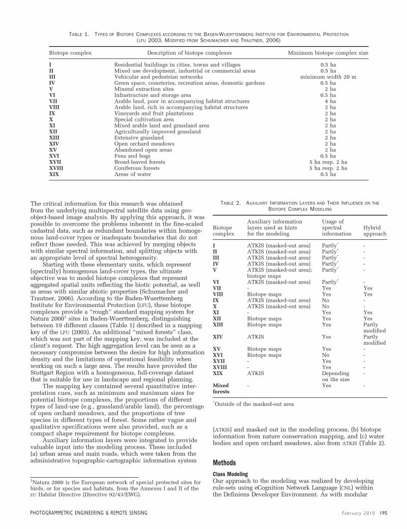
PHOTOGRAMMETRIC ENGINEER ING & REMOTE SENS ING Feb r ua r y 2010 195
The critical information for this research was obtainedfrom the underlying multispectral satellite data using geo-object-based image analysis. By applying this approach, it waspossible to overcome the problems inherent in the fine-scaledcadastral data, such as redundant boundaries within homoge-nous land-cover types or inadequate boundaries that do notreflect those needed. This was achieved by merging objectswith similar spectral information, and splitting objects withan appropriate level of spectral heterogeneity.
Starting with these elementary units, which represent(spectrally) homogenous land-cover types, the ultimateobjective was to model biotope complexes that representaggregated spatial units reflecting the biotic potential, as wellas areas with similar abiotic properties (Schumacher andTrautner, 2006). According to the Baden-WuerttembergInstitute for Environmental Protection (LFU), these biotopecomplexes provide a “rough” standard mapping system forNatura 20001 sites in Baden-Wuerttemberg, distinguishingbetween 19 different classes (Table 1) described in a mappingkey of the LFU (2003). An additional “mixed forests” class,which was not part of the mapping key, was included at theclient’s request. The high aggregation level can be seen as anecessary compromise between the desire for high informationdensity and the limitations of operational feasibility whenworking on such a large area. The results have provided theStuttgart Region with a homogeneous, full-coverage datasetthat is suitable for use in landscape and regional planning.
The mapping key contained several quantitative inter-pretation cues, such as minimum and maximum sizes forpotential biotope complexes, the proportions of differenttypes of land-use (e.g., grassland/arable land), the percentageof open orchard meadows, and the proportions of treespecies in different types of forest. Some rather vague andqualitative specifications were also provided, such as acompact shape requirement for biotope complexes.
Auxiliary information layers were integrated to providevaluable input into the modeling process. These included(a) urban areas and main roads, which were taken from theadministrative topographic-cartographic information system
(ATKIS) and masked out in the modeling process, (b) biotopeinformation from nature conservation mapping, and (c) waterbodies and open orchard meadows, also from ATKIS (Table 2).
MethodsClass ModelingOur approach to the modeling was realized by developingrule-sets using eCognition Network Language (CNL) withinthe Definiens Developer Environment. As with modular
TABLE 1. TYPES OF BIOTOPE COMPLEXES ACCORDING TO THE BADEN-WUERTTEMBERG INSTITUTE FOR ENVIRONMENTAL PROTECTION(LFU 2003, MODIFIED FROM SCHUMACHER AND TRAUTNER, 2006)
Biotope complex Description of biotope complexes Minimum biotope complex size
I Residential buildings in cities, towns and villages 0.5 haII Mixed use development, industrial or commercial areas 0.5 haIII Vehicular and pedestrian networks minimum width 20 mIV Green space, cemeteries, recreation areas, domestic gardens 0.5 haV Mineral extraction sites 2 haVI Infrastructure and storage area 0.5 haVII Arable land, poor in accompanying habitat structures 4 haVIII Arable land, rich in accompanying habitat structures 2 haIX Vineyards and fruit plantations 2 haX Special cultivation area 2 haXI Mixed arable land and grassland area 2 haXII Agriculturally improved grassland 2 haXIII Extensive grassland 2 haXIV Open orchard meadows 2 haXV Abandoned open areas 2 haXVI Fens and bogs 0.5 haXVII Broad-leaved forests 5 ha resp. 2 haXVIII Coniferous forests 5 ha resp. 2 haXIX Areas of water 0.5 ha
TABLE 2. AUXILIARY INFORMATION LAYERS AND THEIR INFLUENCE ON THEBIOTOPE COMPLEX MODELING
Auxiliary information Usage ofBiotope layers used as hints spectral Hybrid complex for the modeling information approach
I ATKIS (masked-out area) Partly* -II ATKIS (masked-out area) Partly* -III ATKIS (masked-out area) Partly* -IV ATKIS (masked-out area) Partly* -V ATKIS (masked-out area); Partly* -
biotope mapsVI ATKIS (masked-out area) Partly* -VII - Yes YesVIII Biotope maps Yes YesIX ATKIS (masked-out area) No -X ATKIS (masked-out area) No -XI - Yes YesXII Biotope maps Yes YesXIII Biotope maps Yes Partly
modifiedXIV ATKIS Yes Partly
modifiedXV Biotope maps Yes -XVI Biotope maps No -XVII - Yes -XVIII - Yes -XIX ATKIS Depending -
on the sizeMixed - Yes -forests
*Outside of the masked-out area
1Natura 2000 is the European network of special protected sites forbirds, or for species and habitats, from the Annexes I and II of theEU Habitat Directive (Directive 92/43/EWG).
193-202_GB-606.qxd 1/15/10 10:36 AM Page 195

196 Feb r ua r y 2010 PHOTOGRAMMETRIC ENGINEER ING & REMOTE SENS ING
programming languages, CNL supports programming tasks suchas branching, looping, and defining of variables. More specifi-cally, it enables the addressing of individual objects andsupports manipulating and supervising the process of generat-ing scaled objects in a region-specific manner. In this way thesteps involved in segmentation and classification can becoupled in a cyclic process, which we have called classmodeling (Tiede et al., 2008a). This is a supervised regional-ization technique that goes beyond the concept of a strict andunidirectional sequence of segmentation and subsequentclassification. The initial segmentation results are not espe-cially crucial for the derivation of “meaningful” objects andboth under- and over-segmentation can be accommodated byclass modeling (in contrast to the premise of “optimum”segmentation results at an initial stage stated by Burnett andBlaschke, 2003). Additional expert knowledge such as specificconstraints for the object building process or the inclusion ofauxiliary data sets, enriches not only the classification of unitscreated by intrinsically limited segmentation algorithms, butalso the entire information extraction workflow (Figure 2). Wenote that, although spectrally heterogeneous arrangements(such as some of the biotope complex types) can barely bedelineated directly through segmentation algorithms, they canbe modeled in the aforementioned way.
In our case, a basic land-use/land-cover multi-scaleclassification of the elementary units created was based ontheir spectral properties, which could be selected in specificaggregates for each form. Since gradual transitions can occurin this process, fuzzy-classifications were applied in some
cases, implementing labeling based on expert knowledge-based probabilities. Furthermore, the additional informationlayers could also function as evidence (or sometimes asconstraints) through spatial relationships, and hence werealso incorporated into the classification. Based on thispreliminary classification, we modeled the biotope complexesaccording to the LFU (2003) guidelines. Table 2 shows thebiotope complexes and indicates the use of spectral informa-tion and/or auxiliary information in the modeling process.
Those biotope complexes which were modeled automati-cally to a certain degree but had to be subsequently reworked(hybrid approach; see the next section) are also indicated.Figure 2 presents a schematic overview of the modelingprocess. The iterative cycles of our class modeling approachwere, in this case, an important element in stepwise growingand merge operations for objects, without which specificationsof shape or the proportion of land-use types for the biotopecomplexes could not be controlled in an adequate manner.
Biotope Complex ModellerA hybrid approach was chosen for those cases in whichthe results of the semi-automated generation of biotopecomplexes did not meet the specifications of the mappingkey due to a large number of degrees of freedom (i.e., the“orchard problem”; Lang and Langanke, 2006) and thelimitations of the single-date satellite data set. This wasparticularly applicable for complexes that showed spectralheterogeneity such as the “mixed arable land and grasslandarea” (XI), but also for the “arable land” (VII and VIII) and“agriculturally improved grassland” (XII) complex types. Forthese areas, a processing time and effort optimizing methodwas developed by coupling specific strengths of the “man”and “machine” evaluation systems (Lang et al., 2008;Weinke et al., 2008). A tool was programmed (the biotopecomplex modeler extension for ArcGIS®; Figure 3) to assist
Figure 2. Schematic overview of the biotope complexmodeling process (from Tiede et al., 2008b; modified).
Figure 3. Biotope complex modeler extension forArcGIS®, assisting experts in aggregating classifiedelementary units in a simple and rapid manner.
193-202_GB-606.qxd 1/15/10 10:36 AM Page 196

PHOTOGRAMMETRIC ENGINEER ING & REMOTE SENS ING Feb r ua r y 2010 197
experts in aggregating the remaining units in a simple andrapid manner.
The interpreter instantly obtains information on theselected units, such as aggregated areas and land-usecompositions, and human perception capabilities are thusefficiently integrated. The implementation of this hybridapproach (Lang et al., 2008) represents a major achievementin the semi-automated generation of complex target classes.
Cadastre CompatibilityIt was requested that the geometry of the final results shouldconform to the ALK cadastral data, which meant that biotopecomplexes were required to share the same object bound-aries as those provided by the digital cadastral map wher-ever these boundaries indicated changing biotope classes.The client’s requirement was for an accurate and compatibledataset for administrative purposes, with a higher geometricaccuracy than those data sets already available such asCORINE (Coordinated Information on the (European) Environ-ment). Conformity to the ALK cadastral data had alreadybeen taken into account in the delineation of the elementaryunits, but a scale-gap was introduced through the use ofimage data with a GSD of 5 m, particularly in the case of allnewly-derived boundaries representing changes of biotopeclass not reflected in the cadastral map.
In order to meet the client’s requirements, it was thereforenecessary to adjust the biotope complex boundaries so thatthey matched the existing cadastral geometry; similar prob-lems have previously been addressed by, for example, Walterand Fritsch (1999) and Butenuth et al. (2007). Combinationsof established GIS tools and additionally programmed solu-tions were used to solve three resulting problems, specifically(a) replacing biotope complex boundaries with correspondingcadastral boundaries by allowing a spatial displacementtolerance (buffer size) dependent on the pixel size of theimage data, (b) removing cadastral boundaries within eachbiotope complex, and (c) introducing new boundaries whichwere not reflected in the cadastral data set but which repre-sent changes in biotope complex class. For these new bound-aries smoothing and generalization algorithms (Bodanskyet al., 2002; Douglas and Peucker, 1973) were applied.
Multi-stage Validation ApproachDue to the multi-stage character of the entire workflow(Figure 2) and the client’s specific request for a product thatwould be fully integrated geometrically, a thematic accuracyassessment would not have been adequate to provide therequired proof of the usability of the final product. Valida-tion was therefore performed in several stages. Figure 4aillustrates the typical or “ideal” workflow, in which the mainaims were the provision of reliable results and an assuredquality. In addition, an extended validation concept wasimplemented that provided usability and a full integrationinto the user’s existing workflow. This concept is illustratedin Figure 4b and outlined in the following four steps:
1. The delineated elementary units were assessed, verified andimproved; this was a fundamental step since all subsequentsteps relied on the quality of these units.
2. This step used the elementary units to model the biotopecomplexes according to the mapping key.
3. Those biotope complex types which could not be directlymodeled underwent another verification cycle that involvedthe use of the biotope complex modeler (manual grouping).
4. The resulting complexes were validated by field visits; sinceadditional structural features had to be collected anyway, themajority of the complexes were checked in this way.
A final verification comprised (to a limited extent) ofdismissing the delineated boundaries or introducing newones. Since an assessment of the inaccuracies introduced inthe final adjustment of the biotope complex boundaries wasrequired, the confidence level was analyzed by Object FateAnalysis (OFA), a temporal object comparison proposed bySchöpfer et al. (2008) for assessing landscape units as theychange from one point in time to another. OFA measures thedeviation of boundaries between two relatively similardatasets; in this study it estimated the inaccuracy introducedinto the boundary positions of the final biotope complexes(see the next section for further details).
Object Fate Analysis (OFA) for Assessing Boundary AccuracyOFA is a method for investigating the deviation betweenboundaries of objects in two different representations. WithOFA the topological relationships between overlapping
Figure 4. Typical validation workflow (A), and extended multi-stage validation concept (B).
193-202_GB-606.qxd 1/15/10 10:36 AM Page 197

198 Feb r ua r y 2010 PHOTOGRAMMETRIC ENGINEER ING & REMOTE SENS ING
objects are categorized by an error band, and different errorbandwidths applied. The number of topological relation-ships within each category changes with the bandwidth, andthese numbers are analyzed to determine the error band-width that best describes the deviation of the boundaries.
The focus of OFA is on finding object comparisons inwhich the boundaries coincide relatively well. These compar-isons are distinguished from other comparisons where objectsexhibit a pronounced overlap, as may occur in the classifica-tion process, for example, due to thematic uncertainty whenobjects are merged with neighboring objects (Figure 5).
In the following description of OFA, the two datasets tobe investigated were named classification and reference. All ofthe classification objects were compared to all of the referenceobjects, in the manner illustrated in Figure 6. Essentially, anextended epsilon error band for polygons was applied (Zhangand Goodchild, 2002) to the division of the topologicalrelationships between classification objects and their corre-sponding reference objects into two clusters, “similar todisjoint” (C1) and “similar to equal” (C2) (Egenhofer andHerring, 1991; Straub and Heipke, 2004). The object relation-ships were divided into C1 and C2 by evaluating whether thecentroid of the classification object fell inside the referenceobject (C2) or not (C1). In OFA the relationship between eachclassification object and the corresponding reference objectcould be categorized as either “good,” “expanding” (bothbelonging to C2), “invading,” or “not interfering” (bothbelonging to C1). A buffer applied to the reference objectboundary serves as the decision criterion for this categoriza-tion, in analogy to an epsilon error band. The categories“good” and “not interfering” were further separated into twosub-categories by applying a buffer of size zero. The resultingcategories “good I” and “not interfering I” were excluded fromfurther analysis because they did not provide any informationon the amount of boundary deviation (Figure 6).
This categorization process was applied several timeswith an increasing buffer distance, and how the categorieschanged with buffer distance was observed for all therelationships. The ratio Re_ge in Equation 1 compares theserelationships for every buffer distance and can be used toevaluate these changes:
, (1)
where n is the total number of relationships occurringwithin a specified category, for all comparisons between theclassification objects and the reference objects (Lang et al.,2008; modified).
Re_ge has the value 1 for the buffer distance 0, and willdecrease with increasing buffer distance as the relationshipschange their category from “expanding” to “good II.” After aspecific buffer distance, the rate of decrease of the ratio willslow down. The “good II” relationships at that bufferdistance were caused by classification objects that onlyoverlapped the reference object boundary as a result of anerror in boundary placement, and not because they includedareas outside the boundary.
Results and DiscussionAltogether some 31,698 biotope complexes were delineatedfor the entire Stuttgart Region (see Figure 7) includingcomplexes aggregated by experts using the above mentionedhybrid approach. Figure 8 illustrates two examples ofsuccessfully derived biotope complexes. The average size ofeach complex was 11.5 ha: Table 3 lists the number ofbiotope complexes delineated in each category and theirtotal areas.
Validation SequenceValidation of the results was performed in several stepscovering the different stages of the biotope complex model-ing approach, as discussed in the methods section andillustrated in Figure 4.
Thematic Accuracy Assessment of the Elementary UnitsThe classified elementary units were evaluated using astatistical point-based accuracy assessment based on strati-fied random sampling (Congalton, 1991). Units with aclassification based mainly on additional information layers(urban areas, main roads) were not considered. A referencedata set with 300 randomly distributed points (at least 20 perclass) was generated and visual comparison with the SPOT
Re_ ge �nexp
ngood � nexp
Figure 5. Final biotope complex (black outline) overlaidwith elementary units. Three different types are high-lighted: Object (a) coincides relatively well, object(b) includes a minor area outside the biotope complexboundary, and object (c) having its major area outsideof the biotope complex.
Figure 6. Categorization of the interaction betweenclassification objects and reference objects (Schöpferet al., 2008; modified).
193-202_GB-606.qxd 1/15/10 10:36 AM Page 198

PHOTOGRAMMETRIC ENGINEER ING & REMOTE SENS ING Feb r ua r y 2010 199
imagery was performed. The point-based accuracy assess-ment revealed an overall classification accuracy of 85 percent(Kapppa coefficient � 0.8356). Table 4 presents an overviewof the producer’s accuracy and the user’s accuracy perelementary unit. The moderate accuracy values of 75 percentfor the “broad-leaved forests” elementary unit resulted fromthe spectral similarities of this unit to other forest types,especially the “mixed forests.” “Arable land, rich in accom-panying habitat structures” showed a relatively low user’saccuracy of 55 percent because of misidentification of land-use or land-cover patterns due to spectral and texturaloverlap with other units such as “open orchard meadows”and with the outskirts of built-up and infrastructure areas.
Verification of Units with Spectral HeterogeneityComplexes with a spectral heterogeneity (biotope complexesVII, VIII, XI, and XII) underwent another verification cyclethat involved use of the biotope complex modeler (cf. theMethods Section) and were aggregated by experts from pre-derived elementary units. Thus, not only were the resultingbiotope complexes validated, but also all elementary unitsthat were potential building blocks for these complexes (e.g.,agricultural area).
Field Evaluation/Boundary AssessmentA field evaluation of the generated units was carried out byexperts in habitat mapping, who performed qualitativemapping of each biotope complex (e.g., the potentialimportance for target species) as a prerequisite of theBiotope Information and Management System. Inadequatelymodeled biotope complexes were amended manually, andan analysis conducted for a sub-area of 583 km2 to comparethe revised results with the modeled biotope complexes.
Within this area about 86 percent of the biotope complexboundaries were correctly delineated, and about 96 percentof the removed boundaries (compared to cadastre data level)were correctly removed; only 3.6 percent of the final biotopecomplex boundaries had to be introduced manually. For amore detailed comparison between the cadastral data(serving as starting units) and the modeled biotope com-plexes, see Tiede et al. (2007).
Boundary Assessment using OFAThe last part of the validation sequence evaluated theinaccuracies that were introduced into the boundaries of thefinal biotope complexes as a result of matching the delin-eation of the elementary units to the boundaries of the finalbiotope complexes, or from other processes in the workflowthat involved this scale gap. The boundaries of the elemen-tary units were based on the 5 m GSD raster resolution of theSPOT image. Many of the boundaries in the final biotopecomplexes were based on the ALK vector geometry withabout 1 m accuracy. To measure the boundary deviationbetween these two datasets, OFA compared the elementaryunits with the final biotope complexes (Figure 9).
OFA was carried out on the BIMS project data for thedistrict of Berglen, in the Stuttgart Region. For a comparisonof the elementary units (used as the classification) and thefinal biotope complexes (providing the reference) the objectrelationship categories were evaluated and the Re_ge ratioscalculated for buffer distances ranging from 0 to 10 m. At a3.5 m buffer distance, a significant decrease occurred in theRe_ge ratio, which then remained quite stable for larger bufferdistances (Figure 10).
This buffer distance of 3.5 m shows the inaccuracy thatwas introduced into the final biotope complexes by the
Figure 7. Resulting biotope complexes for the entire Stuttgart region, includingcomplexes aggregated by experts using the hybrid approach (for visualization purposesthe 20 different biotope complex types were thematically grouped).
193-202_GB-606.qxd 1/15/10 10:36 AM Page 199

200 Feb r ua r y 2010 PHOTOGRAMMETRIC ENGINEER ING & REMOTE SENS ING
Figure 8. (1) Elementary units (1a) and successfully derived biotope complex “mixedarable land and grassland area” (1b) using the proposed hybrid approach (highlighted,with underlying SPOT image); (2) Automatically delineated “open orchard meadows”(below, with underlying orthophoto) illustrating delineation based on the 5 m GSD ofthe SPOT image (2a), and the same biotope complex after adjustment of the bound-aries to match the existing cadastral geometry (2b).
TABLE 3. NUMBER AND SIZE OF THE DELINEATED BIOTOPE COMPLEXES(SCHUMACHER ET AL, 2007; MODIFIED)
Biotope Sum [area Mean [area [% of total complex [#] in ha] in ha] area]
I 2,565 29,191.95 11.38 8II 4,569 25,260.53 5.53 6.9III 1,519 8,177.95 5.38 2.2IV 2,092 9,074.62 4.34 2.5V 69 744.54 10.79 0.2VI 275 968.12 3.52 0.3VII 3,196 75,364.84 23.58 20.6VIII 123 1,892.47 15.39 0.5IX 474 5,316.18 11.22 1.5X 122 621.11 5.09 0.2XI 1,714 27,399.32 15.99 7.5XII 2,725 30,159.61 11.07 8.3XIII 286 2,154.65 7.53 0.6XIV 2,517 30,367.98 12.07 8.3XV 102 550.16 5.39 0.2XVI 2 10.58 5.29 0XVII 2,717 50,247.02 18.49 13.8XVIII 1,382 13,271.77 9.6 3.6XIX 240 1,638.96 6.83 0.4mixed 5,009 52,590.70 10.5 14.4forest
31,698 365,003.06
TABLE 4. PRODUCER’S AND USER’S ACCURACY FOR ELEMENTARY UNITS
Elementary Producer’s User’sunits Accuracy Accuracy
Grassland area 81.82% 87.10%Arable land 93.10% 81.82%Arable land, rich in 91.67% 55.00%accompanying habitat structuresBuild-up and infrastructure 78.95% 96.77%(outside of the masked-out urban area)Extensive grassland 76.19% 80.00%Open orchard meadows 89.29% 96.15%Fens and bogs 100.00% 80.00%Broad-leaved forests 75.00% 75.00%Mixed forests 79.31% 93.88%Coniferous forests 100.00% 72.73%Areas of water 95.24% 100.00%
applied workflow. Many of the boundaries of the finalproduct originate from the ALK, which has an accuracy of1 m; this adds up to a spatial accuracy of 4.5 m for the finalbiotope complexes.
193-202_GB-606.qxd 1/15/10 10:36 AM Page 200

PHOTOGRAMMETRIC ENGINEER ING & REMOTE SENS ING Feb r ua r y 2010 201
ConclusionsA class modeling approach has been successfully applied tothe Biotope Information and Management System (BIMS)project, providing a means for delineating and monitoringaggregated spatial units relevant to regional planning tasks.Class modeling offers flexibility in providing problem-oriented solutions for advanced analysis tasks, involving bothoperator and expert (or user) in rule-set generation. Whilethis type of production system lacks any machine learningcomponent (as opposed to, e.g., neural networks or supportvector machines), the explicit integration of expert knowl-edge makes it capable of addressing structurally aggregatedclasses and supporting scene-specific high-level segmentationwith the delineation of conceptual boundaries (Tiede et al.,2008a; Tiede and Lang, 2008). In this case involving dedi-cated land-use analysis, the use of multitemporal data (withhigher resolution of some biotope complexes) would haveled to even more reliable results as well as greater efficiency.Altogether, a better data base would imply a lower post-processing effort and a higher possible degree of automation.
The exercise of fully validating a cyclic approach raisesthe problem of which specific steps to validate. Is it suffi-cient to check only the final result by ground truthing, ormust each crucial step in the entire workflow be examined?We suggest the latter. The validation sequence discussedincludes a series of validation steps that include verification,improvement, quality assurance, reliability, and evenusability, through which we were able to substantiate thatthe final product would fully satisfy the operational require-ments of the client. From a methodology perspective, theapplication of OFA allowed us to introduce a confidencelevel for object boundaries that took into account both thespecifics of the image data and the required target geometry.
Although generally considered to be of high potential,remote sensing often still lacks the full confidence ofagencies, authorities, and decision making structures, whereoperational work on a practical day-to-day level is required.To cope with the challenges imposed by the “usability”requirement (in its broadest and most ambitious sense),competitive approaches are required that are able to comple-ment established, but tedious, manual procedures. Thispaper presents an example of the type of solution that isrequired, both in Europe and globally, for operationalmonitoring of land-use dynamics.
AcknowledgmentsThis study was carried out within the Biotope Informationand Management System (BIMS) project with the object ofproviding a periodic update of the regional plan. The projectwas financed through the Verband Region Stuttgart. Theauthors would like to thank Jens Schumacher from theGruppe für ökologische Gutachten for fruitful discussionsduring the course of the project and his effective projectmanagement.
ReferencesAddink, E.A., S.M. de Jong, and E.J. Pebesma, 2007. The importance
of scale in object-based mapping of vegetation parameters withhyperspectral imagery, Photogrammetric Engineering & RemoteSensing, 73(8):905–912.
Abler, R., J.S. Adams, and P. Gould, 1972. Spatial organization:The geographer’s view of the world, Prentice-Hall International,London, 287 p.
Albrecht, F., 2008. Assessing the spatial accuracy of object-basedimage classifications, Proceedings of the Geoinformatics ForumSalzburg: Geospatial Crossroads @ GI_Forum ’08 (A. Car,J. Strobl and G. Griesebner, editors), 01–04 July, Salzburg,Wichmann, Heidelberg, pp. 11–20.
Baltsavias, E.P., 2004. Object extraction and revision by imageanalysis using existing geodata and knowledge: current statusand steps towards operational systems, ISPRS Journal ofPhotogrammetry and Remote Sensing, 58(3–4):129–151.
Benz, U., P. Hofmann, G. Willhauck, I. Lingenfelder, and M. Heynen,2004. Multi-resolution, object-oriented fuzzy analysis of remotesensing data for GIS-ready information, ISPRS Journal ofPhotogrammetry and Remote Sensing, 58(3–4):239–258.
Blaschke, T., D. Tiede, and S. Lang, 2006. An object-based informa-tion extraction methodology incorporating a-priori spatialinformation, Proceedings of the 4th ESA Conference on ImageInformation Mining, November, Madrid (ESA, Madrid),unpaginated CD-ROM.
Bodansky, E., A. Gribov, and M. Pilouk, 2002. Smoothing andcompression of lines obtained by raster-to-vector conversion,Graphics Recognition: Algorithms and Applications,2390:256–265.
Burnett, C., and T. Blaschke, 2003. A multi-scale segmentation /object relationship modelling methodology for landscapeanalysis, Ecological Modelling, 168(3): 233–249.
Figure 9. Resulting biotope complex boundaries (blacklines) after adjustment to match the existing cadastralgeometry overlaid with the boundaries of the elementaryunits (grey).
Figure 10. The Re_ge ratio (vertical axis) for a range ofbuffer distances (Albrecht. 2008; modified).
193-202_GB-606.qxd 1/15/10 10:36 AM Page 201

202 Feb r ua r y 2010 PHOTOGRAMMETRIC ENGINEER ING & REMOTE SENS ING
Butenuth, M., G.v. Gösseln, M. Tiedge, C. Heipke, U. Lipeck, andM. Sester, 2007. Integration of heterogeneous geospatial data ina federated database, ISPRS Journal of Photogrammetry andRemote Sensing, 62(5):328–346.
Castilla, G., and G.J. Hay, 2008. Image objects and geographicobjects, Object-Based Image Analysis - Spatial Concepts forKnowledge-driven Remote Sensing Applications (T. Blaschke,S. Lang, and G.J. Hay, editors), Springer, Berlin, pp. 91–110.
Congalton, R., 1991. A review of assessing the accuracy of classifica-tions of remotely sensed data, Remote Sensing of Environment,37:35–46.
De Wit, A.J., and J.G. Clevers, 2004. Efficiency and accuracy of per-field classification for operational crop mapping, Interna-tional Journal of Remote Sensing, 68(11):1155–1161.
Douglas, D.H., and T.K. Peucker, 1973. Algorithms for the reductionof the number of points required to represent a digitized line orits caricature, Cartographica: The International Journal forGeographic Information and Geovisualization, 10(2):112–122.
Egenhofer, M.J., and J.R. Herring, 1991. Categorizing Binary Topolog-ical Relations between Regions, Lines, and Points in GeographicDatabases, Technical Report, Department of Surveying Engineer-ing, University of Maine, Orono, Maine, 28 p.
Gamba, P., and F. Dell’Acqua, 2007. Data fusion related to GISand remote sensing, Integration of GIS and Remote Sensing(V. Mesev, editor), John Wiley and Sons, Chichester, pp. 43–68.
Hall, O., G.J. Hay, A. Bouchard, and D.J. Marceau, 2004. Detectingdominant landscape objects through multiple scales: Anintegration of object-specific methods and watershed segmenta-tion, Landscape Ecology, 19(1):59–76.
Hay, G., T. Blaschke, D.J. Marceau, and A. Bouchard, 2003. Acomparison of three image-object methods for the multiscaleanalysis of landscape structure, ISPRS Journal of Photogramme-try and Remote Sensing, 57(5):327–345.
Hay, G.J., and G. Castilla, 2008. Geographic object-based imageanalysis (GEOBIA): A new name for a new discipline, Object-Based Image Analysis - Spatial Concepts for Knowledge-drivenRemote Sensing Applications (T. Blaschke, S. Lang, andG.J. Hay, editors), Springer, Berlin, pp. 75–89.
Lang, S., 2008. Object-based image analysis for remote sensingapplications: Modeling reality - Dealing with complexity,Object-Based Image Analysis - Spatial Concepts for Knowledge-driven Remote Sensing Applications (T. Blaschke, S. Lang, andG.J. Hay, editors), Springer, Berlin, pp. 3–28.
Lang, S., E. Schöpfer, and T. Langanke, 2008. Combined object-based classification and manual interpretation - Synergies for aquantitative assessment of parcels and biotopes, GeocartoInternational, 23(4):1–16.
Lang, S., D. Tiede, J. Schumacher, and D. Hölbling, 2007. Individualobject delineation revising cadastral boundaries by means ofVHSR data, Proceedings of SPIE: Remote Sensing for Environ-mental Monitoring, GIS Applications, and Geology VII, 17–20September, Florence, 6749, 8 p.
Lang, S., and T. Langanke, 2006. Object-based mapping and object-relationship modeling for land use classes and habitats,Photogrammetrie, Fernerkundung, Geoinformation, 1/2006:5–18.
LfU, Landesanstalt Für Umweltschutz Baden-Württemberg, editor,2003. Handbuch zur Erstellung von Pflege- und Entwick-lungsplänen für die Natura 2000-Gebiete in Baden- Württember,Version 1.0. - Fachdienst Naturschutz, Naturschutz Praxis,Natura 2000, Karlsruhe, 467 p.
Mesev, V., and A. Walrath, 2007. GIS and remote sensing integration:In search of a definition, Integration of GIS and Remote Sensing(V. Mesev, editor), John Wiley and Sons, Chichester, pp. 1–16.
Niemeyer, I., and M.J. Canty, 2001. Object-oriented post-classifica-tion of change images, Proceedings of SPIE: InternationalSymposium on Remote Sensing, 17–21 September, Toulouse,4545, pp. 100–108.
Ozdarici A., and M. Turker, 2005. Comparison of different spatialresolution images for parcel-based crop mapping, Spatial/Spatio-Temporal Data Mining (SDM) and Learning, 24–25November, Ankara, Turkey, International Society for Photogram-metry and Remote Sensing, WG II/2 Workshop, unpaginatedCD-ROM.
Schöpfer, E., S. Lang, and F. Albrecht, 2008. Object-fate analysis - Spatial relationships for the assessment of objecttransition and correspondence, Object-Based Image Analysis -Spatial Concepts for Knowledge-driven Remote SensingApplications (T. Blaschke, S. Lang, and G.J. Hay, editors),Springer, Berlin, pp. 785–801.
Schöpfer, E., S. Lang, and J. Strobl, in press. Segmentation andobject-based image analysis, Remote Sensing of Urban andSuburban Areas (C. Juergens and T. Rashed, editors), Kluwer,Amsterdam, In press.
Schumacher, J., S. Lang, D. Tiede, D. Hölbling, J. Rietze, andJ. Trautner, 2007. Einsatz von GIS und objekt-basierter analysevon fernerkundungsdaten in der regionalen planung methodenund erste Erfahrungen aus dem Biotopinformations- undManagement System (BIMS) Region Stuttgart, AngewandteGeoinformatik 2007 - Beiträge zum 19. AGIT-Symposium(J. Strobl, T. Blaschke, and G. Griesebner, editors), 04–06 July,Salzburg, Wichmann, Heidelberg, pp. 703–708.
Schumacher, J., and J. Trautner, 2006. Spatial modeling for thepurpose of regional planning using species related expert-knowledge, The Biotope Information and Management Systemof Stuttgart region (BIMS) and its deduction from the Informa-tion System on Target Species in Baden-Württemberg, Trendsin Knowledge-Based Landscape Modeling (E. Buhmann,S. Jørgensen, and J. Strobl, editors), 18–20 Mai 2006, Dessau,Wichmann, Heidelberg, pp. 89–103.
Strahler, A.H., C.E. Woodcock, and J. Smith, 1986. Integrating per-pixel classification for improved land cover classification,Remote Sensing of the Environment, 71:282–296.
Straub, B.M., and C. Heipke, 2004. Concepts for internal andexternal evaluation of automatically delineated tree tops,Proceedings of the ISPRS Working Group VIII/2 - Laser-Scanners for Forest and Landscape Assessment, 03–06 October,Freiburg, International Archives of Photogrammetry, RemoteSensing and Spatial Information Sciences, XXXVI, Part 8/W2,pp 62–65.
Tiede, D., and S. Lang, 2008. Distributed computing for accelerateddwelling extraction in refugee camps using VHSR satelliteimagery, Proceedings of the Geoinformatics Forum Salzburg:Geospatial Crossroads @ GI_Forum ’08, (A. Car, J. Strobl, andG. Griesebner, editors), 01–04 July, Salzburg, Wichmann,Heidelberg, pp. 256–261.
Tiede, D., S. Lang, and C. Hoffmann, 2008a. Type-specific classmodelling for one-level representation of single trees, Object-Based Image Analysis - Spatial Concepts for Knowledge-drivenRemote Sensing Applications (T. Blaschke, S. Lang, andG.J. Hay, editors), Springer, Berlin, pp. 133–151.
Tiede, D., S. Lang, F. Albrecht, and D. Hölbling, 2008b. Classmodelling of biotope complexes - Success and remainingchallenges, GEOBIA 2008 - Pixels, Objects, Intelligence:GEOgraphic Object Based Image Analysis for the 21st Century,05–07 August, Calgary, Canada (University of Calgary, Calgary,Alberta, Canada), pp. 234–239.
Tiede, D., M. Moeller, S. Lang, and D. Hölbling, 2007. Adapting,splitting and merging cadastral boundaries according tohomogenous LULC Types Derived from SPOT 5 Data,Photogrammetric Image Analysis - PIA07, 19–21 September,Munich, International Archives of Photogrammetry, RemoteSensing and Spatial Information Sciences, 36 (3/W49A):99–104.
Tiede, D., and J. Strobl, 2006. Polygon-based regionalisation in aGIS environment, Trends in Knowledge-Based LandscapeModeling, 18–20 Mai, Dessau (E. Buhmann, S. Jørgensen, andJ. Strobl, editor, Wichmann, Heidelberg), pp. 54–59.
Walter, V., and D. Fritsch, 1999. Matching spatial data sets: Astatistical approach, International Journal of GeographicalInformation Science 13(5):445–473.
Weinke, E., S. Lang, and M. Preiner, 2008. Strategies for semi-automated habitat delineation and spatial change assessment inan Alpine environment, Object-Based Image Analysis - SpatialConcepts for Knowledge-driven Remote Sensing Applications(T. Blaschke, S. Lang, and G.J. Hay, editors), Springer, Berlin,pp. 711–732.
Zhang, J., and M.F. Goodchild, 2002. Uncertainty in GeographicalInformation, Taylor and Francis, London, 266 p.
193-202_GB-606.qxd 1/15/10 10:36 AM Page 202

PHOTOGRAMMETRIC ENGINEERING & REMOTE SENSING Februar y 2010 203
Profess ional Directory
ASPRS Meeting Schedule
Save the dates!!!ASPRS 2010 Annual Conference
April 26 – 30, 2010Town and Country Hotel
San Diego, California
ASPRS 2010 Fall ConferenceNovember 15-18, 2010
Doubletree Hotel at Entrance to Universal OrlandoOrlando, Florida
ASPRS 2011 Annual Conference May 1 – 5, 2011
Midwest Airlines Center/Hyatt HotelMilwaukee, Wisconsin
ASPRS 2011 Fall Pecora Conference
November 14–17, 2011Hilton Hotel at Washington Dulles
AirportHerndon, Virginia
ASPRS 2012 Annual ConferenceMarch 19–23, 2012
Sacramento Convention Center (TBD)Sacramento, California
ASPRS 2013 Annual ConferenceMarch 24–28, 2013
Baltimore Marriott Waterfront HotelBaltimore, Maryland
COLORADO
OHIO
IDAHO
KANSAS
PENNSYLVANIA
OREGON
OKLAHOMA
Aerial Surveys International, LLCP.O. Box 13037500 Astra Way, Unit 3EWatkins, CO 80137Phone (303) 261-9990Fax (303) 261-9996Mark Schubertwww.aerialsurveysintl.com
Precision Aerial Photography LMK 2000 (ABGPS)Z/I Scanning & B&W/ Color Lab
WEST VIRGINIA
ILLINOIS
TEXAS
Complete Expertise.Where you need it…when you need it.
NEW EQUIPMENTDigital Mapping Camera (DMC)
Optech Gemini Airborne LiDAR
Commander Turbine Aircraft
Hydrographic Equipment
SERVICESSurvey
Mapping
Remote Sensing
Aerial Imagery
Airborne & Terrestrial LiDAR
GIS
Engineering
800-254-5345 | www.wilsonco.com
February Layout 2.indd 203February Layout 2.indd 203 1/19/2010 3:28:19 PM1/19/2010 3:28:19 PM

204 Februar y 2010 PHOTOGRAMMETRIC ENGINEERING & REMOTE SENSING
Everyone will benefit if YOUMake a commitment to Your Profession and Join ASPRS Today.
Which membership is right for me?
Active Involved or interested in the practice of photogrammetry, remote sensing, and/or geographic information systems and related sciences. Full member benefi ts including; the right to vote and hold offi ce, discounts on ASPRS conference registration fees, group insurance policy,
eligibility for awards, discounts off ASPRS publications.
$135.00 Domestic, 2nd Class $184.00 Canada, Air1 $195.00 Foreign, ISAL
Associate Have been a student member for at least one year but are no longer eligible for student membership status. Eligible for this membership for a period of no more than three years immediately following their time as a student member. Associate Members shall be entitled to the same rights and privileges of the Society as an Active Member.
$90.00 Domestic, 2nd Class $137.00 Canada, Air1 $150.00 Foreign, ISAL
Student A Student Member shall be working towards a degree at a university or college. Certifi cation of student status (examples may include copies
of student identifi cation or current registration, faculty or sponsor signature, etc) is required for each year of student membership. Attach a copy of your student id or certifying faculty name and institution _________________________________________________________
A person is not eligible for student membership if he/she has previously held an Active or Associate Member status. Student members do not vote or hold offi ce until they advance to Associate Membership.
$45.00 Domestic, 2nd Class $89.00 Canada, Air1 $105.00 Foreign, ISAL
ASPRS membership is for one year (12 months); 12 issues of PE&RS. Membership renewal is based on the anniversary date of the month you joined. Membership certifi cates are available for an additional cost. Please allow 4-6 weeks for delivery.
Dues for Active, Associate, and Student domestic members includes Second Class Postage of PE&RS. Members residing in Canada receive PE&RS via CPM Service (Canada Publication Mail, 4-12 day delivery time). Dues for Mexico and all other foreign include Airmail Pub. Service postage to PE&RS (7-20 day delivery time worldwide). In addition all dues includes a postage surcharge. 1DUES INCLUDES POSTAGE AND GST. (ASPRS is required by the Canada Customs and Revenue Agency to collect 5% of the total amount of dues and postage for Canada’s Goods and Services Tax — GST #135123065.)
Member Information New Member Renewal (id number ____________________ )
Mr. Ms. Dr. other: ________________________________
Name (please print): _________________________________________________
Check appropriate box for mailing address home business
Address: ___________________________________________________________
___________________________________________________________________
Country: ________________________
Company’s name/workplace: _________________________________________
Business Phone*: _________________ Home Phone*: ___________________
fax*: _____________________________ e-mail*: ________________________
*DO NOT PUBLISH: Business Phone Home Phone Fax E-mail
Member Sponsorship (not mandatory)
Sponsor’s Member ID: ______________________________________________
Sponsor’s Name: __________________________________________________
Method of Payment: Payment must be submitted with application.
Payment must be made in US Dollars drawn on a US Bank or appropriate credit card. Make checks payable to ASPRS.
Check (Print name on check.)
Visa MasterCard American Express
Credit Card Account Number Expires (MO/YR)
Signature Date
Membership dues includes an annual subscription to PE&RS valued at $61.00. Non-member subscription price is $330.00 (libraries, universities, private companies etc.) Members may NOT deduct the subscription price from dues. ASPRS is an educational organization exempt from taxation under the 501(c) (3) code of the Internal Revenue Service. Dues payments are not deductible as a charitable contribution for federal tax purposes, but may be deductible as a business expense. Please check with your tax preparer.
Total Amount Enclosed: $ ________
Membership Certifi cateHand-engrossed, framable certifi cate of membership is availble for additional charge. $20.00
5410 Grosvenor Lane, Suite 210, Bethesda, Maryland 20814-2160 · t e l 301.493.0290 · fax 301.493.0208 · email [email protected] · www.asprs.org
February Layout 2.indd 204February Layout 2.indd 204 1/15/2010 1:41:16 PM1/15/2010 1:41:16 PM

Maximize Your RecognitionAchievementAdvancement
Benefi ts of ASPRS MembershipThe benefi ts of membership in the American Society for Photogrammetry and Remote Sensing
far exceed the initial investment. Member benefi ts and services include:
JOIN ASPRS TODAY!
· Monthly issue of Photogrammetric Engineering & Remote Sensing (PE&RS) · Discounts on all ASPRS publications · Job Fair Access · Discounts on registration fees for ASPRS Annual Meetings and Specialty Conferences · Discounts on ASPRS Workshops · Receipt of Region Newsletter · Region specialty conferences, workshops, technical tours and social events · Opportunity to participate in ISPRS activities
· Invitations to Technical Committee and Division meetings · Local, regional, national and international networking opportunities · Eligibility for over $18,000 in National and Region awards, scholarships and fellowships · Opportunity to Access the ASPRS Membership Directory on the internet (search for other active individual members, sustaining members, and certifi ed professionals)· Eligibility for car rental and hotel discounts · Opportunity to enroll in group insurance programs
Cover.indd 3Cover.indd 3 1/15/2010 2:05:01 PM1/15/2010 2:05:01 PM

If there’s an issue you’ll spot it.If there’s an issue a few centimeters from that issue you’ll spot it.
Today, every business is under pressure to increase efficiency and profitability.
Which is why Trimble GeoSpatial has integrated premier aerial and land mobile mapping systems with the world’s leading analysis software to create a range of solutions that are
perfectly suited to bring the benefits of geospatial data to any enterprise.
Geo-referenced aerial and terrestrial data give you the detail you need to manage assets and operations more efficiently—with turn times and details that have never been available before.
Trimble is focused on ideas that make good business sense. Our new GeoSpatial products deliver the latest in a long line of innovations designed to surpass the demands of an ever-changing business world. Learn more at: www.trimble.com/geospatial
STOP BY OUR BOOTH AT THE MARCH ILMF AND APRIL ASPRS SHOWS.
See how to make better use of better data at every stage of a project.
© 2009, Trimble Navigation Limited. All rights reserved. Trimble and the Globe & Triangle logo is a trademark of Trimble Navigation Limited, registered in the United States and in other countries. All other trademarks are the property of their respective owners. GEO-007
Cover.indd 4Cover.indd 4 1/15/2010 2:05:18 PM1/15/2010 2:05:18 PM
Copyright © 2022 FDOKUMEN