Developing value-added processing techniques for corn masa ...
595
Iowa State University Digital Repository @ Iowa State University Retrospective eses and Dissertations 2001 Developing value-added processing techniques for corn masa processing byproduct streams Kurt A. Rosentrater Iowa State University, [email protected] Follow this and additional works at: hp://lib.dr.iastate.edu/rtd Part of the Agriculture Commons , Bioresource and Agricultural Engineering Commons , and the Food Processing Commons is Dissertation is brought to you for free and open access by Digital Repository @ Iowa State University. It has been accepted for inclusion in Retrospective eses and Dissertations by an authorized administrator of Digital Repository @ Iowa State University. For more information, please contact [email protected]. Recommended Citation Rosentrater, Kurt A., "Developing value-added processing techniques for corn masa processing byproduct streams" (2001). Retrospective eses and Dissertations. Paper 452.
-
Upload
khangminh22 -
Category
Documents
-
view
0 -
download
0
Transcript of Developing value-added processing techniques for corn masa ...
Iowa State UniversityDigital Repository @ Iowa State University
Retrospective Theses and Dissertations
2001
Developing value-added processing techniques forcorn masa processing byproduct streamsKurt A. RosentraterIowa State University, [email protected]
Follow this and additional works at: http://lib.dr.iastate.edu/rtd
Part of the Agriculture Commons, Bioresource and Agricultural Engineering Commons, and theFood Processing Commons
This Dissertation is brought to you for free and open access by Digital Repository @ Iowa State University. It has been accepted for inclusion inRetrospective Theses and Dissertations by an authorized administrator of Digital Repository @ Iowa State University. For more information, pleasecontact [email protected].
Recommended CitationRosentrater, Kurt A., "Developing value-added processing techniques for corn masa processing byproduct streams" (2001).Retrospective Theses and Dissertations. Paper 452.
INFORMATION TO USERS
This manuscript has been reproduced from the microfilm master. UMI films
the text directly from the original or copy submitted. Thus, some thesis and
dissertation copies are in typewriter face, while others may be from any type of
computer printer.
The quality of this reproduction is dependent upon the quality of the
copy submitted. Broken or indistinct print, colored or poor quality illustrations
and photographs, print bleedthrough, substandard margins, and improper
alignment can adversely affect reproduction.
In the unlikely event that the author did not send UMI a complete manuscript
and there are missing pages, these will be noted. Also, if unauthorized
copyright material had to be removed, a note will indicate the deletion.
Oversize materials (e.g., maps, drawings, charts) are reproduced by
sectioning the original, beginning at the upper left-hand comer and continuing
from left to right in equal sections with small overlaps.
Photographs included in the original manuscript have been reproduced
xerographically in this copy. Higher quality 6e x 9" black and white
photographic prints are available tor any photographs or illustrations appearing
in this copy for an additional charge. Contact UMI directly to order.
Bell & Howell Information and Learning 300 North Zeeb Road, Ann Arbor, Ml 48106-1346 USA
800-521-0600

Developing value-added processing techniques for com masa processing byproduct
streams
by
Kurt August Rosentrater
A dissertation submitted to the graduate faculty
in partial fulfillment of the requirements for the degree of
DOCTOR OF PHILOSOPHY
Major: Agricultural Engineering (Food and Process Engineering)
Major Professors: Thomas L. Richard and Carl J. Bern
Iowa State University
Ames, Iowa
2001
Copyright © Kurt August Rosentrater, 2001. All rights reserved.
UMI Number. 3003267
Copyright 2001 by
Rosentrater, Kurt August
All rights reserved.
UMI UMI Microform 3003267
Copyright 2001 by Bell & Howell Information and Learning Company. All rights reserved. This microform edition is protected against
unauthorized copying under Title 17, United States Code.
Bell & Howell Information and Learning Company 300 North Zeeb Road
P.O. Box 1346 Ann Arbor, Ml 48106-1346
ii
Graduate College Iowa State University
This is to certify that the Doctoral dissertation of
Kurt August Rosentrater
has met the dissertation requirements of Iowa State University
Co-Major Professor
For the Major Program
For the Graduate College
Signature was redacted for privacy.
Signature was redacted for privacy.
Signature was redacted for privacy.
Signature was redacted for privacy.

m
DEDICATION
I dedicate this dissertation to my wife, friend, and partner, Kari, without whom this
endeavor would never have reached fruition. Her patience, endurance, support, and love
have been invaluable over the years. I sincerely wish to express my gratitude to her for all
she has done ... and continues to do. Thank you Kari for helping me achieve this dream.
iv
TABLE OF CONTENTS
LIST OF FIGURES
LIST OF TABLES
NOMENCLATURE
ACKNOWLEDGEMENTS
ABSTRACT
CHAPTER 1. GENERAL INTRODUCTION
RATIONALE FOR STUDY OBJECTIVES OF STUDY LIMITATIONS OF STUDY DISSERTATION ORGANIZATION REFERENCES
CHAPTER 2. GENERAL LITERATURE REVIEW 6
CORN MASA PROCESSING 6 GRAIN PROCESSING BYPRODUCTS UTILIZATION 9 BYPRODUCT UTILIZATION PHILOSOPHY 20 PHYSICAL AND NUTRITIONAL PROPERTY TESTING 21 SUMMARY AND CONCLUSIONS 22 REFERENCES 22
CHAPTER 3. PHYSICAL AND NUTRITIONAL PROPERTIES OF CORN MASA BYPRODUCT STREAMS 30
ABSTRACT 30 INTRODUCTION 32 MATERIALS AND METHODS 35 RESULTS AND DISCUSSION 42 SUMMARY AND CONCLUSIONS 62 ACKNOWLEDGMENTS 63 REFERENCES 63 APPENDIX 3-A. CMB PHYSICAL AND NUTRITIONAL PROPERTY DATA 68
CHAPTER 4. EXTRUSION PROCESSING LITERATURE REVIEW 154
INTRODUCTION 154 PROCESSING PARAMETERS AND EFFECTS 155
vii
x
xiii
xxii
xxv
1
1 2 3 3 4
V
PROCESS MODELING 157 SUMMARY AND CONCLUSIONS 177 REFERENCES 177
CHAPTER 5. DEVELOPMENT OF FEED INGREDIENTS USING CORN MASA BYPRODUCTS. I. SMALL-SCALE EXTRUSION 179
ABSTRACT 179 INTRODUCTION 181 MATERIALS AND METHODS 184 RESULTS AND DISCUSSION 193 SUMMARY AND CONCLUSIONS 237 ACKNOWLEDGMENTS 239 REFERENCES 239 APPENDIX 5-A. LABORATORY-SCALE EXTRUSION DATA 245
CHAPTER 6. DEVELOPMENT OF FEED INGREDIENTS USING CORN MASA BYPRODUCTS. II. LARGE-SCALE EXTRUSION 275
ABSTRACT 275 INTRODUCTION 276 MATERIALS AND METHODS 280 RESULTS AND DISCUSSION 289 SUMMARY AND CONCLUSIONS 327 ACKNOWLEDGMENTS 328 REFERENCES 328 APPENDIX 6-A. PILOT-SCALE EXTRUSION DATA 333
CHAPTER 7. ECONOMIC MODELING OF REPROCESSING ALTERNATIVES FOR CORN MASA BYPRODUCTS 342
ABSTRACT 342 INTRODUCTION 343 MATERIALS AND METHODS 349 RESULTS AND DISCUSSION 373 SUMMARY AND CONCLUSIONS 395 ACKNOWLEDGMENTS 397 REFERENCES 397 APPENDIX 7-A. ECONOMICS OF RECYCLING CMB MODEL -
FORTRAN PROGRAM 406 APPENDIX 7-B. EQUIPMENT AND BUILDING INFORMATION
IMPLEMENTED IN ECONOMICS OF RECYCLING CMB MODEL 441
CHAPTER 8. GENERAL CONCLUSIONS AND FUTURE WORK 562

GENERAL CONCLUSIONS FUTURE WORK
vii
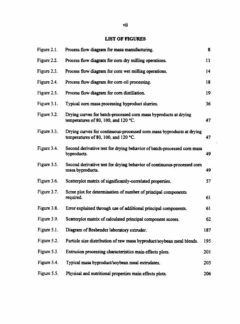
LIST OF FIGURES
Figure 2.1. Process flow diagram for masa manufacturing. 8
Figure 2.2. Process flow diagram for com dry milling operations. 11
Figure 2.3. Process flow diagram for corn wet milling operations. 14
Figure 2.4. Process flow diagram for com oil processing. 18
Figure 2.5. Process flow diagram for com distillation. 19
Figure 3.1. Typical com masa processing byproduct slurries. 36
Figure 3.2. Drying curves for batch-processed com masa byproducts at drying temperatures of 80,100, and 120 °C. 47
Figure 3.3. Drying curves for continuous-processed com masa byproducts at drying temperatures of 80,100, and 120 °C. 47
Figure 3.4. Second derivative test for drying behavior of batch-processed com masa byproducts. 49
Figure 3.5. Second derivative test for drying behavior of continuous-processed com masa byproducts. 49
Figure 3.6. Scatterplot matrix of significantly-correlated properties. 57
Figure 3.7. Scree plot for determination of number of principal components required. 61
Figure 3.8. Error explained through use of additional principal components. 61
Figure 3.9. Scatterplot matrix of calculated principal component scores. 62
Figure 5.1. Diagram of Brabender laboratory extruder. 187
Figure 5.2. Particle size distribution of raw masa byproduct/soybean meal blends. 195
Figure 5.3. Extrusion processing characteristics main effects plots. 201
Figure 5.4. Typical masa byproduct/soybean meal extradâtes. 205
Figure 5.5. Physical and nutritional properties main effects plots. 206
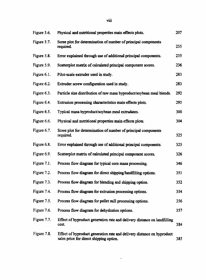
viii
Figure 5.6. Physical and nutritional properties main effects plots. 207
Figure 5.7. Scree plot for determination of number of principal components required. 235
Figure 5.8. Error explained through use of additional principal components. 235
Figure 5.9. Scatterplot matrix of calculated principal component scores. 236
Figure 6.1. Pilot-scale extruder used in study. 283
Figure 6.2. Extruder screw configuration used in study. 283
Figure 6.3. Particle size distribution of raw masa byproduct/soybean meal blends. 292
Figure 6.4. Extrusion processing characteristics main effects plots. 295
Figure 6.5. Typical masa byproduct/soybean meal extradâtes. 300
Figure 6.6. Physical and nutritional properties main effects plots. 304
Figure 6.7. Scree plot for determination of number of principal components required. 325
Figure 6.8. Error explained through use of additional principal components. 325
Figure 6.9. Scatterplot matrix of calculated principal component scores. 326
Figure 7.1. Process flow diagram for typical com masa processing. 346
Figure 7.2. Process flow diagram for direct shipping/landfilling options. 351
Figure 7.3. Process flow diagram for blending and shipping option. 352
Figure 7.4. Process flow diagram for extrusion processing options. 354
Figure 7.5. Process flow diagram for pellet mill processing options. 356
Figure 7.6. Process flow diagram for dehydration options. 357
Figure 7.7. Effect of byproduct generation rate and delivery distance on landfilling cost. 384
Figure 7.8. Effect of byproduct generation rate and delivery distance on byproduct sales price for direct shipping option. 385
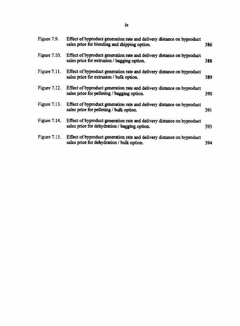
ix
Figure 7.9. Effect of byproduct generation rate and delivery distance on byproduct sales price for blending and shipping option. 386
Figure 7.10. Effect of byproduct generation rate and delivery distance on byproduct sales price for extrusion / bagging option. 388
Figure 7.11. Effect of byproduct generation rate and delivery distance on byproduct sales price for extrusion / bulk option. 389
F igure 7.12. Effect of byproduct generation rate and delivery distance on byproduct sales price for pelleting / bagging option. 390
Figure 7.13. Effect of byproduct generation rate and delivery distance on byproduct sales price for pelleting / bulk option. 391
Figure 7.14. Effect of byproduct generation rate and delivery distance on byproduct sales price for dehydration / bagging option. 393
F igure 7.15. Effect of byproduct generation rate and delivery distance on byproduct sales price for dehydration / bulk option. 394
12
15
15
20
43
55
56
58
60
68
73
76
194
199
208
224
227
233
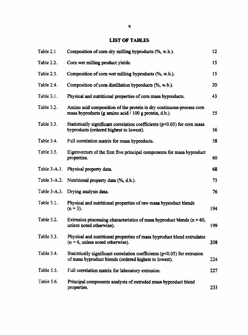
x
LIST OF TABLES
Composition of com dry milling byproducts (%, w.b.).
Com wet milling product yields.
Composition of com wet milling byproducts (%, w.b.).
Composition of com distillation byproducts (%, w.b.).
Physical and nutritional properties of com masa byproducts.
Amino acid composition of the protein in dry continuous-process com masa byproducts (g amino acid /100 g protein, d.b.).
Statistically significant correlation coefficients (p<0.05) for com masa byproducts (ordered highest to lowest).
Full correlation matrix for masa byproducts.
Eigenvectors of the first five principal components for masa byproduct properties.
Physical property data.
Nutritional property data (%, d.b.).
Drying analysis data.
Physical and nutritional properties of raw masa byproduct blends (n = 3).
Extrusion processing characteristics of masa byproduct blends (n = 60, unless noted otherwise).
Physical and nutritional properties of masa byproduct blend extradâtes (n = 6, unless noted otherwise).
Statistically significant correlation coefficients (p<0.05) for extrusion of masa byproduct blends (ordered highest to lowest).
Full correlation matrix for laboratory extrusion.
Principal components analysis of extruded masa byproduct blend properties.
xi
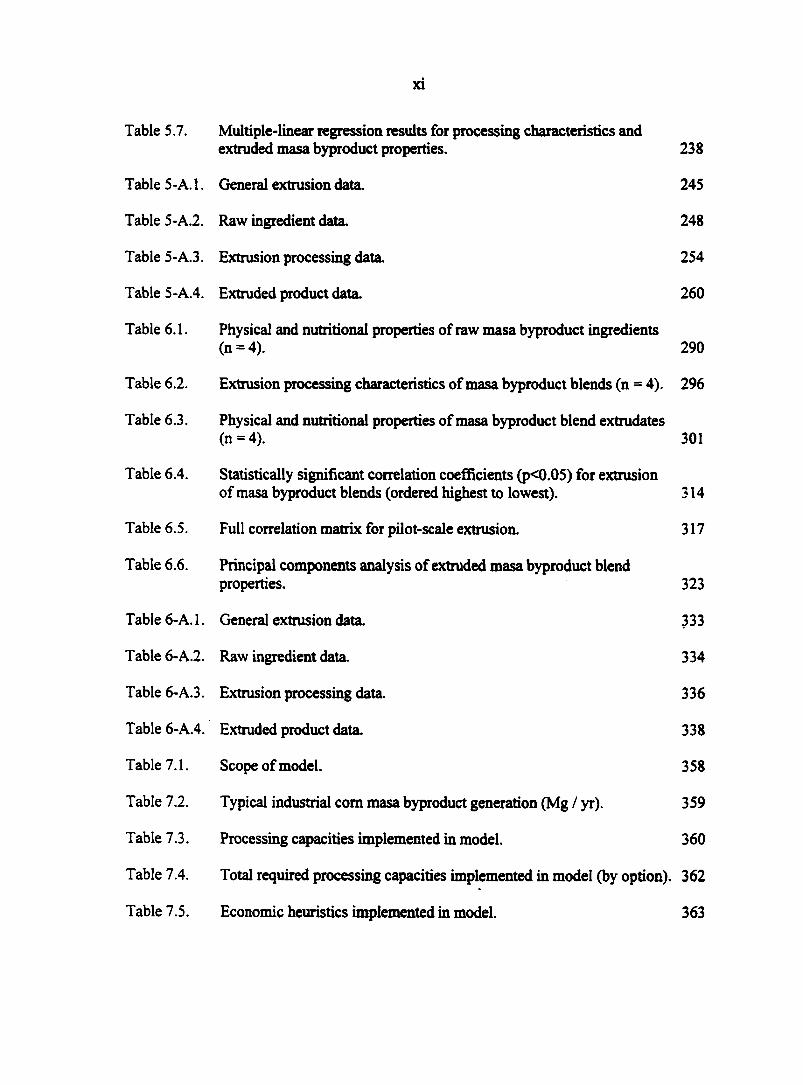
Table 5.7. Multiple-linear regression results for processing characteristics and extruded masa byproduct properties. 238
Table 5-A. 1. General extrusion data. 245
Table 5-A.2. Raw ingredient data. 248
Table 5-A.3. Extrusion processing data. 254
Table 5-A.4. Extruded product data. 260
Table 6.1. Physical and nutritional properties of raw masa byproduct ingredients (n = 4). 290
Table 6.2. Extrusion processing characteristics of masa byproduct blends (n = 4). 296
Table 6.3. Physical and nutritional properties of masa byproduct blend extradâtes (n = 4). 301
Table 6.4. Statistically significant correlation coefficients (p<0.05) for extrusion of masa byproduct blends (ordered highest to lowest). 314
Table 6.5. Full correlation matrix for pilot-scale extrusion. 317
Table 6.6. Principal components analysis of extruded masa byproduct blend properties. 323
Table 6-A. 1. General extrusion data. 333
Table 6-A.2. Raw ingredient data. 334
Table 6-A.3. Extrusion processing data. 336
Table 6-A.4. Extruded product data. 338
Table 7.1. Scope of model. 358
Table 7.2. Typical industrial corn masa byproduct generation (Mg / yr). 359
Table 7.3. Processing capacities implemented in model. 360
Table 7.4. Total required processing capacities implemented in model (by option). 362
Table 7.5. Economic heuristics implemented in model. 363
xii
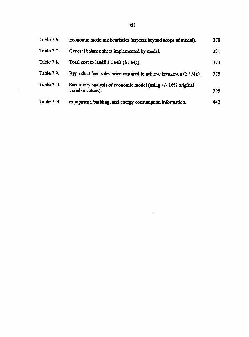
Table 7.6. Economic modeling heuristics (aspects beyond scope of model). 370
Table 7.7. General balance sheet implemented by model. 371
Table 7.8. Total cost to landfill CMB ($/Mg). 374
Table 7.9. Byproduct feed sales price required to achieve breakeven ($ / Mg). 375
Table 7.10. Sensitivity analysis df economic model (using +/-10% original variable values). 395
Table 7-B. Equipment, building, and energy consumption information. 442
xiii
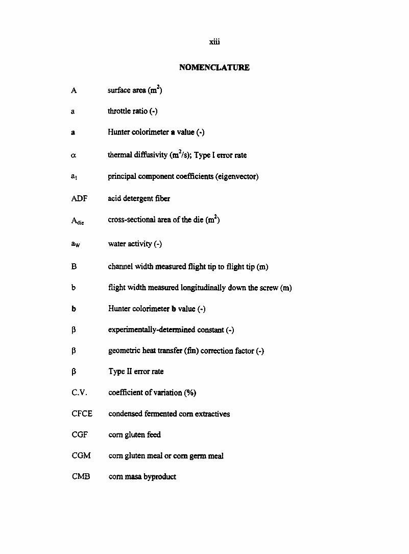
NOMENCLATURE
A surface area (m2)
a throttle ratio (-)
a Hunter colorimeter a value (-)
a thermal dififusivity (m2/s); Type I error rate
at principal component coefficients (eigenvector)
ADF acid detergent fiber
Adie cross-sectional area of the die (m2)
aw water activity (-)
B channel width measured flight tip to flight tip (m)
b flight width measured longitudinally down the screw (m)
b Hunter colorimeter b value (-)
P experimentally-determined constant (-)
P geometric heat transfer (fin) correction factor (-)
P Type II error rate
C.V. coefficient of variation (%)
CFCE condensed fermented corn extractives
CGF com gluten feed
CGM com gluten meal or com germ meal
CMB corn masa byproduct
xiv
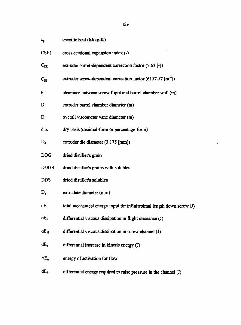
cp specific heat (kJ/kg-K)
CSEI cross-sectional expansion index (-)
CSR extruder barrel-dependent correction factor (7.63 [-])
Css extruder screw-dependent correction factor (6157.57 [m*3])
8 clearance between screw flight and barrel chamber wall (m)
D extruder barrel chamber diameter (m)
D overall viscometer vane diameter (m)
d.b. dry basis (decimal-form or percentage-form)
Dd extruder die diameter (3.175 [mm])
DDG dried distiller's grain
DDGS dried distiller's grains with solubles
DDS dried distiller's solubles
De extrudate diameter (mm)
dE total mechanical energy input for infinitesimal length down screw (J)
dEg differential viscous dissipation in flight clearance (J)
dEH differential viscous dissipation in screw channel (J)
dEk differential increase in kinetic energy (J)
AEn energy of activation for flow
dEp differential energy required to raise pressure in the channel (J)
XV
AP pressure drop during die exit (Pa)
DR drying rate (g H20 / g sample-h)
Dr screw root diameter (m)
Ds diameter of the screw (m)
AT change in temperature (K)
dvx/dy velocity gradient perpendicular to flow direction ( 1 /s)
e actual flight width (m)
e pumping efficiency of the dough down screw channel (-)
E total mechanical energy input to extruder screw (J)
Emcch total mechanical energy input (J)
Ep fraction of motor energy required to transport dough down channel (-)
Etotai total energy input into extruder (J)
F force required to move a surface (N)
Fd flow factor due to pumping (-)
Fdc shape correction factor accounting for screw curvature (-)
Fde shape correction factor accounting for end effects (-)
F dt drag flow shape correction factor (-)
Fp flow factor due to drag (-)
Fpc shape correction factor accounting for screw curvature (-)
xvi
Fpc shape correction factor accounting for end effects (-)
Fpt pressure flow shape correction factor (-)
g acceleration due to gravity (9.8 m/s2)
y velocity gradient perpendicular to flow direction (1/s)
G, drag flow correction factor (-)
G2 pressure flow correction factor (-)
GMD geometric mean diameter (mm)
GSD geometric standard deviation (mm)
H channel height (m)
H distance between barrel wall and screw base (m)
H overall viscometer vane height (m)
H phase change enthalpy (J/kg)
Hi channel height at beginning of screw (m)
H2 channel height at end of screw (m)
H$ height of the screw flight (m)
r| apparent viscosity at a given shear rate (Pa-s)
H reference apparent viscosity value (Pa-s)
T| i reference apparent viscosity value (Pa-s)
Tlapp apparent viscosity of the dough in the extruder (Pa-s)
xvu
Tio reference apparent viscosity value (Pa-s)
HSS high screw speed (rpm)
HTP high temperature profile (C)
K experimentally-determined constant (-)
K geometric correction factor (-)
k thermal conductivity (W/m-K)
kg thermal conductivity of organic solids (W/m-K)
kw thermal conductivity of water (W/m-K)
L Hunter colorimeter L value (-)
L length of thermocouple (m)
I screw tip-to-tip distance (m)
Ld longitudinal length of die opening (m)
LEI longitudinal expansion index (-)
LSS low screw speed (rpm)
LTP low temperature profile (C)
m consistency coefficient (-)
m dynamic (Newtonian) viscosity (Pa-s)
M material moisture content (decimal dry basis)
M moisture content (decimal basis)
M.C. material moisture content
xviii
MCf moisture content of extruded product (%, w.b.)
MC| moisture content of initial raw feed ingredient (%, w.b.)
Hd apparent viscosity of food dough in the die (Pa-s)
mdic mass flowrate through die (kg/s)
mfecd feed material throughput rate (g/min)
mprod extrudate product throughput rate (g/min)
MQ mass flowrate through die (kg/s)
nigX latent heat added due to direct steam injection (J)
N rotational speed of screw (rev/min)
n flow behavior index (-)
n sample size (number of units)
NDF neutral detergent fiber
OC out of conditioner
OE out of extruder
OEjj,. out of extruder & allowed to air dry at ambient conditions
P pressure (Pa)
P.C. principal component eigenvector
Pdic die pressure (Pa)
q heat transfer through barrel walls due to jackets (J)
xix
9 helix angle of screw (-)
Q volumetric flowrate (throughput) (m3/s)
Qd volumetric flowrate due to drag effects (m3/s)
Qdic volumetric flowrate through die (m3/s)
Qieak volumetric flowrate of leakage flow (m3/s)
Qp volumetric flowrate due to pressure effects (m3/s)
R die radius (m)
p fluid density (kg/m3)
R universal gas constant (8.314 J/g-mol-K)
r correlation coefficient
p mass density (kg/m3)
R2 coefficient of determination
pd density of dough in the extruder drive (g/cm3)
rdie density of dough in die (kg/m3)
pcx bulk density of resulting extradâtes (g/cm3)
rpm revolutions per minute
pw density of water at the temperature of the extruder die (g/cm3)
SBM soybean meal
S ME specific mechanical energy (J/g)
XX
T fluid temperature (K)
T oven drying temperature (C); torque exerted on extruder drive (N-m)
x shear stress (Pa)
t time (s)
t(y) a particle's residence time in screw channel (s)
Tb temperature of barrel wall (K)
TL temperature sensed by thermocouple (K)
Tm torque exerted on viscometer vane at yield point (N-m)
T0 reference temperature (K)
Ts shear stress reference value (Pa)
Ty resultant yield stress (N/m2)
Tyx shear stress exerted on fluid (Pa)
V peripheral flight tip speed (m/s)
Vdie velocity of dough in die (m/s)
VEI volumetric expansion index (-)
Vx dough velocity perpendicular across screw channel (m/s)
Vz dough velocity down screw channel (m/s)
W actual screw channel width (m)
W heat transfer through barrel walls due to jackets (J)
xxi
co rate of screw rotation (angular velocity) (rad/s)
co extruder screw angular velocity (rad/s)
w.b. wet basis (decimal-form or percentage-form)
WAI water absorption index (-)
WSI water solubility index (-)
x x-direction (-)
X, original property variable matrix
Xa mass fraction of ash (-)
Xc mass fraction of carbohydrate (-)
Xf mass fraction of fat (-)
Xp mass fraction of protein (-)
Xw mass fraction of water (-)
Y coordinate direction perpendicular between plates (-)
y y-direction (-)
yp.c. principal component score (calculated value)
Z length of channel travel during one screw revolution (m)
Z total length of screw (m)
z distance traveled down screw channel (m)
z z-direction (-)
xxii
ACKNOWLEDGMENTS
I would like to acknowledge many people for their contributions to my endeavors as a
graduate student at Iowa State University. First and foremost, I wish to thank Dr. Tom
Richard and Dr. Carl Bern for their continued willingness over the last several years to
unfailingly lend guidance, support, suggestions, critiques, and assistance to me, and their
flexibility with regards to both my off-campus employment schedule and my research
program. Furthermore, I want to thank Dr. Rolando Flores for setting me on this research
path, for his guidance and support during this process, and for the opportunity to conduct
large-scale extrusion research at Kansas State University. I additionally want to thank the
other faculty members who served on my graduate committee, read my dissertation, and
provide suggestions for its improvement, and helped me along my way, including Dr. Dianne
Cook, Dr. Gerald Colver, and Dr. Alan Trenkle.
I would also like to thank the Recycling and Reuse Technology Transfer Center
(RRTTC) at the University of Northern Iowa, the Iowa Biotechnology Byproducts
Consortium (BBC), and the Department of Grain Science and Industry at Kansas State
University for financial support during the course of this research project. Further, I wish to
thank the Center for Crops Utilization Research (CCUR) at Iowa State University for use of
facilities and equipment.
I have also appreciated the assistance, advice, and expertise provided by many of the
faculty in the Agricultural and Biosystems Engineering Department at Iowa State University,
including Dr. Stewart Melvin, Dr. Dwaine Bundy, Dr. Duane Mangold, Dr. Carl Anderson,
Dr. Tom Glanville, and Dr. Zivko Nikolov. Further, I would like to thank the Main Office
staff of the Agricultural and Biosystems Engineering Department, including Mary Ellen
xxiii
Hurt, Barb Kalsem, Judy Reischauer, and Sue Ziegenbusch, who have helped me enormously
throughout the years with a variety of dilemmas and emergencies.
Additionally, I wish to thank other faculty at Iowa State University that have
contributed to a very fulfilling experience at Iowa State over the years, including Dr. Charles
Glatz, Dr. Donald Young, Dr. Ambar Mitra, and Dr. Larry Northup, who introduced me to
the exciting world of engineering, and Dr. Adrian Bennett, Dr. Steve Kawaler, Dr. George
Bowen, Dr. Kenneth Madison, and Dr. Hamilton Cravens, who taught me that the world
consists of more than just engineering science, and includes the humanities and social
sciences as well.
I further wish to thank the NASA Space Grant Consortium and the National Science
Foundation for undergraduate research opportunities and scholarships, which spurred my
interest in research, and ultimately led me to graduate school.
I also wish to thank Todd & Sargent, Inc., and especially Paul Noelck, manager of the
Design Development Department, for allowing me to pursue my academic interests while
allowing me to put into practice my engineering education.
I would like to thank my family for their love, support, and encouragement over the
years including Marilyn and Kevin Zadow, Ryan and Karen Rosentrater, Carrie Rosentrater,
Jenny and Elliott Zadow, and Joyce and Leonard Kastengren. I would especially like to
thank Marilyn, Joyce, and Leonard, my mother, grandmother, and grandfather, respectively,
for teaching me the value of hard work and determination. I could not have gotten here
without them.

xxiv
I would also like to thank my wife's family for their love, encouragement, and
support, including Marlene and Tony Pape, Laurie and Richard Hadley, Pam Pape-Lindstrom
and Chris Lindstrom, Melissa and Aubrey Privitt, Danette Pape, and Nicole Pape.
I also want to thank our neighbors and friends here in Ames, for all they have done,
and for their love and support, including Gin and Andrea Brown, and Diane, Julie, and Nate
Prindle, and Charlene and Tom Olson.
I additionally wish to thank all my friends who have encouraged and helped me over
the years, some of whom have suffered through various classes and program with me,
including Dan Valen, Doug Allen, Kevin and Erin Gaul, Sue Kiehne, Sel Dibooglu, Jason
Urban, Liz McMahon, Todd Furlong, Wallace Greenlees, Doug Ward, and the Bioprocess
Engineering Group at ISU (Amy Mangold-Konkoly, Atila Konkoly, Fernando Perez-Munoz,
Fen Fen Jamin, Herman Katopo, Maria Ambert-Sanchez, Helen Park, Desmond Lam, Jian
Yuan, Linfeng Wang, Paula Beckman, and Glen Ripke).
Further, I want to thank the person who initially set me on this course many years
ago: Mary Brinkman, my elementary school science teacher. She imparted to me an
enthusiasm for science and technology that has lasted over the years, which eventually led
me to engineering science, and which blossomed into a desire to attend graduate school. I
am indebted to her for the fact that I think "science is fun".
Last but not least, I am forever indebted to my wife, Kari, and my daughter, Emma.
Words cannot describe my thankfulness for your love, patience, support, and understanding
during this process. Thank you for being there for me. I could not have done this without
you or your help.
XXV
ABSTRACT
The objective of this project was to develop value-added disposal/reuse alternatives
for com masa processing residues (i.e., waste, or byproduct, slurries). To accomplish this,
the project was divided into four distinct phases. The first phase entailed identification and
quantification of relevant physical and nutritional properties of typical com masa processing
residues. As a result, these byproducts appear suitable for use as livestock feed additives, or
components thereof. These byproducts are very high in moisture content, but dried, they are
high in fiber, and would probably be best suited for ruminant diets. Additionally, when
dried, these products have a substantial calcium content, so there may exist potential for use
as a calcium source for livestock rations. The second phase encompassed blending and
extruding corn masa processing byproducts with soybean meal on a laboratory-scale, and
investigating the effects of blend ratio, extrusion temperature, and extruder screw speed on
extrusion processing variables and final extrudate product physical and nutritional
characteristics. The third phase entailed blending and extruding com masa processing
byproducts with soybean meal on a pilot-scale, and investigating the effects of blend ratio,
extrusion temperature, and extruder screw speed on extrusion processing variables and final
extrudate product physical and nutritional characteristics. Extrusion processing during these
stages produced extradâtes with nutritional properties similar to the raw ingredient blends,
excellent durability, and little product expansion. The final phase of the project encompassed
development of a computer model to assess the economics of various disposal and recycling
alternatives for com masa processing byproducts. It was determined that, under the current
economic climate, direct shipping of the raw byproduct slurry is the most economical
disposal option for masa processing residues.
1
CHAPTER 1
GENERAL INTRODUCTION
RATIONALE FOR STUDY
Due to mounting economic and environmental concerns, landfilling of agricultural
and food processing waste materials has declined, and alternative disposal methods have
become popular research subjects. Current options for food processing waste products
include reprocessing, recycling, resale, incineration, composting, biomass energy production,
land application as soil conditioners, and reuse as livestock feed ingredients (Bohlsen et al.,
1997; Derr and Dhillon, 1997; Ferris et al., 1995; Wang et al., 1997). ). This dissertation
examines livestock feed development alternatives using com masa processing byproducts.
Com masa production is an area of the grain processing industry that generates large
quantities of waste materials, but to date, has received little attention regarding byproduct
disposal alternatives. Instead, masa processing byproduct streams are typically disposed of
in landfills. Com masa is used in the production of com tortilla chips and com tortillas,
which have been a staple in the diets of Mexican and Central American peoples for centuries,
and continue to be to this very day. Foods made with tortillas include tacos, tostadas,
tamales, quesadillas, panuchos, and enchiladas, to name just a few (Krause et al., 1992; Ortiz,
1985; Serna-Saldivar et al., 1990). The waste stream from com masa processing, which
consists primarily of fiber-rich pericarp tissues, represent com mass losses that occur during
processing, and estimates of these losses have ranged from 5.0% to 17.0% of the original
com dry matter (Bressani et al., 1958; Gonzalez de Palacios, 1980; Katz et al., 1974; Khan et
al., 1982; Pflugfelder et al., 1988; Rooney and Sema-Saldivar, 1987; Serna-Saldivar et al.;
1990).
2
These processing losses can be economically significant due to lost masa yield, waste
processing and disposal costs, and potential environmental pollution and subsequent legal
penalties (Khan et al., 1982; Rooney and Serna-Saldivar, 1987; Serna-Saldivar et al., 1990).
This waste generation is of particular concern in areas of substantial masa processing, such as
in Mexico City, where over 2400 Mg of com is processed every day into com masa for
tortilla production (Gonzalez-Martinez, 1984), and in areas where masa manufacturers are
considering constructing new processing plants.
Developing value-added alternatives for the byproducts of masa manufacturing would
be beneficial not only to the masa processor, due to increased revenue from the sale of the
byproducts, and decreased landfill disposal fees, but also to the surrounding communities,
due to decreased pollution hazards from the masa processing plant.
OBJECTIVES OF STUDY
The overall intent of this project was to develop value-added disposal/reuse
alternatives for com masa processing residues. To accomplish this, the main objectives of
this study were as follows:
1. To quantify relevant physical and nutritional properties of typical com masa
processing residues (i.e., byproduct slurries).
2. To blend and extrude com masa processing byproducts with soybean meal on a
laboratory-scale, and investigate the effects of blend ratio, extrusion temperature, and
extruder screw speed on extrusion processing variables and final extrudate product
physical and nutritional characteristics.
3. To blend and extrude com masa processing byproducts with soybean meal on a pilot-
scale, and investigate the effects of blend ratio, extrusion temperature, and extruder
3
screw speed on extrusion processing variables and final extrudate product physical
and nutritional characteristics.
4. To conduct an economic assessment of various disposal and recycling alternatives for
com masa processing byproducts.
LIMITATIONS OF STUDY
This study was limited to the pursuit of the aforementioned objectives, using com
masa byproduct slurries obtained from Minsa Corporation's processing facility located in Red
Oak, Iowa. This study is not intended to optimize the com masa milling process, or reduce
the quantity of byproducts produced during masa processing. Masa processing residue
streams are approximately 90% water (Rosentrater et al., 1999); developing a more efficient
dewatering process for these materials, however, is beyond the scope of this project The
development of livestock feed ingredients using com masa byproducts is limited to extrusion
processing of blends of masa byproducts and soybean meal; other feed processing options
and operations were not studied experimentally. The economic comparisons were therefore
based on information found in literature. Although livestock feeding trials are an essential
tool in developing and assessing the suitability of byproduct feed materials, logistical and
financial constraints precluded their use in this study. Addressing the areas beyond the scope
of this study will provide fertile ground for future investigations.
DISSERTATION ORGANIZATION
This dissertation is written following the manuscript (i.e., paper) format. Each
chapter is self-contained, and includes introductions, literature reviews, materials and
methods, results and discussions, conclusions, references, tables, figures, and data as
4
appropriate for each chapter. The complete raw data are then provided in subsequent
appendices at the end of each chapter where appropriate.
Chapter 1 (this chapter) is a general introduction to this project. Chapter 2 is a
general literature review which discusses several issues: com masa milling processes;
byproduct utilization within the grain processing industry; general byproduct utilization
philosophies; and physical and nutritional characterization of agricultural and biological
materials. Chapter 3, which has been published, in part, in Applied Engineering in
Agriculture (Rosentrater et al., 1999), addresses the first main objective of this project:
characterizing, physically and nutritionally, typical com masa byproduct slurries. Chapter 4
is a general literature review of extrusion processing. Chapter 5 pertains to the second
objective, and discusses laboratory-scale extrusion of com masa byproducts with blends of
soybean meal; this chapter will be submitted, in part, to a food processing journal, such as
Cereal Chemistry. Chapter 6, also to be submitted, in part, to a food processing journal, such
as Cereal Chemistry, deals with pilot-scale extrusion of blends of masa byproducts and
soybean meal (i.e., the third objective). Chapter 7 assesses the economics involved with
various recycling and reuse disposal options for com masa residue streams, which is the
fourth objective of the study, and will be submitted, in part, to a materials recycling journal,
such as Waste Management and Research. Chapter 8 draws general conclusions from this
project and provides insights for potential future work in this area.
REFERENCES
Bohlsen, D., S. Weeder, and S. Wang. 1997. Tracking organic waste. Resource 4(9): 13-14.
Bressani, R., R. Paz y Paz, and N. S. Scrimshaw. 1958. Com nutrient losses: chemical changes in com during preparation of tortillas. Journal of Agricultural Food Chemistry 6:770.
5
Derr, D. A. and P. S. Dhillon. 1997. The economics of recycling food residuals. BioCycle 38(4): 55-56.
Ferris, D. A., R. A. Flores, C. W. Shanklin, and M. K. Whitworth. 1995. Proximate analysis of food service wastes. Applied Engineering in Agriculture 11(4): 567-572.
Gonzalez de Palacios, M. 1980. Characteristics of corn and sorghum for tortilla processing. Unpublished M.S. Thesis. College Station, TX: Texas A&M University.
Gonzalez-Martinez, S. 1984. Biological treatability of the wastewaters from the alkaline cooking of maize (Indian corn). Environmental Technology Letters 5(8): 365-372.
Katz, S. H., M. L. Hediger, and L. A. Valleroy. 1974. Traditional maize processing techniques in the New World. Science 184: 765.
Khan, M. N., M. C. Des Rosiers, L. W. Rooney, R. G. Morgan, and V. E. Sweat. 1982. Com tortillas: evaluation of corn cooking procedures. Cereal Chemistry 59(4): 279-284.
Krause, V. M., K. L. Tucker, H. V. Kuhnlein, C. Y. Lopez-Palacios, M. Ruz, and N. W. Solomons. 1992. Rural-urban variation in limed maize use and tortilla consumption by women in Guatemala. Ecology of Food and Nutrition 28: 279-288.
Ortiz, E. L. 1985. The cuisine of Mexico: com tortilla dishes. Gourmet 45(May): 62-63.
Pflugfelder, R. L., L. W. Rooney, and R. D. Waniska. 1988. Dry matter losses in commercial com masa production. Cereal Chemistry 65(2): 127-132.
Rooney, L. W. and S. O. Serna-Saldivar. 1987. Food uses of whole corn and dry-milled fractions. In Corn Chemistry and Technology, ed. S. A. Watson and P. E. Ramstad, 399-430. St. Paul, MN: American Association of Cereal Chemists.
Rosentrater, K. A., R. A. Flores, T. L. Richard, and C. J. Bern. 1999. Physical and nutritional properties of com masa by-product streams. Applied Engineering in Agriculture 15(5): 515-523.
Serna-Saldivar, S. O., M. H. Gomez, and L. M. Rooney. 1990. Technology, chemistry, and nutritional value of alkaline-cooked com products. Advances in Cereal Science and Technology 10: 243-306.
Wang, L., R. A. Flores, and L. A. Johnson. 1997. Processing feed ingredients from blends of soybean meal, whole blood, and red blood cells. Transactions of the ASAE 40(3): 691-697.
6
CHAPTER 2
GENERAL LITERATURE REVIEW
This chapter reviews the corn processing industry and focuses on the various
byproducts and alternative strategies for their utilization. Byproducts are those materials that
are of secondary importance, as opposed to primary products (e.g., masa, starch, etc.). They
have historically been viewed as waste, but increasingly are recognized as critical to the
economic viability of the facility, and thus are also referred to as coproducts. This overview
provides a context for the current effort to utilize byproducts from com masa production.
CORN MASA PROCESSING
This chapter will present only a very brief introduction to com masa processing. For
thorough reviews, the reader is encouraged to see Gomez et al. (1987), Parades-Lopez and
Saharopulos-Parades (1983), Rooney and Serna-Saldivar (1987), and Serna-Saldivar et al.
(1990).
White com is grown on over 650,000 acres in the United States. This food-grade
corn is used to manufacture com masa (CACES, 2000). Com masa is used in the production
of com snack foods, such as com and tortilla chips, and has traditionally been utilized in the
preparation of com tortillas, which have been a staple in the diet of Central American peoples
for centuries. Foods made with tortillas include tacos, tostadas, tamales, quesadillas,
panuchos, and enchiladas, to name but a few (Krause et al., 1992; Ortiz, 1985; Serna-
Saldivar et al., 1990). Currently, the appeal of Mexican foods and snacks in the U.S. is
undergoing an upsurge in popularity. Over $4 billion of Mexican foods were marketed in
1986, and approximately $2.5 billion of tortilla chips were produced in 1994 (Gomez et al.,
1987; Wood, 1994). Com masa is produced, essentially, by replicating on an industrial-scale
7
ancient Aztec methods. Whole com is cooked with 120 to 300% water (original com weight
basis) and 0.1 to 2.0% lime (original com weight basis) for 0.5 to 3.0 hr at 80 to 100 °C, and
is then steeped for up to 24 hr. This process, called nixtamalization, can either be a batch or
a continuous process, depending on production equipment. The cooked grain (nixtamal), is
then separated from the steep liquor (nejayote), which is rich in lime and dissolved com
pericarp tissue. The nixtamal is washed to remove any excess lime and pericarp, and is then
stone ground to produce com masa. The masa will then be molded, cut, or extruded and then
baked or fried to make tortillas, com chips, or tortilla chips, or will be dried and milled into
flour (Gomez et al., 1987; Rooney and Serna-Saldivar, 1987; Serna-Saldivar et al., 1990).
The steep liquor and rinse water contain between 2 and 6% total (dissolved and
suspended) solids. Generally the suspended solids (50 to 60% of the total solids) are
removed by screening, centrifugation, or decanting, and the water and dissolved solids are
sent to municipal water facilities for treatment, while the removed suspended solids are
transported to and disposed of in landfills. These solids, which consist primarily of fiber-rich
pericarp tissue, represent com dry matter loss that occurs during processing, and have been
estimated at 8.5 to 12.5% of the original com dry matter (Pflugfelder et al., 1988), 8.0 to
17.0% (Rooney and Serna-Saldivar, 1987), 7.0 to 13.0% (Khan et al., 1982), 5.0 to 14.0%
(Katz et al., 1974), 11.0 to 12.0% Bressani et al., 1958), and 13.3% (Gonzalez de Palacios,
1980). Com dry matter loss during nixtamalization is affected by many processing variables,
which include com hybrid and quality, lime type and concentration, cooking and steeping
times and temperatures, friction during washing and transport, and process equipment used.
These processing losses can be economically significant, due to lost masa yield, waste
processing and disposal costs, and potential environmental pollution, especially in areas of
8
substantial masa processing, such as Mexico City, where over 24001 of com is processed
every day into com masa for tortilla production (Gomez et al., 1987; Gonzalez-Martinez,
1984; Khan et al., 1982; Pflugfelder et al., 1988; Rooney and Sema-Saldivar, 1987; Serna-
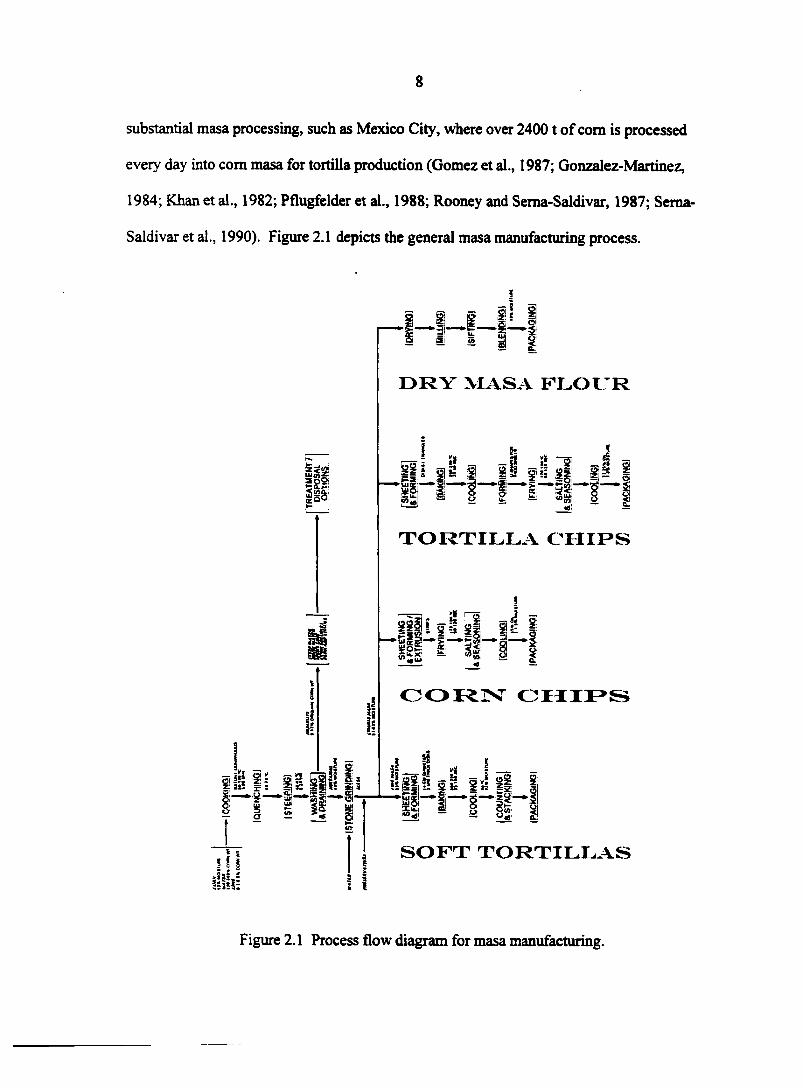
Saldivar et al., 1990). Figure 2.1 depicts the general masa manufacturing process.
I
i i h l i I I i l l Is i—s—ring*
s
i-H DRY MASA FLOUR
p! |i g
i
k ii
m-il i
TORTILLA CHIPS
•114-1-'u> «e
41 hi
CORN CHIPS
il=J
liiiii
iliJli | i fsl l | S
y 8^:
SOFT TORTILLAS
! I
Figure 2.1 Process flow diagram for masa manufacturing.
9
The largest corn masa manufacturer in the world is Mexico-based Maseca (Grupo
Industrial Maseca), which mills approximately 1.7 million Mg of corn each year, and the
second-largest masa manufacturer is Minsa, also based in Mexico, which mills
approximately 1.1 million Mg each year (Mexican Commentary, 2000; Minsa, 2000).
GRAIN PROCESSING BYPRODUCTS UTILIZATION
Before developing value-added alternatives for com masa processing byproducts, it is
beneficial to review byproduct (i.e., coproduct or waste product) utilization from other areas
in the grain processing industry. Specifically, com processing (i.e., yellow com) byproducts
will be discussed. This was chosen for review because yellow com is the leading crop grown
in the United States, and it accounts for approximately 25% of all crop acres grown in the
U.S. (NCGA, 1998).
Corn Processing Byproducts
Com is the most extensive agricultural crop grown in the United States. During 1997
and 1998, the U.S. produced 41% of the world's com. Excluding com use for silage,
73,720,000 acres and 9,365,574,000 bushels were harvested, which accounted for 25% of all
U.S. crop production (NCGA, 1998).
The majority of U.S. com is used primarily as a component for livestock rations. In
1997,5,850,000,000 bushels were fed to livestock, which accounted for approximately 63%
of all the com produced (NCGA, 1998). There are, however, many other industrial and food
uses that have been developed utilizing corn, outside the livestock arena. The three largest
industrial uses for com include com sweeteners, industrial starches, and fuel ethanol.
Sweetener production (including high fructose com syrup, glucose, and dextrose) consumed
790,000,000 bushels of com in 1997, fuel ethanol used 500,000,000 bushels, and com starch
10
production utilized 235,000,000 bushels. Combined, these three industrial uses for corn
accounted for 16.3% of the corn harvested. The remainder of the food and industrial uses for
corn, which each amounted to a small fraction of the total com use, included com oil,
breakfast cereals, pharmaceuticals, confectionery products, food starches, and other
miscellaneous foods and products (CRA, 1998; NCGA, 1998).
Four main processes exist for converting raw com into the aforementioned primary
industrial products, and also into secondary byproducts, or coproducts. These include com
dry milling, com wet milling, com oil processing, and com alcohol distilling; each will be
discussed in turn.
Corn Dry Milling
The com dry milling process has been thoroughly reviewed by Alexander (1987). In
short, the process consists of cleaning incoming corn, tempering it to approximately 20%
moisture content prior to processing, degerminating (using a Beall degerminator) to dehull
the com kernel and remove the germ fraction, drying, cooling, sifting and separating the
stream into components, milling the components using roller mills, separating the resulting
streams, and finally drying and cooling each product stream. A typical process flow diagram
for com dry milling, which gives greater detail than this brief description, is shown in Figure
2.2 (based on Alexander, 1987).
The primary products that are produced from com dry milling are com grits, com
meal, and com flour. Additionally, the germ, which is separated in the process, can be
further processed into com oil. The main com dry milling byproduct is a material called
"hominy feed", which generally consists of broken com fragments (separated prior to
processing), bran, standard meal (endosperm fines), and germ cake, which is the residual

11
RAW CORN I I
SCREENER i t
WASHER
1 TEMPER
I ;
DEGERMINATOR
' i DRYER/COOLER DRYER/COOLER
?
GRINDING
f ?
EXPELLER SIFTING
I f CRUDE OIL, DRYER/COOLER GRITS,
HOMINY MEAL, FEED FLOUR
Figure 2.2. Process flow diagram for com dry milling operations.
germ left after expelling or extraction (to obtain com oil). Hominy feed is the single greatest
material produced by com dry milling, and accounts for approximately 35% of the com input
to the process. To produce hominy feed, these byproduct materials are combined, dried,
ground in a hammermill, and then sold as a livestock feed (Alexander, 1987; Wright, 1987).
Typical nutritional compositions for hominy feed, as well as the standard meal, germ cake,
and bran fractions, are shown in Table 2.1 (from Alexander, 1987). A more detailed
nutritional summary, including vitamins, minerals, and amino acid compositions for hominy
feed can be found in Wright (1987). Not all com dry millers incorporate the germ into the
hominy feed; thus, hominy feed can have a variable composition, depending on where the
12
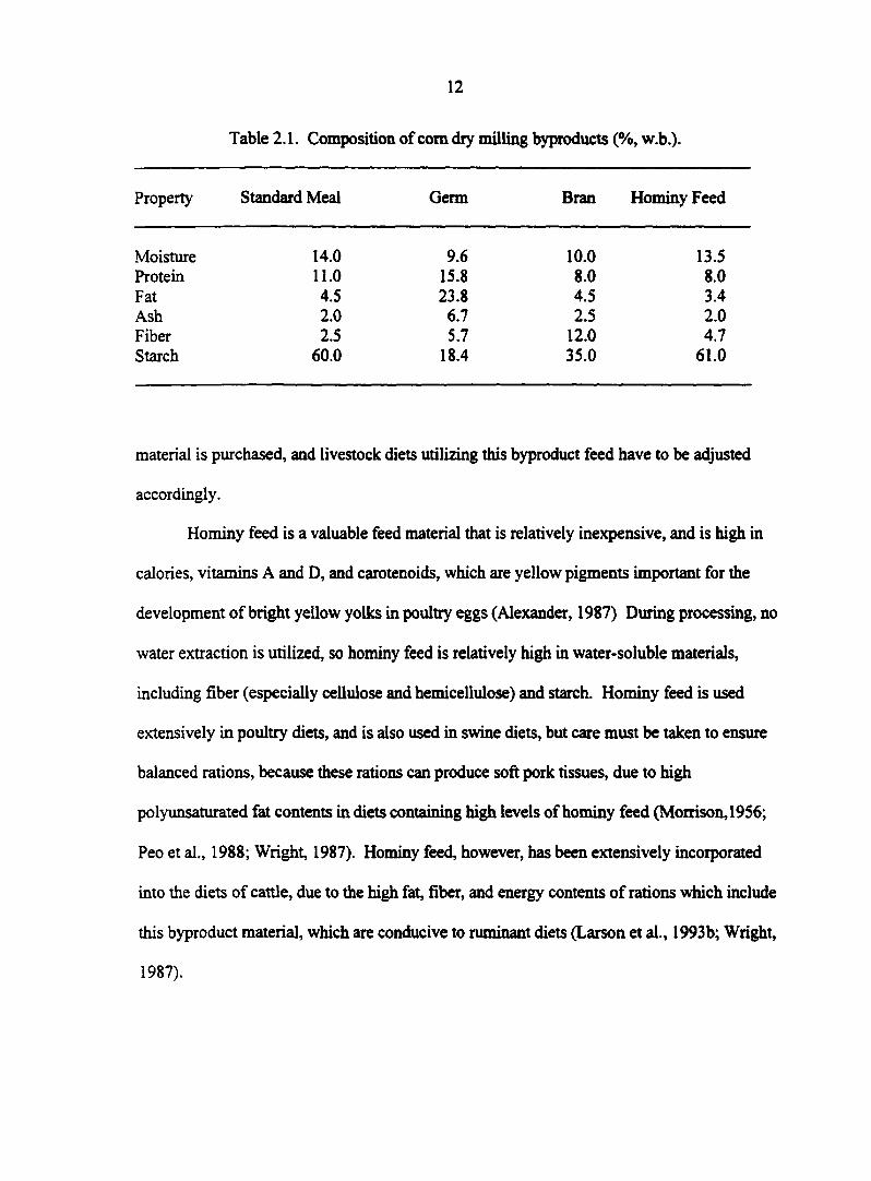
Table 2.1. Composition of com dry milling byproducts (%, w.b.).
Property Standard Meal Germ Bran Hominy Feed
Moisture 14.0 9.6 10.0 13.5 Protein 11.0 15.8 8.0 8.0 Fat 4.5 23.8 4.5 3.4 Ash 2.0 6.7 2.5 2.0 Fiber 2.5 5.7 12.0 4.7 Starch 60.0 18.4 35.0 61.0
material is purchased, and livestock diets utilizing this byproduct feed have to be adjusted
accordingly.
Hominy feed is a valuable feed material that is relatively inexpensive, and is high in
calories, vitamins A and D, and carotenoids, which are yellow pigments important for the
development of bright yellow yolks in poultry eggs (Alexander, 1987) During processing, no
water extraction is utilized, so hominy feed is relatively high in water-soluble materials,
including fiber (especially cellulose and hemicellulose) and starch. Hominy feed is used
extensively in poultry diets, and is also used in swine diets, but care must be taken to ensure
balanced rations, because these rations can produce soft pork tissues, due to high
polyunsaturated fat contents in diets containing high levels of hominy feed (Morrison,1956;
Peo et al., 1988; Wright, 1987). Hominy feed, however, has been extensively incorporated
into the diets of cattle, due to the high fat, fiber, and energy contents of rations which include
this byproduct material, which are conducive to ruminant diets (Larson et al., 1993b; Wright,
1987).
13
Recently, research has been conducted on developing alternative uses (other than
livestock feed ingredients) for com dry milling byproduct materials. For instance, the bran
fraction, which is high in fiber, has been extruded into a ready-to-eat (RTE) breakfast cereal.
It has also been incorporated into plywood adhesives. Further, germ cake, which has had the
oil extracted, is high in protein and fiber, and has been used as a component for several
fortified foods (Alexander, 1987).
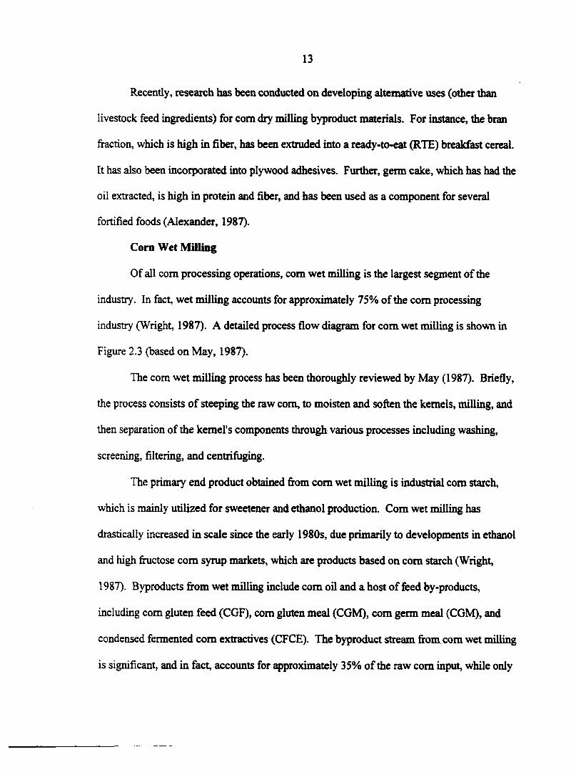
Corn Wet Milling
Of all com processing operations, com wet milling is the largest segment of the
industry. In fact, wet milling accounts for approximately 75% of the com processing
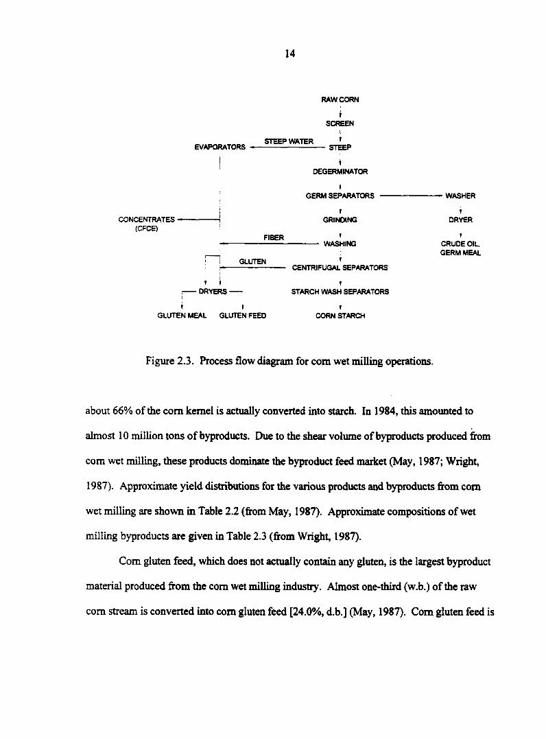
industry (Wright, 1987). A detailed process flow diagram for com wet milling is shown in
Figure 2.3 (based on May, 1987).
The com wet milling process has been thoroughly reviewed by May (1987). Briefly,
the process consists of steeping the raw com, to moisten and soften the kernels, milling, and
then separation of the kernel's components through various processes including washing,
screening, filtering, and centrifuging.
The primary end product obtained from com wet milling is industrial com starch,
which is mainly utilized for sweetener and ethanol production. Com wet milling has
drastically increased in scale since the early 1980s, due primarily to developments in ethanol
and high fructose com syrup markets, which are products based on com starch (Wright,
1987). Byproducts from wet milling include com oil and a host of feed by-products,
including com gluten feed (CGF), com gluten meal (COM), com germ meal (COM), and
condensed fermented com extractives (CFCE). The byproduct stream from com wet milling
is significant, and in fact, accounts for approximately 35% of the raw com input, while only
14
RAW CORN
SCREEN
EVAPORATORS STEEP WATER
STEEP
1 DEGERMINATOR
f
GERM SEPARATORS WASHER
CONCENTRATES • (CFCE)
FIBER
GLUTEN
f
GRINDING
1 WASHING
CENTRIFUGAL SEPARATORS
DRYER
f
CRUDE OIL. GERM MEAL
t ? DRYERS•
I STARCH WASH SEPARATORS
I t GLUTEN MEAL GLUTEN FEED
f
CORN STARCH
Figure 2.3. Process flow diagram for com wet milling operations.
about 66% of the com kernel is actually converted into starch. In 1984, this amounted to
almost 10 million tons of byproducts. Due to the shear volume of byproducts produced from
com wet milling, these products dominate the byproduct feed market (May, 1987; Wright,
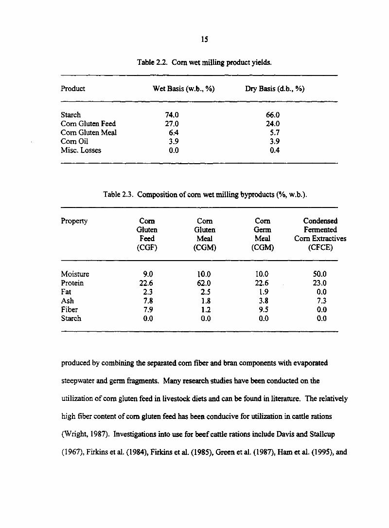
1987). Approximate yield distributions for the various products and byproducts from com
wet milling are shown in Table 2.2 (from May, 1987). Approximate compositions of wet
milling byproducts are given in Table 2.3 (from Wright, 1987).
Com gluten feed, which does not actually contain any gluten, is the largest byproduct
material produced from the com wet milling industry. Almost one-third (w.b.) of the raw
com stream is converted into com gluten feed [24.0%, d.b.] (May, 1987). Com gluten feed is
15
Table 2.2. Corn wet milling product yields.
Product Wet Basis (w.b., %) Dry Basis (d.b., %)
Starch 74.0 66.0 Com Gluten Feed 27.0 24.0 Com Gluten Meal 6.4 5.7 Com Oil 3.9 3.9 Misc. Losses 0.0 0.4
Table 2.3. Composition of corn wet milling byproducts (%, w.b.).
Property Com Com Com Condensed Gluten Gluten Germ Fermented Feed Meal Meal Com Extractives
(CGF) (CGM) (CGM) (CFCE)
Moisture 9.0 10.0 10.0 50.0 Protein 22.6 62.0 22.6 23.0 Fat 2.3 2.5 1.9 0.0 Ash 7.8 1.8 3.8 7.3 Fiber 7.9 1.2 9.5 0.0 Starch 0.0 0.0 0.0 0.0
produced by combining the separated com fiber and bran components with evaporated
steepwater and germ fragments. Many research studies have been conducted on the
utilization of com gluten feed in livestock diets and can be found in literature. The relatively
high fiber content of com gluten feed has been conducive for utilization in cattle rations
(Wright, 1987). Investigations into use for beef cattle rations include Davis and Stallcup
(1967), Firkins et al. (1984), Firkins et al. (1985), Green et al. (1987), Ham et al. (1995), and
16
Turk (1951). Incorporation into dairy cattle diets have been studied by Clamohoy et al.
(1968), Hutjens et al. (1985), Jaster et al. (1984), Staples et al (1984), and Turk (1951). Use
in swine diets has been studied by Mollis et al. (1985); Yen et al. (1971), and Yen et al.
(1974), and amino acid deficiencies have necessitated the need for supplemental feed
ingredients, such as soybean meal (Wright, 1987). Investigations into use in poultry rations
include Anonymous (1982), Bayley et al. (1971), Heiman (1961), Stinger et al. (1944), and
Wright (1957), and amino acid deficiencies have necessitated feed supplementation for
poultry rations as well (Wright, 1987). Actually, over 80% of the corn gluten feed produced
by wet milling is exported, especially to European states (Wright, 1987).
Corn gluten meal basically consists of the residual protein components after starch
has been separated from the product stream. Studies have also been conducted into the
utilization of corn gluten meal in livestock diets. Several researchers have studied this
byproduct for use in cattle rations: Annexstad et al. (1987), Burroughs and Trenkle (1978),
Klopfenstein et al. (1985), Loerch et al. (1983), and Stem et al. (1983). Researchers have
also investigated use in poultry diets, because of the good coloring that this feed ingredient
lends to egg yolks and poultry skin, and include Fletcher et al. (1985), Halloran (1970), and
Marusich and Wilgus (1968).
Com germ meal is the fraction of the germ remaining after the com oil has been
removed. Com germ meal is generally incorporated into com gluten feed. It is especially
useful as a nutrient carrier, with high water and oil absorbency properties (May, 1987).
Concentrated com steepwater, which is known as condensed fermented com
extractives (CFCE), or dried steep liquor concentrate (DSLC) is high in vitamins and protein,
and has also found success as a livestock feed ingredient, especially in poultry and swine
17
rations (Cornelius et al., 1973; Harmon et al., 1975a; Harmon et al., 1975b; Hazen and
Waldroup, 1972; Lilbum and Jensen, 1984; Marrett et al., 1968; Potter and Shelton, 1977;
Potter and Shelton, 1978; Russo et al., 1960; Russo and Heiman, 1959; Wright, 1981). This
byproduct feed ingredient, made from steepwater which has been dehydrated to almost 50%
solids, consists of the soluble portions of the com kernel, and is sold as a slurry to livestock
operations (May, 1987; Wright, 1987).
Corn Oil Processing
Corn oil is actually a byproduct (i.e., coproduct) material, not a primary product, of
the com milling industry. Approximately 90% of com oil is produced as a coproduct of com
wet milling, while about 10% is a byproduct of com dry milling operations. Thus, com oil
production has increased contemporaneously with the increasing com sweetener and starch
markets (i.e., wet milling industry) of the last several years (Orthoefer and Sinram, 1987).
Corn oil processing has been thoroughly reviewed by Orthoefer and Sinram (1987).
Briefly, crude com oil is obtained from the separated germ (a residual from both wet and dry
com milling) either though mechanical expelling or by hexane extraction. The crude oil is
then filtered (to remove solids), degummed (to remove phospholipids), washed in an alkaline
solution (to remove free fatty acids and extraneous colors), bleached (to produce proper
product color), the wax is removed (because corn waxes produce a "cloudy" oil, which is not
acceptable) via a process known as "winterization" (i.e., a cold filtration [~ 4 °C] utilising
diatomaceous earth) or the oil is hydrogenated to resist oxidation, and the oil is then
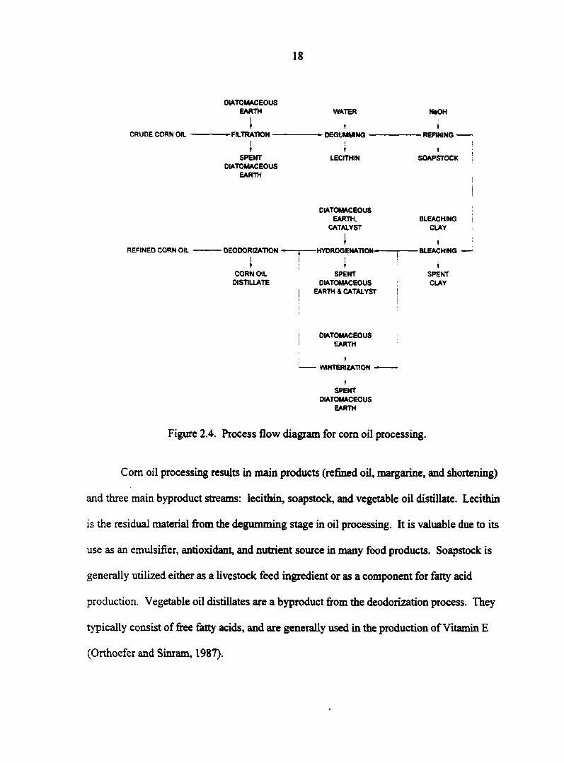
deodorized (to remove off-flavors and odors). A typical process flow diagram for com oil
processing is shown in Figure 2.4 (based on Orthoefer and Sinram, 1987).
18
OIATOMACEOUS EARTH WATER NaOH
CRUDE CORN OIL -FILTRATION-
SPENT OIATOMACEOUS
EARTH
DEGUMMING
»
LECITHIN
»
• REFINING -
SOAPSTOCK
REFINED CORN OIL • DEODORIZATION •
f CORN OIL
DISTILLATE
OIATOMACEOUS EARTH,
CATALYST
1 —HYDROGENATION—
t SPENT
OIATOMACEOUS EARTH & CATALYST
OIATOMACEOUS EARTH
I WINTERIZAT10N
I SPENT
OIATOMACEOUS EARTH
BLEACHING CLAY
I -BLEACHING
SPENT CLAY
Figure 2.4. Process flow diagram for corn oil processing.
Com oil processing results in main products (refined oil, margarine, and shortening)
and three main byproduct streams: lecithin, soapstock, and vegetable oil distillate. Lecithin
is the residual material from the degumming stage in oil processing. It is valuable due to its
use as an emulsifier, antioxidant, and nutrient source in many food products. Soapstock is
generally utilized either as a livestock feed ingredient or as a component for fatty acid
production. Vegetable oil distillates are a byproduct from the deodorization process. They
typically consist of free fatty acids, and are generally used in the production of Vitamin E
(Orthoefer and Sinram, 1987).
19
Corn Alcohol Distillation
Ethanol and beverage alcohol are produced by industrial fermentation of com starch,
which is produced through com wet milling. The distillation process has been reviewed by
Wright (1987). Briefly, com alcohol distillation consists of fermenting com starch, or other
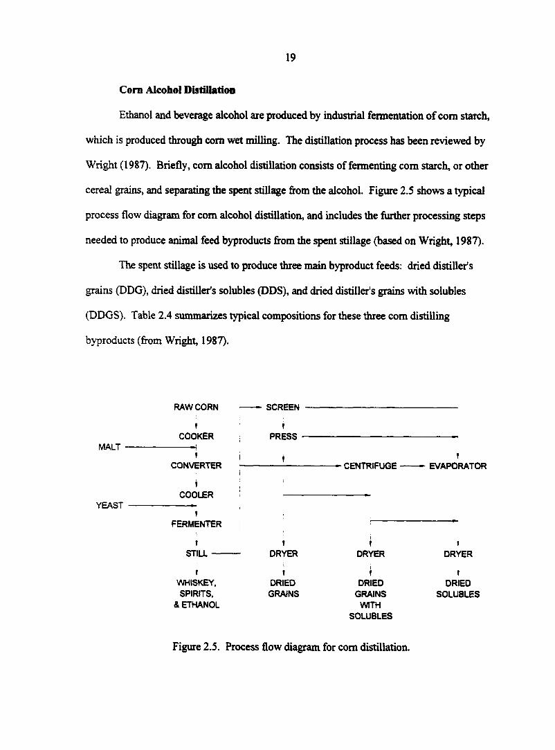
cereal grains, and separating the spent stillage from the alcohol. Figure 2.5 shows a typical
process flow diagram for com alcohol distillation, and includes the further processing steps
needed to produce animal feed byproducts from the spent stillage (based on Wright, 1987).
The spent stillage is used to produce three main byproduct feeds: dried distiller's
grains (DDG), dried distiller's solubles (DDS), and dried distiller's grains with solubles
(DDGS). Table 2.4 summarizes typical compositions for these three com distilling
byproducts (from Wright, 1987).
RAW CORN SCREEN
MALT
f COOKER
I CONVERTER
f PRESS
f CENTRIFUGE
f EVAPORATOR
YEAST COOLER
f FERMENTER
STILL —
! WHISKEY, SPIRITS,
& ETHANOL
! DRYER
i 1
DRIED GRAINS
f DRYER
t DRIED
GRAINS WITH
SOLUBLES
?
DRYER
f DRIED
SOLUBLES
Figure 2.5. Process flow diagram for com distillation.
20
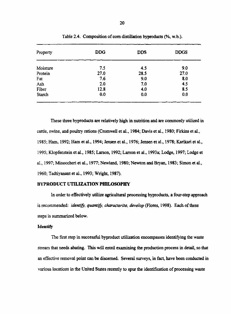
Table 2.4. Composition of com distillation byproducts (%, w.b.).
Property DDG DDS DDGS
Moisture 7.5 4.5 9.0 Protein 27.0 28.5 27.0 Fat 7.6 9.0 8.0 Ash 2.0 7.0 4.5 Fiber 12.8 4.0 8.5 Starch 0.0 0.0 0.0
These three byproducts are relatively high in nutrition and are commonly utilized in
cattle, swine, and poultry rations (Cromwell et al., 1984; Davis et al., 1980; Firkins et al.,
1985; Ham, 1992; Ham et al., 1994; Jensen et al., 1976; Jensen et al., 1978; Karikari et al.,
1995; Klopfenstein et al., 1985; Larson, 1992; Larson et al., 1993a; Lodge, 1997; Lodge et
al., 1997; Minoccheri et al., 1977; Newland, 1980; Newton and Bryan, 1983; Simon et al.,
1960; Tadtiyanant et al., 1993; Wright, 1987).
BYPRODUCT UTILIZATION PHILOSOPHY
In order to effectively utilize agricultural processing byproducts, a four-step approach
is recommended: identify, quantify, characterize, develop (Flores, 1998). Each of these
steps is summarized below.
Identify
The first step in successful byproduct utilization encompasses identifying the waste
stream that needs abating. This will entail examining the production process in detail, so that
an effective removal point can be discerned. Several surveys, in fact, have been conducted in
various locations in the United States recently to spur the identification of processing waste
21
streams (Bohlsen et al., 1997; Flores and Shanklin, 1998; Flores et al., 1999; Goldstein and
Glenn, 1997; Nelson and Flores, 1994; Youde and Prenguber, 1991).
Quantify
The second step encompasses quantifying the waste stream (i.e., how much waste is
produced and what fraction of the inputs and outputs is converted into waste). It would also
be beneficial at this stage to examine the production process to determine if the process could
be altered to reduce the quantity of waste generated. Care must be taken in this step,
however, due to proprietary concerns of many companies.
Characterize
This stage in byproduct utilization planning involves the quantification of physical
and nutritional properties of the waste stream. This stage is important for product
development, and will be discussed in more detail later.
Develop
This final stage involves developing a value-added use for the waste material. This
could be blending with another material, extruding or drying this material and shipping for
use as a livestock feed additive, composting for later use as a soil conditioning amendment,
or even developing a whole new market for this material. During this stage it is also
important to examine the economics involved with each reprocessing / reuse alternative that
is proposed for this byproduct material (Derr and Dhillon, 1997).
PHYSICAL AND NUTRITIONAL PROPERTY TESTING
Little information has been gathered regarding the properties of most industrial and
agricultural processing byproducts. To effectively utilize and add value to byproducts,
though, physical and nutritional properties must be quantified. Characterization of byproduct
22
materials provides data that are essential for livestock diet formulation, design of equipment
and processing facilities, and optimization of unit operations such as spray drying, extrusion,
blending, mixing, separating, heating, freezing, dehydration, and material flow. Physical
properties include moisture content, water activity, density, yield stress, pH, color, and
drying analysis. Nutritional properties include protein, carbohydrate, crude fat, ash, mineral
composition, amino acid composition, and fiber content. Property testing can be
accomplished following methods and procedures established by previous work in physical
and nutritional property characterization (Ferris et al., 1995; Giese, 1995; Hsu et al., 1991;
Jones and Von Bargen, 1992; Rosentrater and Flores, 1997; Stroshine and Hamann, 1995).
SUMMARY AND CONCLUSIONS
Now that a context for masa byproduct utilization has been established vis-à-vis the
grain processing industry, its associated byproducts and their subsequent utilization, it is now
time to discuss the first stage in the development of value-added byproduct utilization for the
corn masa industry: characterizing, both physically and nutritionally, typical masa byproduct
streams.
REFERENCES
Alexander, R. J. 1987. Com dry milling: Processes, products, and applications. In Corn Chemistry and Technology, eds. S. A. Watson and P. E. Ramstad, 351-376. St. Paul, MN: American Association of Cereal Chemists, Inc.
Annexstad, R. J., M. D. Stem, D. E. Otterby, J. G. Linn, and W. P. Hansen. 1987. Extruded soybeans and com gluten meal as supplemental protein sources for lactating dairy cattle. Journal of Dairy Science 70(4): 814-822.
Anonymous. 1982. Corn wet-milled feed products. Washington, D.C.: Com Refiners Association.
23
Bayley, H. S., J. D. Summers, and S. J. Slinger. 1971. A nutritional evaluation of com wet-milling by-products with growing chicks and turkey poults, adult roosters, and turkeys, rats, and swine. Cereal Chemistry 48(1): 27-33.
Bohlsen, D., S. Weeder, and S. Wang. Tracking organic waste. Resource 4(9): 13-14.
Bressani, R., R. Paz y Paz, and N. S. Scrimshaw. 1958. Corn nutrient losses: chemical changes in corn during preparation of tortillas. Journal of Agricultural Food Chemistry 6: 770.
Burroughs, W. and A. Trenkle. 1978. Naturally protected protein (com gluten meal) vs. unprotected protein (soybean meal) in supplements for calves up to 650 pounds weight. A. S. Leaflet R269. Ames, IA: Iowa State University Cooperative Extension Service.
Clamohoy, L. L., O. A. Palad, L. E. Nazareno, L. S. Castillo, J. S. Bontuyan, P. L. Ordinaria, and K. L. Turk. 1968. Feeding value of com gluten feed in rations for lactating dairy cows and growing dairy heifers. Animal Husbandry Agricultural Journal October: 29-34.
College of Agricultural, Consumer, and Environmental Sciences (CAGES). 2000. Illinois Specialty Farm Products. University of Illinois at Urbana-Champaign. Available online: web.aces.uiuc.edu/value/factsheets/fact-foodcorn.htm [September 3,2000].
Corn Refiners Association (CRA). 1998. 1998 Com Annual. Washington, D C.: National Com Refiners Association, Inc.
Cornelius, S. G., J. P. Totsch, and B. G. Harmon. 1973. Metabolizable energy of DSLC for swine. Journal of Animal Science 37: 277
Cromwell, G. L., T. S. Stahly, and H. J. Monegue. 1984. Distillers dried grains with solubles for growing-finishing swine. 1984 Swine Research Report. Lexington, KY: University of Kentucky Agricultural Experiment Station.
Davis, C., M. Hut)ens, and L. Berger. 1980. Should you consider distillers' and brewers' byproducts? Hoards Dairyman 125(7): 546-547.
Davis, G. V. and O. T. Stallcup. 1967. Effect of soybean meal, raw soybeans, com gluten feed, and urea on the concentration of rumen fluid components at intervals after feeding. Journal of Dairy Science 50:1638-1644.
Derr, D. A. and P. S. Dhillon. 1997. The economics of recycling food residuals. BioCycle 38(4): 55-56.
24
Ferris, D. A., R. A. Flores, C. W. Shanklin, and M. K. Whitworth. 1995. Proximate analysis of food service wastes. Applied Engineering in Agriculture 11(4): 567-572.
Firkins, J. L., L. L. Berger, G.C. Fahey, Jr., and N. R. Merchen. 1984. Ruminai nitrogen degradability and escape of wet and dry distillers grains and wet and dry corn gluten feeds. Journal of Dairy Science 67:1936-1944.
Firkins, J. L., L. L. Berger, and G.C. Fahey, Jr. 1985. Evaluation of wet and dry distillers grains and wet and dry corn gluten feeds for ruminants. Journal of Animal Science 60: 847-860.
Fletcher, D. L., C. M. Papa, and H. R. Halloran. 1985. Utilization and yolk coloring capability of dietary xanthophylls from yellow corn, corn gluten meal, alfalfa, and coastal bermudagrass. Poultry Science 64:1458-1463.
Flores, R. A. 1998. Making agricultural leftovers more palatable. Resource 5(4): 13-14.
Flores, R. A. and C. W. Shanklin. 1998. What's needed to use more agribusiness residues? BioCycle (November): 82-83.
Flores, R. A., C. W. Shanklin, M. Loza-Garay, and S. H. Wie. 1999. Quantification and characterization of food processing wastes/residues. Compost Science & Utilization 7(1): 63-71.
Giese, J. 1995. Measuring physical properties of foods. Food Technology (February): 54-63.
Goldstein, N. and J. Glenn. 1997. The state of garbage in America. BioCycle (May): 71-75.
Gomez, M. H., L. W. Rooney, R. D. Waniska, and R. L. Pflugfelder. 1987. Dry corn masa flours for tortilla and snack food production. Cereal Foods World 32(5): 372-377.
Gonzalez de Palacios, M. 1980. Characteristics of corn and sorghum for tortilla processing. Unpublished M.S. Thesis. College Station, TX: Texas A&M University.
Gonzalez-Martinez, S. 1984. Biological treatability of the wastewaters from the alkaline cooking of maize (Indian corn). Environmental Technology Letters 5(8): 365-372.
Green, D. A., R. A. Stock, F. K. Goedeken, and T. J. Klopfenstein. 1987. Energy value of corn wet milling by-product feeds for finishing ruminants. Journal of Animal Science 65(6): 1655-1666.
Halloran, H. R. 1970. Review of the most important xanthophyll products in the U.S. Feedstuffs October: 31.
25
Ham, G. A. 1992. Com byproducts for growing and finishing cattle. Unpublished M.S. Thesis. Lincoln, NE: University of Nebraska.
Ham, G. A., R. A. Stock, T. J. Klopfenstein, E. M. Larson, D. H. Shain, and R. P. Huffman. 1994. Wet com distillers byproducts compared with dried com distillers grains with solubles as a source of protein and energy for ruminants. Journal of Animal Science 72(12): 3246-3257.
Ham, G. A., R. A. Stock, T. J. Klopfenstein, and R. P. Huffman. 1995. Determining the net energy value of wet and dry com gluten feed in beef growing and finishing diets. Journal of Animal Science 73(2): 353-359.
Harmon, B. G., A. Galo, S. G. Cornelius, D. H. Baker, and A. H. Jensen. 1975a. Condensed fermented com solubles with germ meal and bran (DSLC) as a nutrient source for swine. I. Amino acid limitation. Journal of Animal Science 40:242-246.
Harmon, B. G., A. Galo, J. E. Pettigrew, S.G. Cornelius, D. H. Baker, and A. H. Jensen. 1975b. Condensed fermented com solubles with germ meal and bran (DSLC) as a nutrient source for swine. II. Amino acid substitution. Journal of Animal Science 40: 247-250.
Hazen, K. R. and P. W. Waldroup. 1972. Improvement of interior egg quality by com dried steep liquor concentrate. Poultry Science 51:1816-1817.
Heiman, V. 1961. Com gluten feed in layer and breeder rations. Feed Profile 71968. Englewood Cliffs, NJ: CPC International.
Hollis, G. R., R. A. Easter, J. D. Weigel, and S. G. Bidner. 1985. Swine. In Corn Gluten Feed, the Future of Feeding, 10-13. Bloomington, IL: Illinois Com Growers Association.
Hsu, M. -H., J. D. Mannapperuma, and R. P. Singh. 1991. Physical and thermal properties of pistachios. Journal of Agricultural Engineering Research 49: 311-321.
Hutjens, M. F., J. C. Weigel, and S. G. Bidner. 1985. Dairy cattle. In Corn Gluten Feed, the Future of Feeding, 6-7. Bloomington, IL: Illinois Com Growers Association.
Jaster, E. H., C. R. Staples, G. C. McCoy, and C. L. Davis. 1984. Evaluation of wet com gluten feed, oatlage, sorghum-soybean silage, and alfalfa haylage for dairy heifers. Journal of Dairy Science 67:1976-1978.
Jensen, L. S., C. H. Chang, and D. V. Maurice. 1976. Improvement in interior egg quality and reduction in liver fat in hens fed brewers dried grains. Poultry Science. 55: 1841-1847.
26
Jensen, L. S., C. H. Chang, and S. P. Wilson. 1978. Interior egg quality: Improvement by distillers feeds and trace elements. Poultry Science 57: 648-654.
Jones, D. and K. L. Von Bargen. 1992. Some physical properties of milkweed pods. Transactions of the ASAE 35(1): 243-246.
Karikari, P. K., P. Gyawa, K. Asare, and S. S. Yambillah. 1995. The reproductive response of N'dama cows to brewers' spent grain supplementation in a hot humid environment. Tropical Agriculture 71(4): 315-318.
Katz, S. H., M. L. Hediger, and L. A. Valleroy. 1974. Traditional maize processing techniques in the New World. Science 184:765.
Khan, M. N., M. C. Des Rosiers, L. W. Rooney, R. G. Morgan, and V. E. Sweat. 1982. Com tortillas: evaluation of com cooking procedures. Cereal Chemistry 59(4): 279-284.
Klopfenstein, T., R. Stock, and R. Britton. 1985. Relevance of bypass protein to cattle feeding. Prof Animal Science 1:27-31.
Krause, V. M., K. L. Tucker, H. V. Kuhnlein, C. Y. Lopez-Palacios, M. Ruz, and N. W. Solomons. 1992. Rural-urban variation in limed maize use and tortilla consumption by women in Guatemala. Ecology of Food and Nutrition 28:279-288.
Larson, E. M. 1992. Com byproducts for finishing cattle. Unpublished M.S. Thesis. Lincoln, NE: University of Nebraska.
Larson, E. M., R. A. Stock, T. J. Klopfenstein, M. H. Sindt, and R. P. Huffman. 1993a. Feeding value of wet distillers byproducts for finishing ruminants. Journal of Animal Science 71(8): 2228-2236.
Larson, E. M., R. A. Stock, T. J. Klopfenstein, M. H. Sindt, and D. H. Shain. 1993b. Energy value of hominy feed for finishing ruminants. Journal of Animal Science 71(5): 1092-1099.
Lilbum, M. S., and L. S. Jensen. 1984. Evaluation of com fermentation solubles as a feed ingredient for laying hens. Poultry Science 63: 542-547.
Lodge, S. L. 1997. Evaluation of wet distillers composite for finishing ruminants. Journal of Animal Science 75(1): 44-50.
Lodge, S. L., R. A. Stock, T. J. Klopfenstein, D. H. Shain, and D. W. Herold. 1997. Evaluation of com and sorghum distillers byproducts. Journal of Animal Science 75(1): 37-43.
27
Loerch, S. C., L. L. Berger, D. Gianola, and G. C. Fahey, Jr. 1983. Effects of dietary protein source and energy level on in situ nitrogen disappearance of various protein sources. Journal of Animal Science 56:206-216.
Marrett, L. E., H. R. Bird, and M. L. Sunde. 1968. Growth promoting effect of com fermentation condensed solubles. Poultry Science 47:1691-1692.
Marusich, W. L. and H. S. Wilgus. 1968. Evaluating the pigmentation value of feestuffs for poultry rations. In Proceedings of the Arkansas Formula Feed Conference, 9-22.
Fayetteville, AR: University of Arkansas.
May, J. B. 1987. Wet milling: Process and products. In Corn Chemistry and Technology, eds. S. A. Watson and P. E. Ramstad, 377-397. St Paul, MN: American Association of Cereal Chemists, Inc.
Mexican Commentary. 2000. Grupo Industrial Maseca ADS - Symbol (MSK) - NYSE. Mexican Commentary. Available online: http : wwpeople.delphi.com/agoozner/mskinfo.htm [September 3,2000].
Minoccheri, F., F. Negrini, and S. Grazia. 1977. Behavior of some muscle and serum enzymes in meat swine fed dry (grain) and distillers waste. (Comportamento di alcuni enzimi muscolari e sierici in suini salumificio alimentati "a seco" e in "in borlanda".) Boll. Soc. Ital. Biol. Sper 53(1/2): 61-67.
Minsa. 2000. Corporate Information - Manufacturing. Minsa Southwest Corporation. Available online: www.minsa.com/english/htm/ci-man.htm [August 19,2000].
Morrison, F. B. 1956. Feeds and Feeding. Ithaca, NY: Morrison Publication Co.
National Com Growers Association (NCGA). 1998. The World of Corn. Kansas City, MO: McConnick Advertising Agency.
Nelson, R. G. and R. A. Flores. 1994. Survey of processing residues generated by Kansas agribusinesses. Applied Engineering in Agriculture 10(5): 703-708.
Newland, H. W. 1980. Use of com distillers by-products for swine feed byproducts. Ohio Swine Research Industry Report Animal Science Series Ohio Agricultural Research Development Center, 18-21.
Newton, G. L. and W. L. Bryan. 1983. Use of com stillage in diets for growing-finishing swine. In 3rd Annual Solar and Biomass Workshop, 202-205. Washington, D C.: United States Department of Agriculture.
28
Orthoefer, F. T. and R. D. Sinram. 1987. Com oil: Composition, processing and utilization. In Corn Chemistry and Technology, eds. S. A. Watson and P. E. Ramstad, 535-551. St. Paul, MN: American Association of Cereal Chemists, Inc.
Ortiz, E. L. 1985. The cuisine of Mexico: com tortilla dishes. Gourmet 45(May): 62-63.
Parades-Lopez, O. and M. E. Saharopulos-Parades. 1983. Maize - a review of tortilla production technology. Bakers Digest 57(5): 16-25.
Peo, Jr., E. R., J. D. Hancock, and A. J. Lewis. 1988. Hominy feed - an important com byproduct for growing-finishing swine. Nebraska Cooperative Extension Service, 30-31.
Pflugfelder, R. L., L. W. Rooney, and R. D. Waniska. 1988. Dry matter losses in commercial com masa production. Cereal Chemistry 65(2): 127-132.
Potter, L. M. and J. R. Shelton. 1977. Evaluation of com fermentation solubles, menhaden fish meal, methionine, and hydrolyzed feather meal in diets of young turkeys. Poultry Science 57: 1586-1593.
Potter, L. M. and J. R. Shelton. 1978. Evidence of an unidentified growth factor in com fermentation solubles for young turkeys. Nutrition Reports International 17: 509-517.
Rooney, L. W. and S. O. Sema-Saldivar. 1987. Food uses of whole com and dry-milled fractions. In Corn Chemistry and Technology, ed. S. A. Watson and P. E. Ramstad, 399-430. St. Paul, MN: American Association of Cereal Chemists.
Rosentrater, K. and R. Flores. 1997. Physical and rheological properties of slaughterhouse swine blood and blood components. Transactions of the ASAE 40(3): 683-689.
Russo, J. M. and V. Heiman. 1959. Ability of com fermentation condensed solubles to replace unidentified growth factor sources for chickens. Poultry Science 38: 1325-1328.
Russo, J. M., S. A. Watson, and V. Heiman. 1960. Source of chick growth stimulus in com fermentation condensed solubles. Poultry Science 39:1408-1412.
Sema-Saldivar, S. O., M. H. Gomez, and L. M. Rooney. 1990. Technology, chemistry, and nutritional value of alkaline-cooked com products. Advances in Cereal Science and Technology 10:243-306.
Simon, T., L. Tsang, and P. J. Schaible. 1960. The value of com fermentation solubles in poultry nutrition. Poultry Science 39: 251-257.
29
Slinger, S. J., J. H. Pettit, and E. V. Evans., 1944. The use of corn gluten feed to replace meat meal in poultry rations. Scientific Agriculture 24:234-239.
Staples, C. R., C. L. Davis, G. C. McCoy, and J. H. Clark. 1984. Feeding value of wet com gluten feed for lactating dairy cows. Journal of Dairy Science 67:1214-1220.
Stern, M. D., L. M. Rode, R. W. Prange, R. H. Stauffacher, and L. D. Satter. 1983. Ruminai protein degradation of com gluten meal in lactating dairy cattle fitted with duodenal T-type cannulae. Journal of Animal Science 56:194-205.
Stroshine, R. and D. Hamann. 1995. Physical Properties of Agricultural Materials and Food Products. West Lafayette, IN: Copy Cat.
Tadtiyanant, C., J. J. Lyons, and J. M Vandepopuliere. 1993. Brewers condensed solubles used as a feedstuff in broiler diets. Poultry Science 72(10): 1897-1905.
Turk, K. L. 1951. Com gluten feed. Flour Feed August: 12-15.
Wood, M. 1994. What makes tortillas and tacos taste so good? Agricultural Research 42(11): 17.
Wright, K. N. 1957. What's ahead for com gluten feed? Feed Merchant May: 64-76.
Wright, K. N. 1981. Com wet-milling byproducts - com steep liquor. In II th Annual Liquid Feed Symposium, 29-40. Arlington, VA: American Feed Industry Association.
Wright, K.N. 1987. Nutritional properties and feeding value of com and its by-products. In Corn Chemistry and Technology, eds. S. A. Watson and P. E. Ramstad, 447-478. St. Paul, MN: American Association of Cereal Chemists, Inc.
Yen, J. T., D. H. Baker, B. G. Harmon, and A. H. Jensen. 1971. Com gluten feed in swine diets and effect of pelleting on tryptophan availability to pigs and rats. Journal of Animal Science 33:987-991.
Yen, J. T., J. D. Brooks, and A. H. Jensen. 1974. Metabolizable energy value of com gluten feed. Journal of Animal Science 39:335-337.
Youde, J. and B. Prenguber. 1991. Classifying the food waste stream. BioCycle 32(10): 70-71.
30
CHAPTER 3
PHYSICAL AND NUTRITIONAL PROPERTIES OF CORN MASA BYPRODUCT STREAMS
A paper published, in part, in Applied Engineering in Agriculture
K. A. Rosentrater, R. A. Flores, T. L. Richard, and C. J. Bern
ABSTRACT
Production of com masa-based products is flourishing in the United States, as is the
generation of masa processing waste. Masa byproducts show potential for value-added
utilization, an option which could produce less pollution in the environment and lead to
economic benefits for masa processors. Physical and nutritional properties of these
byproducts are needed for the proper design of processing operations and byproduct
applications, but information concerning masa byproducts is not currently available. Thus
the objective of this study was to fully characterize typical masa byproduct streams. The
masa byproducts studied had moisture contents between 88.15 and 89.29 (%, w.b.), water
activity values between 0.999 and 1.000 (-), mass densities between 1030.85 and 1047.32
(kg/m-1), yield stress values between 1440.04 and 1618.08 (N/m2), pH values between 6.17
and 6.30 (-), Hunter L values between 35.15 and 49.13 (-), a values between 0.27 and 0.98 (-
), and b values between 6.85 and 9.38 (-). Drying curves were developed to predict drying
behavior. The dried byproducts had protein contents between 4.76 and 4.90 (%, d.b.), crude
fat contents from 0.74 to 5.76 (%, d.b.), ash contents between 17.41 and 19.09 (%, d.b.), and
carbohydrate contents from 71.93 to 75.41 (%, d.b.), which was due primarily to fiber, with
hemicellulose levels of 20.82 to 24.0 (%, d.b.) and cellulose between 30.55 and 31.83 (%,
31
d.b.). Dry masa byproducts also consisted of 4.68 (%, d.b.) calcium. Dehydrated masa
byproducts therefore seem very suitable for use as livestock feed additives.
Keywords
Evaluation, Food processing, Food waste, Residue characterization, Residue
utilization.
Author Information
Journal Paper No. J-18033 of the Iowa Agriculture and Home Economics Experiment
Station, Ames, Iowa, Project No. 3326, and supported by Hatch Act and State of Iowa Funds.
Contribution No. 99-3-J from the Kansas Agricultural Experiment Station.
The authors are Kurt A. Rosentrater, ASAE Student Member, Graduate Student,
Agricultural and Biosystems Engineering Dept., Iowa State University, Ames, Iowa;
Rolando A. Flores, ASAE Member Engineer, Associate Professor, Department of Grain
Science and Industry, Kansas State University, Manhattan, Kansas (formerly with the
Agricultural and Biosystems Engineering Dept. and Food Science and Human Nutrition
Dept., Iowa State University, Ames, Iowa); Thomas L. Richard, ASAE Member, Assistant
Professor, Agricultural and Biosystems Engineering Dept., Iowa State University, Ames,
Iowa; and Carl J. Bern, ASAE Member Engineer, Professor, Agricultural and Biosystems
Engineering Dept., Iowa State University, Ames, Iowa. Corresponding author: Rolando
A. Flores, Kansas State University, 104 Shellenberger Hall, Manhattan, Kansas, 66506-2201;
tel.: (913) 532-4064; fax: (913) 532 7010; e-mail: [email protected].
32
INTRODUCTION
Agricultural processing industries produce great quantities of waste materials. From
1991 to 1992 agribusinesses in Kansas alone produced over 72,000 Mg/yr of waste products
and processing residues. Approximately 10% (7173 Mg/yr) of these wastes were attributable
to the grain processing industry (Nelson and Flores, 1994). Due to heightened economic and
environmental concerns, landfilling has declined as the typical waste disposal method of
choice, and other disposal alternatives have been more frequently investigated. Current
options include reprocessing/recycling, resale, incineration, composting, biomass energy
production, land application as soil conditioning materials, and reuse as livestock feed
ingredients. The last alternative includes both direct feeding of the waste products and
feeding the byproducts after further processing (i.e., dehydration, extrusion, or blending with
other feed components) (Bohlsen et al., 1997).
In recent years, many research efforts have been aimed toward the development of
livestock feed additives from agricultural wastes and byproducts. One aspect has included
the investigation of non-meat food wastes as potential feed products (Polanski, 1992).
Another area has included the development of feed ingredients from slaughterhouse
byproducts (Luzier and Summerfelt, 1995; Martins and Guzman, 1994; Wang et al., 1997).
The utilization of grain processing byproducts as livestock feed components has also been
extensively researched (Ham et al., 1994,1995; Hussein and Berger, 1995; Larson et al.,
1993). Com masa production is one facet of the grain processing industry that generates
large quantities of waste materials, but to date, has received little research attention regarding
alternatives for byproduct disposal.
33
Corn masa is used in the production of corn snack foods and tortilla chips, and has
traditionally been utilized for the preparation of tortillas, which have been a staple in the diet
of Mexican and Central American peoples for centuries. Foods made with com masa and
tortillas include tacos, tostadas, tamales, quesadillas, panuchos, enchiladas, and others
(Krause et al., 1992; Ortiz, 1985; Sema-Saldivar et al., 1990). Currently, Mexican foods and
corn-based snacks in the United States are becoming more popular. Over $4 billion worth of
Mexican foods were marketed in 1986, and approximately $2.5 billion worth of tortilla chips
were produced in 1994 (Gomez et al., 1987; Wood, 1994). Tortilla sales alone were
estimated at $4 billion for 2000 A.D. (Solganik, 1997), and are expected to reach $5.5 billion
by 2003 A.D. (TLA, 2001). Corn masa is produced by simulating ancient Aztec processing
methods on an industrial-scale. Whole com is cooked with 120 to 300% water (original com
weight basis) and 0.1 to 2.0% lime (original com weight basis) for 0.5 to 3.0 h at 80 to 100
°C, and is then steeped for up to 24 h. This process, called nixtamalization, can be either a
batch process or a continuous process, depending on production equipment. The cooked
grain (nixtamal) is then separated from the steep liquor (nejayote), which is rich in lime and
dissolved com pericarp tissue, is washed to remove any excess lime and pericarp, and is then
stone ground to produce com masa. The masa will then be molded, cut, or extruded, and
then baked or fried to make tortillas, com chips, or tortilla chips; or it will be dried and
milled into com masa flour (Gomez et al., 1987; Rooney and Sema-Saldivar, 1987; Sema-
Saldivar et al., 1990).
The steep liquor and the rinse water contain between 2 and 6% total (dissolved and
suspended) solids. Generally the suspended solids (50 to 60% of the total solids) are
34
removed by screening, centrifugation, or decanting, and disposed of in landfills. The
remaining water and dissolved solids are sent to municipal facilities for treatment. The total
solids in the waste stream, which consist primarily of fiber-rich pericarp tissues, represent
com dry matter loss that occurs during processing. Estimates of the original com dry matter
loss have ranged from 5.0% to 17.0%. The following were found in the literature: 8.5 to
12.5% (Pflugfelder et al., 1988), 8.0 to 17.0% (Rooney and Sema-Saldivar, 1987), 7.0 to
13.0% (Khan et al., 1982), 5.0 to 14.0% (Katz et al., 1974), 11.0 to 12.0% (Bressani et al.,
1958), and 13.3% (Gonzalez de Palacios, 1980). Com dry matter loss during nixtamalization
is affected by many processing variables, including com hybrid and quality, lime type and
concentration, cooking and steeping times and temperatures, friction experienced during
washing and transport, and processing equipment used. These processing losses can be
economically significant due to lost masa yield, waste processing and disposal costs, and
potential environmental pollution and associated fines. This waste generation is of particular
concern in areas of substantial masa processing, such as Mexico City, where over 2400 Mg
of com is processed every day into com masa for tortilla production (Gonzalez-Martinez,
1984).
Gonzalez-Martinez (1984) investigated four biological treatment options for
"nejayote", including activated sludge processing, anaerobic contact processing, submerged
aerobic fixed-film cascade reacting, and anaerobic packed-bed reacting, all of which met with
various success. However, little research has been conducted into alternative disposal
methods for com masa dry matter losses (i.e., the separated suspended solids), and none
could be found regarding the utilization of com masa waste solids in livestock feed rations.
35
To effectively utilize and add value to these byproducts, physical and nutritional
properties for com masa residual streams must be quantified. Characterization of byproduct
materials provides data that are essential for livestock diet formulation, design of equipment
and processing facilities, and optimization of unit operations such as drying, extrusion,
blending, mixing, separating, heating, freezing, dehydration, and material flow (Ferris et al.,
1995; Stroshine and Hamann, 1995). Little information has been gathered concerning the
properties of com masa byproducts, however. Because of the great demand for corn masa-
based products in the United States, and throughout the world, the objective of this study was
to characterize and quantify the physical and nutritional properties of typical com masa
byproduct streams, so that subsequent byproduct applications may effectively be developed
for these waste materials. Physical properties studied included moisture content, water
activity, mass density, yield stress, pH, color, and drying behavior. Nutritional properties
studied included protein, crude fat, ash, mineral composition, amino acid composition, and
fiber content.
MATERIALS AND METHODS
Sample Collection and Preparation
Com masa byproduct samples, which were gray, pasty, semi-solid slurries (Figure
3.1), were obtained from a local white com masa processing facility after the decanting stage
in the production process (i.e., the samples collected were the suspended solids that had been
separated from the waste stream). Five 3.5 L samples were collected at random times from
random batches and random production runs, from both a batch and a continuous processing
line during the fall of 1996.
36
Figure 3.1. Typical com masa processing byproduct slurries.
The 10 samples were then placed in frozen storage at -10 °C until testing commenced. Prior
to analysis, the samples were thawed at room temperature (25 °C ± 2 °C) for 24 h. All
physical properties were determined at room temperature, except moisture content and drying
analysis, which were conducted at temperatures proscribed by the appropriate methods used.
All nutritional tests were conducted as specified by the standard method used for each
property.
Experimental Design
To investigate the properties of typical corn masa byproducts, five samples from each
of two masa production processes (e.g., a batch process and a continuous process) were
analyzed; thus two populations were present in this study. All properties were studied using
a Completely Randomized Design. For all physical property testing (moisture content, water
activity, density, yield stress, pH, color, and drying analysis), five replicates were taken from
each of the 10 samples (five samples were taken per production line), which led to an overall
sample size of 25 experimental units for each production process (i.e., population). This
37
maintained the Type-I (a) and Type-II (P) error rates at the 0.05 level and allowed the
detectable statistically significant difference between populations to remain at 1.0 standard
deviation. Protein, crude fat, and ash testing were performed with two replicates taken from
each of the 10 samples, which led to an overall sample size of 10 experimental units from
each population. This maintained the Type-I (a) and Type-II (P) error rates at the 0.05 level,
but the detectable difference between populations increased to 1.8 standard deviations. Fiber
analysis was conducted with three replicates from each sample, which produced a sample
size of 15 experimental units for each production process (i.e., each population). This
maintained the Type-I (a) and Type-II (P) error rates at the 0.05 level, and the detectable
difference between populations was set at 1.4 standard deviations (Nelson, 1985). Formal
statistical analyses on the collected data were performed via Microsoft Excel (Microsoft,
1993) and SAS (SAS, 1992) software, and included t-tests to investigate difference between
population means for each property, correlation analysis, to examine relationships between
variables, and principal components analysis (PCA), to look for outliers, clusters, and
curvature in the multivariate data set.
Amino acid composition was studied on the continuous-process samples only, as was
mineral analysis. One replicate from each of the five samples was used in the amino acid
study, whereas one replicate from two of the five samples was randomly selected for mineral
analysis. Neither amino acid composition nor mineral composition was included in the
formal statistical analysis that was conducted on all other physical and nutritional properties.
Rather, limited amino acid and mineral analysis was conducted to provide baseline estimates
for corn masa byproducts, but the scope was constrained by time and resources available.
38
Physical Properties
Moisture Content and Water Activity
Moisture content (wet basis - w.b.) of the masa byproduct samples was determined
using a method similar to AACC Standard Method 44-15 A ("Moisture-Air-Oven Methods")
(AACC, 1995). Byproduct samples of 2 to 3 g were placed in open tared aluminum moisture
dishes that were 8-cm in diameter and 2.5-cm in height (Style 10, Ellisco, Inc., Baltimore,
MD), and were dried at 130 °C for 3 h in a forced-convection laboratory oven (Thelco Model
160DM, Precision Scientific, Inc., Chicago, IL). After drying, the samples were allowed to
cool in a desiccator, and sample mass was then measured with an electronic balance (Model
A-250, Denver Instrument Co., Arvada, CO). To determine water activity of the masa
byproducts, 4 g samples were placed in a previously calibrated water activity meter (Aqualab
Model CX-2, Decagon Devices, Inc., Pullman, WA).
Mass Density
The density of each byproduct sample was determined using a specific gravity cup
(Model H-38000-12, Cole-Parmer Instrument Co., Bamngton, IL) and an electronic balance.
The specific gravity cup has a known mass (150.25 g) and volume (83.2 cm3); hence, to
measure sample density, the cup was filled completely with sample material, the lid was
placed on the cup, excess sample material was removed, and the filled cup was then weighed
on the balance.
Yield Stress
The yield stress of the byproduct samples was determined using the vane method with
a digital viscometer (Model HBDV n+, Brookfield Engineering, Stoughton, MA) and a four-
39
finned vane; each fin was 1.01 cm in height and was 1.4 mm in thickness, and the vane had
an overall diameter of 1.2 cm (accounting for the each fin and the vane shaft). Byproduct
samples were placed in a 150 mL beaker which was 8 cm in height and 5.3 cm in diameter;
the vane was then placed 2 cm below the sample surface, and a controlled constant shear rate
of 0.34 s'1 (0.5 rpm) was applied to the viscometer. Using the vane method with a controlled
shear rate, the yield stress was determined using the following equation:
where Tm is the torque exerted on the vane at yielding, D is the overall vane diameter, H is
the overall vane height, and xy is the resultant yield stress (Dzuy and Soger, 1985; Yoo et al.,
1995).
To determine the pH of the masa byproduct samples, 10 g samples were placed in a
50 mL glass beaker. A benchtop pH meter (Model PHB-62, Omega Engineering, Inc.,
Stamford, CT) was then used to measure the pH.
The color of each masa byproduct sample was determined using a Hunter Colorimeter
(Model LabScan SN-12414, Hunter Associates Laboratory, Inc., Reston, VA), using a view
port and view-area size of 1.27 cm (0.5 in), and the L-a-b opposable color scales (Hunter,
1983). The samples were placed in 100 mm diameter x 15 mm diameter plastic petri dishes
(3.1)
PH
Color
40
and were positioned in the instrument for color determination after proper instrument
calibration.
Drying Analysis
The drying studies that were performed on the masa byproducts were similar to those
conducted by Rosentrater and Flores (1997) on swine blood components. Masa byproduct
samples of 2 to 3 g were placed in open, tared, aluminum moisture dishes that were 8 cm in
diameter and 2.5 cm in height (Style 10, Ellisco, Inc., Baltimore, MD) and were placed in a
forced-convection laboratory oven (Thelco Model 160DM, Precision Scientific, Inc.,
Chicago, IL). Samples were dried at temperatures of 80,100, and 120 6C for 2 h, and sample
mass over time was measured with an electronic balance. Sample masses were recorded
every 5 min during the first hour of testing and every 10 min thereafter. Thus, drying curves
were developed on a dry basis (d.b.) and drying rate prediction equations as a function of
moisture content and drying temperature were developed for the two byproducts.
Nutritional Properties
Proximate Composition
Proximate analysis of dry masa byproduct samples included the determination of
protein, crude fat, and ash contents. Protein and crude fat analyses were conducted by the
Meat Laboratory at Iowa State University, Ames, IA. Protein analysis followed the AACC
Standard Method 46-11A ("Crude Protein-Improved Kjeldahl Method, Copper Catalyst
Modification"), using a factor of N x 6.25 (AACC, 1995). Crude fat was determined using
the AACC Standard Method 30-25 ("Crude Fat in Wheat, Com, and Soy Flour, Feeds, and
Cooked Feeds") (AACC, 1995). Ash content was determined using the AACC Standard
41
Method 08-03 ("Ash-Rapid [2-Hour, 600=] Method") (AACC, 1995), which utilized 2 g
samples placed in a muffle furnace at 600 °C for 2 h. Because protein, fat, ash, and
carbohydrate contents sum to 100% in the dry byproduct, the carbohydrate contents of the
dry masa byproduct samples could be calculated by differencing the measured results (e.g.,
protein, fat, and ash).
Fiber Composition
Fiber analysis was conducted by the Forage Quality Laboratory at Iowa State
University, Ames, IA, using the Van Soest fiber detergent system to determine Neutral
Detergent Fiber (NDF), Acid Detergent Fiber (ADF), and lignin fractions of the masa
byproduct samples. These methods are widely used for the determination of fiber
composition of biological materials and potential livestock feed ingredients (Moore and
Hatfield, 1994; Van Soest et al., 1991).
Mineral Composition
Mineral analysis of the masa byproduct samples were conducted by the Analytical
Services Laboratory at Iowa State University, Ames, IA, and included the determination of
calcium, potassium, magnesium, and phosphorous, which are major minerals. Prior to
analysis, all samples were dried at 103 °C for 24 h. The portions used for calcium,
potassium, and magnesium were then digested in nitric acid and hydrogen peroxide. Calcium
and magnesium determinations were performed using Method S ME WW 3111 B, which
utilized flame atomic absorption spectrophotometry, and potassium analysis was conducted
using Method SMEWW 3500-K D, which utilized flame photometry (APHA, 1995).
Phosphorous content was determined by dry ashing the samples using Method AOAC 2.020c
42
and then performing spectrophotometry measurements using the molybdovanadophosphate
method prescribed in Method AO AC 2.026 (AOAC, 1980).
Amino Acid Composition
Amino acid profiles of the masa byproduct samples were conducted by the Protein
Structure Core Facility at the University of Nebraska Medical Center, Omaha, NE. The
samples were dried, subjected to 6 N HC1 hydrolysis for 20 h at 110 °C, and then analyzed in
an automated amino acid analyzer (Model 6300, Beckman Instruments, Inc., Fullerton, CA).
RESULTS AND DISCUSSION
Physical Properties
Moisture Content and Water Activity
The moisture content results are shown in Table 3.1. Masa byproducts are very wet
materials, even after the decanting process, and have moisture contents near 90% (w.b.).
These moisture levels preclude the direct shipping of the byproduct materials for
incorporation into disposal alternatives; instead, a drying mechanism will be required to .
reduce the high cost which is associated with the transportation of water. Further, the water
activity levels for the masa byproduct samples (Table 3.1) are greater than 0.999; thus the
byproducts are susceptible to microbial spoilage.
Water activity quantifies the amount of "free" water (i.e., unbound water) available in
materials for use by microorganisms and chemical agents, and hence is a measure of
susceptibility to spoilage and deterioration. Products with no free water (aw = 0.0) are not at
risk for spoilage, whereas materials with 100% free water (aw = 1.0) are at risk for rapid
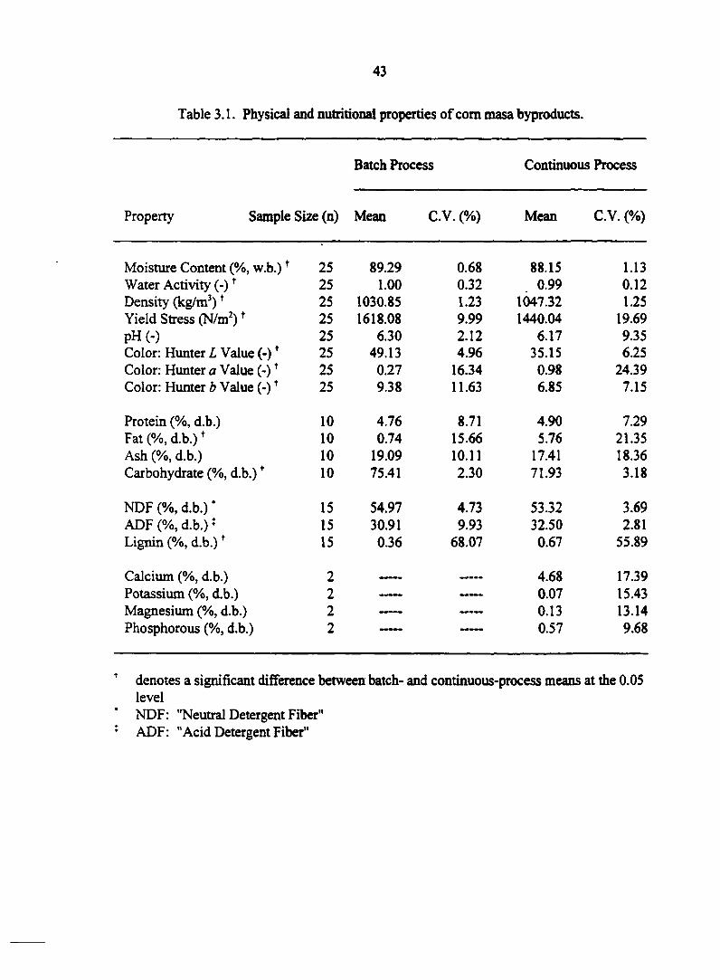
43
Table 3.1. Physical and nutritional properties of corn masa byproducts.
Batch Process Continuous Process
Property Sample Size (n) Mean C.V. (%) Mean C.V. (%)
Moisture Content (%, w.b.)f 25 89.29 0.68 88.15 1.13 Water Activity (-)f 25 1.00 0.32 0.99 0.12 Density (kg/m3)1 25 1030.85 1.23 1047.32 1.25 Yield Stress (N/m2)f 25 1618.08 9.99 1440.04 19.69 pH(-) 25 6.30 2.12 6.17 9.35 Color: Hunter L Value (-)f 25 49.13 4.96 35.15 6.25 Color: Hunter a Value (-)f 25 0.27 16.34 0.98 24.39 Color: Hunter b Value (-)t 25 9.38 11.63 6.85 7.15
Protein (%, d.b.) 10 4.76 8.71 4.90 7.29 Fat (%, d.b.) + 10 0.74 15.66 5.76 21.35 Ash (%, d.b.) 10 19.09 10.11 17.41 18.36 Carbohydrate (%, d.b.)f 10 75.41 2.30 71.93 3.18
NDF (%, d.b.) ' 15 54.97 4.73 53.32 3.69 ADF (%, d.b.) : 15 30.91 9.93 32.50 2.81 Lignin (%, d.b.)f 15 0.36 68.07 0.67 55.89
Calcium (%, d.b.) 2 4.68 17.39 Potassium (%, d.b.) 2 0.07 15.43 Magnesium (%, d.b.) 2 —— 0.13 13.14 Phosphorous (%, d.b.) 2 0.57 9.68
' denotes a significant difference between batch- and continuous-process means at the 0.05 level NDF: "Neutral Detergent Fiber"
; ADF: "Acid Detergent Fiber"
44
spoilage, which is the case for masa byproducts. Materials become safe from bacteria growth
below water activities of approximately 0.9, safe from mold growth below approximately 0.8,
and safe from yeast growth below approximately 0.7 (Barbosa-Canovas and Vega-Mercado,
1996).
In order to effectively utilize masa byproducts, dehydration is necessary to prevent
microbial spoilage, and can be accomplished through drying, blending, or extrusion
processing to reduce moisture levels to approximately 12 % (w.b.), which is typically
recommended for feed products because it substantially minimizes transportation costs and
has been determined to be microbiologically safe (Beauchat, 1981).
Mass Density
As shown in Table 3.1, masa byproducts had density values slightly greater than that
of water (which is 999 kg/m3 at a reference temperature of approximately 10 °C). This was
not unexpected due to the high moisture contents of the byproduct samples. The mean values
were significantly different (p<0.05), however, which may reflect differences in the resulting
material structures due to differences in the batch and continuous processing operations.
Yield Stress
Masa byproducts, as shown in Table 3.1, have very large yield stresses that are
similar in magnitude to those of minced fish paste (1600-2300 N/m2 ) (Nakayama et al.,
1980). Yield stress is a Theological parameter that quantifies the shear stress required to
initiate flow in a liquid or semi-solid material, results from the existence of particle
structures, and is vital for the design of transport processes and operations (Steffe, 1992).
45
Because masa byproducts have such large yield stress values, special consideration will need
to be given when designing conveying operations for these materials for further processing.
pH
The pH results are shown in Table 3.1. It was expected that pH values of the masa
byproducts would be fairly high because nixtamalization generally employs a pH greater than
10.0 during the lime cooking process (Sema-Saldivar et al., 1990). Instead, the resulting pH
values were fairly low (between 6.17 and 6.30). This may have occurred due to a large
portion of the lime washing away with the rinse water during processing, or possibly due to
microbial activity during transit between the processing facility and the laboratory.
Investigating the cause of the low pH values would be a valuable future study.
Color
The Hunter L, a, and b results are shown in Table 3.1, and show some differences in
color between the batch-processed and the continuous-processed masa byproducts, even
though both processes used the same source and hybrid of raw white corn. Essentially, these
results describe masa byproducts as gray material with a small degree of yellowness.
Drying Analysis
Drying analysis of biological materials is important for the proper design of drying
processes and equipment. This type of analysis is used to determine drying times and
temperatures for a material of specified initial and final moisture contents. For the masa
byproducts in this study, sample mass over time was monitored and used to determine
moisture contents and the resulting drying rates at drying temperatures of 80,100, and 120
°C. A multiple regression procedure with STEPWISE model selection (SAS, 1992),
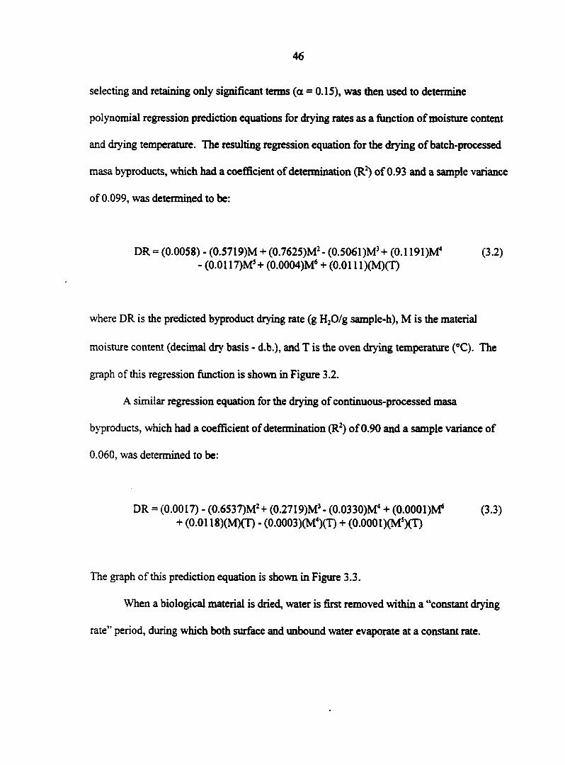
46
selecting and retaining only significant terms (a = 0.15), was then used to determine
polynomial regression prediction equations for drying rates as a function of moisture content
and drying temperature. The resulting regression equation for the drying of batch-processed
masa byproducts, which had a coefficient of determination (R2) of 0.93 and a sample variance
of 0.099, was determined to be:
DR = (0.0058) - (0.5719)M + (0.7625)M2- (0.5061)M3+ (0.1191)M4 (3.2) - (0.0117)MS + (0.0004)M6 + (0.0111 )(M)(T)
where DR is the predicted byproduct drying rate (g H20/g sample-h), M is the material
moisture content (decimal dry basis - d.b.), and T is the oven drying temperature (°C). The
graph of this regression function is shown in Figure 3.2.
A similar regression equation for the drying of continuous-processed masa
byproducts, which had a coefficient of determination (R2) of 0.90 and a sample variance of
0.060, was determined to be:
DR = (0.0017) - (0.6537)M2+ (0.2719)M3 - (0.0330)M4 + (O.OOOl)M6 (3.3) + (0.0118)(M)(T) - (0.0003)(M4)(T) + (0.0001)(M5)(T)
The graph of this prediction equation is shown in Figure 3.3.
When a biological material is dried, water is first removed within a "constant drying
rate" period, during which both surface and unbound water evaporate at a constant rate.
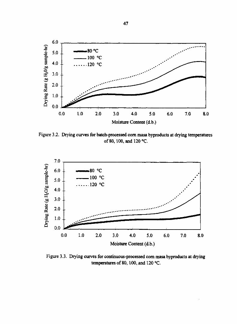
47
100 °C
0.0 1.0 2.0 3.0 4.0 5.0
Moisture Content (d.b.)
6.0 7.0 8.0
Figure 3.2. Drying curves for batch-processed com masa byproducts at drying temperatures of 80, 100, and 120 °C.
o
t g =• CO
| 2.0
•E 10
7.0
6.0
5.0
4.0
3.0
u
o ©
OO 1
100 °c
120 °C
_ - =
0.0 1.0 2.0 3.0 4.0 5.0
Moisture Content (d.b.)
6.0 7.0 8.0
Figure 3.3. Drying curves for continuous-processed com masa byproducts at drying temperatures of 80,100, and. 120 °C.
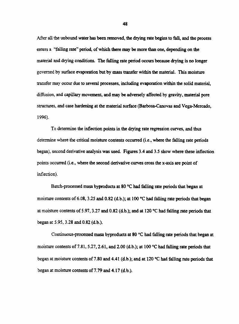
48
After all the unbound water has been removed, the drying rate begins to fall, and the process
enters a "falling rate" period, of which there may be more than one, depending on the
material and drying conditions. The falling rate period occurs because drying is no longer
governed by surface evaporation but by mass transfer within the material. This moisture
transfer may occur due to several processes, including evaporation within the solid material,
diffusion, and capillary movement, and may be adversely affected by gravity, material pore
structures, and case hardening at the material surface (Barbosa-Canovas and Vega-Mercado,
1996).
To determine the inflection points in the drying rate regression curves, and thus
determine where the critical moisture contents occurred (i.e., where the falling rate periods
began), second derivative analysis was used. Figures 3.4 and 3.5 show where these inflection
points occurred (i.e., where the second derivative curves cross the x-axis are point of
inflection).
Batch-processed masa byproducts at 80 °C had falling rate periods that began at
moisture contents of 6.08,3.25 and 0.82 (d.b.); at 100 °C had falling rate periods that began
at moisture contents of 5.97,3.27 and 0.82 (d.b.); and at 120 °C had falling rate periods that
began at 5.95, 3.28 and 0.82 (d.b.).
Continuous-processed masa byproducts at 80 °C had falling rate periods that began at
moisture contents of 7.81,5.27,2.61, and 2.00 (d.b.); at 100 °C had falling rate periods that
began at moisture contents of 7.80 and 4.41 (d.b.); and at 120 °C had falling rate periods that
began at moisture contents of 7.79 and 4.17 (d.b.).
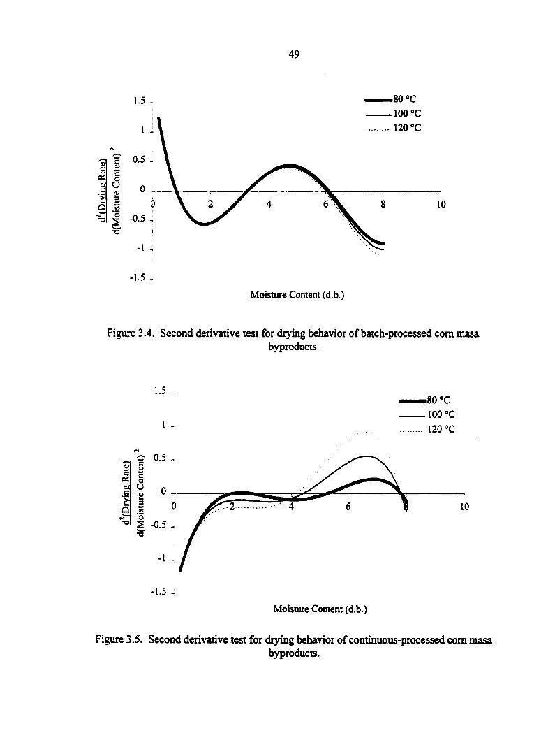
49
1.5 , ^—80 °C
100 °c 120 °C
a s 5 f : % o _
2 1 ! b 2 "0-5 -i
•o i
-1.5 -
Moisture Content (d.b.)
Figure 3.4. Second derivative test for drying behavior of batch-processed com masa byproducts.
1.5 -80 °C
100 °C 1 " 120 °C
0.5
3
.2 O S -0.5 •n"
-1.5 -
Moisture Content (d.b.)
Figure 3.5. Second derivative test for drying behavior of continuous-processed com masa byproducts.
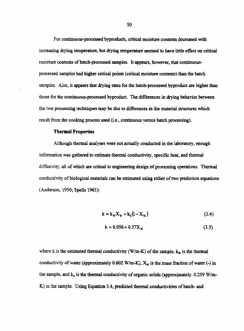
50
For continuous-processed byproducts, critical moisture contents decreased with
increasing drying temperature, but drying temperature seemed to have little effect on critical
moisture contents of batch-processed samples. It appears, however, that continuous-
processed samples had higher critical points (critical moisture contents) than the batch
samples. Also, it appears that drying rates for the batch-processed byproduct are higher than
those for the continuous-processed byproduct The differences in drying behavior between
the two processing techniques may be due to differences in the material structures which
result from the cooking process used (i.e., continuous versus batch processing).
Thermal Properties
Although thermal analyses were not actually conducted in the laboratory, enough
information was gathered to estimate thermal conductivity, specific heat, and thermal
diffusivity, all of which are critical to engineering design of processing operations. Thermal
conductivity of biological materials can be estimated using either of two prediction equations
(Anderson, 1950; Spells 1961):
k — kwXw + ks(l — Xw )
k = 0.056 + 0.57% w
(3.4)
(35)
where k is the estimated thermal conductivity (W/m-K) of the sample, kw is the thennal
conductivity of water (approximately 0.602 W/m-K), Xw is the mass fraction of water (-) in
the sample, and kg is the thermal conductivity of organic solids (approximately. 0.259 W/m-
K) in the sample. Using Equation 3.4, predicted thennal conductivities of batch- and
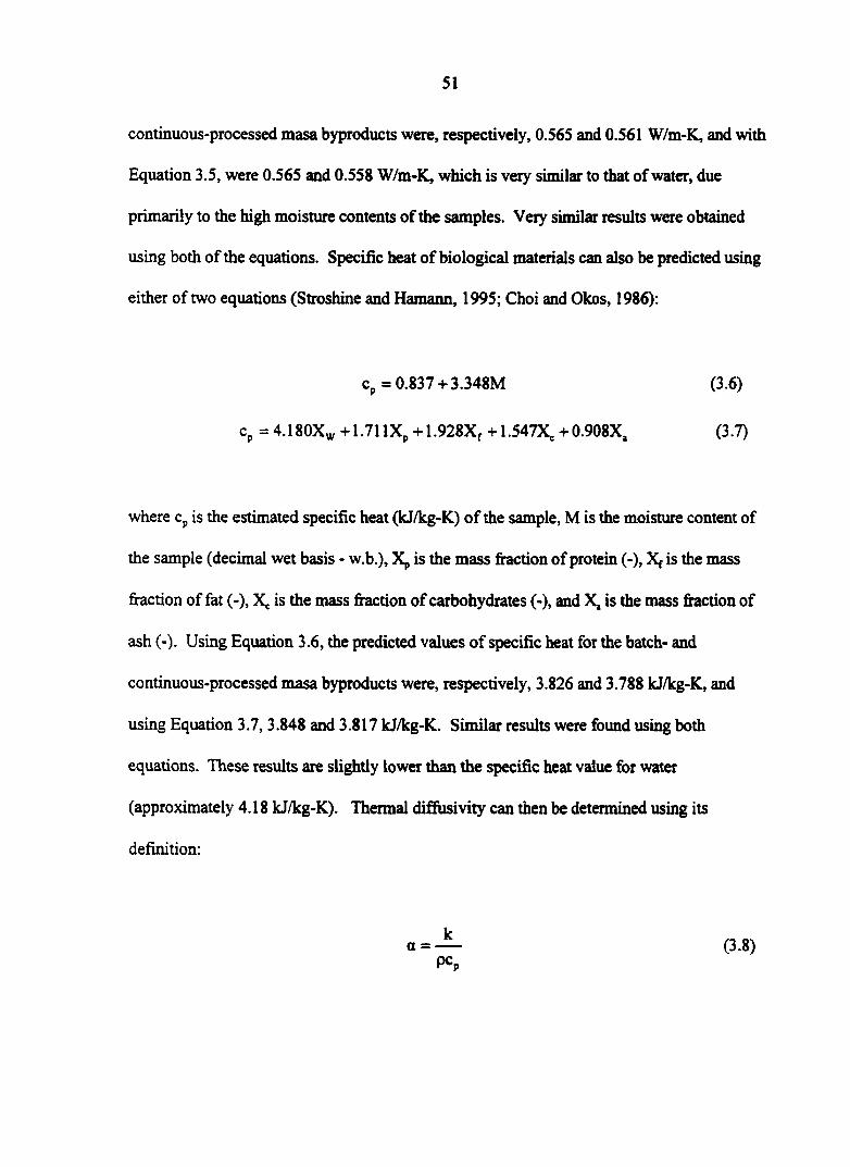
51
continuous-processed masa byproducts were, respectively, 0.565 and 0.561 W/m-K, and with
Equation 3.5, were 0.565 and 0.558 W/m-K, which is very similar to that of water, due
primarily to the high moisture contents of the samples. Very similar results were obtained
using both of the equations. Specific heat of biological materials can also be predicted using
either of two equations (Stroshine and Hamann, 1995; Choi and Okos, 1986):
where cp is the estimated specific heat (kJ/kg-K) of the sample, M is the moisture content of
the sample (decimal wet basis - w.b.), Xp is the mass fraction of protein (-), X, is the mass
fraction of fat (-), Xc is the mass fraction of carbohydrates (-), and X, is the mass fraction of
ash (-). Using Equation 3.6, the predicted values of specific heat for the batch- and
continuous-processed masa byproducts were, respectively, 3.826 and 3.788 kJ/kg-K, and
using Equation 3.7, 3.848 and 3.817 kJ/kg-K. Similar results were found using both
equations. These results are slightly lower than the specific heat value for water
(approximately 4.18 kJ/kg-K). Thermal diffusivity can then be determined using its
definition:
c p = 0 . 8 3 7 + 3 . 3 4 8 M (3.6)
c„ = 4.180XW + 1.711Xp +1.928Xf + 1.547XC +0.908X. (3.7)
k (3.8) (X — —
PCp
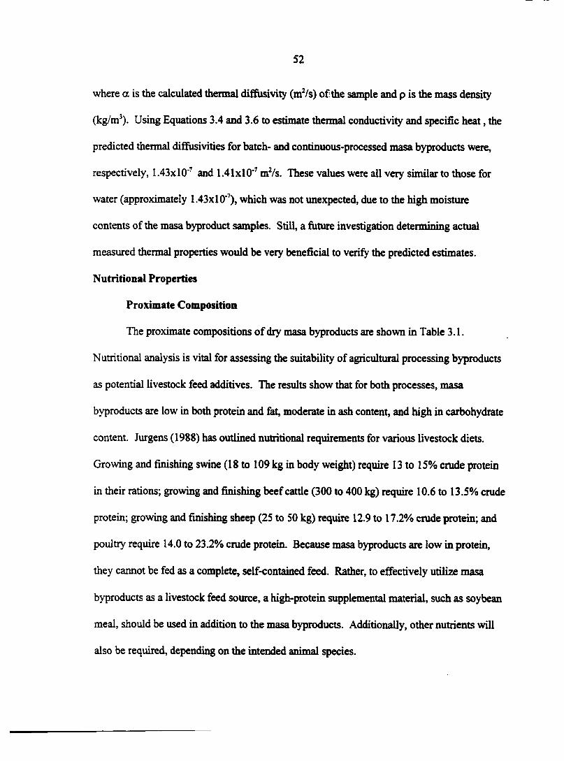
52
where a is the calculated thermal diffusivity (m2/s) of the sample and p is the mass density
(kg/m3). Using Equations 3.4 and 3.6 to estimate thennal conductivity and specific heat, the
predicted thermal difiusivities for batch- and continuous-processed masa byproducts were,
respectively, 1.43xl0"7 and 1.41xl0"7 m2/s. These values were all very similar to those for
water (approximately 1.43xl0"7), which was not unexpected, due to the high moisture
contents of the masa byproduct samples. Still, a future investigation determining actual
measured thermal properties would be very beneficial to verify the predicted estimates.
Nutritional Properties
Proximate Composition
The proximate compositions of dry masa byproducts are shown in Table 3.1.
Nutritional analysis is vital for assessing the suitability of agricultural processing byproducts
as potential livestock feed additives. The results show that for both processes, masa
byproducts are low in both protein and fat, moderate in ash content, and high in carbohydrate
content. Jurgens (1988) has outlined nutritional requirements for various livestock diets.
Growing and finishing swine (18 to 109 kg in body weight) require 13 to 15% crude protein
in their rations; growing and finishing beef cattle (300 to 400 kg) require 10.6 to 13.5% crude
protein; growing and finishing sheep (25 to 50 kg) require 12.9 to 17.2% crude protein; and
poultry require 14.0 to 23.2% crude protein. Because masa byproducts are low in protein,
they cannot be fed as a complete, self-contained feed. Rather, to effectively utilize masa
byproducts as a livestock feed source, a high-protein supplemental material, such as soybean
meal, should be used in addition to the masa byproducts. Additionally, other nutrients will
also be required, depending on the intended animal species.
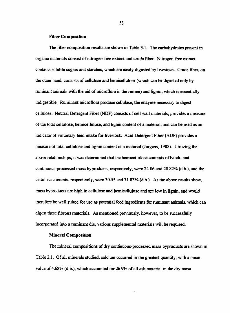
53
Fiber Composition
The fiber composition results are shown in Table 3.1. The carbohydrates present in
organic materials consist of nitrogen-free extract and crude fiber. Nitrogen-free extract
contains soluble sugars and starches, which are easily digested by livestock. Crude fiber, on
the other hand, consists of cellulose and hemicellulose (which can be digested only by
ruminant animals with the aid of microflora in the rumen) and lignin, which is essentially
indigestible. Ruminant microflora produce cellulase, the enzyme necessary to digest
cellulose. Neutral Detergent Fiber (NDF) consists of cell wall materials, provides a measure
of the total cellulose, hemicellulose, and lignin content of a material, and can be used as an
indicator of voluntary feed intake for livestock. Acid Detergent Fiber (ADF) provides a
measure of total cellulose and lignin content of a material (Jurgens, 1988). Utilizing the
above relationships, it was determined that the hemicellulose contents of batch- and
continuous-processed masa byproducts, respectively, were 24.06 and 20.82% (d.b.), and the
cellulose contents, respectively, were 30.55 and 31.83% (d.b.). As the above results show,
masa byproducts are high in cellulose and hemicellulose and are low in lignin, and would
therefore be well suited for use as potential feed ingredients for ruminant animals, which can
digest these fibrous materials. As mentioned previously, however, to be successfully
incorporated into a ruminant die, various supplemental materials will be required.
Mineral Composition
The mineral compositions of dry continuous-processed masa byproducts are shown in
Table 3.1. Of all minerals studied, calcium occurred in the greatest quantity, with a mean
value of 4.68% (d.b.), which accounted for 26.9% of all ash material in the dry masa
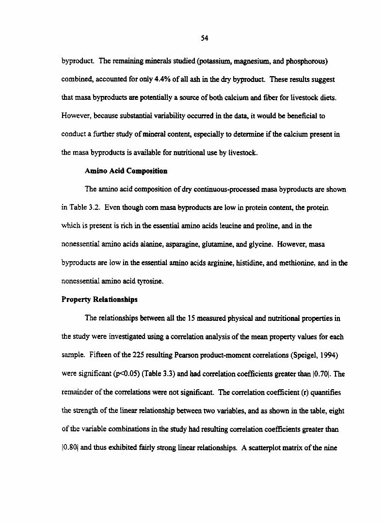
54
byproduct. The remaining minerals studied (potassium, magnesium, and phosphorous)
combined, accounted for only 4.4% of all ash in the dry byproduct. These results suggest
that masa byproducts are potentially a source of both calcium and fiber for livestock diets.
However, because substantial variability occurred in the data, it would be beneficial to
conduct a further study of mineral content, especially to determine if the calcium present in
the masa byproducts is available for nutritional use by livestock.
Amino Acid Composition
The amino acid composition of dry continuous-processed masa byproducts are shown
in Table 3.2. Even though com masa byproducts are low in protein content, the protein
which is present is rich in the essential amino acids leucine and proline, and in the
nonessential amino acids alanine, asparagine, glutamine, and glycine. However, masa
byproducts are low in the essential amino acids arginine, histidine, and methionine, and in the
nonessential amino acid tyrosine.
Property Relationships
The relationships between all the 15 measured physical and nutritional properties in
the study were investigated using a correlation analysis of the mean property values for each
sample. Fifteen of the 225 resulting Pearson product-moment correlations (Speigel, 1994)
were significant (p<0.05) (Table 3.3) and had correlation coefficients greater than |0.70|. The
remainder of the correlations were not significant The correlation coefficient (r) quantifies
the strength of the linear relationship between two variables, and as shown in the table, eight
of the variable combinations in the study had resulting correlation coefficients greater than
|0.80| and thus exhibited fairly strong linear relationships. A scatterplot matrix of the nine
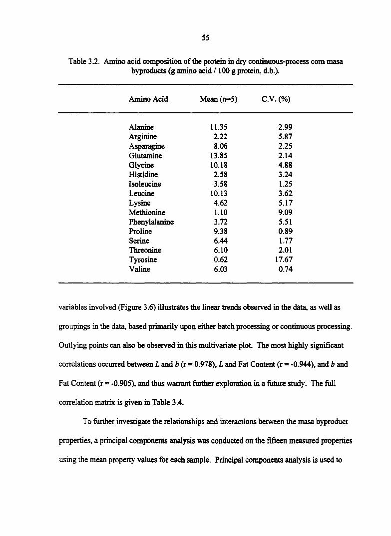
55
Table 3.2. Amino acid composition of the protein in dry continuous-process com masa byproducts (g amino acid / 100 g protein, d.b.).
Amino Acid Mean (n=5) C.V. (%)
Alanine 11.35 2.99 Arginine 2.22 5.87 Asparagine 8.06 2.25 Glutamine 13.85 2.14 Glycine 10.18 4.88 Histidine 2.58 3.24 Isoleucine 3.58 1.25 Leucine 10.13 3.62 Lysine 4.62 5.17 Methionine 1.10 9.09 Phenylalanine 3.72 5.51 Proline 9.38 0.89 Serine 6.44 1.77 Threonine 6.10 2.01 Tyrosine 0.62 17.67 Valine 6.03 0.74
variables involved (Figure 3.6) illustrates the linear trends observed in the data, as well as
groupings in the data, based primarily upon either batch processing or continuous processing.
Outlying points can also be observed in this multivariate plot. The most highly significant
correlations occurred between L and b(j = 0.978), L and Fat Content (r = -0.944), and b and
Fat Content (r = -0.905), and thus warrant further exploration in a future study. The full
correlation matrix is given in Table 3.4.
To further investigate the relationships and interactions between the masa byproduct
properties, a principal components analysis was conducted on the fifteen measured properties
using the mean property values for each sample. Principal components analysis is used to
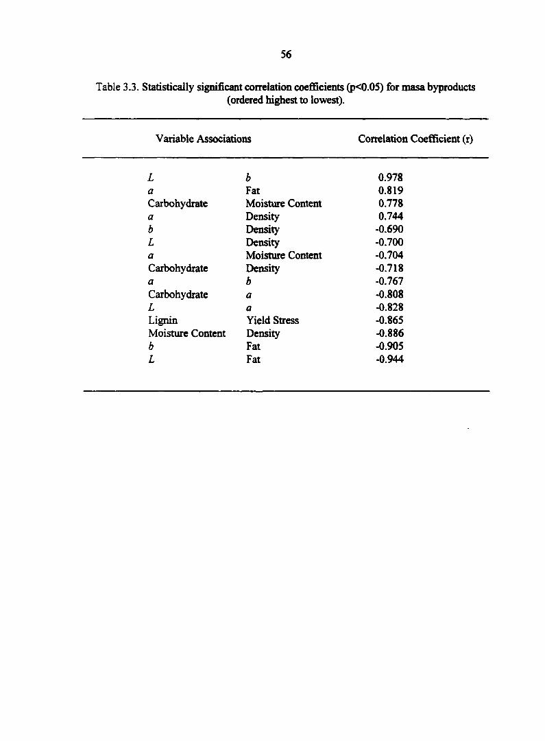
56
Table 3.3. Statistically significant correlation coefficients (p<0.05) for masa byproducts (ordered highest to lowest).
Variable Associations Correlation Coefficient (r)
L b 0.978 a Fat 0.819 Carbohydrate Moisture Content 0.778 a Density 0.744 b Density -0.690 L Density -0.700 a Moisture Content -0.704 Carbohydrate Density -0.718 a b -0.767 Carbohydrate a -0.808 L a -0.828 Lignin Yield Stress -0.865 Moisture Content Density -0.886 b Fat -0.905 L Fat -0.944
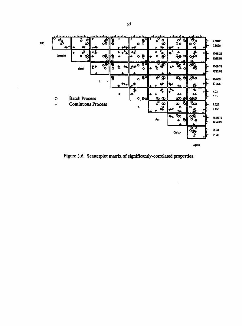
57
R*1 1111111 n l n i t l i
m CP
l l l l l l i l l IIIll^ ̂ % IiiuIiii . 111111111
oo #•+ 4-
o5° •*
MC S
d
oo
Fi;
* +•**•
7̂ 7
° s> • *•
+ O f
—«y
Density
* Yield t* °o
0 +
»
* A|
t *• ?+ _±_
O 6 o 8
o
9
orf*>
+ o 4b
1 **
+ »
* * T
o
®o % V- -
*
0 Batch Process + Continuous Process
° Qo —s-a <P œ
jsa
Ash
CD O
-2l
% %0
+• % &
Cetio *
°4h
Lignin
Figure 3.6. Scatterplot matrix of significantly-correlated properties.

58
Table 3.4. Full correlation matrix for masa byproducts.
M.C. aw Density Yield pH Lab
M.C. 1.000 aw 0.525 1.000 Density -0.886 -0.489 1.000 Yield 0.389 -0.150 -0.469 1.000 pH -0.057 0.582 -0.130 0.008 1.000 L 0.587 0.397 -0.700 0.546 0.223 1.000 a -0.704 -0.137 0.744 -0.547 0.184 -0.828 1.000 b 0.588 0.425 -0.690 0.548 0.228 0.978 -0.767 1.000 Protein 0.063 -0.021 0.049 -0.116 -0.214 -0.209 0.001 -0.079 Fat -0.388 -0.121 0.559 -0.610 -0.180 -0.944 0.819 -0.905 Ash -0.379 0.117 0.139 0.155 0.505 0.420 -0.023 0.366 Carbo. 0.778 0.011 -0.718 0.475 -0.305 0.554 -0.808 0.550 NDF 0.601 0.376 -0.502 -0.204 -0.057 0.327 -0.413 0.300 ADF -0.372 -0.128 0.482 -0.645 0.034 -0.369 0.412 -0.334 Lignin -0.489 0.102 0.528 -0.865 -0.115 -0.385 0.451 -0.353
Protein Fat Ash Carbo. NDF ADF Lignin
M.C. aw Density Yield pH L a b Protein 1.000 Fat 0.203 1.000 Ash -0.536 -0.482 1.000 Carbo. 0.202 -0.544 -0.465 NDF -0.068 -0.206 -0.408 ADF 0.174 0.299 -0.245 Lignin 0.237 0.438 0.086
1.000 0.639 1.000
-0.080 0.410 1.000 -0.567 -0.073 0.429 1.000
59
reduce the dimensionality of multivariate data by summarizing the variance in the data and
projecting it into a set of uncorrected orthogonal linear combinations of the original
variables. These linear combinations, or principal components, have the form:
y P.C. — 8|X| + a2^2 + + ai5^15 (3 9)
where yPC is a principal component value, or score, a, through al5 are the principal
component coefficients (i.e., eigenvectors), and X, through X,$ are the original property
variable vectors (i.e., values that were measured in the study) (Everitt and Dunn, 1991). The
results for the principal components analysis are presented in Table 3.5, which shows the
eigenvectors and eigenvalues for the first five principal components.
Although the scree plot (Figure 3.7) suggests that six or seven principal components
can be used to summarize the data, the first five principal components accounted for 92.6%
of the total variability in the data (Figure 3.8), and thus provide both a convenient and
comprehensive summary of the information contained in the original 15 property variables,
utilizing a reduced dimensionality of only five variables for the multivariate data set.
Although the interpretation of principal components is very subjective, the first principal
component appears to be an indication of material structure, while the second principal
component appears to be an indication of chemical composition.
Another advantage to using principal components analysis to summarize data is the
ability to identify outliers, curvature, and clustering in multivariate data sets, through
examination of low-dimensional scatterplots of the calculated principal component scores
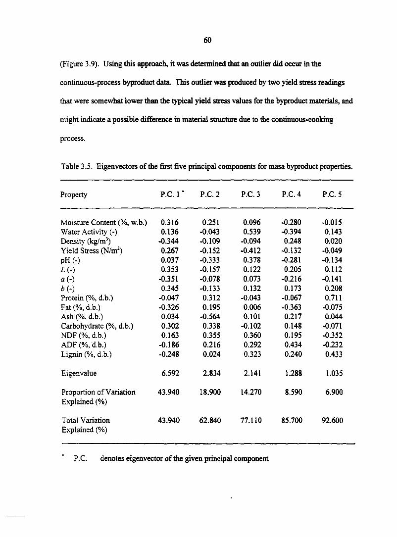
(Figure 3.9). Using this approach, it was determined that an outlier did occur in the
continuous-process byproduct data. This outlier was produced by two yield stress readings
that were somewhat lower than the typical yield stress values for the byproduct materials, and
might indicate a possible difference in material structure due to the continuous-cooking
process.
Table 3.5. Eigenvectors of the first five principal components for masa byproduct properties.
Property P.C. 1 ' P.C. 2 P.C. 3 P.C. 4 P.C. 5
Moisture Content (%, w.b.) 0.316 0.251 0.096 -0.280 -0.015 Water Activity (-) 0.136 -0.043 0.539 -0.394 0.143 Density (kg/m3) -0.344 -0.109 -0.094 0.248 0.020 Yield Stress (N/m2) 0.267 -0.152 -0.412 -0.132 -0.049 pH (-) 0.037 -0.333 0.378 -0.281 -0.134 L ( - ) 0.353 -0.157 0.122 0.205 0.112 a(-) -0.351 -0.078 0.073 -0.216 -0.141 b ( - ) 0.345 -0.133 0.132 0.173 0.208 Protein (%, d.b.) -0.047 0.312 -0.043 -0.067 0.711 Fat (%, d.b.) -0.326 0.195 0.006 -0.363 -0.075 Ash (%, d.b.) 0.034 -0.564 0.101 0.217 0.044 Carbohydrate (%, d.b.) 0.302 0.338 -0.102 0.148 -0.071 NDF (%, d.b.) 0.163 0.355 0.360 0.195 -0.352 ADF (%, d.b.) -0.186 0.216 0.292 0.434 -0.232 Lignin (%, d.b.) -0.248 0.024 0.323 0.240 0.433
Eigenvalue 6.592 2.834 2.141 1.288 1.035
Proportion of Variation 43.940 18.900 14.270 8.590 6.900 Explained (%)
Total Variation 43.940 62.840 77.110 85.700 92.600 Explained (%)
P.C. denotes eigenvector of the given principal component
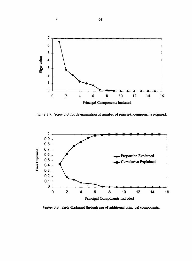
61
7
6
5
4
3
2
1
0
2 8 12 0 4 6 10 14 16
Principal Components Included
Figure 3.7. Scree plot for determination of number of principal components required.
Proportion Explained
Cumulative Explained
Ê
0.2 ,
2 12 0 6 8 10 4 14 16
Principal Components Included
Figure 3.8. Error explained through use of additional principal components.
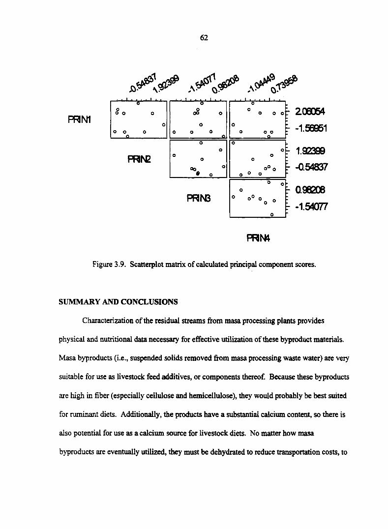
62
»<«V .XX 1 • ' ' ' 1 ' ' ' ' I ' 1 • ' I ' ' ' » * • > • » ' » >
PRN1 °
Oo
0°
°
o o
o
o
à o oo o
o o o o
O
6 1 • — 0 _ O o o
o 0 O O
-0
206054
-1.56951
PRISE
o o
o o
o °
o o
o o o
1.92399
-0.54837
PRN3
0 o o
° «
0
0.96206
-1.54077
PRN4
Figure 3.9. Scatterplot matrix of calculated principal component scores.
SUMMARY AND CONCLUSIONS
Characterization of the residual streams from masa processing plants provides
physical and nutritional data necessary for effective utilization of these byproduct materials.
Masa byproducts (i.e., suspended solids removed from masa processing waste water) are very
suitable for use as livestock feed additives, or components thereof. Because these byproducts
are high in fiber (especially cellulose and hemicellulose), they would probably be best suited
for ruminant diets. Additionally, the products have a substantial calcium content, so there is
also potential for use as a calcium source for livestock diets. No matter how masa
byproducts are eventually utilized, they must be dehydrated to reduce transportation costs, to
63
decrease microbial activity, and to increase shelf life. This can be accomplished through
drying, blending, or extrusion processing, all of which would be appropriate areas for future
investigations.
The following chapters will examine these alternatives for converting masa
byproducts into value-added livestock feed materials. Chapters 5 and 6 will examine
laboratory- and pilot-scale extrusion, respectively, while Chapter 7 describes the
development of an economic analysis model that includes a range of byproduct processing
alternatives. First, however, chapter 4 will review the theory and analysis of extrusion
processing to provide a basic background for examining extrusion technology.
ACKNOWLEDGMENTS
The authors would like to thank the Recycling and Reuse Technology Transfer Center
(RRTTC) at the University of Northern Iowa, Cedar Falls, LA, for financial support, the
Center for Crops Utilization Research (CCUR) at Iowa State University, Ames, IA, for use of
equipment and facilities, and Minsa Corporation for providing corn masa byproduct samples.
They would also like to acknowledge the assistance of Dr. Helen Park during initial stages of
nutritional analysis.
REFERENCES
American Association of Cereal Chemists (AACC). 1995. Approved Methods of the American Association of Cereal Chemists. St. Paul, MN: American Society of Cereal Chemists, Inc.
American Public Health Association (APHA). 1995. Standard Methods for the Examination of Water and Wastewater, 19th ed. New York, NY: American Public Health Association.
64
Anderson, S. A. 1950. Automatic Refrigeration. Norberg, Denmark: MacLaren and Son Ltd. for Don Foss.
Association of Official Analytical Chemists (AOAC). 1980. Official Methods of Analysis of the AOAC International, 13th ed. Arlington, VA: Association of Official Analytical Chemists International.
B arbosa-Canovas, G. V. and H. Vega-Mercado. 1996. Dehydration of Foods. New York, NY : International Thomson Publishing.
Beauchat, L. R. 1981. Microbial stability as affected by water activity. Cereal Foods World 26(7): 345-349.
Bohlsen, D., S. Weeder, and S. Wang. 1997. Tracking organic waste. Resource 4(9): 13-14.
Bressani, R., R. Paz y Paz, and N. S. Scrimshaw. 1958. Corn nutrient losses: chemical changes in com during preparation of tortillas. Journal of Agricultural Food Chemistry 6: 770.
Choi, Y. and M. Okos. 1986. Thermal properties of liquid foods-review, la Physical and Chemical Properties of Food, ed. M. Okos, 35-77. St. Joseph, MI: American Society of Agricultural Engineers.
Dzuy, N. Q. and D. V. Boger. 1985. Direct yield stress measurement with the vane method. Journal ofRheology 29(3): 335-347.
Everitt, B. S. and G. Dunn. 1991. Applied Multivariate Data Analysis. New York, NY: Halsted Press.
Ferris, D. A., R. A. Flores, C. W. Shanklin, and M. K. Whitworth. 1995. Proximate analysis of food service wastes. Applied Engineering in Agriculture 11(4): 567-572.
Gomez, M. H., L. W. Rooney, R. D. Waniska, and R. L. Pflugfelder. 1987. Diy com masa flours for tortilla and snack food production. Cereal Foods World 32(5): 372-377.
Gonzalez de Palacios, M. 1980. Characteristics of com and sorghum for tortilla processing. Unpublished M.S. Thesis. College Station, TX: Texas A&M University.
Gonzalez-Martinez, S. 1984. Biological treatability of the wastewaters from the alkaline cooking of maize (Indian com). Environmental Technology Letters 5(8): 365-372.
65
Ham, G. A., R. A. Stock, T. J. Kopfenstein, E. M. Larson, D. J. Shain, and R. P. Huffman. 1994. Wet com distillers byproducts compared with dried com distillers grains with solubles as a source of protein and energy for ruminants. Journal of Animal Science 72: 3246.
Ham, G. A., R. A. Stock, T. J. Klopfenstein, and R. P. Huffman. 1995. Determining the net energy value of wet and dry com gluten feed in beef growing and finishing diets. Journal of Animal Science 73(2): 353-359.
Hunter Associates Laboratory, Inc. 1983. Instruction Manual: Hunterlab LabScan Spectro Colorimeter. Reston, VA: Hunter Associates Laboratory, Inc.
Hussein, H. S. and L. L. Berger. 1995. Effects of feed intake and dietary level of wet com gluten feed on feedlot performance, digestibility of nutrients, and carcass characteristics of growing-finishing beef heifers. Journal of Animal Science 73: 3246.
Jurgens, M. H. 1988. Animal Feeding and Nutrition. Dubuque, LA: Kendall/Hunt Publishing Company.
Katz, S. H., M. L. Hediger, and L. A. Valleroy. 1974. Traditional maize processing techniques in the New World. Science 184: 765.
Khan, M. N., M. C. Des Rosiers, L. W. Rooney, R. G. Morgan, and V. E. Sweat. 1982. Com tortillas: evaluation of com cooking procedures. Cereal Chemistry 59(4): 279-284.
Krause, V. M., K. L. Tucker, H. V. Kuhnlein, C. Y. Lopez-Palacios, M. Ruz, and N. W. Solomons. 1992. Rural-urban variation in limed maize use and tortilla consumption by women in Guatemala. Ecology of Food and Nutrition 28: 279-288.
Larson, E. M., R. A. Stock, T. J. Klopfenstein, J. H. Sindt, and R. P. Huffman. 1993. Feeding value of wet distillers byproducts for finishing ruminants. Journal of Animal Science 71: 2228.
Luzier, J. M. and R. C. Summerfelt. 1995. Partial replacement of fish meal with spray-dried blood powder to reduce phosphorous concentrations in diets for juvenile rainbow trout, Oncorhynchus mykiss (Walbaum). Aquaculture Research 26(8): 577.
Martins, S. N. and E. C. Guzman. 1994. Effect of drying method of bovine blood on the performance of growing for tambaqui ( Colossoma macropomum, Curier 1818) in experimental culture tanks. Aquaculture 124(1-4): 335-341.
66
Microsoft Excel v. 5.0a. 1993. Redmond, WA: Microsoft Corporation.
Moore, K. J. and R. D. Hatfield. 1994. Carbohydrates and forage quality. In Forage Quality, Evaluation, and Utilization, ed. G. C. Fahey, Jr., M. Collins, D. R. Martens, and L. E. Moser, 229-280. Madison, WI: American Society of Agronomy.
Nakayama, T., E. Niwa, and I. Hamada. 1980. Pipe transportation of minced fish paste. Journal of Food Science 45: 844-847.
Nelson, L.S. 1985. Sample size tables for analysis of variance. Journal of Quality Technology 17(3): 167-168.
Nelson, R. G. and R. A. Flores. 1994. Survey of processing residues generated by Kansas agribusinesses. Applied Engineering in Agriculture 10(5): 703-708.
Ortiz, E. L. 1985. The cuisine of Mexico: com tortilla dishes. Gourmet 45(May): 62-63.
Pflugfelder, R. L., L. W. Rooney, and R. D. Waniska. 1988. Dry matter losses in commercial corn masa production. Cereal Chemistry 65(2): 127-132.
Polanski, J. 1992. Legalizing the feeding of nonmeat food wastes to livestock. Applied Engineering in Agriculture 11(1): 115-119.
Rooney, L. W. and S. O. Sema-Saldivar. 1987. Food uses of whole corn and dry-milled fractions. In Corn Chemistry and Technology, ed. S. A. Watson and P. E. Ramstad, 399-430. St. Paul, MN: American Association of Cereal Chemists.
Rosentrater, K. A. and R. A. Flores. 1997. Physical and rheological properties of slaughterhouse swine blood and blood components. Transactions of the ASAE 40(3): 683-689.
SAS v. 6.08. 1992. Cary, NC: SAS Institute, Inc.
Sema-Saldivar, S. O., M. H. Gomez, and L. M. Rooney. 1990. Technology, chemistry, and nutritional value of alkaline-cooked com products. Advances in Cereal Science and Technology 10:243-306.
Speigel, M. R. 1994. Statistics. New York, NY: McGraw-Hill, Inc.
Spells, K. E. 1961. Thermal conductivity of some biological fluids. Physics in Medicine and Biology 5(2): 139-153.
67
Steffe, J. F. 1992. Rheological Methods in Food Process Engineering. East Lansing, MI: Freeman Press.
Stroshine, R. and D. Hamann. 1995. Physical Properties of Agricultural Materials and Food Products. West Lafayette, IN: Copy Cat.
Tortilla Industry Association (TIA). 2001. Tortilla consumption continues to grow in U.S. and abroad. Tortilla Industry Association. Available online: www.tortilla-info.com/prrevenue98.htm [Accessed January 08,2001].
Van Soest, P. J., J. B. Robertson, and B. A. Lewis. 1991. Methods for dietary fiber, neutral detergent fiber, and nonstarch polysaccharides in relation to animal nutrition. Journal of Dairy Science 74(10): 3583-3597.
Wang, L., R. A. Flores, and L. A. Johnson. 1997. Processing feed ingredients from blends Of soybean meal, whole blood, and red blood cells. Transactions of the ASAE 40(3): 691-697.
Wood, M. 1994. What makes tortillas and tacos taste so good? Agricultural Research 42(11):17.
Yoo, B., M. A. Rao, and J. F. Steffe. 1995. Yield stress of food dispersions with the vane method at controlled shear rate and shear stress. Journal of Texture Studies 26: 1-10.
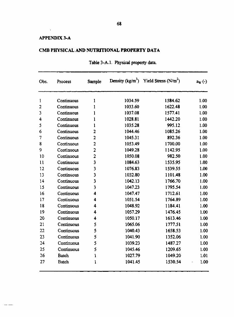
APPENDIX 3-A
CMB PHYSICAL AND NUTRITIONAL PROPERTY DATA
Table 3-A.l. Physical property data.
Obs. Process Sample Density (kg/m3) Yield Stress (N/m2) aw (•)
1 Continuous 1 1034.59 1584.62 1.00 2 Continuous 1 1033.60 1622.48 1.00 3 Continuous 1 1037.08 1577.41 1.00 4 Continuous 1 1028.81 1442.20 1.00 5 Continuous 1 1035.28 995.12 1.00 6 Continuous 2 1044.46 1085.26 1.00 7 Continuous 2 1045.31 892.36 1.00 8 Continuous 2 1053.49 1700.00 1.00 9 Continuous 2 1049.28 1142.95 1.00 10 Continuous 2 1050.08 982.50 1.00 11 Continuous 3 1084.63 1535.95 1.00 12 Continuous 3 1076.83 1539.55 1.00 13 Continuous 3 1032.80 1101.48 1.00 14 Continuous 3 1042.13 1766.70 1.00 15 Continuous 3 1047.23 1795.54 1.00 16 Continuous 4 1047.47 1712.61 1.00 17 Continuous 4 1051.54 1764.89 1.00 18 Continuous 4 1048.92 1184.41 1.00 19 Continuous 4 1057.29 1476.45 1.00 20 Continuous 4 1050.17 1613.46 1.00 21 Continuous 5 1065.06 1777.51 1.00 22 Continuous 5 1040.43 1658.53 1.00 23 Continuous 5 1041.90 1352.06 1.00 24 Continuous 5 1039.23 1487.27 1.00 25 Continuous 5 1045.46 1209.65 1.00 26 Batch 1 1027.79 1049.20 1.01 27 Batch 1 1041.45 1530.54 • 1.00
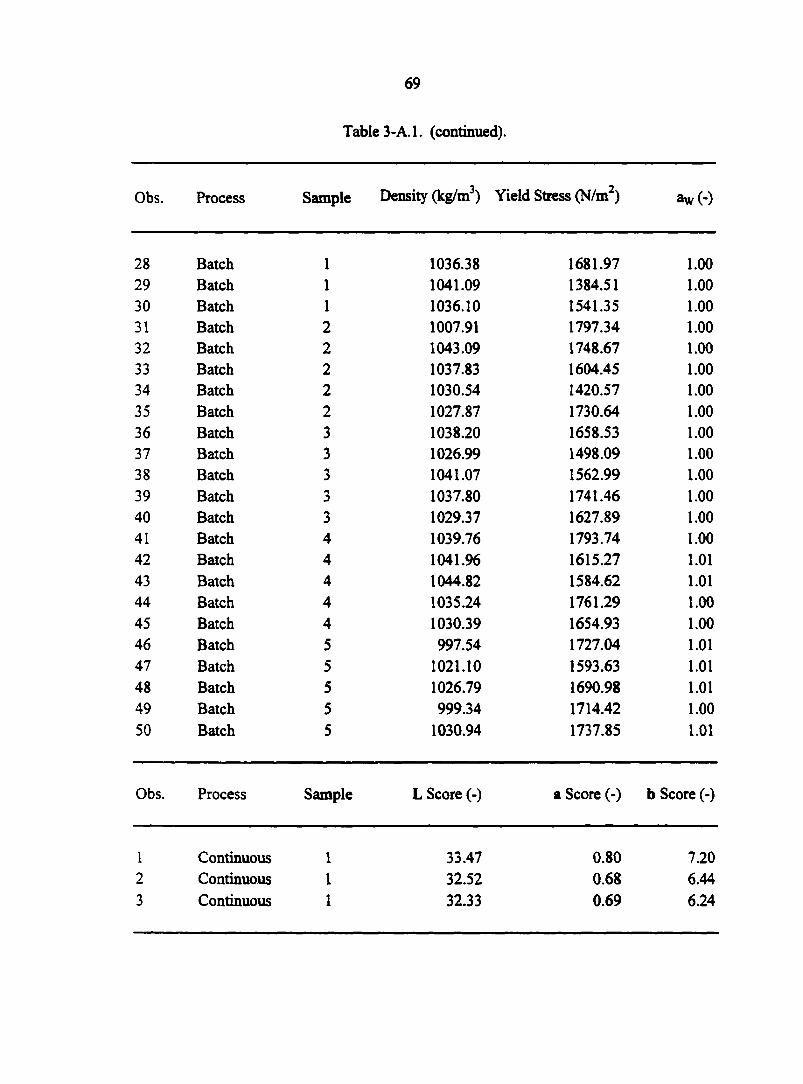
69
Table 3-A.l. (continued).
Obs. Process Sample Density (kg/m3) Yield Stress (N/m2) aw (*)
28 Batch 1 1036.38 1681.97 1.00 29 Batch 1 1041.09 1384.51 1.00 30 Batch 1 1036.10 1541.35 1.00 31 Batch 2 1007.91 1797.34 1.00 32 Batch 2 1043.09 1748.67 1.00 33 Batch 2 1037.83 1604.45 1.00 34 Batch 2 1030.54 1420.57 1.00 35 Batch 2 1027.87 1730.64 1.00 36 Batch 3 1038.20 1658.53 1.00 37 Batch 3 1026.99 1498.09 1.00 38 Batch 3 1041.07 1562.99 1.00 39 Batch 3 1037.80 1741.46 1.00 40 Batch 3 1029.37 1627.89 1.00 41 Batch 4 1039.76 1793.74 1.00 42 Batch 4 1041.96 1615.27 1.01 43 Batch 4 1044.82 1584.62 1.01 44 Batch 4 1035.24 1761.29 1.00 45 Batch 4 1030.39 1654.93 1.00 46 Batch 5 997.54 1727.04 1.01 47 Batch 5 1021.10 1593.63 1.01 48 Batch 5 1026.79 1690.98 1.01 49 Batch 5 999.34 1714.42 1.00 50 Batch 5 1030.94 1737.85 1.01
Obs. Process Sample L Score (-) a Score (-) b Score (-)
1 Continuous 1 33.47 0.80 7.20 2 Continuous 1 32.52 0.68 6.44 3 Continuous 1 32.33 0.69 6.24
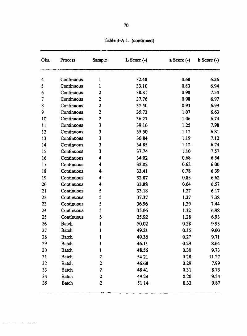
70
Table 3-A.l. (continued).
Obs. Process Sample L Score (-) a Score (-) b Score (-)
4 Continuous 1 32.48 0.68 6.26 5 Continuous 1 33.10 0.83 6.94 6 Continuous 2 38.81 0.98 7.54 7 Continuous 2 37.76 0.98 6.97 8 Continuous 2 37.50 0.93 6.99 9 Continuous 2 35.73 1.07 6.63 10 Continuous 2 36.27 1.06 6.74 11 Continuous 3 39.16 1.25 7.98 12 Continuous 3 35.50 1.12 6.81 13 Continuous 3 36.84 1.19 7.12 14 Continuous 3 34.85 1.12 6.74 15 Continuous 3 37.74 1.10 7.57 16 Continuous 4 34.02 0.68 6.54 17 Continuous 4 32.02 0.62 6.00 18 Continuous 4 33.41 0.78 6.39 19 Continuous 4 32.87 0.85 6.62 20 Continuous 4 33.88 0.64 6.57 21 Continuous 5 33.18 1.27 6.17 22 Continuous 5 37.37 1.27 7.38 23 Continuous 5 36.96 1.29 7.44 24 Continuous 5 35.06 1.32 6.98 25 Continuous 5 35.92 1.28 6.93 26 Batch 1 50.02 0.28 9.95 27 Batch 1 49.21 0.35 9.60 28 Batch 1 49.36 0.27 9.71 29 Batch 1 46.11 0.29 8.64 30 Batch 1 48.56 0.30 9.73 31 Batch 2 54.21 0.28 11.27 32 Batch 2 46.60 0.29 7.99 33 Batch 2 48.41 0.31 8.73 34 Batch 2 49.24 0.20 9.54 35 Batch 2 51.14 0.33 9.87
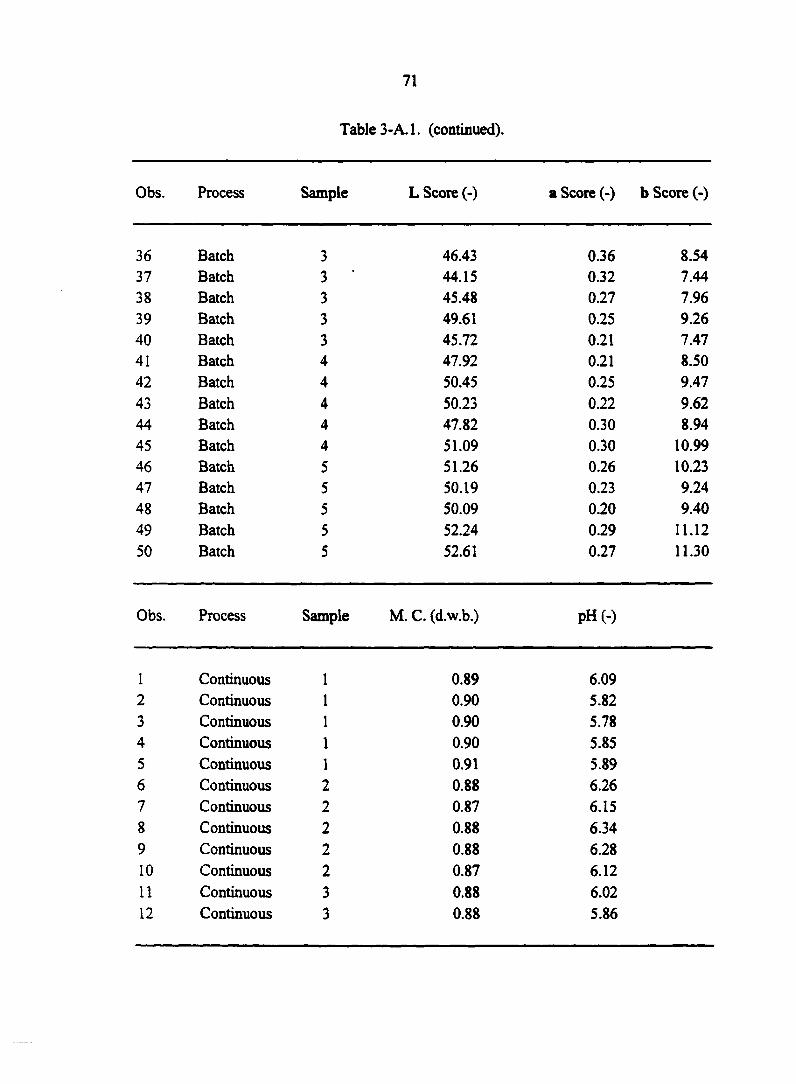
71
Table 3-A.l. (continued).
Obs. Process Sample L Score (-) a Score (-) b Score (-)
36 Batch 3 46.43 0.36 8.54 37 Batch 3 44.15 0.32 7.44 38 Batch 3 45.48 0.27 7.96 39 Batch 3 49.61 0.25 9.26 40 Batch 3 45.72 0.21 7.47 41 Batch 4 47.92 0.21 8.50 42 Batch 4 50.45 0.25 9.47 43 Batch 4 50.23 0.22 9.62 44 Batch 4 47.82 0.30 8.94 45 Batch 4 51.09 0.30 10.99 46 Batch 5 51.26 0.26 10.23 47 Batch 5 50.19 0.23 9.24 48 Batch 5 50.09 0.20 9.40 49 Batch 5 52.24 0.29 11.12 50 Batch 5 52.61 0.27 11.30
Obs. Process Sample M. C. (d.w.b.) pH(-)
1 Continuous 1 0.89 6.09 2 Continuous 1 0.90 5.82 3 Continuous 1 0.90 5.78 4 Continuous 1 0.90 5.85 5 Continuous 1 0.91 5.89 6 Continuous 2 0.88 6.26 7 Continuous 2 0.87 6.15 8 Continuous 2 0.88 6.34 9 Continuous 2 0.88 6.28 10 Continuous 2 0.87 6.12 11 Continuous 3 0.88 6.02 12 Continuous 3 0.88 5.86
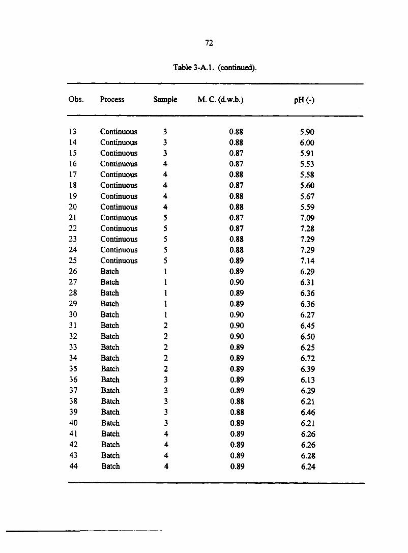
Obs
13 14 15 16 17 18 19 20 21
22 23 24 25 26 27 28 29 30 31 32 33 34 35 36 37 38 39 40 41 42 43 44
72
Table 3-A.l. (continued).
Process Sample M. C. (d.w.b.) pH (-)
Continuous 3 0.88 5.90 Continuous 3 0.88 6.00 Continuous 3 0.87 5.91 Continuous 4 0.87 5.53 Continuous 4 0.88 5.58 Continuous 4 0.87 5.60 Continuous 4 0.88 5.67 Continuous 4 0.88 5.59 Continuous 5 0.87 7.09 Continuous 5 0.87 7.28 Continuous 5 0.88 7.29 Continuous 5 0.88 7.29 Continuous 5 0.89 7.14 Batch 1 0.89 6.29 Batch 1 0.90 6.31 Batch 1 0.89 6.36 Batch 1 0.89 6.36 Batch 1 0.90 6.27 Batch 2 0.90 6.45 Batch 2 0.90 6.50 Batch 2 0.89 6.25 Batch 2 0.89 6.72 Batch 2 0.89 6.39 Batch 3 0.89 6.13 Batch 3 0.89 6.29 Batch 3 0.88 6.21 Batch 3 0.88 6.46 Batch 3 0.89 6.21 Batch 4 0.89 6.26 Batch 4 0.89 6.26 Batch 4 0.89 6.28 Batch 4 0.89 6.24
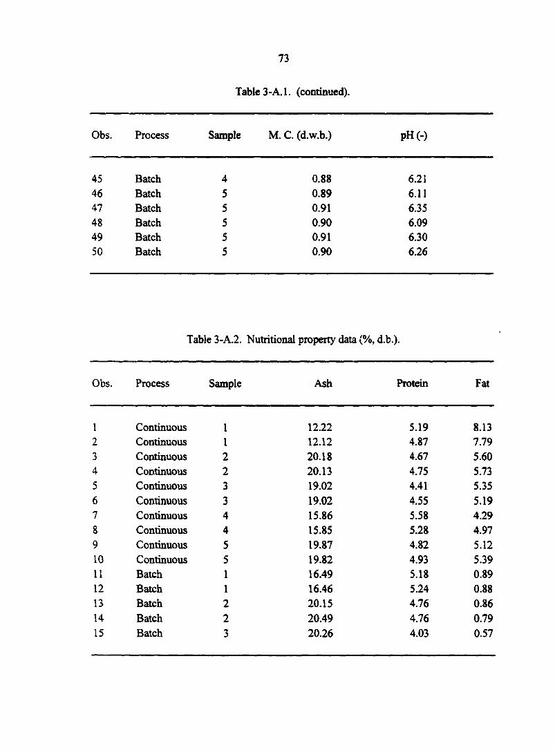
73
Table 3-A.l. (continued).
Obs. Process Sample M. C. (d.w.b.) pH(-)
45 Batch 4 0.88 6.21 46 Batch 5 0.89 6.11 47 Batch 5 0.91 6.35 48 Batch 5 0.90 6.09 49 Batch 5 0.91 6.30 50 Batch 5 0.90 6.26
Table 3-A.2. Nutritional property data (%, d.b.).
Obs. Process Sample Ash Protein Fat
1 Continuous 1 12.22 5.19 8.13 2 Continuous 1 12.12 4.87 7.79 3 Continuous 2 20.18 4.67 5.60 4 Continuous 2 20.13 4.75 5.73 5 Continuous 3 19.02 4.41 5.35 6 Continuous 3 19.02 4.55 5.19 7 Continuous 4 15.86 5.58 4.29 8 Continuous 4 15.85 5.28 4.97 9 Continuous 5 19.87 4.82 5.12 10 Continuous 5 19.82 4.93 5.39 11 Batch 1 16.49 5.18 0.89 12 Batch 1 16.46 5.24 0.88 13 Batch 2 20.15 4.76 0.86 14 Batch 2 20.49 4.76 0.79 15 Batch 3 20.26 4.03 0.57
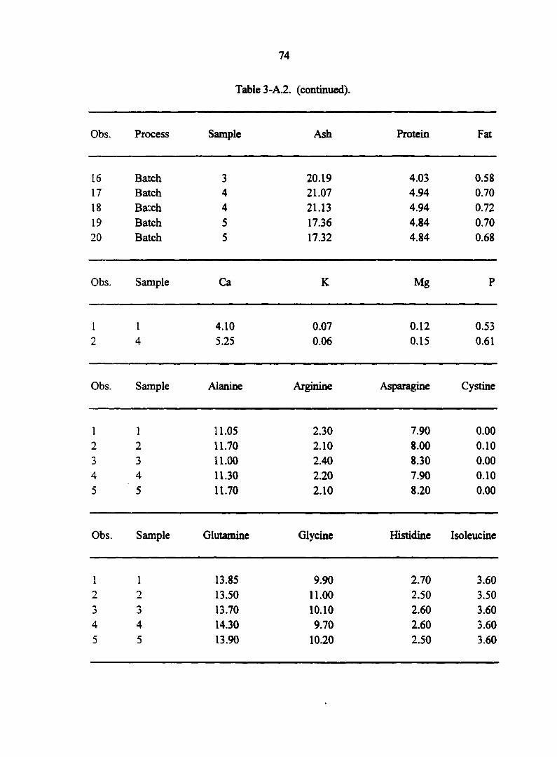
74
Table 3-A.2. (continued).
Obs. Process Sample Ash Protein Fat
16 Batch 3 20.19 4.03 0.58 17 Batch 4 21.07 4.94 0.70 18 Batch 4 21.13 4.94 0.72 19 Batch 5 17.36 4.84 0.70 20 Batch 5 17.32 4.84 0.68
Obs. Sample Ca K Mg P
1 1 4.10 0.07 0.12 0.53 2 4 5.25 0.06 0.15 0.61
Obs. Sample Alanine Arginine Asparagine Cystine
1 1 11.05 2.30 7.90 0.00 2 2 11.70 2.10 8.00 0.10 3 3 11.00 2.40 8.30 0.00 4 4 11.30 2.20 7.90 0.10 5 5 11.70 2.10 8.20 0.00
Obs. Sample Glutamine Glycine Histidine Isoleucine
1 1 13.85 9.90 2.70 3.60 2 2 13.50 11.00 2.50 3.50 3 3 13.70 10.10 2.60 3.60 4 4 14.30 9.70 2.60 3.60 5 5 13.90 10.20 2.50 3.60
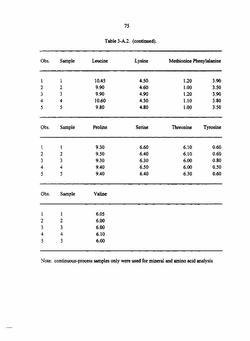
75
Table 3-A.2. (continued).
Obs. Sample Leucine Lysine Methionine Phenylalanine
1 1 10.45 4.50 1.20 3.90 2 2 9.90 4.60 1.00 3.50 3 3 9.90 4.90 1.20 3.90 4 4 10.60 4.30 1.10 3.80 5 5 9.80 4.80 1.00 3.50
Obs. Sample Proline Serine Threonine Tyrosine
1 1 9.30 6.60 6.10 0.60 2 2 9.50 6.40 6.10 0.60 3 3 9.30 6.30 6.00 0.80 4 4 9.40 6.50 6.00 0.50 5 5 9.40 6.40 6.30 0.60
Obs. Sample Valine
1 1 6.05 2 2 6.00 3 3 6.00 4 4 6.10 5 5 6.00
Note: continuous-process samples only were used for mineral and amino acid analysis
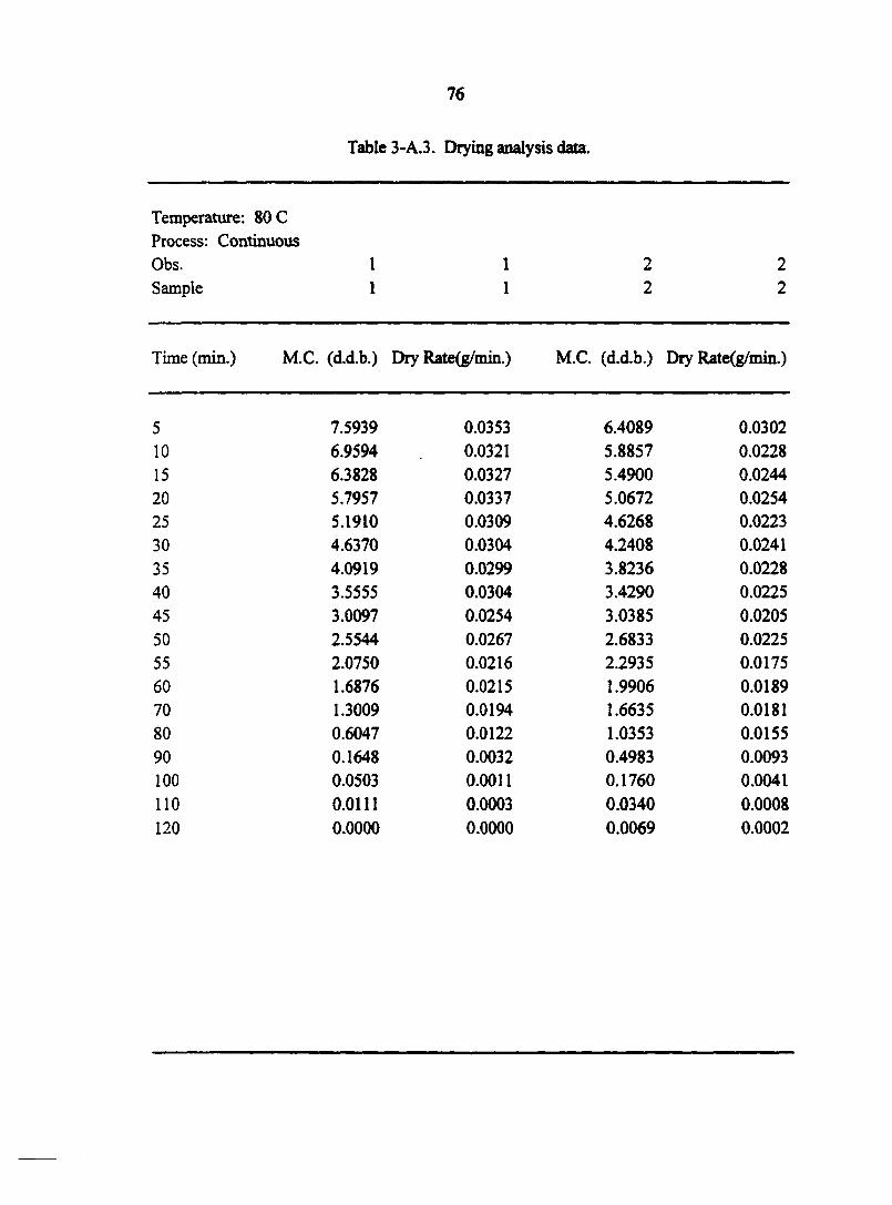
76
Table 3-A.3. Drying analysis data.
Temperature: 80 C Process: Continuous Obs. 1 1 2 2 Sample 1 1 2 2
Time (min.) M.C. (d.d.b.) Dry Rate(g/min.) M.C. (d.d.b.) Dry Rate(g/min.)
5 7.5939 0.0353 6.4089 0.0302 10 6.9594 0.0321 5.8857 0.0228 15 6.3828 0.0327 5.4900 0.0244 20 5.7957 0.0337 5.0672 0.0254 25 5.1910 0.0309 4.6268 0.0223 30 4.6370 0.0304 4.2408 0.0241 35 4.0919 0.0299 3.8236 0.0228 40 3.5555 0.0304 3.4290 0.0225 45 3.0097 0.0254 3.0385 0.0205 50 2.5544 0.0267 2.6833 0.0225 55 2.0750 0.0216 2.2935 0.0175 60 1.6876 0.0215 1.9906 0.0189 70 1.3009 0.0194 1.6635 0.0181 80 0.6047 0.0122 1.0353 0.0155 90 0.1648 0.0032 0.4983 0.0093 100 0.0503 0.0011 0.1760 0.0041 110 0.0111 0.0003 0.0340 0.0008 120 0.0000 0.0000 0.0069 0.0002

77
Table 3-A.3. (continued).
Temperature: 80 C Process: Continuous Obs. 3 3 4 4 Sample 3 3 4 4
Time (min.) M.C. (d.d.b.) Dry Rate(g/min.) M.C. (d.d.b.) Dry Rate(g/min.)
5 7.0830 0.0458 6.5960 0.0470 10 6.2673 0.0349 5.9269 0.0448 15 5.6450 0.0311 5.2893 0.0430 20 5.0902 0.0349 4.6780 0.0441 25 4.4686 0.0308 4.0509 0.0372 30 3.9202 0.0334 3.5218 0.0395 35 3.3257 0.0272 2.9599 0.0372 40 2.8403 0.0309 2.4310 0.0392 45 2.2897 0.0250 1.8740 0.0306 50 1.8439 0.0252 1.4393 0.0314 55 1.3949 0.0207 0.9923 0.0218 60 1.0257 0.0167 0.6822 0.0187 70 0.7281 0.0126 0.4156 0.0109 80 0.2780 0.0060 0.1064 0.0028 90 0.0638 0.0010 0.0256 0.0004 100 0.0267 0.0008 0.0134 0.0005 110 0.0000 0.0000 0.0000 0.0000 120 0.0000 0.0000 0.0000 0.0000

78
Table 3-A.3. (continued).
Temperature: 80 C Process: Continuous Obs. 5 5 6 6 Sample 5 5 1 I
Time (min.) M.C. (d.d.b.) Dry Rate(g/min.) M.C. (d.d.b.) Dry Rate(g/min.)
5 5.8445 0.0643 7.7931 0.0435 10 4.9005 0.0504 6.9139 0.0383 15 4.1608 0.0480 6.1398 0.0373 20 3.4566 0.0480 5.3859 0.0340 25 2.7518 0.0393 4.6982 0.0288 30 2.1755 0.0373 4.1156 0.0309 35 1.6288 0.0327 3.4905 0.0301 40 1.1485 0.0311 2.8820 0.0264 45 0.6916 0.0199 2.3487 0.0261 50 0.3999 0.0145 1.8210 0.0240 55 0.1875 0.0063 1.3366 0.0180 60 0.0954 0.0031 0.9721 0.0170 70 0.0496 0.0013 0.6279 0.0102 80 0.0123 0.0004 0.2174 0.0044 90 0.0006 0.0000 0.0388 0.0008 100 0.0000 0.0000 0.0069 0.0002 110 0.0000 0.0000 0.0000 0.0000 120 0.0000 0.0000 0.0000 0.0000

79
Table 3-A.3. (continued).
Temperature: 80 C Process: Continuous Obs. 7 7 8 8 Sample 2 2 3 3
Time (min.) M.C. (d.d.b.) Dry Rate(g/min.) M.C. (d.d.b.) Dry Rate(g/min.)
5 6.0225 0.0373 6.1160 0.0530 10 5.4563 0.0327 5.2445 0.0442 15 4.9609 0.0319 4.5179 0.0414 20 4.4769 0.0311 3.8370 0.0389 25 4.0058 0.0255 3.1982 0.0326 30 3.6183 0.0298 2.6632 0.0346 35 3.1666 0.0300 2.0946 0.0314 40 2.7109 0.0229 1.5787 0.0241 45 2.3632 0.0238 1.1824 0.0234 50 2.0024 0.0210 0.7976 0.0187 55 1.6839 0.0181 0.4906 0.0123 60 1.4096 0.0182 0.2879 0.0102 70 1.1335 0.0166 0.1199 0.0031 80 0.6299 0.0127 0.0187 0.0006 90 0.2454 0.0066 0.0000 0.0000 100 0.0467 0.0015 0.0000 0.0000 110 0.0000 0.0000 0.0000 0.0000 120 0.0000 0.0000 0.0000 0.0000

\ Table 3-A.3. (continued).
Temperature: 80 C Process: Continuous Obs. 9 9 10 10 Sample 4 4 5 5
Time (min.) M.C. (d.d.b.) Dry Rate(g/min.) M.C. (d.d.b.) Dry Rate(g/min.)
5 5.6067 0.0581 6.5650 0.0838 10 4.7624 0.0487 5.1584 0.0657 15 4.0555 0.0462 4.0551 0.0622 20 3.3848 0.0450 3.0104 0.0551 25 2.7308 0.0349 2.0863 0.0408 30 2.2239 0.0359 1.4018 0.0364 35 1.7029 0.0336 0.7905 0.0235 40 1.2143 0.0268 0.3954 0.0144 45 0.8254 0.0227 0.1537 0.0060 50 0.4964 0.0143 0.0530 0.0019 55 0.2890 0.0086 0.0205 0.0012 60 0.1641 0.0060 0.0000 0.0000 70 0.0775 0.0023 0.0000 0.0000 80 0.0122 0.0004 0.0000 0.0000 90 0.0012 0.0000 0.0000 0.0000 100 0.0000 0.0000 0.0000 0.0000 110 0.0000 0.0000 0.0000 0.0000 120 0.0000 0.0000 0.0000 0.0000

81
Table 3-A.3. (continued).
Temperature: 80 C Process: Continuous Obs. 11 11 12 12 Sample 1 1 2 2
Time (min.) M.C. (d.d.b.) Dry Rate(g/min.) M.C. (d.d.b.) Dry Rate(g/min.)
5 6.5195 0.0483 6.3018 0.0440 10 5.6400 0.0360 5.5052 0.0308 15 4.9847 0.0392 4.9475 0.0322 20 4.2719 0.0366 4.3655 0.0280 25 3.6054 0.0359 3.8585 0.0285 30 2.9527 0.0304 3.3427 0.0241 35 2.3986 0.0301 2.9066 0.0245 40 1.8511 0.0293 2.4636 0.0233 45 1.3182 0.0241 2.0420 0.0209 50 0.8788 0.0195 1.6630 0.0189 55 0.5231 0.0146 1.3210 0.0191 60 0.2577 0.0083 0.9754 0.0153 70 0.1074 0.0024 0.6985 0.0131 80 0.0189 0.0005 0.2248 0.0054 90 0.0000 0.0000 0.0290 0.0008 100 0.0000 0.0000 0.0000 0.0000 110 0.0000 0.0000 0.0000 0.0000 120 0.0000 0.0000 0.0000 0.0000

82
Table 3-A.3. (continued).
Temperature: 80 C Process: Continuous Obs. 13 13 14 14 Sample 3 3 4 4
Time (min.) M.C. (d.d.b.) Dry Rate(g/min.) M.C. (d.d.b.) Dry Rate(g/min.)
5 6.0898 0.0546 6.1280 0.0673 10 5.1238 0.0375 5.0826 0.0402 15 4.4602 0.0380 4.4587 0.0480 20 3.7881 0.0381 3.7134 0.0468 25 3.1139 0.0357 2.9863 0.0436 30 2.4821 0.0307 2.3096 0.0348 35 1.9388 0.0263 1.7699 0.0316 40 1.4740 0.0227 1.2795 0.0275 45 1.0729 0.0233 0.8528 0.0188 50 0.6601 0.0164 0.5615 0.0148 55 0.3707 0.0121 0.3314 0.0099 60 0.1571 0.0052 0.1773 0.0049 70 0.0644 0.0018 0.1006 0.0020 80 0.0000 0.0000 0.0394 0.0005 90 0.0000 0.0000 0.0233 0.0008 100 0.0000 0.0000 0.0000 0.0000 110 0.0000 0.0000 0.0000 0.0000 120 0.0000 0.0000 0.0000 0.0000

83
Table 3-A.3. (continued).
Temperature: 80 C Process: Continuous Obs. 15 15 16 16 Sample 5 5 1 1
Time (min.) M.C. (d.d.b.)
/—\ 1 s M.C. (d.d.b.) Dry Rate(g/min.)
5 7.8295 0.0802 6.5786 0.0518 10 6.4062 0.0595 5.6941 0.0442 15 5.3501 0.0612 4.9395 0.0445 20 4.2628 0.0576 4.1787 0.0367 25 3.2393 0.0519 3.5523 0.0401 30 2.3182 0.0426 2.8677 0.0378 35 1.5625 0.0334 2.2211 0.0328 40 0.9687 0.0256 1.6613 0.0320 45 0.5149 0.0151 1.1152 0.0231 50 0.2475 0.0077 0.7198 0.0247 55 0.1104 0.0033 0.2970 0.0080 60 0.0511 0.0012 0.1606 0.0060 70 0.0295 0.0008 0.0584 0.0016 80 0.0000 0.0000 0.0041 0.0001 90 0.0000 0.0000 0.0000 0.0000 100 0.0000 0.0000 0.0000 0.0000 110 0.0000 0.0000 0.0000 0.0000 120 0.0000 0.0000 0.0000 0.0000
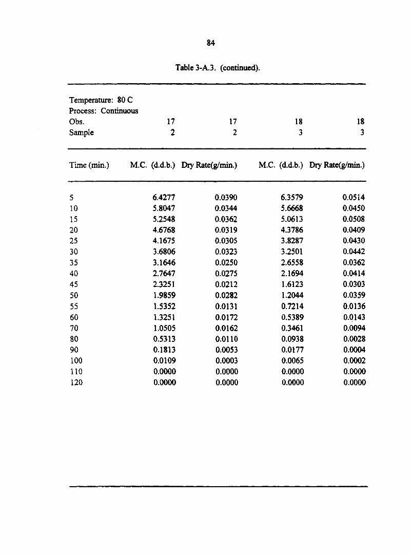
84
Table 3-A.3. (continued).
Temperature: 80 C Process: Continuous Obs. 17 17 18 18 Sample 2 2 3 3
Time (min.) M.C. (d.d.b.) Dry Rate(g/min.) M.C. (d.d.b.) Dry Rate(g/min.)
5 6.4277 0.0390 6.3579 0.0514 10 5.8047 0.0344 5.6668 0.0450 15 5.2548 0.0362 5.0613 0.0508 20 4.6768 0.0319 4.3786 0.0409 25 4.1675 0.0305 3.8287 0.0430 30 3.6806 0.0323 3.2501 0.0442 35 3.1646 0.0250 2.6558 0.0362 40 2.7647 0.0275 2.1694 0.0414 45 2.3251 0.0212 1.6123 0.0303 50 1.9859 0.0282 1.2044 0.0359
55 1.5352 0.0131 0.7214 0.0136 60 1.3251 0.0172 0.5389 0.0143 70 1.0505 0.0162 0.3461 0.0094 80 0.5313 0.0110 0.0938 0.0028 90 0.1813 0.0053 0.0177 0.0004 100 0.0109 0.0003 0.0065 0.0002 110 0.0000 0.0000 0.0000 0.0000 120 0.0000 0.0000 0.0000 0.0000
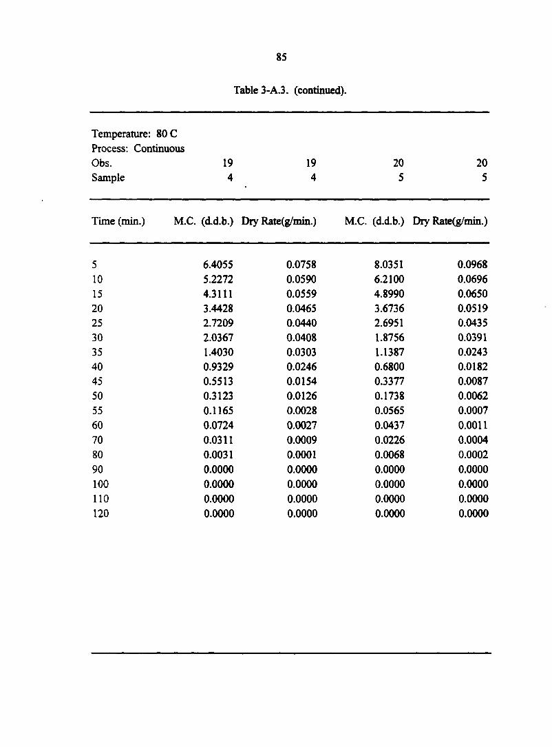
85
Table 3-A.3. (continued).
Temperature: 80 C Process: Continuous Obs. 19 19 20 20 Sample 4 4 5 5
Time (min.) M.C. (d.d.b.) Dry Rate(g/min.) M.C. (d.d.b.) Dry Rate(g/min.)
5 6.4055 0.0758 8.0351 0.0968 10 5.2272 0.0590 6.2100 0.0696 15 4.3111 0.0559 4.8990 0.0650 20 3.4428 0.0465 3.6736 0.0519 25 2.7209 0.0440 2.6951 0.0435 30 2.0367 0.0408 1.8756 0.0391 35 1.4030 0.0303 1.1387 0.0243 40 0.9329 0.0246 0.6800 0.0182 45 0.5513 0.0154 0.3377 0.0087 50 0.3123 0.0126 0.1738 0.0062 55 0.1165 0.0028 0.0565 0.0007 60 0.0724 0.0027 0.0437 0.0011 70 0.0311 0.0009 0.0226 0.0004 80 0.0031 0.0001 0.0068 0.0002 90 0.0000 0.0000 0.0000 0.0000 100 0.0000 0.0000 0.0000 0.0000 110 0.0000 0.0000 0.0000 0.0000 120 0.0000 0.0000 0.0000 0.0000

86
Table 3-A.3. (continued).
Temperature: 80 C Process: Continuous Obs. 21 21 22 22 Sample 1 1 2 2
Time (min.) M.C. (d.d.b.) Dry Rate(g/min.) M.C. (d.d.b.)
1 s
5 7.1495 0.0550 6.3632 0.0404 10 6.2607 0.0478 5.6750 0.0354 15 5.4890 0.0447 5.0726 0.0301 20 4.7674 0.0535 4.5605 0.0382 25 3.9041 0.0400 3.9104 0.0400 30 3.2581 0.0435 3.2290 0.0206 35 2.5549 0.0357 2.8787 0.0276 40 1.9777 0.0316 2.4085 0.0238 45 1.4677 0.0331 2.0024 0.0246 50 0.9338 0.0208 1.5836 0.0164 55 0.5985 0.0188 1.3039 0.0164 60 0.2955 0.0106 1.0249 0.0136 70 0.1250 0.0029 0.7935 0.0115 80 0.0304 0.0006 0.4003 0.0077 90 0.0116 0.0004 0.1387 0.0035 100 0.0000 0.0000 0.0198 0.0006 110 0.0000 0.0000 0.0000 0.0000 120 0.0000 0.0000 0.0000 0.0000

87
Table 3-A.3. (continued).
Temperature: 80 C Process: Continuous Obs. 23 23 24 24 Sample 3 3 4 4
Time (min.) M.C. (d.d.b.) Dry Rate(g/min.) M.C. (d.d.b.) S 1
5 6.8500 0.0490 6.6743 0.0723 10 6.1230 0.0448 5.5745 0.0576 15 5.4571 0.0439 4.6986 0.0520 20 4.8055 0.0600 3.9072 0.0558 25 3.9142 0.0400 3.0593 0.0500 30 3.3202 0.0334 2.2990 0.0561 35 2.8248 0.0382 1.4459 0.0355 40 2.2581 0.0301 0.9060 0.0270 45 1.8105 0.0323 0.4948 0.0212 50 1.3312 0.0205 0.1727 0.0069 55 1.0264 0.0194 0.0681 0.0031 60 0.7389 0.0153 0.0213 0.0010 70 0.5123 0.0123 0.0055 0.0002 80 0.1467 0.0046 0.0000 0.0000 90 0.0110 0.0004 0.0000 0.0000 100 0.0000 0.0000 0.0000 0.0000 110 0.0000 0.0000 0.0000 0.0000 120 0.0000 0.0000 0.0000 0.0000
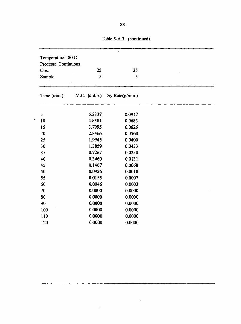
88
Table 3-A.3. (continued).
Temperature: 80 C Process: Continuous Obs. 25 25 Sample 5 5
Time (min.) M.C. (d.d.b.) Dry Rate(g/min.)
5 6.2337 0.0917 10 4.8381 0.0683 15 3.7995 0.0626 20 2.8466 0.0560 25 1.9945 0.0400 30 1.3859 0.0433 35 0.7267 0.0250 40 0.3460 0.0131 45 0.1467 0.0068 50 0.0426 0.0018 55 0.0155 0.0007 60 0.0046 0.0003 70 0.0000 0.0000 80 0.0000 0.0000 90 0.0000 0.0000 100 0.0000 0.0000 110 0.0000 0.0000 120 0.0000 0.0000

89
Table 3-A.3. (continued).
Temperature: 100 C Process: Continuous Obs. 1 1 2 2 Sample 1 1 2 2
Time (min.) M.C. (d.d.b.) Dry Rate(g/min.) M.C. (d.d.b.) Dry Rate(g/min.)
5 6.1709 0.0720 6.6351 0.0633 10 5.2205 0.0602 5.6675 0.0476 15 4.4253 0.0574 4.9404 0.0462 20 3.6675 0.0517 4.2341 0.0473 25 2.9847 0.0389 3.5110 0.0384 30 2.4709 0.0499 2.9248 0.0448 35 1.8114 0.0266 2.2408 0.0240 40 1.4604 0.0277 1.8744 0.0274 45 1.0946 0.0271 1.4551 0.0276 50 0.7372 0.0207 1.0327 0.0218 55 0.4638 0.0186 0.7002 0.0225 60 0.2184 0.0083 0.3567 0.0111 70 0.1094 0.0030 0.1870 0.0038 80 0.0304 0.0012 0.0706 0.0013 90 0.0000 0.0000 0.0306 0.0010 100 0.0000 0.0000 0.0000 0.0000 110 0.0000 0.0000 0.0000 0.0000 120 0.0000 0.0000 0.0000 0.0000

90
Table 3-A.3. (continued).
Temperature: 100 C Process: Continuous Obs. 3 3 4 4 Sample 3 3 4 4
Time (min.) M.C. (d.d.b.) Dry Rate(g/min.) M.C. (d.d.b.) Dry Rate(g/min.)
5 6.3975 0.0822 6.0431 0.1085 10 5.0003 0.0658 4.5162 0.0690 15 3.8820 0.0596 3.5455 0.0681 20 2.8681 0.0616 2.5865 0.0679 25 1.8201 0.0425 1.6310 0.0451 30 1.0983 0.0428 0.9958 0.0400 35 0.3703 0.0135 0.4323 0.0147 40 0.1414 0.0061 0.2252 0.0091 45 0.0384 0.0023 0.0965 0.0040 50 0.0000 0.0000 0.0408 0.0010 55 0.0000 0.0000 0.0267 0.0017 60 0.0000 0.0000 0.0031 0.0002 70 0.0000 0.0000 0.0000 0.0000 80 0.0000 0.0000 0.0000 0.0000 90 0.0000 0.0000 0.0000 0.0000 100 0.0000 0.0000 0.0000 0.0000 110 0.0000 0.0000 0.0000 0.0000 120 0.0000 0.0000 0.0000 0.0000

91
Table 3-A.3. (continued).
Temperature: 100 C Process: Continuous Obs. 5 5 6 6 Sample 5 5 1 1
Time (min.) M.C. (d.d.b.) Dry Rate(g/min.) M.C. (d.d.b.) Dry Rate(g/min.)
5 6.6308 0.1331 7.2936 0.0622 10 4.2842 0.0916 6.2819 0.0469 15 2.6700 0.0777 5.5195 0.0515 20 1.2994 0.0552 4.6817 0.0444 25 0.3255 0.0152 3.9597 0.0446 30 0.0578 0.0025 3.2341 0.0441 35 0.0145 0.0002 2.5166 0.0404 40 0.0109 0.0006 1.8602 0.0370 45 0.0000 0.0000 1.2581 0.0298 50 0.0000 0.0000 0.7737 0.0220 55 0.0000 0.0000 0.4155 0.0138 60 0.0000 0.0000 0.1908 0.0076 70 0.0000 0.0000 0.0670 0.0015 80 0.0000 0.0000 0.0172 0.0005 90 0.0000 0.0000 0.0000 0.0000 100 0.0000 0.0000 0.0000 0.0000 110 0.0000 0.0000 0.0000 0.0000 120 0.0000 0.0000 0.0000 0.0000
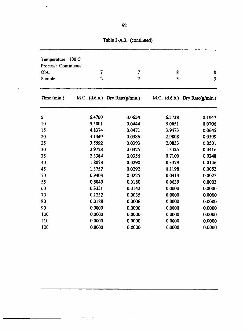
92
Table 3-A.3. (continued).
Temperature: 100 C Process: Continuous Obs. 7 7 8 8 Sample 2 2 3 3
Time (min.) M.C. (d.d.b.) Dry Rate(g/min.) M.C. (d.d.b.) Dry Rate(g/min.)
5 6.4760 0.0654 6.5728 0.1047 10 5.5001 0.0444 5.0051 0.0706 15 4.8374 0.0471 3.9473 0.0645 20 4.1349 0.0386 2.9808 0.0599 25 3.5592 0.0393 2.0833 0.0501 30 2.9728 0.0425 1.3325 0.0416 35 2.3384 0.0356 0.7100 0.0248 40 1.8078 0.0290 0.3379 0.0146 45 1.3757 0.0292 0.1198 0.0052 50 0.9403 0.0225 0.0413 0.0025 55 0.6040 0.0180 0.0039 0.0003 60 0.3351 0.0142 0.0000 0.0000 70 0.1232 0.0035 0.0000 0.0000 80 0.0188 0.0006 0.0000 0.0000 90 0.0000 0.0000 0.0000 0.0000 100 0.0000 0.0000 0.0000 0.0000 110 0.0000 0.0000 0.0000 0.0000 120 0.0000 0.0000 0.0000 0.0000
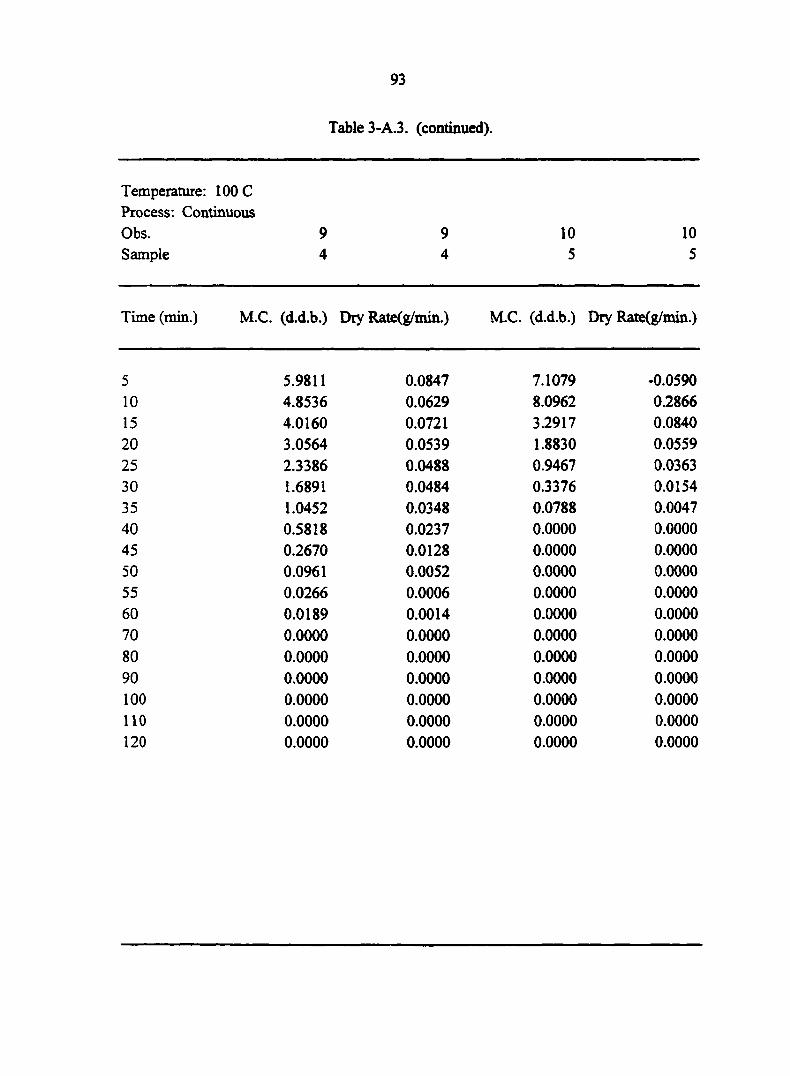
93
Table 3-A.3. (continued).
Temperature: 100 C Process: Continuous Obs. 9 9 10 10 Sample 4 4 5 5
Time (min.) M.C. (d.d.b.) Dry Rate(g/min.) M.C. (d.d.b.) Dry Rate(g/min.)
5 5.9811 0.0847 7.1079 -0.0590 10 4.8536 0.0629 8.0962 0.2866 15 4.0160 0.0721 3.2917 0.0840 20 3.0564 0.0539 1.8830 0.0559 25 2.3386 0.0488 0.9467 0.0363 30 1.6891 0.0484 0.3376 0.0154 35 1.0452 0.0348 0.0788 0.0047 40 0.5818 0.0237 0.0000 0.0000 45 0.2670 0.0128 0.0000 0.0000 50 0.0961 0.0052 0.0000 0.0000 55 0.0266 0.0006 0.0000 0.0000 60 0.0189 0.0014 0.0000 0.0000 70 0.0000 0.0000 0.0000 0.0000 80 0.0000 0.0000 0.0000 0.0000 90 0.0000 0.0000 0.0000 0.0000 100 0.0000 0.0000 0.0000 0.0000 110 0.0000 0.0000 0.0000 0.0000 120 0.0000 0.0000 0.0000 0.0000
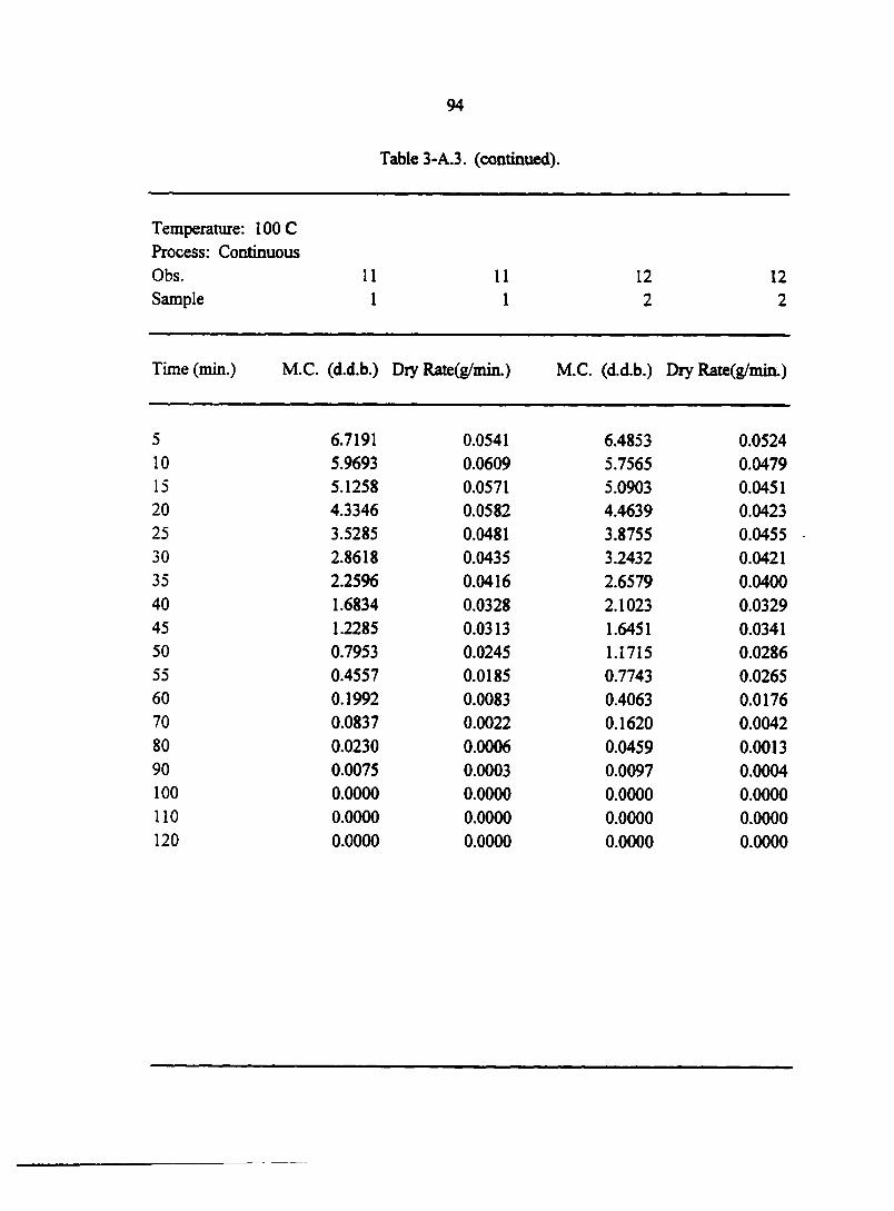
94
Table 3-A.3. (continued).
Temperature: 100 C Process: Continuous Obs. 11 11 12 12 Sample 1 1 2 2
Time (min.) M.C. (d.d.b.) Dry Rate(g/min.) M.C. (d.d.b.) Dry Rate(g/min.)
5 6.7191 0.0541 6.4853 0.0524 10 5.9693 0.0609 5.7565 0.0479 15 5.1258 0.0571 5.0903 0.0451 20 4.3346 0.0582 4.4639 0.0423 25 3.5285 0.0481 3.8755 0.0455 30 2.8618 0.0435 3.2432 0.0421 35 2.2596 0.0416 2.6579 0.0400 40 1.6834 0.0328 2.1023 0.0329 45 1.2285 0.0313 1.6451 0.0341 50 0.7953 0.0245 1.1715 0.0286 55 0.4557 0.0185 0.7743 0.0265 60 0.1992 0.0083 0.4063 0.0176 70 0.0837 0.0022 0.1620 0.0042 80 0.0230 0.0006 0.0459 0.0013 90 0.0075 0.0003 0.0097 0.0004 100 0.0000 0.0000 0.0000 0.0000 110 0.0000 0.0000 0.0000 0.0000 120 0.0000 0.0000 0.0000 0.0000
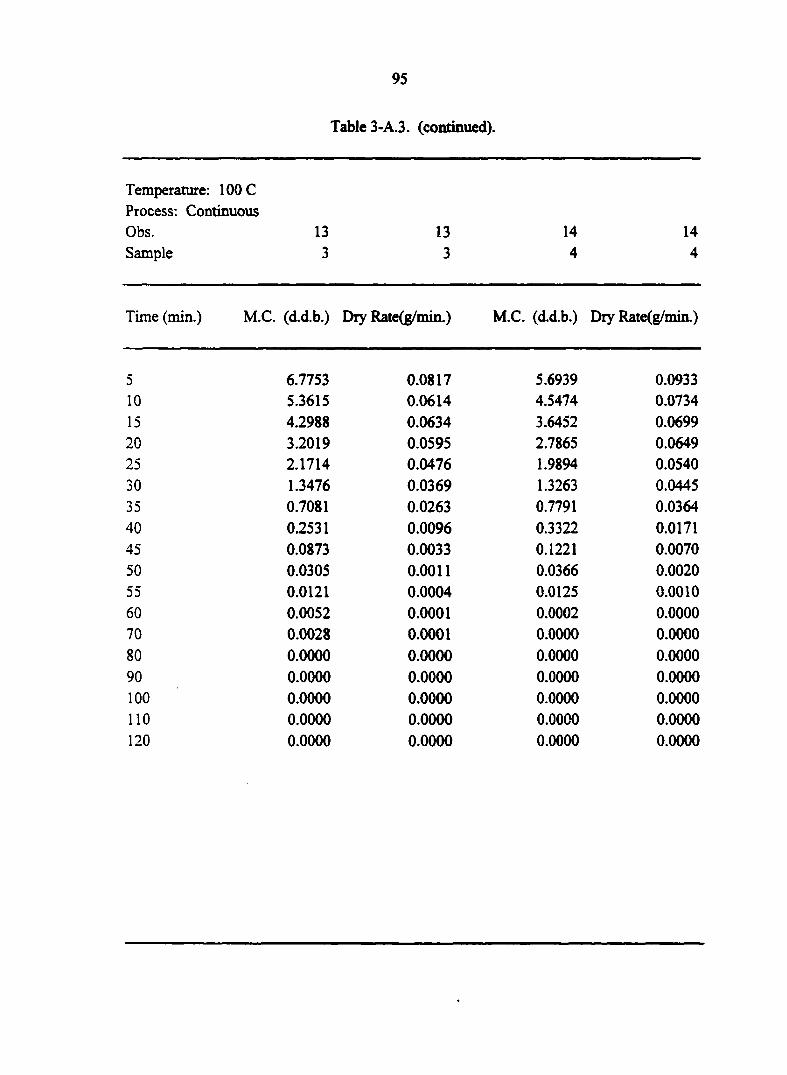
95
Table 3-A.3. (continued).
Temperature: 100 C Process: Continuous Obs. 13 13 14 14 Sample 3 3 4 4
Time (min.) M.C. (d.d.b.) r
s 1 4 M.C. (d.d.b.) Dry Rate(g/min.)
5 6.7753 0.0817 5.6939 0.0933 10 5.3615 0.0614 4.5474 0.0734 15 4.2988 0.0634 3.6452 0.0699 20 3.2019 0.0595 2.7865 0.0649 25 2.1714 0.0476 1.9894 0.0540 30 1.3476 0.0369 1.3263 0.0445 35 0.7081 0.0263 0.7791 0.0364 40 0.2531 0.0096 0.3322 0.0171 45 0.0873 0.0033 0.1221 0.0070 50 0.0305 0.0011 0.0366 0.0020 55 0.0121 0.0004 0.0125 0.0010 60 0.0052 0.0001 0.0002 0.0000 70 0.0028 0.0001 0.0000 0.0000 80 0.0000 0.0000 0.0000 0.0000 90 0.0000 0.0000 0.0000 0.0000 100 0.0000 0.0000 0.0000 0.0000 110 0.0000 0.0000 0.0000 0.0000 120 0.0000 0.0000 0.0000 0.0000

96
Table 3-A.3. (continued).
Temperature: 100 C Process: Continuous Obs. 15 15 16 16 Sample 5 5 1 1
Time (min.) M.C. (d.d.b.) Dry Rate(g/min.) M.C. (d.d.b.) Dry Rate(g/min.)
5 6.2346 0.1143 7.1798 0.0623 10 4.2744 0.0816 6.1858 0.0642 15 2.8748 0.0700 5.1612 0.0532 20 1.6734 0.0484 4.3116 0.0538 25 0.8439 0.0318 3.4524 0.0505 30 0.2981 0.0135 2.6466 0.0441 35 0.0672 0.0039 1.9432 0.0405 40 0.0000 0.0000 1.2963 0.0319 45 0.0000 0.0000 0.7864 0.0241 50 0.0000 0.0000 0.4017 0.0159 55 0.0000 0.0000 0.1481 0.0060 60 0.0000 0.0000 0.0520 0.0022 70 0.0000 0.0000 0.0169 0.0005 80 0.0000 0.0000 0.0000 0.0000 90 0.0000 0.0000 0.0000 0.0000 100 0.0000 0.0000 0.0000 0.0000 110 0.0000 0.0000 0.0000 0.0000 120 0.0000 0.0000 0.0000 0.0000
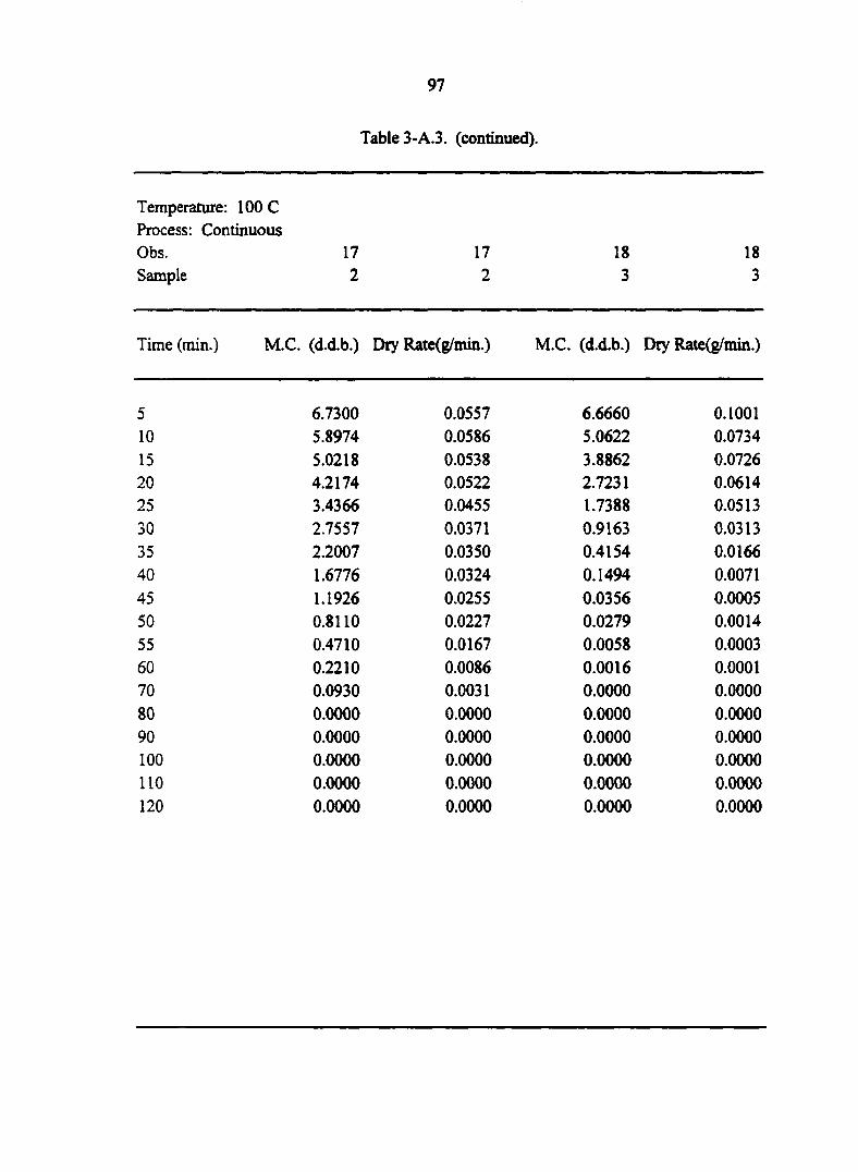
97
Table 3-A.3. (continued).
Temperature: 100 C Process: Continuous Obs. 17 17 18 18 Sample 2 2 3 3
Time (min.) M.C. (d.d.b.) Dry Rate(g/min.) M.C. (d.d.b.)
1 s
5 6.7300 0.0557 6.6660 0.1001 10 5.8974 0.0586 5.0622 0.0734 15 5.0218 0.0538 3.8862 0.0726 20 4.2174 0.0522 2.7231 0.0614 25 3.4366 0.0455 1.7388 0.0513 30 2.7557 0.0371 0.9163 0.0313 35 2.2007 0.0350 0.4154 0.0166 40 1.6776 0.0324 0.1494 0.0071 45 1.1926 0.0255 0.0356 0.0005 50 0.8110 0.0227 0.0279 0.0014 55 0.4710 0.0167 0.0058 0.0003 60 0.2210 0.0086 0.0016 0.0001 70 0.0930 0.0031 0.0000 0.0000 80 0.0000 0.0000 0.0000 0.0000 90 0.0000 0.0000 0.0000 0.0000 100 0.0000 0.0000 0.0000 0.0000 110 0.0000 0.0000 0.0000 0.0000 120 0.0000 0.0000 0.0000 0.0000

98
Table 3-A.3. (continued).
Temperature: 100 C Process: Continuous Obs. 19 19 20 20 Sample 4 4 5 5
Time (min.) M.C. (d.d.b.) Dry Rate(g/min.) M.C. (d.d.b.) Dry Rate(g/min.)
5 6.2169 0.1026 6.5894 0.1287 10 4.9780 0.0836 4.6781 0.0936 15 3.9688 0.0767 3.2886 0.0795 20 3.0425 0.0674 2.1087 0.0644 25 2.2287 0.0573 1.1526 0.0412 30 1.5370 0.0468 0.5410 0.0214 35 0.9715 0.0387 0.2227 0.0103 40 0.5046 0.0245 0.0692 0.0032 45 0.2082 0.0117 0.0220 0.0013 50 0.0667 0.0034 0.0033 0.0002 55 0.0254 0.0014 0.0000 0.0000 60 0.0080 0.0007 0.0000 0.0000 70 0.0000 0.0000 0.0000 0.0000 80 0.0000 0.0000 0.0000 0.0000 90 0.0000 0.0000 0.0000 0.0000 100 0.0000 0.0000 0.0000 0.0000 no 0.0000 0.0000 0.0000 0.0000 120 0.0000 0.0000 0.0000 0.0000

99
Table 3-A.3. (continued).
Temperature: 100 C Process: Continuous Obs. 21 21 22 22 Sample 1 1 2 2
Time (min.) M.C. (d.d.b.) y—
\ 1 s M.C. (d.d.b.) Dry Rate(g/min.)
5 6.5223 0.0765 6.1785 0.0545 10 5.2395 0.0594 5.3071 0.0522 15 4.2432 0.0514 4.4718 0.0461 20 3.3814 0.0483 3.7342 0.0459 25 2.5709 0.0410 3.0003 0.0466 30 1.8829 0.0350 2.2550 0.0388 35 1.2959 0.0292 1.6347 0.0381 40 0.8068 0.0220 1.0253 0.0301 45 0.4371 0.0149 0.5441 0.0206 50 0.1875 0.0074 0.2140 0.0106 55 0.0627 0.0019 0.0448 0.0025 60 0.0315 0.0005 0.0048 0.0003 70 0.0238 0.0007 0.0000 0.0000 80 0.0000 0.0000 0.0000 0.0000 90 0.0000 0.0000 0.0000 0.0000 100 0.0000 0.0000 0.0000 0.0000 110 0.0000 0.0000 0.0000 0.0000 120 0.0000 0.0000 0.0000 0.0000

100
Table 3-A.3. (continued).
Temperature: 100 C Process: Continuous Obs. 23 23 24 24 Sample 3 3 4 4
Time (min.) M.C. (d.d.b.) Dry Rate(g/min.) M.C. (d.d.b.) Dry Rate(g/min.)
5 6.0801 0.0956 6.0662 0.0997 10 4.7448 0.0727 4.7295 0.0757 15 3.7302 0.0693 3.7145 0.0639 20 2.7624 0.0609 2.8579 0.0590 25 1.9? 20 0.0550 2.0670 0.0517 30 1.1435 0.0394 1.3740 0.0422 35 0.5929 0.0287 0.8086 0.0336 40 0.1921 0.0104 0.3576 0.0179 45 0.0464 0.0023 0.1180 0.0063 50 0.0137 0.0010 0.0335 0.0015 55 0.0000 0.0000 0.0139 0.0009 60 0.0000 0.0000 0.0024 0.0002 70 0.0000 0.0000 0.0000 0.0000 80 0.0000 0.0000 0.0000 0.0000 90 0.0000 0.0000 0.0000 0.0000 100 0.0000 0.0000 0.0000 0.0000 110 0.0000 0.0000 0.0000 0.0000 120 0.0000 0.0000 0.0000 0.0000
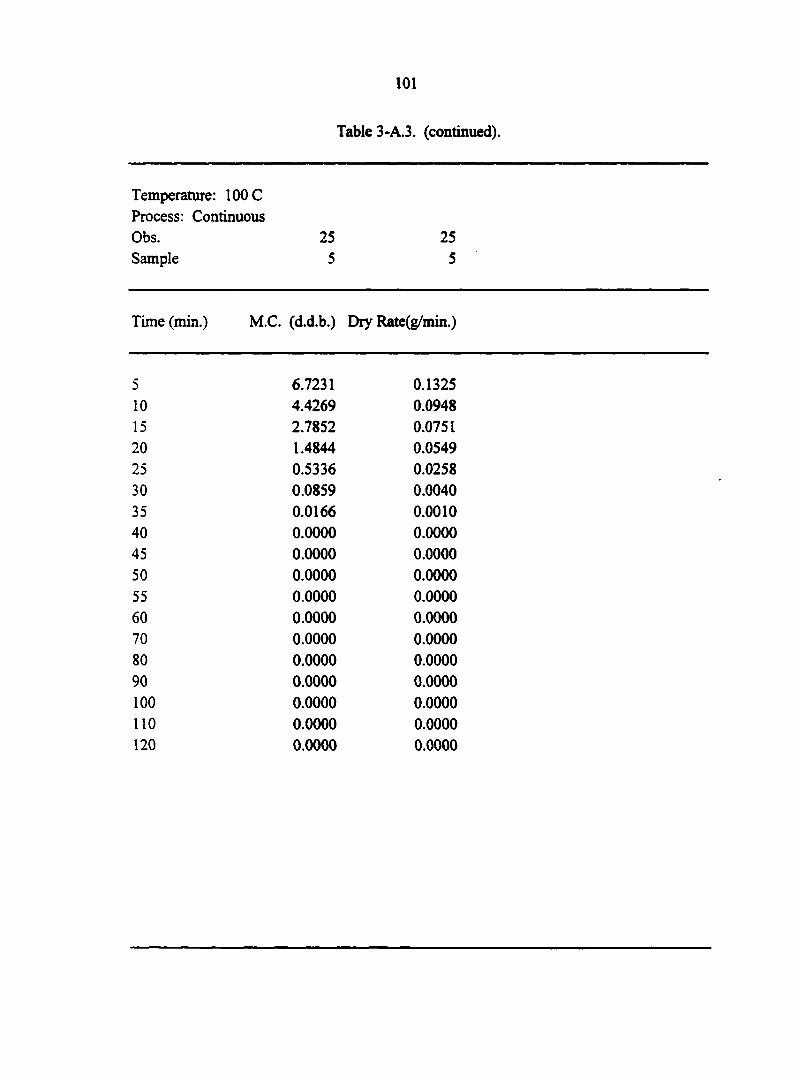
101
Table 3-A.3. (continued).
Temperature: 100 C Process: Continuous Obs. 25 25 Sample 5 5
Time (min.) M.C. (d.d.b.) Dry Rate(g/min.)
5 6.7231 0.1325 10 4.4269 0.0948 15 2.7852 0.0751 20 1.4844 0.0549 25 0.5336 0.0258 30 0.0859 0.0040 35 0.0166 0.0010 40 0.0000 0.0000 45 0.0000 0.0000 50 0.0000 0.0000 55 0.0000 0.0000 60 0.0000 0.0000 70 0.0000 0.0000 80 0.0000 0.0000 90 0.0000 0.0000 100 0.0000 0.0000 110 0.0000 0.0000 120 0.0000 0.0000
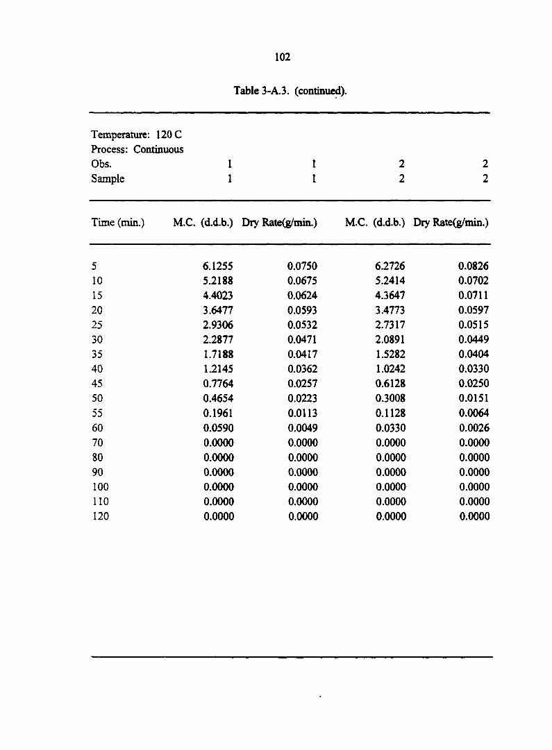
102
Table 3-A.3. (continued).
Temperature: 120 C Process: Continuous Obs. 1 1 2 2 Sample 1 1 2 2
Time (min.) M.C. (d.d.b.) Dry Rate(g/min.) M.C. (d.d.b.) Dry Rate(g/min.)
5 6.1255 0.0750 6.2726 0.0826 10 5.2188 0.0675 5.2414 0.0702 15 4.4023 0.0624 4.3647 0.0711 20 3.6477 0.0593 3.4773 0.0597 25 2.9306 0.0532 2.7317 0.0515 30 2.2877 0.0471 2.0891 0.0449 35 1.7188 0.0417 1.5282 0.0404 40 1.2145 0.0362 1.0242 0.0330 45 0.7764 0.0257 0.6128 0.0250 50 0.4654 0.0223 0.3008 0.0151 55 0.1961 0.0113 0.1128 0.0064 60 0.0590 0.0049 0.0330 0.0026 70 0.0000 0.0000 0.0000 0.0000 80 0.0000 0.0000 0.0000 0.0000 90 0.0000 0.0000 0.0000 0.0000 100 0.0000 0.0000 0.0000 0.0000 110 0.0000 0.0000 0.0000 0.0000 120 0.0000 0.0000 0.0000 0.0000

103
Table 3-A.3. (continued).
Temperature: 120 C Process: Continuous Obs. 3 3 4 4 Sample 3 3 4 4
Time (min.) M.C. (d.d.b.) Dry Rate(g/min.) M.C. (d.d.b.) Dry Rate(g/min.)
5 6.1484 0.1056 6.1979 0.1026 10 4.6812 0.0924 4.7715 0.0848 15 3.3966 0.0750 3.5937 0.0730 20 2.3538 0.0648 2.5792 0.0660 25 1.4536 0.0501 1.6626 0.0529 30 0.7571 0.0339 0.9272 0.0374 35 0.2857 0.0153 0.4069 0.0218 40 0.0737 0.0045 0.1045 0.0069 45 0.0117 0.0008 0.0081 0.0006 50 0.0000 0.0000 0.0000 0.0000 55 0.0000 0.0000 0.0000 0.0000 60 0.0000 0.0000 0.0000 0.0000 70 0.0000 0.0000 0.0000 0.0000 80 0.0000 0.0000 0.0000 0.0000 90 0.0000 0.0000 0.0000 0.0000 100 0.0000 0.0000 0.0000 0.0000 110 0.0000 0.0000 0.0000 0.0000 120 0.0000 0.0000 0.0000 0.0000

104
Table 3-A.3. (continued).
Temperature: 120 C Process: Continuous Obs. 5 5 6 6 Sample 5 5 1 1
Time (min.) M.C. (d.d.b.) Dry Rate(g/min.) M.C. (d.d.b.) Dry Rate(g/min.)
5 6.8504 0.1851 6.5004 0.0889 10 4.0585 0.1300 4.8546 0.0676 15 2.0971 0.0807 3.6029 0.0595 20 0.8799 0.0459 2.5011 0.0422 25 0.1870 0.0106 1.7195 0.0396 30 0.0278 0.0015 0.9870 0.0268 35 0.0054 0.0000 0.4907 0.0249 40 0.0048 0.0003 0.0300 0.0016 45 0.0000 0.0000 0.0000 0.0000 50 0.0000 0.0000 0.0000 0.0000 55 0.0000 0.0000 0.0000 0.0000 60 0.0000 0.0000 0.0000 0.0000 70 0.0000 0.0000 0.0000 0.0000 80 0.0000 0.0000 0.0000 0.0000 90 0.0000 0.0000 0.0000 0.0000 100 0.0000 0.0000 0.0000 0.0000 110 0.0000 0.0000 0.0000 0.0000 120 0.0000 0.0000 0.0000 0.0000

105
Table 3-A.3. (continued).
Temperature: 120 C Process: Continuous Obs. 7 7 8 8 Sample 2 2 3 3
Time (min.) M.C. (d.d.b.) Dry Rate(g/min.) M.C. (d.d.b.) Dry Rate(g/min.)
5 6.0283 0.1290 7.0169 0.1483 10 4.3541 0.0915 4.3489 0.1022 15 3.1667 0.0781 2.5101 0.0844 20 2.1524 0.0635 0.9914 0.0425 25 1.3276 0.0496 0.2263 0.0108 30 0.6838 0.0321 0.0317 0.0018 35 0.2677 0.0206 0.0000 0.0000 40 0.0000 0.0000 0.0000 0.0000 45 0.0000 0.0000 0.0000 0.0000 50 0.0000 0.0000 0.0000 0.0000 55 0.0000 0.0000 0.0000 0.0000 60 0.0000 0.0000 0.0000 0.0000 70 0.0000 0.0000 0.0000 0.0000 80 0.0000 0.0000 0.0000 0.0000 90 0.0000 0.0000 0.0000 0.0000 100 0.0000 0.0000 0.0000 0.0000 110 0.0000 0.0000 0.0000 0.0000 120 0.0000 0.0000 0.0000 0.0000

106
Table 3-A.3. (continued).
Temperature: 120 C Process: Continuous Obs. 9 9 10 10 Sample 4 4 5 5
Time (min.) M.C. (d.d.b.)
Ï
4 M.C. (d.d.b.) Dry Rate(g/min.)
5 6.2232 0.1420 6.5093 0.1979 10 4.2378 0.0984 3.4366 0.1166 15 2.8610 0.0896 1.6267 0.0729 20 1.6084 0.0545 0.4950 0.0266 25 0.8456 0.0375 0.0823 0.0043 30 0.3211 0.0175 0.0149 0.0010 35 0.0764 0.0040 0.0000 0.0000 40 0.0204 0.0015 0.0000 0.0000 45 0.0000 0.0000 0.0000 0.0000 50 0.0000 0.0000 0.0000 0.0000 55 0.0000 0.0000 0.0000 0.0000 60 0.0000 0.0000 0.0000 0.0000 70 0.0000 0.0000 0.0000 0.0000 80 0.0000 0.0000 0.0000 0.0000 90 0.0000 0.0000 0.0000 0.0000 100 0.0000 0.0000 0.0000 0.0000 110 0.0000 0.0000 0.0000 0.0000 120 0.0000 0.0000 0.0000 0.0000

107
Table 3-A.3. (continued).
Temperature: 120 C Process: Continuous Obs. 11 11 12 12 Sample 1 1 2 2
Time (min.) M.C. (d.d.b.) Dry Rate(g/min.) M.C. (d.d.b.) Dry Rate(g/min.)
5 6.5395 0.0904 6.3906 0.1190 10 4.9645 0.0658 4.3890 0.0777 15 3.8185 0.0626 3.0811 0.0670 20 2.7290 0.0554 1.9542 0.0513 25 1.7645 0.0489 1.0905 0.0422 30 0.9133 0.0207 0.3806 0.0150 35 0.5524 0.0219 0.1279 0.0064 40 0.1717 0.0089 0.0209 0.0012 45 0.0164 0.0009 0.0000 0.0000 50 0.0000 0.0000 0.0000 0.0000 55 0.0000 0.0000 0.0000 0.0000 60 0.0000 0.0000 0.0000 0.0000 70 0.0000 0.0000 0.0000 0.0000 80 0.0000 0.0000 0.0000 0.0000 90 0.0000 0.0000 0.0000 0.0000 100 0.0000 0.0000 0.0000 0.0000 110 0.0000 0.0000 0.0000 0.0000 120 0.0000 0.0000 0.0000 0.0000

108
Table 3-A.3. (continued).
Temperature: 120 C Process: Continuous Obs. 13 13 14 14 Sample 3 3 4 4
Time (min.) M.C. (d.d.b.) Dry Rate(g/min.) M.C. (d.d.b.) Dry Rate(g/min.)
5 6.2656 0.1432 6.2024 0.1376 10 4.1818 0.1068 3.9669 0.0858 15 2.6279 0.0859 2.5737 0.0665 20 1.3779 0.0633 1.4932 0.0480 25 0.4574 0.0292 0.7128 0.0325 30 0.0320 0.0013 0.1849 0.0072 35 0.0131 0.0009 0.0679 0.0020 40 0.0000 0.0000 0.0357 0.0009 45 0.0000 0.0000 0.0208 0.0013 50 0.0000 0.0000 0.0000 0.0000 55 0.0000 0.0000 0.0000 0.0000 60 0.0000 0.0000 0.0000 0.0000 70 0.0000 0.0000 0.0000 0.0000 80 0.0000 0.0000 0.0000 0.0000 90 0.0000 0.0000 0.0000 0.0000 100 0.0000 0.0000 0.0000 0.0000 110 0.0000 0.0000 0.0000 0.0000 120 0.0000 0.0000 0.0000 0.0000

109
Table 3-A.3. (continued).
Temperature: 120 C Process: Continuous Obs. 15 15 16 16 Sample 5 5 1 1
Time (min.) M.C. (d.d.b.) Dry Rate(g/min.) M.C. (d.d.b.) Dry Rate(g/min.)
5 6.7578 0.1816 6.2004 0.1045 10 3.2718 0.0977 4.6236 0.0692 15 1.3973 0.0592 3.5792 0.0715 20 0.2607 0.0132 2.5008 0.0550 25 0.0077 0.0004 1.6707 0.0480 30 0.0000 0.0000 0.9469 0.0358 35 0.0000 0.0000 0.4063 0.0162 40 0.0000 0.0000 0.1618 0.0090 45 0.0000 0.0000 0.0260 0.0017 50 0.0000 0.0000 0.0000 0.0000 55 0.0000 0.0000 0.0000 0.0000 60 0.0000 0.0000 0.0000 0.0000 70 0.0000 0.0000 0.0000 0.0000 80 0.0000 0.0000 0.0000 0.0000 90 0.0000 0.0000 0.0000 0.0000 100 0.0000 0.0000 0.0000 0.0000 110 0.0000 0.0000 0.0000 0.0000 120 0.0000 0.0000 0.0000 0.0000

110
Table 3-A.3. (continued).
Temperature: 120 C Process: Continuous Obs. 17 17 18 18 Sample 2 2 3 3
Time (min.) M.C. (d.d.b.) Dry Rate(g/min.) M.C. (d.d.b.) Dry Rate(g/min.)
5 5.8274 0.0997 5.9771 0.1432 10 4.4517 0.0730 4.0516 0.0858 15 3.4437 0.0695 2.8981 0.0865 20 2.4840 0.0559 1.7345 0.0632 25 1.7126 0.0492 0.8841 0.0443 30 1.0340 0.0432 0.2886 0.0186 35 0.4373 0.0191 0.0390 0.0029 40 0.1739 0.0109 0.0000 0.0000 45 0.0232 0.0017 0.0000 0.0000 50 0.0000 0.0000 0.0000 0.0000 55 0.0000 0.0000 0.0000 0.0000 60 0.0000 0.0000 0.0000 0.0000 70 0.0000 0.0000 0.0000 0.0000 80 0.0000 0.0000 0.0000 0.0000 90 0.0000 0.0000 0.0000 0.0000 100 0.0000 0.0000 0.0000 0.0000 110 0.0000 0.0000 0.0000 0.0000 120 0.0000 0.0000 0.0000 0.0000

I l l
Table 3-A.3. (continued).
Temperature: 120 C Process: Continuous Obs. 19 19 20 20 Sample 4 4 5 5
Time (min.) M.C. (d.d.b.)
1 8 M.C. (d.d.b.) Dry Rate(g/min.)
5 5.6993 0.1596 6.8551 0.2108 10 3.1218 0.0875 3.4599 0.1149 15 1.7083 0.0687 1.6093 0.0744 20 0.5988 0.0306 0.4113 0.0227 25 0.1053 0.0056 0.0451 0.0002 30 0.0149 0.0007 0.0422 0.0019 35 0.0029 0.0002 0.0122 0.0008 40 0.0000 0.0000 o.'oooo 0.0000 45 0.0000 0.0000 0.0000 0.0000 50 0.0000 0.0000 0.0000 0.0000 55 0.0000 0.0000 0.0000 0.0000 60 0.0000 0.0000 0.0000 0.0000 70 0.0000 0.0000 0.0000 0.0000 80 0.0000 0.0000 0.0000 0.0000 90 0.0000 0.0000 0.0000 0.0000 100 0.0000 0.0000 0.0000 0.0000 110 0.0000 0.0000 0.0000 0.0000 120 0.0000 0.0000 0.0000 0.0000

112
Table 3-A.3. (continued).
Temperature: 120 C Process: Continuous Obs. 21 21 22 22 Sample 1 1 2 2
Time (min.) M.C. (d.d.b.) Dry Rate(g/min.) M.C. (d.d.b.) Dry Rate(g/min.)
5 6.3427 0.1000 6.3782 0.0928 10 5.0451 0.0852 5.0998 0.0719 15 3.9398 0.0857 4.1092 0.0783 20 2.8280 0.0628 3.0303 0.0586 25 2.0135 0.0548 2.2233 0.0525 30 1.3027 0.0466 1.5003 0.0439 35 0.6986 0.0319 0.8955 0.0313 40 0.2848 0.0162 0.4642 0.0200 45 0.0744 0.0047 0.1891 0.0109 50 0.0130 0.0006 0.0383 0.0028 55 0.0057 0.0004 0.0000 0.0000 60 0.0000 0.0000 0.0000 0.0000 70 0.0000 0.0000 0.0000 0.0000 80 0.0000 0.0000 0.0000 0.0000 90 0.0000 0.0000 0.0000 0.0000 100 0.0000 0.0000 0.0000 0.0000 110 0.0000 0.0000 0.0000 0.0000 120 0.0000 0.0000 0.0000 0.0000

113
Table 3-A.3. (continued).
Temperature: 120 C Process: Continuous Obs. 23 23 24 24 Sample 3 3 4 4
Time (min.) M.C. (d.d.b.) Dry Rate(g/min.) M.C. (d.d.b.) Dry Rate(g/min.)
5 6.6479 0.1422 6.1484 0.1552 10 4.2127 0.0866 4.1286 0.0998 15 2.7301 0.0792 2.8300 0.0996 20 1.3736 0.0441 1.5344 0.0601 25 0.6178 0.0279 0.7525 0.0409 30 0.1401 0.0072 0.2207 0.0151 35 0.0175 0.0010 0.0237 0.0018 40 0.0000 0.0000 0.0000 0.0000 45 0.0000 0.0000 0.0000 0.0000 50 0.0000 0.0000 0.0000 0.0000 55 0.0000 0.0000 0.0000 0.0000 60 0.0000 0.0000 0.0000 0.0000 70 0.0000 0.0000 0.0000 0.0000 80 0.0000 0.0000 0.0000 0.0000 90 0.0000 0.0000 0.0000 0.0000 100 0.0000 0.0000 0.0000 0.0000 110 0.0000 0.0000 0.0000 0.0000 120 0.0000 0.0000 0.0000 0.0000
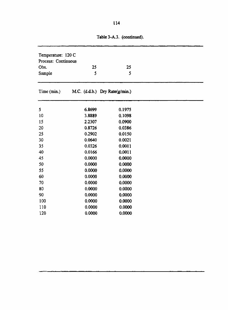
114
Table 3-A.3. (continued).
Temperature: 120 C Process: Continuous Obs. 25 25 Sample 5 5
Time (min.) M.C. (d.d.b.) Dry Rate(g/min.)
5 6.8699 0.1975 10 3.8889 0.1098 15 2.2307 0.0900 20 0.8726 0.0386 25 0.2902 0.0150 30 0.0640 0.0021 35 0.0326 0.0011 40 0.0166 0.0011 45 0.0000 0.0000 50 0.0000 0.0000 55 0.0000 0.0000 60 0.0000 0.0000 70 0.0000 0.0000 80 0.0000 0.0000 90 0.0000 0.0000 100 0.0000 0.0000 110 0.0000 0.0000 120 0.0000 0.0000
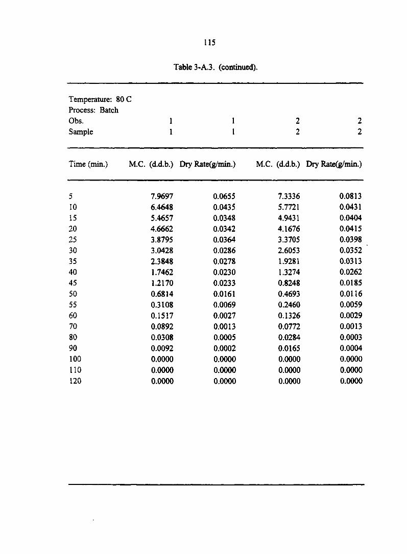
115
Table 3-A.3. (continued).
Temperature: 80 C Process: Batch Obs. 1 1 2 2 Sample 1 1 2 2
Time (min.) M.C. (d.d.b.) Dry Rate(g/min.) M.C. (d.d.b.) Dry Rate(g/min.)
5 7.9697 0.0655 7.3336 0.0813 10 6.4648 0.0435 5.7721 0.0431 15 5.4657 0.0348 4.9431 0.0404 20 4.6662 0.0342 4.1676 0.0415 25 3.8795 0.0364 3.3705 0.0398 30 3.0428 0.0286 2.6053 0.0352 35 2.3848 0.0278 1.9281 0.0313 40 1.7462 0.0230 1.3274 0.0262 45 1.2170 0.0233 0.8248 0.0185 50 0.6814 0.0161 0.4693 0.0116 55 0.3108 0.0069 0.2460 0.0059 60 0.1517 0.0027 0.1326 0.0029 70 0.0892 0.0013 0.0772 0.0013 80 0.0308 0.0005 0.0284 0.0003 90 0.0092 0.0002 0.0165 0.0004 100 0.0000 0.0000 0.0000 0.0000 110 0.0000 0.0000 0.0000 0.0000 120 0.0000 0.0000 0.0000 0.0000
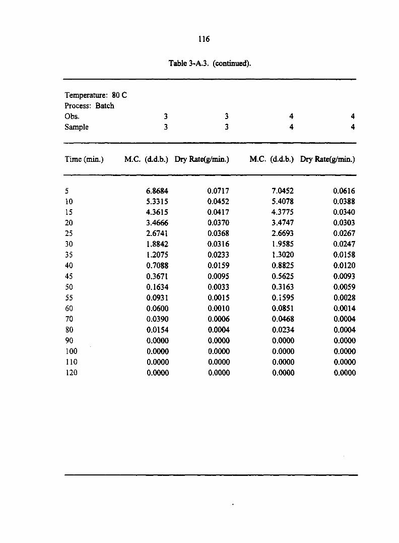
116
Table 3-A.3. (continued).
Temperature: 80 C Process: Batch Obs. 3 3 4 4 Sample 3 3 4 4
Time (min.) M.C. (d.d.b.) Dry Rate(g/min.) M.C. (d.d.b.) Dry Rate(g/min.)
5 6.8684 0.0717 7.0452 0.0616 10 5.3315 0.0452 5.4078 0.0388 15 4.3615 0.0417 4.3775 0.0340 20 3.4666 0.0370 3.4747 0.0303 25 2.6741 0.0368 2.6693 0.0267 30 1.8842 0.0316 1.9585 0.0247 35 1.2075 0.0233 1.3020 0.0158 40 0.7088 0.0159 0.8825 0.0120 45 0.3671 0.0095 0.5625 0.0093 50 0.1634 0.0033 0.3163 0.0059 55 0.0931 0.0015 0.1595 0.0028 60 0.0600 0.0010 0.0851 0.0014 70 0.0390 0.0006 0.0468 0.0004 80 0.0154 0.0004 0.0234 0.0004 90 0.0000 0.0000 0.0000 0.0000 100 0.0000 0.0000 0.0000 0.0000 1 1 0 0.0000 0.0000 0.0000 0.0000 120 0.0000 0.0000 0.0000 0.0000

117
Table 3-A.3. (continued).
Temperature: 80 C Process: Batch Obs. 5 5 6 6 Sample 5 5 1 1
Time (min.) M.C. (d.d.b.) Dry Rate(g/min.) M.C. (d.d.b.) Dry Rate(g/min.)
5 7.5969 0.0901 8.3138 0.1001 10 5.5745 0.0475 5.6011 0.0574 15 4.5094 0.0486 4.0466 0.0538 20 3.4183 0.0447 2.5875 0.0379 25 2.4143 0.0414 1.5604 0.0298 30 1.4861 0.0306 0.7523 0.0154 35 0.7998 0.0212 0.3355 0.0073 40 0.3241 0.0085 0.1377 0.0024 45 0.1329 0.0033 0.0732 0.0009 50 0.0588 0.0009 0.0488 0.0011 55 0.0382 0.0005 0.0195 0.0000 60 0.0265 0.0003 0.0190 0.0001 70 0.0193 0.0003 0.0168 0.0000 80 0.0058 0.0000 0.0168 0.0003 90 0.0054 0.0001 0.0000 0.0000 100 0.0000 0.0000 0.0000 0.0000 110 0.0000 0.0000 0.0000 0.0000 120 0.0000 0.0000 0.0000 0.0000

118
Table 3-A.3. (continued).
Temperature: 80 C Process: Batch Obs. 7 7 8 8 Sample 2 2 3 3
Time (min.) M.C. (d.d.b.) Dry Rate(g/min.) M.C. (d.d.b.) Dry Rate(g/min.)
5 7.6571 0.0870 7.0333 0.1068 10 5.9388 0.0513 4.7536 0.0569 15 4.9257 0.0466 3.5393 0.0492 20 4.0059 0.0473 2.4898 0.0407 25 3.0707 0.0433 1.6213 0.0307 30 2.2149 0.0380 0.9650 0.0235 35 1.4650 0.0286 0.4641 0.0139 40 0.9000 0.0213 0.1678 0.0039 45 0.4793 0.0135 0.0837 0.0021 50 0.2122 0.0059 0.0393 0.0009 55 0.0948 0.0019 0.0205 0.0000 60 0.0569 0.0005 0.0201 0.0005 70 0.0470 0.0007 0.0094 0.0001 80 0.0182 0.0004 0.0051 0.0001 90 0.0040 0.0001 0.0013 0.0000 100 0.0000 0.0000 0.0000 0.0000 110 0.0000 0.0000 0.0000 0.0000 120 0.0000 0.0000 0.0000 0.0000

119
Table 3-A.3. (continued).
Temperature: 80 C Process: Batch Obs. 9 9 10 10 Sample 4 4 5 5
Time (min.) M.C. (d.d.b.) Dry Rate(g/min.) M.C. (d.d.b.) Dry Rate(g/min.)
5 7.5099 0.1291 7.8671 0.1079 10 4.0714 0.0614 5.2021 0.0616 15 2.4358 0.0461 3.6798 0.0495 20 1.2083 0.0301 2.4560 0.0419 25 0.4065 0.0111 1.4200 0.0312 30 0.1108 0.0021 0.6497 0.0160 35 0.0559 0.0007 0.2549 0.0060 40 0.0362 0.0001 0.1057 0.0019 45 0.0346 0.0003 0.0583 0.0006 50 0.0256 0.0004 0.0440 0.0009 55 0.0144 0.0000 0.0227 0.0000 60 0.0144 0.0002 0.0227 0.0004 70 0.0085 0.0001 0.0138 0.0002 80 0.0043 0.0000 0.0049 0.0000 90 0.0043 0.0001 0.0049 0.0001 100 0.0000 0.0000 0.0000 0.0000 110 0.0000 0.0000 0.0000 0.0000 120 0.0000 0.0000 0.0000 0.0000

120
Table 3-A.3. (continued).
Temperature: 80 C Process: Batch Obs. 11 11 12 12 Sample 1 1 2 2
Time (min.) M.C. (d.d.b.) Dry Rate(g/min.) M.C. (d.d.b.) Dry Rate(g/min.)
5 8.1404 0.0774 7.7226 0.0903 10 6.2654 0.0436 5.7714 0.0525 15 5.2107 0.0460 4.6374 0.0572 20 4.0978 0.0339 3.4019 0.0444 25 3.2760 0.0315 2.4421 0.0470 30 2.5138 0.0283 1.4270 0.0304 35 1.8276 0.0213 0.7692 0.0186 40 1.3128 0.0210 0.3665 0.0110 45 0.8048 0.0144 0.1292 0.0026 50 0.4552 0.0094 0.0730 0.0011 55 0.2266 0.0048 0.0493 0.0006 60 0.1094 0.0019 0.0372 0.0004 70 0.0625 0.0010 0.0285 0.0001 80 0.0165 0.0002 0.0233 0.0005 90 0.0077 0.0002 0.0000 0.0000 100 0.0000 0.0000 0.0000 0.0000 110 0.0000 0.0000 0.0000 0.0000 120 0.0000 0.0000 0.0000 0.0000
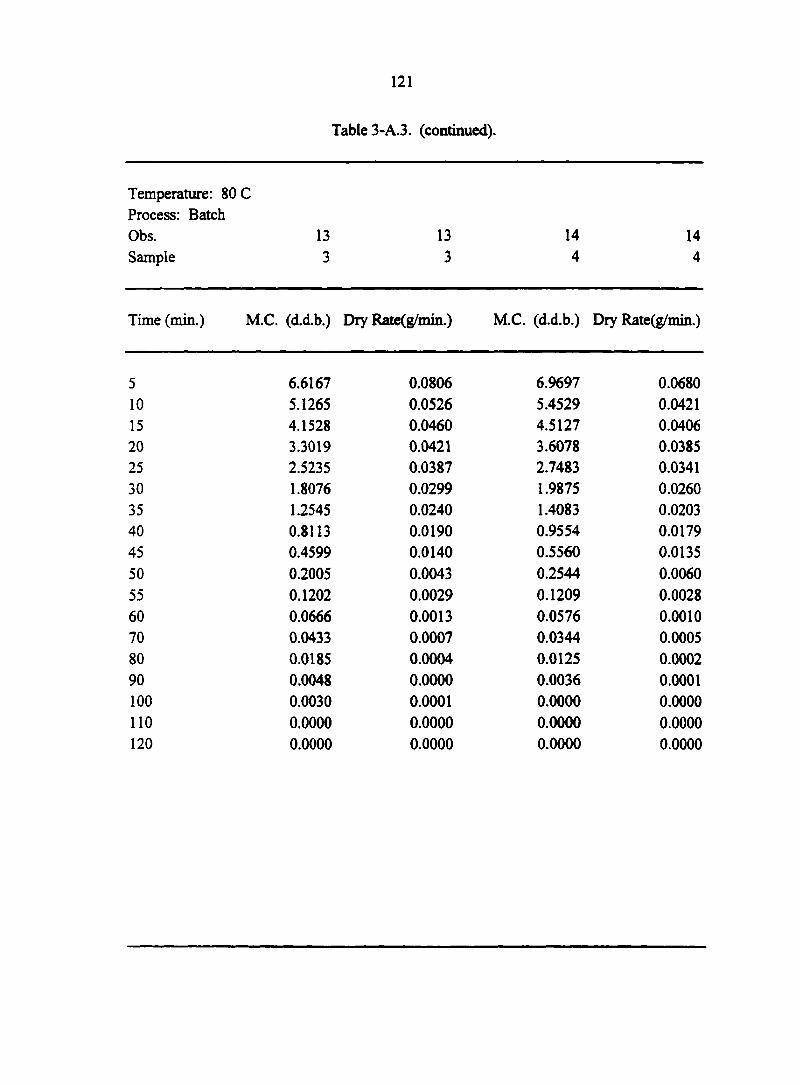
121
Table 3-A.3. (continued).
Temperature: 80 C Process: Batch Obs. 13 13 14 14 Sample 3 3 4 4
Time (min.) M.C. (d.d.b.) Dry Rate(g/min.) M.C. (d.d.b.) Dry Rate(g/min.)
5 6.6167 0.0806 6.9697 0.0680 10 5.1265 0.0526 5.4529 0.0421 15 4.1528 0.0460 4.5127 0.0406 20 3.3019 0.0421 3.6078 0.0385 25 2.5235 0.0387 2.7483 0.0341 30 1.8076 0.0299 1.9875 0.0260 35 1.2545 0.0240 1.4083 0.0203 40 0.8113 0.0190 0.9554 0.0179 45 0.4599 0.0140 0.5560 0.0135 50 0.2005 0.0043 0.2544 0.0060 55 0.1202 0.0029 0.1209 0.0028 60 0.0666 0.0013 0.0576 0.0010 70 0.0433 0.0007 0.0344 0.0005 80 0.0185 0.0004 0.0125 0.0002 90 0.0048 0.0000 0.0036 0.0001 100 0.0030 0.0001 0.0000 0.0000 110 0.0000 0.0000 0.0000 0.0000 120 0.0000 0.0000 0.0000 0.0000

122
Table 3-A.3. (continued).
Temperature: 80 C Process: Batch Obs. 15 15 16 16 Sample 5 5 1 1
Time (min.) M.C. (d.d.b.) Dry Rate(g/min.) M.C. (d.d.b.) Dry Rate(g/min.)
5 7.7937 0.0865 7.9183 0.1149 10 5.8867 0.0497 5.4356 0.0708 15 4.7920 0.0463 3.9049 0.0566 20 3.7726 0.0414 2.6811 0.0483 25 2.8594 0.0395 1.6366 0.0394 30 1.9881 0.0288 0.7861 0.0220 35 1.3530 0.0253 0.3103 0.0093 40 0.7951 0.0181 0.1093 0.0034 45 0.3962 0.0099 0.0363 0.0010 50 0.1781 0.0036 0.0151 0.0000 55 0.0983 0.0017 0.0151 0.0001 60 0.0617 0.0006 0.0134 0.0000 70 0.0476 0.0005 0.0134 0.0000 80 0.0264 0.0006 0.0134 0.0001 90 0.0000 0.0000 0.0073 0.0002 100 0.0000 0.0000 0.0000 0.0000 110 0.0000 0.0000 0.0000 0.0000 120 0.0000 0.0000 0.0000 0.0000

123
Table 3-A.3. (continued).
Temperature: 80 C Process: Batch Obs. 17 17 18 18 Sample 2 2 3 3
Time (min.) M.C. (d.d.b.) Dry Rate(g/min.) M.C. (d.d.b.) Dry Rate(g/min.)
5 7.5487 0.1014 7.2772 0.1173 10 5.5435 0.0572 4.9045 0.0644 15 4.4130 0.0615 3.6018 0.0611 20 3.1962 0.0490 2.3654 0.0439 25 2.2263 0.0430 1.4771 0.0365 30 1.3750 0.0303 0.7390 0.0216 35 0.7757 0.0217 0.3019 0.0099 40 0.3461 0.0116 0.1016 0.0025 45 0.1163 0.0037 0.0510 0.0011 50 0.0431 0.0004 0.0295 0.0007 55 0.0344 0.0007 0.0158 0.0005 60 0.0198 0.0003 0.0057 0.0000 70 0.0134 0.0001 0.0057 0.0001 80 0.0111 0.0003 0.0000 0.0000 90 0.0000 0.0000 0.0000 0.0000 100 0.0000 0.0000 0.0000 0.0000 110 0.0000 0.0000 0.0000 0.0000 120 0.0000 0.0000 0.0000 0.0000
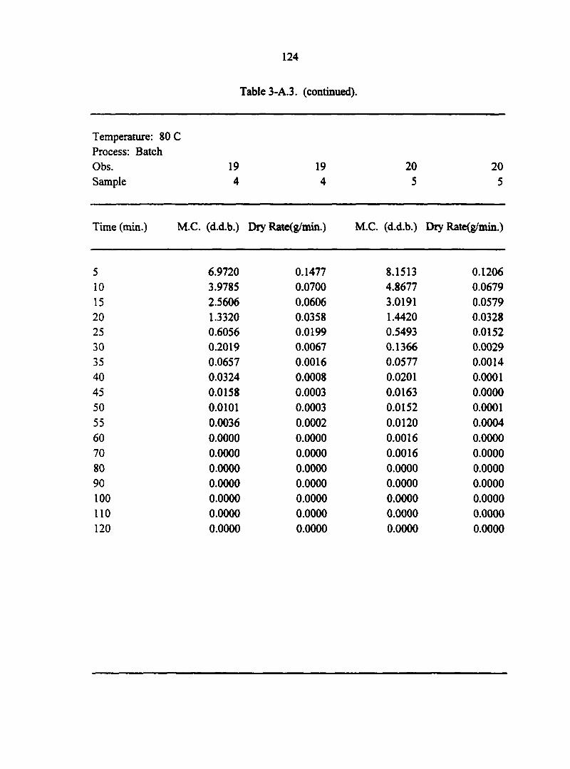
124
Table 3-A.3. (continued).
Temperature: 80 C Process: Batch Obs. 19 19 20 20 Sample 4 4 5 5
Time (min.) M.C. (d.d.b.) Dry Rate(g/min.) M.C. (d.d.b.) Dry Rate(g/min.)
5 6.9720 0.1477 8.1513 0.1206 10 3.9785 0.0700 4.8677 0.0679 15 2.5606 0.0606 3.0191 0.0579 20 1.3320 0.0358 1.4420 0.0328 25 0.6056 0.0199 0.5493 0.0152 30 0.2019 0.0067 0.1366 0.0029 35 0.0657 0.0016 0.0577 0.0014 40 0.0324 0.0008 0.0201 0.0001 45 0.0158 0.0003 0.0163 0.0000 50 0.0101 0.0003 0.0152 0.0001 55 0.0036 0.0002 0.0120 0.0004 60 0.0000 0.0000 0.0016 0.0000 70 0.0000 0.0000 0.0016 0.0000 80 0.0000 0.0000 0.0000 0.0000 90 0.0000 0.0000 0.0000 0.0000 100 0.0000 0.0000 0.0000 0.0000 110 0.0000 0.0000 0.0000 0.0000 120 0.0000 0.0000 0.0000 0.0000
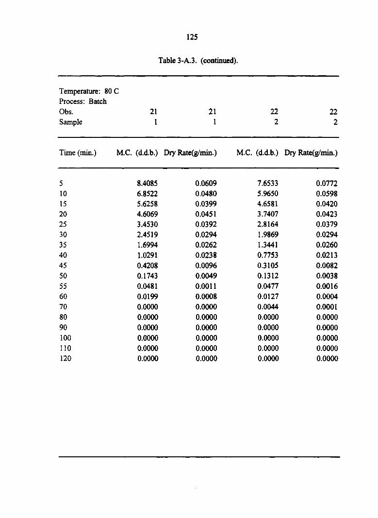
125
Table 3-A.3. (continued).
Temperature: 80 C Process: Batch Obs. 21 21 22 22 Sample 1 1 2 2
Time (min.) M.C. (d.d.b.) Dry Rate(g/min.) M.C. (d.d.b.) Dry Rate(g/min.)
5 8.4085 0.0609 7.6533 0.0772 10 6.8522 0.0480 5.9650 0.0598 15 5.6258 0.0399 4.6581 0.0420 20 4.6069 0.0451 3.7407 0.0423 25 3.4530 0.0392 2.8164 0.0379 30 2.4519 0.0294 1.9869 0.0294 35 1.6994 0.0262 1.3441 0.0260 40 1.0291 0.0238 0.7753 0.0213 45 0.4208 0.0096 0.3105 0.0082 50 0.1743 0.0049 0.1312 0.0038 55 0.0481 0.0011 0.0477 0.0016 60 0.0199 0.0008 0.0127 0.0004 70 0.0000 0.0000 0.0044 0.0001 80 0.0000 0.0000 0.0000 0.0000 90 0.0000 0.0000 0.0000 0.0000 100 0.0000 0.0000 0.0000 0.0000 110 0.0000 0.0000 0.0000 0.0000 120 0.0000 0.0000 0.0000 0.0000

126
Table 3-A.3. (continued).
Temperature: 80 C Process: Batch Obs. 23 23 24 24 Sample 3 3 4 4
Time (min.) M.C. (d.d.b.) Dry Rate(g/min.) M.C. (d.d.b.) Dry Rate(g/min.)
5 8.0654 0.0920 7.1641 0.0848 10 5.8692 0.0708 5.6710 0.0694 15 4.1785 0.0552 4.4491 0.0617 20 2.8621 0.0509 3.3625 0.0573 25 1.6477 0.0359 2.3529 0.0502 30 0.7905 0.0199 1.4692 0.0363 35 0.3146 0.0109 0.8292 0.0315 40 0.0544 0.0001 0.2740 0.0103 45 0.0516 0.0005 0.0923 0.0038 50 0.0401 0.0009 0.0257 0.0009 55 0.0181 0.0005 0.0092 0.0004 60 0.0072 0.0003 0.0018 0.0000 70 0.0000 0.0000 0.0011 0.0000 80 0.0000 0.0000 0.0007 0.0000 90 0.0000 0.0000 0.0000 0.0000 100 0.0000 0.0000 0.0000 0.0000 110 0.0000 0.0000 0.0000 0.0000 120 0.0000 0.0000 0.0000 0.0000
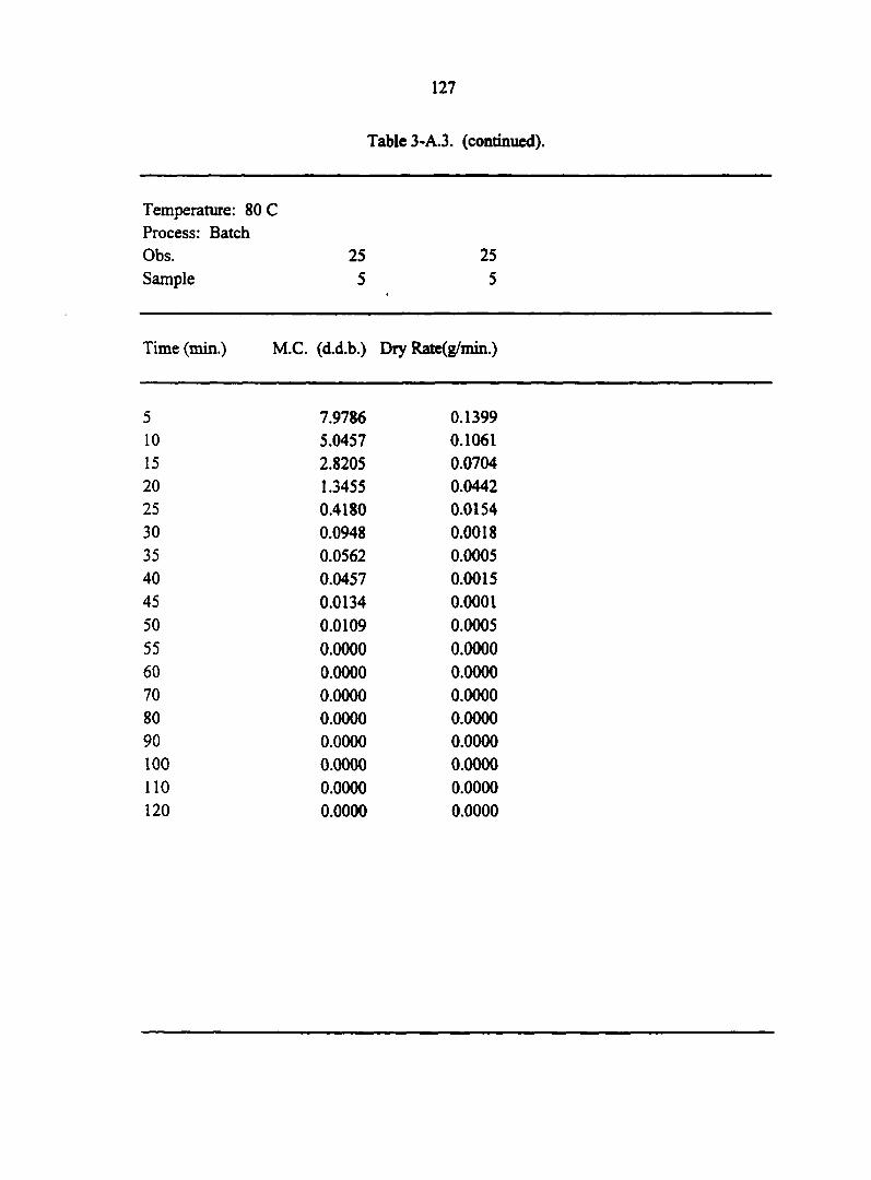
127
Table 3-A.3. (continued).
Temperature: 80 C Process: Batch Obs. Sample
25 25 5 5
Time (min.) M.C. (d.d.b.) Dry Rate(g/min.)
5 7.9786 0.1399 10 5.0457 0.1061 15 2.8205 0.0704 20 1.3455 0.0442 25 0.4180 0.0154 30 0.0948 0.0018 35 0.0562 0.0005 40 0.0457 0.0015 45 0.0134 0.0001 50 0.0109 0.0005 55 0.0000 0.0000 60 0.0000 0.0000 70 0.0000 0.0000 80 0.0000 0.0000 90 0.0000 0.0000 100 0.0000 0.0000 110 0.0000 0.0000 120 0.0000 0.0000
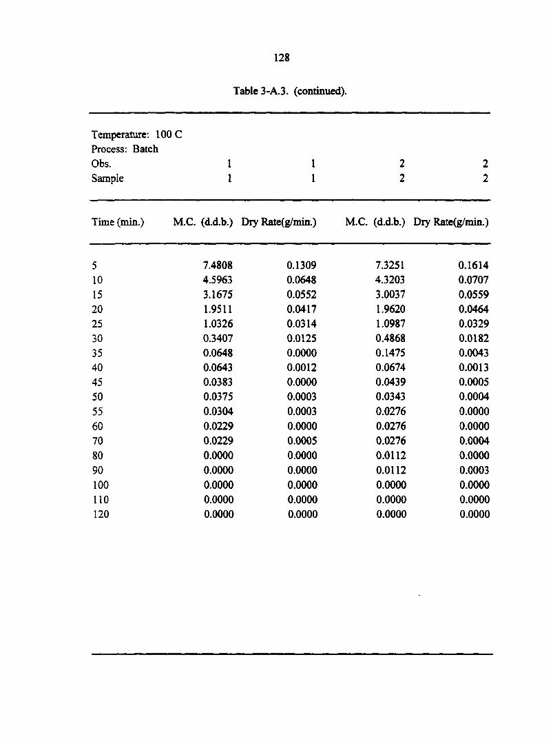
128
Table 3-A.3. (continued).
Temperature: 100 C Process: Batch Obs. 1 1 2 2 Sample 1 1 2 2
Time (min.) M.C. (d.d.b.) Dry Rate(g/min.) M.C. (d.d.b.) Dry Rate(g/min.)
5 7.4808 0.1309 7.3251 0.1614 10 4.5963 0.0648 4.3203 0.0707 15 3.1675 0.0552 3.0037 0.0559 20 1.9511 0.0417 1.9620 0.0464 25 1.0326 0.0314 1.0987 0.0329 30 0.3407 0.0125 0.4868 0.0182 35 0.0648 0.0000 0.1475 0.0043 40 0.0643 0.0012 0.0674 0.0013 45 0.0383 0.0000 0.0439 0.0005 50 0.0375 0.0003 0.0343 0.0004 55 0.0304 0.0003 0.0276 0.0000 60 0.0229 0.0000 0.0276 0.0000 70 0.0229 0.0005 0.0276 0.0004 80 0.0000 0.0000 0.0112 0.0000 90 0.0000 0.0000 0.0112 0.0003 100 0.0000 0.0000 0.0000 0.0000 110 0.0000 0.0000 0.0000 0.0000 120 0.0000 0.0000 0.0000 0.0000
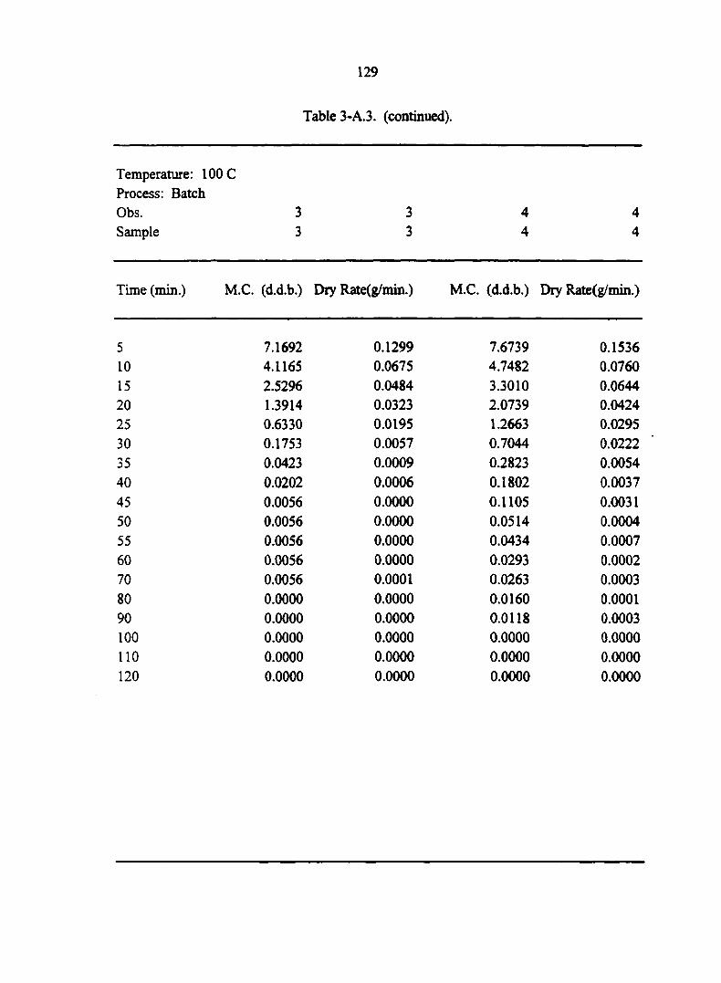
129
Table 3-A.3. (continued).
Temperature: 100 C Process: Batch Obs. 3 3 4 4 Sample 3 3 4 4
Time (min.) M.C. (d.d.b.) Dry Rate(g/min.) M.C. (d.d.b.) Dry Rate(g/min.)
5 7.1692 0.1299 7.6739 0.1536 10 4.1165 0.0675 4.7482 0.0760 15 2.5296 0.0484 3.3010 0.0644 20 1.3914 0.0323 2.0739 0.0424 25 0.6330 0.0195 1.2663 0.0295 30 0.1753 0.0057 0.7044 0.0222 35 0.0423 0.0009 0.2823 0.0054 40 0.0202 0.0006 0.1802 0.0037 45 0.0056 0.0000 0.1105 0.0031 50 0.0056 0.0000 0.0514 0.0004 55 0.0056 0.0000 0.0434 0.0007 60 0.0056 0.0000 0.0293 0.0002 70 0.0056 0.0001 0.0263 0.0003 80 0.0000 0.0000 0.0160 0.0001 90 0.0000 0.0000 0.0118 0.0003 100 0.0000 0.0000 0.0000 0.0000 110 0.0000 0.0000 0.0000 0.0000 120 0.0000 0.0000 0.0000 0.0000
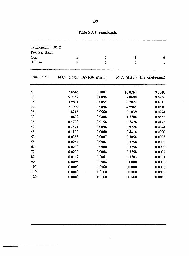
130
Table 3-A.3. (continued).
Temperature: 100 C Process: Batch Obs. 5 5 6 6 Sample 5 5 1 1
Time (min.) M.C. (d.d.b.) Dry Rate(g/min.) M.C. (d.d.b.) Dry Rate(g/min.)
5 7.8646 0.1881 10.8261 0.1610 10 5.2382 0.0896 7.8600 0.0856 15 3.9874 0.0855 6.2822 0.0915 20 2.7939 0.0696 4.5965 0.0810 25 1.8216 0.0560 3.1039 0.0724 30 1.0402 0.0408 1.7708 0.0555 35 0.4700 0.0156 0.7476 0.0122 40 0.2524 0.0096 0.5228 0.0044 45 0.1190 0.0060 0.4414 0.0030 50 0.0355 0.0007 0.3858 0.0005 55 0.0254 0.0002 0.3758 0.0000 60 0.0232 0.0000 0.3758 0.0000 70 0.0232 0.0004 0.3758 0.0002 80 0.0117 0.0001 0.3703 0.0101 90 0.0098 0.0004 0.0000 0.0000 100 0.0000 0.0000 0.0000 0.0000 110 0.0000 0.0000 0.0000 0.0000 120 0.0000 0.0000 0.0000 0.0000
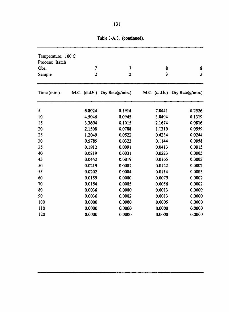
131
Table 3-A.3. (continued).
Temperature: 100 C Process: Batch Obs. 7 7 8 8 Sample 2 2 3 3
Time (min.) M.C. (d.d.b.) Dry Rate(g/min.) M.C. (d.d.b.) Dry Rate(g/min.)
5 6.8024 0.1914 7.0441 0.2526 10 4.5046 0.0945 3.8404 0.1319 15 3.3694 0.1015 2.1674 0.0816 20 2.1508 0.0788 1.1319 0.0559 25 1.2049 0.0522 0.4234 0.0244 30 0.5785 0.0323 0.1144 0.0058 35 0.1912 0.0091 0.0413 0.0015 40 0.0819 0.0031 0.0223 0.0005 45 0.0442 0.0019 0.0165 0.0002 50 0.0219 0.0001 0.0142 0.0002 55 0.0202 0.0004 0.0114 0.0003 60 0.0159 0.0000 0.0079 0.0002 70 0.0154 0.0005 0.0056 0.0002 80 0.0036 0.0000 0.0013 0.0000 90 0.0036 0.0002 0.0013 0.0000 100 0.0000 0.0000 0.0005 0.0000 110 0.0000 0.0000 0.0000 0.0000 120 0.0000 0.0000 0.0000 0.0000
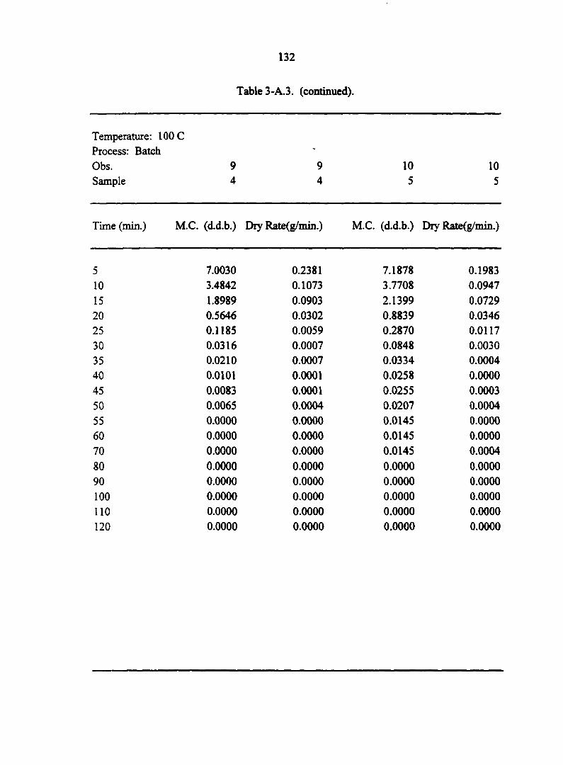
132
Table 3-A.3. (continued).
Temperature: 100 C Process: Batch -
Obs. 9 9 10 10 Sample 4 4 5 5
Time (min.) M.C. (d.d.b.)
I s M.C. (d.d.b.) Dry Rate(g/min.)
5 7.0030 0.2381 7.1878 0.1983 10 3.4842 0.1073 3.7708 0.0947 15 1.8989 0.0903 2.1399 0.0729 20 0.5646 0.0302 0.8839 0.0346 25 0.1185 0.0059 0.2870 0.0117 30 0.0316 0.0007 0.0848 0.0030 35 0.0210 0.0007 0.0334 0.0004 40 0.0101 0.0001 0.0258 0.0000 45 0.0083 0.0001 0.0255 0.0003 50 0.0065 0.0004 0.0207 0.0004 55 0.0000 0.0000 0.0145 0.0000 60 0.0000 0.0000 0.0145 0.0000 70 0.0000 0.0000 0.0145 0.0004 80 0.0000 0.0000 0.0000 0.0000 90 0.0000 0.0000 0.0000 0.0000 100 0.0000 0.0000 0.0000 0.0000 110 0.0000 0.0000 0.0000 0.0000 120 0.0000 0.0000 0.0000 0.0000

133
Table 3-A.3. (continued).
Temperature: 100 C Process: Batch Obs. 11 11 12 12 Sample 1 1 2 2
Time (min.) M.C. (d.d.b.) Dry Rate(g/min.) M.C. (d.d.b.) Dry Rate(g/min.)
5 7.6455 0.1188 7.8636 0.1376 10 5.2588 0.0649 4.4766 0.0718 15 3.9538 0.0595 2.7095 0.0496 20 2.7580 0.0510 1.4874 0.0366 25 1.7331 0.0400 0.5854 0.0162 30 0.9301 0.0335 0.1856 0.0057 35 0.2564 0.0077 0.0463 0.0003 40 0.1009 0.0026 0.0389 0.0002 45 0.0482 0.0003 0.0340 0.0001 50 0.0426 0.0011 0.0305 0.0002 55 0.0201 0.0001 0.0261 0.0000 60 0.0185 0.0000 0.0261 0.0007 70 0.0185 0.0002 0.0084 0.0000 80 0.0117 0.0003 0.0084 0.0002 90 0.0000 0.0000 0.0000 0.0000 100 0.0000 0.0000 0.0000 0.0000 110 0.0000 0.0000 0.0000 0.0000 120 0.0000 0.0000 0.0000 0.0000

134
Table 3-A.3. (continued).
T emperature: 100 C Process: Batch Obs. 13 13 14 14 Sample 3 3 4 4
Time (min.) M.C. (d.d.b.) Dry Rate(g/min.) M.C. (d.d.b.)
1 $
5 6.9111 0.1459 7.4326 0.1802 10 3.9746 0.0691 3.4756 0.0656 15 2.5835 0.0560 2.0360 0.0546 20 1.4559 0.0398 0.8375 0.0293 25 0.6543 0.0222 0.1941 0.0078 30 0.2068 0.0083 0.0224 0.0003 35 0.0402 0.0009 0.0149 0.0003 40 0.0229 0.0003 0.0088 0.0000 45 0.0161 0.0000 0.0079 0.0004 50 0.0157 0.0007 0.0000 0.0000 55 0.0012 0.0000 0.0000 0.0000 60 0.0012 0.0000 0.0000 0.0000 70 0.0012 0.0000 0.0000 0.0000 80 0.0012 0.0000 0.0000 0.0000 90 0.0000 0.0000 0.0000 0.0000 100 0.0000 0.0000 0.0000 0.0000 110 0.0000 0.0000 0.0000 0.0000 120 0.0000 0.0000 0.0000 0.0000

135
Table 3-A.3. (continued).
Temperature: 100 C Process: Batch Obs. 15 15 16 16 Sample 5 5 1 1
Time (min.) M.C. (d.d.b.) Dry Rate(g/min.) M.C. (d.d.b.) Dry Rate(g/min.)
5 6.8662 0.1605 7.2804 0.1991 10 2.1367 0.0484 3.0124 0.0647 15 0.7113 0.0201 1.6261 0.0487 20 0.1179 0.0025 0.5815 0.0220 25 0.0448 0.0002 0.1102 0.0042 30 0.0395 0.0011 0.0193 0.0001 35 0.0077 0.0000 0.0167 0.0000 40 0.0077 0.0003 0.0167 0.0004 45 0.0000 0.0000 0.0077 0.0000 50 0.0000 0.0000 0.0077 0.0000 55 0.0000 0.0000 0.0077 0.0004 60 0.0000 0.0000 0.0000 0.0000 70 0.0000 0.0000 0.0000 0.0000 80 0.0000 0.0000 0.0000 0.0000 90 0.0000 0.0000 0.0000 0.0000 100 0.0000 0.0000 0.0000 0.0000 110 0.0000 0.0000 0.0000 0.0000 120 0.0000 0.0000 0.0000 0.0000

136
Table 3-A.3. (continued).
Temperature: 100 C Process: Batch Obs. 17 17 18 18 Sample 2 2 3 3
Time (min.) M.C. (d.d.b.) Dry Rate(g/min.) M.C. (d.d.b.) Dry Rate(g/min.)
5 6.6977 0.1805 7.3524 0.2167 10 3.7166 0.0752 3.1092 0.0747 15 2.4747 0.0689 1.6472 0.0607 20 1.3370 0.0459 0.4581 0.0199 25 0.5785 0.0255 0.0693 0.0019 30 0.1566 0.0081 0.0313 0.0001 35 0.0235 0.0001 0.0286 0.0000 40 0.0221 0.0006 0.0286 0.0008 45 0.0129 0.0000 0.0125 0.0000 50 0.0126 0.0002 0.0125 0.0006 55 0.0099 0.0004 0.0016 0.0001 60 0.0026 0.0000 0.0000 0.0000 70 0.0026 0.0000 0.0000 0.0000 80 0.0026 0.0001 0.0000 0.0000 90 0.0000 0.0000 0.0000 0.0000 100 0.0000 0.0000 0.0000 0.0000 110 0.0000 0.0000 0.0000 0.0000 120 0.0000 0.0000 0.0000 0.0000

137
Table 3-A.3. (continued).
Temperature: 100 C Process: Batch Obs. 19 19 20 20 Sample 4 4 5 5
Time (min.) M.C. (d.d.b.) Dry Rate(g/min.) M.C. (d.d.b.) Dry Rate(g/min.)
5 7.3509 0.2421 7.1778 0.2279 10 2.8785 0.0833 2.7910 0.0709 15 1.3391 0.0551 1.4261 0.0493 20 0.3221 0.0132 0.4781 0.0200 25 0.0783 0.0027 0.0928 0.0036 30 0.0277 0.0000 0.0235 0.0002 35 0.0277 0.0003 0.0192 0.0005 40 0.0218 0.0000 0.0100 0.0002 45 0.0218 0.0001 0.0069 0.0000 50 0.0196 0.0000 0.0069 0.0000 55 0.0196 0.0000 0.0069 0.0004 60 0.0196 0.0000 0.0000 0.0000 70 0.0196 0.0001 0.0000 0.0000 80 0.0163 0.0004 0.0000 0.0000 90 0.0000 0.0000 0.0000 0.0000 100 0.0000 0.0000 0.0000 0.0000 110 0.0000 0.0000 0.0000 0.0000 120 0.0000 0.0000 0.0000 0.0000

138
Table 3-A.3. (continued).
Temperature: 100 C Process: Batch Obs. 21 21 22 22 Sample 1 1 2 2
Time (min.) M.C. (d.d.b.) Dry Rate(g/min.) M.C. (d.d.b.) Dry Rate(g/min.)
5 8.5417 0.1141 8.3486 0.1297 10 5.8688 0.0733 5.1949 0.0718 15 4.1509 0.0847 3.4502 0.0708 20 2.1668 0.0504 1.7297 0.0402 25 0.9864 0.0349 0.7521 0.0250 30 0.1687 0.0070 0.1434 0.0058 35 0.0042 0.0000 0.0029 0.0000 40 0.0037 0.0000 0.0024 0.0000 45 0.0033 0.0000 0.0019 0.0000 50 0.0028 0.0000 0.0015 0.0000 55 0.0023 0.0000 0.0010 0.0000 60 0.0019 0.0000 0.0005 0.0000 70 0.0014 0.0000 0.0000 0.0000 80 0.0009 0.0000 0.0000 0.0000 90 0.0005 0.0000 0.0000 0.0000 100 0.0000 0.0000 0.0000 0.0000 110 0.0000 0.0000 0.0000 0.0000 120 0.0000 0.0000 0.0000 0.0000
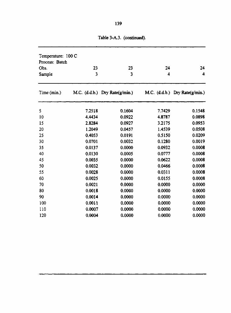
139
Table 3-A.3. (continued).
Temperature: 100 C Process: Batch Obs. 23 23 24 24 Sample 3 3 4 4
Time (min.) M.C. (d.d.b.) Dry Rate(g/min.) M.C. (d.d.b.) Dry Rate(g/min.)
5 7.2518 0.1604 7.7429 0.1548 10 4.4434 0.0922 4.8787 0.0898 15 2.8284 0.0927 3.2175 0.0953 20 1.2049 0.0457 1.4539 0.0508 25 0.4053 0.0191 0.5150 0.0209 30 0.0701 0.0032 0.1280 0.0019 35 0.0137 0.0000 0.0932 0.0008 40 0.0130 0.0005 0.0777 0.0008 45 0.0035 0.0000 0.0622 0.0008 50 0.0032 0.0000 0.0466 0.0008 55 0.0028 0.0000 0.0311 0.0008 60 0.0025 0.0000 0.0155 0.0008 70 0.0021 0.0000 0.0000 0.0000 80 0.0018 0.0000 0.0000 0.0000 90 0.0014 0.0000 0.0000 0.0000 100 0.0011 0.0000 0.0000 0.0000 110 0.0007 0.0000 0.0000 0.0000 120 0.0004 0.0000 0.0000 0.0000
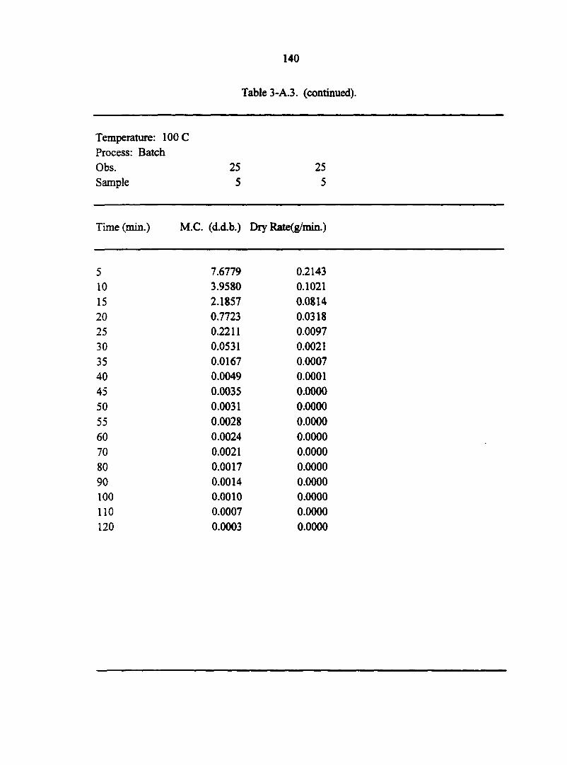
140
Table 3-A.3. (continued).
Temperature: 100 C Process: Batch Obs. 25 25 Sample 5 5
Time (min.) M.C. (d.d.b.) Dry Rate(g/min.)
5 7.6779 0.2143 10 3.9580 0.1021 15 2.1857 0.0814 20 0.7723 0.0318 25 0.2211 0.0097 30 0.0531 0.0021 35 0.0167 0.0007 40 0.0049 0.0001 45 0.0035 0.0000 50 0.0031 0.0000 55 0.0028 0.0000 60 0.0024 0.0000 70 0.0021 0.0000 80 0.0017 0.0000 90 0.0014 0.0000 100 0.0010 0.0000 110 0.0007 0.0000 120 0.0003 0.0000

141
Table 3-A.3. (continued).
Temperature: 120 C Process: Batch Obs. 1 1 2 2 Sample 1 1 2 2
Time (min.) M.C. (d.d.b.) Dry Rate(g/min.) M.C. (d.d.b.) Dry Rate(g/min.)
5 8.5067 0.1769 7.6185 0.1453 10 4.5677 0.0965 3.9724 0.0832 15 2.4185 0.0753 1.8835 0.0560 20 0.7422 0.0318 0.4789 0.0177 25 0.0338 0.0012 0.0351 0.0000 30 0.0062 0.0003 0.0341 0.0014 35 0.0000 0.0000 0.0000 0.0000 40 0.0000 0.0000 0.0000 0.0000 45 0.0000 0.0000 0.0000 0.0000 50 0.0000 0.0000 0.0000 0.0000 55 0.0000 0.0000 0.0000 0.0000 60 0.0000 0.0000 0.0000 0.0000 70 0.0000 0.0000 0.0000 0.0000 80 0.0000 0.0000 0.0000 0.0000 90 0.0000 0.0000 0.0000 0.0000 100 0.0000 0.0000 0.0000 0.0000 110 0.0000 0.0000 0.0000 0.0000 120 0.0000 0.0000 0.0000 0.0000

142
Table 3-A.3. (continued).
Temperature: 120 C Process: Batch Obs. 3 3 4 4 Sample 3 3 4 4
Time (min.) M.C. (d.d.b.)
1 $ M.C. (d.d.b.) Dry Rate(g/min.)
5 7.3491 0.1742 7.1527 0.1693 10 3.4512 0.0918 3.6115 0.0915 15 1.3966 0.0527 1.6980 0.0669 20 0.2175 0.0085 0.2986 0.0133 25 0.0273 0.0003 0.0213 0.0000 30 0.0215 0.0010 0.0213 0.0005 35 0.0000 0.0000 0.0117 0.0006 40 0.0000 0.0000 0.0000 0.0000 45 0.0000 0.0000 0.0000 0.0000 50 0.0000 0.0000 0.0000 0.0000 55 0.0000 0.0000 0.0000 0.0000 60 0.0000 0.0000 0.0000 0.0000 70 0.0000 0.0000 0.0000 0.0000 80 0.0000 0.0000 0.0000 0.0000 90 0.0000 0.0000 0.0000 0.0000 100 0.0000 0.0000 0.0000 0.0000 110 0.0000 0.0000 0.0000 0.0000 120 0.0000 0.0000 0.0000 0.0000

143
Table 3-A.3. (continued).
Temperature: 120 C Process: Batch Obs. 5 5 6 6 Sample 5 5 1 1
Time (min.) M.C. (d.d.b.) Dry Rate(g/min.) M.C. (d.d.b.) Dry Rate(g/min.)
5 7.6059 0.2490 7.8241 0.1380 10 3.2979 0.1234 4.8721 0.0920 15 1.1637 0.0594 2.9029 0.0770 20 0.1367 0.0069 1.2546 0.0500 25 0.0166 0.0010 0.1849 0.0075 30 0.0000 0.0000 0.0252 0.0012 35 0.0000 0.0000 0.0000 0.0000 40 0.0000 0.0000 0.0000 0.0000 45 0.0000 0.0000 0.0000 0.0000 50 0.0000 0.0000 0.0000 0.0000 55 0.0000 0.0000 0.0000 0.0000 60 0.0000 0.0000 0.0000 0.0000 70 0.0000 0.0000 0.0000 0.0000 80 0.0000 0.0000 0.0000 0.0000 90 0.0000 0.0000 0.0000 0.0000 100 0.0000 0.0000 0.0000 0.0000 110 0.0000 0.0000 0.0000 0.0000 120 0.0000 0.0000 0.0000 0.0000

144
Table 3-A.3. (continued).
Temperature: 120 C Process: Batch Obs. 7 7 8 8 Sample 2 2 3 3
Time (min.) M.C. (d.d.b.) Dry Rate(g/min.) M.C. (d.d.b.) Dry Rate(g/min.)
5 7.3617 0.1591 7.3097 0.1851 10 4.6131 0.0997 2.9601 0.0920 15 2.8919 0.0792 0.7984 0.0329 20 1.5247 0.0575 0.0244 0.0001 25 0.5320 0.0251 0.0226 0.0008 30 0.0981 0.0054 0.0047 0.0002 35 0.0045 0.0003 0.0000 0.0000 40 0.0000 0.0000 0.0000 0.0000 45 0.0000 0.0000 0.0000 0.0000 50 0.0000 0.0000 0.0000 0.0000 55 0.0000 0.0000 0.0000 0.0000 60 0.0000 0.0000 0.0000 0.0000 70 0.0000 0.0000 0.0000 0.0000 80 0.0000 0.0000 0.0000 0.0000 90 0.0000 0.0000 0.0000 0.0000 100 0.0000 0.0000 0.0000 0.0000 110 0.0000 0.0000 0.0000 0.0000 120 0.0000 0.0000 0.0000 0.0000

145
Table 3-A.3. (continued).
Temperature: 120 C Process: Batch Obs. 9 9 10 10 Sample 4 4 5 5
Time (min.) M.C. (d.d.b.) Dry Rate(g/min.) M.C. (d.d.b.) Dry Rate(g/min.)
5 7.0856 0.1954 7.8811 0.2422 10 3.7688 0.1062 3.0483 0.1058 15 1.9660 0.0759 0.9377 0.0417 20 0.6774 0.0338 0.1061 0.0028 25 0.1032 0.0040 0.0503 0.0012 30 0.0346 0.0020 0.0255 0.0000 35 0.0000 0.0000 0.0255 0.0013 40 0.0000 0.0000 0.0000 0.0000 45 0.0000 0.0000 0.0000 0.0000 50 0.0000 0.0000 0.0000 0.0000 55 0.0000 0.0000 0.0000 0.0000 60 0.0000 0.0000 0.0000 0.0000 70 0.0000 0.0000 0.0000 0.0000 80 0.0000 0.0000 0.0000 0.0000 90 0.0000 0.0000 0.0000 0.0000 100 0.0000 0.0000 0.0000 0.0000 110 0.0000 0.0000 0.0000 0.0000 120 0.0000 0.0000 0.0000 0.0000
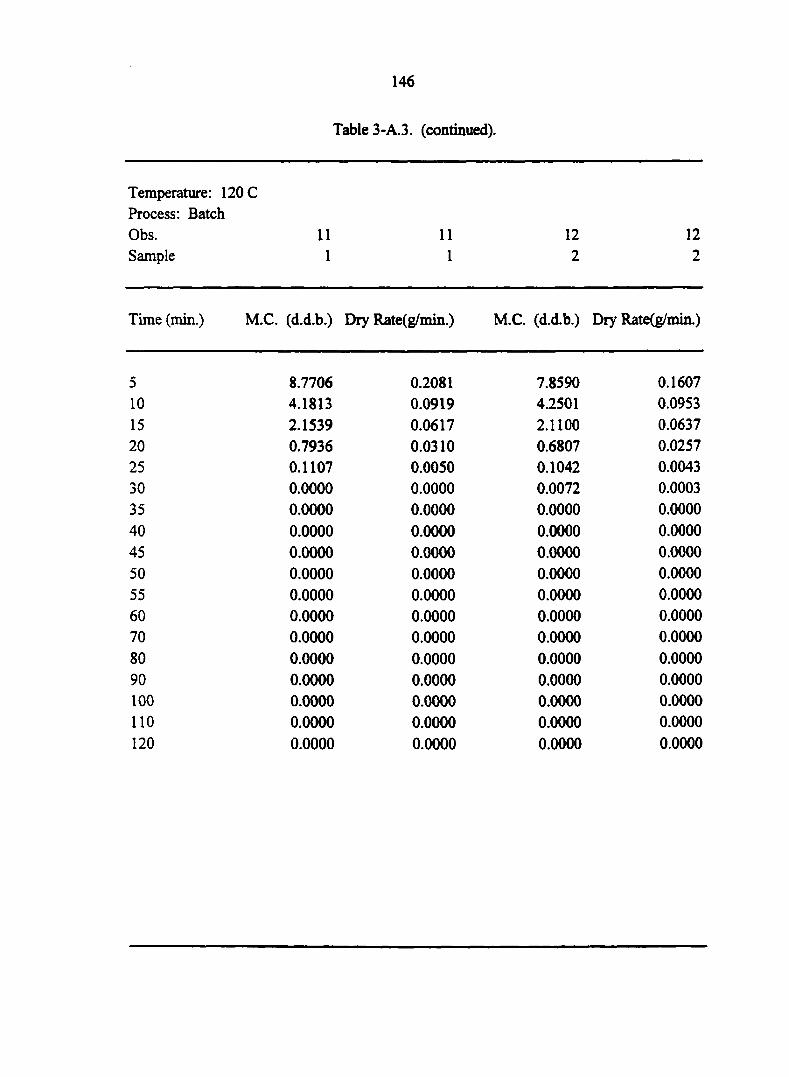
146
Table 3-A.3. (continued).
Temperature: 120 C Process: Batch Obs. 11 11 12 12 Sample 1 1 2 2
Time (min.) M.C. (d.d.b.) Dry Rate(g/min.) M.C. (d.d.b.) Dry Rate(g/min.)
5 8.7706 0.2081 7.8590 0.1607 10 4.1813 0.0919 4.2501 0.0953 15 2.1539 0.0617 2.1100 0.0637 20 0.7936 0.0310 0.6807 0.0257 25 0.1107 0.0050 0.1042 0.0043 30 0.0000 0.0000 0.0072 0.0003 35 0.0000 0.0000 0.0000 0.0000 40 0.0000 0.0000 0.0000 0.0000 45 0.0000 0.0000 0.0000 0.0000 50 0.0000 0.0000 0.0000 0.0000 55 0.0000 0.0000 0.0000 0.0000 60 0.0000 0.0000 0.0000 0.0000 70 0.0000 0.0000 0.0000 0.0000 80 0.0000 0.0000 0.0000 0.0000 90 0.0000 0.0000 0.0000 0.0000 100 0.0000 0.0000 0.0000 0.0000 110 0.0000 0.0000 0.0000 0.0000 120 0.0000 0.0000 0.0000 0.0000

147
Table 3-A.3. (continued).
Temperature: 120 C Process: Batch Obs. 13 13 14 14 Sample 3 3 4 4
Time (min.) M.C. (d.d.b.) Dry Rate(g/min.) M.C. (d.d.b.) Dry Rate(g/min.)
5 7.8210 0.1857 7.5413 0.1819 10 3.9992 0.1042 4.0473 0.1060 15 1.8556 0.0634 2.0119 0.0689 20 0.5510 0.0224 0.6877 0.0318 25 0.0897 0.0042 0.0776 0.0033 30 0.0041 0.0002 0.0134 0.0000 35 0.0000 0.0000 0.0134 0.0007 40 0.0000 0.0000 0.0000 0.0000 45 0.0000 0.0000 0.0000 0.0000 50 0.0000 0.0000 0.0000 0.0000 55 0.0000 0.0000 0.0000 0.0000 60 0.0000 0.0000 0.0000 0.0000 70 0.0000 0.0000 0.0000 0.0000 80 0.0000 0.0000 0.0000 0.0000 90 0.0000 0.0000 0.0000 0.0000 100 0.0000 0.0000 0.0000 0.0000 110 0.0000 0.0000 0.0000 0.0000 120 0.0000 0.0000 0.0000 0.0000
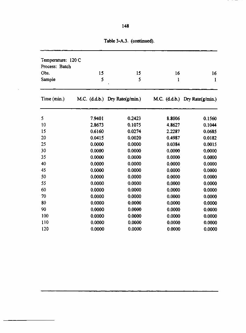
148
Table 3-A.3. (continued).
Temperature: 120 C Process: Batch Obs. 15 15 16 16 Sample 5 5 1 1
Time (min.) M.C. (d.d.b.) Dry Rate(g/min.) M.C. (d.d.b.) Dry Rate(g/min.)
5 7.9401 0.2423 8.8006 0.1560 10 2.8673 0.1075 4.8627 0.1044 15 0.6160 0.0274 2.2287 0.0685 20 0.0415 0.0020 0.4987 0.0182 25 0.0000 0.0000 0.0384 0.0015 30 0.0000 0.0000 0.0000 0.0000 35 0.0000 0.0000 0.0000 0.0000 40 0.0000 0.0000 0.0000 0.0000 45 0.0000 0.0000 0.0000 0.0000 50 0.0000 0.0000 0.0000 0.0000 55 0.0000 0.0000 0.0000 0.0000 60 0.0000 0.0000 0.0000 0.0000 70 0.0000 0.0000 0.0000 0.0000 80 0.0000 0.0000 0.0000 0.0000 90 0.0000 0.0000 0.0000 0.0000 100 0.0000 0.0000 0.0000 0.0000 110 0.0000 0.0000 0.0000 0.0000 120 0.0000 0.0000 0.0000 0.0000
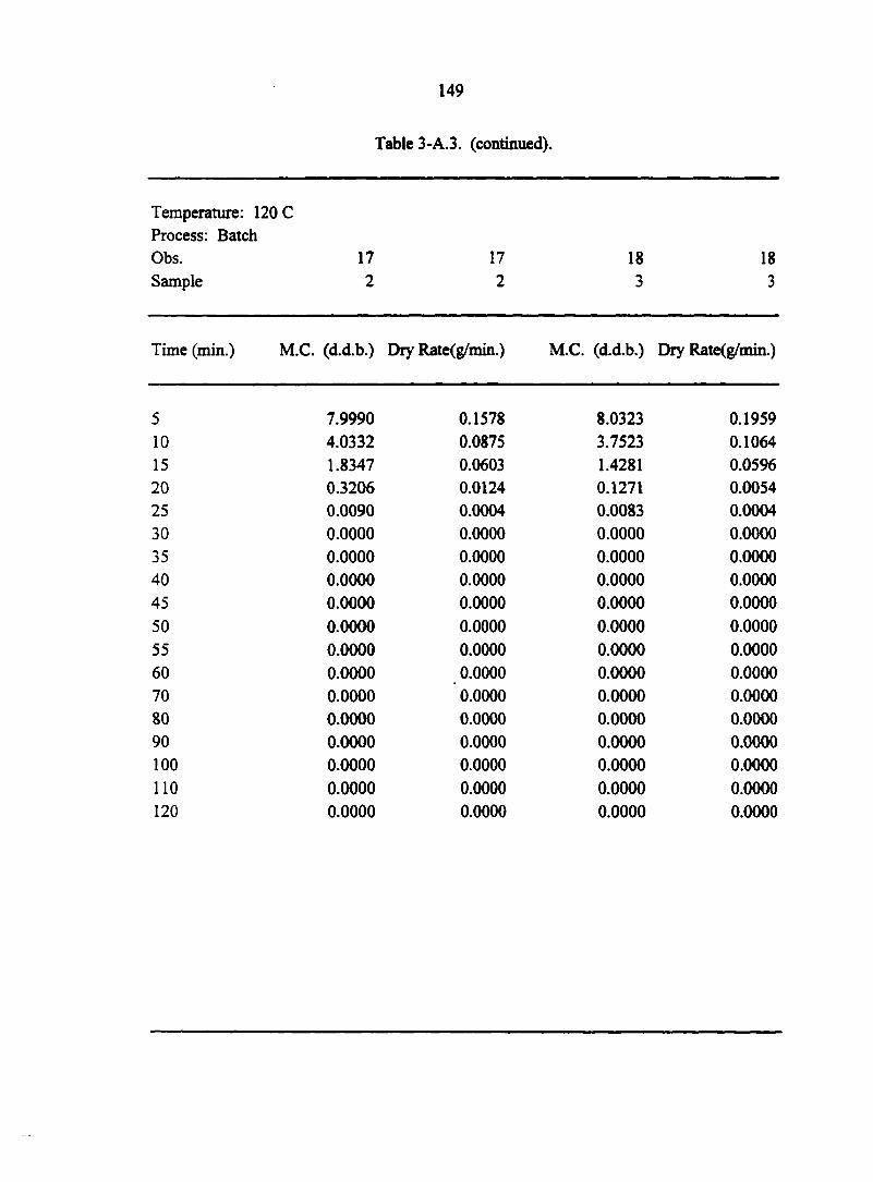
149
Table 3-A.3. (continued).
Temperature: 120 C Process: Batch Obs. 17 17 18 18 Sample 2 2 3 3
Time (min.) M.C. (d.d.b.) Dry Rate(g/min.) M.C. (d.d.b.) Dry Rate(g/min.)
5 7.9990 0.1578 8.0323 0.1959 10 4.0332 0.0875 3.7523 0.1064 15 1.8347 0.0603 1.4281 0.0596 20 0.3206 0.0124 0.1271 0.0054 25 0.0090 0.0004 0.0083 0.0004 30 0.0000 0.0000 0.0000 0.0000 35 0.0000 0.0000 0.0000 0.0000 40 0.0000 0.0000 0.0000 0.0000 45 0.0000 0.0000 0.0000 0.0000 50 0.0000 0.0000 0.0000 0.0000 55 0.0000 0.0000 0.0000 0.0000 60 0.0000 0.0000 0.0000 0.0000 70 0.0000 0.0000 0.0000 0.0000 80 0.0000 0.0000 0.0000 0.0000 90 0.0000 0.0000 0.0000 0.0000 100 0.0000 0.0000 0.0000 0.0000 110 0.0000 0.0000 0.0000 0.0000 120 0.0000 0.0000 0.0000 0.0000
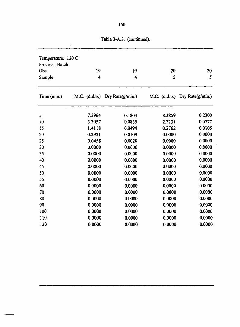
150
Table 3-A.3. (continued).
Temperature: 120 C Process: Batch Obs. 19 19 20 20 Sample 4 4 5 5
Time (min.) M.C. (d.d.b.) Dry Rate(g/min.) M.C. (d.d.b.) Dry Rate(g/min.)
5 7.3964 0.1804 8.3859 0.2300 10 3.3057 0.0835 2.3231 0.0777 15 1.4118 0.0494 0.2762 0.0105 20 0.2921 0.0109 0.0000 0.0000 25 0.0458 0.0020 0.0000 0.0000 30 0.0000 0.0000 0.0000 0.0000 35 0.0000 0.0000 0.0000 0.0000 40 0.0000 0.0000 0.0000 0.0000 45 0.0000 0.0000 0.0000 0.0000 50 0.0000 0.0000 0.0000 0.0000 55 0.0000 0.0000 0.0000 0.0000 60 0.0000 0.0000 0.0000 0.0000 70 0.0000 0.0000 0.0000 0.0000 80 0.0000 0.0000 0.0000 0.0000 90 0.0000 0.0000 0.0000 0.0000 100 0.0000 0.0000 0.0000 0.0000 110 0.0000 0.0000 0.0000 0.0000 120 0.0000 0.0000 0.0000 0.0000

151
Table 3-A.3. (continued).
Temperature: 120 C Process: Batch Obs. 21 21 22 22 Sample 1 1 2 2
Time (min.) M.C. (d.d.b.) Dry Rate(g/min.) M.C. (d.d.b.) Dry Rate(g/min.)
5 8.7387 0.1670 7.8738 0.1638 10 4.2311 0.0969 4.1687 0.1050 15 1.6161 0.0441 1.7938 0.0469 20 0.4244 0.0157 0.7322 0.0299 25 0.0000 0.0000 0.0561 0.0001 30 0.0000 0.0000 0.0543 0.0003 35 0.0000 0.0000 0.0484 0.0021 40 0.0000 0.0000 0.0000 0.0000 45 0.0000 0.0000 0.0000 0.0000 50 0.0000 0.0000 0.0000 0.0000 55 0.0000 0.0000 0.0000 0.0000 60 0.0000 0.0000 0.0000 0.0000 70 0.0000 0.0000 0.0000 0.0000 80 0.0000 0.0000 0.0000 0.0000 90 0.0000 0.0000 0.0000 0.0000 100 0.0000 0.0000 0.0000 0.0000 110 0.0000 0.0000 0.0000 0.0000 120 0.0000 0.0000 0.0000 0.0000
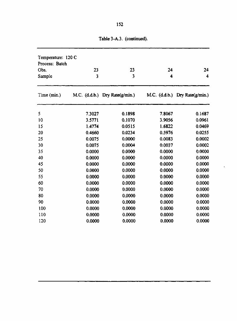
152
Table 3-A.3. (continued).
Temperature: 120 C Process: Batch Obs. 23 23 24 24 Sample 3 3 4 4
Time (min.) M.C. (d.d.b.) Dry Rate(g/min.) M.C. (d.d.b.) Dry Rate(g/min.)
5 7.3027 0.1898 7.8067 0.1687 10 3.5771 0.1070 3.9056 0.0961 15 1.4774 0.0515 1.6822 0.0469 20 0.4660 0.0234 0.5976 0.0255 25 0.0075 0.0000 0.0083 0.0002 30 0.0075 0.0004 0.0037 0.0002 35 0.0000 0.0000 0.0000 0.0000 40 0.0000 0.0000 0.0000 0.0000 45 0.0000 0.0000 0.0000 0.0000 50 0.0000 0.0000 0.0000 0.0000 55 0.0000 0.0000 0.0000 0.0000 60 0.0000 0.0000 0.0000 0.0000 70 0.0000 0.0000 0.0000 0.0000 80 0.0000 0.0000 0.0000 0.0000 90 0.0000 0.0000 0.0000 0.0000 100 0.0000 0.0000 0.0000 0.0000 110 0.0000 0.0000 0.0000 0.0000 120 0.0000 0.0000 0.0000 0.0000
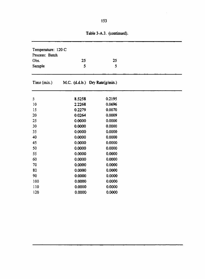
153
Table 3-A.3. (continued).
Temperature: 120 C Process: Batch Obs. 25 25 Sample 5 5
Time (min.) M.C. (d.d.b.) Dry Rate(g/min.)
5 8.5258 0.2195 10 2.2268 0.0696 15 0.2279 0.0070 20 0.0264 0.0009 25 0.0000 0.0000 30 0.0000 0.0000 35 0.0000 0.0000 40 0.0000 0.0000 45 0.0000 0.0000 50 0.0000 0.0000 55 0.0000 0.0000 60 0.0000 0.0000 70 0.0000 0.0000 80 0.0000 0.0000 90 0.0000 0.0000 100 0.0000 0.0000 110 0.0000 0.0000 120 0.0000 0.0000
154
CHAPTER 4
EXTRUSION PROCESSING LITERATURE REVIEW
Prior to discussing the extrusion of masa byproducts, it is useful to review the
fundamentals of extrusion and the mathematics associated with this unit operation.
INTRODUCTION
Extrusion has become a common processing method for the food and feed industries.
It combines several unit operations in one machine, including pumping, mixing, cooking,
shaping, and forming. Although various extruders exist, there are essentially two basic types:
single-screw and twin-screw. Discussion in this chapter will be restricted to single-screw
extruders, because that is the type used for experimentation in this study. Essentially,
extruders are machines that accept incoming feed material, convey this material down a
chamber using a flighted screw, apply heat to this material as it is conveyed (through
frictional viscous dissipation, by heated jackets surrounding the extruder barrel, and by direct
steam injection), and then force this dough (which usually becomes a plasticized mass due to
heating and mixing) out of a small opening, known as a die. Product shaping and forming
occur at the die exit, due to expansion because of pressure release and moisture evaporation
effects, and due to the type of die exit and shearing knives used to cut the outgoing product
(Fellows, 1996; Gould, 1996).
The extrusion process, and the final extrudate products, are drastically affected by
many processing parameters, including extrusion time, extrusion temperature, screw
rotational speed, die opening size and shape, and raw ingredient moisture content and
composition. The objective of this chapter is to discuss various processing parameters and
their effects on both extrusion processing and resulting extruded products. The second goal
155
of this chapter is to present, in a limited fashion, basic equations which have been used to
describe and model extrusion processing. Most of the equations presented here have not
been incorporated into this overall research project due to project constraints, but are given
here for informational purposes only.
PROCESSING PARAMETERS AND EFFECTS
A very brief discussion regarding the most important factors and their effects on the
extrusion process and on the resulting extrudate products will follow. The parameters which
have the greatest effect on extrusion are screw speed, barrel temperature, die diameter, feed
ingredient moisture content, and feed ingredient particle size. Specifically, the effects of
these parameters on apparent viscosity of the dough melt, the energy input required, and
product expansion will be discussed.
Screw Speed
As screw speed increases, the apparent viscosity of the food dough melt decreases.
This occurs because food doughs behave pseudoplastically, which means their non-
Newtonian nature exhibits a decrease in viscosity as shear strain rate (rate of material
deformation) increases (e.g., they are called shear thinning fluids due to this behavior).
Typically, the specific mechanical energy input (SME) is an indication of the viscous
dissipation of mechanical energy, which is provided by the screw drive shaft, into the dough
due to fhctional resistance (Marsman et al., 1995). The SME, in fact, quantifies the
competing effects of viscosity changes due to changes in screw speed (i.e., the pseudoplastic
behavior), and the resulting change in the torque which is required to convey the dough
through the extruder at an increased shaft speed. Typically, it has been noted that as screw
speed increases, SME also increases, due to the changes in energy input to the screw being of
156
a greater order of magnitude than the decrease in torque associated with the decrease in
apparent viscosity due to the shear thinning behavior of the non-Newtonian material (Mercier
et al., 1989). A decrease in apparent viscosity also leads to a more expanded product upon
exiting the die (Chen et al., 1979; Kokini et al., 1992; Mercier et al., 1989).
Barrel Temperature
An increase in extruder barrel temperature generally leads to a decrease in dough
apparent viscosity. This decrease in viscosity requires less energy input (SME) into the drive
shaft to turn the screw at a given speed. As mentioned previously, a decrease in viscosity
produces a more expanded product upon die exit. Furthermore, a higher temperature
produces more water evaporation upon die exit, also leading to a more expanded product
(Chen et al., 1979; Kokini et al., 1992; Mercier et al., 1989).
Die Diameter
It appears that die size has little effect on apparent viscosity in the screw channel.
But, as die diameter increases, SME required decreases, due to the lower pressure buildup
behind the die prior to exit (i.e., less force is required to push the dough through the die, and
thus less force is required to turn the screw). As the pressure drop across the die decreases,
the resulting extradâtes expand less, due to less water evaporation upon die exit (Mercier et
al., 1989).
Feed Moisture Content
An increased moisture content of the feed / dough ingredients produces a lower
apparent viscosity in the dough, and thus, it also produces a lower SME required. As
moisture content increases, however, product and die temperatures and pressures decrease,
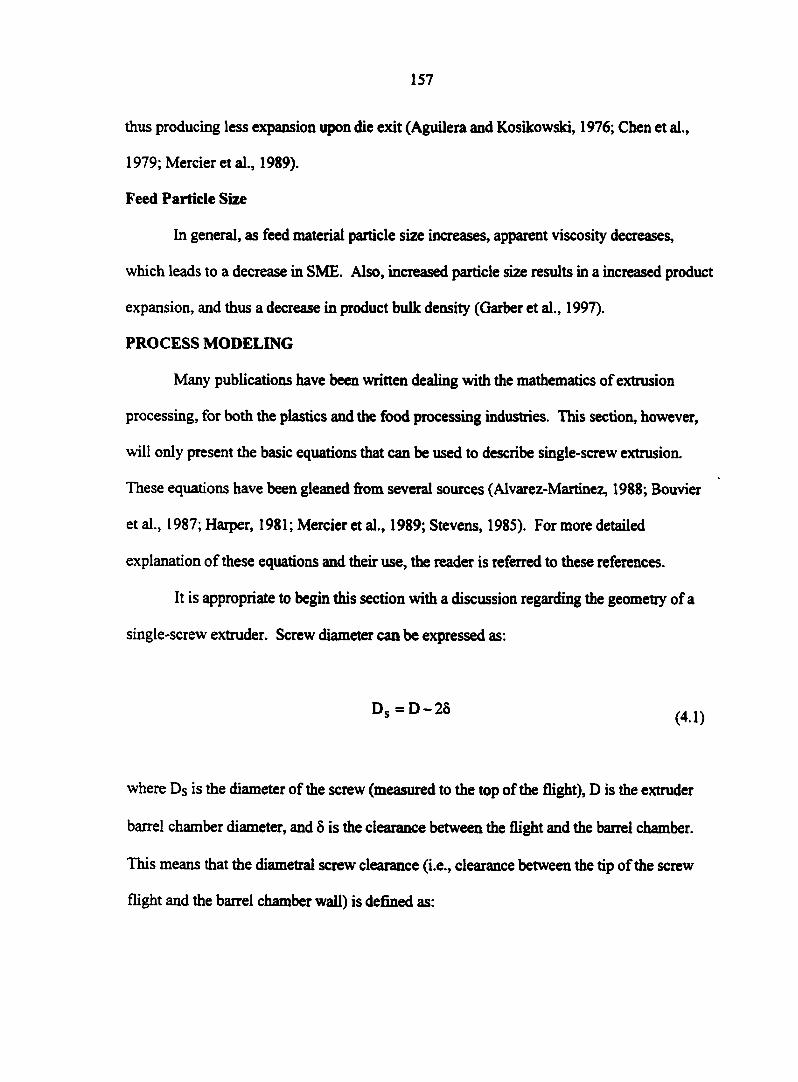
157
thus producing less expansion upon die exit (Aguilera and Kosikowski, 1976; Chen et al.,
1979; Mercier et al., 1989).
Feed Particle Size
In general, as feed material particle size increases, apparent viscosity decreases,
which leads to a decrease in SME. Also, increased particle size results in a increased product
expansion, and thus a decrease in product bulk density (Garber et al., 1997).
PROCESS MODELING
Many publications have been written dealing with the mathematics of extrusion
processing, for both the plastics and the food processing industries. This section, however,
will only present the basic equations that can be used to describe single-screw extrusion.
These equations have been gleaned from several sources (Alvarez-Martinez, 1988; Bouvier
et al., 1987; Harper, 1981; Mercier et al., 1989; Stevens, 1985). For more detailed
explanation of these equations and their use, the reader is referred to these references.
It is appropriate to begin this section with a discussion regarding the geometry of a
single-screw extruder. Screw diameter can be expressed as:
Ds = D-28 p,.,)
where Ds is the diameter of the screw (measured to the top of the flight), D is the extruder
barrel chamber diameter, and 8 is the clearance between the flight and the barrel chamber.
This means that the diametral screw clearance (i.e., clearance between the tip of the screw
flight and the barrel chamber wall) is defined as:
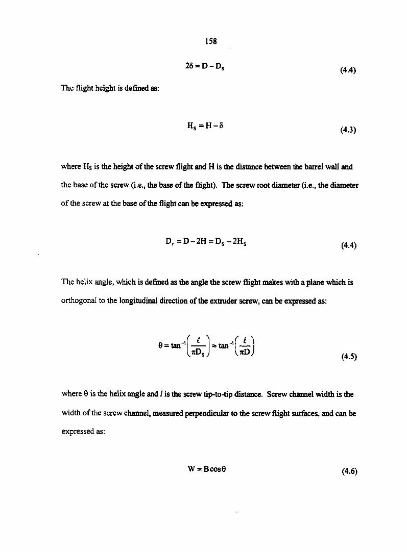
158
2S = D-Ds (4.4)
The flight height is defined as:
Hs =H-S (4.3)
where Hs is the height of the screw flight and H is the distance between the barrel wall and
the base of the screw (i.e., the base of the flight). The screw root diameter (i.e., the diameter
of the screw at the base of the flight can be expressed as:
Dr = D-2H = Ds -2HS (4.4)
The helix angle, which is defined as the angle the screw flight makes with a plane which is
orthogonal to the longitudinal direction of the extruder screw, can be expressed as:
9 = tan -i %D
stan"1
s y (4.5)
where 9 is the helix angle and / is the screw tip-to-tip distance. Screw channel width is the
width of the screw channel, measured perpendicular to the screw flight surfaces, and can be
expressed as:
W = BcosB (4.6)
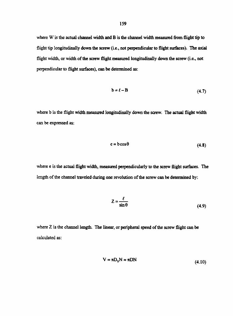
159
where W is the actual channel width and B is the channel width measured from flight tip to
flight tip longitudinally down the screw (i.e., not perpendicular to flight surfaces). The axial
flight width, or width of the screw flight measured longitudinally down the screw (i.e., not
perpendicular to flight surfaces), can be determined as:
b = £-B (4.7)
where b is the flight width measured longitudinally down the screw. The actual flight width
can be expressed as:
e = bcos6 (4.8)
where e is the actual flight width, measured perpendicularly to the screw flight surfaces. The
length of the channel traveled during one revolution of the screw can be determined by:
sinô (4.9)
where Z is the channel length. The linear, or peripheral speed of the screw flight can be
calculated as:
V = TIDsN « TtDN (4.10)
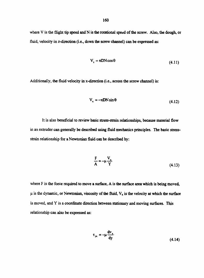
160
where V is the flight tip speed and N is the rotational speed of the screw. Also, the dough, or
fluid, velocity in z-direction (i.e., down the screw channel) can be expressed as:
VZ=TIDNCOS8 (411)
Additionally, the fluid velocity in x-direction (i.e., across the screw channel) is:
Vx = -TtDN sin 8 ^ ^
It is also beneficial to review basic stress-strain relationships, because material flow
in an extruder can generally be described using fluid mechanics principles. The basic stress-
strain relationship for a Newtonian fluid can be described by:
A Y (4.13)
where F is the force required to move a surface, A is the surface area which is being moved,
p. is the dynamic, or Newtonian, viscosity of the fluid, Vx is the velocity at which the surface
is moved, and Y is a coordinate direction between stationary and moving surfaces. This
relationship can also be expressed as:
dvx T»
(4.14)
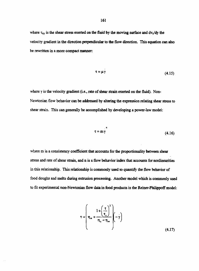
161
where ixy is the shear stress exerted on the fluid by the moving surface and dvx/dy the
velocity gradient in the direction perpendicular to the flow direction. This equation can also
be rewritten in a more compact manner:
where y is the velocity gradient (i.e., rate of shear strain exerted on the fluid). Non-
Newtonian flow behavior can be addressed by altering the expression relating shear stress to
shear strain. This can generally be accomplished by developing a power-law model:
where m is a consistency coefficient that accounts for the proportionality between shear
stress and rate of shear strain, and n is a flow behavior index that accounts for nonlinearities
in this relationship. This relationship is commonly used to quantify the flow behavior of
food doughs and melts during extrusion processing. Another model which is commonly used
to fit experimental non-Newtonian flow data in food products is the Reiner-Philippoff model:
(4.15)
0 t = my (4.16)
v y (4.17)
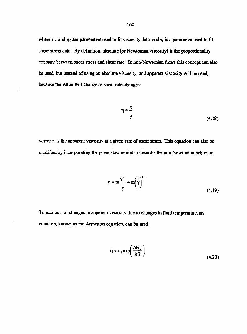
162
where ri® and r|0 are parameters used to fit viscosity data, and t, is a parameter used to fit
shear stress data. By definition, absolute (or Newtonian viscosity) is the proportionality
constant between shear stress and shear rate. In non-Newtonian flows this concept can also
be used, but instead of using an absolute viscosity, and apparent viscosity will be used,
because the value will change as shear rate changes:
where r| is the apparent viscosity at a given rate of shear strain. This equation can also be
modified by incorporating the power-law model to describe the non-Newtonian behavior:
To account for changes in apparent viscosity due to changes in fluid temperature, an
equation, known as the Arrhenius equation, can be used:
t n = -
Y (4.18)
(4.19)
(4.20)
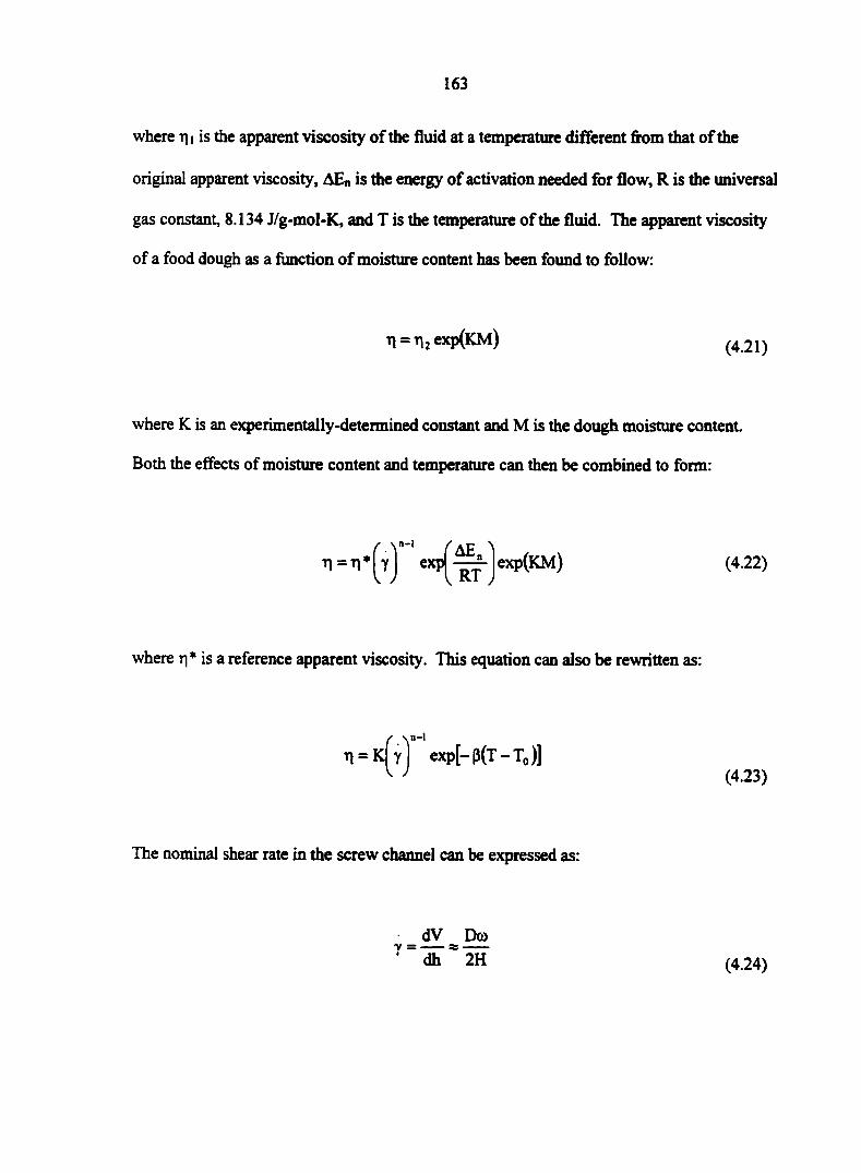
163
where rji is the apparent viscosity of the fluid at a temperature different from that of the
original apparent viscosity, AEn is the energy of activation needed for flow, R is the universal
gas constant, 8.134 J/g-mol-K, and T is the temperature of the fluid. The apparent viscosity
of a food dough as a function of moisture content has been found to follow:
n = ri2exp(KM) (4 21)
where K is an experimentally-determined constant and M is the dough moisture content.
Both the effects of moisture content and temperature can then be combined to form:
n = n * h e ; IXP(La™ exp^KM^
/ Ar. , . (4.22)
where r|* is a reference apparent viscosity. This equation can also be rewritten as:
,0-1
n = K[ Y exp[-p(T-T0)] (4.23)
The nominal shear rate in the screw channel can be expressed as:
dV Deo
dh 2H (4.24)
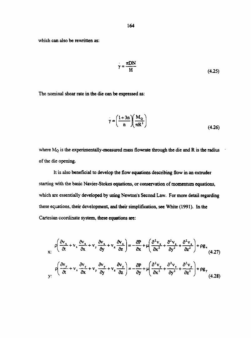
164
which can also be rewritten as:
(4.25)
The nominal shear rate in the die can be expressed as:
• f l + 3n T " ~ (4.26)
where MQ is the experimentally-measured mass Gowrate through the die and R is the radius
of the die opening.
It is also beneficial to develop the flow equations describing flow in an extruder
starting with the basic Navier-Stokes equations, or conservation of momentum equations,
which are essentially developed by using Newton's Second Law. For more detail regarding
these equations, their development, and their simplification, see White (1991). In the
Cartesian coordinate system, these equations are:
y:

165
(dvz dv dvz 9vz) dP f d2v d2v d2v /
z.\dt +Vx dx +Vy dy +Vz dz ) dz+M[»c r + "^r+™fery
+ Pg, (4.29)
To simplify these, several assumptions have been made regarding the flow inside an
extruder: a Newtonian fluid, incompressible, laminar flow, steady state flow, no-slip exists
at surface boundaries, forces due to gravity and inertial are small and can be ignored.
Applying these simplifying assumptions leads to:
x:
dP 3T"
^d2v„ d2v ^
y:
z:
dP dy 14
dP
1 d y 2 ;
a2v, 52vy l y + /
dx2 ^ J
d2vz
dx2 dy2 )
(4.30)
(4.31)
(4.32)
Conservation of mass, or the continuity equation, can be expressed as:
dvK dv —-+ — dx dy
- + —ï- = 0
(4.33)
The velocity profile in the screw channel, down the channel (i.e., in the z-direction) can be
expressed as:
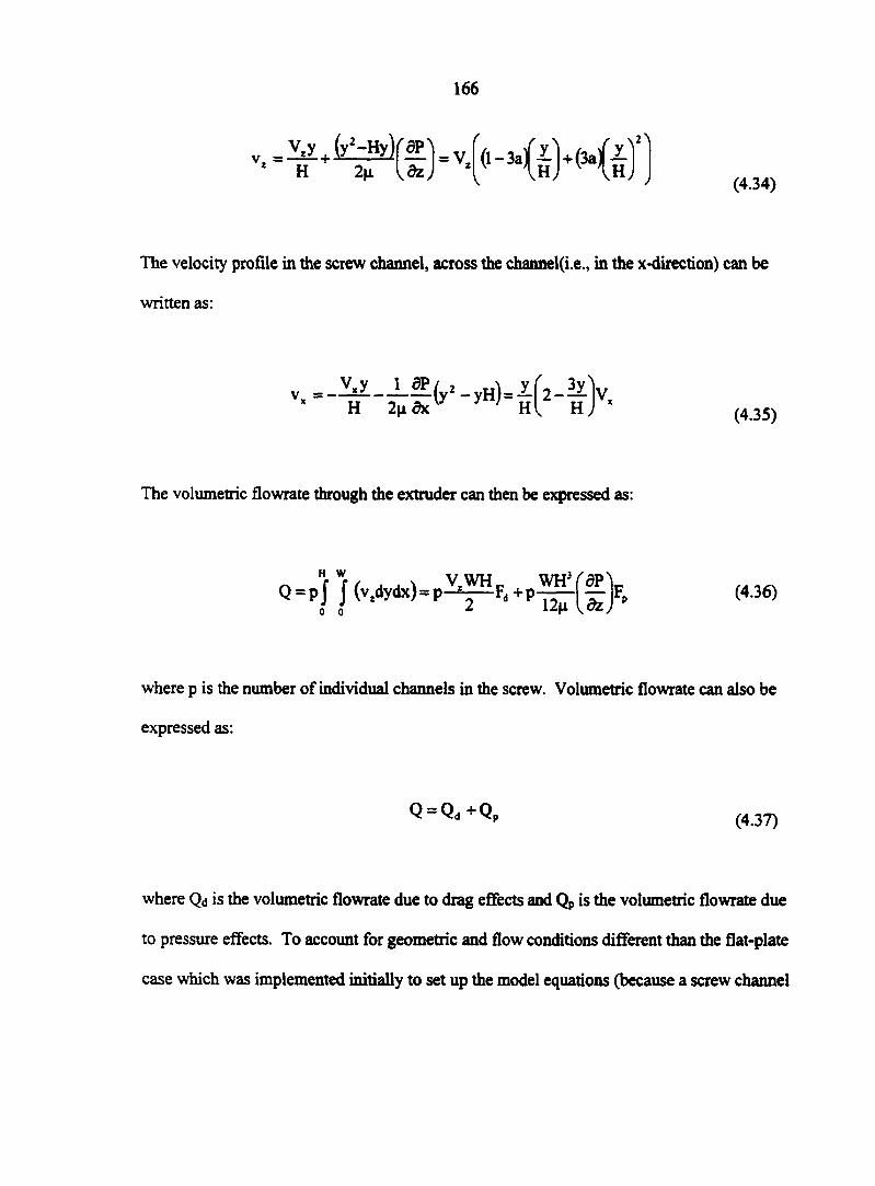
166
-¥-^fW<'-Kâ*wU 2\
(4.34)
The velocity profile in the screw channel, across the channel(i.e., in the x-direction) can be
written as:
(4.35)
The volumetric flowrate through the extruder can then be expressed as:
Q = P f J (vzdydx)=p^~Fd + P^"[^)Fp (4.36)
where p is the number of individual channels in the screw. Volumetric flowrate can also be
expressed as:
Q Qd+ Q p (4.37)
where Q<j is the volumetric flowrate due to drag effects and Qp is the volumetric flowrate due
to pressure effects. To account for geometric and flow conditions different than the flat-plate
case which was implemented initially to set up the model equations (because a screw channel
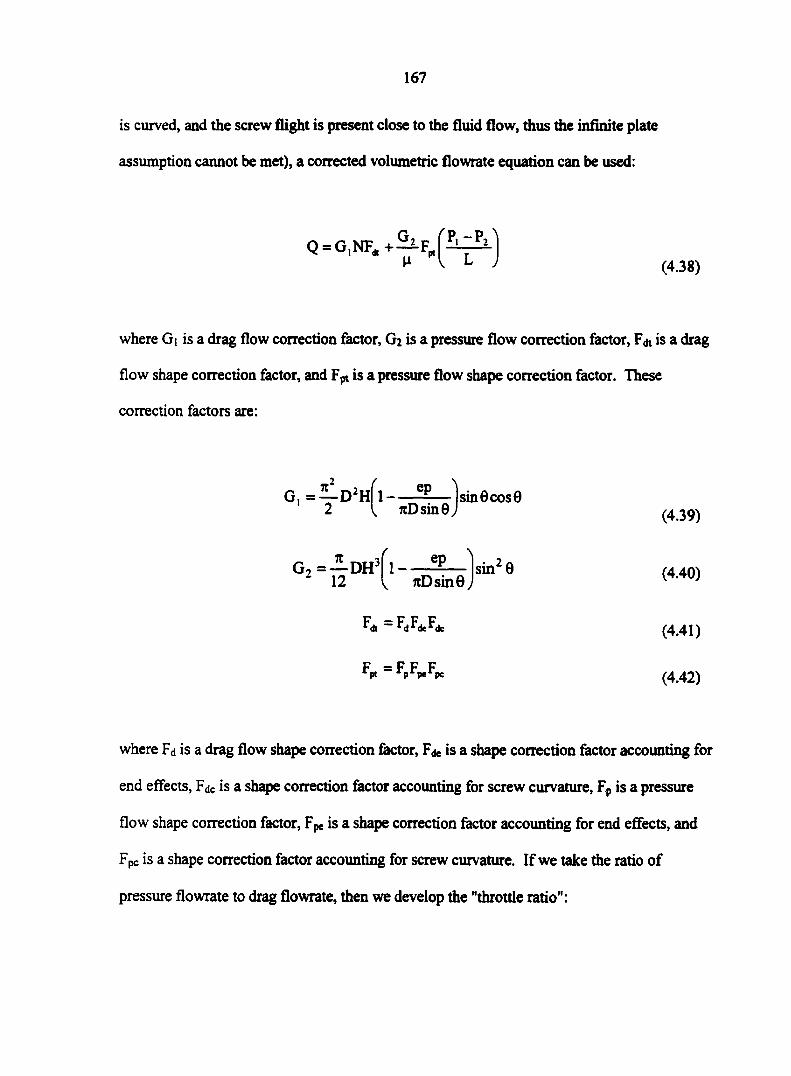
167
is curved, and the screw flight is present close to the fluid flow, thus the infinite plate
assumption cannot be met), a corrected volumetric flowrate equation can be used:
^ < L J (4.38)
where Gt is a drag flow correction factor, G% is a pressure flow correction factor, F* is a drag
flow shape correction factor, and Fpt is a pressure flow shape correction factor. These
correction factors are:
G, = ^-D2H 1 —-^7—-sin 0 cos 6 2 L rcDsinOj (439)
G2 = —DH 2 12
( 1-
ep
rcDsinG; sin 0 (4.40)
Fd.-FdFdeFd= (4.41)
Fpt FpFpeFpc (4.42)
where Fa is a drag flow shape correction factor, FdC is a shape correction factor accounting for
end effects, FdC is a shape correction factor accounting for screw curvature, Fp is a pressure
flow shape correction factor, Fpe is a shape correction factor accounting for end effects, and
FpC is a shape correction factor accounting for screw curvature. If we take the ratio of
pressure flowrate to drag flowrate, then we develop the "throttle ratio":
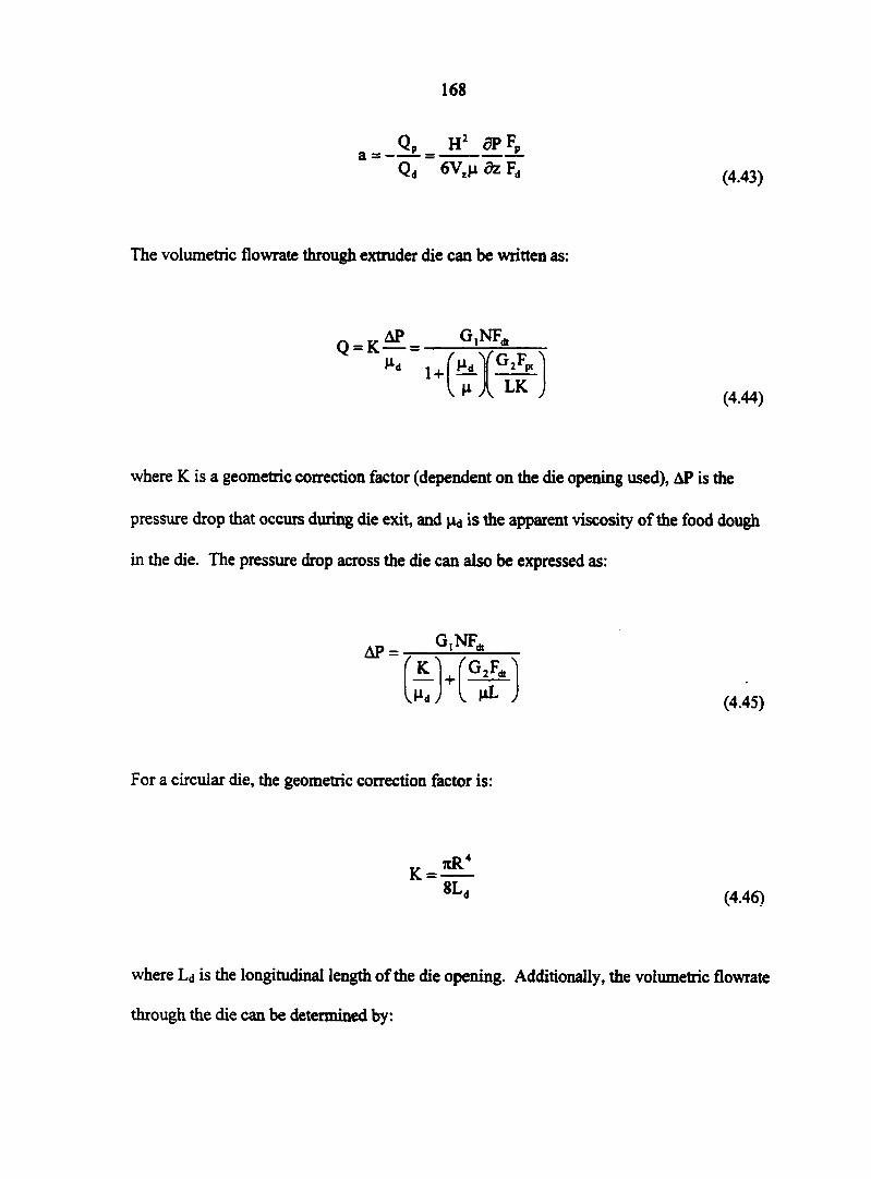
168
p H2 gPF„
Qd 6Vzn dz Fd (4.43)
The volumetric flowrate through extruder die can be written as:
Q = K — = Hd
G,NF^
LK (4.44)
where K is a geometric correction factor (dependent on the die opening used), AP is the
pressure drop that occurs during die exit, and ^ is the apparent viscosity of the food dough
in the die. The pressure drop across the die can also be expressed as:
AP = G,NF*
f k! f + l^d J V
G,F.
HL (4.45)
For a circular die, the geometric correction factor is:
K = nR4
8L„ (4.46)
where La is the longitudinal length of the die opening. Additionally, the volumetric flowrate
through the die can be determined by:
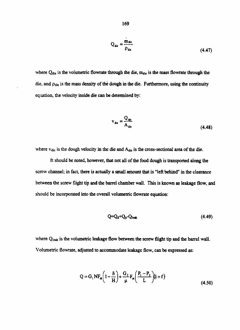
169
(4.47)
where Qdie is the volumetric flowrate through the die, m#* is the mass flowrate through the
die, and paie is the mass density of the dough in the die. Furthermore, using the continuity
equation, the velocity inside die can be determined by:
where Vdt is the dough velocity in the die and Adie is the cross-sectional area of the die.
It should be noted, however, that not all of the food dough is transported along the
screw channel; in fact, there is actually a small amount that is "left behind" in the clearance
between the screw flight tip and the barrel chamber wall. This is known as leakage flow, and
should be incorporated into the overall volumetric flowrate equation:
where Qieak is the volumetric leakage flow between the screw flight tip and the barrel wall.
Volumetric flowrate, adjusted to accommodate leakage flow, can be expressed as:
(4.48)
Q=Qd+Qp-Qic*k (4.49)
(4.50)
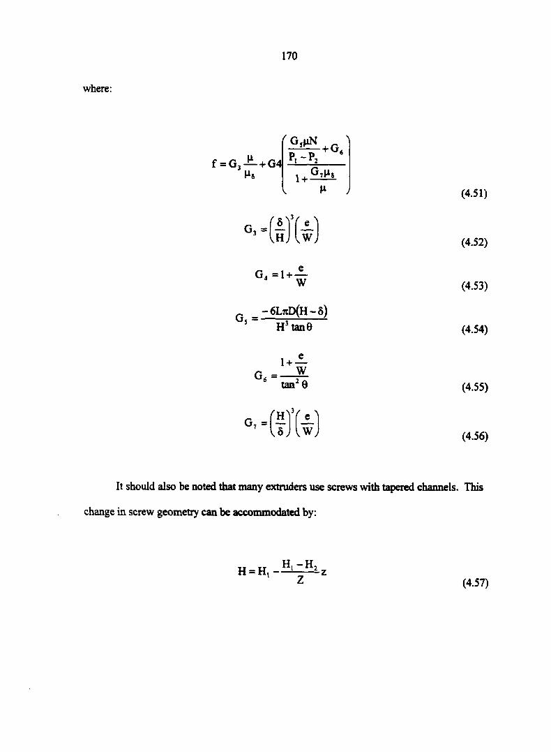
where:
170
f = G3—+G4| Ms
GsVN
P,-P2 + G,
1 +
(4.51)
°3 I HJ l w ;
G < = 1 + w
G« = _ — 6LTTD(H — ô)
H tan©
G, = tan2 0
° 7 = Ï HYf e x
W
(4.52)
(4.53)
(4.54)
(4.55)
(4.56)
It should also be noted that many extruders use screws with tapered channels. This
change in screw geometry can be accommodated by :
H = Ht ——z Z (4.57)
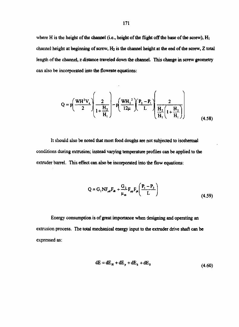
171
where H is the height of the channel (i.e., height of the flight off the base of the screw), Hi
channel height at beginning of screw, Hz is the channel height at the end of the screw, Z total
length of the channel, z distance traveled down the channel. This change in screw geometry
can also be incorporated into the flowrate equations:
Q = P WH2V.
. " Ï ;
-p rWi^
12n J P2-P1
5lfl+H0 HJJ (4.58)
It should also be noted that most food doughs are not subjected to isothermal
conditions during extrusion; instead varying temperature profiles can be applied to the
extruder barrel. This effect can also be incorporated into the flow equations:
Q-G.NF^+^F, ZP,-P2
X
(4.59)
Energy consumption is of great importance when designing and operating an
extrusion process. The total mechanical energy input to the extruder drive shaft can be
expressed as:
dE = dEH +dEp +dEk +dEs (4.60)
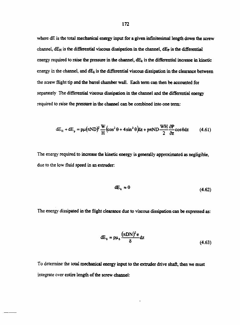
172
where dE is the total mechanical energy input for a given infinitesimal length down the screw
channel, dE» is the differential viscous dissipation in the channel, dEp is the differential
energy required to raise the pressure in the channel, dEk is the differential increase in kinetic
energy in the channel, and dE§ is the differential viscous dissipation in the clearance between
the screw flight tip and the barrel chamber wall. Each term can then be accounted for
separately The differential viscous dissipation in the channel and the differential energy
required to raise the pressure in the channel can be combined into one term:
The energy required to increase the kinetic energy is generally approximated as negligible,
due to the low fluid speed in an extruder:
The energy dissipated in the flight clearance due to viscous dissipation can be expressed as:
dEH +dEp = ph(ttND)2 —(cos2 9 + 4sin2 o)dz + mtND ^ cosQdz (4.61)
dEk «0 (4.62)
(4.63)
To determine the total mechanical energy input to the extruder drive shaft, then we must
integrate over entire length of the screw channel:
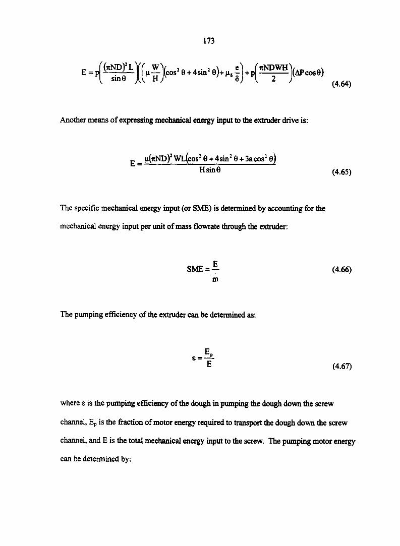
173
E = p
(4.64)
Another means of expressing mechanical energy input to the extruder drive is:
E = _ EI(FTND)2 Wl(COS2 8 + 4sin2 6 +3Acos1 @) H sin 6 (4.65)
The specific mechanical energy input (or SME) is determined by accounting for the
mechanical energy input per unit of mass flowrate through the extruder:
SME = — m
(4.66)
The pumping efficiency of the extruder can be determined as:
% (4.67)
where e is the pumping efficiency of the dough in pumping the dough down the screw
channel, Ep is the fraction of motor energy required to transport the dough down the screw
channel, and E is the total mechanical energy input to the screw. The pumping motor energy
can be determined by:
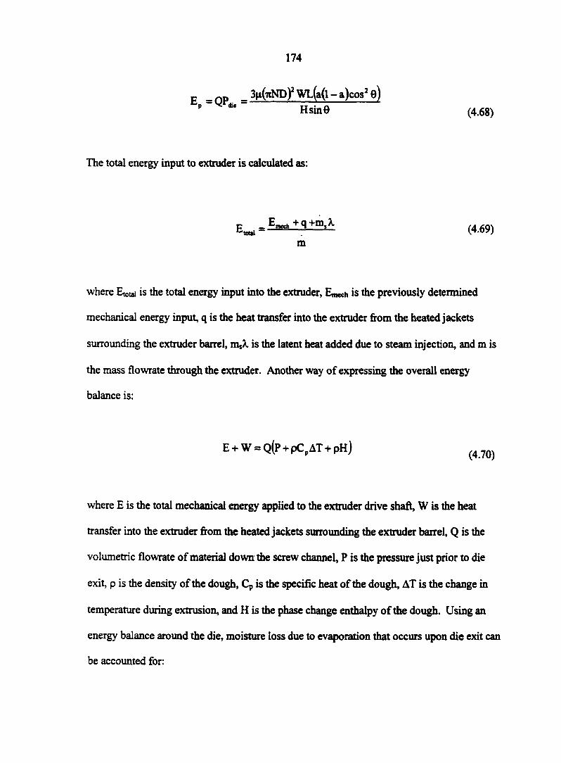
174
r- 3n(itND)!WL(a(l-a)cos!0) E' 'QP- " Hsin6 (4.68)
The total energy input to extruder is calculated as:
— ————— : (4.69) m
where Etotai is the total energy input into the extruder, Emech is the previously determined
mechanical energy input, q is the heat transfer into the extruder from the heated jackets
surrounding the extruder barrel, msX is the latent heat added due to steam injection, and m is
the mass flowrate through the extruder. Another way of expressing the overall energy
balance is:
E + W = Q(P + pCpAT + pH) (4J0)
where £ is the total mechanical energy applied to the extruder drive shaft, W is the heat
transfer into the extruder from the heated jackets surrounding the extruder barrel, Q is the
volumetric flowrate of material down the screw channel, P is the pressure just prior to die
exit, p is the density of the dough, Cp is the specific heat of the dough, AT is the change in
temperature during extrusion, and H is the phase change enthalpy of the dough. Using an
energy balance around the die, moisture loss due to evaporation that occurs upon die exit can
be accounted for:
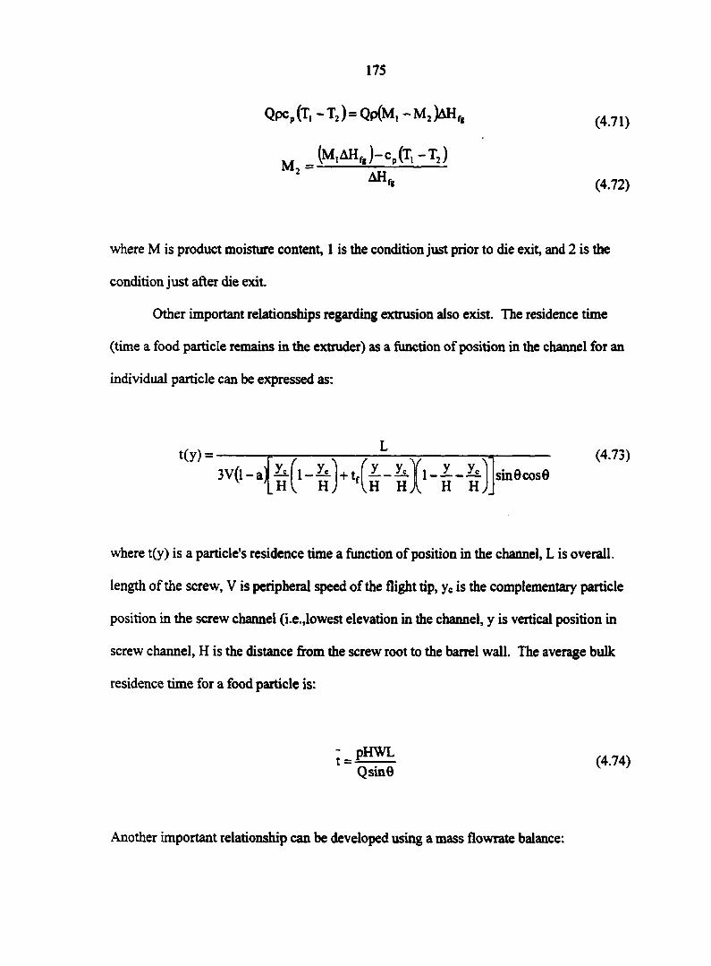
175
Qpc.(T, -T,) = Qp(Ml-M2)AH,
M2 = (M,AHfl)-cp(T, -T;)
ah fg
(4.71)
(4.72)
where M is product moisture content, 1 is the condition just prior to die exit, and 2 is the
condition just after die exit.
Other important relationships regarding extrusion also exist. The residence time
(time a food particle remains in the extruder) as a function of position in the channel for an
individual particle can be expressed as:
t(y) = -
3V(l -•ten. h h j h h;
(4.73)
sin6cos6
where t(y) is a particle's residence time a function of position in the channel, L is overall,
length of the screw, V is peripheral speed of the flight tip, ye is the complementary particle
position in the screw channel (i.e.,lowest elevation in the channel, y is vertical position in
screw channel, H is the distance from the screw root to the barrel wall. The average bulk
residence time for a food particle is:
• - s < « >
Another important relationship can be developed using a mass flowrate balance:
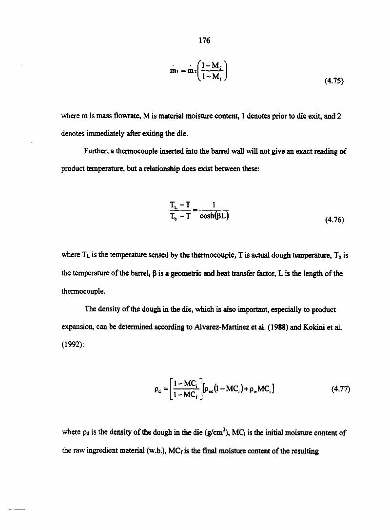
176
mi = r
(4.75)
where m is mass flowrate, M is material moisture content, 1 denotes prior to die exit, and 2
denotes immediately after exiting the die.
Further, a thermocouple inserted into the barrel wall will not give an exact reading of
product temperature, but a relationship does exist between these:
where Tl is the temperature sensed by the thermocouple, T is actual dough temperature, Ty is
the temperature of the barrel, p is a geometric and heat transfer factor, L is the length of the
thermocouple.
The density of the dough in the die, which is also important, especially to product
expansion, can be determined according to Alvarez-Martinez et al. (1988) and Kokini et al.
(1992):
TL-T _ 1 Tb -T cosh(pL) (4.76)
P d = Y ^ - k ( l - M C , ) + p . M C l ] (4.77)
where pd is the density of the dough in the die (g/cm3), MC,- is the initial moisture content of
the raw ingredient material (w.b.), MCf is the final moisture content of the resulting
177
extradates (w.b.), pex is the bulk density of the resulting extradâtes (g/cm3), and pw is the
density of water at the die temperature (g/cm3).
SUMMARY AND CONCLUSIONS
As shown by the above discussion, mathematically describing and modeling the
extrusion process is a formidable task, with many parameters, factors, and variables
simultaneously interacting. Implementing the above models for the extrusion in this project
is beyond the scope of the current study, but has been presented to show the various
relationships involved in the process.
The next chapter describes laboratory extrusion of masa processing byproducts.
While most of the mathematical models presented here are not utilized, a few key equations
have been implemented in the study.
REFERENCES
Aguilera, J. M. and F. V. Kosikowski. 1976. Soybean extruded product: a response surface analysis. Journal of Food Science 41(3): 647-651.
Alvarez-Martinez, L., K. P. Kondury, and J. M. Harper. 1988. A general model for expansion of extruded products. Journal of Food Science 53(2): 609-615.
Bouvier, J. M., G. Fayard, and J. T. Clayton. 1987. Flow rate and heat transfer modeling extrusion cooking of soy protein. Journal of Food Engineering 6(1987): 123-141.
Chen, A. H., Y. C. Jao, J. W. Larkin, and W. E. Goldstein. 1979. Rheological model of soy dough in extrusion. Journal of Food Processing Engineering 2(4): 337-342.
Fellows, P. J. 1996. Food Processing Technology Principles and Practice. Abingtion, England: Woodhead Publishing Limited.
Garber, B. W., H. E. Huff, and F. Hsieh. 1997. Influence of particle size on the twin-screw extrusion of com meal. Cereal Chemistry 74:656-661.
Gould, W. A. 1996. Unit Operations for the Food Industries. Baltimore, MD: CTI Publications, Inc.

178
Harper, J. M. 1981. Extrusion of Foods, Volume I. Boca Raton, FL: CRC Press, Inc.
Kokini, J. L., C. N. Chang and L. S. Lai. 1992. The role of rheological properties on extrudate expansion. In Food Extrusion Science and Technology, ed. J. L. Kokini, C. T. Ho, and M. V. Karewe, 631-652. New York: Marcel Dekker, Inc.
Marsman, G. J. P., H. Gruppen, D. J. vanZuilichem, J. W. Resink and A. G. J. Voragen. 1995. The influence of screw configuration on the In Vitro digestibility and protein solubility of soybean and rapeseed meals. Journal of Food Engineering 26(1): 13-28.
Mercier, C., P. Linko, and J. M. Harper. Extrusion Cooking. St. Paul, MN: American Association of Cereal Chemists, Inc.
Stevens, M. J. 1985. Extruder Principles and Operation. Essex, England: Elevier Applied Science Publishers LTD.
White, F. M. 1991. Viscous Fluid Flow. New York, NY: McGraw-Hill, Inc.
179
CHAPTERS
DEVELOPMENT OF FEED INGREDIENTS USING CORN MASA BYPRODUCTS. I. SMALL-SCALE EXTRUSION
A paper to be submitted, in part, to Cereal Chemistry
K. A. Rosentrater, T. L. Richard, C. J. Bern, and R. A. Flores
ABSTRACT
Corn masa by-product streams are high in fiber and are amenable for utilization in
livestock feed ingredients. This approach has the potential to produce a viable alternative to
landfilling, the traditional means of disposal for these processing residues. Separated
suspended solids from a masa processing waste stream were blended with soybean meal at
four levels (0%, 10%, 20% and 30% byproducts, wet basis), and were then extruded in a
laboratory-scale extruder at screw speeds of 50 rpm (5.24 rad/s) and 100 rpm (10.47 rad/s)
with extruder temperature profiles of 80-90-100 °C and 100-110-120 °C. Processing
conditions, including dough temperature, die temperature, drive torque required, specific
mechanical energy consumption, product and feed material throughput, dough apparent
viscosity, and dough density, were monitored during extrusion, and the resulting extruded
products were subjected to extensive physical and nutritional characterization, in order to
determine optimal processing conditions for the blends under investigation. Extrudate
analysis included moisture content, water activity, crude protein, in-vitro protein digestibility,
crude fat, ash, product diameter, expansion ratios, bulk density, true density, color, water
absorption and solubility, and durability. All blends studied were suitable for extrusion at the
processing conditions used. Blend ratio had little effect on either processing parameters or
180
the measured extrudate properties. Extrusion processing temperature and screw speed,
however, significantly affected both processing and product properties, with higher screw
speeds resulting in greater processing capacity, and higher temperatures producing drier
products. After extrusion processing, an additional drying operation is recommended, to
reduce the moisture content of the extrudates to levels that are microbiologically stable. This
drying stage was not incorporated into this study, however.
Keywords
Evaluation, Extrusion, Food Processing, Food Waste, Residue Utilization, Soybean
Meal.
Author Information
Journal Paper No. J-XXXXX of the Iowa Agriculture and Home Economics
Experiment Station, Ames, Iowa, Project No. 3326, and supported by Hatch Act and State of
Iowa Funds.
The authors are Kurt A. Rosentrater, ASAE Student Member, Graduate Student,
Agricultural and Biosystems Engineering Dept., Iowa State University, Ames, Iowa;
Thomas L. Richard, ASAE Member, Assistant Professor, Agricultural and Biosystems
Engineering Dept., Iowa State University, Ames, Iowa; Carl J. Bern, ASAE Fellow
Engineer, Professor, Agricultural and Biosystems Engineering Dept., Iowa State University,
Ames, Iowa; and Rolando A. Flores, ASAE Member Engineer, Associate Professor,
Department of Grain Science and Industry, Kansas State University, Manhattan, Kansas.
Corresponding author: Thomas L. Richard, Iowa State University, 214B Davidson Hall,
Ames, Iowa, 50011, tel.: (515) 294-0465, fax: (515) 294-2255, email: [email protected].
181
INTRODUCTION
Due to mounting economic and environmental concerns, landfilling of agricultural
and food processing waste materials has declined, and alternative disposal methods are being
increasingly investigated. Current options include reprocessing, recycling, resale,
incineration, composting, biomass energy production, land application as soil conditioners,
and reuse as livestock feed additives. This paper focuses on reuse as livestock feed materials,
which can include either direct feeding of the waste products or feeding the byproducts after
additional processing (Bohlsen et al., 1997; Derr and Dhillon, 1997; Ferris et al., 1995; Wang
et al., 1997).
Many research efforts have focused on the development of livestock feed ingredients
from grain processing byproducts. Particular attention has been given to com gluten meal,
distillers' byproducts, and brewers' byproducts (Annexstad, et al., 1987; Davis et al., 1980;
Ham et al., 1995; Larson et al., 1993; Lodge et al., 1997). Com masa production, however, is
one area of the grain processing industry that generates large quantities of waste materials,
but to date, has received little attention vis-à-vis byproduct disposal alternatives.
Com masa is used in the production of com tortilla chips and com tortillas, which
have been a staple in the diets of Mexican and Central American peoples for centuries.
Foods made with tortillas include tacos, tostadas, tamales, quesadillas, panuchos, and
enchiladas (Krause et al., 1992; Ortiz, 1985; Serna-Saldivar et al., 1990). Currently, Mexican
foods and corn-based snacks in the United States are booming in popularity. Tortilla sales
alone were estimated at $4 billion for 2000 A.D. (Solganik, 1997), and are expected to reach
$5.5 billion by 2003 A.D. (TLA, 2001). Com masa is produced by simulating ancient Aztec
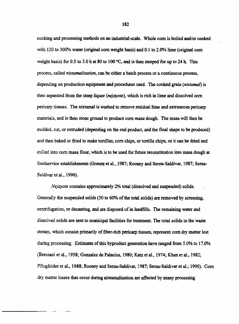
182
cooking and processing methods on an industrial-scale. Whole com is boiled and/or cooked
with 120 to 300% water (original corn weight basis) and 0.1 to 2.0% lime (original com
weight basis) for 0.5 to 3.0 h at 80 to 100 6C, and is then steeped for up to 24 h. This
process, called nixtamalization, can be either a batch process or a continuous process,
depending on production equipment and procedures used. The cooked grain (nixtamal) is
then separated from the steep liquor (nejayote), which is rich in lime and dissolved corn
pericarp tissues. The nixtamal is washed to remove residual lime and extraneous pericarp
materials, and is then stone ground to produce com masa dough. The masa will then be
molded, cut, or extruded (depending on the end product, and the final shape to be produced)
and then baked or fried to make tortillas, com chips, or tortilla chips, or it can be dried and
milled into com masa flour, which is to be used for future reconstitution into masa dough at
foodservice establishments (Gomez et al., 1987; Rooney and Sema-Saldivar, 1987; Seraa-
Saldivar et al., 1990).
Nejayote contains approximately 2% total (dissolved and suspended) solids.
Generally the suspended solids (50 to 60% of the total solids) are removed by screening,
centrifugation, or decanting, and are disposed of in landfills. The remaining water and
dissolved solids are sent to municipal facilities for treatment. The total solids in the waste
stream, which consist primarily of fiber-rich pericarp tissues, represent com dry matter lost
during processing. Estimates of this byproduct generation have ranged from 5.0% to 17.0%
(Bressani et al., 1958; Gonzalez de Palacios, 1980; Katz et al., 1974; Khan et al., 1982;
Pflugfelder et al., 1988; Rooney and Sema-Saldivar, 1987; Sema-Saldivar et al.; 1990). Com
dry matter losses that occur during nixtamalization are affected by many processing
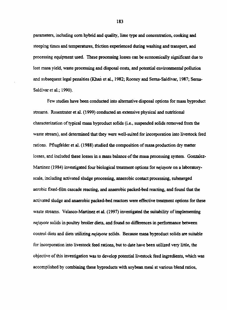
183
parameters, including com hybrid and quality, lime type and concentration, cooking and
steeping times and temperatures, friction experienced during washing and transport, and
processing equipment used. These processing losses can be economically significant due to
lost masa yield, waste processing and disposal costs, and potential environmental pollution
and subsequent legal penalties (Khan et al., 1982; Rooney and Sema-Saldivar, 1987; Sema-
Saldivar et al.; 1990).
Few studies have been conducted into alternative disposal options for masa byproduct
streams. Rosentrater et al. (1999) conducted an extensive physical and nutritional
characterization of typical masa byproduct solids (i.e., suspended solids removed from the
waste stream), and determined that they were well-suited for incorporation into livestock feed
rations. Pflugfelder et al. (1988) studied the composition of masa production dry matter
losses, and included these losses in a mass balance of the masa processing system. Gonzalez-
Martinez (1984) investigated four biological treatment options for nejayote on a laboratory-
scale, including activated sludge processing, anaerobic contact processing, submerged
aerobic fixed-film cascade reacting, and anaerobic packed-bed reacting, and found that the
activated sludge and anaerobic packed-bed reactors were effective treatment options for these
waste streams. Velasco-Martinez et al. (1997) investigated the suitability of implementing
nejayote solids in poultry broiler diets, and found no differences in performance between
control diets and diets utilizing nejayote solids. Because masa byproduct solids are suitable
for incorporation into livestock feed rations, but to date have been utilized very little, the
objective of this investigation was to develop potential livestock feed ingredients, which was
accomplished by combining these byproducts with soybean meal at various blend ratios,
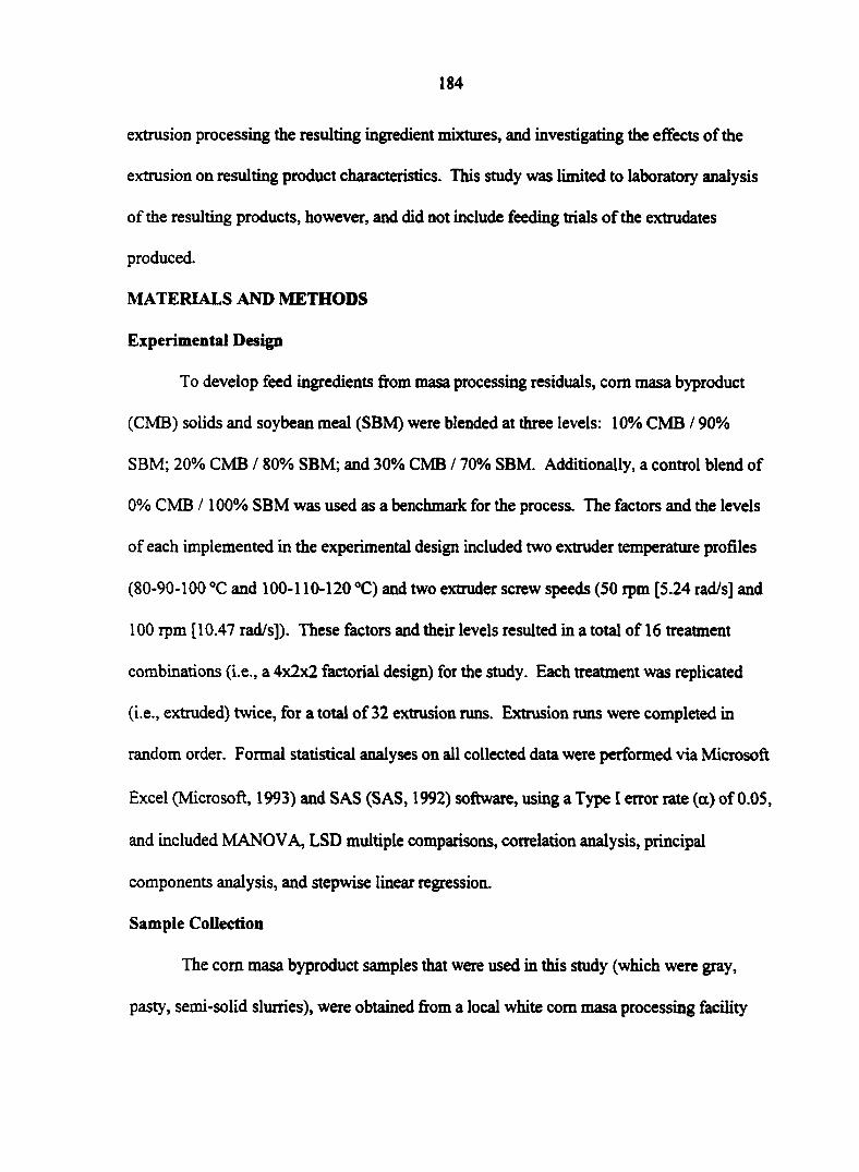
184
extrusion processing the resulting ingredient mixtures, and investigating the effects of the
extrusion on resulting product characteristics. This study was limited to laboratory analysis
of the resulting products, however, and did not include feeding trials of the extrudates
produced.
MATERIALS AND METHODS
Experimental Design
To develop feed ingredients from masa processing residuals, com masa byproduct
(CMB) solids and soybean meal (SBM) were blended at three levels: 10% CMB / 90%
SBM; 20% CMB Z 80% SBM; and 30% CMB / 70% SBM. Additionally, a control blend of
0% CMB /100% SBM was used as a benchmark for the process. The factors and the levels
of each implemented in the experimental design included two extruder temperature profiles
(80-90-100 °C and 100-110-120 °C) and two extruder screw speeds (50 rpm [5.24 rad/s] and
100 rpm [10.47 rad/s]). These factors and their levels resulted in a total of 16 treatment
combinations (i.e., a 4x2x2 factorial design) for the study. Each treatment was replicated
(i.e., extruded) twice, for a total of 32 extrusion runs. Extrusion runs were completed in
random order. Formal statistical analyses on all collected data were performed via Microsoft
Excel (Microsoft, 1993) and SAS (SAS, 1992) software, using a Type I error rate (a) of 0.05,
and included MANOVA, LSD multiple comparisons, correlation analysis, principal
components analysis, and stepwise linear regression.
Sample Collection
The corn masa byproduct samples that were used in this study (which were gray,
pasty, semi-solid slurries), were obtained from a local white com masa processing facility
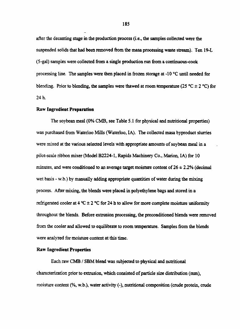
185
after the decanting stage in the production process (i.e., the samples collected were the
suspended solids that had been removed from the masa processing waste stream). Ten 19-L
(5-gal) samples were collected from a single production run from a continuous-cook
processing line. The samples were then placed in frozen storage at -10 °C until needed for
blending. Prior to blending, the samples were thawed at room temperature (25 °C ± 2 °C) for
24 h.
Raw Ingredient Preparation
The soybean meal (0% CMB, see Table 5.1 for physical and nutritional properties)
was purchased from Waterloo Mills (Waterloo, LA). The collected masa byproduct slurries
were mixed at the various selected levels with appropriate amounts of soybean meal in a
pilot-scale ribbon mixer (Model B2224-1, Rapids Machinery Co., Marion, LA) for 10
minutes, and were conditioned to an average target moisture content of 26 ± 2.2% (decimal
wet basis - w.b.) by manually adding appropriate quantities of water during the mixing
process. After mixing, the blends were placed in polyethylene bags and stored in a
refrigerated cooler at 4 °C ± 2 °C for 24 h to allow for more complete moisture uniformity
throughout the blends. Before extrusion processing, the preconditioned blends were removed
from the cooler and allowed to equilibrate to room temperature. Samples from the blends
were analyzed for moisture content at this time.
Raw Ingredient Properties
Each raw CMB / SBM blend was subjected to physical and nutritional
characterization prior to extrusion, which consisted of particle size distribution (mm),
moisture content (%, w.b.), water activity (-), nutritional composition (crude protein, crude
186
fat, and ash contents [%, d.b.]), and color analysis (Hunter L-a-b values [-]). The results of
these determinations are shown in Table 5.1. The particle size distribution was analyzed, and
the geometric mean particle diameter and geometric standard deviation for each blend was
determined, using the ASAE standard method S319.2 ("Method of Determining and
Expressing Fineness of Feed Materials by Sieving") (ASAE 1996), with a Ro-tap shaker and
appropriate sieving screens (W.S. Tyler, Inc., Mentor, OH). Moisture content was
determined using 15-g samples dried at 103 °C for 72 h, following the AACC standard
method 44-15 A ("Moisture-Air-Oven Methods") (AACC, 1995). Water activity of the
blends was measured by placing 4-g samples into a calibrated water activity meter (Aqualab
Model CX-2, Decagon Devices, Inc., Pullman, WA). Proximate composition analyses
included the determination of crude protein, crude fat, and ash contents of the blends, and
were conducted, respectively, following AACC standard method 46-11A ("Crude Protein-
Improved Kjeldahl Method, Copper Catalyst Modification"), using a nitrogen conversion
factor of Nx6.25, AACC standard method 30-25 ("Crude Fat in Wheat, Corn, and Soy Flour,
Feeds, and Cooked Feeds"), and AACC standard method 08-03 ("Ash-Rapid [2-Hour, 600e]
Method") (AACC, 1995). The color of each blend was determined using a Hunter
Colorimiter (Model LabScan SN-12414, Hunter Associates laboratory, Inc., Reston, VA),
which had been properly calibrated with appropriate standard color tiles, using a view-port
and view-area size of 1.27 cm (0.5 in), and the L-a-b opposable color scales (Hunter, 1983).
Three samples (n = 3) from each of the four blends were utilized for each property
determination on all raw ingredient blends.
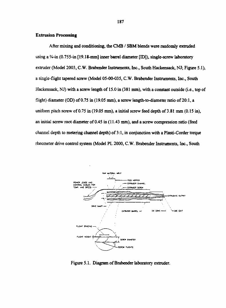
187
Extrusion Processing
After mixing and conditioning, the CMB / SBM blends were randomly extruded
using a %-in (0.755-in [19.18-mm] inner barrel diameter [ID]), single-screw laboratory
extruder (Model 2003, C.W. Brabender Instruments, Inc., South Hackensack, NJ; Figure 5.1),
a single-flight tapered screw (Model 05-00-035, C.W. Brabender Instruments, Inc., South
Hackensack, NJ) with a screw length of 15.0 in (381 mm), with a constant outside (i.e., top of
flight) diameter (OD) of 0.75 in (19.05 mm), a screw length-to-diameter ratio of 20:1, a
uniform pitch screw of 0.75 in (19.05 mm), a initial screw feed depth of 3.81 mm (0.15 in),
an initial screw root diameter of 0.45 in (11.43 mm), and a screw compression ratio (feed
channel depth to metering channel depth) of 3:1, in conjunction with a Plasti-Corder torque
rheometer drive control system (Model PL 2000, C.W. Brabender Instruments, Inc., South
RAW MATERIAL INPUT
POWER LEADS AN0 CONTROL CABLES FOR TEMP, AND SPEED »
-rCtD MOPPC* - EXTRUOC* CHANNEL
- CXTRUCE» SCREW
-CXTflUOATt OUTPUT
EXTRUDER BARREL —' x—oic ex IT
ruCHT SPACING —..
rjCMT HEIGHT
/ I SCREW QumCTER
-SCREW FLIGHTS
Figure 5.1. Diagram of Brabender laboratory extruder.
188
Hackensack, NJ). The extruder barrel had eight equally-spaced grooves 3.175 mm (1/8 in)
wide by 0.794 mm (1/32 in) deep running longitudinally along the length of the barrel to
improve material shearing and mixing, and had a 3.175-mm (1/8-in) diameter circular die
mounted on the extruder exit. A low temperature profile (LTP) of 80-90-100 °C, and a high
temperature profile (HTP) of 100-110-120 °C were used in this study. The extruder
temperature profile corresponded to the temperature at the feeding, metering, and die
sections, respectively, of the extruder. In this study, a low extruder screw speed (LSS) of 50
rpm [5.24 rad/s] and a high screw speed (HSS) of 100 rpm [10.47 rad/s] were used.
Processing conditions during extrusion were monitored by measuring dough
temperature (°C), die temperature (°C), net torque exerted on the extruder drive (N-m) (i.e.,
net torque accounts for the amount of torque required under no-load conditions versus the
amount required during processing), specific mechanical energy (SME) consumed during
processing (J/g), product throughput rate (g/min), feed material throughput rate (g/min),
dough apparent viscosity in the extruder (Pa-s), and dough density in the die (g/cm3). The die
temperature (measured in the die section of the extruder) and the dough temperature
(measured at the end of the metering zone) were determined using stock thermocouples
(Model 05-00-348, C.W. Brabender Instruments, Inc., South Hackensack, NJ) inserted into
the extruder. Torque readings were recorded by the extruder's computer control system
during processing. Product throughput was determined by collecting extrudate samples at
30-s time intervals, allowing the samples to cool for 1 h under ambient conditions, and then
measuring the mass of the collected material using an electronic balance (Model A-250,
Denver Instrument Co., Arvada, CO). By using a dry matter mass balance, the material
189
throughput rate (i.e., the raw ingredient feed rate) could be determined (Alvarez-Martinez et
al., 1988; Harper, 1981):
where m&«, is the rate of feed material throughput (g/min), m^ is the measured rate of
extrudate product throughput (g/min), MCf is the moisture content of the collected extrudate
product samples (w.b.), and MC, is the initial moisture content of the raw feed ingredient
material prior to extrusion (w.b.). This dry matter mass balance is required to account for
moisture loss due to evaporation when material exits the die. The specific mechanical
energy, the energy input per unit rate of flow required to convey the material through the
extruder, was calculated according to Harper (1981) and Martelli (1983):
where SME is the specific mechanical energy consumed (J/g), T is the torque exerted on the
extruder drive (N-m), to is the angular velocity of the screw (rad/s), and ny is the raw feed
material throughput (g/min). The apparent viscosity of the dough in the extruder during
processing was calculated by approximating the extruder behavior as that of a coaxial
viscometer, but corrected for the tapered screw geometry vis-à-vis the extruder barrel
(5.1)
SME = T m 60 (5.2)
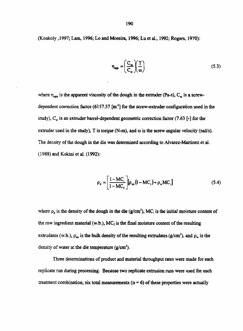
190
(Konkoly ,1997; Lam, 1996; Lo and Moreira, 1996; Lu et al., 1992; Rogers, 1970):
where is the apparent viscosity of the dough in the extruder (Pa-s), C* is a screw-
dependent correction factor (6157.57 [m3] for the screw-extruder configuration used in the
study), Cg. is an extruder barrel-dependent geometric correction factor (7.63 [-] for the
extruder used in the study), T is torque (N-m), and to is the screw angular velocity (rad/s).
The density of the dough in the die was determined according to Alvarez-Martinez et al.
(1988) and Kokini et al. (1992):
where pd is the density of the dough in the die (g/cm3), MC, is the initial moisture content of
the raw ingredient material (w.b.), MCf is the final moisture content of the resulting
extrudates (w.b.), pw is the bulk density of the resulting extrudates (g/cm3), and pw is the
density of water at the die temperature (g/cm3).
Three determinations of product and material throughput rates were made for each
replicate run during processing. Because two replicate extrusion runs were used for each
treatment combination, six total measurements (n = 6) of these properties were actually
(5.3)
P, = k(i-Mc,)+pwMc l] (5.4)
191
recorded for each treatment combination. Thirty observations were taken during each
extrusion run for die and dough temperatures, torque, SME, dough viscosity, and dough
density (measurements were recorded every 30 s during processing). Because 2 replicate
extrusion runs were conducted for each treatment combination, 60 total observations (n = 60)
for each treatment combination for each of these processing variables were actually
measured.
Extruded Product Analysis
After extrusion processing, the resulting extrudate samples were allowed to cool
under ambient conditions for three hours, placed in polyethylene bags, and stored at room
temperature. To investigate the effects of the extrusion processing on the masa byproduct /
soybean meal mixtures, several physical and nutritional properties were then measured on the
extruded products. These properties included: moisture content (%, w.b.), water activity (-),
proximate composition (crude protein, crude fat, and ash contents [%, d.b.]), in-vitro protein
digestibility (%), product diameter (mm), expansion ratios (cross-sectional expansion index,
longitudinal expansion index, and volumetric expansion index [-]), bulk density (g/cm3), true
density (g/cm3), color (Hunter L-a-b values [-]), water absorption index (-),water solubility
index (-), and durability (%). Moisture content, water activity, proximate analyses, and color
were determined using the methods previously described for the raw ingredient blends. The
in-vitro protein digestibility study was conducted by the Department of Animal Science at
Iowa State University following Bookwalter et al. (1987) and Mertz et al. (1984). Extrudate
samples were cut to a length of 2 cm, were weighed on an electronic balance (Model A-250,
Denver Instrument Co., Arvada, CO), and were measured for diameter using a digital
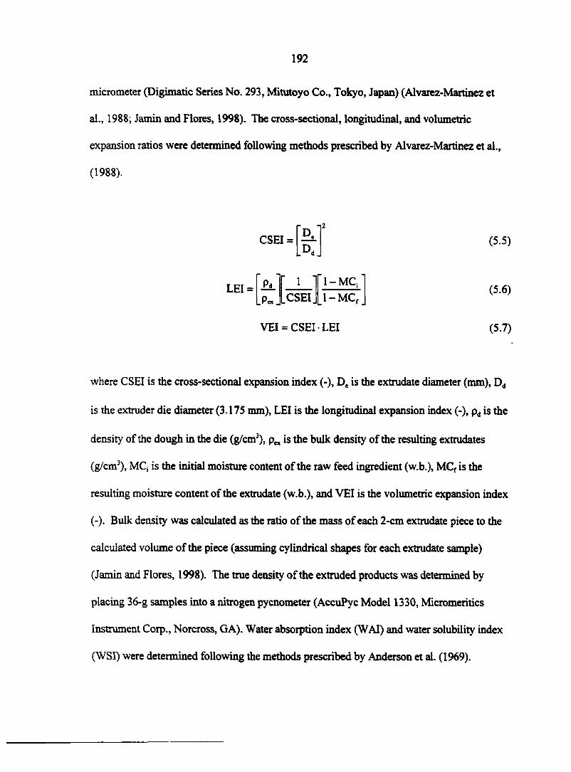
192
micrometer (Digimatic Series No. 293, Mitutoyo Co., Tokyo, Japan) (Alvarez-Martinez et
al., 1988; Jamin and Flores, 1998). The cross-sectional, longitudinal, and volumetric
expansion ratios were determined following methods prescribed by Alvarez-Martinez et al.,
(1988).
CSEI = D,
D,
LEI = Pd 1 " l -MC,"
-p«_ .CSEI. 1 -MCf
VEI = CSEI LEI
(5.5)
(5.6)
(5.7)
where CSEI is the cross-sectional expansion index (-), De is the extrudate diameter (mm), Dd
is the extruder die diameter (3.175 mm), LEI is the longitudinal expansion index (-), pd is the
density of the dough in the die (g/cm3), p„ is the bulk density of the resulting extrudates
(g/cm3), MQ is the initial moisture content of the raw feed ingredient (w.b.), MCf is the
resulting moisture content of the extrudate (w.b.), and VEI is the volumetric expansion index
(-). Bulk density was calculated as the ratio of the mass of each 2-cm extrudate piece to the
calculated volume of the piece (assuming cylindrical shapes for each extrudate sample)
(Jamin and Flores, 1998). The true density of the extruded products was determined by
placing 36-g samples into a nitrogen pycnometer (AccuPyc Model 1330, Micromeritics
Instrument Corp., Norcross, GA). Water absorption index (WAI) and water solubility index
(WSI) were determined following the methods prescribed by Anderson et al. (1969).
193
Durability of extrudate samples was determined by following the ASAE standard method
S269.4 ("Cubes, Pellets, and Crumbles - Definitions and Methods for Determining Density,
Durability, and Moisture Content") (ASAE, 1996). Three samples from each extrusion run
were analyzed for each property determination. Because two replicate extrusion runs were
utilized in the experimental design, six total observations (n = 6) were present for each
treatment combination (except the durability analysis, which utilized only one sample for
each replicate run [n = 2 total observations]).
RESULTS AND DISCUSSION
Raw Ingredient Properties
The results for the raw ingredient characterizations are shown in Table 5.1. The 30%
CMB blend had the highest geometric mean particle diameter (GMD), the 0% blend had the
lowest, and as masa byproduct fraction increased in the blend, the mean particle diameter
increased. Additionally, all blends exhibited similar particle size distributions and all
followed log-normal behavior typically displayed (Figure 5.2) by ground feed materials
(Bern and Hurburgh, 1998; McEllhiney, 1985). It appears that as the fraction of masa
byproduct in the blend increased, higher agglomeration occurred in the blend, which led to
the greater geometric mean particle diameters for higher masa byproduct fractions. This
effect may be due to the byproduct particles' ability to bind with the soybean meal particles.
The 10% blend had the highest geometric standard deviation (GSD), while the 30% blend
had the lowest. No clear pattern emerged between geometric standard deviation and blend
ratio, but all GSD values were quite low.
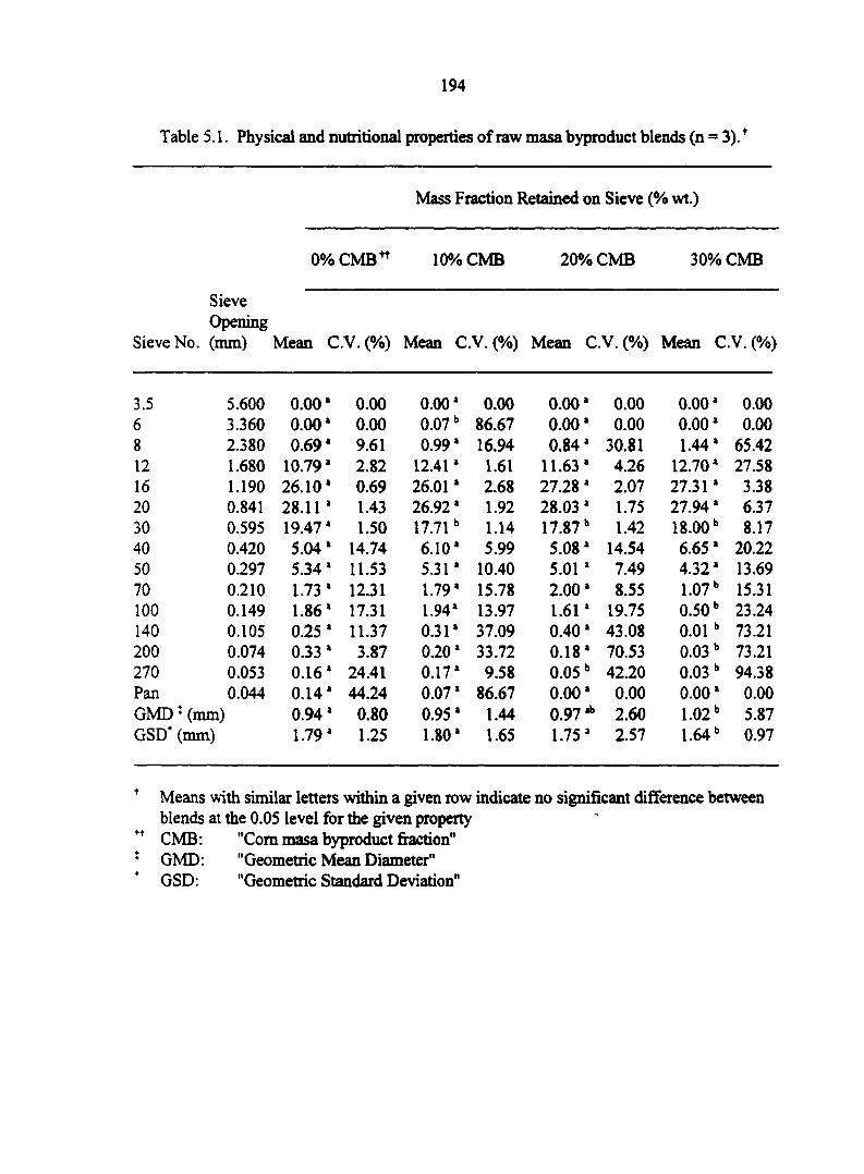
194
Table 5.1. Physical and nutritional properties of raw masa byproduct blends (n = 3).f
Mass Fraction Retained on Sieve (% wt.)
0% CMBn 10% CMB 20% CMB 30% CMB
Sieve Opening
Sieve No. (mm) Mean C.V. (%) Mean C.V. (%) Mean C.V. (%) Mean C.V. (%)
3.5 5.600 0.00 • 0.00 0.00* 0.00 0.00* 0.00 0.00* 0.00 6 3.360 0.001 0.00 0.07b 86.67 0.00* 0.00 0.00* 0.00 8 2.380 0.691 9.61 0.99* 16.94 0.84* 30.81 1.44* 65.42 12 1.680 10.79* 2.82 12.41 * 1.61 11.63* 4.26 12.70* 27.58 16 1.190 26.101 0.69 26.01 * 2.68 27.28 * 2.07 27.31 * 3.38 20 0.841 28.11 * 1.43 26.92 * 1.92 28.03 * 1.75 27.94 * 6.37 30 0.595 19.47 * 1.50 17.71b 1.14 17.87b 1.42 18.00b 8.17 40 0.420 5.041 14.74 6.10* 5.99 5.08* 14.54 6.65* 20.22 50 0.297 5.341 11.53 5.31* 10.40 5.01 * 7.49 4.32* 13.69 70 0.210 1.73' 12.31 1.79* 15.78 2.00* 8.55 1.07b 15.31 100 0.149 1.86* 17.31 1.94* 13.97 1.61* 19.75 0.50b 23.24 140 0.105 0.25* 11.37 0.31* 37.09 0.40* 43.08 0.01b 73.21 200 0.074 0.33* 3.87 0.20* 33.72 0.18* 70.53 0.03b 73.21 270 0.053 0.16* 24.41 0.17* 9.58 0.05" 42.20 0.03b 94.38 Pan 0.044 0.14* 44.24 0.07* 86.67 0.00* 0.00 0.00* 0.00 GMD • (mm) 0.94' 0.80 0.95* 1.44 0.97* 2.60 1.02b 5.87 GSD' (mm) 1.79* 1.25 1.80* 1.65 1.75* 2.57 1.64b 0.97
' Means with similar letters within a given row indicate no significant difference between blends at the 0.05 level for the given property
++ CMB: "Com masa byproduct fraction" ; GMD: "Geometric Mean Diameter"
GSD: "Geometric Standard Deviation"
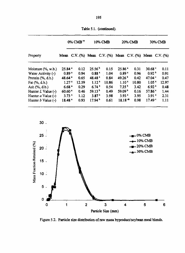
195
Table 5.1. (continued).
0% CMBn 10% CMB 20% CMB 30% CMB
Property Mean C.V. (%) Mean C.V. (%) Mean C.V. (%) Mean C.V. (%)
Moisture (%, w.b.) 25.841 0.12 25.56b 0.15 25.861 0.31 30.68c 0.11 Water Activity (-) 0.891 0.94 0.881 1.04 0.891 0.96 0.92b 0.91 Protein (%, d.b.) 48.641 0.65 48.48a 0.84 49.26b 0.42 47.04c 0.47 Fat (%, d.b.) 1.271 12.59 1.121 10.86 1.10' 10.80 1.05' 12.97 Ash (%, d.b.) 6.681 0.29 6.741 0.54 7.35b 3.42 6.92' 0.48 Hunter L Value (-) 60.601 0.46 59.13" 0.49 59.09b 0.16 57.86 e 1.44 Hunter a Value (-) 3.73' 1.12 3.871 3.98 3.93* 3.95 3.91* 2.31 Hunter b Value (-) 18.481 0.93 17.94b 0.61 18.18* 0.98 17.49 = 1.11
1 5 5 |
; % CO
30
25
20 -
15
10
5 -
.0% CMB
. 10% CMB
.20% CMB
.30% CMB
2 3 4
Particle Size (mm)
Figure 5.2. Particle size distribution of raw masa byproduct/soybean meal blends.
196
The 30% blend also had the highest resulting moisture content of all the blends, while the
10% blend had the lowest No clear pattern emerged between blend ratio and moisture
content, except that the 30% blend had the highest moisture content, which was expected at
the outset of the study. When the raw ingredient mixtures were initially blended, the CMB
was blended with the SBM on an "as-is" (i.e., wet) basis, and additional water was added to
achieve a moisture content target of approximately 26% (w.b.). This target moisture content
was used in the study because it has been determined to be acceptable for extrusion
processing of soybean meal with various byproduct additives (Wang et al., 1996). Masa
byproducts are approximately 90% water (w.b.), and blending at the 30% level produced a
mixture that inherently had a moisture content greater than all other mixtures, as well as
greater than the target level (i.e., greater than 26%). Although this blend was higher in
moisture than the target, it was used in the study due to the importance of utilizing as high a
byproduct blend ratio as possible. All other blends, however, had moisture contents very
close to 26% (w.b.).
Additionally, the 30% blend had the highest water activity of all blends, whereas the
10% blend had the lowest, which was behavior similar to that of the moisture content data.
All blends had water activity values greater than 0.88, which is too high for safe storage. It
was anticipated, however, that the extrusion cooking process would dry the materials to some
extent, and reduce both moisture content and water activity levels for all blends.
The nutritional composition analysis showed that the 20% blend had the highest
protein content, while the 30% blend had the lowest. No clear pattern between protein
content and raw ingredient blend existed, however. All blends had protein levels similar to
197
raw soybean meal. The 0% blend had the highest fat content, but the 30% blend had the
lowest. Although the differences were not statistically significant, the data appear to show
that as the CMB blend ratio increased, the fat content decreased. All blends, however, were
very low in fat content. The 20% blend held the highest ash content, but the 0% blend had
the lowest. No clear pattern between ash content and raw ingredient blend existed, however.
All blends were very similar in ash content. All blends used in this study had nutrient levels
similar to those of unadulterated soybean meal; the level of corn masa byproduct addition
introduced only small alterations in these overall nutritional levels. Typically, soybean meal
has a nutritional composition of approximately 10% moisture, 44 - 48% protein, 0.5% fat,
6% ash, and 40% carbohydrate content (Erickson, 1995).
From the color analysis, the 0% blend had the highest Hunter L value, a measure of
lightness (100 = white) / darkness (0 = black), while the 30% had the lowest. It appears that
as the CMB ratio increased, the L value decreased across all blends (i.e., the blend became
slightly darker). The 20% blend had the highest Hunter a value, a chromaticity measure of
redness (+) / greenness (-), but the 0% had the lowest, and no significant differences between
blend levels for the a values existed. The 0% blend had the highest Hunter b value, a
chromaticity measure of yellowness (+) / blueness (-), but the 30% had the lowest. No clear
trends appeared between b value and blend ratio, however. All blends produced very similar
color results, and essentially, these results describe the raw ingredient blends as yellow
materials with a slight degree of browness.
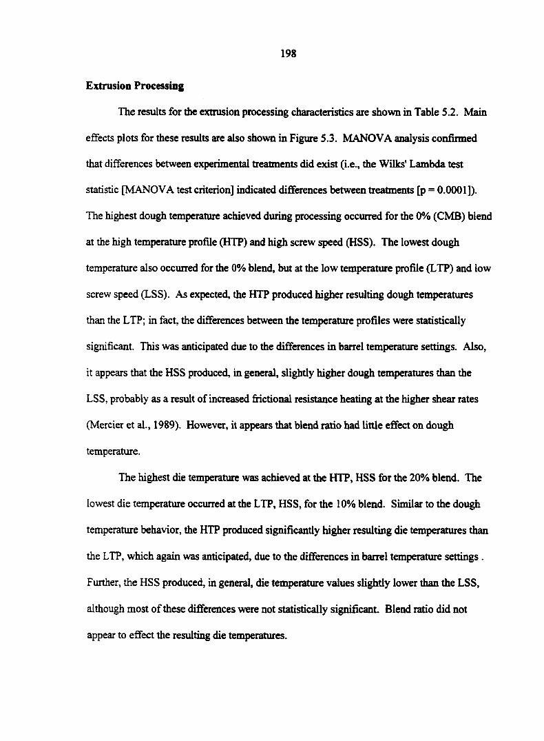
198
Extrusion Processing
The results for the extrusion processing characteristics are shown in Table 5.2. Main
effects plots for these results are also shown in Figure 5.3. MANOVA analysis confirmed
that differences between experimental treatments did exist (i.e., the Wilks' Lambda test
statistic [MANOVA test criterion] indicated differences between treatments [p = 0.0001]).
The highest dough temperature achieved during processing occurred for the 0% (CMB) blend
at the high temperature profile (HTP) and high screw speed (HSS). The lowest dough
temperature also occurred for the 0% blend, but at the low temperature profile (LTP) and low
screw speed (LSS). As expected, the HTP produced higher resulting dough temperatures
than the LTP; in fact, the differences between the temperature profiles were statistically
significant. This was anticipated due to the differences in barrel temperature settings. Also,
it appears that the HSS produced, in general, slightly higher dough temperatures than the
LSS, probably as a result of increased frictional resistance heating at the higher shear rates
(Mercier et al., 1989). However, it appears that blend ratio had little effect on dough
temperature.
The highest die temperature was achieved at the HTP, HSS for the 20% blend. The
lowest die temperature occurred at the LTP, HSS, for the 10% blend. Similar to the dough
temperature behavior, the HTP produced significantly higher resulting die temperatures than
the LTP, which again was anticipated, due to the differences in barrel temperature settings .
Further, the HSS produced, in general, die temperature values slightly lower than the LSS,
although most of these differences were not statistically significant Blend ratio did not
appear to effect the resulting die temperatures.
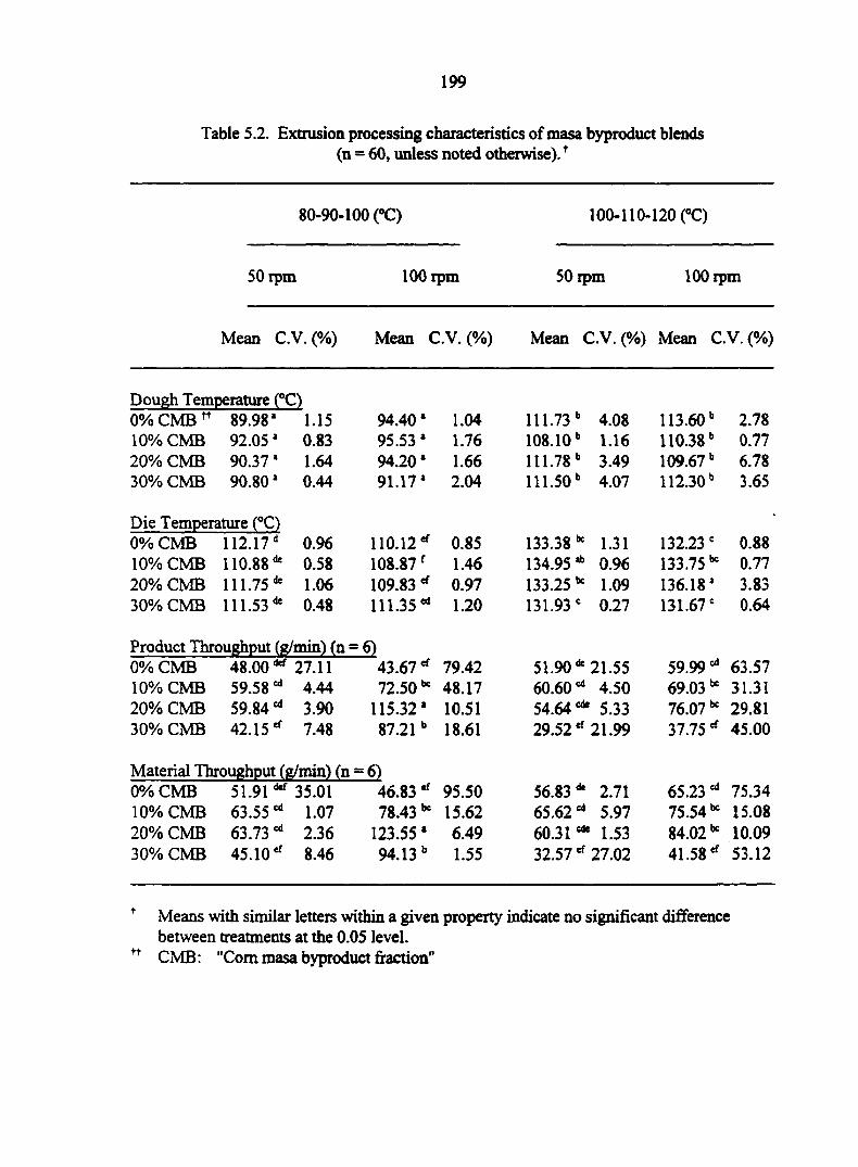
199
Table 5.2. Extrusion processing characteristics of masa byproduct blends (n = 60, unless noted otherwise).f
80-90-100 (°C) 100-110-120 (T)
50rpm 100 rpm 50rpm 100 rpm
Mean C.V. (%) Mean C.V. (%) Mean C.V. (%) Mean C.V.(%)
Dough Temperature (°C) 0% CMB ft 89.981 1.15 94.401 1.04 111.73b 4.08 113.60" 2.78 10% CMB 92.051 0.83 95.53 ' 1.76 108.10" 1.16 110.38" 0.77 20% CMB 90.37 ' 1.64 94.201 1.66 111.78" 3.49 109.67 " 6.78 30% CMB 90.801 0.44 91.17* 2.04 111.50" 4.07 112.30" 3.65
Die Temperature (°C) 0% CMB 112.17 0.96 110.12 " 0.85 133.38 k 1.31 132.23 c 0.88 10% CMB
3 00 00 © 0.58 108.87f 1.46 134.95 * 0.96 133.7566 0.77
20% CMB 111.75 ^ 1.06 109.83 " 0.97 133.25 k 1.09 136.18' 3.83 30% CMB 111.53 * 0.48 111.3564 1.20 131.93 e 0.27 131.67 = 0.64
Product Throughput (g/min) (n = cd 0% CMB 48.00 27.11 43.67" 79.42 51.90* 21.55 59.99 cd 63.57
10% CMB 59.58 * 4.44 72.50 k 48.17 60.60 * 4.50 69.03 be 31.31 20% CMB 59.84"» 3.90 115.32' 10.51 54.64 e* 1 5.33 76.07 be 29.81 30% CMB 42.15" 7.48 87.21b 18.61 29.52 " 21.99 37.75 tf 45.00
Material Throughput (g/min) (n Z61 0% CMB 51.91 *" 35.01 46.83 * 95.50 56.83 * 2.71 65.23 * 75.34 10% CMB 63.55 ^ 1.07 78.43 * 15.62 65.62 * 5.97 75.5466 15.08 20% CMB 63.73 66 2.36 123.55 * 6.49 60.31 1.53 84.02 "c 10.09 30% CMB 45.10" 8.46 94.13 b 1.55 32.57 * 27.02 41.58" 53.12
+ Means with similar letters within a given property indicate no significant difference between treatments at the 0.05 level.
n CMB: "Com masa byproduct fraction"
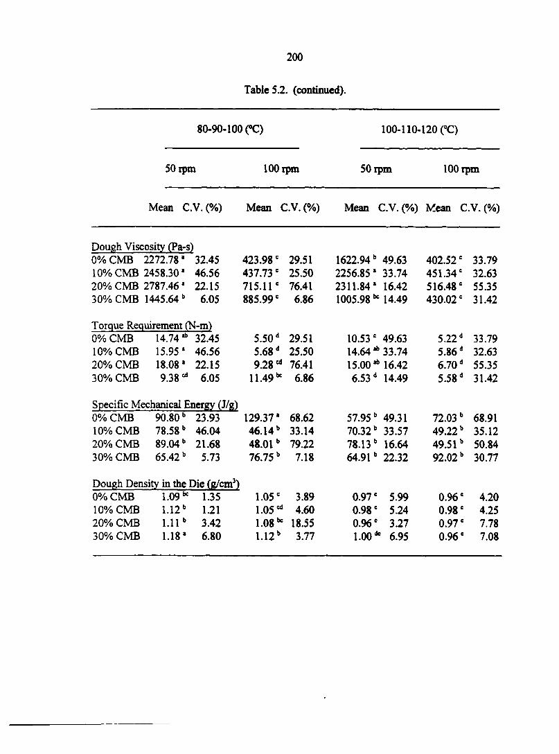
200
Table 5.2. (continued).
80-90-100 (°C) 100-110-120 (°C)
50 rpm 100 rpm 50 rpm 100 rpm
Mean C.V. (%) Mean C.V. (%) Mean C.V. (%) Mean C.V. (%)
Dough Viscosity (Pa-s) 0% CMB 2272.781 32.45 423.986 29.51 1622.94" 49.63 402.52e 33.79 10% CMB 2458.301 46.56 437.73c 25.50 2256.85 * 33.74 451.34 e 32.63 20% CMB 2787.461 22.15 715.11c 76.41 2311.84* 16.42 516.48 e 55.35 30% CMB 1445.64 " 6.05 885.99 e 6.86 1005.98 •* 14.49 430.02e 31.42
Torque Requirement (N-m) 0% CMB 14.74 *" 32.45 5.50d 29.51 10.53 e 49.63 5.22d 33.79 10% CMB 15.95 1 46.56 5.68d 25.50 14.64 * 33.74 5.86d 32.63 20% CMB 18.081 22.15 9.28 e- 76.41 15.00*" 16.42 6.70d 55.35 30% CMB 9.38 ^ 6.05 11.49be 6.86 6.53 d 14.49 5.58d 31.42
Specific Mechanical Energy (J/g) 0% CMB 90.80 " 23.93 129.37* 68.62 57.95 " 49.31 72.03 " 68.91 10% CMB 78.58" 46.04 46.14" 33.14 70.32b 33.57 49.22 " 35.12 20% CMB 89.04" 21.68 48.01 " 79.22 78.13 " 16.64 49.51 " 50.84 30% CMB 65.42 " 5.73 76.75 " 7.18 64.91" 22.32 92.02 " 30.77
Dough Density in the Die (g/cm3) 0% CMB 1.09k 1.35 1.05 e 3.89 0.97 e 5.99 0.96 e 4.20 10% CMB 1.12" 1.21 1.05* 4.60 0.98 e 5.24 0.98 e 4.25 20% CMB 1.11" 3.42 1.08"= 18.55 0.96 e 3.27 0.97 e 7.78 30% CMB 1.181 6.80 1.12" 3.77 1.00 * 6.95 0.96 e 7.08
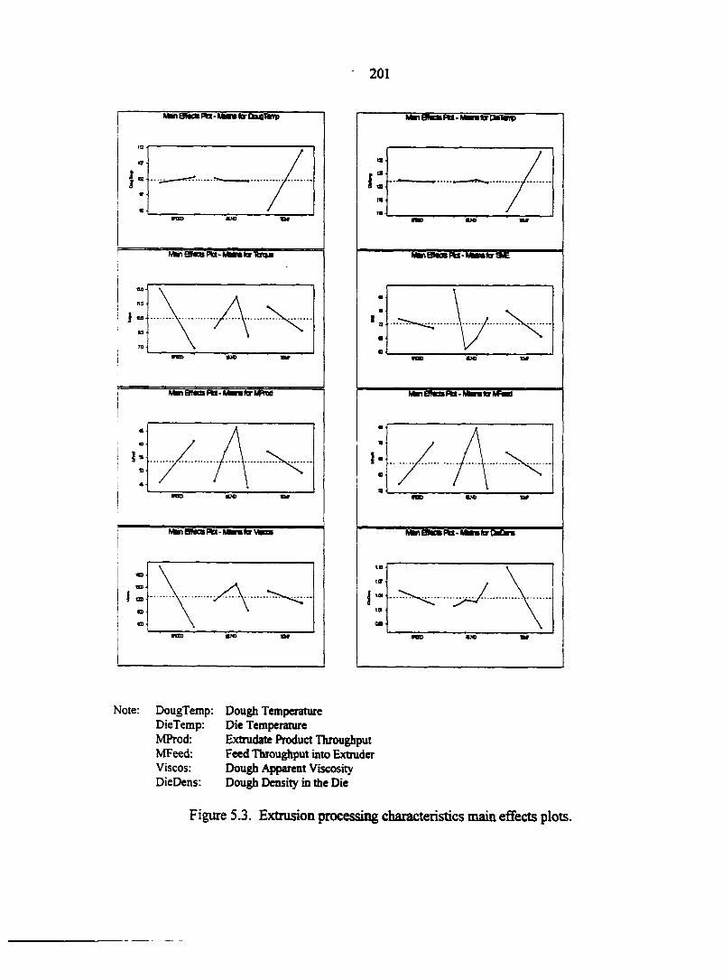
201
WnBhtilAe-lWeWrOneTieip
•AnBNcsRa-MmfenS^a
MmBMOsRS-MntarMtoti
λ S
«
WiBIWiAa-Mesfa'Wcas
<9
MfeiBMcttM-MnterCWUnip
Mmata»ta-Mhm«ar3C'
•
MnateBRX-MntorMFad
id
MnBURt-MnforCUn
13
SOD
Note: DougTemp: Dough Temperature DieTemp: Die Temperature MProd: Extrudate Product Throughput MFeed: Feed Throughput into Extruder Viscos: Dough Apparent Viscosity DieDens: Dough Density in the Die
Figure 5.3. Extrusion processing characteristics main effects plots.
202
The highest product throughput rate occurred at the LTP, HSS for the 20% blend.
The lowest product throughput was at the HTP, LSS, for the 30% blend. Because the feed
material throughput rate was calculated based on the measured product throughput rate, the
behavior of feed material throughput was identical to product throughput In general, the
HSS produced higher throughput than the LSS, which was expected. During extrusion,
higher screw speeds typically produce higher mass flowrates, because of the increased ability
of the extruder to convey material through the machine (Bouvier et al., 1987; Mercier et al.,
1989). Increased temperature profile appeared to lower the throughput rate, but blend ratio
had an uncertain effect on the throughput rate.
The highest dough viscosity occurred at the LTP, LSS for the 20% blend. The lowest
dough viscosity was at the HTP, HSS, for the 0% blend. Screw speed had a significant effect
on resulting dough viscosity: viscosity for the LSS was much higher than that for the HSS.
Additionally, the HTP appeared to produce viscosity results lower than those for the LTP, in
general. Blend ratio did not appear to effect the resulting viscosity values. Most food
doughs, including soy doughs, are pseudoplastic materials (i.e., an increase in shear rate
produces a decrease in the material's apparent viscosity). Further, viscosity typically
decreases as processing temperature increases (Chen et al., 1979; Kokini et al., 1992). These
behaviors, which were exhibited in this study, occur due to the structural changes that occur
in the food dough (i.e., unfolding of molecules and material structures) during processing.
The highest torque required occurred at the LTP, LSS for the 20% blend. The lowest
torque requirement was at the HTP, HSS, for the 0% blend. Screw speed had a significant
effect on resulting torque, with the LSS producing higher torque values than the HSS.
203
Because the CMB / SBM blends behaved pseudoplastically, and apparent viscosity decreased
with increasing screw speed, the resultant torque required by the screw to convey the dough
decreased. Further, it appears that the HTP had, in general, lower torque values than their
respective values for the LTP; this again, was the result of dough viscosity decreasing with
increased temperature (Mercier et al., 1989). Blend ratio did not appear to effect resulting
torque requirements, however.
The lowest specific mechanical energy requirement was at the LTP, HSS, for the 10%
blend. The highest specific mechanical energy (SME) input occurred at the LTP, HSS for the
0% blend. Although this value was significantly higher than all other SME values, and it did
have high variability; the results for this treatment combination might actually be an
"outlier". More investigation is required to verify the results from this treatment
combination. For the remainder of the treatments, no clear effects due to temperature profile,
screw speed, or blend ratio emerged from ANOVA, but increased speed and temperature
appeared to produce lower SME values. Typically, the SME is an indication of the viscous
dissipation of mechanical energy, which is provided by the screw drive shaft, into the dough
due to fractional resistance (Marsman et al., 1995). The SME, in fact, quantifies the
competing effects of viscosity changes due to changes in screw speed (i.e., pseudoplastic
behavior), and the resulting change in the torque which is required to convey the dough
through the extruder. Typically, it has been noted that as screw speed increases, SME also
increases, due to the changes in energy input to the screw being of a greater order of
magnitude than the decrease in torque associated with the decrease in apparent viscosity due
to the shear thinning behavior of the non-Newtonian material (Mercier et al., 1989).
204
The highest dough density in the die occurred at the LTP, LSS for the 30% blend.
The lowest dough density was at the HTP, HSS, for the 0% blend. The LTP produced
density values significantly higher than those for the HTP. Additionally, the HSS appeared
to produce density values slightly lower than those for the LSS. Further, blend ratio did not
appear to effect the density values. The primary reason that the higher processing
temperature produced lower dough density in the die values was because of the higher
expansion associated with the higher temperature, which led to a lower resulting value for
extrudate bulk density. Alvarez-Martinez et al. (1988) studied starch extrudate expansion,
and determined that the value for dough density in the die could be approximated as constant
at a value of 1.2 g/cm3. The results from the current study are similar, but are slightly lower,
and range from 0.96 to 1.18 g/cm3. This could be due to raw ingredient differences.
From the data and main effects plots, it can be seen that the 30% CMB blend typically
had spurious results vis-à-vis all other blend ratios. This behavior is probably due to the
higher initial moisture content of that blend prior to extrusion.
Extruded Product Analysis
Typical extradâtes produced during extrusion processing in this study are shown in
Figure 5.4. Main effects plots for the extruded product results are shown in Figure 5.5 and
5.6. The results for the extruded product characterization tests are shown in Table 5.3.
MANOVA analysis confirmed that differences between experimental treatments did exist
(i.e., the Wilks1 Lambda test statistic [MANOVA test criterion] indicated differences between
treatments [p = 0.0001]). The highest resulting extrudate moisture content occurred at the
LTP, LSS, for the 30% blend. The lowest extrudate moisture content was at the HTP, HSS,
205
Figure 5.4. Typical raasa byproduct/soybean meal extradâtes.
for the 20% blend. In general, the HTP produced extradates with significantly lower
resulting moisture contents than the LTP. Within each temperature profile, screw speed
appeared to produce a slight decrease in moisture content. The 30% blend, which had the
highest original moisture content prior to extrusion, also had the highest resulting extradate
moisture content after extrusion, for all processing conditions. The remainder of the blends
did not show any blend effect on final moisture content.
Because of the high temperatures involved, extrusion processing has a drying effect
on feed materials. When a dough melt is transported through an extruder die, high
temperatures and pressures build up prior to material exiting the die, and up to 8 percentage
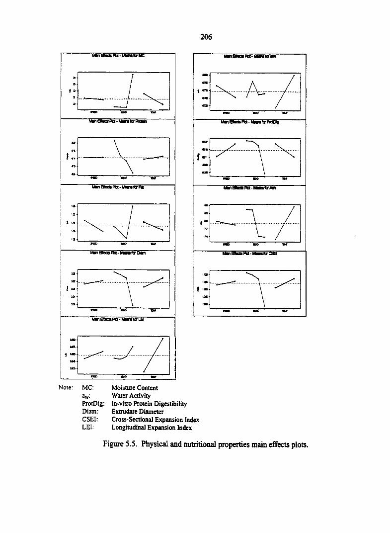
206
MnBtanx-Mmfo'MC
wnâSSÂÈMBStoHëBn
WnBTecttFW-rtBBtoS"
Mn sites Ptt-Mmfv dan
«AnBkamci-WmxKrLE
MtiBMm-MntoiW
nwinn'ii FM->»»»torFWCg
Î •"
U M
WnSksna-MnftriS
I
Note: MC: Moisture Content aw: Water Activity ProtDig: In-vitro Protein Digestibility Diam: Extrudate Diameter CSEI: Cross-Sectional Expansion Index LEI: Longitudinal Expansion Index
Figure 5.5. Physical and nutritional properties main effects plots.
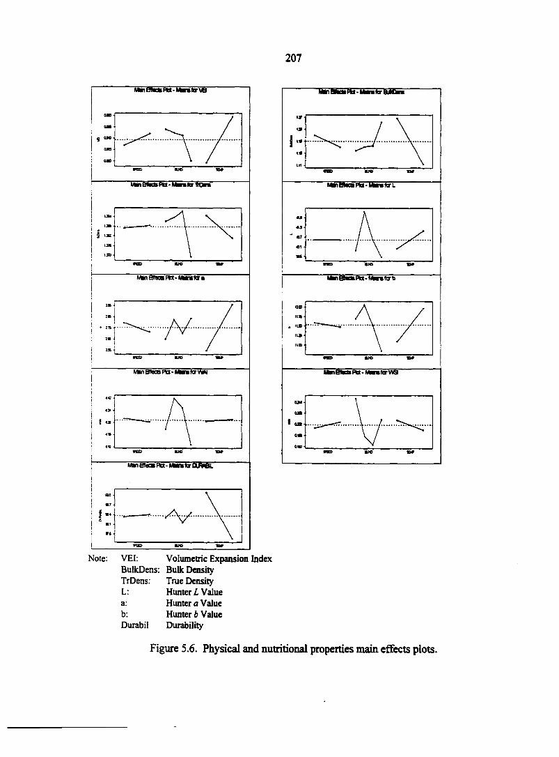
207
MjnBMcBRt-MmtarvB '
g «se-
SIB -
I »
| -* H I :B
MfnaMcsna-Mnto'iiOra
MmStacBPtt-Mntra
Mn afecs PU - Mn fer VMI
ManEffKBRot-MnftraflittC
MnBMRl-MrafirBlOm"
A*iOWnma-*w*#»L
Mn0MtRa-Mnfcrb
ft*
It»
TVS
MnBMna-Mm«arWSr
Note: VEI: Volumetric Expansion Index BulkDens: Bulk Density TrDens: True Density L: Hunter I Value a: Hunter a Value b: Hunter b Value Durabil Durability
Figure 5.6. Physical and nutritional properties main effects plots.

208
Table 5.3. Physical and nutritional properties of masa byproduct blend extradâtes (n = 6, unless noted otherwise).f
80-90-100 (°C) 100-110-120 CC)
50 rpm 100 rpm 50 rpm 100 rpm
Mean C.V. (%) Mean C.V. (%) Mean C.V. (%) Mean C.V. (%)
Moisture Content (%, w.b.) 0% CMB ft 19.82* 2.45 20.39 rf 3.45 18.78hi 0.65 19.33 * 1.24 10% CMB 20.60 * 1.12 19.498 1.42 19.428 5.00 18.53 ij 2.13 20% CMB 21.04d 0.68 20.54 * 3.13 18.17j 2.57 18.13j 2.54 30% CMB 25.79 ' 3.25 25.18b 0.52 23.48e 2.11 23.63 e 1.69
Water Activity (-) 0.81 * 0% CMB 0.70 5.15 0.66 e 4.54 0.82' 2.25 0.81 * 2.75
10% CMB 0.80 * 2.08 0.7666 4.67 0.821 3.12 0.811 2.33 20% CMB 0.74 * 4.41 0.68 e 9.78 0.80 * 2.37 0.8016 2.83 30% CMB 0.75* 19.71 0.60f 9.12 0.85 1 2.09 0.841 2.79
Protein (%, d.b.) 0% CMB 48.391 0.48 48.351 0.56 48.291 0.31 48.421 0.39 10% CMB 47.60b 0.56 47.60b 0.70 47.49b 0.61 47.52b 0.65 20% CMB 47.32b 0.50 47.36b 0.54 47.15 b 0.25 47.24b 0.47 30% CMB 46.35c 0.44 46.19 e 0.56 47.06b 0.54 47.06b 1.08
f Means with similar letters within a given property indicate no significant difference between treatments at the 0.05 level.
tf CMB: "Com masa byproduct fraction" : CSEI: "Cross-Sectional Expansion Index" " LEI: "Longitudinal Expansion Index"
VEI: "Volumetric Expansion Index" WAI: "Water Absorption Index" WSI: "Water Solubility Index"

209
Table 5.3. (continued).
80-90-100 (°C) 100-110-120 (°C)
50 rpm 100 rpm 50 rpm 100 rpm
Mean C.V. (%) Mean C.V. (%) Mean C.V. (%) Mean C.V. (%)
Protein Digestibility (%, d.b.) 0% CMB 83.651 0.33 80.88b 3.20 80.82b 3.28 83.79 * 0.21 10% CMB 83.74* 0.10 80.62b 3.38 80.93b 2.82 83.83 * 0.09 20% CMB 83.79 * 0.16 80.89b 2.74 80.46b 3.68 83.79 * 0.17 30% CMB 83.82 * 0.11 80.62b 3.23 79.73 b 4.57 83.59 * 0.47
Fat (%, d.b.) 0% CMB 1.24 " 3.54 1.17e4 6.07 1.11* 4.97 1.12 e* 5.88 10% CMB 1.24 ** 1.95 1.10* 7.55 1.10* 15.31 1.06* 6.25 20% CMB 1.24 k 10.43 1.08 * 8.14 1.02 e 13.21 1.00 e 14.32 30% CMB 1 23 bed 11.93 1.19" 12.59 1.40* 12.45 1.31 * 6.86
Ash (%, d.b.) 0% CMB 6.81b 0.81 6.77b 1.16 10.13* 29.42 10.11* 24.10 10% CMB 8.39*- 20.59 7.59b 6.17 9.77* 29.46 7.98b 9.71 20% CMB 7.82b 16.05 7.13b 5.91 7.17b 7.15 7.53- 13.43 30% CMB 6.93 b 1.08 6.91b 0.92 6.95b 2.41 8.77*- 36.50
Diameter (mm) 0% CMB 3.33 16 1.29 3.36*- 2.08 3.39* 2.61 3.40* 2.02 10% CMB 3.32* 0.93 3.37* 1.16 3.39* 1.19 3.35- 2.81 20% CMB 3.29 k 1.49 3.37- 1.21 3.34*- 2.06 3.36- 3.05 30% CMB 3.15e 2.27 3.16* 1.58 3.24" 5.80 3.24 e4 2.38
CSEI (-) : 0% CMB 1.10,b 2.63 1.12*- 4.14 1.14* 5.22 1.15* 4.05 10% CMB 1.09* 2.01 1.13* 2.33 1.14* 2.39 1.11- 5.66 20% CMB 1.0766 2.98 1.12*- 2.44 1.11*- 4.15 1.12* 6.08 30% CMB 0.98 e 4.54 0.99* 3.16 1.05 e4 11.52 1.04 e4 4.72
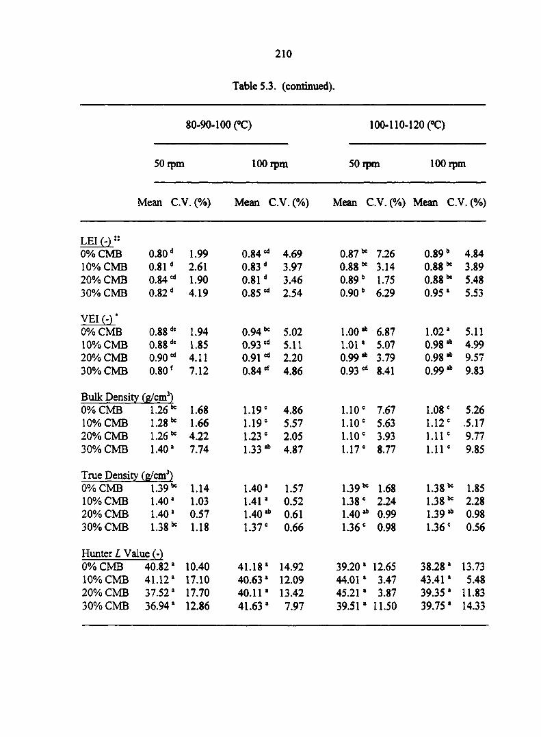
210
Table 5.3. (continued).
80-90-100 CO 100-110-120 (°C)
50ipm 100 rpm 50 rpm 100 rpm
Mean C.V.(%) Mean C.V.(%) Mean C.V.(%) Mean C.V.(%)
LEI (-)î$
0% CMB 0.80d 1.99 0.84* 4.69 0.87 * 7.26 0.89b 4.84 10% CMB 0.81d 2.61 0.83 d 3.97 0.8866 3.14 0.88 16 3.89 20% CMB 0.84* 1.90 0.81d 3.46 0.89b 1.75 0.88 * 5.48 30% CMB 0.82d 4.19 0.85* 2.54 0.90b 6.29 0.95* 5.53
VEI (-) ' 0% CMB 0.88de 1.94 0.94 k 5.02 î.oo- 6.87 1.02* 5.11 10% CMB 0.88de 1.85 0.93* 5.11 1.01* 5.07 0.98- 4.99 20% CMB 0.90* 4.11 0.91 * 2.20 0.99- 3.79 0.98- 9.57 30% CMB 0.80f 7.12 0.84 tf 4.86 0.93* 8.41 0.99- 9.83
Bulk Density (g/cm3) 0% CMB 1.26 k 1.68 1.19e 4.86 1.10e 7.67 1.08 e 5.26 10% CMB 1.28 ^ 1.66 1.19e 5.57 1.10e 5.63 1.12e .5.17 20% CMB 1.26 k 4.22 1.23 e 2.05 1.10e 3.93 1.11e 9.77 30% CMB 1.401 7.74 1.33- 4.87 1.17e 8.77 1.11e 9.85
True Density (g/cm3) 0% CMB 1.39* 1.14 1.40® 1.57 1.3966 1.68 1.38 h" 1.85 10% CMB 1.401 1.03 1.41® 0.52 1.38 e 2.24 1.3866 2.28 20% CMB 1.401 0.57 1.40* 0.61 1.40- 0.99 1.39- 0.98 30% CMB 1.38 k 1.18 1.37 e 0.66 1.36 e 0.98 1.36 e 0.56
Hunter L Value (-) 0% CMB 40.821 10.40 41.18* 14.92 39.20 * 12.65 38.28 ® 13.73 10% CMB 41.12® 17.10 40.63 * 12.09 44.01* 3.47 43.41 ® 5.48 20% CMB 37.52 ® 17.70 40.11* 13.42 45.21 * 3.87 39.35 ® 11.83 30% CMB 36.94* 12.86 41.63 * 7.97 39.51 * 11.50 39.75 ® 14.33
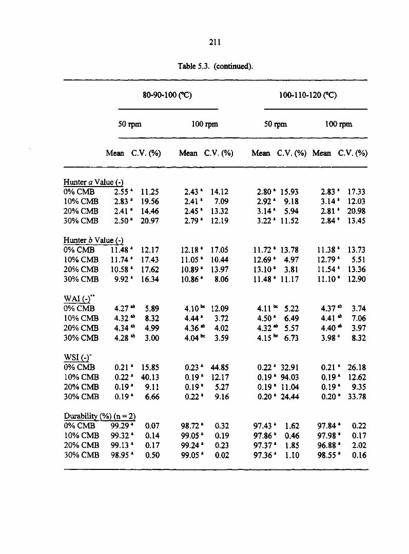
211
Table 5.3. (continued).
80-90-100 (°C) 100-110-120 (°C)
50 rpm 100 rpm 50 rpm 100 rpm
Mean C.V.(%) Mean C.V. (%) Mean C.V.(%) Mean C.V. (%)
Hunter a Value (-) 0% CMB 2.551 11.25 2.43 1 14.12 2.80* 15.93 2.83' 17.33 10% CMB 2.831 19.56 2.411 7.09 2.921 9.18 3.14' 12.03 20% CMB 2.41' 14.46 2.451 13.32 3.14' 5.94 2.81' 20.98 30% CMB 2.50a 20.97 2.791 12.19 3.221 11.52 2.84' 13.45
Hunter b Value (-) 0% CMB 11.481 12.17 12.18 1 17.05 11.721 13.78 11.38' 13.73 10% CMB 11.74 * 17.43 11.05 1 10.44 12.691 4.97 12.79 ' 5.51 20% CMB 10.581 17.62 10.891 13.97 13.101 3.81 11.54' 13.36 30% CMB 9.92 1 16.34 10.861 8.06 11.481 11.17 11.10' 12.90
WAI (-)" 0% CMB 4.27- 5.89 4.10* 12.09 4.11 * 5.22 4.37- 3.74 10% CMB 4.32- 8.32 4.441 3.72 4.50' 6.49 4.41 - 7.06 20% CMB 4.34- 4.99 4.36- 4.02 4.32- 5.57 4.40- 3.97 30% CMB 4.28- 3.00 4.04 k 3.59 4.15 k 6.73 3.98 e 8.32
WSI (-)' 0% CMB 0.211 15.85 0.231 44.85 0.22' 32.91 0.21' 26.18 10% CMB 0.221 40.13 0.19a 12.17 0.19' 94.03 0.19' 12.62 20% CMB 0.191 9.11 0.191 5.27 0.19' 11.04 0.19' 9.35 30% CMB 0.191 6.66 0.221 9.16 0.20' 24.44 0.20' 33.78
Durability (%) (n = 2) 0% CMB 99.29a 0.07 98.721 0.32 97.43 1 1.62 97.84 ' 0.22 10% CMB 99.321 0.14 99.051 0.19 97.861 0.46 97.98 ' 0.17 20% CMB 99.13 1 0.17 99.241 0.23 97.37 ' 1.85 96.88 ' 2.02 30% CMB 98.951 0.50 99.051 0.02 97.36 ' 1.10 98.55 ' 0.16
212
points of the raw ingredient's moisture will actually evaporate due to the sudden change to
ambient pressure and temperature (Faubion et al., 1982). The moisture content loss for the
blends in this study ranged from 4.82 to 7.73 percentage points (w.b.), with the higher
temperature profile producing greater moisture loss than the lower temperature profile. The
final moisture contents of the extradâtes ranged from 18.13 to 25.79 percentage points (w.b.),
however, which is still too high for safe storage, and thus an additional drying step is
required subsequent to extrusion processing (Faubion et al., 1982; Miller, 1985; Wang et al.,
1997). Materials with high moisture contents have higher transportation costs, decreased
stability and storability, and ultimately have limited market area and profitability (Derr and
Dhillon, 1997). To alleviate these difficulties and effectively utilize the CMB / SBM blends
as livestock feed additives, the extradâtes must be dehydrated to an maximum recommended
moisture content of approximately 12 % (w.b.), which is recommended for feed products,
because this moisture level substantially reduces transportation costs and is microbiologically
stable (Beauchat, 1981).
The highest extrudate water activity occurred at the HTP, LSS, for the 30% blend.
The lowest extrudate water activity was at the LTP, HSS, for the 30% blend. The HTP
produced extradâtes with significantly higher water activity values than the LTP. Within
each temperature profile, the HSS generally produced extradâtes with somewhat lower water
activity values than the LSS. Blend, however, did not appear to effect extrudate water
activity. Water activity quantifies the amount of "free" water (i.e., unbound water) available
in materials for use by microorganisms and chemical agents, and hence is a measure of a
material's susceptibility to spoilage and deterioration. Products with no free water (aw = 0.0)
213
are not at risk for spoilage, while materials with 100% free water (aw = 1.0) are at high risk
for rapid spoilage. Because extrusion processing reduces the moisture content of the feed
material, the associated water activity level also decreases. The water activity loss for the
blends in this study ranged from 0.06 to 0.32, and the final water activity levels of the
extradâtes ranged from 0.60 to 0.85. Through dehydration, high-moisture materials become
less expensive to transport and become microbiologically stable. Materials become safe from
bacteria growth below water activities of approximately 0.9, safe from mold growth below
approximately 0.8, and safe from yeast growth below approximately 0.7 (Barbosa-Canovas
and Vega-Mercado, 1996). In order to effectively utilize masa byproduct extradates as
livestock feed ingredients, dehydration subsequent to extrusion is necessary to reduce
extrudate water activity levels, and thus prevent microbial spoilage during storage.
From the proximate nutritional analysis, it was determined that for all processing
conditions, the 0% blend was significantly higher in protein than all other blends, and protein
content decreased as CMB fraction increased, which was anticipated. The 30% blend
produced the lowest protein contents, but all other blends at all other processing conditions
were statistically similar in protein content. Further, it appeared that as screw speed
increased, extradate protein levels slightly increased, and the HTP appeared to produce
slightly higher protein than the LTP. High-temperature processing in an extruder unfolds and
redistributes protein molecules within the plasticized mass in the barrel. At high
temperatures proteins undergo thermal denaturation and form insoluble aggregates, and
amino acids are altered or destroyed, which leads to a final product with lower-quality
protein (Cumming et al., 1973; Dahl and Villota, 1991; Nielsen, 1976). As shown by the
214
composition analysis, protein content levels generally did decrease slightly with increasing
processing temperature, which indicates that thermal denaturation is indeed occurring, at
least to a small extent, during extrusion processing of the masa byproduct blends.
Not only is the amount of protein present important to a feed material, but the
digestibility of that protein is also essential. The highest extrudate protein digestibility
occurred at the HTP, HSS, for the 10% blend. The lowest extrudate protein digestibility was
at the HTP, LSS, for the 30% blend. The LTP, LSS and the HTP, HSS both exhibited similar
protein digestibility results across all blends, which were significantly higher than the LTP,
HSS and the HTP, LSS results, which also both exhibited similar results. Further, it appears
that as speed increased, digestibility also increased, and as temperature increased,
digestibility decreased. Additionally, it appeared that as blend ratio increased, digestibility
decreased. Marsman et al. (1995) determined that raw, unprocessed soybean meal had in-
vitro protein digestibility of approximately 61%, and that extrusion processing the soybean
meal could produce digestibility values of 73 to 85%, which is a substantial increase in the
protein quality, because heat treatments, within certain limits, improves the digestibility of
proteins. They further stated that a digestibility range of approximately 67 to 85% is ideal for
livestock nutrition. Beyond these limits, the feed material is either under-processed
(digestibility < 67%) or over-processed (digestibility > 85%), and is not optimally digested
by livestock. The protein digestibility values for the extruded masa byproduct blends in this
study ranged from 79.73 to 83.83%, and thus fell within the optimal digestibility region.
The highest extrudate fat content occurred at the HTP, LSS, for the 30% blend. The
lowest extrudate fat content was at the HTP, HSS, for the 20% blend. Generally, the HTP
215
produced extradâtes with lower fat contents than the LTP. Further, within each temperature
profile, the HSS produced lower fat contents than the LSS. For the 30% blend at the HTP,
though, both screw speeds produced extradâtes with high fat contents. Overall, however,
blend did not appear to show any effect on final fat content. Typically overall fat content
levels in soybean products are affected little during extrusion processing, but the extruded
products are generally more shelf-stable than the raw ingredients, due to the heat treatment
deactivating fat-splitting enzymes which are present in the raw materials (Nielsen, 1976).
The highest extrudate ash content occurred at the HTP, LSS, for the 0% blend. The
lowest extrudate ash content was at the LTP, HSS, for the 0% blend. The HTP produced, in
general, extradâtes with higher ash contents than the LTP. But both screw speed and blend
ratio appeared to have a decreasing effect on ash content as each of these factors increased.
This behavior can probably be attributed to reactions that occur at the higher temperature
level during the extrusion processing.
The highest extradate diameter occurred at the HTP, HSS, for the 0% blend. The
lowest extrudate diameter was at the LTP, LSS, for the 30% blend. In general, the HTP
produced extradâtes with greater diameters than the LTP. Within each temperature profile, it
appears that the HSS produced slightly greater diameters than the LSS. It appears that as
blend ratio increased, extrudate diameter decreased, although the 30% blend consistently had
the lowest diameter results across all processing conditions. These results show, in general,
that the extruded products had diameter values only slightly greater than the die diameter of
3.175 mm (1/8 in) (i.e., little radial expansion occurred). Similar results were obtained by
Gumming et al. (1972), who studied extrusion of 30% moisture content soybean meal and
216
produced products with relatively constant diameters. Their extradâtes exhibited little
expansion upon extruder die exit, and their results showed that a majority of the physical
changes to the soy feed material occur inside the extruder before exiting the die.
The high temperatures, shear stresses, and shear strains produced during extrusion
processing alter not only the physical characteristics and the nutritional quality of feed
materials, but also affect the complex interactions between the chemical constituents and the
resulting internal cellular structures that occur during water evaporation upon die exit (Miller,
1985). These changes are reflected in the expansion of the material as it passes through the
extruder die, and are quantified through the use of expansion ratios (Moore et al., 1990). It
has been theorized that extradate product expansion is dependent on the rheological
properties of the thermoplastic melt in the extruder channel: radial expansion is dependent
on melt elasticity and elongation is dependent on melt viscosity. It is further believed that the
damage to the protein molecules incurred by the heat treatment in an extruder reduces the
ability of the melt to form an elastic structure upon die exit, thus exhibiting a decreased
expansion (Alvarez-Martinez et al., 1988). The highest extrudate radial expansion, quantified
by the CSEI (Cross-Sectional Expansion Index), occurred at the HTP, HSS, for the 0% blend.
The lowest extradate CSEI value was at the LTP, LSS, for the 30% blend. The CSEI results
exhibit behavior similar those of the diameter results, because the CSEI value is determined
based on product diameter. In general, the HTP produced extradâtes with greater CSEI
results than the LTP, which agrees with the results of Alvarez-Martinez et al. (1988), which
predict higher radial expansions for higher processing temperatures. Within each
temperature profile, it appears that HSS produced slightly greater CSEI values than the LSS.
217
Increasing the blend ratio appeared to cause a decrease in CSEI values, although the 30%
blend consistently had the lowest CSEI results throughout all processing conditions, which
follows the results of Alvarez-Martinez et al. (1988), which predict lower CSEI for higher
moisture materials, due to softening of molecular structures and reduced elastic properties.
Radial extrudate expansion, quantified by the CSEI, is highly dependent on the water and
starch compositions of the extruded material. Products high in starch content generally
exhibit high expansion; soybean meal, however, essentially has no starch, so it was not
surprising that little radial expansion occurred during extrusion processing in this study, as
evidenced by very low CSEI values; this behavior is further caused by the high protein value
of soybean meal, which can incur heat damage during processing and thus further restrict
expansion (Gumming et al., 1972; Nielsen, 1976). Dahl and Villota (1991) extruded soybean
flour and produced CSEI values between 0.5 and 1.6 (-). CSEI values from this study fall
within that range.
The Longitudinal Expansion Index (LEI) quantifies the elongation of extradâtes as
they pass through the extruder die. The highest extrudate LEI value occurred at the HTP,
HSS, for the 30% blend. The lowest extrudate LEI value was at the LTP, LSS, for the 0%
blend. In general, the HTP produced extradates with higher LEI values than the LTP.
Within each temperature profile, the HSS generally produced higher LEI values than the
LSS, which follows behavior described by Kokini et al. (1992). LEI depends on the melt
viscosity, and as shown by the results in this study, higher screw speeds led to lower melt
apparent viscosities, which led to more elongated structures upon die exit than those
exhibited at the lower screw speeds. Blend did not appear to have an effect on LEI values.
218
Overall, however, the LEI values were very low, which ultimately points to little longitudinal
expansion for the extruded blends in this study.
Overall extrudate volumetric expansion, quantified by the Volumetric Expansion
Index (VEI), relates the effects of the radial and longitudinal expansion, through the
interaction of the CSEI and the LEI. The highest extrudate VEI value occurred at the HTP,
HSS, for the 0% blend. The lowest extrudate VEI value was at the LTP, LSS, for the 30%
blend. The HTP produced VEI values significantly greater than those produced by the LTP.
Additionally, within each temperature profile, it appears that VEI was generally greater for
the HSS than for the LSS. Further, the 30% blend, at all processing conditions, consistently
produced the lowest VEI values, and it appeared that increasing blend ratio lead to lower VEI
results. In general, the results indicate that the extruded products, for all blends and
processing conditions used in this study, exhibited little expansion upon die exit, which was
expected. This behavior is typical for soybean materials because of the very low starch
content, which is key to product expansion via the starch gelatinization process (Nielsen,
1976).
Another measure of the internal structure of an extrudate is bulk density. The highest
extrudate bulk density value occurred at the LTP, LSS, for the 30% blend. The lowest
extrudate bulk density was at the HTP, HSS, for the 0% blend. The LTP condition produced
higher bulk density values than the HTP. Within the LTP, the LSS produced higher values
than the HSS. Within the HTP, however, increased screw speed produced slightly lower bulk
density values. From the main effects plots, however, it appears that as temperature is
increased, bulk density is decreased. Additionally, an increasing blend ratio appeared to
219
produce a greater extrudate bulk density. Bulk density generally decreases as processing
temperature is increased, a behavior which was exhibited in this study, which leads to a more .
porous extrudate structure, and thus an increased water penetration (Badrie and Mellowes,
1991; Gumming et al., 1972). Further, Badrie and Mellowes (1991) predict that as feed
ingredient moisture content increases, the resulting bulk density will also increase, which is a
behavior also exhibited in this study. Bouvier et al. (1987) studied extrusion of soy dough,
and determined extrudate bulk density values of approximately 1.25 g/cm3, similar to values
found in the current study.
Bulk density is a unit of measurement that quantifies a material's mass per unit
volume, and includes the entrapped air within interior pores. To determine the density of a
material excluding the internal pores, the true density must be used (Stroshine and Hamann,
1995). The highest extrudate true density value occurred at the LTP, HSS, for the 10%
blend. The lowest extrudate true density was at the HTP, 30% blend, at both the LSS and
HSS. The LTP produced extradâtes with slightly higher true density values than the HTP,
which is behavior similar to that of bulk density (i.e., higher processing temperatures
produced more porous structures). Within each temperature profile, however, screw speed
appeared to have only a small effect on density: increasing the speed lead to a small increase
in true density. The 30% blend consistently had the lowest true density of all blends, at all
processing conditions. All other blends, however, did not appear to exhibit a blend effect on
true density, for any processing condition. Generally, true density values were slightly higher
than the bulk density values, which is due to accounting for the entrained air within the
extrudate structures.
220
From the color analysis, it can be seen that overall, the extruded products were
substantially darker in appearance than the raw ingredient blends, with the L, a, and b results
all much lower in value than the respective values for the raw ingredients. The highest
extrudate Hunter L value occurred at the HTP, LSS, for the 20% blend. The lowest extrudate
Hunter L value was at the LTP, LSS, for the 30% blend. No significant differences existed
between Hunter L value results for any processing conditions or blends for the extradâtes,
although it appears that as processing temperature increased, the L value slightly increased.
The highest extrudate Hunter a value occurred at the HTP, LSS, for the 30% blend. The
lowest extrudate Hunter a value was at the LTP, LSS, for the 20% blend, and at the LTP,
HSS, for the 10% blend, but no significant differences existed between Hunter a value results
for any processing conditions or blends for the extradâtes. It appears, however, that as speed
increased, the a value slightly decreased; as the temperature increased, the a value slightly
increased. The highest extrudate Hunter b value occurred at the HTP, HSS, for the 10%
blend. The lowest extrudate Hunter b value was at the LTP, LSS, for the 30% blend. No
significant differences existed between Hunter b value results for any processing conditions
or blends for the extradâtes; however, it appears that in increased speed and an increased
temperature resulted in, respectively, slightly decreased b value and slightly increased b
value. Essentially these results describe the extruded products as brown in appearance. The
extruded products are darker and browner than the raw ingredient blends because of the high-
temperature heat treatment during the extrusion cooking process. High processing
temperatures exacerbate protein reactions with reducing sugars in nonenzymatic (Maillard)
browning processes, which lead to not only darker products, but also products with reduced
221
nutritional quality (i.e., destruction of amino acids) (Badrie and Mellowes, 1991; Dahl and
Villota, 1991).
The relationships between an extruded product and water, especially absorption and
solubility behavior, are important to the functionality of the material. These relationships are
quantified through the Water Absorption Index (WAI) and the Water Solubility Index (WSI).
The highest extrudate WAI value occurred at the HTP, LSS, for the 10% blend. The lowest
extrudate WAI value was at the HTP, HSS, for the 30% blend. No clear patterns for the WAI
values emerged for any processing conditions or blends. Typically, the water absorption
ability of an extrudate increases with increasing processing temperature, due to more
expanded products, because products which have higher expansion generally have a more
porous structure (Maga and Lorenz, 1978). Bressani et al. (1978) extruded blends of com
and soybean products, and measured WAI values on the resulting extradâtes between 4.64
and 5.12, which compares favorably to the results obtained in this study. Solubility
quantifies a material's ability to solubilize in water. The highest extrudate WSI value
occurred at the LTP, HSS, for the 0% blend. The lowest extrudate WSI value actually
occurred at several settings: LTP, LSS, for the 30% blend, for the 20% blend, all settings,
and for the 10% blend, all settings but the LTP, LSS. No significant differences existed
between WSI values for any processing conditions or blends for the extradates, however.
Typically as processing temperature increases, proteins within a soy-based thermoplastic
melt in an extruder are increasingly altered and redistributed, and the protein molecules
become insoluble (Gumming et al., 1973). As seen from the data in this study, the ability of
the extruded masa/soybean meal blends to solubilize in water is quite low.
222
During handling and storage, feed materials are subjected to many destructive forces,
including impact, shear, compression, abrasion, and other interactions with surrounding
materials. These destructive forces damage the feed materials and produce broken and dusty
feedstuff's, which subsequently decreases quality and value, and increases susceptibility to
deterioration (Stroshine and Hamann, 1995). Durability is the quality characteristic that
quantifies the ability of a feed material to resist these destructive forces. Higher durability
indicates a higher resistance to damage, and can be achieved via several means. High
temperature conditioning and processing of the feed material leads to improved product
durability, as does decreasing the raw ingredient particle size; both methods improve
durability due to increasing the surface area of the feed material, which allows for more
thorough moisture addition, which then produces denser extruded pellets. On the other hand,
larger particle sizes lead to decreased durability, due to the production of fissures in the
extruded products, which are inherently more susceptible to damage and breakage (Tabil and
Sokhansanj, 1996). Because higher temperatures are achieved with extrusion processing,
product durability is generally greater than that of pellets produced through traditional steam
pelleting (Hilton et al., 1981). The highest extrudate durability occurred at the LTP, LSS, for
the 10% blend. The lowest extrudate durability was at the HTP, HSS, for the 20% blend.
Although the LTP appeared to have slightly higher durability results than the HTP, no
significant differences actually existed between durability results for any processing
conditions or blends for the extradâtes. The durability values of the extruded products in this
study were quite high, ranging from 96.88 to 99.32%, which shows that the extruded CMB /
223
SBM blends were highly resistive to the destructive forces commonly encountered by feed
materials, which is a highly beneficial property for feed ingredients.
Property Relationships
The relationships between all the 34 measured physical, nutritional, and extruder
operational properties (excluding durability) in the study were investigated using a
correlation analysis. Fifty-five of the resulting 1156 Pearson product-moment correlations
(Speigel, 1994) were significant (p<0.05) (Table 5.4); the remainder of the correlations were
not. The correlation coefficient (r) quantifies the strength of the linear relationship between
two variables, and as shown in the table, 37 of the variable combinations in the study had
resulting correlation coefficients greater than |0.80|; 17 of the variable combinations had
resulting correlation coefficients greater than |0.90|, and thus exhibited fairly strong linear
relationships. Several of these correlations, however, were expected prior to analysis,
because of their relationships via equations (5.1) through (5.7): CSEI and diameter; material
throughput and product throughput; bulk density and dough density in the die; dough
viscosity and torque; CSEI and VEI; diameter and VEI; die
temperature and dough density in the die; dough viscosity and extruder speed; bulk density
and VEI.
Several other correlations existed that were intuitively anticipated prior to analysis.
The high correlation between raw ingredient moisture content and raw ingredient water
activity was expected, because a high moisture content should allow more water to be
available for microbial use. Also, the strong correlation between extrudate moisture content
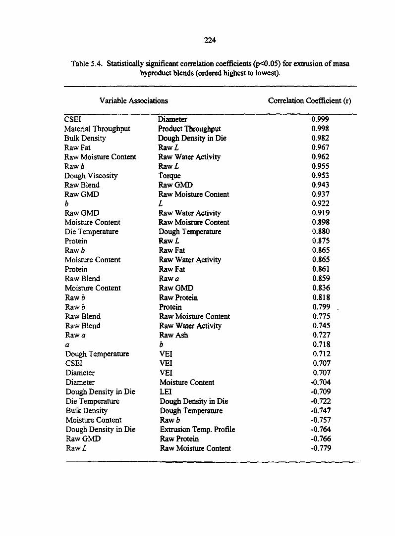
224
Table 5.4. Statistically significant correlation coefficients (p<0.05) for extrusion of masa byproduct blends (ordered highest to lowest).
Variable Associations Correlation Coefficient (r)
CSEI Diameter 0.999 Material Throughput Product Throughput 0.998 Bulk Density Dough Density in Die 0.982 Raw Fat Raw L 0.967 Raw Moisture Content Raw Water Activity 0.962 Raw b Raw L 0.955 Dough Viscosity Torque 0.953 Raw Blend Raw GMD 0.943 Raw GMD Raw Moisture Content 0.937 b L 0.922 Raw GMD Raw Water Activity 0.919 Moisture Content Raw Moisture Content 0.898 Die Temperature Dough Temperature 0.880 Protein RawZ, 0.875 Raw b Raw Fat 0.865 Moisture Content Raw Water Activity 0.865 Protein Raw Fat 0.861 Raw Blend Raw a 0.859 Moisture Content Raw GMD 0.836 Raw b Raw Protein 0.818 Raw b Protein 0.799 . Raw Blend Raw Moisture Content 0.775 Raw Blend Raw Water Activity 0.745 Raw a Raw Ash 0.727 a b 0.718 Dough Temperature VEI 0.712 CSEI VEI 0.707 Diameter VEI 0.707 Diameter Moisture Content -0.704 Dough Density in Die LEI -0.709 Die Temperature Dough Density in Die -0.722 Bulk Density Dough Temperature -0.747 Moisture Content Raw 6 -0.757 Dough Density in Die Extrusion Temp. Profile -0.764 Raw GMD Raw Protein -0.766 RawZ Raw Moisture Content -0.779
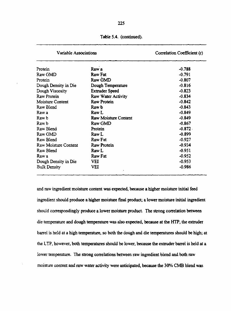
225
Table 5.4. (continued).
Variable Associations Correlation Coefficient (r)
Protein Raw a -0.788 Raw GMD Raw Fat -0.791 Protein Raw GMD -0.807 Dough Density in Die Dough Temperature -0.816 Dough Viscosity Extruder Speed -0.823 Raw Protein Raw Water Activity -0.834 Moisture Content Raw Protein -0.842 Raw Blend Rawb -0.843 Raw a RawL -0.849 Raw b Raw Moisture Content -0.849 Rawb Raw GMD -0.867 Raw Blend Protein -0.872 Raw GMD RawL -0.899 Raw Blend Raw Fat -0.927 Raw Moisture Content Raw Protein -0.934 Raw Blend Raw L -0.951 Raw a Raw Fat -0.952 Dough Density in Die VEI -0.953 Bulk Density VEI -0.986
and raw ingredient moisture content was expected, because a higher moisture initial feed
ingredient should produce a higher moisture final product; a lower moisture initial ingredient
should correspondingly produce a lower moisture product. The strong correlation between
die temperature and dough temperature was also expected, because at the HTP, the extruder
barrel is held at a high temperature, so both the dough and die temperatures should be high; at
the LTP, however, both temperatures should be lower, because the extruder barrel is held at a
lower temperature. The strong correlations between raw ingredient blend and both raw
moisture content and raw water activity were anticipated, because the 30% CMB blend was
226
at a higher moisture content and water activity than the three other blends. Further, the
relatively strong correlations between dough density in the die and both the extrusion
temperature profile and the dough temperature were likely, because dough density in the die
depends on die temperature; die temperature depends on the extrusion temperature profile, as
does the dough temperature. As dough temperature increases, the extrudate expansion
increases; as expansion increases, both the bulk density and the dough density in the die
decrease, due to a more porous structure which is developing in the extrudate (this has been
previously discussed). Furthermore, as moisture content increases, expansion decreases, due
to a more softened extrudate texture. This has also been previously discussed. The full
correlation matrix is given in Table 5.5.
Several correlations involve the color (L - a - b ) values, and are interesting, because
they hold potential for developing prediction relationships between the color variables and
the other variables with which they are associated. These correlations deserve a further
investigation into quantifying these relationships.
To further investigate the relationships and interactions between the raw ingredient
properties, the extrusion processing properties, and the resulting extrudate properties, a
principal components analysis was conducted using all 34 variables under study (excluding
durability). Principal components analysis is used to reduce the dimensionality of
multivariate data by summarizing the variance in the data and projecting it into a set of
uncorrelated orthogonal linear combinations (i.e., eigenvectors) of the original variables.
These linear combinations, or principal components, have the form:
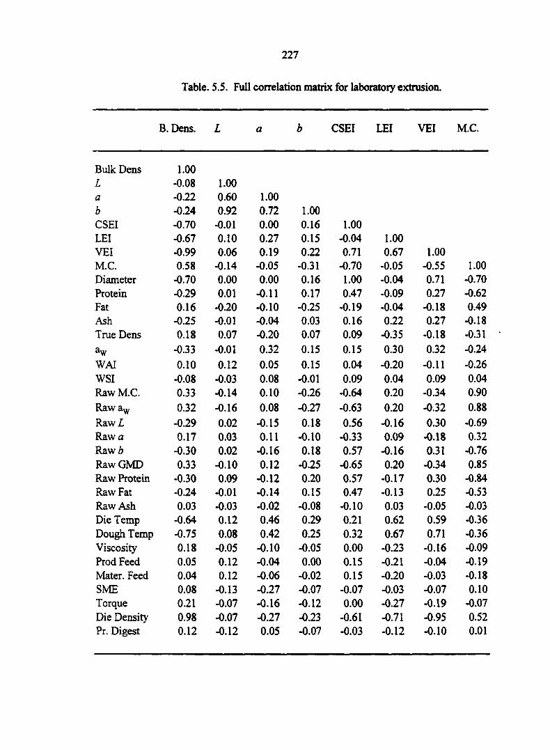
227
Table. 5.5. Full correlation matrix for laboratory extrusion.
B. Dens. L a b CSEI LEI VEI M.C.
Bulk Dens 1.00 L -0.08 1.00 a -0.22 0.60 1.00 b -0.24 0.92 0.72 1.00 CSEI -0.70 -0.01 0.00 0.16 1.00 LEI -0.67 0.10 0.27 0.15 -0.04 1.00 VEI -0.99 0.06 0.19 0.22 0.71 0.67 1.00 M.C. 0.58 -0.14 -0.05 -0.31 -0.70 -0.05 -0.55 1.00 Diameter -0.70 0.00 0.00 0.16 1.00 -0.04 0.71 -0.70 Protein -0.29 0.01 -0.11 0.17 0.47 -0.09 0.27 -0.62 Fat 0.16 -0.20 -0.10 -0.25 -0.19 -0.04 -0.18 0.49 Ash -0.25 -0.01 -0.04 0.03 0.16 0.22 0.27 -0.18 True Dens 0.18 0.07 -0.20 0.07 0.09 -0.35 -0.18 -0.31 aw -0.33 -0.01 0.32 0.15 0.15 0.30 0.32 -0.24
WAI 0.10 0.12 0.05 0.15 0.04 -0.20 -0.11 -0.26 WSI -0.08 -0.03 0.08 -0.01 0.09 0.04 0.09 0.04 Raw M.C. 0.33 -0.14 0.10 -0.26 -0.64 0.20 -0.34 0.90 Raw aw 0.32 -0.16 0.08 -0.27 -0.63 0.20 -0.32 0.88
RawZ, -0.29 0.02 -0.15 0.18 0.56 -0.16 0.30 -0.69 Raw a 0.17 0.03 0.11 -0.10 -0.33 0.09 -0.18 0.32 Raw b -0.30 0.02 -0.16 0.18 0.57 -0.16 0.31 -0.76 Raw GMD 0.33 -0.10 0.12 -0.25 -0.65 0.20 -0.34 0.85 Raw Protein -0.30 0.09 -0.12 0.20 0.57 -0.17 0.30 -0.84 Raw Fat -0.24 -0.01 -0.14 0.15 0.47 -0.13 0.25 -0.53 Raw Ash 0.03 -0.03 -0.02 -0.08 -0.10 0.03 -0.05 -0.03 Die Temp -0.64 0.12 0.46 0.29 0.21 0.62 0.59 -0.36 Dough Temp -0.75 0.08 0.42 0.25 0.32 0.67 0.71 -0.36 Viscosity 0.18 -0.05 -0.10 -0.05 0.00 -0.23 -0.16 -0.09 Prod Feed 0.05 0.12 -0.04 0.00 0.15 -0.21 -0.04 -0.19 Mater. Feed 0.04 0.12 -0.06 -0.02 0.15 -0.20 -0.03 -0.18 SME 0.08 -0.13 -0.27 -0.07 -0.07 -0.03 -0.07 0.10 Torque 0.21 -0.07 -0.16 -0.12 0.00 -0.27 -0.19 -0.07 Die Density 0.98 -0.07 -0.27 -0.23 -0.61 -0.71 -0.95 0.52 Pr. Digest 0.12 -0.12 0.05 -0.07 -0.03 -0.12 -0.10 0.01
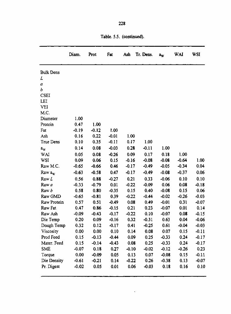
228
Table. 5.5. (continued).
Diam. Prot Fat Ash Tr. Dens. aw WAI WSI
Bulk Dens L a b
CSEI LEI VEI M.C. Diameter 1.00 Protein 0.47 1.00 Fat -0.19 -0.12 1.00 Ash 0.16 0.22 -0.01 1.00 True Dens 0.10 0.35 -0.11 0.17 1.00 aw 0.14 0.08 -0.03 0.28 -0.11 1.00 WAI 0.05 0.08 -0.26 0.09 0.17 0.18 1.00 WSI 0.09 0.06 0.15 -0.16 -0.08 -0.08 -0.64 1.00 Raw M.C. -0.65 -0.66 0.46 -0.17 -0.49 -0.05 -0.34 0.04 Raw aw -0.63 -0.58 0.47 -0.17 -0.49 -0.08 -0.37 0.06
RawZ, 0.56 0.88 -0.27 0.21 0.33 -0.06 0.10 0.10 Raw a -0.33 -0.79 0.01 -0.22 -0.09 0.06 0.08 -0.18 Raw b 0.58 0.80 -0.35 0.15 0.40 -0.08 0.15 0.06 Raw GMD -0.65 -0.81 0.39 -0.22 -0.44 -0.02 -0.26 -0.03 Raw Protein 0.57 0.51 -0.49 0.08 0.49 -0.01 0.31 -0.07 Raw Fat 0.47 0.86 -0.15 0.21 0.23 -0.07 0.01 0.14 Raw Ash -0.09 -0.43 -0.17 -0.22 0.10 -0.07 0.08 -0.15 Die Temp 0.20 0.09 -0.16 0.32 -0.31 0.63 0.04 -0.06 Dough Temp 0.32 0.12 -0.17 0.41 -0.25 0.61 -0.04 -0.03 Viscosity 0.00 0.00 0.10 0.14 0.08 0.07 0.15 -0.11 Prod Feed 0.15 -0.13 -0.44 0.09 0.25 -0.33 0.24 -0.17 Mater. Feed 0.15 -0.14 -0.43 0.08 0.25 -0.33 0.24 -0.17 SME -0.07 0.18 0.27 -0.10 -0.02 -0.12 -0.26 0.23 Torque 0.00 -0.09 0.05 0.13 0.07 -0.08 0.15 -0.11 Die Density -0.61 -0.21 0.14 -0.22 0.26 -0.38 0.13 -0.07 Pr. Digest -0.02 0.05 0.01 0.06 -0.03 0.18 0.16 0.10
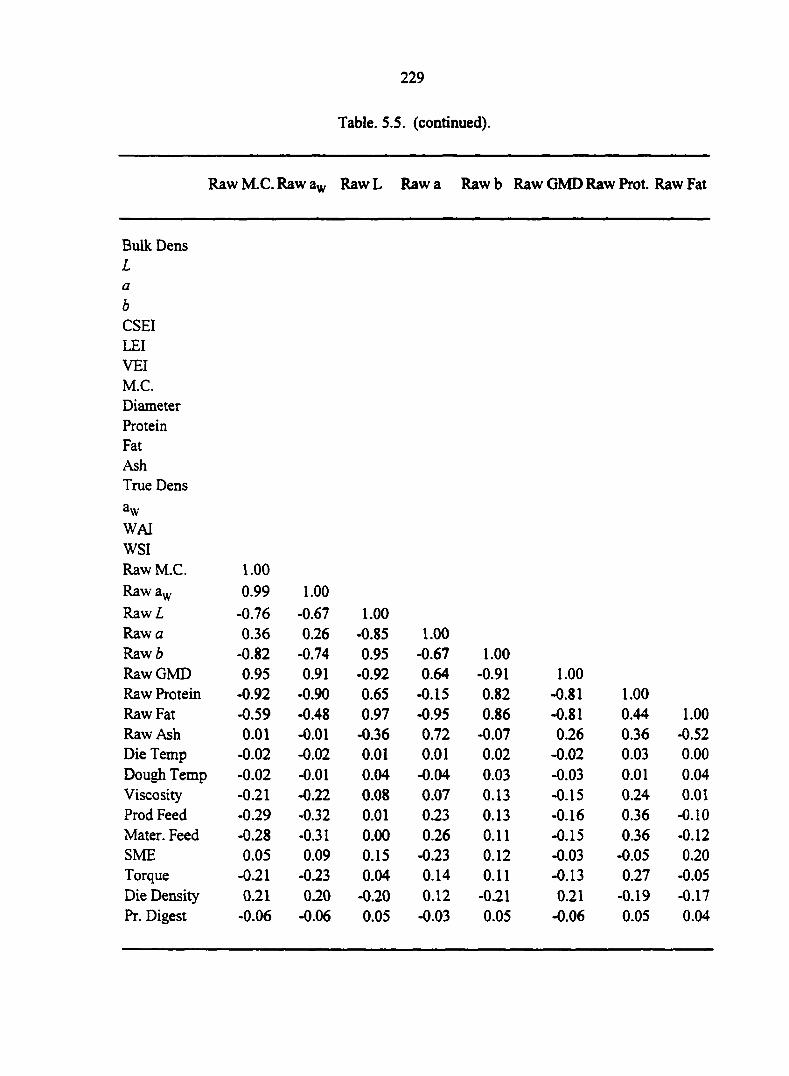
229
Table. 5.5. (continued).
Raw M.C. Raw aw RawL Raw a Rawb Raw GMD Raw Prot. Raw Fat
Bulk Dens L a
b
CSEI LEI VEI M.C. Diameter Protein Fat Ash True Dens aw WAI WSI Raw M.C. 1.00 Raw aw 0.99 1.00
RawZ, -0.76 -0.67 1.00 Raw a 0.36 0.26 -0.85 1.00 Raw b -0.82 -0.74 0.95 -0.67 1.00 Raw GMD 0.95 0.91 -0.92 0.64 -0.91 1.00 Raw Protein -0.92 -0.90 0.65 -0.15 0.82 -0.81 1.00 Raw Fat -0.59 -0.48 0.97 -0.95 0.86 -0.81 0.44 1.00 Raw Ash 0.01 -0.01 -0.36 0.72 -0.07 0.26 0.36 -0.52 Die Temp -0.02 -0.02 0.01 0.01 0.02 -0.02 0.03 0.00 Dough Temp -0.02 -0.01 0.04 -0.04 0.03 -0.03 0.01 0.04 Viscosity -0.21 -0.22 0.08 0.07 0.13 -0.15 0.24 0.01 Prod Feed -0.29 -0.32 0.01 0.23 0.13 -0.16 0.36 -0.10 Mater. Feed -0.28 -0.31 0.00 0.26 0.11 -0.15 0.36 -0.12 SME 0.05 0.09 0.15 -0.23 0.12 -0.03 -0.05 0.20 Torque -0.21 -0.23 0.04 0.14 0.11 -0.13 0.27 -0.05 Die Density 0.21 0.20 -0.20 0.12 -0.21 0.21 -0.19 -0.17 Pr. Digest -0.06 -0.06 0.05 -0.03 0.05 -0.06 0.05 0.04

230
Table. 5.5. (continued).
Raw Ash Die T. Dough T. Vise. Product Feed S ME
Bulk Dens L a b
CSEI LEI VEI M.C. Diameter Protein Fat Ash True Dens aw WAI WSI Raw M.C. Rawaw
RawZ Raw a Raw b Raw GMD Raw Protein Raw Fat Raw Ash 1.00 Die Temp 0.03 1.00 Dough Temp -0.02 0.88 1.00 Viscosity 0.14 -0.13 -0.24 1.00 Prod Feed 0.33 -0.21 -0.13 -0.14 1.00 Mater. Feed 0.35 -0.22 -0.13 -0.14 1.00 1.00 SME -0.12 -0.17 -0.18 0.20 -0.61 -0.60 1.00 Torque 0.22 -0.23 -0.31 0.95 0.05 0.06 0.21 Die Density 0.02 -0.72 -0.81 0.23 0.10 0.09 0.09 Pr. Digest -0.01 0.00 -0.08 0.05 -0.03 -0.04 -0.02
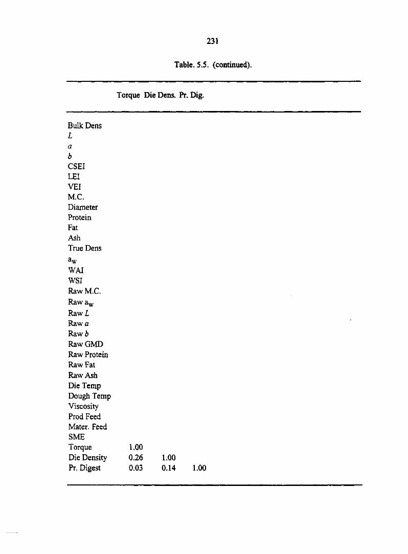
231
Table. 5.5. (continued).
Torque Die Dens. Pr. Dig.
Bulk Dens L a b CSEI LEI VEI M.C. Diameter Protein Fat Ash True Dens aw WAI WSI Raw M.C. Raw aw
RawZ, Raw a Raw b Raw GMD Raw Protein Raw Fat Raw Ash Die Temp Dough Temp Viscosity Prod Feed Mater. Feed SME Torque 1 Die Density 0 Pr. Digest 0
.00
.26 1.00
.03 0.14 1.00

232
y P.C. ~ &lX| + •••+" & 34X34 (5.8)
where yP C is a principal component value, or score, a, through au are the principal
component coefficients (i.e., eigenvectors), and X, through X„ are the original property
variable vectors (i.e., values that were measured in the study) (Everitt and Dunn, 1991). The
results for the principal components analysis are presented in Table 5.6, which shows the
eigenvectors and eigenvalues for the first seven principal components, as well as the
proportion of variation explained through the use of each principal component included.
These first seven principal components accounted for 81.17% of the total variability in the
data, and thus provide both a convenient and comprehensive summary of the information
contained in the original 34 variables, but utilizing a reduced dimensionality of only seven
variables. A "scree" plot of the principal component eigenvalues (Figure 5.7) and a plot of
the error explained through the use of principal components (Figure 5.8) confirms that the
use of seven principal components is adequate to summarize the multivariate data in the
study. Although the interpretation of principal components is very subjective, it appears that
the first principal component may be an indication of raw ingredient properties, while the
second principal component might be an indication of extruder processing characteristics.
Another advantage to using principal components analysis to summarize multivariate
data is the ability to identify outliers, curvature, and clustering in multivariate data through
examination of low-dimensional scatterplots of the calculated principal component scores
(Figure 5.9). Using this approach, no curvature was indicated in this multivariate data set,
but it was determined that an outlier did exist (e.g., see PC 2 versus PC 3 plot). Investigation
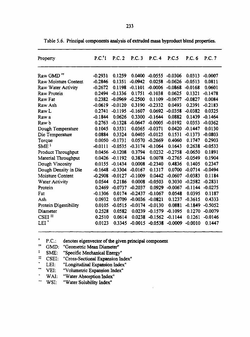
233
Table 5.6. Principal components analysis of extruded masa byproduct blend properties.
Property P.C.fl P.C. 2 P.C. 3 P.C. 4 P.C.5 P.C. 6 P.C. 7
Raw GMDtf -0.2931 0.1259 0.0400 -0.0555 -0.0306 0.0313 -0.0007 Raw Moisture Content -0.2846 0.1351 -0.0942 0.0258 -0.0626 -0.0513 0.0811 Raw Water Activity -0.2672 0.1198 -0.1101 -0.0006 -0.0868 -0.0168 0.0601 Raw Protein 0.2494 -0.1336 0.1751 -0.1038 0.0625 0.1321 -0.1478 Raw Fat 0.2382 -0.0969 -0.2500 0.1109 -0.0677 -0.0827 0.0084 Raw Ash -0.0619 -0.0120 0.3190 -0.2332 0.0493 0.2391 -0.2183 RawL 0.2741 -0.1195 -0.1607 0.0692 -0.0358 -0.0382 0.0325 Raw a -0.1844 0.0626 0.3300 -0.1644 0.0882 0.1439 -0.1464 Raw b 0.2763 -0.1328 -0.0647 -0.0005 -0.0192 0.0353 -0.0362 Dough Temperature 0.1045 0.3531 0.0365 -0.0371 0.0420 -0.1447 0.0130 Die Temperature 0.0884 0.3324 0.0405 -0.0125 0.1531 -0.1373 -0.0803 Torque 0.0050 -0.1731 0.0570 -0.2669 0.4060 0.1747 0.2903 SME: -0.0111 -0.0535 -0.3174 -0.1064 0.1643 0.2638 -0.0533 Product Throughput 0.0456 -0.1208 0.3794 0.0232 -0.2758 -0.0650 0.1891 Material Throughput 0.0426 -0.1192 0.3834 0.0078 -0.2765 -0.0549 0.1904 Dough Viscosity 0.0155 -0.1434 0.0008 -0.2340 0.4836 0.1405 0.2347 Dough Density in Die -0.1648 -0.3304 -0.0167 0.1317 0.0700 -0.0714 -0.0494 Moisture Content -0.2908 -0.0127 -0.1009 0.0442 -0.0607 -0.0383 0.1184 Water Activity 0.0544 0.2186 0.0008 -0.0503 0.3030 -0.2582 -0.2831 Protein 0.2469 -0.0737 -0.2037 0.0929 -0.0067 -0.1144 -0.0275 Fat -0.1306 0.0174 -0.2437 -0.1067 0.0548 0.0395 0.1187 Ash 0.0932 0.0709 -0.0036 -0.0821 0.1237 -0.3615 0.4333 Protein Digestibility 0.0105 -0.0515 -0.0174 -0.0130 0.0881 -0.1849 -0.5052 Diameter 0.2528 0.0582 0.0239 -0.1579 -0.1095 0.1270 -0.0079 CSEI " 0.2510 0.0614 0.0238 -0.1562 -0.1144 0.1261 -0.0146 LEI' 0.0123 0.3345 -0.0015 -0.0538 -0.0009 -0.0010 0.1447
+ P.C.: denotes eigenvector of the given principal component +t GMD: "Geometric Mean Diameter" i SME: "Specific Mechanical Energy" " CSEI: "Cross-Sectional Expansion Index"
LEI: "Longitudinal Expansion Index" VEI: "Volumetric Expansion Index" WAI: "Water Absorption Index"
~ WSI: "Water Solubility Index"
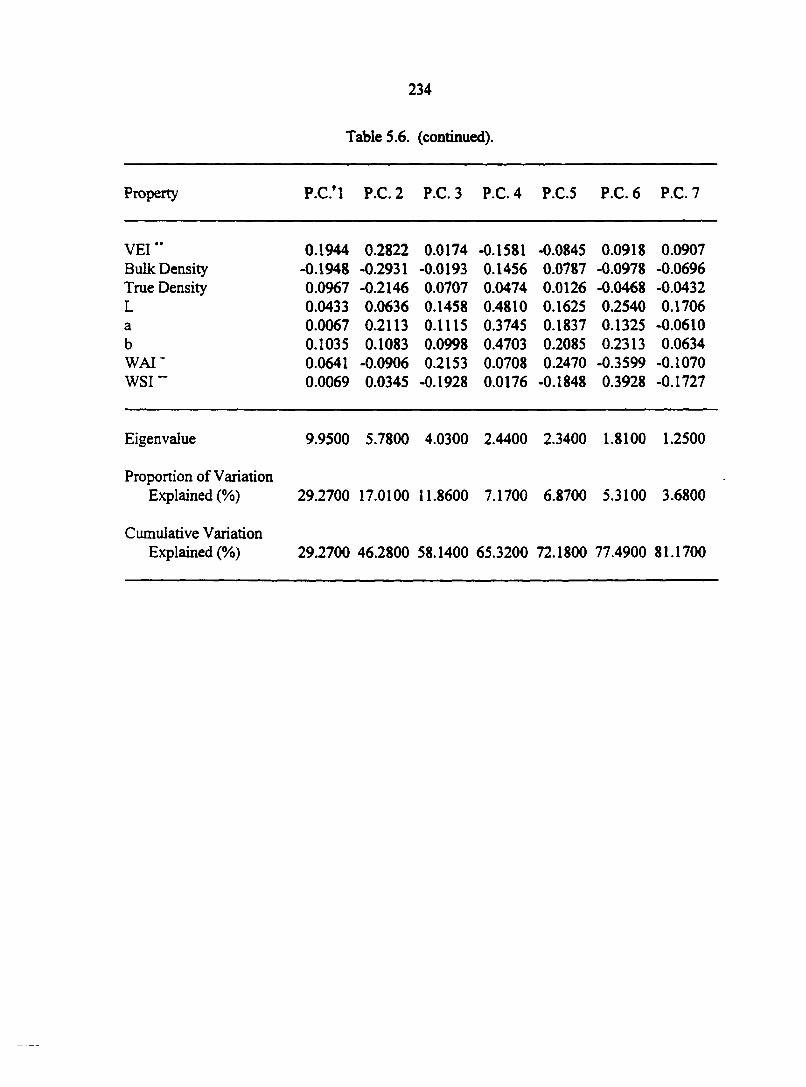
234
Table 5.6. (continued).
Property P.C/1 P.C. 2 P.C. 3 P.C. 4 P.C.5 P.C. 6 P.C. 7
VEI " 0.1944 0.2822 0.0174 -0.1581 -0.0845 0.0918 0.0907 Bulk Density -0.1948 -0.2931 -0.0193 0.1456 0.0787 -0.0978 -0.0696 True Density 0.0967 -0.2146 0.0707 0.0474 0.0126 -0.0468 -0.0432 L 0.0433 0.0636 0.1458 0.4810 0.1625 0.2540 0.1706 a 0.0067 0.2113 0.1115 0.3745 0.1837 0.1325 -0.0610 b 0.1035 0.1083 0.0998 0.4703 0.2085 0.2313 0.0634 WAI* 0.0641 -0.0906 0.2153 0.0708 0.2470 -0.3599 -0.1070 WSI~ 0.0069 0.0345 -0.1928 0.0176 -0.1848 0.3928 -0.1727
Eigenvalue 9.9500 5.7800 4.0300 2.4400 2.3400 1.8100 1.2500
Proportion of Variation Explained (%) 29.2700 17.0100 11.8600 7.1700 6.8700 5.3100 3.6800
Cumulative Variation Explained (%) 29.2700 46.2800 58.1400 65.3200 72.1800 77.4900 81.1700
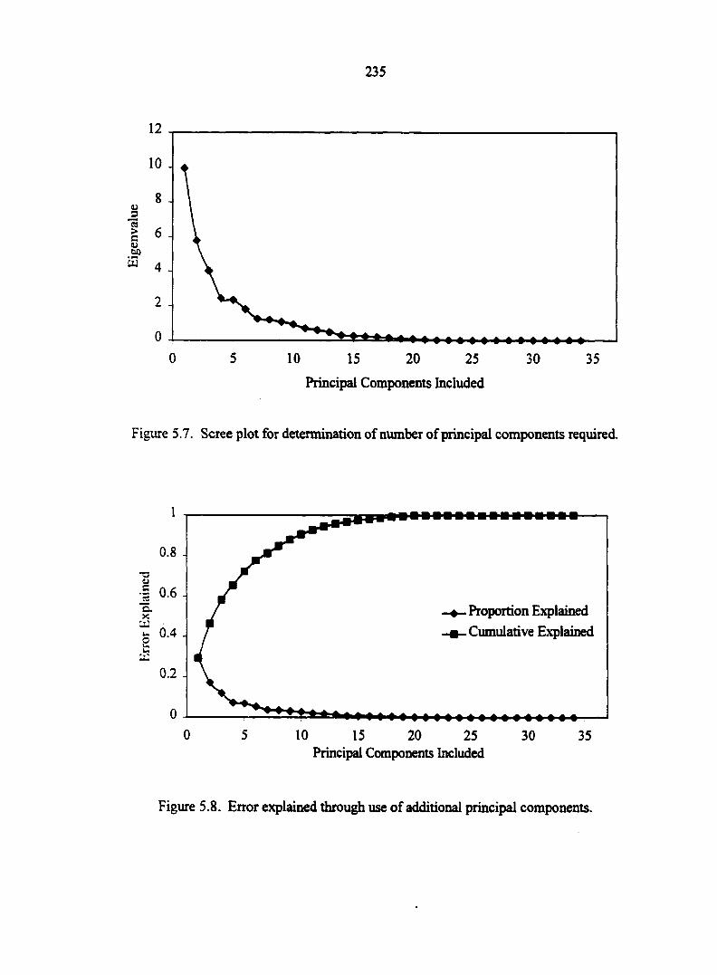
235
12
10
8
6
4
2
0
5 0 10 15 20 25 30 35
Principal Components Included
Figure 5.7. Scree plot for determination of number of principal components required.
Proportion Explained
Cumulative Explained
c. X U
0.4 .
0 5 10 15 20 25 30 35 Principal Components Included
Figure 5.8. Error explained through use of additional principal components.
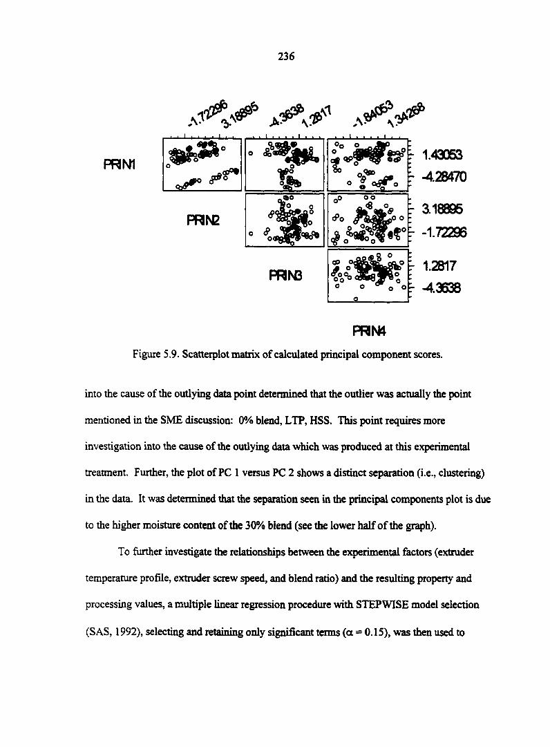
236
PR NI
4
o
1111
« « « « i « i
5s
°°o
*8
PRN2 T : ° : £ f
PRN3 r O O o o'-
o
PRN4
Figure 5.9. Scatterplot matrix of calculated principal component scores.
into the cause of the outlying data point determined that the outlier was actually the point
mentioned in the SME discussion: 0% blend, LTP, HSS. This point requires more
investigation into the cause of the outlying data which was produced at this experimental
treatment. Further, the plot of PC 1 versus PC 2 shows a distinct separation (i.e., clustering)
in the data. It was determined that the separation seen in the principal components plot is due
to the higher moisture content of the 30% blend (see the lower half of the graph).
To further investigate the relationships between the experimental factors (extruder
temperature profile, extruder screw speed, and blend ratio) and the resulting property and
processing values, a multiple linear regression procedure with STEPWISE model selection
(SAS, 1992), selecting and retaining only significant terms (a = 0.15), was then used to
237
determine polynomial regression prediction equations for the extruder processing
characteristics and resulting extrudate properties based on the values of the three
experimental factors. Table 5.7 shows the results from this regression analysis; only results
having an R2 greater than 0.60 are shown, however. From these results, it can be seen that
only extrudate moisture content (R2 = 0.95) could be very well predicted using the
experimental factors in the study. Dough temperature (R2 = 0.89) and extrudate protein
content (R2 = 0.83) could be relatively well predicted. All other processing characteristics
and extrudate property values could not be well predicted using the values of the
experimental factors in the study.
Even though the current study has been extensive, it would be useful to further
investigate relationships and interactions between the raw ingredient properties, extrusion
processing properties, and resulting extrudate product properties.
SUMMARY AND CONCLUSIONS
This study has provided information essential for the further development of livestock
feed additives utilizing blends of soybean meal and corn masa byproducts via extrusion
processing. Laboratory-scale extrusion of these blends produced extradâtes with nutritional
properties similar to those of the raw ingredient blends, with improved protein digestibility
due to the thermal effects of the extrusion processing. Because soybean meal was used as a
blending agent, little product expansion occurred at the extruder die, primarily due to lack of
starchy components in the blends. Additionally, the resulting products had low water
absorption and solubility. An additional drying step is required for the extruded products to
reduce moisture content and water activity levels to acceptable ranges, in order to prevent
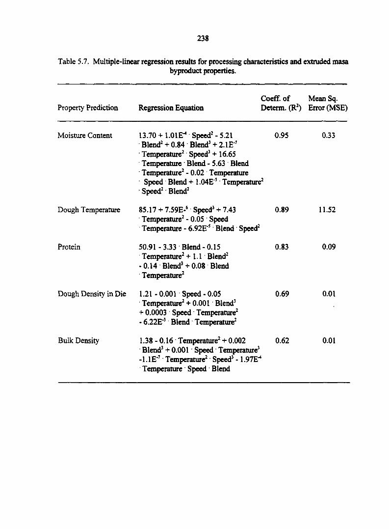
238
Table 5.7. Multiple-linear regression results for processing characteristics and extruded masa byproduct properties.
Property Prediction Regression Equation Determ.
Moisture Content 13.70 + 1.01E"4 Speed2 - 5.21 Blend2 + 0.84 Blend3 + 2.IE"7
Temperature2 Speed3 +16.65 Temperature Blend - 5.63 Blend Temperature2 - 0.02 Temperature Speed Blend + 1.04E"5 Temperature2
Speed2 Blend2
0.95
Dough Temperature 85.17 + 7.59E-6 Speed3 + 7.43 Temperature2 - 0.05 Speed Temperature - 6.92E"5 Blend Speed2
0.89
Protein 50.91 -3.33 Blend-0.15 Temperature2 +1.1 Blend2
- 0.14 Blend3 + 0.08 Blend Temperature2
0.83
Dough Density in Die
Bulk Density
1.21 -0.001 Speed-0.05 Temperature2 + 0.001 Blend3
+ 0.0003 Speed Temperature2
- 6.22E"3 Blend Temperature2
Coeff. of Mean Sq. (R2) Error (MSE)
0.33
11.52
0.09
0.69 0.01
0.62 0.01 1.38 - 0.16 Temperature2 + 0.002 Blend3 + 0.001 Speed Temperature3
-1.1E"7 Temperature2 Speed3 - 1.97E"4
Temperature Speed Blend
239
microbial spoilage during transport and storage. During processing, the dough melt in the
extruder behaved as a pseudoplastic material, which is typical of most food doughs, requiring
less torque required to convey the dough as screw speed increased. Blend ratio affected
processing and product properties very little; most effects were due to screw speed and
processing temperature. All blends were amenable to extrusion processing at the processing
conditions used in this study. Extrusion processing produced extradâtes with excellent
durability, which is essential to retaining quality during transport and storage of pelleted feed
ingredients.
The next stage in developing livestock feed ingredients from com masa byproducts
could logically follow three possible courses: an extrusion scale-up with blends of masa
byproducts and soybean meal (which is described in the next chapter); a livestock feeding
trial with these resulting extruded products; or processing with ingredients other than
soybean meal to produce livestock feed additives. The latter two options were not pursued.
ACKNOWLEDGMENTS
The authors would like to thank the Recycling and Reuse Technology Transfer Center
(RRTTC) at the University of Northern Iowa, Cedar Falls, IA, and the Iowa Biotechnology
Byproducts Consortium, for financial support; the Center for Crops Utilization Research
(CCUR) at Iowa State University, Ames, IA, for use of equipment and facilities, and Minsa
Corporation for providing com masa byproduct samples.
REFERENCES
American Association of Cereal Chemists (AACC). 1995. Approved Methods of the American Association of Cereal Chemists. St. Paul, MN: American Society of Cereal Chemists, Inc.
240
American Society of Agricultural Engineers (ASAE). 1996. ASAE Standards, Engineering Practices, and Data. St. Joseph, MI: American society of Agricultural Engineers.
Alvarez-Martinez, L., K. P. Kondury, and J. M. Harper. 1988. A general model for expansion of extruded products. Journal of Food Science 53(2): 609-615.
Anderson, R. A., H. F Conway, V. F. Pfeifer, and E. L. Griffin, Jr. 1969. Gelatinization of com grits by roll- and extrusion-cooking. Cereal Science Today 14(1): 4-12.
Annexstad, R. J., M. D. Stern, D. E. Otterby, J. G. Linn, and W. P. Hansen. 1987. Extruded soybeans and com gluten meal as supplemental protein sources for lactating dairy cattle. Journal of Dairy Science 70(4): 814-822.
Badrie, N. and W. A. Mellowes. 1991. Effect of extrusion variables on cassava extradâtes. Journal of Food Science 56(5): 1334-1337.
Barbosa-Canovas, G. V. and H. Vega-Mercado. 1996. Dehydration of Foods. New York, NY: International Thomson Publishing.
Bern, C. J. and C. R. Hurburgh. 1998. Managing Grain After Harvest: AE 469/569 course notes. Ames, IA: Iowa State University Bookstore Course Works.
Beauchat, L. R. 1981. Microbial stability as affected by water activity. Cereal Foods World 26(7): 345-349.
Bohlsen, D., S. Weeder, and S. Wang. 1997. Tracking organic waste. Resource 4(9): 13-14.
Bookwalter, G. N., A. W. Kirleis, and E. T. Mertz. 1987. In vitro digestibility of protein in milled sorghum and other processed cereals with and without soy-fortification. Journal of Food Science 52(6): 1577.
Bouvier, M. H., G. Fayard, and J. T. Clayton. 1987. Flow rate and heat transfer modeling in extrusion cooking of soy protein. Journal of Food Engineering 6(2): 123-141.
Bressani, R., R. Paz y Paz, and N. S. Scrimshaw. 1958. Com nutrient losses: chemical changes in com during preparation of tortillas. Journal of Agricultural and Food Chemistry 6(10): 770-774.
Bressani, R., J. E. Braham, L. G. Elias, R. Cuevas, and M. R. Molina. 1978. Protein quality of a whole com/whole soybean mixture processed by a simple extrusion cooker. Journal of Food Science 43(5): 1563-1565.
241
Chen, A. H., Y. C. Jao, J. W. Larkin, and W. E. Goldstein. 1979. Rheological model of soy dough in extrusion. Journal of Food Processing Engineering 2(4): 337-342.
Gumming, D. B., D. W. Stanley, and J. M. DeMan. 1972. Texture - structure relationships in texturized soy protein II. Textural properties and ultrastructure of an extruded soybean product. Journal of Canadian Institute of Science and Technology 5(3): 124-128.
Gumming, D. B., D. W. Stanley, and J. M. DeMan. 1973. Fate of water soluble soy protein during thermoplastic extrusion. Journal of Food Science 38(2): 320-323.
Dahl, S. R. and R. Villota. 1991. Effect of thermal denaturation on the texturization of soybean protein via twin-screw extrusion. Journal of Canadian Institute of Science and Technology 24(3/4): 143-150.
Davis, C., M. Hutjens, and L. Berger. 1980. Should you consider distillers' and brewers' byproducts? Hoards Dairyman 125(7): 546-547.
Derr, D. A. and P. S. Dhillon. 1997. The economics of recycling food residuals. BioCycle 38(4): 55-56.
Erickson, D. R. 1995. Practical handbook of soybean processing and utilization. Champaign, IL: AOCS Press.
Everitt, B. S. and G. Dunn. 1991. Applied Multivariate Data Analysis. New York, NY: Halsted Press.
Faubion, J. M., R. C. Hoseney, and P. A. Seib. 1982. Functionality of grain components in extrusion. Cereal Foods World 27(5): 212-216.
Ferris, D. A., R. A. Flores, C. W. Shanklin, and M. K. Whitworth. 1995. Proximate analysis of food service wastes. Applied Engineering in Agriculture 11(4): 567-572.
Gomez, M. H., L. W. Rooney, R. D. Waniska, and R. L. Pflugfelder. 1987. Dry corn masa flours for tortilla and snack food production. Cereal Foods World 32(5): 372-377.
Gonzalez de Palacios, M. 1980. Characteristics of corn and sorghum for tortilla processing. Unpublished M.S. Thesis. College Station, TX: Texas A&M University.
Gonzalez-Martinez, S. 1984. Biological treatability of the wastewaters from the alkaline cooking of maize (Indian com). Environmental Technology Letters 5(8): 365-372.
242
Ham, G. A., R. A. Stock, T. J. Klopfenstein, and R. P. Huffman. 1995. Determining the net energy value of wet and dry com gluten feed in beef growing and finishing diets. Journal of Animal Science 73(2): 353-359.
Harper, J. M. 1981. Extrusion of Foods, Volume 1. Boca Raton, FL: CRC Press, Inc.
Hilton, J. W., C. Y. Cho, and S. J. Slonger. 1981. Effect of extrusion processing and steam pelleting diets on pellet durability, pellet water absorption, and the physiological response of rainbow trout (Salmo Gaird-Neri R.). Aquaculture 25(2/3): 185-194.
Hunter Associates Laboratory, Inc. 1983. Instruction Manual: Hunterlab LabScan Spectro Colorimeter. Reston, VA: Hunter Associates Laboratory, Inc.
Jamin, F. F. and R. A. Flores. 1998. Effect of separation and grinding of com dry-milled streams on physical properties of single-screw low-speed extruded products. Cereal Chemistry 75(6): 775-779.
Katz, S. H., M. L. Hediger, and L. A. Valleroy. 1974. Traditional maize processing techniques in the New World. Science 184(4138): 765-773.
Khan, M. N., M. C. Des Rosiers, L. W. Rooney, R. G. Morgan, and V. E. Sweat. 1982. Com tortillas: evaluation of com cooking procedures. Cereal Chemistry 59(4): 279-284.
Kokini, J. L., C. N. Chang and L. S. Lai. 1992. The role of rheological properties on extrudate expansion. In Food Extrusion Science and Technology, ed. J. L. Kokini, C. T. Ho, and M. V. Karewe, 631-652. New York: Marcel Dekker, Inc.
Konkoly, A. M. 1997. Rheological characterization of commercially available cream cheese and physical properties of com and peanut composite flour extradâtes. Unpublished M.S. Thesis. Iowa State University: Ames, IA.
Krause, V. M., K. L. Tucker, H. V. Kuhnlein, C. Y. Lopez-Palacios, M. Ruz, and N. W. Solomons. 1992. Rural-urban variation in limed maize use and tortilla consumption by women in Guatemala. Ecology of Food and Nutrition 28(4): 279-288.
Lam, C. M. D. 1996. Effects of processing parameters and material on fish feed extrusion with momentum transfer consideration. Unpublished M.S. Thesis. Iowa State University: Ames, IA.
Larson, E. M., R. A. Stock, T. J. Klopfenstein, J. H. Sindt, and R. P. Huffman. 1993. Feeding value of wet distillers byproducts for finishing ruminants. Journal of Animal Science 71(8): 2228-2236.
243
Lo, T. L. and R. G. Moreira. 1996. Product quality modeling of a twin-screw extrusion process. In 1996 Institute of Food Technologists Annual Meeting, technical poster session: rheology/extrusion, Paper No. 80A-21. New Orleans, LA, June 22-26.
Lodge, S. L., R. A. Stock, T. J. Klopfenstein, D. H. Shain, and D. W. Herold. 1997. Evaluation of corn and sorghum distillers byproducts. Journal of Animal Science 74(1): 37-43.
Lu, A., F. Hsieh, J. Tan, H. E. Huff, and S. J. Mulvaney. 1992. Dynamic analysis of process variables for a twin-screw food extruder. Food Science Technology Lebensm Wiss Technol 25(3): 261-270.
Maga, J. A. and K. Lorenz. 1978. Sensory and functional properties of extruded com-soy blends. LWTLebensmitt Wissensch Technology 11(4): 185-187.
Marsman, G. J. P., H. Gruppen, D. J. vanZuilichem, J. W. Resink and A. G. J. Voragen. 1995. The influence of screw configuration on the In Vitro digestibility and protein solubility of soybean and rapeseed meals. Journal of Food Engineering 26(1): 13-28.
Martelli, F. G. 1983. Twin Screw Extruders: A Basic Understanding. Van Nostrand Reinhold: New York, NY.
McEllhiney, R. R. 1985. Feed Manufacturing Technology III. Arlington, VA: American Feed Industry Association.
Mercier, C., P. Linko, and J. M. Harper, eds. 1989. Extrusion Cooking. St. Paul, MN: American Association of Cereal Chemists.
Mertz, E. T., M. M. Hassen, C. Cairns-Whittern, A. W. Kirleis, L. Tu, and J. D. Axtell. 1984. Pepsin digestibility of proteins in sorghum and other major cereals. Proceedings of the National Academy of Science 81(1): 1.
Microsoft Excel v. 5.0a. 1993. Redmond, WA: Microsoft Corporation.
Miller, R. C. 1985. Low moisture extrusion: effects of cooking moisture on product characteristics. Journal of Food Science 50(1): 249-253.
Moore, D., A. Sanei, E. Van Hecke, and J. M. Bouvier. 1990. Effect of ingredients on physical/structural properties of extradâtes. Journal of Food Science 55(5): 1383-1387.
Nielsen, E. 1976. Whole seed processing by extrusion cooking. Journal of the American Oil Chemists Society 53(6): 305-309.
244
Ortiz, E. L. 1985. The cuisine of Mexico: com tortilla dishes. Gourmet 45(May): 62-63.
Pflugfelder, R. L., L. W. Rooney, and R. D. Waniska. 1988. Dry matter losses in commercial com masa production. Cereal Chemistry 65(2): 127-132.
Rogers, M. G. 1970. Rheological interpretation of Brabender Plasti-Corder (extruder head) data. Industrial Engineering and Chemical Process Design Development 9(1): 49-52.
Rooney, L. W. and S. O. Sema-Saldivar. 1987. Food uses of whole com and dry-milled fractions. In Corn Chemistry and Technology, ed. S. A. Watson and P. E. Ramstad, 399-430. St. Paul, MN: American Association of Cereal Chemists.
Rosentrater, K. A., R. A. Flores, T. L. Richard, and C. J. Bern. 1999. Physical and nutritional properties of com masa byproduct streams. Applied Engineering in Agriculture 15(5): 515-523.
SAS v. 6.08. 1992. Cary, NC: SAS Institute, Inc.
Sema-Saldivar, S. O., M. H. Gomez, and L. M. Rooney. 1990. Technology, chemistry, and nutritional value of alkaline-cooked com products. Advances in Cereal Science and Technology v. 10:243-306.
Solganik, H. 1997. A toast to tortillas. Food Processing 58(11): 64-65.
Speigel, M. R. 1994. Statistics. New York, NY: McGraw-Hill, Inc.
Stroshine, R. and D. Hamann. 1995. Physical Properties of Agricultural Materials and Food Products. West Lafayette, IN: Copy Cat.
Tabil, L., Jr. and S. Sokhansanj. 1996. Process conditions affecting the physical quality of alfalfa pellets. Applied Engineering in Agriculture 12(3): 345-350.
Tortilla Industry Association (TIA). 2001. Tortilla consumption continues to grow in U.S. and abroad. Tortilla Industry Association. Available online: www.tortilla-info.com/prrevenue98.htm [Accessed January 08,2001].
Velasco-Martinez, M., O. Angulo, D. O. Vazquez-Couturier, A. Arroyo-Lara, and J. A. Monroy-Rivera. 1997. Effect of dried solids of nejayote on broiler growth. Poultry Science 76(11): 1531-1534.
Wang, L., R. A. Flores, and L. A. Johnson. 1997. Processing feed ingredients from blends of soybean meal, whole blood, and red blood cells. Transactions of the ASAE 40(3): 691-697.
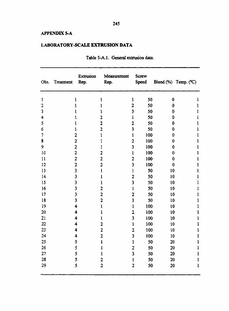
245
APPENDIX 5-A
LABORATORY-SCALE EXTRUSION DATA
Table 5-A.l. General extrusion data.
Extrusion Obs. Treatment Rep.
Measurement Screw Rep. Speed Blend (%) Temp. (°C)
1 1 1 1 50 0 2 1 1 2 50 0 3 1 1 3 50 0 4 1 2 1 50 0 5 1 2 2 50 0 6 1 2 3 50 0 7 2 I 1 100 0 8 2 1 2 100 0 9 2 1 3 100 0 10 2 2 1 100 0 11 2 2 2 100 0 12 2 2 3 100 0 13 3 1 1 50 10 14 3 1 2 50 10 15 3 1 3 50 10 16 3 2 1 50 10 17 3 2 2 50 10 18 3 2 3 50 10 19 4 1 1 100 10 20 4 1 2 100 10 21 4 1 3 100 10 22 4 2 1 100 10 23 4 2 2 100 10 24 4 2 3 100 10 25 5 1 1 50 20 26 5 1 2 50 20 27 5 1 3 50 20 28 5 2 1 50 20 29 5 2 2 50 20
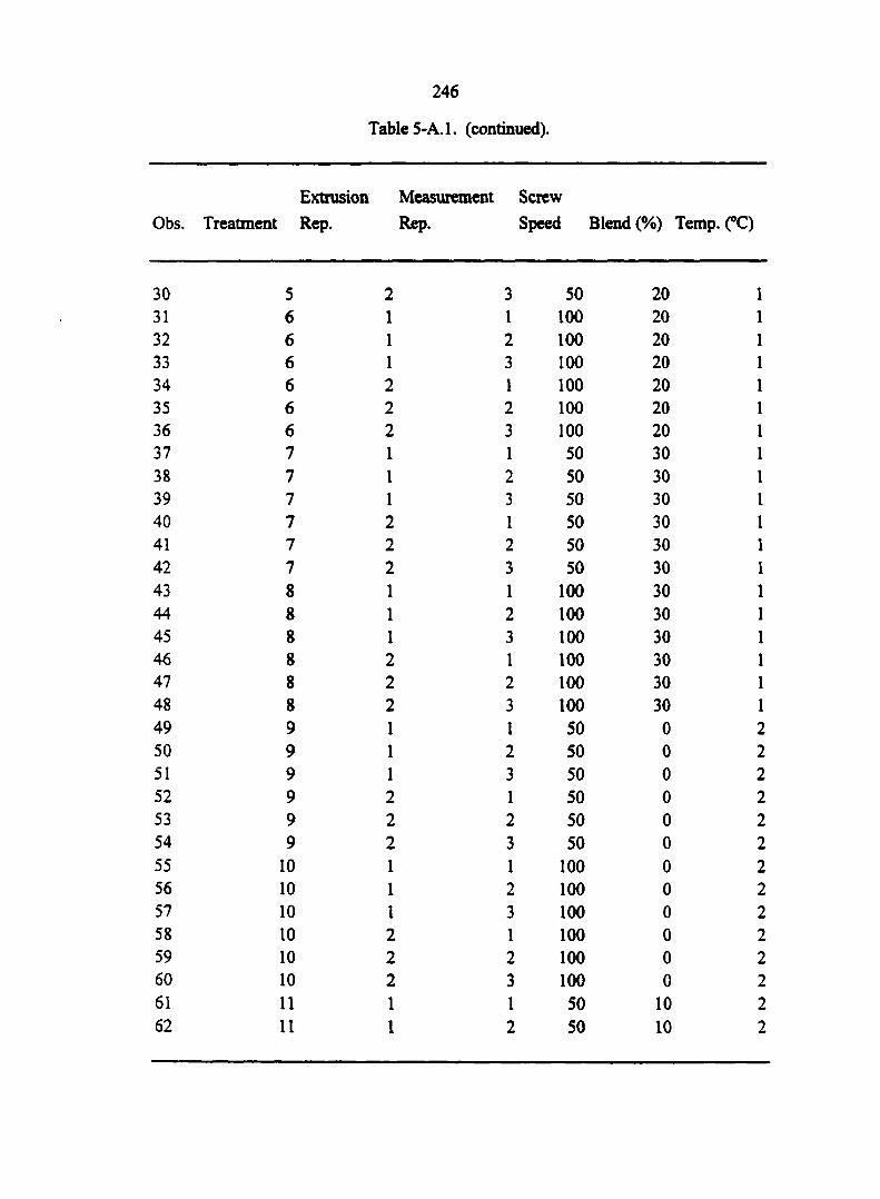
Obs
30 31 32 33 34 35 36 37 38 39 40 41 42 43 44 45 46 47 48 49 50 51 52 53 54 55 56 57 58 59 60 61 62
246
Table 5-A.l. (continued).
Extrusion Measurement Screw
Treatment Rep. Rep. Speed Blend (%) Temp. (°C)
5 2 3 50 20 1 6 1 1 100 20 1 6 1 2 100 20 1 6 1 3 100 20 1 6 2 1 100 20 1 6 2 2 100 20 1 6 2 3 100 20 1 7 1 1 50 30 1 7 1 2 50 30 1 7 1 3 50 30 1 7 2 1 50 30 1 7 2 2 50 30 1 7 2 3 50 30 1 8 1 1 100 30 1 8 1 2 100 30 1 8 1 3 100 30 1 8 2 1 100 30 1 8 2 2 100 30 1 8 2 3 100 30 1 9 1 1 50 0 2 9 1 2 50 0 2 9 1 3 50 0 2 9 2 1 50 0 2 9 2 2 50 0 2 9 2 3 50 0 2
10 1 1 100 0 2 10 1 2 100 0 2 10 1 3 100 0 2 10 2 1 100 0 2 10 2 2 100 0 2 10 2 3 100 0 2 11 1 1 50 10 2 11 1 2 50 10 2
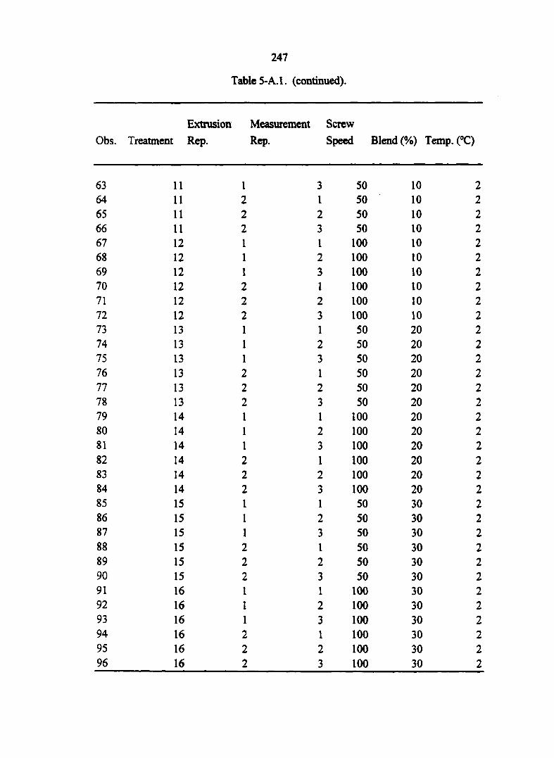
Obs,
63 64 65 66 67 68 69 70 71 72 73 74 75 76 77 78 79 80 81 82 83 84 85 86 87 88 89 90 91 92 93 94 95 96
247
Table 5-A.L (continued).
Extrusion Measurement Screw
Treatment Rep. Rep. Speed Blend (%) Temp. (°C)
11 1 3 50 10 2 11 2 1 50 10 2 11 2 2 50 10 2 11 2 3 50 10 2 12 1 1 100 10 2 12 1 2 100 10 2 12 1 3 100 10 2 12 2 1 100 10 2 12 2 2 100 10 2 12 2 3 100 10 2 13 1 1 50 20 2 13 1 2 50 20 2 13 1 3 50 20 2 13 2 1 50 20 2 13 2 2 50 20 2 13 2 3 50 20 2 14 1 1 100 20 2 14 1 2 100 20 2 14 1 3 100 20 2 14 2 1 100 20 2 14 2 2 100 20 2 14 2 3 100 20 2 15 1 1 50 30 2 15 1 2 50 30 2 15 1 3 50 30 2 15 2 1 50 30 2 15 2 2 50 30 2 15 2 3 50 30 2 16 1 1 100 30 2 16 1 2 100 30 2 16 1 3 100 30 2 16 2 1 100 30 2 16 2 2 100 30 2 16 2 3 100 30 2
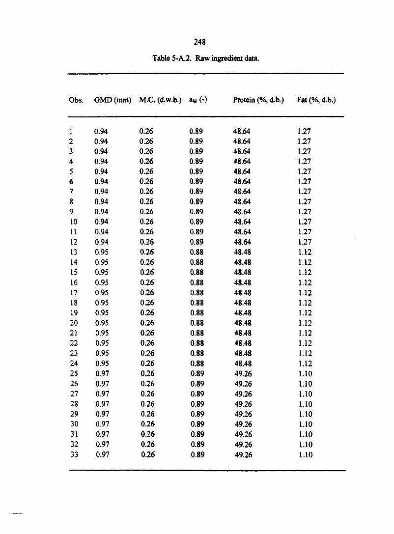
248
Table 5-A.2. Raw ingredient data.
Obs. GMD (mm) M.C. (d.w.b.) aw (-) Protein (%, d.b.) Fat (%, d.b.)
1 0.94 0.26 0.89 48.64 1.27 2 0.94 0.26 0.89 48.64 1.27 3 0.94 0.26 0.89 48.64 1.27 4 0.94 0.26 0.89 48.64 1.27 5 0.94 0.26 0.89 48.64 1.27 6 0.94 0.26 0.89 48.64 1.27 7 0.94 0.26 0.89 48.64 1.27 8 0.94 0.26 0.89 48.64 1.27 9 0.94 0.26 0.89 48.64 1.27 10 0.94 0.26 0.89 48.64 1.27 11 0.94 0.26 0.89 48.64 1.27 12 0.94 0.26 0.89 48.64 1.27 13 0.95 0.26 0.88 48.48 1.12 14 0.95 0.26 0.88 48.48 1.12 15 0.95 0.26 0.88 48.48 1.12 16 0.95 0.26 0.88 48.48 1.12 17 0.95 0.26 0.88 48.48 1.12 18 0.95 0.26 0.88 48.48 1.12 19 0.95 0.26 0.88 48.48 1.12 20 0.95 0.26 0.88 48.48 1.12 21 0.95 0.26 0.88 48.48 1.12 22 0.95 0.26 0.88 48.48 1.12 23 0.95 0.26 0.88 48.48 1.12 24 0.95 0.26 0.88 48.48 1.12 25 0.97 0.26 0.89 49.26 1.10 26 0.97 0.26 0.89 49.26 1.10 27 0.97 0.26 0.89 49.26 1.10 28 0.97 0.26 0.89 49.26 1.10 29 0.97 0.26 0.89 49.26 1.10 30 0.97 0.26 0.89 49.26 1.10 31 0.97 0.26 0.89 49.26 1.10 32 0.97 0.26 0.89 49.26 1.10 33 0.97 0.26 0.89 49.26 1.10
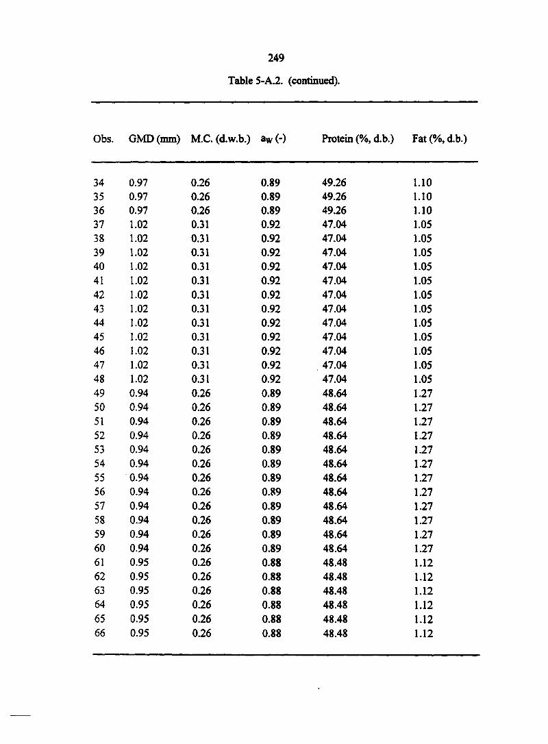
249
Table 5-A.2. (continued).
Obs. GMD (mm) M.C. (d.w.b.) aw (-) Protein (%, d.b.) Fat (%, d.b.)
34 0.97 0.26 0.89 49.26 1.10 35 0.97 0.26 0.89 49.26 1.10 36 0.97 0.26 0.89 49.26 1.10 37 1.02 0.31 0.92 47.04 1.05 38 1.02 0.31 0.92 47.04 1.05 39 1.02 0.31 0.92 47.04 1.05 40 1.02 0.31 0.92 47.04 1.05 41 1.02 0.31 0.92 47.04 1.05 42 1.02 0.31 0.92 47.04 1.05 43 1.02 0.31 0.92 47.04 1.05 44 1.02 0.31 0.92 47.04 1.05 45 1.02 0.31 0.92 47.04 1.05 46 1.02 0.31 0.92 47.04 1.05 47 1.02 0.31 0.92 47.04 1.05 48 1.02 0.31 0.92 47.04 1.05 49 0.94 0.26 0.89 48.64 1.27 50 0.94 0.26 0.89 48.64 1.27 51 0.94 0.26 0.89 48.64 1.27 52 0.94 0.26 0.89 48.64 1.27 53 0.94 0.26 0.89 48.64 1.27 54 0.94 0.26 0.89 48.64 1.27 55 0.94 0.26 0.89 48.64 1.27 56 0.94 0.26 0.89 48.64 1.27 57 0.94 0.26 0.89 48.64 1.27 58 0.94 0.26 0.89 48.64 1.27 59 0.94 0.26 0.89 48.64 1.27 60 0.94 0.26 0.89 48.64 1.27 61 0.95 0.26 0.88 48.48 1.12 62 0.95 0.26 0.88 48.48 1.12 63 0.95 0.26 0.88 48.48 1.12 64 0.95 0.26 0.88 48.48 1.12 65 0.95 0.26 0.88 48.48 1.12 66 0.95 0.26 0.88 48.48 1.12
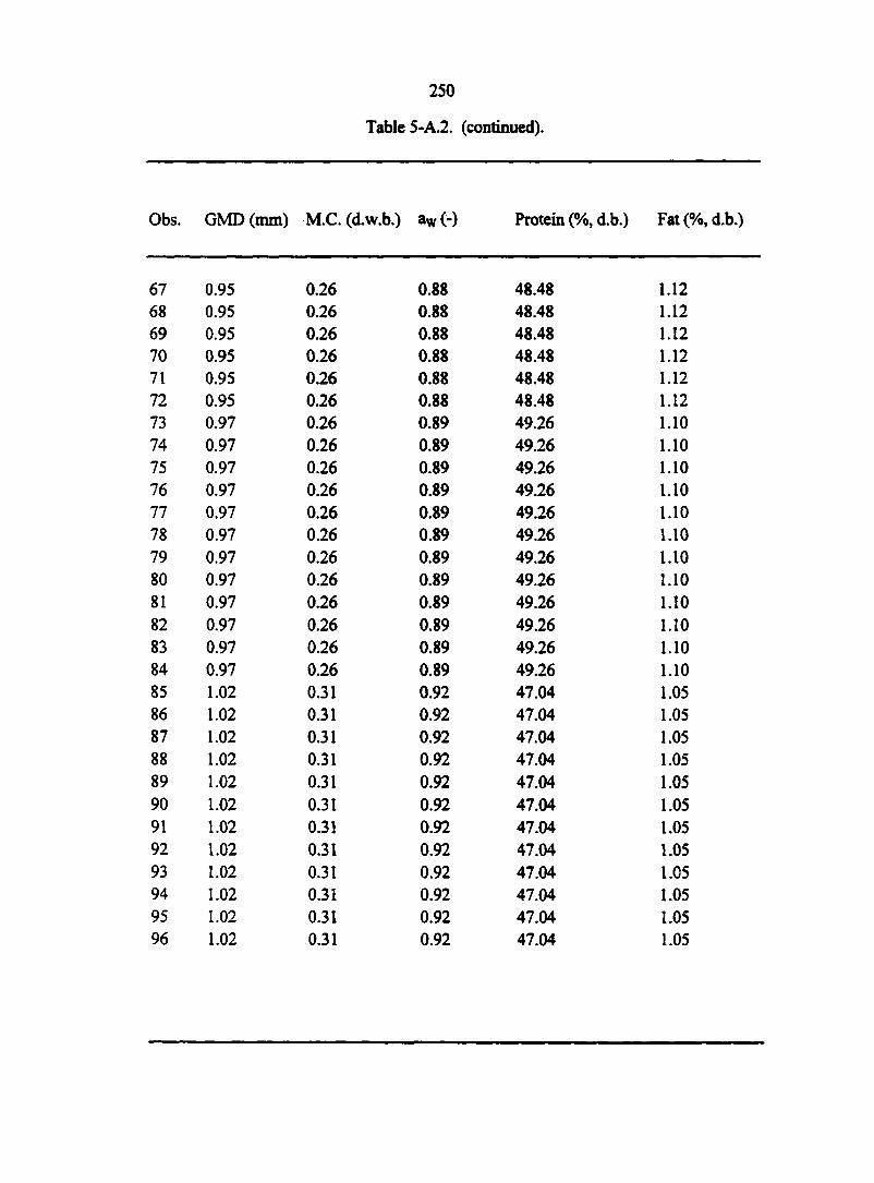
250
Table 5-A.2. (continued).
Obs. GMD (mm) M.C. (d.w.b.) aw(-) Protein (%, d.b.) Fat(%, d.b.)
67 0.95 0.26 0.88 48.48 1.12 68 0.95 0.26 0.88 48.48 1.12 69 0.95 0.26 0.88 48.48 1.12 70 0.95 0.26 0.88 48.48 1.12 71 0.95 0.26 0.88 48.48 1.12 72 0.95 0.26 0.88 48.48 1.12 73 0.97 0.26 0.89 49.26 1.10 74 0.97 0.26 0.89 49.26 1.10 75 0.97 0.26 0.89 49.26 1.10 76 0.97 0.26 0.89 49.26 1.10 77 0.97 0.26 0.89 49.26 1.10 78 0.97 0.26 0.89 49.26 1.10 79 0.97 0.26 0.89 49.26 1.10 80 0.97 0.26 0.89 49.26 1.10 81 0.97 0.26 0.89 49.26 1.10 82 0.97 0.26 0.89 49.26 1.10 83 0.97 0.26 0.89 49.26 1.10 84 0.97 0.26 0.89 49.26 1.10 85 1.02 0.31 0.92 47.04 1.05 86 1.02 0.31 0.92 47.04 1.05 87 1.02 0.31 0.92 47.04 1.05 88 1.02 0.31 0.92 47.04 1.05 89 1.02 0.31 0.92 47.04 1.05 90 1.02 0.31 0.92 47.04 1.05 91 1.02 0.31 0.92 47.04 1.05 92 1.02 0.31 0.92 47.04 1.05 93 1.02 0.31 0.92 47.04 1.05 94 1.02 0.31 0.92 47.04 1.05 95 1.02 0.31 0.92 47.04 1.05 96 1.02 0.31 0.92 47.04 1.05
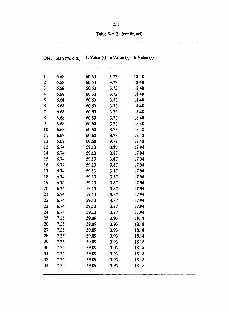
Obs.
1 2 3 4 5 6 7 8 9 10 11 12 13 14 15 16
17 18
19 20 21 22 23 24 25 26 27 28 29 30 31 32 33
251
Table 5-A.2. (continued).
Ash (%, d.b.) L Value (-) a Value (-) b Value (-)
6.68 60.60 3.73 18.48 6.68 60.60 3.73 18.48 6.68 60.60 3.73 18.48 6.68 60.60 3.73 18.48 6.68 60.60 3.73 18.48 6.68 60.60 3.73 18.48 6.68 60.60 3.73 18.48 6.68 60.60 3.73 18.48 6.68 60.60 3.73 18.48 6.68 60.60 3.73 18.48 6.68 60.60 3.73 18.48 6.68 60.60 3.73 18.48 6.74 59.13 3.87 17.94 6.74 59.13 3.87 17.94 6.74 59.13 3.87 17.94 6.74 59.13 3.87 17.94 6.74 59.13 3.87 17.94 6.74 59.13 3.87 17.94 6.74 59.13 3.87 17.94 6.74 59.13 3.87 17.94 6.74 59.13 3.87 17.94 6.74 59.13 3.87 17.94 6.74 59.13 3.87 17.94 6.74 59.13 3.87 17.94 7.35 59.09 3.93 18.18 7.35 59.09 3.93 18.18 7.35 59.09 3.93 18.18 7.35 59.09 3.93 18.18 7.35 59.09 3.93 18.18 7.35 59.09 3.93 18.18 7.35 59.09 3.93 18.18 7.35 59.09 3.93 18.18 7.35 59.09 3.93 18.18

Obs
34 35 36 37 38 39 40 41 42 43 44 45 46 47 48 49 50 51 52 53 54 55 56 57 58 59 60 61 62 63 64 65 66
252
Table 5-A.2. (continued).
Ash (%, d.b.) L Value (-) a Value (-) b Value (-)
7.35 59.09 3.93 18.18 7.35 59.09 3.93 18.18 7.35 59.09 3.93 18.18 6.92 57.86 3.91 17.49 6.92 57.86 3.91 17.49 6.92 57.86 3.91 17.49 6.92 57.86 3.91 17.49 6.92 57.86 3.91 17.49 6.92 57.86 3.91 17.49 6.92 57.86 3.91 17.49 6.92 57.86 3.91 17.49 6.92 57.86 3.91 17.49 6.92 57.86 3.91 17.49 6.92 57.86 3.91 17.49 6.92 57.86 3.91 17.49 6.68 60.60 3.73 18.48 6.68 60.60 3.73 18.48 6.68 60.60 3.73 18.48 6.68 60.60 3.73 18.48 6.68 60.60 3.73 18.48 6.68 60.60 3.73 18.48 6.68 60.60 3.73 18.48 6.68 60.60 3.73 18.48 6.68 60.60 3.73 18.48 6.68 60.60 3.73 18.48 6.68 60.60 3.73 18.48 6.68 60.60 3.73 18.48 6.74 59.13 3.87 17.94 6.74 59.13 3.87 17.94 6.74 59.13 3.87 17.94 6.74 59.13 3.87 17.94 6.74 59.13 3.87 17.94 6.74 59.13 3.87 17.94
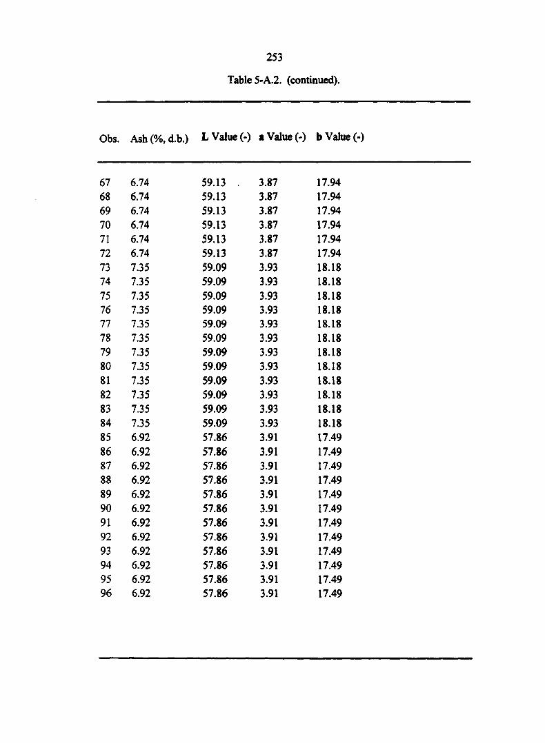
Obs,
67 68 69 70 71 72 73 74 75 76 77 78 79 80 81 82 83 84 85 86 87 88 89 90 91 92 93 94 95 96
253
Table 5-A.2. (continued).
Ash (%, d.b.) L Value (-) a Value (-) b Value (-)
6.74 59.13 . 3.87 17.94 6.74 59.13 3.87 17.94 6.74 59.13 3.87 17.94 6.74 59.13 3.87 17.94 6.74 59.13 3.87 17.94 6.74 59.13 3.87 17.94 7.35 59.09 3.93 18.18 7.35 59.09 3.93 18.18 7.35 59.09 3.93 18.18 7.35 59.09 3.93 18.18 7.35 59.09 3.93 18.18 7.35 59.09 3.93 18.18 7.35 59.09 3.93 18.18 7.35 59.09 3.93 18.18 7.35 59.09 3.93 18.18 7.35 59.09 3.93 18.18 7.35 59.09 3.93 18.18 7.35 59.09 3.93 18.18 6.92 57.86 3.91 17.49 6.92 57.86 3.91 17.49 6.92 57.86 3.91 17.49 6.92 57.86 3.91 17.49 6.92 57.86 3.91 17.49 6.92 57.86 3.91 17.49 6.92 57.86 3.91 17.49 6.92 57.86 3.91 17.49 6.92 57.86 3.91 17.49 6.92 57.86 3.91 17.49 6.92 57.86 3.91 17.49 6.92 57.86 3.91 17.49
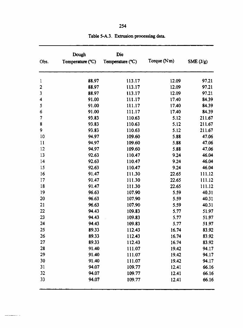
254
Table 5-A.3. Extrusion processing data.
Dough Die
Obs. Temperature (°C) Temperature (°C) Torque (N m) SME (J/g)
1 88.97 113.17 12.09 97.21 2 88.97 113.17 12.09 97.21 3 88.97 113.17 12.09 97.21 4 91.00 111.17 17.40 84.39 5 91.00 111.17 17.40 84.39 6 91.00 111.17 17.40 84.39 7 93.83 110.63 5.12 211.67 8 93.83 110.63 5.12 211.67 9 93.83 110.63 5.12 211.67 10 94.97 109.60 5.88 47.06 11 94.97 109.60 5.88 47.06 12 94.97 109.60 5.88 47.06 13 92.63 110.47 9.24 46.04 14 92.63 110.47 9.24 46.04 15 92.63 110.47 9.24 46.04 16 91.47 111.30 22.65 111.12 17 91.47 111.30 22.65 111.12 18 91.47 111.30 22.65 111.12 19 96.63 107.90 5.59 40.31 20 96.63 107.90 5.59 40.31 21 96.63 107.90 5.59 40.31 22 94.43 109.83 5.77 51.97 23 94.43 109.83 5.77 51.97 24 94.43 109.83 5.77 51.97 25 89.33 112.43 16.74 83.92 26 89.33 112.43 16.74 83.92 27 89.33 112.43 16.74 83.92 28 91.40 111.07 19.42 94.17 29 91.40 111.07 19.42 94.17 30 91.40 111.07 19.42 94.17 31 94.07 109.77 12.41 66.16 32 94.07 109.77 12.41 66.16 33 94.07 109.77 12.41 66.16
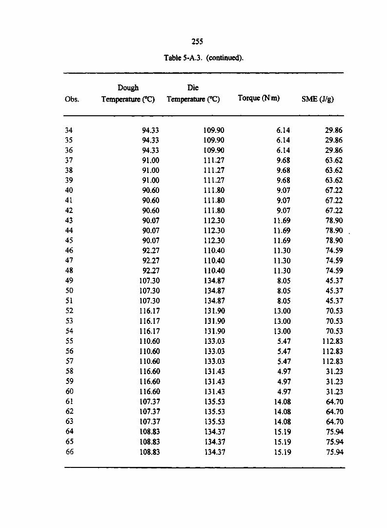
255
Table 5-A.3. (continued).
Dough Die
Obs. Temperature (°C) Temperature (°C) Torque (N m) SME (J/g)
34 94.33 109.90 6.14 29.86 35 94.33 109.90 6.14 29.86 36 94.33 109.90 6.14 29.86 37 91.00 111.27 9.68 63.62 38 91.00 111.27 9.68 63.62 39 91.00 111.27 9.68 63.62 40 90.60 111.80 9.07 67.22 41 90.60 111.80 9.07 67.22 42 90.60 111.80 9.07 67.22 43 90.07 112.30 11.69 78.90 44 90.07 112.30 11.69 78.90 45 90.07 112.30 11.69 78.90 46 92.27 110.40 11.30 74.59 47 92.27 110.40 11.30 74.59 48 92.27 110.40 11.30 74.59 49 107.30 134.87 8.05 45.37 50 107.30 134.87 8.05 45.37 51 107.30 134.87 8.05 45.37 52 116.17 131.90 13.00 70.53 53 116.17 131.90 13.00 70.53 54 116.17 131.90 13.00 70.53 55 110.60 133.03 5.47 112.83 56 110.60 133.03 5.47 112.83 57 110.60 133.03 5.47 112.83 58 116.60 131.43 4.97 31.23 59 116.60 131.43 4.97 31.23 60 116.60 131.43 4.97 31.23 61 107.37 135.53 14.08 64.70 62 107.37 135.53 14.08 64.70 63 107.37 135.53 14.08 64.70 64 108.83 134.37 15.19 75.94 65 108.83 134.37 15.19 75.94 66 108.83 134.37 15.19 75.94
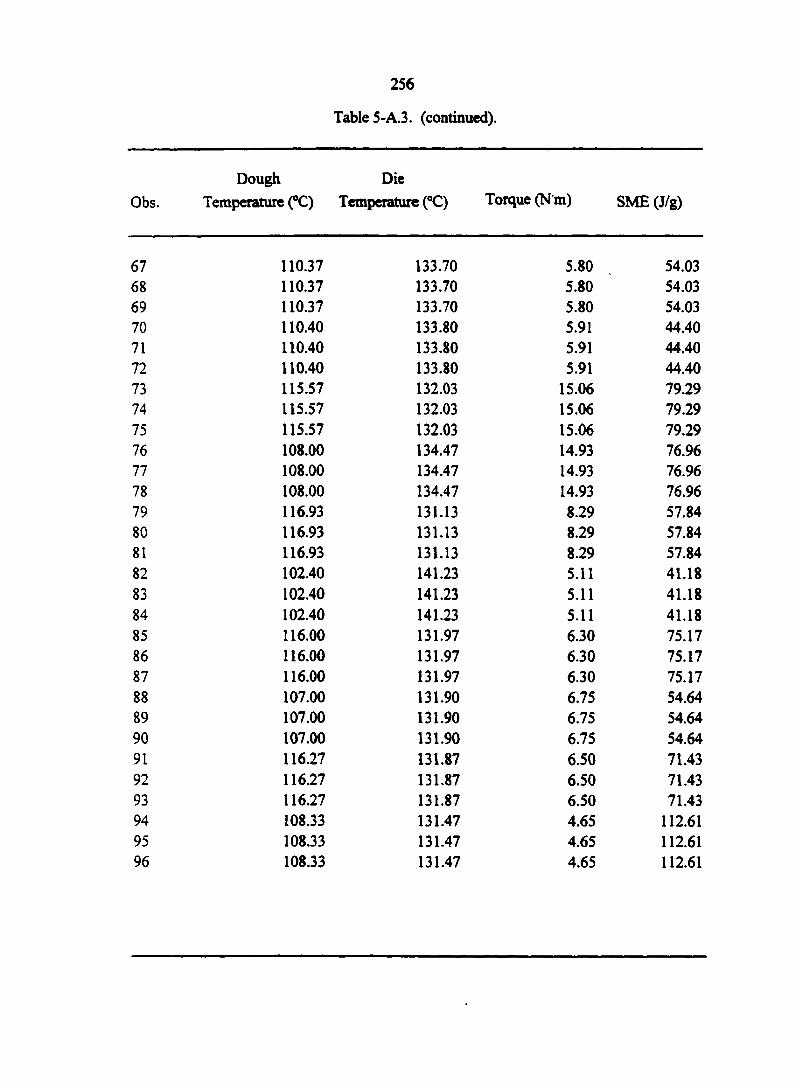
256
Table 5-A.3. (continued).
Obs.
Dough
Temperature (°C)
Die
Temperature (°C) Torque (N m) SME (J/g)
67 110.37 133.70 5.80 54.03 68 110.37 133.70 5.80 54.03 69 110.37 133.70 5.80 54.03 70 110.40 133.80 5.91 44.40 71 110.40 133.80 5.91 44.40 72 110.40 133.80 5.91 44.40 73 115.57 132.03 15.06 79.29 74 115.57 132.03 15.06 79.29 75 115.57 132.03 15.06 79.29 76 108.00 134.47 14.93 76.96 77 108.00 134.47 14.93 76.96 78 108.00 134.47 14.93 76.96 79 116.93 131.13 8.29 57.84 80 116.93 131.13 8.29 57.84 81 116.93 131.13 8.29 57.84 82 102.40 141.23 5.11 41.18 83 102.40 141.23 5.11 41.18 84 102.40 141.23 5.11 41.18 85 116.00 131.97 6.30 75.17 86 116.00 131.97 6.30 75.17 87 116.00 131.97 6.30 75.17 88 107.00 131.90 6.75 54.64 89 107.00 131.90 6.75 54.64 90 107.00 131.90 6.75 54.64 91 116.27 131.87 6.50 71.43 92 116.27 131.87 6.50 71.43 93 116.27 131.87 6.50 71.43 94 108.33 131.47 4.65 112.61 95 108.33 131.47 4.65 112.61 96 108.33 131.47 4.65 112.61
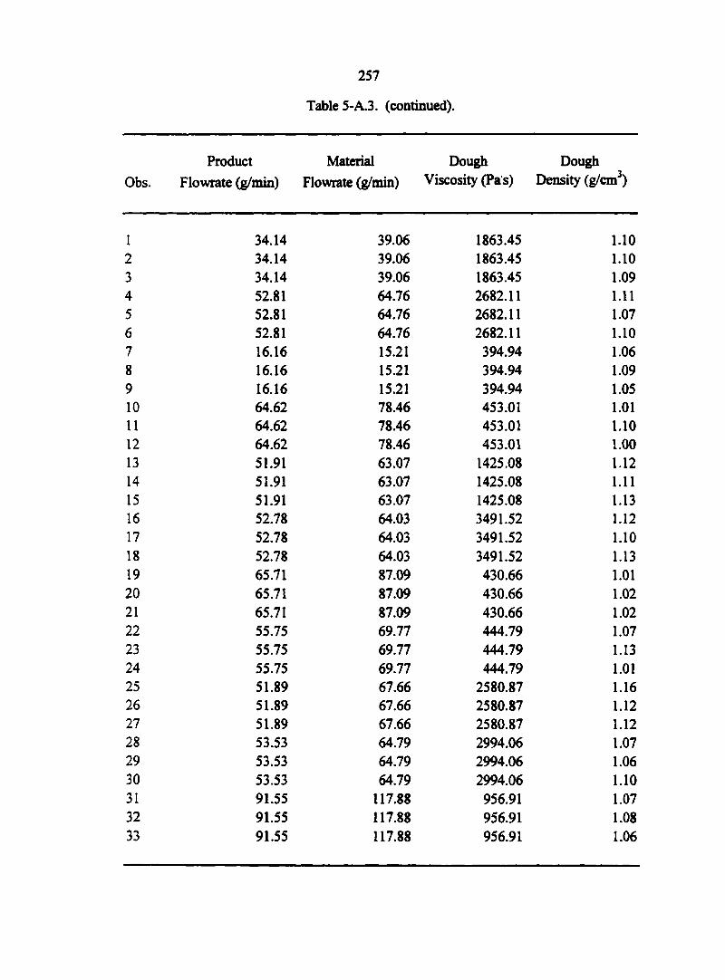
Obs.
1 2 3 4 5 6 7 8 9 10
11 12 13 14 15 16
17 18 19 20
21 22 23 24 25 26 27 28 29 30 31 32 33
257
Table 5-A.3. (continued).
Product Material Dough Dough Flowrate (g/min) Flowrate (g/min) Viscosity (Pa s) Density (g/cm3)
34.14 39.06 1863.45 1.10 34.14 39.06 1863.45 1.10 34.14 39.06 1863.45 1.09 52.81 64.76 2682.11 1.11 52.81 64.76 2682.11 1.07 52.81 64.76 2682.11 1.10 16.16 15.21 394.94 106 16.16 15.21 394.94 1.09 16.16 15.21 394.94 1.05 64.62 78.46 453.01 1.01 64.62 78.46 453.01 1.10 64.62 78.46 453.01 1.00 51.91 63.07 1425.08 1.12 51.91 63.07 1425.08 1.11 51.91 63.07 1425.08 1.13 52.78 64.03 3491.52 1.12 52.78 64.03 3491.52 1.10 52.78 64.03 3491.52 1.13 65.71 87.09 430.66 1.01 65.71 87.09 430.66 1.02 65.71 87.09 430.66 1.02 55.75 69.77 444.79 1.07 55.75 69.77 444.79 1.13 55.75 69.77 444.79 1.01 51.89 67.66 2580.87 1.16 51.89 67.66 2580.87 1.12 51.89 67.66 2580.87 1.12 53.53 64.79 2994.06 1.07 53.53 64.79 2994.06 1.06 53.53 64.79 2994.06 1.10 91.55 117.88 956.91 1.07 91.55 117.88 956.91 1.08 91.55 117.88 956.91 1.06
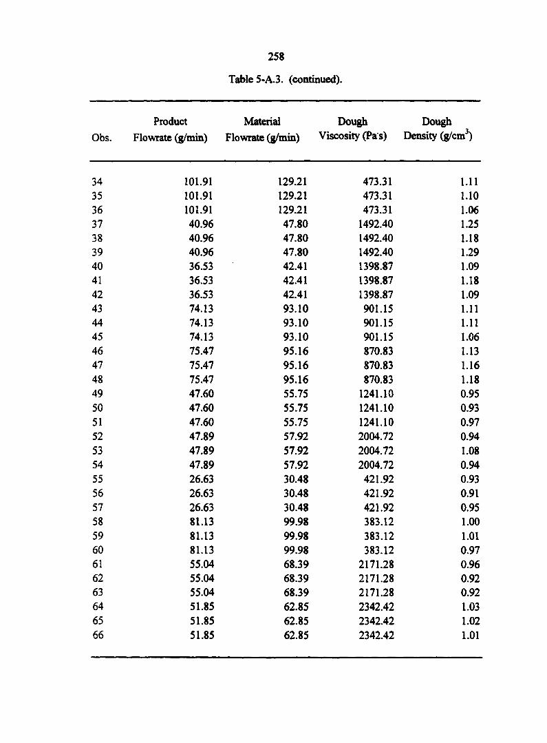
Obs
34 35 36 37 38 39 40 41 42 43 44 45 46 47 48 49 50 51 52 53 54 55 56 57 58 59 60 61
62 63 64 65 66
258
Table 5-A 3, (continued).
Product Material Dough Dough Flowrate (g/min) Flowrate (g/min) Viscosity (Pa s) Density (g/cm3)
101.91 129.21 473.31 1.11 101.91 129.21 473.31 1.10 101.91 129.21 473.31 1.06 40.96 47.80 1492.40 1.25 40.96 47.80 1492.40 1.18 40.96 47.80 1492.40 1.29 36.53 42.41 1398.87 1.09 36.53 42.41 1398.87 1.18 36.53 42.41 1398.87 1.09 74.13 93.10 901.15 1.11 74.13 93.10 901.15 1.11 74.13 93.10 901.15 1.06 75.47 95.16 870.83 1.13 75.47 95.16 870.83 1.16 75.47 95.16 870.83 1.18 47.60 55.75 1241.10 0.95 47.60 55.75 1241.10 0.93 47.60 55.75 1241.10 0.97 47.89 57.92 2004.72 0.94 47.89 57.92 2004.72 1.08 47.89 57.92 2004.72 0.94 26.63 30.48 421.92 0.93 26.63 30.48 421.92 0.91 26.63 30.48 421.92 0.95 81.13 99.98 383.12 1.00 81.13 99.98 383.12 1.01 81.13 99.98 383.12 0.97 55.04 68.39 2171.28 0.96 55.04 68.39 2171.28 0.92 55.04 68.39 2171.28 0.92 51.85 62.85 2342.42 1.03 51.85 62.85 2342.42 1.02 51.85 62.85 2342.42 1.01
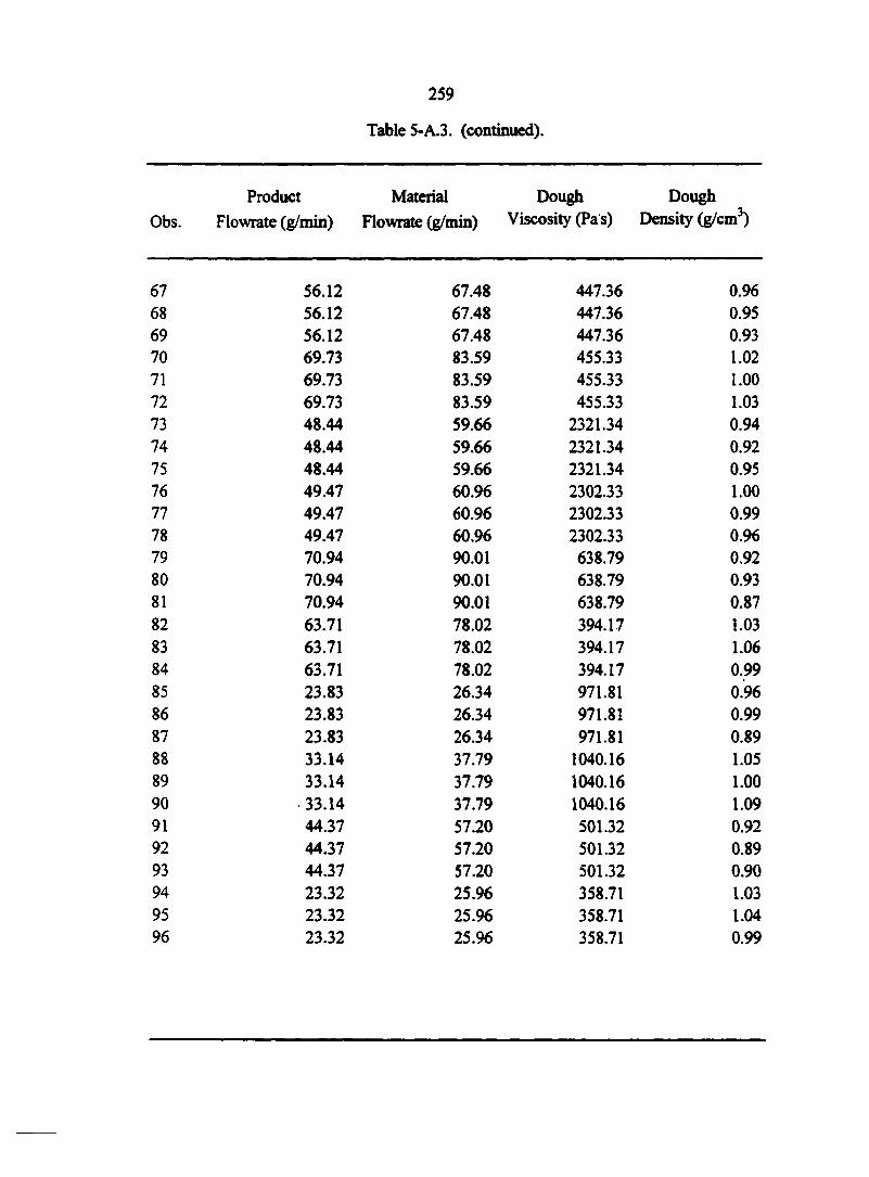
Obs
67 68 69 70 71 72 73 74 75 76 77 78 79 80 81 82 83 84 85 86 87 88 89 90 91 92 93 94 95 96
259
Table S-A.3. (continued).
Product Material Dough Dough Flowrate (g/min) Flowrate (g/min) Viscosity (Pa s) Density (g/cm3)
56.12 67.48 447.36 0.96 56.12 67.48 447.36 0.95 56.12 67.48 447.36 0.93 69.73 83.59 455.33 1.02 69.73 83.59 455.33 1.00 69.73 83.59 455.33 1.03 48.44 59.66 2321.34 0.94 48.44 59.66 2321.34 0.92 48.44 59.66 2321.34 0.95 49.47 60.96 2302.33 1.00 49.47 60.96 2302.33 0.99 49.47 60.96 2302.33 0.96 70.94 90.01 638.79 0.92 70.94 90.01 638.79 0.93 70.94 90.01 638.79 0.87 63.71 78.02 394.17 1.03 63.71 78.02 394.17 1.06 63.71 78.02 394.17 0.99 23.83 26.34 971.81 0.96 23.83 26.34 971.81 0.99 23.83 26.34 971.81 0.89 33.14 37.79 1040.16 1.05 33.14 37.79 1040.16 1.00 33.14 37.79 1040.16 1.09 44.37 57.20 501.32 0.92 44.37 57.20 501.32 0.89 44.37 57.20 501.32 0.90 23.32 25.96 358.71 1.03 23.32 25.96 358.71 1.04 23.32 25.96 358.71 0.99
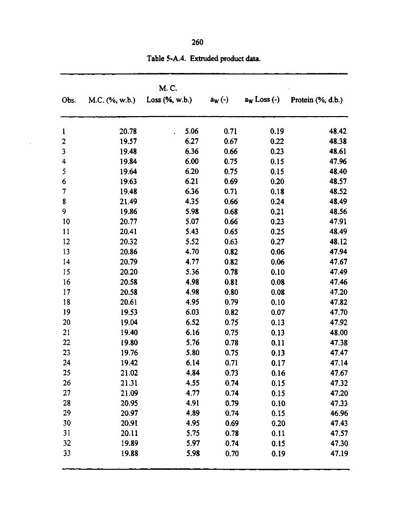
Obs.
1 2 3 4 5 6 7 8 9 10 11 12 13 14 15 16 17 18
19 20
21
22 23 24 25 26 27 28 29 30 31 32 33
260
Table 5-A.4. Extruded product data.
M.C.
M.C. (%, w.b.) Loss (%, w.b.) aw (-) aw Loss (-) Protein (%, d.b.)
20.78 . 5.06 0.71 0.19 48.42 19.57 6.27 0.67 0.22 48.38 19.48 6.36 0.66 0.23 48.61 19.84 6.00 0.75 0.15 47.96 19.64 6.20 0.75 0.15 48.40 19.63 6.21 0.69 0.20 48.57 19.48 6.36 0.71 0.18 48.52 21.49 4.35 0.66 0.24 48.49 19.86 5.98 0.68 0.21 48.56 20.77 5.07 0.66 0.23 47.91 20.41 5.43 0.65 0.25 48.49 20.32 5.52 0.63 0.27 48.12 20.86 4.70 0.82 0.06 47.94 20.79 4.77 0.82 0.06 47.67 20.20 5.36 0.78 0.10 47.49 20.58 4.98 0.81 0.08 47.46 20.58 4.98 0.80 0.08 47.20 20.61 4.95 0.79 0.10 47.82 19.53 6.03 0.82 0.07 47.70 19.04 6.52 0.75 0.13 47.92 19.40 6.16 0.75 0.13 48.00 19.80 5.76 0.78 0.11 47.38 19.76 5.80 0.75 0.13 47.47 19.42 6.14 0.71 0.17 47.14 21.02 4.84 0.73 0.16 47.67 21.31 4.55 0.74 0.15 47.32 21.09 4.77 0.74 0.15 47.20 20.95 4.91 0.79 0.10 47.33 20.97 4.89 0.74 0.15 46.96 20.91 4.95 0.69 0.20 47.43 20.11 5.75 0.78 0.11 47.57 19.89 5.97 0.74 0.15 47.30 19.88 5.98 0.70 0.19 47.19
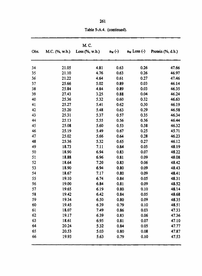
34 35 36 37 38 39 40 41 42 43 44 45 46 47 48 49 50 51 52 53 54 55 56 57 58 59 60 61 62 63 64 65
261
Table 5-A.4. (continued).
M. C.
M.C. (%, w.b.) Loss (%, w.b.) aw (-) aw Loss (-) Protein (%, d.b.)
21.05 4.81 0.63 0.26 47.66 21.10 4.76 0.63 0.26 46.97 21.22 4.64 0.61 0.27 47.46 25.66 5.02 0.89 0.03 46.14 25.84 4.84 0.89 0.03 46.35 27.43 3.25 0.88 0.04 46.24 25.36 5.32 0.60 0.32 46.63 25.27 5.41 0.62 0.30 46.19 25.20 5.48 0.63 0.29 46.58 25.31 5.37 0.57 0.35 46.34 25.13 5.55 0.56 0.36 46.44 25.08 5.60 0.53 0.38 46.32 25.19 5.49 0.67 0.25 45.71 25.02 5.66 0.64 0.28 46.23 25.36 5.32 0.65 0.27 46.12 18.73 7.11 0.84 0.05 48.19 18.90 6.94 0.83 0.07 48.22 18.88 6.96 0.81 0.09 48.08 18.64 7.20 0.83 0.06 48.42 18.90 6.94 0.80 0.09 48.43 18.67 7.17 0.80 0.09 48.41 19.10 6.74 0.84 0.05 48.31 19.00 6.84 0.81 0.09 48.52 19.65 6.19 0.80 0.10 48.14 19.42 6.42 0.84 0.05 48.68 19.34 6.50 0.80 0.09 48.35 19.45 6.39 0.79 0.10 48.51 18.07 7.49 0.86 0.03 47.33 19.17 6.39 0.83 0.06 47.36 18.61 6.95 0.81 0.07 47.10 20.24 5.32 0.84 0.05 47.77 20.53 5.03 0.80 0.08 47.87 19.93 5.63 0.79 0.10 47.53
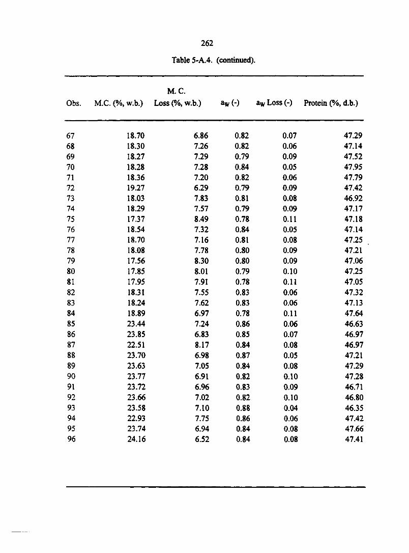
Obs
67 68 69 70 71 72 73 74 75 76 77 78 79 80 81
82 83 84 85 86 87 88 89 90 91 92 93 94 95 96
262
Table 5-A.4. (continued).
M. C.
M.C. (%, w.b.) Loss (%, w.b.) aw (-) aw Loss (-) Protein (%, d.b.)
18.70 6.86 0.82 0.07 47.29 18.30 7.26 0.82 0.06 47.14 18.27 7.29 0.79 0.09 47.52 18.28 7.28 0.84 0.05 47.95 18.36 7.20 0.82 0.06 47.79 19.27 6.29 0.79 0.09 47.42 18.03 7.83 0.81 0.08 46.92 18.29 7.57 0.79 0.09 47.17 17.37 8.49 0.78 0.11 47.18 18.54 7.32 0.84 0.05 47.14 18.70 7.16 0.81 0.08 47.25 18.08 7.78 0.80 0.09 47.21 17.56 8.30 0.80 0.09 47.06 17.85 8.01 0.79 0.10 47.25 17.95 7.91 0.78 0.11 47.05 18.31 7.55 0.83 0.06 47.32 18.24 7.62 0.83 0.06 47.13 18.89 6.97 0.78 0.11 47.64 23.44 7.24 0.86 0.06 46.63 23.85 6.83 0.85 0.07 46.97 22.51 8.17 0.84 0.08 46.97 23.70 6.98 0.87 0.05 47.21 23.63 7.05 0.84 0.08 47.29 23.77 6.91 0.82 0.10 47.28 23.72 6.96 0.83 0.09 46.71 23.66 7.02 0.82 0.10 46.80 23.58 7.10 0.88 0.04 46.35 22.93 7.75 0.86 0.06 47.42 23.74 6.94 0.84 0.08 47.66 24.16 6.52 0.84 0.08 47.41
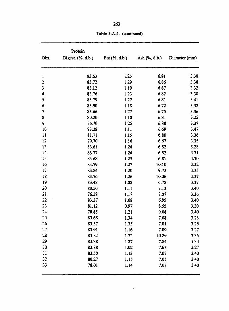
Obs
1 2 3 4 5 6 7 8 9 10
11 12 13 14 15 16
17 18
19 20 21
22
23 24 25 26 27 28 29 30 31 32 33
263
Table 5-A.4. (continued).
Protein
Digest (%, d.b.) Fat (%, d.b.) Ash (%, d.b.) Diameter (mm)
83.63 1.25 6.81 3.30 83.72 1.29 6.86 3.30 83.12 1.19 6.87 3.32 83.76 1.23 6.82 3.30 83.79 1.27 6.81 3.41 83.90 1.18 6.72 3.32 83.66 1.27 6.75 3.36 80.20 1.10 6.81 3.25 76.70 1.25 6.88 3.37 83.28 1.11 6.69 3.47 81.71 1.15 6.80 3.36 79.70 1.16 6.67 3.35 83.61 1.24 6.82 3.28 83.77 1.24 6.82 3.31 83.68 1.25 6.81 3.30 83.79 1.27 10.10 3.32 83.84 1.20 9.72 3.35 83.76 1.26 10.06 3.37 83.48 1.08 6.78 3.37 80.50 1.11 7.13 3.40 76.38 1.17 7.07 3.36 83.37 1.08 6.95 3.40 81.12 0.97 8.55 3.30 78.85 1.21 9.08 3.40 83.68 1.34 7.08 3.23 83.57 1.35 7.01 3.25 83.91 1.16 7.09 3.27 83.82 1.32 10.29 3.35 83.88 1.27 7.84 3.34 83.88 1.02 7.63 3.27 83.50 1.13 7.07 3.40 80.27 1.15 7.05 3.40 78.01 1.14 7.03 3.40
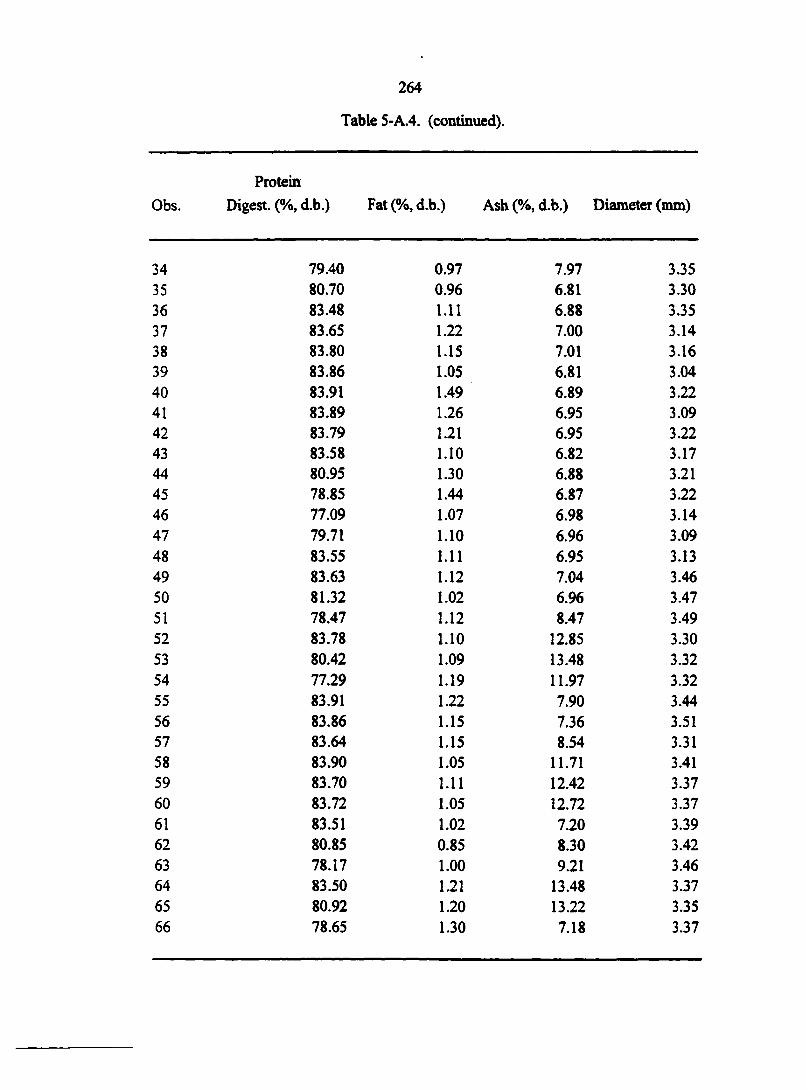
34 35 36 37 38 39 40 41 42 43 44 45 46 47 48 49 50 51 52 53 54 55 56 57 58 59 60 61
62 63 64 65 66
264
Table 5-A.4. (continued).
Protein
Digest. (%, d.b.) Fat (%, d.b.) Ash (%, d.b.) Diameter (mm)
79.40 0.97 7.97 3.35 80.70 0.96 6.81 3.30 83.48 1.11 6.88 3.35 83.65 1.22 7.00 3.14 83.80 1.15 7.01 3.16 83.86 1.05 6.81 3.04 83.91 1.49 6.89 3.22 83.89 1.26 6.95 3.09 83.79 1.21 6.95 3.22 83.58 1.10 6.82 3.17 80.95 1.30 6.88 3.21 78.85 1.44 6.87 3.22 77.09 1.07 6.98 3.14 79.71 1.10 6.96 3.09 83.55 1.11 6.95 3.13 83.63 1.12 7.04 3.46 81.32 1.02 6.96 3.47 78.47 1.12 8.47 3.49 83.78 1.10 12.85 3.30 80.42 1.09 13.48 3.32 77.29 1.19 11.97 3.32 83.91 1.22 7.90 3.44 83.86 1.15 7.36 3.51 83.64 1.15 8.54 3.31 83.90 1.05 11.71 3.41 83.70 1.11 12.42 3.37 83.72 1.05 12.72 3.37 83.51 1.02 7.20 3.39 80.85 0.85 8.30 3.42 78.17 1.00 9.21 3.46 83.50 1.21 13.48 3.37 80.92 1.20 13.22 3.35 78.65 1.30 7.18 3.37
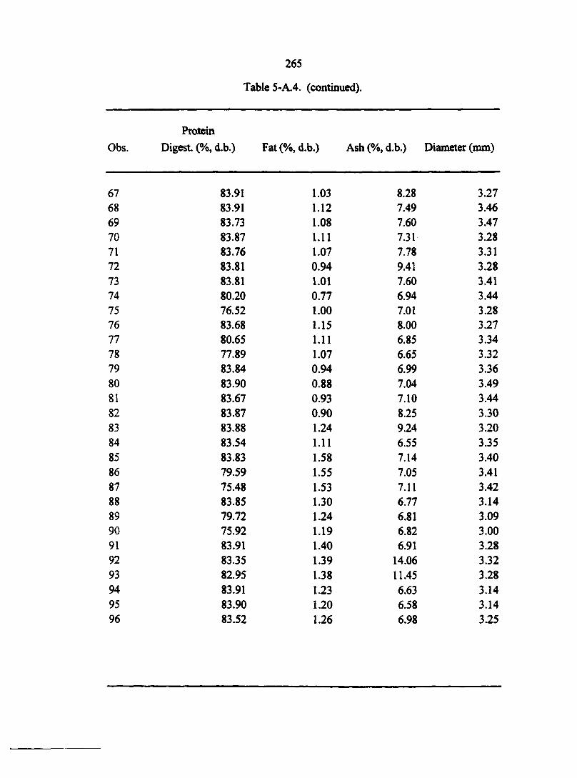
67 68 69 70 71 72 73 74 75 76 77 78 79 80 81 82 83 84 85 86 87 88
89 90 91 92 93 94 95 96
265
Table 5-A.4. (continued).
Protein
Digest. (%, d.b.) Fat(%, d.b.) Ash(%,d.b.) Diameter (mm)
83.91 1.03 8.28 3.27 83.91 1.12 7.49 3.46 83.73 1.08 7.60 3.47 83.87 1.11 7.31 3.28 83.76 1.07 7.78 3.31 83.81 0.94 9.41 3.28 83.81 1.01 7.60 3.41 80.20 0.77 6.94 3.44 76.52 1.00 7.01 3.28 83.68 1.15 8.00 3.27 80.65 1.11 6.85 3.34 77.89 1.07 6.65 3.32 83.84 0.94 6.99 3.36 83.90 0.88 7.04 3.49 83.67 0.93 7.10 3.44 83.87 0.90 8.25 3.30 83.88 1.24 9.24 3.20 83.54 1.11 6.55 3.35 83.83 1.58 7.14 3.40 79.59 1.55 7.05 3.41 75.48 1.53 7.11 3.42 83.85 1.30 6.77 3.14 79.72 1.24 6.81 3.09 75.92 1.19 6.82 3.00 83.91 1.40 6.91 3.28 83.35 1.39 14.06 3.32 82.95 1.38 11.45 3.28 83.91 1.23 6.63 3.14 83.90 1.20 6.58 3.14 83.52 1.26 6.98 3.25
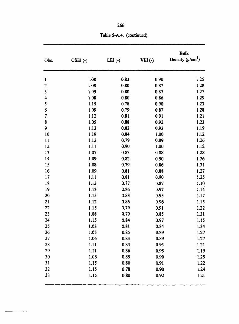
Obs
1 2 3 4 5 6 7 8 9 10
11 12
13 14 15 16
17 18
19 20 21 22 23 24 25 26 27 28
29 30 31 32 33
266
Table 5-A.4. (continued).
Bulk CSEI (-) LEI (-) VEI (-) Density (g/cm3)
1.08 0.83 0.90 1.25 1.08 0.80 0.87 1.28 1.09 0.80 0.87 1.27 1.08 0.80 0.86 1.29 1.15 0.78 0.90 1.23 1.09 0.79 0.87 1.28 1.12 0.81 0.91 1.21 1.05 0.88 0.92 1.23 1.13 0.83 0.93 1.19 1.19 0.84 1.00 1.12 1.12 0.79 0.89 1.26 1.11 0.90 1.00 1.12 1.07 0.83 0.88 1.28 1.09 0.82 0.90 1.26 1.08 0.79 0.86 1.31 1.09 0.81 0.88 1.27 1.11 0.81 0.90 1.25 1.13 0.77 0.87 1.30 1.13 0.86 0.97 1.14 1.15 0.83 0.95 1.17 1.12 0.86 0.96 1.15 1.15 0.79 0.91 1.22 1.08 0.79 0.85 1.31 1.15 0.84 0.97 1.15 1.03 0.81 0.84 1.34 1.05 0.85 0.89 1.27 1.06 0.84 0.89 1.27 1.11 0.83 0.93 1.21 1.11 0.86 0.95 1.19 1.06 0.85 0.90 1.25 1.15 0.80 0.91 1.22 1.15 0.78 0.90 1.24 1.15 0.80 0.92 1.21
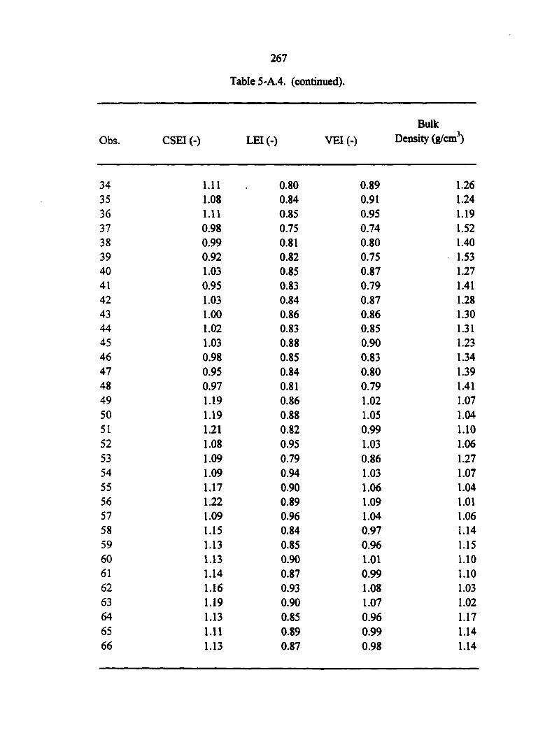
Obs
34 35 36 37 38 39 40 41 42 43 44 45 46 47 48 49 50 51 52 53 54 55 56 57 58 59 60 61
62 63 64 65 66
267
Table 5-A.4. (continued).
Bulk
CSEI (-) LEI (-) VEI (-) Density (g/cm3)
1.11 0.80 0.89 1.26 1.08 0.84 0.91 1.24 1.11 0.85 0.95 1.19 0.98 0.75 0.74 1.52 0.99 0.81 0.80 1.40 0.92 0.82 0.75 1.53 1.03 0.85 0.87 1.27 0.95 0.83 0.79 1.41 1.03 0.84 0.87 1.28 1.00 0.86 0.86 1.30 1.02 0.83 0.85 1.31 1.03 0.88 0.90 1.23 0.98 0.85 0.83 1.34 0.95 0.84 0.80 1.39 0.97 0.81 0.79 1.41 1.19 0.86 1.02 1.07 1.19 0.88 1.05 1.04 1.21 0.82 0.99 1.10 1.08 0.95 1.03 1.06 1.09 0.79 0.86 1.27 1.09 0.94 1.03 1.07 1.17 0.90 1.06 1.04 1.22 0.89 1.09 1.01 1.09 0.96 1.04 1.06 1.15 0.84 0.97 1.14 1.13 0.85 0.96 1.15 1.13 0.90 1.01 1.10 1.14 0.87 0.99 1.10 1.16 0.93 1.08 1.03 1.19 0.90 1.07 1.02 1.13 0.85 0.96 1.17 1.11 0.89 0.99 1.14 1.13 0.87 0.98 1.14
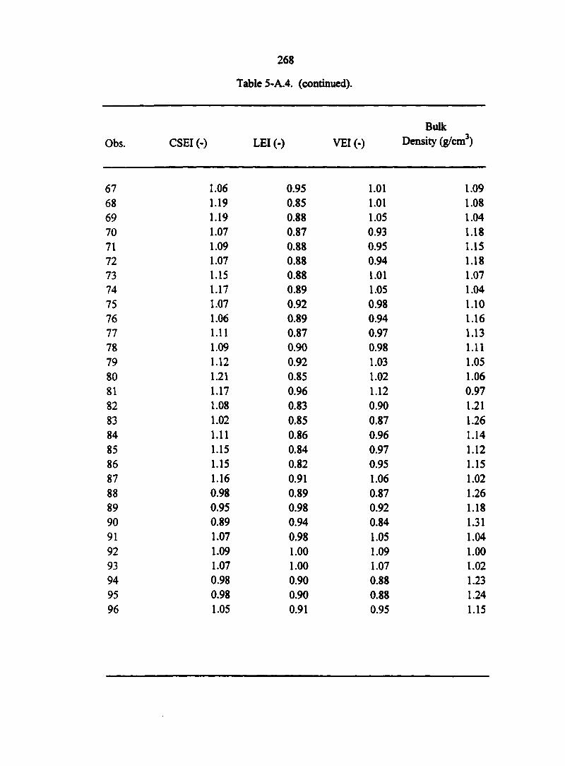
Obs
67 68 69 70 71 72 73 74 75 76 77 78 79 80 81 82
83 84 85 86 87 88 89 90 91 92 93 94 95 96
268
Table 5-A.4. (continued).
Bulk CSEI (-) LEI (-) VEI (-) Density (g/cm3)
1.06 0.95 1.01 1.09 1.19 0.85 1.01 1.08 1.19 0.88 1.05 1.04 1.07 0.87 0.93 1.18 1.09 0.88 0.95 1.15 1.07 0.88 0.94 1.18 1.15 0.88 1.01 1.07 1.17 0.89 1.05 1.04 1.07 0.92 0.98 1.10 1.06 0.89 0.94 1.16 1.11 0.87 0.97 1.13 1.09 0.90 0.98 1.11 1.12 0.92 1.03 1.05 1.21 0.85 1.02 1.06 1.17 0.96 1.12 0.97 1.08 0.83 0.90 1.21 1.02 0.85 0.87 1.26 1.11 0.86 0.96 1.14 1.15 0.84 0.97 1.12 1.15 0.82 0.95 1.15 1.16 0.91 1.06 1.02 0.98 0.89 0.87 1.26 0.95 0.98 0.92 1.18 0.89 0.94 0.84 1.31 1.07 0.98 1.05 1.04 1.09 1.00 1.09 1.00 1.07 1.00 1.07 1.02 0.98 0.90 0.88 1.23 0.98 0.90 0.88 1.24 1.05 0.91 0.95 1.15
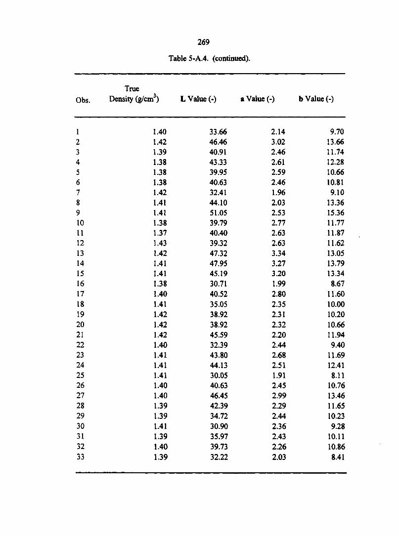
Obs
1 2 3 4 5 6 7 8 9 10 11 12 13 14 15 16
17 18
19 20 21
22 23 24 25 26 27 28 29 30 31 32 33
269
Table 5-A.4. (continued).
True Density (g/cm3) L Value (-) a Value (-) b Value (-)
1.40 33.66 2.14 9.70 1.42 46.46 3.02 13.66 1.39 40.91 2.46 11.74 1.38 43.33 2.61 12.28 1.38 39.95 2.59 10.66 1.38 40.63 2.46 10.81 1.42 32.41 1.96 9.10 1.41 44.10 2.03 13.36 1.41 51.05 2.53 15.36 1.38 39.79 2.77 11.77 1.37 40.40 2.63 11.87 1.43 39.32 2.63 11.62 1.42 47.32 3.34 13.05 1.41 47.95 3.27 13.79 1.41 45.19 3.20 13.34 1.38 30.71 1.99 8.67 1.40 40.52 2.80 11.60 1.41 35.05 2.35 10.00 1.42 38.92 2.31 10.20 1.42 38.92 2.32 10.66 1.42 45.59 2.20 11.94 1.40 32.39 2.44 9.40 1.41 43.80 2.68 11.69 1.41 44.13 2.51 12.41 1.41 30.05 1.91 8.11 1.40 40.63 2.45 10.76 1.40 46.45 2.99 13.46 1.39 42.39 2.29 11.65 1.39 34.72 2.44 10.23 1.41 30.90 2.36 9.28 1.39 35.97 2.43 10.11 1.40 39.73 2.26 10.86 1.39 32.22 2.03 8.41
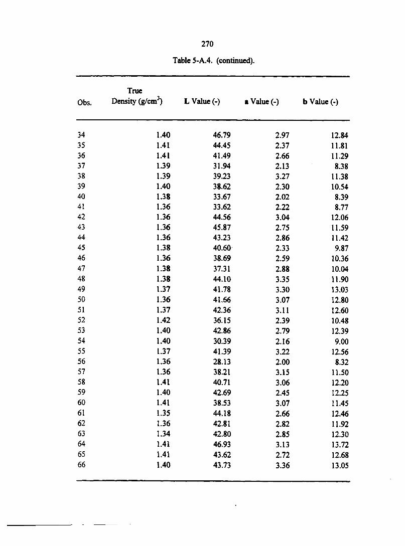
Obs
34 35 36 37 38 39 40 41 42 43 44 45 46 47 48 49 50 51 52 53 54 55 56 57 58 59 60 61
62 63 64 65 66
270
Table 5-A.4. (continued).
True Density (g/cm3) L Value (-) a Value (-) b Value (-)
1.40 46.79 2.97 12.84 1.41 44.45 2.37 11.81 1.41 41.49 2.66 11.29 1.39 31.94 2.13 8.38 1.39 39.23 3.27 11.38 1.40 38.62 2.30 10.54 1.38 33.67 2.02 8.39 1.36 33.62 2.22 8.77 1.36 44.56 3.04 12.06 1.36 45.87 2.75 11.59 1.36 43.23 2.86 11.42 1.38 40.60 2.33 9.87 1.36 38.69 2.59 10.36 1.38 37.31 2.88 10.04 1.38 44.10 3.35 11.90 1.37 41.78 3.30 13.03 1.36 41.66 3.07 12.80 1.37 42.36 3.11 12.60 1.42 36.15 2.39 10.48 1.40 42.86 2.79 12.39 1.40 30.39 2.16 9.00 1.37 41.39 3.22 12.56 1.36 28.13 2.00 8.32 1.36 38.21 3.15 11.50 1.41 40.71 3.06 12.20 1.40 42.69 2.45 12.25 1.41 38.53 3.07 11.45 1.35 44.18 2.66 12.46 1.36 42.81 2.82 11.92 1.34 42.80 2.85 12.30 1.41 46.93 3.13 13.72 1.41 43.62 2.72 12.68 1.40 43.73 3.36 13.05
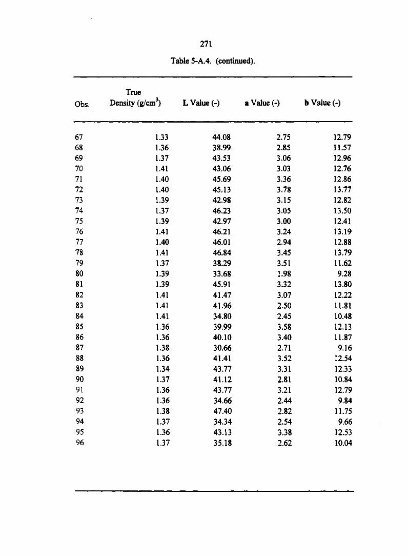
Obs
67 68 69 70 71 72 73 74 75 76 77 78 79 80 81 82 83 84 85 86 87 88 89 90 91 92 93 94 95 96
271
Table 5-A.4. (continued).
True Density (g/cm3) L Value (-) a Value (-) b Value (-)
1.33 44.08 2.75 12.79 1.36 38.99 2.85 11.57 1.37 43.53 3.06 12.96 1.41 43.06 3.03 12.76 1.40 45.69 3.36 12.86 1.40 45.13 3.78 13.77 1.39 42.98 3.15 12.82 1.37 46.23 3.05 13.50 1.39 42.97 3.00 12.41 1.41 46.21 3.24 13.19 1.40 46.01 2.94 12.88 1.41 46.84 3.45 13.79 1.37 38.29 3.51 11.62 1.39 33.68 1.98 9.28 1.39 45.91 3.32 13.80 1.41 41.47 3.07 12.22 1.41 41.96 2.50 11.81 1.41 34.80 2.45 10.48 1.36 39.99 3.58 12.13 1.36 40.10 3.40 11.87 1.38 30.66 2.71 9.16 1.36 41.41 3.52 12.54 1.34 43.77 3.31 12.33 1.37 41.12 2.81 10.84 1.36 43.77 3.21 12.79 1.36 34.66 2.44 9.84 1.38 47.40 2.82 11.75 1.37 34.34 2.54 9.66 1.36 43.13 3.38 12.53 1.37 35.18 2.62 10.04
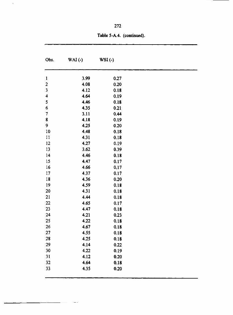
272
Table 5-A.4. (continued).
Obs. WAI (-) WSI (-)
1 3.99 0.27 2 4.08 0.20 3 4.12 0.18 4 4.64 0.19 5 4.46 0.18 6 4.35 0.21 7 3.11 0.44 8 4.18 0.19 9 4.25 0.20 10 4.48 0.18 11 4.31 0.18 12 4.27 0.19 13 3.62 0.39 14 4.46 0.18 15 4.47 0.17 16 4.66 0.17 17 4.37 0.17 18 4.36 0.20 19 4.59 0.18 20 4.31 0.18 21 4.44 0.18 22 4.65 0.17 23 4.47 0.18 24 4.21 0.23 25 4.22 0.18 26 4.67 0.18 27 4.55 0.18 28 4.25 0.18 29 4.14 0.22 30 4.22 0.19 31 4.12 0.20 32 4.64 0.18 33 4.35 0.20
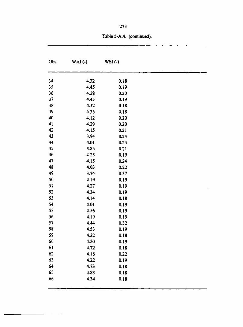
Obs
34 35 36 37 38 39 40 41 42 43 44 45 46 47 48 49 50 51 52 53 54 55 56 57 58 59 60 61 62 63 64 65 66
273
Table 5-A.4. (continued).
WAI (-) WSI (-)
4.32 0.18 4.45 0.19 4.28 0.20 4.45 0.19 4.32 0.18 4.35 0.18 4.12 0.20 4.29 0.20 4.15 0.21 3.94 0.24 4.01 0.23 3.85 0.21 4.25 0.19 4.15 0.24 4.03 0.22 3.74 0.37 4.19 0.19 4.27 0.19 4.34 0.19 4.14 0.18 4.01 0.19 4.56 0.19 4.19 0.19 4.44 0.32 4.53 0.19 4.32 0.18 4.20 0.19 4.72 0.18 4.16 0.22 4.22 0.19 4.73 0.18 4.83 0.18 4.34 0.18
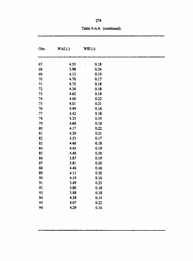
274
Table 5-A.4. (continued).
Obs. WAI (-) WSI (-)
67 4.55 0.18 68 3.98 0.24 69 4.13 0.19 70 4.70 0.17 71 4.75 0.18 72 4.36 0.18 73 4.62 0.18 74 4.06 0.22 75 4.01 0.21 76 4.49 0.16 77 4.42 0.18 78 4.33 0.19 79 4.60 0.18 80 4.17 0.22 81 4.20 0.21 82 4.53 0.17 83 4.46 0.18 84 4.45 0.19 85 4.46 0.30 86 3.87 0.19 87 3.81 0.20 88 4.46 0.16 89 4.11 0.20 90 4.19 0.16 91 3.49 0.33 92 3.80 0.18 93 3.88 0.18 94 4.38 0.14 95 4.07 0.22 96 4.29 0.16
275
CHAPTER 6
DEVELOPMENT OF FEED INGREDIENTS USING CORN MASA BYPRODUCTS. H. LARGE-SCALE EXTRUSION
A paper to be submitted, in part, to Cereal Chemistry
K. A. Rosentrater, T. L. Richard, C. J. Bern, and R. A. Flores
ABSTRACT
Corn masa processing residues appear to be readily incorporated into livestock feed
rations, which can be a viable alternative to landfilling, the traditional means of masa
byproduct disposal. Suspended solids removed from a masa processing waste stream were
blended with soybean meal at three levels (0%, 10%, and 20% waste solids), conditioned to a
moisture content of approximately 27% (w.b), and were extruded in a pilot-scale extruder at
screw speeds of206 rpm (21.6 rad/s) and 360 rpm (37.7 rad/s). Processing conditions,
including die temperature and pressure, dough density, drive exertion index, product and feed
material throughput rates, and moisture addition within the conditioner, were monitored
during extrusion, and the resulting extruded products were subjected to physical and
nutritional characterization, to determine optimal processing conditions for the blends.
Extrudate analysis included moisture content, water activity, ash content, product diameter,
expansion ratios, bulk density, color, and product durability. All blends studied were suitable
for extrusion at the processing conditions used, however, one processing condition was not
able to produce a cohesive extrudate product, but instead produced a feed crumble. Blend
ratio had little effect on either processing parameters or the measured extrudate properties.
Instead, the extrusion screw speed significantly affected both processing and product
properties, with higher speeds producing higher processing temperatures, and thus drier
276
products. After extrusion processing, an additional drying operation is recommended, to
reduce the moisture content of the extradâtes to levels that are microbiologically stable. This
drying stage was incorporated into this study, and did adequately dry the extruded products.
Keywords
Evaluation, Extrusion, Food Processing, Food Waste, Residue Utilization, Soybean
Meal.
Author Information
Journal Paper No. J-XXXXX of the Iowa Agriculture and Home Economics
Experiment Station, Ames, Iowa, Project No. 3326, and supported by Hatch Act and State of
Iowa Funds.
The authors are Kurt A. Rosentrater, Graduate Student, Agricultural and
Biosystems Engineering Dept., Iowa State University, Ames, Iowa; Thomas L. Richard,
Assistant Professor, Agricultural and Biosystems Engineering Dept., Iowa State University,
Ames, Iowa; Carl J. Bern, Professor, Agricultural and Biosystems Engineering Dept., Iowa
State University, Ames, Iowa; and Rolando A. Flores, Associate Professor, Department of
Grain Science and Industry, Kansas State University, Manhattan, Kansas. Corresponding
author: Thomas L. Richard, Iowa State University, 214B Davidson Hall, Ames, Iowa,
50011, tel.: (515) 294-0465, fax: (515) 294-2255, email: [email protected].
INTRODUCTION
Landfilling of agricultural and food processing wastes has declined over the last
several years, due to increased environmental awareness and economic constraints and/or
penalties. Alternative disposal strategies have been increasingly implemented, and include
reprocessing and recycling of byproducts within the plant, resale for other end-uses,
277
incineration, composting, biomass energy production, land application as soil conditioners,
and incorporation into livestock feed rations (Bohlsen et al., 1997; Derr and Dhillon, 1997;
Ferris et al., 1995; Power and Dick, 2000; Wang et al., 1997). This paper focuses on reuse as
livestock feed materials after subsequent value-added extrusion processing.
Many byproduct feeds have been developed in the grain processing industry,
especially for com milling processes, including com dry milling, com wet milling, and com
alcohol distillation. The main byproduct from com dry milling is hominy feed. The main
byproducts from com wet milling include com gluten feed (CGF), com gluten meal (COM),
corn germ meal (COM), and condensed fermented com extractives (CFCE). From com
alcohol distilling, the main feed byproducts are dried distiller's grains (DDG), dried distiller's
solubles (DDS), and dried distiller's grains with solubles (DDGS). Many studies have
examined the incorporation of these grain processing byproduct materials into livestock
diets: Annexstad et al. (1987), Cornelius et al. (1973), Larson et al. (1993), Lodge et al.
(1997), Simon et al. (1960), Stem et al. (1983), Tadtiyanant et al. (1993).
Com masa processing, however, is one area of the grain industry that generates large
quantities of waste materials, but to date, has received little attention in the development of
byproduct disposal alternatives. Com masa is used to produce com tortillas and com tortilla
chips. Tortillas have been a staple in the diets of Mexican and Central American peoples for
centuries. Common foods made with tortillas include tacos, tamales, quesadillas, and
enchiladas (Krause et al., 1992; Ortiz, 1985; Sema-Saldivar et al., 1990). Currently, Mexican
foods and corn-based snacks in the United States are booming in popularity. Tortilla sales
alone were estimated at $4 billion for 2000 A.D. (Solganik, 1997), and are expected to reach
$5.5 billion by 2003 A.D. (TIA, 2001).
278
Modem com masa is produced by simulating the ancient Aztec art of lime cooking
and processing of corn, but on an industrial-scale. Whole com is boiled and/or cooked with
120 to 300% water (original com weight basis) and 0.1 to 2.0% lime (original com weight
basis) for 0.5 to 3.0 h at 80 to 100 °C, and is then steeped for up to 24 h. This process, called
nixtamalization, can be either a batch process or a continuous process, depending on
production equipment. The cooked grain (nixtamal) is then separated from the steep liquor
(nejayote), which is rich in lime and dissolved com pericarp tissue. The nixtamal is washed
to remove any excess lime and pericarp, and is then stone ground to produce a dough (masa).
The masa is then molded, cut, or extruded, and is then baked or fried to make tortillas, tortilla
chips, or com chips. The masa can also be dried and milled into masa flour, which can later
be reconstituted and made into fresh tortillas at various food service establishments (Gomez
et al., 1987; Rooney and Serna-Saldivar, 1987; Sema-Saldivar et al., 1990).
Nejayote contains approximately 2% total (dissolved and suspended) solids.
Generally the suspended solids (50 to 60% of the total solids) are removed by screening,
centrifugation, or decanting, and are disposed of in landfills. The remaining water and
dissolved solids are sent to municipal water facilities for treatment. The total solids in the
waste stream, which consist primarily of fiber-rich pericarp tissues, represent com dry matter
losses that occur during processing. Estimates of this com mass loss have ranged from 5.0%
to 17.0% (Bressani et al., 1958; Gonzalez de Palacios, 1980; Katz et al., 1974; Khan et al.,
1982; Pflugfelder et al., 1988; Rooney and Sema-Saldivar, 1987; Sema-Saldivar et al.;
1990). The com dry matter lost during nixtamalization is affected by many processing
parameters, including com hybrid and quality, lime concentration, cooking and steeping
times and temperatures, friction and damage during washing and transport, and process
279
equipment used. These processing losses can be economically significant due to lost masa
yield, waste processing and disposal costs, potential environmental pollution, and subsequent
legal penalties (Khan et al., 1982; Rooney and Sema-Saldivar, 1987; Sema-Saldivar et al.;
1990).
Few studies have been conducted into alternative disposal options for masa byproduct
streams, but results seem to indicate that they are amenable to incorporation into livestock
feed rations. Rosentrater et al. (1999) conducted an extensive physical and nutritional
characterization of typical masa byproduct streams (i.e., separated suspended solids).
Pflugfelder et al. (1988) studied the composition of masa processing dry matter losses, and
included these losses in a mass balance of the masa production system. Gonzalez-Martinez
(1984) investigated four biological treatment options for nejayote on a laboratory-scale,
including activated sludge processing, anaerobic contact processing, submerged aerobic
fixed-film cascade reacting, and anaerobic packed-bed reacting, and found that the activated
sludge and anaerobic packed-bed reactors were effective treatment options for these waste
waters. Velasco-Martinez et al. (1997) investigated the suitability of implementing nejayote
solids in poultry broiler diets, and found no differences in performance between control diets
and diets utilizing nejayote solids. Chapter 5 (this dissertation) developed potential livestock
feed ingredients by blending nejayote solids (i.e., separated suspended solids) with soybean
meal at various blend levels and then extruding the blends at different processing conditions.
The objective of this investigation was to continue the development of value-added
masa byproduct feed ingredients by combining these byproducts with soybean meal at
various blend ratios, extruding the resulting mixtures on a pilot-scale, and investigating the
effects of the extrusion processing on resulting product characteristics. This study was

280
limited to laboratory analysis of the extrudate products, however, and did not include feeding
trials of these products.
MATERIALS AND METHODS
Experimental Design
To develop feed ingredients from masa processing residuals, this experiment used
two primary factors: blend ratio and extruder screw speed. Com masa byproduct (CMB)
solids and soybean meal (SBM) were blended at two levels: 10% CMB / 90% SBM and
20% CMB / 80% SBM. Additionally, a control blend of 0% CMB /100% SBM was used to
benchmark the process. Two extruder screw speeds were used: a low screw speed (LSS) of
206 rpm (21.6 rad/s) and a high screw speed (HSS) of 360 rpm (37.7 rad/s). The 0% CMB
and the 20% CMB blends were extruded at both screw speeds, while the 10% blend was only
extruded at the LSS. Each treatment was extruded once, which resulted in a total of 5
extrusion runs. Extrusion runs were completed with the lower screw speed first, while the
blends were run in random order for a given screw speed. Formal statistical analyses on all
collected data were performed via Microsoft Excel (Microsoft, 1993) and SAS (SAS, 1992)
software, using a Type I error rate (a) of 0.05, and included MANOVA, LSD multiple
comparisons, correlation analysis, and principal components analysis.
Sample Collection
Corn masa byproduct samples (which were gray, pasty, semi-solid slurries) were
obtained from a local com masa processing plant after the decanting stage in the production
process (i.e., the samples collected were the suspended solids that had been removed from
the masa processing waste stream). Approximately 200 lb. (90.7 kg) of byproducts were
collected from a single production run from a continuous-cook processing line at the facility.
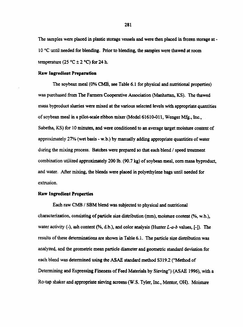
281
The samples were placed in plastic storage vessels and were then placed in frozen storage at -
10 °C until needed for blending. Prior to blending, the samples were thawed at room
temperature (25 °C ± 2 °C) for 24 h.
Raw Ingredient Preparation
The soybean meal (0% CMB, see Table 6.1 for physical and nutritional properties)
was purchased from The Farmers Cooperative Association (Manhattan, KS). The thawed
masa byproduct slurries were mixed at the various selected levels with appropriate quantities
of soybean meal in a pilot-scale ribbon mixer (Model 61610-011, Wenger Mfg., Inc.,
Sabetha, KS) for 10 minutes, and were conditioned to an average target moisture content of
approximately 27% (wet basis - w.b.) by manually adding appropriate quantities of water
during the mixing process. Batches were prepared so that each blend / speed treatment
combination utilized approximately 200 lb. (90.7 kg) of soybean meal, corn masa byproduct,
and water. After mixing, the blends were placed in polyethylene bags until needed for
extrusion.
Raw Ingredient Properties
Each raw CMB / SBM blend was subjected to physical and nutritional
characterization, consisting of particle size distribution (mm), moisture content (%, w.b.),
water activity (-), ash content (%, d.b.), and color analysis (Hunter L-a-b values, [-]). The
results of these determinations are shown in Table 6.1. The particle size distribution was
analyzed, and the geometric mean particle diameter and geometric standard deviation for
each blend was determined using the ASAE standard method S319.2 ("Method of
Determining and Expressing Fineness of Feed Materials by Sieving") (ASAE 1996), with a
Ro-tap shaker and appropriate sieving screens (W.S. Tyler, Inc., Mentor, OH). Moisture
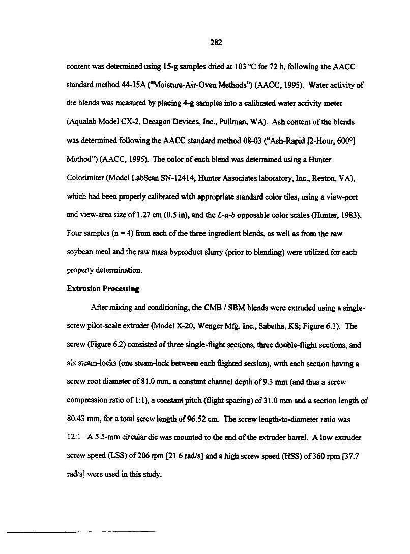
282
content was determined using 15-g samples dried at 103 °C for 72 h, following the AACC
standard method 44-15A ("Moisture-Air-Oven Methods") (AACC, 1995). Water activity of
the blends was measured by placing 4-g samples into a calibrated water activity meter
(Aqualab Model CX-2, Decagon Devices, Inc., Pullman, WA). Ash content of the blends
was determined following the AACC standard method 08-03 ("Ash-Rapid [2-Hour, 600°]
Method") (AACC, 1995). The color of each blend was determined using a Hunter
Colorimiter (Model LabScan SN-12414, Hunter Associates laboratory, Inc., Reston, VA),
which had been properly calibrated with appropriate standard color tiles, using a view-port
and view-area size of 1.27 cm (0.5 in), and the L-a-b opposable color scales (Hunter, 1983).
Four samples (n = 4) from each of the three ingredient blends, as well as from the raw
soybean meal and the raw masa byproduct slurry (prior to blending) were utilized for each
property determination.
Extrusion Processing
After mixing and conditioning, the CMB / SBM blends were extruded using a single-
screw pilot-scale extruder (Model X-20, Wenger Mfg. Inc., Sabetha, KS; Figure 6.1). The
screw (Figure 6.2) consisted of three single-flight sections, three double-flight sections, and
six steam-locks (one steam-lock between each flighted section), with each section having a
screw root diameter of 81.0 mm, a constant channel depth of 9.3 mm (and thus a screw
compression ratio of 1:1), a constant pitch (flight spacing) of 31.0 mm and a section length of
80.43 mm, for a total screw length of96.52 cm. The screw length-to-diameter ratio was
12:1. A 5.5-mm circular die was mounted to the end of the extruder barrel. A low extruder
screw speed (LSS) of206 rpm [21.6 rad/s] and a high screw speed (HSS) of360 rpm [37.7
rad/s] were used in this study.
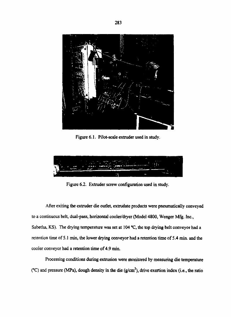
283
Figure 6.1. Pilot-scale extruder used in study.
Figure 6.2. Extruder screw configuration used in study.
After exiting the extruder die outlet, extrudate products were pneumatically conveyed
to a continuous belt, dual-pass, horizontal cooler/dryer (Model 4800, Wenger Mfg. Inc.,
Sabetha, KS). The drying temperature was set at 104 °C, the top drying belt conveyor had a
retention time of 5.1 min, the lower drying conveyor had a retention time of 5.4 min. and the
cooler conveyor had a retention time of 4.9 min.
Processing conditions during extrusion were monitored by measuring die temperature
(°C) and pressure (MPa), dough density in the die (g/cm3), drive exertion index (i.e., the ratio
284
of motor current used during processing to motor current under no-load conditions) (-),
product throughput rate (kg/min), feed material throughput rate (kg/min), and feed material
input rate into the conditioner (kg/min). The die temperature (measured in the die section of
the extruder) was determined using stock thermocouples inserted into the extruder die
section. Die pressure was measured via a pressure transducer mounted in the die section.
Dough density in the die was determined according to Alvarez-Martinez et al. (1988) and
Kokini et al. (1992):
Pd -1-MCj
l-MCf |p„(l-MCi)+p„MCl] (6.1)
where pd is the density of the dough in the die (g/cm3), MQ is the initial moisture content of
the raw ingredient material (i.e., from the conditioner) (w.b.), MCf is the final moisture
content of the resulting extradâtes at the extruder exit, prior to drying (w.b.), pex is the bulk
density of the resulting extradâtes (g/cm3), and p* is the density of water at the die
temperature (g/cm3). The drive exertion index was determined by taking the ratio of the
measured motor load (A) during processing to the no-load value (A) at the same extruder
screw speed. Product throughput rate (kg/min) was determined by collecting extrudate
output samples for 30-s intervals during processing. By using a dry matter mass balance, the
material throughput rate (i.e., the raw ingredient feed rate to the extruder) could be
determined (Alvarez-Martinez et al., 1988; Harper, 1981):
285
mfeed - mprod l-MCf
1-MC (6.2)
where mfeed is the rate of feed material throughput (kg/min), mprod is the measured rate of
extrudate product throughput (kg/min), MCf is the moisture content of the collected extrudate
product samples (w.b.), and MC, is the initial moisture content of the raw feed ingredient
material prior to extrusion (w.b ). Four measurements (n = 4) were taken for all processing
parameters during each extrusion run. Each extrusion run was approximately thirty minutes
in length; steady state was generally reached for each extrusion run after approximately five
minutes of processing; measurements were taken at approximately five-minute intervals after
the process reached steady state.
Extruded Product Analysis
After extrusion processing, drying, and cooling, the resulting extrudate products were
placed in polyethylene bags, and stored at room temperature. To investigate the effects of
extrusion processing on the CMB / SBM mixtures, several physical and nutritional properties
were measured on the extruded products. These properties included moisture content (%,
w.b.), water activity (-), ash content (%, d.b ), product diameter (mm), expansion ratios
(cross-sectional expansion index [-], longitudinal expansion index [-], volumetric expansion
index [-]), bulk density (g/cm3), color (Hunter L-a-b values [-]), and durability (%). Moisture
content, water activity, ash content, and color were determined using the methods previously
described for the raw ingredient blends. Further, moisture content levels were also measured
at three other stages during processing: raw material entering the extruder barrel (i.e., exiting
the preconditioned, extradâtes exiting the extruder (prior to entering the dryer/cooler), and
286
extrudate samples collected prior to entering the dryer/cooler, but allowed to air dry under
ambient conditions for 2 hours. Extrudate samples were cut to a length of 2 cm, were
weighed on an electronic balance (Model A-250, Denver Instrument Co., Arvada, CO), and
were measured for diameter using a digital micrometer (Digimatic Series No. 293, Mitutoyo
Co., Tokyo, Japan) (Alvarez-Martinez et al., 1988; Jamin and Flores, 1998). The cross-
sectional, longitudinal, and volumetric expansion ratios were determined following methods
prescribed by Alvarez-Martinez et al., (1988):
CSEI = L D d j
LEI = Pd 1 "l-MC,"
-p«. .CSEI. [l-MCf J VEI = CSEI LEI
(6.3)
(6.4)
(6.5)
where CSEI is the cross-sectional expansion index (-), De is the extrudate diameter (mm), Dj
is the die diameter (5.5 mm), LEI is the longitudinal expansion index (-), pa is the density of
the dough in the die, p«% is the bulk density of the extrudate (g/cm3), MQ is the initial
moisture content of the raw feed ingredient (w.b.), MCf is the final resulting moisture content
of the extrudate (w.b.), and VEI is the volumetric expansion index (-). Bulk density was
calculated as the ratio of the weight of each 2-cm extrudate piece to the calculated volume of
the piece (assuming cylindrical shapes for each extrudate sample) (Jamin and Flores, 1998).
Durability of extrudate samples was determined by following the ASAE standard method
S269.4 ("Cubes, Pellets, and Crumbles - Definitions and Methods for Determining Density,
287
Durability, and Moisture Content") (ASAE, 1996). Four samples from each extrusion run
were analyzed for each property determination (n=4).
Scale
Chapter 5 (this dissertation) extruded blends of CMB / SBM using a laboratory-scale
extruder. This study (i.e., this chapter) examined extruding similar blends, but with a pilot-
scale extruder. Scale-up of food processing operations has historically presented formidable
challenges to process engineers, but does need to be addressed. Levine (1989) discussed
several challenges and opportunities for scale-up of extrusion operations, and has suggested
dividing an extruder into two regions, then and treating each as separate entities: a transport
zone (encompassing the screw) and a forming zone (which encompasses the die zone).
Within each of the zones, a geometric scale and a dynamic scale must be considered. To
determine geometric scale, appropriate dimensions in each of these zones must be
considered. In the transport zone, the appropriate dimension is the screw diameter, and
geometric scale can be determined with Equation 6.6:
S = P — ( 6 . 6 )
^satw|hU>
where S is the geometric scale factor and Dsocw is the screw diameter (pilot or laboratory
extruder). Comparing the current pilot-scale study with the previous laboratory-scale study
resulted in a geometric scale of 7.0 in the transport zone. In the die zone, the appropriate
dimension is the die diameter, and geometric scale can be determined with Equation 6.7:
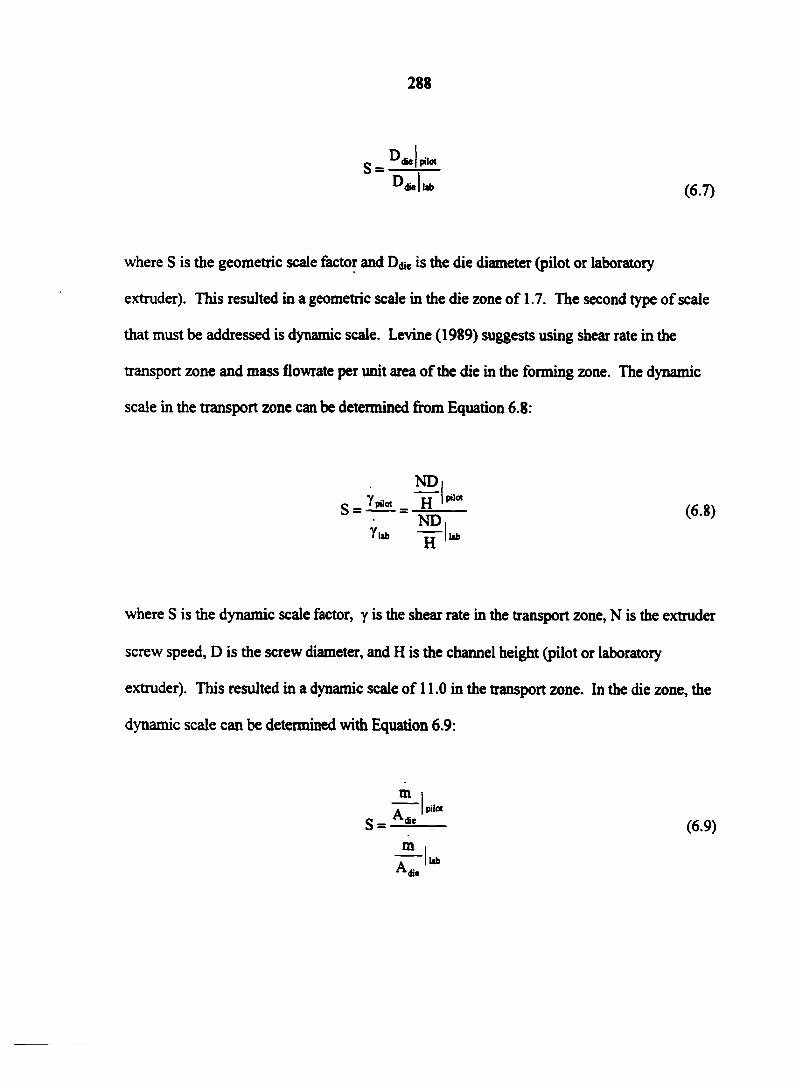
288
^die I pilot
(6.7)
where S is the geometric scale factor and D#* is the die diameter (pilot or laboratory
extruder). This resulted in a geometric scale in the die zone of 1.7. The second type of scale
that must be addressed is dynamic scale. Levine (1989) suggests using shear rate in the
transport zone and mass flowrate per unit area of the die in the forming zone. The dynamic
scale in the transport zone can be determined from Equation 6.8:
where S is the dynamic scale factor, y is the shear rate in the transport zone, N is the extruder
screw speed, D is the screw diameter, and H is the channel height (pilot or laboratory
extruder). This resulted in a dynamic scale of 11.0 in the transport zone. In the die zone, the
dynamic scale can be determined with Equation 6.9:
NDi
S = I*SL= H ND,
(6.8)
(6.9) m
a |ub die
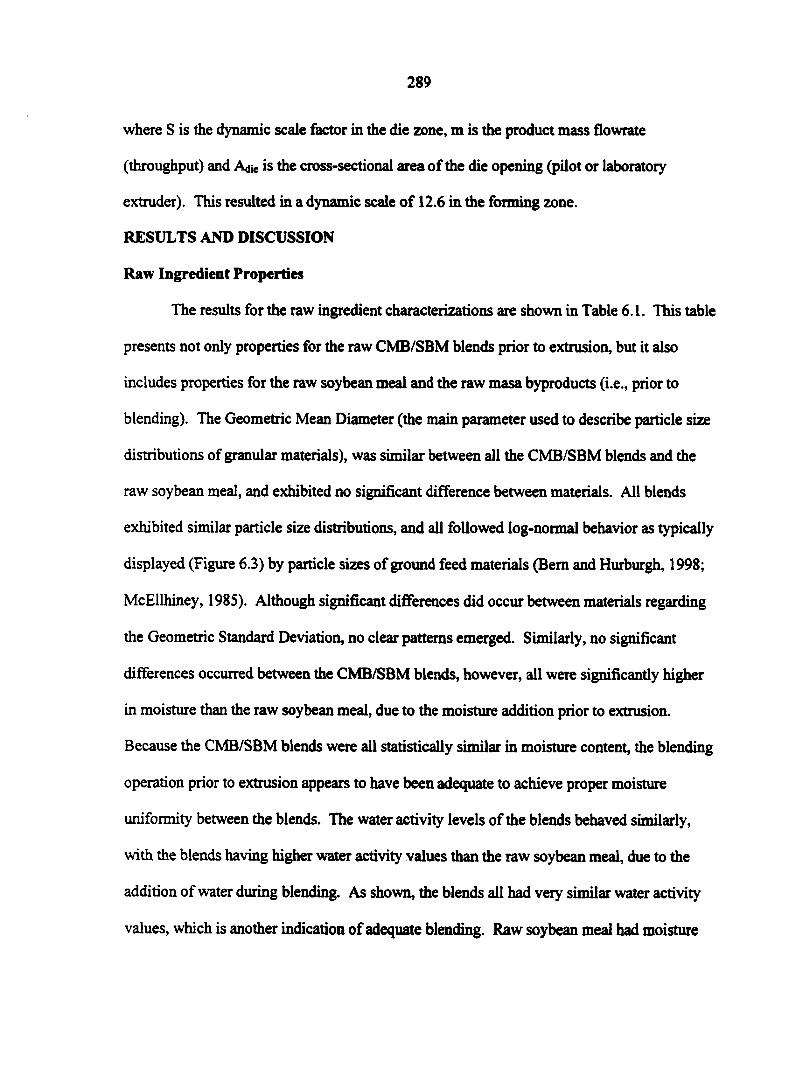
289
where S is the dynamic scale factor in the die zone, m is the product mass flowrate
(throughput) and Ad* is the cross-sectional area of the die opening (pilot or laboratory
extruder). This resulted in a dynamic scale of 12.6 in the forming zone.
RESULTS AND DISCUSSION
Raw Ingredient Properties
The results for the raw ingredient characterizations are shown in Table 6.1. This table
presents not only properties for the raw CMB/SBM blends prior to extrusion, but it also
includes properties for the raw soybean meal and the raw masa byproducts (i.e., prior to
blending). The Geometric Mean Diameter (the main parameter used to describe particle size
distributions of granular materials), was similar between all the CMB/SBM blends and the
raw soybean meal, and exhibited no significant difference between materials. All blends
exhibited similar particle size distributions, and all followed log-normal behavior as typically
displayed (Figure 6.3) by particle sizes of ground feed materials (Bern and Hurburgh, 1998;
McEllhiney, 1985). Although significant differences did occur between materials regarding
the Geometric Standard Deviation, no clear patterns emerged. Similarly, no significant
differences occurred between the CMB/SBM blends, however, all were significantly higher
in moisture than the raw soybean meal, due to the moisture addition prior to extrusion.
Because the CMB/SBM blends were all statistically similar in moisture content, the blending
operation prior to extrusion appears to have been adequate to achieve proper moisture
uniformity between the blends. The water activity levels of the blends behaved similarly,
with the blends having higher water activity values than the raw soybean meal, due to the
addition of water during blending. As shown, the blends all had very similar water activity
values, which is another indication of adequate blending. Raw soybean meal had moisture
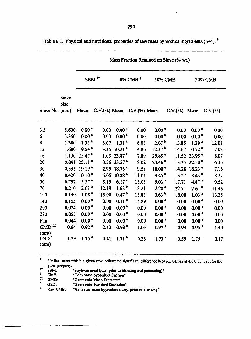
290
Table 6.1. Physical and nutritional properties of raw masa byproduct ingredients (n=4).r
Mass Fraction Retained on Sieve (% wt.)
SBMt+ 0% CMB* 10% CMB 20% CMB
Sieve Size
Sieve No. (mm) Mean C.V.(%) Mean C.V.(%) Mean C.V.(%) Mean C.V.(%)
3.5 5.600 6 3.360 8 2.380 12 1.680 16 1.190 20 0.841 30 0.595 40 0.420 50 0.297 70 0.210 100 0.149 140 0.105 200 0.074 270 0.053 Pan 0.044 GMD:t 0.94 (mm) GSD* 1.79 (mm)
0.00* 0.00 0.00* 0.00 1.33* 6.07 9.54* 4.35
25.47 * 1.03 25.11* 0.56 19.19* 2.95 10.10* 6.05 5.57* 8.15 2.61* 12.19 1.08* 15.00 0.00* 0.00 0.00* 0.00 0.00* 0.00 0.00* 0.00 0.92* 2.43
1.73* 0.41
0.00* 0.00 0.00* 0.00 1.31 * 6.03
10.21 * 4.86 23.87 * 7.89 23.57 * 8.02 18.75 * 9.58 10.88 * 11.04 6.17* 13.05 1.62 b 18.21 0.47b 15.83 0.11 * 15.89 0.00* 0.00 0.00* 0.00 0.00* 0.00 0.93* 1.05
1.71 b 0.33
0.00* 0.00 0.00* 0.00 2.07b 13.85
12.37b 14.67 25.85 * 11.52 24.46* 13.34 18.00* 14.28 9.45* 15.27 5.03* 17.71 2.28* 22.71 0.63 b 18.08 0.00* 0.00 0.00* 0.00 0.00* 0.00 0.00* 0.00 0.97* 2.94
1.73* 0.59
0.00* 0.00 0.00* 0.00 1.39* 12.08
10.72 * 7.02 23.95 * 8.07 22.50* 6.36 16.23 * 7.16 8.43* 8.27 4.87* 9.52 2.61* 11.46 1.03* 13.35 0.00* 0.00 0.00* 0.00 0.00* 0.00 0.00* 0.00 0.95* 1.40
1.75° 0.17
* Similar letters within a given row indicate no significant difference between blends at the 0.05 level for the given property.
y SBM: "Soybean meal (raw, prior to blending and processing)" ̂ CMB: "Com masa byproduct fraction"
~ GMD: "Geometric Mean Diameter" GSD: "Geometric Standard Deviation"
£ Raw CMB: "As-is raw masa byproduct slurry, prior to blending"
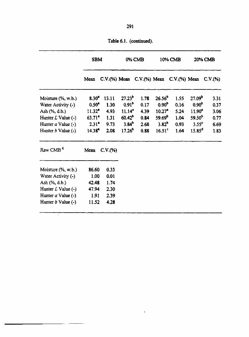
291
Table 6.1. (continued).
SBM 0% CMB 10% CMB 20% CMB
Mean C.V.(%) Mean C.V.(%) Mean C.V.(%) Mean C.V.(%)
Moisture (%, w.b.) 8.30* 13.11 27.23" 1.78 26.56b 1.55 27.09b 3.31 Water Activity (-) 0.50* 1.30 0.91b 0.17 0.90b 0.16 0.90b 0.37 Ash (%, d.b.) 11.32* 4.93 11.14* 4.39 10.27* 5.24 11.90* 3.06 Hunter L Value (-) 63.71* 1.31 60.42" 0.84 59.69b 1.04 59.50b 0.77 Hunter a Value (-) 2.31* 9.73 3.84" 2.68 3.82b 0.93 3.55e 6.69 Hunter b Value (-) 14.38* 2.08 17.26b 0.88 16.51e 1.64 U
i 00
1.83
Raw CMB€ Mean C.V.(%)
Moisture (%, w.b.) 86.60 0.33 Water Activity (-) 1.00 0.01 Ash (%, d.b.) 42.48 1.74 Hunter L Value (-) 47.94 2.30 Hunter a Value (-) 1.91 2.39 Hunter b Value (-) 11.52 4.28
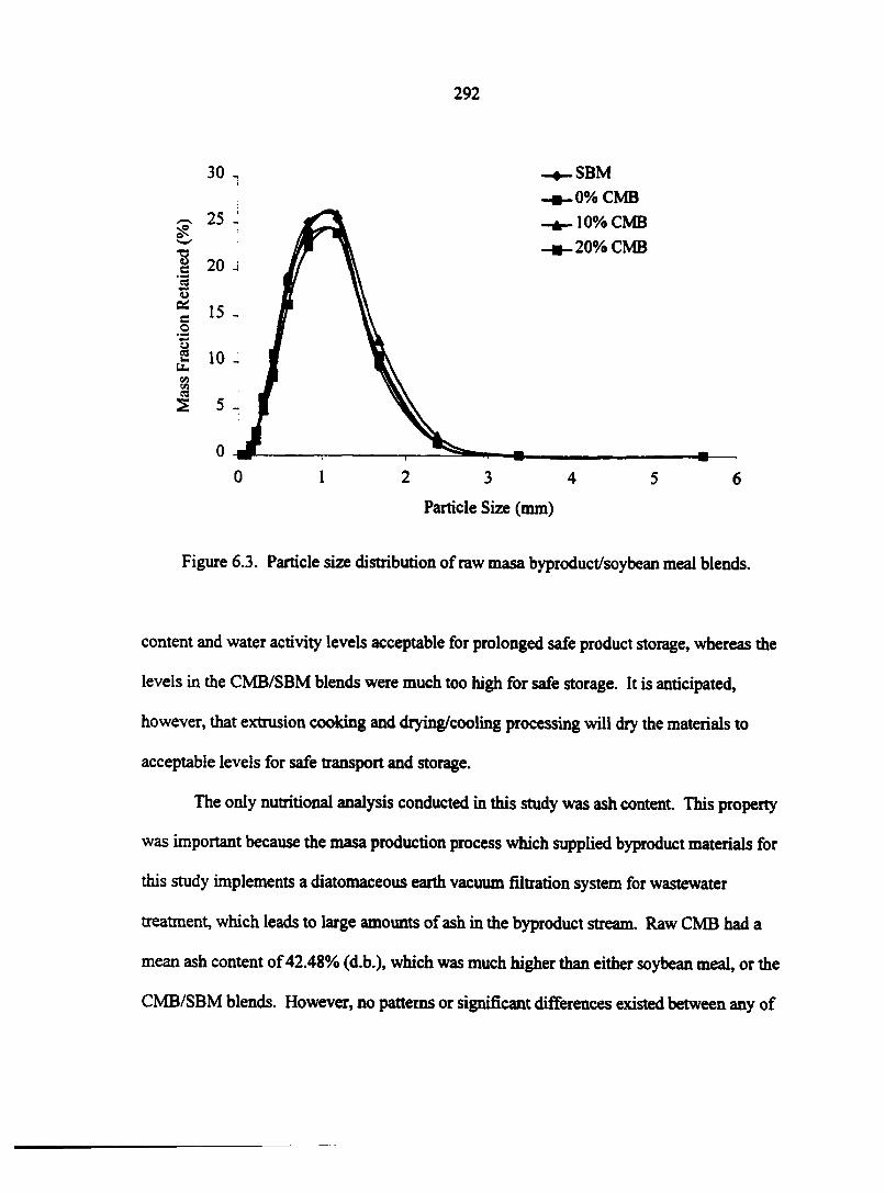
292
30 . .SBM
.0% CMB
.10% CMB
.20% CMB
2 3 4
Particle Size (mm)
Figure 6.3. Particle size distribution of raw masa byproduct/soybean meal blends.
content and water activity levels acceptable for prolonged safe product storage, whereas the
levels in the CMB/SBM blends were much too high for safe storage. It is anticipated,
however, that extrusion cooking and drying/cooling processing will dry the materials to
acceptable levels for safe transport and storage.
The only nutritional analysis conducted in this study was ash content. This property
was important because the masa production process which supplied byproduct materials for
this study implements a diatomaceous earth vacuum filtration system for wastewater
treatment, which leads to large amounts of ash in the byproduct stream. Raw CMB had a
mean ash content of42.48% (d.b.), which was much higher than either soybean meal, or the
CMB/SBM blends. However, no patterns or significant differences existed between any of
293
the blends or the raw soybean meal for ash content, even at the 20% blend level. This was
due to the high moisture content of CMB. Even when blended at the 20% level, over 86% of
the byproduct is water, so the CMB solids comprise less than 4% of total solids of the
mixture. Thus an insignificant effect on blend ash content was expected a priori.
From the color analysis, it can be seen that the Hunter L value, a measure of lightness
(100=white) / darkness (0=black), decreased as the fraction of CBM in the blend increased
(i.e., became darker). This was also expected beforehand, due to the gray nature of the
byproduct (which can be seen by the Hunter L values for the CMB in Table 6.1). Moreover,
all blends were significantly darker than the raw soybean meal. The Hunter a value, a
chromaticity measure of redness (+) / greenness (-), also decreased as the CBM fraction in
the blend increased (i.e. became less red, and more green). However, all blends were
significantly redder than the raw soybean meal. Additionally, the Hunter b value, a
chromaticity measure of yellowness (+) / blueness (-), also decreased as the CBM fraction in
the blend increased (i.e., became less yellow and more blue), and all blends were
significantly yellower than the raw soybean meal.
The properties of the CMB used in this study were similar to those found by
Rosentrater et al. (1999), who extensively examined the physical and nutritional
characteristics of com masa byproduct streams. Moisture content, water activity, Hunter L
value, Hunter a value, and Hunter b value all closely matched the results of the previous
study; ash content, however, was markedly different. Rosentrater et al. (1999) found ash
contents between 17 and 19% (d.b ), which were much lower than the ash levels in the CMB
used in this study (42.48% [d.b.]). This is primarily due to two distinct wastewater
separation processes for the production of CMB: byproducts for this study were the result of
294
a vacuum filtration process which used diatomaceous earth as a filter precoat, and hence had
a higher resulting ash level; Rosentrater et al. (1999) used CMB which had been separated
from the masa processing wastewater via centrifugation.
Extrusion Processing
These results are shown in main effects plots (Figure 6.4), and the trends seen will be
discussed below. The results for the extrusion processing measurements are shown in Table
6.2. MANOVA analysis confirmed that differences between experimental treatments did
exist (i.e., the Wilks' Lambda test statistic [MANOVA test criterion] indicated differences
between treatments [p = 0.0001]). The highest die temperature achieved during processing
occurred for the 20% CMB blend at the high screw speed (HSS). The lowest die temperature
occurred for the 0% CMB blend at the low screw speed (LSS). In general, as the CMB
fraction increased, die temperature increased, and as screw speed increased, die temperature
increased. This probably occurred due to increased frictional resistance heating (i.e., viscous
dissipation heating) at the higher shear rates produced by the higher screw speeds, and it may
be related to slightly increased residence time at the higher screw speed (Mercier et al.,
1989).
The highest die pressure was produced at the 0% blend, at the LSS. All other
extrusion runs produced lower die pressures, and were similar in quantity. This leads to an
inconclusive interpretation of behavioral trends for die pressure; the high readings for the 0%
blend, LSS, however, might have been due to processing instabilities occurring during this
(i.e., first) production run. Die pressure did decrease as speed increased, however.
The highest dough density occurred at the LSS, for both the 0% and the 10% blends.
The lowest density occurred at the HSS, 0% blend. From the limited data, it appears that
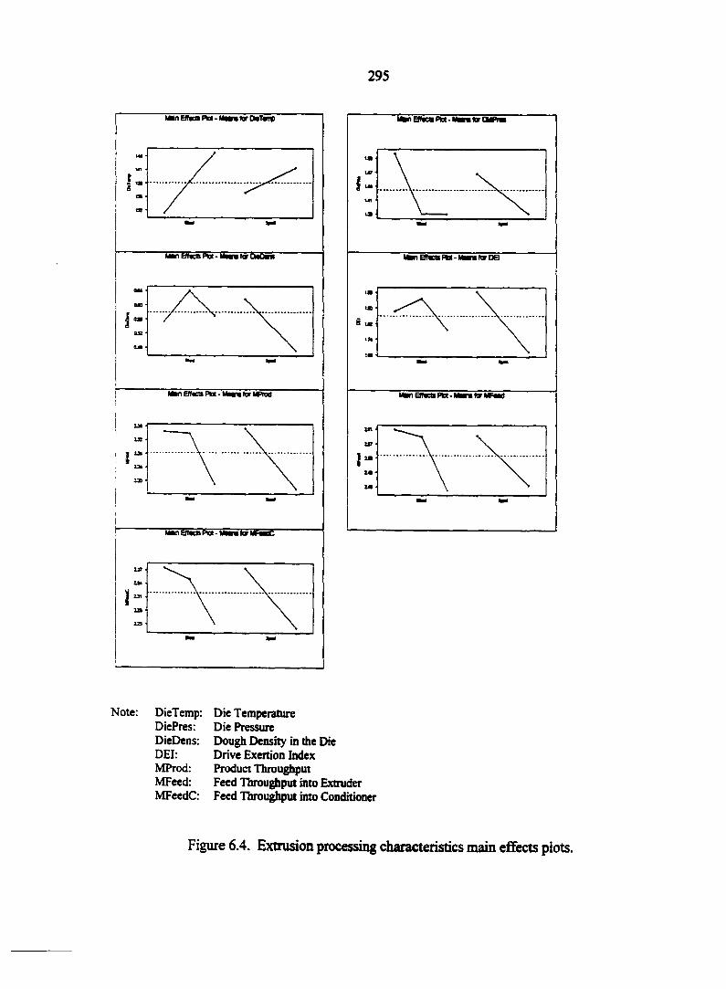
295
Man Eftcsnx-Mara tar OMTOTP
Man Efftco P*x - Man tar CMOV*
Man BTca PM • Mm for kRM
ManEfl«caPiot-MmtariyF«MC
•Hn EMM PU - Man tor OMPra
I*
WnEfhceAoi-Mm force
te
te
k*n BT*a Ptot - Mm for *F«ed
14
Note: DieTemp: Die Temperature DiePres: Die Pressure DieDens: Dough Density in the Die DEI: Drive Exertion Index MProd: Product Throughput MFeed: Feed Throughput into Extruder MFeedC: Feed Throughput into Conditioner
Figure 6.4. Extrusion processing characteristics main effects plots.
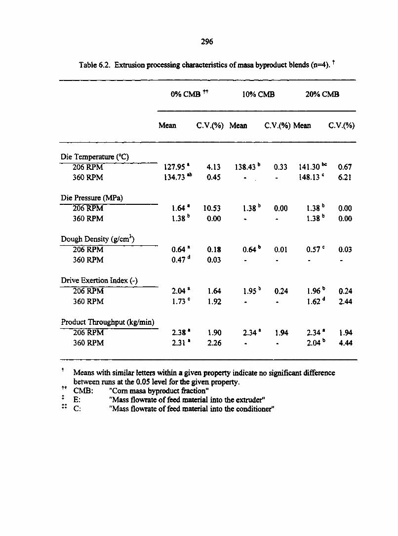
296
Table 6.2. Extrusion processing characteristics of masa byproduct blends (n=4).f
0% CMB n 10% CMB 20% CMB
Mean C.V.(%) Mean C.V.(%) Mean C.V.(%)
Die Temperature (°C) 206 RPM 127.95* 4.13 138.43b 0.33 141.30 * 0.67 360 RPM 134.73 * 0.45 - - 148.13 e 6.21
Die Pressure (MPa) 206 RPM 1.64* 10.53 1.38b 0.00 1.38b 0.00 360 RPM 1.38b 0.00 - - 1.38b 0.00
Dough Density (g/cm3) 206 RPM 0.64* 0.18 0.64b 0.01 0.57 e 0.03 360 RPM 0.47d 0.03 ....
Drive Exertion Index (-) 206 RPM 2.04* 1.64 1.95b 0.24 1.96b 0.24 360 RPM 1.73 e 1.92 - - 1.62d 2.44
Product Throughput (kg/min) 206 RPM 2.38* 1.90 2.34* 1.94 2.34* 1.94 360 RPM 2.31 * 2.26 - - 2.04b 4.44
f Means with similar letters within a given property indicate no significant difference between runs at the 0.05 level for the given property.
y CMB: "Com masa byproduct fraction" ^ E: "Mass flowrate of feed material into the extruder" ** C: "Mass flowrate of feed material into the conditioner"
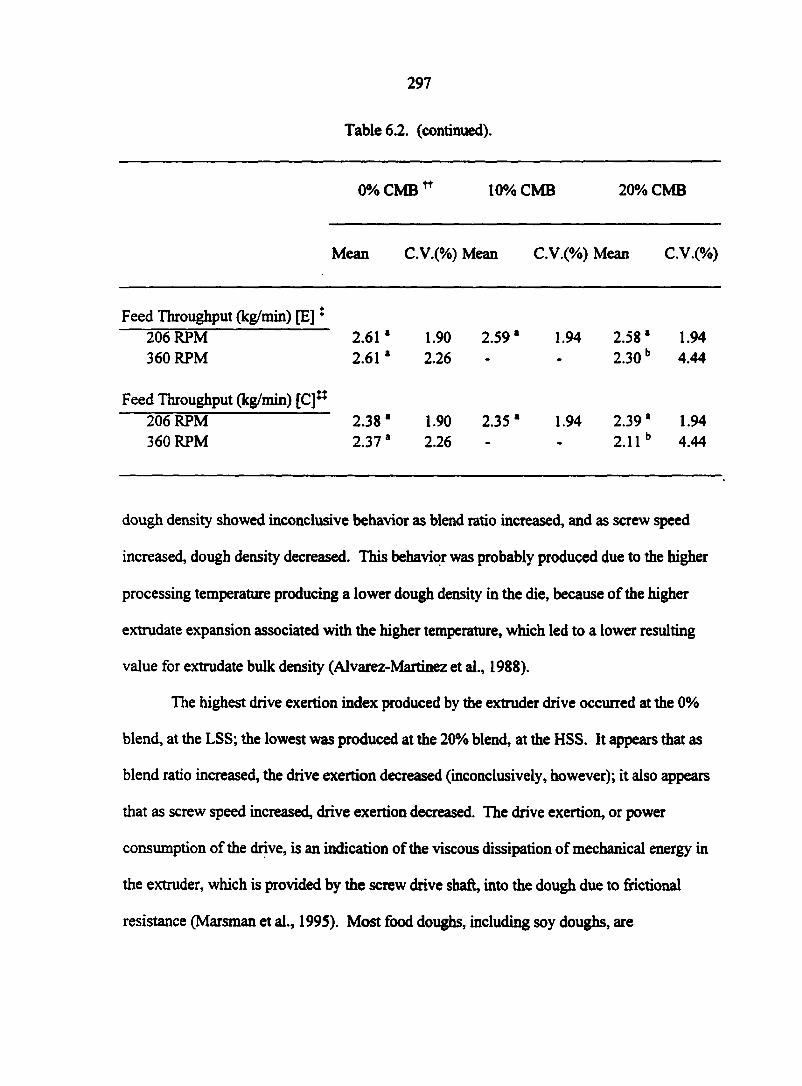
297
Table 6.2. (continued).
0% CMB n 10% CMB 20% CMB
Mean C.V.(%) Mean C.V.(%) Mean C.V.(%)
Feed Throughput (kg/min) [E]$
206 RPM 2.61 * 1.90 2.59* 1.94 2.58* 1.94 360 RPM 2.61 * 2.26 - - 2.30b 4.44
Feed Throughput (kg/min) [C]$î
206 RPM 2.38* 1.90 2.35* 1.94 2.39* 1.94 360 RPM 2.37* 2.26 - - 2.11 b 4.44
dough density showed inconclusive behavior as blend ratio increased, and as screw speed
increased, dough density decreased. This behavior was probably produced due to the higher
processing temperature producing a lower dough density in the die, because of the higher
extrudate expansion associated with the higher temperature, which led to a lower resulting
value for extrudate bulk density (Alvarez-Martinez et al., 1988).
The highest drive exertion index produced by the extruder drive occurred at the 0%
blend, at the LSS; the lowest was produced at the 20% blend, at the HSS. It appears that as
blend ratio increased, the drive exertion decreased (inconclusively, however); it also appears
that as screw speed increased, drive exertion decreased. The drive exertion, or power
consumption of the drive, is an indication of the viscous dissipation of mechanical energy in
the extruder, which is provided by the screw drive shaft, into the dough due to frictional
resistance (Marsman et al., 1995). Most food doughs, including soy doughs, are
298
pseudoplastic materials (i.e., an increase in shear rate produces a decrease in the material's
apparent viscosity, and hence the resultant torque required by the screw to convey the dough
is decreased). Further, viscosity typically decreases as processing temperature increases
(Chen et al., 1979; Kokini et al., 1992; Mercier et al., 1989). These behaviors, which were
exhibited in this study, occur due to the structural changes that occur in the food dough (i.e.,
unfolding and aligning of molecules and structures) during processing.
The highest product mass throughput rate occurred at the 0% blend, LSS. The lowest
occurred at the 20% blend, HSS. In general, it appears that as blend ratio increased, product
throughput decreased. This was more pronounced at the HSS than at the LSS, however.
Also, it appears that as screw speed increased, product throughput decreased. Because the
feed material throughput rate to the extruder was calculated based on the measured product
throughput rate, the behavior of feed material throughput was similar to product throughput.
During extrusion, higher screw speeds typically produce higher mass flowrates, because of
the increased ability of the extruder to convey material through the machine (Bouvier et al.,
1987; Mercier et al., 1989).
The dry-matter mass balance that was used to determine extruder feed material
throughput rate (Equation 6.2) was then applied across the preconditioner to determine the
raw ingredient feed throughput rate into the conditioner. These results (Table 6.2) show that
this throughput rate also follows a similar behavioral pattern to the product and extruder feed
throughput rates (due to the mass balance). Further, moisture content results (Table 6.3)
show that the moisture content level of the raw blends was increased from approximately
27% (w.b.) by the addition of steam and hot water in the conditioner at a rate between 0.19
and 0.24 kg/min., which was done to facilitate extrusion processing. No clear trends are
299
present regarding blend level or screw speed and the amount of moisture addition in the
conditioner prior to extrusion, however.
Extruded Product Analysis
Typical extradâtes produced during extrusion are shown in Figure 6.5. The results
for the extruded product characterization tests are shown in Table 6.3, and main effects plots
are shown in Figure 6.6. MANOVA analysis confirmed that differences between
experimental treatments did exist (i.e., the Wilks' Lambda test statistic [MANOVA test
criterion] indicated differences between treatments [p = 0.0001]). In this study, all extrudate
properties were determined on products exiting the dryer/cooler. Moisture content levels,
however, were measured at four stages of processing (in addition to the measurements
conducted on the raw materials) as previously described: raw material entering the extruder
barrel (i.e., exiting the preconditioner), extradâtes exiting the extruder (prior to entering the
dryer/cooler), extradâtes exiting the dryer/cooler, and extradate samples collected prior to
entering the dryer/cooler, but allowed to air dry under ambient conditions. The materials
entering the extruder (after discharging from the conditioner), were fairly uniform in
moisture content. As shown in Table 6.3, there were no statistical differences in moisture
content between extrusion runs. It can be seen that the moisture levels have been raised in
the conditioner by 5.5 to 6.7 percentage points (w.b.) over the initial raw materials due to the
preconditioning. This was done to facilitate the extrusion processing and to produce
consistent end products, by increasing the moisture content and the temperature of the raw
materials prior to extrusion.
Moisture content levels of the extradâtes exiting the extrader (prior to drying) show a
marked decrease in moisture content The highest moisture level occurred at the LSS, 0%
300
Figure 6.5. Typical masa byproduct Z soybean meal extrudates.

301
Table 6.3. Physical and nutritional properties of masa byproduct blend extrudates (n=4).t
0% CMB n 10% CMB 20% CMB
Mean C.V. (%) Mean C.V. (%) Mean C.V. (%)
Moisture Content (%, w.b.) [OC] * 206 RPM 33.63a 3.26 33.19a 0.75 32.59a 1.12 360 RPM 33.921 2.74 - - 33.26a 1.78
Moisture Content (%, w.b.) [OE] ** 206 RPM 27.17a 3.48 26.06 * 3.30 25.49b 1.94 360 RPM 25.38b 4.39 - - 24.75b 4.01
Moisture Content (%, w.b.) €
206 RPM 8.32a 5.25 6.95b 11.51 4.72c 15.75 360 RPM 4.54c 2.16 - - 3.89c 3.29
Moisture Content (%, w.b.) [OE#r]+
206 RPM 20.96 a 6.56 21.65a 3.97 19.71a 4.63 360 RPM 17.57b 11.78 - - 19.92 a 3.60
Water Activity (-) 206 RPM 0.51a 1.80 0.47b 1.14 0.41c 1.94 360 RPM 0.43c 2.26 - - 0.42c 3.98
+ Means with similar letters within a given property indicate no significant difference between runs at the 0.05 level for the given property.
y CMB: "Com masa byproduct fraction" : OC: "Feed material collected at conditioner exit, prior to extrusion"
OE : "Extrudate samples collected at extruder exit, prior to drying" OEair "Extrudate samples collected at extruder exit, subjected to air drying"
6 "Extrudate samples collected out of dryer/cooler discharge" ^ CSEI: "Cross-Sectional Expansion Index" *e LEI: "Longitudinal Expansion Index"
VEI: "Volumetric Expansion Index"
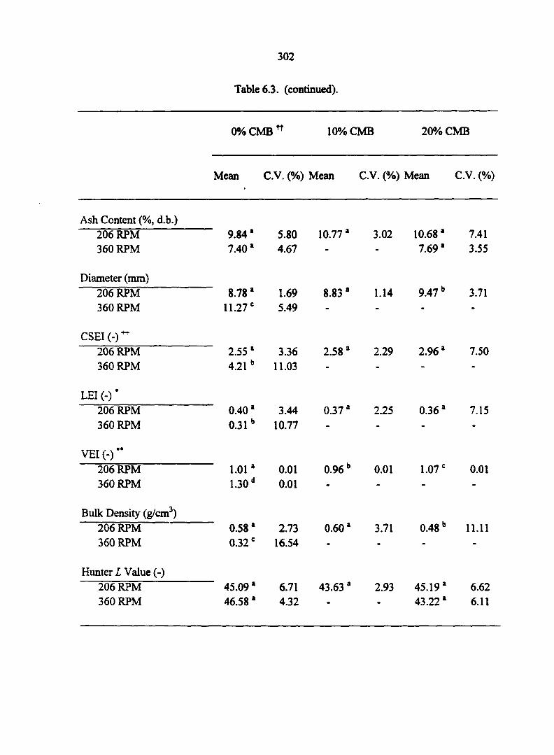
302
Table 6.3. (continued).
0% CMB n 10% CMB 20% CMB
Mean C.V. (%) Mean C.V. (%) Mean C.V. (%)
Ash Content (%, d.b.) 206 RPM 9.84 e 5.80 10.77a 3.02 10.68a 7.41 360 RPM 7.40 e 4.67 - - 7.69 e 3.55
Diameter (mm) 206 RPM 8.78 e 1.69 8.83a 1.14 9.47b 3.71 360 RPM 11.27 e 5.49 ....
CSEI(-) 206 RPM 2.55 e 3.36 2.58a 2.29 2.96 e 7.50 360 RPM 4.21b 11.03 ....
LEI (-)
206 RPM 0.40 e 3.44 0.37 e 2.25 0.36 e 7.15 360 RPM 0.31b 10.77 ....
VEI (-) "
206 RPM 1.01e 0.01 0.96b 0.01 1.07 e 0.01 360 RPM 1.30d 0.01 ....
Bulk Density (g/cm3)
206 RPM 0.58 e 2.73 0.60e 3.71 0.48b 11.11 360 RPM 0.32 e 16.54 ....
Hunter L Value (-)
206 RPM 45.09 e 6.71 43.63 e 2.93 45.19 e 6.62 360 RPM 46.58 e 4.32 - - 43.22 e 6.11
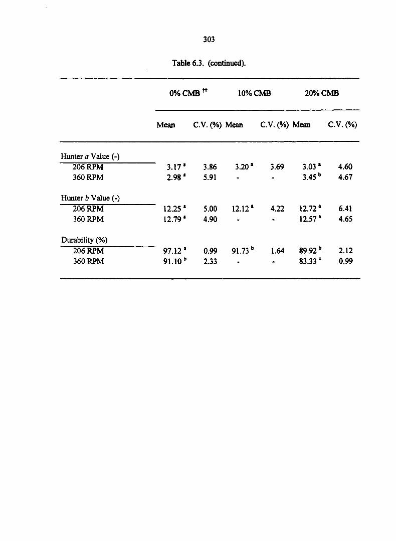
303
Table 6.3. (continued).
0% CMB n 10% CMB 20% CMB
Mean C.V. (%) Mean C.V. (%) Mean C.V. (%)
Hunter a Value (-) 206 RPM 3.17' 3.86 3.20a 3.69 3.031 4.60 360 RPM 2.98* 5.91 - - 3.45b 4.67
Hunter b Value (-) 206 RPM 12.25a 5.00 12.121 4.22 12.721 6.41 360 RPM 12.79' 4.90 - - 12.57 ' 4.65
Durability (%) 206 RPM 97.12' 0.99 91.73b 1.64 89.92 b 2.12 360 RPM 91.10b 2.33 - - 83.33 e 0.99
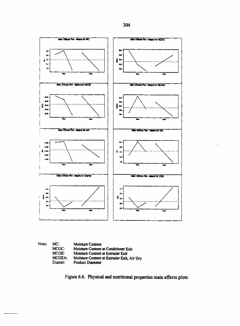
304
Man Effaça Pti - Mm for MC
»
Man Efto PU - Mn for MCGE
! ManEflacmna-MwmforMV I
Man Effacs PW. Mm far curat
Man BMC* ft* • Mm for MOOC
m*
Man Effaca nt - Mm tor MCOEA
MnEINcaPtt-MmtorÂSr
Man EMca n* - Mm for CSB
13
1»
Note: MC: Moisture Content MCOC : Moisture Content at Conditioner Exit MCOE: Moisture Content at Extruder Exit MCOEA: Moisture Content at Extruder Exit, Air Dry Diamet: Product Diameter
Figure 6.6. Physical and nutritional properties main effects plots.
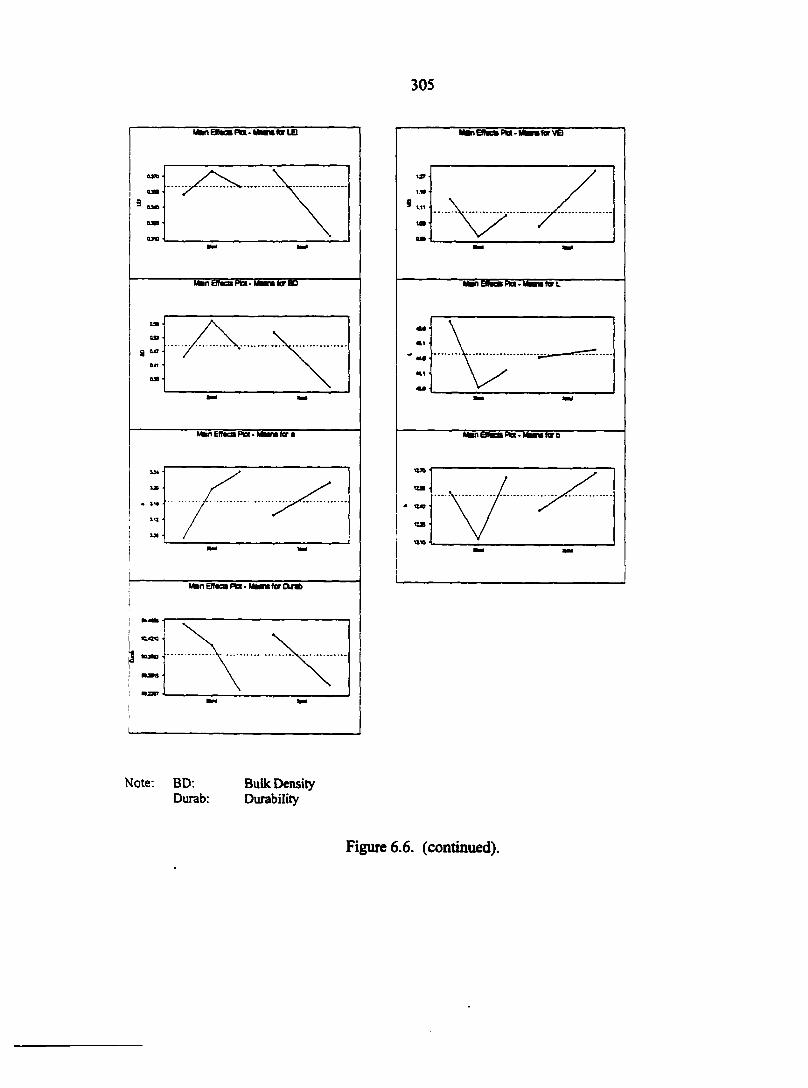
305
Mki EtMea Hot • IMnnr LEI
Man Eftacs PW - Mara ta BO
MuiEftacsPU-MNnafora
Man Btacs not - Mmtb for Outt
MarBTacsPU-MariforVE)
MnEMcBRa-MHratarT
Man £ff«ca Ma - ilwni for o
Note: BD: Bulk Density Durab: Durability
Figure 6.6. (continued).
306
blend. The lowest level occurred at the HSS, 20% blend. It appears that, in general, as blend
ratio increased, extrudate moisture content decreased. Also, it appears that as screw speed
increased, extrudate moisture content decreased. Because of the high temperatures involved,
extrusion processing has a drying effect on feed materials. When a dough melt is transported
through an extruder die, up to 8 percentage points of the raw ingredient's moisture will
evaporate due to the sudden change in state to ambient pressure and temperature (Faubion et
al., 1982). The moisture content loss for the blends in this study ranged from 6.46 to 8.54
percentage points (w.b.), with the higher processing temperatures produced by the higher
screw speeds producing greater moisture loss than the lower screw speeds (and thus lower
processing temperature). The final moisture contents of the extrudates ranged from 24.75 to
27.17 percentage points (w.b.), however, which was still too high for safe storage, and thus a
further drying step was required (Faubion et al., 1982; Miller, 1985; Wang et al., 1997).
Feed materials with high moisture contents have higher transportation costs, decreased
stability and storability, and ultimately have limited market area and profitability (Derr and
Dhillon, 1997). To alleviate these difficulties and effectively utilize the masa
byproduct/soybean meal blends as livestock feed additives, these extrudates must be
dehydrated to an ideal maximum moisture content of approximately 12 % (w.b.), which is
recommended for feed products, because this moisture level substantially reduces
transportation costs and is microbiologically stable (Beauchat, 1981).
It can be seen that the drying/cooling stage of the production process did indeed
substantially reduce extrudate moisture content to safe levels, with final moisture content
level between 3.89 and 8.32% (w.b.). The highest moisture level occurred for the 0% blend
at the LSS; the lowest moisture level occurred for the HSS, 20% blend. It is interesting to
307
note that these levels appeared to correspond to the highest and lowest levels exiting the
extruder. These moisture content levels were too low, however, which can also lead to
product damage; another investigation should be undertaken to optimize this drying process.
By examining the moisture levels of the extrudates which were allowed to air dry, it
can be seen that moisture levels did decrease, but these final moisture levels were not low
enough to be microbiologically stable. In fact, moisture content reductions due to air drying
alone were between 4.41 and 7.81 percentage points (w.b.), while reductions due to the
dryer/cooler were between 18.85 and 20.86 percentage points (w.b.). Although air drying
seems to be more economically justifiable, it actually is not, because the extrudates are not
dried to a moisture content low enough to resist microbial action. The extrudates definitely
do need to undergo a mechanical drying phase in order to attain a low enough moisture
content to become shelf stable.
The highest extrudate water activity occurred at the LSS, for the 0% blend. The
lowest extrudate water activity was at the LSS, for the 20% blend. It appears that water
activity decreased as blend ratio increased, which intuitively, should be the reverse of the
observed trend. The effect of screw speed, appears to show a decrease in water activity as
speed increases, in general. Water activity quantifies the amount of "free" water (i.e.,
unbound water) available in materials for use by microorganisms and chemical agents, and
hence is a measure of a material's susceptibility to spoilage and deterioration. Products with
no free water (aw = 0.0) are not at risk for spoilage, while materials with 100% free water (aw
= 1.0) are at high risk for rapid spoilage. Because extrusion processing reduces the moisture
content of the feed material, the associated water activity level also decreases. Through
dehydration, high-moisture materials become less expensive to transport and become
308
microbiologically stable. Materials become safe from bacteria growth below water activities
of approximately 0.9, safe from mold growth below approximately 0.8, and safe from yeast
growth below approximately 0.7 (Barbosa-Canovas and Vega-Mercado, 1996). The final
water activity levels of the extrudates ranged from 0.41 to 0.51, and are microbiologically
stable. When Chapter 5 produced CMB/SBM blend extrudates using a laboratory-scale
extruder, the extrudates were not subjected to a drying/cooling stage, as they were in the
current study. Whereas the extrudates in this study are shelf-stable, those produced by
Chapter 5 were not.
The highest extrudate ash content occurred at the 10% blend, LSS, while the lowest
ash content occurred at the 0% blend, HSS. It appears that as screw speed increased, ash
content decreased, however, no statistically significant differences were present.
The largest extrudate diameter occurred at the 0% blend, HSS, while the lowest
occurred at the 0% blend, LSS. As blend ratio increased, the effect on product diameter was
unclear. It appears that diameter increased as screw speed increased. It must be noted,
however, that the 20% blend, HSS production run was not able to produce a cohesive,
consistent extrudate pellet. Instead, this run produced a "crumble"-type of feed material. As
the results show, all other runs produced cohesive extrudate products with diameters
somewhat greater than the die opening (i.e., cross-sectional expansion occurred). In fact, the
extrudates had resulting diameters approximately twice that of the die exit (D*: = 5.5 mm).
This expansion in diameter, however, is small compared to the behavior of starchy materials,
which exhibit very pronounced expansion upon die exit. Cumming et al. (1972) studied
extrusion of 30% moisture content soybean meal and produced products with relatively
constant diameters, which exhibited little expansion upon extruder die exit; their results
309
showed that most physical and structural changes to the soy feed material occur inside the
extruder before exiting the die.
The high temperatures, shear stresses and shear strains produced during extrusion
processing alter not only the physical characteristics and the nutritional quality of feed
materials, but also affect the complex interactions between the chemical constituents and the
resulting internal cellular structures that occur during water evaporation upon die exit
(Miller, 1985). These changes are reflected in the expansion of the material as it passes
through the extruder die, and are quantified through the use of expansion ratios (Moore et al.,
1990). It has been theorized that extrudate product expansion is dependent on the rheological
properties of the thermoplastic melt in the extruder channel: radial expansion is dependent
on melt elasticity and longitudinal elongation is dependent on melt viscosity. It is further
believed that the damage to the protein molecules incurred by the heat treatment in an
extruder reduces the ability of the melt to form an elastic structure upon die exit, and thus
produces a decreased expansion (Alvarez-Martinez et al., 1988). The highest extrudate radial
expansion, quantified by the CSEI (Cross-Sectional Expansion Index), occurred at the HSS,
for the 0% blend. The lowest extrudate CSEI value was at the LSS, for the 0% blend. The
CSEI results exhibit behavior similar those of the diameter results, because the CSEI value is
determined based on product diameter. In general, it appears radial expansion behavior was
unclear as blend ratio increased, but increased as screw speed increased (and thus processing
temperature increased). This agrees with the results of Alvarez-Martinez et al. (1988), which
predict higher radial expansions for higher processing temperatures. Radial extrudate
expansion, quantified by the CSEI, is highly dependent on the water and starch compositions
of the extruded material. Products high in starch content generally exhibit high expansion;
310
soybean meal, however, essentially has no starch, so it was not surprising that limited radial
expansion occurred during extrusion processing in this study, as evidenced by relatively low
CSEI values in general (Gumming et al., 1972; Nielsen, 1976).
The Longitudinal Expansion Index (LEI) quantifies the elongation of extrudates as
they pass through the extruder die. The highest extrudate LEI value occurred at the 0%
blend, HSS. The lowest extrudate LEI value was at the 0% blend, LSS. In general, the LSS
produced extrudates with higher LEI values than the HSS. It appears that as blend ratio
increased, elongation showed unclear behavior; the observed differences were not
statistically significant. Overall, however, the LEI values were very low, which ultimately
points to little longitudinal expansion for the extruded blends in this study.
Overall extrudate volumetric expansion, quantified by the Volumetric Expansion
Index (VEI), relates the effects of the radial and the longitudinal expansion, through the
interaction of the CSEI and the LEI. The highest extrudate VEI value occurred at the HSS,
for the 0% blend. The lowest extrudate VEI value was at the LSS, for the 10% blend.
Within a given screw speed, the effect of blend ratio on volumetric expansion is unclear,
however, it appears that as screw speed increases, volumetric expansion also increases.
Overall, however, the VEI values are quite low, and in fact these results indicate that the
extruded products, for all blends and processing conditions, exhibited little volumetric
expansion upon die exit, which was expected. This behavior is typical for soybean-based
extrudates, because of the very low starch content, which is key to product expansion via the
starch gelatinization process (Nielsen, 1976).
Another measure of the internal structure of an extrudate is bulk density. The highest
bulk density occurred at the 10% blend, LSS; the lowest occurred at the 0% blend, HSS. No
311
trend could be established between bulk density and blend ratio, but it does appear that bulk
density decreased as screw speed increased, which could be due to an increase in processing
temperature at increased screw speeds, due to heating by viscous dissipation. Bulk density
generally decreases as processing temperature is increased, a behavior which was exhibited
in this study, which leads to a more expanded product, and thus a more porous extrudate
structure and an increased water penetration and hence a decreased bulk density (Badrie and
Mellowes, 1991; Gumming et al., 1972).
From the color analysis, it can be seen that overall, the extruded products were
substantially darker in appearance than the raw ingredient blends, with the L, a, and b results
all much lower than the respective values for the raw ingredients. The highest extrudate
Hunter L value occurred at the 0% blend, HSS, and the lowest occurred at the 20% blend,
HSS. No clear patterns, or significant differences occurred between any of the extrudates,
although it appears that the L value slightly increased as screw speed increased.. The highest
Hunter a value occurred at the 20% blend, HSS; while the lowest occurred at the 0% blend,
HSS. Again, no significant differences were present in the Hunter a data, although it appears
that as both blend ratio and screw speed increased, the resulting a value also increased. The
highest Hunter b value occurred at the 0% blend, HSS, while the lowest occurred at the 10%
blend, LSS. Again, no clear patterns, or significant differences, emerged in the blend data,
but it did appear that b increased as screw speed increased. Essentially these results describe
the extruded products as light brown in appearance. The extruded products are darker and
browner than the raw ingredient blends because of the high-temperature heat treatment
during the extrusion cooking process and the additional drying and cooling stages. High
processing temperatures exacerbate protein reactions with reducing sugars in nonenzymatic
312
(Maillard) browning processes, which lead to not only darker products, but also products
with reduced nutritional quality (i.e., destruction of amino acids) (Badrie and Mellowes,
1991; Dahl and Villota, 1991).
During handling and storage, feed materials are subjected to many destructive forces,
including impact, shear, compression, abrasion, and other interactions with surrounding
materials. These destructive forces damage feed materials and produce broken and dusty
feedstuffs, which subsequently decreases quality and value, and increases susceptibility to
deterioration (Stroshine and Hamann, 1995). Durability is the quality characteristic that
quantifies the ability of a feed material to resist these destructive forces. Higher durability
indicates a higher resistance to damage, and can be achieved by several means. High
temperature conditioning and processing of feed material leads to improved product
durability, as does decreasing the raw ingredient particle size; both methods improve
durability due to increasing the surface area of the feed material, which allows for more
thorough moisture addition, which then produces denser extruded pellets. On the other hand,
larger particle sizes lead to decreased durability, due to the production of fissures in the
extruded products, which are inherently more susceptible to damage and breakage (Tabil and
Sokhansanj, 1996). Because higher temperatures are achieved with extrusion processing,
product durability is generally greater than that of pellets produced through traditional steam
pelleting (Hilton et al., 1981). The highest extrudate durability occurred at the 0% blend,
LSS; the lowest durability occurred at the 20% blend. HSS. It appears that as blend ratio
increased, durability decreased. It also appears that as screw speed increased, durability
decreased. The durability values of the extruded products in this study were quite high,
ranging from 83.33 to 97.12%, which shows that the extruded CMB / SBM blends were
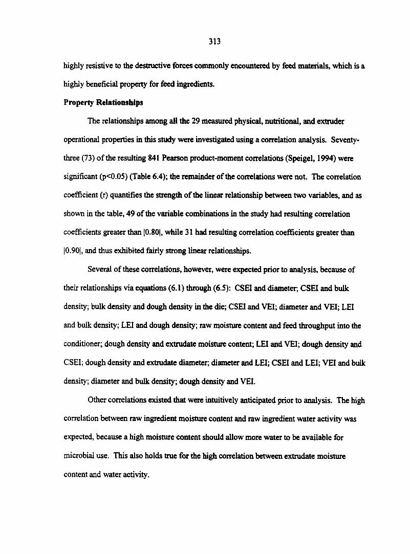
313
highly resistive to the destructive forces commonly encountered by feed materials, which is a
highly beneficial property for feed ingredients.
Property Relationships
The relationships among all the 29 measured physical, nutritional, and extruder
operational properties in this study were investigated using a correlation analysis. Seventy-
three (73) of the resulting 841 Pearson product-moment correlations (Speigel, 1994) were
significant (p<0.05) (Table 6.4); the remainder of the correlations were not. The correlation
coefficient (r) quantifies the strength of the linear relationship between two variables, and as
shown in the table, 49 of the variable combinations in the study had resulting correlation
coefficients greater than (0.801, while 31 had resulting correlation coefficients greater than
|0.90|, and thus exhibited fairly strong linear relationships.
Several of these correlations, however, were expected prior to analysis, because of
their relationships via equations (6.1) through (6.5): CSEI and diameter; CSEI and bulk
density; bulk density and dough density in the die; CSEI and VEI; diameter and VEI; LEI
and bulk density; LEI and dough density; raw moisture content and feed throughput into the
conditioner; dough density and extrudate moisture content; LEI and VEI; dough density and
CSEI; dough density and extrudate diameter; diameter and LEI; CSEI and LEI; VEI and bulk
density; diameter and bulk density; dough density and VEI.
Other correlations existed that were intuitively anticipated prior to analysis. The high
correlation between raw ingredient moisture content and raw ingredient water activity was
expected, because a high moisture content should allow more water to be available for
microbial use. This also holds true for the high correlation between extrudate moisture
content and water activity.
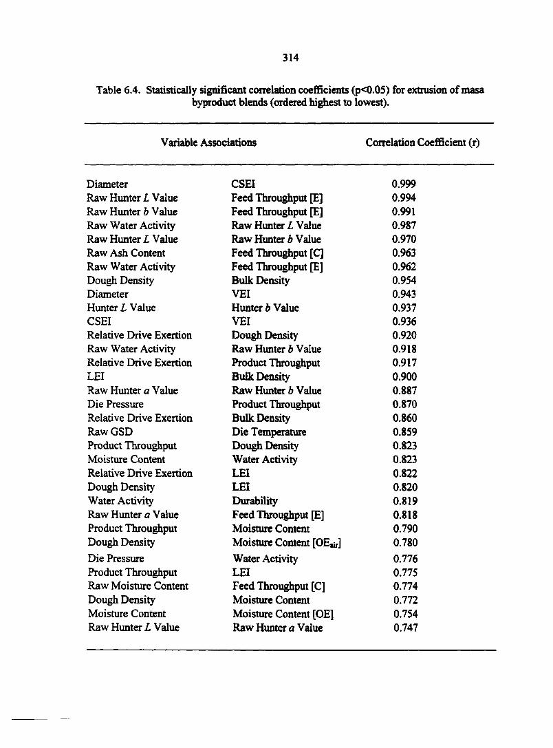
314
Table 6.4. Statistically significant conelation coefficients (p<0.05) for extrusion of masa byproduct blends (ordered highest to lowest).
Variable Associations Correlation Coefficient (r)
Diameter CSEI 0.999 Raw Hunter L Value Feed Throughput [E] 0.994 Raw Hunter b Value Feed Throughput [E] 0.991 Raw Water Activity Raw Hunter L Value 0.987 Raw Hunter L Value Raw Hunter b Value 0.970 Raw Ash Content Feed Throughput [C] 0.963 Raw Water Activity Feed Throughput [E] 0.962 Dough Density Bulk Density 0.954 Diameter VEI 0.943 Hunter L Value Hunter b Value 0.937 CSEI VEI 0.936 Relative Drive Exertion Dough Density 0.920 Raw Water Activity Raw Hunter b Value 0.918 Relative Drive Exertion Product Throughput 0.917 LEI Bulk Density 0.900 Raw Hunter a Value Raw Hunter b Value 0.887 Die Pressure Product Throughput 0.870 Relative Drive Exertion Bulk Density 0.860 RawGSD Die Temperature 0.859 Product Throughput Dough Density 0.823 Moisture Content Water Activity 0.823 Relative Drive Exertion LEI 0.822 Dough Density LEI 0.820 Water Activity Durability 0.819 Raw Hunter a Value Feed Throughput [E] 0.818 Product Throughput Moisture Content 0.790 Dough Density Moisture Content [OE^] 0.780
Die Pressure Water Activity 0.776 Product Throughput LEI 0.775 Raw Moisture Content Feed Throughput [C] 0.774 Dough Density Moisture Content 0.772 Moisture Content Moisture Content [OE] 0.754 Raw Hunter L Value Raw Hunter a Value 0.747
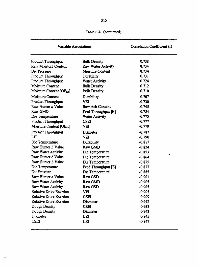
315
Table 6.4. (continued).
Variable Associations Correlation Coefficient (r)
Product Throughput Bulk Density 0.738 Raw Moisture Content Raw Water Activity 0.734 Die Pressure Moisture Content 0.734 Product Throughput Durability 0.731 Product Throughput Water Activity 0.724 Moisture Content Bulk Density 0.712 Moisture Content [OE^r] Bulk Density 0.710
Moisture Content Durability 0.707 Product Throughput VEI -0.730 Raw Hunter a Value Raw Ash Content -0.745 Raw GMD Feed Throughput [E] -0.754 Die Temperature Water Activity -0.773 Product Throughput CSEI -0.777 Moisture Content [OE«r] VEI -0.779
Product Throughput Diameter -0.787 LEI VEI -0.790 Die Temperature Durability -0.817 Raw Hunter L Value Raw GMD -0.824 Raw Water Activity Die Temperature -0.853 Raw Hunter b Value Die Temperature -0.864 Raw Hunter L Value Die Temperature -0.875 Die Temperature Feed Throughput [E] -0.877 Die Pressure Die Temperature -0.885 Raw Hunter a Value RawGSD -0.901 Raw Water Activity Raw GMD -0.905 Raw Water Activity RawGSD -0.905 Relative Drive Exertion VEI -0.905 Relative Drive Exertion CSEI -0.909 Relative Drive Exertion Diameter -0.912 Dough Density CSEI -0.933 Dough Density Diameter -0.943 Diameter LEI -0.945 CSEI LEI -0.947
316
Table 6.4. (continued).
Variable Associations Correlation Coefficient (r)
VEI Bulk Density -0.948 Raw Hunter L Value RawGSD -0.961 CSEI Bulk Density -0.967 Diameter Bulk Density -0.973 Dough Density VEI -0.980 RawGSD Feed Throughput [E] -0.986 Raw Hunter b Value RawGSD -0.999
Many of the correlations do provide useful insight into the relationships between
products and processes. For instance, the drive exertion index is related to the dough density
(r=0.92), which then affects product throughput, and subsequently product expansion and
thus product bulk density. Product throughput is also related to final extrudate moisture
content (r=0.79), which also affects product water activity, bulk density, and durability.
Further, die temperature affects product water activity (r=-0.773) and durability (r=-0.817).
Several correlations involve the color (L - a - b ) values, and are interesting, because
they hold potential for developing prediction relationships between the color variables and
the other variables with which they are associated. These correlations deserve further
investigation to quantify these relationships. The full correlation matrix is shown in Table
6.5.
To further investigate the relationships and interactions among the raw ingredient
properties, the extrusion processing properties, and the resulting extrudate properties, a
principal components analysis was conducted using all 29 variables under study. Principal
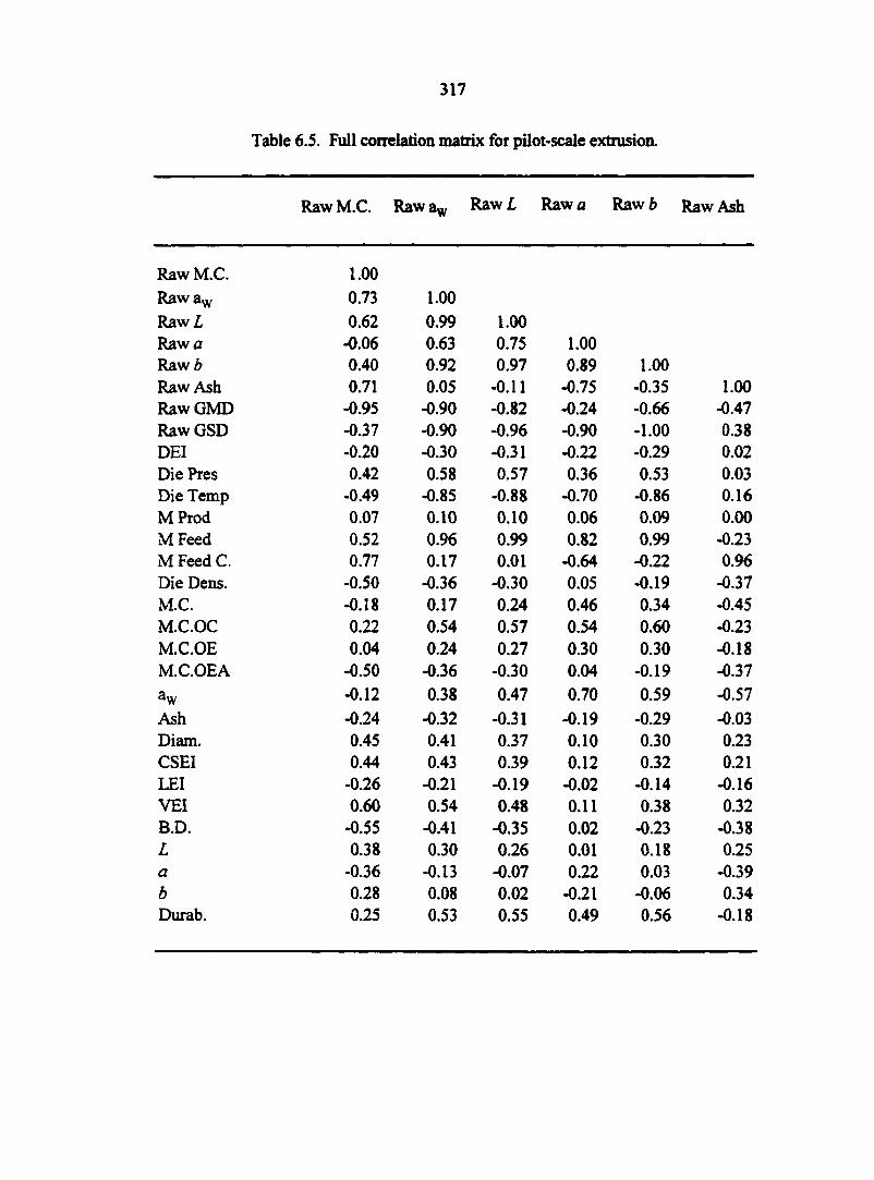
317
Table 6.5. Full correlation matrix for pilot-scale extrusion.
Raw M.C. Rawaw Raw L Raw a Raw 6 Raw Ash
Raw M.C. 1.00 Raw aw 0.73 1.00 Raw I 0.62 0.99 1.00 Raw a -0.06 0.63 0.75 1.00 Raw b 0.40 0.92 0.97 0.89 1.00 Raw Ash 0.71 0.05 -0.11 -0.75 -0.35 1.00 Raw GMD -0.95 -0.90 -0.82 -0.24 -0.66 -0.47 RawGSD -0.37 -0.90 -0.96 -0.90 -1.00 0.38 DEI -0.20 -0.30 -0.31 -0.22 -0.29 0.02 Die Près 0.42 0.58 0.57 0.36 0.53 0.03 Die Temp -0.49 -0.85 -0.88 -0.70 -0.86 0.16 M Prod 0.07 0.10 0.10 0.06 0.09 0.00 M Feed 0.52 0.96 0.99 0.82 0.99 -0.23 M Feed C. 0.77 0.17 0.01 -0.64 -0.22 0.96 Die Dens. -0.50 -0.36 -0.30 0.05 -0.19 -0.37 M.C. -0.18 0.17 0.24 0.46 0.34 -0.45 M.C.OC 0.22 0.54 0.57 0.54 0.60 -0.23 M.C.OE 0.04 0.24 0.27 0.30 0.30 -0.18 M.C.OEA -0.50 -0.36 -0.30 0.04 -0.19 -0.37 aw -0.12 0.38 0.47 0.70 0.59 -0.57
Ash -0.24 -0.32 -0.31 -0.19 -0.29 -0.03 Diam. 0.45 0.41 0.37 0.10 0.30 0.23 CSEI 0.44 0.43 0.39 0.12 0.32 0.21 LEI -0.26 -0.21 -0.19 -0.02 -0.14 -0.16 VEI 0.60 0.54 0.48 0.11 0.38 0.32 B.D. -0.55 -0.41 -0.35 0.02 -0.23 -0.38 L 0.38 0.30 0.26 0.01 0.18 0.25 a -0.36 -0.13 -0.07 0.22 0.03 -0.39 b 0.28 0.08 0.02 -0.21 -0.06 0.34 Durab. 0.25 0.53 0.55 0.49 0.56 -0.18
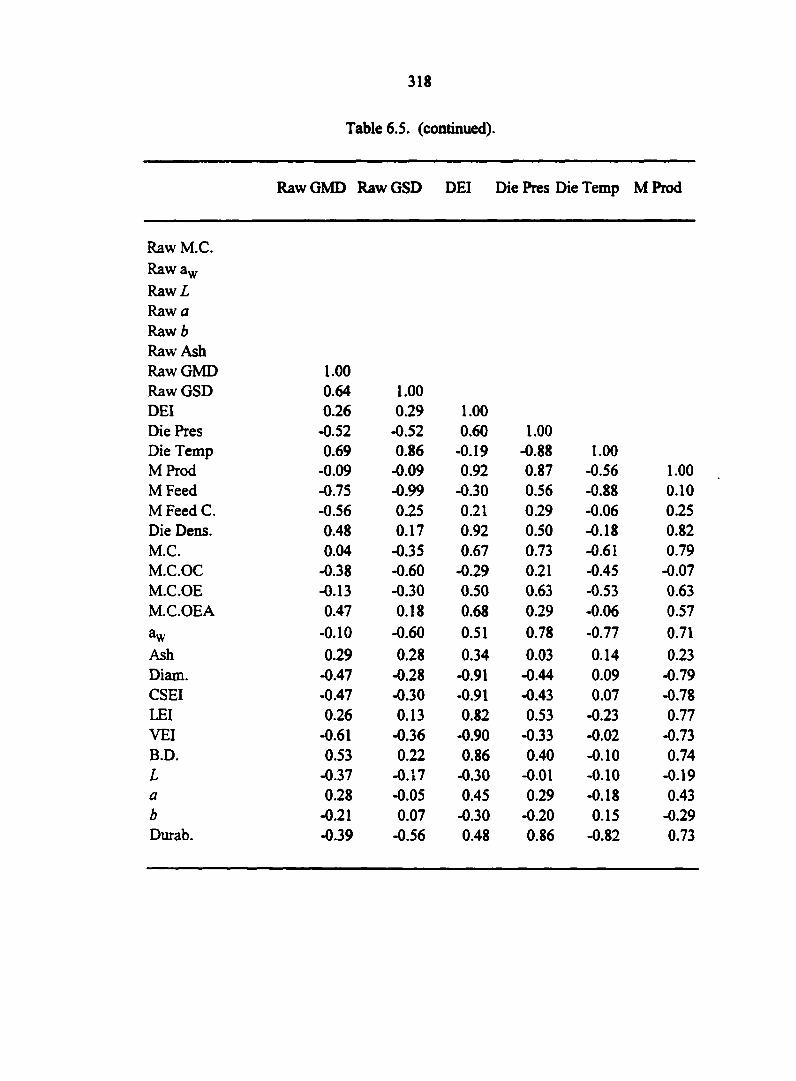
318
Table 6.5. (continued).
Raw GMD Raw GSD DEI Die Près Die Temp M Prod
Raw M.C. Raw aw
RawZ R a w a R a w b Raw Ash Raw GMD 1.00 Raw GSD 0.64 1.00 DEI 0.26 0.29 1.00 Die Près -0.52 -0.52 0.60 1.00 Die Temp 0.69 0.86 -0.19 -0.88 1.00 M Prod -0.09 -0.09 0.92 0.87 -0.56 1.00 M Feed -0.75 -0.99 -0.30 0.56 -0.88 0.10 M Feed C. -0.56 0.25 0.21 0.29 -0.06 0.25 Die Dens. 0.48 0.17 0.92 0.50 -0.18 0.82 M.C. 0.04 -0.35 0.67 0.73 -0.61 0.79 M.C.OC -0.38 -0.60 -0.29 0.21 -0.45 -0.07 M.C.OE -0.13 -0.30 0.50 0.63 -0.53 0.63 MCOEA 0.47 0.18 0.68 0.29 -0.06 0.57 aw -0.10 -0.60 0.51 0.78 -0.77 0.71
Ash 0.29 0.28 0.34 0.03 0.14 0.23 Diam. -0.47 -0.28 -0.91 -0.44 0.09 -0.79 CSEI -0.47 -0.30 -0.91 -0.43 0.07 -0.78 LEI 0.26 0.13 0.82 0.53 -0.23 0.77 VEI -0.61 -0.36 -0.90 -0.33 -0.02 -0.73 B.D. 0.53 0.22 0.86 0.40 -0.10 0.74 L -0.37 -0.17 -0.30 -0.01 -0.10 -0.19 a 0.28 -0.05 0.45 0.29 -0.18 0.43 b -0.21 0.07 -0.30 -0.20 0.15 -0.29 Durab. -0.39 -0.56 0.48 0.86 -0.82 0.73
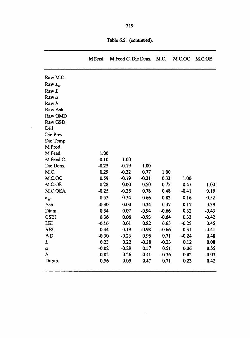
319
Table 6.5. (continued).
M Feed M Feed C. Die Dens. M.C. M.C.OC M.C.OE
Raw M.C. Raw aw
R a w L R a w a R a w b Raw Ash Raw GMD RawGSD DEI Die Près Die Temp M Prod M Feed 1.00 M Feed C. -0.10 1.00 Die Dens. -0.25 -0.19 1.00 M.C. 0.29 -0.22 0.77 1.00 M.C.OC 0.59 -0.19 -0.21 0.33 1.00 M.C.OE 0.28 0.00 0.50 0.75 0.47 1.00 M.C.OE A -0.25 -0.25 0.78 0.48 -0.41 0.19 aw 0.53 -0.34 0.66 0.82 0.16 0.52 Ash -0.30 0.00 0.34 0.37 0.17 0.39 Diam. 0.34 0.07 -0.94 -0.66 0.32 -0.43 CSEI 0.36 0.06 -0.93 -0.64 0.33 -0.42 LEI -0.16 0.01 0.82 0.65 -0.25 0.45 VEI 0.44 0.19 -0.98 -0.66 0.31 -0.41 B.D. -0.30 -0.23 0.95 0.71 -0.24 0.48 L 0.23 0.22 -0.38 -0.23 0.12 0.08 a -0.02 -0.29 0.57 0.51 0.06 0.55 b -0.02 0.26 -0.41 -0.36 0.02 -0.03 Durab. 0.56 0.05 0.47 0.71 0.23 0.42
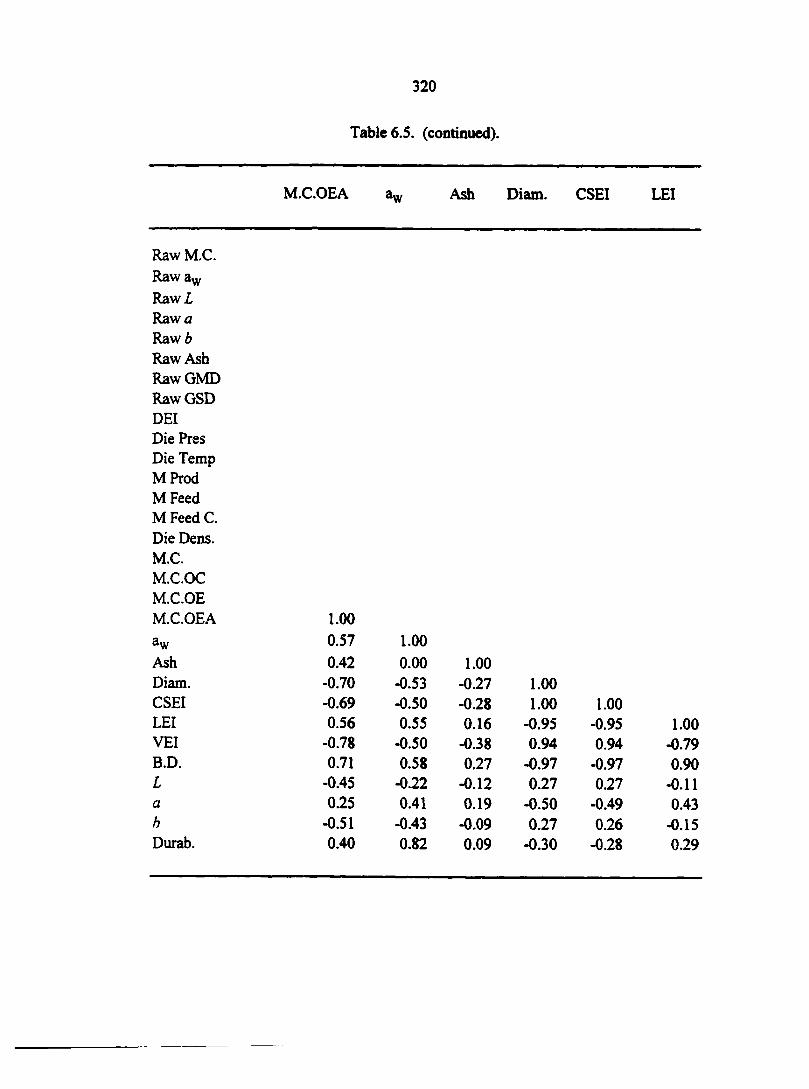
320
Table 6.5. (continued).
M.C.OEA aw Ash Diam. CSEI LEI
Raw M.C. Raw aw
R a w L R a w a R a w b Raw Ash Raw GMD RawGSD DEI Die Près Die Temp M Prod M Feed M Feed C. Die Dens. M.C. M.C.OC M.C.OE M.C.OEA 1.00 aw 0.57 1.00 Ash 0.42 0.00 1.00 Diam. -0.70 -0.53 -0.27 1.00 CSEI -0.69 -0.50 -0.28 1.00 1.00 LEI 0.56 0.55 0.16 -0.95 -0.95 1.00 VEI -0.78 -0.50 -0.38 0.94 0.94 -0.79 B.D. 0.71 0.58 0.27 -0.97 -0.97 0.90 L -0.45 -0.22 -0.12 0.27 0.27 -0.11 a 0.25 0.41 0.19 -0.50 -0.49 0.43 h -0.51 -0.43 -0.09 0.27 0.26 -0.15 Durab. 0.40 0.82 0.09 -0.30 -0.28 0.29
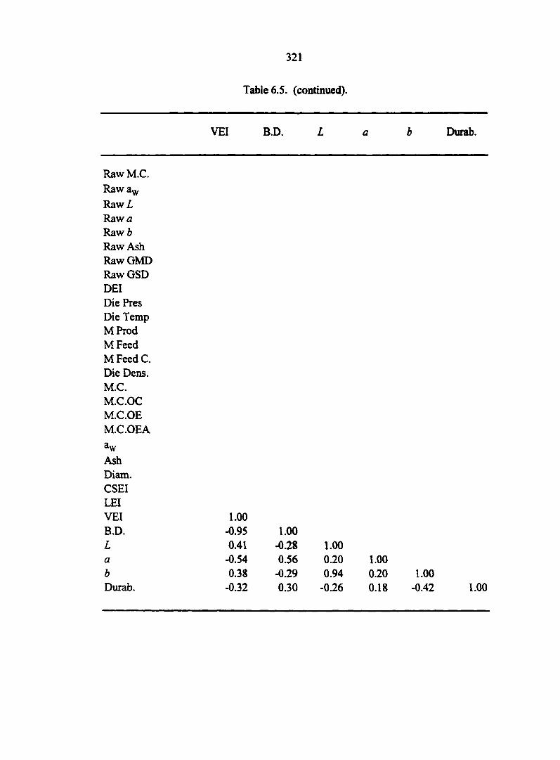
321
Table 6.5. (continued).
VEI B.D. Lab Durab.
Raw M.C. Raw aw
R a w L Raw a Raw 6 Raw Ash Raw GMD Raw GSD DEI Die Près Die Temp M Prod M Feed M Feed C. Die Dens. M.C. M.C.OC M.C.OE M.C.OEA aw Ash Diam. CSEI LEI VEI 1.00 B.D. -0.95 1.00 L 0.41 -0.28 1.00 a -0.54 0.56 0.20 1.00 b 0.38 -0.29 0.94 0.20 1.00 Durab. -0.32 0.30 -0.26 0.18 -0.42
322
components analysis is used to reduce the dimensionality of multivariate data by
summarizing the variance in the data and projecting it into a set of uncorrected orthogonal
linear combinations (i.e., eigenvectors) of the original variables. These linear combinations,
or principal components, have the form:
Y PC. ~ + ®2^2 + •••+ a2*X 29 (6.10)
where yp.c. is a principal component value, or score, a; through a%9 are the principal
component coefficients (i.e., eigenvectors), and Xi through X29 are the original property
variable vectors (i.e., values that were measured in the study) (Everitt and Dunn, 1991). The
results for the principal components analysis are presented in Table 6.6, which shows the
eigenvectors and eigenvalues for the first five principal components, as well as the proportion
of variation explained through the use of each principal component. These first five principal
components accounted for 94.16% of the total variability in the data, and thus provide both a
convenient and comprehensive summary of the information contained in the original 29
variables, but utilizing a reduced dimensionality of only five variables. A "scree" plot of the
principal component eigenvalues (Figure 6.7) and a plot of the error explained through the
use of principal components (Figure 6.8) suggest that the use of six principal components is
needed; however, the use of five principal components is adequate to summarize the
multivariate data in the study, because 94.16% of the error in the data can be explained
through the use of five, which is adequate for the purposes of this study. Although the
interpretation of principal components is very subjective, it appears that the first principal
component may be an indication of dough flowability and resulting expansion after
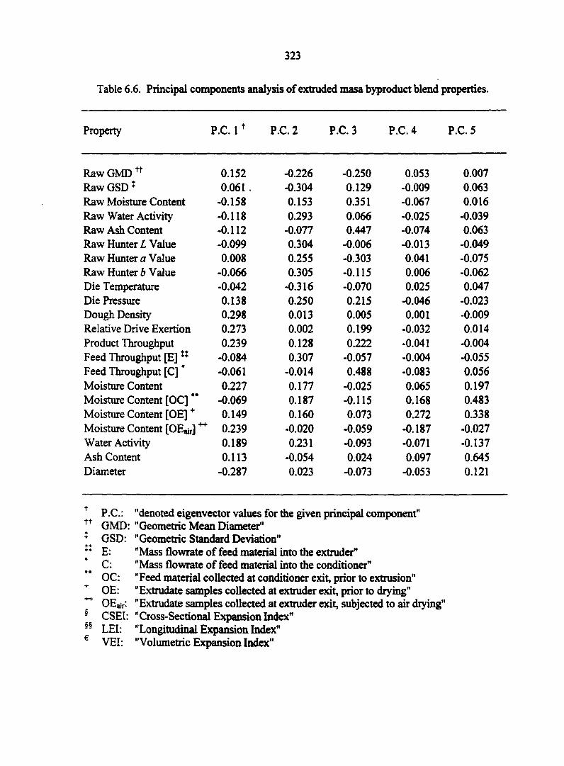
323
Table 6.6. Principal components analysis of extruded masa byproduct blend properties.
Property P.C. 1f P.C. 2 P.C. 3 P.C. 4 P.C. 5
Raw GMD tf 0.152 -0.226 -0.250 0.053 0.007 Raw GSD * 0.061 . -0.304 0.129 -0.009 0.063 Raw Moisture Content -0.158 0.153 0.351 -0.067 0.016 Raw Water Activity -0.118 0.293 0.066 -0.025 -0.039 Raw Ash Content -0.112 -0.077 0.447 -0.074 0.063 Raw Hunter L Value -0.099 0.304 -0.006 -0.013 -0.049 Raw Hunter a Value 0.008 0.255 -0.303 0.041 -0.075 Raw Hunter b Value -0.066 0.305 -0.115 0.006 -0.062 Die Temperature -0.042 -0.316 -0.070 0.025 0.047 Die Pressure 0.138 0.250 0.215 -0.046 -0.023 Dough Density 0.298 0.013 0.005 0.001 -0.009 Relative Drive Exertion 0.273 0.002 0.199 -0.032 0.014 Product Throughput 0.239 0.128 0.222 -0.041 -0.004 Feed Throughput [E] ** -0.084 0.307 -0.057 -0.004 -0.055 Feed Throughput [C] ' -0.061 -0.014 0.488 -0.083 0.056 Moisture Content 0.227 0.177 -0.025 0.065 0.197 Moisture Content [OC] -0.069 0.187 -0.115 0.168 0.483 Moisture Content [OE]+ 0.149 0.160 0.073 0.272 0.338 Moisture Content [OEair] """ 0.239 -0.020 -0.059 -0.187 -0.027 Water Activity 0.189 0.231 -0.093 -0.071 -0.137 Ash Content 0.113 -0.054 0.024 0.097 0.645 Diameter -0.287 0.023 -0.073 -0.053 0.121
f P.C.: "denoted eigenvector values for the given principal component" y GMD: "Geometric Mean Diameter" ^ GSD: "Geometric Standard Deviation" ** E: "Mass flowrate of feed material into the extruder"
C: "Mass flowrate of feed material into the conditioner" OC: "Feed material collected at conditioner exit, prior to extrusion" OE: "Extrudate samples collected at extruder exit, prior to drying"
""" OEair-. "Extrudate samples collected at extruder exit, subjected to air drying" 5 CSEI: "Cross-Sectional Expansion Index" §§ LEI: "Longitudinal Expansion Index" € VEI: "Volumetric Expansion Index"
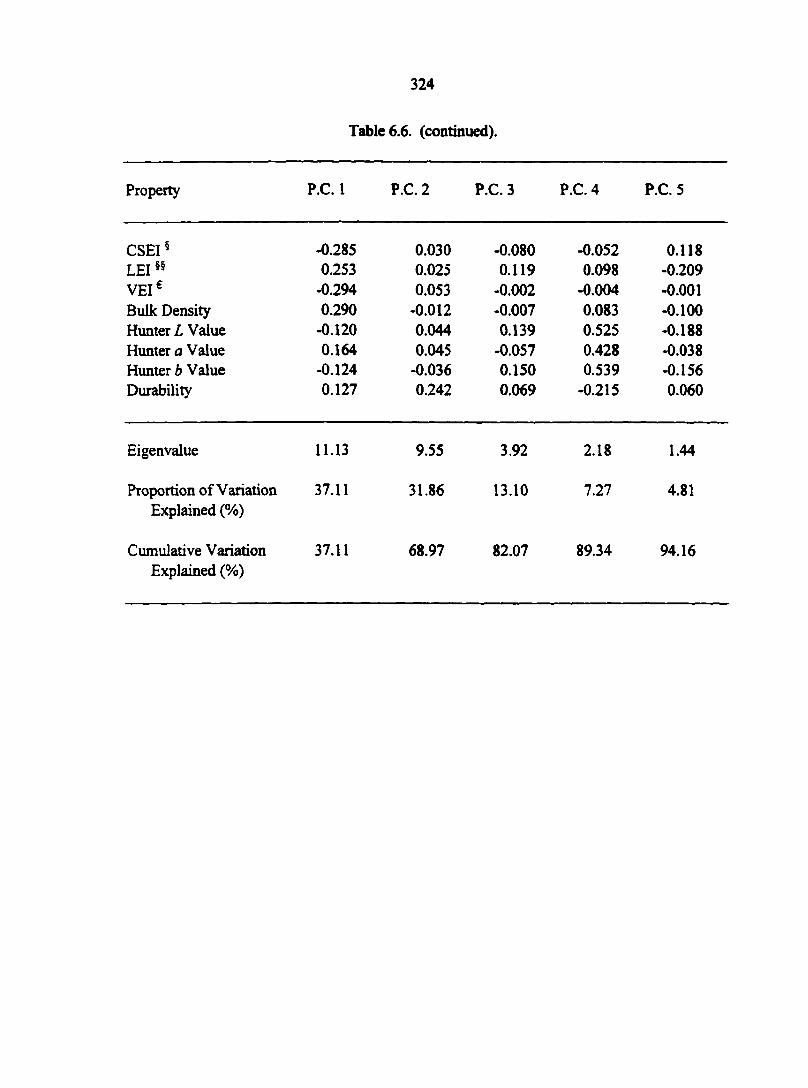
324
Table 6.6. (continued).
Property P.C.I P.C. 2 P.C. 3 P.C. 4 P.C. 5
CSEI5 -0.285 0.030 -0.080 -0.052 0.118 LEI§§ 0.253 0.025 0.119 0.098 -0.209 vei€ -0.294 0.053 -0.002 -0.004 -0.001 Bulk Density 0.290 -0.012 -0.007 0.083 -0.100 Hunter L Value -0.120 0.044 0.139 0.525 -0.188 Hunter a Value 0.164 0.045 -0.057 0.428 -0.038 Hunter b Value -0.124 -0.036 0.150 0.539 -0.156 Durability 0.127 0.242 0.069 -0.215 0.060
Eigenvalue 11.13 9.55 3.92 2.18 1.44
Proportion of Variation 37.11 31.86 13.10 7.27 4.81 Explained (%)
Cumulative Variation 37.11 68.97 82.07 89.34 94.16 Explained (%)
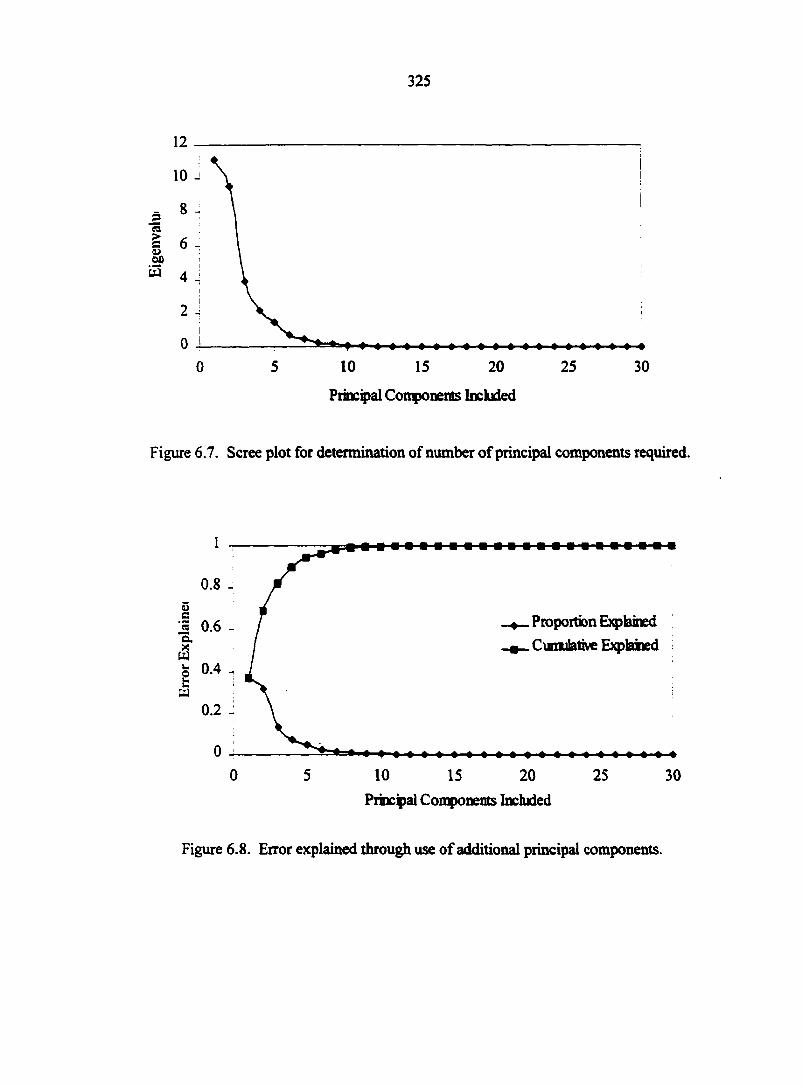
325
10 J
25 5 10 15 20 30 0
Principal Components Included
Figure 6.7. Scree plot for determination of number of principal components required.
5 c « 0.6 -
I 5 0.4 . S
0.2 -
Cumulative Explahed
5 10 0 15 20 25 30
Principal Components Included
Figure 6.8. Error explained through use of additional principal components.
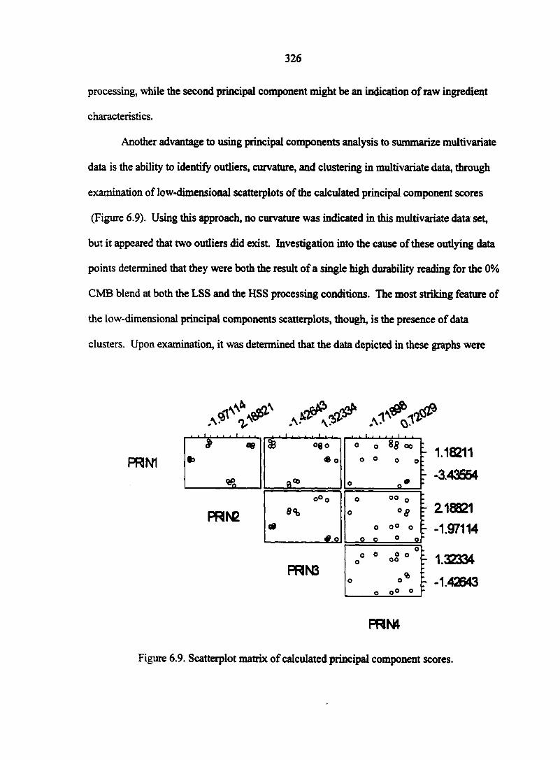
326
processing, while the second principal component might be an indication of raw ingredient
characteristics.
Another advantage to using principal components analysis to summarize multivariate
data is the ability to identify outliers, curvature, and clustering in multivariate data, through
examination of low-dimensional scatterplots of the calculated principal component scores
(Figure 6.9). Using this approach, no curvature was indicated in this multivariate data set,
but it appeared that two outliers did exist. Investigation into the cause of these outlying data
points determined that they were both the result of a single high durability reading for the 0%
CMB blend at both the LSS and the HSS processing conditions. The most striking feature of
the low-dimensional principal components scatterplots, though, is the presence of data
clusters. Upon examination, it was determined that the data depicted in these graphs were
PR NI
.V*^^
» % ID
%
oB °eo
• o
a*
o o 8g oo :
o o o 0 *
" o°o o
o
O
O
TTT
PRN2 8<b o ° 8 :
00 O 0° 0 1
o o 0 o •
PRN3
0° 0 oS 0 °i.
0» L o o° 0 :
PRN4
Figure 6.9. Scatterplot matrix of calculated principal component scores.
327
indeed clustered according to extrusion run, with each run (i.e., treatment combination)
representing a unique cluster in principal component space.
Even though the current study has been extensive, it would be useful to further
investigate the complex relationships and interactions between the raw ingredient properties,
extrusion processing properties, and resulting extrudate product properties, perhaps as a
future investigation.
SUMMARY AND CONCLUSIONS
This study has provided information essential for the further development of livestock
feed additives utilizing blends of soybean meal and com masa byproducts via extrusion
processing. Pilot-scale extrusion and subsequent drying/cooling of these blends produced
extradâtes that were dry and microbiologically stable. Because soybean meal was used as
the blending agent, however, little product expansion occurred at the extruder die exit,
primarily due to lack of starchy components in the blends. Extrusion processing produced
extradâtes with excellent durability, which is essential to retaining quality during transport
and storage of pelleted feed materials. During processing, the dough melt in the extruder
barrel required less energy to convey the dough as screw speed increased, which is typical of
pseudoplastic materials, such as extruded food doughs. Most effects were due to changes in
screw speed, which in turn affected processing temperature. All blends were amenable to
extrusion processing at the conditions used in this study. The HSS, 20% blend, however, did
not produce a consistent, cohesive extrudate product; instead, a "crumble"-type of feed
product was produced.
The next stage in developing livestock feed ingredients from com masa byproduct
materials could logically follow three possible courses: a livestock feeding trial could be
328
conducted with these resulting extruded products; masa byproducts could be processed with
ingredients other than soybean meal to produce livestock feed additives; or feed ingredient
production using other processing methods could be investigated. Although these options for
further study were beyond the scope of the current project, an economic analysis model for
various reprocessing alternatives for com masa processing byproducts was developed, and is
discussed in Chapter 7.
ACKNOWLEDGMENTS
The authors would like to thank the Iowa Biotechnology Byproducts Consortium and
the Grain Science and Industry Department, Kansas State University, Manhattan, KS, for
financial support; the KSU Extrusion Center Pilot Plant, Grain Science and Industry
Department, Kansas State University, Manhattan, KS, and the Center for Crops Utilization
Research (CCUR), Iowa State University, Ames, LA, for use of equipment and facilities; and
Minsa Corporation for providing com masa byproduct samples.
REFERENCES
American Association of Cereal Chemists (AACC). 1995. Approved Methods of the American Association of Cereal Chemists. St. Paul, MN: American Society of Cereal Chemists, Inc.
American Society of Agricultural Engineers (ASAE). 1996. ASAE Standards, Engineering Practices, and Data. St Joseph, MI: American society of Agricultural Engineers.
Alvarez-Martinez, L., K. P. Kondury, and J. M. Harper. 1988. A general model for expansion of extruded products. Journal of Food Science 53(2): 609-615.
Annexstad, R. J., M. D. Stem, D. E. Otterby, J. G. Linn, and W. P. Hansen. 1987. Extruded soybeans and corn gluten meal as supplemental protein sources for lactating dairy cattle. Journal of Dairy Science 70(4): 814-822.
Badrie, N. and W. A. Mellowes. 1991. Effect of extrusion variables on cassava extrudates. Journal of Food Science 56(5): 1334-1337.
329
Beauchat, L. R. 1981. Microbial stability as affected by water activity. Cereal Foods World 26(7): 345-349.
Bern, C. J. and C. R. Hurburgh. 1998. Managing Grain After Harvest: AE 469/569 course notes. Ames, LA: Iowa State University Bookstore CourseWorks.
Bohlsen, D., S. Weeder, and S. Wang. 1997. Tracking organic waste. Resource 4(9): 13-14.
Bouvier, M. H., G. Fayard, and J. T. Clayton. 1987. Flow rate and heat transfer modeling in extrusion cooking of soy protein. Journal of Food Engineering 6(2): 123-141.
Bressani, R., R. Paz y Paz, and N. S. Scrimshaw. 1958. Corn nutrient losses: chemical changes in corn during preparation of tortillas. Journal of Agricultural and Food Chemistry 6(10): 770-774.
Chen, A. H., Y. C. Jao, J. W. Larkin, and W. E. Goldstein. 1979. Rheological model of soy dough in extrusion. Journal of Food Processing Engineering 2(4): 337-342.
Cornelius, S. G., J. P. Totsch, and B. G. Harmon. 1973. Metabolizable energy of DSLC for swine. Journal of Animal Science 37:277.
Cumming, D. B., D. W. Stanley, and J. M. DeMan. 1973. Fate of water soluble soy protein during thermoplastic extrusion. Journal of Food Science 38(2): 320-323.
Dahl, S. R. and R. Villota. 1991. Effect of thermal denaturation on the texturization of soybean protein via twin-screw extrusion. Journal of Canadian Institute of Science and Technology 24(3/4): 143-150.
Derr, D. A. and P. S. Dhillon. 1997. The economics of recycling food residuals. BioCycle 38(4): 55-56.
Everitt, B. S. and G. Dunn. 1991. Applied Multivariate Data Analysis. New York, NY: Halsted Press.
Faubion, J. M., R. C. Hoseney, and P. A. Seib. 1982. Functionality of grain components in extrusion. Cereal Foods World 27(5): 212-216.
Ferris, D. A., R. A. Flores, C. W. Shanklin, and M. K. Whitworth. 1995. Proximate analysis of food service wastes. Applied Engineering in Agriculture 11(4): 567-572.
Gomez, M. H., L. W. Rooney, R. D. Waniska, and R. L. Pflugfelder. 1987. Dry corn masa flours for tortilla and snack food production. Cereal Foods World 32(5): 372-377.
Gonzalez de Palacios, M. 1980. Characteristics of com and sorghum for tortilla processing. Unpublished M.S. Thesis. College Station, TX: Texas A&M University.
330
Gonzalez-Martinez, S. 1984. Biological treatability of the wastewaters from the alkaline cooking of maize (Indian com). Environmental Technology Letters 5(8): 365-372.
Hilton, J. W., C. Y. Cho, and S. J. Slonger. 1981. Effect of extrusion processing and steam pelleting diets on pellet durability, pellet water absorption, and the physiological response of rainbow trout (Salmo Gaird-Neri R.). Aquaculture 25(2/3): 185-194.
Jamin, F. F. and R. A. Flores. 1998. Effect of separation and grinding of corn dry-milled streams on physical properties of single-screw low-speed extruded products. Cereal Chemistry 75(6): 775-779.
Katz, S. H., M. L. Hediger, and L. A. Valleroy. 1974. Traditional maize processing techniques in the New World. Science 184(4138): 765-773.
Khan, M. N., M. C. Des Rosiers, L. W. Rooney, R. G. Morgan, and V. E. Sweat. 1982. Corn tortillas: evaluation of com cooking procedures. Cereal Chemistry 59(4): 279-284.
Kokini, J. L., C. N. Chang and L. S. Lai. 1992. The role of Theological properties on extrudate expansion. In Food Extrusion Science and Technology, ed. J. L. Kokini, C. T. Ho, and M. V. Karewe, 631-652. New York: Marcel Dekker, Inc.
Krause, V. M., K. L. Tucker, H. V. Kuhnlein, C. Y. Lopez-Palacios, M. Ruz, and N. W. Solomons. 1992. Rural-urban variation in limed maize use and tortilla consumption by women in Guatemala. Ecology of Food and Nutrition 28(4): 279-288.
Larson, E. M., R. A. Stock, T. J. Klopfenstein, J. H. Sindt, and R. P. Huffman. 1993. Feeding value of wet distillers' byproducts for finishing ruminants. Journal of Animal Science 71(8): 2228-2236.
Levine, L. 1989. Scaleup, experimentation, and data evaluation. In Extrusion Cooking. St. Paul, MN: American Association of Cereal Chemists.
Lodge, S. L., R. A. Stock, T. J. Klopfenstein, D. H. Shain, and D. W. Herald. 1997. Evaluation of com and sorghum distillers byproducts. Journal of Animal Science 74(1): 37-43.
Marsman, G. J. P., H. Gruppen, D. J. vanZuilichem, J. W. Resink and A. G. J. Voragen. 1995. The influence of screw configuration on the In Vitro digestibility and protein solubility of soybean and rapeseed meals. Journal of Food Engineering 26(1): 13-28.
Mercier, C., P. Linko, and J. M. Harper, eds. 1989. Extrusion Cooking. St. Paul, MN: American Association of Cereal Chemists.
331
Microsoft Excel v. 5.0a. 1993. Redmond, WA: Microsoft Corporation.
Miller, R. C. 1985. Low moisture extrusion: effects of cooking moisture on product characteristics. Journal of Food Science 50(1): 249-253.
Moore, D., A. Sanei, E. Van Hecke, and J. M. Bouvier. 1990. Effect of ingredients on physical/structural properties of extrudates. Journal of Food Science 55(5): 1383-1387.
Nielsen, E. 1976. Whole seed processing by extrusion cooking. Journal of the American Oil Chemists Society 53(6): 305-309.
Ortiz, E. L. 1985. The cuisine of Mexico: com tortilla dishes. Gourmet 45(May): 62-63.
Pflugfelder, R. L., L. W. Rooney, and R. D. Waniska. 1988. Dry matter losses in commercial corn masa production. Cereal Chemistry 65(2): 127-132.
Power, J. F. and W. A. Dick (Editors). 2000. Land Application of Agricultural, Industrial, and Municipal By-Products. SSSA Book Series: 6. Soil Science Society of America. Madison, WI. 653 pp.
Rooney, L. W. and S. O. Serna-Saldivar. 1987. Food uses of whole com and dry-milled fractions. In Corn Chemistry and Technology, ed. S. A. Watson and P. E. Ramstad, 399-430. St. Paul, MN: American Association of Cereal Chemists.
Rosentrater, K. A., R. A. Flores, T. L. Richard, and C. J. Bern. 1999. Physical and nutritional properties of com masa byproduct streams. Applied Engineering in Agriculture 15(5): 515-523.
SAS v. 6.08. 1992. Cary, NC: SAS Institute, Inc.
Sema-Saldivar, S. O., M. H. Gomez, and L. M. Rooney. 1990. Technology, chemistry, and nutritional value of alkaline-cooked com products. Advances in Cereal Science and Technology v. 10:243-306.
Simon, T., L. Tsang, and P. J. Schaible. 1960. The value of com fermentation solubles in poultry nutrition. Poultry Science 39:251-257.
Solganik, H. 1997. A toast to tortillas. Food Processing 58(11): 64-65.
Speigel, M. R. 1994. Statistics. New York, NY: McGraw-Hill, Inc.
Stem, M. D., L. M. Rode, R. W. Prange, R. H. Stauffacher, and L. D. Satter. 1983/ Ruminai protein degradation of com gluten meal in lactating dairy cattle fitted with duodenal T-type cannulae. Journal of Animal Science 56:194-205.
332
Stroshine, R. and D. Hamann. 1995. Physical Properties of Agricultural Materials and Food Products. West Lafayette, IN: Copy Cat.
Tabil, L., Jr. and S. Sokhansanj. 1996. Process conditions affecting the physical quality of alfalfa pellets. Applied Engineering in Agriculture 12(3): 345-350.
Tadtiyanant, C., J. J. Lyons, and J. M. Vandepopuliere. 1993. Brewers condensed solubles used as a feedstuff in broiler diets. Poultry Science 72(10): 1897-1905.
Tortilla Industry Association (TIA). 2001. Tortilla consumption continues to grow in U.S. and abroad. Tortilla Industry Association. Available online: www.tortilla-info.com/prrevenue98.htni [Accessed January 08,2001].
Velasco-Martinez, M., O. Angulo, D. O. Vazquez-Couturier, A. Arroyo-Lara, and J. A. Monroy-Rivera. 1997. Effect of dried solids of nejayote on broiler growth. Poultry Science 76(11): 1531-1534.
Wang, L., R. A. Flores, and L. A. Johnson. 1997. Processing feed ingredients from blends of soybean meal, whole blood, and red blood cells. Transactions of the ASAE 40(3): 691-697.
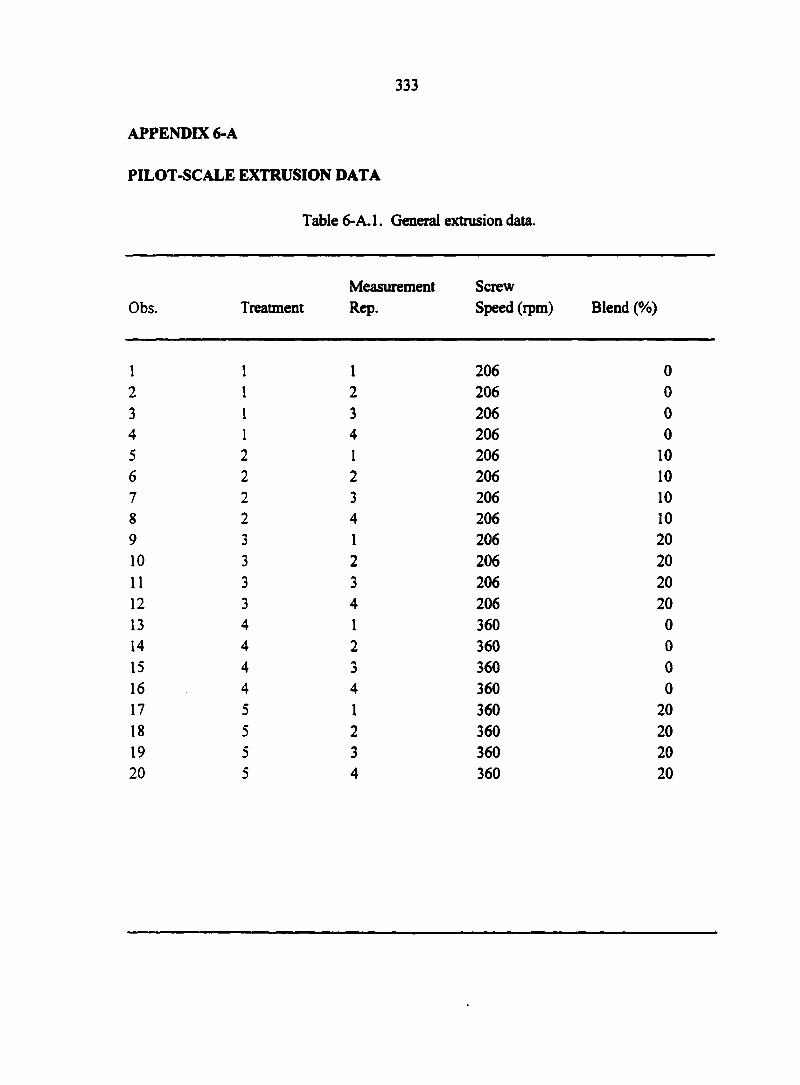
333
APPENDIX 6-A
PILOT-SCALE EXTRUSION DATA
Table 6-A.l. General extrusion data.
Obs. Treatment Measurement Rep.
Screw Speed (rpm) Blend (%)
1 1 1 206 0
2 1 2 206 0
3 1 3 206 0 4 1 4 206 0 5 2 1 206 10
6 2 2 206 10 7 2 3 206 10 8 2 4 206 10 9 3 1 206 20
10 3 2 206 20 11 3 3 206 20
12 3 4 206 20 13 4 1 360 0
14 4 2 360 0 15 4 3 360 0 16 4 4 360 0 17 5 1 360 20 18 5 2 360 20 19 5 3 360 20 20 5 4 360 20
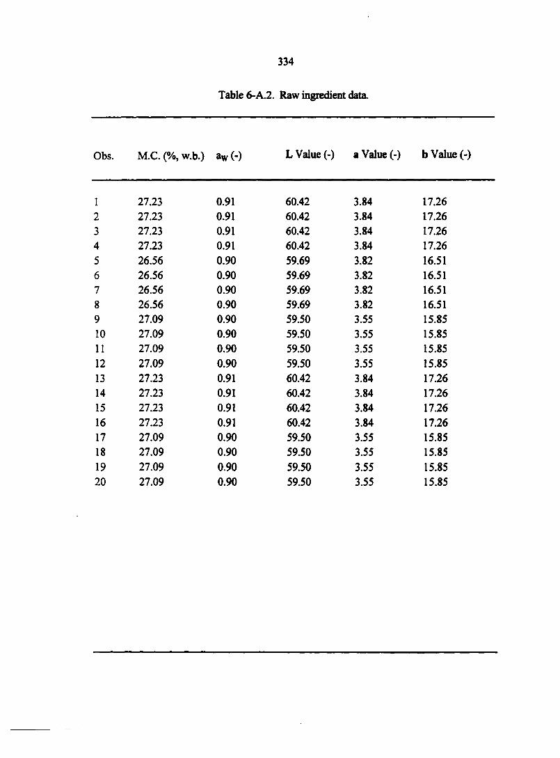
334
Table 6-A.2. Raw ingredient data.
Obs. M.C. (%, w.b.) aw (-) L Value (-) a Value (-) b Value (-)
1 27.23 0.91 60.42 3.84 17.26
2 27.23 0.91 60.42 3.84 17.26 3 27.23 0.91 60.42 3.84 17.26 4 27.23 0.91 60.42 3.84 17.26
5 26.56 0.90 59.69 3.82 16.51 6 26.56 0.90 59.69 3.82 16.51 7 26.56 0.90 59.69 3.82 16.51 8 26.56 0.90 59.69 3.82 16.51 9 27.09 0.90 59.50 3.55 15.85 10 27.09 0.90 59.50 3.55 15.85
11 27.09 0.90 59.50 3.55 15.85
12 27.09 0.90 59.50 3.55 15.85 13 27.23 0.91 60.42 3.84 17.26
14 27.23 0.91 60.42 3.84 17.26 15 27.23 0.91 60.42 3.84 17.26 16 27.23 0.91 60.42 3.84 17.26 17 27.09 0.90 59.50 3.55 15.85 18 27.09 0.90 59.50 3.55 15.85
19 27.09 0.90 59.50 3.55 15.85 20 27.09 0.90 59.50 3.55 15.85
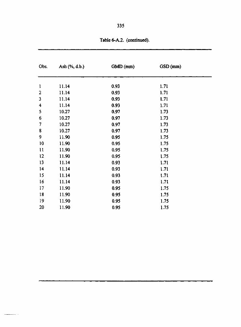
Obs.
1 2 3
4
5
6 7
8 9
10
11 12 13
14
15
16
17
18
19
20
335
Table 6-A.2. (continued).
Ash (%, d.b.) GMD (mm) GSD (mm)
11.14 0.93 1.71
11.14 0.93 1.71
11.14 0.93 1.71 11.14 0.93 1.71 10.27 0.97 1.73 10.27 0.97 1.73 10.27 0.97 1.73 10.27 0.97 1.73 11.90 0.95 1.75 11.90 0.95 1.75 11.90 0.95 1.75 11.90 0.95 1.75 11.14 0.93 1.71 11.14 0.93 1.71 11.14 0.93 1.71 11.14 0.93 1.71 11.90 0.95 1.75 11.90 0.95 1.75 11.90 0.95 1.75 11.90 0.95 1.75
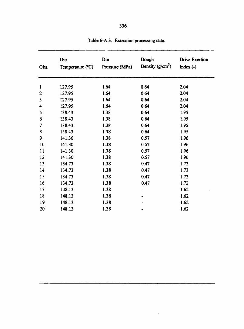
Obs
1
2 3 4 5 6 7 8
9 10
11 12
13
14 15 16 17 18
19 20
336
Table 6-A.3. Extrusion processing data.
Die Die Dough Drive Exertion
Temperature (°C) Pressure (MPa) Density (g/cm3) Index (-)
127.95 1.64 0.64 2.04 127.95 1.64 0.64 2.04 127.95 1.64 0.64 2.04 127.95 1.64 0.64 2.04 138.43 1.38 0.64 1.95 138.43 1.38 0.64 1.95
138.43 1.38 0.64 1.95 138.43 1.38 0.64 1.95 141.30 1.38 0.57 1.96
141.30 1.38 0.57 1.96 141.30 1.38 0.57 1.96 141.30 1.38 0.57 1.96
134.73 1.38 0.47 1.73
134.73 1.38 0.47 1.73 134.73 1.38 0.47 1.73 134.73 1.38 0.47 1.73
148.13 1.38 - 1.62 148.13 1.38 - 1.62 148.13 1.38 - 1.62 148.13 1.38 . 1.62
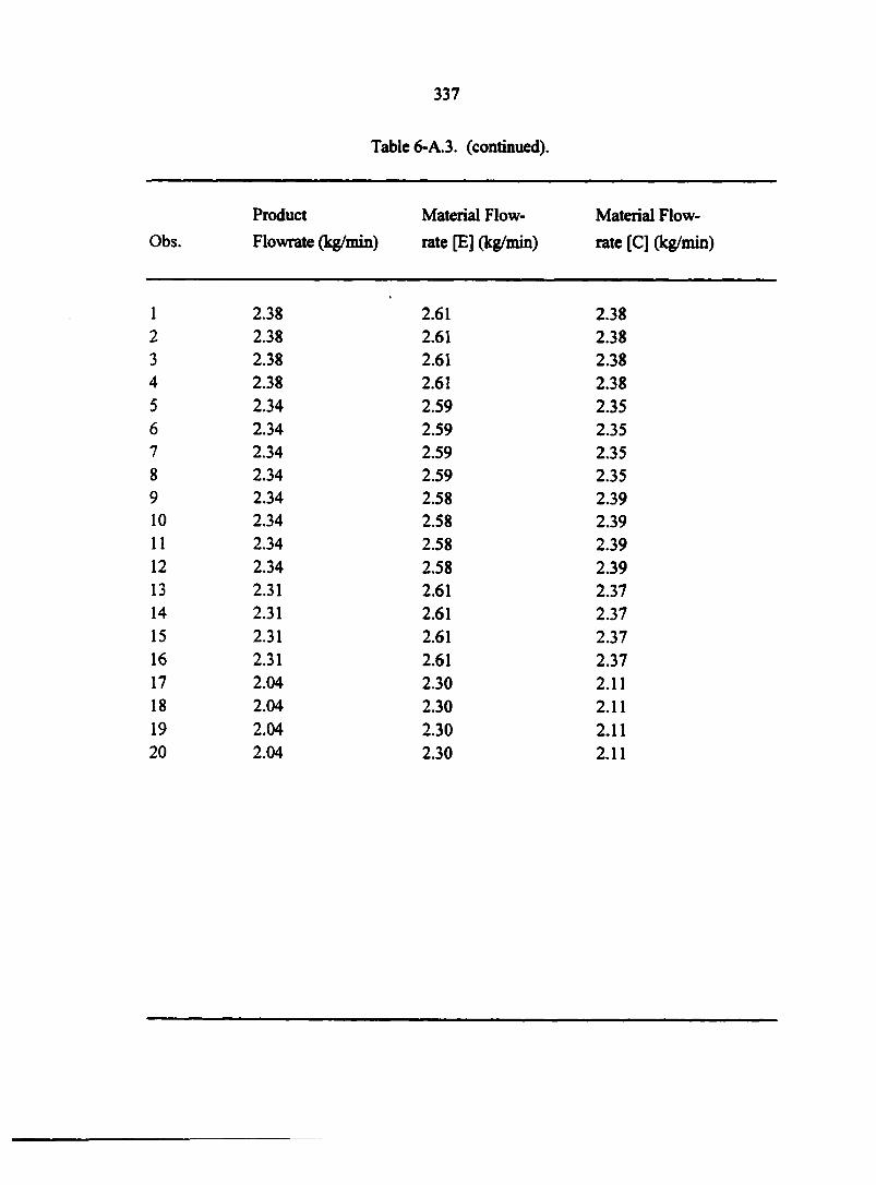
Obs
1
2 3 4
5 6
7 8
9 10
11 12 13
14 15
16 17 18
19 20
337
Table 6-A.3. (continued).
Product Material Flow- Material Flow-
Flowrate (kg/min) rate [E] (kg/min) rate [C] (kg/min)
2.38 2.61 2.38 2.38 2.61 2.38 2.38 2.61 2.38 2.38 2.61 2.38 2.34 2.59 2.35 2.34 2.59 2.35 2.34 2.59 2.35 2.34 2.59 2.35 2.34 2.58 2.39 2.34 2.58 2.39 2.34 2.58 2.39 2.34 2.58 2.39 2.31 2.61 2.37 2.31 2.61 2.37 2.31 2.61 2.37 2.31 2.61 2.37 2.04 2.30 2.11 2.04 2.30 2.11 2.04 2.30 2.11 2.04 2.30 2.11
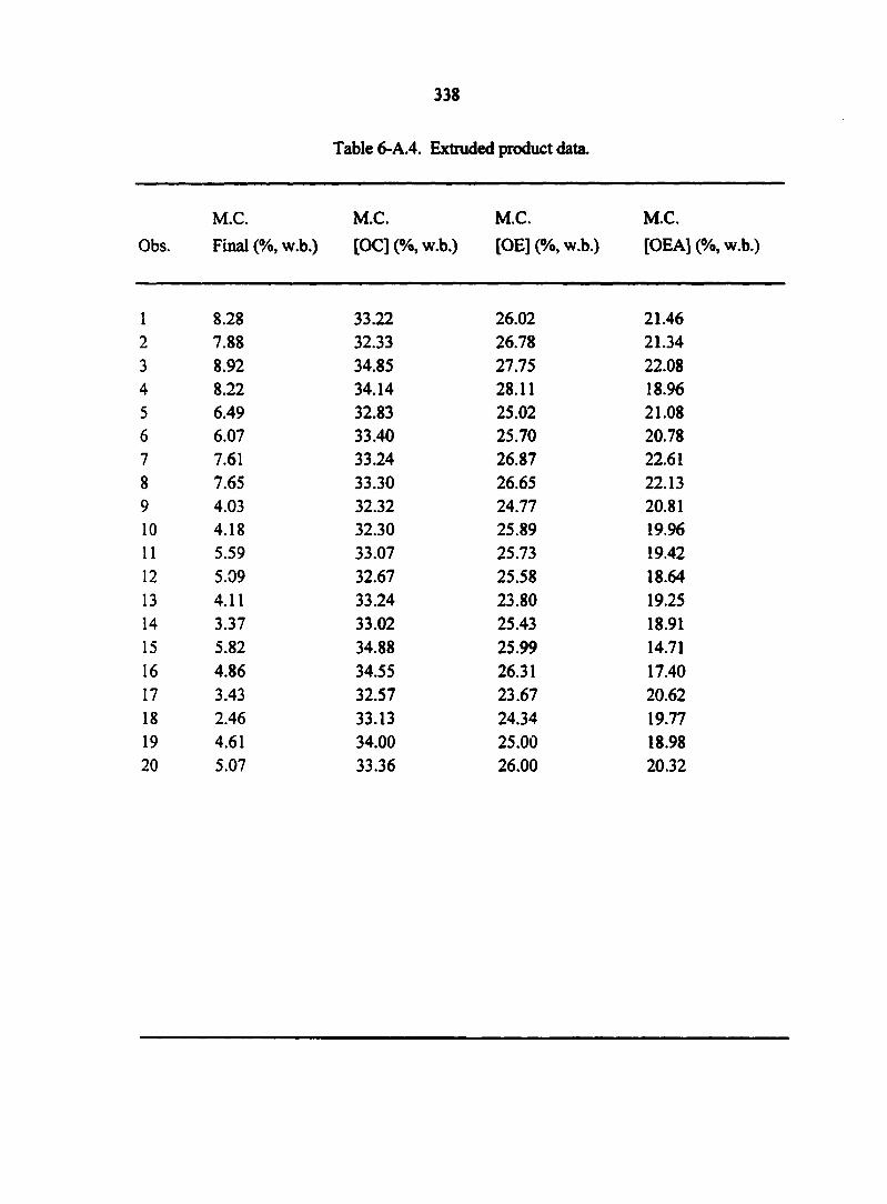
Obs
1 2 3 4 5 6
7
8 9 10
11 12
13
14 15
16
17 18
19 20
338
Table 6-A.4. Extruded product data.
M.C. M.C. M.C. M.C.
Final (%, w.b.) [OC] (%, w.b.) [OE] (%, w.b.) [OEA] (%, w.b.)
8.28 33.22 26.02 21.46 7.88 32.33 26.78 21.34
8.92 34.85 27.75 22.08 8.22 34.14 28.11 18.96
6.49 32.83 25.02 21.08 6.07 33.40 25.70 20.78 7.61 33.24 26.87 22.61
7.65 33.30 26.65 22.13 4.03 32.32 24.77 20.81 4.18 32.30 25.89 19.96 5.59 33.07 25.73 19.42 5.09 32.67 25.58 18.64 4.11 33.24 23.80 19.25 3.37 33.02 25.43 18.91 5.82 34.88 25.99 14.71 4.86 34.55 26.31 17.40 3.43 32.57 23.67 20.62 2.46 33.13 24.34 19.77 4.61 34.00 25.00 18.98 5.07 33.36 26.00 20.32
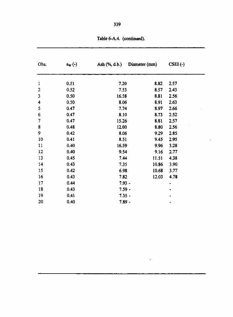
Obs
1
2 3 4 5 6 7
8
9 10
11 12 13 14 15
16 17 18
19 20
339
Table 6-A.4. (continued).
aw (-) Ash (%, d.b.) Diameter (mm) CSEI (-)
0.51 7.20 8.82 2.57
0.52 7.53 8.57 2.43 0.50 16.58 8.81 2.56 0.50 8.06 8.91 2.63 0.47 7.74 8.97 2.66 0.47 8.10 8.73 2.52 0.47 15.26 8.81 2.57 0.48 12.00 8.80 2.56 0.42 8.06 9.29 2.85 0.41 8.51 9.45 2.95 0.40 16.59 9.96 3.28 0.40 9.54 9.16 2.77
0.45 7.44 11.51 4.38 0.43 7.35 10.86 3.90 0.42 6.98 10.68 3.77 0.43 7.82 12.03 4.78 0.44 7.93 - -
0.43 7.59 - -
0.41 7.35 - -
0.40 7.89 - -
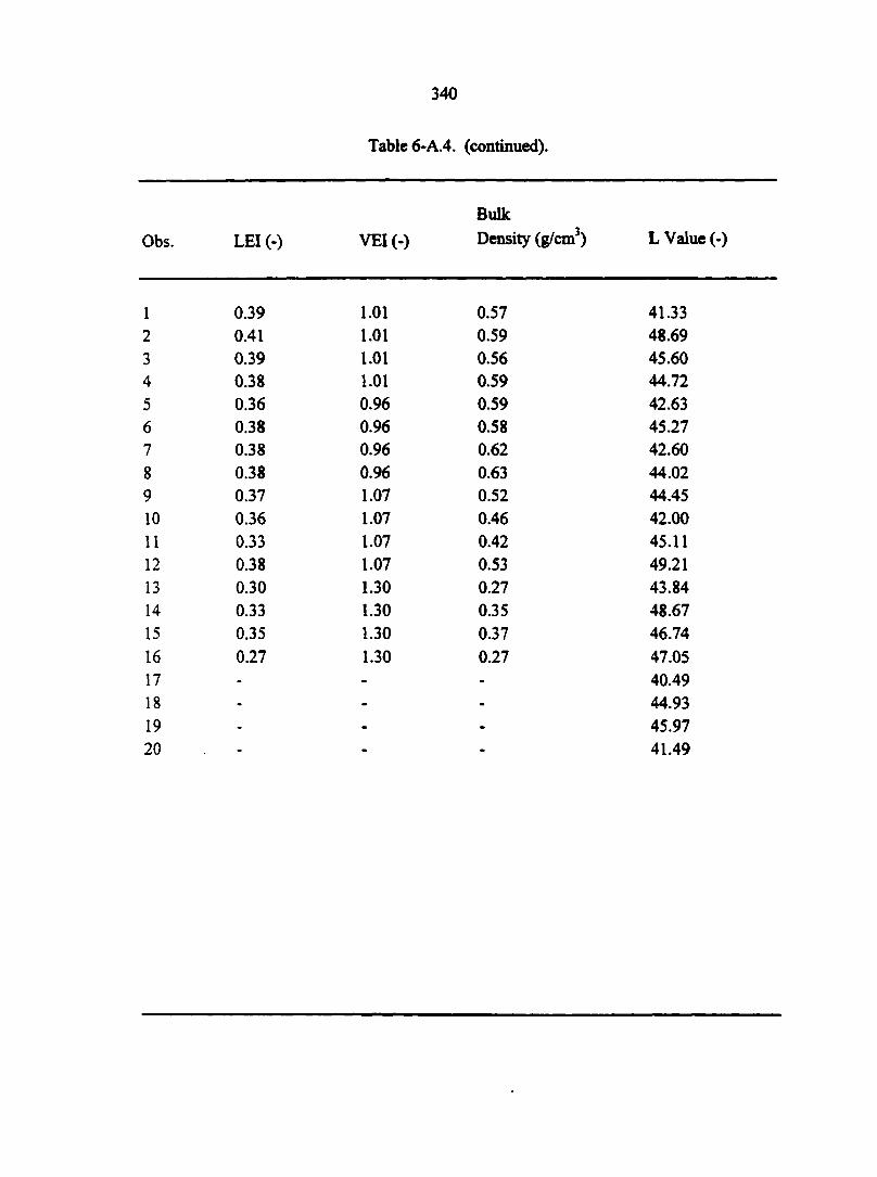
Obs
1 2 3 4 5 6 7
8 9 10
11 12
13 14 15
16 17 18
19 20
340
Table 6-A.4. (continued).
Bulk
LEI (-) VEI (-) Density (g/cm3) L Value (-)
0.39 1.01 0.57 41.33 0.41 1.01 0.59 48.69 0.39 1.01 0.56 45.60 0.38 1.01 0.59 44.72
0.36 0.96 0.59 42.63 0.38 0.96 0.58 45.27 0.38 0.96 0.62 42.60
0.38 0.96 0.63 44.02 0.37 1.07 0.52 44.45
0.36 1.07 0.46 42.00 0.33 1.07 0.42 45.11 0.38 1.07 0.53 49.21 0.30 1.30 0.27 43.84 0.33 1.30 0.35 48.67 0.35 1.30 0.37 46.74
0.27 1.30 0.27 47.05 - - - 40.49 - - - 44.93 - - - 45.97 - - . 41.49
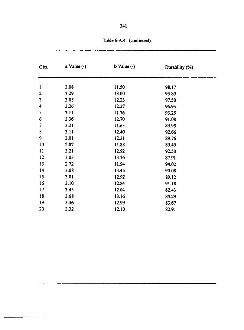
Obs
1 2 3 4 5 6 7 8 9 10
11 12
13 14 15
16
17
18 19 20
341
Table 6-A 4, (continued).
a Value (-) b Value (-) Durability (%)
3.08 11.50 98.17 3.29 13.00 95.89 3.05 12.23 97.50 3.26 12.27 96.93 3.11 11.76 93.25 3.36 12.70 91.08 3.21 11.63 89.95 3.11 12.40 92.66 3.01 12.31 89.76 2.87 11.88 89.49 3.21 12.92 92.50 3.03 13.76 87.91 2.72 11.94 94.02 3.08 13.45 90.08 3.01 12.92 89.12 3.10 12.84 91.18 3.45 12.04 82.43 3.68 13.16 84.29 3.36 12.99 83.67 3.32 12.10 82.91
342
CHAPTER 7
ECONOMIC MODELING OF REPROCESSING ALTERNATIVES FOR CORN MASA BYPRODUCTS
A paper to be submitted, in part, to Waste Management and Research
K. A. Rosentrater, T. L. Richard, R. A. Flores, and C. J. Bern
ABSTRACT
Rapidly increasing production of corn masa flour for tortillas, chips, and related snack
foods is resulting in large quantities of organic residuals requiring environmentally sound
management These com masa residual streams appear suitable for use as a livestock feed
material, which could provide the masa manufacturer with viable means of recycling these
wastes, and thus avoiding landfilling costs. Possibilities for developing livestock feed
include direct shipping to livestock feeding facilities, blending prior to shipping, extrusion
processing, pellet mill processing, and dehydration. To assess the most viable option for
reprocessing masa byproducts as livestock feed materials, an economic model was developed
to compare each of these options. Through use of this model, it was determined that direct
shipping was by far the most inexpensive means of recycling masa residuals. Blending prior
to shipping resulted in a cost three to 14 times greater than the cost of direct shipping. The
cost of recycling via extrusion or pellet mill processing was between four and 18 times
greater than the cost of direct shipping. The cost of dehydration was 35 to 76 times the cost
of direct shipping. It was also determined that bagged feed was considerably more expensive
to produce than bulk feed. Additionally, recycling costs increased as delivery distance
increased, due to increased labor, equipment, and fuel costs, but decreased as production
capacity increased (i.e., developed economies of scale). Thus, due to substantial cost
343
savings, it is recommended that direct shipping and feeding be implemented as the recycling
option of choice for masa processing byproducts. Similar results are likely for other high-
moisture food processing residuals destined for utilization as livestock feed.
Keywords
Drying, Extrusion, Food Processing, Food Waste, Pelleting, Residue Utilization
Author Information
Journal Paper No. J-XXXXX of the Iowa Agriculture and Home Economics
Experiment Station, Ames, Iowa, Project No. 3326, and supported by Hatch Act and State of
Iowa Funds.
The authors are Kurt A. Rosentrater, Graduate Student, Agricultural and
Biosystems Engineering Dept., Iowa State University, Ames, Iowa; Thomas L. Richard,
Assistant Professor, Agricultural and Biosystems Engineering Dept., Iowa State University,
Ames, Iowa; Rolando A. Flores, Associate Professor, Department of Grain Science and
Industry, Kansas State University, Manhattan, Kansas; and Carl J. Bern, Professor,
Agricultural and Biosystems Engineering Dept., Iowa State University, Ames, Iowa.
Corresponding author: Thomas L Richard, Iowa State University, 214B Davidson Hall,
Ames, Iowa, 50011, tel.: (515) 294-0465, fax: (515) 294-2255, email: [email protected].
INTRODUCTION
Landfilling, the traditional disposal method for agricultural and food processing waste
materials, has declined over the last several years, due to both increased environmental
awareness and economic constraints and/or penalties. Alternative disposal strategies have
been increasingly implemented in the agricultural and food industries; some include
reprocessing and recycling of byproducts within the processing plant itself, resale for other
344
end-uses, incineration, biomass energy production, and use as a nutrient source for
fermentation (Bohlsen et al., 1997; Derr and Dhillon, 1997; Ferns et al., 1995; Glatz et al.,
1985; Godfrey, 1983; Onyegegbu, 1982; Smith et al., 1974; Wang et al., 1997).
Composting, another byproduct recycling option, converts organic waste streams into
soil conditioning and fertilizing amendments (Golueke, 1992), and has gained popularity in
recent years as an effective disposal method for organic and food residuals (Kashmanian et
al., 2000). It has been successfully used for a variety of food wastes, including gelatin
extraction residues (Hyde and Consolazio, 1982), cranberry mash residuals (Steuteville,
1992), tomato processing wastes (Vallini et al., 1984), brewery residues (Beers and Getz,
1992), grape pomace wastes from wineries (Logsdon, 1992), and food service establishment
organics (Goldstein, 1992; Shambaugh and Mascaro, 1997; Spencer, 1991).
Many processing waste streams are not composted, but instead are directly land
applied (Kashmanian et al., 2000). Examples of noncomposted organic materials being
recycled by direct land application include dairy processing waste sludges (Ritchie, 1992),
brewery sludges (Naylor and Severson, 1984), newsprint (Edwards et al., 1994), and paper
mill wastewater sludges (Pepin and Coleman, 1984). However, several concerns exist
regarding land application, such as odors, waste drift, and pollution (Edwards et al., 1994;
Forste, 1987; Harrison et al., 1998; and Petruzzelli, 1989).
Many research efforts have focused on incorporating processing residual streams into
livestock diets. One aspect of this work has included the direct feeding of food service and
food processing wastes (Glenn, 1997; Polanski, 1995; Price et al., 1985). Another area has
included the development of feed ingredients from slaughterhouse byproducts (Luzier and
Summerfelt, 1995; Martins and Guzman, 1994; Wang et al., 1997). Additionally, many
345
byproduct feed materials for livestock have been developed in the grain processing industry,
especially within com milling processes, including com dry milling, com wet milling, and
com alcohol distillation. The main byproduct from com dry milling is hominy feed. The
main byproducts from com wet milling include com gluten feed, com gluten meal, com germ
meal, and condensed fermented com extractives. From com alcohol distilling, the main feed
byproducts are dried distiller's grains (DDG), dried distiller's solubles (DOS), and dried
distiller's grains with solubles (DDGS). Many investigations have examined the
incorporation of these grain processing byproduct materials into livestock diets: Annexstad et
al. (1987), Cornelius et al. (1973), Ham et al. (1995), Hussein and Berger, (1995), Larson et
al. (1993), Lodge et al. (1997), Simon et al. (1960), Stem et al. (1983), Tadtiyanant et al.
(1993).
Com masa processing, however, is one arena in the grain industry that generates large
quantities of waste materials, but to date, has received little attention in developing byproduct
disposal alternatives. Com masa is used to produce com tortillas and com tortilla chips.
Tortillas have been a staple in the diets of Mexican and Central American peoples for
centuries. Common foods made with tortillas include tacos, tamales, quesadillas, and
enchiladas (Krause et al., 1992; Ortiz, 1985; Sema-Saldivar et al., 1990). Currently, Mexican
foods and corn-based snacks in the United States are booming in popularity. Tortilla sales
alone were estimated at $4 billion for 2000 A.D. (Solganik, 1997), and are expected to reach
$5.5 billion by 2003 A.D. (TIA, 2001).
Com masa is produced by simulating the ancient Aztec art of lime cooking com on an
industrial-scale (Figure 7.1). Whole com is cooked with 120 to 300% water (original com
weight basis) and 0.1 to 2.0% lime (original com weight basis) for 0.5 to 3.0 h at 80 to 100
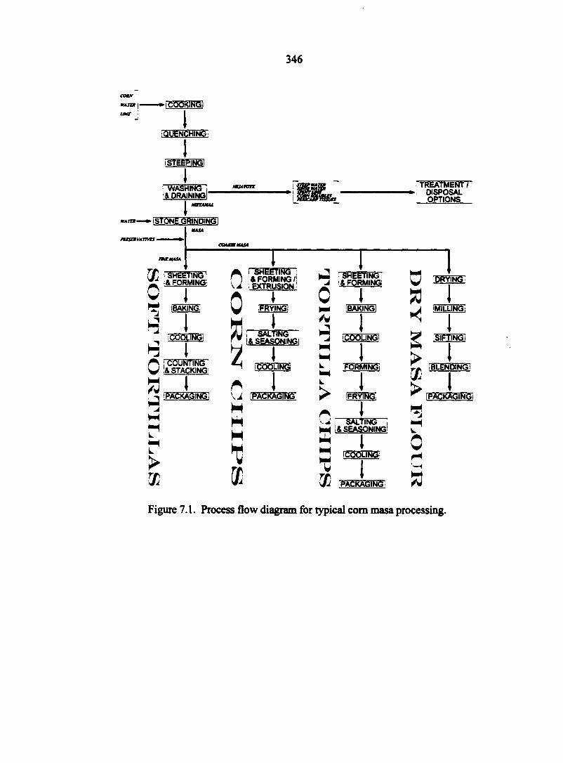
346
COUt I « 4 7 1 * j -
UHt I I
i QUENCHING i
1 I STEEPING!
I • WASHING Ntunm i& DRAINING
I •mot—» fsTONE GRINDING!
tUSaVATTVB •
TT) I SHEETING J ̂I&FORMING!
tt i BAKING.
H3 1 COOLING!
S 1 m rrrouNTiMG V L& STACKING!
P I -, PACKAGING!
L r
01 SHEEtlNG ! 4 FORMING/!
1 EXTRUSION'
n 4 V iFRYINGl
rSREETiNBl J L& FORMING!
0 I
SALTING I & SEASONING! % ï I
H COOLING!
A I \J I PACKAGING
H W W
/w
L
L
1ÔÔ6 -INÔI
^ iFftliNG
m 1 -.J SALTING ! H * SEASONING!
I I ̂ COOLING;
5 1 s/i [PACKAGING!
TREATMENT I | DISPOSAL
OPTIONS
LJ ! DRYING I
% 1 ̂ ! MILLING I
y sirfiNé H
• lï >
BLENDING!
PACKAGING!
0 M
%
Figure 7.1. Process flow diagram for typical com masa processing.
347
°C, and is then steeped for up to 24 h. This process, called nixtamalization, can be either a
batch process or a continuous process, depending on production equipment The cooked
grain (nixtamal) is then separated from the steep liquor (nejayote), which is rich in lime and
corn pericarp tissues. The nixtamal is washed to remove any excess lime and pericarp, and is
then stone ground to produce a dough called masa. The masa is then molded, cut or
extruded, and then baked or fried to make tortillas, tortilla chips, or com chips. The masa
can also be dried and milled into masa flour, which is later reconstituted and made into fresh
tortillas at food service establishments (Gomez et al., 1987; Parades-Lopez and Saharopulos-
Parades, 1983; Ramirez-Wong etal., 1994; Rooney and Sema-Saldivar, 1987; Sema-Saldivar
etal., 1990).
The nejayote waste stream contains approximately 2% total (dissolved and
suspended) solids. Typically the suspended solids (50 to 60% of the total solids) are
removed by screening, centrifugation, or decanting, and are disposed of in landfills. The
remaining water and dissolved solids are sent to municipal water facilities for treatment. The
total solids in the waste stream, which consist primarily of fiber-rich pericarp tissues,
represent com dry matter losses that occur during processing. Estimates of this original com
dry matter loss have ranged from 5.0% to 17.0% (Bressani et al., 1958; Gonzalez de Palacios,
1980; Katz et al., 1974; Khan et al., 1982; Pflugfelder et al., 1988; Rooney and Sema-
Saldivar, 1987; Sema-Saldivar et al.; 1990). The com mass loss during nixtamalization is
affected by many processing parameters, including com hybrid, lime concentration, cooking
and steeping times and temperatures, friction and damage during washing and transport, and
process equipment used. These processing losses can be economically significant due to lost
masa yield, waste processing and disposal costs, potential environmental pollution, and
348
subsequent legal penalties (Khan et al., 1982; Rooney and Sema-Saldivar, 1987; Sema-
Saldivar et al.; 1990).
A few studies have been conducted into alternative disposal options for masa
byproduct streams, and results seem to indicate that they are amenable to incorporation into
livestock rations. Rosentrater et al. (1999) conducted an extensive physical and nutritional
characterization of typical masa byproduct solids (i.e., suspended solids removed from the
nejayote stream). Pflugfelder et al. (1988) studied the composition of masa processing dry
matter losses, and included these losses in a mass balance of the masa production system.
Gonzalez-Martinez (1984) investigated four biological treatment options for nejayote on a
laboratory-scale, including activated sludge processing, anaerobic contact processing,
submerged aerobic fixed-film cascade processing, and anaerobic packed-bed processing, and
found that the activated sludge and anaerobic packed-bed reactors were effective treatment
options for these waste waters. Velasco-Martinez et al. (1997) investigated the suitability of
implementing nejayote solids in poultry broiler diets, and found no differences in
performance between control diets and diets utilizing nejayote solids. In this dissertation
(Chapter 5) livestock feed ingredients were produced by mixing nejayote solids with soybean
meal at various blend ratios and then extruding the blends at different processing conditions.
Chapter 6 continued the development of feed ingredients, by conducting a pilot-scale
extrusion study using similar mixtures of nejayote solids and soybean meal.
Before a recycling or reuse alternative is adopted for a given byproduct stream, each
viable option should be examined for feasibility, with a special consideration given to the
economics associated with each choice. This type of assessment is necessary for the
decision-making of management, so that the most cost-effective disposal method can be
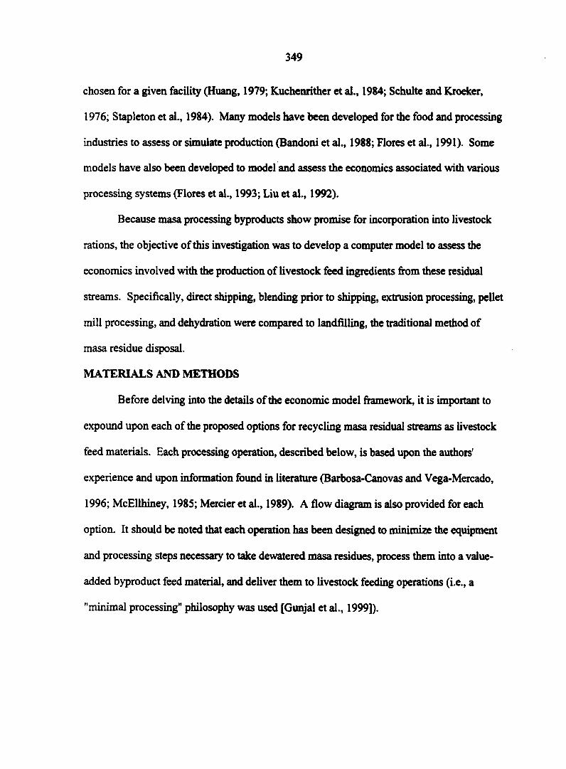
349
chosen for a given facility (Huang, 1979; Kuchenrither et al., 1984; Schulte and Kroeker,
1976; Stapleton et al., 1984). Many models have been developed for the food and processing
industries to assess or simulate production (Bandoni et al., 1988; Flores et al., 1991). Some
models have also been developed to model and assess the economics associated with various
processing systems (Flores et al., 1993; Liu et al., 1992).
Because masa processing byproducts show promise for incorporation into livestock
rations, the objective of this investigation was to develop a computer model to assess the
economics involved with the production of livestock feed ingredients from these residual
streams. Specifically, direct shipping, blending prior to shipping, extrusion processing, pellet
mill processing, and dehydration were compared to landfilling, the traditional method of
masa residue disposal.
MATERIALS AND METHODS
Before delving into the details of the economic model framework, it is important to
expound upon each of the proposed options for recycling masa residual streams as livestock
feed materials. Each processing operation, described below, is based upon the authors'
experience and upon information found in literature (Barbosa-Canovas and Vega-Mercado,
1996; McEllhiney, 1985; Mercier et al., 1989). A flow diagram is also provided for each
option. It should be noted that each operation has been designed to minimize the equipment
and processing steps necessary to take dewatered masa residues, process them into a value-
added byproduct feed material, and deliver them to livestock feeding operations (i.e., a
"minimal processing" philosophy was used [Gunjal et al., 1999]).
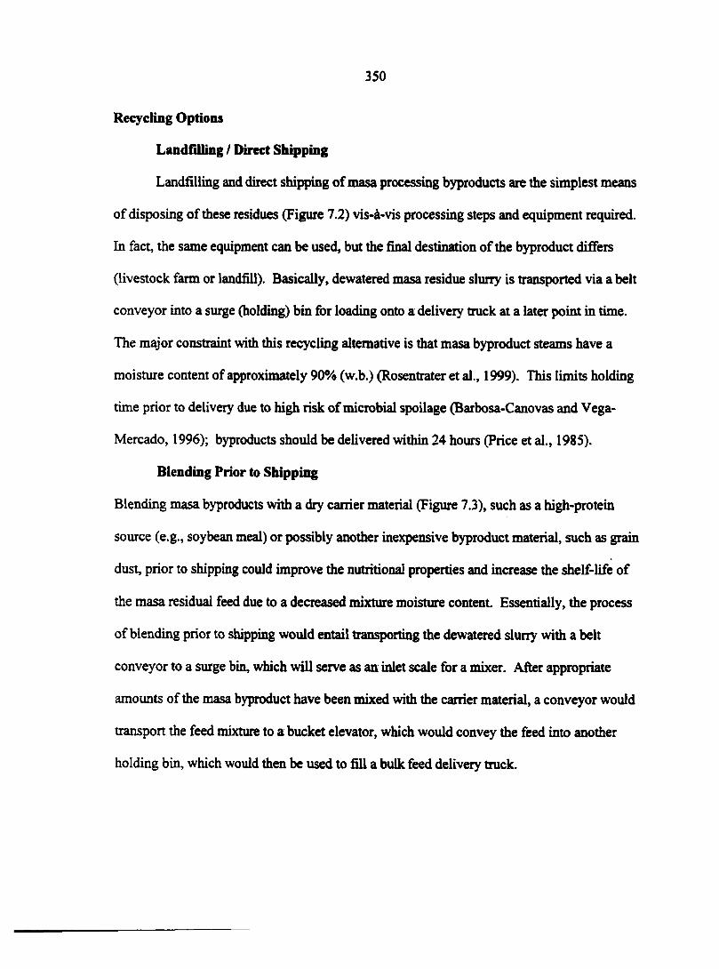
350
Recycling Options
Landfilling / Direct Shipping
Landfilling and direct shipping of masa processing byproducts are the simplest means
of disposing of these residues (Figure 7.2) vis-à-vis processing steps and equipment required.
In fact, the same equipment can be used, but the final destination of the byproduct differs
(livestock farm or landfill). Basically, dewatered masa residue slurry is transported via a belt
conveyor into a surge (holding) bin for loading onto a delivery truck at a later point in time.
The major constraint with this recycling alternative is that masa byproduct steams have a
moisture content of approximately 90% (w.b.) (Rosentrater et al., 1999). This limits holding
time prior to delivery due to high risk of microbial spoilage (Barbosa-Canovas and Vega-
Mercado, 1996); byproducts should be delivered within 24 hours (Price et al., 1985).
Blending Prior to Shipping
Blending masa byproducts with a dry carrier material (Figure 7.3), such as a high-protein
source (e.g., soybean meal) or possibly another inexpensive byproduct material, such as grain
dust, prior to shipping could improve the nutritional properties and increase the shelf-life of
the masa residual feed due to a decreased mixture moisture content. Essentially, the process
of blending prior to shipping would entail transporting the dewatered slurry with a belt
conveyor to a surge bin, which will serve as an inlet scale for a mixer. After appropriate
amounts of the masa byproduct have been mixed with the carrier material, a conveyor would
transport the feed mixture to a bucket elevator, which would convey the feed into another
holding bin, which would then be used to fill a bulk feed delivery truck.
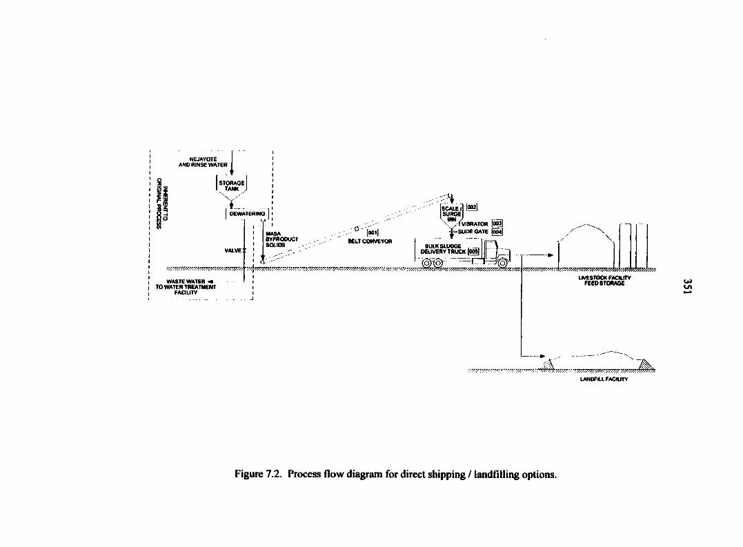
NEJAYOTE AND RINSE WATER
STORAGE TANK )
v_„ __ OEWATERINO
VALVE
WASTE WATER -4 TO WATER TREATMENT
FACILITY
<4 Is^ETII SURGE
MASA BYPRODUCT SOLIDS
-• [oo-l BELT CONVEYOR
BULK SLUDGE DELIVERY TRUCK
- (Q)%0) I '•SVl7/SV///WV^VW/.VVSVV///Z.V/,V'*VS7'S/SV//SAyVrV.7/.y? r̂-?V//.'',rA&/)7V////VV /̂/'/;SS///SV///.t7V/;//A
yfVIBRATOR |0Ô3| ¥-SUM GATE (roi]
% X
LIVESTOCK FACILITY FEED STORAGE
LANDFILL FACILITY
Figure 7.2. Process flow diagram for direct shipping / landfilling options.
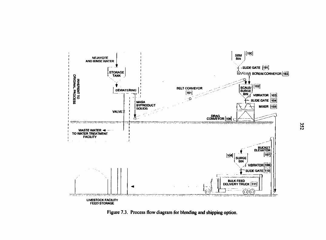
NEJAYOTE AND RINSE WATER
Si m
STORAGE TANK ,
DEWATERING
8
VALVE:
WASTE WATER -# TO WATER TREATMENT
FACILITY
SBM BIN
.j , SLIDE GATE [l9l|
fefeSSS SCREW CONVEYOR
MASA BYPRODUCT SOLIDS
a -
BELT CONVEYOR
|l°l| O '
DRAG r—| CONVEYOR [106| V_
SCALE/ SURGEJ
VIBRATOR [l03]
j= SLIDE GATE |ÏÔ4]
H«*l
BUCKET ELEVATOR
\m\ SURGE
. J VIBRATOR [ÎWL SLIDE GATE
I BULK FEED
DELIVERY TRUCK (ill]
3 :
LIVESTOCK FACILITY FEED STORAGE
'•'/ -, '/// y/'', ; V7/77. r'rn. •
Figure 7.3. Process flow diagram for blending and shipping option.
353
Extrusion Processing
Extrusion processing of masa byproducts (Figure 7.4) is very process intensive. Also,
a major constraint with this type of processing is the moisture content range which is
amenable to extrusion (i.e., the raw masa byproduct stream must be mixed with a dry carrier
material to reduce the moisture content). Similar to blending prior to shipping, the masa
residues will be transported via a belt conveyor to a scale/surge bin above a mixer. After
appropriate amounts of the masa byproducts have been mixed with a high-protein material,
such as soybean meal, or another dry material, the feed mixture will then be transported to a
bucket elevator, and will then be placed in another holding/surge bin. The material will then
be metered at an appropriate rate out of the bin, using a screw conveyor, to a preconditioner,
where steam and water will be added, so that the material is properly prepared for extrusion.
After exiting the extruder, the pelletted feed material will be pneumatically conveyed
to a dryer/cooler, where water will be removed until the feed product is at an appropriate
moisture content level, and will then be cooled. (It is recommended that feed materials have
a final moisture content between 10 and 15 % [w.b.], because this moisture level is
microbiologically stable [Beauchat, 1981; McEllhiney, 1985g]. A bucket elevator will then
transport the dried pelletted feed material into a surge bin for holding.
At this point, there are two possible alternatives that could be implemented: the
processed feed can either be delivered in bag form or in bulk form to the farm. If a bagged
form is chosen, the feed will then exit the surge bin into a bagging scale, and then will enter
an automatic bagging and palletizing system. Then, a forklift will place the bagged and
palletted feed onto a delivery truck. If, however, a bulk feed is desired, the surge bin would
empty directly into a bulk feed delivery truck.

NEJAYOTE AND RINSE WATER
STORAGE TANK I
DE WATERING
VALVE
?%%%%%%%% % ?//////.
WASTEWATER •« TO WATER TREATMENT
FACWTY
mi SBM BIN ELEVATOR
m
MASA BYPRODUCT SOUDS /
BELT CONVEYOR
PI „ 0
(Ml) SUDE GATE | •
SCREW CONVEYOR NVA'/i
M ^ j -- - |sCAl£/|l?®l
, | SURGE |
T l VBRATOR (j»] |i«] 6UOEOATE •)-
(roj MIXER
coKSS9OR|2M1[
[Vr\:
CYCLONE SEPARATOR
t EXTRUOEOPROOUCT
FAN p* EXHAUST AIR
VVIBRATOR 12» SUOE GATE $10
* STEAM WATER CONVEYOR 211
CONDITIONS 212
ORAO CONVEYOR [2I7| EXTRUDER |m]
?%;%%% w • %% VW////A wmv.W/.W///.
J BAGGED FEED
DELIVERY TRUCK I»»)
•wrr/?AyA:rM7/,7ZAWAy? LIVESTOCK FACUTY
FEED STORAGE
rsr/r/?V//7/?AVA'WV////r//n\ ^(oj(o)J r; ••nvsss/Awwsw.w/warAV/vr̂ /m.̂ '.'A'
''/r̂ FT.'TPZ' r̂w.yS/7//rWS*tytyAVA>/ 'S.rv.™ PALLETIZED
sm*,
[220] SCA1C
6EWBI BAMER @ gu
n 'Mr
'W/V'AV/.'/.'Ar
SUOE GATE
>/*'vsAV?'.rvKfyAv:.vsswywAVAvr,v?ArATAr,r/r̂ rK7/rwr'?zrFsv7Arrs/yrty7vr>''/r-f'.-r.
fin^srrft r 1 OEWERV TRUCK Ittcj I
l(5)'t=:rn— LIVESTOCK FACWTY
FEED STORAGE
Figure 7.4. Process flow diagram for extrusion processing options.
355
Pellet Mill Processing
Producing masa byproduct feed material from a pellet mill processing line is very
similar to the extrusion process (Figure 7.5). Pellet mill processing is also confined to a
limited moisture content range, and thus the masa byproduct slurry will once again need to be
blended with a dry material prior to processing. The major difference between pellet mill
and extrusion processing is that the pelletted feed will discharge from the pellet mill directly
into the dryer/cooler. Once again, the feed can be either bagged or left in bulk form.
Dehydration
Dehydration of masa byproduct slurries is not as process intensive as either extrusion
or pelleting (Figure 7.6), but it will have substantial fuel costs because the slurry is so wet.
After dewatering, masa residues will be transported via a belt conveyor to a surge bin, and
then directly into a dryer. Again, the feed can either be bagged or left in bulk form.
Economic Model Heuristics
Scope of Model
As mentioned previously, the purpose of this model is to compare the economics of
five reprocessing alternatives (Table 7.1) for corn masa residues with the costs associated
with landfilling of this waste stream. Specifically, the objective of this economic model is to
determine byproduct feed sales price required for each option to reach the breakeven point
each year of operation, and compare these results to the costs of landfilling. Thus, a masa
manufacturer may be able to choose the most appropriate recycling option for a given
facility.
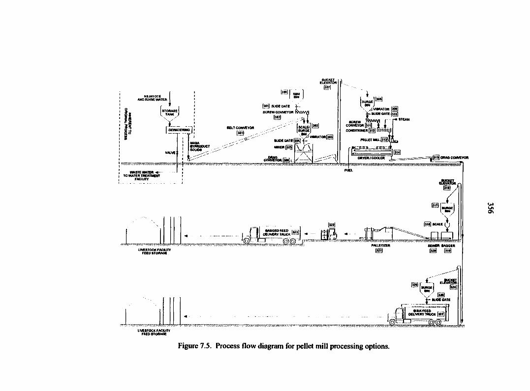
NEJAYOTE AND RINSE WATER
STORAGE I TANK
V i
W5» VS7WS, 'V7W///S7X77//S'W.
WASTE WATER -TO WATER TREATMENT
FACILITY
ELEVATOR («']
[ill] SUOE OATE
SCREW CONVEYOR
I# BEIT CONVEYOR
@ -
•ypfvooucT souos , -I 5-
vwr*tor|w] SUOE OATE
MUER^M]
6C8S68ORBI.J1 ov/v/'v////. vw/y////.
LIJ® . A VIBRATOR [w>l j. sum oate [so]
re STEAM
ORYERf COOLER gj5oRAOCOWEYOR
eBSŒR, |yg
'/J'J7Trrrr?r>r.W L
vswr*!*/ :ry,i G
•AGOEOFEEO («il DELIVERY TRUCK™
w {o)(a •]\ " RTS. " • -r V'VZTF.v+'tvW'l::\y,yv////.rwx?7rz7?V
RW SCALE
hy/h "ri?7/7, rzr,J, LIVESTOCK FAOUTV
FEED STORAGE
W7W7777V/S/M7/F/r///S*Wtf777m#: FALLETIZER SEWER SAGGER
(Ml) @ M
IS C EtRBsa l^K8] \x m f- SUM GATE
:r/'r::vyyAy.rA^y//,v#/Z',r&'A/s'+/srsfV"V7y/-'y>vvr̂ 'sX'y,:y!'Tr.',:y7 LIVESTOCK FACILITY
FEED STORAGE
BULK FEED — OEUVERY TRUCK «Î]
OuO v/zw/rwbfc/A
0\
Figure 7.5. Process flow diagram for pellet mill processing options.
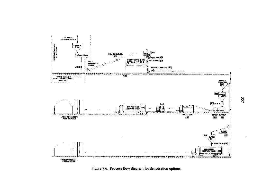
NEJAYOTE AND RINSE WATER
STORAGE TANK J
WASTEWATER «• TO WATER TREATMENT
FACWTV
MASA BYPRODUCT SOUOS
BELT CONVEYOR
M . o
, '•) „ , |sc*i£/|6®?l ISURGEJ _
""ZF VBRATOH [«to] DRRER Z COOLER [«05] +-SLŒ OATE FISI «to o jLTzzm a: .it
J SCREW CONVEYOR |«0>|
tytftQ- 1
y/7/77
eBSSS,,
li'ti BAGGED FEED
OBJVERY TRUCK 111»!
r/.ws?rs///,w/mv. 'w/.vmvw//mw////a'.twv.vmv LIVESTOCK FACILITY
FEED STORAGE
:o)(o) • r '̂ vr.v/}/.
" JR r/7V7///,'W. VVWW/V/'//.-:•vww/'»s&zvw7tvm>:-PAUETIZER
| W SCALE
SEWBL BAOOER
LIVESTOCK FACILITY FEED STORAGE
f|
r EiftSnS eg
SUOE GATE IjitJ
DELIVERY TRUCK [420J
VS////S///7W
Figure 7.6. Process flow diagram for dehydration options.
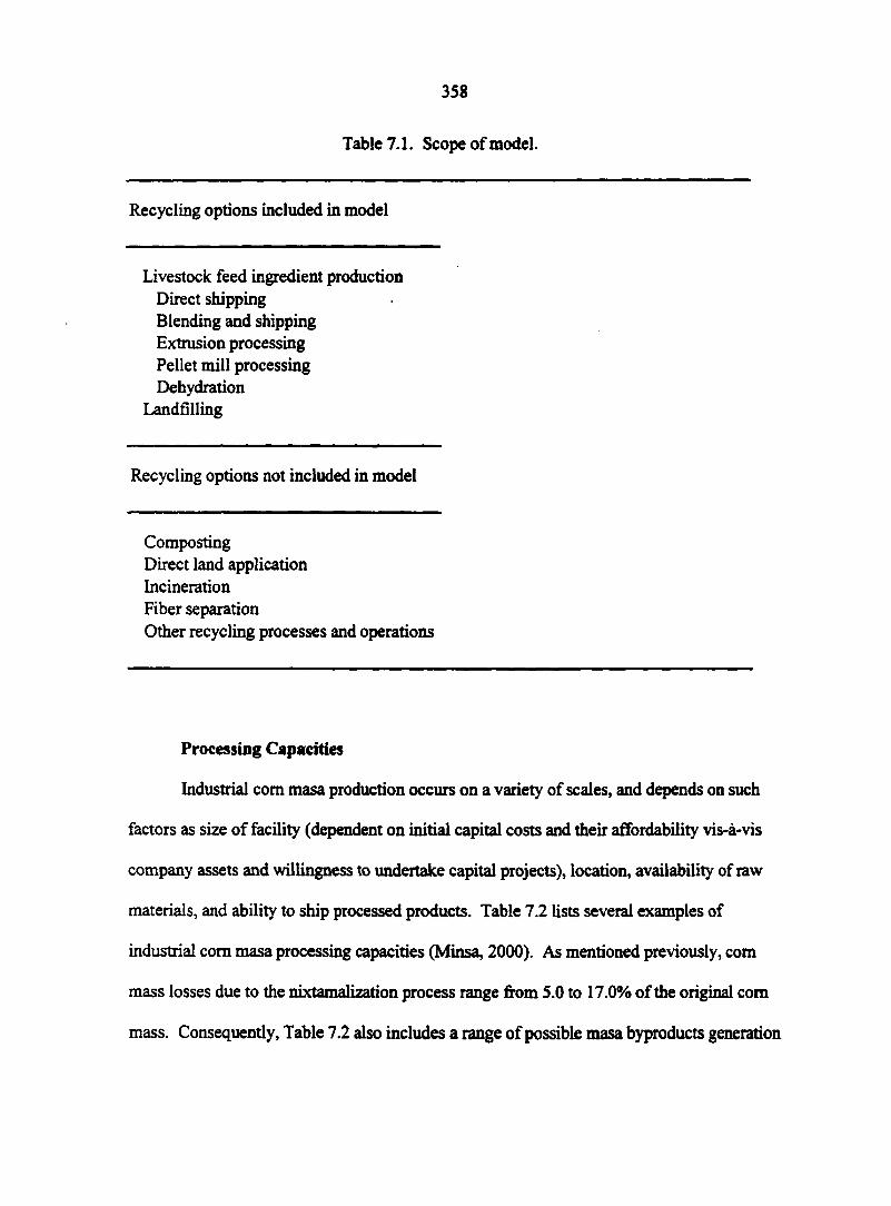
358
Table 7.1. Scope of model.
Recycling options included in model
Livestock feed ingredient production Direct shipping Blending and shipping Extrusion processing Pellet mill processing Dehydration
Landfilling
Recycling options not included in model
Composting Direct land application Incineration Fiber separation Other recycling processes and operations
Processing Capacities
Industrial corn masa production occurs on a variety of scales, and depends on such
factors as size of facility (dependent on initial capital costs and their affordability vis-à-vis
company assets and willingness to undertake capital projects), location, availability of raw
materials, and ability to ship processed products. Table 7.2 lists several examples of
industrial corn masa processing capacities (Minsa, 2000). As mentioned previously, com
mass losses due to the nixtamalization process range from 5.0 to 17.0% of the original com
mass. Consequently, Table 7.2 also includes a range of possible masa byproducts generation
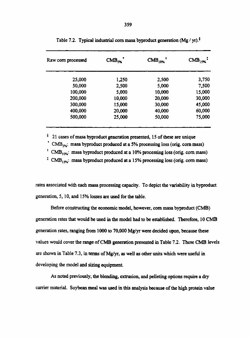
359
Table 7.2. Typical industrial corn masa byproduct generation (Mg / yr).$
Raw corn processed CMBS%" CMB10%f CMBlJ%*
25,000 1,250 2,500 3,750 50,000 2,500 5,000 7,500
100,000 5,000 10,000 15,000 200,000 10,000 20,000 30,000 300,000 15,000 30,000 45,000 400,000 20,000 40,000 60,000 500,000 25,000 50,000 75,000
5 21 cases of masa byproduct generation presented, 15 of these are unique
CMBS%: masa byproduct produced at a 5% processing loss (orig. corn mass) t CMB10%: masa byproduct produced at a 10% processing loss (orig. com mass)
: CMB15%: masa byproduct produced at a 15% processing loss (orig. corn mass)
rates associated with each masa processing capacity. To depict the variability in byproduct
generation, 5,10, and 15% losses are used for the table.
Before constructing the economic model, however, corn masa byproduct (CMB)
generation rates that would be used in the model had to be established. Therefore, 10 CMB
generation rates, ranging from 1000 to 70,000 Mg/yr were decided upon, because these
values would cover the range of CMB generation presented in Table 7.2. These CMB levels
are shown in Table 7.3, in terms of Mg/yr, as well as other units which were useful in
developing the model and sizing equipment
As noted previously, the blending, extrusion, and pelleting options require a dry
carrier material. Soybean meal was used in this analysis because of the high protein value
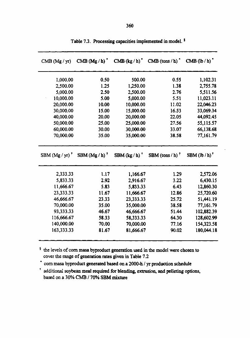
360
Table 7.3. Processing capacities implemented in model.5
CMB (Mg/yr) CMB (Mg/h) * CMB(kg/h)' CMB (tons/h)* CMB (lb/h)'
1,000.00 0.50 500.00 0.55 1,102.31 2,500.00 1.25 1,250.00 1.38 2,755.78 5,000.00 2.50 2,500.00 2.76 5,511.56
10,000.00 5.00 5,000.00 5.51 11,023.11 20,000.00 10.00 10,000.00 11.02 22,046.23 30,000.00 15.00 15,000.00 16.53 33,069.34 40,000.00 20.00 20,000.00 22.05 44,092.45 50,000.00 25.00 25,000.00 27.56 55,115.57 60,000.00 30.00 30,000.00 33.07 66,138.68 70,000.00 35.00 35,000.00 38.58 77,161.79
SBM (Mg / yr)+ SBM(Mg/h)f SBM(kg/h)+ SBM(tons/h)f SBM(lb/h)+
2,333.33 1.17 1,166.67 1.29 2,572.06 5,833.33 2.92 2,916.67 3.22 6,430.15
11,666.67 5.83 5,833.33 6.43 12,860.30 23,333.33 11.67 11,666.67 12.86 25,720.60 46,666.67 23.33 23,333.33 25.72 51,441.19 70,000.00 35.00 35,000.00 38.58 77,161.79 93,333.33 46.67 46,666.67 51.44 102,882.39
116,666.67 58.33 58,333.33 64.30 128,602.99 140,000.00 70.00 70,000.00 77.16 154,323.58 163,333.33 81.67 81,666.67 90.02 180,044.18
5 the levels of com masa byproduct generation used in the model were chosen to cover the range of generation rates given in Table 7.2
* corn masa byproduct generated based on a 2000-h / yr production schedule + additional soybean meal required for blending, extrusion, and pelleting options,
based on a 30% CMB / 70% SBM mixture
361
and common use in the feed industry. Table 7.3 also gives required soybean meal (SBM)
capacities, based on a 30% CMB / 70% SBM mixture for these recycling options (this
mixture ratio was used because it utilized the greatest byproduct amount, and would still be
able to be processed; see Chapter 5 for further discussion).
Regarding overall processing line capacities, landfilling, direct shipping, and
dehydration require only CMB, whereas blending, extrusion, and pelleting require CMB and
SBM. The total processing line capacities for each reprocessing option are given in Table
7.4. Both Tables 7.3 and 7.4 are necessary to size processing equipment and to develop the
model.
Model Assumptions
The premise of this model is that an existing masa production facility exists. This
model examines the costs associated with installing and running a reprocessing line in an
existing corn masa production facility. Also, this model examines the costs associated with
landfilling the masa byproducts instead of recycling or reprocessing. The assumptions
incorporated into this model are explicated in Table 7.5. Therefore, model assumptions will
only be discussed briefly here. For more details regarding the assumptions of the model, see
Table 7.5.
The model that was developed included both intrinsic variables and user-specified
variables. Intrinsic variables (3) included CMB disposal option (i.e., five reprocessing
options and landfilling), CMB generation rate (Table 7.3) and delivery distance (0 to 100
miles). User-specified variables (5) included interest rate, electricity price, gasoline price,
blending agent (soybean meal) price, and landfill tipping fee.
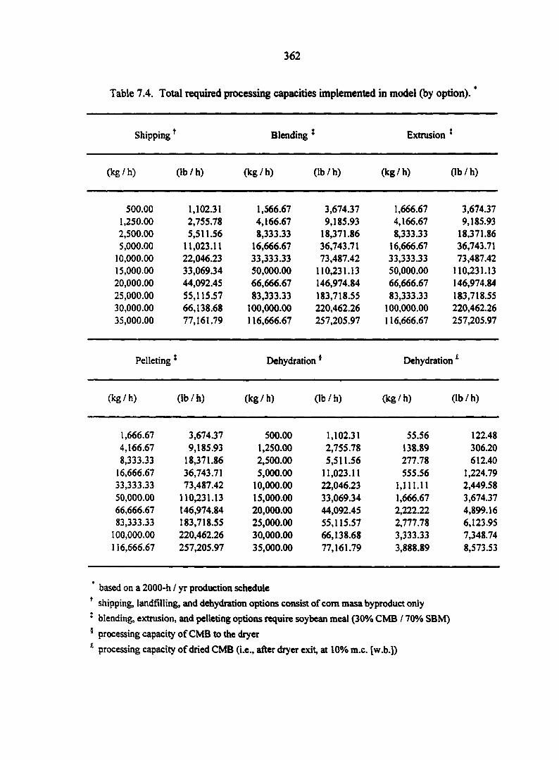
362
Table 7.4. Total required processing capacities implemented in model (by option). *
Shipping t Blending : Extrusion :
(kg/h) (lb/h) (kg/h) (lb/h) (kg/h) (lb/h)
500.00 1,102.31 1,566.67 3,674.37 1,666.67 3,674.37 1,250.00 2,755.78 4,166.67 9,185.93 4,166.67 9,185.93 2,500.00 5,511.56 8,333.33 18,371.86 8,333.33 18,371.86 5,000.00 11,023.11 16,666.67 36,743.71 16,666.67 36,743.71
10,000.00 22,046.23 33,333.33 73,487.42 33,333.33 73,487.42 15,000.00 33,069.34 50,000.00 110,231.13 50,000.00 110,231.13 20,000.00 44,092.45 66,666.67 146,974.84 66,666.67 146,974.84 25,000.00 55,115.57 83,333.33 183,718.55 83,333.33 183,718.55 30,000.00 66,138.68 100,000.00 220,462.26 100,000.00 220,462.26 35,000.00 77,161.79 116,666.67 257,205.97 116,666.67 257,205.97
Pelleting : Dehydration * Dehydration£
(kg/h) ( lb/h) (kg/h) ( lb/h) (kg/h) ( lb/h)
1,666.67 3,674.37 500.00 1,102.31 55.56 122.48 4,166.67 9,185.93 1,250.00 2,755.78 138.89 306.20 8,333.33 18,371.86 2,500.00 5,511.56 277.78 612.40
16,666.67 36,743.71 5,000.00 11,023.11 555.56 1,224.79 33,333.33 73,487.42 10,000.00 22,046.23 1,111.11 2,449.58 50,000.00 110,231.13 15,000.00 33,069.34 1,666.67 3,674.37 66,666.67 146,974.84 20,000.00 44,092.45 2,222.22 4,899.16 83,333.33 183,718.55 25,000.00 55,115.57 2,777.78 6,123.95
100,000.00 220,462.26 30,000.00 66,138.68 3,333.33 7,348.74 116,666.67 257,205.97 35,000.00 77,161.79 3,888.89 8,573.53
based on a 2000-h / yr production schedule f shipping, landfilling, and dehydration options consist of corn masa byproduct only $ blending, extrusion, and pelleting options require soybean meal (30% CMB / 70% SBM) 5 processing capacity of CMB to the dryer £ processing capacity of dried CMB (i.e., after dryer exit, at 10% m.c. [w.b.])
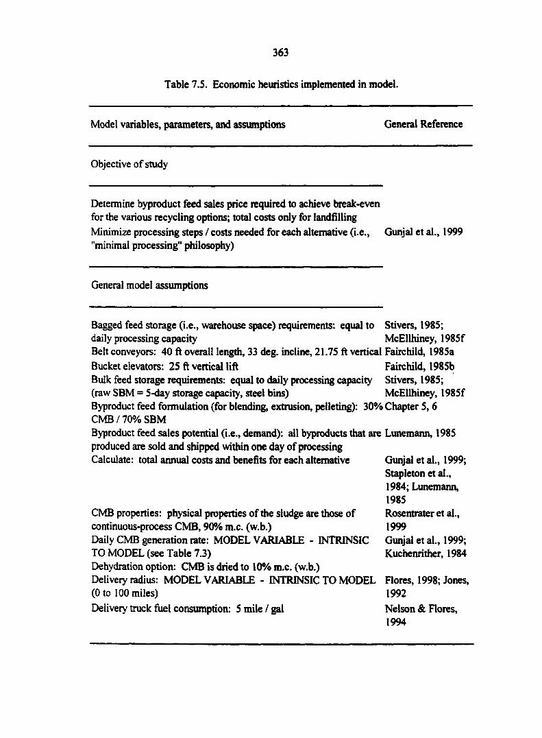
363
Table 7.5. Economic heuristics implemented in model.
Model variables, parameters, and assumptions General Reference
Objective of study
Determine byproduct feed sales price required to achieve break-even for the various recycling options; total costs only for landfilling
Minimize processing steps / costs needed for each alternative (i.e., Gunjal et al., 1999 "minimal processing" philosophy)
General model assumptions
Bagged feed storage (i.e., warehouse space) requirements: equal to Stivers, 1985; daily processing capacity McEllhiney, 1985f Belt conveyors: 40 ft overall length, 33 deg. incline, 21.75 ft vertical Fairchild, 1985a
Bucket elevators: 25 ft vertical lift Fairchild, 1985b Bulk feed storage requirements: equal to daily processing capacity Stivers, 1985; (raw SBM = 5-day storage capacity, steel bins) McEllhiney, I985f Byproduct feed formulation (for blending, extrusion, pelleting): 30% Chapter 5,6 CMB / 70% SBM Byproduct feed sales potential (i.e., demand): all byproducts that are Lunemann, 1985 produced are sold and shipped within one day of processing Calculate: total annual costs and benefits for each alternative Gunjal et al., 1999;
Stapleton et al., 1984; Lunemann, 1985 Rosentrater et al., 1999 Gunjal et al., 1999; Kuchenrither, 1984
CMB properties: physical properties of the sludge are those of continuous-process CMB, 90% m.c. (w.b.) Daily CMB generation rate: MODEL VARIABLE - INTRINSIC TO MODEL (see Table 7.3) Dehydration option: CMB is dried to 10% m.c. (w.b.) Delivery radius: MODEL VARIABLE - INTRINSIC TO MODEL (0 to 100 miles)
Delivery truck fuel consumption: 5 mile / gal
Flores, 1998; Jones, 1992
Nelson & Flores, 1994
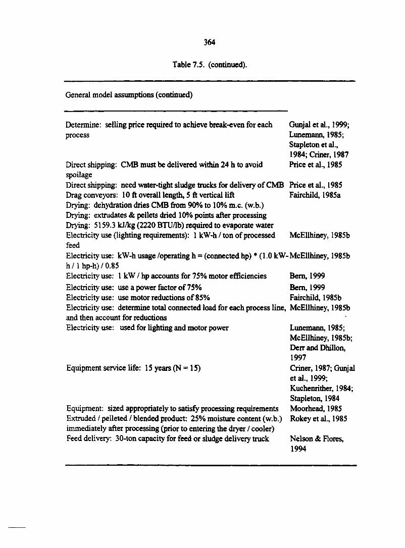
364
Table 7.5. (continued).
General model assumptions (continued)
Determine: selling price required to achieve break-even for each Gunjal et al., 1999; process Lunemann, 1985;
Stapleton et al., 1984; Criner, 1987
Direct shipping: CMB must be delivered within 24 h to avoid Price et al., 1985 spoilage Direct shipping: need water-tight sludge trucks for delivery of CMB Price et al., 1985 Drag conveyors: 10 ft overall length, 5 ft vertical lift Fairchild, 1985a Drying: dehydration dries CMB from 90% to 10% m.c. (w.b.) Drying: extradâtes & pellets dried 10% points after processing Drying: 5159.3 kJ/kg (2220 BTU/lb) required to evaporate water Electricity use (lighting requirements): 1 kW-h / ton of processed McEllhiney, 1985b feed Electricity use: kW-h usage /operating h = (connected hp) * (1.0 kW- McEllhiney, 1985b h /1 hp-h) / 0.85 Electricity use: 1 kW / hp accounts for 75% motor efficiencies Bern, 1999
Electricity use: use a power factor of 75% Bern, 1999 Electricity use: use motor reductions of 85% Fairchild, 1985b Electricity use: determine total connected load for each process line, McEllhiney, 1985b and then account for reductions Electricity use: used for lighting and motor power Lunemann, 1985;
McEllhiney, 1985b; Derr and Dhillon, 1997
Equipment service life: 15 years (N = 15) Criner, 1987; Gunjal et al., 1999; Kuchenrither, 1984; Stapleton, 1984
Equipment: sized appropriately to satisfy processing requirements Moorhead, 1985 Extruded / pelleted / blended product: 25% moisture content (w.b.) Rokey et al., 1985 immediately after processing (prior to entering the dryer / cooler) Feed delivery: 30-ton capacity for feed or sludge delivery truck Nelson & Flores,
1994
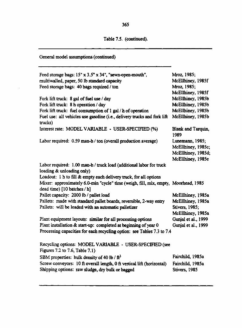
365
Table 7.5. (continued).
General model assumptions (continued)
Feed storage bags: 15" x 3.5" x 34", "sewn-open-mouth", multiwalled, paper, 50 lb standard capacity Feed storage bags: 40 bags required / ton
Fork lift truck: 8 gal of fuel use Z day Fork lift truck: 8 h operation / day Fork lift truck: fuel consumption of 1 gal / h of operation Fuel use: all vehicles use gasoline (i.e., delivery trucks and fork lift trucks)
Interest rate: MODEL VARIABLE - USER-SPECIFIED (%)
Labor required: 0.59 man-h / ton (overall production average)
Mroz, 1985; McEllhiney, 1985f Mroz, 1985; McEllhiney, 1985f McEllhiney, 1985b McEllhiney, 1985b McEllhiney, 1985b McEllhiney, 1985b
Blank and Tarquin, 1989 Lunemann, 1985; McEllhiney, 1985c; McEllhiney, 1985d; McEllhiney, 1985e
Labor required: 1.00 man-h / truck load (additional labor for truck loading & unloading only) Loadout: 1 h to fill & empty each delivery truck, for all options Mixer: approximately 6.0-min "cycle" time (weigh, fill, mix, empty, Moorhead, 1985 dead time) [10 batches / h] Pallet capacity: 2000 lb / pallet load Pallets: made with standard pallet boards, reversible, 2-way entry Pallets: will be loaded with an automatic palletizer
Plant equipment layouts: similar for all processing options Plant installation & start-up: completed at beginning of year 0 Processing capacities for each recycling option: see Tables 7.3 to 7.4
McEllhiney, 1985a McEllhiney, 1985a Stivers, 1985; McEllhiney, 1985a Gunjal et al., 1999 Gunjal et al., 1999
Recycling options: MODEL VARIABLE - USER-SPECIFIED (see Figures 7.2 to 7.6, Table 7.1)
SBM properties: bulk density of 40 lb / ft3 Fairchild, 1985a
Screw conveyors: 10 ft overall length, 0 ft vertical lift (horizontal) Fairchild, 1985a Shipping options: raw sludge, dry bulk or bagged Stivers, 1985
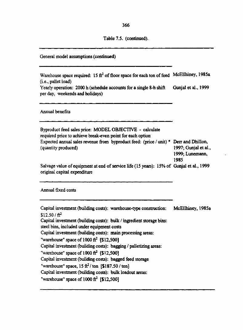
366
Table 7.5. (continued).
General model assumptions (continued)
Warehouse space required: 15 ft2 of floor space for each ton of feed McEllhiney, 1985a (i.e., pallet load) Yearly operation: 2000 h (schedule accounts for a single 8-h shift Gunjal et al., 1999 per day, weekends and holidays)
Annual benefits
Byproduct feed sales price: MODEL OBJECTIVE - calculate required price to achieve break-even point for each option Expected annual sales revenue from byproduct feed: (price / unit) * Derr and Dhillon, (quantity produced) 1997; Gunjal et al.,
1999; Lunemann, 1985
Salvage value of equipment at end of service life (15 years): 15% of Gunjal et al., 1999 original capital expenditure
Annual fixed costs
Capital investment (building costs): warehouse-type construction: McEllhiney, 1985a
$12.50/ft2
Capital investment (building costs): bulk / ingredient storage bins: steel bins, included under equipment costs Capital investment (building costs): main processing areas:
"warehouse" space of 1000 ft2 [$12,500] Capital investment (building costs): bagging / palletizing areas:
"warehouse" space of 1000 ft2 [$12,500] Capital investment (building costs): bagged feed storage
"warehouse" space, 15 ft2/ton [$187.50 / ton] Capital investment (building costs): bulk loadout areas:
"warehouse" space of 1000 ft2 [$12,500]
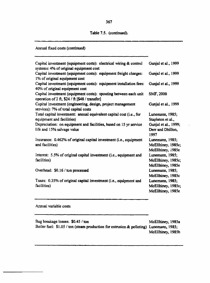
367
Table 7.5. (continued).
Annual fixed costs (continued)
Capital investment (equipment costs): electrical wiring & control systems: 4% of original equipment cost Capital investment (equipment costs): equipment freight charges: 1% of original equipment cost Capital investment (equipment costs): equipment installation fees: 40% of original equipment cost Capital investment (equipment costs): spouting between each unit operation of 2 ft, $24 / ft [$48 / transfer] Capital investment (engineering, design, project management services) : 7% of total capital costs Total capital investment: annual equivalent capital cost (i.e., for equipment and facilities) Depreciation: on equipment and facilities, based on 15 yr service life and 15% salvage value
Insurance: 0.462% of original capital investment (i.e., equipment and facilities)
Interest: 5.5% of original capital investment (i.e., equipment and facilities)
Overhead: $0.16/ ton processed
Taxes: 0.35% of original capital investment (i.e., equipment and facilities)
Gunjal et al., 1999
Gunjal et al., 1999
Gunjal et al., 1999
SMF, 2000
Gunjal et al., 1999
Lunemann, 1985; Stapleton et al., Gunjal et al., 1999; Derr and Dhillon, 1997 Lunemann, 1985; McEllhiney, 1985c; McEllhiney, 1985e Lunemann, 1985; McEllhiney, 1985c; McEllhiney, 1985e Lunemann, 1985; McEllhiney, 1985c Lunemann, 1985; McEllhiney, 1985c; McEllhiney, 1985e
Annual variable costs
Bag breakage losses: $0.45 / ton McEllhiney, 1985a Boiler fuel: $1.05 / ton (steam production for extrusion & pelleting) Lunemann, 1985;
McEllhiney, 1985b
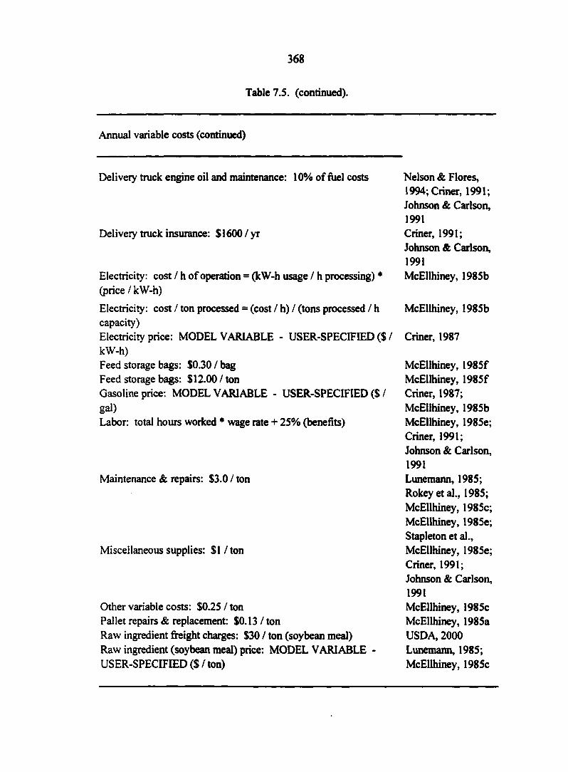
368
Table 7.5. (continued).
Annual variable costs (continued)
Delivery truck engine oil and maintenance: 10% of fuel costs
Delivery truck insurance: $1600 / yr
Electricity: cost / h of operation = (kW-h usage / h processing) * (price / kW-h)
Electricity: cost / ton processed = (cost / h) / (tons processed / h capacity) Electricity price: MODEL VARIABLE - USER-SPECIFIED ($ / kW-h) Feed storage bags: $0.30 / bag Feed storage bags: $12.00 / ton Gasoline price: MODEL VARIABLE - USER-SPECIFIED ($ / gal) Labor: total hours worked * wage rate + 25% (benefits)
Maintenance & repairs: $3.0 / ton
Miscellaneous supplies: $1 / ton
Other variable costs: $0.25 / ton Pallet repairs & replacement: $0.13 / ton Raw ingredient freight charges: $30 / ton (soybean meal) Raw ingredient (soybean meal) price: MODEL VARIABLE USER-SPECIFIED ($ / ton)
Nelson & Flores, 1994; Criner, 1991; Johnson & Carlson, 1991 Criner, 1991; Johnson & Carlson, 1991 McEllhiney, 1985b
McEllhiney, 1985b
Criner, 1987
McEllhiney, I985f McEllhiney, 1985f Criner, 1987; McEllhiney, 1985b McEllhiney, 1985e; Criner, 1991; Johnson & Carlson, 1991 Lunemann, 1985; Rokeyetal., 1985; McEllhiney, 1985c; McEllhiney, 1985e; Stapleton et al., McEllhiney, 1985e; Criner, 1991; Johnson & Carlson, 1991 McEllhiney, 1985c McEllhiney, 1985a USDA, 2000 Lunemann, 1985; McEllhiney, 1985c
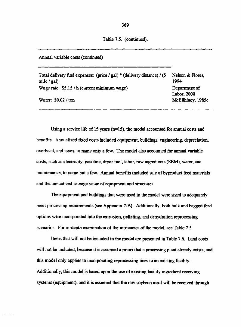
369
Table 7.5. (continued).
Annual variable costs (continued)
Total delivery fuel expenses: (price / gal) * (delivery distance) / (5 Nelson & Flores, mile Z gal) 1994
Wage rate: $5.15 Zh (current minimum wage) Department of Labor, 2000
Water: $0.02 Z ton McEllhiney, 1985c
Using a service life of 15 years (n=15), the model accounted for annual costs and
benefits. Annualized fixed costs included equipment, buildings, engineering, depreciation,
overhead, and taxes, to name only a few. The model also accounted for annual variable
costs, such as electricity, gasoline, dryer fuel, labor, raw ingredients (SBM), water, and
maintenance, to name but a few. Annual benefits included sale of byproduct feed materials
and the annualized salvage value of equipment and structures.
The equipment and buildings that were used in the model were sized to adequately
meet processing requirements (see Appendix 7-B). Additionally, both bulk and bagged feed
options were incorporated into the extrusion, pelleting, and dehydration reprocessing
scenarios. For in-depth examination of the intricacies of the model, see Table 7.5.
Items that will not be included in the model are presented in Table 7.6. Land costs
will not be included, because it is assumed a priori that a processing plant already exists, and
this model only applies to incorporating reprocessing lines to an existing facility.
Additionally, this model is based upon the use of existing facility ingredient receiving
systems (equipment), and it is assumed that the raw soybean meal will be received through
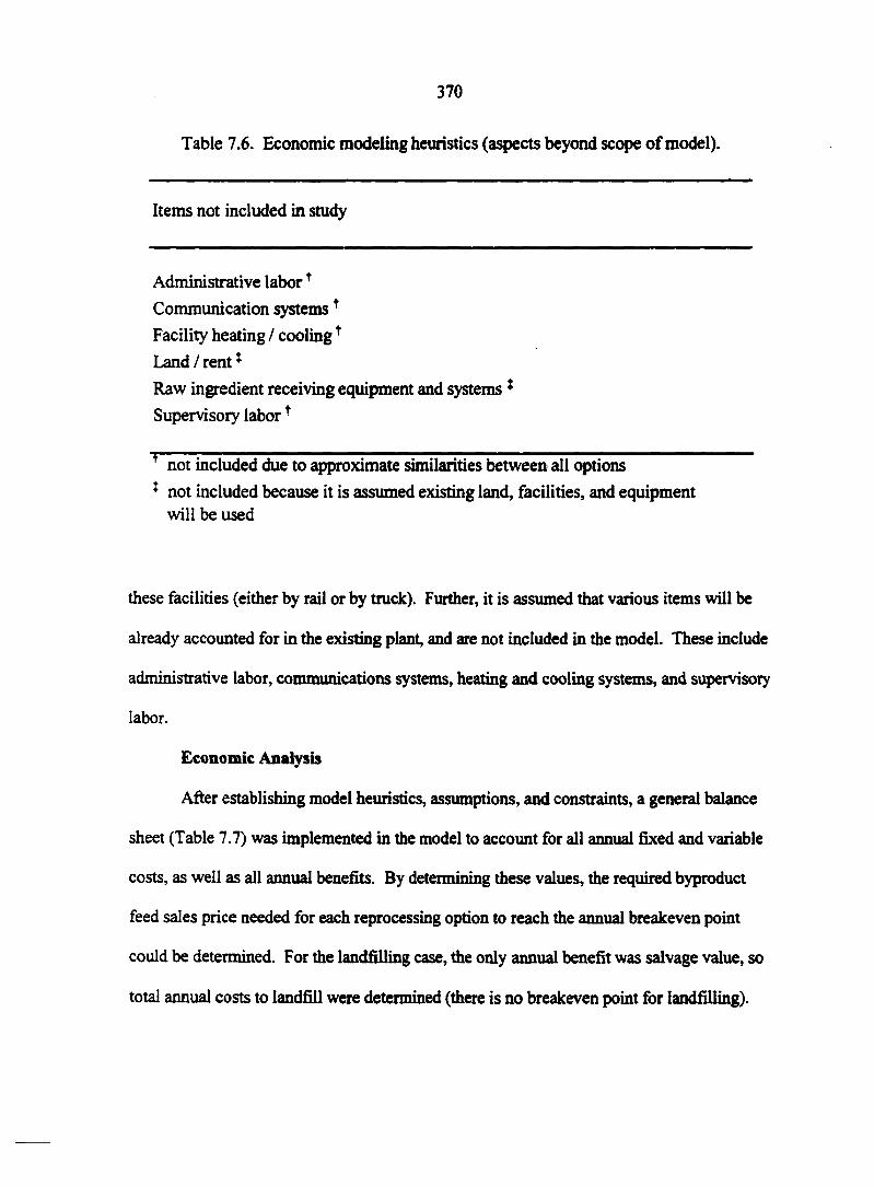
370
Table 7.6. Economic modeling heuristics (aspects beyond scope of model).
Items not included in study
Administrative laborf
Communication systemst
Facility heating / coolingf
Land / rent *
Raw ingredient receiving equipment and systems *
Supervisory laborf
r not included due to approximate similarities between all options
* not included because it is assumed existing land, facilities, and equipment will be used
these facilities (either by rail or by truck). Further, it is assumed that various items will be
already accounted for in the existing plant, and are not included in the model. These include
administrative labor, communications systems, heating and cooling systems, and supervisory
labor.
Economic Analysis
After establishing model heuristics, assumptions, and constraints, a general balance
sheet (Table 7.7) was implemented in the model to account for all annual fixed and variable
costs, as well as all annual benefits. By determining these values, the required byproduct
feed sales price needed for each reprocessing option to reach the annual breakeven point
could be determined. For the landfilling case, the only annual benefit was salvage value, so
total annual costs to landfill were determined (there is no breakeven point for landfilling).
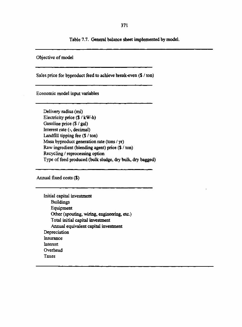
371
Table 7.7. General balance sheet implemented by model.
Objective of model
Sales price for byproduct feed to achieve break-even ($ / ton)
Economic model input variables
Delivery radius (mi) Electricity price ($ / kW-h) Gasoline price ($ / gal) Interest rate (-, decimal) Landfill tipping fee ($ / ton) Masa byproduct generation rate (tons / yr) Raw ingredient (blending agent) price ($ / ton) Recycling / reprocessing option Type of feed produced (bulk sludge, dry bulk, dry bagged)
Annual fixed costs ($)
Initial capital investment Buildings Equipment Other (spouting, wiring, engineering, etc.) Total initial capital investment Annual equivalent capital investment
Depreciation Insurance Interest Overhead Taxes
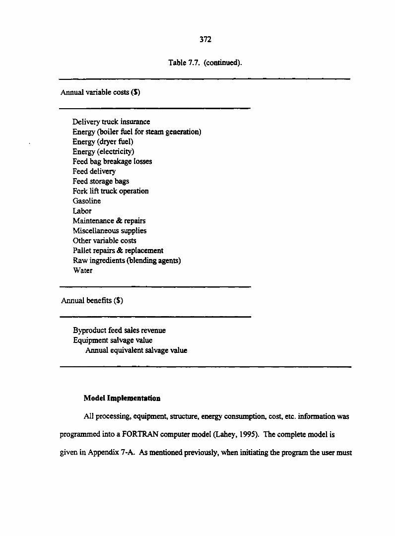
372
Table 7.7. (continued).
Annual variable costs ($)
Delivery truck insurance Energy (boiler fuel for steam generation) Energy (dryer fuel) Energy (electricity) Feed bag breakage losses Feed delivery Feed storage bags Fork lift truck operation Gasoline Labor Maintenance & repairs Miscellaneous supplies Other variable costs Pallet repairs & replacement Raw ingredients (blending agents) Water
Annual benefits ($)
Byproduct feed sales revenue Equipment salvage value
Annual equivalent salvage value
Model Implementation
All processing, equipment, structure, energy consumption, cost, etc. information was
programmed into a FORTRAN computer model (Lahey, 1995). The complete model is
given in Appendix 7-A. As mentioned previously, when initiating the program the user must
373
specify values for five variables (interest rate, electricity price, gasoline price, blending agent
[soybean meal for this study] price, and landfill tipping fee). Additionally, the user must
specify which recycling option to use, as well as bagged or bulk feed for the extrusion,
pelleting, and dehydration options. Then, the model calculates total annual costs (for the
landfilling option) or required feed sales price to annually breakeven (for all five other
reprocessing options).
For the current study, values of the five user-specified variables were chosen based on
values representative of those found in the central United States during the summer of 2000.
Values chosen included an interest rate of 9.50% (Federal Reserve, 2000; HSH, 2000), an
electricity price of $0.07 / kW-h (EIA, 2000b; EIA, 2000c), a gasoline price of $1.50 / gal
($0.40 Z L) (EIA, 2000a), a soybean meal price of $150.00 / ton ($165.35 / Mg) (TFC, 2000),
and a tipping fee of $50.00 / ton ($55.12 / Mg) (Ackerman, 1997; Goldstein, 1992; Johnson
and Carlson, 1991; Jones, 1992).
It must be noted that these variables can be altered by the user to accommodate the
fluid, and sometimes volatile, economic conditions of the U.S. marketplace.
RESULTS AND DISCUSSION
Output results from the economic model, using the aforementioned values for the
input variables, are presented in Tables 7.8 and 7.9. The values in the table are the byproduct
feed sales price ($/Mg) required for each recycling option to reach the breakeven point
annually, and the total production costs for the landfilling option.
As mentioned previously, two variables, intrinsic to the model, varied at the same rate
between all recycling options: CMB generation rate (Mg / yr) and delivery distance (miles).
Thus, the data presented in Table 7.8 and Table 7.9 are given as a function of CMB
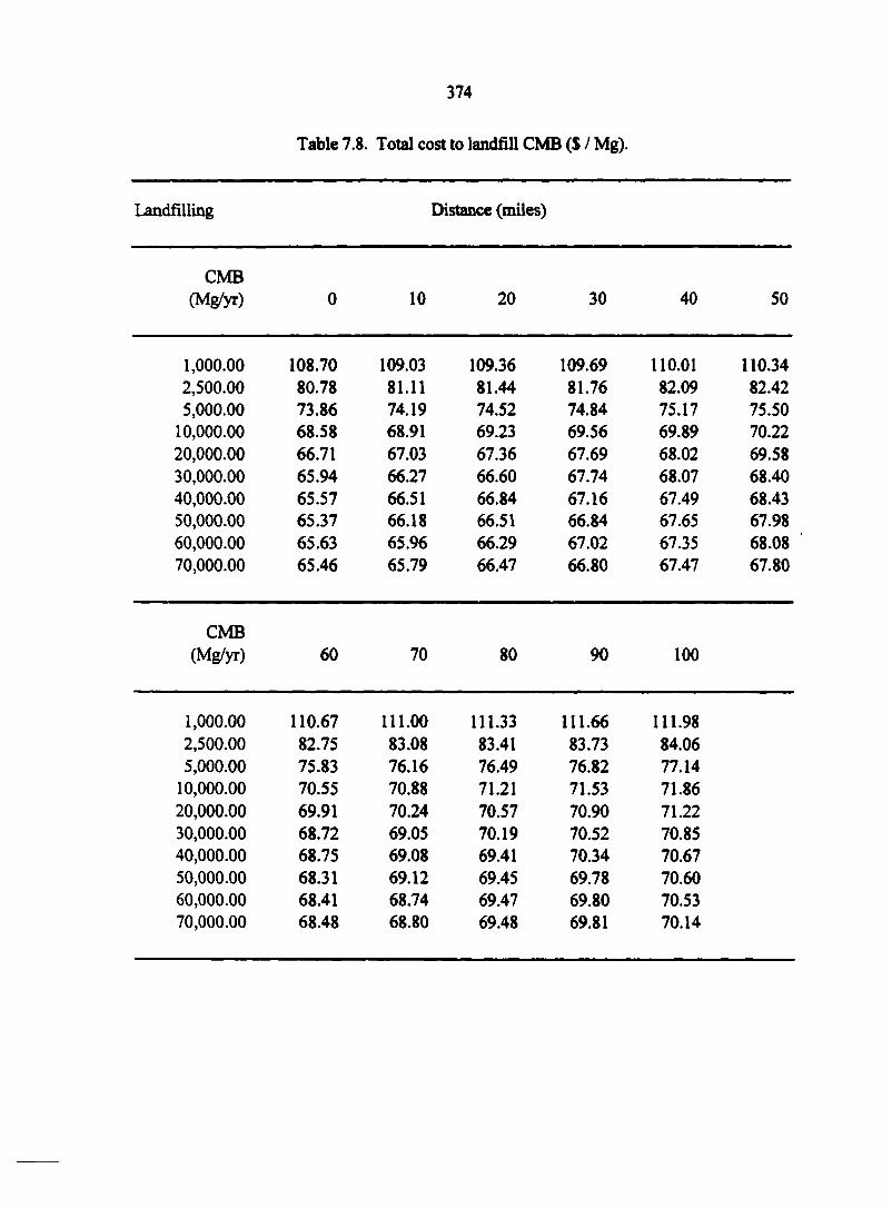
374
Table 7.8. Total cost to landfill CMB ($ / Mg).
Landfilling Distance (miles)
CMB (Mg/yr) 0 10 20 30 40 50
1,000.00 108.70 109.03 109.36 109.69 110.01 110.34 2,500.00 80.78 81.11 81.44 81.76 82.09 82.42 5,000.00 73.86 74.19 74.52 74.84 75.17 75.50
10,000.00 68.58 68.91 69.23 69.56 69.89 70.22 20,000.00 66.71 67.03 67.36 67.69 68.02 69.58 30,000.00 65.94 66.27 66.60 67.74 68.07 68.40 40,000.00 65.57 66.51 66.84 67.16 67.49 68.43 50,000.00 65.37 66.18 66.51 66.84 67.65 67.98 60,000.00 65.63 65.96 66.29 67.02 67.35 68.08 70,000.00 65.46 65.79 66.47 66.80 67.47 67.80
CMB (Mg/yr) 60 70 80 90 100
1,000.00 110.67 111.00 111.33 111.66 111.98 2,500.00 82.75 83.08 83.41 83.73 84.06 5,000.00 75.83 76.16 76.49 76.82 77.14
10,000.00 70.55 70.88 71.21 71.53 71.86 20,000.00 69.91 70.24 70.57 70.90 71.22 30,000.00 68.72 69.05 70.19 70.52 70.85 40,000.00 68.75 69.08 69.41 70.34 70.67 50,000.00 68.31 69.12 69.45 69.78 70.60 60,000.00 68.41 68.74 69.47 69.80 70.53 70,000.00 68.48 68.80 69.48 69.81 70.14
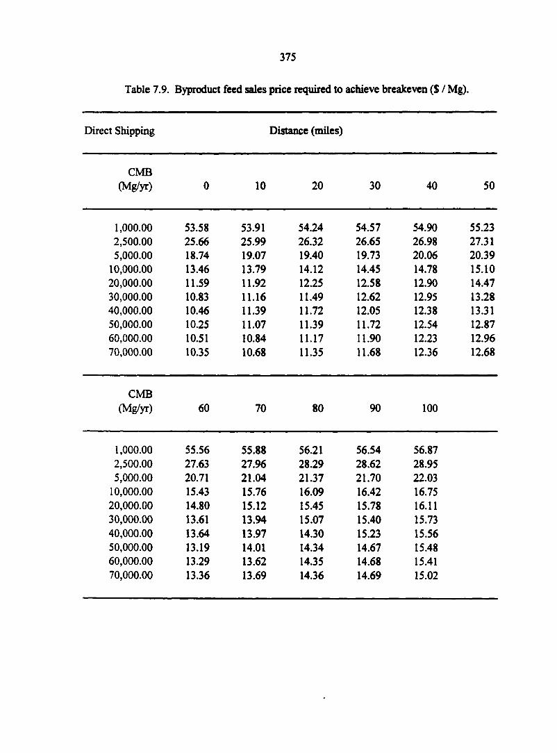
375
Table 7.9. Byproduct feed sales price required to achieve breakeven ($ / Mg).
Direct Shipping Distance (miles)
CMB (Mg/yr) 0 10 20 30 40 50
1,000.00 53.58 53.91 54.24 54.57 54.90 55.23 2,500.00 25.66 25.99 26.32 26.65 26.98 27.31 5,000.00 18.74 19.07 19.40 19.73 20.06 20.39
10,000.00 13.46 13.79 14.12 14.45 14.78 15.10 20,000.00 11.59 11.92 12.25 12.58 12.90 14.47 30,000.00 10.83 11.16 11.49 12.62 12.95 13.28 40,000.00 10.46 11.39 11.72 12.05 12.38 13.31 50,000.00 10.25 11.07 11.39 11.72 12.54 12.87 60,000.00 10.51 10.84 11.17 11.90 12.23 12.96 70,000.00 10.35 10.68 11.35 11.68 12.36 12.68
CMB (Mg/yr) 60 70 80 90 100
1,000.00 55.56 55.88 56.21 56.54 56.87 2,500.00 27.63 27.96 28.29 28.62 28.95 5,000.00 20.71 21.04 21.37 21.70 22.03
10,000.00 15.43 15.76 16.09 16.42 16.75 20,000.00 14.80 15.12 15.45 15.78 16.11 30,000.00 13.61 13.94 15.07 15.40 15.73 40,000.00 13.64 13.97 14.30 15.23 15.56 50,000.00 13.19 14.01 14.34 14.67 15.48 60,000.00 13.29 13.62 14.35 14.68 15.41 70,000.00 13.36 13.69 14.36 14.69 15.02
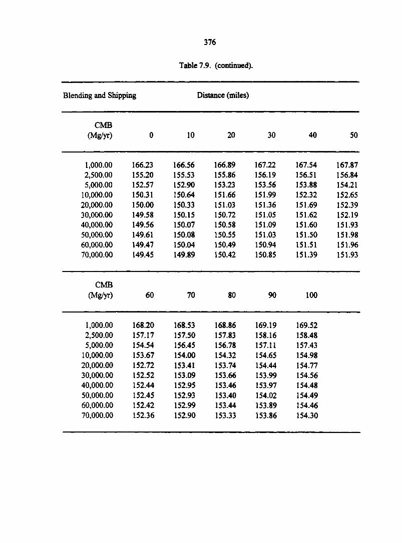
376
Table 7.9. (continued).
Blending and Shipping Distance (miles)
CMB (Mg/yr) 0 10 20 30 40 50
1,000.00 166.23 166.56 166.89 167.22 167.54 167.87 2,500.00 155.20 155.53 155.86 156.19 156.51 156.84 5,000.00 152.57 152.90 153.23 153.56 153.88 154.21
10,000.00 150.31 150.64 151.66 151.99 152.32 152.65 20,000.00 150.00 150.33 151.03 151.36 151.69 152.39 30,000.00 149.58 150.15 150.72 151.05 151.62 152.19 40,000.00 149.56 150.07 150.58 151.09 151.60 151.93 50,000.00 149.61 150.08 150.55 151.03 151.50 151.98 60,000.00 149.47 150.04 150.49 150.94 151.51 151.96 70,000.00 149.45 149.89 150.42 150.85 151.39 151.93
CMB (Mg/yr) 60 70 80 90 100
1,000.00 168.20 168.53 168.86 169.19 169.52 2,500.00 157.17 157.50 157.83 158.16 158.48 5,000.00 154.54 156.45 156.78 157.11 157.43
10,000.00 153.67 154.00 154.32 154.65 154.98 20,000.00 152.72 153.41 153.74 154.44 154.77 30,000.00 152.52 153.09 153.66 153.99 154.56 40,000.00 152.44 152.95 153.46 153.97 154.48 50,000.00 152.45 152.93 153.40 154.02 154.49 60,000.00 152.42 152.99 153.44 153.89 154.46 70,000.00 152.36 152.90 153.33 153.86 154.30
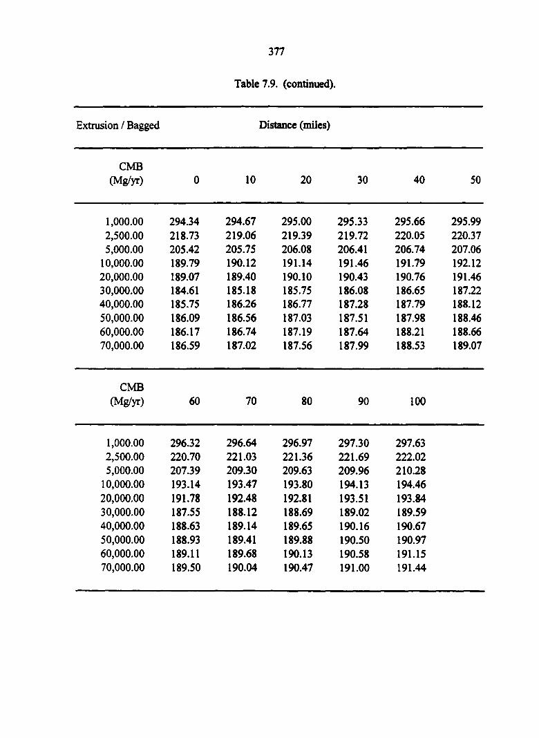
377
Table 7.9. (continued).
Extrusion / Bagged Distance (miles)
CMB (Mg/yr) 0 10 20 30 40 50
1,000.00 294.34 294.67 295.00 295.33 295.66 295.99 2,500.00 218.73 219.06 219.39 219.72 220.05 220.37 5,000.00 205.42 205.75 206.08 206.41 206.74 207.06
10,000.00 189.79 190.12 191.14 191.46 191.79 192.12 20,000.00 189.07 189.40 190.10 190.43 190.76 191.46 30,000.00 184.61 185.18 185.75 186.08 186.65 187.22 40,000.00 185.75 186.26 186.77 187.28 187.79 188.12 50,000.00 186.09 186.56 187.03 187.51 187.98 188.46 60,000.00 186.17 186.74 187.19 187.64 188.21 188.66 70,000.00 186.59 187.02 187.56 187.99 188.53 189.07
CMB (Mg/yr) 60 70 80 90 100
1,000.00 296.32 296.64 296.97 297.30 297.63 2,500.00 220.70 221.03 221.36 221.69 222.02 5,000.00 207.39 209.30 209.63 209.96 210.28
10,000.00 193.14 193.47 193.80 194.13 194.46 20,000.00 191.78 192.48 192.81 193.51 193.84 30,000.00 187.55 188.12 188.69 189.02 189.59 40,000.00 188.63 189.14 189.65 190.16 190.67 50,000.00 188.93 189.41 189.88 190.50 190.97 60,000.00 189.11 189.68 190.13 190.58 191.15 70,000.00 189.50 190.04 190.47 191.00 191.44
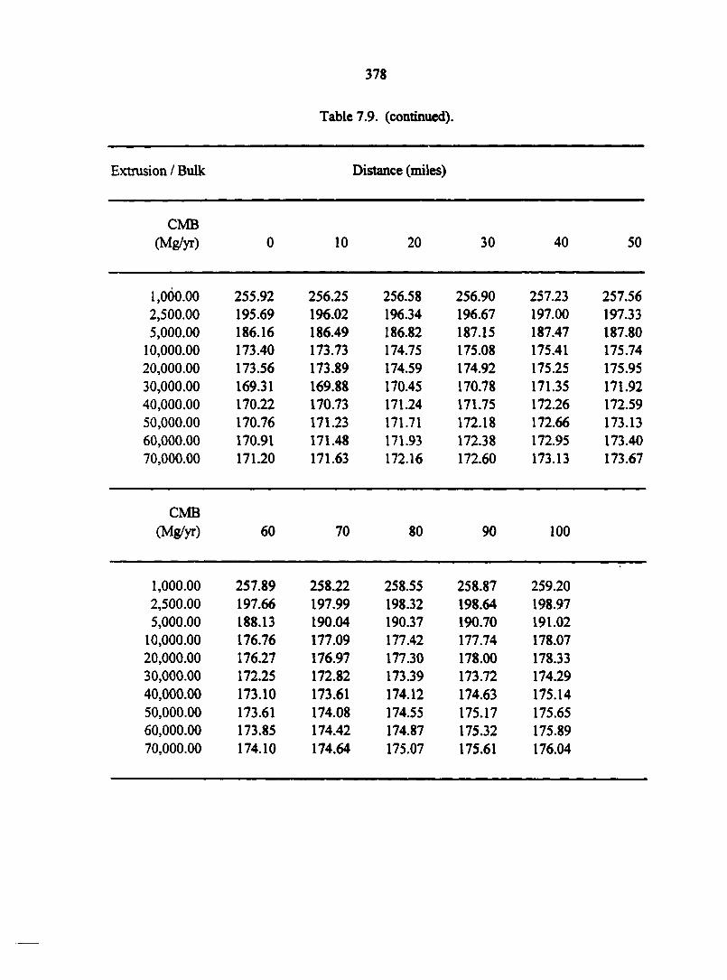
378
Table 7.9. (continued).
Extrusion / Bulk Distance (miles)
CMB (Mg/yr) 0 10 20 30 40 50
1,000.00 255.92 256.25 256.58 256.90 257.23 257.56 2,500.00 195.69 196.02 196.34 196.67 197.00 197.33 5,000.00 186.16 186.49 186.82 187.15 187.47 187.80
10,000.00 173.40 173.73 174.75 175.08 175.41 175.74 20,000.00 173.56 173.89 174.59 174.92 175.25 175.95 30,000.00 169.31 169.88 170.45 170.78 171.35 171.92 40,000.00 170.22 170.73 171.24 171.75 172.26 172.59 50,000.00 170.76 171.23 171.71 172.18 172.66 173.13 60,000.00 170.91 171.48 171.93 172.38 172.95 173.40 70,000.00 171.20 171.63 172.16 172.60 173.13 173.67
CMB (Mg/yr) 60 70 80 90 100
1,000.00 257.89 258.22 258.55 258.87 259.20 2,500.00 197.66 197.99 198.32 198.64 198.97 5,000.00 188.13 190.04 190.37 190.70 191.02
10,000.00 176.76 177.09 177.42 177.74 178.07 20,000.00 176.27 176.97 177.30 178.00 178.33 30,000.00 172.25 172.82 173.39 173.72 174.29 40,000.00 173.10 173.61 174.12 174.63 175.14 50,000.00 173.61 174.08 174.55 175.17 175.65 60,000.00 173.85 174.42 174.87 175.32 175.89 70,000.00 174.10 174.64 175.07 175.61 176.04
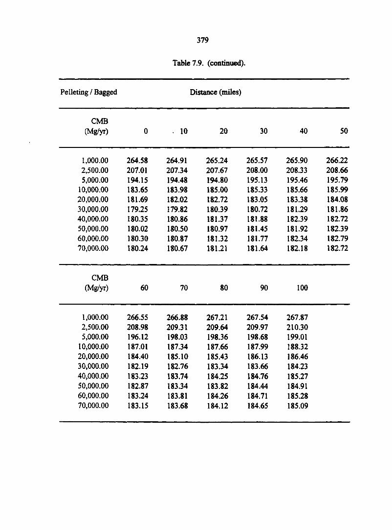
379
Table 7.9. (continued).
Pelleting / Bagged Distance (miles)
CMB (Mg/yr) 0 .10 20 30 40 50
1,000.00 264.58 264.91 265.24 265.57 265.90 266.22 2,500.00 207.01 207.34 207.67 208.00 208.33 208.66 5,000.00 194.15 194.48 194.80 195.13 195.46 195.79
10,000.00 183.65 183.98 185.00 185.33 185.66 185.99 20,000.00 181.69 182.02 182.72 183.05 183.38 184.08 30,000.00 179.25 179.82 180.39 180.72 181.29 181.86 40,000.00 180.35 180.86 181.37 181.88 182.39 182.72 50,000.00 180.02 180.50 180.97 181.45 181.92 182.39 60,000.00 180.30 180.87 181.32 181.77 182.34 182.79 70,000.00 180.24 180.67 181.21 181.64 182.18 182.72
CMB (Mg/yr) 60 70 80 90 100
1,000.00 266.55 266.88 267.21 267.54 267.87 2,500.00 208.98 209.31 209.64 209.97 210.30 5,000.00 196.12 198.03 198.36 198.68 199.01
10,000.00 187.01 187.34 187.66 187.99 188.32 20,000.00 184.40 185.10 185.43 186.13 186.46 30,000.00 182.19 182.76 183.34 183.66 184.23 40,000.00 183.23 183.74 184.25 184.76 185.27 50,000.00 182.87 183.34 183.82 184.44 184.91 60,000.00 183.24 183.81 184.26 184.71 185.28 70,000.00 183.15 183.68 184.12 184.65 185.09
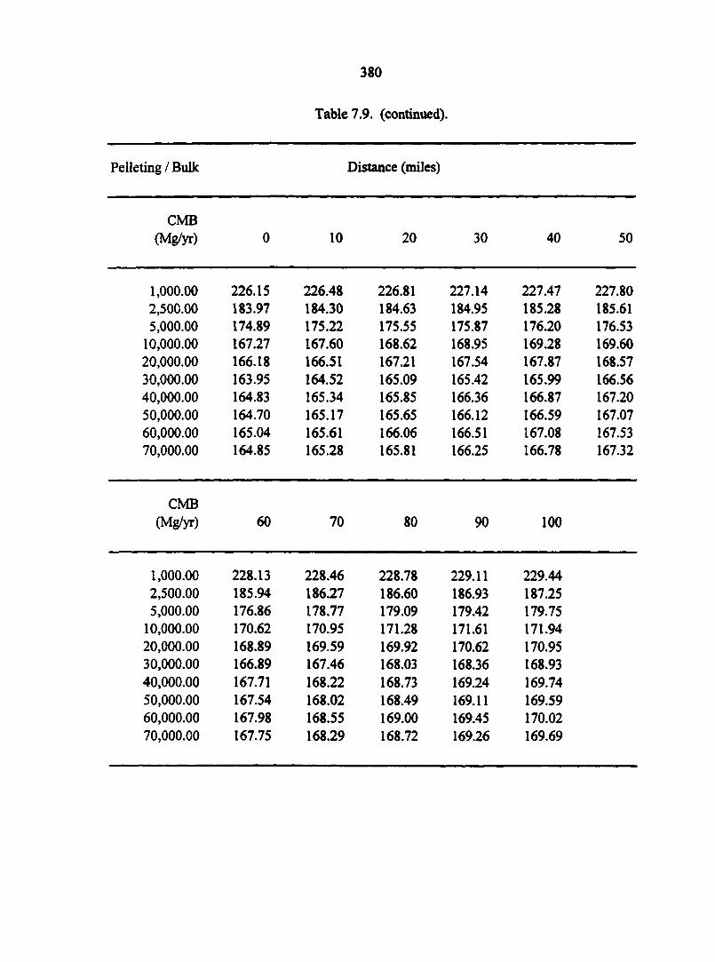
380
Pelleting / Bulk
Table 7.9. (continued).
Distance (miles)
CMB (Mg/yr) 0 10 20 30 40 50
1,000.00 226.15 226.48 226.81 227.14 227.47 227.80 2,500.00 183.97 184.30 184.63 184.95 185.28 185.61 5,000.00 174.89 175.22 175.55 175.87 176.20 176.53
10,000.00 167.27 167.60 168.62 168.95 169.28 169.60 20,000.00 166.18 166.51 167.21 167.54 167.87 168.57 30,000.00 163.95 164.52 165.09 165.42 165.99 166.56 40,000.00 164.83 165.34 165.85 166.36 166.87 167.20 50,000.00 164.70 165.17 165.65 166.12 166.59 167.07 60,000.00 165.04 165.61 166.06 166.51 167.08 167.53 70,000.00 164.85 165.28 165.81 166.25 166.78 167.32
CMB (Mg/yr) 60 70 80 90 100
1,000.00 228.13 228.46 228.78 229.11 229.44 2,500.00 185.94 186.27 186.60 186.93 187.25 5,000.00 176.86 178.77 179.09 179.42 179.75
10,000.00 170.62 170.95 171.28 171.61 171.94 20,000.00 168.89 169.59 169.92 170.62 170.95 30,000.00 166.89 167.46 168.03 168.36 168.93 40,000.00 167.71 168.22 168.73 169.24 169.74 50,000.00 167.54 168.02 168.49 169.11 169.59 60,000.00 167.98 168.55 169.00 169.45 170.02 70,000.00 167.75 168.29 168.72 169.26 169.69
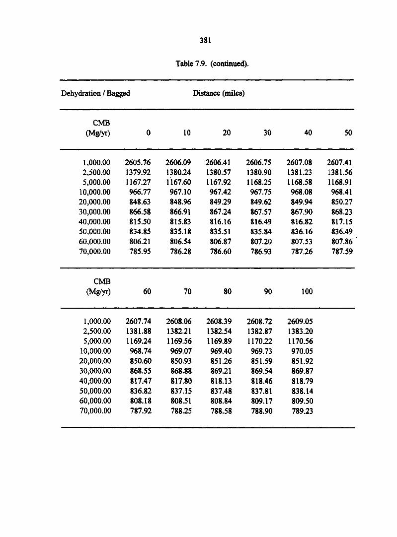
381
Table 7.9. (continued).
Dehydration / Bagged Distance (miles)
CMB (Mg/yr) 0 10 20 30 40 50
1,000.00 2605.76 2606.09 2606.41 2606.75 2607.08 2607.41 2,500.00 1379.92 1380.24 1380.57 1380.90 1381.23 1381.56 5,000.00 1167.27 1167.60 1167.92 1168.25 1168.58 1168.91
10,000.00 966.77 967.10 967.42 967.75 968.08 968.41 20,000.00 848.63 848.96 849.29 849.62 849.94 850.27 30,000.00 866.58 866.91 867.24 867.57 867.90 868.23 40,000.00 815.50 815.83 816.16 816.49 816.82 817.15 50,000.00 834.85 835.18 835.51 835.84 836.16 836.49 60,000.00 806.21 806.54 806.87 807.20 807.53 807.86 70,000.00 785.95 786.28 786.60 786.93 787.26 787.59
CMB (Mg/yr) 60 70 80 90 100
1,000.00 2607.74 2,500.00 1381.88 5,000.00 1169.24
10,000.00 968.74 20,000.00 850.60 30,000.00 868.55 40,000.00 817.47 50,000.00 836.82 60,000.00 808.18 70,000.00 787.92
2608.06 2608.39 1382.21 1382.54 1169.56 1169.89 969.07 969.40 850.93 851.26 868.88 869.21 817.80 818.13 837.15 837.48 808.51 808.84 788.25 788.58
2608.72 2609.05 1382.87 1383.20 1170.22 1170.56 969.73 970.05 851.59 851.92 869.54 869.87 818.46 818.79 837.81 838.14 809.17 809.50 788.90 789.23
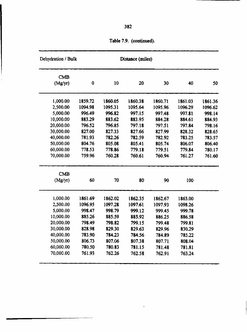
382
Table 7.9. (continued).
Dehydration / Bulk Distance (miles)
CMB (Mg/yr) 0 10 20 30 40 50
1,000.00 1859.72 1860.05 1860.38 1860.71 1861.03 1861.36 2,500.00 1094.98 1095.31 1095.64 1095.96 1096.29 1096.62 5,000.00 996.49 996.82 997.15 997.48 997.81 998.14
10,000.00 883.29 883.62 883.95 884.28 884.61 884.93 20,000.00 796.52 796.85 797.18 797.51 797.84 798.16 30,000.00 827.00 827.33 827.66 827.99 828.32 828.65 40,000.00 781.93 782.26 782.59 782.92 783.25 783.57 50,000.00 804.76 805.08 805.41 805.74 806.07 806.40 60,000.00 778.53 778.86 779.18 779.51 779.84 780.17 70,000.00 759.96 760.28 760.61 760.94 761.27 761.60
CMB (Mg/yr) 60 70 80 90 100
1,000.00 1861.69 1862.02 1862.35 1862.67 1863.00 2,500.00 1096.95 1097.28 1097.61 1097.93 1098.26 5,000.00 998.47 998.79 999.12 999.45 999.78
10,000.00 885.26 885.59 885.92 886.25 886.58 20,000.00 798.49 798.82 799.15 799.48 799.81 30,000.00 828.98 829.30 829.63 829.96 830.29 40,000.00 783.90 784.23 784.56 784.89 785.22 50,000.00 806.73 807.06 807.38 807.71 808.04 60,000.00 780.50 780.83 781.15 781.48 781.81 70,000.00 761.93 762.26 762.58 762.91 763.24
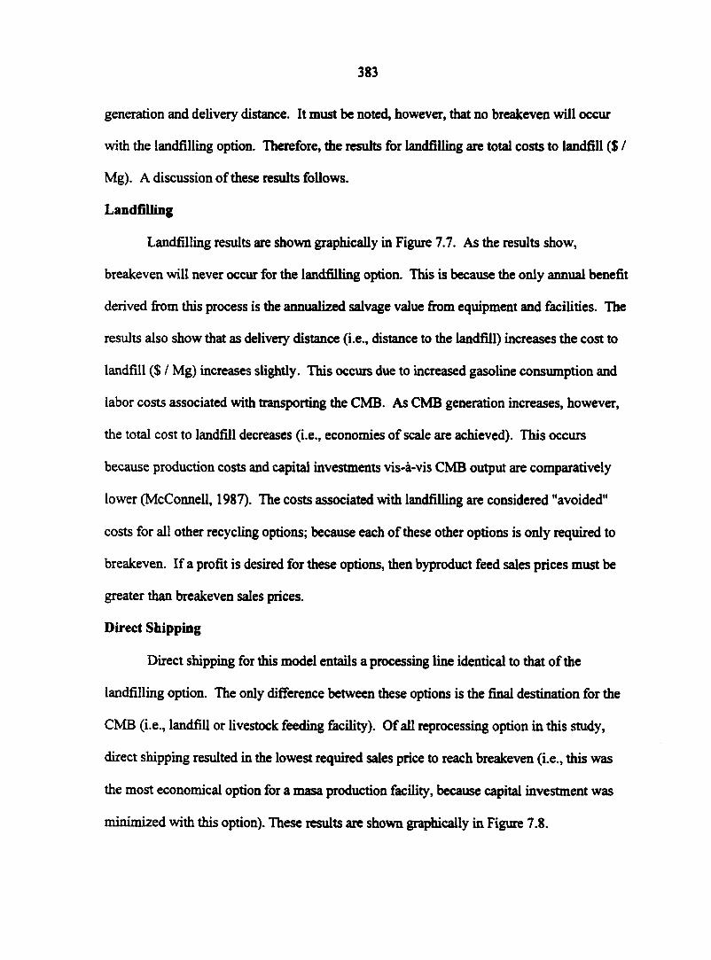
383
generation and delivery distance. It must be noted, however, that no breakeven will occur
with the landfilling option. Therefore, the results for landfilling are total costs to landfill ($ /
Mg). A discussion of these results follows.
Landfilling
Landfilling results are shown graphically in Figure 7.7. As the results show,
breakeven will never occur for the landfilling option. This is because the only annual benefit
derived from this process is the annualized salvage value from equipment and facilities. The
results also show that as delivery distance (i.e., distance to the landfill) increases the cost to
landfill ($ / Mg) increases slightly. This occurs due to increased gasoline consumption and
labor costs associated with transporting the CMB. As CMB generation increases, however,
the total cost to landfill decreases (i.e., economies of scale are achieved). This occurs
because production costs and capital investments vis-à-vis CMB output are comparatively
lower (McConnell, 1987). The costs associated with landfilling are considered "avoided"
costs for all other recycling options; because each of these other options is only required to
breakeven. If a profit is desired for these options, then byproduct feed sales prices must be
greater than breakeven sales prices.
Direct Shipping
Direct shipping for this model entails a processing line identical to that of the
landfilling option. The only difference between these options is the final destination for the
CMB (i.e., landfill or livestock feeding facility). Of all reprocessing option in this study,
direct shipping resulted in the lowest required sales price to reach breakeven (i.e., this was
the most economical option for a masa production facility, because capital investment was
minimized with this option). These results are shown graphically in Figure 7.8.
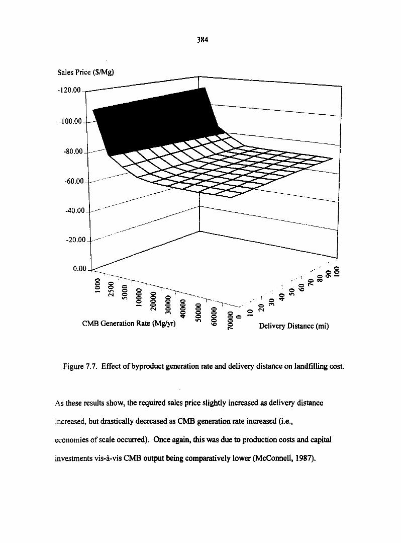
384
Sales Price ($/Mg)
-120.00
-100.00
-80.00
-60.00
-40.00
0.00
© 00
s " l l î (N O fi
CMB Generation Rate (Mg/yr)
©
= 8 " 8 O
Delivery Distance (mi)
Figure 7.7. Effect of byproduct generation rate and delivery distance on landfilling cost.
As these results show, the required sales price slightly increased as delivery distance
increased, but drastically decreased as CMB generation rate increased (i.e.,
economies of scale occurred). Once again, this was due to production costs and capital
investments vis-à-vis CMB output being comparatively lower (McConnell, 1987).
385
Sales Price ($/Mg)
60.00
50.00-1
40.00
30.00
20.00-1
10.00
0.00
CMB Generation Rate (Mg/yr) so © Delivery Distance (mi)
Figure 7.8. Effect of byproduct generation rate and delivery distance on byproduct sales price for direct shipping option.
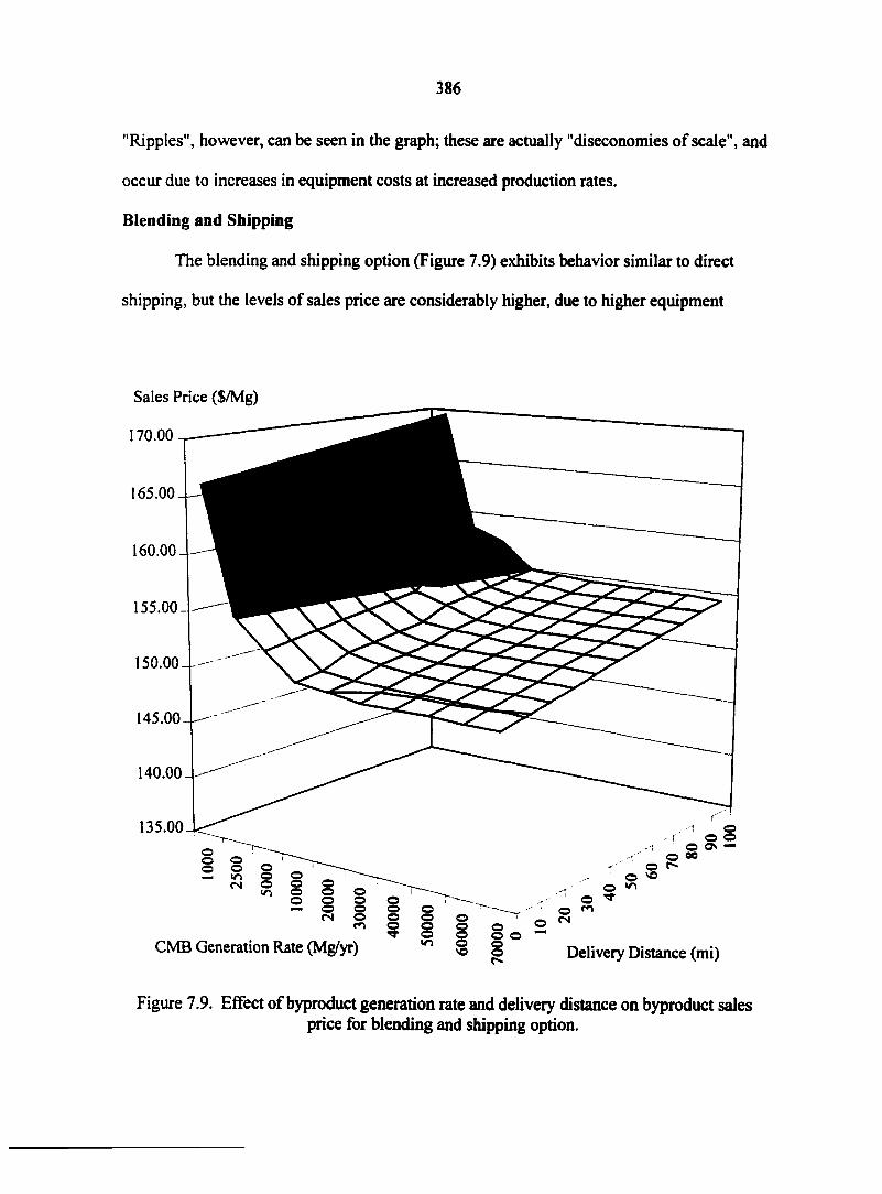
386
"Ripples", however, can be seen in the graph; these are actually "diseconomies of scale", and
occur due to increases in equipment costs at increased production rates.
Blending and Shipping
The blending and shipping option (Figure 7.9) exhibits behavior similar to direct
shipping, but the levels of sales price are considerably higher, due to higher equipment
Sales Price ($/Mg)
170.00
160.00
155.00-
150.00--
145.00
140.00
135.00
O «>
o ^
CMB Generation Rate (Mg/yr) Delivery Distance (mi)
Figure 7.9. Effect of byproduct generation rate and delivery distance on byproduct sales price for blending and shipping option.
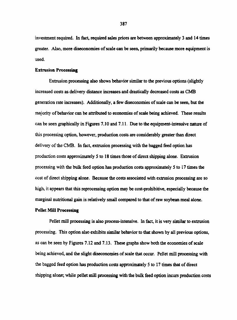
387
investment required. In fact, required sales prices are between approximately 3 and 14 times
greater. Also, more diseconomies of scale can be seen, primarily because more equipment is
used.
Extrusion Processing
Extrusion processing also shows behavior similar to the previous options (slightly
increased costs as delivery distance increases and drastically decreased costs as CMB
generation rate increases). Additionally, a few diseconomies of scale can be seen, but the
majority of behavior can be attributed to economies of scale being achieved. These results
can be seen graphically in Figures 7.10 and 7.11. Due to the equipment-intensive nature of
this processing option, however, production costs are considerably greater than direct
delivery of the CMB. In fact, extrusion processing with the bagged feed option has
production costs approximately 5 to 18 times those of direct shipping alone. Extrusion
processing with the bulk feed option has production costs approximately 5 to 17 times the
cost of direct shipping alone. Because the costs associated with extrusion processing are so
high, it appears that this reprocessing option may be cost-prohibitive, especially because the
marginal nutritional gain is relatively small compared to that of raw soybean meal alone.
Pellet Mill Processing
Pellet mill processing is also process-intensive. In fact, it is very similar to extrusion
processing. This option also exhibits similar behavior to that shown by all previous options,
as can be seen by Figures 7.12 and 7.13. These graphs show both the economies of scale
being achieved, and the slight diseconomies of scale that occur. Pellet mill processing with
the bagged feed option has production costs approximately 5 to 17 times that of direct
shipping alone; while pellet mill processing with the bulk feed option incurs production costs
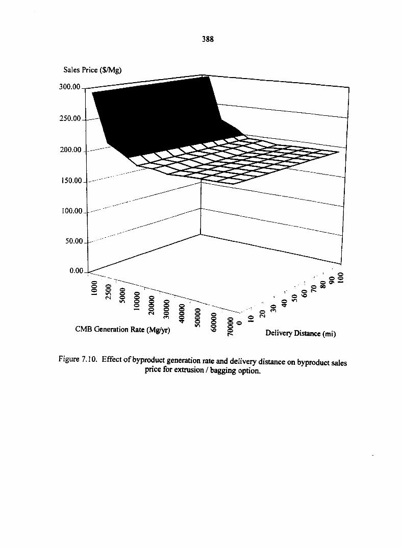
388
Sales Price ($/Mg)
300.00
250.00
200.00
150.00
CMB Generation Rate (Mg/yr) Delivery Distance (mi)
Figure 7.10. Effect of byproduct generation rate and delivery distance on byproduct sales price for extrusion / bagging option.
389
Sales Price ($/Mg)
300.00
250.00
200.00
150.00
100.00
50.00-
0.00 r o © o S '
... . O V
(N <5 ô d o ̂" l o o ® ' 5 I 1° "
CMB Generation Rate (Mg/yr) ° Delivery Distance (mi)
Figure 7.11. Effect of byproduct generation rate and delivery distance on byproduct sales price for extrusion / bulk option.
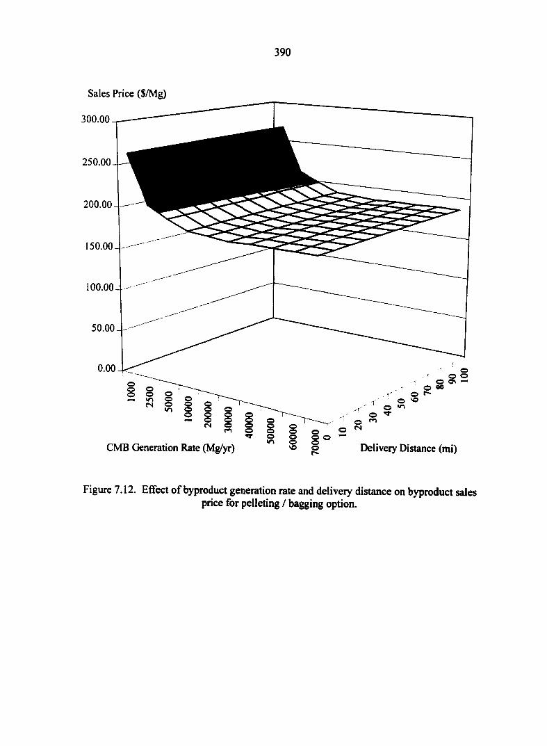
390
Sales Price ($/Mg)
300.00
250.00
200.00
150.00-
100.00-
50.00-
0.00
CMB Generation Rate (Mg/yr) Delivery Distance (mi)
Figure 7.12. Effect of byproduct generation rate and delivery distance on byproduct sales price for pelleting / bagging option.
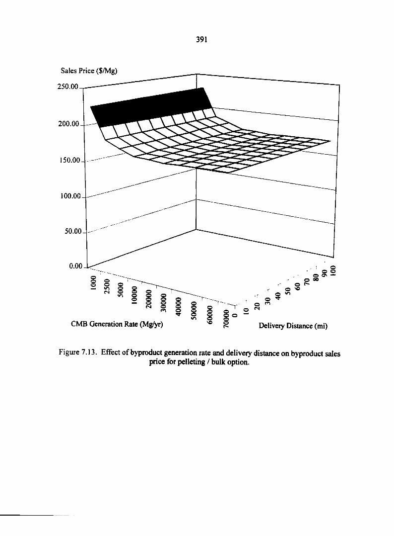
391
Sales Price ($/Mg)
250.00
200.00
150.00 J
100.004
50.004
0.00
CMB Generation Rate (Mg/yr) Delivery Distance (mi)
Figure 7.13. Effect of byproduct generation rate and delivery distance on byproduct sales price for pelleting / bulk option.
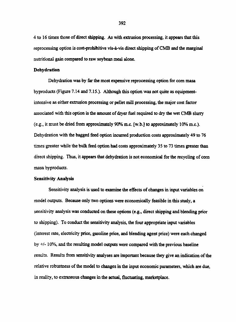
392
4 to 16 times those of direct shipping. As with extrusion processing, it appears that this
reprocessing option is cost-prohibitive vis-à-vis direct shipping of CMB and the marginal
nutritional gain compared to raw soybean meal alone.
Dehydration
Dehydration was by far the most expensive reprocessing option for corn masa
byproducts (Figure 7.14 and 7.15.). Although this option was not quite as equipment-
intensive as either extrusion processing or pellet mill processing, the major cost factor
associated with this option is the amount of dryer fuel required to dry the wet CMB slurry
(e.g., it must be dried from approximately 90% m.c. [w.b.] to approximately 10% m.c.).
Dehydration with the bagged feed option incurred production costs approximately 49 to 76
times greater while the bulk feed option had costs approximately 35 to 73 times greater than
direct shipping. Thus, it appears that dehydration is not economical for the recycling of corn
masa byproducts.
Sensitivity Analysis
Sensitivity analysis is used to examine the effects of changes in input variables on
model outputs. Because only two options were economically feasible in this study, a
sensitivity analysis was conducted on these options (e.g., direct shipping and blending prior
to shipping). To conduct the sensitivity analysis, the four appropriate input variables
(interest rate, electricity price, gasoline price, and blending agent price) were each changed
by +/-10%, and the resulting model outputs were compared with the previous baseline
results. Results from sensitivity analyses are important because they give an indication of the
relative robustness of the model to changes in the input economic parameters, which are due,
in reality, to extraneous changes in the actual, fluctuating, marketplace.
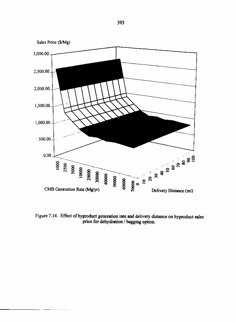
393
Sales Price ($/Mg)
3,000.00
2,500.00-
2,000.00
1,500.00
1,000.00
500.00
0.00
CMB Generation Rate (Mg/yr) Delivery Distance (mi)
Figure 7.14. Effect of byproduct generation rate and delivery distance on byproduct sales price for dehydration / bagging option.
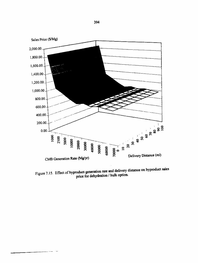
394
Sales Price ($/Mg)
2,000.00
1,800.00
1,600.00
1,400.00
1,200.00
1,000.00-
800.00
600.00
400.00
200.00-
CMB Generation Rate (Mg/yr) Delivery Distance (mi)
Figure 7.15. Effect of byproduct generation rate and delivery distance on byproduct sales price for dehydration / bulk option.
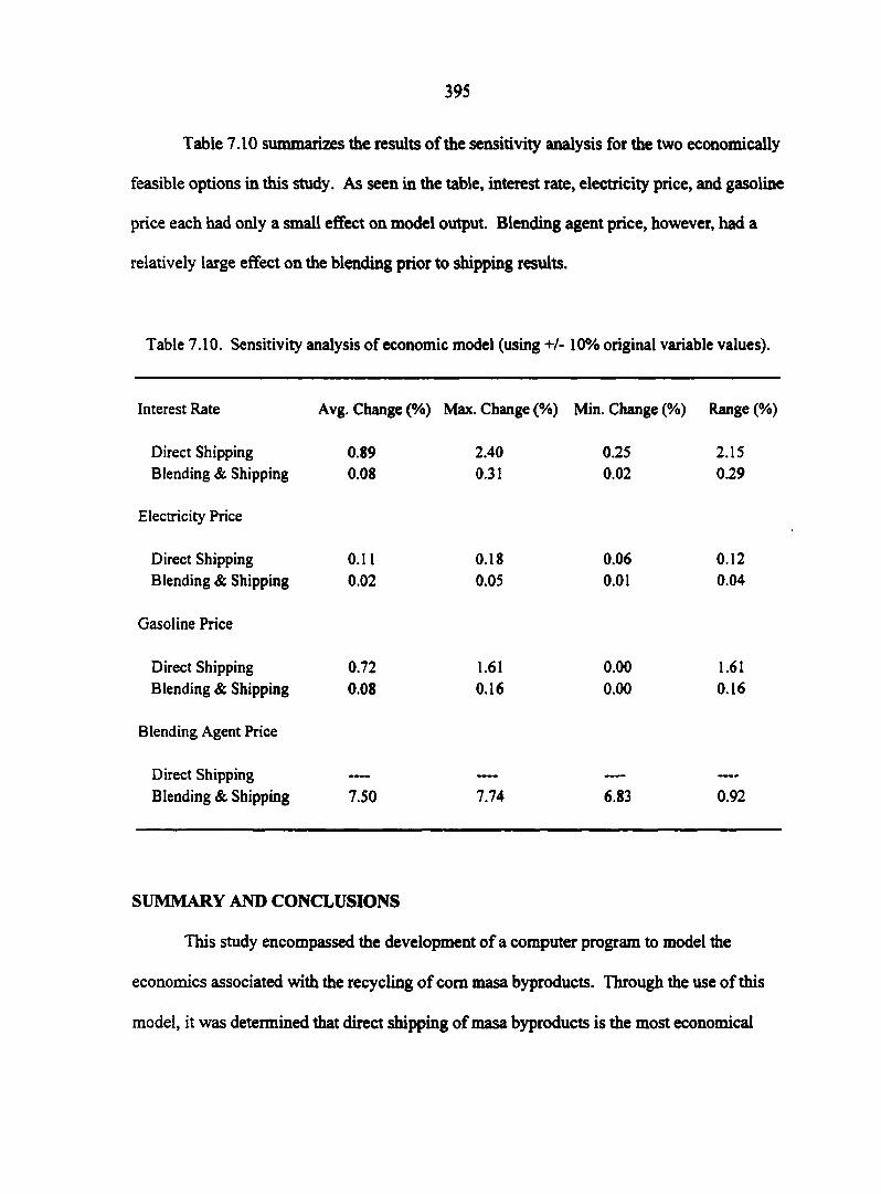
395
Table 7.10 summarizes the results of the sensitivity analysis for the two economically
feasible options in this study. As seen in the table, interest rate, electricity price, and gasoline
price each had only a small effect on model output. Blending agent price, however, had a
relatively large effect on the blending prior to shipping results.
Table 7.10. Sensitivity analysis of economic model (using +/-10% original variable values).
Interest Rate Avg. Change (%) Max. Change (%) Min. Change (%) Range (%)
Direct Shipping 0.89 2.40 0.25 2.15 Blending & Shipping 0.08 0.31 0.02 0.29
Electricity Price
Direct Shipping 0.11 0.18 0.06 0.12 Blending & Shipping 0.02 0.05 0.01 0.04
Gasoline Price
Direct Shipping 0.72 1.61 0.00 1.61 Blending & Shipping 0.08 0.16 0.00 0.16
Blending Agent Price
Direct Shipping — — — — Blending & Shipping 7.50 7.74 6.83 0.92
SUMMARY AND CONCLUSIONS
This study encompassed the development of a computer program to model the
economics associated with the recycling of com masa byproducts. Through the use of this
model, it was determined that direct shipping of masa byproducts is the most economical
396
choice for the com masa manufacturer. Blending masa byproducts with soybean meal is a
more expensive recycling option, although still economically feasible, while extrusion
processing and pellet mill processing are substantially more expensive, and thus, these
options are cost-prohibitive. Furthermore, dehydration is much too expensive to justify
economically.
With regard to the blending, extrusion, and pelleting options, because CMB is
approximately 90% water, even at a blending ratio of 30% CMB / 70% SBM, the addition of
CMB to SBM alters the nutrient makeup of the soybean meal only minutely (i.e., only 3% of
the blend's solids originate from the CMB). Thus, the byproduct feed is essentially soybean
meal (i.e., for all practical purposes). It appears that blending and delivery may be
economically feasible, because it only adds $19.52/ton (at most) to the original cost of
soybean meal ($ 150.00/ton). Extrusion adds a maximum cost of $109.20/ton (bulk feed) and
$147.63/ton (bagged feed), while pelleting adds a maximum cost of $79.44/ton (bulk) and
$ 117.87/ton (bagged) over the original cost of the soybean meal ($150.00/ton). Thus, the
increase in cost utilizing extrusion and pelleting is exorbitant vis-à-vis the nutrient gain by
processing the soybean meal with CMB.
Therefore, it appears that the most economically feasible recycling option for com
masa byproducts is direct delivery, but, blending and shipping are also feasible, just
somewhat more costly. Both options should be studied further in a real setting. It appears,
however, that the extrusion, pelleting, and dehydration options are too cost prohibitive to
implement.
The intent of this project was to examine the economics associated with the
development of a livestock feed ingredient produced from corn masa processing byproducts.
397
Because the scope was limited to the production of a single feed ingredient only, the
development of an entire feed ration for a particular animal species is left to future work, and
will entail the incorporation of corn, vitamins, minerals, etc., and will require feeding trials
before the effectiveness of this type of feed ration is known.
It should be noted that the price of soybean meal, as with all other agricultural
commodities, fluctuates drastically over time (TFC, 2000). Consequently, these changes will
need to be taken into consideration, and can be easily inputted into this model to
accommodate these price changes, and should shift the results slightly up or down the price
scale, but the behavior exhibited should remain the same: recycling costs increase as
delivery distance increases, and costs decrease as masa production capacity increases.
ACKNOWLEDGMENTS
The authors would like to acknowledge those whose help was essential for the
completion of this project, especially that of K. P. Rosentrater, for assistance with the
economic analysis, and various equipment vendors, for willingness to provide equipment
information and costs.
REFERENCES
Ackerman, F. 1997. Recycling: Looking beyond the bottom line. BioCycle (May): 67-70.
Annexstad, R. J., M. D. Stem, D. E. Otterby, J. G. Linn, and W. P. Hansen. 1987. Extruded soybeans and com gluten meal as supplemental protein sources for lactating dairy cattle. Journal of Dairy Science 70(4): 814-822.
Bandoni, J. A., E. Rotstein, and J. A. Romagnoli. 1988. Simulation modelling and optimal operation of an apple juice concentrate plant Journal of Food Engineering 7(3): 159-175.
Barbosa-Canovas, G. V. and H. Vega-Mercado. 1996. Dehydration of Foods. New York, NY: International Thomson Publishing.
398
Beauchat, L. R. 1981. Microbial stability as affected by water activity. Cereal Foods World 26(7): 345-349.
Beers, A. R. and T. J. Getz. 1992. Composting biosolids saves $3.3 million in landfill costs. BioCycle 33(5): 42,76-77.
Bern, C.J. 1999. Electricity for Agricultural Applications - AST 360/AE 363. Ames, IA: Iowa State University Book Store CourseWorks.
Blank, L. T. and A. J. Tarquin. 1989. Engineering Economy. New York, NY: McGraw-Hill, Inc.
Bohlsen, D., S. Weeder, and S. Wang. 1997. Tracking organic waste. Resource 4(9): 13-14.
Bressani, R., R. Paz y Paz, and N. S. Scrimshaw. 1958. Corn nutrient losses: chemical changes in corn during preparation of tortillas. Journal of Agricultural and Food Chemistry 6(10): 770-774.
Cornelius, S. G., J. P. Totsch, and B. G. Harmon. 1973. Metabolizable energy of DSLC for swine. Journal of Animal Science 37: 277.
Criner, G. K. 1987. Economic feasibility of anaerobic digesters. BioCycle (February): 51-53.
Criner, G. K. 1991. Anaerobic treatment of food wastes. BioCycle (April): 80-83.
Department of Labor. 2000. Minimum wage laws in the states. United States Department of Labor. Available online: www.dol.gov/dol/esa/public/minwage/america.html [August 19,2000].
Derr, D. A. and P. S. Dhillon. 1997. The economics of recycling food residuals. BioCycle 38(4): 55-56.
Edwards. J. H., R. H. Walker, E. A. Guertal, L. D. Norton, and J. T. Eason. 1994. Options for recycling organics on farm land. BioCycle 35(11): 66-68.
EIA. 2000a. August 2000. Energy Information Administration. Available online: www.eia.doe.gov/emeu/steo/pub/steotexthtml#prices [August 19,2000].
EIA. 2000b. Iowa. Energy Information Administration. Available online: www.eia.doe.gov/cneaf7electricity/st profiles/iowa/ia.html [August 19,2000],
EIA. 2000c. United States. Energy Information Administration. Available online: www.eia.doe.gov/cneagelectricity/st profiles/us/us.html [August 19,2000].
399
Fairchild, F. J. 1985a. Conveyors. In Feed Manufacturing Technology III, ed. R. R. McEllhiney, Ch. 8, 66-82. Arlington, VA: American Feed Industry Association.
Fairchild, F. J. 1985b. Bucket elevators. In Feed Manufacturing Technology III, ed. R. R. McEllhiney, Ch. 9, 83-87. Arlington, VA: American Feed Industry Association.
Federal Reserve. 2000. Federal funds daily rates. Federal Reserve Bank of New York. Available online: www.ny.frb.org/pihome/statistics/dlyrates.htnil [August 19,2000].
Ferris, D. A., R. A. Flores, C. W. Shanklin, and M. K. Whitworth. 1995. Proximate analysis of food service wastes. Applied Engineering in Agriculture 11(4): 567-572.
Flores. R. A. 1998. Making agricultural leftovers more palatable. Resource 5(4): 13-14.
Flores, R. A., E. S. Posner, G. A. Milliken, and C. W. Deyoe. 1991. Modeling the milling of hard red winter wheat: Estimation of cumulative ash and protein recovery. Transactions of the ASAE 34(5): 2117-2122.
Flores, R. A., E. S. Posner, R. Phillips, and C. W. Deyoe. 1993. Modeling the economic evaluation of wheat flour milling operations. Transactions of the ASAE 36(4): 1143-1149.
Forste, J. B. 1987. Complying with land application regulations. BioCycle (October): 49-53.
Glatz, B. A., M. D. Floetenmeyer, and E. G. Hammond. 1985. Fermentation of bananas and other food wastes to produce microbial lipid. Journal of Food Protection 48(7): 574-577.
Glenn, J. 1997. Marketing food residuals as animal feed. BioCycle 38(4): 43-50.
Godfrey, T. 1983. Effluent, byproduct and biogas. In Industrial Enzymology: The Application of Enzymes in Industry, ed. T. Godfrey and J. Reichelt, 294-304. New York, NY: Nature Press.
Goldstein, N. 1992. Composting the commercial organic stream. BioCycle 33(5): 46-52.
Golueke, C. G. 1992. Bacteriology of composting. BioCycle (January): 55-57.
Gomez, M. H., L. W. Rooney, R. D. Waniska, and R. L. Pflugfelder. 1987. Dry com masa flours for tortilla and snack food production. Cereal Foods World 32(5): 372-377.
Gonzalez de Palacios, M. 1980. Characteristics of corn and sorghum for tortilla processing. Unpublished M.S. Thesis. College Station, TX: Texas A&M University.
400
Gonzalez-Martinez, S. 1984. Biological treatability of the wastewaters from the alkaline cooking of maize (Indian corn). Environmental Technology Letters 5(8): 365-372.
Gunjal, K., M. Owusu-Manu, H. S. Ramaswamy, and F. Amankwah. 1999. Minimal processing of fish and pork in Quebec: A financial feasibility study. Canadian Agricultural Engineering 41(4): 247-251.
Ham, G. A., R. A. Stock, T. J. Klopfenstein, and R. P. Huffman. 1995. Determining the net energy value of wet and dry corn gluten feed in beef growing and finishing diets. Journal of Animal Science 73(2): 353-359.
Harrison, E. Z., M. McBride, B. Richards, and T. Steenhuis. 1998. Sludge effects on land: A case for caution. Resource (September): 11-12.
HSH Associates. 2000. ARM indices: The prime rate. HSH Associates, Financial Publishers. Available online: www.hsh.com/indices/prime.html [August 19,2000].
Huang, W. 1979. A framework for economic analysis of livestock and crop byproducts utilization. American Journal of Agricultural Economics 61(1): 91-96.
Hussein, H. S. and L. L. Berger. 1995. Effects of feed intake and dietary level of wet corn gluten feed on feedlot performance, digestibility of nutrients, and carcass characteristics of growing-finishing beef heifers. Journal of Animal Science 73: 3246.
Hyde, M. A. and G. A. Consolazio. 1982. Composting of food processing waste sludges. BioCycle 23(1): 58-60.
Johnson, M. and W.L.Carlson. 1991. Calculating volume-based garbage fees. BioCycle (February): 48-50.
Jones, B.J. 1992. Composting food and vegetative waste. BioCycle (March): 69-71.
Kashmanian, R.M., D. Kluchinski, T. L. Richard, and J. M. Walker. 2000. Quantities, Characteristics, Barriers, and Incentives for Use of Organic Municipal By-products, pp. 127-167. In: Land Application of Agricultural, Industrial, and Municipal Byproducts. J. F. Power and W. A. Dick (Editors). Soil Science Society of America. Madison, WI. 653 p.
Katz, S. H., M. L. Hediger, and L. A. Valleroy. 1974. Traditional maize processing techniques in the New World. Science 184(4138): 765-773.
Khan, M. N., M. C. Des Rosiers, L. W. Rooney, R. G. Morgan, and V. E. Sweat 1982. Com tortillas: evaluation of com cooking procedures. Cereal Chemistry 59(4): 279-284.
401
Krause, V. M., K. L. Tucker, H. V. Kuhnlein, C. Y. Lopez-Palacios, M. Ruz, and N. W. Solomons. 1992. Rural-urban variation in limed maize use and tortilla consumption by women in Guatemala. Ecology of Food and Nutrition 28(4): 279-288.
Kuchenrither, R. D., W. J. Martin, D. G. Smith, and P. J. Psaris. 1984. An economic comparison of composting and dual utilization. BioCycle 25(5): 33-37.
Lahey Computer Systems, Inc. 1995. LP77 Personal FORTRAN v. 3.00. Incline Village, NV: Lahey Computer Systems, Inc.
Larson, E. M., R. A. Stock, T. J. Klopfenstein, J. H. Sindt, and R. P. Huffman. 1993. Feeding value of wet distillers' byproducts for finishing ruminants. Journal of Animal Science 71(8): 2228-2236.
Liu, M. C., R. A. Flores, C. W. Deyoe, and E. S. Posner. 1992. Assessment of a computer simulation model for the flour-milling industry. Cereal Foods World 37(8): 649-654.
Lodge, S. L., R. A. Stock, T. J. Klopfenstein, D. H. Shain, and D. W. Herald. 1997. Evaluation of com and sorghum distillers byproducts. Journal of Animal Science 74(1): 37-43.
Logsdon, G. 1992. Pomace is a grape resource. BioCycle 33(2): 40-41.
Lunemann, R. J. 1985. Plant feasibility, design, and construction. In Feed Manufacturing Technology III, ed. R. R. McEllhiney, Ch. 4,22-26. Arlington, VA: American Feed Industry Association.
Luzier, J. M. and R. C. Summerfelt. 1995. Partial replacement of fish meal with spray-dried blood powder to reduce phosphorous concentrations in diets for juvenile rainbow trout, Oncorhynchus mykiss (Walbaum). Aquaculture Research 26(8): 577.
Martins, S. N. and E. C. Guzman. 1994. Effect of drying method of bovine blood on the performance of growing for tambaqui (Colossoma macropomum, Curier 1818) in experimental culture tanks. Aquaculture 124(l-4):335-341.
McConnell, C. R. 1987. Economics Principles, Problems, and Policies. New York, NY: McGraw-Hill Book Company.
McEllhiney, R. R. 1985. Feed Manufacturing Technology III. Arlington, VA: American Feed Industry Association.
McEllhiney, R. R. 1985a. Warehousing and loading. In Feed Manufacturing Technology III, ed. R. R. McEllhiney, Ch. 21,209-215. Arlington, VA: American Feed Industry Association.
402
McEllhiney, R. R. 1985b. Energy cost centers. In Feed Manufacturing Technology III, ed. R. R. McEllhiney, Ch. 49,414-418. Arlington, VA: American Feed Industry Association.
McEllhiney, R. R. 1985c. Planning and budgeting. In Feed Manufacturing Technology III, ed. R. R. McEllhiney, Ch. 58,470-476. Arlington, VA: American Feed Industry Association.
McEllhiney, R. R. 1985d. Manufacturing cost control. In Feed Manufacturing Technology III, ed. R. R. McEllhiney, Ch. 59,477-485. Arlington, VA: American Feed Industry Association.
McEllhiney, R. R. 1985e. Product costing. In Feed Manufacturing Technology 111, ed. R. R. McEllhiney, Ch. 60,486-490. Arlington, VA: American Feed Industry Association.
McEllhiney, R. R. 1985f. Inventory control. In Feed Manufacturing Technology III, ed. R. R. McEllhiney, Ch. 64, 512-521. Arlington, VA: American Feed Industry Association.
McEllhiney, R. R. 1985g. Shrink control in feed manufacturing. In Feed Manufacturing Technology III, ed. R. R. McEllhiney, Ch. 65, 522-527. Arlington, VA: American Feed Industry Association.
Mercier, C., P. Linko, and J. M. Harper, eds. 1989. Extrusion Cooking. St. Paul, MN: American Association of Cereal Chemists.
Minsa. 2000. Corporate Information - Manufacturing. Minsa Southwest Corporation. Available online: www.minsa.com/english/htm/ci-man.htm [August 19,2000].
Moorhead, D. F. 1985. Continuous proportioning systems. In Feed Manufacturing Technology III, ed. R. R. McEllhiney, Ch. 16, 159-163. Arlington, VA: American Feed Industry Association.
Mroz, T. J. 1985. Feed packaging. In Feed Manufacturing Technology III, ed. R.R. McEllhiney, Ch. 20,205-208. Arlington, VA: American Feed Industry Association.
Naylor, L. M. and K. V. Severson. 1984. Brewery sludge as fertilizer. BioCycle 25(3): 48-51.
Nelson, R. G. and R, A. Flores. 1994. Survey of processing residues generated by Kansas agribusinesses. Applied Engineering in Agriculture 10(5): 703-708.
403
Onyegegbu. S. O. 1982. Production of biogas from tropical waste food materials. In Proc. Energex '82: A Forum on Energy Self-Reliance, ed. F. A. Curtis, 936-938. Regina, SK, Canada: Solar Energy Society of Canada.
Ortiz, E. L. 1985. The cuisine of Mexico: com tortilla dishes. Gourmet 45(May): 62-63.
Parades-Lopez, O. and M. E. Saharopulos-Parades. 1983. Maize - A review of tortilla production technology. Bakers Digest 57(5): 16-25.
Pepin, R. G. and P. Coleman. 1984. Paper mill sludge and ash as soil conditioner. BioCycle 25(4): 52-55.
Petruzzelli, G. 1989. Recycling wastes in agriculture: Heavy metal bioavailability. Agriculture, Ecosystems and Environment 27(1/4): 493-503.
Pflugfelder, R. L., L. W. Rooney, and R. D. Waniska. 1988. Dry matter losses in commercial com masa production. Cereal Chemistry 65(2): 127-132.
Polanski, J. 1995. Legalizing the feeding of nonmeat food wastes to livestock. Applied Engineering in Agriculture 11(1): 115-119.
Price, A. T., D. A. Derr, J. L. Suhr, and A. J. Higgins. 1985. Food waste recycling through swine. BioCycle 26(2): 34-37.
Ramirez-Wong, B., V. E. Sweat, P. I. Torres, and L. W. Rooney. 1994. Cooking time, grinding, and moisture content effect on fresh com masa texture. Cereal Chemistry 71(4): 337-343.
Ritchie, J. D. 1992. Fertilizing with cheese plant sludge. BioCycle 33(2): 65.
Rokey, G. J., J. R. Krehbiel, K. E. Matson, G. R. Huber, and Wenger Manufacturing. 1985. Production of pet food. In Feed Manufacturing Technology III, ed. R. R. McEllhiney, Ch. 23,222-237. Arlington, VA: American Feed Industry Association.
Rooney, L. W. and S. O. Sema-Saldivar. 1987. Food uses of whole com and dry-milled fractions. In Corn Chemistry and Technology, ed. S. A. Watson and P. E. Ramstad, 399-430. St. Paul, MN: American Association of Cereal Chemists.
Rosentrater, K. A., R. A. Flores, T. L. Richard, and C. J. Bern. 1999. Physical and nutritional properties of com masa byproduct streams. Applied Engineering in Agriculture 15(5): 515-523.
S MF. 2000. Sargent Metal Fabricating's Sales Book. Ames, LA: Sargent Metal Fabricating
404
Schulte, D. D. and E. J. Kroeker. 1976. The role of systems analysis in the use of agricultural wastes. Journal of Environmental Quality 5(3): 221-227.
Serna-Saldivar, S. O., M. H. Gomez, and L. M. Rooney. 1990. Technology, chemistry, and nutritional value of alkaline-cooked corn products. Advances in Cereal Science and Technology 10:243-306.
Shambaugh, J. A. and P. Mascaro. 1997. Composting organics at a military base. BioCycle 38(1): 45-49.
Simon, T., L. Tsang, and P. J. Schaible. 1960. The value of com fermentation solubles in poultry nutrition. Poultry Science 39: 251-257.
Smith, R. N., P. Houslay, and A. Whitaker. 1974. Recycling of food wastes - microbiology and economics. Journal of Applied Chemistry 24(6): 376-377.
Solganik, H. 1997. A toast to tortillas. Food Processing 58(11): 64-65.
Spencer, R. 1991. Food waste composting facility plants recycling seeds. BioCycle 32(4): 42-44.
Stapleton, J., J. Morreale, and E. Kiviat. 1984. No landfill space for apple waste. BioCycle 25(3): 46-47.
Stem, M. D., L. M. Rode, R. W. Prange, R. H. Stauffacher, and L. D. Salter. 1983. Ruminai protein degradation of com gluten meal in lactating dairy cattle fitted with duodenal T-type cannulae. Journal of Animal Science 56:194-205.
Steuteville, R. 1992. Food residues become community asset. BioCycle 33(4): 56-57.
Stivers, T. E. 1985. Feed plant layout and design, hi Feed Manufacturing Technology III, ed. R. R. McEllhiney, Ch. 5,27-58. Arlington, VA: American Feed Industry Association.
Tadtiyanant, C., J. J. Lyons, and J. M. Vandepopuliere. 1993. Brewers condensed solubles used as a feedstuff in broiler diets. Poultry Science 72(10): 1897-1905.
TFC. 2000. Soybean meal (CBOT) weekly price chart. TFC Commodity Charts. Available online: www.futures.tradingcharts.eom/chart/SM/W.html [August 19,2000].
Tortilla Industry Association (TIA). 2001. Tortilla consumption continues to grow in U S. and abroad. Tortilla Industry Association. Available online: www.tortilla-info.com/prrevenue98.htm [Accessed January 08,2001].
405
USDA. 2000. Grain transportation report. United States Department of Agriculture. Available online: www.ams.usda.gov/tmd/grain.html [July 25,2000].
Vallini, G., M. L. Bianchin, A. Fera, and M. De Bertoldi. 1984. Composting agro-industrial byproducts. BioCycle 25(4): 43-51.
Velasco-Martinez, M., O. Angulo, D. O. Vazquez-Couturier, A. Arroyo-Lara, and J. A. Monroy-Rivera. 1997. Effect of dried solids of nejayote on broiler growth. Poultry Science 76(11): 1531-1534.
Wang, L., R. A. Flores, and L. A. Johnson. 1997. Processing feed ingredients from blends of soybean meal, whole blood, and red blood cells. Transactions of the ASAE 40(3): 691-697.
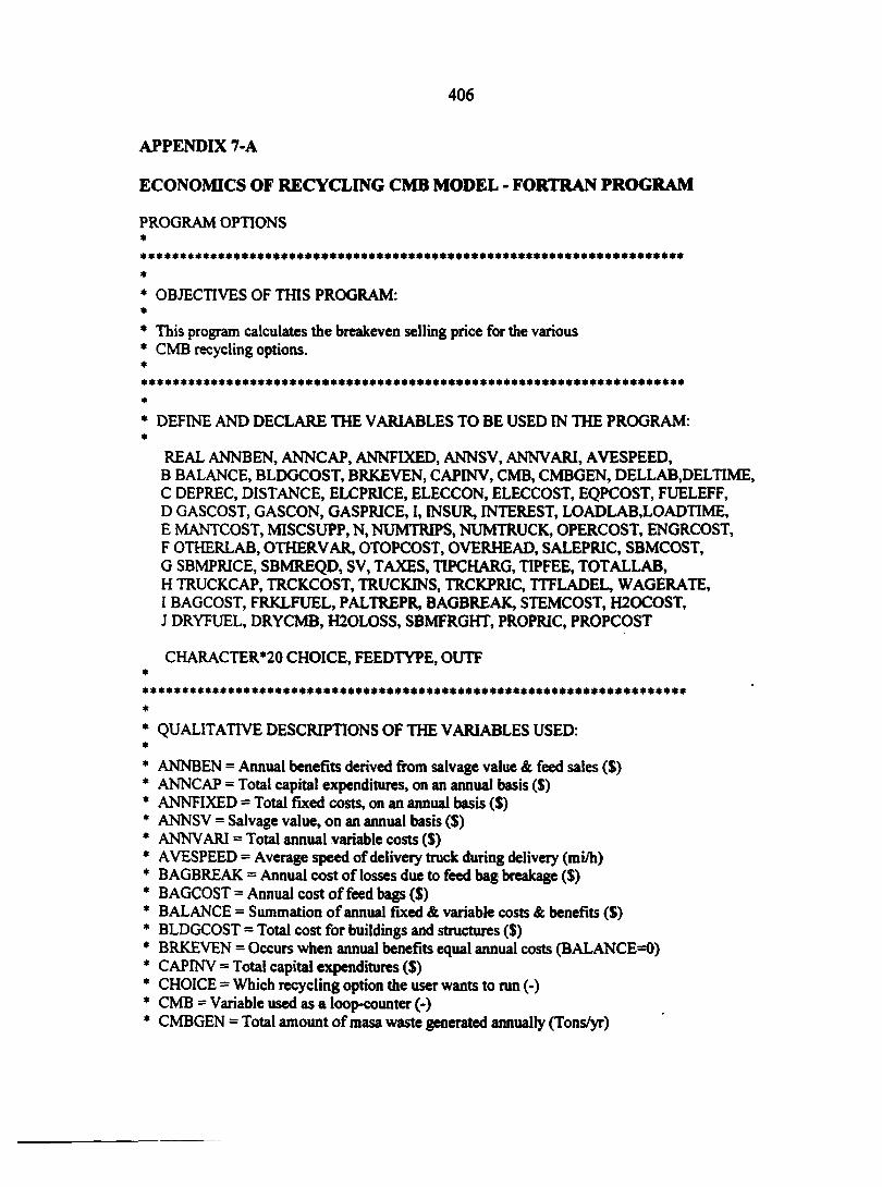
406
APPENDIX 7-A
ECONOMICS OF RECYCLING CMB MODEL - FORTRAN PROGRAM
PROGRAM OPTIONS
OBJECTIVES OF THIS PROGRAM:
This program calculates the breakeven selling price for the various CMB recycling options.
DEFINE AND DECLARE THE VARIABLES TO BE USED IN THE PROGRAM:
REAL ANNBEN, ANNCAP, ANNFIXED, ANNSV, ANNVARI, AVESPEED, B BALANCE, BLDGCOST, BRKEVEN, CAPINV, CMB, CMBGEN, DELLAB.DELTIME, C DEPREC, DISTANCE, ELCPRICE, ELECCON, ELECCOST, EQPCOST, FUELEFF, D GASCOST, GASCON, GASPRICE, I, INSUR, INTEREST, LOADLAB,LOADTIME, E MANTCOST, MISCSUPP, N, NUMTRIPS, NUMTRUCK, OPERCOST, ENGRCOST, F OTHERLAB, OTHERVAR, OTOPCOST, OVERHEAD, SALEPRIC, SBMCOST, G SBMPRICE, SBMREQD, SV, TAXES, TIPCHARG, TIPFEE, TOTALLAB, H TRUCKCAP, TRCKCOST, TRUCKINS, TRCKPRIC, TTFLADEL, WAGERATE, I BAGCOST, FRKLFUEL, PALTREPR, BAGBREAK, STEMCOST, H20C0ST, J DRYFUEL, DRYCMB, H20L0SS, SBMFRGHT, PROPRIC, PROPCOST
CHARACTERS CHOICE, FEEDTYPE, OUTF *
*
* QUALITATIVE DESCRIPTIONS OF THE VARIABLES USED: #
* ANNBEN = Annual benefits derived from salvage value & feed sales ($) * ANNCAP = Total capital expenditures, on an annual basis ($) * ANNFIXED = Total fixed costs, on an annual basis ($) * ANNSV = Salvage value, on an annual basis ($) * ANNVARI = Total annual variable costs ($) * AVESPEED = Average speed of delivery truck during delivery (mi/h) * BAGBREAK = Annual cost of losses due to feed bag breakage ($) * BAGCOST = Annual cost of feed bags ($) * BALANCE = Summation of annual fixed & variable costs & benefits ($) * BLDGCOST = Total cost for buildings and structures ($) * BRKEVEN = Occurs when annual benefits equal annual costs (BALANCE=0) * CAPINV = Total capital expenditures ($) * CHOICE = Which recycling option the user wants to run (-) * CMB = Variable used as a loop-counter (-) * CMBGEN = Total amount of masa waste generated annually (Tons/yr)
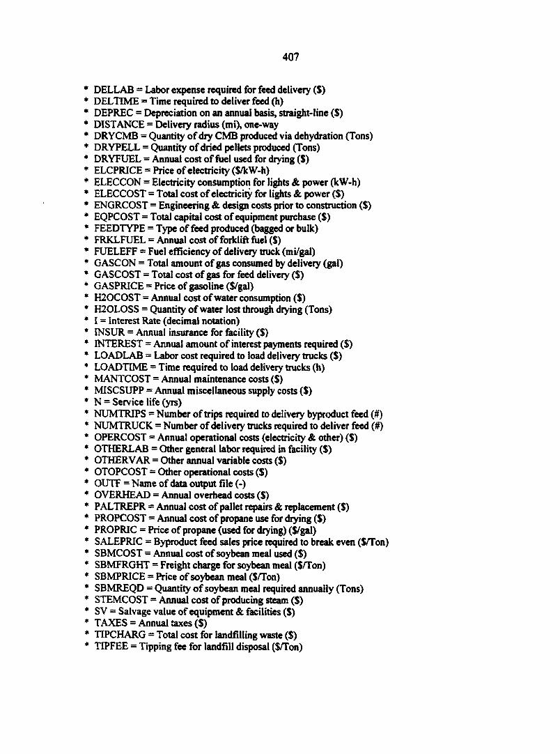
407
DELLAB = Labor expense required for feed delivery ($) DELTIME = Time required to deliver feed (h) DEPREC = Depreciation on an annual basis, straight-line ($) DISTANCE = Delivery radius (mi), one-way DRYCMB = Quantity of dry CMB produced via dehydration (Tons) DRYPELL = Quantity of dried pellets produced (Tons) DRYFUEL = Annual cost of fuel used for drying ($) ELCPRICE = Price of electricity ($/kW-h) ELECCON - Electricity consumption for lights & power (kW-h) ELECCOST = Total cost of electricity for lights & power ($) ENGRCOST = Engineering & design costs prior to construction ($) EQPCOST = Total capital cost of equipment purchase ($) FEEDTYPE = Type of feed produced (bagged or bulk) FRKLFUEL = Annual cost of forklift fuel ($) FUELEFF = Fuel efficiency of delivery truck (mi/gal) GASCON = Total amount of gas consumed by delivery (gal) GASCOST = Total cost of gas for feed delivery ($) GASPRICE = Price of gasoline ($/gal) H20C0ST = Annual cost of water consumption ($) H20L0SS = Quantity of water lost through drying (Tons) I = Interest Rate (decimal notation) INSUR = Annual insurance for facility ($) INTEREST = Annual amount of interest payments required ($) LOADLAB = Labor cost required to load delivery trucks ($) LOAD TIME = Time required to load delivery trucks (h) MANTCOST = Annual maintenance costs ($) MISCSUPP = Annual miscellaneous supply costs ($) N = Service life (yrs) NUMTRIPS = Number of trips required to delivery byproduct feed (#) NUM TRUCK = Number of delivery trucks required to deliver feed (#) OPERCOST = Annual operational costs (electricity & other) ($) OTHERLAB = Other general labor required in facility ($) OTHERVAR = Other annual variable costs ($) OTOPCOST = Other operational costs ($) QUTF = Name of data output file (-) OVERHEAD = Annual overhead costs ($) PALTREPR - Annual cost of pallet repairs & replacement ($) PROPCOST = Annual cost of propane use for drying ($) PROPRIC = Price of propane (used for drying) ($/gal) SALEPRIC = Byproduct feed sales price required to break even ($/Ton) SBMCOST = Annual cost of soybean meal used ($) SBMFRGHT = Freight charge for soybean meal ($/Ton) SBMPRICE = Price of soybean meal ($/Ton) SBMREQD = Quantity of soybean meal required annually (Tons) STEMCOST = Annual cost of producing steam ($) SV = Salvage value of equipment & facilities ($) TAXES = Annual taxes ($) TIPCHARG = Total cost for landfilling waste ($) TIPFEE = Tipping fee for landfill disposal ($/Ton)
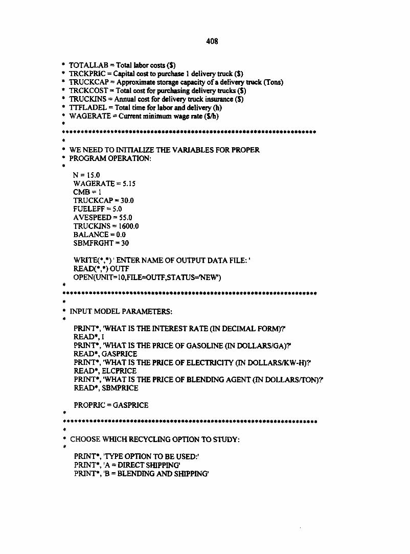
408
TOTALLAB = Total labor costs ($) TRCKPRIC = Capital cost to purchase 1 delivery truck ($) TRUCKCAP = Approximate storage capacity of a delivery truck (Tons) TRCKCOST = Total cost for purchasing delivery trucks ($) TRUCKINS = Annual cost for delivery truck insurance ($) TTFLADEL = Total time for labor and delivery (h) WAGERATE = Current minimum wage rate ($/h)
WE NEED TO INITIALIZE THE VARIABLES FOR PROPER PROGRAM OPERATION:
N = 15.0 WAGERATE = 5.15 CMB = 1 TRUCKCAP = 30.0 FUELEFF = 5.0 AVESPEED = 55.0 TRUCKINS = 1600.0 BALANCE = 0.0 SBMFRGHT = 30
WRITE(V) ' ENTER NAME OF OUTPUT DATA FILE: ' READ(V) OUTF OPEN(UNIT= 10,FILE=OUTF,STATUS=rNEW)
INPUT MODEL PARAMETERS:
PRINT*, 'WHAT IS THE INTEREST RATE (IN DECIMAL FORM)? READ*, I PRINT*, 'WHAT IS THE PRICE OF GASOLINE (IN DOLLARS/GA)? READ*, GASPRICE PRINT*, WHAT IS THE PRICE OF ELECTRICITY (IN DOLLARS/KW-H)?' READ*, ELCPRICE PRINT*, 'WHAT IS THE PRICE OF BLENDING AGENT (IN DOLLARS/TON)?' READ*, SBMPRICE
PROPRIC = GASPRICE
CHOOSE WHICH RECYCLING OPTION TO STUDY:
PRINT*, TYPE OPTION TO BE USED:' PRINT*, 'A = DIRECT SHIPPING' PRINT*, B = BLENDING AND SHIPPING'
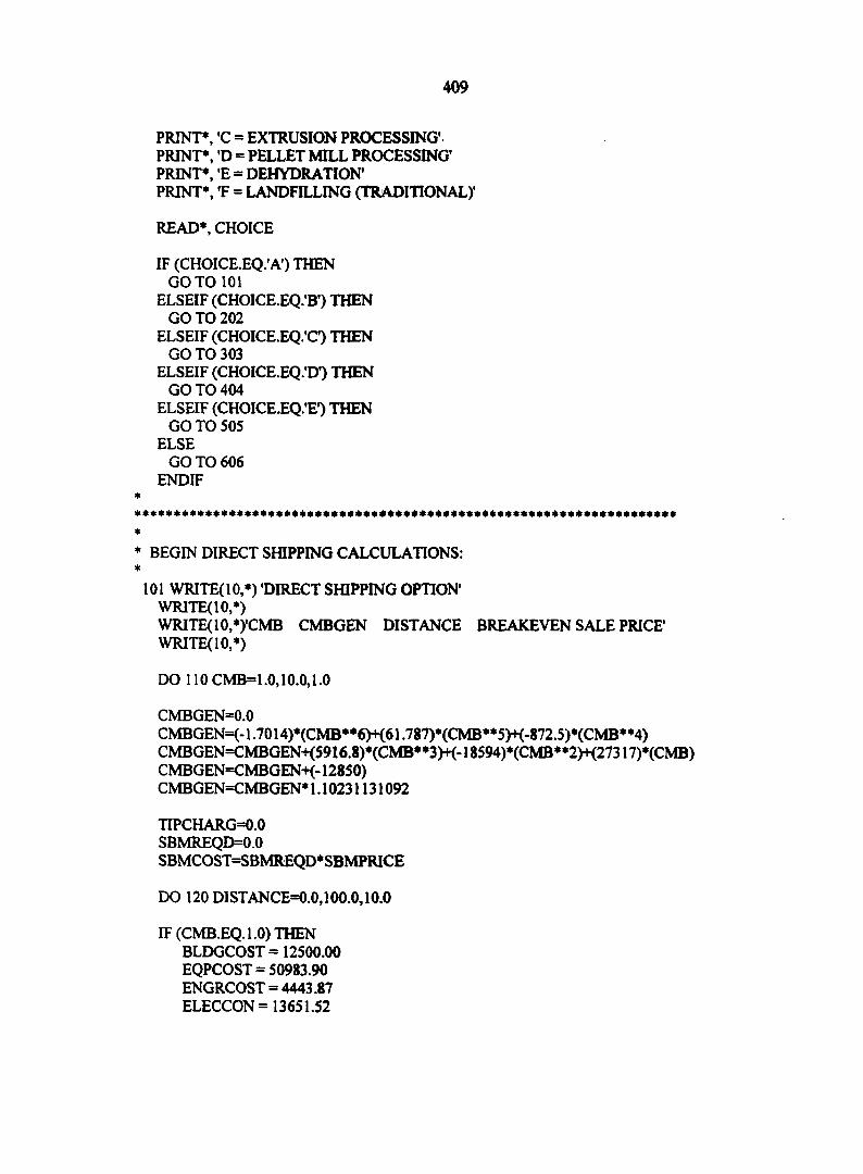
409
PRINT*, 'C = EXTRUSION PROCESSING' PRINT*, 'D = PELLET MILL PROCESSING' PRINT*, 'E = DEHYDRATION* PRINT*, 'F = LANDFILLING (TRADITIONAL)'
READ*, CHOICE
IF (CHOICE.EQ.A) THEN GOTO 101
ELSEIF (CHOICE EQ.'B ) THEN GO TO 202
ELSEIF (CHOICE.EQ.C) THEN GO TO 303
ELSEIF (CHOICE.EQ.D) THEN GO TO 404
ELSEIF (CHOICE.EQ.E) THEN GO TO 505
ELSE GO TO 606
ENDIF
* BEGIN DIRECT SHIPPING CALCULATIONS: *
101 WRITE(10,*) DIRECT SHIPPING OPTION* WRITE(10,*) WRITE(10,*)'CMB CMBGEN DISTANCE BREAKEVEN SALE PRICE' WRITE(10,*)
DO 110 CMB=1.0,10.0,1.0
CMBGEN=0.0 CMBGEN=(-1,7014)*(CMB**6)+(61.787)*(CMB**5>K-872.5)*(CMB**4) CMBGEN=CMBGEN+(5916.8)*(CMB* *3)+(-18594)*(CMB**2)+(27317)*(CMB) CMBGEN=CMBGEN+(-12850) CMBGEN=CMBGEN*1.10231131092
TIPCHARG=0.0 SBMREQD=0.0 SBMCOST=SBMREQD*SBMPRICE
DO 120 DISTANCE=0.0,100.0,10.0
ff (CMB.EQ. 1.0) THEN BLDGCOST = 12500.00 EQPCOST = 50983.90 ENGRCOST = 4443.87 ELECCON= 13651.52
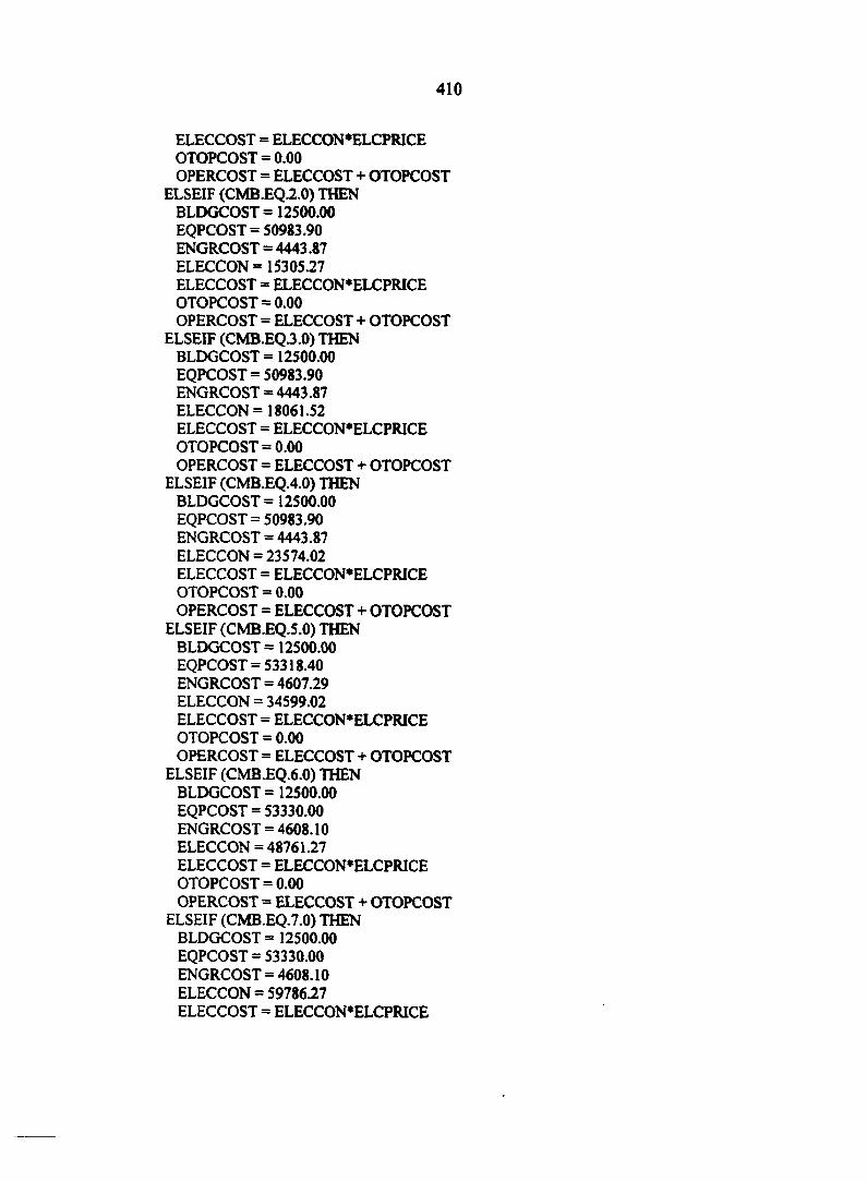
410
ELECCOST = ELECCON*ELCPRICE OTOPCOST = 0.00 OPERCOST = ELECCOST + OTOPCOST
ELSEIF (CMB.EQ.2.0) THEN BLDGCOST = 12500.00 EQPCOST = 50983.90 ENGRCOST = 4443.87 ELECCON = 15305.27 ELECCOST = ELECCON*ELCPRICE OTOPCOST = 0.00 OPERCOST = ELECCOST + OTOPCOST
ELSEIF (CMB.EQ3.0) THEN BLDGCOST =12500.00 EQPCOST = 50983.90 ENGRCOST = 4443.87 ELECCON = 18061.52 ELECCOST = ELECCON'ELCPRICE OTOPCOST = 0.00 OPERCOST = ELECCOST + OTOPCOST
ELSEIF (CMB.EQ.4.0) THEN BLDGCOST =12500.00 EQPCOST = 50983.90 ENGRCOST = 4443.87 ELECCON = 23574.02 ELECCOST = ELECCON*ELCPRICE OTOPCOST = 0.00 OPERCOST = ELECCOST + OTOPCOST
ELSEIF (CMB.EQ.5.0) THEN BLDGCOST =12500.00 EQPCOST = 53318.40 ENGRCOST = 4607.29 ELECCON = 34599.02 ELECCOST = ELECCON*ELCPRICE OTOPCOST = 0.00 OPERCOST = ELECCOST + OTOPCOST
ELSEIF (CMB.EQ.6.0) THEN BLDGCOST = 12500.00 EQPCOST = 53330.00 ENGRCOST = 4608.10 ELECCON = 4876127 ELECCOST = ELECCON*ELCPRICE OTOPCOST = 0.00 OPERCOST = ELECCOST + OTOPCOST
ELSEIF (CMB.EQ.7.0) THEN BLDGCOST = 12500.00 EQPCOST = 53330.00 ENGRCOST = 4608.10 ELECCON = 5978627 ELECCOST = ELECCON'ELCPRICE
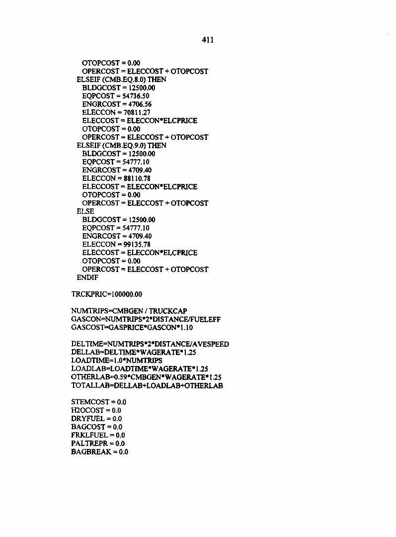
411
OTOPCOST = 0.00 OPERCOST = ELECCOST + OTOPCOST
ELSEIF (CMB.EQ.8.0) THEN BLDGCOST = 12500.00 EQPCOST = 54736.50 ENGRCOST = 4706.56 ELECCON = 70811.27 ELECCOST = ELECCON*ELCPRICE OTOPCOST = 0.00 OPERCOST = ELECCOST + OTOPCOST
ELSEIF (CMB.EQ.9.0) THEN BLDGCOST = 12500.00 EQPCOST = 54777.10 ENGRCOST = 4709.40 ELECCON = 88110.78 ELECCOST = ELECCON * ELCPRICE OTOPCOST = 0.00 OPERCOST = ELECCOST + OTOPCOST
ELSE BLDGCOST = 12500.00 EQPCOST = 54777.10 ENGRCOST = 4709.40 ELECCON = 99135.78 ELECCOST = ELECCON*ELCPRICE OTOPCOST = 0.00 OPERCOST = ELECCOST + OTOPCOST
ENDIF
TRCKPRIC=100000.00
NUMTRIPSCMBGEN / TRUCKCAP GASCON=NUMTRIPS*2*DISTANCE/FUELEFF GASCOST=GASPRICE*GASCON* 1.10
DELTIME=NUMTRIPS*2*DISTANCE/AVESPEED DELLAB=DELT1ME* WAGERATE* 1.25 LOADTIME=1.0*NUMTRIPS LOADLAB=LOADTIME*WAGERATE* 1.25 OTHERLAB=0.59*CMBGEN* WAGERATE* 1.25 TOTALLAB=DELLAB+LOADLAB+OTHERLAB
STEMCOST = 0.0 H20C0ST = 0.0 DRYFUEL = 0.0 BAGCOST = 0.0 FRKLFUEL = 0.0 PALTREPR = 0.0 BAGBREAK = 0.0
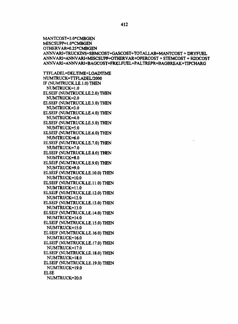
412
MANTCOST=3.0*CMBGEN MISCSUPP=1.0*CMBGEN OTHERVAR=0.25 •CMBGEN ANNVARI=TRUCKINS+SBMCOST+GASCOST+TOTALLAB+MANTCOST + DRYFUEL ANNV ARI=ANNVARI+MISC SUPP+OTHERVAR+OPERCOST + STEMCOST + H20C0ST ANNV ARI=ANNV ARI+B AGCOST+FRKLFUEL+PALTREPR+B AGBRE AK+TIPCHARG
TTFLADEL=DELTIME+LOADTIME NUMTRUCK=TTFLADEL/2000 IF (NUMTRUCK.LE. 1.0) THEN
NI IMTRUCK= 1.0 ELSEIF (NUMTRUCK.LE.2.0) THEN
NUMTRUCK=2.0 ELSEIF (NUMTRUCK.LE.3.0) THEN
NUMTRUCK=3.0 ELSEIF (NUMTRUCK.LE.4.0) THEN
NUMTRU CK=4.0 ELSEIF (NUMTRUCK.LE.5.0) THEN
NUMTRUCK=5.0 ELSEIF (NUMTRUCK.LE.6.0) THEN
NUMTRUCK=6.0 ELSEIF (NUMTRUCK.LE.7.0) THEN
NUMTRUCK=7.0 ELSEIF (NUMTRUCK.LE.8.0) THEN
NUMTRUCK=8.0 ELSEIF (NUMTRUCK.LE.9.0) THEN
NUMTRUCK=9.0 ELSEIF (NUMTRUCK.LE. 10.0) THEN
NUMTRUCK= 10.0 ELSEIF (NUMTRUCK.LE.11.0) THEN
NUMTRUCK= 11.0 ELSEIF (NUMTRUCK.LE. 12.0) THEN
NUMTRUCK= 12.0 ELSEIF (NUMTRUCK.LE.13.0) THEN
NUMTRUCK= 13.0 ELSEIF (NUMTRUCK.LE. 14.0) THEN
NUMTRUCK=14.0 ELSEIF (NUMTRUCK.LE.15.0) THEN
NUMTRUCK= 15.0 ELSEIF (NUMTRUCK.LE. 16.0) THEN
NUMTRU CK= 16.0 ELSEIF (NUMTRUCK.LE.17.0) THEN
NUMTRUCK= 17.0 ELSEIF (NUMTRUCK.LE. 18.0) THEN
NUMTRUCK=18.0 ELSEIF (NUMTRUCKXE. 19.0) THEN
NUMTRUCK= 19.0 ELSE
NUMTRUCK=20.0
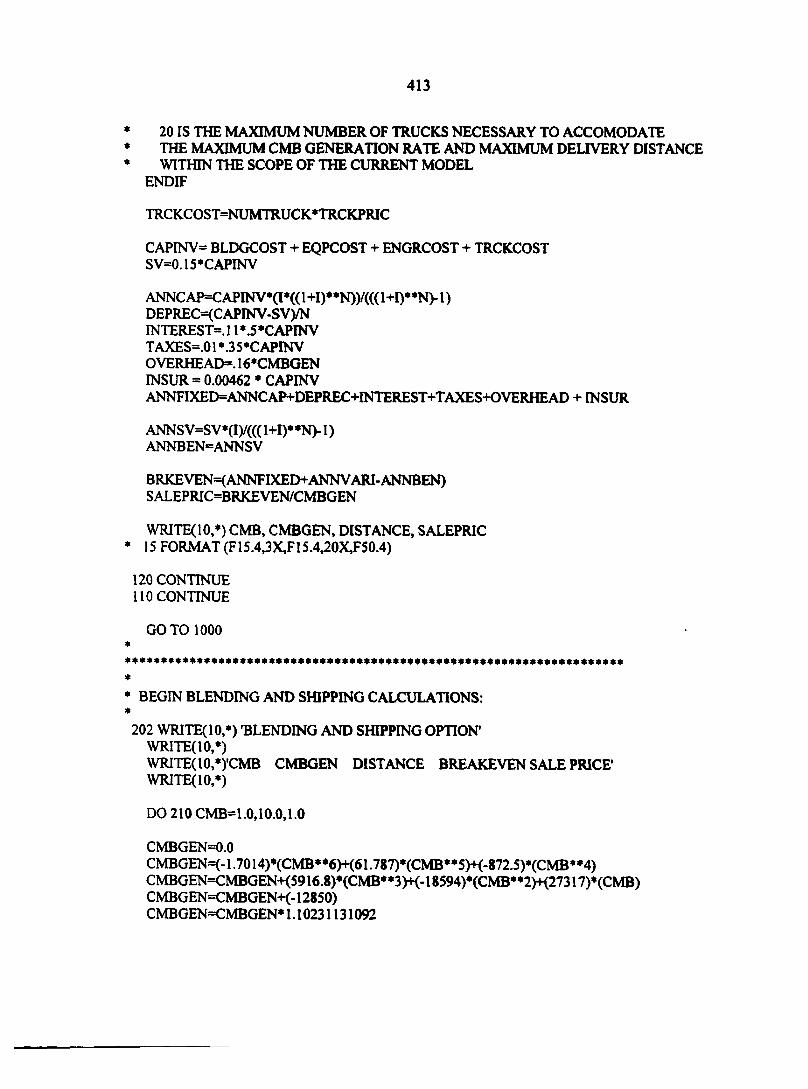
413
* 20 IS THE MAXIMUM NUMBER OF TRUCKS NECESSARY TO ACCOMODATE * THE MAXIMUM CMB GENERATION RATE AND MAXIMUM DELIVERY DISTANCE * WITHIN THE SCOPE OF THE CURRENT MODEL
END IF
TRCKCOST=NUMTRUCK*TRCKPRIC
CAPINV= BLDGCOST + EQPCOST + ENGRCOST + TRCKCOST SV=0.15*CAPINV
ANNC AP=C APINV*(I*(( 1 +I)**N))/((( 1+1)* *N> 1 ) DEPREC=(CAPINV-SVyN INTERESTS 11*.5*CAPINV TAXES=.01 * .3 5 «CAPINV OVERHEAD®. 16 «CMBGEN INSUR = 0.00462 * CAPINV ANNFIXED=ANNCAP+DEPREC+INTEREST+TAXES+OVERHEAD + INSUR
ANNSV=SV*(I)/(((1+I)**N)-1) ANNBEN=ANNSV
BRKEVEN=<ANNFIXED+ANNVARI-ANNBEN) SALEPRIC=BRKEVEN/CMBGEN
WRITE(10,*) CMB, CMBGEN, DISTANCE, SALEPRIC * 15 FORMAT (F15.4,3X,FI5.4,20X,F50.4)
120 CONTINUE 110 CONTINUE
GOTO 1000
BEGIN BLENDING AND SHIPPING CALCULATIONS:
202 WRITE(10,*) BLENDING AND SHIPPING OPTION WRITE(10,*) WRITE(10,*)'CMB CMBGEN DISTANCE BREAKEVEN SALE PRICE' WRITEOC,*)
DO 210 CMB=1.0,10.0,1.0
CMBGEN=0.0 CMBGEN=(-1.7014)*(CMB**6)+(61.787)*(CMB**5)+(-872.5)*(CMB**4) CMBGEN=CMBGEN+(5916.8)*(CMB**3H-18594)*(CMB**2)+(27317)*(CMB) CMBGEN=CMBGEN+(-12850) CMBGEN=CMBGEN*1.10231131092
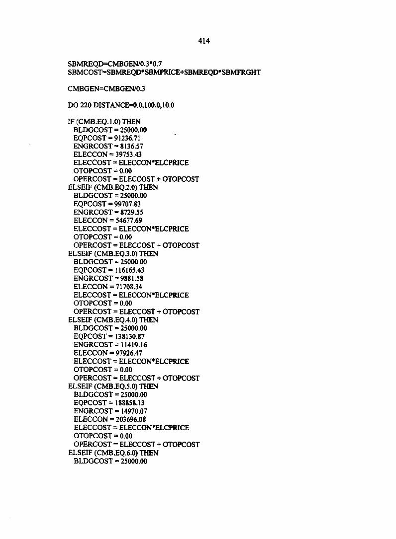
414
SBMREQD=CMBGEN/0J*0.7 SBMCOST=SBMREQD*SBMPRICE+SBMREQD*SBMFRGHT
CMBGEN=CMBGEN/0.3
DO 220 DISTANCE=0.0,100.0,10.0
IF (CMB.EQ.1.0) THEN BLDGCOST = 25000.00 EQPCOST = 91236.71 ENGRCOST = 8136.57 ELECCON = 39753.43 ELECCOST = ELECCON'ELCPRICE OTOPCOST = 0.00 OPERCOST = ELECCOST + OTOPCOST
ELSEIF (CMB.EQ.2.0) THEN BLDGCOST = 25000.00 EQPCOST = 99707.83 ENGRCOST = 8729.55 ELECCON = 54677.69 ELECCOST = ELECCON'ELCPRICE OTOPCOST = 0.00 OPERCOST = ELECCOST + OTOPCOST
ELSEIF (CMB.EQ.3.0) THEN BLDGCOST = 25000.00 EQPCOST = 116165.43 ENGRCOST = 9881.58 ELECCON = 71708.34 ELECCOST = ELECCON'ELCPRICE OTOPCOST = 0.00 OPERCOST = ELECCOST + OTOPCOST
ELSEIF (CMB.EQ.4.0) THEN BLDGCOST = 25000.00 EQPCOST = 138130.87 ENGRCOST = 11419.16 ELECCON = 97926.47 ELECCOST = ELECCON*ELCPRICE OTOPCOST = 0.00 OPERCOST = ELECCOST + OTOPCOST
ELSEIF (CMB.EQ.5.0) THEN BLDGCOST = 25000.00 EQPCOST = 188858.13 ENGRCOST = 14970.07 ELECCON = 203696.08 ELECCOST = ELECCON*ELCPRICE OTOPCOST = 0.00 OPERCOST = ELECCOST + OTOPCOST
ELSEIF (CMB.EQ.6.0) THEN BLDGCOST = 25000.00
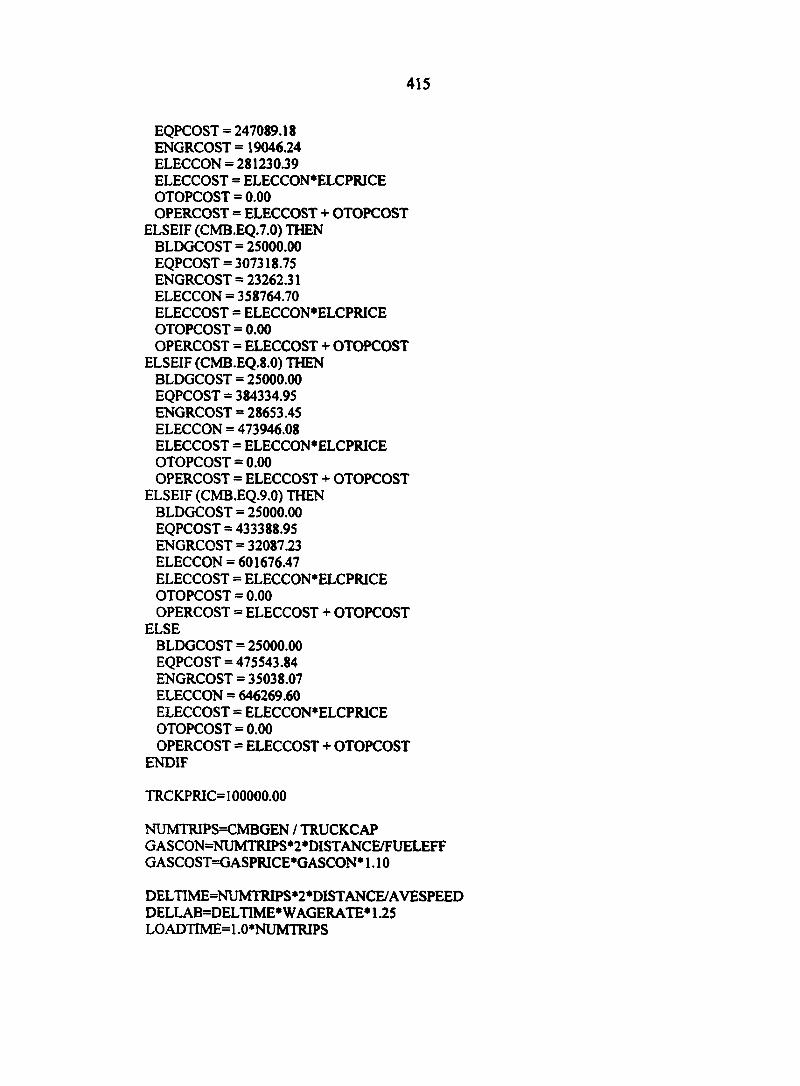
415
EQPCOST = 247089.18 ENGRCOST = 19046.24 ELECCON = 281230.39 ELECCOST = ELECCON*ELCPRICE OTOPCOST = 0.00 OPERCOST = ELECCOST + OTOPCOST
ELSEIF (CMB.EQ.7.0) THEN BLDGCOST = 25000.00 EQPCOST = 307318.75 ENGRCOST = 23262.31 ELECCON = 358764.70 ELECCOST = ELECCON*ELCPRICE OTOPCOST = 0.00 OPERCOST = ELECCOST + OTOPCOST
ELSEIF (CMB.EQ.8.0) THEN BLDGCOST = 25000.00 EQPCOST = 384334.95 ENGRCOST = 28653.45 ELECCON = 473946.08 ELECCOST = ELECCON*ELCPRICE OTOPCOST = 0.00 OPERCOST = ELECCOST + OTOPCOST
ELSEIF (CMB.EQ.9.0) THEN BLDGCOST = 25000.00 EQPCOST = 433388.95 ENGRCOST = 32087.23 ELECCON = 601676.47 ELECCOST = ELECCON*ELCPRICE OTOPCOST = 0.00 OPERCOST = ELECCOST + OTOPCOST
ELSE BLDGCOST = 25000.00 EQPCOST = 475543.84 ENGRCOST = 35038.07 ELECCON = 646269.60 ELECCOST = ELECCON*ELCPRICE OTOPCOST = 0.00 OPERCOST = ELECCOST + OTOPCOST
ENDIF
TRCKPRIC=100000.00
NUMTRIPS=CMBGEN / TRUCKCAP GASCON=NUMTRIPS*2*DISTANCE/FUELEFF GASCOST=GASPRICE*GASCON* 1.10
DELTIME=NUMTRIPS*2*DISTANCE/AVESPEED DELLAB=DELTIME* WAGERATE* 1.25 LOADTIME= 1.0 *NUMTRIPS
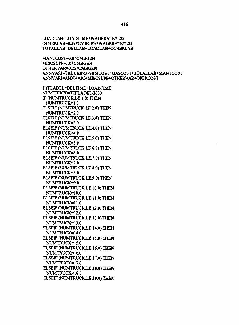
416
LOADLAB=LOADTIME* WAGERATE* 1.25 OTHERLAB=0.59*CMBGEN* WAGERATE* 1.25 TOT ALL AB=DELLAB+LOADLAB+OTHERLAB
MANTCOST=3.0*CMBGEN MISC SUP P=1.0*CMBGEN OTHERVAR=0.25*CMBGEN ANNVARI=TRUCKJNS+SBMCOST+GASCOST+TOTALLAB+MANTCOST ANNV ARI=ANNV ARI+MISCSUPP+OTHERVAR+OPERCOST
TTFLADEL=DELTIME-HLOADTIME NUMTRUCK=TTFLADEL/2000 IF (NUMTRUCK.LE.1.0) THEN
NUMTRUCK= 1.0 ELSEIF (NUMTRUCK.LE.2.0) THEN
NUMTRUCK=2.0 ELSEIF (NUMTRUCK.LE.3.0) THEN
NUMTRU C K=3.0 ELSEIF (NUMTRUCK.LE.4.0) THEN
NUMTRUCK=4.0 ELSEIF (NUMTRUCK.LE.5.0) THEN
NUMTRUCK=5.0 ELSEIF (NUMTRUCK.LE.6.0) THEN
NUMTRUCK=6.0 ELSEIF (NUMTRUCK.LE.7.0) THEN
NUMTRUCK=7.0 ELSEIF (NUMTRUCK.LE.8.0) THEN
NUMTRUCK=8.0 ELSEIF (NUMTRUCK.LE.9.0) THEN
NUMTRUCK=9.0 ELSEIF (NUMTRUCK.LE. 10.0) THEN
NUMTRUCK=10.0 ELSEIF (NUMTRUCK.LE. 11.0) THEN
NUMTRUCK=11.0 ELSEIF (NUMTRUCK.LE.12.0) THEN
NUMTRUCK= 12.0 ELSEIF (NUMTRUCKXE. 13.0) THEN
NUMTRUCK=13.0 ELSEIF (NUMTRUCK.LE. 14.0) THEN
NUMTRUCK= 14.0 ELSEIF (NUMTRUCK.LE.15.0) THEN
NUMTRUCK= 15.0 ELSEIF (NUMTRUCK.LE. 16.0) THEN
NUMTRUCK= 16.0 ELSEIF (NUMTRUCK.LE.17.0) THEN
NUMTRUCK= 17.0 ELSEIF (NUMTRUCK1E. 18.0) THEN
NUMTRUCK=18.0 ELSEIF (NUMTRUCK.LE.19.0) THEN
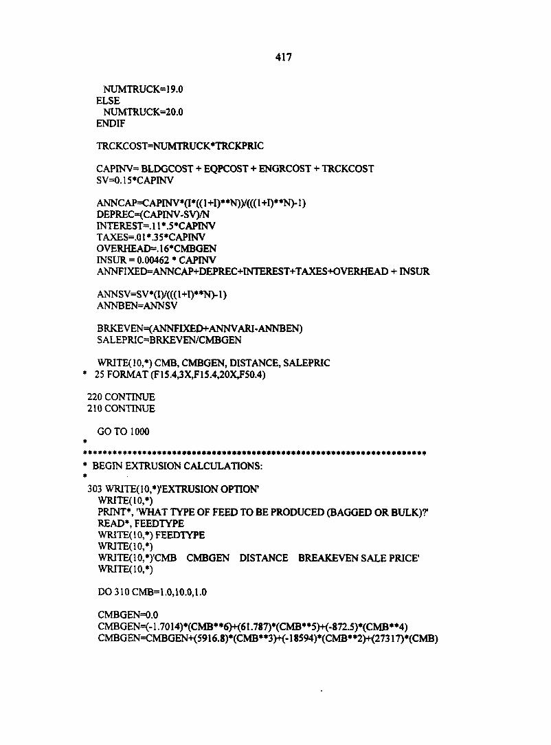
417
NUMTRUCK= 19.0 ELSE
NUMTRUCK=20.0 ENDIF
TRCKCOST=NUMTRUCK*TRCKPRIC
CAPINV= BLDGCOST + EQPCOST + ENGRCOST + TRCKCOST SV=0.15 «CAPINV
ANNCAPCAPINV*(I*((1+D**N))/(((1+I)**N)-1) DEPREC=(CAPINV-SV)/N INTEREST3.11 *.5 «CAPINV TAXES=.01*.35*CAPINV OVERHEAD®. 16*CMBGEN INSUR = 0.00462 « CAPINV ANNFIXED=ANNCAP+DEPREC+INTEREST+TAXES+OVERHEAD + INSUR
ANNSV=SV*(I)/((( l+l)**N)-1 ) ANNBEN=ANN S V
BRKEVEN=(ANNFIXED+ANNVARI-ANNBEN) SALEPRIC=BRKEVEN/CMBGEN
WRITE(10,«) CMB, CMBGEN, DISTANCE, SALEPRIC « 25 FORMAT (F15.4,3X,F15.4,20XF50.4)
220 CONTINUE 210 CONTINUE
GOTO 1000
« BEGIN EXTRUSION CALCULATIONS: *
303 WRITE(10,*)'EXTRUSION OPTION1
WRITE(10,*) PRINT*, WHAT TYPE OF FEED TO BE PRODUCED (BAGGED OR BULK)? READ*, FEEDTYPE WRITE(10,*) FEEDTYPE WRITE(10,*) WRITE( 10, *)'CMB CMBGEN DISTANCE BREAKEVEN SALE PRICE' WRITE(10,*)
DO 310 CMB= 1.0,10.0,1.0
CMBGEN=0.0 CMBGENK-1.7014)*(CMB**6)+(61.787)*(CMB»*5)+(-872.5)*(CMB**4) CMBGEN=CMBGEN-K5916.8)*(CMB**3K-18594)*(CMB**2)+(27317)*(CMB)
418
CMBGENCMBGEN-K-12850) CMB GEN=CMBGEN* 1.10231131092
SBMREQD=CMBGEN/0.3 *0.7 SBMCOST=SBMREQD*SBMPRICE+SBMREQD*SBMFRGHT
CMBGEN=CMBGEN/0.3
DRYPELL=CMBGEN*0.75/0.85 H20L0S S=CMBGEN-DRYPELL
DO 320 DISTANCE=0.0,100.0,10.0
IF (FEEDTYPE.EQ.'BAGGED') THEN IF (CMB.EQ.1.0) THEN
BLDGCOST = 27755.77 EQPCOST =1128955.06 ENGRCOST = 80969.76 ELECCON = 963675.00 ELECCOST = ELECCON*ELCPRICE OTOPCOST =0.0 OPERCOST = ELECCOST + OTOPCOST
ELSEIF (CMB.EQ.2.0) THEN BLDGCOST = 31889.44 EQPCOST =1162828.87 ENGRCOST = 83630.28 ELECCON = 978599.26 ELECCOST = ELECCON*ELCPRICE OTOPCOST = 0.0 OPERCOST = ELECCOST + OTOPCOST
ELSEIF (CMB.EQ.3.0) THEN BLDGCOST = 38778.89 EQPCOST = 1399816.97 ENGRCOST = 100701.71 ELECCON = 1455237.75 ELECCOST = ELECCON*ELCPRICE OTOPCOST = 0.0 OPERCOST = ELECCOST + OTOPCOST
ELSEIF (CMB.EQ.4.0) THEN BLDGCOST = 52557.77 EQPCOST = 1655404.09 ENGRCOST =119557.33 ELECCON = 1867338.23 ELECCOST = ELECCON*ELCPRICE OTOPCOST = 0.0 OPERCOST = ELECCOST + OTOPCOST
ELSEIF (CMB.EQ.5.0) THEN BLDGCOST = 80115.55 EQPCOST = 2913402.81
419
ENGRCOST = 209546.29 ELECCON = 3562127.45 ELECCOST = ELECCON*ELCPRICE OTOPCOST = 0.0 OPERCOST = ELECCOST + OTOPCOST
ELSEIF (CMB.EQ.6.0) THEN BLDGCOST = 107673.33 EQPCOST = 3253695.10 ENGRCOST = 235295.79 ELECCON = 3926720.59 ELECCOST = ELECCON*ELCPRICE OTOPCOST = 0.0 OPERCOST = ELECCOST + OTOPCOST
ELSEIF (CMB.EQ.7.0) THEN BLDGCOST =135231.10 EQPCOST = 4781439.66 ENGRCOST = 344166.95 ELECCON = 5773666.66 ELECCOST = ELECCON'ELCPRICE OTOPCOST = 0.0 OPERCOST = ELECCOST + OTOPCOST
ELSEIF (CMB.EQ.8.0) THEN BLDGCOST = 162788.88 EQPCOST = 6071694.50 ENGRCOST = 436413.84 ELECCON = 7471593.14 ELECCOST = ELECCON'ELCPRICE OTOPCOST = 0.0 OPERCOST = ELECCOST + OTOPCOST
ELSEIF (CMB.EQ.9.0) THEN BLDGCOST = 190346.65 EQPCOST = 7385302.19 ENGRCOST = 530295.42 ELECCON = 9204029.41 ELECCOST = ELECCON'ELCPRICE OTOPCOST = 0.0 OPERCOST = ELECCOST + OTOPCOST
ELSE BLDGCOST = 217904.42 EQPCOST = 8897683.13 ENGRCOST = 638091.13 ELECCON =11016465.68 ELECCOST = ELECCON'ELCPRICE OTOPCOST = 0.0 OPERCOST = ELECCOST + OTOPCOST
ENDIF ELSE
IF (CMB.EQ.1.0) THEN BLDGCOST = 25000.00
420
EQPCOST =864235.81 ENGRCOST = 62246.51 ELECCON = 855439.70 ELECCOST = ELECCON*ELCPRICE OTOPCOST = 0.0 OPERCOST = ELECCOST + OTOPCOST
ELSEIF (CMB.EQ.2.0) THEN BLDGCOST = 25000.00 EQPCOST = 898109.62 ENGRCOST = 64617.67 ELECCON = 870363.97 ELECCOST = ELECCON*ELCPRICE OTOPCOST = 0.0 OPERCOST = ELECCOST + OTOPCOST
ELSEIF (CMB.EQ.3.0) THEN BLDGCOST = 25000.00 EQPCOST= 1135097.72 ENGRCOST = 81206.84 ELECCON = 1347002.45 ELECCOST = ELECCON*ELCPRICE OTOPCOST = 0.0 OPERCOST = ELECCOST + OTOPCOST
ELSEIF (CMB.EQ.4.0) THEN BLDGCOST = 25000.00 EQPCOST = 1383434.84 ENGRCOST = 98590.44 ELECCON = 1759102.94 ELECCOST = ELECCON'ELCPRICE OTOPCOST = 0.0 OPERCOST = ELECCOST + OTOPCOST
ELSEIF (CMB.EQ.5.0) THEN BLDGCOST = 25000.00 EQPCOST = 2598488.91 ENGRCOST = 183644.22 ELECCON = 3438205.89 ELECCOST = ELECCON*ELCPRICE OTOPCOST = 0.0 OPERCOST = ELECCOST + OTOPCOST
ELSEIF (CMB.EQ.6.0) THEN BLDGCOST = 25000.00 EQPCOST = 2837376.90 ENGRCOST = 200366.38 ELECCON = 3771426.47 ELECCOST = ELECCON'ELCPRICE OTOPCOST = 0.0 OPERCOST = ELECCOST + OTOPCOST
ELSEIF (CMB.EQ.7.0) THEN BLDGCOST = 25000.00 EQPCOST = 4120539.81
421
ENGRCOST = 290187.79 ELECCON = 5508568.62 ELECCOST = ELECCON*ELCPRICE OTOPCOST = 0.0 OPERCOST = ELECCOST + OTOPCOST
ELSEIF (CMB.EQ.8.0) THEN BLDGCOST = 25000.00 EQPCOST = 5360614.50 ENGRCOST = 376993.01 ELECCON = 7190808.83 ELECCOST = ELECCON*ELCPRICE OTOPCOST = 0.0 OPERCOST = ELECCOST + OTOPCOST
ELSEIF (CMB.EQ.9.0) THEN BLDGCOST = 25000.00 EQPCOST = 6572817.89 ENGRCOST = 461847.25 ELECCON = 8891872.55 ELECCOST = ELECCON*ELCPRICE OTOPCOST = 0.0 OPERCOST = ELECCOST + OTOPCOST
ELSE BLDGCOST = 25000.00 EQPCOST = 7840617.18 ENGRCOST = 550593.20 ELECCON = 10594504.90 ELECCOST = ELECCON*ELCPRICE OTOPCOST = 0.0 OPERCOST = ELECCOST + OTOPCOST
ENDIF ENDIF
TRCKPRIC=100000.00
NUMTRIPS=CMBGEN / TRUCKCAP GASCON=NUMTRIPS*2*DISTANCE/FUELEFF GASCOST=GASPRICE*GASCON* 1.10
DELTIME=NUMTRIPS*2*DISTANCE/AVESPEED DELLAB=DELTIME* WAGERATE* 1.25 LOADTIME=l .0*NUMTRIPS LOADLAB=LOADTIME* WAGERATE* 1.25 OTHERLAB=0.59*CMBGEN* WAGERATE* 1.25 TOT ALLAB=DELLAB+LOADLAB+OTHERLAB
STEMCOST = 1.05*CMBGEN H20C0ST = 0.02*CMBGEN PROPCOST = 2220* H2OLOSS*2000/92000*PROPRIC DRYFUEL = PROPCOST
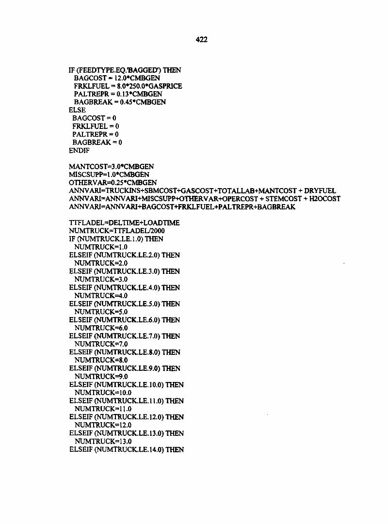
422
IF (FEEDTYPE.EQ.'BAGGED') THEN BAGCOST = 12.0*CMBGEN FRKLFUEL = 8.0*250.0*GASPRICE PALTREPR = 0.13 «CMBGEN BAGBREAK = 0.45 «CMBGEN
ELSE BAGCOST = 0 FRKLFUEL = 0 PALTREPR = 0 BAGBREAK = 0
ENDIF
MANTCOST=3.0*CMBGEN MISCSUPP=1.0*CMBGEN OTHERVAR=0.25 «CMBGEN ANNVARI=TRUCKINS+SBMCOST+GASCOST+TOTALLAB+MANTCOST + DRYFUEL ANNV ARI=ANNV ARI+MISCSUPP+OTHERVAR+OPERCOST + STEMCOST + H20C0ST ANNVARI=ANNVARI+BAGCOST+FRKLFUEL+PALTREPR+BAGBREAK
TTFLADEL=DELTIME+LOADTIME NUMTRUCK=TTFLADEL/2000 IF (NUMTRUCK.LE. 1.0) THEN
NUMTRUCK= 1.0 ELSEIF (NUMTRUCK.LE.2.0) THEN
NUMTRUCK=2.0 ELSEIF (NUMTRUCK.LE.3.0) THEN
NUMTRUCK=3.0 ELSEIF (NUMTRUCK.LE.4.0) THEN
NUMTRUCK=4.0 ELSEIF (NUMTRUCK.LE.5.0) THEN
NUMTRUCK=5.0 ELSEIF (NUMTRUCK.LE.6.0) THEN
NUMTRUCK=6.0 ELSEIF (NUMTRUCK.LE.7.0) THEN
NUMTRUCK=7.0 ELSEIF (NUMTRUCK.LE.8.0) THEN
NUMTRUCK=8.0 ELSEIF (NUMTRUCK.LE.9.0) THEN
NUMTRUCK=9.0 ELSEIF (NUMTRUCK.LE. 10.0) THEN
NUMTRUCK= 10.0 ELSEIF (NUMTRUCK.LE.11.0) THEN
NUMTRUCK=11.0 ELSEIF (NUMTRUCK.LE. 12.0) THEN
NUMTRUCK= 12.0 ELSEIF (NUMTRUCK.LE.13.0) THEN
NUMTRUCK=13.0 ELSEIF (NUMTRUCK.LE.14.0) THEN
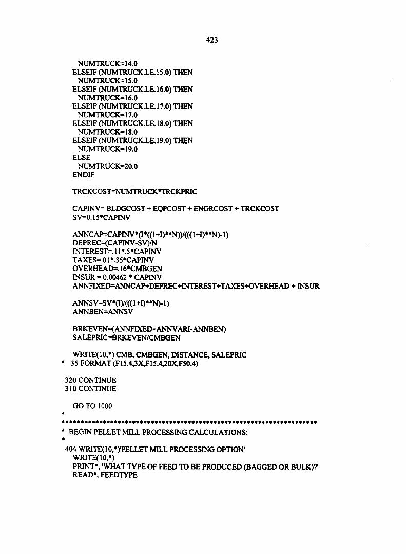
423
NUMTRUCK= 14.0 ELSEIF (NUMTRUCK.LE. 15.0) THEN
NUMTRUCK= 15.0 ELSEIF (NUMTRUCK.LE. 16.0) THEN
NUMTRUCK=16.0 ELSEIF (NUMTRUCK.LE. 17.0) THEN
NUMTRUCK=17.0 ELSEIF (NUMTRUCK.LE. 18.0) THEN
NUMTRUCK=18.0 ELSEIF (NUMTRUCK.LE. 19.0) THEN
NUMTRUCK=19.0 ELSE
NUMTRUCK=20.0 ENDIF
TRCKCOST=NUMTRUCK*TRCKPRIC
CAPINV= BLDGCOST + EQPCOST + ENGRCOST + TRCKCOST SV=0.15*CAPINV
ANNC AP=CAPINV*(I*(( 1 +I)**N))/(((1+I)**N)-1 ) DEPREC=(CAPINV-SV)/N INTERESTS 11 *.5*CAPINV TAXES=.01 * .3 5'C APINV OVERHEAD^. 16*CMBGEN INSUR = 0.00462 * CAPINV ANNFIXED=ANNCAP+DEPREC+INTEREST+TAXES+OVERHEAD + INSUR
ANN S V=S V *(I)/((( 1 +1)* *N)-1 ) ANNBEN=ANNSV
BRKEVEN=(ANNFIXED+ANNV ARI-ANNBEN) SALEPRIC=BRKEVEN/CMBGEN
WRITE(10,*) CMB, CMBGEN, DISTANCE, SALEPRIC * 35 FORMAT (F15.4,3X,F15.4,20XF50.4)
320 CONTINUE 310 CONTINUE
GOTO 1000
• BEGIN PELLET MILL PROCESSING CALCULATIONS: *
404 WRITE(10,*)'PELLET MILL PROCESSING OPTION' WRITE(10,*) PRINT*, 'WHAT TYPE OF FEED TO BE PRODUCED (BAGGED OR BULK)?' READ*, FEEDTYPE
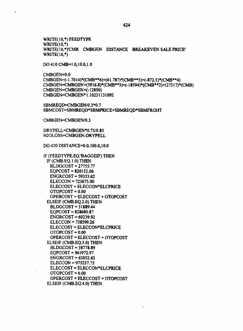
424
WRITE(10,*) FEEDTYPE WRITE(10,*) WRITE( 10, *)'CMB CMBGEN DISTANCE BREAKEVEN SALE PRICE' WRITE(10,*)
DO 410 CMB=1.0,10.0,1.0
CMBGEN=0.0 CMBGEN=(-1.7014)*(CMB**6)+(61.787)*(CMB**5)+(-872.5)*(CMB**4) CMBGEN=CMBGEN+(5916.8)*(CMB**3>K-18594)*(CMB**2)+(27317)*(CMB) CMBGEN=CMBGEN+(-12850) CMBGEN=CMBGEN* 1.10231131092
SBMREQD=CMBGEN/0.3*0.7 SBMCOST=SBMREQD*SBMPRICE+SBMREQD*SBMFRGHT
CMBGENCMBGEN/0.3
DRYPELL=CMBGEN*0.75/0.85 H20L0SSCMBGEN-DRYPELL
DO 420 DISTANCE=0.0,100.0,10.0
IF (FEEDTYPE.EQ.'BAGGED') THEN IF (CMB.EQ.l .0) THEN
BLDGCOST = 27755.77 EQPCOST = 820153.06 ENGRCOST= 59353.62 ELECCON = 723675.00 ELECCOST = ELECCON*ELCPRICE OTOPCOST = 0.00 OPERCOST = ELECCOST + OTOPCOST
ELSEIF (CMB.EQ.2.0) THEN BLDGCOST = 31889.44 EQPCOST = 828680.87 ENGRCOST = 60239.92 ELECCON = 738599.26 ELECCOST = ELECCON*ELCPRICE OTOPCOST = 0.00 OPERCOST = ELECCOST + OTOPCOST
ELSEIF (CMB.EQ.3.0) THEN BLDGCOST = 38778.89 EQPCOST = 861972.97 ENGRCOST = 63052.63 ELECCON = 975237.75 ELECCOST = ELECCON*ELCPRICE OTOPCOST = 0.00 OPERCOST = ELECCOST + OTOPCOST
ELSEIF (CMB.EQ.4.0) THEN
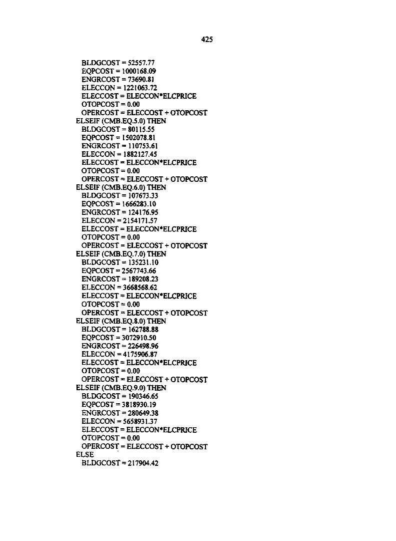
425
BLDGCOST = 52557.77 EQPCOST = 1000168.09 ENGRCOST = 73690.81 ELECCON = 1221063.72 ELECCOST = ELECCON*ELCPRICE OTOPCOST = 0.00 OPERCOST = ELECCOST + OTOPCOST
ELSEIF (CMB.EQ.5.0) THEN BLDGCOST = 80115.55 EQPCOST = 1502078.81 ENGRCOST = 110753.61 ELECCON = 1882127.45 ELECCOST = ELECCON*ELCPRICE OTOPCOST = 0.00 OPERCOST = ELECCOST + OTOPCOST
ELSEIF (CMB.EQ.6.0) THEN BLDGCOST = 107673.33 EQPCOST =1666283.10 ENGRCOST = 124176.95 ELECCON = 2154171.57 ELECCOST = ELECCON*ELCPRICE OTOPCOST = 0.00 OPERCOST = ELECCOST + OTOPCOST
ELSEIF (CMB.EQ.7.0) THEN BLDGCOST = 135231.10 EQPCOST = 2567743.66 ENGRCOST = 189208.23 ELECCON = 3668568.62 ELECCOST = ELECCON'ELCPRICE OTOPCOST = 0.00 OPERCOST = ELECCOST + OTOPCOST
ELSEIF (CMB.EQ.8.0) THEN BLDGCOST = 162788.88 EQPCOST = 3072910.50 ENGRCOST = 226498.96 ELECCON = 4175906.87 ELECCOST = ELECCON'ELCPRICE OTOPCOST = 0.00 OPERCOST = ELECCOST + OTOPCOST
ELSEIF (CMB.EQ.9.0) THEN BLDGCOST = 190346.65 EQPCOST = 3818930.19 ENGRCOST = 280649.38 ELECCON = 5658931.37 ELECCOST = ELECCON'ELCPRICE OTOPCOST = 0.00 OPERCOST = ELECCOST + OTOPCOST
ELSE BLDGCOST = 217904.42
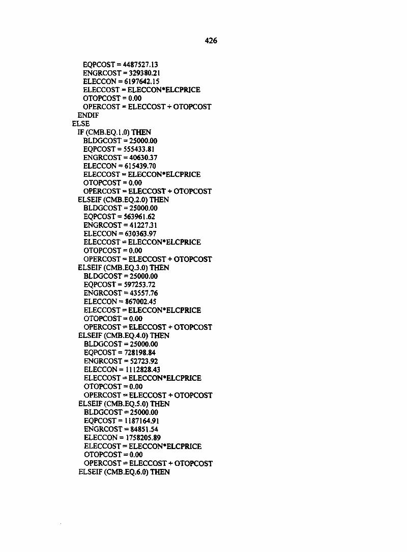
426
EQPCOST = 4487527.13 ENGRCOST = 329380.21 ELECCON = 6197642.15 ELECCOST = ELECCON*ELCPRICE OTOPCOST = 0.00 OPERCOST = ELECCOST + OTOPCOST
ENDIF ELSE
IF (CMB.EQ.1.0) THEN BLDGCOST = 25000.00 EQPCOST = 555433.81 ENGRCOST = 4063037 ELECCON = 615439.70 ELECCOST = ELECCON*ELCPRICE OTOPCOST = 0.00 OPERCOST = ELECCOST + OTOPCOST
ELSEIF (CMB.EQ.2.0) THEN BLDGCOST = 25000.00 EQPCOST =563961.62 ENGRCOST = 4122731 ELECCON = 630363.97 ELECCOST = ELECCON*ELCPRICE OTOPCOST = 0.00 OPERCOST = ELECCOST + OTOPCOST
ELSEIF (CMB.EQ.3.0) THEN BLDGCOST = 25000.00 EQPCOST = 597253.72 ENGRCOST = 43557.76 ELECCON =867002.45 ELECCOST = ELECCON'ELCPRICE OTOPCOST = 0.00 OPERCOST = ELECCOST + OTOPCOST
ELSEIF (CMB.EQ.4.0) THEN BLDGCOST = 25000.00 EQPCOST = 728198.84 ENGRCOST = 52723.92 ELECCON = 1112828.43 ELECCOST = ELECCON*ELCPRICE OTOPCOST = 0.00 OPERCOST = ELECCOST + OTOPCOST
ELSEIF (CMB.EQ.5.0) THEN BLDGCOST = 25000.00 EQPCOST = 1187164.91 ENGRCOST = 84851.54 ELECCON = 1758205.89 ELECCOST = ELECCON*ELCPRICE OTOPCOST = 0.00 OPERCOST = ELECCOST + OTOPCOST
ELSEIF (CMB.EQ.6.0) THEN
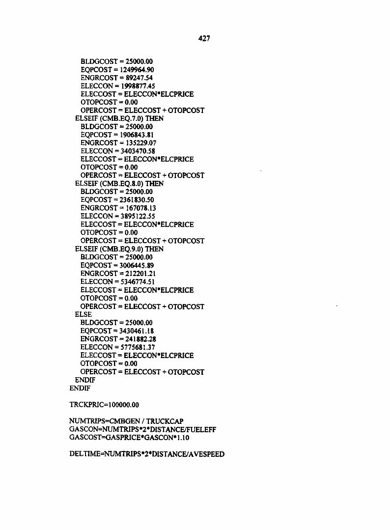
427
BLDGCOST = 25000.00 EQPCOST = 1249964.90 ENGRCOST =89247.54 ELECCON = 1998877.45 ELECCOST = ELECCON*ELCPRICE OTOPCOST = 0.00 OPERCOST = ELECCOST + OTOPCOST
ELSEIF (CMB.EQ.7.0) THEN BLDGCOST = 25000.00 EQPCOST = 1906843.81 ENGRCOST = 135229.07 ELECCON = 3403470.58 ELECCOST = ELECCON*ELCPRICE OTOPCOST = 0.00 OPERCOST = ELECCOST + OTOPCOST
ELSEIF (CMB.EQ.8.0) THEN BLDGCOST = 25000.00 EQPCOST = 2361830.50 ENGRCOST = 167078.13 ELECCON = 3895122.55 ELECCOST = ELECCON*ELCPRICE OTOPCOST = 0.00 OPERCOST = ELECCOST + OTOPCOST
ELSEIF (CMB.EQ.9.0) THEN BLDGCOST = 25000.00 EQPCOST = 3006445.89 ENGRCOST = 212201.21 ELECCON = 5346774.51 ELECCOST = ELECCON'ELCPRICE OTOPCOST = 0.00 OPERCOST = ELECCOST + OTOPCOST
ELSE BLDGCOST = 25000.00 EQPCOST = 3430461.18 ENGRCOST = 241882.28 ELECCON = 5775681.37 ELECCOST = ELECCON'ELCPRICE OTOPCOST = 0.00 OPERCOST = ELECCOST + OTOPCOST
ENDIF ENDIF
TRCKPRIC=100000.00
NUMTRIPS=CMBGEN Z TRUCKCAP GASCON=NUMTRIPS*2*DISTANCE/FUELEFF GASCOST=GASPRICE*GASCON* 1.10
DELTIME=NUMTRIPS*2*DISTANCE/AVESPEED
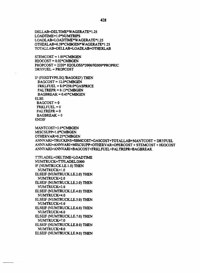
428
DELLAB=DELTIME*WAGERATE* 1.25 LC)ADTIME=1.0*NUMTRIPS LOADLAB=LOADTIME*WAGERATE* 1.25 OTHERLAB=0.59*CMBGEN* WAGERATE* 1.25 TOTALLAB=DELLAB+LOADLAB+OTHERLAB
STEMCOST = 1.05*CMBGEN H20C0ST = 0.02*CMBGEN PROPCOST = 2220* H2OLOSS*2000/92000*PROPRIC DRYFUEL = PROPCOST
IF (FEEDTYPE.EQ.BAGGED) THEN BAGCOST = 12.0*CMBGEN FRKLFUEL = 8.0*250.0*GASPRICE PALTREPR = 0.13*CMBGEN BAGBREAK = 0.45*CMBGEN
ELSE BAGCOST = 0 FRKLFUEL = 0 PALTREPR = 0 BAGBREAK = 0
ENDIF
MANTCOST=3.0*CMBGEN MISCSUPP=1.0*CMBGEN OTHER VAR=0.25 *CMBGEN ANNVARI=TRUCKINS+SBMCOST+GASCOST+TOTALLAB+MANTCOST + DRYFUEL ANNV ARI=ANNVARI+MISCSUPP+OTHERVAR+OPERCOST + STEMCOST + H20C0ST ANNVARI=ANNVARI+BAGCOST+FRKLFUEL+PALTREPR+BAGBREAK
TTFLADEL-DELTIME+LOADTIME NUMTRUCK=TTFLADEL/2000 IF (NUMTRUCK.LE. 1.0) THEN
NUMTRUCK= 1.0 ELSEIF (NUMTRUCK.LE.2.0) THEN
NUMTRUCK=2.0 ELSEIF (NUMTRUCK.LE.3.0) THEN
NUMTRUCK=3.0 ELSEIF (NUMTRUCK.LE.4.0) THEN
NUMTRUCK=4.0 ELSEIF (NUMTRUCK.LE.5.0) THEN
NUMTRUCK=5.0 ELSEIF (NUMTRUCK.LE.6.0) THEN
NUMTRUCK=6.0 ELSEIF (NUMTRUCK.LE.7.0) THEN
NUMTRUCK=7.0 ELSEIF (NUMTRUCK.LE.8.0) THEN
NUMTRUCK=8.0 ELSEIF (NUMTRUCK.LE.9.0) THEN
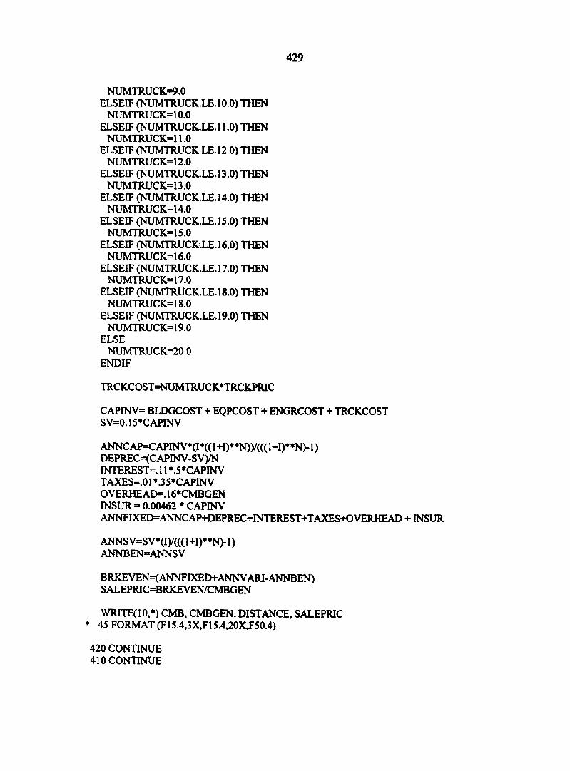
429
NUMTRUCK=9.0 ELSEIF (NUMTRUCK.LE.10.0) THEN
NUMTRUCK= 10.0 ELSEIF (NUMTRUCK.LE.11.0) THEN
NUMTRUCK=11.0 ELSEIF (NUMTRUCK.LE. 12.0) THEN
NUMTRUCK= 12.0 ELSEIF (NUMTRUCK.LE. 13.0) THEN
NUMTRUCK= 13.0 ELSEIF (NUMTRUCK.LE. 14.0) THEN
NUMTRU CK= 14.0 ELSEIF (NUMTRUCK.LE.15.0) THEN
NUMTRUCK= 15.0 ELSEIF (NUMTRUCK.LE. 16.0) THEN
NUMTRUCK= 16.0 ELSEIF (NUMTRUCK.LE.17.0) THEN
NUMTRUCK=17.0 ELSEIF (NUMTRUCK.LE.18.0) THEN
NUMTRUCK=18.0 ELSEIF (NUMTRUCK.LE. 19.0) THEN
NUMTRUCK=19.0 ELSE
NUMTRUCK=20.0 ENDIF
TRCKCOST=NUMTRUCK*TRCKPRIC
CAPINV= BLDGCOST + EQPCOST + ENGRCOST + TRCKCOST SV=0.15*CAPINV
ANNCAPCAPINV *(!*(( 1 +I)**N))/(((1+I)**N)-1 ) DEPREC=(C APINV-SV)/N INTEREST^. 11 *.5 *C APINV TAXES=.01 *.35*CAPINV OVERHEAD=. 16*CMBGEN INSUR = 0.00462 * CAPINV ANNFIXED=ANNCAP+DEPREC+INTEREST+TAXES+OVERHEAD + INSUR
ANNSV=SV*(I)/(((1+I)**N)-1) ANNBEN=ANNSV
BRKEVEN=(ANNFIXEI>ANNVARI-ANNBEN) SALEPRIC=BRKEVEN/CMBGEN
WRITE(10,*) CMB, CMBGEN, DISTANCE, SALEPRIC * 45 FORMAT ^15.4,3X^15.4^0X^50.4)
420 CONTINUE 410 CONTINUE
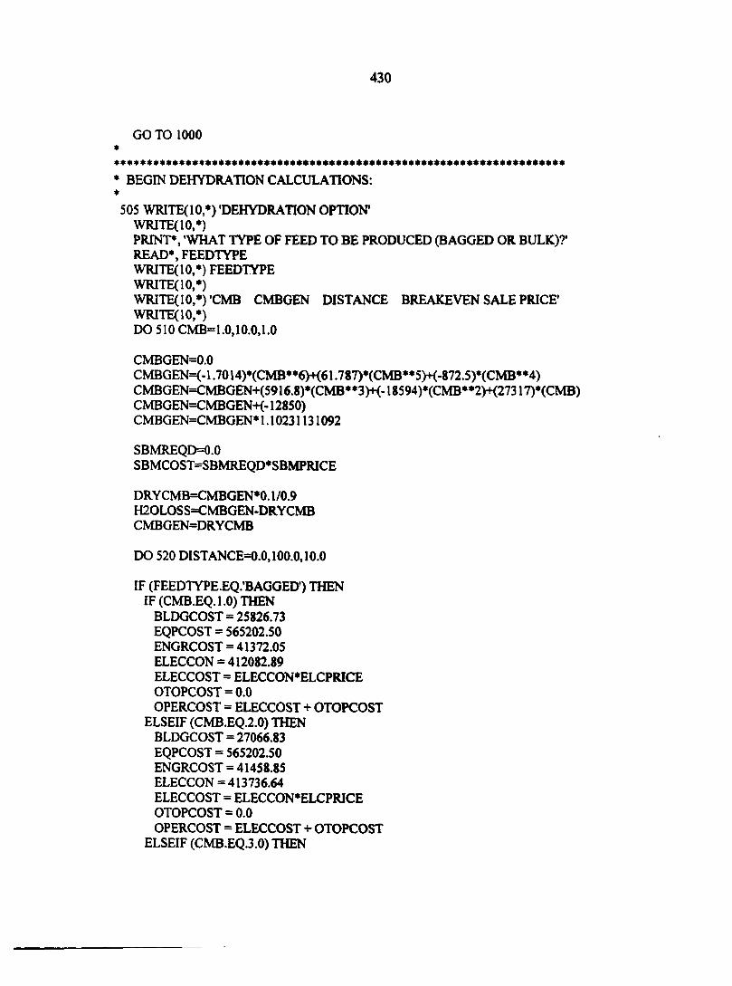
430
GO TO 1000
• BEGIN DEHYDRATION CALCULATIONS: *
505 WRITE(10,*) DEHYDRATION OPTION1
WRITE(10,*) PRINT*, 'WHAT TYPE OF FEED TO BE PRODUCED (BAGGED OR BULK)?' READ*, FEEDTYPE WRITE(10,*) FEEDTYPE WRITE(10,*) WRITE(10,*)'CMB CMBGEN DISTANCE BREAKEVEN SALE PRICE' WRITE(10,*) DO 510 CMB= 1.0,10.0,1.0
CMBGEN=0.0 CMBGEN=(-1,7014)*(CMB**6)+(61.787)*(CMB**5>K-872.5)*(CMB**4) CMBGEN=CMBGEN+(5916.8)*(CMB**3>K- 18594)*(CMB**2>K27317)*(CMB) CMBGEN=CMBGEN+(-12850) CMBGEN=CMBGEN* 1.10231131092
SBMREQD=0.0 SBMCOST=SBMREQD*SBMPRICE
DRY CMB=CMBGEN*0.1/0.9 H20L0SS=CMBGEN-DRYCMB CMBGEN=DRYCMB
DO 520 DISTANCE=0.0,100.0,10.0
IF (FEEDTYPEEQ.'BAGGED) THEN IF (CMB.EQ.1.0) THEN
BLDGCOST = 25826.73 EQPCOST = 565202.50 ENGRCOST = 41372.05 ELECCON = 412082.89 ELECCOST = ELECCON*ELCPRICE OTOPCOST = 0.0 OPERCOST = ELECCOST + OTOPCOST
ELSEIF (CMB.EQ2.0) THEN BLDGCOST = 27066.83 EQPCOST » 565202.50 ENGRCOST = 41458.85 ELECCON = 413736.64 ELECCOST = ELECCON*ELCPRICE OTOPCOST = 0.0 OPERCOST = ELECCOST + OTOPCOST
ELSEIF (CMB.EQ.3.0) THEN
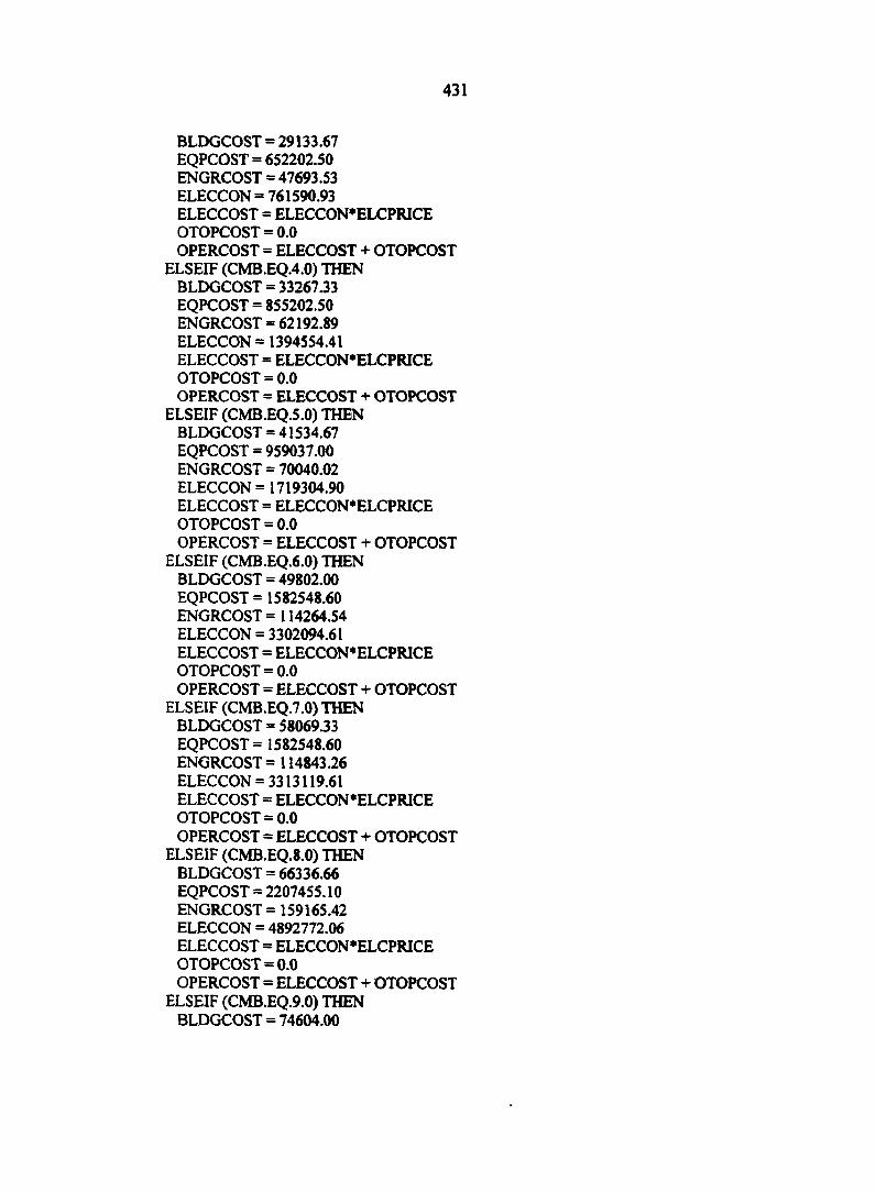
431
BLDGCOST = 29133.67 EQPCOST = 652202.50 ENGRCOST = 47693.53 ELECCON = 761590.93 ELECCOST = ELECCON*ELCPRICE OTOPCOST = 0.0 OPERCOST = ELECCOST + OTOPCOST
ELSEIF (CMB.EQ.4.0) THEN BLDGCOST = 3326733 EQPCOST = 855202.50 ENGRCOST = 62192.89 ELECCON =1394554.41 ELECCOST = ELECCON'ELCPRICE OTOPCOST = 0.0 OPERCOST = ELECCOST + OTOPCOST
ELSEIF (CMB.EQ.5.0) THEN BLDGCOST = 41534.67 EQPCOST = 959037.00 ENGRCOST = 70040.02 ELECCON = 1719304.90 ELECCOST = ELECCON*ELCPRICE OTOPCOST = 0.0 OPERCOST = ELECCOST + OTOPCOST
ELSEIF (CMB.EQ.6.0) THEN BLDGCOST = 49802.00 EQPCOST = 1582548.60 ENGRCOST = 114264.54 ELECCON = 3302094.61 ELECCOST = ELECCON'ELCPRICE OTOPCOST = 0.0 OPERCOST = ELECCOST + OTOPCOST
ELSEIF (CMB.EQ.7.0) THEN BLDGCOST = 5806933 EQPCOST = 1582548.60 ENGRCOST = 114843.26 ELECCON = 3313119.61 ELECCOST = ELECCON*ELCPRICE OTOPCOST = 0.0 OPERCOST = ELECCOST + OTOPCOST
ELSEIF (CMB.EQ.8.0) THEN BLDGCOST = 66336.66 EQPCOST = 2207455.10 ENGRCOST = 159165.42 ELECCON = 4892772.06 ELECCOST = ELECCON'ELCPRICE OTOPCOST = 0.0 OPERCOST = ELECCOST + OTOPCOST
ELSEIF (CMB.EQ.9.0) THEN BLDGCOST = 74604.00
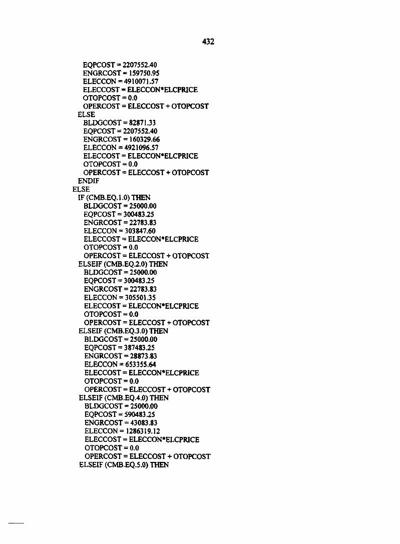
432
EQPCOST = 2207552.40 ENGRCOST = 159750.95 ELËCCON = 4910071.57 ELECCOST = ELECCON*ELCPRICE OTOPCOST = 0.0 OPERCOST = ELECCOST + OTOPCOST
ELSE BLDGCOST = 82871J3 EQPCOST = 2207552.40 ENGRCOST = 160329.66 ELECCON = 4921096.57 ELECCOST = ELECCON*ELCPRICE OTOPCOST = 0.0 OPERCOST = ELECCOST + OTOPCOST
ENDIF ELSE
IF (CMB.EQ.1.0) THEN BLDGCOST = 25000.00 EQPCOST = 300483.25 ENGRCOST = 22783.83 ELECCON = 303847.60 ELECCOST = ELECCON * ELCPRICE OTOPCOST = 0.0 OPERCOST = ELECCOST + OTOPCOST
ELSEIF (CMB.EQ.2.0) THEN BLDGCOST = 25000.00 EQPCOST = 300483.25 ENGRCOST = 22783.83 ELECCON = 305501.35 ELECCOST = ELECCON*ELCPRICE OTOPCOST = 0.0 OPERCOST = ELECCOST + OTOPCOST
ELSEIF (CMB.EQ.3.0) THEN BLDGCOST = 25000.00 EQPCOST = 387483.25 ENGRCOST = 28873.83 ELECCON = 653355.64 ELECCOST = ELECCON*ELCPRICE OTOPCOST = 0.0 OPERCOST = ELECCOST + OTOPCOST
ELSEIF (CMB.EQ.4.0) THEN BLDGCOST = 25000.00 EQPCOST = 59048325 ENGRCOST = 43083.83 ELECCON = 1286319.12 ELECCOST = ELECCON*ELCPRICE OTOPCOST = 0.0 OPERCOST = ELECCOST + OTOPCOST
ELSEIF (CMB.EQ.5.0) THEN
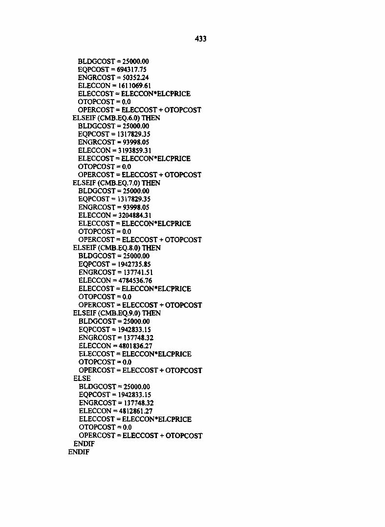
433
BLDGCOST = 25000.00 EQPCOST = 694317.75 ENGRCOST = 5035224 ELECCON =1611069.61 ELECCOST = ELECCON*ELCPRICE OTOPCOST = 0.0 OPERCOST = ELECCOST + OTOPCOST
ELSEIF (CMB.EQ.6.0) THEN BLDGCOST = 25000.00 EQPCOST = 1317829.35 ENGRCOST = 93998.05 ELECCON = 3193859.31 ELECCOST = ELECCON'ELCPRICE OTOPCOST = 0.0 OPERCOST = ELECCOST + OTOPCOST
ELSEIF (CMB.EQ.7.0) THEN BLDGCOST = 25000.00 EQPCOST = 1317829.35 ENGRCOST = 93998.05 ELECCON = 3204884.31 ELECCOST = ELECCON*ELCPRICE OTOPCOST = 0.0 OPERCOST = ELECCOST + OTOPCOST
ELSEIF (CMB.EQ.8.0) THEN BLDGCOST = 25000.00 EQPCOST = 1942735.85 ENGRCOST = 137741.51 ELECCON = 4784536.76 ELECCOST = ELECCON'ELCPRICE OTOPCOST = 0.0 OPERCOST = ELECCOST + OTOPCOST
ELSEIF (CMB.EQ.9.0) THEN BLDGCOST = 25000.00 EQPCOST = 1942833.15 ENGRCOST =137748.32 ELECCON = 4801836.27 ELECCOST = ELECCON'ELCPRICE OTOPCOST = 0.0 OPERCOST = ELECCOST + OTOPCOST
ELSE BLDGCOST = 25000.00 EQPCOST = 1942833.15 ENGRCOST = 137748.32 ELECCON = 4812861.27 ELECCOST = ELECCON*ELCPRICE OTOPCOST = 0.0 OPERCOST = ELECCOST + OTOPCOST
ENDIF ENDIF
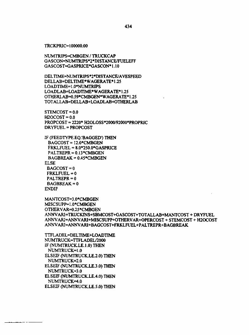
434
TRCKPRIC=100000.00
NUMTRIPS=CMBGEN / TRUCKCAP GASCON=NUMTRIPS*2*DISTANCE/FUELEFF GASCOST=GASPRICE*GASCON* 1. 10
DELTIME=NUMTRIPS*2*DISTANCE/AVESPEED DELLAB=DELTIME* WAGERATE* 1.25 LOADTIME= 1,0'NUMTRIPS LOADLAB=LOADTIME*WAGERATE* 1.25 OTHERLAB=0.59*CMBGEN*WAGERATE* 1.25 TOT ALLAB=DELLAB+LOADLAB+OTHERLAB
STEMCOST = 0.0 H20C0ST = 0.0 PROPCOST = 2220* H2OLOSS*2000/92000»PROPRIC DRYFUEL = PROPCOST
IF (FEEDTYPE-EQ.'BAGGED') THEN BAGCOST = 12.0*CMBGEN FRKLFUEL = 8.0*250.0*GASPRICE PALTREPR = 0.13*CMBGEN BAGBREAK = 0.45*CMBGEN
ELSE BAGCOST = 0 FRKLFUEL = 0 PALTREPR = 0 BAGBREAK = 0
ENDIF
MANTCOST=3.0*CMBGEN MISCSUPP=1.0*CMBGEN OTHERVAR=0.25*CMBGEN ANNV ARI=TRUCKINS+SBMCOST+G ASCOST+TOTALL AB+MANTCOST + DRYFUEL ANNV ARI=ANNV ARI+MISCSUPP+OTHERVAR+OPERCOST + STEMCOST + H20C0ST ANNVARI=ANNVARI+BAGCOST+FRKLFUEL+PALTREPR+BAGBREAK
TTFLADEL=DELTIME+LOADTIME NUMTRUCK=TTFLADEL/2000 IF (NUMTRUCK.LE. 1.0) THEN
NUMTRUCK=1.0 ELSEIF (NUMTRUCK.LE.2.0) THEN
NUMTRUCK=2.0 ELSEIF (NUMTRUCKXE.3.0) THEN
NUMTRUCK=3.0 ELSEIF (NUMTRUCK.LE.4.0) THEN
NUMTRUCK=4.0 ELSEIF (NUMTRUCK.LE.5.0) THEN
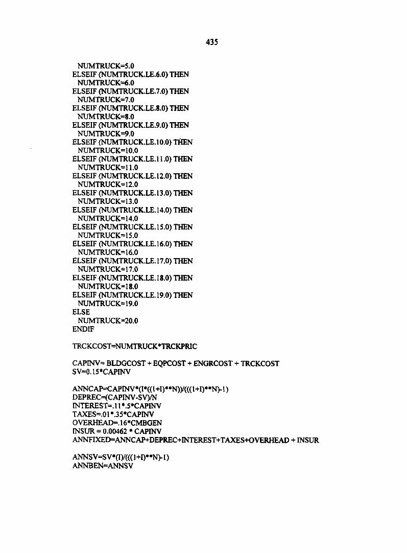
435
NUMTRUCK=5.0 ELSEIF (NUMTRUCK.LE.6.0) THEN
NUMTRUCK=6.0 ELSEIF (NUMTRUCK.LE.7.0) THEN
NUMTRUCK=7.0 ELSEIF (NUMTRUCK.LE.8.0) THEN
NUMTRUCK=8.0 ELSEIF (NUMTRUCK.LE.9.0) THEN
NUMTRUCK=9.0 ELSEIF (NUMTRUCK.LE. 10.0) THEN
NUMTRUCK= 10.0 ELSEIF (NUMTRUCK.LE.11.0) THEN
NUMTRUCK=11.0 ELSEIF (NUMTRUCK.LE. 12.0) THEN
NUMTRUCK=12.0 ELSEIF (NUMTRUCK.LE. 13.0) THEN
NUMTRUCK= 13.0 ELSEIF (NUMTRUCK.LE. 14.0) THEN
NUMTRUCK= 14.0 ELSEIF (NUMTRUCK.LE.15.0) THEN
NUMTRUCK= 15.0 ELSEIF (NUMTRUCK.LE.16.0) THEN
NUMTRUCK= 16.0 ELSEIF (NUMTRUCK.LE.17.0) THEN
NUMTRUCK=17.0 ELSEIF (NUMTRUCK.LE.18.0) THEN
NUMTRUCK=18.0 ELSEIF (NUMTRUCK.LE. 19.0) THEN
NUMTRUCK=19.0 ELSE
NUMTRUCK=20.0 ENDIF
TRCKCOST=NUMTRUCK*TRCKPRIC
CAPINV= BLDGCOST + EQPCOST + ENGRCOST + TRCKCOST SV=0.15*CAPINV
ANNC AP=C APINV*(I*(( 1 +1)* *N))/((( l+I)**N)-1 ) DEPREC=(CAPINV-SV)/N INTEREST=. 11 * .5 *C APINV TAXES=.01*.35*CAPINV OVERHEAD=. 16*CMBGEN INSUR = 0.00462 * CAPINV ANNFIXED=ANNCAP+DEPREC+INTEREST+TAXES+OVERHEAD + INSUR
ANNSV=SV*(I)/((( 1 +I)**N)-1 ) ANNBEN=ANNSV
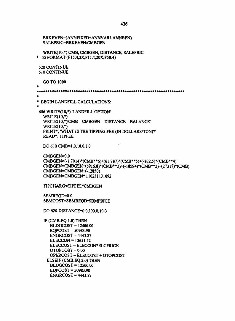
436
BRKEVEN=(ANNFIXED+ANNVARI-ANNBEN) SALEPRIC=BRKEVEN/CMBGEN
WRITE(10,*) CMB, CMBGEN, DISTANCE, SALEPRIC * 55 FORMAT (F15.4,3X,F1S.4,20X,F50.4)
520 CONTINUE 510 CONTINUE
GO TO 1000
BEGIN LANDFILL CALCULATIONS:
606 WRITE(10,*) -LANDFILL OPTION* WRITE(10,*) WRITE( 10,*)'CMB CMBGEN DISTANCE BALANCE' WRITE(10,*) PRINT*, 'WHAT IS THE TIPPING FEE (IN DOLLARS/TON)?' READ*, TIPFEE
DO 610 CMB=1.0,10.0,1.0
CMBGEN=0.0 CMBGEN=(-1.7014)*(CMB**6>K61.787)*(CMB**5)+(-872.5)*(CMB**4) CMBGEN=CMBGEN+(5916.8)*(CMB**3)+(-18594)*(CMB**2)+(27317)*(CMB) CMBGEN=CMBGEN+(-12850) CMBGEN=CMBGEN* 1.10231131092
TIPCHARG=TIPFEE*CMBGEN
SBMREQD=0.0 SBMCOST=SBMREQD*SBMPRICE
DO 620 DISTANCE=0.0,100.0,10.0
IF (CMB.EQ.1.0) THEN BLDGCOST = 12500.00 EQPCOST = 50983.90 ENGRCOST = 4443.87 ELECCON = 13651.52 ELECCOST = ELECCON*ELCPRICE OTOPCOST = 0.00 OPERCOST = ELECCOST + OTOPCOST
ELSEIF (CMB.EQ.2.0) THEN BLDGCOST = 12500.00 EQPCOST = 50983.90 ENGRCOST = 4443.87
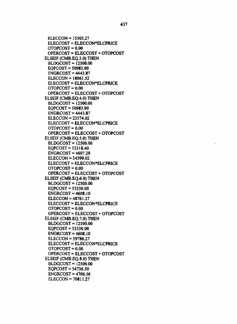
437
ELECCON = 15305.27 ELECCOST = ELECCON*ELCPRICE OTOPCOST = 0.00 OPERCOST = ELECCOST + OTOPCOST
ELSEIF (CMB.EQ.3.0) THEN BLDGCOST = 12500.00 EQPCOST =50983.90 ENGRCOST = 4443.87 ELECCON = 18061.52 ELECCOST = ELECCON*ELCPRICE OTOPCOST = 0.00 OPERCOST = ELECCOST + OTOPCOST
ELSEIF (CMB.EQ.4.0) THEN BLDGCOST = 12500.00 EQPCOST = 50983.90 ENGRCOST = 4443.87 ELECCON = 23574.02 ELECCOST = ELECCON'ELCPRICE OTOPCOST = 0.00 OPERCOST = ELECCOST + OTOPCOST
ELSEIF (CMB.EQ.5.0) THEN BLDGCOST = 12500.00 EQPCOST = 53318.40 ENGRCOST = 4607.29 ELECCON = 34599.02 ELECCOST = ELECCON'ELCPRICE OTOPCOST = 0.00 OPERCOST = ELECCOST + OTOPCOST
ELSEIF (CMB.EQ.6.0) THEN BLDGCOST = 12500.00 EQPCOST = 53330.00 ENGRCOST = 4608.10 ELECCON = 48761.27 ELECCOST = ELECCON'ELCPRICE OTOPCOST = 0.00 OPERCOST = ELECCOST + OTOPCOST
ELSEIF (CMB.EQ.7.0) THEN BLDGCOST = 12500.00 EQPCOST = 53330.00 ENGRCOST = 4608.10 ELECCON = 59786.27 ELECCOST = ELECCON'ELCPRICE OTOPCOST = 0.00 OPERCOST = ELECCOST + OTOPCOST
ELSEIF (CMB.EQ.8.0) THEN BLDGCOST =12500.00 EQPCOST = 54736.50 ENGRCOST = 4706.56 ELECCON = 70811.27
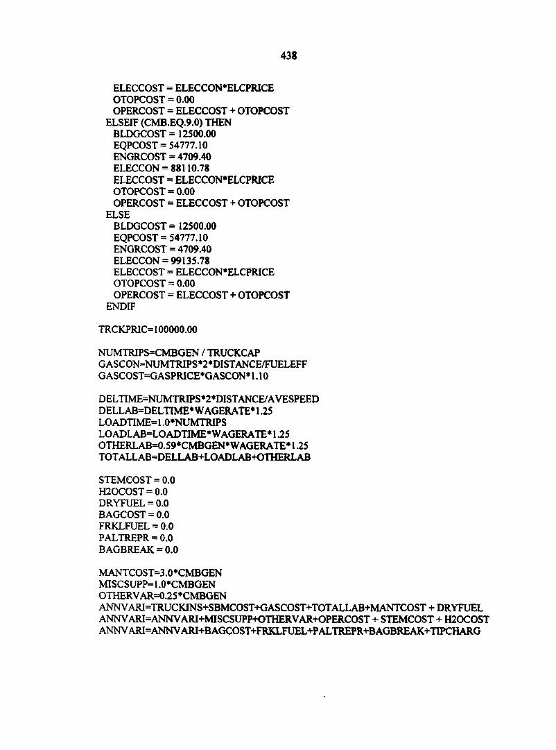
438
ELECCOST = ELECCON*ELCPRICE OTOPCOST = 0.00 OPERCOST = ELECCOST + OTOPCOST
ELSEIF (CMB.EQ.9.0) THEN BLDGCOST = 12500.00 EQPCOST =54777.10 ENGRCOST = 4709.40 ELECCON = 88110.78 ELECCOST = ELECCON'ELCPRICE OTOPCOST = 0.00 OPERCOST = ELECCOST + OTOPCOST
ELSE BLDGCOST = 12500.00 EQPCOST = 54777.10 ENGRCOST = 4709.40 ELECCON = 99135.78 ELECCOST = ELECCON'ELCPRICE OTOPCOST = 0.00 OPERCOST = ELECCOST + OTOPCOST
ENDIF
TRCKPRIC= 100000.00
NUMTRIPSCMBGEN / TRUCKCAP GASCON=NUMTRIPS*2*DISTANCE/FUELEFF GASCOST=GASPRICE*GASCON* 1.10
DELTIME=NUMTRIPS*2*DISTANCE/AVESPEED DELLAB=DELTIME*WAGERATE* 1.25 LOADTIME=l ,0'NUMTRIPS LOADLAB=LOADTIME*WAGERATE* 1.25 OTHERLAB=0.59«CMBGEN» WAGERATE* 1.25 TOT ALL AB=DELLAB+LOADLAB+OTHERLAB
STEMCOST = 0.0 H20C0ST = 0.0 DRYFUEL = 0.0 BAGCOST = 0.0 FRKLFUEL = 0.0 PALTREPR = 0.0 BAGBREAK = 0.0
MANTCOST=3.0*CMBGEN MISC SUPP= 1.0 *CMBGEN OTHERVAR=0.25* CMBGEN ANNVARI=TRUCKINS+SBMCOST+GASCOST+TOTALLAB+MANTCOST + DRYFUEL ANNV ARI=ANNV ARI+MISCSUPP+OTHERVAR+OPERCOST + STEMCOST + H20C0ST ANNV ARI=ANNV ARI+B AGCOST+FRKLFUEL+PALTREPR+BAGBREAK+TIPCHARG
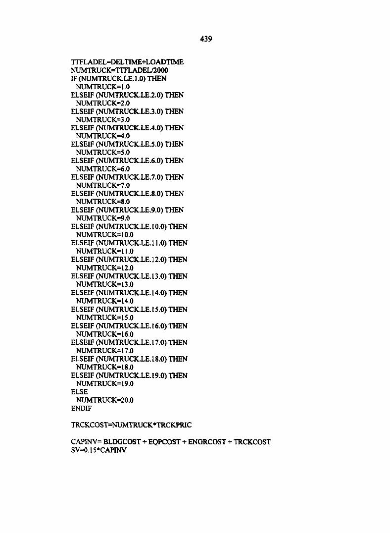
439
TTFLADEL=DELTIME+LOADTIME NUMTRUCK=TTFLADEL/2000 IF (NUMTRUCK.LE. 1.0) THEN
NUMTRUCK= 1.0 ELSEIF (NUMTRUCK.LE.2.0) THEN
NUMTRUCK=2.0 ELSEIF (NUMTRUCK.LE.3.0) THEN
NUMTRUCK=3.0 ELSEIF (NUMTRUCK.LE.4.0) THEN
NUMTRU C K=4.0 ELSEIF (NUMTRUCK.LE.5.0) THEN
NUMTRUCK=5.0 ELSEIF (NUMTRUCK.LE.6.0) THEN
NUMTRU C K.=6.0 ELSEIF (NUMTRUCK.LE.7.0) THEN
NUMTRUCK=7.0 ELSEIF (NUMTRUCK.LE.8.0) THEN
NUMTRUCK=8.0 ELSEIF (NUMTRUCK.LE.9.0) THEN
NUMTRU C K=9.0 ELSEIF (NUMTRUCK.LE.10.0) THEN
NUMTRUCK=10.0 ELSEIF (NUMTRUCK.LE. 11.0) THEN
NUMTRUCK=11.0 ELSEIF (NUMTRUCK.LE.12.0) THEN
NUMTRU CK= 12.0 ELSEIF (NUMTRUCK.LE.13.0) THEN
NUMTRU CK= 13.0 ELSEIF (NUMTRUCK.LE. 14.0) THEN
NUMTRUCK= 14.0 ELSEIF (NUMTRUCK.LE. 15.0) THEN
NUMTRUCK=15.0 ELSEIF (NUMTRUCK.LE. 16.0) THEN
NUMTRUCK=16.0 ELSEIF (NUMTRUCK.LE.17.0) THEN
NUMTRUCK= 17.0 ELSEIF (NUMTRUCK.LE.18.0) THEN
NUMTRUCK= 18.0 ELSEIF (NUMTRUCK.LE.19.0) THEN
NUMTRUCK=19.0 ELSE
NUMTRUCK=20.0 ENDIF
TRCKCOST=NUMTRUCK*TRCKPRIC
CAPINV= BLDGCOST + EQPCOST + ENGRCOST + TRCKCOST SV=0.15 *CAPINV
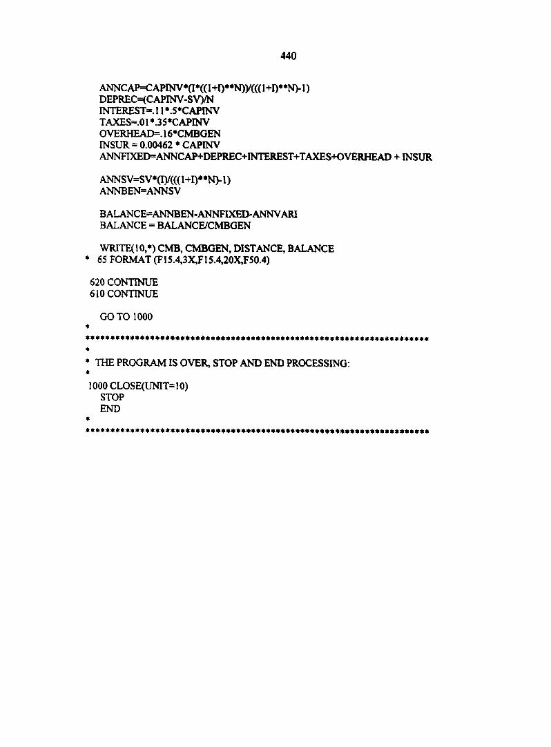
440
ANNCAP=CAPINV*a*((l+I)**N))/(((l+De*N>l) DEPREC=(CAPINV-SV)/N INTERESTS 11*.5»CAPINV TAXES=.0I*.35*CAPINV OVERHEAD^ 16*CMBGEN INSUR = 0.00462 * CAPINV ANNFIXED=ANNCAP+DEPREC+INTEREST+TAXES+OVERHEAD + INSUR
ANNSV=SV*(I)/((( 1+I)**N> 1 ) ANNBEN=ANNSV
BALANCE=ANNBEN-ANNFIXED-ANNVARI BALANCE = BALANCE/CMBGEN
WRITEC10,*) CMB, CMBGEN, DISTANCE, BALANCE * 65 FORMAT (F15.4,3X,FI5.4,20XF50.4)
620 CONTINUE 610 CONTINUE
GOTO 1000
THE PROGRAM IS OVER, STOP AND END PROCESSING:
1000 CLOSE(UNIT= 10) STOP END

441
APPENDIX 7-B
EQUIPMENT AND BUILDING INFORMATION IMPLEMENTED IN ECONOMICS OF RECYCLING CMB MODEL
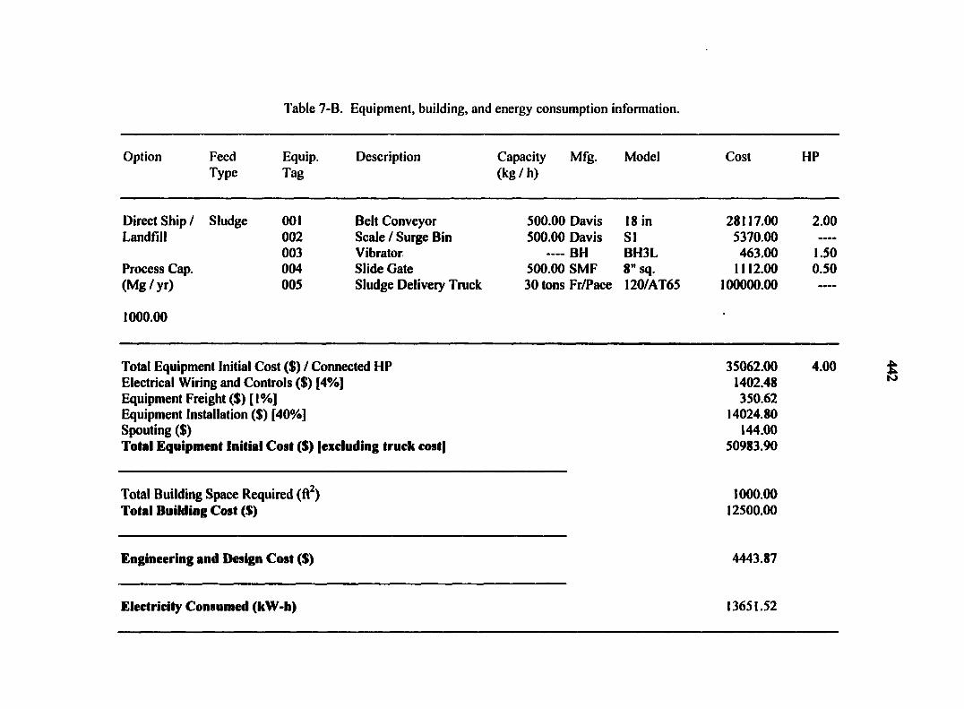
Table 7-B. Equipment, building, and energy consumption information.
Option Feed Type
Equip. Tag
Description Capacity Mfg. (kg / h)
Model Cost HP
Direct Ship / Sludge 001 Belt Conveyor 500.00 Davis 18 in 28117.00 2.00 Landfill 002 Scale / Surge Bin 500.00 Davis SI 5370.00
003 Vibrator — BH BH3L 463.00 1.50 Process Cap. 004 Slide Gate 500.00 SMF 8" sq. 1112.00 0.50 (Mg/yr) 005 Sludge Delivery Truck 30 tons Fr/Pace 120/AT65 100000.00
1000.00
Total Equipment Initial Cost ($) / Connected HP 35062.00 4.00 Electrical Wiring and Controls ($) [4%] 1402.48 Equipment Freight ($) [ I %] 350.62 Equipment Installation ($) [40%] 14024.80 Spouting ($) 144.00 Total Equipment Initial Cost ($) [excluding truck cost) 50983.90
Total Building Space Required (ft2) 1000.00 Total Building Cost ($) 12500.00
Engineering and Design Cost ($) 4443.87
Electricity Consumed (kW-h) 13651.52
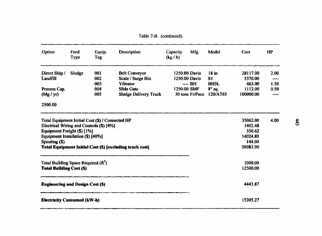
Table 7-B. (continued).
Option Feed Type
Equip. Tag
Description Capacity (kg / h)
Mfg. Model Cost HP
Direct Ship / Sludge 001 Belt Conveyor 1250.00 Davis 18 in 28117.00 2.00 Landfill 002 Scale / Surge Bin 1250.00 Davis SI 5370.00 ——
003 Vibrator ---- BH BH3L 463.00 1.50 Process Cap. 004 Slide Gate 1250.00 SMF 8" sq. 1112.00 0.50 (Mg / yr) 005 Sludge Delivery Truck 30 tons Fr/Pace I20ZAT65 100000.00 ....
2500.00
Total Equipment Initial Cost ($) / Connected HP 35062.00 4.00 Electrical Wiring and Controls ($) [4%] 1402.48 Equipment Freight ($) [ 1 %] 350.62 Equipment Installation ($) [40%] 14024.80 Spouting ($) 144.00 Total Equipment Initial Cost ($) [excluding truck cost] 50983.90
Total Building Space Required (ft2) 1000.00 Total Building Cost ($) 12500.00
Engineering and Design Cost ($) 4443.87
Electricity Consumed (kW-h) 15305.27
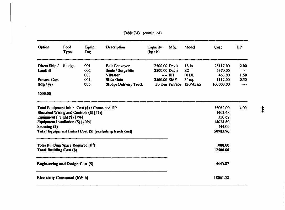
Table 7-B. (continued).
Option Feed Type
Equip. Tag
Description Capacity (kg / h)
Mfg. Model Cost HP
Direct Ship / Sludge 001 Belt Conveyor 2500.00 Davis 18 in 28117.00 2.00 Landfill 002 Scale / Surge Bin 2500.00 Davis S2 5370.00 —-
003 Vibrator ———— BH BH3L 463.00 1.50 Process Cap. 004 Slide Gate 2500.00 SMF 8 " sq. 1112.00 0.50 (Mg/yr) 005 Sludge Delivery Truck 30 tons Fr/Pace 120/AT65 100000.00
5000.00
Total Equipment Initial Cost ($) / Connected HP 35062.00 4.00 Electrical Wiring and Controls ($) [4%] 1402.48 Equipment Freight ($) [ I %] 350.62 Equipment Installation ($) [40%] 14024.80 Spouting ($) 144.00 Total Equipment Initial Cost ($) (excluding truck costj 50983.90
Total Building Space Required (ft2) 1000.00 Total Building Cost ($) 12500.00
Engineering and Design Cost ($) 4443.87
Electricity Consumed (kW-h) 18061.52

Table 7-B. (continued).
Option Feed Equip. Description Capacity Mfg. Model Cost HP Type Tag (kg / h)
Direct Ship / Sludge 001 Belt Conveyor 5000.00 Davis 18 in 28117.00 2.00 Landfill 002 Scale / Surge Bin 5000.00 Davis S5 5370.00 —-
003 Vibrator ---- BH BH3L 463.00 1.50 Process Cap. 004 Slide Gate 5000.00 SMF 8" sq. 1112.00 0.50 (Mg/yr) 005 Sludge Delivery Truck 30 tons Fr/Pace I20/AT65 100000.00 —«
10000.00
Total Equipment Initial Cost ($) / Connected HP 35062.00 4.00 Electrical Wiring and Controls ($) [4%] 1402.48 Equipment Freight ($) [ 1 %] 350.62 Equipment Installation ($) [40%] 14024.80 Spouting ($) 144.00 Total Equipment Initial Cost ($) [excluding truck cost] 50983.90
Total Building Space Required (ft2) 1000.00 Total Building Cost ($) 12500.00
Engineering and Design Cost ($) 4443.87
Electricity Consumed (kW-h) 23574.02

Table 7-B. (continued).
Option Feed Type
Equip. Tag
Description Capacity (kg/h)
Mfg. Model Cost HP
Direct Ship / Sludge 001 Belt Conveyor 10000.00 Davis 18 in 28117.00 2.00 Landfill 002 Scale / Surge Bin 10000.00 Davis S10 6980.00 ——
003 Vibrator BH BH3L 463.00 1.50 Process Cap. 004 Slide Gate 10000.00 SMF 8" sq. 1112.00 0.50 (Mg/yr) 005 Sludge Delivery Truck 30 tons Fr/Pace 120/AT65 100000.00 ....
20000.00
Total Equipment Initial Cost ($) / Connected HP 36672.00 4.00 Electrical Wiring and Controls ($) [4%] 1466.88 Equipment Freight ($) [ 1 %] 366.72 Equipment Installation ($) [40%] 14668.80 Spouting ($) 144.00 Total Equipment Initial Cost ($) (excluding truck cost] 53318.40
Total Building Space Required (ft2) 1000.00 Total Building Cost ($) 12500.00
Engineering and Design Cost ($) 4607.29
Electricity Consumed (kW-h) 34599.02

Table 7-B. (continued).
Option Feed Equip. Description Capacity Mfg. Model Cost HP Type Tag (kg / h)
Direct Ship / Sludge 001 Belt Conveyor 15000.00 Davis 18 in 28125.00 3.00 Landfill 002 Scale / Surge Bin 15000.00 Davis S20 6980.00
003 Vibrator BH BH3L 463.00 1.50 Process Cap. 004 Slide Gate 15000.00 SMF 8 " sq. 1112.00 0.50 (Mg/yr) 005 Sludge Delivery Truck 30 tons Fr/Pace 120/AT65 100000.00 ——
30000.00
Total Equipment Initial Cost ($) / Connected HP 36680.00 5.00 Electrical Wiring and Controls ($) [4%] 1467.20 Equipment Freight ($) [ I %] 366.80 Equipment Installation ($) [40%] 14672.00 Spouting ($) 144.00 Total Equipment Initial Cost ($) [excluding truck cost] 53330.00
Total Building Space Required (ft2) 1000.00 Total Building Cost ($) 12500.00
Engineering and Design Cost ($) 4608.10
Electricity Consumed (kW-h) 48761.27
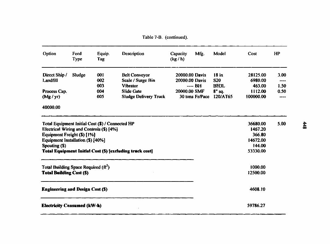
Table 7-B. (continued).
Option Feed Equip. Description Capacity Mfg. Model Cost HP Type Tag (kg / h)
Direct Ship / Sludge 001 Belt Conveyor 20000.00 Davis 18 in 28125.00 3.00 Landfill 002 Scale / Surge Bin 20000.00 Davis S20 6980.00
003 Vibrator — BH BH3L 463.00 1.50 Process Cap. 004 Slide Gate 20000.00 SMF 8" sq. 1112.00 0.50 (Mg/yr) 005 Sludge Delivery Truck 30 tons Fr/Pace I20/AT65 100000.00 ——
40000.00
Total Equipment Initial Cost ($) / Connected HP 36680.00 5.00 Electrical Wiring and Controls ($) [4%] 1467.20 Equipment Freight ($) [ 1 %] 366.80 Equipment Installation ($) [40%] 14672.00 Spouting ($) 144.00 Total Equipment Initial Cost ($) [excluding truck cost) 53330.00
Total Building Space Required (ft2) 1000.00 Total Building Cost ($) 12500.00
Engineering and Design Cost ($) 4608.10
Electricity Consumed (kW-h) 59786.27

Table 7-B. (continued).
Option Feed Type
Equip. Tag
Description Capacity Mfg. (kg/h)
Model Cost HP
Direct Ship / Sludge 001 Belt Conveyor 25000.00 Davis 18 in 28125.00 3.00 Landfill 002 Scale / Surge Bin 25000.00 Davis S40 7950.00
003 Vibrator — BH BH3L 463.00 1.50 Process Cap. 004 Slide Gate 25000.00 SMF 8" sq. 1112.00 0.50 (Mg/yr) 005 Sludge Delivery Truck 30 tons Fr/Pace 120/AT65 100000.00 —-
50000.00
Total Equipment Initial Cost ($) / Connected HP 37650.00 5.00 Electrical Wiring and Controls ($) [4%] 1506.00 Equipment Freight ($) [ 1 %] 376.50 Equipment Installation ($) [40%] 15060.00 Spouting ($) 144.00 Total Equipment Initial Cost ($) (excluding truck cost] 54736.50
Total Building Space Required (ft2) 1000.00 Total Building Cost ($) 12500.00
Engineering and Design Cost ($) 4706.56
Electricity Consumed (kW-h) 70811.27

Table 7-B. (continued).
Option Feed Equip. Description Capacity Mfg. Model Cost HP Type Tag (kg / h)
Direct Ship / Sludge 001 Belt Conveyor 30000.00 Davis 18 in 28153.00 5.00 Landfill 002 Scale / Surge Bin 30000.00 Davis S40 7950.00 ——
003 Vibrator BH BH3L 463.00 1.50 Process Cap. 004 Slide Gate 30000.00 SMF 8" sq. 1112.00 0.50 (Mg/yr) 005 Sludge Delivery Truck 30 tons Fr/Pace I20/AT65 100000.00 ....
60000.00
Total Equipment Initial Cost ($) / Connected HP 37678.00 7.00 Electrical Wiring and Controls ($) [4%] 1507.12 Equipment Freight ($) [ 1 %] 376.78 Equipment Installation ($) [40%] 15071.20 Spouting ($) 144.00 Total Equipment Initial Cost ($) (excluding truck cost] 54777.10
Total Building Space Required (ft2) 1000.00 Total Building Cost ($) 12500.00
Engineering and Design Cost ($) 4709.40
Electricity Consumed (kW-h) 88110.78

Table 7-B. (continued).
Option Feed Equip. Description Capacity Mfg. Model Cost HP Type Tag (kg / h)
Direct Ship / Sludge 001 Belt Conveyor 35000.00 Davis 18 in 28153.00 5.00 Landfill 002 Scale / Surge Bin 35000.00 Davis S60 7950.00 —-
003 Vibrator — BH BH3L 463.00 1.50 Process Cap. 004 Slide Gate 35000.00 SMF 8" sq. 1112.00 0.50 (Mg/yr) 005 Sludge Delivery Truck 30 tons Fr/Pace 120/AT65 100000.00
70000.00
Total Equipment Initial Cost ($) / Connected HP 37678.00 7.00 Electrical Wiring and Controls ($) [4%] 1507.12 Equipment Freight ($) [ I %] 376.78 Equipment Installation ($) [40%] 15071.20 Spouting ($) 144.00 Total Equipment Initial Cost ($) [excluding truck cost] 54777.10
Total Building Space Required (ft2) 1000.00 Total Building Cost ($) 12500.00
Engineering and Design Cost ($) 4709.40
Electricity Consumed (kW-h) 99135.78
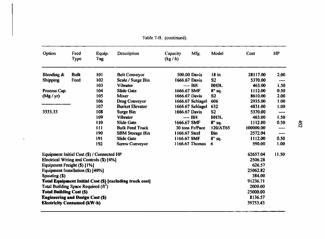
Table 7-B. (continued).
Option Feed Type
Equip. Tag
Description Capacity Mfg. (kg / h)
Model Cost HP
Blending & Bulk 101 Belt Conveyor 500.00 Davis 18 in 28117.00 2.00 Shipping Feed 102 Scale / Surge Bin 1666.67 Davis S2 5370.00 —-
103 Vibrator — BH BH3L 463.00 1.50 Process Cap. 104 Slide Gate 1666.67 SMF 8" sq. 1112.00 0.50 (Mg/yr) 105 Mixer 1666.67 Davis S2 8610.00 2.00
106 Drag Conveyor 1666.67 Schlagel 606 2935.00 1.00 107 Bucket Elevator 1666.67 Schlagel 632 4831.00 1.00
3333.33 108 Surge Bin 1666.67 Davis S2 5370.00 •——»
109 Vibrator — BH BH3L 463.00 1.50 110 Slide Gate 1666.67 SMF 8" sq. 1112.00 0.50 I I I Bulk Feed Truck 30 tons Fr/Pace I20/AT65 100000.00 ——
190 SBM Storage Bin 1166.67 Steel Bin 2572.04 —-
191 Slide Gate 1166.67 SMF 8" sq. 1112.00 0.50 192 Screw Conveyor 1166.67 Thomas 6 590.00 1.00
Equipment Initial Cost ($) / Connected HP Electrical Wiring and Controls ($) [4%] Equipment Freight ($) [l%] Equipment Installation ($) [40%] Spouting ($) Total Equipment Initial Cost ($) (excluding truck cost] Total Building Space Required (ft2) Total Building Cost ($) Engineering and Design Cost ($) Electricity Consumed (kW-h)
62657.04 2506.28 626.57
25062.82 384.00
91236.71 2000.00
25000.00 8136.57
39753.43
11.50
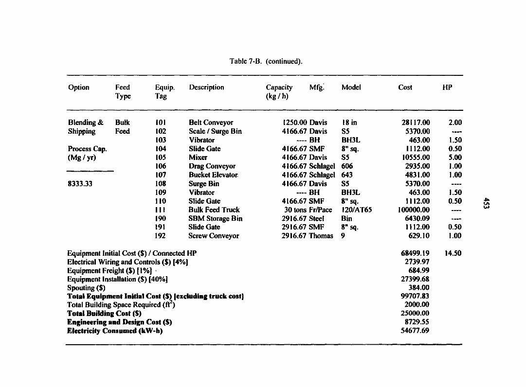
Table 7-B. (continued).
Option Feed Type
Equip. Tag
Description Capacity Mfg. (kg / h)
Model Cost HP
Blending & Bulk 101 Belt Conveyor 1250.00 Davis 18 in 28117.00 2.00 Shipping Feed 102 Scale / Surge Bin 4166.67 Davis S5 5370.00 ——
103 Vibrator — BH BH3L 463.00 1.50 Process Cap. 104 Slide Gate 4166.67 SMF 8" sq. 1112.00 0.50 (Mg / yr) 105 Mixer 4166.67 Davis S5 10555.00 5.00
106 Drag Conveyor 4166.67 Schlagel 606 2935.00 1.00 107 Bucket Elevator 4166.67 Schlagel 643 4831.00 1.00
8333.33 108 Surge Bin 4166.67 Davis S5 5370.00 109 Vibrator — BH BH3L 463.00 1.50 110 Slide Gate 4166.67 SMF 8" sq. 1112.00 0.50 I I I Bulk Feed Truck 30 tons Fr/Pace 120/AT65 100000.00 190 SBM Storage Bin 2916.67 Steel Bin 6430.09 191 Slide Gate 2916.67 SMF 8" sq. 1112.00 0.50 192 Screw Conveyor 2916.67 Thomas 9 629.10 1.00
Equipment Initial Cost ($) / Connected HP 68499.19 14.50 Electrical Wiring and Controls ($) [4%] 2739.97 Equipment Freight ($) [1%] • 684.99 Equipment Installation ($) [40%] 27399.68 Spouting ($) 384.00 Total Equipment Initial Cost ($) [excluding truck cost] 99707.83 Total Building Space Required (ft ) 2000.00 Total Building Cost ($) 25000.00 Engineering and Design Cost ($) 8729.55 Electricity Consumed (kW-h) 54677.69

Table 7-B. (continued).
Option Feed Equip. Description Capacity Mfg. Model Cost HP Type Tag (kg / h)
Blending & Bulk 101 Belt Conveyor 2500.00 Davis 18 in 28117.00 2.00 Shipping Feed 102 Scale / Surge Bin 8333.33 Davis S10 6980.00 —-
103 Vibrator — BH BH3L 463.00 1.50 Process Cap. 104 Slide Gate 8333.33 SMF 8" sq. 1112.00 0.50 (Mg / yr) 105 Mixer 8333.33 Davis S10 12255.00 7.50
106 Drag Conveyor 8333.33 Schlagel 606 2935.00 1.00 107 Bucket Elevator 8333.33 Schlagel 654 4831.00 1.00
16666.67 108 Surge Bin 8333.33 Davis S10 6980.00 ——
109 Vibrator —— BH BH3L 463.00 1.50 110 Slide Gate 8333.33 SMF 8" sq. 1112.00 0.50 I I I Bulk Feed Truck 30 tons Fr/Pace I20/AT65 100000.00 ——
190 SBM Storage Bin 5833.33 Steel Bin 12860.16 ----
191 Slide Gate 5833.33 SMF 8" sq. 1112.00 0.50 192 Screw Conveyor 5833.33 Thomas 9 629.10 1.00
Equipment Initial Cost ($) / Connected HP 79849.26 17.00 Electrical Wiring and Controls ($) [' »%] 3193.97 Equipment Freight ($) [l%] 798.49 Equipment Installation ($) [40%] 31939.70 Spouting ($) 384.00 Total Equipment Initial Cost ($) (excluding truck cost] 116165.43 Total Building Space Required (ft ) 2000.00 Total Building Cost ($) 25000.00 Engineering and Design Cost ($) 9881.58 Electricity Consumed (kW-h) 71708.34

Table 7-B. (continued).
Option Feed Equip. Description Capacity Mfg. Model Cost HP Type Tag (kg / h)
Blending & Bulk 101 Belt Conveyor 5000.00 Davis 18 in 28117.00 2.00 Shipping Feed 102 Scale / Surge Bin 16666.67 Davis S20 6980.00
103 Vibrator — BH BH3L 463.00 1.50 Process Cap. 104 Slide Gate 16666.67 SMF 8" sq. 1112.00 0.50 (Mg/yr) 105 Mixer 16666.67 Davis S20 14385.00 10.00 (Mg/yr)
106 Drag Conveyor 16666.67 Schlagel 606 2935.00 1.00 107 Bucket Elevator 16666.67 Schlagel 665 4831.00 1.00
33333.33 108 Surge Bin 16666.67 Davis S20 6980.00 109 Vibrator — BH BH3L 463.00 1.50 110 Slide Gate 16666.67 SMF 8" sq. 1112.00 0.50 I I I Bulk Feed Truck 30 tons Fr/Pace I20/AT65 100000.00 190 SBM Storage Bin 11666.67 Steel Bin 25720.34 ----
191 Slide Gate 11666.67 SMF 8" sq. 1112.00 0.50 192 Screw Conveyor 11666.67 Thomas 12 787.50 1.00
Equipment initial Cost ($) / Connected HP 94997.84 19.50 Electrical Wiring and Controls ($) [4%] 3799.91 Equipment Freight ($) [ 1 %] 949.98 Equipment Installation ($) [40%] 37999.14 Spouting ($) 384.00 Total Equipment Initial Cost ($) (excluding truck cost] 138130.87 Total Building Space Required (ft2) 2000.00 Total Building Cost ($) 25000.00 Engineering and Design Cost ($) 11419.16 Electricity Consumed (kW-h) 97926.47
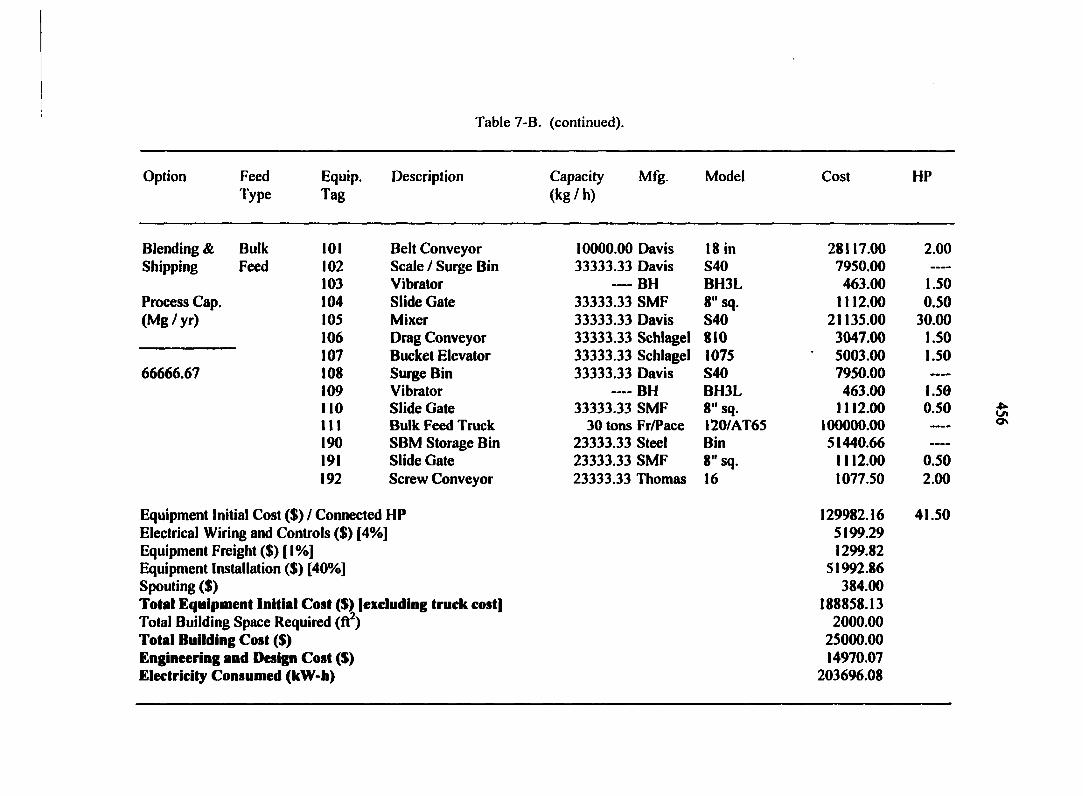
Table 7-B. (continued).
Option Feed Type
Equip. Tag
Description Capacity Mfg. (kg / h)
Model Cost HP
Blending & Bulk 101 Belt Conveyor 10000.00 Davis 18 in 28117.00 2.00 Shipping Feed 102 Scale / Surge Bin 33333.33 Davis S40 7950.00
103 Vibrator — BH BH3L 463.00 1.50 Process Cap. 104 Slide Gate 33333.33 SMF 8" sq. 1112.00 0.50 (Mg/yr) 105 Mixer 33333.33 Davis S40 21135.00 30.00
106 Drag Conveyor 33333.33 Schlagel 810 3047.00 1.50 107 Bucket Elevator 33333.33 Schlagel 1075 5003.00 1.50
66666.67 108 Surge Bin 33333.33 Davis S40 7950.00 ———
109 Vibrator — BH BH3L 463.00 1.50 110 Slide Gate 33333.33 SMF 8" sq. 1112.00 0.50 I I I Bulk Feed Truck 30 tons Fr/Pace 120/AT65 100000.00 -*•*——
190 SBM Storage Bin 23333.33 Steel Bin 51440.66 191 Slide Gate 23333.33 SMF 8" sq. 1112.00 0.50 192 Screw Conveyor 23333.33 Thomas 16 1077.50 2.00
Equipment Initial Cost ($) / Connected HP 129982.16 41.50 Electrical Wiring and Controls ($) [4%] 5199.29 Equipment Freight ($) [ 1%] 1299.82 Equipment Installation ($) [40%] 51992.86 Spouting ($) 384.00 Total Equipment Initial Cost ($) (excluding truck cost] 188858.13 Total Building Space Required (ft ) 2000.00 Total Building Cost ($) 25000.00 Engineering and Design Cost ($) 14970.07 Electricity Consumed (kW-h) 203696.08
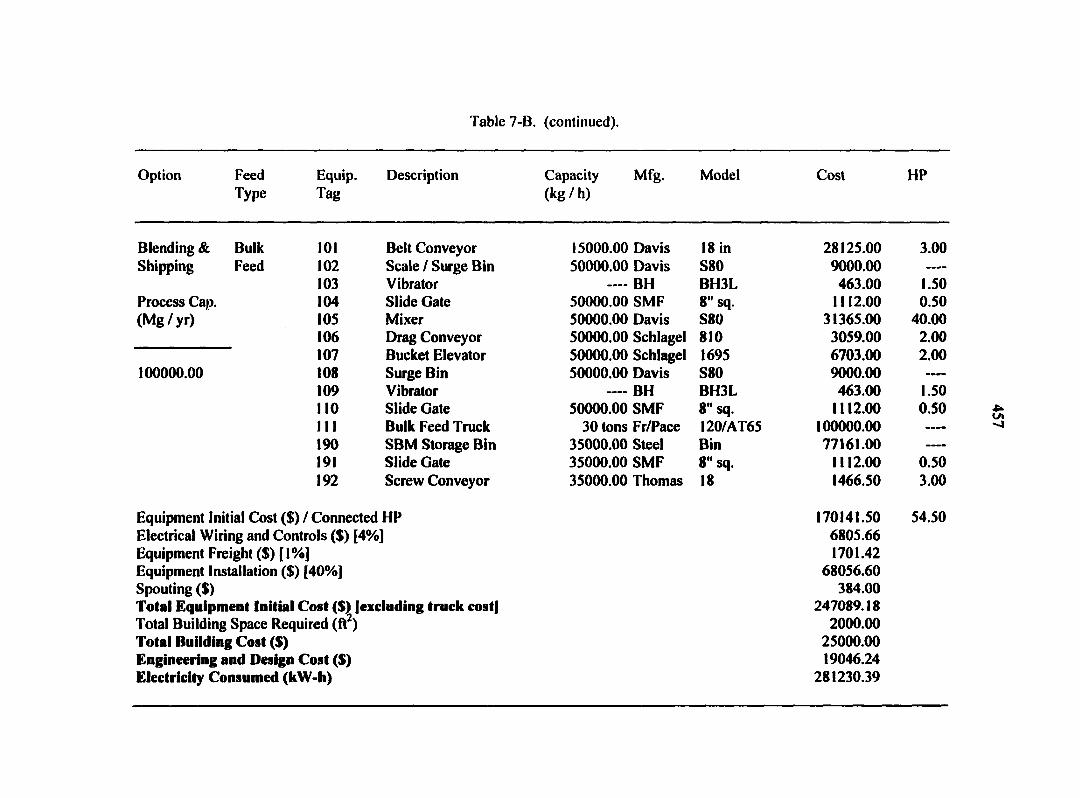
Table 7-B. (continued).
Option Feed Type
Equip. Tag
Description Capacity Mfg. (kg / h)
Model Cost HP
Blending & Bulk 101 Belt Conveyor 15000.00 Davis 18 in 28125.00 3.00 Shipping Feed 102 Scale / Surge Bin 50000.00 Davis S80 9000.00
103 Vibrator — BH BH3L 463.00 1.50 Process Cap. 104 Slide Gate 50000.00 SMF 8" sq. 1112.00 0.50 (Mg/yr) 105 Mixer 50000.00 Davis S80 31365.00 40.00
106 Drag Conveyor 50000.00 Schlagel 810 3059.00 2.00 107 Bucket Elevator 50000.00 Schlagel 1695 6703.00 2.00
100000.00 108 Surge Bin 50000.00 Davis S80 9000.00 109 Vibrator — BH BH3L 463.00 1.50 110 Slide Gate 50000.00 SMF 8" sq. 1112.00 0.50 111 Bulk Feed Truck 30 tons Fr/Pace 120/AT65 100000.00 190 SBM Storage Bin 35000.00 Steel Bin 77161.00 191 Slide Gate 35000.00 SMF 8" sq. 1112.00 0.50 192 Screw Conveyor 35000.00 Thomas 18 1466.50 3.00
Equipment Initial Cost ($) / Connected HP 170141.50 54.50 Electrical Wiring and Controls ($) [4%] 6805.66 Equipment Freight ($) [l%] 1701.42 Equipment Installation ($) [40%] 68056.60 Spouting ($) 384.00 Total Equipment Initial Cost ($) [excluding truck cost] 247089.18 Total Building Space Required (ft ) 2000.00 Total Building Cost ($) 25000.00 Engineering and Design Cost ($) 19046.24 Electricity Consumed (kW-h) 281230.39
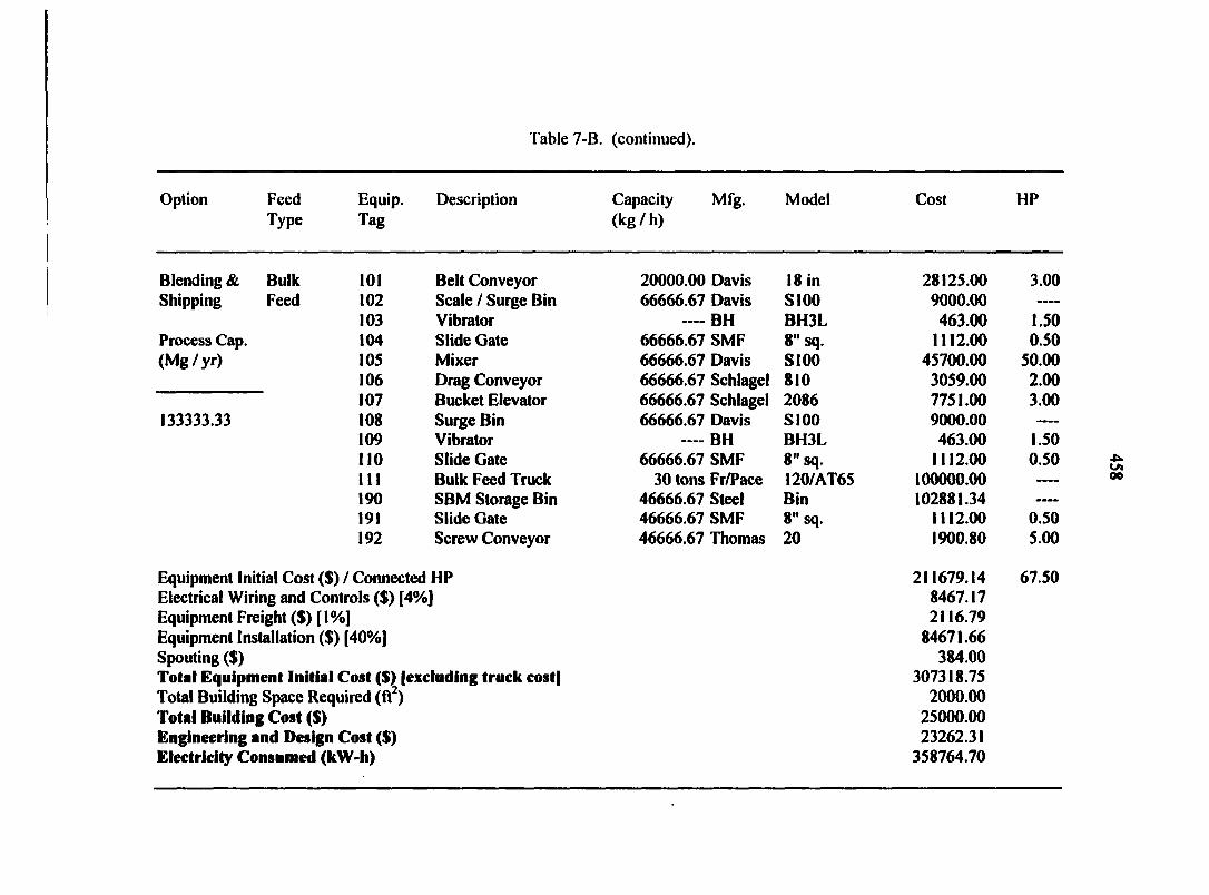
Table 7-B. (continued).
Option Feed Equip. Description Capacity Mfg. Model Cost HP Type Tag (kg / h)
Blending & Bulk 101 Belt Conveyor 20000.00 Davis 18 in 28125.00 3.00 Shipping Feed 102 Scale / Surge Bin 66666.67 Davis S100 9000.00 —-
103 Vibrator — BH BH3L 463.00 1.50 Process Cap. 104 Slide Gate 66666.67 SMF 8" sq. 1112.00 0.50 (Mg/yr) 105 Mixer 66666.67 Davis SI00 45700.00 50.00
106 Drag Conveyor 66666.67 Schlagel 810 3059.00 2.00 107 Bucket Elevator 66666.67 Schlagel 2086 7751.00 3.00
133333.33 108 Surge Bin 66666.67 Davis S100 9000.00 ----
109 Vibrator —— BH BH3L 463.00 1.50 110 Slide Gate 66666.67 SMF 8" sq. 1112.00 0.50 111 Bulk Feed Truck 30 tons Fr/Pace 120/AT65 100000.00 ——
190 SBM Storage Bin 46666.67 Steel Bin 102881.34 191 Slide Gate 46666.67 SMF 8" sq. 1112.00 0.50 192 Screw Conveyor 46666.67 Thomas 20 1900.80 5.00
Equipment Initial Cost ($) / Connected HP 211679.14 67.50 Electrical Wiring and Controls ($) [4%] 8467.17 Equipment Freight ($) [l%] 2116.79 Equipment Installation ($) [40%] 84671.66 Spouting ($) 384.00 Total Equipment Initial Cost ($) [excluding truck cost] 307318.75 Total Building Space Required (ft ) 2000.00 Total Building Cost ($) 25000.00 Engineering and Design Cost ($) 23262.31 Electricity Consumed (kW-h) 358764.70
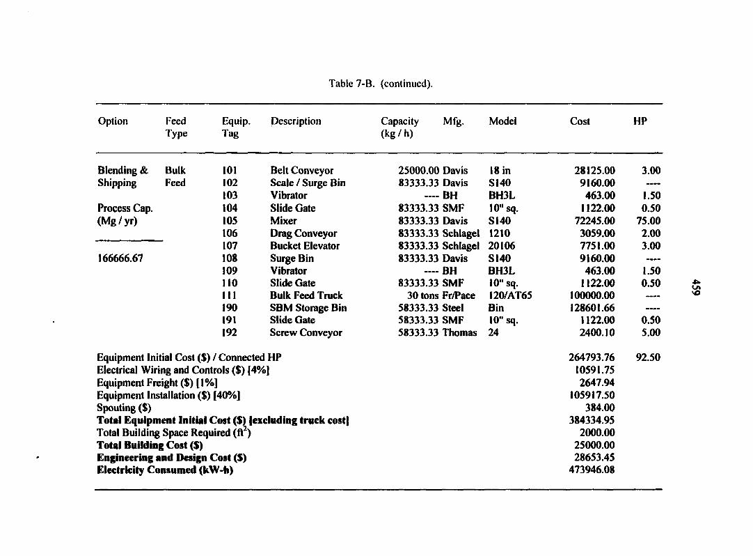
Table 7-B. (continued).
Option Feed Type
Equip. Tag
Description Capacity (kg / h)
Mfg. Model Cost
Blending & Bulk 101 Belt Conveyor 25000.00 Davis 18 in 28125.00 Shipping Feed 102 Scale / Surge Bin 83333.33 Davis S140 9160.00
103 Vibrator BH BH3L 463.00 Process Cap. 104 Slide Gate 83333.33 SMF 10" sq. 1122.00 (Mg / yr) 105 Mixer 83333.33 Davis S140 72245.00
106 Drag Conveyor 83333.33 Schlagel 1210 3059.00 107 Bucket Elevator 83333.33 Schlagel 20106 7751.00
166666.67 108 Surge Bin 83333.33 Davis S140 9160.00 109 Vibrator BH BH3L 463.00 110 Slide Gate 83333.33 SMF 10" sq. 1122.00 I I I Bulk Feed Truck 30 tons Fr/Pace 120/AT65 100000.00 190 SBM Storage Bin 58333.33 Steel Bin 128601.66 191 Slide Gate 58333.33 SMF 10" sq. 1122.00 192 Screw Conveyor 58333.33 Thomas 24 2400.10
Equipment Initial Cost ($) / Connected HP Electrical Wiring and Controls ($) [4%] Equipment Freight ($) [1%] Equipment Installation ($) [40%] Spouting ($) Total Equipment Initial Cost ($) (excluding truck cost] Total Building Space Required (ft2) Total Building Cost ($) Engineering and Design Cost ($) Electricity Consumed (kW-h)
264793.76 10591.75 2647.94
105917.50 384.00
384334.95 2000.00
25000.00 28653.45
473946.08
HP
3.00
1.50 0.50
75.00 2.00 3.00
1.50 0.50
0.50 5.00
92.50
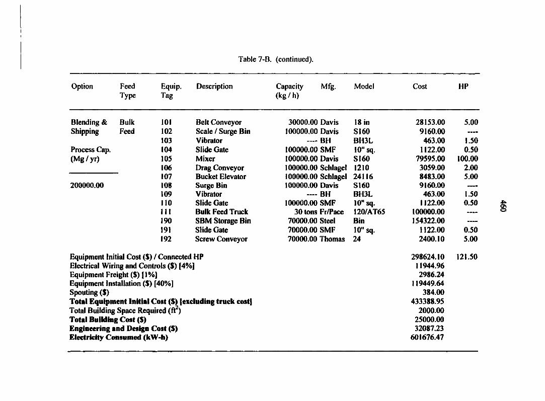
Table 7-B. (continued).
Option Feed Equip. Description Capacity Mfg. Model Cost HP Type Tag (kg / h)
Blending & Bulk 101 Belt Conveyor 30000.00 Davis 18 in 28153.00 5.00 Shipping Feed 102 Scale / Surge Bin 100000.00 Davis S160 9160.00 —•
103 Vibrator — BH BH3L 463.00 1.50 Process Cap. 104 Slide Gate 100000.00 SMF 10" sq. 1122.00 0.50 (Mg / yr) 105 Mixer 100000.00 Davis S160 79595.00 100.00
106 Drag Conveyor 100000.00 Schlagel 1210 3059.00 2.00 107 Bucket Elevator 100000.00 Schlagel 24116 8483.00 5.00
200000.00 108 Surge Bin 100000.00 Davis S160 9160.00 ————
109 Vibrator — BH BH3L 463.00 1.50 110 Slide Gate 100000.00 SMF 10" sq. 1122.00 0.50 I I I Bulk Feed Truck 30 tons Fr/Pace 120/AT65 100000.00 190 SBM Storage Bin 70000.00 Steel Bin 154322.00 ——
191 Slide Gate 70000.00 SMF 10" sq. 1122.00 0.50 192 Screw Conveyor 70000.00 Thomas 24 2400.10 5.00
Equipment Initial Cost ($) / Connected HP 298624.10 121.50 Electrical Wiring and Controls ($) [4%] 11944.96 Equipment Freight ($) [1%] 2986.24 Equipment Installation ($) [40%] 119449.64 Spouting ($) 384.00 Total Equipment Initial Coat ($) [excluding truck cost] 433388.95 Total Building Space Required (ft ) 2000.00 Total Building Cost ($) 25000.00 Engineering and Design Cost ($) 32087.23 Electricity Consumed (kW-h) 601676.47
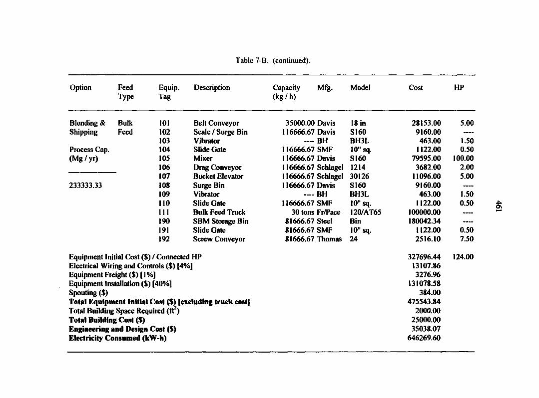
Table 7-B. (continued).
Option Feed Equip. Description Capacity Mfg. Model Cost HP Type Tag (kg/h)
Blending & Bulk 101 Belt Conveyor 35000.00 Davis 18 in 28153.00 5.00 Shipping Feed 102 Scale / Surge Bin 116666.67 Davis S160 9160.00 — Shipping Feed
103 Vibrator — BH BH3L 463.00 1.50 Process Cap. 104 Slide Gate 116666.67 SMF 10" sq. 1122.00 0.50 (Mg/yr) 105 Mixer 116666.67 Davis S160 79595.00 100.00
106 Drag Conveyor 116666.67 Schlagel 1214 3682.00 2.00 107 Bucket Elevator 116666.67 Schlagel 30126 11096.00 5.00
233333.33 108 Surge Bin 116666.67 Davis S160 9160.00 ——
109 Vibrator — BH BH3L 463.00 1.50 110 Slide Gate ll 6666.67 SMF 10" sq. 1122.00 0.50 111 Bulk Feed Truck 30 tons Fr/Pace I20/AT65 100000.00 ----
190 SBM Storage Bin 81666.67 Steel Bin 180042.34 •—
191 Slide Gate 81666.67 SMF 10" sq. 1122.00 0.50 192 Screw Conveyor 81666.67 Thomas 24 2516.10 7.50
Equipment Initial Cost ($) / Connected HP 327696.44 124.00 Electrical Wiring and Controls ($) [4%] 13107.86 Equipment Freight ($) [l%] 3276.96 Equipment Installation ($) [40%] 131078.58 Spouting ($) 384.00 Total Equipment Initial Cost ($) [excluding truck cost] 475543.84 Total Building Space Required (ft ) 2000.00 Total Building Cost ($) 25000.00 Engineering and Design Cost ($) 35038.07 Electricity Consumed (kW-h) 646269.60
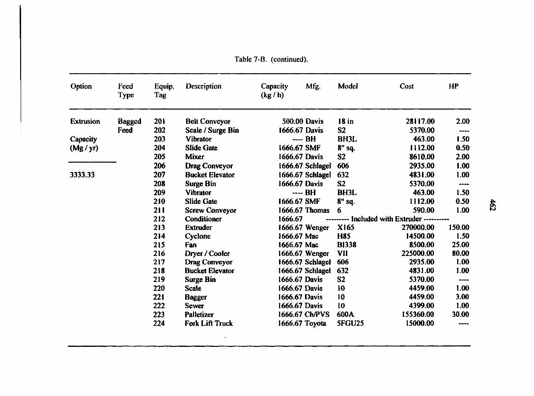
Table 7-B. (continued).
Option Feed Type
Equip. Tag
Description Capacity (kg / h)
Mfg. Model Cost HP
Extrusion
Capacity (Mg/yr)
3333.33
Bagged 201 Belt Conveyor 500.00 Davis 18 in 28117.00 2.00 Feed 202 Scale / Surge Bin 1666.67 Davis S2 5370.00 —-
203 Vibrator — BH BH3L 463.00 1.50 204 Slide Gate 1666.67 SMF 8" sq. 1112.00 0.50 205 Mixer 1666.67 Davis S2 8610.00 2.00 206 Drag Conveyor 1666.67 Schlagel 606 2935.00 1.00 207 Bucket Elevator 1666.67 Schlagel 632 4831.00 1.00 208 Surge Bin 1666.67 Davis S2 5370.00 —-
209 Vibrator — BH BH3L 463.00 1.50 210 Slide Gate 1666.67 SMF 8" sq. 1112.00 0.50 211 Screw Conveyor 1666.67 Thomas 6 590.00 1.00 212 Conditioner 1666.67 Included with Extruder 213 Extruder 1666.67 Wenger X165 270000.00 150.00 214 Cyclone 1666.67 Mac H85 14500.00 1.50 215 Fan 1666.67 Mac B1338 8500.00 25.00 216 Dryer / Cooler 1666.67 Wenger VII 225000.00 80.00 217 Drag Conveyor 1666.67 Schlagel 606 2935.00 1.00 218 Bucket Elevator 1666.67 Schlagel 632 4831.00 1.00 219 Surge Bin 1666.67 Davis S2 5370.00 ——
220 Scale 1666.67 Davis 10 4459.00 1.00 221 Bagger 1666.67 Davis 10 4459.00 3.00 222 Sewer 1666.67 Davis 10 4399.00 1.00 223 Palletizer 1666.67 Ch/PVS 600A 155360.00 30.00 224 Fork Lift Truck 1666.67 Toyota 5FGU25 15000.00

Table 7-B. (continued).
Option Feed Type
Equip. Tag
Description Capacity (kg/h)
Mfg. Model Cost HP
Extrusion Bagged 225 Bag Feed Truck Feed 290 SBM Storage Bin
Capacity 291 Slide Gate (Mg / yr) 292 Screw Conveyor
30 tons Fr/Pace 1166.67 Steel 1166.67 SMF 1166.67 Thomas
120/AT65 Bin 8" sq. 6
100000.00 2572.04 1112.00 590.00
0.50 1.00
3333.33
Equipment Initial Cost ($) / Connected HP Electrical Wiring and Controls ($) [4%] Equipment Freight ($) [1%] Equipment Installation ($) [40%] Spouting ($) Total Equipment Initial Cost ($) (excluding truck cost]
778060.04 31122.40 7780.60
311224.02 768.00
1128955.06
306.00
Total Building Space Required (ft ) Total Building Cost ($)
2220.46 27755.77
Engineering and Design Cost ($) 80969.76
Electricity Consumed (kW-h) 963675.00
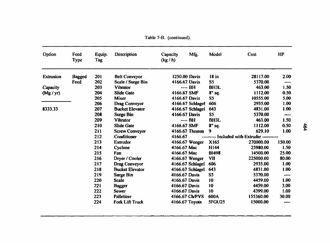
Table 7-B. (continued).
Option
Extrusion
Capacity (Mg / yr)
8333.33
Feed Equip. Description Capacity Mfg. Model Cost HP Type Tag (kg / h)
Bagged 201 Belt Conveyor 1250.00 Davis 18 in 28117.00 2.00 Feed 202 Scale / Surge Bin 4166.67 Davis S5 5370.00
203 Vibrator — BH BH3L 463.00 1.50 204 Slide Gate 4166.67 SMF 8" sq. 1112.00 0.50 205 Mixer 4166.67 Davis S5 10555.00 5.00 206 Drag Conveyor 4166.67 Schlagel 606 2935.00 1.00 207 Bucket Elevator 4166.67 Schlagel 643 4831.00 1.00 208 Surge Bin 4166.67 Davis S5 5370.00 209 Vibrator — BH BH3L 463.00 1.50 210 Slide Gate 4166.67 SMF 8" sq. 1112.00 0.50 211 Screw Conveyor 4166.67 Thomas 9 629.10 1.00 212 Conditioner 4166.67 Included with Extruder 213 Extruder 4166.67 Wenger XI65 270000.00 150.00 214 Cyclone 4166.67 Mac H144 25980.00 1.50 215 Fan 4166.67 Mac B1498 14500.00 25.00 216 Dryer / Cooler 4166.67 Wenger VII 225000.00 80.00 217 Drag Conveyor 4166.67 Schlagel 606 2935.00 1.00 218 Bucket Elevator 4166.67 Schlagel 643 4831.00 1.00 219 Surge Bin 4166.67 Davis S5 5370.00 •—
220 Scale 4166.67 Davis 10 4459.00 1.00 221 Bagger 4166.67 Davis 10 4459.00 3.00 222 Sewer 4166.67 Davis 10 4399.00 1.00 223 Palletizer 4166.67 Ch/PVS 600A 155360.00 30.00 224 Fork Lift Truck 4166.67 Toyota 5FGU25 15000.00 —-
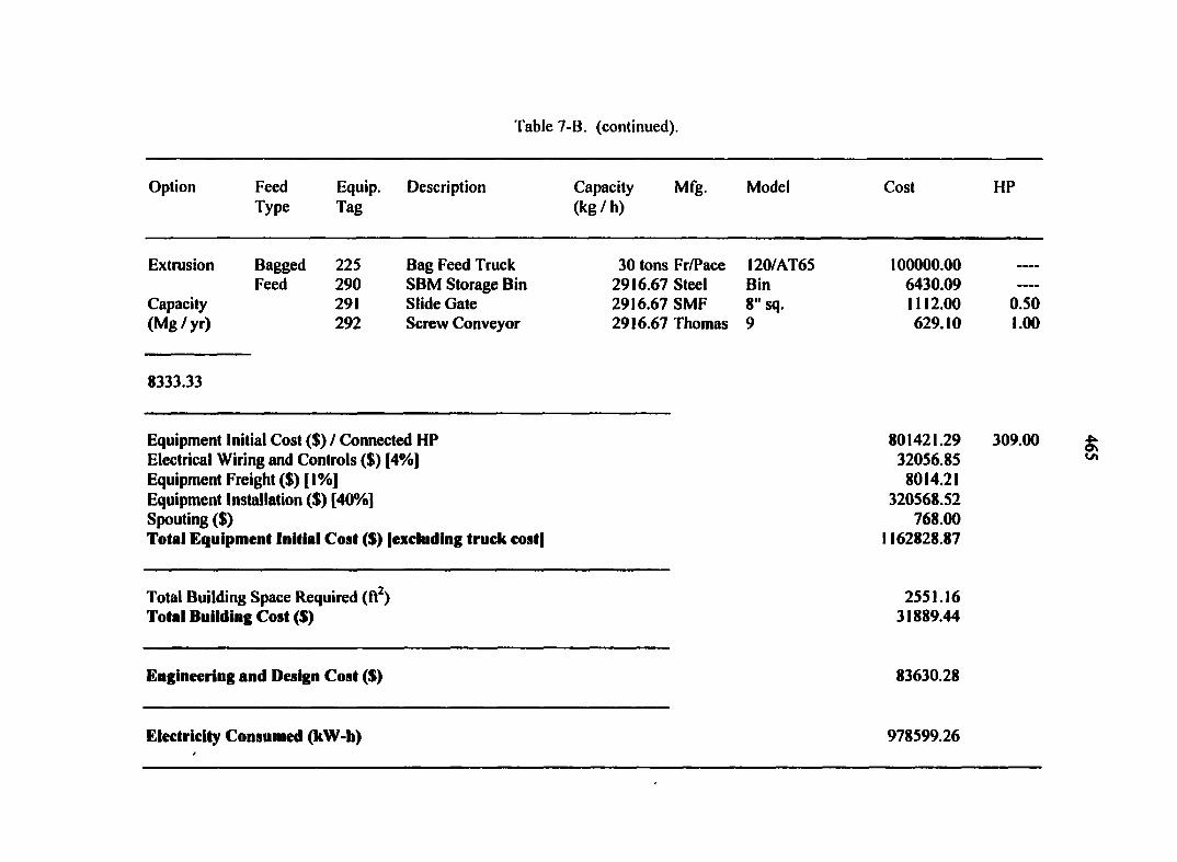
Table 7-B. (continued).
Option Feed Type
Equip. Tag
Description Capacity (kg / h)
Mfg. Model Cost HP
Extrusion Bagged 225 Bag Feed Truck Feed 290 SBM Storage Bin
Capacity 291 Slide Gate (Mg / yr) 292 Screw Conveyor
30 tons Fr/Pace 2916.67 Steel 2916.67 SMF 2916.67 Thomas
120/AT65 Bin 8" sq. 9
100000.00 6430.09 1112.00 629.10
0.50 1.00
8333.33
Equipment Initial Cost ($) / Connected HP Electrical Wiring and Controls ($) [4%] Equipment Freight ($) [l%] Equipment Installation ($) [40%] Spouting ($) Total Equipment Initial Cost ($) (excluding truck cost]
801421.29 32056.85 8014.21
320568.52 768.00
1162828.87
309.00
Total Building Space Required (ft ) Total Building Cost ($)
2551.16 31889.44
Engineering and Design Cost ($) 83630.28
Electricity Consumed (kW-h) 978599.26
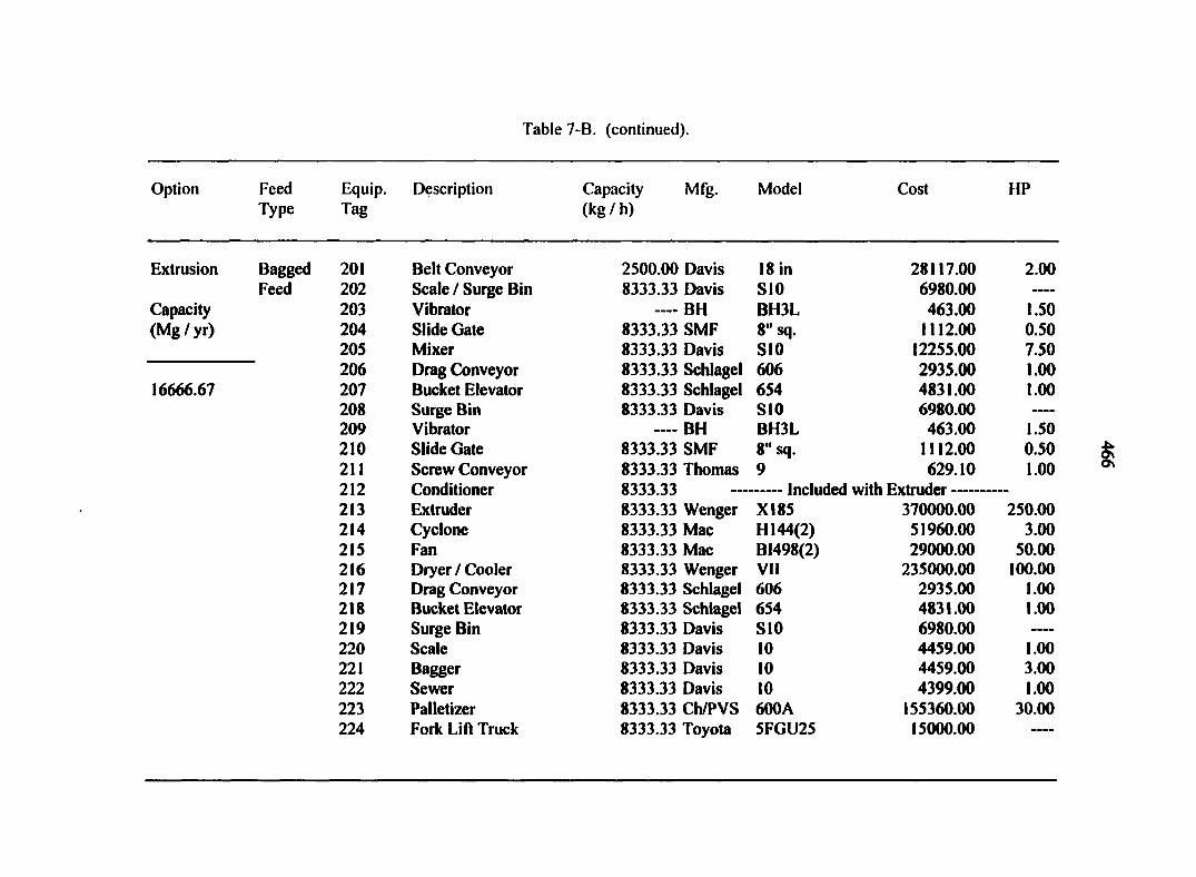
Table 7-B. (continued).
Option Feed Equip. Description Capacity Mfg. Model Cost HP Type Tag (kg / h)
Extrusion
Capacity (Mg/yr)
16666.67
Bagged 201 Belt Conveyor 2500.00 Davis 18 in 28117.00 2.00 Feed 202 Scale / Surge Bin 8333.33 Davis SI0 6980.00 —-
203 Vibrator — BH BH3L 463.00 1.50 204 Slide Gate 8333.33 SMF 8" sq. 1112.00 0.50 205 Mixer 8333.33 Davis S10 12255.00 7.50 206 Drag Conveyor 8333.33 Schlagel 606 2935.00 1.00 207 Bucket Elevator 8333.33 Schlagel 654 4831.00 1.00 208 Surge Bin 8333.33 Davis S10 6980.00 ————
209 Vibrator «— BH BH3L 463.00 1.50 210 Slide Gate 8333.33 SMF 8" sq. 1112.00 0.50 211 Screw Conveyor 8333.33 Thomas 9 629.10 1.00 212 Conditioner 8333.33 Included with Extruder 213 Extruder 8333.33 Wenger X185 370000.00 250.00 214 Cyclone 8333.33 Mac H 144(2) 51960.00 3.00 215 Fan 8333.33 Mac B1498(2) 29000.00 50.00 216 Dryer / Cooler 8333.33 Wenger VII 235000.00 100.00 217 Drag Conveyor 8333.33 Schlagel 606 2935.00 1.00 218 Bucket Elevator 8333.33 Schlagel 654 4831.00 1.00 219 Surge Bin 8333.33 Davis SI0 6980.00 220 Scale 8333.33 Davis 10 4459.00 1.00 221 Bagger 8333.33 Davis 10 4459.00 3.00 222 Sewer 8333.33 Davis 10 4399.00 1.00 223 Palletizer 8333.33 Ch/PVS 600A 155360.00 30.00 224 Fork Lift Truck 8333.33 Toyota 5FGU25 15000.00 ....

Table 7-B. (continued).
Option Feed Type
Equip. Tag
Description Capacity (kg / h)
Mfg. Model Cost HP
Extrusion Bagged 225 Bag Feed Truck Feed 290 SBM Storage Bin
Capacity 291 Slide Gate (Mg / yr) 292 Screw Conveyor
30 tons Fr/Pace 5833.33 Steel 5833.33 SMF 5833.33 Thomas
120/AT65 Bin 8" sq. 9
100000.00 12860.16 1112.00 629.10
0.50 1.00
16666.67
Equipment Initial Cost ($) / Connected HP Electrical Wiring and Controls ($) [4%] Equipment Freight ($) [I%] Equipment Installation ($) [40%] Spouting ($) Total Equipment Initial Cost ($) [excluding truck cost]
964861.36 38594.45 9648.61
385944.54 768.00
1399816.97
458.00
Total Building Space Required (ft ) Total Building Cost ($)
3102.31 38778.89
Engineering and Design Cost ($) 100701.71
Electricity Consumed (kW-h) 1455237.75
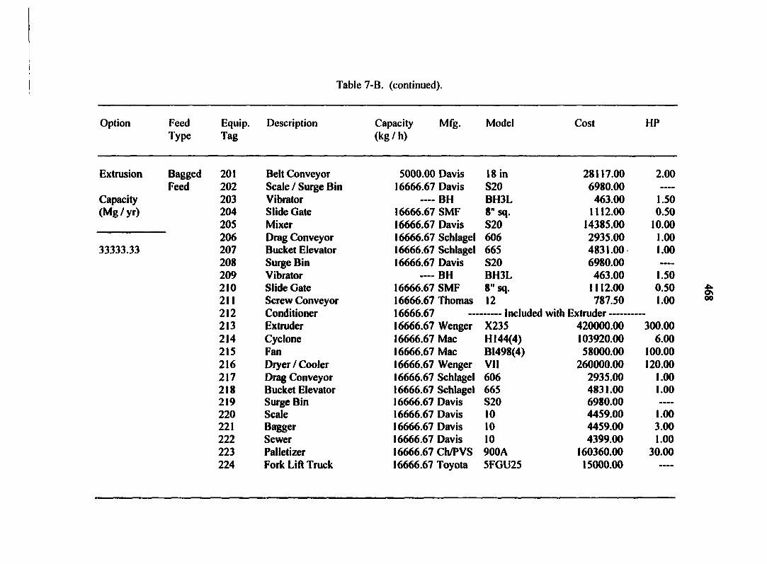
Table 7-B. (continued).
Option Feed Equip. Description Capacity Mfg. Model Cost HP Type Tag (kg / h)
Extrusion
Capacity (Mg/yr)
33333.33
Bagged 201 Belt Conveyor 5000.00 Davis 18 in 28117.00 2.00 Feed 202 Scale / Surge Bin 16666.67 Davis S20 6980.00 ----
203 Vibrator — BH BH3L 463.00 1.50 204 Slide Gate 16666.67 SMF 8" sq. 1112.00 0.50 205 Mixer 16666.67 Davis S20 14385.00 10.00 206 Drag Conveyor 16666.67 Schlagel 606 2935.00 1.00 207 Bucket Elevator 16666.67 Schlagel 665 4831.00 1.00 208 Surge Bin 16666.67 Davis S20 6980.00 •—
209 Vibrator — BH BH3L 463.00 1.50 210 Slide Gate 16666.67 SMF 8" sq. 1112.00 0.50 211 Screw Conveyor 16666.67 Thomas 12 787.50 1.00 212 Conditioner 16666.67 213 Extruder 16666.67 Wenger X235 420000.00 300.00 214 Cyclone 16666.67 Mac H144(4) 103920.00 6.00 215 Fan 16666.67 Mac B1498(4) 58000.00 100.00 216 Dryer / Cooler 16666.67 Wenger VU 260000.00 120.00 217 Drag Conveyor 16666.67 Schlagel 606 2935.00 1.00 218 Bucket Elevator 16666.67 Schlagel 665 4831.00 1.00 219 Surge Bin 16666.67 Davis S20 6980.00 ----
220 Scale 16666.67 Davis 10 4459.00 1.00 221 Bagger 16666.67 Davis 10 4459.00 3.00 222 Sewer 16666.67 Davis 10 4399.00 1.00 223 Palletizer 16666.67 Ch/PVS 900A 160360.00 30.00 224 Fork Lift Truck 16666.67 Toyota 5FGU25 15000.00 -™

Table 7-B. (continued).
Option Feed Type
Equip. Tag
Description Capacity (kg / h)
Mfg. Model Cost HP
Extrusion Bagged 225 Bag Feed Truck Feed 290 SBM Storage Bin
Capacity 291 Slide Gate (Mg / yr) 292 Screw Conveyor
30 tons Fr/Pace 11666.67 Steel 11666.67 SMF 11666.67 Thomas
120/AT65 Bin 8" sq. 12
100000.00 25720.34
1112.00 787.50
0.50 1.00
33333.33
Equipment Initial Cost ($) / Connected HP Electrical Wiring and Controls ($) [4%J Equipment Freight ($) [ 1%] Equipment Installation ($) [40%] Spouting ($) Total Equipment Initial Cost ($) (excluding truck cost]
1141128.34 45645.13 11411.28
456451.34 768.00
1655404.09
583.50
Total Building Space Required (ft2) Total Building Cost ($)
4204.62 52557.77
Engineering and Design Cost ($) 119557.33
Electricity Consumed (kW-h) 1867338.23
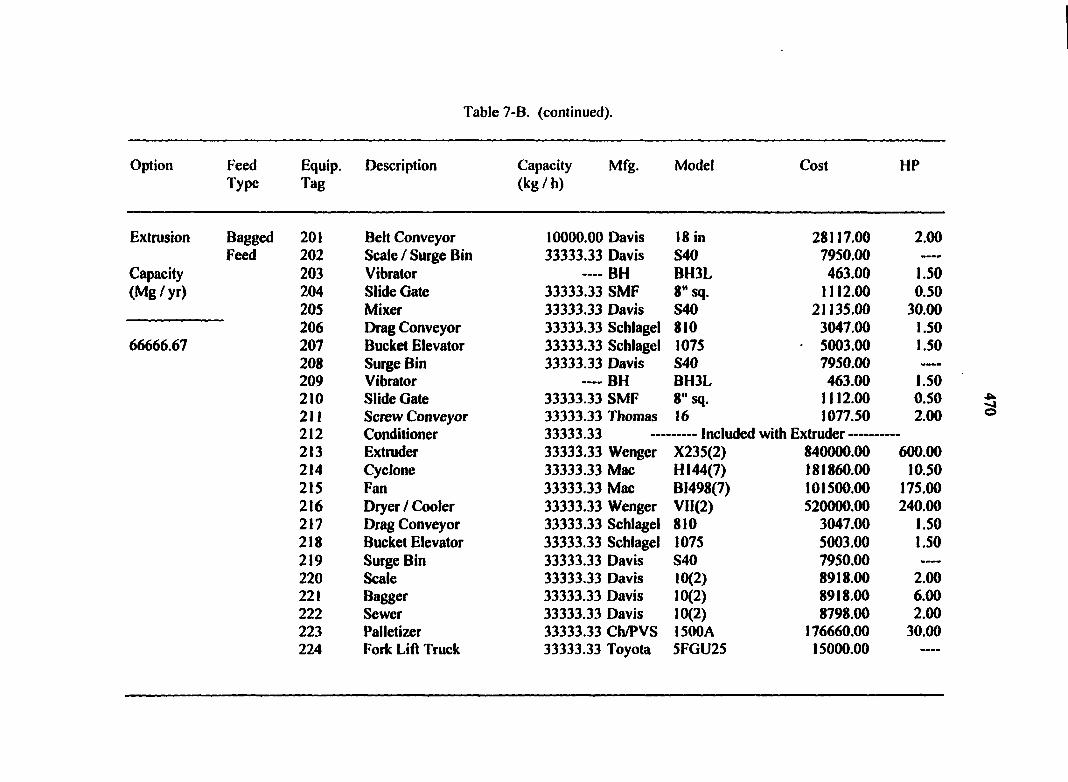
Table 7-B. (continued).
Option
Extrusion
Capacity (Mg/yr)
66666.67
Feed Equip. Description Capacity Mfg. Model Cost HP Type Tag (kg/h)
Bagged 201 Belt Conveyor 10000.00 Davis 18 in 28117.00 2.00 Feed 202 Scale / Surge Bin 33333.33 Davis S40 7950.00
203 Vibrator — BH BH3L 463.00 1.50 204 Slide Gate 33333.33 SMF 8" sq. 1112.00 0.50 205 Mixer 33333.33 Davis S40 21135.00 30.00 206 Drag Conveyor 33333.33 Schlagel 810 3047.00 1.50 207 Bucket Elevator 33333.33 Schlagel 1075 5003.00 1.50 208 Surge Bin 33333.33 Davis S40 7950.00 209 Vibrator — BH BH3L 463.00 1.50 210 Slide Gate 33333.33 SMF 8" sq. 1112.00 0.50 211 Screw Conveyor 33333.33 Thomas 16 1077.50 2.00 212 Conditioner 33333.33 Included with Extruder 213 Extruder 33333.33 Wenger X235(2) 840000.00 600.00 214 Cyclone 33333.33 Mac H 144(7) 181860.00 10.50 215 Fan 33333.33 Mac B1498(7) 101500.00 175.00 216 Dryer / Cooler 33333.33 Wenger Vll(2) 520000.00 240.00 217 Drag Conveyor 33333.33 Schlagel 810 3047.00 1.50 218 Bucket Elevator 33333.33 Schlagel 1075 5003.00 1.50 219 Surge Bin 33333.33 Davis S40 7950.00 *—-
220 Scale 33333.33 Davis 10(2) 8918.00 2.00 221 Bagger 33333.33 Davis 10(2) 8918.00 6.00 222 Sewer 33333.33 Davis 10(2) 8798.00 2.00 223 Palletizer 33333.33 Ch/PVS 1500A 176660.00 30.00 224 Fork Lift Truck 33333.33 Toyota 5FGU25 15000.00 ----
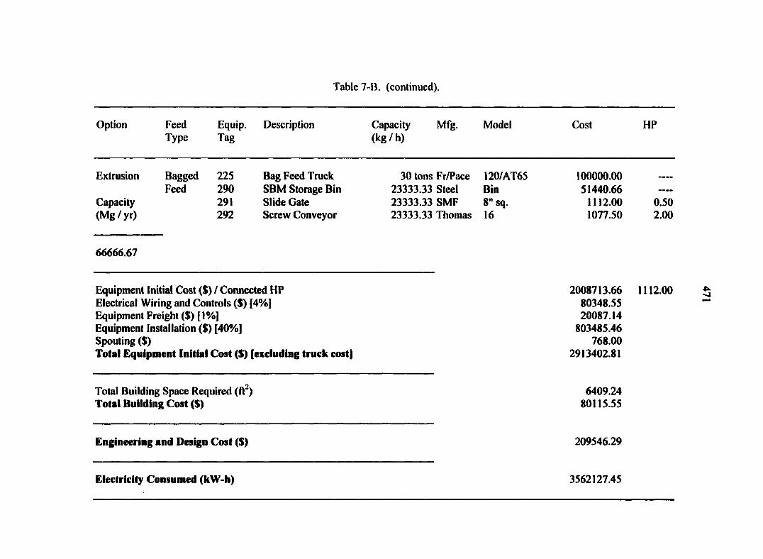
Table 7-B. (continued).
Option Feed Type
Equip. Tag
Description Capacity (kg / h)
Mfg. Model Cost HP
Extrusion Bagged 225 Bag Feed Truck Feed 290 SBM Storage Bin
Capacity 291 Slide Gate (Mg Z yr) 292 Screw Conveyor
30 tons Fr/Pace 23333.33 Steel 23333.33 SMF 23333.33 Thomas
120/AT65 Bin 8" sq. 16
100000.00 51440.66 1112.00 1077.50
0.50 2.00
66666.67
Equipment Initial Cost ($) Z Connected HP 2008713.66 1112.00 Electrical Wiring and Controls ($) [4%] 80348.55 Equipment Freight ($) [1%] 20087.14 Equipment Installation ($) [40%] 803485.46 Spouting ($) 768.00 Total Equipment Initial Cost ($) [excluding truck cost] 2913402.81
Total Building Space Required (ft2) 6409.24 Total Building Cost ($) 80115.55
Engineering and Design Cost ($) 209546.29
Electricity Consumed (kW-h) 3562127.45
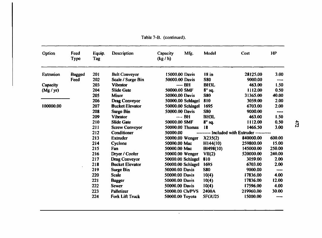
Table 7-B. (continued).
Option
Extrusion
Capacity (Mg/yr)
100000.00
Feed Type
Bagged Feed
Equip. Tag
Description Capacity Mfg. (kg / h)
Model Cost HP
201 Belt Conveyor 15000.00 Davis 18 in 28125.00 3.00 202 Scale / Surge Bin 50000.00 Davis S80 9000.00 —-
203 Vibrator — BH BH3L 463.00 1.50 204 Slide Gate 50000.00 SMF 8" sq. 1112.00 0.50 205 Mixer 50000.00 Davis S80 31365.00 40.00 206 Drag Conveyor 50000.00 Schlagel 810 3059.00 2.00 207 Bucket Elevator 50000.00 Schlagel 1695 6703.00 2.00 208 Surge Bin 50000.00 Davis S80 9000.00 209 Vibrator — BH BH3L 463.00 1.50 210 Slide Gate 50000.00 SMF 8" sq. 1112.00 0.50 211 Screw Conveyor 50000.00 Thomas 18 1466.50 3.00 212 Conditioner 50000.00 Included with Extruder 213 Extruder 50000.00 Wenger X235(2) 840000.00 600.00 214 Cyclone 50000.00 Mac H144(10) 259800.00 15.00 215 Fan 50000.00 Mac BI498(10) 145000.00 250.00 216 Dryer / Cooler 50000.00 Wenger VII(2) 520000.00 240.00 217 Drag Conveyor 50000.00 Schlagel 810 3059.00 2.00 218 Bucket Elevator 50000.00 Schlagel 1695 6703.00 2.00 219 Surge Bin 50000.00 Davis S80 9000.00 220 Scale 50000.00 Davis 10(4) 17836.00 4.00 221 Bagger 50000.00 Davis 10(4) 17836.00 12.00 222 Sewer 50000.00 Davis 10(4) 17596.00 4.00 223 Palletizer 50000.00 Ch/PVS 2400A 219960.00 30.00 224 Fork Lift Truck 50000.00 Toyota 5FGU25 15000.00 ——
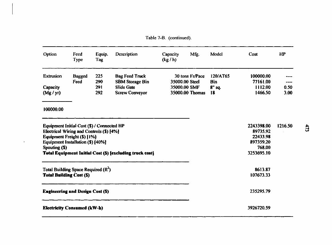
Table 7-B. (continued).
Option Feed Type
Equip. Tag
Description Capacity (kg / h)
Mfg. Model Cost HP
Extrusion Bagged 225 Bag Feed Truck Feed 290 SBM Storage Bin
Capacity 291 Slide Gate (Mg / yr) 292 Screw Conveyor
30 tons Fr/Pace 35000.00 Steel 35000.00 SMF 35000.00 Thomas
I20/AT65 Bin 8" sq. 18
100000.00 77161.00
1112.00 1466.50
0.50 3.00
100000.00
Equipment Initial Cost ($) / Connected HP 2243398.00 1216.50 Electrical Wiring and Controls ($) [4%] 89735.92 Equipment Freight ($) [1%] 22433.98 Equipment Installation ($) [40%] 897359.20 Spouting ($) 768.00 Total Equipment Initial Cost ($) (excluding truck cost) 3253695.10
Total Building Space Required (ft2) 8613.87 Total Building Cost ($) 107673.33
Engineering and Design Cost ($) 235295.79
Electricity Consumed (kW-h) 3926720.59
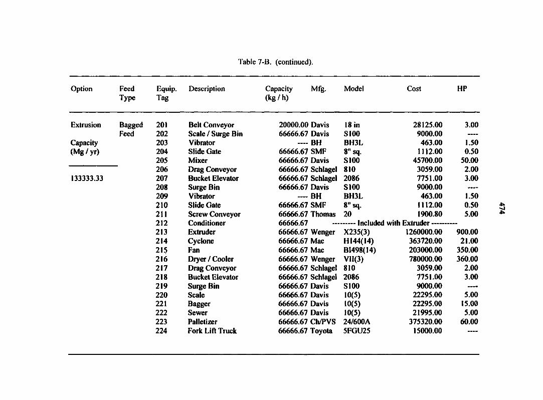
Table 7-B. (continued).
Option
Extrusion
Capacity (Mg / yr)
133333.33
Feed Equip. Description Capacity Mfg. Model Cost HP Type Tag (kg/h)
Bagged 201 Belt Conveyor 20000.00 Davis 18 in 28125.00 3.00 Feed 202 Scale / Surge Bin 66666.67 Davis S100 9000.00
203 Vibrator — BH BH3L 463.00 1.50 204 Slide Gate 66666.67 SMF 8" sq. 1112.00 0.50 205 Mixer 66666.67 Davis S100 45700.00 50.00 206 Drag Conveyor 66666.67 Schlagei 810 3059.00 2.00 207 Bucket Elevator 66666.67 Schlagei 2086 7751.00 3.00 208 Surge Bin 66666.67 Davis S100 9000.00 209 Vibrator —— BH BH3L 463.00 1.50 210 Slide Gate 66666.67 SMF 8" sq. 1112.00 0.50 211 Screw Conveyor 66666.67 Thomas 20 1900.80 5.00 212 Conditioner 66666.67 Included with Extruder 213 Extruder 66666.67 Wenger X235(3) 1260000.00 900.00 214 Cyclone 66666.67 Mac H144(14) 363720.00 21.00 215 Fan 66666.67 Mac B1498(14) 203000.00 350.00 216 Diyer / Cooler 66666.67 Wenger V1I(3) 780000.00 360.00 217 Drag Conveyor 66666.67 Schlagei 810 3059.00 2.00 218 Bucket Elevator 66666.67 Schlagei 2086 7751.00 3.00 219 Surge Bin 66666.67 Davis S100 9000.00 —--
220 Scale 66666.67 Davis 10(5) 22295.00 5.00 221 Bagger 66666.67 Davis 10(5) 22295.00 15.00 222 Sewer 66666.67 Davis 10(5) 21995.00 5.00 223 Palletizer 66666.67 Ch/PVS 24/600A 375320.00 60.00 224 Fork Lift Truck 66666.67 Toyota 5FGU25 15000.00 —-

Table 7-B. (continued).
Option Feed Type
Equip. Tag
Description Capacity (kg/h)
Mfg. Model Cost HP
Extrusion Bagged 225 Bag Feed Truck Feed 290 SBM Storage Bin
Capacity 291 Slide Gate (Mg / yr) 292 Screw Conveyor
30 tons Fr/Pace 46666.67 Steel 46666.67 SMF 46666.67 Thomas
120/AT65 Bin 8" sq. 20
100000.00 102881 34
1112.00 1900.80
0.50 5.00
133333.33
Equipment Initial Cost ($) / Connected HP Electrical Wiring and Controls ($) [4%J Equipment Freight ($) [ l%] Equipment Installation ($) [40%] Spouting ($) Total Equipment Initial Cost ($) (excluding truck cost]
3297014.94 131880.60 32970.15
1318805.98 768.00
4781439.66
1793.50
Total Building Space Required (ft ) Total Building Cost ($)
10818.49 135231.10
Engineering and Design Cost ($) 344166.95
Electricity Consumed (kW-h) 5773666.66
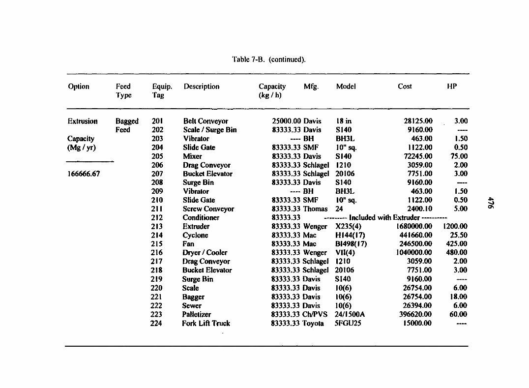
Table 7-B. (continued).
Option Feed Equip. Description Capacity Mfg. Model Cost HP Type Tag (kg / h)
Extrusion
Capacity (Mg/yr)
166666.67
Bagged 201 Belt Conveyor 25000.00 Davis 18 in 28125.00 3.00 Feed 202 Scale / Surge Bin 83333.33 Davis S140 9160.00
203 Vibrator — BH BH3L 463.00 1.50 204 Slide Gate 83333.33 SMF 10" sq. 1122.00 0.50 205 Mixer 83333.33 Davis S140 72245.00 75.00 206 Drag Conveyor 83333.33 Schlagei 1210 3059.00 2.00 207 Bucket Elevator 83333.33 Schlagei 20106 7751.00 3.00 208 Surge Bin 83333.33 Davis S140 9160.00 —-
209 Vibrator — BH BH3L 463.00 1.50 210 Slide Gate 83333.33 SMF 10" sq. 1122.00 0.50 211 Screw Conveyor 83333.33 Thomas 24 2400.10 5.00 212 Conditioner 83333.33 Included with Extruder 213 Extruder 83333.33 Wenger X235(4) 1680000.00 1200.00 214 Cyclone 83333.33 Mac HI44(I7) 441660.00 25.50 215 Fan 83333.33 Mac BI498(I7) 246500.00 425.00 216 Dryer / Cooler 83333.33 Wenger VII(4) 1040000.00 480.00 217 Drag Conveyor 83333.33 Schlagei 1210 3059.00 2.00 218 Bucket Elevator 83333.33 Schlagei 20106 7751.00 3.00 219 Surge Bin 83333.33 Davis SI40 9160.00 220 Scale 83333.33 Davis 10(6) 26754.00 6.00 221 Bagger 83333.33 Davis 10(6) 26754.00 18.00 222 Sewer 83333.33 Davis 10(6) 26394.00 6.00 223 Palletizer 83333.33 Ch/PVS 24/1500A 396620.00 60.00 224 Fork Lift Truck 83333.33 Toyota 5FGU25 15000.00 —-

Table 7-B. (continued).
Option Feed Type
Equip. Tag
Description Capacity (kg/h)
Mfg. Model Cost HP
Extrusion Bagged 225 Bag Feed Truck Feed 290 SBM Storage Bin
Capacity 291 Slide Gate (Mg / yr) 292 Screw Conveyor
30 tons Fr/Pace 58333.33 Steel 58333.33 SMF 58333.33 Thomas
I20/AT65 Bin 10" sq. 24
100000.00 128601.66
1122.00 2400.10
0.50 5.00
166666.67
Equipment Initial Cost ($) / Connected HP 4186845.86 2323.00 Electrical Wiring and Controls ($) [4%] 167473.83 Equipment Freight ($)[!%] 41868.46 Equipment Installation ($) [40%] 1674738.34 Spouting ($) 768.00 Total Equipment Initial Cost ($) [excluding truck cost] 6071694.50
Total Building Space Required (ft2) 13023.11 Total Building Cost ($) 162788.88
Engineering and Design Cost ($) 436413.84
Electricity Consumed (kW-h) 7471593.14
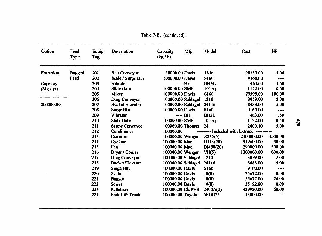
Table 7-B. (continued).
Option Feed Equip. Description Capacity Mfg. Model Cost HP Type Tag (kg/h)
Extrusion
Capacity (Mg/yr)
200000.00
Bagged 201 Belt Conveyor 30000.00 Davis 18 in 28153.00 5.00 Feed 202 Scale / Surge Bin 100000.00 Davis S160 9160.00
203 Vibrator — BH BH3L 463.00 1.50 204 Slide Gate 100000.00 SMF 10" sq. 1122.00 0.50 205 Mixer 100000.00 Davis S160 79595.00 100.00 206 Drag Conveyor 100000.00 Schlagei 1210 3059.00 2.00 207 Bucket Elevator 100000.00 Schlagei 24116 8483.00 5.00 208 Surge Bin 100000.00 Davis S160 9160.00 ----
209 Vibrator — BH BH3L 463.00 1.50 210 Slide Gate 100000.00 SMF 10" sq. 1122.00 0.50 211 Screw Conveyor 100000.00 Thomas 24 2400.10 5.00 212 Conditioner 100000.00 Included with Extruder 213 Extruder 100000.00 Wenger X235(5) 2100000.00 1500.00 214 Cyclone 100000.00 Mac H 144(20) 519600.00 30.00 215 Fan 100000.00 Mac BI498(20) 290000.00 500.00 216 Dryer / Cooler 100000.00 Wenger V1I(5) 1300000.00 600.00 217 Drag Conveyor 100000.00 Schlagei 1210 3059.00 2.00 218 Bucket Elevator 100000.00 Schlagei 24116 8483.00 5.00 219 Surge Bin 100000.00 Davis S160 9160.00 —.
220 Scale 100000.00 Davis 10(8) 35672.00 8.00 221 Bagger 100000.00 Davis 10(8) 35672.00 24.00 222 Sewer 100000.00 Davis 10(8) 35192.00 8.00 223 Palletizer 100000.00 Ch/PVS 2400A(2) 439920.00 60.00 224 Fork Lift Truck 100000.00 Toyota 5FGU25 15000.00 —-

Table 7-B. (continued).
Option Feed Type
Equip. Tag
Description Capacity (kg / h)
Mfg. Model Cost HP
Extrusion Bagged 225 Bag Feed Truck Feed 290 SBM Storage Bin
Capacity 291 Slide Gate (Mg / yr) 292 Screw Conveyor
30 tons Fr/Pace 70000.00 Steel 70000.00 SMF 70000.00 Thomas
120/AT65 Bin 10" sq. 24
100000.00 154322.00
1122.00 2400.10
0.50 5.00
200000.00
Equipment Initial Cost ($) / Connected HP 5092782.20 2863.50 Electrical Wiring and Controls ($) [4%] 203711.29 Equipment Freight ($) [ I %] 50927.82 Equipment Installation ($) [40%] 2037112.88 Spouting ($) 768.00 Total Equipment Initial Cost ($) [excluding truck cost] 7385302.19
Total Building Space Required (ft2) 15227.73 Total Building Cost ($) 190346.65
Engineering and Design Cost ($) 530295.42
Electricity Consumed (kW-h) 9204029.41
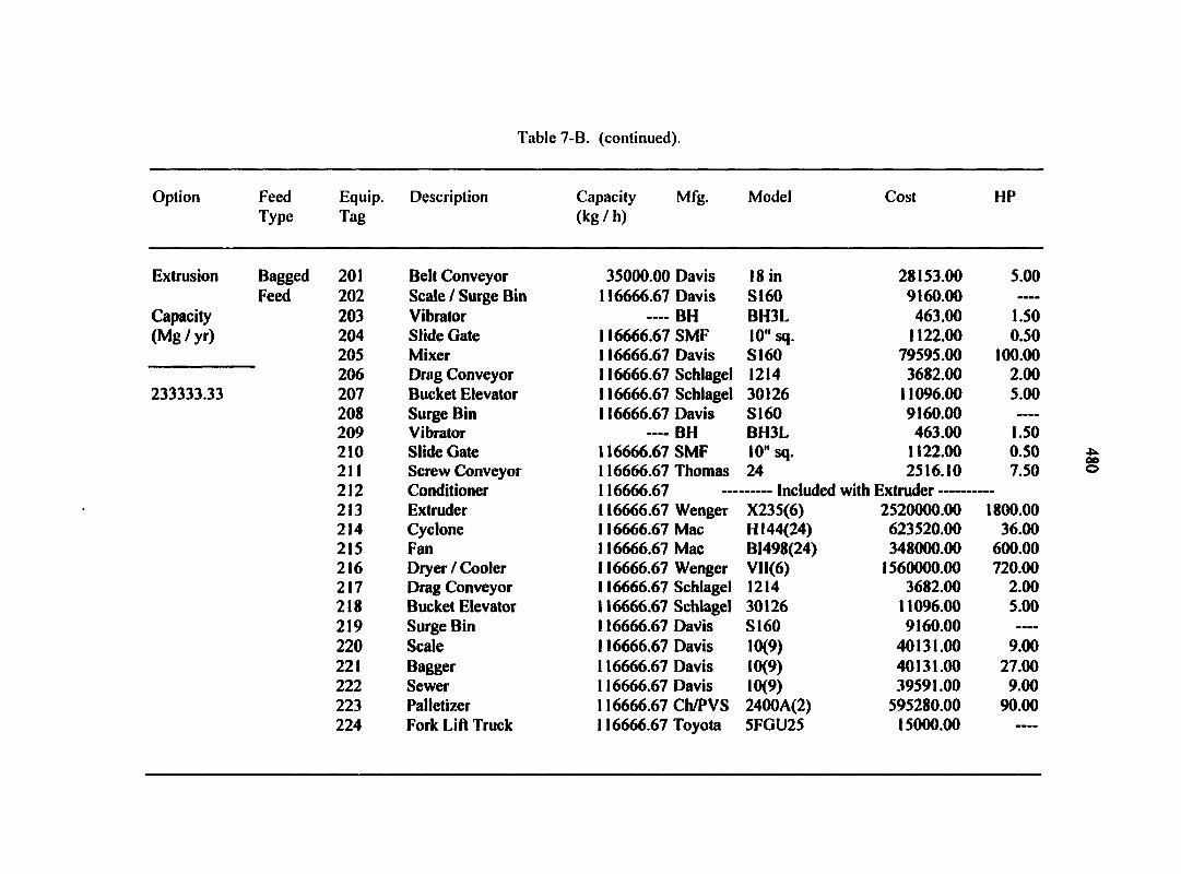
Table 7-B. (continued).
Option Feed Type
Equip. Tag
Description Capacity Mfg. (kg / h)
Model Cost HP
Extrusion Bagged 201 Belt Conveyor 35000.00 Davis 18 in 28153.00 5.00 Feed 202 Scale / Surge Bin 116666.67 Davis S160 9160.00
Capacity 203 Vibrator — BH BH3L 463.00 1.50 (Mg / yr) 204 Slide Gate 116666.67 SMF 10" sq. 1122.00 0.50
205 Mixer 116666.67 Davis S160 79595.00 100.00 206 Drag Conveyor 116666.67 Schlagei 1214 3682.00 2.00
233333.33 207 Bucket Elevator 116666.67 Schlagei 30126 11096.00 5.00 208 Surge Bin 116666.67 Davis SI60 9160.00 —•
209 Vibrator — BH BH3L 463.00 1.50 210 Slide Gate 116666.67 SMF 10" sq. 1122.00 0.50 211 Screw Conveyor 116666.67 Thomas 24 2516.10 7.50 212 Conditioner 116666.67 Included with Extruder 213 Extruder 116666.67 Wenger X235(6) 2520000.00 1800.00 214 Cyclone 116666.67 Mac H144(24) 623520.00 36.00 215 Fan 116666.67 Mac BI498(24) 348000.00 600.00 216 Dryer / Cooler 116666.67 Wenger Vll(6) 1560000.00 720.00 217 Drag Conveyor 116666.67 Schlagei 1214 3682.00 2.00 218 Bucket Elevator 116666.67 Schlagei 30126 11096.00 5.00 219 Surge Bin 116666.67 DaVis S160 9160.00 ——
220 Scale 116666.67 Davis 10(9) 40131.00 9.00 221 Bagger 116666.67 Davis 10(9) 40131.00 27.00 222 Sewer 116666.67 Davis 10(9) 39591.00 9.00 223 Palletizer 116666.67 Ch/PVS 2400A(2) 595280.00 90.00 224 Fork Lift Truck 116666.67 Toyota 5FGU25 15000.00 ——
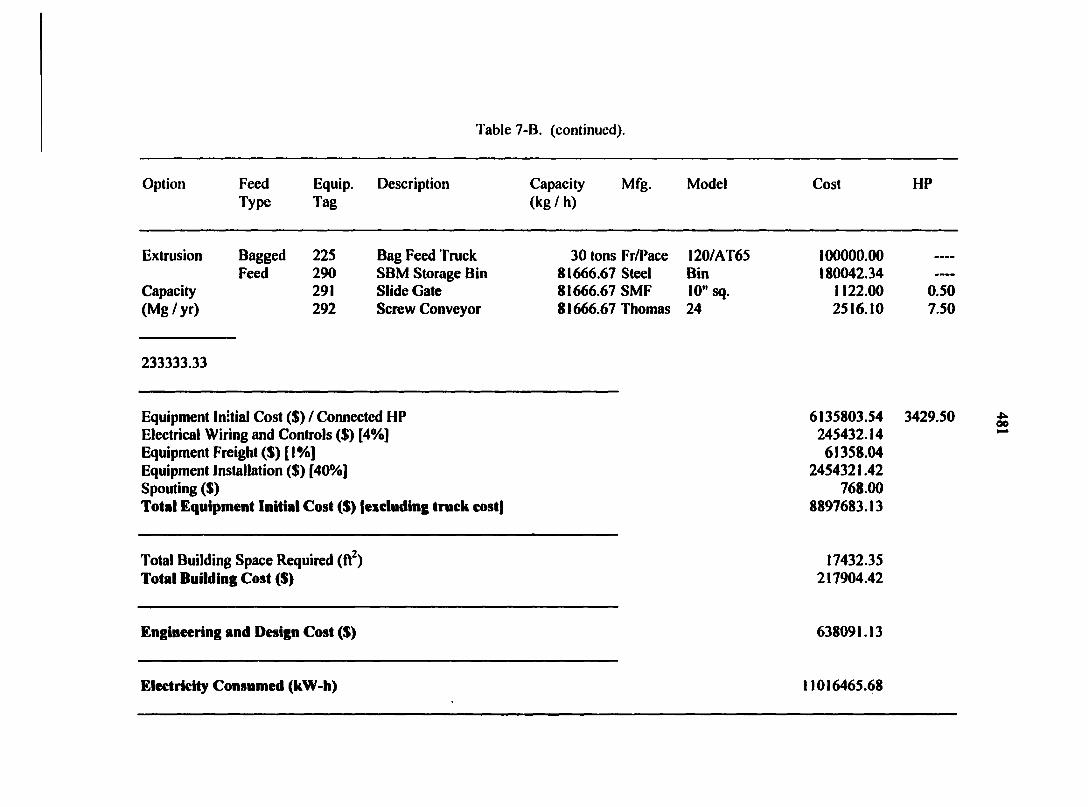
Table 7-B. (continued).
Option Feed Type
Equip. Tag
Description Capacity (kg / h)
Mfg. Model Cost HP
Extrusion Bagged 225 Bag Feed Truck Feed 290 SBM Storage Bin
Capacity 291 Slide Gate (Mg / yr) 292 Screw Conveyor
30 tons Fr/Pace 81666.67 Steel 81666.67 SMF 81666.67 Thomas
120/AT65 Bin 10" sq. 24
100000.00 180042.34
1122.00 2516.10
0.50 7.50
233333.33
Equipment Initial Cost ($) / Connected HP 6135803.54 3429.50 Electrical Wiring and Controls ($) [4%] 245432.14 Equipment Freight ($)[!%] 61358.04 Equipment Installation ($) [40%] 2454321.42 Spouting ($) 768.00 Total Equipment Initial Cost ($) [excluding truck cost] 8897683.13
Total Building Space Required (ft2) 17432.35 Total Building Cost ($) 217904.42
Engineering and Design Cost ($) 638091.13
Electricity Consumed (kW-h) 11016465.68
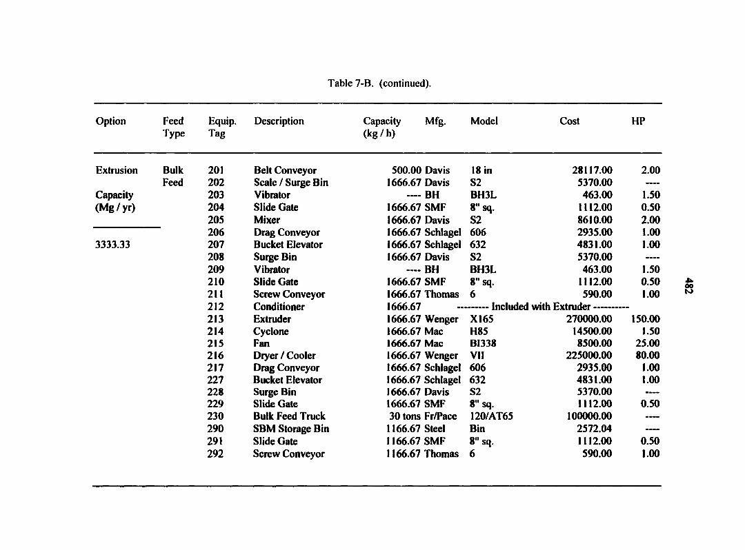
Table 7-B. (continued).
Option Feed Equip. Description Capacity Mfg. Model Cost HP Type Tag (kg/h)
Extrusion
Capacity (Mg/yr)
3333.33
Bulk Feed
201 Belt Conveyor 500.00 Davis 18 in 28117.00 2.00 202 Scale / Surge Bin 1666.67 Davis S2 5370.00 —•
203 Vibrator — BH BH3L 463.00 1.50 204 Slide Gate 1666.67 SMF 8" sq. 1112.00 0.50 205 Mixer 1666.67 Davis S2 8610.00 2.00 206 Drag Conveyor 1666.67 Schlagei 606 2935.00 1.00 207 Bucket Elevator 1666.67 Schlagei 632 4831.00 1.00 208 Surge Bin 1666.67 Davis S2 5370.00 —-
209 Vibrator — BH BH3L 463.00 1.50 210 Slide Gate 1666.67 SMF 8" sq. 1112.00 0.50 211 Screw Conveyor 1666.67 Thomas 6 590.00 1.00 212 Conditioner 1666.67 Included with Extruder 213 Extruder 1666.67 Wenger X165 270000.00 150.00 214 Cyclone 1666.67 Mac H85 14500.00 1.50 215 Fan 1666.67 Mac BI338 8500.00 25.00 216 Dryer / Cooler 1666.67 Wenger VII 225000.00 80.00 217 Drag Conveyor 1666.67 Schlagei 606 2935.00 1.00 227 Bucket Elevator 1666.67 Schlagei 632 4831.00 1.00 228 Surge Bin 1666.67 Davis S2 5370.00 229 Slide Gate 1666.67 SMF 8" sq. 1112.00 0.50 230 Bulk Feed Truck 30 tons Fr/Pace 120/AT65 100000.00 ----
290 SBM Storage Bin 1166.67 Steel Bin 2572.04 ---•
291 Slide Gate 1166.67 SMF 8" sq. 1112.00 0.50 292 Screw Conveyor 1166.67 Thomas 6 590.00 1.00

Table 7-B. (continued).
Option Feed Equip. Description Capacity Mfg. Model Cost HP Type Tag (kg / h)
Extrusion Bulk Feed
Capacity (Mg/yr)
3333.33
Equipment Initial Cost ($) / Connected HP 595495.04 271.50 Electrical Wiring and Controls ($) [4%] 23819.80 Equipment Freight ($) ( I %] 5954.95 Equipment Installation ($) [40%] 238198.02 Spouting ($) 768.00 Total Equipment Initial Cost ($) [excluding truck cost] 864235.81
Total Building Space Required (ft2) 2000.00 Total Building Cost ($) 25000.00
Engineering and Design Cost ($) 62246.51
Electricity Consumed (kW-h) 855439.70
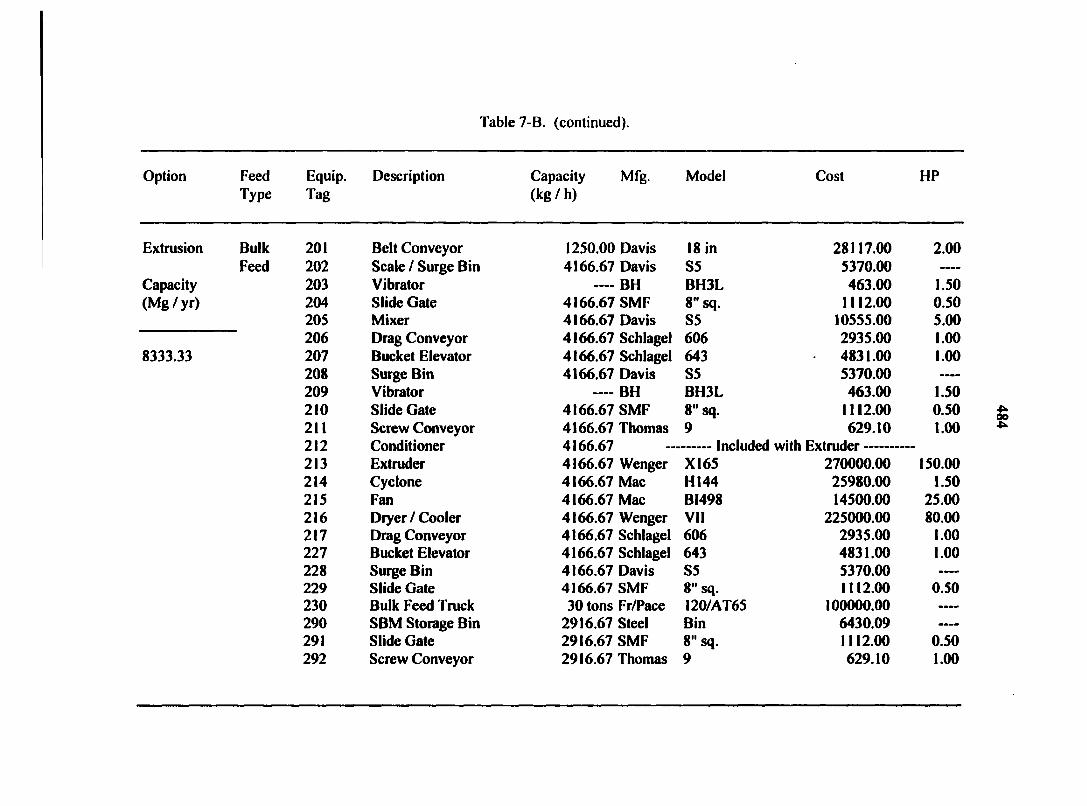
Table 7-B. (continued).
Option
Extrusion
Capacity (Mg/yr)
8333.33
Feed Type
Bulk Feed
Equip. Tag
Description Capacity Mfg. (kg / h)
Model Cost HP
201 Belt Conveyor 1250.00 Davis 18 in 28117.00 2.00 202 Scale / Surge Bin 4166.67 Davis S5 5370.00 ——
203 Vibrator — BH BH3L 463.00 1.50 204 Slide Gate 4166.67 SMF 8" sq. 1112.00 0.50 205 Mixer 4166.67 Davis S5 10555.00 5.00 206 Drag Conveyor 4166.67 Schlagei 606 2935.00 1.00 207 Bucket Elevator 4166.67 Schlagei 643 4831.00 1.00 208 Surge Bin 4166.67 Davis S5 5370.00 ——
209 Vibrator —— BH BH3L 463.00 1.50 210 Slide Gate 4166.67 SMF 8" sq. 1112.00 0.50 211 Screw Conveyor 4166.67 Thomas 9 629.10 1.00 212 Conditioner 4166.67 Included with Extruder 213 Extruder 4166.67 Wenger X165 270000.00 150.00 214 Cyclone 4166.67 Mac H144 25980.00 1.50 215 Fan 4166.67 Mac BI498 14500.00 25.00 216 Dryer / Cooler 4166.67 Wenger VII 225000.00 80.00 217 Drag Conveyor 4166.67 Schlagei 606 2935.00 1.00 227 Bucket Elevator 4166.67 Schlagei 643 4831.00 1.00 228 Surge Bin 4166.67 Davis S5 5370.00 —-
229 Slide Gate 4166.67 SMF 8" sq. 1112.00 0.50 230 Bulk Feed Truck 30 tons Fr/Pace 120/AT65 100000.00 ——
290 SBM Storage Bin 2916.67 Steel Bin 6430.09 ——
291 Slide Gate 2916.67 SMF 8" sq. 1112.00 0.50 292 Screw Conveyor 2916.67 Thomas 9 629.10 1.00
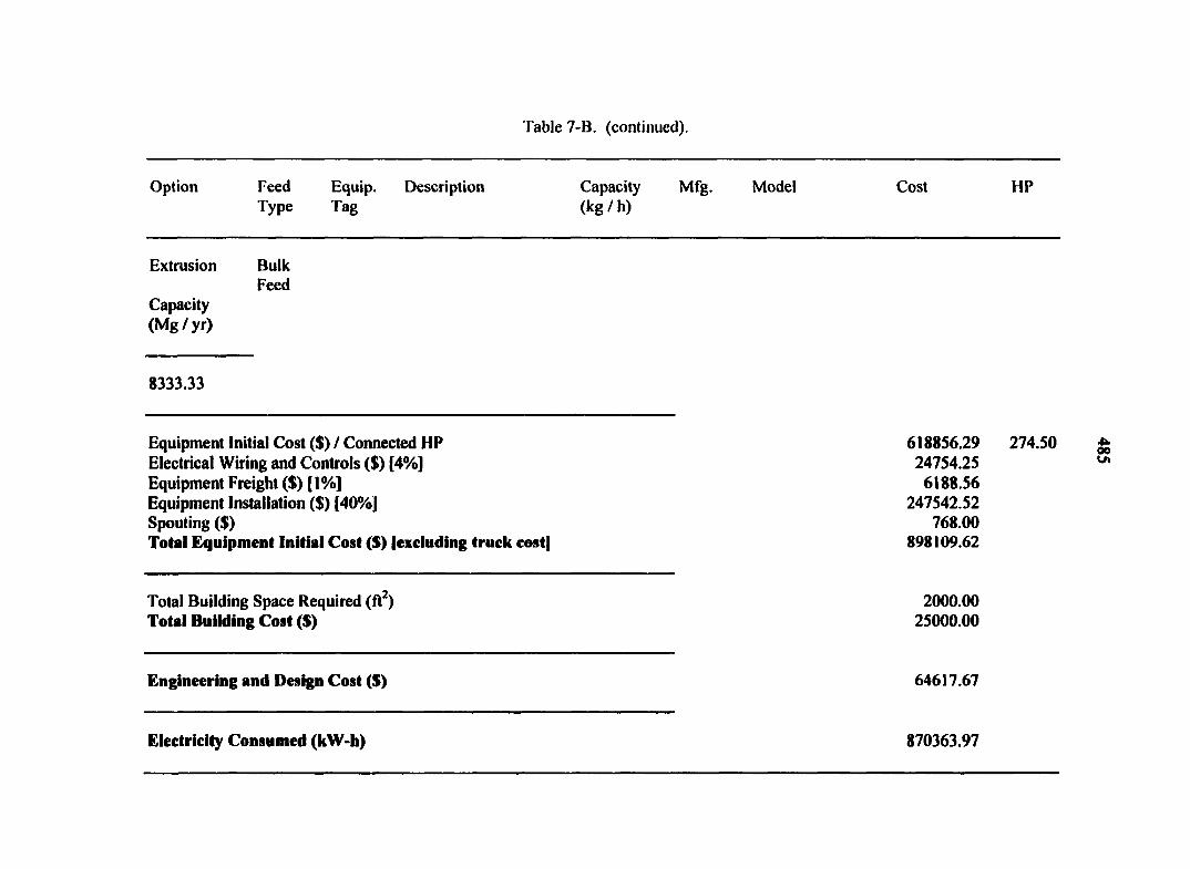
Table 7-B. (continued).
Option Feed Equip. Description Capacity Mfg. Model Cost HP Type Tag (kg / h)
Extrusion Bulk Feed
Capacity (Mg/yr)
8333.33
Equipment Initial Cost ($) / Connected HP 618856.29 274.50 Electrical Wiring and Controls ($) [4%] 24754.25 Equipment Freight ($) [1%] 6188.56 Equipment Installation ($) [40%] 247542.52 Spouting ($) 768.00 Total Equipment Initial Cost ($) [excluding truck cost] 898109.62
Total Building Space Required (ft2) 2000.00 Total Building Cost ($) 25000.00
Engineering and Design Cost ($) 64617.67
Electricity Consumed (kW-h) 870363.97
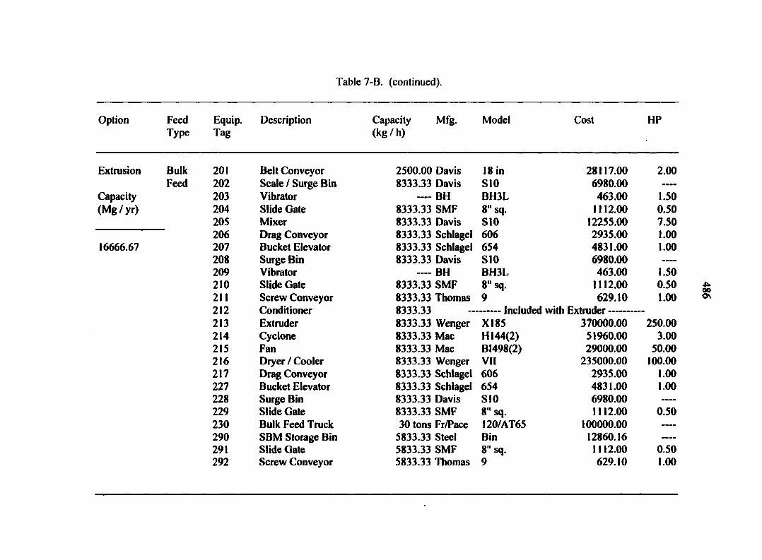
Table 7-B. (continued).
Option Feed Equip. Description Capacity Mfg. Model Cost HP Type Tag (kg / h)
Extrusion
Capacity (Mg/yr)
16666.67
Bulk Feed
201 Belt Conveyor 2500.00 Davis 18 in 28117.00 2.00 202 Scale / Surge Bin 8333.33 Davis S10 6980.00 •—
203 Vibrator — BH BH3L 463.00 1.50 204 Slide Gate 8333.33 SMF 8" sq. 1112.00 0.50 205 Mixer 8333.33 Davis S10 12255.00 7.50 206 Drag Conveyor 8333.33 Schlagei 606 2935.00 1.00 207 Bucket Elevator 8333.33 Schlagei 654 4831.00 1.00 208 Surge Bin 8333.33 Davis SI0 6980.00 ——
209 Vibrator — BH BH3L 463.00 1.50 210 Slide Gate 8333.33 SMF 8" sq. 1112.00 0.50 211 Screw Conveyor 8333.33 Thomas 9 629.10 1.00 212 Conditioner 8333.33 Included with Extruder —
213 Extruder 8333.33 Wenger XI85 370000.00 250.00 214 Cyclone 8333.33 Mac H 144(2) 51960.00 3.00 215 Fan 8333.33 Mac BI498(2) 29000.00 50.00 216 Dryer / Cooler 8333.33 Wenger VII 235000.00 100.00 217 Drag Conveyor 8333.33 Schlagei 606 2935.00 1.00 227 Bucket Elevator 8333.33 Schlagei 654 4831.00 1.00 228 Surge Bin 8333.33 Davis SI0 6980.00 ——
229 Slide Gate 8333.33 SMF 8" sq. 1112.00 0.50 230 Bulk Feed Truck 30 tons Fr/Pace 120/AT65 100000.00 ——
290 SBM Storage Bin 5833.33 Steel Bin 12860.16 ——
291 Slide Gate 5833.33 SMF 8" sq. 1112.00 0.50 292 Screw Conveyor 5833.33 Thomas 9 629.10 1.00

Table 7-B. (continued).
Option Feed Equip. Description Capacity Mfg. Model Cost HP Type Tag (kg / h)
Extrusion Bulk Feed
Capacity (Mg/yr)
16666.67
Equipment Initial Cost ($) / Connected HP 782296.36 423.50 Electrical Wiring and Controls ($) [4%] 31291.85 Equipment Freight ($) [ I %] 7822.96 Equipment Installation ($) [40%] 312918.54 Spouting ($) 768.00 Total Equipment Initial Cost ($) [excluding truck cost] 1135097.72
Total Building Space Required (ft2) 2000.00 Total Building Cost ($) 25000.00
Engineering and Design Cost ($) 81206.84
Electricity Consumed (kW-h) 1347002.45
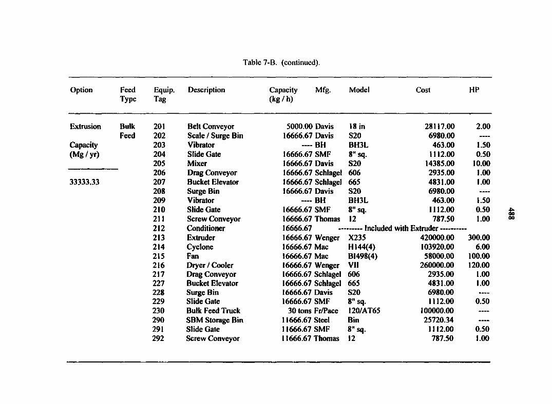
Table 7-B. (continued).
Option
Extrusion
Capacity (Mg/yr)
33333.33
Feed Type
Bulk Feed
Equip. Tag
Description Capacity Mfg. (kg / h)
Model Cost HP
201 Belt Conveyor 5000.00 Davis 18 in 28117.00 2.00 202 Scale / Surge Bin 16666.67 Davis S20 6980.00 203 Vibrator — BH BH3L 463.00 1.50 204 Slide Gate 16666.67 SMF 8" sq. 1112.00 0.50 205 Mixer 16666.67 Davis S20 14385.00 10.00 206 Drag Conveyor 16666.67 Schlagei 606 2935.00 1.00 207 Bucket Elevator 16666.67 Schlagei 665 4831.00 1.00 208 Surge Bin 16666.67 Davis S20 6980.00 —-
209 Vibrator — BH BH3L 463.00 1.50 210 Slide Gate 16666.67 SMF 8" sq. 1112.00 0.50 211 Screw Conveyor 16666.67 Thomas 12 787.50 1.00 212 Conditioner 16666.67 Included with Extruder 213 Extruder 16666.67 Wenger X235 420000.00 300.00 214 Cyclone 16666.67 Mac H 144(4) 103920.00 6.00 215 Fan 16666.67 Mac B1498(4) 58000.00 100.00 216 Dryer / Cooler 16666.67 Wenger VII 260000.00 120.00 217 Drag Conveyor 16666.67 Schlagei 606 2935.00 1.00 227 Bucket Elevator 16666.67 Schlagei 665 4831.00 1.00 228 Surge Bin 16666.67 Davis S20 6980.00 229 Slide Gate 16666.67 SMF 8" sq. 1112.00 0.50 230 Bulk Feed Truck 30 tons Fr/Pace I20/AT65 100000.00 •••-
290 SBM Storage Bin 11666.67 Steel Bin 25720.34 —»
291 Slide Gate 11666.67 SMF 8" sq. 1112.00 0.50 292 Screw Conveyor 11666.67 Thomas 12 787.50 1.00
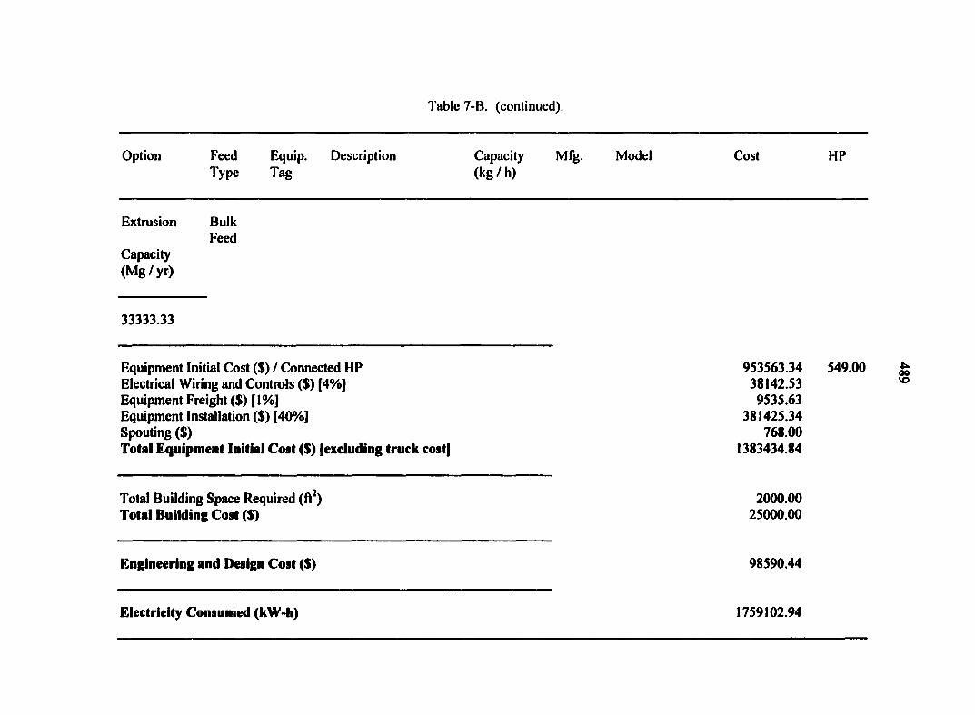
Extrusion Bulk Feed
Capacity (Mg / yr)
33333.33
Table 7-B. (continued).
Option Feed Equip. Description Type Tag
Capacity (kg/h)
Mfg. Model Cost HP
Equipment Initial Cost ($) / Connected HP 953563.34 549.00 Electrical Wiring and Controls ($) [4%] 38142.53 Equipment Freight ($) [ 1 %] 9535.63 Equipment Installation ($) [40%] 381425.34 Spouting ($) 768.00 Total Equipment Initial Cost ($) [excluding truck cost] 1383434.84
Total Building Space Required (ft2) 2000.00 Total Building Cost ($) 25000.00
Engineering and Design Cost ($) 98590.44
Electricity Consumed (kW-h) 1759102.94
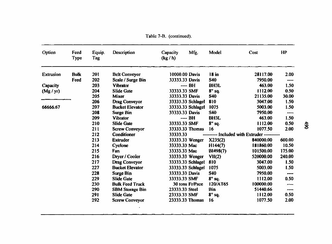
Table 7-B. (continued).
Option
Extrusion
Capacity (Mg/yr)
66666.67
Feed Type
Bulk Feed
Equip. Tag
Description Capacity (kg / h)
Mfg. Model Cost HP
201 Belt Conveyor 10000.00 Davis 18 in 28117.00 2.00 202 Scale / Surge Bin 33333.33 Davis S40 7950.00 203 Vibrator *— BH BH3L 463.00 1.50 204 Slide Gate 33333.33 SMF 8" sq. 1112.00 0.50 205 Mixer 33333.33 Davis S40 21135.00 30.00 206 Drag Conveyor 33333.33 Schlagei 810 3047.00 1.50 207 Bucket Elevator 33333.33 Schlagei 1075 5003.00 1.50 208 Surge Bin 33333.33 Davis S40 7950.00 209 Vibrator ———— BH BH3L 463.00 1.50 210 Slide Gate 33333.33 SMF 8" sq. 1112.00 0.50 211 Screw Conveyor 33333.33 Thomas 16 1077.50 2.00 212 Conditioner 33333.33 Included with Extruder 213 Extruder 33333.33 Wenger X235(2) 840000.00 600.00 214 Cyclone 33333.33 Mac H 144(7) 181860.00 10.50 215 Fan 33333.33 Mac BI498(7) 101500.00 175.00 216 Dryer / Cooler 33333.33 Wenger VI 1(2) 520000.00 240.00 217 Drag Conveyor 33333.33 Schlagei 810 3047.00 1.50 227 Bucket Elevator 33333.33 Schlagei 1075 5003.00 1.50 228 Surge Bin 33333.33 Davis S40 7950.00 229 Slide Gate 33333.33 SMF 8" sq. 1112.00 0.50 230 Bulk Feed Truck 30 tons Fr/Pace I20/AT65 100000.00 290 SBM Storage Bin 23333.33 Steel Bin 51440.66 ----
291 Slide Gate 23333.33 SMF 8" sq. 1112.00 0.50 292 Screw Conveyor 23333.33 Thomas 16 1077.50 2.00

Table 7-B. (continued).
Option Feed Equip. Description Capacity Mfg. Model Cost HP Type Tag (kg / h)
Extrusion Bulk Feed
Capacity (Mg/yr)
66666.67
Equipment Initial Cost ($) / Connected HP 1791531.66 1072.50 Electrical Wiring and Controls ($) [4%] 71661.27 Equipment Freight ($) [ I%] 17915.32 Equipment Installation ($) [40%] 716612.66 Spouting ($) 768.00 Total Equipment Initial Cost ($) [excluding truck cost] 2598488.91
Total Building Space Required (ft2) 2000.00 Total Building Cost ($) 25000.00
Engineering and Design Cost ($) 183644.22
Electricity Consumed (kW-h) 3438205.89
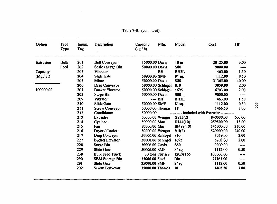
Table 7-B. (continued).
Option
Extrusion
Capacity (Mg/yr)
100000.00
Feed Type
Bulk Feed
Equip. Tag
Description Capacity Mfg. (kg / h)
Model Cost HP
201 Belt Conveyor 15000.00 Davis 18 in 28125.00 3.00 202 Scale / Surge Bin 50000.00 Davis S80 9000.00 203 Vibrator — BH BH3L 463.00 1.50 204 Slide Gate 50000.00 SMF 8" sq. 1112.00 0.50 205 Mixer 50000.00 Davis S80 31365.00 40.00 206 Drag Conveyor 50000.00 Schlagei 810 3059.00 2.00 207 Bucket Elevator 50000.00 Schlagei 1695 6703.00 2.00 208 Surge Bin 50000.00 Davis S80 9000.00 209 Vibrator — BH BH3L 463.00 1.50 210 Slide Gate 50000.00 SMF 8" sq. 1112.00 0.50 211 Screw Conveyor 50000.00 Thomas 18 1466.50 3.00 212 Conditioner 50000.00 Included with Extruder 213 Extruder 50000.00 Wenger X235(2) 840000.00 600.00 214 Cyclone 50000.00 Mac H 144(10) 259800.00 15.00 215 Fan 50000.00 Mac BI498(I0) 145000.00 250.00 216 Dryer / Cooler 50000.00 Wenger Vll(2) 520000.00 240.00 217 Drag Conveyor 50000.00 Schlagei 810 3059.00 2.00 227 Bucket Elevator 50000.00 Schlagei 1695 6703.00 2.00 228 Surge Bin 50000.00 Davis S80 9000.00 229 Slide Gate 50000.00 SMF 8" sq. 1112.00 0.50 230 Bulk Feed Truck 30 tons Fr/Pace 120/AT65 100000.00 ——-
290 SBM Storage Bin 35000.00 Steel Bin 77161.00 —•
291 Slide Gate 35000.00 SMF 8" sq. 1112.00 0.50 292 Screw Conveyor 35000.00 Thomas 18 1466.50 3.00

Table 7-B. (continued).
Option Feed Equip. Description Type Tag
Capacity Mfg. Model (kg / h)
Cost HP
Extrusion Bulk Feed
Capacity (Mg/yr)
100000.00
Equipment Initial Cost ($)/Connected HP 1956282.00 1167.00 Electrical Wiring and Controls ($) [4%] 78251.28 Equipment Freight ($) [ 1 %] 19562.82 Equipment Installation ($) [40%] 782512.80 Spouting ($) 768.00 Total Equipment Initial Cost ($) [excluding truck cost] 2837376.90
Total Building Space Required (ft2) 2000.00 Total Building Cost ($) 25000.00
Engineering and Design Cost ($) 200366.38
Electricity Consumed (kW-h) 3771426.47

Table 7-B. (continued).
Option
Extrusion
Capacity (Mg / yr)
133333.33
Feed Type
Bulk Feed
Equip. Tag
Description Capacity Mfg. (kg / h)
Model Cost HP
201 Belt Conveyor 20000.00 Davis 18 in 28125.00 3.00 202 Scale / Surge Bin 66666.67 Davis S100 9000.00 —-
203 Vibrator — BH BH3L 463.00 1.50 204 Slide Gate 66666.67 SMF 8" sq. 1112.00 0.50 205 Mixer 66666.67 Davis S100 45700.00 50.00 206 Drag Conveyor 66666.67 Schlagei 810 3059.00 2.00 207 Bucket Elevator 66666.67 Schlagei 2086 7751.00 3.00 208 Surge Bin 66666.67 Davis S100 9000.00 209 Vibrator —— BH BH3L 463.00 1.50 210 Slide Gate 66666.67 SMF 8" sq. 1112.00 0.50 211 Screw Conveyor 66666.67 Thomas 20 1900.80 5.00 212 Conditioner 66666.67 Included with Extruder 213 Extruder 66666.67 Wenger X235(3) 1260000.00 900.00 214 Cyclone 66666.67 Mac H144(14) 363720.00 21.00 215 Fan 66666.67 Mac B1498(14) 203000.00 350.00 216 Dryer / Cooler 66666.67 Wenger VII(3) 780000.00 360.00 217 Drag Conveyor 66666.67 Schlagei 810 3059.00 2.00 227 Bucket Elevator 66666.67 Schlagei 2086 7751.00 3.00 228 Surge Bin 66666.67 Davis S100 9000.00 ----
229 Slide Gate 66666.67 SMF 8" sq. 1112.00 0.50 230 Bulk Feed Truck 30 tons Fr/Pace 120/AT65 100000.00 ----
290 SBM Storage Bin 46666.67 Steel Bin 102881.34 ----
291 Slide Gate 46666.67 SMF 8" sq. 1112.00 0.50 292 Screw Conveyor 46666.67 Thomas 20 1900.80 5.00

Table 7-B. (continued).
Option Feed Equip. Description Capacity Mfg. Model Cost HP Type Tag (kg / h)
Extrusion Bulk Feed
Capacity (Mg / yr)
133333.33
Equipment Initial Cost ($) / Connected HP 2841221.94 1709.00 Electrical Wiring and Controls ($) [4%] 113648.88 Equipment Freight ($) [ I %] 28412.22 Equipment Installation ($) [40%] 1136488.78 Spouting ($) 768.00 Total Equipment Initial Cost ($) [excluding truck cost] 4120539.81
Total Building Space Required (ft2) 2000.00 Total Building Cost ($) 25000.00
Engineering and Design Cost ($) 290187.79
Electricity Consumed (kW-h) 5508568.62
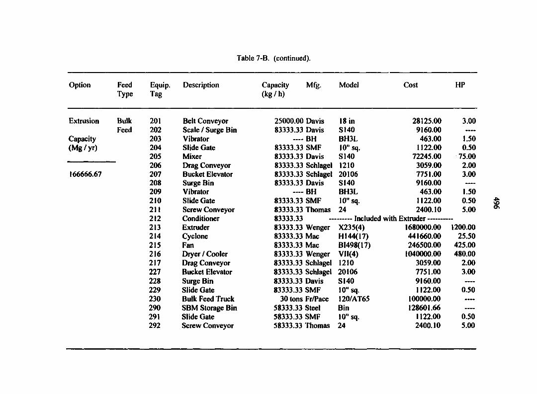
Table 7-B. (continued).
Option
Extrusion
Capacity (Mg/yr)
166666.67
Feed Type
Bulk Feed
Equip. Tag
Description Capacity Mfg. (kg / h)
Model Cost HP
201 Belt Conveyor 25000.00 Davis 18 in 28125.00 3.00 202 Scale / Surge Bin 83333.33 Davis S140 9160.00 ——
203 Vibrator BH BH3L 463.00 1.50 204 Slide Gate 83333.33 SMF 10" sq. 1122.00 0.50 205 Mixer 83333.33 Davis S140 72245.00 75.00 206 Drag Conveyor 83333.33 Schlagei 1210 3059.00 2.00 207 Bucket Elevator 83333.33 Schlagei 20106 7751.00 3.00 208 Surge Bin 83333.33 Davis S140 9160.00 209 Vibrator — BH BH3L 463.00 1.50 210 Slide Gate 83333.33 SMF 10" sq. 1122.00 0.50 211 Screw Conveyor 83333.33 Thomas 24 2400.10 5.00 212 Conditioner 83333.33 Included with Extruder 213 Extruder 83333.33 Wenger X235(4) 1680000.00 1200.00 214 Cyclone 83333.33 Mac H 144(17) 441660.00 25.50 215 Fan 83333.33 Mac BI498(17) 246500.00 425.00 216 Dryer / Cooler 83333.33 Wenger V1I(4) 1040000.00 480.00 217 Drag Conveyor 83333.33 Schlagei 1210 3059.00 2.00 227 Bucket Elevator 83333.33 Schlagei 20106 7751.00 3.00 228 Surge Bin 83333.33 Davis S140 9160.00 •-*—
229 Slide Gate 83333.33 SMF 10" sq. 1122.00 0.50 230 Bulk Feed Truck 30 tons Fr/Pace 120/AT65 100000.00 ——
290 SBM Storage Bin 58333.33 Steel Bin 128601.66 291 Slide Gate 58333.33 SMF 10" sq. 1122.00 0.50 292 Screw Conveyor 58333.33 Thomas 24 2400.10 5.00

Table 7-B. (continued).
Option Feed Equip. Description Capacity Mfg. Model Cost HP Type Tag (kg / h)
Extrusion Bulk Feed
Capacity (Mg / yr)
166666.67
Equipment Initial Cost ($) / Connected HP 3696445.86 2233.50 Electrical Wiring and Controls ($) [4%] 147857.83 Equipment Freight ($) [ 1 %] 36964.46 Equipment Installation ($) [40%] 1478578.34 Spouting ($) 768.00 Total Equipment Initial Cost ($) [excluding truck cost] 5360614.50
Total Building Space Required (ft2) 2000.00 Total Building Cost ($) 25000.00
Engineering and Design Cost ($) 376993.01
Electricity Consumed (kW-h) 7190808.83

Table 7-B. (continued).
Option Feed Equip. Description Capacity Mfg. Model Cost HP Type Tag (kg / h)
Extrusion
Capacity (Mg/yr)
200000.00
Bulk Feed
201 Belt Conveyor 30000.00 Davis 18 in 28153.00 5.00 202 Scale / Surge Bin 100000.00 Davis SI60 9160.00 —-
203 Vibrator —— BH BH3L 463.00 1.50 204 Slide Gate 100000.00 SMF 10" sq. 1122.00 0.50 205 Mixer 100000.00 Davis S160 79595.00 100.00 206 Drag Conveyor 100000.00 Schlagel 1210 3059.00 2.00 207 Bucket Elevator 100000.00 Schlagel 24116 8483.00 5.00 208 Surge Bin 100000.00 Davis S160 9160.00 209 Vibrator BH BH3L 463.00 1.50 210 Slide Gate 100000.00 SMF 10" sq. 1122.00 0.50 211 Screw Conveyor 100000.00 Thomas 24 2400.10 5.00 212 Conditioner 100000.00 Included with Extruder 213 Extruder 100000.00 Wenger X235(5) 2100000.00 1500.00 214 Cyclone 100000.00 Mac H 144(20) 519600.00 30.00 215 Fan 100000.00 Mac B1498(20) 290000.00 500.00 216 Diyer / Cooler 100000.00 Wenger VH(5) 1300000.00 600.00 217 Drag Conveyor 100000.00 Schlagel 1210 3059.00 2.00 227 Bucket Elevator 100000.00 Schlagel 24116 8483.00 5.00 228 Surge Bin 100000.00 Davis S160 9160.00 229 Slide Gate 100000.00 SMF 10" sq. 1122.00 0.50 230 Bulk Feed Truck 30 tons Fr/Pace I20/AT65 100000.00 —-
290 SBM Storage Bin 70000.00 Steel Bin 154322.00 *—
291 Slide Gate 70000.00 SMF 10" sq. 1122.00 0.50 292 Screw Conveyor 70000.00 Thomas 24 2400.10 5.00

Table 7-B. (continued).
Option Feed Equip. Description Capacity Mfg. Model Cost HP Type Tag (kg / h)
Extrusion Bulk Feed
Capacity (Mg/yr)
200000.00
Equipment Initial Cost ($) / Connected HP 4532448.20 2764.00 Electrical Wiring and Controls ($) |4%] 181297.93 Equipment Freight ($) [ I %] 45324.48 Equipment Installation ($) [40%] 1812979.28 Spouting ($) 768.00 Total Equipment Initial Cost ($) (excluding truck cost| 6572817.89
Total Building Space Required (ft2) 2000.00 Total Building Cost ($) 25000.00
Engineering and Design Cost ($) 461847.25
Electricity Consumed (kW-h) 8891872.55

Table 7-B. (continued).
Option
Extrusion
Capacity (Mg/yr)
233333.33
Feed Type
Bulk Feed
Equip. Tag
Description Capacity (kg / h)
Mfg. Model Cost HP
201 Belt Conveyor 35000.00 Davis 18 in 28153.00 5.00 202 Scale / Surge Bin 116666.67 Davis SI60 9160.00 —«
203 Vibrator —— BH BH3L 463.00 1.50 204 Slide Gate 116666.67 SMF 10 " sq. 1122.00 0.50 205 Mixer 116666.67 Davis S160 79595.00 100.00 206 Drag Conveyor 116666.67 Schlagel 1214 3682.00 2.00 207 Bucket Elevator 116666.67 Schlagel 30126 11096.00 5.00 208 Surge Bin 116666.67 Davis S160 9160.00 209 Vibrator —— BH BH3L 463.00 1.50 210 Slide Gate 116666.67 SMF 10" sq. 1122.00 0.50 211 Screw Conveyor 116666.67 Thomas 24 2516.10 7.50 212 Conditioner 116666.67 Included with Extruder 213 Extruder 116666.67 Wenger X235(6) 2520000.00 1800.00 214 Cyclone 116666.67 Mac H 144(24) 623520.00 36.00 215 Fan 116666.67 Mac 81498(24) 348000.00 600.00 216 Dryer / Cooler 116666.67 Wenger VI 1(6) 1560000.00 720.00 217 Drag Conveyor 116666.67 Schlagel 1214 3682.00 2.00 227 Bucket Elevator 116666.67 Schlagel 30126 11096.00 5.00 228 Surge Bin 116666.67 Davis SI60 9160.00 —••
229 Slide Gate 116666.67 SMF 10" sq. 1122.00 0.50 230 Bulk Feed Truck 30 tons Fr/Pace I20/AT65 100000.00 —-
290 SBM Storage Bin 81666.67 Steel Bin 180042.34 —-
291 Slide Gate 81666.67 SMF 10" sq. 1122.00 0.50 292 Screw Conveyor 81666.67 Thomas 24 2516.10 7.50
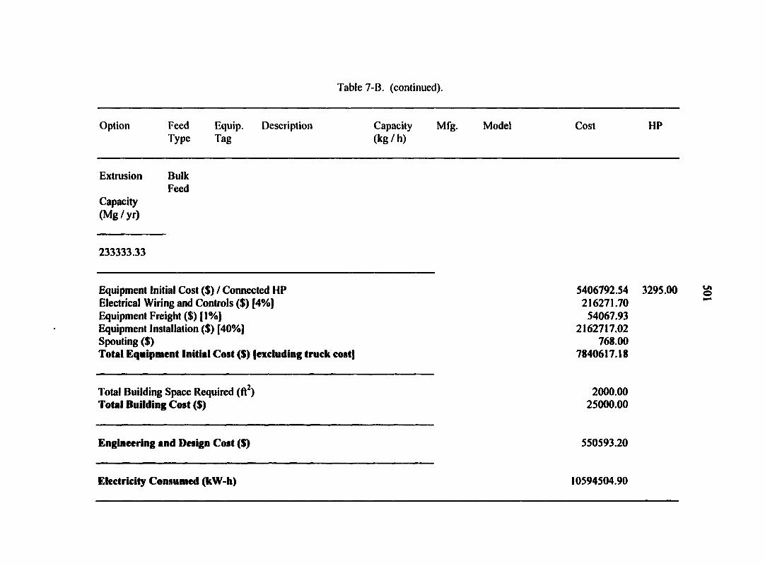
Table 7-B. (continued).
Option Feed Equip. Description Capacity Mfg. Model Cost HP Type Tag (kg / h)
Extrusion Bulk Feed
Capacity (Mg/yr)
233333.33
Equipment Initial Cost ($) / Connected HP 5406792.54 3295.00 Electrical Wiring and Controls ($) [4%] 216271.70 Equipment Freight ($) [ 1 %] 54067.93 Equipment Installation ($) [40%] 2162717.02 Spouting ($) 768.00 Total Equipment Initial Cost ($) (excluding truck cost] 7840617.18
Total Building Space Required (ft2) 2000.00 Total Building Cost ($) 25000.00
Engineering and Design Cost ($) 550593.20
Electricity Consumed (kW-h) 10594504.90
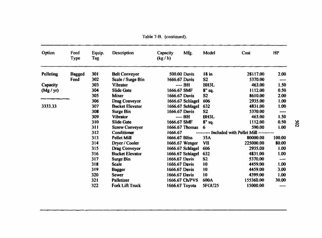
Table 7-B. (continued).
Option Feed Type
Equip. Tag
Description Capacity Mfg. (kg/h)
Model Cost HP
Pelleting Bagged 301 Belt Conveyor 500.00 Davis 18 in 28117.00 2.00 Feed 302 Scale / Surge Bin 1666.67 Davis S2 5370.00
Capacity 303 Vibrator — BH BH3L 463.00 1.50 (Mg/yr) 304 Slide Gate 1666.67 SMF 8" sq. 1112.00 0.50
305 Mixer 1666.67 Davis S2 8610.00 2.00 306 Drag Conveyor 1666.67 Schlagel 606 2935.00 1.00
3333.33 307 Bucket Elevator 1666.67 Schlagel 632 4831.00 1.00 308 Surge Bin 1666.67 Davis S2 5370.00 309 Vibrator —— BH BH3L 463.00 1.50 310 Slide Gate 1666.67 SMF 8" sq. 1112.00 0.50 311 Screw Conveyor 1666.67 Thomas 6 590.00 1.00 312 Conditioner 1666.67 Included with Pellet Mill 313 Pellet Mill 1666.67 Bliss 35A 80000.00 100.00 314 Dryer / Cooler 1666.67 Wenger VII 225000.00 80.00 315 Drag Conveyor 1666.67 Schlagel 606 2935.00 1.00 316 Bucket Elevator 1666.67 Schlagel 632 4831.00 1.00 317 Surge Bin 1666.67 Davis S2 5370.00 —-
318 Scale 1666.67 Davis 10 4459.00 1.00 319 Bagger 1666.67 Davis 10 4459.00 3.00 320 Sewer 1666.67 Davis 10 4399.00 1.00 321 Palletizer 1666.67 Ch/PVS 600A 155360.00 30.00 322 Fork Lift Truck 1666.67 Toyota 5FGU25 15000.00 ——
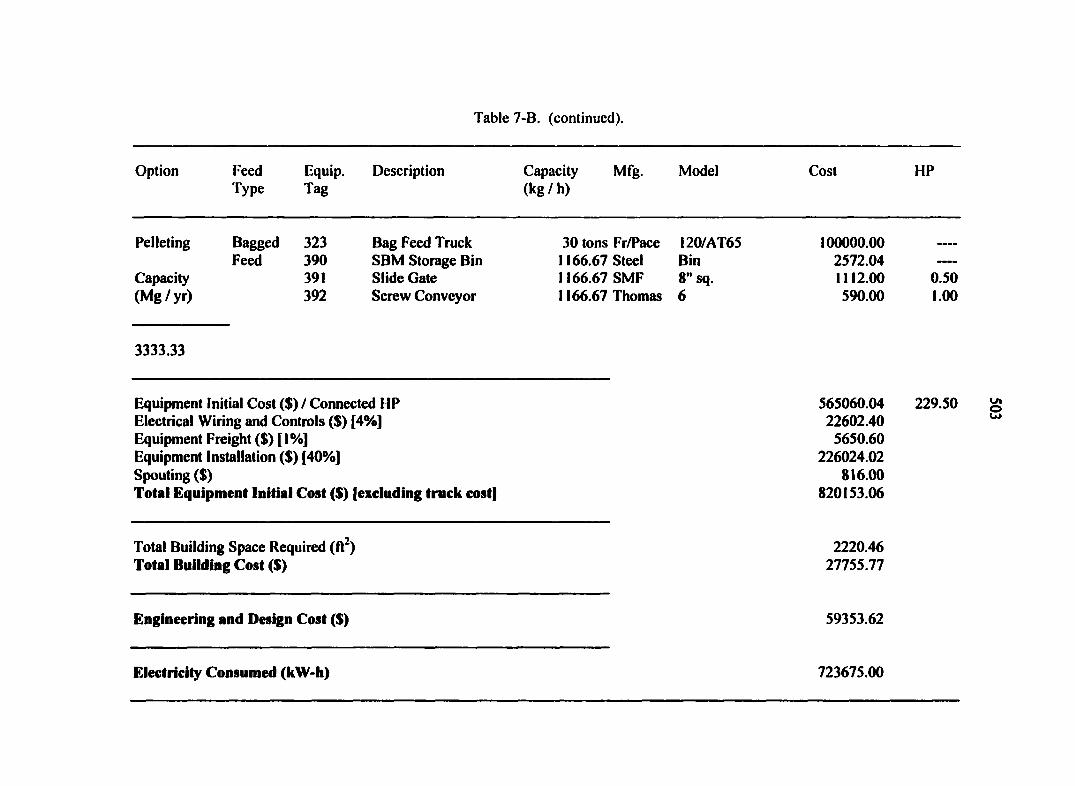
Table 7-B. (continued).
Option Feed Type
Equip. Tag
Description Capacity (kg / h)
Mfg. Model Cost HP
Pelleting Bagged 323 Bag Feed Truck Feed 390 SBM Storage Bin
Capacity 391 Slide Gate (Mg / yr) 392 Screw Conveyor
30 tons Fr/Pace 1166.67 Steel 1166.67 SMF 1166.67 Thomas
120/AT65 Bin 8" sq. 6
100000.00 2572.04 1112.00 590.00
0.50 1.00
3333.33
Equipment Initial Cost ($) / Connected HP Electrical Wiring and Controls ($) [4%] Equipment Freight ($)[!%] Equipment Installation ($) [40%] Spouting ($) Total Equipment Initial Cost ($) (excluding truck cost)
565060.04 22602.40 5650.60
226024.02 816.00
820153.06
229.50
Total Building Space Required (ft ) Total Building Cost ($)
2220.46 27755.77
Engineering and Design Cost ($) 59353.62
Electricity Consumed (kW-h) 723675.00

Table 7-B. (continued).
Option Feed Equip. Description Capacity Mfg. Model Cost HP Type Tag (kg / h)
Pelleting
Capacity (Mg/yr)
8333.33
Bagged 301 Belt Conveyor 1250.00 Davis 18 in 28117.00 2.00 Feed 302 Scale / Surge Bin 4166.67 Davis S5 5370.00
303 Vibrator —— BH BH3L 463.00 1.50 304 Slide Gate 4166.67 SMF 8" sq. 1112.00 0.50 305 Mixer 4166.67 Davis S5 10555.00 5.00 306 Drag Conveyor 4166.67 Schlagel 606 2935.00 1.00 307 Bucket Elevator 4166.67 Schlagel 643 4831.00 1.00 308 Surge Bin 4166.67 Davis S5 5370.00 309 Vibrator — BH BH3L 463.00 1.50 310 Slide Gate 4166.67 SMF 8" sq. 1112.00 0.50 311 Screw Conveyor 4166.67 Thomas 9 629.10 1.00 312 Conditioner 4166.67 Included with Pellet Mill 313 Pellet Mill 4166.67 Bliss 35A 80000.00 100.00 314 Dryer / Cooler 4166.67 Wenger VII 225000.00 80.00 315 Drag Conveyor 4166.67 Schlagel 606 2935.00 1.00 316 Bucket Elevator 4166.67 Schlagel 643 4831.00 1.00 317 Surge Bin 4166.67 Davis S5 5370.00 318 Scale 4166.67 Davis 10 4459.00 1.00 319 Bagger 4166.67 Davis 10 4459.00 3.00 320 Sewer 4166.67 Davis 10 4399.00 1.00 321 Palletizer 4166.67 Ch/PVS 600A 155360.00 30.00 322 Fork Lift Truck 4166.67 Toyota 5FGU25 15000.00 —-

Table 7-B. (continued).
Option Feed Type
Equip. Tag
Description Capacity (kg/h)
Mfg. Model Cost HP
Pelleting Bagged 323 Bag Feed Truck Feed 390 SBM Storage Bin
Capacity 391 Slide Gate (Mg / yr) 392 Screw Conveyor
8333.33
30 tons Fr/Pace 120/AT65 2916.67 Steel Bin 2916.67 SMF 8" sq. 2916.67 Thomas 9
100000.00 6430.09 1112.00 629.10
0.50 1.00
Equipment Initial Cost ($) Z Connected HP Electrical Wiring and Controls ($) [4%] Equipment Freight ($) [ 1 %] Equipment Installation ($) [40%] Spouting ($) Total Equipment Initial Cost ($) [excluding truck cost]
570941.29 22837.65 5709.41
228376.52 816.00
828680.87
232.50
Total Building Space Required (ft ) Total Building Cost ($)
2551.16 31889.44
Engineering and Design Cost ($) 60239.92
Electricity Consumed (kW-h) 738599.26
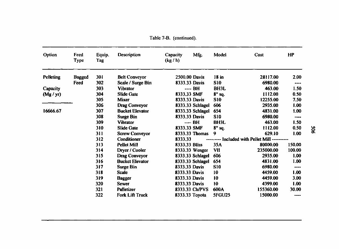
Table 7-B. (continued).
Option
Pelleting
Capacity (Mg/yr)
Feed Type
Bagged Feed
16666.67
Equip. Tag
Description Capacity (kg / h)
Mfg. Model Cost HP
301 Belt Conveyor 2500.00 Davis 18 in 28117.00 2.00 302 Scale / Surge Bin 8333.33 Davis S10 6980.00 303 Vibrator — — — — BH BH3L 463.00 1.50 304 Slide Gate 8333.33 SMF 8" sq. 1112.00 0.50 305 Mixer 8333.33 Davis S10 12255.00 7.50 306 Drag Conveyor 8333.33 Schlagel 606 2935.00 1.00 307 Bucket Elevator 8333.33 Schlagel 654 4831.00 1.00 308 Surge Bin 8333.33 Davis S10 6980.00 ———
309 Vibrator BH BH3L 463.00 1.50 310 Slide Gate 8333.33 SMF 8" sq. 1112.00 0.50 311 Screw Conveyor 8333.33 Thomas 9 629.10 1.00 312 Conditioner 8333.33 Included with Pellet Mill 313 Pellet Mill 8333.33 Bliss 35A 80000.00 150.00 314 Dryer / Cooler 8333.33 Wenger VII 235000.00 100.00 315 Drag Conveyor 8333.33 Schlagel 606 2935.00 1.00 316 Bucket Elevator 8333.33 Schlagel 654 4831.00 1.00 317 Surge Bin 8333.33 Davis S10 6980.00 -™
318 Scale 8333.33 Davis 10 4459.00 1.00 319 Bagger 8333.33 Davis 10 4459.00 3.00 320 Sewer 8333.33 Davis 10 4399.00 1.00 321 Palletizer 8333.33 Ch/PVS 600A 155360.00 30.00 322 Fork Lift Truck 8333.33 Toyota 5FGU25 15000.00 ----
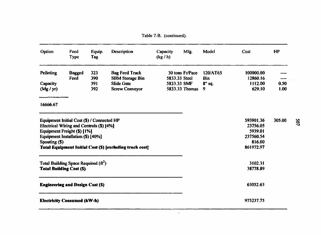
Table 7-B. (continued).
Option Feed Type
Equip. Tag
Description Capacity (kg / h)
Mfg. Model Cost HP
Pelleting Bagged 323 Bag Feed Truck Feed 390 SBM Storage Bin
Capacity 391 Slide Gate (Mg / yr) 392 Screw Conveyor
30 tons Fr/Pace 120/AT65 5833.33 Steel Bin 5833.33 SMF 8" sq. 5833.33 Thomas 9
100000.00 12860.16 1112.00 629.10
0.50 1.00
16666.67
Equipment Initial Cost ($) / Connected HP Electrical Wiring and Controls ($) [4%] Equipment Freight ($) [ I %J Equipment Installation ($) [40%] Spouting ($) Total Equipment Initial Cost ($) [excluding truck cost|
593901.36 23756.05 5939.01
237560.54 816.00
861972.97
305.00
Total Building Space Required (ft2) Total Building Cost ($)
3102.31 38778.89
Engineering and Design Cost ($) 63052.63
Electricity Consumed (kW-h) 975237.75
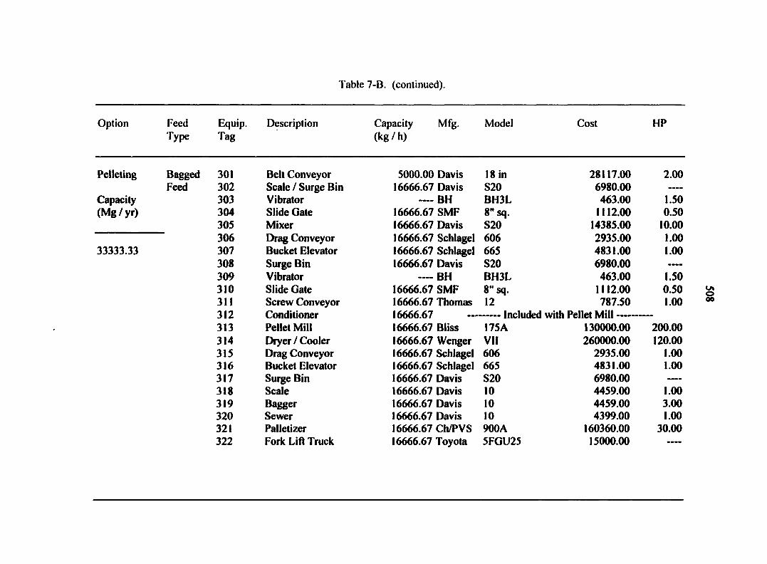
Table 7-B. (continued).
Option Feed Type
Equip. Tag
Description Capacity (kg / h)
Mfg. Model Cost HP
Pelleting
Capacity (Mg/yr)
33333.33
Bagged 301 Belt Conveyor 5000.00 Davis 18 in 28117.00 2.00 Feed 302 Scale / Surge Bin 16666.67 Davis S20 6980.00
303 Vibrator — BH BH3L 463.00 1.50 304 Slide Gate 16666.67 SMF 8" sq. 1112.00 0.50 305 Mixer 16666.67 Davis S20 14385.00 10.00 306 Drag Conveyor 16666.67 Schlagel 606 2935.00 1.00 307 Bucket Elevator 16666.67 Schlagel 665 4831.00 1.00 308 Surge Bin 16666.67 Davis S20 6980.00 309 Vibrator — BH BH3L 463.00 1.50 310 Slide Gate 16666.67 SMF 8 " sq. 1112.00 0.50 311 Screw Conveyor 16666.67 Thomas 12 787.50 1.00 312 Conditioner 16666.67 Included with Pellet Mill 313 Pellet Mill 16666.67 Bliss 175 A 130000.00 200.00 314 Diyer / Cooler 16666.67 Wenger VII 260000.00 120.00 315 Drag Conveyor 16666.67 Schlagel 606 2935.00 1.00 316 Bucket Elevator 16666.67 Schlagel 665 4831.00 1.00 317 Surge Bin 16666.67 Davis S20 6980.00 ....
318 Scale 16666.67 Davis 10 4459.00 1.00 319 Bagger 16666.67 Davis 10 4459.00 3.00 320 Sewer 16666.67 Davis 10 4399.00 1.00 321 Palletizer 16666.67 Ch/PVS 900A 160360.00 30.00 322 Fork Lift Truck 16666.67 Toyota 5FGU25 15000.00 ....
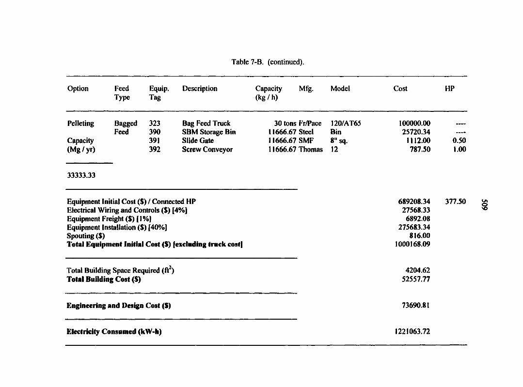
Table 7-B. (continued).
Option Feed Type
Equip. Tag
Description Capacity (kg / h)
Mfg. Model Cost HP
Pelleting Bagged 323 Bag Feed Truck Feed 390 SBM Storage Bin
Capacity 391 Slide Gate (Mg / yr) 392 Screw Conveyor
33333.33
30 tons Fr/Pace 11666.67 Steel 11666.67 SMF 11666.67 Thomas
120/AT65 Bin 8" sq. 12
100000.00 25720.34 1112.00 787.50
0.50 1.00
Equipment Initial Cost ($) Z Connected HP Electrical Wiring and Controls ($) [4%] Equipment Freight ($) [l%] Equipment Installation ($) [40%] Spouting ($) Total Equipment Initial Cost ($) [excluding truck cost]
689208.34 27568.33 6892.08
275683.34 816.00
1000168.09
377.50
Total Building Space Required (ft ) Total Building Cost ($)
4204.62 52557.77
Engineering and Design Cost ($) 73690.81
Electricity Consumed (kW-h) 1221063.72
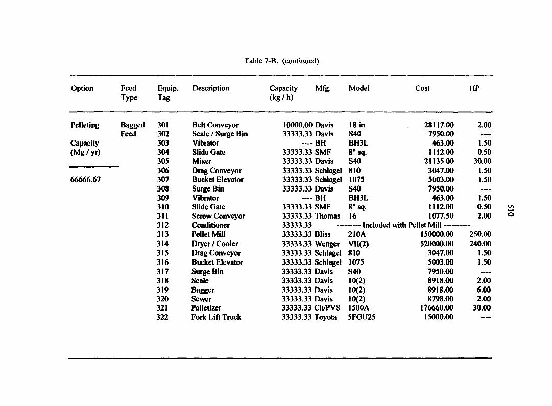
Table 7-B. (continued).
Option Feed Type
Equip. Tag
Description Capacity Mfg. (kg / h)
Model Cost HP
Pelleting Bagged 301 Belt Conveyor 10000.00 Davis 18 in 28117.00 2.00 Feed 302 Scale / Surge Bin 33333.33 Davis S40 7950.00 ——
Capacity 303 Vibrator — BH BH3L 463.00 1.50 (Mg / yr) 304 Slide Gate 33333.33 SMF 8" sq. 1112.00 0.50
305 Mixer 33333.33 Davis S40 21135.00 30.00 306 Drag Conveyor 33333.33 Schlagel 810 3047.00 1.50
66666.67 307 Bucket Elevator 33333.33 Schlagel 1075 5003.00 1.50 308 Surge Bin 33333.33 Davis S40 7950.00 -•••
309 Vibrator — BH BH3L 463.00 1.50 310 Slide Gate 33333.33 SMF 8" sq. 1112.00 0.50 311 Screw Conveyor 33333.33 Thomas 16 1077.50 2.00 312 Conditioner 33333.33 Included with Pellet Mill 313 Pellet Mill 33333.33 Bliss 210A 150000.00 250.00 314 Dryer / Cooler 33333.33 Wenger VH(2) 520000.00 240.00 315 Drag Conveyor 33333.33 Schlagel 810 3047.00 1.50 316 Bucket Elevator 33333.33 Schlagel 1075 5003.00 1.50 317 Surge Bin 33333.33 Davis S40 7950.00 •—
318 Scale 33333.33 Davis 10(2) 8918.00 2.00 319 Bagger 33333.33 Davis 10(2) 8918.00 6.00 320 Sewer 33333.33 Davis 10(2) 8798.00 2.00 321 Palletizer 33333.33 Ch/PVS 1500A 176660.00 30.00 322 Fork Lift Truck 33333.33 Toyota 5FGU25 15000.00 —-

Table 7-B. (continued).
Option Feed Type
Equip. Tag
Description Capacity (kg / h)
Mfg. Model Cost HP
Pelleting Bagged 323 Bag Feed Truck Feed 390 SBM Storage Bin
Capacity 391 Slide Gate (Mg / yr) 392 Screw Conveyor
66666.67
30 tons Fr/Pace 23333.33 Steel 23333.33 SMF 23333.33 Thomas
I20/AT65 Bin 8" sq. 16
100000.00 51440.66
1112.00 1077.50
0.50 2.00
Equipment Initial Cost ($) / Connected HP Electrical Wiring and Controls ($) [4%] Equipment Freight ($) [1%] Equipment Installation ($) [40%] Spouting ($) Total Equipment Initial Cost ($) (excluding truck cost]
1035353.66 41414.15 10353.54
414141.46 816.00
1502078.81
576.50
Total Building Space Required (ft ) Total Building Cost ($)
6409.24 80115.55
Engineering and Design Cost ($) 110753.61
Electricity Consumed (kW-h) 1882127.45
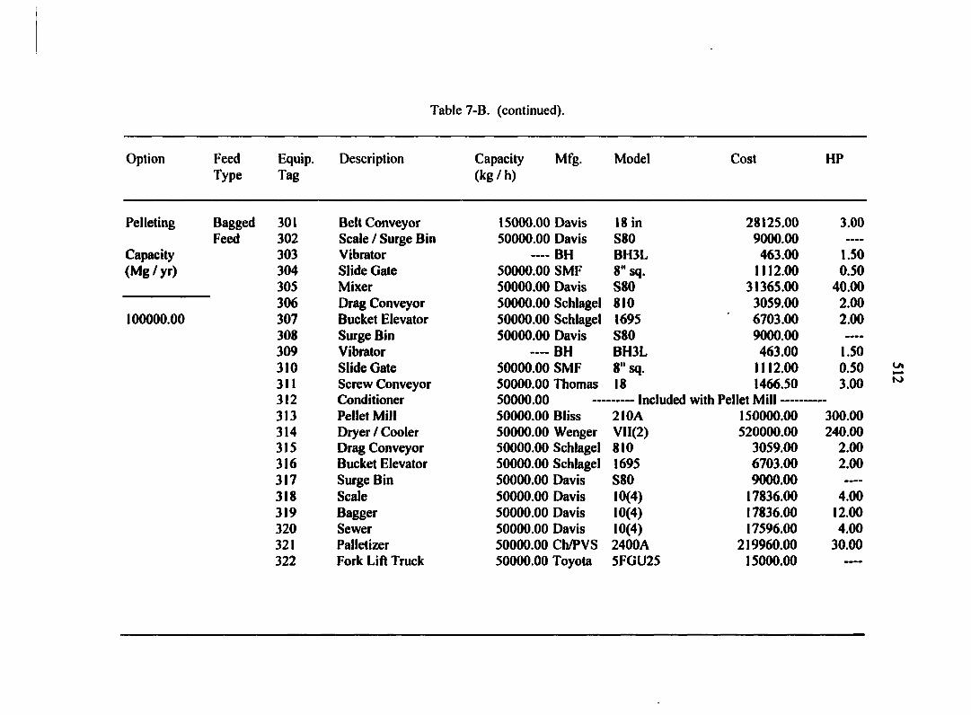
Table 7-B. (continued).
Option
Pelleting
Capacity (Mg/yr)
100000.00
Feed Equip. Description Capacity Mfg. Model Cost HP Type Tag (kg / h)
Bagged 301 Belt Conveyor 15000.00 Davis 18 in 28125.00 3.00 Feed 302 Scale / Surge Bin 50000.00 Davis S80 9000.00 ——
303 Vibrator — BH BH3L 463.00 1.50 304 Slide Gate 50000.00 SMF 8" sq. 1112.00 0.50 305 Mixer 50000.00 Davis S80 31365.00 40.00 306 Drag Conveyor 50000.00 Schlagel 810 3059.00 2.00 307 Bucket Elevator 50000.00 Schlagel 1695 6703.00 2.00 308 Surge Bin 50000.00 Davis S80 9000.00 309 Vibrator — BH BH3L 463.00 1.50 310 Slide Gate 50000.00 SMF 8" sq. 1112.00 0.50 311 Screw Conveyor 50000.00 Thomas 18 1466.50 3.00 312 Conditioner 50000.00 Included with Pellet Mill 313 Pellet Mill 50000.00 Bliss 2I0A 150000.00 300.00 314 Dryer / Cooler 50000.00 Wenger Vll(2) 520000.00 240.00 315 Drag Conveyor 50000.00 Schlagel 810 3059.00 2.00 316 Bucket Elevator 50000.00 Schlagel 1695 6703.00 2.00 317 Surge Bin 50000.00 Davis S80 9000.00 ——
318 Scale 50000.00 Davis 10(4) 17836.00 4.00 319 Bagger 50000.00 Davis 10(4) 17836.00 12.00 320 Sewer 50000.00 Davis 10(4) 17596.00 4.00 321 Palletizer 50000.00 Ch/PVS 2400A 219960.00 30.00 322 Fork Lift Truck 50000.00 Toyota 5FGU25 15000.00 —-
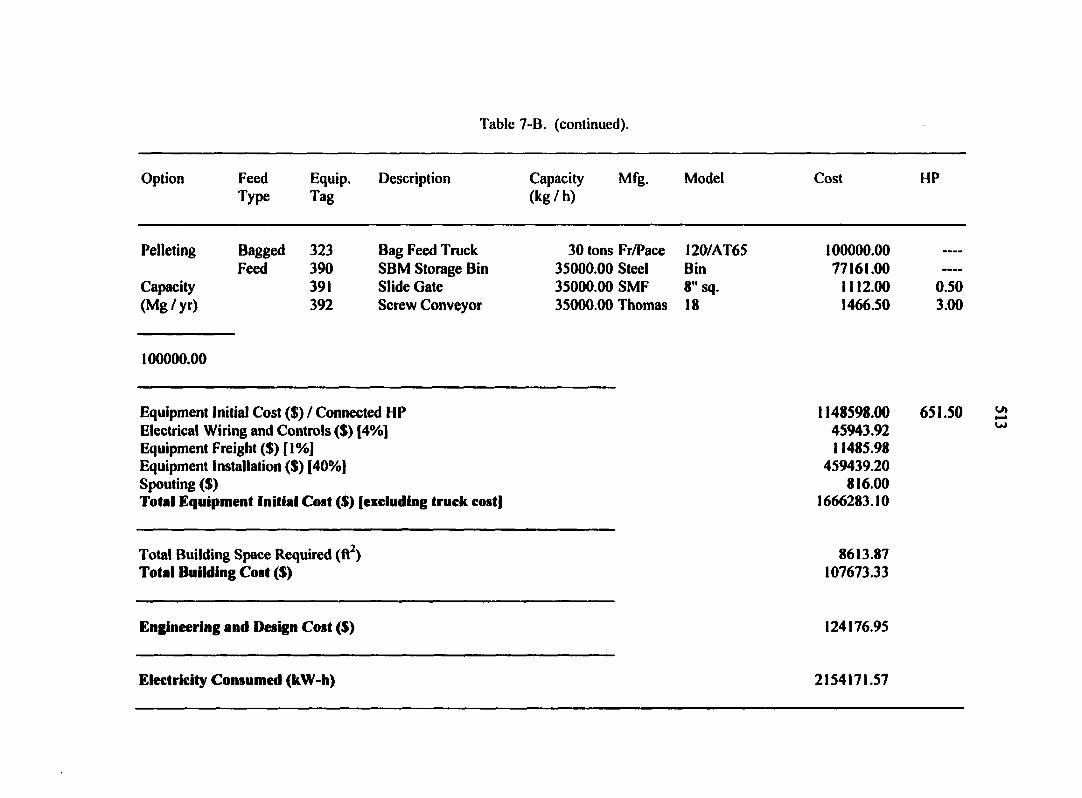
Table 7-B. (continued).
Option Feed Type
Equip. Tag
Description Capacity (kg / h)
Mfg. Model Cost HP
Pelleting Bagged 323 Bag Feed Truck Feed 390 SBM Storage Bin
Capacity 391 Slide Gate (Mg Z yr) 392 Screw Conveyor
100000.00
30 tons Fr/Pace 35000.00 Steel 35000.00 SMF 35000.00 Thomas
I20/AT65 Bin 8" sq. 18
100000.00 77161.00
1112.00 1466.50
0.50 3.00
Equipment Initial Cost ($) Z Connected HP Electrical Wiring and Controls ($) [4%] Equipment Freight ($) [\%] Equipment Installation ($) [40%] Spouting ($) Total Equipment Initial Cost ($) [excluding truck cost]
1148598.00 45943.92 11485.98
459439.20 816.00
1666283.10
651.50
Total Building Space Required (ft ) Total Building Cost ($)
8613.87 107673 33
Engineering and Design Cost ($) 124176.95
Electricity Consumed (kW-h) 2154171.57
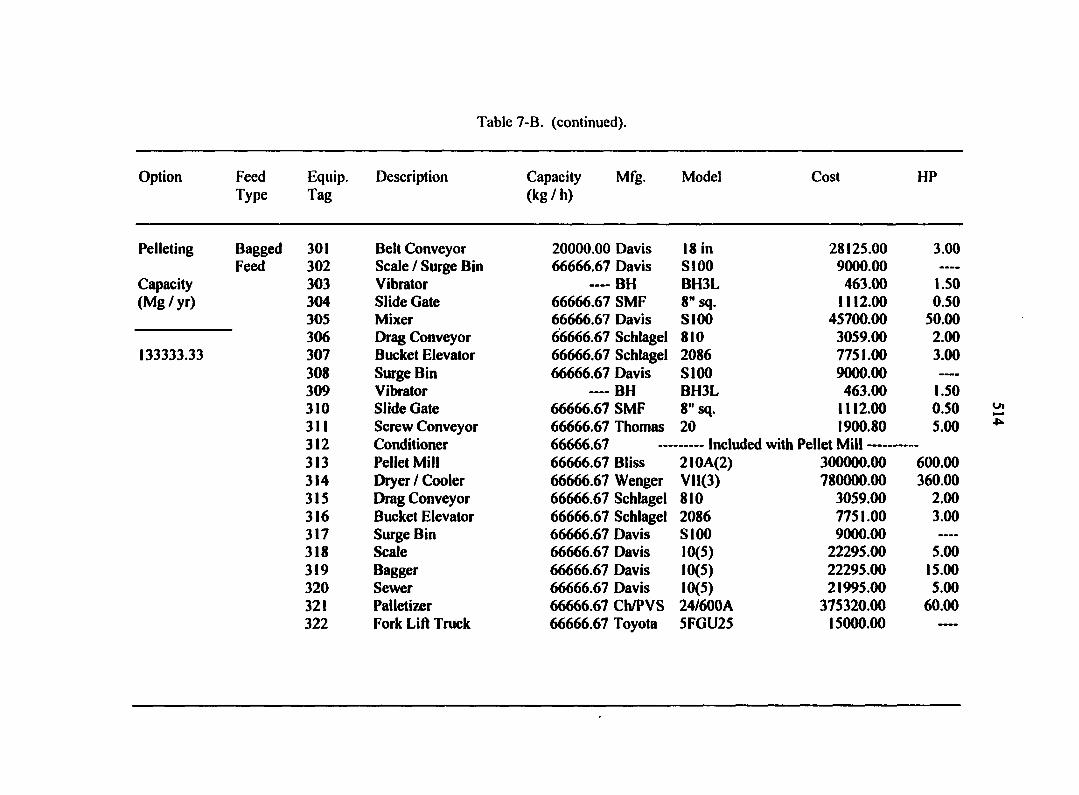
Table 7-B. (continued).
Option Feed Equip. Description Capacity Mfg. Model Cost HP Type Tag (kg/ h)
Pelleting
Capacity (Mg/yr)
133333.33
Bagged 301 Belt Conveyor 20000.00 Davis 18 in 28125.00 3.00 Feed 302 Scale / Surge Bin 66666.67 Davis S100 9000.00 ——
303 Vibrator — BH BH3L 463.00 1.50 304 Slide Gate 66666.67 SMF 8" sq. 1112.00 0.50 305 Mixer 66666.67 Davis S100 45700.00 50.00 306 Drag Conveyor 66666.67 Schlagel 810 3059.00 2.00 307 Bucket Elevator 66666.67 Schlagel 2086 7751.00 3.00 308 Surge Bin 66666.67 Davis S100 9000.00 ———•
309 Vibrator — BH BH3L 463.00 1.50 310 Slide Gate 66666.67 SMF 8" sq. 1112.00 0.50 311 Screw Conveyor 66666.67 Thomas 20 1900.80 5.00 312 Conditioner 66666.67 Included with Pellet Mill 313 Pellet Mill 66666.67 Bliss 210A(2) 300000.00 600.00 314 Dryer / Cooler 66666.67 Wenger VI 1(3) 780000.00 360.00 315 Drag Conveyor 66666.67 Schlagel 810 3059.00 2.00 316 Bucket Elevator 66666.67 Schlagel 2086 7751.00 3.00 317 Surge Bin 66666.67 Davis S100 9000.00 318 Scale 66666.67 Davis 10(5) 22295.00 5.00 319 Bagger 66666.67 Davis 10(5) 22295.00 15.00 320 Sewer 66666.67 Davis 10(5) 21995.00 5.00 321 Palletizer 66666.67 Ch/PVS 24/600A 375320.00 60.00 322 Fork Lift Truck 66666.67 Toyota 5FGU25 15000.00 —«
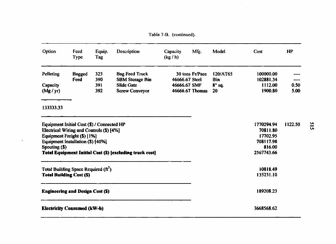
Table 7-B. (continued).
Option Feed Type
Equip. Tag
Description Capacity (kg / h)
Mfg. Model Cost HP
Pelleting Bagged 323 Bag Feed Truck Feed 390 SBM Storage Bin
Capacity 391 Slide Gate (Mg / yr) 392 Screw Conveyor
30 tons Fr/Pace 46666.67 Steel 46666.67 SMF 46666.67 Thomas
120ZAT65 Bin 8" sq. 20
100000.00 102881.34
1112.00 1900.80
0.50 5.00
133333.33
Equipment Initial Cost ($) / Connected HP 1770294.94 1122.50 Electrical Wiring and Controls ($) [4%] 70811.80 Equipment Freight ($) [ 1 %] 17702.95 Equipment Installation ($) [40%] 708117.98 Spouting ($) 816.00 Total Equipment Initial Cost ($) [excluding truck cost) 2567743.66
Total Building Space Required (ft2) 10818.49 Total Building Cost ($) 135231.10
Engineering and Design Cost ($) 189208.23
Electricity Consumed (kW-h) 3668568.62
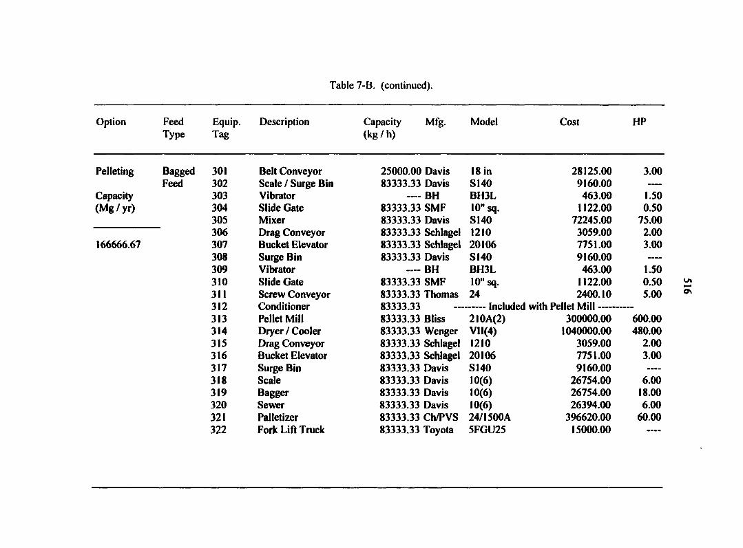
Table 7-B. (continued).
Option Feed Type
Equip. Tag
Description Capacity (kg / h)
Mfg. Model Cost HP
Pelleting
Capacity (Mg/yr)
Bagged Feed
166666.67
301 Belt Conveyor 25000.00 Davis 18 in 28125.00 3.00 302 Scale / Surge Bin 83333.33 Davis S140 9160.00 -»•-
303 Vibrator —— BH BH3L 463.00 1.50 304 Slide Gate 83333.33 SMF 10" sq. 1122.00 0.50 305 Mixer 83333.33 Davis S140 72245.00 75.00 306 Drag Conveyor 83333.33 Schlagel 1210 3059.00 2.00 307 Bucket Elevator 83333.33 Schlagel 20106 7751.00 3.00 308 Surge Bin 83333.33 Davis S140 9160.00 —-
309 Vibrator —— BH BH3L 463.00 1.50 310 Slide Gate 83333.33 SMF 10" sq. 1122.00 0.50 311 Screw Conveyor 83333.33 Thomas 24 2400.10 5.00 312 Conditioner 83333.33 Included with Pellet Mill 313 Pellet Mill 83333.33 Bliss 210A(2) 300000.00 600.00 314 Dryer / Cooler 83333.33 Wenger VII(4) 1040000.00 480.00 315 Drag Conveyor 83333.33 Schlagel 1210 3059.00 2.00 316 Bucket Elevator 83333.33 Schlagel 20106 7751.00 3.00 317 Surge Bin 83333.33 Davis S140 9160.00 —-
318 Scale 83333.33 Davis 10(6) 26754.00 6.00 319 Bagger 83333.33 Davis 10(6) 26754.00 18.00 320 Sewer 83333.33 Davis 10(6) 26394.00 6.00 321 Palletizer 83333.33 Ch/PVS 24/1500A 396620.00 60.00 322 Fork Lift Truck 83333.33 Toyota 5FGU25 15000.00

Table 7-B. (continued).
Option Feed Type
Equip. Tag
Description Capacity (kg / h)
Mfg. Model Cost HP
Pelleting Bagged 323 Bag Feed Truck Feed 390 SBM Storage Bin
Capacity 391 Slide Gate (Mg / yr) 392 Screw Conveyor
166666.67
30 tons Fr/Pace 58333.33 Steel 58333.33 SMF 58333.33 Thomas
120/AT65 Bin 10" sq. 24
100000.00 128601.66
1122.00 2400.10
0.50 5.00
Equipment Initial Cost ($) / Connected HP Electrical Wiring and Controls ($) [4%] Equipment Freight ($) [l%] Equipment Installation ($) [40%] Spouting ($) Total Equipment Initial Coat ($) (excluding truck cost]
2118685.86 84747.43 21186.86
847474.34 816.00
3072910.50
1272.50
Total Building Space Required (ft ) Total Building Cost ($)
13023.11 162788.88
Engineering and Design Cost ($) 226498.96
Electricity Consumed (kW-h) 4175906.87

Table 7-B. (continued).
Option
Pelleting
Capacity (Mg/yr)
Feed Type
Bagged Feed
200000.00
Equip. Tag
Description Capacity (kg / h)
Mfg. Model Cost HP
301 Belt Conveyor 30000.00 Davis 18 in 28153.00 5.00 302 Scale / Surge Bin 100000.00 Davis S160 9160.00 ——
303 Vibrator —— BH BH3L 463.00 1.50 304 Slide Gate 100000.00 SMF 10" sq. 1122.00 0.50 305 Mixer 100000.00 Davis S160 79595.00 100.00 306 Drag Conveyor 100000.00 Schlagel 1210 3059.00 2.00 307 Bucket Elevator 100000.00 Schlagel 24116 8483.00 5.00 308 Surge Bin 100000.00 Davis SI60 9160.00 ——
309 Vibrator •——— BH BH3L 463.00 1.50 310 Slide Gate 100000.00 SMF 10" sq. 1122.00 0.50 311 Screw Conveyor 100000.00 Thomas 24 2400.10 5.00 312 Conditioner 100000.00 Included with Pellet Mill 313 Pellet Mill 100000.00 Bliss 210A(3) 450000.00 900.00 314 Dryer / Cooler 100000.00 Wenger VI 1(5) 1300000.00 600.00 315 Drag Conveyor 100000.00 Schlagel 1210 3059.00 2.00 316 Bucket Elevator 100000.00 Schlagel 24116 8483.00 5.00 317 Surge Bin 100000.00 Davis S160 9160.00 ----
318 Scale 100000.00 Davis 10(8) 35672.00 8.00 319 Bagger 100000.00 Davis 10(8) 35672.00 24.00 320 Sewer 100000.00 Davis 10(8) 35192.00 8.00 321 Palletizer 100000.00 Ch/PVS 2400A(2) 439920.00 60.00 322 Fork Lift Truck 100000.00 Toyota 5FGU25 15000.00

Table 7-B. (continued).
Option Feed Type
Equip. Tag
Description Capacity (kg / h)
Mfg. Model Cost HP
Pelleting Bagged 323 Bag Feed Truck Feed 390 SBM Storage Bin
Capacity 391 Slide Gate (Mg / yr) 392 Screw Conveyor
200000.00
30 tons Fr/Pace 70000.00 Steel 70000.00 SMF 70000.00 Thomas
120/AT65 Bin 10" sq. 24
100000.00 154322.00
1122.00 2400.10
0.50 5.00
Equipment Initial Cost ($) / Connected HP Electrical Wiring and Controls ($) [4%] Equipment Freight ($) [l%] Equipment Installation ($) [40%] Spouting ($) Total Equipment Initial Cost ($) [excluding truck cost]
2633182.20 105327.29 26331.82
1053272.88 816.00
3818930.19
1733.50
Total Building Space Required (ft2) Total Building Cost ($)
15227.73 190346.65
Engineering and Design Cost ($) 280649.38
Electricity Consumed (kW-h) 5658931.37
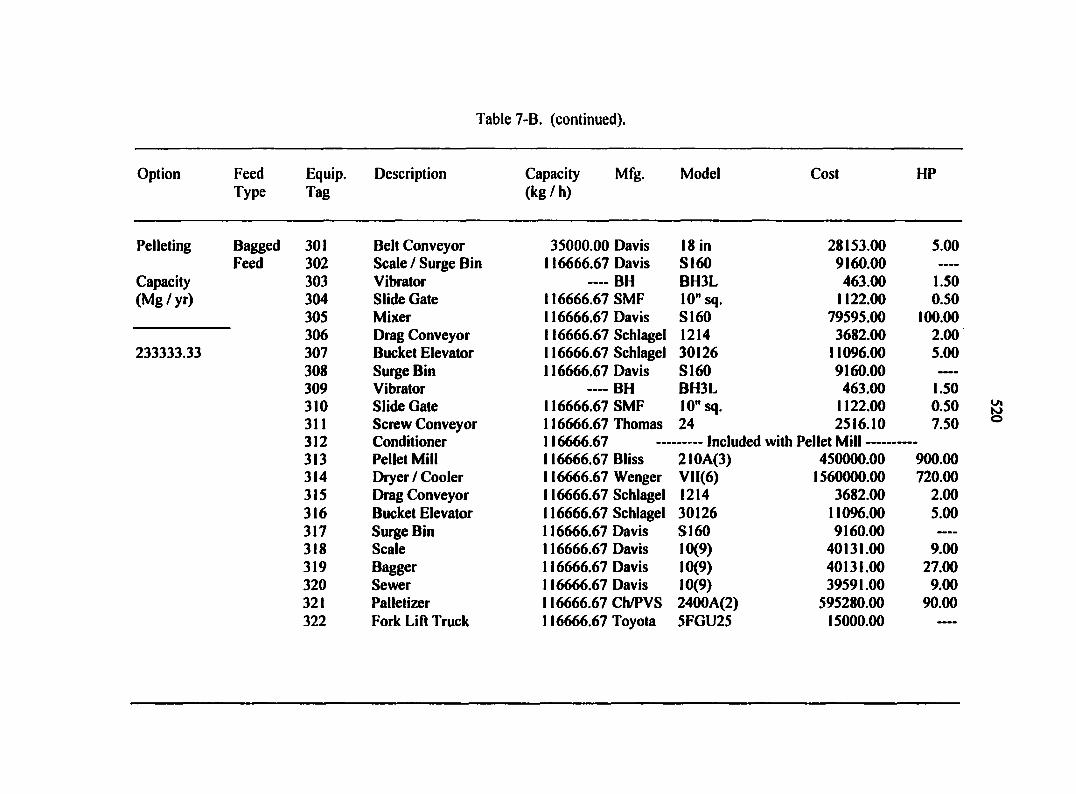
Table 7-B. (continued).
Option Feed Type
Equip. Tag
Description Capacity Mfg. (kg / h)
Model Cost HP
Pelleting Bagged 301 Belt Conveyor 35000.00 Davis 18 in 28153.00 5.00 Feed 302 Scale / Surge Bin 116666.67 Davis S160 9160.00 -*•—
Capacity 303 Vibrator — BH BH3L 463.00 1.50 (Mg/yr) 304 Slide Gate 116666.67 SMF 10" sq. 1122.00 0.50
305 Mixer 116666.67 Davis S160 79595.00 100.00 306 Drag Conveyor 116666.67 Schlagel 1214 3682.00 2.00
233333.33 307 Bucket Elevator 116666.67 Schlagel 30126 11096.00 5.00 308 Surge Bin 116666.67 Davis S160 9160.00 ••••
309 Vibrator — BH BH3L 463.00 1.50 310 Slide Gate 116666.67 SMF 10" sq. 1122.00 0.50 311 Screw Conveyor 116666.67 Thomas 24 2516.10 7.50 312 Conditioner 116666.67 Included with Pellet Mill 313 Pellet Mill 116666.67 Bliss 210A(3) 450000.00 900.00 314 Dryer / Cooler 116666.67 Wenger Vll(6) 1560000.00 720.00 315 Drag Conveyor 116666.67 Schlagel 1214 3682.00 2.00 316 Bucket Elevator 116666.67 Schlagel 30126 11096.00 5.00 317 Surge Bin 116666.67 Davis S160 9160.00 —-
318 Scale 116666.67 Davis 10(9) 40131.00 9.00 319 Bagger 116666.67 Davis 10(9) 40131.00 27.00 320 Sewer 116666.67 Davis 10(9) 39591.00 9.00 321 Palletizer 116666.67 Ch/PVS 2400A(2) 595280.00 90.00 322 Fork Lift Truck 116666.67 Toyota 5FGU25 15000.00 ....

Table 7-B. (continued).
Option Feed Type
Equip. Tag
Description Capacity (kg/h)
Mfg. Model Cost HP
Pelleting Bagged 323 Bag Feed Truck Feed 390 SBM Storage Bin
Capacity 391 Slide Gate (Mg / yr) 392 Screw Conveyor
233333.33
30 tons Fr/Pace 120/AT65 81666.67 Steel Bin 81666.67 SMF 10" sq. 81666.67 Thomas 24
Equipment Initial Cost ($) / Connected HP Electrical Wiring and Controls ($) [4%] Equipment Freight ($) [1%] Equipment Installation ($) [40%] Spouting ($) Total Equipment Initial Cost ($) [excluding truck cost)
100000.00 180042.34
1122.00 2516.10
3094283.54 123771.34 30942.84
1237713.42 816.00
4487527.13
0.50 7.50
1893.50
Total Building Space Required (ft2) Total Building Cost ($)
17432.35 217904.42
Engineering and Design Cost ($) 329380.21
Electricity Consumed (kW-h) 6197642.15
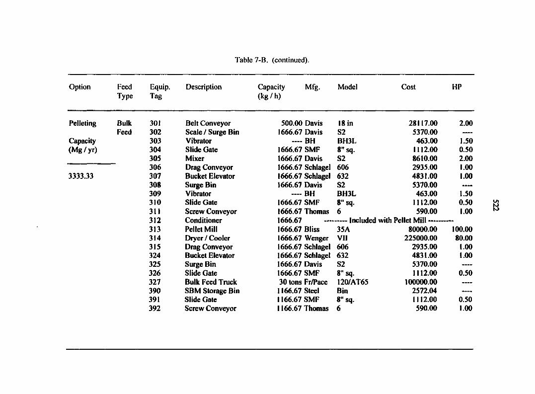
Table 7-B. (continued).
Option
Pelleting
Capacity (Mg/yr)
3333.33
Feed Type
Bulk Feed
Equip. Tag
Description Capacity Mfg. (kg/h)
Model Cost HP
301 Belt Conveyor 500.00 Davis 18 in 28117.00 2.00 302 Scale / Surge Bin 1666.67 Davis S2 5370.00 ----
303 Vibrator — BH BH3L 463.00 1.50 304 Slide Gate 1666.67 SMF 8" sq. 1112.00 0.50 305 Mixer 1666.67 Davis S2 8610.00 2.00 306 Drag Conveyor 1666.67 Schlagel 606 2935.00 1.00 307 Bucket Elevator 1666.67 Schlagel 632 4831.00 1.00 308 Surge Bin 1666.67 Davis S2 5370.00 309 Vibrator -— BH BH3L 463.00 1.50 310 Slide Gate 1666.67 SMF 8" sq. 1112.00 0.50 311 Screw Conveyor 1666.67 Thomas 6 590.00 1.00 312 Conditioner 1666.67 Included with Pellet Mill 313 Pellet Mill 1666.67 Bliss 35A 80000.00 100.00 314 Dryer / Cooler 1666.67 Wenger VII 225000.00 80.00 315 Drag Conveyor 1666.67 Schlagel 606 2935.00 1.00 324 Bucket Elevator 1666.67 Schlagel 632 4831.00 1.00 325 Surge Bin 1666.67 Davis S2 5370.00 326 Slide Gate 1666.67 SMF 8" sq. 1112.00 0.50 327 Bulk Feed Truck 30 tons Fr/Pace 120/AT65 100000.00 •••—
390 SBM Storage Bin 1166.67 Steel Bin 2572.04 391 Slide Gate 1166.67 SMF 8" sq. 1112.00 0.50 392 Screw Conveyor 1166.67 Thomas 6 590.00 1.00

Table 7-B. (continued).
Option Feed Equip. Description Capacity Mfg. Model Cost HP Type Tag (kg / h)
Pelleting Bulk Feed
Capacity (Mg/yr)
3333.33
Equipment Initial Cost ($) / Connected HP 382495.04 195.00 Electrical Wiring and Controls ($) [4%] 15299.80 Equipment Freight ($) [ I %] 3824.95 Equipment Installation ($) [40%] 152998.02 Spouting ($) 816.00 Total Equipment Initial Cost ($) [excluding truck cost) 555433.81
Total Building Space Required (ft2) 2000.00 Total Building Cost ($) 25000.00
Engineering and Design Cost ($) 40630.37
Electricity Consumed (kW-h) 615439.70
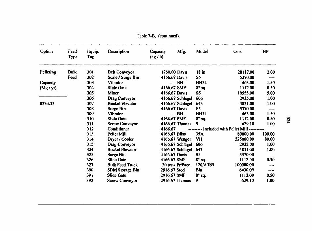
Table 7-B. (continued).
Option Feed Type
Equip. Tag
Description Capacity (kg / h)
Mfg. Model Cost HP
Pelleting
Capacity (Mg / yr)
8333.33
Bulk Feed
301 Belt Conveyor 1250.00 Davis 18 in 28117.00 2.00 302 Scale / Surge Bin 4166.67 Davis S5 5370.00 ——
303 Vibrator — BH BH3L 463.00 1.50 304 Slide Gate 4166.67 SMF 8" sq. 1112.00 0.50 305 Mixer 4166.67 Davis S5 10555.00 5.00 306 Drag Conveyor 4166.67 Schlagel 606 2935.00 1.00 307 Bucket Elevator 4166.67 Schlagel 643 4831.00 1.00 308 Surge Bin 4166.67 Davis S5 5370.00 —-
309 Vibrator —— BH BH3L 463.00 1.50 310 Slide Gate 4166.67 SMF 8" sq. 1112.00 0.50 311 Screw Conveyor 4166.67 Thomas 9 629.10 1.00 312 Conditioner 4166.67 Included with Pellet Mill 313 Pellet Mill 4166.67 Bliss 35A 80000.00 100.00 314 Dryer Z Cooler 4166.67 Wenger VII 225000.00 80.00 315 Drag Conveyor 4166.67 Schlagel 606 2935.00 1.00 324 Bucket Elevator 4166.67 Schlagel 643 4831.00 1.00 325 Surge Bin 4166.67 Davis S5 5370.00 326 Slide Gate 4166.67 SMF 8" sq. 1112.00 0.50 327 Bulk Feed Truck 30 tons Fr/Pace I20/AT65 100000.00 390 SBM Storage Bin 2916.67 Steel Bin 6430.09 391 Slide Gate 2916.67 SMF 8" sq. 1112.00 0.50 392 Screw Conveyor 2916.67 Thomas 9 629.10 1.00
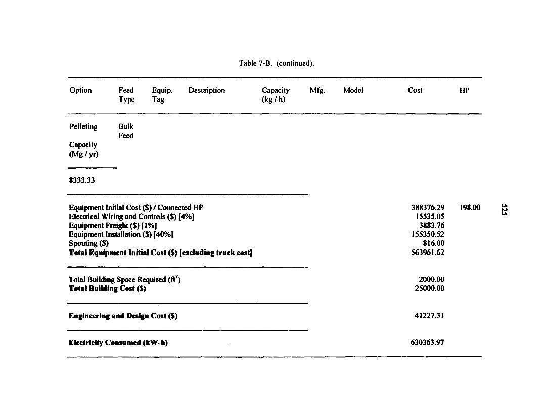
Pelleting
Capacity (Mg / yr)
Bulk Feed
8333.33
Table 7-B. (continued).
Option Feed Type
Equip. Tag
Description Capacity (kg/h)
Mfg. Model Cost HP
Equipment Initial Cost ($) / Connected HP 388376.29 198.00 Electrical Wiring and Controls ($) [4%] 15535.05 Equipment Freight ($) [ 1 %] 3883.76 Equipment Installation ($) [40%] 155350.52 Spouting ($) 816.00 Total Equipment Initial Cost ($) [excluding truck cost] 563961.62
Total Building Space Required (ft2) 2000.00 Total Building Cost ($) 25000.00
Engineering and Design Cost ($) 41227.31
Electricity Consumed (kW-h) 630363.97
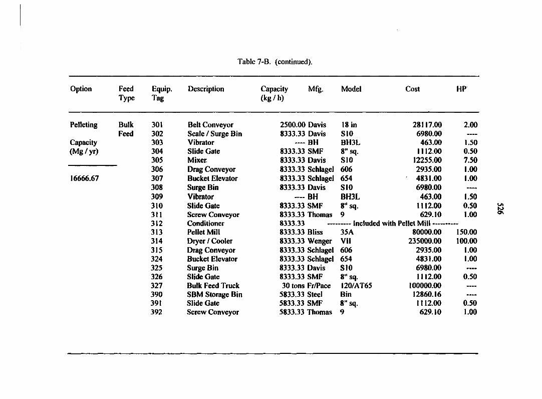
Table 7-B. (continued).
Option
Pelleting
Capacity (Mg/yr)
16666.67
Feed Type
Bulk Feed
Equip. Tag
Description Capacity (kg / h)
Mfg. Model Cost HP
301 Belt Conveyor 2500.00 Davis 18 in 28117.00 2.00 302 Scale / Surge Bin 8333.33 Davis S10 6980.00 303 Vibrator ———— BH BH3L 463.00 1.50 304 Slide Gate 8333.33 SMF 8" sq. 1112.00 0.50 305 Mixer 8333.33 Davis S10 12255.00 7.50 306 Drag Conveyor 8333.33 Schlagel 606 2935.00 1.00 307 Bucket Elevator 8333.33 Schlagel 654 4831.00 1.00 308 Surge Bin 8333.33 Davis S10 6980.00 ——
309 Vibrator BH BH3L 463.00 1.50 310 Slide Gate 8333.33 SMF 8" sq. 1112.00 0.50 311 Screw Conveyor 8333.33 Thomas 9 629.10 1.00 312 Conditioner 8333.33 Included with Pellet Mill 313 Pellet Mill 8333.33 Bliss 35A 80000.00 150.00 314 Dryer / Cooler 8333.33 Wenger VII 235000.00 100.00 315 Drag Conveyor 8333.33 Schlagel 606 2935.00 1.00 324 Bucket Elevator 8333.33 Schlagel 654 4831.00 1.00 325 Surge Bin 8333.33 Davis SI0 6980.00 ----
326 Slide Gate 8333.33 SMF 8" sq. 1112.00 0.50 327 Bulk Feed Truck 30 tons Fr/Pace I20/AT65 100000.00 ——
390 SBM Storage Bin 5833.33 Steel Bin 12860.16 391 Slide Gate 5833.33 SMF 8" sq. 1112.00 0.50 392 Screw Conveyor 5833.33 Thomas 9 629.10 1.00

Pelleting
Capacity (Mg/yr)
Bulk Feed
16666.67
Table 7-B. (continued).
Option Feed Type
Equip. Tag
Description Capacity (kg / h)
Mfg. Model Cost HP
Equipment Initial Cost ($) / Connected HP 411336.36 270.50 Electrical Wiring and Controls ($) [4%] 16453.45 Equipment Freight ($) [1%] 4113.36 Equipment Installation ($) [40%] 164534.54 Spouting ($) 816.00 Total Equipment Initial Cost ($) [excluding truck cost] 597253.72
Total Building Space Required (ft2) 2000.00 Total Building Cost ($) 25000.00
Engineering and Design Cost ($) 43557.76
Electricity Consumed (kW-h) 867002.45
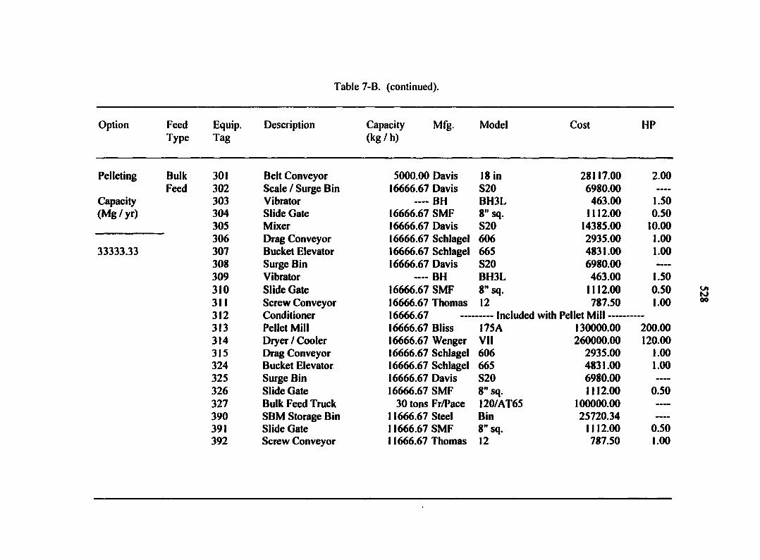
Table 7-B. (continued).
Option
Pelleting
Capacity (Mg/yr)
33333.33
Feed Type
Bulk Feed
Equip. Tag
Description Capacity (kg/h)
Mfg. Model Cost HP
301 Belt Conveyor 5000.00 Davis 18 in 28117.00 2.00 302 Scale / Surge Bin 16666.67 Davis S20 6980.00 •—
303 Vibrator BH BH3L 463.00 1.50 304 Slide Gate 16666.67 SMF 8" sq. 1112.00 0.50 305 Mixer 16666.67 Davis S20 14385.00 10.00 306 Drag Conveyor 16666.67 Schlagel 606 2935.00 1.00 307 Bucket Elevator 16666.67 Schlagel 665 4831.00 1.00 308 Surge Bin 16666.67 Davis S20 6980.00 •—
309 Vibrator BH BH3L 463.00 1.50 310 Slide Gate 16666.67 SMF 8" sq. 1112.00 0.50 311 Screw Conveyor 16666.67 Thomas 12 787.50 1.00 312 Conditioner 16666.67 Included with Pellet Mill 313 Pellet Mill 16666.67 Bliss 175 A 130000.00 200.00 314 Dryer / Cooler 16666.67 Wenger VII 260000.00 120.00 315 Drag Conveyor 16666.67 Schlagel 606 2935.00 1.00 324 Bucket Elevator 16666.67 Schlagel 665 4831.00 1.00 325 Surge Bin 16666.67 Davis S20 6980.00 —-
326 Slide Gate 16666.67 SMF 8 " sq. 1112.00 0.50 327 Bulk Feed Truck 30 tons Fr/Pace 120/AT65 100000.00 —-
390 SBM Storage Bin 11666.67 Steel Bin 25720.34 ——
391 Slide Gate 11666.67 SMF 8" sq. 1112.00 0.50 392 Screw Conveyor 11666.67 Thomas 12 787.50 1.00

Table 7-B. (continued).
Option Feed Equip. Description Type Tag
Capacity Mfg. Model (kg / h)
Cost HP
Pelleting Bulk Feed
Capacity (Mg/yr)
33333.33
Equipment Initial Cost ($) / Connected HP 501643.34 343.00 Electrical Wiring and Controls ($) [4%] 20065.73 Equipment Freight ($) [1%] 5016.43 Equipment Installation ($) [40%] 200657.34 Spouting ($) 816.00 Total Equipment Initial Cost ($) [excluding truck cost] 728198.84
Total Building Space Required (ft2) 2000.00 Total Building Cost ($) 25000.00
Engineering and Design Cost ($) 52723.92
Electricity Consumed (kW-h) 1112828.43
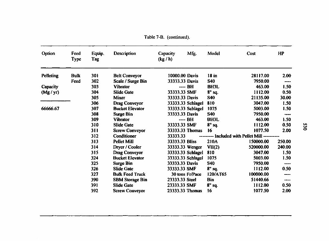
Table 7-B. (continued).
Option
Pelleting
Capacity (Mg/yr)
66666.67
Feed Type
Bulk Feed
Equip. Tag
Description Capacity (kg / h)
Mfg. Model Cost HP
301 Belt Conveyor 10000.00 Davis 18 in 28117.00 2.00 302 Scale / Surge Bin 33333.33 Davis S40 7950.00 303 Vibrator BH BH3L 463.00 1.50 304 Slide Gate 33333.33 SMF 8" sq. 1112.00 0.50 305 Mixer 33333.33 Davis S40 21135.00 30.00 306 Drag Conveyor 33333.33 Schlagel 810 3047.00 1.50 307 Bucket Elevator 33333.33 Schlagel 1075 5003.00 1.50 308 Surge Bin 33333.33 Davis S40 7950.00 ——
309 Vibrator ———— BH BH3L 463.00 1.50 310 Slide Gate 33333.33 SMF 8" sq. 1112.00 0.50 311 Screw Conveyor 33333.33 Thomas 16 1077.50 2.00 312 Conditioner 33333.33 Included with Pellet Mill 313 Pellet Mill 33333.33 Bliss 210A 150000.00 250.00 314 Dryer / Cooler 33333.33 Wenger V1I(2) 520000.00 240.00 315 Drag Conveyor 33333.33 Schlagel 810 3047.00 1.50 324 Bucket Elevator 33333.33 Schlagel 1075 5003.00 1.50 325 Surge Bin 33333.33 Davis S40 7950.00 ----
326 Slide Gate 33333.33 SMF 8 " sq. 1112.00 0.50 327 Bulk Feed Truck 30 tons Fr/Pace I20/AT65 100000.00 —-
390 SBM Storage Bin 23333.33 Steel Bin 51440.66 391 Slide Gate 23333.33 SMF 8 " sq. 1112.00 0.50 392 Screw Conveyor 23333.33 Thomas 16 1077.50 2.00

Pelleting Bulk Feed
Capacity (Mg / yr)
66666.67
Table 7-B. (continued).
Option Feed Equip. Description Capacity Mfg. Model Cost HP Type Tag (kg / h)
Equipment Initial Cost ($) / Connected HP 818171.66 537.00 Electrical Wiring and Controls ($) [4%] 32726.87 Equipment Freight ($) [1%] 8181.72 Equipment Installation ($) [40%] 327268.66 Spouting ($) 816.00 Total Equipment Initial Cost ($) [excluding truck cost) 1187164.91
Total Building Space Required (ft2) 2000.00 Total Building Cost ($) 25000.00
Engineering and Design Cost ($) 84851.54
Electricity Consumed (kW-h) 1758205.89

Table 7-B. (continued).
Option Feed Equip. Description Capacity Mfg. Model Cost HP Type Tag (kg / h)
Pelleting Bulk 301 Belt Conveyor 15000.00 Davis 18 in 28125.00 3.00 Feed 302 Scale / Surge Bin 50000.00 Davis S80 9000.00
Capacity 303 Vibrator — BH BH3L 463.00 1.50 (Mg/yr) 304 Slide Gate 50000.00 SMF 8" sq. 1112.00 0.50
305 Mixer 50000.00 Davis S80 31365.00 40.00 306 Drag Conveyor 50000.00 Schlagel 810 3059.00 2.00
100000.00 307 Bucket Elevator 50000.00 Schlagel 1695 6703.00 2.00 308 Surge Bin 50000.00 Davis S80 9000.00 309 Vibrator -—- BH BH3L 463.00 1.50 310 Slide Gate 50000.00 SMF 8" sq. 1112.00 0.50 311 Screw Conveyor 50000.00 Thomas 18 1466.50 3.00 312 Conditioner 50000.00 Included with Pellet Mill 313 Pellet Mill 50000.00 Bliss 2I0A 150000.00 300.00 314 Dryer / Cooler 50000.00 Wenger VI 1(2) 520000.00 240.00 315 Drag Conveyor 50000.00 Schlagel 810 3059.00 2.00 324 Bucket Elevator 50000.00 Schlagel 1695 6703.00 2.00 325 Surge Bin 50000.00 Davis S80 9000.00 ——-
326 Slide Gate 50000.00 SMF 8" sq. 1112.00 0.50 327 Bulk Feed Truck 30 tons Fr/Pace 120/AT65 100000.00 —-
390 SBM Storage Bin 35000.00 Steel Bin 77161.00 391 Slide Gate 35000.00 SMF 8" sq. 1112.00 0.50 392 Screw Conveyor 35000.00 Thomas 18 1466.50 3.00
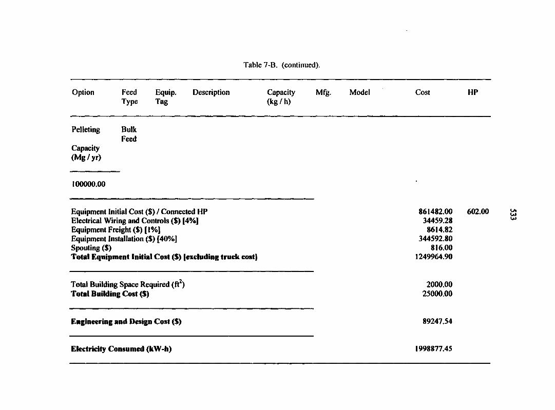
Table 7-B. (continued).
Option Feed Equip. Description Capacity Mfg. Model Cost HP Type Tag (kg / h)
Pelleting Bulk Feed
Capacity (Mg / yr)
100000.00
Equipment Initial Cost ($) / Connected HP 861482.00 602.00 Electrical Wiring and Controls ($) [4%] 34459.28 Equipment Freight ($) [!%] 8614.82 Equipment Installation ($) [40%] 344592.80 Spouting ($) 816.00 Total Equipment Initial Cost ($) [excluding truck cost] 1249964.90
Total Building Space Required (ft2) 2000.00 Total Building Cost ($) 25000.00
Engineering and Design Cost ($) 89247.54
Electricity Consumed (kW-h) 1998877.45
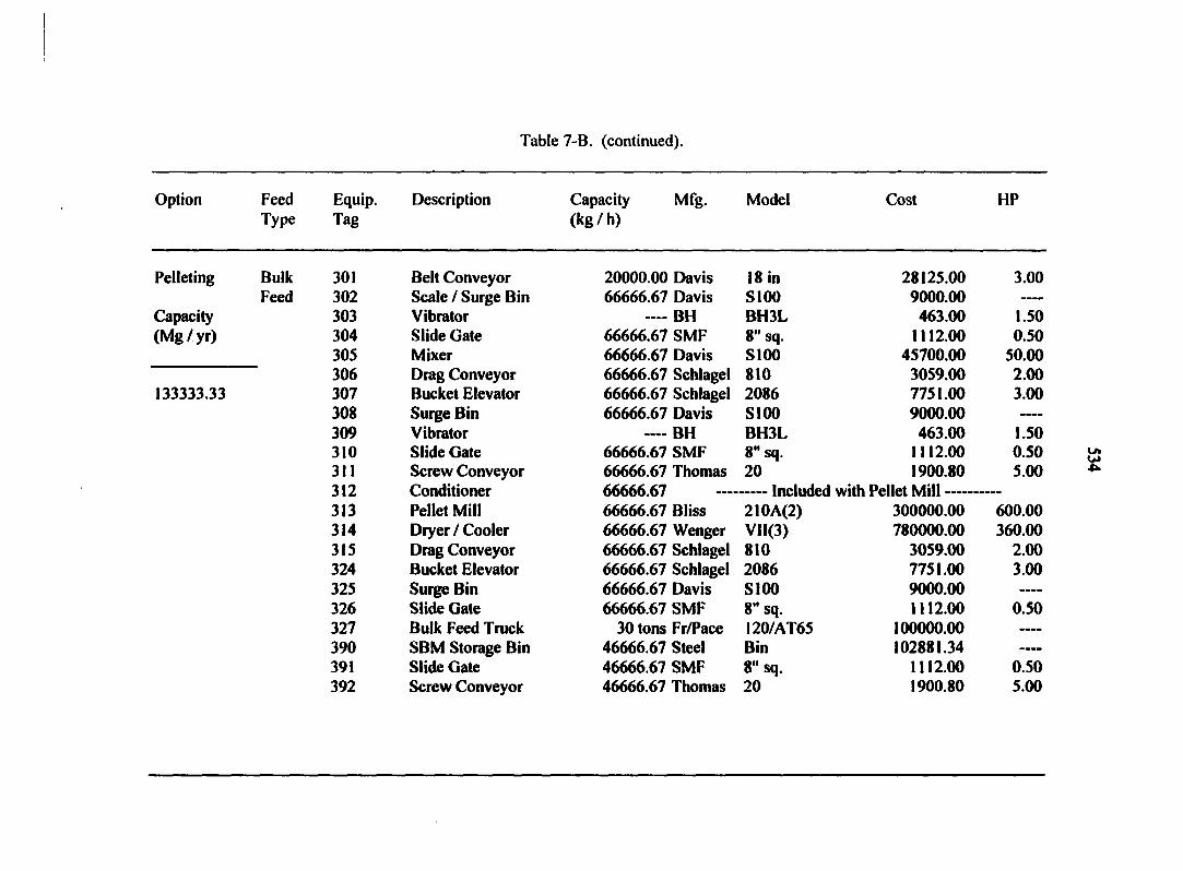
Table 7-B. (continued).
Option Feed Equip. Description Capacity Mfg. Model Cost HP Type Tag (kg / h)
Pelleting
Capacity (Mg/yr)
133333.33
Bulk Feed
301 Belt Conveyor 20000.00 Davis 18 in 28125.00 3.00 302 Scale / Surge Bin 66666.67 Davis S100 9000.00 ----
303 Vibrator BH BH3L 463.00 1.50 304 Slide Gate 66666.67 SMF 8" sq. 1112.00 0.50 305 Mixer 66666.67 Davis S100 45700.00 50.00 306 Drag Conveyor 66666.67 Schlagel 810 3059.00 2.00 307 Bucket Elevator 66666.67 Schlagel 2086 7751.00 3.00 308 Surge Bin 66666.67 Davis SI00 9000.00 309 Vibrator —» w BH BH3L 463.00 1.50 310 Slide Gate 66666.67 SMF 8" sq. 1112.00 0.50 311 Screw Conveyor 66666.67 Thomas 20 1900.80 5.00 312 Conditioner 66666.67 Included with Pellet Mill 313 Pellet Mill 66666.67 Bliss 210A(2) 300000.00 600.00 314 Dryer / Cooler 66666.67 Wenger VII(3) 780000.00 360.00 315 Drag Conveyor 66666.67 Schlagel 810 3059.00 2.00 324 Bucket Elevator 66666.67 Schlagel 2086 7751.00 3.00 325 Surge Bin 66666.67 Davis SI00 9000.00 326 Slide Gate 66666.67 SMF 8" sq. 1112.00 0.50 327 Bulk Feed Truck 30 tons Fr/Pace I20/AT65 100000.00 —-
390 SBM Storage Bin 46666.67 Steel Bin 102881.34 391 Slide Gate 46666.67 SMF 8" sq. 1112.00 0.50 392 Screw Conveyor 46666.67 Thomas 20 1900.80 5.00
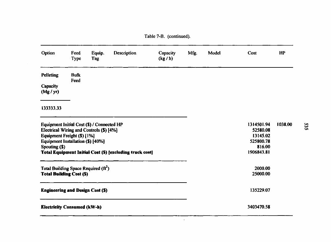
Table 7-B. (continued).
Option Feed Equip. Description Type Tag
Capacity Mfg. Model (kg/h)
Cost HP
Pelleting Bulk Feed
Capacity (Mg/yr)
133333.33
Equipment Initial Cost ($) / Connected HP 1314501.94 1038.00 Electrical Wiring and Controls ($) [4%] 52580.08 Equipment Freight ($) [ I %] 13145.02 Equipment Installation ($) [40%] 525800.78 Spouting ($) 816.00 Total Equipment Initial Cost ($) [excluding truck cost[ 1906843.81
Total Building Space Required (ft2) 2000.00 Total Building Cost ($) 25000.00
Engineering and Design Cost ($) 135229.07
Electricity Consumed (kW-h) 3403470.58
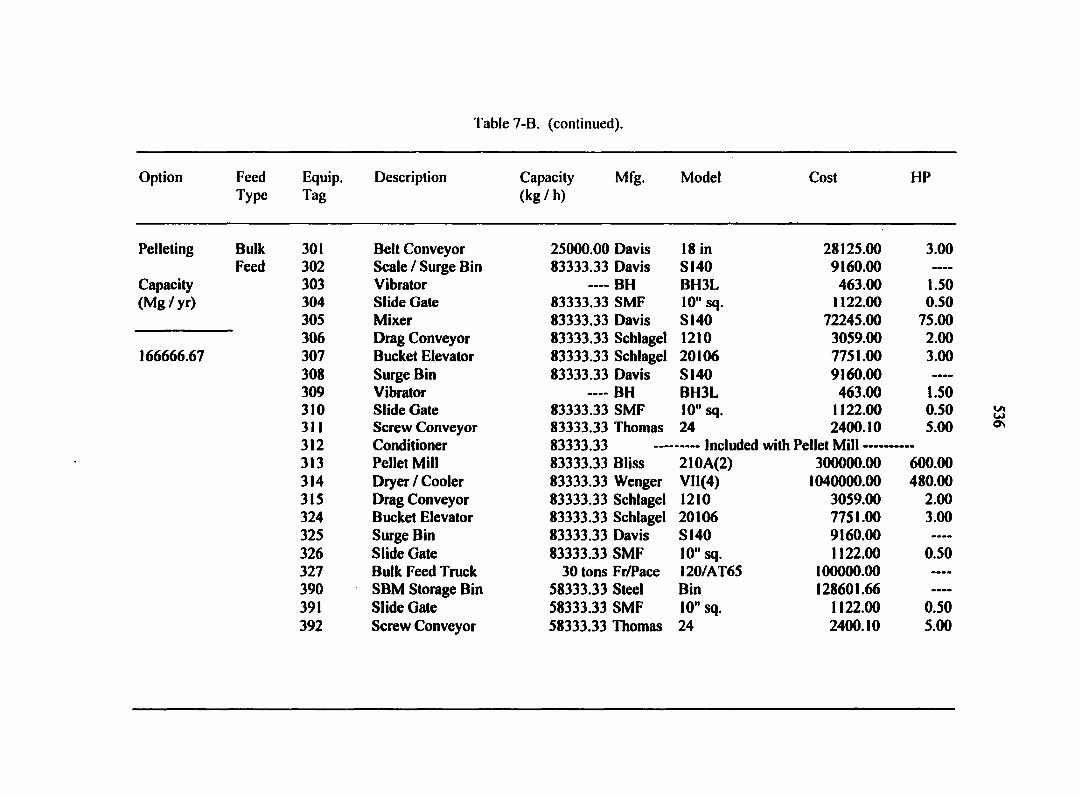
Table 7-B. (continued).
Option
Pelleting
Capacity (Mg / yr)
166666.67
Feed Type
Bulk Feed
Equip. Tag
Description Capacity (kg / h)
Mfg. Model Cost HP
301 Belt Conveyor 25000.00 Davis 18 in 28125.00 3.00 302 Scale / Surge Bin 83333.33 Davis S140 9160.00 ——
303 Vibrator BH BH3L 463.00 1.50 304 Slide Gate 83333.33 SMF 10 " sq. 1122.00 0.50 305 Mixer 83333.33 Davis S140 72245.00 75.00 306 Drag Conveyor 83333.33 Schlagel 1210 3059.00 2.00 307 Bucket Elevator 83333.33 Schlagel 20106 7751.00 3.00 308 Surge Bin 83333.33 Davis S140 9160.00 309 Vibrator BH BH3L 463.00 1.50 310 Slide Gate 83333.33 SMF 10 " sq. 1122.00 0.50 311 Screw Conveyor 83333.33 Thomas 24 2400.10 5.00 312 Conditioner 83333.33 Included with Pellet Mill 313 Pellet Mill 83333.33 Bliss 210A(2) 300000.00 600.00 314 Dryer / Cooler 83333.33 Wenger VI1(4) 1040000.00 480.00 315 Drag Conveyor 83333.33 Schlagel 1210 3059.00 2.00 324 Bucket Elevator 83333.33 Schlagel 20106 7751.00 3.00 325 Surge Bin 83333.33 Davis SI40 9160.00 ----
326 Slide Gate 83333.33 SMF 10 " sq. 1122.00 0.50 327 Bulk Feed Truck 30 tons Fr/Pace 120/AT65 100000.00 —™
390 SBM Storage Bin 58333.33 Steel Bin 128601.66 391 Slide Gate 58333.33 SMF 10" sq. 1122.00 0.50 392 Screw Conveyor 58333.33 Thomas 24 2400.10 5.00
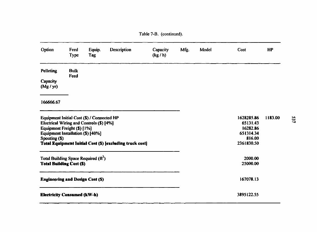
Table 7-B. (continued).
Option Feed Equip. Description Capacity Mfg. Model Cost HP Type Tag (kg / h)
Pelleting Bulk Feed
Capacity (Mg/yr)
166666.67
Equipment Initial Cost ($) / Connected HP 1628285.86 1183.00 Electrical Wiring and Controls ($) [4%] 65131.43 Equipment Freight ($) [ I %] 16282.86 Equipment Installation ($) [40%] 651314.34 Spouting ($) 816.00 Total Equipment Initial Cost ($) [excluding truck cost) 2361830.50
Total Building Space Required (ft2) 2000.00 Total Building Cost ($) 25000.00
Engineering and Design Cost ($) 167078.13
Electricity Consumed (kW-h) 3895122.55
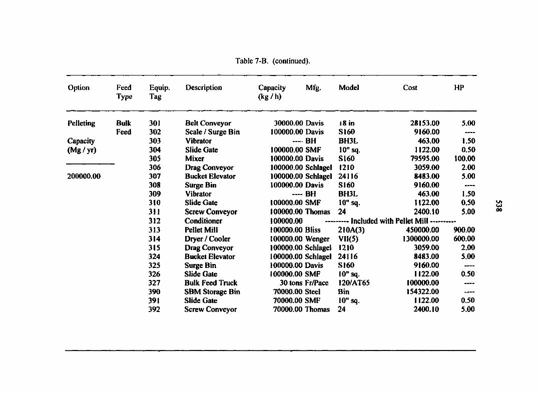
Table 7-B. (continued).
Option Feed Equip. Description Capacity Mfg. Model Cost HP Type Tag (kg / h)
Pelleting Bulk 301 Belt Conveyor 30000.00 Davis 18 in 28153.00 5.00 Feed 302 Scale / Surge Bin 100000.00 Davis S160 9160.00
Capacity 303 Vibrator — BH BH3L 463.00 1.50 (Mg/yr) 304 Slide Gate 100000.00 SMF 10" sq. 1122.00 0.50
305 Mixer 100000.00 Davis S160 79595.00 100.00 306 Drag Conveyor 100000.00 Schlagel 1210 3059.00 2.00
200000.00 307 Bucket Elevator 100000.00 Schlagel 24116 8483.00 5.00 308 Surge Bin 100000.00 Davis S160 9160.00 309 Vibrator — BH BH3L 463.00 1.50 310 Slide Gate 100000.00 SMF 10" sq. 1122.00 0.50 311 Screw Conveyor 100000.00 Thomas 24 2400.10 5.00 312 Conditioner 100000.00 Included with Pellet Mill 313 Pellet Mill 100000.00 Bliss 2I0A(3) 450000.00 900.00 314 Dryer / Cooler 100000.00 Wenger VII(5) 1300000.00 600.00 315 Drag Conveyor 100000.00 Schlagel 1210 3059.00 2.00 324 Bucket Elevator 100000.00 Schlagel 24116 8483.00 5.00 325 Surge Bin 100000.00 Davis SI60 9160.00 —-
326 Slide Gate 100000.00 SMF 10" sq. 1122.00 0.50 327 Bulk Feed Truck 30 tons Fr/Pace I20/AT65 100000.00 390 SBM Storage Bin 70000.00 Steel Bin 154322.00 ----
391 Slide Gate 70000.00 SMF 10" sq. 1122.00 0.50 392 Screw Conveyor 70000.00 Thomas 24 2400.10 5.00
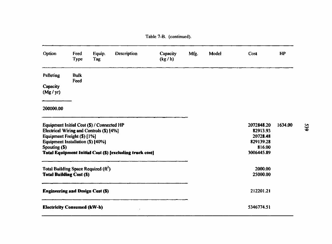
Pelleting
Capacity (Mg/yr)
Bulk Feed
200000.00
Table 7-B. (continued).
Option Feed Type
Equip. Tag
Description Capacity (kg / h)
Mfg. Model Cost HP
Equipment Initial Cost ($) / Connected HP 2072848.20 1634.00 Electrical Wiring and Controls ($) [4%] 82913.93 Equipment Freight ($) [ 1 %] 20728.48 Equipment Installation ($) [40%] 829139.28 Spouting ($) 816.00 Total Equipment Initial Cost ($) [excluding truck cost] 3006445.89
Total Building Space Required (ft2) 2000.00 Total Building Cost ($) 25000.00
Engineering and Design Cost ($) 212201.21
Electricity Consumed (kW-h) 5346774.51
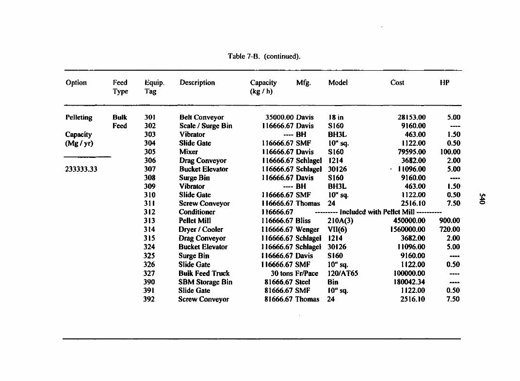
Table 7-B. (continued).
Option
Pelleting
Capacity (Mg/yr)
233333.33
Feed Type
Bulk Feed
Equip. Tag
Description Capacity (kg / h)
Mfg. Model Cost HP
301 Belt Conveyor 35000.00 Davis 18 in 28153.00 5.00 302 Scale / Surge Bin 116666.67 Davis S160 9160.00 303 Vibrator BH BH3L 463.00 1.50 304 Slide Gate 116666.67 SMF 10 " sq. 1122.00 0.50 305 Mixer 116666.67 Davis S160 79595.00 100.00 306 Drag Conveyor 116666.67 Schlagel 1214 3682.00 2.00 307 Bucket Elevator 116666.67 Schlagel 30126 11096.00 5.00 308 Surge Bin 116666.67 Davis S160 9160.00 —-
309 Vibrator ---- BH BH3L 463.00 1.50 310 Slide Gate 116666.67 SMF 10" sq. 1122.00 0.50 311 Screw Conveyor 116666.67 Thomas 24 2516.10 7.50 312 Conditioner 116666.67 Included with Pellet Mill 313 Pellet Mill 116666.67 Bliss 210A(3) 450000.00 900.00 314 Dryer / Cooler 116666.67 Wenger Vll(6) 1560000.00 720.00 315 Drag Conveyor 116666.67 Schlagel 1214 3682.00 2.00 324 Bucket Elevator 116666.67 Schlagel 30126 11096.00 5.00 325 Surge Bin 116666.67 Davis S160 9160.00 326 Slide Gate 116666.67 SMF 10" sq. 1122.00 0.50 327 Bulk Feed Truck 30 tons Fr/Pace 120/AT65 100000.00 ————
390 SBM Storage Bin 81666.67 Steel Bin 180042.34 ——
391 Slide Gate 81666.67 SMF 10" sq. 1122.00 0.50 392 Screw Conveyor 81666.67 Thomas 24 2516.10 7.50
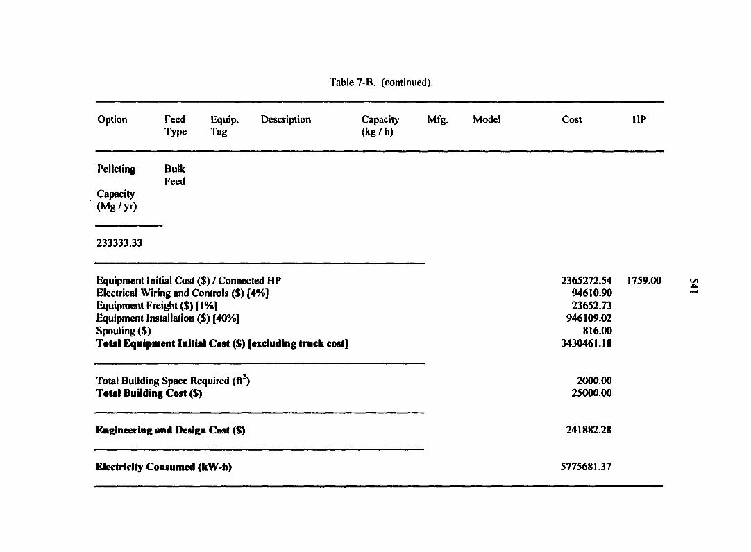
Table 7-B. (continued).
Option Feed Equip. Description Capacity Mfg. Model Cost HP Type Tag (kg / h)
Pelleting Bulk Feed
Capacity (Mg/yr)
233333.33
Equipment Initial Cost ($) / Connected HP 2365272.54 1759.00 Electrical Wiring and Controls ($) [4%] 94610.90 Equipment Freight ($) [ 1 %] 23652.73 Equipment Installation ($) [40%] 946109.02 Spouting ($) 816.00 Total Equipment Initial Cost ($) [excluding truck cost[ 3430461.18
Total Building Space Required (ft2) 2000.00 Total Building Cost ($) 25000.00
Engineering and Design Cost ($) 241882.28
Electricity Consumed (kW-h) 5775681.37
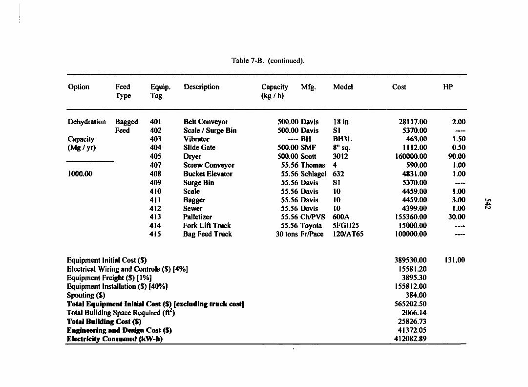
Table 7-B. (continued).
Option Feed Equip. Description Capacity Mfg. Model Cost HP Type Tag (kg / h)
Dehydration Bagged 401 Belt Conveyor 500.00 Davis 18 in 28117.00 2.00 Feed 402 Scale / Surge Bin 500.00 Davis SI 5370.00
Capacity 403 Vibrator — BH BH3L 463.00 1.50 (Mg/yr) 404 Slide Gate 500.00 SMF 8" sq. 1112.00 0.50
405 Dryer 500.00 Scott 3012 160000.00 90.00 407 Screw Conveyor 55.56 Thomas 4 590.00 1.00
1000.00 408 Bucket Elevator 55.56 Schlagel 632 4831.00 1.00 409 Surge Bin 55.56 Davis SI 5370.00 ----
410 Scale 55.56 Davis 10 4459.00 1.00 411 Bagger 55.56 Davis 10 4459.00 3.00 412 Sewer 55.56 Davis 10 4399.00 1.00 413 Palletizer 55.56 Ch/PVS 600A 155360.00 30.00 414 Fork Lift Truck 55.56 Toyota 5FGU25 15000.00 ----
415 Bag Feed Truck 30 tons Fr/Pace 120/AT65 100000.00 ----
Equipment Initial Cost ($) 389530.00 131.00 Electrical Wiring and Controls ($) [4%] 15581.20 Equipment Freight ($) [\%] 3895.30 Equipment Installation ($) [40%] 155812.00 Spouting ($) 384.00 Total Equipment Initial Cost ($) (excluding truck cost] 565202.50 Total Building Space Required (ft ) 2066.14 Total Building Cost ($) 25826.73 Engineering and Design Cost ($) 41372.05 Electricity Consumed (kW-h) 412082.89
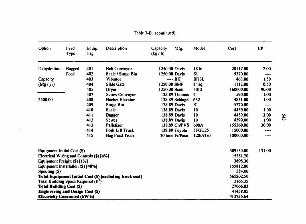
Table 7-B. (continued).
Option Feed Equip. Description Capacity Mfg. Model Cost HP Type Tag (kg / h)
Dehydration Bagged 401 Belt Conveyor 1250.00 Davis 18 in 28117.00 2.00 Feed 402 Scale / Surge Bin 1250.00 Davis SI 5370.00 —•
Capacity 403 Vibrator — BH BH3L 463.00 1.50 (Mg/yr) 404 Slide Gate 1250.00 SMF 8" sq. 1112.00 0.50
405 Dryer 1250.00 Scott 3012 160000.00 90.00 407 Screw Conveyor 138.89 Thomas 4 590.00 1.00
2500.00 408 Bucket Elevator 138.89 Schlagel 632 4831.00 1.00 409 Surge Bin 138.89 Davis SI 5370.00 —-
410 Scale 138.89 Davis 10 4459.00 1.00 411 Bagger 138.89 Davis 10 4459.00 3.00 412 Sewer 138.89 Davis 10 4399.00 1.00 413 Palletizer 138.89 Ch/PVS 600A 155360.00 30.00 414 Fork Lift Truck 138.89 Toyota 5FGU25 15000.00 415 Bag Feed Truck 30 tons Fr/Pace 120/AT65 100000.00
Equipment Initial Cost ($) 389530.00 131.00 Electrical Wiring and Controls ($) [4%] 15581.20 Equipment Freight ($) [\%] 3895.30 Equipment Installation ($) [40%] 155812.00 Spouting ($) 384.00 Total Equipment Initial Cost ($) [excluding truck cost] 565202.50 Total Building Space Required (ft ) 2165.35 Total Building Cost ($) 27066.83 Engineering and Design Cost ($) 41458.85 Electricity Consumed (kW-h) 413736.64
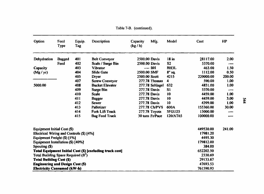
Table 7-B. (continued).
Option Feed Type
Equip. Tag
Description Capacity Mfg. (kg / h)
Model Cost HP
Dehydration Bagged 401 Belt Conveyor 2500.00 Davis 18 in 28117.00 2.00 Feed 402 Scale / Surge Bin 2500.00 Davis S2 5370.00
Capacity 403 Vibrator —— BH BH3L 463.00 1.50 (Mg / yr) 404 Slide Gate 2500.00 SMF 8" sq. 1112.00 0.50
405 Dryer 2500.00 Scott 4215 220000.00 200.00 407 Screw Conveyor 277.78 Thomas 4 590.00 1.00
5000.00 408 Bucket Elevator 277.78 Schlagel 632 4831.00 1.00 409 Surge Bin 277.78 Davis SI 5370.00 410 Scale 277.78 Davis 10 4459.00 1.00 411 Bagger 277.78 Davis 10 4459.00 3.00 412 Sewer 277.78 Davis 10 4399.00 1.00 413 Palletizer 277.78 Ch/PVS 600A 155360.00 30.00 414 Fork Lift Truck 277.78 Toyota 5FGU25 15000.00 415 Bag Feed Truck 30 tons Fr/Pace 120/AT65 100000.00 —-
Equipment Initial Cost ($) 449530.00 241.00 Electrical Wiring and Controls ($) [' l%] 17981.20 Equipment Freight ($) [1%] 4495.30 Equipment Installation ($) [40%] 179812.00 Spouting ($) 384.00 Total Equipment Initial Cost ($) [excluding truck cost] 652202.50 Total Building Space Required (ft ) 2330.69 Total Building Cost ($) 29133.67 Engineering and Design Cost ($) 47693.53 Electricity Consumed (kW-h) 761590.93
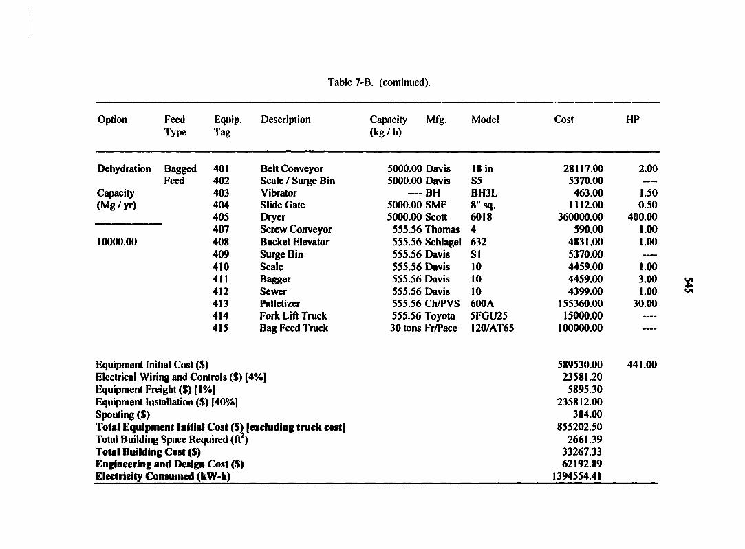
Table 7-B. (continued).
Option Feed Equip. Description Capacity Mfg. Model Cost HP Type Tag (kg / h)
Dehydration Bagged 401 Belt Conveyor 5000.00 Davis 18 in 28117.00 2.00 Feed 402 Scale / Surge Bin 5000.00 Davis S5 5370.00 ----
Capacity 403 Vibrator — BH BH3L 463.00 1.50 (Mg / yr) 404 Slide Gate 5000.00 SMF 8" sq. 1112.00 0.50
405 Dryer 5000.00 Scott 6018 360000.00 400.00 407 Screw Conveyor 555.56 Thomas 4 590.00 1.00
10000.00 408 Bucket Elevator 555.56 Schlagel 632 4831.00 1.00 409 Surge Bin 555.56 Davis SI 5370.00 ——
410 Scale 555.56 Davis 10 4459.00 1.00 411 Bagger 555.56 Davis 10 4459.00 3.00 412 Sewer 555.56 Davis 10 4399.00 1.00 413 Palletizer 555.56 Ch/PVS 600A 155360.00 30.00 414 Fork Lift Truck 555.56 Toyota 5FGU25 15000.00 —-
415 Bag Feed Truck 30 tons Fr/Pace I20/AT65 100000.00 —-
Equipment Initial Cost ($) 589530.00 441.00 Electrical Wiring and Controls ($) [4%] 23581.20 Equipment Freight ($) [ 1 °A »] 5895.30 Equipment Installation ($) [40%] 235812.00 Spouting ($) 384.00 Total Equipment Initial Cost ($) [excluding truck cost] 855202.50 Total Building Space Required (ft ) 2661.39 Total Building Cost ($) 33267.33 Engineering and Design Cost ($) 62192.89 Electricity Consumed (kW-h) 1394554.41
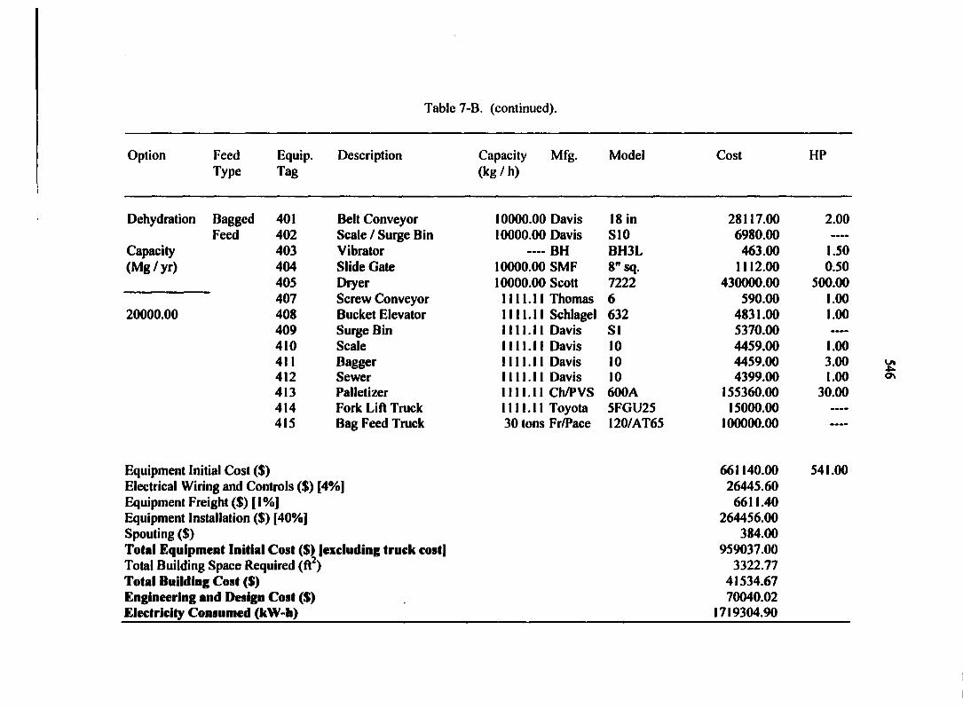
Table 7-B. (continued).
Option Feed Type
Equip. Tag
Description Capacity Mfg. (kg / h)
Model Cost HP
Dehydration Bagged 401 Belt Conveyor 10000.00 Davis 18 in 28117.00 2.00 Feed 402 Scale / Surge Bin 10000.00 Davis S10 6980.00 —-
Capacity 403 Vibrator — BH BH3L 463.00 1.50 (Mg/yr) 404 Slide Gate 10000.00 SMF 8" sq. 1112.00 0.50
405 Dryer 10000.00 Scott 7222 430000.00 500.00 407 Screw Conveyor 1111.11 Thomas 6 590.00 1.00
20000.00 408 Bucket Elevator 1111.11 Schlagel 632 4831.00 1.00 409 Surge Bin 1111.11 Davis SI 5370.00 410 Scale 1111.11 Davis 10 4459.00 1.00 411 Bagger 1111.11 Davis 10 4459.00 3.00 412 Sewer 1111.11 Davis 10 4399.00 1.00 413 Palletizer 1111.11 Ch/PVS 600A 155360.00 30.00 414 Fork Lift Truck 1111.11 Toyota 5FGU25 15000.00 415 Bag Feed Truck 30 tons Fr/Pace 120/AT65 100000.00 ——
Equipment Initial Cost ($) 661140.00 541.00 Electrical Wiring and Controls ($) [4%] 26445.60 Equipment Freight ($) [1%] 6611.40 Equipment Installation ($) [40%] 264456.00 Spouting ($) 384.00 Total Equipment Initial Cost ($) [excluding truck cost] 959037.00 Total Building Space Required (ft ) 3322.77 Total Building Cost ($) 41534.67 Engineering and Design Cost ($) 70040.02 Electricity Consumed (kW-h) 1719304.90

Table 7-B. (continued).
Option Feed Equip. Description Capacity Mfg. Model Cost HP Type Tag (kg / h)
Dehydration Bagged 401 Belt Conveyor 15000.00 Davis 18 in 28125.00 3.00 Feed 402 Scale / Surge Bin 15000.00 Davis S20 6980.00 —»
Capacity 403 Vibrator — BH BH3L 463.00 1.50 (Mg/yr) 404 Slide Gate 15000.00 SMF 8" sq. 1112.00 0.50
405 Dryer 15000.00 Scott 7222(2) 860000.00 1000.00 407 Screw Conveyor 1666.67 Thomas 6 590.00 1.00
30000.00 408 Bucket Elevator 1666.67 Schlagel 632 4831.00 1.00 409 Surge Bin 1666.67 Davis S2 5370.00 410 Scale 1666.67 Davis 10 4459.00 1.00 411 Bagger 1666.67 Davis 10 4459.00 3.00 412 Sewer 1666.67 Davis 10 4399.00 1.00 413 Palletizer 1666.67 Ch/PVS 600A 155360.00 30.00 414 Fork Lift Truck 1666.67 Toyota 5FGU25 15000.00 415 Bag Feed Truck 30 tons Fr/Pace 120/AT65 100000.00
Equipment Initial Cost ($) 1091148.00 1042.00 Electrical Wiring and Controls ($) [4%] 43645.92 Equipment Freight ($) [1%] 10911.48 Equipment Installation ($) [40%] 436459.20 Spouting ($) 384.00 Total Equipment Initial Cost ($) [excluding truck cost] 1582548.60 Total Building Space Required (ft ) 3984.16 Total Building Cost ($) 49802.00 Engineering and Design Cost ($) 114264.54 Electricity Consumed (kW-h) 3302094.61
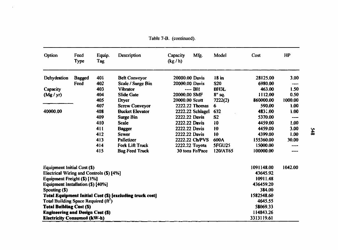
Table 7-B. (continued).
Option Feed Type
Equip. Tag
Description Capacity (kg / h)
Mfg. Model Cost HP
Dehydration Bagged 401 Belt Conveyor 20000.00 Davis 18 in 28125.00 3.00 Feed 402 Scale / Surge Bin 20000.00 Davis S20 6980.00 ——
Capacity 403 Vibrator —• BH BH3L 463.00 1.50 (Mg/yr) 404 Slide Gate 20000.00 SMF 8" sq. 1112.00 0.50
405 Dryer 20000.00 Scott 7222(2) 860000.00 1000.00 407 Screw Conveyor 2222.22 Thomas 6 590.00 1.00
40000.00 408 Bucket Elevator 2222.22 Schlagel 632 483'..00 1.00 409 Surge Bin 2222.22 Davis S2 5370.00 410 Scale 2222.22 Davis 10 4459.00 1.00 411 Bagger 2222.22 Davis 10 4459.00 3.00 412 Sewer 2222.22 Davis 10 4399.00 1.00 413 Palletizer 2222.22 Ch/PVS 600A 155360.00 30.00 414 Fork Lift Truck 2222.22 Toyota 5FGU25 15000.00 ——
415 Bag Feed Truck 30 tons Fr/Pace 120/AT65 100000.00 ----
Equipment Initial Cost ($) 1091148.00 1042.00 Electrical Wiring and Controls ($) [4%] 43645.92 Equipment Freight ($) [1%] 10911.48 Equipment Installation ($) [40%] 436459.20 Spouting ($) 384.00 Total Equipment Initial Cost ($) (excluding truck cost] 1582548.60 Total Building Space Required (ft ) 4645.55 Total Building Cost ($) 58069.33 Engineering and Design Cost ($) 114843.26 Electricity Consumed (kW-h) 3313119.61
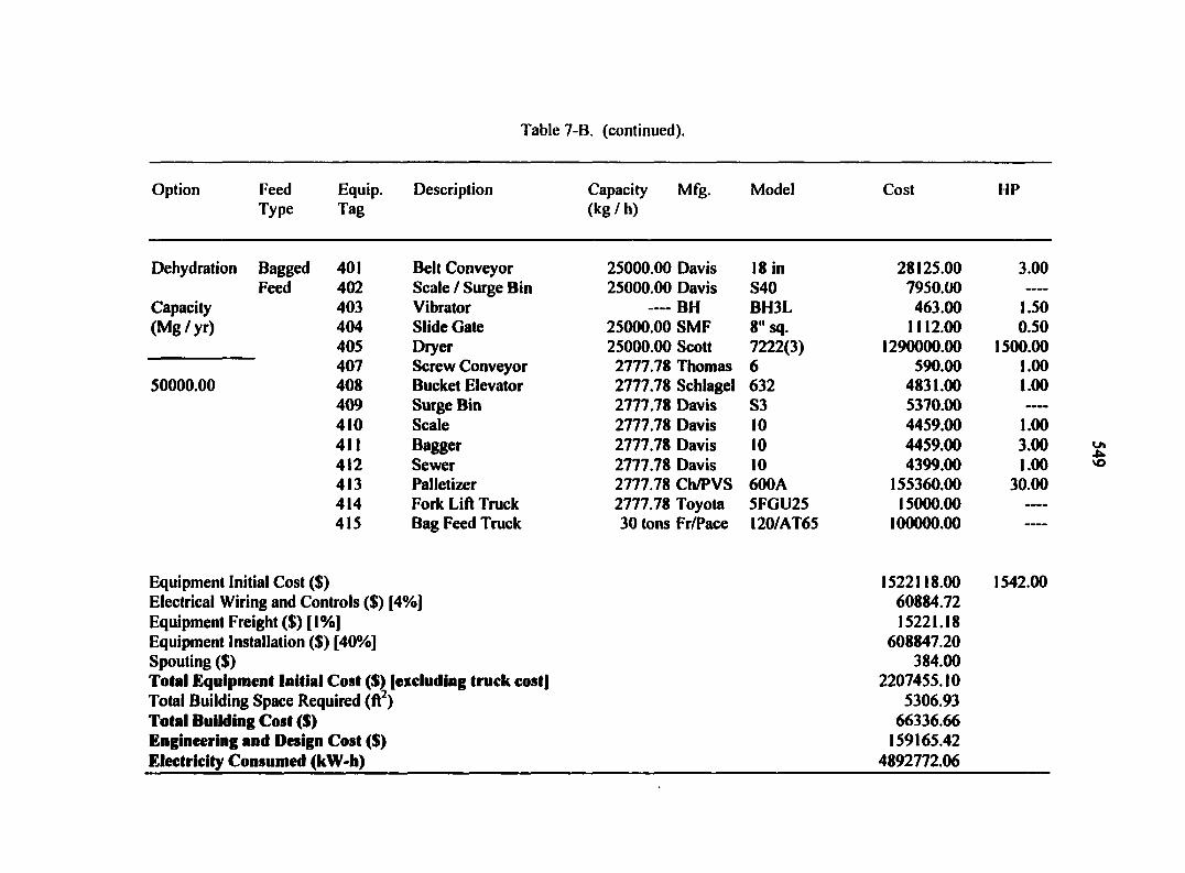
Table 7-B. (continued).
Option Feed Type
Equip. Tag
Description Capacity (kg Z h)
Mfg. Model Cost HP
Dehydration Bagged 401 Belt Conveyor 25000.00 Davis 18 in 28125.00 3.00 Feed 402 Scale / Surge Bin 25000.00 Davis S40 7950.00
Capacity 403 Vibrator — — BH BH3L 463.00 1.50 (Mg/yr) 404 Slide Gate 25000.00 SMF 8" sq. 1112.00 0.50
405 Dryer 25000.00 Scott 7222(3) 1290000.00 1500.00 407 Screw Conveyor 2777.78 Thomas 6 590.00 1.00
50000.00 408 Bucket Elevator 2777.78 Schlagel 632 4831.00 1.00 409 Surge Bin 2777.78 Davis S3 5370.00 410 Scale 2777.78 Davis 10 4459.00 1.00 411 Bagger 2777.78 Davis 10 4459.00 3.00 412 Sewer 2777.78 Davis 10 4399.00 1.00 413 Palletizer 2777.78 Ch/PVS 600A 155360.00 30.00 414 Fork Lift Truck 2777.78 Toyota 5FGU25 15000.00 415 Bag Feed Truck 30 tons Fr/Pace I20/AT65 100000.00 ----
Equipment Initial Cost ($) 1522118.00 1542.00 Electrical Wiring and Controls ($) [' 1%] 60884.72 Equipment Freight ($) [l%] 15221.18 Equipment Installation ($) [40%] 608847.20 Spouting ($) 384.00 Total Equipment Initial Cost ($) [excluding truck cost] 2207455.10 Total Building Space Required (ft ) 5306.93 Total Building Cost ($) 66336.66 Engineering and Design Cost ($) 159165.42 Electricity Consumed (kW-h) 4892772.06

Table 7-B. (continued).
Option Feed Type
Equip. Tag
Description Capacity Mfg. (kg / h)
Model Cost HP
Dehydration Bagged 401 Belt Conveyor 30000.00 Davis 18 in 28153.00 5.00 Feed 402 Scale / Surge Bin 30000.00 Davis S40 7950.00
Capacity 403 Vibrator — BH BH3L 463.00 1.50 (Mg/yr) 404 Slide Gate 30000.00 SMF 8" sq. 1112.00 0.50
405 Dryer 30000.00 Scott 7222(3) 1290000.00 1500.00 407 Screw Conveyor 3333.33 Thomas 9 629.10 1.00
60000.00 408 Bucket Elevator 3333.33 Schlagel 632 4831.00 1.00 409 Surge Bin 3333.33 Davis S3 5370.00 410 Scale 3333.33 Davis 10 4459.00 1.00 411 Bagger 3333.33 Davis 10 4459.00 3.00 412 Sewer 3333.33 Davis 10 4399.00 1.00 413 Palletizer 3333.33 Ch/PVS 600A 155360.00 30.00 414 Fork Lift Truck 3333.33 Toyota 5FGU25 15000.00 415 Bag Feed Truck 30 tons Fr/Pace 120/AT65 100000.00
Equipment Initial Cost ($) 1522185.10 1544.00 Electrical Wiring and Controls ($) [' \%] 60887.40 Equipment Freight ($) [l%] 15221.85 Equipment Installation ($) [40%] 608874.04 Spouting ($) 384.00 Total Equipment Initial Cost ($) [excluding truck cost] 2207552.40 Total Building Space Required (ft ) 5968.32 Total Building Cost ($) 74604.00 Engineering and Design Cost ($) 159750.95 Electricity Consumed (kW-h) 4910071.57
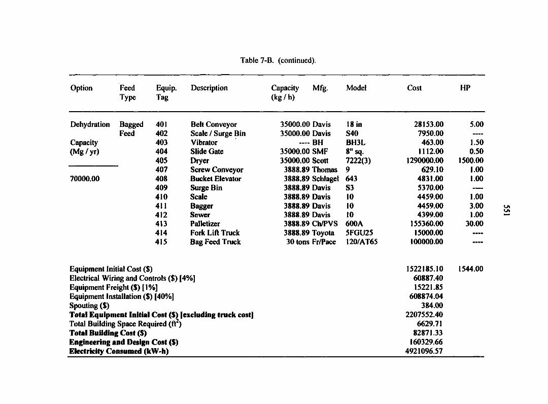
Table 7-B. (continued).
Option Feed Type
Equip. Tag
Description Capacity Mfg. (kg / h)
Model Cost HP
Dehydration Bagged 401 Belt Conveyor 35000.00 Davis 18 in 28153.00 5.00 Feed 402 Scale / Surge Bin 35000.00 Davis S40 7950.00 —»
Capacity 403 Vibrator — BH BH3L 463.00 1.50 (Mg/yr) 404 Slide Gate 35000.00 SMF 8" sq. 1112.00 0.50
405 Dryer 35000.00 Scott 7222(3) 1290000.00 1500.00 407 Screw Conveyor 3888.89 Thomas 9 629.10 1.00
70000.00 408 Bucket Elevator 3888.89 Schlagel 643 4831.00 1.00 409 Surge Bin 3888.89 Davis S3 5370.00 410 Scale 3888.89 Davis 10 4459.00 1.00 411 Bagger 3888.89 Davis 10 4459.00 3.00 412 Sewer 3888.89 Davis 10 4399.00 1.00 413 Palletizer 3888.89 Ch/PVS 600A 155360.00 30.00 414 Fork Lift Truck 3888.89 Toyota 5FGU25 15000.00 ——
415 Bag Feed Truck 30 tons Fr/Pace 120/AT65 100000.00 ——
Equipment Initial Cost ($) 1522185.10 1544.00 Electrical Wiring and Controls ($) [4%] 60887.40 Equipment Freight ($) [1%] 15221.85 Equipment Installation ($) [40%] 608874.04 Spouting ($) 384.00 Total Equipment Initial Cost ($) [excluding truck cost] 2207552.40 Total Building Space Required (ft ) 6629.71 Total Building Cost ($) 82871.33 Engineering and Design Cost ($) 160329.66 Electricity Consumed (kW-h) 4921096.57

Table 7-B. (continued).
Option Feed Type
Equip. Tag
Description Capacity Mfg. (kg / h)
Model Cost HP
Dehydration Bulk 401 Belt Conveyor 500.00 Davis 18 in 28117.00 2.00 Feed 402 Scale / Surge Bin 500.00 Davis SI 5370.00
Capacity 403 Vibrator — BH BH3L 463.00 1.50 (Mg/yr) 404 Slide Gate 500.00 SMF 8" sq. 1112.00 0.50
405 Dryer 500.00 Scott 3012 160000.00 90.00 407 Screw Conveyor 55.56 Thomas 4 590.00 1.00
1000.00 417 Bucket Elevator 55.56 Schlagel 632 4831.00 1.00 418 Surge Bin 55.56 Davis SI 5370.00 419 Slide Gate 55.56 SMF 8" sq. 1112.00 0.50 420 Bulk Feed Truck 30 tons Fr/Pace I20/AT65 100000.00
Equipment Initial Cost ($) 206965.00 96.50 Electrical Wiring and Controls ($) [4%] 8278.60 Equipment Freight ($) [l%] 2069.65 Equipment Installation ($) [40%] 82786.00 Spouting ($) 384.00 Total Equipment Initial Cost ($) [excluding truck cost] 300483.25 Total Building Space Required (ft ) 2000.00 Total Building Cost ($) 25000.00 Engineering and Design Cost ($) 22783.83 Electricity Consumed (kW-h) 303847.60
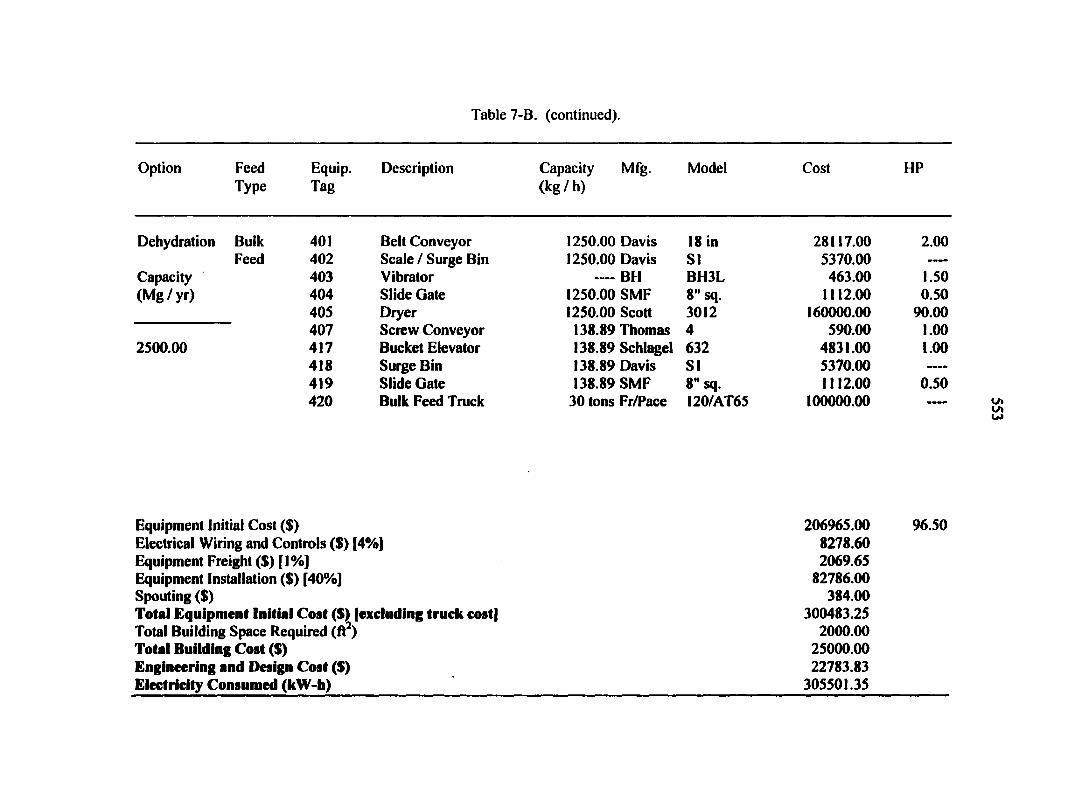
Table 7-B. (continued).
Option Feed Equip. Description Capacity Mfg. Model Cost HP Type Tag (kg/h)
Dehydration Bulk 401 Belt Conveyor 1250.00 Davis 18 in 28117.00 2.00 Feed 402 Scale / Surge Bin 1250.00 Davis SI 5370.00
Capacity 403 Vibrator — BH BH3L 463.00 1.50 (Mg / yr) 404 Slide Gate 1250.00 SMF 8" sq. 1112.00 0.50
405 Dryer 1250.00 Scott 3012 160000.00 90.00 407 Screw Conveyor 138.89 Thomas 4 590.00 1.00
2500.00 417 Bucket Elevator 138.89 Schlagel 632 4831.00 1.00 418 Surge Bin 138.89 Davis SI 5370.00 ——
419 Slide Gate 138.89 SMF 8" sq. 1112.00 0.50 420 Bulk Feed Truck 30 tons Fr/Pace 120/AT65 100000.00 ———»
Equipment Initial Cost ($) 206965.00 Electrical Wiring and Controls ($) [4%] 8278.60 Equipment Freight ($) [ 1 %] 2069.65 Equipment Installation ($) [40%] 82786.00 Spouting ($) 384.00 Total Equipment Initial Cost ($) [excluding truck cost] 300483.25 Total Building Space Required (ft2) 2000.00 Total Building Cost ($) 25000.00 Engineering and Design Cost ($) 22783.83 Electricity Consumed (kW-h) 305501.35
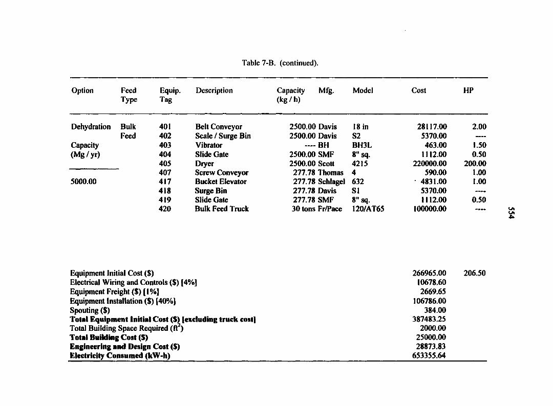
Table 7-B. (continued).
Option Feed Equip. Description Capacity Mfg. Model Cost HP Type Tag (kg / h)
Dehydration Bulk 401 Belt Conveyor 2500.00 Davis 18 in 28117.00 2.00 Feed 402 Scale / Surge Bin 2500.00 Davis S2 5370.00
Capacity 403 Vibrator —— BH BH3L 463.00 1.50 (Mg/yr) 404 Slide Gate 2500.00 SMF 8" sq. 1112.00 0.50
405 Dryer 2500.00 Scott 4215 220000.00 200.00 407 Screw Conveyor 277.78 Thomas 4 590.00 1.00
5000.00 417 Bucket Elevator 277.78 Schlagel 632 4831.00 1.00 418 Surge Bin 277.78 Davis SI 5370.00 ———-
419 Slide Gate 277.78 SMF 8" sq. 1112.00 0.50 420 Bulk Feed Truck 30 tons Fr/Pace 120/AT65 100000.00
Equipment Initial Cost ($) 266965.00 206.50 Electrical Wiring and Controls ($) [4%] 10678.60 Equipment Freight ($) [l%] 2669.65 Equipment Installation ($) [40%] 106786.00 Spouting ($) 384.00 Total Equipment Initial Cost ($) [excluding truck cost] 387483.25 Total Building Space Required (ft ) 2000.00 Total Building Cost ($) 25000.00 Engineering and Design Cost ($) 28873.83 Electricity Consumed (kW-h) 653355.64

Table 7-B. (continued).
Option Feed Equip. Description Capacity Mfg. Model Cost HP Type Tag (kg / h)
Dehydration Bulk 401 Belt Conveyor 5000.00 Davis 18 in 28117.00 2.00 Feed 402 Scale / Surge Bin 5000.00 Davis S5 5370.00
Capacity 403 Vibrator — BH BH3L 463.00 1.50 (Mg/yr) 404 Slide Gate 5000.00 SMF 8" sq. 1112.00 0.50
405 Dryer 5000.00 Scott 6018 360000.00 400.00 407 Screw Conveyor 555.56 Thomas 4 590.00 1.00
10000.00 417 Bucket Elevator 555.56 Schlagel 632 4831.00 1.00 418 Surge Bin 555.56 Davis SI 5370.00 —-
419 Slide Gate 555.56 SMF 8" sq. 1112.00 0.50 420 Bulk Feed Truck 30 tons Fr/Pace I20/AT65 100000.00
Equipment Initial Cost ($) 406965.00 406.50 Electrical Wiring and Controls ($) [4%) 16278.60 Equipment Freight ($) [ l%] 4069.65 Equipment Installation ($) [40%) 162786.00 Spouting ($) 384.00 Total Equipment Initial Cost ($) [excluding truck cost) 590483.25 Total Building Space Required (ft ) 2000.00 Total Building Cost ($) 25000.00 Engineering and Design Cost ($) 43083.83 Electricity Consumed (kW-h) 1286319.12

Table 7-B. (continued).
Option Feed Type
Equip. Tag
Description Capacity Mfg. (kg / h)
Model Cost HP
Dehydration Bulk 401 Belt Conveyor 10000.00 Davis 18 in 28117.00 2.00 Feed 402 Scale / Surge Bin 10000.00 Davis S10 6980.00 ———
Capacity 403 Vibrator — BH BH3L 463.00 1.50 (Mg / yr) 404 Slide Gate 10000.00 SMF 8" sq. 1112.00 0.50
405 Dryer 10000.00 Scott 7222 430000.00 500.00 407 Screw Conveyor 1111.11 Thomas 6 590.00 1.00
20000.00 417 Bucket Elevator 1111.11 Schlagel 632 4831.00 1.00 418 Surge Bin 1111.11 Davis SI 5370.00 419 Slide Gate 1111.11 SMF 8 " sq. 1112.00 0.50 420 Bulk Feed Truck 30 tons Fr/Pace 120/AT65 100000.00
Equipment Initial Cost ($) 478575.00 506.50 Electrical Wiring and Controls ($) [4%] 19143.00 Equipment Freight ($) [l%] 4785.75 Equipment Installation ($) [40%] 191430.00 Spouting ($) 384.00 Total Equipment Initial Cost ($) [excluding truck cost] 694317.75 Total Building Space Required (ft ) 2000.00 Total Building Cost ($) 25000.00 Engineering and Design Cost ($) 50352.24 Electricity Consumed (kW-h) 1611069.61
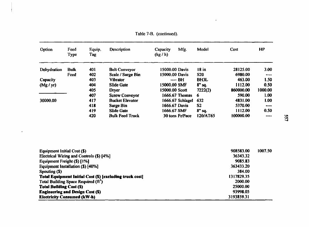
Table 7-B. (continued).
Option Feed Type
Equip. Tag
Description Capacity (kg / h)
Mfg. Model Cost HP
Dehydration Bulk 401 Belt Conveyor 15000.00 Davis 18 in 28125.00 3.00 Feed 402 Scale / Surge Bin 15000.00 Davis S20 6980.00 -*™
Capacity 403 Vibrator BH BH3L 463.00 1.50 (Mg/yr) 404 Slide Gate 15000.00 SMF 8" sq. 1112.00 0.50
405 Dryer 15000.00 Scott 7222(2) 860000.00 1000.00 407 Screw Conveyor 1666.67 Thomas 6 590.00 1.00
30000.00 417 Bucket Elevator 1666.67 Schlagel 632 4831.00 1.00 418 Surge Bin 1666.67 Davis S2 5370.00 ——
419 Slide Gate 1666.67 SMF 8" sq. 1112.00 0.50 420 Bulk Feed Truck 30 tons Fr/Pace 120/AT65 100000.00
Equipment Initial Cost ($) Electrical Wiring and Controls ($) [4%] Equipment Freight ($) [I%] Equipment Installation ($) [40%] Spouting ($) Total Equipment Initial Cost ($) [excluding truck cost] Total Building Space Required (ft2) Total Building Cost ($) Engineering and Design Cost ($) Electricity Consumed (kW-h)
908583.00 36343.32 9085.83
363433.20 384.00
1317829.35 2000.00
25000.00 93998.05
3193859.31
1007.50

Table 7-B. (continued).
Option Feed Type
Equip. Tag
Description Capacity (kg / h)
Mfg. Model Cost HP
Dehydration Bulk 401 Belt Conveyor 20000.00 Davis 18 in 28125.00 3.00 Feed 402 Scale / Surge Bin 20000.00 Davis S20 6980.00 »—
Capacity 403 Vibrator ---- BH BH3L 463.00 1.50 (Mg/yr) 404 Slide Gate 20000.00 SMF 8" sq. 1112.00 0.50
405 Dryer 20000.00 Scott 7222(2) 860000.00 1000.00 407 Screw Conveyor 2222.22 Thomas 6 590.00 1.00
40000.00 417 Bucket Elevator 2222.22 Schlagel 632 4831.00 1.00 418 Surge Bin 2222.22 Davis S2 5370.00 ™—-
419 Slide Gate 2222.22 SMF 8" sq. 1112.00 0.50 420 Bulk Feed Truck 30 tons Fr/Pace 120/AT65 100000.00
Equipment Initial Cost ($) Electrical Wiring and Controls ($) [4%] Equipment Freight ($) [1%] Equipment Installation ($) [40%] Spouting ($) Total Equipment Initial Cost ($) [excluding truck cost] Total Building Space Required (ft2) Total Building Cost ($) Engineering and Design Cost ($) Electricity Consumed (kW-h)
908583.00 36343.32 9085.83
363433.20 384.00
1317829.35 2000.00
25000.00 93998.05
3204884.31
1007.50

Table 7-B. (continued).
Option Feed Type
Equip. Tag
Description Capacity (kg / h)
Mfg. Model Cost HP
Dehydration Bulk 401 Belt Conveyor 25000.00 Davis 18 in 28125.00 3.00 Feed 402 Scale / Surge Bin 25000.00 Davis S40 7950.00 --*•
Capacity 403 Vibrator — BH BH3L 463.00 1.50 (Mg/yr) 404 Slide Gate 25000.00 SMF 8" sq. 1112.00 0.50
405 Dryer 25000.00 Scott 7222(3) 1290000.00 1500.00 407 Screw Conveyor 2777.78 Thomas 6 590.00 1.00
50000.00 417 Bucket Elevator 2777.78 Schlagel 632 4831.00 1.00 418 Surge Bin 2777.78 Davis S3 5370.00 ——*
419 Slide Gate 2777.78 SMF 8" sq. 1112.00 0.50 420 Bulk Feed Truck 30 tons Fr/Pace 120/AT65 100000.00
Equipment Initial Cost ($) 1339553.00 1507.50 Electrical Wiring and Controls ($) [4%] 53582.12 Equipment Freight ($) [l%] 13395.53 Equipment Installation ($) [40%] 535821.20 Spouting ($) 384.00 Total Equipment Initial Cost ($) [excluding truck cost] 1942735.85 Total Building Space Required (ft ) 2000.00 Total Building Cost ($) 25000.00 Engineering and Design Cost ($) 137741.51 Electricity Consumed (kW-h) 4784536.76
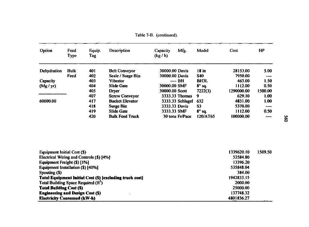
Table 7-B. (continued).
Option Feed Type
Equip. Tag
Description Capacity (kg / h)
Mfg. Model Cost HP
Dehydration Bulk 401 Belt Conveyor 30000.00 Davis 18 in 28153.00 5.00 Feed 402 Scale / Surge Bin 30000.00 Davis S40 7950.00
Capacity 403 Vibrator —— BH BH3L 463.00 1.50 (Mg/yr) 404 Slide Gate 30000.00 SMF 8" sq. 1112.00 0.50
405 Dryer 30000.00 Scott 7222(3) 1290000.00 1500.00 407 Screw Conveyor 3333.33 Thomas 9 629.10 1.00
60000.00 417 Bucket Elevator 3333.33 Schlagel 632 4831.00 1.00 418 Surge Bin 3333.33 Davis S3 5370.00 —™
419 Slide Gate 3333.33 SMF 8" sq. 1112.00 0.50 420 Bulk Feed Truck 30 tons Fr/Pace 120/AT65 100000.00 ••••
Equipment Initial Cost ($) Electrical Wiring and Controls ($) [4%] Equipment Freight ($) [ 1 %] Equipment Installation ($) [40%] Spouting ($) Total Equipment Initial Cost ($) [excluding truck cost] Total Building Space Required (ft2) Total Building Cost ($) Engineering and Design Cost ($) Electricity Consumed (kW-h)
1339620.10 53584.80 13396.20
535848.04 384.00
1942833.15 2000.00
25000.00 137748.32
4801836.27
1509.50
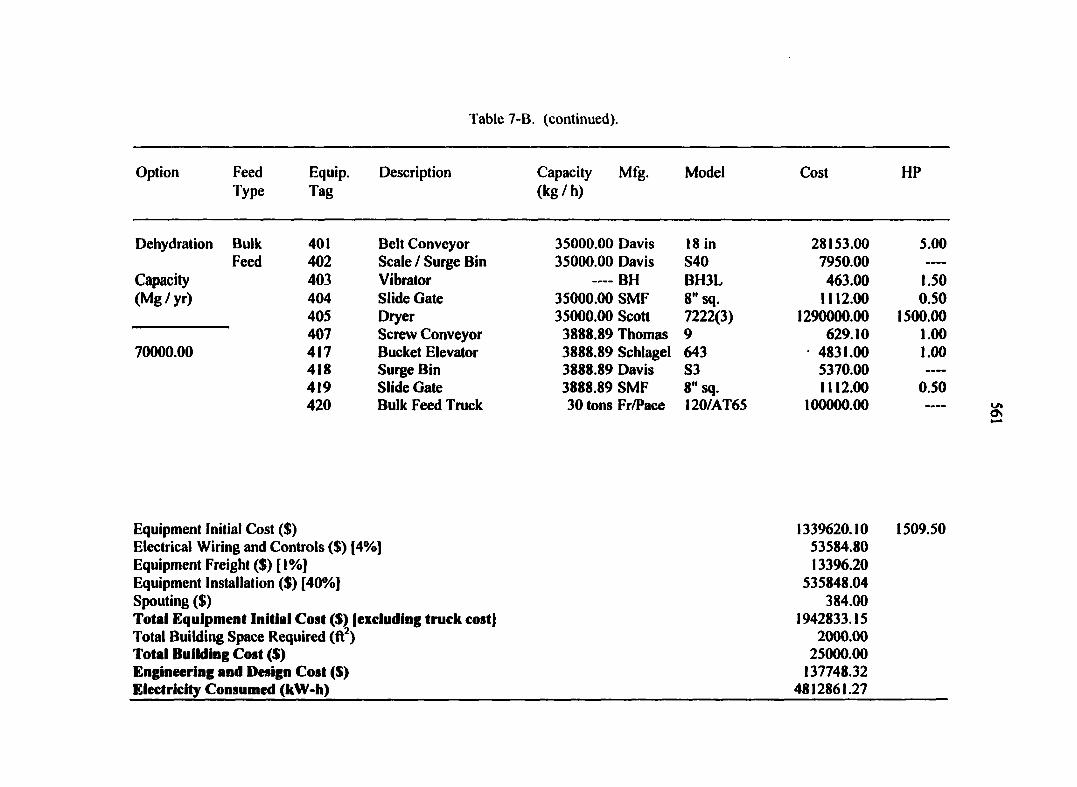
Table 7-B. (continued).
Option Feed Type
Equip. Tag
Description Capacity (kg/h)
Mfg. Model Cost HP
Dehydration Bulk 401 Belt Conveyor 35000.00 Davis 18 in 28153.00 5.00 Feed 402 Scale / Surge Bin 35000.00 Davis S40 7950.00 ----
Capacity 403 Vibrator BH BH3L 463.00 1.50 (Mg/yr) 404 Slide Gate 35000.00 SMF 8" sq. 1112.00 0.50
405 Dryer 35000.00 Scott 7222(3) 1290000.00 1500.00 407 Screw Conveyor 3888.89 Thomas 9 629.10 1.00
70000.00 417 Bucket Elevator 3888.89 Schlagel 643 4831.00 1.00 418 Surge Bin 3888.89 Davis S3 5370.00 —-
419 Slide Gate 3888.89 SMF 8" sq. 1112.00 0.50 420 Bulk Feed Truck 30 tons Fr/Pace 120/AT65 100000.00 ————
Equipment Initial Cost ($) Electrical Wiring and Controls ($) [4%] Equipment Freight ($) [1%] Equipment Installation ($) [40%] Spouting ($) Total Equipment Initial Cost ($) (excluding truck cost] Total Building Space Required (ft2) Total Building Cost ($) Engineering and Design Cost ($) Electricity Consumed (kW-h)
1339620.10 53584.80 13396.20
535848.04 384.00
1942833.15 2000.00
25000.00 137748.32
4812861 27
1509.50
562
CHAPTERS
GENERAL CONCLUSIONS AND FUTURE WORK
GENERAL CONCLUSIONS
The overall intent of this project was to develop value-added disposal/reuse
alternatives for corn masa processing residues. Four main objectives were delineated in
Chapter 1 to accomplish this, and a summary of each of these stages of the project will be
discussed below:
1. Typical byproduct residual streams from a com masa processing plant were subjected
to physical and nutritional property analysis; this was discussed in Chapter 3. Masa
byproducts (i.e., suspended solids removed from masa processing waste water)
appear suitable for use as livestock feed additives, or components thereof. These
byproducts are very high in moisture content; but dried, they are high in fiber
(especially cellulose and hemicellulose), and would probably be best suited for
ruminant diets. Additionally, when dried, these products have a substantial calcium
content, so there may exist potential for use as a calcium source for livestock rations.
2. Corn masa byproducts were blended with soybean meal and extruded on a laboratory
scale, and the effects of blend ratio, extrusion temperature, and extruder screw speed
on extrusion processing variables and final extrudate physical and nutritional
characteristics was investigated; this was discussed in Chapter 5. Laboratory-scale
extrusion of these blends produced extradâtes with nutritional properties similar to
those of the raw ingredient blends, with improved protein digestibility due to the
effects of the extrusion processing. Because soybean meal was used as a blending
agent, little product expansion occurred at the extruder die, primarily due to lack of
563
starchy components in the blends. Additionally, the resulting products had low water
absorption and solubility. During processing, the dough melt in the extruder behaved
as a pseudoplastic material, which is typical of most food doughs, requiring less
torque required to convey the dough as screw speed increased. Blend ratio affected
processing and product properties very little; most effects were due to screw speed
and processing temperature. All blends were amenable to extrusion processing at the
processing conditions used in this study. Extrusion processing produced extradâtes
with excellent durability, which is essential to retaining quality during transport and
storage of pelleted feed ingredients. An additional drying step was required for the
extruded products to reduce moisture and water activity levels to acceptable ranges,
in order to prevent microbial spoilage during storage.
3. Corn masa byproducts were blended with soybean meal and extruded on a pilot scale
to investigate the effects of blend ratio and extruder screw speed on extrusion
processing variables and final extrudate product physical and nutritional
characteristics; this was discussed in Chapter 6. Pilot-scale extrusion and drying of
these blends produced extradâtes that were dry and microbiologically stable. As was
observed for soybean meal blends at the laboratory-scale, little product expansion
occurred at the extruder die exit, primarily due to lack of starchy components in the
blends. Pilot-scale extrusion processing also produced extradates with excellent
durability, which is essential to retaining quality during transport and storage of
pelleted feed ingredients. During processing, the dough melt in the extruder barrel
required less force to convey the dough as screw speed increased, again consistent
with the results from the laboratory-scale extrusion. Further, blend ratio seemed to
564
affect processing and product properties very little; most effects were due to changes
in screw speed, which in turn affected processing temperature. All blends were
amenable to extrusion processing at the conditions used in this study.
4. An economic assessment of various disposal and recycling alternatives for com masa
processing byproducts was conducted; this was discussed in Chapter 7. This study
encompassed the development of a computer program to model the economics
associated with the recycling of com masa byproducts. Through the use of this
model, it was determined that direct shipping of masa byproducts is the most
economical choice for the com masa manufacturer. Blending masa byproducts with
soybean meal is a more expensive recycling option, while extrusion processing and
pellet mill processing are substantially more expensive; thus, these options are cost-
prohibitive. Furthermore, dehydration is much too expensive to justify economically.
FUTURE WORK
This research project represents, essentially, the initial stages of value-added
byproduct development for com masa residual slurries. To effectively utilize this waste
stream, a host of additional work is possible, and, in fact, would be beneficial. A few
suggestions for this possible future work are discussed below.
1. More extensive physical and nutritional characterization of com masa byproducts
needs to be undertaken. Other relevant properties include thermal properties (specific
heat, thermal conductivity, and thermal diffusivity) and rheological properties
(apparent viscosities at various rates of strain, flow behavior index, consistency
coefficient). Additionally, an investigation of the microscopic structures of this waste
material would be beneficial. This material is a heterogeneous mixture of com tissues
565
and water, and examination of the microstructures would lend insight into possible
methods for effective low-cost dewatering.
2. A more thorough investigation of the nutritional properties of com masa byproducts
should also be undertaken. This study quantified the protein, carbohydrate, fat, and
ash content of masa byproduct streams, as well as fiber content, a few key minerals,
and amino acids. Further nutritional analyses could include soluble and insoluble
dietary fiber, and could possibly include a more thorough mineral and vitamin
analysis.
3. As mentioned previously, further dewatering of the masa residual stream would be
beneficial, because less waste material would need to be handled, reprocessed, and
delivered. Areas of investigation in this regard could include improving the current
centrifugation techniques, studying vacuum separation, and examining membrane
separation methods.
4. Because the moisture content of the masa byproducts in this study was so high, these
materials are easily susceptible to microbial degradation and spoilage. Future studies
of com masa byproducts could include investigating alternative strategies to extrusion
and drying to enhance shelf-life of the wet materials (e.g., chemical additives).
Additionally, an investigation to quantify the microbial activities within com masa
byproduct streams would be beneficial to help determine suitable courses of action
vis-à-vis product preservation. Subsequent to this, a fermentation study might be
conducted to determine the possibility of either using this processing step to preserve
masa byproducts prior to feeding to livestock, or using masa byproducts as a
feedstock for industrial fermentation operations.
566
5. Finally, corn masa byproduct streams should be studied from other processing plants,
at other locations, in both the United States and in Mexico, which utilize equipment
and processing steps unique to other facilities.
Developing value-added alternatives for the byproducts of masa manufacturing would
be beneficial not only to the masa processor, due to increased revenue from the sale of the
byproducts, and decreased landfill disposal fees, but also to the surrounding communities,
due to decreased solids load to local water treatment plants and decreased pollution potential
from the masa processing plant.