ii

Design and Development of a High Swirl Burner with

gaseous fuel injection through porous tubes

A thesis submitted to the Graduate School of the University of Cincinnati in partial fulfillment of

the requirements for the degree of

MASTER OF SCIENCE (M.S)

In the Department of Mechanical & Materials Engineering of the College of Engineering and

Applied Science

September 2017

By

Arul Kumaran Ramalingam Ammaiyappan

B.E. Production Engineering, 2012

Committee Chair: Professor San-Mou Jeng

ii

ABSTRACT

Lean Premixed combustors reduce NOx emissions by burning fuel at “fuel-lean” conditions. The

presence of excess air in the lean mixture reduces the combustion temperature. Since thermal NOx

reduces exponentially with temperature, the reduction of temperature brings about a reduction in

NOx emissions. The presence of fuel rich zones leads to the formation of prompt NOx. Uniform

mixing of fuel and air reduces prompt NOx by eliminating “fuel-rich” pockets in the reaction zone.

In this project, gaseous fuel is injected through eight porous tubes that are aligned parallel to the

axis of an axial swirler. The axial swirler differs from other axial swirlers in that it also serves as

a transition zone for the fuel-air mixture. While the downstream side of the axial swirler resembles

other axial swirlers, the upstream side of the swirler has eight circular holes arranged

circumferentially. The circular flow area on the upstream side of the axial swirler transitions into

the trapezoidal space between the vanes of on the downstream side. The porous tubes are attached

to the holes on the upstream side of the swirler. The diameter of these holes matches the inner

diameter of the porous tubes. Air is passed through the porous tubes and gaseous fuel mixes with

air from the outside of the porous tube. The swirler helps the flow transition from a circular cross-

sectional area (porous tubes) to a trapezoidal cross-sectional area (space between adjacent vanes

in an axial swirler is trapezoidal).

The aerodynamics of this swirler is studied using non-reacting flow PIV. PIV measurements are

done on the axial plane to study the recirculation zone and on the cross-plane to study the tangential

iii

and radial velocities. A parametric study of centerbodies is conducted using PIV to attempt to

narrow down to the centerbody that prevents attachment of recirculation zone to the swirler exit.

Combustion testing is conducted at different preheat temperatures (400°F, 500°F, 600°F) and at

different equivalence ratios (0.55, 0.6, 0.65) for flame imaging and emission measurement. The

NOx emissions are plotted as a function of the adiabatic flame temperature.

iv

ACKNOWLEDGEMENT

I would like to thank my professor Dr. San Mou Jeng for giving me an opportunity to work

in Combustion & Fire Research Laboratory (CFRL). I owe a deep debt of gratitude to my professor

for nurturing my interest in experimental fluid mechanics and awarding me a Graduate Research

Assistantship.

Secondly, I would like to thank Umesh Bhayaraju for being a mentor and guiding me

during my stint at Combustion Research Laboratory. I had the opportunity to interact with Dr.

Bhayaraju on a daily basis and I learnt a lot about Particle Image Velocimetry and Laser Doppler

Anemometry from him.

I would like to thank Hamza and Jenny for allowing me to make a contribution to their

conference papers and teaching me to use some of the instruments at CFRL.

I would also like to thank Dr. Samir Tambe for his guidance during industrial projects and

his suggestions during lab meetings.

v

TABLE OF CONTENTS

ABSTRACT ................................................................................................................................ ii

ACKNOWLEDGEMENT ......................................................................................................... iv

TABLE OF CONTENTS ............................................................................................................ v

LIST OF FIGURES ................................................................................................................... vii

LIST OF EQUATIONS .............................................................................................................. x

LIST OF TABLES ..................................................................................................................... xi

1. INTRODUCTION ................................................................................................................... 1

1.1 MOTIVATION ............................................................................................................. 1

1.1.1 Pre-formation NOx control ................................................................................... 1

1.2 LITERATURE REVIEW ............................................................................................. 2

1.2.1 Dry Low NOx Combustion ......................................................................................... 2

1.2.2 Formation of recirculation zone in swirl stabilized combustion ................................. 4

1.2.3 Mixing of Two Jets ................................................................................................... 10

1.2.4 Fuel injection using Porous tubes ............................................................................. 10

1.2.5 Particle Image Velocimetry ...................................................................................... 12

1.2.6 Formation of NOx ..................................................................................................... 18

1.3 SCOPE OF THE THESIS .......................................................................................... 21

2. EXPERIMENTAL SET-UP .................................................................................................. 22

2.1 SUMMARY..................................................................................................................... 22

2.1.1 Pre-mixer design ....................................................................................................... 22

2.1.2 Challenges in using porous tubes for fuel injection .................................................. 27

vi

2.1.3 Specifications of the axial swirler ............................................................................. 29

2.2 PIV EXPERIMENTAL SET-UP..................................................................................... 30

2.3 COMBUSTION EXPERIMENTAL SET-UP................................................................. 31

3. RESULTS AND DISCUSSION ............................................................................................ 33

3.1 PRE-MIXER AERODYNAMICS .................................................................................. 33

3.1.1 PIV results ................................................................................................................. 33

3.1.2 Horizontal plane PIV results ..................................................................................... 38

3.1.3 Parametric study of centerbodies .............................................................................. 45

3.2 COMBUSTION TESTING ............................................................................................. 51

3.2.1 Flame characterization .............................................................................................. 51

3.2.2 NOx emission measurement ..................................................................................... 52

4. FUTURE WORK AND RECOMMENDATIONS ............................................................... 55

REFERENCES .......................................................................................................................... 57

APPENDIX ............................................................................................................................... 59

vii

LIST OF FIGURES

Figure 1.1 : Cross section of GE LM 6000 DLN Combustor (Joshi et al).................................................... 3

Figure 1.2: Cross-sectional view of a DACARS configuration (Joshi et al) ................................................ 4

Figure 1.3: Flat vanes vs Curved vanes (Lefebvre) ...................................................................................... 5

Figure 1.4: Axisymmetric vortex breakdown (Doherty et al, 2001) ............................................................. 6

Figure 1.5: A typical swirl flow field (Yang et al, 2009) .............................................................................. 7

Figure 1.6: Main flow and recirculation region (Lefebvre) .......................................................................... 7

Figure 1.7: Typical axial swirl velocity profiles (Lefebvre) ......................................................................... 7

Figure 1.8: Types of Swirlers ........................................................................................................................ 8

Figure 1.9: Axial swirler notation(Lefebvre) ................................................................................................ 9

Figure 1.10 : Porous tube parallel flow (Non Mee Boon, 2015) ................................................................. 10

Figure 1.11: Experimental set-up for a porous injector (Non Mee Boon, 2015) ........................................ 11

Figure 1.12: Sudden flow expansion (Non Mee Boon, 2015) .................................................................... 11

Figure 1.13: Particle Image Velocimetry – Concept (Dantec Dynamics)................................................... 13

Figure 1.14: Interrogation window (LaVision) ........................................................................................... 14

Figure 1.15: Auto correlation (LaVision) ................................................................................................... 15

Figure 1.16: Cross correlation (LaVision DaVis 8.0 Manual, 2011) .......................................................... 16

Figure 1.17: Vector position depending on overlap size and interrogation window size (LaVision) ......... 17

Figure 1.18: Multi-pass PIV operation - constant interrogation window size (LaVision) .......................... 18

Figure 1.19: NOx vs Time (Lefebvre) ........................................................................................................ 19

Figure 2.1: Pre-mixer I mounted for cold-flow PIV ................................................................................... 24

Figure 2.2: Comparison between Pre-mixer I* and Pre-mixer II ................................................................ 24

Figure 2.3: Plastic Pre-mixer II used for cold flow PIV ............................................................................. 25

Figure 2.4: Metal Pre-mixer III design (for combustion testing) ................................................................ 25

Figure 2.5: Axial swirler design used in Pre-mixers II & III ...................................................................... 26

Figure 2.6: Circular to trapezoidal transition of the swirler in Pre-mixers II & III..................................... 26

Figure 2.7: Pre-mixer III assembly showing the arrangement of porous tubes .......................................... 27

Figure 2.8 (left): Metal swirler (Pre-mixer III) with the centerbody .......................................................... 28

viii

Figure 2.9 (right): A picture of all the pre-mixer III components before assembly .................................... 28

Figure 2.10: The plastic swirler (Pre-mixer II), centerbody and shroud used for cold flow PIV ............... 28

Figure 2.11: Vane profile showing vane outlet angle of 60° and stagger angle of 30° ............................... 29

Figure 2.12: Premixer III CAD assembly showing the mounting plate and confinement .......................... 30

Figure 2.13: PIV Experimental set-up ........................................................................................................ 32

Figure 3.1: Unconfined case PIV with the alumina seeding particles ........................................................ 33

Figure 3.2: Time averaged Axial velocity at 4% pressure drop - Unconfined case .................................... 34

Figure 3.3: Time averaged Axial velocity at 4% pressure drop - Confined case ........................................ 35

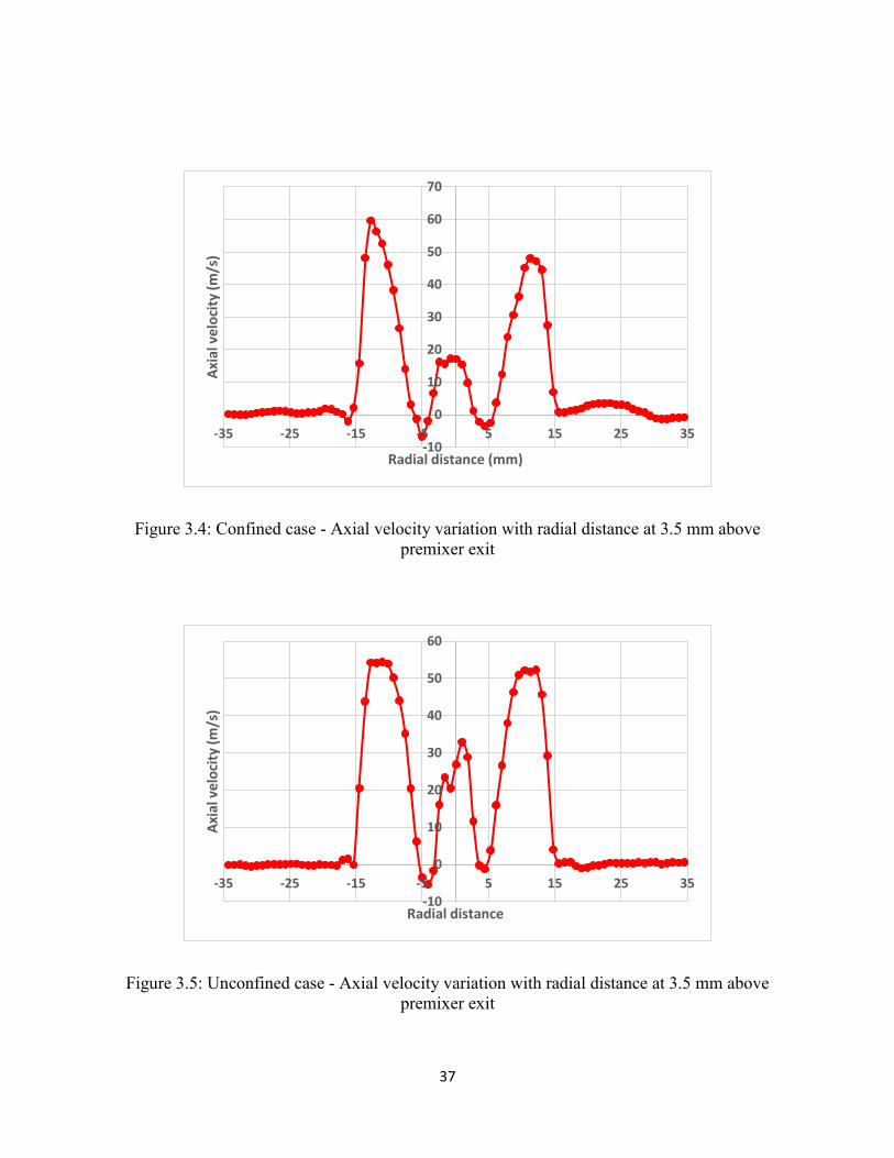
Figure 3.4: Confined case - Axial velocity variation with radial distance at 3.5 mm above premixer exit 37

Figure 3.5: Unconfined case - Axial velocity variation with radial distance at 3.5 mm above premixer exit

.................................................................................................................................................................... 37

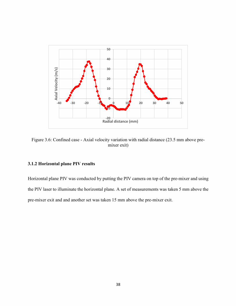
Figure 3.6: Confined case - Axial velocity variation with radial distance (23.5 mm above pre-mixer exit)

.................................................................................................................................................................... 38

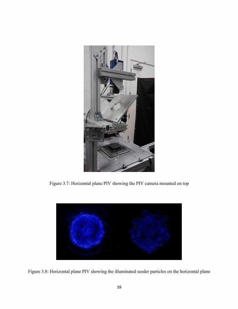
Figure 3.7: Horizontal plane PIV showing the PIV camera mounted on top.............................................. 39

Figure 3.8: Horizontal plane PIV showing the illuminated seeder particles on the horizontal plane ......... 39

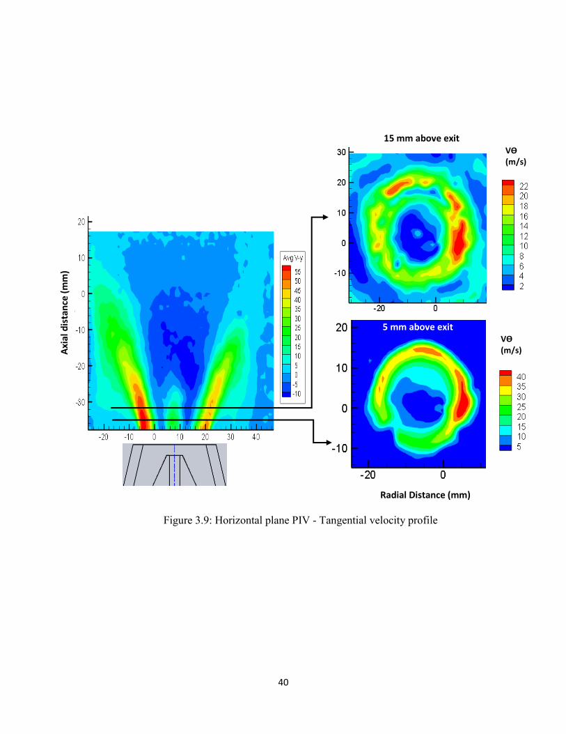
Figure 3.9: Horizontal plane PIV - Tangential velocity profile .................................................................. 40

Figure 3.10: Radial and tangential velocity along the diameter of the pre-mixer ....................................... 42

Figure 3.11: Tangential velocity along the diameter on Y-axis – 5mm above pre-mixer exit ................... 43

Figure 3.12: Radial velocity distribution along the diameter on Y-axis – 5mm above pre-mixer exit ....... 43

Figure 3.13: Tangential velocity distribution along the diameter on X-axis .............................................. 44

Figure 3.14: Radial velocity distribution along the diameter on X-axis ..................................................... 44

Figure 3.15: Parametric study of center-bodies .......................................................................................... 46

Figure 3.16: Comparison between Straight hole and Diverging hole center-bodies................................... 46

Figure 3.17: S2 configuration axial velocity profile ................................................................................... 47

Figure 3.18: D4 configuration axial velocity profile .................................................................................. 47

Figure 3.19: S4 configuration axial velocity profile ................................................................................... 48

Figure 3.20: D2 configuration axial velocity profile .................................................................................. 48

Figure 3.21: S4 configuration - Axial velocity vs Radial distance ............................................................. 49

Figure 3.22: S2 configuration - Axial velocity variation with radial distance ........................................... 49

Figure 3.23: Flame imaging ........................................................................................................................ 52

ix

Figure 3.24: NOx vs Adiabatic Flame Temperature ................................................................................... 54

Figure 4.1: CFD flow domain for the pre-mixer ......................................................................................... 55

Figure 4.2: Centerbody ............................................................................................................................... 61

Figure 4.3: Mounting plate ......................................................................................................................... 62

Figure 4.4: Shroud ...................................................................................................................................... 63

Figure 4.5:Ring ........................................................................................................................................... 64

Figure 4.6: Bottom plate ............................................................................................................................. 65

x

LIST OF EQUATIONS

Equation 1.1: Swirl number……………………………………………………………………….5

Equation 1.2: Swirl number……………………………………………………………………….5

Equation 1.3: Mass flow rate of a swirler…………………………………………………………8

Equation 1.4: Area of a swirler……………………………………………………………………9

Equations 1.5-1.8: Zeldovich mechanism………………………………………………………..19

Equations 1.9: Prompt NOx……………………………………………………………………...20

Equations 2.0: Calculation of NOx at 15% O2………………………………………………….53

xi

LIST OF TABLES

Table 1-1: Typical swirler specification values (Lefebvre et al) .................................................... 9

Table 3-1: Parametric study of bluff bodies ................................................................................. 45

Table 3-2: Air flow rate and Fuel flow rate at different pre-heat temperatures ............................ 53

1

1. INTRODUCTION

1.1 MOTIVATION

The primary pollutants emitted by gas-turbine engines are NOx, CO and Unburnt Hydrocarbons

(UHCs). Gas turbine manufacturers use a variety of techniques to reduce emissions. Some

techniques are aimed at modifying the combustion conditions to prevent the formation of NOx

while some techniques control NOx emissions after its formation (after treatment).

1.1.1 Pre-formation NOx control

The pre-formation emission control strategies can be further classified into wet control strategies

and dry control strategies. Wet controls inject a diluent (water or steam) directly into the combustor

to reduce the flame temperature and reduce thermal NOx. Although the lower peak temperature

has a beneficial effect on NOx emissions, it can reduce combustion efficiency and prevent

complete combustion (Evolution of best available control technology, Appendix 8.1E). In addition

to this, wet controls need large volumes of purified water. Dry control strategies reduce NOx by

using excess of air to reduce the combustion temperature. Some of the popular dry control

strategies are Lean Premixed combustion, Lean Premixed Pre-vaporized combustion and two stage

combustion. Gas turbine manufacturers use different names to refer to their Lean Premixed

Combustion technologies. Dry Low NOx, Dry Low Emissions, SoLo NOx are some of the popular

trade names for the Lean Premixed Combustion Technology.

In one of the standards of performance for new stationary combustion turbines (40 CFR 60, subpart

KKKK, dated February 18, 2005), the Environmental Protection Agency states, “Turbine

2

manufacturers have significantly reduced CO emissions from combustion turbines by developing

lean premix technology. Lean premix combustion design not only produces lower NOx than

diffusion flame technology, but also lowers CO and volatile organic compounds (VOC), due to

increased combustion efficiency.” It also states, “Stationary combustion turbines do not contribute

significantly to ambient CO levels.” Therefore, NOx remains the primary pollutant of concern

from gas turbine combustion.

1.2 LITERATURE REVIEW

1.2.1 Dry Low NOx Combustion

In premixed combustion, the fuel and air are mixed at the molecular level prior to burning (RK

Cheng et al). The combustion of liquid fuel droplets or solid fuel particles is not premixed and

hence premixed combustion is relevant only to gas phase combustion. For practical burners, this

primarily means methane or propane burners (RK Cheng et al).

The GE LM 6000 is a popular aero-derivative DLN Combustor.

3

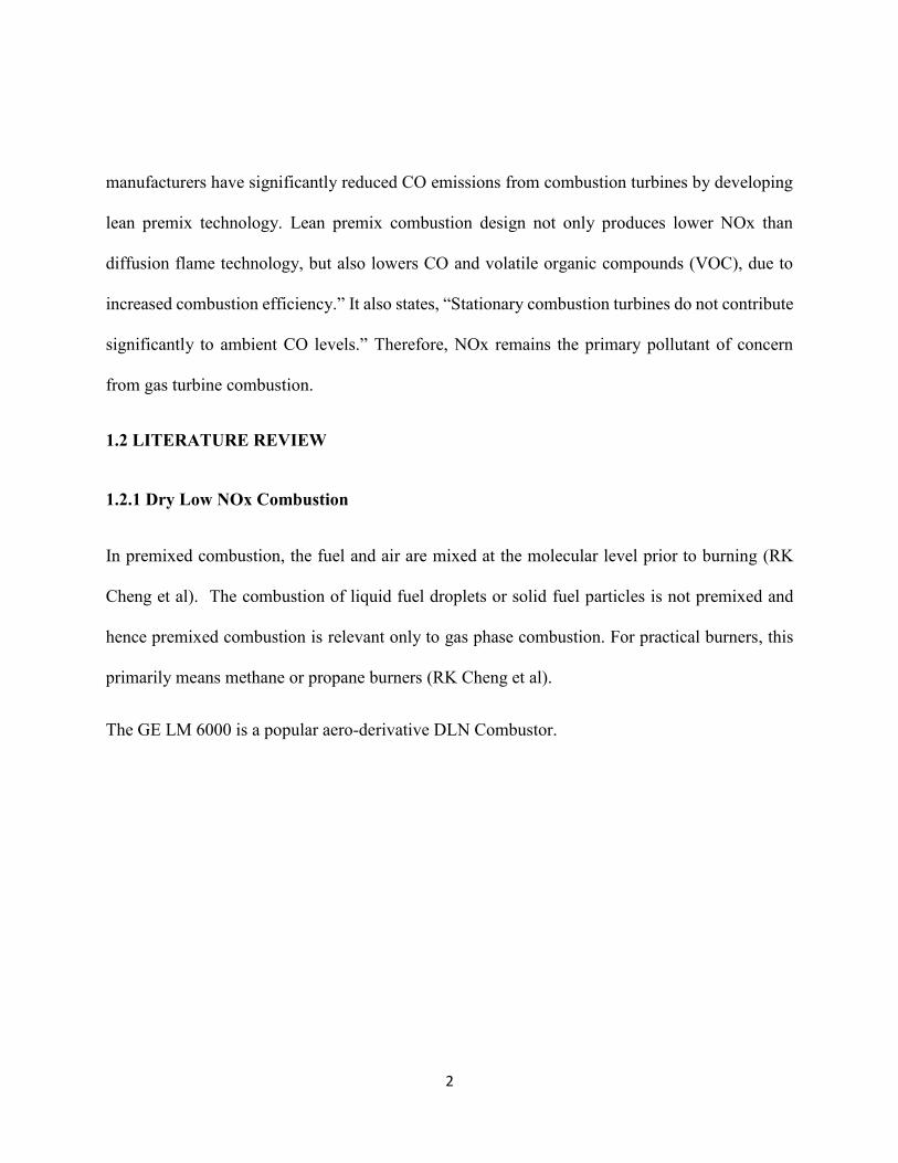
Figure 1.1 : Cross section of GE LM 6000 DLN Combustor (Joshi et al)

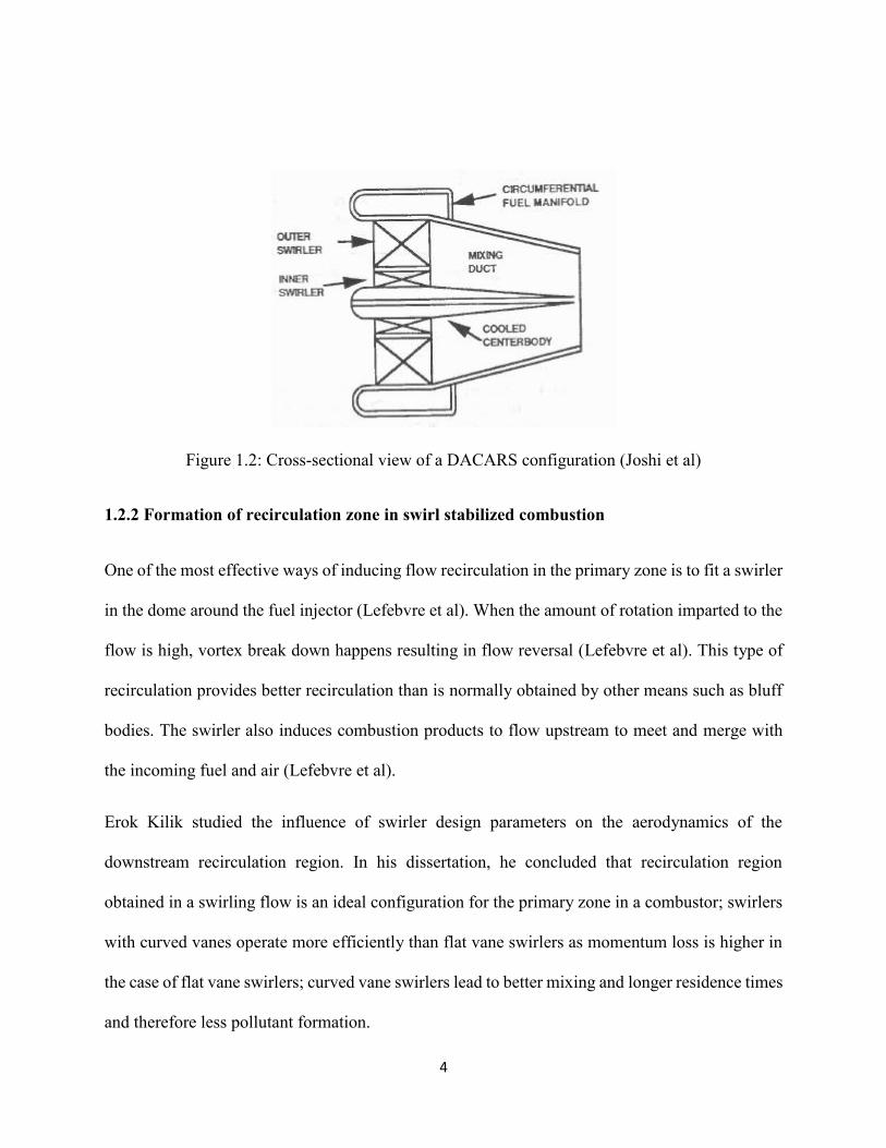
This combustor uses a configuration of Double Annular Counter Rotating Swirler (DACARS)

with a conical centerbody along the centerline of the premixer to supply liquid fuel to an atomizer

at its tip. To prevent flashback, this mixer features a reduction in duct diameter towards the

premixer exit to create an accelerating flow. The area reduction is about 2:1 (Joshi et al)

The objective of this pre-mixer was to produce a homogeneous mixture of fuel and air at the

premixer exit. The LM 6000 pre-mixer shown in the figure has fuel injection holes on the swirl

vanes of the outer swirler. Fuel is injected through three holes in the trailing edge of each outer

swirl vane and one hole in the outer wall of the mixing duct in between each swirl vane (Joshi et

al). To prevent the centerbody from coming in contact with the flame, the centerbody is made

shorter than the mixing duct (Joshi et al).

4

Figure 1.2: Cross-sectional view of a DACARS configuration (Joshi et al)

1.2.2 Formation of recirculation zone in swirl stabilized combustion

One of the most effective ways of inducing flow recirculation in the primary zone is to fit a swirler

in the dome around the fuel injector (Lefebvre et al). When the amount of rotation imparted to the

flow is high, vortex break down happens resulting in flow reversal (Lefebvre et al). This type of

recirculation provides better recirculation than is normally obtained by other means such as bluff

bodies. The swirler also induces combustion products to flow upstream to meet and merge with

the incoming fuel and air (Lefebvre et al).

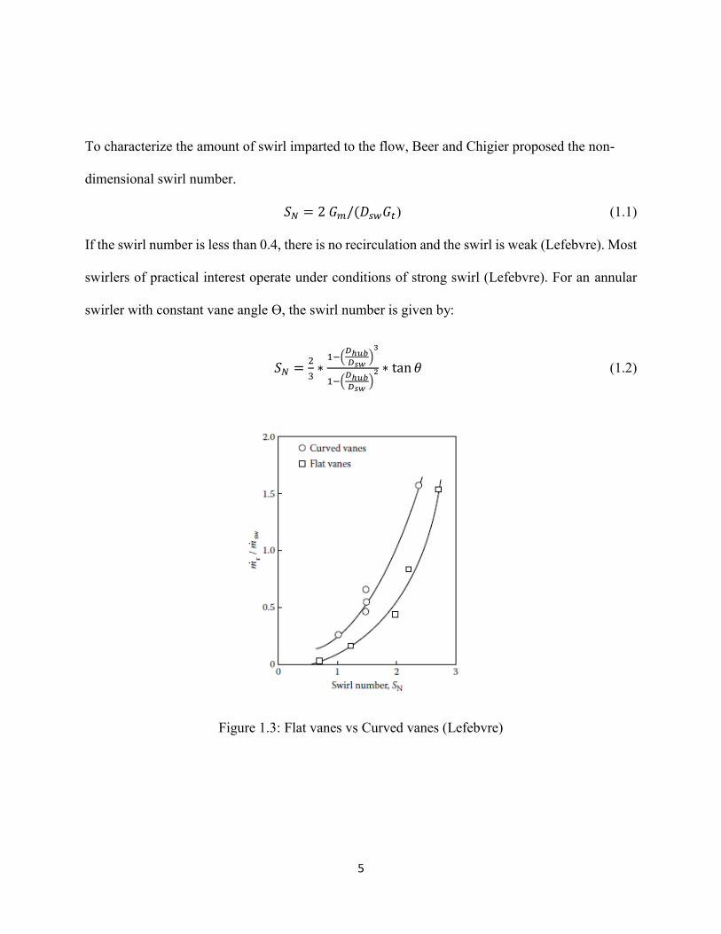
Erok Kilik studied the influence of swirler design parameters on the aerodynamics of the

downstream recirculation region. In his dissertation, he concluded that recirculation region

obtained in a swirling flow is an ideal configuration for the primary zone in a combustor; swirlers

with curved vanes operate more efficiently than flat vane swirlers as momentum loss is higher in

the case of flat vane swirlers; curved vane swirlers lead to better mixing and longer residence times

and therefore less pollutant formation.

5

To characterize the amount of swirl imparted to the flow, Beer and Chigier proposed the non-

dimensional swirl number.

𝑆𝑁 = 2 𝐺𝑚/(𝐷𝑠𝑤𝐺𝑡) (1.1)

If the swirl number is less than 0.4, there is no recirculation and the swirl is weak (Lefebvre). Most

swirlers of practical interest operate under conditions of strong swirl (Lefebvre). For an annular

swirler with constant vane angle ϴ, the swirl number is given by:

𝑆𝑁 =2

3∗

1−(𝐷ℎ𝑢𝑏𝐷𝑠𝑤

)3

1−(𝐷ℎ𝑢𝑏𝐷𝑠𝑤

)2 ∗ tan 𝜃 (1.2)

Figure 1.3: Flat vanes vs Curved vanes (Lefebvre)

6

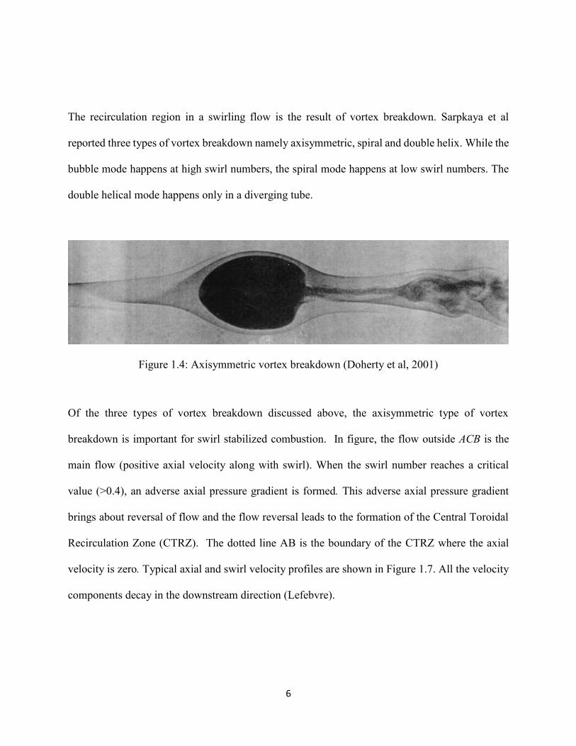
The recirculation region in a swirling flow is the result of vortex breakdown. Sarpkaya et al

reported three types of vortex breakdown namely axisymmetric, spiral and double helix. While the

bubble mode happens at high swirl numbers, the spiral mode happens at low swirl numbers. The

double helical mode happens only in a diverging tube.

Figure 1.4: Axisymmetric vortex breakdown (Doherty et al, 2001)

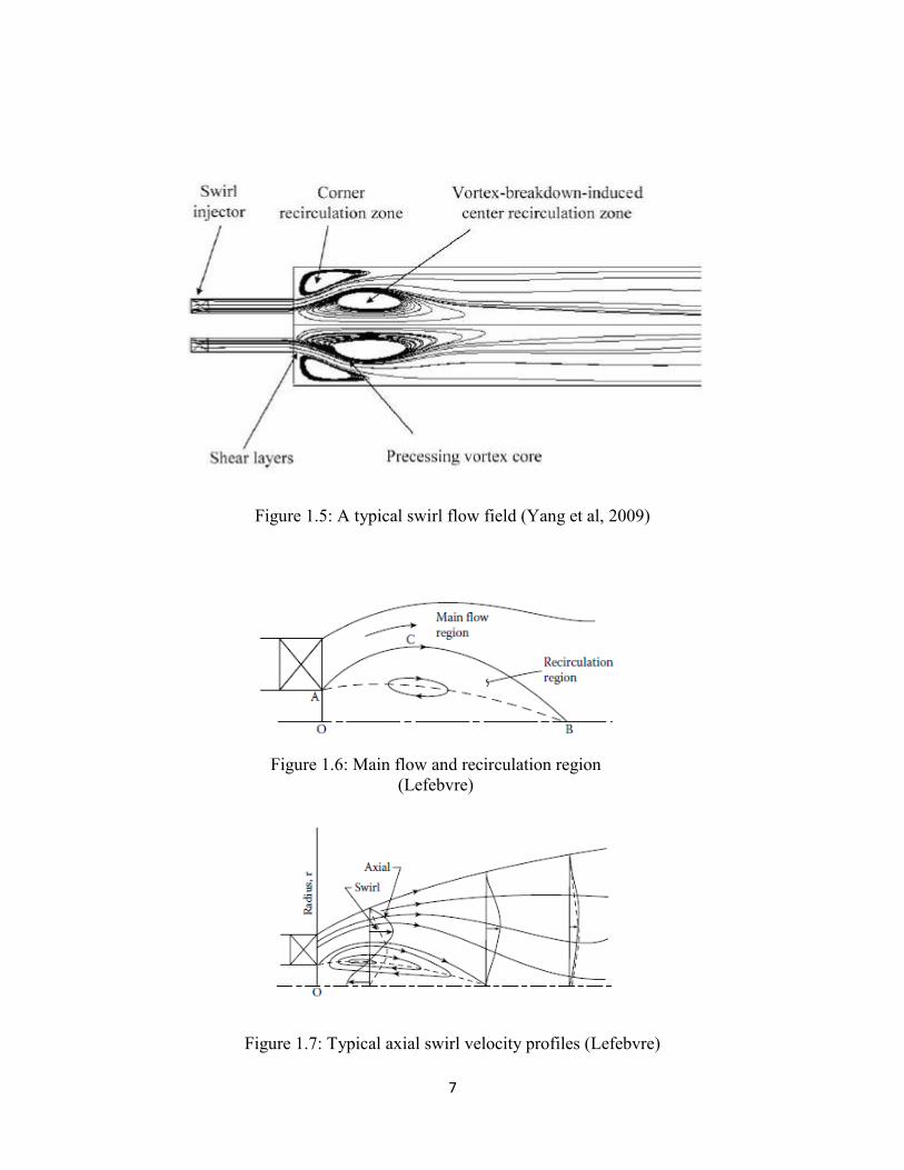
Of the three types of vortex breakdown discussed above, the axisymmetric type of vortex

breakdown is important for swirl stabilized combustion. In figure, the flow outside ACB is the

main flow (positive axial velocity along with swirl). When the swirl number reaches a critical

value (>0.4), an adverse axial pressure gradient is formed. This adverse axial pressure gradient

brings about reversal of flow and the flow reversal leads to the formation of the Central Toroidal

Recirculation Zone (CTRZ). The dotted line AB is the boundary of the CTRZ where the axial

velocity is zero. Typical axial and swirl velocity profiles are shown in Figure 1.7. All the velocity

components decay in the downstream direction (Lefebvre).

7

Figure 1.5: A typical swirl flow field (Yang et al, 2009)

Figure 1.7: Typical axial swirl velocity profiles (Lefebvre)

Figure 1.6: Main flow and recirculation region

(Lefebvre)

8

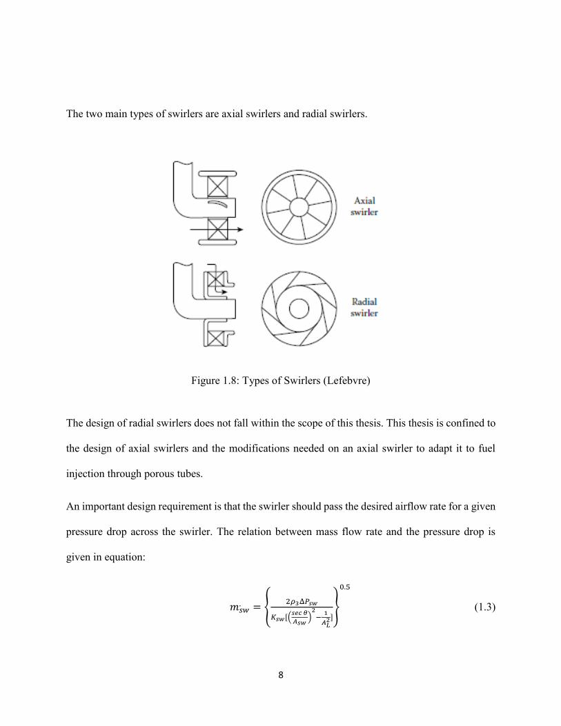
The two main types of swirlers are axial swirlers and radial swirlers.

Figure 1.8: Types of Swirlers (Lefebvre)

The design of radial swirlers does not fall within the scope of this thesis. This thesis is confined to

the design of axial swirlers and the modifications needed on an axial swirler to adapt it to fuel

injection through porous tubes.

An important design requirement is that the swirler should pass the desired airflow rate for a given

pressure drop across the swirler. The relation between mass flow rate and the pressure drop is

given in equation:

𝑚𝑠𝑤. = {

2𝜌3Δ𝑃𝑠𝑤

𝐾𝑠𝑤[(𝑠𝑒𝑐 𝜃

𝐴𝑠𝑤)

2−

1

𝐴𝐿2]

}

0.5

(1.3)

9

𝐴𝑠𝑤 = (𝜋

4) ∗ (𝐷𝑠𝑤

2 − 𝐷ℎ𝑢𝑏2 ) − 0.5𝑛𝑣𝑡𝑣(𝐷𝑠𝑤 − 𝐷ℎ𝑢𝑏) (1.4)

Figure 1.9: Axial swirler notation(Lefebvre)

The figure above shows a flat-vaned swirler whose vane angle is constant and equal to θ. With

curved vane swirlers, the inlet blade angle is zero and the outlet angle is θ.

Table 1-1: Typical swirler specification values (Lefebvre et al)

Vane angle 30° to 60°

Vane thickness 0.7 to 1.5 mm

Number of vanes 8 to 16

𝐾𝑠𝑤 1.3 for flat vanes and 1.15 for curved vanes

ϪP 4 % of atmospheric pressure

10

1.2.3 Mixing of Two Jets

Injecting fuel through a slit into a co-flowing air stream is similar to mixing of two streams

separated by a shear layer. In this project, gaseous fuel is injected through a porous tube from

outside. The gaseous fuel meets the free air stream flowing on the inside of the porous tube. The

fuel that is injected through the pores on the porous tube does not have enough momentum to

penetrate the air stream. As a result, the fuel grazes the wall and the mixing is controlled by

turbulence (Non Mee Boon, 2015).

Figure 1.10 : Porous tube parallel flow (Non Mee Boon, 2015)

1.2.4 Fuel injection using Porous tubes

Non-Mee Boon, in his MS thesis, used porous tubes in a swirl injector to inject gaseous fuel. The

experimental set-up used in his thesis is shown in Figure 1.11 & 1.12.

U2, 𝜌2, T2

U1, 𝜌1, T1

Air

Fuel

11

Porous tube (with fuel and air)

Axial Swirler Combustion chamber

Mixing region

The flow expands

suddenly in this region.

Air

Fuel (gaseous

)

Figure 1.11: Experimental set-up for a porous injector (Non Mee Boon, 2015)

Figure 1.12: Sudden flow expansion (Non Mee Boon, 2015)

12

This porous tube injector uses one porous tube for each swirl vane to inject gaseous fuel. The

gaseous fuel from outside meets the air flowing inside the porous tube. In this project, two sets of

porous tubes with different porosities are used and it was determined that the porosity size (7

micron and 30 micron) does not influence the fuel air mixing distribution. In this design, the flow

suddenly expands as it passes from the porous tube into the swirler leading to a possible

recirculation region inside the swirler as shown in Figure 1.12.

1.2.5 Particle Image Velocimetry

PIV is an experimental technique that uses a sheet of laser to illuminate a plane in a flow

field for a short duration (of the order of micro-seconds). The flow is seeded with tiny alumina

particles. When the laser sheet illuminates a plane in the flow field, a digital camera captures a

frame of the flow field and saves it. After a specified time duration (usually a couple of micro-

seconds), the laser pulses again and the camera captures another frame of the flow field. The PIV

software compares the two frames taken in quick succession to calculate the movement of the tiny

alumina particles that were illuminated by the laser pulse. The software uses the displacement of

the particles in a given direction and the time duration between the laser pulses to calculate the

velocity of the particles in that direction. Since the particles are small enough to faithfully follow

the flow, the velocity of the particles at a location is the velocity of the fluid at that location.

The laser pulse acts as a photographic flash for the digital camera. The laser light serves two

purposes. It avoids blurred images and helps focus the laser beam into a thin light sheet. A thin

light sheet is essential in PIV to illuminate the seeder particles in a plane. To obtain high light

13

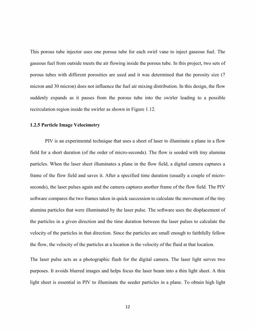
energy within a short duration, a pulsed laser is used in PIV (LaVision website/Velocimetry

website). A New Wave Research Solo 120 XT PIV laser is used for this project.

The number of pulses that a laser can deliver per second is the Pulse Repetition Rate of the laser.

The Solo 120 XT laser has a repetition rate of 15 Hz. A cylindrical lens generates the thin sheet

of laser light from a laser beam to illuminate a plane of the flow field.

Figure 1.13: Particle Image Velocimetry – Concept (Dantec Dynamics)

14

For PIV, a special CCD camera that can transfer the first frame fast enough to be ready to capture

the second frame is used. The LaVision Imager Intense PIV camera used for this project has a

frame rate of 10 Hz and a resolution of 1376 X 1040 pixels.

The tracer particles chosen for PIV should be small enough to faithfully follow the flow but large

enough to scatter the laser beam. The ability of a particle to faithfully follow a flow is given by the

Stokes number. In this project, alumina particles are used as tracers.

Measurement volume refers to the area of interest in the flow field. The velocity vectors are

obtained only for this area in the flow field.

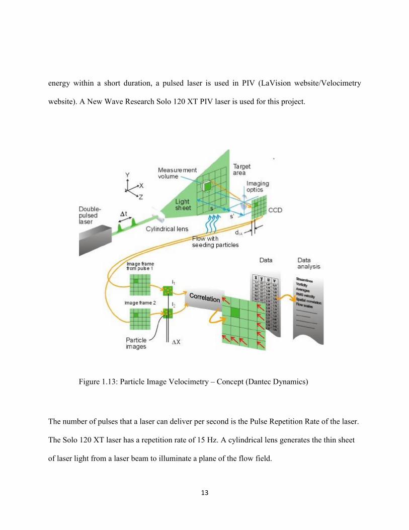
For vector calculation, the PIV software divides the image into a number of interrogation windows.

The default interrogation window is square. The size of the interrogation window is determined

such that all particles within this area have moved homogeneously in the same direction and the

same distance. For good results, the number of particles within one interrogation window should

be at least ten (LaVision). 32 X 32 and 64 X 64 are some of the common interrogation window

sizes.

Figure 1.14: Interrogation window (LaVision)

15

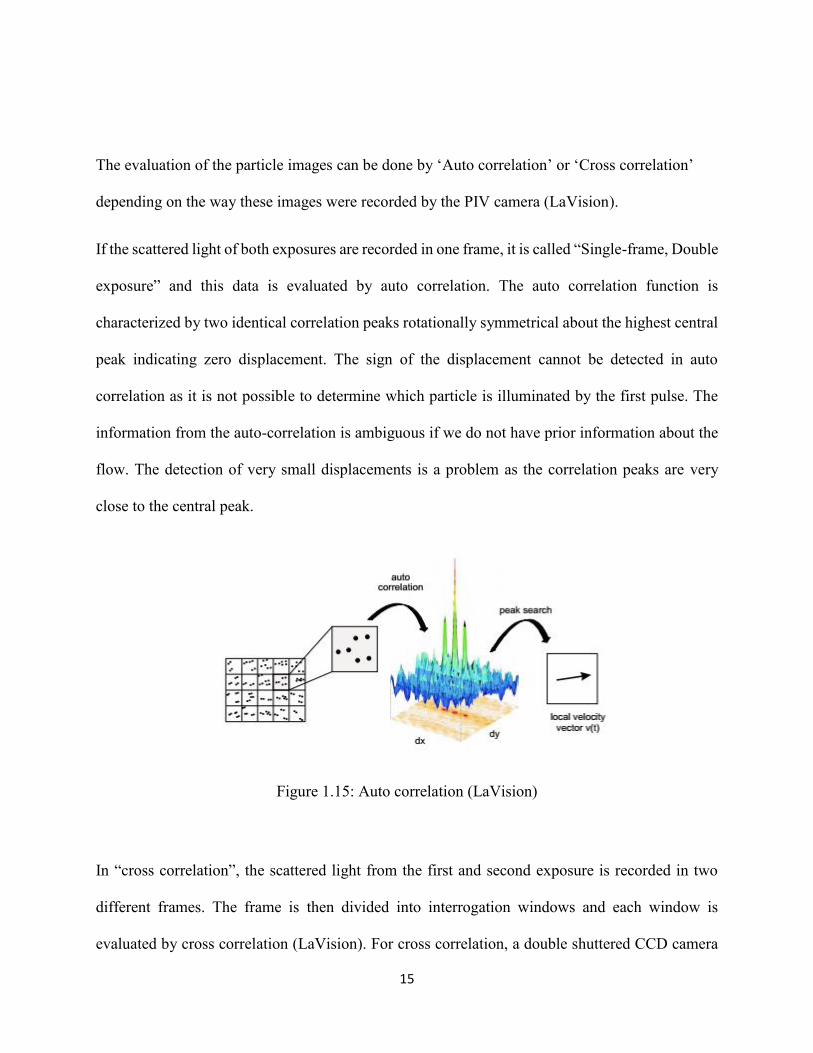
The evaluation of the particle images can be done by ‘Auto correlation’ or ‘Cross correlation’

depending on the way these images were recorded by the PIV camera (LaVision).

If the scattered light of both exposures are recorded in one frame, it is called “Single-frame, Double

exposure” and this data is evaluated by auto correlation. The auto correlation function is

characterized by two identical correlation peaks rotationally symmetrical about the highest central

peak indicating zero displacement. The sign of the displacement cannot be detected in auto

correlation as it is not possible to determine which particle is illuminated by the first pulse. The

information from the auto-correlation is ambiguous if we do not have prior information about the

flow. The detection of very small displacements is a problem as the correlation peaks are very

close to the central peak.

Figure 1.15: Auto correlation (LaVision)

In “cross correlation”, the scattered light from the first and second exposure is recorded in two

different frames. The frame is then divided into interrogation windows and each window is

evaluated by cross correlation (LaVision). For cross correlation, a double shuttered CCD camera

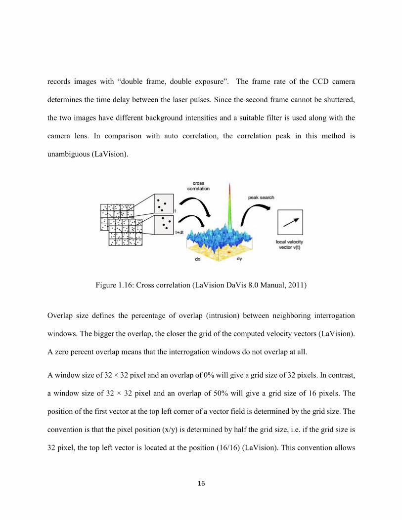
16

records images with “double frame, double exposure”. The frame rate of the CCD camera

determines the time delay between the laser pulses. Since the second frame cannot be shuttered,

the two images have different background intensities and a suitable filter is used along with the

camera lens. In comparison with auto correlation, the correlation peak in this method is

unambiguous (LaVision).

Figure 1.16: Cross correlation (LaVision DaVis 8.0 Manual, 2011)

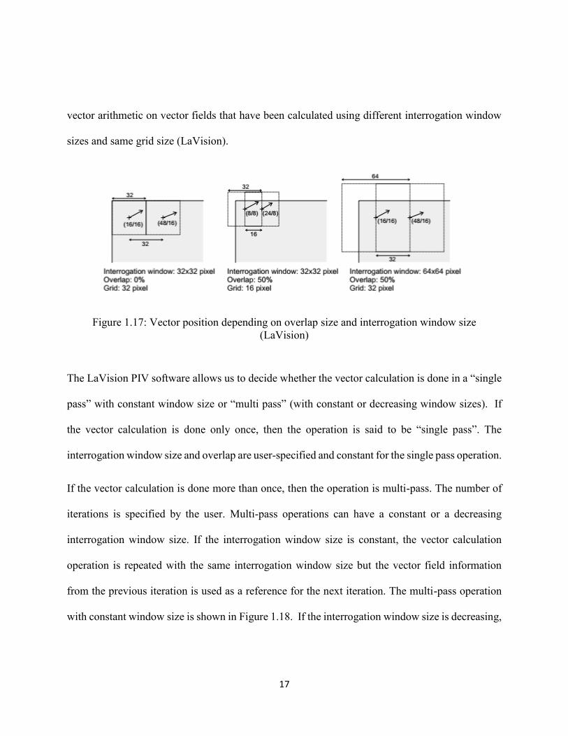
Overlap size defines the percentage of overlap (intrusion) between neighboring interrogation

windows. The bigger the overlap, the closer the grid of the computed velocity vectors (LaVision).

A zero percent overlap means that the interrogation windows do not overlap at all.

A window size of 32 × 32 pixel and an overlap of 0% will give a grid size of 32 pixels. In contrast,

a window size of 32 × 32 pixel and an overlap of 50% will give a grid size of 16 pixels. The

position of the first vector at the top left corner of a vector field is determined by the grid size. The

convention is that the pixel position (x/y) is determined by half the grid size, i.e. if the grid size is

32 pixel, the top left vector is located at the position (16/16) (LaVision). This convention allows

17

vector arithmetic on vector fields that have been calculated using different interrogation window

sizes and same grid size (LaVision).

Figure 1.17: Vector position depending on overlap size and interrogation window size

(LaVision)

The LaVision PIV software allows us to decide whether the vector calculation is done in a “single

pass” with constant window size or “multi pass” (with constant or decreasing window sizes). If

the vector calculation is done only once, then the operation is said to be “single pass”. The

interrogation window size and overlap are user-specified and constant for the single pass operation.

If the vector calculation is done more than once, then the operation is multi-pass. The number of

iterations is specified by the user. Multi-pass operations can have a constant or a decreasing

interrogation window size. If the interrogation window size is constant, the vector calculation

operation is repeated with the same interrogation window size but the vector field information

from the previous iteration is used as a reference for the next iteration. The multi-pass operation

with constant window size is shown in Figure 1.18. If the interrogation window size is decreasing,

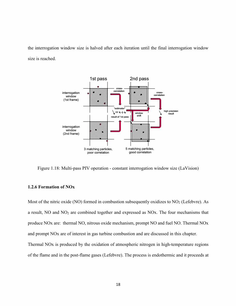
18

the interrogation window size is halved after each iteration until the final interrogation window

size is reached.

Figure 1.18: Multi-pass PIV operation - constant interrogation window size (LaVision)

1.2.6 Formation of NOx

Most of the nitric oxide (NO) formed in combustion subsequently oxidizes to NO2 (Lefebvre). As

a result, NO and NO2 are combined together and expressed as NOx. The four mechanisms that

produce NOx are: thermal NO, nitrous oxide mechanism, prompt NO and fuel NO. Thermal NOx

and prompt NOx are of interest in gas turbine combustion and are discussed in this chapter.

Thermal NOx is produced by the oxidation of atmospheric nitrogen in high-temperature regions

of the flame and in the post-flame gases (Lefebvre). The process is endothermic and it proceeds at

19

a significant rate only at temperatures above around 1850 K (Lefebvre). Thermal NOx is produced

by the extended Zeldovich mechanism which is given below.

O2 = 2O (1.5)

O + N2 ↔ NO + N (1.6)

N + O2 ↔ NO + O (1.7)

N + OH ↔ NO + H (1.8)

Thermal NOx increases exponentially with flame temperature and the dependence is shown in

the figure. Inlet air temperature and residence time also influence NOx formation.

Figure 1.19: NOx vs Time (Lefebvre)

Prompt NOx is prevalent in rich flames. Under certain conditions, NO is found very early in the

flame region (Lefebvre).

20

N2 + CH = HCN + N (1.9)

Under lean-premixed conditions, the HCN oxidizes to NO mainly by a sequence of reactions

involving HCN → CN →NCO → NO (Lefebvre)

The California Analytical Instruments 600 CLD emission analyzer is used for the

measurement (dry analysis) of NO and NO2. The analyzer uses the principle of chemiluminescence

for analyzing the NO or NOx concentration of a gaseous sample. In the NO mode, the

chemiluminescent reaction between ozone and NO produces NO2 and oxygen. The intensity of the

light produced by this reaction is proportional to the mass flow rate of the NO2 into the reaction

chamber and is measured by a photodiode and amplification electronics. In the NOx mode, an

internal NO2 to NO convertor converts the NO2 in the sample to NO and then the NO concentration

is measured like it is done in the NO mode.

The California Analytical Instruments 600 NDIR emission analyzer is used for the analysis

of CO and CO2. The method of operation is based on the infrared absorption characteristics of the

gas. The analyzer uses a single infrared beam to measure the gas concentration. The beam is

modulated by a chopper system and is passed through a sample cell of predetermined length

containing the gas sample (CO/CO2). As the beam passes through the cell, the sample gas absorbs

some of the energy of the beam. The attenuated beam is then introduced into the front chamber of

a two-chamber infra-red microflow detector filled with the sample gas. As a result, the beam

experience further absorption of energy and the pressure increases in both the chambers. The

differential pressure between the front and rear chambers triggers a gas flow between the

chambers. A mass flow sensor detects this gas flow and converts it into an output signal.

21

1.3 SCOPE OF THE THESIS

The objective of this thesis is to design and test the performance an axial swirler that makes use of

porous tube fuel injection. The swirler differs from conventional axial swirlers in the method of

fuel injection. The swirler designed in this thesis incorporates a passage that facilitates a smooth

transition of flow from the porous tube to the swirler. It is this transition region that differentiates

this swirler from conventional axial swirlers.

In Chapter II, the design of the swirler and the experimental set-up are discussed. The PIV set-up

that is used to study the pre-mixer aerodynamics is discussed along with the set-up used for

combustion testing.

In Chapter III, the results of the PIV, flame imaging and emission results are discussed. 2D PIV is

used to characterize the axial, radial and tangential velocities. To measure the radial and tangential

velocities, horizontal plane PIV is done. Axial velocity data and Horizontal plane PIV results are

discussed. A parametric study of center-bodies is conducted to attempt to prevent the recirculation

zone from coming in contact with the injector tip. Combustion testing is done for flame

characterization and NOx emission measurements. The flame images are shown and the NOx

emission results are discussed.

In Chapter IV, future work and recommendations are discussed. A CFD model is attempted using

ANSYS Fluent and the scope for future CFD work is discussed.

22

2. EXPERIMENTAL SET-UP

2.1 SUMMARY

The design and testing of this pre-mixer was done at the Combustion and Fire Research

Laboratory (CFRL) located at the off-campus research facility in Center Hill. The CFRL has eight

test cells. The aerodynamics and combustion testing of this injector was done at Cells 1 & 2

respectively. CFRL has a main compressor that supplies air at a pressure of 150 psi with a

maximum flow rate of 2 lb/s. The compressor has a de-moisturizing system and a reservoir. The

air enters the test cells through a 4" pipe. A pressure regulator is used at the entrance of the test

cell to control the mass flow rate. The test cells have an exhaust blower to prevent inhalation of

any hazardous smoke resulting from combustion. The design and assembly of the pre-mixer is also

discussed in this section. The pre-mixer is an assembly of five components and eight porous tubes.

2.1.1 Pre-mixer design

Three pre-mixers are designed as part of this project. Each pre-mixer is an assembly of an axial

swirler, a centerbody and shroud. A plastic pre-mixer (Pre-mixer I) is designed based on 1-D

calculations and rapid proto-typed in ABS. In this pre-mixer, the design feasibility to achieve a

smooth transition from the circular cross sectional area to the trapezoidal inter-vanal space is

checked. Cold flow PIV is conducted for this plastic pre-mixer and the results are used to optimize

the design of the swirler. Based on the PIV results, the design of the swirler and mixing length are

optimized. The redesigned pre-mixer (named pre-mixer II) is rapid proto-typed in plastic. Pre-

mixer II has a different vane profile, centerbody and shroud when compared to Pre-mixer I. The

comparison between Pre-mixer I and Pre-mixer II is shown in the Figure 2.2. Cold flow PIV is

23

conducted for this swirler (pre-mixer II). After studying the cold flow PIV results of the plastic

pre-mixer (Pre-mixer II), it is rapid proto-typed in metal (316L Stainless Steel). There is no

difference in terms of geometry between pre-mixer II and pre-mixer III. The geometry of the

swirler, centerbody and shroud are the same for pre-mixer II and pre-mixer III. Since Pre-mixer II

is used only for cold-flow measurements, it does not have the set-up for porous tubes that is present

in Pre-mixer III. Pre-mixer III assembly is shown in Figure 2.4.

The metal pre-mixer (Pre-mixer III) is used only for combustion testing. For cold flow PIV, the

plastic swirlers are used without the porous tubes as there is no fuel-air mixing (no combustion) in

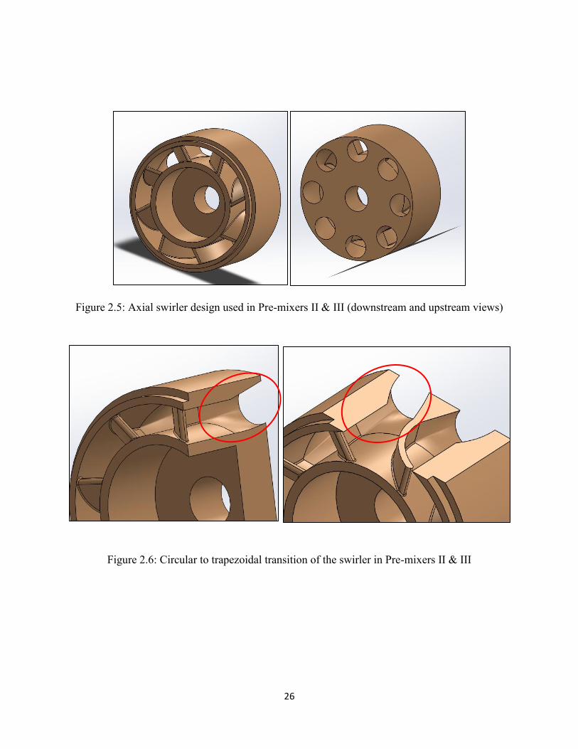
a non-reacting case PIV. The axial swirlers designed in this thesis differs from conventional axial

swirlers in the method of fuel injection. This is shown in Figure 2.5 & 2.6. The number of vanes

in these axial swirlers are the same as the design done by Non-Mee Boon to facilitate carry over

of some auxiliary parts. In conventional axial swirlers, there are holes on the vanes that serve the

purpose of fuel injection (refer GE DLN combustors). In the axial swirlers used in this project,

gaseous fuel is injected through porous tubes (made of sintered stainless steel) aligned in the axial

direction. The porous tubes are directly connected to the space between the vanes. Since the porous

tubes are circular in cross section and the inter-vane space is trapezoidal, the flow needs to

transition from a circular cross section to a trapezoidal cross section. This is achieved by

incorporating a passage that helps the flow transition from a circular cross sectional area to a

trapezoidal cross sectional area as shown in Figures 2.5 & 2.6.

24

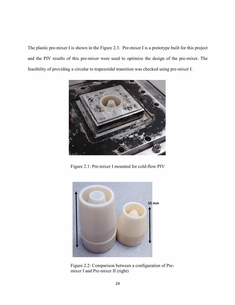
The plastic pre-mixer I is shown in the Figure 2.3. Pre-mixer I is a prototype built for this project

and the PIV results of this pre-mixer were used to optimize the design of the pre-mixer. The

feasibility of providing a circular to trapezoidal transition was checked using pre-mixer I.

Figure 2.1: Pre-mixer I mounted for cold-flow PIV

55 mm

Figure 2.2: Comparison between a configuration of Pre-

mixer I and Pre-mixer II (right)

25

Upstream and downstream side of the axial swirler

Axial swirler modified for porous tube fuel injection

Figure : A cross section of the pre-mixer assembly

Centerbody

Shroud

Axial Swirler

Porous tube

Air Air

Fuel

Circular to trapezoidal transition

Air

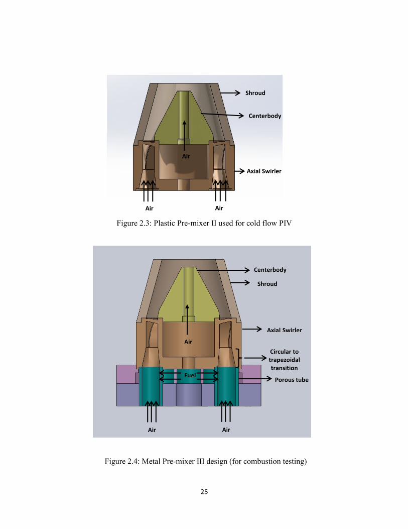
Figure 2.4: Metal Pre-mixer III design (for combustion testing)

Shroud

Centerbody

Axial Swirler

Air Air

Air

Figure 2.3: Plastic Pre-mixer II used for cold flow PIV

26

Figure 2.5: Axial swirler design used in Pre-mixers II & III (downstream and upstream views)

Figure 2.6: Circular to trapezoidal transition of the swirler in Pre-mixers II & III

27

2.1.2 Challenges in using porous tubes for fuel injection

A conventional axial swirler is designed to pass the desired mass flow rate at a given pressure

drop. The diameter of the swirler is varied to achieve the desired mass flow rate at a given pressure

drop. In this swirler, an increase in the diameter of the swirler will not lead to an increase in mass

flow rate because the effective area of this swirler is determined by the diameter of the porous

tubes that are used for fuel injection. In addition to this, the additional length of the premixer

needed to accommodate the porous tube leads to an increase in resistance to air flow.

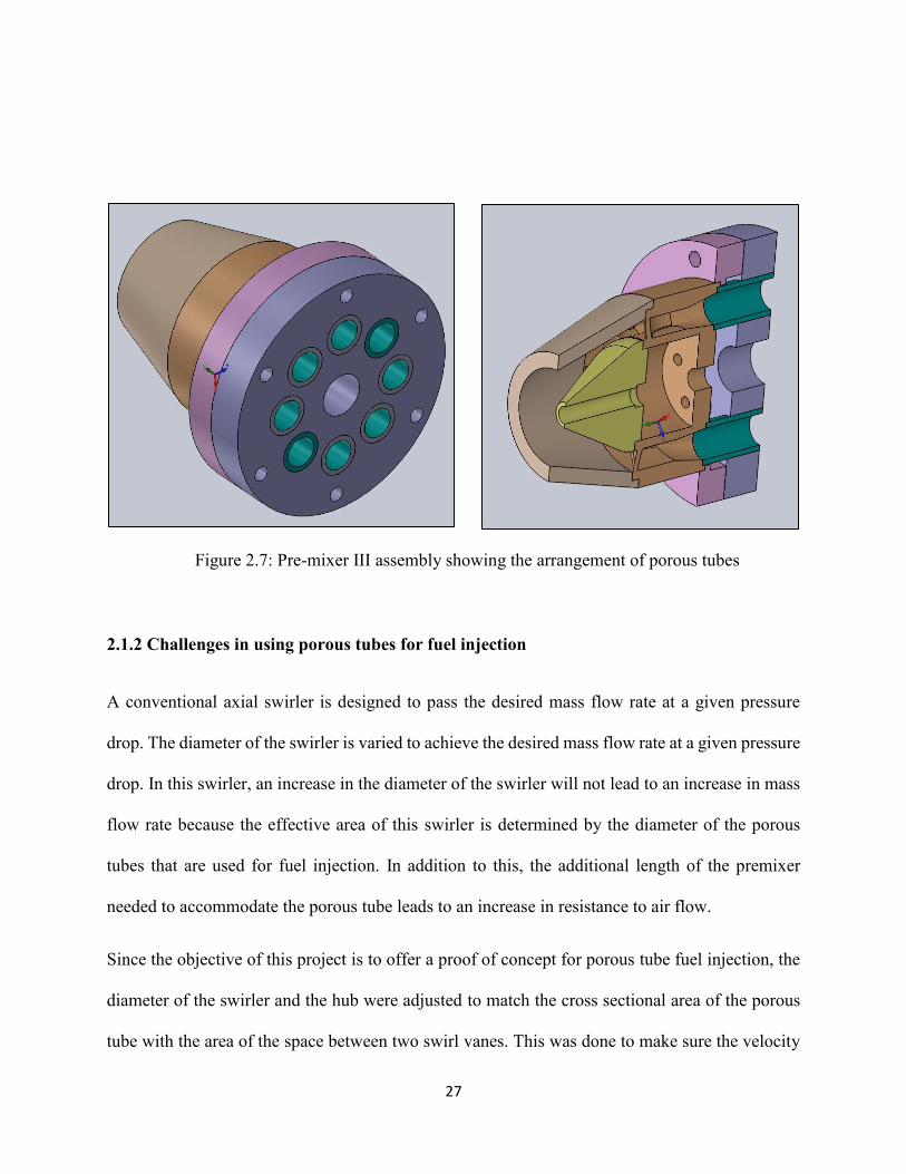
Since the objective of this project is to offer a proof of concept for porous tube fuel injection, the

diameter of the swirler and the hub were adjusted to match the cross sectional area of the porous

tube with the area of the space between two swirl vanes. This was done to make sure the velocity

Figure 2.7: Pre-mixer III assembly showing the arrangement of porous tubes

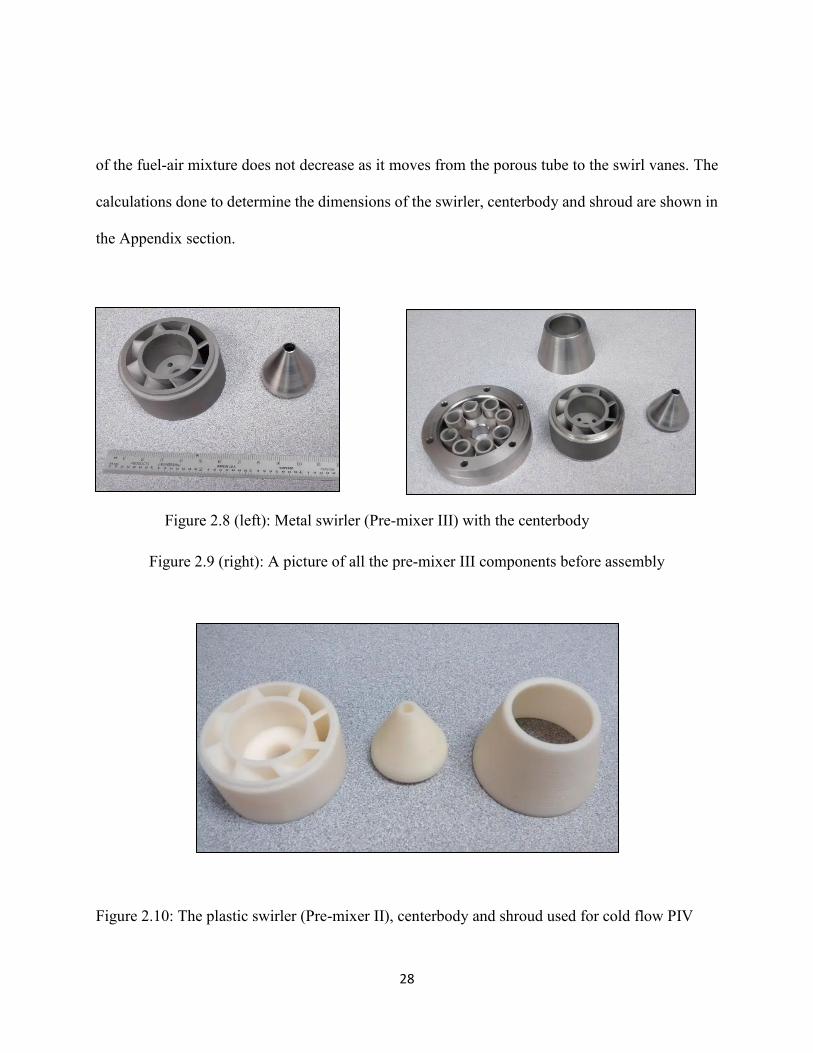
28

of the fuel-air mixture does not decrease as it moves from the porous tube to the swirl vanes. The

calculations done to determine the dimensions of the swirler, centerbody and shroud are shown in

the Appendix section.

Figure 2.9 (right): A picture of all the pre-mixer III components before assembly

Figure 2.8 (left): Metal swirler (Pre-mixer III) with the centerbody

Figure 2.10: The plastic swirler (Pre-mixer II), centerbody and shroud used for cold flow PIV

29

2.1.3 Specifications of the axial swirler

The axial swirler has eight curved vanes with a vane outlet angle of 60° and a vane incidence angle

of 0°. The stagger angle for the vane is 30°. The curved vane follows a circular arc of radius 17.3

mm. The swirler has central blading and the vanes do not have any holes for fuel injection. The

vanes have a constant thickness of 1.5 mm. The trailing edges of the vanes have fillets and the

vane outlet angle was measured before the fillets were given.

30°

60°

Axis of the swirler

Figure 2.11: Vane profile showing vane outlet angle of 60° and

stagger angle of 30°

30

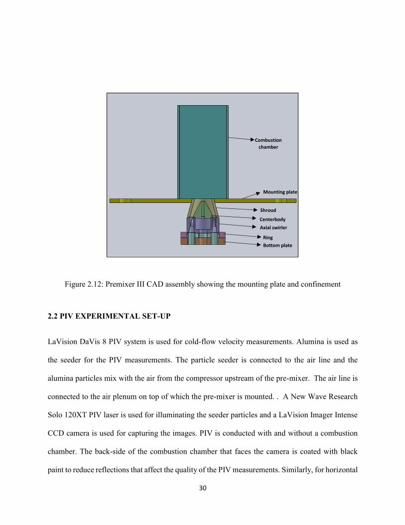
Figure 2.12: Premixer III CAD assembly showing the mounting plate and confinement

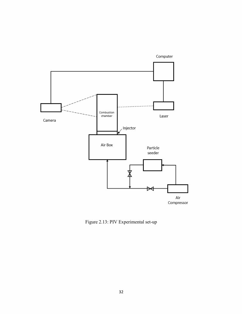
2.2 PIV EXPERIMENTAL SET-UP

LaVision DaVis 8 PIV system is used for cold-flow velocity measurements. Alumina is used as

the seeder for the PIV measurements. The particle seeder is connected to the air line and the

alumina particles mix with the air from the compressor upstream of the pre-mixer. The air line is

connected to the air plenum on top of which the pre-mixer is mounted. . A New Wave Research

Solo 120XT PIV laser is used for illuminating the seeder particles and a LaVision Imager Intense

CCD camera is used for capturing the images. PIV is conducted with and without a combustion

chamber. The back-side of the combustion chamber that faces the camera is coated with black

paint to reduce reflections that affect the quality of the PIV measurements. Similarly, for horizontal

Combustion

chamber

Shroud

Axial swirler

Centerbody

Mounting plate

Ring

Bottom plate

31

plane PIV, the pre-mixer itself is coated with black paint to avoid reflections. Before recording,

the camera lens is focused on the seeder particles using the “live mode” and calibration is

performed by using the PIV calibration plate. Lights are switched off before recording. The PIV

laser is adjusted to a high power mode that delivers 48 mJ per pulse at 532 nm. 200 images are

taken for the case without combustion chamber. For the case with combustion chamber, the

number of images is reduced as the seeder particles soil the glass combustion chamber. The cross

correlation method is used to process PIV data. A constant interrogation window size of 32 X 32

with an overlap of 50% and a two-pass processing is used for the processing of images.

2.3 COMBUSTION EXPERIMENTAL SET-UP

Flame imaging and emission measurement are done at cell 2 of CFRL. The flame images are

captured using the PIV camera. The test rig has a 24 kW heater that can preheat air upto 850°F.

For measuring the dry NOx values, an oil cooled emission testing probe is placed 6 inches above

the exit of the pre-mixer. The temperature of the probe is maintained at 230 °F to avoid water

condensation. The sample is passed through a filter that is maintained at 350 °F and then through

a chiller. The probe is used to measure the emissions at three locations, one inch apart, along a

straight line in the middle of the combustion chamber. The emission values were then averaged

and the average was used for the plots between NOx and Adiabatic flame temperature.

32

Figure 2.13: PIV Experimental set-up

33

3. RESULTS AND DISCUSSION

3.1 PRE-MIXER AERODYNAMICS

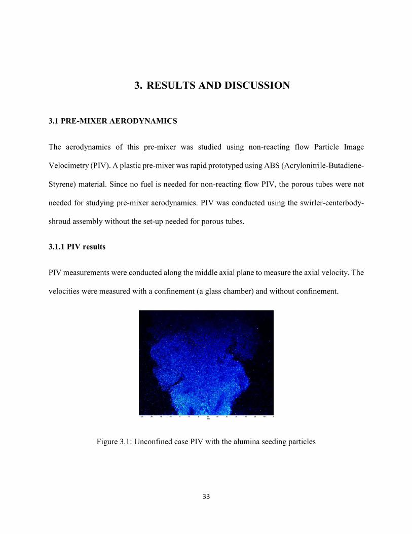
The aerodynamics of this pre-mixer was studied using non-reacting flow Particle Image

Velocimetry (PIV). A plastic pre-mixer was rapid prototyped using ABS (Acrylonitrile-Butadiene-

Styrene) material. Since no fuel is needed for non-reacting flow PIV, the porous tubes were not

needed for studying pre-mixer aerodynamics. PIV was conducted using the swirler-centerbody-

shroud assembly without the set-up needed for porous tubes.

3.1.1 PIV results

PIV measurements were conducted along the middle axial plane to measure the axial velocity. The

velocities were measured with a confinement (a glass chamber) and without confinement.

Figure 3.1: Unconfined case PIV with the alumina seeding particles

34

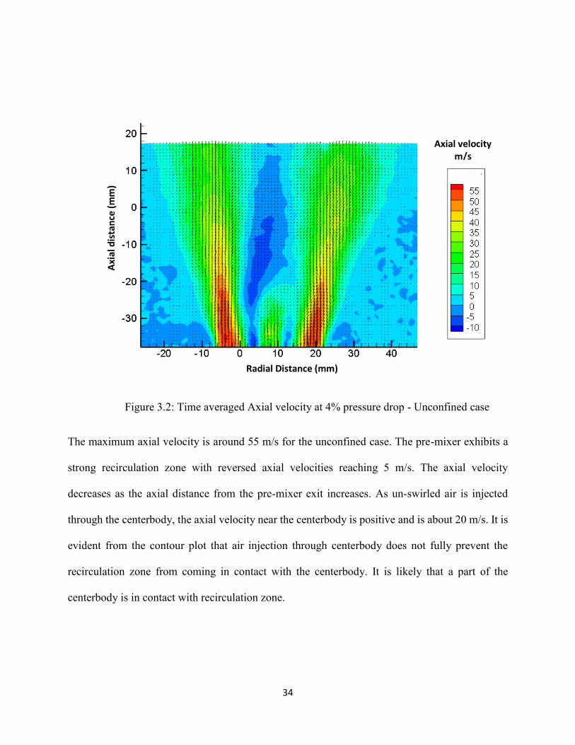
The maximum axial velocity is around 55 m/s for the unconfined case. The pre-mixer exhibits a

strong recirculation zone with reversed axial velocities reaching 5 m/s. The axial velocity

decreases as the axial distance from the pre-mixer exit increases. As un-swirled air is injected

through the centerbody, the axial velocity near the centerbody is positive and is about 20 m/s. It is

evident from the contour plot that air injection through centerbody does not fully prevent the

recirculation zone from coming in contact with the centerbody. It is likely that a part of the

centerbody is in contact with recirculation zone.

Axial velocity m/s

Figure 3.2: Time averaged Axial velocity at 4% pressure drop - Unconfined case

Radial Distance (mm)

Axi

al d

ista

nce

(m

m)

35

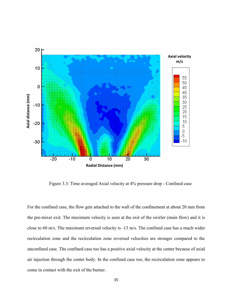
For the confined case, the flow gets attached to the wall of the confinement at about 20 mm from

the pre-mixer exit. The maximum velocity is seen at the exit of the swirler (main flow) and it is

close to 60 m/s. The maximum reversed velocity is -13 m/s. The confined case has a much wider

recirculation zone and the recirculation zone reversed velocities are stronger compared to the

unconfined case. The confined case too has a positive axial velocity at the center because of axial

air injection through the center body. In the confined case too, the recirculation zone appears to

come in contact with the exit of the burner.

Axial velocity m/s

Figure 3.3: Time averaged Axial velocity at 4% pressure drop - Confined case

Radial Distance (mm)

Axi

al d

ista

nce

(m

m)

36

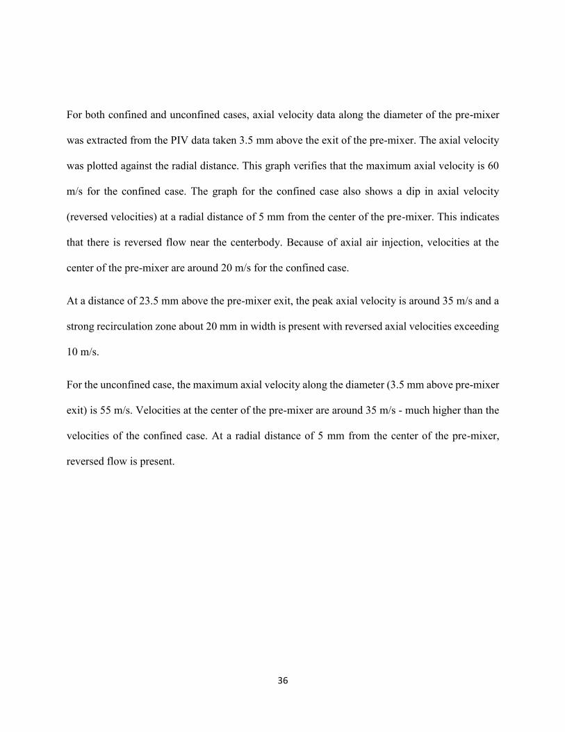
For both confined and unconfined cases, axial velocity data along the diameter of the pre-mixer

was extracted from the PIV data taken 3.5 mm above the exit of the pre-mixer. The axial velocity

was plotted against the radial distance. This graph verifies that the maximum axial velocity is 60

m/s for the confined case. The graph for the confined case also shows a dip in axial velocity

(reversed velocities) at a radial distance of 5 mm from the center of the pre-mixer. This indicates

that there is reversed flow near the centerbody. Because of axial air injection, velocities at the

center of the pre-mixer are around 20 m/s for the confined case.

At a distance of 23.5 mm above the pre-mixer exit, the peak axial velocity is around 35 m/s and a

strong recirculation zone about 20 mm in width is present with reversed axial velocities exceeding

10 m/s.

For the unconfined case, the maximum axial velocity along the diameter (3.5 mm above pre-mixer

exit) is 55 m/s. Velocities at the center of the pre-mixer are around 35 m/s - much higher than the

velocities of the confined case. At a radial distance of 5 mm from the center of the pre-mixer,

reversed flow is present.

37

Figure 3.4: Confined case - Axial velocity variation with radial distance at 3.5 mm above

premixer exit

Figure 3.5: Unconfined case - Axial velocity variation with radial distance at 3.5 mm above

premixer exit

-10

0

10

20

30

40

50

60

70

-35 -25 -15 -5 5 15 25 35

Axi

al v

elo

city

(m

/s)

Radial distance (mm)

-10

0

10

20

30

40

50

60

-35 -25 -15 -5 5 15 25 35

Axi

al v

elo

city

(m/s

)

Radial distance

38

Figure 3.6: Confined case - Axial velocity variation with radial distance (23.5 mm above pre-

mixer exit)

3.1.2 Horizontal plane PIV results

Horizontal plane PIV was conducted by putting the PIV camera on top of the pre-mixer and using

the PIV laser to illuminate the horizontal plane. A set of measurements was taken 5 mm above the

pre-mixer exit and and another set was taken 15 mm above the pre-mixer exit.

-20

-10

0

10

20

30

40

50

-40 -30 -20 -10 0 10 20 30 40 50

Axi

al V

elo

city

(m

/s)

Radial distance (mm)

39

Figure 3.7: Horizontal plane PIV showing the PIV camera mounted on top

Figure 3.8: Horizontal plane PIV showing the illuminated seeder particles on the horizontal plane

40

Vϴ (m/s)

Vϴ (m/s)

5 mm above exit

Figure 3.9: Horizontal plane PIV - Tangential velocity profile

15 mm above exit

Axi

al d

ista

nce

(m

m)

Radial Distance (mm)

41

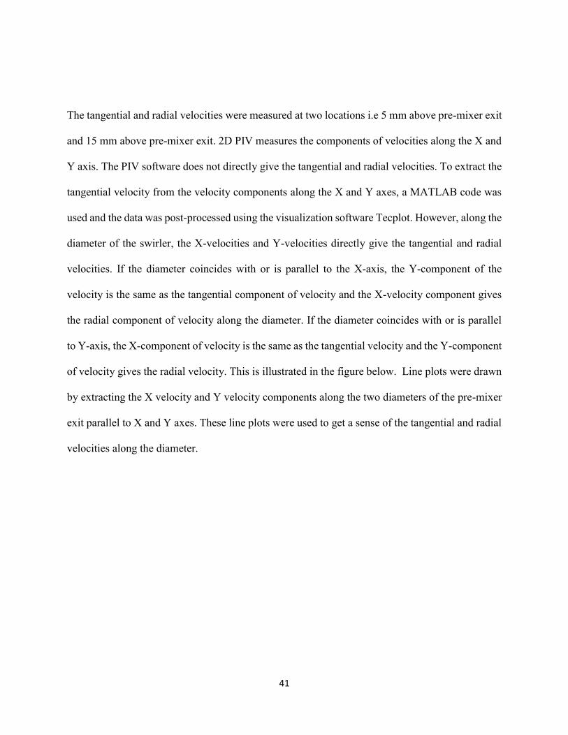
The tangential and radial velocities were measured at two locations i.e 5 mm above pre-mixer exit

and 15 mm above pre-mixer exit. 2D PIV measures the components of velocities along the X and

Y axis. The PIV software does not directly give the tangential and radial velocities. To extract the

tangential velocity from the velocity components along the X and Y axes, a MATLAB code was

used and the data was post-processed using the visualization software Tecplot. However, along the

diameter of the swirler, the X-velocities and Y-velocities directly give the tangential and radial

velocities. If the diameter coincides with or is parallel to the X-axis, the Y-component of the

velocity is the same as the tangential component of velocity and the X-velocity component gives

the radial component of velocity along the diameter. If the diameter coincides with or is parallel

to Y-axis, the X-component of velocity is the same as the tangential velocity and the Y-component

of velocity gives the radial velocity. This is illustrated in the figure below. Line plots were drawn

by extracting the X velocity and Y velocity components along the two diameters of the pre-mixer

exit parallel to X and Y axes. These line plots were used to get a sense of the tangential and radial

velocities along the diameter.

42

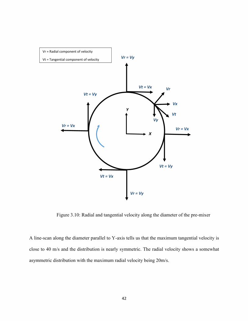
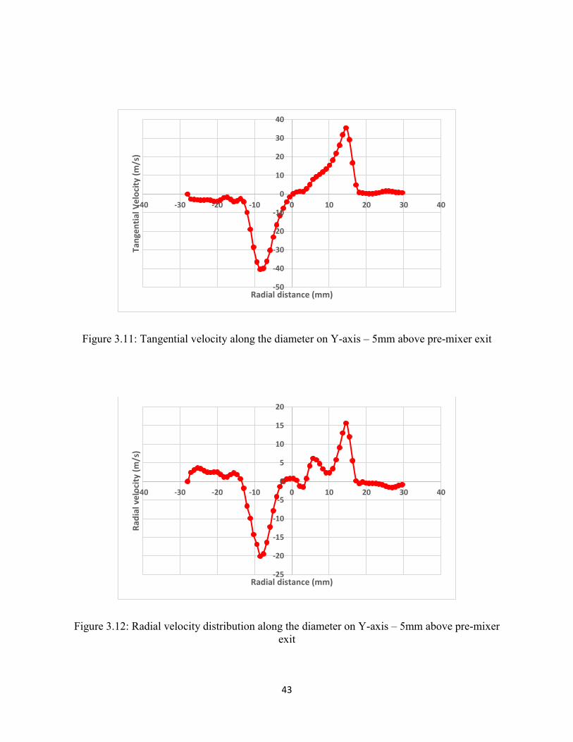
A line-scan along the diameter parallel to Y-axis tells us that the maximum tangential velocity is

close to 40 m/s and the distribution is nearly symmetric. The radial velocity shows a somewhat

asymmetric distribution with the maximum radial velocity being 20m/s.

Vr = Vy

Vr = Vy

Vr = Vx

Vt = Vy

Vt = Vx

Vr = Vx

Vt = Vy

Vt = Vx

Vr

Vt

Vx

Vy

Y

X

Vr = Radial component of velocity

Vt = Tangential component of velocity

Figure 3.10: Radial and tangential velocity along the diameter of the pre-mixer

43

Figure 3.11: Tangential velocity along the diameter on Y-axis – 5mm above pre-mixer exit

Figure 3.12: Radial velocity distribution along the diameter on Y-axis – 5mm above pre-mixer

exit

-50

-40

-30

-20

-10

0

10

20

30

40

-40 -30 -20 -10 0 10 20 30 40

Tan

gen

tial

Ve

loci

ty (

m/s

)

Radial distance (mm)

-25

-20

-15

-10

-5

0

5

10

15

20

-40 -30 -20 -10 0 10 20 30 40

Rad

ial v

elo

city

(m

/s)

Radial distance (mm)

44

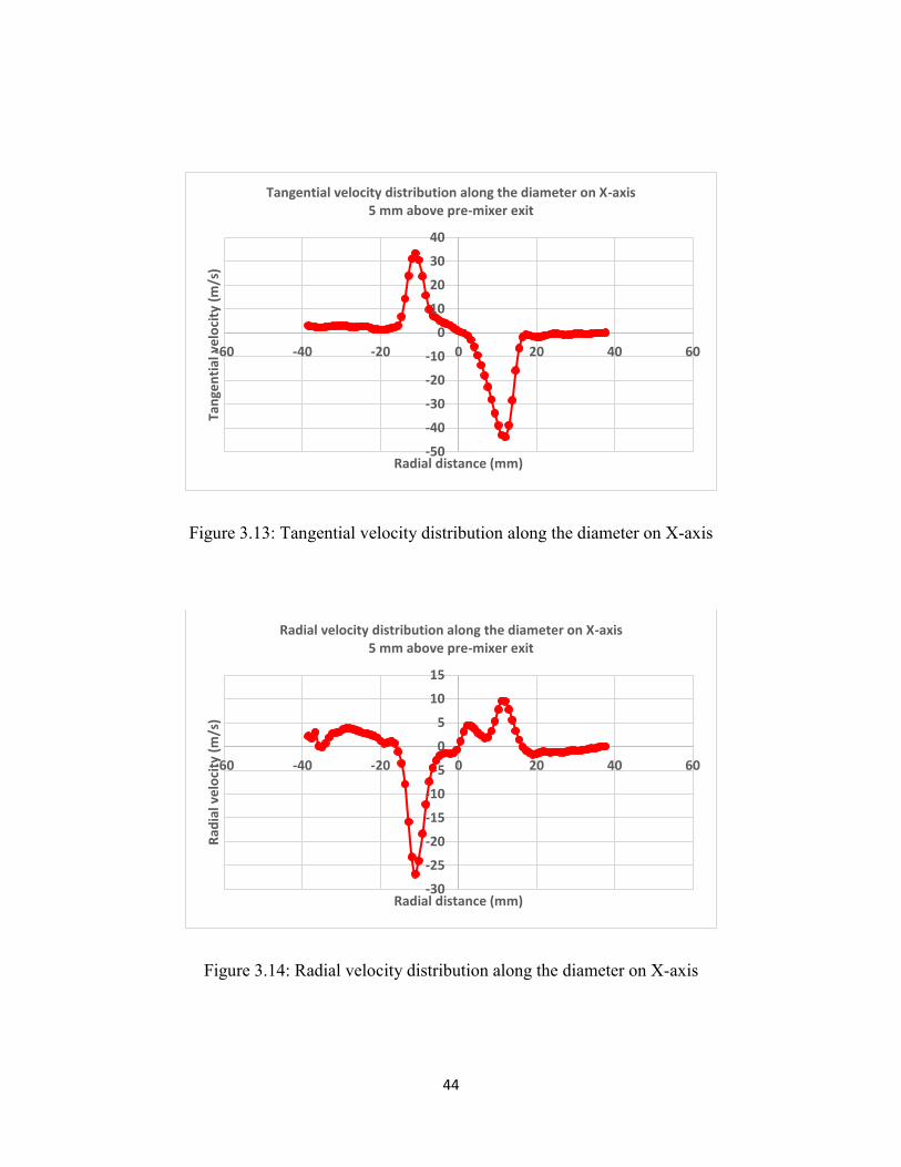
Figure 3.13: Tangential velocity distribution along the diameter on X-axis

Figure 3.14: Radial velocity distribution along the diameter on X-axis

-50

-40

-30

-20

-10

0

10

20

30

40

-60 -40 -20 0 20 40 60

Tan

gen

tial

ve

loci

ty (

m/s

)

Radial distance (mm)

Tangential velocity distribution along the diameter on X-axis5 mm above pre-mixer exit

-30

-25

-20

-15

-10

-5

0

5

10

15

-60 -40 -20 0 20 40 60

Rad

ial v

elo

city

(m

/s)

Radial distance (mm)

Radial velocity distribution along the diameter on X-axis5 mm above pre-mixer exit

45

3.1.3 Parametric study of centerbodies

Since the axial velocity profile at the exit of the pre-mixer suggests that some part of reversed flow

is coming in contact with the exit of the pre-mixer, four configurations of centerbody were rapid-

prototyped in plastic and cold-flow PIV was conducted to study the velocity distribution and the

recirculation zone. The goal of this parametric study was to find out if there is a centerbody

configuration that pushes the recirculation zone away from the exit of the injector. This study was

done with the combustion chamber (with confinement).

The recess distance which is the distance by which the centerbody is “recessed” into the outercone

is varied along with the shape of the hole in the centerbody that is used for axial air injection. The

recess distance was changed by changing the height of the centerbody.

Table 3-1: Parametric study of bluff bodies

Configuration Name Centerbody hole Recess distance

S4 Straight 4 mm

S2 Straight 2 mm

D4 Diverging 4 mm

D2 Diverging 2 mm

46

Straight (or) Diverging

Recess distance

Figure 3.15: Parametric study of center-bodies

D4 - 4 mm Recess distance

Diverging

S4 - 4 mm Recess distance Straight

7 mm 7 mm

5 mm

Figure 3.16: Comparison between Straight hole and Diverging hole center-bodies

47

Figure 3.17: S2 configuration axial velocity profile (time averaged)

Figure 3.18: D4 configuration axial velocity profile (time averaged)

Axial velocity m/s

Axial velocity m/s

Radial Distance (mm)

Radial Distance (mm)

Axi

al d

ista

nce

(m

m)

Axi

al d

ista

nce

(m

m)

48

Figure 3.19: S4 configuration axial velocity profile (time averaged)

Figure 3.20: D2 configuration axial velocity profile (time averaged)

Axial velocity m/s

Axial velocity m/s

Radial Distance (mm)

Radial Distance (mm)

Axi

al d

ista

nce

(m

m)

Axi

al d

ista

nce

(m

m)

49

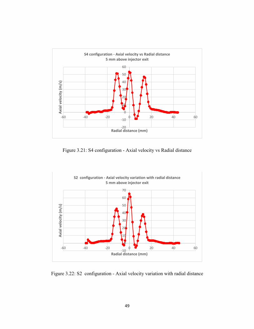
Figure 3.21: S4 configuration - Axial velocity vs Radial distance

Figure 3.22: S2 configuration - Axial velocity variation with radial distance

-20

-10

0

10

20

30

40

50

60

-60 -40 -20 0 20 40 60

Axi

al v

elo

city

(m

/s)

Radial distance (mm)

S4 configuration - Axial velocity vs Radial distance5 mm above injector exit

-10

0

10

20

30

40

50

60

70

-60 -40 -20 0 20 40 60

Axi

al v

elo

city

(m

/s)

Radial distance (mm)

S2 configuration - Axial velocity variation with radial distance5 mm above injector exit

50

From the axial velocity profile of the four configurations, it is evident that S4 comes the closest to

pushing the recirculation away from the exit of the injector. S4 centerbody pushes the recirculation

zone away on one side but the recirculation zone still remains attached to the burner on the other

side. The variation of axial velocity profile 5 mm above the exit of the injector with respect to

radial distance was plotted for two configurations S4 and S2. The peak axial velocity through the

S2 centerbody was around 65 m/s. On the other hand, the axial velocity through the S4 centerbody

is 55 m/s. Since the S4 configuration has a recess distance of 4 mm, the axial flow through the

centerbody starts interacting with the swirl flow earlier than the S2 configuration which has a

recess distance of 2 mm. As the flow starts to interact with the swirl flow earlier than S2

configuration, the axial velocity slows down by 10 m/s for the S4 configuration. The flow from

the S4 centerbody also diverges and this is the reason why the recirculation zone is pushed farther

from the exit of the injector on one side. For the D2 and D4 configurations, the axial velocity is

low and the recirculation zone remains fully attached to the exit of the injector on both sides.

51

3.2 COMBUSTION TESTING

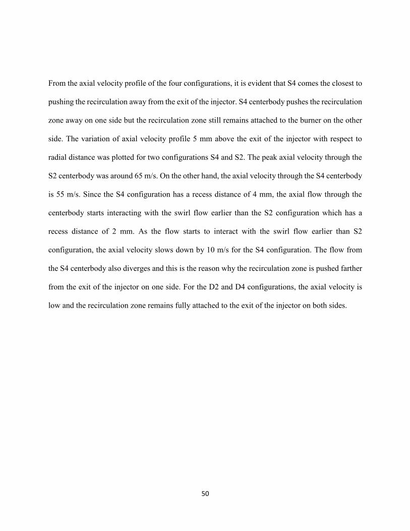
3.2.1 Flame characterization

The PIV camera is used to take images of the flame at different equivalence ratios and pre-heat

temperatures. The flame images are shown in Figure 3.23 . At an equivalence ratio of 0.55, the

flame is present in the recirculation zone and regions with low positive axial velocities because of

the lower turbulent flame speed. As the equivalence ratio is increased, the flame becomes brighter

because of higher heat release. The reaction zone is approximately 75 mm in length for the cases

where the equivalence ratio is 0.65.

400°F and 4% atm pressure drop

Φ = 0.55 Φ = 0.6 Φ = 0.65

52

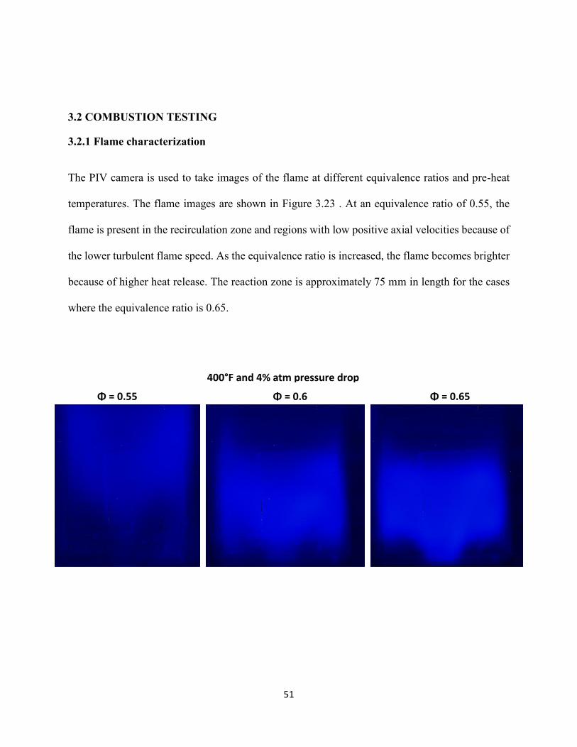
3.2.2 NOx emission measurement

The NOx emissions are measured at three different air pre-heat temperatures namely 400 °F, 500

°F and 600 °F. For each pre-heat temperature the emissions are measured at three different

equivalence ratios namely 0.55, 0.6 and 0.65. The emission is measured at three locations along a

500°F and 4% atm pressure drop

Φ = 0.55 Φ = 0.6 Φ = 0.65

600°F and 4% atm pressure drop

Φ = 0.55 Φ = 0.6 Φ = 0.65

Figure 3.23: Flame imaging

53

straight line inside the combustor and the emissions are averaged. The measurements are done at

a pressure drop of 4%. The air flow rate is calculated at different pre-heat temperatures and the

corresponding fuel-flow rate is calculated for a given equivalence ratio. The air flow rates and fuel

flow rates at different pre-heat temperatures and equivalence ratios are given in the table below.

Table 3-2: Air flow rate and Fuel flow rate at different pre-heat temperatures

Air pre-heat

Temperature Air flow rate

(lb/hr) Fuel flow rate (lb/hr)

°F K Φ0.55 Φ0.6 Φ0.65

400 477.59 141.95 4.54 4.95 5.36

500 533.15 134.35 4.30 4.69 5.08

600 588.71 127.86 4.09 4.46 4.83

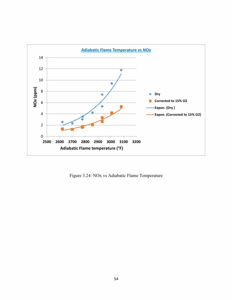
The adiabatic flame temperature is calculated for a given temperature and equivalence ratio using

an online tool (Adiabatic Flame temperature calculator, CERFACS website) and the NOx values

are plotted as a function of the Adiabatic Flame Temperature. The NOx values (dry) are corrected

to 15% O2 based on Equation 2.0 and both the values are shown in the plot in Figure 3.24. For an

Adiabatic Flame Temperature of 2900 °F, the NOx emissions are around 2.5 ppm.

𝑋𝑁𝑂𝑥,𝑑𝑟𝑦 (15% 𝑂2) = (𝑋𝑁𝑂(𝑑𝑟𝑦) + 𝑋𝑁𝑂2(𝑑𝑟𝑦)).20.9 − 15

20.9 − 𝑋𝑂2,%𝑑𝑟𝑦

(2.0)

54

Figure 3.24: NOx vs Adiabatic Flame Temperature

0

2

4

6

8

10

12

14

2500 2600 2700 2800 2900 3000 3100 3200

NO

x (p

pm

)

Adiabatic Flame temperature (°F)

Adiabatic Flame Temperature vs NOx

Dry

Corrected to 15% O2

Expon. (Dry )

Expon. (Corrected to 15% O2)

55

4. FUTURE WORK AND RECOMMENDATIONS

CFD simulations can be used to identify a center-body configuration that pushes the recirculation

zone fully away from the pre-mixer exit. Initial simulations were run for this purpose using

ANSYS FLUENT. The flow domain is shown in the figure below.

The CFD model needs further refinement to be able to predict the center-body configuration that

prevents the recirculation zone from attaching to the pre-mixer exit.

Figure 4.1: CFD flow domain for the pre-mixer

56

57

REFERENCES

Lefebvre, A. H. and Ballal D. R (2010), Gas turbine combustion (Third Edition), CRC press.

Joshi N, Epstein M, Durlak S, Marakovits S & Sabla P (1994), Development of a Fuel Air Premixer

for Aeroderivative Dry Low Emissions Combustors (94-GT-253), ASME paper

Non Mee Boon (2015), Design and Development of a Porous Injector for Gaseous Fuels Injection

in Gas Turbine Combustor, MS Thesis, University of Cincinnati.

Bender W. R, Lean Pre-mixed Combustion (3.2.1.2), The Gas Turbine Handbook, National Energy

Technology Laboratory

M.R. Johnson, R.K. Cheng and L.W. Kostiuk (1994), Low NOx Production through Lean

Premixed Combustion, American Flame Research Committee, Kingston, Canada, April 17-19,

1994

LaVision DaVis 8.0, PIV Flowmaster Product Manual, 2011

CAI 600 series Emission analyzer, Product Data Sheet

Erol Kilik, The influence of swirler design parameters on the aerodynamics of the downstream

recirculation (1976), PhD Thesis, Cranfield Institute of Technology.

Adrian R, Westerweel J (2011), “Particle image velocimetry”, Cambridge University Press, New

York.

Huang Y & Yang V (2009), Dynamics and stability of lean-premixed swirl-stabilized combustion,

Progress in Energy and Combustion Science (pg 293-364)

Swirl flows (1986), A. K. Gupta, D. G. Lilley, and N. Syred, Abacus Press

Sarpkaya T (1971), On stationary and travelling vortex breakdowns, J . Fluid Mech. (1971), vol.

45, part 3, pp. 545-559

Lucca-Negro O & O'Doherty T (2001), Vortex breakdown: a review, Progress in Energy and

Combustion Science, Volume 27, Issue 4, 2001, Pages 431–481

Particle Image Velocimetry, Online velocimetry portal (www.velocimetry.net)

Measurement principles of PIV, Dantec Dynamics website (www.dantecdynamics.com)

Evolution of best available control technology, Appendix 8.1E, California Energy Commission

58

Adiabatic Flame temperature calculator, CERFACS website

(http://elearning.cerfacs.fr/combustion/tools/adiabaticflametemperature/index.php)

Jianing Li, Mahmoud Hamza, Arul Kumaran, Umesh Bhayaraju and San-Mou Jeng (2016),

Study of development of a Novel Dual Phase Airblast injector for a Gas Turbine Combustor,

ASME Turbo Expo 2016: Turbomachinery Technical Conference and Exposition (GT2016-

56340), Seoul, South Korea.

Mahmoud Hamza, Arul Kumaran, Jianing Li, Umesh Bhayaraju and San-Mou Jeng (2016),

Investigation of a Novel Fuel Injector for a Dry Low NOx combustor, ASME Turbo Expo 2016:

Turbomachinery Technical Conference and Exposition (GT2016-56722), Seoul, South Korea.

Umesh Bhayaraju, Mahmoud Hamza, San-Mou Jeng (2017), Development of Porous Injection

Technology(PIT) to reduce emissions for DLN combustors (Micromixer and Swirl injectors),

ASME Turbo Expo 2017: Turbomachinery Technical Conference and Exposition (GT2017-

63976 - draft submitted)

Stephen Turns, An Introduction to Combustion: Concepts and Applications (Third Edition), The

McGraw Hill Companies

59

APPENDIX

Cross sectional Area of the eight porous tubes

Radius of the porous tube = 4.5 mm

Cross sectional Area 𝐴 = 𝜋𝑟2

𝐴 = 𝜋 ∗ 4.5 ∗ 4.5 = 63.585 𝑚𝑚2

Area of the eight porous tubes = 63.585 ∗ 8 = 508.68 𝑚𝑚2

Area of the trapezoidal space between the vanes

The area of the trapezoidal space between the vanes can be directly measured by Solidworks

Area of the trapezoidal space between two vanes = 78 𝑚𝑚2

Area of the trapezoidal space between the vanes for the swirler = 78 ∗ 8 = 624 𝑚𝑚^2

Increase in Area as the circular hole transitions into a trapezoidal space

= 624

508.68= 1.226 = 22.6%.

As the air-fuel mixture moves from the circular hole to the trapezoidal space, the velocity comes

down by 22.6%

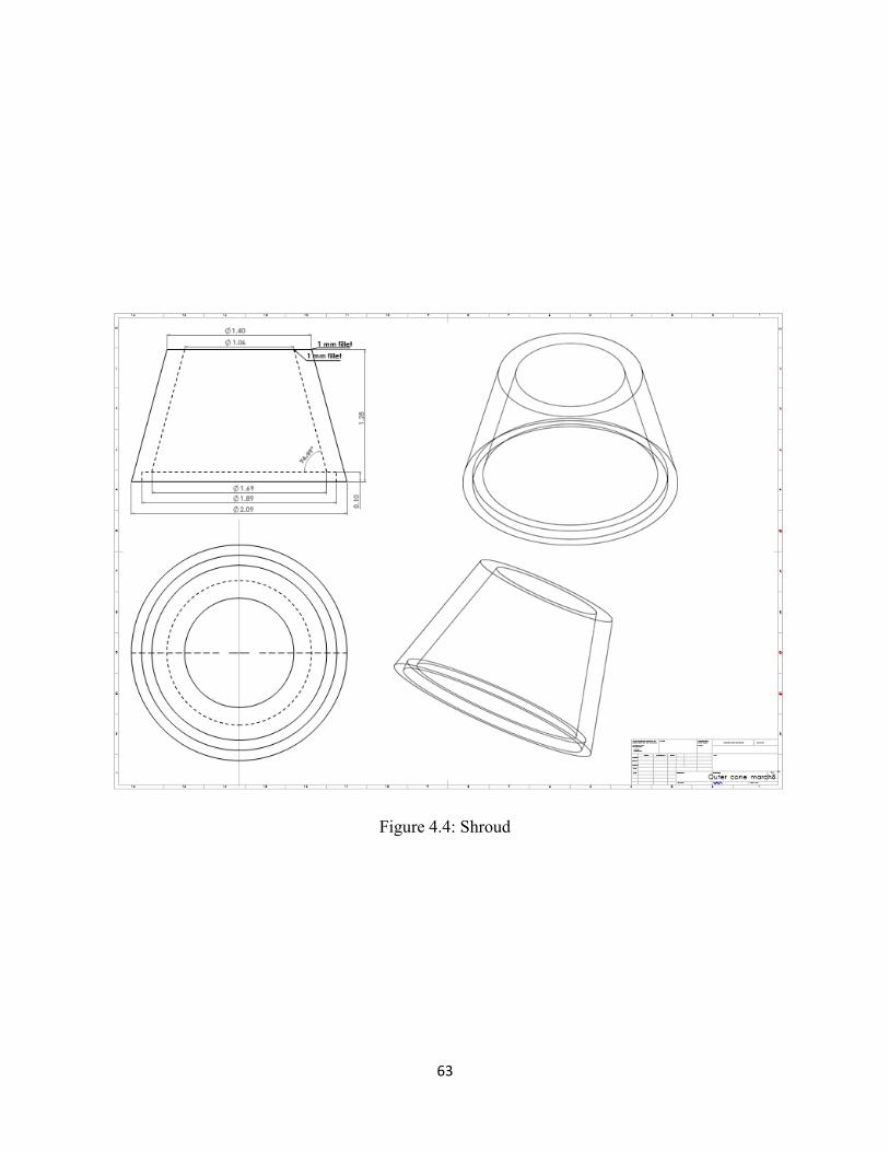
Area of the annulus between the shroud and centerbody

Both the centerbody and the shroud resemble the frustum of a right circular cone. The annulus

area is the area between the centerbody and the shroud at the top surface of the centerbody. To

prevent a reduction of velocity as the air-fuel mixture moves downstream from the trapezoidal

space between the vanes, the desired annulus area is 624 𝑚𝑚2.

60

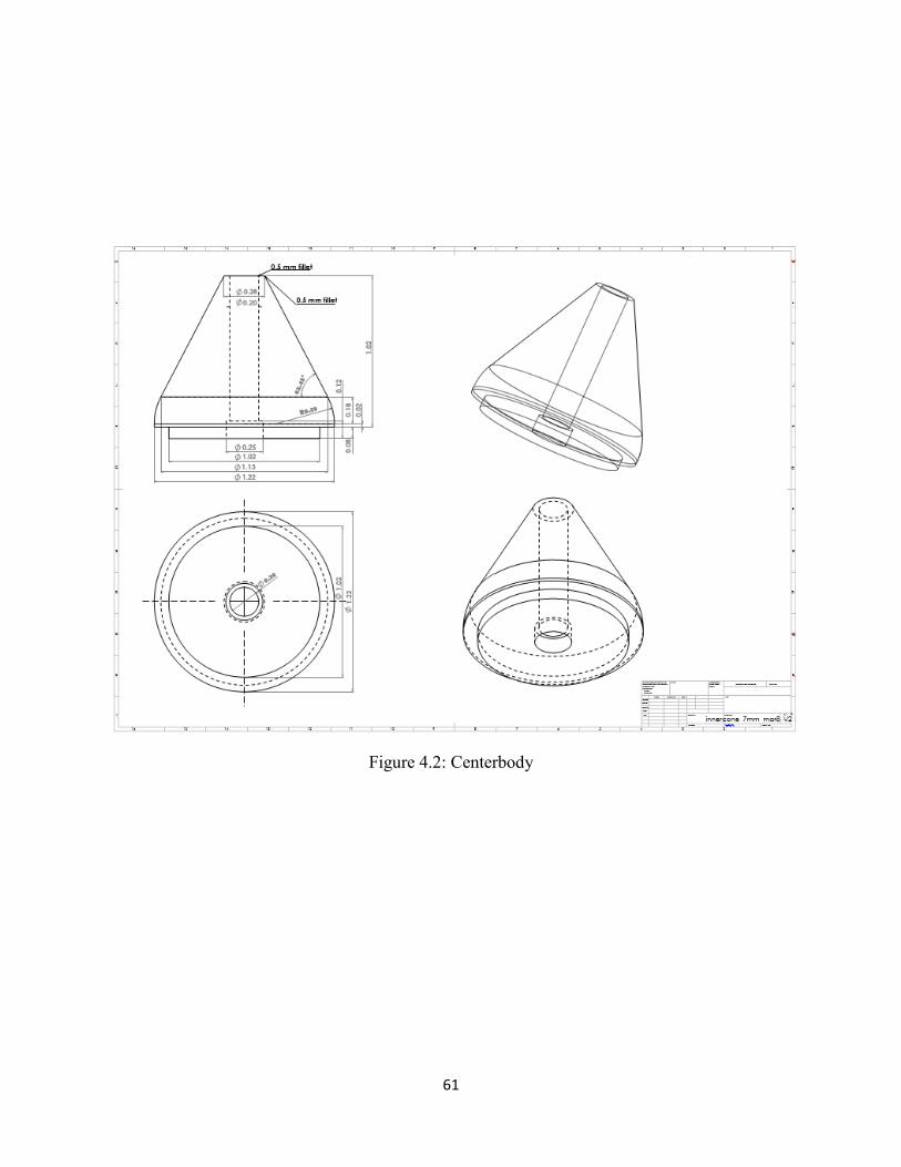
The base diameter of the centerbody is decided by the inner diameter (hub diameter) of the

swirler and is 31 𝑚𝑚. The top circle diameter D2 of the centerbody is 7 mm (hole diameter of 5

mm and 1 mm thickness for rapid prototyping). The Area of the shroud at the top surface of the

centerbody is A1.

The circular area at the top of the centerbody = 𝐴2 = 𝜋 ∗ 3.5 ∗ 3.5 = 38.46 𝑚𝑚2

The annulus area is given by 𝐴1 − 𝐴2 = 624 𝑚𝑚2

The desired area of the shroud at the top surface of the centerbody is 𝐴1 = 624 + 38.46 =

662.46 𝑚𝑚2.

Radius of the shroud at the top surface of the centerbody = √662.46

√𝜋= 14.52 𝑚𝑚

From the radii of the centerbody and shroud, the cone angles are calculated. The centerbody cone

angle and the shroud cone angle are 62.45 ° and 74.97 ° respectively.

Mass flow rate calculation for a given pressure drop

The mass flow rate at a given pressure drop is given by 𝑄𝑚 = 𝜌 ∗ 𝐶𝑑 ∗ 𝐴 ∗ √{2Δ𝑃

𝜌}

61

Figure 4.2: Centerbody

62

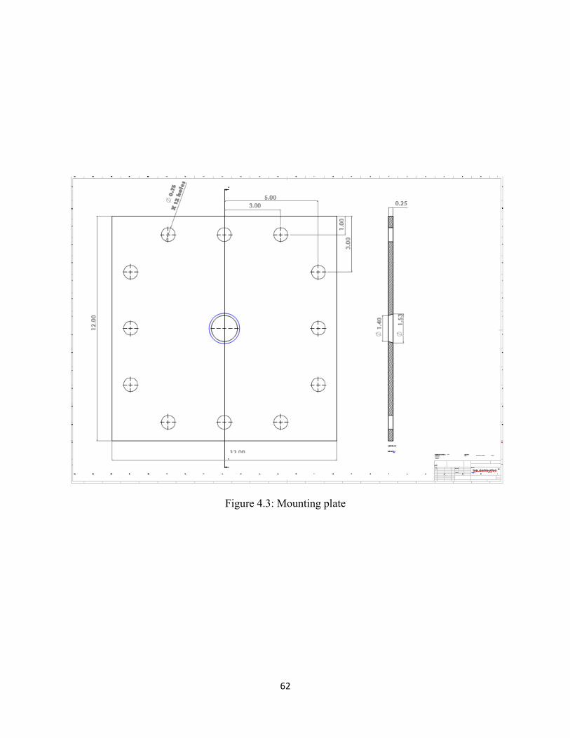
Figure 4.3: Mounting plate

63

Figure 4.4: Shroud

64

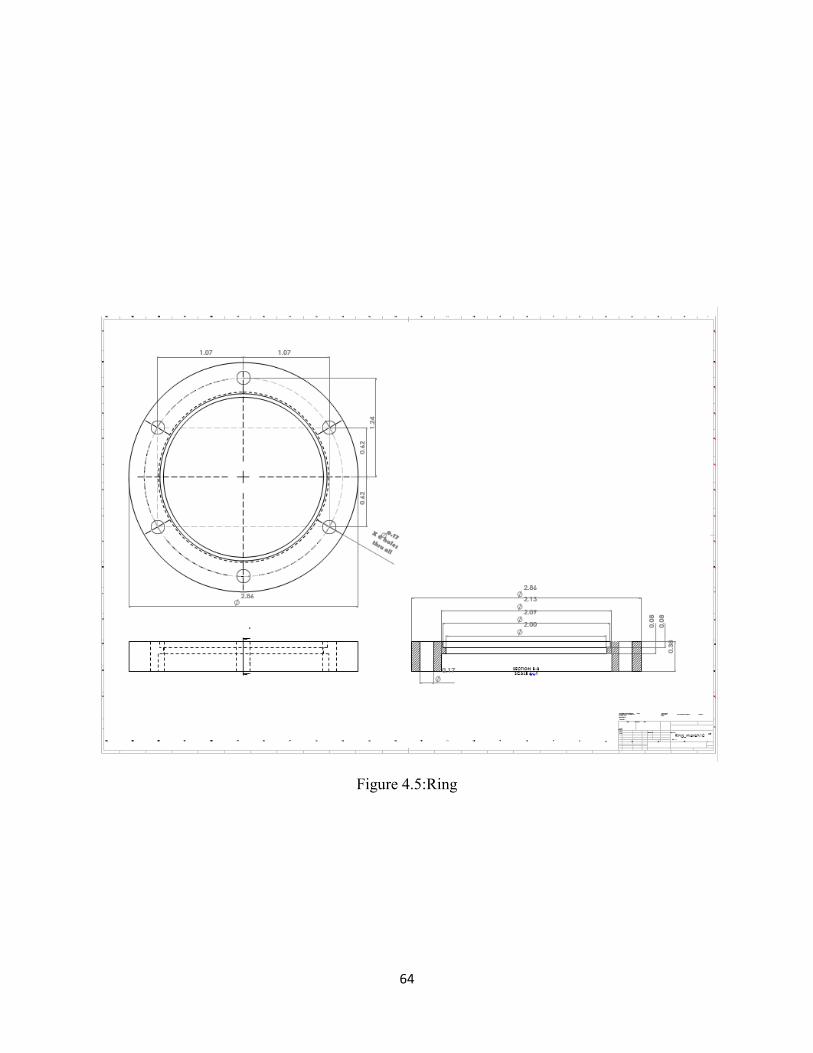
Figure 4.5:Ring

65

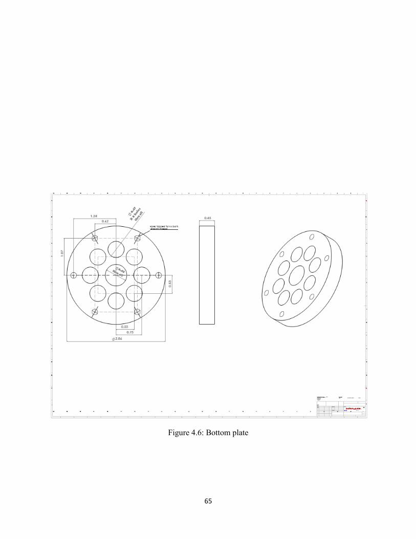
Figure 4.6: Bottom plate