investigation of swirl pipe for improving cleaning efficiency in ...

INVESTIGATION OF SWIRL PIPE FOR

IMPROVING CLEANING EFFICIENCY IN

CLOSED PROCESSING SYSTEM

Guozhen Li, BEng, MSc

Thesis submitted to the University of Nottingham

for the degree of Doctor of Philosophy

December 2015

I

ABSTRACT

This thesis provides unique insights into the fundamentals of improving the

efficiency of ‘Clean-In-Place’ procedures in closed processing systems by locally

introducing intensified hydrodynamic force from swirl flows induced by an

optimised four-lobed swirl pipe without increasing the overall flow velocities.

The studies, carried out employing Computational Fluid Dynamics (CFD)

techniques, pressure transmitters and a fast response Constant Temperature

Anemometer (CTA) system, covered further optimisation of the four-lobed swirl

pipe, RANS-based modelling and Large Eddy Simulation of the swirl flows, and

experimental validation of the CFD models through the measurements of

pressure drop and wall shear stress in swirl flows with various Reynolds Number.

The computational and experimental work showed that the swirl pipe gives rise

to a clear increase of mean wall shear stress to the downstream with its value

and variation trend being dependent on swirl intensity. Moreover, it promotes a

stronger fluctuation rate of wall shear stress to the downstream especially

further downstream where swirl effect is less dominant.

As the increase of either the mean or the fluctuation rates of wall shear stress

contributes to the improvement of CIP procedures in the closed processing

systems. This thesis demonstrates that, with the ability to exert strengthened

hydrodynamic force to the internal surface of the pipe downstream of it without

increasing the overall flow velocity, the introduction of swirl pipe to the CIP

procedures should improve the cleaning efficiency in the closed processing

systems, consequently shortening the downtime for cleaning, and reducing the

costs for chemicals and power energy.

II

ACKNOWLEGEMENTS

I would like to thank the graduate school of the University of Nottingham for the

scholarship granted to me to make this PhD possible.

I owe a great debt of gratitude to my supervisors, Dr. Philip Hall and Prof. Nick

Miles for their precious support, advice, guidance, encouragement, inspiration

and invaluable input to this research.

I extend my gratitude to:

Zheng Wang for his help and valuable input to the establishment of the rig.

Phillip Windsor, Jie Dong, Chi Zheng and Julian Zhu for their support and help

with the installation of rig.

Prof. Xiaogang Yang for his advice on Large Eddy Simulations.

Prof. Tao Wu for his valued input and critical evaluation of my work.

My friends Kaiqi Shi, Kam Hoe Yin and Weiguang Su for their useful experiences

and helpful discussions.

My friends Jie Dong and Lele Zhang who make hard times easier and dull

moments funnier.

Finally, I am especially grateful to my parents, my sisters Suping and Suzheng,

my brother GuoPing and my aunt for their love, support and understanding

which are precious to me.

III

TABLE OF CONTENTS

ABSTRACT ......................................................................................... I

ACKNOWLEGEMENTS ........................................................................ II

TABLE OF CONTENTS ...................................................................... III

LIST OF FIGURES .......................................................................... VIII

LIST OF TABLES ............................................................................. XVI

NOMENCLATURE ...........................................................................XVII

CHAPTER 1: INTRODUCTION .............................................................. 1

1.1 General Introduction .................................................................. 1

1.2 Aims and Objectives .................................................................. 4

1.3 Thesis Outline ........................................................................... 5

CHAPTER 2: LITERATURE REVIEW ..................................................... 8

2.1 Cleaning of Closed Processing Pipe System .................................... 8

2.1.1 Fouling of Pipe Surface ....................................................... 8

2.1.2 Clean In Place ................................................................... 9

2.1.3 Cleaning Efficiency........................................................... 10

2.2 Hydrodynamic Effects of Cleaning Liquid ..................................... 15

2.2.1 Hydrodynamic Factors ...................................................... 15

2.2.2 Mechanism of Particle Detachment in Flow .......................... 20

2.3 Swirl Flow ............................................................................... 21

2.3.1 Swirl Induction Pipes........................................................ 21

2.3.2 Modelling Swirling Flow .................................................... 28

2.3.3 Definition of Terms and Equations for Swirl Flow .................. 37

2.4 Measuring Swirl Flow................................................................ 41

2.4.1 Measuring Flowfield ......................................................... 41

2.4.2 Measuring Wall Shear Stress ............................................. 45

2.4.3 Measuring Cleanability ..................................................... 50

IV

2.5 Conclusion .............................................................................. 52

CHAPTER 3: TRANSITION AND SWIRL PIPE CREATION ................... 53

3.1 Introduction ............................................................................ 53

3.2 Geometry Calculation ............................................................... 53

3.2.1 Four-lobed Transition Pipe Calculation ................................. 54

3.2.2 Different Types of Transition .............................................. 60

3.2.3 Spreadsheet for 4-lobed Transition Pipe .............................. 65

3.2.4 Spreadsheet for 4-lobed Swirl Inducing Pipe ........................ 66

3.3 Geometry Creation ................................................................... 66

3.3.1 Transition Pipe Creation .................................................... 66

3.3.2 Swirl Inducing Pipe Creation .............................................. 68

3.3.3 Optimized Swirl Pipe Creation ............................................ 70

3.4 Conclusions ............................................................................. 73

CHAPTER 4: COMPUTATIONAL FLUID DYNAMICS METHODOLOGY .... 74

4.1 Introduction ............................................................................ 74

4.2 Modelling Turbulence ................................................................ 76

4.2.1 RANS Approach ............................................................... 79

4.2.2 Near Wall Treatment for Wall-Bounded Turbulence Flows ....... 86

4.3 Numerical Schemes .................................................................. 96

4.3.1 Solver ............................................................................ 97

4.3.2 Numerical Discretization ................................................. 101

4.4 CFD Model Formulation ........................................................... 109

4.4.1 CFD Software Package .................................................... 109

4.4.2 Enabling Assumptions .................................................... 109

4.4.3 Flow Domain ................................................................. 110

4.4.4 Meshing ....................................................................... 112

4.4.5 Boundary Conditions ...................................................... 133

4.4.6 Solution Methodology ..................................................... 135

4.4.7 Judging Convergence ..................................................... 142

V

4.5 Conclusions .......................................................................... 146

CHAPTER 5: FURTHER OPTIMISATION OF THE 4-LOBED SWIRL PIPE

..................................................................................................... 147

5.1 Introduction .......................................................................... 147

5.2 Numerical Method and Models ................................................. 150

5.3 Results and Discussions .......................................................... 152

5.3.1 Pressure Drop ............................................................... 152

5.3.2 Swirl Development within Swirl Pipes ............................... 154

5.3.3 Swirl Effectiveness ......................................................... 157

5.3.4 Swirl Decay .................................................................. 159

5.3.5 Wall shear stress ........................................................... 161

5.4 Conclusions .......................................................................... 165

CHAPTER 6: RANS-BASED SIMULATION OF SWIRL FLOW

DOWNSTREAM OF THE OPTIMISED SWIRL PIPE ............................ 167

6.1 Introduction .......................................................................... 167

6.2 Simulation Setup ................................................................... 168


6.3.1 Pressure Drop ............................................................... 169

6.3.2 Tangential Velocity ......................................................... 171

6.3.3 Swirl Decay .................................................................. 177

6.3.4 Wall Shear Stress .......................................................... 180

6.4 Conclusions .......................................................................... 192

CHAPTER 7: LARGE EDDY SIMULATION OF SWIRL FLOW DOWNSTREAM

OF THE OPTIMISED SWIRL PIPE .................................................... 194

7.1 Introduction .......................................................................... 194

7.2 Large Eddy Simulation............................................................ 195

7.2.1 Filtering Operation ......................................................... 196

7.2.2 Sub-Grid-Scale Models ................................................... 197

VI

7.3 Simulation Setup ................................................................... 202

7.3.1 Meshing ....................................................................... 202

7.3.2 Initial Conditions for LES ................................................. 204

7.3.3 Discretization for LES ..................................................... 204

7.3.4 Choice of SGS Model ...................................................... 205


7.4.1 Unsteady Swirl Flow ....................................................... 208

7.4.2 Pressure Drop ............................................................... 214

7.4.3 Tangential Velocity ......................................................... 216

7.4.4 Swirl Decay ................................................................... 218

7.4.5 Wall Shear Stress .......................................................... 222

7.5 Conclusions ........................................................................... 235

CHAPTER 8: VALIDATION OF THE COMPUTATIONAL FLUID DYNAMICS

RESULTS ....................................................................................... 237

8.1 Introduction .......................................................................... 237

8.2 Dealing with Errors and Uncertainties in CFD ............................. 237

8.3 Hydraulic Rig Layout ............................................................... 240

8.4 Producing Swirl Pipe by Investment Casting ............................... 243

8.5 Pressure Drop Validation ......................................................... 246

8.5.1 Pressure Drop Measurement ............................................ 246

8.5.2 Pressure Drop in Swirl Flow (1m cylindrical+0.4m swirl pipe+4m

cylindrical) ............................................................................ 248

8.5.3 Pressure Drop in Non-Swirl Flow (1m cylindrical+0.4m control

pipe+4m cylindrical) .............................................................. 253

8.5.4 Pressure Drop across Swirl Pipe Only ................................ 257

8.6 Wall Shear Stress Validation .................................................... 261

8.6.1 Constant Temperature Anemometry (CTA) ......................... 261

8.6.2 Calibration of the Hot-Film Probe...................................... 264

8.6.3 Measurements of Mean Wall Shear Stress in Swirl Flows ...... 270

VII

8.6.4 Fluctuation of Wall Shear Stress in Swirl Flows ................... 279

8.7 Conclusions .......................................................................... 286

CHAPTER 9: CONCLUSIONS AND FUTURE WORK ............................ 288

9.1 Conclusions .......................................................................... 288

9.1.1 Further Optimisation of the 4-Lobed Swirl Pipe .................. 288

9.1.2 RANS-Based Simulation of Swirl Flows .............................. 288

9.1.3 Large Eddy Simulation of Swirl Flows ............................... 289

9.1.4 Experimental Validation .................................................. 290

9.2 Contribution to Knowledge ...................................................... 290

9.3 Further Work ........................................................................ 291

9.3.1 CFD Modelling ............................................................... 291

9.3.2 Experimental Work ........................................................ 293

REFERENCE .................................................................................... 295

APPENDICES.................................................................................. 308

Appendix 2.1 Mechanism of Particle Detachment in Flow ................... 308

Appendix 3.1 Spreadsheet for 4-Lobed Transition Pipe ...................... 317

Appendix 3.2 Spreadsheet for 4-Lobed Swirl Inducing Pipe ............... 319

Appendix 3.3 Cross-section Development of the 4-Lobed Transition Pipe

................................................................................................ 320

Appendix 5.1 Optimization of a Four-Lobed Swirl Pipe for Clean-In-Place

Procedures ................................................................................. 322

Appendix 8.1 Drawing of the Optimised Swirl Pipe for Investment Casting

................................................................................................ 331

Appendix 8.2 Experimental and Calculated data for Calibrating the Tot-film

Sensor ...................................................................................... 333

VIII

LIST OF FIGURES

Figure 2.1.1 Sinner circles for three different cleaning situations (after

PathogenCombat, 2011) ...................................................................... 11

Figure 2.1.2 Microscope pictures of biofilm grown under three conditions (after

PathogenCombat, 2011) ...................................................................... 14

Figure 2.2.1 Geometries used for showing the influence of flow patterns on the

cleanability of equipment (after Friis and Jensen, 2002) ........................... 17

Figure 2.3.1 Three types of swirl generators (after Najafi et al., 2011) ........ 22

Figure 2.3.2 Classification of Swirl Types (After Steenbergen and Voskamp,

1998), corresponding to the three types of swirl generators ...................... 22

Figure 2.3.3 Swirly-Flo pipe used by Raylor and Ganeshliangam (after

Ganeshalingham, 2002) ....................................................................... 24

Figure 2.3.4 Optimal Swirl inducing pipe, 400mm length, P:D=8 ............... 25

Figure 2.3.5 Transition pipes prior/after swirl inducing pipe ....................... 27

Figure 2.4.1 Schematic Diagram of PIV Setup and Camera Angle with the Laser

at an Angle (after Ariyaratne, 2005) ...................................................... 44

Figure 3.2.1 Fully developed swirl pipe cross-section ................................ 54

Figure 3.2.2 Transition Pipe at Intermediate Stage as Lobes Develop (γ= 65°)

........................................................................................................ 56

Figure 3.2.3 Indication of total area of 4 segmental lobes (a), total area of inner

segments (b) and total lobe area (c) at intermediate stage ....................... 59

Figure 3.2.4 Axial and tangential velocity contours at fully developed and

intermediate stage of transition pipe (2m/s inlet velocity). ........................ 62

Figure 3.2.5 Lobe area developments with pipe length for α, β and linear

transitions ......................................................................................... 63

Figure 3.3.1 Demonstration of 18 sections used to sweep and blend into

transition pipe .................................................................................... 67

Figure 3.3.2 Graph of 𝛾 versus length for transition pipe .......................... 68

IX

Figure 3.3.3 Demonstration of 21 sections used to sweep and blend into half of

the full swirl inducing pipe ................................................................... 69

Figure 3.3.4 Graph of twist versus length for swirl inducing pipe ............... 70

Figure 3.3.5 Entry transition pipe prior to (a) and exit transition pipe after (b)

swirl inducing pipe (after Ariyaratne, 2005) ............................................ 71

Figure 3.3.6 The optimized 600mm length 4-lobed swirl pipe .................... 72

Figure 3.3.7 The further optimized 400mm length 4-lobed swirl pipe ......... 73

Figure 4.2.1 Near-Wall Region in Turbulent Flows (after ANSYS 2011a) ...... 87

Figure 4.3.1 Overview of the Pressure-Based Segregated (a) and Coupled (b)

Solution Methods .............................................................................. 100

Figure 4.4.1 Configuration of simulation geometry ................................ 110

Figure 4.4.2 Velocity profiles downstream of circular pipe inlet ................ 112

Figure 4.4.3 Circular Pipe face Mesh and Distribution of Highly Skewed Cells

..................................................................................................... 116

Figure 4.4.4 A detail view of the interface at the swirl/circular pipe intersection

..................................................................................................... 118

Figure 4.4.5 Discontinuity in contour of wall shear stress at the circular/swirl

and swirl/circular interfaces ............................................................... 119

Figure 4.4.6 Face meshes of swirl inducing pipe, transition pipe, and circular

pipe ................................................................................................ 120

Figure 4.4.7 Face meshes of swirl inducing pipe, transition pipe, and circular

pipe ................................................................................................ 122

Figure 4.4.8 Swirl pipe meshes with unstructured grid by Ariyaratne (2005) and

structured hexahedral grid with O-block ............................................... 123

Figure 4.4.9 y+ contours for computational domain geometry (2m/s inlet

velocity) .......................................................................................... 125

Figure 4.4.10 Histogram of QEAS quality distribution ............................... 131

Figure 4.4.11 Histogram of Aspect Ratio quality distribution .................... 132

Figure 4.4.12 Pressure downstream of swirl pipe for various turbulence models

and wall functions (3m/s inlet velocity) ................................................ 136

X

Figure 4.4.13 Tangential velocity downstream of swirl pipe for various

turbulence models and wall functions (3m/s inlet velocity) ...................... 137

Figure 4.4.14 Pressure downstream of swirl pipe for various advection schemes

(3m/s inlet velocity) .......................................................................... 138

Figure 4.4.15 Tangential velocity downstream of swirl pipe for various advection

schemes (3m/s inlet velocity) ............................................................. 139

Figure 4.4.16 Pressure downstream of swirl pipe for various pressure

interpolation schemes (3m/s inlet velocity) ........................................... 140

Figure 4.4.17 Tangential velocity downstream of swirl pipe for various pressure

interpolation schemes (3m/s inlet velocity) ........................................... 141

Figure 4.4.18 Pressure and tangential velocity after swirl pipe for various

Pressure-velocity coupling schemes (3m/s inlet velocity) ........................ 142

Figure 4.4.19 Scaled residuals for a final simulation model ..................... 143

Figure 4.4.20 Variation of static pressure at inlet as solution proceeding (last

100 iterations) ................................................................................. 144

Figure 4.4.21 Variation of wall shear stress 0.5m downstream of swirl pipe with

iteration number (last 100 iterations) .................................................. 144

Figure 4.4.22 Histogram of mass imbalance .......................................... 145

Figure 4.4.23 Variation of mass imbalance (inlet-outlet) as solution was

proceeding (last 100 iterations) .......................................................... 145

Figure 5.1.1 Optimal Swirl inducing pipe and transition pipes .................. 147

Figure 5.1.2 Two configurations of swirl pipes ....................................... 150

Figure 5.2.1 Configuration of simulation geometries ............................... 151

Figure 5.3.1 Pressure drop across the two swirl pipes in flows with various inlet

velocities ......................................................................................... 153

Figure 5.3.2 Tangential velocity distribution within the two swirl pipes for

various inlet velocities ....................................................................... 155

Figure 5.3.3 Swirl intensity distribution within the two swirl pipes for various

inlet velocities .................................................................................. 156

Figure 5.3.4 Swirl effectiveness variation within the two swirl pipes for various

XI


Figure 5.3.5 Tangential velocity distribution downstream of the two swirl pipes

for various inlet velocities .................................................................. 160

Figure 5.3.6 Swirl intensity variation downstream of the two swirl pipes for


Figure 5.3.7 Tangential wall shear stress distribution downstream of the two

swirl pipes for various inlet velocities ................................................... 162

Figure 5.3.8 Non-dimensional tangential WSS distribution downstream of the

two swirl pipes for various inlet velocities ............................................. 163

Figure 5.3.9 Axial wall shear stress distribution downstream of the two swirl

pipes for various inlet velocities .......................................................... 164

Figure 5.3.10 Total wall shear stress distribution downstream of the two swirl

pipes for various inlet velocities .......................................................... 165

Figure 6.2.1 Configuration of simulation geometry ................................ 168

Figure 6.3.1 Static pressure variation in the horizontal pipe system for various


Figure 6.3.2 Tangential velocity (m/s) distribution within and downstream swirl

pipe for various velocities .................................................................. 173

Figure 6.3.3 Classification of swirl types (After Steenbergen and Voskamp, 1998)

..................................................................................................... 174

Figure 6.3.4 Tangential velocity profiles in radial direction (2m/s inlet velocity)

..................................................................................................... 174

Figure 6.3.5 Tangential velocity variation downstream of swirl pipe exit .... 175

Figure 6.3.6 Correlation of initial tangential velocity with inlet velocity ..... 176

Figure 6.3.7 Correlation of swirl pipe effect distance with inlet velocities ... 177

Figure 6.3.8 Swirl intensity variation downstream of swirl pipe exit .......... 179

Figure 6.3.9 Correlation of swirl decay rate with Reynolds number ........... 179

Figure 6.3.10 Tangential WSS variation downstream of swirl pipe exit ...... 182

Figure 6.3.11 Non-dimensional tangential WSS variation downstream of swirl

pipe exit .......................................................................................... 183

XII

Figure 6.3.12 Axial wall shear stress variation downstream of swirl pipe exit

...................................................................................................... 184

Figure 6.3.13 Axial velocity profiles in radial direction (2m/s velocity) ...... 185

Figure 6.3.14 Correlation of average axial WSS with Reynolds number ..... 185

Figure 6.3.15 Contours of WSS at interior wall of swirl pipe and downstream for

inlet velocities of 1m/s, 1.5m/s, 2m/s, 2.5m/s, 3m/s respectively from top to

bottom ............................................................................................ 188

Figure 6.3.16 Circular distribution of WSS at 0.5m, 1m, and 1.5m downstream

of swirl pipe exit (2m/s inlet velocity) .................................................. 189

Figure 6.3.17 Contours of axial and tangential velocity at cross-flow planes

0.5m, 1m, and 1.5m downstream of swirl pipe exit (2m /s inlet velocity) .. 189

Figure 6.3.18 Wall shear stress variation downstream of swirl pipe exit for


Figure 7.3.1 Fine grid in the near wall region of cylindrical pipe and swirl pipe for

LES ................................................................................................. 202

Figure 7.3.2 y+ contours of computational domain geometry for LES (2m/s inlet

velocity) .......................................................................................... 203

Figure 7.3.3 Comparison of wall shear stress distribution for various SGS

models and RANS (2m/s inlet velocity) ................................................ 206

Figure 7.3.4 Comparison of tangential velocity distribution for various SGS

models and RANS (2m/s inlet velocity) ................................................ 208

Figure 7.4.1 Comparison of axial and tangential velocity contours obtained by

RANS and LES (2m/s inlet velocity) ..................................................... 210

Figure 7.4.2 Velocity vectors in cross-flow planes 0.2m, 0.5m and 1m

downstream of the swirl pipe (2m/s inlet velocity) ................................. 211

Figure 7.4.3 Pathline of swirl flow downstream of swirl pipe showing vortices

(2m/s inlet velocity) .......................................................................... 212

Figure 7.4.4 The four curved axes about which the four vortices rotate ..... 213

Figure 7.4.5 Static pressure variation in the flow system for various inlet

velocities predicted by LES and RANS .................................................. 215

XIII

Figure 7.4.6 Tangential velocity variation downstream of swirl pipe exit for LES

and RANS ........................................................................................ 217

Figure 7.4.7 Swirl intensity variation downstream of swirl pipe exit for LES and

RANS (1m/s inlet velocity) ................................................................. 218


RANS (1.5m/s inlet velocity) .............................................................. 219




RANS (2.5m/s inlet velocity) .............................................................. 220



Figure 7.4.12 Swirl intensity decay trend downstream of swirl pipe exit obtained

by LES for various inlet velocities ........................................................ 222

Figure 7.4.13 Contours of instantaneous wall shear stress in swirl pipe and

circular pipes obtained by LES for inlet velocities of 1m/s, 1.5m/s, 2m/s, 2.5m/s,

3m/s respectively from top to bottom .................................................. 224

Figure 7.4.14 Contours of time averaged wall shear stress in swirl pipe and

circular pipes obtained by LES for inlet velocities of 1m/s, 1.5m/s, 2m/s, 2.5m/s,

3m/s respectively from top to bottom .................................................. 225

Figure 7.4.15 The four vortex core regions within swirl pipe and downstream

circular pipe for inlet velocities of 1m/s, 2m/s and 3m/s respectively from top to

bottom ............................................................................................ 227

Figure 7.4.16 Wall shear stress variation downstream of swirl pipe exit obtained

by LES and RANS for various inlet velocities ......................................... 228

Figure 7.4.17 wall shear stress variation over time at circumferences of the swirl

pipe exit and its downstream (3m/s inlet velocity) ................................. 229

Figure 7.4.18 Variation of normalized wall shear stress fluctuation rate in swirl

and circular pipes (1m/s inlet velocity) ................................................ 231


XIV

and circular pipes (1.5m/s inlet velocity) .............................................. 231


and circular pipes (2m/s inlet velocity) ................................................. 232


and circular pipes (2.5m/s inlet velocity) .............................................. 232


and circular pipes (3m/s inlet velocity) ................................................. 233

Figure 8.3.1 Schematic diagram and layout of the experimental rig .......... 242

Figure 8.4.1 Demonstration of the investment casting process for optimised

swirl pipe ......................................................................................... 245

Figure 8.5.1 Swirl pipe, pressure transmitter, magnetic flow meter and squirrel

data logger ...................................................................................... 247

Figure 8.5.2 Pressure drop versus flow velocity for 1m cylindrical+0.4m swirl

pipe+4m cylindrical pipe .................................................................... 250

Figure 8.5.3 Comparison of the pressure drop in swirl flow obtained by

experimentation and CFD ................................................................... 251

Figure 8.5.4 Crevices in the cylindrical/cylindrical and swirl/cylindrical

connections; internal surface roughness of swirl pipe ............................. 253

Figure 8.5.5 Pressure drop versus flow velocity for 1m cylindrical+0.4m control

pipe+4m cylindrical pipe .................................................................... 255

Figure 8.5.6 Comparison of the pressure drop in cylindrical pipe flow obtained

by experimentation and the Darcy–Weisbach equation ........................... 256

Figure 8.5.7 Demonstration of the calculation of pressure drop across the swirl

pipe only by subtraction ..................................................................... 257

Figure 8.5.8 Pressure drop across swirl pipe only obtained by experimentation

and CFD for various flow velocities ...................................................... 259

Figure 8.5.9 Comparison of Pressure Loss across optimised swirl pipe with

previously used swirl pipes ................................................................. 260

Figure 8.6.1 Glue-on hot-film probe and MiniCTA 54T42 ......................... 263

Figure 8.6.2 Allocation of the hot-film sensor at the five points on the

XV

circumference .................................................................................. 265

Figure 8.6.3 Measurement flow chart for sensor calibration ..................... 267

Figure 8.6.4 Calibration of hot-film sensor (sensor at top) ...................... 268

Figure 8.6.5 Calibration of hot-film sensor (sensor at +45°) ................... 269

Figure 8.6.6 Calibration of hot-film sensor (sensor at middle) ................. 269

Figure 8.6.7 Calibration of hot-film sensor (sensor at -45°) .................... 270

Figure 8.6.8 Calibration of hot-film sensor (sensor at bottom) ................. 270

Figure 8.6.9 Measurement procedure for wall shear stress ...................... 271

Figure 8.6.10 Mean wall shear stress downstream of swirl pipe for various flow

velocities ......................................................................................... 273

Figure 8.6.11 Mean wall shear stress downstream of control pipe for various

flow velocities .................................................................................. 273

Figure 8.6.12 Comparison of mean wall shear stress downstream of swirl pipe

obtained by experimentation and CFD models ...................................... 276

Figure 8.6.13 Flow direction in the near wall region of swirl flow .............. 278

Figure 8.6.14 Examples of wall shear stress fluctuation downstream of swirl pipe

measured by hot-film probe ............................................................... 280

Figure 8.6.15 Normalized voltage fluctuation rates downstream of swirl pipe for

various flow velocities ....................................................................... 282

Figure 8.6.16 Normalized voltage fluctuation rates downstream of control pipe

for various flow velocities .................................................................. 282

Figure 8.6.17 Comparison of the normalized fluctuation rate of voltage signals

under swirl flow and non-swirl flow conditions ...................................... 283

XVI

LIST OF TABLES

Table 2.1.1 Effects of chemical and hydraulic (or physical) processes on soil

removal (after Graβhoff 1997) .............................................................. 13

Table 4.4.1 Y+ value for different sections of the geometry at different inlet

velocities ......................................................................................... 126

Table 4.4.2 A summary of the mesh independence test results ................ 128

Table 4.4.3 Skewness ranges and cell quality ........................................ 129

Table 4.4.4 Skewness ranges and cell quality ........................................ 130

Table 4.4.5 Simulation conditions at inlet ............................................. 134

Table 5.2.1 Models and parameters used for the simulations ................... 151

Table 5.3.1 Comparison of the two swirl pipe in swirl induction ................ 153

Table 6.2.1 Simulation conditions at inlet ............................................. 169

Table 6.3.1 The unit length pressure losses for swirl and circular pipes ..... 170

Table 6.3.2 Swirl decay rate calculated in terms of friction factor ............. 179

Table 8.5.1 Flow velocities at which pressure drop measurements were

performed ....................................................................................... 247

Table 8.5.2 Pressure drop across 1m cylindrical+0.4m swirl pipe+4m cylindrical

pipe for various velocities ................................................................... 249

Table 8.5.3 Mean experimental pressure drop in swirl flow and comparison to

CFD ................................................................................................ 249

Table 8.5.4 Pressure drop across 1m cylindrical+0.4m control pipe+4m

cylindrical pipe for various velocities .................................................... 254

Table 8.5.5 Mean experimental pressure drop in cylindrical pipe flow and

comparison to Darcy–Weisbach equation .............................................. 254

Table 8.5.6 Comparison of the experimental pressure drop across the swirl pipe

only with the RANS and LES results ..................................................... 258

Table 8.6.1 Mean wall shear stress downstream of swirl pipe and control pipe for

various flow velocities ........................................................................ 274

Table 8.6.2 Comparison of mean wall shear stress in swirl flows obtained by

experimentation and CFD models ........................................................ 275

XVII

NOMENCLATURE

A Area m2

AH Material dependent Hamaker constant

CD Drag coefficient

𝐶𝜇 Dimensionless constant

𝐶𝑤 Empirical constant (0.15)

𝐶𝑠 Smagorinsky constant

d particle diameter m

D Pipe diameter m

dh Hydraulic diameter m

E Wall functions empirical constant (= 9.793)

𝐸𝑎 Acquired voltage output from Constant Temperature

Anemometry v

𝐸𝑐𝑜𝑟𝑟 Corrected voltage v

f Fanning friction factor of the pipe

f’ Moody friction factor (f’ = 4f)

g the gravitational acceleration m/s2

I Turbulence intensity %

k Turbulent kinetic energy m2/s2

Ks Wall roughness height m

L Length of pipe corresponding to pressure loss m

l length scale of the large-scale turbulence

m Particle mass kg

MD Moment of the surface stresses N·m

p Wetted perimeter m

p Static pressure pa

𝑄𝐸𝐴𝑆 Equi-Angle Skew, a normalised measure of mesh

skewness

XVIII

R Pipe radius m

r Radius at point where tangential velocity is calculated m

Re Reynolds number

Rep Particle Reynolds number

S Swirl number or swirl intensity

S0 Initial swirl intensity

𝑇𝑤 Sensor hot temperature (60℃) ℃

𝑇0 Ambient reference temperature related to the last

acquisition ℃

𝑇𝑎 Ambient temperature during acquisition ℃

u Flow velocity m/s

𝑢 Axial velocity m/s

u’ Root-mean-squared of velocity fluctuation m/s

U Mean flow velocity m/s

U* Dimensionless velocity

𝑢𝜏 Friction velocity, defined as √𝜏𝑤

𝜌

V Average velocity of the fluid flow m/s

V Particle volume m3

v Velocity scale of large-scale turbulence

w Tangential velocity m/s

x Distance downstream of swirl pipe m

y Normal distance to the wall m

y+ Non-dimensional distance of a point from the wall =

𝜌𝑦𝑢𝜏

𝜇

z0 Particle-to-surface distance m

α Empirical coefficient

β Swirl decay rate parameter = α*f’

∆ Filter cutoff width m

∆𝑃 Pressure loss due to friction in pipe pa

XIX

ε Turbulence dissipation rate

λ Friction factor for fully developed flow

κ Von Kármán constant (= 0.4187)

μt Turbulent viscosity kg/ms

μ Dynamic viscosity kg/ms

ρ Fluid density kg/m3

𝜏𝑤 Wall shear stress pa

𝜏𝑤𝜃 Tangential wall shear stress pa

𝜏𝑤𝜃′ Non-dimensional tangential wall shear stress

Ω𝑖𝑗 Vorticity s-1

Abbreviations

CFD Computational Fluid Dynamics

CIP Clean-In-Place

CTA Constant Temperature Anemometer

CMC Carboxymethyl cellulose

CCD Charge Coupled Device

DNS Direct numerical simulation

EHEDG European Hygienic Equipment Design Group

ERT Electrical Resistance Tomography

FDM Finite-Difference Method

FVM Finite-Volume Method

FEM Finite-Element Method

ICEM CFD The Integrated Computer Engineering and Manufacturing code

for Computational Fluid Dynamics

LES Large Eddy Simulation

LDV Laser Doppler Velocimetry

LDA Laser Doppler Anemometry

PRESTO! PREssure STaggering Option

XX

PISO Pressure-Implicit with Splitting of Operators

PIV Particle Image Velocimetry

PDA Phase Doppler Anemometry

PVC Precessing vortex core

QUICK Quadratic Upstream Interpolation for Convection Kinetics

RSM Reynolds Stress model

RNG Renormalization group

WMLES Algebraic Wall-Modeled LES Model

Chapter 1

1

CHAPTER 1: INTRODUCTION

1.1 General Introduction

At the University of Nottingham (UK), research into design and optimisation of

swirl induction pipes has been taking since 1993. Early emphasis concentrated

on the physical effects of swirl section, later research was directed toward

optimizing the swirl pipe configuration, number of lobes, pitch to diameter ratio

and transition pipes. Currently, a number of potential applications have been

identified for swirl pipes and the advantages of applying swirl pipes have been

investigated through experimental work and Computational Fluid Dynamics

(CFD) modelling.

Previous researchers have shown that a Swirly-Flo pipe before a bend can

reduce wear and produce better particle distribution through the bend (Raylor,

1998, Wood et al., 2001). A three-lobed helix pipe applied in pneumatic

transport locally increased the conveying velocity and produced an improved

particle distribution across the downstream section of the horizontal pipe

(Fokeer, 2006). Ariyaratne (2005) further optimized a four-lobed near-optimal

swirl pipe recommended by Ganeshalingam (2002) by adding a transition pipe

either prior to or after the near-optimal swirl pipe providing a gradual transition

from circular to lobed cross-section and vice versa . The swirl pipe was applied

to hydraulic transport and the induced swirl flow was found to provide better

particle distribution and prevent solids dragging along the bottom of the pipe.

Another potential application identified for swirl pipe was the cleaning of pipes.

It is well documented and proven by previous research on swirl pipes that the

tangential velocity component imparted upon swirl flows effectively sweeps and

lifts deposited particles in the bottom of the pipe into the main stream (Heywood

Chapter 1

2

and Alderman, 2003, Fokeer, 2006, Ariyaratne, 2005). It is expected that the

swirl flow induced by the swirl pipe can potentially intensify hydrodynamic

impact on pipe surface and consequently increase cleaning efficiency

downstream of it. Though the beneficial effects of swirl pipes have been proven

in wear prevention, in pneumatic and hydraulic transport, the relation of

geometrically induced swirl flow and the cleaning of pipe surface in a closed

processing system is not clear, and it is not entirely understood how the swirl

pipe and the system it is applied to operate.

Therefore, this research aims to investigate the hydrodynamic potential of an

optimized 4-lobed swirl pipe on improving cleaning efficiency in a closed

processing system.

Rapid and effective cleaning of closed processing systems is very important in

many industries, especially in the beverage and food industries where

production lines are cleaned daily to maintain both high heat transfer rates and

low pressure drops in heat treatment units and more importantly, to ensure the

appropriate level of microbial quality and thus the safety of the products

(Leliévre et al., 2002, Jensen et al., 2005). In many cases, the only practical way

to clean closed processing systems is by using Clean-In-Place (CIP) procedures

which is a method of cleaning the interior surfaces of pipes, vessels, process

equipment and associated fittings, without disassembling them (Friis and

Jensen, 2002). Efficient CIP processes will result not only in reduced downtime

and costs for cleaning but also decreased environmental impact (in the disposal

of spent chemicals) (Gillham et al., 1999).

Researchers have shown that in some areas some bacteria may remain on

equipment surfaces after standard CIP procedures (Elevers et al., 1999,

Leliévre et al., 2002). Traditional methods of improving CIP efficiency include

increasing the overall cleaning fluid velocity, the concentration and temperature

Chapter 1

3

of the cleaning chemical and longer running time. For a company these methods

increase costs and downtime, reducing production efficiency, and for the

environment it is an additional load due to the extra chemical consumption.

Due to the fact that CIP cleaning is typically performed at constant flow rates

throughout the system, and the cleaning time is decided based on the criteria

that the area most difficult to clean must be cleaned at the end of the process.

One of the concerns related to improvement of cleaning efficiency is finding a

way to locally increase the hydrodynamic force of cleaning fluid acting at the

fluid/equipment interfaces without increasing the overall cleaning fluid velocity.

Swirl pipe may serve as an alternative approach to achieve this condition

without consuming considerably more energy.

The advantage of swirl pipe, especially after transition pipe is added, over other

swirl generation devices is that it has minimal intrusion to the flow. The swirl

motion is geometrically induced to the downstream by the spiral lobed

cross-section of the swirl pipe which avoids the insertion of any objects which

would otherwise be mounted inside the pipe, such as blades, helical ribs and

honeycomb structures that might contribute to problems regarding the fouling

and cleaning of the pipes. Moreover, with the introduction of transition pipes,

the swirl pipe is easier to connect to a circular pipe than other devices. However,

swirl pipes cause a higher pressure loss than circular pipes and the acquired

swirl pattern decays downstream along the pipe. Therefore, excessive use of

swirl pipes to increase hydrodynamic effects indiscriminately for the whole

pipeline may be too costly. Localized intervention of the swirl pipe should prove

to be more cost effective.

Despite the large body of literature on the swirl flows and their applications,

there is still a lack of understanding of geometrically induced swirl flow involved

in pipe cleaning. In the studies of CIP, most published work utilizes flows

Chapter 1

4

parallel to a test surface and experiments have been mainly performed in the

laminar flow regime (Friis and Jensen, 2002). The use of geometrically induced

turbulent swirl flow in the pipe cleaning industry is still lacking attention. The

unique contribution of this thesis to the literature is the application of

geometrically induced swirl flow induced by an optimized four-lobed swirl pipe

to CIP procedures in order to increase cleaning efficiency in closed processing

systems without increasing the overall flow velocity. In doing so, this study

provides better understanding of the fluid dynamics of the geometrically

induced swirl flow, especially in the boundary layer where cleaning takes place.

1.2 Aims and Objectives

The primary focus of this study is to investigate the potential of a swirl flow

induced by an optimized 4-lobed swirl pipe on improving cleaning efficiency of

closed processing systems by locally increasing hydrodynamic effects

downstream of it without increasing the overall velocity.

The intention of the research is to:

Complete a comprehensive literature survey on factors influencing

cleaning efficiency in closed processing system especially the

hydrodynamic effects of cleaning fluid, the hydrodynamic properties of

swirl flows and its applications, the experimental and modelling

techniques used by current and previous researchers to gain knowledge

of methodology.

Create and optimize the 3D geometry of a 4-lobed swirl pipe and produce

a stainless steel casting prototype for experimental work.

Establish a steady state CFD model through RANS approach to obtain

averaged value of the geometrically induced swirl flows in terms of its

tangential velocity, swirl intensity, swirl decay rate and the wall shear

stress exerted on the pipe surface.

Chapter 1

5

Carry out Large Eddy Simulations and provide insight into the

unsteadiness of wall shear stress of the swirl flows.

Build a hydraulic rig and validate the CFD results using experimentally

measured pressure loss and wall shear stress.

1.3 Thesis Outline

This thesis consists of 9 chapters. The following gives a brief description of each

chapter contained.

The current chapter, Chapter 1 gives a general background context and

motivation against which this study was carried out, the aims and objectives of

this work and the outline structure of the thesis.

Chapter 2 is a literature review concerning the required knowledge of two topics,

namely the cleaning of closed processing system and studies on swirl flows. In

this chapter, the definition of Clean-In-Place and the factors influencing its

efficiency especially the hydrodynamic factors of the cleaning fluid are conveyed.

Previous research on swirl pipes is summarized. The important terms and

equations for swirl flow are explained. The techniques in terms of swirl flow

modelling and measurement are reviewed.

Chapter 3 details the calculation and geometry creation process of a transition

pipe and a swirl inducing pipe. Based on the calculation, the spreadsheets that

include necessary data for the sketch of cross-sections of transition and swirl

inducing pipe are generated. The cross-sections are swept and blended into

transition and swirl inducing pipe respectively using the software Pro/Engineer.

The optimised 4-lobed swirl pipe, which was not tested previously, is defined.

Chapter 4 covers the computational fluid dynamics methodology involved in

Chapter 1

6

modelling turbulent flow. The discussion focuses mainly on the

Reynolds-averaged Navier–Stokes (RANS) approach. The turbulence models for

RANS, discretization schemes and meshing of the pipe geometries are

presented. The general set up of the simulation models used for RANS modelling

are summarized.

Chapter 5 focuses on further optimisation of the 600mm length 4-lobed swirl

pipe by shortening the length of its swirl inducing pipe section (resulting in a

400mm length swirl pipe). A numerical comparison of the horizontally mounted

four-lobed 600mm length swirl pipe and the further optimised 400mm length

swirl pipe in terms of swirl induction effectiveness into flows passing through

them is presented.

Chapter 6 presents a computational fluid dynamics model (RANS approach) of

the swirl flows that is induced in a fluid flow passing through the horizontally

mounted optimized 400mm length swirl pipe. Pressure loss, tangential velocity,

swirl type, swirl intensity and its decay rate of the swirl flow are investigated in

flows with various inlet velocities. Special attention is paid to the potential of the

swirl flow on improving ‘Clean-In-Place’ efficiency by locally increasing the

mean wall shear stress downstream of the swirl pipe without increasing inlet

velocity.

In Chapter 7, Large Eddy Simulations (LES) are carried out in order to see the

unsteadiness of the geometrically induced swirl flow downstream of the

optimised 400mm swirl pipe. The fluctuation rate of wall shear stress in the

sections along the pipe are calculated and compared. In order to avoid intensive

literature review on CFD method in Chapter 4, definitions and models regarding

LES approach are presented in this Chapter.

Chapter 8 concerns the establishment of the experimental hydraulic rig and the

Chapter 1

7

validation of the simulation results, mainly the pressure loss and the wall shear

stress variation downstream of the swirl pipe. The measured pressure loss for a

series of flow velocities are compared to the predicted results. A glue-on hot film

is calibrated and used to measure the mean value and the fluctuation rate of the

wall shear stress downstream of the swirl pipe. The experimental results are

compared to the RANS and LES results. The sources associated with

experimental errors are discussed.

Finally, Chapter 9 draws together the conclusions from computational and

experimental research in this thesis and discusses the implications of the

present findings for research and practice. Possible future work to advance the

present research are suggested and discussed.

Chapter 2

8

CHAPTER 2: LITERATURE REVIEW

2.1 Cleaning of Closed Processing Pipe System

2.1.1 Fouling of Pipe Surface

Fouling problems of the pipe surface in closed processing systems are common

in many industries. For instance, in oil transportation industry, wax deposition

on the inner walls of crude oil pipelines presents a costly problem in the

production and transportation of oil. The timely removal of deposited wax is

required to address the reduction in flow rate that it causes, as well as to avoid

the eventual loss of a pipeline in the event that it becomes completely clogged

(Aiyejina et al., 2011).

Rapid and effective cleaning of closed processing pipe systems is especially

important in food industries. Protein in milk processing systems (Changani et al.,

1997), yeast, bacteria and beer stone on the inside of beer tubing systems

(MATIC, 2010) can decrease the heat transfer rate, increase the pressure in

heat treatment unit, and more over affect the quality and flavour of the product.

Another common problem in closed processing pipe system is the formation of

biofilms, as biofilms grow wherever there is water (SpiroFlo, 2010). Biofilms are

a collection of microorganisms surrounded by the slime they secrete, attached

to the pipe surface (Dreesen, 2003). For closed systems, biofilm geometry is

mainly a two dimensional structure which is often composed of patches (cells,

exopolymers, and food residues) and/or isolated cells (PathogenCombat, 2011).

Within the protective slime, the bacteria build communities to take apart and

consume nutrients that no single bacteria could break down alone. In addition,

the biofilms concentrate nutrients with polymer webs in order to survive despite

Chapter 2

9

water purification tactics. This highly efficient combination makes the bacteria

in the biofilm a near self-sufficient community. (Dreesen, 2003, SpiroFlo, 2010,

Coghlan, 1996).

More than 99% of all bacteria live in biofilm communities but some can be

beneficial. For instance, sewage treatment plants rely on biofilms to remove

contaminants from water. However, biofilms can also cause problems by

corroding pipes, clogging water filters, causing rejection of medical implants,

and harbouring bacteria that contaminate food in processing systems. This in

turn can create a hazard to food quality and human health (Dreesen, 2003).

Efficient cleaning of fouling in processing systems is vital in food industries.

2.1.2 Clean In Place

In the food and beverage industries, production lines are often cleaned daily to

maintain both high heat transfer rates and low pressure drops in heat treatment

units and more importantly, to ensure the appropriate level of microbial quality

and thus the safety of the products (Leliévre et al., 2002, Jensen et al., 2005).

In many cases, the only practical way to clean closed processing systems is by

using Clean-In-Place (CIP) procedures. CIP is a method of cleaning the interior

surfaces of pipes, vessels, process equipment and associated fittings, without

disassembling them (Friis and Jensen, 2002). A closed food processing system

is defined as one which is built of pipe works, pumps, valves, heat exchanger,

etc. and tanks for the purpose of processing food products (PathogenCombat,

2011). The common ground for closed processing systems is that the primary

cleaning method applied is CIP (PathogenCombat, 2011, Changani et al., 1997).

CIP is usually performed through the circulation of formulated detergents. This

typically involves a warm water rinse, washing with alkaline and/or acidic

solution, and a clear rinse with warm water to flush out residual cleaning agents

Chapter 2

10

(Dev et al., 2014). Efficient CIP processes will result not only in reduced

downtime and costs for cleaning but also reduced environmental impact (in the

disposal of spent chemicals) (Gillham et al., 1999). Industries that rely heavily

on CIP are those requiring frequent internal cleaning of their processes to meet

the high levels of hygiene. These include: dairy, beverage, brewing, processed

foods, pharmaceutical, and cosmetics industries. The benefit to industries by

using CIP is that the cleaning is faster, less labour intensive, more repeatable

and reproducible, and poses less chemical exposure risks to people.

2.1.3 Cleaning Efficiency

Cleaning is a complex operation with its efficiency depending on many factors,

e.g. the soil to be removed, cleaning time, temperature of the cleaning agent

and the hydrodynamic force of the moving liquid (Lelieveld et al., 2003, Jensen

et al., 2005).

Lelièvre et al. (2002a) reported that soil removal is obviously affected by

cleaning conditions such as the nature of cleaning agent, its concentration, its

temperature, its contact time with surfaces, and lastly, the favourable effect of

hydrodynamics. These factors mentioned are also reported in the studies of

Changani et al. (1997) and Sharma et al. (1991).

According to PathogenCombat (2011), a large European research project

looking at safe food production, cleaning efficiency depends on four energy

factors as presented using Sinners Circle (Figure 2.1.1). The factors are:

Mechanical energy (or hydrodynamic effect) to physically remove soil

Chemical action from detergents to dissolve soil in order to facilitate

removal

Thermal energy - the cleaning temperature

Cleaning time

Chapter 2

11

An efficient combination of those factors varies depending on the type of soil

and the severity of the fouling. The idea is that a restriction in one factor may be

compensated by increasing the effect of one or more of others.

Figure 2.1.1 Sinner circles for three different cleaning situations (after

PathogenCombat, 2011)

Figure 2.1.1 displays three different cleaning situations using Sinners Circle to

describe the relative importance of the four factors: the time, hydrodynamics,

chemistry and temperature. The Sinners circle does not explain the actual

“amount” of each factor; it only indicates relative correlation between them.

Research established that the time taken to clean is a function of temperature,

flow dynamics, and the cleaning chemical concentration. Other factors affect

cleaning include the finish on the closed processing equipment surface, the

geometry of the equipment, and the overall process design (Changani et al.,

1997).

2.1.3.1 Cleaning Agent

Detergent and its operating temperature play an important role in CIP

procedure. Leliévre et al. (2002a) investigated the respective contribution of

both cleaning agent (sodium hydroxide 0.5%) and mechanical action of the fluid

Chapter 2

12

flow on the cleaning efficiency. The trial was carried out in stainless steel pipes

soiled by B. cereus spores under static conditions. They concluded that the

sodium hydroxide and the wall shear stress have a combined action on the

spore removal. The cleaning agent induced a decrease in the adhesion strength

of B. cereus spores, ensuring their removal when a wall shear stress is applied

since the hydrodynamic forces become greater than the adhesion force

(Bergman and Trägårdh, 1990, YIANTSIOS and KARABELAS, 1995).

This conclusion was also supported by other researchers. Visser (1995) stated

the removal of colloid particles is controlled by the wall shear stress, but the

presence of a cleaning detergent ensures a decrease in the adhesion force and,

consequently, improves the removal of these particles. Sharma et al. (1991)

also found that high concentration of sodium hydroxide (high pH values as with

sodium hydroxide) was found to induce a decrease in the adhesion force of

colloids to surface. According to Hall (1998), mechanical action and cleaning

agent were fully linked to ensure a complete removal of a biofilm of

Pseudomonas fragi.

Graβhoff (1997) summarizes the contributions of chemical and hydraulic factors

to soil removal as shown in Table 2.1.1. Table 2.1.1 was based on the

consideration that cleaning of protein with NaOH-based solutions involved three

stages, namely deposit swelling, uniform erosion and a final decay phase. In the

swelling stage, the deposit swells on contact with alkali to form an open protein

matrix of high void fraction; this ‘uniform’ swollen layer is removed by a

combination of surface shear and diffusion in the erosion phase. The final ‘decay’

phase occurs when the swollen layer is thin and no longer uniform, and involves

removal of isolated ‘islands’ by shear/mass transport. The process is complex

and the interaction of NaOH with the protein matrix is concentration dependent

(Gillham et al., 1999, Graβhoff, 1997, Bird and Fryer, 1991). The rate of

cleaning in the breakdown stage is more sensitive to wall shear stress than

Chapter 2

13

other stages, while the uniform stage is more sensitive to the temperature. The

three stages of the cleaning process have been shown to be sensitive to

different combinations of operating parameters and solution chemistry (Bird

and Fryer, 1991).

Table 2.1.1 Effects of chemical and hydraulic (or physical) processes on

soil removal (after Graβhoff 1997)

Factor Effect

Chemical reaction

/modification

Swelling of deposit matrix-change of voidage

Dissolution-erosion

Ageing-change in deposit composition and structure over

time

Hydraulic action

of reagent flow

Mass transfer of reagent and reaction products from

deposit interface to bulk solution

Lift-removal of particulate soil from surface

Scouring-entrained particulates

Surface shear stress-mechanical erosion

2.1.3.2 Adhesion Strength of Soil

According to Sharma et al. (1991), the adhesion strength of soil to pipe surface

varies according to the material of soil, the contact area, particle diameter etc.

Sharma et al. studied the effect of particle material on the release of particles

from a glass surface. The two kinds of particles are ten-micrometre glass and

polystyrene microspheres. It was observed that it is more difficult to displace

polystyrene particles than glass microspheres. One explanation is that the

polystyrene particles are much more deformable, giving rise to larger contact

areas. The results suggested that particles with a smaller Young’s modulus are

more difficult to removal.

Sharma et al. calculated the values of contact radius for different particle

Chapter 2

14

diameters for polystyrene and glass. The contact radii for polystyrene particles

were found to be substantially larger than those for glass. It was also found that

adhesive force increases with the particle diameter for both polystyrene and

glass particles. However the adhesive force for polystyrene is significantly more

than that of glass for all particle diameters.

The adhesion strength of soil to pipe surface is also affected by the flow

condition under which it is formed. PathogenCombat (2011) found that biofilm

resistance to flow during cleaning depends on the flow conditions during the

build-up process. Figure 2.1.2 shows the difference between biofilm grown in

three different conditions: static conditions, laminar flow and turbulent flow.

The difference between the biofilm appearances is the direct result of different

action of flow on bacterial growth. Dreesen (2003) also stated that how the

biofilm layer reaches certain equilibrium thickness depends on the flow

condition and nutrient level.

Static Laminar Turbulent

Figure 2.1.2 Microscope pictures of biofilm grown under three

conditions (after PathogenCombat, 2011)

Other factors influence the adhesion strength of soil to pipe surface may include

surface roughness of the equipment, and deposition time, which is the length of

time for particles to settle at the equipment surface. (Sharma et al., 1991).

Since the adhesion strength between soil and pipe surface is determined by

many factors, it is difficult to find a universal value for a certain category of soil.

The adhesion strength value has to be related to a specific condition.

Chapter 2

15

2.2 Hydrodynamic Effects of Cleaning Liquid

2.2.1 Hydrodynamic Factors

Investigations concerning the influence of the hydrodynamics of the flow on

cleaning of surfaces in the food industry exposed to real-life flow conditions are

still limited (Friis and Jensen, 2002).

Published work stated that cleaning efficiency depends, besides other criteria,

on the hydrodynamic effect. The flow of detergent is an important factor in the

cleaning of closed processing equipment. The cleaning liquid generates local

tangential force acting on the soil on the surface and acts as a carrier for the

chemicals and heat (Jensen et al., 2007). The shear force of the cleaning fluid at

fluid/equipment interfaces are of importance in the cleaning mechanism. The

removal kinetics is functions of fluid detergent velocity and of the wall shear

stress (Gallot-Lavallée et al., 1984, Graβhoff, 1992, Visser, 1970, Sharma,

1991). In addition, the wall shear stress was proposed as a more local removal

control parameter than the velocity (Paz et al., 2013, Paz et al., 2012).

Experimental studies have been performed in laminar regime and most of the

studies conclude that the wall shear stress is the controlling factor for the rate

and amount of microbial adhesion and removal (Duddridge et al., 1982, Powell

and Slater, 1982, Fowler and McKay, 1980, Hall, 1998).

Lelièvre et al. (2002a) investigated the removal of Bacillus cereus spores on

304L stainless steel pipes. A simple model assuming a process combining

removal and deposition during cleaning was established. The simple model was

experimentally confirmed that the flow condition applied during soiling

procedures has a significant effect on removal rate constant. In addition, the

effective removal rate constant is significantly influenced by the wall shear

Chapter 2

16

stress applied during cleaning.

Lélievre et al. (2002) performed local wall shears stress analysis and

cleanability experiments on different pieces of equipment made of stainless

steel that represent production lines. In their study, the influence of the mean

wall shear stress on bacterial removal was confirmed. The influence of loop

arrangement was shown, particularly with the upstream effect of the gradual

expansion pipe. Moreover, this work demonstrated the effect of the fluctuation

rate on bacterial removal. It indicated that some low wall shear stress zones

could be considered as cleanable because in these areas a high level of

turbulence was observed, therefore, a high fluctuation rate. They therefore

suggested that to predict cleaning, it is necessary to take into account not only

the mean local wall shear stress, but also its fluctuation rate (Leliévre et al.,

2002). The presence of large wall shear stress fluctuation is because of flow

pattern and hence, the geometry (Jensen et al., 2005).

Fluctuation rate of the wall shear stress was also studied by other researchers.

Paulsson and Bergman’s work (Paulsson and Trägårdh, 1989, Bergman and

Trägårdh, 1990) showed that the mean wall shear stress has an influence on the

removal of clay deposit but no influence of the fluctuation rate of the wall shear

stress was demonstrated. Bénézech et al. (1998) compared experimental

removal results (Bacillus spores in complex medium) with local measurements

of wall shear stress made by Focke et al. (1985) in a corrugated plate heat

exchanger. They concluded that the relevant parameter for cleaning efficiency

was the fluctuation rate of wall shear stress.

Jensen et al. (2005) numerically investigated the test set-up of Leliévre et al.

(2002) in terms of wall shear stress and its fluctuation (in the form of turbulence

intensity of the flow) using steady-state computational fluid dynamics (CFD)

simulation adopting STAR-CD. A good correlation has been demonstrated

Chapter 2

17

between CFD predictions and measured values of wall shear stress in discrete

points by Leliévre et al. (2002). The author suggested that a combination of the

mean wall shear stress and the fluctuating part of the wall shear stress can be

used for evaluating cleaning properties.

Friis and Jensen (2002) investigated the design of closed process equipment

with respect to cleanability. Computational fluid dynamics was applied. The

study of hydrodynamic cleanability of closed processing equipment was

discussed based on modelling the flow pass through a valve house, an up-stand

and various expansions in tubes as shown in Figure 2.2.1. The CFD simulations

were validated using the standardized cleaning test proposed by the European

Hygienic Engineering and Design Group.

(a) Upper mix-proof valve housing; (b) up-stand geometry with h/D≈0.2;

(c) 8.6° concentric expansion; (d) 8.6° eccentric expansion

Figure 2.2.1 Geometries used for showing the influence of flow

patterns on the cleanability of equipment (after Friis and Jensen, 2002)

Their study showed that the wall shear stress was one of but not the sole

parameter involved in the cleaning process of closed process equipment. The

Chapter 2

18

nature of the fluid flow was also an important factor determining the cleaning

efficiencies. It was found that the fluid exchange downstream of the up-stand

was three times slower than in the main stream, which was caused by a

recirculation zone in this area. Recirculation zones are known to be a problem.

In the up-stand and tube expansion where the fluid exchanges in a steady

recirculation is much slower than that in the main stream. The EHEDG test

(Richardson et al., 2000) showed that tubes with recirculation were more

difficult to clean. Friis and Jensen concluded that the wall shear stress plays a

major role in cleaning of closed process systems. Another significant factor is

the nature of recirculation zone presented. Steady recirculation zones such as

the one found in the up-stand and concentric expansion can reduce cleaning

efficiency. They further concluded that, since turbulent flow is often fully

three-dimensional, this must be included in the CFD model. Therefore,

three-dimensional modelling is recommended for complex geometries in order

to predict the entire flow behaviour.

Jensen and Friis (2005) reported that the most difficult to clean areas are

dead-ends and crevices in the geometry (resulting in recirculation zones) and

shadow zones (resulting in stagnation points). In and around these features are

low wall shear stress and fluid exchange (mass transfer), both of which reduce

the cleaning efficiency. Fluid exchange in the cleaning area was also reported by

PathogenCombat (2011), their study indicates that a combination of mean wall

shear stress and fluid exchange is responsible for proper cleaning in complex

geometries. Flow pattern, flow turbulence were also found to influence cleaning

especially for complex geometries.

Hwang and Woo (2007) concluded that wall shear stress is of great importance

in the fluid mechanics, as it represents the local tangential force by the fluid on

a surface in contact with it. A laminar flow regime induces lower velocity

gradients than a turbulent flow thus lower shear stress.

Chapter 2

19

PathogenCombat (2011) stated that to improve cleaning efficiency, it is

beneficial to promote turbulent flow or to introduce flow disturbance. These flow

phenomena are advantageous during both production and cleaning. Turbulent

flow is achieved at high flow rate (i.e. Reynolds number above 10,000). The

alternative solution is to induce flow disturbances which locally may introduce

flow patterns similar to turbulence and this way reduce residual contamination

downstream.

Disturbances can be induced by geometry e.g. contractions, expansions or

asymmetrical features as seen in a curvature or bend. PathogenCombat

summarized methods to improve Cleaning-In-Place efficiency as following:

Local enhancement of turbulence intensity and wall shear stress of flow

Introduction of high mean wall shear stress

Applying pulsating turbulent flow as a mean to break static flow patterns

Of the three methods proposed, swirl pipe may have the potential to locally

enhance turbulence intensity and wall shear stress of cleaning flow.

Among the factors mentioned, the wall shear stress, which is a measure of the

mechanical action of fluid flow on a process surface, is considered the

dominating factor for cleaning. The effective removal rate is significantly

influenced by the wall shear stress applied during cleaning (Leliévre et al.,

2002). The mean wall shear stress is especially relevant as a measure of

cleaning efficiency in straight pipes, large parts of pumps, valves etc. In general,

there is a threshold value of wall shear stress above which cleaning is

considered efficient. The threshold is defined as the lowest mean wall shear

stress sufficient to remove the specific type of soil or biofilm on the pipe surface

(PathogenCombat, 2011). This so-called critical wall shear stress for removal of

Chapter 2

20

specific microorganisms on various surfaces was also reported by Duddridge et

al. (1982), Powell and Slater (1982), Fowler and McKay (1980), Jensen and

Friis (2004) and, Bari and Veale (2012). For instance, Jensen and Friis (2012)

suggested a critical wall shear stress of 3 Pa as a basis for their specific study.

While Bari and Veale (2012) claimed that a wall shear stress as low as 0.15 Pa

can be cleanable given a high fluctuation level.

The fluctuation rate of the wall shear stress was also reported to be important in

the CIP efficiency. Some authors therefore suggested that to predict cleaning, it

is necessary to take into account not only the mean local wall shear stress, but

also its fluctuation rate (Friis and Jensen, 2002, Jensen et al., 2005, Bari and

Veale, 2012, Leliévre et al., 2002).

According to the literature, it is reported that, for straight circular pipes, the

mean wall shear stress and its fluctuation are the dominating factors controlling

cleaning. While for cleaning of more complex geometries and difficult to clean

areas, the influencing factor may also include the flow pattern, flow exchange,

flow turbulence, and the property of the recirculation zone.

Based on the understanding of swirl induction pipes which can locally change

the flow pattern of the pipe flow, introduce greater turbulence into flow,

enhance heat exchange at the wall, and induce higher velocity gradient at the

wall, it is therefore positive that swirl pipe has the potential of enhancing

cleaning efficiency.

2.2.2 Mechanism of Particle Detachment in Flow

Though investigations based on experiments and CFD simulation has shown the

correlation of wall shear stress and soil cleaning. A theoretical basis of how the

particle is detached from the surface is necessary to understand the cleaning

Chapter 2

21

process and mechanism. A model proposed by Lorthois et al. (2001) and later

was adopted by several other researchers was summarized in Appendix 2.1.

This model demonstrates a positive correlation between the adhesion force that

binds particles to the pipe surface and the wall shear stress of flow to remove

particles.

2.3 Swirl Flow

2.3.1 Swirl Induction Pipes

Swirl flow in a pipe can be defined as a combination of vortex and axial motions,

with helical streamlines (Baker and Sayre, 1974). Swirl flow, which contains a

tangential velocity component, is always accompanied by an increase in velocity

fluctuations (Fokeer, 2006, Algifri et al., 1988).

Swirl flows are usually used in gas turbine engines, furnaces, burners and

cyclones with the purpose of heat transfer enhancement, mixing, separation etc.

Generally three methods can be employed in order to generate swirl flows

(Gupta et al., 1984):

In method one as shown in Figure 2.3.1a, passing through a rotational

section, fluid flow acquires tangential momentum and enters the pipe in

the form of a swirling flow.

In method two as shown in Figure 2.3.1b, fluid flow is introduced to the

pipe through fixed blades (vanes), which are mounted inside of the pipe

with a specified angle. In this case, the blades’ angle appears as an

effective parameter on flow field swirl intensity.

In method three as shown in Figure 2.3.1c, fluid flow is introduced to the

pipe by means of tangential inlet so that it can acquire rotational

momentum and enters the pipe in the form of a swirling flow.

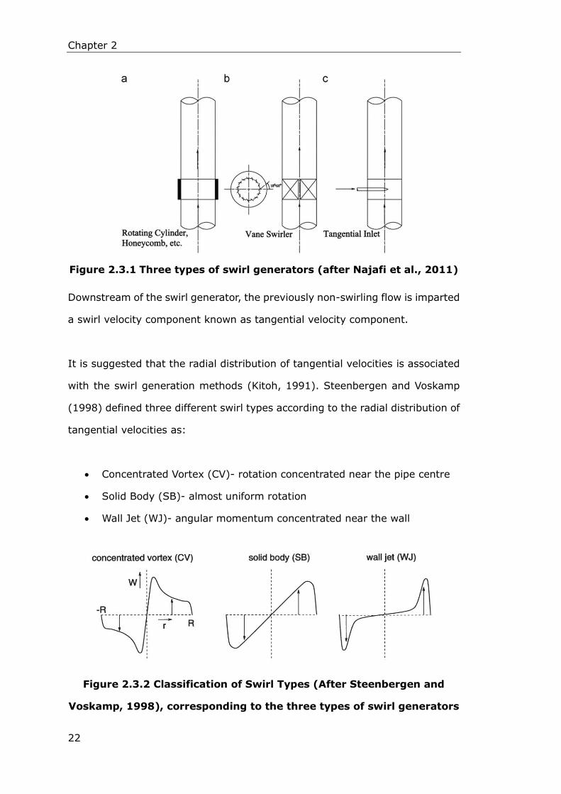
Chapter 2

22

Figure 2.3.1 Three types of swirl generators (after Najafi et al., 2011)

Downstream of the swirl generator, the previously non-swirling flow is imparted

a swirl velocity component known as tangential velocity component.

It is suggested that the radial distribution of tangential velocities is associated

with the swirl generation methods (Kitoh, 1991). Steenbergen and Voskamp

(1998) defined three different swirl types according to the radial distribution of

tangential velocities as:

Concentrated Vortex (CV)- rotation concentrated near the pipe centre

Solid Body (SB)- almost uniform rotation

Wall Jet (WJ)- angular momentum concentrated near the wall

Figure 2.3.2 Classification of Swirl Types (After Steenbergen and

Voskamp, 1998), corresponding to the three types of swirl generators

Chapter 2

23

In addition to the three methods, swirl induction pipes with non-circular

cross-sections have been investigated in order to induce swirl into flow passing

through them. These included pipes with spiral ribs or fins located within the

pipe (Robinson, 1921, Yuille, 1927, Wolfe, 1967, Charles et al., 1971, Schriek et

al., 1974), pipes with rifles installed inside (Howard, 1939), and tubes with

spiral grooves (Spanner, 1940). Those swirl induction pipes were applied

respectively to mitigate the problem of subsiding and the deposit of particles in

the pipe, improve tubular heat exchangers, reduce pipe wear, increase particle

conveying efficiency, and save power. It should be noted that the insertions of

ribs or fins mounted inside the pipe will be subject to direct impact from the

particles in the flow giving rise to damage and wear of the pipe. Moreover, when

applied in food or beverage industries, the insertions may contribute to

problems regarding fouling and cleaning of the pipes.

At the University of Nottingham, research into helically formed swirl induction

pipes can be traced back to 1993, when Jones suggested a new idea to the

problem of settling particles in which a pipe section could be given a helical

profile to promote suspension of particles at relatively low velocities (Jones,

1997). The idea was investigated later by Raylor (1998), Ganeshalingham

(2002), Tonkin (2004), Ariyaratne (2005) and Fokeer (2006). It should be

mentioned that the swirl induction pipes investigated avoid the use of insertions

of ribs, fins or vanes inside the pipes. Rather it is the helically shaped geometry

of the swirl pipe that force the fluid passing through it to rotate within itself and

direct to downstream. A chronological review of their work is given below.

1998 (Raylor, 1998): Raylor’s experimental investigation was based upon a

swirl pipe found in marine boilers which are used to improve heat exchanger

efficiency. The pipe, as shown in Figure 2.3.3, has the trade name ‘Swirly-Flo

pipe’. Raylor’s investigation aimed at pipe induced swirling flow to reduce wear

and produce better distribution throughout a bend.

Chapter 2

24

Longitudinal view Cross-sectional view

Figure 2.3.3 Swirly-Flo pipe used by Raylor and Ganeshliangam (after

Ganeshalingham, 2002)

Raylor used commercial CFD software Fluent to examine various pipe shapes

and flow fields in swirl inducing pipe. He suggested that when the pitch to

diameter ratio in a geodesic pipe decreased, the swirl produced increased with

increasing pressure loss. Raylor designed an experimental rig and used water

and plastic beads mixture to test the simulation results. He concluded that

Swirly-Flo pipe produces an increase in pressure drop across its length

compared to a standard pipe. Swirly-Flo pipe induced swirling flow before a

bend produced less pressure drop across the bend than non-swirling flow for

water and water/plastic beads mixture. Swirling particles before the bend

ensured a more even distribution of particles throughout the bend which has the

potential to remove the characteristic wear zone.

The pitch to diameter ratio (P:D) is an important parameter defining the

character of the twisted swirl induction pipe. Pitch is defined as the axial

distance travelled by the rib as it rotates through 360 degrees (Singh and

Charles, 1976). This was the basis Raylor used for definition of the pitch of the

swirl induction pipe.

Chapter 2

25

2002 (Ganeshalingam, 2002): Ganeshalingham continued Raylor’s

investigation on the ‘Swirly-Flo pipe’ and validated the CFD code used with

results from Particle Image Velocimetry (PIV), Electrical Resistance Tomography

(ERT) and pressure measurements. Ganeshalingham simulated the radial

distribution of tangential velocities downstream of the Swirly-Flo pipe and it was

shown to fit with ‘Wall Jet’ swirl type classified by Steenbergen and Voskamp

(1998) according to radial distribution of tangential velocity field. An

exponential decay of the swirl downstream of a swirl pipe was implied from CFD

and the decay was reported to be faster at higher Reynolds number.

Ganeshalingham also carried out further optimisation of the swirl-inducing pipe

using CFD and continued experimental work on solid-liquid mixture flows.

Ganeshalingham tested various cross-sections (triangular, square, pentagonal,

hexagonal and 2,3,4,5 and 6 lobed cross-sections) of pipe and concluded that

the 4-lobed cross-section was most effective at swirl generation over the others.

Ganeshalingham recommended a P:D ratio of 8 and 400mm of length as optimal

for the 4-lobed pipe. This optimal swirl inducing pipe is shown in Figure 2.3.4

with its configuration being as follows:

The swirl pipe has a 4-lobed cross-section.

The 4-lobed cross-section extends helically around and along the pipe.

Axial distance travelled by each lobe as it rotates through 360° is

400mm.

The equivalent diameter of the swirl pipe is 50mm.

Its pitch to diameter ratio is 8.

Figure 2.3.4 Optimal Swirl inducing pipe, 400mm length, P:D=8

Chapter 2

26

This 4-lobed near-optimal design was further optimized and tested

experimentally later by Ariyaratne (2005).

2004 (Tonkin, 2004): Tonkin investigated the application of the 4-lobed

near-optimal swirl inducing pipe to various pipe configurations, when pumping a

range of fluid and fluid/particle mixtures. Tonkin studied experimentally the

effect of the 4-lobed near-optimal swirl inducing pipe on coal-water, sand-water

and magnetite-water slurries of various particle sizes. The results showed that

swirl induction produced greater benefit for denser slurries and higher

concentrations. In addition, the swirl induced into slurries containing larger and

denser particles was found to decay more rapidly.

Tonkin also investigated application of swirl inducing pipe to non-Newtonian

(shear thinning) carrier liquids. A time independent fluid, CMC (carboxymethyl

cellulose) was chosen to avoid changes in rheology as pumping time increased.

PIV was used to measure the axial and tangential velocity of swirling flows

downstream of the 4-lobed near-optimal swirl pipe with water and CMC. It was

concluded that a significant tangential velocity was generated when pumping

water in the turbulent regime, however, when the fluid viscosity was increased,

leading to laminar flow, no significant tangential velocity was detected.

2005 (Ariyaratne, 2005): Ariyaratne further optimized the 4-lobed

near-optimal swirl inducing pipe by designing a transition pipe for use as an

entry and exit duct with the swirl inducing pipe, providing a gradual transition

from circular to lobed cross-section and vice versa. The optimisation was carried

out by using single-phase simulation employing Computational Fluid Dynamics.

The CFD model was validated by experimental measurements of pressure loss.

Transition pipes either before or after the swirl inducing pipe were found to

reduce entry and exit pressure losses by providing a gradual transition from

Chapter 2

27

circular to lobed cross-section. They also increased induced swirl and reduced

swirl decay. Ariyaratne concluded that a β type transition with transition

multiplier n=0.5 was optimum for both the entry and exit transition from several

geometries tested. The configuration of transition pipe, as shown in Figure 2.3.5,

is:

The transition pipe’s cross-section changes from a circular to a 4-lobed

shape gradually.

The areas of the cross-sections are constant and equal to that of the swirl

pipe.

The length of the transition pipe is 100mm, and each lobe rotates by 90°.

Its pitch to diameter ratio is 8.

(a) Entry transition pipe (b) Exit transition pipe

Figure 2.3.5 Transition pipes prior/after swirl inducing pipe

Ariyaratne suggested that the entry and exit transition should be an integral

part of the swirl inducing pipe as it results in an efficient swirl induction which

reduces energy costs from high pressure losses that otherwise occur due to

sudden changes in flow geometry. Ariyaratne carried out settling slurry

experiments, which showed that swirl induction resulted in better particle

distribution and prevented solids dragging along the bottom of the pipe. This

implies reduction in localised erosion and provides an opportunity to operate at

lower flow velocities without blockage.

2006 (Fokeer, 2006): Fokeer investigated the application of geometrically

induced swirl by a three lobed helix pipe on a lean phase of particulate

Chapter 2

28

suspension in air along a horizontal pipe section. The research employed high

speed photography, Particle Image Velocity (PIV), Laser Doppler Anemometry,

and Computational Fluid Dynamics to obtain the characteristic of the air flow

behaviour. It was concluded that the swirl pipe imparts a wall jet type swirl to

both an air-only flow and a lean pneumatic flow with velocity and momentum

shifts from axial to tangential closer to the wall. The swirl was found to decay

proportionally with the distance downstream of the swirl pipe and inversely to

the flow’s Reynolds number. Additional pressure loss caused by the swirl pipe

was found to be proportional to the Reynolds number of the flow and increased

further with an addition of particles to the swirling flow.

Based on the suggestion of Ariyaratne (2005), a 400mm length swirl inducing

pipe together with 100mm length entry and exit transition pipes at both ends as

an integral pipe should be optimized in swirl induction. This optimised swirl pipe

has a total length of 600mm (100mm+400mm+100mm). In this study, a

further optimised swirl pipe that is comprised of a 100mm length entry

transition pipe, half of the 400mm length swirl inducing pipe, and a 100mm

length exit transition pipe is proposed. This further optimised swirl pipe has a

total length of 400mm (100mm+200mm+100mm) which is 200mm shorter

than Ariyaratne suggested. This further optimized 4-lobed swirl pipe is found

numerically in Chapter 5 to be more cost-effective in swirl induction and is

therefore used in this study.

2.3.2 Modelling Swirling Flow

2.3.2.1 Modelling turbulence

Swirl flow is turbulent and caused considerable degree of anisotropy in stress

and dissipation tensor leading to a highly anisotropic eddy viscosity (Kitoh,

1991). Turbulent flows are characterized by fluctuations in velocity and pressure

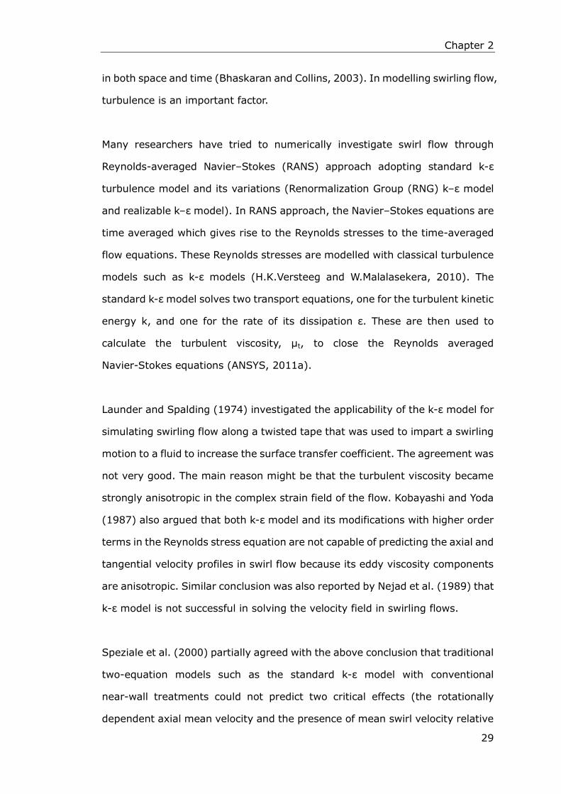
Chapter 2

29

in both space and time (Bhaskaran and Collins, 2003). In modelling swirling flow,

turbulence is an important factor.

Many researchers have tried to numerically investigate swirl flow through

Reynolds-averaged Navier–Stokes (RANS) approach adopting standard k-ε

turbulence model and its variations (Renormalization Group (RNG) k–ε model

and realizable k–ε model). In RANS approach, the Navier–Stokes equations are

time averaged which gives rise to the Reynolds stresses to the time-averaged

flow equations. These Reynolds stresses are modelled with classical turbulence

models such as k-ε models (H.K.Versteeg and W.Malalasekera, 2010). The

standard k-ε model solves two transport equations, one for the turbulent kinetic

energy k, and one for the rate of its dissipation ε. These are then used to

calculate the turbulent viscosity, μt, to close the Reynolds averaged

Navier-Stokes equations (ANSYS, 2011a).

Launder and Spalding (1974) investigated the applicability of the k-ε model for

simulating swirling flow along a twisted tape that was used to impart a swirling

motion to a fluid to increase the surface transfer coefficient. The agreement was

not very good. The main reason might be that the turbulent viscosity became

strongly anisotropic in the complex strain field of the flow. Kobayashi and Yoda

(1987) also argued that both k-ε model and its modifications with higher order

terms in the Reynolds stress equation are not capable of predicting the axial and

tangential velocity profiles in swirl flow because its eddy viscosity components

are anisotropic. Similar conclusion was also reported by Nejad et al. (1989) that

k-ε model is not successful in solving the velocity field in swirling flows.

Speziale et al. (2000) partially agreed with the above conclusion that traditional

two-equation models such as the standard k-ε model with conventional

near-wall treatments could not predict two critical effects (the rotationally

dependent axial mean velocity and the presence of mean swirl velocity relative

Chapter 2

30

to the rotating pipe) associated with turbulent flow in an axially rotating pipe.

However, the author argued that at high Reynolds numbers, the traditional

two-equation models could be used to predict this only with the implementation

of a more sophisticated near-wall treatment that predicts a non-zero Reynolds

shear stress τrθ. But this was not applicable to cases with low Reynolds number.

Bali (1998) proved that the k-ε turbulent model can successfully predict the

weak swirl flow. In his study, the pneumatic swirling flow investigated has a

small tangential velocity imparted to the air flow in the pipe using a propeller

type swirl generator. The experimental and numerical axial and tangential

velocity distributions along the pipe were found to be in good agreement. The

standard k-ε model was also used by Ganeshalingham (2002) to investigate

swirling flow induced by Swirly-Flo pipes which is a weakly swirling flow.

Ganeshalingham stated that RNG k-ε model, Realizable k-ε model and Reynolds

Stress Model (RSM) should show substantial improvements in results compared

to standard k-ε where the flow features include streamline curvature and

rotation, but the accuracy gained is not considerable when the extra time

consumed is taken into account. Similar conclusion was drawn by Ariyaratne

(2005) and Fokeer (2006). Ariyaratne (2005) decided to use standard k-ε model

for initial work due to the large number of cases to be studied in optimizing the

swirl pipe. Fokeer (2006) also decided to first use the k-ε model to obtain a

baseline solution, which can then be improved by employing the Reynolds

Stress Model.

The shortcomings of the standard k-ε model are summarized as follows (ANSYS,

2011a):

Chapter 2

31

It is valid when all Reynolds stresses are of the same order (isotropic

eddy viscosity). If the eddy viscosity is not isotropic, the standard k-ε

model is inadequate.

Applicability is limited to high Reynolds number flows.

The model is semi-empirical; transport equations for k and ε involve

constants that are taken from measurements.

Near wall treatment is accomplished via a wall function.

The advantage of standard k-ε model is its robustness, economy and reasonable

accuracy for a wide range of turbulent flows in industrial flow simulations.

Najafi et al. (2011) investigated the trend of swirl intensity decay rate and its

affecting factors through a turbulent swirl decay pipe flow. The swirling flow is

created by means of a rotating honeycomb which produces solid body rotation

at the inlet of a fixed pipe. In some of the cases, swirling flow being discussed

had a swirl number as large as 0.6. In such turbulent flows viscosity is typically

anisotropic (Kitoh, 1991), so the Najafi et al. adopted the Reynolds Stress

model (RSM) formulation, which was considered to be the most reliable

turbulence model (Najafi et al., 2005, Spall and Ashby, 2010). The numerical

results were validated and compared with existing experimental data and

mathematical relations, showing satisfactory coincide.

The RSM closes the Reynolds-averaged Navier-Stokes equations by solving

transport equations for the Reynolds stresses, together with an equation for the

dissipation rate. This means that seven additional transport equations are

required in a 3D flow (ANSYS, 2011a). The advantages and disadvantages of

Reynolds Stress model are as follow (H.K.Versteeg and W.Malalasekera, 2010) :

Advantages:

Chapter 2

32

Potentially the most general of all classical turbulence models.

Only initial and/or boundary conditions need to be supplied.

Very accurate calculation of mean flow properties and all Reynolds stress

for many simple and more complex flows including wall jets, asymmetric

channel and non-circular duct and curved flows.

Disadvantages:

Very large computing costs (seven extra partial differential equations).

Not as widely validated as the k-ε models.

Performs just as poorly as the k-ε model in some flows due to identical

problems with the ε-equation modelling (e.g. axisymmetric jets and

unconfined recirculating flows).

According to ANSYS FLUENT User’s Guide (ANSYS, 2011b), for modelling

turbulent flow with a significant amount of swirl, ANSYS FLUENT suggests the

consideration of using one of the advanced turbulence models: the RNG k-ε

model, realizable k-ε model, or Reynolds stress model. The appropriate choice

depends on the strength of the swirl, which can be gauged by the swirl number.

For flows with weak to moderate swirl (S<0.5), both the RNG k-ε model and

realizable k-ε model yield appreciable improvement over the standard k-ε model.

For highly swirling flows (S>0.5), the RSM is strongly recommended. The

effects of strong turbulence anisotropy can be modelled rigorously only by the

second-moment closure adopted in the Reynolds stress model. This

recommendation was followed in this study in the steady state RANS simulation

of the swirl flows induced by the optimized swirl pipe.

With the rising of computing power, large eddy simulation (LES) methods are

gaining popularity in industrial flow investigations over recent years though the

mainstay for industrial flow simulation is still the Reynolds averaged

Chapter 2

33

Navier-Stokes (RANS) method. The LES is superior to RANS method in that it

resolves directly the large turbulent structures and models only the influence of

the sub-grid scales on the resolved ones (H.K.Versteeg and W.Malalasekera,

2010). The LES has the potential for improved accuracy when the resolution of

the largest eddies is important or when turbulent fluctuations of flow variables

are needed.

Conway et al. (2000) applied the LES technique to the subsonic turbulent flow

between the blades of a swirl generator. The large time-dependent streamwise

vortices due to the blade surface curvature, the large scale time-dependent

structures associated with the wake of the blades were captured by the LES.

Wegner et al. (2004) evaluated the performance of the unsteady RANS method

employing a Reynolds stress model in predicting the precessing vortex core

(PVC) phenomenon. Good agreement of mean velocities was achieved when

comparing the unsteady RANS results to available experimental data and LES

computations. However the energy contained in the coherent motion of the PVC

was significantly under-predicted by the unsteady RANS. It is concluded that

unsteady RANS is able to capture the precessing vortex core phenomenon both

qualitatively and in parts also quantitatively. Wegner et al. stated that for 3D

time-dependent simulation, the computational cost for LES is significantly

increased when compared to steady state RANS. LES is very good for flow

systems where flow is governed by large, turbulent structures, which can be

captured by fairly coarse mesh. However, if the resolving of boundary layers is

important, LES may give partially dissatisfying predictions in these regions,

unless fine mesh is used. Many researchers have suggested hybrid LES-RANS

methods to get around this bottleneck of LES near walls, where RANS is used

near the wall while LES is utilized in the remaining part of the domain (Durbin,

2002).

Chapter 2

34

Mikulčić et al. (2014) studied the highly swirled gas-solid flow inside a cement

cyclone using LES with the Smagorinsky Subgrid-Scale model being employed

for sub-grid scale modelling. A three dimensional geometry of a real industrial

scroll type cyclone was used for the LES simulation employing a commercial

finite volume CFD code FIRE. The turbulent fluctuations of the gas phase, the

pressure drop, and concentration of particles associated with the complex

swirled two-phase flow inside the cement cyclone were obtained. The

numerically obtained results were compared with available measurement data,

and showed good correlation with it.

Yang and Kær (2012) studied the flow structure of a isothermal swirling in the

Sydney swirl flame database using both a RANS-based RNG k-ε turbulence

model and a large eddy simulation with dynamic Smagorinsky-Lilly model. The

streamlines indicated that the formation mechanisms of vortex breakdown

detected from the two methods were different. The LES and RANS showed very

different vorticity fields. Moreover the RANS fails to predict the precessing

vortex core. The author concluded that the LES shows better agreement with

the measurements in the statistical results and also better predict the flow

pattern of the recirculation zones.

So far, the simulation investigations of the swirl flow induced by the swirl

induction pipes are confined in the RANS method. The fluctuation property of

the flow variables and the swirl flow instability has not been revealed yet. In

Chapter 7 of this thesis, LES was attempted in order to provide insight into the

unsteady property of the geometrically induced swirl flow.

2.3.2.2 Wall Shear Stress Modelling in swirl flows

Jensen et al. (2005) suggested that the technique used for measuring the mean

and the fluctuating parts of wall shear stress has its shortcomings with respect

Chapter 2

35

to hygiene. Because measurements can only be performed in a predefined

number of discrete points, and the equipment tested has to be specially

designed to mount the measuring probes. An alternative approach of applying

computational fluid dynamics (CFD) was proposed. CFD is widely used with

great success within other industries for prediction of flow patterns, quantitative

hydrodynamic parameters, chemical processes, etc.

It used to be difficult for CFD simulation to predict wall shear stress

quantitatively (Wilcox, 1998, Bouainouche et al., 1997). However, with the

development of computer technology, models for simulating near-wall flow have

been implemented in commercially available CFD codes. Prediction of wall shear

stress was proven to be very good in some cases (Wilcox, 1998, Jensen et al.,

2005).

Even though, investigations on wall shear stress in swirl flows are few. The

study carried out by Zhu et al. (2012), PathogenCombat (2011), and Jensen et

al. (2005) mentioned above, were performed either in circular pipes or complex

geometries like sudden/gradual expansion or contraction, and up-stand etc.

with non-swirling flows. So their studies cannot entirely reflect the wall shear

stress variation and distribution pattern of swirl flows within the circular pipes or

complex geometries.

The case involving simulation of wall shear stress in swirl flow is found in the

study of Najafi et al. (2011) whose purpose was to investigate the swirl intensity

decay rate of internal swirl flow downstream a rotating cylinder honeycomb (a

swirl generator). Their simulation found that an increase in the inlet swirl

intensity causes a rise in tangential wall shear stress and directing to the

downstream. In addition, the variation of the swirl intensity of the swirl flow field

was found similar to that of the tangential wall shear stress indicating that the

value of tangential wall shear stress is proportional to the swirl intensity. The

Chapter 2

36

definitions of swirl intensity and tangential wall shear stress are seen in section

2.3.3.

It should be mentioned that the swirl flows generated by the rotating cylinder

honeycomb and the swirl flows induced by the swirl induction pipes are not

entirely the same in that:

The swirl induction mechanism is different that the former one was

produced by flow passing through a rotational section, while the latter

was induced by stationary spiral walls of the pipe.

The circumferential distribution of wall shear stress downstream of the

rotating cylinder honeycomb is even because of its circular cross-section

shape. While the circumferential distribution of wall shear stress

downstream of the swirl pipe may be uneven due to the lobed

cross-section of the swirl pipe.

The swirl flow Najafi et al. studied can be very strong (swirl number

reaches 0.6). While swirl flow induced by the swirl pipe is a kind of weakly

swirl flow (swirl number less than 0.15).

Despite the above difference, the positive correlation of swirl intensity and

tangential wall shear stress indicated by Najafi et al. has provided a good

expectation that the swirl flow induced by the swirl pipe should give rise to the

tangential wall shear stress, consequently an increase of overall wall shear

stress at the internal pipe surface downstream of the swirl pipe.

Chapter 2

37

2.3.3 Definition of Terms and Equations for Swirl Flow

This section introduces a number of terms and equations that will be used in

studying swirl flows.

Swirl number S (swirl intensity)

Although there is no standard for quantifying the strength of the swirl inside a

pipe, the swirl number S, also termed swirl intensity, is commonly used. It

defined as the ratio of the angular momentum flux to the axial momentum flux,

multiplied by the hydraulic radius (Li and Tomita, 1994, Steenbergen and

Voskamp, 1998, Rocklage-Marliani G., 2003):

𝑆 =∫ 𝑢𝑤𝑟2. 𝑑𝑟

𝑅

0

𝑅 ∫ 𝑢2𝑟. 𝑑𝑟𝑅

0

(2.3.1)

S = swirl intensity

w = tangential velocity, m/s

r = radius at point where tangential velocity is calculated, m

R = pipe radius, m

u = axial velocity, m/s

Swirl decay

Swirl will decay downstream of the swirl pipe which is caused by transport of

angular momentum to the pipe wall. To determine the distance over which swirl

will prevail in the pipe several researchers had studied the swirl decay law

(Steenbergen and Voskamp, 1998, Li and Tomita, 1994, Halsey, 1987,

Reader-Harris, 1994). There was no unanimous agreement on the decay rates

in swirling flow, in most reference, the observed swirl intensity fit with

exponential decay functions:

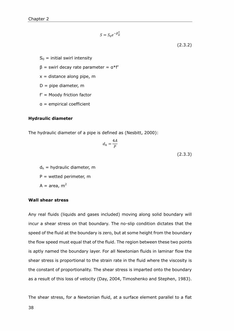
Chapter 2

38

𝑆 = 𝑆0𝑒−𝛽

𝑥

𝐷

(2.3.2)

S0 = initial swirl intensity

β = swirl decay rate parameter = α*f’

x = distance along pipe, m

D = pipe diameter, m

f’ = Moody friction factor

α = empirical coefficient

Hydraulic diameter

The hydraulic diameter of a pipe is defined as (Nesbitt, 2000):

𝑑ℎ =4𝐴

𝑃

(2.3.3)

dh = hydraulic diameter, m

P = wetted perimeter, m

A = area, m2

Wall shear stress

Any real fluids (liquids and gases included) moving along solid boundary will

incur a shear stress on that boundary. The no-slip condition dictates that the

speed of the fluid at the boundary is zero, but at some height from the boundary

the flow speed must equal that of the fluid. The region between these two points

is aptly named the boundary layer. For all Newtonian fluids in laminar flow the

shear stress is proportional to the strain rate in the fluid where the viscosity is

the constant of proportionality. The shear stress is imparted onto the boundary

as a result of this loss of velocity (Day, 2004, Timoshenko and Stephen, 1983).

The shear stress, for a Newtonian fluid, at a surface element parallel to a flat

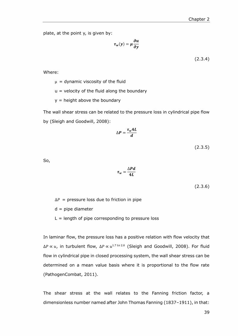
Chapter 2

39

plate, at the point y, is given by:

𝝉𝒘(𝒚) = 𝝁𝝏𝒖

𝝏𝒚

(2.3.4)

Where:

μ = dynamic viscosity of the fluid

u = velocity of the fluid along the boundary

y = height above the boundary

The wall shear stress can be related to the pressure loss in cylindrical pipe flow

by (Sleigh and Goodwill, 2008):

∆𝑷 =𝝉𝒘𝟒𝑳

𝒅

(2.3.5)

So,

𝝉𝒘 =∆𝑷𝒅

𝟒𝑳

(2.3.6)

∆𝑃 = pressure loss due to friction in pipe

d = pipe diameter

L = length of pipe corresponding to pressure loss

In laminar flow, the pressure loss has a positive relation with flow velocity that

∆𝑃 ∝ 𝑢, in turbulent flow, ∆𝑃 ∝ 𝑢1.7 𝑡𝑜 2.0 (Sleigh and Goodwill, 2008). For fluid

flow in cylindrical pipe in closed processing system, the wall shear stress can be

determined on a mean value basis where it is proportional to the flow rate

(PathogenCombat, 2011).

The shear stress at the wall relates to the Fanning friction factor, a

dimensionless number named after John Thomas Fanning (1837–1911), in that:

http://en.wikipedia.org/wiki/Shear_stress

Chapter 2

40

𝝉𝒘 =𝒇𝝆𝒖𝟐

𝟐

(2.3.7)

where:

𝜏𝑤= shear stress at the wall

f = Fanning friction factor of the pipe

u = fluid velocity in the pipe

ρ = density of the fluid

The friction factor is a function of flow Reynolds number and the ratio of wall

roughness to pipe diameter, more information are covered in the book of

Douglas et al. (2006).

Tangential wall shear stress

It is concluded that the existence of tangential wall shear stress in the swirl flow

causes reduction of fluid flow swirl intensity (Steenbergen and Voskamp, 1998,

Kitoh, 1991).

Kitoh (1991) derived an expression for the tangential wall shear stress by

treatment of the Reynolds averaged angular momentum equation for

incompressible, stationary and axially symmetric flow. The equation later used

by Steenbergen and Voskamp (1998) and Najafi et al. (2011) reads:

𝜏𝑤𝜃(𝑥) =𝜌

𝑅2∫ 𝑟2

𝑅

0

𝜕

𝜕𝑥(�� + 𝑢𝑤 − 𝜇

𝜕��

𝜕𝑥)𝑑𝑟

(2.3.8)

where �� and �� are the time averaged value of the axial and tangential velocity

components respectively; 𝑢 and 𝑤 are the instantaneous fluctuation of the

axial and tangential velocity components respectively; 𝜌 is the density; 𝑅 is

the radius of the pipe; 𝜇 is the kinematic viscosity; 𝑥 and 𝑟 are the axial and

radial position; 𝑟2�� is the flux density of angular momentum per unit mass at

Chapter 2

41

radial position 𝑟. Turbulent shear stress 𝑢𝑤 and viscous shear stress 𝜇𝜕��/𝜕𝑥

acting in the cross-flow plane can be neglected in turbulent flow having a slow

axial development. Equation 2.3.8 actually illustrates that the change in the

integrated flux of angular momentum on a cross section of flow is balanced by

the moments exerted on the flow by the tangential wall shear stress. By

interchanging integration and differentiation the following equation is obtained:

𝜏𝑤𝜃(𝑥) =𝜌

𝑅2

𝜕

𝜕𝑥∫ 𝑟2

𝑅

0

(��)𝑑𝑟

(2.3.9)

Equation 2.3.9 is made non-dimensional by the transformations of x→x/D,

r→r/R, ��→��/Um and ��→��/Um, with Um being bulk velocity and D pipe diameter.

The non-dimensional tangential wall shear stress is rearranged as:

𝜏𝑤𝜃′ (𝑥) =

𝜏𝑤𝜃(𝑥)

0.5𝜌𝑈𝑚2

=1

2

𝑑𝑆

𝑑 (𝑥𝐷)

(2.3.10)

with S being the swirl intensity as defined in equation 2.3.1. Equation 2.3.10

indicates that at the downstream region of the swirl pipe exit, the

non-dimensional tangential wall shear stress is a linear function of the axial

gradient of swirl intensity.

2.4 Measuring Swirl Flow

2.4.1 Measuring Flowfield

Invasive and non-invasive techniques can be employed in order to measure

flowfield. Invasive techniques used probes present within the flow for data

capture. A number of researchers have used invasive method to measure swirl

flows. For instance, Ito et al. (1980) used an electrolytic solution that has the

kinematic viscosity nearly equal to that of water to measure swirling flow

electrochemically. A spherical multi-electrode probe was used to measure the

three dimensional velocity components. Kitoh (1991) used a hot wire probe to

Chapter 2

42

measure the flow angle and the mean velocity of a swirling water flow. Li and

Tomita (1994) also used an invasive method to measure the radial velocity and

pressure profiles at 15 different pipe sections in swirling pneumatic flow using a

3-holed spherical head probe. Measurements were carried out at 20 radial

locations at each section and the swirl intensity was calculated.

The pressure and pressure drop within the flow system is normally measured

using invasive pressure sensors. For instance, Senoo and Nagata (1972) used a

cobra probe and a sphere static probe to measure the direction and static

pressure of swirling air flow. Tonkin (2004) and Su et al. (2010) chose

differential pressure transducers for pressure measurement in swirl and

non-swirl flow respectively. To select a pressure transducer, the line pressure

and pressure drop range should be estimated in advance. Ariyaratne (2005)

initially used piezo-resistive pressure sensors to measure pressure drop.

However, it was found the calibration of these sensors changed rapidly and it

needed to be re-calibrated regularly. Therefore she used an inverted

manometer in the subsequent tests which provided more accurate pressure

drop results. Fokeer (2006) used U-tube water manometers and inclined

manometers filled with a liquid of specific gravity 0.8 to measure the gauge

pressure of pneumatic swirling flow. George (2007) used two types of pressure

measuring devices, simple manometer tube and liquid pressure gauge for the

measurement of pressure drop of the swirl pipe.

The disadvantage of the invasive methods is that the local disturbances and

changes of flow in the probe area may result in poor measurements. On the

other hand, non-invasive techniques have no physical parts within the flow and

therefore do not cause any flow disturbance. These techniques include LDV

(Laser Doppler Velocimetry), PDA (Phase Doppler Anemometry), PIV (Particle

Image Velocimetry) and all tomography techniques.

Chapter 2

43

Particle image velocimetry (PIV) is an optical method of flow visualization used

in education and research. It is used to obtain instantaneous velocity

measurements and related properties in fluids. The fluid is seeded with tracer

particles which, for sufficiently small particles, are assumed to faithfully follow

the flow dynamics. The flow in the target area is then illuminated with a laser

light sheet and the motion of the particles is recorded using a CCD (Charge

Coupled Device) camera. A sequence of two light pulses is recorded and the

images are divided into subsections called interrogation areas. The

interrogation areas are next correlated pixel by pixel. The correlation produces

a signal peak identifying the common particle displacement. This displacement

can then be used to construct a 2D vector map (Smits and Lim, 2000).

Ganeshalingam (Ganeshalingam, 2002) used Dantec FlowMap PIV system (with

one CCD camera) to measure axial velocity of the flow downstream of the swirl

inducing pipe and showed a good agreement with CFD predicted values.

However, his attempt at measuring tangential velocity was not successful. To

measure tangential velocity, Tonkin (2004) attempted a different setup of the

PIV by placing the camera perpendicular to the cross-section and focusing

through an optical window. Initially only a part of the cross-section was visible

with the tangential viewer. It was adapted by adding a viewing box filled with

water to prevent total internal reflection, and the whole pipe cross-section could

be viewed. The disadvantage of Tonkin’s method is that, with the use of

tangential viewer, measurements at distance further downstream than L/D=5

(5 pipe diameters) may not be possible since the camera cannot focus that far

through the viewer. This will prevent analysis of swirl decay downstream of the

swirl pipe. Therefore, Ariyaratne (2005) decided to attempt PIV measurement

of tangential velocity with the laser and camera at an angle of 90° as shown in

Figure 2.4.1. However, this attempt was unsuccessful.

Chapter 2

44

Figure 2.4.1 Schematic Diagram of PIV Setup and Camera Angle with

the Laser at an Angle (after Ariyaratne, 2005)

Fokeer (2006) initially attempted PIV technique to understand the pneumatic

swirl flow field downstream of the three lobed swirl pipe. A DANTEC FlowMap

2100 Particle Image Velocimetry (PIV) system was used. It was found that a

lack of good seeding implied poor quality of the results and it was not possible

to obtain a seeding material which would produce seeding particles in the three

microns range without dirtying the endoscope. It was therefore decided to

perform a series of Laser Doppler Anemometry (LDA) experiments.

LDA is a single point optical measuring technique which enables the velocity of

the seeded particles conveyed by a fluid flow to be measured in a non-intrusive

manner. The area of interest within the flow field is sampled by a crossed-beam

point by point. The local velocity of the fluid can be determined by analysing the

Doppler-equivalent frequency of the laser light scattered by the seeded particles

within the flow. This technique was employed by Fokeer to measure the flowfield

for three different Reynolds number air flows seeded with oil droplets of an

average diameter of 3 microns. The instantaneous local fluid velocities

components in the three directions were measured at four planes perpendicular

to the pipe axis (130 measurement points per plane) downstream of both the

control and swirl pipe sections. The measured u, v and w velocity components

were converted into cylindrical polar velocity components ux, ur and uθ.

Chapter 2

45

Successful use of LDA in swirl flows has also been reported by Nejad et al.

(1989), Parchen and Steenbergen (1998) and Rocklage-Marliani et al. (2003).

2.4.2 Measuring Wall Shear Stress

The measurement of mean and time resolved wall shear stress in a turbulent

boundary layer is of vital importance to the fluid mechanics community. Wall

shear stress sensors are traditionally classified by measurement method into

two distinct groups, direct or indirect techniques.

The direct techniques directly measure the shear force acting on the model

surface. Direct sensors measure the integrated force produced by the wall shear

stress on a flush-mounted movable "floating" element. The floating element is

attached to either a displacement transducer or is part of a feedback

force-rebalance configuration. The performance of these devices has been

limited by the following issues (Sheplak et al., 2004, Winter, 1977):

The tradeoff between sensor spatial resolution and the ability to measure

small forces.

Measurement errors associated with sensor misalignment and required

gaps.

Measurement errors associated with pressure gradients.

Cross-axis sensitivity to acceleration, vibration, and thermal expansion

effects.

Sensitivity drifts due to thermal-expansion effects.

Methods of this kind have stronger intrusion to the local flow field. Its

measurement errors caused by stronger pressure gradient in swirl flow can be

significant. More importantly, it only gives an integrated value of wall shear

stress and cannot give a time-resolved wall shear stress fluctuation. Therefore

Chapter 2

46

this method is not applicable for swirling flow.

Indirect sensors are generally simpler to fabricate and are more robust than

floating-element sensors. Indirect techniques require an empirical or theoretical

correlation, typically valid for very specific conditions, to relate the measured

property to the wall shear stress. The MEMS (Microelectromechanical systems)

community has produced a variety of different indirect transduction schemes

such as hot-film sensors, micro-optical systems to measure near-wall velocity

gradients, and mechanical micro-fences (Sheplak et al., 2004).

Of the indirect sensors, the thermal-based stress sensors were widely used. The

operating principle of thermal shear stress sensor is the transduction of

heat-transfer rate to voltage. Su et al. (2010) measured the mean and time

varying fluctuation property of local wall shear stress of horizontal air-water

bubbly flows in a circular pipe of 35mm inner diameter using a TSI-1268W hot

film probe. The hot film sensor was made of a thin platinum film with dimensions

of 1.0×0.127 mm and coated with a thin layer of quartz. The TSI-1268W probe

is cast into the mounting block and is flush-mounted on the internal surface of

the section. A pair of pressure taps was used to measure the pressure gradient

in the region where the hot film probe is located. The pressure taps are

connected to a 1151 capacitive differential pressure transducer with a

measuring range of 0-5 kPa and accuracy of 12.5 Pa. The wall shear stress is

calculated from the measured pressure gradient of single-phase water flow and

is used for calibration. Vaze and Banerjee (2012), also used a Hot Film

Anemometry to measure the wall shear stress in an air-water two phase flow.

Berca (2007) measured the wall friction in the cone of an industrial turbine

model using a flush mounted hot-film probe. Berca designed a rotating

supporter to adjust the angle made by the longitudinal direction of the hot file

and the flow direction at the measuring point to obtain the maximal heat

Chapter 2

47

dissipation and hence the largest wall shear stress.

The main limitations of the thermal-based stress sensors technique when being

used for quantitative wall shear stress measurements are (Winter, 1977,

Haritonidis, 1989, Sheplak et al., 2004):

Difficulty in obtaining a unique calibration or relationship between heat

transfer and wall shear stress.

Reduction in sensitivity and problems in the dynamic response due to the

frequency-dependent conductive heat transfer into the substrate.

Measurement errors associated with mean temperature drift of the fluid.

Flow perturbations due to heat transfer to the flow.

Methods other than Microelectromechanical systems have been used by

researchers for wall shear stress measurements. For instance, Leliévre et al.

(2002) carried out local measurements of wall shear stress by analogy with

mass transfer using an electrochemical technique. Platinum microelectrodes

were placed close to the surface of stainless steel production lines. Each

microelectrode consisted of cross-sectioned platinum wire of 1 mm in diameter.

The local electrochemical measurements were carried out using a polarographic

method involving the reduction of ferricyanide ions on the microcathodes. The

reverse reaction occurred on the anode (nickel pipes inserted in the circuit). The

measured electrochemical current increased with the applied voltage until the

potential between the two electrodes was such that the current flowing through

the circuit was controlled by the rate of diffusion of the reacting species to the

surface of the working electrode. It then stabilised at a value named “limiting

diffusional current”. The average limiting current could be related to the average

shear rate at the surface of the electrode. Same method was adopted later by

Jensen et al. (2005), Hanratty and Campbell (1983). Rode et al. (1994) pointed

out that this electrochemical method could be used for the investigation of

Chapter 2

48

extremely non-homogeneous turbulent flow conditions with high amplitude

fluctuations of the instantaneous local shear rate.

Gijsen et al. (1997) proposed an alternative method to determine the wall shear

stress for flow in a rectangular duct. A highly deformable gel layer is used as the

sensing element. The gel layer is attached to the inner wall of a flow model. The

wall shear stress, exerted by the fluid, deforms the gel layer slightly. The small

deformation of the gel layer can be measured accurately by means of speckle

pattern interferometry. Through the known properties of the gel, the wall shear

stress can be inferred from the deformation of the gel layer. The author stated

that the measured wall shear stress far enough from the sidewall showed a good

agreement with the computed wall shear stress for both the Newtonian and the

non-Newtonian fluid.

Rudolph et al. (2009) presented a new wall shear stress measurement

technique using the thermal tuft technique. The experimental investigations

were carried out for turbulent flow conditions in an open wind tunnel facility. The

thermal tuft is created through Joule heating and the resulting temperature is

detected with an infrared camera. The surface temperature distribution around

a small heated spot was used to visualise and quantify the near wall flow.

Große and Schröder (2008) introduced a method of using the micro-pillar

wall-shear stress sensor MPS3 to measure the dynamic wall shear stress in

turbulent pipe flow. The sensor device consisted of a flexible micro-pillar which

extends from the wall into the viscous sublayer. The pillar-tip deflection caused

by the exerting fluid forces serves as a measure for the local wall-shear stress.

The pillar is statically calibrated in linear shear flow. A second-order estimate of

the pillar dynamic response based on experimentally determined sensor

characteristics shows the potential of the sensor configuration to also measure

the dynamic wall-shear stress. Große and Schröder stated that the results

Chapter 2

49

demonstrate a convincing agreement of the mean and dynamic wall-shear

stress obtained with the MPS3 sensor technique with analytical, experimental,

and numerical results from the literature.

Berthe et al. (2009) developed a new method for the spatial and temporal

assessment of the wall shear stress. This wall-PIV technique can be regarded as

a special development of the classical PIV. It permitted to look selectively at the

flow closed to the wall. The selection was made by using a fluid, which does not

permit the light to penetrate deeply into the flow. The fluid contained a

molecular dye and seeded with buoyant particles illuminated by a

monochromatic, diffuse light. Due to the dye, the depth of view is limited to the

near wall layer. Due to the limited penetration depth of the light only the

particles moving close to the wall are lighted. Within the illuminated layer, the

particles appear more or less bright, depending of their distance to the wall. A

grey value analysis with a special image processing program permitted to

determine this distance, which was necessary for the calculation of the wall

shear stress.

In experimental fluid mechanics, particle image velocimetry (PIV) is now the

most common way to measure velocity. However, conventional PIV is usually

difficult to apply to near-wall regions because of the low tracer density, high

velocity gradient and strong wall reflection. Such problems are compounded

when performing standard PIV next to inclined or curved boundaries. Nguyen et

al. (2010) proposed a near-wall technique named interfacial PIV (IPIV) for wall

shear stress measurement of near-wall flow over inclined and curved

boundaries. The method handles curved boundaries by means of conformal

transformation, directly measures the wall gradient, and yields the near-wall

tangential velocity profile. The obtained results showed that stereo-IPIV wall

gradient measurement yields good accuracy if the condition on apparent

wall-normal tracer displacement on each camera image is satisfied.

Chapter 2

50

2.4.3 Measuring Cleanability

Cleanability of the equipment surfaces is a very important issue in closed

processing system. Equipment that is difficult to clean will need more severe

CIP procedures that require more aggressive chemicals and longer cleaning and

decontamination cycles. This will typically result in higher cost, longer downtime,

reduced lifetime of the equipment and more effluent (EHEDG, 2004). Therefore,

evaluation of the relative cleanability of the equipment is important in

facilitating the design and testing of the closed processing equipment

(K-patents, 2013). Researchers have developed a number of methods to

examine the hygienic status of equipment surface after cleaning. These

methods can also be adopted to evaluate the cleaning efficiency of the CIP

procedures.

For instance, Bénézech et al. (2002) proposed a practical and quantitative

method for assessing complex food equipment cleanability. After soiling a

positive displacement pump by a composite model food made of custard and

Bacillus cereus spores isolated from a food processing line, a mild

cleaning-in-place procedure was carried out using basic detergents of sodium

hydroxide and nitric acid. After cleaning, surfaces potentially in contact with the

contaminated food were overlaid with nutrient agar containing a tetrazolium

salt. Residual contaminants appeared as small red colonies and contamination

levels could be defined. A non-parametric statistical analysis was performed to

compare the different areas in the pump and three cleanability levels were

defined.

Leliévre et al. (2002) carried out cleanability experiments in stainless steel

equipment. Bacillus cereus CUETM 98/4 isolated from an industrial dairy

processing line was used as spore-forming strain. The spores were produced

and harvested as described by Faille et al. (1997). They were suspended at 105

Chapter 2

51

CFU ml−1 in saline (0.145 M NaCl). The tested items were soiled in static

conditions in the laboratory to allow a homogeneous adhesion to be obtained.

They were vertically filled with the soiling suspension for 1 h at room

temperature and turned over each 10 minutes. Finally, the items were drained.

After the insertion of soiled items, the rig was rinsed for 2 min at 300 l h−1.

Cleaning was then performed with sodium hydroxide (0.5% w=w) at 60 ℃ for

10 minutes. Following the method of Husmarka et al. (1999), the adhering

bacteria remaining after the CIP procedure were counted by the agar overlay

technique using agar supplemented by tetrazolium chloride (TTC).

In another experiment performed by Lelièvre et al. (2002a), contaminated milk

was used to soil the pipes. Two flow conditions were used: static or turbulent.

Under static conditions, pipes were vertically filled with soiling suspension for an

hour at 20 ℃. Under turbulent conditions, the contaminated milk was circulated

at 1.8m/s for an hour at 20 ℃. The spore detection method remained the same.

Friis and Jensen (2002) performed hygiene test of mix-proof valve using EHEDG

(European Hygienic Equipment Design Group) test (EHEDG, 1992). Prior to

soiling the test pieces were autoclaved for 30 minutes at 120 ℃. Soiling was

conducted using a mixture of Bacillus stearothermophilus, Calidolactis and sour

milk, followed by 4 hours of drying with air. The component was rinsed with

water for 1 minute followed by washing for 10 minutes with a 63 ℃ 1%

detergent solution and then rinsed again with cold water for 1 minute. Finally,

the component was dismantled and filled with Shapton and Hindes agar and

incubated for 20 hours at 58 ℃. Remaining spores on the surfaces appeared as

yellowish colouration on the purple agar.

Guillemot et al. (2007) used the strain of S. cerevisiae for soiling. After cleaning,

the number of yeast cells remaining adherent to polystyrene was counted by

means of optical microscopy and an image acquisition software.

Chapter 2

52

From the above methods, a cleanability test is typically comprised of fouling of

the equipment using contaminants such as spores (Bénézech et al., 2002,

Leliévre et al., 2002), contaminated milk (Lelièvre et al., 2002a, Friis and Jensen,

2002), or strain of S. cerevisiae (Guillemot et al., 2007), cleaning of the

equipment using CIP procedures, and quantification of the residual

contaminants.

2.5 Conclusion

The fouling of internal pipe surfaces in the closed processing systems and

their cleaning employing Clean-In-Place (CIP) procedures were

introduced.

The factor influencing cleaning efficiency of CIP procedures especially the

hydrodynamic factors were summarized. A combination of the mean wall

shear stress and the fluctuation of wall shear stress can be used for

assessing the efficiency of CIP.

The previous researches on swirl induction pipes were reviewed. The

terms and equations will be used in this study were defined.

The simulation of swirl flows using RANS and LES methods were

discussed and compared. The works concerning wall shear stress

modelling were reviewed.

The techniques with respect to measurements of flowfield of swirl flow,

pressure drop, wall shear stress and cleanability of the CIP procedures

have been reviewed.

Chapter 3

53

CHAPTER 3: TRANSITION AND SWIRL PIPE

CREATION

3.1 Introduction

Ganeshalingam (2002) tested various cross-sections of pipe (3, 4, 5 and 6 lobed)

and concluded, based on the evaluation criteria of Swirl Effectiveness (the ratio

of the swirl intensity produced to the pressure loss), that the 4-lobed

cross-section was most effective at swirl generation. He recommended a P:D

ratio of 8 and 400mm of length as optimal for the 4-lobed pipe, namely the swirl

inducing pipe. Later, Ariyaratne (2005) designed transition pipe which provides

a gradual transition from circular to lobed cross-section and vice versa and

connected it either prior to the 400mm length swirl inducing pipe as the entry

transition or after it as the exit transition. The transition pipe was found to

increase swirl induction at the exit of the swirl pipe and reduce pressure losses.

This chapter details the calculation and geometry creation process of the

transition pipe and swirl inducing pipe. Based on the calculation, the

spreadsheets that include necessary data for the sketch of cross-sections of

transition and swirl inducing pipe are generated. The cross-sections are later

swept and blended into transition and swirl inducing pipe respectively using

Pro/Engineer. An optimised 4-lobed swirl pipe is defined which was not tested

previously.

3.2 Geometry Calculation

This section presents the calculation process used to create spreadsheets that

define the geometry of the 4-lobed transitions. These spreadsheets include the

transition pipe cross-sections at any given length along the z co-ordinate axis as

Chapter 3

54

it gradually develops from a circular to a 4 lobed cross-section. This information

will be used later on by Pro/Engineer to create solid, 3 dimensional models for

CFD modelling and experimental work.

The swirl pipe calculation is less complex and is partially included in the

transition pipe calculation, thus only a brief calculation process is presented.

3.2.1 Four-lobed Transition Pipe Calculation

The calculation procedures for the four-lobed transition pipe are summarized as

below (Ariyaratne, 2005):

1. Calculate rf (lobe radius for fully developed swirl pipe) by equating swirl pipe

cross-sectional area to circular pipe area of radius R1 to give equal flow area.

Cross-sectional area of swirl pipe = area of square (BDEF) + area of 4 lobes =

circular pipe.

2𝑟𝑓 × 2𝑟𝑓 +𝜋𝑟𝑓

2

2× 4 = 4𝑟𝑓

2 + 2𝜋𝑟𝑓2 = (4 + 2𝜋)𝑟𝑓

2 = 𝜋𝑅12

therefore

𝑟𝑓 = √𝑅1

2

2 +4𝜋

Figure 3.2.1 Fully developed swirl pipe cross-section

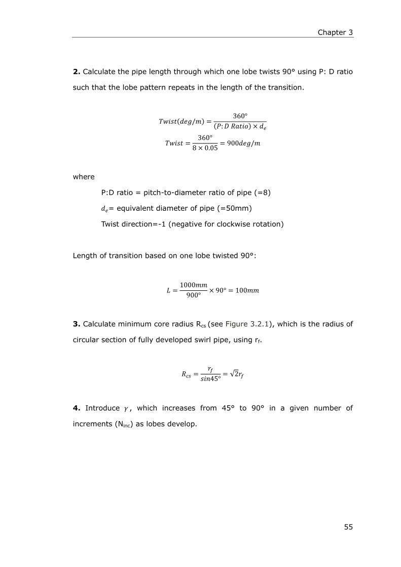
Chapter 3

55

2. Calculate the pipe length through which one lobe twists 90° using P: D ratio

such that the lobe pattern repeats in the length of the transition.

𝑇𝑤𝑖𝑠𝑡(𝑑𝑒𝑔/𝑚) =360°

(𝑃:𝐷 𝑅𝑎𝑡𝑖𝑜) × 𝑑𝑒

𝑇𝑤𝑖𝑠𝑡 =360°

8 × 0.05= 900𝑑𝑒𝑔/𝑚

where

P:D ratio = pitch-to-diameter ratio of pipe (=8)

𝑑𝑒= equivalent diameter of pipe (=50mm)

Twist direction=-1 (negative for clockwise rotation)

Length of transition based on one lobe twisted 90°:

𝐿 =1000𝑚𝑚

900°× 90° = 100𝑚𝑚

3. Calculate minimum core radius Rcs (see Figure 3.2.1), which is the radius of

circular section of fully developed swirl pipe, using rf.

𝑅𝑐𝑠 =𝑟𝑓

𝑠𝑖𝑛45°= √2𝑟𝑓

4. Introduce 𝛾 , which increases from 45° to 90° in a given number of

increments (Ninc) as lobes develop.

Chapter 3

56

Figure 3.2.2 Transition Pipe at Intermediate Stage as Lobes Develop

(𝛄= 65°)

In Figure 3.2.2

r= lobe radius at intermediate stage of transition.

R= circular core radius for intermediate stage of transition pipe.

y= distance of lobe centre from origin O.

𝛾= angle made between the line perpendicular to the lobe origin (point B) and

the lobe radius r.

𝛾/deg= 45° → 90°, from no lobes (stage 1) to fully developed lobes in given

number of incremental steps.

It can be seen from Figure 3.2.2 that:

𝐴𝑟𝑒𝑎 𝑜𝑓 𝑠𝑒𝑔𝑚𝑒𝑛𝑡 𝐵𝐶𝐷 = 𝑎𝑟𝑒𝑎 𝑜𝑓 𝑠𝑒𝑐𝑡𝑜𝑟 𝐴𝐵𝐶𝐷 – 𝑎𝑟𝑒𝑎 𝑜𝑓 𝑡𝑟𝑖𝑎𝑛𝑔𝑙𝑒 𝐴𝐵𝐷

𝐴𝑟𝑒𝑎 𝑜𝑓 𝑠𝑒𝑐𝑡𝑜𝑟 𝐴𝐵𝐶𝐷 = 1

2𝑟2𝜃 =

1

2𝑟2 × 2𝛾 = 𝑟2𝛾

𝐴𝑟𝑒𝑎 𝑜𝑓 𝑡𝑟𝑖𝑎𝑛𝑔𝑙𝑒 𝐴𝐵𝐷 = 𝑟𝑠𝑖𝑛𝛾 × 𝑟𝑐𝑜𝑠𝛾 = 𝑟2𝑠𝑖𝑛𝛾𝑐𝑜𝑠𝛾 = 𝑟2 ×1

2𝑠𝑖𝑛2𝛾

𝐴𝑟𝑒𝑎 𝑜𝑓 𝑠𝑒𝑔𝑚𝑒𝑛𝑡 𝐵𝐶𝐷 = 𝑟2𝛾 −1

2𝑟2𝑠𝑖𝑛2𝛾 = 𝑟2(𝛾 −

1

2𝑠𝑖𝑛2𝛾)

5. Introduce variables f and f1 to facilitate calculation of area of segments and y.

Chapter 3

57

Introduce variable 𝑓 and allow:

𝑓 = (𝛾 −1

2𝑠𝑖𝑛2𝛾)

(3.1)

Therefore

𝐴𝑟𝑒𝑎 𝑜𝑓 𝑠𝑒𝑔𝑚𝑒𝑛𝑡 𝐵𝐶𝐷 = 𝑓𝑟2

In triangle ABO, apply Sine Rule,

𝑅

𝑠𝑖𝑛 (180° − 𝛾)=

𝑦

𝑠𝑖𝑛 (𝛾 − 45°)

𝑅

𝑠𝑖𝑛𝛾=

𝑦

𝑠𝑖𝑛𝛾𝑐𝑜𝑠45° − 𝑐𝑜𝑠𝛾𝑠𝑖𝑛45°

Divided by cos 60° and multiply sin 60°,

𝑦 =1

√2𝑅 [

𝑠𝑖𝑛𝛾 − 𝑐𝑜𝑠𝛾

𝑠𝑖𝑛𝛾] =

1

√2𝑅 [1 −

1

𝑡𝑎𝑛𝛾]

Introduce another variable 𝑓1 and allow:

𝑓1 =1

√2[1 −

1

𝑡𝑎𝑛𝛾]

(3.2)

Therefore

𝑦 = 𝑓1𝑅

(3.3)

Up to now, variable 𝑓 facilitates the calculation of segmental area and 𝑓1

facilitates the calculation of y.

6. At each increment of 𝛾 , calculate R (intermediate core radius), r

(intermediate lobe radius) and y keeping the cross-section area equal for all

stages.

Calculate R for intermediate stage with equal cross-sectional area at all stages:

𝜋𝑅12 = 𝑎𝑟𝑒𝑎 𝑜𝑓 𝑝𝑖𝑝𝑒 𝑤𝑖𝑡ℎ 𝑛𝑜 𝑙𝑜𝑏𝑒𝑠 (𝑠𝑡𝑎𝑔𝑒1, 𝑐𝑖𝑟𝑐𝑢𝑙𝑎𝑟 𝑝𝑖𝑝𝑒)

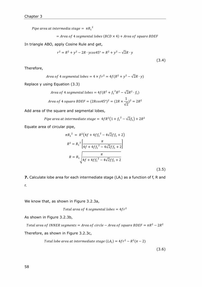
Chapter 3

58

𝑃𝑖𝑝𝑒 𝑎𝑟𝑒𝑎 𝑎𝑡 𝑖𝑛𝑡𝑒𝑟𝑚𝑒𝑑𝑖𝑎 𝑠𝑡𝑎𝑔𝑒 = 𝜋𝑅12

= 𝐴𝑟𝑒𝑎 𝑜𝑓 4 𝑠𝑒𝑔𝑚𝑒𝑛𝑡𝑎𝑙 𝑙𝑜𝑏𝑒𝑠 (𝐵𝐶𝐷 × 4) + 𝐴𝑟𝑒𝑎 𝑜𝑓 𝑠𝑞𝑢𝑎𝑟𝑒 𝐵𝐷𝐸𝐹

In triangle ABO, apply Cosine Rule and get,

𝑟2 = 𝑅2 + 𝑦2 − 2𝑅 ∙ 𝑦𝑐𝑜𝑠45° = 𝑅2 + 𝑦2 − √2𝑅 ∙ 𝑦

(3.4)

Therefore,

𝐴𝑟𝑒𝑎 𝑜𝑓 4 𝑠𝑒𝑔𝑚𝑒𝑛𝑡𝑎𝑙 𝑙𝑜𝑏𝑒𝑠 = 4 × 𝑓𝑟2 = 4𝑓(𝑅2 + 𝑦2 − √2𝑅 ∙ 𝑦)

Replace y using Equation (3.3)

𝐴𝑟𝑒𝑎 𝑜𝑓 4 𝑠𝑒𝑔𝑚𝑒𝑛𝑡𝑎𝑙 𝑙𝑜𝑏𝑒𝑠 = 4𝑓(𝑅2 + 𝑓12𝑅2 − √2𝑅2 ∙ 𝑓1)

𝐴𝑟𝑒𝑎 𝑜𝑓 4 𝑠𝑞𝑢𝑎𝑟𝑒 𝐵𝐷𝐸𝐹 = (2𝑅𝑐𝑜𝑠45°)2 = (2𝑅 ×1

√2)2 = 2𝑅2

Add area of the square and segmental lobes,

𝑃𝑖𝑝𝑒 𝑎𝑟𝑒𝑎 𝑎𝑡 𝑖𝑛𝑡𝑒𝑟𝑚𝑒𝑑𝑖𝑎𝑡𝑒 𝑠𝑡𝑎𝑔𝑒 = 4𝑓𝑅2(1 + 𝑓12 − √2𝑓1) + 2𝑅2

Equate area of circular pipe,

𝜋𝑅12 = 𝑅2(4𝑓 + 4𝑓𝑓1

2 − 4√2𝑓𝑓1 + 2)

𝑅2 = 𝑅12 [

𝜋

4𝑓 + 4𝑓𝑓12 − 4√2𝑓𝑓1 + 2

]

𝑅 = 𝑅1√𝜋

4𝑓 + 4𝑓𝑓12 − 4√2𝑓𝑓1 + 2

(3.5)

7. Calculate lobe area for each intermediate stage (LAi) as a function of f, R and

r.

We know that, as shown in Figure 3.2.3a,

𝑇𝑜𝑡𝑎𝑙 𝑎𝑟𝑒𝑎 𝑜𝑓 4 𝑠𝑒𝑔𝑚𝑒𝑛𝑡𝑎𝑙 𝑙𝑜𝑏𝑒𝑠 = 4𝑓𝑟2

As shown in Figure 3.2.3b,

𝑇𝑜𝑡𝑎𝑙 𝑎𝑟𝑒𝑎 𝑜𝑓 𝐼𝑁𝑁𝐸𝑅 𝑠𝑒𝑔𝑚𝑒𝑛𝑡𝑠 = 𝐴𝑟𝑒𝑎 𝑜𝑓 𝑐𝑖𝑟𝑐𝑙𝑒 − 𝐴𝑟𝑒𝑎 𝑜𝑓 𝑠𝑞𝑢𝑎𝑟𝑒 𝐵𝐷𝐸𝐹 = 𝜋𝑅2 − 2𝑅2

Therefore, as shown in Figure 3.2.3c,

𝑇𝑜𝑡𝑎𝑙 𝑙𝑜𝑏𝑒 𝑎𝑟𝑒𝑎 𝑎𝑡 𝑖𝑛𝑡𝑒𝑟𝑚𝑒𝑑𝑖𝑎𝑡𝑒 𝑠𝑡𝑎𝑔𝑒 (𝐿𝐴𝑖) = 4𝑓𝑟2 − 𝑅2(𝜋 − 2)

(3.6)

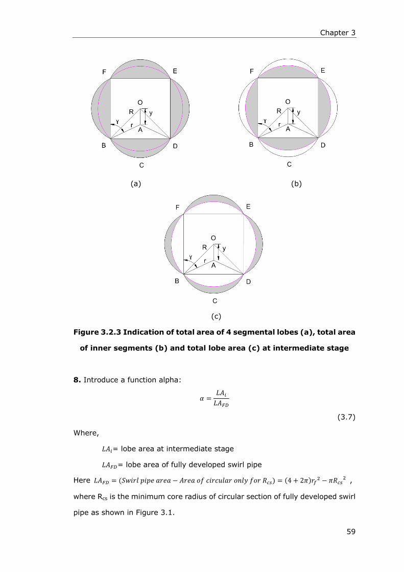
Chapter 3

59

(a) (b)

(c)

Figure 3.2.3 Indication of total area of 4 segmental lobes (a), total area

of inner segments (b) and total lobe area (c) at intermediate stage

8. Introduce a function alpha:

𝛼 =𝐿𝐴𝑖

𝐿𝐴𝐹𝐷

(3.7)

Where,

𝐿𝐴𝑖= lobe area at intermediate stage

𝐿𝐴𝐹𝐷= lobe area of fully developed swirl pipe

Here 𝐿𝐴𝐹𝐷 = (𝑆𝑤𝑖𝑟𝑙 𝑝𝑖𝑝𝑒 𝑎𝑟𝑒𝑎 − 𝐴𝑟𝑒𝑎 𝑜𝑓 𝑐𝑖𝑟𝑐𝑢𝑙𝑎𝑟 𝑜𝑛𝑙𝑦 𝑓𝑜𝑟 𝑅𝑐𝑠) = (4 + 2𝜋)𝑟𝑓2 − 𝜋𝑅𝑐𝑠

2 ,

where Rcs is the minimum core radius of circular section of fully developed swirl

pipe as shown in Figure 3.1.

Chapter 3

60

9. To avoid discontinuity in the case of a linear relationship, vary lobe area along

length as a cosine relationship. Function 𝛼 can now be defined as desired to

determine lobe development in transition.

Define x/L (length ratio) as a cosine function of 𝛼,

𝑥

𝐿=

𝑐𝑜𝑠−1(1 − 2𝛼)

𝜋

(3.8)

Where

x = intermediate length

L = total length

The above function can be varied to give different types of transition

development based on lobe area growth.

Intermediate twist is calculated using:

𝑇𝑤𝑖𝑠𝑡[0,90°] =𝑥

𝐿× 90° × 𝑇𝑤𝑖𝑠𝑡 𝑑𝑖𝑟𝑒𝑐𝑡𝑖𝑜𝑛

(3.9)

Where twist direction is -1 (negative for clockwise rotation)

𝛾 increases from 45° to 90° in given number of increments (Ninc) as lobes

develop. For each increment of 𝛾, function f and f1 are calculated using Equation

(3.1) and (3.2) respectively. These in turn are used to calculate R form equation

(3.5), y from Equation (3.3) and r from Equation (3.4) at each increment stage.

Lobe area is calculated using Equation (3.6), 𝛼 using Equation (3.7), x/L using

Equation (3.8) and the respective twist using Equation (3.9).

10. Tabulate calculated data at each stage of 𝛾 as it increases 45° to 90°.

3.2.2 Different Types of Transition

The transition pipe consists of gradual change of cross-section from circular to 4

Chapter 3

61

lobed cross-sections. Other than the 𝛼 transition discussed in section 3.2.1

bullet 8, there is also a 𝛽 type of transition which is based on the relationship of

the lobe area growth with length. In addition, applying a different transition

multiplier, n, to 𝛼 or 𝛽 would generate a set of different transition curves.

Moreover, a variable helix factor could also be introduced.

3.2.2.1 𝛂 transition

As defined in Equation (3.7), variable 𝛼 is the ratio of lobe area at any

intermediate stage to the total lobe area for fully developed lobes. In order to

avoids discontinuity that would result from the use of a linear relationship, 𝛼

was equated to a cosine relation of pipe length as defined in Equation (3.8). This

cosine function of 𝛼, as shown below, gives a smooth transition.

𝛼 = [1 − 𝑐𝑜𝑠 [𝜋

𝑥𝐿]

2]

(3.10)

3.2.2.2 𝛃 transition

Ganeshalingam (2002) indicated that there were two distinctive types of flow

within the 4-lobed swirl pipe, namely the core flow and the lobe flow. It is clear

from Figure 3.2.4 that, within the fully developed 4-lobed swirl pipe and the

intermediate stage of the transition pipe, the core flow inside the inner circle

consisted mainly of axial velocity, while the lobe flow in the lobe zones consisted

mainly of tangential velocity.

It was therefore expected that defining the transition in terms of lobe area

growth to the core area (circular area only) would give better results for 4-lobed

transition. This was achieved by intruding a variable 𝛽, which is defined as a

ratio of lobe area to the core area.

Chapter 3

62

𝛽 =

𝐿𝐴𝑖

𝜋𝑅2 − 𝐿𝐴𝑖

𝐿𝐴𝐹𝐷

𝜋𝑅2 − 𝐿𝐴𝐹𝐷

(3.11)

For the calculation of 𝛽 type transition pipe, variable 𝛽 then replaced 𝛼 in

Equation (3.7) and (3.8). Figure 3.2.5 depicts the lobe area development with

the pipe length for 𝛼 , 𝛽 and linear transitions. It can be seen that the 𝛽

transition provides a faster lobe development than 𝛼 transition. Since the lobes,

where tangential velocity is mainly concentrated, prevail for a longer length, it is

expected that the 𝛽 transition would result in greater swirl induction.

Ariyaratne (2005) carried out CFD modelling and confirmed that, as expected,

𝛽 transition was more effective at swirl induction than 𝛼. Its value of swirl

effectiveness was 5% greater than that of 𝛼. Therefore variable 𝛽 will later be

used in the calculation and creation of a transition pipe.

Figure 3.2.4 Axial and tangential velocity contours at fully developed

and intermediate stage of transition pipe (2m/s inlet velocity).

Chapter 3

63

Figure 3.2.5 Lobe area developments with pipe length for α, β and

linear transitions

3.2.2.3 Transition Multiplier

Applying a transition multiplier to variable α and β and Equation (3.10) and

(3.11) change to:

𝛼 = [1 − 𝑐𝑜𝑠 [𝜋

𝑥𝐿]

2]

𝑛

(3.12)

and

𝛽 = [

𝐿𝐴𝑖

𝜋𝑅2 − 𝐿𝐴𝑖

𝐿𝐴𝐹𝐷

𝜋𝑅2 − 𝐿𝐴𝐹𝐷

]

𝑛

(3.13)

Thus Equation (3.10) and (3.11) are instances of the transition multiplier being

n=1. A series of transition curves can be created by varying the value of n.

Generally, an n value smaller than 1 gives greater lobe area growth near the

Chapter 3

64

start, while an n value larger than 1 decreases the lobe development near the

start compared with n being 1. Besides, for the same value of transition

multiplier n, the lobe development for 𝛽 transition is nearer the start than for

the 𝛼 transition therefore a quicker lobe development for 𝛽 transition.

Ariyaratne (2005) numerically compared the effect of different n values and

found that the smaller the value of the transition multiplier n, the greater the

tangential velocity generated, however the greater the pressure loss. She used

the swirl effectiveness parameter as a balance of tangential velocity and

pressure loss, and found that the swirl effectiveness was optimum at a value of

n=0.5 where the lobes developed faster in the transition than with the original

𝛽 transition case of n=1. This transition multiplier n=0.5 for 𝛽 transition will

therefore be used for the transition pipe creation.

3.2.2.4 Variable Helix

The types of transitions discussed above all have a constant change in twist with

respect to the length, namely geodesic helices. Raylor (1998) proposed a

brachistochrone helix for a swirl pipe, where the twist has a power law

relationship with respect to length ratio.

𝑇𝑤𝑖𝑠𝑡 = (𝑥

𝐿)𝑡

× 𝑇𝑤𝑖𝑠𝑡𝐴𝑛𝑔𝑙𝑒

t= power law variable for twist which can be changed to apply an increasing or

decreasing helix as desired.

When

t<1: the helix is faster nearer the start of the transition

t=1: constant or geodesic helix where twist is linear with length

t>1: the helix is faster nearer the end of the transition

Chapter 3

65

It was found that, as the t value, and thereby the helix increases, the tangential

velocity generated increases together with the pressure drop (Ariyaratne, 2005).

However, the study of Ariyaratne (2005) showed that no advantage was gained

from the use of the variable helix studied over the geodesic helix for entry

transition. She argued that although the variable helix gives ‘optimum swirl’ it is

not the ‘minimal cost’ design. She concluded that, based on the swirl

effectiveness criterion, geodesic proves to be better than the variable helix

designs for an entry transition. Therefore, the geodesic helix t=1 will be adopted

later on in the geometry creation process.

3.2.3 Spreadsheet for 4-lobed Transition Pipe

Based on the transition pipe calculation and the optimisation results from

Ariyaratne (2005), the spreadsheet for 4-lobed transition pipe was generated as

shown in Appendix 3.1 Spreadsheet for 4-Lobed Transition Pipe. This

spreadsheet only includes necessary data for geometry creation using

Pro/Engineer, data such as x and y co-ordinates, lobe areas are not exhibited

explicitly. The basic information of the transition pipe defined by the

spreadsheet is summarized as below:

Lobe number 4

Total length 100mm Length of transition based on one lobe

twisted 90 degrees

Equivalent diameter 50mm

Pitch: Diameter ratio 8:1

Type of transition 𝛽

Transition multiplier n=0.5

Variable helix t=1 Geodesic helix

Twist degrees 900° Degrees of twist per metre

Twist direction -1 -1=clockwise

rf 13.8182mm Lobe radius (fully developed)

Rcs 19.5418mm Minimum core radius (fully developed)

LA(total) 763.7834mm2 Lobe area for fully developed swirl pipe

Total cross-section area 1963.4954mm2

Chapter 3

66

3.2.4 Spreadsheet for 4-lobed Swirl Inducing Pipe

The swirl inducing pipe forms as the fully developed 4-lobed swirl pipe

cross-section (as shown in Figure 3.2.1) extends helically along the pipe axis.

The core radius Rcs and lobe radius rf for the fully developed swirl pipe section

can be calculated from section 3.2.1 bullets 1~3. The swirl inducing pipe has a

pitch to diameter ratio of 8 indicating that the length for the 4-lobed

cross-section rotates by 360 degrees is equivalent to 8 diameters that is 400mm.

From Equation (3.9), the twist degree is 900 degrees per metre. Therefore, if we

create one cross-section in the interval of every 10mm along the pipe, the twist

angle between the adjacent two cross-sections is 9 degrees.

Based on above discussion, the spreadsheet was created which includes 21

sections along the pipe axis. The 21 sections will form a 200mm length swirl

pipe that is half of the 400mm length swirl inducing pipe. A detailed spreadsheet

for the swirl inducing pipe is presented in Appendix 3.2 Spreadsheet for 4-Lobed

Swirl Inducing Pipe.

3.3 Geometry Creation

3.3.1 Transition Pipe Creation

The transition pipe was created in a Pro/Engineer software using an advanced

swept blend feature. The swept blend is a combination between a general blend

and a sweep feature in the Pro/Engineer. It allows for blending together several

varying cross-sections following a specific trajectory.

Originally 10 cross-sections including the circle and the fully developed swirl

pipe section were sketched in the X-Y plane based on a constant 𝛾 interval of 5

degrees. The use of constant 𝛾 interval cross-sections was because 𝛾 directly

signifies the lobe changes and provides better accuracy in sweeping one

Chapter 3

67

cross-section onto the following one when the swept blend is used in the

Pro/Engineer. In the swept blend process:

Selected Z-axis as trajectory so the cross-sections were normal to the

trajectory.

All the sketched sections in the X-Y plane were made to have the same

number of 4 curves and consequently 4 intersection points (Figure

3.3.1a).

Specified a start point from the four points for each sections making sure

that the points were traceable and following a clockwise twist.

Specified the depths between the two adjacent two cross-sections

according to the spreadsheet.

Confirmed the above operations and the cross-sections were swept and

blended along Z-axis transforming them into the transition pipe as shown

in Figure 3.3.1c.

(a)

(b)

(c)


transition pipe

It was noticed that, due to the application of a transition multiplier n=0.5 for the

𝛽 transition, 𝛾 increase and x/L increment did not form a linear correlation. As

shown in Figure 3.3.2, there are steeper cross-section transitions in the start 5

Chapter 3

68

degrees 𝛾 interval (45°→50°) and the end 𝛾 interval of 5 degrees (85°→90°).

An attempt was later made to allow more accurate transitions between the 1st

and 2nd section and between the final and penultimate section by adding 4

intermediate sections respectively. The added sections are marked in red open

squares as demonstrated in Figure 3.3.2. Therefore, 18 sections (see Figure

3.3.1a) were used in the sweeping and blending to create the final transition

pipe model. A detailed 4-lobed transition development of the 18 sections and

the start points is also available in Appendix 3.3 Cross-section Development of

the 4-Lobed Transition Pipe.

Figure 3.3.2 Graph of 𝜸 versus length for transition pipe

(Red open squares indicate sections inserted afterward)

3.3.2 Swirl Inducing Pipe Creation

The same swept blend method was adopted in creating the 200mm length,

50mm equivalent diameter swirl inducing pipe, which is half of the full swirl

inducing pipe.

The swept blend process was carried out as below:

Chapter 3

69

21 sections of fully developed 4-lobed cross-sections were sketched in

the X-Y plane as shown in Figure 3.3.3a.

The 21 sections were evenly distributed between the start and the end of

the half swirl inducing pipe along Z-axis with the twist angle between the

adjacent two sections were 9°.

The distance between the adjacent two sections were evenly set to be

x/L=0.05 (10mm). The twist degree with pipe length increase is shown in

Figure 3.3.4 which exhibits a linear relationship.

Specified a start point at each section and made sure the start points

rotate clockwise. The feature swept the 2D face along Z trajectory onto

the following face one by one and blended them into the swirl inducing

pipe as shown in Figure 3.3.3c.

(a)

(b)

(c)


half of the full swirl inducing pipe

Chapter 3

70

Figure 3.3.4 Graph of twist versus length for swirl inducing pipe

3.3.3 Optimized Swirl Pipe Creation

Ariyaratne (2005) connected either the transition prior to the 400mm length

swirl inducing pipe as the entry transition (see Figure 3.3.5a) or after the

400mm length swirl inducing pipe as the exit transition (see Figure 3.3.5b). She

found that the 4-lobed β transition with transition multiplier n=0.5 was optimum

in both cases of entry and exit transition from several geometries tested. The

entry transition was found to be able to increase swirl generated at the exit of

the swirl pipe and reduce pressure losses. While the use of exit transition

reduced exit pressure losses, decreased the swirl decay rate thereby sustaining

the induced swirl for longer distance.

According to Ariyaratne’s suggestion, a swirl pipe comprising a 400mm length

swirl inducing pipe, an entry transition pipe prior to it and an exit transition pipe

after it should be considered to be an ‘optimised swirl pipe’. This type of

optimised swirl pipe is not entirely understood and will be studied in this

investigation.

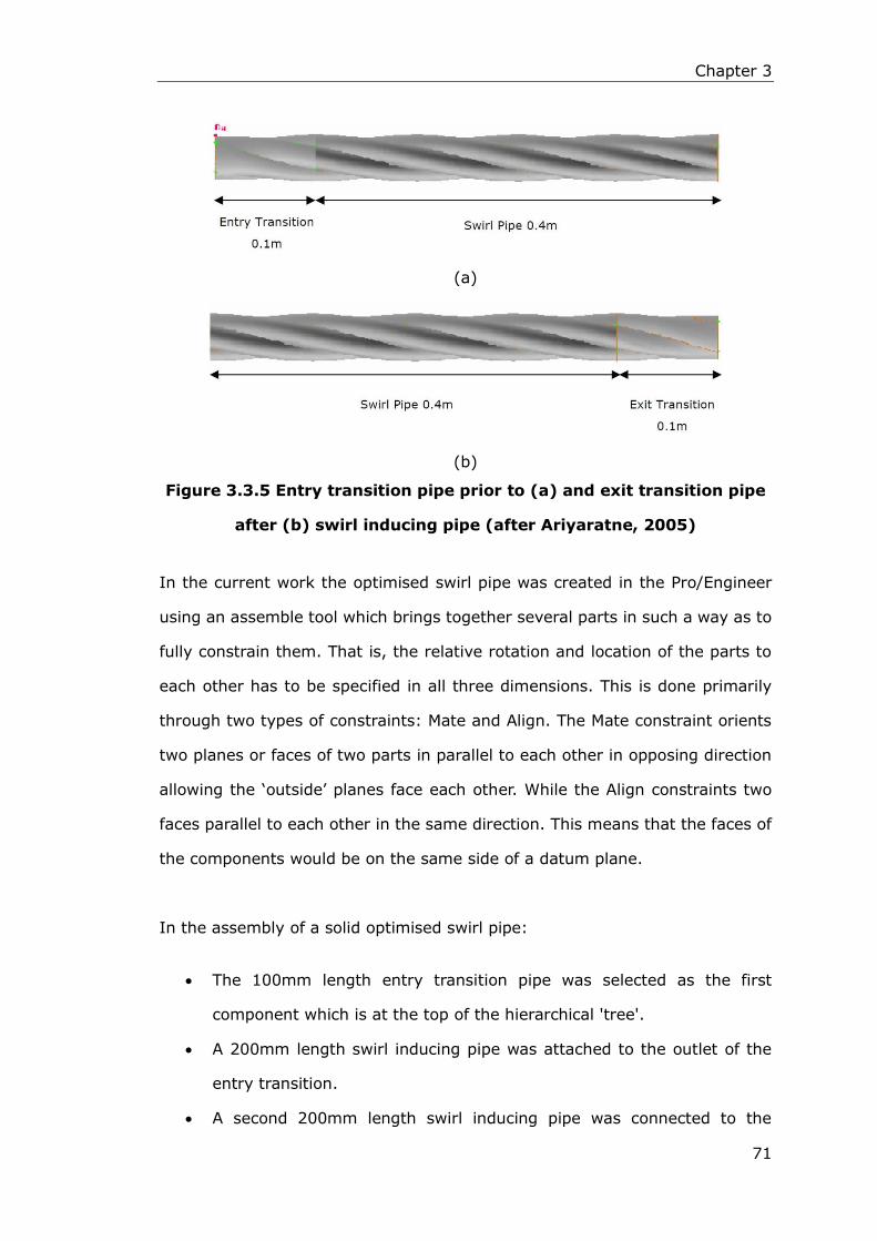
Chapter 3

71

(a)

(b)

Figure 3.3.5 Entry transition pipe prior to (a) and exit transition pipe

after (b) swirl inducing pipe (after Ariyaratne, 2005)

In the current work the optimised swirl pipe was created in the Pro/Engineer

using an assemble tool which brings together several parts in such a way as to

fully constrain them. That is, the relative rotation and location of the parts to

each other has to be specified in all three dimensions. This is done primarily

through two types of constraints: Mate and Align. The Mate constraint orients

two planes or faces of two parts in parallel to each other in opposing direction

allowing the ‘outside’ planes face each other. While the Align constraints two

faces parallel to each other in the same direction. This means that the faces of

the components would be on the same side of a datum plane.

In the assembly of a solid optimised swirl pipe:

The 100mm length entry transition pipe was selected as the first

component which is at the top of the hierarchical 'tree'.

A 200mm length swirl inducing pipe was attached to the outlet of the

entry transition.

A second 200mm length swirl inducing pipe was connected to the

Chapter 3

72

exposed 4-lobed face of the first swirl inducing pipe.

A second 100mm length transition pipe was attached to the second swirl

inducing pipe with the two 4-lobed faces opposite to each other.

The joints of every two parts was constrained using two align and one

mate constraints.

The four components were then merged into one component and saved

as a .STP file for use with ICED CFD.

The assembled optimised 4-lobed swirl pipe is displayed in Figure 3.3.6 which

has a total length of 600mm, equivalent diameter of 50mm and a pitch to

diameter ratio of 8:1.

Figure 3.3.6 The optimized 600mm length 4-lobed swirl pipe

However, in this configuration:

The swirl pipe has the lobed cross-section rotated by 540º (one and a

half swirl) instead of 360 º (one swirl), which was used in the previous

designs.

The longer swirl pipe results in more pressure loss due to the increase in

contact area and thus friction.

When the entry transition pipe was used in conjunction with the swirl

pipe, a higher tangential velocity was generated. However, the induced

swirl appeared to be constrained by the swirl inducing pipe geometry. A

shorter length of swirl inducing pipe will therefore be required to

generate an equivalent amount of swirl (Ariyaratne, 2005).

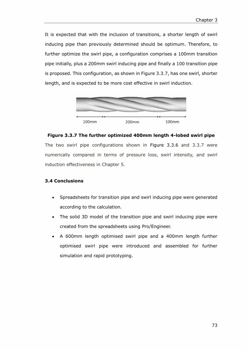
Chapter 3

73

It is expected that with the inclusion of transitions, a shorter length of swirl

inducing pipe than previously determined should be optimum. Therefore, to

further optimize the swirl pipe, a configuration comprises a 100mm transition

pipe initially, plus a 200mm swirl inducing pipe and finally a 100 transition pipe

is proposed. This configuration, as shown in Figure 3.3.7, has one swirl, shorter

length, and is expected to be more cost effective in swirl induction.

Figure 3.3.7 The further optimized 400mm length 4-lobed swirl pipe

The two swirl pipe configurations shown in Figure 3.3.6 and 3.3.7 were

numerically compared in terms of pressure loss, swirl intensity, and swirl

induction effectiveness in Chapter 5.

3.4 Conclusions

Spreadsheets for transition pipe and swirl inducing pipe were generated

according to the calculation.

The solid 3D model of the transition pipe and swirl inducing pipe were

created from the spreadsheets using Pro/Engineer.

A 600mm length optimised swirl pipe and a 400mm length further

optimised swirl pipe were introduced and assembled for further

simulation and rapid prototyping.

Chapter 4

74

CHAPTER 4: COMPUTATIONAL FLUID DYNAMICS

METHODOLOGY

4.1 Introduction

Computational fluid dynamics or CFD is the analysis of systems involving fluid

flow, heat transfer and associated phenomena such as chemical reactions by

means of computer-based simulation. The technique is very powerful and spans

a wide range of industrial and non-industrial application areas (H.K.Versteeg

and W.Malalasekera, 2010). CFD has several unique advantages over

experiment-based approaches to the fluid systems. For instance, it substantially

reduces time and costs of new designs and has the ability to study systems

where controlled experiments are difficult or impossible to perform. The CFD

method is employed in the present research to supplement the experimental

investigations because of its cost effectiveness and the limitations of the

available experimental techniques.

In CFD, applying the fundamental laws of mechanics to a fluid flow, including

turbulent ones, gives the governing equations for fluid flow which represent

mathematical statements of the conservation laws of physics (H.K.Versteeg and

W.Malalasekera, 2010, Bhaskaran and Collins, 2003):

The mass of a fluid is conserved

The rate of change of momentum equals the sum of the forces on a fluid

particle (Newton’s second law)

The rate of change of energy is equal to the sum of the rate of heat

addition to and the rate of work done on a fluid particle (first law of

thermodynamics)

Chapter 4

75

The partial differential equations for the three fundamental principles are the

continuity equation, the momentum equations, and the energy equation

respectively. They are termed the ‘Navier-Stokes Equation’. Since this study

assumes the swirl flows to be isothermal, only the continuity and momentum

equations are concerned.

Continuity equation for mass conservation:

The continuity equation was derived by applying the law of conservation of mass

to a fluid flow making sure that the rate of increase of mass inside the control

volume is equal to the net rate of mass into and out of the control volume across

its faces. The continuity equation for an incompressible flow, in Cartesian form

is given by:

𝜕𝜌

𝜕𝑡+ ∇ ∙ (𝜌�� ) = 0

(4.1)

Where 𝜕𝜌/𝜕𝑡 represents the rate of change of mass with time in an infinitesimal

control volume; ∇ ∙ (𝜌�� )describes the convection of the mass through the

control volume.

Momentum equations for momentum conservation:

Apply the Newton’s Second Law of Motion to the fluid flow and ensure that the

rate of change of momentum of the fluid particles is equal to the total force due

to surface stresses and body forces acting in an aligned direction of a chosen

coordinate axis. The momentum equation is obtained in terms of the viscous

stress acting on a particle in the fluid as:

𝜕(𝜌�� )

𝜕𝑡+ 𝜌(�� ∙ ∇)�� = 𝜌�� + (−∇𝑝 + ∇ ∙ 𝜏𝑖𝑗)

(4.2)

Chapter 4

76

Where 𝜕(𝜌�� )/𝜕𝑡 represents the rate of change of momentum with time;

𝜌(�� ∙ ∇)�� describes the advection of momentum; 𝜌�� represents the body forces

(include gravity and buoyancy); (−∇𝑝 + ∇ ∙ 𝜏𝑖𝑗) represents the forces due to

pressure and stress gradients in the fluid.

It is not possible to solve the above partial differential equations (PDEs)

analytically for most engineering problems. Therefore approximate modelling

methods have been developed to calculate the statistical characteristics of the

turbulent motion by discretising the flow equations to produce a numerical

analogue of them.

The strategy of CFD is to replace the continuous problem domain with a discrete

domain using a grid. In the discrete domain, each flow variable is defined only at

the grid points (Bhaskaran and Collins, 2003). When the boundary and initial

conditions that are specific to the flow problem being simulated have been

applied, they can be solved using a variety of direct or iterative solution

techniques producing a numerical simulation of the given flow problem (Shaw,

1992).

4.2 Modelling Turbulence

All flows encountered in engineering practice become unstable above a certain

Reynolds number. For pipe flows, the Reynolds number is defined by Re=(U×D×ρ)/

μ where U is velocity, ρ is density, and μ is viscosity. At low Reynolds numbers

flows are laminar. At higher Reynolds numbers flows are observed to become

turbulent. A chaotic and random state of motion develops in which the velocity

and pressure fluctuate continuously with time within substantial regions of flow.

The turbulent swirl flow in this study is a combination of vortex and axial

motions. Due to the presence of a tangential velocity component, swirl flow is

always accompanied by an increase in velocity fluctuations (Fokeer, 2006, Algifri

Chapter 4

77

et al., 1988).

Turbulence causes the appearance of eddies in the flow with a wide range of

length and time scales that interact in a dynamically complex way. Due to the

importance of turbulence in engineering practice, several numerical methods

have been developed to capture the important effects of the turbulence. The

methods can be grouped into the following three categories (H.K.Versteeg and

W.Malalasekera, 2010):

Turbulence models for Reynolds-averaged Navier–Stokes (RANS)

equations: In this approach, prior to the application of numerical

methods, the Navier–Stokes equations are time averaged. It was found

that extra terms, the so-called Reynolds stresses, appear in the

time-averaged (or Reynolds-averaged) flow equations due to the

interactions between various turbulent fluctuations. These Reynolds

stresses are modelled with classical turbulence models, among which the

best known are the standard k-ε turbulence model and its variations, and

the Reynolds stress model. This approach predicts the mean flow and the

effects of turbulence on mean flow properties. The computing resources

required for reasonably accurate flow computations are modest, so this

approach has been the mainstay of engineering flow calculations over

the last three decades. Besides, RANS turbulence models are the only

modelling approach for steady state simulation of turbulent flows. Due to

its shorter simulation time, simplified post-processing, and the

importance and interest of time-averaged values from an industrial

prospect, steady RANS is the most widely used approach for industrial

flows.

Large eddy simulation: LES is an intermediate form of turbulence

calculations which tracks the behaviour of the larger eddies. The method

Chapter 4

78

involves space filtering of the unsteady Navier–Stokes equations prior to

the computations, which passes the larger eddies and rejects the smaller

eddies. The motion of the largest eddies is directly resolved in the

calculation in at least a portion of the domain, while eddies smaller than

the mesh size are modelled by means of a so-called sub-grid scale model.

Conceptually, LES is situated somewhere between DNS and RANS. LES is

inherently an unsteady method and unsteady flow equations must be

solved, so the demands on computing resources in terms of storage and

volume of calculations are large. LES has the potential for improved

accuracy when the resolution of the largest eddies is important or when

unsteady data is needed. However, this method is computationally

expensive due to the required higher grid resolution and small time steps

for unsteady simulation which generates long run times and large

volumes of data.

Direct numerical simulation (DNS): these simulations compute the

mean flow and all turbulent velocity fluctuations. The unsteady Navier–

Stokes equations are solved on spatial grids that are sufficiently fine that

they can resolve the Kolmogorov length scales at which energy

dissipation takes place and with time steps sufficiently small to resolve

the period of the fastest fluctuations. These calculations are highly costly

in terms of computing resources, so the method is not used for industrial

flow computations.

It is theoretically possible to resolve the Navier-Stokes equations for the

turbulent swirl flow using Direct Numerical Simulation (DNS); however it is not

feasible for practical engineering problems given that the volume of the

computational domain used in this research is very large and it is prohibitive to

obtain sufficiently fine grid resolution everywhere required for DNS.

Chapter 4

79

Considering the intensive cost of NDS in terms of computing resource and the

unaffordable run time for the calculation of the whole spectrum of turbulence

which can be of small scales and high frequency, the alternative RANS and LES

approaches will be adopted in this study for the investigation of swirl pipe

induced swirl flow as both methods result in a modified set of Navier-Stokes

equations that are computationally less expensive to solve.

The initial simulation work (in Chapter 5 and 6) will focus on the mean flow

properties using a RANS approach since the time-averaged values are of

interest for industrial applications. LES (in Chapter 7) will be used as a

supplement to study the fluctuation property of some variables of the swirl flow.

The principles and models in terms of the LES approach will be introduced in

Chapter 7. This approach can be affordable to some extent as the filtering

operation results in mesh resolution requirements that are much less restrictive

than with DNS, though in practice, extremely fine meshes and large computer

resource are still required.

4.2.1 RANS Approach

For most engineering purposes it is unnecessary to resolve the details of the

turbulent fluctuations. Information about the time-averaged properties of the

flow (e.g. mean velocities, mean pressures, mean stresses etc.) are almost

always satisfied for most problems. Therefore, the vast majority of turbulent

flow computations has been and for the foreseeable future will continue to be

carried out with procedures based on the Reynolds-averaged Navier–Stokes

(RANS) equations (H.K.Versteeg and W.Malalasekera, 2010).

In Reynolds averaging, the effects of fluctuation on the mean flow are

investigated using the Reynolds decomposition (Reynolds averaging) approach.

The Navier-Stokes equations are time averaged over a large enough time

Chapter 4

80

compared to the typical timescale of turbulent fluctuation in order to average

out the unsteadiness of a turbulent flow. Flow variables u (hence u, v and w) and

pressure p in the instantaneous (exact) Navier-Stokes equations are substituted

by the sum of a mean and fluctuation component.

u=U + u’ u=U + u’ v=V + v’ w=W + w’ p=P + p’

Where U is the time average of u (the steady component), u’ is the fluctuation

part (or perturbations, their average equals zero). Substituting the Reynolds

decomposition into the equations for conservation of mass and momentum and

taking the time average by applying the rules which govern time averages of

fluctuating properties (H.K.Versteeg and W.Malalasekera, 2010). This yields the

Reynolds Averaged Navier-Stokes Equations for incompressible flow:

𝜕(𝑢𝑖)

𝜕𝑡+

𝜕

𝜕𝑥𝑗(𝑢𝑖𝑢𝑗) = −

1

𝜌

𝜕𝑝

𝜕𝑥𝑖+

𝜕

𝜕𝑥𝑗[ν(

𝜕𝑢𝑖

𝜕𝑥𝑗+

𝜕𝑢𝑗

𝜕𝑥𝑖)] − 𝑢𝑖

′𝑢𝑗′

(4.3)

The process of time averaging has introduced new terms −𝑢𝑖′𝑢𝑗

′ called Reynolds

stress. This nonlinear Reynolds stress term requires additional modelling to

close the RANS equation for solving, and has led to the creation of many

different turbulence models of which the standard k-ε turbulence model and its

variations (RNG k-ε model and Realizable k-ε model), and the Reynolds stress

model are widely used.

In k-ε models, the Reynolds stress tensor can be calculated using the isotropic

eddy viscosity assumption that the ratio between Reynolds stress and mean

rate of deformation is the same in all directions. The k-ε model family are two

equation models. Two transport equations, one for the turbulent kinetic energy

k, and one for the rate of its dissipation ε, are solved. These are then used to

calculate the turbulent viscosity, μt, to close the RANS equations. While,

abandoning the assumption of isotropic eddy viscosity, the RSM closes the RANS

Chapter 4

81

by solving transport equations for Reynolds stresses, together with an equation

for the dissipation rate.

4.2.1.1 The Standard k-ε Model

The standard k-ε model, proposed by Launder and Spalding (1972) is a

two-equation turbulence model that allows the determination of both the

turbulent length and time scale by solving two separate transport equations. It

is a semi-empirical model, and the derivation of the model equations relies on

phenomenological considerations and empiricism.

The standard k–ε model has two model equations; one for kinetic energy k and

one for its dissipation rate ε. k and ε are used to define velocity scale v and

length l representative of the large-scale turbulence as follow:

𝑣 = 𝑘1/2

𝑙 =𝑘3/2

휀

(4.4)

Applying dimensional analysis, the eddy viscosity is specified as:

𝜇𝑡 = 𝐶𝜌𝑣𝑙 = 𝜌𝐶𝜇

𝑘2

휀

(4.5)

where 𝐶𝜇 is a dimensionless constant.

The standard k–ε model uses the following transport equations for k and ε

respectively:

𝜕(𝜌𝑘)

𝜕𝑡+ 𝑢𝑖

𝜕(𝜌𝑢𝑗𝑘)

𝜕𝑥𝑗=

𝜕

𝜕𝑥𝑗(𝜇𝑡

𝜎𝑘

𝜕𝑘

𝜕𝑥𝑗) + 𝜇𝑡

𝜕𝑢𝑖

𝜕𝑥𝑗(𝜕𝑢𝑖

𝜕𝑥𝑗+

𝜕𝑢𝑗

𝜕𝑥𝑖) − 𝜌휀

(4.6)

Chapter 4

82

and

𝜕(𝜌휀)

𝜕𝑡+ 𝑢𝑖

𝜕(𝜌𝑢𝑗휀)

𝜕𝑥𝑗=

𝜕

𝜕𝑥𝑗(𝜇𝑡

𝜎𝜀

𝜕휀

𝜕𝑥𝑗) + 𝐶𝜀1

휀

𝑘𝜇𝑡

𝜕𝑢𝑖

𝜕𝑥𝑗(𝜕𝑢𝑖

𝜕𝑥𝑗+

𝜕𝑢𝑗

𝜕𝑥𝑖) − 𝜌𝐶𝜀2

휀2

𝑘

(4.7)

In words the equations are:

Rate of change of k or ε + Transport of k or ε by convection = Transport of k or

ε by diffusion + Rate of production of k or ε - Rate of destruction of k or ε.

Production and destruction of turbulent kinetic energy are always closely linked.

Dissipation rate ε is large where production of k is large. The model equation for

ε assumes that its production and destruction terms are proportional to the

production and destruction terms of the k-equation.

The inherent production of turbulence is what is responsible for the transfer of

energy from the mean flow to the turbulence, and is counterbalanced by the

interaction of the Reynolds stresses and mean velocity gradient. On the other

hand, the destruction term represents the dissipation of energy into heat due to

viscous nature of the flow.

The equations contain five adjustable constants: 𝜇𝑡, 𝜎𝑘, 𝜎𝜀, 𝐶𝜀1 and 𝐶𝜀2. The

standard k–ε model employs values for the constants that are obtained by

comprehensive data fitting for a wide range of turbulent flows:

𝜇𝑡=0.09 𝜎𝑘=1.00 𝜎𝜀=1.30 𝐶𝜀1=1.44 𝐶𝜀2=1.92

The advantage of robustness, economy, and reasonable accuracy for a wide

range of turbulent flows make the standard k–ε model popular for industrial

flows. However this model does not perform very well for flows with boundary

Chapter 4

83

layer separation, sudden changes in the mean strain rate such as swirling and

rotating flows and flows over curved surfaces. Moreover, the k-ε model is based

on the Boussinesq hypothesis, which inherently assumes that the turbulent

viscosity is isotropic. This is a major source of error when using the k-ε model for

simulating strong swirling flows as turbulent eddy viscosity is an anisotropic

quantity which is affected by geometry.

4.2.1.2 RNG k–ε Model and Realizable k–ε Model

Both the RNG and realizable k–ε models are the variations of the standard k–ε

model. The RNG turbulence model is derived from the instantaneous

Navier-Stokes equations, using a mathematical technique called

“renormalization group” (RNG) methods. The analytical derivation results in a

model with constants different from those in the standard k–ε model, and

additional terms and functions in the transport equations for k and ε. The RNG

model includes the following refinements (ANSYS, 2011a):

The RNG k–ε model has an additional term in its ε equation that improves

the accuracy for rapidly strained flows.

The effect of swirl on turbulence is included in the RNG model, enhancing

accuracy for swirling flows.

The RNG theory provides an analytical formula for turbulent Prandtl

numbers, while the standard k–ε model uses user-specified, constant

values.

The standard k–ε model is a high-Reynolds number model, the RNG

theory provides an analytically derived differential formula for effective

viscosity that accounts for low-Reynolds number effects.

Therefore, the RNG k–ε model is more accurate and reliable for a wider class of

flow than the standard k–ε model.

Chapter 4

84

The realizable k–ε model proposed by Shih et al. (1995) differs from the

standard k–ε model in two important ways:

The realizable k–ε model contains an alternative formulation for the

turbulent viscosity.

A modified transport equation for the dissipation rate ε has been derived

from an exact equation for the transport of the mean-square vorticity

fluctuation.

The term “realizable” means that the model satisfies certain mathematical

constraints on the Reynolds stresses, consistent with the physics of turbulent

flows. Neither the standard k–ε model nor the RNG k–ε model is realizable.

Both the realizable and RNG k–ε models have shown substantial improvements

over the standard k–ε model where the flow features include strong streamline

curvature, vortices, and rotation. Since the model is still relatively new, it is not

clear in exactly which instances the realizable k–ε model consistently

outperforms the RNG model. However, initial studies have shown that the

realizable model provides the best performance of all the k–ε model versions for

several validations of separated flows and flows with complex secondary flow

features (ANSYS, 2011a).

4.2.1.3 Reynolds Stress Model (RSM)

Reynolds stress model abandons the Boussinesq hypothesis of isotropic eddy

viscosity. It closes the Reynolds-averaged Navier-Stokes equations by solving

transport equations for the Reynolds stresses, together with an equation for the

dissipation rate. This means that seven additional transport equations are

required in 3D flows.

Chapter 4

85

The transport equation for the transport of the Reynolds Stresses is (Speziale et

al., 1991):

𝜕

𝜕𝑡(𝜌𝑢𝑖′𝑢𝑗

′ )+

𝜕

(𝜕𝑥𝑘)(𝜌𝑢𝑘𝑢𝑖′𝑢𝑗

′ )=

−𝜌(𝑢𝑖′𝑢𝑘

′ 𝜕𝑢𝑗

𝜕𝑥𝑘+ 𝑢𝑗

′𝑢𝑘′ 𝜕𝑢𝑗

𝜕𝑥𝑘) −

𝜕

𝜕𝑥𝑘[(𝜇 +

𝜇𝑡

𝜎𝑘)

𝜕

𝜕𝑥𝑘(𝑢𝑖

′𝑢𝑗′ )] + 𝑝 (

𝜕𝑢𝑖′

𝜕𝑥𝑗+

𝜕𝑢𝑗′

𝜕𝑥𝑖)

−

2

3𝛿𝑖𝑗𝜌휀

(4.8)

Where the terms on the left hand side of Equation (4.8) are local time derivative

and convection, the terms on the right hand side are stress production, diffusion,

pressure-strain and dissipation respectively. 𝜇 and 𝜇𝑡 are the dynamic and

eddy viscosity, with 𝛿𝑖𝑗 being the Kronecker delta function.

The pressure-strain term is modelled by

𝑝 (𝜕𝑦𝑖

′

𝜕𝑥𝑗+

𝜕𝑦𝑗′

𝜕𝑥𝑖) = −𝜌휀 (𝑐𝑠1𝑎𝑖𝑗 − 𝑐𝑠2 (𝑎𝑖𝑘𝑎𝑘𝑗 +

1

3𝑎𝑚𝑛𝑎𝑚𝑛𝛿𝑖𝑗)) − 𝑐𝑟1𝑃𝑎𝑖𝑗 + 𝜌𝑘𝑆𝑖𝑗(𝑐𝑟2

−𝑐𝑟3√𝑎𝑖𝑗𝑎𝑖𝑗) + 𝑐𝑟4𝜌𝑘 (𝑎𝑖𝑘𝑆𝑗𝑘 + 𝑆𝑖𝑘𝑎𝑗𝑘 −2

3𝑎𝑚𝑛𝑆𝑚𝑛𝛿𝑖𝑗) + 𝑐𝑟5𝜌𝑘(𝑎𝑖𝑘Ω𝑗𝑘 + 𝑎𝑗𝑘Ω𝑖𝑘)

(4.9)

where 𝑎𝑖𝑗 is the Reynolds-Stress anisotropy term, 𝑆𝑖𝑗 the strain rate and Ω𝑖𝑗

the vorticity, with 𝑎𝑖𝑗 =𝑢𝑖

′𝑢𝑘′

𝑘−

2

3𝛿𝑖𝑗 , 𝑆𝑖𝑗 =

1

2(𝜕𝑢𝑗

𝜕𝑥𝑖+

𝜕𝑢𝑖

𝜕𝑥𝑗) , Ω𝑖𝑗 =

1

2(𝜕𝑢𝑖

𝜕𝑥𝑗−

𝜕𝑢𝑗

𝜕𝑥𝑖) and

𝑃 = (1/2)𝑃𝑘𝑘 , k is the turbulence kinetic energy, and 휀 the turbulence eddy

dissipation rate computed from the additional transport equation

𝜕𝜌휀

𝜕𝑡+

𝜕

𝜕𝑥𝑘(𝜌𝑢𝑘휀) =

𝜕

𝜕𝑥𝑘[(𝜇 +

𝜇𝑡

𝜎𝜀)

𝜕휀

𝜕𝑥𝑘] +

휀

𝑘(𝑐𝜀1𝑃 − 𝑐𝜀2𝜌휀)

(4.10)

The various constants used in this RSM are 𝜌𝑘 =0.68, 𝜌𝜀 =1.3, 𝑐𝜀1 =1.45,

𝑐𝜀2=1.83, 𝑐𝑠1=1.7, 𝑐𝑠2=-1.05, 𝑐𝑟1=1.7, 𝑐𝑟2=0.9, 𝑐𝑟3=0.8, 𝑐𝑟4=0.625, 𝑐𝑟5=0.2.

Since the RSM accounts for the effects of streamline curvature, swirl, rotation,

and rapid changes in strain rate in a more rigorous manner than one-equation

and two-equation models, it has greater potential to give accurate predictions

for complex flows (ANSYS, 2011a).

Chapter 4

86

4.2.2 Near Wall Treatment for Wall-Bounded Turbulence Flows

Turbulent flows are significantly affected by the presence of walls. In fluid

dynamics, the boundary condition at a stationary wall is one of no-slip boundary

condition, that all three components of the fluid velocity on a solid surface are

equal to the respective velocity components of the surface (Lauga et al., 2005).

In order to satisfy this, the mean velocity at the wall has to be zero, thereby

creating a steep velocity gradient (from zero at the walls to the mean flow

velocity at the core) very close to the wall. This gives rise to the so-called

“near-wall region”.

The k–ε models and the RSM discussed above are designed for modelling

turbulent core flows and therefore the prediction will be inaccurate in the

“near-wall region”, which is a crucial region for the successful prediction of

wall-bounded turbulent flows. Special wall modelling procedures are therefore

needed to be implemented to make these turbulence models suitable for

wall-bounded flows.

The turbulent boundary layer adjacent to a solid surface is composed of two

regions (H.K.Versteeg and W.Malalasekera, 2010, ANSYS, 2011a):

Chapter 4

87

Figure 4.2.1 Near-Wall Region in Turbulent Flows (after ANSYS 2011a)

• The inner region: 10-20% of the total thickness of wall layer; the shear

stress is (almost) constant and equal to the wall shear stress 𝜏𝑤. Within

this region there are three zones. In order of increasing distance from the

wall it has:

- The linear (viscous) sublayer: the innermost layer where flow is

almost laminar because the effects of turbulence are damped out by

the wall itself. Viscous stresses dominate the flow adjacent to surface.

- The buffer layer: viscous and turbulent stresses are of similar

magnitude.

- The log-law layer (or fully turbulent region): this is a region where the

boundary layer and the external flow merge. Turbulence plays a

major role.

• The outer region or law-of-the-wake layer: inertia-dominated core

flow far from wall; free from direct viscous effects.

In order to resolve the velocity gradient and better predict the flow behaviour in

the near-wall region, a higher mesh density and special wall modelling

Chapter 4

88

procedures are therefore required. The turbulence models previously discussed

are primarily valid for fully turbulent flows. Close to the solid walls, there are

inevitably regions where the local Reynolds number of turbulence is so small

that viscous effects predominate over turbulent ones. Consideration must be

given to make the models suitable for wall-bounded flows. Thus the overall

success of all modern turbulence models is determined in large by the treatment

of the boundary conditions at solid walls (Chen and Patel, 1988).

Generally, there are two approaches to model the near-wall regions, the wall

function method and the near-wall modelling method (ANSYS, 2011a).

In the wall function method, the viscosity-affected inner region (viscous

sublayer and buffer layer) is not resolved. Instead, semi-empirical formulas

called “wall functions” are used to bridge the viscosity-affected regions between

the wall and fully-turbulent region. The use of the wall functions obviates the

need to modify the turbulence models to account for the presence of the wall.

In the near-wall modelling method, the turbulence models are modified to

enable the viscosity-affected region to be resolved with a mesh all the way to

the wall, including the viscous sublayer, namely the “near-wall modelling”

approach.

4.2.2.1 Wall Functions

Depending on the choice of turbulent model, ANSYS FLUENT 14.0 offers the

following choices of wall-function approaches:

• Standard Wall Functions

• Non-Equilibrium Wall Functions

• Scalable Wall Functions

Chapter 4

89

1. Standard Wall Functions

The standard wall functions are based on the work of Launder and Spalding

(1974), and have been most widely used in industrial flows. Standard wall

functions are available with k-ε models and Reynolds Stress models.

In standard wall functions, the law-of–the wall for mean velocity yields

𝑈∗ =1

𝑘ln (𝐸𝑦+)

(4.11)

Where

U*≡

𝑈𝑃𝐶𝜇1/4

𝑘𝑃1/2

𝜏𝑊/𝜌

(4.12)

is the dimensionless velocity.

𝑦+ ≡𝜌𝐶𝜇

1/4𝑘𝑃

1/2𝑦𝑃

𝜇

(4.13)

is the dimensionless distance from the wall.

And

k = von Kármán constant (= 0.4187)

E = empirical constant (= 9.793)

𝐶𝜇=constant (=0.09)

Up = mean velocity of the fluid at the near-wall node P

kP = turbulence kinetic energy at the near-wall node P

yP = distance from point P to the wall

𝜇 = dynamic viscosity of the fluid

𝜏𝑊 = wall shear stress

Chapter 4

90

The log-law is employed when y+ > 11.225. When the mesh is that y+ < 11.225

at the wall-adjacent cells, FLUENT applies the laminar stress-strain relationship

that can be written as U*=y+.

The wall boundary conditions for the solution variables, including mean velocity,

temperature, species concentration, k, and ε, are all taken care of by the wall

functions.

The standard wall functions work reasonably well for a broad range of

wall-bounded flows. However, they tend to become less reliable when the flow

situations depart from the ideal conditions that are assumed in their derivation.

Among others, the constant-shear and local equilibrium assumptions are the

ones that most restrict the universality of the standard wall functions.

Accordingly, when the near-wall flows are subjected to severe pressure

gradients, and when the flows are strongly non-equilibrium, the quality of the

predictions is likely to be compromised.

The non-equilibrium wall functions are offered as an additional option, which

can potentially improve the results in such situations.

2. Non-Equilibrium Wall Functions

In addition to the standard wall function described above, a two-layer-based,

non-equilibrium wall function is also available (Kim and Choudhury, 1995).

Non-equilibrium wall functions are available with k-ε models and Reynolds

Stress Transport models.

The key elements in the non-equilibrium wall functions are as follows:

Chapter 4

91

• Launder and Spalding’s log-law for mean velocity is sensitized to

pressure-gradient effects.

• The two-layer-based concept is adopted to compute the budget of

turbulence kinetic energy ( 𝐺𝑘 , 휀) in the wall-neighbouring cells.

The law-of-the-wall for mean temperature or species mass fraction remains the

same as in standard wall functions. While the log-law for mean velocity

sensitized to the pressure gradients is

��𝐶𝜇1/4

𝑘1/2

𝜏𝑊/𝜌=

1

𝑘𝑙𝑛(𝐸

𝜌𝐶𝜇1/4

𝑘1/2𝑦

𝜇)

(4.14)

Where

�� = 𝑈 −1

2

𝑑𝑝

𝑑𝑥[

𝑦𝑣

𝜌𝑘√𝑘𝑙𝑛 (

𝑦

𝑦𝑣) +

𝑦 − 𝑦𝑣

𝜌𝑘√𝑘+

𝑦𝑣2

𝜇]

(4.15)

And 𝑦𝑣 is the physical viscous sublayer thickness, and is computed from

𝑦𝑣 ≡𝜇𝑦+

𝜌𝐶𝜇1/4

𝑘𝑃1/2

(4.16)

𝑦+= 11.225

The non-equilibrium wall function employs the two-layer concept in computing

the budget of turbulence kinetic energy at the wall-adjacent cells, which is

needed to solve the k equation at the wall-neighbouring cells. The

wall-neighbouring cells are assumed to consist of a viscous sublayer and a fully

turbulent layer.

Chapter 4

92

The turbulence kinetic energy budget for the wall neighbouring cells depends on

the proportions of the viscous sublayer and the fully turbulent layer, which

varies widely from cell to cell in highly non-equilibrium flows. The

non-equilibrium wall functions account for the effect of pressure gradients on

the distortion of the velocity profiles. In such cases the assumption of local

equilibrium, when the production of the turbulent kinetic energy is equal to the

rate of its destruction, is no longer valid. Therefore, the non-equilibrium wall

functions, in effect, partly account for the non-equilibrium effects that are

neglected in the standard wall functions.

Due to the capability to partly account for the effects of pressure gradients, the

non-equilibrium wall functions are recommended for use in complex flows

involving separation, reattachment and impingement where the mean flow and

turbulence are subjected to pressure gradients and rapid changes.

3. Scalable Wall Functions

Scalable wall functions avoid the deterioration of standard wall functions under

grid refinement below y+<11. These wall functions produce consistent results

for grids of arbitrary refinement. For grids which are coarser than y+ >11, the

standard wall functions are identical.

The purpose of scalable wall functions is to force the usage of the log law in

conjunction with the standard wall functions approach. This is achieved by

introducing a limiter in the y+ calculations such that

��+ = 𝑀𝐴𝑋(𝑦+, 𝑦𝑙𝑖𝑚𝑖𝑡+ )

(4.17)

Where 𝑦𝑙𝑖𝑚𝑖𝑡+ =11.225.

Chapter 4

93

When the scalable wall functions is used, the y+ formulation used for any

standard wall function formula is replaced by ��+.

Limitations of the Wall Function Approach

The standard wall functions give reasonable predictions for the majority of

high-Reynolds number wall-bounded flows. The non-equilibrium wall functions

further extend the applicability of the wall function approach by including the

effects of pressure gradient.

However, the above wall functions become less reliable when the flow conditions

depart too much from the ideal conditions underlying the wall functions.

Examples are as follows:

• Pervasive low-Reynolds-number or near-wall effects (e.g., flow through a

small gap or highly viscous, low-velocity fluid flow).

• Massive transpiration through the wall (blowing/suction).

• Severe pressure gradients leading to boundary layer separations.

• Strong body forces (e.g., flow near rotating disks, buoyancy-driven

flows).

• High three-dimensionality in the near-wall region (e.g., Ekman spiral flow,

strongly skewed 3D boundary layers).

According to ANASYS FLUENT Theory Guide (2011a), if any of the above

features listed prevail in the flow that is modelling, near-wall modelling

approach combined with the adequate mesh resolution in the near-wall region

should be employed.

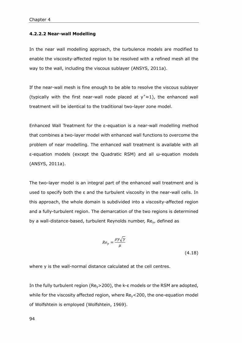
Chapter 4

94

4.2.2.2 Near-wall Modelling

In the near wall modelling approach, the turbulence models are modified to

enable the viscosity-affected region to be resolved with a refined mesh all the

way to the wall, including the viscous sublayer (ANSYS, 2011a).

If the near-wall mesh is fine enough to be able to resolve the viscous sublayer

(typically with the first near-wall node placed at y+≈1), the enhanced wall

treatment will be identical to the traditional two-layer zone model.

Enhanced Wall Treatment for the ε-equation is a near-wall modelling method

that combines a two-layer model with enhanced wall functions to overcome the

problem of near modelling. The enhanced wall treatment is available with all

ε-equation models (except the Quadratic RSM) and all ω-equation models

(ANSYS, 2011a).

The two-layer model is an integral part of the enhanced wall treatment and is

used to specify both the ε and the turbulent viscosity in the near-wall cells. In

this approach, the whole domain is subdivided into a viscosity-affected region

and a fully-turbulent region. The demarcation of the two regions is determined

by a wall-distance-based, turbulent Reynolds number, Rey, defined as

𝑅𝑒𝑦 =𝜌𝑦√𝑦

𝜇

(4.18)

where y is the wall-normal distance calculated at the cell centres.

In the fully turbulent region (Rey>200), the k-ε models or the RSM are adopted,

while for the viscosity affected region, where Rey<200, the one-equation model

of Wolfshtein is employed (Wolfshtein, 1969).

Chapter 4

95

The enhanced wall treatment approach allows the fully turbulent law to be easily

modified and extended to take into account other effects such as pressure

gradients or variable properties. This approach also guarantees the correct

asymptotic behaviour for large and small values of y+ and reasonable

representation of velocity profiles in the cases where y+ falls inside the wall

buffer region (3<y+<10) (Fokeer, 2006).

For the numerical investigation of the swirl inducing pipe, Ariyaratne (2005)

used standard wall functions to optimize swirl pipe and transition pipe. She

carried out a comparison to the use of non-equilibrium wall functions approach

for the case of Swirl pipe (400mm) + Exit transition (100mm). It was observed

that the trends were closely followed in both cases and the difference in final

result was 3% greater pressure drop and 0.3% lower tangential velocity when

standard wall functions were used.

Fokeer (2006) ran two identical cases, one employing the standard wall function

and the other the non-equilibrium wall function. Distribution of static pressure

and velocity magnitude throughout the model were compared and both wall

functions produced very similar results. The maximum percentage difference

between the two wall functions for static pressure and velocity magnitude

parameters was only 0.9%. The standard wall function case converged 1%

faster than the non-equilibrium wall function case. Since no significant

advantage resulted from using a non-equilibrium wall function, Fokeer decided

to employ the standard wall function.

Najafi et al. (2011) stated that for modelling the region close to the walls whose

appropriate selection was of crucial importance in calculation of shear stresses,

and the two layer zone models were employed. This near-wall flow modelling

method by the two layer model of Norris and Reynolds was also used by Jensen

et al. (2005) in their study of wall shear stress variation along a rig comprising

Chapter 4

96

circular pipe, sudden and gradual expansion and contractions.

It is recommended to use the enhanced wall treatment for all models for which

it is available. It provides the most consistent wall shear stress and wall heat

transfer predictions with the least sensitivity to y+ values (ANSYS, 2011b).

However, ANSYS FLUENT User's Guide (2011b) also states that, for swirling

flows encountered in devices such as cyclone separators and swirl combustors,

near-wall turbulence modelling is often a secondary issue, because the fidelity

of the predictions in these cases is mainly determined by the accuracy of

turbulence model in the core region. While in cases where wall activity

participates in the generation of swirl, non-equilibrium wall functions can often

improve the predictions since they use a law of the wall for mean velocity

sensitized to pressure gradients.

4.3 Numerical Schemes

In ANSYS FLUENT, governing integral equations for the conservation of mass

and momentum, and (when appropriate) for energy and other scalars such as

turbulence and chemical species are solved by a control-volume-based

technique that consists of:

Division of the domain into discrete control volumes using a

computational grid.

Integration of the governing equations on the individual control volumes

to construct algebraic equations for the discrete dependent variables

(“unknowns”) such as velocities, pressure, temperature, and conserved

scalars.

Linearization of the discretized equations and solution of the resultant

linear equation system to yield updated values of the dependent

variables.

Chapter 4

97

4.3.1 Solver

To solve a fluid flow numerically, ANSYS FLUENT allows user to choose one of

the two numerical methods: pressure-based solver and density-based solver.

The pressure-based solver traditionally has been used for incompressible and

mildly compressible flows. On the other hand, the density-based approach was

originally designed for high-speed compressible flows. Both approaches are now

applicable to a broad range of flows (from incompressible to highly

compressible). However, for high-speed compressible flows, the density-based

formulation may give an accuracy advantage over the pressure-based solver.

Two algorithms exist under the pressure-based solver in ANSYS FLUENT: a

segregated algorithm and a coupled algorithm. In the segregated algorithm the

governing equations are solved sequentially, segregated from one another,

while in the coupled algorithm the momentum equations and the pressure

based continuity equation are solved in a coupled manner. In general, the

coupled algorithm significantly improves the convergence speed over the

segregated algorithm; however, the memory requirement for the coupled

algorithm is more than the segregated algorithm.

The density-based solver in ANSYS FLUENT solves the governing equations of

continuity, momentum, and (where appropriate) energy and species transport

simultaneously as a set, or vector, of equations. Governing equations for

additional scalars (e.g., turbulence or radiation quantities) will be solved

sequentially. There are also two formulations existing under the density-based

solver: implicit and explicit. The implicit and explicit density-based formulations

differ in the way that they linearize the coupled equations.

Chapter 4

98

Though both pressure-based and density-based solvers can be used for a broad

range of flows, in some cases however one formulation may perform better than

the other in yielding a solution more quickly or resolve certain flow features

better (ANSYS, 2011b). Generally, the pressure-based solver provides more

physical models or features that are not available with the density-based solver.

In terms of this study on swirl pipe, some solution techniques that may be

beneficial in swirling or rotating flow calculations are only available in the

pressure based solver. For this reason, and since impressible water is studied,

the default pressure-based solver, which was also used by Ariyaratne (2005)

and Fokeer (2006), will be adopted.

The pressure-based solver employs an algorithm which belongs to a general

class of methods called the projection method (Chorin, 1968). In this method,

the constraint of mass conservation (continuity) of the velocity field is achieved

by solving a pressure (or pressure correction) equation that is derived from the

continuity and the momentum equations in such a way that the velocity field,

corrected by the pressure, satisfies the continuity. Since the governing

equations are nonlinear and coupled to one another, the solution process

involves iterations wherein the entire set of governing equations is solved

repeatedly until the solution converges.

ANSYS FLUENT provides two pressure-based solver algorithms, a segregated

algorithm, and a coupled algorithm. In this study, a segregated algorithm was

employed as it is memory-efficient than the coupled algorithm.

4.3.1.1 The Pressure-Based Segregated Algorithm

In the segregated algorithm, the individual governing equations for the solution

variables (e.g 𝑢, 𝑣, 𝑤, 𝑝, 𝑇, 𝑘, 휀 etc.) are solved sequentially. Each governing

equation is “decoupled” or “segregated” from other equations while being

Chapter 4

99

solved. The segregated algorithm is memory-efficient, because the discretized

equations need only be stored in the memory one at a time. However, the

solution convergence is relatively slow, as the equations are solved in a

decoupled manner.

With the segregated algorithm, the iteration process consists of the following

steps as demonstrated in Figure 4.3.1:

1. Update fluid properties (e.g., density, viscosity, specific heat) including

turbulent viscosity (diffusivity) based on the current solution.

2. Solve the momentum equations one after another, using the recently

updated values of pressure and face mass fluxes.

3. Solve the pressure correction equation using recently obtained velocity

field and mass-flux.

4. Correct the face mass fluxes, pressure, and the velocity field using the

pressure correction obtained from step 3.

5. Solve the equations for additional scalars, if any, such as turbulent

quantities, energy, species, and radiation intensity using the current

values of the solution variables.

6. Update the source terms arising from the interactions among different

phases when multiphase is involved.

7. Check for convergence of the equations.

The steps are continued until the convergence criteria are met.

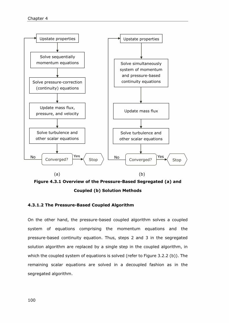
Chapter 4

100

(a) (b)

Figure 4.3.1 Overview of the Pressure-Based Segregated (a) and

Coupled (b) Solution Methods

4.3.1.2 The Pressure-Based Coupled Algorithm

On the other hand, the pressure-based coupled algorithm solves a coupled

system of equations comprising the momentum equations and the

pressure-based continuity equation. Thus, steps 2 and 3 in the segregated

solution algorithm are replaced by a single step in the coupled algorithm, in

which the coupled system of equations is solved (refer to Figure 3.2.2 (b)). The

remaining scalar equations are solved in a decoupled fashion as in the

segregated algorithm.

Upstate properties

Solve sequentially

momentum equations

Solve pressure-correction

(continuity) equations

Update mass flux,

pressure, and velocity

Solve turbulence and

other scalar equations

Converged? Stop Yes No

Upstate properties

Solve simultaneously

system of momentum

and pressure-based

continuity equations

Update mass flux

Solve turbulence and

other scalar equations

Converged? Stop Yes No

Chapter 4

101

Since the momentum and continuity equations are solved in a closely coupled

manner, the rate of solution convergence significantly improves when

compared to the segregated algorithm. However, the memory requirement

increases by 1.5–2 times that of the segregated algorithm since the discrete

system of all momentum and pressure-based continuity equations needs to be

stored in the memory when solving for the velocity and pressure fields (rather

than just a single equation, as is the case with the segregated algorithm).

4.3.2 Numerical Discretization

In order to solve a fluid flow numerically, the computational domain, including

the surfaces and boundaries have to be discretized. This can be done using

either one of three different methods (Versteeg and Malalasekera, 1995):

Finite-Difference Method (FDM), Finite-Volume Method (FVM) or Finite-Element

Method (FEM). Recent CFD packages, including ANSYS FLUENT, apply

Finite-Volume Method more because it can be used on either a structured or

unstructured mesh, rigorously enforces conservation, is directly relatable to

physical quantities (mass flux, etc.), and is easier to program in terms of CFD

code development.

ANSYS FLUENT uses a control-volume-based technique which converts a

general scalar transport equation to an algebraic equation that can be solved

numerically. In the FVM method, the numerical algorithm consists of the

following steps (H.K.Versteeg and W.Malalasekera, 2010):

Integration of the governing equations of fluid flow over all the (finite)

control volumes of the domain.

Discretisation – conversion of the resulting integral equations, which

results in a system of algebraic equations that are written in matrix for

convenience.

Solution of the algebraic equations is then gained by an iterative method.

Chapter 4

102

The discretized scalar transport equation contains the unknown scalar variable

𝜙 at the cell centre as well as the unknown values in the surrounding neighbour

cells. This equation will, in general, be non-linear due to the convection term.

Phenomena such as turbulence and chemical reactions introduce additional

nonlinearities. The strategy used to handle the nonlinearity is to linearize the

equations about a guess value of the solution and to iterate until the guess

agrees with the solution to a specified tolerance level (Bhaskaran and Collins,

2003).

The linearized form of the discretized scalar transport equation can be written as

𝑎𝑃𝜙 = ∑𝑎𝑛𝑏 𝜙𝑛𝑏 + b. where the subscript 𝑛𝑏 refers to neighbouring cells, 𝑎𝑃 and

𝑎𝑛𝑏 are the linearized coefficients for 𝜙 and 𝜙𝑛𝑏. The number of neighbours for

each cell depends on the mesh topology, but will typically equal the number of

faces enclosing the cell (boundary cells being the exception). Similar equations

can be written for each cell in the mesh. This results in a set of algebraic

equations with a sparse coefficient matrix. For scalar equations, ANSYS FLUENT

solves this linear system using a point implicit (Gauss-Seidel) linear equation

solver in conjunction with an algebraic multigrid (AMG) method.

4.3.2.1 Spatial Discretization

In the Finite-Volume Method, the computational domain is divided into a finite

number of elements known as control volumes by the regular and irregular

arrangement of nodes, known as the mesh. Flow parameters are resolved

around these nodes, so that the fluid flow can be described mathematically by

specifying its velocity at all points in space and time.

ANSYS FLUENT, by default, stores discrete values (e.g. pressure, velocities and

turbulence) of the scalar at the cell centres. However, face values are required

Chapter 4

103

for the convection terms and must be interpolated from the cell centre values.

This is achieved through an upwind scheme. Upwinding means that the face

value is derived from quantities in the cell upstream, or “upwind” relative to the

direction of the normal velocity.

Upwind advection schemes

ANSYS FLUENT provides several upwind advection schemes for momentum,

kinetic energy, dissipation rate and Reynolds Stresses: first-order upwind,

second-order upwind, power law, QUICK and third-Order MUSCL scheme.

In the first-order upwind scheme, quantities at cell faces are determined by

assuming that the cell centre values of any field variable represent a

cell-average value and hold throughout the entire cell. Therefore, when

first-order upwinding is selected, the face value is set equal to the cell-centre

value of in the upstream cell.

When second-order upwind scheme is used, the higher-order accuracy

quantities at cell faces are achieved through a Taylor series expansion of the

cell-centred solution about the cell centroid. The face value is the sum of the

cell-centred value and the product of its gradient in the upstream cell multiplies

the displacement vector from the upstream cell centroid to the face centroid.

The power-law discretization scheme interpolates the face value of a variable

using a solution the same as to a one-dimensional convection-diffusion equation.

QUICK (Quadratic Upstream Interpolation for Convection Kinetics) type

schemes are based on a weighted average of second-order-upwind and central

interpolations of the variable. The third-Order MUSCL scheme was conceived

from the original MUSCL (Monotone Upstream-Centred Schemes for

Conservation Laws) by blending a central differencing scheme and

second-order upwind.

Chapter 4

104

ANSYS FLUENT states that, when flow is aligned with the mesh, the numerical

diffusion will be naturally low; a first-order scheme yields better convergence

without any significant loss of accuracy. However, when flow is not aligned with

the mesh, the first-order convective discretization increases numerical

discretization error. The second-order scheme generally obtains more accurate

results especially for complex flows. In summary, while the first-order

discretization generally yields better convergence than the second-order

scheme, it generally will yield less accurate results, especially on

triangular/tetrahedral meshes.

The QUICK and third-order MUSCL discretization schemes may provide better

accuracy than the second-order scheme for rotating or swirling flows. In general,

however, the second-order scheme is sufficient and the QUICK and third-order

MUSCL schemes will not provide significant improvements in accuracy. The

power law scheme will generally yield the same accuracy as the first-order

scheme.

Note that when LES are used, the bounded central differencing and central

differencing schemes are available.

Pressure interpolation schemes

Similarly, the face values of pressure are computed from the cell values

adopting pressure interpolation schemes. The ones available in ANSYS FLUENT,

when pressure-based solver is used, include: standard, second-order,

body-force-weighted, linear and the PRESTO! (PREssure STaggering Option)

scheme.

The standard scheme works well when the pressure variation between cell

centres is smooth. When there are jumps or large gradients in the momentum

Chapter 4

105

source terms between control volumes, the pressure profile has a high gradient

at the cell face, and cannot be interpolated using standard scheme. The

standard scheme will have trouble handling flows with a large body force (such

as strongly swirling flow) and the presence of curvature.

The second-order scheme reconstructs the face pressure in the manner used for

second-order accurate convection terms. This scheme may provide some

improvement over the standard and linear schemes, but it may have some

trouble if it is used at the start of a calculation and/or with a bad mesh. This

method is not applicable for porous medium and the use of the VOF (Volume of

Fluid) or mixture model for multiphase flow.

The body-force-weighted scheme computes the face pressure by assuming that

the normal gradient of the difference between pressure and body forces is

constant. This works well if the body forces are known a priori in the momentum

equations (e.g., buoyancy and axisymmetric swirl calculations).

The linear scheme computes the face pressure as the average of the pressure

values in the adjacent cells. The PRESTO! scheme uses the discrete continuity

balance for a “staggered” control volume about the face to compute the

“staggered” (i.e., face) pressure.

Generally, for problems involving large body forces, the body-force-weighted

scheme is recommended. While For flows with high swirl numbers,

high-Rayleigh-number natural convection, high-speed rotating flows, flows

involving porous media, and flows in strongly curved domains, the PRESTO!

scheme is recommended.

Pressure-velocity coupling

Chapter 4

106

The momentum equation is normally solved with a guessed pressure field, and

therefore the resulting face flux, does not satisfy the continuity equation. This is

rectified by applying a pressure-velocity coupling algorithm, which uses a

combination of continuity and momentum equations to derive an equation for

pressure (or pressure correction) so that the corrected face flux satisfies the

continuity equation.

When pressure-based segregated solver is used, ANSYS FLUENT provides three

segregated types of algorithms: SIMPLE, SIMPLEC and PISO.

The SIMPLE algorithm uses a relationship between velocity and pressure

corrections to enforce mass conservation and to obtain the pressure field. It

substitutes the flux correction equations into the discrete continuity equation to

obtain a discrete equation for the pressure correction in the cell. The SIMPLEC

procedure is similar to the SIMPLE procedure however it offers different

expression for the face flux correction.

The PISO (Pressure-Implicit with Splitting of Operators) scheme is based on the

higher degree of the approximate relation between the corrections for pressure

and velocity. It improves the efficiency of calculation allowing the new velocities

and corresponding fluxes to satisfy the momentum balance after the

pressure-correction equation is solved by including neighbour correction and

skewness correction.

According to ANSYS FLUENT User’s Guide, steady-state calculations will

generally use SIMPLE or SIMPLEC, while PISO is recommended for transient

calculations. PISO may also be useful for steady-state and transient calculations

on highly skewed meshes.

Chapter 4

107

4.3.2.2 Temporal Discretization

For modeling unsteady flows, the governing equations must be discretized in

both space and time. The spatial discretization for the time-dependent

equations is the same as the steady-state case. While the discretization in time

are realized adopting the temporal discretization by splitting the time in the

continuous flow into discrete time steps.

Temporal discretization involves the integration of every term in the differential

equations over a time step ∆𝑡. For a variable 𝜙, the time evolution can be

expressed as:

∂ϕ

∂t= 𝐹(𝜙)

(4.19)

where the function 𝐹 incorporates any spatial discretization.

First-Order Implicit

If the time derivative is discretized using backward differences, the first-order

accurate temporal discretization is given by:

𝜙𝑛+1 − 𝜙𝑛

Δ𝑡= 𝐹(𝜙)

(4.20)

Once the time derivative has been discretized, the Implicit Time Integration can

be used to evaluate 𝐹(𝜙): in particular, which time level of 𝜙 should be used in

evaluating 𝐹. The method is to evaluate 𝐹(𝜙) at the future level:

𝜙𝑛+1 − 𝜙𝑛

Δ𝑡= 𝐹(𝜙𝑛+1)

(4.21)

This implicit equation can be solved iteratively at each time level before moving

to the next time step. This fully implicit scheme is advantageous in that it is

unconditionally stable with respect to time step size.

Chapter 4

108

Second-Order Implicit

The second-order discretization is expressed as:

3𝜙𝑛+1 − 4𝜙𝑛 + 𝜙𝑛−1

2Δ𝑡= 𝐹(𝜙)

(4.22)

Where

𝜙 = a scalar quantity

𝑛 + 1 = value at the next time level, 𝑡 + Δ𝑡

𝑛 = value at the current time level, 𝑡

𝑛 − 1 = value at the previous time level, 𝑡 − Δ𝑡

Since the same Implicit Time Integration is used to evaluate 𝐹(𝜙), this temporal

discretization method is named the Second-Order Implicit.

For the second-order discretization, Bounded Second Order Implicit Time

Integration is also available. This refers to the Bounded Second Order Implicit.

This formulation is only used in the pressure-based solver not available with the

density-based solver.

Generally speaking, the First Order Implicit formulation is sufficient for most

problems. Either Second Order Implicit or Bounded Second Order Implicit gives

improved accuracy. The Bounded Second Order Implicit formulation provides

the same accuracy as the Second Order Implicit formulation, however it

provides better stability.

Chapter 4

109

4.4 CFD Model Formulation

4.4.1 CFD Software Package

ANSYS FLUENT academic code 14.0 (ANSYS, 2011b) is employed in simulating

the swirl flow induced by the optimized 4-lobed swirl pipe. The ANSYS FLUENT

code is written in C computer language and makes full use of the flexibility and

power offered by this language. The code is a state-of-the-art computer

program for modeling fluid flow, heat transfer, and chemical reactions in

complex geometries (ANSYS, 2013b).

ANSYS Fluent uses a client/server architecture which enables it to run as

separate simultaneous processes on a personal workstation which has two

3.3GHz 4 core processors, 48GB memory with a 64-Bit Window 7 operating

system. The academic version of ANSYS FLUENT offers parallel solver (local

machine) which enables the user to compute a solution using 4 processors on

the same workstation.

ANSYS FLUENT offers insight into how the swirl pipe will behave in the real

cleaning industry before a single prototype is built.

4.4.2 Enabling Assumptions

Prior to setting up and running a CFD simulation, assumptions need to be made

to reduce the complexity of the flow problem in terms of the physical and

chemical phenomena that need to be considered to a manageable level whilst

preserving the salient features of the problem at hand (H.K.Versteeg and

W.Malalasekera, 2010). For the RANS approach, the following assumptions are

made to simplify the single phase swirl flow as follows:

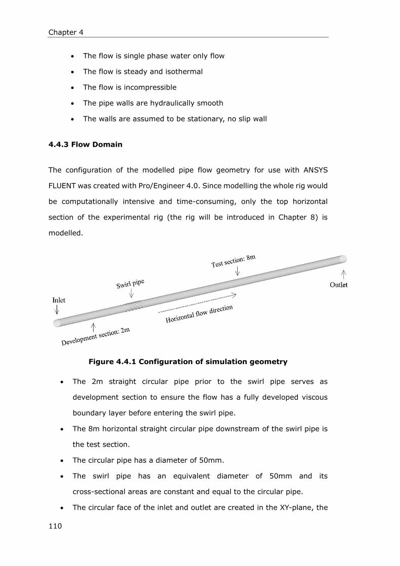
Chapter 4

110

The flow is single phase water only flow

The flow is steady and isothermal

The flow is incompressible

The pipe walls are hydraulically smooth

The walls are assumed to be stationary, no slip wall

4.4.3 Flow Domain

The configuration of the modelled pipe flow geometry for use with ANSYS

FLUENT was created with Pro/Engineer 4.0. Since modelling the whole rig would

be computationally intensive and time-consuming, only the top horizontal

section of the experimental rig (the rig will be introduced in Chapter 8) is

modelled.

Figure 4.4.1 Configuration of simulation geometry

The 2m straight circular pipe prior to the swirl pipe serves as

development section to ensure the flow has a fully developed viscous

boundary layer before entering the swirl pipe.

The 8m horizontal straight circular pipe downstream of the swirl pipe is

the test section.

The circular pipe has a diameter of 50mm.

The swirl pipe has an equivalent diameter of 50mm and its

cross-sectional areas are constant and equal to the circular pipe.

The circular face of the inlet and outlet are created in the XY-plane, the

Chapter 4

111

fluid flows in the horizontal Z direction.

It is important to establish a fully developed viscous boundary layer. When this

is achieved, the flow is fully-developed and there is no variation of the velocity

profile in the axial direction. Previous researcher Ariyaratne (2005) ran a

simulation over a 0.5m circular pipe and used the ‘outlet’ velocity profile

obtained as the ‘velocity profile’. The ‘velocity profile’ was then applied to the

inlet of 0.1m or 0.2m circular pipes that were connected prior to the swirl pipes

or control (circular) pipes. Therefore, the development section of the pipe

geometries Ariyaratne used has an equivalent length of 0.6m or 0.7m.

In the current study, attempts were made to further ensure fully turbulent flow

by increasing the length of the development section into 1m, 1.5m and 2m. The

simulation results showed that, without the use of a ‘velocity profile’, a 1.5m

length circular pipe prior to the swirl pipe was able to reach a steady velocity

profile before entering the swirl pipe. As can be seen from Figure 4.4.2, the

velocity profiles in the planes 1.5m, 1.6m, 1.7m and 1.8m downstream of the

inlet are identical indicating that the flow is fully developed at these distances

from the inlet. Considering a proper safety margin, a development section of 2m

without ‘velocity profile’ was finally used for all cases.

To ensure the swirl motion decayed completely before researching the outlet of

the computational domain, test sections of length of 3m, 5m, 6m and 8m were

attempted. It was found, especially for a larger inlet velocity, a test section of

8m was required to cover the decay process of the induced swirl flow.

Chapter 4

112

Figure 4.4.2 Velocity profiles downstream of circular pipe inlet

4.4.4 Meshing

As has been discussed in section 4.3.2.1, before the governing equations can be

numerically solved, the flow domain including the surface of all the boundaries

need to be discretised into a finite number of elements known as control

volumes by the regular or irregular arrangement of nodes, namely the mesh.

Flow parameters are resolved around these nodes, so that the fluid flow can be

described mathematically by specifying its velocity at all points in space and

time.

How the mesh is arranged within the domain is largely influenced by the

structure of the domain and the positions of the critical regions where there are

high gradients in the space of the flow, typically fine mesh are required at these

locations to describe the rapid variation accurately.

Chapter 4

113

The mesh is typically made up of nodes from 3D elements such as 4-noded

tetrahedrons, 5-noded pyramids, 6-noded prisms (or wedges) and 8-noded

hexahedrons. Two types of mesh structures can be arranged from these 3D

elements. They are:

Regular structured grid (structured) where:

The meshes are typically made up of hexahedrons.

The node points are regularly arranged throughout a cuboid, which can

be stretched to fit the particular geometry of the problem as if the mesh

is made of rubber.

Any point in the mesh connects to the same neighbouring points after the

stretching process.

Implicit relationship exists between the label of a cell or a point and the

labels of its neighbours in a structured mesh, which enables data to be

found easily.

Irregular structured grid (unstructured) where:

The meshes are often made up of tetrahedrons.

Node points are filled within the space of concern without being

connected with a regular topology.

The information that any particular node is attached to an element

cannot be known from the form of the mesh.

A numerical table must exist which labels the arrangement of the mesh

by listing which nodes are attached to each element.

The advantage of a structured mesh is that it enables the solver program to run

faster than when an unstructured mesh is used. In addition, the hexahedral

cells within the structured mesh can be built to align with the flow thereby

minimising the numerical diffusion.

Chapter 4

114

On the other hand, the use of an unstructured mesh significantly reduces the

amount of time spent generating meshes as it is created by automatic mesh

generation algorithms. Secondly, unstructured mesh can handle more complex

geometries due to its flexibility. Thirdly, an unstructured mesh made up of

triangular or tetrahedral cells created for complex geometries often has far

fewer cells than the equivalent structured mesh consisting hexahedral cells.

Because the geometry of the swirl inducing pipe and the transition pipes contain

sharp angles at the intersection of the lobes and the lobed cross section extends

helically around and along the pipe axis making the geometry very complex.

Therefore previous researcher Ariyaratne (2005) used meshes comprised

unstructured tetrahedral elements for all geometries of swirl, transition and

circular pipes employing Gambit software. Ariyaratne also investigated other

potentially better meshes using structured hexahedral elements however no

alternatives were found.

The mesh Fokeer (2006) generated for meshing the 3-lobed swirl pipe was also

based on the unstructured hexahedral mesh. Though, Fokeer used a region of

fine mesh, called the boundary layer mesh, along the solid wall surfaces of the

3-lobed swirl pipe and the circular pipes, enabling the modelling of the rapid

velocity variation through the boundary layer.

Due to the complex geometry of the swirl pipes, previous researchers

Ganeshalingam (2002) and Jones (2002) used unstructured tetrahedral mesh

for their studies.

However, it was found that:

When an unstructured tetrahedral mesh is used, the flow can never be

aligned with the grid, which causes numerical diffusion.

Chapter 4

115

An unstructured mesh made up of tetrahedral cells also tends to have a

large aspect ratio, which affect the skewness of the cell, and in turn

hinder the accuracy and convergence (Ariyaratne, 2005).

The unstructured mesh requires more elements for refinement compared

to a structured mesh of the same geometry, leading to higher computing

cost (Fokeer, 2006).

In this study, the accurate prediction of flow parameters in the boundary layer,

such as wall shear stress, are of crucial importance. However, when an accurate

prediction of a boundary layer is required, the boundary layer meshes should

consist of quads, hexes, or prisms, and the use of pyramid or tetrahedral cells

immediately adjacent to the wall should be avoided (Bakker, 2002). Therefore,

a method of meshing the computational domain using structured hexahedral

elements has to be found.

4.4.4.1 Attempts Made Using Gambit

According to the above discussion, the unstructured tetrahedral cells Ariyaratne

used is not applicable to this study as strict mesh control is required in the

boundary layer. Therefore, attempts were made to mesh the swirl pipe and

circular pipes using structured hexahedral elements adopting the Gambit

software. However, no satisfactory solution was found.

In the first attempt, the geometry of the flow domain was divided into 3

sections: the development section, the swirl pipe and the test section of circular

pipe with every two neighbouring sections sharing one ‘internal’ face. Therefore

two sheared internal faces were within the geometry to make the flow domain

continuous between the adjacent two sections. The swirl inducing pipe was

firstly meshed using hexahedral cells with boundary layer mesh included along

the solid wall surface. The circular pipes were meshed by sweeping the two

Chapter 4

116

surface meshes of the swirl pipe forward or backward along the geometry. It

was found that:

As shown in Figure 4.4.3(a), the mesh of the circular pipes followed the

nodes arrangement pattern of the swirl pipe resulting in uneven nodes

distribution across the circular pipe cross-section.

Highly skewed cells existed in four regions of the circular pipe which are

in accordance with the four intersections of the lobes (see Figure

4.4.3(b).

Highly skewed cells were also found in the intersections of lobes. The

poor mesh quality would impede accuracy and convergence of the

solution (see Figure 4.4.3(c)).

Due to the poor mesh quality, this method was not employed.

(a) (b)

(c)

Figure 4.4.3 Circular Pipe face Mesh and Distribution of Highly Skewed

Cells

Chapter 4

117

In order to eliminate effects of ‘internal’ face sheared by the adjacent two

sections, a second attempt was made to build and mesh the three sections

separately without any sheared faces between sections. The meshes of the

three sections were imported into FLUENT and the ‘Grid interface’ feature was

applied at the interface of the adjacent two sections to allow the three sections

to be bridged together. The Grid interface enables the exchange of all

parameters in governing equations between the adjacent two sections.

This method:

Allowed the nodes arrangement to fit for the different geometries of the

three sections respectively.

Provided the improved mesh quality though still not satisfactory.

Ensured flow continuity between three geometries through the use of

‘Grid interface’.

However, the grid interfaces of the circular pipe and the swirl pipe that were

attached together have different nodes arrangement patterns therefore the

nodes of the two interfaces do not exactly align with each other (see Figure

4.4.4). The use of this non-conformal mesh interface violates normal best

practice and may cause flow discontinuity at the swirl/circular pipe interface.

Chapter 4

118

Figure 4.4.4 A detail view of the interface at the swirl/circular pipe

intersection

The mesh generated was tested using a standard k-ε model and the standard

wall functions. The simulation results showed that, there were no discontinuities

in terms of axial, tangential velocity and pressure in the vicinity of swirl/circular

pipe interface. However, wall shear stress discontinuity did exist at the

swirl/circular pipe interface as shown in Figure 4.4.5. Due to the importance of

accurate prediction of wall shear stress for this study and the unsatisfactory

mesh quality, this method was deemed unacceptable.

circular

swirl

interface

Chapter 4

119

Figure 4.4.5 Discontinuity in contour of wall shear stress at the

circular/swirl and swirl/circular interfaces

The third attempt was to firstly merge the three sections into an integrated

geometry. The inlet and outlet faces of the geometry were then meshed using

quadrilateral cells with boundary layer mesh applied in the wall region. The

whole geometry was then meshed by sweeping the two face meshes of inlet and

outlet as ‘source’ throughout the whole domain. The surface meshes of the inlet,

the cross-section of the circular and swirl pipe are shown in Figure 4.4.6a to

Figure 4.4.6c respectively. It can be found that the fine mesh region in the inlet

mesh where boundary layer mesh was applied stopped being concentrated only

near the wall area as it was swept toward the swirl pipe. This is against the

purpose of the use of boundary layer mesh in order to accurately model the

rapid velocity variation and the wall shear stress in the near wall region. Another

drawback of the grid was the high skewed mesh spotted in the intersections of

the lobes. Generally, the Equi-Angle, which is a normalised measure of

skewness, should be less than 0.65 for hexahedral cells. Figure 4.4.6d showed

that poor mesh cells with an Equi-Angle value larger than 0.65 existed in the

intersections of the lobes in the swirl pipe. Considering the difficulties in

controlling the mesh refinement in the boundary layer region and the existence

Contour of Wall Shear Stress (pascal)

Chapter 4

120

of highly skewed cells which may affect the simulation accuracy and

convergence, this meshing method was deemed not sufficient.

Figure 4.4.6 Face meshes of swirl inducing pipe, transition pipe, and

circular pipe

4.4.4.2 Multi-Block Structured Mesh by ICEM

Afterward, a multi-block structured mesh was considered for the discretization

of the swirl and circular pipes. This method is a compromise between computing

cost and flexibility where the computational domain is subdivided into different

blocks which can be structurally meshed using hexahedral cells. This method is

complex but more computer efficient than an unstructured mesh and it

facilitates control in specifying refinement needed along certain surfaces or

walls, especially for meshing around complex geometries.

(a) (b) (c)

(d)

Contour of Cell Equi-Angle Skew

Chapter 4

121

ICEM CFD (The Integrated Computer Engineering and Manufacturing code for

Computational Fluid Dynamics) (ANSYS, 2013d) mesh generation software was

used to mesh the computational domain with structured hexahedral cells. ICEM

CFD uses a primarily top-down blocking approach to efficiently mesh complex

models using all hexahedral cells without the need to subdivide the geometry.

The ICEM CFD offers the capability to parametrically create grids from geometry

by the association of blocks with topologically similar geometries of the

computational domain.

A general process used in meshing the flow geometry shown in Figure 4.4.1 is

summarized as below:

Firstly import the .STP file into ICEM CFD and modify its position to

ensure that the inlet is located in the origin of coordinates and the flow

direction is in parallel with Z axis.

Create a block to contain the whole geometry.

Split the block into three blocks corresponding to the 2m cylindrical pipe,

the 0.6m (or 0.4m) optimized swirl pipe and the 8m cylindrical test

section.

The block corresponding to the 0.6m (or 0.4m) swirl pipe was sub-split

into 6 (or 4) blocks with each sub-block having a length of 100mm (each

lobe rotates 90° over the 100mm length).

Rotate each sub-block through 90° by moving clockwise the vertexes of

the sub-block to fit the rotation of the lobes. Make sure the edges of

sub-blocks and curves of the swirl pipe stretch in the same direction as

shown in Figure 4.4.7a.

Associate vertexes, edges and faces of blocks to the points, curves and

surface of the topologically similar geometries. The arrows in Figure

4.4.7b show the associations.

Chapter 4

122

Further split all the blocks and sub-blocks into O-grid blocks where the

mesh radially propagates from the pipe centre towards the outer wall

domain. This will result in an orthogonal mesh to better capture near-wall

or boundary layer flow.

Set up nodes number of the edges and mesh law; pre-mesh the

geometry; check the mesh quality; smooth the mesh if necessary;

convert to mesh; select solver and output mesh file for use with ANSYS

FLUENT.

(a) Rotated O-grid blocks

(b) Association between blocks and geometry

(c) surface mesh at the intersection of lobes

Figure 4.4.7 Face meshes of swirl inducing pipe, transition pipe, and

circular pipe

Chapter 4

123

Figure 4.4.7c demonstrates the surface mesh at the intersection of lobes in a

section of swirl pipe showing that the block is well fitted to the geometry.

A detail cross-sectional view of the O-grid mesh is shown in Figure 4.4.8b.

Figure 4.4.8 also presents a comparison of mesh generated by an unstructured

tetrahedral grid and structured hexahedral grid.

(a) unstructured tetrahedral grid

(b) Structured hexahedral grid

Figure 4.4.8 Swirl pipe meshes with unstructured grid by Ariyaratne

(2005) and structured hexahedral grid with O-block

Chapter 4

124

The advantages of the structured hexahedral grid using O-block over the

previously used unstructured tetrahedral grid are that it:

Allows the mesh to be arranged in a way that faithfully reflects the

geometric characteristics of the flow domain.

Provides control of the fine regular mesh in the boundary layer which

facilities accurate prediction of wall shear stress in the near-wall region.

Minimises the numerical diffusion since the structured hexahedral mesh

was built to align with the flow.

Improves largely the mesh quality which promotes solution

convergence.

4.4.4.3 Mesh Adaption for Wall Functions

There are two approaches to model the near-wall regions, the enhanced wall

treatment method and the wall function method. If the enhanced wall treatment

is used, the near-wall mesh should be sufficiently fine everywhere to be able to

resolve the viscous sub-layer, a very thin region next to a wall, typically only 1%

of the boundary layer thickness. Typically, the first near-wall node should be

placed at y+ ≈ 1, where y+ is the non-dimensional distance of a point from the

wall (ANSYS, 2011a). This condition is difficult to achieve due to the high

three-dimensionality in the lobe interaction region of the swirl pipe.

Therefore, the wall function approach will be used, and non-equilibrium wall

functions will be chosen as they give an improved prediction than standard wall

functions. Besides, the wall function method allows specifying the roughness of

the internal pipe surface to represent the internal surface finish of stainless

pipes typically found within the closed processing systems.

The wall functions approach uses the ‘log law’ whereby the mean velocity is

taken as a logarithmic function of the distance from the wall in the fully

Chapter 4

125

turbulent region. The log-law is valid for y+ between 30 and 60. Therefore, it is

important to carry out mesh adaption for wall functions to make sure the first

node where the velocity is calculated is located in the log-law region. This was

done by adjusting the distances from the first node of the mesh to the wall to

generate a series of mesh files. The meshes were then tested independently in

simulations with same boundary conditions and solver settings. After the

solution converged, y+ values were calculated to check which mesh allows the

y+ to be in the right range, and if not continue the adaption.

From Figure 4.4.9, for a velocity of 2m/s, the distance from the first node of the

mesh to the wall being 0.8mm would place y+ between 30 and 60 for

development section and the test section. The y+ value is slightly larger than 60

in the vicinity of the four lobe peaks of the swirl pipe. This should not affect the

simulation results as it only accounts for a small portion of the swirl pipe and the

y+ is close to 60. Besides, other reference suggests that the layer where y+

takes values between 30 and 500 is the log-law layer (H.K.Versteeg and

W.Malalasekera, 2010).

Figure 4.4.9 y+ contours for computational domain geometry (2m/s

inlet velocity)

Contour of Wall Yplus

Chapter 4

126

Table 4.4.1 Y+ value for different sections of the geometry at different

inlet velocities

Inlet

velocity

Distances from first node to

wall (mm)

Y+ value

Development

section Swirl pipe Test section

1m/s

1.4

34.3<Y+<47.9 25.58<Y+<59.7 33.7<Y+<45.1

1.5m/s

1

35.7<Y+<50.9 27.2<Y+<64.6 34.2<Y+<48.9

2m/s

0.8

37.2<Y+<53.9 31.9<Y+<75.4 35.5<Y+<51.6

2.5m/s

0.6

34.1<Y+<50.8 30.1<Y+<70.8 32.7<Y+<48.3

3m/s

0.5

33.4<Y+<50.8 29.5<Y+<70.49 32.1<Y+<47.9

Chapter 4

127

It was found this 0.8mm value was not applicable for other velocities. So

another four series of y+ adaption were carried out for the 1m/s, 1.5m/s,

2.5m/s and 3m/s cases respectively. The distance from the first row of the mesh

to the pipe wall and the corresponding y+ value for the three sections are

summarized in Table 4.4.1. The y+ is reasonable between 30 and 60 for all

cases.

4.4.4.4 Mesh Independence Test

To ensure that the errors associated with the size of mesh were minimized, a

quick mesh independence test was carried out. This was done by refining the

mesh height in the direction parallel with the swirl pipe and circular pipes (Z axis)

until the change of the parameters monitored decreases to the order of 1%. The

mesh size in the cross-section plane (X-Y plane) was made sufficiently fine

already in order to meet the Y+ requirement at the wall. For instance, in the

mesh generated for the 1m/s flow velocity, the largest mesh size in the

cross-section plane is 1.51mm; this is already smaller than the finally used

mesh height of 2mm. Therefore, mesh independence test for cross-section

mesh is not necessary.

In the mesh independence tests, the initial mesh height of 3mm was refined by

shortening the mesh height to 2.5mm and 2mm. The three mesh files were

imported to the CFD models and numerically compared. All the solver

parameters including flow and boundary conditions were same for each test

case. The average tangential velocity and wall shear stress, etc. at planes

downstream of the swirl pipe exit were checked. Table 4.4.2 presents a

summary of the results. The percentages are a comparison of the value to that

obtained from the refined mesh-2. From the table, the differences in the value

of parameters obtained from refined mesh-1 and refined mesh-2 are mostly

within the order of 1%. Refined mesh-1 should be reasonably concluded as

Chapter 4

128

mesh independent. However, considering the importance of the accurate

simulation of tangential velocity and wall shear stress in this study, the refined

mesh-2 with a mesh height of 2mm was used for all RANS based simulations.

Table 4.4.2 A summary of the mesh independence test results

Model parameters:

600mm length swirl pipe

Pipe diameter 50mm

Single phase water

Inlet velocity 1.5m/s

Items Initial mesh

3mm

Refined mesh-1

2.5mm

Refined mesh-2

2mm

Total no. of cells 2819460 3382960 4227720

Pressure

(pa)

0.1m after 2466.5513 (-1.39) 2429.9509 (-0.11%) 2432.6831

0.3m after 2352.1868 (-0.13%) 2354.0349 (-0.05%) 2355.1926

Axial

velocity

(m/s)

0.1m after 1.5335 (-0.44%) 1.5260 (-0.06%) 1.5269

0.3m after 1.5183 (-0.07%) 1.5186 (-0.05%) 1.5193

Tangential

velocity

(m/s)

0.1m after 0.2307 (-4.27%) 0.2183(-1.34%) 0.2212

0.3m after 0.1864 (-2.15%) 0.1880 (-1.31%) 0.1905

Wall shear

stress (pa)

Swirl pipe

exit 5.42 (-1.63%) 5.45 (-1.08%) 5.51

0.3m after 5.37 (-1.28%) 5.39 (-0.91%) 5.44

4.4.4.5 Checking Mesh Quality

Checking the quality of the mesh is essential as it plays a significant role in the

accuracy and the stability of the numerical computation (ANSYS, 2011b). For

the hexahedral mesh elements, the EquiAngle Skew and the Aspect Ratio are

Chapter 4

129

normally used for checking its quality.

Skewness is one of the primary quality measures for a mesh. It determines how

close a face or cell of triangle is to an ideal equilateral triangle or a quad is to an

ideal equiangular quad (ANSYS, 2013c). The Equi-Angle Skew is a normalised

measure of skewness defined as:

𝑄𝐸𝐴𝑆 = max(𝑄𝑚𝑎𝑥 − 𝑄𝑒𝑞

180 − 𝑄𝑒𝑞,𝑄𝑒𝑞 − 𝑄𝑚𝑖𝑛

𝑄𝑒𝑞)

(4.23)

𝑄𝑚𝑎𝑥 = largest angle in face or cell.

𝑄𝑚𝑖𝑛 = smallest angle in face or cell.

𝑄𝑒𝑞 = angle for equiangular face or cell, E.g., 60 for triangle, 90 for square.

According to the definition of skewness, a value of 0 indicates an equilateral cell

(best) and a value of 1 indicates a completely degenerate cell. Degenerate cells

(slivers) are characterized by nodes that are nearly coplanar. Cells with a

skewness value above 1 are invalid.

For the 𝑄𝐸𝐴𝑆 value between 0 and 1, Table 4.4.3 gives the mesh qualities with

respect to a range of skewness values.

Table 4.4.3 Skewness ranges and cell quality

Skewness Cell Quality

1 degenerate

0.9–<1 bad (sliver)

0.75–0.9 poor

0.5–0.75 fair

0.25–0.5 good

>0–0.25 excellent

0 equilateral

Table 4.4.4 reports the Equiangle skewness ranges of cells of the meshes for

1m/s, 2m/s and 3m/s flow velocities in the form of the number of elements and

percentages. A clearer histogram of QEAS distribution is also available in Figure

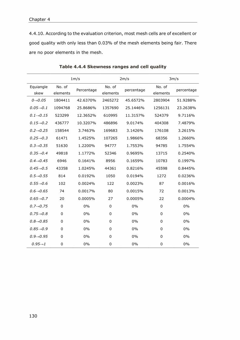
Chapter 4

130

4.4.10. According to the evaluation criterion, most mesh cells are of excellent or

good quality with only less than 0.03% of the mesh elements being fair. There

are no poor elements in the mesh.

Table 4.4.4 Skewness ranges and cell quality

1m/s 2m/s 3m/s

Equiangle

skew

No. of

elements Percentage

No. of

elements percentage

No. of

elements percentage

0→0.05 1804411 42.6370% 2465272 45.6572% 2803904 51.9288%

0.05→0.1 1094768 25.8686% 1357690 25.1446% 1256131 23.2638%

0.1→0.15 523299 12.3652% 610995 11.3157% 524379 9.7116%

0.15→0.2 436777 10.3207% 486896 9.0174% 404308 7.4879%

0.2→0.25 158544 3.7463% 169683 3.1426% 176108 3.2615%

0.25→0.3 61471 1.4525% 107265 1.9866% 68356 1.2660%

0.3→0.35 51630 1.2200% 94777 1.7553% 94785 1.7554%

0.35→0.4 49818 1.1772% 52346 0.9695% 13715 0.2540%

0.4→0.45 6946 0.1641% 8956 0.1659% 10783 0.1997%

0.45→0.5 43358 1.0245% 44361 0.8216% 45598 0.8445%

0.5→0.55 814 0.0192% 1050 0.0194% 1272 0.0236%

0.55→0.6 102 0.0024% 122 0.0023% 87 0.0016%

0.6→0.65 74 0.0017% 80 0.0015% 72 0.0013%

0.65→0.7 20 0.0005% 27 0.0005% 22 0.0004%

0.7→0.75 0 0% 0 0% 0 0%

0.75→0.8 0 0% 0 0% 0 0%

0.8→0.85 0 0% 0 0% 0 0%

0.85→0.9 0 0% 0 0% 0 0%

0.9→0.95 0 0% 0 0% 0 0%

0.95→1 0 0% 0 0% 0 0%

Chapter 4

131

Figure 4.4.10 Histogram of QEAS quality distribution

Another important indicator of the mesh quality is the Aspect Ratio which is a

measure of the stretching of a cell. It is computed as the ratio of the maximum

value to the minimum value of any of the following distances: the normal

distances between the cell centroid and face centroids, and the distances

between the cell centroid and nodes.

There is no unified criterion on a certain Aspect Ratio under which the mesh is

considered acceptable. However, some references argued that whilst large

Aspect Ratios may be acceptable in some problems, a general rule of thumb

might be to avoid Aspect Ratios in excess of 5:1 (Selvam and Govindaswamy,

2001).

Figure 4.4.11 shows the histogram of Aspect Ratio distributions of the cells of

the mesh generated for simulating swirl flow with 1m/s, 2m/s and 3m/s

velocities. It is clear that the Aspect Ratio of the cells within the meshes for 1

m/s and 2m/s flow velocities are all less than 4. For the mesh generated for flow

with a velocity of 3 m/s, only 3.79% of the cells have an Aspect Ratio exceeds

Chapter 4

132

5 with the largest value being 7.25. The relatively large Aspect Ratio for the 3

m/s case is due to the very fine boundary layer mesh at the near wall region.

Compared with the 1 m/s and 2 m/s cases, the mesh used for the 3 m/s case

has an even finer mesh in the boundary layer which results in more flat

hexahedrons along the pipe wall thus increasing the Aspect Ratio.

Further refinement of the mesh for the 3 m/s case may decrease the Aspect

Ratio. However it is deemed unnecessary considering the increase in

computational cost and time for calculation. Moreover, the meshes for all cases

lead to convergence of the solutions with no difficulties.

Therefore, it can be concluded that the meshes generated for all cases

successfully pass the mesh quality test.

Figure 4.4.11 Histogram of Aspect Ratio quality distribution

Chapter 4

133

4.4.5 Boundary Conditions

4.4.5.1 Operation Conditions

The operating conditions allow the user to set the operating pressure, include

the effects of gravity and specify other operating variables. Following the

FLUENT documentation, the zero operating pressure was used which would

minimise errors due to the small pressure drop across the flow domain

compared to atmospheric pressure. The gravity acting on the negative y-axis at

9.81 m/s2 was included. The operating density was not specified, thus

permitting the solver to calculate it by averaging over all cells.

4.4.5.2 Inlet Boundary Conditions

At the inlet, a uniform mean flow velocity boundary condition was applied. The

material used was single phase, incompressible water with its density and

viscosity being specified as 998.2kgm-3 and 1.003×10-3 kgm-1s-1 respectively.

The turbulence of the flow was specified in terms of intensity and hydraulic

diameter at the inlet. The turbulence intensity is defined as the ratio of the

root-mean-square of the velocity fluctuations to the mean velocity. It was

calculated by (ANSYS, 2011b):

I=0.16×(Re)-1/8, Re=(U×D×ρ)/ μ

Where Re is the Reynolds number, U is the average velocity, ρ is the density, and

μ is the viscosity.

The hydraulic diameter was set to be the same as the pipe diameter of 50mm.

A series of simulations was carried out with varying velocities from 1m/s to

3m/s. The corresponding Reynolds number and turbulence intensity are listed in

Table 4.4.5.

Chapter 4

134

Table 4.4.5 Simulation conditions at inlet

Inlet velocity (m/s) Reynolds number Turbulence intensity (%)

1 49,760 4

1.5 74,641 3.9

2 99,521 3.8

2.5 124,401 3.7

3 149,282 3.6

4.4.5.3 Outlet Boundary Conditions

A pressure outlet boundary condition with zero uniform static pressure was

imposed at the outlet of the computational model. This boundary condition

results in a better rate of convergence when backflow occurs during iteration.

The turbulence was specified in terms of intensity and hydraulic diameter at the

outlet in the same way as the inlet.

4.4.5.4 Wall Boundary Conditions:

The pipe walls were specified as being stationary and no-slip walls to match the

simulation conditions. The no-slip condition for viscous fluids is that at a solid

boundary, the fluid will have zero velocity relative to the boundary.

The wall roughness of the development section and the test section was set by

specifying the roughness height, Ks, as 1.237 x 10-06m which is the same value

as the measured roughness of transparent Perspex pipes used in the

experimental rig. The roughness was measured employing a surface roughness

tester. The internal surface roughness of the swirl pipe was specified as 9 x

10-06m which is the measured roughness of the stainless steel swirl pipe

produced through investment casting. The two roughness values are small

enough that the walls can be considered as hydraulically smooth.

Chapter 4

135

4.4.6 Solution Methodology

4.4.6.1 Solver Setting

The steady state simulations were carried out with single phase water with the

flow being assumed to be steady, incompressible and isothermal. The

pressure-based segregated solver was used as it is recommended for

incompressible flows. Reynolds Stress Model (RSM) was used in all cases, unless

stated, otherwise the LES method was used. For the near wall treatment,

initially the standard wall function was used to implement the wall boundary

condition which was later improved by employing the non-equilibrium function.

The SIMPLE discretization technique was applied for the pressure–velocity

coupling and a second order upwind scheme was employed for the viscous

terms. The following sections provide further details of the solver parameters.

4.4.6.2 Turbulence Model and Wall Treatment

As has been discussed in section 4.2.1 that the RSM accounts for the effects of

streamline curvature, swirl, rotation, and rapid changes in strain rate in a more

rigorous manner than one-equation and two-equation models, it has greater

potential to give accurate predictions for complex flows (ANSYS, 2011a). The

flow being modelled is swirling and in such turbulent flows viscosity is typically

anisotropic, therefore the most reliable turbulence model, the Reynolds Stress

Model (RSM) was chosen (Najafi et al., 2011, Fokeer et al., 2010).

For modelling the regions close to the walls, whose appropriate selection is of

crucial importance in the calculation of shear stress, a two-layer-based,

non-equilibrium wall function was employed which can partly account for the

effects of pressure gradients in the wall area. Non-equilibrium wall functions are

recommended for use in complex flows where the mean flow and turbulence are

subjected to pressure gradients and rapid changes. In such flows,

Chapter 4

136

improvements can be obtained, particularly in the prediction of wall shear and

heat transfer (ANSYS, 2011a).

It was found that direct use of the RSM and the Non-Equilibrium wall functions

with second order discretization at the start lead to divergence of the solution.

Attempts were made to facilitate convergence by initially using the standard k–

ε model with standard wall functions to obtain a baseline solution which was

then improved by applying the Realizable k–ε model together with the

Non-Equilibrium functions. After that, RSM was applied to further improve the

solution until it reasonably converged.

Figure 4.4.12 Pressure downstream of swirl pipe for various turbulence

models and wall functions (3m/s inlet velocity)

Figure 4.4.12 shows the distribution of static pressure downstream of the swirl

pipe obtained using various turbulence models and wall functions. It can be

seen that the biggest difference occurs at the location where flow emerges from

the swirl pipe with the realizable k–ε model and the Non-Equilibrium wall

functions giving the most conservative prediction followed by RSM and the

Non-Equilibrium wall functions (0.49% larger) and, finally, the standard k–ε

model and standard wall functions (5.77% larger). Figure 4.4.12 may suggest

that, for the prediction of pressure, the selection of wall function may play an

Chapter 4

137

important role since when the Non-Equilibrium wall functions are selected, the

use of the realizable k-ε model or RSM makes a very small difference; whilst

with the standard wall function a clear difference is observed. This difference

may be attributed to the advantage of the non-equilibrium wall function which

can partly account for the effects of pressure gradients in the wall area.


turbulence models and wall functions (3m/s inlet velocity)

Figure 4.4.13 depicts the variation of average tangential velocity in the planes

downstream of the swirl pipe for various turbulence models and wall functions.

it shows that the RSM and Non-Equilibrium wall functions combination gives the

largest prediction of initial tangential velocity just downstream of the swirl pipe

followed by realizable k–ε model (1.89% lower) and, finally, the standard k–ε

model (1.92 lower). However, the tangential velocity predicted by the RSM

model decreases faster with increasing downstream distance with a maximum

difference of 17.3% lower than that obtained by the standard k–ε model and

maximum 17.8 % lower than that predicted by the realizable k–ε model. From

the figure, despite the use of different wall functions, the standard k–ε model

and realizable k–ε model gives similar predictions of tangential velocity. On the

other hand, although same Non-Equilibrium wall functions are chosen, the use

of the RSM results in a clear difference in predicted tangential velocity compared

Chapter 4

138

to the realizable k–ε model. Figure 4.4.13 indicates the importance of the

turbulence model in predicting the turbulent flow region. The difference

between the RSM and k–ε models is due to the difference in how the models

handle the turbulent swirl flow induced by the swirl pipe. Conceptually, RSM

should give more reliable predictions.

4.4.6.3 Advection Schemes for Viscous Terms

Three identical cases were run with each case employing First order upwind,

Second order upwind and QUICK schemes respectively for viscous terms (the

momentum, kinetic energy, dissipation rate and Reynolds Stresses). The

variation of static pressure and tangential velocity determined by the three

schemes are presented below.

Figure 4.4.14 Pressure downstream of swirl pipe for various advection

schemes (3m/s inlet velocity)

Figure 4.4.14 shows that the three schemes yield very close pressure

downstream of the swirl pipe with the main difference occuring at the exit of the

swirl pipe where the QUICK scheme gives the highest pressure followed by

second order (1.07% lower) and first order schemes (2.71% lower).

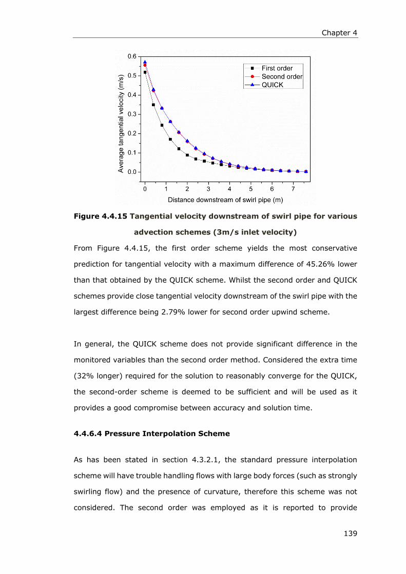
Chapter 4

139


advection schemes (3m/s inlet velocity)

From Figure 4.4.15, the first order scheme yields the most conservative

prediction for tangential velocity with a maximum difference of 45.26% lower

than that obtained by the QUICK scheme. Whilst the second order and QUICK

schemes provide close tangential velocity downstream of the swirl pipe with the

largest difference being 2.79% lower for second order upwind scheme.

In general, the QUICK scheme does not provide significant difference in the

monitored variables than the second order method. Considered the extra time

(32% longer) required for the solution to reasonably converge for the QUICK,

the second-order scheme is deemed to be sufficient and will be used as it

provides a good compromise between accuracy and solution time.

4.4.6.4 Pressure Interpolation Scheme

As has been stated in section 4.3.2.1, the standard pressure interpolation

scheme will have trouble handling flows with large body forces (such as strongly

swirling flow) and the presence of curvature, therefore this scheme was not

considered. The second order was employed as it is reported to provide

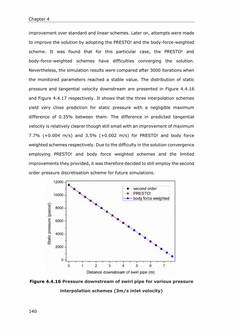
Chapter 4

140

improvement over standard and linear schemes. Later on, attempts were made

to improve the solution by adopting the PRESTO! and the body-force-weighted

scheme. It was found that for this particular case, the PRESTO! and

body-force-weighted schemes have difficulties converging the solution.

Nevertheless, the simulation results were compared after 3000 iterations when

the monitored parameters reached a stable value. The distribution of static

pressure and tangential velocity downstream are presented in Figure 4.4.16

and Figure 4.4.17 respectively. It shows that the three interpolation schemes

yield very close prediction for static pressure with a negligible maximum

difference of 0.35% between them. The difference in predicted tangential

velocity is relatively clearer though still small with an improvement of maximum

7.7% (+0.004 m/s) and 3.5% (+0.002 m/s) for PRESTO! and body force

weighted schemes respectively. Due to the difficulty in the solution convergence

employing PRESTO! and body force weighted schemes and the limited

improvements they provided, it was therefore decided to still employ the second

order pressure discretisation scheme for future simulations.

Figure 4.4.16 Pressure downstream of swirl pipe for various pressure

interpolation schemes (3m/s inlet velocity)

Chapter 4

141


pressure interpolation schemes (3m/s inlet velocity)

4.4.6.5 Pressure-velocity Coupling Scheme

Since the PISO scheme is recommended for transient calculations, only the

SIMPLE and SIMPLEC algorithm were considered for the steady state

simulations. The difference was compared by running two identical cases, each

employing SIMPLE or SIMPLEC pressure-velocity coupling schemes respectively.

Figure 4.4.18 shows that the SIMPLE and SIMPLEC schemes yield almost

identical results with the maximum difference in pressure and tangential

velocity being 0.06% and 0.04% respectively lower for the SIMPLE scheme.

Since no advantage resulted from the use of SIMPLEC pressure-velocity

coupling schemes, it was decided to employ the SIMPLE pressure-velocity

coupling schemes.

Chapter 4

142

Figure 4.4.18 Pressure and tangential velocity after swirl pipe for

various Pressure-velocity coupling schemes (3m/s inlet velocity)

4.4.7 Judging Convergence

The iterative process is repeated until the change in the variable from one

iteration to the next becomes so small that the solution can be considered

converged. There are no universal metrics for judging convergence; however it

is common to require the scaled residuals to be in the order of 10-3 to 10-4 or less

for convergence.

It should be noted that residual definitions that are useful for one class of

problem are sometimes misleading for other classes of problems. Therefore it is

a good idea to judge convergence not only by examining residual levels, but also

by monitoring relevant integrated quantities and checking for mass and energy

balances.

Generally, there are three indicators that convergence has been reached:

Chapter 4

143

1. The residuals have decreased to a sufficient degree.

The solution has converged when the convergence criterion for each variable

has been reached. The default criterion is that each residual will be reduced to

a value of less than 10-3. In this study, the convergence criterion used for all

cases was that the scaled residuals of x, y, z velocities, k, and ε, and Reynolds

stresses have decreased by four orders of magnitude. Figure 4.4.19 shows the

scaled residuals for a final simulation model of the swirl flow where a value of

10-4 has been reached for all variables.

Figure 4.4.19 Scaled residuals for a final simulation model

2. The solution no longer changes with more iterations.

Sometimes the residuals may not fall below the convergence criterion set in the

case setup. However, monitoring the representative flow variables through

iterations may show that the residuals have stagnated and do not change with

further iterations. This could also be considered as convergence.

Figure 4.4.20 shows the inlet pressure convergence of the last 100 iterations as

Chapter 4

144

the solution was proceeding. The convergence of the wall shear stress at the

position 0.5m downstream of the swirl pipe was also checked which is presented

in Figure 4.4.21. It is clear that the two variables have levelled out.

Figure 4.4.20 Variation of static pressure at inlet as solution

proceeding (last 100 iterations)

Figure 4.4.21 Variation of wall shear stress 0.5m downstream of swirl

pipe with iteration number (last 100 iterations)

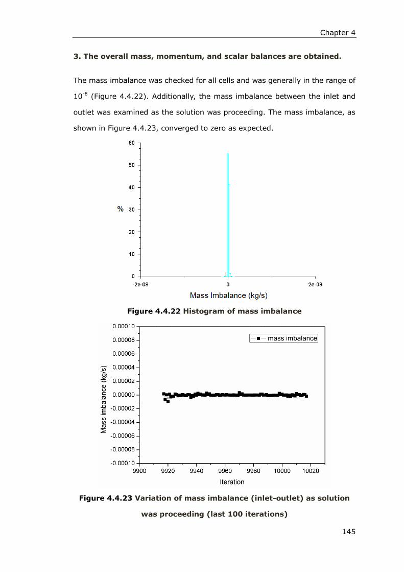
Chapter 4

145

3. The overall mass, momentum, and scalar balances are obtained.

The mass imbalance was checked for all cells and was generally in the range of

10-8 (Figure 4.4.22). Additionally, the mass imbalance between the inlet and

outlet was examined as the solution was proceeding. The mass imbalance, as

shown in Figure 4.4.23, converged to zero as expected.

Figure 4.4.22 Histogram of mass imbalance

Figure 4.4.23 Variation of mass imbalance (inlet-outlet) as solution

was proceeding (last 100 iterations)

Chapter 4

146

4.5 Conclusions

CFD was applied to model the swirl flow induced by the optimised 4-lobed

swirl pipe. The principles and methods underlying CFD were introduced

in this chapter.

The k-ε and RSM Turbulence models for Reynolds-averaged Navier–

Stokes (RANS) equations were described and compared. In the

‘near-wall region’ where turbulence models fail to give accuracy

prediction, the near wall treatment methods were presented.

In this study, the finite volume method based ANSYS FLUENT code was

used to solve the governing equations. The numerical methods of the

solvers and the numerical discretization technique applied were covered.

The formulation of the model used for simulating the swirl flow was

described in detail including enabling assumptions, configuration of the

flow domain and boundary conditions, etc.

Various approaches attempted to discretise the flow domain using

structured hexahedral mesh were explained, of which a Multi-Block

structured mesh using ICEM CFD was adopted. To ensure errors

associated with the mesh are minimised, mesh adaption for wall

functions, mesh independence tests and mesh quality tests were carried

out.

For the solution of the swirl flow field, the turbulence models and wall

functions were tested and compared, with the RSM turbulence and

Non-Equilibrium wall functions being employed in the final model. The

discretization schemes for the viscous terms, pressure-velocity coupling

and pressure interpolation were evaluated and selected respectively.

Convergence of the solution was identified by monitoring the scaled

residuals, flow variables and mass balances.

Chapter 5

147

CHAPTER 5: FURTHER OPTIMISATION OF THE

4-LOBED SWIRL PIPE

5.1 Introduction

It has been stated previously that, based on the evaluation criteria of Swirl

Effectiveness, Ganeshalingam (2002) recommended a 4-lobed swirl inducing

pipe with a P:D ratio of 8 and the length of 400mm as an optimal design. As

shown in Figure 5.1.1a, this optimal swirl inducing pipe has an equivalent

diameter of 50mm and has the 4-lobed cross-section rotated by 360° through a

length of 400mm.

(a) Optimal Swirl inducing pipe, 400mm length, P:D=8

(b) Entry transition pipe, (c) Exit transition pipe

Figure 5.1.1 Optimal Swirl inducing pipe and transition pipes

It was found that there were high entry and exit pressure losses across this

optimal swirl inducing pipe when connected to circular pipes due to the sudden

change in cross-section from lobed to circular and vice versa. Transition

geometries prior to and after the swirl pipe were suggested to eliminate these

pressure losses. This should further improve the applicability of the swirl

inducing pipes. However the transition section should be short and effective.

Otherwise it will increase overall pressure drop and, in the case of exit transition,

Chapter 5

148

may decrease swirl intensity.

Ariyaratne (2005) designed and optimized a transition pipe for use as an entry

and exit duct with the optimal swirl inducing pipe. The transition pipes either

before or after the swirl inducing pipe were found to reduce entry and exit

pressure losses by providing a gradual transition from circular to lobed

cross-section. They also increased induced swirl and reduced swirl decay. As

shown in Figure 5.1.1b and Figure 5.1.1c, the transition pipe’s cross-section

changes from circular to 4-lobed shape and vice versa gradually. The area of the

cross-sections is constant and equal to that of the swirl inducing pipe. The

length of transition pipe is 100mm, and each lobe rotates by 90°.

Based on the study of Ariyaratne (2005), a swirl pipe configuration of 100mm

entry transition prior + 400mm swirl inducing pipe + 100mm exit transition pipe

after (as shown in Figure 5.1.2a) should deem to be optimum. However, in this

configuration:

The entry and exit transition pipes are used in place of the cylindrical

pipes making the total length of the swirl pipe 600mm instead of 400mm.

The longer swirl pipe results in more pressure loss due to the increase in

contact area and thus friction.

The swirl pipe has the lobed cross-section rotated by 540º (one and a

half swirl) instead of 360º (one swirl), as in the previous design.

Ariyaratne (2005) stated that when the entry transition pipe was used in

conjunction with the swirl pipe, a higher tangential velocity was

generated. However, the induced swirl appeared to be constrained by the

swirl inducing pipe geometry. Ariyaratne therefore suggested that a

shorter length of swirl inducing pipe will therefore be required to

generate an equivalent amount of swirl.

In this chapter, we numerically investigated the swirl development within

this 600mm length swirl pipe and found that the swirl intensity induced

Chapter 5

149

reaches the highest value in the middle of the 400mm swirl inducing pipe

(0.3m in the X axis in Figure 5.3.3), and starts to decrease in the second

half of the swirl inducing pipe (0.3m to 0.5m in the X axis in Figure 5.3.3).

It suggested that the second half of the swirl inducing pipe constrains

and weakens the development of the swirl.

Therefore, with the inclusion of transitions, a shorter length of 200mm swirl

inducing pipe should provide improved swirl induction effectiveness. A swirl

inducing pipe shorter than 200mm will decrease pressure loss but also result in

decreased overall swirl intensity. While a swirl inducing pipe longer than 200mm

will constrain and weaken the swirl induced and also give rise to greater press

loss. Therefore, a swirl pipe configuration of 100mm entry transition pipe +

200mm swirl inducing pipe + 100 exit transition pipe was proposed. Other

lengths of swirl pipes were not considered as they are less effective in swirl

induction resulting in lower initial swirl intensity at swirl pipe exit. This

configuration, as shown in Figure 5.1.2b, has one swirl, a total length of 400mm

and an equivalent diameter of 50mm.

This chapter presents a numerical comparison of the two configurations of

horizontally mounted four-lobed swirl pipes in terms of swirl induction

effectiveness into flows passing through them. Pressure losses, swirl

development within the two swirl pipes, and their swirl effectiveness are

analysed and compared. Besides, comparisons of swirl decay and wall shear

stress downstream of the swirl pipes for various velocities were also covered. A

more detailed numerical comparison of the two swirl pipes was presented in a

conference at San Francisco USA, June 07-08, 2015 (Li et al., 2015). The

conference paper is referred to Appendix 5.1 for easy reference.

Chapter 5

150

(a) 100+400+100 swirl pipe, 600mm length, one and a half swirl

(b) 100+200+100 swirl pipe, 400mm length, one swirl

Figure 5.1.2 Two configurations of swirl pipes

5.2 Numerical Method and Models

Configurations of the two modelled pipe flow systems employing the 600mm

length and 400mm length swirl pipes respectively are shown in Figure 5.2.1.

The numerical method, models used and the meshing method are described in

the Chapter 4 section 4.4. A series of simulations were carried out with inlet

velocities of 1m/s, 2m/s and 3m/s. The solver parameters and boundary

conditions are summarised in Table 5.2.1.

Chapter 5

151

Figure 5.2.1 Configuration of simulation geometries

Table 5.2.1 Models and parameters used for the simulations

Items Parameters

Solver

Pressure-based Segregated Solver

Steady state simulation

Absolute velocity formulation

Material Water: Density=998.2kg/m3, Viscosity=0.001003kg/m-s

Viscous model RSM, Non-Equilibrium wall functions

Operating

conditions

Operating pressure=0 Pascal

Gravity=9.81m/s2

Boundary

conditions

INLET: Velocity inlet boundary condition

Velocity magnitude=1, 2, 3 m/s

Turbulence Intensity=4%, 3.8% and 3.6% respectively

Hydraulic Diameter = 50 mm

OUTLET: Pressure outlet boundary condition

Gauge Pressure=0 Pascal

Turbulence specification method: k and epsilon

WALL: wall boundary condition

Stationary no slip wall

Roughness height=9 x 10-06m for swirl pipe;

1.237 x 10-06m for circular pipes

Solution

methods

Second order upwind for momentum, kinetic energy,

dissipation rate and Reynolds Stresses

Pressure interpolation: Second order

Pressure-Velocity coupling: SIMPLE(Semi-Implicit

Method for Pressure-Linked Equations)

Chapter 5

152

The convergence criterion used for all cases was that the scaled residuals of x,

y, z velocities, k, and ε, and Reynolds stresses have decreased by four orders of

magnitude. The mass flow rate at the outlet was monitored and the solution was

deemed to have reached a steady state when this parameter achieved a

constant value over a large number of iterations.

5.3 Results and Discussions

5.3.1 Pressure Drop

The pressure loss across the lobed swirl pipe itself is greater than circular pipe

due to the additional turbulence generated through artificial roughness of the

non-circular pipe surfaces (Ganeshalingam, 2002, Ariyaratne, 2005). The

energy lost is partly converted into angular momentum of the swirling flow.

Figure 5.3.1 demonstrates the pressure drop of the flow within the 600mm and

400mm length swirl pipes for flows with velocities being 3m/s, 2m/s, and 1m/s

respectively.

From Figure 5.3.1, it can be seen that:

A larger inlet velocity causes larger pressure drop in both the

100+400+100 swirl pipe and the 100+200+100 swirl pipe.

For a given flow velocity, the overall pressure drop caused by the

100+400+100 swirl pipe is always larger than that caused by the

100+200+100 swirl pipe due to its larger contact area with fluid and thus

pipe friction.

The differences in production of pressure drops by the two swirl pipes are

more obvious in flows with higher velocities.

The entry and exit transition pipes result in less pressure loss compared

with the swirl inducing pipe. This is clearer for high velocity flows.

Chapter 5

153

Figure 5.3.1 Pressure drop across the two swirl pipes in flows with

various inlet velocities

Table 5.3.1 gives the overall pressure losses caused by the 600mm length and

400mm length swirl pipes in flows with various velocities. Compared to the

100+200+100 swirl pipe, the 100+400+100 swirl pipe resulted in additional

pressure losses of 41%, 38% and 35% respectively for flows with 1m/s, 2m/s

and 3m/s velocities.

Table 5.3.1 Comparison of the two swirl pipe in swirl induction

Velocity

(m/s)

Pressure drop

(Pascal)

Final tangential

velocity (m/s) Final swirl intensity Swirl effectiveness

600mm

swirl

pipe

400mm

swirl

pipe

600mm

swirl

pipe

400mm

swirl

pipe

600mm

swirl

pipe

400mm

swirl

pipe

600mm

swirl

pipe

400mm

swirl

pipe

1 233.24 165.25 0.156 0.156 0.106 0.106 0.228 0.321

2 866.2 625.86 0.33 0.345 0.115 0.125 0.265 0.398

3 1894.99 1399.5 0.545 0.555 0.129 0.133 0.305 0.428

Chapter 5

154

5.3.2 Swirl Development within Swirl Pipes

Figure 5.3.2 shows the development of tangential velocity within the

100+400+100 swirl pipe and 100+200+100 swirl pipe for the three inlet

velocities of 3m/s, 2m/s and 1m/s. It is clear that:

Both swirl pipes induce greater tangential velocities in flows with higher

velocities.

For both swirl pipes, exit transition pipes cause a decrease in tangential

velocity.

For the three inlet velocities and for the 100+400+100 swirl pipe, a

sharper tangential velocity increase is seen from the middle of the entry

transition pipe (0.05m in the X axis) and reaches the highest value in the

vicinity of the middle of the 400mm swirl inducing pipe (0.4m in the X

axis). The tangential velocity decreases slightly in the second half of the

swirl inducing pipe indicating that it is acting as a constraint to the

induced tangential velocity.

While in the case of 100+200+100 swirl pipe, the whole 200mm swirl

Chapter 5

155

inducing pipe contributes to the tangential velocity development with the

largest value appearing at the join of the swirl inducing pipe and the exit

transition pipe and the largest values in tangential velocity are almost the

same as the 100+400+100 swirl pipe.

The final tangential velocities at the exit of the 100+200+100 swirl pipe

are slightly larger than that of the 100+400+100 pipe for inlet velocities

of 2m/s and 3m/s. For a flow of 1m/s velocity, no difference in the final

tangential velocity was identified.

Figure 5.3.2 Tangential velocity distribution within the two swirl pipes

for various inlet velocities

Figure 5.3.3 depicts the variation of swirl intensity within the two swirl pipes for

the three velocities. Generally, for both swirl pipes, the first 0.3m length

contributes to swirl induction with the swirl intensity value and its variation

almost identical. The highest swirl intensity value appears in the 0.3m in the X

axis for both swirl pipes. However, starting from 0.3m in the X axis, for the

600mm swirl pipe, both the second half of the swirl inducing pipe and the exit

Chapter 5

156

transition pipe act as a constraint to the swirl induced previously. While for the

400mm length swirl pipe, only the exit pipe constrain the swirl induce. Due to

the presence of the second half of the swirl inducing pipe in the 600mm length

swirl pipe, which did not contribute to but weaken the swirl induction, the final

swirl intensity at the exit of the 100+400+100 pipe is smaller than that of the

100+200+100 swirl pipe especially for larger flow velocities. The detailed initial

swirl intensity downstream of both pipes for the three velocities is listed in Table

5.3.1. This confirmed again that, in the case of 100+400+100 swirl pipe, the

second half of the swirl inducing pipe constrains and weakens the development

of swirl and therefore needs to be removed. Besides, it was found the 400mm

length swirl pipe also gives rise to greater swirl intensity and wall shear stress to

the downstream which also lasts for longer downstream distance. The detailed

numerical comparison of the 400mm and 600mm length swirl pipes in terms of

the downstream wall shear stress and swirl intensity is discussed in a

conference paper which is attached in Appendix 5.1 for easy reference (Li et al.,

2015).

Figure 5.3.3 Swirl intensity distribution within the two swirl pipes for

Chapter 5

157


5.3.3 Swirl Effectiveness

Ganeshalingam (2002) defined a Swirl Effectiveness parameter based on the

ratio of the swirl intensity produced to the pressure loss, and used it in all swirl

effectiveness calculations. The effectiveness of swirl induction was deemed to

be the swirl intensity that could be induced for a given pressure drop. This

parameter is also used in this research for the comparison of the two swirl pipe

configurations in terms of swirl induction effectiveness.

𝑆𝑤𝑖𝑟𝑙 𝐸𝑓𝑓𝑒𝑐𝑡𝑖𝑣𝑒𝑛𝑒𝑠𝑠 =𝑆𝑤𝑖𝑟𝑙 𝐼𝑛𝑡𝑒𝑛𝑠𝑖𝑡𝑦

∆𝑃𝜌 × 𝑢2

2

(5.1)

Where ∆𝑃 is pressure drop, 𝜌 is density, and 𝑢 is flow velocity.

Figure 5.3.4 shows the swirl effectiveness variation for both pipes with the three

different inlet velocities. At each position, the value is calculated as the overall

swirl effectiveness from the inlet of the swirl pipe to that specific position.

Figure 5.3.4 Swirl effectiveness variation within the two swirl pipes for

Chapter 5

158


In the entry transition pipe for the two swirl pipes, there is a quick increase in

swirl effectiveness. This is due to the gradual transition from circular to the

lobed cross-section which reduces frictional losses from the pipe walls thereby

producing a more effective swirl induction from a smaller pressure drop.

The quick increase in swirl intensity prevails within the swirl inducing pipe that

it is immediately adjacent to the entry transition pipe where the swirl

effectiveness reaches its highest value in this duration (0.1~0.15m). The high

swirl effectiveness value benefits from the averaging of pressure losses caused

by the entry transition pipe and the swirl inducing pipe section (0.1~0.15m).

Afterward, the increase in swirl intensity slows down until it reaches a maximum

value in the vicinity of 0.3m in the horizontal axis as shown in

Figure 5.3.2 where the swirl inducing pipe still contributes to swirl induction

despite of the drop in swirl effectiveness (which is due to the increase in the

average pressure loss). Until this position, the two swirl pipes have almost

identical swirl induction effectiveness.

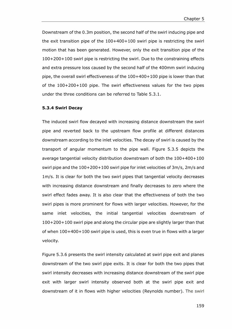
Chapter 5

159

Downstream of the 0.3m position, the second half of the swirl inducing pipe and

the exit transition pipe of the 100+400+100 swirl pipe is restricting the swirl

motion that has been generated. However, only the exit transition pipe of the

100+200+100 swirl pipe is restricting the swirl. Due to the constraining effects

and extra pressure loss caused by the second half of the 400mm swirl inducing

pipe, the overall swirl effectiveness of the 100+400+100 pipe is lower than that

of the 100+200+100 pipe. The swirl effectiveness values for the two pipes

under the three conditions can be referred to Table 5.3.1.

5.3.4 Swirl Decay

The induced swirl flow decayed with increasing distance downstream the swirl

pipe and reverted back to the upstream flow profile at different distances

downstream according to the inlet velocities. The decay of swirl is caused by the

transport of angular momentum to the pipe wall. Figure 5.3.5 depicts the

average tangential velocity distribution downstream of both the 100+400+100

swirl pipe and the 100+200+100 swirl pipe for inlet velocities of 3m/s, 2m/s and

1m/s. It is clear for both the two swirl pipes that tangential velocity decreases

with increasing distance downstream and finally decreases to zero where the

swirl effect fades away. It is also clear that the effectiveness of both the two

swirl pipes is more prominent for flows with larger velocities. However, for the

same inlet velocities, the initial tangential velocities downstream of

100+200+100 swirl pipe and along the circular pipe are slightly larger than that

of when 100+400+100 swirl pipe is used, this is even true in flows with a larger

velocity.

Figure 5.3.6 presents the swirl intensity calculated at swirl pipe exit and planes

downstream of the two swirl pipe exits. It is clear for both the two pipes that

swirl intensity decreases with increasing distance downstream of the swirl pipe

exit with larger swirl intensity observed both at the swirl pipe exit and

downstream of it in flows with higher velocities (Reynolds number). The swirl

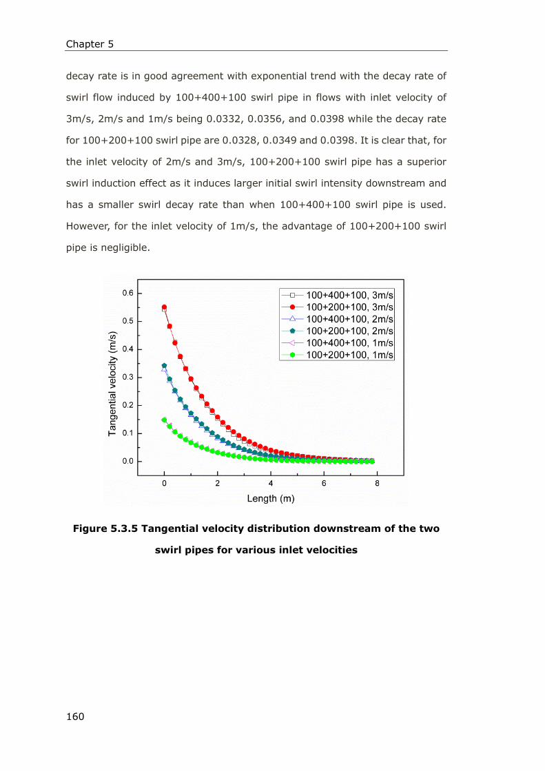
Chapter 5

160

decay rate is in good agreement with exponential trend with the decay rate of

swirl flow induced by 100+400+100 swirl pipe in flows with inlet velocity of

3m/s, 2m/s and 1m/s being 0.0332, 0.0356, and 0.0398 while the decay rate

for 100+200+100 swirl pipe are 0.0328, 0.0349 and 0.0398. It is clear that, for

the inlet velocity of 2m/s and 3m/s, 100+200+100 swirl pipe has a superior

swirl induction effect as it induces larger initial swirl intensity downstream and

has a smaller swirl decay rate than when 100+400+100 swirl pipe is used.

However, for the inlet velocity of 1m/s, the advantage of 100+200+100 swirl

pipe is negligible.

Figure 5.3.5 Tangential velocity distribution downstream of the two

swirl pipes for various inlet velocities

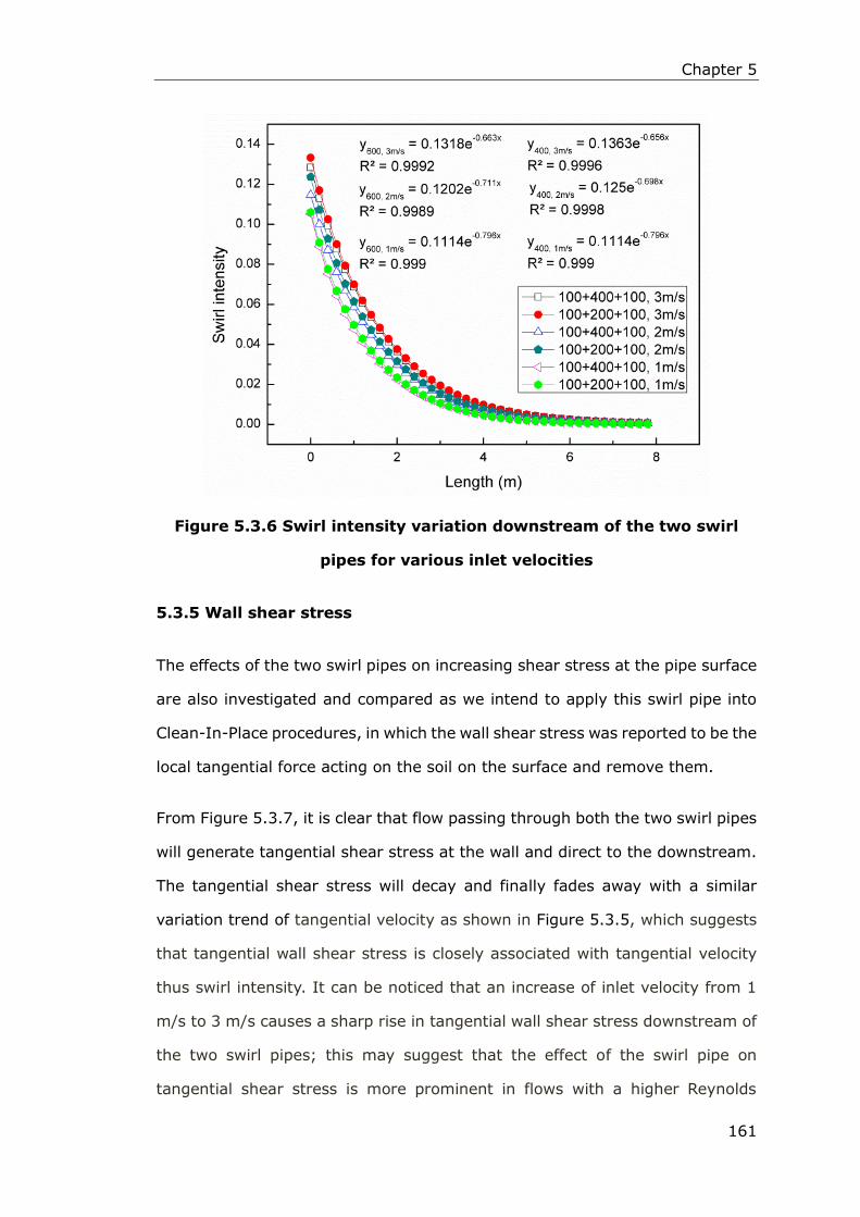
Chapter 5

161

Figure 5.3.6 Swirl intensity variation downstream of the two swirl

pipes for various inlet velocities

5.3.5 Wall shear stress

The effects of the two swirl pipes on increasing shear stress at the pipe surface

are also investigated and compared as we intend to apply this swirl pipe into

Clean-In-Place procedures, in which the wall shear stress was reported to be the

local tangential force acting on the soil on the surface and remove them.

From Figure 5.3.7, it is clear that flow passing through both the two swirl pipes

will generate tangential shear stress at the wall and direct to the downstream.

The tangential shear stress will decay and finally fades away with a similar

variation trend of tangential velocity as shown in Figure 5.3.5, which suggests

that tangential wall shear stress is closely associated with tangential velocity

thus swirl intensity. It can be noticed that an increase of inlet velocity from 1

m/s to 3 m/s causes a sharp rise in tangential wall shear stress downstream of

the two swirl pipes; this may suggest that the effect of the swirl pipe on

tangential shear stress is more prominent in flows with a higher Reynolds

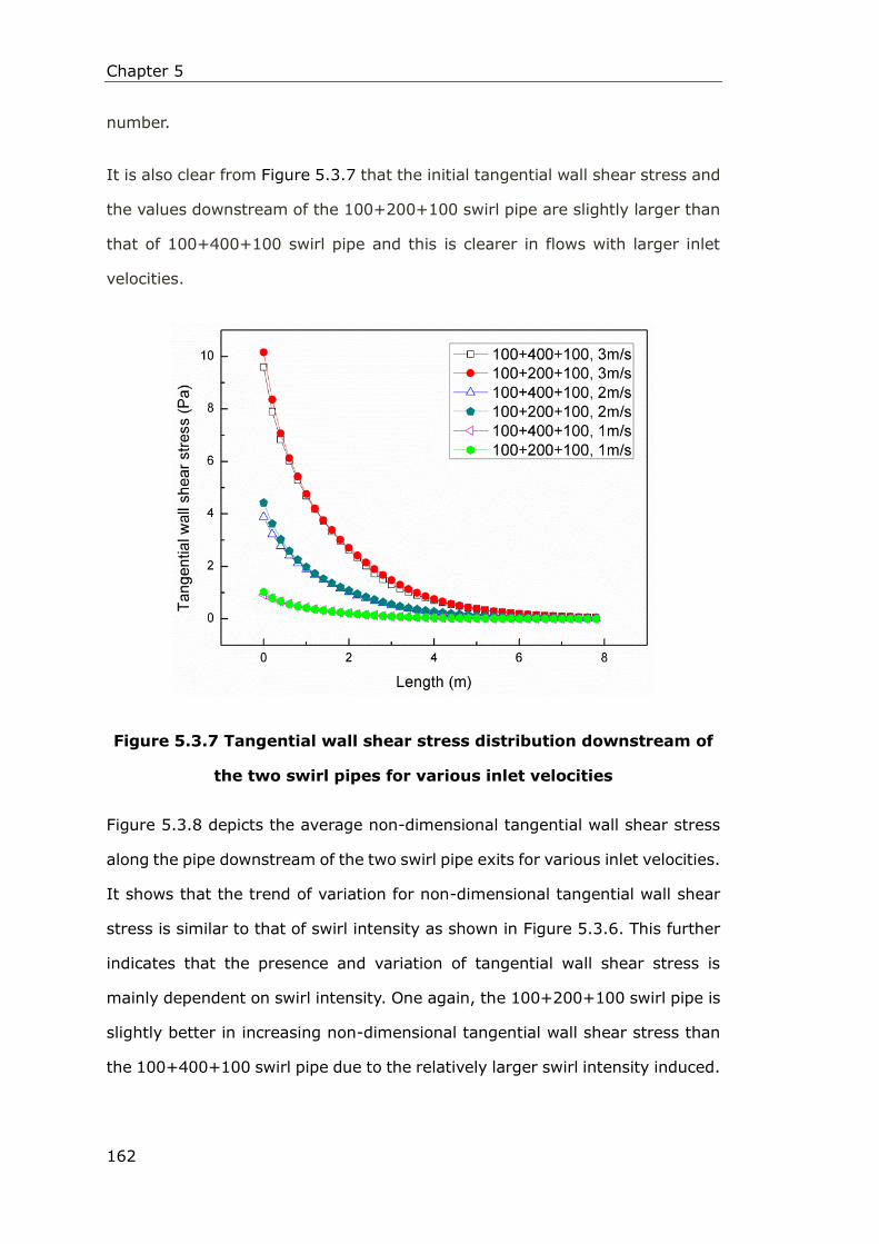
Chapter 5

162

number.

It is also clear from Figure 5.3.7 that the initial tangential wall shear stress and

the values downstream of the 100+200+100 swirl pipe are slightly larger than

that of 100+400+100 swirl pipe and this is clearer in flows with larger inlet

velocities.

Figure 5.3.7 Tangential wall shear stress distribution downstream of

the two swirl pipes for various inlet velocities

Figure 5.3.8 depicts the average non-dimensional tangential wall shear stress

along the pipe downstream of the two swirl pipe exits for various inlet velocities.

It shows that the trend of variation for non-dimensional tangential wall shear

stress is similar to that of swirl intensity as shown in Figure 5.3.6. This further

indicates that the presence and variation of tangential wall shear stress is

mainly dependent on swirl intensity. One again, the 100+200+100 swirl pipe is

slightly better in increasing non-dimensional tangential wall shear stress than

the 100+400+100 swirl pipe due to the relatively larger swirl intensity induced.

Chapter 5

163

Figure 5.3.8 Non-dimensional tangential WSS distribution downstream

of the two swirl pipes for various inlet velocities

Figure 5.3.9 presents the average axial wall shear stress downstream of the two

swirl pipe exits for various inlet velocities. It shows that the two swirl pipes also

has the effect of increasing axial wall shear stress downstream them but in a

very slight way and lasts for a short distance compared with tangential wall

shear stress. The effect of the swirl pipes on axial wall shear becomes less

obvious with decreasing inlet velocity (Reynolds number). Their effect is almost

negligible for flows with an inlet velocity of 1 m/s. with the same inlet velocities,

100+200+100 swirl pipe induces a slightly higher axial wall shear stress

increase than that of 100+400+100 swirl pipe, however, its advantage stops

being obvious in flows with lower velocities.

Chapter 5

164

Figure 5.3.9 Axial wall shear stress distribution downstream of the two

swirl pipes for various inlet velocities

Figure 5.3.10 shows the total wall shear stress, which is the combined action of

the tangential and axial shear stress component acting on the pipe surface,

downstream of the two swirl pipes. It is clear that swirl pipes locally increases

mean wall shear stress downstream of it, with the increased value and effective

distance more remarkable for a faster inlet flow velocity (a large Reynolds

number and large swirl intensity). For a flow velocity of 3m/s which is typically

the velocity of cleaning fluid circulating in a Clean-In-Place procedure,

100+400+100 swirl pipe raises mean shear stress at the wall from 17.8 Pascal

prior swirl pipe inlet to 22 Pascal (23.5% increase) just downstream of it. The

wall shear stress decays in accordance with swirl intensity, and in the point 1m

(20D) downstream swirl pipe exit the increase in wall shear stress is 5%. While

the 100+200+100 swirl pipe rises wall shear stress from 17.8 Pascal before it to

23.7 Pascal (33.1% increase) downstream of it and maintains at least 5%

increase in mean wall shear stress in the position 1.1m (22D) downstream of it .

Such it can be concluded that 100+200+100 swirl pipe is better in increasing

Chapter 5

165

and maintaining wall shear stress downstream it than that of 100+400+100

swirl pipe. However, the advantage of 100+200+100 swirl pipe on increasing

total wall shear stress is not that obvious in flows with lower velocities, and for

an inlet velocity of 1m/s, the different is almost negligible.

Figure 5.3.10 Total wall shear stress distribution downstream of the

two swirl pipes for various inlet velocities

From the above discussion, the 100+200+100 swirl pipe induces slightly

greater or the same level of swirl into flows passing through it for less pressure

losses than the longer 100+400+100 pipe. It is also clear that the

100+200+100 swirl pipe is more cost effective in increasing wall shear stress

downstream of it than when a 100+400+100 swirl pipe. This swirl pipe

configuration is ‘optimized’ in swirl induction and will therefore be used for the

following investigations.

5.4 Conclusions

The overall pressure drop caused by the 100+400+100 swirl pipe is

larger than the 100+200+100 swirl pipe for the same inlet velocities due

Chapter 5

166

to the longer swirl inducing pipe.

For the 100+400+100 swirl pipe, the second half of the 400mm swirl

inducing pipe serves as a constraint to the swirl induced resulting in

lower (same level as for 1m/s velocity) initial tangential velocity or swirl

intensity at the exit of swirl pipe than the 100+200+100 swirl pipe.

The overall swirl effectiveness of the 100+200+100 swirl pipe is greater

than that of the 100+400+100 swirl pipe.

The induced tangential velocity, swirl intensity and the effective

distances are larger downstream of the 100+200+100 swirl pipe than

when 100+400+100 swirl pipe is used with its advantage is more true in

flows with larger Reynolds Number.

Swirl pipes impose a tangential wall shear stress within itself and direct

to downstream, its value and variation trend is dependent on swirl

intensity. The induced tangential wall shear stress after the

100+200+100 swirl pipe is larger than when 100+400+100 swirl pipe is

used due to the relatively larger swirl intensity.

The axial and total wall shear stress are also larger downstream of the

100+200+100 swirl pipe than that of the 100+400+100 swirl pipe with

its advantage being more true in flows with a larger inlet velocity.

A shorter length of 200mm swirl inducing pipe used in conjunction with

the entry and exit transition sections is suggested to be more cost

effective in swirl induction, and will therefore be employed for further

research.

Chapter 6

167

CHAPTER 6: RANS-BASED SIMULATION OF SWIRL

FLOW DOWNSTREAM OF THE OPTIMISED SWIRL

PIPE

6.1 Introduction

This chapter presents a computational fluid dynamics model of the swirl flow

that is induced in a fluid flow passing through the horizontally mounted

optimized four-lobed 400mm length swirl pipe. The steady state CFD model

based on the RANS approach provides time-averaged properties of the swirl

flows (e.g. mean velocities, mean pressures, mean stresses etc.). Analysis will

focus on the variation of flow parameters downstream of the swirl pipe as this is

the duration where CIP may benefit from the use of swirl pipe.

Pressure loss, tangential velocity, swirl type, swirl intensity and its decay rate of

the swirl flow downstream of the swirl pipe are investigated in flows with various

inlet velocities. Special attention is paid to the potential of the swirl flow on

improving CIP efficiency by increasing the mean wall shear stress to the

downstream without increasing the operation velocity. The wall shear stress is a

measure of the mechanical action of fluid flow on a process surface with the

mean wall shear stress especially relevant as a measure of cleaning efficiency in

straight pipes, large parts of pumps, valves and so on (PathogenCombat, 2011).

The numerical results indicate that the swirl pipe may improve efficiency of CIP

procedures by locally increasing mean wall shear stress to the downstream

without the need to increase the flow velocity, consequently shortening the

downtime for cleaning, and reducing the costs for chemicals and power energy.

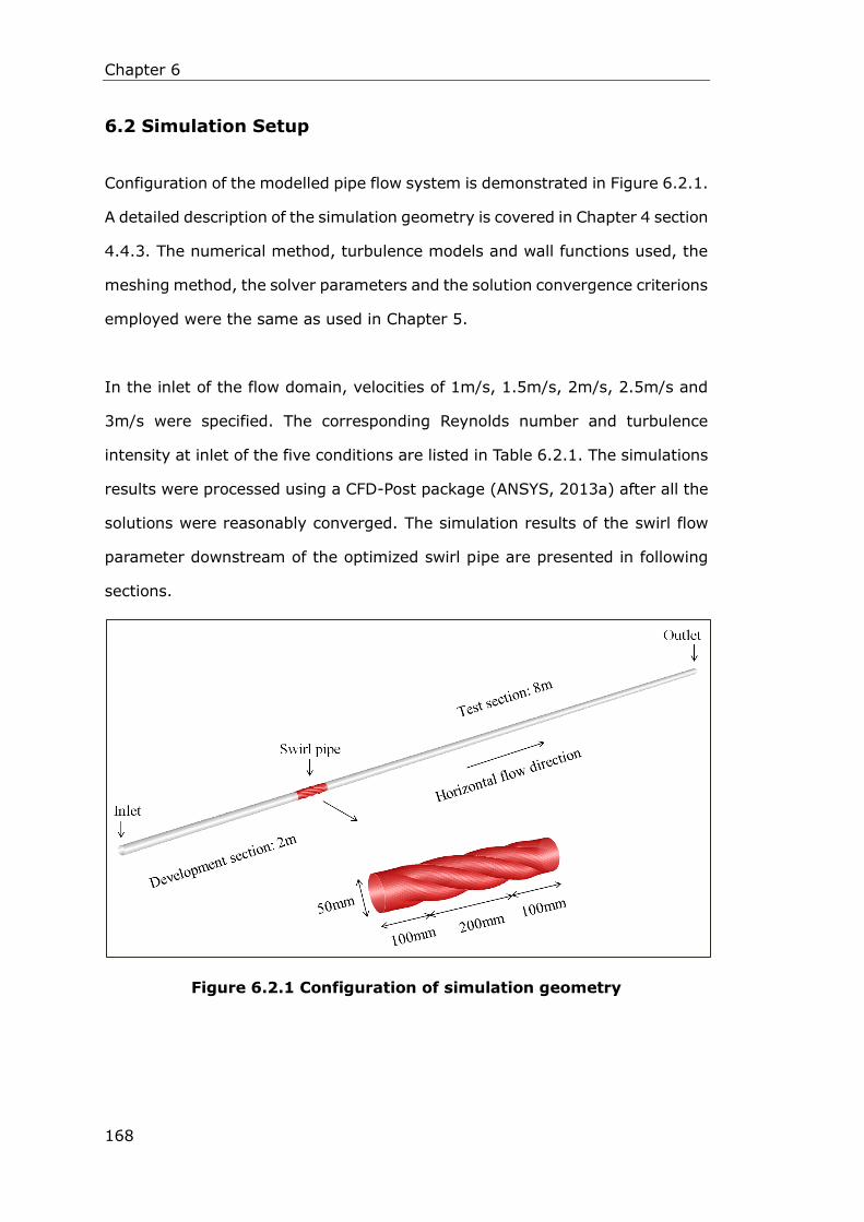
Chapter 6

168

6.2 Simulation Setup

Configuration of the modelled pipe flow system is demonstrated in Figure 6.2.1.

A detailed description of the simulation geometry is covered in Chapter 4 section

4.4.3. The numerical method, turbulence models and wall functions used, the

meshing method, the solver parameters and the solution convergence criterions

employed were the same as used in Chapter 5.

In the inlet of the flow domain, velocities of 1m/s, 1.5m/s, 2m/s, 2.5m/s and

3m/s were specified. The corresponding Reynolds number and turbulence

intensity at inlet of the five conditions are listed in Table 6.2.1. The simulations

results were processed using a CFD-Post package (ANSYS, 2013a) after all the

solutions were reasonably converged. The simulation results of the swirl flow

parameter downstream of the optimized swirl pipe are presented in following

sections.

Figure 6.2.1 Configuration of simulation geometry

Chapter 6

169

Table 6.2.1 Simulation conditions at inlet

Inlet velocity

(m/s) Reynolds number

Turbulence intensity

(%)

Hydraulic diameter

(mm)

1 49,760 4 50

1.5 74,641 3.9 50

2 99,521 3.8 50

2.5 124,401 3.7 50

3 149,282 3.6 50


6.3.1 Pressure Drop

Pressure is the force applied to a unit area of surface. In a dynamic system,

pressure typically is defined using three terms, the static pressure, the dynamic

pressure and the total pressure. The static pressure can be identified for every

point in a body of fluid, regardless of whether the fluid is in motion or not. The

dynamic pressure is associated with the velocity or the flow of the fluid. The

total pressure is the sum of the static pressure and the dynamic pressure.

For the current flow system where the circular and swirl pipe have a constant

cross-sectional area, the dynamic pressure is constant throughout the system

for a given flow velocity. The static pressure was used to understand the flow

behaviour within the top horizontal section of the rig that was modelled.

Figure 6.3.1 shows the variation of averaged static gauge pressure over the

area of the planes downstream of the inlet throughout the whole flow system.

The CFD results show that the value of pressure and its loss along the pipe

system are proportional to the velocity (Reynolds number) of the flow. The swirl

pipe (2m~2.4m in X axis) causes a more significant drop in pressure than the

circular pipes; this is more obvious in flows with larger Reynolds number.

Chapter 6

170

Figure 6.3.1 Static pressure variation in the horizontal pipe system for


Table 6.3.1 summarizes the per unit length pressure loss within the duration 1

meter prior the swirl pipe, the swirl pipe and the durations of 0~1m, 1~2m,

2~3m … 6~7m downstream of the swirl pipe. It can be seen that the pressure

losses across the 4-lobed swirl pipe are greater than that of the circular pipes

(2.1~2.45 times corresponding to 1~3m/s velocity). The greater pressure

losses are due to the additional turbulence generated through the artificial

roughness of the non-circular pipe cross-sections of the swirl pipe.

Table 6.3.1 The unit length pressure losses for swirl and circular pipes

ΔP

Velocity

1m

prior,

Pa/m

Swirl

pipe,

Pa/m

0~1m

after,

Pa/m

1~2m

after,

Pa/m

2~3m

after,

Pa/m

3~4m

after,

Pa/m

4~5m

after,

Pa/m

5~6m

after,

Pa/m

6~7m

after,

Pa/m

1 m/s 198.4 413.1 206.5 201.5 202.9 202.7 202.4 202.8 202.8

1.5m/s 406.9 907.2 449.4 417.0 414.2 415.4 414.4 415.2 415.2

2 m/s 679.5 1564.7 753.6 696.3 690.7 693.1 691.2 692.4 692.6

2.5m/s 1012.8 2426.7 1125.4 1035.6 1026.9 1030.0 1027.3 1030.2 1030.7

3 m/s 1406.3 3457.8 1568.0 1441.6 1425.2 1432.4 1427.7 1428.8 1430.0

swirl pipe

Chapter 6

171

Table 6.3.1 also shows that, for the circular pipes, the unit length pressure

losses just downstream of the swirl pipe are slightly greater than that occurred

in the circular pipe prior the swirl pipe, this is more true in flows with higher

velocities. The increase in pressure loss downstream of swirl pipe declines with

increasing downstream distance as the swirl effects fades away.

The increase in pressure losses may be due to the swirling flow regime which

decreases the thickness of the boundary layer resulting in an increase in shear

stress at the wall. It is documented that, in cylindrical pipe flow, the wall shear

stress has a proportional relation to the pressure loss in that 𝜏𝑤 =∆𝑃𝑑

4𝐿 (Sleigh

and Goodwill, 2008), where d is pipe diameter, L is the length of pipe

corresponding to pressure loss. Therefore, the greater pressure loss in the

circular pipe downstream of the swirl pipe indicates that the swirl pipe increases

wall shear stress in the duration just downstream of it.

6.3.2 Tangential Velocity

The swirl pipe adds a rotating momentum to the flow within itself and the

circular pipe downstream of it, turning the fluid clockwise in addition to the axial

velocity along the pipe. The velocity component, which mainly affects the swirl

flow field, is the tangential velocity component, which has a distribution

dependent on the swirl generation mechanism (Najafi et al., 2011). Generally

three well known methods may be employed in order to produce swirl flow

(Gupta et al., 1984):

Chapter 6

172

In the first method, passing through a rotational section, fluid flow

acquires tangential momentum and enters the pipe in the form of a swirl

flow.

In method two, fluid flow enters the pipe through fixed blades (vanes),

which are mounted inside of the pipe with a specified angle.

The third method is that fluid flow enters the pipe by means of a

tangential inlet so that it can acquire rotational momentum and enter the

pipe in the form of a swirl flow.

The swirl pipe induces swirl into flow in a way similar to the first method, but the

swirl pipe does not rotate, rather it is the helical geometry of the swirl pipe that

forces the fluid which passes through it to rotate within itself and the circular

pipe downstream.

Tangential velocity contour plots in the radial and axial directions for various

flow velocities are illustrated in Figure 6.3.2 with the interval distance of the

adjacent cross-sections being 4D (0.2m). It shows that the swirl pipe induces

swirl (tangential velocity) within itself and the swirl prevails for some distance

downstream and decays gradually. In the radial direction, where swirl exists,

the tangential velocity is zero at the centre of the pipe. This increases to the

highest value in the near wall region and then decreases to zero at the pipe wall.

The contours exhibit a characteristic quadrangular shape which is attributed to

the 4-lobed swirl pipe. However, this quadrangular nature is more difficult to

identify the further away from the swirl pipe exit. The contour also shows that

the orientation of quadrangular contour changes with distance downstream,

indicating a rotating flow. Figure 6.3.2 depicts that the tangential velocity

induced by the swirl pipe are greater in flows with larger velocity which also

prevails for a longer downstream distance.

Chapter 6

173

Figure 6.3.2 Tangential velocity (m/s) distribution within and downstream swirl pipe for various velocities

swirl pipe entry swirl pipe exit 0.4m after 0.8m after 1.2m after

3m/s:

2m/s:

1m/s:

Chapter 6

174

Based on the radial distribution of tangential velocity field, three swirl types can

be distinguished as shown in Figure 6.3.3 (Steenbergen and Voskamp, 1998):

Concentrated Vortex (CV)- rotation concentrated near the pipe centre

Solid Body (SB)- almost uniform rotation

Wall Jet (WJ)- angular momentum concentrated near the wall

Figure 6.3.3 Classification of swirl types (After Steenbergen and

Voskamp, 1998)

Figure 6.3.4 Tangential velocity profiles in radial direction (2m/s inlet

velocity)

Chapter 6

175

Figure 6.3.4 shows the radial distribution of tangential velocity in several

cross-sectional flow planes within the swirl pipe and downstream of it (2m/s

inlet velocity for instance). It is clear that, compared with Figure 6.3.3, the swirl

type inside the swirl pipe itself is in good agreement with wall jet definition.

However, it gradually develops into a solid body type. 1.2m after the swirl pipe

exit the type of swirl is better fitted to a solid body.

Figure 6.3.5 Tangential velocity variation downstream of swirl pipe exit

Figure 6.3.5 depicts the average tangential velocity distribution downstream of

the swirl pipe for various inlet velocities. It is clear from the plot that tangential

velocity decreases with increasing downstream distance and finally decreases to

zero where the swirl effect fades away. Figure 6.3.5 also shows that a greater

initial tangential velocity at the exit of swirl pipe was generated with a larger

flow velocity. An attempt was made to find the relation between the initial

tangential velocity and the inlet velocity by linear fitting of the five pairs of data.

The fitting resulted in a straight line with a coefficient of determination close to

1. However this straight line makes no engineering sense at zero parameters

because it indicates a positive tangential velocity value with an inlet velocity of

zero. Therefore the (0, 0) point was included and several fittings were

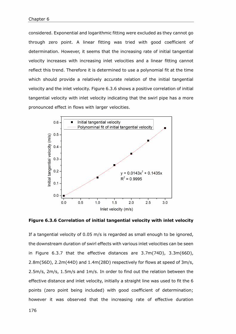
Chapter 6

176

considered. Exponential and logarithmic fitting were excluded as they cannot go

through zero point. A linear fitting was tried with good coefficient of

determination. However, it seems that the increasing rate of initial tangential

velocity increases with increasing inlet velocities and a linear fitting cannot

reflect this trend. Therefore it is determined to use a polynomial fit at the time

which should provide a relatively accurate relation of the initial tangential

velocity and the inlet velocity. Figure 6.3.6 shows a positive correlation of initial

tangential velocity with inlet velocity indicating that the swirl pipe has a more

pronounced effect in flows with larger velocities.

Figure 6.3.6 Correlation of initial tangential velocity with inlet velocity

If a tangential velocity of 0.05 m/s is regarded as small enough to be ignored,

the downstream duration of swirl effects with various inlet velocities can be seen

in Figure 6.3.7 that the effective distances are 3.7m(74D), 3.3m(66D),

2.8m(56D), 2.2m(44D) and 1.4m(28D) respectively for flows at speed of 3m/s,

2.5m/s, 2m/s, 1.5m/s and 1m/s. In order to find out the relation between the

effective distance and inlet velocity, initially a straight line was used to fit the 6

points (zero point being included) with good coefficient of determination;

however it was observed that the increasing rate of effective duration

Chapter 6

177

downstream of the swirl pipe decreases with increasing inlet velocities and a

straight line cannot reflect this trend. Therefore it was decided to use a

polynomial fitting. Figure 6.3.7 shows that the swirl effect prevails a longer

downstream distance in flows with larger velocities. However, the descending

increasing rate of the curve may also suggests that the pipe wall exerts greater

resistance to the swirl flow generated in flows with larger velocities resulting in

a decreased increasing rate of swirl effective distance.

Figure 6.3.7 Correlation of swirl pipe effect distance with inlet

velocities

6.3.3 Swirl Decay

The induced swirl flow decays with increasing distance downstream the swirl

pipe and reverts back to the upstream flow profile at different pipe diameters

downstream according to the inlet velocities. The decay of swirl is caused by the

transport of angular momentum to the pipe wall (Steenbergen and Voskamp,

1998).

To quantify the swirl intensity S of the swirl flow, the numerator and

Chapter 6

178

denominator in equation 𝑺 =∫ 𝒖𝒘𝒓𝟐𝒅𝒓

𝑹

𝟎

𝑹∫ 𝒖𝟐𝑹

𝟎 𝒓𝒅𝒓 (equation 2.3.1, Chapter 2) were

calculated in CFD-post by integrating 𝒖𝒘𝒓 and 𝒖𝟐 over planes downstream of

the swirl pipe exit. Figure 6.3.8 presents the swirl intensity calculated at swirl

pipe exit and planes 4D, 8D, 12D, 16D and so on downstream of the swirl pipe

exit. It can be seen from the figure that swirl intensity decreases with increasing

distance downstream of the swirl pipe exit with larger swirl intensity observed

both at the swirl pipe exit and downstream of it in flows with higher velocities

(Reynolds number).

The swirl decay rate is in good agreement with exponential trend of 𝑺 = 𝑺𝟎𝒆𝜷

𝒙

𝑫

(equation 2.3.2, Chapter 2), where S0 is the initial swirl intensity, and 𝜷 is the

swirl decay rate. The swirl decay rates for inlet velocity of 1m/s, 1.5m/s, 2m/s,

2.5m/s and 3m/s are 0.040, 0.036, 0.035, 0.034 and 0.032 respectively. It is

clear that the swirl decay rate decreases with increasing inlet velocities,

indicating that swirl prevails for a longer downstream distance in flows with a

larger Reynolds number. A detailed correlation of swirl decay rate with flow

Reynolds number is presented in Figure 6.3.9.

Steenbergen and Voskamp (1998) concluded that in turbulent swirl flow in

smooth pipes at a swirl number within 0≤S ≤0.18, the swirl decay rate is related

to the friction factor of the pipe 𝑓 ,. They suggested a value of 𝛽 = [(1.49 ±

0.07) × 𝑓 ,] for 0≤S≤0.18 (experiments were carried out with water at

50,000<Re<300,000, S0=0.18).

The friction factor 𝑓 , can be obtained by solving the Colebrook equation and the

Blasius equation 𝑓𝐷 =0.3164

𝑅𝑒0.25 which is valid for Re=3×103~1×105. The value of 𝛽

calculated in terms of 𝑓 , for swirl flows at various speeds are shown in Table

6.3.2.

Chapter 6

179

Figure 6.3.8 Swirl intensity variation downstream of swirl pipe exit

Figure 6.3.9 Correlation of swirl decay rate with Reynolds number

Table 6.3.2 Swirl decay rate calculated in terms of friction factor

Velocity Reynolds

number

CFD Colebrook equation Blasius equation

𝛽 𝑓 , 𝛽 𝑓 , 𝛽

1 m/s 49,760 0.04 0.021 1.90𝑓 , 0.0211 1.90𝑓 ,

1.5m/s 74,641 0.036 0.0192 1.88𝑓 , 0.0191 1.88𝑓 ,

Chapter 6

180

2 m/s 99,521 0.035 0.0181 1.93𝑓 , 0.0178 1.97𝑓 ,

2.5m/s 124,401 0.034 0.0173 1.97𝑓 , 0.0168 2.02𝑓 ,

3 m/s 149,282 0.032 0.0167 1.92𝑓 , 0.0161 1.99𝑓 ,

The values of decay rate are higher than the expected value suggested by

Steenbergen and Voskamp. This may attribute to the fact that Colebrook

equation and the Blasius equation tend to underestimate the friction factor

value as they are primarily dedicated for calculating friction factor in

non-swirling cylindrical pipe flow. In the case of swirl flow, the two equations

may underestimate the friction factor. Another possible reason might be the

difference in the swirl induction method of the current geometrically induced

swirl flow. However, there is no unanimous agreement regarding this point.

Kitoh (1991) and Steenbergen and Voskamp (1998) concluded that swirl

intensity is independent of the mechanism of swirl generation while Najafi (2011)

stated that the swirl intensity decay rate is not solely a function of Reynolds

number, but depends on the type of the swirl generation as well.

6.3.4 Wall Shear Stress

Published work reports that Clean-In-Place efficiency of closed processing

equipment depends, among other criteria, on the hydrodynamic effect. The

cleaning liquid generates local tangential force acting on the soil on the surface

and acts as a carrier for the chemicals and heat (Jensen et al., 2007). The

removal kinetics is a function of the fluid detergent velocity and of the wall shear

stress (Gallot-Lavallée et al., 1984, Graβhoff, 1992, Visser, 1970, Sharma,

1991). In general, there is a threshold value of both mean and local wall shear

stress above which cleaning is considered efficient. The threshold is defined as

the lowest mean wall shear stress sufficient to remove the specific type of soil on

the pipe surface (PathogenCombat, 2011). A so-called critical wall shear stress

for removal of specific microorganisms on various surfaces was also reported by

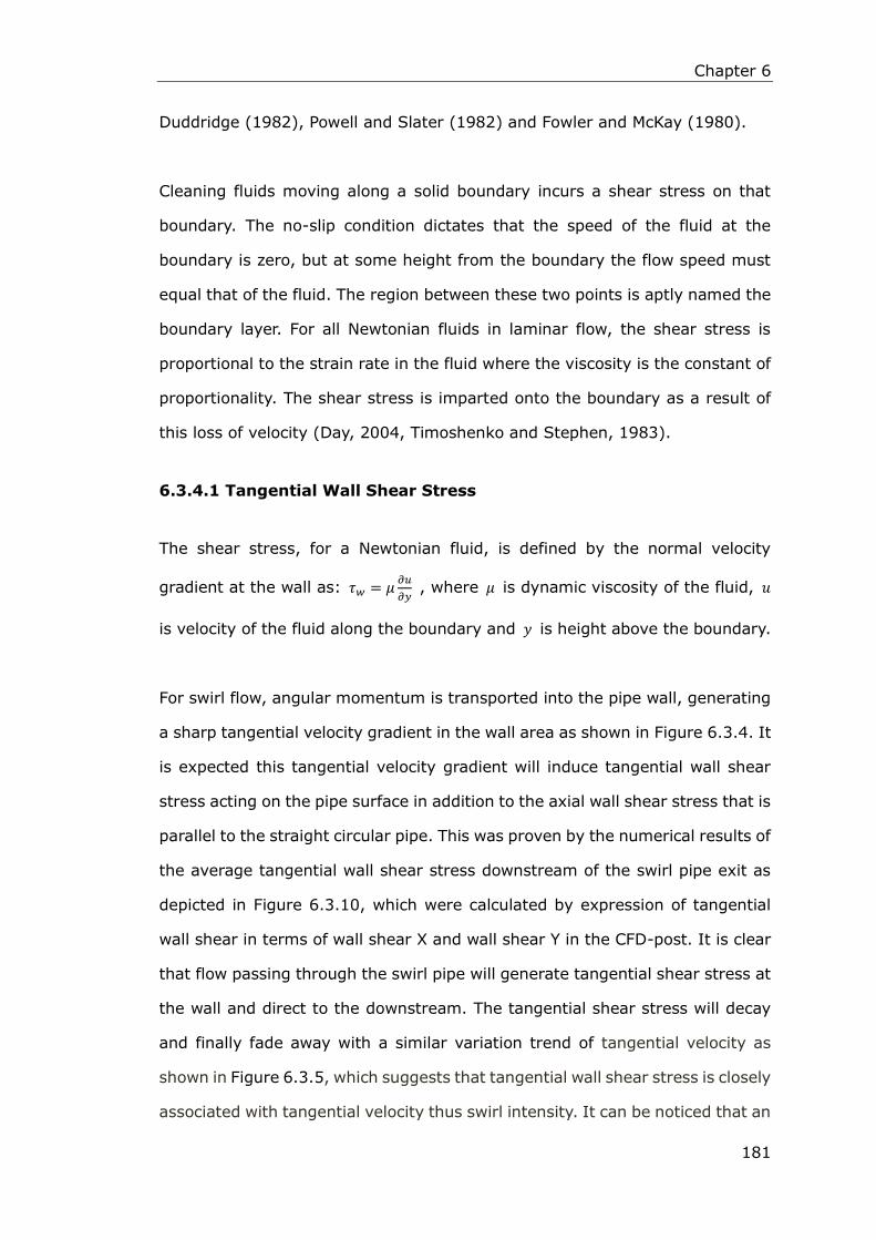
Chapter 6

181

Duddridge (1982), Powell and Slater (1982) and Fowler and McKay (1980).

Cleaning fluids moving along a solid boundary incurs a shear stress on that

boundary. The no-slip condition dictates that the speed of the fluid at the

boundary is zero, but at some height from the boundary the flow speed must

equal that of the fluid. The region between these two points is aptly named the

boundary layer. For all Newtonian fluids in laminar flow, the shear stress is

proportional to the strain rate in the fluid where the viscosity is the constant of

proportionality. The shear stress is imparted onto the boundary as a result of

this loss of velocity (Day, 2004, Timoshenko and Stephen, 1983).

6.3.4.1 Tangential Wall Shear Stress

The shear stress, for a Newtonian fluid, is defined by the normal velocity

gradient at the wall as: 𝜏𝑤 = 𝜇𝜕𝑢

𝜕𝑦 , where 𝜇 is dynamic viscosity of the fluid, 𝑢

is velocity of the fluid along the boundary and 𝑦 is height above the boundary.

For swirl flow, angular momentum is transported into the pipe wall, generating

a sharp tangential velocity gradient in the wall area as shown in Figure 6.3.4. It

is expected this tangential velocity gradient will induce tangential wall shear

stress acting on the pipe surface in addition to the axial wall shear stress that is

parallel to the straight circular pipe. This was proven by the numerical results of

the average tangential wall shear stress downstream of the swirl pipe exit as

depicted in Figure 6.3.10, which were calculated by expression of tangential

wall shear in terms of wall shear X and wall shear Y in the CFD-post. It is clear

that flow passing through the swirl pipe will generate tangential shear stress at

the wall and direct to the downstream. The tangential shear stress will decay

and finally fade away with a similar variation trend of tangential velocity as

shown in Figure 6.3.5, which suggests that tangential wall shear stress is closely

associated with tangential velocity thus swirl intensity. It can be noticed that an

Chapter 6

182

increase of inlet velocity from 1 m/s to 3 m/s causes a sharp rise in tangential

wall shear stress downstream of swirl pipe; this suggests that the effect of the

swirl pipe on tangential shear stress is more prominent in flows with a higher

Reynolds number.

Figure 6.3.10 Tangential WSS variation downstream of swirl pipe exit

Figure 6.3.11 depicts the average non-dimensional tangential wall shear stress

along the cylindrical pipe downstream of the swirl pipe exit for various inlet

velocities. It shows that the trend of variation for non-dimensional tangential

wall shear stress is similar to that of swirl intensity as shown in Figure 6.3.8. The

correlation coefficient of the swirl intensity and the non-dimensional tangential

wall shear stress downstream of the swirl pipe is calculated through the

following correlation function:

𝐶𝑜𝑟𝑟𝑒𝑙(𝑋, 𝑌) =∑(𝑥 − ��)(𝑦 − ��)

√∑(𝑥 − ��)2 ∑((𝑦 − ��)2

(6.3.1)

where �� and �� are the means of array x and array y.

The correlation coefficients are 0.998726, 0.998783, 0.999239, 0.999419 and

0.999484 for swirl flows at speed of 3m/s, 2.5m/s, 2m/s, 1.5m/s and 1 m/s

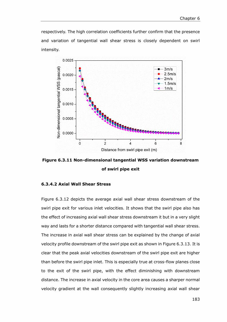
Chapter 6

183

respectively. The high correlation coefficients further confirm that the presence

and variation of tangential wall shear stress is closely dependent on swirl

intensity.

Figure 6.3.11 Non-dimensional tangential WSS variation downstream

of swirl pipe exit

6.3.4.2 Axial Wall Shear Stress

Figure 6.3.12 depicts the average axial wall shear stress downstream of the

swirl pipe exit for various inlet velocities. It shows that the swirl pipe also has

the effect of increasing axial wall shear stress downstream it but in a very slight

way and lasts for a shorter distance compared with tangential wall shear stress.

The increase in axial wall shear stress can be explained by the change of axial

velocity profile downstream of the swirl pipe exit as shown in Figure 6.3.13. It is

clear that the peak axial velocities downstream of the swirl pipe exit are higher

than before the swirl pipe inlet. This is especially true at cross-flow planes close

to the exit of the swirl pipe, with the effect diminishing with downstream

distance. The increase in axial velocity in the core area causes a sharper normal

velocity gradient at the wall consequently slightly increasing axial wall shear

Chapter 6

184

stress. The effect of the swirl pipe on axial wall shear becomes less obvious with

decreasing inlet velocity (Reynolds number). Its effect is almost negligible for

flows with an inlet velocity of 1.5 m/s and 1 m/s. From Figure 6.3.12, the axial

wall shear stress is more sensitive to flow velocity (Reynolds number). For

cross-flow planes where axial wall shear stress is constant for various inlet

velocities, the correlation of axial wall shear stress and flow velocities can be

plotted as shown in Figure 6.3.14. As the exponential and logarithmic fittings

cannot go through zero point and a straight line cannot reflect the increased

increasing rate of axial wall shear stress with increasing Reynold number, the

polynomial fit becomes a reasonable choice. Figure 6.3.14 shows that generally

the axial wall shear stress is positively correlated to the Reynolds number of the

flow and the increasing rate of axial wall shear stress is faster in flows with

larger Reynolds number. This is expected as a larger Reynolds number means

greater turbulence of the flow and hence stronger impact at the wall.

Figure 6.3.12 Axial wall shear stress variation downstream of swirl

pipe exit

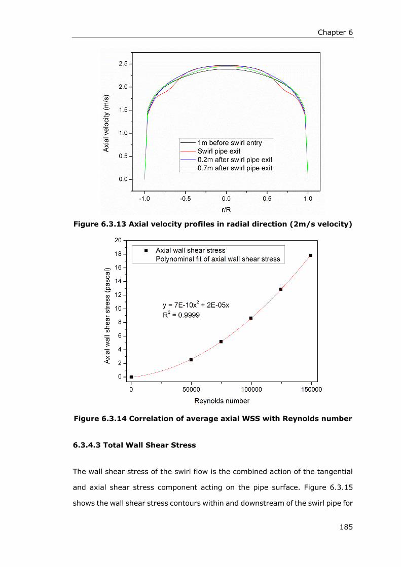
Chapter 6

185

Figure 6.3.13 Axial velocity profiles in radial direction (2m/s velocity)

Figure 6.3.14 Correlation of average axial WSS with Reynolds number

6.3.4.3 Total Wall Shear Stress

The wall shear stress of the swirl flow is the combined action of the tangential

and axial shear stress component acting on the pipe surface. Figure 6.3.15

shows the wall shear stress contours within and downstream of the swirl pipe for

Chapter 6

186

inlet velocities of 1 m/s, 1.5 m/s, 2 m/s, 2.5 m/s, and 3 m/s respectively from

top to bottom. A scale up of 1.2 is applied to the X-Y plane in order to see clearly

the wall shear stress distributions. From the contours, an increase of wall shear

stress is observed starting from the swirl pipe inlet, with the largest value

existing within the swirl pipe at the intersection of lobes where the non-circular

wall results in additional resistance to the flow. Downstream of the swirl pipe

exit, the increase in wall shear stress prevails following the spiral pattern of the

swirl pipe with a longer effective distance and larger wall shear stress increase

observed in flows with higher inlet velocity. From Figure 6.3.15, the pitch to

diameter ratio of the spiral distribution pattern of wall shear stress also

increases with increasing downstream distance reflecting the decay of swirl

flow.

The shear stress at the circumference of the pipe wall downstream of the swirl

pipe exit is not evenly distributed but has four peaks and valleys as shown in

Figure 6.3.16, with the gap between the peak and valley more obvious at

circumferences close to the swirl pipe exit. The wave-like variation of wall shear

stress along the pipe circumference is expected from the uneven distribution of

axial and tangential velocity contours within the cross-flow planes as shown in

Figure 6.3.17. At the four corners of the characteristic quadrangular shape in

both axial and tangential velocity contours, velocities are higher than other

areas indicating a sharper velocity gradient at the wall, resulting in greater wall

shear stress increase in the four corners.

Chapter 6

187

Chapter 6

188

Figure 6.3.15 Contours of WSS at interior wall of swirl pipe and downstream for inlet velocities of 1m/s, 1.5m/s,

2m/s, 2.5m/s, 3m/s respectively from top to bottom

Chapter 6

189

Figure 6.3.16 Circular distribution of WSS at 0.5m, 1m, and 1.5m

downstream of swirl pipe exit (2m/s inlet velocity)

Figure 6.3.17 Contours of axial and tangential velocity at cross-flow

planes 0.5m, 1m, and 1.5m downstream of swirl pipe exit (2m /s inlet

velocity)

Axial

velocity:

Tangential

velocity:

0.5m after swirl pipe exit 1m after swirl pipe exit 1.5m after swirl pipe exit

Chapter 6

190

The mean wall shear stress downstream of the swirl pipe exit is calculated for

the various inlet velocities as it is reported to be a measure of cleaning efficiency

in straight pipes, large parts of pumps, valves and so on. The plot is presented

in Figure 6.3.18. It is clear that swirl pipe locally increases mean wall shear

stress downstream of it, with the increased value and effective distance more

remarkable for a faster inlet flow velocity (thus a large Reynolds number and

large swirl intensity). For flow at a lower speed of 1m/s, the increase in wall

shear stress is not obvious.

At the flow velocity of 3m/s which is typically the velocity of cleaning fluid

circulating in a Clean-In-Place procedure, swirl pipe raises mean shear stress at

the wall from 17.8 Pascal prior swirl pipe entry to 23.3 Pascal (30.9% increase)

just downstream of swirl pipe exit; and within 1.1m (22D) downstream swirl

pipe exit, mean wall shear stress has an increase of at least 5%. For inlet

velocities of 2.5m/s, 2m/s, 1.5m/s and 1m/s, the effective distance within

which the wall shear stress has at least 5% increase are 1m (20D), 0.9m (18D),

0.6m (12D) and 0.5m (10D) respectively. The 5% increase of wall shear stress,

though small, can be important in improving Clean-In-Place efficiency in the

closed processing system. Due to the decay nature of the geometrically induced

swirl flow, the application of swirl pipe should be particularly useful in the areas

that are most difficult to clean in the pipe system, as the cleaning time is

dependent on the degree of cleanliness of such areas.

Chapter 6

191

Figure 6.3.18 Wall shear stress variation downstream of swirl pipe exit

for various inlet velocities

Besides locally increasing the maximum and mean wall shear stress of cleaning

fluid without increasing the flow velocity, swirl pipe should also enhance the

transport of heat and cleaning agent, typically 0.5% sodium hydroxide and/or

phosphoric acid, to the pipe wall area, enhancing its contact with fouling at wall.

This is expected as the current swirl pipe is developed from a swirly shaped pipe

found in marine boilers which is used to improve heat exchanger efficiency. The

cleaning agent and its operating temperature induce a decrease in the adhesion

strength of fouling to the pipe surface, facilitating fouling removal when a wall

shear stress is applied.

From the above discussion, swirl pipes mounted in the closed processing system

have the potential to locally increase CIP efficiency in the stage of cleaning

without increasing the overall flow speed. While in the stage of food or beverage

processing, where flow velocity is much lower, the existence of the swirl pipe

would not have much influence on the material passing through it.

Compared with other swirl induction methods, the swirl pipe is much easier to

Chapter 6

192

install into the pipe system by flanges or clamps, and more importantly the local

intervention of swirl pipe has minimal intrusion to the flow which avoids the

insertion of any objects which would otherwise be mounted inside the pipe, such

as blades, helical ribs and honeycomb structures that might contribute to

problems regarding the fouling and cleaning of the pipes.

6.4 Conclusions

In this chapter, the potential of a swirl flow induced by an optimised four-lobed

swirl pipe on improving Clean-In-Place efficiency has been numerically

investigated. The objective has been the prediction of swirl intensity and its

decay law downstream of the swirl pipe, the shear stress at the pipe wall

exerted by the geometrically induced swirling flow and its relationship with swirl

intensity and the Reynolds number.

The geometrically induced swirl flow property with respect to tangential velocity,

swirl intensity and shear stress at wall were analysed. The following results have

been obtained:

Swirl pipe imparts a tangential velocity into flow passing through it with

the swirl effect more prominent in flows with a large Reynolds number.

The tangential velocity contour forms a characteristic quadrangular

shape due to the 4-lobed cross section of swirl pipe. Its swirl type fits to

a ‘solid body’ downstream of the swirl pipe exit.

The swirl decay rate of swirl pipe induced swirling flow is in good

agreement with exponential trend with the decay rate decreasing with

increasing Reynolds number. The decay rate is a little higher than the

expected value suggested in the literature which may attribute to the fact

that Colebrook equation and the Blasius equation tend to underestimate

the friction factor value.

Chapter 6

193

Swirl pipe imposes a tangential wall shear stress within itself and direct

to downstream, its value and variation trend is dependent on swirl

intensity.

Axial wall shear stress is mainly proportional to the Reynolds number,

though the presence of the swirl pipe slightly increases its value within

and downstream of it.

The wall shear stress value along the pipe circumference forms a

wave-like distribution, with the gap between peak and valley more

obvious at circumferences close to the swirl pipe exit.

Swirl pipe locally increases mean wall shear stress downstream of it, with

the increased value and effective distance more remarkable for flow with

a larger Reynolds number.

From the simulation results, swirl pipe should be able to improve the cleaning

efficiency of Clean-In-Place procedures in closed processing systems by locally

increasing wall shear stress downstream of it without increasing overall

velocities of cleaning fluid. The beneficial effects of swirl pipe are more obvious

in flows with higher velocities where both the effective distance and wall shear

stress increase are larger than lower velocities. The swirl pipe should be

particularly useful in the areas that are most difficult to clean in the pipe system,

as the cleaning time is dependent on the degree of cleanliness of such areas.

Chapter 7

194

CHAPTER 7: LARGE EDDY SIMULATION OF SWIRL

FLOW DOWNSTREAM OF THE OPTIMISED SWIRL

PIPE

7.1 Introduction

So far, the simulation study of the swirl flows induced by swirl pipes were

restricted to the RANS approach, which is the mainstay for engineering flow

calculations owing to its modest requirement on computing resource,

reasonably accurate prediction and simplified post-processing. However, it was

found the RANS cannot capture the turbulent velocity fluctuations with time,

giving only the mean flow field and the effects of turbulence on mean flow

properties (H.K.Versteeg and W.Malalasekera, 2010). For this reason, the

time-dependent property of the swirl flow was not revealed and reported by

previous researchers on swirl pipe. As the swirl flow induced by the swirl pipe is

inherently unsteady and three-dimensional, it is therefore important to

understand the unsteady property of the swirl flow and perhaps its correlation

with CIP procedures in closed processing systems.

In this chapter the Large Eddy Simulation (LES) approach was attempted in

order to understand the unsteadiness of the geometrically induced swirl flow.

LES has had very limited impact on industrial flows due to the very high grid

resolution requirement and the prohibitive computational cost in terms of long

run times and large volumes of data. However it has the potential for improved

accuracy when resolving the largest eddies is important, and more importantly

it provides unsteady data needed to see the fluctuation in the flow variables.

The general concepts and models concerning LES were introduced. The vortex

Chapter 7

195

core regions within the swirl flow were identified. The instantaneous and time

averaged pressure drop, tangential velocity and swirl decay of the unsteady

swirl flow were analysed and compared with the RANS results. The instability of

the flow variables was revealed. Special attention was paid to the increase of the

mean wall shear stress just downstream of the swirl pipe and the enhancement

of the fluctuation rate of the wall shear stress further downstream of the swirl

pipe.

7.2 Large Eddy Simulation

Turbulent flows are characterized by eddies with a wide range of length and time

scales. The smaller eddies are nearly isotropic and have a universal behaviour.

They are less dependent on the geometry, with the smallest eddies are

responsible for the dissipation of the turbulence kinetic energy. On the other

hand, the large eddies, which interact with and extract energy from the mean

flow, are more anisotropic. Their behaviours are dictated by the geometries and

boundary conditions of the flow involved.

It is possible, in theory, to resolve directly the whole spectrum of turbulence

scales using a direct numerical simulation (DNS) approach where no modelling

is required. However, NDS is unaffordable for practical engineering problems

involving high Reynolds number flows because the cost needed for DNS to

resolve the whole range of scales is proportional to Re3. Obviously, for flows with

high Reynolds number, the cost becomes prohibitive.

Large eddy simulation (LES) offers a different approach to the computation of

turbulent flows which accepts that the larger eddies need to be computed for

each problem are resolved with a time-dependent simulation. On the other hand,

the universal behaviours of the smaller eddies are modelled with a compact

Subgrid-Scale Model.

Chapter 7

196

7.2.1 Filtering Operation

Different from time-averaging used in the RANS approach, the LES uses a

spatial filtering operation to separate the larger and smaller eddies. The

operation involves the application of a filtering function and a certain cut-off

width to the unsteady Navier-Stokes equations. During the spatial filtering,

those eddies with a length scale greater than the cut-off width are retained and

will be resolved in an unsteady flow computation. While the information related

to the turbulent eddies which are smaller than the cut-off width is destroyed.

The LES performs the spatial filtering operation by means of a filter function

𝐺(𝑥, 𝑥′,Δ) as below (H.K.Versteeg and W.Malalasekera, 2010):

��(𝑥, 𝑡) ≡ ∫ ∫ ∫ 𝐺(𝑥, 𝑥′

∞

−∞

∞

−∞

∞

−∞

, ∆)𝜙(𝑥′, 𝑡)𝑑𝑥1′𝑥2

′𝑥3′

(7.2.1)

Where ��(𝑥, 𝑡) = filtered function

𝜙(𝑥′, 𝑡) = original (unfiltered) function

∆ = filter cutoff width

The filtering operation is an integration carried out in the three-dimensional

space. It is designed to split an input into a desirable, retained part and an

undesirable, rejected part.

The commonest forms of the filtering function in three-dimensional LES are

Top-hat (or box filter), Gaussian filter and Spectral cut-off. Of which the Top-hat

filter is used in finite volume implementation of LES which is defined as:

𝐺(𝑥, 𝑥′, ∆) = {1/∆3 0

|𝑥 − 𝑥′| ≤ ∆/2

|𝑥 − 𝑥′| > ∆/2

(7.2.2)

The cut-off width Δ of the filter determines what is retained and what is rejected.

Chapter 7

197

In most practical (and commercial) implementations of LES, for

three-dimensional CFD computation with the finite volume method, the cut-off

width is often taken to be the cubic root of the grid cell volume (and no explicit

filtering is performed):

∆= √∆𝑥∆𝑦∆𝑧3

(7.2.3)

where ∆𝑥, ∆𝑦, ∆𝑧 are the length, width and height of the grid cells respectively.

Applying the filtering operation to the governing equations obtains the filtered

equations of the flow motion. For incompressible Newtonian fluid flow they are:

𝜕��𝑖

𝜕𝑥𝑖= 0,

𝜕��𝑖

𝜕𝑡+

𝜕

𝜕𝑥𝑗(��𝑖��𝑗) = −

1

𝜌

𝜕��

𝜕𝑥𝑖−

𝜕𝜏𝑖𝑗

𝜕𝑥𝑗+ 𝜈

𝜕2��𝑖

𝜕𝑥𝑗𝜕𝑥𝑗

(7.2.4)

where 𝜏𝑖𝑗 = 𝑢𝑖𝑢𝑗 − ��𝑖��𝑗 is the sub-grid-scale stress that must be modelled by

Sub-Grid-Scale Models.

7.2.2 Sub-Grid-Scale Models

The spatial filtering gives rise to sub-grid-scale (SGS) stresses due to the

interaction effects between the larger, resolved eddies and the smaller

unresolved ones. The sub-grid-scale stresses are unknown and require

modelling.

ANSYS FLUENT offers sub-grid-scale turbulence models employing the

Boussinesq hypothesis as in the RANS models that the turbulent stresses is

proportional to the mean rate of strain. They compute the sub-grid-scale

turbulence stress using (Conway et al., 2000):

𝜏𝑖𝑗 −1

3𝜏𝑘𝑘𝛿𝑖𝑗 = −2𝜇𝑡𝑆��𝑗

(7.2.5)

Chapter 7

198

where 𝜇𝑡 is the sub-grid-scale turbulent viscosity. 𝜏𝑘𝑘 is the isotropic part of

the sub-grid-scale stress. It is not modelled but added to the filtered static

pressure term. 𝛿𝑖𝑗 is the Kronecker delta (𝛿𝑖𝑗 = 1 if 𝑖 = 𝑗 and 𝛿𝑖𝑗 = 0 if 𝑖 ≠ 𝑗).

𝑆��𝑗 is the local rate-of-strain of the resolved flow 𝑆��𝑗 =1

2(𝜕��𝑖

𝜕��𝑗+

𝜕��𝑗

𝜕��𝑖).

ANSYS FLUENT provides the following models for 𝜇𝑡：the Smagorinsky-Lilly

model, the dynamic Smagorinsky-Lilly model, the Wall-Adapting Local

Eddy-Viscosity (WALE) model, the Algebraic Wall-Modeled LES Model (WMLES)

model, and the dynamic kinetic energy subgrid-scale model (ANSYS, 2011a).

The most common and simplest explicit SGS is that of the Smagorinsky-Lilly

model (Smagorinsky, 1963).

7.2.2.1 Smagorinsky-Lilly Model

In the Smagorinsky-Lilly model, the eddy-viscosity 𝜇𝑡 is modelled by

𝜇𝑡 = 𝜌𝐿𝑠2|𝑆|

(7.2.6)

where |𝑆| ≡ √2𝑆��𝑗𝑆��𝑗 , 𝐿𝑠 is the mixing length for sub-grid scales which is

computed using

𝐿𝑠 = 𝑚𝑖𝑛(𝑘𝑑, 𝐶𝑠∆)

(7.2.7)

where 𝑘 is the von Kármán constant, 𝑑 is the distance to the closest wall, ∆ is

the local grid scale which is computed according to the volume of the

computational cell using ∆= 𝑉1/3, 𝐶𝑠 is the Smagorinsky constant.

Lilly (1967) carried out a theoretical analysis of the decay rates of isotropic

turbulent eddies in the inertial subrange of the energy spectrum and suggested

values of 𝐶𝑠 between 0.17 and 0.21. However, in the presence of shear, near

solid boundary or in transitional flows, this value was found to cause excessive

Chapter 7

199

damping of large-scale fluctuations and must be decreased (Piomelli, 1999). A

𝐶𝑠 value around 0.1 was found to give the best results for a wide range of flows,

which is the default value in ANSYS FLUENT.

7.2.2.2 Dynamic Smagorinsky-Lilly Model

The Smagorinsky-Lilly Model is purely dissipative that the direction of energy

flow is exclusively from eddies at the resolved scales towards the sub-grid

scales. It does not allow for the intermittent transport of energy from the small

scales to the large ones. This backscattering phenomenon is important when

modelling transition. Germano et al. (1996) and Lilly (1967) introduced a

dynamic modelling idea which can account for the backscatter.

In the dynamic model, the model constant 𝐶 is dynamically computed as the

calculation progresses based on the energy content of the smallest resolved

scale. This is accomplished by applying to the equations of motion a test filter

whose filter width ∆ is typically equal to twice the grid filter width ∆ (∆= 2∆).

Both the grid filter and the test filter produce a resolved flow field. The

difference between the two resolved fields is the contribution of the small scales

whose size is in between the grid filter and the test filter. The information related

to these scales is used to compute the model constant.

Both the sub-test stresses 𝑇𝑖𝑗 and the sub-grid stresses 𝜏𝑖𝑗 are modelled using

Smagorinsky-Lilly Model assuming that the constant 𝐶 is the same for both

filtering operations.

𝜏𝑖𝑗 −1

3𝛿𝑖𝑗𝜏𝑘𝑘 = −2𝐶Δ2|𝑆|𝑆��𝑗

𝑇𝑖𝑗 −1

3𝛿𝑖𝑗𝑇𝑘𝑘 = −2𝐶Δ2|𝑆|𝑆𝑖𝑗

(7.2.8)

The grid filtered SGS and the test-filtered SGS are related by the Germano

Chapter 7

200

identity that (Germano et al., 1996):

𝑇𝑖𝑗 − ��𝑖𝑗 = 𝐿𝑖𝑗 = ��𝑖��𝑗 − ��𝑖 ��𝑗

(7.2.9)

where 𝐿𝑖𝑗 (the contribution from the region between test-filter and grid-filter

scale) is computable from the resolved large eddy field.

Lilly (1967) suggested a least-squares approach to evaluate local values of C:

𝐶2 =⟨𝐿𝑖𝑗𝑀𝑖𝑗⟩

⟨𝑀𝑖𝑗𝑀𝑖𝑗⟩

with 𝑀𝑖𝑗 = −2Δ2|𝑆|𝑆𝑖𝑗 + 2Δ2|𝑆|𝑆��𝑗

(7.2.10)

The angular brackets <> indicate an averaging procedure which is to avoid

numerical instability. The model constant C obtained using the dynamic

Smagorinsky-Lilly model varies in time and space over a fairly wide range. In

ANSYS FLUENT, it is clipped at zero and 0.23 by default.

7.2.2.3 Algebraic Wall-Modeled LES Model (WMLES)

Despite the wide use in the academic community, LES has had very limited

impact on industrial simulations for high Reynolds number, wall-bounded flows

due to the prohibitive computational cost to resolve energy-carrying eddies in

the near-wall region. Hybrid RANS-LES approaches have been developed which

significantly reduce the computational cost of such configurations. These

include the Detached-Eddy Simulation (DES) and its recent modification the

delayed DES (DDES), and wall-modelling in LES (WMLES) (Shur et al., 2008).

The wall-modelling approach is based on the RANS calculation in the inner layer.

The inner-layer RANS is solved in a grid that is refined in the wall-normal

direction and is embedded in the outer-layer, coarse LES mesh. Which provides

instantaneous wall shear stresses and heat fluxes at the wall to the concurrent

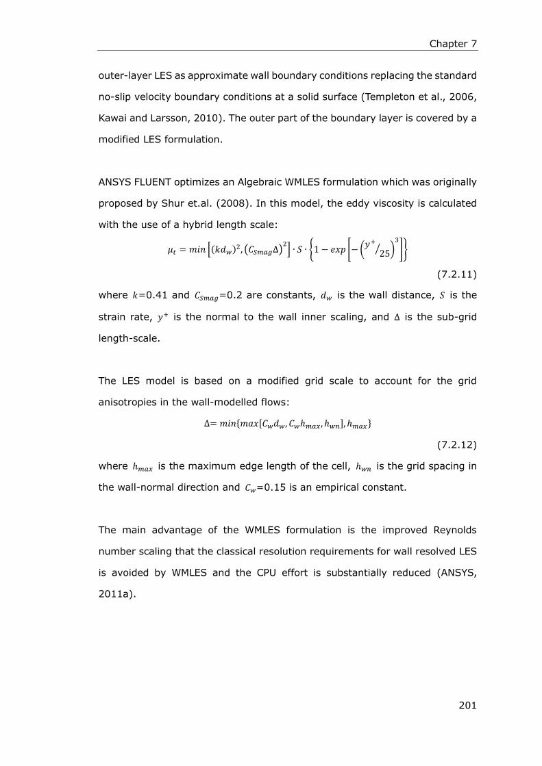
Chapter 7

201

outer-layer LES as approximate wall boundary conditions replacing the standard

no-slip velocity boundary conditions at a solid surface (Templeton et al., 2006,

Kawai and Larsson, 2010). The outer part of the boundary layer is covered by a

modified LES formulation.

ANSYS FLUENT optimizes an Algebraic WMLES formulation which was originally

proposed by Shur et.al. (2008). In this model, the eddy viscosity is calculated

with the use of a hybrid length scale:

𝜇𝑡 = 𝑚𝑖𝑛 [(𝑘𝑑𝑤)2, (𝐶𝑆𝑚𝑎𝑔∆)2] ∙ 𝑆 ∙ {1 − 𝑒𝑥𝑝 [−(

𝑦+

25⁄ )

3

]}

(7.2.11)

where 𝑘=0.41 and 𝐶𝑆𝑚𝑎𝑔=0.2 are constants, 𝑑𝑤 is the wall distance, 𝑆 is the

strain rate, 𝑦+ is the normal to the wall inner scaling, and ∆ is the sub-grid

length-scale.

The LES model is based on a modified grid scale to account for the grid

anisotropies in the wall-modelled flows:

∆= 𝑚𝑖𝑛{𝑚𝑎𝑥[𝐶𝑤𝑑𝑤, 𝐶𝑤ℎ𝑚𝑎𝑥 , ℎ𝑤𝑛], ℎ𝑚𝑎𝑥}

(7.2.12)

where ℎ𝑚𝑎𝑥 is the maximum edge length of the cell, ℎ𝑤𝑛 is the grid spacing in

the wall-normal direction and 𝐶𝑤=0.15 is an empirical constant.

The main advantage of the WMLES formulation is the improved Reynolds

number scaling that the classical resolution requirements for wall resolved LES

is avoided by WMLES and the CPU effort is substantially reduced (ANSYS,

2011a).

Chapter 7

202

7.3 Simulation Setup

7.3.1 Meshing

The geometry of the computational domain used in the LES is the same as that

used in the RANS approach. The multi-block, structured meshing scheme

described in section 4.4.4 is used in the spatial discretization of the geometry.

Near the wall, the largest scales in the turbulent spectrum are nevertheless

geometrically very small and require a very find grid and a small time step.

Therefore, a much finer mesh is generated so as to meet the excessively high

resolution requirements for the wall boundary layers, typically 𝑦+ ≤ 1 is

required for near-wall grid points.

Figure 7.3.1 Fine grid in the near wall region of cylindrical pipe and

swirl pipe for LES

Initially a very small distance of 0.02mm from the wall to the first node of the

mesh was specified with a growth ratio of 1.1 towards pipe centre. It was found

that degenerate cells (slivers) appeared along the pipe wall which would impede

convergence of the solution. Attempts were made to improve the mesh quality

Chapter 7

203

by gradually increasing the distance between the wall and the first node of the

mesh from 0.02mm, 0.03mm, 0.04mm to 0.05mm. Simulation tests suggested

that at a value of 0.05mm the solution was reasonably converged and the 𝑦+

value was in an acceptable range.

In addition, the grid was not only refined in the wall normal direction (X-Y plane)

but also refined in the Z direction so as to resolve turbulence in the wall parallel

plane. In the stream wise direction, grid refinement was carried out by

shortening the mesh height to 1.5mm and 1mm. It was found a grid with a

mesh height of 1mm demands excessively large computing resources in terms

of storage and volume of calculation for the LES that the current workstation is

not suited for this task. Therefore a mesh height of 1.5mm is used in the stream

wise direction. Figure 7.3.1 shows the final grid in the wall normal and wall

parallel direction for the geometry of the computational domain.

Figure 7.3.2 y+ contours of computational domain geometry for LES

(2m/s inlet velocity)

Figure 7.3.2 shows the y+ contours of the sections of the flow geometry. The y+

values are between 1.3-5.24, 1.15-6.82, and 1.04-5.24 for the development

section, swirl pipe and test section respectively. Though the y+ value is greater

than 1, it is the finest grid that can be reached due to the limitation of the

Contour of Wall Yplus

Chapter 7

204

computing power of the current workstation. In practice, a y+ value less than 10

may be acceptable for engineering flows.

7.3.2 Initial Conditions for LES

Large eddy simulation involves running a transient solution from the initial

condition using an appropriate time step size. The solution must be run long

enough to become independent of the initial condition and to enable the

statistics of the flow field to be determined.

At the inlet, the No Perturbations fluctuating velocity algorithm is employed that

the stochastic components of the flow at the velocity inlet boundaries are

neglected. This option is suitable as the level of turbulence at the inflow

boundary does not play a major role in the accuracy of the overall solution. The

outlet boundary condition is less troublesome and a pressure outlet boundary

condition is specified at the outlet. The pipe walls are specified as being

stationary and the no-slip walls condition is used.

In this study, the large eddy simulation started by running a steady state RANS

simulation using a standard k–ε model together with a near wall modelling

approach which enables the viscosity-affected region to be resolved with the

fine mesh all the way to the wall, including the viscous sub-layer. After

convergence of the solution, the turbulence model was changed into a realizable

k–ε model and RSM and run until the flow field was reasonably converged. Then

an instantaneous velocity field was generated out of the steady state RANS

results as the initial condition for the LES. This approach creates a much more

realistic initial field for the LES run. In addition, it will reduce the time needed for

the LES simulation to reach a statistically stable state.

7.3.3 Discretization for LES

Activate LES, and ANSYS FLUENT will turn on the unsteady solver option. The

Chapter 7

205

Bounded Second Order Implicit formulation was chosen for temporal

discretization as it provides better stability despite the same accuracy as the

Second Order Implicit formulation. Frequently a time-dependent problem has a

very fast “startup” transient that decays rapidly. Therefore, a conservatively

small time step size ∆𝑡 was set initially for the first number of time steps. The

∆𝑡 was gradually increased to 0.01s as the calculation proceeded.

To verify that the choice for ∆𝑡 was proper, the contour of the Courant number

was checked after the calculation is complete. The Courant number was found

reasonably within a value of 40 in the most sensitive transient regions of the

domain. This meets the requirement that it should not exceed a value of 20-40

(ANSYS, 2011b).

As for the spatial discretization, the first-order upwind or power law scheme

should be avoided, as they may overly damp out the energy of the resolved

eddies. The central-differencing based schemes are recommended for all

equations when LES model is used. Here the bounded central-differencing

scheme was used for momentum which is the default option for use with LES.

The second order pressure discretisation scheme was employed for Pressure

interpolation. The SIMPLE scheme was used for pressure-velocity coupling.

7.3.4 Choice of SGS Model

Three identical cases were run each employing Smagorinsky-Lilly, Dynamic

Smagorinsky-Lilly and WMLES Sub-Grid-Scale Model respectively. A time step

size of 0.01s and 200 time steps (0.01×200=2s) were set for the transient

solution. Data sampling for time statistics was enabled in order to obtain the

mean flow quantities. It allows for the calculation of the mean or

root-mean-square of the variables by collecting time statistics at each sampling

interval while performing the simulation. The variation of the mean wall shear

stress and the mean tangential velocity downstream of the swirl pipe for the

Chapter 7

206

three cases and the RANS approach are presented in Figure 7.3.3 and 7.3.4.

Figure 7.3.3 Comparison of wall shear stress distribution for various

SGS models and RANS (2m/s inlet velocity)

The configurations employing the Smagorinsky-Lilly or Dynamic

Smagorinsky-Lilly SGS models belong to the category of Wall-Resolved LES

where very fine grid spacing is needed close to the wall to filter out the smallest

turbulent scales and to get the near-wall structures resolved. Figure 7.3.3

shows that the Smagorinsky-Lilly and Dynamic Smagorinsky-Lilly model give

almost identical underestimation on wall shear stress downstream of swirl pipe

despite the dynamic constant C used for the Dynamic Smagorinsky-Lilly model.

The reason for this may be due to the high resolution requirements for the wall

boundary layers with the current mesh not being fine enough for the

Wall-Resolved LES. Because near the wall, even the ‘large’ eddies become

relatively small and require a Reynolds number dependent resolution.

When resolving the exterior flow, the grid resolution is weakly dependent on the

Reynolds number as Re0.4 (Chen, 2011). When the LES is implemented on

coarse grids near the wall, errors arise from numerical discretization and SGS

Chapter 7

207

modelling. The velocity gradient in the near-wall region is under predicted by a

discretization scheme using no-slip boundary conditions on coarse grids. This

leads to underestimation of the wall shear stress and incorrect kinetic energy

production, and distortion of the exterior LES (Chen, 2011).

No-slip boundary conditions cannot be applied directly at high Reynolds

numbers if the mesh is too coarse in the near-wall region as the distance

between the first point off-wall and the wall is much larger than the

characteristic length-scales of the modelled zone (Monfort et al., 2010).

Alternatively, the WMLES approach replaces the no-slip boundary condition with

approximate wall boundary conditions by RANS calculation in the inner layer.

The RANS calculation is an in-time-accurate calculation and provides

instantaneous wall shear stresses and heat fluxes at the wall to the concurrent

outer-layer LES as approximate wall boundary conditions (Kawai and Larsson,

2010). From Figure 7.3.3, the WMLES approach provides increased wall shear

stress predictions than the Wall-Resolved method. The simulation values are

closer to the RANS results however it has a larger initial wall shear stress just

downstream of the swirl pipe exit which has a steeper decrease along the

streamwise direction than the RANS with some fluctuation in values. This is

expected as the LES is inherently an unsteady method which is more robust in

capturing unsteadiness in turbulence.

Figure 7.3.4 shows that the WMLES and the RANS approach give close

prediction on tangential velocity of the swirl flow. While the Smagorinsky-Lilly

and the Dynamic Smagorinsky-Lilly SGS models tend to overestimate the swirl

effect of the flow. This suggests that, when these models are used, there will be

a mismatch between the near wall region and the exterior flow as a stronger

swirl flow should yield larger wall shear stresses at the internal pipe surface.

Therefore, it is decided to use the WMLES SGS model for the LES, which should

Chapter 7

208

give more reliable predictions than the Smagorinsky-Lilly or Dynamic

Smagorinsky-Lilly SGS model.

Figure 7.3.4 Comparison of tangential velocity distribution for various

SGS models and RANS (2m/s inlet velocity)


7.4.1 Unsteady Swirl Flow

The unsteady RANS approach was used to capture the unsteadiness of the swirl

flow, however it was found that with the proceeding solution, the flow statistics,

and the contours monitored, became stable and stopped changing with flow

time. It gave the same results as the steady RANS approach.

It is claimed that RANS is not applicable for handling unsteady flows unless

there is a spectral gap between the unsteadiness and the turbulence. To capture

the unsteadiness using unsteady RANS, the averaging period should be much

smaller than the time scale of the unsteady mean motion. Meanwhile, the time

period should be orders of magnitude higher than the time scale of the random

fluctuations for the time averaging to make sense (Wegner et al., 2004). The

Chapter 7

209

unsteady RANS may capture the unsteadiness with the use of periodic or time

dependent boundary. However, in this study with constant inlet velocity,

unsteady RANS failed to present a fluctuating swirl flow field.

LES, on the other hand, is an inherently time dependent method. Hence, it

handles unsteady flows well. Figure 7.4.1 shows a comparison of axial and

tangential velocity contours obtained by RANS and the instantaneous contours

by LES. The LES gives more detailed turbulent swirl flow field than the RANS. In

the LES method, the characteristic quadrangular shaped distribution of the axial

velocity contours is more robust than the RANS with a clear indication of four

vortex cores at the four corners of the quadrangle corresponding to the four

lobes of the swirl pipe. However, in the cross-flow planes further downstream,

the flow pattern becomes chaotic indicating the mixing of the four vortex cores.

The four vortex cores are clearer in the velocity vectors in cross-flow planes

0.2m, 0.5m and 1m downstream of the swirl pipe as shown in Figure 7.4.2. The

LES clearly captures four rotating movement of the four vortex cores (marked

with ×) within the flow field. It is also clear that the location of the vortex cores

change with increasing downstream distance, indicating that the four vortices

rotate about the pipe’s geometrical axis forming an integrated swirling effect

throughout the downstream duration of the swirl pipe. The swirl effect decays

with downstream distance due to the retarding force from the friction of the

internal pipe surface. The vortex cores become ambiguous by reasons of swirl

decay and mixing of vortexes. Animation of velocity contour showed that the

vortex centres varies slightly around their rotation axis indicating the unsteady

nature of the turbulent flow. The unsteadiness of flow is more remarkable in

cross-flow planes further downstream of the swirl pipe.

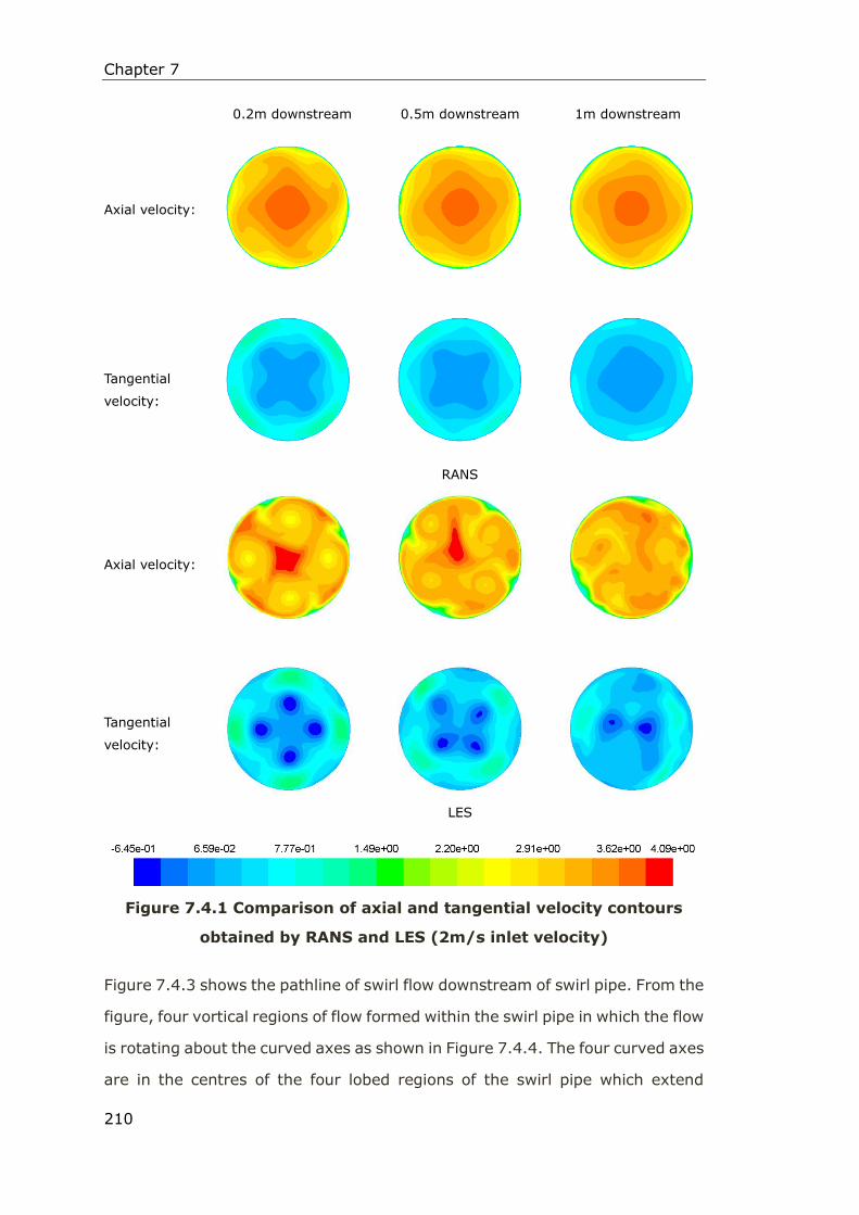
Chapter 7

210

0.2m downstream 0.5m downstream 1m downstream

Axial velocity:

RANS

Tangential

velocity:

Axial velocity:

LES

Tangential

velocity:

Figure 7.4.1 Comparison of axial and tangential velocity contours

obtained by RANS and LES (2m/s inlet velocity)

Figure 7.4.3 shows the pathline of swirl flow downstream of swirl pipe. From the

figure, four vortical regions of flow formed within the swirl pipe in which the flow

is rotating about the curved axes as shown in Figure 7.4.4. The four curved axes

are in the centres of the four lobed regions of the swirl pipe which extend

Chapter 7

211

helically about the geometrical axis of the swirl pipe and the downstream

circular pipe. Downstream of the swirl pipe, the four vortices prevail following

the pattern as in the swirl pipe, rotating respectively about the four curved axes

extended from the centre of the four lobed regions. Because the four curved

axis rotate about the axis of the downstream circular pipe, the four rotational

vortexes revolve about the circular pipe axis forming an integrated swirl flow

throughout the flow field.

Velocity vectors coloured by helicity (m/s2)

Figure 7.4.2 Velocity vectors in cross-flow planes 0.2m, 0.5m and 1m

downstream of the swirl pipe (2m/s inlet velocity)

The vortices formed passing through the swirl pipe, move forward, twist and

interact in complex ways. Animation of the velocity magnitude indicates that,

further downstream of the swirl pipe where the swirl effect is less prominent,

the pattern of spiral flow becomes chaotic and fades away. However, in this

duration, the flow velocity fluctuates faster in space and time suggesting

stronger unsteadiness.

0.2m after swirl pipe 0.5m after swirl pipe 1m after swirl pipe

×

×

×

×

×

× ×

×

×

×

Chapter 7

212

Swirl pipe 0.2m after swirl pipe 0.4m after swirl pipe

Side view

Front view

Figure 7.4.3 Pathline of swirl flow downstream of swirl pipe showing vortices (2m/s inlet velocity)

Vortex core

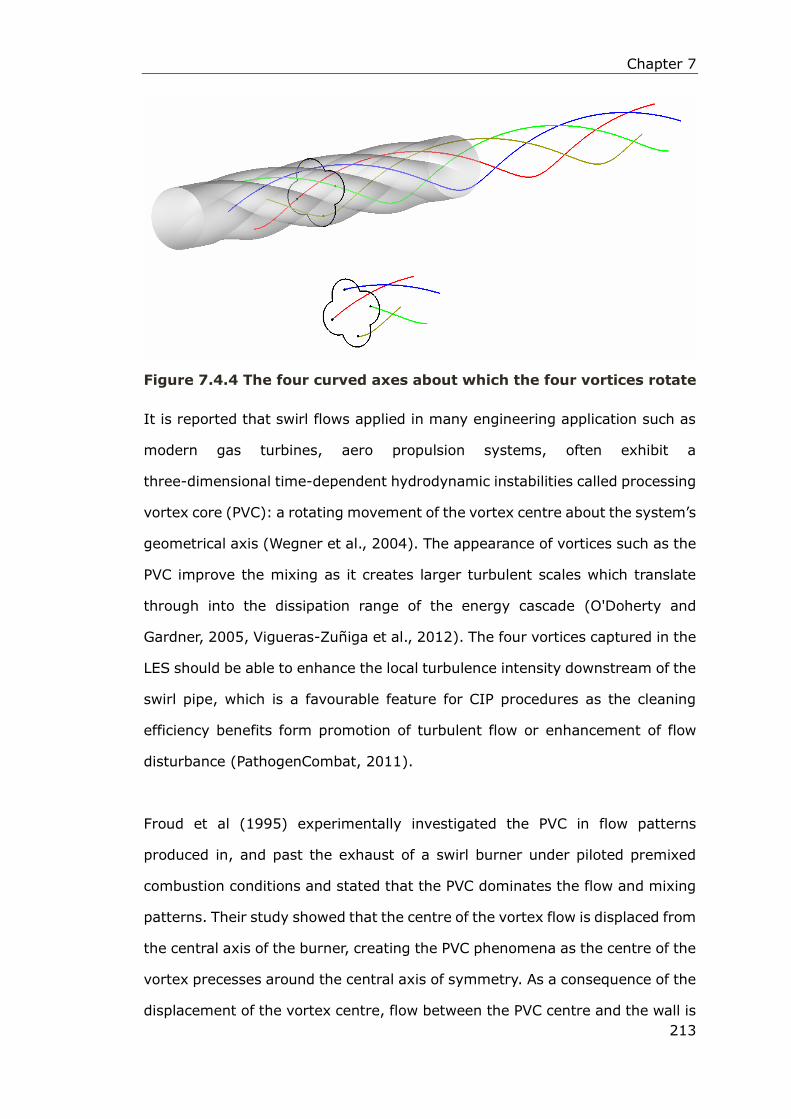
Chapter 7

213

Figure 7.4.4 The four curved axes about which the four vortices rotate

It is reported that swirl flows applied in many engineering application such as

modern gas turbines, aero propulsion systems, often exhibit a

three-dimensional time-dependent hydrodynamic instabilities called processing

vortex core (PVC): a rotating movement of the vortex centre about the system’s

geometrical axis (Wegner et al., 2004). The appearance of vortices such as the

PVC improve the mixing as it creates larger turbulent scales which translate

through into the dissipation range of the energy cascade (O'Doherty and

Gardner, 2005, Vigueras-Zuñiga et al., 2012). The four vortices captured in the

LES should be able to enhance the local turbulence intensity downstream of the

swirl pipe, which is a favourable feature for CIP procedures as the cleaning

efficiency benefits form promotion of turbulent flow or enhancement of flow

disturbance (PathogenCombat, 2011).

Froud et al (1995) experimentally investigated the PVC in flow patterns

produced in, and past the exhaust of a swirl burner under piloted premixed

combustion conditions and stated that the PVC dominates the flow and mixing

patterns. Their study showed that the centre of the vortex flow is displaced from

the central axis of the burner, creating the PVC phenomena as the centre of the

vortex precesses around the central axis of symmetry. As a consequence of the

displacement of the vortex centre, flow between the PVC centre and the wall is

Chapter 7

214

squeezed, producing a considerable increase in tangential velocity. Similar

conclusion was also reported by Huang and Yang (2009).

From the tangential velocity contours shown in Figure 7.4.1, the strong

tangential velocity concentrates in the four regions between vortex core and the

pipe wall. The considerable increase in tangential velocity may be caused by the

rotational movement of the vortex centre squeezing the flow field at the side

against the pipe wall.

7.4.2 Pressure Drop

The variation of time averaged pressure (over 2 seconds), the instantaneous

pressure predicted by LES and the pressure predicted by RANS are shown in

Figure 7.4.5. For both the LES and RANS method, the pressure drop within the

swirl pipe is greater than the circular pipes; this is more obvious in flows with

larger velocities (Reynolds number). However, the LES approach tends to

underestimate (18%-23% lower) the overall pressure drop especially in flows

with higher velocities.

The difference between LES and RANS may attribute to the following two

reasons:

Firstly, the different methods in near-wall region treatment with the

RANS approach using semi-empirical wall functions to bridge the

viscosity-affected regions between the wall and fully-turbulent region;

while the LES employed a Hybrid RANS-LES approach to resolve

energy-carrying eddies in the near-wall region.

Secondly, in the RANS approach, wall roughness of the swirl pipe and

circulars pipes were specified as the same value as the experimental rig.

While in the LES, such values cannot be specified and the pipe wall was

treated as a hydraulic smooth pipe.

Chapter 7

215

Nevertheless, in RANS, the roughness height of 1.237 x 10-06m for circular pipe

and 9 x 10-06m for swirl pipe are small enough that the walls are hydraulically

smooth. In a smooth pipe flow, the viscous sub-layer completely submerges the

effect of roughness height of the pipe. In this condition, the friction factor λ is a

function of the Reynolds number and is independent of the effect of surface

roughness on the flow (Rao and Kumar, 2007). Therefore, it’s more likely that

the difference in pressure drop prediction is caused by the different near-wall

region treatments employed by RANS and LES.

Figure 7.4.5 Static pressure variation in the flow system for various

inlet velocities predicted by LES and RANS

It is also clear from Figure 7.4.5 that, for the LES, the pressure drops faster in

the circular pipe just downstream of the swirl pipe (indicated by the steeper

slope) than further downstream (relatively smaller slope). As discussed in

section 6.3.1, a greater pressure drop just downstream of swirl pipe was also

observed in the RANS approach, but it is less significant. It is therefore expected

that, the inherently time dependent LES method should give a more radical

prediction of the increase in wall shear stress in the duration just downstream of

the swirl pipe than the RANS.

swirl pipe

Chapter 7

216

7.4.3 Tangential Velocity

Figure 7.4.6 depicts the area averaged tagential velocity over cross-flow planes

downstream of the swirl pipe obtained by RANS and LES (time averaged value

over 2 seconds and instantatious value respectively) for various inlet velocities.

The figure shows that:

The initial tangential velocities are almost identical in both methods with

greater tangential velocities being induced in flows with larger velocities,

which also prevail for longer downstream duration.

The tangential velocity induced decreases with increasing downstream

distance for both the RANS and LES. However, in the LES method, the

tangential velocity decreases more slowly, prevailing for a longer

downstream distance at a relatively larger value.

From the transient LES results, the instantaneous tangential velocity

fluctuates about the time averaged LES value, revealing the unsteady

nature of the turbulent swirling flow. The fluctuation degree increases

with increasing flow velocity, indicating greater turbulence intensity in

flows with a larger Reynolds number.

The transient LES results also suggests that a greater fluctuation in

tangential velocity takes place in cross-flow planes that are further

downstream of the swirl pipe where the vortex cores interacts and

dissipates. While just downstream of the swirl pipe, the tangential

velocity is relatively stable. It seems like the flow just downstream of the

swirl pipe is stabilized by the swirl.

Chapter 7

217

Figure 7.4.6 Tangential velocity variation downstream of swirl pipe exit for LES and RANS

Chapter 7

218

7.4.4 Swirl Decay

Figure 7.4.7-7.4.11 present the swirl intensity calculated at the swirl pipe exit,

and planes 2D, 4D, 6D and so on downstream of the swirl pipe for various inlet

velocities using RANS, time averaged LES and transient LES. It is clear from the

plots:

The initial swirl intensity is almost identical for both RANS and LES with

its value positively proportional to flow velocity (Reynold number).

The swirl intensity decreases with increasing distance downstream of the

swirl pipe for both RANS and LES. However, in LES, the swirl decays

slower than RANS permitting the swirl effect to prevail for a longer

distance at relatively stronger swirl intensity.

The instantaneous swirl intensity obtained by LES shows fluctuation

about the time averaged value with greater fluctuation spotted in

cross-flow planes where the swirl effect is less dominant. This is

especially true in flows with larger velocities (Reynold number).

Figure 7.4.7 Swirl intensity variation downstream of swirl pipe exit for

LES and RANS (1m/s inlet velocity)

Chapter 7

219


LES and RANS (1.5m/s inlet velocity)



Chapter 7

220


LES and RANS (2.5m/s inlet velocity)



Figure 7.4.12 demonstrates that the swirl decay rate predicted by LES

(averaged value over 2 seconds) is in good agreement with exponential trend.

The swirl decay rate is 0.019, 0.018, 0.018, 0.017 and 0.017 for flow velocity of

Chapter 7

221

1m/s, 1.5m/s, 2m/s, 2.5m/s and 3m/s respectively. The swirl decay rate

decreases with increasing velocity indicating that the application of the swirl

pipe is more effective in flows with higher velocities. Compared with the

corresponding RANS results of 0.040, 0.036, 0.035, 0.034 and 0.032, the swirl

decay rate predicted by LES is smaller suggesting a more robust swirl flow.

For a hydraulically smooth pipe the friction factor can be approximated by the

Blasius equation 𝑓𝐷 =0.3164

𝑅𝑒0.25 (valid for Re=3×103~1×105). The swirl decay rate is

related to the friction factor 𝑓 , as 0.90𝑓 ,, 0.94𝑓 ,, 1.01𝑓 ,, 1.02𝑓 , and 1.06𝑓 ,

respectively for 1m/s, 1.5m/s, 2m/s, 2.5m/s and 3m/s flow velocities. This swirl

decay value is smaller compared to 𝛽 = [(1.49 ± 0.07) × 𝑓 ,] (for 0≤S≤0.18)

suggested by Steenbergen and Voskamp (1998). However, this result is not

entirely reliable as the Blasius equation is mainly applicable to non-swirling

flows where the pipe friction factor is largely the same everywhere throughout

the pipe. While in the case of swirl flow, there may be an uneven distribution of

the friction factor due to the variation of flow regimes throughout the flow

system. Secondly, it is not entirely understood what the surface roughness of

the pipes were in the LES model. The approximation of the friction factor using

Blasius equation may introduce further discrepancy between LES and the

empirical equation.

Theoretically, the LES, based on spatial filtering, has the potential for improved

accuracy when the resolution of the largest eddies is important as these eddies

have the most energy and fluxes and are explicitly calculated, leaving only the

small eddies, with little energy and fluxes to be modelled. Since the larger

eddies in the turbulent swirling flow is inherently unsteady and

three-dimensional, the LES is likely to be more accurate than the RANS.

Chapter 7

222

Figure 7.4.12 Swirl intensity decay trend downstream of swirl pipe exit

obtained by LES for various inlet velocities

7.4.5 Wall Shear Stress

Figure 7.4.13 and 7.4.14 display the contours of instantaneous and time

averaged wall shear stress exerted on the swirl pipe and circular pipe surfaces

obtained by LES for inlet velocities of 1m/s, 1.5m/s, 2m/s, 2.5m/s and 3m/s

from top to bottom. From the contours:

It is clear the swirl pipe raises the wall shear stress on its internal surface

which prevails in the downstream circular pipe with the increase in wall

shear stress and its distance downstream proportional to the flow

velocity (Reynolds number). The results indicate that the swirl pipe has a

more significant effect in flows with higher velocities.

Downstream of the swirl pipe, the wall shear stress distribution is not

uniform but follows the spiral pattern of the swirl pipe. The four regions

that experienced greatest wall shear stress extend helically about the

circular pipe axis forming a four-stranded-rope distribution. The spiral

distribution attributes to the four lobes of the swirl pipe and is the

Chapter 7

223

extension of their effects on the circular pipe downstream.

From the instantaneous contours shown in Figure 7.4.13, the spiral

pattern of wall shear stress distribution stops being clear with increasing

downstream distance and becomes chaotic in space and time. This

indicates greater fluctuation of the flow in the duration that is further

downstream of swirl pipe where the vortices dissipate and the swirl

intensity becomes sufficiently weak.

In the durations where the swirl intensity is zero or sufficiently small,

there is still a wall shear stress increase due to the stronger instability of

the flows and this increase of the wall shear stress prevails for some

distance dependent on the flow velocity.

Comparing the instantaneous and the time averaged contours, it seems

the spiral pattern just downstream of the swirl pipe varies only slightly

over time. The animations made during the solution of the LES also

showed that the wall shear stress fluctuation just downstream of the

swirl pipe is smaller than that further downstream, although the

fluctuations do increase with increasing inlet velocities. This again

suggests that the stronger swirl just downstream of the swirl pipe tends

to stabilize or depress the fluctuation of the flow.

It has been reported, the rotating flow will be stable if the angular

momentum flux 𝜌𝑤𝑟 increases with 𝑟 (solid body rotation) (Syred,

2006). Where the 𝑤 is the tangential velocity at a specific radius r, m/s.

As has been shown in Figure 6.3.4 the tangential velocity increases with

𝑟 and the swirl gradually develops into a solid body type downstream of

the swirl pipe. Therefore, the flow regime is relatively stable just

downstream of the swirl pipe. This may explain why the wall shear stress

distribution pattern stays relatively unchanged in the duration just

downstream of the swirl pipe.

Chapter 7

224

Figure 7.4.13 Contours of instantaneous wall shear stress in swirl pipe

and circular pipes obtained by LES for inlet velocities of 1m/s, 1.5m/s,


Chapter 7

225

Figure 7.4.14 Contours of time averaged wall shear stress in swirl pipe

and circular pipes obtained by LES for inlet velocities of 1m/s, 1.5m/s,


Chapter 7

226

Figure 7.4.15 shows the vortex core regions inside the pipe system for various

inlet velocities. The vortex cores demonstrated is an isosurface of the strength

of swirling motion around a local axis, which are used to visualize and

understand vortex regions. The isosurface of swirling strength were coloured by

tangential velocity in order to show how it changes throughout the vortex core

regions.

From the isosurface, four vortex cores can be identified which are formed inside

the lobed area of the swirl pipe and precess rotationally about the curved axis in

the centre of the lobes as illustrated in Figure 7.4.4. Getting out of the swirl pipe,

the vortex cores precess for a distance following the same pattern as within the

swirl pipe however decay and fade away with increasing downstream distance.

Stronger vortices are observed in flows with larger inlet velocities which also

tend to precess for a longer distance.

Figure 7.4.15 illustrates that greater tangential velocity (indicated by the red

and yellow colours) appears in the four spiral regions between the four rotating

vortex core regions and the pipe wall. This is because the flow between the

rotating vortex core centres and the wall is squeezed, producing a considerable

increase in tangential velocity (Froud et al., 1995, Huang and Yang, 2009). The

tangential velocity (consequently swirl intensity) gives rise to a tangential wall

shear stress. As has been concluded previously that the presence and variation

of tangential wall shear stress is closely dependent on swirl intensity (tangential

velocity), it is therefore understood why the increase of wall shear stress

downstream of the swirl pipe forms a spiral pattern distribution.

Chapter 7

227

Inlet velocity: 1m/s



Figure 7.4.15 The four vortex core regions within swirl pipe and

downstream circular pipe for inlet velocities of 1m/s, 2m/s and 3m/s

respectively from top to bottom

Chapter 7

228

Instantaneous and time averaged mean wall shear stress downstream of swirl

pipe exit obtained by LES and the RANS results are presented in Figure 7.4.16.

The figure demonstrates that, for both LES and RANS, there is a clear mean wall

shear stress increase downstream of the swirl pipe with the increased value and

the prevailing distance being larger for flows with faster velocities.

Figure 7.4.16 Wall shear stress variation downstream of swirl pipe exit

obtained by LES and RANS for various inlet velocities

The LES gives greater wall shear stress prediction in the duration just

downstream of the swirl pipe which also varies more swiftly along the circular

pipe. Comparing to the wall shear stress value 1m prior to the outlet of the flow

system (7m~8m in the x axis) where the time average wall shear stress value is

relatively stable for all velocities, the initial wall shear stress just downstream of

the swirl pipe increases by 54%(2.2 Pa), 61%(5.3 Pa), 57% (9.5Pa), 58%(15Pa)

and 53%(20Pa) respectively for inlet velocities of 1m/s, 1.5m/s, 2m/s, 2.5m/s

and 3m/s. The LES results suggest a more robust and dynamic swirl flow. While

the RANS gives more conservative prediction with the initial wall shear stress

just downstream of the swirl pipe being 35%, 36%, 36%, 28% and 31% lower

than the LES results for inlet velocities of 3m/s, 2.5m/s, 2m/s, 1.5m/s and 1m/s

respectively.

Chapter 7

229

The transient LES result demonstrates that the wall shear stress fluctuates

about the time averaged value as it decays, showing peaks and valleys along

the stream-wise direction. The amplitude of the fluctuation increases with

increasing flow velocity, indicating stronger instability of the flow. For a given

velocity, especially for larger ones, the wall shear stress has a more pronounced

fluctuation further downstream of the swirl pipe. This is more clearly illustrated

in Figure 7.4.17 the wall shear stress variation over time (2s) at circumferences

of the swirl pipe exit, 0.4m, 0.8m, 1.6m, 3.2m, 4.8m and 6.4m downstream of

the swirl pipe. Figure 7.4.17 shows that the mean wall shear stress at

circumferences just downstream of the swirl pipe (swirl pipe outlet, 0.4m and

0.8m downstream) is large but stays relatively steady over time. However, as

the wall shear stress decreases with increasing downstream distance, the

circumferences further downstream (1.6m, 3.2m, 1.8m and 6.4m downstream)

start to experience stronger fluctuation in wall shear stress.

Figure 7.4.17 wall shear stress variation over time at circumferences of

the swirl pipe exit and its downstream (3m/s inlet velocity)

Chapter 7

230

The averaged wall shear stress at circumferences 1m and 0.5m prior to the swirl

pipe, the swirl pipe exit, 0.4m, 0.8m, 1.2m, 1.6m, 2m, 2.4m … and 7.6m after

the swirl pipe were monitored and recorded every 0.01s over 2s as the LES

solution was proceeding. At each circumference, the 200 wall shear stress data

were normalized by dividing their mean. This is to eliminate the effects of

different wall shear stress levels at different circumferences on the fluctuation

rates. The normalized fluctuation rate of the wall shear stress was calculated by

𝑁𝑜𝑟𝑚𝑎𝑙𝑖𝑧𝑒𝑑 𝑓𝑙𝑢𝑐𝑡𝑢𝑎𝑡𝑖𝑜𝑛 𝑟𝑎𝑡𝑒 = [1

𝑁 − 1∑(𝜏𝑤𝑖

′ − 𝜏𝑤′ )2

𝑁

𝑖=1

]

1/2

(7.4.1)

where the 𝜏𝑤𝑖′ is the normalized wall shear stress and the 𝜏𝑤

′ is its mean. The

equation is actually the standard deviation of the normalized data. A similar

equation was used by Su et al. (2010). However no normalization was applied

as the flow they studied was non-swirling with no level difference of wall shear

stress over circumferences.

The variation of the normalized wall shear stress fluctuation rate throughout the

system for various inlet velocities is depicted in Figure 7.4.18 to 7.4.22. This

demonstrates that the swirling flow downstream of the swirl pipe generally

gives rise to stronger fluctuations in the wall shear stress than the non-swirling

flow prior to the swirl pipe. Just downstream of the swirl pipe, the fluctuation

rate is relatively low (as the flow tends to be stabilized by the stronger swirl in

this duration) which increases with increasing downstream distance and then

maintains at a larger fluctuation level up to the outlet of the circular pipe though

experiencing ups and downs. It is not clear how long the fluctuation would last

after getting out of the outlet due to the limitation of the length of the simulation

domain. However it should be expected the stronger flow fluctuation would

prevail for some further distance thereafter especially for flows with larger inlet

velocities.

Chapter 7

231

Figure 7.4.18 Variation of normalized wall shear stress fluctuation rate

in swirl and circular pipes (1m/s inlet velocity)


in swirl and circular pipes (1.5m/s inlet velocity)

Chapter 7

232




in swirl and circular pipes (2.5m/s inlet velocity)

Chapter 7

233



It is well documented that the wall shear stress is a measure of the mechanical

action of fluid flow acting on the soil on the internal pipe surface (Jensen et al.,

2007). And the mean wall shear stress is especially relevant as a measure of

cleaning efficiency in straight pipes, large parts of pumps, valves and so on (Paz

et al., 2013, PathogenCombat, 2011).

Some studies showed that the fluctuation in the value of the wall shear stress

was of major importance for CIP processes. Bari and Veale (2012) claimed that

a wall shear stress as low as 0.15 Pa can be cleanable for their application given

a high fluctuation level. Lélievre et al. (2002) reported the effect of the

fluctuation rate on bacterial removal, indicating that some low wall shear stress

zones could be considered as cleanable given that in these areas, a high level of

turbulence, hence a high fluctuation rate, was observed. They therefore

suggested that to predict cleaning, it is necessary to take into account not only

the mean local wall shear stress, but also its fluctuation rate. Jensen et al. (2005)

suggested that a combination of the mean wall shear stress and the fluctuating

part of the wall shear stress can be used for evaluating cleaning properties.

Chapter 7

234

The LES results showed that, without increasing the overall inlet velocity, the

swirl pipe increases mean wall shear stress downstream and the increase

prevails for a distance as the swirl decays. Within this distance, the swirl pipe is

expected to improve the cleaning efficiency of Clean-In-Place procedures in

closed processing systems without greatly increasing energy consumption, thus

potentially reducing time and cost for the company.

While in the further downstream duration where the swirl effect is less dominant

and the wall shear stress increase is less significant, the flow experiences a high

level of turbulence, resulting in a high fluctuation rate in the wall shear stress.

The internal pipe surface during this phase could also be considered cleanable

as local enhancement of turbulence intensity is reported to improve CIP

efficiency in closed processing systems (PathogenCombat, 2011). Therefore the

swirl pipe retains the potential in CIP enhancement at the further downstream

duration by local introduction of flow disturbance, consequently high wall shear

stress fluctuation rate.

In this section, with the help of LES, which is an inherent unsteady method, the

mean and fluctuation rate of the wall shear stress downstream of the swirl pipe

was explored. The LES presented a more robust and promising swirling flow.

The beneficial effects of swirl pipe were identified not only in increasing the

mean wall shear stress just downstream but also by inducing a high fluctuation

rate of the wall shear stress in further downstream where the increase in mean

wall shear stress is less significant. As both of these factors contribute to

process equipment cleaning, it is expected the local application of the swirl pipe

could enhance CIP procedures in closed processing systems over a longer

downstream distance than previously believed.

Chapter 7

235

7.5 Conclusions

In this chapter, a LES model with WMLES as Sub-Grid-Scale model was

established with the aim of understanding the unsteady property of the swirl

flow induced by the swirl pipe. The time averaged and unsteady property of flow

variables was examined. The general variation trend of the flow parameters was

consistent with the RANS. However, some new findings have been noted:

Four vortex core regions were identified forming inside the lobes of the

swirl pipe which precess spirally about the circular pipe axis for some

distance and then dissipate.

Compared to RANS, the LES approach underestimate (18%-23% lower)

the overall pressure drop within the flow system.

The initial tangential velocities predicted by LES were found almost

identical with the RANS however they decrease more slowly, prevailing

for a longer downstream distance at a relatively larger value.

The instantaneous tangential velocity was found fluctuating about the

time averaged LES value with a greater fluctuation in the tangential

velocity observed in the cross-flow planes that are further downstream

of the swirl pipe where the swirl effect is less dominant.

In the LES model the swirl was better retained as a smaller swirl decay

rate than RANS was predicted, suggesting a more robust and vigorous

swirl flow.

The fluctuation level of the swirl intensity increased as the swirl decayed.

It may suggest that the flow subjected to strong swirl tends to be more

stable.

The increase of the wall shear stress within the swirl pipe and the

downstream circular pipe formed a spiral pattern distribution. This may

be due to the flow between the rotating vortex core centres and the wall

being squeezed, producing a considerable increase in tangential velocity

Chapter 7

236

which consequently gives rise to a tangential wall shear stress.

The LES predicted a greater mean wall shear stress just downstream of

the swirl pipe which also varies more swiftly along the circular pipe.

The normalized wall shear stress fluctuation rate with time was

calculated and showed that further downstream the swirl effect is less

dominant and the wall shear stress increase is less significant but the

flow experiences a high level of turbulence, resulting in a high

fluctuation rate in the wall shear stress.

As the increase of either the mean or the fluctuation rates of the wall

shear stress contribute to pipeline cleaning, it is expected the local

application of the swirl pipe could be a promising approach to enhance

the CIP procedures in closed processing systems.

Chapter 8

237

CHAPTER 8: VALIDATION OF THE COMPUTATIONAL

FLUID DYNAMICS RESULTS

8.1 Introduction

This chapter concerns the experimental validation of the simulation results,

mainly the pressure drop and wall shear stress obtained in chapter 6 and 7.

Pressure drop measurement is relatively easier to implement in flow

measurement and is useful to validate some aspects of a flow field. The wall

shear stress is the governing hydrodynamic factor influencing CIP efficiency in a

closed processing system and therefore it is important to be measured.

The pressure drops across the optimised swirl pipe in various flow velocities

were measured employing a pair of pressure transmitters. The experimental

results were compared to the CFD models and the pressure drops across

previously used swirl induction pipes.

The wall shear stresses in the swirl flows were measured using a fast response

Constant Temperature Anemometer (CTA) system comprising a Glue-on

hot-film probe and a MiniCTA 54T42. The hot-film sensor is capable of obtaining

the mean wall shear stress and its fluctuation rate. Before measurement, the

hot-film probe was calibrated in cylindrical pipe flows where the wall shear

stress is directly proportional to the streamwise pressure gradient.

8.2 Dealing with Errors and Uncertainties in CFD

At the end of a simulation, the user needs to make a judgement whether the

results are “good enough”. In estimating the trust and confidence in CFD

modelling, the definitions of error and uncertainty have been widely accepted

Chapter 8

238

(AIAA, 1998, Oberkampf and Trucano, 2002, H.K.Versteeg and W.Malalasekera,

2010).

Error: a recognisable deficiency in a CFD model that is not caused by

lack of knowledge. This includes:

Numerical errors - roundoff errors, iterative errors, discretisation

errors

Coding errors – mistakes or ‘bugs’ of the software.

User error – human errors through incorrect use of the software.

Uncertainty: A potential deficiency in a model that is caused by a lack of

knowledge. This is caused by:

Input uncertainty – inaccuracies due to limited information or

approximate representation of geometry, boundary conditions,

material properties, etc.

Physical model uncertainty – inconsistencies between real flows

and CFD due to inadequate representation of physical or chemical

processes or due to simplifying assumptions in the modelling

process (e.g. treated as incompressible or steady flow).

Among them, the user errors can be reduced or avoided to a large extent

through appropriate training and experience. The reduction of coding errors

relies on the software engineering/quality assurance.

For the errors and uncertainty that are unavoidable in CFD modelling, methods

were developed to quantify the level of confidence in the CFD results. This

involves the process of verification and validation (H.K.Versteeg and

W.Malalasekera, 2010):

Verification: the process of determining that a model implementation

accurately represents the developer’s conceptual description of the

Chapter 8

239

model and the solution to the model. Put it briefly ‘solving the equations

right’. This process quantifies the errors.

Validation: the process of determining the degree to which a model is

an accurate representation of the real world from the viewpoint of the

intended uses of the model. In short it is ‘solving the right equations’.

This process quantifies the uncertainty.

In the modelling of swirl flow induced by the swirl pipe, efforts have been made

to minimize the ‘errors’ in terms of iterative convergence and discretisation.

This includes:

Second order accuracy applied to all viscous terms

Global residuals control of at least four orders of magnitude

Structured hexahedron mesh to ensure minimal numerical diffusion

Mesh adaption for wall functions (for RANS)

Mesh independence test

Second order accuracy for temporal discretization (for LES)

Sufficiently small time step size (for LES)

In the reduction of possible input uncertainty on the boundary conditions,

considerations have been taken on:

Extending the development section of the domain so that the inlet

boundary is sufficiently far from the swirl pipe and will not affect the flow

in this region.

Including the effects of gravity on flow.

Specifying surface roughness of the swirl pipe and cylindrical pipe with

the same value as the experimental rig in the RANS model.

Generating an instantaneous velocity field out of a steady state RANS

model as the initial condition for the LES.

Chapter 8

240

In the case of quantitative assessment of physical model uncertainty, it requires

comparison of the CFD results with high-quality experimental results

(Oberkampf and Trucano, 2002). Thus the ultimate test of a CFD model is a

comparison between its output and experimental data. If the difference

between computed and experimental values looks sufficiently small the CFD

model is considered to be validated. For this reason, a hydraulic rig was

designed and established to validate the CFD results.

8.3 Hydraulic Rig Layout

The hydraulic rig is designed to validate the numerical model by measuring the

following parameters in flows with different velocities in the horizontal direction:

Pressure drop due to the presence of the swirl pipe (using pressure

transmitters).

Mean wall shear stress downstream of the swirl pipe (using a Hot Film

probe).

Fluctuation rate of wall shear stress downstream of the swirl pipe (using

a Hot Film probe).

The layout and dimension of the rig is shown in Figure 8.3.1. All the

experimental work was carried out on the top horizontal section of the rig.

The hydraulic rig is composed of sanitary stainless steel pipes,

transparent Perspex pipes, a swirl pipe, bends, valves, a de-aerator, tank,

pump, frequency convertor and sensors with the purpose of circulating

water at various velocities.

The internal pipe diameter of both stainless steel and Perspex pipes is 50

mm. The tank has a capacity of 100L and is filled with 80L water. The

vertical centrifugal pump has a capacity of 30m3/h with its power being

Chapter 8

241

3kw.

The flow rates are controlled by adjusting the frequency convertor.

The magnetic flow meter is installed in the vertical section of the rig

which has a distance of 8D from the upper and lower bends. It covers the

range of 0~30m3/h with an accuracy of at least 0.2%.

The two pressure transmitters have a measuring range of 40kpa

(400mbar) and accuracy of 40pa (±0.1%). Pressure transmitter 1 is

installed 1m away from the bend to avoid bend effects and 1m prior to

the swirl pipe to avoid swirl effects. Pressure transmitter 2 is mounted

4m downstream of the swirl pipe, where swirl effect should be fairly

small.

The hot film anemometer will be mounted in the positions downstream of

the swirl pipe to measure mean wall shear stress and its fluctuation.

The current (4-20mA) induced by the magnetic flow meter and the

pressure transmitters are fed to a PC through a Squirrel Data Logger.

Chapter 8

242

Schematic diagram of the hydraulic rig

Figure 8.3.1 Schematic diagram and layout of the experimental rig

Chapter 8

243

8.4 Producing Swirl Pipe by Investment Casting

Stainless steel optimised swirl pipe was made for experimentation using an

Investment Casting method. The Investment Casting is also known as the lost

wax process. It is one of the oldest manufacturing processes by which complex

shapes can be made with high accuracy. Connectors were designed for the two

ends of the swirl pipe so that commercially available dairy clamps can be used to

connect it with the transparent Perspex pipes. The drawings of the swirl pipe for

investment casting are detailed in Appendix 8.1.

The process in developing the stainless steel swirl pipe is summarized as below:

Pattern production

The process begins with production of one-piece heat-disposable

patterns of swirl pipe. These patterns are made of wax adopting a 3D

printing technique, which have the exact geometry of the required swirl

pipe, but can be made slightly larger in order to compensate the

volumetric shrinkage during the solidification of the stainless steel in the

ceramic mould.

Pattern assembly

The patterns are fastened onto runners which are attached to the

pouring cup. The patterns, runners and pouring cups comprise the

cluster or tree, which is used to produce the ceramic mould.

Producing ceramic shell mould

In this process the entire cluster is dipped into ceramic slurry, drained,

and then coated with ceramic sand. After drying, this process is repeated

for seven or eight times until a self-supporting shell is formed.

Removing the wax

The coated cluster is positioned in a high temperature furnace where the

Chapter 8

244

wax pattern melts and runs out through the gates, runners and pouring

cup. This leaves a ceramic shell containing the cavity of the desired

casting shape of the swirl pipe.

Casting

The ceramic shell moulds are fired to burn out the traces of pattern

material (wax) and to preheat the moulds in preparation for casting. The

hot moulds may be poured using static pressure of the molten metal heat

or with assistance of vacuum, pressure and/or centrifugal force. This

enables production of the trickiest details of the original wax pattern of

the swirl pipe.

Cleaning

After the poured moulds have cooled, the mould material is removed

from the casting cluster by mechanical vibration, abrasive blasting and

chemical cleaning. The individual castings are then removed from the

cluster.

Machining and finishing

The dairy clamp connectors of the casting swirl pipe are then polished by

machining; the surface is treated with sandblasting.

Figure 8.4.1 demonstrates the technological process of manufacturing the

optimised swirl pipe.

Chapter 8

245

Figure 8.4.1 Demonstration of the investment casting process for optimised swirl pipe

Chapter 8

246

8.5 Pressure Drop Validation

8.5.1 Pressure Drop Measurement

The normal procedure for measuring pressure drop is to measure the static

pressure at the wall in the upstream and downstream pipe. This is complicated

in swirl flows induced by the swirl pipe which:

Leads to non-equilibrium pressure distribution in the cross-sectional flow

planes downstream.

Causes the static pressure at the wall to be higher than the

cross-sectional average (KRISHNA, 2009).

Gives rise to dynamic pressure that is stored in the swirling motion

(KRISHNA, 2009).

In order to avoid the swirl effect on pressure measurement, the pressure

tapping 1 was moved to 1m prior to the swirl pipe and pressure tapping 2 was

positioned 4m downstream of the swirl pipe. A pair of pressure transmitters, as

shown in Figure 8.5.1b, with a measuring range of 0-40kPa and accuracy of

±0.1% was used to measure the pressure drop between pressure tapping one

and pressure tapping two (L=5.4m including swirl pipe or control pipe). The flow

rates were controlled by adjusting the frequency convertor which controls the

rotating speed of the motor of the pump consequently the mass flow rate. Flow

rates were monitored by a magnetic flow meter, as shown in Figure 8.5.1c, with

an accuracy of 0.2%. The pressure transmitters and magnetic flow meter have

been calibrated by the manufacturer (Endress+Hauser) before delivery.

Chapter 8

247

a: Swirl pipe

b: Pressure transmitter (E+H)

c: Magnetic flow meter (E+H)

d: Squirrel Data Logger

Figure 8.5.1 Swirl pipe, pressure transmitter, magnetic flow meter and

squirrel data logger

The baseline velocities against which the pressure drop measurements were

performed are listed in Table 8.5.1. The standard 4-20mA current induced by

the pressure transmitters and the magnetic flow meter were fed to a PC with the

help of a Squirrel Data Logger (Figure 8.5.1d) where the analog signals were

converted into digital signals for recognition by the PC. The data logger has a

sampling interval of 1s and readings are stored every logging interval. Therefore

60 readings of flow rate and static pressure values can be acquired per minute.

Table 8.5.1 Flow velocities at which pressure drop measurements were

performed

Velocity (m/s) Mass flow rate (m3/h) Re

1.00 7.065 49761

1.25 8.831 62201

1.50 10.598 74641

1.75 12.364 87081

2.00 14.130 99521

2.25 15.896 111962

2.50 17.663 124402

Chapter 8

248

The general measurement procedures were as below:

1) Install swirl pipe on the rig. Carry out zero point correction for the

pressure transmitters if their initial readings were not zero. This is to

correct the pressure resulting from the orientation of the device.

2) Turn on the pump; adjust frequency convertor while observing the mass

flow rate monitor to obtain a required velocity, 1m/s (7.065m3/h).

3) Wait for the flow rate reading to stabilize, log readings for pressure at

pressure tapping 1 and 2, and the mass flow rate. The logging lasts for 5

minutes, therefore approximately 300 reading were collected for each

sensor.

4) Adjust the frequency convertor to obtain a velocity of 1.25m/s

(8.831m3/h); repeat step 3) to log data.

5) Repeat step 4) up to a velocity of 2.5m/s. It was found at higher

velocities that the de-aerator could not sufficiently remove bubbles,

therefore velocities higher than 2.5m/s were not attempted.

6) Stop the pump; and reproduce another two sets of experiments by

repeating step 1) to 5).

In order to calculate the pressure drop across the 400mm length swirl pipe only,

pressure drops in cylindrical pipes were measured as well. A similar procedure

was used as described above, however the swirl pipe was replaced by a 0.4m

length transparent cylindrical Perspex control pipe.

8.5.2 Pressure Drop in Swirl Flow (1m cylindrical+0.4m swirl pipe+4m

cylindrical)

At each velocity, the mean and standard deviation of the approximately 300

readings of flow velocity and pressure drop were calculated with the results for

the three tests listed in Table 8.5.2.

Chapter 8

249

Table 8.5.2 Pressure drop across 1m cylindrical+0.4m swirl pipe+4m cylindrical pipe for various velocities

Test 1 Test 2 Test 3

Velocity

(m/s)

S.D. of

velocity

Pressure drop

(Pascal)

S.D. of

pressure drop

Velocity

(m/s)

S.D. of

velocity

Pressure drop

(Pascal)

S.D. of

pressure drop

Velocity

(m/s)

S.D. of

velocity

Pressure drop

(Pascal)

S.D. of

pressure drop

1.000 0.001 1422.937 6.134 1.000 0.001 1458.920 6.408 1.000 0.001 1457.393 8.568

1.250 0.001 2029.391 10.533 1.249 0.001 2066.987 9.868 1.251 0.001 2053.529 10.036

1.502 0.001 2731.939 9.949 1.501 0.001 2768.630 10.758 1.500 0.001 2745.751 11.002

1.750 0.002 3523.672 14.796 1.750 0.002 3565.523 15.138 1.751 0.002 3550.592 14.785

2.001 0.002 4427.042 20.071 1.999 0.002 4473.593 18.682 2.001 0.002 4459.634 20.973

2.246 0.010 5436.053 61.906 2.249 0.009 5498.100 57.868 2.252 0.008 5495.750 49.425

2.496 0.023 6594.215 158.099 2.501 0.023 6660.634 161.078 2.503 0.025 6664.360 168.218

Table 8.5.3 Mean experimental pressure drop in swirl flow and comparison to CFD

Experimental RANS

(Pascal)

LES

(Pascal)

Error RANS to

experimental

%

Error LES to

experimental

% Velocity (m/s)

Positive error of

Velocity

Negative error of

Velocity

Pressure drop

(Pascal)

Positive error of

pressure drop

Negative error of

pressure drop

1.000 0.000 0.000 1446.417 12.504 23.480 1177.224 967.576 -18.61 -33.11

1.250 0.001 0.001 2049.969 17.018 20.578 1780.268

-13.16

1.501 0.001 0.001 2748.773 19.856 16.835 2465.825 2110.99 -10.29 -23.20

1.750 0.000 0.000 3546.596 18.928 22.924 3259.197

-8.1

2.000 0.001 0.001 4453.423 20.170 26.381 4139.821 3507.27 -7.04 -21.25

2.249 0.003 0.003 5476.634 21.466 40.581 5132.492

-6.28

2.500 0.003 0.004 6639.736 24.623 45.521 6208.421 5371.91 -6.5 -19.09

Chapter 8

250

The pressure drops between tappings 1 and 2 are plotted against flow velocities

for the three tests are shown in Figure 8.5.2. The differences of measured

pressure drop at all velocities are within 2.46% throughout all three tests

indicating good reproducibility and reliability of the experimental data. It is clear

from Figure 8.5.2 and Table 8.5.2, the standard deviation of the measured

velocity and pressure drop increases with increasing velocity, suggesting

greater fluctuation of the flow variables in flows with higher velocities.

Figure 8.5.2 Pressure drop versus flow velocity for 1m

cylindrical+0.4m swirl pipe+4m cylindrical pipe

The mean value of the three tests in terms of measured flow velocities and

pressure drop caused by flow passing through the swirl pipe and cylindrical

pipes were calculated and presented in Table 8.5.3 with their maximum positive

and negative errors from the mean being included. The corresponding pressure

drops across the same duration within the RANS and LES model were extracted

and included in Table 8.5.3 as well, with the pressure drops extracted at exact

values of flow velocity of 1, 1.25, 1.5, 1.75, 2, 2.25 and 2.5m/s.

It should be borne in mind that during experimentation it was difficult to attain

the exact flow velocities of 1, 1.25, 1.5, 1.75, 2, 2.25 and 2.5m/s and direct

Chapter 8

251

comparison of these experimental values with CFD results may introduce

additional error associated with the difference in flow velocities. Previous

researcher attempted to estimate the experimental pressure drop at the above

exact velocities by fitting a quadratic polynomial to the experimental data points

(Ariyaratne, 2005). However it was found in Table 8.5.3 that the mean velocities

attained in the experimentation were sufficiently close to the exact flow

velocities intended. Therefore, those values were used to quantify the difference

between the experimental results and the CFD results. The method of quadratic

polynomial curve fitting was not used as it also introduces errors to the

calculated values.

Figure 8.5.3 Comparison of the pressure drop in swirl flow obtained by

experimentation and CFD

Figure 8.5.3 demonstrates the comparison of the experimental data with the

RANS and LES simulation results. It is clear that pressure drop increases with

increasing flow velocity for both experimental and CFD results. However,

compared to the experimental data, the RANS and LES results were more

conservative especially for the LES. The pressure drop predicted by RANS and

LES are 6.5~18.6% lower and 19.1~33.1% lower respectively than the

experimental value. The difference between the experimental and CFD values

Chapter 8

252

may be due to the discrepancies between real flows and CFD model in that:

Firstly, there are two types of pressure loss in the pipe system: 1) major

loss due to friction in the pipe; 2) minor loss due to the components in

the system (White, 2003). In the experimental rig, there are five

connections (fittings) of cylindrical/cylindrical pipe or cylindrical/swirl

pipe by dairy clamps between the two pressure transmitters. Crevices

(see Figure 8.5.4a, 8.5.4b) were found in the interface of the connections

which could cause localized disruption of the flow and thus give rise to

minor pressure losses. The contribution of crevices on pressure drop may

account for a larger proportion of the overall pressure drop in flows with

lower velocities consequently amplifying the difference with the CFD

results.

Secondly, the internal surface roughness of the swirl pipe was estimated

by the manufacturer to be 9 x 10-06m; however measurements were

carried out at the two ends of the swirl pipe (as they are accessable)

where the surface was smooth as machining was applied (see Figure

8.5.4c). Inside the swirl pipe, the surface roughness is expected to be

larger than 9 x 10-06m. This should result in an additional pressure drop

in the experimentation which was not included in the RANS model.

Thirdly, in the RANS model, surface roughness was specified in the wall

functions with the estimated value of the swirl pipe and cylindrical pipes.

And the steady state simulation gave a prediction of time averaged

pressure drop over a sufficiently long time. This should minimize the

discrepancies between real flows and the RANS model giving better

agreement. While in the near-wall treatment of the LES model, the

internal pipe surface was treated as hydraulically smooth and the surface

roughness cannot be specified. Uncertainty may be brought in because of

the approximate representation of the wall boundaries. Moreover, the

pressure drop in LES was the time averaged value over 2 seconds.

Chapter 8

253

Prolonging the sampling time may increase the accuracy slightly;

however it is not regarded to be cost-effective considering the massive

time needed for computation.

a: Cylindrical/cylindrical

pipe connection

b: Swirl /cylindrical

pipe connection

c: Internal surface roughness

of swirl pipe

Figure 8.5.4 Crevices in the cylindrical/cylindrical and swirl/cylindrical

connections; internal surface roughness of swirl pipe

8.5.3 Pressure Drop in Non-Swirl Flow (1m cylindrical+0.4m control

pipe+4m cylindrical)

In this set of experiments the swirl pipe was replaced by a 0.4m cylindrical,

transparent perspex control pipe with pressure drops between the two

tappings measured for various flow velocities employing the same procedures

mentioned previously. Three identical tests were performed and the results are

shown in Table 8.5.4.

Chapter 8

254

Table 8.5.4 Pressure drop across 1m cylindrical+0.4m control pipe+4m cylindrical pipe for various velocities

Test 1 Test 2 Test 3

Velocity

(m/s)

S.D. of

velocity

Pressure drop

(Pascal)

S.D. of

pressure drop

Velocity

(m/s)

S.D. of

velocity

Pressure drop

(Pascal)

S.D. of

pressure drop

Velocity

(m/s)

S.D. of

velocity

Pressure drop

(Pascal)

S.D. of

pressure drop

1.000 0.003 1283.272 9.381 1.001 0.002 1335.212 8.640 1.001 0.001 1319.330 5.872

1.250 0.001 1829.188 8.902 1.250 0.001 1856.999 9.178 1.250 0.001 1853.928 8.780

1.504 0.003 2460.075 14.382 1.501 0.001 2479.067 11.221 1.499 0.001 2466.599 10.236

1.751 0.003 3177.938 16.171 1.751 0.002 3208.120 14.884 1.750 0.002 3184.954 14.392

2.011 0.013 4038.701 69.960 2.005 0.009 4045.800 49.118 2.000 0.002 4000.206 19.902

2.254 0.024 4935.189 184.879 2.247 0.024 4940.538 142.208 2.248 0.011 4907.284 61.617

2.485 0.036 5890.860 270.691 2.504 0.024 5969.367 173.307 2.497 0.026 5900.098 165.994

Table 8.5.5 Mean experimental pressure drop in cylindrical pipe flow and comparison to Darcy–Weisbach equation

Experimental Darcy–Weisbach equation

Velocity

(m/s)

Positive error

of velocity

Negative error

of velocity

Pressure drop

(Pascal)

Positive error of

pressure drop

Negative error of

pressure drop

Colebrook

equation

(Pascal)

Blasius

Equation

(Pascal)

Error Colebrook to

experimental

%

Error Blasius to

experimental

%

1.001 0.000 0.001 1312.605 22.608 29.333 1131.959 1141.895 -13.76 -13.01

1.250 0.000 0.000 1846.705 10.294 17.517 1684.463 1687.402 -8.79 -8.63

1.501 0.003 0.002 2468.581 10.487 8.505 2328.601 2321.592 -5.67 -5.95

1.751 0.000 0.000 3190.337 17.783 12.399 3070.438 3040.484 -3.76 -4.70

2.005 0.005 0.005 4028.236 17.565 28.030 3902.563 3840.861 -3.12 -4.65

2.250 0.004 0.003 4927.671 12.868 20.387 4830.028 4720.039 -1.98 -4.21

2.495 0.008 0.010 5920.108 49.258 29.248 5828.240 5675.723 -1.55 -4.13

Chapter 8

255

The measured pressure drops in the cylindrical pipes (over 5.4m) for various

velocities in the three tests are plotted in Figure 8.5.5. The differences in the

measured pressure drop at all velocities are within 3.89% showing a good level

of confidence in the experimental data. The mean pressure drops over the 5.4m

cylindrical pipes calculated from the three tests are presented in Table 8.5.5

with their maximum positive and negative errors from the mean being included.

Figure 8.5.5 Pressure drop versus flow velocity for 1m

cylindrical+0.4m control pipe+4m cylindrical pipe

Theoretical pressure drops can be calculated in straight cylindrical pipes through

knowledge of the friction of the pipe and can be estimated according to the

Darcy–Weisbach equation (Sleigh and Goodwill, 2008):

∆𝑃 = 𝑓𝐷 ∙𝐿

𝐷∙𝜌𝑉2

2

(8.5.1)

Where

∆𝑃 is the pressure loss due to friction

𝑓𝐷 is the Darcy friction factor which can be found from a Moody diagram or

by solving the Colebrook equation

L is the length of the pipe

D is the hydraulic diameter

Chapter 8

256

V is the average velocity of the fluid flow

𝜌 is the density of the fluid

The friction factor 𝑓𝐷 under different flow velocities can be obtained by solving

the Colebrook equation or the Blasius equation 𝑓𝐷 =0.3164

𝑅𝑒0.25 which is valid for

Re=3×103~1×105. The theoretical pressure drops calculated employing the

Colebrook and Blasius equation respectively are shown in Table 8.5.5.

Figure 8.5.6 depicts the variation of experimental and theoretical pressure drop

with flow velocity. The experimental and calculated theoretical values showed

good agreement and the experimental values are 1.6%-13.8% and 4.1%-13.0%

higher than the theoretical value based on the Colebrook and Blasius equation

respectively. The same argument in the last section also applies here in that

crevices existed in the fittings between the two pressure tapping giving rise to

minor pressure losses which cannot be covered by the theoretical equations.

Figure 8.5.6 Comparison of the pressure drop in cylindrical pipe flow

obtained by experimentation and the Darcy–Weisbach equation

Chapter 8

257

8.5.4 Pressure Drop across Swirl Pipe Only

The pressure drop across the 400mm optimized swirl pipe was obtained by

subtracting the pressure drop across the 1m and 4m cylindrical pipes (the blue

sections shown in Figure 8.5.7b) with the control pipe in place from the overall

pressure drop between the two pressure tappings with the swirl pipe in place

(pressure drop over 1m cylindrical pipe + 0.4m swirl pipe + 4m cylindrical pipe

as shown in Figure 8.5.7a). The subtraction is based on the assumption that the

pressure losses occurred in the 1m cylindrical pipe and the 4m cylindrical pipe

are the same with the swirl pipe or with the control pipe. It should be noted that

the subtraction introduces further errors into the pressure drop across the swirl

pipe only. A comparison of the experimental pressure drop across the swirl pipe

only with the RANS and LES predictions is in Table 8.5.6. The pressure drop

across swirl pipe only obtained by experimentation and CFD for various flow

velocities is plotted in Figure 8.5.8.

Figure 8.5.7 Demonstration of the calculation of pressure drop across

the swirl pipe only by subtraction

a: 1m cylindrical pipe + 0.4m swirl pipe + 4m cylindrical pipe

c: 0.4m swirl pipe only

b: 1m cylindrical pipe + 0.4m control pipe + 4m cylindrical pipe

Chapter 8

258

Table 8.5.6 Comparison of the experimental pressure drop across the swirl pipe only with the RANS and LES results

Experimental RANS

(Pascal)

LES

(Pascal)

Error RANS to

experimental

%

Error LES to

experimental

% Velocity (m/s)

Positive error of

velocity

Negative error of

velocity

Pressure drop

(Pascal)

Positive error of

pressure drop

Negative error of

pressure drop

1.000 0.000 0.001 231.042 35.112 52.813 166.130 146.39 -28.10 -36.64

1.250 0.001 0.001 340.057 27.312 38.095 260.622

-23.36

1.500 0.004 0.003 463.050 30.343 25.340 364.918 329.44 -21.19 -28.85

1.750 0.000 0.000 592.580 36.711 35.323 490.904

-17.16

2.000 0.006 0.006 723.575 37.735 54.411 629.512 566.56 -13.00 -21.70

2.250 0.007 0.006 913.977 34.334 60.968 799.068

-12.57

2.500 0.011 0.014 1158.154 73.881 74.769 976.598 835.27 -15.68 -27.88

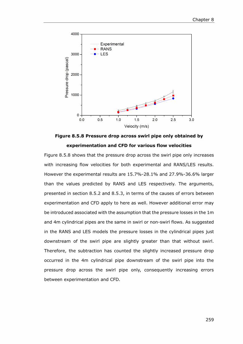
Chapter 8

259

Figure 8.5.8 Pressure drop across swirl pipe only obtained by

experimentation and CFD for various flow velocities

Figure 8.5.8 shows that the pressure drop across the swirl pipe only increases

with increasing flow velocities for both experimental and RANS/LES results.

However the experimental results are 15.7%-28.1% and 27.9%-36.6% larger

than the values predicted by RANS and LES respectively. The arguments,

presented in section 8.5.2 and 8.5.3, in terms of the causes of errors between

experimentation and CFD apply to here as well. However additional error may

be introduced associated with the assumption that the pressure losses in the 1m

and 4m cylindrical pipes are the same in swirl or non-swirl flows. As suggested

in the RANS and LES models the pressure losses in the cylindrical pipes just

downstream of the swirl pipe are slightly greater than that without swirl.

Therefore, the subtraction has counted the slightly increased pressure drop

occurred in the 4m cylindrical pipe downstream of the swirl pipe into the

pressure drop across the swirl pipe only, consequently increasing errors

between experimentation and CFD.

Chapter 8

260

Figure 8.5.9 Comparison of Pressure Loss across optimised swirl pipe

with previously used swirl pipes

Figure 8.5.9 shows a comparison of experimental pressure drops in water

passing across the Swirly-Flo pipe (400mm length) measured by

Ganeshalingam (2002), the swirl inducing pipe (400mm), the swirl inducing

pipe + entry and exit transition (600mm) by Ariyaratne (2005), the optimised

swirl pipe used in this study and the pressure drop across the cylindrical control

pipe. It should be noted that it is not entirely appropriate to compare the

measured pressure drop data for the various types of swirl pipes because:

The Swirly-Flo pipe and the optimised swirl pipe used in this study were

made of steel. However the swirl pipes Ariyaratne (2005) used were

produced by rapid prototyping using plastics, which had a better surface

finish. Therefore, the friction factors of the swirl pipes made of steel were

greater than that of the plastic swirl pipes (surface roughness of

optimised swirl pipe: 9 x 10-06m versus 2.09x10-06m for swirl inducing

pipe).

The cross-sectional area of the (three-lobed) Swirly-Flo pipe was smaller

than that of the cylindrical pipe (Ariyaratne, 2005).

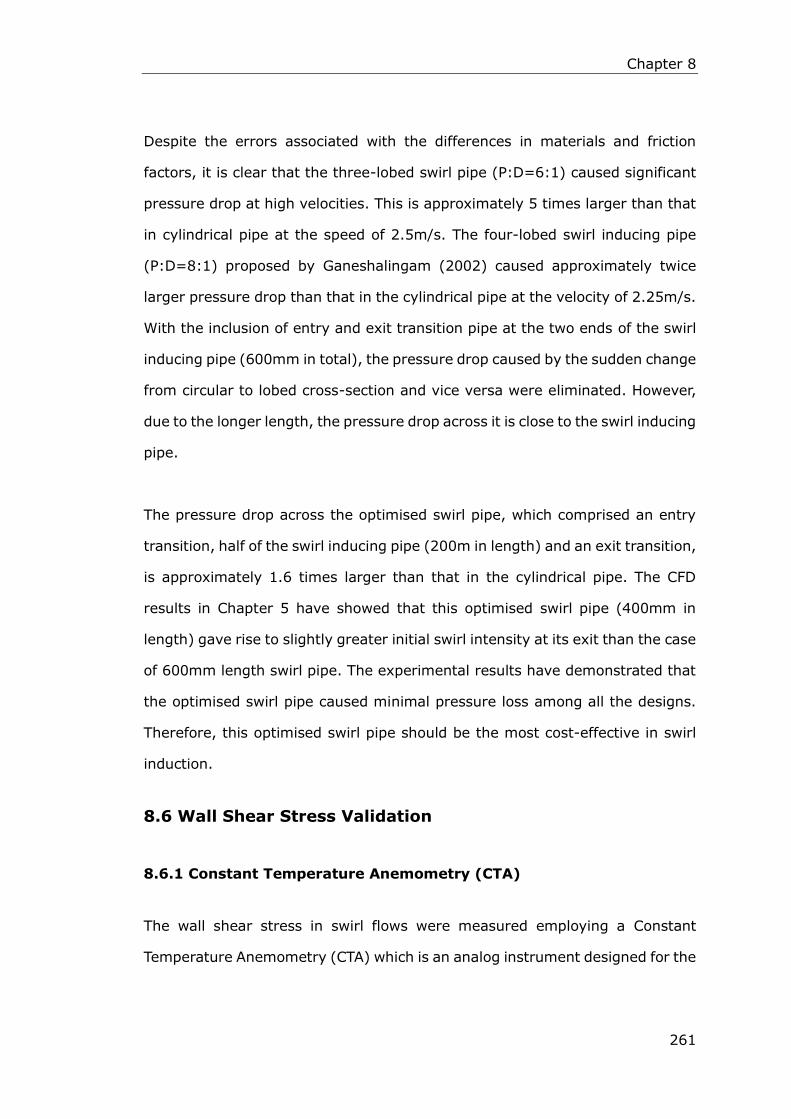
Chapter 8

261

Despite the errors associated with the differences in materials and friction

factors, it is clear that the three-lobed swirl pipe (P:D=6:1) caused significant

pressure drop at high velocities. This is approximately 5 times larger than that

in cylindrical pipe at the speed of 2.5m/s. The four-lobed swirl inducing pipe

(P:D=8:1) proposed by Ganeshalingam (2002) caused approximately twice

larger pressure drop than that in the cylindrical pipe at the velocity of 2.25m/s.

With the inclusion of entry and exit transition pipe at the two ends of the swirl

inducing pipe (600mm in total), the pressure drop caused by the sudden change

from circular to lobed cross-section and vice versa were eliminated. However,

due to the longer length, the pressure drop across it is close to the swirl inducing

pipe.

The pressure drop across the optimised swirl pipe, which comprised an entry

transition, half of the swirl inducing pipe (200m in length) and an exit transition,

is approximately 1.6 times larger than that in the cylindrical pipe. The CFD

results in Chapter 5 have showed that this optimised swirl pipe (400mm in

length) gave rise to slightly greater initial swirl intensity at its exit than the case

of 600mm length swirl pipe. The experimental results have demonstrated that

the optimised swirl pipe caused minimal pressure loss among all the designs.

Therefore, this optimised swirl pipe should be the most cost-effective in swirl

induction.

8.6 Wall Shear Stress Validation

8.6.1 Constant Temperature Anemometry (CTA)

The wall shear stress in swirl flows were measured employing a Constant

Temperature Anemometry (CTA) which is an analog instrument designed for the

Chapter 8

262

measurement of temperature, shear stress, velocity and velocity fluctuations in,

e.g., jets, boundary layers, and transitional flows.

The CTA measurement principle is based on the cooling of the small sensor

placed in the flow. The temperature (resistance) of the sensor is kept constant

by an advanced feedback control loop (servo-loop) that contains an electronic

bridge circuit. In this way, the anemometer produces a continuous voltage that

is proportional to the instantaneous flow velocity.

For the measurement of wall shear stress, a fast response Constant

Temperature Anemometer (CTA) system comprising a Glue-on hot-film probe

and a MiniCTA 54T42 produced by DANTEC Measurement Technology was used.

The Glue-on hot film probe is a special version of the flush-mounting probe

where the sensor is deposited on a 50 μm thick polyimide foil carrying quartz

coating. The hot film is so thin that it is submerged in the viscous region of the

boundary layer. The nickel sensor is 0.1×0.9mm and connected to gold-plated

lead areas. The copper wires soldered to the leads constitute the electrical

connection between the probe cable and the probe. The dimension of the

Glue-on probe is shown in Figure 8.6.1a. The MiniCTA version 54T42 as shown

in Figure 8.6.1b is a single channel anemometer that can be used with many of

Dantec’s wire and film probes. The MiniCTA is mounted in a small box equipped

with BNC connectors (one for the probe cable and one for the output voltage)

and one input connector for a 12 VDC power adapter. The voltage output can be

fed to a PC via a NI A/D board.

The hot-film probe is working on the principle that the heat transfer from a

sufficiently small heated surface depends only on the flow characteristics in the

viscous region of the boundary layer. By similarity between the heat and the

gradient transport of momentum, the amount of the heat transfer into the fluid

gives a measure of the wall shear stress (Berca, 2007).

Chapter 8

263

a: Glue-on hot-film probe 55R47S

b: MiniCTA 54T42

Figure 8.6.1 Glue-on hot-film probe and MiniCTA 54T42

When the hot-film probe glued onto the internal pipe wall is fed with a current

the voltage required to maintain a constant temperature at the hot-film probe is

related to the gradient of the near wall velocity and hence the wall shear stress

or friction velocity (Hanratty and Campbell, 1983, Sumer et al., 1993).

The relationship between the voltage (𝐸𝑎) and the wall shear stress (𝜏𝑤) is given

by:

𝐸𝑎2 = 𝐴 + 𝐵𝜏𝑤

1/3

(8.6.1)

where 𝜏𝑤 is the wall shear stress. 𝐸𝑎 is the voltage required to maintain the

preset temperature. The voltage is provided by the MiniCTA 54T42 which

Chapter 8

264

guarantees that the overheat ratio of the sensor is maintained. A and B are

constants that have to be found by probe calibration.

8.6.2 Calibration of the Hot-Film Probe

In order to perform measurements covering more points downstream of the

swirl pipe, the hot film sensor was fixed, using Loctite 495 glue, to the internal

surface of a removable cylindrical pipe section that has a length of 200mm with

the longitudinal direction of the hot film being perpendicular to the direction of

the flow. The removable section can be positioned at different locations

downstream of the swirl pipe through dairy clamps. At each location

(circumference), 5 measurement points were covered by the sensor at top,

+45°, middle, -45° and bottom by rotating the removable section by 45°

clockwise each time. The installation of the sensors is illustrated in Figure 8.6.2.

Chapter 8

265

Figure 8.6.2 Allocation of the hot-film sensor at the five points on the

circumference

At each of the five points along the circumference, sensor calibration was

carried out in situ to determine the correlation of the output voltage induced by

the hot-film resistance with the wall shear stress. The calibration can be

performed in cylindrical pipe flows where the wall shear stress is directly

proportional to the streamwise pressure gradient by (Su et al., 2010):

𝜏𝑤 =∇𝑃𝑑

4𝐿

(8.6.2)

Where

∆P= pressure loss due to friction in pipe,

d = pipe diameter,

Chapter 8

266

L = length of pipe corresponding to pressure loss

At each of the five points, the sensor calibration was performed by measuring

the pressure drops between the two pressure transmitters and the

corresponding voltage outputs induced by the MiniCTA at a series of flow

velocities. The general procedure was as below:

1) The MiniCTA was set up so that the hot-film sensor had an overheat ratio

of 0.12. At this overheat ratio, the sensor was maintained at a

temperature of 60 ℃ which is the maximum recommended operating

temperature in water conditions.

2) Turned on the magnetic flow meter and the two pressure transmitters

which had a distance of 4.7m between them. The hot film sensor was

positioned in between the two pressure transmitters.

3) Started the pump and obtained flow velocities of 0.75m/s by adjusting

the invertor.

4) Waited for the velocity to stabilise and then turned on the power of the

MiniCTA to heat the hot film sensor. Constantly checking the voltage

output from the MiniCTA until it was relatively stable.

5) Logged readings for the two pressure transmitters (which gave pressure

drop across the 4.7m cylindrical pipe) and the mass flow rate using a

Squirrel Data Logger.

6) Meanwhile, collected voltage readings at a sampling frequency of

1000Hz for 10s employing the MiniCTA Software v4.20. Repeated the

collection another 4 times to get a mean value of voltage from the five

collections of data.

7) Recorded the water temperature for measurement at this velocity using

a thermometer.

8) Powered off the MiniCTA. Adjusted the invertor to obtain a flow velocity of

1m/s. Repeated steps 4), 5), 6) and 7) to log readings of pressure drop,

Chapter 8

267

flow velocity and voltage output.

9) Repeated step 8) another 6 times so as to cover measurements at flow

velocities of 1.25, 1.5, 1.75, 2, 2.25 and 2.5m/s.

The above measurement procedure is summarized in the following flow chart.

Figure 8.6.3 Measurement flow chart for sensor calibration

One of the factors influencing the heat transfer between the heated sensor and

the water is the temperature difference between the water and the hot-film

sensor. Since the hot film’s temperature is kept constant, to avoid this influence,

constant water temperature should be maintained during the course of the

calibration. In the case of an unavoidable temperature change, a temperature

correction is required. The temperature correction for CTA voltage can be

calculated from (Jørgensen, 2002):

𝐸𝑐𝑜𝑟𝑟 = (𝑇𝑤 − 𝑇0

𝑇𝑤 − 𝑇𝑎)0.5

∙ 𝐸𝑎

(8.6.3)

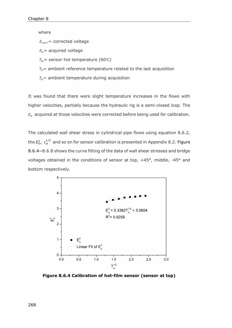
Chapter 8

268

where

𝐸𝑐𝑜𝑟𝑟= corrected voltage

𝐸𝑎= acquired voltage

𝑇𝑤= sensor hot temperature (60℃)

𝑇0= ambient reference temperature related to the last acquisition

𝑇𝑎= ambient temperature during acquisition

It was found that there were slight temperature increases in the flows with

higher velocities, partially because the hydraulic rig is a semi-closed loop. The

𝐸𝑎 acquired at those velocities were corrected before being used for calibration.

The calculated wall shear stress in cylindrical pipe flows using equation 8.6.2,

the 𝐸𝑎2, 𝜏𝑤

1/3 and so on for sensor calibration is presented in Appendix 8.2. Figure

8.6.4~8.6.8 shows the curve fitting of the data of wall shear stresses and bridge

voltages obtained in the conditions of sensor at top, +45°, middle, -45° and

bottom respectively.

Figure 8.6.4 Calibration of hot-film sensor (sensor at top)

Chapter 8

269

Figure 8.6.5 Calibration of hot-film sensor (sensor at +45°)

Figure 8.6.6 Calibration of hot-film sensor (sensor at middle)

Chapter 8

270

Figure 8.6.7 Calibration of hot-film sensor (sensor at -45°)

Figure 8.6.8 Calibration of hot-film sensor (sensor at bottom)

8.6.3 Measurements of Mean Wall Shear Stress in Swirl Flows

In swirl flows, wall shear stress measurements were performed at 10

circumferences starting at 0.13m downstream of swirl pipe and then 0.53m,

1.13m, 1.63m, 2.13m, 2.63m, 3.13m, 3.63m, 4.13m and 4.63m downstream

of the swirl pipe. At each circumference, the sensor was positioned at the five

Chapter 8

271

points in the order indicated in Figure 8.6.9. At each point, voltage acquisition

was performed at velocities of 1m/s, 1.25m/s, 1.5m/s, 1.75m/s, 2m/s, 2.25m/s

and 2.5m/s. At each flow velocity, voltage readings were sampled at a sampling

frequency of 1000Hz for 10s, which was repeated for another 4 times to get a

mean value. Therefore, a total number of 1750 mean voltage readings were

obtained which resulted in 350 mean wall shear stress values at the

circumferences covering a range of locations and flow velocities. The

measurement procedure is shown in Figure 8.6.9.

Figure 8.6.9 Measurement procedure for wall shear stress

At each point, the bridge voltage outputs obtained at each flow velocity were

averaged over the five samplings. The mean voltages were then corrected in

terms of water temperature difference between the calibration in cylindrical pipe

flows and the data acquisition in swirl flows using equation 8.6.3. The corrected

voltages were then converted into wall shear stresses using the calibration

curves obtained in section 8.6.2. The conversion was performed in a way that

Chapter 8

272

the voltage collected in the points of sensor at the top, +45°, middle, -45° and

bottom in swirl flows were converted employing the calibration curves obtained

in the corresponding conditions of sensor at the top, +45°, middle, -45° and

bottom respectively, thus the calibration can be regarded as in situ.

The mean wall shear stress at circumferences downstream of the swirl pipe for

various flow velocities is shown in Figure 8.6.10. Figure 8.6.11 shows the mean

wall shear stress in cylindrical pipe flows at the same flow velocities calculated

from equation 8.6.2. The detailed experimental results shown in the two figures

are referred to Table 8.6.1.

It is clear from the two figures that the wall shear stresses increase with

increasing flow velocities in conditions of both the cylindrical pipe flows and the

swirl flows. However, for the same flow velocity, there is a clear increase of wall

shear stress downstream of the swirl pipe which decreases gradually with

increasing downstream distance as the swirl effect decays. The maximum and

minimum increases of wall shear stress downstream of the swirl pipe, compared

to the wall shear stress in the cylindrical pipe flows with various velocities, are

calculated in Table 8.6.1. It demonstrates a considerable wall shear stress

increase (91% for 2.5m/s flow velocity~279% for 1m/s flow velocity) at the

circumference 0.13m downstream of the swirl pipe; and 15%~105%

(2.5m/s~1m/s) increase of wall shear stress is guaranteed within 4.6m

downstream of the swirl pipe. This at least 15%~105% increase in the wall

shear stress could be important in improving Clean-In-Place efficiency in a

closed processing system.

Chapter 8

273

Figure 8.6.10 Mean wall shear stress downstream of swirl pipe for

various flow velocities

Figure 8.6.11 Mean wall shear stress downstream of control pipe for

various flow velocities

Chapter 8

274

Table 8.6.1 Mean wall shear stress downstream of swirl pipe and control pipe for various flow velocities

Location

Velocity

(m/s)

Wall shear stress in swirl flows

(pascal) WSS in

cylindrical

pipe flows

(pascal)

Max.

increase

(%)

Min.

increase

(%)

0.13m

down-

stream

0.53m

down-

stream

1.13m

down-

stream

1.63m

down-

stream

2.13m

down-

stream

2.63m

down-

stream

3.13m

down-

stream

3.63m

down-

stream

4.13m

down-

stream

4.63m

down-

stream

1 10.873 9.593 10.138 6.309 8.984 7.434 7.679 6.823 5.906 7.124 2.872 278.59 105.64

1.25 16.748 16.411 13.965 9.026 11.761 9.953 10.166 9.165 8.814 9.073 4.112 307.30 114.35

1.5 19.275 19.461 16.145 11.444 14.106 12.225 12.072 11.296 11.331 10.723 5.577 248.95 92.27

1.75 20.985 21.422 17.720 14.630 15.755 13.690 13.817 13.044 13.144 12.094 7.234 196.13 67.18

2 22.206 22.078 18.922 14.790 17.411 15.122 15.634 14.130 15.152 13.632 9.169 142.19 48.67

2.25 23.570 23.590 20.612 15.905 19.188 16.388 16.688 15.233 16.149 14.629 11.349 107.86 28.90

2.5 25.964 24.757 22.815 17.708 20.638 17.205 18.552 16.161 17.778 15.686 13.623 90.59 15.14

Chapter 8

275

Table 8.6.2 Comparison of mean wall shear stress in swirl flows obtained by experimentation and CFD models

WSS

Distance

downstre

-am (m)

2.5m/s flow velocity 2m/s flow velocity 1.5m/s flow velocity 1m/s flow velocity

LES

(Pa)

Error

LES to

experi

mental

(%)

RANS

(Pa)

Error

RANS to

experim

ental

(%)

LES

(Pa)

Error

LES to

experi

mental

(%)

RANS

(Pa)

Error

RANS to

experim

ental

(%)

LES

(Pa)

Error

LES to

experi

mental

(%)

RANS

(Pa)

Error

RANS to

experim

ental

(%)

LES

(Pa)

Error

LES to

experi

mental

(%)

RANS

(Pa)

Error

RANS to

experim

ental

(%)

0.13 23.77 -8.4 15.69 -39.6 16.01 -27.9 10.46 -52.9 8.98 -53.4 6.17 -68.0 3.93 -63.8 2.76 -74.6

0.53 19.00 -23.3 14.47 -41.6 12.72 -42.4 9.74 -55.9 6.88 -64.7 5.82 -70.1 2.92 -69.5 2.66 -72.3

1.13 15.49 -32.1 13.36 -41.4 9.59 -49.3 8.89 -53.0 5.36 -66.8 5.30 -67.2 2.47 -75.7 2.56 -74.7

1.63 13.89 -21.6 13.10 -26.0 8.46 -42.8 8.74 -40.9 4.78 -58.2 5.22 -54.4 2.28 -63.8 2.56 -59.5

2.13 12.45 -39.7 13.05 -36.8 7.92 -54.5 8.73 -49.9 4.35 -69.2 5.22 -63.0 2.14 -76.1 2.54 -71.7

2.63 12.00 -30.2 12.98 -24.5 7.75 -48.7 8.70 -42.5 3.97 -67.5 5.21 -57.4 1.99 -73.2 2.54 -65.9

3.13 11.67 -37.1 12.92 -30.4 7.44 -52.4 8.67 -44.5 3.89 -67.8 5.19 -57.0 2.00 -74.0 2.53 -67.0

3.63 11.58 -28.4 12.89 -20.2 7.35 -48.0 8.65 -38.8 3.81 -66.2 5.18 -54.1 1.92 -71.8 2.53 -62.9

4.13 11.52 -35.2 12.88 -27.6 7.29 -51.9 8.65 -42.9 3.76 -66.8 5.18 -54.3 1.95 -67.0 2.53 -57.1

4.63 11.20 -28.6 12.87 -17.9 7.07 -48.1 8.64 -36.6 3.54 -67.0 5.18 -51.7 1.95 -72.6 2.53 -64.5

Chapter 8

276

Figure 8.6.12 Comparison of mean wall shear stress downstream of

swirl pipe obtained by experimentation and CFD models

The wall shear stress measured in swirl flows were compared to the RANS and

LES models where data are available. The comparison is shown in Table 8.6.2

and Figure 8.6.12. Compared with the CFD results, the experimental

measurements tend to overestimate the wall shear stress in swirl flows

especially in the conditions of lower velocities and at circumferences further

downstream of the swirl pipe. A detailed differences in percentage between

experimental and CFD results are referred in Table 8.6.2. Despite the

Chapter 8

277

differences (8%-76% lower for LES and 13%-75% lower for RANS), the

experimentation confirms the tendency shown in the CFD models that swirl pipe

induces a clear increase in the mean wall shear stress downstream which

prevails for a downstream duration proportional to the flow velocity. Within the

duration, the swirl pipe could be expected to improve the CIP efficiency in a

closed processing system.

Hereafter discuss sources that may contribute to the experimental errors. They

are:

Errors associated with calibration

The calibration of the hot-film probe was performed in cylindrical pipe

flows where the wall shear stress can be calculated from the pressure

drop due to friction of the pipe between the two pressure transmitters. As

was discussed in section 8.5.2 the measured pressure drop accounted for

the minor loss due to the components in the system, such as the

connections (fittings) of cylindrical/cylindrical pipe between the two

pressure transmitters, therefore the overall pressure drop measured was

larger than the pressure drop due to friction of the pipe. This

overestimated pressure drop, when applied to calibration, contributes to

an overestimation of the wall shear stress in swirl flows. From Table 8.5.5,

the error associated with pressure drop measurement was greater in

flows with lower velocities, resulting stronger overestimation of wall

shear stress in swirl flows with lower velocities.

In addition, the difference between the fitting of the straight line and the

points of (𝜏𝑤1/3

, 𝐸𝑎2) on the graph (curve fitting errors), which is within

2%-10%, contributes to the errors associated with calibration.

The angle made by the hot-film probe with the flow

The maximum heat dissipation between the probe and the water takes

Chapter 8

278

place when the longitudinal direction of the hot film is perpendicular to

the direction of the flow (Berca, 2007), which means the maximum

voltage value at the output of the CTA. This requirement was met in

cylindrical pipe flows during the probe calibration as the Glue-on probe

was fixed onto the internal surface of the removable section by Loctite

495 glue with the longitudinal direction of the hot film being

perpendicular to the pipe axis. However, in swirl flows the direction of the

flow in the near wall region is not perpendicular to the cross-flow planes

as shown in Figure 8.6.13, thus the angle made between the longitudinal

direction of the sensor and the flow direction in the measurement points

is less than 90° (approximately 70°). This is especially true in the

duration just downstream of the swirl pipe where swirl prevails. Due to

this, the wall shear stress just downstream of the swirl pipe was

underestimated. Therefore, the rate of decrease of the experimental wall

shear stress downstream of the swirl pipe is not as steep as the CFD

prediction, especially the LES.

Figure 8.6.13 Flow direction in the near wall region of swirl flow

Influence of change of the probe-water temperature

Another influence over the measurements of the wall shear stress is

given by the variation in the water temperature due to, firstly the change

in the ambient environment as no air conditioning was equipped in the

laboratory, and secondly the rig being a semi-closed loop so that the

Chapter 8

279

water temperature tended to increase slightly in flows with higher

velocities. Since the hot-film’s temperature is kept constant, the heat

transfer by convection between probe and water changes with water

temperature. The error associated with water temperature variation was

minimized by carrying out temperature correction against the CTA

voltage output.

Wall effects

The hot-film probe was attached to the internal surface of the pipe and

some amount of the measured heat of the probe is conducted to the wall.

The conduction of the heat to the pipe wall is minimized by using the

insulating polyimide foil. If not, the wall shear stress will be

overestimated.

Contamination of the hot-film probe

Another parameter taken into account is the contamination of the

hot-film probe with the water impurities. Contaminants may adhere to

the sensor and reduce the heat transfer resulting in a downward drift in

the calibration (Jørgensen, 2002). To avoid this, cleaning of the probe

was done at regular intervals using lens cleaning paper.

Despite the factors influencing the measurements with the hot-film probe,

which were unavoidable due to the defects of the experimental apparatus and

the complexity when applied in swirl flows, the experimental results has

demonstrated the applicability of hot-film anemometer applied in wall shear

stress measurement in swirl flows.

8.6.4 Fluctuation of Wall Shear Stress in Swirl Flows

The instantaneous wall shear stress at each measurement points can be

calculated through the instantaneous voltage signals from the MiniCTA. The

temporal wall shear stress over 1 second at the position 0.53m downstream of

Chapter 8

280

swirl pipe with the condition of sensor at top and the flow velocity of 1, 1.5 and

2m/s are demonstrated in Figure 8.6.14. It was observed that the wall shear

stress varies erratically about its mean value with time, with the fluctuation

amplitude growing slightly with increasing flow velocities.

Figure 8.6.14 Examples of wall shear stress fluctuation downstream of

swirl pipe measured by hot-film probe

The normalized fluctuation rate of the wall shear stress can be calculated from

equation 7.4.1. However, as has been described in section 8.6.3 at each

measurements point voltage was sampled at a frequency of 1000Hz for 10s,

repeated 5 times. With the coverage of 5 points at each of the 10

circumferences and the 7 flow velocities under which measurements were

performed, this resulted in a total number of 17,500,000 voltage values needed

Chapter 8

281

to be calculated into wall shear stress. This becomes computationally costly and

unaffordable.

The MiniCTA Software v4.20 is capable of performing calculations of the statistic

derivatives of the raw data: mean, standard deviation, and turbulent intensity.

Where the turbulence intensity, I, is defined as the ratio of the

root-mean-square of the velocity fluctuations u’, to the mean flow velocity U.

Therefore:

𝐼 =𝑢′

𝑈=

[1

𝑁 − 1∑ (𝑢𝑖 − 𝑈)2𝑁

𝑖=1 ]1/2

𝑈= [

1

𝑁 − 1∑(

𝑢𝑖

𝑈− 1)

2𝑁

𝑖=1

]

1/2

(8.6.4)

Where 𝑢𝑖

𝑈 is the normalized velocity. Equation 8.6.4 has the same form as

equation 7.4.1 that is used for calculating the normalized fluctuation rate of wall

shear stress. The turbulence intensity calculated from the raw data in the

MiniCTA software is actually the normalized fluctuation rate of the instantaneous

voltage signals. Since the same calibration curves were used in converting

voltages at various circumferences into wall shear stresses, the normalized

fluctuation rate of the wall shear stress should be proportional to turbulence

intensity of the instantaneous bridge voltage. It is therefore decided to describe

the unsteady behaviour of the normalized wall shear stress using the

normalized fluctuation rate of the bridge voltage signals, which should

demonstrate consistent variation trend of the wall shear stress fluctuation rate

downstream of the swirl pipe.

Figure 8.6.15 and 8.6.16 illustrate the variation of the mean normalized voltage

fluctuation rates (averaged from the five points at each circumference)

downstream of the swirl and control pipes for various flow velocities. A clearer

comparison of the normalized fluctuation rate of voltage signals under swirl flow

and non-swirl flow conditions for various velocities is exhibited in Figure 8.6.17.

Chapter 8

282

Figure 8.6.15 Normalized voltage fluctuation rates downstream of

swirl pipe for various flow velocities

Figure 8.6.16 Normalized voltage fluctuation rates downstream of

control pipe for various flow velocities

Chapter 8

283

Figure 8.6.17 Comparison of the normalized fluctuation rate of voltage

signals under swirl flow and non-swirl flow conditions

Chapter 8

284

Figure 8.6.15~17 suggest that firstly swirl pipe induces a stronger fluctuation

rate in the wall shear stress downstream than the non-swirl flow conditions. This

is expected as swirl flow, which contains a tangential velocity component, is

always accompanied by an increase in velocity fluctuations. Just downstream of

the swirl pipe, the fluctuation rate is relatively low (might be stabilized by the

stronger swirl just downstream of the swirl pipe) which increases with

increasing downstream distance and reaches a maximum where possibly the

vortex cores interact and dissipate. Afterward, the greater fluctuation rate

induced prevails along the circular pipe experiencing ups and downs. The

variation trend in the wall shear stress fluctuation suggested from Figure 8.6.15

shows good consistency with the LES predictions illustrated in Figure

7.4.18~22.

In fully developed cylindrical pipe flows, the turbulence intensity at the core can

be estimated from the below formula derived from empirical correlation (ANSYS,

2011b):

𝐼 =𝑢′

𝑈= 0.16(𝑅𝑒𝑑ℎ

)−1/8

(8.6.5)

Where 𝑅𝑒𝑑ℎ is the Reynolds number based on the pipe hydraulic diameter 𝑑ℎ.

This formula was used to estimate the turbulence intensity on the inlet

boundary conditions for the CFD model. It can be found from Table 6.2.1 that

the turbulence intensity decreases slightly with increasing Reynolds number of

the flow. A consistent trend can be found in Figure 8.6.15 and 8.6.16 with the

turbulence intensity reducing slightly with increasing flow velocity in both swirl

and non-swirl conditions.

It should be noted that a decreasing turbulent intensity does not mean that the

flow becomes less turbulent. It just means that the root-mean-square of the

Chapter 8

285

velocity fluctuations u’ divided by the mean flow velocity U decreases. In fluid

dynamics, the root-mean-square of the velocity fluctuations u’ expresses the

average magnitude of the velocity fluctuations. It links to the turbulence kinetic

energy k by 𝑢′ = (2

3𝑘)

1/2 with k being the mean kinetic energy per unit mass

associated with eddies in turbulent flow (H.K.Versteeg and W.Malalasekera,

2010). Actually both the velocity fluctuation and the mean velocity increase with

increasing flow velocity, but the mean velocity increases even more, therefore

turbulence intensity decreases. The turbulence intensity helps to indicate the

variation of wall shear stress fluctuation rate downstream of swirl pipe under a

fixed flow velocity by eliminating the level difference of the mean wall shear

stress downstream of the swirl pipe.

It was also observed that, for the conditions of 2, 2.25 and 2.5m/s flow

velocities, the fluctuation rate, once reaching a maximum value, experiences a

clear decreasing trend. This may due to the inadequate efficiency of the

De-aerator which cannot sufficiently remove bubbles at higher flow velocities. It

has been suggested that the introduction of bubbles into the flow suppresses

the overall fluctuation of the wall shear stress in the pipe flow (Su et al., 2010).

In a fully closed processing system with no bubbles, the fluctuation rate of the

wall shear stress at the internal pipe surface may be stronger.

The variation of normalized wall shear stress fluctuation rate, presented in the

form of normalized fluctuation rate of voltage signals, has demonstrated that

further downstream where the increase in the wall shear stress fades, the wall

shear stress maintains a stronger fluctuation rate than in the non-swirl flow,

which should contribute to the enhancement of CIP procedures over that

duration in a closed processing system.

Chapter 8

286

8.7 Conclusions

This chapter presented the experimental validation of the simulation results.

The concepts of error/uncertainty and verification/validation were introduced.

Efforts have been made to minimize the errors and uncertainties of the CFD

models were summarized. The layout and specification of the hydraulic rig for

validating the CFD results were described as were the processes of developing

the stainless steel optimised swirl pipe using investment casting.

The measurement procedures employed to validate the pressure drop across

the optimised swirl pipe using a pair of pressure transmitters were described

and the possible reasons to the differences between experimental and CFD

results were discussed. The following results have been obtained:

The experimental pressure drops across the optimised swirl pipe in flows

with various velocities are found to be 15.7%-28.1% and 27.9%-36.6%

larger than the values predicted by RANS and LES respectively.

The pressure drop across the optimised swirl pipe is approximately 1.6

times larger than that measured in cylindrical pipe flow.

The optimised swirl pipe causes minimal pressure loss from all the

various swirl pipe designs, which should be most cost-effective in swirl

induction.

The wall shear stresses in swirl flows were measured by a Glue-on hot film

sensor and a MiniCTA. The working principle of the measurement apparatus, the

calibration procedures performed in cylindrical pipe flows and the

measurements in swirl flows were detailed. The sources that may contribute to

the experimental errors using hot-film sensor in swirl flows were discussed in

terms of the sensor calibration, angle made by the hot-film probe with flow,

influence of the change of the water temperature, etc. Despite the experimental

Chapter 8

287

errors, the following findings can be noted:

The experimental results confirm the CFD simulation that, without

increasing flow velocity, the swirl pipe induces a clear increase in the

mean wall shear stress downstream which decreases gradually with

increasing downstream distance.

The hot-film sensor tends to overestimate the mean wall shear stress

downstream of the swirl pipe comparing to CFD with the RANS and LES

predictions being 8%-76% and 13%-75% lower than the experimental

results for various flow velocities.

The normalized wall shear stress fluctuation rate, presented in the form

of a normalized fluctuation rate of voltage signals, is greater downstream

of the swirl pipe than in the conditions of non-swirl flows indicating

stronger kinetic energy of the swirling flows. The variation of the

normalized fluctuation rate is in consistent with that obtained in the LES

model.

The wall shear stress measurement demonstrates that, with the increase

of the mean wall shear stress just downstream of the swirl pipe and the

prevailing of greater wall shear stress fluctuation rate further

downstream of swirl pipe where the increase of wall shear stress fades

away, the swirl pipe should enhance the CIP procedures over a

considerable downstream distance, at least within the measurement

scope of the experimentation (4.6m), in a closed processing system.

It can be concluded that the experimentation has validated to a large extent the

CFD models in that the swirl pipe should improve the cleaning efficiency of CIP

procedures in closed processing systems.

Chapter 9

288

CHAPTER 9: CONCLUSIONS AND FUTURE WORK

9.1 Conclusions

This thesis intended to address the fundamentals of improving the cleaning

efficiency of CIP procedures in closed processing systems by locally introducing

an intensified hydrodynamic force from swirl flow induced by an optimised swirl

pipe without increasing the overall operating flow velocities. The investigation,

carried out employing CFD and experimentation, covered further optimisation

of the 4-lobed swirl pipe, RANS and LES simulation of the swirl flows induced by

the optimised swirl pipe, and experimental validation of the numerical results.

The following conclusions can be drawn from the investigation:

9.1.1 Further Optimisation of the 4-Lobed Swirl Pipe

The further optimized 400mm length swirl pipe, which has a shorter

length of swirl inducing pipe than previous research suggested, resulted

in slightly greater initial swirl intensity at its exit at the expense of less

pressure loss than the 600mm length swirl pipe.

A shorter length of 200mm swirl inducing pipe used in conjunction with

an entry and exit transition pipe was proven to be optimal in swirl

induction.

9.1.2 RANS-Based Simulation of Swirl Flows

The initial swirl intensity downstream of the swirl pipe was found to be

proportional to the flow velocity. The swirl flows were observed to decay

exponentially with distance downstream of the swirl pipe and inversely to

the Reynolds number of the flow.

Swirl pipe imposes a tangential wall shear stress within itself which

Chapter 9

289

directs to downstream. A close positive correlation of swirl intensity and

the tangential wall shear stress was identified which confirmed that the

presence and variation of tangential wall shear stress is closely

dependent on swirl intensity.

The wall shear stress downstream of the swirl pipe was not evenly

distributed but followed the pattern of the swirl pipe resulting in a

wave-like circumferential distribution.

Swirl pipe locally increased mean wall shear stress downstream of it, with

the increased value and effective distance more pronounced for a flow

with a larger Reynolds number.

9.1.3 Large Eddy Simulation of Swirl Flows

The LES identified four vortex core regions forming inside the lobes of the

swirl pipe which precess spirally about the circular pipe axis for some

distance and then dissipate. The RANS failed to predict the vortex core

regions within the swirl flows.

The instantaneous tangential velocity, swirl intensity and wall shear

stress were observed fluctuating about the time averaged value with a

greater fluctuation level were detected in cross-flow planes that are

further downstream of the swirl pipe where the swirl effect is less

dominant. The fluctuation also increased with increasing flow velocities.

The spiral pattern of the wall shear stress increases downstream of the

swirl pipe which was due to the flow between the rotating vortex core

centres and the wall being squeezed, producing a considerable increase

in tangential velocity which then gave rise to a tangential wall shear

stress.

The calculation of a normalized wall shear stress fluctuation rate showed

that, further downstream of the swirl pipe where the swirl effect and the

increase of the mean wall shear stress is less dominant, the flow

Chapter 9

290

experiences a high level of turbulence, resulting in a high fluctuation rate

in the wall shear stress.

9.1.4 Experimental Validation

The experimental pressure drops across the optimised swirl pipe were in

good agreement with the RANS and LES predictions. The optimised swirl

pipe gave the lowest pressure loss of all the swirl induction pipes tested

experimentally.

The wall shear stress measurements employing a hot-film anemometer

validated the CFD models in that the swirl pipe induces a clear increase in

both the mean and fluctuation rate of the wall shear stress downstream

with the prevailing distance being proportional to the Reynolds number

of the flow.

The experimentation confirmed the CFD prediction that, with the ability

to promote intensified hydrodynamic impact on the internal pipe surface,

the swirl pipe should enhance the CIP procedures in closed processing

systems over a considerable downstream distance dependent on the

Reynolds number of the flow.

9.2 Contribution to Knowledge

This thesis contributes to the knowledge in that:

A comprehensive literature survey of experimental and computational

works were carried out in terms of cleaning of closed processing systems,

swirl flow modelling and measurements, and equations and terms used

by previous researchers.

A further optimised 4-lobed swirl pipe has been identified and proven to

be optimal in inducing swirl in pipes in comparison to previously used

swirl induction pipes.

Chapter 9

291

A positive correlation between the tangential wall shear stress and the

swirl intensity of swirl flows has been recognized in the CFD models,

which explained why a swirl pipe exerts greater wall shear stress

downstream than a circular pipe.

An insight into the instability of the swirl flows have been given by the

LES indicating intensified fluctuation of tangential velocity, swirl intensity

and the wall shear stress in swirl flows.

Rotating vortex cores have been identified within the swirl flows using

LES which explains the formation of the spiral pattern of the wall shear

stress distribution downstream of the swirl pipe.

The increase in the mean wall shear stress and its fluctuation rate

downstream of the swirl pipe was investigated numerically and

experimentally under various flow velocities.

The fundamentals of CIP improvement in closed processing systems

employing an optimised swirl pipe have been addressed. A better

understanding of hydrodynamics of swirl flows applied in CIP procedures

has been gained especially in the boundary layer where cleaning takes

place.

9.3 Further Work

This section gives recommendations for future research in order to further

advance the present research.

9.3.1 CFD Modelling

In the 3D time-dependent LES model of the present research, a Hybrid

RANS-LES approach was used in the near-wall regions as it avoids the

use of a very fine mesh in the near-wall region which results in

substantially increased computational cost that is not affordable for the

current personal workstation. The application of a wall resolved LES with

Chapter 9

292

a fine mesh in the near-wall regions should be attempted which may

provide improved predictions.

With the rise of computing power, possibilities of a multiphase large eddy

simulation should be examined. The numerical calculation of the

particle-water flow can be performed using either an Euler-Euler or an

Euler-Lagrange approach with the inclusion of forces such as forces

between water and particle, inter-particles etc. The particles should be

positioned initially only on the internal pipe walls with the adhesion force

between the particles and the wall being specified so that the behaviour

of the particles can be observed once the shear stress from the swirl flow

is applied. However, such adhesion force model is not available in the

FLUENT code and is yet to be developed. Moreover, even if such a model

is available, the multiphase LES can be highly computationally expensive

and prohibitive for industrial flows.

So far, the optimisation criterion for swirl induction pipes has been the

swirl effectiveness, which is based on the ratio of the swirl intensity

produced to the pressure loss. As has been identified in the CFD models

the swirl intensity and the tangential wall shear stress is positively

correlated. Therefore, a swirl pipe that is optimal in swirl induction should

also be optimal in increasing the overall wall shear stress of the swirl flow.

However, in some cases, a higher cost of pressure loss may be acceptable

to obtain greater wall shear stress. An optimisation criterion that

emphasises more on the swirl intensity and less on the pressure loss may

be more applicable in some conditions. Numerical optimisation of the

swirl pipe based on this criterion is suggested.

The beneficial effects of swirl pipe have been proven in the cleaning of

straight circular pipes. Its potential in the cleaning of more complex

geometries such as contractions, expansions, up-stands and bends has

not been investigated yet.

Chapter 9

293

9.3.2 Experimental Work

Previous researchers have used Particle Image Velocimetry (PIV) with a

single CCD (Charge Couple Device) camera to measure the flow field of

swirl flows. However their attempts in measuring the tangential velocity

component were not successful or satisfactory. The application of a

stereo PIV which measures three velocity components in a plane (2D3C)

using two CCD cameras may facilitate the measurement of tangential

velocity, swirl intensity and the decay of the swirl flow.

Glue-on hot film probe has been used for wall shear stress

measurements in this study. The probe was calibrated in cylindrical pipe

flows with the longitudinal direction of the hot film being perpendicular to

the direction of the flow as maximum heat dissipation between the probe

and the water takes place in this condition. However in swirl flows, the

flow direction and the longitudinal direction of the hot film cannot be

arranged entirely perpendicular to each other as the Glue-on probe once

fixed on the pipe surface cannot be adjusted, thus resulting in the

underestimation of the measured wall shear stress. This experimental

error may be minimized by using a flush-mounted hot film probe which

may allow the control of the angle made by the flush-mounted probe by

designing a support so that it can be rotated by 5° or 10° each time. A

correlation of the voltage outputs and the angles of the flush-mounted

probe can be found which can be used to correct the wall shear stress

measurements.

Though the hydrodynamic advantages of the swirl pipe have been proven

numerically and experimentally. Its performance in real cleaning practice

has not been examined. The cleanability of the swirl flow induced by the

swirl pipe can be assessed using an EHEDG (European Hygienic

Equipment Design Group) test method (Jensen and Friis, 2004). The

degree of cleanliness can be related to the removal of a soured milk soil

Chapter 9

294

containing bacterial spores and can be assessed by evaluating the

number of remaining spores after cleaning using the turbulent swirl flow.

Reference

295

REFERENCE

AIAA 1998. Guide for the Verification and Validation of Computational Fluid

Dynamics Simulations. AIAA Guide G-077-1998. Reston, VA: American Institute of

Aeronautics and Astronautics.

AIYEJINA, A., CHAKRABARTI, D. P., PILGRIM, A. & SASTRY, M. K. S. 2011. Wax

formation in oil pipelines: A critical review. International Journal of Multiphase Flow,

37, 671-694.

ALGIFRI, A. H., BHARDWAJ, R. K. & RAO, Y. V. N. 1988. Turbulence measurements

in decaying swirl flow in a pipe. Applied Scientific Research, 45, 233-250.

ANSYS. 2011a. ANSYS FLUENT 14.0 Theory Guide [Online]. Canonsburg, PA, USA.

Available:

http://148.204.81.206/Ansys/150/ANSYS%20Fluent%20Theory%20Guide.pdf

[Accessed 2012.03.05].

ANSYS. 2011b. ANSYS FLUENT 14.0 User's Guide [Online]. Canonsburg, PA, USA.

Available:

http://148.204.81.206/Ansys/150/ANSYS%20Fluent%20Users%20Guide.pdf

[Accessed 2012.03.01].

ANSYS. 2013a. ANSYS CFD-Post Users Guide [Online]. Canonsburg, PA, USA.

Available: http://orange.engr.ucdavis.edu/Documentation12.1/121/CFX/xpost.pdf

[Accessed 2012.03.15].

ANSYS. 2013b. ANSYS Fluent Getting Started Guide [Online]. Canonsburg, PA, USA.

Available:

https://uiuc-cse.github.io/me498cm-fa15/lessons/fluent/refs/ANSYS%20Fluent%

20Getting%20Started%20Guide.pdf [Accessed 2012.03.09].

ANSYS. 2013c. ANSYS Fluent Meshing Users Guide [Online]. Canonsburg, PA, USA.

Available:

http://148.204.81.206/Ansys/150/ANSYS%20Fluent%20Meshing%20Users%20G

uide.pdf [Accessed 2012.03.09].

ANSYS. 2013d. ANSYS ICEM CFD Tutorial Manual [Online]. Canonsburg, PA, USA.

Available:

http://www.petrodanesh.ir/Virtual%20Education/Mechanics/ICEM-CFD/PTEC-ICE

M%20CFD%2014.5%20Tutorial%20Files.pdf [Accessed 2012.03.12].

ARIYARATNE, C. 2005. DESIGN AND OPTIMISATION OF SWIRL PIPES AND

TRANSITION GEOMETRIES FOR SLURRY TRANSPORT. PhD Thesis, University of

http://148.204.81.206/Ansys/150/ANSYS%20Fluent%20Theory%20Guide.pdf

http://148.204.81.206/Ansys/150/ANSYS%20Fluent%20Users%20Guide.pdf

http://orange.engr.ucdavis.edu/Documentation12.1/121/CFX/xpost.pdf

https://uiuc-cse.github.io/me498cm-fa15/lessons/fluent/refs/ANSYS%20Fluent%20Getting%20Started%20Guide.pdf

https://uiuc-cse.github.io/me498cm-fa15/lessons/fluent/refs/ANSYS%20Fluent%20Getting%20Started%20Guide.pdf

http://148.204.81.206/Ansys/150/ANSYS%20Fluent%20Meshing%20Users%20Guide.pdf

http://148.204.81.206/Ansys/150/ANSYS%20Fluent%20Meshing%20Users%20Guide.pdf

http://www.petrodanesh.ir/Virtual%20Education/Mechanics/ICEM-CFD/PTEC-ICEM%20CFD%2014.5%20Tutorial%20Files.pdf

http://www.petrodanesh.ir/Virtual%20Education/Mechanics/ICEM-CFD/PTEC-ICEM%20CFD%2014.5%20Tutorial%20Files.pdf

Reference

296

Nottingham.

BAKER, D. W. & SAYRE, C. L. 1974. Decay of Swirling Turbulent Flow of

Incompressible Fluids in Long Pipes. In: DOWDELL, R. (ed.) Flow: its measurement

and control in science and industry. Pittsburgh: Instrument Society of America,

301-312.

BAKKER, A. 2002. Boundary Layers and separation [Online]. Available:

www.bakker.org/dartmouth06/engs150/11-bl.pdf [Accessed 2012.03.15].

BALI, T. 1998. Modelling of heat transfer and fluid flow for decaying swirl flow in a

circular pipe. International Communications in Heat and Mass Transfer, 25,

349-358.

BARI, S. & VEALE, D. 2012. Improvement of BIB packaging product filling valve CIP

performance and efficiency. Food and Bioproducts Processing, 90, 849-857.

BÉNÉZECH, T., FAILLE, C. & LÉCRIGNY-NOLF, S. (eds.) 1998. Removal of Bacillus

spores from closed equipment surfaces under cleaning-in-place conditions,

Cambridge: Jesus College.

BÉNÉZECH, T., LELIÈVRE, C., MEMBRÉ, J. M., VIET, A.-F. & FAILLE, C. 2002. A new

test method for in-place cleanability of food processing equipment. Journal of Food

Engineering, 54, 7-15.

BERCA, E.-L. 2007. INSTRUMENTATION DEVELOPMENT FOR WALL SHEAR STRESS

APPLICATIONS IN 3D COMPLEX FLOWS. PhD Thesis, ÉCOLE POLYTECHNIQUE

FÉDÉRALE DE LAUSANNE.

BERGMAN, B. O. & TRÄGÅRDH, C. 1990. An approach to study and model the

hydrodynamic cleaning effect. Journal of Food Process Engineering, 13, 135-154.

BERTHE, A., KONDERMANN, D., CHRISTENSEN, C., GOUBERGRITS, L., GARBE, C.,

AFFELD, K. & KERTZSCHER, U. 2009. Three-dimensional, three-component wall-PIV.

Experiments in Fluids, 48, 983-997.

BHASKARAN, R. & COLLINS, L. 2003. Introduction to CFD Basics [Online]. Available:

https://instruct1.cit.cornell.edu/courses/fluent/cfd/intro.pdf [Accessed

2012.04.09].

BIRD, M. R. & FRYER, P. J. 1991. An experimental study of the cleaning of surfaces

fouled by whey proteins. Trans IChemE, Food Bioprod Proc, 69C, 13-21.

BOUAINOUCHE, M., BOURABAA, N. & DESMET, B. 1997. Numerical study of the wall

shear stress produced by the impingement of a plane turbulent jet on a plate. Int J

Numer Meth H, 7(6), 548–564.

http://www.bakker.org/dartmouth06/engs150/11-bl.pdf

https://instruct1.cit.cornell.edu/courses/fluent/cfd/intro.pdf

Reference

297

CHANGANI, S. D., BELMAR-BEINY, M. T. & FRYER, P. J. 1997. Engineering and

chemical factors associated with fouling and cleaning in milk processing.

Experimental Thermal and Fluid Science, 14, 392-406.

CHARLES, M. E., CHEH, C. H.-S. & CHU, L. H.-L. 1971. The flow of “settling” slurries

in tubes with internal spiral ribs. The Canadian Journal of Chemical Engineering, 49,

737-741.

CHEN, H. C. & PATEL, V. C. 1988. Near Wall turbulence models for complex flows

including separation. AIAA Journal, 26(6), 641-648.

CHEN, Z. 2011. Wall Modeling for Implicit Large-Eddy Simulation. PhD Thesis,

Technische Universität München.

CHORIN, A. J. 1968. Numerical Solution of the Navier-Stokes Equations.

Mathematics of Computation, 22, 745-762.

COGHLAN, A. 1996. Slime City. New Scientist, 15 (2045), 32-36.

CONWAY, S., CARAENI, D. & FUCHS, L. 2000. Large eddy simulation of the flow

through the blades of a swirl generator. International Journal of Heat and Fluid Flow,

21, 664-673.

DAY, M. A. 2004. The no-slip condition of fluid dynamics. Erkenntnis 33, 285–296.

DÉCAVÉ, E., DEMILLY, M., FOURCADE, B., BRUCKER, F., BOULANGÉ , L. & BRECHET,

Y. 2005. Biological cell detachment kinetics from an inert substrate. Philosophical

Magazine, 85: 3173.

DEV, S. R. S., DEMIRCI, A., GRAVES, R. E. & PURI, V. M. 2014. Optimization and

modeling of an electrolyzed oxidizing water based Clean-In-Place technique for farm

milking systems using a pilot-scale milking system. Journal of Food Engineering,

135, 1-10.

DOUGLAS, J. F., GASORIEK, J. M., SWAFFIELD, J. A. & JACK, L. B. 2006. Fluid

Mechanics (5th Edition), PEARSON Prentice Hall.

DREESEN, P. 2003. Biofilm:The Key to Understanding and Controlling Bacterial

Growth in Automated Animal Drinking Water Systems [Online]. Available:

http://www.edstrom.com/file.aspx?DocumentId=21 [Accessed 2012.03.06].

DUDDRIDGE, J. E., KENT, C. A. & LAWS, J. F. 1982. Effect of surface shear stress on

the attachment of Pseudomonas fluorescence to stainless steel under defined flow

conditions. Biotechnol Bioengng, 24, 153-164.

DURBIN, P. A. 2002. A perspective on recent developments in RANS modeling. In:

FUEYO, W. R. (ed.) Engineering Turbulence Modelling and Experiments 5. Oxford:

http://www.edstrom.com/file.aspx?DocumentId=21

Reference

298

Elsevier Science Ltd, 3-16.

EHEDG 1992. A method for assessing the in-place cleanability of food processing

equipment. Trends in Food Science & Technology, 3, 325–328.

EHEDG 2004. EHEDG Guidelines: Hygienic Equipment Design Criteria. In: FLENNER,

S. (ed.). European Hygienic Engineering and Design Group.

ELEVERS, K. T., PETERS, A. C. & GRIFFITH, C. J. 1999. Development of biofilms and

control of biofilm in the food industry In: WIMPENNY, J., GILBERT, P., WALKER, J.,

BRADING, M. & BAYSTON, R. (eds.) Biofims: The good, the bad, the ugly (pp.

139-145). UK: Bioline, 139-145.

FAILLE, C., LEBRET, V., GAVINI, F. & MAINGONNAT, J. F. 1997. Injury and lethality of

heat treatment of Bacillus cereus spores suspended in buffer and poultry meat.

Journal of Food Protection, 60, 544–547.

FOCKE, W., ZACHARIADES, J. & OLIVIER, I. 1985. The effect of corrugation

inclination angle on the thermodynamic performance of plate heat exchangers.

International Journal of Heat and Mass Transfer, 28, 1469-1479.

FOKEER, S. 2006. An Investigation of Geometrically Induced Swirl Applied to Lean

Phase Pneumatic Flows. PhD Thesis, University of Nottingham.

FOKEER, S., LOWNDES, I. S. & HARGREAVES, D. M. 2010. Numerical modelling of

swirl flow induced by a three-lobed helical pipe. Chemical Engineering and

Processing: Process Intensification, 49, 536-546.

FOWLER, H. W. & MCKAY, A. J. 1980. The measurement of microbial adhesion. In:

BERKELEY, R. C. W., LYNCH, J. M., MELLING, J., RUTTER, P. R. & VINCENT, B. (eds.)

Microbial Adhesion to Surfaces. Chichester: Ellis Horwood Limited, 143–161

FRIIS, A. & JENSEN, B. B. B. 2002. Prediction of Hygiene in Food Processing

Equipment Using Flow Modelling. Food and Bioproducts Processing, 80, 281-285.

FROUD, D., O'DOHERTY, T. & SYRED, N. 1995. Phase averaging of the precessing

vortex core in a swirl burner under piloted and premixed combustion conditions.

Combustion and Flame, 100, 407-412.

GALLOT-LAVALLÉE, T., M. LALANDE, M. & CORRIEU, G. 1984. Cleaning kinetics

modeling of holding tubes fouled during milk pasteurization. Journal of Food Process


GANESHALINGAM, J. 2002. Swirl Induction for Improved Solid-Liquid Flow in Pipes.

PhD Thesis, University of Nottingham.

GEORGE, D. D. 2007. Effects of 4-lobe swirl-inducing pipe on pressure drop. Master

Reference

299

Thesis, University of Nottingham.

GERMANO, M., PIOMELLI, U., MOIN, P. & CABOT., W. H. 1996. Dynamic

Subgrid-Scale Eddy Viscosity Model, Stanford, CA, Center for Turbulence Research.

GIJSEN, F. J. H., GOIJAERTS, A. M., VOSSE, F. N. V. D. & JANSSEN, J. D. 1997. A new

method to determine wall shear stress distribution. Journal of Rheology, 41(5),

995-1006.

GILLHAM, C. R., FRYER, P. J., HASTING, A. P. M. & WILSON, D. I. 1999.

Cleaning-in-Place of Whey Protein Fouling Deposits. Food and Bioproducts

Processing, 77, 127-136.

GRAΒHOFF, A. 1992. Hygienic design:The basis for computer controlled automation.

Food and Bioproducts Processing, Transactions of The Institution of Chemical

Engineers Part C, 70, 69-77.

GRAΒHOFF, A. 1997. Cleaning of heat treatment equipment. In: FEDERATION, I. D.

(ed.) Fouling and Cleaning of Heat Treatment Equipment. Brussels: International

Dairy Federation, 32-44.

GROßE, S. & SCHRÖDER, W. 2008. Dynamic wall-shear stress measurements in

turbulent pipe flow using the micro-pillar sensor MPS3. International Journal of Heat

and Fluid Flow, 29, 830-840.

GUILLEMOT, G., LORTHOIS, S., SCHMITZ, P. & MERCIER-BONIN, M. 2007.

Evaluating the Adhesion Force Between Saccharomyces Cerevisiae Yeast Cells and

Polystyrene From Shear-Flow Induced Detachment Experiments. Chemical

Engineering Research and Design, 85, 800-807.

GUPTA, A., LILLEY, D. G. & SYRED, N. 1984. Swirl Flow. Energy and Engineering

Sciences Series. Tunbridge Wells: Abacus Press, 475.

H.K.VERSTEEG & W.MALALASEKERA 2010. An Introduction To Computational Fluid

Dynamics:The Finite Volume Method Second Edition, England, Prentice Hall.

HALL, J. E. 1998. Computational fluid dynamics: A tool for hygienic design. In:

WILSON, D. I., FRYER, P. J. & HASTING, A. P. M. (eds.) Fouling and cleaning in food

processing. Cambridge: Jesus College, 144-151.

HALSEY, D. M. 1987. Flowmeters in Swirling Flows. Journal of Physics E: Scientific

Instruments, 20, 1036-1040.

HANRATTY, T. J. & CAMPBELL, J. A. 1983. Measurement of wall shear stress. In:

GOLDSTEIN, R. J. (ed.) Fluid mechanics measurements. Washington, DC:

Hemisphere Corporation, 559–615.

Reference

300

HARITONIDIS, J. H. 1989. The Measurement of Wall Shear Stress. In: GAD-EL-HAK,

M. (ed.) Advances in Fluid Mechanics Measurements. Springer-Verlag, 229-261.

HEYWOOD, N. I. & ALDERMAN, N. J. 2003. Developments in Slurry Pipeline

Technologies. Chem. Engng. Progress, April, 36-43.

HOWARD, G. W. 1939. Effects of Rifling on Four-Inch Pipe Transporting Solids.

Transactions of the American Society of Civil Engineers, 106, 135-147.

HUANG, Y. & YANG, V. 2009. Dynamics and stability of lean-premixed

swirl-stabilized combustion. Progress in Energy and Combustion Science, 35,

293-364.

HUBBE, M. A. 1984. Theory of detachment of colloidal particles from flat surfaces

exposed to flow. Colloids and Surfaces 12, 151-178.

HUSMARKA, U., FAILLEB, C., RÖNNERA, U. & BENEZECHC, T. 1999. Bacillus spores

and moulding with TTC agar: A useful method for the assessment of food processing

equipment cleanability. Biofouling, 14, 15-24.

HWANG, Y. K. & WOO, N. S. 2007. Wall Shear Stress in the Helical Annular Flow with

Rotating Inner Cylinder. DIFFUSION AND DEFECT DATA PART B SOLID STATE

PHENOMENA, 120, 261-266.

ITO, S., OGAWA, O. & KURODA, C. 1980. Turbulent Swirling Flow in a Circular Pipe.

JOURNAL OF CHEMICAL ENGINEERING OF JAPAN, 13, 6-10.

JENSEN, B. B. B. & FRIIS, A. 2004. Critical wall shear stress for the EHEDG test

method. Chemical Engineering and Processing: Process Intensification, 43,

831-840.

JENSEN, B. B. B. & FRIIS, A. 2005. Predicting the cleanability of mix-proof valves by

use of wall shear stress. Journal of Food Process Engineering, 28, 89-106.

JENSEN, B. B. B., FRIIS, A., BÉNÉZECH, T., LEGENTILHOMME, P. & LELIÈVRE, C.

2005. Local Wall Shear Stress Variations Predicted by Computational Fluid

Dynamics for Hygienic Design. Food and Bioproducts Processing, 83, 53-60.

JENSEN, B. B. B., STENBY, M. & NIELSEN, D. F. 2007. Improving the cleaning effect

by changing average velocity. Trends in Food Science & Technology, 18, S58-S63.

JONES, T. F. 1997. Pipe Designfor Improved Particle Distribution and Reduced Wear.

ECSC Final Report 7220-EA/841.

JONES, T. F. & GANESHALINGAM, J. 2002. Towards optimal swirl-inducing pipe. 15th

International Symposium on Hydrotransport. Banff, Canada: BHR Group.

JØRGENSEN, F. E. 2002. How to measure turbulence with hotwire anemometers

Reference

301

[Online]. DANTEC DYNAMICS. Available:

http://www.dantecdynamics.com/Admin/Public/DWSDownload.aspx?File=files%2f

filer%2fsupport_and_download%2fresearch_and_education%2fpracticalguide.pdf

[Accessed April 5th 2013].

K-PATENTS. 2013. EHEDG method for assessing the in-place cleanability of food

processing equipment [Online]. EHEDG. Available:

http://www.kpatents.com/assets/files/downloads/tcn_1-00-02_ehedg_test.pdf

[Accessed 2015.01.12].

KAWAI, S. & LARSSON, J. 2010. A dynamic wall model for large-eddy simulation of

high Reynolds number compressible flows. CTR Annual Research Briefs, 25-37.

KIM, S.-E. & CHOUDHURY, D. 1995. A Near-Wall Treatment Using Wall Functions

Sensitized to Pressure Gradient. In ASME FED Vol. 217,Separated and Complex

Flows. ASME.

KITOH, O. 1991. Experimental study of turbulent swirling flow in a straight pipe.

Journal of Fluid Mechanics, 225, 445-479.

KOBAYASHI, T. & YODA, M. 1987. Modified k-ε model for turbulent swirling flow in a

straight pipe. JSME International Journal, Series 2: Fluids Engineering, Heat

Transfer, Power Combustion, Thermophysical Properties

259, 66-71.

KRISHNA, M. S. R. V. 2009. Investigation of Swirl Flows Applied to the Oil and Gas

Industry. Master's thesis, Texas A&M University.

LAUGA, E., BRENNER, M. P. & STONE, H. A. 2005. Microfluidics: The No-Slip

Boundary Condition. In: EDITORS J. FOSS, C. T., A. YARIN, SPRINGER (ed.)

Handbook of Experimental Fluid Dynamics. New-York.

LAUNDER, B. E. & SPALDING, D. B. 1972. Lectures in Mathematical Models of

Turbulence, London, England, Academic Press Inc.

LAUNDER, B. E. & SPALDING, D. B. 1974. The numerical computation of turbulent

flows. Computer Methods in Applied Mechanics and Engineering, 3, 269-289.

LELIEVELD, H. L. M., MOSTERT, M. A., HOLAH, J. & WHITE, B. 2003. Hygiene in Food

Processing, Cambridge, UK, Woodhead Publishing.

LELIÈVRE, C., ANTONINI, G., FAILLE, C. & BÉNÉZECH, T. 2002a. Cleaning-in-Place

Modelling of Cleaning Kinetics of Pipes Soiled by Bacillus Spores Assuming a Process

Combining Removal and Deposition. Food and Bioproducts Processing, 80,

305-311.

LELIÉVRE, C., LEGENTILHOMMEB, P., CÉCILE GAUCHERB, LEGRANDB, J., FAILLEA, C.

http://www.dantecdynamics.com/Admin/Public/DWSDownload.aspx?File=files%2ffiler%2fsupport_and_download%2fresearch_and_education%2fpracticalguide.pdf

http://www.dantecdynamics.com/Admin/Public/DWSDownload.aspx?File=files%2ffiler%2fsupport_and_download%2fresearch_and_education%2fpracticalguide.pdf

http://www.kpatents.com/assets/files/downloads/tcn_1-00-02_ehedg_test.pdf

Reference

302

& BÉNÉZECHA, T. 2002. Cleaning in place: effect of local wall shear stress variation

on bacterial removal from stainless steel equipment. Chemical Engineering Science,

57, 1287-1297.

LI, G., HALL, P., MILES, N. & WU, T. 2015. Optimization of a Four-Lobed Swirl Pipe for

Clean-In-Place Procedures. ICCE 2015 : International Conference on Clean Energy.

San Francisco, USA: World Academy of Science, Engineering and Technology.

LI, H. & TOMITA, Y. 1994. Characteristics of Swirling Flow in a Circular Pipe. Journal

of Fluids Engineering, 116, 373-373.

LILLY, D. K. 1967. The Representation of Small-Scale Tubulence in Numerical

Simulation Experiments. In: GOLDSTINE, H. H., ed. Proceedings of the IBM

Scientific Computing Symposium on Environmental Sciences, 1967 Yorktown

Heights, New York. International Business Machines Corporation (IBM), 195-210.

LORTHOIS, S., SCHMITZ, P. & ANGLES-CANO, E. 2001. Experimental Study of

Fibrin/Fibrin-Specific Molecular Interactions Using a Sphere/Plane Adhesion Model.

JOURNAL OF COLLOID AND INTERFACE SCIENCE, 241, 52-62.

MATIC, M. 2010. Importance of Beer Line Cleaning [Online]. Available:

http://www.micromatic.com/draft-keg-beer-edu/importance-beer-line-cleaning-ai

d-72.html [Accessed 2012.03.06].

MIKULČIĆ, H., VUJANOVIĆ, M., ASHHAB, M. D. S. & DUIĆ, N. 2014. Large eddy

simulation of a two-phase reacting swirl flow inside a cement cyclone. Energy, 75,

89-96.

MONFORT, D., BENHAMADOUCHE, S. & SAGAUT, P. 2010. Meshless approach for wall

treatment in Large-Eddy Simulation. Computer Methods in Applied Mechanics and


NAJAFI, A. F., MOUSAVIAN, S. M. & AMINI, K. 2011. Numerical investigations on

swirl intensity decay rate for turbulent swirling flow in a fixed pipe. International

Journal of Mechanical Sciences, 53, 801-811.

NAJAFI, A. F., SAIDI, M. H., SADEGHIPOUR, M. S. & SOUHAR, M. 2005. Numerical

analysis of turbulent swirling decay pipe flow. International Commission In Heatand

Mass Transfer, 32. ElsevierPublisher 627–638.

NEJAD, A. S., VANKA, S. P., FAVALORO, S. C., SAMIMY, M. & LANGENFELD, C. 1989.

Applcation of laser velocimetry for characterization of confined swirling flow. Journal

of Engineering for Gas Turbines and Power, 111, 36-45.

NESBITT, B. 2000. Guide to European Pumps and Pumping. European Guide Series

(REP), Europe, John Wiley and Sons Ltd.

http://www.micromatic.com/draft-keg-beer-edu/importance-beer-line-cleaning-aid-72.html

http://www.micromatic.com/draft-keg-beer-edu/importance-beer-line-cleaning-aid-72.html

Reference

303

NGUYEN, T. D., WELLS, J. C. & NGUYEN, C. V. 2010. Wall shear stress measurement

of near-wall flow over inclined and curved boundaries by stereo interfacial particle

image velocimetry. International Journal of Heat and Fluid Flow, 31, 442-449.

O'DOHERTY, T. & GARDNER, R. 2005. Turbulent Length Scales in an Isothermal

Swirling Flow. The 8th Symposium on Fluid Control, Measurement and Visualization.

Japan.

OBERKAMPF, W. L. & TRUCANO, T. G. 2002. Verification and validation in

computational fluid dynamics. Progress in Aerospace Sciences, 38, 209-272.

PARCHEN, R. R. & STEENBERGEN, W. J. 1998. An Experimental and Numerical

Study of Turbulent Swirling Pipe Flows. Fluids Eng, 120(1), 54-61.

PATHOGENCOMBAT. 2011. Factors affecting fouling and cleanability of closed food

contact surface [Online]. EU Integrated Project PathogenCombat. Available:

http://www.pathogencombat.com/Publications/~/media/Adtomic/Unique%20Achi

evements/Leaflets/Factors%20affecting%20fouling%20and%20cleanability%20of

%20closed%20food%20contact%20surface.ashx [Accessed 2012.03.08].

PAULSSON, B. O. & TRÄGÅRDH, C. 1989. Removal of soil particles in wall boundary

layer flows-The hydrodynamic effect. In: M. G. KESSLER, K. WELCHNER & LUND, D.

B., eds. Fouling and cleaning in food processing, June, 1989 1989 prien.

PAZ, C., SUÁREZ, E., CONCHEIRO, M. & PORTEIRO, J. 2013. Experimental study of

soot particle fouling on ribbed plates: Applicability of the critical local wall shear

stress criterion. Experimental Thermal and Fluid Science, 44, 364-373.

PAZ, C., SUÁREZ, E., EIRÍS, A. & PORTEIRO, J. 2012. Experimental evaluation of the

critical local wall shear stress around cylindrical probes fouled by diesel exhaust

gases. Experimental Thermal and Fluid Science, 38, 85-93.

PIOMELLI, U. 1999. Large eddy simulation achievements and challenges. Progress

in Aerospace Science, 35, 335-362.

POWELL, M. S. & SLATER, N. K. H. 1982. Removal rates of bacterial cells from glass

surfaces by fluid shear. Biotechnol Bioengng, 24, 2527-2537.

RAO, A. R. & KUMAR, B. 2007. Friction Factor for Turbulent Pipe Flow [Online].

Department of Civil Engineering, IISc, Bangalore-560012, India. Available:

http://eprints.iisc.ernet.in/id/eprint/9587 [Accessed 1 Dec. 2014].

RAYLOR, B. 1998. Pipe design for improved particle distribution and improved wear.


READER-HARRIS, M. J. 1994. The decay of swirl in a pipe. International Journal of

Heat and Fluid Flow, 15 212-217.

http://www.pathogencombat.com/Publications/~/media/Adtomic/Unique%20Achievements/Leaflets/Factors%20affecting%20fouling%20and%20cleanability%20of%20closed%20food%20contact%20surface.ashx



http://eprints.iisc.ernet.in/id/eprint/9587

Reference

304

RICHARDSON, P. S., GEORGE, R. M. & THORN, R. D. 2000. Application of

computational fluid dynamics simulation to the modelling of cleanability of food

processing equipment. Food & Drink 2000 Processing Solutions for Innovative

Products. Rugby, UK: Institution of Chemical Engineers, 64-66.

ROBINSON, A. W. 1921. Delivery pipe for hydraulic dredging machine. US patent

application.

ROCKLAGE-MARLIANI, G., SCHMIDTS, M. & VASANTA RAM, V. 2003.

Three-Dimensional Laser-Doppler Velocimeter Measurements in Swirling Turbulent

Pipe Flow. Flow, Turbulence and Combustion, 70, 43-67.

ROCKLAGE-MARLIANI G., S. M. A. R. V. I. V. 2003. Three-dimensional Laser-Doppler

Velocimeter Measurements in Swirling Turbulent Pipe Flow. Flow Turbulence and

Combustion, 70, 43-67.

RODE, S., MIDOUX, N., LATI:, M. A., S., A. & SAATDJIAN, E. 1994. Hydrodynamic of

liquid flows in packed beds:An experimental study using of electrochemical shear

rate sensors. Chemical Engineering Science, 49, 889-900.

RUDOLPH, I., REYER, M. & NITSCHE, W. 2009. A WALL SHEAR STRESS

MEASUREMENT TECHNIQUE USING THE THERMAL WAKES OF SMALL HEATED

SPOTS. Proceedings of The Institution of Mechanical Engineers Part G-journal of

Aerospace Engineering, 683-690.

SCHRIEK, W., SMITH, L. G., HAAS, D. B. & HUSBAND, W. H. W. 1974. The Potential

of Helically Ribbed Pipes for Solids Transport. Canadian Mining and Metallurgical

Bulletin. Canadian Institute of Mining and Metallurgy, 84-91.

SELVAM, R. P. & GOVINDASWAMY, S. 2001. AEROELASTIC ANALYSIS OF BRIDGE

GIRDER SECTION USING COMPUTER MODELING [Online]. University of Arkansas.

Available: http://ntl.bts.gov/lib/11000/11100/11186/1095.pdf [Accessed

2014.05.14].

SENOO, Y. & NAGATA, T. 1972. Swirl flow in long pipes with different roughness.

Bulletin of the JSME, 15, 1514-1521.

SHARMA, M. M., CHAMOUN, H., SARMA, D. S. H. S. R. & SCHECHTER, R. S. 1991.

Factors Controlling the Hydrodynamic Detachment of Particles from Surfaces.

Journal of Colloid and Interface Science, 149, 121-134.

SHARMA, M. M., CHAMOUN, H., & SITA RAMA SARMA, D. S. H. 1991. Factors

controlling the hydrodynamic detachment of particles from surfaces. Journal of

Colloid interface Science, 28(3), 121-134.

SHAW, C. T. 1992. Using Computational Fluid Dynamics, New York, Prentice Hall.

http://ntl.bts.gov/lib/11000/11100/11186/1095.pdf

Reference

305

SHEPLAK, M., CATTAFESTA, L. & NISHIDA, T. 2004. MEMS Shear Stress Sensors:

Promise and Progress. 24th AIAA Aerodynamic Measurement Technology and

Ground Testing Conference. Portland, OR.

SHIH, T.-H., LIOU, W. W., SHABBIR, A., YANG, Z. & ZHU, J. 1995. A New k–ε

Eddy-Viscosity Model for High Reynolds Number Turbulent Flows. Computers &

Fluids, 24, 227–238.

SHUR, M. L., SPALART, P. R., STRELETS, M. K. & TRAVIN, A. K. 2008. A hybrid

RANS-LES approach with delayed-DES and wall-modelled LES capabilities.

International Journal of Heat and Fluid Flow, 29, 1638-1649.

SINGH, V. P. & CHARLES, M. E. 1976. The flow of sand/water slurries in horizontal

pipes with internal spiral ribs — effect of rib height. The Canadian Journal of

Chemical Engineering, 54, 249-254.

SLEIGH, A. & GOODWILL, I. 2008. An Introduction to Fluid Mechanics [Online].

Available: www.efm.leeds.ac.uk/CIVE/FluidsLevel1 [Accessed 2012.03.06].

SMAGORINSKY, J. 1963. General Circulation Experiments with the Primitive

Equations. Monthly Weather Review, 91, 99-164.

SMITS, A. J. & LIM, T. T. 2000. Flow visualisation: techniques and examples,

Imperial College Press.

SPALL, R. E. & ASHBY, B. M. 2010. A Numerical Study of Vortex Breakdown in

Turbulent Swirling Flows. Journal of Fluids Engineering, 122, 179–183.

SPANNER, E. F. 1940. Improvements in tubular heat exchanger apparatus. GB

patent application.

SPEZIALE, C. G., S. SARKAR & B.GATSKI, T. 1991. Modelling the Pressure-Strain

Correlation of Turbulence: An Invariant Dynamical Systems Approach. J. Fluid Mech,

227, 245-272.

SPEZIALE, C. G., YOUNIS, B. A. & BERGER, S. A. A. 2000. Analysis and modelling of

turbulent flow in an axially rotating pipe. Journal of Fluid Mechanics, 407, 1-26.

SPIROFLO, I. 2010. spiroflo and biofilms [Online]. Littleton, USA. Available:

http://www.spiroflo.com/media/spiroflo_and_biofilms_brochure.pdf [Accessed

2012.03.09].

STEENBERGEN, W. & VOSKAMP, J. 1998. The rate of decay of swirl in turbulent pipe

flow. Flow measurement and instrumentation, 9, 67-78.

SU, Y., ZHANG, M., ZHU, X., HU, Q. & GENG, Y. 2010. Measurements of wall shear

stress in horizontal air–water bubbly flows. Flow measurement and instrumentation,

http://www.efm.leeds.ac.uk/CIVE/FluidsLevel1

http://www.spiroflo.com/media/spiroflo_and_biofilms_brochure.pdf

Reference

306

21, 373-381.

SUMER, B. M., ARNSKOV, M. M., CHRISTIANSEN, N. & 2, F. E. J. 1993.

Two-component hot-film probe for measurements of wall shear stress. Experiments

in Fluids, 15, 380-384.

SYRED, N. 2006. A review of oscillation mechanisms and the role of the precessing

vortex core (PVC) in swirl combustion systems. Progress in Energy and Combustion

Science, 32, 93-161.

TEMPLETON, J. A., MOIN, P. & WANG, M. 2006. WALL MODELS FOR LARGE-EDDY

SIMULATION BASED ON OPTIMAL CONTROL THEORY [Online]. California: Flow

Physics and Computation Division, Department of Mechanical Engineering, Stanford

University. Available:

http://web.stanford.edu/group/fpc/Publications/TF/templeton.pdf [Accessed

2014.10.03].

TIMOSHENKO & STEPHEN, P. 1983. History of Strength of Materials, Dover

Publications

TONKIN, R. J. J. 2004. Swirling pipeflow of non-Newtonian and particle-laden fluids.


VAZE, M. J. & BANERJEE, J. 2012. Estimation of Wall Shear Stress in Two-Phase Flow

Using Hot Film Anemometry 2012 International Conference on Fluid Dynamics and

Thermodynamics Technologies (FDTT 2012). Singapore.

VERSTEEG, H. K. & MALALASEKERA, W. 1995. An Introduction to computational

fluid dynamics The finite volume method, Longman House, Burnt Mill, Harlow,

Longman Scientific & Technical.

VIGUERAS-ZUÑIGA, M. O., VALERA-MEDINA, A. & SYRED, N. 2012. Studies of the

Precessing Vortex Core in Swirling Flows. Journal of Applied Research and

Technology, 10, 755-765.

VISSER, J. 1970. Measurement of the force of adhesion between submicron

carbon-black particles and a cellulose film in aqueous solution. Journal of Colloid

interface Science, 34(1), 26-31.

VISSER, J. 1976. Adhesion of colloidal Particles. In: MATIJEVIC, E. (ed.) Surface and

Colloid Science. New York: Wiley, 3-84.

VISSER, J. 1995. PARTICLE ADHESION AND REMOVAL: A REVIEW. Particle Science

and Technology, 13, 169-196.

WEGNER, B., MALTSEV, A., SCHNEIDER, C., SADIKI, A., DREIZLER, A. & JANICKA, J.

2004. Assessment of unsteady RANS in predicting swirl flow instability based on LES

http://web.stanford.edu/group/fpc/Publications/TF/templeton.pdf

Reference

307

and experiments. International Journal of Heat and Fluid Flow, 25, 528-536.

WHITE, F. 2003. Fluid Mechanics. In: HOLMAN, J. P. & LLOYD, J. (eds.) Fourth

Edition. Mc Graw-Hill Publishing Co. .

WILCOX, D. C. 1998. Turbulence Modelling for CFD (2nd Edition), La Canada CA, D

C W Industries.

WINTER, K. G. 1977. An Outline of the Techniques Available for the Measurement of

Skin Friction in Turbulent Boundary Layers. Progress in the Aeronautical Sciences,

18, 1-57.

WOLFE, S. E. 1967. Method and apparatus for transporting slurries. US patent

application.

WOLFSHTEIN, M. 1969. The Velocity and Temperature Distribution of

One-Dimensional Flow with Turbulence Augmentation and Pressure Gradient.

International Journal of Heat and Mass Transfer, 12, 301-318.

WOOD, R. J. K., JONES, T. F., MILES, N. J. & GANESHALINGAM, J. 2001. Upstream

swirl-induction for reduction of erosion damage from slurries in pipeline bends.

Wear, 250 (2001), 770-778.

YANG, Y. & KÆR, S. K. 2012. Comparison of Reynolds Averaged Navier-Stokes

Based Simulation and Large-eddy Simulation for One Isothermal Swirling Flow.

Journal of Thermal Science, 21, 154-161.

YIANTSIOS, S. G. & KARABELAS, A. J. 1995. Detachment of Spherical Microparticles

Adhering on Flat Surfaces by Hydrodynamic Forces. JOURNAL OF COLLOID AND

INTERFACE SCIENCE, 176, 74-85.

YUILLE, N. 1927. Dredger Pipeline. US patent application.

ZHU, H., LIN, Y., ZENG, D., ZHOU, Y. & XIE, J. 2012. Simulation analysis of flow field

and shear stress distribution in internal upset transition zone of drill pipe.

Engineering Failure Analysis, 21, 67-77.

ZOETEWEIJ, M., DONCK, J. V. D. & VERSLUIS, R. 2008. Particle removal in linear

shear flow: model prediction and experimental validation [Online]. The Netherlands:

TNO Science and Industry. Available:

http://www.mstconf.com/UMaine%20Presentations/Particle11zoeteweijarticle.pdf

[Accessed 2012.03.02].

http://www.mstconf.com/UMaine%20Presentations/Particle11zoeteweijarticle.pdf

Appendix 2.1

308

APPENDICES

Appendix 2.1 Mechanism of Particle Detachment in Flow

The model presented here is proposed by Lorthois et al. (2001) to estimate the

net adhesion force of fibrin-coated spherical latex beads on fibrin-coated flat

surface. The model was used later by Guillemot et al. (2007) to evaluate the

adhesion force between Saccharomyces cerevisiae yeast cells and polystyrene.

In this model, it is assumed the presence of specific bonds between particles

and surfaces defines the contact area (contact radii a); and the roughness of

polystyrene is small compared to the characteristic thickness (l) of the protein

meshwork binding the particle to the flat surface.

The particles on a surface experience several forces. These forces can be related

to the particle itself, or being induced by the flow field at the location of the

particle (Zoeteweij et al., 2008). The relevant forces acting on a particle are

shown schematically in Figure A2.1.1 (Guillemot et al., 2007).

Appendix 2.1

309

Figure A2.1.1 Schematic diagram of a particle adhering to a flat surface

and definition of hydrodynamic forces, torque and adhesion force

exerted over the particle (after Guillemot et al. ,2007)

Where D: drag force; L: lift force; Γ0: torque at sphere centre; Fad: adhesion

force; r: particle radii; a: contact area radii; l: characteristic thickness of the

protein meshwork binding the particle to the polymeric plate; α: the angle which

defines the direction of deformation of the material constituting the sticking

layer.

Adhesion Force

The gravity force and the Van der Waals force are directly related to the particle,

and not affected by the flow. They are the adhesion force attach the particles on

the equipment surface (Zoeteweij et al., 2008).

The gravity force is given by:

𝑭𝑮 = 𝒎 ∙ 𝒈 = 𝝆 ∙ 𝑽 ∙ 𝒈 A2.1.1

Where:

FG=gravity force

m= particle mass

Appendix 2.1

310

V=particle volume

g= the gravitational acceleration

The second contribution is the Van der Waals force, which is for a spherical

article given by:

𝑭𝑽 =𝑨𝑯 ∙ 𝒅

𝟏𝟐𝒛𝟎𝟐(𝟏 +

𝟐𝒂𝟐

𝒛𝟎 ∙ 𝒅)

A2.1.2

Where:

AH = material dependent Hamaker constant

d= particle diameter

z0= particle-to-surface distance (usually assumed to be z0=0.4 nm)

a = contact area radius of the particle, as shown in Figure A2.1.1

For most metals and glass particles, the gravity becomes important for particle

diameters larger than 1.0 mm. For plastic materials, this transition occurs at 10

mm. For smaller particles, the gravity interaction (proportional to d3) can be

neglected, and the Van der Waals force (proportional to d) is the most relevant

interaction. Electrostatic and capillary forces are not taken into account in here.

Removal Force

The surrounding fluid exerts pressure forces and viscous forces on an object.

The components of the resultant force acting on the object immersed in the fluid

are the drag force and the lift force (Bakker, 2002).

Cleaning flow will exert forces on the particles, which can be classified in lift and

drag force. Near the surface, a boundary layer will be present in the flow. In this

boundary layer, there is a gradient in the stream-wise velocity. Close to the wall

the velocities are small, a linear velocity profile is assumed in the boundary

layer.

Appendix 2.1

311

The velocity gradient results in a lift force FL acting perpendicular to the

stream-wise direction, pointing towards the region with higher velocities. Since

the particles are in the boundary layer of the flow, these particle will experience

a lift force FL expressed by (Zoeteweij et al., 2008):

𝑭𝑳 = 𝟏. 𝟔𝟏𝟓 ∙ 𝜼 ∙ 𝒅𝟐 (𝝆

𝜼

𝝏𝒖

𝝏𝒚)𝟏/𝟐

𝑼𝑷

A2.1.3

Where:

∂u/∂y = gradient in y-direction of the velocity profile u(y), the term

must be evaluated at the centre of the particle, at y=d/2

p = location of particle whose flow velocity is UP

d = particle diameter

η = fluid viscosity

The drag force represents the force that is exerted on a particle by a flow in

stream-wise direction. The drag force is given by:

𝑭𝑫 =𝟏

𝟐𝝆𝑼𝟐 ∙ 𝑪𝑫 ∙ 𝑨 A2.1.4

Where:

ρ = fluid density

U = characteristic fluid velocity at the position of the particle (=UP)

CD = drag coefficient

A = effective area of the particle perpendicular to the flow direction

For small particles (particle Reynolds number in the Stokes range 10-4 < Rep <

2), the value of the drag coefficient CD is given by:

Appendix 2.1

312

𝑪𝑫 = 𝟏. 𝟕𝟎𝟎𝟗 ∙ 𝒇 = 𝟏. 𝟕𝟎𝟎𝟗𝟐𝟒

𝑹𝒆𝒑

A2.1.5

The term f = 24/Rep represents the friction on a spherical particle falling in a

static fluid column. The pre-factor 1.7009 corrects for the effect of the wall,

which changes the flow pattern around the particle and thus the drag force.

Particle Motions

Based on the particle and flow properties, possible particle behaviours can be

categorized in: complete removal by lift, sliding over the surface and rolling over

the surface (Zoeteweij et al., 2008).

The particle motion in flow is based on the force and the torque balance between

the forces. When the lift force is larger than the adhesive force (Van der Waals

force and the gravity force) FL ≥ FV+FG, particles will be lifted up from the

surface.

In situations where the drag force is larger than the static friction force, the

particle will start sliding over the surface. The static friction of a particle on a

surface is expressed by the static friction factor µ. The minimum force needed to

overcome static friction is 𝐹𝑓𝑟𝑖𝑐𝑡𝑖𝑜𝑛 = 𝜇∑𝐹⊥. F⊥ are forces perpendicular to the

surface. So for particle sliding, the inequality is 𝐹𝐷 ≥ 𝜇(𝐹𝑉 + 𝐹𝐺

+ 𝐹𝐿 ) = 𝜇(𝐹𝑉 + 𝐹𝐺 −

𝐹𝐿) with lift force is in the opposite direction.

Particle rotation happens when:

𝑴𝑫 + 𝑭𝑫𝑳𝟏 + 𝑭𝑳𝑳𝟐 ≥ (𝑭𝑽 + 𝑭𝑮)𝑳𝟐

A2.1.6

Where:

Appendix 2.1

313

L1= length of arm of torque for drag force, equals d/2 assuming that the

contact radius is very small compared to the particle diameter d

L2= length of arm of torque for drag force, equals the contact radius a

MD= moment of the surface stresses

Among the different motions (lift, sliding and rotation), particle rotation turns

out to be the responsible mechanism of particle removal. The lift force is, in

general, much smaller than the adhesion force. Some researchers define the

critical hydrodynamic force as the fluid drag force acting on an attached particle

required to initiate rolling (Sharma et al., 1991).

Visser (1976) suggested that the lift force contributes negligibly to the

dislodging force acting on the particle. He considered the fluid drag as a

tangential force contributing to the dislodging force, and expressed the

tangential force in terms of shear stress acting on the wall. This gives:

𝑭𝑯 = 𝟑𝟐𝑹𝟐𝝉𝒘 A2.1.7

Where R is the particle radius, he postulated that the removal of spherical

particles from a flat surface is determined by the magnitude of the wall shear

stress 𝜏𝑤 . He also postulated that the tangential force required for particle

release is proportional to the adhesion force:

𝑭𝑯 = 𝜸𝑭𝒂𝒅 A2.1.8

Where 𝐹𝑎𝑑 is the adhesion force, 𝐹𝐻 is tangential force, 𝛾 is a proportionality

constant that will depend on the particle release mechanism.

If the release mechanism is sliding, 𝛾 is the coefficient of friction.

Appendix 2.1

314

If the release mechanism is rolling, the constant of proportionality has been

evaluated by Hubbe (1984) by performing a torque balance and is given as :

𝑭𝒂𝒅 ∙ 𝒂 = 𝟏. 𝟑𝟗𝟗𝑭𝑯 ∙ 𝑹 A2.1.9

Where a is the radius of the contact area (see Figure A2.1.1). It is a function of

particle material and size and surface forces acting between the particle and

contact surface. It is demonstrated by Sharma’s (1991) centrifuge experiments

that the mechanism of detachment is rolling rather than sliding or lifting.

The equation theoretically provides a physical insight into how hydrodynamic

force affects detachment from a surface and a method for estimating the

hydrodynamic force required to release an attached particle. But it cannot be

precise because surface roughness appears to play a key role in determining the

release force (Sharma et al., 1991).

Relationship between Adhesion Force and Wall Shear Stress

It is necessary to demonstrate the relationship of adhesion force that binds

particles to the pipe surface and the wall shear stress at detachment since wall

shear stress is considered the governing factor for cleaning.

From Figure A2.1.1 (Guillemot et al., 2007), it is easy to have

𝒓𝟐 = 𝒂𝟐 + (𝒓 − 𝒍)𝟐 A2.1.10

Based on the simplification that l is negligible compared to r (Lorthois et al.,

2001, Décavé et al., 2005), we have

a = √2lr A2.1.11

Appendix 2.1

315

Use the classical expression of hydrodynamic drag, torque at sphere centre, and

lift in the ideal case of a laminar infinite linear shear flow over a single spherical

particle in contact with an infinite plane at rest. And Adopt Newton’s second law.

The relationship of adhesion force and wall shear stress can be expressed in the

follow equations.

‖𝑭𝒂𝒅‖𝒄𝒐𝒔𝜶 = 𝟑𝟐.𝟎𝒓𝟐𝝉𝒘 A2.1.12

‖𝑭𝒂𝒅‖𝒂𝒔𝒊𝒏𝜶 = 𝟒𝟑.𝟗𝒓𝟑𝝉𝒘 A2.1.13

α is the angle which defines the direction of deformation of the material

constituting the sticking layer (see Figure A2.1.1).

Eliminating α between these two equations leads we have

𝝉𝒘 =‖𝑭𝒂𝒅‖

𝒓𝟐√𝟏𝟎𝟐𝟒 + 𝟗𝟔𝟒(𝒓/𝒍)

A2.1.14

‖𝑭𝒂𝒅‖ = 𝝉𝒘𝒓𝟐√𝟏𝟎𝟐𝟒 + 𝟗𝟔𝟒(𝒓/𝒍)

A2.1.15

Equation 2.14 and 2.15 theoretically demonstrate a positive correlation

between adhesion force of particle to equipment surface and fluid shear stress

on the wall. It seems that if the adhesion force is determined, wall shear stress

required to remove, for example half of the initially attached particles, can be

calculated using

‖𝐅𝐚𝐝‖ = 𝛕𝐰𝟓𝟎%𝐫𝟐√𝟏𝟎𝟐𝟒 + 𝟗𝟔𝟒(𝐫/𝐥) A2.1.16

However, adhesion force value between particle and pipe surface is influenced

by many factors as discussed in section 2.1.3.2. Very few literatures report the

Appendix 2.1

316

adhesion force value. And even the value reported can only reflect that specific

experiment condition. It is not universally applicative. And direct measurement

of the adhesion force value can be very complex.

An alternative approach to show the advantages of swirling flow with respect to

non-swirling flow could be comparing the percentage of residual particles after

cleaning using the two kind of flow in same temperature and flow rate. Or to

compare the velocity required for the two kind of flow to achieve same

cleanability. For theoretically a lower velocity is required to yield the same level

of local wall shear stress compared with non-swirling flow.

According to the literature, a relationship of wall shear stress and cleaning

efficiency was established experimentally and theoretically. So it is possible to

use wall shear stress to investigate the potential of swirl pipe on cleaning in

straight circular pipe.

Appendix 3.1

317

Appendix 3.1 Spreadsheet for 4-Lobed Transition Pipe

Table A3.1 Spreadsheet for 4-Lobed Transition Pipe

γ(deg) γ(rad) f1 f R(mm) y(mm) r(mm) β(n=0.5) x/L Twist(t=1)

45 0.7854 0 0.2854 25 0 25 0 0 0

46 0.8029 0.0243 0.3032 24.8809 0.6036 24.4578 0.1224 0.2275 20.4775

47 0.8203 0.0477 0.3215 24.7622 1.1816 23.9412 0.1731 0.2732 24.5840

48 0.8378 0.0704 0.3405 24.6437 1.7355 23.4486 0.2120 0.3046 27.4146

49 0.8552 0.0924 0.3601 24.5254 2.2668 22.9785 0.2448 0.3295 29.6567

50 0.8727 0.1138 0.3803 24.4074 2.7769 22.5296 0.2738 0.3506 31.5512

51 0.8901 0.1345 0.4010 24.2895 3.2670 22.1005 0.3000 0.3690 33.2137

52 0.9076 0.1547 0.4224 24.1718 3.7382 21.6902 0.3242 0.3857 34.7097

53 0.9250 0.1743 0.4444 24.0543 4.1917 21.2975 0.3468 0.4009 36.0803

54 0.9425 0.1934 0.4669 23.9368 4.6285 20.9216 0.3681 0.4150 37.3532

55 0.9599 0.2120 0.4901 23.8194 5.0493 20.5614 0.3883 0.4283 38.5480

56 0.9774 0.2302 0.5138 23.7020 5.4551 20.2161 0.4077 0.4409 39.6793

57 0.9948 0.2479 0.5381 23.5846 5.8467 19.8849 0.4262 0.4529 40.7584

58 1.0123 0.2653 0.5629 23.4672 6.2248 19.5672 0.4442 0.4644 41.7940

59 1.0297 0.2822 0.5883 23.3498 6.5901 19.2622 0.4615 0.4755 42.7934

60 1.0472 0.2989 0.6142 23.2323 6.9431 18.9692 0.4784 0.4863 43.7626

61 1.0647 0.3151 0.6406 23.1148 7.2846 18.6878 0.4949 0.4967 44.7066

62 1.0821 0.3311 0.6676 22.9971 7.6150 18.4172 0.5110 0.5070 45.6297

63 1.0996 0.3468 0.6950 22.8792 7.9348 18.1571 0.5268 0.5171 46.5359

64 1.1170 0.3622 0.7230 22.7612 8.2446 17.9070 0.5423 0.5270 47.4287

65 1.1345 0.3774 0.7514 22.6429 8.5449 17.6663 0.5577 0.5368 48.3112

66 1.1519 0.3923 0.7803 22.5245 8.8359 17.4346 0.5728 0.5465 49.1864

67 1.1694 0.4070 0.8097 22.4057 9.1181 17.2116 0.5878 0.5562 50.0573

68 1.1868 0.4214 0.8395 22.2867 9.3919 16.9969 0.6027 0.5659 50.9266

69 1.2043 0.4357 0.8697 22.1674 9.6577 16.7900 0.6175 0.5755 51.7972

70 1.2217 0.4497 0.9003 22.0478 9.9157 16.5908 0.6323 0.5852 52.6720

71 1.2392 0.4636 0.9314 21.9278 10.1663 16.3988 0.6471 0.5950 53.5539

72 1.2566 0.4773 0.9627 21.8074 10.4097 16.2138 0.6619 0.6050 54.4461

73 1.2741 0.4909 0.9945 21.6865 10.6463 16.0355 0.6768 0.6150 55.3520

74 1.2915 0.5043 1.0266 21.5653 10.8763 15.8636 0.6918 0.6253 56.2754

75 1.3090 0.5176 1.0590 21.4435 11.0999 15.6979 0.7069 0.6358 57.2205

76 1.3265 0.5308 1.0917 21.3213 11.3173 15.5381 0.7222 0.6466 58.1920

77 1.3439 0.5439 1.1247 21.1985 11.5289 15.3840 0.7377 0.6577 59.1955

78 1.3614 0.5568 1.1580 21.0752 11.7347 15.2355 0.7536 0.6693 60.2375

79 1.3788 0.5697 1.1915 20.9513 11.9350 15.0922 0.7698 0.6814 61.3258

80 1.3963 0.5824 1.2253 20.8268 12.1299 14.9541 0.7864 0.6941 62.4701

81 1.4137 0.5951 1.2592 20.7016 12.3197 14.8209 0.8034 0.7076 63.6824

Appendix 3.1

318

82 1.4312 0.6077 1.2934 20.5758 12.5044 14.6924 0.8211 0.7220 64.9778

83 1.4486 0.6203 1.3277 20.4493 12.6843 14.5686 0.8394 0.7375 66.3767

84 1.4661 0.6328 1.3621 20.3221 12.8594 14.4492 0.8585 0.7545 67.9065

85 1.4835 0.6452 1.3967 20.1941 13.0300 14.3340 0.8786 0.7734 69.6067

86 1.5010 0.6577 1.4314 20.0653 13.1960 14.2231 0.8997 0.7949 71.5371

87 1.5184 0.6700 1.4662 19.9357 13.3578 14.1161 0.9221 0.8200 73.7969

88 1.5359 0.6824 1.5010 19.8053 13.5153 14.0131 0.9461 0.8508 76.5763

89 1.5533 0.6948 1.5359 19.6740 13.6686 13.9138 0.9719 0.8928 80.3553

90 1.5708 0.7071 1.5708 19.5418 13.8180 13.8182 1.0000 1.0000 90.0000

Appendix 3.2

319

Appendix 3.2 Spreadsheet for 4-Lobed Swirl Inducing Pipe

Table A3.2 Spreadsheet for 4-Lobed Swirl Inducing Pipe

Sections Rcs (mm) rf (mm) x/L Twist( deg) clockwise

1 19.5418 13.8182 0 0

2 19.5418 13.8182 0.05 9

3 19.5418 13.8182 0.1 18

4 19.5418 13.8182 0.15 27

5 19.5418 13.8182 0.2 36

6 19.5418 13.8182 0.25 45

7 19.5418 13.8182 0.3 54

8 19.5418 13.8182 0.35 63

9 19.5418 13.8182 0.4 72

10 19.5418 13.8182 0.45 81

11 19.5418 13.8182 0.5 90

12 19.5418 13.8182 0.55 99

13 19.5418 13.8182 0.6 108

14 19.5418 13.8182 0.65 117

15 19.5418 13.8182 0.7 126

16 19.5418 13.8182 0.75 135

17 19.5418 13.8182 0.8 144

18 19.5418 13.8182 0.85 153

19 19.5418 13.8182 0.9 162

20 19.5418 13.8182 0.95 171

21 19.5418 13.8182 1 180

Appendix 3.3

320

Appendix 3.3 Cross-section Development of the 4-Lobed

Transition Pipe

Section 1, γ = 45°









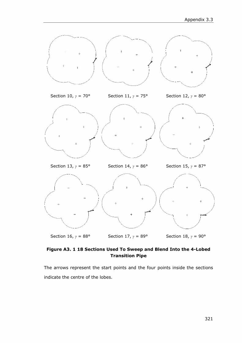
Appendix 3.3

321










Figure A3. 1 18 Sections Used To Sweep and Blend Into the 4-Lobed

Transition Pipe

The arrows represent the start points and the four points inside the sections

indicate the centre of the lobes.

Appendix 5.1

322

Appendix 5.1 Optimization of a Four-Lobed Swirl Pipe for

Clean-In-Place Procedures

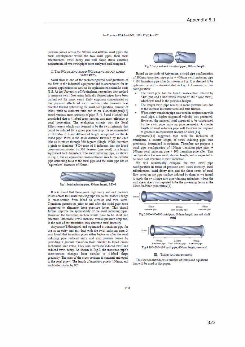
Appendix 5.1

323

Appendix 5.1

324

Appendix 5.1

325

Appendix 5.1

326

Appendix 5.1

327

Appendix 5.1

328

Appendix 5.1

329

Appendix 5.1

330

Appendix 8.1

331

Appendix 8.1 Drawing of the Optimised Swirl Pipe for

Investment Casting

Figure A8.1.1 Drawing of the transition pipe and dairy clamp connector

Appendix 8.1

332

Figure A8.1.2 Drawing of the optimized swirl pipe

Appendix 8.2

333

Appendix 8.2 Experimental and Calculated data for Calibrating the Tot-film Sensor

The experimental data of pressure and voltage and the calculated wall shear stress in cylindrical pipe flows, 𝐸𝑎2, 𝜏𝑤

1/3 for calibrating the

hot-film sensor is shown in Table A8.2.1~A8.2.5 for conditions of sensor at top, +45°, middle, -45° and bottom respectively.

Table A8.2.1 Experimental and calculated data for calibrating the hot-film sensor (sensor at top)

T

℃

Velocity

m/s

Ea2

corrected Ecorr Ea mean Ea1 Ea2 Ea3 Ea4 Ea5

Coefficient

of error of Eai

Pressure

at 1

Pa

Pressure

at 2

Pa

Pressure drop

Pa

Tw

Pa Tw

1/3

21.5 0.750 3.441 1.85493 1.85493 1.85703 1.85559 1.85405 1.85354 1.85442 0.00075 2550.880 1717.476 833.404 2.217 1.304

21.5 1.001 3.571 1.88974 1.88974 1.88991 1.88966 1.89057 1.88925 1.88930 0.00028 3204.841 1986.657 1218.184 3.240 1.480

21.5 1.250 3.636 1.90687 1.90687 1.90776 1.90643 1.90642 1.90704 1.90670 0.00029 4161.576 2479.717 1681.859 4.473 1.648

21.5 1.498 3.723 1.92961 1.92961 1.93084 1.92975 1.92877 1.92938 1.92930 0.00040 5295.704 3072.169 2223.535 5.914 1.808

21.6 1.750 3.754 1.93759 1.93507 1.93579 1.93440 1.93568 1.93498 1.93451 0.00033 6600.375 3741.069 2859.306 7.605 1.966

21.7 1.999 3.779 1.94399 1.93894 1.93875 1.93946 1.93834 1.93909 1.93906 0.00022 8071.421 4518.331 3553.090 9.450 2.114

22 2.243 3.813 1.95267 1.93995 1.94084 1.94008 1.94030 1.93918 1.93933 0.00036 9697.876 5386.864 4311.012 11.465 2.255

22.2 2.513 3.834 1.95798 1.94010 1.94127 1.94004 1.94014 1.93916 1.93990 0.00039 11690.290 6419.580 5270.710 14.018 2.411

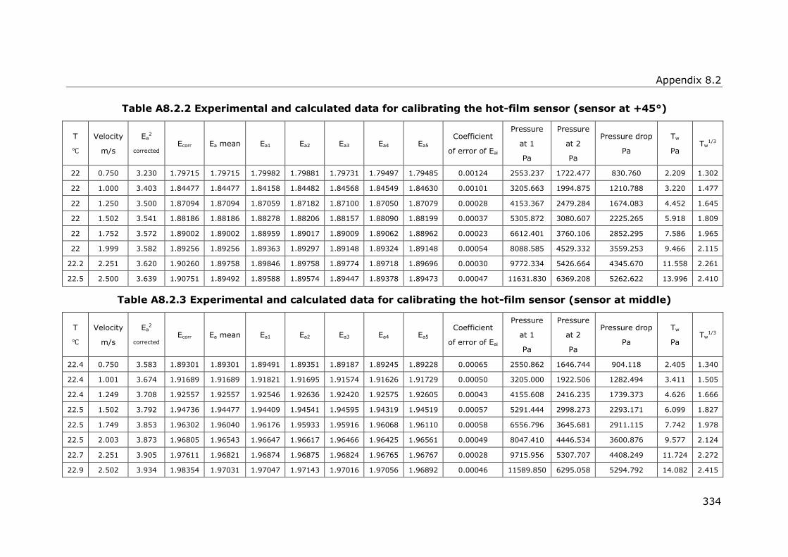
Appendix 8.2

334

Table A8.2.2 Experimental and calculated data for calibrating the hot-film sensor (sensor at +45°)

T

℃

Velocity

m/s

Ea2


Coefficient

of error of Eai

Pressure

at 1

Pa

Pressure

at 2

Pa

Pressure drop

Pa

Tw

Pa Tw

1/3

22 0.750 3.230 1.79715 1.79715 1.79982 1.79881 1.79731 1.79497 1.79485 0.00124 2553.237 1722.477 830.760 2.209 1.302

22 1.000 3.403 1.84477 1.84477 1.84158 1.84482 1.84568 1.84549 1.84630 0.00101 3205.663 1994.875 1210.788 3.220 1.477

22 1.250 3.500 1.87094 1.87094 1.87059 1.87182 1.87100 1.87050 1.87079 0.00028 4153.367 2479.284 1674.083 4.452 1.645

22 1.502 3.541 1.88186 1.88186 1.88278 1.88206 1.88157 1.88090 1.88199 0.00037 5305.872 3080.607 2225.265 5.918 1.809

22 1.752 3.572 1.89002 1.89002 1.88959 1.89017 1.89009 1.89062 1.88962 0.00023 6612.401 3760.106 2852.295 7.586 1.965

22 1.999 3.582 1.89256 1.89256 1.89363 1.89297 1.89148 1.89324 1.89148 0.00054 8088.585 4529.332 3559.253 9.466 2.115

22.2 2.251 3.620 1.90260 1.89758 1.89846 1.89758 1.89774 1.89718 1.89696 0.00030 9772.334 5426.664 4345.670 11.558 2.261

22.5 2.500 3.639 1.90751 1.89492 1.89588 1.89574 1.89447 1.89378 1.89473 0.00047 11631.830 6369.208 5262.622 13.996 2.410

Table A8.2.3 Experimental and calculated data for calibrating the hot-film sensor (sensor at middle)

T

℃

Velocity

m/s

Ea2


Coefficient

of error of Eai

Pressure

at 1

Pa

Pressure

at 2

Pa

Pressure drop

Pa

Tw

Pa Tw

1/3

22.4 0.750 3.583 1.89301 1.89301 1.89491 1.89351 1.89187 1.89245 1.89228 0.00065 2550.862 1646.744 904.118 2.405 1.340

22.4 1.001 3.674 1.91689 1.91689 1.91821 1.91695 1.91574 1.91626 1.91729 0.00050 3205.000 1922.506 1282.494 3.411 1.505

22.4 1.249 3.708 1.92557 1.92557 1.92546 1.92636 1.92420 1.92575 1.92605 0.00043 4155.608 2416.235 1739.373 4.626 1.666

22.5 1.502 3.792 1.94736 1.94477 1.94409 1.94541 1.94595 1.94319 1.94519 0.00057 5291.444 2998.273 2293.171 6.099 1.827

22.5 1.749 3.853 1.96302 1.96040 1.96176 1.95933 1.95916 1.96068 1.96110 0.00058 6556.796 3645.681 2911.115 7.742 1.978

22.5 2.003 3.873 1.96805 1.96543 1.96647 1.96617 1.96466 1.96425 1.96561 0.00049 8047.410 4446.534 3600.876 9.577 2.124

22.7 2.251 3.905 1.97611 1.96821 1.96874 1.96875 1.96824 1.96765 1.96767 0.00028 9715.956 5307.707 4408.249 11.724 2.272

22.9 2.502 3.934 1.98354 1.97031 1.97047 1.97143 1.97016 1.97056 1.96892 0.00046 11589.850 6295.058 5294.792 14.082 2.415

Appendix 8.2

335

Table A8.2.4 Experimental and calculated data for calibrating the hot-film sensor (sensor at -45°)

T

℃

Velocity

m/s

Ea2


Coefficient

of error of Eai

Pressure

at 1

Pa

Pressure

at 2

Pa

Pressure drop

Pa

Tw

Pa Tw

1/3

22.1 0.749 3.569 1.88926 1.88926 1.89172 1.88863 1.88698 1.88864 1.89031 0.00096 2589.182 1767.294 821.888 2.186 1.298

22.1 1.000 3.671 1.91608 1.91608 1.91594 1.91594 1.91603 1.91657 1.91592 0.00014 3244.629 2045.595 1199.034 3.189 1.472

22.1 1.250 3.697 1.92277 1.92277 1.92521 1.92406 1.92259 1.92174 1.92025 0.00101 4200.877 2542.147 1658.730 4.412 1.640

22.1 1.498 3.790 1.94671 1.94671 1.94713 1.94724 1.94684 1.94636 1.94601 0.00027 5327.060 3125.848 2201.212 5.854 1.802

22.2 1.753 3.831 1.95729 1.95471 1.95489 1.95471 1.95561 1.95388 1.95446 0.00032 6649.118 3816.713 2832.405 7.533 1.960

22.4 2.001 3.874 1.96825 1.96045 1.96013 1.96098 1.96004 1.96052 1.96058 0.00019 8131.750 4586.707 3545.043 9.428 2.113

22.5 2.238 3.902 1.97545 1.96500 1.96552 1.96531 1.96485 1.96456 1.96476 0.00020 9730.105 5423.617 4306.488 11.453 2.254

22.6 2.498 3.917 1.97902 1.96592 1.96535 1.96698 1.96576 1.96509 1.96642 0.00039 11690.910 6468.104 5222.806 13.890 2.404

Table A8.2.5 Experimental and calculated data for calibrating the hot-film sensor (sensor at bottom)

T

℃

Velocity

m/s

Ea2


Coefficient

of error of Eai

Pressure

at 1

Pa

Pressure

at 2

Pa

Pressure drop

Pa

Tw

Pa Tw

1/3

22.5 0.750 3.639 1.90761 1.90761 1.90456 1.90725 1.90782 1.91020 1.90820 0.00106 2545.863 1754.958 790.905 2.103 1.281

22.5 1.003 3.731 1.93168 1.93168 1.93168 1.93234 1.93307 1.93011 1.93118 0.00058 3206.430 2024.181 1182.249 3.144 1.465

22.5 1.250 3.797 1.94846 1.94846 1.94998 1.94670 1.94865 1.94897 1.94801 0.00063 4163.741 2544.002 1619.739 4.308 1.627

22.6 1.502 3.861 1.96496 1.96233 1.96295 1.96436 1.96153 1.96124 1.96160 0.00067 5307.829 3109.221 2198.608 5.847 1.802

22.6 1.754 3.890 1.97235 1.96972 1.97151 1.97114 1.96848 1.96850 1.96896 0.00075 6620.224 3792.948 2827.276 7.519 1.959

22.7 1.994 3.917 1.97917 1.97388 1.97273 1.97511 1.97321 1.97423 1.97413 0.00047 8052.990 4553.290 3499.700 9.308 2.104

22.9 2.236 3.956 1.98896 1.97832 1.97899 1.97837 1.97759 1.97816 1.97850 0.00026 9672.930 5412.948 4259.982 11.330 2.246

23 2.514 3.976 1.99403 1.98069 1.98192 1.98133 1.97985 1.98032 1.98003 0.00045 11686.510 6456.997 5229.513 13.908 2.405

investigation of swirl pipe for improving cleaning efficiency in ...

Documents

Transcript of investigation of swirl pipe for improving cleaning efficiency in ...