Chapter 4 – Pipe Flow

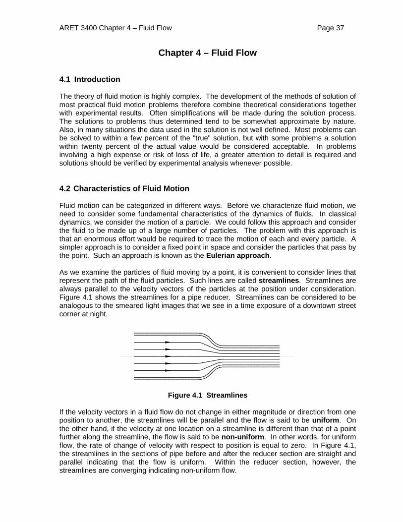
ARET 3400 Chapter 4 – Fluid Flow Page 37

Chapter 4 – Fluid Flow 4.1 Introduction The theory of fluid motion is highly complex. The development of the methods of solution of most practical fluid motion problems therefore combine theoretical considerations together with experimental results. Often simplifications will be made during the solution process. The solutions to problems thus determined tend to be somewhat approximate by nature. Also, in many situations the data used in the solution is not well defined. Most problems can be solved to within a few percent of the "true" solution, but with some problems a solution within twenty percent of the actual value would be considered acceptable. In problems involving a high expense or risk of loss of life, a greater attention to detail is required and solutions should be verified by experimental analysis whenever possible. 4.2 Characteristics of Fluid Motion Fluid motion can be categorized in different ways. Before we characterize fluid motion, we need to consider some fundamental characteristics of the dynamics of fluids. In classical dynamics, we consider the motion of a particle. We could follow this approach and consider the fluid to be made up of a large number of particles. The problem with this approach is that an enormous effort would be required to trace the motion of each and every particle. A simpler approach is to consider a fixed point in space and consider the particles that pass by the point. Such an approach is known as the Eulerian approach. As we examine the particles of fluid moving by a point, it is convenient to consider lines that represent the path of the fluid particles. Such lines are called streamlines. Streamlines are always parallel to the velocity vectors of the particles at the position under consideration. Figure 4.1 shows the streamlines for a pipe reducer. Streamlines can be considered to be analogous to the smeared light images that we see in a time exposure of a downtown street corner at night.

Figure 4.1 Streamlines If the velocity vectors in a fluid flow do not change in either magnitude or direction from one position to another, the streamlines will be parallel and the flow is said to be uniform. On the other hand, if the velocity at one location on a streamline is different than that of a point further along the streamline, the flow is said to be non-uniform. In other words, for uniform flow, the rate of change of velocity with respect to position is equal to zero. In Figure 4.1, the streamlines in the sections of pipe before and after the reducer section are straight and parallel indicating that the flow is uniform. Within the reducer section, however, the streamlines are converging indicating non-uniform flow.


If the velocity vectors at a given position remain constant in both magnitude and direction over the period of time under consideration, then the flow is referred to as being steady. On the other hand, if the velocity at a given position varies with time, the flow is said to be unsteady or non-steady. Examples of the various types of flow and their characteristics are summarized in Table 4.1. Table 4.1 Types of Flow

Type of Flow Example Steady, uniform flow Flow at a constant rate through a long

straight pipe of constant cross-section. Steady non-uniform flow Flow at a constant rate through a tapering

pipe. Non-steady, uniform flow Accelerating or decelerating flow through a

long straight pipe of constant cross-section. Non-steady, non-uniform flow Accelerating or decelerating flow through a

tapering pipe. The majority of the problems addressed in this text will involve steady uniform flow. However, we will examine non-uniform flow in open channels, and will consider unsteady flow when examining a phenomenon known as 'water hammer'. 4.2 Laminar and Turbulent Flow In addition to the classifications discussed in Section 4.1, fluid flow can be classified as either laminar or turbulent. In laminar flow, the streamlines move in smooth consistent paths. In turbulent flow, the particle motion is random. In general, if the flow is slow and/or the fluid is highly viscous, the flow will be laminar, whereas if the flow is rapid and/or the viscosity of the fluid is low, the flow will be turbulent. Technically, turbulent flow will be non-steady. At a given location, the velocity will vary with time. However, if we average the velocity over a reasonable period of time, the time- averaged velocity will be constant and the flow can then be considered to be steady flow. When studying the causes and conditions for turbulent flow, Reynolds determined that the ratio of the inertia forces to the viscous forces was an important parameter. We can consider Newton's second law, ΣF = ma, as being applied to a 'particle' of fluid. The right side of the equation represents the 'inertia forces'. The sum of the forces on the left side of the equation consists of the pressure force, Fp, which tends to drive the motion of the fluid and the viscous or friction force, Fv, which tends to retard the motion. In order to satisfy the equation the vector sum of the pressure force and the viscous force equals the 'inertia force'. This is shown graphically in Figure 4.2.

Figure 4.2 Forces acting on a particle of fluid

ARET 3400 Chapter 4 – Fluid Flow 9

The ratio of the inertia forces to the viscous forces is known as Reynolds number and, for a closed conduit, can be represented as

ν

=vdNR (4.1)

where v = velocity of the fluid d = a characteristic dimension (the diameter for a round pipe)

ν = kinematic viscosity = ρµ .

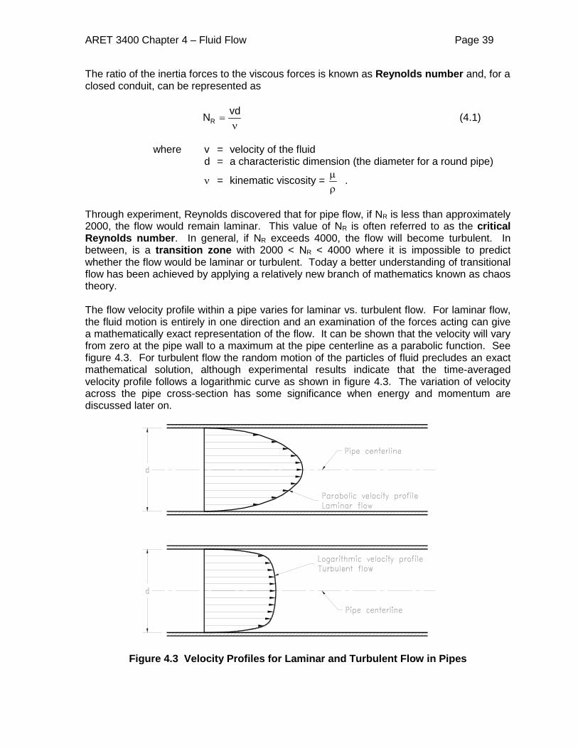
Through experiment, Reynolds discovered that for pipe flow, if NR is less than approximately 2000, the flow would remain laminar. This value of NR is often referred to as the critical Reynolds number. In general, if NR exceeds 4000, the flow will become turbulent. In between, is a transition zone with 2000 < NR < 4000 where it is impossible to predict whether the flow would be laminar or turbulent. Today a better understanding of transitional flow has been achieved by applying a relatively new branch of mathematics known as chaos theory. The flow velocity profile within a pipe varies for laminar vs. turbulent flow. For laminar flow, the fluid motion is entirely in one direction and an examination of the forces acting can give a mathematically exact representation of the flow. It can be shown that the velocity will vary from zero at the pipe wall to a maximum at the pipe centerline as a parabolic function. See figure 4.3. For turbulent flow the random motion of the particles of fluid precludes an exact mathematical solution, although experimental results indicate that the time-averaged velocity profile follows a logarithmic curve as shown in figure 4.3. The variation of velocity across the pipe cross-section has some significance when energy and momentum are discussed later on.

Figure 4.3 Velocity Profiles for Laminar and Turbulent Flow in Pipes

ARET 3400 Chapter 4 – Fluid Flow 0

Example 4.1

Oil with a relative density of 0.925 and an absolute viscosity of 0.10 Pa⋅s flows through a 6.0 mm diameter pipe with a mean velocity of 2.0 m/s. Will the flow be laminar or turbulent? Solution:

20000.11110.0

)006.0)(/0.2)(/1000)(925.0( 3

<=⋅

===sPa

msmmkgvdvdNR µρ

ν

Therefore the flow will be laminar.

4.3 The Continuity Equation for Steady Incompressible Flows Many problems in engineering can be solved by considering the flow to be steady and incompressible. For most problems, liquids can be considered incompressible, although, as was noted in Section 2.7, they do compress to a certain degree. Figure 4.4 shows a section of pipe with a liquid flowing through it. We will consider the body of fluid that initially lies between the between sections 1-1 and 2-2. Such a body of fluid is known as a control volume. In some ways it is analogous to the free-body diagram used in statics.

Figure 4.4 Flow through a control volume

The mass of the fluid entering the control volume in a period of time, ∆t, can be given as ρv1A1∆t, where v1 is the velocity of fluid entering the control volume and A1 is the cross-sectional area of the pipe at section 1-1. Similarly the mass leaving the control volume is ρv2A2∆t. For incompressible steady flow, the principle of conservation of mass requires that the mass entering the control volume equals the mass leaving the control volume. We have ρv1A1∆t = ρv2A2∆t Dividing through by ρ and ∆t gives v1A1 = v2A2 = Q (4.2) where Q is the volume flow rate (usually in m3/s).


Equation 4.2 is known as the steady state continuity equation for incompressible flow. It should be noted that the velocities indicated are the mean velocities.

Example 4.2

Water flows through a pipe reducer section at a rate of 30 L/s. The pipe diameter before the reducer is 200 mm and the diameter after the reducer is 150 mm. Determine the velocity in both sections of pipe. Solution:

=== 2

3

11 )200.0(

4)/03.0(msm

AQv

π0.955 m/s === 2

3

22 )150.0(

4)/030.0(m

smAQv

π1.698 m/s

4.4 The Energy Equation As well as satisfying the principle of conservation of mass, the principle of conservation of energy must also be satisfied. Energy can take many forms. In applying the principle of conservation of energy, we will consider potential energy due to position in the earth's gravitational field, kinetic energy, pressure energy, heat energy and shaft work. Consider the device shown in Figure 4.5. The fluid enters the device with potential, kinetic and pressure energy. Within the device, heat energy may be added to the fluid and/or heat energy will be lost due to friction (viscous drag). In addition, the device may do some shaft work as for example power a turbine.

Figure 4.5 Energy in a fluid flow


Pressure energy: Pressure energy is another form of potential energy and is equal to the product of the pressure and a volume. For an incompressible fluid, the volume of fluid entering the control volume during the time period, ∆t, is the same as that leaving and is equal to Q∆t. The pressure energy of the fluid entering the system is given as p1Q∆t and the pressure energy of the fluid leaving the system is p2Q∆t. Gravitational Potential Energy: The mass entering the system in a given period of time, ∆t, is ρv1A1∆t = ρQ∆t. The potential energy, m⋅g⋅h, of this mass is P.E.1 = ρQ∆t⋅g⋅z1. Similarly the potential energy of the mass leaving the control volume is P.E.2 = ρQ∆t⋅g⋅z2. Kinetic Energy: The kinetic energy is given by ½mv2. Therefore, the mass entering the control volume during the time, ∆t, has kinetic energy K.E.1 = ½ ρQ∆t⋅v1

2 and the mass leaving the system has kinetic energy K.E.2 = ½ ρQ∆t⋅v2

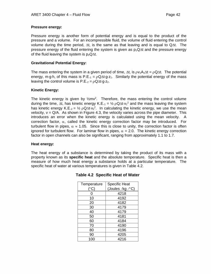
2. In calculating the kinetic energy, we use the mean velocity, v = Q/A. As shown in Figure 4.3, the velocity varies across the pipe diameter. This introduces an error when the kinetic energy is calculated using the mean velocity. A correction factor, α, called the kinetic energy correction factor may be introduced. For turbulent flow in pipes, α ≈ 1.05. Since this is close to unity, the correction factor is often ignored for turbulent flow. For laminar flow in pipes, α = 2.0. The kinetic energy correction factor in open channels can also be significant, ranging from approximately 1.1 to 1.7. Heat energy: The heat energy of a substance is determined by taking the product of its mass with a property known as its specific heat and the absolute temperature. Specific heat is then a measure of how much heat energy a substance holds at a particular temperature. The specific heat of water at various temperatures is given in Table 4.2. Table 4.2 Specific Heat of Water

Temperature (°C)

Specific Heat (Joules ⁄ kg ⁄ °C)

0 4218 10 4192 20 4182 30 4179 40 4179 50 4181 60 4184 70 4190 80 4196 90 4205 100 4216


The fluid entering the system has a heat energy given as ρQ∆t⋅e1, where e1 is the energy per unit mass for the fluid entering the system. Similarly the heat energy of the fluid leaving the system is ρQ∆t⋅e2. In addition heat may be added to the system. The heat added to the system per unit mass will be designated as q. Shaft Work: The shaft work done by the system per unit mass will be designated as w'. Energy Balance: The energy balance will be done on a per unit mass basis. The gravitational, kinetic, pressure, and heat energy terms will have to be divided by ρQ∆t to obtain energy per unit mass. The energy per unit mass being added to the system is:

ρ

1p + 2

v 21 + g⋅z1 + e1 + q (4.3)

The energy per unit mass taken out of the system is:

ρ2p +

2v 2

2 + g⋅z2 + e2 + w' (4.4)

The law of conservation of energy states that the energy must balance; that is that the total system energy must remain constant. It is customary to divide through by g and represent the energies as energy head with units of metres (or feet). This in effect gives the energy per unit weight. Equating 4.3 and 4.4, and dividing through by g gives:

g

p1

ρ +

g2v 2

1 + z1 + g

q ee 21 +− = g

p2

ρ +

g2v 2

2 + z2 + gw' (4.5)

In most cases the only heat transfer that takes place is due to heat generated by friction. In these situations this heat is lost from the system and the q is negative (-q). The total head lost to friction, hf, can then given by

hf = g

q ee 12 −− (4.6)

Rewriting equation 4.5 substituting in 4.6 gives

gp1

ρ +

g2v 2

1 + z1 – hf = g

p2

ρ +

g2v 2

2 + z2 + gw' (4.7)


Equation 4.7 is known as the steady flow energy equation. It should be noted that, in the form given, it is valid only for constant density fluids. The term w' ⁄ g represents the shaft work per unit weight done by the fluid. When shaft work is done on the fluid as for instance from the action of a pump, w' ⁄ g will be negative. In some problems, friction may be neglected and if there is no shaft work done by or on the fluid, then equation 4.7 reduces to

gp1

ρ +

g2v 2

1 + z1 = g

p2

ρ +

g2v 2

2 + z2 (4.8)

Equation 4.8 is known as Bernoulli's equation. In this text we will normally use the more general equation 4.7.

Example 4.3

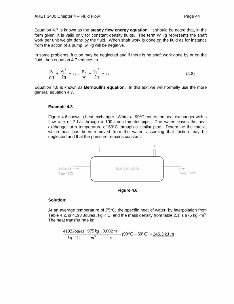
Figure 4.6 shows a heat exchanger. Water at 90°C enters the heat exchanger with a flow rate of 2 L/s through a 100 mm diameter pipe. The water leaves the heat exchanger at a temperature of 60°C through a similar pipe. Determine the rate at which heat has been removed from the water, assuming that friction may be neglected and that the pressure remains constant.

Figure 4.6 Solution: At an average temperature of 75°C, the specific heat of water, by interpolation from Table 4.2, is 4193 Joules ⁄ kg ⁄ °C, and the mass density from table 2.1 is 975 kg ⁄ m3. The heat transfer rate is:

=°−°⋅⋅⋅°⋅

C)60C90(002.0975C

4193 3

3 sm

mkg

kgJoules

245.3 kJ ⁄ s


4.5 Hydraulic and Energy Grade Lines As a further clarification of the energy head in a pipeline, consider the diagram in Figure 4.7.

Figure 4.7 Energy and Hydraulic grade lines In the reservoir, the entire energy head consists of potential energy. As the liquid flows through the pipe, energy loss due to friction reduces the total head by an amount hf that is proportional to the distance traveled in the pipe. A plot of the total available energy head is called the energy grade line (EGL). The EGL will have sudden drops at locations where minor losses occur, such as at fittings. As the water enters the pipe, it accelerates. A portion of the energy head in the pipe consists of kinetic energy, represented by v2/2g (neglecting the energy correction factor). A line can be plotted which represents the subtraction of the kinetic energy from the EGL. This line, known as the hydraulic grade line (HGL), represents the sum of the potential and pressure energy. 4.6 Friction Head Losses Friction head losses occur throughout the length of a pipe due to viscous drag. For turbulent flow, the head loss to friction, hf, cannot be explicitly determined by direct application of mathematical and physical theory. The most popular formula based on experiment was derived by the French Engineer Henri Darcy (1803 – 1858) and the German Professor Julius Weisbach (1806 – 1871) in about 1845. This formula is therefore known as the Darcy – Weisbach formula, and is given as

g2v

dLfh

2

f ⋅= (4.9)

where f = Darcy-Weisbach friction factor L = length of pipe d = pipe diameter v = fluid velocity g = gravitational acceleration


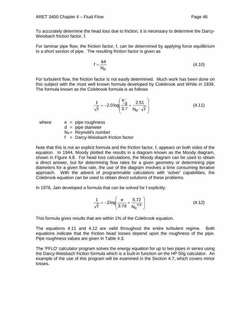
To accurately determine the head loss due to friction, it is necessary to determine the Darcy-Weisbach friction factor, f. For laminar pipe flow, the friction factor, f, can be determined by applying force equilibrium to a short section of pipe. The resulting friction factor is given as

RN64f = (4.10)

For turbulent flow, the friction factor is not easily determined. Much work has been done on this subject with the most well known formula developed by Colebrook and White in 1939. The formula known as the Colebrook formula is as follows

⋅+−=

fN51.2

7.3d

elog0.2

f1

R (4.11)

where e = pipe roughness

d = pipe diameter NR = Reynold's number f = Darcy-Weisbach friction factor

Note that this is not an explicit formula and the friction factor, f, appears on both sides of the equation. In 1944, Moody plotted the results in a diagram known as the Moody diagram, shown in Figure 4.8. For head loss calculations, the Moody diagram can be used to obtain a direct answer, but for determining flow rates for a given geometry or determining pipe diameters for a given flow rate, the use of the diagram involves a time consuming iterative approach. With the advent of programmable calculators with 'solver' capabilities, the Colebrook equation can be used to obtain direct solutions of these problems. In 1976, Jain developed a formula that can be solved for f explicitly:

+−= 9.0

RN72.5

d7.3elog2

f1 (4.12)

This formula gives results that are within 1% of the Colebrook equation. The equations 4.11 and 4.12 are valid throughout the entire turbulent regime. Both equations indicate that the friction head losses depend upon the roughness of the pipe. Pipe roughness values are given in Table 4.3. The 'PFLO' calculator program solves the energy equation for up to two pipes in series using the Darcy-Weisbach friction formula which is a built-in function on the HP 50g calculator. An example of the use of this program will be examined in the Section 4.7, which covers minor losses.


Table 4.3 Pipe Roughness Values

Pipe Material e (mm) e(ft) Drawn Tubing, Plastic 0.0015 0.000005 Commercial Steel (enamel coated) 0.0048 0.000016 Commercial Steel (new) 0.045 0.00015 Cast Iron, Ductile Iron (new) 0.26 0.00085 Cast Iron (asphalt coated) 0.12 0.0004 Galvanized Iron 0.15 0.0005 Corrugated metal 45 0.15 Concrete (steel forms, smooth) 0.18 0.0006 Concrete (average) 0.36 0.0012 Concrete (rough, visible form marks) 0.60 0.002

Figure 4.8 Moody Diagram 4.7 Hazen-Williams Formula for Friction Losses in Pipes The Hazen-Williams formula is an empirical formula, which was developed to determine losses due to friction for water flow in pipes. The formula gives reasonable results for pipe sizes greater than or equal to 50 mm in diameter and for velocities of less 3 m/s. This is typical of the ranges found in most municipal water supply systems, where the pipe sizes are usually 150 mm or larger and the velocities are usually restricted to a maximum of 2 m/s. Because the formula is empirical and is not dimensionally correct, there are two versions of the formula, one for metric and one for the fps or British system.


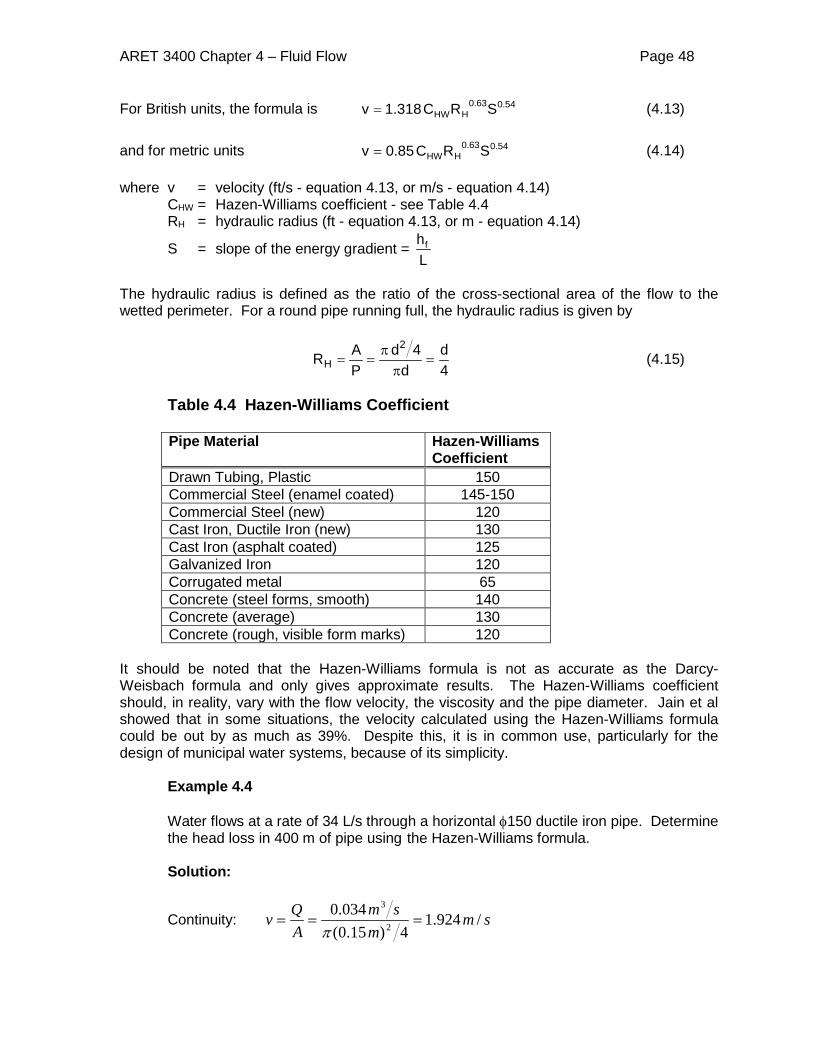
For British units, the formula is 54.063.0HHW SRC318.1v = (4.13)

and for metric units 54.063.0

HHW SRC85.0v = (4.14) where v = velocity (ft/s - equation 4.13, or m/s - equation 4.14) CHW = Hazen-Williams coefficient - see Table 4.4 RH = hydraulic radius (ft - equation 4.13, or m - equation 4.14)

S = slope of the energy gradient = Lhf

The hydraulic radius is defined as the ratio of the cross-sectional area of the flow to the wetted perimeter. For a round pipe running full, the hydraulic radius is given by

4d

d4d

PAR

2

H =π

π== (4.15)

Table 4.4 Hazen-Williams Coefficient

Pipe Material Hazen-Williams Coefficient

Drawn Tubing, Plastic 150 Commercial Steel (enamel coated) 145-150 Commercial Steel (new) 120 Cast Iron, Ductile Iron (new) 130 Cast Iron (asphalt coated) 125 Galvanized Iron 120 Corrugated metal 65 Concrete (steel forms, smooth) 140 Concrete (average) 130 Concrete (rough, visible form marks) 120

It should be noted that the Hazen-Williams formula is not as accurate as the Darcy-Weisbach formula and only gives approximate results. The Hazen-Williams coefficient should, in reality, vary with the flow velocity, the viscosity and the pipe diameter. Jain et al showed that in some situations, the velocity calculated using the Hazen-Williams formula could be out by as much as 39%. Despite this, it is in common use, particularly for the design of municipal water systems, because of its simplicity.

Example 4.4 Water flows at a rate of 34 L/s through a horizontal φ150 ductile iron pipe. Determine the head loss in 400 m of pipe using the Hazen-Williams formula. Solution:

Continuity: smm

smAQv /924.1

4)15.0(034.0

2

3

===π


Hazen-Williams:

02546.0)4/150.0)(130(85.0

/924.185.0

54.01

63.0

54.01

63.0 =

=

=

msm

RCvS

HHW

=⋅=⋅= )400()02546.0(LSh f m 10.19 m

4.8 Minor Losses In addition to the friction head losses that occur throughout the length of the pipe, losses occur due to turbulence at elbows, bends, tees, valve fittings etc. as well as at entrances and exits and where contraction or expansion takes place. These losses are called minor losses, however, in short runs with many fixtures, they can be very significant. In general minor losses are dependent upon the square of the velocity. One approach to including minor losses involves assigning a K factor to each minor loss. The losses are

expressed in terms of g2

v2. The total loss in the system is then given as

g2vK

dLfh

2

f

∑+= (4.16)

where ΣK represents the sum of the minor loss K factors. A summary of common K factors is given in table 4.5, but where possible K factors should be obtained from valve and fitting manufacturer's data as the tabulated values are approximate. Another approach is to use what is known as the equivalent length method. With this method, an equivalent length of straight pipe is added to the length used in the Darcy-Weisbach equation. The equivalent length may be obtained from manufacturer's data or may be determined from a known K factor. The equivalent length, Le, in terms of K is

fdKLe⋅

= (4.17)

Note that equation 4.17 implies that the equivalent length depends upon the friction factor, f, which in turn implies that it is dependent upon the velocity and viscosity as well as the pipe roughness. Equivalent lengths from manufacturers are usually constant for a given diameter, and therefore results obtained using this method are approximate in nature. They are usually valid for a particular fluid and may reflect a flow velocity that is reasonable for a design situation where the fitting is likely to be used. In this text, we shall use the minor loss coefficient or K factor method.


Table 4.5 Loss Coefficients for Valves and Fittings

Item K Standard 45° Elbow 0.35 Standard 90° Elbow 0.75 Long Radius 90° Elbow 0.45 Coupling 0.04 Union 0.04 Gate Valve Open 0.2 ¾ Open 0.9 ½ Open 4.5 ¼ Open 24.0 Globe Valve Open 6.4 ½ Open 9.5 Tee (along run, line flow) 0.4 Tee (branch flow) 1.5 Entrance loss (flush end) 0.5 Entrance loss (projecting end) 1.0 Exit loss (pipe to tank) 1.0 Sudden Contraction (d/D = 0.50) 0.32 " " (d/D = 0.25) 0.39 " " (d/D = 0.10) 0.46 Sudden Expansion (d/D = 0.50) 0.56 " " (d/D = 0.25) 0.88 " " (d/D = 0.10) 0.99

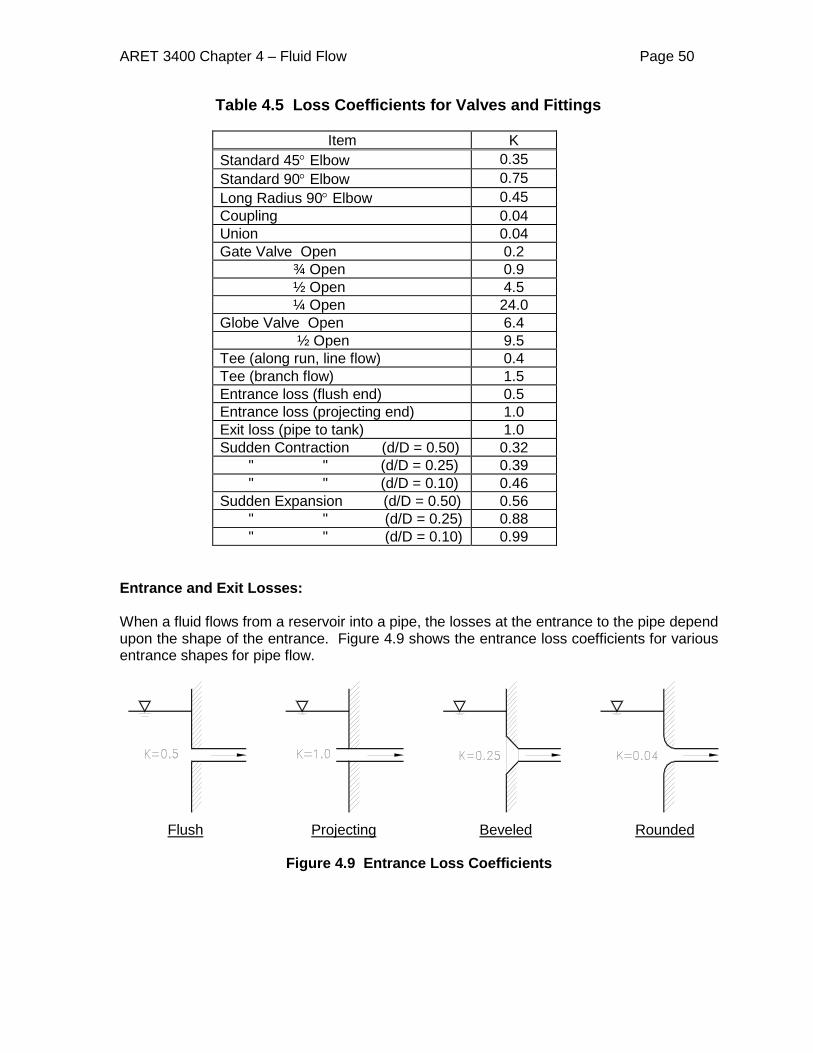
Entrance and Exit Losses: When a fluid flows from a reservoir into a pipe, the losses at the entrance to the pipe depend upon the shape of the entrance. Figure 4.9 shows the entrance loss coefficients for various entrance shapes for pipe flow.

Flush Projecting Beveled Rounded

Figure 4.9 Entrance Loss Coefficients


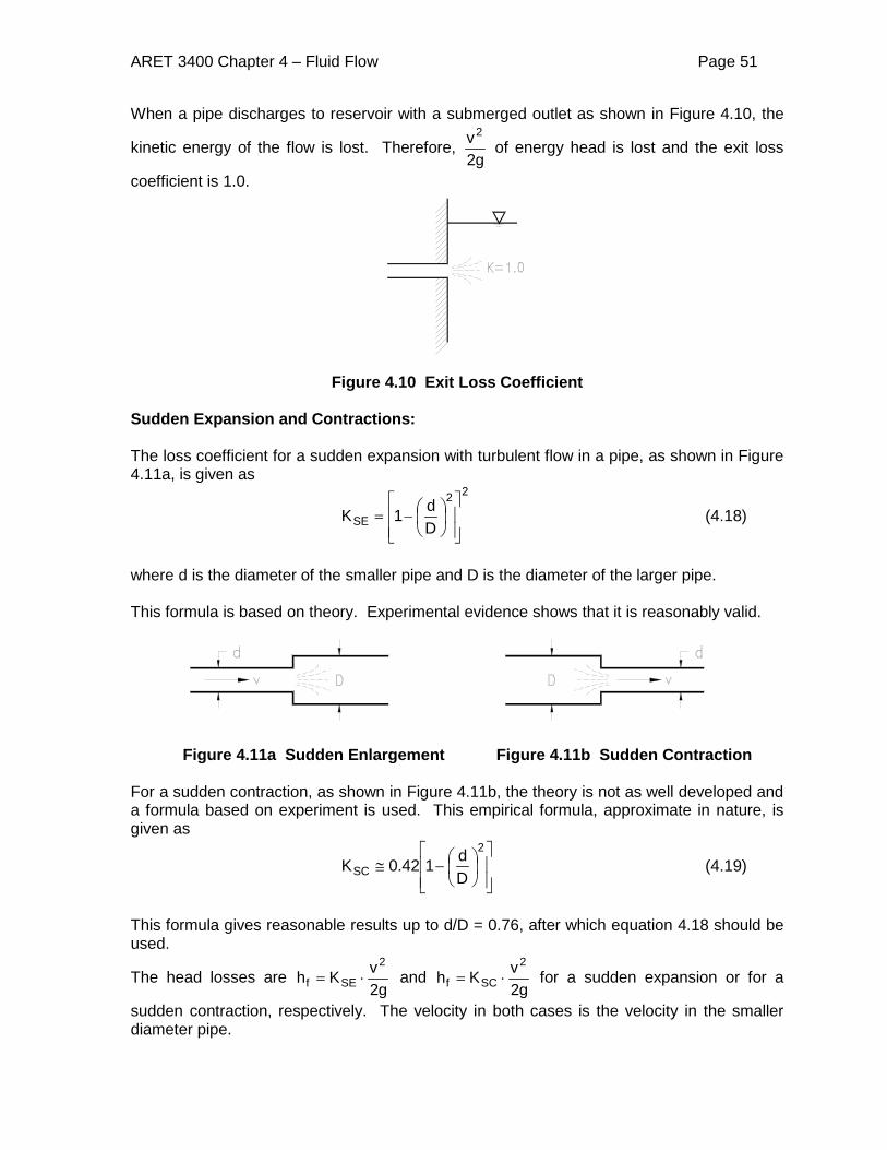
When a pipe discharges to reservoir with a submerged outlet as shown in Figure 4.10, the

kinetic energy of the flow is lost. Therefore, g2

v2 of energy head is lost and the exit loss

coefficient is 1.0.

Figure 4.10 Exit Loss Coefficient

Sudden Expansion and Contractions: The loss coefficient for a sudden expansion with turbulent flow in a pipe, as shown in Figure 4.11a, is given as

22

SE Dd1K

−= (4.18)

where d is the diameter of the smaller pipe and D is the diameter of the larger pipe.

This formula is based on theory. Experimental evidence shows that it is reasonably valid.

Figure 4.11a Sudden Enlargement Figure 4.11b Sudden Contraction For a sudden contraction, as shown in Figure 4.11b, the theory is not as well developed and a formula based on experiment is used. This empirical formula, approximate in nature, is given as

−≅

2

SC Dd142.0K (4.19)

This formula gives reasonable results up to d/D = 0.76, after which equation 4.18 should be used.

The head losses are g2

vKh2

SEf ⋅= and g2

vKh2

SCf ⋅= for a sudden expansion or for a

sudden contraction, respectively. The velocity in both cases is the velocity in the smaller diameter pipe.


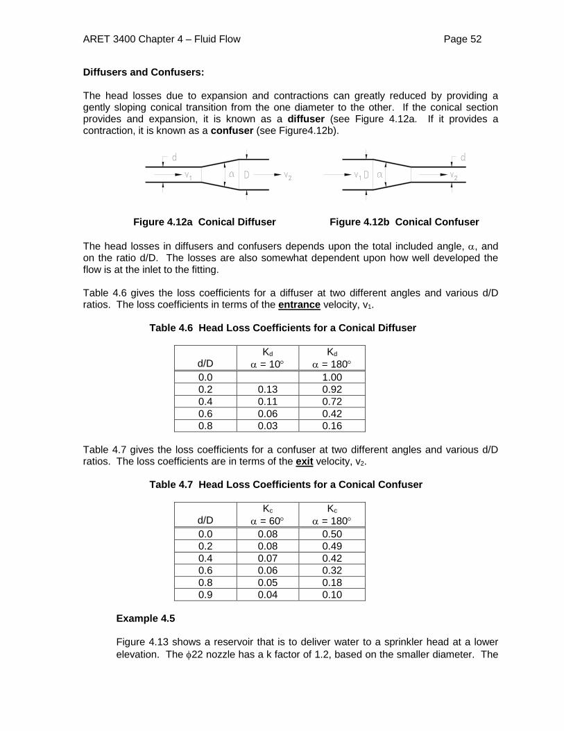
Diffusers and Confusers: The head losses due to expansion and contractions can greatly reduced by providing a gently sloping conical transition from the one diameter to the other. If the conical section provides and expansion, it is known as a diffuser (see Figure 4.12a. If it provides a contraction, it is known as a confuser (see Figure4.12b).

Figure 4.12a Conical Diffuser Figure 4.12b Conical Confuser

The head losses in diffusers and confusers depends upon the total included angle, α, and on the ratio d/D. The losses are also somewhat dependent upon how well developed the flow is at the inlet to the fitting. Table 4.6 gives the loss coefficients for a diffuser at two different angles and various d/D ratios. The loss coefficients in terms of the entrance velocity, v1. Table 4.6 Head Loss Coefficients for a Conical Diffuser

d/D

Kd α = 10°

Kd α = 180°

0.0 1.00 0.2 0.13 0.92 0.4 0.11 0.72 0.6 0.06 0.42 0.8 0.03 0.16

Table 4.7 gives the loss coefficients for a confuser at two different angles and various d/D ratios. The loss coefficients are in terms of the exit velocity, v2. Table 4.7 Head Loss Coefficients for a Conical Confuser

d/D

Kc α = 60°

Kc α = 180°

0.0 0.08 0.50 0.2 0.08 0.49 0.4 0.07 0.42 0.6 0.06 0.32 0.8 0.05 0.18 0.9 0.04 0.10

Example 4.5 Figure 4.13 shows a reservoir that is to deliver water to a sprinkler head at a lower elevation. The φ22 nozzle has a k factor of 1.2, based on the smaller diameter. The


water is to discharge from the nozzle with a velocity of 28m/s. The 1400m long aluminum pipe has an e = 0.00004m, and includes an open gate valve. Using the HP 50g calculator program 'PFLO', determine:

a.) The volume flow rate for this discharge. b.) The height h at which the water in the reservoir must be kept in order to get this

discharge rate.

Figure 4.13

Solution: a.) From continuity, the required flow rate is

Q = v⋅A = smmsm /01064.04

)022.0()/28( 32

=⋅π

, or 10.64 L/s.

b.) With the 'PFLO' program, the exit loss must be added to the sum of the K factors.

Since the nozzle is a different diameter than the pipe, the pipeline will have to be modeled as two pipes in series. The loss in the nozzle is taken care of, so the length of φ22 mm pipe can be taken as zero. The ΣK2 is then determined as follows

Knozzle = 1.2 Kexit = 1.0 to account for the exit loss (v2 present). __________ ΣK2 = 2.2

Summing up the minor loss coefficients in the pipe gives Kentrance = 0.50 Kvalve = 0.20 3 × K45 = 1.05 K90 = 0.73

____________ ΣK1 = 2.5


The input to the 'PFLO' program is summarized below: p1 = 0 p2 =0 ρ = 999 kg/m3 g = 9.81 m/s2 z1 = ? z2 = 0 e1 =0.00004 m d1 = 0.075 m Q = 0.01064 m3/s ν = 1.306 × 10-6 m2/s L1 =1400m ΣK1 = 2.5 e2 = 0.00004 m d2 = 0.022 m L2 = 0 ΣK2 = 2.2 w' = 0 Solving for h = z1 gives h = 197.3 m.

Try other ways:

4.9 Pipelines and Pipe Networks Pipelines: If all the elements of a pipe system are connected in series, the system is known as a pipeline. The 'PFLO' program is designed to solve pipeline problems with up to two different diameters of pipe. As shown in the previous example, however, a nozzle with a given diameter must be treated like a pipe of different diameter to properly account for the exit loss. The 'PFLO' program can be used to solve pipeline problems involving up to four different diameters of pipes on an iterative basis.

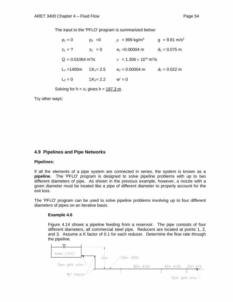
Example 4.6 Figure 4.14 shows a pipeline feeding from a reservoir. The pipe consists of four different diameters, all commercial steel pipe. Reducers are located at points 1, 2, and 3. Assume a K factor of 0.1 for each reducer. Determine the flow rate through the pipeline.


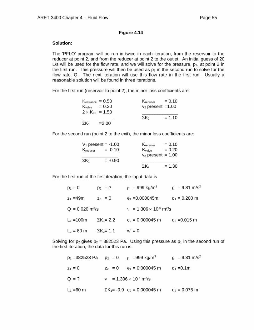
Figure 4.14 Solution: The 'PFLO' program will be run in twice in each iteration; from the reservoir to the reducer at point 2, and from the reducer at point 2 to the outlet. An initial guess of 20 L/s will be used for the flow rate, and we will solve for the pressure, p2, at point 2 in the first run. This pressure will then be used as p1 in the second run to solve for the flow rate, Q. The next iteration will use this flow rate in the first run. Usually a reasonable solution will be found in three iterations. For the first run (reservoir to point 2), the minor loss coefficients are:

Kentrance = 0.50 Kreducer = 0.10 Kvalve = 0.20 v2 present =1.00 2 × K90 = 1.50 ______________ ____________ ΣK2 = 1.10

ΣK1 =2.00 For the second run (point 2 to the exit), the minor loss coefficients are:

V1 present = -1.00 Kreducer = 0.10 Kreducer = 0.10 Kvalve = 0.20 ______________ v2 present = 1.00 ΣK1 = -0.90 ______________ ΣK2 = 1.30

For the first run of the first iteration, the input data is

p1 = 0 p2 = ? ρ = 999 kg/m3 g = 9.81 m/s2 z1 =49m z2 = 0 e1 =0.000045m d1 = 0.200 m Q = 0.020 m3/s ν = 1.306 × 10-6 m2/s L1 =100m ΣK1 = 2.2 e2 = 0.000045 m d2 =0.015 m L2 = 80 m ΣK2 = 1.1 w' = 0

Solving for p2 gives p2 = 382523 Pa. Using this pressure as p1 in the second run of the first iteration, the data for this run is:

p1 =382523 Pa p2 = 0 ρ =999 kg/m3 g = 9.81 m/s2 z1 = 0 z2 = 0 e1 = 0.000045 m d1 =0.1m Q = ? ν = 1.306 × 10-6 m2/s L1 =60 m ΣK1= -0.9 e2 = 0.000045 m d2 = 0.075 m


L2 = 20 m ΣK2= 1.2 w' = 0

Solving for Q gives Q = 0.0403 m3/s. The second iteration starts the first run with this value for Q and yields a new Q = 0.03885 m3/s. A third iteration starting with a Q of 0.03885 m3/s yields a new Q = 0.0390 m3/s. The change from the previous iteration is negligible so the final answer can be given as Q = 0.0390 m3/s or 39.0 L/s.

Pipe Networks: A system in which the elements are not in series is known as a pipe network. One of the simplest forms of pipe networks consists of a single branch flow as shown in Figure 4.15.

Figure 4.15

Usually with such a system, the total flow rate, Q, is known and it is desired to determine the flow rate in each branch, Q1 and Q2. The proportion of the flow that enters a given branch is dependent upon the frictional resistance in that branch. The solution is based on two principles that can be applied to larger, more complicated networks. The first principle is that continuity or conservation of mass can be applied to each node. In other words, the sum of the flows entering a node must equal the sum of the flows leaving the node. In Figure 4.15, this principle yields the following equation: Q = Q1 + Q2 (4.20) The second principle states that the energy head at any given point can only have a single unique value. This principle implies that the head loss to friction through branch 1 must be the same as the head loss through branch 2, or hf1 = hf2 (4.21) In more complicated networks, a direction of flow is assumed for each line. This principle is then applied by stating that the sum of the head losses around any loop must be zero. Head losses are summed in one direction, usually counter-clockwise. For example, when moving counter-clockwise around the single loop in the network shown in Figure 4.15, hf2 would be positive because the direction of Q2 matches the counter-clockwise loop direction. On the other hand, hf1 would be taken as negative since Q1 opposes the counter-clockwise loop direction. In effect equation 4.21 becomes hf2 − hf1 = 0 (4.22) Equation 4.22 is seen to be identical to equation 4.21.


The two equations 4.20 and 4.22 (or 4.21) can be solved for the two unknown flow rates. The HP 50g calculator program 'PPIPE' solves equation 4.22 for the simple case of a single branch flow. The program only solves for Q1. Q2 is then obtained by applying equation 4.20:

Q2 = Q – Q1 (4.23)

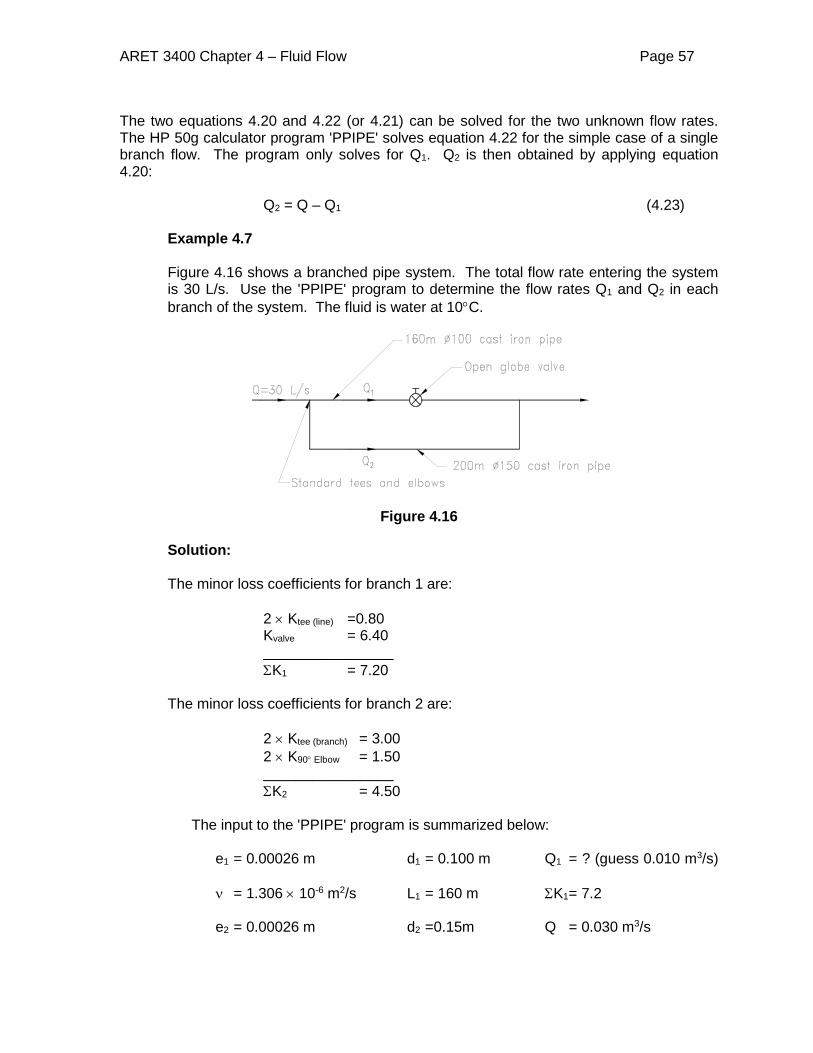
Example 4.7 Figure 4.16 shows a branched pipe system. The total flow rate entering the system is 30 L/s. Use the 'PPIPE' program to determine the flow rates Q1 and Q2 in each branch of the system. The fluid is water at 10°C.

Figure 4.16

Solution: The minor loss coefficients for branch 1 are:

2 × Ktee (line) =0.80 Kvalve = 6.40 ________________

ΣK1 = 7.20

The minor loss coefficients for branch 2 are:

2 × Ktee (branch) = 3.00 2 × K90° Elbow = 1.50 ________________

ΣK2 = 4.50

The input to the 'PPIPE' program is summarized below: e1 = 0.00026 m d1 = 0.100 m Q1 = ? (guess 0.010 m3/s) ν = 1.306 × 10-6 m2/s L1 = 160 m ΣK1 = 7.2 e2 = 0.00026 m d2 =0.15m Q = 0.030 m3/s


L2 =200m ΣK2 = 4.5 Solving for Q1 gives Q1 = 0.008232 m3/s, or 8.23 L/s. Q2 = Q – Q1 = 30 L/s – 8.23 L/s = 21.77 L/s.

Branch systems or networks do not have to be closed systems. Figure 4.17 shows a branched system involving three reservoirs.

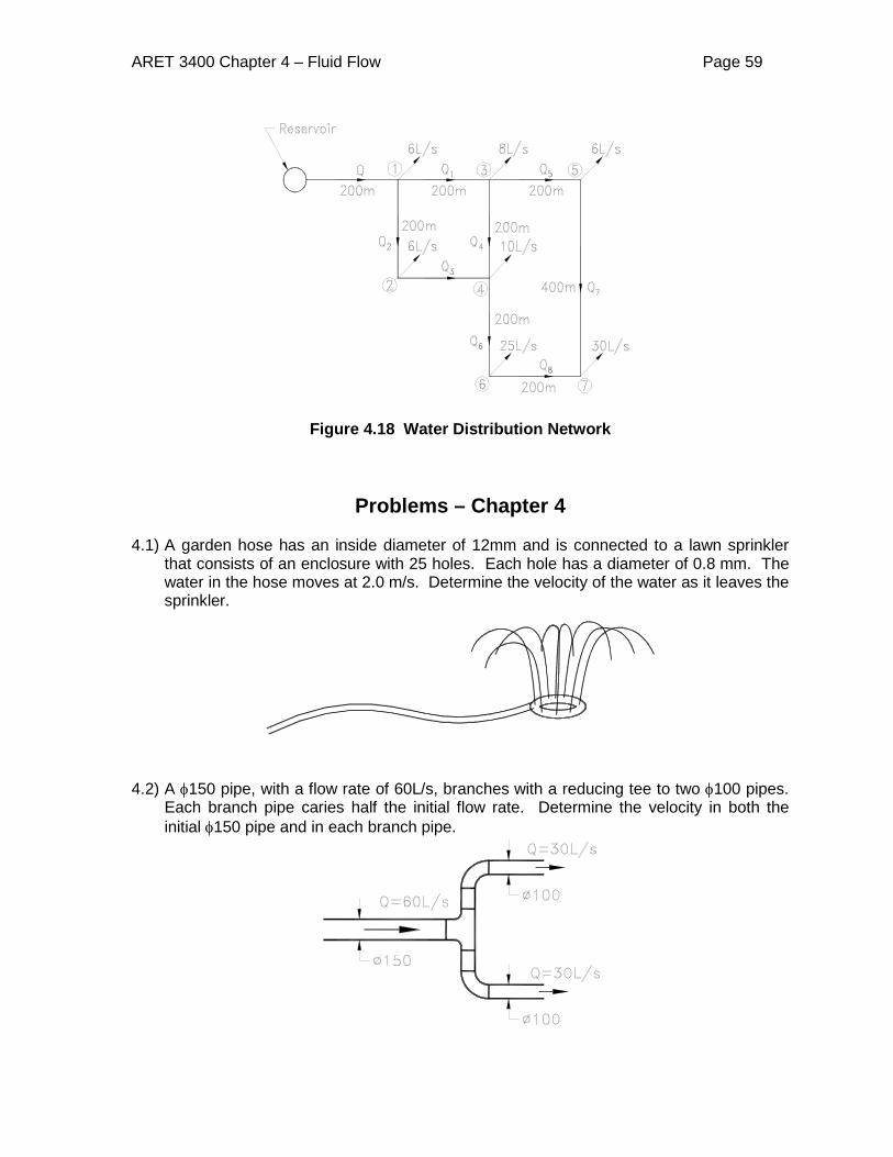
Figure 4.17 Branched System with Reservoirs In this case the node equation is Q1 + Q2 = Q3 and the other equations involve the elevations of the free surfaces together with the head loss in each pipe section. Note that there can only be one unique head at the node. The equations become z1 – hf1 = z2 – hf2, and z2 – hf2 = z3 + hf3. Water distribution systems usually involve networks that are much more complicated. Figure 4.18 shows a relatively simple water distribution system. In addition to the information shown, the elevation of each node would have to be known. Such complicated network problems are usually solved using a computer network analysis program. Many of these programs even allow the user to input the system with a graphical interface or a CAD program. The shaft work, w’, discussed in Section 4.4 is measured in unit time. If a fluid is pumped by motors to the reservoir at higher elevation, the power of the motors is determined as: 𝑃𝑃 = 𝜌𝜌𝜌𝜌𝑤𝑤′ Where 𝜌𝜌 = density of the fluid (kg/m3 or lb/ft3); Q = volume flow rate (m3/s or ft3/s); 𝑤𝑤′ = shaft work (m2/s2 or ft2/s2). The SI unit for the power is Watt (W), which is equivalent to kg.m2/s3. The US unit for the power is ft.lb/s. A traditional common unit is horsepower (HP). 1HP = 550 ft⋅lb/s; 1HP = 746 Watts.


Figure 4.18 Water Distribution Network

Problems – Chapter 4 4.1) A garden hose has an inside diameter of 12mm and is connected to a lawn sprinkler

that consists of an enclosure with 25 holes. Each hole has a diameter of 0.8 mm. The water in the hose moves at 2.0 m/s. Determine the velocity of the water as it leaves the sprinkler.

4.2) A φ150 pipe, with a flow rate of 60L/s, branches with a reducing tee to two φ100 pipes.

Each branch pipe caries half the initial flow rate. Determine the velocity in both the initial φ150 pipe and in each branch pipe.


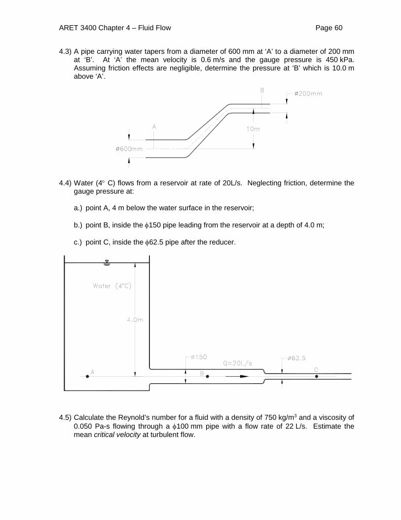
4.3) A pipe carrying water tapers from a diameter of 600 mm at ‘A’ to a diameter of 200 mm at ‘B’. At ‘A’ the mean velocity is 0.6 m/s and the gauge pressure is 450 kPa. Assuming friction effects are negligible, determine the pressure at ‘B’ which is 10.0 m above ‘A’.

4.4) Water (4° C) flows from a reservoir at rate of 20L/s. Neglecting friction, determine the

gauge pressure at: a.) point A, 4 m below the water surface in the reservoir; b.) point B, inside the φ150 pipe leading from the reservoir at a depth of 4.0 m; c.) point C, inside the φ62.5 pipe after the reducer.

4.5) Calculate the Reynold’s number for a fluid with a density of 750 kg/m3 and a viscosity of

0.050 Pa-s flowing through a φ100 mm pipe with a flow rate of 22 L/s. Estimate the mean critical velocity at turbulent flow.


4.6) Municipal water supply lines are typically designed for a maximum flow velocity of 2 m/s. Determine the Reynolds Number for water (4° C) flowing at this velocity in a φ200 water main. Is the flow laminar or turbulent?

4.7) A liquid, with a kinematic viscosity of 450 mm2/s, flows through a φ75 mm pipe at a rate

of 8.0 L/s. What type of flow is to be expected? 4.8) What is the maximum diameter of pipe required to ensure turbulent flow for water (4°C)

at a flow rate of 5L/s? What is the minimum diameter of pipe that will ensure laminar flow at the same rate?

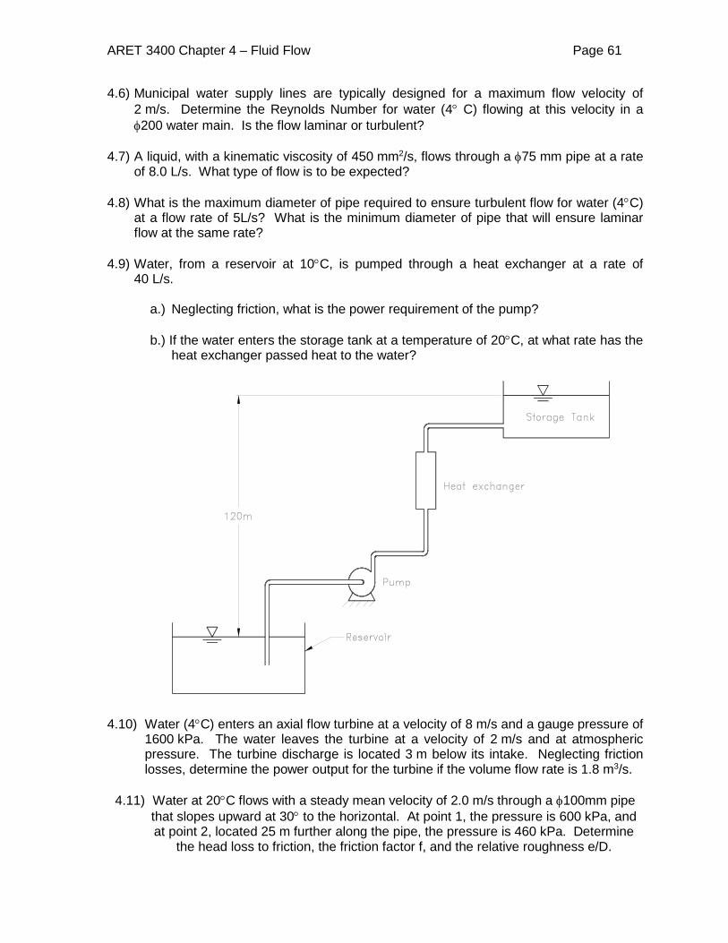
4.9) Water, from a reservoir at 10°C, is pumped through a heat exchanger at a rate of

40 L/s.

a.) Neglecting friction, what is the power requirement of the pump? b.) If the water enters the storage tank at a temperature of 20°C, at what rate has the

heat exchanger passed heat to the water?

4.10) Water (4°C) enters an axial flow turbine at a velocity of 8 m/s and a gauge pressure of

1600 kPa. The water leaves the turbine at a velocity of 2 m/s and at atmospheric pressure. The turbine discharge is located 3 m below its intake. Neglecting friction losses, determine the power output for the turbine if the volume flow rate is 1.8 m3/s.

4.11) Water at 20°C flows with a steady mean velocity of 2.0 m/s through a φ100mm pipe

that slopes upward at 30° to the horizontal. At point 1, the pressure is 600 kPa, and at point 2, located 25 m further along the pipe, the pressure is 460 kPa. Determine

the head loss to friction, the friction factor f, and the relative roughness e/D.


4.12) Water (4°C) flows with a steady mean velocity of 4.0 m/s through a φ400 penstock.

The pipe slopes down at 60° to the horizontal. At point 1, the pressure is 100 kPa, and at point 2 located 80 m further along the pipe, the pressure is 740 kPa. Determine the head loss to friction, the friction factor, f and the relative roughness e/d.

4.13) The diagram below shows a φ100 cast iron pipe leading from a reservoir. Determine

the flow rate through the pipe.

4.14) The diagram below shows a cast iron pipeline that feeds from a reservoir into to a

4.0 m diameter tank. Determine the rate at which the water is rising in the tank when the level of water in the reservoir is 18 m higher than the level in the tank.


4.15) A new 1500 m long ductile iron pipe, e = 0.12 mm, t is to have a discharge of 90 L/s

of water at 10°C with a head loss not to exceed 12.0 m. Determine the required pipe diameter.

4.16) Sewage is to be pumped for 2300 m through a φ200 horizontal plastic sewer pipe.

What pressure must the pump develop if the flow rate is 100 L/s. The sewage can be treated as water at 10°C and the pipe discharges to the atmosphere.

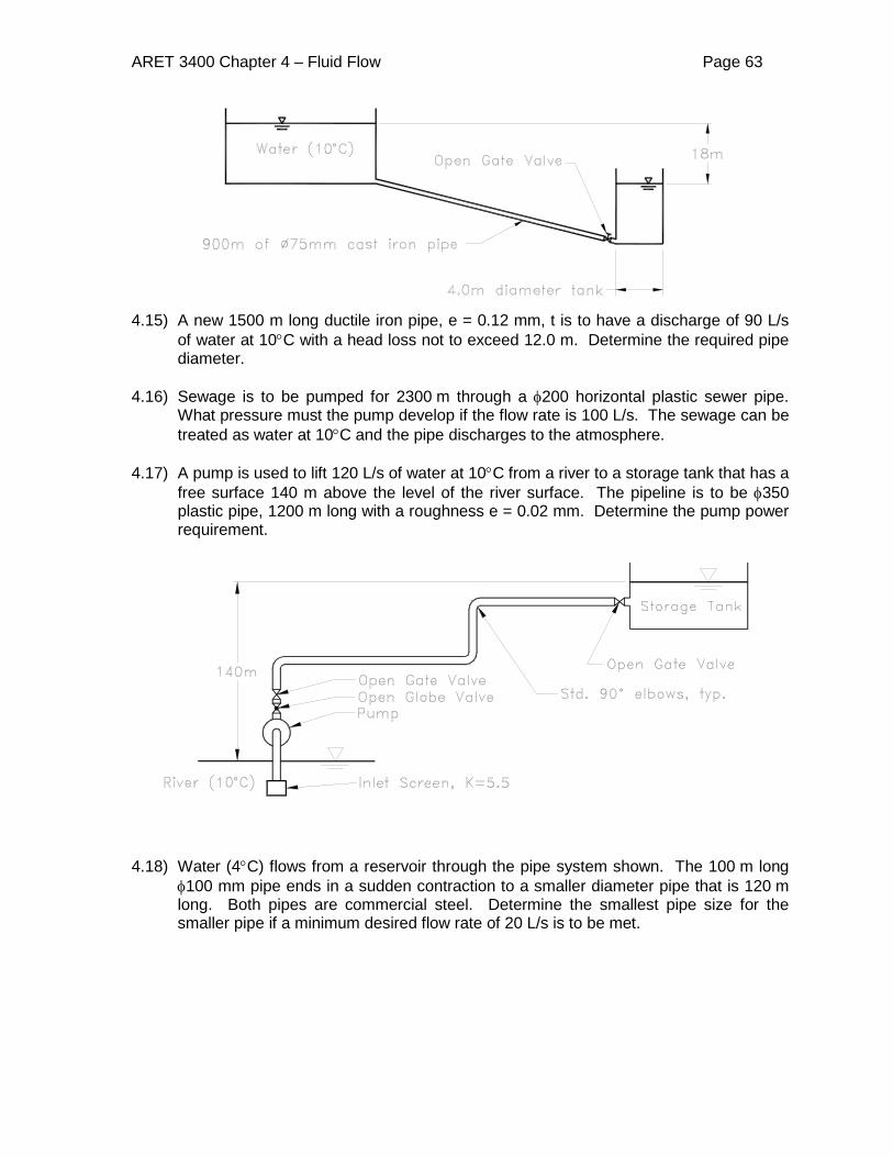
4.17) A pump is used to lift 120 L/s of water at 10°C from a river to a storage tank that has a

free surface 140 m above the level of the river surface. The pipeline is to be φ350 plastic pipe, 1200 m long with a roughness e = 0.02 mm. Determine the pump power requirement.

4.18) Water (4°C) flows from a reservoir through the pipe system shown. The 100 m long

φ100 mm pipe ends in a sudden contraction to a smaller diameter pipe that is 120 m long. Both pipes are commercial steel. Determine the smallest pipe size for the smaller pipe if a minimum desired flow rate of 20 L/s is to be met.


4.19) Water at 20°C flows from a reservoir through 200 m of φ150 pipe and 80 m of φ75

pipe as shown. The pipe is galvanized iron. Determine the flow rate.

4.20) A pump is used to lift 66L/s of waste water at 4°C from a box culvert to a storage tank prior to treatment. The pipeline is galvanized steel. The φ100 intake pipe is 8m long and has a screen, k = 5.0, a 90° elbow and an open gate valve. The pipe on the discharge side is also φ100 and is 40 m long and has two 90° elbows, two open gate valves and a swing check valve with k = 4.6. Determine the electrical power requirement in kilowatts assuming the pump has an efficiency of 70% and the electric motor has an efficiency of 90%.


4.21) An irrigation system is to rely on gravity feed through 2300 m of aluminum pipe with a roughness e = 0.08 mm as shown. Determine the required pipe diameter.

4.22) Determine the flow rate through the gravity feed irrigation system shown. The

pipeline consists of 1400 m of φ100 aluminum irrigation pipe with a roughness e = 0.06 mm.

4.23) Water at 10°C flows through a branched pipe system as shown. Branch 1 is 400 m

long and branch 2 is 220 m long. Determine the flow rates Q1 and Q2 in each branch. The pipe material is commercial steel pipe.


4.24) Water (80°C) flows through a branched galvanized steel pipe system as shown. Determine the flow rates Q1 and Q2 in each branch.

Chapter 4 – Pipe Flow

Documents

Transcript of Chapter 4 – Pipe Flow