Experimental study on the Capture/Desorption of gaseous ...

HAL Id: tel-03331636https://tel.archives-ouvertes.fr/tel-03331636

Submitted on 2 Sep 2021

HAL is a multi-disciplinary open accessarchive for the deposit and dissemination of sci-entific research documents, whether they are pub-lished or not. The documents may come fromteaching and research institutions in France orabroad, or from public or private research centers.

L’archive ouverte pluridisciplinaire HAL, estdestinée au dépôt et à la diffusion de documentsscientifiques de niveau recherche, publiés ou non,émanant des établissements d’enseignement et derecherche français ou étrangers, des laboratoirespublics ou privés.

Experimental study on the Capture/Desorption ofgaseous iodine (I2, CH3I) on environmental aerosols

Hanaa Houjeij

To cite this version:Hanaa Houjeij. Experimental study on the Capture/Desorption of gaseous iodine (I2, CH3I) onenvironmental aerosols. Other. Université de Bordeaux, 2020. English. NNT : 2020BORD0172.tel-03331636

https://tel.archives-ouvertes.fr/tel-03331636

https://hal.archives-ouvertes.fr

THÈSE PRÉSENTÉE

POUR OBTENIR LE GRADE DE

DOCTEUR DE

L’UNIVERSITÉ DE BORDEAUX

Sciences Chimiques

Chimie Analytique et Environnementale

Hanaa HOUJEIJ

Etude expérimentale des réactions de capture/désorption

des iodes gazeux (I2, CH3I) sur des aérosols

environnementaux

Sous la direction de : Dr. Sophie SOBANSKA

Encadrante : Dr. Anne Cécile GREGOIRE Soutenue le 13 Novembre 2020 Membres du jury: Mme. MASCETTI Joëlle Directeur de recherche, CNRS Présidente

Mme TOUBIN Céline Professeure, Université de Lille Rapporteur M. WORTHAM Henri Professeur, Aix-Marseille Université Rapporteur

M. LOUIS Florent Maître de Conférences, Université de Lille Examinateur M. MASSON Olivier Ingénieur de recherche, IRSN Examinateur M. VILLENAVE Eric Professeur, Université de Bordeaux Examinateur

M. COUSSAN Stéphane Chargé de recherche, CNRS Invité

Titre : Etude expérimentale des réactions de capture/désorption

des iodes gazeux (I2, CH3I) sur des aérosols environnementaux _____________________________________________________________________________________________________

Résumé

Lors d'un grave accident de centrale nucléaire l'iode gazeux I131, émit principalement sous les

formes I2 ou CH3I, peut affecter la santé humaine et l'environnement lors de son rejet dans

l'atmosphère. Les modèles de dispersion de l'iode ne tiennent pas compte de la réactivité de

l'iode avec les espèces gazeuses ou les aérosols atmosphériques. Cependant, la modification

de la spéciation chimique et/ou la forme physique des composés de l’iode n’est pas sans

conséquence sur leur dispersion et leurs impacts sanitaires. Dans le cadre de l'amélioration

des outils de simulation de la dispersion atmosphérique de l’iode radioactif, ce travail vise à

contribuer à l'état actuel des connaissances sur la chimie de l'iode par une approche

expérimentale permettant la compréhension des processus d'interaction entre CH3I gazeux,

les aérosols et l'eau.

L'interaction entre CH3I et l'eau a été étudiée à l'échelle moléculaire par des expériences en

matrice cryogénique appuyées par des calculs théoriques. Un excès d'eau en regard de CH3I,

a été utilisé pour simuler les conditions atmosphériques. Les dimères et trimères de CH3I sont

observés malgré la quantité élevée d'eau ainsi que la formation d’agrégats mixtes de CH3I et

de polymères d’eau. Ceci peut s'expliquer par la faible affinité du CH3I pour l'eau. Dans

l'atmosphère, CH3I et H2O gazeux formeront probablement des agrégats d'eau et des

polymères de CH3I au lieu d'hétéro complexes de type (CH3I)m-(H2O)n. L'interaction entre CH3I

et la glace amorphe en tant que modèle de glace atmosphérique a fait l'objet d'une étude

préliminaire. L'adsorption de CH3I sur la glace amorphe et sa désorption complète au-delà de

47 K ont été observés.

L'étude expérimentale des processus d’interactions entre CH3I et le NaCl sec et humide

comme modèle des sels marins a été réalisée en utilisant la Spectroscopie Infrarouge à

Transformée de Fourier par Réflexion Diffuse (DRIFTS). Les spectres DRIFTS de NaCl mettent

en évidence CH3I adsorbé sur la surface de NaCl. Les spectres FTIR montrent de nouvelles

bandes d’absorption, qui ont été attribuées à une nouvelle géométrie d’interaction de CH3I

avec NaCl. Le processus d'adsorption de CH3I sur NaCl est probablement une chimisorption

puisqu'aucune désorption n'a été observée. Nous avons démontré que l'adsorption du CH3I

n’atteint pas la saturation même après 5 heures d’exposition. Ce processus présente une

cinétique d’ordre 1 par rapport à la concentration de CH3I en phase gazeuse. Les coefficients

d'absorption sont de l'ordre de 10-11, avec une énergie globale d'absorption de -38 kJ.mol-1.

Ces résultats montrent une faible probabilité de capture des molécules de CH3I par la surface

de NaCl. La présence d'eau à la surface de NaCl ne semble pas modifier l'interaction entre CH3I

et NaCl, ce qui est cohérent avec sa faible affinité pour l'eau.

Les interactions de CH3I avec divers solides inorganiques et organiques comme modèles pour

les aérosols atmosphériques ont été étudiées à l’aide d’un réacteur statique couplé à la

chromatographie en phase gazeuse permettant de suivre la phase gazeuse. Nous avons

montré une faible interaction entre CH3I et les aérosols étudiés indiquant sa faible affinité

pour les surfaces des aérosols quelle que soit leur composition. Nous émettons l'hypothèse

que la teneur en eau en surface de l'aérosol est un paramètre clé. Ainsi, lorsqu'il est libéré

dans l'atmosphère, CH3I interagit très peu avec la surface des aérosols et reste en phase

gazeuse. Cependant, bien qu’en faible teneur, CH3I est irréversiblement adsorbé à la surface

des sels d’halogénures, ce qui pourrait être pris en compte dans le modèle de dispersion pour

en évaluer l’impact.

__________________________________________________________________________________

Mots clés

Spectroscopie, réactivité, chimie de l'iode, aérosols, sureté nucléaire, chimie atmosphérique

Title: Experimental study on the Capture/Desorption of gaseous

iodine (I2, CH3I) on environmental aerosols _____________________________________________________________________________________________________

Abstract

Gaseous iodine I131 mainly under I2 or CH3I forms, when released into the atmosphere during

a severe nuclear power plant accident may affect both human health and environment. The

atmospheric dispersion models of iodine do not take into account the potential reactivity of

iodine with atmospheric gas or particles species. However, the modification of the chemical

speciation and/or the physical form of iodine compounds is not without consequences on the

transport of iodine in the atmosphere and its health effects. Within the framework of

improving the atmospheric dispersion tools of radioactive iodine, this work aims to contribute

to the actual state of knowledge of atmospheric iodine chemistry by experimental approaches

focusing on understanding the CH3I-aerosols and CH3I-water interaction processes.

The interaction between CH3I and water at the molecular scale has been investigated using

cryogenic matrix experiments supported by theoretical DFT calculations. A large excess of

water regarding CH3I was used in order to mimic atmospheric conditions. Dimers and trimers

of CH3I are observed despite the high water amount in the initial mixture together with mixed

aggregates between CH3I and water polymers. This may be explained by the low affinity of

CH3I with water. This result highlights that, in the atmosphere, gaseous CH3I and H2O will likely

form aggregates of water and CH3I polymers instead of (CH3I)m-(H2O)n hetero complexes.

Further, the interaction between CH3I and amorphous ice as a model of atmospheric ice have

been preliminary investigated. The adsorption of CH3I on amorphous has been observed but

with a complete desorption of CH3I above 47 K.

Experimental study of interaction processes between gaseous iodine (CH3I) and both dry and

wet NaCl as surrogate of sea salt aerosols has been carried out using Diffuse Reflectance

Infrared Fourier Transformed Spectroscopy (DRIFTS). The DRIFTS spectra of NaCl surface

clearly evidenced adsorbed CH3I on the NaCl surface particles. The FTIR spectra revealed new

absorption bands that have been attributed to a new adsorption geometry. The adsorption

process of CH3I on NaCl is likely a chemisorption since no desorption was observed. We have

demonstrated that the adsorption of CH3I on NaCl did not reach saturation even after 5 hours

of continuous flow of CH3I. CH3I capture at the NaCl surface presents a 1st order kinetics

relative to its gas phase concentration. The uptake coefficients were determined to be in the

order of 10-11, with a global adsorption energy of about -38 kJ.mol− 1. These results show a low

probability of CH3I molecules to be captured by NaCl surface. The presence of water on the

surface of NaCl seems to have no effect on the interaction between CH3I and NaCl, which is

consistent with the low affinity of CH3I for water.

The interactions of CH3I with various inorganic and organic powdered solids as models for

atmospheric aerosols have been investigated using static reactor coupled with gas

chromatography (GC) allowing the monitoring of the gas phase. We have highlighted a weak

interaction between CH3I and inorganic and organic aerosols indicating a low affinity of CH3I

whatever the aerosol surface composition. We hypothesis that the water content at the

aerosol surface is a key parameter. So that, when released in the atmosphere, CH3I will

interact very little with the surface of the aerosols and will stay in the gaseous phase. However,

although in low content, a part of CH3I is irreversibly adsorbed on the surface of the halide

salts that could be considered in the atmospheric iodine model to estimate potential impact.

___________________________________________________________________________

Keywords

Spectroscopy, iodine chemistry, reactivity, aerosol, nuclear safety, atmospheric chemistry

___________________________________________________________________________

Unité de recherche

[Institut des Sciences Moléculaires, UMR 5255, 351 Cours de la Libération, 33405 Talence]

[Laboratoire expérimentation environnement et chimie, IRSN/PSN-RES/SEREX, 13115 Saint

Paul Lez Durance Cedex]

To my parents,

To Rabih Maatouk,

To my brother and sister.

Acknowledgment

The output of this PhD thesis has been accomplished with the guidance and support of many

people whom I am grateful for. The work was done in collaboration between ISM laboratory

(L'Institut des Sciences Moléculaires, UMR CNRS 5255) and L2EC laboratory (Laboratoire

Expérimentation Environnement et Chimie, IRSN/PSN-RES/SEREX), for that I want to start

acknowledging Laurent Cantrel and Eric Fouquet for welcoming me in their research

unities. Also, I gratefully acknowledge the funding received for my PhD from Institut de

Radioprotection et de Sûreté Nucléaire and Région Nouvelle Aquitaine.

First, I want to express my gratitude and special thanks for my supervisors Dr. Sophie Sobanska

and Dr. Anne-cecile Gregoire that took time to hear, discuss, track and guide my work to

achieve the settled objectives throughout the entire thesis. They were always ready to give

help, ideas and advices at various milestones, which helped in my thesis progress.

Second, I express my thanks to all the jury members for their time to evaluate and approve

my work. In particular, I would like to thank Professor Céline Toubin and Professor Henri

Wortham for agreeing to be the referees of this work, as well as Dr. Joëlle Mascetti, Dr. Florent

Louis, Dr. Olivier Masson and Professor Eric Villenave that accepted to evaluate this work as

examiners. Also, many thanks to Dr. Stéphane Coussan for accepting our invitation to my

defense.

I want to thank all the people I worked with in ISM and L2EC, particularly Gwenaëlle Le

Bourdon for formation on DRIFTS instrumentation as well as Christian Aupetit for formation

on matrix instrumentation and the continual assistance received from both. Joëlle Mascetti

and Stéphane Coussan, thank you for making me discover the principle of matrix technique,

for the very enriching discussions and your help in interpreting matrix results. Thanks to Sonia

Taamalli and Florent Louis for their guidance and formation on DFT calculations. Guillaume

Bourbon thank you for helping me to develop the static reactor setups. Charly Tornabene, you

were always there in the laboratory and ready to help and advice me, thank you for the

formation on ICP-MS. Coralie Alvarez and Julie Nguyen, thank you for the formation on the GC

technique. Thanks to Elouan Le Fessant for his help on carrying ICP-MS analysis.

I would like to thank all the L2EC and ISM members who participated in the good atmosphere

and who allowed me to work in excellent conditions.

Finally, I must express my deepest gratitude to my parents who despite the long distance

always give me love, support and motivation especially throughout my tough days. Also, many

thanks to my husband Rabih Maatouk for being beside me and for his support, you are always

there for me! Also, I want to thank all the friends and family in Lebanon and France for their

invaluable support and care.

Glossary

FPs: Fission Products

PWR: Pressurized Water Reactor

TED: Thyroid Equivalent Dose

PA: Proton Acceptor

PD: Proton Donor

nmr: non rotating monomer

DRIFTS: Diffuse Reflectance Fourier Transform Infrared Spectroscopy

ICP-MS: Inductively Coupled Plasma- Mass Spectrometery

GC: Gas Chromatography

MIS: Matrix Isolation Spectroscopy

FTIR: Fourier Transform Infrared Spectroscopy

Table of content

Executive summary in French .......................................................................................... 24

General Introduction ....................................................................................................... 34

Chapter 1: Context .......................................................................................................... 40

1.1 Pressurized water reactor (PWR) ............................................................................. 40

1.1.1 Description and operation of a Pressurized Water Reactor (PWR) .................... 40

1.1.2 Production of fission products ......................................................................... 42

1.2 Nuclear severe accident ............................................................................................. 44

1.2.1 Nuclear severe accident scenarios .................................................................... 45

1.2.2 Source term ..................................................................................................... 47

1.3 Lessons learned from radioiodine release into the atmosphere .................................. 48

1.3.1 Dispersion of radioiodine .................................................................................. 49

1.3.2 Radioprotection................................................................................................ 51

1.4 Conclusion ................................................................................................................. 53

Chapter 2: State of art Iodine chemistry in the atmosphere ............................................. 58

2.1 Main sources of iodine compounds ............................................................................ 58

2.2 Gaseous Iodine reactivity .......................................................................................... 61

2.3 Iodine heterogeneous reactivity ................................................................................ 67

2.3.1 Atmospheric aerosols ........................................................................................ 68

2.3.2 Role of water ..................................................................................................... 71

2.3.3 Gas-aerosol interaction – overview of the general concepts ................................. 73

2.3.4 Experimental tools and techniques for studying aerosol-gas interactions .............. 77

2.3.4.1 Flow tube and flow tube-like techniques ..................................................... 79

2.3.4.2 Droplet train reactor ................................................................................... 81

2.3.4.3 Knudsen cell ................................................................................................. 82

2.3.4.4 Diffuse Reflectance Infrared Fourier Transform Spectroscopy (DRIFTS) .......... 84

2.3.4.5 Atmospheric simulation chamber .................................................................. 85

2.3.5 Single particle and molecular mechanism approach ...................................... 86

2.3.5.1 Single particle approach .................................................................... 86

2.3.5.2 Molecular approach .......................................................................... 87

2.3.5.3 Theoretical calculation ....................................................................... 88

2.4 Literature review on interaction between atmospheric aerosols and iodine compounds

....................................................................................................................................... 89

2.4.1 Heterogeneous reaction of inorganic iodine species with halide salt aerosols ..... 89

2.4.2 Interaction between iodine species and ice ........................................................ 93

2.4.2.1 Uptake of iodine species on ice ................................................................ 93

2.4.2.2 Photodissociation of CH3I on ice ............................................................... 97

2.4.3 Heterogeneous interaction of organic iodine with carbonaceous aerosols ......... 101

2.4.4 Modelling of inorganic species with undefined surfaces ..................................... 102

2.5 Conclusion ................................................................................................................ 103

Chapter 3: Cryogenic experiments .................................................................................. 122

3.1. Material and Methods ............................................................................................ 122

3.1.1 Description of the cryogenic experimental set ups ............................................ 122

3.1.1.1 Experimental setup at ISM laboratory ................................................... 122

3.1.1.2 Experimental setup at PIIM laboratory ................................................... 124

3.1.2 Sample deposition and spectral acquisition methods ........................................ 125

3.1.3 Experimental grid .............................................................................................. 126

3.1.3.1 Preparation of samples for studying CH3I-H2O interactions at ISM laboratory

...................................................................................................................................... 126

3.1.3.2 Preparation of samples for studying CH3I- amorphous ice (ASW) interactions

in PIIM laboratory .......................................................................................................... 126

3.1.4 Density Functional Theory (DFT) calculation ...................................................... 127

3.2. Results and discussion ............................................................................................. 128

3.2.1 Formation of (CH3I)x clusters ............................................................................ 128

3.2.1.1 DFT calculation results .......................................................................... 128

3.2.1.2 Experimental vibrational spectra ............................................................ 132

3.2.2 Formation of CH3I-H2O complexes .................................................................... 134

3.2.2.1 DFT calculation results ........................................................................... 134

3.2.2.2 Experimental vibrational spectra ............................................................ 148

3.2.3 Preliminary results on the interaction of CH3I with amorphous ice ..................... 156

3.3 Conclusion and perspectives ................................................................................... 159

Chapter 4: DRIFTS experiments ...................................................................................... 162

4.1. Material and Methods ........................................................................................... 162

4.1.1 Reagents ........................................................................................................ 162

4.1.2 DRIFTS Experimental setup ............................................................................... 163

4.1.2.1 DRIFTS Cell and gas supply ...................................................................... 163

4.1.2.2 Experimental protocol ............................................................................. 166

4.1.2.3 Spectral acquisition using DRIFTS .............................................................. 167

4.1.2.4 Spectral data processing for quantification .............................................. 167

4.1.3. Inductively coupled plasma mass spectrometer measurements ........................ 168

4.1.4. Experiment grid for DRIFTS experiments and validation ................................... 169

4.1.4.1 Dry Condition .......................................................................................... 169

4.1.4.2. Humid conditions .................................................................................... 174

4.1.4.3 Variation of the temperature conditions .................................................. 175

4.2. Spectral assignment ................................................................................................ 176

4.2.1 Dry conditions ................................................................................................ 176

4.2.1.1 Band assignment in the CH3 stretching region ........................................ 176

4.2.1.2 Band assignment in the CH3 deformation region .................................... 181

4.2.1.3 Band assignment in the CH3 rocking region .............................................. 184

4.2.1.4 New bands attribution ........................................................................... 185

4.2.1.5 Summary of bands assignment ................................................................ 191

4.2.2 Influence of humidity ........................................................................................ 192

4.2.2.1 Exposure of wet NaCl to dry CH3I.............................................................. 192

4.2.2.2 Influence of water on the CH3I desorption ................................................ 196

4.3. Time evolution of CH3I on NaCl surface during CH3I exposure, static and Ar flow phases

...................................................................................................................................... 196

4.3.1 Evolution of CH3I on NaCl surface in dry conditions ........................................... 197

4.3.1.1 Experiment with exposure to CH3I during 5 hours ..................................... 197

4.3.1.2 Experiment with shorter exposure duration and longer desorption phases

...................................................................................................................................... 203

4.3.1.3 Experiment by increasing temperature during the Ar flow phase .............. 205

4.3.1.4 Experiments featuring different CH3I concentrations in the gas phase ...... 207

4.3.1.5 Experiment featuring variation in contact time ........................................ 209

4.3.2 CH3I exposure on dry NaI and KBr .................................................................... 210

4.3.3 Evolution of CH3I on wet NaCl ........................................................................... 211

4.3.4 Determination of uptake coefficient of CH3I adsorption by NaCl surface ............ 212

4.3.4.1 Quantification of iodine on NaCl .............................................................. 212

4.3.4.2 Conversion factor .................................................................................... 213

4.3.4.3 Uptake coefficient ................................................................................... 213

4.3.5 Rate evolution with temperature ...................................................................... 216

4.4. Conclusion ............................................................................................................... 219

Chapter 5: Static reactor experiments ............................................................................ 224

5.1 Materials and methods ............................................................................................ 224

5.1.1 Reagents .......................................................................................................... 224

5.1.2 Experimental setup .......................................................................................... 225

5.1.3 Gas phase CH3I sampling and GC analyses ........................................................ 228

5.1.4 Protocol description for experiments performed in continuous gas conditions ... 228

5.1.5 Experiment grid for continuous conditions ........................................................ 230

5.2. Results and discussion ............................................................................................. 231

5.2.1 Empty reactors ................................................................................................. 231

5.2.2 Reactor filled with inorganic solids ................................................................... 235

5.2.3 Reactor filled with organic solids ...................................................................... 237

5.3 Conclusion and perspectives ..................................................................................... 239

General conclusion and perspectives .............................................................................. 242

Annex 1: CH3I chemical properties .................................................................................. 247

Annex 2: Infrared Spectroscopy techniques .................................................................... 247

1-Principle of Infrared spectroscopy ............................................................................... 247

2-Principle of Fourier Transform Infrared spectroscopy ................................................... 249

3-Diffuse Reflectance Fourier Transform Infrared Spectroscopy ...................................... 250

Annex 3: Uncertainty estimation of the band area observed in DRIFTS spectra and effect of

closing or opening valves on static conditions ................................................................ 254

Annex 4: Principle of Inductively coupled plasma mass spectroscopy (ICP-MS) ................ 257

Annex 5: Gas chromatography (GC) ................................................................................ 258

Annex 6: Method of calculating the uncertainty of GC and ICP-MS measurements .......... 261

Annex 7: ICP-MS data and conversion factor calculation ................................................. 262

Annex 8: Time evolution of CH3I outlet concentration in static reactors filled with solids . 265

Table of Figures Figure 1. 1 Pressurized Water Reactor [1]. ------------------------------------------------------------------------------------------- 40

Figure 1. 2 The International Nuclear and Radiological Event Scale (INES) [16]. ------------------------------------------ 44

Figure 1. 3 Physical phenomena during a severe accident [27]. ---------------------------------------------------------------- 45

Figure 1. 4 Summary description of the processes involved in the release and transfer of fission products (FPs) to

the environment during a core melt accident [2]. ---------------------------------------------------------------------------------- 46

Figure 1. 5 Exposure pathways from releases of radioactive material to the environment [41].---------------------- 51

Figure 1. 6 Evolution of dose coefficient as function age via inhalation [42]. ---------------------------------------------- 53

Figure 2. 1 Simplified Diagram representing the reactivity of iodine in the atmosphere taken from [5]. ----------- 61

Figure 2. 2 Gas-phase iodine chemistry leading to the formation of INOx species [48]. --------------------------------- 64

Figure 2. 3 Summary diagram of the iodine reactivity in the atmosphere [6, 7]. ------------------------------------------ 66

Figure 2. 4 Family mass evolution of iodine, injection 2013 January 1st, at 7 am as a function of time with iodine

release (a) 98 ppt of I2 and (b) 196 ppt of CH3I. (Organic in green, iodine in violet, iodine oxide in orange, inorganic

in blue and radicals in red) [62]. -------------------------------------------------------------------------------------------------------- 67

Figure 2. 5 Atmospheric cycling of aerosols, issued from Pöschl, 2005 [73]. ------------------------------------------------ 68

Figure 2. 6 Average lifetime dependence on the size of atmospheric aerosol particle [111]. -------------------------- 70

Figure 2. 7 Diagram of kinetic states of atmospheric humidity [127]. -------------------------------------------------------- 72

Figure 2. 8 Schematic illustration of the key processes describing gas uptake by atmospheric particles. ---------- 75

Figure 2. 9 Example of wetted flow tube used for measurements of uptake of trace gases on liquid film adapted

from Dievart et., [146]. -------------------------------------------------------------------------------------------------------------------- 80

Figure 2. 10 Example of aerosol flow tube experimental set-up used to measure HO2 uptake coefficients adapted

from I. George et al., [150]. MFC-mass flow controller; RH/T-temperature and humidity probe; CPM-channel

photomultiplier, FAGE-Fluorescence Assay by Gas Expansion; HEPA–High Efficiency Particulate Air. --------------- 81

Figure 2. 11 Schematic diagram of typical droplet train flow reactor for measurement of uptake coefficients of

trace gases into liquids [151]. ----------------------------------------------------------------------------------------------------------- 82

Figure 2. 12 Example of vibrating orifice monodisperse aerosol generator [152]. ---------------------------------------- 82

Figure 2. 13 Example of a Knudsen cell for the investigation of heterogeneous reactions using either continuous

flow or pulsed gas admission. The rotatable orifice plate can put up to four molecular-beam forming orifices into

line of sight with the ionizer of the mass spectrometric (MS) detector from M. Rossi et al., [153]. ------------------ 83

Figure 2. 14 Example of DRIFTS apparatus [162]. ---------------------------------------------------------------------------------- 85

Figure 2. 15 Outdoor SAPHIR atmosphere reaction chamber in Jülich, Germany dedicated for both homogenous

and heterogenous interaction processes [167]. ------------------------------------------------------------------------------------ 86

Figure 2. 16 Secondary electron (SE) images of CaCO3 particles before (images on left) and after (images on right)

reaction with gaseous HNO3 in the presence of water vapor (PHNO3 =14±1 µTorr and 36±1% RH for 2h) [180].

--------------------------------------------------------------------------------------------------------------------------------------------------- 87

Figure 2. 17 Schematic presentation of the cryogenic matrix isolation principle [185]. --------------------------------- 88

Figure 3. 1 (a) Matrix chamber seen from the front [1] adapted for FTIR spectrometer coupling (b) photo of the

matrix chamber at ISM. ----------------------------------------------------------------------------------------------------------------- 123

Figure 3. 2 Schematic diagram of the experimental setup of (a) CH3I in Ar matrix from 10 to 35 K, (b) CH3I and H2O

in Ar matrix from 10 to 35 K. The scheme was adapted from [2]. ----------------------------------------------------------- 124

Figure 3. 3 Schematic diagram of the experimental setup adapted from [2] with two possible injection positions:

for gas mixtures and for solids. The chromium-platted anti-radiation shield reduces the useful surface of

deposition to a disc of 10 mm diameter -------------------------------------------------------------------------------------------- 125

Figure 3. 4 B97X-D/ aug-cc-pVTZ-PP-predicted geometries (distances in Å) and Gibbs free energies (G in kJ/mol)

of CH3I dimers. ----------------------------------------------------------------------------------------------------------------------------- 128

Figure 3. 5 B97X-D/ aug-cc-pVTZ-PP-predicted geometries (distances in Å) and Gibbs free energies (G in kJ/mol)

of CH3I trimers. ---------------------------------------------------------------------------------------------------------------------------- 129

Figure 3. 6 IR spectra of CH3I/Ar sample at 10 K in the 3100-2750 cm-1 and 1350-750 cm-1 spectral range

corresponding to the CH3 stretching, deformation and rocking regions, respectively. --------------------------------- 132

Figure 3. 7 IR spectra of the annealing of CH3I/Ar sample until 35 K in the spectral range (a) 3080-2944 cm-1 (b)

1270-1237 cm-1 (c) 905-870 cm-1. Bands denoted in green, pink and orange are assigned to CH3I monomer, CH3I

dimer and CH3I trimer, respectively. ------------------------------------------------------------------------------------------------- 134

Figure 3. 8B97X-D/ aug-cc-pVTZ-PP-predicted geometry (distances in Å) and Gibbs free energy (G in kJ.mol-1)

of CH3I.H2O isomers. --------------------------------------------------------------------------------------------------------------------- 135

Figure 3. 9 B97X-D/ aug-cc-pVTZ-PP-predicted geometry (distances in Å) and Gibbs free energy (G in kJ.mol-1)

of CH3I.(H2O)2 isomers. ------------------------------------------------------------------------------------------------------------------ 136

Figure 3. 10 B97X-D/ aug-cc-pVTZ-PP-predicted geometry (distances in Å) and Gibbs free energy (G in kJ mol-

1) of (CH3I)2.(H2O) isomers. ------------------------------------------------------------------------------------------------------------- 138


1) of CH3I.(H2O)3 isomers. --------------------------------------------------------------------------------------------------------------- 141


1) of (CH3I)2.(H2O)2 isomers. ------------------------------------------------------------------------------------------------------------ 144

Figure 3. 13 IR spectra in 2 (bending CH), 6 (rocking CH3) regions of pure methyl iodide matrix (trace (a)) (CH3I/Ar

= 1/1000), recorded at 10 K, and of mixed CH3I/H2O/Ar = 1/24/1500, recorded at 10 K (trace (b)). --------------- 148

Figure 3. 14 IR spectra in the 1 (symmetric stretching),3 (antisymmetric stretching) and2 (bending mode)

regions of pure water polymer matrix (trace (a)) (H2O/Ar = 7/1000), recorded at 4 K, and of mixed CH3I/H2O/Ar =

1/24/1500, recorded at 10 K (trace (b)). -------------------------------------------------------------------------------------------- 149

Figure 3. 15 The four surface modes of amorphous ice, dH (3720 and 3698cm−1), dO (3549 cm−1), and s4 (3503

cm−1) [15]. ----------------------------------------------------------------------------------------------------------------------------------- 156

Figure 3. 16 The observed IR spectra in (a) the OH dangling region and (b) the CH3 deformation region. Pure

amorphous ice is in black and the successive 3 mbar depositions of CH3I/Ar on pure amorphous ice are in red and

green. The OH dangling modes are marked by pink dashed lines. CH3I tentatively assigned bands are marked by

blue dashed lines. ------------------------------------------------------------------------------------------------------------------------- 157

Figure 3. 17 The observed IR spectra in the zone of the OH dangling of amorphous ice for the experiment of

desorption of CH3I from pure amorphous ice after CH3I deposition and then annealing up to 47 K. All spectra were

recorded at 4K. ---------------------------------------------------------------------------------------------------------------------------- 158

Figure 4. 1 Particle size distribution of the manually grinded NaCl particles by sieving on grids ranging between

300 μm and 50 µm. ----------------------------------------------------------------------------------------------------------------------- 163

Figure 4. 2 Scheme of DRIFTS experimental setup under dry conditions. -------------------------------------------------- 164

Figure 4. 3 DRIFTS experimental setup from GSM-ISM. ------------------------------------------------------------------------ 165

Figure 4. 4 Scheme of DRIFTS experimental setup under humid conditions. ---------------------------------------------- 166

Figure 4. 5 Typical DRIFTS spectra in mid IR spectral range [4000-600 cm-1] of dry NaCl surface exposed to 5 hours

of CH3I flow (108mL.min-1, 1000 ppm) at 296 K and 1 atm. ------------------------------------------------------------------- 176

Figure 4. 6 DRIFTS spectra in the 3050-2800 cm-1 IR spectral range of NaCl surface exposed to 5 hours of CH3I

(108mL.min-1, 1000 ppm) continuous flow at 296 K and 1 atm. Blue bands are CH3I adsorbed on NaCl and green

bands are CH3I in gas phase near the surface. ------------------------------------------------------------------------------------ 177

Figure 4. 7 DRIFTS spectra in the 2963-2935 cm-1 IR spectral range of NaCl exposed to 5 hours of continuous CH3I

flow (108mL.min-1,1000 ppm) at 296 K and 1 atm decomposed with Gaussian function using FityK software. 177


(108mL.min-1, 1000 ppm) continuous flow at 296 K and 1 atm. Blue bands are CH3I adsorbed on NaCl, green bands

are CH3I in gas phase near the surface, and red bands are new bands. --------------------------------------------------- 181

Figure 4. 9 DRIFTS spectra in the 1305-1160 cm-1 IR spectral range of NaCl exposed to 5 hours of continuous CH3I

flow (108mL.min-1,1000 ppm) at 296 K and 1 atm decomposed with Gaussian function using FityK software. 182

Figure 4. 10 (a) DRIFTS spectrum of 23Ag/Y (2.5) after saturation with CH3I (1333 ppm/Ar) at 373 K [13] and (b)

IR spectrum IR spectrum of the TiO2 at 308 K in contact with 2 Torr of CH3I [12]. -------------------------------------- 182

Figure 4. 11 DRIFTS spectrum in the CH3 deformation range of adsorbed CH3I of 23Ag/Y(2.5) after saturation with

CH3I (1333 ppm/Ar) at 373 K decomposed using Gaussian fit [13]. --------------------------------------------------------- 183

Figure 4. 12 Proposed adsorption geometry of CH3I to metallic surface [19]. -------------------------------------------- 184


(108mL.min-1, 1000 ppm) continuous flow at 296 K and 1 atm. Bands in black are unassigned bands. ---------- 185

Figure 4. 14 The direct and indirect mechanism of the Cl-(H2O) +CH3I substitution reaction from [33]. ---------- 188

Figure 4. 15 DRIFTS spectra in the 1400-900 cm-1 IR spectral range of NaCl surface (in black), NaI (in dark yellow)

and KBr (in violet) exposed to 1 hour of CH3I (108mL.min-1, 1000 ppm) continuous flow at 296 K and 1 atm. Bands

in blue are adsorbed CH3I, green are gaseous CH3I near the surface and red are new bands. ----------------------- 189

Figure 4. 16 DRIFTS spectra in the 1550-940 cm-1 IR spectral range of NaCl surface from dry NaCl of DRIFTS

experiment in black and dry NaCl recovered from the balloon experiment at 296 K and 1 atm. Bands in blue are

CH3I adsorbed on NaCl and red are new bands. ---------------------------------------------------------------------------------- 190

Figure 4. 17 Scheme of the CH3I adsorption on NaCl representing the bands at 1073 and 1024 cm-1. Mulliken

charges from DFT calculation perfomed using ωB97XD/aug-cc-pVTZ-PP. ------------------------------------------------ 191

Figure 4. 18 DRIFTS spectra in the 4000-700 cm-1 of dry and wet NaCl surface exposed to 5 hours of CH3I

(108mL.min-1, 1000 ppm) continuous flow at 296 K and 1 atm. ------------------------------------------------------------- 193

Figure 4. 19 DRIFTS spectra in the 3050-2750 cm-1 IR spectral range of dry and wet NaCl surface exposed to 5

hours of CH3I (108mL.min-1, 1000 ppm) continuous flow at 296 K and 1 atm. Bands in blue are adsorbed CH3I on

NaCI, green are gaseous CH3I near the surface, black are unassigned bands, red bands are new bands and violet

bands are bands observed with only wet NaCl. ----------------------------------------------------------------------------------- 194

Figure 4. 20 DRIFTS spectra in the 1500-700 cm-1 IR spectral range of dry and wet NaCl surface exposed to 5 hours

of CH3I (108mL.min-1, 1000 ppm) continuous flow at 296 K and 1 atm. Bands in blue are adsorbed CH3I on NaCI,

green are gaseous CH3I near the surface, black are unassigned bands, red are new bands and violet are bands

observed with only wet NaCl. ---------------------------------------------------------------------------------------------------------- 195

Figure 4. 21 DRIFTS spectra in the 1350-750 cm-1 IR spectral range of dry NaCl surface (RH=20%) exposed to 5

hours of continuous CH3I flow (108mL.min-1, 1000 ppm) and then to 40 minutes of wet Ar continuous flow

(RH=50%) at 296 K and 1 atm. Bands in blue are adsorbed CH3I on NaCl, green are gaseous CH3I near the surface,

black are unassigned bands and red bands are new bands. ------------------------------------------------------------------ 196

Figure 4. 22 DRIFTS spectra in the deformation (1400-900 cm-1) of NaCl surface as a function of exposure time of

the continuous CH3I (108mL.min-1, 1000 ppm) flow at 296 K and 1 atm. Bands in blue are adsorbed CH3I on NaCl,

green are gaseous CH3I near the surface and red are new bands. ---------------------------------------------------------- 197

Figure 4. 23 DRIFTS spectra of NaCl after 5 hours of CH3I continuous flow, then under static conditions for 1 hour

and finally under 1 hour of continuous Ar flow in the spectral range 1400-900 cm-1. Bands in blue are CH3I

adsorbed on NaCl, in green are gaseous CH3I and red are new bands. ---------------------------------------------------- 198

Figure 4. 24 Area of the 1262 cm-1 as a function of time during CH3I exposure, static phase and Ar flow phases.

The isolated bands are determined using Gaussian fit function. Exposure phase denotes the continuous flow of

108 mL.min-1 of CH3I (1000 ppm) on NaCl. The static phase denotes the static conditions after 5 hours of CH3I flow

and Ar flow phase denotes the continuous Ar flow after the static conditions. ------------------------------------------ 199

Figure 4. 25 Sum of the area of the 1275, 1244, 1220 and 1183 cm-1 bands as a function of time during CH3I

exposure, static and Ar flow phases of CH3I on NaCl. The decomposed area is determined using Gaussian fit

function. Exposure phase denotes the continuous flow of 108 mL.min-1 of CH3I (1000 ppm) on NaCl. The static

phase denotes the static conditions after 5 hours of CH3I flow and Ar flow phase denotes continuous Ar flow after

the static conditions. --------------------------------------------------------------------------------------------------------------------- 200

Figure 4. 26 Area of the 1073 and 1024 cm-1 bands as a function of time during CH3I exposure, static and Ar flow

phases of CH3I on NaCl. The decomposed area is determined using Gaussian fit function. Exposure phase denotes

the continuous flow of 108 mL.min-1 of CH3I (1000 ppm) on NaCl. The static phase denotes the static conditions

after 5 hours of CH3I flow and Ar flow phase denotes continuous Ar flow hour after the static conditions. ----- 200

Figure 4. 29 DRIFTS spectra of NaCl after 2 hours of CH3I continuous flow, then after static conditions for 24 hours

and finally after 8 hours of Ar flow in the 1400-700 cm-1 spectral region. Bands in blue are adsorbed CH3I, in green

are gaseous CH3I and red bands are new bands. --------------------------------------------------------------------------------- 204

Figure 4. 30 DRIFTS spectra of NaCl in the spectral range 1400-900 cm-1 after 1 hour of CH3I continuous flow, then

under static conditions for 4 hours and finally under Ar flow at 296 K for 1 hour, at 373 K for 15 minutes , 473 K

for 15 minutes and 623 K for 15 minutes. Bands in blue are CH3I adsorbed on NaCl, green are gaseous CH3I and

red bands are new unidentified bands. --------------------------------------------------------------------------------------------- 206

Figure 4. 31 Sum of the area of 1275, 1244, 1220, 1183, 1073 and 1024 cm-1 bands as a function of time during

exposure phase of CH3I on NaCl. The decomposed area of 1275, 1244, 1200 and 1183 cm -1 is determined using

Gaussian fit function. Exposure phase denotes the continuous flow of 108 mL.min-1 of 1000 (first repeat), 500 ppm

(first repeat) and 200 ppm of CH3I in gas phase. A: area and t= time. ----------------------------------------------------- 207

Figure 4. 32 Double log curve of rate of adsorbed CH3I (sum of band aera at 1275, 1244, 1220, 1183 cm-1 ), new

band area at 1073 cm-1 and 1024 cm-1, and sum of all CH3 adsorption related bands in the CH3 spectral

deformation region (sum of band area at 1275, 1244, 1220, 1183, 1073 and 1024 cm -1) versus CH3I gaseous

concentration at 1000, 500, 200 ppm. ---------------------------------------------------------------------------------------------- 209


exposure phase. The decomposed area is determined using Gaussian fit. Exposure phase denotes the continuous

flow of 108 mL.min-1 and 216 mL.min-1 of CH3I (500 ppm) on NaCl. A: area and t= time. ---------------------------- 210

Figure 4. 34 Sum of the area of the 1275, 1244, 1220, 1183, 1073 and 1024 cm-1 bands as a function of time

during exposure phase of CH3I on NaCl, NaI and KBr. The decomposed area of 1275, 1244, 1220, 1183 cm-1 is

determined using Gaussian fit function. Exposure phase denotes the continuous flow of 108 mL.min-1 of CH3I (1000

ppm). A: area and t= time. ------------------------------------------------------------------------------------------------------------- 211


exposure phase. The decomposed area is determined using Gaussian fit. Exposure phase denotes the continuous

flow of 108 mL.min-1 of CH3I (1000 ppm) on wet NaCl (RH=60%). A: area and t= time. ------------------------------ 212

Figure 4. 36 DRIFTS spectra in the 1400-900 cm-1 IR spectral range of dry NaCl surface exposed for 5 hours to CH3I

continuous flow (108mL.min-1, 1000 ppm) as a function of temperature at 1 atm. Bands in blue are CH3I adsorbed

by NaCl, green are the gaseous CH3I and red are new bands. ---------------------------------------------------------------- 217

Figure 4. 37 Plot of ln (Rate) versus 1/T. Rate is the rate of the time evolution of the sum of the area of the 1275,

1244, 1220, 1183, 1073 and 1024 cm-1 bands and T is the temperature in kelvin. ------------------------------------- 219

Figure 5. 1 Photo of the (a) small stainless reactor and (b) large glass reactor. ----------------------------------------- 225

Figure 5. 2 Scheme of the static reactor setup. ----------------------------------------------------------------------------------- 227

Figure 5. 3 [CH3I]outlet as function of contact time. ------------------------------------------------------------------------------- 229

Figure 5. 4 The evolution of [CH3I] outlet as function of time in the empty small reactor for an injected CH3I

concentration of 100 ppb and 108 mL.min-1 continuous gas flow under RH=20% at 296 K and 1 atm. ----------- 232

Figure 5. 5 The evolution of [CH3I] outlet as function of time in the empty large reactor for an injected CH3I

concentration of 100 ppb and 108 mL.min-1 continuous gas flow under RH=20% at 296 K and 1 atm. ----------- 233


concentration of 1 ppb and 77 mL.min-1 continuous gas flow under RH=20% at 296 K and 1 atm. 1 ppb= 1000 ppt.

------------------------------------------------------------------------------------------------------------------------------------------------- 234

Figure 5. 7 The evolution of [CH3I] outlet as function of time in the empty large reactor for an injected CH3I of 1

ppb and 77 mL.min-1 continuous gas flow under RH=20% at 296 K and 1 atm. 1 ppb= 1000 ppt. ------------------ 234

Figure 5. 8 The evolution of [CH3I] outlet as function of time in the small and large glass reactor filled with 1g and

18g of NaCl, respectively for an injected CH3I concentration of 100 ppb and 108 mL.min-1 continuous gas flow

under RH=20% at 296 K and 1 atm. -------------------------------------------------------------------------------------------------- 235

Figure 5. 9 The evolution of [CH3I] outlet as function of time in the small and large reactor filled with 1g and 18g

of NH4NO3, respectively for an injected CH3I concentration of 100 ppb and 108 mL.min-1 continuous gas flow under

RH=20% at 296 K and 1 atm. ---------------------------------------------------------------------------------------------------------- 235


of NaCl, respectively for an injected CH3I concentration of 1 ppb and 77 mL.min-1 continuous gas flow under

RH=20% at 296 K and 1 atm. 1 ppb=1000 ppt. ----------------------------------------------------------------------------------- 236


of Na2 CO3, respectively for an injected CH3I concentration of 1 ppb and 77 mL.min-1 continuous gas flow under

RH=20% at 296 K and 1 atm. 1 ppb=1000 ppt ------------------------------------------------------------------------------------ 236


of glutaric acid, respectively for an injected CH3I concentration of 100 ppb and 108 mL.min-1 continuous gas flow

under RH=20% at 296 K and 1 atm. -------------------------------------------------------------------------------------------------- 237

Figure 5. 13 The evolution of [CH3I] outlet as function of time in the small stainless and large glass reactor filled

with 1g and 15g of trisodium citrate dihydrate, respectively for an injected CH3I concentration of 100 ppb and 108

mL.min-1 continuous gas flow under RH=20% at 296 K and 1 atm. --------------------------------------------------------- 238


of glutaric acid, respectively for an injected CH3I concentration of 1 ppb and 77 mL.min-1 continuous gas flow

under RH=20% at 296 K and 1 atm. 1 ppb=1000 ppt. --------------------------------------------------------------------------- 238


of trisodium citrate dehydrate, respectively for an injected CH3I concentration of 1 ppb and 77 mL.min-1

continuous gas flow under RH=20% at 296 K and 1 atm. 1 ppb=1ppt. ----------------------------------------------------- 239

Figure A. 1 Simplified spring ball model to represent the harmonic oscillator [2]. -------------------------------------- 248

Figure A. 2 Measurement principle of a FTIR spectrometer [3]. -------------------------------------------------------------- 249

Figure A. 3 Mechanisms generating the infrared spectrum of a powder [4]. --------------------------------------------- 250

Figure A. 4 Scheme of a layer of particles that absorb and diffuse light [5]. ---------------------------------------------- 251

Figure A. 5 Typcial DRIFTS spectra in the 4000-650 cm-1 spectral range expressed in pseudo-absorbance for NaCl

exposed to 5 hours of CH3I (108mL.min-1,1000 ppm) flow at 296 K and 1 atm. The spectra are from dry experiments

repeat 1, repeat 2 and repeat 3. ------------------------------------------------------------------------------------------------------ 254

Figure A. 6 ICP-MS scheme. Q-pole: Quadrupole [7]. --------------------------------------------------------------------------- 258

Figure A. 7 GC scheme [8]. -------------------------------------------------------------------------------------------------------------- 258

Figure A. 8 The evolution of [CH3I] outlet as function of time in the large reactor filled with 14-18g of oxalic and

Na2CO3 solids for an injected CH3I concentration of 100 ppb and 108 mL.min-1 continuous gas flow under RH=20%

at 296 K and 1 atm. ---------------------------------------------------------------------------------------------------------------------- 265

Figure A. 9 The evolution of [CH3I] outlet as function of time in the large reactor filled with 18g of NH4NO3 solid

for an injected CH3I concentration of 1 ppb and 77 mL.min-1 continuous gas flow under RH=20% at 296 K and 1

atm. ------------------------------------------------------------------------------------------------------------------------------------------- 265

Figure A. 10 The evolution of [CH3I] outlet as function of time in the small reactor filled with 1g of different organic

and inorganic solids for an injected CH3I concentration of 100 ppb and of 108 mL.min-1 continuous gas flow under

RH=20% at 296 K and 1 atm ----------------------------------------------------------------------------------------------------------- 266

20

Table of Tables Table 1. 1 The various levels of defence-in-depth [2]. ______________________________________________ 41

Table 1.2 Estimated Iodine isotopic composition and activity in the spent fuel of a 900 MWe PWR estimated from

Phébus FPT2 test initial inventory [12] and total iodine mass reported in [2]. mI: Excited nuclear isomer

(m:metastable). ____________________________________________________________________________ 43

Table 1. 3 Released radioactive iodine quantity into the atmosphere, during the main accidents (NPPs and

reprocessing plants). ________________________________________________________________________ 45

PBq: PetaBq and TBq: TerraBq. 1TBq = 1012 Bq and 1PBq = 1015 Bq. _________________________________ 45

Table 1. 4 Evaluated iodine source terms S1, S2 and S3 in 2000 for a 900 MWe PWR [2,31]. Source terms are given

in percentages of the initial activity present in the reactor core. _____________________________________ 48

Table 1. 5 Comparison of the estimated atmospheric release of radioiodine from the nuclear accidents at

Chernobyl and Fukushima [13]. ________________________________________________________________ 49

Table 1. 6 Selected maximum radionuclide concentrations in air after the accidents of Chernobyl and Fukushima,

arranged by distance from the NPPs [13]. Conversion to ppt volumic based on 131I specific activity of 4.6 1015bq.g-

1. ________________________________________________________________________________________ 50

Table 1. 7 Estimated volatile 131I composition of major releases during the Fukushima Daiichi accident. The

particulate fraction is the supplement to 100% [25]. _______________________________________________ 51

Table 1. 8 Dose coefficient in Sv.Bq-1 for 131I to calculate estimated thyroid equivalent dose for 1-years-old, 5-

years-old, 10-years-old, 15-years-old, and adults via Inhalation [42, in supplementary information]. ________ 52

Table 2. 1 Field measurements of the concentration range of iodine species [6-8] and their estimated atmospheric

lifetime [9, 10]. _____________________________________________________________________________ 59

Table 2. 2 Maximum absorption cross section (σ) at 298K [40]. ______________________________________ 62

Table 2. 3 Estimates of the annual global natural emissions of primary and secondary aerosols measured in

Teragram per year (1Tgyr−1=106 ton. yr−1). Note that the actual range of uncertainty may encompass values

larger and smaller than those reported here. These values are based on review of Laj et Sellegri (2003) [91]. _ 69

Table 2. 4 Average lifetimes of various aerosol type [113]. __________________________________________ 71

Table 2. 5 Main used experimental symbols for the uptake coefficient. ________________________________ 77

Table 2. 6 Summary of the principle commonly used methods for the measurement of reactive uptake in gas-solid

/ liquid reactions. The surface characteristics, the accessible range of ɣ, the gas-solid contact time and the working

pressure range are reported [126, 119]. _________________________________________________________ 78

Table 2. 7 Table summarizing the used methods for the measurement of uptake in HOI-Halide interactions. The

interaction, the temperature, the observed ɣ and the products observed are reported [138, 197, 198]. ɣo: uptake

coefficient at zero time, ɣss: uptake at steady state condition, ɣobs = uptake coefficient observed and not precised

if it is at zero time or steady state conditions. ____________________________________________________ 93

Table 2. 8 Uptake and interfacial reactions of halogen compounds on ice and HX-doped ice at 200K. (H, halogen,

HI: Interhalogen). The initial uptake measurement refers to the net effect of combined adsorption and desorption

rate [202]. ________________________________________________________________________________ 96

Table 2. 9 summarizing the used methods for the measurement of uptake in HOI-Halide interactions. The

interaction, the temperature, the ɣ and the products observed are reported [197, 199, 200, 201, 202]. ɣo : uptake

coefficient at zero time, ɣss : uptake at steady state condition, ɣobs = uptake coefficient observed and not precised

if it is at zero time or steady state conditions. ____________________________________________________ 97

Table 2. 10 Table summarizing the used methods for the photodissociation of CH3I on ice. _______________ 101

21

The ice type, the temperature, the pressure, wavelength and the products observed are reported [204, 205, 206].

ASW: Amorphous solid water and PASW: porous amorphous solid water. REMPI: resonance enhanced

multiphoton ionization (REMPI). UHV: Ultra high Vacuum chamber, XPS: X-ray photoelectron spectroscopy, TOF-

MS: time-of-flight mass spectrometer, TPD-QMS: Temperature programmed desorption coupled to quadrupole

mass spectrometer (QMS) and UPS: Ultra- violet photoelectron spectroscopy. _________________________ 101

Table 2. 11 Estimated rate loss of iodine on aerosols based on free-regime approximation [9]. ____________ 103

Table 3. 1 Calculated wavenumbers (cm-1) and intensities (I) of CH3I monomer, HH and HT dimers and THT and

TTH trimers. The IR bands are predicted at the B97X-D/aug-cc-pVTZ-PP level of theory. The frequency shifts are

calculated with respect to the monomer position (=monomer- __________________________________ 131

Table 3. 2 Experimental IR band positions for and (in cm-1) for CH3I (1000 ppm) in Ar matrix, observed

and calculated shift from the monomer and tentative assignment (in bold the most intense IR bands). _____ 133

Table 3. 3 Calculated wavenumbers (cm-1) and intensities (I) of CH3I.H2O complexes compared to the calculated

wavenumber (cm-1) and intensities (I) of CH3I monomer and H2O monomer and dimer. The IR bands are predicted

at theB97X-D/aug-cc-pVTZ-PP level of theory. The frequency shifts are calculated with respect to the monomer

position (monomer- ________________________________________________________________ 136

Table 3. 4 Calculated wavenumbers (cm-1) and intensities (I) of CH3I.(H2O)2 complexes compared to the calculated


at the B97X-D/aug-cc-pVTZ-PP level of theory. The frequency shifts are calculated with respect to the monomer

position (= monomer- ________________________________________________________________ 138

Table 3. 5 Calculated wavenumbers (cm-1) and intensities (I) of (CH3I)2.(H2O) complexes compared to the

calculated wavenumber (cm-1) and intensities (I) of CH3I monomer and H2O monomer and dimer. The IR bands

are predicted at the B97X-D/aug-cc-pVTZ-PP level of theory. The frequency shifts are calculated with respect to

the monomer position (= monomer- _____________________________________________________ 140

Table 3. 6 Calculated wavenumbers (cm-1) and intensities (I) of CH3I.(H2O)3 complexes compared to the calculated


at the B97X-D/aug-cc-pVTZ-PP level of theory. The frequency shifts are calculated with respect to the monomer

position (=monomer- ________________________________________________________________ 143

Table 3. 7 Calculated wavenumbers (cm-1) and intensities (I) of (CH3I)2.(H2O)2 complexes compared to the

calculated wavenumbers (cm-1) and intensities (I) of CH3I monomer and H2O monomer and dimer. The IR bands

are predicted at the B97X-D/aug-cc-pVTZ-PP level of theory. The frequency shifts are calculated with respect to

the monomer position (=monomer- _____________________________________________________ 146

Table 3. 8 Experimental IR band positions for 1, 2, and 6 (in cm-1) in CH3I spectral range for mixed CH3I/H2O/Ar

= 1/24/1500, recorded at 10 K, calculated spectral shifts () to experimental spectrum of CH3I monomer and

tentative assignments. (=calculated-experimental ________________________________________________ 150

Table 3. 9 Experimental IR band positions for 1, and 3 (in cm-1) in H2O spectral range for reference spectra of

monomer and dimer, mixed CH3I/H2O/Ar = 1/24/1500, recorded at 10 K, for H2O (4:1000) at 4K, calculated

spectral shifts ) to experimental spectrum for H2O monomer and tentative assignments. (=calculated-

experimental _______________________________________________________________________________ 151

Table 3. 9 continued _______________________________________________________________________ 152

Table 4. 1 Comparison of Kubelka-Munk and Pseudo absorbance theories, which can be adapted for diffuse

reflectance [3]. ____________________________________________________________________________ 168

Table 4. 2 Experimental conditions for CH3I exposure, static and continuous Ar flow phases of dry experiment with

NaCl – scenario (i). _________________________________________________________________________ 171

22


NaCl – scenario (ii). ________________________________________________________________________ 171


NaCl – scenario (iii). ________________________________________________________________________ 172

Table 4. 5 Experimental conditions for CH3I exposure, static and continuous Ar flow phases of dry experiment

with NaCl – scenario (iv). ____________________________________________________________________ 172


NaCl – scenario (v). ________________________________________________________________________ 173


NaI and KBr – scenario (i). ___________________________________________________________________ 173

Table 4. 8 Experimental conditions for CH3I exposure, static and continuous Ar flow phases of experiment with

humid NaCl. ______________________________________________________________________________ 174

Table 4. 9 Experimental conditions for CH3I exposure, static and final continuous Ar flow phases of experiment

with NaCl featuring humidified argon in the last phase. ___________________________________________ 175

Table 4. 10 Experimental conditions for CH3I exposure, static and continuous Ar flow phases of experiment with

NaCl at different temperatures _______________________________________________________________ 175

Table 4. 11 Identification of IR absorption bands in cm-1 of CH3I in gas phase from the literature. __________ 178

Table 4. 12 Identification of IR absorption bands in cm-1 of CH3I adsorbed on zeolite and catalyst surfaces. FTIR:

Fourier Transform Infrared Spectroscopy and DRIFTS: Diffuse Reflectance Infrared Fourier Transform

Spectroscopy. _____________________________________________________________________________ 179

Table 4. 13 Identification of IR absorption bands in cm-1 of CH3I adsorbed on single metallic surfaces. HREELS:

High-Resolution Electron Energy Loss Spectroscopy. RAIRS: Reflection-Absorption Infrared Spectroscopy. ___ 180

Table 4. 14 IR absorption bands in cm-1 of CH2I2 in gas I(g) and adsorbed (ads). HREELS: High-Resolution Electron

Energy Loss Spectroscopy. ___________________________________________________________________ 186

Table 4. 15 IR absorption bands in cm-1 of CH3OH observed from the adsorption of CH3I on Zeolites [13]. DRIFTS:

Diffuse Reflectance Infrared Fourier Transform Spectroscopy. ______________________________________ 187

Table 4. 16 IR absorption bands in cm-1 of CH3Cl in gas (g) and adsorbed (ads). IRAS: Infrared Reflection Absorption

Spectroscopy, FTIR: Fourier Transform Infrared Spectroscopy, RAIRS: Reflection Absorption Infrared Spectroscopy.

________________________________________________________________________________________ 187

Table 4. 17 Tentative assignment of the observed IR absorption bands in cm-1 of CH3I in gas (g) and adsorbed

(ads)on the surface of dry NaCl at 296 K and 1 atm. ______________________________________________ 192

Figure 4. 27 Time evolution of the band area ratio during the CH3I exposure phase: ratio of the Area of the new

band (1073 and 1024 cm-1 respectively)/ Area of theCH3I ads (sum of the area 1275, 1244, 1220 and 1183 cm-1

bands). __________________________________________________________________________________ 201


exposure phase of CH3I on NaCl, repeated three times. The decomposed area of 1275, 1244, 1220 and 1183 cm-1

is determined using Gaussian fit function. Exposure phase denotes the continuous flow of 108 mL.min-1 of CH3I

(1000 ppm) on NaCl. A: area and t= time. ______________________________________________________ 202

Table 4. 18 The calculated loss of adsorbed CH3I between exposure phase and static and Ar flow phases. A is the

sum of the area of 1275, 1244, 1220, 1183, 1073 and 1024 cm-1 bands. Aexp denotes the area at the end of

exposure phase, Astatic denotes the average area during static phase and AAr denotes the average area of the last

32 minutes in Ar flow phase. _________________________________________________________________ 203


sum of area of 1275, 1244, 1220, 1183, 1073 and 1024 cm-1 bands. Aexp denotes the area at the end of exposure

23

phase, Astatic denotes the average area of the last 32 minutes in static phase and AAr denotes the average area of

the last 32 minutes in Ar flow phase. __________________________________________________________ 205


sum of the area of 1275, 1244, 1220, 1183, 1073 and 1024 cm-1 bands. Aexp denotes the area at the end of

exposure phase, Astatic denotes the average area of the last 32 minutes in static phase and AAr denotes the area

at different temperature in Ar flow phase ______________________________________________________ 206

Table 4. 21 Summary of the rate in arbitrary unit.min-1 versus CH3I concentration in gas phase. The sum of the

area of the bands at 1275, 1244, 1220 and 1183 cm -1 represent the adsorbed CH3I referenced in the literature.

The bands at 1073 and 1024 cm-1 represent the adsorbed C3v CH3I (new adsorption geometry). The last column

(sum of the area of all CH3 bands in the deformation region related to adsorbed CH3I) represent the total CH3I

adsorbed on NaCl. The rate is determined from the slope of Area (arbitrary units) versus time (minutes). ___ 208

Table 4. 22 Calculation of %CH3I residual on NaCl. ______________________________________________ 213

Table 4. 23 Average uptake coefficient of CH3I on NaCl particles for an exposure phase duration of 5 hours and

under dry conditions and at 296K and 1 atm. 1000 ppm= 2.48 × 1022 molecule.m-3, 500 ppm= 1.24 × 1022

molecule.m-3, and 200 ppm= 4.96 × 1021 molecule.m-3. Tc= contact time ______________________________ 215

Table 4. 24 Average uptake coefficient of CH3I on NaCl particles for an exposure phase duration of 5 hours and

under dry conditions and at 296K and 1 atm, 500 ppm= 1.24 × 1022 molecule.m-3. Tc= contact time ________ 215

Table 4. 25 Initial uptake coefficient of CH3I (1000 ppm) on NaCl, NaI and KBr particles for an exposure phase

duration of 1 hour and under dry conditions, 55 ms contact time and at 296 K and 1 atm. 1000 ppm= 2.48 × 1022

molecule. m-3._____________________________________________________________________________ 216

Table 4. 26 Summary of observed rate of the area of the sum of 1275, 1244, 1220, 1183, 1073 and 1024 cm-1

bands at different temperature (in kelvin) during 5 hours of CH3I flow (1000 ppm, 108 mL.min-1). Rate is

determined from the slope of area of the sum of 1275, 1244, 1220, 1183, 1073 and 1024 cm-1 bands versus time.

R2 is the coefficient of the linear fit. ___________________________________________________________ 218

Table 5. 1 Characteristics and featured conditions of the small stainless reactor. _______________________ 226

Table 5. 2 Characteristics and featured conditions of the large glass reactor. __________________________ 227

Table 5. 3 Prepared [CH3I] in ppb as function of CH3I concentration (ppb) and Ar or Air flow (mL.min-1) at 1 atm

and 296 K. Q: mass flow rate in mL.min-1. ______________________________________________________ 228

Table 5. 4 Formula and structure of organic solids. _______________________________________________ 231

Table A 1 Chemical properties of CH3I [1]. ______________________________________________________ 247

Table A.1 Calculation of the the uncertainity of band using student’s t-distribution law. _________________ 255

Table A.2 Effect of closing or opening valve on static conditions. ____________________________________ 256

Table A.3 Determination of the total amount of iodine taken up by NaCl using ICP-MS technique. _________ 263

Table A.4 Determination of the conversion factor ________________________________________________ 264

Figure A. 10 The evolution of [CH3I] outlet as function of time in the small reactor filled with 1g of different organic

and inorganic solids for an injected CH3I concentration of 100 ppb and of 108 mL.min-1 continuous gas flow under

RH=20% at 296 K and 1 atm. _________________________________________________________________ 266

24

Executive summary in French

L’énergie nucléaire est une source de production d’électricité pilotable et à très faible

émission de carbone (4 g/KWh) (1]. En France, le parc de réacteurs nucléaires électrogènes

comporte 56 unités réparties dans 18 centrales et contribue à hauteur de 70% (2019) à la

production d’électricité au niveau national [2,3]. Ce parc est caractérisé par un très haut

niveau de sûreté assuré par l’exploitant (EDF) et contrôlé par un organisme indépendant -

l’autorité de sureté nucléaire (ASN). Bien que sa probabilité d’occurrence soit très faible (<10-

5 réacteur/an), la survenue d’un accident avec un relâchement de produits de fission à

l’atmosphère n’est pas à exclure – comme lors de l’accident de Fukushima Daiichi survenu le

11 mars 2011– suite au séisme et surtout au tsunami majeur qui ont affecté la côte ouest du

Japon.

Lors d’une telle situation accidentelle, de l’iode (I131) peut être rejeté dans l'atmosphère

principalement sous les formes gazeuses I2 ou CH3I et sous forme aérosol. Si les modèles de

dispersion de l'iode actuellement utilisé à l’IRSN (Institut de Radioprotection et de Sûreté

Nucléaire) prennent en compte ces différentes espèces lors de leur émission, en revanche leur

évolution lors de leur transport dans le compartiment atmosphérique n’est pas encore à ce

stade modélisé [4]. La modification de la spéciation chimique et/ou la forme physique des

composés de l’iode – notamment gazeux – n’est pas sans conséquence du fait de sa radio

toxicité. Récemment, l’IRSN a récemment engagé des travaux visant à mieux prendre en

compte cette réactivité dans les modèles de dispersion [4, 5].

La compréhension de la réactivité de l’iode en phase gazeuse dans la troposphère a beaucoup

progressé ces quarante dernières années permettant de mieux décrire les propriétés

oxydante et photochimique des composés halogénés et leur rôle dans le cycle de l’ozone. Un

mécanisme décrivant la réactivité de l’iode en phase gazeuse ainsi que les interactions avec

les autres composés troposphériques d’importance (ozone, composés organiques volatils,

oxydes d’azote…) ont pu être établis [6] et est en cours d’intégration dans les outils de

modélisation développés par l’IRSN [4, 5]. Cependant, à ce jour, la réactivité des composés

iodés avec les aérosols atmosphériques est encore très peu documentée. Seules quelques

études ont porté sur la réactivité de composés iodés avec des sels d’halogénure représentatifs

de sels marins [7-9] ou bien avec des particules de suie [10,11]. Le comportement des

composés iodés avec l’eau atmosphérique (un des principaux constituants de l’atmosphère)

ou avec des particules de glace n’est également que très peu documentée [12-19].

25

Dans ce contexte, les travaux présentés ici ont eu pour objet de faire progresser la

connaissance sur la réactivité de l’iode dans l’atmosphère d’une part avec la vapeur d’eau et

la glace, et d’autre part, avec les principales classes de particules atmosphériques (sels marin,

aérosols inorganiques secondaire, aérosols organiques). Ces travaux ont porté plus

particulièrement sur l’iodure de méthyle. Cette espèce iodée gazeuse bien que présente en

trace dans la troposphère (jusqu’à 1830 ppt volumique en zone côtière [20]) est un des

composés majeurs qui pourrait être relâché en situation accidentelle d’une installation

nucléaire et présenter, à proximité du point de rejet, des concentrations bien supérieures à

celles observées naturellement. En outre sa longue persistance dans la troposphère (5-11

jours [6,21]) fait que cette espèce peut potentiellement interagir avec de nombreux types de

particules en suspension. L’objectif est de pouvoir (i) identifier la nature des interactions entre

l’iodure de méthyle et les autres composés atmosphériques : micro-hydratation dans le cas

de la vapeur d’eau atmosphérique, adsorption ou absorption à la surface des particules

solides ; (ii) déterminer les paramètres principaux qui régissent ce processus d’interaction

(température, humidité dans une première approche) (iii) de quantifier ces interactions en

déterminant les coefficients de capture apparents.

La formation d’agrégats de CH3I ainsi que l'interaction entre CH3I et l'eau ont été étudiées à

l'échelle moléculaire grâce à la technique des matrices cryogéniques couplée à la

Spectroscopie Infrarouge à Transformée de Fourier. La technique des matrices cryogéniques

permet d’isoler des espèces instables à température ambiante (telles que les intermédiaires

réactionnels, les isomères présentant un puit de potentiel très plat …) et par ce biais d’étudier

les premiers stades de l’hydratation d’une molécule dans son état fondamental. Effectivement

à des températures comprises entre 4 et 10 K, seuls les états fondamentaux sont peuplés. Le

piégeage cryogénique est généralement réalisé dans des gaz rares ou neutres (Ar, Ne, Xe,

N2 …) pour éviter toute réaction chimique entre la matrice et les dopants. A ces températures,

les mouvements des molécules d’intérêt dans la matrice sont très limités offrant une très

bonne résolution spectrale et permettant l’étude des liaisons inter et intra moléculaires

d’espèces piégées dans une même cage matricielle. Les conditions d’observation dans une

matrice cryogénique sont éloignées des conditions atmosphériques classiques ; cependant,

du fait de la très faible concentration en iodure de méthyle dans le mélange gazeux initial

(CH3I/Argon : 1 /1000 ou CH3I/H2O/Argon : 1 /24 /1500), les édifices moléculaires observés

sont très probablement formés en phase gazeuse. En effet, l'atome d'iode est un atome lourd

et permet une diffusion à longue distance très limitée de CH3I dans la matrice d’argon. Aussi,

les dimères et les trimères de CH3I sont probablement formés en phase gazeuse, et piégés en

tant que tels dans la matrice ou séparés dans la même cage matricielle lors de leur dépôt. Ceci

26

est confirmé par les expériences de réchauffement progressif de la matrice de 10K à 35K, qui

montrent une augmentation de la proportion de dimères et trimères avec la température au

détriment de la proportion de monomères, laissant supposer que ceux-ci sont suffisamment

proches pour reformer des clusters dès que la diffusion à courte distance est favorisée.

L’étude des interactions à l’échelle moléculaire permet de mieux comprendre l’étape initiale

d’association entre les molécules et donc la formation des premiers agrégats. Dans une

application atmosphérique, les mécanismes de formation de ces premiers agrégats peuvent

s’assimiler aux premières étapes des processus de nucléation des molécules gazeuses.

L’interprétation des spectres IR a nécessité le support de calculs de chimie théorique afin de

déterminer les paramètres géométriques, énergétiques et spectroscopiques des édifices

moléculaires attendus (dimère et trimère de CH3I et complexes de types (CH3I)n-(H2O)m. Ces

calculs ont été réalisés par les outils utilisant la théorie de la fonctionnelle de la densité (DFT)

au niveau B97X-D avec les bases étendues aug-cc-pVTZ pour H, C et O et aug-cc-PP pour

l’iode.

Pour les mélanges CH3I/Ar 1 :1000, les spectres IR obtenus en matrice Ar ont permis

d’identifier sans ambiguïté la présence du monomère, de dimères et trimères (CH3I)n (avec n

= 1,2 et 3). Ces résultats complètent ceux de la littérature [22] et démontrent que dans ces

conditions de concentration en CH3I la formation de dimères et trimères est favorisée et se

produit en phase gaz avant le piégeage des molécules dans la cage matricielle. Nous n’avons

pas observé de clusters de plus haut degré ((CH3I)n n> 3).

Dans le cas de la microhydratation de CH3I, un excès d'eau en regard de CH3I a été utilisé afin

de simuler l’environnement des molécules de CH3I en conditions atmosphériques. Les

monomères, dimères et trimères de CH3I sont toujours observés malgré la quantité élevée

d'eau. Ces agrégats de CH3I interagissent également avec les agrégats d’eau. La perturbation

des agrégats d’eau par les monomères et clusters de CH3I est plus favorablement observée et

se traduit par un décalage en fréquence des bandes d’absorption caractéristiques de H2O. La

complexité des spectres FTIR dans les régions spectrales des modes de vibration

caractéristiques de H2O et CH3I ne permet pas une identification complète des espèces en

présence. En effet, les nombreuses structures stables (CH3I)n-(H2O)m prédites par les calculs

de chimie théorique présentent des spectres proches avec de faibles décalages en fréquence.

Quatre complexes ont pu être identifiés sans ambiguïté : un complexe de type CH3I-H2O (1 :1),

un complexe de type CH3I-2H2O (1 :2), et deux complexes de type CH3I-3H2O (1 :3). En

27

revanche, les autres complexes candidats (2 :1 ou 2 :2) n’ont pu être identifiés avec certitude,

ce qui n’exclut pas leur présence.

Ces observations indiquent que dans l'atmosphère, CH3I et H2O gazeux formeront

probablement des agrégats d'eau et des clusters de CH3I préférentiellement aux hétéro

complexes de type (CH3I)n-(H2O)m. Ceci peut s'expliquer par la faible affinité du CH3I pour l'eau.

Ces données confortent et complètent significativement les travaux antérieurs [12,22] portant

sur la formation de ces édifices en phase gazeuse.

L'interaction entre CH3I et la glace amorphe en tant que modèle de glace atmosphérique a fait

l'objet d'une étude préliminaire. L'adsorption de CH3I sur la glace amorphe à très basse

température (4K) et la perturbation des modes dH de la surface de la glace amorphe, puis la

désorption complète au-delà de 47 K des molécules de CH3I ont été observés. Cependant ces

processus d’adsorption et de désorption ne sont pas systématiques, ce qui démontrerait des

processus de surface plus complexes. Ces expériences nécessitent une étude plus approfondie

afin de rendre compte de l’influence de la cinétique d’injection sur la capture de CH3I par la

surface.

Par ailleurs il serait intéressant de comprendre :

(1) Comment le CH3I est-il adsorbé sur la surface de glace amorphe pure ? Y a-t-il une liaison

CH3I...H2O ou une formation de complexe ? Y a-t-il une formation de polymère CH3I en

surface ?

(2) Est-il possible de désorber le CH3I en utilisant uniquement l'énergie cinétique d'un flux

gazeux ?

(3) Est-il possible de désorber le CH3I en irradiant sélectivement le mode dH ?

(4) Qu'en est-il du comportement photochimique de CH3I en surface de la glace amorphe?

L'étude expérimentale des processus d’interactions entre CH3I gazeux et le NaCl solide sec et

humide comme modèle des sels marins a été réalisée en utilisant la Spectroscopie Infrarouge

à Transformée de Fourier par Réflexion Diffuse (DRIFTS). Cette technique permet de suivre

l’évolution de la surface d’une phase solide exposée à un gaz en temps réel et est bien adaptée

aux solides transparents au rayonnement infrarouge [23]. Un traitement mathématique

approprié des spectres, permet d’obtenir des informations quantitatives à partir des

intensités des bandes [24]. L’interprétation en termes de nombre de molécules de CH3I

adsorbées par le solide a nécessité une calibration externe par une technique analytique

complémentaire (analyse par ICP-MS de la teneur en iode du sel exposé à CH3I). Cette

28

calibration suppose que la quantité totale d’iode analysée est sous forme CH3I. Cette étude a

été menée dans des conditions expérimentales au plus proche de situations atmosphériques

en condition nocturne (23°C, pression atmosphérique, sel sec, réacteur non éclairé). Seule la

concentration en iodure de méthyle, comprise entre 200 et 1000 ppm, utilisée dans nos

expériences, est très supérieure aux valeurs mesurées dans l’atmosphère et n’est pas réaliste.

Toutefois, ceci permet dans une première approche, d’étudier les processus d’interactions

gaz-solide les plus probants [20].

L’analyse des spectres d’absorption FTIR a porté sur l’évolution des bandes vibrationnelles

caractéristiques de CH3I (3200-700 cm-1). Les bandes vibrationnelles typiques de la liaison C-I

n’ont pu être observées, leur fréquence étant inférieure à la fréquence de coupure imposée

par le matériau de la fenêtre de la cellule DRIFT (ZnSe - 600 cm-1).

Les spectres obtenus mettent en évidence la présence de CH3I adsorbé sur la surface de NaCl,

pour toutes les concentrations étudiées. Cette adsorption est clairement observée par le

déplacement en fréquence du mode vibrationnel de déformation symétrique de CH3, qui, par

rapport à sa fréquence centrée à 1262 cm-1 en phase gazeuse [25], se présente sous forme

d’une bande large déplacée vers le rouge (1244 cm-1) et dont l’intensité croît avec la durée

d’exposition [26]. La décomposition spectrale de cette bande (en utilisant un modèle Gaussien

de description des bandes d’absorption) a permis d’identifier cinq bandes dont quatre

peuvent être attribuées à CH3I adsorbé (1275, 1244, 1220, 1183 cm-1) à la surface de NaCl et

la dernière à CH3I en phase gazeuse en surface du solide diffusant (1262 cm-1). Bien que moins

intenses, les bandes liées aux modes vibrationnels d’élongation de CH3 (2900-3000 cm-1) sont

aussi observées. La présence de plusieurs bandes pour le même mode de vibration peut être

attribuée aux différentes orientations géométriques possibles des molécules de CH3I

adsorbées à la surface des particules de NaCl.

Les spectres FTIR montrent en outre de nouvelles bandes d’absorption IR intenses à 1024 et

1073 cm-1 qui évoluent en fonction du temps d’exposition à CH3I gazeux. Ces deux bandes sont

systématiquement observées lors de l’exposition d’un sel d’halogénure (NaCl, NaI et KBr) à

CH3I et ne sont pas décrites dans des travaux précédents concernant l’adsorption du CH3I sur

des aluminosilicates poreux ou des surfaces métalliques [27-31]. Les fréquences de ces bandes

sont similaires à celles observées sur les spectres de CH3Cl, CH3OH et CH2I2 adsorbés sur une

surface et reportées dans la littérature [26, 32-37]. Cependant, les conditions de formation de

telles espèces décrites dans ces précédents travaux, sont très différentes de nos conditions

expérimentales et la formation de ces espèces à la surface de NaCl suite à l’interaction avec

29

CH3I est hautement improbable. Ces nouvelles bandes qui sont caractéristiques des modes

vibrationnels de déformation des liaisons CH sont directement corrélées aux bandes

observées à 1275, 1244, 1220 et 1183 cm-1 et caractéristiques de l’adsorption de CH3I. Ces

deux bandes à 1024 et 1073 cm-1 sont fortement décalées vers le rouge par rapport à la bande

de déformation de CH3 libre (1262cm-1) ce qui suggère une forte interaction de CH3I avec la

surface de NaCl. Le calcul DFT du monomère de CH3I, montre une orientation du moment

dipolaire de CH3I vers l'atome de carbone, ce qui conduit à une charge de Mulliken

partiellement négative pour l'atome d'iode et partiellement positive pour les atomes

d'hydrogène. Si nous supposons que CH3I est adsorbé sur NaCl avec une configuration C3v,

alors nous pouvons attendre une attraction des atomes d'hydrogène vers les atomes de

chlorure de NaCl en raison de la différence de charge. Ce type d’orientation, non décrite dans

la littérature, peut expliquer un fort déplacement des fréquences des bandes de déformation

de CH3I vers le rouge. L'observation de deux bandes pour cette configuration reflète la non

équivalence des atomes d'hydrogène de CH3I en surface de NaCl.

Le processus d'adsorption de CH3I sur NaCl est probablement une chimisorption

puisqu'aucune désorption n’est observée, qu’elle soit spontanée, induite par un flux d’argon

ou par activation thermique. Nous avons démontré que l'adsorption du CH3I n’atteint pas la

saturation même après 5 heures d’exposition. Cependant, il n’a pas été possible de

déterminer le mécanisme réactionnel d’interaction de CH3I à la surface de NaCl à partir des

seules analyses spectrales. De ce fait, ce processus ne peut être considéré que d’un point de

vue macroscopique – reflétant un mécanisme plus complexe à l’échelle microscopique. Ce

processus présente une cinétique d’ordre 1 par rapport à la concentration de CH3I en phase

gazeuse. La vitesse d’adsorption diminue si la température croît (dans la gamme de

température explorée 25-150°C).

Le coefficient de capture moyen (ss) de CH3I est très faible de l'ordre de 10-11. Ces résultats

montrent une faible probabilité de piégeage des molécules de CH3I par la surface de NaCl,

piégeage qui est néanmoins irréversible. L’interaction de CH3I sur les sels d’halogénure est

d’autant plus forte que l’anion est moins électronégatif (dans l’ordre d’interaction croissante :

NaCl<KBr<NaI). La teneur en eau en surface de l'aérosol pourrait être un paramètre influant

sur le comportement de CH3I dans l’atmosphère. Toutefois, les expériences d’adsorption de

CH3I sur des poudres humidifiées ne montrent pas un comportement très différent de celui

du solide sec. La présence d'eau à la surface de NaCl ne semble pas modifier l'interaction entre

CH3I et NaCl, ce qui serait cohérent avec la faible affinité de CH3I pour l'eau.

30

Les interactions de CH3I avec divers solides comme modèles pour les aérosols atmosphériques

ont été étudiées à l’aide d’un réacteur statique couplé à la chromatographie en phase gazeuse.

Cette technique analytique permet de déterminer la concentration de CH3I de la phase

gazeuse après exposition aux particules solides. Ces solides ont été choisis comme étant

représentatifs de quelques aérosols inorganiques (bicarbonate de sodium, nitrate de sodium,

sulfate de sodium, nitrate d’ammonium) et aérosols organiques tels que des acides

carboxyliques (acide malonique, acide citrique, acide oxalique et leur sels de sodium) et des

acides gras (acide palmitique). Compte de tenu de la faible interaction attendue entre CH3I et

les solides, les paramètres d’étude ont été choisis de telle sorte à favoriser cette interaction :

temps de séjour long dans le lit de particules (0.8 s et 16 s) et faible concentration initiale de

CH3I (entre 1 et 100 ppb). Quelles que soient les conditions expérimentales, aucune

interaction avec CH3I n’a pu être mise en évidence indiquant sa faible affinité pour les surfaces

des aérosols quelle que soit leur composition.

Ainsi, dans les conditions expérimentales qui ont été explorées, CH3I interagit très peu avec la

surface des aérosols solides. Dans l’atmosphere, il resterait principalement en phase gazeuse.

De ce fait, comme mentionné dans la littérature, les processus photochimiques en phase

gazeuse sont vraisemblablement la voie réactive principale impliquant l’iodure de méthyle.

Toutefois, bien qu’en faible proportion, nous avons montré que CH3I est irréversiblement

adsorbé à la surface des sels d’halogénures, ce qui ne serait pas sans conséquence d’une part,

sur la dispersion atmosphérique de l’iode notamment en cas de relâchement accidentel d’iode

radioactif et d’autre part, sur sa photoréactivité.

Les données acquises lors de ces travaux vont permettre de compléter la compréhension du

cycle atmosphérique de l’iode et in fine de mieux modéliser la dispersion atmosphérique d’un

rejet accidentel et donc de mieux anticiper les possibles conséquences sanitaires.

Ces travaux ouvrent de nombreuses perspectives dans le domaine de la réactivité des

composés iodés organiques en conditions atmosphérique. En phase gazeuse, si les processus

photochimiques sont bien documentés, l’influence de la microhydratation sur la

photoréactivité des iodes organiques n’a pas été investiguée à notre connaissance, et encore

moins les effets catalytiques potentiels des aérosols qui pourraient modifier les processus

photochimiques. L’interaction avec la glace est également un champ à explorer.

L’organisation des molécules de CH3I à la surface des sels d’halogénure ainsi que leur

dynamique reste à confirmer. Les calculs de chimie théorique et des expériences en matrice

31

réalisées avec des espèces deutérées telles que CD3I, CD2HI, etc. permettrait de conforter

l’attribution des bandes observées à 1073 et 1024 cm-1 et de proposer un modèle d’interaction

CH3I-surface. Le rôle de l’eau sur l’interaction avec les sels marins reste également à clarifier

par des études théoriques ou expérimentales en utilisant d’autres techniques d’analyse de

surface. Des études avec des concentrations en CH3I représentatives de celles de l’atmosphere

([CH3I]g maximum=2000 ppt) sont nécessaires pour pouvoir transposer nos résultats de

laboratoire à des processus atmosphériques.

Enfin, des travaux similaires concernant l’iode moléculaire (I2), qui est l’autre composé iodé

gazeux d’importance susceptible d’être rejeté dans l’atmosphère en cas d’accident nucléaire,

sont nécessaires pour compléter les modèles de dispersion.

References

[1] EDF “CO2 emissions”. https://www.edf.fr/en/edf/co-sub-2-sub-emissions [Citation in April 2020].

[2] Operational & Long-Term Shutdown Reactors, (2020). https://pris.iaea.org/PRIS/World Statistics/ [Citation in April 2020].

[3] Le nucléaire en chiffres, Source RTE- Billan Électrique 2017- Électricité Fr., (2017). https://www.edf.fr/groupe-edf/espaces-dedies/l-energie-de-a-a-z/toutsurlenergie/produire-de-l-electricite/le-nucleaire-en-chiffres [Citation in April 2020].

[4] J. Trincal, Thèse de Doctorat Modélisation du comportement de l’iode dans l’atmosphère, 2015, Lille University.

[5] C. Fortin, V. Fèvre-Nollet, F. Cousin, P. Lebègue, F. Louis, Box modelling of gas-phase atmospheric iodine chemical reactivity in case of a nuclear accident, Atmos. Environ., 214 (2019) 116838/1-116838/24. https://doi.org/10.1016/j.atmosenv.2019.116838.

[6] A. Saiz-Lopez, J.M.C. Plane, A.R. Baker, L.J. Carpenter, R. Von Glasow, C.G. Juan, G. McFiggans, R.W. Saunders, Atmospheric Chemistry of Iodine, Chem. Rev. 112 (2012) 1773–1804. https://doi.org/10.1021/cr200029u.

[7] J.C. Mossinger, R.A. Cox, Heterogeneous Reaction of HOI with Sodium Halide Salts, Phys. Chem. Chem. Phys., 105 (2001) 5165–5177. https://doi.org/10.1021/cr020507n.

[8] A. Allanic, M.J. Rossi, Heterogeneous reactions of HOI on substrates of atmospheric importance, Geophys. Res. Lett., 104 (1999) 18689–18696. https://doi.org/10.1029/1999JD 900285.

[9] N.S. Holmes, J.W. Adams, J.N. Crowley, Uptake and reaction of HOI and IONO2 on frozen and dry NaCl/NaBr surfaces and H2SO4, Phys. Chem. Chem. Phys., 3 (2001) 1679–1687. https://doi.org/10.1039/b100247n.

32

[10] W. Wang, M. Ge, Y. Tian, L. Yao, A flow tube study of methyl iodine uptake on soot surface, Chem. Phys. Lett., 440 (2007) 348–351. https://doi.org/10.1016/j.cplett.2007.04.053

[11] Y. Shi, W. Weigang, G. MaoFa, The uptake of ethyl iodide on black carbon surface, Chinese Sci. Bull., 53 (2008) 733–738. https://doi.org/10.1007/s11434-007-0488-2.

[12] F. Ito, Infrared studies of the CH3I-H2O complex and large CH3I clusters in Ar matrices, J. Mol. Struct., 1035 (2013) 54–60. https://doi.org/10.1016/j.molstruc.2012.09.027.

[13] S. Taamalli, D. Khiri, S. Suliman, S. Khanniche, C. Ivan, L. Cantrel, M. Ribaucour, F. Louis, Unraveling the Tropospheric Microhydration Processes of Iodous Acid HOIO, ACS Earth Sp. Chem., 4 (2020) 92–100. https://doi.org/10.1021/acsearthspacechem.9b00257.

[14] S. Khanniche, F. Louis, L. Cantrel, I. Černušák, A theoretical study of the microhydration of iodic acid (HOIO2), Comput. Theor. Chem., 1094 (2016) 98–107. https://doi.org/ 10.1016/j.comptc.2016.09.010.

[15] A. Allanic, R. Oppliger, H. van den Bergh, M.J. Rossi, The Heterogeneous Kinetics of the Reactions ClONO2 + HX/ice (X = Br, I), BrONO2 + HI/ice and the Reactivity of the Interhalogens BrCl, ICl and IBr with HX/ice (X = Cl, Br, I) in the Temperature Range 180 to 205 K, Zeitschrift fur Phys. Chemie, 214 (2000) 1479–1500. https://doi.org/ 10.1524/zpch.2000.214.11.1479.

[16] B. Fluckiger, A. Thielmann, L. Gutzwiller, M.J. Rossi, Real Time Kinetics and Thermochemistry of the Uptake of HCl , HBr and HI on Water Ice in the Temperature Range 190 to 210 K, Berichte der Bunsen-gesellschaft-physical Chem. Chem. Phys., 928 (1998) 915–928. https://doi.org/10.1002/BBPC.19981020704.

[17] S.B. Barone, M.A. Zondlo, M.A. Tolbert, Investigation of the Heterogeneous Reactivity of HCl , HBr , and HI on Ice Surfaces, Phys. Chem. A, 103 (1999) 9717–9730. https://doi.org/ 10.1021/jp990400c.

[18] L.T. Chu, L. Chu, Uptake and Interaction of HI on Ice Films, Phys. Chem. B, 101 (1997) 6271–6275. https://doi.org/10.1021/jp963185y.

[19] C.J. Percival, J.C. Mo, R.A. Cox, The uptake of HI and HBr on ice, Phys. Chem. Chem. Phys., 1 (1999) 4565–4570. https://doi.org/10.1039/A904651H.

[20] C. Peters, S. Pechtl, J. Stutz, K. Hebestreit, G. Hönninger, K.G. Heumann, A. Schwarz, J. Winterlik, U. Platt, Reactive and organic halogen species in three different European coastal environments, Atmos. Chem. Phys. 5 (2005) 3357–3375. https://doi.org/10.5194/acp-5-3357-2005.

[21] F.C. Kupper, C.J. Carrano, Key aspects of the iodine metabolism in brown algae : a brief critical review, R. Soc. Chem., Metallomics. 11 (2019) 756–764. https://doi.org/10.1039/ c8mt00327k.

[22] F. Ito, T. Nakanaga, Y. Futami, S. Kudoh, M. Takayanagi, M. Nakata, Isomeric structures of CH3I dimers in a supersonic jet studied by matrix-isolation infrared spectroscopy and ab initio calculation, Chem. Phys. Lett., 343 (2001) 185–191. https://doi.org/ 10.1016/S0009-2614(01)00688-1.

[23] R. Vogt, B.J. Finlayson-Pitts, A Diffuse Reflectance Infrared Fourier Transform Spectroscopic (DRIFTS) study of the surface reaction of NaCl with gaseous NO2 and HNO3, J. Phys. Chem. 98 (1994) 3747–3755. https://doi.org/ 10.1021/j100065a033.

33

[24] J. Sirita, S. Phanichphant, F.C. Meunier, Quantitative analysis of adsorbate concentrations by diffuse reflectance FT-IR, Anal. Chem. 79 (2007) 3912–3918. https://doi.org/10.1021/ ac0702802.

[25] C. Su, J.C. Yeh, C.C. Chen, J.C. Lin, J.L. Lin, Study of adsorption and reactions of methyl iodide on TiO2, J. Catal. 194 (2000) 45–54. https://doi.org/ 10.1006/jcat.2000.2909.

[26] M. Chebbi, B. Azambre, L. Cantrel, A. Koch, A Combined DRIFTS and DR-UV-Vis Spectroscopic in Situ Study on the Trapping of CH3I by Silver-Exchanged Faujasite Zeolite, J. Phys. Chem. C. 120 (2016) 18694–18706. https://doi.org/ 10.1021/acs.jpcc.6b07112.

[27] M.L. Colaianni, P.J. Chen, H. Gutleben, J.T. Yates, Vibrational studies of CH3I on Si(100)-(2×1): adsorption and decomposition of the methyl species, Chem. Phys. Lett. 191 (1992) 561–568. https://doi.org/ 10.1016/0009-2614(92)85589-3.

[28] F. Solymosi, G. Klivényi, HREELS study of CH3I and CH3 adsorbed on Rh(111) surface, J. Electron Spectros. Relat. Phenomena. 64/65 (1993) 499–506. https://doi.org/ 10.1016/0368-2048(93)80115-3.

[39] J. Lin, B.E. Bent, Iodomethane dissociation on Cu(111): Bonding and chemistry of adsorbed methyl groups, J. Vac. Sci. Technol. A Vacuum, Surfaces, Film. 10 (1992) 2202–2209. https://doi.org/ 10.1116/1.578005.

[30] C.J. Jenks, B.E. Bent, N. Bernstein, F. Zaera, The Chemistry of Alkyl Iodides on Copper Surfaces. 1. Adsorption Geometry, Phys. Chem. B. 104 (2000) 3008–3016. https://doi.org/ 10.1021/jp993021s.

[31] M.A. Henderson, G.E. Mitchell, J.M. White, The chemisorption of methyl halides (Cl, Br and I) on Pt (111), Surf. Sci. Lett. 184 (1987) 325–331. https://doi.org/ 10.1016/0167-2584(87)90754-7.

[32] T. Makino, S. Zulaehah, J.S. Gueriba, W.A. Diño, M. Okada, CH3Cl/Cu (410): Interaction and Adsorption Geometry, J. Phys. Chem. C. 122 (2018) 11825–11831. https://doi.org/ 10.1021/acs.jpcc.8b01296.

[33] J. Cserenyi, L. Ovari, T. Bansagi, F.Solymosi, Adsorption and reactions of CH3Cl on Mo C based catalyst, J. Mol. Catal. A Chem. 162 (2000) 335–352. https://doi.org/10.1016/S1381-1169(00)00301-0.

[34] J.Rakso, J.Bontovics, F.Solymosi, Infrared Spectroscopic Study of the Adsorption and Dissociation of Methyl Halides on Silica-Supported Pd, J. Catal. 143 (1993) 138–148. https://doi.org/10.1006/JCAT.1993.1260.

[35] F. Zaera, H. Hoffmann, P.R. Griffiths, Determination of molecular chemisorption geometries using reflection-absorption infrared spectroscopy: alkyl halides on Pt (111), J. Electron Spectros. Relat. Phenomena. 54–55 (1990) 705–715. https://doi.org/ 10.1016/0368-2048(90)80263-A.

[36] G. Klivényi, F. Solymosi, Generation of CH2 species: thermal and photo-induced dissociation of CH2I2 on Rh(111) surface, Surf. Sci. 342 (1995) 168–184. https://doi.org/10.1016/0039-6028(95)00767-9.

[37] M.K. Weldon, C.M. Friend, Spectroscopic characterization of surface methylene on Mo(110), Surf. Sci. 321 (1994) L202-L208. https://doi.org/10.1016/0039-6028(94)90175-9.

34

General Introduction Nuclear energy is one of different sources of energy used to produce electricity by chain

reaction. It is well known that nuclear energy provides efficient and reliable electricity with

producing very low greenhouse gas emissions during operation. U.S., China and France are

the three leading nuclear countries in the world. Indeed, France has the highest density of

nuclear power plants. More than 70% of its electricity has been generated by nuclear power

on 2017 [1], [2] with CO2 emissions of 4g/KWh from nuclear stream [3]. The nuclear power

plants currently in operation in France comprise a total of 56 Pressurized Water Reactors

(PWRs) at 18 nuclear facility sites [4]. Even though nuclear sites are secured and the

probability of having severe nuclear accident is low due to safety measures, the risk of having

a severe nuclear accident to occur such as the accident at Three Mile Island (USA, 1978),

Chernobyl (Ukraine, 1986), and more recently Fukushima (Japan, 2011) still exists. These

accidents have different harmful consequences due to the important release of fission

products. Among them, Iodine (131I) present a particular interest because it is a highly volatile

radiotoxic radionuclide. Indeed, iodine can be released in gaseous form (essentially I2 and RI

– R = alkyl group/chain type CH3I) despite the presence of filtration devices. However, the

release of iodine products into the atmosphere can be highly reactive and can interact with

other species present in the atmosphere (gas or particles) to evolve in gaseous or particulate

form. These interactions can take place in the near field (typically around 11 km with respect

to the point of emission [5]) and at longer distance, which plays an important role on the

dispersion of iodine in the atmosphere. Further, it can impact both human health and

environment.

Over the past 25 years, IRSN (Institut de Radioprotection et de Sûreté Nucléaire) has

developed the integral Accident Source Term Evaluation Code (ASTEC) [6] which is used to

simulate an accidental sequence of a PWR and predict fission products source term and in

particular, the radioiodine source term. Iodine atmospheric dispersion is then modelled by

C3X operational tool [7] also developed by IRSN but without considering the iodine

physical/chemical evolution in the atmosphere, i.e. the gas phase evolution or interaction with

atmospheric aerosols. This is worrisome because the simulated atmospheric dispersion of

radioiodine may be quite different from the actual ones due to the different possible fates of

iodine within the Earth's atmosphere that may drive different chemical forms (gas or

particles). Forthwith, the radiological consequences (thyroid equivalent dose) are predicted

without considering the actual forms of the dispersed iodine. This prediction is indeed

35

dependent on the chemical form of iodine released and can be improved by assuming the

iodine physical/ chemical evolution in the atmosphere.

Recently, the iodine speciation and gas phase chemistry during its atmospheric dispersion

following a severe accident has been a topic for Ph.D. works at IRSN [8, 9]. These studies have

developed a complete reaction mechanism of iodine reactivity in gas phase. However, to date,

very few experimental or theoretical studies have been carried out that look at the iodine-

aerosol interactions under severe accident conditions of nuclear safety interest. Even though,

due to the potential involvement of iodine species in tropospheric ozone loss, only few

atmospheric studies have studied the interactions of iodine-containing species with

particulate matters such as with sodium halides solids [10-12], ice and soot surface [13, 14].

Additionally, the behavior of iodine compounds when exposed to water vapor (one of the

most abundant atmospheric agent) [15- 17] or iced particles is parsley documented [18-21].

Within this framework, the goal of this Ph.D. work is to improve the actual state of knowledge

of atmospheric iodine chemistry focusing on the gaseous iodine - atmospheric aerosols

interaction by experimental works. The objective is to provide reliable data for IRSN in order

to improve the atmospheric dispersion tool of radioactive iodine. Further, it will help to better

predict land contamination and human exposure as well as to optimize counter-measures.

Thus, this thesis focuses on laboratory experiments dealing with the heterogeneous chemical

interactions between modelled atmospheric aerosols and iodine-based gaseous species (CH3I)

under dry and humid conditions. The interaction between CH3I and water vapor or CH3I and

amorphous ice have been also investigated. If these experiments show that there are some

interactions occurring between gaseous iodine (CH3I) and atmospheric aerosols or water

vapor, many preliminary questions will therefore be raised:

1. What is the type of interaction between gaseous iodine and atmospheric aerosols

(physisorption, chemisorption…)?

2. What is the quantity of gaseous iodine taken up by the atmospheric aerosols?

3. What is the influence of temperature and humidity on the interaction?

4. Does gaseous iodine undergo micro hydration process in the atmosphere?

In this context, the 1st purpose of this thesis is to bring knowledge to the field of CH3I reactivity

with water (and ice). This reactivity was investigated at cryogenic temperatures using

cryogenic experimental devices. Theoretical calculations have been performed on a set of

methyl iodide species to support the observed formed species.

36

The 2nd purpose is to understand the influence of atmospheric aerosols on the transport of

gaseous iodine (CH3I). The first experimental study has been focused on the evolution of NaCl

as model of atmospheric sea salt aerosols when exposed to CH3I under dry/humid gas

conditions, at room temperature using DRIFTS (Diffuse Reflectance Infrared Fourier Transform

Spectroscopy) technique. The second experimental study focused on the capture of gaseous

CH3I when it is in contact with models of inorganic and organic aerosols under dry conditions

and at room temperature using static reactor coupled with gas chromatography.

The manuscript is organized as follows:

Chapter 1 describes the context of the thesis. This chapter briefly presents the general

operation of the Pressurized Water Reactor (PWR) and describes a typical nuclear severe

nuclear scenario and its consequences. Additionally, the iodine dispersion issue in the

atmosphere when a nuclear accident occurs is discussed.

Chapter 2 is presenting the state of art concerning the chemistry of iodine in the atmosphere.

This chapter devotes a brief review on the natural sources of iodine, the chemical reactivity of

iodine species in the gas phase, the heterogeneous reactivity of gaseous iodine species with

atmospheric aerosols. Finally, a short review of the experimental methods that can be applied

to have insights on bulk processes and mechanism of heterogeneous reactivity is also given at

the end of this chapter.

Chapter 3 goes through the study of molecular interactions that can occur between CH3I and

water and CH3I deposited on ice surface by using a cryogenic experimental technique. Further,

this chapter devotes the theoretical calculation, which are used to support the experimental

results.

Chapter 4 is dedicated to the study of interaction between CH3I and NaCl as a model of the

main sea salts aerosols using bulk gas-surface experimental tools. This chapter reports mainly

the adsorption process as well as kinetics results using DRIFTS (Diffuse Reflectance Infrared

Fourier Transform Spectroscopy) experiments. The methodology as well as the experimental

uptake coefficients are reported in this chapter.

Chapter 5 deals with the interaction process of CH3I with inorganic and organic solids as main

constituent models of primary and secondary atmospheric aerosols. This chapter reports the

evolution of the gas phase.

37

Conclusion and perspectives will summarize the main insights of this work and the

complementary works to perform.

This work was conducted at ISM (Institut des sciences moléculaires, Groupe Spectroscopie

moléculaire UMR CNRS 5255), Bordeaux University and L2EC (Laboratoire Expérimentation

Environnement et Chimie) at IRSN, Cadarache. A collaboration with PC2A Laboratory

(PhysicoChimie des Processus de Combustion et de l'Atmosphère – UMR CNRS 8522) at Lille

university was established for DFT calculations. Further, the matrix tests carried out at ISM

Laboratory was completed at PIIM Laboratory (Laboratoire de Physique des Interactions

Ioniques et Moléculaires UMR CNRS 7345), Aix-Marseille university.

The work was co-funded by IRSN (l'Institut de Radioprotection et de Sûreté Nucléaire) and

Région Nouvelle Aquitaine through the join SPECAERO project.

38

References

[1] Le nucléaire en chiffres, Source RTE- Billan Électrique 2017- Électricité Fr., (2017). https://www.edf.fr/groupe-edf/espaces-dedies/l-energie-de-a-a-z/tout-sur-l-energie/ produire -de-l-electricite/le-nucleaire-en-chiffres [Citation in April 2020].

[2] Operational & Long-Term Shutdown Reactors, (2020). https://pris.iaea.org/PRIS/WorldStatistics/ [Citation in April 2020].

[3] EDF “CO2 emissions”. https://www.edf.fr/en/edf/co-sub-2-sub-emissions [Citation in April 2020].

[4] IRSN mission Report, Safety and Radiation Protection at Nuclear Power Plants in France in 2015, Fontenay-aux-Roses, France, IRSN Nuclear Safety Division, IRSN/DG/2016-0004, 2017.

[5] L.S. Lebel, R.S. Dickson, G.A. Glowa, Radioiodine in the atmosphere after the Fukushima Dai-ichi nuclear accident, J. Environ. Radioact. 151 (2016) 82–93. https://doi.org/10.1016/j.jenvrad.2015.06.001.

[6] K. Chevalier-Jabet, F. Cousin, L. Cantrel, C. Séropian, Source term assessment with ASTEC and associated uncertainty analysis using SUNSET tool, Nucl. Eng. Des. 272 (2014) 207–218. https://doi.org/10.1016/j.nucengdes.2013.06.042.

[7] M. Tombette, E. Quentric, D. Quélo, J. Benoit, A. Mathieu, I. Korsakissok, D. Didier, C3X : A software platform for assessing the consequences of an accidental release of radioactivity into the atmosphere, 4th European IRPA Congress, Geneva, Switzerland, June 2014.

[8] J. Trincal, Thèse de Doctorat Modélisation du comportement de l’iode dans l’atmosphère, Lille university, France 2015.

[9] C. Fortin, V. Fèvre-Nollet, F. Cousin, P. Lebègue, F. Louis, Box modelling of gas-phase atmospheric iodine chemical reactivity in case of a nuclear accident, Atmos. Environ. 214 (2019) 116838. https://doi.org/10.1016/j.atmosenv.2019.116838.

[10] J.C. Mossinger, R.A. Cox, Heterogeneous Reaction of HOI with Sodium Halide Salts, Phys. Chem. Chem. Phys. 105 (2001) 5165–5177. https://doi.org/10.1021/jp0044678.

[11] A. Allanic, R. Oppliger, H. van den Bergh, M.J. Rossi, The Heterogeneous Kinetics of the Reactions ClONO2 + HX/ice (X = Br, I), BrONO2 + HI/ice and the Reactivity of the Interhalogens BrCl, ICl and IBr with HX/ice (X = Cl, Br, I) in the Temperature Range 180 to 205 K, Zeitschrift Fur Phys. Chemie. 214 (2000) 1479–1500. https://doi.org/10.1524/zpch.2000.214.11.1479.

[12] N.S. Holmes, J.W. Adams, J.N. Crowley, Uptake and reaction of HOI and IONO2 on frozen and dry NaCl/NaBr surfaces and H2SO4, Phys. Chem. Chem. Phys. 3 (2001) 1679–1687. https://doi.org/10.1039/b100247n.

[13] W. Wang, M. Ge, Y. Tian, L. Yao, A flow tube study of methyl iodine uptake on soot surface, Chem. Phys. Lett. 440 (2007) 348–351. https://doi.org/10.1016/j.cplett.2007.04.053.

[14] Y. Shi, W. Weigang, G. MaoFa, The uptake of ethyl iodide on black carbon surface, Chinese Sci. Bull., 53 (2008) 733–738. https://doi.org/10.1007/s11434-007-0488-2.

[15] F. Ito, Infrared studies of the CH3I-H2O complex and large CH3I clusters in Ar matrices, J. Mol. Struct., 1035 (2013) 54–60. https://doi.org/10.1016/j.molstruc.2012.09.027.

39

[16] S. Taamalli, D. Khiri, S. Suliman, S. Khanniche, C. Ivan, L. Cantrel, M. Ribaucour, F. Louis, Unraveling the Tropospheric Microhydration Processes of Iodous Acid HOIO, ACS Earth Sp. Chem., 4 (2020) 92–100. https://doi.org/10.1021/acsearthspacechem.9b00257.

[17] S. Khanniche, F. Louis, L. Cantrel, I. Černušák, A theoretical study of the microhydration of iodic acid (HOIO2), Comput. Theor. Chem., 1094 (2016) 98–107. https://doi.org/ 10.1016/j.comptc.2016.09.010

[18] B. Fluckiger, A. Thielmann, L. Gutzwiller, M.J. Rossi, Real Time Kinetics and Thermochemistry of the Uptake of HCl , HBr and HI on Water Ice in the Temperature Range 190 to 210 K, Berichte der bunsen-gesellschaft-physical Chem. Chem. Phys., 928 (1998) 915–928. https://doi.org/10.1002/bbpc.19981020704.

[19] S.B. Barone, M.A. Zondlo, M.A. Tolbert, Investigation of the Heterogeneous Reactivity of HCl, HBr, and HI on Ice Surfaces, Phys. Chem. A, 103 (1999) 9717–9730. https://doi.org/10.1021/jp990400c.

[20] L.T. Chu, L. Chu, Uptake and Interaction of HI on Ice Films, Phys. Chem. B, 101 (1997) 6271–6275. https://doi.org/10.1021/jp963185y.

[21] C.J. Percival, J.C. Mo, R.A. Cox, The uptake of HI and HBr on ice, Phys. Chem. Chem. Phys., 1 (1999) 4565–4570. https://doi.org/10.1039/A904651H.

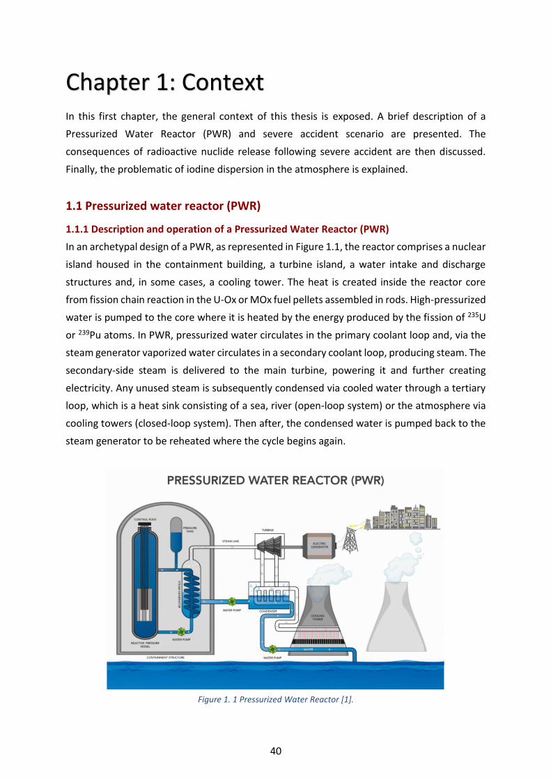
40

Chapter 1: Context In this first chapter, the general context of this thesis is exposed. A brief description of a

Pressurized Water Reactor (PWR) and severe accident scenario are presented. The

consequences of radioactive nuclide release following severe accident are then discussed.

Finally, the problematic of iodine dispersion in the atmosphere is explained.

1.1 Pressurized water reactor (PWR)

1.1.1 Description and operation of a Pressurized Water Reactor (PWR)

In an archetypal design of a PWR, as represented in Figure 1.1, the reactor comprises a nuclear

island housed in the containment building, a turbine island, a water intake and discharge

structures and, in some cases, a cooling tower. The heat is created inside the reactor core

from fission chain reaction in the U-Ox or MOx fuel pellets assembled in rods. High-pressurized

water is pumped to the core where it is heated by the energy produced by the fission of 235U

or 239Pu atoms. In PWR, pressurized water circulates in the primary coolant loop and, via the

steam generator vaporized water circulates in a secondary coolant loop, producing steam. The

secondary-side steam is delivered to the main turbine, powering it and further creating

electricity. Any unused steam is subsequently condensed via cooled water through a tertiary

loop, which is a heat sink consisting of a sea, river (open-loop system) or the atmosphere via

cooling towers (closed-loop system). Then after, the condensed water is pumped back to the

steam generator to be reheated where the cycle begins again.

Figure 1. 1 Pressurized Water Reactor [1].

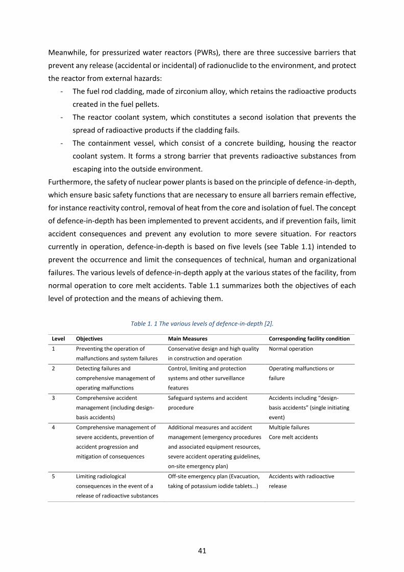
41

Meanwhile, for pressurized water reactors (PWRs), there are three successive barriers that

prevent any release (accidental or incidental) of radionuclide to the environment, and protect

the reactor from external hazards:

- The fuel rod cladding, made of zirconium alloy, which retains the radioactive products

created in the fuel pellets.

- The reactor coolant system, which constitutes a second isolation that prevents the

spread of radioactive products if the cladding fails.

- The containment vessel, which consist of a concrete building, housing the reactor

coolant system. It forms a strong barrier that prevents radioactive substances from

escaping into the outside environment.

Furthermore, the safety of nuclear power plants is based on the principle of defence-in-depth,

which ensure basic safety functions that are necessary to ensure all barriers remain effective,

for instance reactivity control, removal of heat from the core and isolation of fuel. The concept

of defence-in-depth has been implemented to prevent accidents, and if prevention fails, limit

accident consequences and prevent any evolution to more severe situation. For reactors

currently in operation, defence-in-depth is based on five levels (see Table 1.1) intended to

prevent the occurrence and limit the consequences of technical, human and organizational

failures. The various levels of defence-in-depth apply at the various states of the facility, from

normal operation to core melt accidents. Table 1.1 summarizes both the objectives of each

level of protection and the means of achieving them.

Table 1. 1 The various levels of defence-in-depth [2].

Level Objectives Main Measures Corresponding facility condition

1 Preventing the operation of

malfunctions and system failures

Conservative design and high quality

in construction and operation

Normal operation

2 Detecting failures and

comprehensive management of

operating malfunctions

Control, limiting and protection

systems and other surveillance

features

Operating malfunctions or

failure

3 Comprehensive accident

management (including design-

basis accidents)

Safeguard systems and accident

procedure

Accidents including “design-

basis accidents” (single initiating

event)

4 Comprehensive management of

severe accidents, prevention of

accident progression and

mitigation of consequences

Additional measures and accident

management (emergency procedures

and associated equipment resources,

severe accident operating guidelines,

on-site emergency plan)

Multiple failures

Core melt accidents

5 Limiting radiological

consequences in the event of a

release of radioactive substances

Off-site emergency plan (Evacuation,

taking of potassium iodide tablets…)

Accidents with radioactive

release

42

1.1.2 Production of fission products

Most reactors in the world are fueled with uranium that is typically enriched with 3-5% of the

isotope uranium-235 of half-life 7.038 × 108 years and that can undergo the following fission

reaction [2-4]:

𝑛10 + 𝑈92

235 →𝑃𝐹1+𝑃𝐹2+2.5 𝑛10 +200𝑀𝑒𝑉 [R1-1]

Fission occurs when the nucleus of a uranium-235 atom splits into fragments referred to as

fission products (FPs). These fission products are mostly radioactive and accumulate inside the

fuel pellets. Based on elemental analysis of irradiated fuels and with regard to the behavior of

fission products, the chemical state of the fission products under nominal burnup conditions

of a PWR can be classified into the following main groups [2, 5, 6]:

- In the form of dissolved oxides, in particular for strontium (Sr), yttrium (Y), zirconium

(Zr), lanthanum (La), cerium (Ce) and neodymium (Nd);

- In the form of oxide precipitates primarily for barium (Ba) and niobium (Nb);

- In the form of metal precipitates for molybdenum (Mo), technetium (Tc), ruthenium

(Ru), rhodium (Rh) and palladium (Pd);

- Mainly in the form of dissolved atoms for the volatile FPs: bromine (Br), rubidium (Rb),

tellurium (Te), iodine (I) and cesium (Cs). However, the chemical state of these FPs is

not fully known. Above a certain temperature, they can migrate radially within the fuel

pellets and condense in the colder sections, where they form more complex

compounds with fuel elements or other FPs. For example, cesium can form compounds

such as cesium molybdates and cesium uranates;

- In the form of dissolved atoms or intergranular or intragranular gas bubbles: xenon

(Xe) and krypton (Kr) in the case of fission gases. It should be noted that gases that

accumulate at the grain boundaries are more easily released during accident

situations.

Although many hundreds of FPs isotopes are formed in the reactor, most have very short half-

lives and decay days to weeks after their creation. It should be highlighted that 131I isotope

has a short half-life of 8 days which means that it is of concern only with respect to the fuel in

an operating nuclear power plant or with fuel from a reactor core that has been recently shut

down. However, 129I who has a long half-life of 15.7 million year is potentially significant in the

spent nuclear fuel stored at NPPs [7, 8] and in the nuclear spent fuel reprocessing plant [9,

10]. In fact, it was found that the total mass of iodine in the core of a 900 MWe PWR with UO2

fuel, after reactor emergency shutdown is 12.7 kg [2, 11]. Additionally, the isotopic iodine

mass distribution and activity1 in the fuel bundle of a 900 MWe PWR was estimated based on

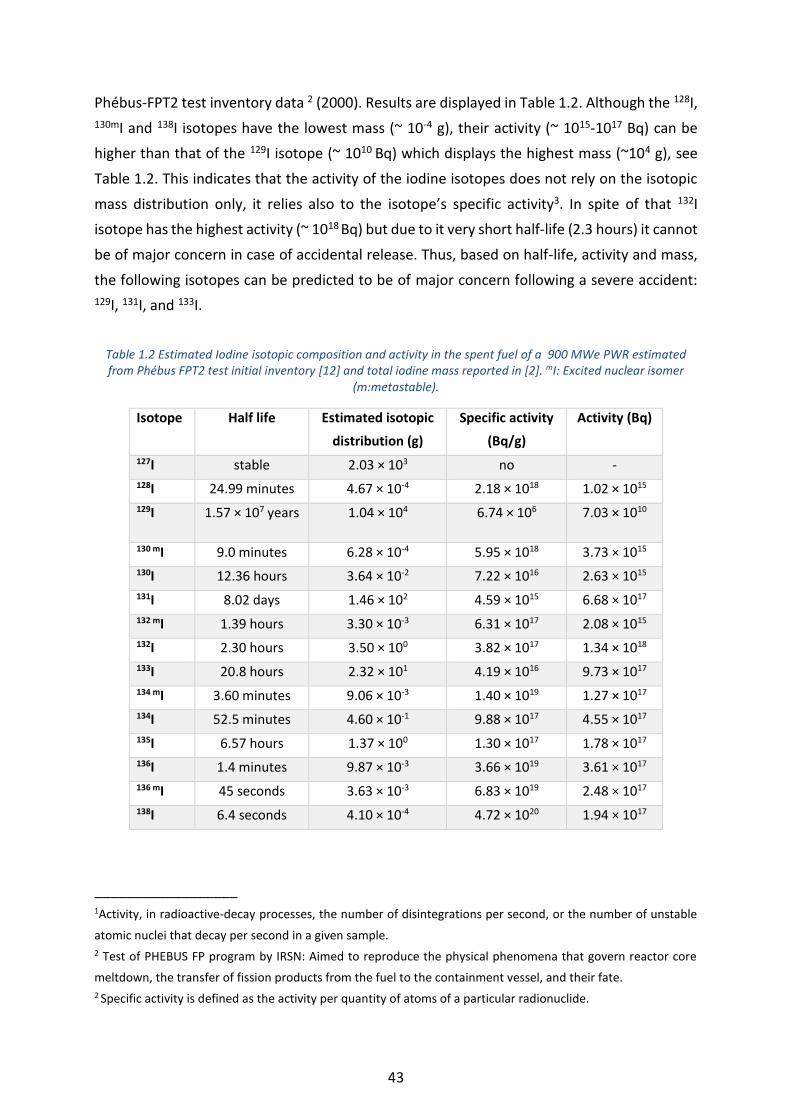
43

Phébus-FPT2 test inventory data 2 (2000). Results are displayed in Table 1.2. Although the 128I,

130mI and 138I isotopes have the lowest mass (~ 10-4 g), their activity (~ 1015-1017 Bq) can be

higher than that of the 129I isotope (~ 1010 Bq) which displays the highest mass (~104 g), see

Table 1.2. This indicates that the activity of the iodine isotopes does not rely on the isotopic

mass distribution only, it relies also to the isotope’s specific activity3. In spite of that 132I

isotope has the highest activity (~ 1018 Bq) but due to it very short half-life (2.3 hours) it cannot

be of major concern in case of accidental release. Thus, based on half-life, activity and mass,

the following isotopes can be predicted to be of major concern following a severe accident: 129I, 131I, and 133I.

Table 1.2 Estimated Iodine isotopic composition and activity in the spent fuel of a 900 MWe PWR estimated from Phébus FPT2 test initial inventory [12] and total iodine mass reported in [2]. mI: Excited nuclear isomer

(m:metastable).

Isotope Half life Estimated isotopic

distribution (g)

Specific activity

(Bq/g)

Activity (Bq)

127I stable 2.03 × 103 no -

128I 24.99 minutes 4.67 × 10-4 2.18 × 1018 1.02 × 1015

129I 1.57 × 107 years 1.04 × 104 6.74 × 106 7.03 × 1010

130 mI 9.0 minutes 6.28 × 10-4 5.95 × 1018 3.73 × 1015

130I 12.36 hours 3.64 × 10-2 7.22 × 1016 2.63 × 1015

131I 8.02 days 1.46 × 102 4.59 × 1015 6.68 × 1017

132 mI 1.39 hours 3.30 × 10-3 6.31 × 1017 2.08 × 1015

132I 2.30 hours 3.50 × 100 3.82 × 1017 1.34 × 1018

133I 20.8 hours 2.32 × 101 4.19 × 1016 9.73 × 1017

134 mI 3.60 minutes 9.06 × 10-3 1.40 × 1019 1.27 × 1017

134I 52.5 minutes 4.60 × 10-1 9.88 × 1017 4.55 × 1017

135I 6.57 hours 1.37 × 100 1.30 × 1017 1.78 × 1017

136I 1.4 minutes 9.87 × 10-3 3.66 × 1019 3.61 × 1017

136 mI 45 seconds 3.63 × 10-3 6.83 × 1019 2.48 × 1017

138I 6.4 seconds 4.10 × 10-4 4.72 × 1020 1.94 × 1017

__________________

1Activity, in radioactive-decay processes, the number of disintegrations per second, or the number of unstable

atomic nuclei that decay per second in a given sample. 2 Test of PHEBUS FP program by IRSN: Aimed to reproduce the physical phenomena that govern reactor core

meltdown, the transfer of fission products from the fuel to the containment vessel, and their fate. 2 Specific activity is defined as the activity per quantity of atoms of a particular radionuclide.

44

1.2 Nuclear severe accident

Incidents and accidents at nuclear facilities are divided into seven categories according to their

severity as established by the International Nuclear and Radiological Event Scale (INES)

presented in Figure 1.2.

During the lifetime of one generation, there were 3 major industrial nuclear accidents with

area contamination in different countries. The first, in 1979, in the second reactor at the Three

Mile Island nuclear power plant at United States. Fortunately, the accident did not have

significant environmental consequences and was rated as level 5 accident (Figure 1.2). The

second, in 1986, on the fourth reactor of the Chernobyl plant in Ukraine. The third, in 2011,

at three of the six reactors at the TEPCO's Fukushima Daiichi NPS in Japan. Chernobyl and

Fukushima accidents, were provisionally rated as Level 7 accident (See Figure 1.2).

Unfortunately, major accident resulted in significant amounts of radioactivity being released

into the environment, for instance 5.2×1018 Bq (Chernobyl) and 6.3×1017 Bq (Fukushima) [13-

15].

Figure 1. 2 The International Nuclear and Radiological Event Scale (INES) [16].

45

Indeed, these severe nuclear accidents have released significant quantities of radioactive

iodine into the atmosphere as shown in Table 1.3. Of the radioactive iodines, iodine-131 is

one of the most significant in terms of environmental and dosimetry impacts, considering its

activity and half-life impact.

Table 1. 3 Released radioactive iodine quantity into the atmosphere, during the main accidents (NPPs and reprocessing plants).

PBq: PetaBq and TBq: TerraBq. 1TBq = 1012 Bq and 1PBq = 1015 Bq.

Accident - date (Score - INES)

131I (equivalent mass)

Total iodine Reference

Kyshtym 29/09/1957 (6)

1-10 PBq (0-2 g)

undetermined Rapport IRSN [17]

Windscale pile 1 10/10/1957 (5)

0.74 -1.8 PBq (0.15 -0.38 g)

undetermined Garland et al. 2007 [18]

Three Miles Island-2 28/03/1979 (5)

0.48 - 0.63 TBq (0.10 - 0.13 g)

0.56 TBq Levin et al., 2013 [19]

Chernobyl 26/04/1986 (7)

1760 PBq (100 - 375 g)

5200 PBq UNSCEAR, 2000 [20] IAEA, 2006 [21]

Fukushima 11/03/2011 (7)

100-200 PBq (21-42 g)

Maximum 300 PBq NISA, 2011 [22] UNSCEAR, 2014 [23] MEXT, 2011 [24] Lebel et al., 2016 [25] Masson et al., 2019 [26]

1.2.1 Nuclear severe accident scenarios

Figure 1. 3 Physical phenomena during a severe accident [27].

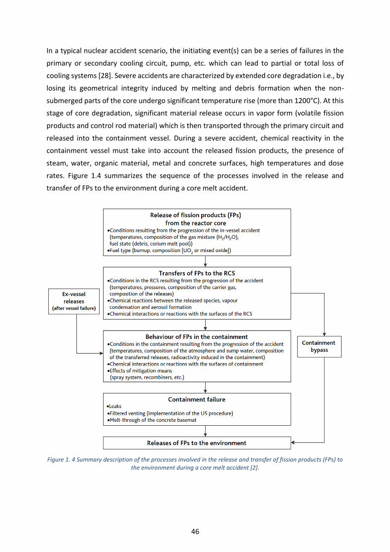
46

In a typical nuclear accident scenario, the initiating event(s) can be a series of failures in the

primary or secondary cooling circuit, pump, etc. which can lead to partial or total loss of

cooling systems [28]. Severe accidents are characterized by extended core degradation i.e., by

losing its geometrical integrity induced by melting and debris formation when the non-

submerged parts of the core undergo significant temperature rise (more than 1200°C). At this

stage of core degradation, significant material release occurs in vapor form (volatile fission

products and control rod material) which is then transported through the primary circuit and

released into the containment vessel. During a severe accident, chemical reactivity in the

containment vessel must take into account the released fission products, the presence of

steam, water, organic material, metal and concrete surfaces, high temperatures and dose

rates. Figure 1.4 summarizes the sequence of the processes involved in the release and

transfer of FPs to the environment during a core melt accident.

Figure 1. 4 Summary description of the processes involved in the release and transfer of fission products (FPs) to

the environment during a core melt accident [2].

47

Moreover, different physical phenomena are liable to occur progressively with core

degradation such as vessel rupture inducing the escape of the degraded core in the lower part

of the containment and then molten core/concrete interaction in the reactor pit, or steam

explosion when the molten core encounters water accumulated in the sump. In the

containment atmosphere, hydrogen combustion can cause direct containment heating and

finally, containment rupture, and leakages as presented in Figure 1.3. This mode of

containment failure is very important as it can allow radioactive species to be released directly

to the environment from virtually the very start of an accident.

It is highlighted that the main radiological significant fission products that are believed to be

released into the environment in case of severe nuclear accident are iodine, cesium and

tellurium. Strontium, ruthenium, barium, molybdenum and the lanthanides are less released.

Among them, special attention is focused on the behavior of iodine given its complexity and

the potential short-term radiological consequences of releases of radioactive iodine to the

environment. The main physical and chemical forms of iodine that can be found in the

containment after a core melt accident are gaseous molecular iodine (I2), particulate iodine

(i.e., in aerosol form, such as cesium iodide [CsI]) and gaseous organic iodine (i.e., methyl

iodide [CH3I]). Among these three physical and chemical forms, organic iodine is the hardest

for existing filtration systems to trap. Additionally, unlike gaseous molecular iodine, the paints

on the wall of the containment do not adsorb gaseous organic iodine but instead they may be

released outside the containment by direct or indirect leak paths [2, 29, 30].

1.2.2 Source term

The amount and isotopic composition of the released radioactive material released from the

core is called “Source Term”, and its quantification has been the main objective of several

international research programs for more than thirty years as it can predict the environmental

consequences from radioactive product release. IRSN defines the source term as a specific

type of release characteristic to a family of reactors and representative of the accident type,

i.e., in general a containment failure mode following complete core melt [1]. The source term

is taken into consideration when defining corrective actions that have to be taken to protect

people under these conditions. Three source terms, listed in decreasing order of severity,

were defined in 1979 as [2]:

– Source term S1 corresponds to short-term containment failure occurring no more than a

few hours after the onset of the accident;

48

– Source term S2 corresponds to direct releases to the atmosphere following loss of

containment integrity occurring one or more days after the onset of the accident;

– Source term S3 corresponds to indirect, delayed releases to the atmosphere through

pathways allowing a significant amount of fission products to be retained.

For instance, the retained iodine source terms for a 900 MWe reactor are listed in Table 1.4.

Data in Table 1.4 shows the importance of avoiding an early containment failure and the role

of filtration i.e., strong reduction of the source term by limiting iodine release to the

atmosphere.

Table 1. 4 Evaluated iodine source terms S1, S2 and S3 in 2000 for a 900 MWe PWR [2,31]. Source terms are given in percentages of the initial activity present in the reactor core.

Source Term S1 S2 S3

% Inorganic iodine

% aerosols 60 2.7 4.2 × 10-3 % molecular iodine 2.5 × 10-8

% Organic iodine 0.7 0.55 0.55

The source terms for a given accident can be evaluated by the ASTEC software (Accident

Source Term Evaluation Code) developed by IRSN since 1995 [32]. The ASTEC code is dedicated

to the detailed modelling of the phenomenology of a severe accident and its consequences.

In general, the ASTEC code models release of FPs according to three categories: (1) volatile FP

releases (Xe, Kr, I, Br, Cs, Rb, Sb, Te) (2) semi-volatile FP releases (3) non-volatile FP releases.

In the case of iodine, IRSN published a summary in 2010 [33] and 2014 [34] detailing the model

of the iodine chemistry in the containment during a core melt accident implemented in the

ASTEC code and its use to conduct safety studies for power reactors during a core meltdown

accident.

1.3 Lessons learned from radioiodine release into the atmosphere

The understanding of the environmental behavior of radioiodine starts with the

understanding of the different chemical and physical forms that radioiodine can take, and how

each of these, individually, behave in the atmosphere. As mentioned in the previous section,

radioiodine can be emitted into the atmosphere either in gaseous or in aerosol form. Once in

the atmosphere, each of the different chemical forms of radioiodine would have been subject

to different chemical and photochemical processes with naturally occurring atmospheric

species as gases and aerosols. Deposition processes are also identified as one of the iodine

depletion pathways from the atmosphere [35].

49

1.3.1 Dispersion of radioiodine

Both Chernobyl and Fukushima accidents caused radionuclide contamination of the

atmosphere. Unlike Chernobyl, the impact of the Fukushima accident was concentrated on a

local scale, but the duration of radioactive release was longer than a month. According to

various studies [13, 15, 23, 36] 131-Iodine isotope has the highest activity in both accidents in

comparison to other Iodine isotope (129I, 133I) as shown in Table 1.5.

Table 1. 5 Comparison of the estimated atmospheric release of radioiodine from the nuclear accidents at Chernobyl and Fukushima [13].

Activity (PBq)

Radionuclide Half life Chernobyl Fukushima

129I 1.57 × 107 years 4×10−5- 4.8×10−5 6.6 × 10−6

131I 8.02 days ~1760 200

133I 20.8 hours 910 146

Notably and by recalling section 1.1.2, this high activity of 131I is linked to its mass in the spent

fuel and its high specific activity. In addition, its several days long half-life allow significant

persistence of this isotope in the atmospheric compartment in case of releases. The other

iodine isotopes which present higher activities in the spent fuel (as shown in Table 1.2), have

nevertheless shorter half lifes (20.8 hours for 133I) so that their persistence in the atmosphere

remains limited in time (and distance). 131-Iodine (131I) is thus considered as one of the

important radionuclides released during a major severe nuclear accident.

Activity concentrations of 131I in air after the accident of Chernobyl and Fukushima, arranged

by distance to the respective NPPs are listed in Table 1.6. This table shows that although, the

half-life of 131I is short enough (8.02 days) to cause high specific activities, but long enough to

allow long-distance (>3000 km) atmospheric dispersion when released into the atmosphere.

Moreover, it should be noted that local meteorological conditions cause great variability in

activity concentrations in environmental media and can result in locations further away being

higher in concentration than closer locations [13, 15, 36].

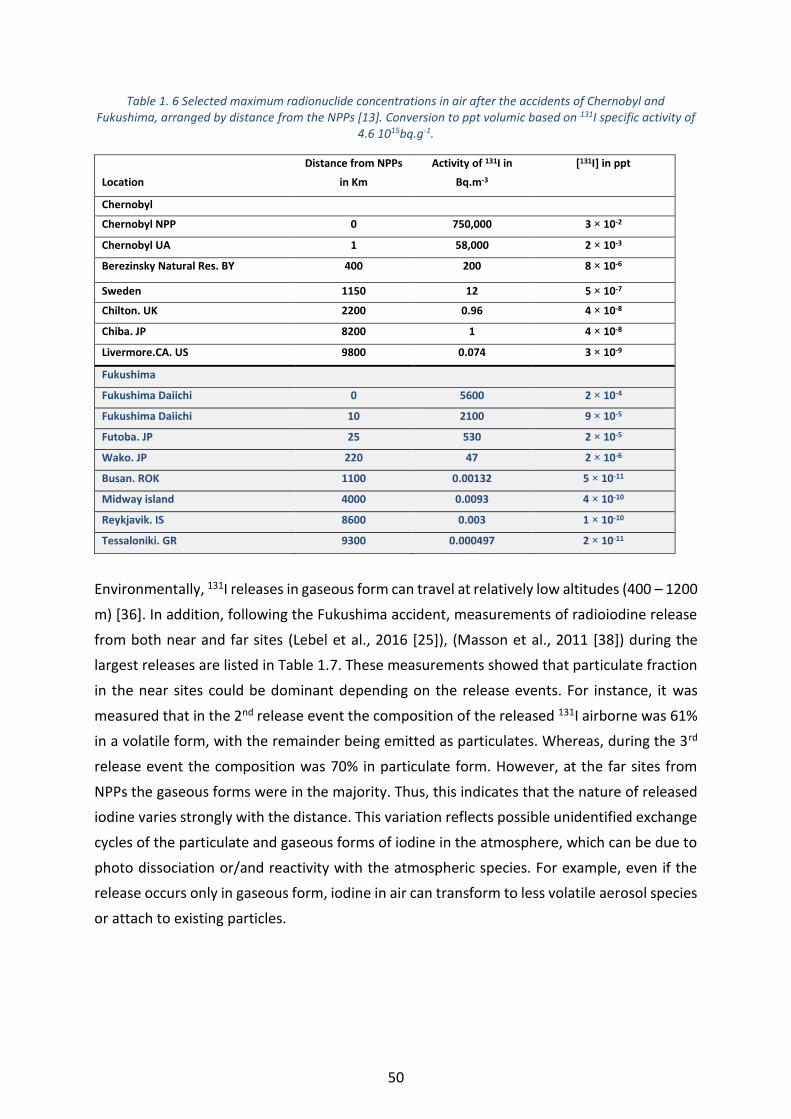
50

Table 1. 6 Selected maximum radionuclide concentrations in air after the accidents of Chernobyl and Fukushima, arranged by distance from the NPPs [13]. Conversion to ppt volumic based on 131I specific activity of

4.6 1015bq.g-1.

Location

Distance from NPPs

in Km

Activity of 131I in

Bq.m-3

[131I] in ppt

Chernobyl

Chernobyl NPP 0 750,000 3 × 10-2

Chernobyl UA 1 58,000 2 × 10-3

Berezinsky Natural Res. BY 400 200 8 × 10-6

Sweden 1150 12 5 × 10-7

Chilton. UK 2200 0.96 4 × 10-8

Chiba. JP 8200 1 4 × 10-8

Livermore.CA. US 9800 0.074 3 × 10-9

Fukushima

Fukushima Daiichi 0 5600 2 × 10-4

Fukushima Daiichi 10 2100 9 × 10-5

Futoba. JP 25 530 2 × 10-5

Wako. JP 220 47 2 × 10-6

Busan. ROK 1100 0.00132 5 × 10-11

Midway island 4000 0.0093 4 × 10-10

Reykjavik. IS 8600 0.003 1 × 10-10

Tessaloniki. GR 9300 0.000497 2 × 10-11

Environmentally, 131I releases in gaseous form can travel at relatively low altitudes (400 – 1200

m) [36]. In addition, following the Fukushima accident, measurements of radioiodine release

from both near and far sites (Lebel et al., 2016 [25]), (Masson et al., 2011 [38]) during the

largest releases are listed in Table 1.7. These measurements showed that particulate fraction

in the near sites could be dominant depending on the release events. For instance, it was

measured that in the 2nd release event the composition of the released 131I airborne was 61%

in a volatile form, with the remainder being emitted as particulates. Whereas, during the 3rd

release event the composition was 70% in particulate form. However, at the far sites from

NPPs the gaseous forms were in the majority. Thus, this indicates that the nature of released

iodine varies strongly with the distance. This variation reflects possible unidentified exchange

cycles of the particulate and gaseous forms of iodine in the atmosphere, which can be due to

photo dissociation or/and reactivity with the atmospheric species. For example, even if the

release occurs only in gaseous form, iodine in air can transform to less volatile aerosol species

or attach to existing particles.

51

Table 1. 7 Estimated volatile 131I composition of major releases during the Fukushima Daiichi accident. The particulate fraction is the supplement to 100% [25].

Volatile iodine fraction

Location (Distance

from NPPs)

14-16 March 2011

(1st release)

19-26 March 2011 (2nd

release)

29-31 March 2011

(3rd Release)

Near sites Daiichi (1 km) undetermined 61% 31%

Daini (11 km) undetermined 15% 34%

Far sites NSRI (112 km) 49% 47% 78%

NCL (116 km) 52% 51% 69%

With this intention, the French Institute of Radioprotection and Nuclear Safety (IRSN) has

developed specific simulation software’s (C3X plateform) capable of reproducing the release

and dispersion of the radionuclides in the atmosphere [39]. However, one potential problem

with such simulation tools is that the transport of 131-Iodine products following an accident

is currently modelled without considering the reactivity of iodine in the atmosphere.

1.3.2 Radioprotection

After a nuclear accident and the release of radionuclides, into the environment, human health

can be affected in several ways, including external and internal exposure as presented in

Figure 1.5. Indeed, gaseous radioactive iodine, especially the 131I isotope, with a half-life of 8

days, poses a health hazard if present in high concentrations due to its easy and almost

irreversible transport to the human thyroid gland, where it can locally induce cancer. In the

case of Chernobyl accident, 131I was largely responsible for absorbed doses to the thyroid,

which were delivered over a relatively short period after the accident (via inhalation and

ingestion) [23, 40].

Figure 1. 5 Exposure pathways from releases of radioactive material to the environment [41].

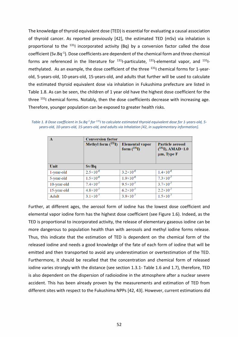
52

The knowledge of thyroid equivalent dose (TED) is essential for evaluating a causal association

of thyroid cancer. As reported previously [42], the estimated TED (mSv) via inhalation is

proportional to the 131I incorporated activity (Bq) by a conversion factor called the dose

coefficient (Sv.Bq-1). Dose coefficients are dependent of the chemical form and three chemical

forms are referenced in the literature for 131I-particulate, 131I-elemental vapor, and 131I-

methylated. As an example, the dose coefficient of the three 131I chemical forms for 1-year-

old, 5-years-old, 10-years-old, 15-years-old, and adults that further will be used to calculate

the estimated thyroid equivalent dose via inhalation in Fukushima prefecture are listed in

Table 1.8. As can be seen, the children of 1 year old have the highest dose coefficient for the

three 131I chemical forms. Notably, then the dose coefficients decrease with increasing age.

Therefore, younger population can be exposed to greater health risks.

Table 1. 8 Dose coefficient in Sv.Bq-1 for 131I to calculate estimated thyroid equivalent dose for 1-years-old, 5-years-old, 10-years-old, 15-years-old, and adults via Inhalation [42, in supplementary information].

Further, at different ages, the aerosol form of iodine has the lowest dose coefficient and

elemental vapor iodine form has the highest dose coefficient (see Figure 1.6). Indeed, as the

TED is proportional to incorporated activity, the release of elementary gaseous iodine can be

more dangerous to population health than with aerosols and methyl iodine forms release.

Thus, this indicate that the estimation of TED is dependent on the chemical form of the

released iodine and needs a good knowledge of the fate of each form of iodine that will be

emitted and then transported to avoid any underestimation or overtestimation of the TED.

Furthermore, it should be recalled that the concentration and chemical form of released

iodine varies strongly with the distance (see section 1.3.1- Table 1.6 and 1.7), therefore, TED

is also dependent on the dispersion of radioiodine in the atmosphere after a nuclear severe

accident. This has been already proven by the measurements and estimation of TED from

different sites with respect to the Fukushima NPPs [42, 43]. However, current estimations did

53

not consider the fate of the iodine species in the atmosphere, which it may influence the 131I-

TEDs. This suggest the following:

- Dose estimation, which takes into account the iodine reactivity in the atmosphere, will

be more valuable.

- The necessity to improve current dispersion tools by considering the reactivity of

iodine species in the atmosphere in order to better predict the thyroid equivalent

dose.

Figure 1. 6 Evolution of dose coefficient as function age via inhalation [42].

1.4 Conclusion

Unfortunately, in the event of a PWR severe accident, an important amount of volatile

radioactive in gaseous form (mainly, I2 and RI-type CH3I) can be released into the atmosphere

compartment where it can induce dramatical consequences on human in case of inhalation /

ingestion. These iodine species are highly reactive and will interact, at least in the near field

(i.e. at least within 11 km with respect to the point of emission) with the other species present

in the atmosphere (gas or particles), where they can evolve either in gaseous or particulate

form. Thus, the knowledge of the reactivity of iodine and its behavior in the atmosphere is

also of prime importance to better predict the dispersion of iodine in the atmosphere in case

of severe accident. Additionally, it will help to better evaluate the radiological health impact

of the accidental releases of iodine. To date, IRSN has launched preliminary research studies

to develop a comprehensive modelling approach to better predict the iodine source term

(ASTEC), and its transfer to the biosphere (SYMBIOSE platform) and more specifically its

dispersion in the atmospheric compartment (C3X software) following a severe nuclear power

plant reactor accident. Currently, these tools integrate the iodine transfer in the environment

54

without considering the possible iodine behavior in the atmosphere. In this context, reactivity

of both gaseous molecular iodine (I2) and iodomethane (CH3I) appears to be of central

importance in understanding the radioiodine dispersion in the atmosphere if a severe nuclear

power plant accident type Chernobyl (Ukraine) and the more recent Fukushima (Japan)

disaster were to occur. Such knowledge is of a major importance to complete the

understanding of iodine dispersion in the atmosphere in order to better protect the

population in case of nuclear severe accident.

References

[1] How Does a Nuclear Reactor Work?, (2019). https://www.energy.gov/ne/articles/nuclear-101-how-does-nuclear-reactor-work. [Citation in April 2020].

[2] D. Jacquemain et al., Nuclear Power Reactor Core Melt Accidents. IRSN book, ISBN: 978-2-7598-1835-8, France, 2015.

[3] C. Alejano, D. Boulanger, M. Brady-raap, l. Jutier, C. Riffard, Y. Rugama, Spent nuclear fuel assay data for isotopic validation, 2011. OECD,NEA/NSC/NPNCS/DOC(2011)5.

[4] Uranium Enrichment, World Nucl. Assoc. [Citation in April 2020].

https://www.world-nuclear.org/information-library/nuclear-fuel-cycle/conversionenrichment-and-fabrication/uranium-enrichment.aspx#.UWrver-IRAs.

[5] H. Kleykamp, The chemical state of the fission’products in oxide fuels, J. Nucl. Mater. 131 (1985) 221–246. https://doi.org/10.1016/0022-3115(85)90460-X

[6] B.J. Lewis, W.T. Thompson, F.C. Iglesias, Fission Product Chemistry in Oxide Fuels, J. Nucl. Mater. 2 (2012) 515-546. https://doi.org/10.1016/B978-0-08-056033-5.00042-2.

[7] Y. Ando, K. Nishihara, H. Takano, Estimation of spent fuel compositions from light water reactors, J. Nucl. Sci. Technol. 37 (2000) 924–933. https:// doi.org/10.1080/18811248.2000. 9714974.

[8] Spent fuel composition, Radioactivity. [Citation in April 2020]. https://www.radioactivity.eu.com/site/pages/Spent_Fuel_Composition.htm.

[9] J.E. Moran, S. Oktay, P.H. Santschi, D.R. Schink, Atmospheric Dispersal of 129 Iodine from Nuclear Fuel Reprocessing Facilities, 33 (1999) 2536–2542. https://doi.org/10.1021/ es9900050.

[10] C.Frechou, D.Calmet, 129I in the environment of the La Hague nuclear fuel reprocessing plant - from sea to land, J. Environ. Radioact. 70 (2003) 43–59. https://doi.org/10.1016/ S0265-931X(03)00127-9.

55

[11] D. Jacquemain et al., Les accident de fusion du coeur des réacteur nucléaires de puissance, IRSN book, ISBN : 978-2-7598-0972-1, France, 2013.

[12] A.C. Gregoire, P. March, F. Payot, G. Ritter, E. Al., Phébus FPPT2 final report – Appendix A – Material inventory IRSN Report DPAM/DIR 2008-272 Phebus IP/08/579, 2008.

[13] G. Steinhauser, A. Brandl, T.E. Johnson, Comparison of the Chernobyl and Fukushima nuclear accidents: A review of the environmental impacts, Sci. Total Environ. 470–471 (2014) 800–817. https://doi.org/10.1016/j.scitotenv.2013.10.029.

[14] V. Kortov, Y. Ustyantsev, Chernobyl accident: Causes, consequences and problems of radiation measurements, Radiat. Meas. 55 (2013) 12–16.https://doi.org/10.1016/j.radm eas.2012.05.015.

[15] T. Imanaka, G. Hayashi, S. Endo, Comparison of the accident process , radioactivity release and ground contamination between Chernobyl and Fukushima-1, J. Radiat. Res. 56 (2015) 56–61. https://doi.org/10.1093/jrr/rrv074.

[16] International Nuclear and Radiological Event Scale, Int. Nucl. Event Scale. (2016). https://www.env.go.jp/en/chemi/rhm/basic-info/1st/02-02-01.html. [Citation in April 2020].

[17] A.C. Grégoire, L’iode dans l’atmosphère : du terme source à la dose, Rapport interne IRSN, n° IRSN/2019-00035, 2019.

[18] J.A. Garland, R. Wakeford, Atmospheric emissions from the Windscale accident of October 1957, Atmos. Environ. 41 (2007) 3904–3920. https://doi.org/10.1016/j.atmo senv .2006.12.049.

[19] R.J. Levin, N.F. De Simone, J.F. Slotkin, B.L. Henson, Incidence of thyroid cancer surrounding three mile island nuclear facility: The 30-year follow-up, Laryngoscope. 123 (2013) 2064–2071. https://doi.org/10.1002/lary.23953.

[20] Unscear, sources and effects of ionizing radiation, Annex J: Exposures and effects of the Chernobyl accident, 2000. https://www.unscear.org/unscear/publications.html.

[21] IAEA, Radiological Assessment Reports Series. Environmental Consequences of the Chernobyl Accident and their Remediation: Twenty Years of Experience, International Atomic Energy Agency report, ISBN 92–0–114705–8, 2006.

[22] NISA, Evaluation of the status of reactor cores in units 1-3 of the Fukushima Daiichi nuclear power plant, 2011. [Citation in April 2020]. http://www.meti.go.jp/press/2011/06/20110606008/20110606008-2.pdf (in Japanese).

[23] Unscear, report to the general assembly scientific annex A: Volume I, 2014.https://www. unscear.org/unscear/publications.html.

[24] MEXT, Radioactive Substance Emission Data, press release, October 20, 2011 in Japanese, 2011. www.meti.go.jp/press/2011/10/20111020001/20111020001.pdf. [Citation in April 2020].

[25] L.S. Lebel, R.S. Dickson, G.A. Glowa, Radioiodine in the atmosphere after the Fukushima Dai-ichi nuclear accident, J. Environ. Radioact. 151 (2016) 82–93. https://doi.org/ 10.1016/j.jenvrad.2015.06.001.

[26] O. Masson, J. Tschiersch, L.S. Lebel, H. Wershofen, J.W. Mietelski, G. Steinhauser, É.Blanchardon, L.Cantrel, A.C. Grégoire, D. Quélo, Radioiodine Releases in Nuclear Emergency

56

Scenarios, In: Nuclear Emergencies. Springer, ISBN: 978-981-13-8327-4, Singapore, 2019. https://doi.org/10.1007/978-981-13-8327-4_15.

[27] Research and development with regard to severe accidents in pressurised water reactors: Summary and outlook. Report IRSN-2007/83, 2007.

[28] A. Karhu, Gas Phase Chemistry and Removal of CH3I during a Severe Accident; Report: NKS-25, ISBN 87-7893-076-6. Corpus ID: 59022982. Danka Services International, DSI., Denmark, 2001.

[29] H. Bruchertseifer, R. Cripps, S. Güntay, B. Jäckel, Experiments on the Retention of the fission product iodine in nuclear reactor accidents (CH--0401). Report NIS/IAEA, reference number 36002863 Gschwend, B. (Ed.). Switzerland, 2004.

[30] S. Dickinson, A. Auvinen, Y. Ammar, L. Bosland, B. Clément, F. Funke, G. Glowa, T. Kärkelä, D.A. Powers, S. Tietze, G. Weber, S. Zhang, Experimental and modelling studies of iodine oxide formation and aerosol behaviour relevant to nuclear reactor accidents, Ann. Nucl. Energy. 74 (2014) 200–207. https://doi.org/10.1016/j.anucene.2014.05.012.

[31] M. Manesse, D., Fallot, A., Billarand, Y., Durin, Réévaluation des termes sources de référence; Note de synthèse, Note technique DPEA/SEAC/2000-036., 2000.

[32] J.P. Van Dorsselaere, C. Seropian, P. Chatelard, F. Jacq, J. Fleurot, P. Giordano, N. Reinke, B. Schwinges, H.J. Allelein, W. Luther, The ASTEC integral code for severe accident simulation, Nucl. Technol. 165 (2009) 293–307. https://doi.org/10.13182/NT09-A4102.

[33] L. Bosland, L. Cantrel, N. Girault, B. Clement, L. Bosland, N. Girault, B. Clement, Modeling of Iodine Radiochemistry in the ASTEC Severe Accident Code : Description and Application to FPT-2 PHEBUS Test, Nucl. Technol. 171 (2010) 99–107. https://doi.org/10. 13182/NT10-A10774.


[35] O.T. Bah, Communication prive, determination expérimentale du dépôt par temps sec de l’iode moléculaire.

[36] T. Christoudias, J. Lelieveld, Modelling the global atmospheric transport and deposition of radionuclides from the Fukushima Dai-ichi nuclear accident, Atmos. Chem. Phys. 13 (2013) 1425–1438. https://doi.org/10.5194/acp-13-1425-2013.

[37] R. Pollanen, I. Valkama, H. Toivonen, Transport of radioactive particles from the Chernobyl accident, Atmos. Environ. 31 (1997) 3575–3590. https://doi.org/10.1016/S1352-2310(97)00156-8.

[38] O. Masson, A. Baeza, J. Bieringer, K. Brudecki, S. Bucci, et al., Tracking of Airborne Radionuclides from the Damaged Fukushima Dai-Ichi Nuclear Reactors by European Networks, Environ. Sci. Technol. 45 (2011) 7670–7677. https://doi.org/10.1021/es2017158.

[39] M. Tombette, E.Quentric, D. Quélo, J. Benoit, A. Mathieu, I. Korsakissok, D. Didier, C3X : A software platform for assessing the consequences of an accidental release of radioactivity into the atmosphere, Poster, France, 2014.http://venus.iis.u-tokyo.ac.jp/English/workshop/ Poster/3rd March/Damien Didier.pdf.

57

[40] A. V Brenner, M.D. Tronko, M. Hatch, T.I. Bogdanova, V.A. Oliynik, J.H. Lubin, L.B. Zablotska, V.P. Tereschenko, R.J. Mcconnell, G.A. Zamotaeva, P.O. Kane, A.C. Bouville, L. V Chaykovskaya, E. Greenebaum, I.P. Paster, V.M. Shpak, E. Ron, I ‑ 131 Dose Response for Incident Thyroid Cancers in Ukraine Related to the Chornobyl Accident, Environ. Health Perspect. 119 (2011) 933–939. https://doi.org/10.1289/ehp.1002674.

[41] M. del R. Perez, E. Van Deventer, B. Amzal, L. Anspaugh, Health Risk Assessment from the Nuclear Accident after the 2011 Great East Japan Earthquake and Tsunami. World health organization report, ISBN 978 92 4 150513 0, Switzerland, 2013.

[42] T. Ohba, T. Ishikawa, H. Nagai, S. Tokonami, A. Hasegawa, Reconstruction of residents thyroid equivalent doses from internal radionuclides after the Fukushima Daiichi nuclear power station accident, Nat. Sci. Reports. 10 (2020) 3639. https://doi.org/10.1038/s41598-020-60453-0.

[43] E. Kim, K. Yajima, S. Hashimoto, K. Tani, Y. Igarashi, T. Iimoto, N. Ishigure, H. Tatsuzaki, M. Akashi, O. Kurihara, Reassessment of internal thyroid doses to 1,080 children examined in a screening survey after the 2011 fukushima nuclear disaster, Health Phys. (2020) 36–52. https://doi.org/10.1097/HP.0000000000001125.

58

Chapter 2: State of art

Iodine chemistry in the atmosphere

In the event of a major nuclear accident, the gaseous iodine species, which are likely to be

emitted into the atmosphere, are essentially identified as I2 and CH3I. Once released into the

atmosphere, they can undergo reactions leading to their conversion into various iodine

species. The quantities emitted can be significant at the point of release compared to naturally

occurring emissions, and are of crucial importance due to the radiotoxicity of radioactive

iodine (131-Iodine in particular). However, the life cycle of these radioactive species emitted

to the atmosphere will be the same as that of the same natural stable species under similar

atmospheric conditions.

In addition to its nuclear safety interests, iodine has a strong interest in the atmospheric

chemistry field due to its oxidizing properties and photochemical reactivity, which play an

important role in tropospheric chemistry. For more than 40 years, numerous experimental

and theoretical works have been carried out on the quantification of iodine forms (gaseous or

particulate) in the troposphere, on the identification of natural sources of iodine release and

finally on its reactivity, with the aim of better understanding the iodine cycle and its

interaction with other compounds present in the troposphere, whether of natural or

anthropogenic origin (ozone, radicals, VOCs, nitrogen oxides, etc.). Thus, many mechanisms

of iodine have been developed and a large database of the iodine cycle data is now available.

This chapter briefly presents the sources of gaseous iodine and its reactivity in the atmosphere

related to the iodine cycle. The sources of atmospheric aerosols and gas-aerosols

heterogeneous interactions are briefly exposed. The experimental approaches described in

the literature to study this reactivity are then briefly presented. Finally, a critical review of the

interaction of gaseous iodine species with atmospheric aerosols is given.

2.1 Main sources of iodine compounds

Iodine is a natural trace element of biological significance, where 127-Iodine is a naturally

occurring iodine isotope, and it is the only non-radioactive and stable iodine isotope. Biogenic

processes in the oceans represent a substantial source of iodine in the lower atmosphere.

Molecular iodine (I2) and organic iodide species such as methyl iodide (CH3I), ethyl iodide

(C2H5I), propyl iodide (isomers :1 and 2-C3H7I), butyl iodide (isomers: 2 and i-C4H9I), methylene

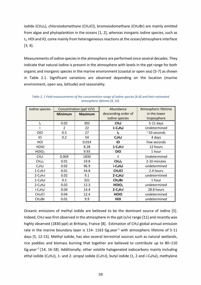
59

iodide (CH2I2), chloroiodomethane (CH2ICl), bromoiodomethane (CH2IBr) are mainly emitted

from algae and phytoplankton in the oceans [1, 2], whereas inorganic iodine species, such as

I2, HOI and IO, come mainly from heterogeneous reactions at the ocean/atmosphere interface

[3, 4].

Measurements of iodine species in the atmosphere are performed since several decades. They

indicate that natural iodine is present in the atmosphere with levels in the ppt range for both

organic and inorganic species in the marine environment (coastal or open sea) [5-7] as shown

in Table 2.1. Significant variations are observed depending on the location (marine

environment, open sea, latitude) and seasonality.

Table 2. 1 Field measurements of the concentration range of iodine species [6-8] and their estimated atmospheric lifetime [9, 10].

Iodine species Concentration (ppt V/V) Abundance descending order of

iodine species

Atmospheric lifetime in the lower troposphere

Minimum Maximum

I2 0.02 302 CH3I 5-11 days

I 2 22 1-C4H9I Undetermined

OIO 0.5 27 I2 ~10 seconds

IO 0.2 54 C2H5I 4 days

HOI 0.014 IO Few seconds

HOIO 8.28 1-C3H7I 12 hours

HOIO2 9.93 OIO 1 hour

CH3I 0.004 1830 I Undetermined

CH2I2 0.01 19.8 CH2I2 2-10 minutes

C2H5I 0.02 96.9 i-C4H9I undetermined

1-C3H7I 0.01 34.8 CH2ICl 2.4 hours

2-C3H7I 0.02 9.1 2-C4H9I undetermined

1-C4H9I 0.2 321 CH2IBr 1 hour

2-C4H9I 0.02 12.3 HOIO2 undetermined

i-C4H9I 0.04 14.4 2-C3H7I 28.8 hours

CH2ICl 0.04 12.4 HOIO undetermined

CH2IBr 0.01 9.9 HOI undetermined

Oceanic emissions of methyl iodide are believed to be the dominant source of iodine [5].

Indeed, CH3I was first observed in the atmosphere in the ppt (v/v) range [11] and recently was

highly observed (1830 ppt) at Brittany, France [8]. Estimation of CH3I global annual emission

rate in the marine boundary layer is 114- 1163 Gg.year-1 with atmospheric lifetime of 5-11

days [5, 12-15]. Methyl iodide, has also several terrestrial sources such as natural wetlands,

rice paddies and biomass burning that together are believed to contribute up to 80–110

Gg.year−1 [14, 16-18]. Additionally, other volatile halogenated iodocarbons mainly including

ethyl iodide (C2H5I), 1- and 2- propyl iodide (C3H7I), butyl iodide (1, 2 and i-C4H9I), methylene

60

iodide (CH2I2), chloroiodomethane (CH2ICl) and bromoiodomethane (CH2IBr), have been

detected in the atmosphere mostly in coastal regions [8, 19, 20]. Furthermore, methyl iodide

has the highest lifetime among the organic iodide species. Thus, methyl iodide is the major

contribute to the amount of organic iodine in the atmosphere.

Alternatively, inorganic iodine compounds (I2, HOI, IO) produced in the ocean surface layer

from the reaction of O3 with iodide are thought to be a dominant global source of iodine

mainly at the coastal margin [3, 21]. For instance, it has been shown that reactive I2 can escape

directly from the ocean surface to the atmosphere when brown algea (kelp, Laminaria

digitate) are subjected to oxidative stress such as by exposure to high irradiance, desiccation,

and atmospheric O3 [3, 22,23]. The emission rate of I2 from the action of O3 at the sea surface

is 0.4-1 Tg.year-1. I2 is highly photo reactive, as its photolysis lifetime is very short ~15 seconds

[4, 24, 25]. Additionally, laboratory data have suggested that inorganic iodide such as

molecular Iodide (I2) [3, 21], hypoiodous acid (HOI) [3], iodine oxide (IO) [21] can be produced

from heterogeneous reactions at the ocean-atmosphere interface.

Field measurements evidenced the presence of iodine rich aerosols in the atmosphere [26,

27]. Recently, iodine aerosol concentrations have been reported to be the highest in the

tropical marine boundary layer (MBL), averaging 5 ng.m−3 with monthly maximum

concentrations of 90 ng.m−3 [28].

Numerous experimental and theoretical works have been carried out on the quantification of

iodine forms (gaseous or particulate) in the troposphere, on the identification of sources of

iodine release and finally on its reactivity, with the aim of better understanding the iodine

cycle and its interaction with other compounds present in the troposphere, whether of natural

or anthropogenic origin (ozone, radicals, VOCs, nitrogen oxide.). Figure 2.1 summarizes the

main sources and fate of iodine species in the atmosphere.

It should be highlighted that anthropogenic releases of atmospheric iodine species are

believed to be negligible on a global scale compared to natural sources. Finally, iodine species

are commonly observed in the atmosphere following severe nuclear accident as shown in

Chapter 1 – though at levels much more lower than the natural occurrence, even at the close

proximity of the accident (see chapter 1, Table 1.6).

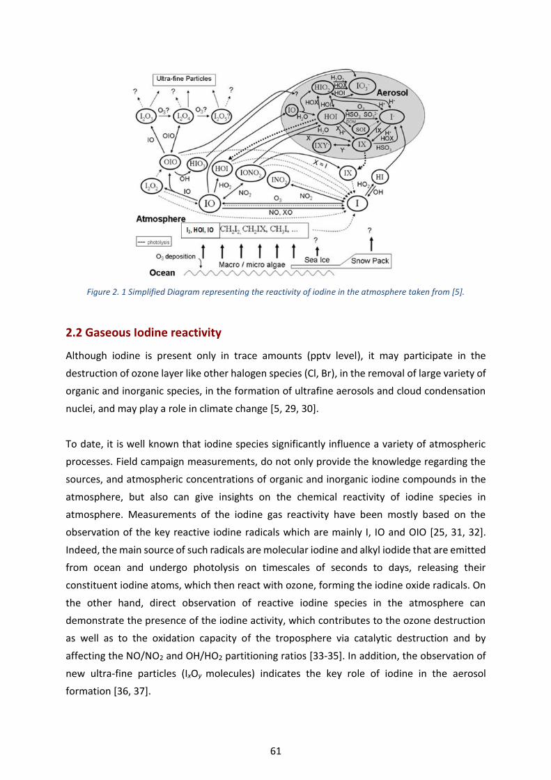
61

Figure 2. 1 Simplified Diagram representing the reactivity of iodine in the atmosphere taken from [5].

2.2 Gaseous Iodine reactivity

Although iodine is present only in trace amounts (pptv level), it may participate in the

destruction of ozone layer like other halogen species (Cl, Br), in the removal of large variety of

organic and inorganic species, in the formation of ultrafine aerosols and cloud condensation

nuclei, and may play a role in climate change [5, 29, 30].

To date, it is well known that iodine species significantly influence a variety of atmospheric

processes. Field campaign measurements, do not only provide the knowledge regarding the

sources, and atmospheric concentrations of organic and inorganic iodine compounds in the

atmosphere, but also can give insights on the chemical reactivity of iodine species in

atmosphere. Measurements of the iodine gas reactivity have been mostly based on the

observation of the key reactive iodine radicals which are mainly I, IO and OIO [25, 31, 32].

Indeed, the main source of such radicals are molecular iodine and alkyl iodide that are emitted

from ocean and undergo photolysis on timescales of seconds to days, releasing their

constituent iodine atoms, which then react with ozone, forming the iodine oxide radicals. On

the other hand, direct observation of reactive iodine species in the atmosphere can

demonstrate the presence of the iodine activity, which contributes to the ozone destruction

as well as to the oxidation capacity of the troposphere via catalytic destruction and by

affecting the NO/NO2 and OH/HO2 partitioning ratios [33-35]. In addition, the observation of

new ultra-fine particles (IxOy molecules) indicates the key role of iodine in the aerosol

formation [36, 37].

62

The observations from field measurements have been accompanied by laboratory and

modelling studies to improve knowledge regarding the reactivity of iodine species in the

atmosphere which can involve an important number of chemical species and reactions

(homogeneous and heterogeneous). During the day, the major fate of iodine-emitted species

by natural oceanic sources is photolysis leading rapidly to the formation of iodine atoms [34,

38, 39], for instance:

CH3I + hν→ CH3 + I, k= (0.5-6.6) × 10-6 s-1 [R2-1]

C2H5I + hν→ C2H5+ I, k=6.6 × 10-6 s-1 [R2-2]

1-C3H7I + hν→ C3H7 + I, k=2.6 × 10-5 s-1 [R2-3]

CH2I2 + hν→ CH3I + I, k=7.3 × 10-3 s-1 [R2-4]

I2 + hν→ I + I, k= (1.2 ± 0.3) × 10-1 s-1 [R2-5]

HOI + hν→ OH + I, k=3.3 × 10-4 s-1 [R2-6]

A summary have been provided on all the photochemical cross sections available in the

literature for different inorganic and organic iodine species [40]. Table 2.2 summarize the

maximum absorption cross section1 in cm-2 for the major observed iodine species.

Table 2. 2 Maximum absorption cross section (σ) at 298K [40].

Iodine species 20Maximum σ × 10

)2(cm

λ (nm)

CH3I 120 265

CH2I2 407 205

C2H5I 121 260

1-C3H7I 141 255

I2 229 500

IO 2050 420

OIO 1030 564

HOI 39.2 340

1 Absorption cross section is the probability that a photon passing through a molecule will be absorbed by that molecule multiplied by the average cross‐sectional area of the molecule.

63

It should be highlighted that in the case of I2, which photodissociates rapidly (~10 s) with a

photodisociation rate coefficient 0.12 ± 0.03 s-1 [41], I atoms are produced just above the

ocean surface. The longer-lived compounds, such as CH3I which has a lifetime of about 5-11

days with a photo dissociation rate coefficient ranges between (0.5-6.6) × 10-6 s-1 [42],

provides a source of iodine throughout the whole troposphere.

Following the photolysis reaction and the production of atomic iodine, ozone destruction can

occur via the three following catalytic cycles [5, 43]:

Cycle 1:

I + O3 → IO + O2, k=1.2×10–12 cm3.molecule-1.s-1 [R2-7]

IO + IO → I + OIO, k=8.0×10–12 cm3.molecule-1.s-1 [R2-8]

OIO + hν → I + O2, k=2.6 × 10-1 s-1 [R2-9]

2O3 → 3O2 [R2-10]

Cycle 2:

I + O3 → IO + O2, k=1.2×10–12 cm3.molecule-1.s-1 [R2-11]

IO + HO2 → HOI + O2, k= 8.6×10–11 cm3.molecule-1.s-1 [R2-12]

HOI +hν → I + OH, k=3.3 × 10-4 s-1 [R2-13]

HO2 + O3 → OH + 2O2 [R2-14]

Cycle 3:

I + O3 → IO + O2, k=1.2×10-12 cm3.molecule-1.s-1 [R2-15]

IO + NO2 → IONO2, k=1.5×10-11 cm3.molecule-1.s-1 [R2-16]

IONO2 + hν → I + NO3, k=1.2 × 10-2 s-1 [R2-17]

NO3 + hν → NO + O2, k=2.8 ×10-11 cm3.molecule-1.s-1 [R2-18]

NO + O3 → NO2 + O2, k=1.9×10-14 cm3.molecule-1.s-1 [R2-19]

2O3 → 3O2 [R2-20]

The reaction of atomic iodine with O3 (R2-7, R2-11 or R2-15) with a reaction rate coefficient

1.2×10–12 cm3.molecule-1.s–1 [40, 44], form the iodine monoxide (IO) radical. This reaction is

believed to be the major fate of iodine radicals (I) and the key step in the iodine catalyzed O3

destruction cycles [45]. Additionally, a number of temporary inorganic reservoir products

(IONO2, HOI, and OIO) can be formed via the IO reactions with NOx, HO2, and IO. This indicates

that IO can disrupt the oxidizing capacity of the atmosphere by modifying the abundance and

distribution of HOx (OH/HO2) and NOx (NO/NO2) mainly through the reactions R2-12 and R2-

16.

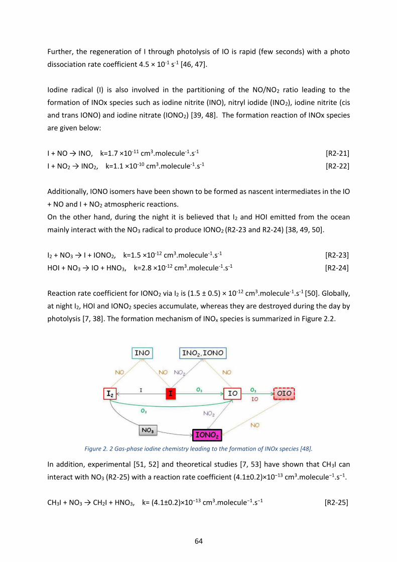
64

Further, the regeneration of I through photolysis of IO is rapid (few seconds) with a photo

dissociation rate coefficient 4.5 × 10-1 s-1 [46, 47].

Iodine radical (I) is also involved in the partitioning of the NO/NO2 ratio leading to the

formation of INOx species such as iodine nitrite (INO), nitryl iodide (INO2), iodine nitrite (cis

and trans IONO) and iodine nitrate (IONO2) [39, 48]. The formation reaction of INOx species

are given below:

I + NO → INO, k=1.7 ×10-11 cm3.molecule-1.s-1 [R2-21]

I + NO2 → INO2, k=1.1 ×10-10 cm3.molecule-1.s-1 [R2-22]

Additionally, IONO isomers have been shown to be formed as nascent intermediates in the IO

+ NO and I + NO2 atmospheric reactions.

On the other hand, during the night it is believed that I2 and HOI emitted from the ocean

mainly interact with the NO3 radical to produce IONO2 (R2-23 and R2-24) [38, 49, 50].

I2 + NO3 → I + IONO2, k=1.5 ×10-12 cm3.molecule-1.s-1 [R2-23]

HOI + NO3 → IO + HNO3, k=2.8 ×10-12 cm3.molecule-1.s-1 [R2-24]

Reaction rate coefficient for IONO2 via I2 is (1.5 ± 0.5) × 10-12 cm3.molecule-1.s-1 [50]. Globally,

at night I2, HOI and IONO2 species accumulate, whereas they are destroyed during the day by

photolysis [7, 38]. The formation mechanism of INOx species is summarized in Figure 2.2.

Figure 2. 2 Gas-phase iodine chemistry leading to the formation of INOx species [48].

In addition, experimental [51, 52] and theoretical studies [7, 53] have shown that CH3I can

interact with NO3 (R2-25) with a reaction rate coefficient (4.1±0.2)×10−13 cm3.molecule−1.s−1.

CH3I + NO3 → CH2I + HNO3, k= (4.1±0.2)×10−13 cm3.molecule−1.s−1 [R2-25]

65

The review on the understanding of the atmospheric gaseous iodine reactivity and the

proposed mechanism by Saiz Lopez et al. [5] only considered the destruction of organic iodine

species by photolysis. However, CH3I can decompose via OH (R2-26) and O (R2-27,31) radicals

[7, 54]:

CH3I + OH → CH2I + H2O, k=6.2 × 10-14 cm3.molecule-1.s-1 [R2-26]

CH3I + O → IO + CH3, k=1.0 × 10-11 cm3.molecule-1.s-1 [R2-27]

CH3I + O → CH2I + HO, k=1.1 × 10-12 cm3.molecule-1.s-1 [R2-28]

CH3I + O → H + I + HC(O)H, k=1.5 × 10-12 cm3.molecule-1.s-1 [R2-29]

CH3I + O → I + CH3O, k=6.8 × 10-13 cm3.molecule-1.s-1 [R2-30]

CH3I + O → HI + HC(O)H, k=1.2 × 10-12 cm3.molecule-1.s-1 [R2-31]

Further, it should be highlighted that the self-reaction of iodine oxides (IO and OIO) and

hydroiodic acid (HI) are known to be predominantly responsible for the production of the

iodine ultra-fine particles (IxOy) [5, 36, 55- 58]. Iodine oxide particles that have been detected

in the atmosphere include I2O2, I2O3, I2O4, and I2O5. A recent study [7] has shown that the I2O5

formation is promoted with a high release of I2 during summer. The gas phase scheme based

on several oxidation steps for the generation of I2O5 was proposed [R2-32] with a reaction

coefficient rate 5 × 10-16 cm3.molecule-1.s-1 for each oxidation step [56]:

I2O2 + O3 → I2O3 + O3→ I2O4 + O3 →I2O5, k=5 × 10-16 cm3.molecule-1.s-1 [R2-32]

I2O3 and I2O4 could also form from the reaction of IOx radicals with a reaction rate coefficient

ranging from 1.1 to 1.7 × 10-16 cm3.molecule-1.s-1 [56]. Moreover, it has been suggested that

I2O5 would appear as a result from the polymerization, [R2-33] [59]:

5I2O4 → 4I2O5 + I2, k= not reported [R2-33]

Briefly, many reaction pathways are known for iodine oxides, however there are still gaps in

the knowledge on the fate of the iodine oxides of IxOy particle form.

All the available data in the field of atmospheric chemistry had highlighted the complexity of

the reactivity of iodine in the atmosphere. In nuclear context, two studies [6, 7] have

developed a gaseous iodine reaction mechanism which consisted into two parts: (1) an

inorganic part with 99 reactions including 11 photolysis reactions involving 23 iodine species

and (2) an organic part composed of 133 reactions including 2 photolysis reaction, for a total

of 55 additional iodine species divided into 23 RACM (Regional Atmospheric Chemistry

Mechanism, [60]) categories [6, 7]. The organic part is new compared to the proposed

mechanism by Sais Lopez et al. [5], who only considered the destruction of organic iodine

66

species by photolysis. Further, the two studies [6, 7] have summarized the overall behavior of

iodine reactivity as shown in Figure 2.3 using ASTEC/SOPHAEROS code (IRSN severe accident

simulation tool [61]) with 0D model calculations. The 0D model is a 0-dimensional model used

to calculate the concentration of chemical species. They describe a system of differential

equations with respect to the time variable without any notion of variation in space and are

therefore very fast to execute. Traditionally, these models are represented in the form of a

box. They allow the determination of speciation and the predominant reactions.

Figure 2. 3 Summary diagram of the iodine reactivity in the atmosphere [6, 7].

In order to better understand the speciation of iodine, the iodine gas-phase mechanism

containing 248 reactions combined to the RACM air quality mechanism was implemented into

the ASTEC simulation tool of IRSN and calculations were performed at 0D. These calculations

were performed by taking into account input parameters that were chosen to represent an

accidental release of iodine from a Pressurized water reactor (Gravelines site) taking into

account realistic air pollutant concentration (O3, NOx, VOCs), meteorological situation, day-

night conditions, and finally nature and concentration of iodine release (I2 or CH3I). As an

example, Figure 2.4 shows the evolution of iodine compounds grouped under 5 main families

(organic and inorganic iodine, iodine-nitrogen species, iodine oxide and radicals) for a release

of I2 (98 ppt) and CH3I (196 ppt) in winter daylight. The rapid evolution of I2 and CH3I gaseous

forms according to the day/night phases, in connection with photolysis processes, and the

presence of certain pollutants in the atmosphere, indicates the strong reactivity of molecular

iodine (I2) under atmospheric conditions. Whereas, less reactivity has been seen for methyl

iodide (CH3I) as shown in Figure 2.4.

67

Figure 2. 4 Family mass evolution of iodine, injection 2013 January 1st, at 7 am as a function of time with iodine release (a) 98 ppt of I2 and (b) 196 ppt of CH3I. (Organic in green, iodine in violet, iodine oxide in orange,

inorganic in blue and radicals in red) [62].

Despite, the exhaustive literature studies carried out over years on iodine chemistry that made

it possible to understand the iodine atmospheric cycle and its speciation in the atmosphere,

the role of water vapor on the iodine cycle has not been investigated yet which is nevertheless

one of the most important atmospheric compounds. The amount of water in the atmosphere

varies greatly depending on the region and altitude. It was shown that water has an influence

on formation of iodine particles [63]. However, some modelling studies have investigated the

microhydration process of several inorganic iodine species such as HOIO [64], HOIO2 [65], INOx

[48] as well as CH3I hydrolysis processes [66] and micro solvation process of CH3I [67-69].

2.3 Iodine heterogeneous reactivity

Atmospheric aerosols particles have a strong impact on climate, atmospheric chemistry,

hydrological cycle and public health [70-72]. To better understand these impacts, it is

necessary not only to identify their sources and sinks and to be able to measure their

concentration, size and chemical composition (elemental and molecular), but also to

understand the mechanisms of formation and/or physio-chemical transformation (ageing) of

particles during their transport in the atmosphere. For instance, gaseous reactive species in

the atmosphere may interact with the aerosols when they collide with their surface. This

interaction can proceed in a heterogeneous chemical reaction at the surface or/and in the

bulk of aerosol particles. The nature of the surface of these particles and the properties of

the condensed phase play a large role in the kinetics of reactive uptake and the subsequent

chemical transformations that may occur.

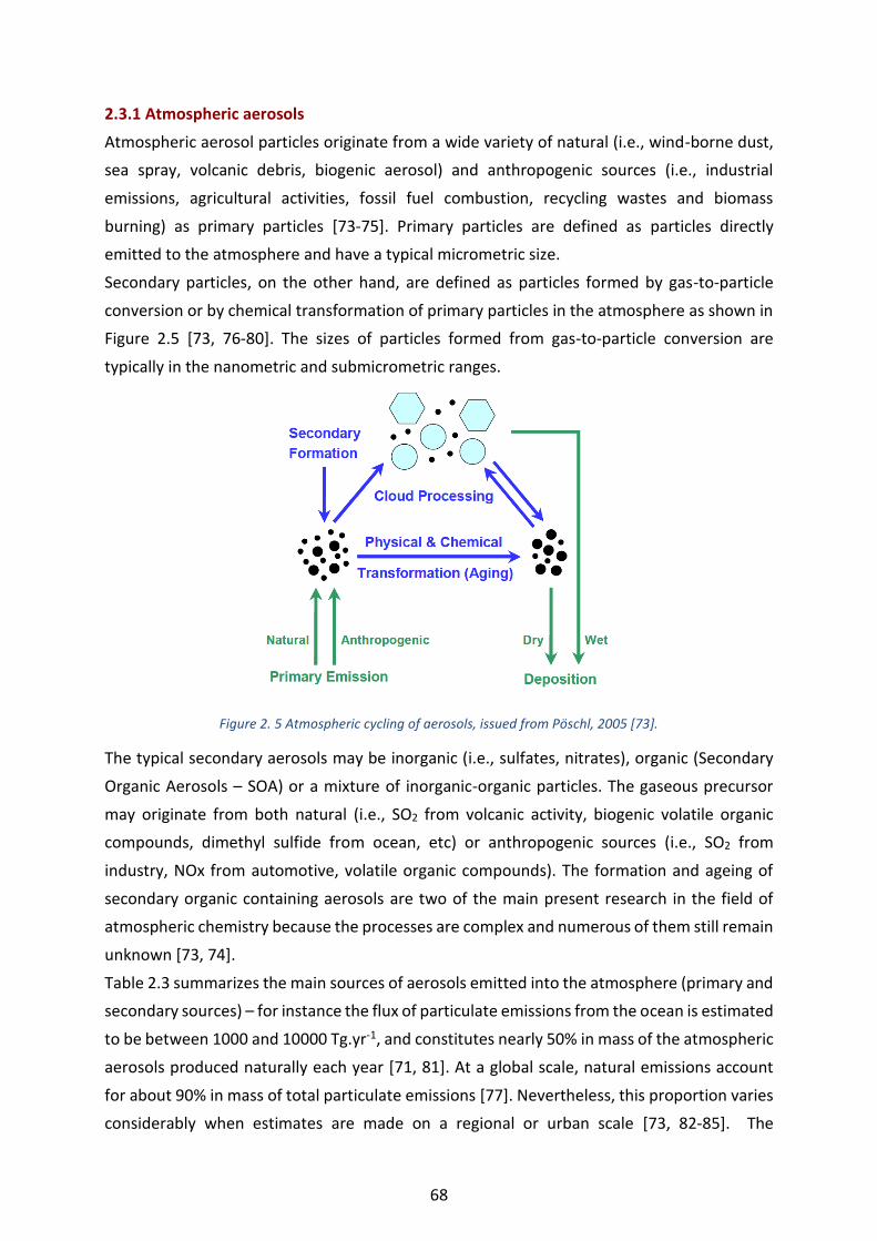
68

2.3.1 Atmospheric aerosols

Atmospheric aerosol particles originate from a wide variety of natural (i.e., wind-borne dust,

sea spray, volcanic debris, biogenic aerosol) and anthropogenic sources (i.e., industrial

emissions, agricultural activities, fossil fuel combustion, recycling wastes and biomass

burning) as primary particles [73-75]. Primary particles are defined as particles directly

emitted to the atmosphere and have a typical micrometric size.

Secondary particles, on the other hand, are defined as particles formed by gas-to-particle

conversion or by chemical transformation of primary particles in the atmosphere as shown in

Figure 2.5 [73, 76-80]. The sizes of particles formed from gas-to-particle conversion are

typically in the nanometric and submicrometric ranges.

Figure 2. 5 Atmospheric cycling of aerosols, issued from Pöschl, 2005 [73].

The typical secondary aerosols may be inorganic (i.e., sulfates, nitrates), organic (Secondary

Organic Aerosols – SOA) or a mixture of inorganic-organic particles. The gaseous precursor

may originate from both natural (i.e., SO2 from volcanic activity, biogenic volatile organic

compounds, dimethyl sulfide from ocean, etc) or anthropogenic sources (i.e., SO2 from

industry, NOx from automotive, volatile organic compounds). The formation and ageing of

secondary organic containing aerosols are two of the main present research in the field of

atmospheric chemistry because the processes are complex and numerous of them still remain

unknown [73, 74].

Table 2.3 summarizes the main sources of aerosols emitted into the atmosphere (primary and

secondary sources) – for instance the flux of particulate emissions from the ocean is estimated

to be between 1000 and 10000 Tg.yr-1, and constitutes nearly 50% in mass of the atmospheric

aerosols produced naturally each year [71, 81]. At a global scale, natural emissions account

for about 90% in mass of total particulate emissions [77]. Nevertheless, this proportion varies

considerably when estimates are made on a regional or urban scale [73, 82-85]. The

69

geographical distribution of particle sources is non uniform, thus tropospheric aerosols vary

widely in concentration and composition over the Earth [86, 87]. Further, in the lower

atmosphere the total particle number and mass concentration can vary in the range of about

102–105 particles.cm-3 and 1–100 µg.m-3, respectively [73, 77, 88-90].

Table 2. 3 Estimates of the annual global natural emissions of primary and secondary aerosols measured in Teragram per year (1Tgyr−1=106 ton. yr−1). Note that the actual range of uncertainty may encompass values larger and smaller than those reported here. These values are based on review of Laj et Sellegri (2003) [91].

Origin of source Source Annual global emission (Tg.year-1)

Average Minimum Maximum

Natural

90 %

Primary

Sea salt aerosols 1300 1000 10000

Mineral dust 1500 1000 3000

Biological debris 50 26 80

Volcanic ash 33 50 1000

Secondary

Biological sulfate 90 80 150

Volcanic sulfate 12 5 60

Organic aerosols 55 40 200

Nitrates 22 15 50

TOTAL 3060 2170 23540

Anthropogenic

10 %

Primary

Soot 20 5 20

Industrial dust 100 40 130

Secondary

Vegetation fires 80 60 160

Organic aerosols 10 5 52

Sulfate 140 120 250

Nitrate 36 25 65

TOTAL 390 300 710

The main constituents of the atmospheric aerosols are inorganic species (such as sulfate,

nitrate, ammonium, sea salt), organic species (also termed organic aerosol - OA),

carbonaceous, mineral species (mostly desert dust) and primary biological aerosol particles

(PBAPs). In fact, atmospheric aerosol particles at the particle scale may present complex

heterogeneous structures featuring both organic and inorganic part due to the complexity of

atmospheric reaction [92- 94]. The chemical composition of aerosols differs considerably,

depending on its source (primary or secondary) and its atmospheric lifetime (ageing) [90, 95,

96].

70

For instance, measurements in the marine boundary layer (MBL) reveal that the primary

inorganic sea salt component dominates the marine aerosols [97- 99]. It is well known that

sea salt aerosols are constituted of inorganic species mainly sodium chloride (NaCl) as well as

various organic species. In many investigations, fatty acids (FA) are reported to be major

constituents of the organic fraction on marine aerosols [100- 103]. Fatty acids are carboxylic

acids with an unbranched aliphatic tail (hydrocarbon chain) which is either saturated (palmitic

acid C16 , myristic acid C14, lauric acid C12 and stearic acid C18) or unsaturated (oleic acid

C18:1 and palmitoleic acid C16:1) [104 -106]. At molecular scale, the organization of FA on the

particle surface is complex and not stable due to influence of water [107]. In contrast, urban

aerosols have a more complex composition and are dominated by sulfate, nitrate and

carbonceaous aerosols [108] with a significant contribution of carboxylic acids such as

malonic, succinic and glutaric acids [109-110].

Lifetime and aerosol size are strongly linked. As can be seen from Figure 2.6 aerosol particles

of 0.001-10 µm diameter can have average lifetimes up to 10 days in the troposphere and up

to 1 year in the stratosphere. However, large particles (> 10 µm) have relatively short average

atmospheric lifetimes (maximum 1 day). This is due to that large particles (large cloud

droplets, ice crystal, etc) tend to precipitate (wet deposition) or settle more rapidly by

deposition under the influence of gravity [111, 112]. On the other hand, the aerosol

composition can also affect its average lifetime as shown in Table 2.4.

Figure 2. 6 Average lifetime dependence on the size of atmospheric aerosol particle [111].

71

Table 2. 4 Average lifetimes of various aerosol type [113].

Aerosol type Size (diameter range) Average lifetime (days)

Sea salt < 1 µm 7.1

2.5 - 10µm 0.7

Mineral dust < 1 µm 10.4

2.5 - 10 µm 2.2

Sulfate < 10 µm 3.8-10

Nitrate < 10 µm 9-9.9

Organic < 10 µm 2-10.4

Carbonaceous

(Biomass burning)

< 1 µm 3

2.3.2 Role of water

The amount of water vapor in the atmosphere varies greatly depending on region and altitude.

It is controlled by the variation of its vapor pressure with temperature. For a given

temperature T, the water vapor pressure is characterized by the relative humidity RH

according to the following equations [114]:

RH=𝑝𝐻2𝑂

𝑝𝐻2𝑂0 [E2-1]

RH=5(Td –T) + 100 [E2-2]

Where 𝑝𝐻2𝑂 is the partial pressure of water vapor contained in air, 𝑝𝐻2𝑂0 is the saturating

vapour pressure of water, Td is the dew point temperature and T is the observed temperature.

The variations of temperature and pressure may result in the formation of water droplets or

iced particles [115] as described by the Clausius–Clapeyron equation (E2-3).

Ln (P1

P2)=

ΔHvap

R (

1

T2−

1

T1) [E2-3]

Where P1 and P2 are the vapor pressures at two temperatures T1 and T2, R is the specific gas

constant and ΔHvap is the the molar enthalpy of vaporization.

Water has also a crucial role in the gas-to-particle conversion, particle reactivity or Cloud

Condensation Nuclei (CCN) formation as observed during field measurements or determined

experimentally [116-118] or demonstrated by molecular simulation [119- 121].

The hygroscopic properties of atmospheric aerosol particles describe how the particles may

uptake water vapor in the atmosphere [122, 123]. As explained by the Köhler theory [124] the

72

phase transition of dry particle material into a saturated aqueous solution is called

deliquescence and occurs when a substance-specific relative humidity (RH) threshold value

(deliquescence relative humidity, DRH) is exceeded. The reverse transition and its RH

threshold value are called efflorescence relative humidity (ERH). For instance, upon hydration

(increase of RH) NaCl particles undergo a deliquescence transition at %DRH=75% at 296 K. The

reverse efflorescence transition occurs %ERH=45% at 296 K [125].

Furthermore, when relative humidity exceeds 100% (super-saturation) ice crystals in the

atmosphere can be formed homogeneously from water droplets in a medium without

aerosols or other impurities at about -38 °C [126]. The diagram of the kinetic states of

humidity (Figure 2.7) highlights the variation of water super-saturation as a function of the

temperature [127]. However, the presence of atmospheric aerosols (nuclei) can greatly

increase the ice nucleating temperature and thus catalyzing the ice formation. In this case, the

formation of ice on atmospheric aerosols occur from the interaction of water molecules with

the surface of the aerosol [128].

Figure 2. 7 Diagram of kinetic states of atmospheric humidity [127].

Between 90 and 273K, the water saturation rate is taken relative to that of hexagonal ice (solid line, part top of

the figure).Along the horizontal dotted line (lower part of the figure), the partial pressure of water is in equilibrium

with the saturating vapor pressure above a surface of ice. The inclined dotted line indicates the oversaturation

required to form ice from a droplet of aqueous solution of a few microns in a homogeneous manner, i.e. without

any particle being present in the droplet. Along the diagonal solid line, the partial water pressure is in equilibrium

with the saturating vapor pressure above a droplet. Between 273 and 350K, the rate of water saturation is taken

relative to liquid water (solid line, upper part of the figure). The dashed curves and dashes represent areas of

homogeneous nucleation from one state to another: g: water vapor, Cr: crystalline ice, l: liquid water, and a:

amorphous ice.

73

2.3.3 Gas-aerosol interaction – overview of the general concepts

Heterogeneous interactions of trace gases with liquid and solid particles strongly influence the

atmospheric properties. Heterogeneous uptake by particles changes the gas phase

concentration of reactive compounds (such as photochemical oxidants, acid gases, free

radical, etc.) which significantly influences the atmospheric processes (such as formation of

photochemical smog, ozone layer depletion, etc.). Moreover, the heterogenous reactivity

affects important physical properties of atmospheric aerosols, such as size, optical properties,

and ability to nucleate cloud droplets [129]. Thus, determination of kinetics and mechanism

of heterogeneous reactions has become increasingly important in understanding the

chemistry of the troposphere.

One of the comprehensive kinetic model framework for heterogeneous interactions was

proposed [130- 135] and provided a basis for consistent description of chemical reactions and

mass transport at the surface and in the bulk of liquid and solid atmospheric particles of both

simple and complex systems. This model is based on NASA–JPL and IUPAC evaluations, which

are a set and a combination of kinetic theories of gases, condensed phases, and interfaces.

Considering the kinetic model cited above, when a gas is in contact with a condensed phase,

gaseous molecules driven by thermal agitation can diffuse towards it and hit the surface. A

fraction of the molecules that hit the liquid or solid surface can be taken up due to

heterogeneous elementary processes including gas phase diffusion, accommodation,

desorption and possible reaction at the gas/surface interface, and for liquids and some

amorphous solid surfaces, absorption, dissolution and bulk reaction. In fact, the observable

interaction of a species on a particle or a droplet surface is the results of a complex process,

which can be decomposed on several elementary processes as shown in Figure 2.8.

[1] Collision: Based on gas kinetic theory and assuming the gas phase concentration is

constant, the rate of collisions of gas species X with a surface can be expressed as Rcoll.

𝐑𝐜𝐨𝐥𝐥 =𝛚 [𝐗]𝐠

𝟒 [E2-4]

[X]g is the gas phase concentration (molecule.m-3) of X and ω is its mean thermal velocity (m.s-

1) given by ω = [8RT/ (πM)]1/2, M is the molar mass (kg.mol-1) of X, R is the gas constant (J.mol-

1), and T is the temperature in kelvin.

[2] Gas diffusion: When efficient heterogeneous loss leads to local depletion of gaseous

molecules [X]g close to the droplet or solid surface and gives rise to a diffusional flux from the

bulk gas directed towards the surface.

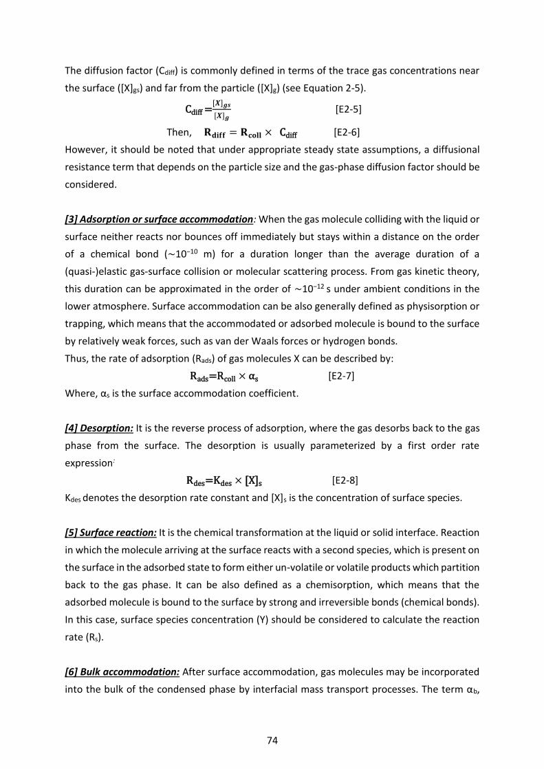
74

The diffusion factor (Cdiff) is commonly defined in terms of the trace gas concentrations near

the surface ([X]gs) and far from the particle ([X]g) (see Equation 2-5).

Cdiff =[𝑿]𝒈𝒔

[𝑿]𝒈 [E2-5]

Then, 𝐑𝐝𝐢𝐟𝐟 = 𝐑𝐜𝐨𝐥𝐥 × Cdiff [E2-6]

However, it should be noted that under appropriate steady state assumptions, a diffusional

resistance term that depends on the particle size and the gas-phase diffusion factor should be

considered.

[3] Adsorption or surface accommodation: When the gas molecule colliding with the liquid or

surface neither reacts nor bounces off immediately but stays within a distance on the order

of a chemical bond (∼10−10 m) for a duration longer than the average duration of a

(quasi-)elastic gas-surface collision or molecular scattering process. From gas kinetic theory,

this duration can be approximated in the order of ∼10−12 s under ambient conditions in the

lower atmosphere. Surface accommodation can be also generally defined as physisorption or

trapping, which means that the accommodated or adsorbed molecule is bound to the surface

by relatively weak forces, such as van der Waals forces or hydrogen bonds.

Thus, the rate of adsorption (Rads) of gas molecules X can be described by:

Rads=Rcoll × αs [E2-7]

Where, αs is the surface accommodation coefficient.

[4] Desorption: It is the reverse process of adsorption, where the gas desorbs back to the gas

phase from the surface. The desorption is usually parameterized by a first order rate

expression:

Rdes=Kdes × [X]s [E2-8]

Kdes denotes the desorption rate constant and [X]s is the concentration of surface species.

[5] Surface reaction: It is the chemical transformation at the liquid or solid interface. Reaction

in which the molecule arriving at the surface reacts with a second species, which is present on

the surface in the adsorbed state to form either un-volatile or volatile products which partition

back to the gas phase. It can be also defined as a chemisorption, which means that the

adsorbed molecule is bound to the surface by strong and irreversible bonds (chemical bonds).

In this case, surface species concentration (Y) should be considered to calculate the reaction

rate (Rs).

[6] Bulk accommodation: After surface accommodation, gas molecules may be incorporated

into the bulk of the condensed phase by interfacial mass transport processes. The term αb,

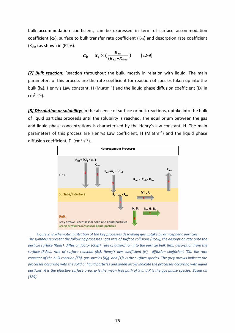
75

bulk accommodation coefficient, can be expressed in term of surface accommodation

coefficient (αs), surface to bulk transfer rate coefficient (Ksb) and desorption rate coefficient

(Kdes) as shown in (E2-6).

𝜶𝒃 = 𝜶𝒔 × ( 𝑲𝒔𝒃

(𝑲𝒔𝒃+𝑲𝒅𝒆𝒔 ) [E2-9]

[7] Bulk reaction: Reaction throughout the bulk, mostly in relation with liquid. The main

parameters of this process are the rate coefficient for reaction of species taken up into the

bulk (kb), Henry’s Law constant, H (M.atm−1) and the liquid phase diffusion coefficient (Dl, in

cm2.s−1).

[8] Dissolution or solubility: In the absence of surface or bulk reactions, uptake into the bulk

of liquid particles proceeds until the solubility is reached. The equilibrium between the gas

and liquid phase concentrations is characterized by the Henry's law constant, H. The main

parameters of this process are Henrys Law coefficient, H (M.atm−1) and the liquid phase

diffusion coefficient, Dl (cm2.s−1).

Figure 2. 8 Schematic illustration of the key processes describing gas uptake by atmospheric particles.

The symbols represent the following processes : gas rate of surface collisions (Rcoll), the adsorption rate onto the

particle surface (Rads), diffusion factor (Cdiff), rate of adsorption into the particle bulk (Rb), desorption from the

surface (Rdes), rate of surface reaction (Rs), Henry’s law coefficient (H), diffusion coefficient (Dl), the rate

constant of the bulk reaction (Kb), gas species [X]g and [Y]s is the surface species. The grey arrows indicate the

processes occurring with the solid or liquid particles and green arrow indicate the processes occurring with liquid

particles. A is the effective surface area, ω is the mean free path of X and X is the gas phase species. Based on

[129].

76

It should be highlighted that in the scientific literature, different rate parameters and

formalisms have been defined and used for the quantitative description and modelling of

these processes.

It is often difficult to experimentally determine which ones, if any, of the processes defined

above, is actually controlling the heterogeneous uptake of trace gas species on a given surface

(solid aerosols, liquid droplets) in either laboratory experiments or in the atmosphere. Thus,

the overall process can be described with a global parameter: the uptake coefficient which is

the ratio of the number of collisions of a given trace gas species leading to uptake on the

surface to the total number of possible collisions per unity of surface and time (ɣ) [133-136]:

ɣ= 𝑵𝒖𝒎𝒃𝒆𝒓 𝒐𝒇 𝒕𝒂𝒌𝒆𝒏 𝒖𝒑 𝒎𝒐𝒍𝒆𝒄𝒖𝒍𝒆𝒔 𝒑𝒆𝒓 𝒖𝒏𝒊𝒕𝒚 𝒐𝒇 𝒔𝒖𝒓𝒇𝒂𝒄𝒆 𝒂𝒏𝒅 𝒕𝒊𝒎𝒆

𝑵𝒖𝒎𝒃𝒆𝒓 𝒐𝒇 𝒄𝒐𝒍𝒍𝒊𝒅𝒊𝒏𝒈 𝒎𝒐𝒍𝒆𝒄𝒖𝒍𝒆𝒔 𝒑𝒆𝒓 𝒖𝒏𝒊𝒕𝒚 𝒐𝒇 𝒔𝒖𝒓𝒇𝒂𝒄𝒆 𝒂𝒏𝒅 𝒕𝒊𝒎𝒆

ɣ is then a dimensionless parameter and represents the probability (0<ɣ<1) that a gas phase

species is removed irreversibly from the gas phase to an active surface at a given temperature.

The actual quantity measured with most of heterogeneous experimental studies is the

observed overall trace gas uptake, ɣobs. Observed uptake is usually determined from the

decrease of the concentration of the trace gaseous (x) species of interest [E2-10] [136-140].

To a lesser extent, and for a purely reactive uptake, ɣobs in some measurements can also be

obtained by quantification of the surface product (Y) concentration [E2-11] [141, 142].

ɣobs (g) = d[X]g

dt ×

𝟏

A × [X]g×/4 [E2-10]

ɣobs (s) = dYs

dt ×

𝟏

A × [X]g×/4 [E2-11]

[X]g is the gas phase concentration of X and Ys is the surface species concentration. ω is the

mean thermal velocity (m.s-1) given by ω = [8RT/ (πM)]1/2, M is the molar mass (kg.mol-1) of X,

R is the gas constant (J.mol-1), and T is the temperature in Kelvin.

Corrections of the uptake are frequently necessary to be taken into account. For instance, in

case of strong uptake leading to local depletion of X close to the surface, a correction factor

(Cdiff) is commonly applied (ɣcorrected = Cdiff ×ɣobs). If the surface is changing with time (in case

of strong uptake), the uptake is time dependent and correction to zero time must be

considered.

77

The uptake coefficients are presented in literature in a variety of experimental symbols form

depending on experimental measurements. An example of the main used experimental

symbols is shown in Table 2.5.

Table 2. 5 Main used experimental symbols for the uptake coefficient.

Symbol Meaning

ɣobs Experimentally observed, results in loss of the molecule from the gas phase or gain of species in solid phase under defined experimental conditions

Experimentally observed, used if the uptake is not precised ɣ0 and ɣss

ɣss or ɣaverage

Experimentally observed, steady state (time independent) uptake coefficient

ɣ0 Experimentally determined initial uptake coefficient that was changing rapidly with time

ɣcorrected The correction of the observed uptake, such as by gas diffusion factor

The advantage of expressing the kinetics in terms of uptake coefficients lies in the fact that

the results are transferable from one experiment to another, even if those experiments

involve significant differences in the surface-to-volume ratio. This would not be the case if

kinetic results were expressed in terms of rate coefficients which are however the primary

experimental observables.

To sum up, the uptake coefficient is a time and concentration dependent quantity. For

extracting information about a specific aspect of the uptake process, i.e. the accommodation

on the surface, specific corrections or experimental conditions have to be used. Thus, the

uptake coefficient can be further parametrized by including the possible occurring

heterogeneous processes. A complete description of the interaction parametrization has been

previously discussed in [129, 131, 133, 134].

2.3.4 Experimental tools and techniques for studying aerosol-gas interactions

Several experimental methods dedicated to laboratory experiments can be used to study

heterogeneous interactions and to determine uptake coefficients. The general principle of

these methods is to put a gaseous phase in contact with a solid or liquid phase of known

surface. The number of gaseous molecules taken up by the solid or the liquid is measured

during a known time interval through either surface or gas monitoring. In this section, the

experimental methods that are most frequently used in the measurement of uptake are

presented. Most methods rely on the determination of loss rates or time dependent

78

concentration changes of gas-phase species in contact with a surface. These include internally

coated flow tube reactors and Knudsen cells for bulk surfaces and films, and aerosol flow tubes

and aerosol chambers for dispersed surfaces. Surface adsorbed reactants and products have

frequently been observed using surface-sensitive techniques, such as reflectance infrared

spectroscopy (Diffuse Reflectance for Infrared Fourier Transform Spectroscopy (DRIFTS)) and

these have in a few cases been applied to kinetics studies [99, 129, 143, 144].

Table 2.6 summarizes the commonly used methods for the measurement of reactive uptake

in gas-solid / liquid reactions. The surface characteristics, the range of accessible ɣ, the gas-

solid contact time and the working pressure range for each method are listed [126, 119]. In

this section, a brief description of the laboratory techniques that can be used to determine

kinetic parameters that characterize heterogeneous reactions in the atmosphere, is given.

Table 2. 6 Summary of the principle commonly used methods for the measurement of reactive uptake in gas-solid / liquid reactions. The surface characteristics, the accessible range of ɣ, the gas-solid contact time and the

working pressure range are reported [126, 119].

Method Surface Monitoring

phase

Accessible

ɣ range

Contact

time

Working

pressure (Bar)

Coated/wetted

flow tube

Solid or liquid

film

Gaseous <10-1 0-103 s 0.0007-1.013

Aerosol flow tube Solid or liquid

aerosol

particles

Gaseous and

solid or

liquid

10-4 -1 0- 30 s 0.001-1.013

Knudsen Cell Powder sample

or aerosol

particles

Gaseous 10-5 - 1 10-104 s < 1.33 × 10-5

DRIFTS Cell Solid surface or

aerosol

particles

Solid 10-10 -10-2 40 -800

min

0.003-1.013

Droplet train flow

reactor

Liquid droplets Gaseous and

droplet

10-3-1 2-20 ms 0.080-0.03

Atmospheric

simulation

Chamber

Aerosol

particles

Gaseous and

solid

10-8 -10-4 100 -900

min

1.013

79

2.3.4.1 Flow tube and flow tube-like techniques

Internally coated or wetted flow tube

Coated and wetted wall flow tubes have been used extensively to measure uptake and

reactions of gases with both liquid and solid surfaces. A detailed review on flow tube

technique is available in [145] which provides also a critical analysis of the interpretation of

flow tube data for gas uptake measurements [145].

The flow tube walls can be coated with the condensed phase (liquid or solid) film of interest.

In a first configuration, the liquid flows down the inner surface of a vertical flow tube as shown

in Figure 2.9. The flow tube has an annular lip at the top over which the liquid spills to create

a thin, uniform film over the entire surface. In the horizontal configuration, the liquid can be

contained in a holder in the flow tube, or it can coat the walls. Alternatively, the flow tube can

be rotated to keep the coating uniform. The second configuration, can be also used for solid

films where the solid phase is deposited on the internal wall of the tube, which is placed inside

the reactor. The vertically mounted wetted wall flow tube is the favored configuration. Unlike

horizontal configuration, the inside wall of the tube is completely covered with a slowly

flowing film of the liquid of interest (see Figure 2.9), thus the liquid surface is constantly

renewed so that a surface of constant composition, free of saturation and reaction products,

is obtained. The gaseous reactant can then be added through a movable injector. The gas

phase composition is continuously monitored by using a suitable analytic technique

depending on the gaseous species or the experimental conditions. A variety of online sensitive

detection for gas phase analysis have been used either spectroscopic (mostly UV and IR

absorption, laser-induced fluorescence) or mass spectrometry with differential pumping (MS).

Values for ɣ above 10-1 are difficult to measure accurately in a wetted wall flow reactor

because of gas-phase diffusion limitations.

80

Figure 2. 9 Example of wetted flow tube used for measurements of uptake of trace gases on liquid film adapted

from Dievart et., [146].

Aerosol flow tube

An evolution of the internally coated flow tube is the aerosol flow tube, aerosol particles (as

solid or liquid) are sprayed into the flow tube reactor, as shown in Figure 2.10. This allows the

study of reactions on a condensed phase under conditions more representative of the real

atmosphere. Aerosols are injected mostly as polydispersed population in the submicrometric

range. The use of sub-micron particles and the fact of mixing gas and aerosols overcome the

uptake rate limitation caused by gas phase diffusion. Additionally, constant renewal of the

aerosols (liquid or solids) avoids surface ageing. This type of system allows the uptake

coefficient measurements in the range of 10-4 -1 [147, 148].

Aerosol suspension can be generated by wet process (nebulization of an aqueous solution or

a liquid suspension) or by dry process (vibrating membrane aerosol generator). The suspended

particles are diluted in the carrier gas (usually N2 or air) and passed through a conditioner

where the aerosols equilibrate to the temperature and humidity conditions before injection.

Together with, the reagent trace gas is diluted in the carrier gas and enters the reactor through

a sliding injector, allowing different exposure times to the aerosols.

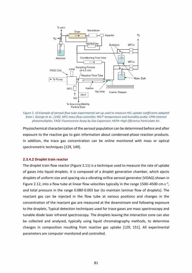
81

Figure 2. 10 Example of aerosol flow tube experimental set-up used to measure HO2 uptake coefficients adapted

from I. George et al., [150]. MFC-mass flow controller; RH/T-temperature and humidity probe; CPM-channel photomultiplier, FAGE-Fluorescence Assay by Gas Expansion; HEPA–High Efficiency Particulate Air.

Physiochemical characterization of the aerosol population can be determined before and after

exposure to the reactive gas to gain information about condensed-phase reaction products.

In addition, the trace gas concentration can be online monitored with mass or optical

spectrometric techniques [129, 149].

2.3.4.2 Droplet train reactor

The droplet train flow reactor (Figure 2.11) is a technique used to measure the rate of uptake

of gases into liquid droplets. It is composed of a droplet generation chamber, which ejects

droplets of uniform size and spacing via a vibrating orifice aerosol generator (VOAG) shown in

Figure 2.12, into a flow tube at linear flow velocities typically in the range 1500–4500 cm.s−1,

and total pressure in the range 0.080-0.003 bar (to maintain laminar flow of droplets). The

reactant gas can be injected in the flow tube at various positions and changes in the

concentration of the reactant gas are measured at the downstream end following exposure

to the droplets. Typical detection techniques used for trace gases are mass spectroscopy and

tunable diode laser infrared spectroscopy. The droplets leaving the interaction zone can also

be collected and analyzed, typically using liquid chromatography methods, to determine

changes in composition resulting from reactive gas uptake [129, 151]. All experimental

parameters are computer monitored and controlled.

82

The gas-droplet interaction time can be varied between 2 and 20 ms, allowing solubility effects

to be investigated. The pressure and droplet diameter in the droplet train flow reactor causes

gas-phase diffusion limitations.

Figure 2. 11 Schematic diagram of typical droplet train flow reactor for measurement of uptake coefficients of

trace gases into liquids [151].

Figure 2. 12 Example of vibrating orifice monodisperse aerosol generator [152].

2.3.4.3 Knudsen cell

Much of the data on heterogeneous reactions in the atmosphere, particularly the earliest

work, were generated using Knudsen cells [153- 157]. Knudsen cell are used for the analysis

of loss from the gas phase due to surface reactions or adsorption. Figure 2.13 presents a

simple schematic diagram of a Knudsen cell. The Knudsen cell reactor consists of a chamber

with an isolated sample compartment and a small orifice through which gas phase reactant

and product species can escape to be detected by mass spectrometry. The orifice (small hole)

83

and the low pressure (<1.33 × 10-5 bar) ensures a molecular regime which overcomes gas

phase diffusion effects. The design of the gas system makes it possible to introduce the

reactive gas in two configurations. The pulsed valve configuration experiment is when a

known number of gas molecules is admitted across a pulsed solenoid valve (0.8-millimeter

orifice) into the reactor and interacts with the reactive surface. The mass spectrometer signal

is recorded as function of time and proportional to the flow of gaseous species out of the

reactor. In the steady state experiment a dual needle valve (Nupro) is used to regulate the gas

allowing a continuous constant flow of the injected gas. The pulsed valve technique has the

advantage that it avoids surface saturation.

When the gas is exposed to a surface that takes up the gas, the concentration of the gas in the

cell and hence the amount exiting the orifice decreases. From the gas phase concentration

change, the net uptake of the gas by the surface can be determined. Uptake coefficient is

accessible between 10-5 and 1 and can be measured accurately. The main advantage of this

experimental set-up is the wide range of condensed phases that can be used; the condensed

phase can be a liquid, a powder, a thin layer, a frozen surface or a monocrystal. The main

disadvantages are the limited use for low vapor pressure samples, and the very low pressure

which is not representative of low tropospheric conditions.

Figure 2. 13 Example of a Knudsen cell for the investigation of heterogeneous reactions using either continuous

flow or pulsed gas admission. The rotatable orifice plate can put up to four molecular-beam forming orifices into line of sight with the ionizer of the mass spectrometric (MS) detector from M. Rossi et al., [153].

84

2.3.4.4 Diffuse Reflectance Infrared Fourier Transform Spectroscopy (DRIFTS)

Diffuse Reflectance Infrared Fourier Transform Infrared spectroscopy (DRIFTS), is a reactor

that allows the in situ monitoring of a solid phase put in contact with a reactive gas phase. This

technique requires the solid to be a diffusing medium.

The fine powdered sample is put in the reaction chamber (DRIFTS), which is located inside an

FTIR instrument as shown on the Figure 2.14. A parabolic mirror focuses the probe beam on

the solid sample and the diffused reflected radiation is focused by another parabolic mirror

on to the detector surface. Moreover, it is possible to monitor the gas phase by coupling the

gas outlet of DRIFTS reactor with a suitable technique implemented at the gas outlet (i.e., Gas

chromatography coupled to mass spectrometer or long path cell connected to UV-Vis or FTIR

spectroscopy). Complementary information on FTIR spectroscopy and DRIFTS techniques are

displayed in annex 2.

DRIFTS is a technique of choice for studying gas-solid interactions, this technique is widely

used in catalysis science [158- 160]. However, it has been proven that DRIFTS is very useful for

providing structural information for all types of solid surfaces and it is extremely useful for

examining samples that are difficult to analyze in transmission [161]. DRIFTS is also very useful

for studying the kinetics and mechanisms of the reactions of infrared-transparent solids (such

NaCl) and gaseous species [142, 162-165].

Measurements difficulties may arise with highly IR absorbing solids. Moreover, DRIFTS can

provide signal of gas phase near the surface [166]. Sometimes it is difficult to estimate the

extent and kinetics of the gas-phase diffusion inside the powdered macroscopic sample. Solid

sample cannot be renewed during the experiment thus surface ageing of the solid sample can

be a limitation. Its main advantages are that it is a fast and non-destructive technique.

This method allows the measurements of solid-phase products when a flow of gases is passed

through the solid. The uptake coefficients (in the range of 10-10 to 10-2) and formation rates of

absorbed/adsorbed product on the solid is determined by quantitative interpretation of the

DRIFTS spectra coupled to post-test complementary techniques allowing the determination

of the total amount of adsorbed/absorbed products during an experiment (IR pellets, ionic

chromatography, inductively coupled plasma mass spectrometer [142]).

85

Figure 2. 14 Example of DRIFTS apparatus [162].

2.3.4.5 Atmospheric simulation chamber

The reaction volume of Atmospheric Simulation Chamber [167] is much larger than in the

previously described reactors: it can range from few m3 (HIRAC chamber) to more than 270

m3 (SAPHIR chamber). Atmospheric simulation chambers are among the most advanced tools

for investigating the atmospheric processes to derive physico-chemical parameters which are

required for air quality and climate models. Atmospheric chambers are used to investigate

both gaseous and/or aerosol-gas interaction processes as SAPHIR chamber shown in Figure

2.15.

Indeed, depending on the irradiation used, atmospheric simulation chambers can be divided

into two categories: outdoor and indoor chambers. Outdoor chambers are often large

transparent reactors (e.g. SAPHIR, HELIOS) that are directly irradiated by solar radiation.

Indoor chambers equipped with artificial irradiation sources (e.g. Xenon lamp, Fluorescent

lamp, halogen lamp) are smaller than the outdoors ones and are mostly dedicated to specific

studies (e.g. CESAM, HIRAC).

Atmospheric chambers can be equipped with a wide range of analytical instruments for online

and offline measurements [168-170] allowing studies of homogeneous or heterogeneous

chemical reactions. As an example, the subsequent temporal decay, composition, and/or

growth of gas phase species is monitored, usually with long optical length FTIR, Mass

Spectrometer or UV-Vis techniques. Additionally, the aerosol composition can be determined

on-line by steam jet aerosol collection/ion chromatography. In some cases, a particle analyzer

86

is coupled to the simulation chamber, such that information on the evolution of particle size

distribution and particle number can also be followed.

Figure 2. 15 Outdoor SAPHIR atmosphere reaction chamber in Jülich, Germany dedicated for both homogenous

and heterogenous interaction processes [167].

2.3.5 Single particle and molecular mechanism approach

2.3.5.1 Single particle approach

Single particle approaches have been generally used to investigate the hygroscopicity of

particles [171], photo reactivity of particles [172], phase partitioning [173] and particle

viscosity [174] as well as chemical characterization of individual particles [175, 176]. To some

extent, each single particle may be considered as a micro-reactor undergoing multiphasic

interactions. Chemical, morphological (size and shape) and phase data of an individual aerosol

particle are of crucial importance for purposes of tracing and understanding the formation

and reaction mechanisms of aerosols. The chemical composition and microphysical state

influence the response of the particle to environmental changes. For instance, a variation in

chemical composition or size of an individual aerosol particle prior and post to exposure to

gas species can be directly linked to its heterogeneous process with gas phase species. As an

example, Figure 2.16 shows the morphological change of CaCO3 particles before and after

exposure to HNO3. Indeed, relating the changes of particles can help in elucidate the

underlying type of heterogeneous process (accommodation, reaction). Additionally,

comparing the morphology from particle scale to the bulk scale can be a challenging step to

confirm the observed heterogeneous process [177-180]. Therefore, studying the

physiochemical properties of particles at particle scale will help in better understanding the

heterogeneous interactions. Nevertheless, it should be highlighted that up to date there are

no experimental system to study the gas-single particle interaction because the volume of one

particle is too small regarding the gas volume.

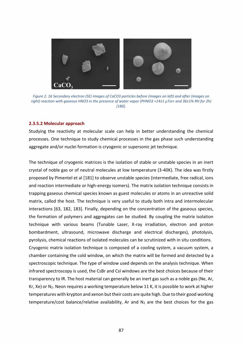
87

Figure 2. 16 Secondary electron (SE) images of CaCO3 particles before (images on left) and after (images on

right) reaction with gaseous HNO3 in the presence of water vapor (PHNO3 =14±1 µTorr and 36±1% RH for 2h) [180].

2.3.5.2 Molecular approach

Studying the reactivity at molecular scale can help in better understanding the chemical

processes. One technique to study chemical processes in the gas phase such understanding

aggregate and/or nuclei formation is cryogenic or supersonic jet technique.

The technique of cryogenic matrices is the isolation of stable or unstable species in an inert

crystal of noble gas or of neutral molecules at low temperature (3-40K). The idea was firstly

proposed by Pimentel et al [181] to observe unstable species (intermediate, free radical, ions

and reaction intermediate or high-energy isomers). The matrix isolation technique consists in

trapping gaseous chemical species known as guest molecules or atoms in an unreactive solid

matrix, called the host. The technique is very useful to study both intra and intermolecular

interactions [63, 182, 183]. Finally, depending on the concentration of the gaseous species,

the formation of polymers and aggregates can be studied. By coupling the matrix isolation

technique with various beams (Tunable Laser, X-ray irradiation, electron and proton

bombardment, ultrasound, microwave discharge and electrical discharges), photolysis,

pyrolysis, chemical reactions of isolated molecules can be scrutinized with in situ conditions.

Cryogenic matrix isolation technique is composed of a cooling system, a vacuum system, a

chamber containing the cold window, on which the matrix will be formed and detected by a

spectroscopic technique. The type of window used depends on the analysis technique. When

infrared spectroscopy is used, the CsBr and CsI windows are the best choices because of their

transparency to IR. The host material can generally be an inert gas such as a noble gas (Ne, Ar,

Kr, Xe) or N2. Neon requires a working temperature below 11 K, it is possible to work at higher

temperatures with krypton and xenon but their costs are quite high. Due to their good working

temperature/cost balance/relative availability, Ar and N2 are the best choices for the gas

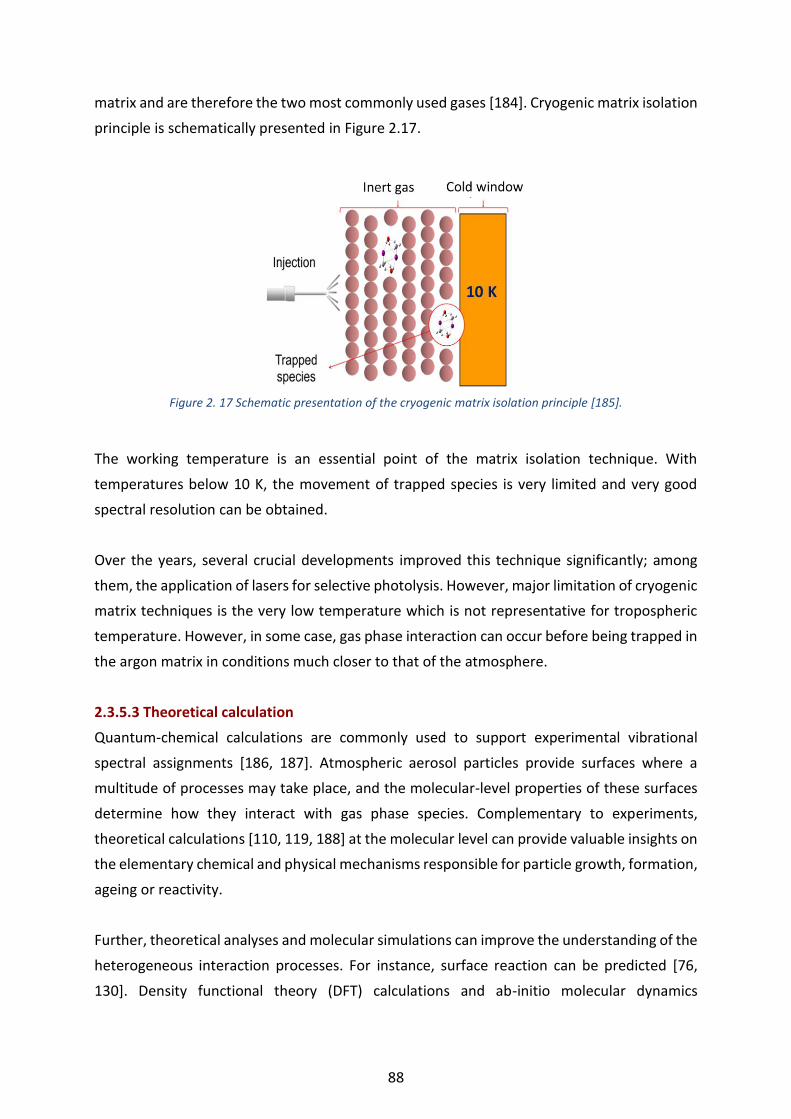
88

matrix and are therefore the two most commonly used gases [184]. Cryogenic matrix isolation

principle is schematically presented in Figure 2.17.

Figure 2. 17 Schematic presentation of the cryogenic matrix isolation principle [185].

The working temperature is an essential point of the matrix isolation technique. With

temperatures below 10 K, the movement of trapped species is very limited and very good

spectral resolution can be obtained.

Over the years, several crucial developments improved this technique significantly; among

them, the application of lasers for selective photolysis. However, major limitation of cryogenic

matrix techniques is the very low temperature which is not representative for tropospheric

temperature. However, in some case, gas phase interaction can occur before being trapped in

the argon matrix in conditions much closer to that of the atmosphere.

2.3.5.3 Theoretical calculation

Quantum-chemical calculations are commonly used to support experimental vibrational

spectral assignments [186, 187]. Atmospheric aerosol particles provide surfaces where a

multitude of processes may take place, and the molecular-level properties of these surfaces

determine how they interact with gas phase species. Complementary to experiments,

theoretical calculations [110, 119, 188] at the molecular level can provide valuable insights on

the elementary chemical and physical mechanisms responsible for particle growth, formation,

ageing or reactivity.

Further, theoretical analyses and molecular simulations can improve the understanding of the

heterogeneous interaction processes. For instance, surface reaction can be predicted [76,

130]. Density functional theory (DFT) calculations and ab-initio molecular dynamics

Figure2. 1 Schematic presentation of the cryogenic matrix isolation technique

89

simulations can be used to understand the adsorption and chemical reaction of gaseous

species on surface by investigating their thermodynamic properties [189-196]. Such

simulation can compute the adsorption energy, adsorption structure, dissociation energy and

possible reactions. Additionally, it is possible to study the evolution of surface coverage as a

function of partial pressure. This evolution can give insights on the adsorption isotherm type

as well as the uptake coefficient [195, 196].

2.4 Literature review on interaction between atmospheric aerosols and iodine

compounds

Some aspects of the atmospheric chemistry of iodine are not yet well covered by studies, such

as the interaction of gaseous iodine compounds with atmospheric aerosols and its resulting

speciation. Indeed, only few studies have been currently published on this topic between

1998-2013. Only few publications addressed the reactivity of HOI, ICl and IBr with halide salts

[138, 197, 198]. Other publications [197, 199-206] have investigated the interaction between

ice and iodine species such as HOI, IONO2, HI, IBr, ICl, I2 and CH3I. Most of these experiments

were investigated under temperatures representative of the troposphere (180-298 K) [138,

197-202]. Two studies investigated the uptake of organic iodine species, CH3I and C2H5I by

soot particles [207, 208]. Modelling work [9] mentioned loss rate of IO, OIO, I2O5, INO2 and

IONO2 with undefined surfaces.

2.4.1 Heterogeneous reaction of inorganic iodine species with halide salt aerosols

The heterogeneous reaction of HOI [197] or HOI/IONO2 [138] with halide salt particles was

investigated experimentally. It has been shown that HOI could be involved in the activation of

halogens from halide salt aerosols (NaCl, KBr, NaBr) due to the formation of interhalogen

species (ICl, IBr) via reaction [R2-31]

HOI + NaX (Cl,Br) or KBr → IX (Cl,Br) + (K,Na)YOH [R2-31]

The reaction was investigated for HOI ranging from 3.0 x 1010 to 2.0 x 1013 molecule.cm-3 on

NaCl and KBr powder salts (source of salts is not precised by the authors) at ambient

temperature (temperature range is not precised by the author) using a Knudsen cell coupled

to a mass spectrometer [197]. They reported maximum value for the initial uptake coefficient

ɣ0 of (4 ±2) × 10-2 and of (5±2) × 10-2 for the reaction of HOI on NaCl and KBr respectively,

measured at zero time or very close to it. Authors [197] have found that the uptake coefficient

decreases with increasing residence time in the Knudsen cell reactor and explained it as

“Surface ageing effects” due to HOI adsorption on the Knudsen cell surface (stainless steel)

90

and subsequent decomposition. The only gaseous product observed in the study of the

reaction of HOI on NaCl was I2, whereas both I2 and IBr were observed with the reaction of

HOI on KBr. Additional experiments were conducted [197] with NaNO3 salts to probe the

decomposition reaction of HOI. The observed initial uptake coefficient on NaNO3 was of the

same order as on NaCl and KBr with a value of ɣ0= (5±2) × 10-2. Only I2 was observed as a

gaseous product with reaction of HOI on NaNO3. Here it should be highlighted that the major

formation of the observed I2 can be due to the decomposition of HOI with Knudsen cell surface

(side product).

To investigate further the possible release of interhalogens via the reaction of HOI with halide

salts, a comprehensive study of the heterogeneous interaction of gaseous HOI ((0.2-8) × 1012

molecule.cm-3) with NaBr thin films (prepared from saturated solution of NaBr (Lancaster

99%+)), commercial NaCl grains (Breckland Scientific, 99%+) and sea-salt granular crystallites

(Community Food Ltd, 99%+, obtained from solar evaporation of seawater free from any

additives or processing aids) was conducted [198]. The authors [198] reported that, during the

course of the optimization of the HOI gaseous source the formation of I2 was noticed,

suggesting a decomposition reaction of HOI on the inner wall of the outer sliding injector. They

have also determined the overall error on the uptake coefficient, which is in the 18%-35%

under their experimental conditions. The interaction was investigated by using a wall

halocarbon coated flow reactor coupled to a mass spectrometer at 278 and 298 K.

Additionally, the authors [198] conducted measurements in the presence of water vapor up

to 23% relative humidity with NaCl and NaBr, and up to 11% relative humidity with sea-salt at

278 K. Experiments with higher relative humidity in the flow tube were not possible. The initial

time dependent uptake (ɣ0) was not very reproducible. As a result, authors have reported that

the heterogeneous interaction of HOI with sodium halide salts to form interhalogens (ICl, IBr)

features a steady state uptake coefficient (after the uptake state had settled to a constant

value) of ɣss= (3.4 ± 0.9) × 10-2 on NaBr, ɣss = (1.6 ± 0.4) × 10-2 on NaCl and ɣss = (6.1 ± 2.1) × 10-

2 on sea-salt independently of the temperature between 278 and 298 K. Moreover, they

determined that the uptake of HOI in the clean reactor (e.g. without salt) is insignificant (ɣss=

(5.0 ± 1.0) × 10-4) compared to the uptake on salts. This indicates that the uptake is quite

significant for the reaction of HOI on halide salts but lower for pure NaCl than for HOI on sea-

salts. This can be due to the increase in defect sites in sea-salt particles, caused by Br-

dislocations and the presence of additional species such as MgCl2. Moreover, the authors

[198] observed a decrease in surface reactivity (surface ageing) as described previously [197].

The ɣ for the reaction decreased with the time exposure of HOI, i.e., after ∼30 mins, ɣss was

determined to be (8.0 ± 3.0) × 10-3, (7.0 ± 0.3) × 10-3, and (1.4 ± 0.4) × 10-2 for NaBr, NaCl, and

91

sea-salts, respectively. In all cases, no dependence of ɣss on relative humidity was observed.

On the exposure of HOI to sea-salts both ICl and IBr were observed as products, with a bromine

release favored over chlorine considering that the composition of sea-salts is 99.5 wt %Cl-

compared to 0.2 wt % Br-. The maximum amount of ICl and/or IBr released to the gas phase

after reaction of HOI with NaCl, NaBr, and sea salt surfaces was 3×1014 molecule.cm-2, 1×1016

molecule.cm-2 and 3×1015 molecule.cm-2 (Cl-)/2×1015 molecule.cm-2(Br-), respectively. It

should be noted that the amount of ICl and IBr released was time dependent. Authors [198]

reported only ICl and IBr as the products detected in the gas phase for the reaction of HOI on

NaCl and NaBr, respectively, whereas a previous study [197] has observed I2 as the main

product.

Furthermore, the authors [198] investigated the interaction of products i.e. ICl, IBr, and I2 with

NaCl, NaBr and Sea-Salts. No interaction of I2, ICl, or IBr was observed with the NaCl surface.

I2 and IBr did not interact with the NaBr surface either. In contrast, ICl was lost rapidly to the

NaBr surface with production of IBr. The steady state uptake coefficient of ICl (3.1 × 1011

molecule.cm-3) on NaBr was determined to be ɣss = (6.8 ± 1.8) × 10-3. On the other hand, I2

did not interact with the sea-salts. The physisorption interaction of IBr (3.0 × 1011 molecule.cm-

3) with sea salts revealed a ɣss= (6.0 ± 2.0) × 10-4, whereas, the reaction of ICl (3.6 × 1011

molecule.cm-3) with sea salts leads to the formation of IBr with a ɣss= (1.2 ± 0.4) × 10-3. It should

be highlighted that after 40 mins, IBr production was no longer observed.

An additional study [138] dedicated to the uptake and reaction of HOI/IONO2 with dry NaCl,

NaBr and mixed salt (NaCl/NaBr) surfaces was achieved using a coated-wall flow tube reactor

coupled to a mass spectrometer at 298 K. Dry and mixed salts of NaCl and NaBr were made

from aqueous solutions of composition (Aldrich, 99+%) 2 M NaCl, 3 × 10-3 M NaBr. The bulk

flow rate was between 400-600 cm3.min-1. It was shown that the reaction of HOI/IONO2 with

mixed salts revealed an immediate release of IBr and a delayed release of ICl as the surface

bromide was depleted. Similarly, on NaCl and NaBr surfaces, the IBr was observed to be

released immediately on the timescale of the experiment, whereas release of ICl was delayed,

respectively. Nevertheless, the authors reported that dry salts might have trace of adsorbed

water, which may facilitate the reaction with HOI/IONO2. The authors only reported a lower

limit for the uptake coefficient on dry salt surfaces ɣobs >10-2 without stating if it is an initial or

steady state uptake.

Similar to dry salts, the authors [138] have also reported the uptake and reaction of mixed

frozen salt film (inserting NaCl/NaBr solution into a precooled flow reactor 258 K, solution

92

concentration was not precised by the author) surfaces using a coated-wall flow tube reactor

coupled to a mass spectrometer at 243 K. With mixed frozen salts, the uptake of HOI/IONO2

produced stoichiometric conversion to a molecular di-halogen (ICl, IBr). However, they

observed that HOI reacts initially with Br- to form IBr, which is immediately released to the gas

phase. The delayed detection of ICl could then be explained by a competition for HOI (or

IONO2) between Br- and Cl- ions. In fact, as the exposure time of HOI/IONO2 to frozen mixed

salts increases, the rate of production of IBr decreases and a concomitant increase in the signal

of ICl is observed. In the case of IONO2 alone, the surface reaction was proceeded directly with

Cl- (or Br-) ions to form ICl (or IBr) and a nitrate ion NO3-. Thus, in this study [138] they could

not distinguish between product formations resulting from HOI or IONO2 uptake into mixed

surfaces. There was no evidence for the formation of I2 in the gas phase. Additionally, the

variation of the initial IONO2/HOI ratio by a factor of three did not alter the observed results.

Finally, they [138] proposed that for the frozen salt, the initial step in the uptake of HOI and

IONO2 may be adsorption at the ice surface, before surface migration to reactive sites (i.e.

with Br-or Cl-) takes place. The observed uptake of both HOI/IONO2 onto a frozen mixed salt

surface were found to be > 5 × 10-2 (uptake value was not precised by the authors if it is initial

or steady state uptake). Additionally, they have found that ICl initial uptake by frozen mixed

salts is > 10-2 and that one molecule of IBr is released per molecule of ICl lost from the gas

phase. On the other hand, the uptake of IBr by frozen mixed salts was observed to be

reversible with no formation of ICl, or Br2 (unreactive).

Therefore, we can conclude that for pure halide salts such as NaCl and NaBr, IBr and ICl were

produced respectively, from the interaction with HOI or HO/IONO2. IBr and ICl were the major

gas products from the interaction of HOI or HOI/IONO2 with mixed dry or frozen halide salts

(NaCl, NaBr). Similarly, IBr was also formed from the uptake of ICl on sea salts, frozen mixed

halide salts (NaCl/Br) and pure NaBr. Additionally, it was proposed that the interaction of

HOI/IONO2 on frozen salts initially takes place at the frozen surface before surface migration

into the reactive sites. Both initial and steady state uptake of HOI and ICl were observed in the

range of 10-3-10-2. Similarly, the uptake of HOI/IONO2 was observed in the range of 10-2, but

limited by gas diffusion. Thus, the uptake coefficients of HOI or HOI/IONO2 are in the same

range for all halide salts.

93

Table 2. 7 Table summarizing the used methods for the measurement of uptake in HOI-Halide interactions. The interaction, the temperature, the observed ɣ and the products observed are reported [138, 197, 198]. ɣo: uptake coefficient at zero time, ɣss: uptake at steady state condition, ɣobs = uptake coefficient observed and not precised if it is at zero time or steady state conditions.

Interaction Technique Temperature Uptake coefficient Products Reference

HOI + NaCl

Knudsen cell Ambient

ɣo =

(4 ± 2) × 10-2 I2

[197] HOI + KBr ɣ0=

(5 ± 2) × 10-2 I2 , IBr

HOI + NaNO3 ɣ0=

(5 ± 2) × 10-2 I2

HOI + NaCl

Coated flow reactor

278 - 298 K

ɣss= (1.6 ± 0.4) × 10-2

ICl

[198]

HOI + NaBr ɣss=

(3.4 ± 0.9) × 10-2 IBr

HOI + Sea salt ɣss =

(6.1 ± 2.1) × 10-2 IBr, ICl

ICl + NaBr

298 K

ɣss = (6.8 ± 1.8) × 10-3

IBr

IBr + Sea salt ɣss=

(6 ± 2) × 10-4 No

products

ICl + Sea salt ɣss =

(1.2 ± 0.4) × 10-3 IBr

HOI/IONO2 + dry NaCl/NaBr

Coated flow reactor

298 K

ɣobs >10-2 IBr, ICl

[138]

HOI/IONO2 + NaBr ɣobs >10-2 ICl

HOI/IONO2 + NaCl ɣobs >10-2 IBr

HOI/IONO2 + frozen NaCl/NaBr

243 K

ɣobs > 5 × 10-2 IBr, ICl

ICl + frozen NaCl/NaBr

ɣ0 >10-2 IBr

2.4.2 Interaction between iodine species and ice

2.4.2.1 Uptake of iodine species on ice

As mentioned previously, most of studies dealing with interaction between aerosols and

iodine species concern the role of ice and snowpack in the reactivity of iodine species found

in the atmosphere such as HOI, IONO2, HI, IBr, ICl and I2.

The interaction of HOI have been investigated [197] in the temperature range 180 to 200 K

with both pure amorphous ice and doped ice films (not precised if amorphous or crystalline)

using a Knudsen cell coupled to a mass spectrometer of volume 1800 cm3. Pure ice was

prepared as thick ice film of up to 2x105 monolayers corresponding to approximately 20 µm

of thickness. HX doped ice was prepared by exposing ice to a flow of HX (X = Cl, Br) of the order

of a few times 1015 molecule.s -1 for a time duration long enough to ensure the adsorption of

about 10 formal monolayers of HX at the interface depending on the uptake coefficient.

94

In the case of pure amorphous ice, the uptake of HOI between 180 to 200 K varied between

2×10-2 -8×10-2 and the initial uptake was determined to be (6.4±2) ×10-2.

In the case of doped ice, the following reaction may take place:

HOI + HX (Cl, Br) → IX (Cl, Br) + H2O [R2-32]

Comparatively to pure amorphous ice, the values of the reactive uptake coefficients were not

significantly influenced by the presence of HX at the interface [197]. The initial uptake

coefficients were (5±2) ×10-2 and (4±2) ×10-2 at 200 K for doped ice with HCl and HBr,

respectively. The only reaction product observed with doped ice and pure amorphous ice

upon thermal desorption was I2, via the decomposition reaction of HOI. None of the products

(ICl, IBr) were observed as a result of the heterogeneous reaction on both amorphous ice and

ice doped samples even after thermal desorption and complete evaporation of the ice sample.

Thus, the uptake seems to lead to an irreversible loss of HOI on both amorphous ice and ice

doped samples.

The adsorption and desorption of HI with amorphous ice have been studied using Knudsen

cell coupled to a mass spectrometer of volume 1830 cm3 [199]. The experiments were carried

out in the temperature range of 190 to 210 K. The high solubility of HI in amorphous ice may

be the reason that the desorption of HI from the ice sample was never observed. The kinetics

of adsorption was found to have a negative temperature dependence. The observed uptake

of HI was temperature dependent and in the range, (1.7-3.3) x 10-1.

Complementary, the interactions of pure HI gas with thin crystalline ice films have been

studied using a Knudsen cell reactor. In addition to the mass spectrometer, the Knudsen cell

reactor was coupled to a Fourier transform infrared-reflection absorption (FTIR-RAS)

spectroscopic probe, a highly sensitive surface/bulk probe [200]. The experiments were

investigated in a wide range of temperatures (185-210 K), flow rates of HI (1.5- 500) × 1013

molecules.s-1, and ice film thicknesses of 10-100 nm. As observed for studies with HOI in

Knudsen cell, the walls of the Knudsen chamber can act as a small and continuous sink for HI

gas-phase. However, HI was efficiently and continuously taken up by ice surfaces with ɣobs ≥

2x 10-2 over a range of atmospherically relevant temperatures (180-210 K) and in all cases of

exposure. The uptake, further, showed no temporal dependence for exposure times up to 60

minutes. At the same time, the incorporation of HI into ice resulted in the formation of

amorphous mixed HI:H2O product layers. The concentrated amorphous HI:H2O mixtures were

shown to be proportional to the flow rate of HI. Authors concluded that HI exist primarily in

95

an ionized or solvated state upon reaction with ice, with no possibility to investigate the

nature of the amorphous multilayer product.

Comparatively, the uptake kinetics of HI was also investigated on stable ice films (thickness

12.5 ± 3.5 µm; not precised if amorphous or crystalline) in the temperature range 200-233 K

using flow tube reactor [201]. The mean value obtained for the steady state uptake for all

conditions was (2.2 ± 0.4) x 10-2 independently of pressure and HI surface concentration in the

temperature range 213-233 K. The uptake below 212 K was limited by diffusion. Thus, an

approximate lower limit of ɣ ≥0.1 below 212 K was obtained. On the other hand, authors [201]

supposed that stable HI multilayers were likely to be formed between 190 and 230 K by the

large continuous uptake of HI on ice.

The reactivity of the Interhalogens (ICl and IBr) and I2 with doped ice “HX/ice” (i.e thin ice film

sample was exposed to a high flow of HX, X = Cl, Br, I, (not stated if amorphous or crystalline

ice film) was investigated in the temperature range 180 to 205 K using Knudsen cell of volume

1830 cm3 [202]. The gaseous flow rate ranges from 3.0 x 1010 to 2.0 x 1013 molecule.cm-3. The

reaction mechanism of interhalogens with doped ice may lead to halogen exchange. Table 2.9,

summarizes the reactions, initial uptake coefficients with ice and HX-doped ice and the

observations including the confirmed reaction products observed after thermal desorption. It

should be highlighted that I2 was actually taken up by HX-doped ice already at 200 K in a non-

reactive way:

I2 + HX (Cl, Br) →H+I2X- (Cl, Br) [R2-33]

The authors [202] suggested that the interaction of I2, IBr and ICl with pure amorphous ice is

ionic type. Significantly, the ɣ0 found on pure ice was highest for ICl (2.3 - 9.0) x 10-2 which has

the highest difference in electronegativity ∆EN of the atoms and has therefore the highest

dipole moment in comparison to IBr and I2. Thus, the expected decrease sequence according

to the known value of ∆EN in ɣ was as follows ICl>IBr >I2.

In all the cases of interhalogen interaction with HX-doped ice, the authors [202] reported that

the reaction is driven by the possibility to form the most stable hydrohalic acid as for reactions

R2-38, R2-39, R2-43 as shown in Table 2.8. Thus, for instance the apparent non-reactive

character of reaction (R2-41) was due to that HCl already represents the most stable

hydrohalic acid relative to HBr. Further, on HX-doped ice they observed a generally increasing

trend of ɣ0 with increasing molecular weight of HX. The only exception to this was the

interaction of ICl with HI. Additionally, in the case for reactions (R2-37) and (R2-42) where IX

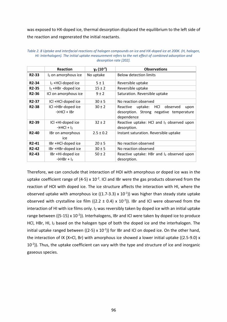
96

was exposed to HX-doped ice, thermal desorption displaced the equilibrium to the left side of

the reaction and regenerated the initial reactants.

Table 2. 8 Uptake and interfacial reactions of halogen compounds on ice and HX-doped ice at 200K. (H, halogen, HI: Interhalogen). The initial uptake measurement refers to the net effect of combined adsorption and

desorption rate [202].

Reaction ɣ0 (10-2) Observations

R2-33 I2 on amorphous ice No uptake Below detection limits

R2-34 I2 +HCl-doped ice 5 ± 1 Reversible uptake

R2-35 I2 +HBr -doped ice 15 ± 2 Reversible uptake

R2-36 ICl on amorphous ice 9 ± 2 Saturation. Reversible uptake

R2-37 ICl +HCl-doped ice 30 ± 5 No reaction observed

R2-38 ICl +HBr-doped ice →HCl + IBr

30 ± 2 Reactive uptake: HCl observed upon desorption. Strong negative temperature dependence

R2-39 ICl +HI-doped ice →HCl + I2

32 ± 2 Reactive uptake: HCl and I2 observed upon desorption.

R2-40 IBr on amorphous ice

2.5 ± 0.2 Instant saturation. Reversible uptake

R2-41 IBr +HCl-doped ice 20 ± 5 No reaction observed

R2-42 IBr +HBr-doped ice 30 ± 5 No reaction observed

R2-43 IBr +HI-doped ice →HBr + I2

50 ± 2 Reactive uptake: HBr and I2 observed upon desorption.

Therefore, we can conclude that interaction of HOI with amorphous or doped ice was in the

uptake coefficient range of (4-5) x 10-2. ICl and IBr were the gas products observed from the

reaction of HOI with doped ice. The ice structure affects the interaction with HI, where the

observed uptake with amorphous ice ((1.7-3.3) x 10-1)) was higher than steady state uptake

observed with crystalline ice film ((2.2 ± 0.4) x 10-2)). IBr and ICl were observed from the

interaction of HI with ice films only. I2 was reversibly taken by doped ice with an initial uptake

range between ((5-15) x 10-2)). Interhalogens, IBr and ICl were taken by doped ice to produce

HCl, HBr, HI, I2 based on the halogen type of both the doped ice and the interhalogen. The

initial uptake ranged between ((2-5) x 10-1)) for IBr and ICl on doped ice. On the other hand,

the interaction of IX (X=Cl, Br) with amorphous ice showed a lower initial uptake ((2.5-9.0) x

10-2)). Thus, the uptake coefficient can vary with the type and structure of ice and inorganic

gaseous species.

97

Table 2. 9 summarizing the used methods for the measurement of uptake in HOI-Halide interactions. The interaction, the temperature, the ɣ and the products observed are reported [197, 199, 200, 201, 202]. ɣo :

uptake coefficient at zero time, ɣss : uptake at steady state condition, ɣobs = uptake coefficient observed and not precised if it is at zero time or steady state conditions.

Interaction Technique Temperature Uptake coefficient Products Reference

HOI + amorphous ice

Knudsen cell

180-200 K ɣ0=

(6 ± 2) x 10-2

-

[197]

HOI + HX/amorphous ice (X=Cl,Br)

200 K ɣ0=

((4-5) ± 2) x 10-2

ICl, IBr

HI + amorphous ice

Knudsen cell 190-210 K ɣobs=

(1.7-3.3) x 10-1

- [199]

HI + crystalline ice thin film

Knudsen cell 185-210 K ɣobs ≥ 2 x 10-2 Amorphous HI:H2O layers

[200]

HI + Ice film Flow tube reactor

213-233 K ɣss =

(2.2 ± 0.4) x 10-2

IBr, ICl [201]

I2 + HX/ice

(X= Cl, Br)

Knudsen cell

200 K

ɣ0 =

(5 -15) x 10-2

-

[202]

ICl + HX/ice

(X= I, Cl, Br)

ɣ0 =

(3.0 - 3.2) x 10-1

- HCl and IBr with HBr/ ice

- HI and I2 with

HI/ice

IBr + HX/ice

(X= I, Cl, Br)

ɣ0 =

(2-5) x 10-1

HBr and I2 with

HBr/ice

IX + amorphous ice (X= Cl, Br)

ɣ0 =

(2.5 -9) x 10-2

ICl

2.4.2.2 Photodissociation of CH3I on ice

Studies dealing with interactions between aerosols and methyl iodide (CH3I) species concern

the role of ice and snowpack in photo reactivity of CH3I species found in the atmosphere. The

measurements performed during field campaigns showed that photochemical processes

occurring within the snowpack may alter the atmospheric composition including the organo-

halogen content [203, 209]. There have been extensive experimental and theoretical studies

on the photodissociation of CH3I in the gas phase [210- 212] or adsorbed on different solid

metallic substrates [213- 216]. Along with this wealth of information, the observation of

organic iodide from field measurements on or in ice (snow) [203] and the discovery of organic

iodide compounds as potential sources of reactive halogen species during ozone depletion

98

processes [217] have motivated investigations of photo dissociation of CH3I adsorbed on ice

[204- 206].

Here, it should be noted that the ice grown in vacuum could exist in several different structural

forms depending on the temperature of the cold substrate. The deposition of water vapor at

substrate temperatures below 130 K results in the formation of low-density porous

amorphous solid water (PASW), while dosing water vapor at higher temperatures (≥130 K)

results in formation of amorphous solid water (ASW). Unlike ASW, PASW contains many

surface defects that facilitate trapping of adsorbates. Crystalline ice is formed by dosing water

vapor at temperatures ≥ 140 K [204].

The photo dissociation of CH3I on PASW (porous amorphous solid water) and ASW

(amorphous solid water) ice was investigated using ultra high vacuum (UHV) chamber with a

base pressure of 6.6 × 10-13 bar [204]. 50 monolayers (1.7 × 10-11 bar) of PASW and ASW ice

were grown on zirconia substrate at 90 K and 130 K, respectively. The 50 monolayers were

grown to assure that interactions associated with the zirconia substrate were removed or

minimized. CH3I was deposited on ice substrate by dosing the CH3I vapor at 1.3 × 10-11 bar for

10 s. Authors [204] performed measurements using time-of-flight mass spectrometer (ToF-

MS) and Temperature programmed desorption (TPD) coupled to a quadrupole mass

spectrometer (QMS) analysis. A pulsed laser light at either 290 or 260 nm was used to irradiate

the sample. The substrate was heated linearly using a rate of 3 K/s.

I2 formation was observed on ASW at both excitation wavelengths (260 nm and 290 nm), but

it was not detectable within sensitivity of author technique on PASW at both wavelengths.

The I2 formation occurred with a much greater yield when using 260 nm compared to 290 nm.

However, the mechanism of I2 formation was not clearly stated, but the authors suggested

that small adsorbed clusters of CH3I on ASW can be ideal for the formation of I2. Additionally,

the authors [204] suggested that the presence of pores in PASW can either make the trapped

CH3I molecules unavailable for photodissociation or trap iodine photo fragments within the

ice substrate. CH3 and I photofragments that were trapped within pores of PASW may

recombine or react to form products that were not detected in this experiment, such as

CH3CH3I or CH3OH.

TPD spectra between 100-220 K of CH3I on ASW, indicated that almost all of the CH3I monomer

and clusters had desorbed at 120 K before water began desorbing [204]. No bonding

interaction between CH3I and ASW was observed. However, the authors suggested that the

99

overall average symmetry of CH3I likely changes from C3v to Cs as it adsorbs. Whereas, for CH3I

deposited on PASW, the pores were filled before CH3I began to accumulate on the surface,

thus the TPD spectrum showed a three-desorption state at 120 K, 150 and 160 K. The structure

of CH3I adsorbed on PASW was not identified. This experiment demonstrated that ice porosity

enhances the trapping of adsorbed CH3I, while pore-free ice likely allows monomer adsorption

and the formation of CH3I clusters.

The photo dissociation of methyl iodide on D2O ASW ice was investigated using ultra high

vacuum (UHV) chamber with a base pressure of 5.3 × 10-13 bar [205]. 1 layer (1.3 × 10-19 bar.

s) of D2O ASW ice was grown on Cu substrate at 100 K. Then CH3I was deposited on ice

substrates by dosing the CH3I vapor at 1.3 × 10-19 bar for 1 s. For photoirradiation, UV photons

were generated from a 100 W high-pressure mercury arc lamp (Oriel). Temperature

programmed desorption (TPD) spectra were collected using time-of-flight mass spectrometry

(TOF-MS) while heating the substrate at a rate of 2 K/s. TPD and X-ray photoelectron

spectroscopy (XPS) analysis were performed before and after irradiation. Ultra- violet

photoelectron spectroscopy (UPS) analysis was performed for Cu, D2O and CH3I/D2O/Cu

substrates.

Before irradiation, the TPD spectra between 100-500 K of CH3I on ASW, showed that all the

mono and multilayers of CH3I desorb from the ice layer at 120 and 130 K, respectively [205]

which is consistent with [204]. The authors suggested that during photo-irradiation between

130-145 K, the dissociated products (CH3 and I) seems to diffuse into the ice film and be

trapped. Moreover, at 430 K the authors suggested a chemisorption of CH3I on Cu substrate

since all ice layers should be removed up to 300 K. No new photodissociated product (such as

I2) was observed.

XPS spectra were measured as function of photo irradiation time (up to 30 minutes) for CH3I

on ice at 100 K [205]. The spectra showed a dramatical change (area of the band and shift by

3 e.v) in the I 3d5/2 XPS band (621 e.v) observed as function of photoirradiation time. This was

explained by that at the beginning of photo irradiation the band observed was for both un-

dissociated and dissociated CH3I. Upon further photo-irradiation, the dissociated CH3I

becomes dominant which results in decrease in area of the band. Additionally, with increasing

photo-irradiation time, the authors suggested an increase in solvated I-, I radical, and/or

chemisorbed I on Cu which explains the shift in the I 3d5/2 XPS band. No other chemical species

formed and/or desorbed from the surface were observed. No bands were observed from the

XPS spectra for CH3I photo irradiated for 5 minutes at 100K and followed by TPD up to 800 K.

100

This confirmed that the diffusion of CH3I towards Cu substrate and that I radicals (or solvated

I-) do not desorb, instead they chemisorb on the Cu surface.

Finally, based on UPS spectra a small shift (-1.0 eV) was observed from electronic work

function2 of all analyzed systems Cu, D2O/Cu and CH3I/D2O/Cu. The authors [205] concluded

that the electrons photo excited from Cu transferred to ice to generate solvated electrons in

the ice film. The solvated electrons then quickly transfer to CH3I to proceed the cleavage of

C‑I bond. Thus, the ice is being an important intermediate by efficiently capturing

photoelectrons emitted from the underlying metal substrate.

Similarly, the system of CH3I adsorbed on thin films of D2O ASW ice grown on Cu at 90 K was

studied using an ultra-high vacuum system with a base pressure of 1.3 × 10-12 bar [206]. Up

to 2- 120 monolayers of D2O were deposited on the Cu surface. 0.2-1 monolayer of CH3I was

then deposited on D2O/Cu. The exact dosing quantity of D2O and CH3I have not been precised

by the authors [206]. The authors used time of flight quadrupole mass spectrometer (TOF-

QMS) to analyse the distributions of the desorbing CH3 fragments after photodissociation

using linearly polarized λ=248 nm light [206]. Observation of photo dissociation of CH3I on

ASW D2O ice in this study are quite similar to the one observed by CH3I on ASW H2O ice [204].

The authors indicated that CH3I adsorbed on D2O forms clusters at low coverages, with a C–I

bond axis orientation. However, no I2 formation upon photodissociation was observed.

Additionally, authors noted that the overall TOF spectrum distribution does not change

significantly with increasing CH3I dose [206]. More photo dissociation yield was observed for

thicker D2O films. In contrast to [205], the authors [206], did not find an evidence of the

dissociation of CH3I mechanism via the temporary solvation of photoelectrons in localized

states of the D2O ASW ice.

2 The work function: acquired spectroscopically by measuring the difference between the Fermi Level and the

cutoff of the ‘tail’ at the low kinetic energy end of the spectrum and then subtracting this value from the incident

photon energy.

101

To sum up and as shown in Table 2.10, that adsorption, diffusion, and desorption of organic

molecules depend largely on the morphology of the ice substrate. Porous ice enhances the

trapping of adsorbed CH3I, whereas pore-free ice likely allows monomer adsorption and the

formation of CH3I clusters. Dissociation can be observed when adsorbed CH3I molecules in (or

on) ASW ice are irradiated by UV photons. A significant dissociation to form either I, I- or I2 is

likely to occur. No clear mechanism for I2 has been reported, in contrast, to gas phase where

only atomic Iodine is observed (see section 2.2). On the other hand, PASW can hinder the CH3I

molecule photodissociation. Nor photodissociation rate or uptake coefficient of CH3I on ice

was reported.

Table 2. 10 Table summarizing the used methods for the photodissociation of CH3I on ice. The ice type, the temperature, the pressure, wavelength and the products observed are reported [204, 205, 206]. ASW: Amorphous solid water and PASW: porous amorphous solid water. REMPI: resonance enhanced multiphoton ionization (REMPI). UHV: Ultra high Vacuum chamber, XPS: X-ray photoelectron spectroscopy, TOF-MS: time-of-flight mass spectrometer, TPD-QMS: Temperature programmed desorption coupled to quadrupole mass spectrometer (QMS) and UPS: Ultra- violet photoelectron spectroscopy.

Ice type Technique Temperature Pressure Wavelength Products Reference

H2O ASW UHV

TOF-MS

REMPI

TPD-QMS

90K 6.6 × 10-13 bar 260nm

290 nm

CH3, I, I2 [204]

H2O PASW UHV

TOF-MS

REMPI

TPD-QMS

130 K 6.6 × 10-13 bar 260nm

290 nm

CH3, I [204]

D2O ASW UHV

TOF-MS

XPS

UPS

100K 5.3 × 10-13 bar Hg lamp CH3, I- [205]

D2O ASW UHV

TOF-QMS

90 K 1.3 × 10-12 bar 248 nm CH3, I [206]

2.4.3 Heterogeneous interaction of organic iodine with carbonaceous aerosols

The heterogeneous interaction of organic iodine species with carbonaceous particles was

investigated in only two papers [207, 208].

The uptake of CH3I on commercial soot film (composition and source of soot is not precised

by the authors) was studied using a coated wall flow tube combined with Time of Flight Mass

Spectrometer at 298 K and with a bulk flow rate of 200 and 500 cm3.min-1 [207]. A fast-initial

consumption of CH3I followed by rapid soot surface deactivation, leading to a decrease of the

CH3I loss rate was observed. CH3I loss on soot film was assumed to be due to two processes:

102

irreversible CH3I uptake and, to less extent, reversible non-reactive adsorption–desorption

processes. The estimated residence time of the reversibly adsorbed CH3I molecules on the

soot surface was of the order of a few seconds. The initial uptake was determined to be

(1.03±0.15) x 10-2. Finally, the authors stated that the fate of the organoiodines on the soot

surfaces needs more research, as the heterogeneous loss of CH3I on soot may influence the

concentration of CH3I throughout the atmosphere.

Further, the uptake of ethyl iodine (C2H5I) on black carbon (Degussa FW2) thin film surface at

298 K was investigated [208] by using a coated wall flow tube combined with a differentially

pumped time-of-flight mass spectrometer. As observed for soot surface when exposed to CH3I

[208], a fast-initial consumption of C2H5I followed by rapid deactivation of the black carbon

leading to a decrease of the C2H5I loss rate was observed. In addition, a partial desorption of

C2H5I was observed when C2H5I was no longer in contact with the black carbon surface. The

initial uptake was determined to be (2.3±0.9) × 10−2. Finally, the authors stated that to get

more conclusive answers on the interaction of C2H5I with black carbon surface, future research

should be directed for characterizing atmospheric carbon aerosol samples and understanding

their heterogeneous interactions.

Therefore, we can conclude that the initial uptake of methyl iodide on black carbon or ethyl

iodide on soot was of the same magnitude. No data on the reaction or the products formed

was given.

2.4.4 Modelling of inorganic species with undefined surfaces

A tropospheric Halogen Chemistry model (THAMO) was developed to investigate the halogen

chemistry chemical mechanism. THAMO is a one-dimensional chemical and transport model

that uses time-implicit integration [9, 39]. This model can simulate the iodine observations,

and thus explore the impact of iodine chemistry in the polar boundary layer. In this model, the

authors [9] computed a first-order rate loss of uptake for halogen heterogeneous uptake on

aerosols, for a number of gas phase species. Table 2.11 shows the calculated first order rate

loss due to uptake of iodine gaseous species (IO, OIO, HI, HOI, INO2, IONO2, I2O5) into

undefined aerosol species of inorganic species. These rate losses seem to confirm the

experimental observations stated before (section 2.4) that iodine species can be reactive with

atmospheric aerosols.

103

Table 2. 11 Estimated rate loss of iodine on aerosols based on free-regime approximation [9].

Loss to undefined aerosols

Species Rate loss

IO 0.02

OIO 1

HI 0.02

HOI 0.02

INO2 0.02

IONO2 0.02

I2O5 0.02

2.5 Conclusion

To sum up, CH3I and I2 that can be emitted naturally or released in case of severe nuclear

accident into the atmosphere may react in gaseous phase and may interact with ice or with

atmospheric aerosols. Although the gaseous phase reaction of halogen compounds is well

documented, there is still a lack of knowledge about the interaction between atmospheric

aerosols and CH3I and I2 gaseous species which are of nuclear interest.

References

[1] S. Solomon, On the role of iodine in ozone depletion, J. Geophys. Res. 99 (1994) 491–499. https://doi.org/10.1029/94JD02028.

[2] A.R. Baker, D. Thompson, M.L.A.M. Campos, S.J. Parry, T.D. Jickells, Iodine concentration and availability in atmospheric aerosol, Atmos. Environ. 34 (2000) 4331–4336.https://doi.org /10.1016/S1352-2310(00)00208-9.

[3] L.J. Carpenter, S.M. Macdonald, M.D. Shaw, R. Kumar, R.W. Saunders, R. Parthipan, J. Wilson, J.M.C. Plane, Atmospheric iodine levels influenced by sea surface emissions of inorganic iodine, Nat. Geosci. 6 (2013) 108–111. https://doi.org/10.1038/ngeo1687.

[4] A. Saiz-Lopez, J.M.C. Plane, Novel iodine chemistry in the marine boundary layer, Geophys. Res. Lett. 31 (2004) L04112. https://doi.org/10.1029/2003GL019215.

[5] A. Saiz-Lopez, J.M.C. Plane, A.R. Baker, L.J. Carpenter, R. Von Glasow, C.G. Juan, G. Mcfiggans, R.W. Saunders, Atmospheric Chemistry of Iodine, Chem. Rev. 112 (2012) 1773–1804. https://doi.org//10.1021/cr200029u.

104

[6] J. Trincal, Thèse de Doctorat Modélisation du comportement de l’iode dans l’atmosphère, Lille university, 2015.

[7] C. Fortin, These de Doctorat Etudes par simulations numériques et moléculaires de la réactivité atmosphérique de l’iode, Lille university, 2019.

[8] C. Peters, S. Pechtl, J. Stutz, K. Hebestreit, G. Hönninger, K.G. Heumann, A. Schwarz, J. Winterlik, U. Platt, Reactive and organic halogen species in three different European coastal environments, Atmos. Chem. Phys. 5 (2005) 3357–3375. https://doi.org/10.5194/acp-5-3357-2005.

[9] A.Saiz-Lopez, J.M.C. Plane, A.S. Mahajan, P.S. Anderson, A.E. Jones, H.K. Roscoe, R.A. Salmon, W.J. Bloss, J.D. Lee, On the vertical distribution of boundary layer halogens over coastal Antarctica : implications for O3, HOx, NOx and the Hg lifetime, Atmos. Chem. Phys. 8 (2008) 887–900. https://doi.org/10.5194/acp-8-887-2008.

[10] K. Law, W. Struges, Chapter 2 Halogenated short-lived substances, in: scientific assessment of ozone depletion: 2006 Report No. 50, (2007).

[11] J.E. Lovelock, R.J. Maggs, R.J. Wade, Halogenated hydrocarbons in and over the Atlantic, Nature. 241 (1973) 194–196. https://doi.org/10.1038/241194a0.

[12] R. Huang, Ph.D. thesis on Reactive Halogen Compounds in the Marine Boundary Layer: Method Developments and Field Measurements, Johannes Gutenberg-Universität, 2009.

[13] C. Ordonez, J.-F. Lamarque, S. Tilmes, D.E. Kinnison, D.R.B. E. L. Atlas, G.S. Santos, G. Brasseur, A. Saiz-Lopez, Bromine and iodine chemistry in a global chemistry-climate model: description and evaluation of very short-lived oceanic sources, Atmos. Chem. Phys. 12 (2012) 1423–1447. https://doi.org/10.5194/acp-12-1423-2012.

[14] N. Bell, L. Hsu, D.J. Jacob, M.G. Schultz, D.R. Blake, J.H. Butler, D.B. King, J.M. Lobert, E. Maier-Reimer, Methyl iodide: Atmospheric budget and use as a tracer of marine convection in global models, J. Geophys. Res. Atmos. 107 (2002) 8/1-8/12. https://doi.org/ 10.1029/200IJD001151.

[15] R.A. Rasmussen, M.A.K. Khalil, R. Gunawardena, S.D. Hoyt, Atmospheric methyl iodide (CH3I), J. Geophys. Res. 87 (1982) 3086–3090. https://doi.org/10.1029/JC087iC04p03086.

[16] C.H. Dimmer, P.G. Simmonds, G. Nickless, M.R. Bassford, Biogenic fluxes of halomethanes from Irish peatland ecosystems, Atmos. Environ. 35 (2001) 321–330. https://doi.org/ 10.1016/S1352-2310(00)00151-5.

[17] K.R. Redeker, N.Y. Wang, J.C. Low, A. McMillan, S.C. Tyler, R.J. Cicerone, Emissions of methyl halides and methane from rice paddies, 290 (2000) 966-969. https://doi.org/10.1126/ science.290.5493.966.

[18] M.O. Andreae, P.Merlet, Emission of trace gases and aerosols from biomass burning, Glob. Biogeochem. 15 (2001) 955–966. https://doi.org/10.1029/2000GB001382.

[19] A. Ekdahl, M. Pedersén, K. Abrahamsson, A study of the diurnal variation of biogenic volatile halocarbons, Mar. Chem. 63 (1998) 1–8. https://doi.org/10.1016/S0304-4203(98)00047-4.

[20] C.E. Jones, K.E. Hornsby, R. Sommariva, R.M. Dunk, R. Von Glasow, G. McFiggans, L.J. Carpenter, Quantifying the contribution of marine organic gases to atmospheric iodine, Geophys. Res. Lett. 37 (2010) L18804. https://doi.org/10.1029/2010GL043990.

105

[21] Y. Sakamoto, A. Yabushita, M. Kawasaki, S. Enami, Direct emission of I2 molecule and IO radical from the heterogeneous reactions of gaseous ozone with aqueous potassium iodide solution, J. Phys. Chem. A. 113 (2009) 7707–7713. https://doi.org/10.1021/jp903486u.

[22] F.C. Kupper, C.J. Carrano, Key aspects of the iodine metabolism in brown algae : a brief critical review, R. Soc. Chem., Met. 11 (2019) 756–764. https://doi.org/10.1039/c8mt00327k.

[23]F.C. Kupper, L.J. Carpenter, Gordon B. McFiggans, C.J. Palmere, T.J. Waite, E.-M. Boneberg, S. Woitsch, M. Weiller, R. Abelaj, D. Grolimund, P. Potin, A. Butler, G.W.L. III, P.M.H. Kroneck, W. Meyer-Klaucke, M.C. Feiters, Iodide accumulation provides kelp with an inorganic antioxidant impacting atmospheric chemistry, Proc. Natl. Acad. Sci. U. S. A. 105 (2008) 6954–6958. https://doi.org/10.1073/pnas.0709959105.

[24] J.A. Garland, H. Curtis, Emission of Iodine from the Sea Surface in the Presence of Ozone, Geophys. Res., 86 (1981) 3183–3186. https://doi.org/10.1029/JC086iC04p03183.

[25] A. Saiz-Lopez, J.A. Shillito, H. Coe, J.M.C. Plane, Measurements and modelling of I2, IO, OIO, BrO and NO3 in the mid-latitude marine boundary layer, Atmos. Chem. Phys. 6 (2006) 1513–1528. Open source.

[26] J. Rancher, M.A. Kritz, Diurnal Fluctuations of Br and I in the Tropical Marine, J. Geophys. Res. 85 (1980) 5581–5587. https://doi.org/10.1029/JC085iC10p05581.

[27] B.S. Gilfedder, R. Chance, U. Dettmann, S.C. Lai, Determination of total and non-water soluble iodine in atmospheric aerosols by thermal extraction and spectrometric detection ( TESI ), Anal. Bioanal. Chem. 398 (2010) 519–526. https://doi.org/10.1007/s00216-010-3923-1.

[28] T.M. Sherwen, M.J. Evans, D. V Spracklen, L.J. Carpenter, R. Chance, A.R. Baker, J.A. Schmidt, T.J. Breider, Global modeling of tropospheric iodine aerosol, Geophys. Res. Lett. 43 (2016) 10012–10019. https://doi.org/10.1002/2016GL070062.

[29] A. Saiz-Lopez, R.P. Fernandez, C. Ordóñez, D.E. Kinnison, J.C.G. Martín, J.F. Lamarque, S. Tilmes, Iodine chemistry in the troposphere and its effect on ozone, Atmos. Chem. Phys. 14 (2014) 13119–13143. https://doi.org/10.5194/acp-14-13119-2014.

[30] T.K. Koenig, S. Baidar, P. Campuzano-Jost, C.A. Cuevas, B. Dix, R.P. Fernandez, H. Guo, S.R. Hall, D. Kinnison, B.A. Nault, K. Ullmann, J.L. Jimenez, A. Saiz-Lopez, R. Volkamer, Quantitative detection of iodine in the stratosphere, Proc. Natl. Acad. Sci. U. S. A. 117 (2020) 1860–1866. https://doi.org/10.1073/pnas.1916828117.

[31] K. Seitz, J. Buxmann, D. Pöhler, T. Sommer, J. Tschritter, T. Neary, C. O’Dowd, U. Platt, The spatial distribution of the reactive iodine species IO from simultaneous active and passive DOAS observations, Atmos. Chem. Phys. 10 (2010) 2117–2128. https://doi.org/10.5194/acp-10-2117-2010.

[32] C.S.E. Bale, T. Ingham, R. Commane, D.E. Heard, W.J. Bloss, Novel measurements of atmospheric iodine species by resonance fluorescence, J. Atmos. Chem. 60 (2008) 51–70. https://doi.org/10.1007/s10874-008-9108-z.

[33] R. Vogt, R. Sander, R. Von Glasow, P.J. Crutzen, Iodine chemistry and its role in halogen activation and ozone loss in the marine boundary layer: A model study, J. Atmos. Chem. 32 (1999) 375–395. https://doi.org/10.1023/A:1006179901037.

106

[34] W.L. Chameides, D.D. Davis, Iodine : Its Possible Role in Tropospheric Photochemistry, J. Geophys. Res. 85 (1980) 7383–7398. https://doi.org/10.1029/JC085iC12p07383.

[35] U. Platt, G. Hönninger, The role of halogen species in the troposphere, Chemosphere. 52 (2003) 325–338. https://doi.org/10.1016/S0045-6535 (03)00216-9.

[36] C.D. O’Dowd, Jose L. Jimenez, Roya Bahreini, R.C. Flagan, J.H. Seinfeld, K. Ha¨meri, L. Pirjola, M. Kulmala, S.G.J.T. Hoffmann, Marine aerosol formation from biogenic iodine emissions, Lett. to Nat. 417 (2002) 632–636. https://doi.org/10.1038/nature00773.1.2.3. 4.5.6.7.8.9.10.

[37] A.S. Mahajan, M. Sorribas, J.C.G. Martín, S.M. MacDonald, M. Gil, J.M.C. Plane, A. Saiz-Lopez, Concurrent observations of atomic iodine, molecular iodine and ultrafine particles in a coastal environment, Atmos. Chem. Phys. 11 (2011) 2545–2555. https://doi.org/10.5194/acp-11-2545-2011.

[38] A. Saiz-Lopez, J.M.C. Plane, C.A. Cuevas, A.S. Mahajan, J.F. Lamarque, D.E. Kinnison, Nighttime atmospheric chemistry of iodine, Atmos. Chem. Phys. 16 (2016) 15593–15604. https://doi.org/10.5194/acp-16-15593-2016.

[39] A.S. Mahajan, H. Oetjen, A. Saiz-Lopez, J.D. Lee, G.B. McFiggans, J.M.C. Plane, Reactive iodine species in a semi-polluted environment, Geophys. Res. Lett. 36 (2009) 1–6. https://doi.org/10.1029/2009GL038018.

[40] J.B. Burkholder, S.P. Sander, J.P.D. Abbat, J.R. Barker, R.E. Huie, C.E. Kolb, M.J.K. Goddard, V.L. Orkin, P.H. Wine, D.M. Wilmouth, Chemical Kinetics and Photochemical Data for Use in Atmospheric Studies Evaluation Number 18, JPL Publication 15-10, Jet Propulsion Laboratory, Pasadena, 2015. http://jpldataeval.jpl.nasa.gov.

[41] A. Saiz-Lopez, R.W. Saunders, D.M. Joseph, S.H. Ashworth, J.M.C. Plane, Absolute absorption cross-section and photolysis rate of I2, Atmos. Chem. Phys. Discuss. 4 (2004) 2379–2403. https://doi.org/10.5194/acpd-4-2379-2004.

[42] O. V. Rattigan, D.E. Shallcross, R.A. Cox, UV absorption cross-sections and atmospheric photolysis rates of CF3I, CH3I, C2H5I and CH2ICl, J. Chem. Soc. - Faraday Trans. 93 (1997) 2839–2846. https://doi.org/10.1039/a701529a.

[43] R. Sommariva, W.J. Bloss, R. Von Glasow, Uncertainties in gas-phase atmospheric iodine chemistry, Atmos. Environ. 57 (2012) 219–232. https://doi.org/10.1016/j.atmosen v.2012.04.032.

[44] E. Jenkin, R.A. Cox, Kinetics Study of the Reactions IO + NO2 + M → IONO2+M, IO+IO → products and I + O3 → IO + O2, J. Phys. Chem. 89 (1985) 192–199. https://doi.org/10.1021 /j100247a040.

[45] L.J. Carpenter, Iodine in the Marine Boundary Layer, Chem. Rev. 103 (2003) 4953–4962. https://doi.org/10.1021/cr0206465.

[46] J.C.G. Martin, P. Spietz, J.P. Burrows, Spectroscopic studies of the I2 / O3 photochemistry Part 1: Determination of the absolute absorption cross sections of iodine oxides of atmospheric relevance, 176 (2005) 15–38. https://doi.org/10.1016/j.jphotochem.200 5.09.024.

[47] W.J. Bloss, D.M. Rowley, R.A. Cox, R.L. Jones, Kinetics and products of the IO self-reaction, J. Phys. Chem. A. 105 (2001) 7840–7854. https://doi.org/10.1021/jp0044936.

107

[48] A. Villard, S. Khanniche, C. Fortin, L. Cantrel, I. Černušák, F. Louis, A theoretical study of the microhydration processes of iodine nitrogen oxides, Int. J. Quantum Chem. 119 (2019) 1–11. https://doi.org/10.1002/qua.25792.

[49] N. Kaltsoyannis, J.M.C. Plane, Quantum chemical calculations on a selection of iodine-containing species (IO, OIO, INO3, (IO)2, I2O3, I2O4 and I2O5) of importance in the atmosphere, Phys. Chem. Chem. Phys. 10 (2008) 1723–1733. https://doi.org/1 0.1039/b715687c.

[50] R.M. Chambers, A.C. Heard, R.P. Wayne, Inorganic Gas-Phase Reactions of the Nitrate Radical : I2 + NO3 and I + NO3, J. Phys. Chem. 96 (1992) 3321–3331. https://doi.org/ 10.1021/j100187a028.

[51] Y. Nakano, Y. Hosho, K. Sadamori, T. Ishiwata, Determination of the rate constant of the reaction of NO3 with C2H5I using time-resolved cavity ring-down spectroscopy, Chem. Phys. Lett. 535 (2012) 26–29. https://doi.org/10.1016/j.cplett.2012.03.040.

[52] N. Yukio, I.T. Ukeguchi Hiromi, K. Yugo, T. Hiroto, I. Atsushi, K.M. Sakaki Shigeyoshi, Study of the Temperature Dependence of the Reaction of NO3 with CH3I and the Estimation of Its Impact on Atmospheric Iodine Chemistry, Chem. Phys. Lett. 208 (2008) 938–946. https://doi.org /10.1246/bcsj.81.938

[53] F.Y. Bai, X. Wang, Y.Q. Sun, X.M. Pan, Atmospheric chemistry of alkyl iodides : theoretical studies on the mechanisms and kinetics of CH3I/C2H5I+NO3 reactions, RSC Adv. 5 (2015) 88087–88095. https://doi.org/ 10.1039/c5ra16215g.

[54] F. Louis, I. Černušák, S. Canneaux, K. Mečiarová, Atmospheric reactivity of CH3I and CH2I2 with OH radicals: A comparative study of the H- versus I-abstraction, Comput. Theor. Chem. 965 (2011) 275–284. https://doi.org/10.1016/j.theochem.2010.09.022.

[55] O. Galvez, J.C.G. Martin, P.C. Gomez, A. Saiz-Lopez, L.F. Pacios, A theoretical study on the formation of iodine oxide aggregates and monohydrates, Phys. Chem. Chem. Phys. 15 (2013) 15572–15583. https://doi.org/10.1039/c3cp51219c.

[56] J.C.G. Martin, O. Galvez, b M.T. Baeza-Romero, T. Ingham, J.M.C. Plane, M.A. Blitz, On the mechanism of iodine oxide particle formation, Phys. Chem. Chem. Phys. 15 (2013) 15612–15622. https://doi.org/10.1039/c3cp51217g.

[57] T. Hoffmann, C.D.O. Dowd, J.H. Seinfeld, Iodine oxide homogeneous nucleation’ for coastal new particle production, Geophys. Res. Lett. 28 (2001) 1949–1952. https://doi.org /10.1029/2000GL012399.

[58] J. Curtius, Nucleation of atmospheric aerosol particles, Comptes Rendus Phys. 7 (2006) 1027–1045. https://doi.org/10.1016/j.crhy.2006.10.018.

[59] B.R.W. Saunders, R. Kumar, J.C.G. Martín, A.S. Mahajan, B.J. Murray, J.M.C. Plane, Studies of the Formation and Growth of Aerosol from Molecular Iodine Precursor, Zeitschrift Für Phys. Chemie. 224 (2010) 1095–1117. https://doi.org/10.1524/zpch.2010.6143.

[60] W.R. Stockwell, F. Kirchner, M. Kuhn, S. Seefeld, A new mechanism for regional atmospheric chemistry modeling, 102 (1997) 25847–25879. https://doi.org/10.1029/9 7JD00849.


108

[62] C. Fortin, V. Fèvre-Nollet, F. Cousin, P. Lebègue, F. Louis, Box modelling of gas-phase atmospheric iodine chemical reactivity in case of a nuclear accident, Atmos. Environ. 214 (2019) 116838. https://doi.org/10.1016/j.atmosenv.2019.116838.

[63] S. Zhang, Thèse de Doctorat: Etudes cinétiques de l'oxydation radicalaire en phase gazeuse d'iodures organiques et de la formation de particules d'oxydes d'iode sous conditions simulées de l'enceinte d'un réacteur nucléaire en situation d'accident grave, Aix-Marseille Université, 2012

[64] S. Taamalli, D. Khiri, S. Suliman, S. Khanniche, C. Ivan, L. Cantrel, M. Ribaucour, F. Louis, Unraveling the Tropospheric Microhydration Processes of Iodous Acid HOIO, ACS Earth Sp. Chem. 4 (2020) 92–100. https://doi.org/10.1021/acsearthspacechem.9b00257.

[65] S. Khanniche, F. Louis, L. Cantrel, I. Černušák, A theoretical study of the microhydration of iodic acid (HOIO2), Comput. Theor. Chem. 1094 (2016) 98–107. https://doi.org/10.1016 /j.comptc.2016.09.010.

[66] M. Ruan, H. Hou, B. Wang, W. Li, Y. Chen, X. Deng, X. Zuo, Computational study on the hydrolysis of halomethanes, Theor. Chem. Acc. 137:181 (2018) 1–10. https://doi.org /10.1007/s00214-018-2389-7.

[67] J. Xie, X. Ma, J. Zhang, P.M. Hierl, A.A. Viggiano, W.L. Hase, Effect of microsolvation on the OH−(H2O)n + CH3I rate constant. Comparison of experiment and calculations for OH−(H2O)2 + CH3I, Int. J. Mass Spectrom. 418 (2017) 122–129. https://doi.org/10.1016/j.ijms.2016.10.017.

[68] J. Xie, R. Otto, R. Wester, W.L. Hase, Chemical dynamics simulations of the monohydrated OH-(H2O) + CH3I reaction. Atomic-level mechanisms and comparison with experiment, J. Chem. Phys. 142 (2015) 2443081-2443088. https://doi.org/10.1063/1.4922451.

[69] B. Bastian, T. Michaelsen, L. Li, M. Ončák, J. Meyer, D.H. Zhang, R. Wester, Imaging Reaction Dynamics of F-(H2O) and Cl-(H2O) with CH3I, J. Phys. Chem. A. 124 (2020) 1929–1939. https://doi.org/10.1021/acs.jpca.0c00098.

[70] J. Lelieveld, K. Klingmüller, A. Pozzer, U. Pöschl, M. Fnais, A. Daiber, T. Münzel, Cardiovascular disease burden from ambient air pollution in Europe reassessed using novel hazard ratio functions, Eur. Heart J. 40 (2019) 1590–1596. https://doi.org/10.1093/eurh eartj/ehz135.

[71] O. Boucher, D. Randall, P. Artaxo, C. Bretherton, G. Feingold, P. Forster, V.-M. Kerminen, Y. Kondo, H. Liao, U. Lohmann, P. Rasch, S.K. Satheesh, S. Sherwood, B. Stevens, X.Y. Zhang, Chapter 7: Clouds and Aerosols. In Climate Change, IPCC report 2013: The Physical Science Basis. Contribution of Working Group I to the Fifth Assessment Report of the Intergovernmental Panel on Climate Change. Cambridge University Press, Cambridge, United Kingdom and New York, USA, 2013. https://doi.org/10.1017/CBO978110741 5324.016.

[72] M. Andreae, H. Annegarn, L. Barrie, J. Feichter, D. Hegg, A. Jayaraman, R. Leaitch, D. Murphy, J. Nganga, G. Pitari, J.E. Penner, Chapter 5:Aerosols, their Direct and Indirect Effects. In Climate Change, IPCC report 2001: The Scientific Basis. Contribution of Working Group I to the Third Assessment Report of the Intergovernmental Panel on Climate Change, Cambridge University Press, Cambridge, United Kingdom and New York, USA 2001. https://doi.org/10. 1029/JD091iD01p01089.

109

[73] U. Pöschl, Atmospheric aerosols: Composition, transformation, climate and health effects, Angew. Chemie-Int. Ed. 44 (2005) 7520–7540. https://doi.org/10.1002/anie.200 501122.

[74] V.R. Després, J. Alex Huffman, S.M. Burrows, C. Hoose, A.S. Safatov, G. Buryak, J. Fröhlich-Nowoisky, W. Elbert, M.O. Andreae, U. Pöschl, R. Jaenicke, Primary biological aerosol particles in the atmosphere: A review, Tellus, Ser. B Chem. Phys. Meteorol. 64 (2012) 155981-1559859. https://doi.org/10.3402/tellusb.v64i0.15598.

[75] Y. Lei, Q. Zhang, K.B. He, D.G. Streets, Primary anthropogenic aerosol emission trends for China, 1990-2005, Atmos. Chem. Phys. 11 (2011) 931–954. https://doi.org/10.5194/acp-11-931-2011.

[76] B.J. Finlayson-Pitts, Reactions at surfaces in the atmosphere: integration of experiments and theory as necessary (but not necessarily sufficient) for predicting the physical chemistry of aerosols, Phys. Chem. Chem. Phys. 11 (2009) 7760–7779. https://doi.org/10. 1039/b916865f.

[77] F. Raes, R. Van Dingenen, V. Elisabetta, J. Wilson, J.P. Putaud, J.H. Seinfeld, P. Adams, Formation and cycling of aerosols in the global troposphere, Atmos. Environ. 34 (2000) 4215–4240. https://doi.org/10.1016/S1474-8177(02)80021-3.

[78] S. Fuzzi, M.O. Andreae, B.J. Huebert, M. Kulmala, T.C. Bond, M. Boy, S.J. Doherty, A. Guenther, M. Kanakidou, K. Kawamura, V.M. Kerminen, U. Lohmann, L.M. Russell, U. Pöschl, Critical assessment of the current state of scientific knowledge, terminology, and research needs concerning the role of organic aerosols in the atmosphere, climate, and global change, Atmos. Chem. Phys. 6 (2006) 2017–2038. https://doi.org/10.5194/acp-6-2017-2006.

[79] J.M. Andino, A. Vivier-Bunge, Chapter 14 Tropospheric Chemistry of Aromatic Compounds Emitted from Anthropogenic Sources. In : Advances in Quantum Chemistry, 1st edition, volume 55, Academic Press, ISBN 9780123743350, 2008. https://doi.org/10.1016/S0065-3276(07) 00214-6.

[80] A.G. Carlton, C. Wiedinmyer, J.H. Kroll, A review of Secondary organic aerosol (SOA) formation from isoprene, Atmos. Chem. Phys. 9 (2009) 4987–5005. https://doi.org/ 10.5194/acp-9-4987-2009.

[81] A. Laskin, D.J. Gaspar, W. Wang, S.W. Hunt, J.P. Cowin, S.D. Colson, B.J. Finlayson-pitts, Reactions at Interface As a Source of Sulfate Formartion in Sea-Salt Particles, Science 301 (2003) 340–345. https://doi.org/10.1126/science.1085374.

[82] P. Laj, J. Klausen, M. Bilde, C. Plaß-Duelmer, et al., Measuring atmospheric composition change, Atmos. Environ. 43 (2009) 5351–5414. https://doi.org/10.1016/j.atmosen v.2009.08.020.

[83] P.S. Monks, C. Granier, S. Fuzzi, et al., Atmospheric composition change - global and regional air quality, Atmos. Environ. 43 (2009) 5268–5350. https://doi.org/10.1016 /j.atmosenv.2009.08.021.

[84] K. Mohiuddin, V. Strezov, P.F. Nelson, E. Stelcer, T. Evans, Mass and elemental distributions of atmospheric particles nearby blast furnace and electric arc furnace operated industrial areas in Australia, Sci. Total Environ. 487 (2014) 323–334. https:// doi.org/10.1016/j.scitotenv.2014.04.025.

110

[85] M. Viana, T.A.J. Kuhlbusch, X. Querol, A. Alastuey, R.M. Harrison, P.K. Hopke, W. Winiwarter, M. Vallius, S. Szidat, A.S.H. Prévôt, C. Hueglin, H. Bloemen, P. Wåhlin, R. Vecchi, A.I. Miranda, A. Kasper-Giebl, W. Maenhaut, R. Hitzenberger, Source apportionment of particulate matter in Europe: A review of methods and results, J. Aerosol Sci. 39 (2008) 827–849. https://doi.org/10.1016/j.jaerosci.2008.05.007.

[86] J.H. Seinfeld, S.N. Pandis, Atmospheric Chemistry and Physics: From Air Pollution to Climate Change, 3rd Edition, Stockholm, Sweden, ISBN: 978-1-118-94740-1, 1998.

[87] G.M. Hidy, V. Mohnen, C.L. Blanchard, Tropospheric aerosols: Size-differentiated chemistry and large-scale spatial distributions, J. Air Waste Manag. Assoc. 63 (2013) 377–404. https://doi.org/10.1080/10962247.2012.760499.

[88] R. Krejci, J. Ström, M. de Reus, J. Williams, H. Fischer, M.O. Andreae, H.-C. Hansson, Spatial and temporal distribution of atmospheric aerosols in the lowermost troposphere over the Amazonian tropical rainforest, Atmos. Chem. Phys. Discuss. 5 (2005) 1527–1543. https://doi.org/10.5194/acpd-4-3565-2004.

[89] J.H. Murillo, S.R. Roman, J.F.R. Marín, B. Cardenas, Source Apportionment of PM2.5 in the Metropolitan Area of Costa Rica Using Receptor Models, Atmos. Clim. Sci. 03 (2013) 562–575. https://doi.org/10.4236/acs.2013.34059.

[90] J.P. Putaud, R. Van Dingenen, A. Alastuey, et al., A European aerosol phenomenology - 3: Physical and chemical characteristics of particulate matter from 60 rural, urban, and kerbside sites across Europe, Atmos. Environ. 44 (2010) 1308–1320. https://doi.org/10. 1016/j.atmosenv.2009.12.011.

[91] P. Laj, K. Sellegri, Les aérosols atmosphéeriques: Impacts locaux, effete globaux, Revue Française des Laboratoires, numero 349, 2003, 23–34. https://doi.org/S0338-9898(03)8046 63.

[92] M.J. Ezell, S.N. Johnson, Y. Yu, V. Perraud, E.A. Bruns, M.L. Alexander, A. Zelenyuk, D. Dabdub, B.J. Finlayson-Pitts, A new aerosol flow system for photochemical and thermal studies of tropospheric aerosols, Aerosol Sci. Technol. 44 (2010) 329–338. https://doi.org/10.1080/02786821003639700.

[93] H. Tervahattu, J. Juhanoja, V. Vaida, A.F. Tuck, J. V. Niemi, K. Kupiainen, M. Kulmala, H. Vehkamäki, Fatty acids on continental sulfate aerosol particles, J. Geophys. Res. D Atmos. 110 (2005) D062071-D062079. https://doi.org/10.1029/2004JD005400.

[94] W.R. Barger, W.D. Garrett, Surface-active organic material in air over the Mediterranean and over the eastern equatorial Pacific, J. Geophys. Res. 81 (1976) 3151–3157. https://doi.org /10.1029/jc081i018p03151.

[95] J.L. Jimenez, M.R. Canagaratna, N.M. Donahue, A.S.H. Prevot, Q. Zhang, at al., Evolution of Organic Aerosols in the Atmosphere, Science. 326 (2009) 1525–1530. https://doi.org /10.1126/science.1180353.

[96] F. Karagulian, C.A. Belis, C. Francisco, C. Dora, A.M. Prüss-ustün, S. Bonjour, H. Adair-rohani, M. Amann, Contributions to cities ’ ambient particulate matter ( PM ): A systematic review of local source contributions at global level, Atmos. Environ. 120 (2015) 475–483. https://doi.org/10.1016/j.atmosenv.2015.08.087.

111

[97] J.M. Schiffer, L.E. Mael, K.A. Prather, R.E. Amaro, and V.H. Grassian, Sea Spray Aerosol: Where Marine Biology Meets Atmospheric Chemistry, ACS Cent. Sci. 4 (2018) 1617–1623. https://doi.org/10.1021/acscentsci.8b00674.

[98] B.J. Finlayson-Pitts, J. James N. Pitts, Chemistry of the Upper and Lower Atmosphere: Theory, Experiments, and Applications, Academic Press, California, ISBN: 978-0-12-257060-5, 2000. https://doi.org/10.1016/B978-0-12-257060-5.X5000-X.

[99] J.W. Chi, W.J. Li, D.Z. Zhang, J.C. Zhang, Y.T. Lin, X.J. Shen, J.Y. Sun, Sea salt aerosols as a reactive surface for inorganic and organic acidic gases in the arctic troposphere, Atmos. Chem. Phys. 15 (2015) 16715–16745. https://doi.org/10.5194/acpd-15-16715-2015.

[100] A.P. Ault, R.C. Moffet, J. Baltrusaitis, D.B. Collins, M.J. Ruppel, L.A. Cuadra-Rodriguez, D. Zhao, T.L. Guasco, C.J. Ebben, F.M. Geiger, T.H. Bertram, K.A. Prather, V.H. Grassian, Size-dependent changes in sea spray aerosol composition and properties with different seawater conditions, Environ. Sci. Technol. 47 (2013) 5603–5612. https://doi.org/10.1021/es400416g.

[101] T.H. Bertram, R.E. Cochran, E.A. Stone, V.H. Grassian, Sea spray aerosol chemical composition: elemental and molecular mimics for laboratory studies of heterogeneous and multiphase reactions, Chem. Soc. Rev. 47 (2018) 2374–2400. https://doi.org /10.1039/c7cs00008a.

[102] L.M. Russell, L.N. Hawkins, A.A. Frossard, P.K. Quinn, T.S. Bates, Carbohydrate-like composition of submicron atmospheric particles and their production from ocean bubble bursting, Proc. Natl. Acad. Sci. U. S. A. 107 (2010) 6652–6657. https://doi.org/10.1073 /pnas.0908905107.

[103] C.D. O’Dowd, M.C. Facchini, F. Cavalli, D. Ceburnis, M. Mircea, S. Decesari, S. Fuzzi, J.Y. Young, J.P. Putaud, Biogenically driven organic contribution to marine aerosol, Nature. 431 (2004) 676–680. https://doi.org/10.1038/nature02959.

[104] A.P. Ault, D. Zhao, C.J. Ebben, M.J. Tauber, F.M. Geiger, K.A. Prather, V.H. Grassian, Raman microspectroscopy and vibrational sum frequency generation spectroscopy as probes of the bulk and surface compositions of size-resolved sea spray aerosol particles, Phys. Chem. Chem. Phys. 15 (2013) 6206–6214. https://doi.org/10.1039/c3cp43899f.

[105] H.M. Hung, P. Ariya, Oxidation of oleic acid and oleic acid/sodium chloride (aq) mixture droplets with ozone: Changes of hygroscopicity and role of secondary reactions, J. Phys. Chem. A. 111 (2007) 620–632. https://doi.org/10.1021/jp0654563.

[106] K. Stemmler, A. Vlasenko, C. Guimbaud, M. Ammann, The effect of fatty acid surfactants on the uptake of nitric acid to deliquesced NaCl aerosol, Atmos. Chem. Phys. 8 (2008) 5127–5141. https://doi.org/10.5194/acp-8-5127-2008.

[107] J. Lovrić, D. Duflot, M. Monnerville, C. Toubin, S. Briquez, Water-Induced Organization of Palmitic Acid at the Surface of a Model Sea Salt Particle: A Molecular Dynamics Study, J. Phys. Chem. A. 120 (2016) 10141–10149. https://doi.org/10.1021/acs.jpca.6b07792.

[108] C. Liang, F. Duan, K. He, Y. Ma, Review on recent progress in observations, source identifications and and countermeasures of PM2.5, Environ. Int. 86 (2016) 150–170. https://doi.org/10.1016/j.envint. 2015.10.016.

112

[109] Z. Kitanovski, I. Grgić, M. Veber, Characterization of carboxylic acids in atmospheric aerosols using hydrophilic interaction liquid chromatography tandem mass spectrometry, J. Chromatogr. A. 1218 (2011) 4417–4425. https://doi.org/10.1016/j.chroma.2011.05.020.

[110] M.N. Chan, M.Y. Choi, N.L. Ng, C.K. Chan, Hygroscopicity of water-soluble organic compounds in atmospheric aerosols: Amino acids and biomass burning derived organic species, Environ. Sci. Technol. 39 (2005) 1555–1562. https://doi.org/10.1021/es049584l.

[111] J. Feichter, T. Leisner, Climate engineering : A critical review of approaches to modify the global energy balance, Eur. Phys. J. Spec. Top. 176 (2009) 81–92. https://doi.org/ 10.1140 /epjst/e2009-01149-8.

[112] G. Pellerin, D. Maro, P. Damay, E. Gehin, O. Connan, P. Laguionie, D. Hébert, Aerosol particle dry deposition velocity above natural surfaces : Quanti fi cation according to the particles diameter, J. Aerosol Sci. 114 (2017) 107–117. https://doi.org/10.1016/j.jaer osci.2017.09.004.

[113] C. Tomasi, A. Lupi, Atmospheric Aerosols: Life Cycles and Effects on Air Quality and Climate, Weinheim, Germany, ISBN: 9783527336449, 2016. https://doi.org/10.1002 /9783 527336449.

[114] P. M. Doran, Bioprocess Engineering Principles, Second Edition, Elsevier Academic Press, Oxford, UK, ISBN: 978-0-12-220851-5, 926, 2013. https://doi.org/10.1016/C2009-0-22348-8.

[115] A.S. Dennis, Chapter III: The formation of clouds and precipitation, in: Weather Modif. by Cloud Seeding, Internatio, Academic press, ISBN 0-12-210650-4, 1980: pp. 28–63.

[116] Y. Deng, S. Kagami, S. Ogawa, K. Kawana, T. Nakayama, R. Kubodera, K. Adachi, T. Hussein, Y. Miyazaki, And, M. Mochida, Hygroscopicity of Organic Aerosols and Their Contributions to CCN Concentrations Over a Midlatitude Forest in Japan, Geophys. Res. Atmos. 123 (2018) 9703–9723. https://doi.org/10.1029/2017JD027292.

[117] J. Hong, S.A.K. Häkkinen, M. Paramonov, M. Äijälä, J. Hakala, T. Nieminen, J. Mikkilä, N.L. Prisle, M. Kulmala, I. Riipinen, M. Bilde, V.M. Kerminen, T. Petäjä, Hygroscopicity , CCN and volatility properties of submicron atmospheric aerosol in a boreal forest environment during the summer of 2010, Atmos. Chem. Phys. 14 (2014) 4733–4748. https://doi.org/10.5194/acp-14-4733-2014.

[118] Z.J. Wu, L. Poulain, W. Birmili, J. Größ, N. Niedermeier, Z.B. Wang, H. Herrmann, A. Wiedensohler, Some insights into the condensing vapors driving new particle growth to CCN sizes on the basis of hygroscopicity measurements, Atmos. Chem. Phys. 15 (2015) 13071–13083. https://doi.org/10.5194/acp-15-13071-2015.

[119] Z. Zhao, K. Kong, S. Wang, Y. Zhou, D. Cheng, W. Wang, X.C. Zeng, H. Li, Understanding Hygroscopic Nucleation of Sulfate Aerosols: Combination of Molecular Dynamics Simulation with Classical Nucleation Theory, Phys. Chem. Lett. 10 (2019) 1126–1132. https://doi.org/10.1021/acs.jpclett.9b00152.

[120] A. Roose, C. Toubin, V.R. Sébastien Dusanter, D. Duflot, Classical Molecular Dynamics Study of Small‐Chain Carboxylic Acid Aerosol Particles , ACS Earth Space Chem. 3 (2019) 380–389. https://doi.org/10.1021/acsearthspacechem.8b00172.

113

[121] M. Tang, D. Cziczo, V. Grassian, and Interactions of Water with Mineral Dust Aerosol : Water Adsorption, Cloud condensation, and Ice Nucleation, Chem. Rev. 116 (2016) 4205-4259. https://doi.org/10.1021/acs.chemrev.5b00529.

[122] E. Swietlicki, H. Hansson, K. Hämeri, B. Svenningsson, et al., Hygroscopic properties of submicrometer atmospheric aerosol particles measured with H- TDMA instruments in various environments - a review, Tellus B Chem. Phys. Meteorol. 60B (2008) 432–469. https:// doi.org/10.1111/j.1600-0889.2008.00350.x.

[123] M. Stock, Y.F. Cheng, W. Birmili, A. Massling, B. Wehner, T. M¨uller, S. Leinert, N. Kalivitis, N. Mihalopoulos, A. Wiedensohler, Hygroscopic properties of atmospheric aerosol particles over the Eastern Mediterranean : implications for regional direct radiative forcing under clean and polluted conditions, Atmos. Chem. Phys. 11 (2011) 4251–4271. https://doi.org /10.5194/acp-11-4251-2011.

[124] H. Köhker, The nucleus in and the growth of hygroscopic droplets, Trans. Faraday Soc. 32 (1936) 1152–1161. https://doi.org/10.1039/TF9363201152.

[125] A. Alshawa, O. Dopfer, S.A.N. Christopher W. Harmon, J.S. Underwood, Hygroscopic growth and deliquescence of NaCl nanoparticles mixed with surfactant SDS, J. Phys. Chem. B. 114 (2010) 2435–2449. https://doi.org/10.1021/jp909661q.

[126] H.R. Pruppacher, New look at homogeneous ice nucleation in supercooled water drops, Atmos. Sci. 11 (1994) 1924–1933. https://doi.org/10.1175/1520-0469(1995)052.

[127] T. Koop, Ebook: Water: Fundamentals as the Basis for Understanding the Environment and Promoting Technology, Volume 187, IOS Press, Amsterdam, ISBN: 978-1-61499-507-4, 2015. https://doi.org/10.3254/978-1-61499-507-4-45.

[128] C. Hoose, O. Möhler, Heterogeneous ice nucleation on atmospheric aerosols : a review of results from laboratory experiments, Atmos. Chem. Phys. 9817 (2012) 9817–9854. https:// doi.org/10.5194/acp-12-9817-2012.

[129] C.E. Kolb, R.A. Cox, J.P.D. Abbatt, M. Ammann, E.J. Davis, D.J. Donaldson, B.C. Garrett, C. George, P.T. Griffiths, D.R. Hanson, M. Kulmala, G. McFiggans, U. Pöschl, I. Riipinen, M.J. Rossi, Y. Rudich, P.E. Wagner, P.M. Winkler, D.R. Worsnop, C.D. O’Dowd, An overview of current issues in the uptake of atmospheric trace gases by aerosols and clouds, Atmos. Chem. Phys. 10 (2010) 10561–10605. https://doi.org/10.5194/acp-10-10561-2010.

[130] R.A. Cox, Evaluation of laboratory kinetics and photochemical data for atmospheric chemistry applications, Chem. Soc. Rev. 41 (2012) 6231–6246. https://doi.org/10.1039 /c2cs35092k.

[131] T. Berkemeier, A.J. Huisman, M. Ammann, M. Shiraiwa, T. Koop, U. Pöschl, Kinetic regimes and limiting cases of gas uptake and heterogeneous reactions in atmospheric aerosols and clouds: A general classification scheme, Atmos. Chem. Phys. 13 (2013) 6663–6686. https://doi.org/10.5194/acp-13-6663-2013.

[132] U. Pöschl, Y. Rudich, M. Ammann, Kinetic model framework for aerosol and cloud surface chemistry and gas-particle interactions: Part 1: general equations, parameters, and terminology, Atmos. Chem. Phys. Discuss. 7 (2007) 5989–6023. https://doi.org/10.5194/acpd-5-2111-2005.

114

[133] J.N. Crowley, M. Ammann, R.A. Cox, R.G. Hynes, M.E. Jenkin, A. Mellouki, M.J. Rossi, J. Troe, T.J. Wallington, Evaluated kinetic and photochemical data for atmospheric chemistry: Volume v -heterogeneous reactions on solid substrates, Atmos. Chem. Phys. 10 (2010) 9059–9223. https://doi.org/10.5194/acp-10-9059-2010.

[134] M. Ammann, U. Pöschl, Y. Rudich, Effects of reversible adsorption and Langmuir-Hinshelwood surface reactions on gas uptake by atmospheric particles, Phys. Chem. Chem. Phys. 5 (2003) 351–356. https://doi.org/10.1039/b208708a.

[135] M. Ammann, R.A. Cox, J.N. Crowley, M.E. Jenkin, A. Mellouki, M.J. Rossi, J. Troe, T.J. Wallington, Evaluated kinetic and photochemical data for atmospheric chemistry: Volume VI - Heterogeneous reactions with liquid substrates, Atmos. Chem. Phys. 13 (2013) 8045–8228. https://doi.org/10.5194/acp-13-8045-2013.

[136] S. Scolaro, Ph.D. thesis on effects of humidity and fatty acid surfactants on the uptake of NO2 to NaCl : Combined study of kinetics and surface analysis, Lille university, 2009.

[137] J.W. Adams, D. Rodriguez, R.A. Cox, The uptake of SO2 on Saharan dust: A flow tube study, Atmos. Chem. Phys. 5 (2005) 2679–2689. https://doi.org/10.5194/acp-5-2679-2005.

[138] N.S. Holmes, J.W. Adams, J.N. Crowley, Uptake and reaction of HOI and IONO2 on frozen and dry NaCl/NaBr surfaces and H2SO4, Phys. Chem. Chem. Phys. 3 (2001) 1679–1687. https://doi.org/10.1039/b100247n.

[139] P. Li, H.A. Al-Abadleh, V.H. Grassian, Measuring heterogeneous uptake coefficients of gases on solid particle surfaces with a Knudsen cell reactor: Complications due to surface saturation and gas diffusion into underlying layers, J. Phys. Chem. A. 106 (2002) 1210–1219. https://doi.org/10.1021/jp011828q.

[140] D.J. Stewart, R.A. Cox, Reactive uptake coefficients for heterogeneous reaction of N2O5 with submicron aerosols of NaCl and natural sea salt, Atmos. Chem. Phys. Discuss. 4 (2004) 569–590. https://doi.org/10.5194/acpd-4-569-2004.

[141] H. Li, T. Zhu, J. Ding, Q. Chen, B. Xu, Heterogeneous reaction of NO2 on the surface of NaCl particles, Sci. China, Ser. B Chem. 49 (2006) 371–378. https://doi.org/10.1007/s11426-006-0371-z.

[142] L.D. Kong, X. Zhao, Z.Y. Sun, Y.W. Yang, H.B. Fu, S.C. Zhang, T.T. Cheng, X. Yang, L. Wang, J.M. Chen, The effects of nitrate on the heterogeneous uptake of sulfur dioxide on hematite, Atmos. Chem. Phys. 14 (2014) 9451–9467. https://doi.org/10.5194/acp-14-9451-2014.

[143] P. Davidovits, C.E. Kolb, L.R. Williams, J.T. Jayne, D.R. Worsnop, Mass Accommodation and Chemical Reactions at Gas − Liquid Interfaces, Chem. Rev. 106 (2006) 1323–1354. https://doi.org/10.1021/cr040366k.

[144] C.E. Kolb, D.R. Worsnop, M.S. Zahniser, P. Davidovits, L.F. Keyser, M.T. Leu, M.J. Molina, D.R. Hanson, A.R. Ravishankara, L.R. Williams, M.A. Tolbert, Laboratory studies of atmospheric heterogeneous chemistry, in: J.R. Barker (Ed.), Prog. Probl. Atmos. Chem., 1995: pp. 771–875. https://doi.org/10.1142/9789812831712_0018.

[145] E.J. Davis, Interpretation of Uptake Coefficient Data Obtained with Flow Tubes, Phys. Chem. A. 112 (2008) 1922–1932. https://doi.org/10.1021/jp074939j.

115

[146] P. Diévart, B. Lyassine Allou, F. Louis, S. Le Calve, Tropospheric multiphase chemistry of 2, 5- and 2, 6-dimethylphenols : Determination of the mass accommodation, Phys. Chem. Chem. Phys. 8 (2006) 1714–1723. https://doi.org/10.1039/b516193b.

[147] C.L. Badger, P.T. Griffiths, I. George, J.P.D. Abbatt, R.A. Cox, Reactive Uptake of N 2 O 5 by Aerosol Particles Containing Mixtures of Humic Acid and Ammonium Sulfate, Phys. Chem. A. 110 (2006) 6986–6994. https://doi.org/10.1021/jp0562678.

[148] C. Wagner, G. Schuster, J.N. Crowley, An aerosol flow tube study of the interaction of N2O5 with calcite , Arizona dust and quartz, Atmos. Environ. 43 (2009) 5001–5008. https:// doi.org/10.1016/j.atmosenv.2009.06.050.

[149] J.D. Hearn, A.J. Lovett, G.D. Smith, Ozonolysis of oleic acid particles: evidence for a surface reaction and secondary reactions involving Criegee intermediates, Physic. 7 (2005) 501–511. https://doi.org/10.1039/B414472D.

[150] I.J. George, P.S.J. Matthews, L.K. Whalley, B. Brooks, A. Goddard, M.T. Baeza-Romero, D. E. Heard, Measurements of uptake coefficients for heterogeneous loss of HO2 onto submicron inorganic salt aerosols, Phys. Chem. Chem. Phys. 15 (2013) 12829–12845. https://doi.org/10.1039/c3cp51831k.

[151] J.T. Jayne, S.X. Duan, P. Davidovits, B. College, D.R. Worsnop, M.S. Zahniser, C.E. Kolb, Uptake of Gas-Phase Aldehydes by Water Surfaces, Phys. Chem. 96 (1992) 5452–5460. https://doi.org/10.1021/j100192a049.

[152] R.N. Berglund, B.Y.H. Liu, Generation of Monodisperse Aerosol Standards, Environ. Sci. Technol. 7 (1973) 147-153. https://doi.org/10.1021/es60074a001.

[153] F. Caloz, F.F. Fenter, K.D. Tabor, M.J. Rossi, M. Carlo, Paper I : Design and construction of a Knudsen-cell reactor for the study of heterogeneous reactions over the temperature range 130-750 K : Performances and limitations, Rev. Sci. Instrum. 68 (1997) 3172–3179. https://doi.org/10.1063/1.1148263

[154] P. Beichert, B.J. Finlayson-pitts, Knudsen Cell Studies of the Uptake of Gaseous HNO3 and Other Oxides of Nitrogen on Solid NaCl: The Role of Surface-Adsorbed Water, J. Phys. Chem. 100 (1996) 15218–15228. https://doi.org/10.1021/jp960925u.

[155] G.M. Underwood, P. Li, V.H. Grassian, A Knudsen Cell Study of the Heterogeneous Reactivity of Nitric Acid on Oxide and Mineral Dust Particles, Phys. Chem. 1005 (2001) 6609–6620. https://doi.org/10.1021/jp002223h.

[156] G.M. Underwood, T.M. Miller, V.H. Grassian, Transmission FT-IR and Knudsen Cell Study of the Heterogeneous Reactivity of Gaseous Nitrogen Dioxide on Mineral Oxide Particles, Phys. Chem. 103 (1999) 6184–6190. https://doi.org/10.1021/jp991586i.

[157] M. Ullerstam, M.S. Johnson, R. Vogt, E. Ljungstr, DRIFTS and Knudsen cell study of the heterogeneous reactivity of SO2 and NO2 on mineral dust, Atmos. Chem. Phys. 3 (2003) 2043–2051. https://doi.org/10.5194/acp-3-2043-2003.

[158] T. Armaroli, T. Bécue, S. Gautier, Diffuse Reflection Infrared Spectroscopy (Drifts): Application to the in Situ Analysis of Catalysts, Oil Gas Sci. Technol. 59 (2004) 215–237. https://doi.org/10.2516/ogst:2004016.

116

[159] Y. Peng, W. Si, X. Li, J. Luo, J. Li, J. Crittenden, J. Hao, Applied Catalysis B : Environmental Comparison of MoO3 and WO3 on arsenic poisoning V2O5/TiO2 catalyst : DRIFTS and DFT study, Appl. Catal. B Environ. 181 (2016) 692–698. https://doi.org/10.1016/j.apcatb. 2015.08.030.

[160] Z. Ma, X. Wu, H. Härelind, D. Weng, B. Wang, Z. Si, NH3-SCR reaction mechanisms of NbOx/Ce0.75Zr0.25O2 catalyst: DRIFTS and kinetics studies, Mol. Catal. A, Chem. 423 (2016) 172–180. https://doi.org/10.1016/j.molcata.2016.06.023.

[161] G. Accardo, R. Cioffi, F. Colangelo, R. D’Angelo, L. De Stefano, F. Paglietti, Diffuse Reflectance Infrared Fourier Transform Spectroscopy for the Determination of Asbestos Species in Bulk Building Materials, Materials (Basel). 7 (2014) 457–470. https://doi.org/10. 3390/ma7010457.

[162] R. Vogt, B.J. Finlayson-Pitts, A Diffuse Reflectance Infrared Fourier Transform Spectroscopic (DRIFTS) study of the surface reaction of NaCl with gaseous NO2 and HNO3, J. Phys. Chem. 98 (1994) 3747–3755. https://doi.org/10.1021/j100065a033.

[163] L. Li, Z.M. Chen, Y.H. Zhang, T. Zhu, S. Li, H.J. Li, L.H. Zhu, B.Y. Xu, Heterogeneous oxidation of sulfur dioxide by ozone on the surface of sodium chloride and its mixtures with other components, J. Geophys. Res. Atmos. 112 (2007) 1–13. https://doi.org/10.1029 /2006JD008207.

[164] S. Seisel, C. Börensen, R. Vogt, R. Zellner, Kinetics and mechanism of the uptake of N2O5 on mineral dust at 298 K, Atmos. Chem. Phys. 5 (2005) 3423–3432. https://doi.org/10.5194 /acp-5-3423-2005.

[165] H.J. Li, T. Zhu, D.F. Zhao, Z.F. Zhang, Z.M. Chen, Kinetics and mechanisms of heterogeneous reaction of NO2 on CaCO3 surfaces under dry and wet conditions, Atmos. Chem. Phys. 10 (2010) 463–474. https://doi.org/10.5194/acp-10-463-2010.

[166] A. Paredes-Nunez, I. Jbir, D. Bianchi, F.C. Meunier, Spectrum baseline artefacts and correction of gas-phase species signal during diffuse reflectance FT-IR analyses of catalysts at variable temperatures, Appl. Catal. A Gen. 495 (2015) 17–22. https://doi.org/10.1016/ j.apcata.2015.01.042.

[167] Outdoor Atmospheric Simulation Chamber SAPHIR. https://helios-cnrs.org/. [citation in April may 2020].

[168] A.P. Prince, J.L. Wade, V.H. Grassian, P.D. Kleiber, M.A. Young, Heterogeneous reactions of soot aerosols with nitrogen dioxide and nitric acid: Atmospheric chamber and Knudsen cell studies, Atmos. Environ. 36 (2002) 5729–5740. https://doi.org/10.1016/S1352-2310(02)00626-X.

[169] M. Folkers, T.F. Mentel, A. Wahner, Influence of an organic coating on the reactivity of aqueous aerosols probed by the heterogeneous hydrolysis of N2O5, Geophys. Res. Lett. 30 (2003) 1644. https://doi.org/10.1029/2003GL017168.

[170] P.K. Mogili, P.D. Kleiber, M.A. Young, V.H. Grassian, Heterogeneous Uptake of Ozone on Reactive Components of Mineral Dust Aerosol : An Environmental Aerosol Reaction Chamber Study, Phys. Chem. A. 3 (2006) 13799–13807. https://doi.org/10.1021/jp063620g.

[171] J.R. Butler, L. Mitchem, K.L. Hanford, L. Treuel, J.P. Reid, In situ comparative measurements of the properties of aerosol droplets of different chemical composition, Faraday Discuss. 137 (2008) 351–366. https://doi.org/10.1039/b706770b.

117

[172] Y.A. Tobon, S. Seng, L.A. Picone, Y.B. Bava, L.C. Juncal, M. Moreau, R.M. Romano, J. Barbillat, S. Sobanska, Photochemistry of single particles using acoustic levitation coupled with Raman microspectrometry, J. Raman Spectrosc. 48 (2017) 1135–1137. https://doi.org /10.1002/jrs.5181.

[173] A.A. Zardini, U.K. Krieger, C. Marcolli, White light Mie resonance spectroscopy used to measure very low vapor pressures of substances in aqueous solution aerosol particles, Opt. Express. 14 (2006) 6951-6962. https://doi.org/10.1364/oe.14.006951.

[174] S. Bastelberger, U.K. Krieger, B. Luo, T. Peter, Diffusivity measurements of volatile organics in levitated viscous aerosol particles, Atmos. Chem. Phys. 17 (2017) 8453–8471. https://doi.org/10.5194/acp-17-8453-2017.

[175] S. Sobanska, H. Hwang, M. Choël, H.J. Jung, H.J. Eom, H. Kim, J. Barbillat, C.U. Ro, Investigation of the chemical mixing state of individual asian dust particles by the combined use of electron probe X-ray microanalysis and raman microspectrometry, Anal. Chem. 84 (2012) 3145–3154. https://doi.org/10.1021/ac2029584.

[176] B.J. Krueger, V.H. Grassian, M.J. Iedema, J. P. Cowin, A. Laskin, Probing Heterogeneous Chemistry of Individual Atmospheric Particles Using Scanning Electron Microscopy and Energy-Dispersive X-ray Analysis, Anal. Chem. 75 (2003) 5170–5179. https://doi.org/10.1021/ac034455t.

[177] U.K. Krieger, C. Marcolli, J.P. Reid, Chem Soc Rev Exploring the complexity of aerosol particle properties and processes using single particle techniques, Chem. Soc. Rev. 41 (2012) 6631–6662. https://doi.org/10.1039/c2cs35082c.

[178] A.P. Ault, J.L. Axson, Atmospheric Aerosol Chemistry: Spectroscopic and Microscopic Advances, Anal. Chem. 89 (2017) 430–452. https://doi.org/10.1021/acs.analchem.6b04670.

[179] M.J. Tang, J.C.J. Camp, L. Rkiouak, J. Mcgregor, I.M. Watson, R.A. Cox, M. Kalberer, A.D. Ward, F.D. Pope, Heterogeneous Interaction of SiO2 with N2O5 : Aerosol Flow Tube and Single Particle Optical Levitation − Raman Spectroscopy Studies, Phys. Chem. 118 (2014) 8817–8827. https://doi.org/10.1021/jp506753c.

[180] A. Laskin, J.P. Cowin, M.J. Iedema, Analysis of individual environmental particles using modern methods of electron microscopy and X-ray microanalysis, Electron Spectros. Relat. Phenomena, 150 (2006) 260–274. https://doi.org/10.1016/j.elspec.2005.06.008.

[181] E. Whittle, D.A. Dows, G.C. Pimentel, Matrix Isolation Method for the Experimental Study of Unstable Species, Chem. Phys. 22 (1954) 1943–1944. https://doi.org/10.1063 /1.1739957.

[182] Z. Guennoun, C. Aupetit, J. Mascetti, Photochemistry of pyrene with water at low temperature: Study of atmospherical and astrochemical interest, J. Phys. Chem. A. 115 (2011) 1844–1852. https://doi.org/10.1021/jp108713n.

[183] S. Lopes, T. Nikitin, R. Fausto, Matrix isolation study of methyl propiolate in argon and nitrogen matrices, Chem. Phys. Lett. 749 (2020) 137427. https://doi.org/10.1016/j.cp lett.2020.137427.

[184] I. Dunkin, Matrix-isolation Techniques: A Practical Approach, Oxford University Press, New yourk, U.S, ISBN:0198558635, 1998. https://doi.org/10.1021/ja9857099.

[185] N.E.Lopez, Thesis: Etude du transfert de protons dans les systemes moleculaires, Aix-Marseille university, (2017).

118

[186] Z. Guennoun, C. Aupetit, J. Mascetti, Photochemistry of coronene with water at 10 K: First tentative identification by infrared spectroscopy of oxygen containing coronene products, Phys.Chem.Chem.Phys. 13 (2011) 7340-7347. https://doi.org/1 0.1039/c0cp01756f.

[187] F. Duvernay, A. Trivella, F. Borget, S. Coussan, J. Aycard, T. Chiavassa, Matrix Isolation Fourier Transform Infrared Study of Photodecomposition of Formimidic Acid, Phys. Chem. A. 109 (2005) 11155–11162. https://doi.org/10.1021/jp054903w.

[188] M. Johansson, J. Lovric, X. Kong, E.S. Thomson, M. Hallquist, J.B.C. Pettersson, Experimental and Computational Study of Molecular Water Interactions with Condensed Nopinone Surfaces Under Atmospherically Relevant Conditions, Phys. Chem. A. 124 (2020) 3652–3661. https://doi.org/10.1021/acs.jpca.9b10970.

[189] Y. Sun, Q. Zhang, W. Wang, Adsorption and heterogeneous reactions of ClONO2 and N2O5 on/with NaCl aerosol, RSC Adv. 6 (2016) 46336–46344. https://doi.org/10.1039 /c6ra03961h.

[190] S.A. Tacey, L. Xu, T. Szilvási, J.J. Schauer, M. Mavrikakis, Quantum chemical calculations to determine partitioning coefficients for HgCl2 on iron-oxide aerosols, Sci. Total Environ. 636 (2018) 580–587. https://doi.org/10.1016/j.scitotenv.2018.04.289.

[191] C. Zhang, X. Zhang, L. Kang, N. Wang, M. Wang, X. Sun, W. Wang, Adsorption and transformation mechanism of NO2 on NaCl(100) surface: A density functional theory study, Sci. Total Environ. 524–525 (2015) 195–200. https://doi.org/10.1016/j.scitotenv.2015.04.010.

[192] H. Chun, J. Kang, B. Han, First principles computational study on the adsorption mechanism of organic methyl iodide gas on triethylenediamine impregnated activated carbon, Phys. Chem. Chem. Phys. 18 (2016) 32050–32056. https://doi.org/10.1039 /c6cp06483c.

[193] A. Kuwabara, Y. Saito, Y. Koyama, F. Oba, K. Matsunaga, I. Tanaka, First Principles Calculation of CO and H2 Adsorption on Strained Pt Surface, Mater. Trans. 49 (2008) 2484–2490. https://doi.org/10.2320/matertrans.mb200817.

[194] B.T. Teng, W.X. Huang, F.M. Wu, X.D. Wen, S.Y. Jiang, CH2I2 adsorption and dissociation on Ag(1 1 1) surface using density functional theory study, Chem. Phys. Lett. 461 (2008) 47–52. https://doi.org/10.1016/j.cplett.2008.06.082.

[195] A. Jadon, Ph.D. thesis on the interactions between Sodium Carbonate Aerosols and Iodine Fission-Products, Lille university, 2018.

[196] A. Kundu, G. Piccini, K. Sillar, J. Sauer, Ab Initio Prediction of Adsorption Isotherms for Small Molecules in Metal-Organic Frameworks, J. Am. Chem. Soc. 138 (2016) 14047–14056. https://doi.org/10.1021/jacs.6b08646.

[197] A. Allanic, M.J. Rossi, Heterogeneous reactions of HOI on substrates of atmospheric importance, Geophys. Res. Lett. 104 (1999) 18689–18696. https://doi.org/10.1029 /1999JD900285.

[198] J.C. Mossinger, R.A. Cox, Heterogeneous Reaction of HOI with Sodium Halide Salts, Phys. Chem. Chem. Phys. 105 (2001) 5165–5177. https://doi.org/10.1021/jp0044678.

[199] B. Fluckiger, A. Thielmann, L. Gutzwiller, M.J. Rossi, Real Time Kinetics and Thennochemistry of the Uptake of HCl , HBr and HI on Water Ice in the Temperature Range

119

190 to 210 K, Berichte der bunsen-gesellschaft-physical Chem. Chem. Phys. 928 (1998) 915–928. https://doi.org/10.1002/BBPC.19981020704.

[200] S.B. Barone, M.A. Zondlo, M.A. Tolbert, Investigation of the Heterogeneous Reactivity of HCl , HBr , and HI on Ice Surfaces, Phys. Chem. A. 103 (1999) 9717–9730. https://doi.org /10.1021/jp990400c.

[201] C.J. Percival, J.C. Mo, R.A. Cox, The uptake of HI and HBr on ice, Phys. Chem. Chem. Phys. 1 (1999) 4565–4570. https://doi.org/10.1039/A904651H.

[202] A. Allanic, R. Oppliger, H. van den Bergh, M.J. Rossi, The Heterogeneous Kinetics of the Reactions ClONO2 + HX/ice (X = Br, I), BrONO2 + HI/ice and the Reactivity of the Interhalogens BrCl, ICl and IBr with HX/ice (X = Cl, Br, I) in the Temperature Range 180 to 205 K, Zeitschrift Fur Phys. Chemie. 214 (2000) 1479–1500. https://doi.org/10.1524/zpch.2000.214.11.1479.

[203] A.L. Swanson, N.J. Blake, J.E. Dibb, M.R. Albert, D.R. Blake, F.S. Rowland, Photochemically induced production of CH3Br , CH3I , C2H5I , ethene , and propene within surface snow at Summit , Greenland, Atmos. Environ. 36 (2002) 2671–2682. https://doi.org/10.1016/S1352-2310(02)00127-9.

[204] A.J. Desimone, B.O. Olanrewaju, G.A. Grieves, T.M. Orlando, Photodissociation of methyl iodide adsorbed on low-temperature amorphous ice surfaces, Chem. Phys. 138 (2013) 084703. https://doi.org/10.1063/1.4790585.

[205] Y. Sohn, J.M. White, Thermal and photochemistry of methyl iodide on ice film grown on Cu(111), Bull. Korean Chem. Soc. 30 (2009) 1470–1474. https://doi.org/10.5012/ bkcs.2009.30.7.1470.

[206] E.R. Miller, G.D. Muirhead, E.T. Jensen, Mechanisms for the near-UV photodissociation of CH3I on D2O/Cu(110), J. Chem. Phys. 138 (2013) 084702. https://doi.org/10.1063 /1.4770225.


[208] Y. Shi, W. Weigang, G. MaoFa, The uptake of ethyl iodide on black carbon surface, Chinese Sci. Bull. 53 (2008) 733–738. https://doi.org/10.1007/s11434-007-0488-2.

[209] F. Domine, Should We Not Further Study the Impact of Microbial Activity on Snow and Polar Atmospheric Chemistry ?, Microorganisms. 7 (2019) 2601-2068. https://doi.org/10.3390 /microorganisms7080260.

[210] G. Li, Y.K. Shin, H.J. Hwang, State-to-state reaction dynamics of CH3I photodissociation at 304 nm, J. Phys. Chem. A. 109 (2005) 9226–9231. https://doi.org/10.1021/jp054421k.

[211] A.B. Alekseyev, H.P. Liebermann, R.J. Buenker, An ab initio study of the CH3I photodissociation. II. Transition moments and vibrational state control of the I* quantum yields, J. Chem. Phys. 126 (2007) 2341031- 23410311. https://doi.org/10.1063/1.2736696.

[212] I. Powis, J.F. Black, Rotational population and alignment of CD3(v=0) photofragments from the A-band excitation of methyl-D3 iodide, J. Phys. Chem. 93 (1989) 2461–2470. https://doi.org/10.1021/j100343a047.

[213] A. Srivastava, R.M. Osgood, State-resolved dynamics of 248 nm methyl-iodide fragmentation on GaAs(110), J. Chem. Phys. 119 (2003) 10298–10306. https://doi.org/ 10.1063/1.1619944.

120

[214] E.T. Jensen, Near-UV photodissociation of oriented CH3I adsorbed on Cu(110)-I, J. Chem. Phys. 123 (2005) 204709. https://doi.org/10.1063/1.2126593.

[215] D.H. Fairbrother, K.A. Briggman, P.C. Stair, E. Weitz, The role of adsorbate structure in the photodissociation dynamics of adsorbed species: Methyl iodide/MgO(100), J. Chem. Phys. 102 (1995) 7267–7276. https://doi.org/10.1063/1.469038.

[216] S.R. Coon, K.B. Myli, V.H. Grassian, Photoproduct characterization and dynamics in the 248 nm photolysis of CH3I thin films on Ag(III), J. Phys. Chem. 99 (1995) 16416–16424. https://doi.org/10.1021/j100044a032.

[217] J.G. Calvert, Glossary of atmospheric chemistry terms, Pure Appl. Chem. 62 (1990) 2167–2219. https://doi.org/10.1351/pac199062112167.

121

This page is left empty

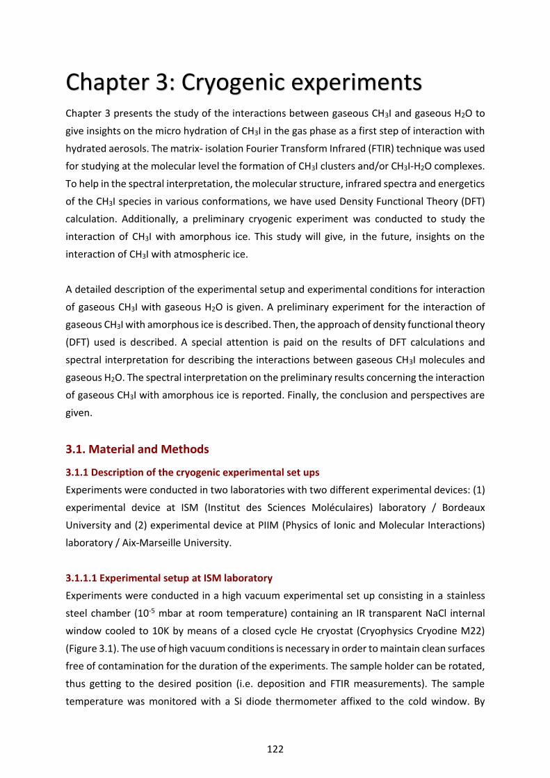
122

Chapter 3: Cryogenic experiments Chapter 3 presents the study of the interactions between gaseous CH3I and gaseous H2O to

give insights on the micro hydration of CH3I in the gas phase as a first step of interaction with

hydrated aerosols. The matrix- isolation Fourier Transform Infrared (FTIR) technique was used

for studying at the molecular level the formation of CH3I clusters and/or CH3I-H2O complexes.

To help in the spectral interpretation, the molecular structure, infrared spectra and energetics

of the CH3I species in various conformations, we have used Density Functional Theory (DFT)

calculation. Additionally, a preliminary cryogenic experiment was conducted to study the

interaction of CH3I with amorphous ice. This study will give, in the future, insights on the

interaction of CH3I with atmospheric ice.

A detailed description of the experimental setup and experimental conditions for interaction

of gaseous CH3I with gaseous H2O is given. A preliminary experiment for the interaction of

gaseous CH3I with amorphous ice is described. Then, the approach of density functional theory

(DFT) used is described. A special attention is paid on the results of DFT calculations and

spectral interpretation for describing the interactions between gaseous CH3I molecules and

gaseous H2O. The spectral interpretation on the preliminary results concerning the interaction

of gaseous CH3I with amorphous ice is reported. Finally, the conclusion and perspectives are

given.

3.1. Material and Methods

3.1.1 Description of the cryogenic experimental set ups

Experiments were conducted in two laboratories with two different experimental devices: (1)

experimental device at ISM (Institut des Sciences Moléculaires) laboratory / Bordeaux

University and (2) experimental device at PIIM (Physics of Ionic and Molecular Interactions)

laboratory / Aix-Marseille University.

3.1.1.1 Experimental setup at ISM laboratory

Experiments were conducted in a high vacuum experimental set up consisting in a stainless

steel chamber (10-5 mbar at room temperature) containing an IR transparent NaCl internal

window cooled to 10K by means of a closed cycle He cryostat (Cryophysics Cryodine M22)

(Figure 3.1). The use of high vacuum conditions is necessary in order to maintain clean surfaces

free of contamination for the duration of the experiments. The sample holder can be rotated,

thus getting to the desired position (i.e. deposition and FTIR measurements). The sample

temperature was monitored with a Si diode thermometer affixed to the cold window. By

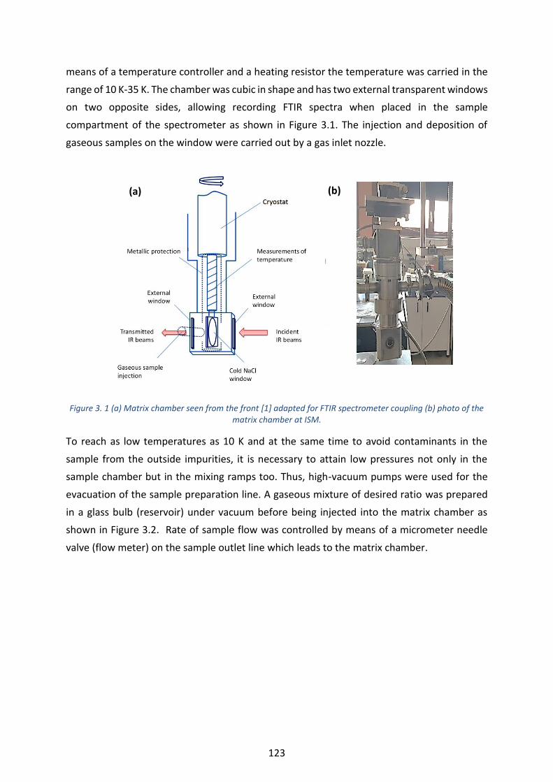
123

means of a temperature controller and a heating resistor the temperature was carried in the

range of 10 K-35 K. The chamber was cubic in shape and has two external transparent windows

on two opposite sides, allowing recording FTIR spectra when placed in the sample

compartment of the spectrometer as shown in Figure 3.1. The injection and deposition of

gaseous samples on the window were carried out by a gas inlet nozzle.

Figure 3. 1 (a) Matrix chamber seen from the front [1] adapted for FTIR spectrometer coupling (b) photo of the

matrix chamber at ISM.

To reach as low temperatures as 10 K and at the same time to avoid contaminants in the

sample from the outside impurities, it is necessary to attain low pressures not only in the

sample chamber but in the mixing ramps too. Thus, high-vacuum pumps were used for the

evacuation of the sample preparation line. A gaseous mixture of desired ratio was prepared

in a glass bulb (reservoir) under vacuum before being injected into the matrix chamber as

shown in Figure 3.2. Rate of sample flow was controlled by means of a micrometer needle

valve (flow meter) on the sample outlet line which leads to the matrix chamber.

(a) (b)

124

Figure 3. 2 Schematic diagram of the experimental setup of (a) CH3I in Ar matrix from 10 to 35 K, (b) CH3I and

H2O in Ar matrix from 10 to 35 K. The scheme was adapted from [2].

The infrared spectra of the gas-isolated samples were recorded in transmission mode using a

Bruker Vertex 70V FTIR spectrometer with a DTGS detector in the spectral range of 4000-400

cm-1, with a spectral resolution of 0.5 cm-1 and each spectrum averaged over approximately

200 scans. Spectra were recorded at 10K. All spectra are ratioed to a background spectrum

which includes the cold window.

3.1.1.2 Experimental setup at PIIM laboratory

Similarly to experiments at ISM laboratory, experiments at PIIM laboratory were conducted in

a high vacuum experimental set up consisting in a stainless-steel chamber (10-5 mbar at room

temperature) containing a gold-plated copper cube cooled to 4K by a closed cycle cryostat

(PT-405 Cryomech). Cryostat head can be rotated to get the desired position (deposition and

reflection spectroscopy measurements). The copper cube is gold plated to protect it from

damage due to deposits of samples that could potentially react with the copper and assure

optimal reflectivity. The sample temperature was monitored with two Si diodes, one was fixed

in the close vicinity of the sample (at less than 1 cm), while the second was located on the

second cooler stage (2.8 K) of the cryogenic head. Temperature was controlled between 4 to

50 K by means of temperature controller and a heating resistance. The chamber was cylinder

in shape with one external transparent window, allowing recording reflection infrared spectra

when the cryostat is placed in a special bench beside the spectrometer (see Figure 3.3). The

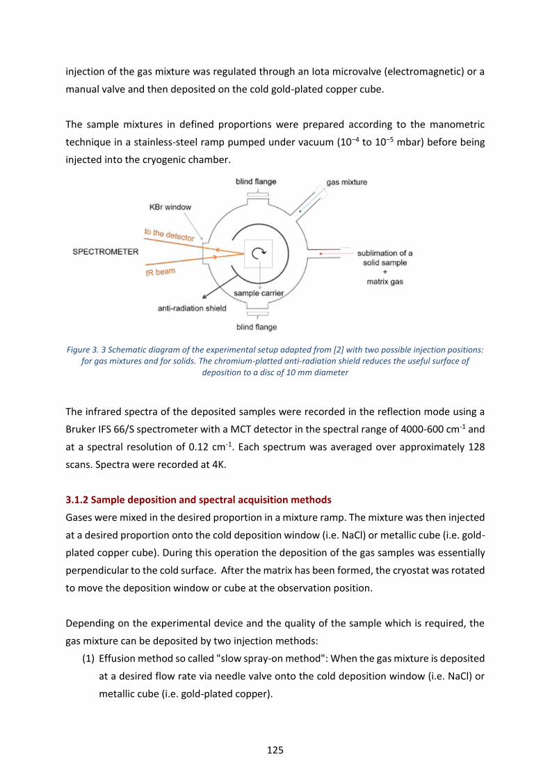
125

injection of the gas mixture was regulated through an Iota microvalve (electromagnetic) or a

manual valve and then deposited on the cold gold-plated copper cube.

The sample mixtures in defined proportions were prepared according to the manometric

technique in a stainless-steel ramp pumped under vacuum (10−4 to 10−5 mbar) before being

injected into the cryogenic chamber.

Figure 3. 3 Schematic diagram of the experimental setup adapted from [2] with two possible injection positions:

for gas mixtures and for solids. The chromium-platted anti-radiation shield reduces the useful surface of deposition to a disc of 10 mm diameter

The infrared spectra of the deposited samples were recorded in the reflection mode using a

Bruker IFS 66/S spectrometer with a MCT detector in the spectral range of 4000-600 cm-1 and

at a spectral resolution of 0.12 cm-1. Each spectrum was averaged over approximately 128

scans. Spectra were recorded at 4K.

3.1.2 Sample deposition and spectral acquisition methods

Gases were mixed in the desired proportion in a mixture ramp. The mixture was then injected

at a desired proportion onto the cold deposition window (i.e. NaCl) or metallic cube (i.e. gold-

plated copper cube). During this operation the deposition of the gas samples was essentially

perpendicular to the cold surface. After the matrix has been formed, the cryostat was rotated

to move the deposition window or cube at the observation position.

Depending on the experimental device and the quality of the sample which is required, the

gas mixture can be deposited by two injection methods:

(1) Effusion method so called "slow spray-on method": When the gas mixture is deposited

at a desired flow rate via needle valve onto the cold deposition window (i.e. NaCl) or

metallic cube (i.e. gold-plated copper).

126

(2) Pulsed method: When the gas phase mixture is deposited in short and repeated pulses

onto the sample holder, i.e. either a NaCl window or a gold-plated copper cube.

3.1.3 Experimental grid

3.1.3.1 Preparation of samples for studying CH3I-H2O interactions at ISM laboratory

Two sets of experiments were conducted to scrutinize the CH3I-H2O interactions at low

temperature using the experimental setup in ISM laboratory (see Figure 3.2):

(a) CH3I in Ar matrix from 10 to 35 K in order to obtain reference spectra when CH3I was

trapped in Ar matrix

(b) CH3I and H2O in Ar matrix from 10 to 35 K.

The two samples were prepared using effusive methodology as described previously. Gaseous

samples of CH3I/Ar (0.1% CH3I - 99.9% Ar, Airproduct) were used without any further

purification at a flow of 1mL.min-1. The matrix ratio was CH3I/Ar = 1/1000. For the observation

of the formation of (CH3I)m-(H2O)n complexes, the vapor of ultrapure H2O (conductivity of 18.2

MΩ Millipore system) was introduced from a glass flask and mixed with CH3I/Ar in a glass

reservoir in the proportion CH3I/ H2O/Ar = 1/24/1500 and injected into the chamber at a rate

of 1 mL.min-1. Deionized water was previously subjected to multiple freeze-pump-thaw cycles

under vacuum to remove dissolved gases. The concentration of H2O/Ar equal to 1/60 was

used to introduce water in a large excess for mimmicking the CH3I environment in the

atmosphere. This CH3I/H2O ratio is chosen to ensure both high water concentration in matrix

and CH3I signal detection since beyond this ratio, signals of water aggregates would overlap

those of (CH3I)m-(H2O)n . Although the injected CH3I concentration (1000 ppm) is higher than

atmospheric CH3I concentration (0.004-2000 ppt) (see section 2.1), it is weak enough to

prevent the formation of CH3I aggregates after deposition. A reference experiment with H2O

trapped in Ar matrix (7/1000) was also recorded at 4 K for comparison. The gaseous samples

were introduced by gas nozzle inlet in effusive mode as described previously and deposited

directly in the vacuum chamber on an NaCl window for 2 hours. The deposited samples at 10

K were annealed to 35 K, close to the sublimation temperature of the argon crystal.

3.1.3.2 Preparation of samples for studying CH3I- amorphous ice (ASW) interactions in PIIM

laboratory

Preliminary experiment at PIIM laboratory was conducted in this work to study the CH3I-

amorphous ice interactions at low temperature (4 K-50 K) using cryogenic technique with

pulsed deposition method and FTIR analysis in reflection mode.

Gaseous samples of CH3I/Ar (0.1% CH3I - 99.9% Ar, Airproduct) were used without any further

purification. As reported in section 3.1.3.1 for the experiment with amorphous ice, deionized

127

water was subjected to multiple freeze−pump−thaw cycles under vacuum to remove dissolved

gases.

A mixture of purified H2O and helium (Air Liquide, ≥99.9999%) gas were prepared in the

mixture ramp previously pumped down to 10-3 mbar at a ratio of H2O/He: 1/25. Amorphous

ice was formed by injecting 22 mbar in 1s of H2O/He gas at 50 K to avoid mainly nitrogen

trapping. The sample was then cooled to 4K. If adsorbed N2 is nevertheless observable, one

could re-increase the temperature up to 50 K to clean the surface and then re cool it back to

4 K. 3 mbar in 500 ms of CH3I/Ar: 1/1000 mixture was then successively injected at the ASW

surface at various temperatures in order to trap uniquely methyl iodide. The temperatures

used were close to or above the argon sublimation temperature (≈ 45 K) to avoid trapping

argon on the surface of the ice.

3.1.4 Density Functional Theory (DFT) calculation

The structure and harmonic vibrational spectra of CH3I monomer, dimers and trimers, and

CH3I-water complexes such as (CH3I)n-(H2O)m (with n = 1,2,3 and m = 1,2,3) were calculated

with Gaussian 09 suit of programs [3] using long range corrected functional B97XD [4] with

the aug-cc-pVTZ basis set for hydrogen, carbon and oxygen atom, while aug-cc-pVTZ-PP basis

set [5] was used for iodine atom that incorporates a small-core relativistic pseudo potential

[6]. Harmonic vibrational frequencies were calculated at the same level of theory, and

remained unscaled. The standard molar entropy (S°10 K) and the heat capacity at constant

pressure (1 bar) were calculated with the script thermo.pl published by the National Institute

of Standards and Technology [7]. The Gibbs energy (G°) in kJ.mol-1 for both CH3I clusters and

complexes was calculated at the B97XD/ aug-cc-pVTZ-PP level of theory. The total basis set

superposition error (BSSE) correction is known to be negligible in micro hydration energetics

[6, 8], therefore this correction was not included in the energetics calculation of this study. It

should be highlighted that DFT calculations were only preformed to support the experimental

results of CH3I-H2O interaction (section 3.1.3.1).

Sections 3.2.1 and 3.2.2 are under review for publication (Title: Infrared matrix- isolation

and theoretical studies of interactions between CH3I and water, Authors: S. Sobanska, H.

Houjeij, S. Coussan, C. Aupetit, S. Taamalli, F. Louis, L. Cantrel, A.C. Gregoire, J. Mascetti).

128

3.2. Results and discussion

3.2.1 Formation of (CH3I)x clusters

3.2.1.1 DFT calculation results

Structures of CH3I monomer, dimers and trimers were investigated using experimental spectra

supported by calculations presented above. Two isomers of (CH3I)2, shown in Figure 3.4, are

found to be stable and will be hereafter referred as Head-to-Tail (HT) and Head-to-Head (HH)

structures. These structures were previously reported using the MP2/ LanL2DZ+fdp level of

theory [9]. It should be highlighted that both levels of theory using MP2/ LanL2DZ+fdp [9]

and B97XD/aug-cc-pVTZ-PP (this work) predict the same (CH3I)2 stable isomers, i.e. HH and

HT, with a difference in the intermolecular distance not exceeding 0.2 Å. A Gibbs free energy

difference of 3.0 and 3.8 kJ/mol is found for HH and HT isomers respectively, between the

method used in this study and the one used previously [9].

Figure 3. 4 B97X-D/ aug-cc-pVTZ-PP-predicted geometries (distances in Å) and Gibbs free energies (G in

kJ/mol) of CH3I dimers.

Two (CH3I)3 isomers are found to be stable (Figure 3.5) and will be hereafter referred as Tail-

to-Head-to-Tail (THT) and Tail-to-Tail-to-Head (TTH). The TTH structure was previously

discussed by Ito et al., [10, 11] to be the most stable structure of (CH3I)3 using the MP2

method. In the present work the Gibbs free energy difference between the 2 isomers is less

than 1 kJ/mol at the B97X-D/ aug-cc-pVTZ-PP level of theory. As a result, THT and TTH could

be considered as isoenergetic. The difference in the intermolecular distance between the level

of theory used in this study and the one used previously [10] does not exceed 0.2 Å. Moreover,

a difference of about 5 kJ/mol in the Gibbs free energy was found between the two levels of

theory.

33Å

37Å

37Å

37Å

38Å

rG 10K = -11.5 kJ mol-1rG 10K = -8.4 kJ mol-1

HHHT

129

Figure 3. 5 B97X-D/ aug-cc-pVTZ-PP-predicted geometries (distances in Å) and Gibbs free energies (G in kJ/mol) of CH3I trimers.

As a result, the difference in binding energies shows that E(B97X, this work) is lower than

E calculated using P2 method [9, 10] for both CH3I dimers and trimers. This interaction

between CH3I molecules is more accurately evaluated using the B97X-D functional that

includes dispersion for a better characterization of the intermolecular complexes under study.

Moreover, the size of the basis set is larger in our work (aug-cc-pVTZ-PP) than the one used in

Ito’s studies (LANDZ+fdp) [9, 10].

The calculated vibrational spectra together with bands relative intensities of the monomer

and the most stable HH, HT, TTH, THT isomers are gathered in Table 3.1. For a more reliable

analysis of CH3I clusters infrared spectra, we used unscaled IR frequencies. It should be noted

that the calculated wavenumber position is likely dependent of the level of theory. For

example, the wavenumber position of the monomer CH3 symmetric deformation mode is

calculated at 1334 cm-1 using the MP2/ LanL2DZ+fdp level of theory [9], whereas it is

calculated at 1297 cm-1 in this work using the B97X-D/aug-cc-pVTZ-PP level of theory. It is

known that the shift from the monomer band due to clustering can be evaluated by theoretical

calculations. For instance, in the CH3 symmetric deformation region the shift of the dimer

mode, with respect to that of the monomer, ranges between -4 and 2 cm-1 using the MP2/

LanL2DZ+fdp level of theory [9], against of -1 to 3 cm-1 in this work using the B97X-D/aug-cc-

pVTZ-PP level of theory. Similar observation is found for the trimer, where the shift ranges

between -7 to -1 cm-1 using the MP2/ LanL2DZ+fdp level of theory [10] and -3 to 8 cm-1 using

the B97X-D/aug-cc-pVTZ-PP one (Table 3.1). It shows that the bands of dimers and trimers

are in close vicinity with those of monomer, what underlies that perturbation induced by CH3I

homo-complexation is weak. Considering that shifts calculated at both levels of theory, that

of the present work and the one used by Ito et al., [9, 10] are of the same magnitude, it is

33Å

33Å

33Å

3Å

34Å

3Å

33Å

3Å

37Å

rG 10K = -27.7 kJ mol-1 rG 10K = -28.3 kJ mol-1

TTHTHT

130

more accurate to uniquely consider those shifts rather than scaled harmonic frequencies to

identify present species. The calculation performed in this study will be used as a support to

discriminate between monomers, dimers and trimers observed by FTIR-isolation matrix

experiments. Those theoretical vibrational spectra will be studied in fingerprint regions in

which they will help to identify species trapped in the matrix.

131

Table 3. 1 Calculated wavenumbers (cm-1) and intensities (I) of CH3I monomer, HH and HT dimers and THT and TTH trimers. The IR bands are predicted at the B97X-D/aug-

cc-pVTZ-PP level of theory. The frequency shifts are calculated with respect to the monomer position (=monomer-

Vibrational Modes CH3I (CH3I)2 dimers (CH3I)3 trimers

monomer HT HH THT TTH

4 C-H stretching degenerated

3214 (0) 3221 (0) 7 3214 (0) 0 3221 (0) 7 3215 (1) 1 3217 (1) 3 3214 (1) 0 3216 (1) 2 3214 (0) 0 3215 (0) 1 3211 (1) -3 3214 (1) 0 3213 (2) -1 3214 (1) 0 3211 (1) -3 3213 (1) -1 3211 (0) -3

3210 (1) -4 3210 (2) -4 3206 (1) -8 3206 (1) -8

1 Symmetric CH3 stretching

3101 (11) 3103 (8) 2 3100 (9) -1 3101 (8) 0 3097 (10) -4 3099 (13) -2 3100 (14) -1 3097 (10) -4 3096 (10) -5

3094 (14) -7 3093 (11) -8

5 CH3 deformation degenerated

1477 (6) 1485 (14) 8 1477 (8) 0 1482 (3) 6 1486 (7) 9 1480 (7) 3 1477 (6) 0 1479 (12) 2 1485 (3) 8 1477 (5) 0 1474 (10) -3 1477 (8) 0 1478 (7) 1 1474 (2) -3 1473 (12) -4 1474 (2) -3 1477 (7) 0

1473 (12) -4 1474 (3) -3 1470 (2) -7 1470 (9) -7

2 Symmetric CH3 deformation

1297 (23) 1300 (41) 3 1297 (12) 0 1300 (39) 3 1305 (2) 8 1297 (1) 0 1296 (40) -1 1297 (10) 0 1296 (46) -1

1295 (16) -2 1294 (27) -3

6 CH3 rocking degenerated

903 (5) 913 (15) 10 906 (7) 3 921 (8) 18 914 (7) 11 910 (4) 7 905 (7) 2 917 (15) 14 911 (10) 7 909 (4) 6 902 (3) -1 911 (7) 8 909 (15) 6 908 (5) 5 901 (4) -2 910 (7) 7 907 (3) 4

906 (10) 3 906 (7) 3 904 (2) 1 905 (4) 2

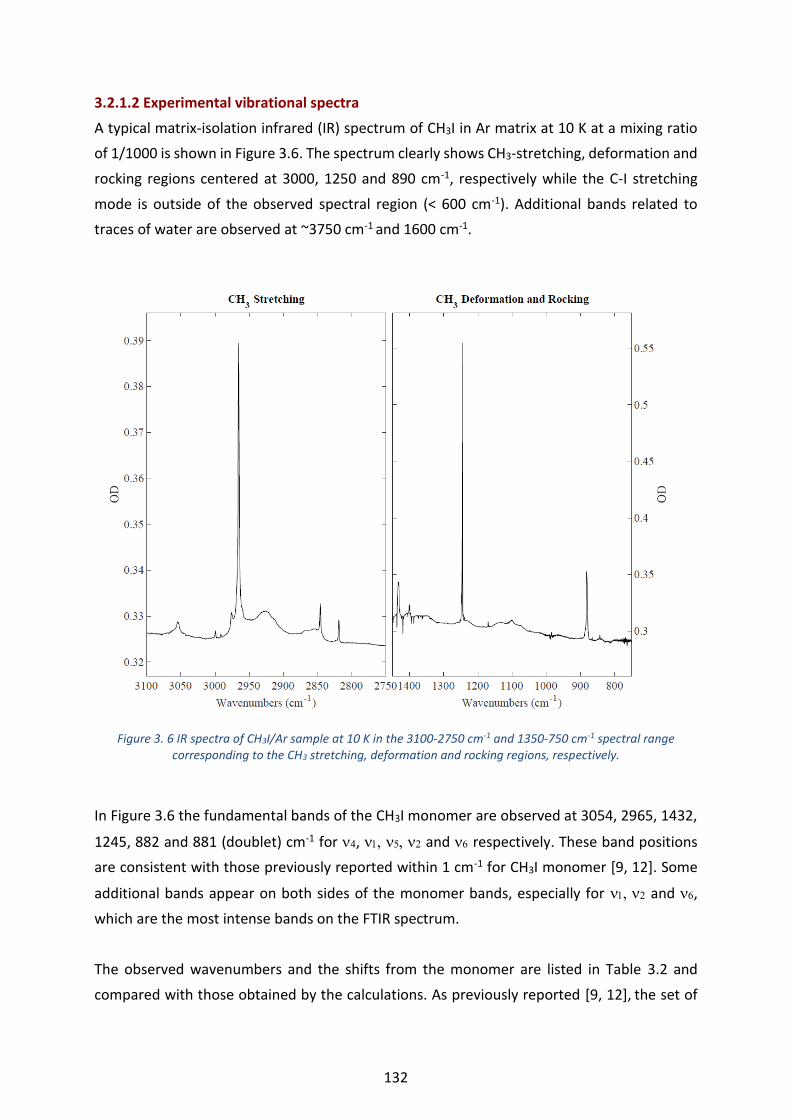
132

3.2.1.2 Experimental vibrational spectra

A typical matrix-isolation infrared (IR) spectrum of CH3I in Ar matrix at 10 K at a mixing ratio

of 1/1000 is shown in Figure 3.6. The spectrum clearly shows CH3-stretching, deformation and

rocking regions centered at 3000, 1250 and 890 cm-1, respectively while the C-I stretching

mode is outside of the observed spectral region (< 600 cm-1). Additional bands related to

traces of water are observed at ~3750 cm-1 and 1600 cm-1.

Figure 3. 6 IR spectra of CH3I/Ar sample at 10 K in the 3100-2750 cm-1 and 1350-750 cm-1 spectral range corresponding to the CH3 stretching, deformation and rocking regions, respectively.

In Figure 3.6 the fundamental bands of the CH3I monomer are observed at 3054, 2965, 1432,

1245, 882 and 881 (doublet) cm-1 for 4, and respectively. These band positions

are consistent with those previously reported within 1 cm-1 for CH3I monomer [9, 12]. Some

additional bands appear on both sides of the monomer bands, especially for and ,

which are the most intense bands on the FTIR spectrum.

The observed wavenumbers and the shifts from the monomer are listed in Table 3.2 and

compared with those obtained by the calculations. As previously reported [9, 12], the set of

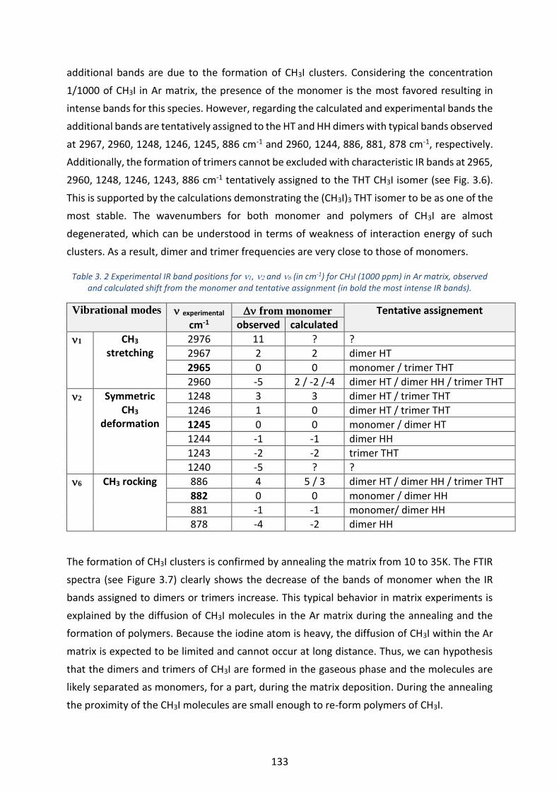
133

additional bands are due to the formation of CH3I clusters. Considering the concentration

1/1000 of CH3I in Ar matrix, the presence of the monomer is the most favored resulting in

intense bands for this species. However, regarding the calculated and experimental bands the

additional bands are tentatively assigned to the HT and HH dimers with typical bands observed

at 2967, 2960, 1248, 1246, 1245, 886 cm-1 and 2960, 1244, 886, 881, 878 cm-1, respectively.

Additionally, the formation of trimers cannot be excluded with characteristic IR bands at 2965,

2960, 1248, 1246, 1243, 886 cm-1 tentatively assigned to the THT CH3I isomer (see Fig. 3.6).

This is supported by the calculations demonstrating the (CH3I)3 THT isomer to be as one of the

most stable. The wavenumbers for both monomer and polymers of CH3I are almost

degenerated, which can be understood in terms of weakness of interaction energy of such

clusters. As a result, dimer and trimer frequencies are very close to those of monomers.

Table 3. 2 Experimental IR band positions for and (in cm-1) for CH3I (1000 ppm) in Ar matrix, observed and calculated shift from the monomer and tentative assignment (in bold the most intense IR bands).

Vibrational modes experimental cm-1

from monomer Tentative assignement

observed calculated

1 CH3 stretching

2976 11 ? ?

2967 2 2 dimer HT

2965 0 0 monomer / trimer THT

2960 -5 2 / -2 /-4 dimer HT / dimer HH / trimer THT

2 Symmetric CH3

deformation

1248 3 3 dimer HT / trimer THT

1246 1 0 dimer HT / trimer THT

1245 0 0 monomer / dimer HT

1244 -1 -1 dimer HH

1243 -2 -2 trimer THT

1240 -5 ? ?

6 CH3 rocking 886 4 5 / 3 dimer HT / dimer HH / trimer THT

882 0 0 monomer / dimer HH

881 -1 -1 monomer/ dimer HH

878 -4 -2 dimer HH

The formation of CH3I clusters is confirmed by annealing the matrix from 10 to 35K. The FTIR

spectra (see Figure 3.7) clearly shows the decrease of the bands of monomer when the IR

bands assigned to dimers or trimers increase. This typical behavior in matrix experiments is

explained by the diffusion of CH3I molecules in the Ar matrix during the annealing and the

formation of polymers. Because the iodine atom is heavy, the diffusion of CH3I within the Ar

matrix is expected to be limited and cannot occur at long distance. Thus, we can hypothesis

that the dimers and trimers of CH3I are formed in the gaseous phase and the molecules are

likely separated as monomers, for a part, during the matrix deposition. During the annealing

the proximity of the CH3I molecules are small enough to re-form polymers of CH3I.

134

Figure 3. 7 IR spectra of the annealing of CH3I/Ar sample until 35 K in the spectral range (a) 3080-2944 cm-1 (b) 1270-1237 cm-1 (c) 905-870 cm-1. Bands denoted in green, pink and orange are assigned to CH3I monomer, CH3I

dimer and CH3I trimer, respectively.

3.2.2 Formation of CH3I-H2O complexes

3.2.2.1 DFT calculation results

The structure and the vibrational spectra of various (CH3I)m–(H2O)n complexes calculated by

B97XD/aug-cc-pVTZ-PP method for m=1, 2 and n=1, 2, 3 was investigated. From this

theoretical work, valuable information can be retrieved on relative stabilities of each species

together with the structure of their vibrational spectra. Indeed, from those results we should

try to define the most accurate spectral regions to discriminate between (CH3I)m, (H2O)n,

(CH3I)m-(H2O)n aggregates and complexes. Ito et al., [11] have demonstrated that

B971/LanL2DZ+fdp reproduce well MP2/aug-cc-pVTZ method, while MP2/LanL2DZ +fdp

method underestimate the intermolecular interaction between 1CH3I and 1H2O. In the

present work, the calculations are performed with B97XD functional with a relativistic

effective core potential and an extended valence basis-set, i.e., aug-cc-pVTZ-PP.

The 1:1 structure was optimized revealing the predicted most stable isomers. The geometry

and the standard Gibbs energy of the 1:1 isomers are presented in Figure 3.8.

1270 1260 1250 1240

0.213

0.284

0.355

0.426

0.497

903 896 889 882 875

0.20

0.24

0.28

0.32

0.36

0.40

OD

OD

35 K

10 K

Wavenumber (cm-1)

30 K

(b)

CH3I/Ar on NaClCH3I/Ar on NaCl

(c)

35 K

10 K

Wavenumber (cm-1)

30 K

3080 3010 2940 2870 2800

0.28

0.32

0.36

0.40

0.44

0.48

0.52

CH3I/Ar on NaCl

OD

35 K

10 K

Wavenumber (cm-1)

30 K

(a)

135

Figure 3. 8B97X-D/ aug-cc-pVTZ-PP-predicted geometry (distances in Å) and Gibbs free energy (G in kJ.mol-1) of CH3I.H2O isomers.

The 1:1 hetero-dimer it presents two stable forms, one pseudo-cyclic, referred as 1:1a, more

stable than an unexpected one, 1:1b, which displays an I….O interaction (rG°10K = -13.5 kJ

mol-1, for 1:1a, against -7.5 kJ mol-1, for 1:1b). Indeed, one could have expected to observe, in

1:1b case, an I…H H-bond interaction, rather than this long-distance interaction between

iodine and oxygen atoms. Is it so surprising? If one compares, iodine’s Pauling

electronegativity of 2.7 with that of hydrogen, which is 2.2, it is perfectly plausible to observe

a hydrogen-bond type interaction between iodine and oxygen, this latter presenting a Pauling

electronegativity of 3.4. Moreover, the methyl iodide dipole moment is oriented toward

carbon atom, which leads a partial positive Mulliken’s charge for iodine atom in this

configuration. It is thus perfectly understandable we observe this I…O interaction.

On the vibrational spectra side, one observes a stronger perturbation for 1:1a, with respect to

each monomer, H2O and CH3I, vibration frequencies, than for 1:1b (see Table 3.3). Water 3

and 1 modes are both red-shifted by -28 and -41 cm-1, while the most promising shift

concerning CH3I moiety seems to be that of the CH3 rocking with a blue-shift of 22 cm-1. For

1:1b, water partner presents two almost equivalent free OH bonds, however red-shifted by -

11 and -10 cm-1 that illustrates the methyl iodide polarity.

1:1a

rG 10K = -13.5 kJ mol-1

1:1b

rG 10K = -7.5 kJ mol-1

33Å

Å

30Å

136

Table 3. 3 Calculated wavenumbers (cm-1) and intensities (I) of CH3I.H2O complexes compared to the calculated wavenumber (cm-1) and intensities (I) of CH3I monomer and H2O monomer and dimer. The IR bands are

predicted at theB97X-D/aug-cc-pVTZ-PP level of theory. The frequency shifts are calculated with respect to

the monomer position (monomer-

Vibrational Mode H2O monomer

H2O dimer

CH3I monomer

CH3I-H2O (1 :1a)

CH3I-H2O (1 :1b)

3 H2O Anti-symmetric stretching

3986 (63) 3974 (85) 3958 (106) -28 3975 (63) -11

3954 (86)

1 H2O Symmetric stretching

3879(5) 3871 (11) 3838 (48) -41 3869 (11) -10

3751 (339)

2 H2O

Bending

1637 (63)

1658 (39) 1642 (49)

5

1636 (67)

-1 1637 (94)

4 C-H stretching

3214 (0) 3215 (0) 1 3207 (1) -7

3213 (5) -1 3207 (1) -7


3101 (11) 3096 (12) -5 3097 (15) -4

5 CH3 deformation

1477 (6) 1484 (5) 7 1478 (6) 1

1474 (4) -3 1478 (6) 1

2 Symmetric CH3 deformation

1297 (23) 1301 (22) 4 1296 (23) -1

6 CH3 rocking 903 (5) 925 (7) 22 900 (5) -3

909 (5) 6 899 (5) -4



Figure 3. 9 B97X-D/ aug-cc-pVTZ-PP-predicted geometry (distances in Å) and Gibbs free energy (G in kJ.mol-1)

of CH3I.(H2O)2 isomers.

For the CH3I.(H2O)2 complexes, there are two stable structures denoted, 1:2a and 1:2b, with

rG°10K of -45.0 and -25.4 kJ mol-1, respectively. If the former one presents a cyclic structure

which can be summarized as a water dimer interacting by two H-bond type interactions with

1:2a

rG 10K = -45.0 kJ mol-1

1:2b

rG 10K = -25.4 kJ mol-1

9Å

3Å

8Å

Å

30Å

30Å

Å

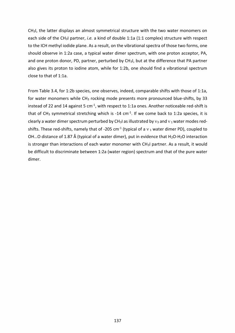
137

CH3I, the latter displays an almost symmetrical structure with the two water monomers on

each side of the CH3I partner, i.e. a kind of double 1:1a (1:1 complex) structure with respect

to the ICH methyl iodide plane. As a result, on the vibrational spectra of those two forms, one

should observe in 1:2a case, a typical water dimer spectrum, with one proton acceptor, PA,

and one proton donor, PD, partner, perturbed by CH3I, but at the difference that PA partner

also gives its proton to iodine atom, while for 1:2b, one should find a vibrational spectrum

close to that of 1:1a.

From Table 3.4, for 1:2b species, one observes, indeed, comparable shifts with those of 1:1a,

for water monomers while CH3 rocking mode presents more pronounced blue-shifts, by 33

instead of 22 and 14 against 5 cm-1, with respect to 1:1a ones. Another noticeable red-shift is

that of CH3 symmetrical stretching which is -14 cm-1. If we come back to 1:2a species, it is

clearly a water dimer spectrum perturbed by CH3I as illustrated by 3 and 1 water modes red-

shifts. These red-shifts, namely that of -205 cm-1 (typical of a 1 water dimer PD), coupled to

OH…O distance of 1.87 Å (typical of a water dimer), put in evidence that H2O-H2O interaction

is stronger than interactions of each water monomer with CH3I partner. As a result, it would

be difficult to discriminate between 1:2a (water region) spectrum and that of the pure water

dimer.

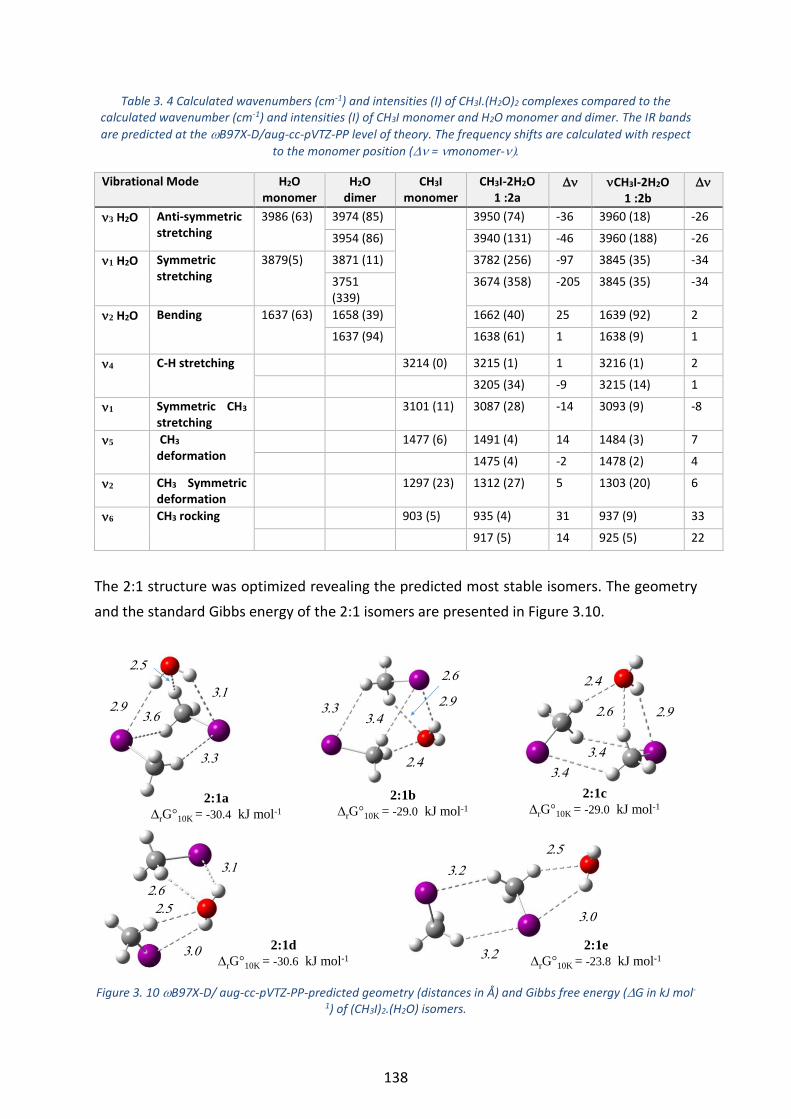
138

Table 3. 4 Calculated wavenumbers (cm-1) and intensities (I) of CH3I.(H2O)2 complexes compared to the calculated wavenumber (cm-1) and intensities (I) of CH3I monomer and H2O monomer and dimer. The IR bands

are predicted at the B97X-D/aug-cc-pVTZ-PP level of theory. The frequency shifts are calculated with respect

to the monomer position (= monomer-

Vibrational Mode H2O monomer

H2O dimer

CH3I monomer

CH3I-2H2O 1 :2a

CH3I-2H2O 1 :2b

3 H2O Anti-symmetric stretching

3986 (63) 3974 (85) 3950 (74) -36 3960 (18) -26

3954 (86) 3940 (131) -46 3960 (188) -26

1 H2O Symmetric stretching

3879(5) 3871 (11) 3782 (256) -97 3845 (35) -34

3751 (339)

3674 (358) -205 3845 (35) -34

2 H2O

Bending

1637 (63)

1658 (39) 1662 (40) 25 1639 (92) 2

1637 (94) 1638 (61) 1 1638 (9) 1

4 C-H stretching

3214 (0) 3215 (1) 1 3216 (1) 2

3205 (34) -9 3215 (14) 1


3101 (11) 3087 (28) -14 3093 (9) -8

5 CH3 deformation

1477 (6) 1491 (4) 14 1484 (3) 7

1475 (4) -2 1478 (2) 4

2 CH3 Symmetric deformation

1297 (23) 1312 (27) 5 1303 (20) 6

6 CH3 rocking

903 (5) 935 (4) 31 937 (9) 33

917 (5) 14 925 (5) 22




1) of (CH3I)2.(H2O) isomers.

2:1c

rG 10K = -29.0 kJ mol-12:1a

rG 10K = -30.4 kJ mol-1

2:1b

rG 10K = -29.0 kJ mol-1

2:1d

rG 10K = -30.6 kJ mol-1

30

3

3

4

34

3

30

3

9

33

9

34

4

333

34

2:1e

rG 10K = -23.8 kJ mol-1

9

139

For the (CH3I)2-H2O complexes, shown in Figure 3.10 we count non less than five stable

structures denoted, 2:1a to 2:1e, with rG°10K lying in a close range of energies (-30.6 to -29.0

kJ mol-1, 2:1b and 2:1c being degenerated), with the exception of 2:1e one which is a little bit

disfavored at -23.8 kJ mol-1). If the three first ones, 2:1a, 2:1b and 2:1c, present quite similar

structures, i.e. CH3I dimer interacting with a water monomer (2:1a presenting a subtle double

PD, on time PA, character, which gives a low stabilization compared to 2:1b and 2:1c, whose

one OH bond remains free), the 2:1d displays water molecule bridging between the two CH3I

molecules while 2:1e presents again the 1:1a moiety in interaction with the other CH3I partner.

Not surprisingly, the most “3D” interacting structures, are the most stable.

On the vibrational point of view, from Table 3.5, one can guess that indeed, in the water

stretching region 2:1e presents red-shifts comparable with those of 1:1a but also overlapping

with those of 1:2b. Having regard to 2:1a and 2:1d, also in water stretching region, they

present comparable red-shifts of -61 cm-1 (3), while 2:1a shares its n1 red-shift of -54 cm-1

with 2:1b and 2:1c. In the CH3 rocking region, all the species should present the same

spectrum, with blue-shifts overlapping with those of the above studied forms.

140

Table 3. 5 Calculated wavenumbers (cm-1) and intensities (I) of (CH3I)2.(H2O) complexes compared to the calculated wavenumber (cm-1) and intensities (I) of CH3I

monomer and H2O monomer and dimer. The IR bands are predicted at the B97X-D/aug-cc-pVTZ-PP level of theory. The frequency shifts are calculated with

respect to the monomer position (= monomer-

Vibrational

modes

H2O

monomer

H2O dimer CH3I

monomer

2CH3I-H2O

2 :1a

2CH3I-H2O

2 :1b

2CH3I-H2O

2 :1c

2CH3I-H2O

2 :1d

2CH3I-H2O

2 :1e

3 H2O

Anti-symmetric

stretching

3986 (63) 3974 (85) 3925 (106) -61 3957 (114) -29 3957 (114) -29 3925 (106) -61 3959 (103) -27

3954 (86)

1 H2O

Symmetric

stretching

3879 (5) 3871 (11) 3825 (84) -54 3825 (65) -54 3825 (66) -54 3833 (28) -46 3842 (40) -32

3751 (339)

2 H2O

Bending

1637 (63) 1658 (39) 1643 (70)

6

1634 (63)

-3

1633 (61)

-4

1646 (71)

9

1640 (49)

3

1637 (94)

4 CH3I

C-H stretching

3214 (0) 3217 (1) 3 3218 (0) 4 3218 (0) 3 3214 (2) 0 3213 (3) -1

3216 (0) 2 3217 (8) 3 3216 (9) 2 3214 (0) 0 3213 (1) -1

3212 (4) -2 3215 (2) 1 3214 (1) 0 3212 (2) -2 3210 (1) -4

3211 (2) -3 3209 (1) -5 3209 (2) -5 3211 (2) -1 3208 (7) -6

1 CH3I Symmetric

CH3 stretching

3101 (11) 3097 (11) -4 3099 (4) -2 3098 (4) -3 3097 (16) -4 3098 (9) -3

3095 (11) -6 3096 (7) -5 3096 (7) -5 3096 (3) -5 3091 (7) -10

v5 CH3I

CH3 deformation

1477 (6) 1483 (11) 6 1496 (7) 19 1495 (6) 18 1488 (3) 11 1484 (5) 7

1477 (3) 0 1483 (25) 6 1482 (28) 4 1481 (19) 4 1481 (3) 4

1473 (2) -4 1477 (8) 0 1478 (8) 1 1475 (10) -2 1478 (9) 1

1469 (8) -8 1472 (12) -5 1474 (9) -2 1470 (7) -7 1472 (9) -5

2 CH3I

Symmetric

CH3deformation

1297 (23) 1302 (35) 5 1308 (10) 11 1307 (8) 10 1302 (16) 5 1302 (27) 5

1297 (5) 0 1301 (45) 0 1301 (48) 4 1298 (28) 1 1297 (21) 0

6 CH3I

CH3 rocking

903 (5) 926 (6) 23 924 (8) 21 925 (8) 22 925 (8) 22 930 (12) 27

916 (11) 13 914 (2) 11 913 (5) 10 921 (6) 18 915 (4) 12

913 (7) 10 913 (5) 10 913 (3) 10 910 (8) 7 911 (8) 7

908 (4) 5 910 (7) 7 908 (7) 5 907 (5) 4 904 (6) 1

141

The 1:3 structure was optimized revealing the predicted most stable isomers. The geometry and

the standard Gibbs energy of the 1:3 isomers are presented in Figure 3.11.

Figure 3. 11 B97X-D/ aug-cc-pVTZ-PP-predicted geometry (distances in Å) and Gibbs free energy (G in kJ mol-1) of

CH3I.(H2O)3 isomers.

The CH3I.(H2O)3 one, displayed in Figure 3.11, could be considered as the first step of CH3I water

embedding, leadimg to models of CH3I trapped in water environment as aggregates or

Amorphous Solid Water (ASW). We found four different stable structures: 1:3a, the most stable

one (rG°10K = -86.4 kJ mol-1) which is a cyclic water trimer perturbed by CH3I molecule which

should present a vibrational spectrum close to that of cyclic water trimer; 1:3b, the least stable

one (rG°10K = -37.5 kJ mol-1), which is some kind of spinning top structure with the three water

molecules interacting independently from each other (i.e. three times 1:1a structure) with the

central CH3I molecule, which should exhibit a spectrum close to that of 1:1a; 1:3c (rG°10K = -59.7

kJ mol-1) which displays a kind of “1:1a+1:2a” structure and should therefore share much in

common with these two structures; 1:3d (rG°10K = -74.9 kJ mol-1) which is a cyclic structure

comprising a non-cyclic water trimer bridging between iodine and H methyl atoms of methyl

iodide. It should be noted that 1:3b and 1:3c should present the strongest CH3 blue-shifts.

1:3a

rG 10K = -86.4 kJ mol-1

1:3b

rG 10K = -37.5 kJ mol-1

1:3c

rG 10K = -59.7 kJ mol-1

1:3d

rG 10K = -74.9 kJ mol-1

9

09

8

30

30

30

3

9

830

78

8

142

One more time, it is obvious the most there are water molecules involved in self H-bond

association, the most the hetero-complex is stable. It come partly from H-bond interaction

efficiency which induces cooperative effects. From the observation of theoretical harmonic

frequencies values (Table 3.6), it is clear that those signals overlap with those of the other forms.

143

Table 3. 6 Calculated wavenumbers (cm-1) and intensities (I) of CH3I.(H2O)3 complexes compared to the calculated wavenumber (cm-1) and intensities (I) of CH3I

monomer and H2O monomer and dimer. The IR bands are predicted at the B97X-D/aug-cc-pVTZ-PP level of theory. The frequency shifts are calculated with

respect to the monomer position (=monomer-

Vibrational modes H2O monomer

H2O

Dimer

CH3I monomer CH3I-3H2O

1 :3a

CH3I-3H2O

1 :3b

CH3I-3H2O

1 :3c

CH3I-3H2O

1 :3d

3 H2O

Anti-symmetric

stretching

3986 (63) 3974 (85) 3950 (60) -36 3962 (54) -24 3961 (94) -25 3949 (74) -37

3954 (86) 3948 (99) -38 3961 (124) -25 3951 (71) -35 3948 (132) -38

3861 (205) -125 3960 (119) -26 3941 (140) -45 3943 (78) -43

1 H2O

Symmetric

stretching

3879(5) 3871 (11) 3716 (294) -63 3849 (19) -30 3848 (29) -31 3761 (354) -118

3751 (339) 3663 (358) -216 3848 (32) -31 3788 (246) -91 3660 (499) -219

3557 (276) -322 3848 (32) -31 3680 (342) -199 3606 (545) -273

2 H2O

Bending

1637 (63)

1658 (39) 1669 (27) 32 1640 (27) 3 1661 (40) 24 1677 (36) 40

1637 (94) 1653 (138) 16 1640 (27) 3 1640 (74) 3 1662 (32) 25

1647 (58) 10 1638 (94) 1 1639 (37) 2 1636 (76) -1

4 CH3I

C-H stretching

3214 (0) 3219 (2) 5 3216 (12) 2 3216 (2) 2 3215 (0) 1

3218 (2) 4 3213 (13) -1 3206 44) -8 3199 (50) -15

1 CH3I

Symmetric

CH3 stretching

3101 (11) 3101 (6) 0 3088 (2) -13 3085 (18) -16 3079 (47) -25

v5 CH3I

CH3 deformation

1477 (6) 1485 (21) 8 1484 (1) 7 1493 (3) 16 1491 (5) 14

1475 (7) -2 1484 (2) 7 1476 (3) -1 1474 (4) -3

2 CH3I

Symmetric CH3

deformation

1297 (23) 1310 (27) 13 1305 (20) 8 1314 (26) 17 1316 (28) 19

6 CH3I

CH3 rocking

903 (5) 918 (5) 15 946 (7) 44 951 (5) 48 940 (3) 37

916 (11) 13 945 (7) 43 929 (5) 26 919 (5) 16

144

The last category of complexes we calculated is (CH3I)2-(H2O)2 complexes, shown in Figure 3.12.

Figure 3. 12 B97X-D/ aug-cc-pVTZ-PP-predicted geometry (distances in Å) and Gibbs free energy (G in kJ mol-1)

of (CH3I)2.(H2O)2 isomers.

We can easily discriminate between two kinds of complexes: those which display a water dimer

part, and those which display two separated water molecules. Excepted for 2:2e (rG°10K = -47.9

kJ mol-1), all the former class present the most stable potentials with rG°10K ranging from -70.1

(2:2b) to -53.8 (2:2j) kJ mol-1. The latter class displays less stable structures with rG°10K ranging

from -47.9 (2:2d) to -33.2 (2:2f) kJ mol-1. It could be understood in terms of H-bond type

interaction strength. Indeed, in the case of a water dimer, there is a strong interaction (as

illustrated by short OH…H bonds of 1.8-1.9 Å), due to the quasi-linear interaction between the

PD O-H bond and the sp3 doublet of the PA partner, while in the second category complexes, the

one without a water dimer part, interactions between PD and PA are less effective.

2:2i

rG 10K = -39.4 kJ mol-1

2:2j

rG 10K = -53.8 kJ mol-1

Distance ranges in Å

OH…O: 1.8-1.9

OH…I: 2.8-2.9/3.1-3.5

H2CH…O: 2.3-2.7

H2CH…I: 3.3-3.7

O…I: 3.2-3.3

2:2a

rG 10K = -63.2 kJ mol-1

2:2b

rG 10K = -70.1 kJ mol-1

2:2c

rG 10K = -47.5 kJ mol-1

2:2d

rG 10K = -47.9 kJ mol-1

2:2e

rG 10K = -47.9 kJ mol-1

2:2f

rG 10K = -33.2 kJ mol-1

2:2g

rG 10K = -61.0 kJ mol-1

2:2h

rG 10K = -63.4 kJ mol-1

145

On the vibrational side, from Table 3.7 it is obvious that one more time considering OH stretching

regions and CH3 one, if all these isomers coexist, it will induce a spectral congestion. However,

some blue shifts in the 2 water bending mode (2:2b, 28 cm-1; 2:2e, 32 cm-1; 2:2g, 35 cm-1; 2:2h,

26 cm-1) could be of some help, even if the 1:2a isomer presents also a blue-shift in this region of

25 cm-1.

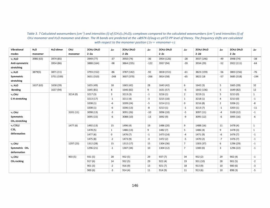
146

Table 3. 7 Calculated wavenumbers (cm-1) and intensities (I) of (CH3I)2.(H2O)2 complexes compared to the calculated wavenumbers (cm-1) and intensities (I) of

CH3I monomer and H2O monomer and dimer. The IR bands are predicted at the B97X-D/aug-cc-pVTZ-PP level of theory. The frequency shifts are calculated

with respect to the monomer position (=monomer-

Vibrational

modes

H2O

monomer

H2O dimer CH3I

monomer

2CH3I-2H2O

2 :2a

2CH3I-2H2O

2 :2b

2CH3I-2H2O

2 :2c

2CH3I-2H2O

2 :2d

2CH3I-2H2O

2 :2e

3 H2O

Anti-symmetric

stretching

3986 (63) 3974 (85) 3949 (77) -37 3950 (74) -36 3954 (126) -28 3937 (146) -49 3948 (74) -38

3954 (86) 3888 (164) -98 3864 (235) -122 3937 (94) -39 3934 (29) -52 3922 (111) -64

1 H2O

Symmetric

stretching

3879(5) 3871 (11) 3793 (152) -86 3787 (142) -92 3818 (151) -61 3823 (159) -56 3803 (156) -76

3751 (339) 3631 (310) -248 3607 (370) -266 3814 (58) -65 3822 (18 -57 3685 (318) -194

2 H2O

Bending

1637 (63)

1658 (39) 1655 (49) 18 1665 (42) 28 1643 (42) 6 1642 (3) 5 1665 (39) 32

1637 (94) 1645 (81) 8 1646 (82) 9 1631 (57) -6 1642 (136) 5 1649 (82) 12

4 CH3I

C-H stretching

3214 (0) 3217 (3) 3 3213 (3) -1 3216 (1) 2 3219 (1) 5 3213 (0) 1

3213 (17) -1 3211 (4) -3 3215 (10) 1 3218 (1) 4 3213 (0) -1

3208 (1) -6 3209 (24) -5 3214 (11) 0 3216 (8) 2 3206 (1) -8

3208 (1) -6 3206 (13) -8 3213 (1) -1 3213 (7) -1 3203 (1) -11

1 CH3I

Symmetric

CH3 stretching

3101 (11) 3098 (13) -3 3091 (26) -10 3096 (10) -5 3097 (11) -4 3100 (12) -1

3095 (15) -6 3088 (10) -13 3092 (9) -9 3095 (12) -6 3095 (16) -6

v5 CH3I

CH3

deformation

1477 (6) 1492 (13) 15 1496 (4) 19 1486 (20) 9 1488 (16) 11 1478 (4) 1

1478 (5) 1 1486 (13) 9 1482 (7) 5 1486 (4) 9 1478 (3) 1

1477 (6) 0 1476 (7) -1 1473 (14) -4 1471 (9) -6 1476 (7) -1

1475 (8) -2 1473 (9) -4 1472 (2) -5 1470 (2) -7 1476 (7) -1

2 CH3I

Symmetric CH3

deformation

1297 (23) 1312 (28) 15 1312 (17) 15 1304 (36) 7 1303 (37) 6 1296 (29) -1

1296 (21) -1 1307 (34) 10 1304 (12) 7 1300 (0) 3 1296 (22) -1

6 CH3I

CH3 rocking

903 (5) 931 (5) 28 932 (5) 29 937 (7) 34 932 (2) 29 902 (4) -1

917 (6) 14 932 (5) 29 922 (4) 19 931 (10) 28 901 (5) -2

901 (3) -2 916 (9) 13 921 (7) 18 913 (9) 10 900 (6) -3

900 (6) -3 914 (4) 11 914 (9) 11 913 (6) 10 898 (3) -5

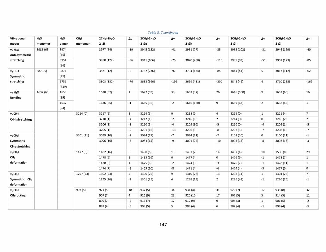
147

Table 3. 7 continued

Vibrational

modes

H2O

monomer

H2O

dimer

CH3I

monomer

2CH3I-2H2O

2 :2f

2CH3I-2H2O

2 :2g

2CH3I-2H2O

2 :2h

2CH3I-2H2O

2 :2i

2CH3I-2H2O

2 :2j

3 H2O

Anti-symmetric

stretching

3986 (63) 3974

(85)

3977 (64) -19 3945 (132) -41 3951 (77) -35 3955 (102) -31 3946 (129) -40

3954

(86)

3950 (122) -36 3911 (106) -75 3870 (200) -116 3935 (83) -51 3901 (173) -85

1 H2O

Symmetric

stretching

3879(5) 3871

(11)

3871 (12) -8 3782 (236) -97 3794 (134) -85 3844 (44) 5 3817 (112) -62

3751

(339)

3803 (132) -76 3683 (360) -196 3659 (411) -200 3843 (46) 4 3710 (288) -169

2 H2O

Bending

1637 (63)

1658

(39)

1638 (67) 1 1672 (59) 35 1663 (37) 26 1646 (100) 9 1653 (60) 16

1637

(94)

1636 (65) -1 1635 (36) -2 1646 (120) 9 1639 (63) 2 1638 (45) 1

4 CH3I

C-H stretching

3214 (0) 3217 (2) 3 3214 (5) 0 3218 (0) 4 3215 (0) 1 3221 (4) 7

3210 (1) -4 3212 (1) -2 3216 (0) 2 3214 (0) 0 3216 (2) 2

3206 (1) -8 3210 (5) -4 3209 (30) -5 3210 (0) -4 3209 (1) -5

3205 (1) -9 3201 (16) -13 3206 (3) -8 3207 (3) -7 3208 (1) -7

1 CH3I

Symmetric

CH3 stretching

3101 (11) 3099 (10) -2 3094 (17) -7 3094 (11) -7 3101 (10) 0 3100 (11) -1

3096 (16) -5 3084 (15) -9 3091 (24) -10 3093 (15) -8 3098 (13) -3

v5 CH3I

CH3

deformation

1477 (6) 1482 (16) 5 1490 (6) 13 1491 (7) 14 1487 (4) 10 1506 (8) 29

1478 (6) 1 1483 (16) 6 1477 (4) 0 1476 (6) -1 1478 (7) 1

1478 (5) 1 1475 (6) -2 1474 (3) -3 1476 (7) -1 1478 (11) 1

1474 (7) -3 1469 (10) -8 1471 (4) -6 1474 (4) -3 1477 (0) 0

2 CH3I

Symmetric CH3

deformation

1297 (23) 1302 (23) 5 1306 (26) 9 1310 (27) 13 1298 (14) 1 1304 (26) 7

1295 (26) -2 1301 (25) 4 1298 (13) 2 1296 (41) -1 1296 (26) -1

6 CH3I

CH3 rocking

903 (5) 921 (5) 18 937 (5) 34 934 (4) 31 920 (7) 17 935 (8) 32

907 (7) 4 926 (9) 23 920 (10) 17 907 (5) 5 914 (5) 11

899 (7) -4 915 (7) 12 912 (9) 9 904 (3) 1 901 (5) -2

897 (4) -6 908 (5) 5 909 (4) 6 902 (4) -1 898 (4) -5

148

Considering, if all those species are co-existing, the spectral congestion that will ensue, a

careful examination of spectral conditions (namely of sample ratio) will be necessary to

identify unambiguously forms present in argon matrices.

3.2.2.2 Experimental vibrational spectra

In Figures 3.13 and 3.14, are displayed on one hand, two methyl iodide spectral regions, i.e.

2 (bending CH) and 6 (rocking mode), and, on the other hand the three water spectral

regions, i.e. 3 (antisymmetric stretching), 1 (symmetric stretching) and 2 (bending). We

selected those spectral domains because, as discussed above, with the help of theoretical

results, we should be able to identify which aggregates and complexes are present in those

experimental conditions (with a large excess of water) supposed to mimic atmospheric ones.

In both figures we present a comparison of pure CH3I spectra (labelled as (a) in Figure 3. 13)

with mixed (CH3I)m(H2O)n ones and of pure water polymers (labelled as (a) in Figure 3. 14).

New or increasing bands, observed in mixed species spectrum, with respect to those of pure

water or methyl iodide ones, are marked with a dashed line (Traces (b) in Figures 3.13 and

3.14

Figure 3. 13 IR spectra in 2 (bending CH), 6 (rocking CH3) regions of pure methyl iodide matrix (trace (a)) (CH3I/Ar = 1/1000), recorded at 10 K, and of mixed CH3I/H2O/Ar = 1/24/1500, recorded at 10 K (trace (b)).

149

Figure 3. 14 IR spectra in the 1 (symmetric stretching),3 (antisymmetric stretching) and2 (bending mode)

regions of pure water polymer matrix (trace (a)) (H2O/Ar = 7/1000), recorded at 4 K, and of mixed CH3I/H2O/Ar = 1/24/1500, recorded at 10 K (trace (b)).

The frequencies and tentative assignment are reported in Tables 3.8 and 3.9.

150

Table 3. 8 Experimental IR band positions for 1, 2, and 6 (in cm-1) in CH3I spectral range for mixed

CH3I/H2O/Ar = 1/24/1500, recorded at 10 K, calculated spectral shifts () to experimental spectrum of CH3I

monomer and tentative assignments. (=calculated-experimental

Vibrational

Mode

CH3I

monomer

CH3I-H2O

Tentative assignments

1 CH3I 2965 2976 11 CH3I

2968 3 dimer HT

2965 0 monomer / trimer THT

2961 -4 dimer HT / dimer HH / trimer THT

2925

2868

2855

2846

2825

2819

2 CH3I 1246 1257 12 CH3I-3H2O (1 :3a)

1245 1256 11 CH3I-3H2O (1 :3a)

1254 9 see text

1250 5 CH3I-2H2O (1 :2a)

1248 3 dimer HT / trimer THT / CH3I-H2O (1:1a)

1246 1 dimer HT / trimer THT

1245 0 monomer / dimer HT /

1243 -2 dimer HH/ trimer THT

1240 -5 CH3I

6 CH3I

909 27 CH3I-2H2O (1:2a) / CH3I-3H2O (1:3c)

882 903 21 CH3I-H2O(1 :1a)

881 899 17 CH3I-2H2O (1:2a) / CH3I-3H2O (1:3a)

896 14 CH3I-3H2O (1:3a)

891 11 CH3I-H2O(1 :1a)

888 6 see text

886 4 dimer HT / dimer HH / trimer THT / CH3I-

3H2O (1:3a)

882 0 monomer / dimer HH

881 -1 monomer/ dimer HH

879 -2 dimer HH

151

Table 3. 9 Experimental IR band positions for 1, and 3 (in cm-1) in H2O spectral range for reference spectra of monomer and dimer, mixed CH3I/H2O/Ar = 1/24/1500, recorded at 10 K, for H2O (4:1000) at 4K, calculated

spectral shifts ) to experimental spectrum for H2O monomer and tentative assignments. (=calculated-

experimental

H2O monomer

and dimer

H2O

4:1000

CH3I-H2O


3776 3777 3777

H2O rovibrational band 3

3757 3756 3756


3753 H2O rovibrational band 3

3752 16 see text

3749 13 see text

3739


3738 3738 3738

H2O dimer PA

3736 3736 3736

H2O 3 (nrm)

3731 3731 H2O rovibrational band 3

3725 3721 3721


3720 -16 CH3I-3H2O (1 :3c)

3716 3716 3716

H2O dimer PD

3711 3711 3711


3713 -23 CH3I-H2O (1:1a) / CH3I-3H2O (1:3c)

3708 3708

H2O dimer PD

3670 3670 3670

H2O dimer PD / H2O rovibrational band 1

3662 3662 H2O dimer PD

3654 3654 3654

H2O dimer PD / H2O rovibrational band 1



3642 4 see text


3638 3638 3638

H2O 1 (nrm)

3633 3633 3633

H2O dimer PA



3623




3609 -29 CH3I-H2O (1 :1a)

3607 3607 3607 -31 H2O rovibrational band 1 / see text

3603 -35 see text

3582 -56 see text

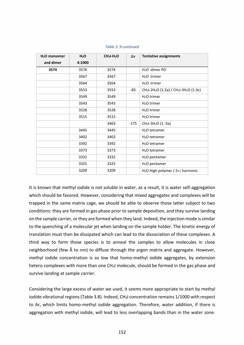
152

Table 3. 9 continued

H2O monomer

and dimer

H2O

4:1000

CH3I-H2O


3574 3576 3574

H2O dimer PD

3567 3567 H2O trimer


3553 3553 -85 CH3I-2H2O (1:2a) / CH3I-3H2O (1:3c)





3463 -175 CH3I-3H2O (1 :3a)

3445 3445 H2O tetramer




3332 3332

H2O pentamer

3325 3325

H2O pentamer

3209 3209 H2O High polymer / 22 harmonic

It is known that methyl iodide is not soluble in water, as a result, it is water self-aggregation

which should be favored. However, considering that mixed aggregates and complexes will be

trapped in the same matrix cage, we should be able to observe those latter subject to two

conditions: they are formed in gas phase prior to sample deposition, and they survive landing

on the sample carrier, or they are formed when they land. Indeed, the injection mode is similar

to the quenching of a molecular jet when landing on the sample holder. The kinetic energy of

translation must then be dissipated which can lead to the dissociation of these complexes. A

third way to form those species is to anneal the samples to allow molecules in close

neighborhood (few Å to nm) to diffuse through the argon matrix and aggregate. However,

methyl iodide concentration is so low that homo-methyl iodide aggregates, by extension

hetero complexes with more than one CH3I molecule, should be formed in the gas phase and

survive landing at sample carrier.

Considering the large excess of water we used, it seems more appropriate to start by methyl

iodide vibrational regions (Table 3.8). Indeed, CH3I concentration remains 1/1000 with respect

to Ar, which limits homo-methyl iodide aggregation. Therefore, water addition, if there is

aggregation with methyl iodide, will lead to less overlapping bands than in the water zone.

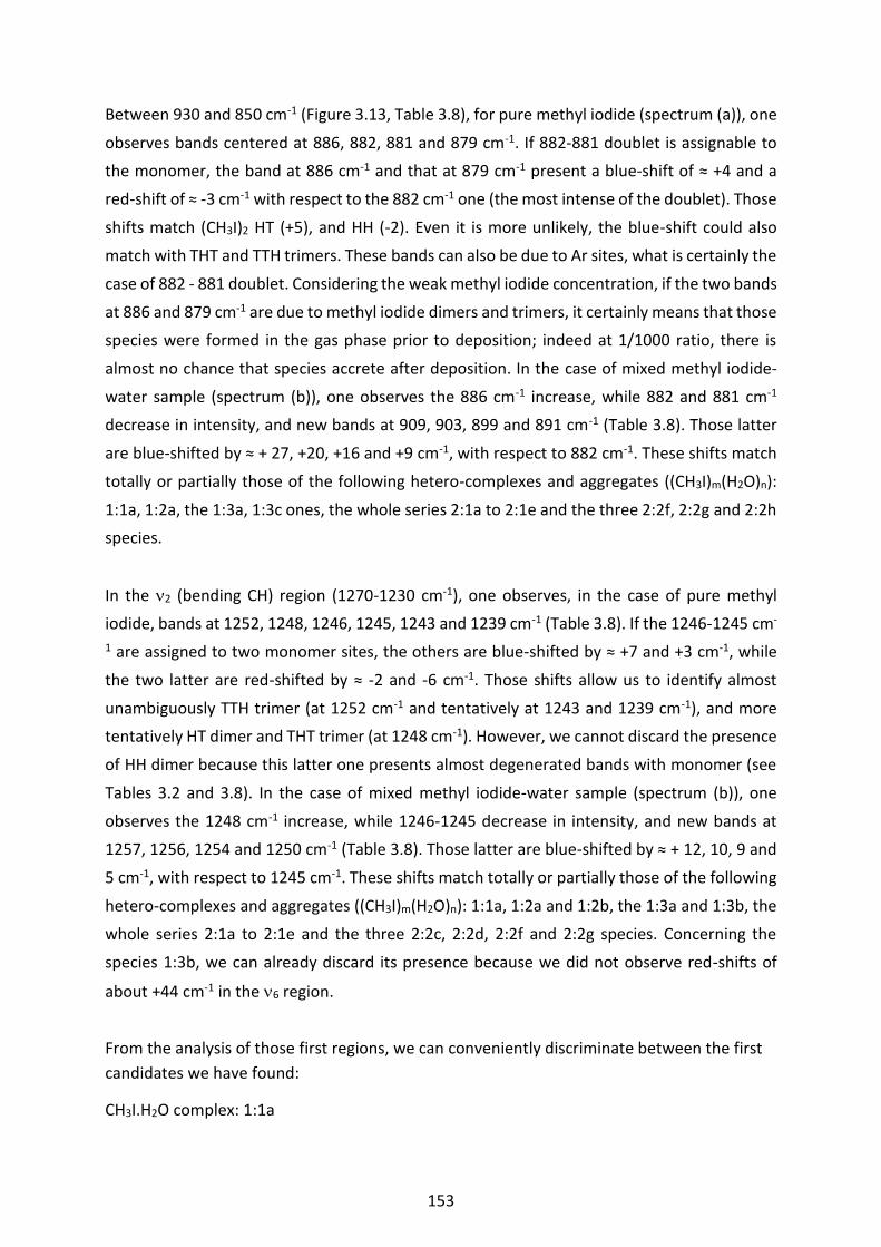
153

Between 930 and 850 cm-1 (Figure 3.13, Table 3.8), for pure methyl iodide (spectrum (a)), one

observes bands centered at 886, 882, 881 and 879 cm-1. If 882-881 doublet is assignable to

the monomer, the band at 886 cm-1 and that at 879 cm-1 present a blue-shift of ≈ +4 and a

red-shift of ≈ -3 cm-1 with respect to the 882 cm-1 one (the most intense of the doublet). Those

shifts match (CH3I)2 HT (+5), and HH (-2). Even it is more unlikely, the blue-shift could also

match with THT and TTH trimers. These bands can also be due to Ar sites, what is certainly the

case of 882 - 881 doublet. Considering the weak methyl iodide concentration, if the two bands

at 886 and 879 cm-1 are due to methyl iodide dimers and trimers, it certainly means that those

species were formed in the gas phase prior to deposition; indeed at 1/1000 ratio, there is

almost no chance that species accrete after deposition. In the case of mixed methyl iodide-

water sample (spectrum (b)), one observes the 886 cm-1 increase, while 882 and 881 cm-1

decrease in intensity, and new bands at 909, 903, 899 and 891 cm-1 (Table 3.8). Those latter

are blue-shifted by ≈ + 27, +20, +16 and +9 cm-1, with respect to 882 cm-1. These shifts match

totally or partially those of the following hetero-complexes and aggregates ((CH3I)m(H2O)n):

1:1a, 1:2a, the 1:3a, 1:3c ones, the whole series 2:1a to 2:1e and the three 2:2f, 2:2g and 2:2h

species.

In the 2 (bending CH) region (1270-1230 cm-1), one observes, in the case of pure methyl

iodide, bands at 1252, 1248, 1246, 1245, 1243 and 1239 cm-1 (Table 3.8). If the 1246-1245 cm-

1 are assigned to two monomer sites, the others are blue-shifted by ≈ +7 and +3 cm-1, while

the two latter are red-shifted by ≈ -2 and -6 cm-1. Those shifts allow us to identify almost

unambiguously TTH trimer (at 1252 cm-1 and tentatively at 1243 and 1239 cm-1), and more

tentatively HT dimer and THT trimer (at 1248 cm-1). However, we cannot discard the presence

of HH dimer because this latter one presents almost degenerated bands with monomer (see

Tables 3.2 and 3.8). In the case of mixed methyl iodide-water sample (spectrum (b)), one

observes the 1248 cm-1 increase, while 1246-1245 decrease in intensity, and new bands at

1257, 1256, 1254 and 1250 cm-1 (Table 3.8). Those latter are blue-shifted by ≈ + 12, 10, 9 and

5 cm-1, with respect to 1245 cm-1. These shifts match totally or partially those of the following

hetero-complexes and aggregates ((CH3I)m(H2O)n): 1:1a, 1:2a and 1:2b, the 1:3a and 1:3b, the

whole series 2:1a to 2:1e and the three 2:2c, 2:2d, 2:2f and 2:2g species. Concerning the

species 1:3b, we can already discard its presence because we did not observe red-shifts of

about +44 cm-1 in the 6 region.

From the analysis of those first regions, we can conveniently discriminate between the first

candidates we have found:

CH3I.H2O complex: 1:1a

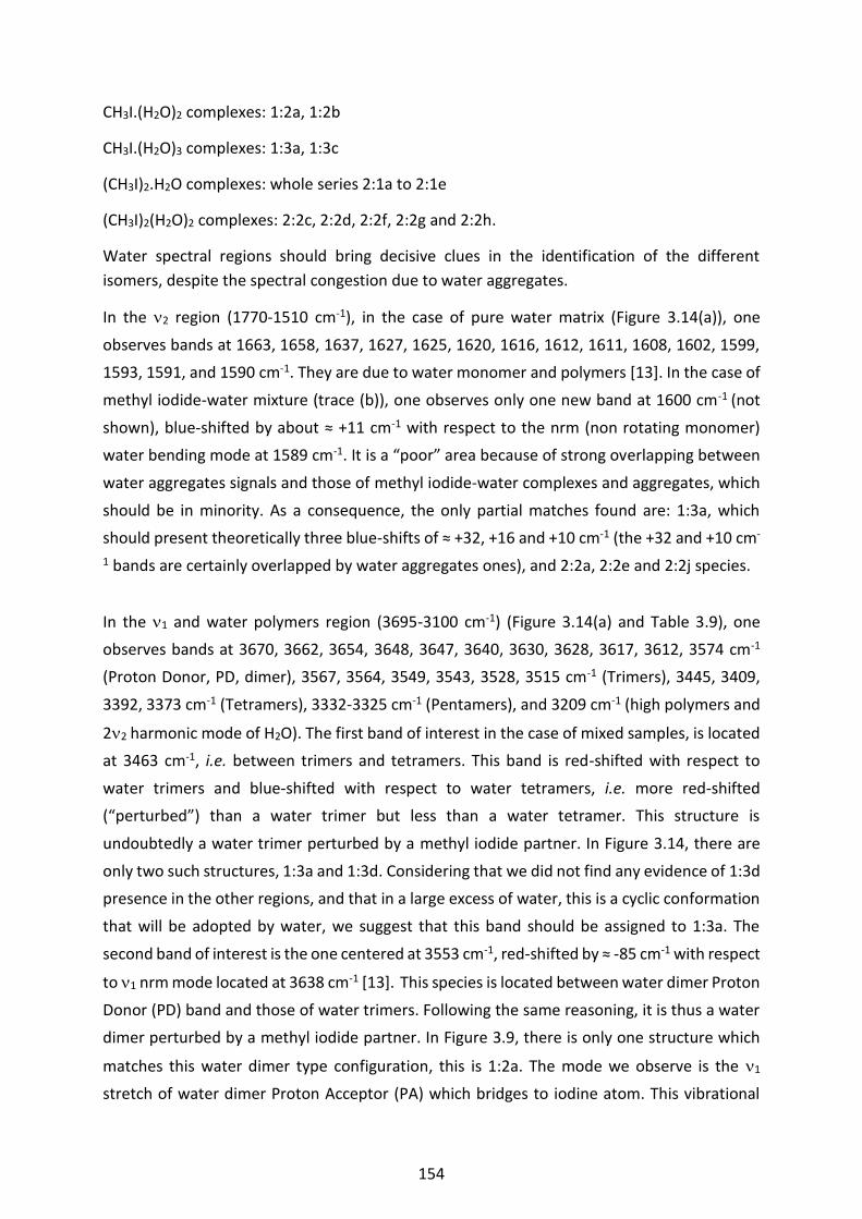
154

CH3I.(H2O)2 complexes: 1:2a, 1:2b

CH3I.(H2O)3 complexes: 1:3a, 1:3c

(CH3I)2.H2O complexes: whole series 2:1a to 2:1e

(CH3I)2(H2O)2 complexes: 2:2c, 2:2d, 2:2f, 2:2g and 2:2h.

Water spectral regions should bring decisive clues in the identification of the different

isomers, despite the spectral congestion due to water aggregates.

In the 2 region (1770-1510 cm-1), in the case of pure water matrix (Figure 3.14(a)), one

observes bands at 1663, 1658, 1637, 1627, 1625, 1620, 1616, 1612, 1611, 1608, 1602, 1599,

1593, 1591, and 1590 cm-1. They are due to water monomer and polymers [13]. In the case of

methyl iodide-water mixture (trace (b)), one observes only one new band at 1600 cm-1 (not

shown), blue-shifted by about ≈ +11 cm-1 with respect to the nrm (non rotating monomer)

water bending mode at 1589 cm-1. It is a “poor” area because of strong overlapping between

water aggregates signals and those of methyl iodide-water complexes and aggregates, which

should be in minority. As a consequence, the only partial matches found are: 1:3a, which

should present theoretically three blue-shifts of ≈ +32, +16 and +10 cm-1 (the +32 and +10 cm-

1 bands are certainly overlapped by water aggregates ones), and 2:2a, 2:2e and 2:2j species.

In the 1 and water polymers region (3695-3100 cm-1) (Figure 3.14(a) and Table 3.9), one

observes bands at 3670, 3662, 3654, 3648, 3647, 3640, 3630, 3628, 3617, 3612, 3574 cm-1

(Proton Donor, PD, dimer), 3567, 3564, 3549, 3543, 3528, 3515 cm-1 (Trimers), 3445, 3409,

3392, 3373 cm-1 (Tetramers), 3332-3325 cm-1 (Pentamers), and 3209 cm-1 (high polymers and

22 harmonic mode of H2O). The first band of interest in the case of mixed samples, is located

at 3463 cm-1, i.e. between trimers and tetramers. This band is red-shifted with respect to

water trimers and blue-shifted with respect to water tetramers, i.e. more red-shifted

(“perturbed”) than a water trimer but less than a water tetramer. This structure is

undoubtedly a water trimer perturbed by a methyl iodide partner. In Figure 3.14, there are

only two such structures, 1:3a and 1:3d. Considering that we did not find any evidence of 1:3d

presence in the other regions, and that in a large excess of water, this is a cyclic conformation

that will be adopted by water, we suggest that this band should be assigned to 1:3a. The

second band of interest is the one centered at 3553 cm-1, red-shifted by ≈ -85 cm-1 with respect

to 1 nrm mode located at 3638 cm-1 [13]. This species is located between water dimer Proton

Donor (PD) band and those of water trimers. Following the same reasoning, it is thus a water

dimer perturbed by a methyl iodide partner. In Figure 3.9, there is only one structure which

matches this water dimer type configuration, this is 1:2a. The mode we observe is the 1

stretch of water dimer Proton Acceptor (PA) which bridges to iodine atom. This vibrational

155

assignment is strongly supported by the theoretical ≈ -97 cm-1 (Table 3.9), found for this

species. However, one has to consider also the presence of 1:3c structure which is a “1:2a

+1:1a” kind of structure. This last form presents a theoretical red-shift of ≈ -91 cm-1 in this

region (and also a blue-shift of ≈ +26 cm-1 in CH3Ias already mentioned above). The other

bands observed in case of methyl iodide-water mixture are centered at 3582, 3603, 3607,

3609 and 3642 cm-1. The four first bands display red-shifts of≈ -56, -35, -31 and -29 cm-1

against a blue-shift of ≈ +4 cm-1 for the last one. The only forms which could partially or totally

match with those shifts are: 1:1a, 1:3c, the whole series 2:1a to 2:1e, and 2:2i.

In the 3 region (3950-3700 cm-1) (Figure 3.14 (a) and Table 3.9)), one observes bands at 3777,

3756, 3753, 3738, 3736, 3731, 3721, 3716, 3711, 3708, 3707, 3703, 3700 and 3695 cm-1. Those

bands are mainly due to water monomer and polymers, the non rotating monomer (nmr) and

rovibrational transitions [13]. Four new bands are observed in the case of mixed sample, at

3752, 3749, 3720 and 3713 cm-1. If the two highest ones are tentatively assigned to 000 → 101

water monomer rovibronic transition perturbed by methyl iodide proximity, the two lowest

ones present red-shift with respect to 3 nrm mode of water monomer, located at 3736 cm-1

[13] of ≈ -23 and -16 cm-1. Species which present possible matching with those red-shifts are:

1:1a, 1:2b, the whole (1-3) series, 2:1b, 2:1c and 2:1e, 2:2c, 2:2f and 2:2i (2-2) (Tables 3.3-3.7).

From the analysis of the three water regions we can conveniently discriminate between the

candidates we have found:

CH3I.H2O complex: 1:1a

CH3I.(H2O)2 complexes: 1:2a, 1:2b

CH3I.(H2O)3 complexes: 1:3a, 1:3b, 1:3c, 1:3d

(CH3I)2.H2O complexes: whole series 2:1a to 2:1e

(CH3I)2(H2O)2 complexes: 2:2a, 2:2c, 2:2e, 2:2f, 2:2i and 2:2j.

In summary, comparing the candidates identified from CH3I and H2O regions, we can almost

confidently state that we have identified 1:1a, 1:2a and 1:3a, 1:3c species (see Figure 3.6, 3.13

and 3.14), together with CH3I dimers and trimers. Concerning the rest of the possible

candidates, either they partially match the observed shifts with no decisive evidence of their

presence, or CH3I being the minority product, 2:1 and 2:2 species are hard to see (with some

exceptions as 2:2i isomer, which is the only form among all those calculated which present a

blue-shift in the 1 water region, or 2:1a, 2:1b and 2:1c which could be responsible for the

band at 3582 cm-1, while that observed at 3603 cm-1 could be assigned to 2:1d and 2:1e

species. Finally, in Tables 3.8 and 3.9, we only gathered the 1:1, 1:2 and 1:3 species (with 1, 2

or 3 water molecules, respectively) because they are the only ones for which we have

156

identified confidently vibrational bands. It may be noted that they present common bands,

this is due to their close structures (see theoretical part). It does not mean that the other

species (i.e. 2:1 and 2:2) are not present. On the contrary, given the nature of the injected

mixtures, and the fact that methyl iodide polymerizes even at low concentrations, there are

several vibrational indices of their presence as detailed above.

3.2.3 Preliminary results on the interaction of CH3I with amorphous ice

Amorphous ice (so called Amorphous Solid Water: ASW) was first produced in laboratory in

1935 [14] and has since been extensively characterized. ASW bulk structure is a four-

coordinated tetrahedral arrangement, much like crystalline water ices (see [15-17]) and

reference herein). Molecules at the surface present potentially four orientations: a four-

coordinated molecule bound in a distorted tetrahedron structure, referred as s4; a tri-

coordinated molecule with one lone electron pair exposed at the surface, dO; a tri-

coordinated molecule with one OH dangling at the surface, dH; and a bi-coordinated molecule

with one lone pair and one OH dangling at the surface, dH (see Figure. 3.15). These surface

modes exhibit vibrational frequencies at 3503, 3549, 3698, and 3720 cm−1, respectively, as

outlined previously [15-17].

Figure 3. 15 The four surface modes of amorphous ice, dH (3720 and 3698cm−1), dO (3549 cm−1), and s4 (3503

cm−1) [15].

In agreement with previous studies [15-17] and in comparison to Figure 3.16, ASW grown in

PIIM laboratory was purely amorphous. Position of the bulk OH stretching and the

characteristic dangling modes at 3720 and 3698 cm−1 match those of ASW (see Figure 3.16(a)),

spectra in black).

157

After formation of ASW, we carried out a series of CH3I/Ar: 1/1000 injections (3 mbar in 500

ms each time) at 44 K and then cooled to 4 K. The IR spectra in the OH dangling (Figure 3.16(a))

and CH3 deformation regions (Figure 3.16(b)) of the two successive depositions of CH3I on

ASW at 4K are marked in red and green in Figure 3.16.

Figure 3. 16 The observed IR spectra in (a) the OH dangling region and (b) the CH3 deformation region. Pure amorphous ice is in black and the successive 3 mbar depositions of CH3I/Ar on pure amorphous ice are in red

and green. The OH dangling modes are marked by pink dashed lines. CH3I tentatively assigned bands are marked by blue dashed lines.

The CH3I interaction with ASW can be firstly interpreted based on dangling bonds (dH) of

ASW. Any perturbation of the dH bands at 3720 and 3698 cm-1 (marked in pink dotted line in

Figure 3.16 (a)) or formation of new bands can give insights on the adsorption of CH3I. An

observation of a band at 3674 cm-1 (marked in blue dotted line in Figure 3.16(a)) shows that

158

CH3I was adsorbed on the surface of ASW. However, a repetition of CH3I deposition on ASW

(spectra marked in green, Figure 3.16(a)) did not indicate any further adsorption of CH3I. On

the other hand, one observe new bands at 1432, 1404 and 1243 cm-1, respectively (marked in

blue dotted line in Figure 3.16(b)) in all deposition experiments (spectra marked in red and

green). However, these observations are only preliminary and more repetition are needed to

well interpret these promising results.

Further, we noticed a complete desorption by annealing to 47 K (spectra in dark yellow in

Figure 3.17). This preliminary result which indicates a desorbing capability of CH3I above 47 K

(complete desorption).

Figure 3. 17 The observed IR spectra in the zone of the OH dangling of amorphous ice for the experiment of desorption of CH3I from pure amorphous ice after CH3I deposition and then annealing up to 47 K. All spectra

were recorded at 4K.

It was reported previously [18-20] that the adsorption, diffusion, and desorption of CH3I on

ice in the range of 90-100 K depend largely on the morphology of the ice substrate. Where

porous ice enhances the trapping of adsorbed CH3I, whereas pore-free ice likely allows

monomer adsorption and the formation of CH3I clusters. Moreover, full desorption was

observed when adsorbed CH3I molecules on ASW ice by increasing temperature between 100-

220 K. These observations were based on monitoring the desorbed species after the

adsorption of CH3I on ASW by temperature programmed desorption (TPD) experiment

“Indirect measurement of adsorbed CH3I”. What is new and interesting with our cryogenic

experiments that in the future we will be able to directly investigate well (1) how the ASW

159

structure is affected (reorganization of ASW surface) when CH3I is adsorbed on it and (2) how

CH3I is bonded/adsorbed to the surface of ASW.

3.3 Conclusion and perspectives

We have investigated the interaction between CH3I and water molecules using argon

cryogenic matrix experiments. The experimental data were supported by theoretical DFT

calculations. The experiments were conducted with a large excess of H2O molecules compared

to CH3I in order to mimic CH3I environment in the atmosphere. Cryogenic matrices seem

pretty accurate in order to describe inter molecular interactions between atmospherically

relevant molecules. Even if working at low temperature and pressure does not mimic

atmospheric conditions it brings insights at molecular level. However, working in these

conditions allows the study of the ground energy potential of those atmospheric complexes

and aggregates. Finally, considering the concentration of methyl iodide used in our

experiments, the aggregates are rather formed in the gas phase and not in the matrix cage.

Dimers and trimers of CH3I are observed despite the high water amount in the initial mixture

that may be explained by the low affinity of CH3I with water. The other complexes such as 2:1

and 2:2 cannot be completely excluded but appear as minor species. The inter molecular

behavior between CH3 and H2O molecules determined for the first time experimentally and

supported by DFT calculation highlights that, in the atmosphere, gaseous methyl iodide and

water will likely form aggregates of water and methyl iodide polymers instead of (CH3I)m-

(H2O)n complexes. This result is consistent with previous theoretical studies, which have

predicted the incomplete hydration of CH3I. Our results have important consequences for the

understanding the alkyl halide solvation in primary processes and thus, Cloud Condensation

Nuclei (CCN) formation from gaseous phases in the atmosphere and contribute to the

understanding of reactive halogen species in tropospheric chemistry. Finally, in the context of

the NNP’s severe accident, our work is contributing to better understand the fate of nuclear

species in the atmosphere and thus, the radionuclide dispersion. In the future, the

photochemical behavior of such CH3I-water aggregates will be investigated as CH3I is known

to be sensitive to the solar radiation.

Further, in this work we have provided a preliminary result on the interaction between CH3I

and amorphous ice. The ensemble of our results shows that surface modes, in particular the

dH dangling bonds, can be perturbed upon adsorption of CH3I. In the future, more

experiments will be carried out to improve this first set of experimental results:

(1) How is CH3I adsorbed on pure amorphous ice surface? is there any CH3I…H2O bonding or

complex formation? is there any CH3I polymer formation?

160

(2) Is it possible to desorb CH3I using only the kinetic energy of a gas stream?

(3) Is it possible to desorb CH3I by selectively irradiating dH?

(4) What about photochemical behavior of CH3I-amorphous ice?

References

[1] S. Seng, Thèse de doctorat : Phototransformation de composés d’intérêt atmosphérique. Etudes spectroscopiques en phase gaz, en matrice cryogénique et à l’échelle des particules individuelles, Université de Lille 2017.

[2] N.E. Lopez, Thèse de doctorat : Etude du transfert de protons dans les systemes moleculaires, Université de Aix-Marseille, (2017).

[3] M.J. Frisch, G. Trucks, H.B. Schlegel, G.E. Scuseria, M.A. Robb, J. Cheeseman, G. Scalmani, V. Barone, B. Mennucci, G.A. Petersson, H. Nakatsuji, M. Caricato, X. Li, H.P. Hratchian, A.F. Izmaylov, J. Bloino, G. Zheng, J. Sonnenberg, M. Hada, D. Fox, Gaussian, E., Gaussian 09 Revision A.1. Gaussian Inc, Gaussian 09 Revis. D.01. Gaussian Inc., Wallingford, CT. (2009).

[4] J. Da Chai, M. Head-Gordon, Long-range corrected hybrid density functionals with damped atom-atom dispersion corrections, Phys. Chem. Chem. Phys. 10 (2008) 6615–6620. https:// doi.org/10.1039/b810189b.

[5] K.A. Peterson, B.C. Shepler, D. Figgen, H. Stoll, On the spectroscopic and thermochemical properties of ClO, BrO, IO, and their anions, J. Phys. Chem. A. 110 (2006) 13877–13883. https://doi.org/10.1021/jp065887l.

[6] A. Villard, S. Khanniche, C. Fortin, L. Cantrel, I. Černušák, F. Louis, A theoretical study of the microhydration processes of iodine nitrogen oxides, Int. J. Quantum Chem. 119 (2019) 1–11. https://doi.org/10.1002/qua.25792.

[7] K.K. Irikura, THERMO.PL, National Institute of Standards and Technology, Gaithersburg, MD, USA 2000. Natl. Inst. Stand. Technol. (2002).

[8] D. Khiri, R. Vandeputte, S. Taamalli, L. Cantrel, F. Louis, Microhydration of caesium metaborate: structural and thermochemical properties of CsBO2 + n H2O (n = 1–4) aggregates, J. Mol. Model. 25 (2019) 1–8. https://doi.org/10.1007/s00894-019-4094-4.

[9] F. Ito, T. Nakanaga, Y. Futami, S. Kudoh, M. Takayanagi, M. Nakata, Isomeric structures of CH3I dimers in a supersonic jet studied by matrix-isolation infrared spectroscopy and ab initio calculation, Chem. Phys. Lett. 343 (2001) 185–191. https://doi.org/10.1016/S0009-2614(01)00688-1.

161

[10] F. Ito, T. Nakanaga, Y. Futami, M. Nakata, Observation of methyl iodide clusters in gas phase by infrared cavity ring-down spectroscopy, Chem. Phys. 286 (2003) 337–345. https://doi.org/10.1016/S0301-0104(02)00919-9.

[11] F. Ito, Infrared studies of the CH3I-H2O complex and large CH3I clusters in Ar matrices, J. Mol. Struct. 1035 (2013) 54–60. https://doi.org/10.1016/j.molstruc.2012.09.027.

[12] A.J. Barnes, M.L. Evans, H.E. Hallam, Infrared cryogenic studies, J. Mol. Struct. 69 (1973) 738–749. https://doi.org/10.1016/0022-2860(83)90026-1.

[13] J.P. Perchard, Anharmonicity and hydrogen bonding. III. Analysis of the near infrared spectrum of water trapped in argon matrix, Chem. Phys. 273 (2001) 217–213. https://doi.org/10.1016/S0301-0104(01)00496-7.

[14] E.F. Burton, W.F. Oliver, The crystal structure of ice at low temperatures, Proc. R. Soc. London. Ser. A - Math. Phys. Sci. 153 (1935) 166–172. https://doi.org/10.1098/rspa.1935.0229.

[15] J.A. Noble, C. Martin, H.J. Fraser, P. Roubin, S. Coussan, Unveiling the surface structure of amorphous solid water via selective infrared irradiation of OH stretching modes, J. Phys. Chem. Lett. 5 (2014) 826–829. https://doi.org/10.1021/jz5000066.

[16] J.A. Noble, C. Martin, H.J. Fraser, P. Roubin, S. Coussan, IR selective irradiations of amorphous solid water dangling modes: Irradiation vs annealing effects, J. Phys. Chem. C. 118 (2014) 20488–20495. https://doi.org/10.1021/jp506943k.

[17] S. Coussan, P. Roubin, J.P. Perchard, Infrared induced isomerizations of water polymers trapped in nitrogen matrix, Chem. Phys. 324 (2006) 527–540. https://doi.org /10.1016/j.chemphys.2005.11.017.

[18] A.J. Desimone, B.O. Olanrewaju, G.A. Grieves, T.M. Orlando, Photodissociation of methyl iodide adsorbed on low-temperature amorphous ice surfaces, Chem. Phys. 138 (2013) 0847031-0847039. https://doi.org/10.1063/1.4790585.

[19] Y. Sohn, J.M. White, Thermal and photochemistry of methyl iodide on ice film grown on Cu(111), Bull. Korean Chem. Soc. 30 (2009) 1470–1474. https://doi.org/10.5012/bkcs. 2009.30.7.1470.

[20] E.R. Miller, G.D. Muirhead, E.T. Jensen, Mechanisms for the near-UV photodissociation of CH3I on D2O/Cu(110), J. Chem. Phys. 138 (2013) 0847021-08470210. https://doi.org/10 .1063/1.477 0225.

162

Chapter 4: DRIFTS experiments Chapter 4 focuses on the study of interactions between NaCl solid particles, as model for the

atmospheric sea salt aerosols, and gaseous CH3I under controlled conditions.

The experiments were conducted using Diffuse Reflectance Infrared Fourier Transform

Spectroscopy (DRIFTS). For our application, this technique will be powerful for following in real

time the reactions of alkali halides as NaCl, which are transparent in the infrared, since the

formation of infrared absorbing intermediates and products, can be detected with ease.

Following the chemical composition evolution of the solid can give quantitative insights on the

gaseous molecules taken up by (i.e. spectro kinetics measurements) if coupled with other

analytical techniques such as inductively coupled plasma mass spectrometry (ICP-MS).

First, a special attention is devoted to the detailed description of the experimental setup and

experimental conditions. In a second step, the spectral characterization of NaCl solid particles

surface during CH3I exposure experiments is described. Next, the kinetics and energetics

interpretations of the CH3I interaction with NaCl are determined. In particular, we insisted on the

interpretation of adsorption/desorption evolution and calculation of the uptake coefficient and

global adsorption to exploit the interaction between CH3I and NaCl. Finally, the conclusion and

perspectives are given.

4.1. Material and Methods

4.1.1 Reagents

Methyl iodide 1000 ppm (0.1% CH3I, 99.9% Ar) and Argon (99.99% pure) gas bottles were

provided from commercial cylinders Air product and Air liquid, respectively. The gases were used

without any further purification. Distilled water and Argon (99.99% pure) gas bottles were used

to prepare wet Argon as mixture to provide humidity varying between < 10% to 80% inside the

DRIFTS cell.

Commercial sodium chloride (NaCl, 99.99%, ALFA AESAR), potassium bromide (KBr, 99+%, SIGMA

ALDRICH) and sodium iodide (NaI, 99+%, ACROS) were used as powder for experiments.

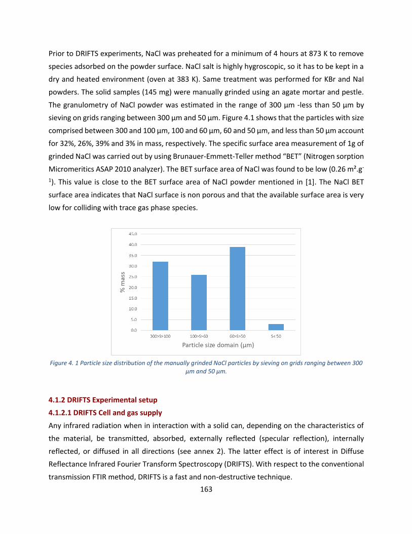
163

Prior to DRIFTS experiments, NaCl was preheated for a minimum of 4 hours at 873 K to remove

species adsorbed on the powder surface. NaCl salt is highly hygroscopic, so it has to be kept in a

dry and heated environment (oven at 383 K). Same treatment was performed for KBr and NaI

powders. The solid samples (145 mg) were manually grinded using an agate mortar and pestle.

The granulometry of NaCl powder was estimated in the range of 300 μm -less than 50 μm by

sieving on grids ranging between 300 μm and 50 µm. Figure 4.1 shows that the particles with size

comprised between 300 and 100 µm, 100 and 60 µm, 60 and 50 µm, and less than 50 µm account

for 32%, 26%, 39% and 3% in mass, respectively. The specific surface area measurement of 1g of

grinded NaCl was carried out by using Brunauer-Emmett-Teller method “BET” (Nitrogen sorption

Micromeritics ASAP 2010 analyzer). The BET surface area of NaCl was found to be low (0.26 m².g-

1). This value is close to the BET surface area of NaCl powder mentioned in [1]. The NaCl BET

surface area indicates that NaCl surface is non porous and that the available surface area is very

low for colliding with trace gas phase species.

Figure 4. 1 Particle size distribution of the manually grinded NaCl particles by sieving on grids ranging between 300

μm and 50 µm.

4.1.2 DRIFTS Experimental setup

4.1.2.1 DRIFTS Cell and gas supply

Any infrared radiation when in interaction with a solid can, depending on the characteristics of

the material, be transmitted, absorbed, externally reflected (specular reflection), internally

reflected, or diffused in all directions (see annex 2). The latter effect is of interest in Diffuse

Reflectance Infrared Fourier Transform Spectroscopy (DRIFTS). With respect to the conventional

transmission FTIR method, DRIFTS is a fast and non-destructive technique.

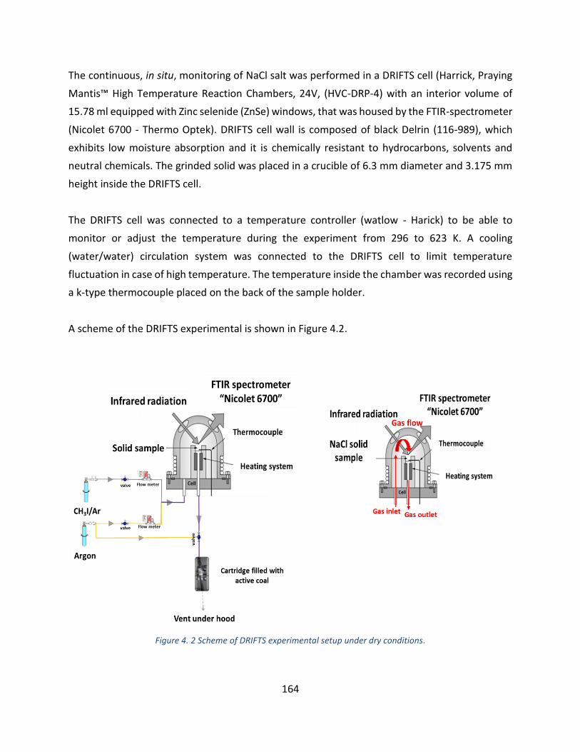
164

The continuous, in situ, monitoring of NaCl salt was performed in a DRIFTS cell (Harrick, Praying

Mantis™ High Temperature Reaction Chambers, 24V, (HVC-DRP-4) with an interior volume of

15.78 ml equipped with Zinc selenide (ZnSe) windows, that was housed by the FTIR-spectrometer

(Nicolet 6700 - Thermo Optek). DRIFTS cell wall is composed of black Delrin (116-989), which

exhibits low moisture absorption and it is chemically resistant to hydrocarbons, solvents and

neutral chemicals. The grinded solid was placed in a crucible of 6.3 mm diameter and 3.175 mm

height inside the DRIFTS cell.

The DRIFTS cell was connected to a temperature controller (watlow - Harick) to be able to

monitor or adjust the temperature during the experiment from 296 to 623 K. A cooling

(water/water) circulation system was connected to the DRIFTS cell to limit temperature

fluctuation in case of high temperature. The temperature inside the chamber was recorded using

a k-type thermocouple placed on the back of the sample holder.

A scheme of the DRIFTS experimental is shown in Figure 4.2.

Figure 4. 2 Scheme of DRIFTS experimental setup under dry conditions.

165

The DRIFTS cell was connected to gas supplying lines allowing gas feed into the dome. The gas is

passing through the powder sample as shown in Figure 4.2. The flow direction from the bottom

to the top of the DRIFTS cell offers the advantage of thermostatically controlling the gases and

tracking the surface reactions at the desired temperature. The gas flow was fitted with valves

and flow meters type Bronkhorst (F-201CV) to control the flow entering the cell. The total flow

rate inside the cell was prepared by controlled mixing of flows from two different lines both

allowing a gas feed in the range of 2-108 mL.min-1 at 273 K and 1 Bar, carrying each:

Dry Argon (line in yellow in Figure 4.2);

Dry CH3I (line in grey in Figure 4.2).

The exit line was mixed with argon and then connected to a cartridge filled with active coal for

CH3I filtering before exhaust (see Figure 4.2). A suction extractor was placed on top of the

chamber to ventilate the released gases in case of leakage. Figure 4.3, shows the DRIFTS

experimental setup with all the connections from the gas bottles to the DRIFTS chamber and then

to the exit under the hood.

Figure 4. 3 DRIFTS experimental setup from GSM-ISM.

The relative humidity inside the DRIFTS cell was regulated by mixing dry argon with humid Ar

after bubbling Ar through glass grits in pure water as shown in Figure 4.4. A relative humidity

sensor (SHT75 Sensirion, precision RH= 10-80% ± 10%) was placed at the exit of the mixing line.

Humidity control was possible by changing the ratio of dry/saturated Ar flows whilst keeping the

total gas flow constant. It should be highlighted that experiments using wet CH3I cannot be

performed due to the fact that H2O may damage the ZnSe DRIFTS windows.

166

Figure 4. 4 Scheme of DRIFTS experimental setup under humid conditions.

A second set of experiments was performed with the objective to determine quantitatively the

amount of CH3I taken by the solid at the end of the experiment. Such determination is possible

by ICP-MS technique after dissolution of the solid in alkaline media (see section 4.1.3). This

second set of experiments was conducted without online IR monitoring but under the same

conditions as the set of experiments performed initially with IR monitoring.

4.1.2.2 Experimental protocol

Prior to each experiment, we checked that there is no leak from all the system by flowing Ar at

108 mL.min-1 forthwith by using a gas leak detector (Jelt, Detect Fuites) and measuring the flow

at the outlet.

Background spectrum is usually collected by DRIFTS using IR transparent potassium bromide

(KBr) solid. However, in our experiments the background was recorded using preheated NaCl

(99.99%) powdered solid.

145 mg of NaCl powder was placed inside the DRIFTS cell at 296 K. Then the chamber was purged

with Argon for 10 minutes to ensure the complete removal of H2O and other pre-adsorbed

species. After, NaCl at 296 K was taken as the background spectra under Ar flow 108mL.min-1. It

167

should be noted that the background was verified at the beginning of each experiment with the

same procedure. Then, the NaCl salt was exposed continuously to CH3I with a constant flow rate

and spectrum were acquired every 8 minutes till 5 hours of exposure. Both NaCl background and

NaCl exposed to CH3I spectra were recorded under the same spectral conditions.

It should be noted that no major evolution of the spectral region of interest was observed in the

spectra recorded after 112 minutes under Ar flow (blank experiment), so that any spectral

evolution observed during NaCl exposition to methyl iodide can be owed to CH3I-NaCl surface

interaction.

4.1.2.3 Spectral acquisition using DRIFTS

In DRIFTS system (NICOLET 6700) the scattered IR energy on the surface is collected by a spherical

mirror that is focused on to the high sensitivity deuterated triglycine sulfate (DTGS) detector with

KBr beam splitter. All infrared spectra were recorded as a function of time in the spectral range

from 4000 to 600 cm−1 at resolution 8 cm-1. 200 scans were accumulated for each spectrum

featuring an overall acquisition duration of 8 minutes. Acquisition of experimental spectra and

background spectra were carried out using Omnic software in the same conditions. The

background subtraction was achieved by the Omnic software for each spectrum. The baseline

was corrected by linear interpolation model using Omnic software. It is highlighted that the C-I

stretching mode at 572 cm-1 cannot be detected by DRIFTS spectra because ZnSe window cuts

the spectrum in the range below 600 cm-1.

4.1.2.4 Spectral data processing for quantification

Regarding the theoretical standpoint of DRIFTS [3] , there is no linear relation between band

intensity and concentration so that the Lambert-Beer law, is not applicable for DRIFTS

experiments. However, similar expressions were developed: the Kubelka-Munk (K-M) or pseudo

absorbance functions corrections as shown in Table 4.1. Complementary informations are

displayed in annex 2.

168

Table 4. 1 Comparison of Kubelka-Munk and Pseudo absorbance theories, which can be adapted for diffuse reflectance [3].

Kubelka-Munk Pseudo absorbance

For highly absorbing adsorbates Poorly absorbing adsorbates

𝒇(𝐑∞) =(𝟏−𝐑∞)𝟐

𝟐𝐑∞=

𝐊

𝐬 =

𝟐.𝟑𝟎𝟑∙𝜺(𝝂)∙𝑪

𝒔 log (1/R ∞) =

𝐂

𝐂𝐨𝐧𝐬𝐭𝐚𝐧𝐭

R∞: Diffuse reflected signal

K: Absorption coefficient

S: Scattering coefficient

Ε: Extinction coefficient

C: Concentration

We have choosen pseudo absorbance to treat our spectral data as we expect to be in the case of

poorly absorbing adsorbates (see annex 2) regarding the literature [3]. The quantification was

based on the integration of a band intensity within limits defined in a fix spectral range using

Fityk software with Levenberg-Marquardt mathematical model [4]. Since one IR bands may

results of several overlapped bands, when it was appropriated, a band decomposition was

performed by Gaussian function [4] multiple band fit using FityK software.

The band area uncertainty was estimated by the repeat of the three experiments performed

under the same conditions (see annex 3). Absolute uncertainty of the band area in the 1400-1000

cm-1 was found between ~ 0.03 to 0.37 at 95% confidence level.

4.1.3. Inductively coupled plasma mass spectrometer measurements

The combination between DRIFTS and inductively coupled plasma mass spectrometer (ICP-MS,

see annex 4) analysis allowed to quantify the adsorbed gaseous phase. The total concentration

of CH3I taken up by NaCl was determined via ICP-MS measurements (see annex 7) performed

after the DRIFTS experiment.

The solid samples were analyzed by ICP-MS (810 MS VARIAN) which is a sensitive technique for

the determination of iodine concentration. A detection and quantification limits of 3 μg.L-1 and 5

μg.L-1, respectively for iodine were determined previously [5]. The uncertainty of measurement

was found to be ± 8% at 95% confidence level [5]– including sample preparation and ICP-MS

analysis (see also annex 6). This technique is nevertheless destructive as it requires dissolution of

the analyte (the solid sample) in aqueous media.

169

The NaCl powder samples exposed to CH3I were prepared as following, instantly after DRIFTS

experiment, to avoid ageing process. 100 mg of NaCl samples were dissolved by 10 mL of NaOH

(0.1 mol.L-1). The dissolved samples were then diluted in NaOH (0.1 mol.L-1) by a factor of 5, 10

and 20 before ICP-MS analysis.

Then it will be possible to translate the band area of IR bands attributed to methyl iodide

adsorption/absorption to the total amount of iodine taken by the solid by a conversion factor [6,

7] that is described later in section 4.3.4.1. Here, it should be highlighted that determination of

conversion factor will be based on the hypothesis that CH3 deformation modes attributed to

adsorbed CH3I represent the total concentration of CH3I taken up by NaCl.

4.1.4. Experiment grid for DRIFTS experiments and validation

In this work, three types of experimental conditions were explored for exposing NaCl to CH3I: (1)

dry flow of CH3I, (2) NaCl exposed to humidity varying between 20 and 80 % (at T= 296 K) and

then to dry CH3I, and (3) NaCl exposed to dry CH3I at temperature comprised between 296 and

423 K. For all experiments, the solid phase evolution was time followed by recording an FTIR

spectrum every 8 minutes (200 scans/spectrum). All these experiments were performed under

ambient pressure (P=1 atm). A protocol of three phases (CH3I exposure phase, static condition

phase and continuous Ar flow phase) was followed for each experimental condition.

4.1.4.1 Dry Condition

As a first step, a study of the interaction of CH3I with dry NaCl was carried out at 296 K, 1 atm and

estimated RH = 20% conditions. The total flow rate inside the cell was prepared by flowing dry

CH3I at 108 mL.min-1.

The experiments have distinguished three separate phases (1) continuous exposure to CH3I flow,

(2) stopping CH3I delivery with closed cell as “static condition” and (3) continuous flow of Ar which

are described below and summarized in the Table 4.2:

“CH3I Exposure” phase (1): NaCl salt samples were exposed to continuous flow of CH3I (1000

ppm) with 108 mL.min-1 flow rate corresponding to contact time (Tc) of 55ms in the NaCl solid

bed. The contact time (Tc) is defined as the average time that a gas species is put in contact with

solid particles. The contact time (Tc) in our DRIFTS configuration is dependent on the solid bed

170

volume, particles size, packing of particles, surface area and gas flow rate. Herein, we firstly

estimated the contact time in the solid bed by the following equation:

Tc= Solid bed volume

Total gas flow [E4-1]

The exposure time was for 5 hours as a maximum. The main purpose of the long exposure time

is that it can represent more appropriately the presence of CH3I in the atmosphere due to its long

half-life time (~5 days) [8].

“Static condition” phase (2): The flow of CH3I was stopped i.e. maintaining the system under

static conditions. It should be highlighted that two types of static conditions can be maintained

either by closing or opening the exit valve. In both cases, the results were the same with a low

difference of about 8% (annex 3).

“Continuous Ar flow” phase (3): After static condition, argon was continuously flowed up for 1

hour.

Steps (2) and (3) were performed to check the spontaneous and induced desorption of CH3I,

respectively.

Five scenarii were investigated for exposing dry NaCl to “dry” CH3I: (i) The capability of CH3I to be

sorbed on NaCl surface (ii) capability of CH3I to desorb, (iii) the influence of the temperature on

the desorption of CH3I, (iv) the influence of the initial CH3I gas concentration and (v) variation of

the estimated contact time in the solid bed [E4-1]. All these experiments were performed under

ambient conditions (RH=20%, P=1 atm and T=296 K) with the same conditions for spectral

acquisition.

(i) The capability of CH3I to be sorbed: was investigated by following the CH3I on the surface of

NaCl over time (Table 4.2).

171

Table 4. 2 Experimental conditions for CH3I exposure, static and continuous Ar flow phases of dry experiment with NaCl – scenario (i).

Experiment with dry NaCl

Phase 1 Phase 2 Phase 3 Repetition

[CH3I]g

in ppm

Contact

time (Tc)

in ms

CH3I/Ar flow

in mL.min-1

CH3I exposure

duration

Static

duration

Continuous Ar flow

(108 mL.min-1)

duration

1000 55 108/0 5 hours 1 hour 1 hour 3

(ii) The capability of CH3I to desorb: was conducted by the continuous flow of CH3I (1000 ppm,

108 mL.min-1) for only two hours on dry NaCl salt (RH= 20% at 296 K) to limit methyl iodide

adsorption. Then the static condition and pure argon continuous flow duration were strongly

increased to evidence (if any) either spontaneous desorption or induced desorption. In this view,

the static conditions were maintained for 24 hours and the phase with pure argon lasted 8 hours.

The experimental conditions are listed in Table 4.3.

Table 4. 3 Experimental conditions for CH3I exposure, static and continuous Ar flow phases of dry experiment with NaCl – scenario (ii).

Experiment with shorter CH3I exposure time

Phase 1 Phase 2 Phase 3

[CH3I]g

in ppm

Contact

time (Tc)

in ms

CH3I/Ar flow

in mL.min-1

CH3I exposure

duration

Static

duration

Continuous Ar flow

(108 mL.min-1)

duration

Repetition

1000 55 108/0

2 hours 23 hours 8 hours 1

(iii) Influence of temperature on the CH3I desorption: As a matter of fact, the reverse process of

adsorption can be thermally activated (desorption), that is why one experiment of heating NaCl

until 623 K was performed with increasing the temperature during continuous Ar flow (in phase

3). NaCl (RH=20%, at 296 K) was exposed to continuous exposure of CH3I (108 mL.min-1, 1000

ppm) for 1 hour. After 1 hour of CH3I continuous flow, the system was maintained under static

conditions for 4 hours. After, NaCl was exposed to continuous Ar flow for 1 hour at 296 K. Then

after, the temperature was gradually increased from room temperature (296 K) to 373, 473 and

finally 623 K with a rate of 3 K.min-1 under continuous Ar flow. After reaching each desired

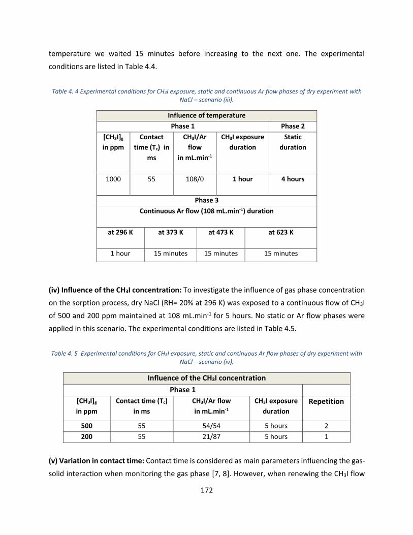
172

temperature we waited 15 minutes before increasing to the next one. The experimental

conditions are listed in Table 4.4.

Table 4. 4 Experimental conditions for CH3I exposure, static and continuous Ar flow phases of dry experiment with NaCl – scenario (iii).

Influence of temperature

Phase 1 Phase 2

[CH3I]g

in ppm

Contact

time (Tc) in

ms

CH3I/Ar

flow

in mL.min-1

CH3I exposure

duration

Static

duration

1000

55 108/0

1 hour 4 hours

Phase 3

Continuous Ar flow (108 mL.min-1) duration

at 296 K

at 373 K

at 473 K

at 623 K

1 hour 15 minutes 15 minutes 15 minutes

(iv) Influence of the CH3I concentration: To investigate the influence of gas phase concentration

on the sorption process, dry NaCl (RH= 20% at 296 K) was exposed to a continuous flow of CH3I

of 500 and 200 ppm maintained at 108 mL.min-1 for 5 hours. No static or Ar flow phases were

applied in this scenario. The experimental conditions are listed in Table 4.5.

Table 4. 5 Experimental conditions for CH3I exposure, static and continuous Ar flow phases of dry experiment with NaCl – scenario (iv).

Influence of the CH3I concentration

Phase 1

[CH3I]g

in ppm

Contact time (Tc)

in ms

CH3I/Ar flow

in mL.min-1

CH3I exposure

duration

Repetition

500 55 54/54 5 hours 2

200 55 21/87 5 hours 1

(v) Variation in contact time: Contact time is considered as main parameters influencing the gas-

solid interaction when monitoring the gas phase [7, 8]. However, when renewing the CH3I flow

173

all along the exposure phase duration by continuous flow and monitoring the solid phase as in

our DRIFTS experiments, this highly suggests that contact time cannot be considered as main

parameter influencing the gas-solid interaction. To verify this fact, we intended to perform

experiments with different contact times. To investigate the influence of contact time on CH3I-

NaCl interaction, dry NaCl (RH = 20% at 296 K) was exposed to continuous CH3I flow (500 ppm,

216 mL.min-1) by increasing the total gas CH3I/Ar flow from 108 mL.min-1 to 216 mL.min-1. Thus,

the estimated contact time was decreased from 55 ms to 27 ms. Similar to experiment shown in

Table 4.2 the duration of the exposure phase was of 5 hours. No static or Ar flow phases were

applied in this scenario. The experimental conditions are listed in Table 4.6.


NaCl – scenario (v).

Variation in contact time

Phase 1

[CH3I]g

in ppm

Contact time (Tc)

in ms

CH3I/Ar flow

in mL.min-1

CH3I exposure

duration

Repetition

500 27 108/108 5 hours 1

Additionally, the adsorption of CH3I on other halide salts (NaI and KBr) was experimented for

comparison as the influence of halide atom is questionable. Table 4.7 lists the conditions of

experiments performed with NaI and KBr at 1 atm, 296 K and RH= 20%. Only the potential

sorption of CH3I on the halide salt was investigated so no static or Ar flow phases were applied

for these experiments.

Table 4. 7 Experimental conditions for CH3I exposure, static and continuous Ar flow phases of dry experiment with NaI and KBr – scenario (i).

Experiment with dry NaI and KBr

Phase 1

Solid [CH3I]g

in ppm

Contact time (Tc)

in ms

CH3I/Ar flow

in mL.min-1

CH3I exposure

duration

Repetition

NaI 1000 55 108/0 1 hour 1

KBr 1000 55 108/0 1 hour 1

174

4.1.4.2. Humid conditions

In a second part, the influence of humidity was investigated. The study focused on the interaction

between dry gaseous CH3I and wet solid NaCl. The objective was to compare the behavior of CH3I

when it is exposed to dry and wet NaCl aerosols. Humidity experiments conditions are listed in

Table 4.8. At 296 K the protocol was as following:

Humidification of NaCl: NaCl was humidified with a 108 mL.min-1 continuous wet Ar flow for 40

minutes with a given %RH of 40, 60 or 80 % at 296 K. It should be noted that the deliquescent

point (DRH) of NaCl is obtained when RH reach 75% at 298 K [11]. However, due to the

uncertainty on the RH measurement (~10%), the DRH point was not reached to avoid any liquid

in the DRIFTS cell.

Dry CH3I flow: Wet NaCl samples were exposed to continuous dry flow of 1000 ppm of CH3I at

flow rate 108 mL.min-1 for 5 hours with a contact time of 55 ms in the solid bed.

Static and continuous Ar flow conditions: The system was maintained under static conditions

and then under continuous Ar flow. The DRIFTS cell was maintained at room temperature (296

K).

Table 4. 8 Experimental conditions for CH3I exposure, static and continuous Ar flow phases of experiment with humid NaCl.

Experiment with wet NaCl


%RH

of

NaCl

[CH3I]g

in ppm

Contact

time (Tc)

in ms

CH3I/Ar

flow

in mL.min-1

CH3I

exposure

duration

Static

duration

Continuous Ar

flow (108

mL.min-1)

duration

Repetition

40 1000 55 108/0 5 hours - 1hour 1

60 1000 55 108/0 5 hours 1hour 1hour 2

80 1000 55 108/0 5 hours 1hour 1hour 2

In addition to the humidity experiments listed above, an experiment was performed for checking

the influence of humidity on desorption of CH3I. The protocol was the following:

Dry CH3I flow: Dry NaCl samples (RH=20%, at 296 K) were exposed to continuous dry flow of 100

ppm of CH3I at flow rate 108 mL.min-1 featuring contact time of 55 ms in the solid bed for 5 hours.

175

Effect of humidity: Then after, wet Ar with RH of 50% (at 296 K) was continuously flowed for 40

minutes.

Conditions of this experiment are listed in Table 4.9.

Table 4. 9 Experimental conditions for CH3I exposure, static and final continuous Ar flow phases of experiment with NaCl featuring humidified argon in the last phase.

Effect of humidity after CH3I was taken up by NaCl

%RH of

NaCl

Contact

time (Tc)

in ms

[CH3I]g

in ppm

CH3I/Ar flow

in mL.min-1

CH3I

exposure

duration

Continuous flow of

108 mL.min-1 wet Ar

(RH=50 %)

Repetition

20 55 1000 108/0 5 hours 40 minutes 1

4.1.4.3 Variation of the temperature conditions

NaCl was introduced in the DRIFTS cell and heated from room temperature (RH=20% at 296 K)

up to 423 K. Once the target temperature has been reached, NaCl was exposed to CH3I (1000

ppm) in a continuous flow at 108 mL.min-1 featuring a contact time of 55 ms in the solid bed. The

system was maintained under static conditions and under continuous Ar flow maintaining

temperature as during the exposure phase. Experiments under different temperature conditions

are listed in Table 4.10.

Table 4. 10 Experimental conditions for CH3I exposure, static and continuous Ar flow phases of experiment with NaCl at different temperatures

Experiment by increasing temperature


Temperature

(K)

[CH3I]g

in ppm

Contact

time (Tc)

in ms

CH3I/Ar

flow

in mL.min-1

CH3I

exposure

duration

Static

duration

Continuous Ar

flow (108

mL.min-1)

duration

Repetition

323 1000 55 108/0 5 hours 1hour 1hour 1

348 1000 55 108/0 5 hours 1hour 1hour 1

373 1000 55 108/0 5 hours 1hour 1hour 1

423 1000 55 108/0 5 hours 1hour 1hour 1

176

4.2. Spectral assignment

4.2.1 Dry conditions

Experiments under dry condition were conducted by the continuous flow of dry CH3I for 5 hours

(108mL.min-1, 1000 ppm) on dry NaCl particles placed in the DRIFTS cell at 296 K and 1 atm (see

section 4.1.4.1, Table 4.2). A representative spectrum of NaCl exposed to CH3I during 5 hours and

recorded in the mid IR region (4000-600 cm-1) is shown in Figure 4.5. Further, we observed a

good repeatability of the observed IR spectra (i.e. IR band position and band area) for spectra

recorded under the same experimental conditions (see annex 3).

Figure 4. 5 Typical DRIFTS spectra in mid IR spectral range [4000-600 cm-1] of dry NaCl surface exposed to 5 hours

of CH3I flow (108mL.min-1, 1000 ppm) at 296 K and 1 atm.

Three typical regions assigned to CH3 stretching, CH3 deformation and CH3 rocking are observed

(Figure 4.5). The typical C-I vibration is not seen since the region is below 600 cm-1. The detailed

description of the CH3 stretching (3050-2800 cm-1), CH3 deformation (1500-900 cm-1) and CH3

rocking (900-700 cm-1) spectral region for a proper assignment is given below.

4.2.1.1 Band assignment in the CH3 stretching region

The first region of interest is the CH3 stretching region (3050-2800 cm-1) which is shown in Figure

4.6. In the CH3 stretching region bands at 3018, 2993, 2981, 2961, 2953, 2855 and 2847 cm-1 are

observed.

177

Overlapped bands in the 2961 cm-1 region were decomposed using gaussian function (see

procedure described 4.1.2.4) and the two identified bands at 2961 and 2953 cm-1 are presented

in Figure 4.7.


(108mL.min-1, 1000 ppm) continuous flow at 296 K and 1 atm. Blue bands are CH3I adsorbed on NaCl and green bands are CH3I in gas phase near the surface.

Figure 4. 7 DRIFTS spectra in the 2963-2935 cm-1 IR spectral range of NaCl exposed to 5 hours of continuous CH3I flow (108mL.min-1,1000 ppm) at 296 K and 1 atm decomposed with Gaussian function using FityK software.

3050 3000 2950 2900 2850 2800

0.000

0.002

0.004

0.006

2993

Log

(1/R

)

Wavenumber (cm-1)

2981

2961

3018 2855 2847

CH3I adsorbed

CH3I gaseous

CH3 Stretching region

2953

178

The IR bands observed at 2981, 2953, and 2847 cm-1 are assigned to the characteristic bands of

CH3I in gas phase (see bands marked in green in the Figure 4.6) as described in the literature [12-

14]. The bands at 2981, 2953 and 2847 cm‐1 are attributed to the CH3 asymmetric stretching, CH3

symmetric stretching and overtone modes of CH3I in gas phase, respectively (Table 4.11). This is

explained by the detection of gaseous CH3I which remains near the NaCl surface when using

DRIFTS measurement.

Table 4. 11 Identification of IR absorption bands in cm-1 of CH3I in gas phase from the literature.

Based on the IR bands observed for CH3I adsorbed on TiO2 [12] and zeolites [13] (Table 4.12), we

have tentativelly assigned the bands observed at 3018, 2961 and 2855 cm-1 (marked in blue in

Figure 4.6) as characteristic bands for CH3I adsorbed on NaCl. The frequencies are attributed to

CH3 asymmetric stretching, symmetric and overtones modes, respectively. Thus, an indicative

blue shift of the CH3 asymmetric stretching, symmetric stretching and asymmetric overtone

modes of CH3I is observed from gas to adsorbed phase.

Additionally, a low intensity band at 2993 cm-1 (Figure 4.6) is observed and also attributed to the

interaction with NaCl. Actually, compared to CH3I adsorbed on various surfaces (see Tables 4.12

and 4.13), the symmetric stretching mode of CH3 varies between 3000 and 2909 cm-1. Thus, 2993

cm-1 is also tentatively attributed to the CH3 symmetric stretching mode of adsorbed CH3I. The

observation of two bands i.e. at 2993 and 2961 cm-1 for the same CH3 stretching mode might be

explained with different geometrical adsorbed structures of CH3I on NaCl surface.

Technique used FTIR FTIR FTIR This work

Vibrational modes CH3I(g)

[12] CH3I(g)

[13]

CH3I(g)

[14]

CH3I(g)

CH3 rocking 883

CH3 symmetric deformation 1261 1251 1251 1262

CH3 asymmetric deformation 1445 1435 1477

CH3 overtone 2850 2854 2847

CH3 symmetric stretching 2959 2969 2971 2953

CH3 asymmetric stretching 2980 3065 3018 2981

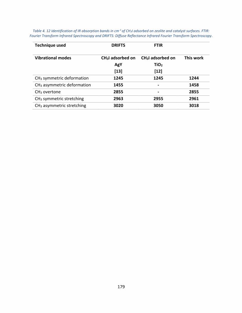
179

Table 4. 12 Identification of IR absorption bands in cm-1 of CH3I adsorbed on zeolite and catalyst surfaces. FTIR: Fourier Transform Infrared Spectroscopy and DRIFTS: Diffuse Reflectance Infrared Fourier Transform Spectroscopy.

Technique used DRIFTS FTIR

Vibrational modes CH3I adsorbed on

AgY

[13]

CH3I adsorbed on

TiO2

[12]

This work

CH3 symmetric deformation 1245 1245 1244

CH3 asymmetric deformation 1455 - 1458

CH3 overtone 2855 - 2855

CH3 symmetric stretching 2963 2955 2961

CH3 asymmetric stretching 3020 3050 3018

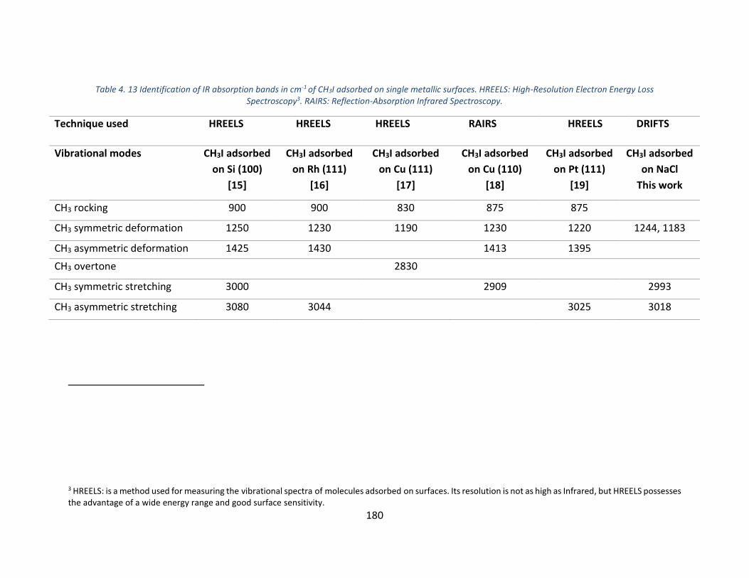
180

Table 4. 13 Identification of IR absorption bands in cm-1 of CH3I adsorbed on single metallic surfaces. HREELS: High-Resolution Electron Energy Loss

Spectroscopy3. RAIRS: Reflection-Absorption Infrared Spectroscopy.

Technique used HREELS HREELS HREELS RAIRS HREELS DRIFTS

Vibrational modes CH3I adsorbed

on Si (100)

[15]

CH3I adsorbed

on Rh (111)

[16]

CH3I adsorbed

on Cu (111)

[17]

CH3I adsorbed

on Cu (110)

[18]

CH3I adsorbed

on Pt (111)

[19]

CH3I adsorbed

on NaCl

This work

CH3 rocking 900 900 830 875 875

CH3 symmetric deformation 1250 1230 1190 1230 1220 1244, 1183

CH3 asymmetric deformation 1425 1430 1413 1395

CH3 overtone 2830


CH3 asymmetric stretching 3080 3044 3025 3018

3 HREELS: is a method used for measuring the vibrational spectra of molecules adsorbed on surfaces. Its resolution is not as high as Infrared, but HREELS possesses the advantage of a wide energy range and good surface sensitivity.

https://www.sciencedirect.com/topics/chemistry/vibrational-spectrum

https://www.sciencedirect.com/topics/engineering/adsorbed-molecule

181

4.2.1.2 Band assignment in the CH3 deformation region

The second region of interest is the CH3 deformation region (1500-900 cm-1), where bands at

1477, 1458, 1275, 1262, 1244, 1220, 1183, 1073 and 1024 cm-1 are observed (Figure 4.8).

Figure 4. 8 DRIFTS spectra in the 1500-900 cm-1 IR spectral range of NaCl surface exposed to 5 hours of CH3I (108mL.min-1, 1000 ppm) continuous flow at 296 K and 1 atm. Blue bands are CH3I adsorbed on NaCl, green

bands are CH3I in gas phase near the surface, and red bands are new bands.

Based on the literature (see Table 4.11), the bands at 1477 and 1262 cm-1 are assigned to the

CH3 asymmetric and symmetric deformations of gaseous CH3I.

The band at 1458 cm-1 is attributed to the CH3 asymmetric deformation of adsorbed CH3I as

reported in the literature with a red shift of 18 cm-1 compared to the gaseous CH3I band (see

Table 4.12). In this spectral region, the band centered at 1244 cm-1 evidenced some shoulders;

the decomposition of this band and the fitting procedure allows to extract the additional

bands at 1275, 1220 and 1183 cm-1 (see Figure 4.9).

182

Figure 4. 9 DRIFTS spectra in the 1305-1160 cm-1 IR spectral range of NaCl exposed to 5 hours of continuous

CH3I flow (108mL.min-1,1000 ppm) at 296 K and 1 atm decomposed with Gaussian function using FityK software.

It should be mentioned, that in the published spectra of adsorbed CH3I on solids, two similar

shoulders are clearly observed on the band centered at 1242 cm-1 (see Figure 4.10) although

they were not assigned.

Figure 4. 10 (a) DRIFTS spectrum of 23Ag/Y (2.5) after saturation with CH3I (1333 ppm/Ar) at 373 K [13] and (b)

IR spectrum IR spectrum of the TiO2 at 308 K in contact with 2 Torr of CH3I [12].

Similarly, the decomposition of the band centered at 1242 cm-1 of adsorbed CH3I on zeolites

[13] allows to extract IR bands at 1256, 1250, 1242, 1231 and 1216 cm-1 (Figure 4.11). Because

the adsorption process is different from zeolites to NaCl, a difference in IR bands shift related

to adsorbed CH3I molecules is expected.

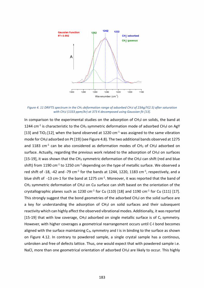
183

Figure 4. 11 DRIFTS spectrum in the CH3 deformation range of adsorbed CH3I of 23Ag/Y(2.5) after saturation with CH3I (1333 ppm/Ar) at 373 K decomposed using Gaussian fit [13].

In comparison to the experimental studies on the adsorption of CH3I on solids, the band at

1244 cm-1 is characteristic to the CH3 symmetric deformation mode of adsorbed CH3I on AgY

[13] and TiO2 [12], when the band observed at 1220 cm-1 was assigned to the same vibration

mode for CH3I adsorbed on Pt [19] (see Figure 4.8). The two additional bands observed at 1275

and 1183 cm-1 can be also considered as deformation modes of CH3 of CH3I adsorbed on

surface. Actually, regarding the previous work related to the adsorption of CH3I on surfaces

[15-19], it was shown that the CH3 symmetric deformation of the CH3I can shift (red and blue

shift) from 1190 cm-1 to 1250 cm-1 depending on the type of metallic surface. We observed a

red shift of -18, -42 and -79 cm-1 for the bands at 1244, 1220, 1183 cm-1, respectively, and a

blue shift of -13 cm-1 for the band at 1275 cm-1. Moreover, it was reported that the band of

CH3 symmetric deformation of CH3I on Cu surface can shift based on the orientation of the

crystallographic planes such as 1230 cm-1 for Cu (110) [18] and 1190 cm-1 for Cu (111) [17].

This strongly suggest that the bond geometries of the adsorbed CH3I on the solid surface are

a key for understanding the adsorption of CH3I on solid surfaces and their subsequent

reactivity which can highly affect the observed vibrational modes. Additionally, it was reported

[15-19] that with low coverage, CH3I adsorbed on single metallic surface is of Cs symmetry.

However, with higher coverages a geometrical rearrangement occurs until C‐I bond becomes

aligned with the surface maintaining C3v symmetry and I is in binding to the surface as shown

on Figure 4.12. In contrary to powdered sample, a single crystal sample has a continous,

unbroken and free of defects lattice. Thus, one would expect that with powdered sample i.e.

NaCl, more than one geometrical orientation of adsorbed CH3I are likely to occur. This highly

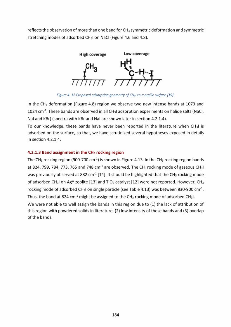
184

reflects the observation of more than one band for CH3 symmetric deformation and symmetric

stretching modes of adsorbed CH3I on NaCl (Figure 4.6 and 4.8).

Figure 4. 12 Proposed adsorption geometry of CH3I to metallic surface [19].

In the CH3 deformation (Figure 4.8) region we observe two new intense bands at 1073 and

1024 cm-1. These bands are observed in all CH3I adsorption experiments on halide salts (NaCl,

NaI and KBr) (spectra with KBr and NaI are shown later in section 4.2.1.4).

To our knowledge, these bands have never been reported in the literature when CH3I is

adsorbed on the surface, so that, we have scrutinized several hypotheses exposed in details

in section 4.2.1.4.

4.2.1.3 Band assignment in the CH3 rocking region

The CH3 rocking region (900-700 cm-1) is shown in Figure 4.13. In the CH3 rocking region bands

at 824, 799, 784, 773, 765 and 748 cm-1 are observed. The CH3 rocking mode of gaseous CH3I

was previously observed at 882 cm-1 [14]. It should be highlighted that the CH3 rocking mode

of adsorbed CH3I on AgY zeolite [13] and TiO2 catalyst [12] were not reported. However, CH3

rocking mode of adsorbed CH3I on single particle (see Table 4.13) was between 830-900 cm-1.

Thus, the band at 824 cm-1 might be assigned to the CH3 rocking mode of adsorbed CH3I.

We were not able to well assign the bands in this region due to (1) the lack of attribution of

this region with powdered solids in literature, (2) low intensity of these bands and (3) overlap

of the bands.

185


(108mL.min-1, 1000 ppm) continuous flow at 296 K and 1 atm. Bands in black are unassigned bands.

4.2.1.4 New bands attribution

As mentioned in the paragraph 4.2.1.2 two intense bands appears systematically at 1073 and

1024 cm-1 when NaCl surface was exposed to CH3I. Because these bands were not reported in

the literature for CH3I molecules adsorbed on surface, we have first hypothesized the

formation of new species.

As it can be seen in Table 4.14, the CH2 bending modes of adsorbed CH2I2 were observed at

1080 cm-1 on Rh [20] or 1030 cm-1 on Mo [21], but was not observed on Ag [22]. The CH2

symmetric stretching and rocking bands of CH2I2 on Mo [19] were observed at 2960 and 750

cm-1, respectively. Whereas, CH2 symmetric stretching and rocking bands of CH2I2 on Rh [20]

were observed at 2940 and 720 cm-1, respectively. Thus, the bands observed at 1073 cm-1,

(Figure 4.8), 1024 cm-1 (Figure 4.8) and 765 cm-1 (Figure 4.13) as well as the band at 2961 cm-

1 (Figure 4.6) could be assigned to CH2I or CH2I2.

186

Table 4. 14 IR absorption bands in cm-1 of CH2I2 in gas I(g) and adsorbed (ads). HREELS: High-Resolution

Electron Energy Loss Spectroscopy.

Technique used Theoretical

calculation

HREELS HREELS

Vibrational modes CH2I2(g)

[23]

CH2I2 adsorbed on

Mo [21]

CH2I2 adsorbed on

Rh [20]

CH2 rocking 714 750 720

CH2 twisting 1028

CH2 bending 1349 1030 1080

CH2 wagging 1103 1100

CH2 symmetric deformation 1390 1350


CH2 asymmetric stretching 3047

However, the formation of such species requires a reaction of CH3I on the surface. The

dissociation of CH3I was described on metallic surface only and at 2 × 10−10 mbar and 250-300

K [24 and reference herein]. Therefore, the dissociation of CH3I on NaCl and formation of CH2I2

under ambient conditions (296 K and 1 atm) is unlikely.

On the other hand, in gas phase the experimental study of the micro solvated reaction of OH-

(H2O) with CH3I indicated the formation of CH2I- by the following proton transfer reaction at

100 K [25]:

OH−(H2O) +CH3I → CH2I− (H2O) +H2O [R4-1]

Additionally, the kinetic experimental study of CH3I reactivity in gas phase at high temperature

(604 K) showed that CH2I2 could be formed by the following reaction [26]:

2CH3I → CH2I2 +CH4 [R4-2]

For our experimental conditions the gas phase of CH3I gas flow was under ambient conditions

(296 K and 1 atm) and CH4 was not detected in any recorded spectrum. Moreover, there is no

possible exitence of OH- in our experimental conditions. Thus, the formation of CH2I2 or CH2I

by the above gas phase mechanisms and then adsorption on NaCl surface is discarded.

The bands at 1073 and 2981 cm-1 can also contributes to the CO stretching mode and CH3

symmetric stretching mode of CH3O adsorbed on surface, respectively, as described previously

[13] (see Table 4.15).

187

Table 4. 15 IR absorption bands in cm-1 of CH3OH observed from the adsorption of CH3I on Zeolites [13]. DRIFTS: Diffuse Reflectance Infrared Fourier Transform Spectroscopy.

Technique used DRIFTS

Vibrational modes CH3O adsorbed on AgY

[13]

CO stretching 1065

CH3 rocking 1120

CH3 symmetric stretching 2870

CH3 asymmetric stretching 2967

It has been shown that a fraction of the adsorbed CH3I on zeolites (AgY) may dissociate and

yield to the formation of methoxy species at 373 K through the following reaction [13]:

CH3I + Ag+ + [SiOAl]- → AgI + SiOCH3Al [R4-3]

However, halide solids surfaces are not reactive as zeolites or Ag surfaces and the experiments

need to be performed at 373 K.

The 2981, 2961, 1458 and 1024 cm-1 bands observed might be consistent with the CH3

symmetric stretching and rocking modes, respectively of CH3Cl formed on surface regarding

previous results [27-30] (see Table 4.16).

Table 4. 16 IR absorption bands in cm-1 of CH3Cl in gas (g) and adsorbed (ads). IRAS: Infrared Reflection Absorption Spectroscopy, FTIR: Fourier Transform Infrared Spectroscopy, RAIRS: Reflection Absorption Infrared

Spectroscopy.

Technique used FTIR IRAS FTIR FTIR RAIRS

Vibrational modes CH3Cl(g)

[28]

CH3Cl

adsorbed

on Cu

[27]

CH3Cl

adsorbed

on PdSiO2

[29]

CH3Cl

adsorbed

on Mo2C

[28]

CH3Cl

adsorbed

on Pt

[30]

CH3 rocking 1015 1013 1022

CH3 symmetric deformation 1355 1336 1350 1350 1336

CH3 degenerate deformation 1455 1436 1433 1444 1438

CH3 overtone 2879 2860

CH3 symmetric stretching 2966 2954 2980 2963 2953

188

There is a considerable interest in understanding the atomic level of halide substitution

reactions [31-33] as following:

X-+ CH3Y → CH3X +Y- [R4-4]

The SN2 halide substition reaction of hydrated chloride with methyl iodide was investigated

by simulations and the reaction mechanism is presented in Figure 4.14 [33]. Compared to the

unsolvated reaction of Cl- with CH3I, the addition of water slightly lowers the reaction

possibility and the rate constant is correspondingly reduced [33]. Therefore, this substitution

reaction obtained with calculations suggests a probable exchange between Cl- of NaCl and I-

of CH3I, more favored under dry conditions.

Figure 4. 14 The direct and indirect mechanism of the Cl-(H2O) +CH3I substitution reaction from [33].

However, in our experiment we are in solid phase. Therefore, to prove or not the exchange

mechanism between I- and Cl- and eventually Br- in solid phase, experiments were conducted

by the continuous flow of CH3I (108mL.min-1, 1000 ppm) for 1 hour on NaI and KBr solid

particles at 296 K and 1 atm (section 4.1.4.1, Table 4.7). The zoomed spectrum in the range

1400-900 cm-1 are shown in Figure 4.15 and compared with the DRIFTS spectrum of NaCl

exposed to CH3I in the same conditions.

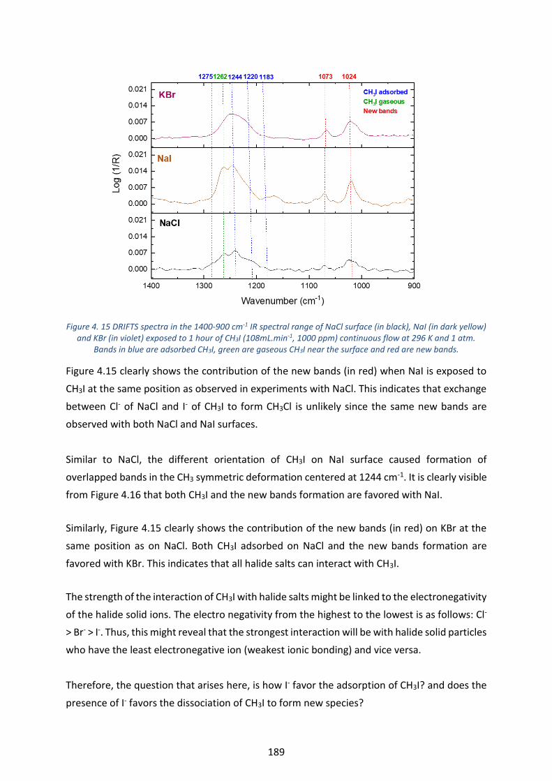
189

Figure 4. 15 DRIFTS spectra in the 1400-900 cm-1 IR spectral range of NaCl surface (in black), NaI (in dark yellow) and KBr (in violet) exposed to 1 hour of CH3I (108mL.min-1, 1000 ppm) continuous flow at 296 K and 1 atm.

Bands in blue are adsorbed CH3I, green are gaseous CH3I near the surface and red are new bands.

Figure 4.15 clearly shows the contribution of the new bands (in red) when NaI is exposed to

CH3I at the same position as observed in experiments with NaCl. This indicates that exchange

between Cl- of NaCl and I- of CH3I to form CH3Cl is unlikely since the same new bands are

observed with both NaCl and NaI surfaces.

Similar to NaCl, the different orientation of CH3I on NaI surface caused formation of

overlapped bands in the CH3 symmetric deformation centered at 1244 cm-1. It is clearly visible

from Figure 4.16 that both CH3I and the new bands formation are favored with NaI.

Similarly, Figure 4.15 clearly shows the contribution of the new bands (in red) on KBr at the

same position as on NaCl. Both CH3I adsorbed on NaCl and the new bands formation are

favored with KBr. This indicates that all halide salts can interact with CH3I.

The strength of the interaction of CH3I with halide salts might be linked to the electronegativity

of the halide solid ions. The electro negativity from the highest to the lowest is as follows: Cl-

> Br- > I-. Thus, this might reveal that the strongest interaction will be with halide solid particles

who have the least electronegative ion (weakest ionic bonding) and vice versa.

Therefore, the question that arises here, is how I- favor the adsorption of CH3I? and does the

presence of I- favors the dissociation of CH3I to form new species?

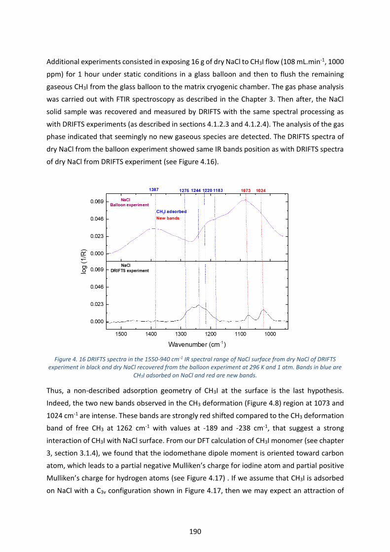
190

Additional experiments consisted in exposing 16 g of dry NaCl to CH3I flow (108 mL.min-1, 1000

ppm) for 1 hour under static conditions in a glass balloon and then to flush the remaining

gaseous CH3I from the glass balloon to the matrix cryogenic chamber. The gas phase analysis

was carried out with FTIR spectroscopy as described in the Chapter 3. Then after, the NaCl

solid sample was recovered and measured by DRIFTS with the same spectral processing as

with DRIFTS experiments (as described in sections 4.1.2.3 and 4.1.2.4). The analysis of the gas

phase indicated that seemingly no new gaseous species are detected. The DRIFTS spectra of

dry NaCl from the balloon experiment showed same IR bands position as with DRIFTS spectra

of dry NaCl from DRIFTS experiment (see Figure 4.16).

Figure 4. 16 DRIFTS spectra in the 1550-940 cm-1 IR spectral range of NaCl surface from dry NaCl of DRIFTS

experiment in black and dry NaCl recovered from the balloon experiment at 296 K and 1 atm. Bands in blue are CH3I adsorbed on NaCl and red are new bands.

Thus, a non-described adsorption geometry of CH3I at the surface is the last hypothesis.

Indeed, the two new bands observed in the CH3 deformation (Figure 4.8) region at 1073 and

1024 cm-1 are intense. These bands are strongly red shifted compared to the CH3 deformation

band of free CH3 at 1262 cm-1 with values at -189 and -238 cm-1, that suggest a strong

interaction of CH3I with NaCl surface. From our DFT calculation of CH3I monomer (see chapter

3, section 3.1.4), we found that the iodomethane dipole moment is oriented toward carbon

atom, which leads to a partial negative Mulliken’s charge for iodine atom and partial positive

Mulliken’s charge for hydrogen atoms (see Figure 4.17) . If we assume that CH3I is adsorbed

on NaCl with a C3v configuration shown in Figure 4.17, then we may expect an attraction of

191

hydrogen atoms toward chloride atoms at the surface of NaCl due to charge difference. The

observation of two bands for this configuration probably reflects the non-equivalent hydrogen

atoms attached to the Cl on NaCl surface (see Figure 4.17).

Finally, as stated previously, the electronegativity of chloride atom is higher than iodine atom,

which might reveal a strongest interaction of hydrogen atom with iodine ion (weakest ionic

bonding).

Figure 4. 17 Scheme of the CH3I adsorption on NaCl representing the bands at 1073 and 1024 cm-1. Mulliken

charges from DFT calculation perfomed using ωB97XD/aug-cc-pVTZ-PP.

4.2.1.5 Summary of bands assignment

Table 4.17 summarizes the tentative bands assignment observed from the interaction of CH3I

on dry NaCl.

Both CH3I gaseous near the surface and adsorbed CH3I are observable. It seems reasonable to

hypothesize that CH3I can adsorb on NaCl in different geometrical configuration that can result

in apparent frequencies in the CH3 stretching and deformation region. The new intense bands

are assigned to the unique C3v geometrical adsorption of CH3I wich occurs specifically with

halide salt surfaces. This geometry was not described in the literature.

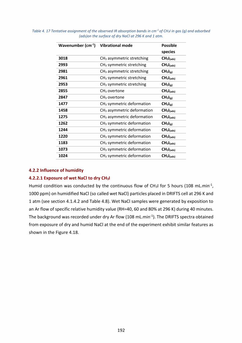
192

Table 4. 17 Tentative assignment of the observed IR absorption bands in cm-1 of CH3I in gas (g) and adsorbed (ads)on the surface of dry NaCl at 296 K and 1 atm.

Wavenumber (cm-1) Vibrational mode Possible

species

3018 CH3 asymmetric stretching CH3I(ads)

2993 CH3 symmetric stretching CH3I(ads)

2981 CH3 asymmetric stretching CH3I(g)

2961 CH3 symmetric stretching CH3I(ads)

2953 CH3 symmetric stretching CH3I(g)

2855 CH3 overtone CH3I(ads)

2847 CH3 overtone CH3I(g)

1477 CH3 symmetric deformation CH3I(g)

1458 CH3 asymmetric deformation CH3I(ads)

1275 CH3 asymmetric deformation CH3I(ads)

1262 CH3 symmetric deformation CH3I(g)

1244 CH3 symmetric deformation CH3I(ads)





4.2.2 Influence of humidity

4.2.2.1 Exposure of wet NaCl to dry CH3I

Humid condition was conducted by the continuous flow of CH3I for 5 hours (108 mL.min-1,

1000 ppm) on humidified NaCl (so called wet NaCl) particles placed in DRIFTS cell at 296 K and

1 atm (see section 4.1.4.2 and Table 4.8). Wet NaCl samples were generated by exposition to

an Ar flow of specific relative humidity value (RH=40, 60 and 80% at 296 K) during 40 minutes.

The background was recorded under dry Ar flow (108 mL.min-1). The DRIFTS spectra obtained

from exposure of dry and humid NaCl at the end of the experiment exhibit similar features as

shown in the Figure 4.18.

193

Figure 4. 18 DRIFTS spectra in the 4000-700 cm-1 of dry and wet NaCl surface exposed to 5 hours of CH3I (108mL.min-1, 1000 ppm) continuous flow at 296 K and 1 atm.

The DRIFTS spectra in the zoomed CH3 stretching (3100-2800 cm-1), CH3 deformation and

rocking (1500-750 cm-1) spectral regions are shown in Figures 4.19 and 4.20, respectively. As

stated previously, when comparing the DRIFTS spectra of dry and humid NaCl at the end of

the experiment, no major difference is observed (Figure 4.19 and 4.20).

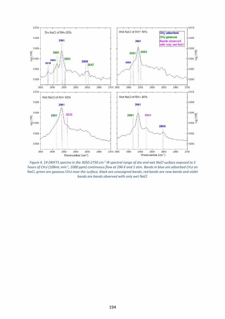
194

Figure 4. 19 DRIFTS spectra in the 3050-2750 cm-1 IR spectral range of dry and wet NaCl surface exposed to 5

hours of CH3I (108mL.min-1, 1000 ppm) continuous flow at 296 K and 1 atm. Bands in blue are adsorbed CH3I on NaCI, green are gaseous CH3I near the surface, black are unassigned bands, red bands are new bands and violet

bands are bands observed with only wet NaCl.

195

Figure 4. 20 DRIFTS spectra in the 1500-700 cm-1 IR spectral range of dry and wet NaCl surface exposed to 5 hours of CH3I (108mL.min-1, 1000 ppm) continuous flow at 296 K and 1 atm. Bands in blue are adsorbed CH3I on

NaCI, green are gaseous CH3I near the surface, black are unassigned bands, red are new bands and violet are bands observed with only wet NaCl.

The main IR bands related to both gaseous CH3I at the NaCl surface and to the adsorbed CH3I

are observed for the wet NaCl experiments, whatever the RH values (Figure 4.19 and Figure

4.20). The new bands at 1073 and 1024 cm-1 are also observable and do not present any major

variation with the increasing RH.

Additional bands with a low intensity are observed at 2935 and 2924 cm-1 when NaCl is

exposed to RH=60% and RH=80%, respectively (see Figure 4.19). Compared to CH3I adsorbed

on various surfaces (see Tables 4.12 and 4.13), both 2924 and 2935 cm-1 can be assigned to

the CH3 symmetric stretching mode of adsorbed CH3I.

Additional bands with a low intensity are observed at 897 and 870 cm-1 when NaCl is exposed

to RH, the intensity of these bands increase with the RH value and are clearly seen for RH=80%.

The bands at 899 and 870 cm-1 can be assigned to the CH3 rocking of adsorbed CH3I (see Table

4.13), respectively.

196

4.2.2.2 Influence of water on the CH3I desorption

To investigate the effect of water on the adsorbed CH3I, a wet Ar was flowed continuously

(108mL.min-1) for 40 minutes under RH=50% after 5 hours of continuous exposure of dry NaCl

to CH3I (1000ppm, 108mL.min-1) (see section 4.1.4.2 and Table 4.9). The DRIFTS spectra in the

zoomed CH3 deformation and rocking (1350-700 cm-1) spectral regions are shown in Figure

4.21.

Figure 4. 21 DRIFTS spectra in the 1350-750 cm-1 IR spectral range of dry NaCl surface (RH=20%) exposed to 5

hours of continuous CH3I flow (108mL.min-1, 1000 ppm) and then to 40 minutes of wet Ar continuous flow (RH=50%) at 296 K and 1 atm. Bands in blue are adsorbed CH3I on NaCl, green are gaseous CH3I near the

surface, black are unassigned bands and red bands are new bands.

We did not observe any major difference under wet Ar flow (RH=50%), except that the band

at 1262 cm-1 corresponding to CH3I in gas phase seems to disappear (Figure 4.21).

4.3. Time evolution of CH3I on NaCl surface during CH3I exposure, static and Ar

flow phases

In this section, the time evolution of adsorbed methyl iodide on NaCl surface is discussed. CH3I

exposure phase, featuring exposure of NaCl to a continuous flow of gaseous CH3I, static phase

featuring static condition and continuous flow of pure argon are considered. Discussion mainly

focusses on the CH3I spectral evolution in deformation region featuring the most intense

adsorption bands (1400-900 cm-1). The kinetic parameters of methyl iodide adsorption in dry

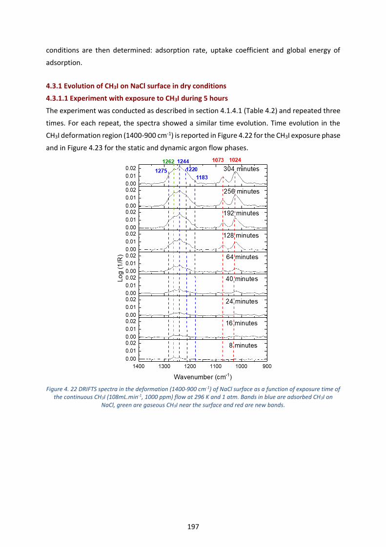
197

conditions are then determined: adsorption rate, uptake coefficient and global energy of

adsorption.

4.3.1 Evolution of CH3I on NaCl surface in dry conditions

4.3.1.1 Experiment with exposure to CH3I during 5 hours

The experiment was conducted as described in section 4.1.4.1 (Table 4.2) and repeated three

times. For each repeat, the spectra showed a similar time evolution. Time evolution in the

CH3I deformation region (1400-900 cm-1) is reported in Figure 4.22 for the CH3I exposure phase

and in Figure 4.23 for the static and dynamic argon flow phases.

Figure 4. 22 DRIFTS spectra in the deformation (1400-900 cm-1) of NaCl surface as a function of exposure time of

the continuous CH3I (108mL.min-1, 1000 ppm) flow at 296 K and 1 atm. Bands in blue are adsorbed CH3I on NaCl, green are gaseous CH3I near the surface and red are new bands.

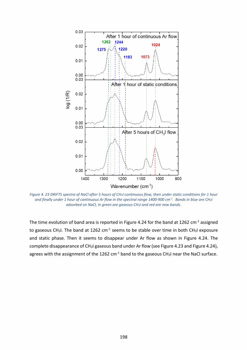
198

Figure 4. 23 DRIFTS spectra of NaCl after 5 hours of CH3I continuous flow, then under static conditions for 1 hour

and finally under 1 hour of continuous Ar flow in the spectral range 1400-900 cm-1. Bands in blue are CH3I adsorbed on NaCl, in green are gaseous CH3I and red are new bands.

The time evolution of band area is reported in Figure 4.24 for the band at 1262 cm-1 assigned

to gaseous CH3I. The band at 1262 cm-1 seems to be stable over time in both CH3I exposure

and static phase. Then it seems to disappear under Ar flow as shown in Figure 4.24. The

complete disappearance of CH3I gaseous band under Ar flow (see Figure 4.23 and Figure 4.24),

agrees with the assignment of the 1262 cm-1 band to the gaseous CH3I near the NaCl surface.

199

Figure 4. 24 Area of the 1262 cm-1 as a function of time during CH3I exposure, static phase and Ar flow phases. The isolated bands are determined using Gaussian fit function. Exposure phase denotes the continuous flow of 108 mL.min-1 of CH3I (1000 ppm) on NaCl. The static phase denotes the static conditions after 5 hours of CH3I

flow and Ar flow phase denotes the continuous Ar flow after the static conditions.

In Figure 4.22, we observed an increase of the IR bands intensity of the CH3I adsorbed bands

with increasing the exposure time. CH3I adsorbed bands at 1244 and 1220 cm-1 clearly

appeared as soon as the first spectrum is recorded i.e; at 8 minutes. Shoulder bands of

adsorbed CH3I at 1275 and 1183 cm-1 started to appear after 16 minutes.

Considering that the bands at 1275, 1244, 1220 and 1183 cm-1 are markers of CH3I adsorption,

thus the evolution of the sum of these band area has been considered in Figure 4.25. No

apparent desorption was observed for the adsorbed CH3I bands by stopping the flow of CH3I

and keeping the cell under static conditions or by continuous flow of Ar as also seen in Figure

4.23. A slight evolution of the CH3I adsorption band area versus time is observed when the

surface is exposed to a continuous Ar flow, that may be explained by the gas phase released.

The new intense bands at 1073 and 1024 cm-1 are clearly seen after 40 and 24 minutes,

respectively (see Figure 4.22). Figure 4.26 displays the area time evolution of the new bands

at 1073 and 1024 cm-1 during CH3I exposure, static and Ar flow phases.

0 50 100 150 200 250 300 350 400 450

-0.2

0.0

0.2

0.4

0.6

Ar flow phase

Static phaseCH3I exposure phase

Are

a (

arb

itra

ry u

nit)

Time (minutes)

CH3I gaseous (1262 cm-1)

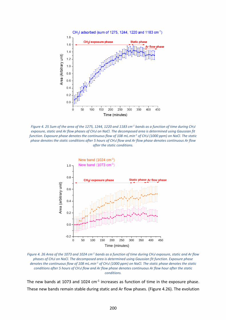
200

Figure 4. 25 Sum of the area of the 1275, 1244, 1220 and 1183 cm-1 bands as a function of time during CH3I exposure, static and Ar flow phases of CH3I on NaCl. The decomposed area is determined using Gaussian fit

function. Exposure phase denotes the continuous flow of 108 mL.min-1 of CH3I (1000 ppm) on NaCl. The static phase denotes the static conditions after 5 hours of CH3I flow and Ar flow phase denotes continuous Ar flow

after the static conditions.

Figure 4. 26 Area of the 1073 and 1024 cm-1 bands as a function of time during CH3I exposure, static and Ar flow

phases of CH3I on NaCl. The decomposed area is determined using Gaussian fit function. Exposure phase denotes the continuous flow of 108 mL.min-1 of CH3I (1000 ppm) on NaCl. The static phase denotes the static

conditions after 5 hours of CH3I flow and Ar flow phase denotes continuous Ar flow hour after the static conditions.

The new bands at 1073 and 1024 cm-1 increases as function of time in the exposure phase.

These new bands remain stable during static and Ar flow phases. (Figure 4.26). The evolution

0 50 100 150 200 250 300 350 400 450

-0.2

0.0

0.2

0.4

0.6

0.8

1.0

New band (1024 cm-1)

New band (1073 cm-1)

Are

a (

arb

itra

ry u

nit)

Time (minutes)

Ar flow phaseStatic phaseCH3I exposure phase

201

of these bands is directly correlated with the well identified bands related to CH3I adsorption

as seen in Figure 4.27. Thus, in the following sections, the sum of the band areas at 1275,

1244, 1220, 1183, 1073 and 1024 cm-1 will be considered to quantify CH3I adsorption on NaCl

(i.e. all the bands related to absorbed CH3 in the CH3 spectral deformation region).

Figure 4. 27 Time evolution of the band area ratio during the CH3I exposure phase: ratio of the Area of the new

band (1073 and 1024 cm-1 respectively)/ Area of theCH3I ads (sum of the area 1275, 1244, 1220 and 1183 cm-1 bands).

During the CH3I exposure phase, the evolution of the adsorption versus time can be

interpolated by a linear function. The rate of methyl iodide adsorption can then be determined

from the linear interpolation of the adsorption band area curve versus time as shown in Figure

4.28.

202


exposure phase of CH3I on NaCl, repeated three times. The decomposed area of 1275, 1244, 1220 and 1183 cm-1 is determined using Gaussian fit function. Exposure phase denotes the continuous flow of 108 mL.min-1 of CH3I

(1000 ppm) on NaCl. A: area and t= time.

It is observable from Figure 4.28 that the rate of adsorption of CH3I is repeatable. The average

rate of adsorption was found to be (6.91 ± 0.33) × 10-3 arbitrary unit.min-1.

During the static and Ar flow phases, the slight decrease which is observed (Figures 4.25 and

4.26) can be interpreted as a desorption of methyl iodide from the NaCl surface. An estimated

calculation of the loss have been conducted as following and results are shown in Table 4.18:

1- Determination of CH3I adsorbed band area of the exposure phase (Aexp) after 5

hours of CH3I continuous flow (end of exposure phase, 304 minutes in Figures 4.25

and 4.26). Area is the sum of the decomposed bands area at 1275, 1244, 1220,

1183, 1073 and 1024 cm-1.

2- Determination of average area of the CH3I adsorbed band during 1 hour of static

conditions (Astatic) (see Figures 4.25 and 4.26, static phase). Area is the sum of the

decomposed bands area at 1275, 1244, 1220, 1183, 1073 and 1024 cm-1.

0 50 100 150 200 250 300 350

0.0

1.1

2.2

0.00

0.88

1.76

2.64

0.0

1.1

2.2

Repeat 2

Repeat 1

A= (7.10 0.15) 10-3 t + 0.28

R2= 0.98

A= (6.72 0.28) 10-3 t + 0.27

R2= 0.94

A= (6.91 0.23) 10-3 t + 0.19

R2= 0.96

Time (minutes)

Are

a (

arb

itra

ry u

ni)

Repeat 3

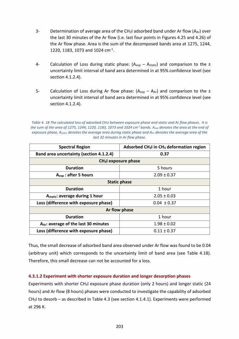
203

3- Determination of average area of the CH3I adsorbed band under Ar flow (AAr) over

the last 30 minutes of the Ar flow (i.e. last four points in Figures 4.25 and 4.26) of

the Ar flow phase. Area is the sum of the decomposed bands area at 1275, 1244,

1220, 1183, 1073 and 1024 cm-1.

4- Calculation of Loss during static phase: (Aexp – Astatic) and comparison to the ±

uncertainty limit interval of band aera determined in at 95% confidence level (see

section 4.1.2.4).

5- Calculation of Loss during Ar flow phase: (Aexp – AAr) and comparison to the ±

uncertainty limit interval of band aera determined in at 95% confidence level (see

section 4.1.2.4).

Table 4. 18 The calculated loss of adsorbed CH3I between exposure phase and static and Ar flow phases. A is the sum of the area of 1275, 1244, 1220, 1183, 1073 and 1024 cm-1 bands. Aexp denotes the area at the end of exposure phase, Astatic denotes the average area during static phase and AAr denotes the average area of the

last 32 minutes in Ar flow phase.

Spectral Region Adsorbed CH3I in CH3 deformation region

Band area uncertainty (section 4.1.2.4) 0.37

CH3I exposure phase

Duration 5 hours

Aexp : after 5 hours 2.09 ± 0.37

Static phase

Duration 1 hour

Astatic: average during 1 hour 2.05 ± 0.03

Loss (difference with exposure phase) 0.04 ± 0.37

Ar flow phase

Duration 1 hour

AAr: average of the last 30 minutes 1.98 ± 0.02

Loss (difference with exposure phase) 0.11 ± 0.37

Thus, the small decrease of adsorbed band area observed under Ar flow was found to be 0.04

(arbitrary unit) which corresponds to the uncertainty limit of band area (see Table 4.18).

Therefore, this small decrease can not be accounted for a loss.

4.3.1.2 Experiment with shorter exposure duration and longer desorption phases

Experiments with shorter CH3I exposure phase duration (only 2 hours) and longer static (24

hours) and Ar flow (8 hours) phases were conducted to investigate the capability of adsorbed

CH3I to desorb – as described in Table 4.3 (see section 4.1.4.1). Experiments were performed

at 296 K.

204

No desorption is observed for the static and continuous Ar flow conditions as shown in Figure

4.29 and Table 4.19. This indicate that the CH3I is strongly adsorbed on NaCl.

Figure 4. 29 DRIFTS spectra of NaCl after 2 hours of CH3I continuous flow, then after static conditions for 24

hours and finally after 8 hours of Ar flow in the 1400-700 cm-1 spectral region. Bands in blue are adsorbed CH3I, in green are gaseous CH3I and red bands are new bands.

205

Table 4. 19 The calculated loss of adsorbed CH3I between exposure phase and static and Ar flow phases. A is the sum of area of 1275, 1244, 1220, 1183, 1073 and 1024 cm-1 bands. Aexp denotes the area at the end of exposure phase, Astatic denotes the average area of the last 32 minutes in static phase and AAr denotes the

average area of the last 32 minutes in Ar flow phase.



CH3I exposure phase

Duration 2 hours

Aexp : after 2 hours 1.30 ± 0.37

Static phase

Duration 24 hours

Astatic: average of the last 30 minutes 1.30 ± 0.02

Loss (difference with exposure phase) 0

Ar flow phase

Duration 8 hours

AAr: average of the last 30 minutes 1.34 ± 0.02

Loss (difference with exposure phase) 0

4.3.1.3 Experiment by increasing temperature during the Ar flow phase

Experiment conditions are reported in Table 4.4 (section 4.1.4.1). Firstly, the duration of the

exposure phase was shorten to one hour, then the static phase lasted 4 hours. These two

phases were performed at 296K. The dynamic argon phase lasted for one hour at 296K and

then the NaCl sample was heated at a rate of 3K/min until 623K – still under argon flow in

order to activate the desorption process (if any). Spectra recording was performed at 373 K,

473 K and 623K. Spectra are displayed in Figure 4.30 (deformation spectral zone). Compared

to the spectrum recorded at the end of the exposure phase, no significant changes are

observed at the end of the static phase nor at the end of the Ar flow phase at 296 K –

consistently with previous tests. At 373 K and 473 K, the spectrum shows a small decrease in

the bands intensity (Figure 4.30). However, this decrease is unmeasurable as shown in Table

4.20. Whereas, at 623 K the spectrum is too perturbed for a reliable interpretation (Figure

4.30).

Therefore, the non-desorbing capability of CH3I under different static, Ar flow and

temperature conditions suggests that CH3I is strongly bonded to NaCl and that the CH3I uptake

by NaCl is occurring via chemisorption process.

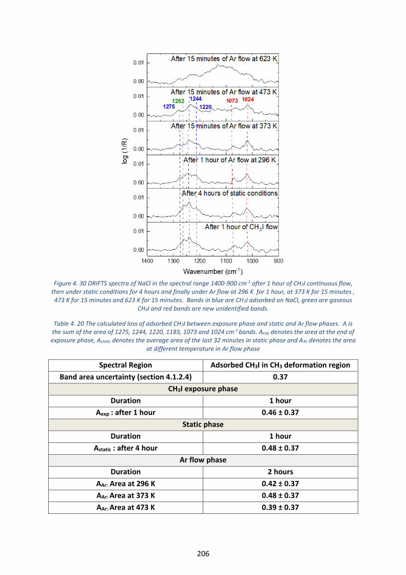
206

Figure 4. 30 DRIFTS spectra of NaCl in the spectral range 1400-900 cm-1 after 1 hour of CH3I continuous flow,

then under static conditions for 4 hours and finally under Ar flow at 296 K for 1 hour, at 373 K for 15 minutes , 473 K for 15 minutes and 623 K for 15 minutes. Bands in blue are CH3I adsorbed on NaCl, green are gaseous

CH3I and red bands are new unidentified bands.

Table 4. 20 The calculated loss of adsorbed CH3I between exposure phase and static and Ar flow phases. A is the sum of the area of 1275, 1244, 1220, 1183, 1073 and 1024 cm-1 bands. Aexp denotes the area at the end of exposure phase, Astatic denotes the average area of the last 32 minutes in static phase and AAr denotes the area

at different temperature in Ar flow phase



CH3I exposure phase

Duration 1 hour

Aexp : after 1 hour 0.46 ± 0.37

Static phase

Duration 1 hour

Astatic : after 4 hour 0.48 ± 0.37

Ar flow phase

Duration 2 hours

AAr: Area at 296 K 0.42 ± 0.37

AAr: Area at 373 K 0.48 ± 0.37

AAr: Area at 473 K 0.39 ± 0.37

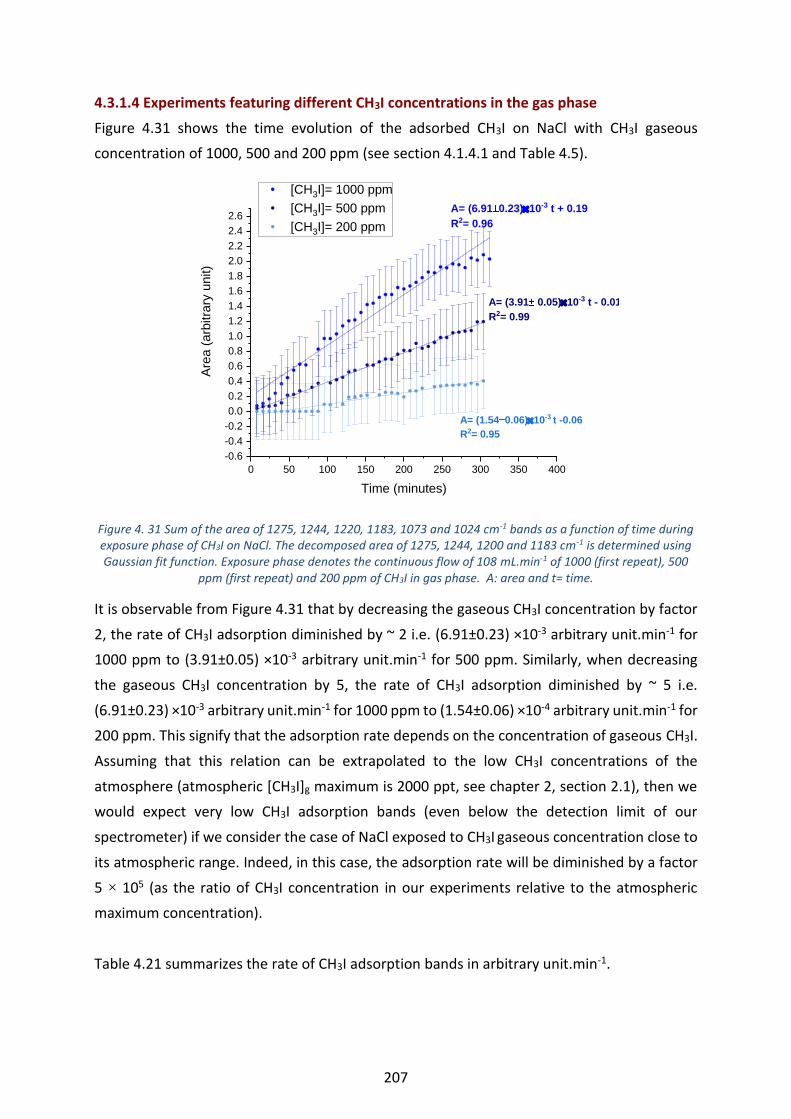
207

4.3.1.4 Experiments featuring different CH3I concentrations in the gas phase

Figure 4.31 shows the time evolution of the adsorbed CH3I on NaCl with CH3I gaseous

concentration of 1000, 500 and 200 ppm (see section 4.1.4.1 and Table 4.5).

Figure 4. 31 Sum of the area of 1275, 1244, 1220, 1183, 1073 and 1024 cm-1 bands as a function of time during exposure phase of CH3I on NaCl. The decomposed area of 1275, 1244, 1200 and 1183 cm-1 is determined using Gaussian fit function. Exposure phase denotes the continuous flow of 108 mL.min-1 of 1000 (first repeat), 500

ppm (first repeat) and 200 ppm of CH3I in gas phase. A: area and t= time.

It is observable from Figure 4.31 that by decreasing the gaseous CH3I concentration by factor

2, the rate of CH3I adsorption diminished by ~ 2 i.e. (6.91±0.23) ×10-3 arbitrary unit.min-1 for

1000 ppm to (3.91±0.05) ×10-3 arbitrary unit.min-1 for 500 ppm. Similarly, when decreasing

the gaseous CH3I concentration by 5, the rate of CH3I adsorption diminished by ~ 5 i.e.

(6.91±0.23) ×10-3 arbitrary unit.min-1 for 1000 ppm to (1.54±0.06) ×10-4 arbitrary unit.min-1 for

200 ppm. This signify that the adsorption rate depends on the concentration of gaseous CH3I.

Assuming that this relation can be extrapolated to the low CH3I concentrations of the

atmosphere (atmospheric [CH3I]g maximum is 2000 ppt, see chapter 2, section 2.1), then we

would expect very low CH3I adsorption bands (even below the detection limit of our

spectrometer) if we consider the case of NaCl exposed to CH3I gaseous concentration close to

its atmospheric range. Indeed, in this case, the adsorption rate will be diminished by a factor

5 × 105 (as the ratio of CH3I concentration in our experiments relative to the atmospheric

maximum concentration).

Table 4.21 summarizes the rate of CH3I adsorption bands in arbitrary unit.min-1.

0 50 100 150 200 250 300 350 400

-0.6

-0.4

-0.2

0.0

0.2

0.4

0.6

0.8

1.0

1.2

1.4

1.6

1.8

2.0

2.2

2.4

2.6A

rea (

arb

itra

ry u

nit)

Time (minutes)

[CH3I]= 1000 ppm

[CH3I]= 500 ppm

[CH3I]= 200 ppm

A= (6.91 0.23)10-3 t + 0.19

R2= 0.96

A= (3.91 0.05)10-3 t - 0.01

R2= 0.99

A= (1.54 0.06)10-3 t -0.06

R2= 0.95

208

Table 4. 21 Summary of the rate in arbitrary unit.min-1 versus CH3I concentration in gas phase. The sum of the area of the bands at 1275, 1244, 1220 and 1183 cm -1 represent the adsorbed CH3I referenced in the literature. The bands at 1073 and 1024 cm-1 represent the adsorbed C3v CH3I (new adsorption geometry). The last column (sum of the area of all CH3 bands in the deformation region related to adsorbed CH3I) represent the total CH3I

adsorbed on NaCl. The rate is determined from the slope of Area (arbitrary units) versus time (minutes).

Adsorption bands

Band Sum of (1275 ,1244,

1220, 1183 cm-1)

1024 cm-1 1073 cm-1 Sum of

(1275 ,1244, 1220,

1183, 1073, 1024

cm-1)

[CH3I]gaseous

(ppm)

Rate in arbitrary unit.min-1

(slope of area versus time)

1000 (4.69±0.30) ×10-3 (1.60±0.08) ×10-3 (6.16±0.27) ×10-4 (6.91±0.23) ×10-3

500 (2.39 ±0.06) ×10-3 (1.07±0.03) ×10-3 (4.27±0.14) ×10-4 (3.91 ±0.05) ×10-3

200 (9.80±0.86) ×10-4 (3.92±0.18) ×10-4 (1.76±0.14) ×10-4 (1.54±0.06) ×10-3

Further, the rate order of adsorbed CH3I on NaCl can be determined from the slope of the bi-

logarithmic plot of rate versus the concentration of CH3I in gas phase [6, 8, 34]. Slope of the

bi-logarithmic plot of the rate of the sum of 1275, 1244, 1220 and 1183 cm-1 bands is

(9.34±0.31) ×10-1 as shown in Figure 4.32. To recall 1073 and 1024 cm-1 represent the CH3I C3v

geometrical configuration on NaCl. The bi-logarithmic plot of rate of adsorption bands at 1073

and 1024 cm-1 versus CH3I concentration gives a slope of (8.26±1.41) ×10-1 and (8.89±1.46)

×10-1, respectively (see Figure 4.32). Finally, the slope of the bi-logarithmic plot of the rate of

the sum of 1275, 1244, 1220, 1183, 1073 and 1024 cm-1 bands is (8.41±0.54) ×10-1 as shown

in Figure 4.32. This indicate that the different geometrical configuration of adsorbed CH3I on

NaCl follows first order rate.

209

Figure 4. 32 Double log curve of rate of adsorbed CH3I (sum of band aera at 1275, 1244, 1220, 1183 cm-1 ), new

band area at 1073 cm-1 and 1024 cm-1, and sum of all CH3 adsorption related bands in the CH3 spectral deformation region (sum of band area at 1275, 1244, 1220, 1183, 1073 and 1024 cm-1) versus CH3I gaseous

concentration at 1000, 500, 200 ppm.

4.3.1.5 Experiment featuring variation in contact time

The influence of the contact time on the adsorption rate was investigated. The experiments

featured a CH3I gas phase concentration of 500 ppm and contact time between the gas flow

and the solid bed of 55 ms and 27 ms respectively (see section 4.1.4.1, Table 4.6).

A similar adsorption rate is observed as shown in Figure 4.33: (3.21 ±0.25) ×10-3 arbitrary

unit.min-1 for a contact time of 27 ms and (3.90 ±0.05) ×10-3 arbitrary unit.min-1 for a contact

time of 55 ms. This shows that the contact time has no effect on the evolution of the adsorbed

CH3I as expected.

2.4 2.6 2.8 3.0 3.2

-4.0

-3.5

-3.0

-2.5

-2.0

Sum of (1275, 1244, 1220, 1183 cm-1)

1073 cm-1

1024 cm-1

Sum of (1275, 1244, 1220, 1183, 1073, 1024 cm-1)

log

(R

ate

)

log C (Concentration)

R=(9.34 0.31 10-1 C - 5.26

R2= 0.99

R=(8.89 1.46) 10-1 C - 5.43

R2= 0.98

R=(8.26 1.41)10- C - 5.66

R2= 0.98

R=(8.41±0.54) 10-1 C - 4.69

R2= 0.99

210


exposure phase. The decomposed area is determined using Gaussian fit. Exposure phase denotes the continuous flow of 108 mL.min-1 and 216 mL.min-1 of CH3I (500 ppm) on NaCl. A: area and t= time.

4.3.2 CH3I exposure on dry NaI and KBr

The experiments were conducted by the continuous flow of CH3I (108mL.min-1, 1000 ppm) for

1 hour on dry NaI and KBr salts (section 4.1.4.1, Table 4.7) and compared to the adsorption on

NaCl salt (Test conditions displayed in Table 4.2).

Figure 4.34 shows the adsorption rate of CH3I on NaI, KBr and NaCl as a function of time.

0 50 100 150 200 250 300 350

-0.4

-0.2

0.0

0.2

0.4

0.6

0.8

1.0

1.2

1.4

1.6

1.8

[CH3I]= 500 ppm,Tc= 27 ms

[CH3I]= 500 ppm,Tc= 55 ms

Are

a (

Arb

itra

ry u

nits)

Time (minutes)

A= (3.21 0.25 10-3 t + 0.20

R2= 0.83

A= (3.90 0.05) 10-3 t - 0.02

R2= 0.99

211

Figure 4. 34 Sum of the area of the 1275, 1244, 1220, 1183, 1073 and 1024 cm-1 bands as a function of time during exposure phase of CH3I on NaCl, NaI and KBr. The decomposed area of 1275, 1244, 1220, 1183 cm-1 is determined using Gaussian fit function. Exposure phase denotes the continuous flow of 108 mL.min-1 of CH3I

(1000 ppm). A: area and t= time.

Adsorption rate are determined for one hour test duration for all conditions. In the case of

NaCl experiment (Repeat 1), the initial adsorption rate determined for the first hour of

exposure phase is slightly higher than that determined for the total exposure phase duration

(5 hours, see Figure 4.25). For 1000 ppm of gaseous CH3I the initial adsorption rate of methyl

iodide on NaI is strongly enhanced with a rate of (3.10±0.87) ×10-2 arbitrary unit.min-1

compared to KBr and NaCl of (1.53±0.31) ×10-3 and (1.03±0.07) ×10-2 arbitrary unit.min-1,

respectively. Seemingly, the adsorption rate increases in the following order: NaCl < KBr < NaI.

The change of adsorption rate with halide solid type indicates the influence of

electronegativity on the adsorption of CH3I on halide particles as stated previously in section

4.2.1.4.

4.3.3 Evolution of CH3I on wet NaCl

Humid condition was conducted as described in see section 4.1.4.2 and Table 4.8. Wet NaCl

samples were generated by exposition to an Ar flow of specific relative humidity value (RH=40,

60 and 80% at 296 K) during 40 minutes.

It is noticed that the CH3I adsorption bands and new bands are observed only after 25 minutes

of CH3I flow, when the NaCl surface starts to dry (see Figure 4.35). The evolution of the

adsorbed bands on wet NaCl is shown in Figure 4.35 and seems similar to the one observed

on dry NaCl. For 1000 ppm of gaseous CH3I the adsorption rate of CH3I on wet NaCl

((7.12±0.09) ×10-3 arbitrary unit.min-1) is very close to the rate on dry NaCl ((6.91 ± 0.23) × 10-

0 15 30 45 60

-0.5

0.0

0.5

1.0

1.5

2.0

NaCl

NaI

KBr

Are

a (

arb

itra

y u

nit)

Time (minutes)

A= (1.53 0.31)10-2 t + 0.06

R2= 0.86

A= (3.10 0.87) 10-2 t - 0.47

R2= 0.81

A= (1.03 0.07)10-2 t - 0.05

R2= 0.97

[CH3I]g = 1000 ppm

212

3 arbitrary unit.min-1). This indicate that wet NaCl seems to have no effect on the adsorption

of CH3I under continuous flow in our conditions. This result agrees with our previous

observations showing that CH3I has a low affinity for water.


exposure phase. The decomposed area is determined using Gaussian fit. Exposure phase denotes the continuous flow of 108 mL.min-1 of CH3I (1000 ppm) on wet NaCl (RH=60%). A: area and t= time.

4.3.4 Determination of uptake coefficient of CH3I adsorption by NaCl surface

4.3.4.1 Quantification of iodine on NaCl

For a quantitative interpretation of the observed IR bands in terms of amount of methyl iodide

taken up by NaCl, we assumed that the area of the bands assigned to adsorbed methyl iodide

is proportional to the total amount of iodine taken up by NaCl (see pseudo absorbance

equation in Table 4.1). This amount is determined by ICP MS analysis after NaCl dissolution in

a given volume of alkaline solution (see section 4.1.3). Post test iodine quantification by ICP-

MS was applied after tests performed in conditions corresponding to scenario i/ as reported

in Table 4.2. For those tests (3 repeat), NaCl powder was recovered immediatelly after CH3I

exposure phase.

By applying the calculation shown in annex 7, the total amount of iodine taken up by NaCl was

determined to be 521 ± 254 ppb at 95% confidence level after 5 hours of CH3I continuous flow

(1000 ppm, 108 mL.min-1) on dry NaCl at 296 K and 1 atm. By converting, the concentration

from ppb to iodine atoms.mgNaCl-1, we found a CH3Iads of (1.68± 0.85) × 1014 molecule. mgNaCl

-

1 .

0 50 100 150 200 250 300 350

-0.2

0.0

0.2

0.4

0.6

0.8

1.0

1.2

1.4

1.6

1.8 CH3I exposure phase

CH3I adsorbed (sum of 1275, 1244, 1220, 1183, 1073 and 1024 cm-1)

A= (7.12 0.09 10-3t - 0.08

R2= 0.99

Are

a (

arb

itra

ry u

ni)

Time (minutes)

213

Comparing the total amount of injected [CH3I]g during the exposition phase to the total

amount of adsorbed [CH3I] ads on NaCl, we found that only 3.10-3 % of initially injected methyl

iodide was found adsorded on NaCl (see Table 4.22), indicating a very low residual amount of

CH3I on NaCl.

Table 4. 22 Calculation of %CH3I residual on NaCl.

Total amount of injected gaseous

CH3Ig in molecules

Total amount of adsorbed CH3I

CH3Iads in molecules

% of CH3I residual on NaCl

=CH3Iads / CH3Ig X 100

8.03 × 1020 (2.47 ± 1.21) × 1016 3 × 10-3 %

4.3.4.2 Conversion factor

The average total amount of iodine taken up by NaCl was found to be (2.47 ± 1.21)× 1016 iodine

atoms (average of the three tests) (see annex 7). The large uncertainty observed here is not

unusual – as already mentioned in previous studies concerning gas solid interaction

quantification [1]:

(1) The consistent variation in manually solid grinding.

(2) The consistent variation in packing of solid particles in the DRIFTS sample holder.

(3) The very low gas-solid interaction.

Conversion of band area into quantity of adsorbed methyl iodide is then determined by the

following relation:

F = 𝑻𝒐𝒕𝒂𝒍 𝒂𝒎𝒐𝒖𝒏𝒕 𝒐𝒇 𝒊𝒐𝒅𝒊𝒏𝒆 𝒕𝒂𝒌𝒆𝒏 𝒃𝒚 𝒕𝒐𝒕𝒂𝒍 𝒔𝒐𝒍𝒊𝒅

𝑩𝒂𝒏𝒅 𝒂𝒓𝒆𝒂 [E4-6]

The conversion factor (F) of (1.14 ± 0.37) × 1016 at 95% confidence level is calculated (average

of the three tests) for the sum of bands at 1275, 1244, 1220, 1183, 1073 and 1024 cm-1

(adsorbed CH3I).

The adsorption of methyl iodide can be therefore converted from band area in arbitrary unit

to the total number of iodine atoms by this conversion factor.

4.3.4.3 Uptake coefficient

The uptake coefficient, ɣ, is defined as the ratio of the gas-surface collision rate to the total

gas-surface collision rate (see section 2.3.2, chapter 2). Saturation effect phase have been

hardly reached after 5 hours of continuous CH3I exposure time (see Figure 4.27). Thus, the

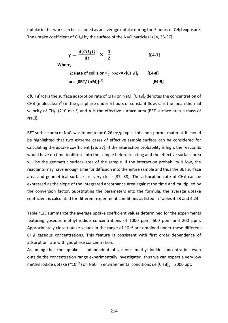
214

uptake in this work can be assumed as an average uptake during the 5 hours of CH3I exposure.

The uptake coefficient of CH3I by the surface of the NaCl particles is [4, 35-37]:

ɣ =𝒅𝑪𝑯𝟑𝑰

𝒅𝒕 ×

𝟏

𝒁 [E4-7]

Where,

Z: Rate of collision= 𝟏

𝟒 ×ω×A×[CH3I]g [E4-8]

ω = [8RT/ (πM)]1/2 [E4-9]

dCH3I/dt is the surface adsorption rate of CH3I on NaCl, [CH3I]g denotes the concentration of

CH3I (molecule.m-3) in the gas phase under 5 hours of constant flow, ω is the mean thermal

velocity of CH3I (210 m.s-1) and A is the effective surface area (BET surface area × mass of

NaCl).

BET surface area of NaCl was found to be 0.26 m2/g typical of a non-porous material. It should

be highlighted that two extreme cases of effective sample surface can be considered for

calculating the uptake coefficient [36, 37]. If the interaction probability is high, the reactants

would have no time to diffuse into the sample before reacting and the effective surface area

will be the geometric surface area of the sample. If the interaction probability is low, the

reactants may have enough time for diffusion into the entire sample and thus the BET surface

area and geometrical surface are very close [37, 38]. The adsorption rate of CH3I can be

expressed as the slope of the integrated absorbance area against the time and multiplied by

the conversion factor. Substituting the parameters into the formula, the average uptake

coefficient is calculated for different experiment conditions as listed in Tables 4.23 and 4.24.

Table 4.23 summarize the average uptake coefficient values determined for the experiments

featuring gaseous methyl iodide concentrations of 1000 ppm, 500 ppm and 200 ppm.

Approximately close uptake values in the range of 10-11 are obtained under these different

CH3I gaseous concentrations. This feature is consistent with first order dependence of

adsorption rate with gas phase concentration.

Assuming that the uptake is independent of gaseous methyl iodide concentration even

outside the concentration range experimentally investigated, thus we can expect a very low

methyl iodide uptake (~10-11) on NaCl in environmental conditions i.e [CH3I]g = 2000 ppt.

215

Table 4. 23 Average uptake coefficient of CH3I on NaCl particles for an exposure phase duration of 5 hours and under dry conditions and at 296K and 1 atm. 1000 ppm= 2.48 × 1022 molecule.m-3, 500 ppm= 1.24 × 1022

molecule.m-3, and 200 ppm= 4.96 × 1021 molecule.m-3. Tc= contact time

[CH3I] in

molecule.m-3

Tc in

ms

Rate of collision

in molecule. s-1

Adsorption rate in

molecule. s-1

ɣss

2.48 × 1022 55 4.74 × 1022 1.31 × 1012 (2.76 ± 0.93) × 10-11

1.24 × 1022 55 2.37 × 1022 7.40 × 1011 (3.17 ± 1.05) × 10-11

4.96 × 1021 55 9.49× 1021 2.92 × 1011 (3.07 ± 1.04) × 10-11

Even if the contact time is decreased by factor 2 (55 ms to 27 ms for 500 ppm of CH3I gas phase

concentration) (see Table 4.24), the average uptake (2.52 ± 0.89) × 10-11 remains close to the

average uptake observed with 55 ms (2.76 ± 0.93) × 10-11. This is consistent with the fact that

contact time has no significant influence on adsorption rate as already discussed. Therefore,

this result agrees with our expectation mentioned on section 4.1.4.1, where in contrary to gas

phase monitoring, experiments based on surface monitoring are independent of contact time

with surface.

Table 4. 24 Average uptake coefficient of CH3I on NaCl particles for an exposure phase duration of 5 hours and under dry conditions and at 296K and 1 atm, 500 ppm= 1.24 × 1022 molecule.m-3. Tc= contact time

[CH3I] in

molecule.m-3

Tc in ms Rate of collision

in molecule. s-1

Rate of adsorption in

molecule. s-1

ɣss

1.24 × 1022 55 2.37 × 1022 7.40 × 1011 (2.76 ± 0.93) × 10-11

1.24 × 1022 27 2.37 × 1022 5.97 × 1011 (2.52 ± 0.89) × 10-11

As seen in section 4.3.2 that the initial adsorption rate of CH3I is highly enhanced with NaI. The

initial uptake coefficient of CH3I on KBr and NaI were estimated assuming i/ the same BET

surface for KBr and NaI as for NaCl (powder grinded in the same manner) ii/ the same

conversion factor of band area into methyl iodide mass taken up at the halide solid surface.

On NaI, the initial uptake coefficient (calculated after one-hour exposure time) is strongly

enhanced (1.24 ± 0.81) × 10-10 in comparison to NaCl (4.12 ± 1.48) × 10-11 and KBr (6.13 ± 3.18)

× 10-11 (see Table 4.25). Thus, uptake coefficient can strongly varies based on the anion of the

halide solid (i.e. Cl- for NaCl and I- for NaI). This highlights the influence of electronegativity on

the adsorption of CH3I on halide particles as stated previously in section 4.2.1.4.

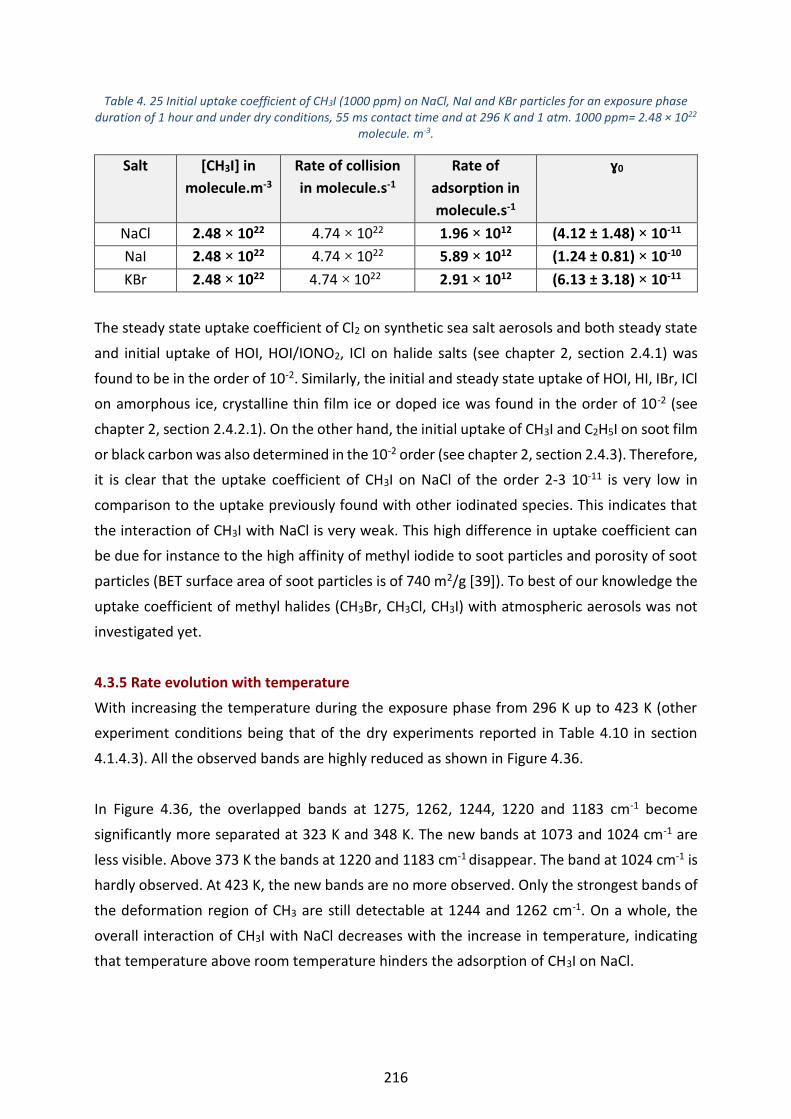
216

Table 4. 25 Initial uptake coefficient of CH3I (1000 ppm) on NaCl, NaI and KBr particles for an exposure phase duration of 1 hour and under dry conditions, 55 ms contact time and at 296 K and 1 atm. 1000 ppm= 2.48 × 1022

molecule. m-3.

Salt [CH3I] in

molecule.m-3

Rate of collision

in molecule.s-1

Rate of

adsorption in

molecule.s-1

ɣ0

NaCl 2.48 × 1022 4.74 × 1022 1.96 × 1012 (4.12 ± 1.48) × 10-11

NaI 2.48 × 1022 4.74 × 1022 5.89 × 1012 (1.24 ± 0.81) × 10-10

KBr 2.48 × 1022 4.74 × 1022 2.91 × 1012 (6.13 ± 3.18) × 10-11

The steady state uptake coefficient of Cl2 on synthetic sea salt aerosols and both steady state

and initial uptake of HOI, HOI/IONO2, ICl on halide salts (see chapter 2, section 2.4.1) was

found to be in the order of 10-2. Similarly, the initial and steady state uptake of HOI, HI, IBr, ICl

on amorphous ice, crystalline thin film ice or doped ice was found in the order of 10-2 (see

chapter 2, section 2.4.2.1). On the other hand, the initial uptake of CH3I and C2H5I on soot film

or black carbon was also determined in the 10-2 order (see chapter 2, section 2.4.3). Therefore,

it is clear that the uptake coefficient of CH3I on NaCl of the order 2-3 10-11 is very low in

comparison to the uptake previously found with other iodinated species. This indicates that

the interaction of CH3I with NaCl is very weak. This high difference in uptake coefficient can

be due for instance to the high affinity of methyl iodide to soot particles and porosity of soot

particles (BET surface area of soot particles is of 740 m2/g [39]). To best of our knowledge the

uptake coefficient of methyl halides (CH3Br, CH3Cl, CH3I) with atmospheric aerosols was not

investigated yet.

4.3.5 Rate evolution with temperature

With increasing the temperature during the exposure phase from 296 K up to 423 K (other

experiment conditions being that of the dry experiments reported in Table 4.10 in section

4.1.4.3). All the observed bands are highly reduced as shown in Figure 4.36.

In Figure 4.36, the overlapped bands at 1275, 1262, 1244, 1220 and 1183 cm-1 become

significantly more separated at 323 K and 348 K. The new bands at 1073 and 1024 cm-1 are

less visible. Above 373 K the bands at 1220 and 1183 cm-1 disappear. The band at 1024 cm-1 is

hardly observed. At 423 K, the new bands are no more observed. Only the strongest bands of

the deformation region of CH3 are still detectable at 1244 and 1262 cm-1. On a whole, the

overall interaction of CH3I with NaCl decreases with the increase in temperature, indicating

that temperature above room temperature hinders the adsorption of CH3I on NaCl.

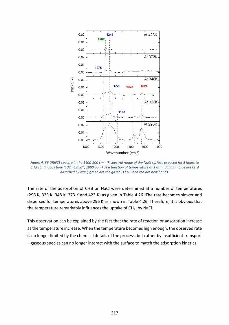
217

Figure 4. 36 DRIFTS spectra in the 1400-900 cm-1 IR spectral range of dry NaCl surface exposed for 5 hours to CH3I continuous flow (108mL.min-1, 1000 ppm) as a function of temperature at 1 atm. Bands in blue are CH3I

adsorbed by NaCl, green are the gaseous CH3I and red are new bands.

The rate of the adsorption of CH3I on NaCl were determined at a number of temperatures

(296 K, 323 K, 348 K, 373 K and 423 K) as given in Table 4.26. The rate becomes slower and

dispersed for temperatures above 296 K as shown in Table 4.26. Therefore, it is obvious that

the temperature remarkably influences the uptake of CH3I by NaCl.

This observation can be explained by the fact that the rate of reaction or adsorption increase

as the temperature increase. When the temperature becomes high enough, the observed rate

is no longer limited by the chemical details of the process, but rather by insufficient transport

– gaseous species can no longer interact with the surface to match the adsorption kinetics.

218

Table 4. 26 Summary of observed rate of the area of the sum of 1275, 1244, 1220, 1183, 1073 and 1024 cm-1 bands at different temperature (in kelvin) during 5 hours of CH3I flow (1000 ppm, 108 mL.min-1). Rate is

determined from the slope of area of the sum of 1275, 1244, 1220, 1183, 1073 and 1024 cm-1 bands versus time. R2 is the coefficient of the linear fit.

Rate of the area versus time

Temperature

(K)

1/T Rate of CH3I

adsorption

R2 Confidence

interval on rate

+/- at 95 % level

ln(Rate)

296 3.38 × 10-3 6.91 ×10-3 0.96 4.67 × 10-4 -4.97

323 3.10 × 10-3 1.24 × 10-3 0.95 9.70 × 10-5 -6.69

348 2.87 × 10-3 1.01 × 10-3 0.90 1.12 × 10-4 -6.90

373 2.68 × 10-3 2.15 × 10-4 0.41 8.54 × 10-5 -8.44

423

2.38 × 10-3 -2.36 × 10-5 0.04

3.97 × 10-2 Negative, not

included

Arrhenius equation is usually used to estimate the activation energy of adsorption for an

elementary process [40]. However, as we were not able to determine the reactional pathway

of CH3I uptake on NaCl, therefore we are not sure if the observed rate at different temperature

corresponds to an elementary process or not.

Therefore, we estimated a global adsorption energy (E) of the adsorption of CH3I on NaCl

(macro process) using Arrhenius equation [E4-10]

k= Ae -E/RT (E4-10)

Where R is the gas constant (8.31 J.mol-1) and the temperature (T) is in Kelvin. k is the rate

constant; A is the pre-exponential factor and E is the global adsorption energy (KJ/mole).

As shown in section 4.3.1.4 the adsorption of CH3I on NaCl is of 1st order. Thus, the adsorption

rate is proportional to the slope of the linear interpolation and dependent on the CH3I gaseous

concentration. Forthwith, the rate constant (k) is given by the following equation:

ln(k) = ln(Rate)-ln([CH3I]) [E4-11]

However, since the gas phase concentration is constant over time (experiment performed

under continuous flow) and the interaction is very low. Therefore, the adsorption rate (Rate)

is assumed to be equal to the rate constant (k).

From the rate of CH3I adsorption given in Table 4.26 and by plotting Ln(Rate) versus 1/T (Figure

4.37) it is possible to determine E from the slope of the linear interpolation of the plot. The

value of E was found to be -38.07 ± 1.69 KJ.mol− 1 at 95% confidence level.

219

Figure 4. 37 Plot of ln (Rate) versus 1/T. Rate is the rate of the time evolution of the sum of the area of the 1275,

1244, 1220, 1183, 1073 and 1024 cm-1 bands and T is the temperature in kelvin.

A negative value of the global adsorption energy is generally a good indication that there is (1)

a reduction in the probability of colliding CH3I molecules with NaCl surface and (2) an overstep

to the diffusion limits of CH3I on NaCl. Therefore, this suggests that we were not more

measuring the adsorption of CH3I on NaCl [41, 42].

Therefore, it seems that the chemisorption process of methyl iodide interaction with NaCl

surface occur at room temperature.

4.4. Conclusion

The heterogeneous interaction of CH3I on wet and dry NaCl salt was investigated using DRIFTS

technique. CH3I adsorption is clearly observed on dry NaCl at 296 K and 1 atm. In addition to

the adsorbed CH3I bands in the CH3 stretching region at 3018, 2993, 2962, and 2855 cm-1 and

in the CH3 deformation region at 1275, 1244, 1220 and 1183 cm-1, the DRIFTS spectra revealed

the presence of new strong vibrational bands at 1073 and 1024 cm-1 which are not referenced

in the literature. Theses bands seems to be linked to the methyl iodide interaction with halide

salt surface, but to the best of our knowledge, no previous studies have considered such

chemical systems featuring organic halogenated gaseous species (i.e. CH3Cl, CH3Br,…) and

halide salts. Owing to the inhomogeneity of the NaCl surface, we hypothesize that these new

bands are attributable to different geometrical form of CH3I (C3v) adsorbed on NaCl.

0.0026 0.0028 0.0030 0.0032 0.0034

-10

-9

-8

-7

-6

-5

Ln(R

ate

)

1/T

K= (4.58 1.69)103 (1/T) - 20.52

R2=0.95

220

The adsorption of CH3I is likely chemisorption since no desorption was observed even after

heating the system. Consistently to the cryogenic study in gas phase, the study of the

interaction between CH3I and wet NaCl showed the low affinity of CH3I towards water.

The CH3Iresidual on NaCl was found to be very low 0.003% and the average uptake coefficients

were determined to be very low in the order of 10-11. This indicates that the interaction

between NaCl and CH3I is very weak. The uptake by NaCl was found to be independent of

contact time and CH3I gaseous concentration (in the ppm range). Though atmospheric CH3I

concentrations, are 10-5-10-6 lower than the concentrations used in our experiments, we can

still expect a very low uptake on NaCl- at least of the same order (10-11). The global energy of

adsorption was found to be -38 KJ.mol− 1, and which suggests that there is a reduction in the

probability of colliding CH3I with NaCl above atmospheric temperature (˃ 296 K).

Although the uptake of CH3I on NaCl is very weak, its irreversible character makes it of

particular importance for the dispersion of CH3I in the atmosphere. Because such irreversible

uptake may occur on surfaces of aerosols particles that are known to be transported and play

a role in the chemistry of the troposphere, which would further affect or participate in

different atmospheric mechanisms.

Finally, it seems challenging to confirm if the new bands are characteristics of different

geometrical configuration C3v of CH3I or not, which would require an additional spectroscopy

analysis using deuterium instead of hydrogen atom (CD3I, CD2HI, etc) and theoretical

calculation taking into consideration different geometrical configuration of adsorbed CH3I.

References

[1] R. Vogt, B.J. Finlayson-Pitts, A Diffuse Reflectance Infrared Fourier Transform Spectroscopic (DRIFTS) study of the surface reaction of NaCl with gaseous NO2 and HN03, J. Phys. Chem. 98 (1994) 3747–3755. https://doi.org/10.1021/j100065a033.

[2] T. Armaroli, T. Bécue, S. Gautier, Diffuse Reflection Infrared Spectroscopy (DRIFTS): Application to the in Situ Analysis of Catalysts, Oil Gas Sci. Technol. 59 (2004) 215–237. https://doi.org/10.2516/ogst:2004016.

221

[3] J. Sirita, S. Phanichphant, F.C. Meunier, Quantitative analysis of adsorbate concentrations by diffuse reflectance FT-IR, Anal. Chem. 79 (2007) 3912–3918. https://doi.org/10.1021 /ac0702802.

[4] C.Lentz, S.Panahian Jand, J.Melke, C.Roth, P.Kaghazch, DRIFTS study of CO adsorption on Pt nanoparticles supported by DFTcalculations, J. Mol. Catal. A : Chemical, 426 (2017) 1-9. https://doi.org/10.1016/j.molcata.2016.10.002

[5] M. Gouello, Thése de doctorat, Chimie de l’iode et composition des aérosols dans le circuit primaire d’un réacteur nucléaire en situation d’accident grave, Université de Grenoble, 2013.

[6] L.D. Kong, X. Zhao, Z.Y. Sun, Y.W. Yang, H.B. Fu, S.C. Zhang, T.T. Cheng, X. Yang, L. Wang, J.M. Chen, The effects of nitrate on the heterogeneous uptake of sulfur dioxide on hematite, Atmos. Chem. Phys. 14 (2014) 9451–9467. https://doi.org/10.5194/acp-14-9451-2014.


[8] A. Saiz-Lopez, J.M.C. Plane, A.R. Baker, L.J. Carpenter, R. Von Glasow, C.G. Juan, G. Mcfiggans, R.W. Saunders, Atmospheric Chemistry of Iodine, Chem. Rev. 112 (2012) 1773–1804. https://doi.org//10.1021/cr200029u.

[9] A. Allanic, M.J. Rossi, Heterogeneous reactions of HOI on substrates of atmospheric importance, Geophys. Res. Lett. 104 (1999) 18689–18696. https://doi.org/10.1029 /1999JD900285.


[11] A. Alshawa, O. Dopfer, S.A.N. Christopher W. Harmon, J.S. Underwood, Hygroscopic growth and deliquescence of NaCl nanoparticles mixed with surfactant SDS, J. Phys. Chem. B. 114 (2010) 2435–2449. https://doi.org/10.1021/jp909661q.

[12] C. Su, J.C. Yeh, C.C. Chen, J.C. Lin, J.L. Lin, Study of adsorption and reactions of methyl iodide on TiO2, J. Catal. 194 (2000) 45–54. https://doi.org/10.1006/jcat.2000.2909.

[13] M. Chebbi, B. Azambre, L. Cantrel, A. Koch, A Combined DRIFTS and DR-UV-Vis Spectroscopic in Situ Study on the Trapping of CH3I by Silver-Exchanged Faujasite Zeolite, J. Phys. Chem. C. 120 (2016) 18694–18706. https://doi.org/10.1021/acs.jpcc.6b07112.

[14] J.L. Duncan, A.M. Ferguson, S. Mathews, Vibrational anharmonicity in CH3I: A joint local and normal mode study, J. Chem. Phys. 91 (1989) 783–790. https://doi.org/10.1063 /1.457131.

[15] M.L. Colaianni, P.J. Chen, H. Gutleben, J.T. Yates, Vibrational studies of CH3I on Si(100)-(2×1): adsorption and decomposition of the methyl species, Chem. Phys. Lett. 191 (1992) 561–568. https://doi.org/10.1016/0009-2614(92)85589-3.

[16] F. Solymosi, G. Klivényi, HREELS study of CH3I and CH3 adsorbed on Rh(111) surface, J. Electron Spectros. Relat. Phenomena. 64/65 (1993) 499–506. https://doi.org/10.1016/0368-2048(93)80115-3.

[17] J. Lin, B.E. Bent, Iodomethane dissociation on Cu(111): Bonding and chemistry of adsorbed methyl groups, J. Vac. Sci. Technol. A Vacuum, Surfaces, Film. 10 (1992) 2202–2209. https://doi.org/10.1116/1.578005.

222

[18] C.J. Jenks, B.E. Bent, N. Bernstein, F. Zaera, The Chemistry of Alkyl Iodides on Copper Surfaces. Adsorption Geometry, Phys. Chem. B. 104 (2000) 3008–3016. https://doi.org/10.1021/jp993021s.

[19] M.A. Henderson, G.E. Mitchell, J.M. White, The chemisorption of methyl halides (Cl, Br and I) on Pt(111), Surf. Sci. Lett. 184 (1987) 325–331. https://doi.org/10.1016/0167-2584(87)90754-7.

[20] G. Klivényi, F. Solymosi, Generation of CH2 species: thermal and photo-induced dissociation of CH2I2 on Rh(111) surface, Surf. Sci. 342 (1995) 168–184.https://doi.org/ 10.1016/0039-6028(95)00767-9.

[21] M.K. Weldon, C.M. Friend, Spectroscopic characterization of surface methylene on Mo (110), Surf. Sci. 321 (1994) L202-L208. https://doi.org/10.1016/0039-6028(94)90175-9.

[22] K.C. Scheer, A. Kis, J. Kiss, J.M. White, Adsorption and reactions of CH2I2 on clean and oxygen-modified Ag (111): a RAIRS and TPD study, Top. Catal. 20 (2002) 43–51. https://doi.org/10.1023/A:1016395214602.

[23] T. Shimanouchi, Tables of Molecular Vibrational Frequences Consolidated, volume I, washington, D.C: National Bureau of Standards, NSRDS-NBS3, 1972. https://doi.org /10.1063/1.555560.

[24] E.M. Karp, T.L. Silbaugh, C.T. Campbell, Energetics of Adsorbed CH3 and CH on Pt(111) by Calorimetry: Dissociative Adsorption of CH3I, J. Phys. Chem. C. 117 (2013) 6325–6336. https://doi.org/10.1021/jp400902f.

[25] R. Otto, Thesis on Dynamics of a Microsolvated Ion-Molecule Reaction, Univ. Freibg. (2011).

[26] S. Furuyama, D.M. Goldex, S.W. Bekson, Kinetic Studies of the Reactions CH2I2 + HI =CH3I +I2 and CH3I =CH4+CH2I2 The Heat of Formation of the Iodomethyl Radical *, Int. J. Chem. Kinet. I (1969) 283–296. https://doi.org/10.1002/kin.550010302.

[27] T. Makino, S. Zulaehah, J.S. Gueriba, W.A. Diño, M. Okada, CH3Cl/Cu (410): Interaction and Adsorption Geometry, J. Phys. Chem. C. 122 (2018) 11825–11831.https://doi.org /10.1021/acs.jpcc.8b01296.

[28] F.S. J. Cserenyi , L. Ovari, T. Bansagi, Adsorption and reactions of CH3Cl on MoC based catalyst, J. Mol. Catal. A Chem. 162 (2000) 335–352. https://doi.org/10.1021/acscatal .5b02424.

[29] J.Rakso, J.Bontovics, F.Solymosi, Infrared Spectroscopic Study of the Adsorption and Dissociation of Methyl Halides on Silica-Supported Pd, J. Catal. 143 (1993) 138–148. https://doi.org/10.1006/jcat.1993.1260.

[30] F. Zaera, H. Hoffmann, P.R. Griffiths, Determination of molecular chemisorption geometries using reflection-absorption infrared spectroscopy: alkyl halides on Pt(111), J. Electron Spectros. Relat. Phenomena. 54–55 (1990) 705–715. https://doi.org/10.1016/0368-2048(90)80263-A.

[31] J. Zhang, U. Lourderaj, S. V. Addepalli, W.A. de Jong, W.L. Hase, Quantum Chemical Calculations of the Cl- + CH3I → CH3Cl + I- Potential Energy Surface, J.Phys. Chem. A. 113 (2009) 1976–1984. https://doi.org/10.1039/c6cp06195h.

223

[32] I. Szabó, G. Czakó, Benchmark ab Initio Characterization of the Complex Potential Energy Surface of the Cl- + CH3I Reaction, J. Phys. Chem. A. 121 (2017) 5748–5757. https://doi.org/ 10.1021/acs.jpca.7b05503.

[33] M. Gu, X. Liu, L. Yang, S. Sun, J. Zhang, Dynamics of Cl-(H2O) + CH3I Substitution Reaction: The Influences of Solvent and Nucleophile, J. Phys. Chem. A. (2019) acs.jpca.9b00348. https://doi.org/10.1021/acs.jpca.9b00348.

[34] M. Ullerstam, M.S. Johnson, R. Vogt, E. Ljungström, DRIFTS and Knudsen cell study of the heterogeneous reactivity of SO2 and NO2 on mineral dust, Atmos. Chem. Phys. Discuss. 3 (2003) 4069–4096. https://doi.org/10.5194/acp-3-2043-2003.


[36] H. Li, T. Zhu, J. Ding, Q. Chen, B. Xu, Heterogeneous reaction of NO2 on the surface of NaCl particles, Sci. China, Ser. B Chem. 49 (2006) 371–378. https://doi.org/10.1007/s11426-006-0371-z.

[37] L. Li, Z.M. Chen, Y.H. Zhang, T. Zhu, S. Li, H.J. Li, L.H. Zhu, B.Y. Xu, Heterogeneous oxidation of sulfur dioxide by ozone on the surface of sodium chloride and its mixtures with other components, J. Geophys. Res. Atmos. 112 (2007) 1–13. https://doi.org/10.1029/2006 JD008207.

[38] P. Li, H.A. Al-Abadleh, V.H. Grassian, Measuring heterogeneous uptake coefficients of gases on solid particle surfaces with a Knudsen cell reactor: Complications due to surface saturation and gas diffusion into underlying layers, J. Phys. Chem. A. 106 (2002) 1210–1219. https://doi.org/10.1021/jp011828q.


[40] B.J. Finlayson-Pitts, J. James N. Pitts, Chemistry of the Upper and Lower Atmosphere: Theory, Experiments, and Applications, Academic Press, California, ISBN: 978-0-12-257060-5, 2000. https://doi.org/10.1016/B978-0-12-257060-5.X5000-X.

[41] R. Kobiraj, N. Gupta, A.K. Kushwaha, M.C. Chattopadhyaya, Determination of equilibrium, kinetic and thermodynamic parameters for the adsorption of Brilliant Green dye from aqueous solutions onto eggshell powder, Indian J. Chem. Technol. 19 (2012) 26–31. Corpus ID: 9344586.

[42] P.A. Parikh, N. Subrahmanyam, Y.S. Bhat, A.B. Halgeri, Kinetics of zeolite-catalysed toluene isopropylation, Chem. Eng. J. Biochem. Eng. J. 54 (1994) 79–85. https://doi.org /10.1016/0923-0467(93)02818-H.

224

Chapter 5: Static reactor experiments Chapter 5 focuses on determining CH3I reactivity with organic and inorganic solids as models

of atmospheric aerosols by monitoring methyl iodide concentration in the gas phase. This

chapter completes the study performed using DRIFTS technique with halide salts (chapter 4).

The DRIFTS technique is not suitable for other compounds chosen as proxy of primary and

secondary atmospheric aerosols (i.e. Na2SO4, Na2CO3, glutaric acid, malonic acid…). Indeed,

the model species own a huge IR absorption, which cannot be attenuated using dilution within

halide solids since these later may directly interfere with CH3I as seen in the chapter 4.

Additionally, the evolution of the CH3I interaction with NaCl determined by following the solid

phase, can be completed using technique following the gaseous phase.

In this chapter, we studied the evolution of CH3I concentration in the gas phase when exposed

to inorganic and organic compounds under dry conditions (RH~20%, at 296 K) using static solid

phase reactor coupled with gas chromatography technique. The static reactors used were

breakthrough type reactor and were only adapted to continuous gas flow conditions. Gas

chromatography coupled to an electron capture detector was adapted to our intentions with

methyl iodide determination in the gas phase in the 1 ppb- 100 ppb concentration range.

The experimental setup featuring a small reactor and a larger one coupled with gas

chromatography is described. The experimental conditions under continuous gas flow

conditions for the study of the interaction of gaseous CH3I with inorganic and organic solids is

listed and justified. Results on the breakthrough curves are then discussed and finally, the

conclusion and perspectives are stated.

5.1 Materials and methods

5.1.1 Reagents

Diluted CH3I in air or argon (0.1% CH3I, 99.9% Ar or Air) bottles were provided by Air products

in a concentration ranging from ppb up to 1000 ppm. Argon (99.99% purity) and Air (80% N2,

20%O2) gas bottles were provided from commercial cylinders Air liquid. The gases were used

without any further purification.

Commercial sodium chloride (NaCl, 99.99% purity, ALFA AESAR), sodium sulphate (Na2SO4,

99% purity, ALFA AESAR), sodium carbonate (Na2CO3, 99+% purity, ACROS), ammonium

nitrate (NH4NO3, 99+% purity, SIGMA ALDRICH) and, malonic acid (99+% purity, ACROS),

sodium stearate (ALFA AESAR, no data on purity), palmitic acid (99+% purity, ACROS), sodium

225

oxalate (99+%, ALFA AESAR), glutaric acid (99+% purity, ALFA AESAR), oxalic acid (AnalaR

NORMAPUR, no data on purity), trisodium citrate diyhdrate (AnalaR NORMAPUR, no data on

purity), trisodium citrate anhydrous (99% purity, AnalaR NORMAPUR), citric acid (AnalaR

NORMAPUR, no data on purity), succinic acid (AnalaR NORMAPUR, no data on purity), citric

acid monohydrate (AnalaR NORMAPUR, no data on purity) were used as powder for

experiments.

All inorganic and organic solid samples were manually grinded using an agate mortar and

pestle. NaCl was preheated for a minimum of 4 hours at 873 K to remove species adsorbed on

the powder surface. NaCl salt is highly hygroscopic, so it was kept in a dry desiccator. Sodium

carbonate and ammonium nitrate were preheated at 473 K, whereas sodium sulphate was

preheated to 323 K. No preheating was performed for organic solids due to the possibility of

solid destruction and safety consideration. Up to 1 g and 14-18 g of powder was used for the

experiments depending on reactor size.

5.1.2 Experimental setup

Two types of static reactors were developed: a small stainless reactor and a large glass reactor

(see Figures 5.1(a) and 5.1(b), respectively).

Figure 5. 1 Photo of the (a) small stainless reactor and (b) large glass reactor.

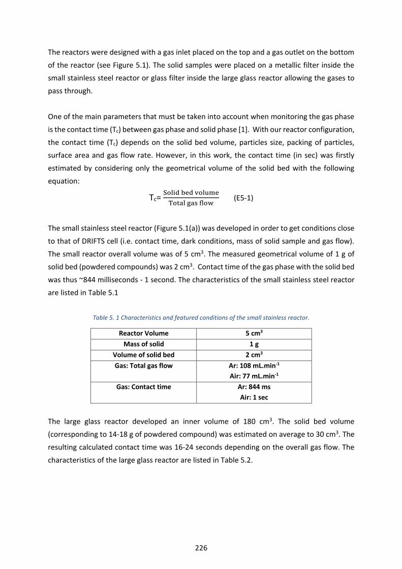
226

The reactors were designed with a gas inlet placed on the top and a gas outlet on the bottom

of the reactor (see Figure 5.1). The solid samples were placed on a metallic filter inside the

small stainless steel reactor or glass filter inside the large glass reactor allowing the gases to

pass through.

One of the main parameters that must be taken into account when monitoring the gas phase

is the contact time (Tc) between gas phase and solid phase [1]. With our reactor configuration,

the contact time (Tc) depends on the solid bed volume, particles size, packing of particles,

surface area and gas flow rate. However, in this work, the contact time (in sec) was firstly

estimated by considering only the geometrical volume of the solid bed with the following

equation:

Tc= Solid bed volume

Total gas flow (E5-1)

The small stainless steel reactor (Figure 5.1(a)) was developed in order to get conditions close

to that of DRIFTS cell (i.e. contact time, dark conditions, mass of solid sample and gas flow).

The small reactor overall volume was of 5 cm3. The measured geometrical volume of 1 g of

solid bed (powdered compounds) was 2 cm3. Contact time of the gas phase with the solid bed

was thus ~844 milliseconds - 1 second. The characteristics of the small stainless steel reactor

are listed in Table 5.1

Table 5. 1 Characteristics and featured conditions of the small stainless reactor.

Reactor Volume 5 cm3

Mass of solid 1 g

Volume of solid bed 2 cm3

Gas: Total gas flow Ar: 108 mL.min-1

Air: 77 mL.min-1

Gas: Contact time Ar: 844 ms

Air: 1 sec

The large glass reactor developed an inner volume of 180 cm3. The solid bed volume

(corresponding to 14-18 g of powdered compound) was estimated on average to 30 cm3. The

resulting calculated contact time was 16-24 seconds depending on the overall gas flow. The

characteristics of the large glass reactor are listed in Table 5.2.

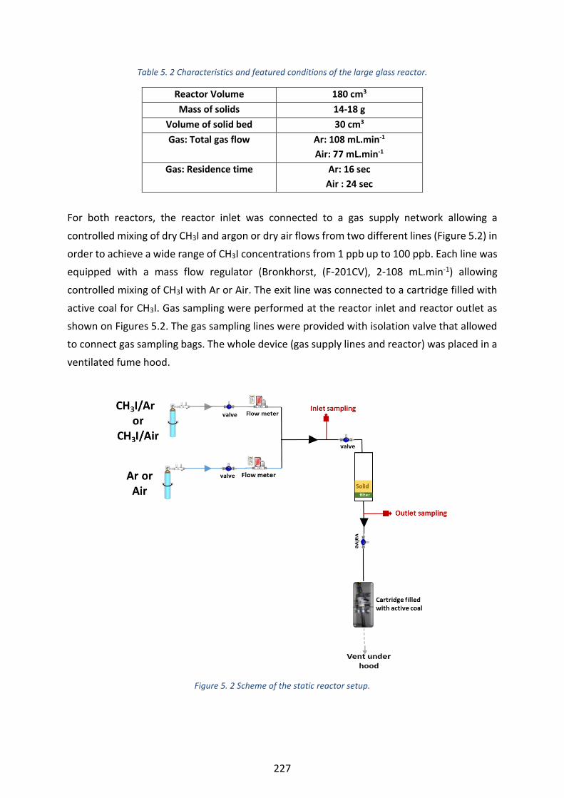
227

Table 5. 2 Characteristics and featured conditions of the large glass reactor.

Reactor Volume 180 cm3

Mass of solids 14-18 g

Volume of solid bed 30 cm3

Gas: Total gas flow Ar: 108 mL.min-1

Air: 77 mL.min-1

Gas: Residence time Ar: 16 sec

Air : 24 sec

For both reactors, the reactor inlet was connected to a gas supply network allowing a

controlled mixing of dry CH3I and argon or dry air flows from two different lines (Figure 5.2) in

order to achieve a wide range of CH3I concentrations from 1 ppb up to 100 ppb. Each line was

equipped with a mass flow regulator (Bronkhorst, (F-201CV), 2-108 mL.min-1) allowing

controlled mixing of CH3I with Ar or Air. The exit line was connected to a cartridge filled with

active coal for CH3I. Gas sampling were performed at the reactor inlet and reactor outlet as

shown on Figures 5.2. The gas sampling lines were provided with isolation valve that allowed

to connect gas sampling bags. The whole device (gas supply lines and reactor) was placed in a

ventilated fume hood.

Figure 5. 2 Scheme of the static reactor setup.

228

The mixed flows as a function of CH3I concentration are listed in Table 5.3, with a total flow

rate of 108 mL.min-1 diluted in Ar or 77 mL.min-1 diluted in Air.

Table 5. 3 Prepared [CH3I] in ppb as function of CH3I concentration (ppb) and Ar or Air flow (mL.min-1) at 1 atm and 296 K. Q: mass flow rate in mL.min-1.

Initial [CH3I] in the

reactor (ppb)

QAr or QAir

(mL.min-1)

QCH3I

(mL.min-1)

[CH3I] supply

100 106 (Ar) 2 5 ppm in Ar

50 107 (Ar) 1 5 ppm in Ar

1 76 (Air) 1 100 ppb in Air

Gas chromatography (GC) coupled with an Electron Capture Detector was used to follow

methyl iodide concentration evolution.

5.1.3 Gas phase CH3I sampling and GC analyses

In continuous flow, the sampling of gaseous CH3I/Ar mixtures at the inlet or outlet (see Figure

5.2) was done by filling a 0.6 L gas bag for 5 minutes.

Analysis of gaseous methyl iodide (CH3I) concentration in the gas phase was performed by gas

chromatography (Agilent7820A) provided with a capillary column of 0.32 mm internal

diameter and 30 mm length and an ECD detector following the methods developed in the L2EC

Laboratory (see annex 5).

Analysis of gas phase in the filled gas bag using GC-ECD can be performed by both manual and

automated injection. The type of injection was dependent on the CH3I concentration range.

Manual injection was applied for the methyl iodide concentration of 100 ppb. Injection

through automated thermodesorption (TD) is retained for the low concentration levels

(1 ppb). Under our experimental conditions, methyl iodide concentration were determined

with an uncertainty interval at 95% confidence level of ± 8 % with TD injection. For manual

injection, the uncertainty interval at 95% confidence level was of ± 14 %. The uncertainty

values were determined previously at L2EC laboratory. The calculation of uncertainty was

based on the combination of accuracy and precision data analysis (annex 6).

5.1.4 Protocol description for experiments performed in continuous gas conditions

Under continuous conditions, gas phase monitoring allows the access to the break through

curves [2]. Contrarily to static conditions, where the total amount of gas taken up by the solid

can be determined [1, 3].

229

Indeed, if CH3I capture on the selected solid particles is low as for NaCl, we expect a rapid

outlet gas phase depletion at the experiment beginning which then increases rapidly until

observing a breakthrough which correspond to saturation of the solid bed. However, if the

residence time in the solid bed is increased, the initial outlet CH3I concentration depletion will

be amplified as shown in Figure 5.3. Then, a relation between the outlet gas phase depletion

and residence time in the solid bed can give an access to the initial gas uptake by solid (0).

Figure 5. 3 [CH3I]outlet as function of contact time.

All experiments were performed at RH=20%, 296K and 1 atm. Small reactor was as DRIFTS

experiments under dark conditions. We assume that the large reactor was also close to dark

conditions since (1) the experiments were performed inside a laboratory with the presence of

only artificial light (2) the UV-Vis light did not penetrate into the solid bed.

Before each experiment, a blank test with a pure Ar flow at 108 mL.min-1 was conducted and

gas phase analyses at both inlet and outlet were performed to check that the experimental

setup was clean. Before injecting the methyl iodide mixed with Ar or Air into the reactor, we

verified the initial CH3I concentration. For this purpose, the gas mixture (CH3I/Ar or CH3I/Air)

was sampled at the inlet of the experimental set up and analyzed by GC. After validating the

methyl iodide concentration at the inlet (inlet sampling in Figure 5.2), the gas mixture was

injected into the reactor. After 1 minute of gas flow through the solid sample, a gas bag of

0.6 L was placed at the reactor outlet (outlet sampling in Figure 5.2) and filled for 6 minutes.

Successive gas bag fillings were performed during the experiment (gas sampling was

performed every 6 minutes). The experiment duration varied between 36 and 300 minutes.

At the end of the test, the overall gas flow was stopped (CH3I and dilution lines), and the solid

was recovered. The reactor was cleaned and then argon was flowed at 108 mL.min-1 all night.

230

5.1.5 Experiment grid for continuous conditions

As a low reactivity between methyl iodide and the inorganic and organic solid is expected, the

static reactor experiments will feature conditions suited to a low gas phase depletion: we

choose to operate with low methyl iodide gas phase concentration (1-100 ppb) and high

amount of solid particles (1-15 g). Such conditions are opposite to that retained for the DRIFTS

experiments - featuring high methyl iodide gas phase concentration (1000 ppm) and low salt

mass (150 mg) in order to allow measurable salt surface structural changes.

The first series of experiments was conducted with the small reactor. The CH3I wall loss was

firstly determined with empty reactor under continuous flow of 100 ppb and 1 ppb of CH3I

(blank experiments). In the small reactor, we firstly aimed to globally investigate the

interaction with different solid models of atmospheric aerosols. Inorganic solids (i.e NaCl,

Na2CO3, NH4NO3 and Na2SO4) and organic solids (i.e glutaric acid, malonic acid, oxalic acid,

succinic acid, palmitic acid, citric acid, citric acid monohydrate, sodium stearate, sodium

oxalate, trisodium citrate dihydrate and anhydrous trisodium citrate) placed inside the small

reactor were exposed successively to a 100 ppb CH3I/Ar continuous flow. Secondly, we chose

to expose CH3I at trace level (1 ppb) to selected inorganic solids (NaCl and Na2CO3) and organic

solids (trisodium citrate dihydrate and glutaric acid). As shown in Table 5.4, the organic solids

featured all carboxylic acid functional groups (i.e. glutaric acid, malonic acid, oxalic acid,

succinic acid, palmitic acid, citric acid and citric acid monohydrate) or were the solids of the

corresponding conjugated bases (i.e. sodium stearate, sodium oxalate, trisodium citrate

dihydrate and anhydrous trisodium citrate). Therefore, we selected one organic solid with

carboxylic acid group (glutaric acid) and one sodium salt of the conjugated base (trisodium

citrate dihydrate).

The second series of experiments was conducted with the large glass reactor. First, blank

experiments were performed with empty reactor under continuous flow of 100 ppb and 1 ppb

of CH3I. Secondly, CH3I (100 ppb)/Ar was exposed to selected three inorganic solids ( NaCl,

Na2CO3, NH4NO3), and three organic solids with carboxylic acid group (glutaric acid, malonic

acid, oxalic acid) and one sodium salt of the conjugated base (trisodium citrate dihydrate).

Later, CH3I (1ppb)/Air was subjected to NaCl, Na2CO3, NH4NO3, trisodium citrate dihydrate and

glutaric acid.

Our selection of organic solids was generally based on: (1) Oxalic acid is generally the

dominant organic species in atmospheric aerosols followed by malonic, (2) glutaric acid can

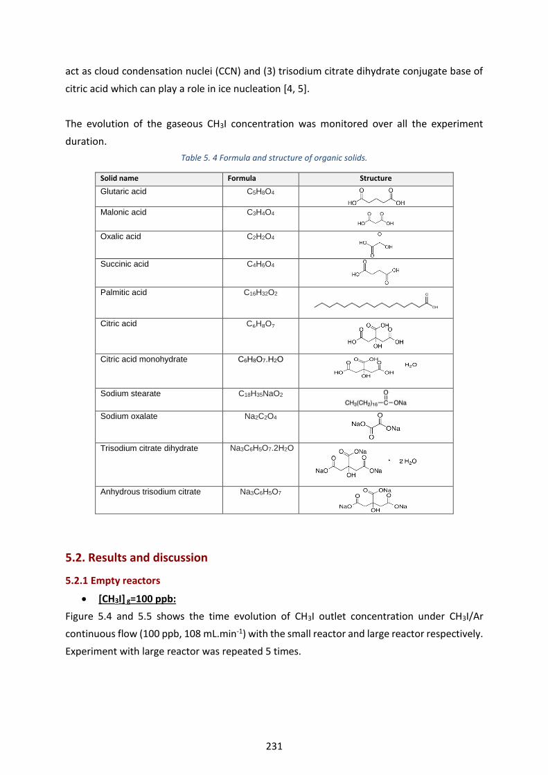
231

act as cloud condensation nuclei (CCN) and (3) trisodium citrate dihydrate conjugate base of

citric acid which can play a role in ice nucleation [4, 5].

The evolution of the gaseous CH3I concentration was monitored over all the experiment

duration.

Table 5. 4 Formula and structure of organic solids.

Solid name Formula Structure

Glutaric acid C5H8O4

Malonic acid C3H4O4

Oxalic acid C2H2O4

Succinic acid C4H6O4

Palmitic acid C16H32O2

Citric acid C₆H₈O₇

Citric acid monohydrate C6H8O7.H2O

Sodium stearate C18H35NaO2

Sodium oxalate Na2C2O4

Trisodium citrate dihydrate Na3C6H5O7.2H2O

Anhydrous trisodium citrate Na3C6H5O7

5.2. Results and discussion

5.2.1 Empty reactors

[CH3I] g=100 ppb:

Figure 5.4 and 5.5 shows the time evolution of CH3I outlet concentration under CH3I/Ar

continuous flow (100 ppb, 108 mL.min-1) with the small reactor and large reactor respectively.

Experiment with large reactor was repeated 5 times.

232

In Figure 5.4, the outlet concentration remained in general close to the range of the expected

one (given the uncertainty range (± 14%) of the GC analyses).

As seen from Figure 5.5, even if the outlet CH3I concentration remained in general close to the

range of the expected one (given the uncertainty range (± 14%) of the GC analyses), a slow

and constant decrease of this concentration of about 12% (marked in dashed box in Figure

5.5) is observed at the beginning of two experiments (experiments 1 and 5). Therefore, this

series of experiments points out the difficulties to obtain a stable CH3I concentration with

empty large glass reactor and will make interpretation of experiments with solids not easy if

low interaction is expected.


concentration of 100 ppb and 108 mL.min-1 continuous gas flow under RH=20% at 296 K and 1 atm.

233

Figure 5. 5 The evolution of [CH3I] outlet as function of time in the empty large reactor for an injected CH3I

concentration of 100 ppb and 108 mL.min-1 continuous gas flow under RH=20% at 296 K and 1 atm.

[CH3I]g=1 ppb:

Figure 5.6 and 5.7 shows the time evolution of CH3I outlet concentration under CH3I/Ar

continuous flow (1 ppb, 77 mL.min-1) with the small reactor and large reactor respectively.

Experiments with both reactors were repeated 2 times.

234

In both reactors, the CH3I outlet concentration as well as the inlet concentration in general

were up to 30% higher than the range of the expected one (given the uncertainty range (± 8%)

of the GC analyses). This underlines the problem of achieving low stable concentrations in the

inlet line by mixing low gaseous flows: i.e. for 1 ppb of CH3I a mixing of 76 mL.min-1 of Air with

1 mL.min-1 of CH3I was needed (see Table 5.3). Nevertheless, during the experiment, the outlet

concentration remained stable and within the uncertainty (± 8%) range of the GC analyses as

shown in Figure 5.6 and 5.7.


concentration of 1 ppb and 77 mL.min-1 continuous gas flow under RH=20% at 296 K and 1 atm. 1 ppb= 1000 ppt.

Figure 5. 7 The evolution of [CH3I] outlet as function of time in the empty large reactor for an injected CH3I of 1

ppb and 77 mL.min-1 continuous gas flow under RH=20% at 296 K and 1 atm. 1 ppb= 1000 ppt.

235

5.2.2 Reactor filled with inorganic solids

Experiments were performed with both small and large reactors filled with 1 g (844 ms -1 sec)

and 18 g (16-24 sec) of inorganic solids, respectively.

[CH3I]g= 100 ppb:

The evolution of the CH3I outlet concentration over time was stable in comparison to blank

experiment when CH3I was exposed to all the selected inorganic solids in both reactors. As an

example, Figure 5.8 and Figure 5.9 shows the time profile of CH3I outlet concentration when

CH3I was exposed to NaCl and NH4NO3. Indeed, the CH3I outlet concentration presented a

similar pattern to that observed with tests performed in the empty reactors (see section

5.2.1). Similar trends were also observed with Na2CO3 and Na2SO4 (annex 8).

Figure 5. 8 The evolution of [CH3I] outlet as function of time in the small and large glass reactor filled with 1g and 18g of NaCl, respectively for an injected CH3I concentration of 100 ppb and 108 mL.min-1 continuous gas

flow under RH=20% at 296 K and 1 atm.


of NH4NO3, respectively for an injected CH3I concentration of 100 ppb and 108 mL.min-1 continuous gas flow under RH=20% at 296 K and 1 atm.

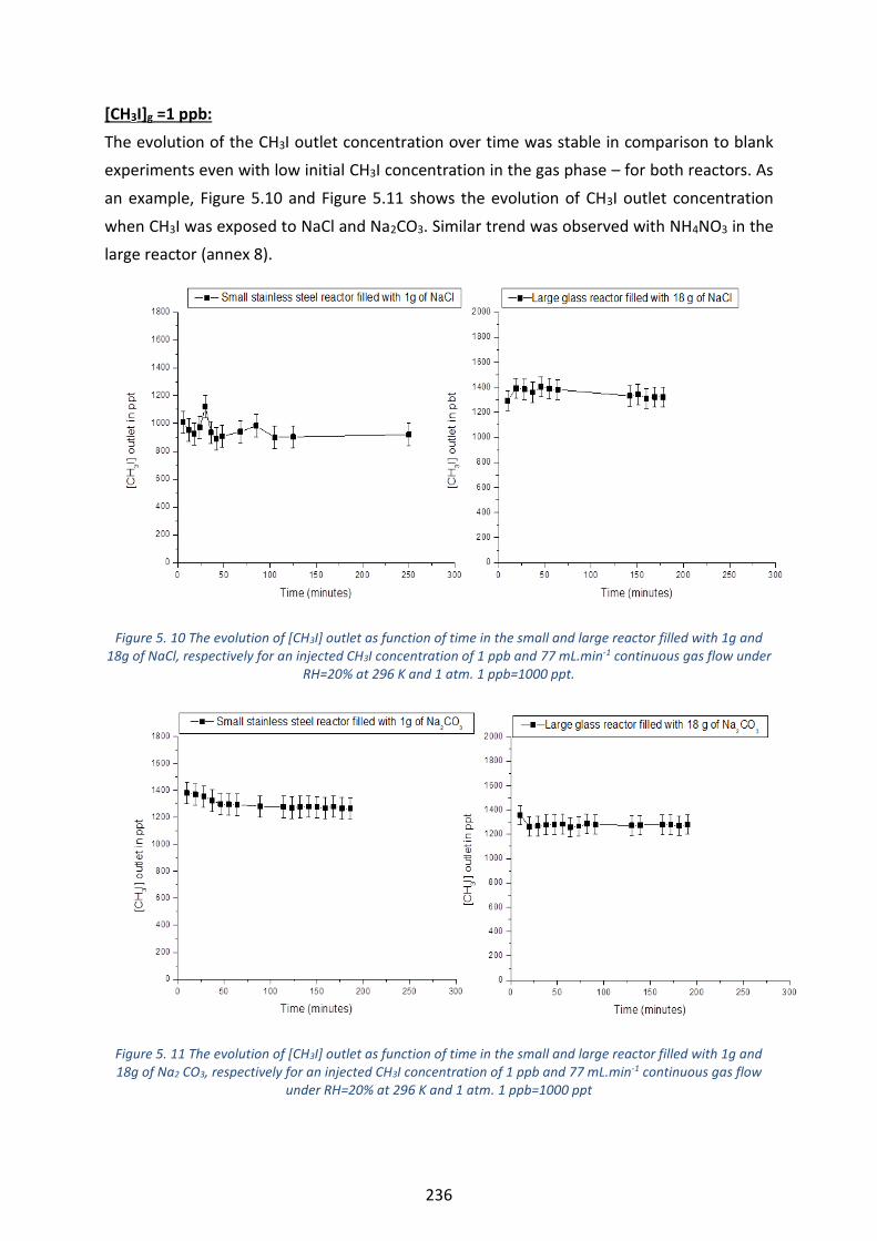
236

[CH3I]g =1 ppb:

The evolution of the CH3I outlet concentration over time was stable in comparison to blank

experiments even with low initial CH3I concentration in the gas phase – for both reactors. As

an example, Figure 5.10 and Figure 5.11 shows the evolution of CH3I outlet concentration

when CH3I was exposed to NaCl and Na2CO3. Similar trend was observed with NH4NO3 in the

large reactor (annex 8).

Figure 5. 10 The evolution of [CH3I] outlet as function of time in the small and large reactor filled with 1g and

18g of NaCl, respectively for an injected CH3I concentration of 1 ppb and 77 mL.min-1 continuous gas flow under RH=20% at 296 K and 1 atm. 1 ppb=1000 ppt.

Figure 5. 11 The evolution of [CH3I] outlet as function of time in the small and large reactor filled with 1g and 18g of Na2 CO3, respectively for an injected CH3I concentration of 1 ppb and 77 mL.min-1 continuous gas flow

under RH=20% at 296 K and 1 atm. 1 ppb=1000 ppt

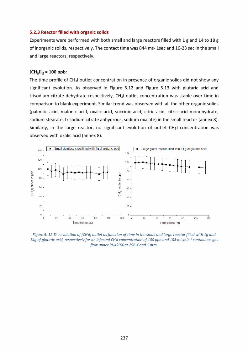
237

5.2.3 Reactor filled with organic solids

Experiments were performed with both small and large reactors filled with 1 g and 14 to 18 g

of inorganic solids, respectively. The contact time was 844 ms- 1sec and 16-23 sec in the small

and large reactors, respectively.

[CH3I] g = 100 ppb:

The time profile of CH3I outlet concentration in presence of organic solids did not show any

significant evolution. As observed in Figure 5.12 and Figure 5.13 with glutaric acid and

trisodium citrate dehydrate respectively, CH3I outlet concentration was stable over time in

comparison to blank experiment. Similar trend was observed with all the other organic solids

(palmitic acid, malonic acid, oxalic acid, succinic acid, citric acid, citric acid monohydrate,

sodium stearate, trisodium citrate anhydrous, sodium oxalate) in the small reactor (annex 8).

Similarly, in the large reactor, no significant evolution of outlet CH3I concentration was

observed with oxalic acid (annex 8).

Figure 5. 12 The evolution of [CH3I] outlet as function of time in the small and large reactor filled with 1g and

14g of glutaric acid, respectively for an injected CH3I concentration of 100 ppb and 108 mL.min-1 continuous gas flow under RH=20% at 296 K and 1 atm.

238

Figure 5. 13 The evolution of [CH3I] outlet as function of time in the small stainless and large glass reactor filled with 1g and 15g of trisodium citrate dihydrate, respectively for an injected CH3I concentration of 100 ppb and

108 mL.min-1 continuous gas flow under RH=20% at 296 K and 1 atm.

CH3I] g=1 ppb:

The evolution of CH3I outlet concentration as function of time in presence of organic solids did

not show any significant evolution in comparison to blank experiment (see section 5.2.1). As

an example, Figure 5.14 and Figure 5.15 shows the evolution of CH3I outlet concentration

when CH3I was exposed to glutaric acid and trisodium citrate dihydrate.

Figure 5. 14 The evolution of [CH3I] outlet as function of time in the small and large reactor filled with 1g and 14g of glutaric acid, respectively for an injected CH3I concentration of 1 ppb and 77 mL.min-1 continuous gas

flow under RH=20% at 296 K and 1 atm. 1 ppb=1000 ppt.

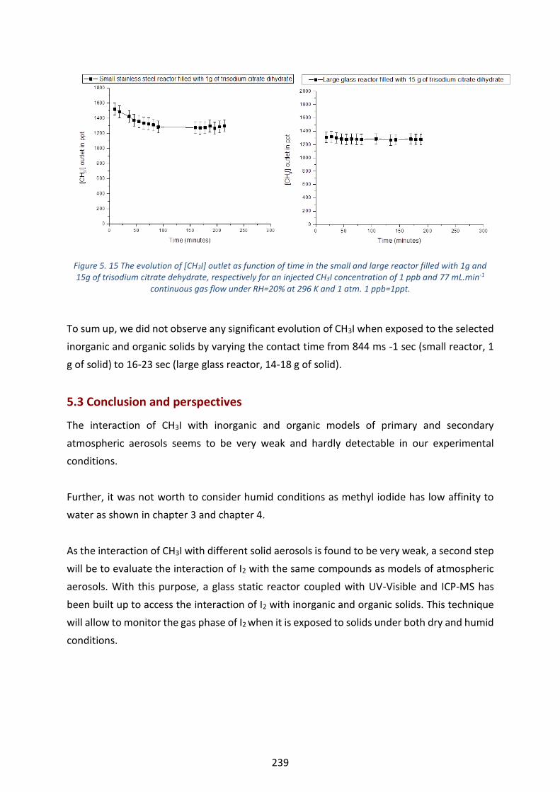
239

Figure 5. 15 The evolution of [CH3I] outlet as function of time in the small and large reactor filled with 1g and 15g of trisodium citrate dehydrate, respectively for an injected CH3I concentration of 1 ppb and 77 mL.min-1

continuous gas flow under RH=20% at 296 K and 1 atm. 1 ppb=1ppt.

To sum up, we did not observe any significant evolution of CH3I when exposed to the selected

inorganic and organic solids by varying the contact time from 844 ms -1 sec (small reactor, 1

g of solid) to 16-23 sec (large glass reactor, 14-18 g of solid).

5.3 Conclusion and perspectives

The interaction of CH3I with inorganic and organic models of primary and secondary

atmospheric aerosols seems to be very weak and hardly detectable in our experimental

conditions.

Further, it was not worth to consider humid conditions as methyl iodide has low affinity to

water as shown in chapter 3 and chapter 4.

As the interaction of CH3I with different solid aerosols is found to be very weak, a second step

will be to evaluate the interaction of I2 with the same compounds as models of atmospheric

aerosols. With this purpose, a glass static reactor coupled with UV-Visible and ICP-MS has

been built up to access the interaction of I2 with inorganic and organic solids. This technique

will allow to monitor the gas phase of I2 when it is exposed to solids under both dry and humid

conditions.

240

References


[2] M.N. Romanías, H. Ourrad, F. Thévenet, V. Riffault, Investigating the Heterogeneous Interaction of VOCs with Natural Atmospheric Particles: Adsorption of Limonene and Toluene on Saharan Mineral Dusts, J. Phys. Chem. A. 120 (2016) 1197–1212. https://doi.org /10.1021/acs.jpca.5b10323.

[3] S. Scolaro, Ph.D. thesis: Effects of humidity and fatty acid surfactants on the uptake of NO2 to NaCl : Combined study of kinetics and surface analysis, Lille University, France (2009).

[4] K. Kawamura, L.L. Ng, I.R. Kaplan, Determination of Organic Acids (C1-C10) in the Atmosphere, Motor Exhausts, and Engine Oils, Environ. Sci. Technol. 19 (1985) 1082–1086. https://doi.org/10.1021/es00141a010.

[5] T.W. Wilson, B.J. Murray, R. Wagner, O. Möhler, H. Saathoff, M. Schnaiter, J. Skrotzki, H.C. Price, T.L. Malkin, S. Dobbie, S.M.R.K. Al-Jumur, Glassy aerosols with a range of compositions nucleate ice heterogeneously at cirrus temperatures, Atmos. Chem. Phys. 12 (2012) 8611–8632. https://doi.org/10.5194/acp-12-8611-2012.

241

This page is left empty

242

General conclusion and perspectives Following a severe accident on a nuclear reactor, radio-iodine species (as 131I) produced by the

fuel fission, may be released into the atmosphere mainly under molecular iodine or methyl

iodide gaseous forms. Radioiodine (131I) species are highly toxic at short term and can affect

both human health and environment. Besides, these iodine products are highly reactive and

may interact with the other species present in the atmosphere (gas or particles) to evolve in

gaseous or particulate form which play an important role on the dispersion of iodine in the

atmosphere. The reactivity of iodine during its dispersion in the atmosphere is up to now not

fully accounted in the IRSN (Institut de Radioprotection et de Sûreté Nucléaire) atmospheric

operational dispersion tools. This is worrisome because the simulated atmospheric dispersion

of radio-iodine may be quite different from the actual one due to the different possible fates

of iodine within the Earth's atmosphere. Forthwith, the radiological consequences (thyroid

equivalent dose) are predicted without considering the derived actual forms of the dispersed

iodine. This prediction is indeed dependent on the chemical form of iodine released i.e.

gaseous, liquid or solid phase and could be improved by assuming the iodine physical/

chemical evolution of radio-iodine in the atmosphere.

Gaseous organic iodine species (CH3I) are naturally emitted at trace level (with a maximum at

2000 ppt) into the atmosphere over oceans through the algae and phytoplankton activities.

Over the last four decades, the fate of emitted iodine species has a great atmospheric interest

because of the oxidizing properties of iodine compounds in the atmosphere and its impact on

the catalytic destruction of the ozone layer. More recently, interest was brought on gaseous

iodine species interaction with atmospheric aerosols, which may affect the physico chemical

form of iodine in the atmosphere and thus, their atmospheric fate. Finally, interactions

between iodine species and water may enhance the iodine role in atmospheric aerosol

nucleation and thus, the cloud condensation nuclei process (CCN).

In this context, the objective of this Ph.D. work was to better enhance the actual state of

knowledge of atmospheric iodine chemistry focusing on the gaseous iodine - atmospheric

aerosols interaction. Understanding the iodine-aerosols or iodine-water interactions can help

in acknowledging the atmospheric iodine dispersion following a severe accident.

To meet the objectives of this Ph.D. work, studies have been performed via the following

experimental approaches:

243

Cryogenic isolation technique supported by Density Functional Theory (DFT)

calculation to study the molecular interaction between CH3I and water and in a

preliminary investigation, the uptake of CH3I on amorphous water ice. Cryogenic

matrices experiments is accurate for describing intermolecular interactions between

atmospherically relevant molecules. Even if working at low temperature and pressure

does not mimic atmospheric conditions, such technique brings insights at molecular

level for the first steps of the process and may help at understanding the mechanisms.

The experiments were conducted with a large excess of H2O molecules compared to

CH3I (CH3I/Ar/H2O: 1/24/1500) in order to mimic CH3I environment in the atmosphere.

This approach allowed the characterization of the product species that may results

from the interaction between CH3I-H2O molecules and CH3I-amorphous ice surface

(chapter 3).

Diffuse Reflectance Infrared Fourier Transformed Spectroscopy (DRIFTS) is useful to

investigate the heterogeneous interaction between CH3I with dry or wet NaCl solid as

surrogate of sea salt aerosols. The experiments were performed under 1 atm at 296 K.

This technique allowed a time monitoring of the evolution of the NaCl powder under

continuous CH3I flow (1000 ppm); and gave information about the adsorption of CH3I

and its reactivity on NaCl. By increasing the temperature of the system, the global

energy of adsorption was determined. Besides, by coupling DRIFTS with ICP-MS

results, the uptake coefficient of CH3I by NaCl was estimated (chapter 4).

Static reactor coupled with gas chromatography (GC) was used to inspect the

interactions of CH3I with different inorganic and organic solids as model of primary and

secondary atmospheric aerosols. Gas chromatography allowed quantitaive analysis of

CH3I in the gas phase at the ppb level. The experiments were conducted with dry solids

under 1 atm at 296 K. Forthwith, the evolution of CH3I concentration in the gas phase

and the global uptake of this gaseous species on a given solid phase was determined

without any concern on the reaction mechanism with the solid (chapter 5).

The main original outputs obtained from this work are summarized below:

(1) The intermolecular behavior between CH3I and excess of H2O molecules trapped in Ar

matrix was determined experimentally at a molecular scale and supported by DFT

calculations. The results highlight that, with excess of water, gaseous methyl iodide

and water molecules will likely form aggregates of water and methyl iodide polymers

instead of (CH3I)n-(H2O)m complexes. This result is consistent with previous theoretical

244

studies, which have predicted the low hydration of CH3I. Therefore, CH3I will stay in

the gaseous phase as homo or hetero water-CH3I aggregates with low influence on

nucleation process.

(2) Preliminary results show that amorphous ice surface modes, in particular the dH

dangling bonds, can be perturbed upon adsorption of CH3I. The appearance of CH3

modes in stretching, deformation and rocking region confirms the adsorption of CH3I

on amorphous ice. However, the adsorption and desorption processes are not clearly

identified.

(3) The DRIFTS experiments clearly evidenced adsorption of CH3I on the NaCl particles.

The DRIFTS spectra showed two new and intense bands at 1024 and 1073 cm-1 which

are typical of the CH3 deformation. These bands are probably assigned to new

geometrical orientation of CH3I adsorbed on halide solids. Theoretical calculations as

well as experimental studies using isotopic products (CD3I, CD2HI, etc) would confirm

the assignment.

(4) The adsorption of CH3I on NaCl is likely chemisorption since no desorption was

observed even after the heating of the system. The presence of water on the surface

of NaCl seems to hinder the interaction between CH3I and NaCl, which can be

explained by the fact that CH3I is insoluble in water. However, further experiments

and/or theoretical studies are necessary for fully unravel the molecular processes.

(5) The adsorption curves featuring the area of the IR band related to the adsorbed CH3I

versus time, show that the adsorption of CH3I on NaCl did not reach any saturation

even after 5 hours of continuous flow of CH3I (1000 ppm). The % CH3Iresidual on NaCl

was found to be low of 0.003%. CH3I adsorption at the NaCl surface follows a pseudo

1st order kinetic law regarding CH3I gas phase concentration. Although the high

concentration of CH3I considered in our experiments, the calculated uptake

coefficients are of low values in the order of 10-11. Indeed, the % CH3Iresidual and the

uptake coefficient values indicate a very weak macroscopic interaction between CH3I

and NaCl in our experimental conditions. Thus, regarding the CH3I atmospheric

concentration, which is in the order of ppt, the influence of aerosols on the behavior

of gaseous CH3I can be considered negligible. The rate of methyl iodide adsorption at

the surface decreases with increasing temperature, which suggests a low probability

245

of the colliding molecules with NaCl when temperature is above 323 K. A global

adsorption energy of -38 KJ/mol was determined.

(6) It was found that CH3I interact with halide salts surface (NaCl, NaI, KBr) in an original

geometrical configuration which has never been described.

(7) The interactions of CH3I with organic and inorganic solids (sodium chloride, sodium

sulphate, sodium carbonate, ammonium nitrate, sodium bicarbonate, malonic acid,

sodium stearate, palmitic acid, sodium oxalate, glutaric acid, oxalic acid, trisodium

citrate diyhdrate, trisodium citrate anhydrous, citric acid, succinic acid and citric acid

monohydrate) were investigated using static reactors in various conditions of

exposure. We have found very weak and hardly detectable interactions by monitoring

the gas phase, even for CH3I concentration at the ppb level.

Finally, considering that our experimental conditions can be transposed to atmospheric

conditions, we hypothesis that CH3I when released will interact very little with the solid

aerosols and will mainly remain in the gaseous phase probably as homo or hetero-

aggregates. Therefore, the photochemical processes occurring in the gaseous phase are

likely the main processes of CH3I reactivity in the atmosphere.

In case of severe nuclear accident such as Fukushima daiichi nuclear power plant accident,

a maximum total 131I iodine concentration reported on site was about 10 MBq.m-3

representing thus less than one ppt (~ 0.4 ppt) which is in the lower concentration range of

naturally occurring iodine. So, even if our study at laboratory scale is far from representing

atmospheric conditions, we can expect still a very low uptake in the environemental

conditions featuring methyl iodide concentrations below the ppb range. Thus, a minimal

uptake in the 10-10 -10-11 range can be still reasonably considered for environmental

conditions.

Although CH3I capture by halide-containing aerosols is weak, the irreversible nature of this

process is not without consequences on the dispersion of atmospheric iodine. This point

should be implement in the radioactive iodine dispersion model to evaluate any influence

on the thyroid equivalent dose, in case of accidental radioactive iodine releases.

Certainly, the uptake coefficient given in this work will give insights for the IRSN modeling

tools to better understand and model radioactive organic iodine atmospheric interactions

and deposits.

246

This work opens new perspectives in the field of the atmospheric organic iodine species.

Actually, up to now, the homogeneous reactivity is investigated, especially the

photoreactivity of CH3I where the influence of water or the potential catalytic effect of

aerosols on these photochemical processes are poorly considered.

It is important to investigate the photochemical behavior of CH3I-water aggregates, which are

known to be sensitive to the solar radiation and representative of atmospheric condition.

Additional experiments are required to explain the interaction of CH3I with amorphous ice at

molecular scale. These studies may be investigated using cryogenic experimental set up that

would improve our understanding on the interaction between CH3I-H2O and CH3I-amorphous

ice exposed to various radiations by responding to the following questions:

How do CH3I-water aggregates behave under solar radiation?

How the adsorption of CH3I does affect the surface structure and reorganization of the

amorphous ice?

Upon adsorption of CH3I on ice, is there any CH3I-H2O bonding or complex formation?

Is there any polymer formation?

Under which conditions can CH3I migrate to the bulk of amorphous ice?

Is it possible to desorb CH3I using only the kinetic energy of a gas stream?

Is it possible to desorb CH3I by selectively irradiating dH?

How does the adsorbed CH3I on amorphous ice behave under solar radiation?

An improved understanding of the adsorption process of CH3I on NaCl surface and

confirmation of the attribution of the new IR bands observed in DRIFTS (Chapter 4) may be

achieved with the help of theoretical calculation and experiments with deutered species of

CH3I. The organisation of the CH3I molecules at the solid surface as well as their dynamic, the

influence of water on these organization and/or reorganization and finally the potential

reactivity are the key questions that can be investigated using theoretical calculations.

Finally, to completely update the radio-iodine atmospheric dispersion modelling, the

interaction of molecular iodine (I2) with water and dry/humid atmospheric aerosols have to

be investigated. Molecular iodine is indeed the other key iodine gaseous compound believed

to be released into the troposphere in case of an accident on a nuclear power plant.

The data gained from these studies will help in the mid-term to improve the capabilities of the

IRSN dispersion tool to better predict radio-iodine dispersion following an accidental release

and be at the state of the art.

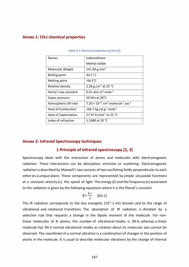
247

Annex 1: CH3I chemical properties

Table A 1 Chemical properties of CH3I [1].

Names Iodomethane

Methyl iodide

Molecular Weight 141.94 g.mol-1

Boiling point 42.5 °C

Melting point -66.5°C

Relative density 2.28 g.cm-3 at 25 °C

Henry’s law constant 0.01 atm.m3.mole-1

Vapor pressure 50 kPa at 20°C

Atmospheric OH rate 7.20 × 10-14 cm3.molecule-1.sec-1

Heat of Combustion 194.7 kg.cal.g-1.mole-1

Heat of Vaporization 27.97 kJ.mol-1 at 25 °C

Index of refraction 1.5380 at 20 °C

Annex 2: Infrared Spectroscopy techniques

1-Principle of Infrared spectroscopy [2, 3]

Spectroscopy deals with the interaction of atoms and molecules with electromagnetic

radiation. These interactions can be absorption, emission or scattering. Electromagnetic

radiation is described by Maxwell’s law consists of two oscillating fields perpendicular to each

other on a unique plane. These components are represented by simple sinusoidal functions

at a constant velocity (c), the speed of light. The energy (E) and the frequency (ν) associated

to the radiation is given by the following equations where h is the Planck’s constant

E= ℎ.𝑐

𝜆 [EA-1]

The IR radiation corresponds to the less energetic (10-3-1 eV) domain and to the range of

vibrational and rotational transitions. The absorption of IR radiation is dictated by a

selection rule that requests a change in the dipole moment of the molecule. For non-

linear molecules of N atoms, the number of vibrational modes is 3N-6, whereas a linear

molecule has 3N-5 normal vibrational modes as rotation about its molecular axis cannot be

observed. The coordinate of a normal vibration is a combination of changes in the position of

atoms in the molecule. It is usual to describe molecular vibrations by the change of internal

248

coordinates: stretching, bending, rocking, etc and normal coordinate (Q). Q can be

constructed and described as a combination of internal coordinates.

In classical mechanics, the simplest description of the chemical bond formed between

two atoms, A and B with corresponding masses in vibration is the harmonic oscillator

(Figure A.1). For the stretching mode, d represents the displacement of the spring (cm), k is

the force constant (N.cm-1) and F is the force required for the spring to get back in its initial

state (N) (EA-2). The reduced mass μ of the two atoms is used [EA-3].

Figure A. 1 Simplified spring ball model to represent the harmonic oscillator [2].

F= k.d [EA-2]

µ=𝑚𝐴 × 𝑚𝐵

𝑚𝐴+ 𝑚𝐵 [EA-3]

The system possesses both kinetic and potential energies (Ek and Ep respectively).

Ek= 1

2 (m1𝑑1

2 + m2𝑑22) [EA-4]

Ep= 1

2 (k𝑑1

2 - k𝑑22) [EA-5]

Using the Lagrange’s set of equations to solve the energy of this vibration, a simple

equation relating the frequency to the reduced mass and the force constant of the

spring is obtained [EA-6]:

ν= 1

2𝜋 √

𝑘

µ [EA-6]

From this equation, we can see that the observed vibrational mode frequency is correlated

with the reduced mass of the molecules.

Solving the Shroedinger wave equation, the energy states of each normal coordinate are given

by:

Eν= (ν +1

2 )

ℎ

2𝜋 √

𝑘

µ [EA-7]

249

Where n is a quantum number that can take values of 0, 1, 2, … and h the Planck constant.

The difference in energy when n changes by 1 is therefore equal to the energy derived using

classical mechanics. For a harmonic oscillator, transitions are allowed only when the quantum

number n changes by one (∆n = ± 1). The observation of overtones ∆n > ± 1 is only possible

because the vibrations are anharmonic.

A vibrational mode is active in infrared absorption spectroscopy if the derivative of the

molecular dipole moment (µ ) with respect to the normal coordinate, dµ

𝑑𝑄 ≠0 .

2-Principle of Fourier Transform Infrared spectroscopy [3]

Fourier-transform infrared spectroscopy (FTIR) is a method of exploring the physical

properties of solids, liquids, and gases. More specifically, it allows the study of the absorptive

and emissive properties of materials. The choice of IR wavelengths in FTIR method is

particularly useful for studying chemical bonds that connect atoms.

Fourier transform infrared (FTIR) spectroscopy is a measurement technique for collecting

infrared spectra and its principle is shown in the scheme A.2. Instead of recording the amount

of energy absorbed when the frequency of the infra-red light is varied (monochromator), the

IR light is guided through a Michelson’s interferometer. The principle is the measurement of

the temporal coherence of the light, using the time-domain measurements of the

electromagnetic radiation. After passing through the sample, the interferogram is measured.

Figure A. 2 Measurement principle of a FTIR spectrometer [3].

Performing a mathematical Fourier transform on this interferogram results in a spectrum

identical to that from conventional (dispersive) infrared spectroscopy. Measurement of a

250

single spectrum is faster with the FTIR technique because information at all frequencies is

collected simultaneously. This allows multiple samples to be collected and averaged together

resulting in an improvement in sensitivity.

3-Diffuse Reflectance Fourier Transform Infrared Spectroscopy [4-6]

The principle of Diffuse Reflection Infrared Fourier Transform Spectroscopy (DRIFTS) is based

on the penetration of incident radiation into a sample of fine particles. In contrast to specular

reflection experiments where light reflected from a polished surface (mirror) is analyzed at a

particular angle, in diffuse reflection, the radiation penetrates the diffusing solid sample,

undergoes reflection, refraction, absorption and scattering effects, and is then re-emitted in

all directions of a surrounding hemisphere (see Figure A.3).

Figure A. 3 Mechanisms generating the infrared spectrum of a powder [4].

When the specular reflection component is low, diffuse reflection spectra will be very similar

to transmittance spectra. The samples are in the form of powders divided and dispersed in a

non-absorbent matrix. However, the quantitative relationship between the absorbed light and

the concentration of the absorbing species will differ in diffuse reflection from the Beer-

Lambert law used in absorption.

Kubelka Munck theory

To interpret the diffuse reflection spectra, it is necessary to know the attenuation suffered by

the incident wave during its propagation in the sample, due to absorption and scattering

phenomena. Kubelka-Munck's theory makes it possible to account for this effect.

As a rule, the specific properties of the material liable to influence the quality of the DRIFTS

spectrum are as follows:

– Refractive index of the sample;

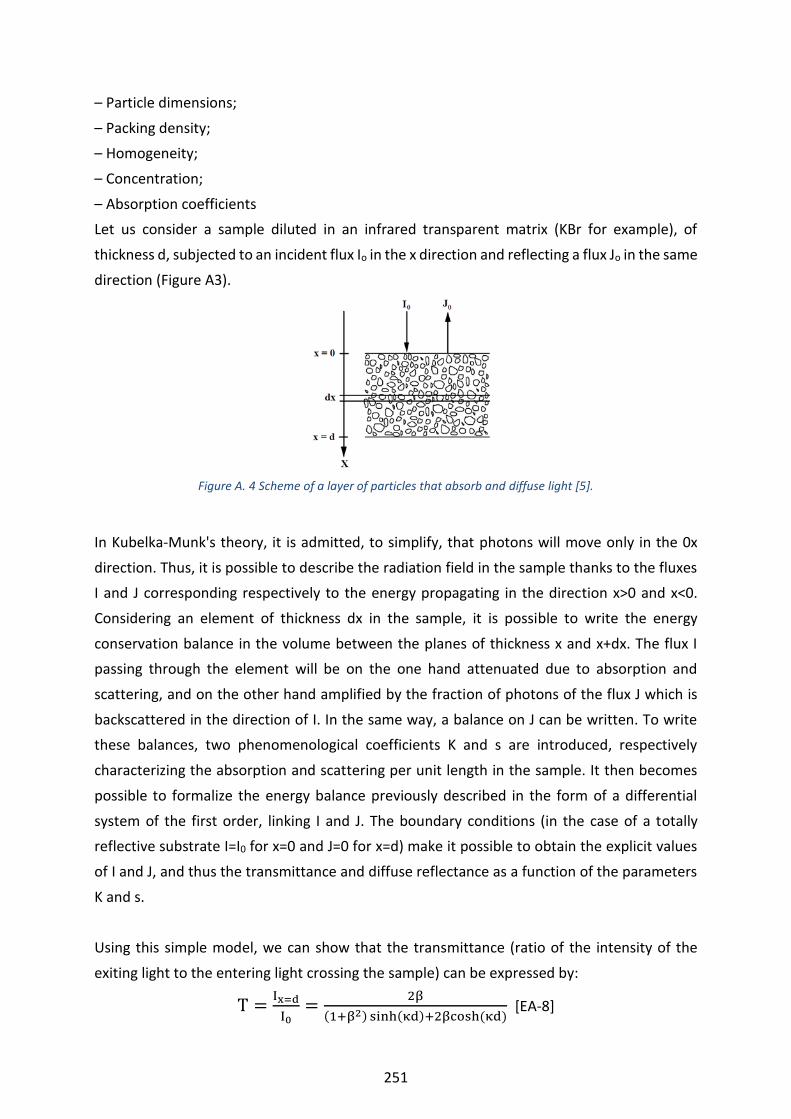
251

– Particle dimensions;

– Packing density;

– Homogeneity;

– Concentration;

– Absorption coefficients

Let us consider a sample diluted in an infrared transparent matrix (KBr for example), of

thickness d, subjected to an incident flux Io in the x direction and reflecting a flux Jo in the same

direction (Figure A3).

Figure A. 4 Scheme of a layer of particles that absorb and diffuse light [5].

In Kubelka-Munk's theory, it is admitted, to simplify, that photons will move only in the 0x

direction. Thus, it is possible to describe the radiation field in the sample thanks to the fluxes

I and J corresponding respectively to the energy propagating in the direction x>0 and x<0.

Considering an element of thickness dx in the sample, it is possible to write the energy

conservation balance in the volume between the planes of thickness x and x+dx. The flux I

passing through the element will be on the one hand attenuated due to absorption and

scattering, and on the other hand amplified by the fraction of photons of the flux J which is

backscattered in the direction of I. In the same way, a balance on J can be written. To write

these balances, two phenomenological coefficients K and s are introduced, respectively

characterizing the absorption and scattering per unit length in the sample. It then becomes

possible to formalize the energy balance previously described in the form of a differential

system of the first order, linking I and J. The boundary conditions (in the case of a totally

reflective substrate I=I0 for x=0 and J=0 for x=d) make it possible to obtain the explicit values

of I and J, and thus the transmittance and diffuse reflectance as a function of the parameters

K and s.

Using this simple model, we can show that the transmittance (ratio of the intensity of the

exiting light to the entering light crossing the sample) can be expressed by:

T =Ix=d

I0=

2β

(1+β2) sinh(κd)+2βcosh (κd) [EA-8]

252

and diffuse reflection:

R =Jx=0

I0=

(1−β2)sinh (κd)

(1+β2) sinh(κd)+2βcosh (κd) [EA-9]

In these expressions : κ = √K(K + 2s) and β = √K

K+2s

While k, the absorption coefficient, is easily known from the Lambert-Beer law, parameter s

is difficult to determine. To circumvent this problem, Kubelka and Munk considered the

limiting case of a sample of infinite thickness (2 or 3 mm of powder satisfies this condition).

This accordingly gives:

T∞ = 0 and R∞ =1−β

1+β [EA-10]

Which can also be placed in the form: f(R∞) =(1−R∞)2

2R∞=

K

s [EA-11]

f(R∞) is called the re-emission function or Kubelka-Munk function. A comparison with a

standard sample consisting of a nonabsorbent powder, i.e. KCl, KBr, etc. (such that k ≅ 0 and

R∞ ≅ 1) helps to determine the ratio:

r∞ =(R∞)sample

(R∞)standard [EA-12]

to which we apply the expression:

f(r∞) =(1−r∞)2

2r∞=

K

s [EA-13]

by replacing k by 2.303.ε(ν).C, where: ε = extinction coefficient (function of the wavenumber

ν); c = sample concentration; this gives:

f(r∞) =2.303∙ε(ν)∙C

s [EA-14]

and if s is a constant, i.e. an intrinsic property of the material which depends on the grain size,

f(r∞), at a given frequency, varies directly with the sample concentration c. This produces a

similar expression to the absorbance expression that enables us to obtain a spectrum

resembling the transmission spectrum.

253

Quantitative analyses of DRIFTS spectra

DRIFTS technique can bring many invaluable insights into the mechanism of heterogeneous

reactions. The qualitative analysis of the DRIFTS spectra is sufficient to assess the nature of

the adsorbates present. However, a fully quantitative analysis of DRIFTS data is required when

the surface concentrations and the specific rate constants of reaction (or desorption) of

adsorbates are needed to carry out complete spectro-kinetic studies.

The Kubelka-Munk and pseudo-absorbance data treatement are the most commonly used

functions when data collected by DRIFTS. The basis of the diffuse reflectance theory used to

quantify the concentration of an adsorbate was developed by Kubelka and Munk and widely

applied to the mid-IR regionsand sometimes to the UV-vis and near-IR regions. The Kubelka-

Munk formula [EA-13, EA-14] relates the diffuse reflectance radiation to the sample

absorption and scattering coefficients k and s, respectively. In practice, many of the conditions

required for the Kubelka-Munk theory to apply are not often met, e.g., because of the

presence of Fresnel (i.e., specular, mirror-like) reflection, matrix absorption, and nonuniform

optical properties of the sample. Signal corrections can be made, even for nondiluted samples,

but the data treatment is complex and the effect of the sample micro- or nanostructure will

also affect the scattering coefficient, making the comparison difficult between differently

prepared samples. In many cases, simple calibration curves have shown that the Kubelka-

Munk equation is not linear with respect to the concentration of the solute, displaying a

curved or brokenline shape. In this case, pseudo absorbance (log (1/R∞)) can be used to

linearly represent the adsorbate concentration given by:

log (1/R ∞) = Concentration

Constant [EA-15]

It has been previously shown [5] that the intensity of adsorbates should be reported in the

form of the Kubelka-Munk function for the case of highly absorbing adsorbates to obtain

DRIFTS data proportional to the adsorbate surface concentrations. Whereas, the intensity of

adsorbates should be reported in the form of pseudo absorbance for the case of poorly

absorbing adsorbates to obtain DRIFTS data proportional to the adsorbate surface

concentrations.

254

Annex 3: Uncertainty estimation of the band area observed in DRIFTS spectra

and effect of closing or opening valves on static conditions

The uncertainity of band area for the bands observed in the deformation region (1400-900

cm-1) are estimated using t distribution (Student’s t-distribution) and results are reported in

Table A.1.

Student’s t-distribution is a probability distribution that is used to estimate population

parameters when the sample size is small and/or when the population variance is unknown.

The confidence interval was constructed as follow:

Step 1: Find the mean, μ and standard deviation, σ for the data.

Step 2: Subtract 1 from your sample size to find the degrees of freedom (df).

Step 3: Subtract the confidence level from 1, then divide by two. This is the alpha (α) level.

Step 4: Look for df (Step 2) and α (Step 3) in the t-distribution table.

Step 5: Divide standard deviation (step 1) by the square root of your sample size (Standard

error).

Step 6: Multiply step 4 by step 5. This value is the confidence interval (at 95%) +/- in absolute.

Figure A. 5 Typcial DRIFTS spectra in the 4000-650 cm-1 spectral range expressed in pseudo-absorbance for NaCl

exposed to 5 hours of CH3I (108mL.min-1,1000 ppm) flow at 296 K and 1 atm. The spectra are from dry experiments repeat 1, repeat 2 and repeat 3.

255

Table A.2 Calculation of the the uncertainity of band using student’s t-distribution law.

Experiment.

Band (cm-1) …………………. Band area (arbitrary unit)

. Mean of band

area Standard deviation

Relative standrad deviation

Standard error

Confidence interval (at

95%) +/- in absolute

Repeat 1 1275+1244+1220+1183+1073+1024

2.34 2.16

0.15

6.97

0.09

0.37

Repeat 2 2.09

Repeat 3 2.07

Repeat 1 1275+1244+1220+1183

1.48 1.43 0.05 3.31 0.03 0.12

Repeat 2 1.43

Repeat 3 1.39

Repeat 1 1073

0.24 0.20 0.04 19.46 0.02 0.10

Repeat 2 0.18

Repeat 3 0.17

Repeat 1 1024

0.59 0.53 0.05 10.03 0.03 0.13

Repeat 2 0.51

Repeat 3 0.49

Repeat 1

1262

0.12 0.13

0.01

9.90

0.01

0.03

Repeat 2 0.15

Repeat 3 0.14

256

Table A.3 Effect of closing or opening valve on static conditions.

Sum of the band area of 1275, 1244, 1220 and 1183 cm-1 in

arbitrary units

After 5 hours of CH3I

flow

After 1 hour of static conditions

(closed valve)

% difference

(ACH3I – AIstatic)/ACH3I

Experiment 1 1.43 1.39 2.9%

After 5 hours of CH3I

flow

After 1 hour of static conditions

(open valve)

% difference

(ACH3I – AIstatic)/ACH3I

Experiment 2 1.48 1.45 2.1%

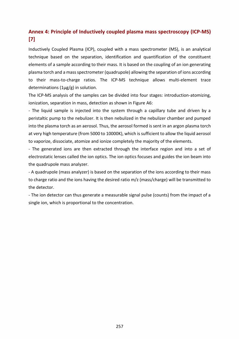
257

Annex 4: Principle of Inductively coupled plasma mass spectroscopy (ICP-MS)

[7]

Inductively Coupled Plasma (ICP), coupled with a mass spectrometer (MS), is an analytical

technique based on the separation, identification and quantification of the constituent

elements of a sample according to their mass. It is based on the coupling of an ion generating

plasma torch and a mass spectrometer (quadrupole) allowing the separation of ions according

to their mass-to-charge ratios. The ICP-MS technique allows multi-element trace

determinations (1μg/g) in solution.

The ICP-MS analysis of the samples can be divided into four stages: introduction-atomizing,

ionization, separation in mass, detection as shown in Figure A6:

- The liquid sample is injected into the system through a capillary tube and driven by a

peristaltic pump to the nebulizer. It is then nebulized in the nebulizer chamber and pumped

into the plasma torch as an aerosol. Thus, the aerosol formed is sent in an argon plasma torch

at very high temperature (from 5000 to 10000K), which is sufficient to allow the liquid aerosol

to vaporize, dissociate, atomize and ionize completely the majority of the elements.

- The generated ions are then extracted through the interface region and into a set of

electrostatic lenses called the ion optics. The ion optics focuses and guides the ion beam into

the quadrupole mass analyzer.

- A quadrupole (mass analyzer) is based on the separation of the ions according to their mass

to charge ratio and the ions having the desired ratio m/z (mass/charge) will be transmitted to

the detector.

- The ion detector can thus generate a measurable signal pulse (counts) from the impact of a

single ion, which is proportional to the concentration.

258

Figure A. 6 ICP-MS scheme. Q-pole: Quadrupole [7].

Annex 5: Gas chromatography (GC) [8]

Gas chromatography (GC) is a widely used analytical technique. It is a separation technique

applicable to gaseous compounds or compounds that can be volatilized by raising

temperature without decomposition (with a molecular weight of less than 300 atomic mass

units). The mobile phase is a gas (helium), so it allows the advancement of analytes in the

column which are in the gaseous state. The mobile phase behaves like an inert carrier gas, it

does not cause any interaction with the analytes to be separated.

Figure A. 7 GC scheme [8].

Injection: The CPG present at the L2EC [8] allows the use of two different injection modes:

manual injection and injection through the thermo-desorber.

259

Manual injector: The sample to be analyzed is introduced into the chromatograph

using a gas sampling syringe (10 or 25 mL) or Tedlar® bag (500mL or 1L). Manual

injection includes an injection loop. The choice of the loop volume is based on the size

of the column and the assumed concentration of the products to be analyzed. The

injection loop system avoids dead volume and ensures a constant injection volume,

which is important for quantitative analysis.

Injection through the thermo-desorber: The sample to be analyzed is not introduced

directly into the chromatograph. This technique is used when the analyte is not

concentrated enough to be detected or quantified. A pre-concentration step is

required. This technique uses the possibility for the analyte to adsorb on a solid phase

(cold-trap), and conversely to desorb in the injector under the effect of heat. Several

modes of injection in the cold-trap are possible: Tedlar® gas bag or sample tube.

The GC has a split/splitless injector that allows the fraction of the sample sent to the column

to be adjusted in relation to the total quantity introduced into the chromatograph. In split

mode, a stream of carrier gas arrives in the injection chamber where it mixes with the injected

sample. A leakage valve divides into two fractions, the smaller of which is the only one to enter

the column. The fraction of the sample entering the column is equal to the split ratio, which

can vary between 1 and 165.

In splitless mode, the entire sample is injected and then entrained into the first turns of the

capillary column. The injector is then swept by the carrier gas which removes the excess

solvent. This procedure is reserved for highly diluted samples. When injecting via the thermo-

desorber, the injection method on the GC must be in splitless mode (because the TD has its

own split).

Column: The gas chromatographic column may be considered the heart of the GC system,

where the separation of sample components takes place. Columns are classified as either

packed or capillary columns.

Packed columns are stainless steel or glass tube filled with particulate packing material (an

adsorbent material, or a support material coated or impregnated with a solid phase). Packed

columns produce broad band shapes and have low separation performance, but can also

handle large sample volumes and are not susceptible to contamination.

The capillary columns usually consist of a fused silica (quartz, SiO2) capillary that is coated with

a polyimide layer. The polyimide layer provides the capillary with flexibility and stability, as

well as its characteristic brownish color. Capillary columns produce sharp band shapes,

achieve excellent separation performance, and are suited to high-sensitivity analysis. The

260

column used in our experiments is a GASPRO capillary (open tube) column. The internal

diameter of the column is 0.32 mm and is 30 m long (twice 15 m). The maximum operating

temperature of this column is 350°C.

Detector: The detector senses a physicochemical property of the analyte and provides a

response which is amplified and converted into an electronic signal to produce a

chromatogram. In L2EC laboratory the GC has two detectors: Thermal Conductivity Detector

(TCD) and Electron Capture Detector (ECD).

The TCD is a universal response detector but is relatively insensitive (of the order of ppb). This

detector is based on a continuous comparison between the heat flux carried by the pure

carrier gas and the heat flux carried by the carrier gas loaded with the molecules to be

analyzed. These heat fluxes are produced by thermistors, through which a direct current of

fixed voltage flows, in a thermostatically controlled enclosure. The thermistors are mounted

in a Wheastone bridge, which allows the evolution of the current to be monitored as a

function of the variation in resistance due to temperature variations around the filaments.

The ECD is a more selective detector and sensitive to halocarbon compounds such as

iodomethane. It is a very sensitive detector that can analyze samples with concentrations of

the order of ppt. ECD has a low-energy radioactive source that allows free electrons to be sent

into the detector. When substances with an affinity for free electrons pass through the

detector, ions are produced which are collected in the existing electrostatic field by an anode

and form an ionization current.

261

Annex 6: Method of calculating the uncertainty of GC and ICP-MS

measurements [9]

An estimate of the expanded measurement uncertainty for manual injection and via the

thermodesorber was determined based on IRSN internal report [8] for GC and Melany’s work

[7] for ICP-MS. These determinations were based on EURACHEM/CITAC Guide [9]. The

estimation of an uncertainty involves a number of successive steps: Specification of the

measurand; Identification of the sources of uncertainty; Quantification of the uncertainty

components; Calculation of the combined uncertainty; Final expression of the measurement

result.

Definition of the measurand: In GC the measurand corresponds to the volume concentration

of methyl iodide (CH3I) in gaseous form (expressed in ppt, ppb or ppm). It is calculated from a

sampling flow rate (Nl/min) and the initial concentration of the standard cylinder. In ICP-MS

the measurand corresponds to the number of moles of the elements 1271 present in the

solutions analyzed after testing in the bench (samples in bubblers, filter solutions, rinsing

solutions).

Sources of uncertainty: The sources of uncertainty are identified (1) for GC the dilution factor

and the analytical method (GC) (2) for ICP-MS the weighing volume of the solution, dilution

factor and the analytical method.

Quantifying the uncertainty components: Determining the accuracy and precision were

conducted to quantify uncertainty of each component volume, analysis and dilution method.

The accuracy used to evaluate the difference between a certified value and a measured result.

The precision takes into account the effects of random factors that influence the

measurement of samples (temperature, pressure, storage conditions, reliability of the method

over time, preparation of solutions, etc).

Calculation of the combined and expanded uncertainty: The compound uncertainty is

associated with the determination of the combination of uncertainty contributions (analysis,

volume and dilution).

The final stage is to multiply the combined standard uncertainty by the chosen coverage factor

in order to obtain an expanded uncertainty. The expanded uncertainty is required to provide

an interval which may be expected to encompass a large fraction of the distribution of values

which could reasonably be attributed to the measurand.

Therefore, the expanded uncertainty for GC measuremnets was found to be 8% and 14 % at 95 % confidence level, for thermos-desorber and manual injection, respectively. For ICP-MS measurements, the uncertainity was found to be 8% at 95 % confidence level.

262

Annex 7: ICP-MS data and conversion factor calculation

Using ICP-MS, we were able to determine the total number of iodine taken up by salt in mg

using [EA-16]:

mt (I) in the solution = [I] in ppb × Volume of NaOH (mL) [EA-16]

Then total mass of iodine taken up by dissolved salt in number of atoms /mg was determined

by [EA-17]:

mt (I) in dissolved salt = 𝐦𝐭(𝐈) 𝐢𝐧 𝐭𝐡𝐞 𝐬𝐨𝐥𝐮𝐭𝐢𝐨𝐧 (𝐦𝐠)

𝐦𝐍𝐚𝐂𝐥 𝐝𝐢𝐬𝐬𝐨𝐥𝐯𝐞𝐝 (𝐦𝐠) × 10-3 ×

𝐀𝐯𝐨𝐠𝐚𝐝𝐫𝐨𝐬 𝐧𝐮𝐦𝐛𝐞𝐫

𝐌𝐨𝐥𝐚𝐫 𝐦𝐚𝐬𝐬 𝐨𝐟 𝐈𝐨𝐝𝐢𝐧𝐞 [EA-17]

The total amount of iodine taken up total salt (number of atoms) is then [EA-18]:

mt (I) in total salt= mt (I) in dissolved salt (number of atoms /mg )× Total mNaCl (mg) [EA-18]

Table A.3 summarize the determination of total number of iodine taken up by salt.

The conversion factor was then determined from the combination of ICP-MS and DRIFTS

results by [EA-19] (see Table A.4):

F = 𝑻𝒐𝒕𝒂𝒍 𝒂𝒎𝒐𝒖𝒏𝒕 𝒐𝒇 𝒊𝒐𝒅𝒊𝒏𝒆 𝒖𝒑𝒕𝒂𝒌𝒆𝒏 𝒃𝒚 𝒔𝒐𝒍𝒊𝒅 (𝑰𝑪𝑷−𝑴𝑺)

𝐁𝐚𝐧𝐝 𝐚𝐫𝐞𝐚 𝐚𝐭 𝐭𝐡𝐞 𝐞𝐧𝐝 𝐨𝐟 𝐞𝐱𝐩𝐨𝐬𝐮𝐫𝐞 𝐩𝐡𝐚𝐬𝐞 (𝐃𝐑𝐈𝐅𝐓𝐒) [EA-19]

263

Table A.4 Determination of the total amount of iodine taken up by NaCl using ICP-MS technique.

Experiment

1: NaCl exposed to 1000 ppm CH3I for 5 hours



Mass of salt in the reactor for exposure to methyl iodide (mg) 150.0 144.2 146.2

Mass of salt dissolved in NaOH (mg) 100.1 100.6 100.3

Mass / volume of NaOH (ml) 10 10 10

ICP MS results and determination of total number of I taken up by the salt :

Analyse 1 (dilution factor=5) 293.679 348.004 432.914

Analyse2 (diulution factor=10) 2.918×102 3.522×102 4.464×102

Analyse 3 (dilution factor= 20) 2.799×102 3.421×102 4.250×102

Retained [CH3I] in ppb in initial 10 mL NaOH 2.884×102 3.474×102 4.345×102

Total mass of iodine in the solution (mg) 2.884×10-3 3.474×10-3 4.345×10-3

Total mass of iodine taken up (mg/mg of salt ) 2.881×10-5 3.455×10-5 4.330×10-5

Total amount of iodine taken up (number of atoms/ mg of salt ) 1.366×1014 1.638×1014 2.053×1014

Total mass of iodine taken up by total mass of salt (mg) 4.322×10-3 4.982×10-3 6.331×10-3

Total amount of iodine taken up by salt (number of atoms) 2.050×1016 2.362×1016 3.002×1016

Absolute uncertertainty interval (+/- number of atoms) 1.640×1015 1.890×1015 2.402×1015

Mean of total amount of iodine taken up by salt (number of atoms) 2.471×1016

Absolute uncertertainty interval at 95% confidence level(+/- number of atoms) 1.206×1016

264

Table A.5 Determination of the conversion factor

IR data : [CH3I]= 1000 ppm, contact time in sample holder = 55 ms , continous flow for 5 hours

Experiment Repeat 1 Repeat 2 Repeat 3

Band (cm-1) 1275+1244+1220+1183+1074+1023 1275+1244+1220+1183+1074+1023 1275+1244+1220+1183+1074+1023

Area (a.u ) - pseudo absorbance 2.085 2.069 2.338 Absolute area uncertainty (+/- surface unit of integrate area) 0.374 0.374 0.374

Conversion factor (number of I atoms/ surface unit of integrated band area) 9.829 ×1015 1.142×1016 1.284×1016 Conversion factor absolute uncertainty (+/-) 1.913 ×1015 2.236×1015 2.277×1015

Mean conversion factor 1.136×1016

Mean conversion factor uncertainty (+/-) 3.740×1015

265

Annex 8: Time evolution of CH3I outlet concentration in static reactors filled

with solids

Figure A. 8 The evolution of [CH3I] outlet as function of time in the large reactor filled with 14-18g of oxalic and

Na2CO3 solids for an injected CH3I concentration of 100 ppb and 108 mL.min-1 continuous gas flow under RH=20% at 296 K and 1 atm.

Figure A. 9 The evolution of [CH3I] outlet as function of time in the large reactor filled with 18g of NH4NO3 solid for an injected CH3I concentration of 1 ppb and 77 mL.min-1 continuous gas flow under RH=20% at 296 K and 1 atm.

266

Figure A. 10 The evolution of [CH3I] outlet as function of time in the small reactor filled with 1g of different

organic and inorganic solids for an injected CH3I concentration of 100 ppb and of 108 mL.min-1 continuous gas flow under RH=20% at 296 K and 1 atm.

267

Reference

[1] https://pubchem.ncbi.nlm.nih.gov/compound/Iodomethane

[2] Y.Neehaul, Ph.D. thesis Study of protein interactions in the respiratory chain by IR

spectroscopy and electrochemistry, Strasbourg University, 2012.

[3] S. Scolaro, Ph.D. thesis on effects of humidity and fatty acid surfactants on the uptake of

NO2 to NaCl : Combined study of kinetics and surface analysis, Lille University, 2009.

[4] T. Armaroli, T. Bécue, S. Gautier, Diffuse Reflection Infrared Spectroscopy (DRIFTS):

Application to the in Situ Analysis of Catalysts, Oil Gas Sci. Technol. 59 (2004) 215–237.

https://doi.org/10.2516/ogst:2004016.

[5] J. Sirita, S. Phanichphant, F.C. Meunier, Quantitative analysis of adsorbate concentrations

by diffuse reflectance FT-IR, Anal. Chem. 79 (2007) 3912–3918. https://doi.org/10.1021

/ac0702802.

[6] E.Siurdyban, Thése de doctorat, Immobilisation de dérivés du cryptophane-A sur des

surfaces planes SiO2/or et OR ainsi que sur des nanoparticules magnétiques, Université de

Bordeaux, 2015.

[7] M. Gouello, Thése de doctorat, Chimie de l’iode et composition des aérosols dans le circuit

primaire d’un réacteur nucléaire en situation d’accident grave, Université de Grenoble, 2013.

[8] C. Alvarez, J.Nguyen-sadassivame «Conduite de l’analyse d’ICH3 par CPG, validation de

méthode d’analyse et calcul d’incertitude,» Rapport interne IRSN - IRSN/2020-00341, 2020.

[9] EuraChem guide, Quantifying Uncertainty in Analytical Measurement, 3rd Edition (2012).

https://www.eurachem.org/index.php/publications/guides/quam

268

Titre : Etude expérimentale des réactions de capture/désorption

des iodes gazeux (I2, CH3I) sur des aérosols environnementaux

L’iode gazeux est émis dans l’atmosphère soit par l’activité biologique des océans soit, pour

l’iode radioactif, lors de situations d’accident nucléaire. Mieux modéliser le

transport/réactivité de ces composés halogénés est essentiel du fait de leur implication dans

la formation/disparition de l’ozone atmosphérique ainsi que des conséquences radiologiques

lors de la dispersion d’iode radioactif. Dans ce contexte, ce travail a concerné les interactions

entre un composé gazeux de l’iode et l’eau ou des aérosols atmosphériques par des

techniques de spectroscopie.

Ce composé gazeux interagit très peu avec les aérosols atmosphériques de sels marins. Avec

l’eau atmosphérique, il se forme des agrégats interagissant avec des polymères d’eau plutôt

que des nouveaux composés. Aux températures typiques de l’atmosphère, l'adsorption de

l’iode gazeux sur la glace amorphe est très peu probable. Ces résultats vont permettre

d’implémenter les connaissances sur le devenir atmosphérique de l’iode.

Title: Experimental study on the Capture/Desorption of gaseous

iodine (I2, CH3I) on environmental aerosols

Iodine is emitted into the atmosphere either by biological activity in the oceans or more

specifically, for radioactive iodine, during a severe nuclear accident. Improving the modelling

of the transport/reactivity of these so-called halogenated compounds in the atmosphere is

important since they are strongly linked to the cycle of ozone formation/depletion and since

the dispersion of radioactive iodine may have radiological consequences. In this context, the

interactions between a gaseous organic iodine compound and water or atmospheric aerosols,

such as sea salts, was studied by using spectroscopic approach.

We have shown very weak interactions with sea salt atmospheric aerosols. With water, it

forms aggregates interacting with water polymers rather than forming new compounds. At

atmospheric temperatures, adsorption of this gaseous organic iodine compound on

amorphous ice is unlikely to occur. These results will allow the implementation of knowledge

on iodine fate in the atmosphere.

Experimental study on the Capture/Desorption of gaseous ...

Documents

Transcript of Experimental study on the Capture/Desorption of gaseous ...