A Experimental Investigation of Acoustic Cavitation in Gaseous Liquids

DTI

S ':'IECTE W11419900J

I~ .=. ENT A.

TheUniversity of Mississippi

AN EXPERIMENTAL INVESTIGATION OFACOUSTIC CAVITATION IN GASEOUS LIQUIDS

BY DTICDARIO FELIPE GAITAN ".ET

* DEC 2 41990,B.S., University of Southwestern Louisiana, 1984

National Center for Physical AcousticsUniversity, MS 38677

September 1990 NS...NT-IS CA I "• --

4 L) h l l lo t m e I j,0�,0d... .. ic.. ..

ByTechnical Report ........... ..............................

prepared for: Di. t .i

Office of Naval ResearchPhysics Division Dl JV•,, 1 1/o0

Contract # N00014-90-J-4021 4.c~d

NCPA.LC.02.90

Approvn tzc, pu'.:Lc relecisal

S9012 21 010

UnclassifiedSECURIT Y CLASSIFICA, ON OF THIS PG-"

Form ApprovedREPORT DOCUMENTATION PAGE OMB No, 0704-0188

la REPORT SECURITY CLASSIFICATION .b, RESTRICTIVE MARKINGS

Unclassified"2a. SECURITY CLASSIFICATION AUTHORITY 3. DISTRIBUTION IAVAILABILITY OF REPORTApproved for public release2b. DECLASSIFICATION / DOWNGRADING SCHEDULE'

Distribution unlimited4 PERFORMING ORGANIZATION REPORT NUMBER($) 5. MONITORING ORGANIZATION REPORT NUMBER(')

NCPA.LC.02.90

6a NAME OF PERFORMING ORGANIZATION 6b. OFFICE SYMBOL 7a, NAME OF MONITORING ORGANIZATION

NatLinal Center for Physical (If appllcable)Acoustics ICOffice of Naval Research

6c. ADDRESS (City, State, and ZIPCode) 7b. ADDRESS (City, State, and ZIP Code)

Coliseum Drive Department of the NavyUniversity, MS 38677 Arlington, VA 22217

Ba. NAME OF FUNDING/SPONSORING 8b, OFFICE SYMBOL 9, PROCUREMENT INSTRUMENT IDENTIFICATION NUMBERORGANIZATION (If applicable)

N00014-90-J-4021B., ADDRESS (City, State, and ZIP Code) 10. SOURCE OF FUNDING NUMBERS

PROGRAM " PROJECT TASK TWORK UNITELEMENT NO, NO. NO. ACCESSION NO,

11. TITLE (Include Security Classification)

An experimental investigation of acoustic cavitation in gaseous liquids.

12. PERSONAL AUTHOR(S)Gaitan, D. Felipe; Crum, Lawrence A.

13a TYPE OF REPORT 13b. TIME COVERED 114. DATE OF REPORT (Year, Month, Day) 115,"PAGE COUNTTechnical I FROM 9_jL-- TO 12__-3 1990, November 8 .. 207

16 SUPPLEMENTARY NOTATION

17 COSATI CODES 18. SUBJECT TERMS (Continue on reverse if necessary and idvntify by block number)FIELD GROUP SUB.GROUP Physical Acoustics Nonlinear Bubble Dynamics

Acoustic Cavitation SonoluminescenceMie Sc@terine Nonlinear Flit Djnqm~fr

I ABSTRAC' (Continue on reverse if necessary and identify by block number)"* High amplitude radial pulsations of a single bubble in several glycerine and water

mixtures were observed in an acoustic stationary wave system at acoustic pressureamplitudes on the order of 150 kPa at 21-25 kHz. Sonoluminescence, a phenomenongenerally attributed to the high temperatures generated during the collapse ofcavitation bubbles, was observed as short light pulses occurring once every acousticperiod. These emissions could be seen to originate at the geometric center of thebubble when observed through a microscope. It was observed that the light emissionsoccurred simultaneously with the bubble collapse. Using a laser scattering technique,experimental radius-time curves were obtained which confirmed the absence of surfacewaves which are expected at pressure amplitudes above 100 kPa. From these radius-time curves, measurements of the pulsation amplitude, the timing of the major bubblecollapse, an(' the number of rebounds were made and compared with several theories. Theimplications of this research on the current understanding of cavitation were discussed.

20. DISTRIBUTION/AVAILABILITY OF ABSTRACT 21. ABSTRACT SECURITY CLASSIFICATIONEJ UNCLASSIFIED/UNLIMITED ,•, SAME AS RPT. [ DTIC USERS Unclassified

22,3 NAME OF RESPONSIBLE INDIVIDUAL 22b, TELEPHONE (Include Area Code) 22c. OFFICE SYMBOLLawrence A. Crum (601) 232-5905 LC

OD Form 1473, JUN 86 Previous editions are obsolete. SECURITY CLASSIFICATION OF THIS PAGE'i6

Absbm

0 AN EXPERIMENTAL INVESTIGATION OF ACOUSTICCAVITATION IN GASEOUS LIQUIDS

GAITAN, DARIO FELIPE. B. S. , University of Southwestern Louisiana,1984. Ph. D. , University of Mississippi, 1990. Dissertation

-* directed by Dr. Lawrence A. Crum.

High amplitude radial pulsations of a single gas bubble in several glycerine and

- water mixtures have been observed in an acoustic stationary wave system at

acoustic pressure amplitudes as high as 1.5 bars. Using a laser scattering

technique, radius-time curves have been obtained experimentally which confirm

the absence of surface waves. Measurements of the pulsation amplitude, the

0 timing of the major bubble collapse, and the number of rebounds have been made

and compared with the theory. From these data, calculations of the internal gas

temperature and pressure during the collapse have been performed. Values of at

least 2,000 K and 2,000 bars have been obtained using a sophisticated model of

- . pherically symmetric bubble dynamics. Simultaneously, sonoluminescence (SL),

a phenomenon discovered in 1933 and attributed today to the high temperatures

and pressures generated during the collapse of the bubbles, were observed as short

light pulses occurring once every acoustic period. The light emissions can be seen

* to originate at the geometric center of the bubble when observed through a

microscope. Also, the simultaneity of the light emissions and the collapse of the

bubble has been confirmed with the aid of a photomultiplier tube. This is the first

recorded observation of SL generated by a single bubble. Comparisons of the

* measured quantities have been made to those predicted by several models. In

addition, the implications of this research on the current understanding of

cavitation related phenomena such as rectified diffusion, surface wave excitation

and sonoluminescence are discussed. Future experiments are suggested.

ACKNOWLEDGEMENTS

I would like to acknowledge my appreciation to the following individuals andorganizations for their contributions to this dissertation and their support duringmy graduate education:

To Dr. Lawrence Crum for his personal and professional advice, criticalcomments, and patience in directing this dissertation.

To Dr. Andrea Prosperetti for his scientific expertise and valuablesuggestions during the course of this project.

To Dr. Ron Roy for technical advice and continuous encouragement inthe pursuit of my career.

To Dr. Charles Church for sharing his knowledge and physical insightsduring many helpful discussions and for his valuable help incalculating the data in Chapter III (rectified diffusion thresholds).

To Milena Gaitan, Sandra Smith, Nancy Roy, and Janice Mills for theirhelp in preparing this manuscript, especially to Sandra Smith forlher friendship and support during the last five years.

To former members of the cavitation group at NCPA, Glynn Holt, SteveHorsburgh and Brian Fowlkes, for many enlightening discussions,technical support and their companionship. I am especiallygrateful to Glynn Holt and Steve Horsburgh for letting me use theirtheoretical calculations on Mie scattering (Chapter II) and surfaceinstabilities threshold (Chapter III), respectively.

To the National Center for Physical Acoustics and the University ofMississippi for their support of this work and to the other membersof my dissertation committee, Dr. Robert Hickling, Dr. MackBreazeale, Dr. James Reidy, and Dr. Charles Hussey, as well as toDr. Roy Arnold, Glynn Holt, and Ali Kolaini for their usefulscientific and editorial comments.

Finally, to my parents, Dario and Luz, for their moral and financialsupport during my educational career and to my wife, Milena, forher encouragement, help and great patience during the writing ofthis dissertation.

0

Table of Contents

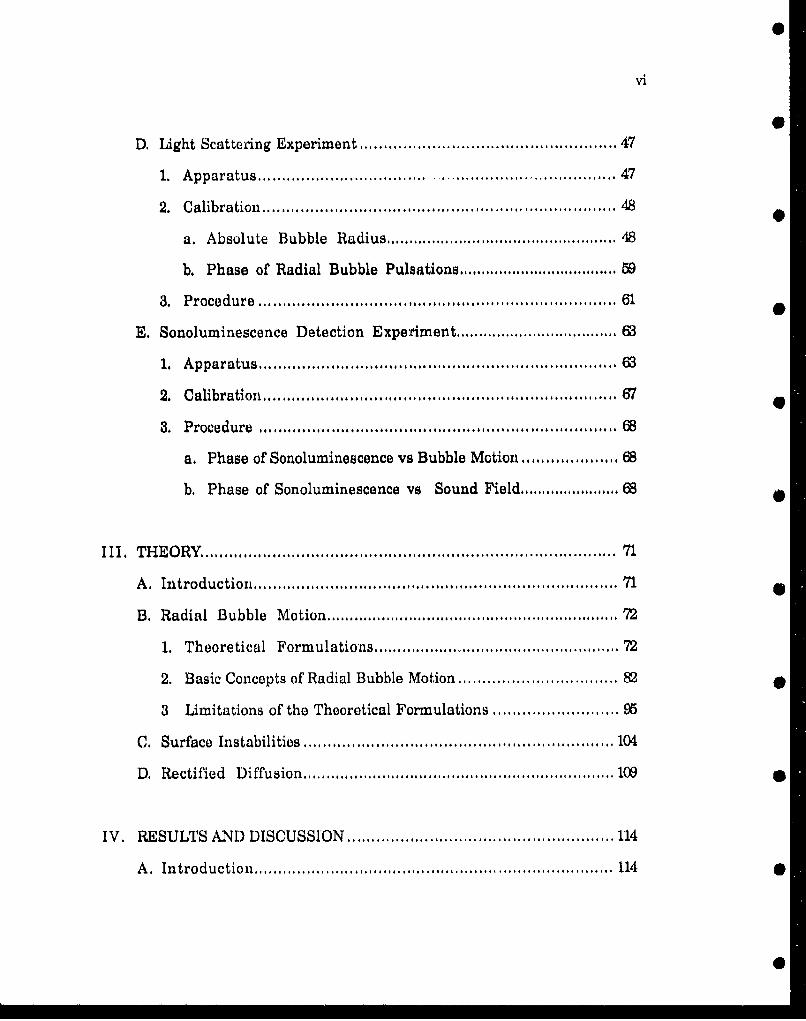
0LIST OF TABLES ..................................................................................... viii

LIST OF FIGURES .................................................................................... ix

* @Chapter

1. 1I',TTRODUCTION ................................ I...................... .... ................ 1

A. Statement of the Problem ............................................................ 1

1B. Historical Perspective ................................................................. 2

1. Models of Sonoluminescence .................................................. 2

2. The Phase of Sonoluminescence ............................................ 10

* 3. Sonoluminescence as a Probe of Acoustic Cavitation ............... 17

4. Acoustic Cavitation and Bubble Dynamics ............................. 21

C. Recapitulation and General Overview of the Dissertation .............. 24

II. APPARATUS AND EXPERIMENTAL PROCEDURE ........................ 27

A. Introduction ........................................................................ 27

B 1. Acoustic Levitation Apparatus .................................................. 28

1. Levitation Cells .............................................................. 28

2 Rise-time Measuring Apparatus ...................................... 33

* 3. Hydrophones ................................................................... 35

C. Calibration of Acoustic Levitation Apparatus .......................... 39

1. Absolute Sound Field Pressure .......................................... 39

* 2. Phase of the Sound Field Pressure .................................... 46

V

vi

D. Light Scattering Experiment ................................................ 47

1. Apparatus ..................................... 47

2. Calibration ......................................... 48

a. Absolute. Bubble Radius ................................................ 48

b. Phase of Radial Bubble Pulsations .....................................

3. P rocedure .......................................................................... 61

E. Sonoluminescence Detection Experiment ................................ 63

1. A pparatus .......................................................................... W

2. Calibration .............................. ....... 67-

3. Procedure ................. ................. ............. ............... ........ ...... 68

a. Phase of Sonoluminescence vs Bubble Motion .................... 68

b. Phase of Sonoluminescence vs Sound Field ....................... 68

III. T H E O R Y ...................................................................................... 71

A . Introduction ....................................................................... 71.

B. Radial B ubble M otion ................................................................ 72

1. Theoretical Formulations .................................................... 72

2. Basic Concepts of Radial Bubble Motion ..................... 82 •

3 Limitations of the Theoretical Formulations ...................... 95

C. Surface Instabilities ................................................................ 104

D . Rectified D iffusion ................................................................... 109 O

IV. RESULTS AND DISCUSSION ....................................................... 114

A . In trod u ction ........................................................................... 114 _

0

vii

B. Light Scattering Experiments .................................................. 123

1. Comparison between Theories and Experiment:

Prosperetti's Theory .......................................................... 123

a. Radius-tim e curves .................................................... 123

b. Pulsation Amplitude .............................. 8

c. Phase of Collapse ...................................................... 16

d. Number of Radial Minima ............................................. 142

e. Comparison with the Polytropic Theory and Flynn's

T h eory ......................................................................... 1W

2. Theoretical Values of Temperature, Pressure and

Relative D ensity ................................................................. 161

3. Phase of Sonoluminescence vs Bubble Motion ....................... 172

C. Time-to-Amplitude Converter System:

Sonoluminescence vs Sound Field ............................................. 174

1. Single Bubble Cavitation Field .............................................. 174

2. M ulti-bubble Cavitation Fields ............................................. 181

V. SUMMARY, CONCLUSIONS AND TOPICS FOR FUTURE STUDY., 185

A. Summ ary of the dissertation .................................................... 185

B . C onclu sions ........................................................................... 186

C. Topics for Future Study ........................................................... 187

R E F E R E N C E S ......................................................................................... 189

APPENDIX A 198......................... . ... ............... 19

S, o , o , , ~ * o , . , * o , 6 , , * i o l • ~ 6 • • o 4 l o ~ o o o o 6 l • , ~ o

0"

0

List of Tables

Table no. Description

1 The phase of SL Predicted by the different models ................... 11

2 Summary of measurements of the phase of sonoluminescence... 14

3 Summary of measured relative densities, temperatures

and pressures inside cavitation bubbles .................................... 18

4 Summary of predictions of R. obtained from

Prosperetti's form ulation ...................................................... 149

5 Summ~ary of predictions of R, obtained from Flynn's

form ulation ......................................................................... 157

6 Summary of predictions of R, obtained from the

polytropic formulation ....................................y...i I.......'.158 07 Summary of maximum theoretical temperatures inside

20-25 gm bubbles for the range of PA used during the

experiments ...................................... 166

8 Summary of maximum theoretical pressures inside 20-25

ptm bubbles for the range of PA used during the experiments ..... 166

9 Summary of maximum theoretical relative densities inside

20-25 ptm bubbles for the range ofpA used during the

experiments ..................................... 1

viii

S

List of Figures

Figure no. Description

1 Schematic drawing of cylindrical acoustic levitation

cell w ith bubble .................................................................. 30

2 Schematic drawing of rectangular acoustic levitation

cell w ith bubble .................................................... ...................

3 Schematic diagram of rise-time measurement

apparatus ............................................................................. 34

4 Schematic drawing of needle hydrophone (NDL1) ...................... 36

5 Plot of the side pill transducer response vs the depth of the

needle hydrophone ............................................. .................... 38

6 Plot of the needle hydrophone response vs the side pill

transducer ......................................................................... 38

7 Pressure profile of cylindrical levitation cell as a

function of depth in GLY42 at f=23.6 ,-Hz ................................. 41

8 Schematic diagrarn of experimental apparatus used to

record the light intensity scattered by the bubble as a

function of tim e ..................................................................... 49

9 Theoretical scattered intensity of the parallel polarized

component S2 as a function of scattering angle

(0 is forward) for ka=661. This corresponds to a radius

ix

x

of 38.6 pým with respect to the Ar-I 488.0 nm line ........................ 53

10 Trheoretical scattered intensity of the parallel component

S2 as a function of equilibrium radius at 66 degrees ................... 5

11 Theoretical scattered intensity of the parallel comnponent

S2 as a function of equilibrium radius at 70 degrees .. ............... 55

12 Theoretical scattered intensity of the parallel component

S2 as a function of equilibrium radius at 80 degrees ............... 56

13 Measured scattered light intensity vs equilibrium bubble

radius for 42% glycerine. The solid line corresponds to a

2 nd degree poly~nomrial fit . ............................ 58

14 Theoretical phase of bubble radius minimum for 42%

glycerine at 0.1, 0.2 and 0,3 bars and f=2' .6 kIIz used

in the phase calibration of the light- scattering apparatus ..... ,......6

15 Schematic diagram of experimental apparatus used to

measure the phase of sonoluminescence relative to the

sound field......................................................... 6

16 Schematic diagram of circuit used to measure the

phase of sonoluminescence relative to the sound field ............ 660

17 Theoretical bubble-response curves calculated using

Prosperetti's formulation for water at PA= 0*' -0.5 bars,

f=21.0 kI-Iz.....................................................................

18 Theoretical radius-t-ime curve calculated using the

polytropic formulation for water at PA= 0* 8 bars,

R,,/ R,,=. 7,f=21. 0 k~z....................... ...... I....... 85

xi

19 Theoretical radius-time curve calculated using the

polytropic formulation for water at PA=0. 8 bars,

RRo/R,,,=0.39, f=21.O kHz ........................................................ 86

20 Theoretical radius-time curve calculated using

Prosperetti's formulation for water at PA= 1 .2 bars,

RR/R,,=O14, f=21.0 kHz ........................................................ 88

21 Theoretical internal temperature-time curve calculated

using Prosperetti's formulation for the same conditions

used in figure 20 ................................................................ 89

22 Theoretical internal pressure-time curve calculated


used in figu re 20 .................................................................... .91

23 Theoretical bubble-response curve calculated using

Prosperetti's formulation for water at PA=1.2 bars, f=21.0 kI-Iz .... 92

24 Theoretical phase-of-collapse curve calculated using

Prosperetti's formulation for the same conditions used

in figure 23 ........................................... 94

25 Theoretical internal temperature curve calculated


used in figure 23 ............................................................ ..... 96

26 Theoretical internal pressure curve calculated using

Prosperetti's formulation for the same conditions used

iM figure 23 ........................................................................ . 97

27 Theoretical liquid pressure vs. liquid temperature at the

xii

interface during one acoustic period for GLY42, Ro,20 pm,

PA=l. 5 bars and f=23.6 kHz. These data were calculated

using Flynn's form ulation ..................................................... 101

28 Pressure-amplitude threshold curve for the excitation of

surface waves calculated by Horsburgh (1990) at f=22.2 kHz

for air bubbles in w ater .......................................................... 107

29 Pressure-amplitude threshold curve for bubble growth by

rectified diffusion calculated by Church (1990) at f=21.0 kHz

in air-saturated w ater ........................................................... Ill

30 Simultaneous oscilloscope traces of sonoluminescence (top)

and acoustic pressure (bottom) for water at f=21.0 kHz

(T =47.6 pmn ) .......................................................................... 115

31 Depiction of cavitation streamers in the cylindrical levitation

cell ..................................................................................... 117

32 Graphic representation of the range of pressure in which

radial stability was observed in water-glycerine mixtures at

f=.21-25 kH z .......................................................................... 121

33 Experimental radius-time curve obtained with the light-

scattering apparatus in 21% glycerine at PA=l. 2 2 bars and

f=22.3 kH z ......................................................................... 124

34. Theoretical calculation of the steady state solution of the

bubble radius for the experimental conditions described in

Fig. 33 and Ro,=20 gm using Prosperetti's formulation .............. 126

35 Measured and theoretical pulsation amplitude (Rimox) vs

"""1

xiii

acoustic pressure amplitude in water using

Prosperetti's formulation at f=21.0 kHz ................................... 129

* 36 Measured and theoretical pulsation amplitude (R.m..) vs

acoustic pressure amplitude in GLY21 using


--- • 37 Measured and theoretical pulsation amplitude (Rvms) vs


Prosperetti's formulation at f=23.0 kHz .................................. 131

- 38 Measured and theoretical pulsation amplitude (R'm,) vs



• 39 Measured and theoretical pulsation amplitude (Rvms) vs


Prosperetti's formulation at f=24.8 kHz ................................. 3,

40 Measured and theoretical phase of bubble collapse (Oc) vs



- 41 Measured and theoretical phase of bubble collapse (01c) vs


Prosperetti's formulation at [=23.3 kHz ................................... 138

• 42 Measured and theoretical phase of bubble collapse (Oic) vs



* 43 Measured and theoretical phase of bubble collapse (Oic) vs

..0_• ., _ - - - - -" -" •• -"M | nm nn

xiv



44 Measured and theoretical phase of bubble collapse (0c) vs


Prosperetti's formulation at f=24.8 kHz ................................. 141

45 Measured and theoretical number of minima (ML) vs



46 Measured and theoretical number of minima (MO vs


Prosperetti's formulations at f=22.3 kHz ................................. 144

47 Measured and theoretical number of minima (Mi) vs


Prosperetti's formulation at f=23.0 kHz ............................... 145

48 Measured and theoretical number of minima (MO vs



49 Measured and theoretical number of minima (M) vs •


Prosperetti's formulation at f=24.8 kHz .................................. 147

50 Measured and theoretical pulsation amplitude (R•m•) vs 0

acoustic pressure amplitude in water using all three

form ulations at f=21,0 kH z .................................................... 151

51 Measured and theoretical pulsation amplitude (Rimax) vs

xv

acoustic pressure amplitude in GLY42 using all three

form ulations at f=23.6 kHz .................................................... 152

52 Measured and theoretical phase of bubble collapse (0.) vs


formulations at f=21.0 kHz ...... ............... ...... ... ................. . 153

53 Measured and theoretical phase of bubble collapse (0o) vs


formulations at f=23.6 kHz .................................................... 154

54 Measured and theoretical number of minima (M') vs


formulations at f=21.0 kHz .................................................... 155

55 Measured and theoretical number of minima (M1 ) vs


form ulations at f-23.6 kX-z ........ ...................... ............. ..... ....... 156

56 Theoretical maximum gas temperature reached during the

bubble collapse in water for R0 =1 5 and 20 microns at

f=21.0 kH z ....................................................................... 16

57 Theoretical maximum gas temperature reached during the

bubble collapse in GLY42 for R,=15 and 20 microns at

f=23.6 kH z ............................................................................ 163

58 Theoretical maximum gas pressure reached duxrng the

bubble collapse in water for Ro-1 5 and 20 microns at

f=21.0 kH z ............................................................................ 164

59 Theoretical maximum gas pressure reached during the

... . ........ ..

xvi

bubble collapse in GLY42 for R,,=1 5 and 20 microns at

f=23.6 kH z ............................................................................ 165

60 Simultaneous plots of the bubble radius (bottom)

representing the bubble radius and sonoluminescence (top)

in GLY21 at PA=l, 2 bars at f=22.3 kHz. ..................................... 173

61 Phase of sonoluminescence emitted by a single bubble

as a function of time. It was measured in water at

PA^-l. bars and f=21.0 kHz using the time-to-amplitude

converter (TAC) system ......................................................... 175



PA-1.2 bars and f=21 0 kHz using the time-to-amplitude

converter (TAC) system during a transition (see text) ................ 177



PA-l.3 bars and f=21.0 kHz using the time-to-amplitude

converter (TAC) system during bubble breakup and

disappearance ...................................................................... 180

64 Phase of sonoluminescence emitted by a multibubble

cavitation field as a function of time. It was measured

in water at PA-l, 3 bars and f=21.0 kHz using the time-to.,

amplitude converter (TAC) system. ........................................ 182

65 Phase of sonoluminescence emitted by a multi-bubble

cavitation field as a function of time. It was meqsured in

O

xvii

water at PA .3 bars and f=21.0 kHz using the time-to-

amplitude converter (TAC) system ..................... 184

Al Calibration chart and specifications for B&K hydrophone

type 8103 .............................................................................. 199

A2 Measured scattered light intensity vs equilibrium bubble

radius for water at f=21.0 kHz. The solid line corresponds to a

2"d degree polynomial fit ................... ......... .... ..................... 200


radius for 35% glycerine mixture at f=23,0 IlHz. The

solid line corresponds to a 2nd degree polynomial fit .................. 201


radius for 42% glycerine mixture at f=23.6 kHz. The

solid line corresponds to a 2nd degree polynomial fit ................. 20

* A5 Measured scattered light intensity vs equilibrium bubble

radius for 60% glycerine mixture at f=24.8 kHz. The

solid line corresponds to a 2nd degree polynomial fit .................. 23

• A6 Experimental radius-time curve obtained with the light-

scattering apparatus in water glycerine at PA=1. 2 2 bars

and f=21.0 kH z ..................................................................... 2%

* A7 Experimental radius-time curve obtained with the light-

scattering apparatus in 35% glycerine at PA= 1 .37 bars

and f=23.0 kH z ................................................................... 205

* A8 Experimental radius-time curve obtained with the light-

0 :_ _ _-. . .

xviii

scattering apparatus in 42% glycerine at PA=1.50 bars

and f=23.6 kH z ..................................................................... 206

A9 Experimental radius-time curve obtained with the light-

scattering apparatus in 60% glycerine it PA=l.27 bars

and f=24.8 kH z ..................................................................... 2W7

0

Chapter I

Introduction

L A. Statement of the Problem

The subject of this dissertation is the dynamics of bubbles in acoustic

cavitation fields of moderate intensities. For the purpose of this study, acoustic

cavitation may be defined as the formation and pulsation of vapor or gas cavities or

bubbles in a liquid through the negative pressure half cycle of a sound field. A

particularly interesting phenomenon associated with the violent pulsations of gas

bubbles is a weak emission of light called sonoluminescence, This light emission0 has been attributed to the high temperatures generated during the rapid

compression of the bubbles, brought about by the action of the sound field, Despite

the extensive amount of research done on both acoustic cavitation and

sonoluminescence, many important questions relating to the nature and

dynamics of these phenomena remain unanswered, Attesting to this uncertainty

is the multiplicity of existing models describing the mechanisms of light

production as well as the number of conflicting views and observations of

cavitation-related phenomena found in the literature.

The motivation behind this research was to answer questions such as: What

is the motion of the light-emitting cavities involved in sonoluminescence ? How

applicable are the present theories of single, spherical bubble dynamics in

describing these cavities ? What are the physical conditions attained in the

------

2

interior of the bubbles during the collapse ? Is it possible to detect

sonoluminescence from a single pulsating bubble ? Answers to these questions

have been pursued for over 50 years and, needless to say, complete answers to all

of them have not boon found here. In the process of seeking those answers,

however, some experimental observations were made which have clarified some of

the past and l rn:se-it research in this field. It is my hope that some of these

observations will point to new directions that future researchers may follow.

L D. Ullb~urical Perspective

Cavitation was first predicted by Leonhard Euler in 1754 when he suggested

that, if the velocity in a liquid was high enough, negative pressures could be

generated and the liquid might "break". This "breaking" was given the name

"cavitation" in 1895 by R.E. Froude, an English naval architect, to describe the

appearance of voids and clouds of bubbles around propellers rotating at high

speeds. Since then, the term "cavitation" has been used to describe the

appearance of voids or bubbles when liquids are sufficiently stressed.

The first theoretical treatment of cavitation was made by Lord Rayleigh in

1917. In it, he derived an equation to describe the motion of a vapor-filled cavity in

a liquid. In this cavity, called a Rayleigh cavity, the internal pressure was less

than the ambient pressure, and they both remained constant, By its definition,

this cavity could not be in equilibrium with the surrounding liquid and began to

collapse immediately, Although very simplistic, this model has been used

successfully to represent cavities formed by rotating propellers and, more

3

generally, by hydrodynamic cavitation. No further improvements to Rayleigh's

theory were made until more than 30 years later, with the introduction of ac

cavitation,

The first systematic study of acoustic cavitation was published by Blake in

1949, In it, Blake describes the formation of bubbles in the focal region of a

parabolic projector where sound waves were made to converge. According to

Blake, bubbles in the cavitation region moved erratically and, if the amplitude

were high enough, they emitted a hissing noise. This hissing, he postulated, was

generated by cavities collapsing under the action of the sound field, These cavities

were used to explain a particularly interesting effect of acoustic cavitation that had

been observed 15 years before. When ultrasound of sufficiently high intensity was

passed through a liquid saturated with gas, a weak emission of light was

observed. This effect was called sonoluminescence, i.e., light "produced" by

sound.

I. B. L Models of Sonoluminescence

First observed by Marinesco et al. in 1933, sonoluminescence (SL) was

discovered when photographic plates became exposed when submerged in an

insonified liquid. It was not until 1947, however, that Paounoff et al. showed that

the exposure of the plates occurred at the pressure antinodes of the standing wave

field. The first attempt to explain this phenomenon was made by Zimakov in 1934.

After studying SL from various aqueous solutions, he concluded that the emission

was caused by an electric discharge between vapor cavities and the glass wall of

4

the container. Frenzel and Schultes (1935), after noticing that light was not

emitted from degassed water, concluded that the emission was caused by friction

between cavitating bubbles and water. Chamber (1936) studied SL from 36

different liquids at an insonation frequency of 10 kHz and was the first to observe

light emission from nonaqueous solutions. He also established an inverse

relationship between SL intensity and the ambient liquid temperature. Based on

his observations, he postulated the first formal model of SL known as Ta

Tribhuminemcent Model, This model suggested that SL was generated by the

sudden destruction of the quasi-crystalline structure of the liquid, a process

similar to the one observed when many crystals are crushed, Since the breaking

of the structure occurred during the cavity formation, this model predicted the

light emission to occur during the expansion phase of the acoustic cycle.

A year later, Levshin and Rzhevkin (1937) concluded that SL originated in the

gas phase (and not in the liquid) after observing that potassium iodide and

pyrogallol, a quencher of photoluminescence in the liquid, did not quench

sonoluminescence, whereas C02, a gas quencher, did. They also proposed that SL

was caused by an electric discharge resulting from the liquid rupture which

excites the vapor filling the cavities, producing sonoluminescence. This theory

was further developed by Harvey (1939), who suggested that these electric charges

were balloelectric in nature; i.e., they were produced by an increase in the surface

charge of fluids. Harvey's model, known as The Balloelectric Model, draws an

analogy with the mechanism through which water droplets in a gas become

charged, as occurs in rain and waterfalls. By suggesting the inverse

phenomenon, i.e., charged bubbles in a liquid, Harvey postulated that an electric

0

field exists in the surrounding liquid which increases as the bubbles are

compressed until a discharge occurs, giving rise to a weak emission. This model,

therefore, predicted the light to be emitted during the compression phase of the

sound field.

Another model, also based on the existence of electric charges on the walls of

cavities, was that of Frenkel (1940) called The Microdisoharge ModAl It postulated

that statistical variations of the charge distribution on the lens-shaped cavity

formed by the rupture of the liquid created regions of opposite charge on the cavity

* wall. As the cavity expanded, it became spherical carising the electric field within

it to strengthen until a discharge occurred during the expansive phase of the

sound field.

* In 1949, Weyl and Marboe proposed that the light was emitted by the radiative

recombination of ions created as the quasi-crystalline structure of the liquid was

destroyed at the newly created surface of an expanding bubble, This model was

called The Mechanochemical Model of sonoluminescence.

Several criticisms have beon made to these early models, mainly due to the

observed lack of sensitivity of the light emission to the electrical conductivity of the

* liquid, which would be expected to affect the electric charge formation. In fact, SL

is often enhanced by the addition of electrolytes (Negishi, 1961) and is particularly

strong in mercury (Kuttruff, 1950). Also, these models suggest that cavitation

* arises from molecular ruptures whereas, at moderate acoustic intensities,

cavitation is known to occur from the growth of stabilized gaseous nuclei (Atchley

etal., 1984).

6

Despite the strong evidence against models of SL based on electrical

discharges, new models are still being introduced. In 1974, Degrois and Baldo

proposed the "new electrical hypothesis" in which charge on gas bubbles arises

from the neutralization of anions on the bubble surface by gas molecules adsorbed

on the inside of the gas-liquid interface. The electrical field is generated as the gas

molecules become polarized due to their asymmetric surroundings, As the bubble

collapses, the charge density increases until it exceeds a critical value, at which

point a discharge of electrons occurs from the inside of the interface into the

liquid. This model has been called The Anion Discharge Model, A thorough

review of this hypothesis has been given by Sehgal and Verral (1982), in which they

show how this model disagrees with the experimental data,

More recently, Margulis (1984) has proposed a new electric charge model in

order to explain some experimental facts such as the observation of electric pulses

in an insonated liquid (Gimenez, 1982), SL flashes during the expansion phase of

the sound field (Golubnichii et al., 1970) and sonoluminescence and sonochemical

reactions in low frequency acoustic fields (Margulis, 1982, 1983). These facts,

however, have only been observed by a few investigators and constitute a very

small percentage of all the available data on sonoluminescence. Margulis' model

is based on the accumulation of charge on a small neck of a "fragmentation

bubble" which is still attached to the parent bubble. Fragmentation bubbles are

caused by spherical instabilities of the pulsating bubbles. The transfer of charge is

effected through the liquid stream passing around the bubble neck at high speeds.

After almost 20 years of investigation, it became clear to researchers that gas

bubbles played a significant role in cavitation and the generation of

7

sonoluminescence. Thus, a practical model for the motion of these bubbles was

necessary to further advance the understanding of cavitation-related phenomena.

To this end, Noltingk and Neppiras (1950) developed the first theory of acoustic

cavitation. The theory used Rayleigh's equation as a starting point, adding to it a

term for an internal pressure due to the gas inside the bubble, a variable pressure

term applicable to acoustic fields as well as the effect of surface tension. They

obtained an ordinary differential equation describing the radial motion of a gas

bubble in terms of the pressure amplitude and frequency of the sound field as well

as the equilibrium radius of the bubble. Their contribution became the first

significant improvement to the theory since Rayleigh's seminal paper in 1917.

Based on their theory, Noltingk and Neppiras introduced The Hot Spot Model

of sonoluminescence. This model is based on the adiabatic heating of the cavity

contents. They proposed that, during cavitation, a gaseous nucleus grows slowly

and isothermally by the action of the sound field, until reaching a maximum

radius, Rmox. At this point, the bubble collapses rapidly, causing the gas inside to

heat up to incandescent temperatures. The maximum temperature reached

inside the bubble is given by

Td = T. &R- x\R,,• /( 1.1 )

where T. is the ambient temperature, Rmn the minimum bubble radius at the end

of the collapse and y the ratio of the specific heat capacities. The gas is then

assumed to radiate like a blackbody.

8

"After integrating the differential equation for the bubble motion for several

sets of parameters, Noltingk and Neppiras found that conditions foi cavitation

(high presr-ures and temperatures both inside and outside the bubble) would only

occur for nuclei less than resonance size (defined later in Chapter III). They also

concluded that cavitation was restricted not only to a finite range of insonification

frequencies and nucleus equilibrium sizes, but also to a fixed range of ambient

and acoustic pressure amplitudes. Their theory was very successful in explaining

many of the observations of SL such as the decrease in SL intensity as the

frequency and ambient pressure were increased as well as the increase in SL

intensity as the acoustic pressure amplitude was increased. It also explained the

dependency of SL intensity on the type of gas dissolved in the liquid. Gases with

larger values of y (monatomic gases) were predicted to emit more light due to the

higher temperatures reached in the interior, as can be seen from equation 1.1 and

confirmed by experimental observations. The theory also showed that lower

internal pressures were obtained with monatomic gases than with polyatomic

gases (air and C0 2, for example), indicating that SL was primarily the result of

high temperatures rather than high pressures.

The Hot Spot mode], however, failed to explain the observed difference in SL

intensity among the inert gases, in which the gases with larger atomic weight

generated more light. As originally postulated, the Hot Spot model did not

consider the heat flow to the surroundings during the short collapse time of the

cavity. In order to explain the experimental evidence, Hickling (1963) was the first

to quantify this effect by considering a model of a spherical cavity containing a

thermally conducting ideal gas in an incompressible liquid. Although having the

9

same value of y, the heavier gases were less thermally conducting duo to their

smaller molecular velocities. Using this model, he successfully explained the SL

intensity data for several gases.

A variation of the Hot Spot model was proposed by Jarman (1960), in which

shock waves in the gas undergoing multiple reflections at the bubble wall were

responsible for the light emissions. The luminescence emitted by this mechanism

is thermal in origin, with small contributions due to Bremsstrahlung and

recombination of ions. This model is very similar in principle to the model

proposed by Noltingk and Neppiras. In addition, the conditions necessary for the

formation of shock waves are not often realized, as will be shown in Chapter III.

Numerous experiments with ultrasound using different liquids and gases

had provided evidence that chemical reactions occurred during cavitation and,

especially, during light emission. Spectral studies of sonoluminescence in

aqueous solutions of electrolytes (Gunther, 1957b) had indicated the emission of

lines and bands characteristic of metal radicals superimposed on a background

continuum which suggested that other sources of radiation were present in

addition to the blackbody. To Griffing (1950, 1952), these observations suggested

that SL was in fact a chemiluminescence. She then proposed The

Chemilumrinescent Model in which the high temperatures generated inside the

collapsing cavity, gave rise to oxidizing agents such as H202 through thermal

dissociation which then dissolved in the surrounding liquid causing further

reactions, some of a chemiluminescent character.

The ideas introduced by the Hot Spot and Chemiluminescent models are

considered today the accepted explanation of the phenomenon of

0.

0

10

0

sonoluminescence. These ideas have been further confirmed during the course of

this investigation.

In 1957, Gunther (1957b) observed for the first time that SL was emitted as

short flashes of light, lasting 1/10th to 1/50th of an acoustic period. If enough SL

were being produced, i.e., if the acoustic intensity were sufficiently high, the

flashes were seen to occur periodically, with the same frequency as that of the

sound field. Several measurements of the phase of the light emission relative to

the sound field have been made since its discovery. When these measurements

failed to provide consistent results, researchers attempted to measure the phase of

SL with respect to the bubble motion, some with relative success. Brief

descriptions of these measurements are given in the next Section.

I. B. 2. The Phase of Sonoluminescence

During the late 1950's and early 1960's, several experiments were performed

in an attempt to determine the relationship between the phase of SL emission and

the phase of the sound field. The motivation behind these experiments was to

discriminate among the different models based on the opposite predictions on the

phase of the SL emission, some of which have been summarized in Table 1. As

shown in this Table, the Triboluminepcence, Microdischarge and

Mechanochemical models all predict the light to bo emitted during bubble growth.

Although it was not known then, the phase of SL relative to the sound field is

dependent on the exp')rimental conditions such as the insonation frequency, the

initial bubble radii and the liquid parameters. Nevertheless, the phase of SL can

O

11

be used to calculate a range of equilibrium radii of the bubbles emitting light in a

particular experimental arrangement, assuming a constant acoustic pressure

_ amplitude, as will be shown later. This fact was first used by Macleay and

Holroyd (1961) in their experiment.

Table 1. The phase of SL predicted by the different models.

- Sonoluminescence 0 SL during bubble growth

Modl * SL during bubble collapse

Triboluminescence ........................ 0Balloelectric ..................................

0 M icrodischarge ............................. 0Mechanochemical ........................ 0Anion Discharge ...........................H ot-spot ............. .. ......................Chemiluminescence ......................

The first attempt to measure the phase of SL relative to the sound field was

made by Gunther et al. (1957a). They were the first to use a PMT to examine SL

0 emissions from a standing wave field at 30 kHz. Using a cathode ray oscilloscope,

they noted that SL was emitted from the pressure antinodes and that it occurred

near the end of the compression phase i.e., 360 measured from the negative-going

• part of the sound cycle. A year later, in 1958, Wagner used a similar experimental

arrangement and found, unlike Gunther et al. (1957a), that SL was emitted close

to the sound pressure minimum (90') in Kr-saturated water. The duration of the

* emission was found to depend on the ambient pressure p., the acoustic pressure

amplitude PA and the solution temperature, but it was usually less than one tenth

of an acoustic period. This disagreement prompted other researchers to

0

40

12

investigate the issue of the phase of SL further. Using a cylindrical transducer

driven at 16.5 kHz to produce an axial pressure antinode in a stationary wave

system, Jarman (1959) found that SL was emitted close to the sound pressure

minimum (90") in non-volatile liquids like water, in agreement with Wagner

(1968). In volatile liquids, he found that SL was emitted near the sound pressure

maximum (270"). To further complicate the picture, Golubnichii et al. (1970) found

that emission occurred close to the beginning of the compression phase (180'), its

exact location depending on the solvent.

It was not until 1961 that researchers began to use theoretical calculations of

bubble motion to predict the nroperties of cavitation fields. An interesting

experiment was performed by Macleay and Holroyd (1961), in which they used the

theory of Noltingk and Neppiras (1950) to predict the phase of SL (i.e., bubble

collapse) for a range of initial bubble radii. In addition, by assuming that the SL

intensity was proportional to R 2mnT 4max (where Rm.n and Tmax are the bubble

radius and the temperature respectively during SL emission) and that bubbles of

all sizes were present in the liquid, they were able to deduce an SL intensity

distribution as a function of the phase of SL emission. This distribution ranged

from 180 to 350 degrees with a well defined peak around 270 degrees. When -

compared with the experimental data, agreement was surprisingly good.

According to their calculations, the peak at 270" corresponded to a bubble radius of

about 2 microns at 400 kHz and 1.8 bars of pressure amplitude. 0

It is now known that the phase of bubble collapse depends on several

parameters such as the driving frequency, pressure amplitude and equilibrium

bubble radius. Also, as noted by Jarman and Taylor (1970), the most likely cause of

S-- .•_ .0

0

13

this widespread disagreement was the use of poorly characterized hydrophones

and of electronics which introduced unknown phase shifts, After calibrating all

their electronics properly, Jarman and Taylor (1970) performed what were then

the most careful measurements of the phase of SL. Using a cylindrical

piezoelectric transducer driven at 14.4 kHz, they found that most SL flashes

occurred around 360. Using the theory of Noltingk and Neppiras, they calculated

the phase to correspond to bubbles of resonance size of 220 microns. In addition,

they reported results at 23 kHz with the phase of most SL flashes occurring around

290'. They also found secondary flashes usually occurring a short time after the

main flash which they attributed to bubble rebounds,

The results of these experiments, as reported by the different authors, have

been summarized in Table 2. The phase of SL is measured from the negative-

going part of the sound cycle and R0 is the equilibrium radius corresponding to the

measured phase of SL reported by the authors. In most cases, the pressure

* amplitude was not known or not reported, which in part explains the large

discrepancies among the different results. This also makes it impossible to

explain these discrepancies in light of the new, more accurate bubble dynamics

_ 7models.

Interestingly, the results of Macleay et al. are the most consistent with the

results of the present study despite the different experimental arrangement.

* 1-However, as pointed out by Jarman and Taylor (1970), the high frequency used in

their experiments provided a poor resolution of phase. Further comparisons will

be made in Chapter IV.

0a

14

Table 2. Summary of measurements of the phase of sonoluminescence.

Insonation Pressure ovst Phaseof Bblefiequency Amplitude Liquid SL Radius ,R.

Experiment (kHz) (bars) (degrees) (4rm)O

Gunther et al. (1957a) 30 -- H2O 360

Wagner (1958) 30 -- H2O 90

Macleay et al. (1961) 400 1.8-2.8 H20 270 0.3-3

Jarman et al.(1970) 14.4 2.2 H20 360 220It I 23.3 -- H2O 90

...........-.................................................................

Gaitan (1990) 21 1.1-1.3 H2O 190-210 1&-20S21-25 1.1-1.5 H 20/G LY 200-250 15-20

In view of the inability to obtain a unique value of the phase of SL, researchers

opted to study how SL varied with the bubble volume rather than with the acoustic

pressure. The first attempt was made by Meyer and Kuttruff in 1959 who

produced cavitation bubbles in ethylene glycol on the end of a nickel rod driven

magnetostrictively at 25 kHz. By illuminating the bubbles with a flash tube

triggered by the time-delayed SL flashes, they visually determined that the SL

flashes occurred during the bubble volume minima. Because the bubbles were

generated on the face of the transducer, i.e., near a solid boundary, they were most

likely collapsing asymmetrically. Although the phase of these bubbles may differ

from that of free, symmetrically collapsing bubbles, the experiment did provide

strong evidence that SL and the bubble collapse occurred simultaneously.

In 1960 another investigator, Negishi, made the first and only attempt

reported in the literature to obtain an experimental radius-time curve of

15

acoustically driven cavitation bubbles using a dark-field illumination technique to

record the volume of the cavitation zone as a function of time. In his experiment,

he projected th.e image of the cavitation bubbles produced by a 28 kHz ferrite

transducer onto a screen, allowing some of the light to pass through a small hole

and strike a PMT. Although the light recorded by the PMT was not linearly

related to the volume of the cavitation bubbles, it was proportional to it, After

turning the light source off, he then recorded the SL emission during cavitation.

With this apparatus, Negishi (1960,1961) was able to determine the phases of the

radial maxima and minima and, plotting these simultaneously with the PMT

output, he demonstrated that the SL flashes coincided with the minimum bubble

cloud volume. Recent studies have shown, however, that bubble clouds behave in a

collective mariner and their motion is, therefore, different from that of a single

bubble.

Other techniques have been designed to investigate collapsing bubbles,

although the bubbles were not acoustically driven. Two of these techniques

utilized laser and spark-induced cavitation which allowed the position of the

bubble to be predicted, as opposed to acoustic cavitation where cavitation events

occurred essentially at random locations in the liquid. In both of these techniques

a local portion of the liquid is heated to high temperatures very rapidly, creating a

vapor cavity instantaneously. As the cavity expands, the vapor cools quickly

allowing the liquid to collapse in the manner of a Rayleigh cavity (see chapter III).

In addition to recording radius as a function of time, researchers have detected

sonoluminescence flashes emitted during the collapse, In 1971, Buzukov and

Teslenko, using a light scattering technique similar to Negishi's, obtained the

16

radius-time curve of a collapsing cavity produced by a single pulse from a ruby

laser. When it was focused on a point in a liquid, a pulsating bubble was created

from which a short flash of light was emitted in coincidence with the minimum

bubble radius during the first compression of the bubble, Simultaneously with the

bubble collapse, they also detected acoustic emissions in the form of shock waves.

A second experiment was performed by Benkovskii et al. in 1974 using spark-

induced cavitation. In this case, cavities were produced in two different

experiments by rapidly melting a thin tungsten wire underwater and by an

electric spark produced between two electrodes immersed in a test liquid. 0

According to Walton et al. (1984), Benkovskii (1974) obtained results similar to

those of laser-induced cavitation using a pulse of 100 kV and 5.10"8 sec duration

applied to point-electrodes 1 mm apart. In addition to the first flash, SL flashes

occurred during the second and even third collapse. Furthermore, Golubnichii et

al. (1979) claimed that with spark-induced cavitation the SL flash does not coincide

with the minimum volume of the bubble. A discrepancy of 12 psec was reported in 0

water but only 1-2 p.sec in glycerine and ethylene glycol. More recently,

researchers have been able to photograph laser-induced cavities with high speed

cameras using conventional and holographic photography. Frame rates as high 0

as 300,000/sec have been achieved by Lauterborn et al, (1986) in his study of laser-

induced cavity collapse, and much has been learned from their observations,

0

0

0

17

L B. 3. Sonoluminescence as a Probe of Acoustic Cavitation

Most of the previous studies of SL have focused on the determination of its

mechanism. Unfortunately, little effort had been made, until recently, to use this

phenomenon to study the physical conditions attained during cavitation. Since SL

is generated by cavitation, information on the properties of the interior of the

cavitation bubble during collapse can be extracted from SL, assuming that the

light is emitted during the collapse. A few measurements of temperature and

pressure were made by researchers, however, using the characteri8ks of the

emitted light. Parameters such as wavelength of maximum emission and

bandwidth at half the maximum intensity (FWHM) have been measured in order

to determine the density (relative to the equilibrium conditions) of the emitting

species. Since one of the results of the present study has been a determination of

the minimum temperature and pressure inside a cavitation bubble necessary to

generate SL, a review of previous measurements will be given next. It should be

noted, however, that the spread of the emitted light spectrum on which some of

these measurements are based may be due to the inhomogeneity of the cavitation

field, as pointed out by Sehgal et al. (1979, 1980). Cavitation is a dynamic process,

and the temperature and pressure fields inside the bubbles fluctuate within a

large range of values as the bubbles expand and collapse. SL may be emitted at

slightly different stages of the bubble motion, in which case the physical conditions

would be different at the time of the light emission. The inhomogeneity of the

cavitation field during which these measurements were made also implies that

18

bubbles of different sizes would be present, reflecting a variety a physical

conditions.

Previous measurements of relative densities, temperatures and pressures of

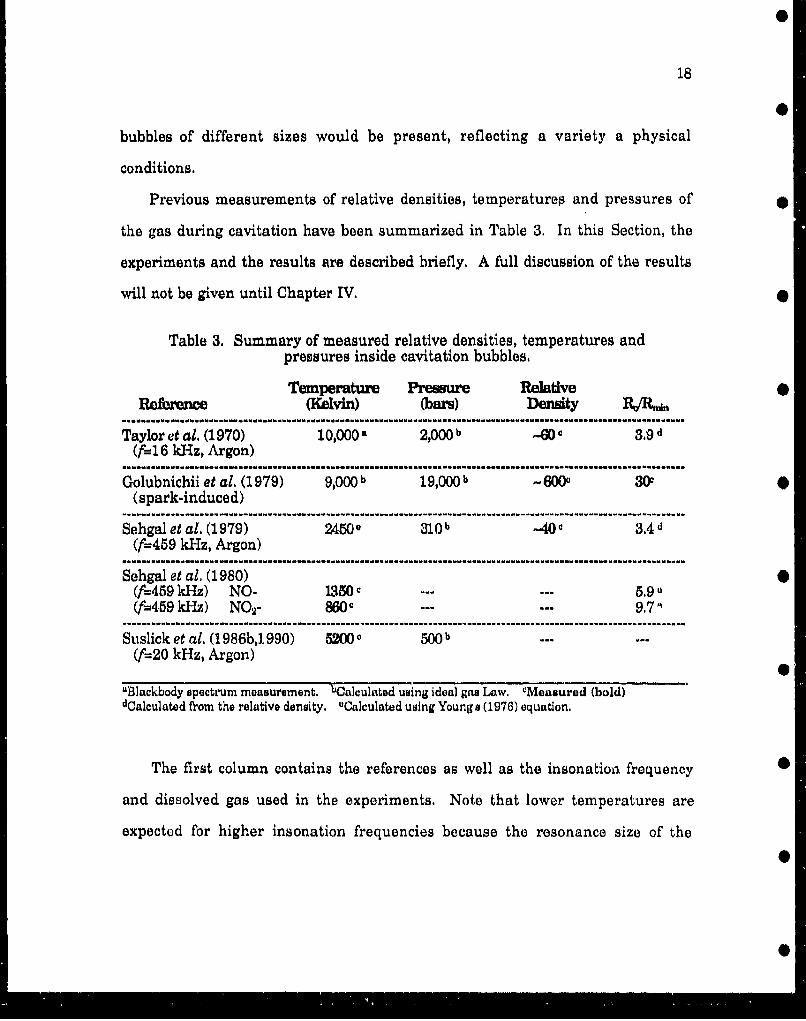
the gas during cavitation have been summarized in Table 3. In this Section, the

experiments and the results are described briefly. A full discussion of the results

will not be given until Chapter IV. 0

Table 3. Summary of measured relative densities, temperatures andpressures inside cavitation bubbles.

Temperature Pressure Relative 0R1ftrence (IMvin) (bars) Density P/Rj

............. . ......... .... • ...... .. .... .......... ......... •........ ...........................

Taylor et al, (1970) 10,000. 2,000 b -6W 3.9 d(f=1 6 kHz, Argon)

Golubnichii et al. (1979) 9,000 b 19,000 b - 600o 30W(spark-induced)

Sehgal et al. (1979) 2450e 31.0b -400j 3.4 d(f=459 kHz, Argon)

Sehgal et al, (1980) 0(f=459 kHz) NO- 1350 C ---... 5.90(f=459 kHz) NO,2- 860 --.. 9.7-

Suslick et al. (1 986b,1 990) 5200 500 b(f=20 kHz, Argon)

'Blackbody spectrum measurement. bCalculated using ideal gas Law, eMeasured (bold)dOalculated from the relative density, "Calculated using Young's (1976) equation.

The first column contains the references as well as the insonation frequency 0

and dissolved gas used in the experiments. Note that lower temperatures are

expected for higher insonation frequencies because the resonance size of the0

19

bubbles is smaller, allowing more heat to escape into the liquid. The dissolved gas

is important when using the specific heat raLio (y) to calculate the temperatures

* (7=5/3-1.67 for monatomic gases, and 7/5=1.4 for diatomic gases). Values in bold

type indicate experimental values, as opposed to values calculated based on

different assumptions, as indicated by the footnotes.

* Taylor and Jarman (1970) measured relative densities (with respect to

equilibrium conditions) of about 60 in various argon-saturated aqueous solutions

at an insonation frequency of 16 kHz. These measurements were based on the

* FWHM of tho sodium D line. Assuming a temperature of 10,000 K - based on

blackbody spectral measurements - they deduced pressures of 2,000 bars from the

ideal gas Law. The determination of temperature by fitting the SL spectra to that

*@ of blackbody radiation is now believed to be incorrect due to the chemiluminescent

rather that incandescent nature of the radiation, as Taylor and Jarman (1970)

have pointed out. Furthermore, even an adiabatic collapse would result in

* temperatures of only - 5,000 K fbr a relaLive density of 60, and y=5/3.

Golubnichii et al, (1979) measured the collapse ratio (Rm/Rmi,, where Rm is the

maximum radius attained by the vapor cavity) of spark-induced cavitation bubbles

0 using the shadowing technique. They obtained values of about 30 which

corresponded to adiabatic temperatures of 9,000 K assuming that the vapor has

cooled to room temperature when R-R.,. They also measured the maximum

0 absolute density reached during the collapse by introducing NaCl into the liquid (a

water-glycerine mixture) and measuring the pressure broadening of the sodium D

lines. This gave n=1.5.1021 m-1, from which they calculated a maximum pressure

0 of 19,000 bars using the ideal gas law.

L

20

More extensive investigations were made by Sehgal et al. at frequencies of 459

kHz. They made independent measurements of the relative density (Sehgal et al.

1979) and of the temperature (Sehgal et al, 1980). The density measurement, like

Taylor's, was made by measuring the line shifts and FWHM of potassium

resonance peaks emitted by insonated aqueous solutions of alkali and halide salts

saturated with argon. They obtained a value of the relative density (with respect to

the density of the medium at STP) of about 40, This corresponds to a collapse ratio

(Ro/Rm~n) of 3.4, where R0 and R1 l. are the initial and minimum bubble radius

reached during the collapse, respectively, Using an equation derived by Young 0

(1976) which compensates for thermal diffusion, they calculated the internal

temperature to be 2450 K and, from the ideal gas law, they calculated internal

pressures of 310 bara.

The measurement of temperature by Sehgal at al. (1980) was based on the

relative distribution of SL intensities from NO- and NO2 - saturated aqueous

solutions. In their experiment, intracavity temperatures of 1350 ± !-0 K and 860 ±

100 K for NO and NO2, respectively were obtained. Collapse ratios were calculated

using Young's (1976) equation to be 5.9 and 9.7 respectively at an acoustic pressure

amplitudes of 6.2 bars, •

A recent, more precise measurement of the temperature inside cavitation

bubbles has been made by Suslick et al. (1986a,b) using a comparative rate

thermometry technique in alkane solutions of metal carbonyls, The technique 0

consisted of measuring the reaction rates of the metal carbonyls as a function of

their concentration inside the cavitation bubbles. The change in concentration

was effected by increasing the bulk temperature of the solutions which increased •

0-

21

the vapor pressure of the metal carbonyls. The overall vapor pressure cf the

solutions was kept constant by using appropriate solvent mixtures. These

solutions were irradiated with a collimated 20 kHz beam from an amplifying horn.

Suslick et al. reported a maxmum temperature of 5200 ± 650 K reached in the gas

phase. In addition, by extrapolating their results, they found a nonzero value of

*@ the reaction rates corresponding to zero metal carbonyl concentration. Based on

this finding, they concluded that a reaction zone existed in the liquid phase with

an effective temperature of -1900 K. The pressure amplitude used in their

* experiment is not specified except for a total acoustic intensity at the horn's

surface of 24 W/cm 2. For comparison, assuming plane waves in water, this

intensity corresponds to about 8 bars.

L B. 4. Acoustic Cavitation and Bubble Dynamics

Cavitation has generally been classified in two types: "Transient" and "stable"

(gaseous) cavitation. This classification traces its origin back when the first visual

observations of cavitation activity were made (Blake, 1949; Willard, 1953), and was

introduced in order to describe these observations. Transient cavitation was used

to describe events that lasted only fractions of a second, usually occurring at high

pressure amplitudes. These events were attributed to vapor or gas bubbles which

expanded to large sizes during the negative part of the pressure cycle, after which

they began to collapse. Because of the large radius attained during the expansion,

their collapse was very rapid and violent, often resulting in the destruction of the

bubbles. Flynn (1964) attempted to defined these terms more precisely. According

22 -

to him, a transient cavity is "that which, on contraction, from some maximum

size, its initial motion approximates that of a Rayleigh cavity.,." whereas a s' 'dIe

cavity "oscillates nonlinearly about its equilibrium radius.". Flynn (1975b) a

further refined this definition of transient and stable cavities in terms of the

equations of bubble dynamics. He defined two functions: an inertial function, ,',

and a pressure function, PF, which represent the inertial and pressure forces 0

controlling the bubble motion and which are functions of time, R. and PA. For

transient cavities, IF is much larger than PF and therefore the motion is inertia

controlled whereas the opposite is true for stable cavities. Flynn then defined a

transient cavitation (dynamical) threshold in terms of the expansion ratio,

Rmax/Ro, i.e., the dynamics of bubbles pulsating with R,,.R, above this threshold

are controlled by IF, whereas bubbles below this threshold are controlled by PF.

After an extensive investigation of the thermal behavior of pulsating bubbles,

Flynn also introduced anexpansion-ratio threshold for the occurrence of thermal

phenomena during cavitation (e.g. sonoluminescence). This threshold was based

on the fact that small bubbles tend to dissipate the internal heat generated during

collapse (isothermal motion), whereas large bubbles behave more adiabatically,

generating high temperatures in their interior. From his calculations, Flynn n

concluded that small bubbles (< 5 ým) reach the dynamical (transient cavitation)

threshold before exhibiting sonoluminescence, Large bubbles (>5 ýtm), on Lhe

other hand, are able to generate high internal temperatures and therefore, exhibit 0

sonoluminescence before becoming a transient. It should be noted here that

becoming "transient" does not necessarily mean that the cavity is not stable.

However, inertia-dominated cavities tend to collapse very rapidly, promoting •

0

23

surface instabilities which often cause breakup. Therefore, when the dynamical

threshold is greatly exceeded, cavities are, in general, not expected to survive for

* more than a few of cycles. Flynn's model of cavitation bubbles will be used to

explain some of the observations made in this study. It will be shown that

observations of the thresholds for sonoluminescence and transient bubble motion

0 agree with this model.

As mentioned previously, several descriptions of the behavior of bubbles in

ultrasonically-induced cavitation. fields were made during the early years of

* cavitation research (Blake, 1949; Willard, 1953; Neppiras et at., 1969). Neppiras

(1980), in his thorough review of acoustic cavitation, describes several types of

cyclic cavitation processes. These observations are presented in this Section as an

* introduction to the study of long-term periodic behavior of' the phase of the light

emitted by cavitation bubbles. It should be noted that Neppiras did not cite any

references when describing these observations and it was, therefore, not possible

* to obtain the original works. Some of these observations are:

i. The gaseous cavitation cycle occurs when a bubble is made to grow by

rectified diffusion (see Chapter III), eventually reaching the transient cavitation

threshold (Flynn, 1964). Then, the bubble immediately expands, implodes and

disintegrates. The residual fragments may be either too small and dissolve

completely or start growing again by coalescence and rectified diffusion. This

process repeats itself, although not very regularly, since the bubbles are variable

in size. It can be observed in high-speed photography of cavitation in gassy liquids

by examining successive frames.

24

0

ii. The dg_. s cycle consists of bubbles growing, as in the case of the

gaseous cavitation cycle, by rectified diffusion in such a way that the conditions for

complete collapse never occur. Eventually the bubble will become large enough to

iloat to the surface, gradally causing the solution to become undersaturated.

This degassing can only occur within a restricted range of R, and PA and,

according to Neppiras (1980), its rate can be maximized by choosing appropriate

treatment conditions related to the bubble-size distribution.

iii. The resonance bubble cycle with emission of microbubbles. At sufficiently

high frequencies, bubbles reach their resonance size before separating out under

gravity. Bubbles of resonance size are highly likely to develop instabilities, exciting

surface modes of vibration. The strong surface vibrations are parametrically

excited at half the driving frequency and are strongly coupled to the radial

pulsations. In an intense field, the surface waves may grow to large amplitudes

and "throw off' microbubbles from the crests. This can occur very rapidly, the

parent bubble apparently exploding, which may explain the "disappearing

bubbles" reported by Nyborg and Hughes (1967). These microbubbles are usually

all equal in size, with radii near k,,/4 where 1, is the wavelength of the surface

oscillation (Neppiras, 1980).

L C. Recapitulation and General Overview of the Dissertation0

The Hot Spot and Chemiluminescent models of the mechanism of light

production during cavitation (known as sonoluminescence) can explain the

majority of the experimental evidence. In addition, previous studies of acoustic

25

0

cavitation have provided many qualitative and semi-quantitative observations. In

particular, fairly convincing data exist which demonstrate the temporal

* coincidence of the sonoluminescence emission and the collapse of bubbles.

Previous studies of cavitation, however, were limited to a general (statistical

average) description of the bubble field due to the inability to specify the bubble-size

* distribution at any particular point in space or time. In a cavitation field, these

cavities or "nuclei" are constantly changing. For this reason, the correlation of

the light emission with the motion of a single bubble has not been possible. The

* only correlation that has been made is bat-veen the collective motion of the bubble

field and the light emission (SL)U In addition, several observations of cyclic

cavitation processes indicate that cavitation bubbles may break up and coalesce in

0 a periodic manner. This dissertation is mostly a collection of experiments using

single- and multiple-bubble cavitation fields designed to advance our

understanding of acoustic cavitation and sonoluminescence.

9The information contained in this dissertation has been organized in the

following manner. Chapter II contains a detailed description of the apparatus

and the experimental procedures used to acquire the data, including the0calibration methods.

Chapter III describes briefly the different mathematical models used to

describe the motion of acoustically driven bubbles. Three formulations of radial

pulsations of bubbles are presented: Keller-Miksis' (1980) with the polytropic

approximation, Prosperetti's (1986) and Flynn's (1975a) formulations. Some basic

concepts of nonlinear bubble dynamics are introduced which are necessary to

26

understand the results of the experiments. In addition, brief descriptions of the

equations describing shape oscillations of bubbles as well as the phenomenon of

rectified diffusion are presented.

In Cbapter IV, the results of the different experiments are presented and

discussed including the observations of the stabilization process for a single

bubble. Rather than following the chronological order of the experiments, data

from the single-bubble experiments are presented first to make the interpretation

of the multi-bubble experimental results easier. Single-bubble data include the

radius-time curves and the phase of SL emission. Then, a study of the phase of SL

in multi-bubble cavitation fields is presented,

Finally, a summary of the dissertation, the conclusions drawn from the

experiments and some topics for future study are given in Chapter V.

Chapter II

* @Apparatus and Experimental Procedure

M. A. Introduction0

In this Chapter, the experimental method used to study cavitation bubbles is

described. The experiment is divided in two parts: 1) the measurement of the

radius-time curve of a single cavitation bubble was obtained and 2) theS

measurement of the phase of the sonoluminescence (SL) emitted by single- and

multi-bubble cavitation relative to the phase of the pressure field as well as relative

to the bubble motion.

In both experiments, a levitation cell was used to excite a stationary wave

sound field in several glycerine/water mixtures. Using this apparatus, single.

and multibubble cavitation was generated at pressure amplitudes in the range 1,0

< PA < 1.5 bars. Several parameters associated with cavitation were measured

including the radial bubble pulsation amplitude, the phase of the bubble collapse,

and the number of rebounds at a fixed pressure amplitude, PA. In addition, the

phase of SL was monitored for long periods of titne in order to study the behavior of

bubbles in cavitation fields,

In the first part of the experiment, a single bubble was levitated at a fixed

position in the levitation cell, while pulsating radially at large amplitudes. Light

from an Ar-Ion laser was scattered off the bubble and detected with a photodiode,

- The amplitude of the scattered light, modulated by the large radial pulsations, was

27

-$

28

converted to radius via an experimental transfer curve in which the bubble radius

was related to the scattered intensity. By this method, experimental radius-time

(R-t) curves of bubbles pulsating periodically (i.e., in a steady state) were obtained.

The radial pulsation amplitude, the timing of the bubble collapse, and the number

of rebounds were measured from the R-t curves.

In the second part of the experiment, SL from a single bubble was detected

with a photomultiplier tube in a light-tight enclosure. Then, by using an

intermediate reference, the emission of SL was correlated in time with the first

part of the experiment in order to obtain the phase of SL emission relative to the

bubble motion. It was determined that SL was emitted during the collapse of the

bubble. Finally, the phase of SL relative to the sound field in single- and

multibubble cavitation was monitored for long periods of time (thousands of

acoustic cyc] s) in order to study the behavior of bubbles in cavitation fields. This

phase was measured with a time-to-amplitude converter and an analog-to-digital

data acquisition system based on a microcomputer.

IL B. Acoustic Levitation Apparatus

L Levitation Cells

The basic apparatus used in the experiments consists of two levitation cells,

one cylindrical and one rectangular, and their driving and controlling electronics,

This Section describes these components in some detail.

A levitation cell is a container filled with liquid in which a stationary acoustic

wave is excited, The radiation force (Crum, 1970) exerted on the gas bubble by the

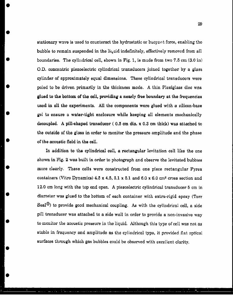
29

stationary wave is used to counteract the hydrostatic or buoyant force, enabling tho

bubble to remain suspended in the liquid indefinitely, effectively removed from all

• boundaries. The cylindrical cell, shown in Fig. 1, is made from two 7.5 cm (3.0 in)

O.D. concentric piezoelectric cylindrical transducers joined together by a glass

cylinder of approximately equal dimensions. These cylindrical transducers were

• poled to be driven primarily in the thickness mode. A thin Plexiglass disc was

glued to the bottom of the cell, providing a nearly free boundary at the frequencies

used in all the experiments. All the components were glued with a. silicon-base

* gel to ensure a water-tight enclosure while keeping all elements mechanically

decoupled. A pill-shaped transducer ( 0.5 cm din. x 0,3 cm thick) was attached to

the outside of the glass in order to monitor the pressure amplitude and the phase

* of the acoustic field in the cell,

In addition to the cylindrical cell, a rectangular levitation cell like the one

shown in Fig. 2 was built in order to photograph and observe the levitated bubbies

more clearly. These cells were constructed from one piece rectangular Pyrex

containers (Vitro Dynamics) 4.5 x 4.5, 5.1 x 5,1 and 6.0 x 6,0 cm21 cross section and

12,0 cm long with the top end open. A piezoelectric cylindrical transducer 5 cm in

diameter was glued to the bottom of each container with extra-rigid epoxy (Torr

Seal®) to provide good mechanical coupling, As with the cylindrical cell, a side

pill transducer was attached to a side wall in order to provide a non-invasive way

to monitor the acoustic pressure in the liquid. Although this type of cell was not as

stable in frequency and amplitude as the cylindrical type, it provided flat optical

surfaces through which gas bubbles could be observed with excellent clarity.

0

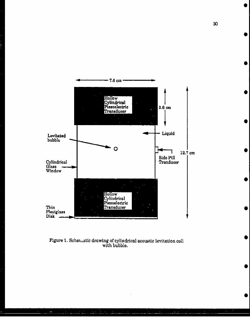
30

Id 7.6 cm

Ho owy~lndrtcal

Piezoelectric 3.6 cmransducer

1 0

Levitated _ -- Liquidbubblf,

0 12.7 cm

0

Side PillCylindrical TranducerGlassWindow

dzoelectrac

Thin TransducerPlexiglassDisk

Figure 1. ScheiJatic drawing of cylindrical acoustic levitation cellwith bubble.

31

Pyrex Glass LiquidRectangularCell

LevitatedBubble 0 Side Pill

• Tranducer

S5 iCylindrical5cm Clnia

Transducer Base2" O.D.

Figure 2. Schematic of rectangtdar acoustic levitation cell.

0

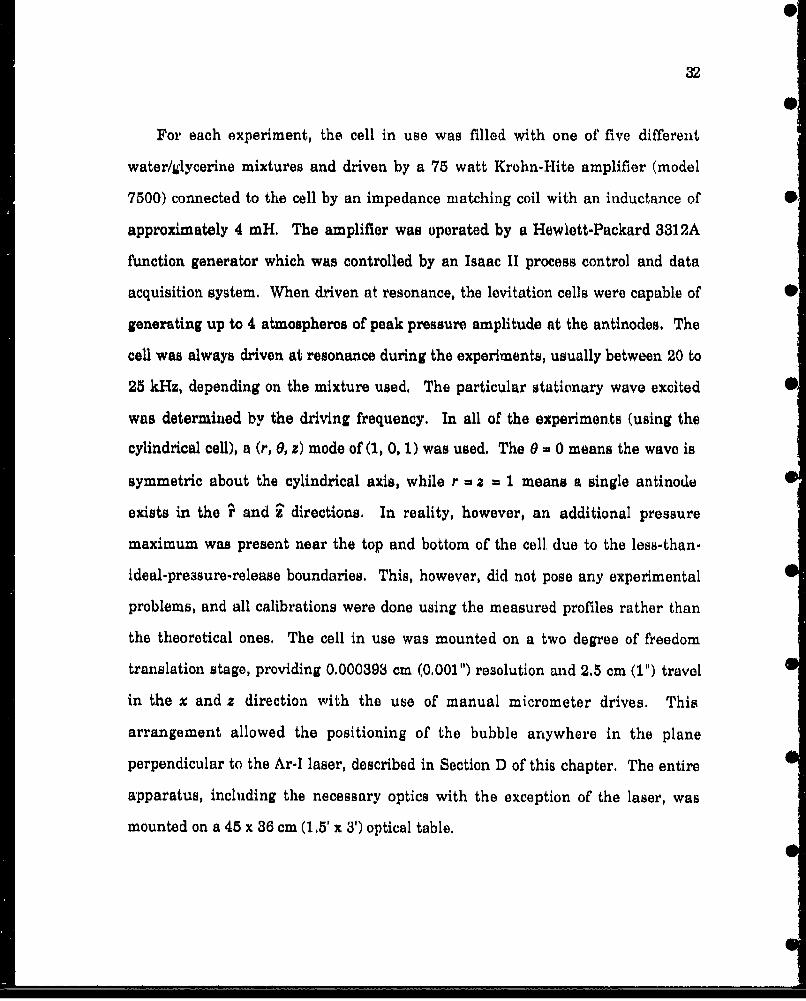
32

For each experiment, the cell in use was filled with one of five different

water/glycerine mixtures and driven by a 75 watt Krohn-Hite amplifier (model

7500) connected to the cell by an impedance matching coil with an inductance of"

approximately 4 mH, The amplifier was operated by a Hewlett-Packard 3312A

function generator which was controlled by an Isaac 11 process control and data

acquisition system. When driven at resonance, the levitation cells were capable of

generating up to 4 atmospheres of peak pressure amplitude at the antinodes. The

cell was always driven at resonance during the experiments, usually between 20 to

25 kHz, depending on the mixture used. The particular stationary wave excited

was determined by the driving frequency. In all of the experiments (using the

cylindrical cell), a (r, 0, z) mode of (1, 0, 1) was used. The 0 = 0 means the wave is

symmetric about the cylindrical axis, while r = z i 1 means a single antinode

exists in the ? and ^ directions. In reality, however, an additional pressure

maximum was present near the top and bottom of the cell, due to the less-than-

ideal-pressure-release boundaries. This, however, did not pose any experimental

problems, and all calibrations were done using the measured profiles rather than

the theoretical ones. The cell in use was mounted on a two degree of freedom

translation stage, providing 0.000393 cm (0.001") resolution and 2,5 cm (1") travel

in the x and z direction with the use of manual micrometer drives. This

arrangement allowed the positioning of the bubble anywhere in the plane

perpendicular to the Ar-I laser, described in Section D of this chapter. The entire

apparatus, including the necessary optics with the exception of the laser, was

mounted on a 45 x 36 cm (1.5' x 3') optical table.

330

In order to keep the side pill transducer calibrated, the system had to be

maintained to within 2 hertz of resonance. In addition, some of the experiments

*O required changes in pressure amplitude to be made quickly, accurately and

repetitively. For this purpose, the amplitude and frequency of the function

generator were controlled via the amplitude modulation (AM) and voltage

* controlled oscillator (VCO) analog inputs, An Apple Ile computer with an Isaac

II data acquisition and control system w&&s used which enabled the operator to

control the system from a terminal keyboard, This data acquisition system also

* served to provide a continuous reading of the acoustic pressure amplitude during

the experiments, This was done by reading the RMS -ioltage from a Fluke 8600A

digital multimeter to which the pill transducer was connected. This voltage was

read via a GPIB interface by the Apple Ile computer, converted to units of

pressure and displayed on the CRT screen. Because the eystem had to be

recalibrated often, this feature provided an immediate value of the pressure in

order to efficiently check the system between calibrations.

Ul. B. 2. Rise-time Measuring Apparatus

One of the methods used to determine the equilibrium size of the bubbles was a

rise-time technique described in the pressure calibration Section. This technique

* required measuring the terminal rise velocity of the bubble when the sound field

was turned off. Thus, the time needed for the bubbles to rise through a known

distance was measured and recorded. The apparatus used to accomplish this will

-- be described in the next paragraph.

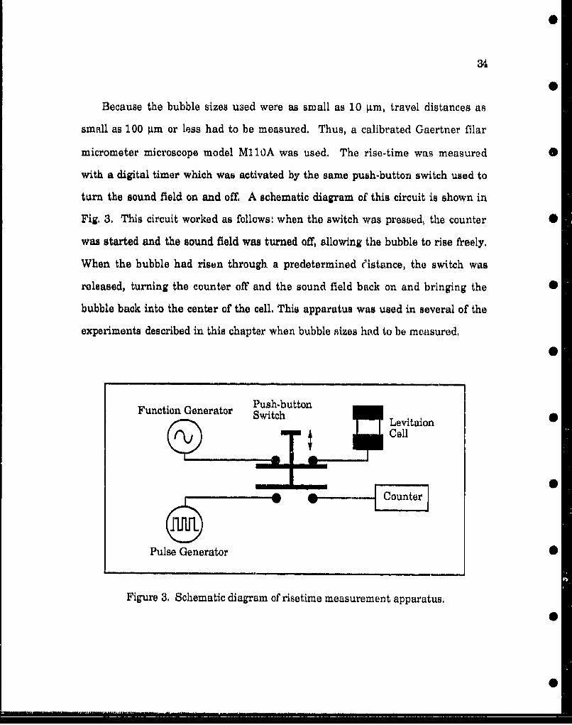
340

Because the bubble sizes u3ed were as small as 10 ptm, travel distances as

small as 100 Am or less had to be measured. Thus, a calibrated Gaertner filar

micrometer microscope model M110A was used. The rise-time was measured

with a digital timer which was activated by the same push-button switch used to

turn the sound field on and off. A schematic diagram of this circuit is shown in

Fig. 3. This circuit worked as follows: when the switch was pressed, the counter 0

was started and the sound field was turned off, allowing the bubble to rise freely.

When the bubble had risen through a predetermined reistance, the switch was

released, turning the counter off and the sound field back on and bringing the -

bubble back into the center of the cell, This apparatus was used in several of the

experiments described in this chapter when bubble sizes had to be measured,

Push-buttonFunction Generator Switch Levitaion

Cell

Pulse Generator 0

Figure 3. Schematic diagram of risetime measurement apparatus.

0

0

0

35

When the Pyrex rectangular cell was used, the bubble radius was also

Aaeasured with the filar micrometer microscope directly, The filar micrometer

used with a 20X magnification had a resolution of approximately ± 5 jtm. This

method provided an estimate of the bubble radius which allowed us to check on the

rise-time results if thermal currents were suspected to be present,

IL B. 3. Hydrophones

• In order to calibrate the side pill transducers, two techniques were employed

which utilized two different hydrophones, Because these hydrophones could not be

used at pressures amplitudes above 0.5 bars without the risk of cavitation damage,

• the pill transducers had to be calibrated at relatively low amplitudes. Extrapolated

values were then used during the experiments. This Section will describe these

hydrophones in more detail.

• The first and most often used device was a needle shaped hydrophone built by

the author which will be referred to as NDL1. A cross section of this device is

shown in Fig. 4. Due to its small dimensions, it affected the sound field in the cell

very little as can be seen in Fig. 5. This figure is a plot of the side pill response vs

the depth of the hydrophone in the cell measured in cm from the bottom of the cell,

This hydrophone was built using a small cylindrical piezoelectric transducer

mounted on two concentric steel needles which provided a rigid support. The

center needle was connected to the inside pole while the outside needle was

connected to the outside pole of the transducer. This geometry provided good

electrical shielding as well as ease of construction, although it was possible that

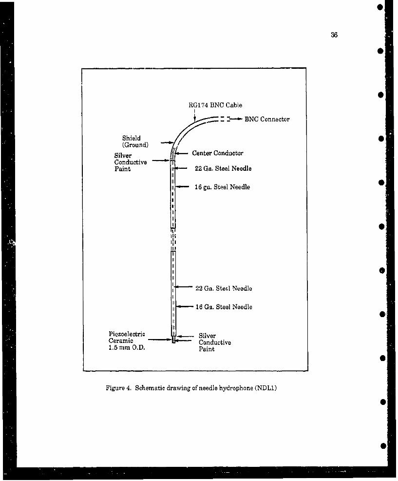
"36

RG174 BNC Cable

- :-i EBNC Connector

Shield /(Ground)

Silver ( Center ConductorConductivePaint i 22 Ga. Steel Needle

16 ga. Steel Needle

I~tC

TI,

*'---22 Ga. SteFl Needle

"16 Ga. Steel Needle

Piezoelectric ' SilverCeramic Conductive1.5 mm O.D. Paint

Figure 4. Schematic drawing of needle hydrophone (NDL1)

01

ir0

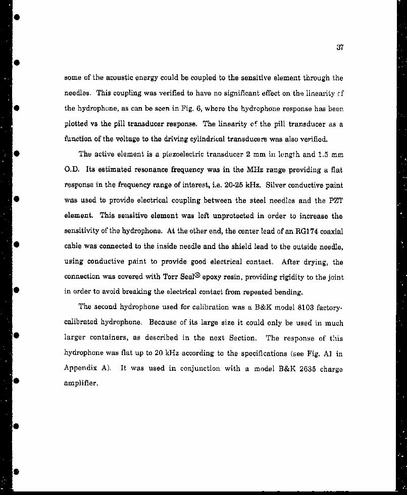
37

some of the acoustic energy could be coupled to the sensitive element through the

needles. This coupling was verified to have no significant effect on the linearity c-

* the hydrophone, as can be seen in Fig. 6, where tbe hydrophone response has been

plotted vs the pill transducer response. The linearity of the pill transducer as a

function of the voltage to the driving cylindrical transducers was also verified.

*@ The active element is a piezoelectric transducer 2 mm in length and 1,5 mm

O.D. Its estimated resonance frequency was in the MHz range providing a flat

response in the frequency range of interest, i.e. 20-25 kHz. Silver conductive paint

-* was used to provide electrical coupling between the steel needles and the PZT

element. This sensitive element was left unprotected in order to increase the

sensitivity of the hydrophone. At the other end, the center lead of an RG174 coaxial

* cable was connected to the inside needle and the shield lead to the outside needle,

using conductive paint to provide good electrical contact. After drying, the

connection was covered with Torr Seal® epoxy resin, providing rigidity to the joint

* in order to avoid breaking the electrical contact from repeated bending.

The second hydrophone used for calibration was a B&K model 8103 factory-

calibrated hydrophone, Because of its large size it could only be used in much

* larger containers, as described in the next Section. The response of this

hydrophone was flat up to 20 kHz according to the specifications (see Fig, Al in

Appendix A). It was used in conjunction with a model B&K 2635 charge

-- amplifier.

0

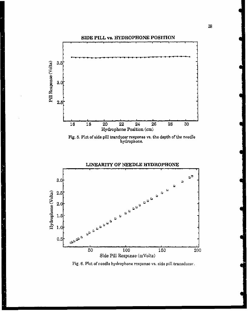
38

SIDE PILL vs. HYDROPHONE POSITION

3.0

' 2.6

16 18 20 22 24 26 28 30Hydrophone Position (cm)

Fig. 5. Plot of side pill tranducer response vs. the depth of the needlehydrophone.

LINEARITY OF NEEDLE HYDROPHONE

3.0

2.5 IM

S2.0 1

rii•1.5 LI

I 1.i

0.5

50 100 150 200Side Pill Response (mVolts)

Fig. 6. Plot of needle hydrophone response vs. side pill transducer.

39

11. C. Calibration of Acoustic Levitation Apparatus

L Absolute Sound Field Pressure

Two different methods for determining the absolute acoustic pressure in the

levitation cells were used. One method gave a direct calibration of the pill

0 transducer. However, the response of the pill was dependent on the liquid used

and a more reliable reference was therefore required, For this purpose, the needle

hydrophone NDL1 was used. The second method consisted of calibrating the

* needle hydrophone directly using a commercially available calibrated reference

(B&K 8103). Thus, the purpose of this procedure was to obtain a calibration

constant for the needle hydrophone (NDL1) which was then used for all the

0 experiments by calibrating the pill transducer separately for each liquid mixture.

In all instances, the output of the side pill transducer was used to record the

acoustic pressure amplitude after being calibrated at the beginning of each

experiment, The methods used to calibrate NDL1 will be described in this Section.

Method A: Levitation Technique. This technique was first :uggested by Gould

(1968), and it consists of measuring the equilibrium radius and position above the

antinode of a bubble levitated at a given pressure amplitude. Using the fact that at

equilibrium the buoyancy and radiation pressure forceE on a levitated bubble are

equal in magnitude and opposite in direction, a linear approximation for the

pressure amplitudo in terms of the bubble radius and its vertical position z

relative to the pressure node in the sound field can be derived. This expression is

given by (Crum,i 970)

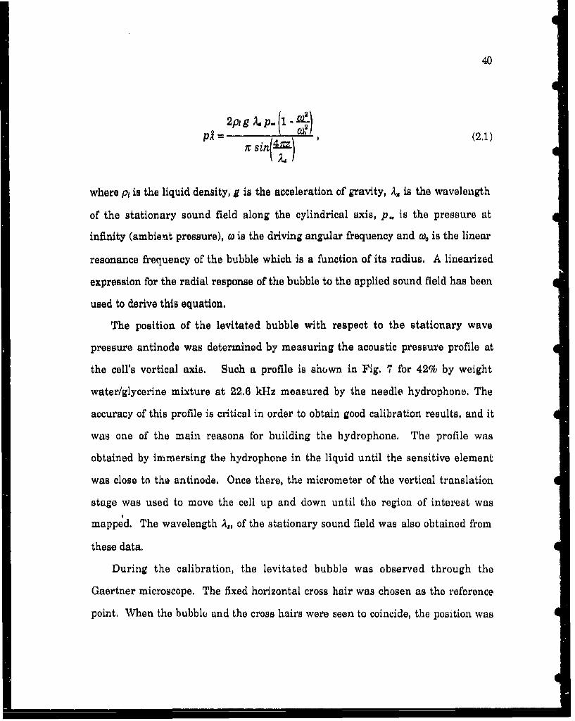
40

2pt g p. (p )N= 2 (2.1)

where p, is the liquid density, g is the acceleration of gravity, X, is the wavelength

of the stationary sound field along the cylindrical axis, p. is the pressure at

infinity (ambient pressure), o is the driving angular frequency and Wo is the linear

resonance frequency of the bubble which is a function of its radius. A linearized

expression for the radial response of the bubble to the applied sound field has been

used to derive this equation.

The position of the levitated bubble with respect to the stationary wave

pressure antinode was determined by measuring the acoustic pressure profile at

the cell's vertical axis. Such a profile is shown in Fig. 7 for 42% by weight

water/glycerine mixture at 22.6 kHz measured by the needle hydrophone. The

accuracy of this profile is critical in order to obtain good calibration results, and it

was one of the main reasons for building the hydrophone. The profile was

obtained by immersing the hydrophone in the liquid until the sensitive element

was close to the antinode. Once there, the micrometer of the vertical translation

stage was used to move the cell up and down until the region of interest was

mapped. The wavelength A,, of the stationary sound field was also obtained from

these data,

During the calibration, the levitated bubble was observed through the

Gaertner microscope. The fixed horizontal cross hair was chosen as the reference

point. When the bubble and the cross hairs were seen to coincide, the position was

41

00

00

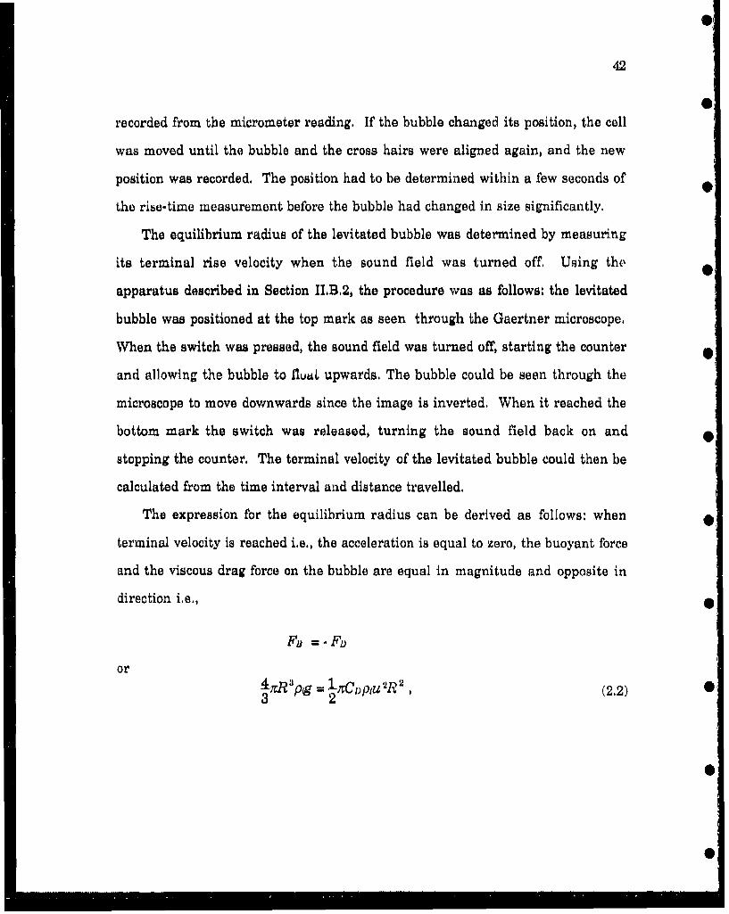
42

recorded from the micrometer reading. If the bubble changed its position, the cell

was moved until the bubble and the cross hairs were aligned again, and the new

position was recorded. The position had to be determined within a few seconds of

the rise-time measurement before the bubble had changed in size significantly.

The equilibrium radius of the levitated bubble was determined by measuring

its terminal rise velocity when the sound field was turned off. Using tho

apparatus described in Section IIB2, the procedure was as follows: the levitated

bubble was positioned at the top mark as seen through the Gaertner microscope,

When the switch was pressed, the Bound field was turned off, starting the counter

and allowing the bubble to fluuL upwards. The bubble could be seen through the

microscope to move downwards since the image is inverted, When it reached the

bottom mark the switch was released, turning the sound field back on and

stopping the counter, The terminal velocity of the levitated bubble could then be

calculated from the time interval and distance travelled.

The expression for the equilibrium radius can be derived as follows: when

terminal velocity is reached i.e., the acceleration is equal to zero, the buoyant force

and the viscous drag force on the bubble are equal in magnitude and opposite in

direction i.e.,

or4 rxR3Pp = 1-xC,,piu2•RI (2.2)3 2

LM0

0

43

0

where R is the bubble radius, u is the terminal rise velocity, and CD is the drag

coefficient given by

O = 24X = 12X(2.3)Re Rptu

0 where Re is the Reynolds number and X is an empirical correction factor

commonly expressed in terms of the Reynolds number,

For smaller bubbles (less than 40 pLm in radius), in which case X = 1, the drag

9 law for a rigid sphere (Stokes's law) can be used, For larger bubbles, more

accurate expressions must be used to account for the deformation of the bubble

such as the Langmuir-Blodgett or Schiller-Nauman empirical drag laws, The0 expression for the radius in terms of the terminal rise velocity Is given by

R = 9.# U X (2.4)0 ~2 p49

The correction factor X, according to Schiller and Nauman, is given by

* =I + 0.15R""'? (2.5)

and according to Langmuir and Blodgett by

x = 1 + 0.197R°M" + 2.6xl 0"Re"" (2.6)

-0

44

Recently, Crum et al. (1984) have found discrepancies between the theory and

experiment of the bubble response when it is driven near its harmonics, i.e.,

integer multiples of the bubble's resonance frequency. Since equation (2.1) was

derived using a linearized expression for the bubble response, Crum's

observations give this method of calibration a certain degree of unreliability. In

order to eliminate this uncertainty, a restriction on the size of the bubbles used

during the calibration was imposed, This modification was suggested by

Prosperetti (1990). Assuming small pulsation amplitudes, it can be shown that

bubbles below about 40 4m pulsate with an amplitude which is independent of

their size, The dependence of the pressure amplitude at the antinode, PA, on the

bubble radius is implicit in the term (a)/ q) 2 in equation (2,1). If the bubble is small,

however, this term is very small and can be ignored, making the expression

independent of the bubble radius. It was verified experimentally that the position

in the cell of bubbles between 20 and 40 gtm was indeed independent of the radius,

Bubbles below 20 ptm, however, did not behave predictably, possibly due to the

presence of foreign material which is known to accumuiate at the gas-liquid

interface or to thermal currents which could easily affect the rise-time

measurements of small bubbles. Thus, several bubbles between 20 ptm and 40 ptm

were used to perform the calibration. This method gave a much smaller standard

deviation (over the repeated measurements), as expected, and was therefore

considered more reliable. Since bubbles are small, we can use Stokes's law (Eq.

2,3 with X = 1) to approximate the viscous drag. Using this approximation, and the

ratio (0/( 0,)2 - 0, the expression for the pressure amplitude simplifies to

45

2plg p- (2.7)

which is a function of the position z only. The calibration was made by levitating a

number of bubbles (one at a time) at a range of pressure amplitudes and recording

their positions. The corresponding pressures were obtained using equation (2,7)

with A, obtained from the pressure profile for GLY42. The statistical mean and

the standard deviation were calculated. Since it was not possible to introduce the

needle hydrophone (NDL1) in the cell while the bubbles were levitated, this

calibration was made with the pill transducer, NDL1 was then calibrated in the

same liquid with no bubbles present,

• Mgthod R: Substitution Method. In this method, a factory-calibrated B&K 81.03

hydrophone was used to calibrate NDL1. It consisted of inserting both the B&K

and NDL1 hydrophones at the same time and side by side in a RF shielded 10

gallon fish tank filled with water. A stationary acoustic wave was set up in the

tank by a 7.6 cm (3") O.D. cylindrical piezoelectric transducer attached to the glass

bottom. The transducer was glued to the tank with silicon gel, and it was driven at

around 21 kHz, the exact frequency depending on the water level. This method

will be discussed in the next paragraph.

In order to ensure that the two hydrophones were sensing the same pressure,

they were positioned near an antinode and their voltage output maximized. If the

sensitive element of NDL1 was within 2 mm of the acoustic center of the B&K

hydrophone (see Appendix Fig. A.1), then the calibration was performed. Several

46

antinodes were used during this calibration, and the results averaged with equal

weights,

These two calibration methods were made in order to account for any

systematic errors inherent to any particular method, The sensitivity of the needle

hydrophone was measured by method A to be 19.9 ± 0.6 and by method B to be 19,6 ±

0,8. volts/bar. The final calibration constant was determined statistically, giving

the result of each method an equal weight, Its value was calculated to be 19,8 ± 0,7

volts/bar corresponding to a standard deviation of about 4%. This value was used

to recalibrate the pill transducer for each experiment, As expected, the calibration

constant for the pill transducer changed for different liquid mixtures and/or liquid

levels, It was thus necessary to recalibrate it often,

IL C. 2. Phase of the Sound Field Pressure

The phase of the pill transducer relative to the acoustic pressure was

determined by direct comparison with the needle (NDLI) hydrophone positioned at

the pressure antinode, Because the resonance frequency of the sensitive element

of NDL1 was in the MHz range, it could be assumed that it responded in phase

with the 20--25 kHz sound field. There still remained an uncertainty of 180' in the

phase due to the unknown polarity of the PZT element, This uncertainty was

resolved in two ways: 1) By applying a static pressure to the sensitive element and

observing the polarity of the voltage output, and 2) By direct comparison with the

phase calibrated B&K hydrophone.

47

0

The phase of the pill was measured using the two zero-crossing circuits

described in Section II.F. A schematic diagram of one of those circuits can be

0 seen as part of the circuit shown in Fig. 16. Each of these circuits produced

periodic narrow pulses at the zero crossing of each signal. These pulses were then

displayed on the digital oscilloscope and the phase difference measured and

0 recorded. The procedure was repeated several times during each experiment

since the phase of the pill transducer relative to the acoustic pressure was found to

depend strongly on the driving frequency and liquid level, It was found, however,

0 that as long as the system was kept at resonance, the phase of the pill remained

constant to within 2.3 degrees even if the water level changed slightly. For this

reason, the frequency control system was designed such that the frequency could

0 be specified with a precision of± 1 Hz.

IL D. Light Scattering Experiment

0 1. Apparatus

In order to record the radius of the bubble as a function of time, linearly

* polarized light from a laser was scattered from the bubble. The scattered light

intensity is modulated by the bubble pulsations and, if measured at the appropriate

angle, this intensity can be converted to an absolute bubble radius. This technique

0 was developed by Hansen (1984) to size air bubbles under similar conditions and

has been used to record small amplitude radial and nonradial bubble oscillations

by Holt (1988) and Horsburgh (1990). A more detailed description of this technique

* and of the apparatus can be found in these references,

0

48

A schematic diagram of the apparatus is shown in Fig. 8, the shaded blocks

indicating the support equipment, The light source used was a 3-watt water-

cooled Lexel model 95 argon-ion laser operated in the TEMO0 mode. An optical

rotating polarizer was placed in front of the laser which provided a 1200:1 linear

polarization ratio. The laser was used at 0.8 watt power at a wavelength of 488

nm. This power setting was determined empirically by using the maximum

power possible before the energy absorbed by the bubble was large enough to affect

its motion. The scattered light was detected by an Oriel 7182-1 photovoltaic silicone

photodiode with integral preamplifier, This photodiode had a detection area of 100

mm 2 and a 488 nm laser line transmission filter in order to reduce background

noise, The output of this diode was connected to both a DC voltmeter which

provided information on the temporal average radius of the bubble and a Stanford

Research Systems model SR560 low-noise preamplifier in order to further increase

the signal-to-noise ratio. The amplifier was set to a gain of 40 dB and was

connected to an AC-coupled LeCroy 9400 digital oscilloscope which recorded the

scattered light intensity of the pulsating bubble as a function time. A National

Instruments GPIB interface was used to transfer the data from the oscilloscope to

a Macintosh II computer for analysis and graphical output.

I. D. 2. Calibration

a. Absolute Bubble Radius

The technique used to calibrate the output of the photodetectors was first

developed by Hansen (1984) and later refined by Holt (1988) and Horsburgh (1990)

49

*0

0 00

*z

r4t

*0

S ý

500

for experiments similar to those described in this work. Using Mie scattering

theory, Hansen (1984) showed that at certain scattering angles a monotonic

relation exists between the light intensity and the bubble radius. Thus, before the

calibration procedure is described, let us first introduce this relation.

The theory describing the scattering of electromagnetic radiation from

dielectric spheres was developed by Gustav Mie in 1908. A complete treatment of it

can be found in Kerker's (1969) excellent book on the subject, and his notation will

be used here. The following are the results applicable to the component of the

scattered intensity in the far field and parallel to the scattering plane (defined by

the incident and scattered directions) for an incident wave of unit intensity:

4- r,2 •cos20 , (2.8)

where r is the distance from the center of the bubble, 0 is the azimuthal angle, and

X is the wave length of the light in the liquid. The scattering amplitude S is given

by

S = • 2n+1 [anrn(cosO) + bnlrn(cosO)]1 (2.9)n.l n(n+l)

where 0 is the scattering angle, and forward scattering corresponds to J3 = 0. The

angular functions are given by

z,,(cosO) =.P (cos 0) (2.10)MinO

0

S

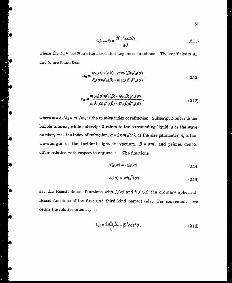
S~51

r. (cos6) = dPWI(COSO), (2.11)dO

where the P,(') (cosO) are the associated Legendre functions. The coefficients a,,

• •and b, are found from

= V'(a)Vn(P) MVn(f)YIn(c)(2.12)

b =T (a) V,(P- Vmn(y n(a) (2.12)0

where m- k,/k 2 - m1 /m2 is the relative index ot refraction. Subscript 1 refers to the

bubble interior, while subscript 2 refers to the surrounding liquid, k is the wave

number, m is the index of refraction, a = 2xmA, / k is the size parameter, ko is the

wavelength of the incident light in vacuum, am = n, and primes denote

differentiation with respect to argumin • The functions

"�"LY,(ax) = 4(a), (2.14)

8n (a) = ah21(ax) (2.15)

are the Ricatti-Bessel functions with ji(a) and h,,f2)(a) the ordinary spherical

Bessel functions of the first and third kind respectively. For convenience, we

define the relative intensity as

=I4e2= L = •cos 2¢ (2.16)A)•

52

For the purpose of illustration, parameters relevant to an air 1'ubble in water

will be chosen, with the incident wavelength being 488 ni. Fig. 9 is a plot of loglo

I,1 vs 0 for 0 to 180 degrees for a size parameter a equal to 661, corresponding to a

bubble of radius 38 ptm. Looking at this graph, we want to determine what the

optimal angle is which would make the intensity a monotonic function of the

radius. If possible, 0 should be less than 90' since the intensity drops considerably

for angles greater than 75", Fig, 10 is a plot of Irej as a function of radius for 0

66". As can be seen, the coarse structure due to the interference of the reflected

and refracted rays make this angle an undesirable one, Fig. 11 shows the same

calculation for an angle 0 = 70'. Although the coarse structure is less pronounced,

Irel is still not a single valued function of the radius. The theoretical relative

intensity for a scattering angle 0 = 80' from the forward direction is shown in Fig,

12 demonstrating the ideal type of radial dependency. The fine structure

disappears when the intensity is calculated using a finite solid angle as would be

the case during the experiment. Because this angle gives the greatest intensity

with a smoothly increasing function of the bubble radius, it was used for all the

experiments. This is the same result obtained by Holt (1988) and Horsburgh (1990)

who had previously demonstrated the validity of Mie theory for this type of

experiment. The calculations shown in Figs. 9-12 were made by Holt using a

modified version of a program developed by Wiscombe (1980).

In order to determine the instantaneous bubble radius from the scattered light

intensity, an intensity-radius transfer curve was obtained. For this purpose,

bubbles of different sizes were levitated and the scattered light intensity recorded.

53

000

cc~

-6

*il 1il A 111 1111Q4S0U DAW-I

0

54

0

0

0 0

0

0r�o

00

0

U 410

0rj2

00

0

I0

0I I I I o

0 0 0 0 0 o

0

55

00

LID cqS41SDIMIDAI JO0

56

coo

00

cui

_1 00c

U4S~U AII-

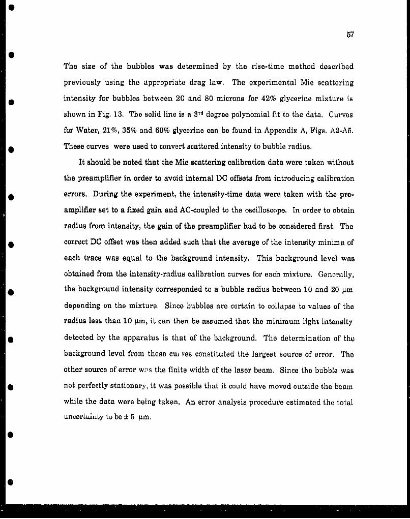
57

The size of the bubbles was determined by the rise-time method described

previously using the appropriate drag law, The experimental Mie scattering

intensity for bubbles between 20 and 80 microns for 42% glycerine mixture is

shown in Fig. 13. The solid line is a 3rd degree polynomial fit to the data. Curves

for Water, 21%, 35% and 60% glycerine can be found in Appendix A, Figs, A2-AS.

These curves were used to convert scattered intensity to bubble radius,

It should be noted that the Mie scattering calibration data were taken without

the preamplifier in order to avoid internal DC offsets from introducing calibration

* errors. During the experiment, the intensity-time data were taken with the pre-

amplifier set to a fixed gain and AC-coupled to the oscilloscope, In order to obtain

radius from intensity, the gain of the preamplifier had to be considered first, The

* correct DC offset was then added such that the average of the intensity minima of

each trace was equal to the background intensity, This background level was

obtained from the intensity-radius calibration curves for each mixture, Generally,

the background intensity corresponded to a bubble radius between 10 and 20 gm

depending on the mixture, Since bubbles are certain to collapse to values of the

radius less than 10 gm, it can then be assumed that the minimum light intensity

* detected by the apparatus is that of the background. The determination of the

background level from these cui yes constituted the largest source of error, The

other source of error w,; the finite width of the laser beam. Since the bubble was

not perfectly stationary, it was possible that it could have moved outside the beam

while the data were being taken. An error analysis procedure estimated the total

uncerLuinhy to be + 5 pnm.

0

58

P-IC

cc

1CI, 1.. I. C;j

rn,____________101LM1

59

H. D. 2. b. Phase of Radial Bubble Pulsations

The phase of the bubble pulsations was measured relative to the calibrated

side pill transducer. For the light scattering experiment, a more direct method

than the one described in Section II,C,2 was devised to calibrate the pill, This

calibration was made relative to the oscillations of a levitated bubble driven at a low

pressure amplitude and far from its resonance frequency. As illustrated in Fig,

14, the theoretical phase of the radial minimum in the region 0.6R,, ! R < 0,75R, is

not only flat but fairly independent of the pressure amplitude. Since this region

corresponds to bubbles away from their harmonic resonances, this phase

corresponds to the only radial minimum occurring each cycle of the driving

pressure. This phase was also found to be independent of the formulation used to

40 calculate it. Thus, by knowing the phase of the bubble pulsations relative to the

sound field, the phase of the pill transducer could also be determined. Bubbles in

this size range were levitated and the simultaneous oscilloscope traces of both the

pill transducer output and scattered light intensity were stored in the computer.

The two traces were displayed on the MacIH CRT screen using Passage II plotting

software. The time difference between minima was measured from which the

phase difference was calculated. The estimated total error of the calibration

procedure was ± 5 degrees. This error was mostly due the uncertainty of the bubble

sizes used in the calibration procedure."0

0-

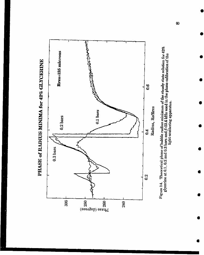
600

~~mo

0

61

EL D. 3. Procedure

The light scattering apparatus described in the previous Section was used to

obtain the radius vs time curves for radial pulsations of bubbles. Five different

glycerine/water mixtures were used in this experiment in order to obtain data for

liquids with several different values of the liquid density, viscosity, surface tension

and speed of sound, These mixtures were pure water, GLY21, GLY35, GLY42 and

GLY60, where the two digits represent the percent by weight of glycerine. The

solutions were prepared from 99,5% pure glycerine and water filtered down to 0.2

p.m in particle size. In order to lower the gas content, the mixtures were

periodically vacuum-filtered through a 5 ptm Teflon filter. This procedure also

served to remove impurities after the liquid had been used for some time.

The procedure was relatively straightforward, once the bubble was stabilized

in the radial mode. After positioning the bubble in the center of the beam,

simultaneous traces of the pill transducer output and scattered light intensity

were stored in the oscilloscope and transferred to the computer for permanent

storage. The process was repeated for each mixture as the pressure amplitude,

PA, was increased using the same bubble whenever possible. At the higher

pressures, the bubble often exhibited vertical oscillations, with a frequency around

1 I-Iz or higher. If the amplitude of these oscillations was large enough so that

part of the time the bubble was off the center of the beam, several traces were

recorded but only the ones with the largest scattered intensities were transferred

to the computer. It was assumed that the largest values were obtained while the

bubble was in the center of' the beam. Each trace corresponded to about 0.2 msec of

S " . . .. ' . . . . .. i . . ..|. . .|• =| . . . .. j .•. . 'q| ;L'" " I

real time. In addition, if the signal-to-noise ratio was too small, as was the case

for the lowest values of the pressure amplitude, time averages over 100 traces were

performed by the LeCroy oscilloscope before transferring the data to the computer.

Because the scattered intensity was periodic over several minutes, no information

was lost in the time-averaging procedure,

All the light intensity traces were converted to radius using the transfer

curves for each liquid mixture, The pulsation amplitude (Rmax), the phase of

collapse (@O)and the number of radial minima (M) of the oscillations were obtained

from these traces. These quantities will be defined more precisely in Chapter III.

The value of the equilibrium radius of the bubble (R.) was obtained by the rise-time

method, although thermal and acoustic pressure currents in the liquid made this

measurement difficult and imprecise, From these measurements, however, it

was determined that the bubble sizes were less than 20 jtm for all of the liquid

mixtures, Mie scattering techniques also were imprecise because of the very low

signal-to-noise ratio at these bubble sizes.

The gas concentration during these measurements was somewhat below

saturation. Since no dependence of the bubble pulsations on the gas concentration

was expected, no attempt was made to control this parameter extensively. During

the single bubble experiments, however, a certain amount of under-saturation

was required in order to suppress cavitation which generated copious streaming

and disturbed the stably pulsating bubble. The higher concentration glycerine

solutions required less under-saturation, since air does not readily dissolve in

glycerine and it is thus naturally "degassed".

0

63

S

II. E. Sonolumin nce Detection Experincnt

L Apparatus

When the pressure amplitude in the levitation cell was high enough to

produce sonoluminescence from cavitation, it was desired to measure the onset as

* well as the phase of the light emission relative to the sound field, This Section

describes the apparatus used to acquire these data.

Because of the low intensity of the light emissions, an eight cubic foot light.

* tight box was built which allowed the use of a photomultiplier tube (PMT) to detect

them. Bulkhead BNC connectors on both side walls were used in order to bring all

the necessary electrical signals in and out of the box. During the experiment, the

_ @front cover was tightly secured with 4 sets of removable 1/4 inch nut and bolt

combinations, A rubber gasket around the edge was used to provide a tight fit

between the cover and the box. A model R585/C617 PMT/preamplifier combination

made by Hamamatsu for single photon counting applications was used to detect

the light emissions. The dark current and gain specifications of this system were

1 count/sec and 105 respectively while the rise and fall times were 15 nanoseconds

each, This system provided a high signal-to-noise ratio as well as a time

resolution on the order of 1/500th of an acoustic period ( < 1 ) necessary to measure

the phase of sonoluminescence accurately, Fig, 15 shows the schematic diagram

* of' this apparatus, the shaded blocks indicating the support equipment,

The phase of SL flashes was measured relative to a reference signal. This

signal consisted of a series of fast electronic pulses generated with a fixed phase

- relative to, and the same frequency as, the sound field. By measuring the time

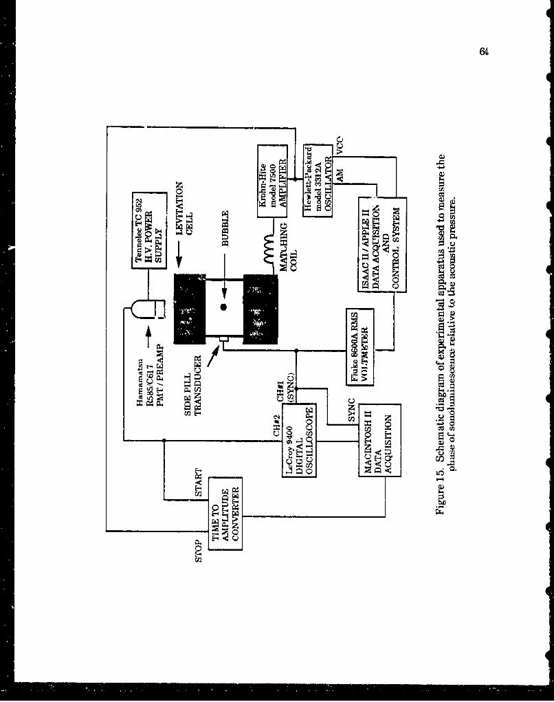
CC

4-4

EoEr.-4

1.-4 0

65

interval between these pulses and SL events, the phase of SL was determined. A

schematic diagram of the circuit used to measure this phase is shown in Fig. 16.

One of the functions of this circuit was to generate NIM* -type pulses (-0.5 V peak

amplitude and 100 nanoseconds long) at the negative-slope zero-crossing of the

periodic, sinusoidally varying signal generated by the side pill transducer. The

40 phase of this signal was usually different from that of the sound field and

therefore required calibration (see Section II.C.2), The pulses were generated by

the zero-crossing detector circuit shown in the upper left region of Fig. 16. The

output of this circuit (Q on the 4047 chip) was connected to the STOP input of the

time-to-amplitude converter (TAC) module. The pulses generated by the PMT

when a sonoluminescence event occurred were connected to the input of an Ortec

constant fraction discriminator in order to convert them to NIM-type pulses. A

variable time delay was then inserted to these pulses with a delay generator unit

before being connected to the START input of the TAC module. The purpose of the

time delay was to maximize the amplitude of the TAC output pulses and,

therefore, the precision of the data acquisition system. The amplitude of the

output pulses generated by the TAC were propotional to the time interval between

START and STOP pulses. This apparatus was designed to facilitate the

measurement of the phase of thousands of sonoluminescence events. To

minimize the amount of dead time in the TAC circuit, the reference signal was

_ •used as the stop pulse. The reference pulses occurred every acoustic cycle at a

fixed phase, while sonoluminescence events usually happened sporadically. If a

_ N IM-nuclear instrumentation module,

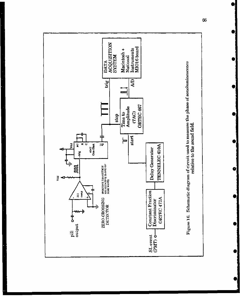
66

z

0II•

• cj.•G•

- -

•" i

•*M

,• C'•

I I I I I I I I I I I I I I I I I

67

stop pulse occurred without a previous valid start pulse, the stop pulse was

ignored by the TAC. Thus, only stop (reference) pulses which occurred after a

start pulse (sonoluminescence event) within the given time interval generated an

output pulse. All other situations were effectively ignored and generated no

output.

The amplitude of the output pulses was measured by a multipurpose I/O

board made by National Instruments (MIO16) with a maximum sampling rate of

100 kHz. The host computer was a MAC II using the Labview@ software. The

* precision of the data acquisition system was 12 bits which corresponded to a

precision of A,=±+0.1 degrees of the phase if measured under noiseless conditions.

Typical noise levels were ± 1 degree. This system was able to sample the phase for

thousands of consecutive cycles. Since the data were acquired with a DMA (direct

memory access) board, the maximum number of data points that could be taken

consecutively was determined by the amount of memory in the Macll computer.

- Typically, each set of data consisted of 1.000 acoustic cycles, equivalent to about 50

msec. However, data sets as long 20,000 acoustic cycles were possible if needed,

corresponding to about 1 sec of real time.

* In order to obtain information on the frequency of sonoluminescence events,

data conversions on the analog-to-digital convertor (ADC) board were triggered

every cycle. Thus, if in a given acoustic cycle no sonoluminescence events

• occurred, or if they occurred outside the maximum time window set in the TAC

module, an analog voltage value of zero was read by the computer. Otherwise, the

amplitude of the pulse carrying the phase information was read. The data were

• displayed on a CRT screen before being stored permanently.

68

11. R 2. Calibration

The calibration of this apparatus was done as follows. First, the front panel

reading of the delay generator module was calibrated using a digital oscilloscope

to measure the true time delay. The resulting second degree polynomial fit was

then incorporated into the conversion routine written in Labview®, Next, two

pulses separated in time by a variable interval were input into the TAC module

using the calibrated delay generator. Similarly, a second degree polynomial fit

was obtained relating the pulse amplitude and the time interval and incorporated

into the conversion routine. After this, the only other calibration factor needed

was the phase shift of the side pill transducer relative to the sound field. This

factor was obtained as explained in Section C.2 of this Chapter.

II. E. 3. Procedure

a. Phase of Sonoluminescence vs Bubble Motion

Using the light scattering apparatus and the photomultiplier (PMT) SL

detection system, the phase of SL was measured relative to the instantaneous

radius of the bubble. This is the most direct way of determining the point during

the bubble motion in which the SL flash is emitted. Since both the photomultiplier

tube (PMT) and the laser could not be on simultaneously, an intermediate phase

reference had to be used. The procedure was as follows: After positioning a

pulsating bubble in the center of the laser beam, an instantaneous intensity-time

69

the computer. The laser and the room lights were then turned off and the PMT

turned on with a black cloth wrapped around it and the levitation cell. Similarly,

0 simultaneous traces of the PMT output and the pill transducer output were stored

in the computer. All traces were obtained very quickly to ensure that all

parameters remained constant. The intensity-time and SL traces could then be

* compared directly after verifying that the two pill output traces were in phase.

IL E. 3. b. Phase of Sonoluminescene v8 Sound Field

0 The phase of SL was measured for different values of the liquid density,

viscosity, surface tension and speed of sound. The time-to-amplitude converter

(TAC) system provided a very efficient method of recording the phase of SL for

thousands of cycles at a time or even in real time if desired. The general

procedure was as follows: After filling the cell with the desired glycerine mixture,

an amplitude and phase calibration of the pill transducer was made using the

procedure described in Section II.C. A bubble was then introduced into the liquid

and made to sonoluminesce at the desired pressure amplitude. After the light-

tight box was closed, the phase of SL was measured for different pressure

0 amplitudes using the TAC system and stored in the computer for later analysis.

The system was checked periodically and kept at resonance in order to maintain

the calibration.

Measurements were also made of the phase of SL during streamer activity

when the cavitation field was composed of many bubbles sonoluminescing

F--0

70

simultaneously. The purpose of this experiment was to study the behavior of

bubbles during intense cavitation activity.

0

0

0

0

0

0

Chapter III

• Theory of Bubble Dynamics

II. A. Introduction

0 In this Chapter, the mathematical formulations used to describe the motion of

a single bubble in a spatially uniform acoustic field are presented. This field is

assumed to vary sinusoidally in time. During the calculations, three differentformulations will be used, the results of which will be compared to the

measurements. These formulations are the Keller-Miksis (1980) radial equation

with a linear polytropic exponent approximation, the Keller-Miksis radialequation with Prosperetti's (1986) exact formulation for the internal pressure, and

Flynn's (1975) formulation, which also includes thermal effects inside the bubble.

These formulations will be referred to as polytropic, Prosperetti's, and Flynn's

formulations respectively. Because of the large pressure amplitudes, PA, used in

the calculations, only formulations that included correction terms for the

compressibility of the liquid were considered. In addition, Section B,2 introduces

some basic concepts of bubble dynamics which will be needed to understand the

results of the experiments. In Section B.3 the assumptions made in the derivation

and the limits of the formulations will be discussed. In particular, the extent to

which these limits are exceeded in the present calculations will be considered.

Two other effects are important when treating acoustically driven bubbles:

surface waves and rectified diffusion. Surface instabilities, also known as surface

71

72

waves or shape oscillations, can occur when the acceleration of the interface

exceeds a certain value. This type of instability usually results in the breakup of

the bubbles at these amplitudes. Similarly, rectified diffusion, a mechanism by

which bubbles can to grow in an acoustic field, exhibits a threshold behavior. The

pressure amplitudes above which surface waves are excited is called the surface

wave threshold, and that above which growth by rectified diffusion is positive is

called the rectified diffusion threshold. Brief presentations of the mathematical

theories used to describe these two phenomena are presented in Sections C and D,

respectively.

InL B. Radial Bubble Motion

L Theoretical Formulations

The first attempt to describe mathematically the collapse of an empty

spherical cavity in a previously undisturbed liquid was made by Rayleigh in 1917.

His work was motivated by the increasing concern over the rapid deterioration of

ship propellers. This deterioration was caused by what is now known as

hydrodynamic cavitation. Rayleigh's equation can be obtained by equating the 0

power at infinity and the time rate of change of the kinetic energy in an

incompressible liquid (Commander, 1985) and it carn be expressed as

RR +aR"- = p2 = p. (3.1)

0-

0

73

where p. is the pressure at infinity (in this case, the ambient pressure), p, is the

liquid density, R the radius of the cavity and dots indicate time derivatives. In his

seminal paper, Rayleigh found an explicit expression for the bubble wall velocity U

as a function of R:

U2= D3) (3.2)_O 3" R3

where R. is the initial radius. As simple as these equations are, they constitute

the basis for all subsequent work on bubble dynamics.

It was not until 30 years later that any significant improvements were made to

Rayleigh's equation. The first of these was made by Plesset (1949) in which he

added the variable pressure term (appropriate for acoustic cavitation) and surface

tension term. This equation, together with a viscous damping term added by

Poritsky (1952) is known today as the Rayleigh-Plesset equation, and is given by

+ PL R W -' (3.3)

* where p. is the gas pressure in the interior of the bubble, PA is the driving pressure

(including ambient pressure), and u is the shear viscosity of the liquid. This is

probably the best known equation describing the spherical motion of a gas bubble

0 in a liquid. Despite the fact that it assumes an incompressible liquid, it is still

used extensively. However, because the velocity of the interface can easily reach

values comparable to the speed of sound in the liquid, it is necessary to include atO

0

74

least first order compressibility terms in this equation, in order to account

properly for the energy stored in the liquid. Following the procedure used by

Keller & Miksis (1980), Prosperetti (1984) has obtained the following equation:

(14)kýRRi+R 3, ý1--ý=ýI+A)- pRt - PAU + B-) ] + g dpin(R,t) (3.4)C 2 3c C, pt c dt

where c is the speed of sound in the liquid, pu(R,t) is the pressure on the liquid side

of the bubble interface, and PA(t + Ric) is the time-delayed driving pressure. pli(R,t)

can be expressed in terms of the internal pressure by the condition on the normal

stress across the boundary

ppR, 0 = pg(R,t) - 2R - 4g R . (3.5)R? R

The relationship between the internal pressure and the bubble radius is

determined mainly by the thermodynamic properties of the gas, Although this

relation can be assumed to be isothermal or adiabatic under some circumstances,

a polytropic relation has often been used (Noltingk and Neppiras, 1950; Flynn,

1964; Prosperetti, 1974; Lauterborn, 1976; Keller and Miksis, 1980) of the form

pS = pO) (3.6)

where ic is the polytropic exponent, and p, is the internal pressure of the bubble at

equilibrium, defined by

. . . . .

0

75

pO =p. + 2a (3,7)R.

The value of K varies between 1 and y, for isothermal and adiabatic motion

* respectively, y being the ratio of the specific heat capacities C,/C,,, where the

subscripts p and v indicate that the pressure and volume are kept constant. This

exponent is calculated according to Prosperetti (1984). In this study, the Keller-

* Miksis radial equation (3.4) with a polytropic approximation is used as an example

of a first order compressible radial equation using a constant speed of sound.

The procedure used to obtain equation (3.4) requires the elimination of higher

* order terms. It is thus expected that several similar equations exist as derived by

different authors. Another commonly used formulation is that of Gilmore (1952).

Although no calculations will be made with this model, it is considered by many

- scientists to be a principal formulation of bubble dynamics. It is therefore

included here for a sense of completeness,

In his formulation, Gilmore considers the onthalpy h of the liquid a

* fundamental quantity. In addition, the quantity r(h + u2 /2) is postulated to

propagate with a velocity c + u where u is the particle velocity, as first suggested by

Kirkwood and Bethe (1942) (see Rozenberg, 1971 for a detailed derivation). The

* resulting equation is known as Gilmore's equation and is given by

*1O (~ + 2(a,01-k 1+ý dLý ) (3.8)- 2 3c Cd &

where H is the firee enthalpy at the bubble wall, which for water is usually given by0 •

.0;-

76

L0

H = n (B+I}" [(p,,(R,t) + B )!;.- (p..(t) + B)] . (3.9)n-1 pi

where the constant B has been measured to be 3000 bars, n 7 and the time

dependent speed of sound is given by

C = + (n-I)I, (3,10)

where c.. is the speed of sound at infinity. Assuming adiabatic motion, the

pressure at the boundary p)(R) , as in the previous formulation, is equal to

p+(R,t) ) (3.11)RBA R R •R

Despite the very different approaches, Gilmore's equation nearly equals equation

(3.4) if the substitution

H = (p -p)(3.12)p.

is made and the speed of sound is kept constant.

Although the polytropic approximation has been generally thought to be a

fairly accurate model, an experimental study by Crum and Prosperetti (1984) has

shown large discrepancies between theory and experiment for oscillations near O

the harmonics of the resonance frequency of the bubble. Since compressibility and

viscous effects are expected to be small at these amplitudes, these results suggest

that thermodynamics play a more important role in the motion of the bubble than 0

77

originally expected. For this reason, a more accurate expression for the internal

pressure has been obtained by Prosperetti et al. (1986), In their formulation,

several approximations have been made. Some of them are: a uniform pressure

field inside the bubble, the temperature in the surrounding liquid remains

unchanged and an ideal gas is assumed. Of course, these approximations place

severe limitations on the model, especially when the pulsations are large and the

wall velocities reach values comparable to the speed of sound. Despite its

limitations, theoretical values of the internal temperature and pressure with a

degree of accuracy comparable only to Flynn's (1975) will be obtained with this

formulation. The following is a brief outline of Prosperetti's model starting with

the conservation equations for the interior of the bubble,

The momentum equation with spherical symmetry can be written as

dut ap r' (3.13)dt P1 Dr

Assuming spatially uniform pressure, the momentum equation reduces to

p = p(t). (3.14)

The conservation of mass equation can be expressed as

dp - -•- +p: V, • 0,(3.15)

where

dt t-[ + U 5-r

0

78

is called the convective derivative, and u=ru lr is the velocity vector in the radial

direction A The conservation of energy equation, ignoring the viscous heating

term, can be written as

S+ I L Tp K(3.16)

where T is the temperature, C. is the specific heat at constant pressure, and K is

the thermal conductivity of the gas. In order to obtain the velocity field in terms of

the temperature, we multiply the conservation of mass equation (3.15) by C'PT and 0add it to energy equation (3.16) to obtain

Capi IT)p U ((K 'Tdp(3.17)

From the ideal gas laws with constant specific heats, we can express

and,- -a. (3.18)r-l ~D p~

Inserting equation (3.18), (3.17) becomes

U---P-+ V u "•(7"-1-) K VT =0. (3.19)

7P 7P

Due to the spherical symmetry assumption, this equation can be integrated

directly to obtain

0l

79

yp("Ur " rP). (3,20)

Using the boundary condition

u(r =R,t)==/ , (3,21)

equation (3.20) can be used to obtain a differential equation for 0 by evaluating it at

r=R:

=((y1) K-'T 1 R - pR) (3.22)

which can be solved simultaneously with the radial equation (3.4) once the

gradient of the temperature field at the boundary is found. For this we use the

energy equation (3.16) which can be now written as

- T m " +uE'P=V'KVT'. (3.23)

The only difficulty in solving this partial differential equation is the

temperature dependence of the thermal conductivity K. One way to solve this

difficulty is by the transformation

=JK(O) dO, (3.24)f T

80

where T.. is the ambient temperature. In addition, it is convenient to have a fixed

rather than a moving boundary condition. Therefore, a new variable is introduced

Y R "_ (3.25)R(t)

Using (3.20), (3.24) and (3.25), the energy equation (3.23) becomes

a + (yA (5D.b 7=)~ p~ 2 (3.26)a ypR' aY G'Y =ayR2

where the Laplacian operator V is now with respect to the variable y, and

K(T) Z-1 K(r) T (3.27)Cp p(p,T) Y P

is the appropriate form of the thermal diffusivity for an ideal gas. The boundary

condition for the vector T is

T(y = I, t) = 0. (3.28)

This condition postulates the continuity of the temperature field across the bubble

wall.

The third formulation used to compare to the experimental results is Flynn's

(1975) in which the thermodynamics of the bubble interior are included. Just as in

Prosperetti's formulation, Flynn assumes that the pressure inside the bubble is

uniform. A major improvement relative to Prosperetti's formulation, however, is

81

that the energy equation in the liquid surrounding the bubble is included.

Preliminary tests indicated that, for the pressure amplitudes considered here, the

temperature in a thin shell of liquid around the bubble is increased significantly

during the radial minima. In this respect, this model should provide additional

information on the thermodynamics of bubble motion.

Unfortunately, the derivation of Flynn's formulation is rather involved. For

this reason, only the radial equation is written here, using Prosperetti's

nomenclature, as follows:

(1 - N)Rit + M'(1 =(1 + A) -1 [ipRt) PAWt)] + -1.1 .- Wpa(Rt) . (3.29)

The major difference between this equation and the Keller-Miksis equation is

the factor (1-1R/c) multiplying the time derivative of the pressure just outside the

bubble, dp5 /dt. Comparing the results of Flynn's and Prosperetti's formulations, it

appears that this extra compressibility term makes a significant contribution

when the bubble wall velocities, U, are high, reducing the strength of the collapse

(Church, 1990b). A more detailed comparison will be given in Chapter IV. For the

details of Flynn's formulation, the interested reader is referred to the cited

literature.

These three formulations are solved numerically. The first two, polytropic

and Prosperetti's, are solved using an IMSL (IMSL, 1987) integration routine.

This routine employs Gear's (1971) "backward differentiation" technique. A

spectral solution scheme developed by Kamath Rnd ProsperotLi (1989) is used to

0

82

solve for the vector r in equation (3.26). Flynn's (1975) set of equations are solved

using an improved Euler method routine written by Church (1990c). Five DEC

MicroVaxes in a cluster configuration are used to perform the computations.

HILB, 2. Basic Concepts of Radial Bubble Motion

The purpose of this Section is to present some general characteristics of the

motion of a single gas bubble driven sinusoidally. Unless otherwise stated, the

examples plotted in this Section were calculated with the polytropic formulation,

which required the least amount of computational time. The other formulations

give qualitatively similar results.

In Fig. 17, several examples of bubble response curves, as predicted by

Prosperetti's formulation for water at f=21 kHz, have been plotted. Here, the

maximum radius (R.,,,) during one period of the driving (acoustic) frequency after

the solution has reached steady state is plotted as a function of the equilibrium

radius (R.) for several values of the pressure amplitude, PA, as indicated by the •

numbers labeling each curve. Since the steady state solution has a period equal to

that of the driving frequency, Rm, is single valued. The resonance radius of an air

bubble in water driven at 21 kHz, for example, is 150 microns. Linear behavior •

usually requires that the pulsation amplitude be less than 10% of the equilibrium

radius. For PA= 0 ,1 bars, the maximum response occurs when the normalized

radius (Ro/RNI) is nearly equal to 1, where the resonance radius is defined as the •

radius of a bubble whose linear resonance frequency is equal to the driving

frequency. Other peaks can be seen at or near R / R,.o,=1/2, 1/3, 1/4 ... etc, each

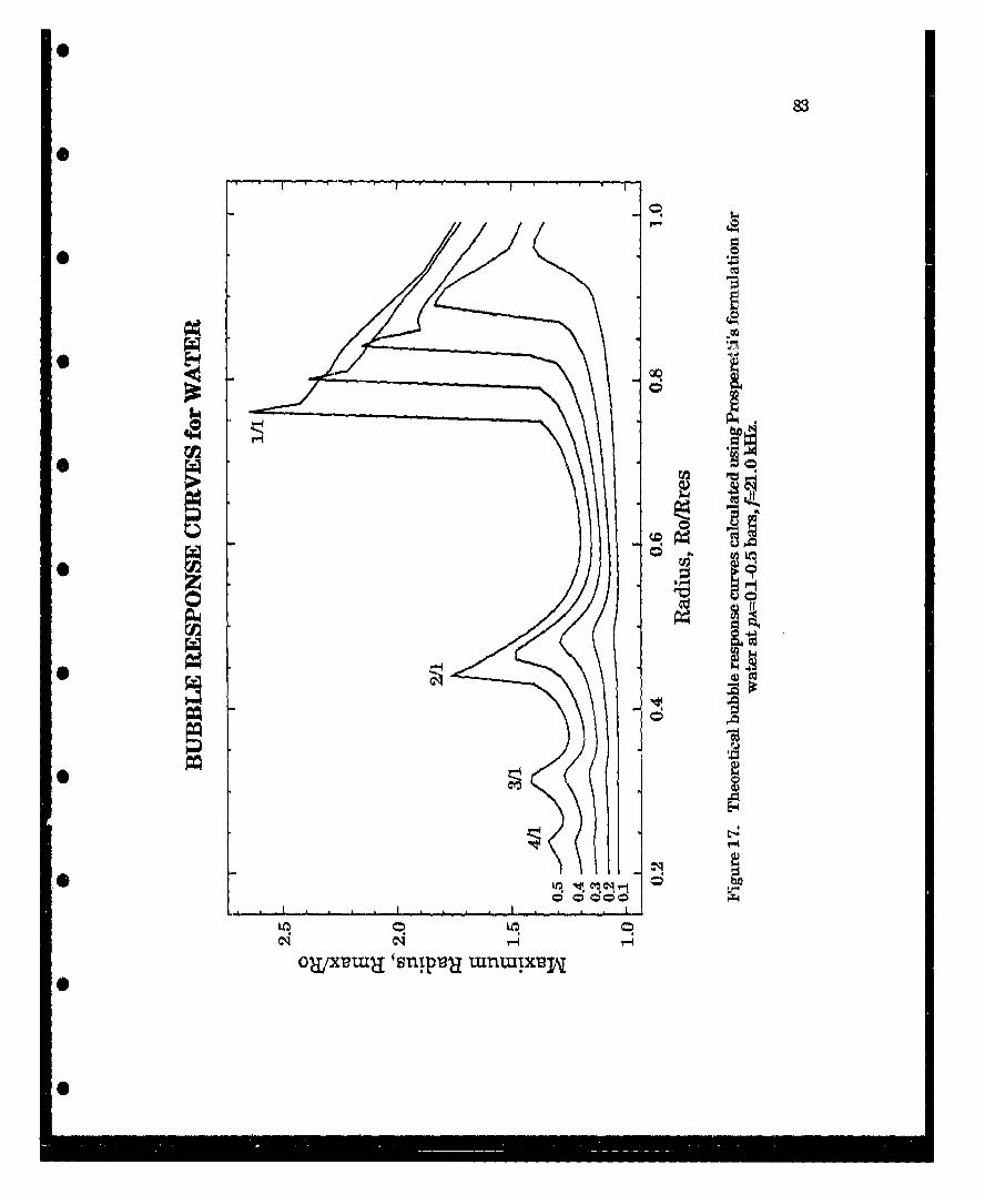
83

0C

0Lo

-c

* 0q

*'

I.' £

011v~Z 0sill inix

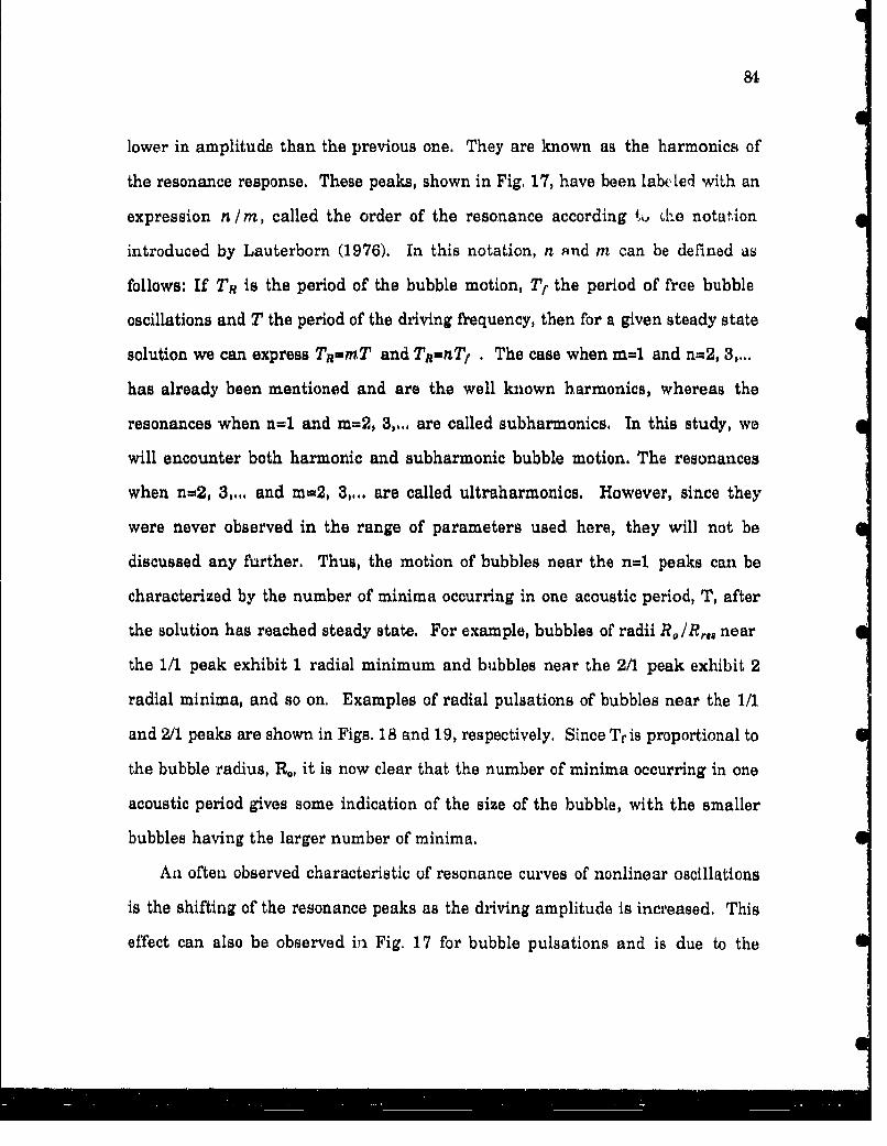
84

lower in amplitude than the previous one. They are known as the harmonics of

the resonance response. These peaks, shown in Fig. 17, have been labeled with an

expression n / m, called the order of the resonance according to the notation

introduced by Lauterborn (1976). In this notation, n snd m can be defined as

follows: If TR is the period of the bubble motion, Tt the period of free bubble

oscillations and T the period of the driving frequency, then for a given steady state

solution we can express T-mmT and TR-nTI . The case when m=1 and n=2, 3,...

has already been mentioned and are the well known harmonics, whereas the

resonances when n=1 and m=2, 3,... are called subharmonics. In this study, we

will encounter both harmonic and subharmonic bubble motion. The resonances

when n=2, 3,... and m=2, 3,,,. are called ultraharmonics, However, since they

were never observed in the range of parameters used here, they will not be

discussed any further. Thus, the motion of bubbles near the n=1 peaks can be

characterized by the number of minima occurring in one acoustic period, T, after

the solution has reached steady state. For example, bubbles of radii RI/Rr near

the 1/1 peak exhibit 1 radial minimum and bubbles near the 2/1 peak exhibit 2

radial minima, and so on, Examples of radial pulsations of bubbles near the 1/1

and 2/1 peaks are shown in Figs. 18 and 19, respectively. Since Tr is proportional to

the bubble radius, I,, it is now clear that the number of minima occurring in one

acoustic period gives some indication of the size of the bubble, with the smaller

bubbles having the larger number of minima.

An often observed characteristic of resonance curves of nonlinear oscillations

is the shifting of the resonance peaks as the driving amplitude is increased. This

effect can also be observed in Fig. 17 for bubble pulsations and is due to the

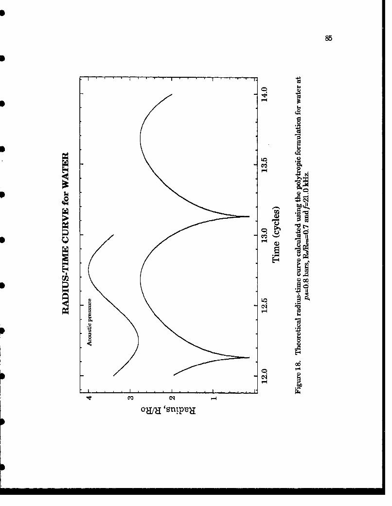
85

06

Scm c0

0-am lnip~0

86

4C.

bn

oa/a lnip*cl

87

0nonlinear "softening" of the restoring force as the bubble expands. In this case,

the shifting causes the left edge of the peaks to steepen and eventually "bend over".

At this point, the two solutions exist simultaneously for the same value of the

bubble radius, Ro/R,,, causing abrupt transitions to occur from one solution to the

other for small changes in RoIR,•,, Transitions of this type are known as "saddle.

node bifurcations" among researchers in the field of nonlinear dynamics.

At pressure amplitudes above 1 bar, the pulsations of small bubbles (< 40 pIm)

develop a characteristic shape. An example of a radius-time curve at large

pressure amplitudes is shown in Fig. 20, This particular example is for a 20 pLm

bubble in water at PA=1.2 bar, In general, the motion consists of a relatively slow

growth during the first half of the acoustic cycle when the pressure is negative,

followed by a rapid collapse and several rebounds. The word "collapse" here refers$to the first bubble contraction after Rmox has been reached, and which is usually

very fast and violent. This timing is usually referred to as the phase of the

collapse, 0., and is measured in degrees from the beginning of the negative

pressure cycle, where 0=0'. The beginning of the compression cycle corresponds to

OC=180. The collapse in Fig. 20, for example, occurs near 220 *,

Not surprisingly, the highest temperatures and pressures are generated in

the interior of the bubble during this collapse. Fig. 21 is a plot of the temperature

inside the bubble for the same conditions as Fig, 20. The large temperature spikes

are generated during the violent, nearly adiabatic, collapses. It is during these

collapses that sonoluminescence is believed to be generated. Similarly, high

pressures are generated in the bubble interior as the gas is rapidly compressed, as

0U - n •Trn amu n•nm •• • •

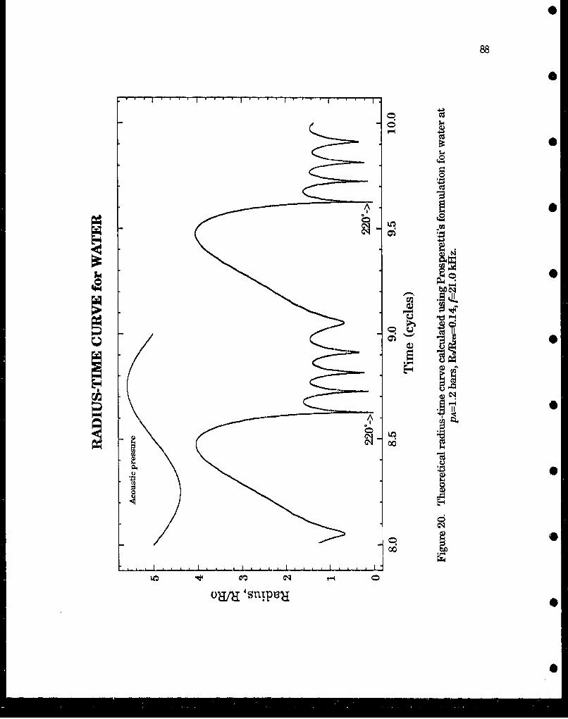
88

VI4.10

o0

r-

oaM Inip0

89

00

*c

*o

0

90

Sshown in Fig. 22. Thi data shown in Figs. 21 and 22 are mostly for illustrative

pvrposes, and the values of the maximum temperatures and pressures, Tmox and

P. respectively, are only estimated. 0In general, then, three quantities can be used to describe the radial pulsations

of bubbles at high pressure amplitudes: the maximum response or pulsation

amplitude (R..), the phase of the collapse (0,) and the number of minima (M)0

which includes the first minima (i.e., the collapse). Note that, just as for low

pressure amplitudes, the number of minima increases as the equilibrium radius

decreases.

Up to this point, all quantities have been given a single value for each solution

assuming that, after reaching steady state, the solutions have the same period as

the driving pressure. This is not always the case, however, especially at high

pressure amplitudes where nonlinear effects are more prominent. In this regime

and under cerLain conditions, the motion of the bubble is such that it repeats itself

only after a multiple number of acoustic periods. This is usually referred to as

subharmonic motion (n=2,3 .... ). For example, subharmonic motion of period Lwo

(n=2), also known as period-two motion, occurs when the period of the radial

pulsations is twice the period of one acoustic cycle (TR=2T). In this case, the values

of RId, 0, @ and MI where the superscript i=1,2, i.e., they alternate between two

different values from one acoustic period to the next. Although period 3, 4, ...etc.

are possible, only period-two solutions were found numerically for the conditions

used in the experiments. Examples of period-two motion can be found in the

response curve shown in Fig. 23 calculated for a bubble driven at 1.2 bars in water

according to Prosperetti's formulation. This type of motion is indicated by

0

91

04*

LooE-4. m

'.P4

00

(s-q4ensac

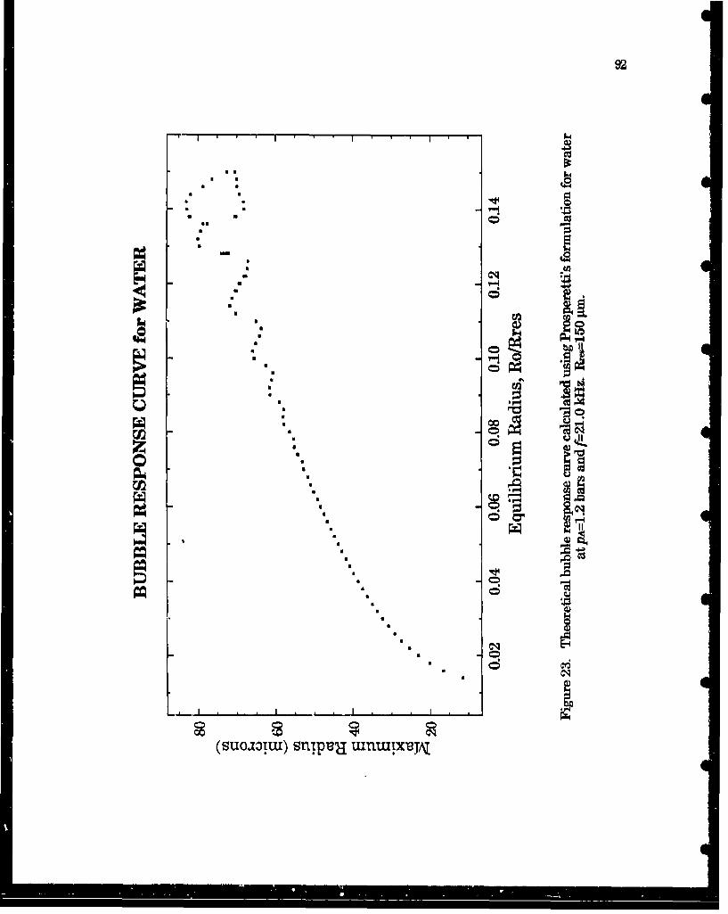
92

*q 4

* 3bb

--j

(uoiu si-auuixeA

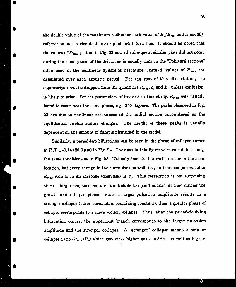
93

the double value of the maximum radius for each value of RoIR,,,, and is usually

referred to as a period-doubling or pitchfork bifurcation. It should be noted that

the values of R',.,, plotted in Fig. 23 and all subsequent similar plots did not occur

during the same phase of the driver, as is usually done in the "Poincard sections"

often used in the nonlinear dynamics literature, Instead, values of Rmax are

calculated over each acoustic period. For the rest of this dissertation, the

superscript i will be dropped from the quantities R,.., , • and M, unless confusion

is likely to arise. For the parameters of interest in this study, Rmaj. was usually

found to occur near the same phase, e.g., 200 degrees. The peaks observed in Fig.

23 are due to nonlinear resonances of the radial motion encountered as the

equilibrium bubble radius changes, The height of these peaks is usually

- •dependent on the amount of damping included in the model.

Similarly, a period-two bifurcation can be seen in the phase of collapse curves

at R0/R--0. 14 (20.3 gtm) in Fig. 24. The data in this figure were calculated using

the same conditions as in Fig. 23. Not only does the bifurcation occur in the same

"location, but every change in the curve does as well; i.e., an increase (decrease) in

R.., results in an increase (decrease) in 0,. This correlation is not surprising

• since a larger response requires the bubble to spend additional time during the

growth and collapse phase. Since a larger pulsation amplitude results in a

stronger collapse (other parameters remaining constant), then a greater phase of

* •collapse corresponds to a more violent collapse. Thus, after the period-doubling

bifurcation occurs, the uppermost branch corresponds to the larger pulsation

amplitude and the stronger collapse. A "stronger" collapse means a smaller

_ collapse ratio (Rm.iIR) which generates higher gas densities, as well as higher

94.

* U40

00

C * 4ase~p si( s-lo

95

temperatures and pressures. This is illustrated in Figs. 25 and 26 where the

maximum internal temperature (T,,.,) and pressure (P,,.,) generated during each

period has been plotted, respectively, for the same conditions used in Fig. 23. T,,.m

has been averaged over the bubble interior. Again, note that these two quantities

are directly correlated to the pulsation amplitude. Also note the high sensitivity of

the temperature and pressure to the pulsation amplitude, i.e., a small change in

Rm., results in a fairly large change in T,. and Pma, . The close relationship

among the quantities R. ,,,Tm,, and Pm, will be useful in Chapter IV where

the experimental results will be discussed.

MI. B. 3 Limitations of the Theoretical Formulations.

The range of acoustical parameters being considered in this study has been

determined by the measurements made during the experiments. These

parameters are the following: driving frequencies between 21 and 25 kHz,

pressure amplitudes between 1 and 1.5 bars, and bubble radii between 15 and 25

microns for five different water/glycerine mixtures. For these parameters, the

temperatures and pressures generated inside the collapsing bubbles have been

measured and calculated in this and other studies (see Chapter I) to be on the

order of thousands of degrees Kelvin and thousands of bars. To date, no model of

cavitation exists which can treat the gas - or even the adjacent liquid - inside a

collapsing bubble adequately for these extreme physical conditions. Each of the

models considered in this study makes different approximations when treating

the bubble's interior. In order to compare the results of the different formulations,

96

000

a 0.

I a 0

(m 49

a a c;

U ma4

Uu~o)-da iuiqjLniT3Z

0

97

0

0

0

'-I£

I"

*

-

�1 -�

*

00

or'0

oC�10*

U

0

0

I

U

0

I

0

I

(s.rnq) SS8Jd

I�T�LI�UI

0

0

0

S

98

the assumptions and limitations of each must be considered. These assumptions

and their general validity for the physical conditions encountered during the

calculations are discussed in this Section. Although we have no a priori certainty

of the accuracy of the theoretical results, an evaluation of the validity of the

assumptions will be made at the maximum values of temperature and pressure

predicted by the more reliable i-odels, for the range of experimental parameters

stated above. These values i-pwesent the worst-case scenario predicted by the

theories and should provide a good test case to their applicability. These values are

10,000 K and 30,000 bars for the gas temperature and pressure, respectively, and

2,000 K and 30,000 bars for the liquid. For the collapse ratio, (Rmin/Rr), a value of

0.12 is used, which corresponds roughly to a 500-fold increase in the gas density.

A wall velocity of the order of the speed of sound in the gas (340 m/sec measured at

STP) is also used.

Five major assumptions were made in deriving the three formulationsS

considered in this study. Four of them are common to all the models. These are:

(W) The bubble remains spherical; (b) The bubble contents obey the ideal gas law; (c)

The internal pressure remains uniform throughout the bubble; and (d) No

evaporation or condensation occurs inside the bubble. The fifth assumption 0

pertains to the thermodynamic behavior of the liquid surrounding the bubble. Let

us now consider the first four assumptions.

Although most criteria of surface instabilities (discussed in the next Section) 0

do not predict the bubble motion to remain radially symmetric under the

conditions given above, assumption (a) is believed to remain valid based on the

0

0

99

experimental observations, namely the light scattering data. This evidence will be

presented in Chapter IV in more detail.

The ideal gas law assumption (assumption (b)) is known experimentally to be

valid in the limit as the specific volume v (volume/unit mass) approaches infinity,

or, equivalently, as the pressure of the gas approaches zero. The simplest way to

* test this assumption is by considering van der Waals equation of state,

* where Rg is the universal gas constant. The term a / 0 is intended to correct for the

intermolecular attraction and the constant b to account for the volume occupied by

the molecules. At the minimum volume considered in this study, i.e., when

* Rj/Ro= 0.12, the term a/0:5 0.1 bars. For the same conditions, the value of b

corresponds to a correction to the volume of less than 0.5 per cent, Thus, for all

practical purposes, assumption (b) may be considered valid.

* Assumption (c) states that the momentum equation (3.13) reduces to p-p(t).

The pressure perturbation contributed by each term in the momentum equation

has been considered by Prosperetti (1988). He concluded that

AP M,-B-, m,2 (3.31)

where Ml is the Mach number of the bubble wall, c, is the speed of sound in the gas

and t0 is a characteristic time. If t0 is substituted by the theoretical minimum

collapse time (- 10 nsec), R by the equilibrium radius (15 microns), and cy by its

value at the maximum temperature reached inside the bubble, then R/cgto has the-0

100

value of - 1. Equation (3.31) then reduces to 4p /p=O(Mn). When the temperature

dependence of c. is taken into account, the Mach number for the bubble wall M11

was found to be around 0.2. It thus appears that pressure perturbations may

occur inside the bubble in some cases, although the conditions necessary for the

formation of shock waves inside the bubble are not likely to be realized.

Assumption (d) states that no condensation or evaporation occurs during the

bubble motion. Evaporation would occur during the collapse when the gas

temperature is increased by the mechanical work done by the liquid, Some of this

energy is transferred to the liquid through regular thermal conduction, causing

some liquid molecules to evaporate. As the bubble rebounds and expands rapidly,

the temperature is decreased, causing the same molecules to condense, releasing

heat into the gas. The result of this process is to transfer energy from one part of

the cycle to the other, acting as a form of thermal damping, It should also be

noted, however, that collapse times are on the order of tens of nanoseconds which

limit the amount of energy deposited into the liquid. Thermal relaxations times of

water are on the order on microseconds. According to the models, temperatures

as high as 2000 K may be reached in the liquid side of the interface, as stated above,

If we assume that this is the case, there is little doubt that assumption (d) is

invalid to some extent, although the short time (<20 nsec) during which these

temperatures persist will probably limit the amount of vaporization. In order to

estimate this amount, the temperature and pressure during the collapse should be

compared to the vapor pressure curve for the liquid. This has been done in Fig. 27

by plotting the pressure vs. temperature in the liquid during one acoustic period

for a 20 gm bubble driven at 1.45 bars at 23.6 kHz representing the conditions

101

ob

Lo

0-4

00

(saiq) enssacl pnbtr

102

stated at the beginning of this Section. The vapor pressure curve for water is also

shown, which defines the boiling point of the liquid as follows: if at a given

temperature the pressure exerted on the liquid is less than its vapor pressure,

then the liquid boils. The vapor pressure curve of water was used in Fig. 27 since

the vapor pressure of glycerine is lower, It can be seen from this figure that the

boiling point of the liquid is never reached for values below the critical point. At

the critical point, the liquid and vapor phase do not separate, i.e., there is no real

difference between the two phases. In this case, the latent heat of vaporization is

zero and no thermal damping due to vaporization exists, Nevertheless, the

thermodynamic properties of the bubble would be very different from those

assumed at equilibrium, and the model becomes invalid under these conditions.

Thus, of the four assumptions considered, (d) is the most likely to be violated,

The fifth major assumption made in the formulations pertains to the

thermodynamics in the bubble's interior. This assumption is reflected in the

expression for the internal pressure, p.. The approximations made in each

formulation in order to obtain this expression will be discussed next.

First, let us consider the least sophisticated of the models, the polytropic

approximation model. This model is mostly limited by the small-amplitude linear

approximation made in calculating the polytropic exponent. In addition, this

approximation makes the integral over a cycle of p.dv identically zero, resulting in

no net loss of energy associated with the heating and cooling of the gas

(Prosperetti, 1988), i.e., no thermal damping. This type of damping is known to be

the main energy dissipation mechanism for the parameters under consideration.

Furthermore, the polytropic exponent is nearly equal to 1, i.e., the bubble motion is

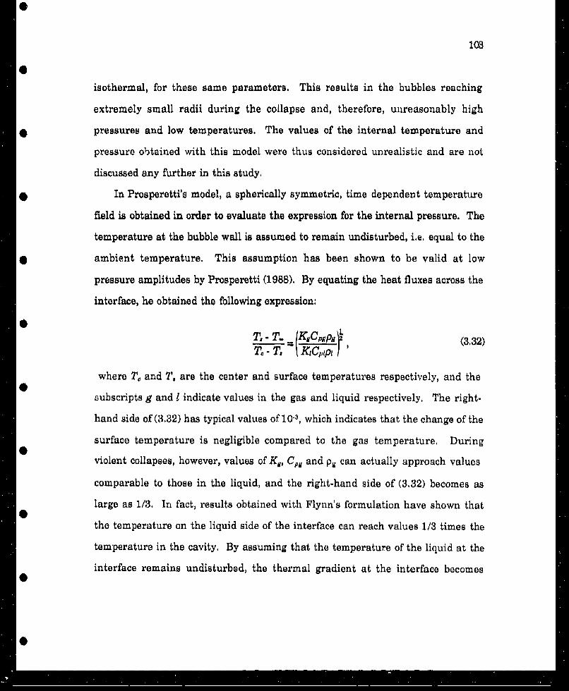
103

isothermal, for these same parameters. This results in the bubbles reaching

extremely small radii during the collapse and, therefore, unreasonably high

-•pressures and low temperatures. The values of the internal temperature and

pressure obtained with this model were thus considered unrealistic and are not

discussed any further in this study.

-- In Prosperetti's model, a spherically symmetric, time dependent temperature

field is obtained in order to evaluate the expression for the internal pressure. The

temperature at the bubble wall is assumed to remain undisturbed, i.e. equal to the

* ambient temperature. This assumption has been shown to be valid at low

pressure amplitudes by Prosperetti (1988), By equating the heat fluxes across the

interface, he obtained the following expression:

T, - T. = (KCpg,py ! (3.32)Z - T. - KLCptPL

where T, and T, are the center and surface temperatures respectively, and the

subscripts g and I indicate values in the gas and liquid respectively, The right-

hand side of (3.32) has typical values of 101, which indicates that the change of the

surface temperature is negligible compared to the gas temperature. During

violent collapses, however, values of K,, Cp, and pg can actually approach values

comparable to those in the liquid, and the right-hand side of (3.32) becomes as

large as 1/3. In fact, results obtained with Flynn's formulation have shown that

the temperature on the liquid side of the interface can reach values 1/3 times the

temperature in the cavity. By assuming that the temperature of the liquid at the

interface remains undisturbed, the thermal gradient at the interface becomes

104

larger, increasing the amount of heat diffusion into the liquid. Thus, it is expected

that the results of this model would be overdamped for the parameters under

consideration.

In Flynn's model, the energy equation in the liquid is included in the

derivation of the expressions for the internal pressure and temperature. In order

to -educe the amount of computer time, however, Flynn was forced to make

further approximations. Although Flynn's formulations appears more

complicated, it was found that they both required about the same amount of

computer time to obtain the solutions for the parameters used in this study.

In Chapter IV, theoretical results of these three models will be presented and

compared with each other. The only known comparison of theoretical results of

bubble pulsations using different models is that by Lastman et al. (1980) who

considered five different radial equations. They assumed adiabatic motion and

found "similar quantitative behavior, even under intense cavitation conditions",

although they only compared pulsation amplitude and phase of collapse. As

shown above, however, the internal temperature and pressure during the collapse

are very sensitive to Rm., and 0. Thus, it is expected that the major difference

among the theoretical results of the formulations considered in this study will be

in the internal temperature and pressure.

[U. C. Surface Instabilities

In order to understand the long term behavior of bubbles (over thousands of

acoustic periods) in cavitation fields, the different mechanisms controlling the size

105

and shape of the bubbles must be considered first. The two principal mechanisms

are gas diffusion across the gas-liquid interface and surface instabilities. Both of

these processes can cause the bubble to either grow or shrink depending on the

physical conditions. Surface tension, by creating a concentration discontinuity

across the interface, forces gas out of the bubble. On the other hand, this diffusion

can be "rectified" by the action of the sound field, and the bubble can be made to

grow. Likewise, surface waves can aid in the growth or dissolution process

through the generation of acoustic streaming near the bubble (Gould, 1975).

Surface waves also have been observed to cause the ejection of microbubbles,

serving as an efficient mechanism of bubble-size reduction (Neppiras et al., 1969).

Thus, the time evolution of acoustically driven bubbles is controlled by many

factors and the fate of each bubble is determined by, among other things, its

equilibrium size and the driving pressure amplitude. In this Section, some

theoretical background of surface instabilities will be presented as well as a recent

instability threshold curve calculated and measured by Horsburgh (1990). The

phenomenon of rectified diffusion will be discussed in the following Section.

When a large bubble is driven at high enough amplitudes, it has been observed

to become unstable, usually breaking up into a cloud of smaller bubbles. Smaller

bubbles, however, are able to retain their spherical shape longer due to the

stronger surface tension effects. These instabilities are cause by the large

accelerations experienced during the collapse of the bubble and near the point of

minimum radius where the motion is rapidly stopped and reversed. An order of

magnitude calculation indicates that a liquid-gas interface becomes unstable

106

when the inward acceleration of a bubble wall exceeds a critical value 4c/pR3

(Hsieh et al., 1960).

When bubbles become spherically unstable in a levitation cell, they can be seen

to move about in an erratic manner, apparently due to the nonlinear coupling

between the sound field and the surface oscillations. The visual observation of this

"dancing" motion was used by Eller and Crum (1970) to measure the pressure

threshold for instabilities for a range of bubble radii. Except for the less common

occurrences of stable surface oscillations, instabilities usually become visually

obvious to the observer, especially if the driving pressure is relatively large. This

surface oscillation threshold has been measured and calculated in the past by

several people (Plesset,1954; Hsieh, 1974; Prosperetti, 1978) and more recently by

Horsburgh (1990).

The calculation of the threshold for surface waves made by Horsburgh (1990)

for R• in the range 10-60 microns is shown in Fig. 28. These calculations were

made for air bubbles in water. Combinations of Ro and PA above this curve result

in the excitation of surface waves, while those below do not. The oscillations of this

curve are due to the harmonic resonances of the radial motion, At these

resonances, lower pressure amplitudes are required to excite surface waves, due

to the larger bubble response, The curve in Fig. 28 will be used to demonstrate the

existence of previously unknown islands of stability in the region above this

threshold curve. For completeness, a brief description of the equations used to

calculate this threshold is included here. The reader is referred to Horsburgh

(1990) for more details. The model is briefly described as follows:

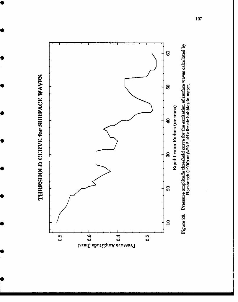
0

107

0

I.......................................................I

�0

U

0

-� ou�

0e�p��

�%�d

'.4

0

00

0

0

e7�

0 .1 ________

0

(s�u�q) epn��dmy GJflSSG.Id

0

108

Let the bubble boundary be perturbed from a spherical surface of radius R to a

surface with radius vector of magnitude r,. Then one may write

ra = R + an Y., (3.33)

where Yn is a spherical harmonic of degree n, and the an's are functions of time to

be determined. The growth or decay of an(t) from a small initial value determines

whether the spherical shape is stable or unstable. Assuming that

a.(t) << R(t) , (3.34)

and keeping only terms of 1st order in an in a lirearized perturbation procedure,

Plesset (1954) found that the an's are independent of each other and that they

satisfy the following differential equation:

Un+ - Itd. - A a, = 0. (3,35)R

Assuming that the density of the liquid is much greater than that of air, A is given

by

A =(n -1) (n +1) (n +2) 3 (3.36)R pIR 3

These equations were derived using an incompressible and inviscid liquid

assumption and will thus be integrated along with the corresponding radial

motion equation, namely Rayleigh-Plesset's:

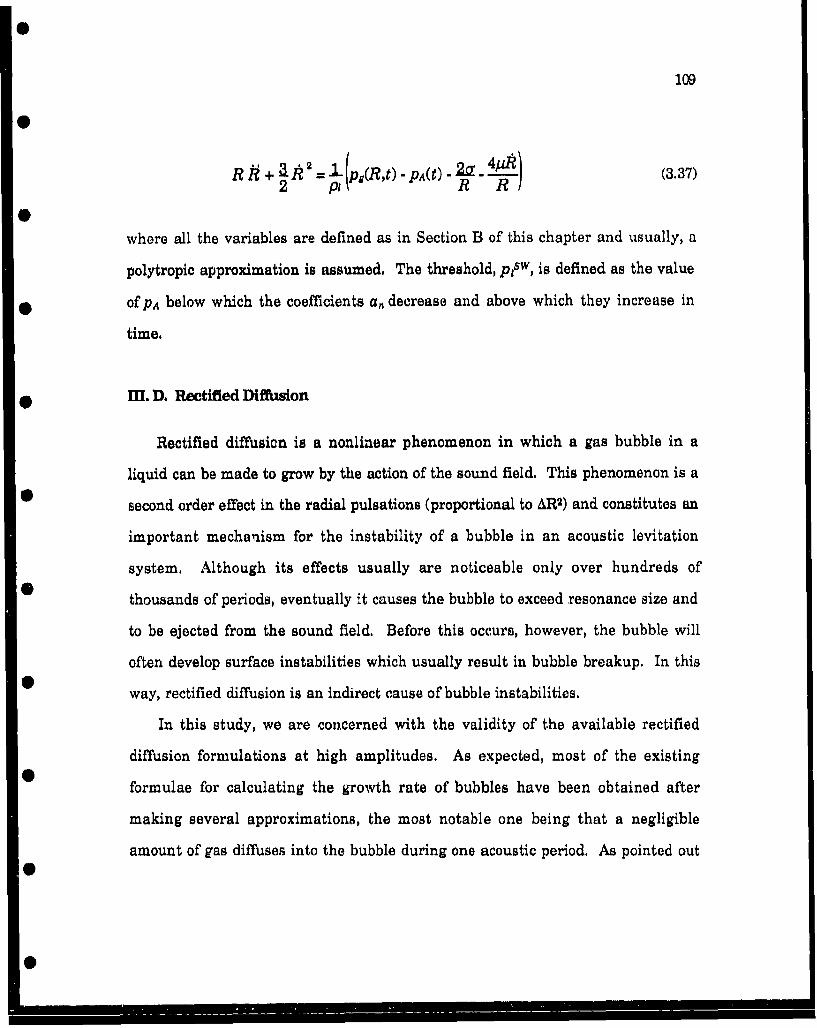
109

R 2 (337

where all the variables are defined as in Section B of this chapter and usually, a

polytropic approximation is assumed. The threshold, pisW, is defined as the value

of PA below which the coefficients a, decrease and above which they increase in

time.

* HI. MD. Rectified Diffusion

Rectified diffusion is a nonlinear phenomenon in which a gas bubble in a

liquid can be made to grow by the action of the sound field. This phenomenon is a

second order effect in the radial pulsations (proportional to AR2 ) and constitutes an

important mechanism for the instability of a bubble in an acoustic levitation

system. Although its effects usually are noticeable only over hundreds of

thousands of periods, eventually it causes the bubble to exceed resonance size and

to be ejected from the sound field. Before this occurs, however, the bubble will

often develop surface instabilities which usually result in bubble breakup. In thisS way, rectified diffusion is an indirect cause of bubble instabilities.

In this study, we are concerned with the validity of the available rectified

diffusion formulations at high amplitudes. As expected, most of the existing

0 formulae for calculating the growth rate of bubbles have been obtained after

making several approximations, the most notable one being that a negligible

amount of gas diffuses into the bubble during one acoustic period. As pointed out0

! " ... .... .

S.. .. " . .='

110

by Eller and Flynn (1965), this is not always the case for large amplitude

pulsations. However, because of the complexity of the mathematical problem and

the time constraints, the formulation developed by Eller and Flynn (1965) in which

the above approximation is made will be used here. The model can be applied to

any periodic radius-time curve and in this respect it is rather general. Using an

integration routine written by Church (1988), the rectified diffusion threshold

shown in Fig. 29 was calculated. The threshold pIRID was calculated for 70% air-

saturated water at 21 kHz for R. in the range 5-60 microns, For a given R., bubbles

driven at a value of PA above this curve will grow while those driven below will

shrink in time. Similar to the surface wave thresholds, the curve in Fig. 29

exhibits variations in the threshold ptRD due to the harmonic resonances of the

bubble motion. Generally, at the resonances, a lower value of PA is needed to make

the bubble grow due to the larger response.

The following is a brief outline of Eller and Flynn's formulation for rectified

diffusion. As stated before, the main approximation is to neglect any diffusion of

gas into the bubble during a single acoustic period. The problem to be solved is

thus determining the gas concentration field c(rt) in the liquid (not the bubble)

from which the rate of change of the number of moles of gas in the bubble will be

obtained from

- - 4rDR2 (3.38)

where D is the gas diffusion constant and r is the distance from the center of the

bubble. The diffusion equation to be used is Fick's law of mass transfer,

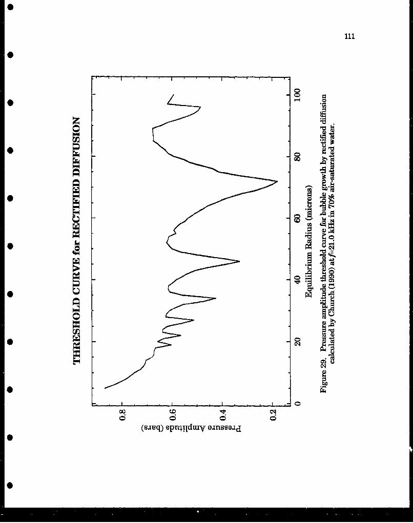
0

111

0

II

0

I0

�

* '.4

di.*

0

0

0* I I * I

Co 0

(�J�q) �Ptl1LdWY 6�IflSS8Jd0

0

112

dt =5-/+u . Vc= D C , (3.39)dt D

0where u is the velocity of the liquid at r. The boundary conditions are given by

c (r,0) = ci, r > R (3.40)

lir c (r,t) = Cj, (3.41)r -4..

c (R,t) = c. t > 0, (3.42)

where cj is the initial, uniform concentration of gas and also the concentration of

gas at infinity, and c, is the concentration of gas in the liquid at the bubble wall. c,

is given by Henry's law, which states that the concentration of gas dissolved in a

liquid is directly proportional to the partial pressure of the gas outside the solution.

Hence, Cs = k"1 pg where k is Henry's constant and is generally a function of"

temperature. Introducing a "high" frequency limit in which the rapidly

oscillating terms of the gas concentration field are ignored, Eller and Flynn

arrived at the following expression for the time-averaged rate of change of the 0

number of moles of gas in a bubble,

ýdA= 4x& P D [A + R. r~!]~ c-• •) (3.43)

where co is the value of c, when R = R0 andA and B are given by

S0

113

A=I -f# dt and B , (3.44)A=Tf R, ,J ý ro

respectively, t is the time and T is one period of the bubble pulsation. Defining the

threshold pressure as the pressure of the acoustic field at which the average

diffusion is zero, we have

•- + . (3,45)Co Rop. B

Thus, A and B are calculated for a given R. and PA such that the above equality is

satisfied to within a certain criterion. When this criterion is met, the value of PA

• is, by definition, the rectified diffusion threshold, pgRD.

"0!

0 1 .. .. I

0

0

Chapter IV

Results and Discussion

IV. A. Introduction

The first experiment performed in this study was designed to determine the

range of active bubble radii in a cavitation field at pressure amplitudes above 1 bar,

that is, above the pressure threshold for light emission (sonoluminescence, SL).

This determination was made by measuring the phase of SL relative to the sound

field and comparing it to the phase of bubble collapse predicted by the different

theories of radial bubble pulsations. Because the SL flashes are very short, and

0 assuming that they are emitted at the time of the collapse, one can then measure

the phase of SL to determine the phase of bubble collapse. Fig. 30 illustrates these

observations by plotting the light flashes as detected by the PMT (top trace)

0 simultaneously with the acoustic pressure (bottom trace) as a function of time.

These data were taken at f=21 kHz, PA-1.5 bars in water, According to the

theories, the phase of bubble collapse varies over a wide range of values depending0

on the bubble size and pressure amplitude, as can be seen in Fig. 24, p. 93. It is

thus possible to estimate the bubble sizes that are active during cavitation by

measuring the phase of SL emission, assuming the theories are correct and that

SL is emitted during the collapse of the bubble. Furthermore, if enough

information is available about the bubble radii and the pressure amplitude, the

applicability of the models can be tested.0

114

0M

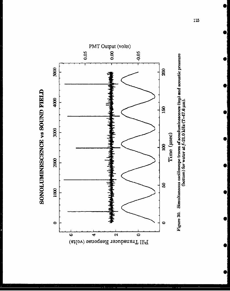
PMT Output (volts)

6 d

IQ,_ _ _ _ _ _ _ _4t.

C. p75ru) _ _ _ _

(SjLoA) asuodsaj ~i~npstw.Ij 111c

116

This initial experiment was performed in a cavitation field generated in a

levitation cell at around 1,5 bars of pressure amplitude. Fig. 31 illustrates the type

of cavitation generated for this experiment. This cavitation consists of streamers

of bubbles nucleated near the cell wall or the liquid surface and driven towards the

pressure antinode by radiation pressure forces also known as Bjerknes forces

(Crum, 1975). The phase of SL emission was measured to be about 200 degrees in

air-saturated water with a standard deviation as large as ± 15 degrees. These

large fluctuations are not due to experimental error. Instead, the large scatter in

the data is probably caused by the influence that the cavitation bubbles had on the

acoustic pressure field in the levitation cell. More specifically, the sound scattered

by the bubbles may be large enough to affect neighboring bubbles, causing the

pressure field experienced by each bubble to fluctuate significantly from one

acoustic period to the next, Furthermore, the presence of bubbles in the cell is

known to change its resonance frequency, causing the cell to "detune" and the

pressure amplitude to change. Since the phase of collapse depends on the

pressure amplitude, these fluctuations result in a large standard deviation of the

data, making the determination of the bubble sizes very imprecise. In addition,

the bubbles in the cavitation field could not be assumed to pulsate with radial

symmetry, and the effect of asymmetric motion on the phase of the collapse was

difficult to determine. The cause of the asymmetric bubble motion will be

discussed later. Thus, although the data obtained allowed an estimate of the

range of initial bubble sizes based on the theories by assuming a constant pressure

amplitude, more data were needed before any comparison between the theories

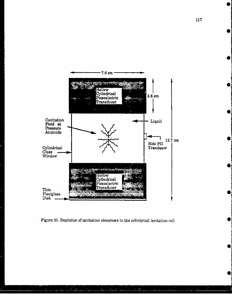
117

. .6cm

Cylindrical 1Piezoelectric 3.6 cm

Cavitation Liquid

PressureAntinode

Side Pill 12.7 cm,

Cylindrical TranducerGlassWindow

CylindricalPiezoelectric

Thin TransducerPlexiglass 4, If kv AA

Disk _

Figure 31. Depiction of cavitation streamers in the cylindrical levitation cell

ii0

118

could be made. Thus, a better experiment for studying cavitation was needed.

Fortunately, a solution for overcoming these difficulties was soon found.

During some of the initial experiments it was noted that the scatter in the

measurements of the phase of SL was occasionally reduced to less than ± 1 degree,

i.e., down to the noise level, making the phase practically constant in time. After

many trials the conditions necessary to reproduce this phenomenon were fourd. It

was learned that as the pressure was increased the degassing action of the sound

fieid was reducing the number of bubbles, causing the cavitation streamers to

become very thin until only a single bubble remained. The remaining bubble was

approximately 20 microns in radius and positioned near the antinode. At this

point, it was remarkably stable, remained fairly constant in size and was later

determined to be pulsating in a purely radial mode. Furthermore, with the room

lights dimmed, a greenish luminous spot the size of a pinhead could be seen with

the unaided eye, near the bubble's position in the liquid, The luminous spot was

then located at the bubble's geometric center by observing it through a microscope.

This light emission was sonoluminescence generated during the collapse of the

bubble at its minimum radius. Although this type of luminescence had been

observed before by several researchers (Saksena et al., 1970, etc.), very sensitive

instruments were usually required and it had never been observed from a single

bubble.

The stabilization of a single, radially pulsating bubble was achieved in slightly

degassed water-glycerine mixtures with glycerine concentrations below 60%. A

description of the visual observations of the stabilization process as the acoustic

pressure was increased can be given as follows: After injecting a gas bubble with a

119

small syringe at about PA= 0 ,6 bars, the bubble exhibited dancing motion indicative

of surface waves and asymmetric collapses (Lauterborn, 1982). As the pressure

amplitude was increased, the dancing motion became more vigorous, causing the

bubble to fragnment. A bubble cluster was then formed as the residual bubbles

moved around the parent bubble. In glycerine mixtures with concentrations

greater than 60%, the radial stability became very difficult, if not impossible, to 0achieve. The buuble system looked more like a cloud and very often developed into

what has been termed a "shuttlecock". When observed through a microscope, the

shuttlecock appeared to be a cloud of microbubbles surrounding a larger bubble of 0

approximately 50 gm in radius. Through the inferaction with the sound field, this

cloud developed a definite pattern of motion from one side of the bubble to the other.

In contrast with single bubbles, the position of the shuttlecock was not on the 0levitation cell's axis but a small distance away from it (0.5-1.0 cm). Microbubbles

appeared to be ejected from the side of the cloud directly away from the antinode

and were immediately attracted towards the cloud by Bjerknes forces (Crum, 0

1975). As the microbubbles reached the opposite end of the bubble cloud from

which they had been ejected, they were pulled in, possibly by interbubble forces

directed towards the center of the cloud. Thus, a rotational pattern was 0established. For lack of a better analogy, the three dimensional pattern formed by

the bubbles has been likened to that formed by the earth's magnetic field lines.

The shuttlecock was observed to emit a low rate of SL flashes.

If the amount of glycerine were less than 60%, however, the bubble cluster

was observed to become smaller and denser as the pressure amplitude was

increased. Just before the stability threshold, the cloud could be seen to collapse

100

upon itself until, at a rather well-defined value of the pressure, a single radially

pulsating bubble emerged. As soon as this transition occurred, the count rate of

SL increased to nearly one flash per cycle. Instead of the usual distorted shape

when streamers were present, the output of the side pill transducer was now very

clean and symmetric. When observed through the microscope, the blurry but

unmistakable outline of the radial pulsation could be discerned. When the sound

field was turned off, the bubble could be seen to rise towards the surface. The

pulsation amplitude was estimated to be between 4 and 5 times the equilibrium

radius.

An interesting observation already mentioned was the well defined pressure

threshold, ptST, at which stability was reached, in addition to a hysteresis effect.

After reaching stability, the pressure could be decreased below the threshold ps•T

and stability was maintained. In general, stable bubbles could be driven at values

of the acoustic pressure 0.1 bar below the stability threshold. If driven above a

certain pressure, the bubble disappeared possibly due to dynamic instabilities, For

convenience, we will call these the lower, pltST, and upper, putsT, stability

thresholds respectively. These thresholds are illustrated in Fig. 32. In water, for

* example, ptsT was measured to be around 1.2 bars, pitr at around 1.1 bars and p, ST

at around 1.3 bars. The range of pressures at which bubbles were stable was 1.1 •

PA:5 1.5 bars depending on the liquid mixture. For water, it was 1.1 PA • 1.3 bars

* whereas for GLY 42 it was 1.3 5PA • 1.5 bars. Thus, higher concentrations of

glycerine required slightly higher pressures in order to achieve radial stability. It

was also found that these ranges could be enlarged (towards the lower pressures)

• by decreasing the dissolved gas content of the liquid. As the amount of dissolved

0

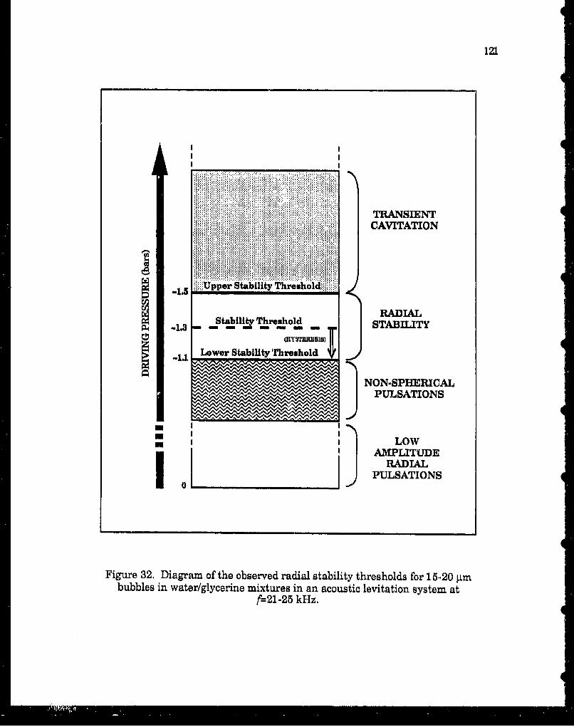
121

.. CAVITATION

WOI

.1Upper Stability Threhl

Stability Threshold RADIAL0 -1.3 no STABILITY

-uLower Stability Threshold

NON-SPHERICALIPULSATIONS

* I LOW'I AMPLITUDE

_______________ 9 PULSATIONS

Figu~re 32. Diagram of the observed radial stability thresholds ['or 15-20 ýtmbubbles in water/glycerine mixtures in an acoustic levitation system at

f=21 -25 kHz.

122S

gas increased, regions of instability within the stability pressure range began to

appear. The upper pressure threshold, putsT, at which the bubble disappeared,

remained constant, however. It became clear then that rectified diffusion playedS

an important role in the stability process.

The observation of an upper pressure amplitude threshold, putsT, above which

pulsating bubbles cannot exist, seems to confirm the existence of a transient

cavitation threshold as defined by Flynn (1964, 1975b). According to Flynn (1975b),

the motion of bubbles pulsating with an expansion ratio (RmOJRQ) above a certain

value become inertia controlled. When that happens, the collapse of the bubbles6tends to be rather violent, often resulting in the destruction of the bubbles during

the collapse. The bubbles studies here (-20 g±m) fall under the "large" category (> 5

jum) which, according to Flynn's model of cavitation bubbles, should exhibit

thermally-related effects (e.g. sonoluminescence) before reaching the transient

cavitation (dynamical) threshold. For 20 gtm bubbles, Flynn predicted a dynamical

threshold of Rmax/Ro - 2.2. These predictions appear to be confirmed by the

observations made here, since SL has been observed from stably pulsating bubbles.

After reaching a value of the expansion ratio RMOZ/Ro - 4, the bubbles become

0 unstable, i.e., disintegrate. Although the observed values of the dynamical

threshold differ somewhat from those predicted by Flynn, it should be noted that

the threshold values defined in his model "most likely act as lower limits to

0 experimental thresholds", as pointed out by Flynn (1975b).

Despite the lack of understanding about the particular mechanisms involved,

the discovery of a single bubble pulsating at large amplitudes has many important

* consequences. Among these is the ability to acquire new, previously unavailable

S

123

and more accurate data about the motion of bubbles in cavitation fields. These

data include (i) an experimental radius-time curve of the bubble, which allowed us

to measure the phase of the collapse, (ii) the phase of sonoluminescence emission,

end (iii) the pulsation amplitude which can be used to test the applicability of the

bubble models. In addition, the simultaneity of SL and the collapse of the bubble

may be verified. We will present the results of the single bubble experiments first,

along with the theoretical results. After this, the results of the measurements of

the phase of SL in multibubble cavitation fields will be discussed.

IV. B. Light Scattering Experiments

1. Comparison between Theories and Experiment: Prosperetti's Theory

a. Radius-time Curve of a Single Bubble

Figure 33 shows a plot of the bubble radius vs time (R-t) at PA= 1 .2 bars in

GLY21 as measured by the photodetector. This figure is a single trace obtained

from the LeCroy oscilloscope. The y-values have been converted from intensity to

radius using the transfer function obtained during the calibration procedure

(Section II.D.2.a). The uncertainty has been calculated to be about ± 5 ý±m. This

figure is a typical example of an R-t curve obtained from a single bubble pulsating

at large amplitudes with a period equal to that of the driving pressure. R-t curves

for a range of pressures between 1.1 and 1.5 bars were obtained for all the liquid

mixtures. The pressure amplitude was determined with an accuracy of about ±0.1

bars, although changes of APA=±0.01 bars were possible with the apparatus used in

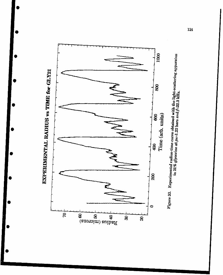
0

0 12A

�'�1�

0* 0

0

-

* 0o

*� P�II

*4)-

0

�cq4)

0* 0

09

cv�

0 0.1

(SUO.iOItU) �rnp�j

0

125

this experiment. All of the radius-time plots obtained at these high driving

pressure amplitudes are characterized by a relatively slow expansion (-15-20

gsec), followed by a rapid collapse (- 5-10 gsec) after which several rebounds occur

before the next cycle starts. The minima of these radius-time curves are bounded

by the background noise level of the detection system, which in this case was

around 20 microns. The occasional glitches in the data causing the bubble radius

to drop below 20 microns were due to electrical random noise and therefore have

no significance. Curves similar to Fig. 33 were also obtained for the other

mixtures and representative curves can be found in Appendix A, Figs. A6-A9.

The number of radial minima during one cycle was usually 4 or 5, although 3

minima occurred occasionally. The differences in the traces taken in different

liquids were mainly in the amplitude of the pulsations and the phase of the first

radial minimum,

For comparison, a theoretical R-t curve using the same experimental

conditions as those of Fig. 33 with R,=20 gm is shown in Fig. 34. The reasons for

choosing this value of R, will be explained below. The overall shape of the two

figures is obviously very similar, including the magnitude of the bubble response

and the rebounds after the collapse. One discrepancy, however, is the number of

minima and the apparent increase in the amplitude of the rebounds in the

experimental R-t curve (Fig. 33), as opposed to the decrease predicted by the theory

(Fig. 34). Some of these small discrepancies will be discussed in the next Sections.

Nevertheless, the resemblance is obvious. Periodic pulsations such as those seen

in Fig. 33 were observed continuously for thousands of acoustic periods. These R-t

curves and the observation of the spherical outline of the bubble pulsations

00

(SUOZolu) snp-el

127

through the microscope when bubbles were levitated in the rectangular cell

constitute the most convincing evidence of the periodicity, stability and spherical

symmetry of the bubble pulsations.

Several parameters of nonlinear bubble pulsations have been measured using

the R-t curves of single bubbles pulsating at large amplitudes (R,/IRo > 3). In the

next Sections, some of these measurements will be presented and compared to the

theoretical values predicted by the different formulations, However, since it was

not possible to determine the equilibrium bubble size accurately, calculations were

made for Ro=1i5, 20 and 25 microns. Although the mechanism by which the

bubbles are stabilized is still not well understood, the bubbles did appear to remain

constant in size for the same acoustical parameters (pressure amplitude, gas

concentration, etc.). However, not all of these parameters were controlled during

the experiments and, for this reason, it cannot be assumed that the data were

taken with the same bubble radius. One of the objectives of this study, then, is to

determine which value or values of R, give the best agreement between a

particular theory and experiment for the three independently measured

parameters: pulsation amplitude Rm,., phase of the bubble collapse 0, and the

number of radial minima M. If agreement is found for the same value of R,, for all

three parameters, it can then be said, with reasonable certainty, that the theory

and experiment agree for those values of R,. If different values are found, it can

then be said that the theory and experiment disagree. Since the theories used for

comparison with the experimental results have been shown to exceed their limits

of applicability, perfect agreement is not expected. Thus, a second objective of this

128

study is to estimate the range of parameters over which these theories are

applicable.

Comparison between the measurements and Prosperetti's model will be made

in the next three sections. Comparison with the other models will be made in

Section B,1.e with the intent of determining the most accurate theory, although

this has proven to be a difficult task due to the large experimental error, It will be

shown that the difference in the predictions of the three theories using the same

conditions is smaller than the error bars of the experimental data. Instead, the

consistency of the results of each particular theory has been used as a test of

applicability. In Section B.2, the theoretical values of the internal temperatures,

pressures and relative densities predicted by Prosperetti's and Flynn's

formulations will be compared. These values will be shown to differ by as much as

100% in some cases. The theoretical temperature calculated at the experimentally

determined threshold for SL will be discussed and compared with previous

measurements. In Section B.3, results for sonoluminescence emitted from a

single bubble will be presented. Also, the experimental radius-time curve will be

plotted simultaneously with the SL flashes in order to demonstrate the

simultaneity of the bubble collapse and the light emission.

IV. B. L b. Pulsation Amplitude

• For each of the R-t curves obtained in the previous Section, the pulsation

amplitude Rm,, was measured and plotted versus PA as shown in Figs. 35-39. In

the same figures, values of the theoretical predictions made by Prosperetti's model0-

0 . . .i i i . . . . . .. .. .. "- i•

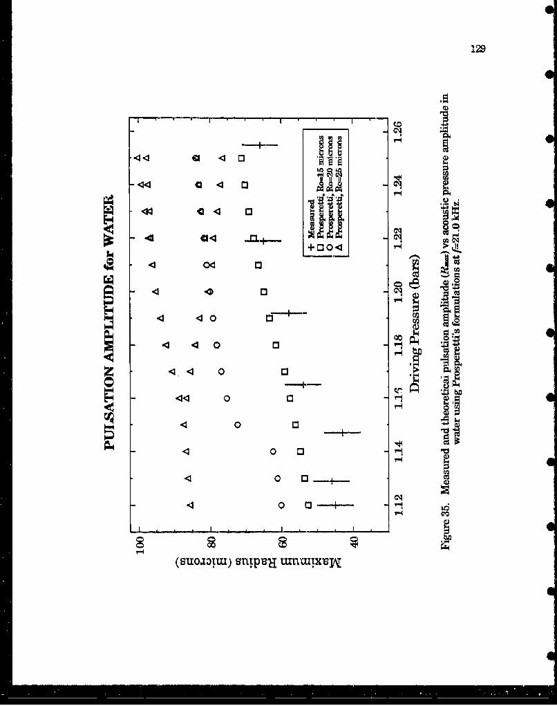
1291

C4)

---- +

44 . 04a(-

0E0

.4 0 C

0003 0 C3

(Suo ltu)SnIP31I l~l-llbu

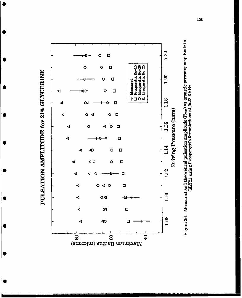
130

00

0 030 -

.4 04- -0 C3

* - 4 0 4 00 a'34 0 400a

.4 0- 0 0C

.4 40 00 3

C3 0

*soi)ui snp4l uin-B--+---

131

0 0 C3ff

0 Q4-

4 0 0 3

0

0t 0 -

00I- ~10 0 3

40

04 0

0 .4-+a-

00

0 0-Q-3--

(SUOOI.L) SnpullLunmx-4

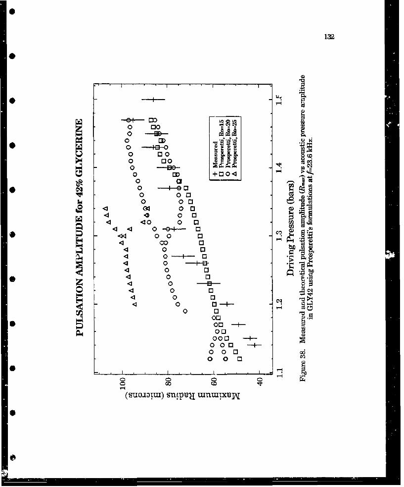
132

0 D011110 ED-'-0 -4--0 0 30 300

~E~ 0 300

0 +040 m

*0 a-L-8020 00

~I40 00Mo 00Etow -d0 0 a

.4 40 00a

.4 . 0 G+ 0

.4 0 0 C44

.4 0 C3.4 0 0 b4 0 -ao 4 0 0 E.4 0 131 0 E-+

0 030 03

0 03

00030 00

00 01 [3

0

(SUOJotlU) sntpu- untuix-eW\

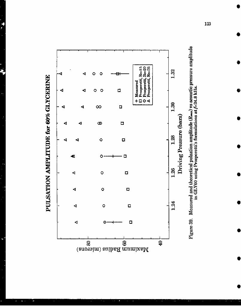
133

<004

4 0 0 a

+C30-4

00.4 4 1

0 07

0-0

ot0 c

0 0 0

(SU.oloul) SnIP13H WflUti1Xt

134

for the same experimental conditions have been plotted for R,=15, 20 and 25

microns, as indicated in the legend. Each measured data point in Figs, 35-39 was

taken from stored oscilloscope traces each consisting of several acoustic periods0for each value Of PA. Most of the time only one trace was stored for each value Of PA

due to the large amount of time and storage space that each trace required. The

error bars placed on these data represent the combined experimental uncertainty0

of + 5 microns, as explained in Section IILE.1. Because of the difficulty in

stabilizing bubbles in GLY60, only a few data points were obtained, Some of the

theoretical curves exhibit abrupt changes caused by resonances of the radial

motion excited at different values of PA. Bifurcations into period-2 and period-4

solutions also occur, especially for the 20 and 25 lim bubbles. These resonances

and bifurcations have been discussed in Section III.B.2 and illustrated in Figs. 23

and 24 where the variables were plotted as a function of R0 instead of PA- When pA

is varied, resonances occur due to the shifting of the peaks toward smaller radii.

Although values were calculated in increments of PA=0.01 bars for each value of

R., not all of the data were displayed. These gaps in the theoretical curves indicate

that no steady state solutions were found in a reasonable (20 acoustic periods)

amount of time.

In general, comparison of the pulsation amplitude data indicates better

agreement with the 15 gtm bubble, although this is not true in every case. The

• experimental data fbr GLY21, for example, agrees partially with the theoretical

results of the 20 pm bubble. It should be noted here that it was probable that the

bubble radius changed as the pressure amplitude was increased. In fact, closer

agreement was found in GLY21 with the theoretical results using the 15 p.m

.0 . . _ , _ _ _-_• - -

135

bubble at the lower pressures but with the 20 u•m bubble at the higher pressures.

The experimental data for GLY42 could even be interpreted as a decrease in the

bubble radius below 15 gtm at the lowest values of PA. This increase in radius with

pressure amplitude may be effected through the phenomenon of rectified diffusion

which, in general, results in larger bubble growth rates as PA is increased, as

stated in Section III.D.

Theoretically, the resonances and bifurcations occur in different places of the

bubble response curve, the exact location being very sensitive to the exact set of

parameters, even for the same values of PA and R.. It was thus not expected to find

agreement between theory and experiment in the regions where quick transitions

occurred. It is interesting to note that although subharmonic motion was

predicted quite often in the range of parameters considered, it was never observed

in the laboratory.

In summary, the pulsation amplitude data shown in Fig. 35 (water), Fig. 37

(GLY35) and Fig. 39 (GLY60) imply that Ro-15 gtm and remains approximately

constant for the range of PA. Fig. 36 (GLY21) and Fig. 38 (GLY42), however, imply

that R. increases with PA. In GLY21, R,, increases from 15 gm to 20 gtm, whereas

in GLY42 it increases from less than 15 gm to about 15 gim. It should be noted that

in the last two sets of data (GLY42 and GLY60), the values of PA reached slightly

lower values than the other sets, which may explain the lower values for Ro.

Period-2 motion was predicted for the 20 gm bubble in GLY21, GLY35 and GLY60

for some values of PA. Period-4 motion was predicted only for water (Fig. 35) for 25

9m.

136

IV. B. 1. c. Phase of Collapse

From the same R-t curves considered in the previous Section, the phase of

collapse Oc was measured using the procedure described in Section II.D.2.b. They

have been plotted in Figs. 40-44 along with the theoretical predictions of

Prosperetti's formulation for 15, 20 and 25 Am bubbles, The estimated total error of

the calibration procedure was ± 5 degrees and it is indicated by the error bars,

These measurements involved a different calibration procedure and the data

obtained are therefore considered independent from the pulsation amplitude data.

The results of the phase of collapse measurements were very similar to the

pulsation amplitude measurements in the previous Section. In summary, these

results can be interpreted as follows- In Fig, 42 (GLY35) and Fig, 44 (GLY60),

R,-20 Am and remains approximately constant. In Fig. 40 (water), R0 appears to

increase from 10 <R, 5 15 pm to 15 5R, < 20 pm aspAincreases, whereas in Fig. 41

(GLY21) and Fig, 43 (GLY42), R.-15 pm at lowPA and Ro-20 pm at high PA. The

largest disagreement between these results and the results of the previous Section

was found for GIY35 and GLY42. The collapse phase data for water predicted

larger radii than the pulsation amplitude data shown in the previous Section,

although the discrepancy was small enough to be within the experimental error.

The reason for this discrepancy is not clear, The fact that more data were taken

for GLY42 and over a larger pressure amplitude range thaa the other liquids may

be part of the reason, It should also be pointed out that some of the data for GLY42

were taken over a two week interval.

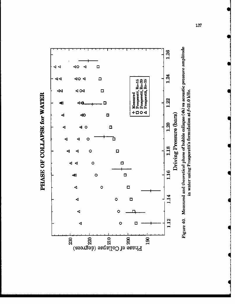
137

44 10 4 13

4< < 04 M

42~~ 43 04 . -4

.40 a

.4 40 D

00 4-4

.4 0

4 000

.43

4 ~0 C -3- -

.. ., ... -..

138

-- e. 00C

0 0o 3

P4 A

*4 0 4 00C

4 .4 0 400a

a 4 C

.440 0 03

o 4 .40 0 M

.4 14 0 B-i-3--

.4 40 0

.0 .40 -5-3

-. _ ____ ___ 0 -

(saaa.59p) asdulloD jo astj-eJ

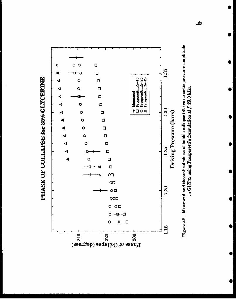
0 0 0 0

40 C3U 4 0 li3.40 03

.40 C +00.4 e

.40 0

.44 0 a

0 0

0 0

Q -e-1 5

000

0-0--

(soaj~ap) esdulloo jo as-ex~d

140

00i

0

o mo M

0 m~

0 0

.0 0

40 00 a

00

04 0 0C3

.4 0 0

'1 0 03- ,

.4 0 0$ci0 a

~ci0---+--20 0 3

00-2-

o 0-2-a---

* _

saaa~ep losdaIloC jo aesTqd.

.4141

+C314.4 00bd

.4 04 3

.4 04 (C3

00

0i iF9 .

(sao~op)asduloo o aseqc

142

0

IV. B. L dL Number of Radial Minima

A third experimental determination that can be used to test the theory is the

number of radial minima observed during one acoustic period. This parameter is

mainly dependent on the bubble size, although some dependence on the pressure

amplitude was found from the -alculations, as pointed out in Section III.B.2,

Figs. 45-49 show the number of minima measured in each liquid mixture and

those predicted by Prosperetti's model for 15, 20 and 25 microns. Non-integer

values of the measured number of minima indicate that two different values were

observed in the same radius-time curve. In that case, the mean of the two values

was plotted. The error bars indicate the estimated error in the measurement.

This error was mostly due to random noise in the R-t curves, which sometimes

resembled the real radial (intensity) minima and interfered with the counting

process. Double values in the theoretical data indicate that a different number of

minima occurred per period in the steady state solution, usually due to

subharmonic motion i.e., m>1 (see Chapter III). Note that subharmonic motion

observed in the figures showing the pulsation amplitude and collapse phase was

not always reflected in the figures showing number of minima. This is because0

only an integer number of minima can occur in one acoustic period, unlike the

pulsation amplitude and collapse phase, which can change in a continuous

fashion.

The number of minima observed were, in general, fewer than the number

expected from the theoretical predictions based on the pulsation amplitude and

collapse phase measurements. This means that the bubble radii predicted based

0M

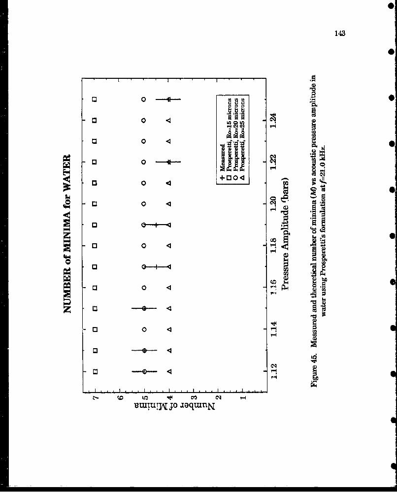
143

13 0

a 0

00

oi 0 - 1

0

0 .4

C3 0 .4

L- ko C-- 4

0----TY JOiqn

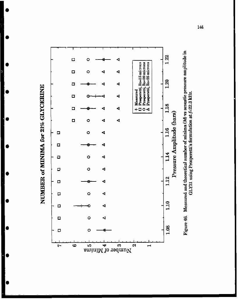
144

00

03 0 -U-

0 0 0

0

00 bA~

13 0 .4 4

C3 0D 4 '.i

0 0-.

*~1 0 *-

imtu 0 o ioqun

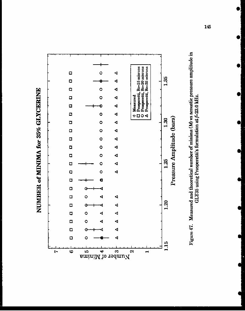
145

Q" N0 .4 AAA

0 043

00 .4ll11i00 .4 + 30- m

0 .4

C3 0 ý4

0 .4

0 2 0 .4

0 04

41

0l 0 . 4

a 0 a 4

o Lo 10 m4 l0 0-+--4 4;q-Ln.

146

o3 cl

00 .--4a ia 4a

E3 * .-- 4+ 041.

*M 0-- .4

0 0 .4

C3 0 .4 -0-M 0 .4

0 .40 0 4 4Cu

00 .400.

03 0 .4

03 0 .40 0 .4

13 0 400 .-.- 40 -- 4

03 0 403 0 4

0 00i 0 4

*3 0 a .403 0 l .4

03 0 a .4

L- tI 0 ILO 0 0 Ni

uuiutu1A joaaIqxuttX

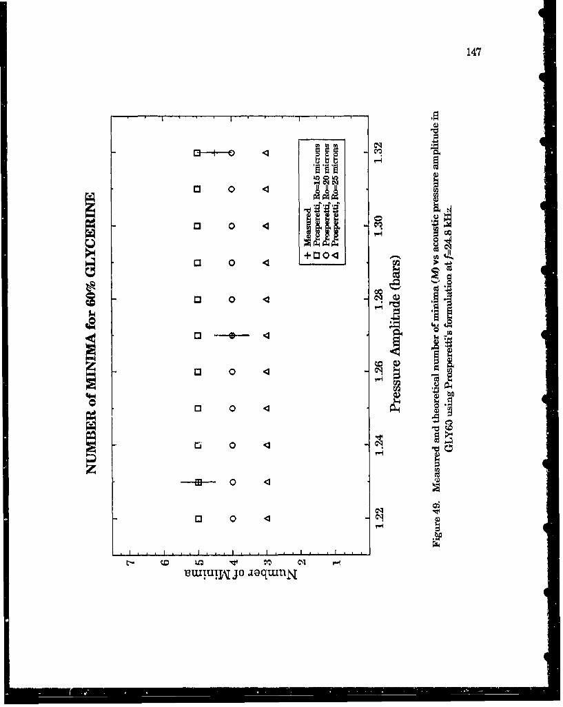
147

30 0 .4 ia 0 4

0 0 .4

D 0 .

U- 0-- .4

13 0 .4

0 0 .4

04I - V-W--- 0 <

0eiu 0 4q~ii

148

on the number of minima were larger since, as shown previously, larger bubbles

pulsate with fewer minima. For instance, Figs. 45 (water) and 46 (GLY21) predict

*• R.-20 gm at low values of PA and R,,-25 gm at the higher values OfPA. Figs. 47

(GLY35) and 48 (GLY42) predict R0,20 jLxn remaining constant for the range Of PA

considered. The results of Fig. 49 (GLY60) are very imprecise due to the few data

_ •points taken. It is not clear why the number of minima observed was fewer than

predicted by the theories, The explanation may be linked to another anomalous

observation in the rebounds of the radius-time curves. As can be seen in Fig. 33,

* the bubble rebounds appear to increase in time within each period instead of

decreasing in the normal decaying fashion, as shown in Fig. 34 where the

theoretical R-t curve has been plotted. The experimental R-t curves seem to

• indicate much larger amplitudes for the rebounds. Larger amplitudes would

indeed result in fewer rebounds because each rebound would require more time.

In this respect, the observed fewer number of minima is consistent with the large

- rebound amplitudes observed in the scattered-light data. However, no explanation

has been found for this increase in the amplitude of the bubble rebounds.

Additional evidence on the size of the bubbles can be obtained by considering

* the periodicity of the solutions, For example, notice that period-two solutions were

predicted by the theory quite often for the 20 jim bubble, except for the case of water,

For the 25 gm bubble few stable, period-1 solutions were obtained. However, all of

• the solutions for R0=15 gm were stable and with the same period as that of the

driving pressure. In this respect, the fact that only bubble pulsations with the

same period as that of the sound field were observed in the laboratory suggests that

-* the bubble radius was less than 20 gim.

S=

149

The conclusions drawn in the last three Sections have been summarized in

Table 4 below.

Table 4. Summary of predictions of Ro obtained from Prosperetti's

formulation.

Theoretical Range of R. for Single Bubble Pulsations

From Rm, From 0, From M...................m................ o ..............................................~mmmimlim~m•

water 10-15 pum 13-18 Ptm 20-25 pum (>)*........ ..e .. .. i ..... ... .. ........... m... ..... .... n....N...i .. ...... m

GLY21 15-20 gan (>) 15-20 pm (>) 20-25 p~m (>)

GLY35 15 ILM 20 pum 20 AM

GLY42 10-15 pm (>) 15-20 pim (>) 20 ptm

GLY60 18 pm 20 pm 15-20 pim* (>) indicates that the value of R0 increased u PA increased.

In summary, the data presented in the last three Sections may be interpreted

to indicate that the equilibrium radii of stabilized bubbles driven at pressure

amplitudes between 1.1 and 1.5 bars in different water/glycerine mixtures were

between 15 and 20 jim. It also is inferred from some of the data that the

equilibrium bubble radii increased as the driving pressure was increased. The

predicted values of R, based on the measurements of R,, and 0,, are consistent for

2 of the 5 data sets. Inconsi,.'a ncies were found in the predictions for water,

GLY35 and GLY42, indicating a disagreement between theory and experiment.

The discrepancy in the water data is within the experimental error, however. The

measured number of minima indicated that the equilibrium bubble radii were

larger - between 20 and 25 im - in apparent contradiction to the previous results.

150

A possible explanation for this disagreement was given in terms of the larger than

expected amplitude of the bubble rebounds evidenced by the scattered-light data.

* The moderate agreement found means that Prosperetti's theory, although fairly

applicable, is not a complete description of a cavitation bubble pulsating at these

amplitudes. The predictions of the theory should not, therefore, be considered

* quantitatively correct but only accurate to within a factor of 2 for the parameters

under consideration.

* lV. B. L e. Comparison with the Polytropic Theory and Flynn'e. Theory

The pulsation amplitude, collapse phase, and number of minima calculated

using the polytropic theory and Flynn's theory for water and GLY42 have been

plotted in Figs. 50-55. For comparison, the experimental and Prosperetti's results

have been plotted simultaneously.

Let us first consider the results from Flynn's model. For clarity, only values

of Ro=15 and 20 jim have been plotted using the solid symbols as indicated in the

legend. However, extrapolated values will be estimated for Flynn's and the

polytrop-'c model data when necessary. The pulsation amplitude data shown in

Fig. 50 (water) indicate that R, > 15 g.m, increasing as PA increases, Furthermore,

based on previous results, R, is most likely < 25 gm. The data shown in Fig. 51

(GLY42) indicate that R, < 15 gim, with Ro increasing to 15 gm as PA was

increased. The phase of collapse data shown in Fig. 52 (water), however, suggest

that 10 < Ro< 20 pnm with R, also increasing as PA increases. The data in Fig. 53

(GLY42) indicate that 15•5 R0• 20 pm increasing with PA. The number of minima

0 0 mr I *

0 0 m

0 * *D30

0 *O0U +DORE

0 bn

0 *@

o e m w

qs~0 09 w~

0 *3@ -

(SU.11-u ni-el -4--mj~

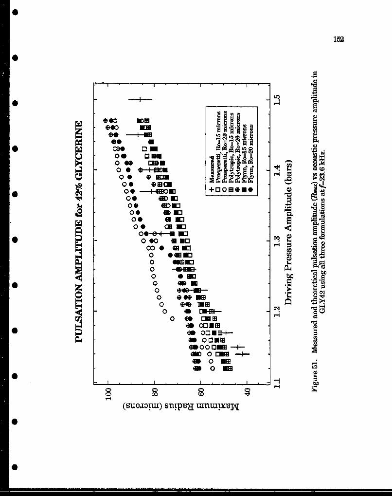
152

004

* 0 N0 CI4E

0. ---- +w

0 09* +oK3m.P4

00--+-a o10 *go n

* 0z0 0*--00 049Em0 *0~t-

0 Go MOM

00OS3 0 ME40OODEE --

m0

153

no p OEM

04

o toCUM

r-4 -2

00 0 p

o 0 ED cU cq~

-U.(sa~a)esulC~oasT.

154

0 i

I ' 1 ' * I ' "

-------- , •

60 C

O0 oe EEOu~ •,( i:: w emni 1 00 e

00 mmn i0 * •G K

e 0 mm

l 0 s "m s 0

00

0 0 0 .

0 so IN -4u

0 o0 $ 0KMo 00 CU

0 a**o00 @ ~EM

* 600 0f-lm-smo 0 a

s o -

0w0

04

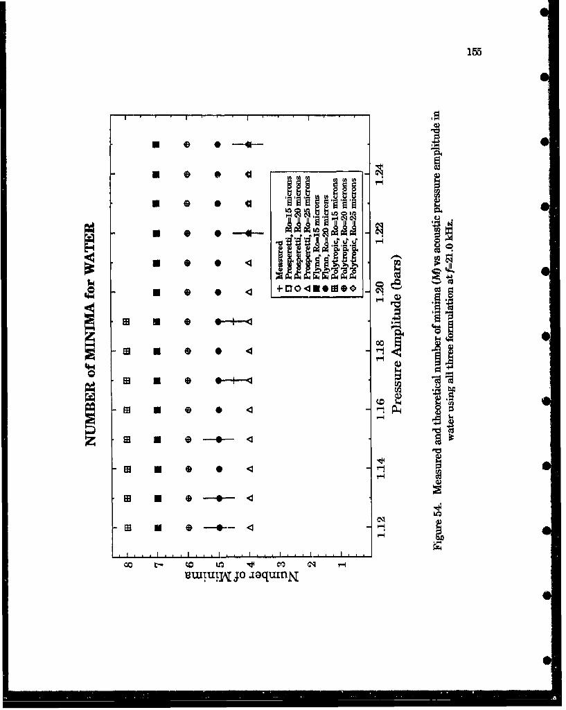
E * 0 . * -

*B 0 0 . i*B , 0 .4

Es U 0 *.--.4

0 0 0- CD LOm

uTuit U 0-0--n

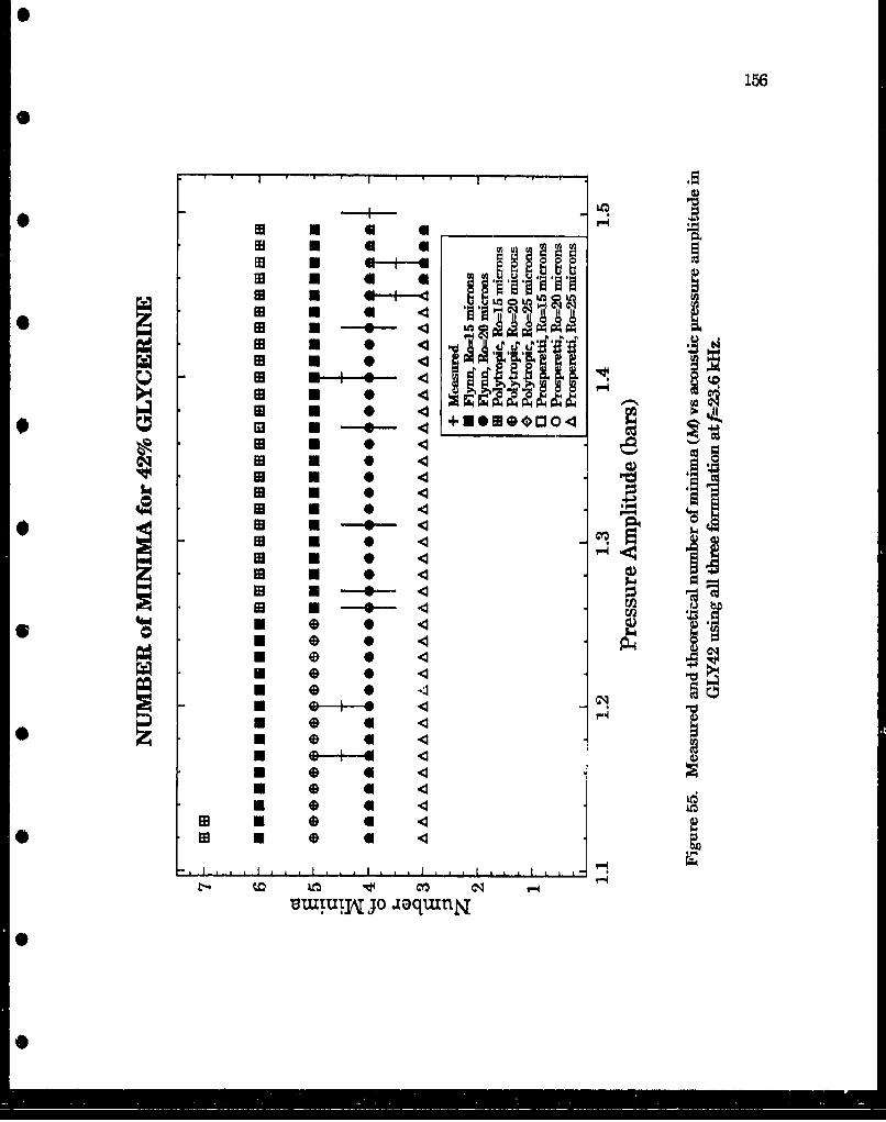
156

0

19 a _ _ _

m U 0 Am U 4I-t--

m aEs U -I-

*m 0m ho- -

Urn. 44

0

inui ijoaq0n

157

data shown in Fig. 54 (water) imply that 20 R ,! 25 pim increasing with PA and

those in Fig. 55 (GLY42) indicate that R, - 20 ptm also increasing slightly with PA.

Note that, in general, the conclusions agree fairly well with Prosperetti's in the

previous Section. The results of Flynn's data have been summarized in Table 5

below.

Table 5. Summary of predictions of R. obtained from Flynn's formulation,

Theoretical Range of R, for Single Bubble Pulsations

From R. From , From M

water 10-15 Am (>) 10-20 ptm (>) 20-25 pum (>)

GLY42 10-15 Ium (>) 15-20 gum (>) 20 pm (>)

* (>) ind7cate that the value of RA increased as PA increa--d,

Let us now consider the results from the polytropic model plotted in the same

Figures using the crossed symbols as indicated in the legend. The pulsation

amplitude data shown in Fig. 50 (v,,ater) indicate that 10 : Ro 5 20 ptm, increasing

as PA increases, The data shown in Fig. 51 (GLY42) indicate that R. 5 15 gm, with

R, increasing to 15 pgm or more as PA increases. The phase of collapse data shown

in Fig. 52 (water), however, suggest that 10 : R0 • 20 irm with R0 also increasing as

PA increases. The data in Fig. 53 (GLY42) indicate that 15 • R, 5 20 ptm increasing

with PA. The number of minima data shown in Fig. 54 (water) imply that 22 < Ro 5

25 pgm increasing with PA. Note that some of the data points are hidden behind the

solid symbols used to represent Flynn's results. For example, the number of

minima for R,=15 is equal to 7 for the higher values of PA and for R,=25 is equal to 5

158

for the lower values of PA. Confusion can be avoided if one knows that the number

of minima usually decreased by one unit (at the most) as PA increased. The data in

Fig. 55 (GLY42) indicate that R." 20 pgm also increases slightly with PA. In

general, these values of R. agree fairly well with those based on Prosperetti's

predictions shown in the previous sections, and even better with those based on

Flynn's predictions. The results of the polytropic model data have been

summarized in Table 6 below.

Table 6. Summary of predictions of R. obtained from the polytropic

formulation.

Theoretical Range of R, for Single Bubble Pulsatlons

water 15-20 ýLm (>)* 10-20 jim (>) 22-25 jim (>)

GLY42 10-15 pAm (>) 15-20 gm (>) 20 pm (>)

* (>) indicate, that the value o R0 increased aB PA increased,

From Tables 4, 5, and 6 it can be seen that the values of Re predicted by the

three formulations based on the same measured parameter (R,.,, , or M) are

very similar - between 15 and 25 microns. Also, self-consistency was found for

Prosperetti's theory in 2 out of 5 liquid mixtures (GLY21 and GLY60), whore the

values of Re based on the measurements of R..X were the same as those based on

the measurements of 0,, as shown in Table 4. This was not the case for water,

GLY35 and GLY42, however. Since theoretical data for Flynn's and the polytropic

theories were calculated for water and GLY42 only (due to time constraints), the

lack of consistency in those two theories is not surprising. However, by looking at

0-

159

the results of Prosperetti's theory and the fact that all theories gave similar

results, we can conclude that although disagreement was found in some cases,

disagreement is not expected to occur in every case. In summary, two conclusions

can be made: 1) The measurements do not constitute a good test to discriminate

between the theories, since the experimental error is larger than the difference

between the values predicted by the theories using the same conditions; 2) the

values of R0 predicted by each particular theory based on the experimental R,,

and 0, are not consistent, indicating that the models are not completely applicable

for the range of parameters considered here.

Sasedt on the theoretical results, some general comments will be made on the

characteristics of each model in the second half of this Section. As seen in Fig. 50

(water) and 51 (GLY42), Prosperetti's model predicted, in general, larger values of

the pulsation amplitude than the other two theories. As expected, the phase of

collapse is also larger, as seen in Figs, 52 (water) and 53 (GLY42). On the other

hand, the values predicted by the polytropic theory were the lowest of the three

theories. These results may be explained in terms of the thermodynamics in the

interior of the bubble.

For the case of the polytropic formulation, the small bubble sizes used in the

calculations resulted in a value of the polytropic exponent nearly equal to 1. This

means the mntion is essentially isothermal. Isothermal motion produces no rise

in the internal temperature, allowing the radius to reach much smaller values,

and generating very high internal pressures and densities. In addition,

isothermal motion usually resulted in lower pulsation amplitudes for the range of

parameters considered in this study. On the other hand, adiabatic collapses

S

160

produce hgher internal temperatures, lower pressures and larger pulsation

amplitudes than isothermal collapses. Thus, the lower pulsation amplitudes

-- predicted by the polytropic theory can be attributed to the isothermal motion of the

bubbles.

The theoretical values of the pulsation amplitude using Flynn's formulation

-* are also consistently lower than those predicted by Prosperetti's, although

somewhat larger than those predicted by the polytropic's, as can be seen in Figs.

50 and 51. These results are the opposite of those expected if the same argument

-* given above were applied. As seated in Chapter III, the rise in temperature at the

bubble wall predicted by Flynn's model would theoretically result in a decrease of

the heat flux away from the bubble ani, consequently, a more adiabatic motion.

* The theGretical results shown in Figs. 50 and 51, however, indicate just the

opposite. Thus, an alternative explanation had to be found. Besides the

expression for the internal pressure, the only other significant difference between

-* Flynn's and Prosperetti's formulation is the extra comoressibility term in the

radial equation (s,:e Chapter III). Calculations made using Prosperetti's

formulations with the extra term found in Flynn's radial equation resulted in

- slightly smaller pulsation amplitudes but much larger radial minima. The

larger radial minima are naturally expected to affect significantly tno internal

temperature and pressure during the bubble's collapse. It should be noted that

* only period-I solutions were predicted by Flynn's model, in contrast to

Prosperetti's which predicted period-2 and period-4 solutions.

In summary, Prosperetti's model was fbund to give the largest pulsation

amplitude and collapse phase, whereas the polytropic model was found to give the

161.

smallest. This was explained by the essentially isothermal behavior predicted byl

the polytropic formulation. In addition, the extra compressibility term found in

Flynn's model was found to affect the bubble motion especially during the collapse,

resulting in slightly smaller pulsation amplitude and collapse phase. The values

of R. predicted by Flynn's theory and polytropic theory are essentially the same as

those predicted by Prosperetti's.

MV. B. 2. Theoretical Values of Temperature, Pressure and Relative Density

The calculated maximum internal temperature (Tma.x) and pressure (P,,) $)

reached during the collapse predicted by Prosperetti's and Flynn's theories for the

set of parameters used during the experiment have been plotted in Figs. 56-59. In

Prosperetti's calculations, the temperatures have been averaged over the bubble's

interior in order to compare them with the temperatures predicted by Flynn's

theory. The internal pressure is assumed uniform in both cases,. Because of the

isothermal bubble motion of the polytropic formulation, the predicted pressures

were unreasonably high and the temperatures unreasonably low. We have,

therefore, not included them in this analysis.

The maximum internal temperatures, pressures and relative densities have

been summarized in Table 7, 8 and 9 below. The relative densities, which have

been normalized with respect to equilibrium conditions, were calculated from

p,.=(R,,R,.#,)3. Note that for water, 1.12 <PA < 1.25 whereas for GLY42, 1.12 <PA•

1.47 so that higher values are expected for GLY42.

UO U

DO 0

DoU

00

* 00 0

0 D3 U

00

DD 00 St*3 N i u

DOESX)D-jejdij 1uou

163

13 0 0 00 0 .0*

Mn 0 No03 0 U. 11

0 0 No0 0 No.

al a

0 0 a h

0 03

0 0 a

00 0 000 aO00 0 900 0 0

00 U3 000 U3 0 0

00 U 0 sO

0 M mO0 C3 0

o3 0 0c0 NCO13 n

C3M (2s

00 m

_ _ _ _ _ __X eajmd aSluau

164

MM 00

O30E 0

0E 0-

0 03 N 0Pe

E-4 we 0

00 D U1

ODE

N~(sie*onsoc -uou

165

00 003 0 m

CO3 0

C3 0 ES

03 0U00 0 ES0

0 0 0 *U3 0 0o A

Do0 **

00

(M 0

~~(M a 0om *

OKOR

E3UO

Smo

I~ a

IMt

(s-vI;.issc Iva .u

166

Table 7. Summary of maximum theoretical temperatures inside 20-25 pgmbubbles for the range of PA used during the experiments.

STIleoretical Range of T,. for Single Bubble Pulsations (Kelvin)

PA (bars) Prosperetti Flynn Prosperetti (Flynn)....-....-...........................................................................................................water (1.12-1.25) 2,500-7,000 2,500-5,000 2,500-6,000

m GLY42 (1,12-1,47) 3,000-10,000 2,500-7,000 3,000-8,000

--------------------------------------------------------------

Table 8. Summary of maximum theoretical pressures inside 20-25 Atm

* $bubbles for the range of pA used during the experiments.

Theoretical Range of P. for Single Bubble Pulsations (bars)

PA (bars) Prosperetti Flynn Prosperetti (Flynn)--------- --------------------------------------------------.......................

_ water (1.12-1.25) 1,000-12,000 2,000-7,000 2,000-8,000-----------------------------------------------------------------..........................................GLY42 (1.12-1.47) 2,000-40,000 2,000-22,000 f,C00-20,00O---------------------------------------------------------------

Table 9. Summary of maximum theoretical relative densities inside 20-25

Am bubbles for the range of PA used during the experiments.

Theoretical Range ofp= for Single Bubble Pulsations

- PA (bars) Prosperetti Flynn Prosperetti (Flynn)

water (1.12-1.25) 150-500 200-400 100-400

GLY42 (1.12-1.47) 200-1300 150-700 200-700- -----------------------------------------------------------

The third column of each Table contains the maximum internal temperatures

(Tma.x), pressures (Po,), and relative densities (p,.,,) predicted by Prosperetti's

0

167

theory, and those predicted by Flynn's theory are shown in the fourth column.

Note that, in every case, the temperatures and pressures predicted by Prosperetti's

theory are higher than those predicted by Flynn's for the same bubble size, even for

the cases where the pulsationi amplitude predicted by Prosperetti's was less, The

fifth column of each Table contains the same quantities calculated using

Prosperetti's formulation with Flynn's radial equation (instead of Keller's). These 0

values will be referred to as Prosperetti (Fiynn)'s. The difference in the

predictions shown in columns four and five is entirely due to the way in which the

internal pressure is obtained by each formulation, i.e., the thermodynamics in the

bubble's interior. Notice how the values of Tmax, Pmax and Pm,, predicted by

Prosperetti's theory are lower when Flynn's radial equation is used instead of

Keller's, suggesting that the additional compressibility term plays a significant

role during the collapse. The values of Tm and P,. predicted by Prosperetti

(Flynn), however, are still higher than those predicted by Flynn's theory by about

10-20%. The values of p,,,, are about the same in both cases. These results

indicate that Prosperetti's theory does not allow as much heat to diffuse out into

the liquid resulting in higher temperatures and pressures than Flynn's theory for

the range of parameters considered here,

As stated earlier in Chapter I, the phenomenon of sonoluminescence is

primarily of thermal origin, i. e., caused by high temperatures rather than high

pressures or densities. The determination of the minimum temperature required

for light emission is, therefore, important in understanding the mechanisms

involved. Since the acoustic pressure threshold for light emission was measured

in this study to be around 1.1 bars, this indicates that, according to the theories, 0

i i iI .. .. ....

S

168

the minimum temperature necessary to generate SL is between 2,000 and 3,000 K,

corresponding to relative densities about 100-200. In the second half of this

* Section, previously measured temperatures and relative densities in the interior of

cavitation bubbles during SL emission will be compared with the theoretical

values. These previous experiments have been described in Chapter I. Since in

this study sonoluminescence has been observed to be generated only by bubbles

between 15-25 gim, it will be assumed that, during all the previous experiments (at

insonation frequencies around 20 kHz), only bubbles in this size range were

responsible for the light emission. It should be pointed out that this observation

does not agree with others made in the past by various researchers which

indicate, based on the phase of the light flashes, that SL was also emitted by much

larger bubbles, e.g. 220 grm (Jarman et al., 1970). However, strong evidence has

been gathered in this study which indicates that only small bubbles collapsing

radially are capable of producing high enough temperatures to generate

sonoluminescence.

Relative densities of about 60 were measured by Taylor et al. (1970) and about

40 by Sehgal et al. (1979) (see Table 3 in Chapter I) during spectral studies of

sonoluminescence. These values are smaller than the minimum (100-200)

predicted by the theories at the measured threshold for light emission. Assuming

that SL was produced by bubbles in the size range measured in this study (15-25

km), tests performed using Prosperetti's theory indicate that a relative density of

60 would not generate temperatures higher than 2000 K, just enough to produce

light emission by most estimates (Saksena et al. 1970). TbP 10,000 K temperature

reported by Taylor et al. was obtained from spectral measurements assuming

169

blackbody radiation, which is now known to be an incorrect assumption. Even an

adiabatic collapse in which the density increased by a factor of 60 would only result

in temperatures less than 5,000 K and pressures less than 1000 bars. S

The relative density measured by Sehgal et al. (1979) of 40 is even lower, which

is also rather unexpected, since bubble dynamics theories that include thermal

dissipation predict higher densities at higher insonation frequencies. This is 0

because, at the higher frequencies, the motion of the active bubbles is more

isothermal (due to their smaller size), requiring a stronger collapse in order to

generate temperatures high enough to produce sonoluminescence. The S

temperature of 2450 K calculated by Sehgal et al. using Young's (1976) equation is,

therefore, much larger than that expected from Flynn's or Prosperetti's theory for

a relative density of 40 and the set of parameters used in Sehgal 's experiment. In S

short, a relative density of 40 is too low to generate the temperatures necessary for

light emission,

In a second experiment, Sehgal et al. (1980) reports measurements of the •

temperature of sonoluminescence emission of 1350 and 860 in NO- and NO 2 -

saturated water at 459 kHz. Again, these temperatures are low by most estimates

of the temperatures necessary for light production. Since these experiments 0

required measuring the spectra of SL, it can be assumed that relatively high

intensities (much above the threshold for light emission) were used during the

experiments to obtain as much light as possible in order to improve the precision •

and accuracy of the measurements. It is mainly for this reason that the relative

densities and temperatures obtained from these experiments are believed to be

rather low. It should be pointed out that some authors justify these results by 0

0

170

arguing that bubble breakup must occur early during the collapse, preventing the

bubble contents from being compressed as much as would be expected from the

theories. This, however, is not supported by the spark-induced cavitation

experiment performed by Golubnichii et al. (1979), or the observations made

during the present study. Golubnichii et al, measured collapse ratios Rm/Rmgn=30,

indicating that the cavity remained spherical during most of the collapse. Note

that, in this case, collapse ratios are measured relative to the maximum radius

R. and should not, therefore, be compared directly with those measured relative to

an equilibrium radius, as is customarily done in acoustic cavitaticn. Since the

cavities generated by electric sparks are mostly composed of vapor, an equilibrium

radius does not exist under normal conditions. Golubnichii et al. also ca•culated a

* temperature of 9,000 K and a pressure of 19,000 bars assuming an adiabatic

collapse and a perfect gas inside the cavity.

The most recent and precise measurement of temperatures inside cavitation

bubbles is that by Suslick et al. (1986b), using a comparative rate thermometry

technique in aqueous solutions at 20 kHz. They measured a temperature of 5200 ±

650 K at acoustic intensities of 24 W/cm2 , which corresponds to about 8 bars

• assuming plane waves, This temperature falls in the middle of the range of the

theoretical temperatures calculated in this study, corresponding to PA- 1 . 3 bars,

much lower than the estimated 8 bars used in Suslick's experiment. It is,

• however, more than sufficient to gener&te sonoluminescence based on the

evidence collected in this study.

As stated earlier, most experiments in which the temperature of collapsing

* cavities was measured probably required high intensity sound fields which

171

generated many cavities at once. In addition, transient cavitation was most likely

the prevalent type of cavitation, implying that light emitting cavities did not last for

more than a couple of acoustic periods. In the stable cavitation observed in this

study, it has been determined that an increase in the acoustic pressure amplitude

results in higher temperatures, as evidenced by the increase in the light emitted

from the bubble. In a cavitation field where many bubbleq are present, it is not

obvious whether an increase in light emission is due to an increase in the amount

of light emitted by each bubble, or an increase in the number of bubbles emitting

light. Since the light emitted by each bubble should be proportional to the

temperatures reached in its interior, it should be interesting to measure the

dependence of the internal temperature on the acoustic intensity in experiments

such as Suslick's. Furthermore, the internal temperatures measured in

Suslick's experiments, which were performed at much higher pressure

amplitudes, (- 8 bars as opposed to : 1.5 bars used in this study), indicate that

present theories of bubble pulsations overestimate the internal temperature and

possibly the internal pressure too. This overestimation may be explained by the

failure of the assumptions made in the models. Specifically, the possible

dissociation of the gas molecules due to the high temperatures attained would

increase the number density and, therefore, the internal (gas) pressure, arresting

the bubble collapse sooner. When temperatures of 5,000 K or higher are reached, it

is also very likely that the energy of the collapse begins to go into other chemical

processes, instead of increasing the temperature of the gas. Some of these

processes include dissociation of the gas molecules and ionization. Thus, as the

strength of the collapse increasos i.e., larger values of PA, the internal

172

temperature is expected to reach a maximum saturation value, In addition, The

models underestimate the effects of energy dissipation due to the compressibility of

the liquid. A highly compressible liquid results in the formation of shock waves

which may carry a significant portion of the collapse energy away from the bubble.

IV. B. 3. Phase of Sonoluminescence v8 Bubble Motion

In order demonstrate the simultaneity of SL and the minimum radius of an

acoustically driven bubble, simultaneous traces of the radius of the bubble and the

light emission have been obtained, Fig. 60 is a plot of the experimental results

clearly showing that SL is produced during the collapse of the bubble, These data

were obtained with the light scattering apparatus and the PMT. We were unable

to obtain an appropriate filter for the PMT which would allow the simultaneous

operation of both the laser and the PMT. Thus, an intermediate phase reference

had to be used in order to properly correlate the light scattered with the PMT

output. This common reference was the side pill transducer whose voltage output

was proportional to the acoustic pressure in the cell, In this way, a trace of the

light intensity scattered and the pill voltage output were obtained simultaneously,

transferred to the computer and stored on disk. Immediately after, traces of the

PMT output (with the laser light turned off) and the pill output were also stored orn

disk. A graphics program was then used to determine the correlation by plotting

the two traces simultaneously as shown in Fig. 60. Since the two sets of data were

taken within a few seconds of each other, it was ensured that all the experimental

conditions remained identical. The uncertainty in this experiment was estimated

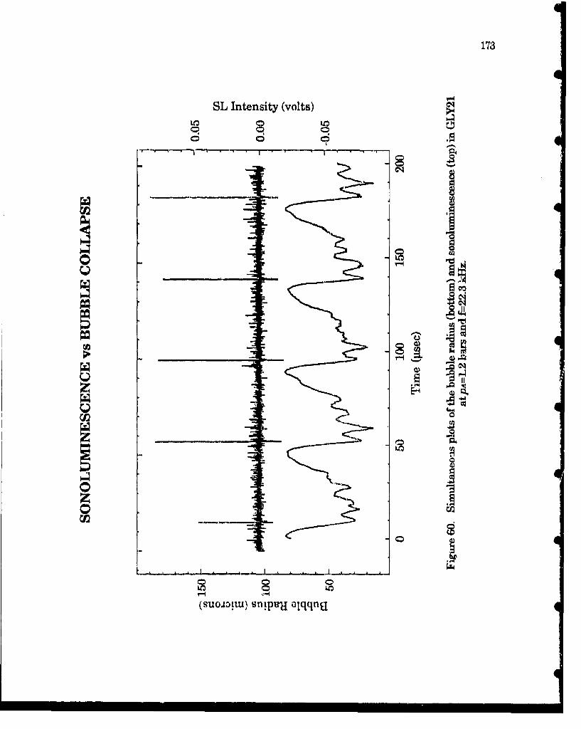
173

SL Intensity (volts)

iLO

I -!Q_________ _i

_ _.. .. _ , , __ .L - , ,41. .

C12

(.•um!• en~•'l~ alq, n

174

to be ± 5 degrees and it is mostly due to the time delay introduced by the

photodetector built-in electronics.

The objective of this experiment was to verify the coincidence of SL with the

minimum bubble volume. The results obtained were interpreted as an indication

that SL and the phase of the bubble collapse occurred simultaneously, In the next

Section, this result will be used to study the phase of the motion of cavitation

bubbles by measuring the phase of SL emission.

IV. C. Time to Amplitude Converter System- Sonoluminescence vs Sound Field

L Single Bubble Cavitation Field

After the simultaneity of the light emission and the collapse of the bubble was

• established, the phase of the SL emission was used to study the behavior and the

time evolution of cavitation bubbles as they interacted with the sound field and

with each other. This was done by measuring the phase of the light emitted by the

0 bubbles in order to obtain the phase of the bubble collapse. In view of the already

established coincidence of the light emission and the bubble collapse, these two

terms will be used interchangeably. In order to interpret the observations made in

0 multibubble cavitation fields, the results for a single bubble will be examined in

this Section. These data were obtained by enclosing the levitation cell system in

the light tight box and measuring the phase of SL emission as described in Section

-QE of Chapter II.

Figure 61 shows the phase of SL at approximately 1.1 bars in water, plotted as

a function of time in units of acoustic periods which also corresponded to the

0

0

175

40

00

zQa10p ~ o sXC

176

sampling period. In this data set, a total 2,000 data points were taken

corresponding to approximately 0.1 sec. The small oscillations on these data are

due to 60 Hz line noise which could not be easily filtered. Typical 60 Hz noise levels

were ± 1 degree which were far less than the actual fluctuations of the data. This

is an exampli: of the phase of the light emission for a single bubble pulsating

radially. In order to determine if a single bubble were present, the output of the

side pill transducer was monitored. This output would become noticeably

irregular and noisy when streamers were present. For a single bubble, however,

the signal was symmetrical except for a small notch, probably due to the shock

wave produced by the bubble collapse. In this case (Fig. 61), the value of the phase

was 201 degrees. A range of values was measured between 190 and 220 degrees for

* pressure amplitudes between 1.0 and 1.4 bars in water.

Occasionally, the levitated bubble was visually observed to become unstable for

a fraction of a second, after which stability was restored. This transition was

* usually accompanied by a vertical shift in the bubble's position. This new position

was always higher i.e., away from the antinode. When the light emission during

this transition was monitored, it was visually observed that the intensity of each

flash was sharply decreased. This occurred simultaneously with a decrease in

the phase of the emission. These observations are illustrated in Fig. 62. The

phase can be clearly seen to decrease sharply during the transition at 600 cycles.

* 'This decrease of the phase may be interpreted as a decrease of the equilibrium

bubble radius i.e., a breakup of the bubble due to surface instabilities. This type of

breakup usually occurs via the ejection of microbubbles (Nyborg and Hughes, 1967;

* Neppiras et al., 1969). After reducing its size, the bubble regains its stability due to

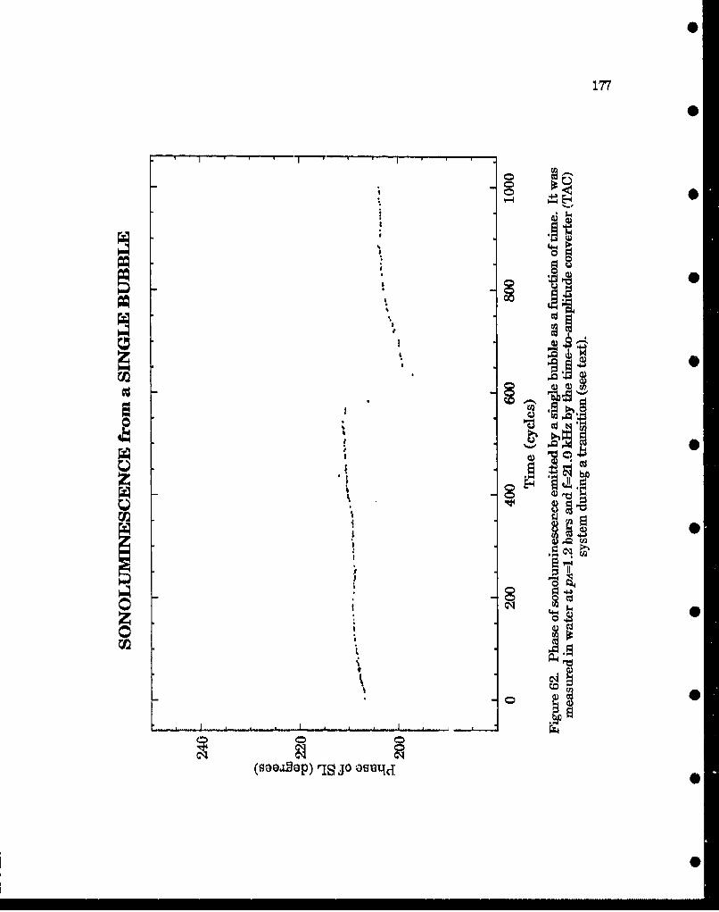
177

00

0u b19

'Il

QS

(sao~oprIS jo osletcl

178

the larger surface pressure (2cr/R,), This occasional, and sometimes periodic,

breakup can be understood in terms of the bubble response curve as a function of

equilibrium radius (Fig, 23). As the bubble grows, resonances are encountered

and the bubble response increases rapidly. If the surface instability threshold

happens to be below one of these peaks, breakup will occur and the bubble size is

quickly reduced. This cycle may repeat depending on PA and the new value of Re,

among other parameters. In addition, by plotting the pulsation amplitude, Rm.,

and the phase of the collapse as a function of Re, a direct correlation between these

two quantities can be established, as shown in Fig. 23 and Fig. 24. Note that when

Rmo. increases (decreases) the phase also increases (decreases). Note that a

change in the radius R, as small as 1 micron can result in the phase of collapse

changing by as much as 20 degrees, depending on the bubble size. Thus, it does

not require a large change in radius to effect a large change in the phase.

It appears that, before the bubble regains stability, its response amplitude and

size must be decreased. This is not surprising, since instabilities in the gas-liquid

interface are triggered by large accelerations, as shown in Chapter III. Thus,

this observation can be explained as follows: After developing instabilities, the

bubble sheds microbubbles, reducing its size and its response amplitude. Both of

these increase the stability of the bubble and the pulsations become spherically

symmetric again. This behavior is commonly seen in single bubbles at the higher

• pressure amplitudes (-1.3-1.4 bars).

In some cases, instabilities occurred repeatedly with a period of a few seconds.

At the higher end of the pressure range for stability, transitions often occurredO

179

consecutively as shown in Fig. 63. In this case, it may be postulated that the

pressure amplitude was so high that surface waves were easily excited, and the

bubble was unable to regain its stability. If the residual bubbles were large enough

or close enough to the initiating bubble, coalescence may occur before they can

dissolve. This may explain the bubble growth implied by the rapid increase in the

phase of collapse shown in Fig. 63. Sometimes the bubble disappears

unexpectedly, as was the case in this particular data set in which the bubble

suddenly stops emitting light around cycle 1250. This bubble disappearance can

also be observed with the unaided eye or through the microscope. A similar type of

bubble annihilation was reported by Nyborg and Hughes (1967) during observation

of cavitation on the surface of a vibrating bar driven at 20 kHz. Using high speed

photography, they reported bubbles which disappeared in less than 6 acoustic

periods. An explanation similar to the above was given by Nyborg et al. (1967) for

this phenomenon.

In summary, we can propose that bubbles grow and breakup in a periodic

fashion during radial pulsations. A breakup is usually reflected by a decrease in

the bubble response and the phase of the collapse. Bubble growth can occur by

coalescence or rectified diffusion and can be detected by an increase of the

response and the phase of the bubble collapse.

IV. C. 2. Multibubble Cavitation Fields

In this Section, the observations made from a cavitation zone composed of

streamers such as those illustrated in Figure 31 will be discussed. High speed

180

SS

Sso~p U2 oaslc

181

photographs taken during the experiments revealed that these streamers

consisted of fast-moving bubbles which were rapidly coalescing and breaking up.

An example of the measurement of the phase of collapse in water at around 1.3

bars is shown in Fig. 64. In this data set, the phase of collapse appears to change

irregularly between 185 and 215 degrees. Most of the measurements made of the

collapse phase in multibubble cavitation fields were in this range. This range

coincided with the collapse phase measured for single bubbles which were

determined to be between 15 and 20 gim in radius. It thus appears that in a

cavitation field at 20 kHz, bubbles that emit SL are in the range 15:5 R, :< 20 pum. SL

is produced by high temperatures and pressures in the interior of the bubbles, and

these high temperatures and pressures are responsible for most cavitation-related

effects. It may then be said that bubbles in the range 15 < R0 - 20 ptm are the only

active bubbles in cavitation fields at 20 kHz. This range of bubble sizes may be even

smaller since some of the scatter in the measured values of the phase may be due

to fluctuations of the driving pressure. Furthermore, the fact that the range of

values for the phase of collapse of single bubbles and cavitation field bubbles

coincide may be an indication that only bubbles pulsating radially emit SL.

Evidence for this hypothesis is also found in the fact that when a single bubble goes

into surface oscillations, the SL output decreases by an order of magnitude. It was

not uncommon to observe a single bubble pulsating radially and emitting SL

flashes every cycle for as many as 1000 consecutive cycles. However, when surface

waves were excited, as evidenced by dancing motion, the average number of SL

flashes was about one in ten cycles. This seems to imply that a spherical collapse

_ __- : •, ,• : . . ... .

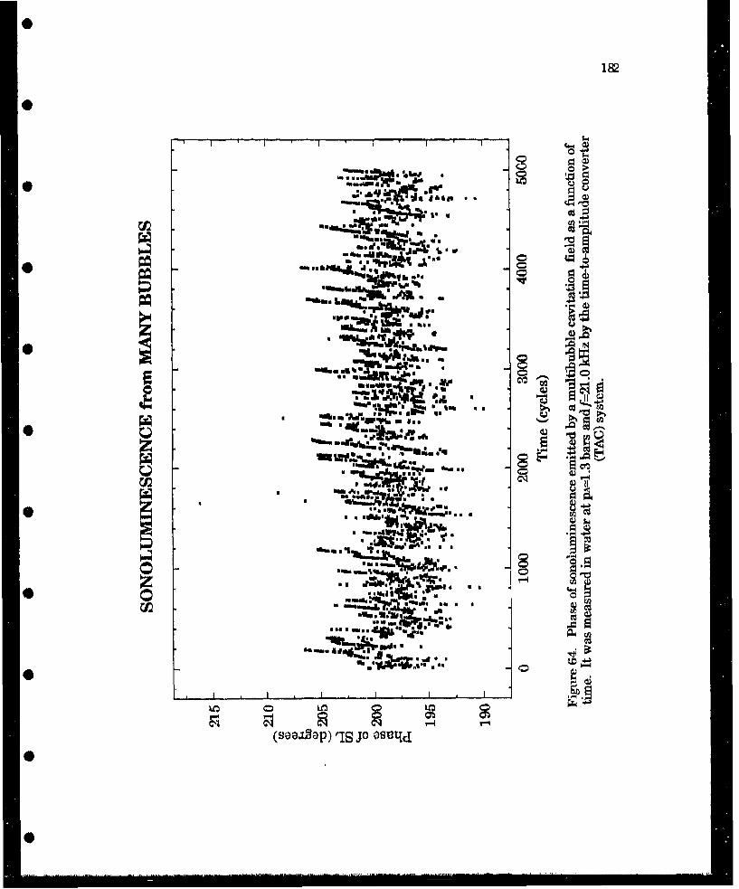
182

00

00 *jqm

00 olow", . ai*

"WN. w

*am

a n *.:V 0

::a

FIRI

a al It An.I3

0 LO

(S~OJ2Jop) 'IS~ JO OsutICI

183

is necessary to generate sufficiently high temperatures and pressures in the

interior of the bubble.

In addition, the data displayod in Fig. 65 reveal the same type of cyclic

behavior observed in a single bubble as described in the previous Section, This

behavior was observed often in a multibubble cavitation field, although it was not

always repeatable. It was usually observed at the higher pressure amplitudes

(1.3-1.5 bars). Nevertheless, these data show that the same cyclic behavior

observed in a single bubble also occurs in a multibubble cavitation field. Similarly,

this behavior can be attributed to the breakup of bubbles by surface instabilities

followed by coalescence or rectified diffasion.

In summary, we have observed cyclic behavior in both single and multibubble

cavitation fields. This behavior has been observed before by other investigators and

can be caused by resonances of the bubble motion encountered as the bubble grows.

These resonances trigger surface instabilities which in turn result in a reduction

of the bubble size due to breakup. As the bubbles regrow by rectified diffusion or

coalescence, the process repeats itself. In addition, the coincidence of the phase of

collapse for both single and multibubble cavitation suggests that spherical

collapses are required to generate the high temperatures and pressures

responsible for most cavitation-related effects.

0

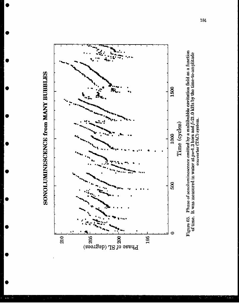
184

0 a

At ua %* % ,Do

a .6. WA%~

A vg ...

a ac 4a - I

Csa~p rb.. joee.

Chapter V

Summary, Conclusions and Topics for Future Study

V. A. Summary of the Dissertation

The purpose of this dissertation was to increase the understanding of the

dynamics of bubbles in cavitation fields. In trying to reach this goal, the following

accomplishments have been made:

1. Experimental radius-time curves for single bubbles pulsating radially at

large amplitudes have been obtained, These bubbles were obtained in

water/glycerine mixtures at pressure amplitudes between 1.1 and 1.5 bars at 20

kHz. These bubbles were observed to exhibit sonoluminescence. The pulsation

amplitude, the phase of the collapse and the number of minima have been

measured for a range of pressure amplitudes and bubble sizes.

2. After verifying the simultaneity of the light emission and the bubble

collapse, the phase of the light emission was observed for thousands of acoustic

periods in order to monitor the long-term behavior of bubbles in the cavitation field.

3. The applicability of three theoretical formulations of bubble dynamics has

been evaluated in a range of acoustic pressure amplitudes near the threshold for

sonoluminescence, These theories have been used to evaluate the internal

temperatures and pressures reached during the bubble collapse at the

experimentally determined threshold for light emission.

1

'13

0 •-- . . • - - .

186

V. B. Cowclusions

The following conclusions were made from the experimental evidence and the

numerical calculations3:

1. Sonoluminescence from stable cavitation at 20 kHz is emitted by bubbles in

the size range 15.20 microns. These bubble are small enough so that, although

pulsating at large amplitudes, they retain the spherical symmetry necessary to

attain the high temperatures required for light emission. Discrepancies were

found between the experimental and theoretical values of the pulsation amplitude,

phase of collapse and the number of rebounds, however. The number of rebounds

was observed to be lower and the amplitude of each rebound larger in amplitude

than expected from the theories. It was concluded that the physical conditions

attained during the collapse were outside the limits of the theories.

2. From the observations of the phase of light emission, it was concluded that

violently pulsating bubbles often undergo fragmentation and coalescence in a

periodic fashion. This process has a period on the order of 500 acoustic periods,

and varies depending on tho acoustic pressure amplitude and other parameters.

3. From the theoretical calculations made for the parameters measured at the

threshold for light emission, it was concluded that internal temperatures in the

range 2,000-3,000K were necessary to produce sonoluminescence. This finding

supports the Chemiluminescent model as the mechanism for light production.

Previous measurements of internal temperatures at PA -8 bars indicate that

present models of bubble pulsations overestimate the internal temperature and

pressure. Internal temperatures are expected to reach an asymptote as more of

187

the collapse energy is deposited into other chemical processes such as dissociation

and ionization.

_* 4. A previously undiscovered stable region exists in the pressure-radius

parameter space above both surface instability and rectified diffusion thresholds

for radially pulsating bubbles. The mechanisms through which this stability is

* attained are not yet understood. Nevertheless, the observations made of bubble

stability indicate the existence of a transient cavitation threshold, which had been

observed and predicted previously in other systems. Above this threshold, rapid

_ bubble collapse promotes surface instabilities which cause the bubble to

disintegrate.

*• V. C. Topics for Future Study

The following are some of the improvements that can be made to the

experiments performed in this study as well as suggestions for further0

investigations.

1. The equilibrium radius of single pulsating bubbles must be determined

accurately in order to confirm the applicability of the modols. Thus, a technique

must be developed to measure bubble radii in the range 15-25 microns. This

technique must be precise (to within 5-10%) and take not. more than a couple of

seconds in order to minimize the amount of diffusion in or out of the bubble.

2. Several techniques exist, including the measurement of SL spectra, that

can be used to measure the internal temperatures and pressures during the

collapse of the bubble. One of the difficulties encountered in performing these

=0

0m

188

measurements previously, is the inhomogeneity of the cavitation field which

contains an undetermined range of bubble sizes. The use of a single pulsating

bubble to generate sonoluminescence should improve the precision of these

measurements.

3. The low signal-to-noise ratio obtained with the laser scattering technique

for small bubble radii presented a major obstacle to the study of the bubble motion

during the final stages of collapse. Techniques using high speed photography and

holography offering high spatial and temporal resolution may provide important

data on the radial stability of pulsating bubbles.

4. The mechanism or mechanisms through which the radial stability of the

bubble is achieved certainly deserve further study. This mechanism may prove to

be important in understanding the motion of bubbles in moderate to high intensity

cavitation fields.

References

A. A. Atchley. "The nucleation of cavitation in aqueous media". Dissertation, U. of

Mississippi (1984).

V. G, Benkovskii, P. I. Golubnichii and S. I. Maslennikov. Soy. Phys. Acoust, 20,

14(1974).

F. G. Blake. "The onset of cavitation in liquids". Tech. Memo. No. 12, Harvard

Acoustics Research Laboratory, (1949).

A. A. Buzukov and V. S, Teslenko. Soviet Phys. J.E.T,P, Lett. 14, 189

L. A. Chambers. Phys. Rev. 49, 881 (1936).

C. C. Church. "Prediction of rectified diffusion during nonlinear bubble pulsations

at biomedical frequencies". J. Acous. Soc. Am. 83, 2210-2217 (1988).

C. C. Church. Private communication (1990a); Private communication (1990b);

Private communic.tion (1990c).

K. W. Commander. "A theoretical investigation of acoustic cavitation".

Dissertation, U. of Mississippi (1985).

L. A. Crum. "The acoustic radiation pressure on a liquid droplet in a stationary

sound field". Tech. Report, U.S. Naval Academy (1970).

189

190

L. A. Crum. "Bjerknes forces on bubbles in a stationary sound field". J. Acous.

Soc. Am. 57,1363 (1975).

L. A. Crum and A. Prosperetti. "Erratum and comments on 'Nonlinear

oscillations of gas bubbles in liquids: An interpretation of some experimental

results' [J. Acous. Soc. Am. 73, 121 (1983)]". J. Acous. Soc. Am. 75, 1910 (1984).

M. Degrois and P. Baldo. Ultrasonics 12,25 (1974).

A. Eller and G. H. Flynn. "Rectified diffusion during nonlinear pulsations of

cavitation bubbles", J. Acous. Soc, Am. 37, 493 (1965).

A. I. Eller and L. A. Crum. "Instability of the motion of a pulsating bubble in a

sound field", J. Acous. Soc. Am. 47, 762 (1970).

R. D. Finch, "Sonoluminescence". Ultrasonics, 1, 87 (1963).

H. G, Flynn. "Physical Acoustics". W. P. Mason ed. vol. 1, part B (Academic

Press, New York, 1964).

H. G. Flynn. "Cavitation dynamics. I A Mathematical formulation". J. Acous.

Soc. Am. 57, 1379 (1975a).

H. G. Flynn. "Cavitation dynamics. II, Free pulsations and models for cavitation

bubbles". J, Acous. Soc. Am. 58, 1160 (1975b).

J. Frenkel. Acta Phys.-chim. U.R.S.S. 12, 317 (1940) (in Russian): as referenced by

Verral et al. (1988).

191

H. Frenzel and H. Schultes. Z. Phys. Chem. 27B, 421 (1935): as referenced by

Verral et al. (1988).

F. R. Gilmore. "The collapse and growth of a spherical bubble in a viscous

compressible liquid". Caltech Hydrodynamics Laboratory report No. 26-4 (1952),

G. Gimenez. "The simultaneous study of light emission and shock waves

produced by cavitation bubbles". J, Acoust, Soc. of Am, 71, 839-846 (1982).

P. I. Golubnichii, V. D. Goncharov and Kh. V. Protopopov, "Sonoluminescence in

liquids: Influence of dissolved gases, departures from thermodynamic theory".

Soy. Phys. Acoust. 15, 464 (1970).

P. I. Golubnichii, V. M. Gromenko and A. D. Filonenko Soviet Phys. tech. Phys.

Lett. 5, 233 (1979).

R. K. Gould. "Simple method for calibrating small omnidirectional hydrophone".

J. Acous. Soc. Am, 43,1185 (1968).

R. K. Gould. "Rectified diffusion is the presence of, and absence of, acoustic

streaming". J. Acous. Soc. Am, 56, 1740 (1975).

V. Griffing. J. Chem. Phys. 18, 997 (1950).

V. Griffing, J. Chem. Phys. 20, 939 (1952).

P. Gunther, E. Heim, A. Schmitt and W. Zeil, Z. Naturf. 12A, 521 (1957a).

0•

192

P. Gunther, W. Zeil, U. Grisar and E. Heim, Zeit. fur Elektrokem, 61,188 (1957b):

as referenced by Walton et al. (1984).0

G. M. Hansen. " Mie scattering as a technique for the sizing of air bubbles".


E, N. Harvey. J. Am. Chem, Soc. 61, 2392 (1939).

R. Hickling. "Effects of thermal conduction in sonoluminescence". J. Acous, Soc,

Am. 35, 967 (1963).

R. G. Holt. "Experimental observations of the nonlinear response of single bubbles

to an applied acoustic field", Dissertation, U. of Mississippi (1988).

S. D. Horsburgh. "Radial instabilities of a pulsating air bubble in water",


D, Y. Hsieh. "Theory of rectified diffusion of mass into gas bubbles". J, Acous. Soc,

Am. 33, 206-215 (1960).

D. Y. Hsieh. "On the thresholds for surface waves and subharmonics of an S

oscillating bubble". J. Acous. Soc. Am. 56, 392 (1974).

IMSL. Mathematical software library. (IMSL, Houston, 1987).

P. Jarman. Proc. Phys. Soc. B 72, 628 (1959).

""II

193

0

P. Jarman. "Sonoluminescence: A discussion". J. Acoust. Soc. of Am. 32, 1459

(1960).

P. Jarman and K. J. Taylor. "The timing of the main and secondary flashes of

sonoluminescence from acoustically cavitated water". Acustica 23, 243 (1970).

* V. Kamath and A. Prosperetti, "Numerical integration methods in gas-bubble

dynamics". J. Acous. Soc. Am. 85,1538 (1989),

J. B. Keller and M. Miksis. "Bubble oscillations of large amplitude". J. Acous. Soc.

Am, 68, 628 (1980).

M. Kerker. The .scattering of light and other electromagnetic radiation. Chapters

0 3-5, (Academic Press., New York, 1969),

JI G. Kirkwood and H. A. Bethe. "The pressure wave produced by an underwater

explosion". OSRD Report No, 558 (1942).

H. Kuttruff. Acustica 12, 230 (Akustische Beihefte) (1962): as referenced by Walton

et al. (1984).0

G. J. Lastman and R. A. Wentzell. "Comparison of five models of spherical bubble

response in an inviscid compressible liquid", J, Acous. Soc. Am, 69, 638-642 (1980),

W. Lauterborn. "Numerical investigation of nonlinear oscillations of gas bubbles

in liquids". J. Acous. Soc. Am,, 59, 283-293 (1976).

S

194

W. Lauterborn and W. Hentshel. "Cavitation bubble dynamics studied by high

speed photography and holog~raphy: part two'. Ultrasonics 26, 59 (1986).

W. Lauterborn. "Cavitation dynamics - new tools for an intricate problem".

Applied Scientific Research 38,165-178 (1982),

V. L. Levshin and S. N. RzLe".i~ti .. Dokiady Akad. Nauk SSR, 16, 407 (1937): as

referenced by Verral et al. (1988).

R. Q. Maclesy and L. V. Hoiroyd. "Space-time anialysis of the sonoluminescence

emitted by cavitated water". J. Appl. Phys. 32, 449-453 (1961).

M. A. Margulis, "Investigation of electrical phenomena connected with cavitation.

IL. On the theory of appearances of sonoluminescence and sonochemical

reactions". Russ, J, Phys. Chem, 58,1450 (1984).

N. Marinesco. J. J. Trillat, C. R. Acad. Sci. 196, 858 (1933): as referenced by Walton 0

ea czl. (1984).

E. Meyer and H. Kuttrufft Z. angew. Phys. 11,325 (1959): as referenced by Walton et

al. (1984).

K. Negishi. Acustica 10, 124 (1960): as referenced by Walton et al. (1984).

K. Negishi. J. Phys. Soc. Japan 16, 1.450 (1961): as referenced by Walton et al,

(1984).

195

E. Neppiras and E, E. Fill, "A cyclic cavitation process", J. Acous. Soc. Am. 46,

1264(1969).

E. Neppiras. "Acoustic cavitation: review". Phys. Lett. Rev. 61,159 (1980).

B. E. Noltingk and E, A, Neppiras. "Cavitation produced by ultrasonics". Proc,

phys. Soc. B 63, 674 (1950),

W. Nyborg and D, E. Hughes, "Bubble annihilation in cavitation streamers", J,

Acous, Soc. Am. 42, 891 (1967).

M. S. Plesset. "On the stability of fluid flows with spherical symmetry", J. Applied

Physics 25, 96 (1954).

M. S. Plesset, "The dynamics of cavitation bubbles", J. Applied Mech. 16, 277

(1949).

H. Poritsky. Proc. 1 st U.S. National Congress in Applied Mechanics (AS,M,E.) 813

(1952).

A. Prosperetti. "Nonlinear oscillations of gas bubbles in liquids: steady-state

solutions". J. Acous. Soc. Am. 56,878 (1974),

A. Prosperetti, L. A. Crum and K. W. Commander. "Nonlincar bubble dynamics".

J. Acous. Soc. Am. 83, 502 (1986).

A. Prosperetti. "Acoustic cavitation series part two - Bubble phenomena in sound

fields: part one". Ultrasonics 22,69 (1984).

S

196

A, Prosperetti and G, Seminara. "Linear stability of a growing or collapsing

bubble in a slightly viscous liquid". Physics of Fluids 21, 1465 (1978).

A. Prosperetti. Private communications (1990)

Lord Rayleigh. "On the pressure developed in a liquid during the collapse of a

spherical cavity". Phil. Mag. 34, 94 (1917).

T. K. Saksena and W. L. Nyborg. "Sonoluminescence from stable cavitation". J.

Chem. Phys, 53, 1722 (1970),

L. D. Rozenberg. High Intgnsity Ulrationir fielda, (Plenum Press, New York,

1971).

C. Sehgal, R. P. Steer, R. G. Sutherland, and R, E. Verral. "Sonoluminescence of

argon saturated alkali metal salt solutions as a probe of acoustic cavitation". J,

Chem. Phys. 70, 2242-2248 (1979).

C. Sehgal, R. P. Steer, R. G. Sutherland, and R. E. Verral, "Sonoluminescence of

NO- and N0 2-saturated water as a probe of acoustic cavitation", J. Phys, Chem, 84,

396-401 (1980).

C. MX Sehgal and R. E. Verral. "A review of the electrical hypothesis of

sonoluminescence". Ultrasonics 20, 37-39 (1982).

K. S. Suslick and D. A. Hammerton. "The site of sonochemical reactions", IEEE

Trans. Ultrason. Ferroelectr. Freq. Control UFFG.33, 143..147 (1986a).

197

0

K. S. Suslick, D. A. Hammerton and R. E. Cline. "The sonochemical hot spot".

Am. Chem. Soc. 108, 5641,5642 (1986b).0

K. S. Suslick. "Sonochemistry". Science 247,1439 (1990).

K. J. Taylor and P. D. Jarman. "The spectra of sonoluminescence". Aust. J. Phys.

23, 319 (1970).

R. E. Verral and C. Sehgal. "Sonoluminescence". Sonehemistr~y: Its cheical.

* physical and binlo•ical effects. K. S. Suslick ed. (VCH Publishers, New York 1988).

W. U. Wagner. Zeit. fur angew. Phys. 10, 445 (1958): as referenced by Finch (1983),

* A. J. Walton and G. T. Reynolds, "Sonoluminescence". Advances in Physics 33,

595(1984)

W. A. Weyl and E. C. Marboe. Research 2, 19 (1949): as referenced by Verral et al,0(1988),

G. W. Willard, "Ultrasonically induced cavitation in water: a step-by-step

* process". J. Acous. Soc. Am., 25, 669 (1953)

W. J. Wiscombe. "Improved Mie scattering algorithms". Applied Optics, 19,1505

(1980).

F. R. Young, "Sonoluminescence from water containing dissolved gases". J.

Acous. Soc. Am, 60,100 (1976)

0e

0"

,

Appendix A

ADDITIONAL FIGURES 0

0

0_

0

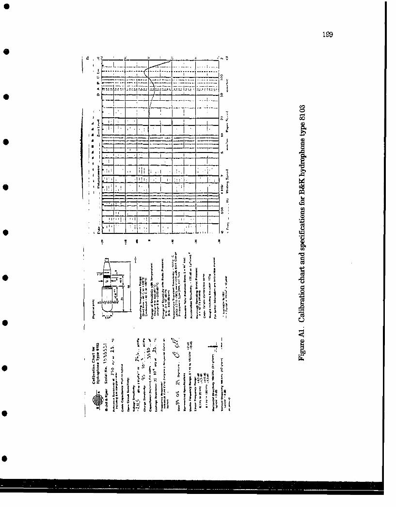
S+ :.-•.-_-.-.-t-. ..-- ..--,-.-... L t ] t. ." _

J , , L,, -

,I .. 1. z-• ,:• - . .i---'

.I ,.' I . + + + :

* o,II * . I IoI.I . - -,

*. .. t+ + I '" -;'°+'+.I+•'•'':+ '+ ++•i

I +""+ "1 t +•, ',,' o++' •'+J],

I+ r *.,..

+ " i -

+.,. t +, . -. + + + + +

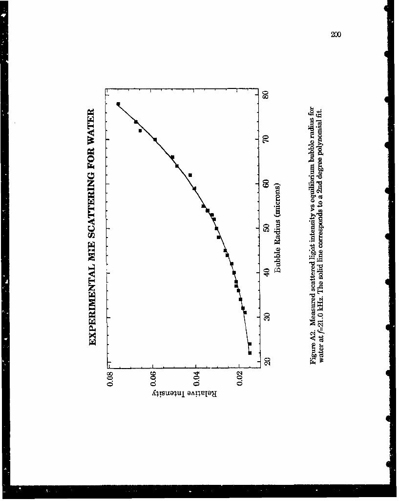
200

0

0 0.

LM 4

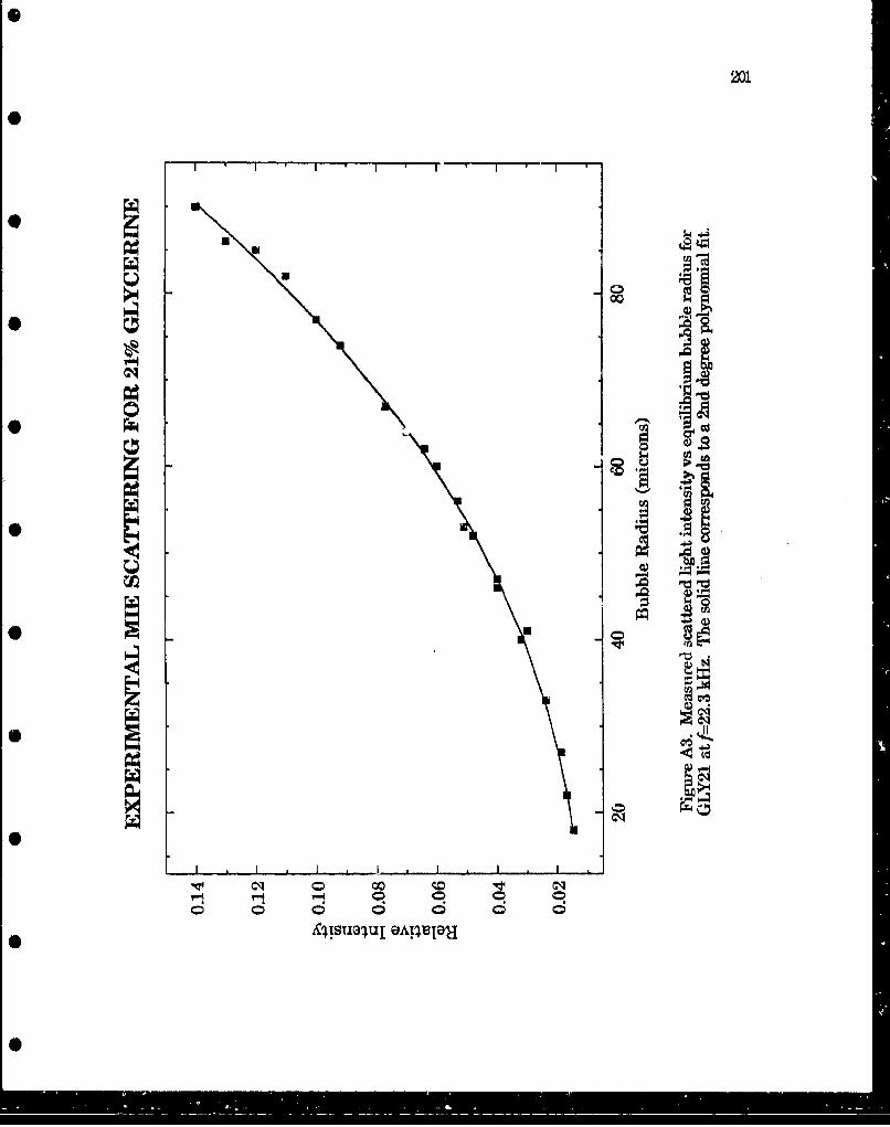
0

201

0

I * I I * I I I * I

**

U

*

.14*

�

i .jt0 �

Q � ii* *

*

0

c�I

0I * I I * L..............�............i............A I I

C'�I 0'-1 0 9 9 90 0 0 0 0 0 0

&�iStZG�UI e��p�j

0

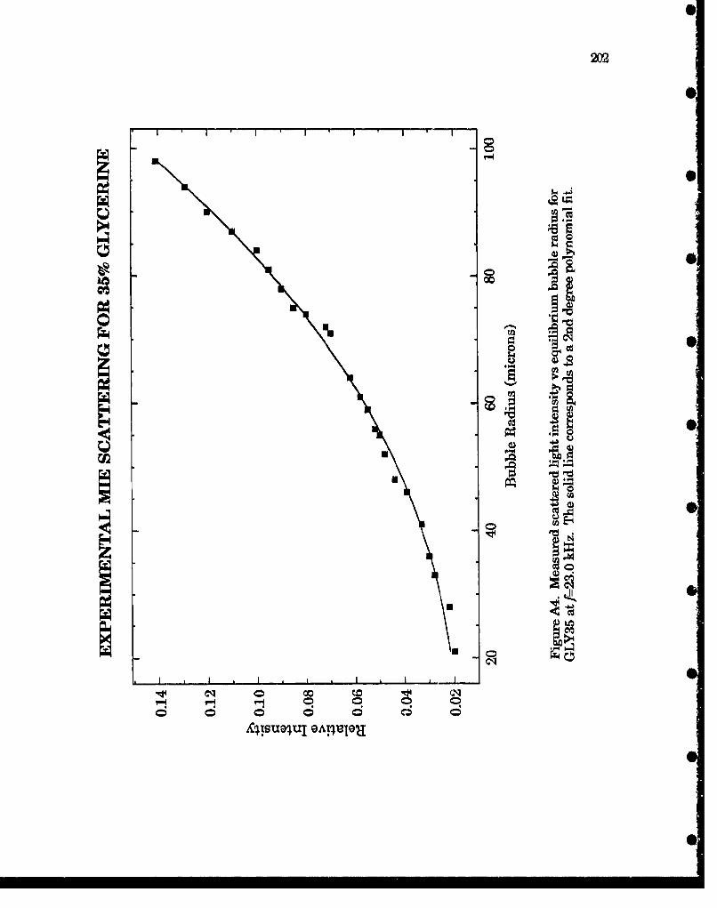
00

cq 0

S41suluI QIJUJ0

2a3

00

*g

Q4S~U A189

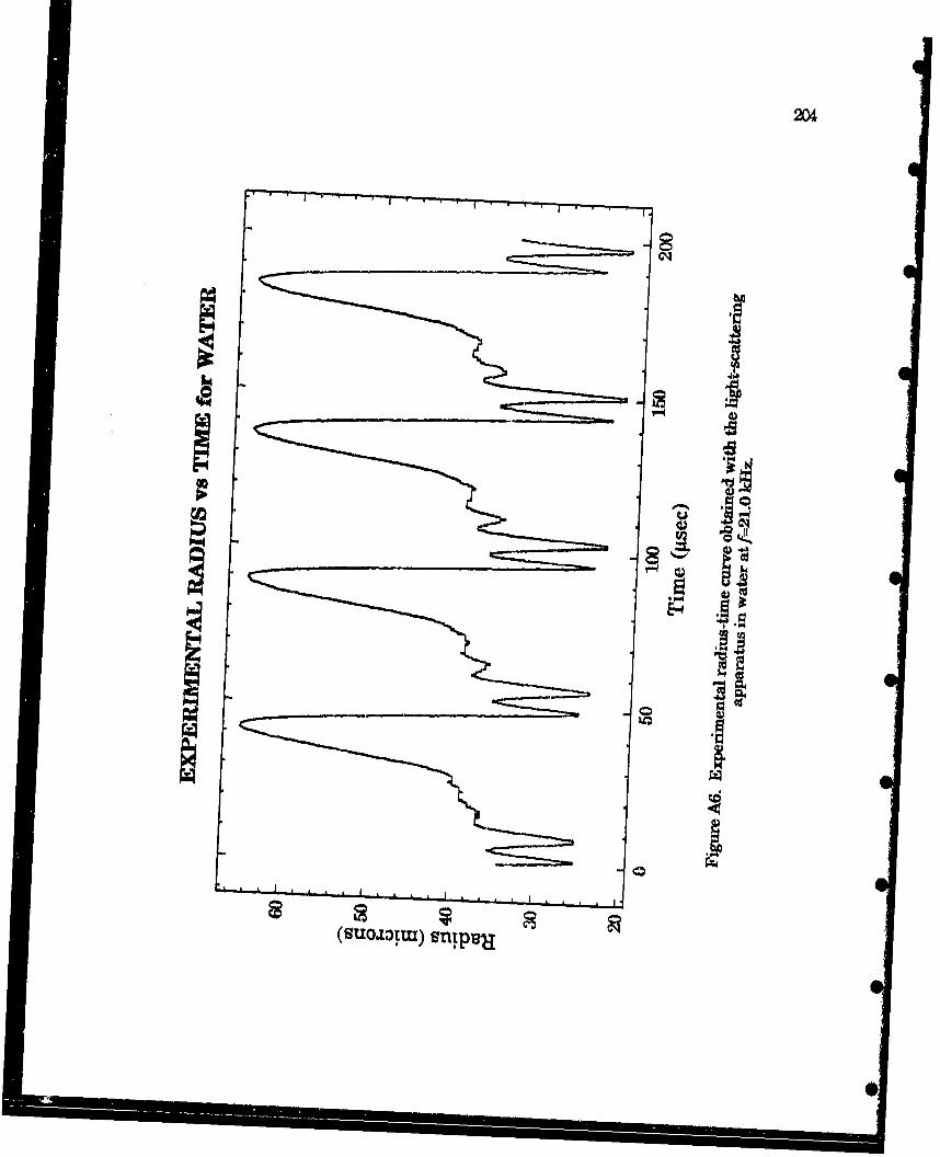
2W~

0-

(suoltm) sipia0

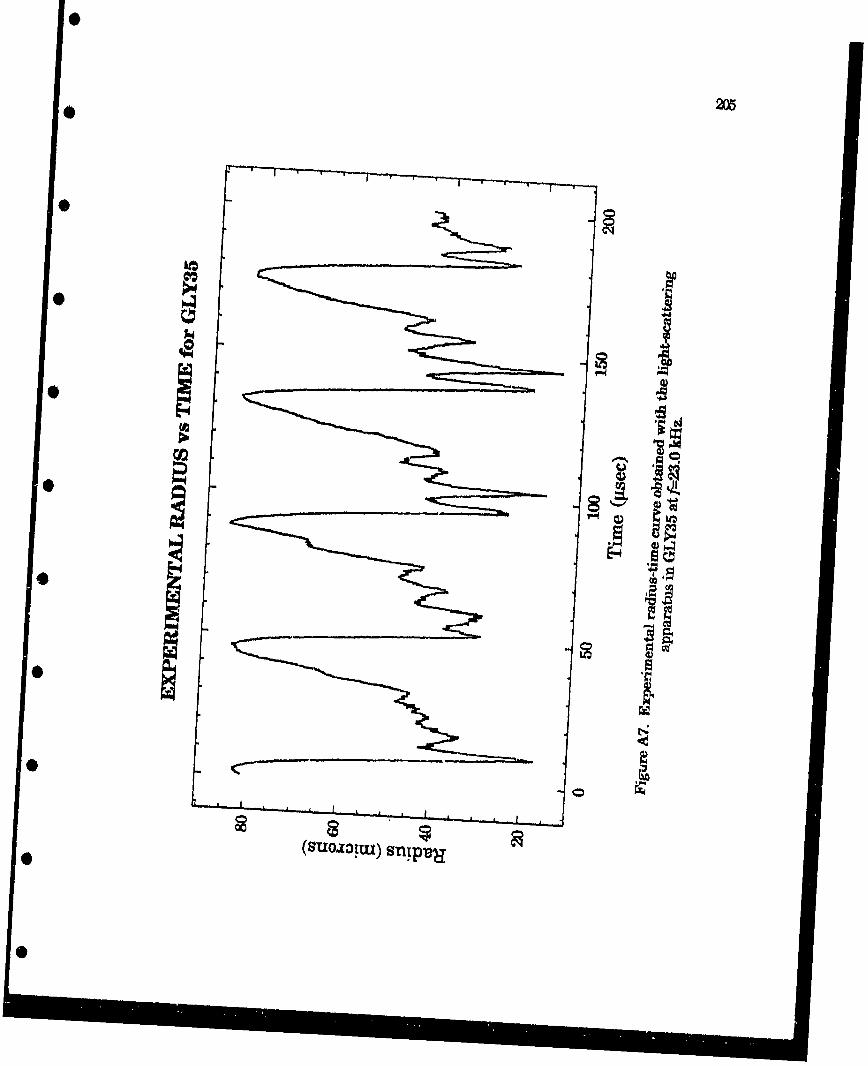
205

C1

S) 4

* ____

(SuOJt~tu)snipe

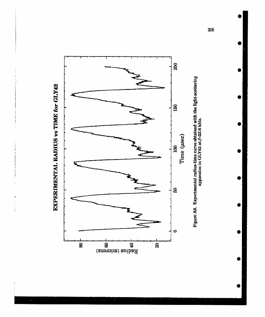
206

0421

Q0

(suo~atul)Smp0

2U

0

(soiu 1.tia

Biographical Sketch of the Author

Dario Felipe Gaitan was born in Medellin, Colombia on June 2, 1961, the

son of Dario Gaitan and Luz Gaviria de Gaitan, He attended high school in

• Medellin at Colegio de San, Jos6, graduating in November, 1978. He received a B.S.

in physics from the University of Southwestern Louisiana in May, 1984.

Felipe is a member of Sigma Pi Sigma, The American Physical Society, and

• the Acoustical Society of America. He enjoys volleyball, racquetball, scuba diving,

hiking, and travelling. He plans to pursue a career in research and teaching and

is currently looking for a post-doctoral position.

His permanent address is Crra. 43E No. 8-20, Medellin, Colombia, South

America.

2D8

0 • . . - • -.- - . -- _- _-.

-0.

.0._

DISTRIBUTICN LIST FORNCPA LC.02.90

TECHNICAL REPORT UNDER CONTRACT N00014-90-J-4021

SCOPY NO,

1 Chief of Naval ResearchOffice of Naval ResearchDepartment of the Navy

• Attn. Marshall Orr

2 DirectorNaval Research LaboratoryWashington, D.C. 20375Attn: Library

3 CommanderDavid Taylor Naval Ship Research and DevelopmentCenterTarget Physics BranchBethesda, MD 20084

* Attn: S. Schreppler (Code 1965)

4 SuperintendentNaval Postgraduate SchoolDepartment of PhysicsMonterey, CA 93940

• Attn: Anthony Atchley

5-9 Commanding Officer and DirectorDefense Technical Information CenterBldg. 5, Cameron Station5010 Duke Street

_ Alexandria, VA 22314

10-20 Dr. L. A. CrumAssociate Director for Basic ResearchNational Center for Physical AcousticsUniversity of Mississippi

0 University, MS 38677

21-30 D. Felipe GaitanNational Center for Physical AcousticsUniversity of MississippiUniversity, MS 38677

0

31 Joseph TownsendBusiness ManagerNational Center for Physical AcousticsUniversity of MississippiUniversity, MS 38677

32 J. E. MatthewsNOARL Numerical Modeling DivisionNSTL, MS 39529-5004

33 Phil MarstonDepartment of PhysicsWashington State UniversityPullman, WA 99164

34 Bob GouldDepartment of PhysicsMiddlebury CollegeMiddlebury, VT 05753

35 Andrea ProsperettiMechanical Engineering DepartmentThe Johns Hopkins UniversityBaltimore, MD 21218

36 Seth PuttermanPhysics DepartmentUniversity of California405 Hilgard AvenueLos Angeles, CA 90024

37 Wesley NyborgPhysics DepartmentUniversity of VermontBurlington, VT 05405

38 A. J. WaltonCambridge University Physics DepartmentCavendish LaboratoryMadingley RoadCambridge CB3 OHEUnited Kingdom

39 Robert C. Dean, Jr.Dean Technology, Inc.SO. Box A-56Hanover, NH 03755

0

40 Kenneth SuslickSchool of Chemical SciencesUniversity of IllinoisUrbana, IL 61801

* 41 Robert D. FinchMechanical Engineering DepartmentUniversity of HoustonHouston, TK 77204-4792

42 Hugh G. FlynnCenter for Biomedical UltrasoundUniversity of RochesterRochester, NY 14627

43 Robert HicklingNational Center for Physical Acoustics

* University of MississippiUniversity, MS 38677

44 C. SehgalDepartment of Physiology and BiophysicsMayo Foundation

* Rochester, MN 55905

45 R. E. VerralDepartment of ChemistryUniversity of SaskatchewanSaskatoon, Saskatchewan S7N OWO

* Canada

46 Steve DanielsPhysical Science LaboratoryOxford UniversitySouth Parks Road

SQOxford OXi 3QZUnited Kingdom

47 Steve GarrettNaval Postgraduate SchoolPhysics Department

* Monterey, CA 93943

A Experimental Investigation of Acoustic Cavitation in Gaseous Liquids

Documents

Transcript of A Experimental Investigation of Acoustic Cavitation in Gaseous Liquids