Likely cavitation and radial motion of stochastic elastic spheres

Likely cavitation and radial motion of stochastic elastic spheres

L. Angela Mihai∗ Thomas E. Woolley† Alain Goriely‡

January 27, 2020

Abstract

The cavitation of solid elastic spheres is a classical problem of continuum mechanics. Here, westudy this problem within the context of “stochastic elasticity” where the constitutive parametersare characterised by probability density functions. We consider homogeneous spheres of stochasticneo-Hookean material, composites with two concentric stochastic neo-Hookean phases, and inho-mogeneous spheres of locally neo-Hookean material with a radially varying parameter. In all cases,we show that the material at the centre determines the critical load at which a spherical cavityforms there. However, while under dead-load traction, a supercritical bifurcation, with stable cav-itation, is obtained in a static sphere of stochastic neo-Hookean material, for the composite andradially inhomogeneous spheres, a subcritical bifurcation, with snap cavitation, is also possible.For the dynamic spheres, oscillatory motions are produced under suitable dead-load traction, suchthat a cavity forms and expands to a maximum radius, then collapses again to zero periodically,but not under impulse traction. Under a surface impulse, a subcritical bifurcation is found in astatic sphere of stochastic neo-Hookean material and also in an inhomogeneous sphere, whereas incomposite spheres, supercritical bifurcations can occur as well. Given the non-deterministic mate-rial parameters, the results can be characterised in terms of probability distributions.

Key words: stochastic elasticity, finite strain analysis, cavitation, oscillations, quasi-equilibratedmotion, probabilities.

“It is a problem of mechanics, highly complicated and irrelevant to probability theoryexcept insofar as it forces us to think a little more carefully about how probability theorymust be formulated if it is to be applicable to real situations.” - E.T. Jaynes (1996) [37]

1 Introduction

Cavitation in solids represents the void-formation within a solid under tensile loads, by analogy to thesimilar phenomenon observed in fluids. For rubber-like materials, this phenomenon was first reportedby Gent and Lindley (1958) [24], whose experiments showed that rubber cylinders ruptured underrelatively small tensile dead loads by opening an internal cavity. The nonlinear elastic analysis ofBall (1982) [7] provided the first theoretical explanation for the formation of a spherical cavity atthe centre of a sphere of isotropic incompressible hyperelastic material in radially symmetric tensionunder prescribed surface displacements or dead loads. There, cavitation was treated as a bifurcationfrom the trivial state at a critical value of the surface traction or displacement, at which the trivialsolution became unstable. This paved the way for numerous applied and theoretical studies devotedto this inherently nonlinear mechanical effect, which is not captured by the linear elasticity theory.

Many important results focusing on rubber-like materials are reviewed in [20, 23, 32]. Recent ex-perimental studies regarding the onset, healing and growth of cavities in elastomers can be found

∗School of Mathematics, Cardiff University, Senghennydd Road, Cardiff, CF24 4AG, UK, Email:[email protected]†School of Mathematics, Cardiff University, Senghennydd Road, Cardiff, CF24 4AG, UK, Email:

[email protected]‡Mathematical Institute, University of Oxford, Woodstock Road, Oxford, OX2 6GG, UK, Email:

[email protected]

1

in [34, 58–60]. Finite element simulations are presented in [40]. While most of this work was car-ried out in the setting of static deformations, in general, the elastodynamics of nonlinear hyperelasticbodies has been less investigated. The governing equations for dynamic large strain deformationsleading to finite amplitude oscillations of spherical and cylindrical shells of homogeneous isotropic in-compressible hyperelastic material, treated as particular cases of quasi-equilibrated motions defined byTruesdell (1962) [81], were reviewed in [82]. Under this type of dynamic deformation, the stress fieldis determined by the current configuration alone, and the body can be brought instantly to rest by ap-plying a suitable pressure impulse on its boundary. Free and forced oscillations of spherical shells werefirst obtained in [29,43,84], using a similar approach as introduced in [41,42] for the axially symmet-ric radial oscillations of infinitely long, isotropic incompressible cylindrical tubes. Oscillatory motioncaused by the dynamic cavitation of a neo-Hookean sphere was considered in [13]. For a wide class ofhyperelastic materials, the static and dynamic cavitation of homogeneous spheres were studied in [7].For a hyperelastic sphere of Mooney-Rivlin material containing a cavity, the numerical solution to thenonlinear problem of large amplitude oscillations was presented in [6]. Theoretical and experimentalstudies of cylindrical and spherical shells of rubber-like material under external pressure were proposedin [85]. The finite amplitude radial oscillations of homogeneous isotropic incompressible hyperelasticspherical and cylindrical shells under a constant pressure difference between the inner and the outersurface were analysed theoretically in [11]. Radial oscillations of non-homogeneous thick-walled cylin-drical and spherical shells of neo-Hookean material, with a material parameter varying continuouslyalong the radial direction, were treated in [18]. In [83], the dynamic inflation of hyperelastic sphericalmembranes of Mooney-Rivlin material subjected to a uniform step pressure was considered, and theabsence of damping was discussed. It was concluded that, as the amplitude and period of oscillationsare strongly influenced by the rate of internal pressure, if the pressure was suddenly imposed and theinflation process was short, then sustained oscillations due to the dominant elastic effects could beobserved. However, in many systems where the pressure is slowly increasing, strong damping wouldgenerally preclude oscillations [15]. The dynamic response of incompressible hyperelastic sphericalshells subjected to periodic loading was examined in [62]. Radial oscillations of spherical shells ofdifferent hyperelastic materials were analysed in [10], where it was found that both the amplitudeand period of oscillations decrease as the stiffness of the material increases. The influence of materialconstitutive law on the dynamic behaviour of spherical membranes was also considered in [65]. In [68],the nonlinear static and dynamic behaviour of a spherical membrane of neo-Hookean or Mooney-Rivlinmaterial, subjected to a uniformly distributed radial pressure on the inner surface, was analysed, andthe influence of the material constants was examined.

Despite these developments, there are important issues that remain unresolved. In particular,the quantification of uncertainties in material parameters and responses resulting from incompleteinformation remain largely unexplored [73]. However, for many materials, deterministic approaches,which are based on average data values, can greatly underestimate or overestimate their properties,and stochastic representations accounting also for data dispersion are needed to improve assessmentand predictions [25,33,39,55,57,80].

For nonlinear elastic materials, stochastic hyperelastic models have recently been described bystrain-energy densities where the parameters are characterised by probability density functions (see[75–79] and also [50]). These are advanced phenomenological models, for which the parameters canbe inferred from macroscopic load-deformation experiments, as shown, for example, in [19]. Theyrely on the finite elasticity theory as prior information, and on the notion of entropy (or uncertainty)[35–37,66,74] to enable the propagation of uncertainties from input data to output quantities of interest[72], and can also be incorporated into Bayesian approaches [8, 45] for model selection [19,50,55,64].

To demonstrate the effect of probabilistic model parameters on predicted mechanical responses,for stochastic homogeneous incompressible hyperelastic bodies, we have analysed theoretically, so far,the static cavitation of a sphere under uniform tensile dead load [48], the inflation of pressurisedspherical and cylindrical shells [46], the classic problem of the Rivlin cube [51], the radial oscillatorymotion of cylindrical and spherical shells under a uniform pressure impulse [47], and the rotationand perversion of stochastic incompressible anisotropic hyperelastic cylindrical tubes [52]. In [48], inaddition to the well-known case of stable cavitation post-bifurcation at the critical dead load, we show,

2

for the first time, the existence of unstable (snap) cavitation for some (deterministic or stochastic)isotropic incompressible materials satisfying Baker-Ericksen (BE) inequalities [5]. In general, theseproblems, for which the elastic solutions are given explicitly, can offer significant insight into how theuncertainties in input parameters are propagated to output quantities. To investigate the effect ofprobabilistic parameters in the case of more complex geometries and loading conditions, numericalapproaches have been proposed in [78, 79]. A similar stochastic methodology can be developed tostudy instabilities in other material systems (e.g., liquid crystal elastomers [16,22,86]), and may leadto more accurate assessment and prediction in many application areas [14,30].

In this paper, we examine the static and dynamic cavitation and post-cavitation behaviour of anincompressible sphere of stochastic hyperelastic material, subject to either a uniform tensile surfacedead load (which is constant in the reference configuration) or an impulse traction (which is keptconstant in the current configuration), and each of them is applied uniformly in the radial direction.Here, cavitation represents the opening of a spherical cavity at the centre of the sphere as a bifur-cated solution from the trivial solution, which becomes unstable at a critical value of the applied load.Moreover, the two different types of loads will lead to different static and dynamic solutions. First, inSection 2, we provide a summary of the stochastic elasticity prerequisites, where, in addition to thestochastic homogeneous material models, for which the elastic parameters are spatially-independentrandom variables at a macroscopic (non-molecular) level, we introduce a class of stochastic inhomo-geneous models described by spatially-dependent strain-energy functions for which the parametersare non-Gaussian random fields. We then recall the notion of quasi-equilibrated motion, where thedeformation field is circulation preserving and, at every time instant, the deformed state is possiblealso as a static equilibrium state under the same forces. Section 3 is devoted to the explicit analysis ofcavitation and finite amplitude oscillations of a homogeneous sphere of stochastic neo-Hookean mate-rial. In Sections 4 and 5, we extend the analysis, respectively, to the cavitation and finite amplitudeoscillations of a composite formed from two concentric homogeneous spheres of different stochasticneo-Hookean material, and to inhomogeneous spheres of locally neo-Hookean material with a radiallyvarying parameter. In each case, the dynamic problem is considered first, then the static problem istreated by reducing the quasi-equilibrated motion to a static equilibrium state. In all cases, we showthat the material at the centre determines the critical load at which a spherical cavity forms. How-ever, there are important differences in the post-cavitation nonlinear elastic responses. While underdead-load traction, supercritical bifurcation, with stable cavitation, is obtained in a static sphere ofstochastic neo-Hookean material, for the composite and radially inhomogeneous spheres, a subcriticalbifurcation, with snap cavitation, is also possible. For the dynamic spheres, oscillatory motions areproduced under suitable dead-load traction, such that a cavity forms and expands to a maximumradius, then collapses again to zero periodically, but not under impulse traction. Under a surfaceimpulse, subcritical bifurcation is found in a static sphere of stochastic neo-Hookean material and alsoin an inhomogeneous sphere, whereas in composite spheres, supercritical bifurcation can occur as well.As the input material parameters are non-deterministic, the results can be characterised in terms ofprobability distributions. In Section 6, we draw concluding remarks and highlight potential extensionsof the stochastic approach.

2 Prerequisites

In this section, we introduce a class of stochastic isotropic incompressible inhomogeneous hyperelasticmodels, where the constitutive parameter is spatially-dependent. This can be regarded as an extensionof the stochastic homogeneous models in [19, 46–48, 50, 51], where both the mean value and varianceof model parameters were constant in space, and also as a particular case of the inhomogeneousanisotropic ones discussed in [78,79], which assumed heterogeneity in variance.

As both static and dynamic spheres of either homogeneous or inhomogeneous stochastic materialwill be considered in the next sections, we also recall the notion of quasi-equilibrated motion definedin [81, 82]. Quasi-equilibrated motions were first treated by us in [47], where the finite amplitudeoscillations of cylindrical and spherical shells of stochastic isotropic incompressible homogeneous hy-perelastic material under uniform pressure impulse were analysed. This type of motions can be reduced

3

to static equilibrium states at any time instant under the given load.

2.1 Stochastic hyperelastic models

We are concerned here with the large strain analysis of spherical bodies of stochastic incompressibleisotropic hyperelastic material, and rely on the following physically realistic assumptions [19, 46–48,50,51]:

(A1) Material objectivity, stating that constitutive equations must be invariant under changes of frameof reference. This requires that the scalar strain-energy function, W = W (F), depending onlyon the deformation gradient F, with respect to the reference configuration, is unaffected by asuperimposed rigid-body transformation (which involves a change of position) after deformation,i.e., W (RTF) = W (F), where R ∈ SO(3) is a proper orthogonal tensor (rotation). Materialobjectivity is guaranteed by defining strain-energy functions in terms of the scalar invariants.

(A2) Material isotropy, requiring that the strain-energy function is unaffected by a superimposedrigid-body transformation prior to deformation, i.e., W (FQ) = W (F), where Q ∈ SO(3). Forisotropic materials, the strain-energy function is a symmetric function of the principal stretches{λi}i=1,2,3 of F, i.e., W (F) =W(λ1, λ2, λ3).

(A3) Baker-Ericksen (BE) inequalities, which state that the greater principal (Cauchy) stress occursin the direction of the greater principal stretch [5, 44], and take the equivalent form(

λi∂W∂λi− λj

∂W∂λj

)(λi − λj) > 0 if λi 6= λj , i, j = 1, 2, 3. (1)

When any two principal stretches are equal, the strict inequality “>” in (1) is replaced by “≥”.

(A4) For any given finite deformation, at any point in the material, the shear modulus, µ, and itsinverse, 1/µ, are second-order random variables, i.e., they have finite mean value and finitevariance [75–79].

Assumptions (A1)-(A3) are general requirements in isotropic finite elasticity [26,49,56,82]. In partic-ular, (A3) implies that the shear modulus is always positive, i.e., µ > 0 [49], while (A4) places randomvariables at the foundation on which to construct hyperelastic models [21,37,50,54,73].

To make our approach analytically tractable, we restrict our attention to a class of inhomogeneousmodels defined by the strain-energy density

W(λ1, λ2, λ3) =µ

2

(λ21 + λ22 + λ23 − 3

), (2)

where the shear modulus, µ = µ(R) > 0, is a random field variable depending on the radius R of theundeformed sphere, and λ1, λ2, and λ3 are the principal stretch ratios. When µ is independent of R,the material model (2) reduces to the stochastic neo-Hookean model [50,75].

For the shear modulus, µ = µ(R), at any fixed R, we rely on the following available information{E [µ] = µ > 0,

E [log µ] = ν, such that |ν| < +∞.(3)

Under the constraints (3), assumption (A4) is guaranteed [69–71,73]. Then, by the maximum entropyprinciple, for any fixed R, µ, follows a Gamma probability distribution with the shape and scaleparameters, ρ1 = ρ1(R) > 0 and ρ2 = ρ2(R) > 0, respectively, satisfying

µ = ρ1ρ2, Var[µ] = ρ1ρ22, (4)

where µ is the mean value, Var[µ] = ‖µ‖2 is the variance, and ‖µ‖ is the standard deviation of µ. Thecorresponding probability density function takes the form [1,28,38]

g(µ; ρ1, ρ2) =µρ1−1e−µ/ρ2

ρρ12 Γ(ρ1), for µ > 0 and ρ1, ρ2 > 0, (5)

4

where Γ : R∗+ → R is the complete Gamma function

Γ(z) =

∫ +∞

0tz−1e−tdt. (6)

The word ‘hyperparameters’ is also used for the parameters ρ1 and ρ2 of the Gamma distribution, todistinguish them from the material parameter µ and other material constants [73, p. 8]. Exampleswhere µ = µ(R) takes specific forms are discussed in Section 5.

2.2 Quasi-equilibrated motion

For the large strain dynamic deformation of an elastic solid, Cauchy’s laws of motion (balance laws oflinear and angular momentum) are governed by the following Eulerian field equations [82, p. 40],

ρx = div T + ρb, (7)

T = TT , (8)

where ρ is the material density, which is assumed constant, x = χ(X, t) is the motion of the elasticsolid, with velocity x = ∂χ(X, t)/∂t and acceleration x = ∂2χ(X, t)/∂t2, b = b(x, t) is the body force,T = T(x, t) is the Cauchy stress tensor, and the superscript T defines the transpose.

To obtain possible dynamical solutions, one can solve Cauchy’s equation for particular motions, orgeneralise known static solutions to dynamical forms using the universal notion of quasi-equilibratedmotion, which is defined as follows.

Definition 2.1 [82, p. 208] A quasi-equilibrated motion, x = χ(X, t), is the motion of an incom-pressible homogeneous elastic solid subject to a given body force, b = b(x, t), whereby, for each valueof t, x = χ(X, t) defines a static deformation that satisfies the equilibrium conditions under the bodyforce b = b(x, t).

Theorem 2.2 [82, p. 208] (see also the proof in [47]) A quasi-equilibrated motion, x = χ(X, t), ofan incompressible homogeneous elastic solid subject to a given body force, b = b(x, t), is dynamicallypossible, subject to the same body force, if and only if the motion is circulation preserving with asingle-valued acceleration potential ξ, i.e.,

x = −grad ξ. (9)

For the condition (9) to be satisfied, it is necessary that

curl x = 0. (10)

Then, the Cauchy stress tensor takes the form

T = −ρξI + T(0), (11)

where T(0) is the Cauchy stress for the equilibrium state at time t and I = diag(1, 1, 1) is the identitytensor. In this case, the stress field is determined by the present configuration alone. In particular,the shear stresses in the motion are the same as those of the equilibrium state at time t.

An immediate consequence of the above theorem is that a quasi-equilibrated motion is dynamicallypossible under a given body force in all elastic materials, if at every time instant the deformation isa possible equilibrium state under that body force in all those materials. Quasi-equilibrated motionsof isotropic materials subject to surface tractions alone are obtained by taking the arbitrary constantin those deformations to be arbitrary functions of time. Under this type of motion, a body can bebrought instantly to rest by applying a suitable pressure impulse on its boundary [82, p. 209]. Examplesinclude the homogeneous motions that are possible in all homogeneous incompressible materials, andalso those considered by us in the next sections.

5

2.3 Radial motion of stochastic hyperelastic spheres

Throughout our analysis, we assume that a sphere of stochastic hyperelastic material defined by (2)is subject to the following radially-symmetric dynamic deformation [47],

r3 = R3 + c3, θ = Θ, φ = Φ, (12)

where (R,Θ,Φ) and (r, θ, φ) are the spherical polar coordinates in the reference and current configu-ration, respectively, such that 0 ≤ R ≤ B, B is the radius of the undeformed sphere, c = c(t) ≥ 0 isthe cavity radius to be calculated, and b = b(t) = 3

√B3 + c(t)3 is the radius of the deformed sphere

at time t (see Figure 1).

Figure 1: Schematic of cross-section of a sphere with undeformed radius B, showing the referencestate (left), and the deformed state, with cavity radius c and outer radius b (right).

By the governing equations (12),

0 = curl x =

(∂φ/∂θ)/r − (∂θ/∂φ)/(r sin θ)

(∂r/∂φ)/(r sin θ)− ∂φ/∂r∂θ/∂r − (∂r/∂θ)/r

, (13)

i.e., the condition (10) is valid for x = (r, θ, φ)T . Therefore, (12) describes a quasi-equilibrated motion,such that

−∂ξ∂r

= r =2cc2 + c2c

r2− 2c4c2

r5, (14)

where ξ is the acceleration potential, satisfying (9). Integrating (14) gives

−ξ = −2cc2 + a2c

r+c4c2

2r4= −rr − 3

2r2. (15)

For the deformation (12), the gradient tensor with respect to the polar coordinates (R,Θ,Φ) isequal to

F = diag

(R2

r2,r

R,r

R

), (16)

and the principal stretch ratios are

λ1 =R2

r2, λ2 = λ3 =

r

R. (17)

The corresponding Cauchy-Green tensor is

B = F2 = diag

(R4

r4,r2

R2,r2

R2

), (18)

6

with the principal invariants

I1 =tr (B) =R4

r4+ 2

r2

R2,

I2 =1

2

[(tr B)2 − tr

(B2)]

=r4

R4+ 2

R2

r2,

I3 = det B = 1.

(19)

The associated Cauchy stress tensor then takes the form [27, pp. 87-91]

T(0) = −p(0)I + β1B + β−1B−1, (20)

where the scalar p(0), which is commonly referred to as the arbitrary hydrostatic pressure [26, pp. 286-287], [56, pp. 198-201], is the Lagrange multiplier for the internal constraint I3 = 1 of incompressibility(i.e., all deformations are isochoric for incompressible materials) [82, pp. 71-72], and the coefficients

β1 = 2∂W

∂I1, β−1 = −2

∂W

∂I2, (21)

are nonlinear material parameters, with W = W (I1, I2, I3) = W(λ1, λ2, λ2), and I1, I2, I3 defined by(19). For this stress tensor, the principal components at time t are as follows,

T (0)rr = −p(0) + β1

R4

r4+ β−1

r4

R4,

T(0)θθ = T (0)

rr +

(β1 − β−1

r2

R2

)(r2

R2− R4

r4

),

T(0)φφ = T

(0)θθ .

(22)

As the stress components depend only on the radius r, the system of equilibrium equations reduces to

∂T(0)rr

∂r= 2

T(0)θθ − T

(0)rr

r. (23)

Hence, by (22) and (23), the radial Cauchy stress for the equilibrium state at t is equal to

T (0)rr (r, t) = 2

∫ (β1 − β−1

r2

R2

)(r2

R2− R4

r4

)dr

r+ ψ(t), (24)

where ψ = ψ(t) is an arbitrary function of time. Substitution of (15) and (24) into (11) then givesthe following principal Cauchy stresses at time t,

Trr(r, t) = −ρ(c2c+ 2cc2

r− c4c2

2r4

)+ 2

∫ (β1 − β−1

r2

R2

)(r2

R2− R4

r4

)dr

r+ ψ(t),

Tθθ(r, t) = Trr(r, t) +

(β1 − β−1

r2

R2

)(r2

R2− R4

r4

),

Tφφ(r, t) = Tθθ(r, t).

(25)

When R2/r2 → 1, all the stress components defined in (25) are equal.

3 Cavitation and radial motion of homogeneous spheres

We first analyse the static and dynamic radially-symmetric deformations of a stochastic homogeneoushyperelastic sphere, where the shear modulus µ of the stochastic model given by (2) is a space-invariant random variable. Hence, the model is of stochastic neo-Hookean type [75], with the shearmodulus µ characterised by the Gamma distribution defined by (5). The radial motion of spheresof neo-Hookean material were treated deterministically in [13], while inhomogeneous cylindrical andspherical shells of neo-Hookean-like material with a radially varying material parameter were analysedin [18]. For homogeneous spheres of stochastic isotropic incompressible hyperelastic material, the staticcavitation under uniform tensile dead load was investigated in [48], while radial oscillatory motions ofhomogeneous cylindrical and spherical shells of stochastic Mooney-Rivlin and neo-Hookean material,respectively, were treated in [47].

7

3.1 Oscillatory motion of a stochastic neo-Hookean sphere under dead-load trac-tion

For a sphere of stochastic neo-Hookean material subject to the quasi-equilibrated motion (12), wedenote the inner and outer radial pressures acting on the curvilinear surfaces, r = c(t) and r = b(t)at time t, as T1(t) and T2(t), respectively [82, pp. 217-219].

Evaluating T1(t) = −Trr(c, t) and T2(t) = −Trr(b, t), using (25), with r = c and r = b, respectively,and subtracting the results, gives

T1(t)− T2(t) = ρ

[(c2c+ 2cc2

)(1

c− 1

b

)− c4c2

2

(1

c4− 1

b4

)]+ 2

∫ b

cµ

(r2

R2− R4

r4

)dr

r

= ρ

[(cc+ 2c2

) (1− c

b

)− c2

2

(1− c4

b4

)]+ 2

∫ b

cµ

(r2

R2− R4

r4

)dr

r

= ρB2

[(c

B

c

B+ 2

c2

B2

)(1− c

b

)− c2

2B2

(1− c4

b4

)]+ 2

∫ b

cµ

(r2

R2− R4

r4

)dr

r.

(26)

By setting the notation

u =r3

R3=

r3

r3 − c3, x =

c

B, (27)

we can then rewrite(c

B

c

B+ 2

c2

B2

)(1− c

b

)− c2

2B2

(1− c4

b4

)=(xx+ 2x2

) [1−

(1 +

1

x3

)−1/3]− x2

2

[1−

(1 +

1

x3

)−4/3]

=

(xx+

3

2x2)[

1−(

1 +1

x3

)−1/3]− x2

2

1

x3

(1 +

1

x3

)−4/3=

1

2x2d

dx

{x2x3

[1−

(1 +

1

x3

)−1/3]}and ∫ b

cµ

(r2

R2− R4

r4

)dr

r=

∫ b

cµ

[(r3

r3 − c3

)2/3

−(r3 − c3

r3

)4/3]dr

r

=1

3

∫ ∞x3+1

µ1 + u

u7/3du.

Thus (26) is equivalent to

2x2T1(t)− T2(t)

ρB2=

d

dx

{x2x3

[1−

(1 +

1

x3

)−1/3]}+

4x2

3ρB2

∫ ∞x3+1

µ1 + u

u7/3du. (28)

Next, assuming that the cavity surface is traction-free, T1(t) = 0 and (28) is equivalent to

2x2Trr(b, t)

ρB2=

d

dx

{x2x3

[1−

(1 +

1

x3

)−1/3]}+

4x2

3ρB2

∫ ∞x3+1

µ1 + u

u7/3du. (29)

We now denote

H(x) =4

3ρB2

∫ x

0

(ζ2∫ ∞ζ3+1

µ1 + u

u7/3du

)dζ, (30)

and set the uniform dead-load traction (see also eq. (2.7) of [13])

Prr(B) =(x3 + 1

)2/3Trr(b, t) =

{0 if t ≤ 0,p0 if t > 0,

(31)

8

where p0 is constant, and x = x(t) is the dimensionless cavity radius, as denoted in (27).In this case, integrating (29) once gives

x2x3

[1−

(1 +

1

x3

)−1/3]+H(x) =

2p0ρB2

(x3 + 1

)1/3+ C, (32)

with H(x) defined by (30), and

C = x20x30

[1−

(1 +

1

x30

)−1/3]+H(x0)−

2p0ρB2

(x30 + 1

)1/3. (33)

Then, after setting the initial conditions x0 = x(0) = 0 and x0 = x(0) = 0, equation (32) takes theform

x2x3

[1−

(1 +

1

x3

)−1/3]+H(x) =

2p0ρB2

[(x3 + 1

)1/3 − 1]. (34)

From (34), we obtain the velocity

x = ±

√√√√√ 2p0ρB2

[(x3 + 1)1/3 − 1

]−H(x)

x3[1−

(1 + 1

x3

)−1/3] . (35)

0.5 1.0 1.5 2.0 2.5 3.0

- 4

- 2

2

4

6

8 V(x)-V(0)

x

x2

Figure 2: Example of potential V (x) with p0 = 15 and µ = 4.05, ρ = B = 1. The periodic orbits liebetween x1 = 0 and x2 ≈ 2.45.

It is useful to note that this nonlinear elastic system is analogous to the motion of a point masswith energy

E =1

2m(x)x2 + V (x), (36)

where the energy is E = C, the potential is given by V (x) = H(x)− 2p0ρB2

(x3 + 1

)1/3and the position-

dependent mass is m(x) = x3[1−

(1 + 1

x3

)−1/3]. Due to the constraints on the function H, the

system has simple dynamics, and the only solutions of interest are either static or periodic solutions.For the given sphere to undergo an oscillatory motion, the following equation,

H(x) =2p0ρB2

[(x3 + 1

)1/3 − 1]

(37)

9

must have exactly two finite distinct positive roots x1, x2 such that 0 ≤ x1 < x2 < ∞, as shown inFigure 2. Then, the minimum and maximum radii of the cavity in the oscillation are x1B and x2B,respectively, and the period of oscillation is equal to

T = 2

∣∣∣∣∫ x2

x1

dx

x

∣∣∣∣ = 2

∣∣∣∣∣∣∣∫ x2

x1

√√√√√ x3[1−

(1 + 1

x3

)−1/3]2p0ρB2

[(x3 + 1)1/3 − 1

]−H(x)

dx

∣∣∣∣∣∣∣ . (38)

For the stochastic sphere, the amplitude and the period of the oscillation are random variables char-acterised by probability distributions.

Evaluating the integral in (30) gives

H(x) =µ

ρB2

[2(x3 + 1

)2/3 − 1

(x3 + 1)1/3− 1

], (39)

and assuming that the shear modulus, µ, which is a random variable, is bounded from below, i.e.,

µ > η, (40)

for some constant η > 0, it follows that H(0) = 0 and limx→∞H(x) =∞.When p0 6= 0, substitution of (39) in (37) gives

p0

[(x3 + 1

)1/3 − 1]

=µ

2

[2(x3 + 1

)2/3 − 1

(x3 + 1)1/3− 1

]. (41)

Equation (41) has one solution at x1 = 0, while the second solution, x2, is a root of

p0 =µ

2

[2(x3 + 1

)1/3+

1

(x3 + 1)1/3+ 2

]. (42)

As the right-hand side of equation (42) is an increasing function of x, this equation has a solution,x2 > 0, if and only if (see also eq. (2.7) of [13])

p0 >5µ

2= lim

x→0+

µ

2

[2(x3 + 1

)1/3+

1

(x3 + 1)1/3+ 2

]. (43)

Then,2p0ρB2

[(x3 + 1

)1/3 − 1]−H(x)

{≥ 0 if x1 ≤ x ≤ x2,< 0 if x > x2.

(44)

In this case, at the centre of the given sphere, a spherical cavity forms and expands until its radiusreaches the value c = x2B, where x2 is the root of (42), then contracts again to zero radius and repeatsthe cycle.

The critical dead load for the onset of cavitation is

limx→0+

p0 =5µ

2. (45)

Regarding the random shear modulus, by (40) and (43), for the motion to be oscillatory, thefollowing condition must hold,

η < µ <2p05. (46)

Then, as µ follows a Gamma distribution, defined by (5), the probability distribution of oscillatorymotions occurring is

P1(p0) =

∫ 2p05

0g(u; ρ1, ρ2)du, (47)

10

Figure 3: Example of Gamma distribution, defined by (5), with hyperparameters ρ1 = 405, ρ2 = 0.01.

Figure 4: Probability distributions of whether oscillatory motions can occur or not for a sphere ofstochastic neo-Hookean material under dead-load traction, when the shear modulus, µ, follows aGamma distribution with ρ1 = 405, ρ2 = 0.01. Continuous coloured lines represent analyticallyderived solutions, given by equations (47)-(48), whereas the dashed versions represent stochasticallygenerated data. The vertical line at the critical value, p0 = 10.125, separates the expected regionsbased only on mean value, µ = ρ1ρ2 = 4.05. The probabilities were calculated from the average of 100stochastic simulations.

11

Figure 5: The function H(x), defined by (39), intersecting the (dashed red) curve2p0ρB2

[(x3 + 1

)1/3 − 1], with p0 = 15 (left), and the associated velocity, given by (35) (right), for a

dynamic sphere of stochastic neo-Hookean material under dead-load traction, when ρ = 1, B = 1, andµ is drawn from the Gamma distribution with ρ1 = 405, ρ2 = 0.01. The dashed black lines correspondto the expected values based only on mean value, µ = ρ1ρ2 = 4.05. Each distribution was calculatedfrom the average of 1000 stochastic simulations.

and that of non-oscillatory motions is

P2(p0) = 1− P1(p0) = 1−∫ 2p0

5

0g(u; ρ1, ρ2)du. (48)

For example, when µ satisfies the Gamma distribution with ρ1 = 405 and ρ2 = 0.01, shown inFigure 3, the probability distributions given by (47)-(48) are shown in Figure 4 (with blue lines forP1 and red lines for P2). Specifically, the interval (0, 5µ), where µ = ρ1ρ2 = 4.05 is the mean valueof µ, was divided into 100 steps, then for each value of p0, 100 random values of µ were numericallygenerated from the specified Gamma distribution and compared with the inequalities defining the twointervals for values of p0. For the deterministic elastic sphere, the critical value p0 = 5µ/2 = 10.125strictly divides the cases of oscillations occurring or not. For the stochastic problem, for the samecritical value, there is, by definition, exactly 50% chance that the motion is oscillatory, and 50% chancethat is not. To increase the probability of oscillatory motion (P1 ≈ 1), one must apply a sufficientlysmall traction, p0, below the expected critical point, whereas a non-oscillatory motion is certain tooccur (P2 ≈ 1) if p0 is sufficiently large. However, the inherent variability in the probabilistic systemmeans that there will also exist events where there is competition between the two cases.

We note that the Gamma distribution represented in Figure 3 is approximately a normal distribu-tion. This is because, when ρ1 much larger than ρ2, the Gamma probability distribution is approxi-mated by a normal distribution (see, e.g., [19,46]). However, elastic moduli cannot be characterised bythe normal distribution, since this distribution is defined on the entire real line whereas elastic moduliare typically positive. In practice, these moduli can meaningfully take on different values, correspond-ing to possible outcomes of experimental tests. Then, the principle of maximum entropy enables theconstruction of their probability distributions, given the available information. Approaches for theexplicit derivation of probability distributions for the elastic parameters of stochastic homogeneousisotropic hyperelastic models calibrated to experimental data were developed in [50,77].

In Figure 5, we illustrate the stochastic function H(x), defined by (39), intersecting the curve2p0ρB2

[(x3 + 1

)1/3 − 1], with p0 = 15, to find the two distinct solutions of equation (37), and the

associated velocity, given by (35), assuming that ρ = 1, B = 1, and µ is drawn from the Gammadistribution with ρ1 = 405 and ρ2 = 0.01 (see Figure 3). Each figure displays a probability histogramat each value of x. The histogram comprises of 1000 stochastic simulations and the colour bar definesthe probability of finding a given value of H(x), or of the associated velocity, respectively, at a given

12

value of x. The dashed black line corresponds to the expected values based only on the mean valueµ = ρ1ρ2 = 4.05, of µ.

Throughout this paper, different simulations were produced by fixing the parameters given ineach figure caption, and repeatedly drawing random samples from the underlying distribution. Ourcomputer simulations were run in Matlab 2018a where we made specific use of inbuilt functions forrandom number generation.

3.2 Static deformation of a stochastic neo-Hookean sphere under dead-load trac-tion

In view of our subsequent analysis, we review here the cavitation of a static sphere of stochasticneo-Hookean material, with the shear modulus µ following the Gamma distribution defined by (5).Incompressible spheres of different stochastic homogeneous hyperelastic material were treated in detailin [48] (see also [12] for the deterministic spheres). In this case, if the surface of the cavity is traction-free, then T1 = 0 and (29) reduces to

Trr(b) =2

3

∫ ∞x3+1

µ1 + u

u7/3du. (49)

After evaluating the integral in (49), the required uniform dead-load traction at the outer surface,R = B, in the reference configuration, takes the form

P =(x3 + 1

)2/3Trr(b) = 2µ

[(x3 + 1

)1/3+

1

4 (x3 + 1)2/3

], (50)

and increases as x increases. The critical dead load for the onset of cavitation is then

P0 = limx→0+

P =5µ

2, (51)

and is equal to that given by (45) for the dynamic sphere [7, 13].

Figure 6: Probability distribution of the applied dead-load traction P causing cavitation of radius cin a static unit sphere (with B = 1) of stochastic neo-Hookean material, when the shear modulus, µ,follows a Gamma distribution with ρ1 = 405, ρ2 = 4.05/ρ1 = 0.01. The dashed black line correspondsto the expected bifurcation based only on mean value, µ = ρ1ρ2 = 4.05.

To analyse the stability of this cavitation, we study the behaviour of the cavity opening, withradius c as a function of P , in a neighbourhood of P0. After differentiating the function given by (50),with respect to the dimensionless cavity radius x = c/B, we have

dP

dx= 2µx2

[1

(x3 + 1)2/3− 1

2 (x3 + 1)5/3

]> 0, (52)

13

i.e., the cavitation is stable (with 100% certainty), regardless of the material parameter µ [48]. Forexample, the post-cavitation stochastic behaviour of the static unit sphere when the shear modulus,µ, follows a Gamma distribution with ρ1 = 405 and ρ2 = 4.05/ρ1 = 0.01 is shown in Figure 6.

3.3 Non-oscillatory motion of a stochastic neo-Hookean sphere under impulsetraction

For a sphere subject to the radially-symmetric dynamic deformation (12), an impulse (suddenly ap-plied) traction, expressed in terms of the Cauchy stresses, is prescribed as follows [47],

2Trr(b, t)

ρB2=

{0 if t ≤ 0,p0 if t > 0,

(53)

where p0 is constant in time. Introducing the dimensionless cavity radius x(t) = c(t)/B and settingthe initial conditions x0 = x(0) = 0 and x0 = x(0) = 0, we obtain the following differential equation

x2x3

[1−

(1 +

1

x3

)−1/3]+H(x) =

p03x3, (54)

where H(x) is given by (39). From (54), we obtain the velocity

x = ±

√√√√ p03 x

3 −H(x)

x3[1−

(1 + 1

x3

)−1/3] , (55)

assuming that p03 x

3 −H(x) ≥ 0. For an oscillatory motion to occur, the equation

H(x) =p03x3 (56)

must have exactly two distinct solutions, x = x1 and x = x2, such that 0 ≤ x1 < x2 <∞.

Figure 7: The function H(x), defined by (39), intersecting the (dashed red) curve p0x3/3, with p0 = 9,

for a dynamic sphere of stochastic neo-Hookean material under impulse traction, when ρ = 1, B = 1,and µ is drawn from the Gamma distribution with ρ1 = 405 and ρ2 = 0.01. The dashed black linescorrespond to the expected values based only on mean value, µ = ρ1ρ2 = 4.05. Note that, betweenthe points of intersection, the values of H(x) are situated above the dashed red curve.

When p0 6= 0, substitution of (39) in (56) gives

p03x3 =

µ

ρB2

[2(x3 + 1

)2/3 − 1

(x3 + 1)1/3− 1

], (57)

14

which has a solution at x1 = 0. The second solution, x2 > 0, is a root of

p0 =3µ

ρB2

[1

(x3 + 1)1/3+

(x3 + 1

)1/3+ 1

(x3 + 1)2/3 + (x3 + 1)1/3 + 1

]. (58)

As the right-hand side of equation (58) is a decreasing function of x, this equation has a solution,x2 > 0, if and only if

p0 > 0 = limx→∞

3µ

ρB2

[1

(x3 + 1)1/3+

(x3 + 1

)1/3+ 1

(x3 + 1)2/3 + (x3 + 1)1/3 + 1

](59)

and

p0 <5µ

ρB2= lim

x→0+

3µ

ρB2

[1

(x3 + 1)1/3+

(x3 + 1

)1/3+ 1

(x3 + 1)2/3 + (x3 + 1)1/3 + 1

]. (60)

However, since this impliesp03x3 −H(x)

{< 0 if x1 < x < x2,> 0 if x > x2,

(61)

the sphere cannot oscillate when p0 is constant in time, as assumed in (53) (see Figure 7).By (53) and (58), the tensile traction, T = Trr(b, t), takes the form

T =3µ

2

[1

(x3 + 1)1/3+

(x3 + 1

)1/3+ 1

(x3 + 1)2/3 + (x3 + 1)1/3 + 1

], (62)

and decreases as x increases. Thus, the critical tension for the onset of cavitation is

T0 = limx→0+

T =5µ

2, (63)

as found also under dead loading.

3.4 Static deformation of a stochastic neo-Hookean sphere under impulse traction

For the static sphere subject to a uniform constant surface load in the current configuration, given interms of the Cauchy stresses, we have

T = 2µ

[1

(x3 + 1)1/3+

1

4 (x3 + 1)4/3

], (64)

which decreases as x increases. Then, the critical tension for cavitation initiation is also given by (63).The post-cavitation behaviour can be inferred from the sign of the derivative of T in a neighbour-

hood of T0. By differentiating (64) with respect to x, we obtain

dT

dx= −2µx2

[1

(x3 + 1)4/3+

1

(x3 + 1)7/3

]< 0, (65)

i.e., the cavitation is unstable, regardless of the material parameter µ [7]. The post-cavitation stochas-tic behaviour of the static homogeneous sphere is shown in Figure 8, for the unit sphere (with B = 1)of stochastic neo-Hookean material, where the shear modulus, µ, is drawn from a Gamma distributionwith shape and scale parameters ρ1 = 405 and ρ2 = 4.05/ρ1 = 0.01, respectively (see also Figure 2of [7]).

15

Figure 8: Probability distribution of the applied impulse traction T causing cavitation of radius c ina static unit sphere (with B = 1) of stochastic neo-Hookean material, when the shear modulus, µ,follows a Gamma distribution with ρ1 = 405 and ρ2 = 0.01. The dashed black line corresponds to theexpected bifurcation based only on the mean value, µ = ρ1ρ2 = 4.05.

4 Cavitation and radial motion of concentric homogeneous spheres

Next, we extend the approach developed in the previous section to investigate the behaviour under thequasi-equilibrated radial motion (12) of a composite formed from two concentric homogeneous spheres(see Figure 9). We restrict our attention to composite spheres with two stochastic neo-Hookeanphases, similar to those containing two concentric spheres of different neo-Hookean material treateddeterministically in [31] and [67]. In this case, we define the following strain-energy function,

W(λ1, λ2, λ3) =

{µ(1)

2

(λ21 + λ22 + λ23 − 3

), 0 < R < A,

µ(2)

2

(λ21 + λ22 + λ23 − 3

), A < R < B,

(66)

where 0 < R < A and A < R < B denote the radii of the inner and outer sphere in the referenceconfiguration, and the corresponding shear moduli µ(1) and µ(2) are spatially-independent random

variables characterised by the Gamma distributions g(u; ρ(1)1 , ρ

(1)2 ) and g(u; ρ

(2)1 , ρ

(2)2 ), defined by (5),

respectively.

4.1 Oscillatory motion of a sphere with two stochastic neo-Hookean phases underdead-load traction

For the composite sphere, we denote the radial pressures acting on the curvilinear surfaces r = c(t)and r = b(t) at time t as T1(t) and T2(t), respectively, and impose the continuity condition for thestress components across their interface, r = a(t). By analogy to (26), we obtain

T1(t)− T2(t) = ρB2

[(c

B

c

B+ 2

c2

B2

)(1− c

b

)− c2

2B2

(1− c4

b4

)]+ 2

∫ a

cµ(1)

(r2

R2− R4

r4

)dr

r+ 2

∫ b

aµ(2)

(r2

R2− R4

r4

)dr

r.

(67)

Using the notation (27), we can write (67) equivalently as follows,

2x2T1(t)− T2(t)

ρB2=

d

dx

{x2x3

[1−

(1 +

1

x3

)−1/3]}

+4x2

3ρB2

∫ x3B3/A3+1

x3+1µ(2)

1 + u

u7/3du+

4x2

3ρB2

∫ ∞x3B3/A3+1

µ(1)1 + u

u7/3du.

(68)

16

Figure 9: Schematic of cross-section of a composite sphere made of two concentric homogeneousspheres, with undeformed radii A and B, respectively, showing the reference state (left), and thedeformed state, with cavity radius c and radii a and b, respectively (right).

In this case, we denote

H(x) =4

3ρB2

∫ x

0

(ζ2∫ ζ3B3/A3+1

ζ3+1µ(2)

1 + u

u7/3du

)dζ

+4

3ρB2

∫ x

0

(ζ2∫ ∞ζ3B3/A3+1

µ(1)1 + u

u7/3du

)dζ,

(69)

and, after evaluating the integrals, we obtain the equivalent form

H(x) =µ(2)

ρB2

[2(x3 + 1

)2/3 − 1

(x3 + 1)1/3− 1

]

+µ(1) − µ(2)

ρB2

A3

B3

2

(x3B3

A3+ 1

)2/3

− 1(x3B

3

A3 + 1)1/3 − 1

. (70)

Then, substitution of (70) in (37) gives

p0

[(x3 + 1

)1/3 − 1]

=µ(2)

2

[2(x3 + 1

)2/3 − 1

(x3 + 1)1/3− 1

]

+µ(1) − µ(2)

2

A3

B3

2

(x3B3

A3+ 1

)2/3

− 1(x3B

3

A3 + 1)1/3 − 1

. (71)

This equation has one solution at x1 = 0, while the second solution, x2 > 0, is a root of

p0 =µ(2)

2

[2(x3 + 1

)1/3+

1

(x3 + 1)1/3+ 2

]

− µ(2)

2

(x3 + 1

)2/3+(x3 + 1

)1/3+ 1(

x3B3

A3 + 1)2/3

+(x3B

3

A3 + 1)1/3

+ 1

2

(x3B3

A3+ 1

)1/3

+1(

x3B3

A3 + 1)1/3 + 2

+µ(1)

2

(x3 + 1

)2/3+(x3 + 1

)1/3+ 1(

x3B3

A3 + 1)2/3

+(x3B

3

A3 + 1)1/3

+ 1

2

(x3B3

A3+ 1

)1/3

+1(

x3B3

A3 + 1)1/3 + 2

.(72)

17

Next, we expand p0, given by (72), to the first order in x3 to obtain

p0 ≈5µ(1)

2+x3

3

[2

(B3

A3− 1

)(µ(2) − µ(1)

)+µ(1)

2

]. (73)

The critical tension for cavity initiation is then

limx→0+

p0 =5µ(1)

2, (74)

and a comparison with (45) shows that it is the same as for the homogeneous sphere made of the samematerial as the inner sphere.

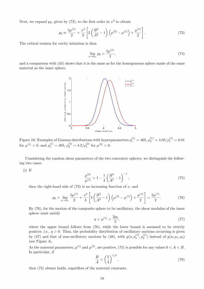
Figure 10: Examples of Gamma distributions with hyperparameters ρ(1)1 = 405, ρ

(1)2 = 4.05/ρ

(1)1 = 0.01

for µ(1) > 0, and ρ(1)1 = 405, ρ

(2)2 = 4.2/ρ

(2)1 for µ(2) > 0.

Considering the random shear parameters of the two concentric spheres, we distinguish the follow-ing two cases:

(i) If

µ(2)

µ(1)> 1− 1

4

(B3

A3− 1

)−1, (75)

then the right-hand side of (73) is an increasing function of x, and

p0 > limx→0+

5µ(1)

2+x3

3

[2

(B3

A3− 1

)(µ(2) − µ(1)

)+µ(1)

2

]=

5µ(1)

2. (76)

By (76), for the motion of the composite sphere to be oscillatory, the shear modulus of the innersphere must satisfy

η < µ(1) <2p05, (77)

where the upper bound follows from (76), while the lower bound is assumed to be strictlypositive, i.e., η > 0. Thus, the probability distribution of oscillatory motions occurring is given

by (47) and that of non-oscillatory motions by (48), with g(u; ρ(1)1 , ρ

(1)2 ) instead of g(u; ρ1, ρ2)

(see Figure 4).

As the material parameters, µ(1) and µ(2), are positive, (75) is possible for any values 0 < A < B.In particular, if

B

A<

(5

4

)1/3

, (78)

then (75) always holds, regardless of the material constants.

18


[(x3 + 1


dynamic composite sphere with two concentric stochastic neo-Hookean phases, with radii A = 1/2and B = 1, respectively, under dead-load traction, when the shear modulus of the inner phase, µ(1),

follows a Gamma distribution with ρ(1)1 = 405, ρ

(1)2 = 4.05/ρ

(1)1 = 0.01, while the shear modulus of the

outer phase, µ(2), is drawn from a Gamma distribution with ρ(2)1 = 405, ρ

(2)2 = 4.2/ρ

(2)1 . The dashed

black lines correspond to the expected values based only on mean values, µ(1) = 4.05 and µ(2) = 4.2.Each distribution was calculated from the average of 1000 stochastic simulations.

(ii) If

µ(2)

µ(1)< 1− 1

4

(B3

A3− 1

)−1, (79)

then the right-hand side in (73) decreases as x increases, hence

0 < p0 <5µ(1)

2. (80)

As the material constants, µ(1) and µ(2), are positive, (79) is possible if and only if

B

A>

(5

4

)1/3

. (81)

However, in this case,

2p0ρB2

[(x3 + 1

)1/3 − 1]−H(x)

{< 0 if x1 < x < x2,> 0 if x > x2,

(82)

and the sphere cannot oscillate.

In Figure 11, we represent the stochastic function H(x), defined by (70), intersecting the curve2p0ρB2

[(x3 + 1

)1/3 − 1]

, with p0 = 15, to find the two distinct solutions to (37), and the associated

velocity, given by (35), for a composite sphere with two concentric stochastic neo-Hookean phases,with radii A = 1/2 and B = 1, respectively, when the shear modulus of the inner phase, µ(1), follows

a Gamma distribution with ρ(1)1 = 405, ρ

(1)2 = 4.05/ρ

(1)1 = 0.01, while the shear modulus of the outer

phase, µ(2), is drawn from a Gamma distribution with ρ(2)1 = 405, ρ

(2)2 = 4.2/ρ

(2)1 (see Figure 10).

19

4.2 Static deformation of a sphere with two stochastic neo-Hookean phases underdead-load traction

For the static composite sphere, if the surface of the cavity is traction-free, then T1 = 0 and (68)reduces to

Trr(b) =2

3

∫ x3B3/A3+1

x3+1µ(2)

1 + u

u7/3du+

2

3

∫ ∞x3B3/A3+1

µ(1)1 + u

u7/3du. (83)

After evaluating the integrals in (83), the required dead-load traction at the outer surface, R = B, inthe reference configuration, is equal to

P =(x3 + 1

)2/3Trr(b)

= 2µ(2)

[(x3 + 1

)1/3+

1

4 (x3 + 1)2/3

]

+ 2(µ(1) − µ(2)

) (x3 + 1

)2/3 1(x3B

3

A3 + 1)1/3 +

1

4(x3B

3

A3 + 1)4/3

.(84)

The critical dead load for the cavity formation is then

P0 = limx→0+

P =5µ(1)

2, (85)

and is the same as for the homogeneous sphere made entirely of the material of the inner sphere [31],as found also in the dynamic case.

To study the stability of this cavitation, we examine the behaviour of the cavity opening, withradius c as a function of P , in a neighbourhood of P0. Expanding the expression of P , given by (84),to the first order in x3, we obtain [31]

P ≈ 5µ(1)

2+x3

3

[4

(B3

A3− 1

)(µ(2) − µ(1)

)+ µ(1)

]. (86)

After differentiating the above function with respect to the dimensionless cavity radius x = c/B, wehave

dP

dx≈ x2

[4

(B3

A3− 1

)(µ(2) − µ(1)

)+ µ(1)

]. (87)

Then, dP/dx → 0 as x → 0+, and the bifurcation at the critical dead load, P0, is supercritical(respectively, subcritical) if dP/dx > 0 (respectively, dP/dx < 0) for arbitrarily small x. From (87),the following two cases are distinguished (see also the discussion in [31]):

(i) If (75) is valid, then the solution presents itself as a supercritical bifurcation, and the cavitationis stable, in the sense that a new bifurcated solution exists locally for values of P > P0, andthe cavity radius monotonically increases with the applied load post-bifurcation. In particular,when µ(1) = µ(2), the problem reduces to the case of a homogeneous sphere made of neo-Hookeanmaterial, for which stable cavitation is known to occur [48].

(ii) If (79) holds, then the bifurcation is subcritical, with the cavitation being unstable, in the sensethat the required dead load starts to decrease post-bifurcation, causing a snap cavitation, i.e., asudden jump in the cavity opening.

Thus, on the one hand, when (78) is satisfied, (75) is valid regardless of the values of µ(1) and µ(2),and the cavitation is guaranteed to be stable (with 100% certainty). On the other hand, if (81) holds,then, as either of the two inequalities (75) and (79) is possible, the probability distribution of stablecavitation in the composite sphere is equal to

P1(µ(2)) =

∫ µ(2)/

[1− 1

4

(B3

A3−1)−1

]0

g(u; ρ(1)1 , ρ

(1)2 )du, (88)

20

while that of unstable (snap) cavitation is

P2(µ(2)) = 1− P1(µ

(2)) = 1−∫ µ(2)/

[1− 1

4

(B3

A3−1)−1

]0

g(u; ρ(1)1 , ρ

(1)2 )du. (89)

Figure 12: Probability distributions of stable or unstable cavitation in a static sphere made of twoconcentric stochastic neo-Hookean phases, with radii A = 1/2 and B = 1, respectively, under dead-load traction, when the shear modulus of the inner sphere, µ(1), follows a Gamma distribution with

ρ(1)1 = 405, ρ

(1)2 = 0.01. Continuous coloured lines represent analytically derived solutions, given by

equations (88)-(89), and the dashed versions represent stochastically generated data. The vertical lineat the critical value, 27µ(1)/28 = 3.9054, separates the expected regions based only on mean value,

µ = ρ(1)1 ρ

(1)2 = 4.05. The probabilities were calculated from the average of 100 stochastic simulations.

Figure 13: Probability distribution of the applied dead-load traction P causing cavitation of radius cin a static sphere of two concentric stochastic neo-Hookean phases, with radii A = 1/2 and B = 1,respectively, when the shear modulus of the inner phase, µ(1), follows a Gamma distribution with

ρ(1)1 = 405, ρ

(1)2 = 4.05/ρ

(1)1 = 0.01, while the shear modulus of the outer phase, µ(2), is drawn from

Gamma distribution with ρ(2)1 = 405, ρ

(2)2 = 3.6/ρ

(2)1 (left) or ρ

(2)1 = 405, ρ

(2)2 = 4.2/ρ

(2)1 (right). The

dashed black lines correspond to the expected bifurcation based only on mean parameter values.

For example, setting A = 1/2 and B = 1, if ρ(1)1 = 405, ρ

(1)2 = 4.05/ρ

(1)1 = 0.01 for the inner sphere,

and ρ(2)1 = 405, ρ

(2)2 = 4.2/ρ

(2)1 for the outer sphere (see Figure 10), then the probability distributions

given by equations (88)-(89) are illustrated numerically in Figure 12 (with blue lines for P1 and red linesfor P2). For the numerical realisations in these plots, the interval (0, 8.1) =

(0, 2µ(1)

)was discretised

into 100 representative points, then for each value of µ(2), 100 random values of µ(1) were numericallygenerated from the specified Gamma distribution and compared with the inequalities defining the two

21

intervals for values of µ(2). For the deterministic elastic case, which is based on the mean value of the

shear modulus, µ(1) = ρ(1)1 ρ

(1)2 = 4.05, the critical value of 27µ(1)/28 = 3.9054 strictly separates the

cases where cavitation instability can, and cannot, occur. However, in the stochastic case, the twostates compete. For example, at the same critical value, there is, by definition, exactly 50% chancethat the cavitation is stable, and 50% chance that is not.

The post-cavitation stochastic behaviours shown in Figure 13 correspond to two different staticcomposite sphere where the shear modulus of the inner phase, µ(1), follows a Gamma distribution with

ρ(1)1 = 405, ρ

(1)2 = 4.05/ρ

(1)1 = 0.01, while the shear modulus of the outer phase, µ(2), is drawn from a

Gamma distribution with ρ(2)1 = 405, ρ

(2)2 = 3.6/ρ

(2)1 (in Figure 13-left) or ρ

(2)1 = 405, ρ

(2)2 = 4.2/ρ

(2)1

(in Figure 13-right). In each case, unstable or stable cavitation is expected, respectively, but there isalso about 5% chance that the opposite behaviour is presented.

4.3 Non-oscillatory motion of a sphere with two stochastic neo-Hookean phasesunder impulse traction

In this case, setting the initial conditions x0 = x(0) = 0 and x0 = x(0) = 0, we obtain equation (54),where H(x) is given by (70). Then, substitution of (70) in (56) gives

p03x3 =

µ(2)

ρB2

[2(x3 + 1

)2/3 − 1

(x3 + 1)1/3− 1

]

+µ(1) − µ(2)

ρB2

A3

B3

2

(x3B3

A3+ 1

)2/3

− 1(x3B

3

A3 + 1)1/3 − 1

. (90)

Equivalently, by (53), in terms of the tensile traction T = Trr(b, t),

2T

3x3 = µ(2)

[2(x3 + 1

)2/3 − 1

(x3 + 1)1/3− 1

]

+(µ(1) − µ(2)

) A3

B3

2

(x3B3

A3+ 1

)2/3

− 1(x3B

3

A3 + 1)1/3 − 1

. (91)

This equation has one solution at x1 = 0, while the second solution, x2 > 0, is a root of

T =3µ(2)

2

[ (x3 + 1

)1/3+ 1

(x3 + 1)2/3 + (x3 + 1)1/3 + 1+

1

(x3 + 1)1/3

]

+3(µ(1) − µ(2)

)2

(x3B

3

A3 + 1)1/3

+ 1(x3B

3

A3 + 1)2/3

+(x3B

3

A3 + 1)1/3

+ 1

+1(

x3B3

A3 + 1)1/3

. (92)

After expanding T , given by (92), to the first order in x3, we have

T ≈ 5µ(1)

2+ x3

[B3

A3

(µ(2) − µ(1)

)− µ(2)

]. (93)

The associated critical tension for cavity initiation is

T0 = limx→0+

T =5µ(1)

2, (94)

and a comparison with that given by (63) shows that it is the same as for the homogeneous spheremade of the same material as the inner sphere.

We now distinguish the following two cases:

22

Figure 14: The function H(x), defined by (70), and the (dashed red) curve p0x3

3 , with different valuesof p0, for a dynamic sphere made of two concentric stochastic neo-Hookean phases, with radii A = 1/2and B = 1, respectively, under impulse traction, when ρ = 1 and the shear modulus of the inner

sphere, µ(1), follows a Gamma distribution with ρ(1)1 = 405, ρ

(1)2 = 0.01, while for the outer sphere, the

shear modulus, µ(2), follows a Gamma distribution with ρ(2)1 = 405, ρ

(1)2 = 0.02 (left) or ρ

(2)1 = 405,

ρ(1)2 = 0.005 (right). The dashed black lines correspond to the expected values based only on mean

value parameters.

(i) If

µ(2)

µ(1)>

(1− A3

B3

)−1, (95)

then the right-hand side of (93) is an increasing function of x, hence

T > limx→0+

5µ(1)

2+ x3

[B3

A3

(µ(2) − µ(1)

)− µ(2)

]=

5µ(1)

2. (96)

By (96), for the motion of the composite sphere to be oscillatory, the shear modulus of the innersphere must satisfy

η < µ(1) <2T

5, (97)

where the lower bound is assumed to be strictly positive, i.e., η > 0. Equivalently, by (53), interms of the constant p0,

η < µ(1) <p05ρB2, (98)

However, in this case,p03x3 −H(x) > 0, (99)

for all x > 0, and the sphere does not oscillate (see Figure 14-left).

(ii) If

µ(2)

µ(1)<

(1− A3

B3

)−1, (100)

then the right-hand side of (93) decreases as x increases, hence

0 < T <5µ(1)

2, (101)

or equivalently, by (53),

0 < p0 <5µ(1)

ρB2. (102)

23

However, in this case,p03x3 −H(x)

{< 0 if x1 < x < x2,> 0 if x > x2,

(103)

and the sphere cannot oscillate (see Figure 14-right).

Note that, since the material parameters, µ(1) and µ(2), are positive, both (95) and (100) arepossible for any values 0 < A < B.

4.4 Static deformation of a sphere with two stochastic neo-Hookean phases underimpulse traction

For the static composite sphere subject to a uniform constant surface load in the current configuration,given in terms of the Cauchy stresses, the tensile traction takes the form

T = 2µ(2)

[1

(x3 + 1)1/3+

1

4 (x3 + 1)4/3

]

+ 2(µ(1) − µ(2)

) 1(x3B

3

A3 + 1)1/3 +

1

4(x3B

3

A3 + 1)4/3

. (104)

The critical traction for the onset of cavitation is thus also given by (94).

Figure 15: Probability distributions of stable or unstable cavitation in a static sphere made of twoconcentric stochastic neo-Hookean phases, with radii A = 1/2 and B = 1, respectively, under impulse

traction, when the shear modulus of the inner sphere, µ(1), follows a Gamma distribution with ρ(1)1 =

405, ρ(1)2 = 0.01. Continuous coloured lines represent analytically derived solutions, given by equations

(107)-(108), and the dashed versions represent stochastically generated data. The vertical line at thecritical value, 8µ(1)/7 = 4.6286, separates the expected regions based only on mean value, µ =

ρ(1)1 ρ

(1)2 = 4.05. The probabilities were calculated from the average of 100 stochastic simulations.

To investigate the stability of this cavitation, we examine the behaviour of the cavity opening,with scaled radius x as a function of T , in a neighbourhood of T0. Expanding the expression of T ,given by (104), to the first order in x3, we have

T ≈ 5µ(1)

2+

4x3

3

[B3

A3

(µ(2) − µ(1)

)− µ(2)

], (105)

anddT

dx≈ 4x2

[B3

A3

(µ(2) − µ(1)

)− µ(2)

]. (106)

Then, dT/dx → 0 as x → 0+, and the bifurcation at the critical impulse load, T0, is supercritical(respectively, subcritical) if dT/dx > 0 (respectively, dT/dx < 0) for arbitrarily small x. From (106),the following two cases arise:

24

Figure 16: Probability distribution of the applied impulse traction T causing cavitation of radius cin a static sphere of two concentric stochastic neo-Hookean phases, with radii A = 1/2 and B = 1,respectively, when the shear modulus of the inner phase, µ(1), follows a Gamma distribution with

ρ(1)1 = 405, ρ

(1)2 = 4.05/ρ

(1)1 = 0.01, while the shear modulus of the outer phase, µ(2), is drawn Gamma

distribution with ρ(2)1 = 405, ρ

(2)2 = 0.005 (left) or ρ

(2)1 = 405, ρ

(2)2 = 0.02 (right). The dashed black

lines correspond to the expected bifurcation based only on mean parameter values.

(i) If (95) holds, then the solution after bifurcation is supercritical, and the cavitation is stable, inthe sense that a new bifurcated solution exists locally for values of T > T0, and the cavity radiusmonotonically increases with the applied load post-bifurcation.

(ii) If (100) holds, then the bifurcated solution is subcritical, with the cavitation being unstable,in the sense that the required dead load starts to decrease post-bifurcation, causing a snapcavitation, i.e., a sudden jump in the cavity opening. In particular, when µ(1) = µ(2), theproblem reduces to the case of a homogeneous sphere of neo-Hookean material, for which unstablecavitation always occurs (see Section 3).

As either of the two inequalities (95) and (100) is possible, the probability distribution of stablecavitation in the composite sphere is equal to (see Figure 15)

P1(µ(2)) =

∫ µ(2)(1−A3

B3

)0

g(u; ρ(1)1 , ρ

(1)2 ) du, (107)

while that of unstable (snap) cavitation is

P2(µ(2)) = 1− P1(µ

(2)) = 1−∫ µ(2)

(1−A3

B3

)0

g(u; ρ(1)1 , ρ

(1)2 ) du. (108)

The post-cavitation stochastic behaviours shown in Figure 16 correspond to two different staticcomposite sphere where the shear modulus of the inner phase, µ(1), follows a Gamma distribution

with ρ(1)1 = 405, ρ

(1)2 = 4.05/ρ

(1)1 = 0.01, while the shear modulus of the outer phase, µ(2), is drawn

from a Gamma distribution with ρ(2)1 = 405, ρ

(2)2 = 0.005 (in Figure 16-left) or ρ

(2)1 = 405, ρ

(2)2 = 0.02

(in Figure 16-right). Note that, in each case, unstable or stable cavitation is expected, respectively,but there is other values of the parameters lead to the opposite behaviour.

5 Cavitation and radial motion of inhomogeneous spheres

We further examine the cavitation of radially inhomogeneous, incompressible spheres of stochastichyperelastic material. Cavitation of radially inhomogeneous hyperelastic spheres of compressible or

25

incompressible material in static equilibrium was investigated in [67]. Here, we adopt a neo-Hookean-like model, where the constitutive parameter varies continuously along the radial direction. Ourinhomogeneous model is similar to those proposed in [18], where the dynamic inflation of sphericalshells was treated explicitly.

In particular, we define the class of stochastic inhomogeneous hyperelastic models (2), with theshear modulus taking the form (see also eq. (29) of [18])

µ(R) = C1 + C2R3

B3, (109)

where µ(R) > 0, for all 0 ≤ R ≤ B. For simplicity, we further assume that, for any fixed R, the meanvalue µ of µ = µ(R) is independent of R, (namely the expected value of C2 is 0), whereas its variance,Var[µ] changes with R. Then, C1 = µ(0) > 0 is a single-valued (deterministic) constant and C2 is arandom value, defined by a given probability distribution.

Alternative modelling formulations where both the mean value and variance of the shear modulusmay vary with R are discussed at the end of this section.

Figure 17: Examples of Gamma distribution, with hyperparameters ρ1 = 405 · B6/R6 and ρ2 =0.01 · R6/B6, for the shear modulus µ(R), given by (109). In this case, C1 = µ = ρ1ρ2 = 4.05 andC2 = µ(B)− C1.

When the mean value of the shear modulus µ(R), described by (109), does not depend on R, itfollows that, for any fixed R,

µ = C1, Var[µ] = Var[C2]R6

B6, (110)

where Var[C2] is the variance of C2. Note that, at R = 0, the value µ(0) = C1 represents the materialproperty at the centre of the sphere, which is a unique point, whereas at any fixed R > 0, the standarddeviation ‖µ‖ =

√Var[µ] is proportional to the volume 4πR3/3 of the sphere with radius R.

By (4) and (110), the hyperparameters of the corresponding Gamma distribution, defined by (5),take the form

ρ1 =C1

ρ2, ρ2 =

Var[µ]

C1=

Var[C2]

C1

R6

B6. (111)

For example, one can choose two constant values, C0 > 0 and C1 > 0, and set the hyperparametersfor the Gamma distribution at any given R as follows,

ρ1 =C1

C0

B6

R6, ρ2 = C0

R6

B6. (112)

By (109), C2 = (µ(R)− C1)B3/R3 is the shifted Gamma-distributed random variable with mean

value C2 = 0 and variance Var[C2] = ρ1ρ22B

6/R6 = C0C1. When R decreases towards zero, by (112),

26

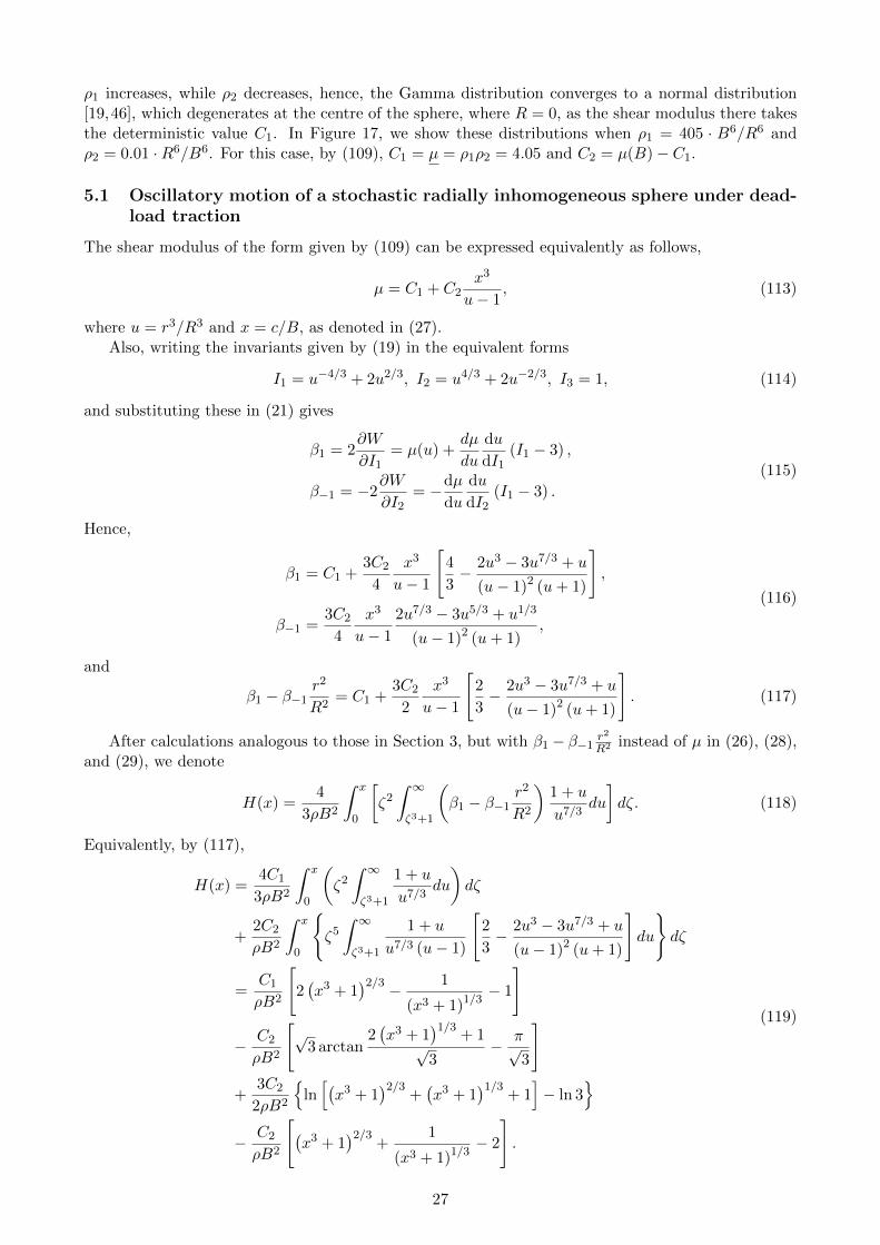
ρ1 increases, while ρ2 decreases, hence, the Gamma distribution converges to a normal distribution[19,46], which degenerates at the centre of the sphere, where R = 0, as the shear modulus there takesthe deterministic value C1. In Figure 17, we show these distributions when ρ1 = 405 · B6/R6 andρ2 = 0.01 ·R6/B6. For this case, by (109), C1 = µ = ρ1ρ2 = 4.05 and C2 = µ(B)− C1.

5.1 Oscillatory motion of a stochastic radially inhomogeneous sphere under dead-load traction

The shear modulus of the form given by (109) can be expressed equivalently as follows,

µ = C1 + C2x3

u− 1, (113)

where u = r3/R3 and x = c/B, as denoted in (27).Also, writing the invariants given by (19) in the equivalent forms

I1 = u−4/3 + 2u2/3, I2 = u4/3 + 2u−2/3, I3 = 1, (114)

and substituting these in (21) gives

β1 = 2∂W

∂I1= µ(u) +

dµ

du

du

dI1(I1 − 3) ,

β−1 = −2∂W

∂I2= −dµ

du

du

dI2(I1 − 3) .

(115)

Hence,

β1 = C1 +3C2

4

x3

u− 1

[4

3− 2u3 − 3u7/3 + u

(u− 1)2 (u+ 1)

],

β−1 =3C2

4

x3

u− 1

2u7/3 − 3u5/3 + u1/3

(u− 1)2 (u+ 1),

(116)

and

β1 − β−1r2

R2= C1 +

3C2

2

x3

u− 1

[2

3− 2u3 − 3u7/3 + u

(u− 1)2 (u+ 1)

]. (117)

After calculations analogous to those in Section 3, but with β1 − β−1 r2

R2 instead of µ in (26), (28),and (29), we denote

H(x) =4

3ρB2

∫ x

0

[ζ2∫ ∞ζ3+1

(β1 − β−1

r2

R2

)1 + u

u7/3du

]dζ. (118)

Equivalently, by (117),

H(x) =4C1

3ρB2

∫ x

0

(ζ2∫ ∞ζ3+1

1 + u

u7/3du

)dζ

+2C2

ρB2

∫ x

0

{ζ5∫ ∞ζ3+1

1 + u

u7/3 (u− 1)

[2

3− 2u3 − 3u7/3 + u

(u− 1)2 (u+ 1)

]du

}dζ

=C1

ρB2

[2(x3 + 1

)2/3 − 1

(x3 + 1)1/3− 1

]

− C2

ρB2

[√

3 arctan2(x3 + 1

)1/3+ 1

√3

− π√3

]

+3C2

2ρB2

{ln[(x3 + 1

)2/3+(x3 + 1

)1/3+ 1]− ln 3

}− C2

ρB2

[(x3 + 1

)2/3+

1

(x3 + 1)1/3− 2

].

(119)

27

Then, by setting the dead load (31) and substituting (119) in (37), we obtain

p0

[(x3 + 1

)1/3 − 1]

=C1

2

[2(x3 + 1

)2/3 − 1

(x3 + 1)1/3− 1

]

− C2

2

[√

3 arctan2(x3 + 1

)1/3+ 1

√3

− π√3

]

+3C2

4

{ln[(x3 + 1

)2/3+(x3 + 1

)1/3+ 1]− ln 3

}− C2

2

[(x3 + 1

)2/3+

1

(x3 + 1)1/3− 2

].

(120)

Equation (120) has a solution at x1 = 0, while the second solution, x2 > 0, is a root of

p0 =C1

2

[2(x3 + 1

)1/3+

1

(x3 + 1)1/3+ 2

]

− C2

2

[(x3 + 1

)1/3 − 1

(x3 + 1)1/3

].

(121)

To obtain the right-hand side of the above equation, we have assumed that, in (120), x is sufficientlysmall, such that, after expanding the respective functions to the second order in (x3 + 1)1/3,[

√3 arctan

2(x3 + 1

)1/3+ 1

√3

− π√3

] [(x3 + 1

)1/3 − 1]−1≈

3−(x3 + 1

)1/34

(122)

andln[(x3 + 1

)2/3+(x3 + 1

)1/3+ 1]− ln 3

(x3 + 1)1/3 − 1≈

7−(x3 + 1

)1/36

. (123)

Next, expanding the right-hand side of the equation (121) to the first order in x3 gives

p0 ≈5C1

2+x3

6(C1 − 2C2) . (124)

The critical dead load for the onset of cavitation is then

limx→0+

p0 =5C1

2, (125)

and is the same as for the homogeneous sphere made entirely from the material found at the centreof the inhomogeneous sphere.

Considering the parameters C1 and C2, we have the following two cases:

(i) When C1 > 2C2, the right-hand side in (124) is an increasing function of x, and therefore,

p0 >5C1

2. (126)

(ii) When C1 < 2C2, the right-hand side in (124) decreases as x increases, hence,

0 < p0 <5C1

2. (127)

However, since2p0ρB2

[(x3 + 1

)1/3 − 1]−H(x)

{< 0 if x1 < x < x2,> 0 if x > x2,

(128)

the sphere cannot oscillate.

28


[(x3 + 1


dynamic sphere of stochastic radially inhomogeneous neo-Hookean-like material under dead-load trac-tion, when ρ = 1, B = 1, and, for any fixed R, µ(R), given by (109), follows a Gamma distributionwith ρ1 = 405/R6 and ρ2 = 0.01 ·R6. The dashed black lines correspond to the expected values basedonly on mean parameter values. Each distribution was calculated from the average of 1000 stochasticsimulations.

In Figure 18, we illustrate the stochastic function H(x), defined by (119), intersecting the (dashed

red) curve 2p0ρB2

[(x3 + 1

)1/3 − 1], with p0 = 15, to find the two distinct solutions to (37), and the

associated velocity, given by (35), for a unit sphere (with B = 1) of stochastic radially inhomogeneousneo-Hookean-like material when the random field shear modulus µ(R) is given by (109), with ρ1 =405/R6 and ρ2 = 0.01 · R6 (see Figure 17). In particular, ρ1 = 405 and ρ2 = 0.01 at R = B, hence,by (109), C1 = µ = ρ1ρ2 = 4.05 and C2 = µ(B)− C1. For these functions, although the mean values,represented by black dashed lines, are the same as for those depicted in Figure 5, their stochasticbehaviours are quite different compared to the case of a stochastic neo-Hookean sphere. Specifically,as we observe from

5.2 Static deformation of a stochastic radially inhomogeneous sphere under dead-load traction

For the static inhomogeneous sphere, when the cavity surface is traction-free, at the outer surface, byanalogy to (49), and using (117), we have

Trr(b) =2

3

∫ ∞x3+1

(β1 − β−1

r2

R2

)1 + u

u7/3du

=2C1

3

∫ ∞x3+1

1 + u

u7/3du+ C2x

3

∫ ∞x3+1

1 + u

u7/3 (u− 1)

[2

3− 2u3 − 3u7/3 + u

(u− 1)2 (u+ 1)

]du.

(129)

Equivalently, after evaluating the integrals,

Trr(b) = 2C1

[1

(x3 + 1)1/3+

1

4 (x3 + 1)4/3

]

− C2

2x3

2(x3 + 1

)4/3+ 4

(x3 + 1

)+ 3

(x3 + 1

)2/3+ 2

(x3 + 1

)1/3+ 1

(x3 + 1)8/3 + 2 (x3 + 1)7/3 + 3 (x3 + 1)2 + 2 (x3 + 1)5/3 + (x3 + 1)4/3.

(130)

29

After multiplying by(x3 + 1

)2/3the above Cauchy stress, and denoting λb = b/B =

(x3 + 1

)1/3, the

required tensile dead load at the outer surface, R = B, in the reference configuration, takes the form

P = 2C1

(λb +

1

4λ2b

)− C2

2

(λ3b − 1

) 2λ4b + 4λ3b + 3λ2b + 2λb + 1

λ6b + 2λ5b + 3λ4b + 2λ3b + λ2b. (131)

The critical dead-load traction for the initiation of cavitation is

P0 = limλb→1

P =5C1

2=

5µ(0)

2, (132)

and is the same as for the homogeneous sphere made entirely from the material found at its centre [67],as found also for the dynamic sphere.

To examine the post-cavitation behaviour, we take the first derivative of P , given by (131), withrespect to λb,

dP

dλb= 2C1

(1− 1

2λ3b

)− 3C2

2

2λ4b + 4λ3b + 3λ2b + 2λb + 1

λ4b + 2λ3b + 3λ2b + 2λb + 1

− C2

(λ3b − 1

) 4λ3b + 6λ2b + 3λb + 1

λ6b + 2λ5b + 3λ4b + 2λ3b + λ2b

− C2

(λ3b − 1

) (2λ4b + 4λ3b + 3λ2b + 2λb + 1) (

3λ5b + 5λ4b + 6λ3b + 3λ2b + λb)(

λ6b + 2λ5b + 3λ4b + 2λ3b + λ2b)2 .

(133)

Letting λb → 1 in (133), we obtain

limλb→1

dP

dλb= C1 − 2C2. (134)

In Figure 19, we represent the scaled dead load, P/C2, with P given by (131) as a function of λb, andits derivative with respect to λb, for different values of the ratio C1/C2.

Figure 19: Examples of the scaled dead load, P/C2 (left), with P given by (131), and its derivativewith respect to λb (right), for a radially inhomogeneous sphere with different values of the ratio C1/C2.

The following two types of cavitated solution are now possible:

(i) If C1 > 2C2, or equivalently, if µ(B) = C1 + C2 < 3C1/2, then cavitation is stable;

(ii) If C1 < 2C2, or equivalently, if µ(B) = C1 + C2 > 3C1/2, then snap cavitation occurs.

30

Figure 20: Probability distributions of stable or unstable cavitation for a static stochastic sphere ofradially inhomogeneous neo-Hookean-like material, under dead-load traction, when µ(B) = C1 + C2,

given by (109), follows a Gamma distribution with ρ(1)1 = 405 and ρ

(1)2 = 0.01. Continuous coloured

lines represent analytically derived solutions, given by equations (135)-(136), and the dashed versionsrepresent stochastically generated data. The vertical line at the critical value, 2µ/3 = 2.7, separatesthe expected regions based only on mean value, µ = ρ1ρ2 = 4.05. The probabilities were calculatedfrom the average of 100 stochastic simulations.

Figure 21: Probability distribution of the applied dead-load traction, P , causing cavitation of radiusc in a radially inhomogeneous sphere, when ρ = 1, B = 1, and, for any fixed R, µ(R), given by (109),follows a Gamma distribution with ρ1 = 405/R6 and ρ2 = 0.01 ·R6. The dashed black line correspondsto the expected bifurcation based only on mean value, µ = C1 = 4.05.

31

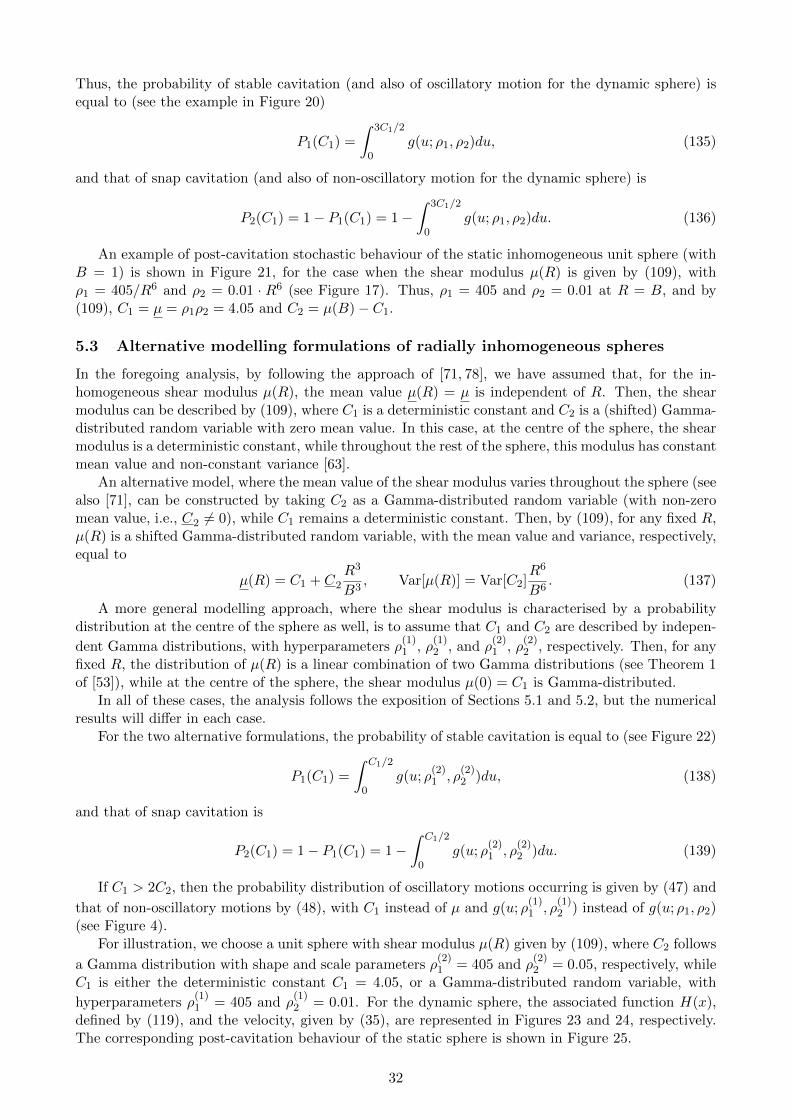
Thus, the probability of stable cavitation (and also of oscillatory motion for the dynamic sphere) isequal to (see the example in Figure 20)

P1(C1) =

∫ 3C1/2

0g(u; ρ1, ρ2)du, (135)

and that of snap cavitation (and also of non-oscillatory motion for the dynamic sphere) is

P2(C1) = 1− P1(C1) = 1−∫ 3C1/2

0g(u; ρ1, ρ2)du. (136)

An example of post-cavitation stochastic behaviour of the static inhomogeneous unit sphere (withB = 1) is shown in Figure 21, for the case when the shear modulus µ(R) is given by (109), withρ1 = 405/R6 and ρ2 = 0.01 · R6 (see Figure 17). Thus, ρ1 = 405 and ρ2 = 0.01 at R = B, and by(109), C1 = µ = ρ1ρ2 = 4.05 and C2 = µ(B)− C1.

5.3 Alternative modelling formulations of radially inhomogeneous spheres

In the foregoing analysis, by following the approach of [71, 78], we have assumed that, for the in-homogeneous shear modulus µ(R), the mean value µ(R) = µ is independent of R. Then, the shearmodulus can be described by (109), where C1 is a deterministic constant and C2 is a (shifted) Gamma-distributed random variable with zero mean value. In this case, at the centre of the sphere, the shearmodulus is a deterministic constant, while throughout the rest of the sphere, this modulus has constantmean value and non-constant variance [63].

An alternative model, where the mean value of the shear modulus varies throughout the sphere (seealso [71], can be constructed by taking C2 as a Gamma-distributed random variable (with non-zeromean value, i.e., C2 6= 0), while C1 remains a deterministic constant. Then, by (109), for any fixed R,µ(R) is a shifted Gamma-distributed random variable, with the mean value and variance, respectively,equal to

µ(R) = C1 + C2

R3

B3, Var[µ(R)] = Var[C2]

R6

B6. (137)

A more general modelling approach, where the shear modulus is characterised by a probabilitydistribution at the centre of the sphere as well, is to assume that C1 and C2 are described by indepen-

dent Gamma distributions, with hyperparameters ρ(1)1 , ρ

(1)2 , and ρ

(2)1 , ρ

(2)2 , respectively. Then, for any

fixed R, the distribution of µ(R) is a linear combination of two Gamma distributions (see Theorem 1of [53]), while at the centre of the sphere, the shear modulus µ(0) = C1 is Gamma-distributed.

In all of these cases, the analysis follows the exposition of Sections 5.1 and 5.2, but the numericalresults will differ in each case.

For the two alternative formulations, the probability of stable cavitation is equal to (see Figure 22)

P1(C1) =

∫ C1/2

0g(u; ρ

(2)1 , ρ

(2)2 )du, (138)

and that of snap cavitation is

P2(C1) = 1− P1(C1) = 1−∫ C1/2

0g(u; ρ

(2)1 , ρ

(2)2 )du. (139)

If C1 > 2C2, then the probability distribution of oscillatory motions occurring is given by (47) and

that of non-oscillatory motions by (48), with C1 instead of µ and g(u; ρ(1)1 , ρ

(1)2 ) instead of g(u; ρ1, ρ2)

(see Figure 4).For illustration, we choose a unit sphere with shear modulus µ(R) given by (109), where C2 follows

a Gamma distribution with shape and scale parameters ρ(2)1 = 405 and ρ

(2)2 = 0.05, respectively, while

C1 is either the deterministic constant C1 = 4.05, or a Gamma-distributed random variable, with

hyperparameters ρ(1)1 = 405 and ρ

(1)2 = 0.01. For the dynamic sphere, the associated function H(x),

defined by (119), and the velocity, given by (35), are represented in Figures 23 and 24, respectively.The corresponding post-cavitation behaviour of the static sphere is shown in Figure 25.

32

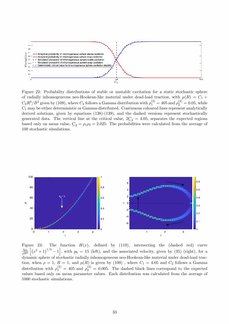
Figure 22: Probability distributions of stable or unstable cavitation for a static stochastic sphereof radially inhomogeneous neo-Hookean-like material under dead-load traction, with µ(R) = C1 +

C2R3/B3 given by (109), where C2 follows a Gamma distribution with ρ

(2)1 = 405 and ρ

(2)2 = 0.05, while

C1 may be either deterministic or Gamma-distributed. Continuous coloured lines represent analyticallyderived solutions, given by equations (138)-(139), and the dashed versions represent stochasticallygenerated data. The vertical line at the critical value, 2C2 = 4.05, separates the expected regionsbased only on mean value, C2 = ρ1ρ2 = 2.025. The probabilities were calculated from the average of100 stochastic simulations.


[(x3 + 1


dynamic sphere of stochastic radially inhomogeneous neo-Hookean-like material under dead-load trac-tion, when ρ = 1, B = 1, and µ(R) is given by (109) , where C1 = 4.05 and C2 follows a Gamma

distribution with ρ(2)1 = 405 and ρ

(2)2 = 0.005. The dashed black lines correspond to the expected

values based only on mean parameter values. Each distribution was calculated from the average of1000 stochastic simulations.

33


[(x3 + 1


dynamic sphere of stochastic radially inhomogeneous neo-Hookean-like material under dead-load trac-tion, when ρ = 1, B = 1, and µ(R) is given by (109) , where C1 follows a Gamma distribution with

ρ(1)1 = 405 and ρ

(1)2 = 0.01, while C2 follows a Gamma distributions with ρ

(2)1 = 405 and ρ

(2)2 = 0.005.

The dashed black lines correspond to the expected values based only on mean parameter values. Eachdistribution was calculated from the average of 1000 stochastic simulations.

Figure 25: Probability distribution of the applied dead-load traction, P , causing cavitation of radiusc in a radially inhomogeneous sphere, when ρ = 1, B = 1, and µ(R) is given by (109), where C2

follows a Gamma distribution with ρ(2)1 = 405 and ρ

(2)2 = 0.05, while C1 = 4.05 (left), or C1 follows

a Gamma distribution with ρ(1)1 = 405 and ρ

(1)2 = 0.01 (right). The dashed black line corresponds to

the expected bifurcation based only on mean value parameters.

34

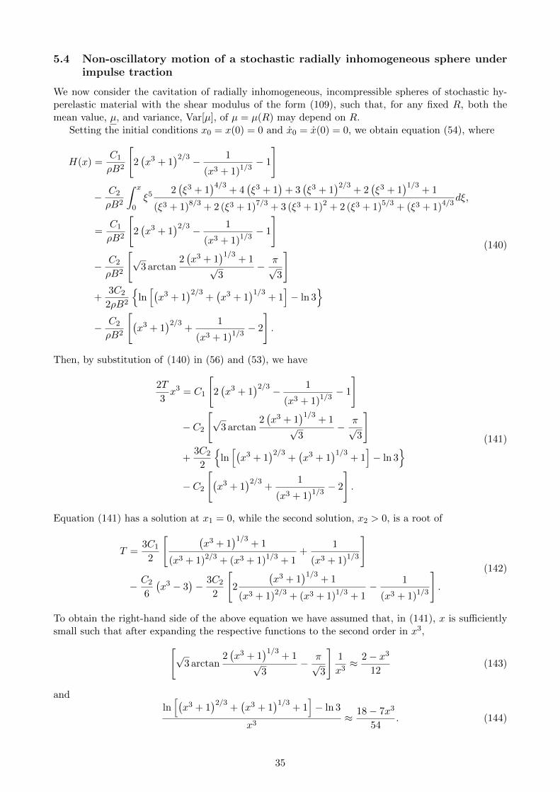
5.4 Non-oscillatory motion of a stochastic radially inhomogeneous sphere underimpulse traction

We now consider the cavitation of radially inhomogeneous, incompressible spheres of stochastic hy-perelastic material with the shear modulus of the form (109), such that, for any fixed R, both themean value, µ, and variance, Var[µ], of µ = µ(R) may depend on R.

Setting the initial conditions x0 = x(0) = 0 and x0 = x(0) = 0, we obtain equation (54), where

H(x) =C1

ρB2

[2(x3 + 1

)2/3 − 1

(x3 + 1)1/3− 1

]

− C2

ρB2

∫ x

0ξ5

2(ξ3 + 1

)4/3+ 4

(ξ3 + 1

)+ 3

(ξ3 + 1

)2/3+ 2

(ξ3 + 1

)1/3+ 1

(ξ3 + 1)8/3 + 2 (ξ3 + 1)7/3 + 3 (ξ3 + 1)2 + 2 (ξ3 + 1)5/3 + (ξ3 + 1)4/3dξ,

=C1

ρB2

[2(x3 + 1

)2/3 − 1

(x3 + 1)1/3− 1

]

− C2

ρB2

[√

3 arctan2(x3 + 1

)1/3+ 1

√3

− π√3

]

+3C2

2ρB2

{ln[(x3 + 1

)2/3+(x3 + 1

)1/3+ 1]− ln 3

}− C2

ρB2

[(x3 + 1

)2/3+

1

(x3 + 1)1/3− 2

].

(140)

Then, by substitution of (140) in (56) and (53), we have

2T

3x3 = C1

[2(x3 + 1

)2/3 − 1

(x3 + 1)1/3− 1

]

− C2

[√

3 arctan2(x3 + 1

)1/3+ 1

√3

− π√3

]

+3C2

2

{ln[(x3 + 1

)2/3+(x3 + 1

)1/3+ 1]− ln 3

}− C2

[(x3 + 1

)2/3+

1

(x3 + 1)1/3− 2

].

(141)

Equation (141) has a solution at x1 = 0, while the second solution, x2 > 0, is a root of

T =3C1

2

[ (x3 + 1

)1/3+ 1

(x3 + 1)2/3 + (x3 + 1)1/3 + 1+

1

(x3 + 1)1/3

]

− C2

6

(x3 − 3

)− 3C2

2

[2

(x3 + 1

)1/3+ 1

(x3 + 1)2/3 + (x3 + 1)1/3 + 1− 1

(x3 + 1)1/3

].

(142)

To obtain the right-hand side of the above equation we have assumed that, in (141), x is sufficientlysmall such that after expanding the respective functions to the second order in x3,[

√3 arctan

2(x3 + 1

)1/3+ 1

√3

− π√3

]1

x3≈ 2− x3

12(143)

andln[(x3 + 1

)2/3+(x3 + 1

)1/3+ 1]− ln 3

x3≈ 18− 7x3

54. (144)

35

Next, expanding the right-hand side of the equation (142) to first order in x3 gives

T ≈ 5C1

2− x3

3(2C1 + C2) . (145)

The critical dead load for the onset of cavitation is then

T0 = limx→0+

T =5C1

2, (146)

and is the same as for the homogeneous sphere made entirely from the material found at the centreof the inhomogeneous sphere.

Noting that 2C1 + C2 = µ(0) + µ(B) > 0, the right-hand side in (145) decreases as x increases,hence,

0 < T <5C1

2, (147)

or equivalently, by (53),

0 < p0 <5C1

ρB2. (148)

However,2p0ρB2

x3 −H(x)

{< 0 if x1 < x < x2,> 0 if x > x2,

(149)

and the sphere cannot oscillate.

5.5 Static deformation of a stochastic radially inhomogeneous sphere under im-pulse traction

For the static inhomogeneous sphere, when the cavity surface is traction-free, at the outer surface, thetensile traction takes the form

T = 2C1

[1

(x3 + 1)1/3+

1

4 (x3 + 1)4/3

]

− C2

2x3

2(x3 + 1

)4/3+ 4

(x3 + 1

)+ 3

(x3 + 1

)2/3+ 2

(x3 + 1

)1/3+ 1

(x3 + 1)8/3 + 2 (x3 + 1)7/3 + 3 (x3 + 1)2 + 2 (x3 + 1)5/3 + (x3 + 1)4/3.

(150)

Denoting λb = b/B =(x3 + 1

)1/3, the required tensile load at the outer surface, R = B, can be

written equivalently as follows,

T = 2C1

(1

λb+

1

4λ4b

)− C2

2

(λ3b − 1

) 2λ4b + 4λ3b + 3λ2b + 2λb + 1

λ8b + 2λ7b + 3λ6b + 2λ5b + λ4b. (151)

Thus the critical load for the initiation of cavitation is

T0 = limλb→1

T =5C1

2=

5µ(0)

2, (152)

and is the same as for the homogeneous sphere made entirely from the material found at its centre,as found also for the dynamic sphere.

To examine the post-cavitation behaviour, we take the first derivative of T , given by (151), withrespect to λb,

dT

dλb= −2C1

(1

λ2b+

1

λ5b

)− 3C2

2

2λ4b + 4λ3b + 3λ2b + 2λb + 1

λ6b + 2λ5b + 3λ4b + 2λ3b + λ2b

− C2

(λ3b − 1

) 4λ3b + 6λ2b + 3λb + 1

λ8b + 2λ7b + 3λ6b + 2λ5b + λ4b

− C2

(λ3b − 1

) (2λ4b + 4λ3b + 3λ2b + 2λb + 1) (

4λ7b + 7λ6b + 9λ5b + 5λ4b + 2λ3b)(

λ8b + 2λ7b + 3λ6b + 2λ5b + λ4b)2 .

(153)

36

Figure 26: Probability distribution of the applied impulse traction, T , causing cavitation of radius cin a radially inhomogeneous sphere, when ρ = 1, B = 1, and, for any fixed R, µ(R), given by (109),follows a Gamma distribution with ρ1 = 405/R6 and ρ2 = 0.01 ·R6. The dashed black line correspondsto the expected bifurcation based only on mean value, µ = C1 = 4.05.

Figure 27: Probability distribution of the applied impulse traction, T , causing cavitation of radiusc in a radially inhomogeneous sphere, when ρ = 1, B = 1, and µ(R) is given by (109), where C2

follows a Gamma distribution with ρ(2)1 = 405 and ρ

(2)2 = 0.05, while C1 = 4.05 (left), or C1 follows

a Gamma distribution with ρ(1)1 = 405 and ρ

(1)2 = 0.01 (right). The dashed black line corresponds to

the expected bifurcation based only on mean value parameters.

37

Letting λb → 1 in (153), we obtain

limλb→1

dT

dλb= −4C1 − 2C2 = −2C1 − 2 (C1 + C2) = −2µ(0)− 2µ(B) < 0. (154)

Hence, only snap cavitation can occur.In Figures 26 and 27, we show examples of post-cavitation stochastic behaviour of the static

inhomogeneous unit sphere (with B = 1).

6 Conclusion

We have presented here a theoretical study of static and dynamic cavitation, and possible oscillatorymotions, of homogeneous spheres of stochastic neo-Hookean material, of composite spheres with twoconcentric stochastic neo-Hookean phases, and of inhomogeneous spheres of neo-Hookean-like materialwith the material parameter varying continuously in the radial direction. For these materials, theelastic parameters are either spatially-independent random variables, or spatially-dependent randomfields, described by Gamma probability density functions at a continuum level.

In our approach, the radially-symmetric dynamic deformation of each sphere was treated as a quasi-equilibrated motion. Then, the static deformation was examined by reducing the quasi-equilibratedmotion to a static equilibrium state. Universally, we find that the critical load at which a nontrivialcavitated solution appears is the same as for the homogeneous sphere composed entirely of the materialfound at its centre. However, there are important differences in the post-cavitation behaviours underthe different constitutive formulations and loading conditions. These different conditions give us avariety of different behaviours, specifically:

• For a neo-Hookean sphere, cavitation is stable and the motion is oscillatory under dead-loadtraction, while under the impulse traction, cavitation is unstable and the radial motion is non-oscillatory;

• In composite spheres with two concentric neo-Hookean phases subject to either dead-load orimpulse traction, both stable and unstable cavitation can be obtained, depending on the materialparameters of the two phases. However, oscillatory motion only occurs when cavitation is stableunder dead-load traction;

• For radially inhomogeneous spheres under dead-load traction, both stable and unstable cavita-tion occur, and oscillatory motion is found when cavitation is stable under dead-load traction.Under impulse traction, cavitation is unstable and the motion is non-oscillatory.

Usually, in many application areas, the Gaussian (normal) distribution is assumed to describe therandom variation that occurs in the available data. However, many material measurements show askewed distribution where mean values are low, variances are large, and values cannot be negative(see, e.g., [19]). These are important features of the data that need to be incorporated in models. Forsmall variability, the Gaussian and Gamma distributions both fit well to experimental data collectedfrom material tests [19, 46]. This guides us to choose the distribution that is adequate also for casesexhibiting large variability, i.e., the Gamma distribution. If the data cannot be smaller than a certainbound different from zero, then a shift parameter can be incorporated to define a three-parameterdistribution. To compare directly our stochastic results with the deterministic ones, we sampled fromdistributions where the parameters were set to have mean values corresponding to the deterministicsystem. Thus, the mean value of the distribution is guaranteed to converge to the expected value.

We found that, in contrast to the deterministic problem where a single critical value strictlyseparates the stable and unstable cases, for the stochastic problem, there is a probabilistic intervalwhere the stable and unstable states compete, in the sense that both have a quantifiable chance tobe obtained with a given probability. This means that solutions exist in the stochastic case wheredeterministically they should not. Generally, for the stochastic solution, the variance changes non-uniformly around the mean value, suggesting that, as the variance increases, the average value becomes

38

less significant from the physical point of view. A natural question that is yet to be consider is: whatis the effect of individual parameters on the variance in the stochastic solution?

For the finite dynamic deformations, attention was given to the periodic (oscillatory) motion andthe time-dependent stresses, while taking into account the stochastic model parameters. In this case,the amplitude and period of the oscillation of the stochastic bodies are characterised by probabilitydistributions, and there is a parameter interval where both the oscillatory and non-oscillatory motionscan occur with a given probability. For the oscillating spheres, a cavity would form and expand untilits radius reaches a maximum value, then contract again to zero periodically. An immediate extensionof this could be to consider similar spheres where there is pressure at the cavity surface as well.

One could also apply the stochastic approach to the dynamic cavitation of spheres where the‘base’ neo-Hookean material is replaced, for example, by a material with the following strain-energyfunction [48],

W(λ1, λ2, λ3) =µ1

2m2

(λ2m1 + λ2m2 + λ2m3 − 3

)+

µ22n2

(λ2n1 + λ2n2 + λ2n3 − 3

), (155)

where the exponents m and n are fixed, and the coefficients µ1 and µ2 are given, such that the shearmodulus in infinitesimal deformation satisfies µ = µ1 +µ2 > 0. As is well know, in this case, assumingthat the BE inequalities (1) hold, cavitation occurs if and only if [7, 12,32,48]

−3

4< m,n <

3

2. (156)

Therefore, cavitation is expected in a neo-Hookean sphere (with m = 1 and n = 0), but not in aMooney-Rivlin sphere (with m = 1 and n = −1). The cases where m ∈ {−1/2, 1} and n = 0 arediscussed also as particular examples in [7], and the spheres where m ∈ {1/2, 3/4, 1, 5/4} and n = 0are analysed explicitly in [12]. For these well-behaved spheres, under uniform dead-load traction, thecavitated solution is always stable, and it makes little difference whether the model coefficients arestochastic or not, although, in the stochastic case, the solution appears somewhat ’hazy’ (albeit withthe variance changing non-uniformly) around the mean value [48].

Similarly, for a sphere made of a material described by (155) subject to uniform radial impulsetraction, if the BE inequalities and (156) are satisfied, then cavitation always occurs and making themodel parameters stochastic only generates some dispersion around the usual deterministic solution.However, in this sphere, cavitation can also happen through a subcritical bifurcation where unstable(snap) cavitation takes place for values less than the critical dead load that causes cavitation. Hence,a sudden jump to a cavitated solution with a finite internal radius can be observed. For example,when the strain-energy density takes the form [48]

W(λ1, λ2, λ3) =µ12

(λ21 + λ22 + λ23 − 3

)+ 2µ2

(λ−11 + λ−12 + λ−13 − 3

), (157)

both stable and unstable cavitation can occur, depending on the values of the material coefficients µ1and µ2 (see Figure 3 of [48]). Then, in a stochastic sphere, the stable and unstable cases compete [48].

We further note that the theorem on quasi-equilibrated motion cannot be applied when the mate-rial is compressible [82, pp. 208-209]. As our analysis relies on the notion of quasi-equilibrated motion,the same approach cannot be employed for compressible spheres. However, while stochastic versions ofcompressible hyperelastic materials can also be constructed [76], there are not many theoretical resultsavailable on oscillatory motions of finitely deformed compressible hyperelastic spheres [2]. Neverthe-less, elastodynamic problems involving more complex constrained, or unconstrained materials, canstill be formulated, where the motion is not quasi-equilibrated, and the corresponding solution canthen be tackled computationally. More generally, radial asymmetry, various behaviour laws, with orwithout damping, and thermal effects may also be of great theoretical and physical interest.

Acknowledgement. The support by the Engineering and Physical Sciences Research Council ofGreat Britain under research grants EP/R020205/1 to Alain Goriely and EP/S028870/1 to L. AngelaMihai is gratefully acknowledged.

39

References

[1] Abramowitz M, Stegun IA. 1964. Handbook of Mathematical Functions with Formulas, Graphs,and Mathematical Tables, National Bureau of Standards, Applied Mathematics Series, vol. 55,Washington.

[2] Akyuz U, Ertepinar A. 1998. Stability and asymmetric vibrations of pressurized compressiblehyperelastic cylindrical shells, International Journal of Non-Linear Mechanics 34, 391-404.

[3] Aranda-Iglesias D, Vadillo G, Rodrıguez-Martnez JA. 2015. Constitutive sensitivity of the oscilla-tory behaviour of hyperelastic cylindrical shells, Journal of Sound and Vibration 358, 199-216.

[4] Aranda-Iglesias D, Rodrıguez-Martnez JA, Rubin MB. 2018. Nonlinear axisymmetric vibrations ofa hyperelastic orthotropic cylinders, International Journal of Non-Linear Mechanics 99, 131-143.

[5] Baker M, Ericksen JL. 1954. Inequalities restricting the form of stress-deformation relations forisotropic elastic solids and Reiner-Rivlin fluids, Journal of the Washington Academy of Sciences44, 24-27.

[6] Balakrishnan R, Shahinpoor M. 1978. Finite amplitude oscillations of a hyperelastic sphericalcavity, International Journal of Non-Linear Mechanics 13, 171-176.

[7] Ball JM. 1982. Discontinuous equilibrium solutions and cavitation in nonlinear elasticity, Philo-sophical Transactions of the Royal Society A 306, 557-611.

[8] Bayes T. 1763. An essay toward solving a problem in the doctrine of chances, Philosophical Trans-actions of the Royal Society 53, 370-418.

[9] Beatty MF. 2007. On the radial oscillations of incompressible, isotropic, elastic and limited elasticthick-walled tubes, International Journal of Non-Linear Mechanics 42, 283-297.

[10] Beatty MF. 2011. Small amplitude radial oscillations of an incompressible, isotropic elastic spher-ical shell, Mathematics and Mechanics of Solids 16, 492-512.

[11] Calderer C. 1983. The dynamical behaviour of nonlinear elastic spherical shells, Journal of Elas-ticity 13, 17-47.

[12] Chou-Wang M-S, Horgan CO. 1989. Void nucleation and growth for a class of incompressiblenonfinearly elastic materials, International Journal of Solids and Structures 25, 1239-1254.

[13] Chou-Wang M-S, Horgan CO.1989. Cavitation in nonlinear elastodynamics for neo-Hookean ma-terials, International Journal of Engineering Science 27, 967-973.

[14] Cidonio G, Glinka M, Dawson JI, Oreffo ROC. 2019. The cell in the ink: Improvingbiofabrication by printing stem cells for skeletal regenerative medicine, Biomaterials, doi:10.1016/j.biomaterials.2019.04.009.

[15] De Pascalis R, Parnell WJ, Abrahams ID, Shearer T, Daly DM, Grundy D. 2018. The inflationof viscoelastic balloons and hollow viscera, Proceedings of the Royal Society A 474, 20180102.

[16] DeSimone A, Teresi L. 2009. Elastic energies for nematic elastomers, The European PhysicalJournal E 29, 191-204.

[17] Elishakoff I, Soize C (eds). 2012. Nondeterministic Mechanics, Springer, New York.

[18] Ertepinar A, Akay HU. 1976. Radial oscillations of nonhomogeneous, thick-walled cylindrical andspherical shells subjected to finite deformations, International Journal of Solids and Structures 12,517-524.

40

[19] Fitt D, Wyatt H, Woolley TE, Mihai LA. 2019. Uncertainty quantification of elastic materialresponses: testing, stochastic calibration and Bayesian model selection, Mechanics of Soft Materials(doi: 10.1007/s42558-019-0013-1).

[20] Fond, C. 2001. Cavitation criterion for rubber materials: a review of void-growth models, Journalof Polymer Science: Part B 39, 2081-2096.

[21] Freiling C. 1986. Axioms of symmetry: Throwing darts at the real number line, The Journal ofSymbolic Logic 51(1), 190-200.

[22] Fried E, Sellers S. 2004. Free-energy density functions for nematic elastomers, Journal of Mechan-ics and Physics of Solids 52, 1671-1689.

[23] Gent AN. 1991. Cavitation in rubber: a cautionary tale, Rubber Chemistry and Technology 63,G49-G53.

[24] Gent AN, Lindley PB. 1959. Internal rupture of bonded rubber cylinders in tension, Proceedingsof the Royal Society of London A 249, 195-205.

[25] Ghanem R, Higdon D, Owhadi H (Eds.). 2017. Handbook of Uncertainty Quantification, Springer,New-York, 2017.

[26] Goriely A. 2017. The Mathematics and Mechanics of Biological Growth, Springer-Verlag, NewYork.

[27] Green AE, Adkins JE. 1970. Large Elastic Deformations (and Non-linear Continuum Mechanics),2nd ed, Oxford University Press, Oxford.

[28] Grimmett GR, Stirzaker DR. 2001. Probability and Random Processes, 3rd ed, Oxford UniversityPress, Oxford.

[29] Heng GZ, Solecki R. 1963. Free and forced finite amplitude oscillations of an elastic thick-walledhollow sphere made of incompressible material, Archiwum Mechaniki Stosowanej 3, 427-433.

[30] Holmes DP. 2019. Elasticity and stability of shape-shifting structures, Current Opinion in Colloid& Interface Science 40, 118-137.

[31] Horgan CO, Pence TJ. 1989. Cavity formation at the center of a composite incompressible non-linearly elastic sphere, Journal of Applied Mechanics 56, 302-308.

[32] Horgan CO, Polignone DA. 1995. Cavitation in nonlinearly elastic solids: a review, AppliedMechanics Reviews 48, 471-485.

[33] Hughes I, Hase TPA. 2010. Measurements and Their Uncertainties: A Practical Guide to ModernError Analysis, Oxford University Press, Oxford.

[34] Hutchens SB, Fakhouri S, Crosby AJ. 2016. Elastic cavitation and fracture via injection, SoftMatter 12, 2557.

[35] Jaynes ET. 1957. Information theory and statistical mechanics i, Physical Review 108, 171-190.

[36] Jaynes ET. 1957. Information theory and statistical mechanics ii, Physical Review 106, 620-630.

[37] Jaynes ET. 2003. Probability Theory: The Logic of Science, Cambridge University Press, Cam-bridge, UK.

[38] Johnson NL, Kotz S, Balakrishnan N. 1994. Continuous Univariate Distributions, Vol 1, 2ndedition, John Wiley & Sons, New York.

[39] Kaminski M, Lauke B. 2018. Probabilistic and stochastic aspects of rubber hyperelasticity, Mec-canica 53, 2363-2378.

41

[40] Kang J, Wang C, Tan H. 2018. Cavitation in inhomogeneous soft solids, Soft Matter 14,7979-7986.

[41] Knowles JK. 1960. Large amplitude oscillations of a tube of incompressible elastic material,Quarterly of Applied Mathematics 18, 71-77.

[42] Knowles JK. 1962. On a class of oscillations in the finite-deformation theory of elasticity, Journalof Applied Mechanics 29, 283-286.

[43] Knowles JK, Jakub MT. 1965. Finite dynamic deformations of an incompressible elastic mediumcontaining a spherical cavity, Archive of Rational Mechanics and Analysis 18, 376-387.

[44] Marzano M. 1983. An interpretation of Baker-Ericksen inequalities in uniaxial deformation andstress, Meccanica 18, 233-235.

[45] McGrayne SB. 2012. The Theory That Would Not Die: How Bayes’ Rule Cracked the EnigmaCode, Hunted Down Russian Submarines, an Emerged Triumphant from Two Centuries of Con-troversy, Paperback ed., Yale University Press, New Haven.

[46] Mihai LA, Fitt D, Woolley TE, Goriely A. 2019. Likely equilibria of stochastic hyperelas-tic spherical shells and tubes, Mathematics and Mechanics of Solids, 24(7), 2066-2082 (doi:10.1177/1081286518811881).

[47] Mihai LA, Fitt D, Woolley TE, Goriely A. 2019. Likely oscillatory motions of stochastic hyper-elastic solids, Transactions of Mathematics and Its Applications 3(1), tnz003 (doi: 10.1093/ima-trm/tnz003).

[48] Mihai LA, Fitt D, Woolley TE, Goriely A. 2019. Likely cavitation in stochastic elasticity, Journalof Elasticity 137(1), 27-42 (doi: 10.1007/s10659-018-9706-1).

[49] Mihai LA, Goriely A. 2017. How to characterize a nonlinear elastic material? A review onnonlinear constitutive parameters in isotropic finite elasticity, Proceedings of the Royal Society A473, 20170607 (doi: 10.1098/rspa.2017.0607).

[50] Mihai LA, Woolley TE, Goriely A. 2018. Stochastic isotropic hyperelastic materials: constitutivecalibration and model selection, Proceedings of the Royal Society A 474, 20170858.

[51] Mihai LA, Woolley TE, Goriely A. 2019. Likely equilibria of the stochastic Rivlin cube, Philo-sophical Transactions of the Royal Society A 377, 20180068 (doi: 10.1098/rsta.2018.0068).

[52] Mihai LA, Woolley TE, Goriely A. 2019. Likely chirality of stochastic anisotropichyperelastic tubes, International Journal of Non-Linear Mechanics 114, 9-20 (doi:10.1016/j.ijnonlinmec.2019.04.004).

[53] Moschopoulos PG. 1985. The distribution of the sum of independent Gamma random variables37, 541-544.

[54] Mumford D. 2000. The dawning of the age of stochasticity, Mathematics: Frontiers and Perspec-tives, V. Arnold, M. Atiyah, P. Lax, B. Mazur (eds.), American Mathematical Society, 197-218.

[55] Oden JT. 2018. Adaptive multiscale predictive modelling, Acta Numerica 27, 353-450.

[56] Ogden RW. 1997. Non-Linear Elastic Deformations, 2nd ed, Dover, New York.

[57] Ostoja-Starzewski M. 2007. Microstructural Randomness and Scaling in Mechanics of Materials,Chapman and Hall, CRC Press.

[58] Poulain X, Lefevre V, Lopez-Pamies O, Ravi-Chandar K. 2017. Damage in elastomers: nucleationand growth of cavities, micro-cracks, and macro-cracks, International Journal of Fracture 205, 1-21.

[59] Poulain X, Lopez-Pamies O, Ravi-Chandar K. 2018. Damage in elastomers: Healing of internallynucleated cavities and micro-cracks, Soft Matter 14, 4633-4640.

42

[60] Raayai-Ardakani S, Earla DR, Cohen T. 2019. The intimate relationship between cavitation andfracture, Soft Matter 15, 4999.

[61] Ren J.-s.. 2008. Dynamical response of hyper-elastic cylindrical shells under periodic load, AppliedMathematics and Mechanics 29, 1319-1327.

[62] Ren J.-s.. 2009. Dynamics and destruction of internally pressurized incompressible hyper-elasticspherical shells, International Journal of Engineering Science 47, 745-753.

[63] Riggs JD, Lalonde TL. 2017. Handbook for Applied Modeling: Non-Gaussian and CorrelatedData, Cambridge University Press, Cambridge, UK.

[64] Robert CP. 2007. The Bayesian Choice: From Decision-Theoretic Foundations to ComputationalImplementation, 2nd ed, Springer, New York.

[65] Rodriıguez-Martiınez JA, Fernandez-Saaez J, aera R. 2015. The role of constitutive relation inthe stability of hyper-elastic spherical membranes subjected to dynamic inflation, InternationalJournal of Engineering Science 93, 31-45.

[66] Shannon CE. 1948. A mathematical theory of communication, Bell System Technical Journal 27,379-423, 623-659.

[67] Sivaloganathan, I. 1991. Cavitation, the incompressible limit, and material inhomogeneity, Quar-terly of Applied Mathematics 49, 521-541.

[68] Soares RM, Amaral PFT, Silva FMA, Goncalves PB. 2019. Nonlinear breathing motions andinstabilities of a pressure-loaded spherical hyperelastic membrane, Nonlinear Dynamics 1-22 (doi:10.1007/s11071-019-04855-4).

[69] Soize C. 2000. A nonparametric model of random uncertainties for reduced matrix models instructural dynamics, Probabilistic Engineering Mechanics 15, 277-294.

[70] Soize C. 2001. Maximum entropy approach for modeling random uncertainties in transient elas-todynamics, Journal of the Acoustical Society of America 109, 1979-1996.

[71] Soize C. 2006. Non-Gaussian positive-definite matrix-valued random fields for elliptic stochasticpartial differential operators, Computer Methods in Applied Mechanics and Engineering 195, 26-64.

[72] Soize C. 2013. Stochastic modeling of uncertainties in computational structural dynamics - Recenttheoretical advances, Journal of Sound and Vibration 332, 2379-2395.

[73] Soize C. 2017. Uncertainty Quantification: An Accelerated Course with Advanced Applications inComputational Engineering, Interdisciplinary Applied Mathematics Book 47, Springer, New York.

[74] Soni J, Goodman R. 2017. A Mind at Play: How Claude Shannon Invented the Information Age,Simon & Schuster, New York.

[75] Staber B, Guilleminot J. 2015. Stochastic modeling of a class of stored energy functions forincompressible hyperelastic materials with uncertainties, Comptes Rendus Mecanique 343, 503-514.

[76] Staber B, Guilleminot J. 2016. Stochastic modeling of the Ogden class of stored energy functionsfor hyperelastic materials: the compressible case, Journal of Applied Mathematics and Mechan-ics/Zeitschrift fur Angewandte Mathematik und Mechanik 97, 273-295.

[77] Staber B, Guilleminot J. 2017. Stochastic hyperelastic constitutive laws and identification pro-cedure for soft biological tissues with intrinsic variability, Journal of the Mechanical Behavior ofBiomedical Materials 65, 743-752.

43

[78] Staber B, Guilleminot J. 2018. A random field model for anisotropic strain energy functions andits application for uncertainty quantification in vascular mechanics, Computer Methods in AppliedMechanics and Engineering 333, 94-113.

[79] Staber B, Guilleminot J, Soize C, Michopoulos J, Iliopoulos A. 2019. Stochastic modeling andidentification of an hyperelastic constitutive model for laminated composites, Computer Methodsin Applied Mechanics and Engineering 347, 425-444.

[80] Sullivan TJ. 2015. Introduction to Uncertainty Quantification, Springer-Verlag, New York.

[81] Truesdell C. 1962. Solutio generalis et accurata problematum quamplurimorum de motu corporumelasticorum incomprimibilium in deformationibus valde magnis, Archive of Rational Mechanics andAnalysis 11, 106-113.

[82] Truesdell C, Noll W. 2004. The Non-Linear Field Theories of Mechanics, 3rd ed, Springer-Verlag,New York.

[83] Verron E, Khayat RE, Derdouri A, Peseux B. 1999. Dynamic inflation of hyperelastic sphericalmembranes, Journal of Rheology 43, 1083-1097.

[84] Wang CC. 1965. On the radial oscillations of a spherical thin shell in the finite elasticity theory,Quarterly of Applied Mathematics 23, 270-274.

[85] Wang CC, Ertepinar A. 1972. Stability and vibrations of elastic thick-walled cylindrical andspherical shells subjected to pressure, International Journal of Non-Linear Mechanics 7, 539-555.

[86] Warner M, Terentjev EM. 2007. Liquid Crystal Elastomers, paper back, Oxford University Press,Oxford, UK.

44

Likely cavitation and radial motion of stochastic elastic spheres

Documents

Transcript of Likely cavitation and radial motion of stochastic elastic spheres