Cross-axis sensitivity of accelerographs with pendulum like transducers—mathematical model and the...

EARTHQUAKE ENGINEERING AND STRUCTURAL DYNAMICS

Earthquake Engng. Struct. Dyn. 27, 1031–1051 (1998)

CROSS-AXIS SENSITIVITY OF ACCELEROGRAPHS WITHPENDULUM LIKE TRANSDUCERS—MATHEMATICAL MODEL

AND THE INVERSE PROBLEM

MARIA I. TODOROVSKA ∗

Civil and Environmental Engineering Department, University of Southern California, Los Angeles, CA 90089-2531, U.S.A.

SUMMARY

A mathematical model for a three-component accelerograph is presented that accounts for the e�ects of transducer mis-alignment and cross-axis sensitivity. The former refers to departures in the alignment of the transducer penduli (typicallyof the order of few degrees) from an ideal orthogonal system, and the latter to a transducer recording components ofmotion in directions other than its principal sensitivity axis. Transducer misalignment magni�es the e�ects of cross-axissensitivity. These e�ects are signi�cant only for large amplitude recordings (peak acceleration close to 1g), for examplein the near-�eld of the 1994 Northridge, California, earthquake. The misalignment angles and the angular ampli�cationconstant can be determined by a static tilt test, performed in the �eld, and solving a generalized inverse problem. Thispaper presents an algorithm for solution of this inverse problem on a routine basis. Practical implementation of the algo-rithm and results for 76 instruments of the Los Angeles Strong Motion Array are presented in a separate paper. ? 1998John Wiley & Sons, Ltd.

KEY WORDS: instrumentation; accelerographs; strong earthquake motion recording; data processing; instrument correction;cross-axis sensitivity; misalignment

INTRODUCTION

Accurate recording and processing1;2 of strong earthquake motion in the free-�eld and in structures is impor-tant for a variety of studies in earthquake engineering and engineering seismology (e.g., earthquake sourcemechanism studies, development of scaling models for prediction of various characteristics of strong groundmotion, analyses of response of engineered structures and in system identi�cation). It is intrinsic to everyphysical measurement that it is a�ected, to some degree, by the characteristics of the measuring device (sensorsand recording system), and also by the data-processing techniques. Reconstruction of the measured quantityfrom the recorded data requires postulating a realistic mathematical model of the measuring device, detailedcalibration, and analysis of noise.3–15 In the case of strong earthquake motion, the �nal result is accelerationtime history, with large signal-to-noise ratio in a speci�ed frequency interval, then used to calculate velocityand displacement, and Fourier and response spectra, all distributed in digital form.16;17

One ‘imperfection’ of accelerographs with pendulum like transducers is cross-axis sensitivity, which isampli�ed by transducer misalignment (the principal sensitivity axes of the transducers are not parallel to theirnominal directions). This paper presents a mathematical model for one such accelerograph and an algorithmfor measuring the misalignment angles. Errors in strong motion data caused by the associated e�ects werepreviously addressed by Skinner and Stephenson,18 and by Wong and Trifunac.19 The latter derived theequations of motion for the transducer, and illustrated the e�ects of cross-axis sensitivity and misalignment

∗ Correspondence to: Maria I. Todorovska, Civil and Environmental Engineering Department, University of Southern California, LosAngeles, CA 90089-2531, U.S.A.

CCC 0098–8847/98/101031–21$17·50 Received 11 February 1997

? 1998 John Wiley & Sons, Ltd. Revised 31 July 1997

1032 M. I. TODOROVSKA

for two example accelerograms. They concluded that, for accelerations ranging from about 0·05g to about 1g(g is the acceleration due to gravity) the change of amplitude of acceleration due to cross-axis sensitivityfor perfectly aligned transducers is of the order of 0·1 per cent to about 3 per cent, and for nonalignedtransducers and for typical misalignment angles, of the order of 0·5 per cent to about 5 per cent. Since theirwork, this problem has received little attention, because not many large accelerations were recorded, untilrecently. During the Northridge, California, earthquake of 17 January 1994 (ML = 6·7), accelerations close toand exceeding 1g were recorded,20 mostly by analogue accelerographs, thus requiring correction for transducermisalignment and cross-axis sensitivity.The mathematical model in this paper follows the work of Wong and Trifunac,19 but is presented for di�erent

orientation of the co-ordinate axes, to be consistent with strong motion accelerographs of Los Angeles Array.21

The proposed algorithm for measuring the transducer misalignment angles and sensitivity is new. It exploitsthe redundancy of the test measurements and has been developed for routine analysis of test results. Also, itdoes not require that the tilt table, used to test the instrument, be perfectly horizontal, a requirement whichis time consuming to implement in �eld conditions. Based on the new algorithm, an interactive computerprogram (TILT) was written for routine processing of test results.21 This program also corrects for inclinedincidence of light beam onto the �lm, which is important for accurate estimates of the transducer sensitivity.Using this program, the misalignment angles and sensitivity constants were measured for the Los AngelesStrong Motion Network.21;22 The results of this experiment show the range of values for the misalignmentangles for a typical strong motion array.Based on the mathematical model presented in this paper an algorithm for correction of accelerograms

for the e�ects of misalignment and cross-axis sensitivity was developed21 and incorporated in the standarddata processing programs of Lee and Trifunac.2 An analysis of the signi�cance of these corrections21 showsthat these e�ects distort the recorded acceleration time series, and cause long period errors in the calculatedvelocities and displacements. While the change in peak values is, in general, not large, the long period errors indisplacement may be important in applications such as system identi�cation and analysis of di�erential motions,for example. Correcting the errors caused by misalignment and cross-axis sensitivity is also important inapplications that require combination of the recorded components of motion, such as computation of rotationalcomponents of motion, or of motions in some general direction.

MATHEMATICAL MODEL

Design outline of an accelerographMutatis mutandis, the following will apply to any accelerograph with pendulum-like transducers. To be

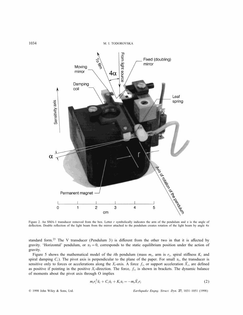
speci�c, an SMA-1 accelerograph3 was chosen, which makes the derived equations directly applicable to theLos Angeles Strong Motion Array.21;22 An SMA-1 accelerograph has three transducers, measuring motion inthree perpendicular directions (L; T and V ); which are approximately parallel to the edges of the instrumentbox (8× 8× 14 in). Ground acceleration in positive L, T and V directions results in upward (positive) tracede ection on the �lm. Figure 1 shows a view from above of the box with the cover removed, and Figure 2a transducer removed from the box.The transducer consists of a plastic plate cantilevered by two leaf springs. Damping, proportional to velocity,

is provided by a coil attached to the plate and placed inside a permanent magnetic �eld. The transducer canbe modelled as a single-degree-of-freedom oscillator, i.e. a physical pendulum with mass m, arm r, spiralsti�ness K and spiral damping C. Nominal values for the natural frequency !N =K=(mr2) and the dampingratio � (2!N�=C=(mr2)) are 25Hz × 2� rad = 50� rad=s and 0·6 (±0·05) of critical. Light is provided bya bulb attached to the instrument box. For each transducer, by a system of �xed mirrors, a light beam isdirected toward a small mirror, attached to and moving with the transducer pendulum (Figures 2 and 3). Ifthe pendulum rotates by an angle �, after re ection from this mirror, the light beam is rotated by 2�. By a�xed mirror, the light beam is re ected back to the moving mirror. After the second re ection, the light beamis again rotated by angle 2�; the total rotation relative to the incident ray is 4�. By a cylindrical lens, the light

? 1998 John Wiley & Sons, Ltd. Earthquake Engng. Struct. Dyn. 27, 1031–1051 (1998)

MATHEMATICAL MODEL AND INVERSE PROBLEM 1033

Figure 1. An SMA-1 strong motion accelerograph (a view from above, with the top cover removed)

beam is focused onto the �lm (70mm wide) through a thin slit. The total path of the light beam between themirror attached to the transducer and just before reaching the �lm (the optical path) is d=12·5 cm (nominalvalue). If in no load condition, the light beam is perpendicular to the �lm and

tan 4�=yd: (1)

The transducer response is proportional to the ground acceleration in the frequency range from 0 to about25Hz. The overall sensitivity is about 1·7 cm=g (1g acceleration in the direction of the sensitivity axis resultsin y=1·7 cm trace de ection on the �lm). The angle � is small, of the order of few degrees (1g accelerationalong the sensitivity axis results in tan 4�=1·7=12·5=0·136 or �=1·9◦).

Equations of motion for small de ections and perfectly aligned transducersFigure 4 shows a schematic representation of the transducers inside the box. The penduli are represented

by rectangular plates, and the pivot axes by short line segments with circles at the ends. This representation isconvenient to verify the directions and signs in the mathematical model with respect to the actual con�guration.Ideally, the sensitivity axes should be parallel to the edges of the box.Indices i=1; 2 and 3 are assigned to the L, T and V transducers, respectively. Further, axes X1, X2

and X3 are introduced, parallel to the L, T and V axes, but pointing in the opposite direction (Figure 4).The angles of de ection �i, i=1; 2 and 3, are shown in Figure 4 by vectors with double arrows. Positive�i results in upward trace de ection on the �lm (positive yi). Axes X1, X2 and X3 form neither a right-handed nor a left-handed co-ordinate system, and are di�erent from axes xp1 , xp2 and xp3 used by Wongand Trifunac19 (X1 = xp1 ; X2 = xp2 ; X3 =−xp3 ). Also, the direction of angles �1, �2, and �3 is di�erent. (If�pi ’s are the angles in their paper, than �1 =−�p

1 , �2 =−�p2 and �3 = �p

3 ). Axes X1, X2 and X3 are, ori-entated so that the dynamic equilibrium equations for all the three penduli, for small de ections, have the



Figure 2. An SMA-1 transducer removed from the box. Letter r symbolically indicates the arm of the pendulum and � is the angle ofde ection. Double re ection of the light beam from the mirror attached to the pendulum creates rotation of the light beam by angle 4�

standard form.23 The V transducer (Pendulum 3) is di�erent from the other two in that it is a�ected bygravity. ‘Horizontal’ pendulum, or �3 = 0, corresponds to the static equilibrium position under the action ofgravity.Figure 5 shows the mathematical model of the ith pendulum (mass mi, arm is ri, spiral sti�ness Ki and

spiral damping Ci). The pivot axis is perpendicular to the plane of the paper. For small �i, the transducer issensitive only to forces or accelerations along the Xi-axis. A force fi, or support acceleration �Xi, are de�nedas positive if pointing in the positive Xi-direction. The force, fi, is shown in brackets. The dynamic balanceof moments about the pivot axis through O implies

mir2i ��i + Ci�̇i + Ki�i=−mi �Xiri (2)



Figure 3. Schematic representation of the optical path in an SMA-1 accelerograph. The �lm transport, light path and cylindrical lens areshown as viewed along the transverse (T) axis (see Figure 1). The longitudinal (L) accelerometer and doubling mirror are shown asviewed from the vertical (V) axis. The transverse (T) and vertical (V) transducers have additional 90◦ mirrors (not shown) receivinglight from mirror no. 3, and re ecting it again, after it was de ected by the transducer mirrors, towards the cylindrical focussing lens in

front of the �lm

Figure 4. Schematic representation of the three transducers in an SMA-1 accelerograph, all in ‘normal’ position. Symbols L, V and Tindicate the directions of the sensitivity axes. Axes X1, X2 and X3 are used to describe the motion. Angles �1, �2 and �3 measure the

de ection of the L-, T- and V-transducer, respectively

Figure 5. Mathematical model of the transducer—a physical pendulum of length ri , mass mi , sti�ness Ki and damping Ci . For smallde ections �i , the pendulum is sensitive only to forces or accelerations along the Xi-axis



Introducing circular frequency !i, damping ratio, �i, and angular sensitivity constant, s�i , such that

!2i =Ki=(mir2i ) (3)

2!i�i=Ci=(mir2i ) (4)

and

s�i =1

!2i ri(5)

equation (2) results in

��i + 2!i�i�̇i + !2i �i=−!2i s�i�Xi (6)

The constants mi, Ki, Ci and ri are di�cult to measure, but !i, �i, and s�i can be measured easily.3

The natural frequency of the transducer (∼25Hz) is higher than most frequencies carrying the major portionof energy in strong ground motion. Then, !2i �i is larger than the other two terms in the LHS of equation (6),which implies

�i ≈−s�i �Xi (7)

Equation (7) shows that the response, �i, is approximately proportional to support acceleration in the −Xi

direction, i.e. in positive L, T or V directions.The angular sensitivity s�i equals the angle of de ection caused by unit acceleration and is in units

rad× s2=m. The inverse of s�i is the angular ampli�cation constant

a�i =

1s�i

(8)

in units m=(rad× s2). The ampli�cation equals the ground acceleration that results in 1 rad de ection of thependulum. In has been customary to use g as unit of acceleration, which leads to sensitivity and ampli�cationconstants, s�;wi and a�;w

i , in units rad=g and g=rad. The relationship between s�i and s�;wi is

s�;wi = s�i g (9)

and a�;wi is the inverse of s�;wi . The sensitivity of accelerographs recording on �lm is usually evaluated directly

from trace de ection on the �lm, yi, and is expressed in units cm=g. If sensitivity syi is the trace de ectionyi when 1g acceleration is measured, and if in neutral position the light beam is perpendicular to the �lm,from equation (1), it follows that

syi =d tan (4s�i ) (10)

The angular sensitivity s�i is a constant, speci�c for each transducer. If there are no obstacles, k times largeracceleration along the sensitivity axis would result in k times larger angle of de ection, �i, but not in ktimes larger de ection on the �lm, yi, as yi is not a linear function of �i. Therefore, the sensitivity syi is afunction of the acceleration, and equation (10) gives the value for acceleration 1g. This implies that errorsare introduced if the de ection on the �lm, yi, is scaled directly to acceleration units by constant sensitivity,syi . An analysis of these errors is presented in References 21 and 22.

Equations of motion for large de ections and misaligned transducersCo-ordinate axes X1, X2 and X3 (Figure 4) are perpendicular to each other, and if the transducers are

perfectly aligned to these axes, for small de ections, three orthogonal components of motion are recorded.However, the actual position of each pendulum is, in general, slightly o� this ideal position. Three auxiliary co-ordinate systems can be introduced, with respect to which the penduli are perfectly aligned and transformations



Figure 6. Misalignment angles for the three penduli (’i , i and �i , i=1, 2 and 3), shown by double arrows

de�ning the position of the auxiliary systems, with respect to the orthogonal X1–X2–X3 system. Then, theequations of motion can be transformed to the X1–X2–X3 system, and relationships between the unknowncomponents of motion in the X1–X2–X3 co-ordinate system and the angles of de ection �i, i=1, 2 and 3 canbe established.(a) Auxiliary co-ordinate systems and transformations. The auxiliary co-ordinate system for the ith pen-

dulum is X (i)1 –X

(i)2 –X

(i)3 . Axes X (i)

1 , X(i)2 and X (i)

3 point approximately in same direction as axes X1, X2 andX3, but are slightly o�. The alignment of the penduli with respect to these co-ordinate systems is shown inFigure 6. Axes X (i)

i , i=1, 2, 3 are aligned with the sensitivity axes.The position of the ith auxiliary system can be obtained by consecutive rotation of the system X1–X2–X3

through small angles ’i, �i and i (shown in Figure 6 by vectors) such that’i= rotation about the ideal position of the pivot axis;�i= rotation of the ideal pivot axis about the ideal sensitivity axis; i= rotation of the ideal pivot axis about the axis aligned with the ideal position of the arm of the

pendulum.Let [T (i)], i=1, 2, 3 be transformation matrices that would bring the X1–X2–X3 system parallel to the corre-sponding auxiliary systems (these are products of the corresponding rotation matrices). Then

X (i)1

X (i)2

X (i)3

= [T (i)]

X1X2X3

(11)

Matrices [T (i)] are same as those in Reference 19, subject to the appropriate transformation of the co-ordinateaxes and angles. For the con�guration used in this paper, these matrices can be found in Reference 21.



(b) Equations of motion for large de ections in the aligned reference systems. Due to orthogonality ofthe auxiliary reference systems and alignment, each pendulum is sensitive only to motion in a plane de�nedby two of the co-ordinate axes. These planes are X (1)

1 –X (1)2 for Pendulum 1, X (2)

1 –X (2)2 for Pendulum 2, and

X (3)2 –X (3)

3 for Pendulum 3. Free-body diagrams of the penduli are shown in Figure 7. Dynamic equilibriumof moments about axes X (1)

3 , X (2)3 and X (3)

1 implies

m1r21 ��1 + m1(r1 cos �1) �X(1)1 − m1(r1 sin �1) �X

(1)2 + C1�̇1 + K1�1 = 0 (12a)

m1r22 ��2 − m2(r2 sin �2) �X(2)1 + m2(r2 cos �2) �X

(2)2 + C2�̇2 + K2�2 = 0 (12b)

m3r23 ��3 + m3(r3 cos �3) �X(3)3 + m3(r3 sin �3) �X

(3)2 + C3�̇3 + K3�3 = 0 (12c)

and

cos �1 �X(1)1 − sin �1 �X (1)

2 = r1( ��1 + 2!1�1�̇1 + !21�1) (13a)

sin �2 �X(2)1 + cos �2 �X

(2)2 = r2( ��2 + 2!2�2�̇2 + !22�2) (13b)

sin �3 �X(3)2 + cos �3 �X

(3)3 = r3( ��3 + 2!3�3�̇3 + !23�3) (13c)

The above equations relate the measurable transducer responses �i; i=1, 2 and 3 to components of motionalong the axes of the auxiliary systems.(c) Equations of motion for large de ections, in the non-aligned system. From equation (11), it follows

that the accelerations in the auxiliary reference systems and in the system X1–X2–X3 are related by

�X(i)1

�X(i)2

�X(i)3

= [T (i)]

�X 1�X 2�X 3

; i=1; 2; 3 (14)

The equations of motion in the X1–X2–X3 system can be obtained by substituting { �X (i)1 ; �X

(i)2 ; �X

(i)3 }T in equa-

tions (13) from equation (14). This leads to the system of equations

[T ]

�X 1�X 2�X 3

= {b} (15)

where

[T ] =

cos �1T(1)11 cos �1T

(1)12 cos �1T

(1)13

− sin �1T (1)21 − sin �1T (1)22 − sin �1T (1)23sin �2T

(2)11 − sin �2T (2)12 − sin �2T (2)13

+ cos �2T(2)21 + cos �2T

(1)22 + cos �2T

(2)23

sin �3T(3)21 sin �3T

(3)22 sin �3T

(3)23

+ cos �3T(3)31 + cos �3T

(3)32 + cos �3T

(3)33

(16)

and

{b}=

−r1( ��1 + 2!1�1�̇1 + !21�1)

−r2( ��2 + 2!2�2�̇2 + !22�2)

−r3( ��3 + 2!3�3�̇3 + !23�3)

(17)



Figure 7. Free-body diagrams of the penduli in the auxiliary reference systems, under action of static or dynamic forces

(T (i)lk are terms of matrices [T (i)]). The misalignment angles are usually small (of the order of few degrees).Angles �i are also small which implies

[T ] =

1 −’1 − �1 1−�2 − ’2 1 − 2

3 �3 + ’3 1

+ O(’2i ;

2i ; �

2i ; �

2i ) (18)

The linearized [T ] does not depend on misalignment angles �i.

Response to static forcesStatic forces, de�ned in the X1–X2–X3 reference system can be transformed to the auxiliary systems by

f(i)1f(i)2f(i)3

= [T (i)]

f1f2f3

(19)

where f1; f2 and f3 are force components in the X1–X2–X3 reference system, and f(i)1 , f(i)2 and f(i)3 in the

X (i)1 − X (i)

2 − X (i)3 reference systems. Then the static equilibrium equations can be written with respect to the



aligned system. The free-body diagrams in Figure 7 imply

K1�1 + f(1)2 r1 sin �1 − f(1)1 r1 cos �1 = 0 (20a)

K2�2 + f(2)1 r2 sin �2 − f(2)2 r2 cos �2 = 0 (20b)

K3(�3 + �03)− f(3)3 r3 cos �3 − f(3)2 r3 sin �3 = 0 (20c)

where �03 is the de ection of the V-pendulum caused by its weight, m3g, applied in the positive X (3)3 direction.

In the normal position, when the pendulum is ideally horizontal (the arm of the pendulum is perpendicularto the X (3)

3 -axis), �3 = 0, but the spring is stretched to an angle �03 equal to

�03 = s�;w3 (21)

In terms of the sensitivity constants s�;wi , equations (20) appear as

cos �1f(1)1 − sin �1f(1)2 = �1(m1g)=s

�;w1 (22a)

− sin �2f(2)1 + cos �2f(2)2 = �2(m2g)=s

�;w2 (22b)

sin �3f(3)2 + cos �3f

(3)3 = (�3 + �03)(m3g)=s

�;w3 (22c)

Then, for small de ections the sensitivity s�;wi equals the de ection of the pendulum, �i, when force equalto its weight is applied along the sensitivity axis.From equations (19) and (22), the equilibrium equations can be written in the X1–X2–X3 system

[T ]

f1f2f3

=

�1(m1g)a�;w1

�2(m2g)a�;w2

(�3 + �03)(m3g)a�;w3

(23)

THE INVERSE PROBLEM

The misalignment angles and the sensitivity constants can be determined from equations (23) if the staticforces fi and the de ection angles �i are known. The static tilt test described by Wong and Trifunac19 can beused to obtain a series of independent measurements. The instrument is rotated through accurately measuredangles and trace de ections, yi, are recorded on the �lm. The static force is a fraction of the pendulum weight,and is determined from the angle of rotation. The trace de ections yi are measured by scanning the �lm with300 or 600 points=in resolution (1 in= 2·54 cm) and digitizing the scanned image by a computer. The angles�i are then calculated using equation (1), or by another more accurate procedure, proposed by Todorovskaet al.,21;22 which corrects also for inclined ray incidence onto the �lm. Each instrument position leads to oneequation per pendulum. Finally, three independent systems of equations are obtained. The following presentsan algorithm for solution.

Static tilt testFor each instrument position, static equilibrium is de�ned by equations (23). For stable numerical inversion,

the linearized form of [T ] in equation (18) may be used. Then there are only three unknowns, ’i, i andthe ampli�cation a�;w

i . Minimum three linearly independent equations per pendulum are required. However,it is better to perform additional measurements, because of possible errors or missing data (e.g., for largede ections, the pendulum motion may be limited by an obstacle, or the trace may go o� the �lm). All errorsmay not be obvious from visual �lm inspection, and it is best if an overdetermined system of equations issolved by least squares. Unusually large residuals will indicate that a measurement may be ‘corrupted’. Theproblem is then �xed, or the corresponding equation is disregarded, and the system is solved again.Controlled tilting is performed by the table shown in Figure 8. The instrument is securely attached to a

base plate, which can be rotated about its vertical axis of symmetry (counterclockwise, up to 90◦) and about



Figure 8. Tilt table rotated by 30◦ about its longitudinal axis, and with the instrument plate rotated counterclockwise through 90◦. Thisposition corresponds to the step of the tilt test in which the SMA-1 is rotated about its transverse axis through 30◦, with the key in

lower position

its long axis. Rotation of the base plate about the transverse axis is possible by �rst rotating it through 90◦

horizontally, and then rotating by the desired angle about the long axis of the table. Figure 8 shows the baseplate rotated through 30◦ about the transverse axis.The sequence of steps in a tilt test is shown on the �eld form which is reproduced in Figure 9. The

positions are identi�ed by letters (A through I and B′ through I ′). In each position, the instrument recordsfor about 2 s. Figure 10 shows the �lm, and Figure 11 a sketch of realistic trace de ections (the traces havebeen shifted to avoid intermingling).The tilt table in Figure 8 is di�erent from the one used by Wong and Trifunac19 in that no adjustment is

possible to make it horizontal. In �eld conditions, the table can easily be o� horizontal by few degrees, whichis of the same order of magnitude as the misalignment angles. The algorithm presented in this paper takesthis into account. Two angles, describing the position of the tilt table angles, are treated as unknowns and areevaluated by the presented algorithm for processing the tilt test measurements. One might be tempted to con-struct a tilt table with three adjustable legs and an accurate levelling mechanism. In rough �eld conditions, thiswould require additional work and time. However, even with perfectly horizontal tilt table, the ideal referencesystems for the three transducers would still not be perfectly horizontal, because of manufacturing tolerancesand not so precise placement of the transducers into the instrument housing. The presented algorithm, besidessimplifying the �eld work, also accounts for these imperfections which are not possible to measure directly.The unknown ‘tilt table angles’, in fact, are combination of these imperfections and the directly measurableangles of the tilt table. In what follows, the inverse problem is �rst presented for a perfectly horizontal tilttable, and then for a tilt table that is o� horizontal.



Figure 9. A standard form to be �lled out during a tilts test

Figure 10. Film with tilt test T82·01



Figure 11. A schematic representation of the trace de ections for the standard sequence of instrument positions (see Figures 8 and 9).For clarity, the traces have been shifted vertically relative to each other

Equilibrium equation for a perfectly horizontal tilt tableThe mass of each pendulum is di�erent, and the static forces for a given tilt table position are di�erent.

However, the force normalized by the weight

Fn= {f1; f2; f3}T=(mig) (24)

is the same for all penduli. For perfectly horizontal tilt table, the normalized forces for positions A through Iand B′ through I ′ are:

L: FAn = {0; 0; 1}T (25a)

L: FBn = {0; −1; 0}T (25b)

L: FCn = {0; 0; −1}T (25c)

L: FDn = {0; 1; 0}T (25d)

L: FEn = {0; 0; 1}T (25e)

T : FFn = {0; 0; 1}T (25f)

T : FGn = {1; 0; 0}T (25g)

T : FHn = {−1; 0; 0}T (25h)

T : FIn = {0; 0; 1}T (25i)

L: FB′n = {0; − sin 30◦; cos 30◦}T (25j)

L: FD′n = {0; sin 30◦; cos 30◦}T (25k)

L: FE′n = {0; 0; 1}T (25l)

T : FF′n = {0; 0; 1}T (25m)

T : FG′n = {sin 30◦; 0; cos 30◦}T (25n)

T : FH ′n = {− sin 30◦; 0; cos 30◦}T (25o)

T : FI ′n = {0; 0; 1}T (25p)



L and T to the left of the above equations indicate rotation (or the corresponding ‘normal’ position) aboutthe longitudinal or the transverse axes of the instrument. The superscripts indicate the instrument position.The same superscript can be attached to the corresponding angles of de ection �i. For each position, andeach pendulum one equilibrium equation is obtained, by substituting the corresponding force and angle inequations (23). Positions E and E′ and F and F ′ will be ignored as redundant (E and E′ are same as A, andF and F ′ are same as I).Since the normalized force is same for the three penduli, the equilibrium equations (23) for a particular

position can be written as

1 −’1 − �1 1−�2 − ’2 1 − 2

3 �3 + ’3 1

Fn=

�1 a�;w1

�2 a�;w2

(�3 + �03) a�;w3

(26)

The constants a�;wi represent the ampli�cation.

Equilibrium equation for a nonhorizontal tilt tableThe tilt table is, in general, o� horizontal by angles �1 and �2 representing rotation about the longer and

the shorter axes of the table, as shown in Figure 12. Parts (a) and (b) correspond to the instrument innormal position and in normal position-base plate rotated (Figure 9). The ‘key’ schematically indicates theinstrument orientation (Figure 1). The misalignment angles are also indicated. In the �rst-order approximation,the e�ect of the angles �1 and �2 just adds to the e�ects of the misalignment angles. So, one can assumethat the same equilibrium equations hold as for the case when the table is horizontal, but the misalignmentangles are modi�ed (the modi�cation is di�erent for the ‘normal’ (L) and for the ‘normal-base-plate rotated’(T ) positions). The ‘e�ective’ misalignment angles can be determined from Figure 12, and then ‘e�ective’transformation matrices [T e�L ] and [T

e�T ] can be constructed for tilting about the longitudinal and transverse

axis, respectively. These matrices are

[T e�L ] =

1 −’1 − �1 ( 1 + �2)

−�2 − ’2 1 −( 2 + �1)

( 3 − �2) �3 + (’3 + �1) 1

(27a)

and

[T e�T ] =

1 −’1 − �1 ( 1 − �1)

−�2 − ’2 1 −( 2 + �2)

( 3 + �1) �3 + (’3 + �2) 1

(27b)

and the new equilibrium equations are

L: [T e�L ]Fn=

�1 a�;w1

�2 a�;w2

(�3 + �03) a�;w3

(28a)

T : [T e�T ]Fn=

�1 a�;w1

�2 a�;w2

(�3 + �03) a�;w3

(28b)



Figure 12. A schematic representation of the tilt table and angles �1 and �2 describing by how much the table is o� vertical. Axes X1,X2 and X3, which are aligned to the instrument box, and the misalignment angles are also shown for (a) the ‘normal position’ and (b)

the ‘normal position—base plate rotated’

Matrices [T e�L ] and [Te�T ] can be represented as a sum of the identity matrix and matrices [T’; ], [T�] and

[T�] as follows:

[T e�L ] = [I ] + [T’; ] + [T�] + [T�;L] (29a)

and

[T e�T ] = [I ] + [T’; ] + [T�] + [T�;T ] (29b)

where

[T’; ] =

0 −’1 1

−’2 0 − 2

3 ’3 0

(30)



[T�] =

0 −�1 0

−�2 0 0

0 �3 0

(31)

[T�;L] =

0 0 �2

0 0 −�1

−�2 �1 0

(32a)

and

[T�;T ] =

0 0 −�1

0 0 −�2

�1 �2 0

(32b)

Di�erence equations with respect to normal positionsIf there is no misalignment and the table is horizontal, the traces on the �lm for the normal position,

or normal position-base plate rotated, would correspond to �i=0. In general, this is not the case, and thetrace positions corresponding to �i=0 are not known. However, the distance between the traces for di�erentinstrument positions and the corresponding di�erences in angles � can be determined. Positions A and I canbe used as reference for tilting about the longitudinal and the transverse axes, respectively. From the elevennontrivial equilibrium equations, nine di�erence equations can be constructed:

L; (1): B− A

L; (2): C − A

L; (3): D − A

T; (4): G − I

T; (5): H − I

L; (6): B′ − A

L; (7): D′ − A

T; (8): G′ − I

T; (9): H ′ − I

The de ection angles �i appear on both sides of the equilibrium equations. Therefore, in the di�erenceequations, the absolute angles �i cannot be replaced throughout by the di�erences of angles.We �rst de�ne relative normalized forces

L: Frn=Fn − FA

n (33a)

T : Frn=Fn − FI

n (33b)

and relative angles

L: �ri = �i − �A

i (34a)

T : �ri = �i − �I

i : (34b)

Then the di�erence equations can be written as follows:

L: [[T’; ] + [T�A ]]Frn − {a�;w

i �ri }= [[I ] + [T�r ]]Fr

n − [T�;L]Frn (35a)



and

T : [[T’; ] + [T�I ]]Frn − {a�;w

i �ri }= [[I ] + [T�r ]]Fr

n − [T�;T ]Frn (35b)

resulting in the following three systems of equations for Penduli 1, 2 and 3:

1 −1 −�(1)1

0 −2 −�(2)1

−1 −1 −�(3)1

0 −1 −�(4)1

0 −1 −�(5)112

√32 − 1 −�(6)1

− 12

√32 − 1 −�(7)1

0√32 − 1 −�(8)1

0√32 − 1 −�(9)1

’∗1 1

a�;w1

=

−�(1)10

�(3)1−11

− 12�(6)1

12�(7)1

− 1212

−

−�2

−2�2−�2

�1

�1

�2(√32 − 1)

�2(√32 − 1)

−�1(√32 − 1)

−�1(√32 − 1)

(36a)

0 1 −�(1)2

0 2 −�(2)2

0 1 −�(3)2

−1 1 −�(4)2

1 1 −�(5)2

0 −(√32 − 1) −�(6)2

0 −(√32 − 1) −�(7)2

− 12 −(

√32 − 1) −�(8)2

12 −(

√32 − 1) −�(9)2

’∗2 2

a�;w2

=

1

0

−1�(4)2

−�(5)212

− 12

12�(8)2

− 12�(9)2

−

�1

2�1

�1

�2

�2

−�1(√32 − 1)

−�1(√32 − 1)

−�2(√32 − 1)

−�2(√32 − 1)

(36b)

and

−1 0 −�(1)3

0 0 −�(2)3

1 0 −�(3)3

0 1 −�(4)3

0 −1 −�(5)3

− 12 0 −�(6)312 0 −�(7)3

0 12 −�(8)3

0 − 12 −�(9)3

’∗3 3

a�;w3

=

�(1)3 + 1

2

−�(2)3 + 1

1

1

12�(6)3 − (

√32 − 1)

− 12�(7)3 − (

√32 − 1)

−(√32 − 1)

−(√32 − 1)

−

−�1

0

�1

�1

�1

−�1 12�1 12�1 12−�1 12

(36c)



where

’∗1 =’1 + �A1 (37a)

’∗2 =’2 + �I2 (37b)

’∗3 =’3 + �A3 (37c)

It can be seen that in the 3× 9=27 equations there are 3× 5 + 2=17 unknowns. The �ve unknownsfor each pendulum are the misalignment angles, ’i and i, the ampli�cation constant, a

�;wi , and the absolute

de ection angles for the two normal positions, �Ai and �I

i . The additional two unknowns, common for all thependuli, are the angles of the tilt table, �1 and �2. The number of equations is still larger than the numberof unknowns. The following features of equations (36a) and (36b) should be noted: (1) the equations for thedi�erent penduli are coupled through �1 and �2, and (2) solution only for the sums ’i+�A

i and ’i+�Ii can be

obtained (otherwise the problem is ill-posed). Also, all the unknown angles are small and, ideally, least squaresshould be applied to the uncoupled systems of equations with respect to the di�erent penduli. Therefore, �rstthe angles �1 and �2 should be evaluated using some independent equations and then substituted into theuncoupled systems. Other independent equations are needed to calculate angles ’i from the sums ’i+�A

i and’i + �I

i .

Evaluation of �1 and �2—iterationThe di�erence equations can be constructed by subtracting the static equilibrium equations for the two

normal positions A and I . Let �A−Ii be the relative angle

�A−Ii = �A

i − �Ii (38)

The normalized absolute forces FAn and F

In are the same and can be factored out. The new di�erence equation

is then

A− I : [[T�A ]− [T�I ] + [T�;L]− [T�;T ]]

001

= {�A−I

i a�;wi } (39)

Only the third component of the normalized force vector is non-zero, which further simpli�es this equation.Since the third columns of matrices [T�A ] and [T�I ] are zero, their product with the force vector is a zerovector, and only the matrices [T�;L] and [T�;T ] remain in equation (39). These two matrices have zero entryin the third row of the third column, and the third equation of the system is trivially satis�ed. What remainsfrom the system are the following two equations:

�1 + �2 = �A−I1 a�;w

1 (40a)

− �1 + �2 = �A−I2 a�;w

2 (40b)

which imply

�1 = 0·5(�A−I1 a�;w

1 − �A−I2 a�;w

2 ) (41a)

�2 = 0·5(�A−I1 a�;w

1 + �A−I2 a�;w

2 ) (41b)

Equations (41) require that the ampli�cation constants a�;w1 and a�;w

2 are known before angles �1 and �2 areestimated. These two constants are stable quantities and their estimate is not a�ected much by the changes inthe misalignment angles or by angles �1 and �2. Therefore, iteration can be performed as follows. The �rstapproximation can be obtained by solving the di�erence equations assuming �1 = 0 and �2 = 0. These �rstestimates are then substituted into equations (41), solving for �1 and �2. The new estimates of �1 and �2 are



then substituted into the di�erence equations whose solution gives new estimates for a�;w1 , a�;w

2 , ’∗i and i.The iteration is repeated as required by a preset accuracy criterion. The convergence is very fast. Accuracyof 0·01◦ is achieved only in few steps.

Evaluation of �Ai and �I

i , and ’i

What remains is to �nd angles ’i from ’∗1 =’1 + �A1 , ’

∗2 =’2 + �I

2 and ’∗3 =’3 + �A3 . The equilibrium

equations for the two normal positions, A and I , can be used for this purpose. Due to the particular arrange-ments of zeroes in the normalized force vectors FA

n and FIn and in matrices [T’; ] and [T�], all ’i and �i

drop out in the LHS of these equations, which reduce to

A:

001

+

1− 20

+

000

+

�2−�10

=

a�;w1 �A

1

a�;w2 �A

2

a�;w3 (�A

3 + �03)

(42a)

and

I :

001

+

1− 20

+

000

+

−�1−�20

=

a�;w1 �I

1

a�;w2 �I

2

a�;w3 (�I

3 + �03)

(42b)

Recalling the expression for �03 (equations (21)), from the above equations it follows that

�A1 = ( 1 + �2)=a

�;w1 (43a)

�A2 = −( 2 + �1)=a

�;w2 (43b)

�A3 = 0 (43c)

�I1 = ( 1 − �1)=a

�;w1 (44a)

�I2 = −( 2 + �2)=a

�;w2 (44b)

�I3 = 0 (44c)

It is seen that the �rst-order analysis implies that the angles of de ection, when the instrument is in normalpositions for the �rst two penduli (L and T ), are equal to the e�ective misalignment angles 1 and 2 forthe particular normal position, while for the third pendulum (V ) those angles are zero. A corollary of this isthat the di�erence �A

3 − �I3 = 0, and this should be seen in the tilt test results. Indeed, in all of our results for

the Los Angeles Strong Motion Network, there were noticeable jumps between the traces for the two normalpositions (e.g., Positions E and F , or E′ and F ′) only for the L and T penduli.21

Finally, the misalignment angles ’i are obtained from

’1 =’∗1 − �A1 (45a)

’2 =’∗2 − �I2 (45b)

’3 =’∗3 − �A3 (45c)

where ’∗i are as de�ned by equation (39).

DISCUSSION AND CONCLUSIONS

A mathematical model was presented for a typical accelerograph with pendulum like transducers under theaction of static or dynamic forces, considering large de ections and misaligned transducers. Linearizing the



equations eliminates one of the three misalignment angles (�—representing rotation in the plane which containsthe pendulum boom and its pivot axis) which contributes only second-order terms. The presented model canbe generalized to other accelerographs with pendulum-like transducers.The static equilibrium equations and a static tilt test were used to formulate an algorithm for �nding the

misalignment angles and the ampli�cation constants (the inverse problem). The static tilt test consists of asequence of measurements which lead to an overdetermined system of equations for each transducer. Theequations are coupled through the angles of the tilt table, which is not perfectly horizontal. In the proposedalgorithm, the systems of equations are solved independently for each transducer by the singular-value de-composition method.24 The systems are decoupled by substituting estimates for the angles of the tilt table,which are improved by iteration. Therefore, adding the tilt table angles as unknowns did not increase thenumber of unknowns in the numerical inversion. The high accuracy of reading the trace positions on the �lmvia a digital scanner and the combination of iteration and numerical inversion of an overdetermined systemmake the algorithm very stable.21 The procedure of Wong and Trifunac19 did not consider nonhorizontaltilt table, and solved for the unknowns one by one from selected di�erence equations. The new algorithm(and the interactive computer program TILT21), based on least-squares solution of an overdetermined systemof equations (nine equations and three unknowns), is more accurate, introduces redundancy and exibility,and is convenient for routine processing of tilt test results. Results of tilt tests for a typical strong mo-tion array and analysis of the overall accuracy (especially on the estimates of sensitivity) are presented inTodorovska et al.21;22

Another source of error (yet intractable) in measuring strong ground motion is earthquake generated tiltingof the recording instrument. Such tilting in the gravity �eld will cause larger errors in the recorded horizontalaccelerations, and smaller errors in the recorded vertical accelerations (this is analogous to the e�ect of the tilttable angles on the pendulum de ection when the instrument is horizontal, which is signi�cant only for theL and T transducers). These errors may be signi�cant near the source of intermediate and large earthquakes.

REFERENCES

1. M. D. Trifunac and V. W. Lee, ‘Automatic digitization and processing of strong-motion accelerograms, Part I and II’, Report No. CE79-15, Dept. of Civil Eng., Univ. of Southern California, Los Angeles, California, 1979.

2. V. W. Lee and M. D. Trifunac, ‘Automatic digitization and processing of accelerograms using PC’, Report No. CE 90-03, Dept. ofCivil Eng., Univ. of Southern California, Los Angeles, California, 1990.

3. M. D. Trifunac and D. E. Hudson, ‘Laboratory evaluation and instrument corrections of strong motion accelerographs’, ReportEERL 70-04, Earthquake Eng. Res. Lab., Calif. Inst. of Tech., Pasadena, California, 1970.

4. M. D. Trifunac, ‘Zero baseline correction of strong motion accelerograms’, Bull. Seism. Soc. Amer. 61, 1201–1211 (1971).5. M. D. Trifunac, F. E. Udwadia and A. G. Brady, ‘Analysis of errors in digitized strong motion accelerograms’ Bull. Seism. Soc.Amer. 63, 157–187 (1973).

6. M. D. Trifunac and V. W. Lee, ‘A note on the accuracy of computed ground displacements from strong motion accelerograms’, Bull.Seism. Soc. Amer. 64, 1209–1219 (1974).

7. V. W. Lee, A. Amini and M. D. Trifunac, ‘Noise in earthquake accelerograms’, J. Engng. Mech. ASCE 108, 1121–1129 (1982).8. A. Amini and M. D. Trifunac, ‘Optimum frequency and damping for optically recording strong motion accelerographs’, Soil Dyn.Earthquake Engng. 1, 189–194 (1982).

9. A. Amini and M. D. Trifunac, ‘Analysis of a feed-back transducer’, Report No. CE 83-03, Dept. of Civil Engng, Univ. of SouthernCalifornia, Los Angeles, California, 1983.

10. A. Amini and M. D. Trifunac, ‘Analysis of Force Balance Accelerometer’, Soil Dyn. Earthquake Engng 4, 82–90 (1985).11. D. K. Markus, K. Moslem and M. D. Trifunac, ‘A note on controlling the optical density of analog �lm records in strong motion

accelerographs’, Soil Dyn. Earthquake Engng 4, 31–34 (1985).12. A. Amini, R. L. Nigbor and M. D. Trifunac, ‘A note on the noise amplitudes in some strong motion accelerographs’, Soil Dyn.

Earthquake Engng. 6, 180–185 (1987).13. A. Amini, O. Hata and M. D. Trifunac, ‘Experimental analysis of RJL-1, Chinese Force Balance Accelerometer’, Earthquake Engng.

Engng. Vib. 11, 77–88 (1991).14. E. I. Novikova and M. D. Trifunac, ‘Instrument correction for the coupled transducer-galvanometer systems’, Report No. CE 91-02,

Dept. of Civil Engng, Univ. of Southern California, Los Angeles, California, 1991.15. E. I. Novikova and M. D. Trifunac, ‘Digital instrument response correction for the Force Balance Accelerometer’, Earthquake Spectra

8, 429–442 (1992).16. V. W. Lee and M. D. Trifunac, ‘Strong Earthquake Ground Motion Data in EQINFOS: Part I’, Report No. CE 87-01, Dept. of Civil

Eng., Univ. Southern California, Los Angeles, California, 1987.



17. V. W. Lee and M. D. Trifunac, ‘EQINFOS (the Strong Motion Earthquake Data Information System)’, Report No. CE 82-01, Dept.of Civil Eng., Univ. Southern California, Los Angeles, California, 1982.

18. R. I. Skinner and W. R. Stephenson, ‘Accelerograph calibration and accelerogram correction’, Earthquake Engng. Struct. Dyn. 2,71–86 (1973).

19. H. L. Wong and M. D. Trifunac, ‘E�ects of cross-axis sensitivity and misalignment on the response of mechanical-opticalaccelerographs’, Bull. Seism. Soc. Amer. 67, 929–956 (1977).

20. M. D. Trifunac and M. I. Todorovska, Nonlinear soil response—1994 Northridge, California, earthquake, J. Geotech. Engng. ASCE122, 725–735 (1996).

21. M. I. Todorovska, E. I. Novikova, M. D. Trifunac and S. S. Ivanovi�c, ‘Correction for misalignment and cross-axis sensitivity of strongearthquake motion recorded by SMA-1 accelerographs’, Report No. CE 95-06, Dept. of Civil Engrg, Univ. of Southern California,Los Angeles, California, 1995.

22. M. I. Todorovska, E. I. Novikova, M. D. Trifunac and S. S. Ivanovi�c, Advanced sensitivity calibration of the Los Angeles StrongMotion Array, Earthquake Engng. Struct. Dyn. 27, 1053–1068 (1998).

23. L. Meirovitch, Elements of Vibration Analysis, McGraw-Hill, New York, 1975.24. W. H. Press, B. P. Flannery, S. A. Teukolsky and W. T. Vetterling, Numerical Recipes, Cambridge University Press, Cambridge,

MA, 1989.


Cross-axis sensitivity of accelerographs with pendulum like transducers—mathematical model and the...

Documents

Transcript of Cross-axis sensitivity of accelerographs with pendulum like transducers—mathematical model and the...