Digital Object Identifier (DOI) 10.1007/s00211-002-0434-9Numer. Math. (2003) 95: 503–525 Numerische

Mathematik

Convergence of the Peaceman-Rachfordapproximation for reaction-diffusion systems

Stephane Descombes1, Magali Ribot2,∗

1 UMPA, UMR CNRS 5669 Ecole Normale Superieure de Lyon 46 Allee d’Italie 69364Lyon Cedex 07 France; e-mail: sdescomb@umpa.ens-lyon.fr

2 MAPLY, UMR 5585 CNRS Universite Lyon 1 69622 Villeurbanne Cedex France;e-mail: ribot@maply.univ-lyon1.fr

Received May 18, 2001 / Revised version received June 24, 2002 /Published online: March 24, 2003 – c©Springer-Verlag 2003

Summary. Consider a reaction-diffusion system of the form ut − M�u +F(u) = 0, where M is a m × m matrix whose spectrum is included in{�z > 0}. We approximate it by the Peaceman-Rachford approximation de-fined by P(t) = (1 + tF/2)−1(1 + tM�/2)(1 − tM�/2)−1(1 − tF/2). Weprove convergence of this scheme and show that it is of order two.

Mathematics Subject Classification (1991): 65M12

1 Introduction

Reaction-diffusion systems appear in many different situations, in chemistry,in biology, and we are specifically interested in pattern formation. For exam-ple, in [13] page 438, J. D. Murray has given the non dimensional system,with parameters a > 0, b > 0, α > 0, γ > 0, ρ > 0, K > 0 and η > 1,

∂u

∂t= �u + γ

(

a − u − ρuv

1 + u + Ku2

)

,

∂v

∂t= η�v + γ

(

α(b − v) − ρuv

1 + u + Ku2

)

,

(1)

as a mathematical model for pattern formation. This system could be includ-ed in reaction-diffusion systems of the general form with d, m two integers,

∗ We would like to thank Prof. Michelle Schatzman for reading carefully the manuscript.Correspondence to: Stephane Descombes

504 S. Descombes, M. Ribot

1 ≤ d ≤ 3 and M an m × m matrix:

∂u

∂t− M�u + F(u) = 0, x ∈ R

d, t > 0,

u(0, x) = u0(x), x ∈ Rd .

(2)

The simplest numerical scheme for solving this kind of system is the for-ward Euler scheme, but in that case, the time step �t is limited by O(�x2),a drastic condition. Another strategy is to use the backward Euler scheme;while its stability is unconditional, one has to solve a large system of non-linear equations. These two examples show that we need to consider othermethods. A possibility for integrating (2) is the implicit-explicit multistepmethods studied by G. Akrivis, M. Crouzeix and C. Makridakis in [1]. Theyuse two multistep formulae: an implicit one for the linear part and an explicitone for the non linear part. However, they are limited by the condition M

selfadjoint.Approximations based on flow splitting are often proposed; they are de-

fined as follows: let Xtv0 be the solution of{

v − M�v = 0

v(0) = v0

and Y tw0 be the solution of{

w + F(w) = 0

w(0) = w0;then the Lie formula is defined by

Ltu0 = XtY tu0

and is of order one (at least formally). The Strang approximation formula([16], [17]) is defined by

Stu0 = Xt/2Y tXt/2u0

and is of order two (at least formally). We then have to discretize these ap-proximations in time and in space to solve (2). The approximation in timecould be defined, for example, by this formula:

Qtu0 = (1 + tF/2)−1 (1 − tM�/2)−1 u0

which is of order one; this scheme can be studied as in [4], where C. Chiuand N. Walkington study a splitting scheme for solving an hysteretic reac-tion-diffusion system.

On the Peaceman-Rachford approximation 505

In this article we consider only the time discretization and we concentrateon the Peaceman-Rachford formula given by:

P tu0 = (1 + tF/2)−1 (1 + tM�/2) (1 − tM�/2)−1 (1 − tF/2) u0.(3)

Originally introduced in [14] to solve the heat equation (see also [10]),and also called ADI (Alternate Directions Implicit), this method is seldomanalyzed in non commutative and/or nonlinear cases. In the linear case,M. Schatzman has given in [15] a sufficient condition for the stability of

P(t) = (1 + tA/2)−1 (1 − tB/2) (1 + tB/2)−1 (1 − tA/2) ,

when A and B are unbounded positive self adjoint operators and the com-mutator of

√A and

√B is dominated in a very precise way by

√A + √

B,making A and B abstractly of order 2. This situation is realized if for instancex and y are periodic variables, a and b are positive smooth functions of x

and y on R2/Z

2 and

A = − ∂

∂xa

∂

∂x, B = − ∂

∂yb

∂

∂y.

B. O. Dia in [8] has shown some numerical results for this kind of operatorswhich prove a good behavior of this scheme.

Let us now introduce the assumptions on the problem (2) and on thesolution u that we wish to approximate. We assume that F is a Lipschitzcontinuous function of class C7 from R

m to itself satisfying

F(0) = 0,(4)

and that all its derivatives of order at most 7 are bounded. Observe that (4) isnecessary for the existence of solutions in L2(Rd)m. M is an m × m matrixwhose spectrum is included in {�z > 0}. We assume that the initial conditionu0 belongs to L2(Rd)m ∩L∞(Rd)m; then u exists, is unique and satisfies, forall τ > 0,

u ∈ C([0, τ ], L2(Rd)m ∩ L∞(Rd)m).

This assertion is proved in D. Henry [11], section 3.3 p. 52 when u0 belongsonly to L2(Rd)m, the extension when u0 belongs to L2(Rd)m ∩ L∞(Rd)m isstraightforward using the results of the first section of P. de Mottoni and M.Schatzman [5].

We write u(t, .) = T tu0, that is to say T t is the flow associated to (2). Forsimplicity, we shall write henceforth

L(t) = (1 + tM�)(1 − tM�)−1.(5)

506 S. Descombes, M. Ribot

We introduce now some functional spaces; we need an adapted scalarproduct for some of our operators to be contractions. As the spectrum of M

is included in {�z > 0}, the matrix

S =∫ +∞

0e−sM∗

e−sMds(6)

is well defined, symmetric, positive definite and satisfies

M∗S + SM = 1,(7)

as can be verified by a simple integration by parts. The corresponding innerproduct in R

m is

〈x, y〉 = (Sx, y)

and the corresponding norm is∣∣x

∣∣ = 〈x, x〉1/2. The space H = L2(Rd)m is

equipped with the inner product defined by

(f, g)0 =∫

Rd

〈f, g〉 dx,

the associated norm is denoted by |·|0 and the corresponding operator norm by| · |L(L2). We also introduce Hs(Rd)m, the Sobolev space of order s, equippedwith the norm | · |s defined by

|f |2s =∑

|α|≤s

|∂αf |20;

L∞(Rd)m, equipped with the norm | · |∞ and Ws,∞(Rd)m, equipped withthe norm | · |s,∞. Finally, G is the subspace of H 6(Rd)m made out of func-tions which belong to C6(Rd)m whose first sixth derivatives are boundedand, for u0 belonging to G, we denote by C(|u0|6,∞) a constant dependingon max0≤|α|≤6 |∂αu0|∞.

The main result of the article is Theorem 2 which can be stated as follows:

Theorem 2 For all u0 in G and for all τ > 0, there exist C(|u0|6,∞) and h0

such that for all h ∈ (0, h0], for all n such that nh ≤ τ∣∣∣(P h

)nu0 − T nhu0

∣∣∣0

≤ C(|u0|6,∞)h2|u0|6.The article is organized as follows: in Section 2, we consider the linear

case, and we obtain an algebraic expression of the difference e−2t (A+B) −P(2t). The method follows an idea of [9].

In section 3, we validate from the analytical point of view the result of sec-tion 2 when A is the multiplication by a bounded potential V and B = −M�

and deduce an estimate on the difference between et(M�−V ) and P(t) inoperator norms.

On the Peaceman-Rachford approximation 507

In Section 4, we prove Theorem 2 with the help of a comparison with thelinear case.

In section 5, we show some numerical results and explain how we ap-proximate the operator (1 + tF/2)−1 without solving a nonlinear system.

2 Error formula in the linear case

In this section, as in [7], we perform algebraic computations when A and B

are two linear operators. We are interested in the difference between P(2t) =(1+tA)−1(1−tB)(1+tB)−1(1−tA), denoted P2(t), and E(2t) = e−2t (A+B).

We introduce the following notation: [A, B] = AB − BA is the commu-tator of A and B. We recall the identity:

[A, BC] = [A, B]C + B[A, C].

We also recall Duhamel’s formula: if V satisfies

V + AV = f,

then

V (t) = e−tA V (0) +∫ t

0e−(t−s)A f (s) ds.(8)

Finally, we write α = (1 + tA)−1 and β = (1 + tB)−1 and we recall theidentities:

(1 − tA)α = α(1 − tA) = 2α − 1,(9)

1 − α = tαA,(10)

[B, α] = tα[A, B]α.(11)

Analogous identities hold when we exchange A and B, and α and β. Withthese notations, we see that P2(t) = P(2t) = α(1 − tB)β(1 − tA).

Lemma 1 Define

S(t) =(αβ

[B, [A, B]

]β2 − α[A, B]α(Aβ2 + β2A) − α2A3(2β − 1)

+ Aα(α − 2)β[A, B]β − BαB2β2(1 − tA)).

(12)

We have the following identity:

P(2t) − E(2t) = 2∫ t

0s2e−2(t−s)(A+B)S(s) ds.(13)

508 S. Descombes, M. Ribot

Proof. Relation (9), or rather its analogue for B and β, lets us rewrite

P2(t) = α(2β − 1)(1 − tA).

In order to use Duhamel’s formula, we differentiate P2(t), we add 2(A +B)P2(t) and we obtain

P2(t) + 2(A + B)P2(t) = − Aα2(2β − 1)(1 − tA) − 2αBβ2(1 − tA)

− α(2β − 1)A + 2Aα(2β − 1)(1 − tA)

+ 2Bα(2β − 1)(1 − tA).

(14)

The game in this computation is to rearrange the right hand side of (14), inorder to show that it is the product of t2 by a term which we will control.But we have to be careful, since limited expansions are not permissible; andtherefore we drag big remainder terms coming from the rational nature of theapproximation.

We regroup the terms of (14) by separating those which give a multipleof A for t = 0,

Q1(t) = − Aα2(2β − 1)(1 − tA) − α(2β − 1)A

+ 2Aα(2β − 1)(1 − tA)(15)

and those which give a multiple of B for t = 0

Q2(t) = −2αBβ2(1 − tA) + 2Bα(2β − 1)(1 − tA),

so that

P2(t) + 2(A + B)P2(t) = Q1(t) + Q2(t).

Since Q1(0) vanishes, we will try to factor t in Q1(t); for this purpose, wecommute A and β in the second term of Q1(t), obtaining thus

α(2β − 1)A = αA(2β − 1) + 2α[β, A];(16)

and the commutator [β, A] is equal to tβ[A, B]β thanks to formula (11). Wesubstitute (16) into (15), getting

Q1(t) = −Aα2(2β − 1)(1 − tA) + 2tαβ[B, A]β − αA(2β − 1)

+ 2Aα(2β − 1)(1 − tA).

We regroup the terms of degree 0 in t on one hand and the terms of degree 1in t on the other to obtain, after simple factorizations,

Q1(t) = (1 − α)αA(2β − 1) + tAα(α − 2)(2β − 1)A + 2tαβ[B, A]β.

On the Peaceman-Rachford approximation 509

The interesting term is the term of degree 0 and using equation (10), weobtain

Q1(t) = tα2A2(2β − 1) + tAα(α − 2)(2β − 1)A + 2tαβ[B, A]β.(17)

Let us turn to Q2(t).The first term of Q2(t) can be rewritten after commuting B and α

−2αBβ2(1 − tA) = 2[B, α]β2(1 − tA) − 2Bαβ2(1 − tA),

and using formula (11),

= 2tα[A, B]αβ2(1 − tA) − 2Bαβ2(1 − tA).

We regroup the second term of the above expression with the last term ofQ2(t), and the sum simplifies as follows:

Q2(t) = 2tα[A, B]αβ2(1 − tA) − 2Bα(β − 1)2(1 − tA);using formula (10), we obtain

Q2(t) = 2tα[A, B]αβ2(1 − tA) − 2t2BαB2β2(1 − tA).(18)

Finally, thanks to computations (17) and (18) we find that

P2(t) + 2(A + B)P2(t)

= t

(

2αβ[B, A]β + α2A2(2β − 1) + Aα(α − 2)(2β − 1)A

+ 2α[A, B]αβ2(1 − tA) − 2tBαB2β2(1 − tA)

)

.

The factor of t in the above expression vanishes at 0; we rewrite this factoras a sum of two expressions and one term: the terms of the first expressioncontain [A, B], and the terms of the second expression do not, and the lastterm has already the factor t . Thus we define

R1(t) = 2αβ[B, A]β + 2α[A, B]αβ2(1 − tA)

and

R2(t) = α2A2(2β − 1) + Aα(α − 2)(2β − 1)A.

Then

P2(t) + 2(A + B)P2(t) = t(R1(t) + R2(t) − 2tBαB2β2(1 − tA)

).

We compute R1(t): in the same fashion as above, in the first term of R1, wecommute β and [B, A], we regroup the terms with a t factor on one hand, and

510 S. Descombes, M. Ribot

those without on the other hand. Among the terms without a factor t , thereis a [β, [B, A]], that we rewrite tβ [[B, A], B] β, yielding thus a factor t ; forthe last term without t , we use (10), obtaining thus

R1(t) = 2t(αβ [B, [A, B]] β2 − α[A, B]α(Aβ2 + β2A)

).

We proceed analogously for R2(t); this time the commutation takes place inthe second term and we obtain:

R2(t) = 2t(−α2A3(2β − 1) + Aα(α − 2)β[A, B]β

).

Eventually, we find

P2(t) + 2(A + B)P2(t) = 2t2(αβ[B, [A, B]

]β2

− α[A, B]α(Aβ2 + β2A) − α2A3(2β − 1)

+ Aα(α − 2)β[A, B]β − BαB2β2(1 − tA)),

and the proof of (13) is an immediate consequence of Duhamel’s formula(8).

Remark 1 If A and B are bounded, formula (13) shows that the approxima-tion is exactly of order two.

3 Estimates on Matrix Schrodinger operators

Let now A be the multiplication by an m×m matrix V depending on x ∈ Rd ,

and let B be −M�; we assume that V is of class C6 and that it is boundedas well as all its derivatives of order at most 6. We will estimate in that casethe difference between P(t) and E(t) in operator norm, using the expressionfound in section 2. Thus, we calculate [A, B] in that case and we have thefollowing very simple lemma, whose proof is left to the reader.

Lemma 2 There exist bounded functions L0, L1,i , 1 ≤ i ≤ d, and L2 de-pending on the first two derivatives of V and on M such that

[A, B] = [M�, V ] = L0 +d∑

i=1

L1,i∂i + L2�;(19)

there exist also bounded functions N0, N1,i , 1 ≤ i ≤ d, N2, N3,i , 1 ≤ i ≤ d,and N4 depending on the first four derivatives of V and on M , such that

[[A, B], B] = [M�, [M�, V ]]

= N0 +d∑

i=1

N1,i∂i + N2� +d∑

i=1

N3,i∂i� + N4�2.

(20)

On the Peaceman-Rachford approximation 511

Now, let us estimate ‖P(t) − E(t)‖. We recall the following estimates, thatwe will need throughout this section: since A is a bounded operator, thereexists a constant C > 0 such that, for s = 0, . . . , 6,

‖A‖L(Hs) ≤ C(21)

and

‖α‖L(Hs) ≤ 1, ‖β‖L(Hs) ≤ 1;(22)

by definition, for s = 0, . . . , 4,

‖B‖L(Hs+2,H s) ≤ C.(23)

Finally, it has been shown in [6] that the operator B is sectorial in L2(Rd)m,and since A is a bounded operator, there exists a constant C > 0 such that,for t ≤ 1,

∥∥e−t (A+B)

∥∥L(L2)

≤ C.(24)

Lemma 3 We have the following estimates for t ∈ [0, 1]:

‖P(t) − E(t)‖L(H 2,L2) = O (t) ,(25)

‖P(t) − E(t)‖L(H 4,L2) = O(t2) ,(26)

and

‖P(t) − E(t)‖L(H 6,L2) = O(t3) .(27)

Proof. We decompose s2S(s) as T1 + T2 + T3 + T4 + T5 with

T1 = s2αβ [B, [A, B]] β2,

T2 = −s2α[A, B]α(Aβ2 + β2A),

T3 = −s2α2A3(2β − 1),

T4 = s2Aα(α − 2)β[A, B]β,

T5 = −s2BαB2β2(1 − sA).

Then, we can rewrite the integrand in (13) as

T = e−2(t−s)(A+B)(T1 + T2 + T3 + T4 + T5).

We now estimate these five terms, using the estimates (21), (23), (22) and(24). The largest of these terms is T5 since it involves six differentiations.

First, for the first term, using equation (20), we find for u ∈ H 6,

|T1u|L2 ≤ C1s2|u|6.

512 S. Descombes, M. Ribot

Consider now T2; relation (19), together with (21), implies, if u ∈ H 6,

|T2u|L2 ≤ C2s2|u|6.

The term T3u is trivially estimated for u ∈ H 6 by

|T3u|L2 ≤ C3s2|u|6.

The fourth term is treated almost as T2, using (19) and (21), so that if u ∈ H 6,

|T4u|L2 ≤ C4s2|u|6.

Finally, for the fifth term, if u ∈ H 6,

|T5u|L2 ≤ C5s2|u|6.

In conclusion, adding all those estimates, we find that, if u ∈ H 6,

|T u|L2 ≤ Cs2|u|6.Integrating the previous estimate, we obtain equation (27).

Moreover, if u ∈ L2, we have, using estimates (21), (22) and (24),

‖P(t) − E(t)‖L(L2,L2) = O (1) .(28)

Thus, from equations (27) and (28) and with the help of interpolation theory,see for example J. Bergh and J. Lofstrom [2], we obtain for all s ∈ [0, 6],

‖P(t) − E(t)‖L(Hs,L2) = O(t s/2) ,

and especially equations (25) and (26).

4 The nonlinear case

In this section, we consider the nonlinear case and we compare the exactsolution T tu0 to its approximation P tu0.

4.1 Some preliminary and useful lemmas

We recall first a Gronwall type lemma proved in [3].

Lemma 4 (Gronwall) Let Q be a polynomial with positive coefficients sat-isfying Q(0) = 0. We assume that function φ is such that there exists aconstant C ≥ 0 such that for all t ≥ 0

0 ≤ φ(t) ≤ φ(0) + Q(t) + C

∫ t

0φ(s)ds.

Then for all α > 1 there exists t0 > 0 such that for all 0 ≤ t ≤ t0

φ(t) ≤ φ(0)eCt + αQ(t).

The next useful result is

On the Peaceman-Rachford approximation 513

Lemma 5 For t ≥ 0, we have

|L (t)|L(L2) ≤ 1.

Proof. Let u belong to H and let F(u) be its Fourier transform. The Fouriertransform of L (t) u is given by

F(L(t)u)(ξ) = (1 − tM|ξ |2)(1 + tM|ξ |2)−1F(u)(ξ).

Following the definition of H and denoting

v(ξ) = (1 + tM|ξ |2)−1F(u)(ξ),

we have

|L (t) u|20 = |F(L(t)u)|20=

∫

Rd

〈(1 − tM|ξ |2)v(ξ), (1 − tM|ξ |2)v(ξ)〉 dξ,

=∫

Rd

v∗(ξ)(1 − tM∗|ξ |2)S(1 − tM|ξ |2)v(ξ) dξ.

Finally, with the help of (7), we obtain

|L (t) u|20 − |u|20 = −2t

∫

Rd

v∗(ξ)(M∗S + SM)|ξ |2v(ξ) dξ

= −2t

∫

Rd

|ξ |2v∗(ξ)v(ξ) dξ ≤ 0;

this concludes the proof of Lemma 5.

The previous lemma allows us to prove the stability of Peaceman-Rachford scheme in next corollary, which is the first non linear result inthe article:

Corollary 1 There exists a constant C0 > 0 such that for t small enoughand all u0 and v0 in L2(Rd)m

∣∣P tu0 − P tv0

∣∣0 ≤ (1 + C0t)|u0 − v0|0.(29)

Proof. Let us recall that P tu0 is defined by

P tu0 = (1 + tF/2)−1 L (t/2) (1 − tF/2) u0.

Denote u1 = L (t/2) (1 − tF/2) u0 and v1 = L (t/2) (1 − tF/2) v0, wehave

514 S. Descombes, M. Ribot

|u1 − v1|0 ≤ |L (t/2)|L(H) |u0 − v0 − tF (u0)/2 + tF (v0)/2|0,

since F is Lipschitz continuous and using Lemma 5, we deduce that

|u1 − v1|0 ≤ (1 + Ct)|u0 − v0|0.

Next

|P tu0 − P tv0|0 ≤ |u1 − v1|0 + t/2|F(P tu0) − F(P tv0)|0≤ |u1 − v1|0 + Ct/2|P tu0 − P tv0|0≤ (1 + Ct)|u0 − v0|0 + Ct/2|P tu0 − P tv0|0.

Thus, for t small, we obtain that

∣∣P tu0 − P tv0

∣∣0 ≤ (1 + C0t)|u0 − v0|0.

We also need the following linear result:

Lemma 6 There exists a constant C > 0 such that for t small and all u0 inH 2(Rd)m

∣∣(etM� − 1

)u0

∣∣0 ≤ Ct |u0|2,(30)

and such that for t small and all u0 in W 2,∞(Rd)m

∣∣(etM� − 1

)u0

∣∣∞ ≤ Ct |u0|2,∞.(31)

Proof. Since it has been shown in [6] that the operator −M� is sectorial inL2(Rd)m, estimate (30) is a consequence of Henry [11] p. 22. Concerningestimate (31), if we consider the case m = 1, the fundamental solution of theheat equation is given explicitly by

G(t, x) = (4πt)−d/2 exp(−|x|2/4t)χ{t≥0}1

and (31) is an immediate consequence of a Taylor’s formula. The matrixgeneralization is straightforward using the generalized Green function

G(t, x) = (4πMt)−d/2 exp(−M−1|x|2/4t)χ{t≥0}1,

and the fact that∫

∥∥(4πM)−d/2 exp(−M−1|y|2/4)

∥∥ |y|2dy ≤ C.

On the Peaceman-Rachford approximation 515

4.2 The difference between P tu0 and T tu0

We recall that G is the subspace of H 6(Rd)m made out of functions whichbelong to C6(Rd)m whose first sixth derivatives are bounded and, for u0 be-longing to G, we denote by C(|u0|6,∞) a constant depending on max0≤|α|≤6

|∂αu0|∞. We have the following result:

Theorem 1 For u0 in G and t small, the following estimate holds:

|P tu0 − T tu0|0 ≤ C(|u0|6,∞)t3|u0|6.(32)

The proof of Theorem 1 depends on three lemmas and we begin by intro-ducing two auxiliary functions. Define

F1(v) = F(u0) + DF(u0)(v − u0),

v = T taffu0 is the solution of the following system

∂v

∂t− M�v + F1(v) = 0 x ∈ R

d, t > 0,

v(0, x) = u0(x), x ∈ Rd .

(33)

For simplicity we also denote:

G(u0) = DF(u0)u0 − F(u0),

the constant part of F1, so that

F1(v) = DF(u0)v − G(u0).

The system (33) is not the linearized system at u0 but the expansion up toorder one and aff stands for affine. Using Duhamel’s formula, the solutionv = T t

affu0 of (33) is given explicitly by

v = et(M�−DF(u0))u0 +∫ t

0e(t−s)(M�−DF(u0))G(u0)ds.(34)

We expect T taff to be a second order approximation of T t , since there is

one time integration; that this expectation holds is proved in next lemma.

Lemma 7 For u0 in G and t small, the following estimate holds:

|T taffu0 − T tu0|0 ≤ C(|u0|6,∞)t3|u0|2.(35)

516 S. Descombes, M. Ribot

Proof. Let us define the function y = v − u = T taffu0 − T tu0. If we denote

R(u, u0) = F(u) − F1(u), the function y verifies the system

∂y

∂t− M�y + DF(u0)y = R(u, u0) x ∈ R

d, t > 0,

y(0, x) = 0, x ∈ Rd .

(36)

We start by an estimate of |R(u, u0)|0. Taylor’s formula is written

R(u, u0) =∫ 1

0(1 − t)D2F (u0 + t (u − u0)) (u − u0)

⊗2dt(37)

and therefore

|R(u, u0)|0 ≤∣∣∣∣

∫ 1

0(1 − t)D2F (u0 + t (u − u0)) (u − u0)

⊗2dt

∣∣∣∣0

.(38)

Since D2F is bounded, it follows that there exists a constant C > 0 such that

|R(u, u0)|0 ≤ C|u − u0|0|u − u0|L∞ .(39)

Now, let us estimate the two norms of the right hand side of the above in-equality; u − u0 verifies

u(t) − u0 = (etM� − 1

)u0 −

∫ t

0e(t−s)M�F(u)ds.

Since F is a Lipschitz function, and F(0) = 0, we deduce that for t ∈ [0, 1]

|u(t) − u0|0 ≤ ∣∣(etM� − 1

)u0

∣∣0 + C

∫ t

0|u|0ds

≤ ∣∣(etM� − 1

)u0

∣∣0 + C

∫ t

0|u − u0|0ds + Ct |u0|0.

Using the estimate (30) of the norm∣∣(etM� − 1

)u0

∣∣0, we obtain

|u − u0|0 ≤ Ct |u0|2 + C

∫ t

0|u − u0|0ds,(40)

therefore using Lemma 4 we obtain that for t small

|u − u0|0 ≤ Ct |u0|2.Using (31) and arguing as for (40), we have

|u − u0|L∞ ≤ Ct |u0|W 2,∞ + C

∫ t

0|u − u0|L∞ds,

On the Peaceman-Rachford approximation 517

and using Lemma 4 again we get

|u − u0|L∞ ≤ Ct |u0|W 2,∞ ≤ C(|u0|6,∞)t.

Since the function y = v − u is solution of (36), using Duhamel’s formulaand estimate (39) on R(u, u0), we obtain that

|y|0 ≤ C

∫ t

0|u − u0|0|u − u0|L∞ds

≤ C(|u0|6,∞)t3|u0|2.

This concludes the proof of Lemma 7.

For the Peaceman-Rachford approximation of (33), the object equivalentto T t

aff is

P taffv = (1 + tF1/2)−1 L (t/2) (1 − tF1/2) v.(41)

The value of (1 + tF1/2)−1v is obtained by solving

z − tG(u0)/2 + tDF(u0)z/2 = v

and consequently

(1 + tF1/2)−1 v = (1 + tDF(u0)/2)−1 (v + tG(u0)/2) ;(42)

moreover

(1 − tF1/2) v = (1 − tDF(u0)/2) v + tG(u0)/2.

These identities enable us to write P taffv as the sum of a constant term and a

linear term in v:

P taffv = (1 + tDF(u0)/2)−1 L (t/2) (1 − tDF(u0)/2) v(43)

+ t/2 (1 + tDF(u0)/2)−1 (1 + L (t/2)) G(u0).

In the two next lemmas, we prove that the difference between T taff and P t

aff isof order two:

Lemma 8 For u0 in G and t small, the following estimate holds:

|P taffu0 − T t

affu0|0 ≤ C(|u0|6,∞)t3|u0|6.(44)

518 S. Descombes, M. Ribot

Proof. Since v is given by (34), we can write the difference v−w = T taffu0 −

P taffu0 as

v − w = E1 + E2

with E1 the difference between linear terms

E1 =et(M�−DF(u0))u0

− (1 + tDF(u0)/2)−1 L (t/2) (1 − tDF(u0)/2) u0

and E2 the difference between constant terms

E2 = − t/2 (1 + tDF(u0)/2)−1 (1 + L (t/2)) G(u0)

+∫ t

0e(t−s)(M�−DF(u0))G(u0)ds.

Remarking that the first term on the right hand side of (43) is the Peaceman-Rachford approximation of et(M�−DF(u0))u0 and using (27) we have

|E1(t)|L(H 6,L2) ≤ C(|u0|6,∞)t3.

E2 can be rewritten

E2 =∫ t

0 (t, s)ds

with

(t, s) =e(t−s)(M�−DF(u0))G(u0)

− (1 + tDF(u0)/2)−1 (1 + L (t/2)) G(u0)/2.

To conclude the proof of Lemma 8, it suffices to show that∣∣∣∣

∫ t

0 (t, s)ds

∣∣∣∣0

≤ C(|u0|6,∞)t3|u0|6,

which is proved in next lemma.

This is a complicated lemma: as to estimate the three terms of (oneexponential of a sectorial operator and two rational approximations), we needto introduce two new exponential terms, to study their difference with theirrational approximation (using methods similar as those of sections 2 and 3),and finally to estimate the sum of the three exponential terms.

Lemma 9 We have the following estimate∣∣∣∣

∫ t

0 (t, s)ds

∣∣∣∣0

≤ C(|u0|6,∞)t3|u0|6.(45)

On the Peaceman-Rachford approximation 519

Proof. We rewrite the term (t, s) under the form

(t, s) = (e(t−s)(M�−DF(u0)) − et(M�−DF(u0)/2)/2 − e−tDF(u0)/2/2

)G(u0)

+ (et(M�−DF(u0)/2) − (1 + tDF(u0)/2)−1 L (t/2)

)G(u0)/2

+ (e−tDF(u0)/2 − (1 + tDF(u0)/2)−1 )

G(u0)/2.(46)

We have chosen two new exponential terms so that their limited expansionscoincide up to order one with the rational expressions involved in (t, s).The three subexpressions in are called j :

(t, s) = 1(t, s) + 2(t, s) + 3(t, s).

We begin with the last term of the right hand side of (46), i.e. 3. SinceDF(u0) is a bounded operator, it is clear that for small t

| 3(t, s)|0 ≤ C(|u0|6,∞)t2|u0|0.(47)

To simplify the notations we write

A = DF(u0)/2, B = −M�/2,

α = (1 + tDF(u0)/2)−1 , β = (1 − tM�/2)−1 .

We can use the method of Lemma 1 for estimating the second term of theright hand side of (46):

2(t, s) = (e−t(A+2B) − α(2β − 1)

)G(u0)/2.

This calculation is different from the previous ones, since a term is miss-ing from the Peaceman-Rachford approximation. A simple computation (weomit here the details) shows that if we write

Q1(t) = α2A2(2β − 1) + 2α[A, B]αβ2 − 2tBαβ2B2,

we have formally, assuming DF(u0) to be smooth enough,

2(t, s) = −∫ t

0se−(t−s)(A+2B)Q1(s)ds.

Thus, as in the section 3, it is easy to show that the term 2(t, s) satisfies

| 2(t, s)|0 ≤ C(|u0|6,∞)t2|u0|6.(48)

Finally, we have to consider the first term of the right hand side of (46)

1(t, s) = (e−2(t−s)(B+A) − e−t (2B+A)/2 − e−tA/2

)G(u0).

520 S. Descombes, M. Ribot

It follows from Kato [12] that for w ∈ D(S2), the following formula holds:

e−tSw = w − tSw +∫ t

0(t − s)e−sSS2wds = W(S, t)w,

with

|W(S, t)w|0 ≤ Ct2∣∣S2w

∣∣0 .(49)

Applying this estimate for the three terms

e−2(t−s)(B+A)G(u0) , e−t (2B+A)G(u0) and e−tAG(u0)

we obtain

1(t, s) = (2s − t)(A + B)G(u0) + O(t2)G(u0).

Integrating this equality between 0 and t , the following estimate holds∣∣∣∣

∫ t

0 1(t, s)ds

∣∣∣∣0

≤ C(|u0|6,∞)t3|u0|4.(50)

Summarizing (47), (48) and (50), estimate (45) is now clear.

We now reach the last lemma concerning the difference between P taffu0

and P tu0.

Lemma 10 For u0 in G and t small, the following estimate holds:

|P taffu0 − P tu0|0 ≤ C(|u0|6,∞)t3|u0|2.(51)

Proof. Formula (41) gives

P taffu0 = (1 + tF1/2)−1 L (t/2) (1 − tF1/2) u0.

We observe that F1(u0) = F(u0); therefore w = P taffu0 can be rewritten with

the help of (42) as

w = (1 + tDF(u0)/2)−1 L (t/2) (1 − tF/2) u0

+ t/2 (1 + tDF(u0)/2)−1 G(u0);and thus w satisfies

w + tDF(u0)w/2 = L (t/2) (1 − tF/2) u0 + tG(u0)/2.(52)

On the other hand, v = P tu0 satisfies

v + tF (v)/2 = L (t/2) (1 − tF/2) u0.(53)

We subtract (52) from (53)

v − w + tF (v)/2 − tDF(u0)w/2 = −tG(u0)/2.(54)

On the Peaceman-Rachford approximation 521

In (54), we replace F(v) by F1(v) + R(v, u0), which yields

v − w + tDF(u0)v/2 − tG(u0)/2 + tR(v, u0)/2 − tDF(u0)w/2

= −tG(u0)/2,

and therefore

v − w = −t/2 (1 + tDF(u0)/2)−1 R(v, u0).(55)

It remains to estimate R(v, u0) thanks to (39) and we will show

|v − u0|0 ≤ C(|u0|6,∞)t |u0|2.Relation (53) is equivalent to

v − u0 = (1 + tF/2)−1 L (t/2) (1 − tF/2) u0 − u0.

The aim of the following calculation is to write v − u0 as the product of t bya term which can be estimated. Another way of writing (9) is

L (t/2) = 1 + tM� (1 − tM�/2)−1 ,

then

v − u0 = (1 + tF/2)−1 (1 − tF/2) u0 − u0

+ (1 + tF/2)−1 tM� (1 − tM�/2)−1 (1 − tF/2) u0,

= (1 + tF/2)−1 tM� (1 − tM�/2)−1 (1 − tF/2) u0

− (1 + tF/2)−1 (tF (u0))

and the estimate on v − u0 is now clear. This leads to an estimate on v − w

by the product of t3 and of an adequate term.

4.3 Convergence

Theorem 2 For all u0 in G and for all τ > 0, there exist C(|u0|6,∞) and h0

such that for all h ∈ (0, h0], for all n such that nh ≤ τ∣∣∣(P h

)nu0 − T nhu0

∣∣∣0

≤ C(|u0|6,∞)h2|u0|6.

Proof. We fix τ > 0, the triangle inequality gives∣∣∣(P h

)nu0 − T nhu0

∣∣∣0

≤n−1∑

j=0

∣∣∣∣

(P h

)n−j−1P hT jhu0 − (

P h)n−j−1

T (j+1)hu0

∣∣∣∣0

522 S. Descombes, M. Ribot

and we infer from (29) that

∣∣∣(P h

)nu0 − T nhu0

∣∣∣0

≤n−1∑

j=0

(1 + C0h)n−j−1∣∣P hT jhu0 − T hT jhu0

∣∣0 .

(56)

For the case j = 0, it follows from Theorem 1 that |P hu0 − T hu0|0 ≤C(|u0|6,∞)h3|u0|6. For j ≥ 1, we notice that T jhu0 belongs to H 6 and westill use Theorem 1 to obtain

|P hT jhu0 − T hT jhu0|0 ≤ C(|u0|6,∞)h3|T jhu0|6,this yields with (56)

∣∣∣(P h

)nu0 − T nhu0

∣∣∣0

≤ C(|u0|6,∞)nh3|u0|6.

Thus we obtain∣∣∣(P h

)nu0 − T nhu0

∣∣∣0

≤ C(|u0|6,∞)h2|u0|6.

This concludes the proof of Theorem 2.

5 Numerical Implementation

We use the Peaceman-Rachford scheme to solve the system (1) presented inthe introduction and a Ginzburg-Landau equation.

5.1 Leopard spots system

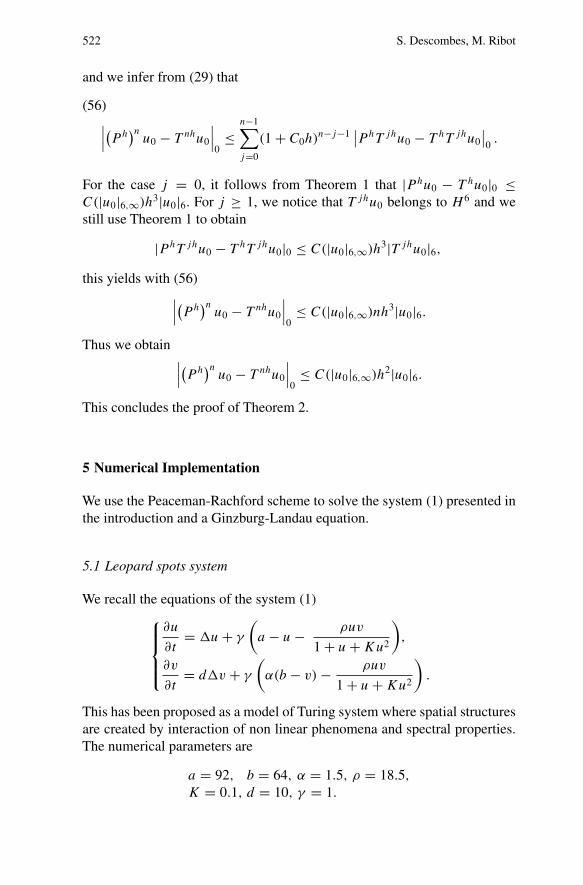
We recall the equations of the system (1)

∂u

∂t= �u + γ

(

a − u − ρuv

1 + u + Ku2

)

,

∂v

∂t= d�v + γ

(

α(b − v) − ρuv

1 + u + Ku2

)

.

This has been proposed as a model of Turing system where spatial structuresare created by interaction of non linear phenomena and spectral properties.The numerical parameters are

a = 92, b = 64, α = 1.5, ρ = 18.5,

K = 0.1, d = 10, γ = 1.

On the Peaceman-Rachford approximation 523

For one time step, we have to do an Euler-forward scheme on the non-lin-ear part, a Crank-Nicolson scheme on the linear part and an Euler-backwardscheme on the non-linear part. It is useful to program several time stepsaltogether, as for n time steps the formula can be written:

P ntu0 =(

(1 + tF/2)−1 L (t/2) (1 − tF/2)

)n

u0

= (1 + tF/2)−1 L (t/2)(

(1 − tF/2) (1 + tF/2)−1 L (t/2)

)n−1

(1 − tF/2) u0

= (1 + tF/2)−1 L (t/2)((

2 (1 + tF/2)−1 − 1)

L (t/2)

)n−1

(1 − tF/2) u0.

In practice, we replace the non linear implicit step by its approximation oforder 2:

(1 + tF/2)−1 1 − tF/2 (1 − tF/2)

28.982227.456825.931424.406122.880721.355319.829918.304516.779215.253813.728412.20310.67769.152277.626896.101514.576133.050761.525380

14.521914.088313.654613.22112.787312.353711.9211.486411.052710.619110.18549.751769.318118.884468.450818.017167.583517.149866.71626.28255

13.922313.517313.112312.707312.302411.897411.492411.087410.682410.27749.872389.467389.062398.657398.252397.84747.44247.037416.632416.22742

13.895413.421312.947212.473111.999111.52511.050910.576910.10289.628729.154658.680588.206517.732447.258376.784296.310225.836155.362084.88801

13.982513.488412.994412.500312.006311.512211.018210.524110.03019.536049.041998.547948.05397.559857.06586.571756.07775.583665.089614.59556

13.950813.461412.97212.482611.993211.503811.014410.52510.03569.546239.056838.567438.078037.588647.099246.609846.120445.631045.141644.65224

13.883713.418412.953212.487912.022711.557411.092210.626910.16179.696429.231168.765918.300667.835417.370166.904916.439665.974415.509165.04391

13.894913.429112.963312.497512.031611.565811.110.634210.16839.702529.23678.770888.305057.839237.373416.907586.441765.975945.510115.04429

13.824513.376412.928312.480312.032211.584111.136110.68810.23999.791859.343788.895728.447657.999587.551517.103456.655386.207315.759245.31117

Fig. 1. The evolution of the solution of (1), starting from four peaks.

524 S. Descombes, M. Ribot

and to compute more easily the Crank-Nicolson scheme and to avoid pro-gramming an Euler-forward scheme, we notice that

L (t/2) = (1 + tM�/2) (1 − tM�/2)−1

=2 (1 − tM�/2)−1 − 1.

The spatial discretization is performed with the finite element method andall computations are made using Freefem+. The evolution of the solution of(1), starting from four peaks is shown in figure 1.

5.2 Ginzburg-Landau equation

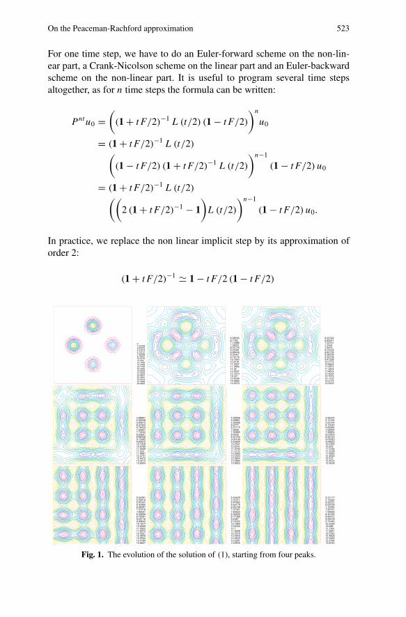
We introduce the quintic Ginzburg-Landau equation:

∂u

∂t= m0�u + m1u + m2|u|2u + m3|u|4u

where the coefficients m0, m1, m2 and m3 belong to the complex plane andu : C → C.

1.187811.125291.062781.000260.9377440.8752270.8127110.7501950.6876790.6251620.5626460.500130.4376140.3750970.3125810.2500650.1875490.1250320.06251620

1.307441.238631.169821.101011.032190.963380.8945670.8257540.7569420.6881290.6193160.5505030.481690.4128770.3440640.2752510.2064390.1376260.06881290

1.296611.228371.160121.091881.023640.9553960.8871540.8189110.7506690.6824260.6141830.5459410.4776980.4094560.3412130.272970.2047280.1364850.06824260

1.288931.221091.153251.085421.017580.9497380.88190.8140610.7462230.6783850.6105460.5427080.4748690.4070310.3391920.2713540.2035150.1356770.06783850

1.311091.242081.173081.104081.035070.9660660.8970610.8280560.7590520.6900470.6210420.5520380.4830330.4140280.3450240.2760190.2070140.1380090.06900470

1.321391.251851.18231.112751.043210.9736580.9041110.8345640.7650170.695470.6259230.5563760.4868290.4172820.3477350.2781880.2086410.1390940.0695474.33681e-

1.322381.252781.183181.113581.043980.9743820.9047830.8351840.7655860.6959870.6263880.5567890.4871910.4175920.3479930.2783950.2087960.1391970.06959874.55365e-

1.295861.227661.159461.091251.023050.9548470.8866430.818440.7502370.6820330.613830.5456270.4774230.409220.3410170.2728130.204610.1364070.06820331.05901e-

1.266351.19971.133051.06640.9997490.9330990.8664490.7997990.7331490.6664990.5998490.5331990.4665490.39990.333250.26660.199950.13330.06664997.51092e-

Fig. 2. The evolution of the solution of the quintic Ginzburg-Landau equation, startingfrom two pulses.

On the Peaceman-Rachford approximation 525

This equation leads to interesting stable pulse-like solutions; these phe-nomena have been studied in [18].

As this equation is a complex one, we split it into a system of two equa-tions, one for the real part, one for the imaginary part and we use exactly thesame scheme as above to solve it with these numerical parameters:

�m0 = 1, �m1 = −0.1, �m2 = 4, �m3 = −2.75,

�m0 = 0, �m1 = 0, �m2 = 1, �m3 = 1.

The numerical results, in figure 2 show collapse between two pulses.

References

1. Akrivis, G., Crouzeix, M., Makridakis, C.: Implicit-explicit multistep finite elementmethods for nonlinear parabolic problems. Math. Comp. 67(222), 457–477 (1998)

2. Bergh, J., Lofstrom,J.: Interpolation spaces. An introduction. Springer-Verlag, Berlin1976, Grundlehren der Mathematischen Wissenschaften, No. 223

3. Besse, C., Bidegaray, B., Descombes, S.: Order estimates in time of splitting methodsfor the nonlinear Schrodinger equation. English SIAM J. Numer. Anal. 40(1), 26–40(2002)

4. Chiu, C., Walkington, N.: An ADI method for hysteretic reaction-diffusion systems.SIAM J. Numer. Anal. 34(3), 1185–1206 (1997)

5. de Mottoni, P., Schatzman, M.: Geometrical evolution of developed interfaces. Trans.Amer. Math. Soc. 347(5), 1533–1589 (1995)

6. Descombes, S.: Convergence of a splitting method of high order for reaction-diffusionsystems. Math. Comp. 70(236) 1481–1501 (2001) (electronic)

7. Descombes, S., Schatzman, M.: Strang’s formula for holomorphic semi-groups.J. Math. Pures Appl. 81(1) 93–114 (2002)

8. Dia, B.O.: Methodes de directions alternees d’ordre eleve en temps. PhD thesis,Universite Claude-Bernard Lyon 1, France, June 1996

9. Dia, B.O., Schatzman, M.: An estimate of the Kac transfer operator. J. Funct. Anal.145(1), 108–135 (1997)

10. Douglas Jr., J.: On the numerical integration of ∂2u/∂x2 + ∂2u/∂y2 = ∂u/∂t byimplicit methods. J. Soc. Indust. Appl. Math. 3, 42–65 (1955)

11. Henry, D.: Geometric theory of semilinear parabolic equations. Berlin: Springer-Verlag, 1981

12. Kato, T.: Perturbation theory for linear operators. Die Grundlehren der mathematis-chen Wissenschaften, Band 132. New York: Springer-Verlag Inc. New York, 1966

13. Murray, J.D.: Mathematical biology. Berlin: Springer-Verlag, second edition, 199314. Peaceman, D.W., Rachford Jr., H.H.: The numerical solution of parabolic and elliptic

differential equations. J. Soc. Indust. Appl. Math. 3, 28–41 (1955)15. Schatzman, M.: Stability of the Peaceman-Rachford formula. J. Funct. Anal. 162,

219–255 (1999)16. Strang, G.: Accurate partial difference methods. I. Linear Cauchy problems. Arch.

Rational Mech. Anal. 12, 392–402 (1963)17. Strang, G.: On the construction and comparison of difference schemes. SIAM J.

Numer. Anal. 5, 506–517 (1968)18. Thual, O., Fauve, S.: Localized structures generated by subcritical instabilities. J. Phys

France. 49, 1829–1833 (1988)