JOURNAL OF GEOPHYSICAL RESEARCH, VOL. 102, NO. D5, PAGES 6131-6142, MARCH 20, 1997

Comparison between vertical ozone soundings and reconstructed potential vorticity maps by contour advection with surgery

A. Mariotti •, M. Moustaoui, B. Legras and H. Teitelbaum Laboratoire de M6t6orologie Dynamique du CNRS, Paris

Abstract. Sudden jumps and deep laminations, observed on vertical stra, tospheric ozone profiles during the European Arctic Stratospheric Ozone Experiment (EA- SOE) (winter 1991-1992) are explained as resulting from transport on isentropic layers. This is obtained by comparing the ozone profiles with high-resolution re- construction of the potential vorticity. Multilayer isentropic contour advection with surgery (CAS) is performed using European Center for Medium Range Weather Forecasts (ECMWF) analyzed winds. The results presented in this work are based on analyzing the location of the edge of the polar vortex, the horizontal and vertica.l extents of filamentary structures and intrusions within the polar vortex. The results are consistent with the a. ssumption of high ozone content within the polar vortex which is valid during normal winter conditions of the northern hemisphere. The resolution required to carry out this study is much higher than that of current op- erational analysis by weather centers, while it is achievable by CAS reconstructions, which provide a dynamical understanding of the ozone variations.

1. Introduction

The dynamics of the polar stratospheric vortex has received a lot of attention over recent years as a part of the ozone hole problem. There is much evidence that the polar air does not mix easily with the mid- latitude air. One striking feature is that sharp horizon- tal gradients in potential vorticity (PV) and chemical constituents are seen on the vortex edge and delimit pouches of polar air outside the vortex, not yet mixed with midlatitude air. The common interpretation is that filaments of polar air are continuously stripped of the polar vortex by isentropic motion and entrained until they mix with midlatitude air [Mcintyre, 1992], while mid-latitude air hardly penetrates the polar re- gion. The efficiency of this process to build up gradi- ents against diffusion is known theoretically [Mariotti et al., 1994] and has been demonstrated experimentally [Waugh et at., 1994; Ptumb et at., 1994].

During wintertime, the lower Arctic stratosphere is normally characterized by high P V values and ozone concentrations with respect to midlatitudes. The dia- batic descent of polar air [Rosenlof and Holton, 1993; Rosenfield et at., 1994] coupled to the poleward merid- ional circulation in the mid and upper stratosphere brings air enriched in ozone from its formation region

Now at ENEA, Roma.

Copyright 1997 by the American Geophysical Union.

Paper number 96JD03509. 0148-0227/97/96JD-0S•0•$0•.00

in the upper tropical stratosphere. In the absence of destruction by chlorine, the lifetime of ozone is of sev- eral months in the lower stratosphere. The production of active chlorine by heterogeneous chemistry on po- lar stratospheric clouds (PSC), which accounts for the destruction of most of the polar ozone in the Antarc- tic, may have a more limited impact in the Arctic where PSCs are not so abundant. In particular, dur- ing the winter 1991-1992, which is considered in this study, temperatures in the Arctic lower stratosphere did not fall after mid-January below the critical tem- perature necessary for PSC formation [Farman et at., 1994]. Therefore, relative abundance of ozone is usu- ally maintained in the vortex and one can trace the boundary between midlatitude and polar air by ozone measurements [Newman et et., 1996].

Dobson [1973] was the first to point out the lami- nated structures observed during ozone probe ascent. Two types of tracer variability exist [Holton, 1987]: the first one is highly correlated with potential temperature fluctuations and can be attributed to vertical displace- ments of material surfaces induced by gravity waves; the second one is not associated with significant poten- tial temperature oscillations and could therefore be pro- duced by quasi-geostrophic motions, for which parcel trajectories nearly coincide with the mean isentropes. Observations can be called upon in favor of both mecha- nisms: measures of ozone and water vapor along vertical profiles during the European Arctic Stratospheric Ex- periment (EASOE) led Teitetbaum et et. [1994, 1996] to conclude that the vertical laminated structure of both

6131

6132 MARIOTTI ET AL.: OZONE SOUNDINGS AND POTENTIAL VORTICITY MAPS

constituents can be generated by gravity waves; a sta- tistical analysis of the relation between ozone laminae and the fluctuations of the polar vortex led Raid at al. [1993] to suggest that laminae could be induced by the mixing of different air masses by synoptic-scale motion.

There have been comparatively few studies trying to relate the small-scale vertical and horizontal structures

of the vortex. In the works by Waugh et al. [1994] and Plumb et al. [1994] the horizontal filamentary distri- bution of PV around the vortex was reconstructed on

several isentropic levels using contour advection with surgery (CAS). The calculated values were highly cor- related with sloping vortex edge and filamentary struc- tures observed by a lidar on board DC-8 missions during the Airborne Arctic Stratosphere Expedition (AASE 1). More recently, Orsolini [1995], who used a multi- layer Prather advection scheme, showed that isentropic transport can qualitatively reproduce the vertical fluc- tuations of the ozone profile measured during EASOE, and Newman at al. [1996] studied the transport of polar air to midlatitudes following the breaking of the polar vortex.

The aim of this work is to investigate in more detail the relation between isentropic transport processes, as depicted by PV multilayer CAS reconstructions, and features observed on vertical ozone profiles from the EASOE stratospheric soundings. The next section de- scribes the data, which are ozone profiles from EASOE and wind fields from ECMWF. Section 3 briefly de- scribes the essentials of the CAS technique. Section 4 validates CAS reconstruction by its characterization of the vortex edge. Section 5 presents the ms,in results on filamentary transport out of the vortex and its link with laminae structure. Section 6 discusses the case of intru-

sion of midlatitude air within the vortex. A discussion

is offered in section 7.

2. Data

The data used in this st•dy are in situ ozone mea- surements made by probes launched during the EASOE campaign which took place in the northern hemisphere during winter 1991-1992. Balloons were launched al- most daily from specific sites. performing vertical sound- ings of various physical parameters, including temper- ature and ozone partial pressure, with a vertical reso- lution of about 200 m (see Pyla [1994] for further de- tails). The EASOE data used in this study are vertical profiles of ozone partial pressure, with potential tem- perature as the vertical coordinate in the range from 300 K to 500 K, to cover from upper troposphere to lower stratosphere. The geographical location of the launching stations is given in Table 1. A nonrecursive low-pass filter, with Kaiser's window [Hamming, 1983], has been applied to remove fluctuations of wavelength lower than 400 m. Estimates of the horizontal drift

of the balloons during uprise, made from in situ wind speed measurements, have led us to neglect this effect throughout our study.

In order to study the relation between specific fea- tures observed on the ozone profiles and transport pro- cesses at the time of the soundings, data from the ECMWF analysis have been used to initialize high- resolution CAS reconstructions of PV fields on isen-

tropic surfaces. The vertical interpolation procedure to calculate PV on these surfaces from archived data

on pressure levels is the same as in the work byBrunat et al. [1995]. All PV values are given in PV units (1 PVU = 10 -• K m • s -• kg-•).

3. Contour Advection Surgery of Potential Vorticity

Under the assumption of adiabatic motion of air par- ticles, PV is a Lagrangian invariant and PV contours are transported like material lines on isentropic stir- faces. The CAS algorithm [Waugh and Plumb, 1994; Norton, 1994] is based on the discretization of the PV field as a set of N contours separated by finite P V jumps. Each of these contours is described by a set of particles distributed along the contour wi•h density locally depending on the curvature. In our case, GAS is initialized with relatively coarse resolution PV fields from ECMWF analysis in T42 spectral resolution. The contours are then advected using velocities taken from observed winds and the nodes are periodically redefined by the surgery algorithm, as indicated below, in order to maintain the accuracy.

After a few days (see, for instance, Figure 2), nu- merous small-scale structures are reconstructed at much

higher resolution than the initial field and the advecting wind. Contrary to the common intuition which would filter out these features as irrelevant. noise, we take them as a prediction of the actual small-scale PV distribu- tion. This unobvious result is well understood within

the idealized framework of two-dimensional turbulence, dominated by long-lived eddies which determine the ve- locity field. The control of local strain by large-scale structures has been mathematically proven under fairly broad conditions by Eyink [1996]. Small-scale filaments and steep gradients then arise as a manifestation of chaotic advection of particles by the flow. This results from the existence of time varying saddle points in the stream function chart [Ottino, 1989]. Stratospheric mo- tion is essentially layerwise with only sparse regions of

Table 1. Geographical Locations of Launching Sta- tions Used in This Study

Station Latitude, Longitude, oN øE

Aberystwyth 52.7 -4.1 Bear Island 74.5 19.0

Heiss Island 80.6 58.1

Hohenpeissenberg 47.5 11.0 Lerwick 60.1 -1.2

Payerne 46.8 6.9 Scoresbysund 70.5 -22.0 Thule 76.5 -68.5 Uccle 50.8 4.4

MARIOTTI ET AL.' OZONE SOUNDINGS AND POTENTIAL VORTICITY MAPS 6133

three dimensional turbulence. By virtue of its strati- fication, it is not prone to the development of synop- tic or subsynoptic baroclinic instabilities. Therefore, by analogy with two-dimensional turbulence, we expect that reconstruction of the fine scale mixing processes is possible through particle advection using coarse reso- lution wind fields as long as the relevant structures of the stream function chart are captured. The validity of this approach has been established by Waugh and Plumb [1994].

All calculations reported in this paper have been per- formed on a hemispherical domain using data (winds and potential vorticity) from ECMWF analysis. These data are given at 6 hour intervals and have been tempo- rally interpolated by a cubic spline method to provide data every half-hour, which is the chosen advection time step. From the original spectral T42 resolution, the horizontal interpolation of the wind at the location of particles is performed in two steps. The wind is first calculated on a hemispherical grid of 256 x 96 points. The velocity at a given point is then calculated as a weighted mean of values at the four surrounding mesh points, with weights inversely proportional to distances. Special care is taken to achieve correct interpolation in the polar region; in this area interpolation is done using the two points lying on the last latitudinal circle of the grid and the velocity at the pole.

The contour surgery algorithm of Dritschel [Dritschel, 1989] allows control of the complicated evolution of the contours during the calculations through two steps. In the first one, it redistributes the particles along the con- tour according to the curvature with density depending

500

'-"450

• 400

.,--4

• 1t50 o

300

..

o

0 5 10 15 2o

Ozone (mPa)

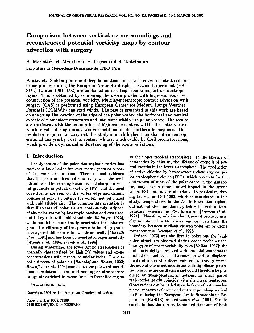
Figure 1. Ozone profiles as a function of potential tem- perature corresponding to radio soundings launched on March 18, 1992, from Bear Island at l100 UT (solid line) and Scoresbysund at 1100 UT (dashed-dotted line).

Table 2. PV Va, lues for the Two Contours, PV•NF and PVst•r, Bracketing the Vortex Edge on the Potential Temperature Levels

•, PVINF, PVsuP, K PVU PVU

350 7 8

362 8 10

375 9 11 400 11 14 420 13 16

450 18 21 475 23 26

Complementary contours are used in section 6 for the study of midlatitude air intrusion.

on a parameter /t. In the second step, it splits one contour in two or merges two contours of equal P V to- gether when the distance between segments gets smaller than that defined by the critical parameter •. Our cal- culations have been carried out with parameter values p = 0.1 and • = 0.0025, following Waugh and Plumb [19941.

4. Vortex Edge Definition and Validation of the Method

Figure 1 shows the ozone profiles on March 18 at 1100 UT taken at the two sites Scoresbysund and Bear Island. At all levels the two profiles exhibit fluctuations with vertical scale of l0 K or smaller, and amplitude decreasing with height. Near 400 K the ozone content measured at Scoresbysund, with partial pressure of the order of 5 mPa, is much smaller than that measured at Bear Island, with partial pressure of the order of 16 mPa. On the contrary, near 450 K, the ozone content is high at the two sites.

A good definition of the vortex boundary is necessary to assess how and when transport into or out of the main body of the vortex occurs. As many preceding works have indicated [e.g. Mcintyre, 1992], the location of the maximum PV gradient is a sound definition of the edge since it agrees with our current understanding of the generation of this edge by erosion processes. Our approach, however, is based on a discretization of P V by a small number of highly resolved contours. Hence, this definition cannot be easily used directly. Instead, we choose to bracket the edge by two contours chosen as follows. We first approximate the location of the vor- tex edge by that of a given contour which fits the line of maximum vorticity gradient within the large-scale analysis of the ECMWF. According to this definition the chosen contour varies with the level and day con- sidered . We then choose for each level two fixed values

of PV (see Table 2) which are close to but always brack- eting the value of maximum PV gradient. Using these two values for CAS calculations, we ensure a bracket- ing of the vortex edge by the two contours. In practice, as discussed below, the two contours often collapse to- gether, thus providing an unambiguous location of the

6134 MARIOTTI ET AL.- OZONE SOUNDINGS AND POTENTIAL VORTICITY MAPS

edge. Contours are distant where erosion or penetra- tion takes place, or as a result of surgery in expelled filaments.

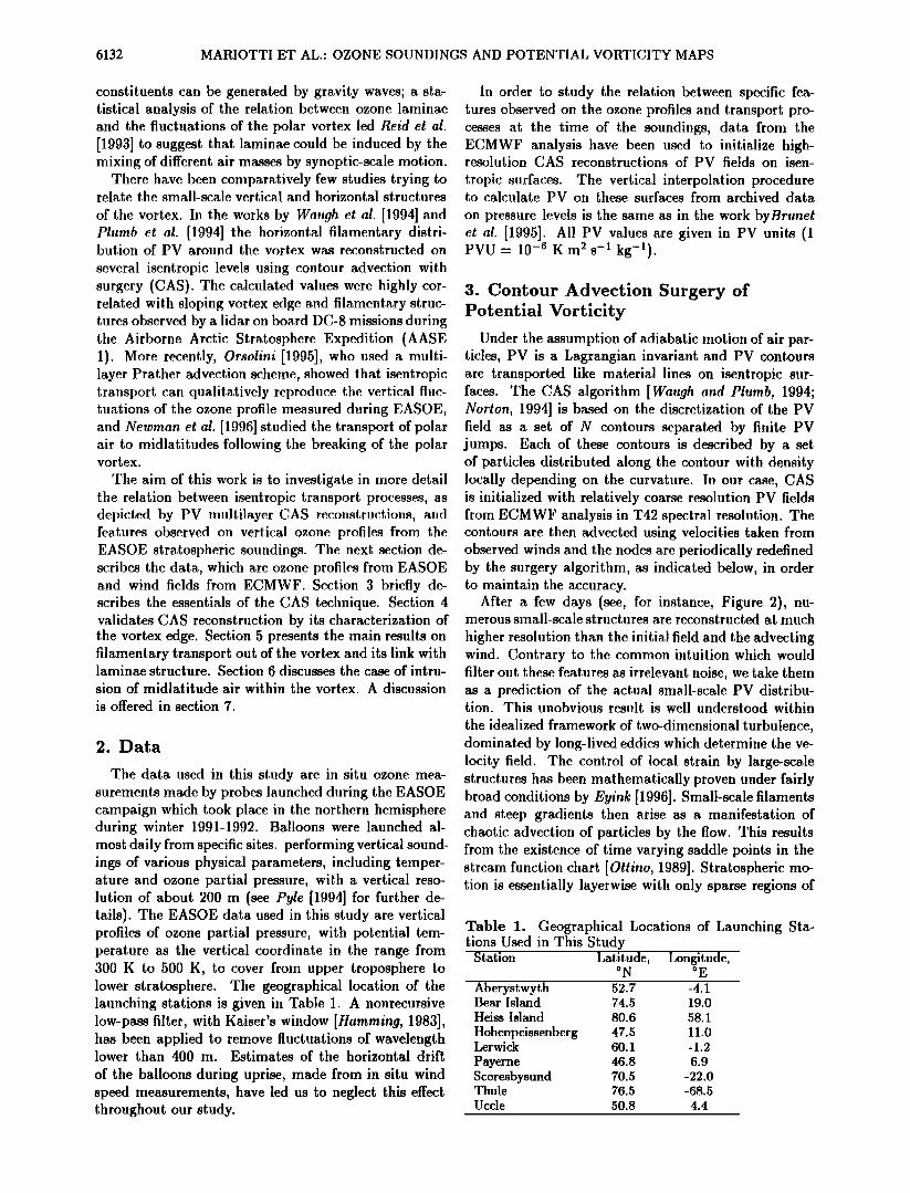
Figure 2a shows a stereographic projection of the northern hemisphere polar vortex as depicted by se- lected iso-PV contours from the ECMWF data at 400 K

on the same day as profiles in Figure 1. The vortex is split into two almost separate components as conditions start to build up for its final springti•ne breakdown. The

Figure 2. Northern hemisphere PV chart at 400 K on March 18, 1992, at 1200 UT. The chart is drawn in po- lar stereographic projection for latitudes north to 35øN. The circle is at 60øN. Shown contours are at values 11 PVU and 14 PVU. Indicated stations are Bear Island

(BI) and Scoresbysund {SC). (a) Field from ECMWF analysis. (b) Field from a CAS calculation initiated on March 13, 1992, at 1200 UT.

5OO

v450

• 4o0

...-•

-• :350 o

300

--T I 'T i •'• T

ß

0 5 10 15 2o

Ozone (mPa)

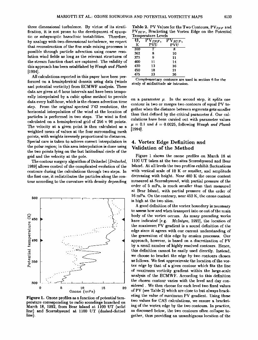
Figure 3. Ozone profiles as a function of potential temperature corresponding to radio soundings launched on January 8, 1992, from Uccle at 1050 UT (solid line) and Letwick at 1130 UT (dashed line).

location of the two sounding stations, Bear Island and Scoresbysund, is reported. They are both on the vortex edge, but the ambiguity of whether they are inside or outside cannot be removed.

The result of PV reconstruction by CAS calculation at 400 K, initiated on March 13 at 1200 UT is shown in Figure 2b using the same contours as in Figure 2a.. It places Scoresbysund outside the polar vortex while Bear Island is located inside. A similar GAS calculation at

450 K (not shown) places the two stations inside the polar vortex. The marked difference in ozone concen- tration observed on the vertical profiles is thus associ- ated, according to GAS, with a sloping vortex edge and penetration into the vortex body occurring at different altitudes for the two sites.

Figure 3 shows the ozone content at the two stations Uccle and Lerwick on January 8, 1992, at 1200 UT. The vertical profiles are very different all the way up to 475 K. Uccle presents a low ozone content which char- acterizes midlatitude air outside the polar vortex while Lerwick presents high values which characterize polar stratospheric air within the vortex. Accordingly, the GAS reconstruction of the PV distribution for this event

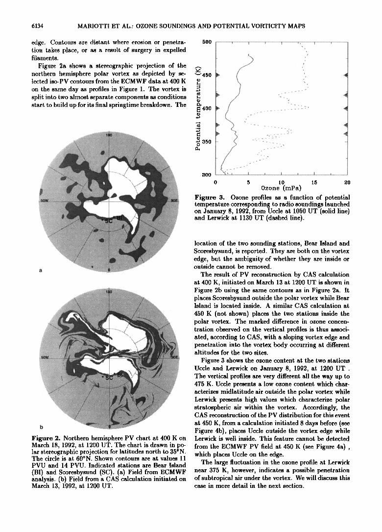
at 450 K, from a calculation initiated 8 days before (see Figure 4b), places Uccle outside the vortex edge while Letwick is well inside. This feature cannot be detected

from the ECMWF PV field at 450 K (see Figure 4a) , which places Uccle on the edge.

The large fluctuation in the ozone profile at Letwick near 375 K, however, indicates a possible penetration of subtropical air under the vortex. We will discuss this case in more detail in the next section.

MARIOTTI ET AL.' OZONE SOUNDINGS AND POTENTIAL VORTICITY MAPS 6135

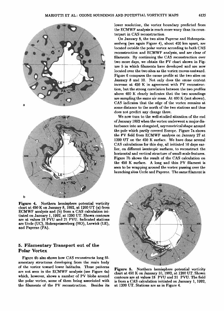
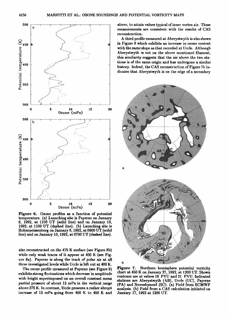
Figure 4. Northern hemisphere potential vorticity chart at 450 K on January 8, 1992, at 1200 UT (a) from ECMWF analysis and (b) from a CAS calculation ini- tiated on January 1, 1992, at 1200 UT. Shown contours are at values 18 PVU and 21 PVU. Indicated stations

are Uccle (UC), Uohenpeissenberg (no), Lerwick (LE), and Payerne (PA).

5. Filamentary Transport out of the Polar Vortex

Figure 4b also shows how CAS reconstructs long fil- amentary structures developing from the main body of the vortex toward lower latitudes. These patterns are not seen in the ECMWF analysis (see Figure 4a) which, however, shows a number of PV blobs around the polar vortex, some of them being associated with the filaments of the PV reconstruction. Besides its

lower resolution, the vortex boundary predicted from the ECMWF analysis is much more wavy than its coun- terpart in CAS reconstruction.

On January 8, the two sites Payerne and Hohenpeis- senberg (see again Figure 4), about 400 km apart, are located outside the polar vortex according to both CAS reconstruction and ECMWF a. nalysis, and are clea. r of filaments. By continuing the CAS reconstruction over two more days, we obtain the PV chart shown in Fig- ure 5 in which filaments have developed and are now located over the two sites a.s the vortex moves eastward.

Figure 6 compares the ozone profile at the two sites on January 8 and 10. Not only does the ozone content. increase at 450 K in agreement with PV reconstruc- tion, but the strong correlation between the two profiles above 400 K clearly indicates that the two soundings are sampling the same air mass. At 400 K (not shown), CAS indicates that the edge of the vortex remains at some dista.nce to the north of the two stations and thus

does not predict any change there. We now turn to the well-studied situation of the end

of January 1992 when the vortex underwent a major dis- turbance into an elongated, asymmetrical shape around the pole which partly covered Europe. Figure 7a shows the PV field from ECMWF a.nalysis on January 27 a.t 1200 UT on the 450 K surface. We have done several

CAS calculations for this day, all initiated 10 days ear- lief, on different isentropic surfaces, to reconstruct the horizontal and vertical structure of small-sca,le features.

Figure 7b shows the result of the CAS ca.lculation on the 450 K surface. A long and thin PV filament is seen to be wrapping around the vortex passing over the launching sites Uccle and Payerne. The same filament is

Figure 5. Northern hemisphere potential vorticity chart at 450 K on January 10, 1992, at 1200 UT. Shown contours are at values 18 PVU and 21 PVU. The field

is from a CAS calculation initiated on January 1, 1992, at 1200 UT. Stations are as in Figure 4.

6136 MARIOTTI ET AL.' OZONE SOUNDINGS AND POTENTIAL VORTICITY MAPS

500

'-' 450

• 400

.,.-•

• 350 o

300

5OO

'-•450

400

350

• •.• • • •- ..........

,. J z ._L .•

10 15 •0

Ozone (mPa)

.......... :-. :' "

300

0 5 l0 15 20

Ozone (rnPa)

Figure 6. Ozone profiles as a function of potential temperature. (a) Launching site is Payerne on January 8, 1992, at l100 UT (solid line) and on January 10, 1992, at 1100 UT (dashed line). (b) Launching site is Hohenpeissenberg on January 8, 1992, at 0900 UT (solid line) and on January 10, 1992, at 0700 UT (dashed line).

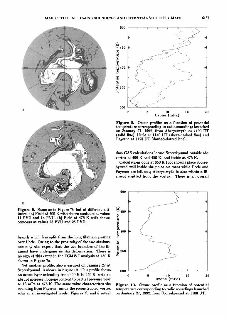
also reconstructed on the 475 K surface (see Figure 8b) while only weak traces of it appear at 400 K (see Fig- ure 8a). Payerne is along t. he track of polar air at, all three investigated levels while Uccle is left, out at 400 K.

The ozone profile measured at Payerne (see Figure 9) exhibits strong fluctuations which decrease in amplitude with height superimposed on an overall constant mean partial pressure of about 13 mPa in the vertical range above 375 K. In contrast, Uccle presents a rather abrupt, increase of 13 mPa going from 400 K to 450 K and

above, to attain values typical of inner vortex air. These measurements are consistent with the results of CAS reconstruction.

A third profile measured at Aberystwyth is also shown in Figure 9 which exhibits an increase in ozone content with the same slope as that recorded at Uccle. Although Aberystwyth is not on the above mentioned filament,, this similarity suggests that the air above the two sta- tions is of the same origin and has undergone a similar history. Indeed, the CAS reconstruction of Figure 7b in- dicates that Aberystwyth is on the edge of a secondary

Figure 7. Northern hemisphere potential vorticity chart at 450 K on January :27, 199:2, at 1.:200 UT. Shown contours are at values 18 PVU and 21 PVU. Indicated

stations are Aberystwyth (AB), Uccle (UC), Payerne (PA) and Scoresbysund (SC). (a) Field from ECMWF analysis. (b) Field from a CAS calculation initiated on January 17, 1992 at 1200 UT.

MARIOTTI ET AL.: OZONE SOUNDINGS AND POTENTIAL VORTICITY MAPS 6137

Figure $. Same as in Figure 7b but a.t different alti- tudes. (a) Field at 400 K with shown contours at values 11 PVU and 14 PVU. (b) Field at 475 K with shown contours at values 23 PVU and 26 PVU.

branch which has split from the long filament passing, over Uccle. Owing to the proximity of the two stations, one may also expect that the two branches of the fil- ament have undergone similar deforma.tion. There is no sign of this event in the ECMWF ana. lysis at 450 K shown in Figure 7a.

Yet another profile, also measured on January 27 at Scoresbysund, is shown in Figure 10. This profile shows an ozone layer extending from 400 K to 450 K, with an abrupt increase in ozone content to partial pressure near to 13 mPa at 475 K. The same value characterizes the

sounding from Payerne, inside the reconstructed vortex edge at all investigated levels. Figures 7b a, nd 8 revea. l

5OO

'•450

1• 400

ø,--4

-'-' •õ0 o

300

0 5 10 1.5 20

Ozone (,nPa)

Figure 9. Ozone profiles as a function of potential temperature corresponding to radio soundings launched on January 27, 1992, from Aberystwyth at 1100 UT (solid line), Uccle at 1140 UT (short-dashed line) and Payerne at 1125 UT (dashed-dotted line).

that CAS calculations locate Scoresbysund outside the vortex at 400 K and 450 K, and inside at 475 K.

Calculations done at 350 K (not shown) place Scores- bysund well inside the polar air mass while Uccle and Payerne are left out; Aberystwyth is also within a fil- ament emitted from the vortex. There is an overall

500

'-• 450

400

350

300

0 5 10 15 2o

Ozone (mPa)

Figure 10. Ozone profile a.s a function of potential temperature corresponding to radio soundings launched on January 27, 1992, from Scoresbysund at 1100 UT.

6138 MARIOTTI ET AL.: OZONE SOUNDINGS AND POTENTIAL VORTICITY MAPS

agreement with the ozone profiles, with the exception of Aberystwyth. We are, however, reluctant to sug- gest that CAS is reliable at 350 K owing to the strong dispersion of the polar air during the 10 days of the integration and the proximity of the tropopause. In particular, the initial conditions derived from ECMWF analysis are very noisy on the subsynoptic scale.

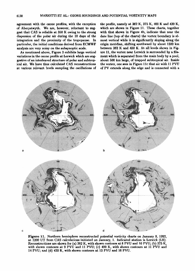
As mentioned above, Figure 3 exhibits large vertical variations in the ozone profile at Letwick which are sug- gestive of an interleaved structure of polar and subtrop- ical air. We have thus calculated CAS reconstructions

at various relevant levels sampling the oscillations of

the profile, namely at 362 K, 375 K, 400 K and 420 K, which are shown in Figure 11. These charts, together with that shown in Figure 4b, indicate that near the date line (top of the charts) the vortex boundary is al- most vertical while it is significantly sloping along the origin meridian, shifting southward by about 1500 km between 362 K and 450 K. At all levels shown in Fig- ure 1 l, the vortex near Letwick is surrounded by a fila- ment which is separated from the main body by a pool, about 500 km large, of trapped subtropical air. Inside the vortex, one sees in Figure 11c that air with I 1 PVU of PV extends along the edge and is connected with a

======================================================================= ::: : ..::::::::.:•.......:..•.:::....::!:!.....•:.:....•......;•i:•q•!:i::i:i:i:i:i:i:i:i:i::i:i:!:::•?•.

========================================================= •. • -• _ =======================================================================

'-:•::::i.-"..-i::::::.'....-':•:::•ii•::::::::ii:: ....................................... ••••••.,•.•-,•. ........ %., •'"•' "'"":••:..• ..... ================================================================================== . : .::.•..::::::::::::::::::::::::::::::::::::::::::::::::::::::::::::::::::::::::::::::::::::::::::::::::::::::::::::::

.... •:•:;:•:•:•:•:•:•:•:•:•*;•;•*•:•:;•!•;•;•i•!•;:•;:•:;:•:;?.•:; :: :: •;•;•;•;:;•;;•il :: i i i :: i • • :: ::i:: :: ::• ::::i ::i::!! i::::::::i•i•i::::::!::::i::ii::ii::::i

.... •;::iii :::•iii:: ::•::•::• .... •:•::•i•..•-.-'. :•i•!•::•i-':•::::•:•:•::•:• ..............................................................................................................................

.... :: ::2.,. :$-:: ::'.. -:.•:: :::: ::::: :: ::::::::. ":':: :: $•::: :•:•:•:•: :•:•: :•: :•:•:•:•:•:•:•-'.::•:•:•:•:•:•:•:•:•:•:•:•:•:•.;•' '-:::::.•::-' '

d ......... ::::*:-z.**i*i•!::i::::!::i::*•iii::ii::iii::::.;.O...*•;;iiiiiiii?:ii::i? :;:-'.:*::*•"• ..........

Figure 11. Northern hemisphere reconstructed potential vorticity charts on January 8, 1992, at 1200 UT from GAS calculations initiated on January, 1. Indicated station is Letwick (LE). Reconstructions are shown for (a) 362 K, with shown contours at 8 PVU and 10 PVU; (b) 375 K, with shown contours at 9 PVU and 11 PVU; (c) 400 K, with shown contours at 11 PVU and 14 PVU; and (d) 420 K, with shown contours at 13 PVU and 16 PVU.

MARIOTTI ET AL.: OZONE SOUNDINGS AND POTENTIAL VORTICITY MAPS 6139

seemingly mixed region in the upper left quadrant. On the edge itself, one finds air with 14 PVU of PV which is connected with the interior of the vortex. This struc-

ture is also visible at 375 K, and there are some hints that it exists at 420 K. Owing to the vertical slope of the vortex, and since Lerwick passes from the exterior of the surrounding filament at 362 K to the deep in- terior of the vortex at 450 K, one expects in this case that the vertical sounding is an image of the horizon- tal structure. Indeed, Figure 3 agrees fairly well with this prediction. At 362 K, the high ozone content can be associated with the filament surrounding the vortex. The fall in ozone content nea. r 375 K can be associated

with the crossing of the region of trapped subtropical air. At 400 K, Lerwick is just under the high PV air on the edge. One may associate the fall in ozone con- tent at 420 K with the crossing of the mixed air region. At 450 K and above, the balloon is well inside the vor- tex and the ozone content does not exhibit any more variations.

6. Intrusive Transport of Midlatitude Air

The deformation and filamentation of the polar vor- tex are able to transport polar air toward midlatitude. We investigate here how transport from low latitude is possible, concentrating on the case of January 22, 1992,, which has been studied by Pbtmb et al. [1994]. During the second half of January 1992, an intense sud- den warming was produced associated with a blocking event over the Atlantic region. This led at all levels to

a strongly deformed polar vortex with significant intru- sion of subtropical air up to the pole itself.

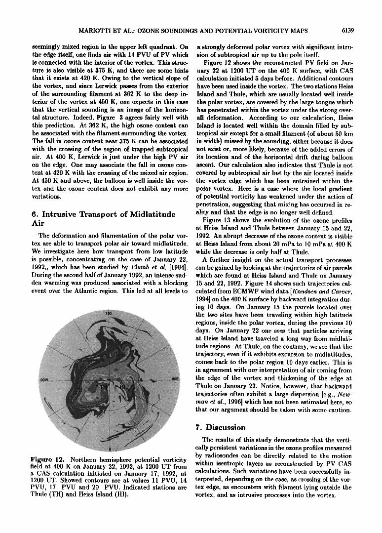
Figure 12 shows the reconstructed PV field on Ja.n- uary 22 at 1200 UT on the 400 K surface, with CAS calculation initiated 5 days before. Additional contours have been used inside the vortex. The two stations tteiss

Island and Thule, which are usually located well inside the polar vortex, are covered by the large tongue which has penetrated within the vortex under the strong over- all deformation. According to our calculation, Ileiss Island is located well within the domain filled by sub- tropical air except for a small filament (of about 50 km in width) missed by the sounding, either because it does not exist or, more likely, because of the added errors of its location and of the horizontal drift during balloon ascent. Our calculation also indicates that Thule is not

covered by subtropical air but by the air located inside the vortex edge which has been entrained within the polar vortex. Here is a case where the local gradient of potential vorticity has weakened under the action of penetration, suggesting that mixing has occurred in re- ality and that the edge is no longer well defined.

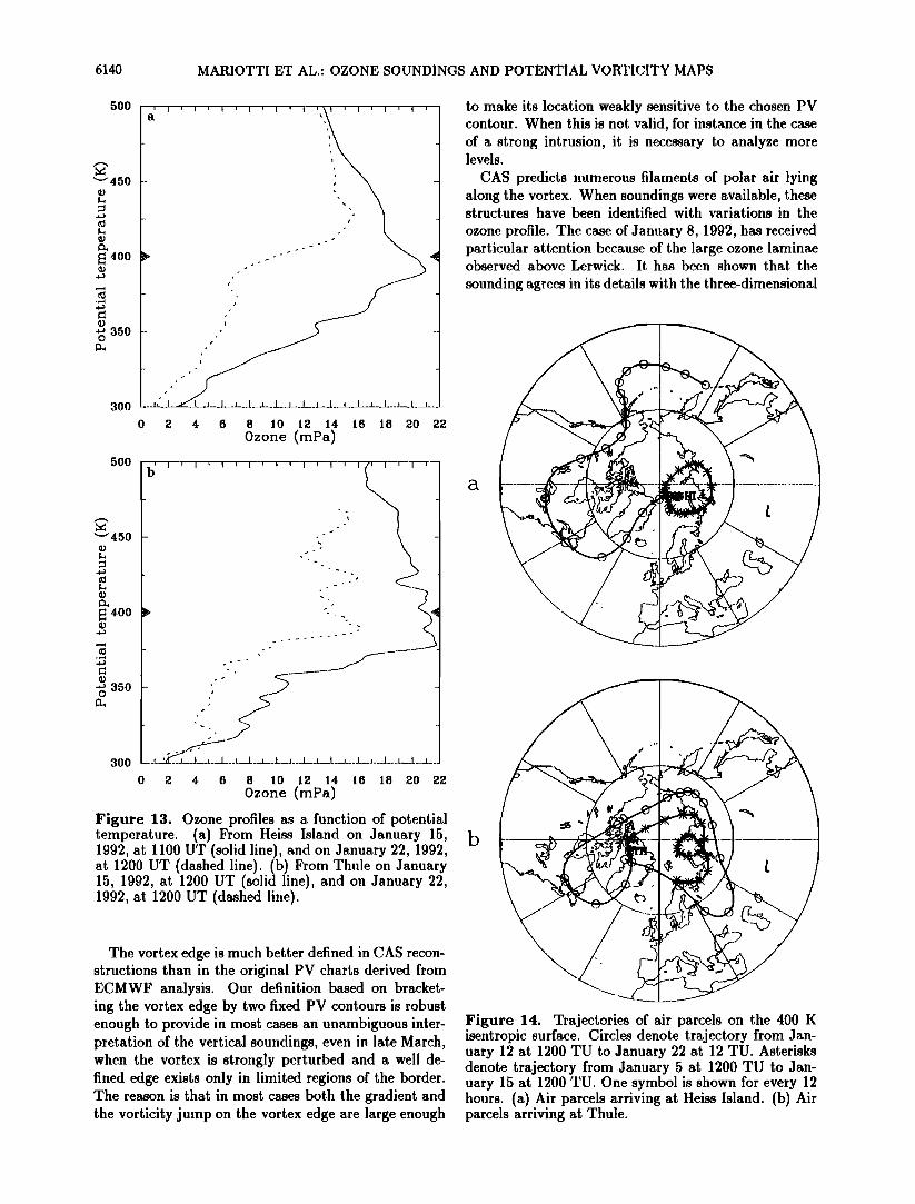
Figure 13 shows the evolution of the ozone profiles at Heiss Island and Thule between January 15 and 22, 1992. An abrupt decrease of the ozone content is visible at Heiss Island from about 20 mPa. to 10 mPa at 400 K

while the decrease is only half at Thule. A further insight on the actual transport processes

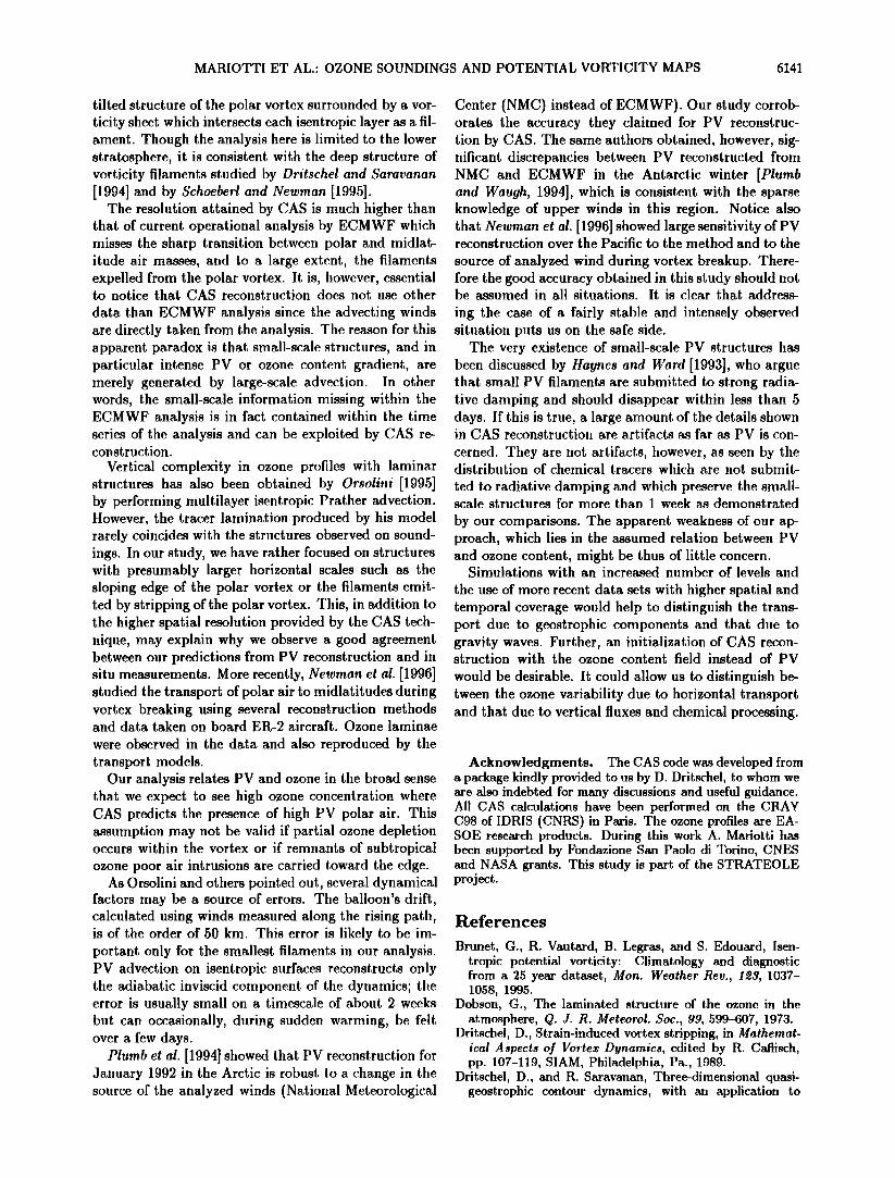
can be gained by looking at the trajectories of air parcels which are found at Heiss Island and Thule on January 15 and 22, 1992. Figure 14 shows such trajectories cal- culated from ECMWF wind data [Knusen and Carver, 1994] on the 400 K surface by backward integration dur- ing 10 days. On January 15 the parcels located over the two sites have been traveling within high latitude regions, inside the polar vortex, during the previous 10 days. On January 22 one sees that particles arriving at Heiss Island have traveled a long way kom midlati- tude regions. At Thule, on the contrary, we see that the trajectory, even if it exhibits excursion to midlatitudes, comes back to the polar region 10 da.ys earlier. This is in agreement with our interpretation of air coming from the edge of the vortex and thickening of the edge at Thule on January 22. Notice, however, that backward trajectories often exhibit a large dispersion [e.g., New- man et al., 1996] which has not been estimated here, so that our argument should be ta. ken with son•e cat•tion.

Figure 12. Northern hemisphere potential vorticity field at 400 K on January 22, 1992, at 1200 UT from a CAS calculation initiated on January 17, 1992, at 1200 UT. Showed contours are at values 11 PVU, 14 PVU, 17 PVU and 20 PVU. Indicated sta. tions are Thule (TH) and Heiss Island (HI).

7. Discussion

The results of this study demonstrate that the verti- cally persistent variations in the ozone profiles measured by radiosondes can be directly related to the motion within isentropic layers as reconstructed by PV CAS calculations. Such variations have been successfully in- terpreted, depending on the case, as crossing of the vor- tex edge, as encounters with filament lying outside the vortex, and as intrusive processes into the vortex.

6140 MARIOTTI ET AL.' OZONE SOUNDINGS AND POTENTIAL VORTICITY MAPS

500

•-• 450

400

350

3OO

500

"'"• 450

400

350

0 2 4 6 8 10 12 14 16 18 20 22

Ozone (mPa)

. ...,,,,•'• -----------------------------L--J-----------•----------.L------------------------- 300

0 2 4 6 8 10 12 14 16 18 20 22

Ozone (mPa)

Fig,re 13. Ozone profiles as a function of potential temperature. (a.) From Heiss Island on January 15, 1992, at 1100 UT (solid line), and on January 22, 1992, a.t 1200 UT (dashed line). (b) From Th,,!e on January 15, 1992, at 1200 UT (solid line), and on January 22, 1992, at 1200 UT (dashed line).

The vortex edge is much better defined in CAS recon- structions than in the original P V charts derived from ECMWF analysis. Our definition based on bracket- ing the vortex edge by two fixed P V contours is robust enough to provide in most cases an unambiguous inter- pretation of the vertical soundings, even in late March, when the vortex is strongly perturbed and a well de- fined edge exists only in limited regions of the border. The reason is that in most cases both the gradient and the vorticity jump on the vortex edge are large enough

to make its location weakly sensitive to the chosen PV contour. When this is not valid, for instance in the case of a strong intrusion, it is necessary to analyze more levels.

CAS predicts numerous filaments of polar air lying along the vortex. When soundings were available, these structures have been identified with variations in the

ozone profile. The case of January 8, 1992, has received particular attention because of the large ozone laminae observed above Lerwick. It has been shown that the

sounding agrees in its details with the three-dimensional

a

b

Figure 14. Trajectories of air parcels on the 400 K isentropic surface. Circles denote trajectory from Jan- uary 12 at 1200 TU to January 22 at 12 TU. Asterisks denote trajectory from January 5 at 1200 TU to Jan- uary 15 at 1200 TU. One symbol is shown for every 12 hours. (a) Air parcels arriving at Heiss Island. (b) Air parcels arriving at Thule.

MARIOTTI ET AL.: OZONE SOUNDINGS AND POTENTIAL VORTIGITY MAPS 6141

tilted structure of the polar vortex surrounded by a vor- ticity sheet which intersects each isentropic layer as a fil- ament. Though the analysis here is limited to the lower stratosphere, it is consistent with the deep structure of vorticity filaments studied by Dritschel and Saravarian [1994] and by Schoeberi and Newman [1995].

The resolution attained by CAS is much higher than that of current operational analysis by ECMWF which misses the sharp transition between polar and midlat- itude air masses, and to a large extent, the filaments expelled from the polar vortex. It is, however, essential to notice that CAS reconstruction does not use other

data than ECMWF analysis since the advecting winds are directly taken from the analysis. The reason for this apparent paradox is that small-scale structures, and in particular intense P V or ozone content gradient, are merely generated by large-scale advection. In other words, the small-scale information missing within the ECMWF analysis is in fact contained within the time series of the analysis and can be exploited by CAS re- construction.

Vertical complexity in ozone profiles with laminar structures has also been obtained by Orsolini [1995] by performing multilayer isentropic Prather advection. However, the tracer lamination produced by his model rarely coincides with the structures observed on sound- ings. In our study, we have rather focused on structures with presumably larger horizontal scales such as the sloping edge of the polar vortex or the filaments emit- ted by stripping of the polar vortex. Tiffs, in addition to the higher spatial resolution provided by the CAS tech- nique, may explain why we observe a good agreement between our predictions from PV reconstruction and in situ measurements. More recently, Newman et ai. [1996] studied the transport of polar air to midlatitudes during vortex breaking using several reconstruction methods and data taken on board ER-2 aircraft. Ozone laminae

were observed in the data and also reproduced by the transport models.

Our analysis relates PV and ozone in the broad sense that we expect to see high ozone concentration where CAS predicts the presence of high PV polar air. This assumption may not be valid if partial ozone depletion occurs within the vortex or if remnants of subtropical ozone poor air intrusions are carried toward the edge.

As Orsolini and others pointed out, several dynamical factors may be a source of errors. The balloon's drift, calculated using winds measured along the rising path, is of the order of 50 km. This error is likely to be im- portant only for the smallest filaments in our analysis. P V advection on isentropic surfaces reconstructs only the adiabatic inviscid component of the dynamics; the error is usually small on a timescale of about 2 weeks but can occasionally, during sudden warming, be felt over a few days.

Plumb et ai. [1994] showed that PV reconstruction for January 1992 in the Arctic is robust to a change in the source of the analyzed winds (National Meteorological

Center (NMC) instead of ECMWF). Our study corrob- orates the accuracy they claimed for P V reconstruc- tion by CAS. The same authors obtained, however, sig- nificant discrepancies between P V reconstructed from NMC and ECMWF in the Antarctic winter [Plumb and Waugh, 1994], which is consistent with the sparse knowledge of upper winds in this region. Notice also that Newman et ai. [1996] showed large sensitivity of PV reconstruction over the Pacific to the method and to the

source of analyzed wind during vortex breakup. There- fore the good accuracy obtained in this study should not be assumed in all situations. It is clear that address-

ing the case of a fairly stable and intensely observed situation puts us on the safe side.

The very existence of small-scale P V structures has been discussed by Haynes and Ward [1993], who argue that small PV filaments are submitted to strong radia- tive damping and should disappear within less than 5 days. If this is true, a large amount of the deta. ils shown in CAS reconstruction are artifacts as far as P V is con-

cerned. They are not artifacts, however, as seen by the distribution of chemical tracers w!fich are not submit-

ted to radiative damping and which preserve the small- scale structures for more tha.n 1 week a.s demonstrated

by our comparisons. The apparent weakness of our a.p- proach, which lies in the assumed relation between PV and ozone content, might be thus of little concern.

Simulations with an increased number of levels and

the use of more recent data sets with higher spatial and temporal coverage would help to distinguish the trans- port due to geostrophic components and that due to gravity waves. Further, a.n initializa. tion of CAS recon- struction with the ozone content field instead of P V

would be desirable. It could allow us to distinguish be- tween tile ozone variability due to horizontal transport and that due to vertical fluxes and chemical processing.

Acknowledgments. The CAS code was developed from a package kindly provided to us by D. Dritschel, to whom we are also indebted for many discussions and useful guidance. All C AS calculations have been performed on the CRAY C98 of IDRIS (CNRS) in Paris. The ozone profiles are EA- SOE research products. During this work A. Mariotti has been supported by Fondazione San Paolo di Torino, CNES and NASA grants. This study is part of the STRATEOLE project.

References

Brunet, G., R. Vautard, B. Legras, and S. Edouard, lsen- tropic potential vorticity: Climatology and diagnostic from a 25 year dataset, Mon. Weather Rev., Iœ$, 1037- 1058, 1995.

Dobson, G., The laminated structure of the ozone in the atmosphere, •. J. R. Meteorol. Soc., 99, 599-607, 1973.

Dritschel, D., Strain-induced vortex stripping, in Mathemat- ical Aspects o• Vortex Dynamics, edited by R. Caflisch, pp. 107-119, SIAM, Philadelphia, Pa., 1989.

Dritschel, D., and R. Saravanan, Three-dimensional quasi- geostrophic contour dynamics, with an application to

6142 MARIOTTI ET AL.: OZONE SOUNDINGS AND POTENTIAL VORTICITY MAPS

stratospheric vortex dynamics, Q. J. R. Meteorol. Soc., 1œ0, 1267-1297, 1994.

Eyink, G., Exact results on stationary turbulence in 2d: Consequences of vorticity conservation, Phglsica D, 91(1-

996. Farman, J. C., A. O'Neill, and R. Swinbank, The dynamics

of the arctic polar vortex during the EASOE campaign, Geoph•ls. Res. Left., œ1(13), 1195-1198, 1994.

Hamming, R., Digital Filters, Prentice-Hall, Englewood Cliffs, N.J., 1983.

Haynes, P. H., and W. E. Ward, The effects of realistic ra- diative transfer on potential vorticity structures, including the influence of background shear and strain, J. A tmos. Sci., 50(20), 3431-3453, 1993.

Holton, J., The production of temporal variability in trace constituents concentrations, in Transport Process in the Middle Atmosphere, edited by G. Visconti, and R. Garcia, pp. 313-326, D. Reidel, Norwell, Mass., 1987.

Knudsen, B., and G. Carver, Accuracy of the isentropic tra- jectories calculated for the EASOE campaign, Geophgls. Res. Left., œ1(13), 1199-1202, 1994.

Mariotti, A., B. Legras, and D. Dritschel, Vortex stripping and the erosion of coherent structures in two-dimensional

flows, Phgls. Fluids A, 6, 3954-3962, 1994. Mcintyre, M. E., Atmospheric dynamics: Some fundamen-

tals, with observational implications, in The Use o]' EOS ]or Studies o] Atmospheric Phgtsics, edited by J. Gille and G. Visconti, Proc. Int. Sch. Phys. "Enrico Fermi", Course CXV, pp. 313-386, North-ttolland, Amsterdam, 1992.

Newman, P., et al., Measurements of polar vortex in the midlatitudes, J. Geophys. Res., IOl(DS), 12,879-12,891, 1996.

Norton, W. A., Breaking Rossby waves in a model strato- sphere diagnosed by a vortex-following coordinate system and a technique for advecting material contours, J. At- mos. Sci., 5•(4), 654-673, 1994.

Orsolini, Y., On the formation of ozone laminae at the edge of the Artic polar vortex, Q. J. R. Meteorol. Soc., IœI, 1923-1941, 1995.

Ottino, J. M., The Kinematics o] Mixing: Stretching, Chaos and Transport. Cambridge Univ. Press., New York, 1989.

Plumb, R., and D. Waugh, High-resolution contour advec- tion using NWP products, in Stratosphere and Numerical Weather Prediction, pp. 107-120, Eur. Cent. for Medium Range Weather Forecasts, Reading, England, 1994.

Plumb, R., et al., Intrusions into the lower stratospheric

Arctic vortex during the winter of 1991/92, J. Geophgls. Res., 99(D1), 1089-1105, 1994.

Pyle, J. A. et al., An overview of the EASOE campaign, Geophgls. Res. Lett., œI(13), 1191-1194, 1994.

Reid, S., G. Vaughan, and E. Kyro, Occurrence of ozone laminae near the boundary of the stratospheric polar vor- tex, J. Geophgls. Res., 98(D5), 8883-8890, 1993.

Rosenfield, J., P. Newman, and M. Schoeberl, Computation of the diabatic descent in the stratospheric polar vortex, J. Geophgls. Res., 99(D8), 16,677-16,689, 1994.

Rosenlof, K., and J. Holton, Estimates of the stratospheric residual circulation using the downward control principle, J. Geophgls. Res., 98(D6), 10,465-10,479, 1993.

Schoeberl, M. R., and P. A. Newman, A multiple-level tra- jectory analysis of vortex filaments, J. Geophg!s. Res., 100(912), 25,801-25,815, 1995.

Teitelbaum, H., J. Ovarlez, H. Kelder, and F. Loft, Some ob- servation of gravity-wave-induced structure in ozone and water vapour during EASOE, Geophys. Res. Left., œI(13), 1483-1486, 1994.

Teitelbaum, H., M. Moustaoui, J. Ovarlez, and H. Kelder, The role of atmospheric waves in the laminated structure of ozone profiles at high latitude, Tellus, 48A, 442-455, 1996.

Waugh, D., and R. Plumb, Contour advection with surgery: A technique for investigating fine scale structure in tracer transport, J. Atmos. Sci., 5•(4), 530-540, 1994.

Waugh, D., et al., Transport of materiM out of the strato- spheric Arctic vortex by Rossby wave breaking, J. Geo- phys. Res., 99(D1), 1071-1088, 1994.

Bernard Legras, Laboratoire de M•t•orologie Dynamique du CNRS, Ecole Normale Sup•rieure, 24 Rue Lhomond, 75231 Paris Cedex 05, France. (e-mail: legras•lmd.ens.fr)

Annarita Mariotti, ENEA, C.R. Casaccia SPl10, via An- guillarese 301, 00060 S. Maria di Galeria, Roma, Italy. (e- mail: amariott•mantegna.casaccia.enea.it)

Mohamed Moustaoui and Hector Teitelbaum, Lab- oratoire de M•t•orologie Dynamique du CNRS, Ecole Polyt echnique, 91128 Palaiseau Cedex, France. (e-mail: mousta•ondes.polytechnique.fr; tei- tel•ondes.polytechnique.fr)

(Received January 10, 1996; revised July 12, 1996; accepted October 22, 1996.)