Time-dependent effects of heat advection and topography on cooling histories during erosion

~.' - 4. I

~ ! ~ , I .+,+'! E L S E V I E R Tectonophysics 270 (1997) 167-195

T ~ S I ~

Time-dependent effects of heat advection and topography on cooling histories during erosion

Neff S. Mancktelow a.,, Bernhard Grasemann u

a Geologisches lnstitut. ETH-Zentrum. Ziirich, CIt-8092, Switzerland b lnstitutfiir Geologie, Universitiit Wien, Althanstrasse 14, Wien, A-1090, Austria

Received 8 May 1995; revised 17 June 1996; accepted 28 November 1996

Abstract

Both erosion and surface topography cause a time-dependent variation in isotherm geometry that can result in significant errors in estimating natural exhumation rates from geochronologic data. Analytical solutions and two-dimensional numerical modelling are used to investigate the magnitude of these inaccuracies for conditions appropriate to many rapidly exhumed mountain chains of rugged relief. It is readily demonstrated that uplift of the topographic surface has a negligible effect on the cooling history of an exhumed rock sample and cannot be quantified by current geochronologic methods. The topography itself perturbs the isotherms to a depth that depends on both the vertical and horizontal scale of the surface relief. Estimations employing different isotopic systems in the same sample with higher closure temperatures (> 200°C) are not generally influenced by topography. However, direct conversion of cooling rates to exhumation rates assuming a simple constant linear geotherm markedly underestimates peak rates, due to variation of the geothermal gradient in time and space and to the time lag between exhumation and cooling. Estimations based on the altitude variation in apatite fission-track ages are less prone to such inaccuracies in geothermal gradient but are affected by near-surface time-dependent variation in isotherm depth due to advection and topography. In tectonicalty active mountain belts, high exhumation rates are coupled with rugged topography, and exhumation rates may be markedly overestimated, by factors of 2 or more. Even at lower exhumation rates on the order of 1 mm/a, the shape of the cooling curve is modified by advection and topography. A convex-concave shape to the cooling curve does not necessarily imply a change of exhumation rate; it may also be attained by a more complicated geothermal gradient induced by topographic relief. Very fast cooling below 100°C, often interpreted as reflecting faster exhumation, can be more simply explained by the lateral cooling effect of topographic relief, with samples exhumed in valleys displaying a different near-surface cooling history to those on ridge crests.

Keywords: exhumation; fission-track dating; geochronology; mathematical models; thermal history; topography

1. Introduction

Heating and cooling of rocks are clearly related to their magmatic, metamorphic and tectonic history,

* Corresponding author.

and this thermal record provides an important con- straint on possible geological models. The cooling history is commonly obtained directly from mineral ages, based on the principle that each isotopic system in each mineral has its own particular closing or blocking temperature (e.g., Dodson, 1973). This ap-

0040-1951/97/$17.00 Copyright © 1997 Elsevier Science B.V. All rights reserved. PH S 0 0 4 0 - 1 9 5 1 ( 9 6 ) 0 0 2 7 9 - X

168 N.S. Mancktelo~l, B. Grasemamt / Tectomq~hysics 270 (1997) 167-195

proach has been used in many studies to estimate the exhumation history, mostly assuming a simple linear geothermal gradient, although more sophisticated numerical thermal models are available (e.g., England and Richardson. 1977: Ruppel et al.. 1988: Ruppel and Hodges, 1994a). Interest has focused on mountain belts undergoing rapid erosion and/or tectonic denudation, such as the Himalayas or the Atps, and it is specifically these areas where the effects of topography and heat advection are likely to be most significant (e.g.. Craw et al., 1994).

Stiiwe et al. (1994) have examined potential effects of topography and erosion on estimations of the exhumation history as derived from apatite fission- track ages, but they considered only steady-state solutions. However. tectonically active regions undergoing rapid erosion will not be in a steady state and the time dependence of isotherm geometry cannot be ignored. Craw et al. (1994) established the importance of these effects on the thermal structure below the Nanga Parbat massif in the Pakistan Hi- malayas, but did not consider the consequent influence on the initial estimation of exhumation rates from geochronologic data, taken as a known value in their numerical models.

This paper utilizes analytical solutions (developed in Appendix A) and two-dimensional finite-difference modelling to determine the time-dependent behaviour of isotherms below actively eroding topography and thus to assess the possible influence of both topography and advection on estimated exhumation rates. The magnitude of potential errors in employing a linear geotherm is also assessed. The analytical solutions have the advantage that they emphasize the physics of the processes inw)lved. allow the relative importance of the different parameters to be readily assessed, and are easily solved on any standard personal computer ~. The solutions also provide necessary checks on the numerical accuracy of 1- and 2-dimensional thermal models. Although principles can be established from the analytical solutions, numerical modelling is necessary to investigate details of specific natural examples, at least as far as the geometry and spatial variation in material

I Programmed examples can be downloaded from h t t p : / / b i - gaxp.geologie.univie.ac.at/geotherm.

properties (conductivity, heat production etc.) can be estimated.

In assessing the effects of advection, the analytical solutions consider only vertical displacements of material points at a rate independent of depth, which are appropriate kinematics tbr exhumation by erosion of rigid blocks. To a first approximation, this simple geometry may also be appropriate for the exhumation of rigid blocks between discrete normal faults, if the effects of lateral heat transfer are not important (see Ruppel et al., 1988; Molnar and Eng- land. 1990; Sonder and Chamberlain, 1992: Ruppel and Hodges, 1994b). The results developed here are complementary to the earlier work of McKenzie (1978) and Jarvis and McKenzie (1980), who considered exhumation by symmetric stretching (i.e. homogeneous pure shear). For this geometry, there is a constant linear gradient in the vertical velocity of material points, decreasing to zero as the surface is approached. The conduction-advection heat equation is consequently non-linear, a solution can only be found by numerical methods (Jarvis and McKen- zie, 1980), and most importantly, the principle of linear superposition no longer applies. Unfortunately, this means that the complementary analytical solutions for the effects of erosion and surface uplift developed in this paper cannot simply be added to the results of Jarvis and McKenzie (1980). Qualita- tively, however, the importance of various parameters in influencing the cooling history during erosion and pure shear stretching can be readily assessed by comparing the two studies.

2. Methods for calculating exhumation rates

As discussed by England and Molnar (1990), although 'uplift' and 'exhumation' are often used indiscriminately in the literature, for rigorous treat- ment it is important to make a clear distinction. Uplift of the exposed surface relative to the geoid results in an overall cooling of the surface, whereas exhumation of rocks relative to this surface moves material points toward an exposed surface at ambient temperature and thus involves upward advection of heat. Clearly, the sum of these two rates gives the rate of uplift of rocks relative to the reference geoid.

Calculating exhumation rates from the cooling

N.S. Mancktelow, B. Grasemann / Tectonophysics 270 (1997) 167-195 169

history is only straightforward if several important assumptions are valid. For example, Parrish (1983) states three conditions necessary for calculating 'true uplift-erosion rates' from fission-track dates: (1) the critical isotherms must have been horizontal; (2) the critical isotherms must remain at a constant depth with respect to the surface; and (3) the uplift rate of the rocks must be equal to the rate of erosion (i.e. there is no change in altitude of the eroding surface). In tectonically active, rapidly eroding regions of strong topography, none of these assumptions will be correct: the question is whether the deviations are sufficient to effect the tectonic interpretation.

Two different methods have then been used to calculate exhumation rates from mineral cooling ages: (1) the mineral-pair method (Wagner et al., 1977), which uses one rock sample with two different mineral cooling ages (e.g., Rb/Sr Mu and Bi); or (2) the altitude-dependence method, which analyses two (or more) rock samples from different altitudes using the same dating method (most commonly fission tracks from apatite; e.g., Wagner and Reimer, 1972; Wag- ner et al., 1977; Fitzgerald and Gleadow, 1988). In practice, for both methods several samples are commonly employed to obtain a statistical average, with the implicit but very important assumption that every sample considered has had an identical exhumation history. Fig. 1 shows the fundamental difference in approach between the two methods, as well as a basic consideration of the influence of an elevation in the geothermal gradient by advection during cooling. In both cases, the exhumation rate is calculated as exhumation rate = Az/Atime but the parameters Az and Atime are established differently.

(1) Using the mineral-pair method (Fig. la, b):

A Z -~- Z blocking temperature I - - Z blocking temperature 2

and

Atime --- /blocking temperature 1 - - /blocking temperature 2

The main problem in this calculation is that assumptions must be made about the geothermal gradient during cooling. It is common practice to assume some 'estimated' static and constant geothermal gradient (e.g., 30°C/km) - - the calculated exhumation rate is clearly directly dependent on this assumed value (e.g., compare Azj and Az2 in Fig. la). A dynamic simulation, which considers heat advection

and the consequent time-dependent progressive elevation of the geothermal gradient, will result in a value for the exhumation rate that is larger (compare Az in Fig. lb to AZ 1 and Az2 in Fig. la)and more realistic than that obtained from the static calculation in Fig. la (Grasemann and Mancktelow, 1993).

(2) Using two rock samples from different heights (Fig. lc, d):

Atime = a g e s a m p l e I - a g e s a m p l e 2

and the vertical distance between sample 1 and sample 2 ( = Az) is already one of the knowns in the calculation (e.g., topographic relief or depth in a drill-hole). The main disadvantage of this method is the necessary assumption that two or more physi- cally separated samples have undergone an identical tectonic and thermal history. If there is no significant tectonic disturbance, Az remains the same during the whole exhumation process because any disturbance of the geothermal gradient during the exhumation clearly does not affect the distance Az (i.e. Azl = Az2 in Fig. lc, d). The main advantage of the method is that it is nearly independent of any assumptions about geothermal gradients provided the critical isotherms were at the same depth for each sample. However, this need not always be the case. In particular, uncertainties arise for samples collected along ridge-to-valley profiles, where topography may influence the isotherm depth (Sttiwe et al., 1994). Isotherms will be elevated under ridges and depressed under valleys. This leads to a lower apparent geothermal gradient when determined along a ridge- to-valley traverse than in a true vertical section and thus to a potential overestimate of the exhumation rate (Sttiwe et al., 1994). Further uncertainty is introduced by non-steady-state isotherms that change their depth during exhumation. Due to the advection of heat, the depth of the blocking temperature isotherm will be deeper for sample 1 than for sample 2, resulting in an additional distance Ay (Fig. ld). The Atime measured between the two samples will therefore be larger, reflecting this longer exhumation path, and the calculated apparent exhumation rate will be too low. Since this is the opposite effect to that of topography and since marked topography and non-steady-state heat advection are expected in rapidly eroding terrains, the interplay between the two effects and their relative importance will deter-

170 N.S. Manckteh)w, B. Grasemann / I'ectonophysics 270 (1997) 167-195

mine the inaccuracies that may occur with this method. This interplay and the potential magnitude of inaccuracies possible under natural conditions is a major theme of the current paper and are discussed in detail below.

There have been several attempts to quantify and correct these uncertainties in apparent exhumation rates using numerical models (e.g., Parrish, 1982: Zeitler, 1985). Grasemann and Mancktelow (1993) showed that, using two blocking temperatures to

calculate the exhumation rate, there is a significant discrepancy between models with and without heat advection, but did not consider the near-surface effects of topography. At the other end of the spec- trum, Brown (1991) showed that the effect of topography, without rapid erosion, will only influence apatite fission-track results to within the uncertainty limits of the method itself. Other systems with higher blocking temperatures (> 200°C) should not be significantly influenced by topographic effects, since

mineral-pair

a 300 500 C °

Az, ~ "

Az, X ~

i \ i \ G ~

z ~ G ~ ® (9

blocking temperatures

method

b

Azi

300 500 C °

0 ' ~'/"

i"q% i

® ® blocking temperatures

attitude-dependence method

c) C °

Az2 ®

l .... b Ock n ,em De ;

d) C °

i i

Z . . . . . b i : : : i Ing" : ~ p 2 Z ' I "

Fig. 1. Difference between the mineral-pair method (a and b) and the altitude-dependence method (c and d). (a) Mineral-pair method for two different steady-state geotherms (G~. G2), resulting in different values for the estimated exhumation Azl and Az2. In (b) the geothermal gradient changes during exhumation, due to heat advection, resulting in a value for AZ that is larger than both Azl and Az2 in (a). With the altitude-dependence method, Aq and Az2 do not change either in the steady-state geotherm example (c) or in the heat advection example (d). However, due to the heat advection, the depth of the blocking temperature isotherm is deeper for sample I than for sample 2, resulting in an additional distance A v.


the penetration depth of the perturbation in isotherms is on the order of the width of isolated ridges (Lees, 1910) or the wavelength of periodic topography (e.g., Turcotte and Schubert, 1982; see further discussion below). Stiiwe et al. (1994) presented an analytical solution of the diffusion-advection equation to estimate the influence of topography on steady-state isotherms during erosion. They concluded that, for moderate to high exhumation rates ( > 1 mm/a) , the true rate could be significantly overestimated by studies using topographic profiles, and presented an approximate corrective formula. However, such results will always represent an upper limit to the potential effect of topography because of the coun- teracting effect of non-steady-state heat advection discussed above.

3. Influence of heat advection

production. The effects of erosion of the radiogenic material can be included by considering the exhumation history as a series of small steps (e.g., in incre- ments of 500 m erosion), for which the surface heat production is varied accordingly (see section including Eqs. (40)-(43) in Appendix A).

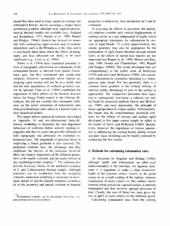
Internal heat generation results in a non-linear initial geothermal gradient, allowing realistic initial near-surface temperature gradients without impossi- bly high values at the base of the lithosphere. An example is presented in Fig. 2 for an exhumation rate of 1 m m / a and a near-surface initial temperature gradient of ca. 25°C/km. From this figure, it is clear that long times ( > 40 Ma), and corresponding deep exhumation ( > 40 km!), would be required to approach steady-state conditions and that the time-dependent behaviour of the isotherms must therefore be considered during exhumation.

Analytical solutions for the time-dependent temperature distribution beneath an eroding surface are presented in Appendix A. As is clear from the discussion following Eq. (17), a steady-state can only be attained with time if the temperature approaches some constant value at depth. Assumption of an initially steadily increasing temperature with depth or of a constant heat flow from the mantle (and thus a constant temperature gradient boundary condition) precludes the establishment of a steady state during exhumation and the temperature at any particular depth will always increase with time.

Eq. (39) in Appendix A is the full time-dependent solution to the heat advection and conduction equation for the boundary conditions proposed by Sttiwe et al. (1994), namely a constant temperature at some large, fixed depth (e.g., say 1300°C at the base of the lithosphere, taken as 100 km thick) and converges to their solution at large times. Heat generation in the lithosphere (including an exponential decay with depth; e.g., Turcotte and Schubert, 1982) is also considered, but an analytical solution is only possible if the distribution of heat production does not change with time. Erosion of radiogenic material, leading to a steady decrease in the surface heat production with time, precludes the development of a true steady state. At large times the solution tends to a quasi- steady state, equivalent to the solution without heat

Surface heat production 2.2 x 10 -6 W m "3 Relaxation depth = 30 km Exhumation rate = 1 mm/a

40-

50- g a 60-

to-

20- -

3o ~ x , ~ I Initial State i 1 ~) @ (~ Steady State \ \ % * . \ \

]OMo no erosion of heat (~) 40 Mo producing material ~ \k~ ~

70- '(DIOMa er°si°n°fhaat X \ ~ \ \ 80- - @ 40 Mo producing material \

steady state for no ~ 90- heat production \

1 O0 - I I I I 0 200 400 600 800

Temperature [°(3] 1000 1200 1400

Fig. 2. Variation in the lithospheric geotherm with time, with and without the effects of erosion of heat producing material. The base of the lithosphere, taken as fixed at 100 km, is assigned a constant temperature of 1300°C, the upper surface a constant temperature of 0°C, the initial volumetric heat production at the surface is taken as 2.2 x 10 -6 W m - 3 , and an exponential decay of the heat production with reduction to 1/e of the surface value at 30 km depth. The parameters selected establish an initial geotherm of ~ 25°C/km in the upper 20 km of the lithosphere. It is important to note that long times and deep exhumation would be required to approach near steady-state.

172 N.S. Mancktelow, B. Grasemann / Tectonophysics 270 (1997) 167 195

0

10

~,20-

..C

0 30

40

5O

Comparison with Benfield 1949a (solid lines) Initial constant 25°C/km geotherm Exhumation rate = 1 mm/a

"rime in Ma 0 5 10 20 40 40 $teadyState i

. . . . .

\ \ \ \ ' , , ' \ \ \ ~ \\ \ , \ \

0 500 1000 1500 2000 2500 Temperature [°C]

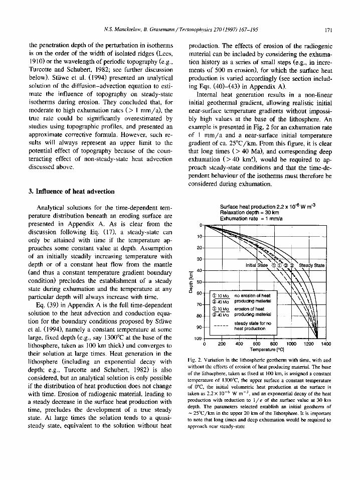
Fig. 3. Comparison between Eq. 39 and the earlier result of Benfield (1949a), for an initial 25°C/km geothermal gradient, an exhumation rate of 1 m m / a and the same boundary conditions. except that Eq. 39 assumes a constant temperature at 100 km depth instead of a constant gradient. From 20 Ma onwards the results diverge reflecting the steady-state upper limit to Eq. 39.

1 mm/a with no heat generation

2500 ~ , ~ S t e a d y 1

,n,t,a, \ ,oo 2000 ~ " ~ G e o t h e r m

; soo-- - _ < \

E 1000. t-

500-

0- 100 80 60 40 20 0

Depth km = Time Ma

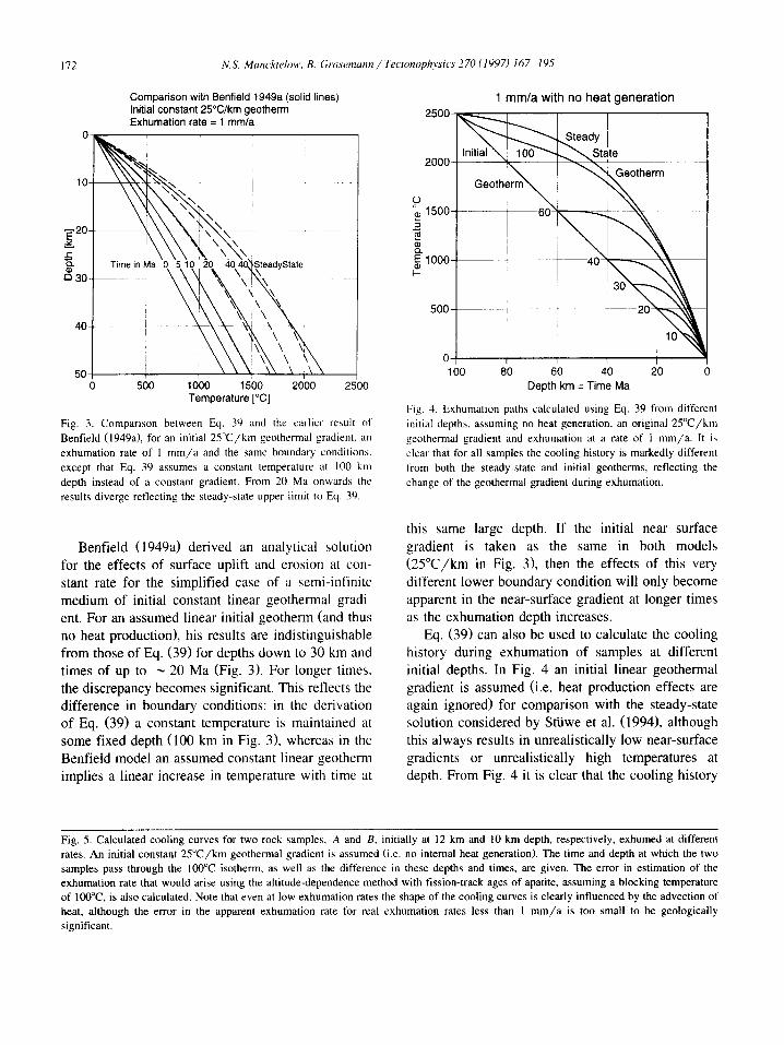
Fig. 4. Exhumation paths calculated using Eq. 39 from different initial depths, assuming no heat generation, an original 25°C/km geothermal gradient and exhumation at a rate of l mm/a . It is clear that for all samples the cooling history is markedly different from both the steady-state and initial geotherms, reflecting the change of the geothermal gradient during exhumation.

Benfield (1949a) derived an analytical solution for the effects of surface uplift and erosion at constant rate for the simplified case of a semi-infinite medium of initial constant linear geothermal gradient. For an assumed linear initial geotherm (and thus no heat production), his results are indistinguishable from those of Eq. (39) for depths down to 30 km and times of up to ~ 20 Ma (Fig. 3). For longer times. the discrepancy becomes significant. This reflects the difference in boundary conditions: in the derivation of Eq. (39) a constant temperature is maintained at some fixed depth (100 km in Fig. 3), whereas in the Benfield model an assumed constant linear geotherm implies a linear increase in temperature with time at

this same large depth. If the initial near surface gradient is taken as the same in both models (25°C/km in Fig. 3), then the effects of this very different lower boundary condition will only become apparent in the near-surface gradient at longer times as the exhumation depth increases.

Eq. (39) can also be used to calculate the cooling history during exhumation of samples at different initial depths. In Fig. 4 an initial linear geothermal gradient is assumed (i.e. heat production effects are again ignored) for comparison with the steady-state solution considered by Stiiwe et al. (1994), although this always results in unrealistically low near-surface gradients or unrealistically high temperatures at depth. From Fig. 4 it is clear that the cooling history

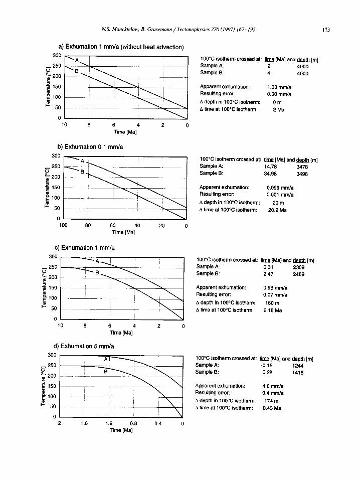
Fig. 5. Calculated cooling curves for two rock samples, A and B, initially at 12 km and 10 km depth, respectively, exhumed at different rates• An initial constant 25°C/km geothermal gradient is assumed (i.e. no internal heat generation). The time and depth at which the two samples pass through the 100°C isotherm, as well as the difference in these depths and times, are given. The error in estimation of the exhumation rate that would arise using the altitude-dependence method with fission-track ages of apatite, assuming a blocking temperature of 100°C, is also calculated. Note that even at low exhumation rates the shape of the cooling curves is clearly influenced by the advection of heat, although the error in the apparent exhumation rate for real exhumation rates less than 1 m m / a is too small to be geologically significant.


a) Exhumation 1 mm/a (without heat advection)

30o

250 i ? " ~ B ,

200

150 I

~" 100 ~ i

50 . . i ~ . _ ' i

o i ! t ; 10 8 6 4 2

Time [Ma]

100°C isotherm crossed at: time [Ma] and depth [m] Sample A: 2 4000 Sample B: 4 4000

Apparent exhumation: 1.00 mm/a Resulting error: 0.00 mm/a

A depth in 100°C isotherm: 0 m t~ time at 100°C isotherm: 2 Ma

b) 300

250 0o

200

l 1so

~ I00 ~- 50

0

I00

Exhumation 0.1 mm/a

i

i 80 60 40

Time [Ma] 20

100°C isotherm crossed at: time [Ma] and depth [m] Sample A: 14.78 3478 Sample B: 34.98 3498


depth in 100°C isotherm: 20 m 6 time at 100°C isotherm: 20.2 Ma

c) Exhumation 1 mm/a

300

250

Z 200

150

E 100

I-- 50

0 10 8 6 4 2 0

Time [Ma]

100*C isotherm crossed at: time [Ma] and depth [m] Sample A: 0.31 2309 Sample B: 2.47 2469


6 depth in 100°C isotherm: 160 m time at 100°C isotherm: 2.16 Ma

d) Exhumation 5 mm/a

3o0

250 i

~-" 2OO i

15o

~" 100 -

I-.- 50

2 1.6 1.2 0.8 0.4 0 Time [Ma]

100°C isotherm crossed at: time [Ma] and depth [m] Sample A: -0.15 1244 Sample B: 0.28 1418


A depth in 100°C isotherm: 174 m /t time at 100°C isotherm: 0.43 Ma

174 N,S. Mancktelow, B. (hztsemaml / 7),ctom~physics 270 (1997) 167-195

for all samples is markedly different from the steady-state geotherm. Fig. 5 illustrates the possible effect of this time-dependent advection on exhumation rates calculated using the altitude-dependence method with apatite fission-track ages, again assuming an initial linear geotherm of 25°C/km. The cooling curves for two rock samples A and B initially located at 12 km depth (300°C) and 10 km depth (250°C) are calculated using constant exhumation rates of 0.1 mm/a , 1 m m / a and 5 mm/a . To the right of the plots, additional information is provided about the time and depth at which rock sam- pies A and B pass through the 100°C isotherm (= blocking temperature for fission-track apatite ages). The other values are the apparent exhumation rate, the resulting error between the apparent exhumation rate and the real exhumation rate, and the difference between the depth and the time when the rock samples pass through their blocking temperatures compared to a model without heat advection.

If the influence of heat advection is neglected, the cooling curves are straight lines (Fig. 5a). With the introduction of heat advection into the model, clearly different cooling curves are developed li)r each of the different exhumation rates (0.1 mm/a , I m m / a and 5 m m / a corresponding to Fig. 5b, c and d. respectively). This reflects the elevation of the origi-

nal steady-state geothermal gradient, even at the lowest exhumation rate of 0.1 m m / a (Fig. 5b). Compared to the stable geotherm example (Fig. 5a), they show slower cooling at the beginning of the simulation, because of the advection of the heat, and faster cooling at the end of the simulation, because of the elevated geothermal gradient near the surface. From these plots it can be seen, therefore, that even very low exhumation rates still clearly influence the shape of the cooling curve. However, the important question is just how far the calculation of exhumation rates using standard methods is influenced by these effects of heat advection, considering, as an example, the two rock samples A and B and a blocking temperature of IO0°C, As discussed above, the error arises due to a decrease in the depth of the blocking temperature isotherm due to heat advection. At exhumation rates of 1 m m / a or less, this error is too small to be geological significant ( < 0.07 m m / a error). At higher exhumation rates, however, the error due to heat advection is not negligible; for example the apparent exhumation for the full 2-Ma long simulation of Fig. 5d would be about 800 m too low. However, even at such high exhumation rates the estimation error is still less than 10% and, being realistic, is of the same order as inaccuracies in the fission-track dating method itself.

300

~250 o

200

150

~'100

~- 50

10

Exhumation 1 mm/a, surface heat production 2.2 x 10 -6 W m "3 relaxation depth 30 km

~, ......................... 100°C isotherm crossed at: time [Ma] and depth [m] Sample A: 0.54 2541 Sample B: 2.62 2617

Apparent exhumation: 0.96 mm/a Resulting error: 0.04 mm/a A depth in 100°C isotherm: 76 m ,,t, time at 100°C isotherm: 2.08 Ma

8 6 4 2 0 Time [Ma]

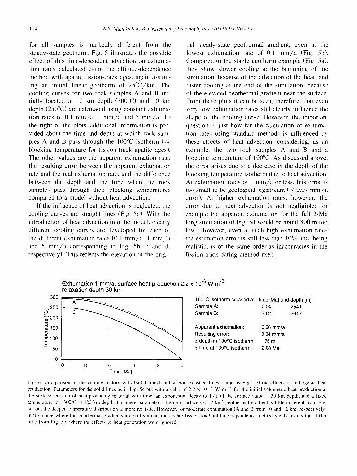
Fig. 6. Comparison of the cooling history with (solid lines) and without (dashed lines, same as Fig. 5c) the effects of radiogenic heat

production. Parameters for the solid lines as in Fig. 5c but with a value of 2.2 × l0 6 W m - ~ for the initial volumetric heat production at the surface, erosion of heat producing material with time. an exponential decay to I / e of the surface value at 30 km depth, and a fixed temperature of 1300°C at 100 km depth. For these parameters, the near surface ( _< 12 kin) geothermal gradient is little different from Fig.

5c, but the deeper temperature distribution is more realistic. However, lbr moderate exhumation (A and B from 10 and 12 kin. respectively) m the range where the geothermal gradients are still ~imilur, the apatite fission-track altitude-dependence method yields results that differ little from Fig. 5c, where the effects of heat generation were ignored


This simple model including the effect of heat advection clearly shows why the uncertainty in calculating the exhumation rate from one rock sample and two blocking temperatures is much greater than that calculated from two rock samples at different altitudes with the same blocking temperature (Fig. 1). As discussed above, the main problem with the first method is that it is practically impossible to determine with any precision the depth at that time when the sample passes through the isotherm corresponding to the blocking temperature. Even in a simple static system, this can only be estimated from an assumed geothermal gradient; in a tectonically active region the isotherms will be constantly changing their depth due to heat advection and thermal

relaxation and the accuracy of the method is further reduced. For example, curve A without advection (Fig. 5a) passes through the 100°C isotherm at a depth of 4000 m, whereas the same curve with heat advection passes through this isotherm at around 2310 m for an exhumation rate of 1 m m / a (Fig. 5c) and only 1240 m for an exhumation rate of 5 m m / a (Fig. 5d).

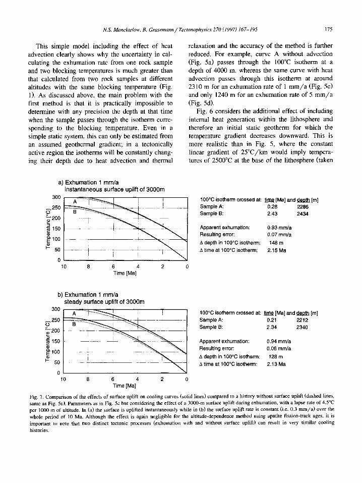
Fig. 6 considers the additional effect of including internal heat generation within the lithosphere and therefore an initial static geotherm for which the temperature gradient decreases downward. This is more realistic than in Fig. 5, where the constant linear gradient of 25°C/km would imply temperatures of 2500°C at the base of the lithosphere (taken

a) Exhumation 1 mm/a instantaneous surface uplift of 3000m

3O0 A ........ J

~ 150 . . . "

0 : i 10 8 6 4 2

Time [Ma]


Apparent exhumation: 0.93 mm/a Resulting error: 0.07 mrn/a

A depth in 100°C isotherm: 148 m A time at 100°C isotherm: 2.15 Ma

b) Exhumation 1 mm/a steady surface uplift of 3000m

I 300 A ....... 1 ' " ' ~

250

15o [ •

o_ ! I 100 E Q) ' ! '

,

0 J 10 8 6 4

Time [Ma]



depth in 100°C isotherm: 128 m A time at 100°C isotherm: 2.13 Ma

Fig. 7. Comparison of the effects of surface uplift on cooling curves (solid lines) compared to a history without surface uplift (dashed lines, same as Fig. 5c). Parameters as in Fig. 5c but considering the effect of a 3000-m surface uplift during exhumation, with a lapse rate of 4.5°C per 1000 m of altitude. In (a) the surface is uplifted instantaneously while in (b) the surface uplift rate is constant (i.e. 0.3 m m / a ) over the whole period of 10 Ma. Although the effect is again negligible for the altitude-dependence method using apatite fission-track ages, it is important to note that two distinct tectonic processes (exhumation with and without surface uplift) can result in very similar cooling

histories.

1 7 6 N.S. Mancktelow, B. Grasemann / Tectonophysics 270 (1997) 167-195

Isotherms during Exhumat ion

, , ! , r i , I I ,,

-5

-10

-15

E

-20

a

~'~- -25

2 .3o E I

i

rr 1 ~ .35 ,"- I o !

E ¢....

x 40 LU

64 56 48 40 32 24 16 8 0 Time [Ma]

Fig. 8. Isotherms during and following a period of rapid exhumation, initially at 2 mm/a and decreasing progressively to a slow 0.125 mm/a, before stopping altogether. Heat production parameters (and thus the initial geotherm) are the same as in Fig. 6. Note that, because of erosion of radiogenic material, the steady-state isotherm depth after the period of exhumation (represented by the arrow tip for each isotherm) is deeper than initially and that long times are required for reattainment of a steady-state, particularly at depths > 20 km.

as 100 k m depth) , whe reas in Fig. 6 a more reason-

able va lue of 1300°C is assumed. However , in prac-

t ice the near - sur face ef fec t is smal l and for tuna te ly

tends to reduce the potent ia l e r ror in e s t ima t ing

e x h u m a t i o n rates.

Fig. 7 cons iders the ef fec t of surface uplif t lead-

ing to coo l ing o f the exposed surface dur ing e ros ion

at 1 m m / a , i.e. cond i t ions o the rwise s imi la r to Fig.

5c. Fig. 7a cons ide r s surface upl i f t of 3000 m occur-

r ing in s t an t aneous ly at the b e g i n n i n g o f e x h u m a t i o n

Temperature-Time Path during Exhumation

o o

E F-

a) 36

~ 1 .4

E ~ 1 . 2

rr 1 c o 0.8

~0.6 t,'-- x

UJ 0 . 4 -

-~ 0 . 2 - E

~ O-

32 28 24 20 16 12 8 4 0 Time [Ma]

E

2 ~

r r ¢.. o

E --1 ¢..

x UJ

LU 36 32 28 24 20 16 12 8 4 0

b) Time [Ma]

Fig. 9. (a) Temperature-time path for a sample exhumed from 18 km depth under the conditions of Fig. 8. Symbols indicate approximate possible closure temperatures for various isotopic systems (K-Ar muscovite ~ 350°C, K-Ar and Rb-Sr biotite ~ 300°C. fission-track zircon ~ 240°C, fission-track apatite ~ 100°C). This simulation demonstrates that elevation of the geothermal gradient results in a convex upwards segment to the cooling curve, whereas the subsequent thermal relaxation results in a concave upwards segment. (b) Interpreted exhumation rates between closure systems in (a), assuming a constant linear geothermal gradient of 25°C. Note that the initial exhumation rate is poorly constrained as the temperature and particularly the time of initiation of exhumation are usually themselves poorly constrained.

us ing Eqs. (39) and (48), and Fig. 7b cons ide r s upl if t

of the same a m o u n t occur r ing at a s teady rate ove r

the 10-Ma pe r iod o f e x h u m a t i o n us ing Eqs. (39) and

(49). A lapse rate o f 4 . 5 ° C / k r n a l t i tude is a s s u m e d

(Bi rch , 1950), so tha t the 3000 m co r r e sponds to a

coo l ing o f the surface o f 13.5°C. For the same


present-day surface temperature (taken as 0°C) and the same assumed initial linear geothermal gradient (25°C/km), uplift and cooling of the surface during erosion implies that prior to erosion the temperature at any depth was higher than in the case without uplift. The cooling curves of Fig. 7 are thus dis- placed to higher temperatures compared to Fig. 5c without uplift, and it is clear that the difference will be less in Fig. 7a, where the upper surface cooled to conditions identical to Fig. 5c at the very beginning of exhumation, than in Fig. 7b, where the cooling occurred progressively with time. However, as can be seen from Fig. 7, uplift accompanying exhumation produces very little change in the errors in exhumation rates estimated by the altitude-dependence method and if anything will decrease the resultant error, so that the effect can in general be neglected. As a corollary, Fig. 7 also clearly demonstrates that even important surface uplift (3000 m) at rapid rates (instantaneous in the case of Fig. 7a) has only a very minor effect on the cooling history of exhumed rock samples, and that these effects are within the accuracy limits of the altitude-dependence method. Thus no direct information on the surface uplift history can be gained by this method (England and Molnar, 1990).

The above discussion has only considered exhumation at a constant rate through time. However, in nature an initially rapid exhumation rate that dies off exponentially may be more realistic and this introduces an additional influence, namely the relaxation of elevated isotherms as the advection effect decays (Grasemann and Mancktelow, 1993). Figs. 8 and 9 consider the cooling history for exhumation at a rate that decreases progressively with time. As can be seen from Fig. 8, the relaxation of isotherms back to a steady-state condition may take a very long time after a period of rapid exhumation, particularly at depths > 20 km. In collisional mountain belts, the elevation of isotherms late in the orogenic history is also strongly promoted by initial thickening of the strongly radiogenic upper crust. Glazner and Bartley (1985) demonstrate that this elevation of isotherms and consequent lithospheric weakness reaches a peak around 30-70 Ma after thrusting. They note that this is one clear reason why the deeply eroded parts of a dying orogen are often favoured as the site of rifting at the start of the next Wilson cycle. Elevated pre-

rifting isotherms have been reported from the South- em Alps (Bertotti and ter Voorde, 1994), where the period between exhumation at the end of the Hercy- nian cycle and the beginning of renewed normal faulting in the Norian is indeed on the order of 50 Ma. In this case, however, the authors favour a thermal pulse due to intrusion shortly before the onset of rifting.

Fig. 9 models how this exhumation history would be reflected in the cooling path and in estimated exhumation rates for an assumed linear geotherm. The temperature-time path of Fig. 9a shows an initial delay of ~ 2 Ma, followed by rapid cooling, the whole curve displaying a time lag behind actual changes in exhumation rate. Cooling at moderate rates continues well beyond the period of rapid exhumation, as the elevated isotherms relax back to a steady state. Taking as an example several represen- tative 'closure temperatures' on this cooling curve, the exhumation rates have been calculated in Fig. 9b on the basis of a constant 25°C/km geothermal gradient. In general, during periods of rapid exhumation the estimated values are too low and tend to lag the real exhumation history in time, but as the exhumation rate diminishes, the continued time lag in thermal response can lead to an overestimation of rates.

4. Influence oftopography

4.1. Theoretical background

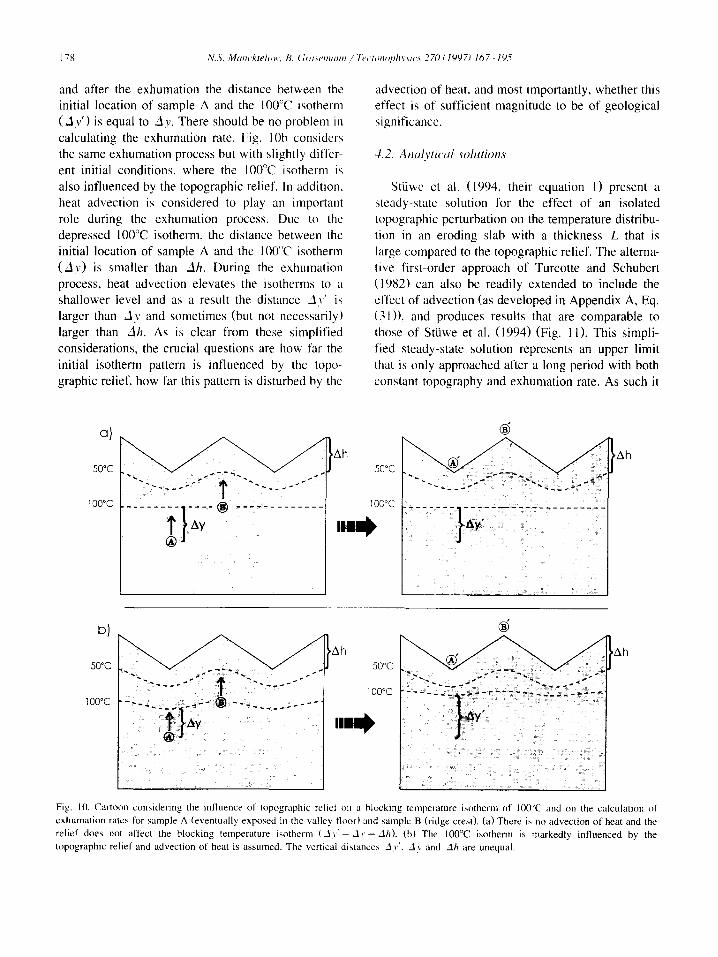
The cartoon of Fig. 10 demonstrates the theoretical influence of topographic relief on the calculation of exhumation rates for two rock samples with an initial vertical separation Ah and a blocking temperature of 100°C. On exhumation, sample A is exposed at the valley floor and sample B at the top of the next ridge, which is Ah higher than the valley bottom. In Fig. 10a, the relief has a certain influence on the 'cool' temperature distribution, but the critical 100°C isotherm is not affected. The distance between the initial location of sample A and the 100°C isotherm (Ay) is equal to the distance Ah. Because there is no advection of heat, the rock samples exhume through a constant but not uniformly distributed isotherm pattern (due to the lateral cooling)

178 N.S. Mam'ktelow, B. Grasemann / Tectomv~hvsic,~ 270 (1997) 167-195

and after the exhumation the distance between the initial location of sample A and the 100°C isotherm (Ay ' ) is equal to J r . There should be no problem in calculating the exhumation rate. Fig. 10b considers the same exhumation process but with slightly different initial conditions, where the 100°C isotherm is also influenced by the topographic relief. In addition. heat advection is considered to play an important role during the exhumation process. Due to the depressed 100°C isotherm, the distance between the initial location of sample A and the 100°C isotherm (Ay) is smaller than kh. During the exhumation process, heat advection elevates the isotherms to a shallower level and as a result the distance .Jr ' is larger than d y and sometimes (but not necessarily) larger than Ah. As is clear from these simplified considerations, the crucial questions are how far the initial isotherm pattern is influenced by the topographic relief, how far this pattern is disturbed by the

advection of heat, and most importantly, whether this effect is of sufficient magnitude to be of geological significance.

4.2. Analytical solutions

Sttiwe et al. (1994, their equation 1) present a steady-state solution for the effect of an isolated topographic perturbation on the temperature distribution in an eroding slab with a thickness L that is large compared to the topographic relief. The alternative first-order approach of Turcotte and Schubert (1982) can also be readily extended to include the effect of advection (as developed in Appendix A, Eq. (31)), and produces results that are comparable to those of Sttiwe et al. (1994) (Fig. 11). This simplified steady-state solution represents an upper limit that is only approached after a long period with both constant topography and exhumation rate. As such it

a)

50°C

100°C

' ! ~ - - . . _ . - ~ ' " . . . . , - , . : - - - "

. . . . . . . . . . . . . .

,Ah 50°C

100°C

"M

~!+:! !i i ̧ i/~ii! ~~

Ah

b)

50°C

I O0°C

~! !i + ~ ~ ~ +j~ ii ~ii ~ i i!~ i' ii +,~i i~i(~ ~'I ii~i ~ ~

,Ah 50°C

100°C

"m

Ah

Fig. 10. Cartoon considering the influence of topographic relief on a blocking temperature isotherm of Ifl0°C and on the calculation of exhumation rates for sample A (eventually exposed in the valley floor) and sample B (ridge crest). (a) There is no advection of heat and the relief does not affect the blocking temperature isotherm (d v' d v= Jh). (b) The 100°C isotherm is markedly influenced by the topographic relief and advection of heat is assumed. The vertical distances Jy ' , /tv and Ah are unequal.


is not very realistic, but does highlight the most important parameters that will influence the isotherm geometry. From Eqs. (31) and (34) it is clear that these parameters are the topographic height and wavelength, and the exhumation rate. To first order (Eq. (26)), the magnitude of the perturbation at any depth will be directly proportional to the amplitude of the periodic topography. The wavelength and the exhumation rate determine the depth of penetration of the topographic effects, since the disturbance will decay to 1/e of its surface value at a depth given by:

2

Y= uK ~ ( u ) 2 + ( 7 ) ' 2

where u is the exhumation rate, ,~ the wavelength of topography and K the thermal diffusivity. It follows that increased wavelength increases the penetration depth of the disturbance due to topography (the expression reduces to )t/27r for u = 0), whereas an

0

1 -

2 ̧

3

~ 4 . e~ Ill 121

5-

i I St~we et al. 1994

Turcotte & Schubert 1982

-

6 ~

7-

8- 0

200°C

i I i 5 10 15 20

Distance [km]

Fig. 11. Comparison of the steady-state result of equation (1) of Stiiwe et al. (1994) with the alternative approach following Tur- cotte and Schubert (1982), developed as Eq. 31 in Appendix A. Parameters are the same as in the original publication of Stiiwe et al. (1994), namely an initial constant geothermal gradient of 10°C/km (no heat generation), a topography of 20 km wavelength and a 3-km height difference between ridges and valleys, and an exhumation rate of 1 m m / a . The isolated perturbation required for the Stiiwe et al. (1994) solution is taken as a packet of 20 wavelengths (only the result from the central full wavelength is presented).

increased exhumation rate has the opposite effect. However, the magnitudes of the effects are very unequal. To highlight this in Fig. 12a and b, the effects of heat advection are ignored and a constant near-surface geothermal gradient of 25°C is assumed. A comparison of these figures clearly demonstrates that the wavelength effect is much the stronger and, within a realistic range, the exhumation rate will not have an important influence on the topographic perturbation of isotherms. However, as considered above, heat advection due to exhumation also affects the near-surface geothermal gradient through Eq. (34), so that increased exhumation rates increase the magnitude of the disturbance at any given depth. As can be seen from Fig. 12c and d, this effect can be quite important.

As discussed in Appendix A, the result for a simple periodic topography forms the basis for considering any general topography by a simple linear sum of sines and cosines, i.e. as a Fourier series. Since short-wavelength components decay more rapidly with depth than longer wavelengths, sec- ondary topography and angular shapes decay rapidly into smoother, broader forms to the isotherms at shallow depths. The longest wavelength component (i.e. on the order of the width of the mountain chain or plateau) will be the last to decay, corresponding to a broad elevation of isotherms under major mountain chains and plateaux (such as the Tibetan plateau).

This approach to considering topography can be further extended to give an analytical solution (Eq. (60) in Appendix A) for the time-dependent variation in temperature below a periodic surface temperature variation introduced instantaneously at some time and maintained constant thereafter. As is clear from Fig. 13, the temperature distribution rapidly approaches the steady-state solution, generally requiring times less than 1 Ma. However, in reality the near surface geothermal gradient will also be time- dependent due to heat advection and requires much longer times to approach a steady state (Fig. 2). By comparison with the steady-state solution, the effects of the parameters considered in Fig. 12a and b should therefore be established rapidly following onset of erosion, whereas the influence of advection considered in Fig. 12c and d will establish its influence more slowly. Consequently, in the initial stages the effect of exhumation may dampen the effects of

180 N.S. Manckteltm. B. Grasemann / Tectonophysics 270 (1997) 167-195

20

oo15 .

~10- O..

E I-- 5-

No Heat Advection 25°C/km Geotherm Depth = 4 km

0 0 1 2 ' 3 ' 4

(a) Exhumation Rate [mm/a]

20

~'16- o

212-

(I)

<~ 4 -

0

(b)

No Heat Advection 25°C/km Geotherm / Depth = 4 km

0 10 20 30 40 50 Topographic Wavelength [km]

300 With Heat Advection 220- =

200-

t50~ 100-

< 50~

. . . . I . . . . I I '

0 1 2 3 4 (C) Exhumation Rate [mm/a]

60

~ 50- 0 o

40-

~ 30-

E20 -

"~ 10-

With Heat A d v e c t i o n /

0 1 2 3 (d) Exhumation Rate [mm/a]

Fig. 12. Influence of different parameters on the amplitude of the periodic disturbance in isotherms due to topography for the steady-state solution (i.e. the value J exp(m 2 y) of Eq. 31 ). In all cases the amplitude of the periodic topography is taken as 1500 m, that is a maximum height difference between ridge crest and valley floor of 3000 m, a lapse rate of 4.5°C/km altitude, a reference temperature at y = 0 of 0°C. and where required, a density of 2800 kg m -z, heat capacity of I I00 J kg / K - i surface heat production of 2.2 X 1 0 - 6 W m -3. and a relaxation depth of 30 km. (a) Effect of exhumation rate on the maximum temperature disturbance at 4 km depth due to topography with 20 km wavelength, for an assumed constant 25°C geothermal gradient (i.e. no heat advection). (b) Effect of wavelength of topography for the same conditions as (a) and an exhumation rate of 1 mm/a. (c) Effect of exhumation rate on the magnitude of the periodic temperature disturbance at the reference plane y = 0, including the effects of heat advection and with topographic wavelength of 20 kin. (d) Same effect considered at depth y = 4 km.

topography , bu t wi th t ime the advec t i on ef fec t domi-

nates. A l t h o u g h this c o m p l e x t i m e - d e p e n d e n t inter-

play be tween pa rame te r s could in pr inc ip le be con-

s idered ana ly t ica l ly us ing the genera l so lu t ion of Eq.

(56), it is more pract ica l to cons ide r the p r ob l em

numer ica l ly .

4.3. N u m e r i c a l mode l l ing

The numer i ca l ca lcu la t ions were made us ing a

f in i t e -d i f fe rence mode l , wh ich solves the t ime-de-

p e n d e n t hea t t r ans fe r Eq. ( l a ) of A p p e n d i x A in two

d imens ions . In o rder to isolate the in f luence of heat

advec t ion , heat p roduc t ion was neg lec ted in the nu-

mer ica l ca lcula t ions . As e s t ab l i shed above , inc lud ing

heat p roduc t ion does not genera l ly have any signif i-

can t effect on es t imates o f e x h u m a t i o n rates (Fig. 6).

For the same reason and to keep eve ry th ing as

s imple as poss ib le , a g e o t h e r m wi th a cons t an t gradi-

ent o f 2 5 ° C / k m serves as init ial condi t ion . A n

equal ly spaced grid wi th 960 X 300 nodes descr ibes

the t empera tu re d i s t r ibu t ion over a hor izon ta l dis-

tance o f 96 k m and a ver t ica l d i s tance of 30 km. The

hea t advec t i on has on ly a ver t ical c o m p o n e n t and

desc r ibes the e x h u m a t i o n o f rock samples loca ted at

va r iab le depth. The surface b o u n d a r y condi t ion , t aken


Temperature with Depth and Time Below a Periodic Surface Temperature with a Wavelength of 20 km

0.8 Depth [km] i,,, 1

~ 0.6

~ 2

_~0.4 3

4

- 5 ,,6

7

0.8 0-

0 0.2 0,4 0.6 Time [Ma]

Fig. 13. Temperature variation with time below a spatially periodic temperature variation of constant amplitude with wavelength 20 km imposed on the surface y = 0 at time t = 0. Note that effective steady-state is established rapidly within 5 km of the surface, requiring generally < 0.5 Ma.

as a constant 0°C, can have various zigzag shapes reflecting different possible topographic wavelengths. The numerical models presented in this work use a fixed altitude of the ridges of 3000 m which corresponds to a topographic amplitude of 1500 m. Note that for computational simplicity, the 0-m datum plane is located on top of the ridges and consequently the valley floor is located at a depth of 3000 m. This system is solved numerically in two dimensions using an ADI (alternating direction implicit) method with a two-step scheme (Peaceman and Rachford, 1955). All parameters used in the following calculations are listed in Table 1.

Fig. 14 shows cooling curves similar to that of Fig. 5c but including the influence of topographic relief with a wavelength of: (a) 6, (b) 12, and (c) 24 km, respectively. In these models, the topography is introduced instantaneously at the beginning of the simulation. However, there is no significant difference in the shape of the cooling curves or in the estimated exhumation rates in models considering exhumation of an already established topography, in which the thermal frame is allowed to adjust to the new upper surface boundary condition for l0 Ma before the onset of exhumation. This reflects the

Table 1 Parameters used in the calculations

Parameter Description Constant/unit

T

L d T / d z At K

U

qm n r . z

X

z Az J x ~h

temperature (K) surface temperature 273 (K) geothermal gradient 25 (K km- i ) finite time step 1000(3 (a) thermal diffusivity 10 -6 (m 2/s) velocity in z direction (exhumation rate)(m/a) mantle heat flux 0.075 ( W / m 2) number of nodes 288000 horizontal x direction 96000 (m) vertical z direction (depth) 30000 (m) grid spacing in z direction 100 (m) grid spacing in x direction 100 (m) topographic relief 3000 (m)

short times necessary for attainment of steady state in the geothermal gradient below topography, as established in Fig. 13. In general, provided both samples were initially above the blocking temperature, the starting depth of exhumation also does not significantly influence the estimated exhumation rates using the altitude-dependence method.

With the onset of exhumation, the initial geothermal gradient of 25°C/km is no longer constant. The distance between isotherms is expanded beneath the ridges and condensed beneath the valleys due to the cooling effect of the topographic relief. Given that the datum plane is at the top of the ridges, sample A (below the valley) starts at 13 km depth and sample B (below the next ridge) at 10 km depth. Allowing the samples to exhume at 1 m m / a for 10 km, both samples reach the 0°C surface at the same time after 10 Ma: sample A at the valley floor (i.e. 3 km below the datum) and sample B at the top of the ridge (at the datum itself). The plots clearly demonstrate the important effect of the topographic wavelength. While the resulting error 2 in the apparent exhumation rate is negligible for a 6-km wavelength (0.05 mm/a , Fig. 14a), the error is geologically significant for 12-km wavelength ( - 0 . 2 8 mm/a , Fig. 14b) and important for a 24-km wavelength ( - 0 . 8 3 mm/a , Fig. 14c). Since the vertical separation between the

2 Error = real rate minus apparent rate; i.e. positive values correspond to an underestimation of the real rate.

182 N.S. Mancktelow, B. Grasemann / lectonophysics 270 (I997) 167-195

a)

300

~, 250

~ 200

150

E 100

5O

0 10

Exhumation 1 mm/a, 6 km wavelength, instantaneous relief

A

g , . . . . . . 8 6 4 2 0

Time [Ma]

100 °C isotherm crossed at: time [Ma] and depth [m] Sample A: 1.57 4570 Sample B: 4.72 4520

Apparent exhumation: 0.95 mm/a Resulting error: 0.05 mm/a A depth in 100°C isotherm: -50 m A time at 100°C isotherm: 3.15 Ma

b)

300

~, 250 ?. 200

= 150

E 100

50

0

Exhumation 1 mm/a, 12 km wavelength, instantaneous relief

A

10 8 6 4 2 0

100 °C isotherm crossed at: time [Ma] and deDth [m] Sample A: 1.40 4400 Sample B: 3.75 3750

Apparent exhumation: 1.28 mm/a Resulting error: -0.28 mm/a A depth in 100°C isotherm: -650 m A time at 100°C isotherm: 2.35 Ma

Time [Ma]

c) Exhumation 1 mm/a, 24 km wavelength, instantaneous relief

300 - ~ •

250 O

200

"~ 150

E 100

50

10 8 6 4 2 0

Time [Ma]

100 °C isotherm crossed at: tim___ee [Ma] and depth [m] Sample A: 1.40 4400 Sample B: 3.04 3040

Apparent exhumation: 1.83 mm/a Resulting error: -0.83 mm/a ?~ depth in 100°C isotherm: -1360 m

time at 100°C isotherm: 1.64 Ma

Fig. 14. Cooling curves similar to thai of Fig. 5c but with topographic relief of wavelengths (a) 6, (b) 12 and (c) 24 km. The relief is developed instantaneously at the beginning of the simulation (results do not differ significantly if a period of thermal relaxation is allowed before onset of exhumation). Ridges are 3000 m high. Given that the datum plane is at the top of the ridges, sample A below the valley starts at 13 km depth (and 325°C) and sample B below the next ridge at l0 km depth (and 250°C): both samples thus undergo 10 km of exhumation relative to their final surface location.


a)

350 -- A ~ ~ -~ . . . _ i I

30O

~, 250 - - B '---- ~ ~

' 2 0 0

150

E 100 ' "

50 r

b) 350

300

~' 250 o

200 -q

15o ¢1

E 100

50

0

c) 350

300

~' 250 o

200 _=

.m 150 O.

E 100

50

Exhuma t i on 5 mm/a, 6 km wave leng th , ins tan taneous re l ief

100 *C isotherm crossed at: time [Ma] and deoth [m] Sample A: 0.14 3700 Sample B: 0.65 3250

Apparent exhumation: 5.9 mm/a Resulting error: -0.9 mm/a /t depth in 100"C isotherm: -500 m .A time at 100"C isotherm: 0.5 Ma

2 1.6 1.2 0.8 0.4 0 Time [Ma]

Exhuma t i on 5 mm/a, 12 km wave leng th , ins tan taneous rel ief

] r T ]

2 1.6 1.2 0.8 0.4 0 Time [Ma]

Exhuma t i on 5 mm/a, 24 km wave leng th , i ns tan taneous rel ief

T - - A

100 *C isotherm crossed at: time [Ma] and deoth [m] Sample A: 0.14 3700 Sample B: 0.45 2250

Apparent exhumation: 16.7 mm/a Resulting error: -11.7 mm/a /t depth in 100"C isotherm: -2100 m ti time at 100"C isotherm: 0.18 Ma

Fig. 15. Modelled cooling curves similar to that of Fig. 14 but with an exhumation rate of 5 mm/a. Clearly in all three models the apparent exhumation rates are strongly influenced by topography and are markedly overestimated: in (a) by ~ 1 mm/a, in (b) by ~ 5 mm/a and in (c) by nearly 12 mm/a, i.e. more than twice the real exhumation rate! It can be seen that the cooling curve A beneath the valley floor is not influenced by the increasing topographic wavelength and the 100°C isotherm is reached for all wavelengths at 0.14 Ma and at a depth of 3700 m. In contrast, cooling curve B beneath the ridge is strongly influenced by the wavelength and the convex-concave shape of the cooling curve is only observed at shorter wavelengths.

100 =C isotherm crossed at: l;imtl [Ma] and delith [m] Sample A: 0.14 3700 Sample B: 0.32 1600

2 1.6 1.2 0.8 0.4 0

Time [Ma]

I i

Apparent exhumation: 9.7 mm/a Resulting error: -4.7 mm/a k, depth in 100"C isotherm: -1450 m A time at 100"C isotherm: 0.31 Ma

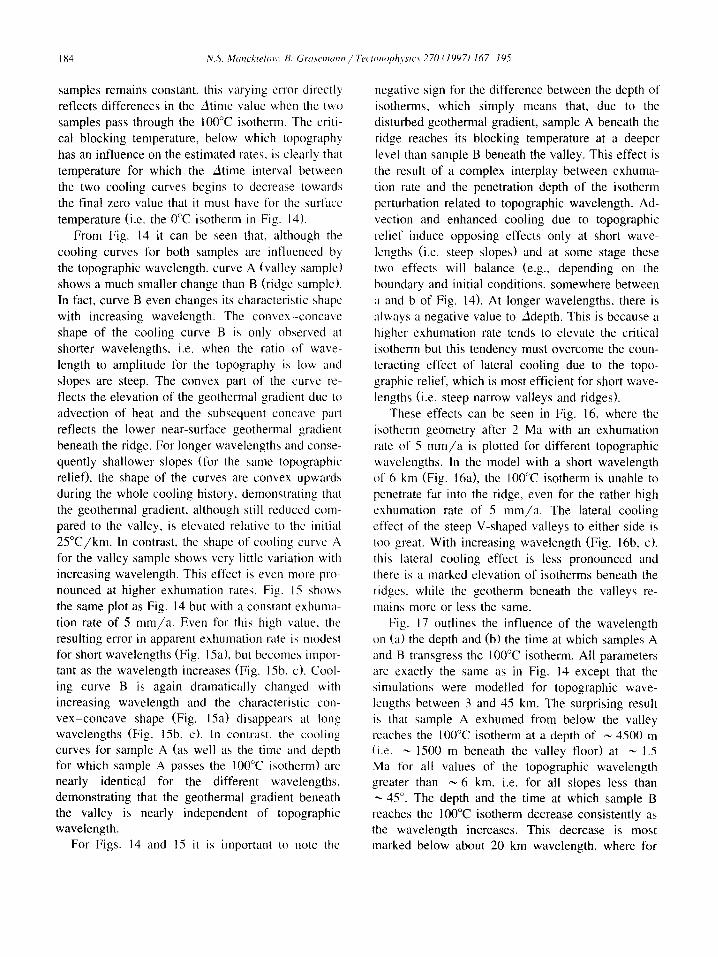
184 N.S. Mancktelow, B. Grasemann / Tectom~physics 270(1997) 167-195

samples remains constant, this varying error directly reflects differences in the Atime value when the two samples pass through the 100°C isotherm. The critical blocking temperature, below which topography has an influence on the estimated rates, is clearly that temperature for which the Atime interval between the two cooling curves begins to decrease towards the final zero value that it must have for the surface temperature (i.e. the 0°C isotherm in Fig. 14).

From Fig. 14 it can be seen that, although the cooling curves for both samples are influenced by the topographic wavelength, curve A (valley sample) shows a much smaller change than B (ridge sample). In tact, curve B even changes its characteristic shape with increasing wavelength. The convex--concave shape of the cooling curve B is only observed at shorter wavelengths, i.e. when the ratio of wavelength to amplitude for the topography is low and slopes are steep. The convex part of the curve reflects the elevation of the geothermal gradient due to advection of heat and the subsequent concave part reflects the lower near-surface geothermal gradient beneath the ridge. For longer wavelengths and consequently shallower slopes (for the same topographic relief), the shape of the curves ale convex upwards during the whole cooling history, demonstrating that the geothermal gradient, although still reduced compared to the valley+ is elevated relative to the initial 25°C/km. In contrast, the shape of cooling curve A for the valley sample shows very little variation with increasing wavelength. This effect is even more pronounced at higher exhumation rates. Fig. 15 shows the same plot as Fig. 14 but with a constant exhumation rate of 5 mm/a . Even for this high value, the resulting error in apparent exhumation rate is modest for short wavelengths (Fig. 15a), but becomes impor tant as the wavelength increases (Fig. 15b, c). Cool- ing curve B is again dramatically changed with increasing wavelength and the characteristic convex-concave shape (Fig. 15a) disappears at long wavelengths (Fig. 15b, c). In contrast, the cooling curves for sample A (as well as the time and depth for which sample A passes the 100°C isotherm) are nearly identical for the different wavelengths, demonstrating that the geothermal gradient beneath the valley is nearly independent of topographic wavelength.

For Figs. 14 and 15 it is important to note the

negative sign for the difference between the depth of isotherms, which simply means that, due to the disturbed geothermal gradient, sample A beneath the ridge reaches its blocking temperature at a deeper level than sample B beneath the valley. This effect is the result of a complex interplay between exhumation rate and the penetration depth of the isotherm perturbation related to topographic wavelength. Ad- vection and enhanced cooling due to topographic relief induce opposing effects only at short wavelengths (i.e. steep slopes) and at some stage these two effects will balance (e.g., depending on the boundary and initial conditions, somewhere between a and b of Fig. 14). At longer wavelengths, there is always a negative value to Jdepth. This is because a higher exhumation rate tends to elevate the critical isotherm but this tendency must overcome the coun- teracting effect of lateral cooling due to the topographic relief, which is most efficient for short wavelengths (i.e. steep narrow valleys and ridges).

These effects can be seen in Fig. 16, where the isotherm geometry after 2 Ma with an exhumation rate of 5 m m / a is plotted for different topographic wavelengths. In the model with a short wavelength of 6 km (Fig. 16a), the 100°C isotherm is unable to penetrate tar into the ridge, even for the rather high exhumation rate o1"5 mm/a . The lateral cooling effect of the steep V-shaped valleys to either side is too great. With increasing wavelength (Fig. 16b, c). this lateral cooling effect is less pronounced and there is a marked elevation of isotherms beneath the ridges, while the geotherm beneath the valleys remains more or less the same.

Fig. 17 outlines the influence of the wavelength tm (a) the depth and (b) the time at which samples A and B transgress the 100°C isotherm. All parameters are exactly the same as in Fig. 14 except that the simulations were modelled for topographic wavelengths between 3 and 45 km. The surprising result is that sample A exhumed from below the valley reaches the 100°C isotherm at a depth of ~ 4500 m (i.e. ~ 1500 m beneath the valley floor) at ~ 1.5 Ma for all values of the topographic wavelength greater than ~ 6 km, i.e. for all slopes less than ~ 45 °. The depth and the time at which sample B reaches the 100°C isotherm decrease consistently as the wavelength increases. This decrease is most marked below about 20 km wavelength, where for


E E

C

.9

E E

X

C 0

..Q

._~ "0

E

E

? ?

E E

8 8

ii~ili!!il

ii!i

E E

? ?

E E

8

iiiiiiiiii i ~ ~!i~i~

~ i~ ~!~ i i!

~i~i~ ̧ ~ ~ii~ ~

E E

? ?

E E E E

c-

O

0 0

186 N.S. M~mcktelow, B. Grasemann / Tectonophysics 270 (1997) 167-195

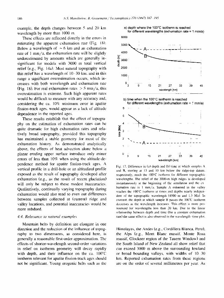
example, the depth changes between 5 and 20 km wavelength by more than 1000 m.

These effects are reflected directly in the errors in estimating the apparent exhumation rate (Fig. 18). Below a wavelength of ~ 6 km and an exhumation rate of 1 mm/a, the exhumation rate will be slightly underestimated by amounts which are generally insignificant for models with 3000 m total vertical relief (e.g., Fig. 14a). Most natural topography with this relief has a wavelength of 10-30 kin, and in this range a significant overestimation occurs, which increases with both wavelength and exhumation rate (Fig. 18). For real exhumation rates > 5 mm/a, this overestimation is extreme. Such high apparent rates would be difficult to measure with any accuracy and, considering the ca. 10% minimum error in apatite fission-track ages, would appear as a lack of altitude dependence in the reported ages.

These results establish that the effect of topography on the estimation of exhumation rates can be quite dramatic for high exhumation rates and rela- tively broad topography, provided this topography has maintained a stable geometry for most of the exhumation history. As demonstrated analytically above, the effects of heat advection alone below a planar eroding upper surface introduce only minor errors of less than 10% when using the altitude-dependence method for apatite fission-track ages. A vertical profile in a drill-hole or an altitudinal profile exposed as the result of topography developed after exhumation (e.g., as the result of recent glaciation) will only be subject to these modest inaccuracies. Qualitatively, continually varying topography during exhumation would also tend to even out differences between samples collected at (current) ridge and valley locations, and potential inaccuracies would be more subdued.

4.4. Releuance to natural examples

Mountain belts by definition are elongate in one direction and the reduction of the influence of topography to two dimensions, as considered here, is generally a reasonable first-order approximation. The effects of shorter-wavelength second-order variations in relief on isotherm geometry will decay rapidly with depth, and their influence on the ca. 100°C isotherm relevant for apatite fission-track ages should not be significant. Young orogenic belts such as the

a) depth where the 100°C isotherm is reached for different wavelengths (exhumation rate = 1 mm/a)

6000

5 0 0 0 ~ _ A . . . . . i

4000 ! i i i

E B ~ ! ~3000 i 1

2000-

1O00r

0 ,

3 9 1'5 21 27 33 39 45 wavelength [km]

4

~ 3

2

b) time when the 100°C isotherm is reached for different wavelengths (exhumation rate = 1 mm/a)

6 r i

~ A . . . . . . . . . . . . . . . . . .

o 3 9 15 21 27 ~3 i9 45 wavelength [km]

Fig. 17. Difference in (a) depth and (b) time at which samples A and B, starting at 13 and 10 km below the ridge-top datum, respectively, reach the 100°C isotherm for different topographic wavelengths. The relief of the 3000-m high ridges is developed instantaneously at the beginning of the simulation and the exhumation rate is 1 mm/a . Sample A exhumed in the valley reaches the 100°C isotherm at times and depths nearly independent of the topographic wavelength (4500 m and 1.5 Ma). In contrast, the depth at which sample B passes the 100°C isotherm decreases as the wavelength increases. This effect is more pronounced /br wavelengths less than 20 km. Due to the linear relationship between depth and time (tor a constant exhumation rate) the same effect is also observed in the wavelength-time plot.

Himalayas, the Andes (e.g., Cordillera Blanca, Peru), the Alps (e.g., Mont Blanc massif, Monte Rosa massif, Glockner region of the Tauern Window) and the South Island of New Zealand all show relief that can exceed 3000 m above the surrounding lowland or broad bounding valleys, with widths of 10-30 kin. Reported exhumation rates from these regions are on the order of several millimetres per year. As


error in the apparent rate for different wavelengths and real exhumation rates

-5 (3 E -lo

~ -15

© -20

-25

-30 5 10 15 20 25 30 35 40 45

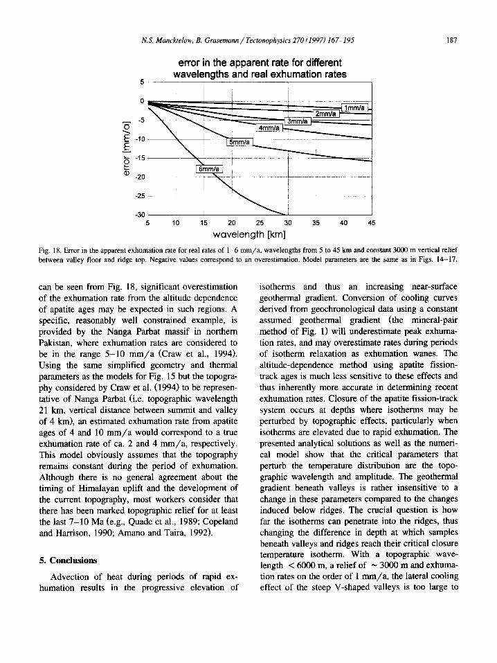
wavelength [km] Fig. 18. Error in the apparent exhumation rate for real rates of 1-6 mm/a, wavelengths from 5 to 45 km and constant 3000 m vertical relief between valley floor and ridge top. Negative values correspond to an overestimation. Model parameters are the same as in Figs. 14-17.

can be seen from Fig. 18, significant overestimation of the exhumation rate from the altitude dependence of apatite ages may be expected in such regions. A specific, reasonably well constrained example, is provided by the Nanga Parbat massif in northern Pakistan, where exhumation rates are considered to be in the range 5-10 m m / a (Craw et al., 1994). Using the same simplified geometry and thermal parameters as the models for Fig. 15 but the topography considered by Craw et al. (1994) to be represen- tative of Nanga Parbat (i.e. topographic wavelength 21 km, vertical distance between summit and valley of 4 km), an estimated exhumation rate from apatite ages of 4 and 10 m m / a would correspond to a true exhumation rate of ca. 2 and 4 mm/a , respectively. This model obviously assumes that the topography remains constant during the period of exhumation. Although there is no general agreement about the timing of Himalayan uplift and the development of the current topography, most workers consider that there has been marked topographic relief for at least the last 7-10 Ma (e.g., Quade et al., 1989; Copeland and Harrison, 1990; Amano and Taira, 1992).

5. C o n c l u s i o n s

Advection of heat during periods of rapid exhumation results in the progressive elevation of

isotherms and thus an increasing near-surface geothermal gradient. Conversion of cooling curves derived from geochronological data using a constant assumed geothermal gradient (the mineral-pair method of Fig. 1) will underestimate peak exhumation rates, and may overestimate rates during periods of isotherm relaxation as exhumation wanes. The altitude-dependence method using apatite fission- track ages is much less sensitive to these effects and thus inherently more accurate in determining recent exhumation rates. Closure of the apatite fission-track system occurs at depths where isotherms may be perturbed by topographic effects, particularly when isotherms are elevated due to rapid exhumation. The presented analytical solutions as well as the numerical model show that the critical parameters that perturb the temperature distribution are the topographic wavelength and amplitude. The geothermal gradient beneath valleys is rather insensitive to a change in these parameters compared to the changes induced below ridges. The crucial question is how far the isotherms can penetrate into the ridges, thus changing the difference in depth at which samples beneath valleys and ridges reach their critical closure temperature isotherm. With a topographic wavelength < 6000 m, a relief of ~ 3000 m and exhumation rates on the order of 1 mm/a , the lateral cooling effect of the steep V-shaped valleys is too large to

188 N.S. Manektelow, B. Grasemann / Tiwtonophysies 270 (1997)167-195

allow isotherms o1 >_ 100°C to penetrate the ridges. The error which results from using the standard altitude-dependence technique to calculate exhumation rates is geologically insignificant, in good agreement with the earlier work of Parrish (1983, 1985). However, with increasing wavelengths and the same vertical relief, valleys become more open and the slopes shallower, the 100°C isotherm can penetrate the ridges, and an overestimation of the real exhumation rate results. This overestimation is geologically significant even at normal exhumation rates ( ~ 1 m m / a ) . It may be dramatic in tectonically active regions for which very rapid cooling rates during exhumation have been reported, for example in the Basin and Range of the southwest USA (Dokka et

al., 1986), the Himalayas (Zeitler et al., 1982: Sorkhabi, 1993), New Zealand (Kamp et al., 1989)

and the Simplon Alps of Switzerland (Mancktelow, 1992). In regions of rapid exhumation and significant relief, reliable results can only be obtained using numerical models.

An important result directly observable in the cooling curves presented in Figs. 5 and 14 is that, even at very low exhumation rates, the shape differs significantly from that normally expected (constant exhumation rates are usually drawn as straight lines on a temperature- t ime diagram). These modelled curves demonstrate that caution is necessary in interpreting exhumation histories from cooling curves derived from geochronological methods. For example, a convex-concave shape to the cooling curve cannot only be achieved by a change in exhumation rate (Grasemann and Mancktelow, 1993; Fig. 9b) but also by a more complicated geothermal gradient induced by topographic relief (Fig. 14a and Fig. 15a). Very fast cooling below 100°C (e.g., Manck- telow, 1992; Sorkhabi, 1993), which is often interpreted as reflecting faster near-surface exhumation, can be more simply explained by the lateral cooling effect of topographic relief (e.g., all the cooling curves for valley sample A in Figs. 14 and 15). The interplay between heat advection and cooling, which has a dynamic influence on the geothermal gradient and the shape of the cooling curves, may become even more complicated if additional parameters such as inhomogeneously distributed conductivities and convective cooling due to near-surface fluid flow are included.

A c k n o w l e d g e m e n t s

E. Hejl, K. Stiiwe and D. Seward are thanked fl)r reading earlier versions of the manuscript and for their helpful suggestions. Thorough and constructive reviews by R. Dokka, C. Ruppel, N. Sleep and M. ter Voorde were much appreciated and improved both content and style.

A p p e n d i x A

A. 1, General theory

The temperature distribution in a homogeneous isotropic solid

whose thermal diffusivity K is independent of temperature is a

particular solution (for given boundary conditions) of the differen-

tial equation: A aT

K V ' - T - i~ 'T+ ( l a ) pC i~t

where T - temperature (K), t - time (s), /, = thermal conductivity (W m i K i), K = thermal diffusivity (m 2 s ~)

- k / p C , g = velocity vector (m s t), p = d e n s i t y ( k g m - ~ ) ,

C = specific heat (J kg - J K r), and A = volumetric heat production (W m ~ ).

In two dimensions with rectangular x y coordinates and

considering only vertical displacements, this equation reduces to:

[ g~-T 02T] OT A OT 1 + + + - ( lb)

where .~ - horizontal distance (m), v = vertical distance (m), positive downwards, u = vertical velocity (m s- ' ), positive upwards (i.e. erosion positive).Sedimentation, with a corresponding negative value for u, is automatically included in the analytical solutions developed below, provided the restriction on homogeneous and isotropic material properties is met, which is unlikely lbr unconsolidated sediments deposited on crystalline basement.

If the material constants are independent of temperature and time, these differential equations are linear in T, allowing linear superposition of solutions and thus a reduction of a more complicated problem into a series of simpler component solutions, which can be added to provide the final result. From the principle of linear superposition, it is immediately obvious that a time-dependent solution can be divided into steady-state (i.e. OT/Ot = 0) and time-dependent components. By taking the heat generation term A / p C entirely into the steady-state solution, the overall problem can be made more tractable, for example:

A K~'~-TI + u~'T I + - - =0 (2a)

p C i+T+

K[- ~'T, + u['T~ = ~ - (2b) Ot

and thus

~ V : ( T , + ~ ) + uV(T, + T , _ ) + - = - A Or,_

pC ot (2c)


For this reason, steady-state solutions will first be developed; these then form the basis for the more general time-dependent solutions. The presence of the erosion term u complicates direct solution of differential equations such as Eq. (2b), but it can be eliminated (e.g., Benfield, 1949a, p. 442; Ozisik, 1980, pp. 74-75) through use of the transformation:

~" = Texp(-~K Y +U2tI4K ] (3)

The reverse transformation is then:

It must be remembered that this transformation must also be applied to the initial and boundary conditions, and in general a constant value of T will transform into a time- and position-dependent value of ~'. Only for the simplest case of a constant zero value tbr T is the transformed value ~" identical. If there is no internal heat generation (i.e. A = 0), the variable ~ must satisfy the homogeneous differential equation:

~ v 2~ = _ ( 5 ) Ot

as can be verified by substituting for T using Eq. (4) in Eq. la, b. There are many standard solutions for this simple form of the heat conduction equation with different boundary conditions and initial temperature distributions (e.g., Carslaw and Jaeger, 1959; Ozisik, 1980).

If the surface conditions are independent of time, it can be easily shown (e.g., Carslaw and Jaeger, 1959, pp. 29-30; Ozisik, 1980, pp. 69-70) that the full solution can be reduced to two problems, one of steady temperature (i.e. the steady-state solution) and one of variable temperature with prescribed initial temperature (given by the difference between the initial and steady-state temperature) and zero surface temperature (since if the surface conditions are independent of time, the difference between the steady-state and the variable temperature at the surface must always be zero). Formally, this can be stated as:

A KV2U q - - - = 0 (6)

pC

where v(x,y) is the steady-state solution independent of t, and

aw KV2W = - - (7)

Ot where w(x,y,t) is the variable temperature solution, with initial value:

w( x ,y , t=O) = / ( x , y ) - t,( x , y ) (8)

and f ( x , y ) is the initial temperature distribution. The final solution (L, + w) clearly satisfies the full differential equation obtained by adding Eqs. (6) and (7).

In sections below that develop solutions for the temperature variation with time following an instantaneous increase in surface temperature, passing use is made of Laplace transformations and Green's functions. A thorough discussion of these techniques is beyond the scope of this appendix and not necessary to follow the method of solution. Interested readers are referred to standard reference works on heat conduction in solids (Carslaw and Jaeger, 1959) or differential equations (Stephenson, 1970).

A.2. Steady-state solutions

A.2.1. Geotherm with heat production, no erosion This will represent the initial condition before onset of erosion

in the time-dependent solutions developed further below, and thus corresponds to f ( x , y ) in Eq. (8) above. For a planar upper surface, the problem reduces to a single dimension and Eqs. (la) and (lb) become:

02T k - ~ v 2 + a = 0 (9)

where k is the conductivity. Following Turcotte and Schubert (1982), an exponential decay of heat production of the form

a = A s e x p ( - h ) (10)

is assumed, where A s is the volumetric heat production at the surface and h is the depth at which the heat production drops to 1 / e of this surface value. Eq. (9) thus becomes:

c92T

Integrating Eq. (11) twice with respect to y gives the result

k T + A s h 2 e x p ( - h ) + c l Y = C 2 (12)

where c I and c 2 are constants of integration, dependent on the boundary conditions. For a slab of finite thickness (e.g., the ~ 100 km thick lithosphere) with known surface temperature T s and constant temperature T L at depth L, the solution is:

As h2 with ot =

k

A.2.2. Geotherm with erosion at a steady rate u, but no heat production

For a planar upper surface and no heat generation (A = 0), Eqs. (la) and (lb) become:

02T OT K Oy------- 2 + U-~y = 0 (14)

The standard solution for such a linear, homogeneous second-order differential equation is given by (e.g., Spiegel, 1968, p. 105):

T = c I exp(m I y ) + c 2 exp(m 2 y ) (15)

where c I and c 2 are constants determined by the boundary conditions and m I and m 2 are the roots of the corresponding quadratic equation, i.e.:

- u + V/~u~ + 0 u m L ,m 2 ,0 (16)

2K K from which it follows that:

(u) T = c , e x p - ~ y +c2 (17)

As y --* ~c T --* T~ = c 2 , and it is clear that a steady-state solution is only possible if the temperature approaches some constant value

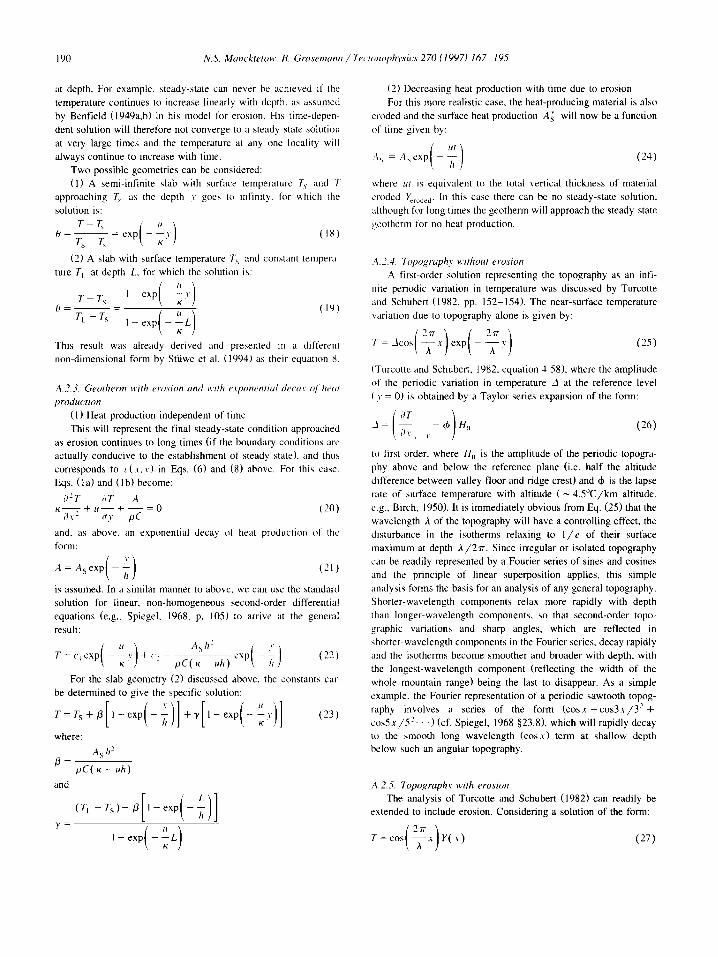
190 N.S. Mancktelow. B. Grasemann /"fectonophysics 270 11997) 167 195

at depth. For example, steady-state can never be achieved if the temperature continues to increase linearly with depth, as assumed by Benfield (1949a,b) in his model for erosion. His time-dependent solution will therefore not converge to a steady-state solution at very large times and the temperature at any one locality will always continue to increase with time.

Two possible geometries can be considered: (1) A semi-infinite slab with surface temperature 7),. and 7

approaching T~ as the depth y goes to infinity, for which the solution is:

0 T s - T , exp - T y (18)

(2) A slab with surface temperature Ts and constant tempera ture T k at depth L, for which the solution is:

- - - ( 19 ) 0 - T L - T s I - e x p ( - U L )

This result was already derived and presented in a difl'erenl non-dimensional form by Stiiwe et al. (1994) as their equation 8,

/3

and

A.2.3. Geothenn with erosion and with erponential decay 0/ Iwat production

(1) Heat production independent o1' time This will represent the final steady-state condition approached

as erosion continues to long times (if the boundary conditions are actually conducive to the establishment of steady state), and thus corresponds to t ' (x .y) in Eqs. (6) and (8) above. For this case, Eqs. (la) and (lb) become:

O2T aT A - - + u - - + - - = 0 ( 2 1 t )

K Ov 2 av pC

and, as above, an exponential decay of heat production of the form:

A = Asex p 121 )

is assumed. In a similar manner to above, we can use the standard solution for linear, non-homogeneous second-order differential equations (e.g., Spiegel, 1968, p. 105) to arrive at the general result:

exp- ,, +c:

For the slab geometry (2) discussed above, the constants can be determined to give the specific solution:

[ [ T = T s + , B l - e x p - + y l - e x p (23)

where:

Ash2

pC( K - uh )

y =

(2) Decreasing heat production with time due to erosion For this more realistic case, the heat-producing material is also

eroded and the surface heat production A~ will now be a function of time given by:

24, 4,, = Asex p h

where u; is equivalent to the total vertical thickness of material eroded Y~,od~a" In this case there can be no steady-state solution, although for long times the geotherm will approach the steady-state geotherm tor no heat production.

A.2.4. Topography without erosion A first-order solution representing the topography as an infi-

nite periodic variation in temperature was discussed by Turcotte and Schubert (1982, pp. 152-154). The near-surface temperature variation due to topography alone is given by:

(Turcottc and Schubert, 1982, equation 4-58), where the amplitude of the periodic variation in temperature A at the reference level ( .v = 0) is obtained by a Taylor series expansion of the form:

J = ( 0T ~ i~Tv, = 0 - 05] H 0 (26)

to first order, where H 0 is the amplitude of the periodic topography above and below the reference plane (i.e. half the altitude difference between valley floor and ridge crest) and ¢b is the lapse rate of surface temperature with altitude ( ~ 4 .5°C/km altitude, e.g., Birch, 1950). It is immediately obvious from Eq. (25) that the wavelength )t of the topography will have a controlling effect, the disturbance in the isotherms relaxing to l / e of their surface maximum at depth 3./27r. Since irregular or isolated topography can be readily represented by a Fourier series of sines and cosines and the principle of linear superposition applies, this simple analysis torms the basis for an analysis of any general topography. Shorter-wavelength components relax more rapidly with depth than longer-wavelength components, so that second-order topographic variations and sharp angles, which are reflected in shorter-wavelength components in the Fourier series, decay rapidly and the isotherms become smoother and broader with depth, with the longest-wavelength component (reflecting the width of the whole mountain range) being the last to disappear. As a simple example, the Fourier representation of a periodic sawtooth topography involves a series of the form ( c o s x + c o s 3 x / 3 2 + c o s 5 x / 5 2 . . .) (cf. Spiegel, 1968 §23.8), which will rapidly decay to the smooth long wavelength (cosx) term at shallow depth below such an angular topography.

A.2.5. Topography with erosion The analysis of Turcotte and Schubert (1982) can readily be

extended to include erosion. Considering a solution of the form:

2rr T = c o s ( - - r ] Y(y) (27)

~ a ]


and substituting for T in Eqs. ( la) and ( lb) for no heat production and steady state gives:

- - + - - - K = 0 ( 2 8 ) Kd~,2 Udv

and the solution is of the same form as Eqs. (15) and (16), with: T = c, exp(rn t 3 ' )+ c2 exp(m2 Y) (29) and

m I , m 2 = 2K

=½[ - u-t- l / (u /2+ { 47r 12 ] _ (30)

K W K I ~ a I ]

Since the temperature variation due to topography obviously has to decay to zero at very large depth (i.e. as y ~oc), the constant c~ corresponding to the positive root m~ must be zero. At 3' = 0, T = Acos(2~rx/A), so that c 2 must have the value A and the solution becomes:

( 2~'x T = Acos~ - - ~ J exp(m 2 y) (31)

where:

m2 = ½ ( - u - ~ / ( u ) 2 + ( 7 ) 2 )

Erosion therefore has the opposite effect to that of topographic wavelength. Increased erosion rate produces a more rapid decay with depth of the temperature variation due to topography. How- ever, the effect of wavelength dominates.

The steady-state solution for erosion of a periodic topography of constant geometry is thus given by adding the variation ex- pressed by Eq. (31) to the steady-state geotherm of Eq. (23), with the result:

+Jcos(2---~x)exp(m2Y) (32)

where by differentiation of Eq. (23): OT u

= - - y + - - ( 3 3 ) 03' ~= 0 K h

and thus A is given by Eq. (26) to be:

(34) ") = "), + ~ - ~ Ho

A.3. Time-dependent solutions

A.3.1. Erosion of a planar surface of constant temperature

(1) Exhumation rate and heat production independent of time

This problem considers the time variation of temperature from an initial steady-state geotherm without erosion, as described by

Eq. (13), to the re-establishment of a steady-state as described by Eq. (23), following onset of erosion at a constant rate u. The method follows the one outlined in the general theory above for surface conditions that are independent of time (surface temperature T s and temperature T L at depth L taken as constant), where the final steady-state solution v(y) of Eq. (6) is given by Eq. (23), the initial temperature distribution f ( y ) is given by Eq. (13), and following Eq. (8), the initial value for the time-dependent temperature function w(y,t), is given by: w(y , t = 0 ) = f ( y ) - v ( y ) (35)

Transforming this initial condition according to Eq. (3), with t = 0, gives:

~(y,t=O)=w(y,t=O)exp 3' (36)

and the solution ~r(y,t) must satisfy the one-dimensional form of the homogeneous differential Eq. (5). The standard solution (Carslaw and Jaeger, 1959, p. 94; Ozisik, 1980, p. 72) is given by:

2 ~ = KO), t )s in to, Yf0 ~'(~ ,t = 0)sin o),,y dy ~r(y,t) ~ e x p ( - . = 2 t, . , ,

(37) n'~-

where o J,, = - - L

On substituting using Eqs. (13), (23), (35) and (36). an analytical solution for the definite integral can be obtained:

bl L t four( y ,t = 0)sin o4, y'dy' =

u _ ! t 2 , 2K h] +~°7'

(exp[(-~K-1)LI[( -~K-I)s in°~.L-%cos°~.LI+°J.}

U b2 Lexp[ L]( sino L- o, cos.L)

exp(-~-~KL)[([-~K]2-oJZ)sinoJ.L-Uo~.cos~o.L] + u} {_ . 2 \ 2 K ] %

+ u 2 exp

b4 exp L -2--~Ksino4,L-- oJ.cosw.L + ~o. ÷ ( _ . t 2 + <

\ 2 K ] (38)

where b]= f l - a

b 3 = ~

192 N.S. Mancktelow. B. Grasemam~ / Tectonophysics 270 (1997) 167-195

which can be substituted back into Eq. (37) to calculate the convergent series and thus ((y,t) . The final solution is then given

by:

T ( y , t ) = ~ ( y , t ) e x p 2/< ) ~ ] + c ( y ) (39)

where r (y) corresponds to the steady-state solution given by Eq. (23).

(2) Exhumation rate and heat production varying with time

The solution given by Eq. (39) does not include the effects o l erosion of the heat-producing layer itself. As noted above, inclusion of this effect precludes the attainment of a true steady state as does the inclusion of exhumation rates that vary with time. In principle, a stepwise analytical solution could be developed in which Eq. (39) becomes the initial geotherm for the next step (at a different exhumation rate and surface heat production), but in practice repetition of integration step Eq. (38) results in very unwieldy solutions. However. the solution Eq. (37) to the general problem of a decaying transient temperature distribution simply reflects the observation that the equation:

= aexp( - ,xw 2 t ) s in (wy) (40 )

(where a and w are independent of r and t) is a solution of the one-dimensional heat conduction Eq. (5) for all values of a and w. The solution must then be found that fits the initial temperature distribution f (y ) at t=O, and this solution will decay to zero with time due to the negative exponential term. In our case, f{ v} is a continuous function with f (0 )= f ( L ) = 0 and can be repre sented by the infinite Fourier sine series:

f(Y)=L,,__~I y ' . t = O ) s i n - - v ' d V ' L . s i n T , (41)

which leads immediately to the final solution (Eq. (37}), However, we can also represent f (y ) by a discrete Fourier sine series valid for N equally spaced data points, namely:

,) N - I plkTr

[ / (y ) ] , = -- E ~;,s~nl / (~2} N = 0 ~ , T ]

where the coefficients of the Fourier sine translorm are given b~: ,V I

k=l for the data array [ f ( Y)]k, k = 0 . . . . . N - I

Standard Fast Fourier Transform (FFT) routines tor the calcu lation of the coefficients F~ in this discrete sine series are readily available (e.g.. Press et al., 1986). The technique employed is to first calculate a series of equally spaced data points (a multiple of 2 as required by the FFT) for the initial temperature distribution using Eq. (13). then for the steady-state solution with the given exhumation rate using Eq. (23). The difference (i.e. the initial transient that should decay to zero with time) is then transformed using Eq. (3) to consider the effect of advection, the discrete Fourier sine series coefficients are calculated and the kth coeffi- cient in the series multiplied by e x p ( - x ( k I)27r2t/L 2] {re- membering that the numbering of the discrete series starts at 0, not 1 ). the inverse transform calculated and the coefficients multiplied

by 2 / N to recover the new data series, which is then transformed back to temperature values using transformation Eq. (4). This new temperature distribution then becomes the initial state for another cycle and the whole sequence can be repeated any number of limes to consider an exhumation history involving variable rates and surface heat production.

,43.2. Erosion of a planar surfbce of non-constant temperature. &)dr initially at zero temperature

Solutions derived here can be added to other solutions to account lbr uplift of the earth's surface relative to sea level, and thus to changes in the surface reference temperature. If L is large, and only changes to the upper-surface temperature are considered. the problem is very well approximated by solutions tot the semi-infinite region y > 0. The general solution for an arbitrary function &(t) for temperature at the surface is given by (e.g., Carslaw and Jaeger, 1959, equation (7), p. 305):

_ y 2 'i ," exp 4 K ~ - - r )

7" ] u ' & ( t ) ' d r (44 ) 2v~TrK (t - r ) U2

Fwo simpler cases can be considered. Case 1: an instantaneous increase in temperature of the surface

T, at time zero, which is maintained constant thereafter. This can be readily solved using Laplace transformation, following Carslaw and Jaeger (1959, p. 305). For ~ a constant, the transformed boundary condition, using Eq. (3) is:

,t)(, ={},t)=T, exp ~ t (45)

The Laplace transform of this function (e.g., Carslaw and Jaeger, 1959, appendix 5 (3)) is:

I d,(/ ' ) = 71 (46)

ll 2 [ ) - - - -

4K

and the solution then:

I ~ - I ; - - • exp( - qy) (47)

It-

P 4K

P where q - ' = - - .

t( Inverting the Laplace transform (e.g., Carslaw and Jaeger,

1959. appendix 5 (19)) and transforming back to temperature T using Eq. (4) gives:

+exp - y erfc 2 ~ , ? ~ (48)

where erfc is the complementary error function:

e r f c ( x ) = ~ £ ~ e x p ( - ~2)d~


Case 2: a linear increase in the surface temperature with time. This problem has already been solved by Benfield (1949a), where his equation 12 can be reduced to the case of zero initial temperature gradient (initial zero temperature throughout the body) to give:

'0 [ [ y+ut~ T = - - (y+ 2u ut)erfc[-2-~7 )

~ ~ y - ~ - -v erfc p (49) ut)exp[_ u ~ [ v-ut~]

where the temperature at the surface at time t is given by Ot.

A.3.3. Erosion of a periodic topography Again for large L, the effects of surface topography are

adequately described by solutions for a semi-infinite solid y > 0. When there is no advection (i.e. no erosion, u = 0), the general three-dimensional solution for a body initially at zero temperature, with its surface at y = 0 maintained at temperature 4a(x,z,t) for t > 0 is given, using Green's function and an instantaneous point source, by (Carslaw and Jaeger, 1959, equation 3, p. 371):

y (t[~ (~ ~b(x',z',r) T(x,y,z,t) 8(,B.K)3/2 JoJ_~j_~ c (t_r)5/2

( (X--X')2"}-y2+(Z--Zt) 2 ) × exp - 4K(t-- r) dx'dz'dr (50)

The corresponding result for two dimensions using an instantaneous line source is:

r(x,y,t)= ~ fof~ 6(x',,) -~ ( t -T ) 2

X e x p [ ( x - x ' ) 2 + y 2 1 ' ~7{7- 7) ]dxd, (51) Since any general topography can be represented by a Fourier

series, there is little loss of generality in considering a periodic topography of the form:

which on transformation using Eq. (3) to consider the effect of erosion becomes:

) The cosine form of the temperature variation in the x-direction

will be maintained for all y and t, and thus the problem reduces to finding the variation in the (transformed) amplitude of this variation with y and t alone, i.e. the value of ~(x =O,y,t). Substituting Eq. (52) in Eq. (51) and collecting variables, we obtain:

A( t )exp - - r - - V t 4K 4K(t--r)

~(x=°'Y")=-~K f o ( i _ , ) 2

[ x '2 ] 2~r ) cos dx'dr (53) x . ~ e x p 4K(t--r) (----£-x'

The function under the integral with respect to x' is even (i.e. f ( - x ' ) = f (x ' ) ) , and can therefore be written in the form:

2 f o exp ( - ax'2)cos(bx')dx ' (54)

where

1 27r a and b = - -

4K(t--r) h

This definite integral can be found in standard tables (e.g., Spiegel, 1968, §15.73), with the value:

½ exp - ~ a (55)

so that on substitution of Eqs. (54) and (55) back into Eq. (53) we

47r 2 ] , , 7 ( t - ~ ) ]

obtain:

v ~(x=O,y,O=

u y2

A( t )exp -~TK 7 4 K ( t - - r )

xf o (t_~)3/'- To simplify, we can make the substitution:

1

4K( t - - r )

to obtain:

dr (56)

2 yexp(44, ) ~r(x = 0 ' y ' t )

where

b=(-" 12+(_ I 2 a = v 2 and \4K] ~A]

for the simplest case where A is a constant independent of t. Reversing the transformation back to temperature T using Eq. (4) gives:

T(x=O,y,t)

2 Ayexp( - - 2-~Y) e x p [ _ (a~:2 + b

The integral in this equation has an analytical solution of the form:

4v~

194 N.S. Mancktelow, B. Grasemann / 7i,('tonophysics 270 (1997) 167-195

which on substitution, returns the solution as:

,3 e x p ( - u ' T( .t = O..v. t ) = --., T~K.' )

where:

(59)

n -" 4 ~ -

and on including the cosine variation with v:

~ 2 e x p ( - - - v l [ e x p ( s v ) e r f c [ ~ + ,V:K)-) r(.,...,..t) = 2 , , I [ ~. 2v,,~

(~01 For infinite wavelength A, Eq. (6(I) reduces to Eq. (48) above

and for infinite time t it converges to the steady-state solution Eq. (31).

Eq. (60) describes the time-dependent variation in temperaturc below a spatially periodic surface temperature of constanl amplitude A. However. because the geothermal gradient will also vary with lime in an eroding terrain (according to Eq. (39)). a topogra phy of constant geometry will not be equivalent Io constant _1 through time, and Eq. (6(I) is only useful as a first approximation to evaluate the time required to approach steady-state behaviour. More realistic models varying the topography and geothermal gradient with time are best approached by numerical finite-dif- terence or finite-element modelling.

References

Amano. K. and Taira. A., 1992. Two-phase uplift ot Higher Himalaya since 17 Ma. Geology, 20:391 394.

Benfield, A.E., 1949a. A problem of the temperature distribution in a moving medium. Q. Appl. Math.. 6:439 443.

Benfield. A.E.. 1949b. The effect of uplift and denudation on underground temperatures..I. Appl. Phys.. 2(1: 66-7(I.

Bertotti, G. and ter Voorde, M.. 1994. Thermal effects of normal faulting during rifted basin l~-)rmation. 2. The Lugano-Val Grande normal fauh and the role of pre-existing thermal anomalies. Tectonophysics. 240: 145-157.

Birch, F., 1950. Flow of heal in the Front Range. Colorado. Bull. Geol. Soc. Am., 61: 567-630.

Brown, R.W.. 1991. Backstacking apatite fission-track "stratigra phy': a method for resolving the erosional and isostatic re bound components of tectonic uplift histories. Geology, 19: 74-77.

Carslaw, H.S. and Jaeger. J.C., 1959. Conduction of Heal in Solids. Clarendon Press, Oxford. 2nd ed.. 51(I pp.

Copeland, P. and Harrison, T.M., 1990. Episodic rapid uplift in

the Himalaya revealed by 4°Ar/~')Ar analysis of detrital K- feldspar and muscovite, Bengal fan. Geology, 18: 354-357.

Craw. D., Koons, P.O., Winslow, D.. Chamberlain, C.P. and Zeitler, P., 1994. Boiling fluids in a region of rapid uplift, Nanga Parbat Massif, Pakistan. Earth Planet. Sci. Lett., 128: 169-182.

l)odson. M.H.. 1973. Closure temperature in cooling geochronological and petrological systems. Contrib. Mineral. Petrol., 4(/: 259-274.

Dokka, RK.. Mahaffie, M.J. and Snoke, A.W., 1986. Ther- mochronologic evidence of major tectonic denudation associ- ated with detachment faulting, Northern Ruby Mountains East Humboldt Range, Nevada. Tectonics, 5: 995-1006.

England, P. and Molnar, P., 1990. Surface uplift, uplift of rocks and exhumation of rocks. Geology. 18:1173-1177.

England, P.C. and Richardson. S.W., 1977. The influence of erosion upon the mineral facies of rocks from different metamorphic environments. J. Geol. Soc. London, 134: 201-213.

Fitzgerald, P.G. and Gleadow, A.J.W., 1988. Fission-track geochronology, tectonics and structure of the Transantarctic Mountains in Northern Victoria Land, Antarctica. Chem. Geol. (Isot. Geosci. Sect.). 73: 169-198.

Glazner, A.F. and Bartley, J.M.. 1985. Evolution of lithospheric strength after thrusting. Geology, 13: 42-45.

Grasemann. B. and Mancktelow, N.S.. 1993. Two-dimensional thermal modelling of normal faulting: the Simplon Fault Zone, Central Alps, Switzerland. Tectonophysics, 225: 155-165.

Jarvis. G.T. and McKenzie, D.P.. 1980. Sedimentary basin forma tion with finite extension rates. Earth Planet. Sci. Lett.. 48: 42-52.

Kamp, P.J.J.. Green, P.F. and White. S.H., 1989. Fission-track analysis reveals character of collisional tectonics in New Zealand. Tectonics. 8:169-195.

Lees. CH., 1910. On the shape of the isogeotherms under mountain ranges in radio-active districts. Proc. R. Soc. London, A 83: 339-346.

Mancktelow. N.S.. 1992. Neogene lateral extension during con- ~ergence in the Central Alps: evidence from interrelated fault- mg and backfolding around the Simplonpass (Switzerland). Tectonophysics, 215:295-317.

McKenzie. D.P., 1078. Some remarks on the development of sedimentary basins. Earth Planet. Sci. Lett., 40: 25-32.

Molnar, P. and England, P., 1990. Temperatures, heat flux. and frictional stress near major thrust faults. J. Geophys. Res., 95: 4833-4856.

(~zisik, M.N., 1980. Heat Conduction. Wiley and Sons, Ne'~ York, 687 pp.

Parrish, R.R, 1982. Cenozoic Thermal and Tectonic History of lhe Coast Mountains of British Columbia as Revealed by Fission-Track and Geological Data and Quantitative Thermal Models. Ph.D. thesis, Univ. British Columbia, Vancouver, 166 pp.

Parrish. R.R., 1983. Cenozoic thermal evolution and tectonics of the Coast Mountains of British Columbia, 1. Fission-track dating, apparent uplift rates, and patterns of uplift. Tectonics, 2: 601-63I.

Parrish. R.R., 1985. Some cautions which should be exercised


when interpreting fission-track and other dates with regard to uplift rate calculations. Nucl. Tracks, 10: 425.

Peaceman, D.W. and Rachford, H.H., 1955. The numerical solution of parabolic and elliptic differential equations. J. Soc. Ind. Appl. Math., 3: 28-41.

Press, W.H., Flannery, B.P., Teukolsky, S.A. and Vetteding, W.T., 1986. Numerical Recipes. The Art of Scientific Com- puting. Cambridge University Press, Cambridge, 818 pp.

Quade, J., Ceding, T.E. and Bowman, J.R., 1989. Development of Asian monsoon revealed by marked ecological shift during the latest Miocene in northern Pakistan. Nature, 342: 163-166.

Ruppel, C. and Hodges, K.V., 1994a. Pressure-temperature-time paths from two-dimensional thermal models: prograde, retro- grade, and inverted metamorphism. Tectonics, 13: 17-44.

Ruppel, C. and Hodges, K.V., 1994b. Role of horizontal thermal conduction and finite time thrust emplacement in simulation of pressure-temperature-time paths. Earth Planet. Sci. Lett., 123: 49-60.

Ruppel, C., Royden, L. and Hodges, K.V., 1988. Thermal model- ing of extensional tectonics: application to pressure-temperature-time histories of metamorphic rocks. Tectonics, 7: 947- 957.

Sonder, L.J. and Chamberlain, C.P., 1992. Tectonic controls of metamorphic field gradients. Earth Planet. Sci. Lett., 111: 517-535.

Sorkhabi, R.B., 1993. Time-temperature pathways of Himalayan

and Trans-Himalayan crystalline rocks: a comparison of fission-track ages. Nucl. Tracks Radiat. Meas., 21: 535-542.

Spiegel, M.R., 1968. Mathematical Handbook of Formulas and Tables. Schaum's Outline Series in Mathematics, McGraw- Hill, New York, 271 pp.

Stephenson, G., 1970. An Introduction to Partial Differential Equations for Science Students. Longman, London, 2nd ed., 152 pp.

Stiiwe, K., White, L. and Brown, R., 1994. The influence of eroding topography on steady-state isotherms. Application to fission-track analysis. Earth Planet. Sci. Lett., 124: 63-74.

Turcotte, D.L. and Schubert, G., 1982. Geodynamics, Applica- tions of Continuum Physics to Geological Problems. John Wiley and Sons, New York, 450 pp.

Wagner, G.A. and Reimer, G.M., 1972. Fission-track tectonics: the tectonic interpretation of fission-track ages. Earth Planet. Sci. Lett., 14: 263-268.

Wagner, G.A., Reimer, G.M. and Jaeger, E., 1977. Cooling ages derived by apatite fission-track, with Rb-Sr and K-Ar dating: the uplift and cooling history of the Central Alps. Univ. Padova, Mem. Sci. Geol., 30: 1-27.

Zeitler, P.K., 1985. Cooling history of the NW Himalaya, Pak- istan. Tectonics, 4: 127-151.

Zeitler, P.K., Johnson, N.M., Naeser, C.W. and Tahirkheli, R.A.K., 1982. Fission-track evidence for Quaternary uplift of the Nanga Parbat region, Pakistan. Nature, 298: 255-257.

Time-dependent effects of heat advection and topography on cooling histories during erosion

Documents

Transcript of Time-dependent effects of heat advection and topography on cooling histories during erosion