Three-dimensional topography corrections of magnetotelluric data

Geophys. J. Int. (2008) 174, 464–474 doi: 10.1111/j.1365-246X.2008.03817.xG

JIG

eom

agne

tism

,ro

ckm

agne

tism

and

pala

eom

agne

tism

Three-dimensional topography corrections of magnetotelluric data

Myung Jin Nam,1,∗ Hee Joon Kim,2 Yoonho Song,3,† Tae Jong Lee3 and Jung Hee Suh4

1Department of Petroleum and Geosystems Engineering, The University of Texas at Austin, Austin, TX 78712, USA2Department of Environmental Exploration Engineering, Pukyong National University, Busan 608-737, Korea3Korea Institute of Geoscience and Mineral Resources, Daejeon 305-350, Korea. E-mail: [email protected], Formerly Department of Civil, Urban and Geosystem Engineering, Seoul National University, Seoul 151-744, Korea

Accepted 2008 April 13. Received 2007 December 6; in original form 2007 March 19

S U M M A R YTopographic effects due to irregular surface terrain may prevent accurate interpretation of mag-netotelluric (MT) data. Three-dimensional (3-D) topographic effects have been investigatedfor a trapezoidal hill model using an edge finite-element method. The 3-D topography gener-ates significant MT anomalies, and has both galvanic and inductive effects in any polarization.This paper presents two different correction algorithms, which are applied to the impedancetensor and to both electric and magnetic fields, respectively, to reduce topographic effectson MT data. The correction procedures using a homogeneous background resistivity derivedfrom a simple averaging method effectively decrease distortions caused by surface topogra-phy, and improve the quality of subsurface interpretation. Nonlinear least-squares inversion oftopography-corrected data successfully recovers most of structures including a conductive orresistive dyke.

Key words: Numerical solutions; Magnetotelluric.

1 I N T RO D U C T I O N

Magnetotelluric (MT) surveys are a powerful tool for investigatingvarious types of deep structures in the earth because of its largepenetration capability. It has been widely used in prospecting foroil, gas and geothermal resources (Goldstein 1988; Orange 1989;Key et al. 2004), and in studying the earth’s crust and upper man-tle (Wannamaker et al. 1989). Recently, three-dimensional (3-D)MT surveys have been increasingly carried out (e.g. Takasugi et al.1992; Newman et al. 2005; Lee et al. 2007), and several 3-D mod-elling and inversion schemes have been developed to understandMT responses to a 3-D earth (e.g. Wannamaker 1991; Mackie &Madden 1993; Mackie et al. 1994; Sasaki 2001; Nam et al. 2007).However, interpreting MT responses is obscure when surface to-pography is undulating, because it can have a substantial effect onMT data. Large interpretation errors may occur in MT surveys con-ducted close to slope variations if field distortions caused by thesurface topography are not considered. Therefore, the reduction ofthese distortions on MT data is an important step in the interpreta-tion of subsurface conductivity distribution (Chouteau & Bouchard1988).

Two-dimensional (2-D) numerical modelling of topographic fea-tures has shown that surface topography affects the H-polarization(TM mode) response when electric fields are measured perpen-dicular to the strike (Wannamaker et al. 1986). Alternately, in the

∗Formerly at: Korea Institute of Geoscience and Mineral Resources, Dae-jeon 305-350, Korea.†Corresponding author.

E-polarization (TE mode), perturbations are small and quickly van-ish, when the typical scale length of topographic features is smallcompared to the skin depth in the subsurface (Baba & Seama 2002).The 2-D topographic effect is only galvanic in the TM mode whileinductive in the TE mode (Vozoff 1991). Thus, in the 2-D case,TM-mode responses are much more important than TE-mode re-sponses. The topographic effect in 3-D is, however, both galvanicand inductive in any polarization (as will be shown in this study),and hence can be more complicated than in 2-D.

For accurate interpretation of MT data, topographic effects canbe included in an interpretation process. In general, two differentapproaches are used: incorporating topography into an earth modelin inversion and correcting distortions due to topography beforeinversion (Schwalenberg & Edwards 2004). The first approach hasbeen applied frequently in 2-D but has been hardly used in 3-D.The second method has been implemented for both 2-D synthetic(Chouteau & Bouchard 1988; Jiracek et al. 1989) and field data(Gurer & Ilkisik 1997) using a distortion-tensor stripping tech-nique (Larsen 1977). Recently, Baba and Chave (2005) presenteda correction method for interpreting marine MT data, where theyincorporated removal of 3-D topographic effects in 2-D inversion.

This study introduces two different correction techniques to re-move topographic effects on 3-D MT responses. The first methodcorrects an MT impedance tensor, while the second method directlyreduces the distortion on horizontal electric and magnetic fields.It is expected that the fields-correction method might yield betteror at least equivalent results to those of the impedance-correctionmethod. This is because the impedance tensor is calculatedfrom horizontal, electric and magnetic fields hence the distortionof the impedance is determined by the effect on the fields. Both

464 C© 2008 The Authors

Journal compilation C© 2008 RAS

by guest on September 17, 2016

http://gji.oxfordjournals.org/D

ownloaded from

http://gji.oxfordjournals.org/

Three-dimensional topography corrections of magnetotelluric data 465

methods will serve as a strong cross-check if they generate the sameresults.

The Larsen’s stripping technique can cause geometrical distor-tions, especially when the subsurface is a 1-D layered earth ratherthan a homogeneous half-space (Chouteau & Bouchard 1988). Toovercome this failure, a stratified earth should be considered in theevaluation of correction coefficients (Gurer & Ilkisik 1997). How-ever, the earth’s resistivities a priori in real applications are notknown. In this paper, a simple averaging procedure to determine ahomogeneous background resistivity for topographic correction isproposed. The background resistivity is determined as an averagevalue of apparent resistivities at each frequency under consideration.We compare correction results using a homogenous background re-sistivity determined by the averaging procedure against those usingthe real background resistivities of a two-layered earth.

A 3-D edge finite-element method (FEM) (Nam et al. 2007)is employed for accurate simulation of topographic effects, whichis most critical in correction approaches. The algorithm solves avector Helmholtz equation of electric fields and uses hexahedralelements to delineate surface topography. The edge FEM is freefrom spurious solutions or vector parasites (Lynch and Paulsen1991; Mur and Lager 2002) and gives electric fields along edges ofhexahedral elements as a solution for the vector Helmholtz equation.This feature is important because the electric fields measured in realMT surveys follow the inclination of the surface terrain.

Using a 3-D trapezoidal hill model, 3-D topographic effects arecompared with 2-D ones to show that the topographic effect in 3-D isboth galvanic and inductive in any polarization. The two correctiontechniques are introduced and validated for a heterogeneous modelwith the same hill structure over a homogeneous or two-layeredearth. The validation denotes that the two correction methods ef-fectively decouple topography-induced anomalies from observedMT data, ultimately giving almost the same results. Correction co-efficients are derived from a homogeneous background resistivitydetermined by an averaging method, though the real subsurfaceis a 1-D layered earth. We conclude by showing subsurface resis-tivity images that are reconstructed through 3-D non-linear least-squares inversion of topography-corrected data generated from theimpedance-correction method.

2 3 - D T O P O G R A P H I C E F F E C T S

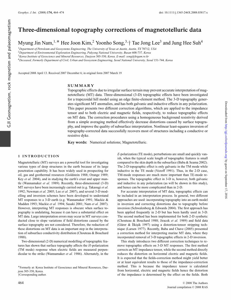
We first investigate topographic effects using a 3-D trapezoidal hillmodel suggested by Nam et al. (2007) (Fig. 1). The hill is 0.45 km

(b) Cross-section(a) Topographic surface

xy

z

earth

air

-1 10x (km)

0

0.45

elevation (km)

100 ohm-m

0.45 km

0.45 km 2 km

2 km

line X

0.45 km

Figure 1. A 3-D topographic model having a 3-D trapezoidal hill (after Nam et al. 2007). (a) Topographic surface view and (b) cross-sectional view in the x–zplane at y = 0.

high, and 0.45 km wide at the hilltop and 2 km at the base, whosex–z and y–z sections at y = 0 and x = 0, respectively, are identical tothe 2-D model used in Wannamaker et al. (1986). The y-directionis assumed to be the strike direction. The earth is a homogeneous100 ohm-m half-space. A whole domain of 9.8 × 9.9 × 22.2 kmis divided into 31 × 31 × 24 (14 earth layers and 10 air layers)elements; the hill is divided into 21 × 21 columns of elements(eight columns of equal width for each hillside and five for thehilltop in each direction) as shown in Fig. 1.

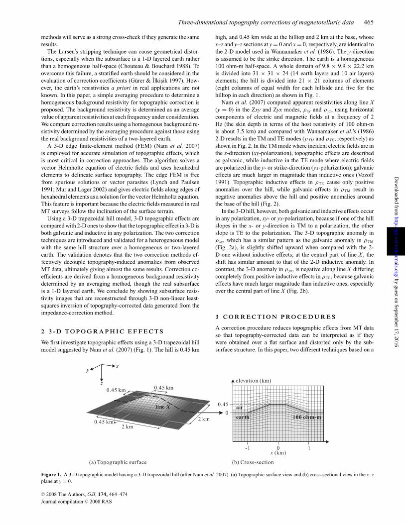
Nam et al. (2007) computed apparent resistivities along line X(y = 0) in the Zxy and Zyx modes, ρ xy and ρ yx, using horizontalcomponents of electric and magnetic fields at a frequency of 2Hz (the skin depth in terms of the host resistivity of 100 ohm-mis about 3.5 km) and compared with Wannamaker et al.’s (1986)2-D results in the TM and TE modes (ρTM and ρTE, respectively) asshown in Fig. 2. In the TM mode where incident electric fields are inthe x-direction (xy-polarization), topographic effects are describedas galvanic, while inductive in the TE mode where electric fieldsare polarized in the y- or strike-direction (yx-polarization); galvaniceffects are much larger in magnitude than inductive ones (Vozoff1991). Topographic inductive effects in ρTE cause only positiveanomalies over the hill, while galvanic effects in ρTM result innegative anomalies above the hill and positive anomalies aroundthe base of the hill (Fig. 2).

In the 3-D hill, however, both galvanic and inductive effects occurin any polarization, xy- or yx-polarization, because if one of the hillslopes in the x- or y-direction is TM to a polarization, the otherslope is TE to the polarization. The 3-D topographic anomaly inρ xy, which has a similar pattern as the galvanic anomaly in ρTM

(Fig. 2a), is slightly shifted upward when compared with the 2-D one without inductive effects; at the central part of line X , theshift has similar amount to that of the 2-D inductive anomaly. Incontrast, the 3-D anomaly in ρ yx, is negative along line X differingcompletely from positive inductive effects in ρTE, because galvaniceffects have much larger magnitude than inductive ones, especiallyover the central part of line X (Fig. 2b).

3 C O R R E C T I O N P RO C E D U R E S

A correction procedure reduces topographic effects from MT dataso that topography-corrected data can be interpreted as if theywere obtained over a flat surface and distorted only by the sub-surface structure. In this paper, two different techniques based on a

C© 2008 The Authors, GJI, 174, 464–474




ownloaded from


466 M. J. Nam et al.

1000

x (km)210-1-2

)m-

mh

o(yti

vitsisertnera

ppa

10

100

x (km)210-1-2

10

1000

)m-

mh

o(yti

vitsisertnera

ppa

100

(a) Z and TM modesxy (b) Z and TE modesyx

Wannamaker et al. (1986)

3D trapezoidal-hill model

Figure 2. Apparent resistivities at 2 Hz along line X (y = 0) for the trapezoidal hill model shown in Fig. 1. Zxy (a) and Zyx (b) modes are, respectively,compared with TM and TE modes given by Wannamaker et al. (1986) (after Nam et al. 2007).

distortion tensor approach (Larsen 1977) are described and tested;one (fields-correction method) reduces distortions on both elec-tric and magnetic fields, while the other (impedance-correctionmethod) reduces distortion on an MT impedance tensor. Originally,the Larsen’s (1977) approach relates distorted fields with undistortedfields in terms of a distortion tensor in order to remove distortionscaused by near surface inhomogeneities. Mozley (1982) used thisdistortion tensor concept to remove topographic effects on MT data.However, the distortion tensor technique results in significant geo-metrical distortion when the real subsurface is a 1-D layered earth(Chouteau & Bouchard 1988) since it assumes the subsurface as ahomogeneous half-space. To compensate for this, this study consid-ers a stratified earth instead of the half-space by proposing a simpleaveraging procedure to determine a homogeneous background re-sistivity for topographic correction at each identified frequency.

From now on, when computing MT responses, apparent resistiv-ities and phases, using the 3-D edge FEM code (Nam et al. 2007),we use horizontal magnetic fields and electric fields parallel to theslope of earth’s surface since these fields are measured in the realMT survey.

3.1 Fields-correction method

The fields-correction method removes topographic effects from bothelectric and magnetic fields by assuming these fields to be linearlyrelated to the corresponding undistorted fields by a 3 × 3 distor-tion tensor (Jiracek et al. 1989). Because 3-D topographic effectsare both galvanic and inductive in any polarization distorting bothelectric and magnetic fields, both xy- and yx-polarizations are con-sidered simultaneously in the fields-correction method.

For correcting the electric field, we assume a relationship betweendistorted and undistorted electric fields as

ED = DE · EU , (1)

where ED is the observed electric-field vector at a frequency anda position, DE is the distortion tensor of electric fields, and EU isthe electric-field vector that is supposed to be obtained through thefields-correction method. The distortion tensor DE can be calcu-lated from the relationship between the electric fields for a layeredmedium with surface topography, Et, and those with the flat surface,Eh, as

Et = DE · Eh . (2)

In eqs (1) and (2), the electric fields EU and Eh are assumed tobe obtained over the flat surface. The vertical electric fields EU

z andEh

z vanish as z → 0 because there are no vertical current flows atthe flat-earth surface (Jiracek et al. 1989). Thus, the two equationscan be rewritten in matrix form as(

E Dx

E Dy

)=

(DE

xx DExy

DEyx DE

yy

) (EU

x

EUy

), (3)

and(Et

x

Ety

)=

(DE

xx DExy

DEyx DE

yy

) (Eh

x

Ehy

), (4)

respectively.The 2 × 2 distortion tensor DE can be derived when two known

orthogonal sources, e.g. xy- and yx-polarizations, are used. Sub-stituting the resulting electric fields, Et and Eh, for both xy- andyx-polarizations into eq. (4) and considering Eh

y1 = Ehx2 = (0,0), we

can obtain(DE

xx DExy

DEyx DE

yy

)=

(Et

x1

/Eh

x1 Etx2

/Eh

y2

Ety1

/Eh

x1 Ety2

/Eh

y2

), (5)

where the subscripts 1 and 2 refer to the xy- and yx-polarizations,respectively. Inserting equation (5) into eq. (3), we obtain the undis-torted electric field EU , as

EUx = (

E Dx DE

yy − E Dy DE

xy

)/(DE

xx DEyy − DE

xy DEyx

),

EUy = (

E Dy DE

xx − E Dx DE

yx

)/(DE

xx DEyy − DE

xy DEyx

),

(6)

Correcting magnetic fields is almost the same as correcting elec-tric fields. The relationship between HD and HU is

HD = DH · HU . (7)

From a relationship between Ht and Hh like eq. (2), we get

Ht = DH · Hh . (8)

Because no vertical component of the magnetic field is producedfor a layered earth [Hh

z = (0,0)], the third column of DH cannot beobtained from eq. (8), and thus must be ignored. Eqs (7) and (8),subsequently, can be approximately expressed in matrix form as(

H Dx

H Dy

)=

(DH

xx DHxy

DHyx DH

yy

)(HU

x

HUy

), (9)

C© 2008 The Authors, GJI, 174, 464–474




ownloaded from



and(H t

x

H ty

)=

(DH

xx DHxy

DHyx DH

yy

)(H h

x

H hy

), (10)

respectively. Considering Hhx1 and Hh

y2 are (0,0), we can obtain fromeq. (10) that(

DHxx DH

xy

DHyx DH

yy

)=

(H t

x2/H hx2 H t

x1

/H h

y1

H ty2/H h

x2 H ty1

/H h

y1

). (11)

By substituting eq. (11) into eq. (9), the undistorted magnetic fieldHU is obtained as

HUx = (

H Dx DH

yy − H Dy DH

xy

)/(DH

xx DHyy − DH

xy DHyx

),

HUy = (

H Dy DH

xx − H Dx DH

yx

)/(DH

xx DHyy − DH

xy DHyx

).

(12)

3.2 Impedance-correction method

The 3-D topography distorts not only off-diagonal but also diago-nal components of an MT impedance tensor (Nam 2006) since bothelectric and magnetic fields are distorted in any polarization. There-fore, all components of an impedance tensor should be utilized toobtain the undistorted off-diagonal components. When correctingthe impedance distortion, the concept of distortion tensor (Larsen1977) is also used, although it was originally proposed to correctonly galvanic distortions.

The impedance-correction method removes distortions on theMT impedance tensor by allowing it to be linearly related to a2 × 2 distortion tensor. The relationship between distorted (ZD)and undistorted (ZU ) impedance tensors is given by

ZD = DZ · ZU , (13)

where DZ is calculated from the relationship between the impedancefor a layered medium with surface topography, Zt, and that with theflat surface, Zh, as

Zt = DZ · Zh . (14)

Eqs (13) and (14) can be rewritten in matrix form as(Z D

xx Z Dxy

Z Dyx Z D

yy

)=

(DZ

xx DZxy

DZyx DZ

yy

)(ZU

xx ZUxy

ZUyx ZU

yy

), (15)

and(Zt

xx Z txy

Z tyx Z t

yy

)=

(DZ

xx DZxy

DZyx DZ

yy

) (Z h

xx Z hxy

Z hyx Z h

yy

), (16)

respectively. Considering both Zhxx = Zh

yy = (0,0) and Zhxy = –Zh

yx fora layered earth, DZ is obtained from eq. (16) as(

DZxx DZ

xy

DZyx DZ

yy

)=

(Zt

xy/Z hxy −Zt

xx

/Z h

xy

Z tyy/Z h

xy −Ztyx

/Z h

xy

). (17)

Substituting eq. (17) into eq. (15), the components of the undistortedimpedance tensor can be obtained as

ZUxx = (

DZyy Z D

xx − DZxy Z D

yx

)/(DZ

xx DZyy − DZ

xy DZyx

),

ZUxy = (

DZyy Z D

xy − DZxy Z D

yy

)/(DZ

xx DZyy − DZ

xy DZyx

),

ZUyx = −(

DZyx Z D

xx − DZxx Z D

yx

)/(DZ

xx DZyy − DZ

xy DZyx

),

ZUyy = −(

DZyx Z D

xy − DZxx Z D

yy

)/(DZ

xx DZyy − DZ

xy DZyx

).

(18)

3.3 Simple averaging procedure

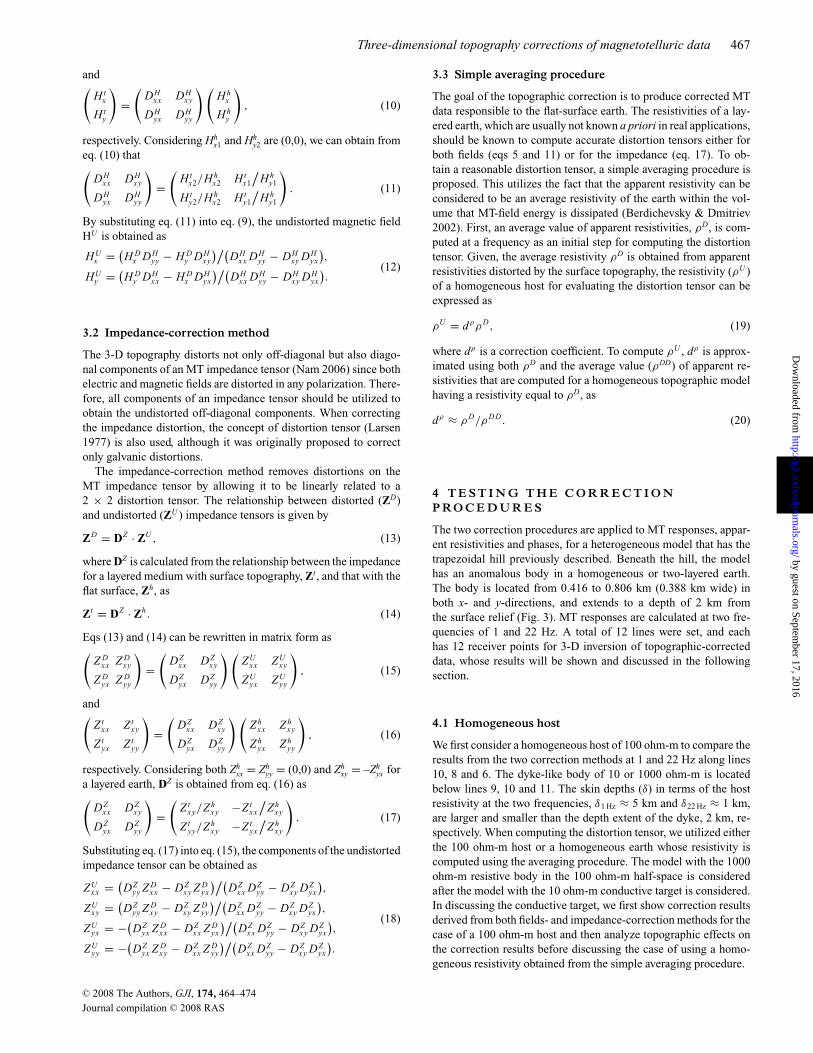
The goal of the topographic correction is to produce corrected MTdata responsible to the flat-surface earth. The resistivities of a lay-ered earth, which are usually not known a priori in real applications,should be known to compute accurate distortion tensors either forboth fields (eqs 5 and 11) or for the impedance (eq. 17). To ob-tain a reasonable distortion tensor, a simple averaging procedure isproposed. This utilizes the fact that the apparent resistivity can beconsidered to be an average resistivity of the earth within the vol-ume that MT-field energy is dissipated (Berdichevsky & Dmitriev2002). First, an average value of apparent resistivities, ρD, is com-puted at a frequency as an initial step for computing the distortiontensor. Given, the average resistivity ρD is obtained from apparentresistivities distorted by the surface topography, the resistivity (ρU )of a homogeneous host for evaluating the distortion tensor can beexpressed as

ρU = dρρD, (19)

where dρ is a correction coefficient. To compute ρU , dρ is approx-imated using both ρD and the average value (ρDD) of apparent re-sistivities that are computed for a homogeneous topographic modelhaving a resistivity equal to ρD, as

dρ ≈ ρD/ρDD . (20)

4 T E S T I N G T H E C O R R E C T I O NP RO C E D U R E S

The two correction procedures are applied to MT responses, appar-ent resistivities and phases, for a heterogeneous model that has thetrapezoidal hill previously described. Beneath the hill, the modelhas an anomalous body in a homogeneous or two-layered earth.The body is located from 0.416 to 0.806 km (0.388 km wide) inboth x- and y-directions, and extends to a depth of 2 km fromthe surface relief (Fig. 3). MT responses are calculated at two fre-quencies of 1 and 22 Hz. A total of 12 lines were set, and eachhas 12 receiver points for 3-D inversion of topographic-correcteddata, whose results will be shown and discussed in the followingsection.

4.1 Homogeneous host

We first consider a homogeneous host of 100 ohm-m to compare theresults from the two correction methods at 1 and 22 Hz along lines10, 8 and 6. The dyke-like body of 10 or 1000 ohm-m is locatedbelow lines 9, 10 and 11. The skin depths (δ) in terms of the hostresistivity at the two frequencies, δ1 Hz ≈ 5 km and δ22 Hz ≈ 1 km,are larger and smaller than the depth extent of the dyke, 2 km, re-spectively. When computing the distortion tensor, we utilized eitherthe 100 ohm-m host or a homogeneous earth whose resistivity iscomputed using the averaging procedure. The model with the 1000ohm-m resistive body in the 100 ohm-m half-space is consideredafter the model with the 10 ohm-m conductive target is considered.In discussing the conductive target, we first show correction resultsderived from both fields- and impedance-correction methods for thecase of a 100 ohm-m host and then analyze topographic effects onthe correction results before discussing the case of using a homo-geneous resistivity obtained from the simple averaging procedure.

C© 2008 The Authors, GJI, 174, 464–474




ownloaded from



0.388

100 ohm-m

: receiver

x (km)

y (km)

1

-1

-0.225

0.225

0.416 0.806 1-1

Line01

L 2ine0

..

..

Line06

Line12

Line08

Line10

(a) Plan view

(b) Cross-section view

100 ohm-m

x (km)

z (km)

2 km

0.388

10 or1000 ohm-m

Figure 3. Plan and cross-section views of a 3-D-hill model which has abody of 10 or 1000 ohm-m in a homogeneous half-space of 100 ohm-m.

4.1.1 Conductive target

Fig. 4 compares correction results for distorted MT responses (×)for the model with the conductive 10 ohm-m dyke in the 100ohm-m host. Distorted apparent resistivities (ρ d) and phases (φd)show significant anomalies produced by the topographic feature(Fig. 4), while MT data (ρ c and φ c) derived through either thefields- (∇) or impedance-correction method (o) are almost freefrom the topography-induced anomalies, and much closer to theflat-surface responses (—; ρ f and φ f ), which are supposed to beobtained through topographic correction. Furthermore, correctedMT responses from both correction methods exhibit almost thesame results at both frequencies demonstrating that both methodsare well cross-verified.

In both Zxy and Zyx modes, distorted MT data, ρ d and φd , alonglines 10, 8 and 6 at 1 Hz will have a similar pattern of 3-D topo-graphic effects but differ in magnitude, if no conductive dyke exists(Fig. 4a). The flat-earth responses for the conductive dyke havelarger anomalies at 1 Hz than at 22 Hz, and have much higher con-trast in resistivity than the dyke-host layer contrast. Since currentgathering is of particular importance at low frequencies, bound-ary charges cause apparent resistivities to vary spatially with muchhigher contrast than the body-host layer contrast (Wannamaker et al.1984). In the Zyx mode, because of charges accumulated at theboundary of the dyke, flat-earth apparent resistivities ρ f along line8 have positive anomalies in the vicinity of the conductive dykerather than negative anomalies (like along line 10); these positiveanomalies have the same origin as the extreme of ρ f observed inthe Zxy mode along line 10.

The positive anomalies in the Zyx mode are larger at 1 Hz thanat 22 Hz (Fig. 4), because there is more accumulation of boundarycharges at 1 Hz than at 22 Hz. In distorted phases, φd , in both Zxy andZyx modes, 3-D topographic effects cause positive anomalies. Thepositive anomalies in φd at 22 Hz (Fig. 4a) are larger than those at 1Hz (Fig. 4a), because galvanic effects become small while inductiveeffects become large as frequency increases (Jiracek 1990).

To investigate effects of the dip angle of surface topographyon correction results, impedance-corrected data for models withvarious heights of the trapezoidal hill are compared (Fig. 5). Sincethe slope angle of the 450 m-high hill (o) is steep enough (greaterthan 30.1◦) when considering the real field situation in MT surveys,smaller angles of about 21.2◦ (�) and 7.4◦ (star) with heights of300 and 100 m, respectively, are considered. All of the correctedresults are almost identical except for those on a hill side havingthe conductive anomaly beneath the slope. Over the hill side, thecorrected data become more close to the flat-surface responses asthe hill-top height decreases.

Next, we analyze how a host resistivity affects the results oftopographic correction, impedance-corrected MT responses using10 ohm-m (♦) or 1000 ohm-m (+) hosts are compared with thoseusing the 100 ohm-m host (Fig. 6). The results are predominatelyunderestimated when using the 10 ohm-m host, while overestimatedwhen using the 1000 ohm-m host, demonstrating the importance ofa proper host resistivity in topographic correction. Fig. 7 shows cor-rection results using the described averaging procedure; generatinghost resistivities are 98.56 and 97.62 ohm-m at 1 and 22 Hz, respec-tively. The correction results for the case of the 100 ohm-m host arealso drawn in grey in Fig. 7 for comparison; they are not observedas they are almost identical to those from the averaging procedure.From now on, correction results from the averaging procedure areshown in black and those from the real host are in grey as shown inFig. 7.

4.1.2 Resistive target

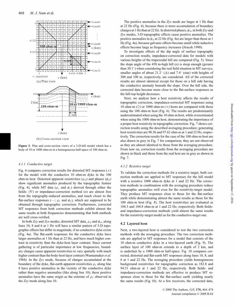
To validate the correction methods for a resistive target, both cor-rection methods are applied to MT responses for the hill modelwith a resistive 1000 ohm-m dyke at 1 and 22 Hz. The correc-tion methods in combination with the averaging procedure reducetopographic anomalies well even for the resistivity-target model.They produce MT responses close to those for the flat-surfaceearth while demonstrating almost the same results as those for the100 ohm-m host (Fig. 8). The host resistivities are evaluated as104.3 and 104.8 ohm-m at 1 and 22 Hz, respectively. Both fields-and impedance-correction methods yield almost the same resultsfor the resistivity-target model as for the conductive-target one.

4.2 Layered host

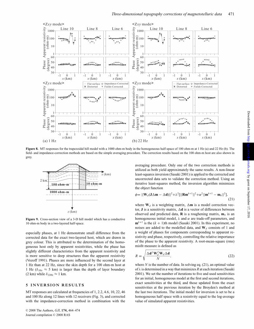
Next, a two-layered host is considered to test the two correctionmethods with the averaging procedure. The two correction meth-ods are applied to MT responses for a model that consists of the10 ohm-m conductive dyke in a two-layered earth (Fig. 9). Thesurface layer of 100 ohm-m extends to a depth of 2 km, andis underlain by a 1000 ohm-m half-space. Fig. 10 compares cor-rected, distorted and flat-earth MT responses along lines 10, 8, and6 at 1 and 22 Hz. The averaging procedure yields homogeneousbackground resistivities for topographic correction as 182.8 and94.51 ohm-m at 1 and 22 Hz, respectively. Both fields- andimpedance-correction methods are effective to produce MT re-sponses close to those for the flat-surface earth yielding nearlythe same results (Fig 10). At a few receivers, the corrected data,

C© 2008 The Authors, GJI, 174, 464–474




ownloaded from



Line 10 Line 8 Line 6

10 11- 0 11- 0-1x (km) x (km) x (km)

10 11- 0 11- 0-1x (km) x (km) x (km)

Impedance-CorrectedFields-Corrected

Flat surfaceDistorted

100

1

10

1000

ytivitsiser

tnera

pp

A)

m-m

ho(

esah

P)eer

ged(

30

40

50

60

100

1

10

1000

ytivitsiser

tnera

pp

A)

m-m

ho(

esah

P)eer

ged(

30

40

50

60

< >Z modexy

< >Z modeyx


10 11- 0 11- 0-1x (km) x (km) x (km)

10 11- 0 11- 0-1x (km) x (km) x (km)



100

1

10

1000

ytivitsiser

tnera

pp

A)

m-m

ho(

esah

P)eer

ged(

30

40

50

60

100

1

10

1000

ytivitsiser

tnera

pp

A)

m-m

ho(

esah

P)eer

ged(

30

40

50

60

< >Z modexy

< >Z modeyx

zH22)b(zH1)a(

Figure 4. MT responses for the hill model with a 10 ohm-m body in the homogeneous half-space of 100 ohm-m at 1 Hz (a) and 22 Hz (b). The field- andimpedance-correction methods are based on the 100 ohm-m host.


10 11- 0 11- 0-1x (km) x (km) x (km)

10 11- 0 11- 0-1x (km) x (km) x (km)

450 m100 m

Flat surface300 m

100

1

10

1000

ytivitsiser

tnera

pp

A)

m-m

ho(

esah

P)eer

ged(

30

40

50

60

100

1

10

1000

ytivitsiser

tnera

pp

A)

m-m

ho(

esah

P)eer

ged(

30

40

50

60

< >Z modexy

< >Z modeyx


10 11- 0 11- 0-1x (km) x (km) x (km)

10 11- 0 11- 0-1x (km) x (km) x (km)

450 m100 m

Flat surface300 m

100

1

10

1000

ytivitsiser

tnera

pp

A)

m-m

ho(

esah

P)eer

ged(

30

40

50

60

100

1

10

1000

ytivitsiser

tnera

pp

A)

m-m

ho(

esah

P)eer

ged(

30

40

50

60

< >Z modexy

< >Z modeyx

zH22)b(zH1)a(

Figure 5. MT responses for trapezoidal hill models of 450, 300 and 100 m high, respectively, with a 10 ohm-m body in the homogeneous half-space of100 ohm-m at 1 Hz (a) and 22 Hz (b). The field- and impedance-correction methods are based on the 100 ohm-m host.

C© 2008 The Authors, GJI, 174, 464–474




ownloaded from




10 11- 0 11- 0-1x (km) x (km) x (km)

10 11- 0 11- 0-1x (km) x (km) x (km)

100 ohm-m1000 ohm-m

Flat surface10 ohm-m

100

1

10

1000

ytivitsiser

tnera

pp

A)

m-m

ho(

esah

P)eer

ged(

30

40

50

60

100

1

10

1000

ytivitsiser

tnera

pp

A)

m-m

ho(

esah

P)eer

ged(

30

40

50

60

< >Z modexy

< >Z modeyx


10 11- 0 11- 0-1x (km) x (km) x (km)

10 11- 0 11- 0-1x (km) x (km) x (km)

100 ohm-m1000 ohm-m

Flat surface10 ohm-m

100

1

10

1000

ytivitsiser

tnera

pp

A)

m-m

ho(

esah

P)eer

ged(

30

40

50

60

100

1

10

1000

ytivitsiser

tnera

pp

A)

m-m

ho(

esah

P)eer

ged(

30

40

50

60

< >Z modexy

< >Z modeyx

zH22)b(zH1)a(

Figure 6. MT responses for the trapezoidal hill model of 450 m high with a 10 ohm-m body in the homogeneous half-space of 100 ohm-m at 1 Hz (a) and22 Hz (b). The field- and impedance-correction methods are based on 10 ohm-m, 100 ohm-m and 1000 ohm-m hosts, respectively.


100

1

10

1000

ytivitsiser

tnera

pp

A)

m-m

ho(

esah

P)eer

ged(

30

40

50

60

10 11- 0 11- 0-1x (km) x (km) x (km)

100

1

10

1000

ytivitsiser

tnera

pp

A)

m-m

ho(

esah

P)eer

ged(

30

40

50

60

10 11- 0 11- 0-1x (km) x (km) x (km)

< >Z modexy

< >Z modeyx Impedance-CorrectedFields-Corrected



10 11- 0 11- 0-1x (km) x (km) x (km)

10 11- 0 11- 0-1x (km) x (km) x (km)



100

1

10

1000

ytivitsiser

tnera

pp

A)

m-m

ho(

esah

P)eer

ged(

30

40

50

60

100

1

10

1000

ytivitsiser

tnera

pp

A)

m-m

ho(

esah

P)eer

ged(

30

40

50

60

< >Z modexy

< >Z modeyx

zH22)b(zH1)a(

Figure 7. MT responses for the trapezoidal hill model with a 10 ohm-m body in the homogeneous half-space of 100 ohm-m at 1 Hz (a) and 22 Hz (b). Thefield- and impedance-correction methods are based on the simple averaging procedure. The correction results based on the 100 ohm-m host are also shown ingrey.

C© 2008 The Authors, GJI, 174, 464–474




ownloaded from




10 11- 0 11- 0-1x (km) x (km) x (km)

10 11- 0 11- 0-1x (km) x (km) x (km)



100

1

10

1000

ytivitsiser

tnera

pp

A)

m-m

ho(

esah

P)eer

ged(

30

40

50

60

100

1

10

1000

ytivitsiser

tnera

pp

A)

m-m

ho(

esah

P)eer

ged(

30

40

50

60

< >Z modexy

< >Z modeyx


10 11- 0 11- 0-1x (km) x (km) x (km)

10 11- 0 11- 0-1x (km) x (km) x (km)



100

1

10

1000

ytivitsiser

tnera

pp

A)

m-m

ho(

esah

P)eer

ged(

30

40

50

60

100

1

10

1000

ytivitsiser

tnera

pp

A)

m-m

ho(

esah

P)eer

ged(

30

40

50

60

< >Z modexy

< >Z modeyx

zH22)b(zH1)a(

Figure 8. MT responses for the trapezoidal hill model with a 1000 ohm-m body in the homogeneous half-space of 100 ohm-m at 1 Hz (a) and 22 Hz (b). Thefield- and impedance-correction methods are based on the simple averaging procedure. The correction results based on the 100 ohm-m host are also shown ingrey.

100 ohm-m

x (km)

z (km)

10 ohm-m2 km

1000 ohm-m

Figure 9. Cross-section view of a 3-D hill model which has a conductive10 ohm-m body in a two-layered half-space.

especially phases, at 1 Hz demonstrate small difference from thecorrected data for the exact two-layered host, which are drawn ingrey colour. This is attributed to the determination of the homo-geneous host only by apparent resistivities, while the phase hasslightly different characteristics from the apparent resistivity andis more sensitive to deep structures than the apparent resistivity(Vozoff 1991). Phases are more influenced by the second layer at1 Hz than at 22 Hz, since the skin depth for a 100 ohm-m host at1 Hz (δ1Hz ≈ 5 km) is larger than the depth of layer boundary(2 km) while δ22Hz ≈ 1 km.

5 I N V E R S I O N R E S U LT S

MT responses are calculated at frequencies of 1, 2.2, 4.6, 10, 22, 46and 100 Hz along 12 lines with 12 receivers (Fig. 3), and correctedwith the impedance-correction method in combination with the

averaging procedure. Only one of the two correction methods isutilized as both yield approximately the same results. A non-linearleast-squares inversion (Sasaki 2001) is applied to the corrected anduncorrected data sets to validate the correction method. Using aniterative least-squares method, the inversion algorithm minimizesthe object function

φ= ||Wd (J�m − �d)||2+λ2[||Rmk+1||2+α2||mk+1 − mb||2],(21)

where Wd is a weighting matrix, �m is a model correction vec-tor, J is a sensitivity matrix, �d is a vector of differences betweenobserved and predicted data, R is a roughening matrix, mb is anhomogeneous initial model, λ and α are trade-off parameters, andmk+1 is the (k + 1)th model (Sasaki 2001). In this experiment, nonoises are added to the modelled data, and Wd consists of 1 anda weight of phases for components corresponding to apparent re-sistivity and phase, respectively, controlling the relative importanceof the phase to the apparent resistivity. A root-mean-square (rms)misfit measure is defined as

R =√

�dT WTd Wd�d

N, (22)

where N is the number of data. In solving eq. (21), an optimal valueof λ is determined in a way that minimizes R at each iteration (Sasaki2001). We set the number of iterations to five and used sensitivitiesfor an initial, homogeneous model at the first and second iterations,exact sensitivities at the third, and those updated from the exactsensitivities at the previous iteration by the Broyden’s method atthe last two iterations. The initial model for inversion is set to be ahomogeneous half space with a resistivity equal to the log-averagevalue of simulated apparent resistivities.

C© 2008 The Authors, GJI, 174, 464–474




ownloaded from




10 11- 0 11- 0-1x (km) x (km) x (km)

10 11- 0 11- 0-1x (km) x (km) x (km)

20

30

40

20

30

40



100

1

10

1000

ytivitsiser

tnera

pp

A)

m-m

ho(

esah

P)eer

ged(

100

1

10

1000

ytivitsiser

tnera

pp

A)

m-m

ho(

esah

P)eer

ged(

< >Z modexy

< >Z modeyx


10 11- 0 11- 0-1x (km) x (km) x (km)

10 11- 0 11- 0-1x (km) x (km) x (km)



100

1

10

1000

ytivitsiser

tnera

pp

A)

m-m

ho(

esah

P)eer

ged(

30

40

50

60

100

1

10

1000

ytivitsiser

tnera

pp

A)

m-m

ho(

esah

P)eer

ged(

30

40

50

60

< >Z modexy

< >Z modeyx

zH22)b(zH1)a(

Figure 10. MT responses for the trapezoidal hill model with a 10 ohm-m body in the two-layered earth at 1 Hz (a) and 22 Hz (b). The field- and impedance-correction methods are based on the simple averaging procedure. The correction results based on the two-layered host are also shown in grey.

5.1 Homogeneous host

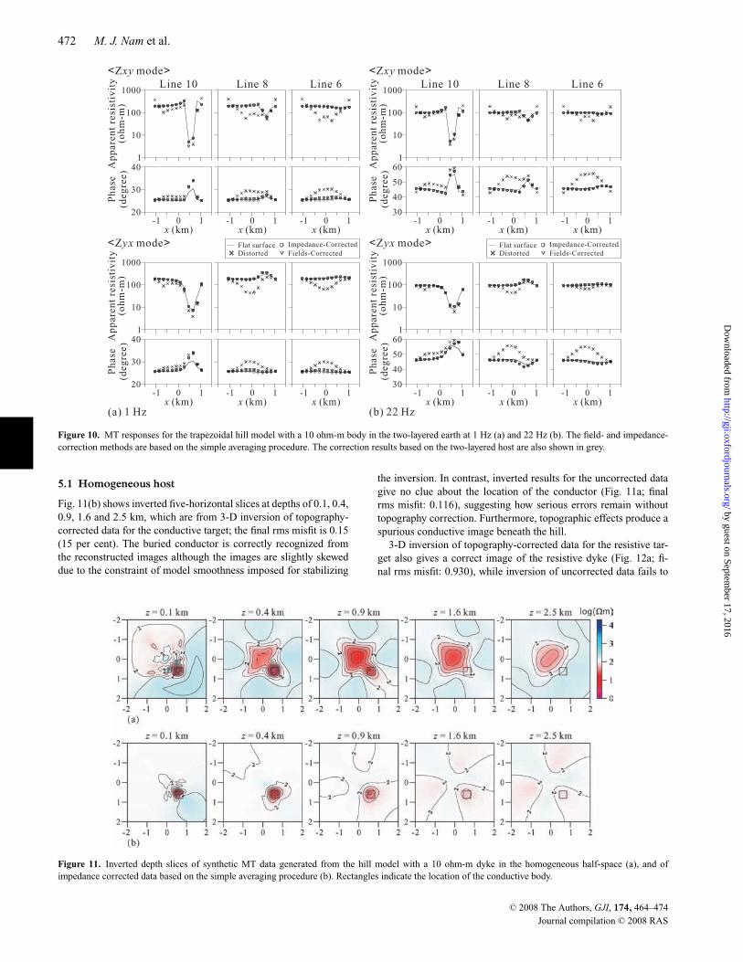
Fig. 11(b) shows inverted five-horizontal slices at depths of 0.1, 0.4,0.9, 1.6 and 2.5 km, which are from 3-D inversion of topography-corrected data for the conductive target; the final rms misfit is 0.15(15 per cent). The buried conductor is correctly recognized fromthe reconstructed images although the images are slightly skeweddue to the constraint of model smoothness imposed for stabilizing

Figure 11. Inverted depth slices of synthetic MT data generated from the hill model with a 10 ohm-m dyke in the homogeneous half-space (a), and ofimpedance corrected data based on the simple averaging procedure (b). Rectangles indicate the location of the conductive body.

the inversion. In contrast, inverted results for the uncorrected datagive no clue about the location of the conductor (Fig. 11a; finalrms misfit: 0.116), suggesting how serious errors remain withouttopography correction. Furthermore, topographic effects produce aspurious conductive image beneath the hill.

3-D inversion of topography-corrected data for the resistive tar-get also gives a correct image of the resistive dyke (Fig. 12a; fi-nal rms misfit: 0.930), while inversion of uncorrected data fails to

C© 2008 The Authors, GJI, 174, 464–474




ownloaded from



Figure 12. Inverted depth slices of synthetic MT data generated from the hill model with a 1000 ohm-m dyke in the homogeneous half-space (a), and ofimpedance-corrected data based on the simple averaging procedure (b). Rectangles indicate the location of the resistive body.

recover the given model (Fig. 12b; final rms misfit: 0.150) only pro-ducing a spurious anomaly as in the case of the conductive target.

5.2 Layered host

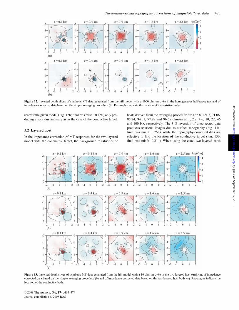
In the impedance correction of MT responses for the two-layeredmodel with the conductive target, the background resistivities of

Figure 13. Inverted depth slices of synthetic MT data generated from the hill model with a 10 ohm-m dyke in the two layered host earth (a), of impedancecorrected data based on the simple averaging procedure (b) and of impedance corrected data based on the two layered host body (c). Rectangles indicate thelocation of the conductive body.

hosts derived from the averaging procedure are 182.8, 121.3, 91.06,85.24, 94.51, 97.87 and 96.65 ohm-m at 1, 2.2, 4.6, 10, 22, 46and 100 Hz, respectively. The 3-D inversion of uncorrected dataproduces spurious images due to surface topography (Fig. 13a;final rms misfit: 0.250), while the topography-corrected data areeffective to find the location of the conductive target (Fig. 13b;final rms misfit: 0.214). When using the exact two-layered earth

C© 2008 The Authors, GJI, 174, 464–474




ownloaded from



for the impedance correction, the corresponding inverted images(Fig. 13c; final rms misfit: 0.219) seem to be slightly better thanthose based on the simple averaging procedure, specifically at adepth of 2.5 km. This can be attributed to the slight differencebetween phases corrected based on the exact two-layered host andon the hosts having the resistivities derived from the averagingprocedure as discussed in Fig. 10(a).

6 C O N C LU S I O N S

A 3-D edge-FEM code is employed to compute MT responses fora model with surface topography and subsurface structure. A 3-Dtopography causes both galvanic and inductive effects in any po-larization, where the galvanic effect is larger than the inductiveeffect in magnitude and opposite in sign. For correcting 3-D to-pographic effects on MT responses, we suggested two correctionprocedures which decrease distortions on the MT impedance tensorand on both electric and magnetic fields, respectively. Both meth-ods are validated using a trapezoidal hill model with a verticallyelongated body. Numerical experiments showed that both methodsin combination with the averaging procedure are effective to reducedistortions caused by topographic effects, and are cross-verifiedby yielding approximately the same results. Most of the subsur-face structure can be recovered, including a conductive or resistivedyke even in a layered earth through non-linear least-squares inver-sion of topography-corrected data. For more accurate interpretation,however, the 3-D inversion incorporating topography into an earthmodel would be needed.

A C K N OW L E D G M E N T S

This work was supported by Basic Research Project of Korea Insti-tute of Geoscience and Mineral Resources (KIGAM) funded by theMinistry of Science and Technology of Korea. HJK was supportedby Korea Research Foundation Grant funded by the Korea Gov-ernment (MOEHRD) (KRF-2006–311-D00985). We would like tothank to Yutaka Sasaki for allowing us to use his inversion code.We also thank the editor and the two reviewers for their commentsthat helped to improve the manuscript.

R E F E R E N C E S

Baba, K. & Chave, A.D., 2005. Correction of seafloor magnetotelluric datafor topographic effects during inversion, J. geophys. Res., 110, B12105.

Baba, K. & Seama, N., 2002. A new technique for the incorporation ofseafloor topography in electromagnetic modelling, Geophys. J. Int., 150,392–402.

Berdichevsky, M.N. & Dmitriev, V.I., 2002. Magnetotellurics in the Contextof the Theory of Ill-Posed Problems, Society of Exploration Geophysicists,81 p.

Chouteau, M. & Bouchard, K. 1988. Two-dimensional terrain correction inmagnetotelluric surveys, Geophysics, 53, 854–862.

Goldstein, N.E., 1988. Subregional and detailed exploration for geothermal-hydrothermal resources, Geotherm. Sci. Tech., 1, 303–431.

Gurer, A. & Ilkisik, M., 1997. The importance of topographic corrections onmagnetotelluric response data from rugged regions of Anatolia, Geophys.Prospect., 45, 111–125.

Jiracek, G.R., 1990. Near surface and topographic distortions in electromag-netic induction, Surv. Geophys., 11, 163–203.

Jiracek, G.R., Redding, R.P. & Kosima, R.K., 1989. Application of theRayleigh-FFT technique to magnetotelluric modiling and correction,Phys. Earth. planet. Inter., 53, 365–375.

Key, K., Constable, S. & Weiss, C., 2004. Mapping 3D salt using 2D marineMT, case study from Gemini Prospect, Gulf of Mexico, 74th Ann. Internat.Mtg, Soc. Expl. Geophys., Expanded Abstract, 596–599.

Larsen, J.C., 1977. Removal of local surface conductivity effects from lowfrequency mantle response curves, Acta Geodaetica Geophysica et Mon-tanistica Scd. Sci. Hungarica, 12, 183–186.

Lee, T.J., Song, Y. & Uchida, T., 2007. Three-dimensional magnetotelluricsurveys for geothermal development in Pohang, Korea, Explor. Geophys.,60, 89–97.

Lynch, D.R. & Paulsen, K.D. 1991. Origin of vector parasites in numericalMaxwell solutions, IEEE Trans. Microwave Theory Techniq., 39, 383–394.

Mackie, R.L. & Madden, T.R., 1993. Three-dimensional magnetotel-luric inversion using conjugate gradients, Geophys. J. Int., 115, 215–229.

Mackie, R.L., Smith, J.T. & Madden, T.R. 1994. Three-dimensional electro-magnetic modeling using finite difference equations: the magnetotelluricexample, Radio Sci., 29, 923–935.

Mozley, E.C., 1982. An investigation of the conductivity distribution in thevicinity of a Cascade volcano, PhD thesis. University of California atBerkeley.

Mur, G. & Lager, I.E. 2002. On the causes of spurious solutions in electro-magnetics, Electromagnetics, 22, 357–367.

Nam, M.J., 2006. A study on 3D topographic effects in magnetotelluricsurveys, PhD thesis. Seoul National University (in Korean with Englishabstract).

Nam, M.J., Kim, H.J., Song, Y., Lee, T.J., Son, J.-S. & Suh, J.H., 2007.Three-dimensional magnetotelluric modeling including surface topogra-phy, Geophys. Prospect., 55, 277–287.

Newman, G.A., Hoversten, M., Gasperikova, E. &, Wannamaker, P.E. 2005.3D Magnetotelluric characterization of the Coso geothermal field, in: Pro-ceedings of Thirtieth Workshop on Geothermal Reservoir Engineering,SGP-TR-176.

Orange, A.S., 1989. Magnetotelluric exploration for hydrocarbons, Proc.IEEE, 77, 287–317.

Sasaki, Y., 2001. Full 3-D inversion of electromagnetic data on PC, J. Appl.Geophys., 46, 45–54.

Schwalenberg, K. & Edwards, R.N., 2004. The effect of seafloor topogra-phy on magnetotelluric fields: an analytical formulation confirmed withnumerical results, Geophys. J. Int., 159, 607–621.

Takasugi, S., Tanaka, K., Kawasaki, N. & Muramatsu, S., 1992. High spatialresolution of the resistivity structure revealed by a dense network MTmeasurement—a case study in the Minamikayabe area, Hokkaido, Japan,J. Geomag. Geoelectr., 44, 289–308.

Vozoff, K. 1991. The magnetotelluric method, in Electromagnetic Methodsin Applied Geophysics, Vol. II, pp. 641–711, ed. Nabighian, M.N., Societyof Exploration Geophysicists.

Wannamaker, P.E., 1991. Advances in three-dimensional magnetotel-luric modeling using integral equations, Geophysics, 56, 1716–1728.

Wannamaker, P.E., Hohmann, G.W. & Ward, S.H., 1984. Magnetotelluricresponses of three-dimensional bodies in layered earths, Geophysics, 49,1517–1533.

Wannamaker, P.E., Stodt, J.A. & Rijo, L., 1986. Two-dimensional topo-graphic responses in magnetotelluric models using finite elements, Geo-physics, 51, 2131–2144.

Wannamaker, P.E. et al., 1989. Magnetotelluric observations across the Juande Fuca subduction system in the EMSLAB project, J. geophys. Res.,94B10, 14 111–14 125.

C© 2008 The Authors, GJI, 174, 464–474




ownloaded from


Three-dimensional topography corrections of magnetotelluric data

Documents

Transcript of Three-dimensional topography corrections of magnetotelluric data