arX

iv:c

ond-

mat

/981

0074

v2 [

cond

-mat

.sta

t-m

ech]

21

Apr

199

9

Lagrangian method for multiple correlations in passive scalar advection

U. Frisch1, A. Mazzino1,2, A. Noullez1 and M. Vergassola1

1 CNRS, Observatoire de la Cote d’Azur, B.P. 4229, 06304 Nice Cedex 4, France.2 INFM–Dipartimento di Fisica, Universita di Genova, I–16146 Genova, Italy.

(February 1, 2008)

A Lagrangian method is introduced for calculating simultaneous n-point correlations of a passivescalar advected by a random velocity field, with random forcing and finite molecular diffusivity κ.The method, which is here presented in detail, is particularly well suited for studying the κ → 0limit when the velocity field is not smooth. Efficient Monte Carlo simulations based on this methodare applied to the Kraichnan model of passive scalar and lead to accurate determinations of theanomalous intermittency corrections in the fourth-order structure function as a function of thescaling exponent ξ of the velocity field in two and three dimensions. Anomalous corrections arefound to vanish in the limits ξ → 0 and ξ → 2, as predicted by perturbation theory.

PACS number(s) : 47.10.+g, 47.27.-i, 05.40.+j

I. INTRODUCTION

Robert Kraichnan’s model of passive scalar advectionby a white-in-time velocity field has been particularly fer-tile ground for theoreticians trying to develop a theoryof intermittency [1–3] (see also Refs. [4,5]). Although themodel leads to closed equations for multiple-point mo-ments, only second-order moments can be obtained inclosed analytic form [6]. Theoretical predictions differedas to the behavior of higher-order quantities, regarding inparticular the survival or the vanishing of intermittencycorrections (anomalies) in certain limits. Obtaining reli-able numerical results was thus an important challenge.Until recently numerical simulations have been based onthe direct integration of the passive scalar partial differ-ential equation and have been limited to two dimensions[5,7,8]. Such calculations are delicate; to wit, the dif-ficulty of observing for the second-order structure func-tion the known high-Peclet number asymptotic scaling[6]. Also, the numerical scheme used in Refs. [5,7] in-volves a slightly anisotropic velocity field which is notexpected to give exactly the right scaling laws for thepassive scalar [9].

Lagrangian methods for tackling the Kraichnan modeland which require only the integration of ordinary dif-ferential equations were recently proposed independentlyby Frisch, Mazzino and Vergassola [10] and by Gat, Pro-caccia and Zeitak [11]. Our goal here is to give a detailedpresentation of the Lagrangian method and to presentnew results.

In Section II we give the theoretical background ofthe Lagrangian method for general random velocity fieldswhich need not be white-in-time. In Section III we inves-tigate the limit of vanishing molecular diffusivity whichdepends crucially on how nearby Lagrangian trajectoriesseparate. We then turn to the Kraichnan model whichis given a Lagrangian formulation (Section IV). Then,we show how it can be solved numerically by a Monte-Carlo method (Section V) and present results in bothtwo and three space dimensions (Section VI). We makeconcluding remarks in Section VII.

II. THE LAGRANGIAN METHOD

The (Eulerian) dynamics of a passive scalar field θ(r, t)advected by a velocity field v(r, t) is described by thefollowing partial differential equation (written in spacedimension d) :

∂tθ(r, t) + v(r, t) · ∇ θ(r, t) = κ∇2θ(r, t) + f(r, t), (1)

where f(r, t) is an external source (forcing) of scalar andκ is the molecular diffusivity. In all that follows we shallassume that θ(r, t) = 0 at some distant time in the pastt = −T (eventually, we shall let T → ∞).

In this section the advecting velocity v and the forcingf can be either deterministic or random. In the lattercase, no particular assumption is made regarding theirstatistical properties.

In order to illustrate the basic idea of the Lagrangianstrategy, let us first set κ = 0. We may then integrate(1) along its characteristics, the Lagrangian trajectoriesof tracer particles, to obtain

θ(r, t) =

∫ t

−T

f(a(s; r, t), s) ds, (2)

where a(s; r, t) is the position at time s ≤ t of the fluidparticle which will be at position r at time t. (Two-time Lagrangian positions of this type were also used inKraichnan’s Lagrangian History Direct Interaction the-ory [12].) This Lagrangian position, which will hence-forth be denoted just a(s), satisfies the ordinary differ-ential equation

da(s)

ds= v (a(s), s) , a(t) = r. (3)

For κ > 0 we shall now give a stochastic generalizationof this Lagrangian representation. Roughly, θ will be theaverage of a random field φ which satisfies an advection–forcing equation with no diffusion term, in which the ad-vecting velocity is the sum of v and a suitable white-noisevelocity generating Brownian diffusion.

1

To be more specific we need to introduce some no-tation. We shall use a set of n d-dimensional time-dependent random vectors

wi(s) = {wi,α; i = 1, . . . , n; α = 1, . . . , d}, (4)

which are Gaussian, identically distributed, independentof each other and independent of both v and f . The timedependence is assumed to be white noise :

〈wi,α(s)wj,β(s′)〉w = δijδαβδ(s − s′). (5)

The notation 〈·〉w stands for “average over the wi’s for afixed realization of v and f”. Similarly, 〈·〉vf stands for“average over v and f for a fixed realization of the wi’s”.Unconditional averages are denoted just 〈·〉. Clearly,

〈·〉 = 〈〈·〉w〉vf = 〈〈·〉vf 〉w . (6)

The white noise, which is a random distribution, is heredenoted by w(s) since it is the time derivative of theBrownian motion (or Wiener–Levy) process. In the nu-merical implementation we shall work with increments ofw(s).

We can now state the main result which is at the basisof our Lagrangian method.

Let φi(r, t) (i = 1, . . . , n) be the solutions of the fol-lowing advection–forcing equations :

∂tφi(r, t) +(

v(r, t) +√

2κwi(t))

· ∇φi(r, t) = f(r, t).

φi(r,−T ) = 0, i = 1, 2, . . . , n. (7)

For any r1, r2, r3, . . . , we have

θ(r1) = 〈φ(r1)〉w , ∀i (8)

θ(r1)θ(r2) = 〈φi(r1)φj(r2)〉w , ∀i 6= j, (9)

θ(r1)θ(r2)θ(r3) = 〈φi(r1)φj(r2)φk(r3)〉w ,

∀i, j, k, i 6= j 6= k 6= i, (10)

..................................................,

where all the fields θ and φ are evaluated at the sametime t.

The proof of (8) is obtained by taking the mean valueof (7) (only over w) and noting that

⟨√2κwi · ∇φi

⟩

w= −κ∇2 〈φi〉w . (11)

(This is a standard result for linear stochastic equationshaving white-noise coefficients; it is derived using Gaus-sian integration by parts (see Ref. [13], Chap. 4). Forsimilar derivations see Refs. [6,14,15].)

To prove (9), we first derive from (7), assuming i 6= j,

∂t (φi(r1)φj(r2)) + [v(r1) · ∇1 + v(r2) · ∇2

+√

2κ(wi · ∇1 + wj · ∇2)]φi(r1)φj(r2) =

f(r1)φj(r2) + f(r2)φj(r1), (12)

where ∇1 and ∇2 stand for ∇r1and ∇r2

. We thenaverage (12) (over w) and use a relation similar to (11)

⟨√2κ (wi · ∇1 + w2 · ∇2)φi(r1)φj(r2)

⟩

w

= −κ(

∇21 + ∇2

2

)

〈φi(r1)φj(r2)〉w . (13)

(Notice that cross terms involving ∇1 · ∇2 disappear be-cause of the independence of wi and wj .) The higherorder equations in (10) and following are proved simi-larly.

Because of the absence of a diffusion operator in (7),its solution has an obvious Lagrangian representation

φi(r, t) =

∫ t

−T

f(ai(s), s) ds, (14)

where

dai(s)

ds= v (ai(s), s) +

√2κwi(s), (15)

ai(t) = r. (16)

So far we have not used the random or deterministiccharacter of v and f . In the random case, taking theaverage of (8)–(10) over v and f , we obtain

〈θ(r1)〉 = 〈φ(r1)〉 , ∀i (17)

〈θ(r1)θ(r2)〉 = 〈φi(r1)φj(r2)〉 , ∀i 6= j (18)

〈θ(r1)θ(r2)θ(r3)〉 = 〈φi(r1)φj(r2)φk(r3)〉 ,

∀i, j, k, i 6= j 6= k 6= i, (19)

.................................................

Eqs. (14), (15), (16), together with (17), (18) andhigher orders, constitute our Lagrangian representationfor multiple-point moments of the passive scalar.

Let us stress that, for moments beyond the first order,it is essential to use more than one white noise. Indeed,we could have made use of just (8) and written

θ(r1)θ(r2) = 〈φi(r1)〉w〈φj(r2)〉w, ∀i, j. (20)

(Including the case i = j.) It is however not possibleto (v, f)-average (20) because it involves a product ofw-averages rather than just one average as in (9).

In the more restricted context of the Kraichnan model,a functional integral representation of nth order momentsinvolving, as here, n white noises has already been givenin Refs. [16,17].

III. THE LIMIT OF VANISHING MOLECULAR

DIFFUSIVITY

Interesting pathologies occur when we bring two ormore Eulerian space arguments of the moments to co-incidence and simultaneously let κ → 0.

This is already seen on the second-order moment〈θ2(r1)〉. From (14) and (18), we have

2

〈θ2(r1)〉 =

∫ t

−T

∫ t

−T

〈f(ai(s), s)f(aj(s′), s′)〉 dsds′,

(21)

for any i 6= j. The differential equations for ai(s) andaj(s) involve different white noises. If, in the limit κ → 0,

we simply ignore the√

2κwi terms in (15), we find thatall the ai(s)’s satisfy the same equation (3) and the sameboundary condition ai(t) = r1. It is then tempting toconclude that all the ai(s)’s are identical, namely arejust the Lagrangian trajectories a(s) of the unperturbedv-flow. As a consequence, we can then rewrite (21) as

〈θ2(r1)〉 =

∫ t

−T

∫ t

−T

〈f(a(s), s)f(a(s′), s′)〉 dsds′,

=

⟨

(∫ t

−T

f(a(s), s) ds

)2⟩

. (22)

For a large class of random forcings f of zero meanthe r.h.s. of (22) will diverge ∝ T as T → ∞. This isfor example the case when f is homogeneous, station-ary and short- (or delta-) correlated in time as in theKraichnan model. The reason of this divergence is that,although the forcing has zero mean, its integral (alongthe Lagrangian trajectory) over times long compared tothe correlation time behaves like Brownian motion (inthe T -variable) and, thus, has a variance ∝ T . Fromthis naıve procedure we would thus conclude that, whenT = ∞, the scalar variance becomes infinite as κ → 0.

This conclusion is actually correct when the v-flow issmooth (differentiable in the space variable) : this is theso-called Batchelor limit which has been frequently in-vestigated [6,16,18–21]. The conclusion however becomesincorrect when the v-flow is only Holder continuous, i.e.its spatial increments over a small distance ℓ vary as afractional power of ℓ (e.g. ℓ1/3 in Kolmogorov 1941 tur-bulence). As pointed out in Ref. [16] (see also Ref. [4]),when v is not smooth the solution to (3) lacks unique-ness, so that two Lagrangian particles which end up atthe same point r1 at time t may have different past histo-ries. This is exemplified with the one-dimensional model

dx

ds= −x1/3, −T ≤ s ≤ t, x(t) = ǫ ≥ 0, (23)

where x is a deputy for ai − aj , the separation betweentwo nearby Lagrangian particles. For ǫ > 0, the solutionof (23) is

x(s) =

[

ǫ2/3 +2

3(t − s)

]3/2

. (24)

If we now set ǫ = 0 in (24) or consider times s such that|t − s| ≫ ǫ2/3, we obtain

x(s) =

[

2

3(t − s)

]3/2

. (25)

This is indeed a solution of (23) with ǫ = 0, but thereis another trivial one, namely x(s) = 0. Related to thisnon-uniqueness is the fact that, when ǫ is small the solu-tion given by (24) becomes independent of ǫ, namely isgiven by the non-trivial solution (25) for ǫ = 0.

Whenever the flow v is just Holder continuous, theseparation of nearby Lagrangian particles proceeds in asimilar way, becoming rapidly independent of the initialseparation. Such a law of separation is much more ex-plosive than would have been obtained for a smooth flowwith sensitive dependence of the Lagrangian trajectories.In the latter case we would have x(s) = ǫ eλ(t−s) (λ > 0),which grows exponentially with t − s but still tends tozero with ǫ.

We propose to call this explosive growth a Richard-son walk, after Lewis Fry Richardson who was the firstto experimentally observe this rapid separation in turbu-lent flow and who was also much interested in the role ofnon-differentiability in turbulence [22]. It is this explo-sive separation which prevents the divergence of 〈θ2(r1)〉when κ → 0 (and more generally of moments with sev-eral coinciding points). Indeed, as the time s moves backfrom s = t, even an infinitesimal amount of moleculardiffusion will slightly separate, say, by an amount ǫ, theLagrangian particles ai(s) and aj(s) which coincide ats = t. Then, the Richardson walk will quickly bring theseparations to values independent of ǫ and, thus of κ.Hence, the double integral in (21), which involves pointsa1(s) and a2(s) with uncorrelated forces when |s − s′|is sufficiently large, may converge for T → ∞. (For itto actually converge more specific assumptions must bemade about the space and time correlations of v and f ,which are satisfied, e.g., in the Kraichnan model.)

An alternative to introducing a small diffusivity is towork at κ = 0, with “point splitting”. For this one re-places 〈θ2(r1)〉 by 〈θ(r1)θ(r

′

1)〉, where r1 and r′

1 areseparated by a distance ǫ. Eventually, ǫ → 0. In practi-cal numerical implementations we found that point split-ting works well for second-order moments but is far lessefficient than using a small diffusivity for higher-ordermoments.

IV. THE KRAICHNAN MODEL

The Kraichnan model [6,1] is an instance of the pas-sive scalar equation (1) in which the velocity and theforcing are Gaussian white noises in their time depen-dence. This ensures that the solution is a Markovprocess in the time variable and that closed momentequations, sometimes called “Hopf equations”, can bewritten for single-time multiple-space moments such as〈θ(r1, t) . . . θ(rn, t)〉. The equation for second-order mo-ments was published for the first time by Kraichnan [6]and, for higher-order moments, by Shraiman and Siggia[20]. Note that Hopf’s work [23] dealt with the charac-teristic functional of random flow; it had no white-noise

3

process and no closed equations, making the use of hisname not so appropriate in the context of white-noiselinear stochastic equations. The fact that closed momentequations exist for such problems has been known for along time (see, e.g., Ref. [14] and references therein). Weshall not need the moment equations and shall not writethem here (for an elementary derivation, see Ref. [15]).

The precise formulation of the Kraichnan model asused here is the following. The velocity field v = {vα, α =1, . . . , d} appearing in (1) is incompressible, isotropic,Gaussian, white-noise in time; it has homogeneous incre-ments with power-law spatial correlations and a scalingexponent ξ in the range 0 < ξ < 2 :

〈[vα(r, t) − vα(0, 0)][vβ(r, t) − vβ(0, 0)]〉 =

2δ(t)Dαβ(r), (26)

where,

Dαβ(r) = rξ[

(ξ + d − 1) δαβ − ξrαrβ

r2

]

. (27)

Note that since no infrared cutoff is assumed on the ve-locity its integral scale is infinite; this is not a problemsince only velocity increments matter for the dynamics ofthe passive scalar. Note also that when a white-in-timevelocity is used in (15), the well known Ito–Stratonovichambiguity could appear [24]. This ambiguity is howeverabsent in our particular case, on account of incompress-ibility.

The random forcing f is independent of v, of zeromean, isotropic, Gaussian, white-noise in time and ho-mogeneous. Its covariance is given by :

〈f(r, t) f(0, 0)〉 = F (r/L) δ(t), (28)

with F (0) > 0 and F (r/L) decreasing rapidly for r ≫ L,where L is the (forcing) integral scale.

In principle, to be a correlation, the function F (r/L)should be of positive type, i.e. have a non-negative d-dimensional Fourier transform. In our numerical workwe find it convenient to work with the step functionΘL(r) which is equal to unity for 0 ≤ r ≤ L and tozero otherwise. Hence, the injection rate of passive scalarvariance is ε = F (0)/2 = 1/2. The fact that the func-tion Θ is not of positive type is no problem. Indeed, letits Fourier transform be written E(k) = E1(k) − E2(k),where E(k) = E1(k) whenever E(k) ≥ 0. Using the stepfunction amounts to replacing in (1) the real forcing f bythe complex forcing f1+if2 where f1 and f2 are indepen-dent Gaussian random functions, white-noise in time andchosen such that their energy spectra (in the space vari-able) are respectively E1(k) and E2(k). Since the passivescalar equation is linear, the solution may itself be writ-ten as θ1 + iθ2 where θ1 and θ2 are the (independent)solutions of the passive scalar equations with respectiveforcing terms f1 and f2. Using the universality with re-spect to the functional form of the forcing [25], it is theneasily shown that the scaling laws for the passive scalarstructure functions are the same as for real forcing.

We shall be interested in the passive scalar structurefunctions of even order 2n (odd order ones vanish bysymmetry), defined as

S2n(r; L) ≡⟨

(θ(r) − θ(0))2n⟩

. (29)

From Ref. [6] (see also Ref. [15]) we know that, for L ≫r ≫ η ∼ κ1/ξ, the second-order structure function isgiven by

S2(r; L) = C2 ε rζ2 , ζ2 = 2 − ξ, (30)

where C2 is a dimensionless numerical constant. If therewere no anomalies, we would have, for n > 1,

S2n(r; L) = C2n εn rnζ2 . (31)

Note that (30) and (31) do not involve the integral scaleL. Actually, for n > 1, we have anomalous scaling withS2n(r; L) ∝ rζ2n and ζ2n < nζ2. More precisely, we have

S2n(r; L) = C2n εn rnζ2

(

L

r

)ζanom

2n

, (32)

ζanom2n ≡ nζ2 − ζ2n, (33)

where the structure function now displays a dependenceon the integral scale L. Our strategy will be to measurethe dependence of S2n(r; L) on L while the separation rand the injection rate ε are kept fixed and, thereby, tohave a direct measurement of the anomaly ζanom

2n .Let us show that, in principle, this can be done

by the Lagrangian method of Section II using 2ntracer (Lagrangian) particles whose trajectories satisfy(15). The structure function of order 2n can be writ-ten as a linear combination of moments of the form〈θ(r1)θ(r2) . . . θ(r2n)〉, where p of the points are at loca-tion r and 2n− p at location 0 (p = 0, . . . , 2n). Becauseof the symmetries of the problem, p and 2n − p give thesame contribution. Thus, we need to work only with then + 1 configurations corresponding to p = 0, . . . , n. Forexample, we have

S4(r; L) = 2⟨

θ4(r)⟩

− 8⟨

θ3(r)θ(0)⟩

+ 6⟨

θ2(r)θ2(0)⟩

.

(34)

Let us first consider the case of the two-point function(second-order moment). Using (14), (18) and the inde-pendence of v and f , we have

〈θ(r1)θ(r2)〉 =⟨

∫ t

−T

∫ t

−T

〈f(a1(s1), s1)f(a2(s2), s2)〉f ds1ds2

⟩

vw

. (35)

Here, 〈·〉f is an average over the forcing and 〈·〉vw denotesaveraging over the velocity and the w’s, and a1(s1) anda2(s2) satisfy (15) with the “final” conditions a1(t) =r1and a2(t) = r2, respectively.

4

In (35) the averaging over f can be carried out explic-itly using (28). With our step-function choice for F , weobtain

〈θ(r1) θ(r2)〉 = 〈T12(L)〉v, (36)

where

T12(L) =

∫ t

−T

ΘL(|a1(s) − a2(s)|) ds (37)

is the amount of time that two tracer particles arrivingat r1 and r2 and moving backwards in time spent withtheir mutual distance |a1(s) − a2(s)| < L. Whether theparticles move backwards or forward in time is actuallyirrelevant for the Kraichnan model since the velocity, be-ing Gaussian, is invariant under reversal.

For the four-point function, we proceed similarly anduse the Wick rules to write fourth-order moments of fin terms of sums of products of second-order moments,obtaining

〈θ(r1)θ(r2)θ(r3)θ(r4)〉 = 〈T12(L)T34(L)〉vw

+ 〈T13(L)T24(L)〉vw

+ 〈T14(L)T23(L)〉vw . (38)

Expressions similar to Eqs. (36) and (38) are easily de-rived for higher order correlations.

We see that the evaluation of structure functions andmoments has been reduced to studying certain statisti-cal properties of the random time that pairs of particlesspend with their mutual distances less than the integralscale L. Generally, the distance between pairs of particlestends to increase with the time elapsed but, occasionally,particles may come very close and stay so; this will bethe source of the anomalies in the scaling.

V. NUMERICAL IMPLEMENTATION OF THE

LAGRANGIAN METHOD

In Section IV we have shown that structure functionsof the passive scalar are expressible in terms of v-averagesof products of factors Tij(L). For the structure functionof order 2n, these products involve configurations of 2nparticles, p of which end at locations r at time s = t andthe remaining 2n − p at location 0. In the Kraichnanmodel v and f are stationary, so that after relaxationof transients, θ also becomes stationary. We may thuscalculate our structure functions at t = 0. Time-reversalinvariance of the v field and of the Lagrangian equationsallows us to run the s-time forward rather than backward.Also, Tij(L) is sensitive only to differences in particle sep-arations, whose evolution depends only on the differenceof the velocities at ai and aj . Furthermore, the v fieldhas homogeneous increments. All this allows us to workwith 2n − 1 particle separations, namely

ai(s) ≡ ai(s) − a2n(s), i = 1, . . . , 2n − 1, (39)

ai(t) = ri ≡ ri − r2n. (40)

Using (15) we find that the quantities ai(s) satisfy 2n−1(vector-valued) differential equations which involve thedifferences of velocities v(ai(s), s) − v(a2n(s), s). Thestatistical properties of the solutions remain unchangedif we subtract a2n(s) from all the space arguments. Wethus obtain the following Lagrangian equations of motionfor the 2n − 1 particle separations :

dai(s)

ds= vi(s) +

√2κwi(s) (41)

vi(s) ≡ v(ai(s), s) − v(0, s), (42)

wi(s) ≡ wi − w2n. (43)

For numerical purposes (41) is discretized in time usingthe standard Euler–Ito scheme of order one half [24]

ai(s + ∆s) − ai(s) =√

∆s (Vi +√

2κ Wi), (44)

where ∆s is the time step and the Vi’s and the Wi’s (i =1, . . . , 2n−1) are d-dimensional Gaussian random vectorschosen independently of each other and independently ateach time step and having the appropriate correlations,which are calculated from (5) and (26), namely

〈Vi,α Vj,β〉 =

Dαβ(ai) + Dαβ(aj) − Dαβ(ai − aj) , (45)

〈Wi,α Wj,β〉 = (1 + δij)δαβ , (46)

where Dαβ(r) is defined in (27).To actually generate these Gaussian random variables,

we use the symmetry and positive definite character ofcovariance matrices like (45) and (46). Indeed, any suchmatrix can be factorized as a product (taking V as anexample) [26]

〈V ⊗ V〉 = LLT , (47)

where L is a nonsingular lower triangular matrix and LT

is its transpose. L can be computed explicitly using theCholesky decomposition method [26], an efficient algo-rithm to compute the triangular factors of positive def-inite matrices. It nevertheless takes O

(

[(2n − 1)d]3/3)

flops to get L from 〈V ⊗ V〉 and this is the most time-consuming operation at each time step. Once L is ob-tained, a suitable set of variables V can be obtained byapplying the linear transformation

V = L N (48)

to a set of independent unit-variance Gaussian randomvariables Ni,α coming from a standard Gaussian randomnumber generator, that is with 〈Ni,α Nj,β〉 = δijδαβ . Theresulting variables (Vi)α then have the required covari-ances.

From the ai(s)’s we obtain the quantities Tij(L) forall the desired values of the integral scale L, typically, a

5

geometric progression up to the maximum value Lmax.The easiest way to evaluate S2n(r; L) is to evolve si-multaneously the n + 1 configurations corresponding top = 0, . . . , n, stopping the current realization when allinter-particle distances in all configurations are largerthan some appropriate large-scale threshold Lth, to whichwe shall come back. The various moments appearing inthe structure functions are then calculated using expres-sion such as (38) in which the (v, w)-averaging is doneby the Monte-Carlo method, that is over a suitably largenumber of realizations. We note that the expressionsfor the structure functions of order higher than two in-volve heavy cancellations between the terms correspond-ing to different configurations of particles. For instance,the three terms appearing in the expression (34) for thefourth-order function, all have dominant contributionsscaling as L2(2−ξ) for large L and a first subdominantcorrection scaling as L2−ξ. The true non-trivial scaling∝ Lζanom

4 emerges only after cancellation of the domi-nant and first subdominant contributions. For small ξthe dominant contributions are particularly large. Inthe presence of such cancellations, Monte-Carlo averag-ing is rather difficult since the relative errors on indi-vidual terms decrease only as the inverse square root ofthe number of realizations. In practice, the number ofrealizations is increased until clean non-spurious scalingemerges. In three dimensions, for S4(r; L), between oneand several millions realizations (depending on the valueof ξ) are required. In two dimensions even more real-izations are needed. For example, to achieve comparablequality of scaling for ξ = 0.75, in three dimensions 4×106

realizations are needed but 14 × 106 are needed in twodimensions.

Now, some comments on the choice of parameters.The threshold Lth must be taken sufficiently large com-

pared to largest integral scale of interest Lmax to ensurethat the probability of returning within Lmax from Lth

is negligible. But choosing an excessively large Lth is toodemanding in computer resources. In practice, the choiceof Lth depends both on the space dimension and on howfar one is from the limit ξ = 0. In three dimensions, it isenough to take Lth = 10 Lmax. In two dimensions thereis a new difficulty when ξ is small. At ξ = 0 the motionof Lagrangian particles and also of separations of pairsof particles is exactly two-dimensional Brownian motion.As it is well-known, in two dimensions, Brownian motionis recurrent (see, e.g., Ref. [27]). Hence, with probabilityone a pair of particles will eventually achieve arbitrarilysmall separations. As a consequence, at ξ = 0 in two di-mensions, the mean square value of θ is infinite. For verysmall positive ξ this mean square saturates but most ofthe contribution comes from scales much larger than theintegral scale. This forces to choose extremely large val-ues of Lth when ξ is small. In practice, for 0.6 ≤ ξ ≤ 0.9we take Lth = 4 × 103 Lmax and beyond ξ = 0.9 wetake Lth = 10 Lmax. (The range ξ < 0.6 has not yetbeen explored.) In view of the accuracy of our results,we have verified that the use of larger values for Lth does

not affect in any significant way the values of the scalingexponents.

The molecular diffusivity κ is chosen in such a waythat r is truly in the inertial range, namely, we demand(i) that the dissipation scale η ∼ κ1/ξ should be muchsmaller than the separation r and (ii) that the time apair of particle spends with a separation comparable toη, which is ∼ η2/κ ∼ η2−ξ should be much smaller thanthe time needed for this separation to grow from r to L,which is ∼ L2−ξ − r2−ξ. The latter condition becomesvery stringent when ξ is close to 2.

Finally, the time step ∆s is chosen small compared tothe diffusion time η2/κ at scale η .

VI. RESULTS

We now present results for structure functions up tofourth order. The three-dimensional results have alreadybeen published in Ref. [10]. The two-dimensional resultsare new. Some results for structure functions of order sixhave been published in Ref. [28] and shall not be repeatedhere (more advanced simulations are in progress).

10-2

10-1

100

Integral scale L

10-4

10-3

S2

FIG. 1. 3-D second-order structure function S2 vs L

for ξ = 0.6. Separation r = 2.7 × 10−2, diffusivityκ = 1.115 × 10−2, number of realizations 4.5 × 106.

A severe test for the Lagrangian method is providedby the second-order structure function S2(r; L), whoseexpression is known analytically [1]. Its behavior beingnon-anomalous, a flat scaling in L should be observed.The L-dependence of S2, measured by the Lagrangianmethod, is shown in Fig. 1 for ξ = 0.6 and d = 3 (allstructure functions are plotted in log–log coordinates).The measured slope is 10−3 and the error on the constantis 3%. (These figures are typical also for other values of ξstudied.) We observe that, for separation r much largerthan the integral scale L, correlations between θ(r) and

6

θ(0) are very small; hence, the scaling for the second-order structure function is essentially given by the L-dependence of 〈θ2〉, namely L2−ξ; the transition to theconstant-in-L behavior around r = L is very sharp, onaccount of the step function chosen for F .

10-2

10-1

Integral scale L

10-8

10-7

S4

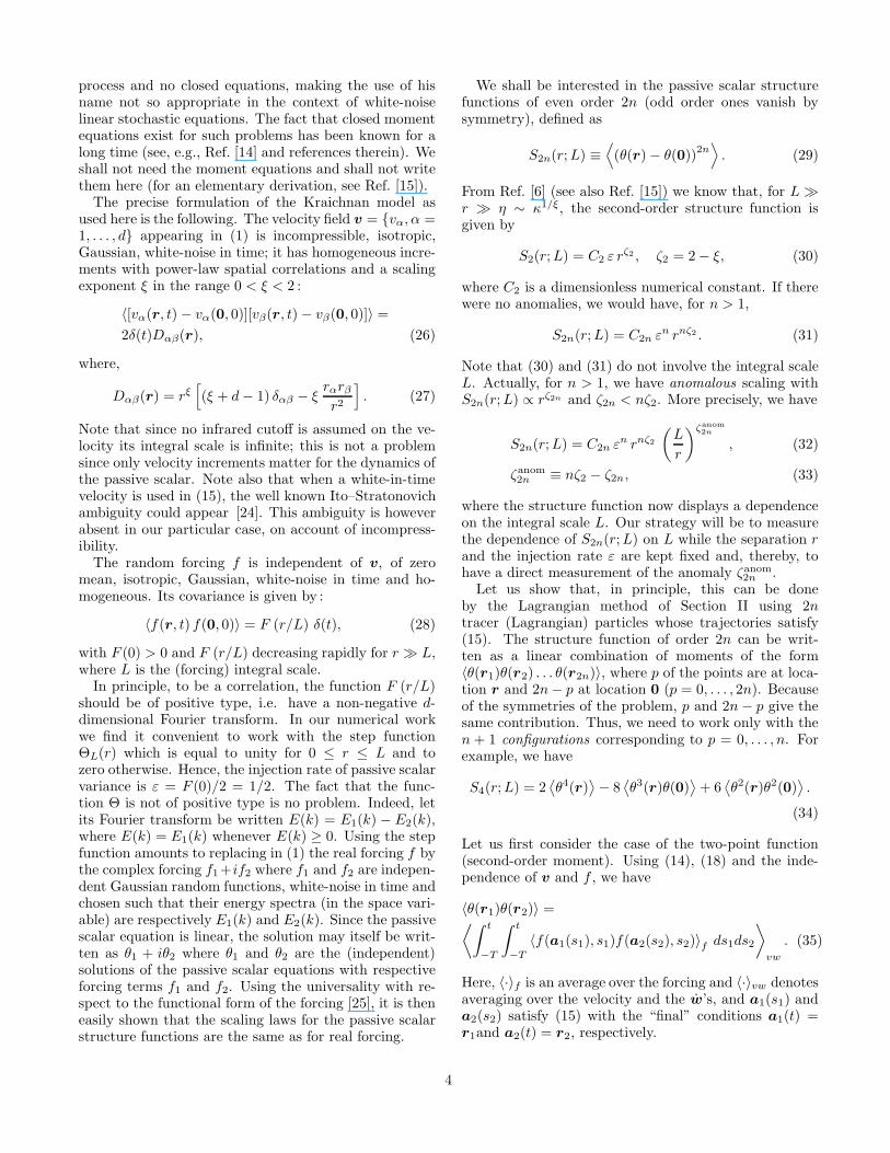
FIG. 2. 3-D fourth-order structure function S4 vs L forξ = 0.2. Separation r = 2.7 × 10−2, diffusivity κ = 0.247,number of realizations 15 × 106.

10-2

10-1

Integral scale L

10-5

10-4

S4

FIG. 3. Same as in Fig. 2 for ξ = 0.9. Parameters :r = 2.7×10−2, κ = 4.4×10−4, number of realizations 8×106.

100

101

102

Integral scale L

10-1

100

S4

FIG. 4. Same as in Fig. 2 for ξ = 1.75. Parameters :r = 2.7 × 10−2, κ = 10−9, number of realizations 1.5 × 106.

10-2

10-1

Integral scale L

10-5

10-4

10-3

S4

FIG. 5. 2-D fourth-order structure function S4 vs L forξ = 0.6. Parameters : r = 2.7×10−2 , κ = 1.1×10−2 , numberof realizations 5 × 106.

7

10-2

10-1

Integral scale L

10-3

10-2

S4

(3)

(1)

(2)

(4)

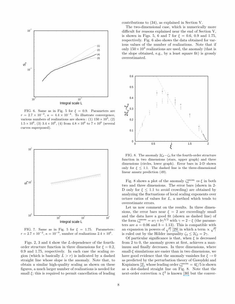
FIG. 6. Same as in Fig. 5 for ξ = 0.9. Parameters arer = 2.7 × 10−2, κ = 4.4 × 10−4. To illustrate convergence,various numbers of realizations are shown : (1) 150× 103, (2)1.5× 106, (3) 3.4× 106, (4) from 4.8× 106 to 7× 106 (severalcurves superposed).

100

101

102

Integral scale L

100

101

102

S4

FIG. 7. Same as in Fig. 5 for ξ = 1.75. Parameters :r = 2.7 × 10−2, κ = 10−9, number of realizations 2.4 × 106.

Figs. 2, 3 and 4 show the L-dependence of the fourth-order structure function in three dimensions for ξ = 0.2,0.9 and 1.75, respectively. In each case the scaling re-gion (which is basically L > r) is indicated by a dashedstraight line whose slope is the anomaly. Note that, toobtain a similar high-quality scaling as shown on thesefigures, a much larger number of realizations is needed forsmall ξ; this is required to permit cancellation of leading

contributions to (34), as explained in Section V.The two-dimensional case, which is numerically more

difficult for reasons explained near the end of Section V,is shown in Figs. 5, 6 and 7 for ξ = 0.6, 0.9 and 1.75,respectively. Fig. 6 also shows the data obtained for var-ious values of the number of realizations. Note that ifonly 150×103 realizations are used, the anomaly (that isthe slope obtained, e.g., by a least square fit) is grosslyoverestimated.

0 0.5 1 1.5 2ξ

0

0.1

0.2

0.3

0.4

0.5

0.6

2ζ 2

−ζ4

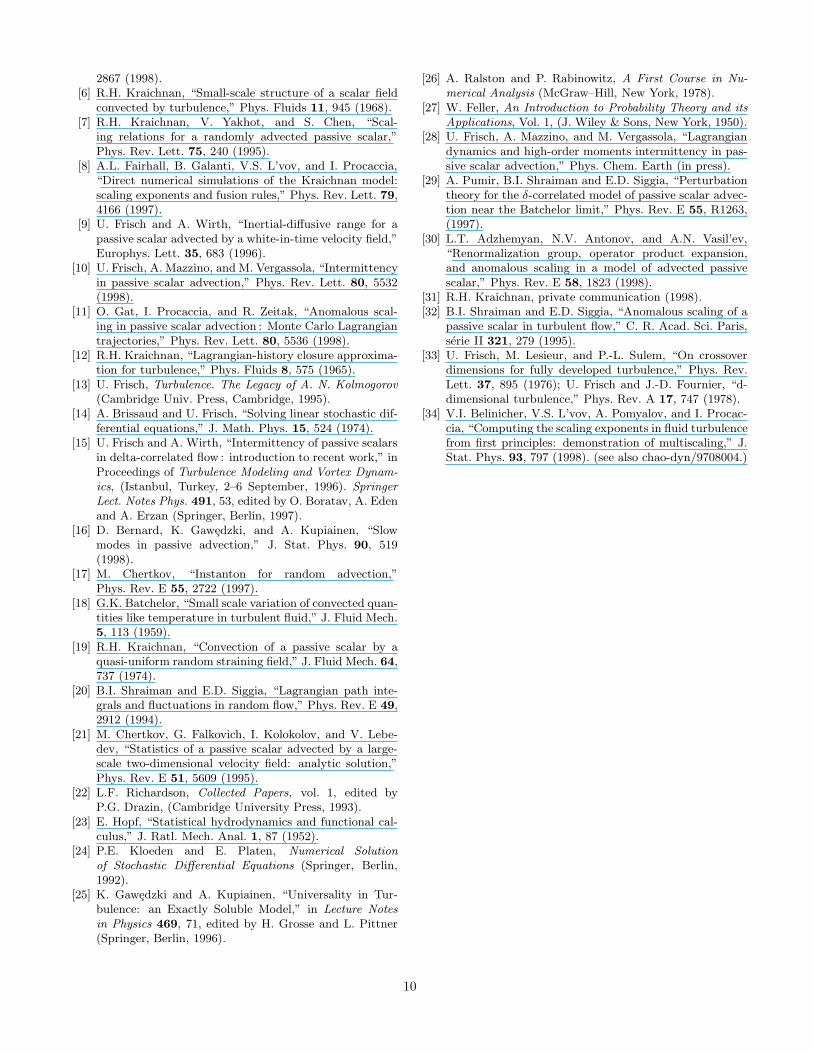
FIG. 8. The anomaly 2ζ2−ζ4 for the fourth-order structurefunction in two dimensions (stars, upper graph) and threedimensions (circles, lower graph). Error bars in 2-D shownonly for ξ ≤ 1.1. The dashed line is the three-dimensionallinear ansatz prediction (49).

Fig. 8 shows a plot of the anomaly ζanom4 vs ξ in both

two and three dimensions. The error bars (shown in 2-D only for ξ ≤ 1.1 to avoid crowding) are obtained byanalyzing the fluctuations of local scaling exponents overoctave ratios of values for L, a method which tends tooverestimate errors.

Let us now comment on the results. In three dimen-sions, the error bars near ξ = 2 are exceedingly smalland the data have a good fit (shown as dashed line) ofthe form ζanom

4 = aγ + bγ3/2 with γ = 2− ξ (the parame-ters are a = 0.06 and b = 1.13). This is compatible withan expansion in powers of

√γ [29] in which a term ∝ √

γis ruled out by the Holder inequality ζ4 ≤ 2ζ2 = 2γ.

Of particular significance is that, when ξ is decreasedfrom 2 to 0, the anomaly grows at first, achieves a max-imum and finally decreases. In three dimensions, wheresmall-ξ simulations are easier than in two dimensions, wehave good evidence that the anomaly vanishes for ξ → 0as predicted by the perturbation theory of Gawedzki andKupiainen [2], whose leading order ζanom

4 = 4ξ/5 is shownas a dot-dashed straight line on Fig. 8. Note that thenext-order correction ∝ ξ2 is known [30] but the conver-

8

gence properties of the ξ-series are not clear. The “linearansatz” prediction for the anomaly given in Refs. [1,7],that is

ζanom4 =

3ζ2 + d

2− 1

2

√

8dζ2 + (d − ζ2)2, (49)

ζ2 = 2 − ξ, (50)

is consistent with our results only near ξ = 1, the pointfarthest from the two limits ξ = 0 and ξ = 2, which bothhave strongly nonlocal dynamics. This suggests a pos-sible relation between deviations from the linear ansatzand locality of the interactions [31]. Whether this con-sistency for ξ = 1 persists for moments of order higherthan four is an open problem.

The fact that the anomalies are stronger in two thanin three dimensions is consistent with their vanishing asd → ∞ [3]. The fact that the maximum anomaly occursfor a value of ξ smaller in two than in three dimensionscan be tentatively interpreted as follows. Near ξ = 0the dynamics is dominated by the nearly ultraviolet-divergent eddy diffusion, whereas near ξ = 2 it is dom-inated by the nearly infrared-divergent stretching. Theformer increases with d, but not the latter. The maxi-mum is achieved when these two effects balance.

VII. CONCLUDING REMARKS

Compared to Eulerian simulations of the partial dif-ferential equation (1) our Lagrangian method has var-ious advantages. When calculating moments of order2n we do not require the complete velocity field at eachtime step but only 2n − 1 random vectors, basically, theset of velocity differences between the locations of La-grangian tracer particles which are advected by the flowand subject to independent Brownian diffusion. As a con-sequence the complexity of the computation (measured innumber of floating point operations) grows polynomiallyrather than exponentially with the dimension d. Further-more, working with tracers naturally allows to measurethe scaling of the structure functions S2n(r; L) vs the in-tegral scale L of the forcing. Physically, this means thatthe injection rate of passive scalar variance (which equalsits dissipation rate) and the separation r are kept fixedwhile the integral scale L is varied. Anomalies, that isdiscrepancies from the scaling exponents which would bepredicted by naıve dimensional analysis, are measuredhere directly through the scaling dependence on L of thestructure functions.

Actually, direct Eulerian simulations and the La-grangian method are complementary. Very high-resolution simulations of the sort found in Ref. [5] arereally not practical in more than two dimensions butdo give access to the entire Eulerian passive scalar field.Hence, they can and have been used to address questionsabout the geometry of the scalar field and about proba-bility distributions.

Although we have presented here the numerical imple-mentation of the Lagrangian method only for the Kraich-nan model, it is clear that the general strategy presentedin Sections II and III is applicable to a wide class of ran-dom flows, for example, with a finite correlation time.

An important aspect of the results obtained for theKraichnan model is that they agree with perturbationtheory [2] for ξ → 0. As is now clear from theory andsimulations, anomalies in the Kraichnan model and otherpassive scalar problems arise from zero modes in the oper-ators governing the Eulerian dynamics of n-point correla-tion functions [2,3,32]. It is likely that some form of zeromodes is also responsible for anomalous scaling in nonlin-ear turbulence problems. An instance are the “fluxlesssolutions” to Markovian closures based on the Navier–Stokes equations in dimension d close to two, which havea power-law spectrum with an exponent depending con-tinuously on d [33]. Attempts to capture intermittencyeffects in three-dimensional turbulence are being madealong similar lines (see, e.g., Ref. [34]). The Kraichnanmodel for passive scalar intermittency puts us on a trailto understanding anomalous scaling in turbulence.

ACKNOWLEDGMENTS

We are most grateful to Robert Kraichnan for innu-merable interactions on the subject of passive scalar in-termittency over many years. We acknowledge usefuldiscussions with M. Chertkov, G. Falkovich, O. Gat,K. Gawedzki, F. Massaioli, S.A. Orszag, I. Procaccia,A. Wirth, V. Yakhot and R. Zeitak. Simulations wereperformed in the framework of the SIVAM project ofthe Observatoire de la Cote d’Azur. Part of them wereperformed using the computing facilities of CASPUR atRome University, which is gratefully acknowledged. Par-tial support from the Centre National de la RechercheScientifique through a “Henri Poincare” fellowship (AM)and from the Groupe de Recherche “Mecanique des Flu-ides Geophysiques et Astrophysiques” (MV) is also ac-knowledged.

[1] R.H. Kraichnan, “Anomalous scaling of a randomly ad-vected passive scalar,” Phys. Rev. Lett. 72, 1016 (1994).

[2] K. Gawedzki and A. Kupiainen, “Anomalous scaling ofthe passive scalar,” Phys. Rev. Lett. 75, 3834 (1995).

[3] M. Chertkov, G. Falkovich, I. Kolokolov, and V. Lebedev,“Normal and anomalous scaling of the fourth-order cor-relation function of a randomly advected passive scalar,”Phys. Rev. E 2, 4924 (1995).

[4] K. Gawedzki, “Intermittency of passive advection,” inAdvances in Turbulence VII, edited by U. Frisch (KluwerAcademic Publishers, London, 1998).

[5] S. Chen and R.H. Kraichnan, “Simulations of a Ran-domly Advected Passive Scalar Field,” Phys. Fluids 10,

9

2867 (1998).[6] R.H. Kraichnan, “Small-scale structure of a scalar field

convected by turbulence,” Phys. Fluids 11, 945 (1968).[7] R.H. Kraichnan, V. Yakhot, and S. Chen, “Scal-

ing relations for a randomly advected passive scalar,”Phys. Rev. Lett. 75, 240 (1995).

[8] A.L. Fairhall, B. Galanti, V.S. L’vov, and I. Procaccia,“Direct numerical simulations of the Kraichnan model:scaling exponents and fusion rules,” Phys. Rev. Lett. 79,4166 (1997).

[9] U. Frisch and A. Wirth, “Inertial-diffusive range for apassive scalar advected by a white-in-time velocity field,”Europhys. Lett. 35, 683 (1996).

[10] U. Frisch, A. Mazzino, and M. Vergassola, “Intermittencyin passive scalar advection,” Phys. Rev. Lett. 80, 5532(1998).

[11] O. Gat, I. Procaccia, and R. Zeitak, “Anomalous scal-ing in passive scalar advection : Monte Carlo Lagrangiantrajectories,” Phys. Rev. Lett. 80, 5536 (1998).

[12] R.H. Kraichnan, “Lagrangian-history closure approxima-tion for turbulence,” Phys. Fluids 8, 575 (1965).

[13] U. Frisch, Turbulence. The Legacy of A. N. Kolmogorov

(Cambridge Univ. Press, Cambridge, 1995).[14] A. Brissaud and U. Frisch, “Solving linear stochastic dif-

ferential equations,” J. Math. Phys. 15, 524 (1974).[15] U. Frisch and A. Wirth, “Intermittency of passive scalars

in delta-correlated flow : introduction to recent work,” inProceedings of Turbulence Modeling and Vortex Dynam-

ics, (Istanbul, Turkey, 2–6 September, 1996). Springer

Lect. Notes Phys. 491, 53, edited by O. Boratav, A. Edenand A. Erzan (Springer, Berlin, 1997).

[16] D. Bernard, K. Gawedzki, and A. Kupiainen, “Slowmodes in passive advection,” J. Stat. Phys. 90, 519(1998).

[17] M. Chertkov, “Instanton for random advection,”Phys. Rev. E 55, 2722 (1997).

[18] G.K. Batchelor, “Small scale variation of convected quan-tities like temperature in turbulent fluid,” J. Fluid Mech.5, 113 (1959).

[19] R.H. Kraichnan, “Convection of a passive scalar by aquasi-uniform random straining field,” J. Fluid Mech. 64,737 (1974).

[20] B.I. Shraiman and E.D. Siggia, “Lagrangian path inte-grals and fluctuations in random flow,” Phys. Rev. E 49,2912 (1994).

[21] M. Chertkov, G. Falkovich, I. Kolokolov, and V. Lebe-dev, “Statistics of a passive scalar advected by a large-scale two-dimensional velocity field: analytic solution,”Phys. Rev. E 51, 5609 (1995).

[22] L.F. Richardson, Collected Papers, vol. 1, edited byP.G. Drazin, (Cambridge University Press, 1993).

[23] E. Hopf, “Statistical hydrodynamics and functional cal-culus,” J. Ratl. Mech. Anal. 1, 87 (1952).

[24] P.E. Kloeden and E. Platen, Numerical Solution

of Stochastic Differential Equations (Springer, Berlin,1992).

[25] K. Gawedzki and A. Kupiainen, “Universality in Tur-bulence: an Exactly Soluble Model,” in Lecture Notes

in Physics 469, 71, edited by H. Grosse and L. Pittner(Springer, Berlin, 1996).

[26] A. Ralston and P. Rabinowitz, A First Course in Nu-

merical Analysis (McGraw–Hill, New York, 1978).[27] W. Feller, An Introduction to Probability Theory and its

Applications, Vol. 1, (J. Wiley & Sons, New York, 1950).[28] U. Frisch, A. Mazzino, and M. Vergassola, “Lagrangian

dynamics and high-order moments intermittency in pas-sive scalar advection,” Phys. Chem. Earth (in press).

[29] A. Pumir, B.I. Shraiman and E.D. Siggia, “Perturbationtheory for the δ-correlated model of passive scalar advec-tion near the Batchelor limit,” Phys. Rev. E 55, R1263,(1997).

[30] L.T. Adzhemyan, N.V. Antonov, and A.N. Vasil’ev,“Renormalization group, operator product expansion,and anomalous scaling in a model of advected passivescalar,” Phys. Rev. E 58, 1823 (1998).

[31] R.H. Kraichnan, private communication (1998).[32] B.I. Shraiman and E.D. Siggia, “Anomalous scaling of a

passive scalar in turbulent flow,” C. R. Acad. Sci. Paris,serie II 321, 279 (1995).

[33] U. Frisch, M. Lesieur, and P.-L. Sulem, “On crossoverdimensions for fully developed turbulence,” Phys. Rev.Lett. 37, 895 (1976); U. Frisch and J.-D. Fournier, “d-dimensional turbulence,” Phys. Rev. A 17, 747 (1978).

[34] V.I. Belinicher, V.S. L’vov, A. Pomyalov, and I. Procac-cia, “Computing the scaling exponents in fluid turbulencefrom first principles: demonstration of multiscaling,” J.Stat. Phys. 93, 797 (1998). (see also chao-dyn/9708004.)

10

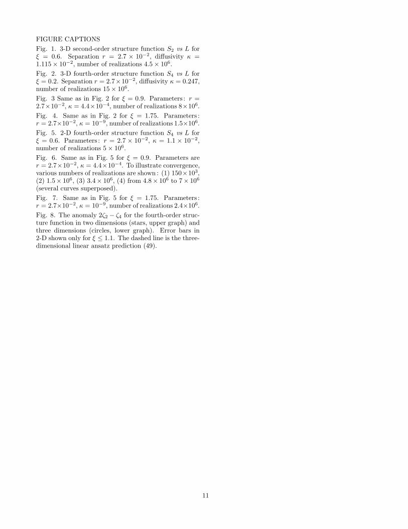
FIGURE CAPTIONS

Fig. 1. 3-D second-order structure function S2 vs L forξ = 0.6. Separation r = 2.7 × 10−2, diffusivity κ =1.115 × 10−2, number of realizations 4.5 × 106.

Fig. 2. 3-D fourth-order structure function S4 vs L forξ = 0.2. Separation r = 2.7×10−2, diffusivity κ = 0.247,number of realizations 15 × 106.

Fig. 3 Same as in Fig. 2 for ξ = 0.9. Parameters : r =2.7×10−2, κ = 4.4×10−4, number of realizations 8×106.

Fig. 4. Same as in Fig. 2 for ξ = 1.75. Parameters :r = 2.7×10−2, κ = 10−9, number of realizations 1.5×106.

Fig. 5. 2-D fourth-order structure function S4 vs L forξ = 0.6. Parameters : r = 2.7 × 10−2, κ = 1.1 × 10−2,number of realizations 5 × 106.

Fig. 6. Same as in Fig. 5 for ξ = 0.9. Parameters arer = 2.7×10−2, κ = 4.4×10−4. To illustrate convergence,various numbers of realizations are shown : (1) 150×103,(2) 1.5× 106, (3) 3.4× 106, (4) from 4.8× 106 to 7× 106

(several curves superposed).

Fig. 7. Same as in Fig. 5 for ξ = 1.75. Parameters :r = 2.7×10−2, κ = 10−9, number of realizations 2.4×106.

Fig. 8. The anomaly 2ζ2 − ζ4 for the fourth-order struc-ture function in two dimensions (stars, upper graph) andthree dimensions (circles, lower graph). Error bars in2-D shown only for ξ ≤ 1.1. The dashed line is the three-dimensional linear ansatz prediction (49).

11